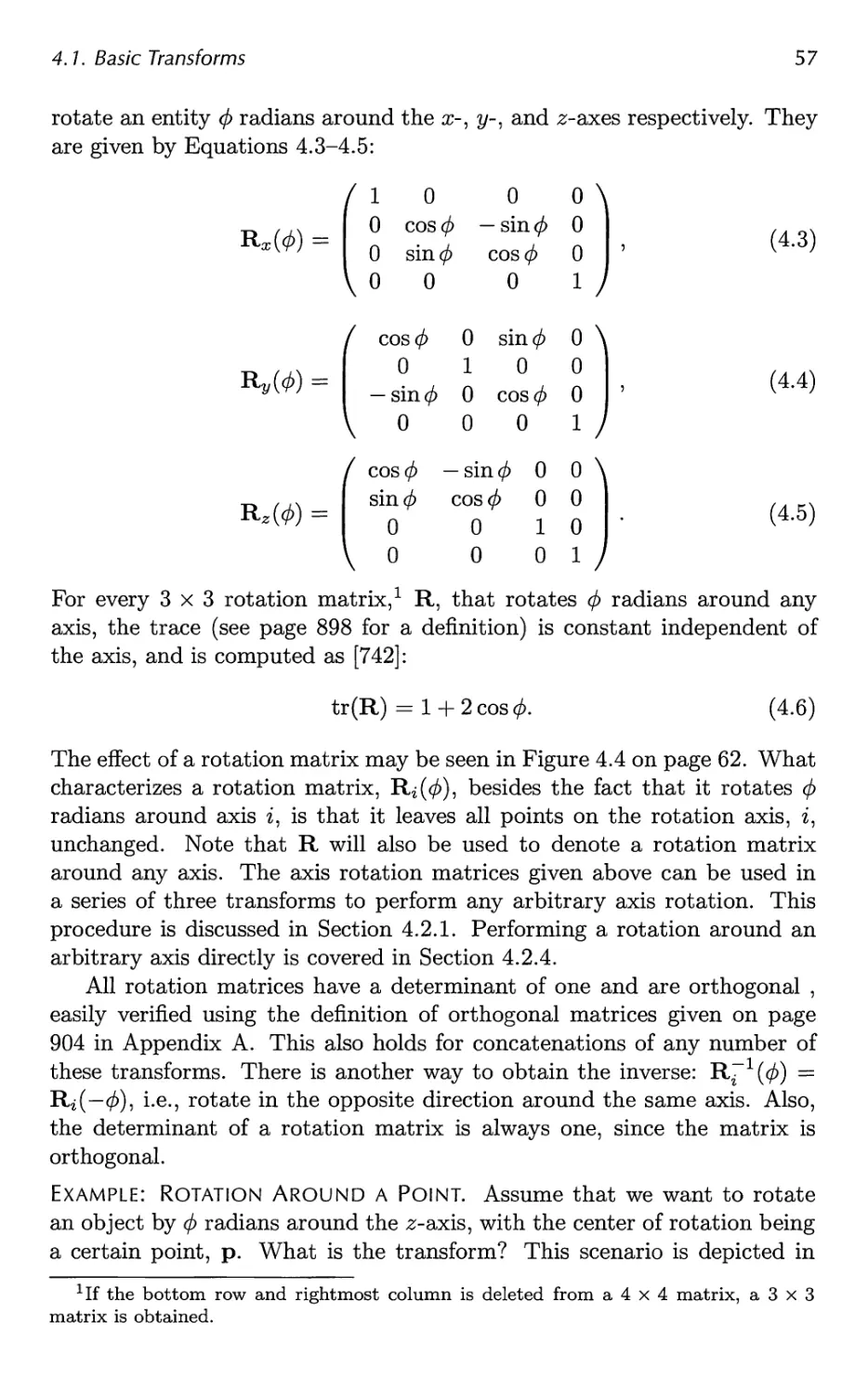
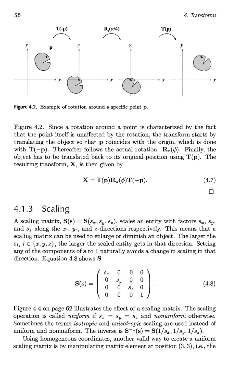
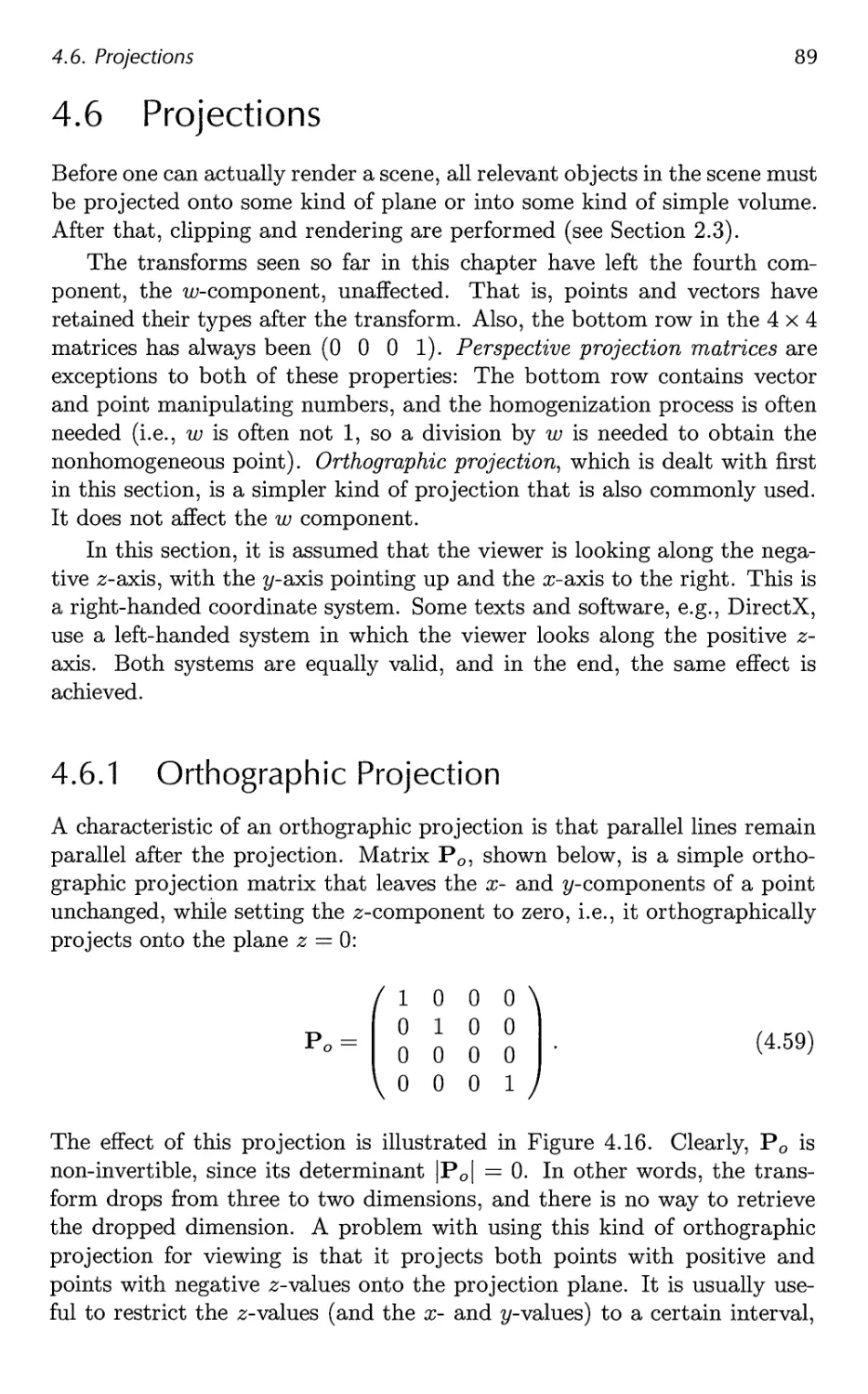
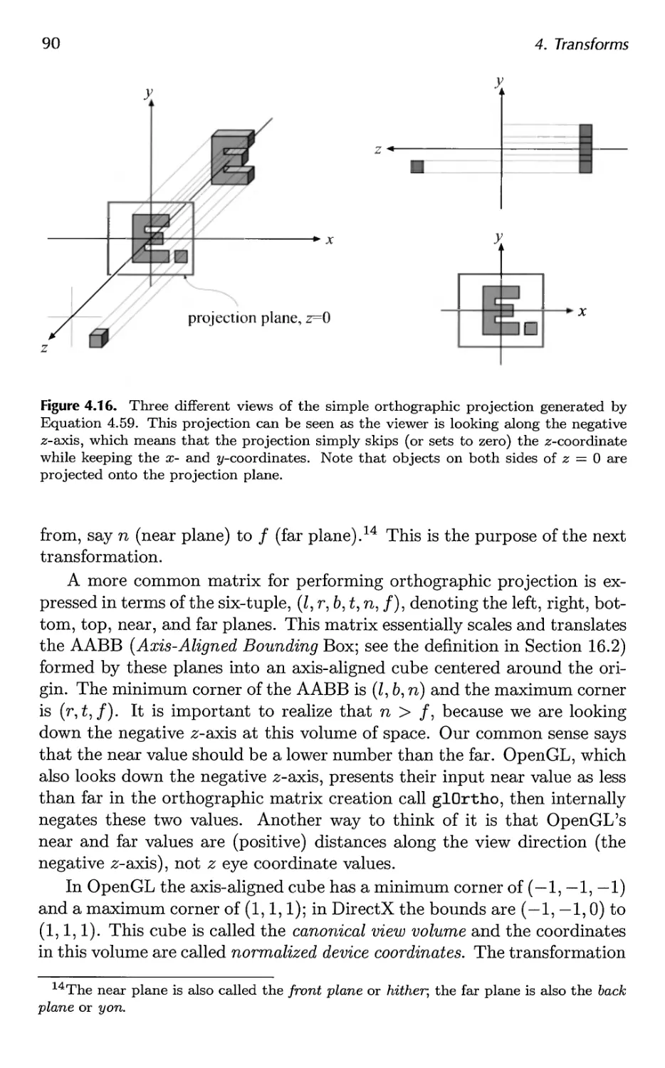
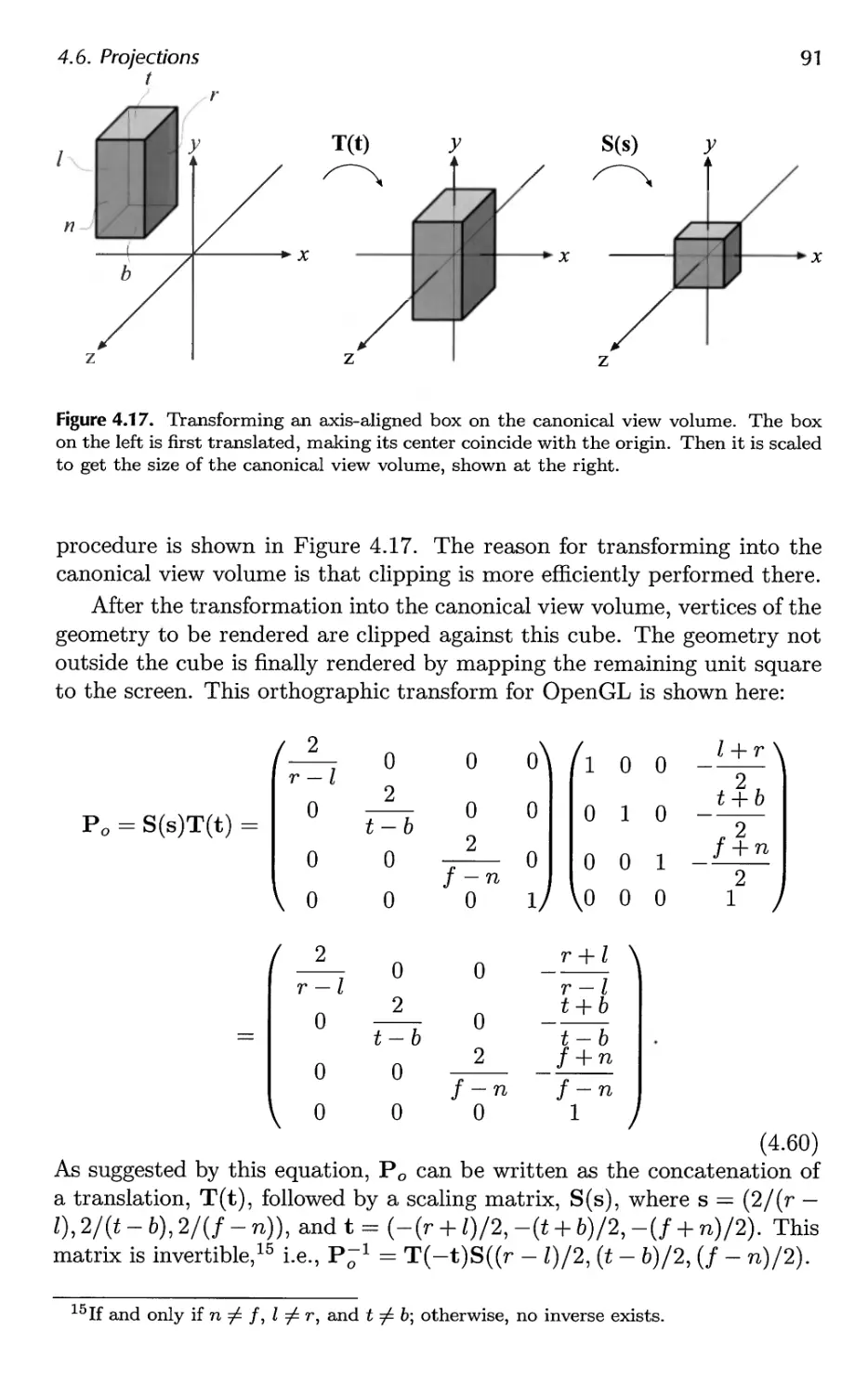
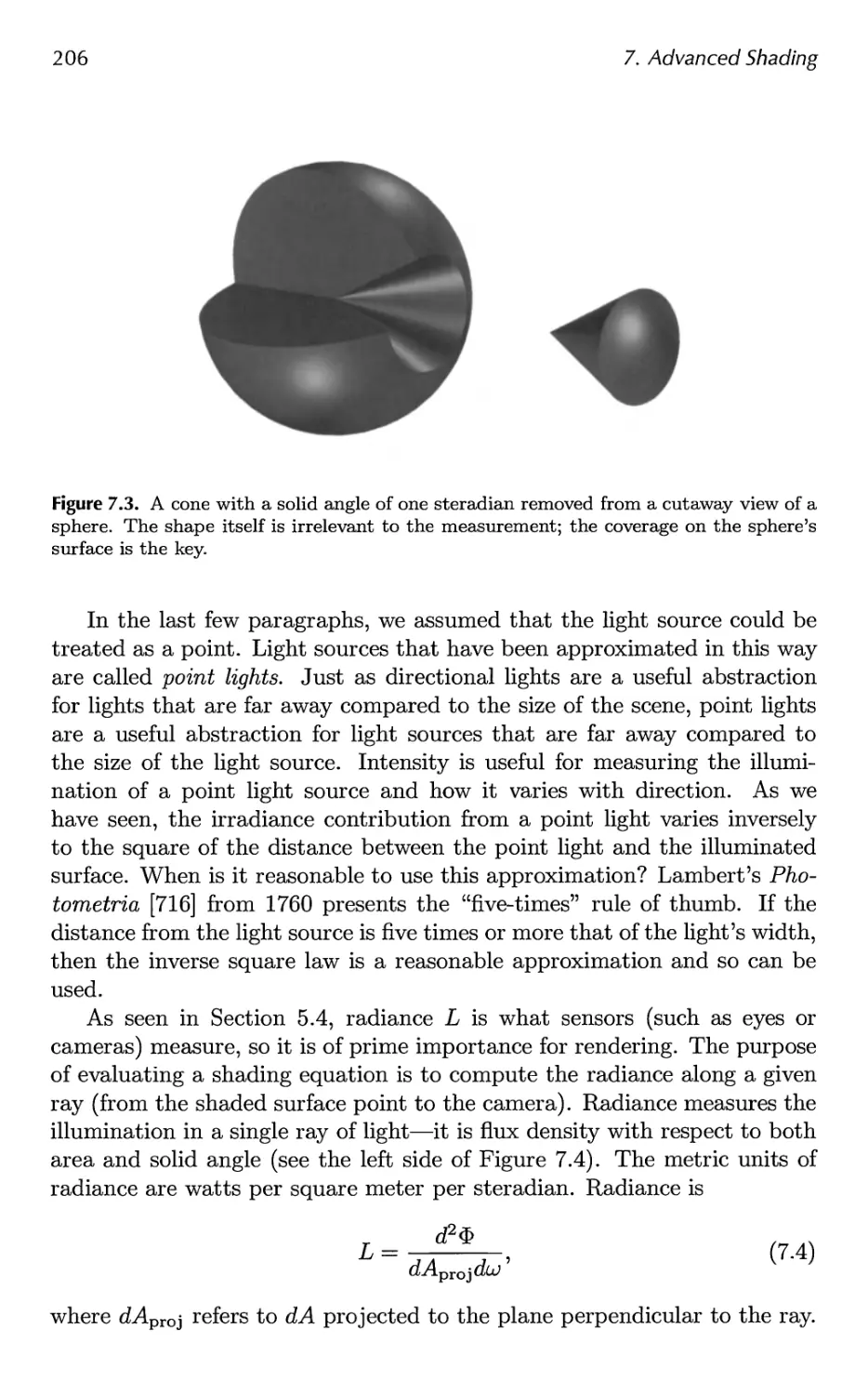
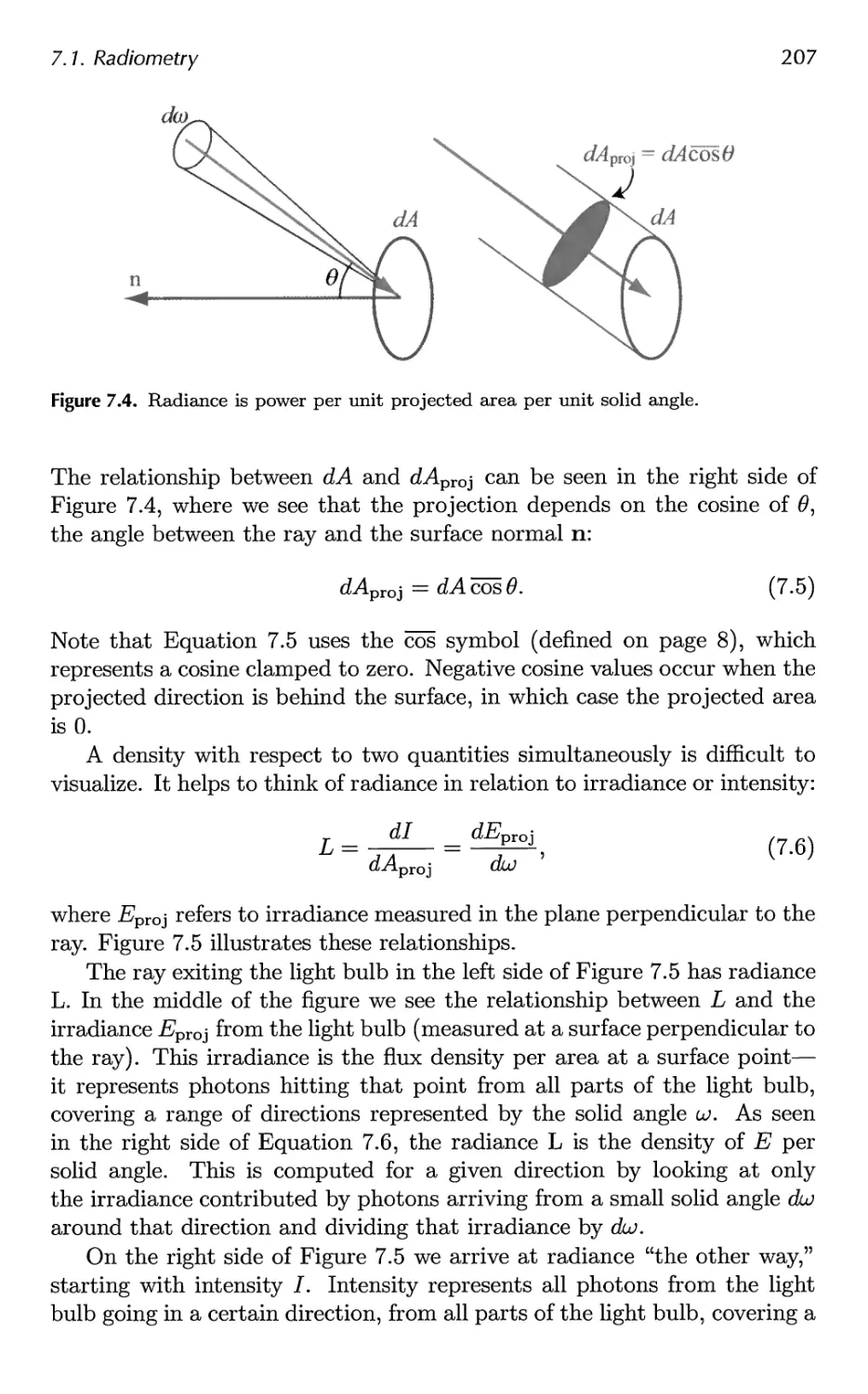
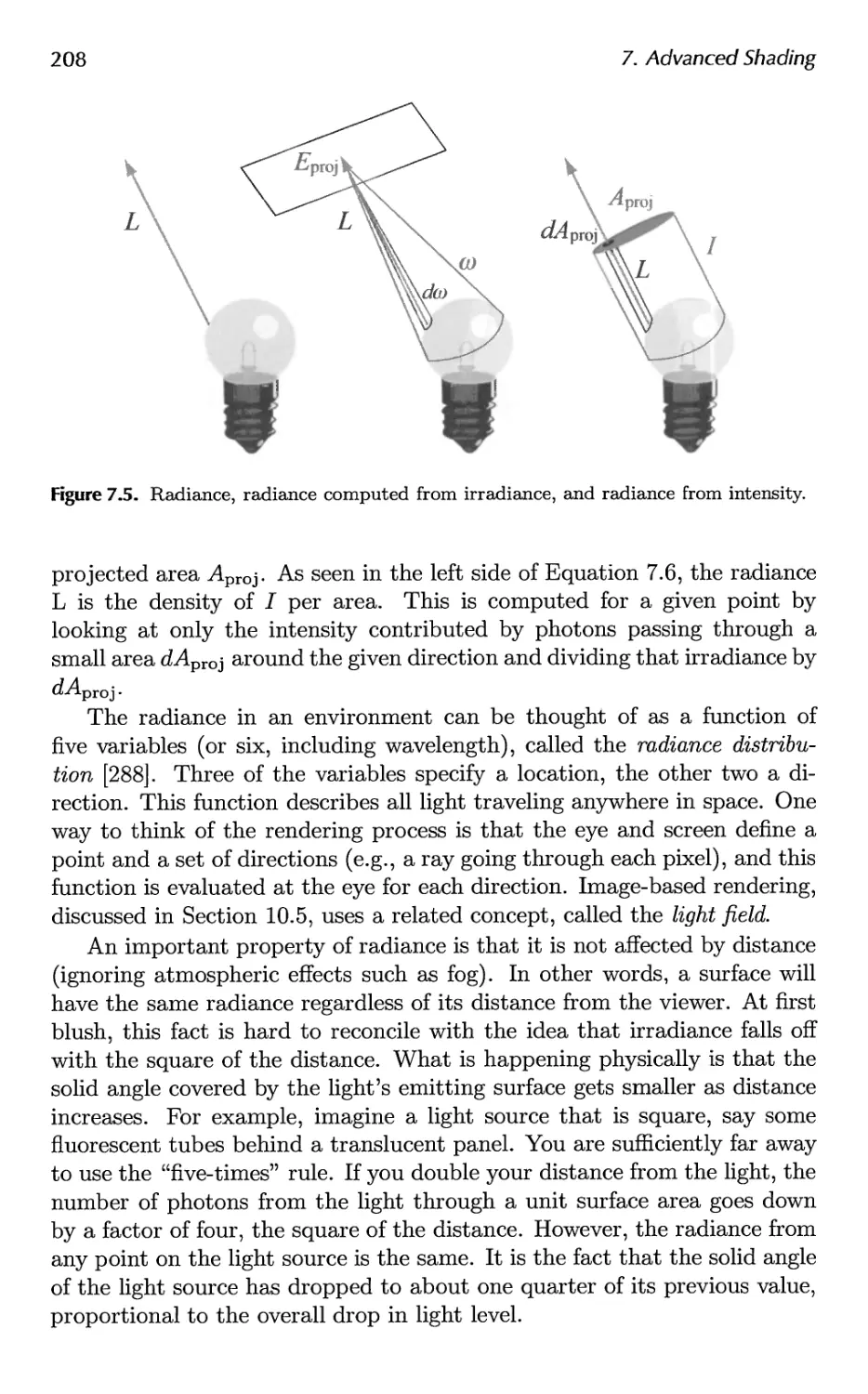
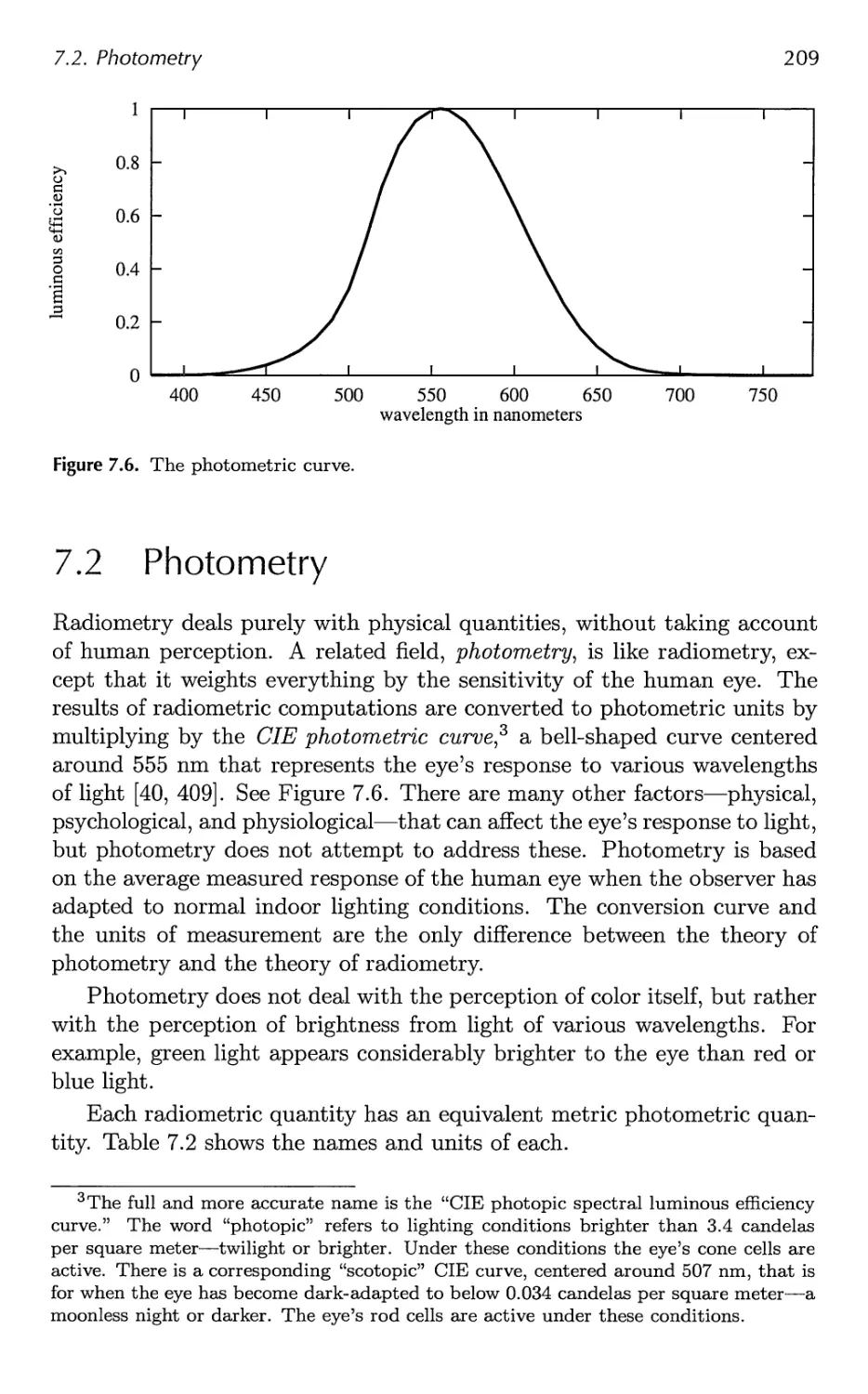
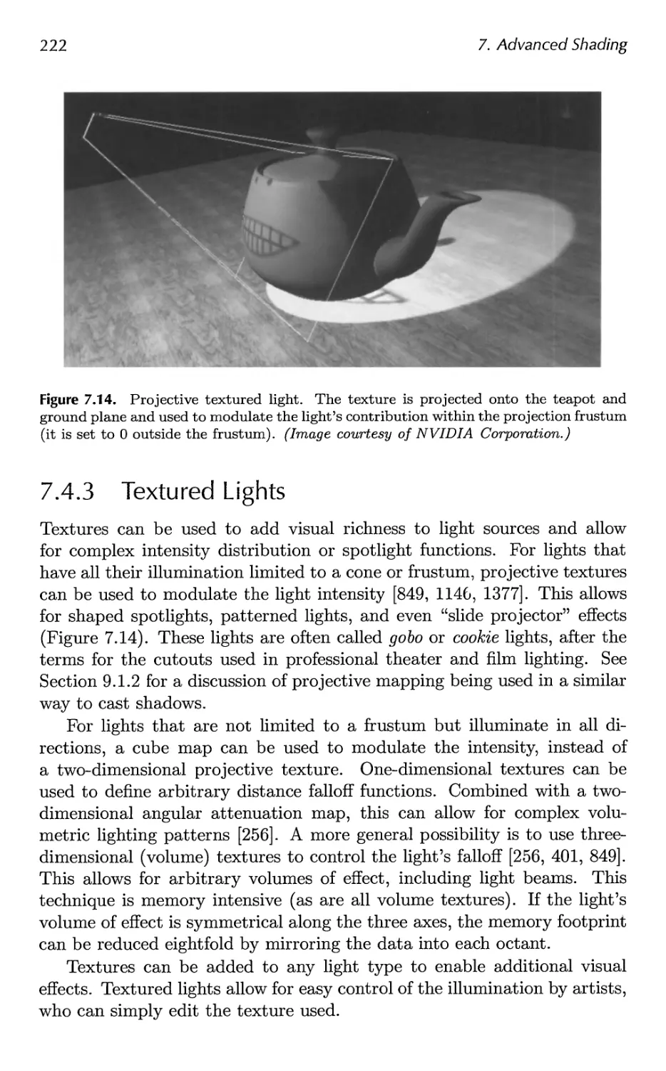
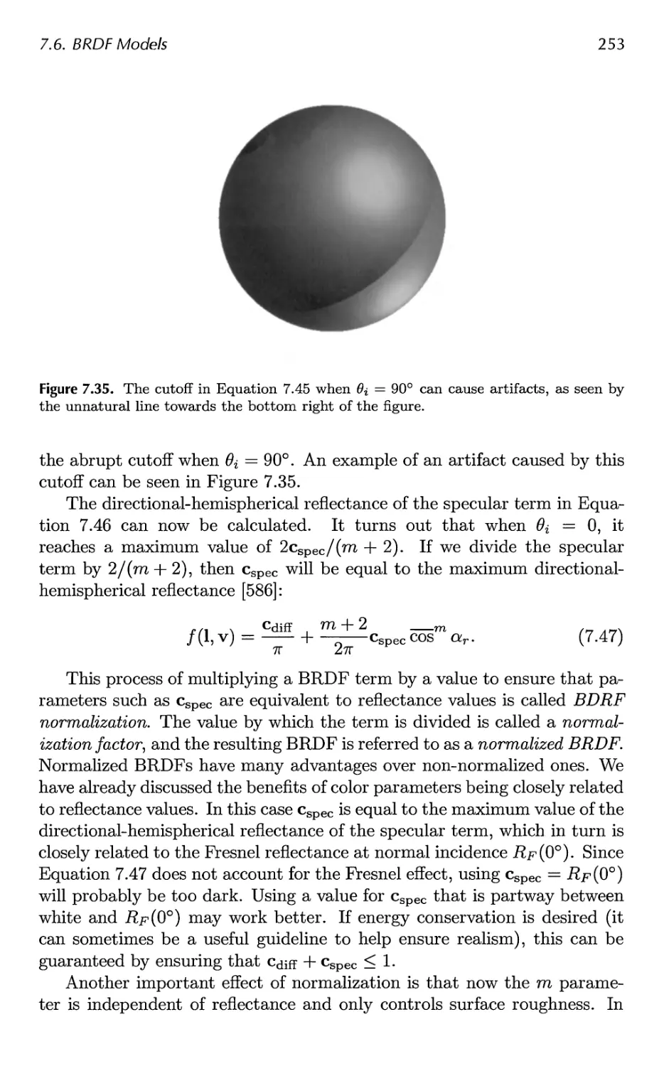
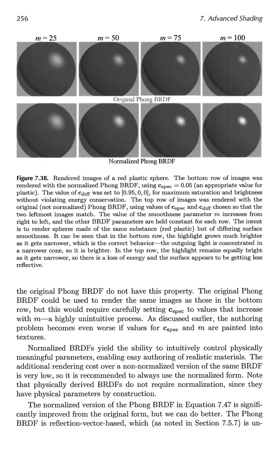
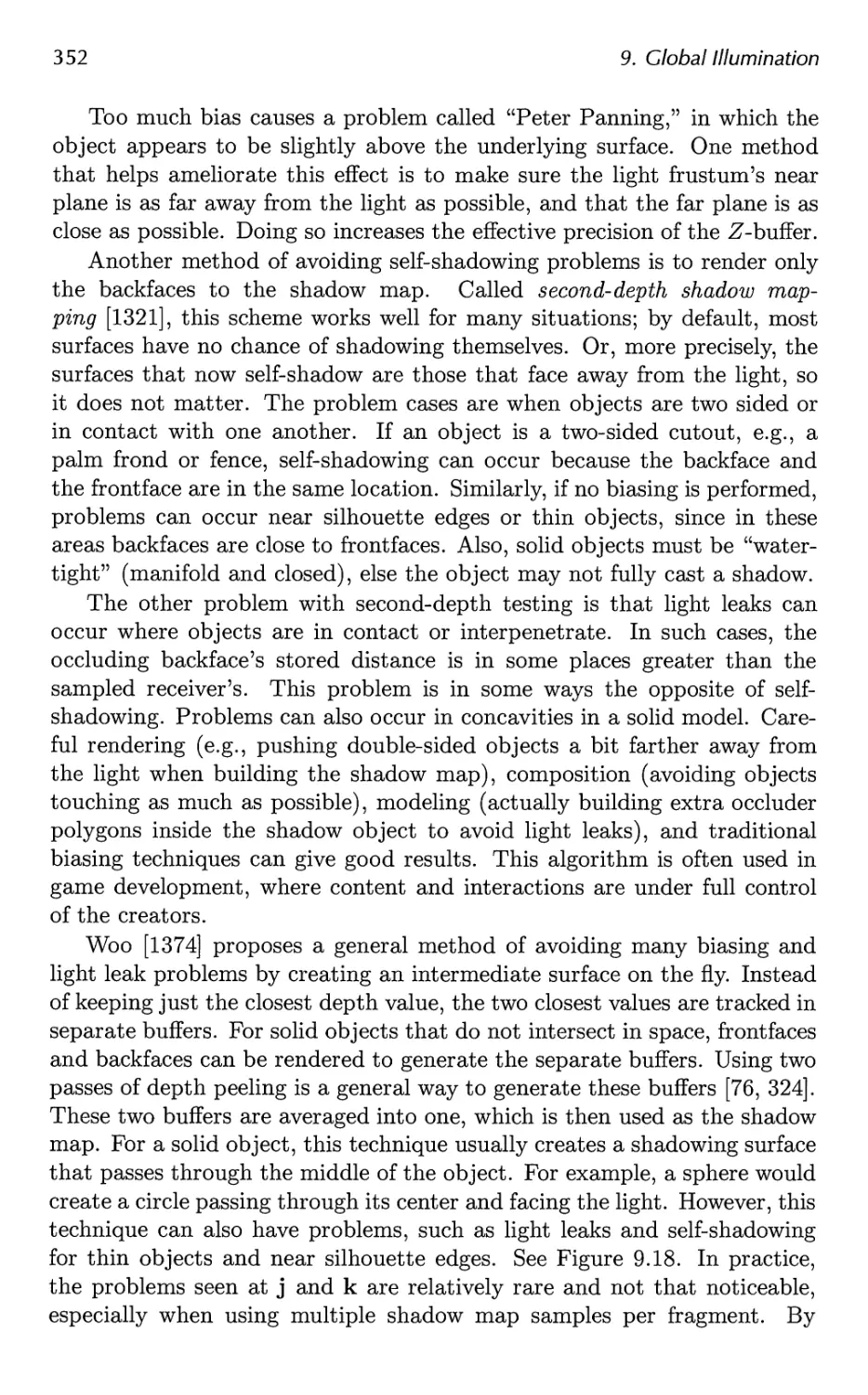
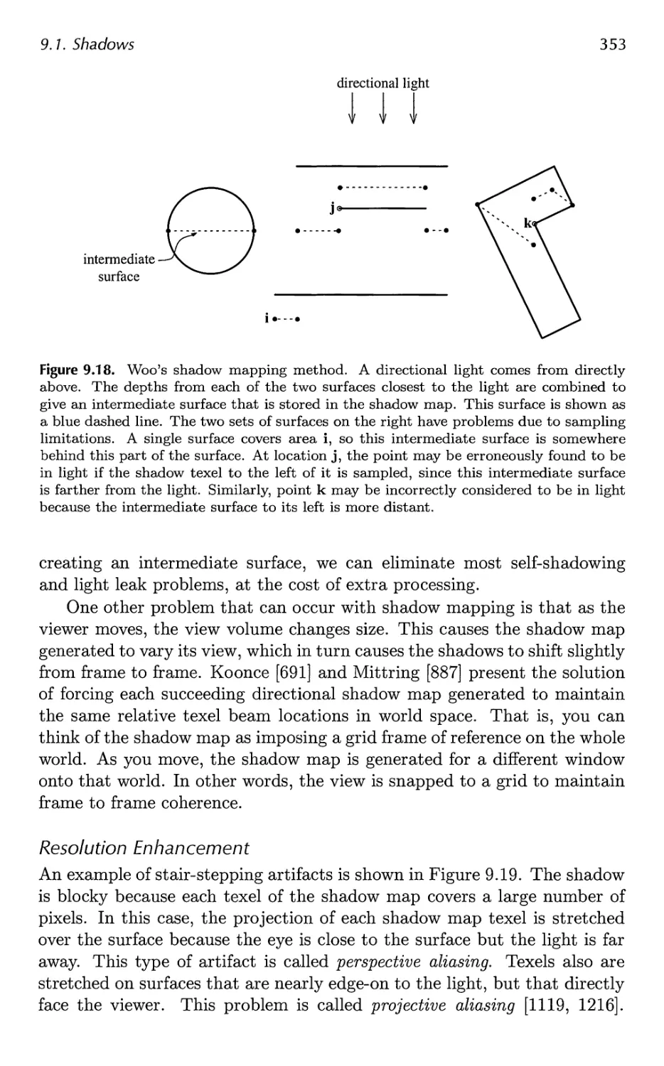
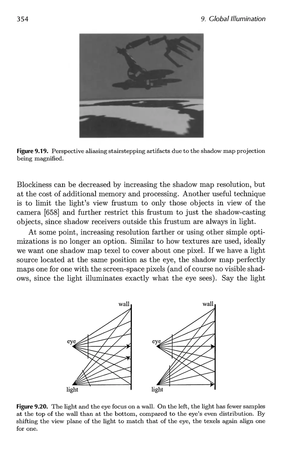
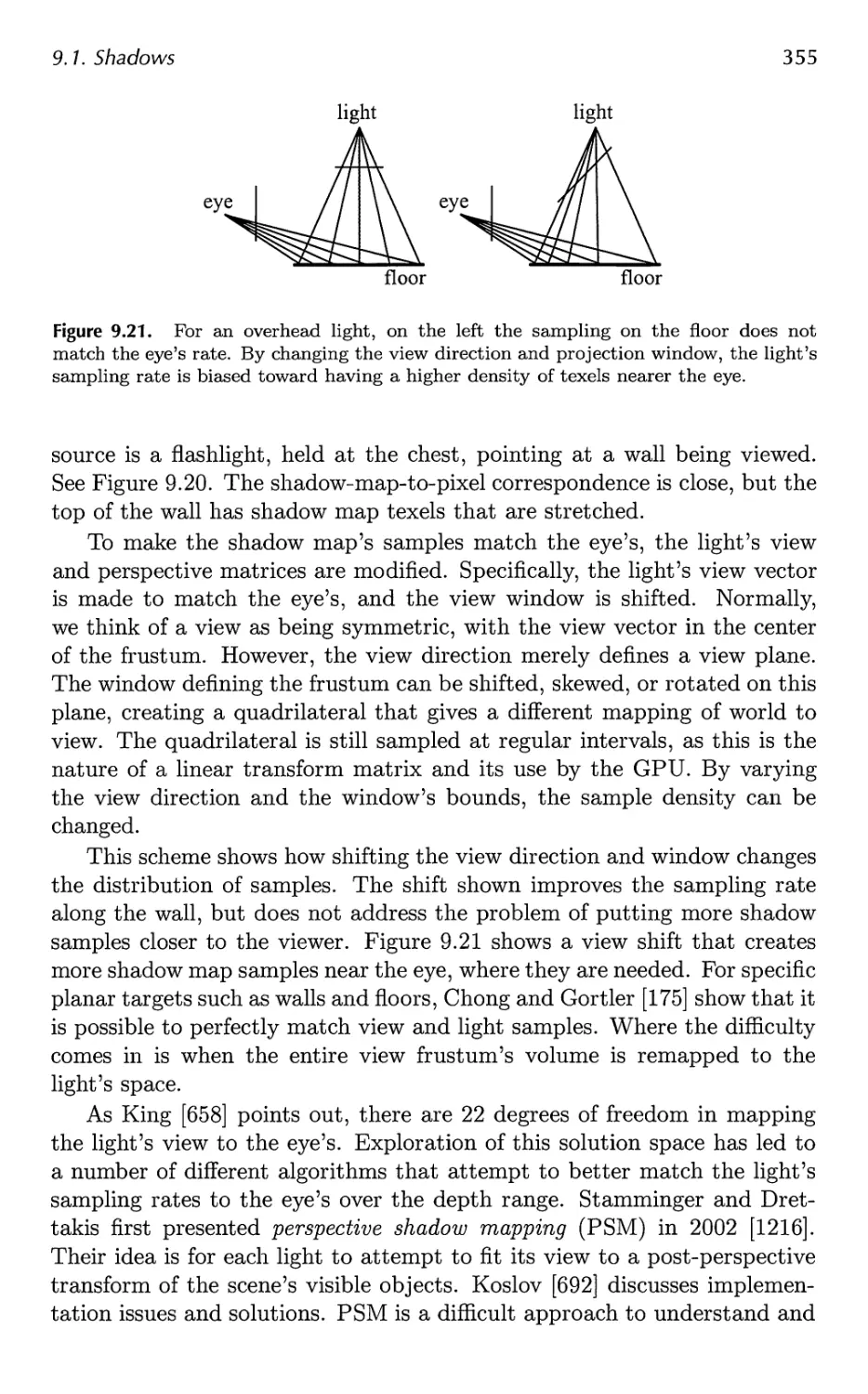
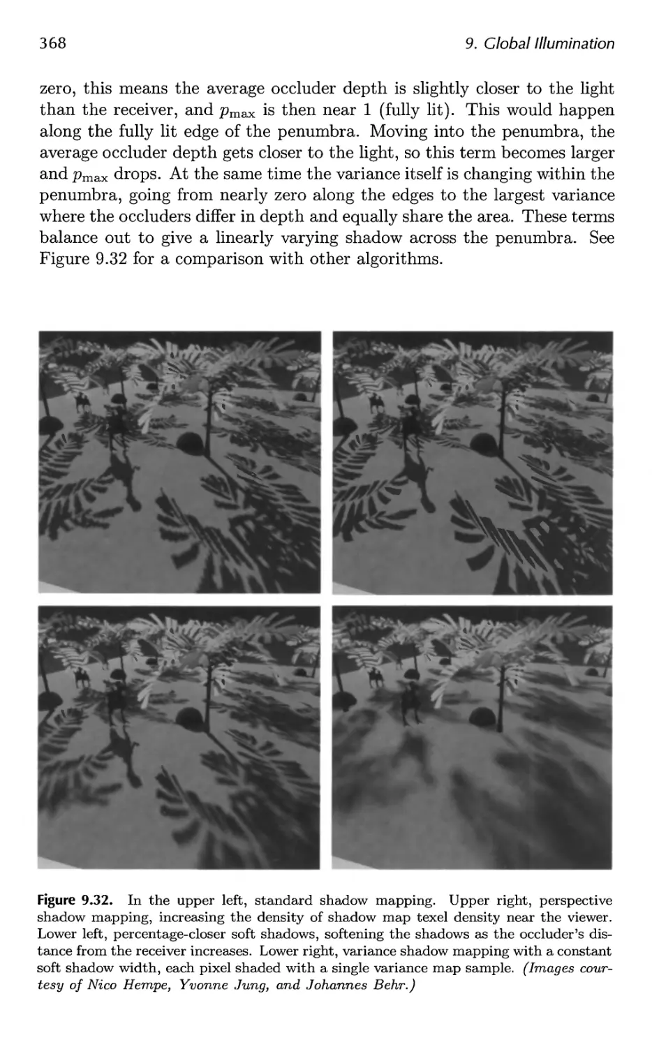
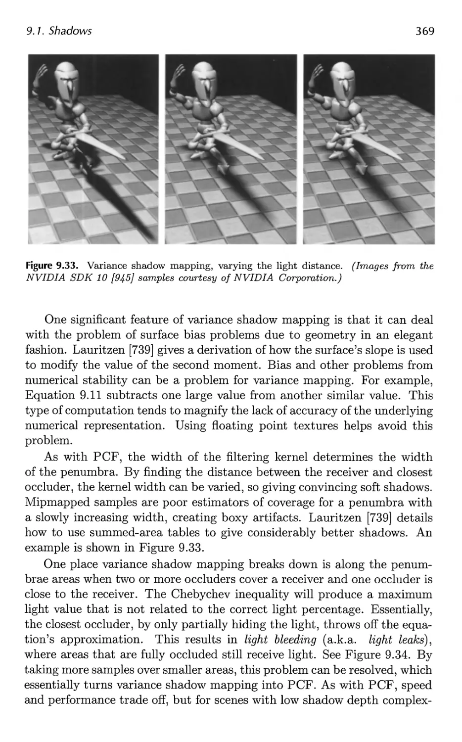
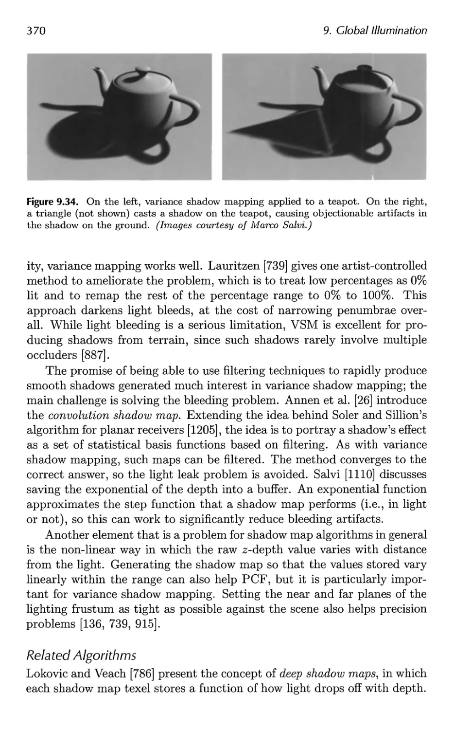
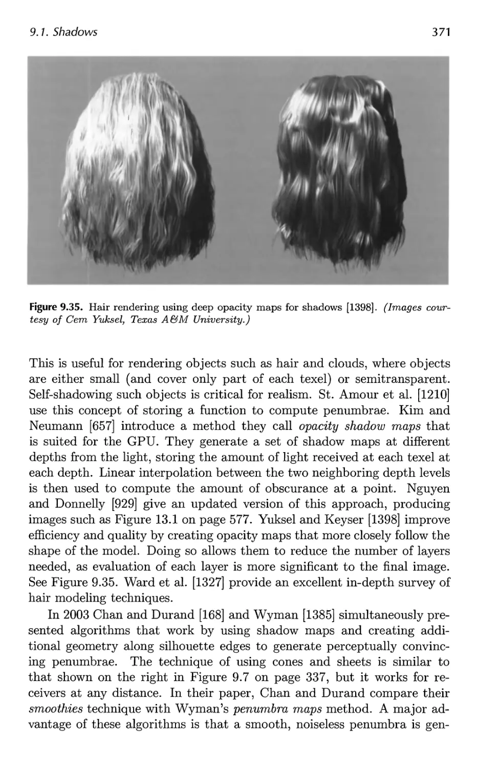
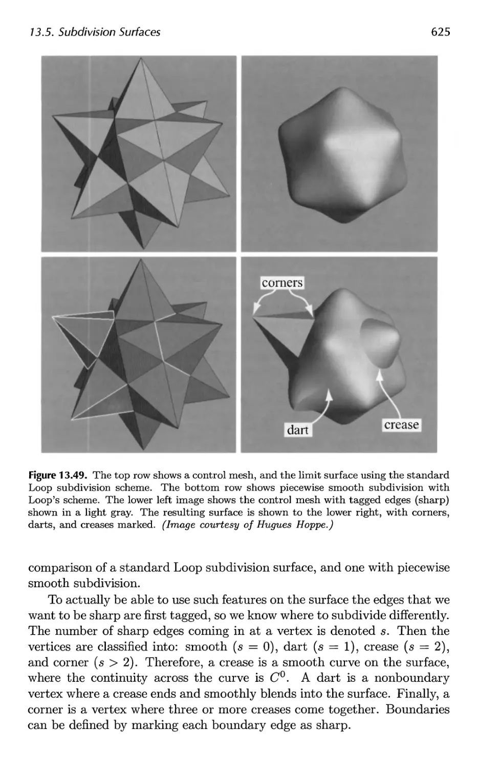
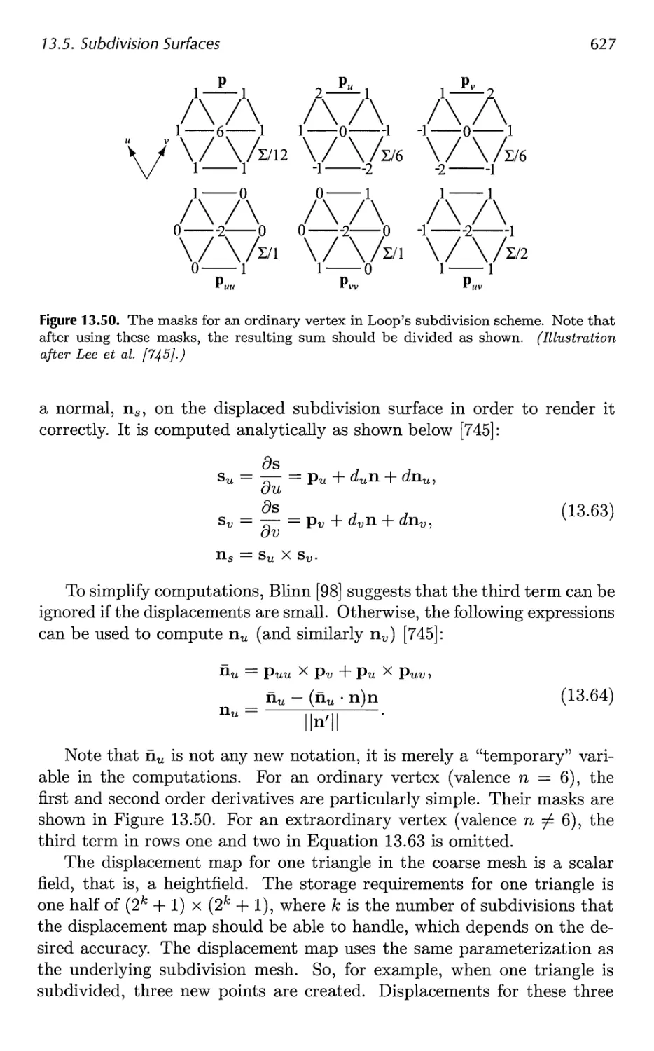
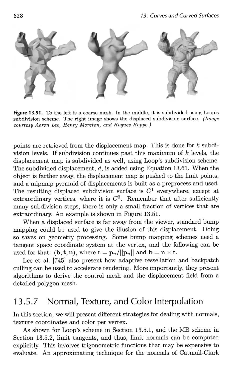
/


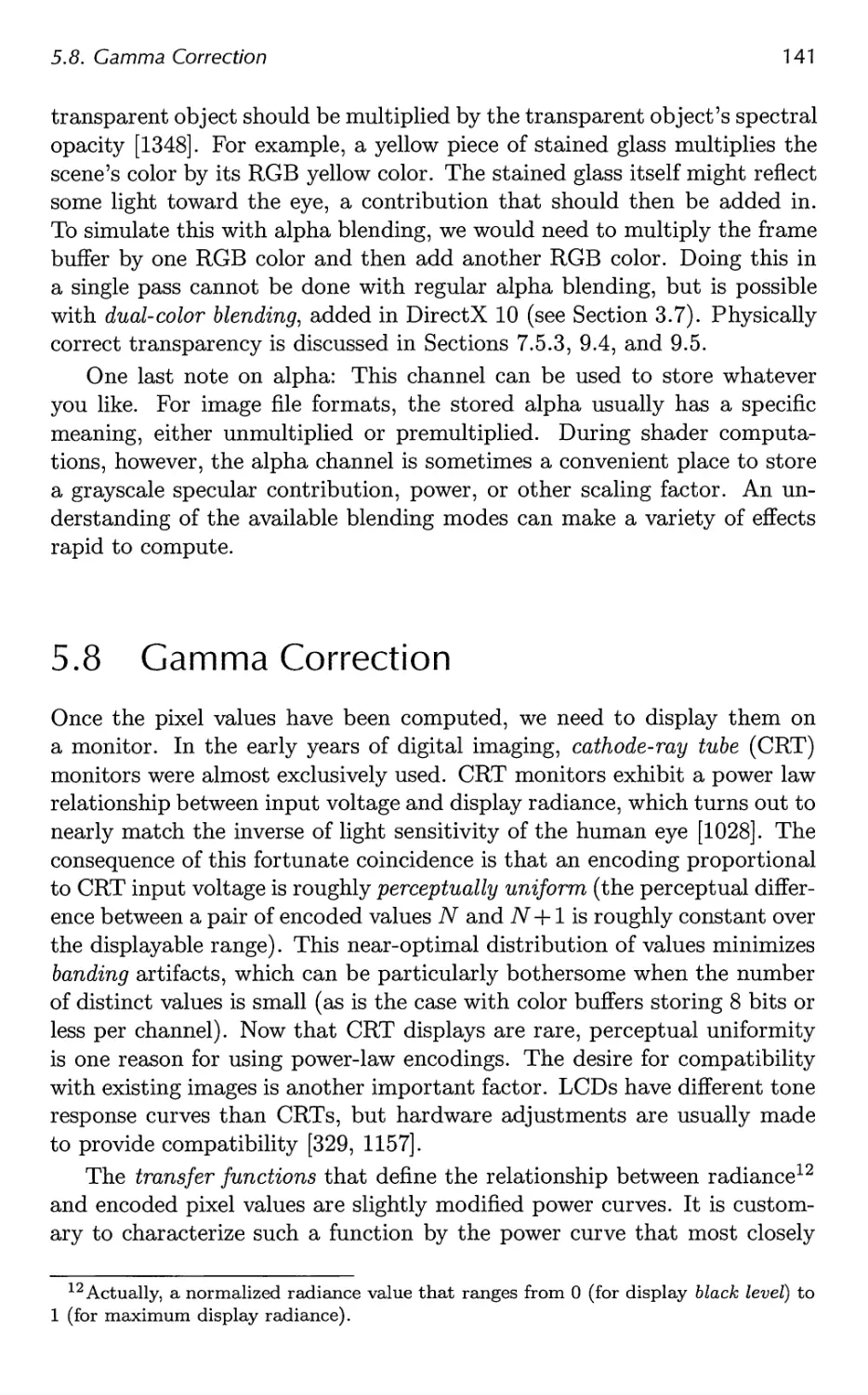


Автор: Akenine-Moller Tomas Haines Eric Hoffman Naty
Теги: computer graphics
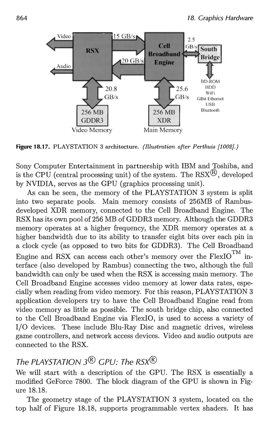
ISBN: 978-1-56881-424-7
Год: 2008


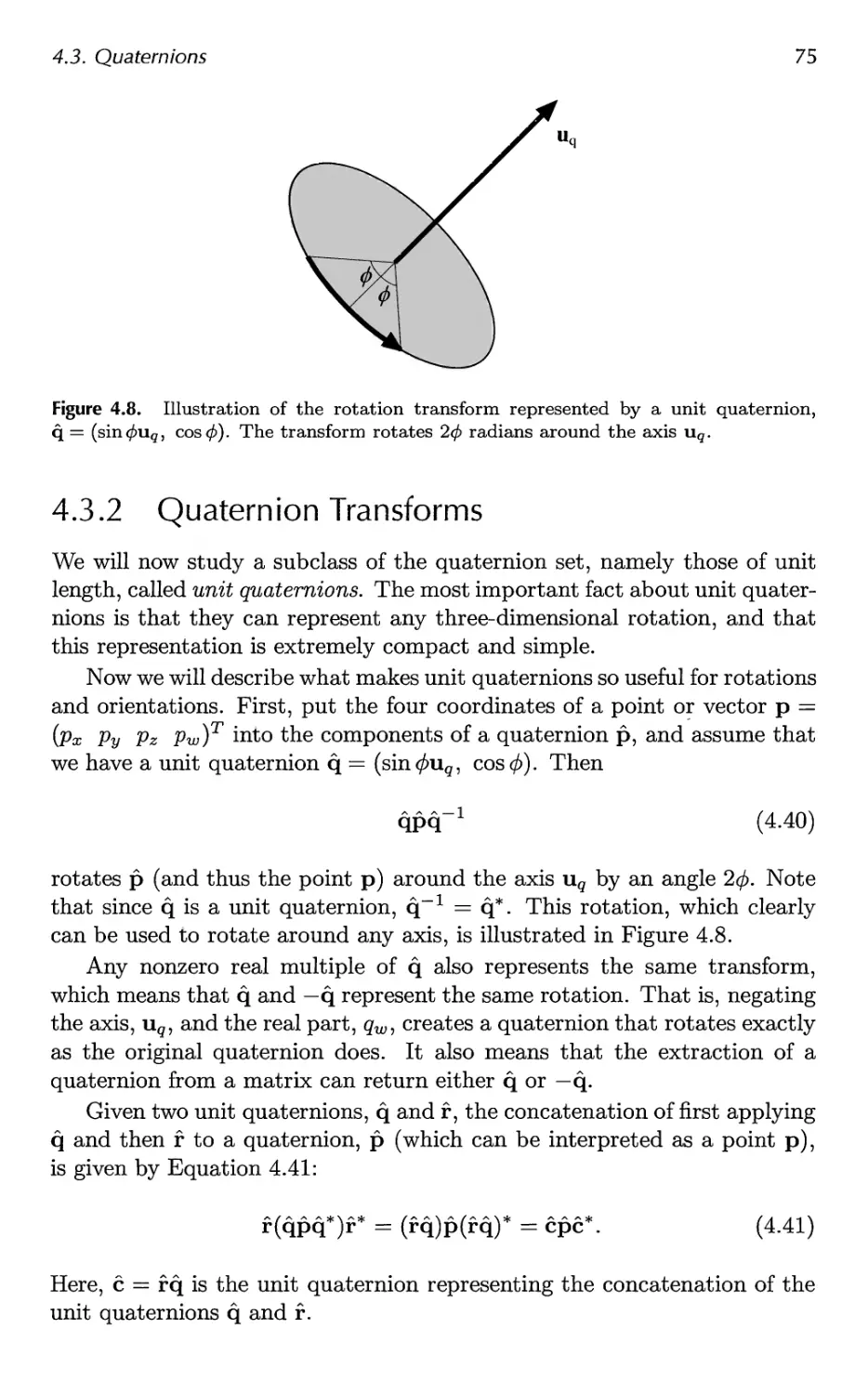
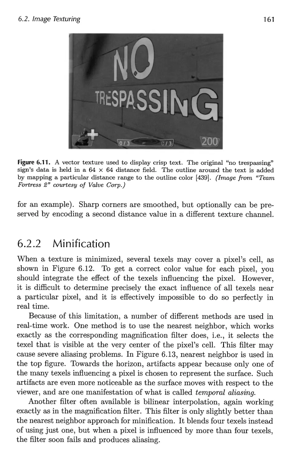
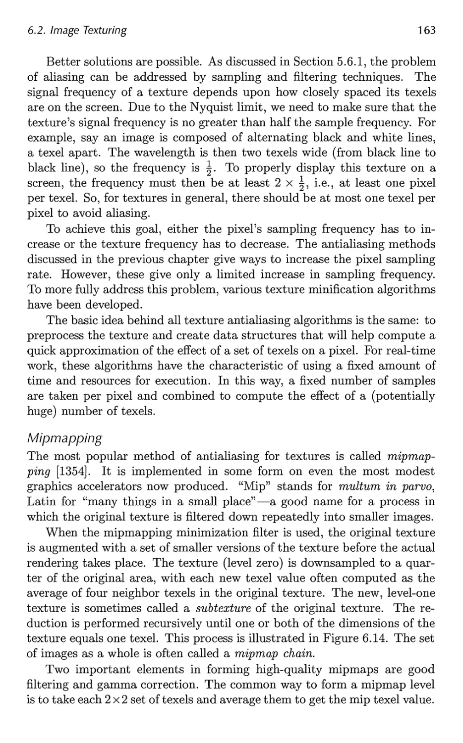
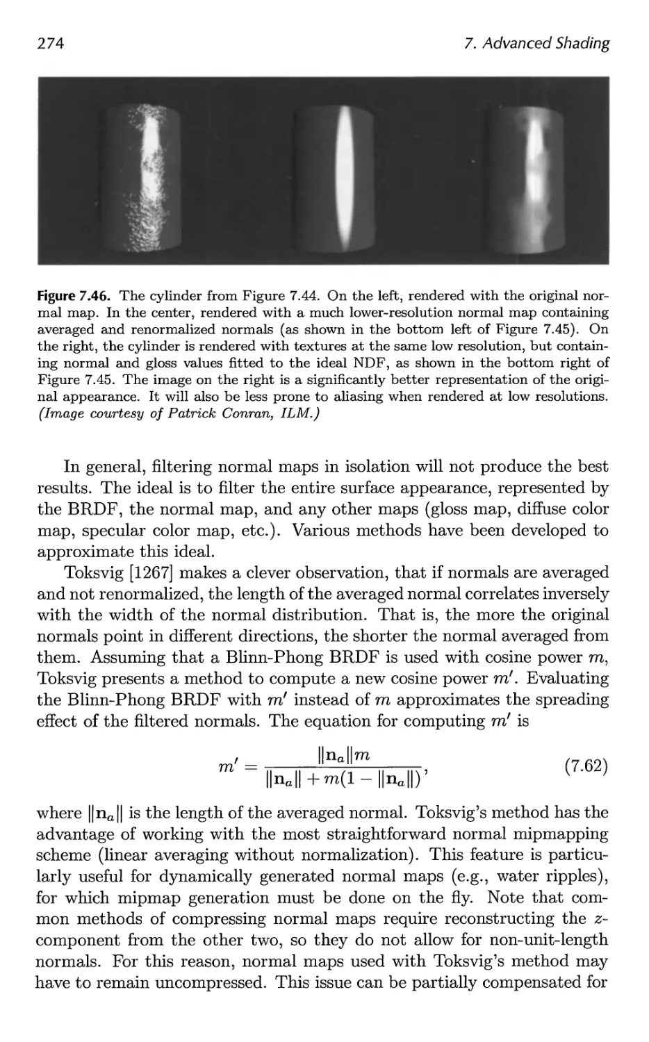
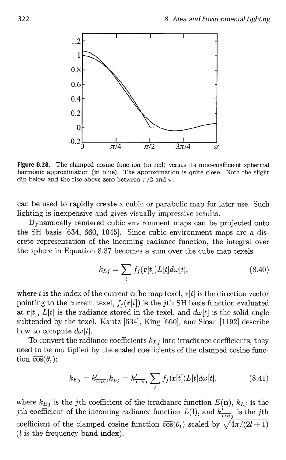
Текст
Real-Time
Rendering
Third Edition
Tomas Akenine-Mollen
Eric Haines
Naty Hoffman
/ /
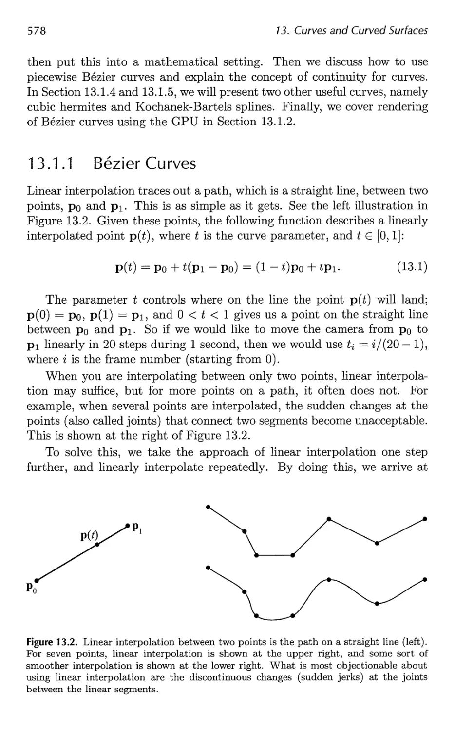
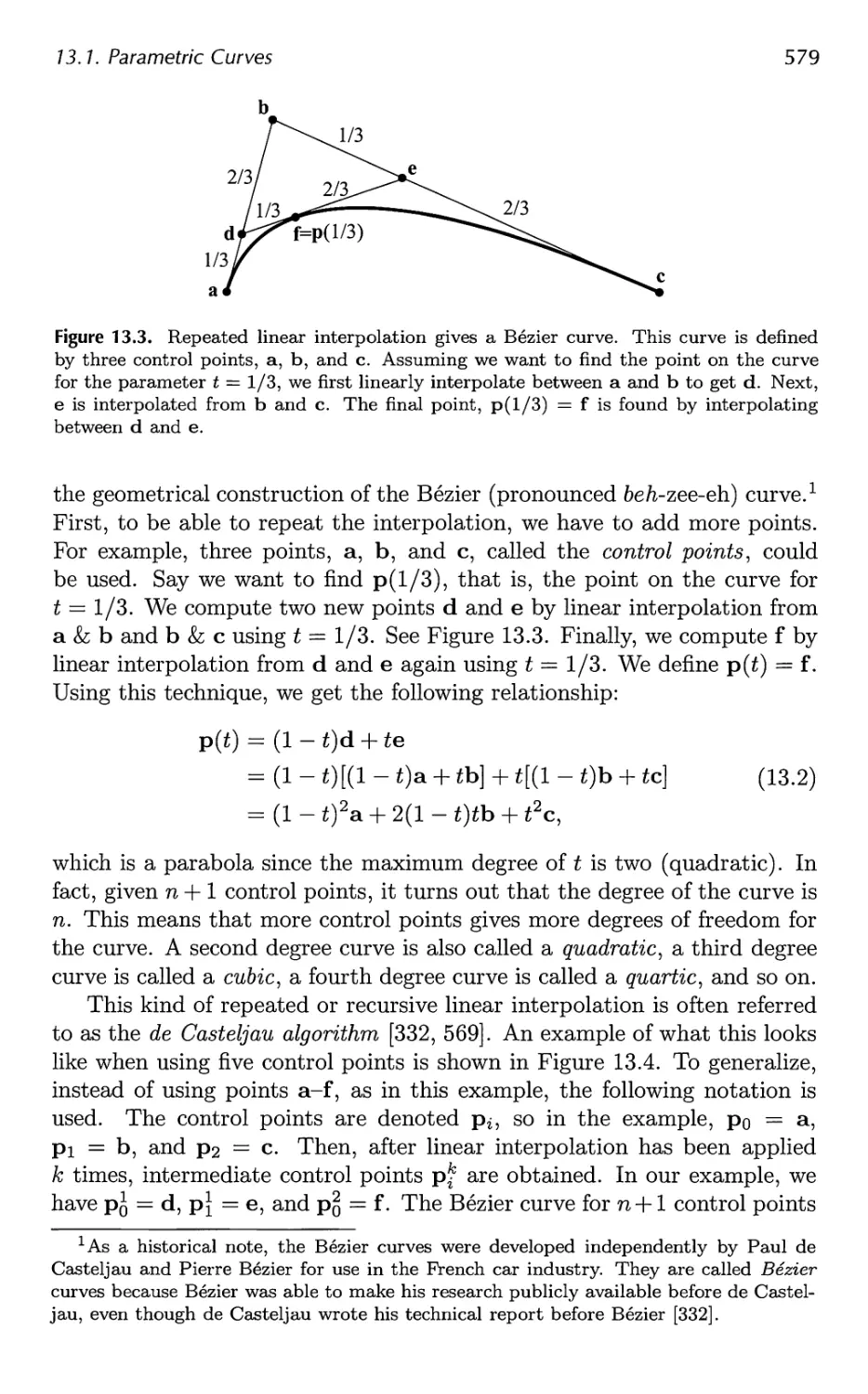
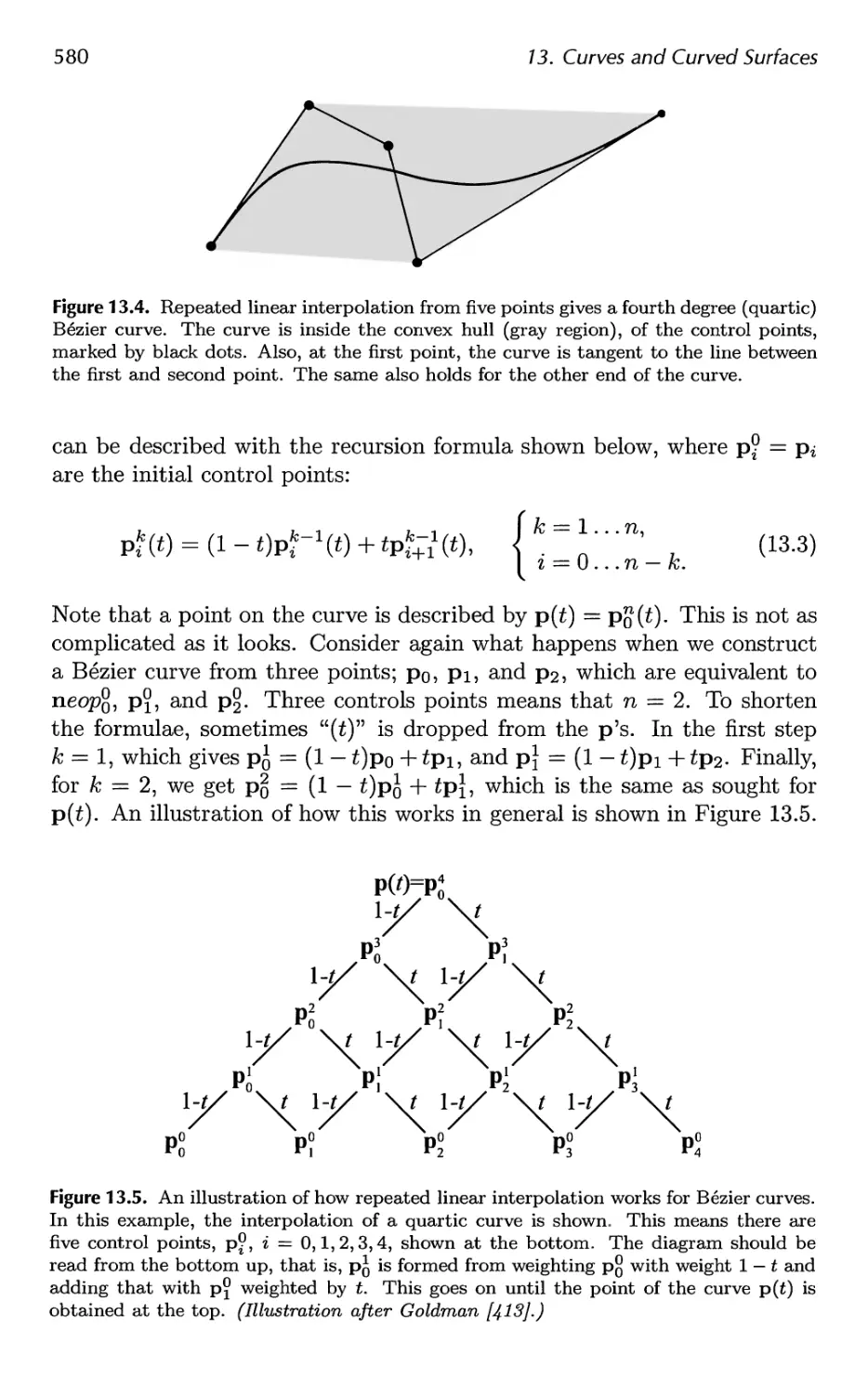
\
•v
Real-Time Renderin
Third Edition
Tomas Akenine-Moller
Eric Haines
Naty Hoffman
R
A K Peters, Ltd.
Wellesley, Massachusetts
Editorial, Sales, and Customer Service Office
A K Peters, Ltd.
888 Worcester Street, Suite 230
Wellesley, MA 02482
www.akpeters.com
Copyright © 2008 by A K Peters, Ltd.
All rights reserved. No part of the material protected by this copyright
notice may be reproduced or utilized in any form, electronic or
mechanical, including photocopying, recording, or by any information storage and
retrieval system, without written permission from the copyright owner.
Library of Congress Cataloging-in-Publication Data
Moller, Tomas, 1971-
Real-time rendering / Tomas Akenine-Moller, Eric Haines, Nathaniel Hoffman.
- 3rd ed.
p. cm.
Includes bibliographical references and index.
ISBN-13: 978-1-56881-424-7 (alk. paper)
1. Computer graphics. 2. Real-time data processing. I. Haines, Eric, 1958- II.
Hoffman, Nathaniel. III. Title
T385.M635 2008
006.6'773--dc22
2008011580
Cover images: ©2008 Sony Computer Entertainment Europe.
LittleBigPlanet developed by Media Molecule. LittleBigPlanet is a
trademark of Sony Computer Entertianment Europe.
Printed in India
12 11 10 09 08
10 987654321
Dedicated to Eva, Felix, and Elina
T. A-M.
Dedicated to Cathy, Ryan, and Evan
E. H.
Dedicated to Dorit, Karen, and Daniel
N. H.
Contents
Preface 11
1 Introduction 1
1.1 Contents Overview 2
1.2 Notation and Definitions 4
2 The Graphics Rendering Pipeline 11
2.1 Architecture 12
2.2 The Application Stage 14
2.3 The Geometry Stage 15
2.4 The Rasterizer Stage 21
2.5 Through the Pipeline 25
3 The Graphics Processing Unit 29
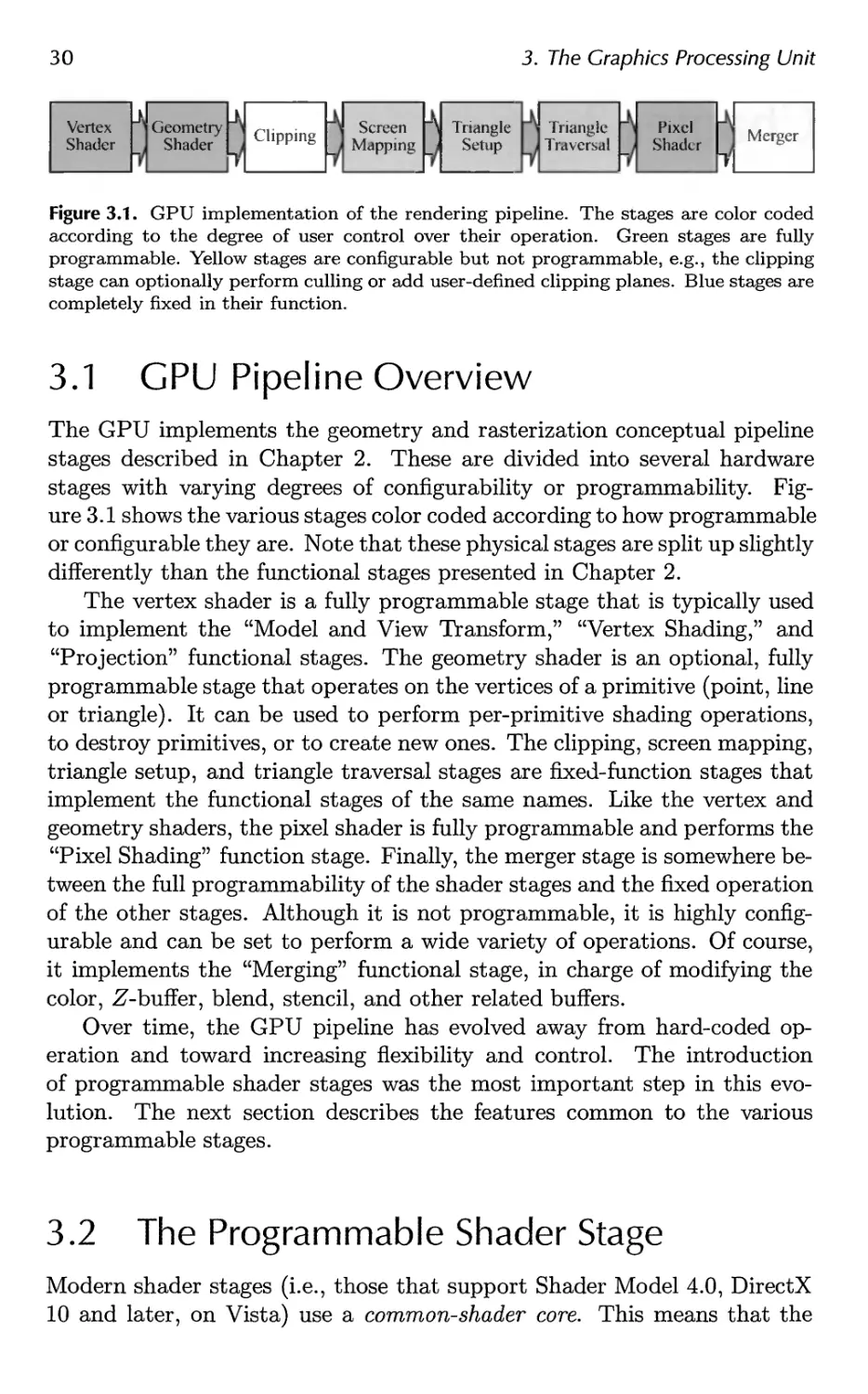
3.1 GPU Pipeline Overview 30
3.2 The Programmable Shader Stage 30
3.3 The Evolution of Programmable Shading 33
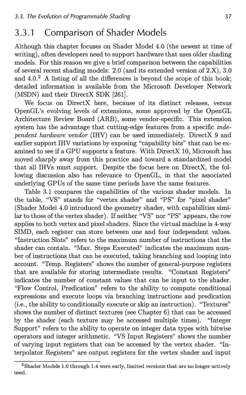
3.4 The Vertex Shader 38
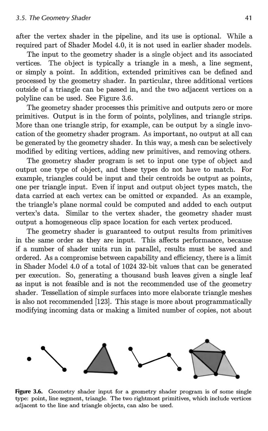
3.5 The Geometry Shader 40
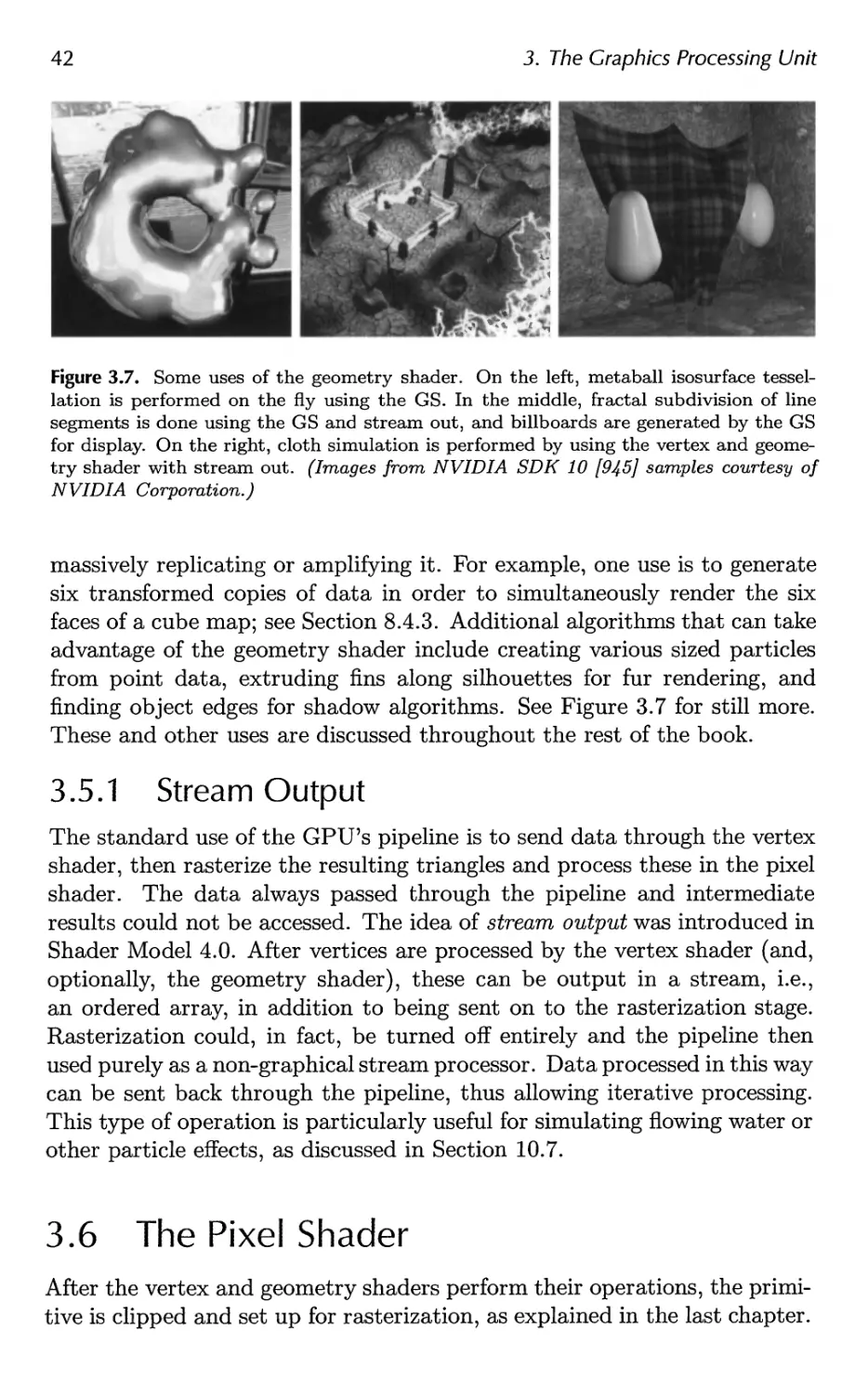
3.6 The Pixel Shader 42
3.7 The Merging Stage 44
3.8 Effects 45
4 Transforms 53
4.1 Basic Transforms 55
4.2 Special Matrix Transforms and Operations 65
4.3 Quaternions 72
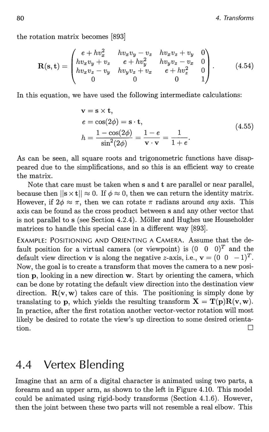
4.4 Vertex Blending 80
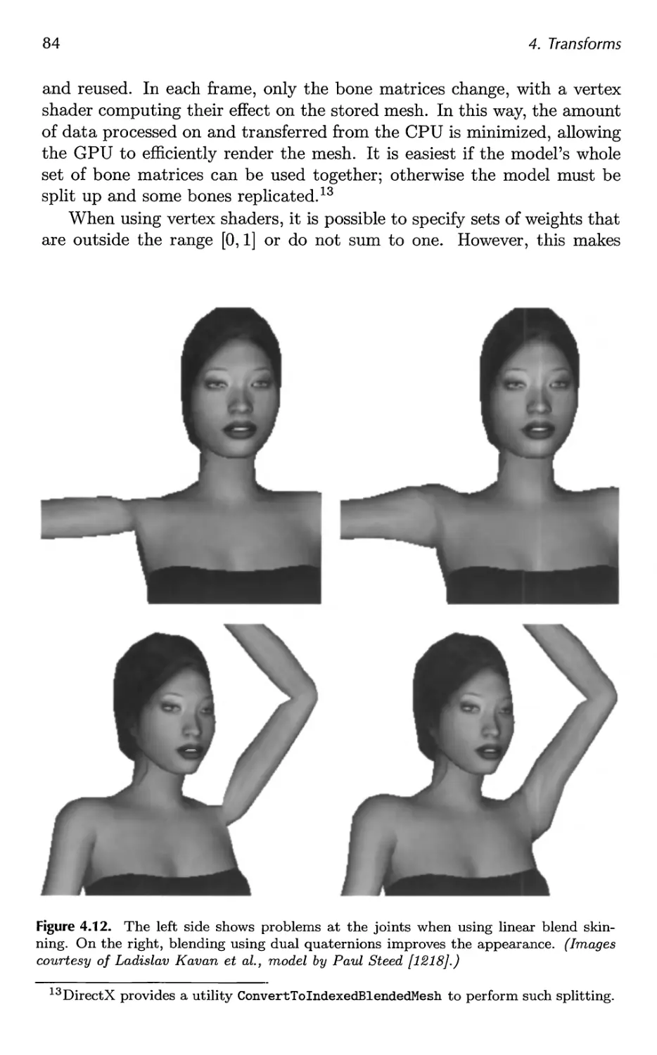
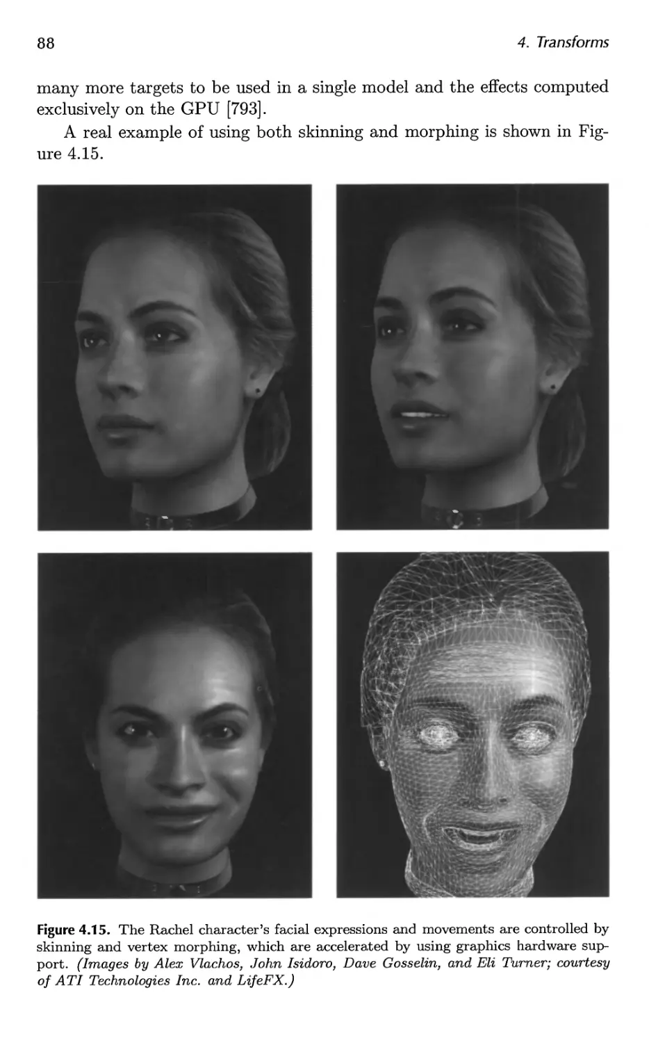
4.5 Morphing 85
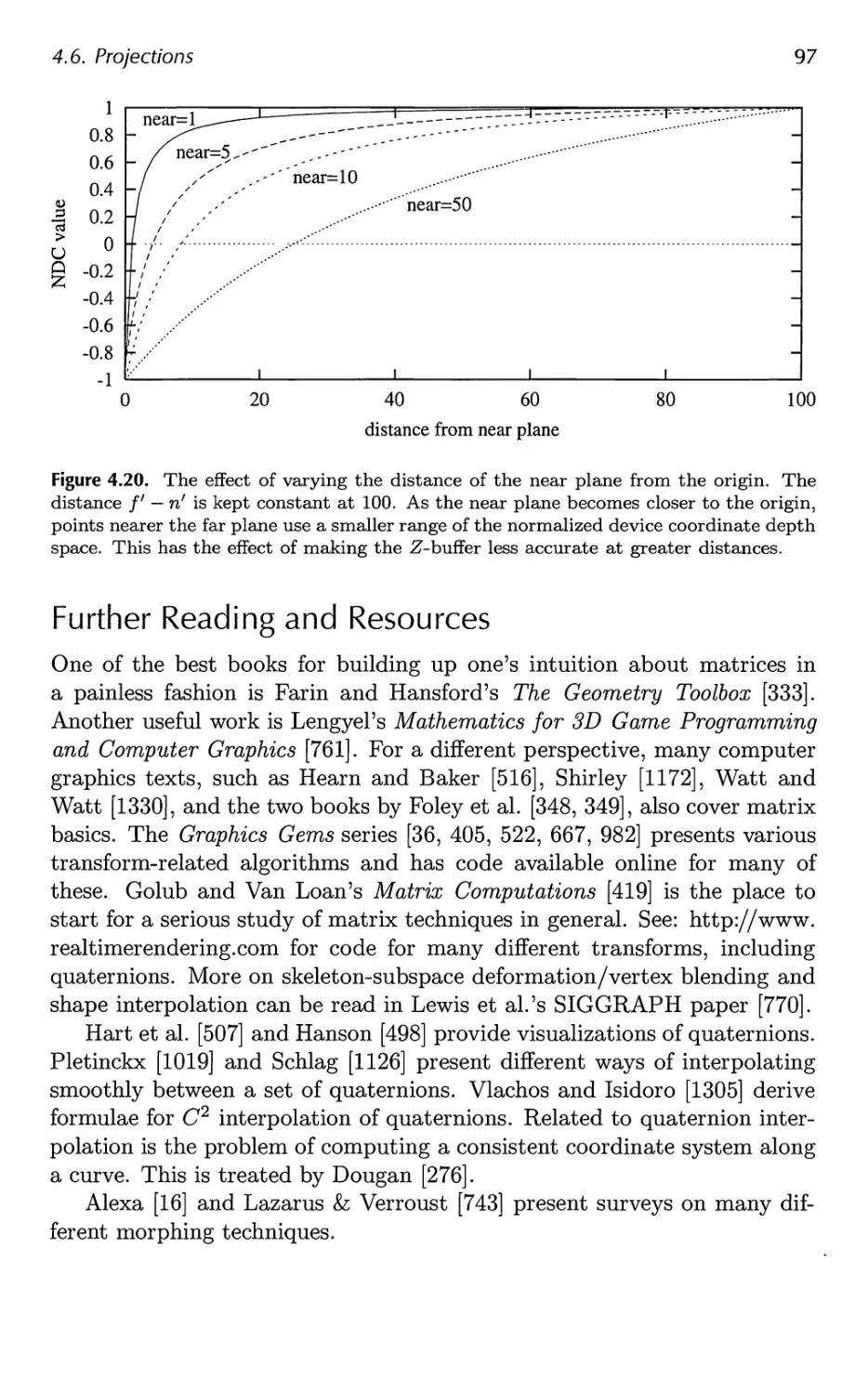
4.6 Projections 89
5 Visual Appearance 99
5.1 Visual Phenomena 99
5.2 Light Sources 100
vii
viii Contents
5.3 Material 104
5.4 Sensor 107
5.5 Shading 110
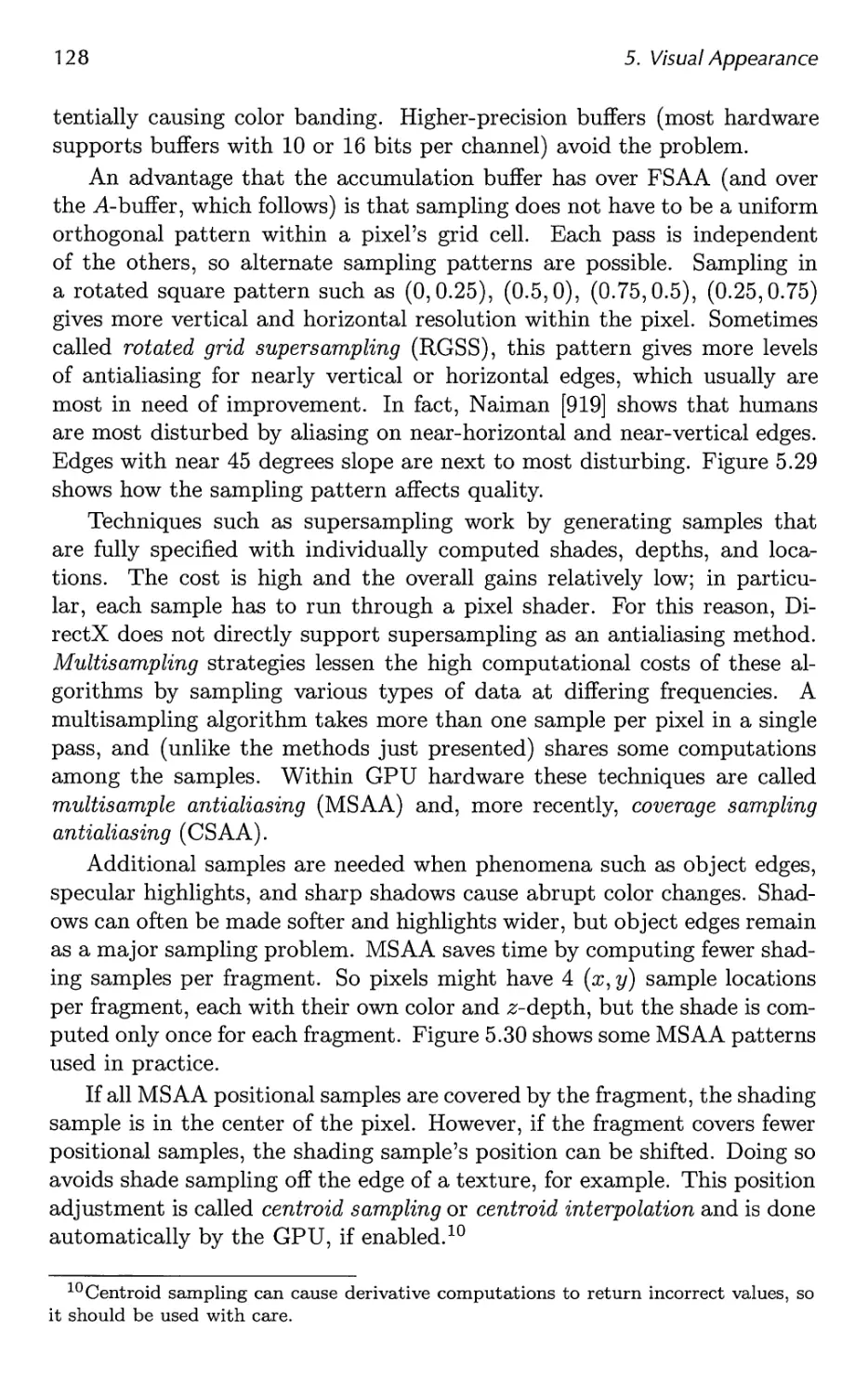
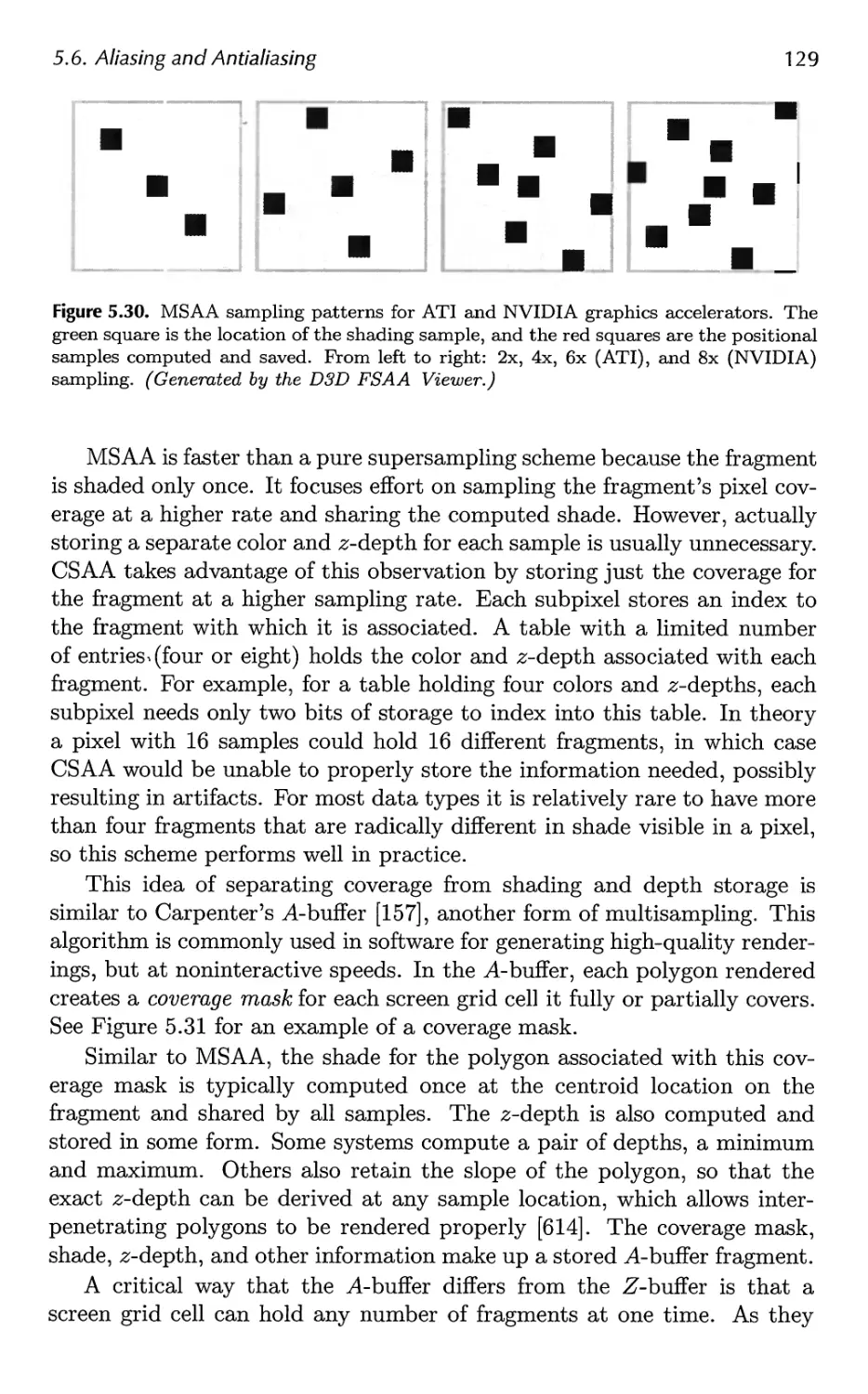
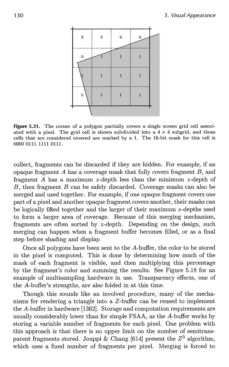
5.6 Aliasing and Antialiasing 116
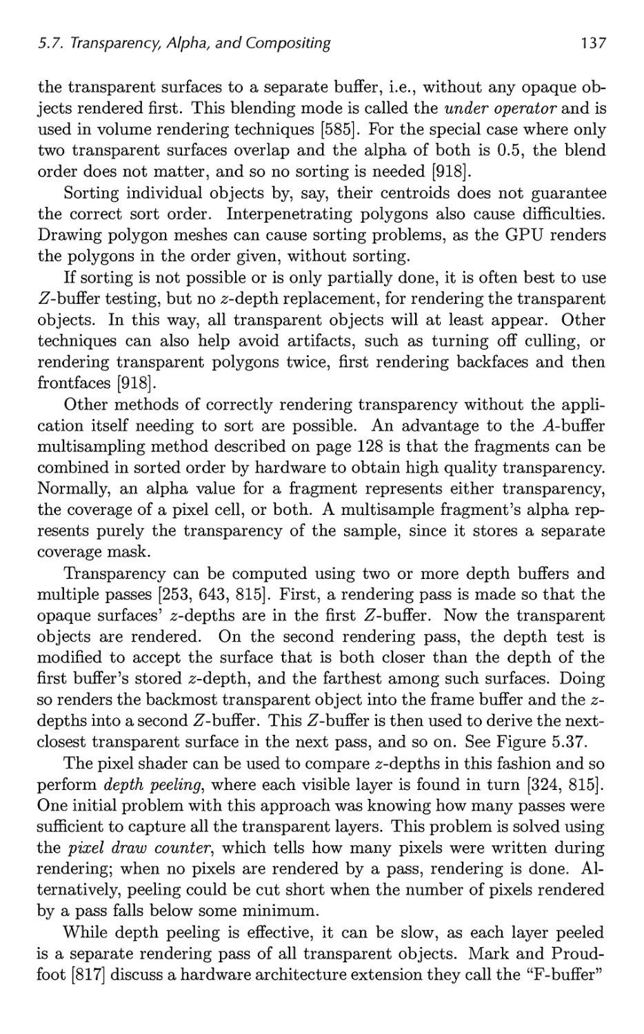
5.7 Transparency, Alpha, and Compositing 134
5.8 Gamma Correction 141
6 Texturing 147
6.1 The Texturing Pipeline 148
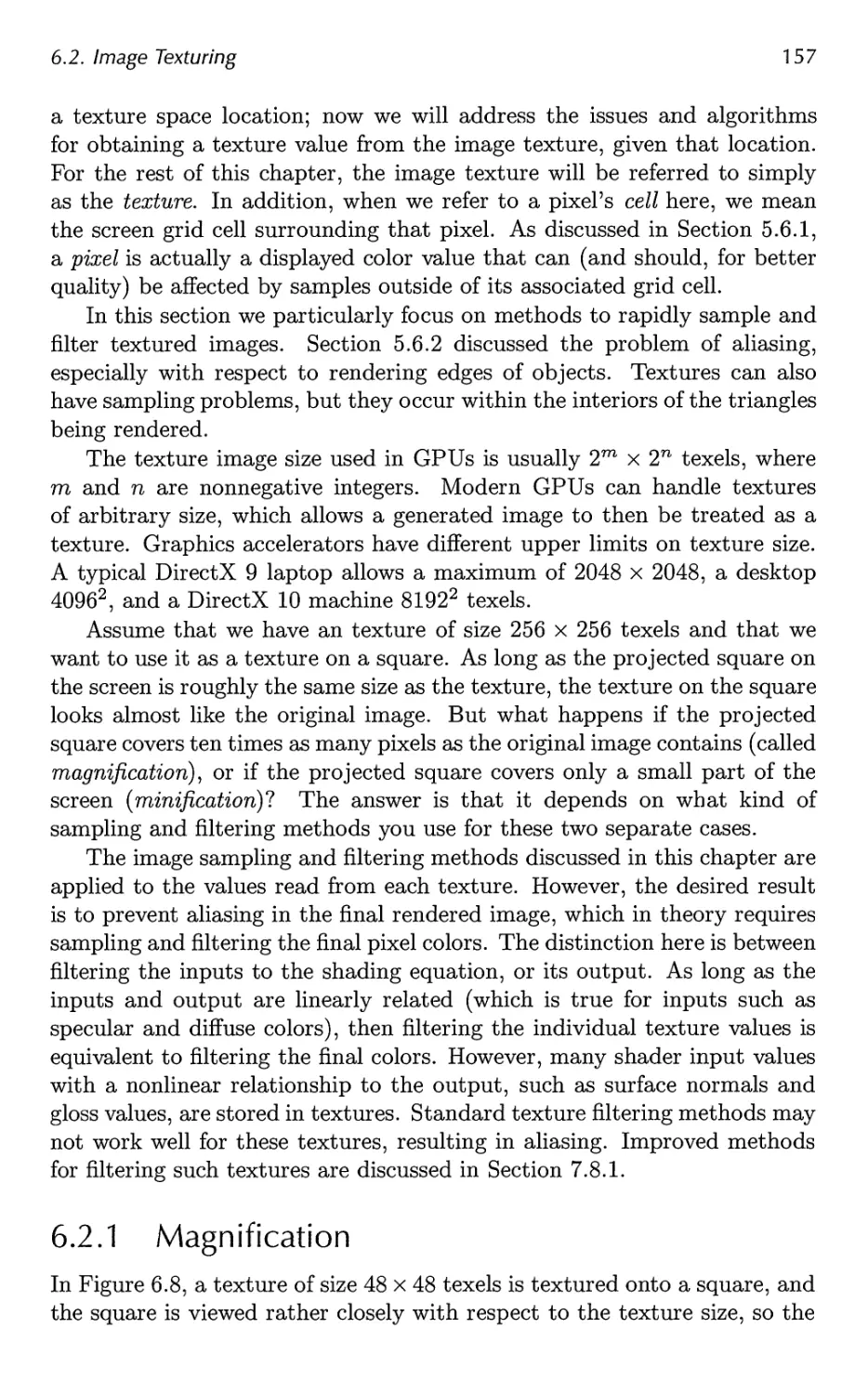
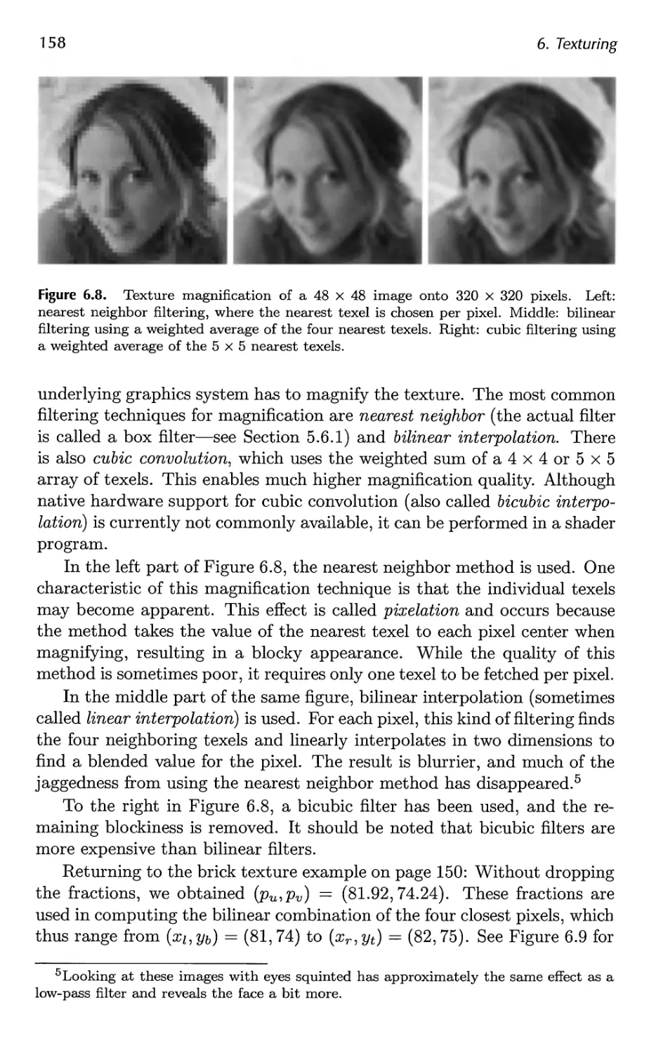
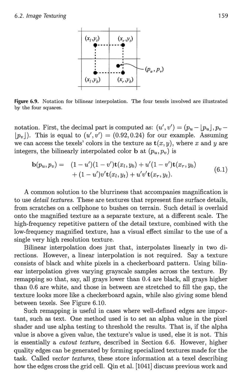
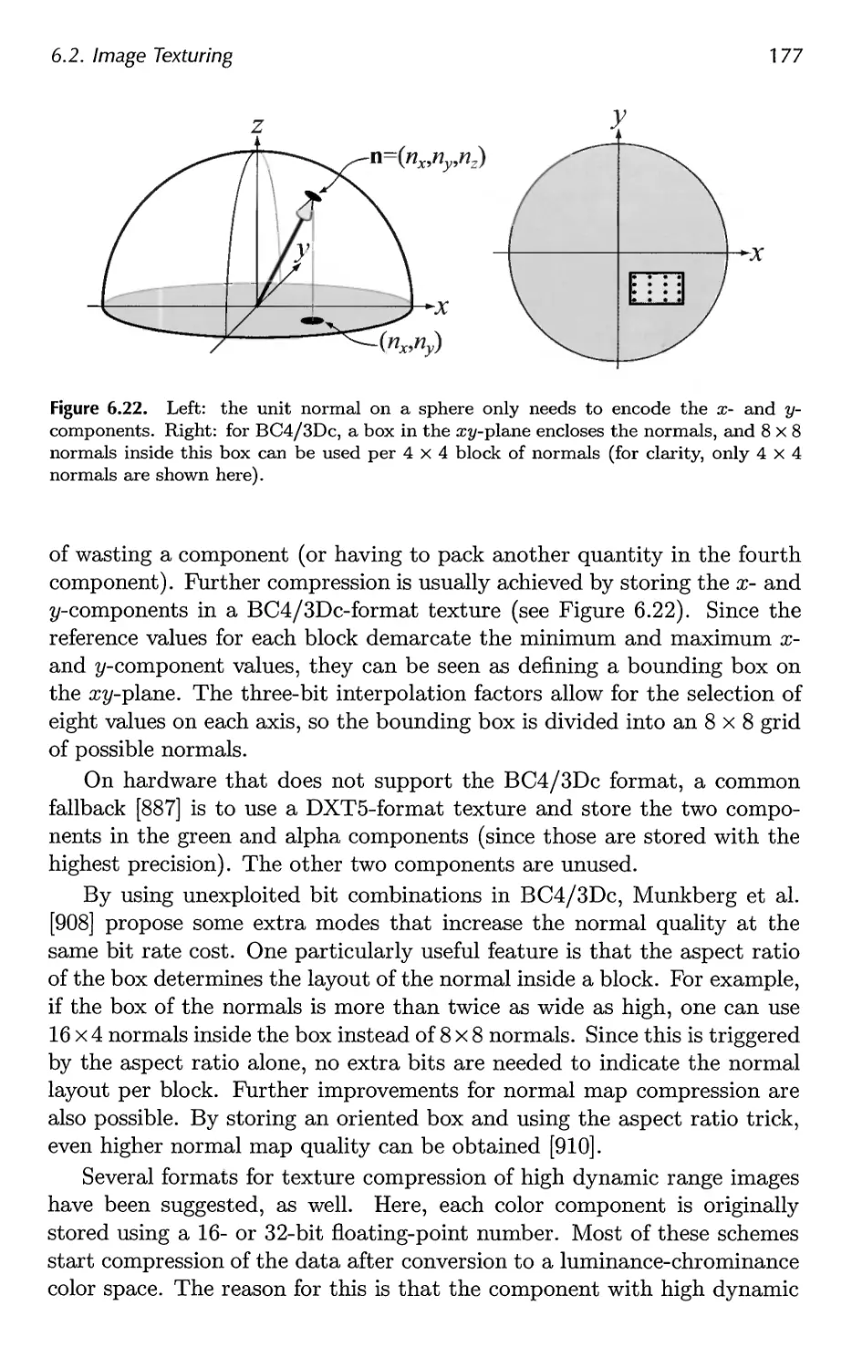
6.2 Image Texturing 156
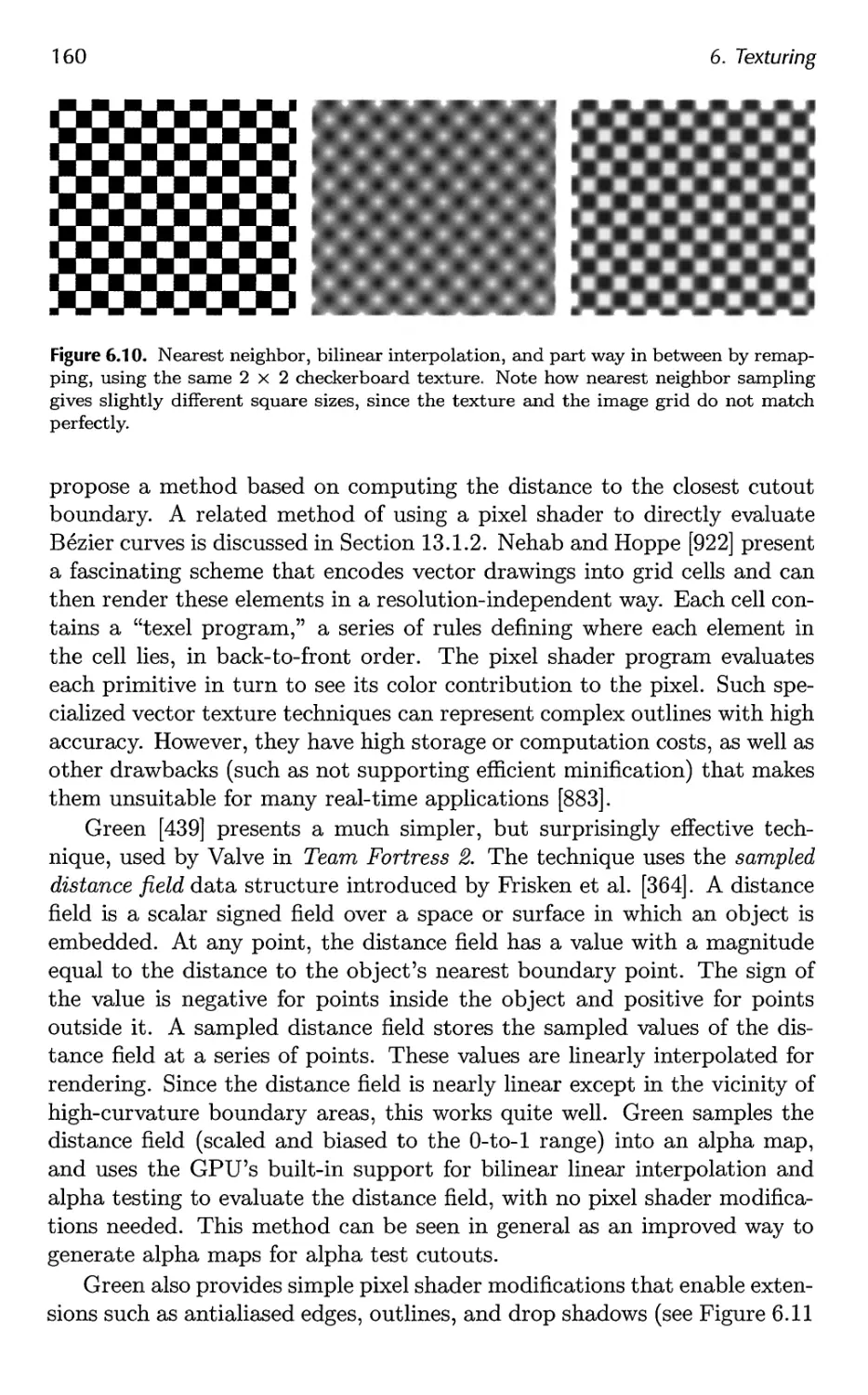
6.3 Procedural Texturing 178
6.4 Texture Animation 180
6.5 Material Mapping 180
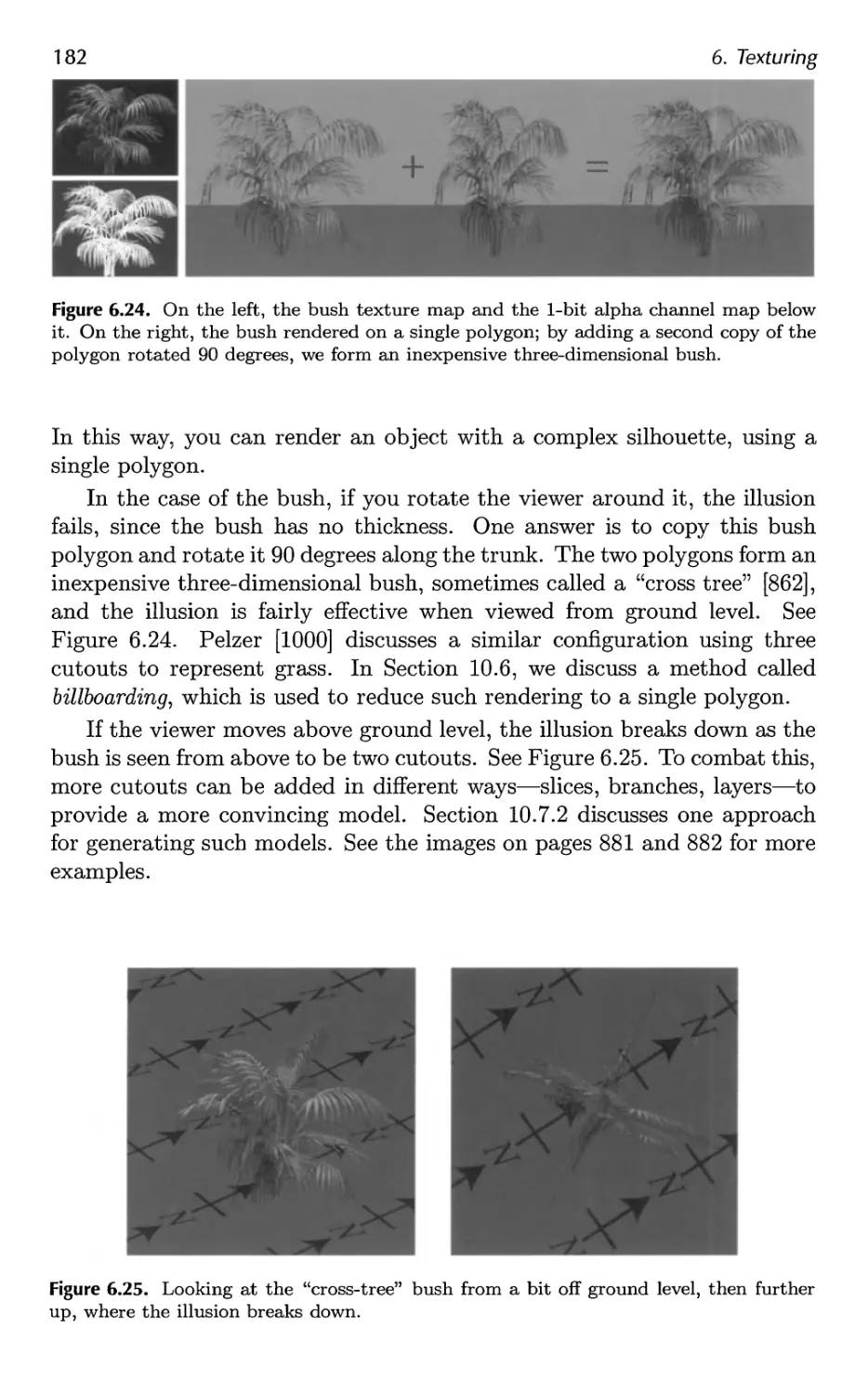
6.6 Alpha Mapping 181
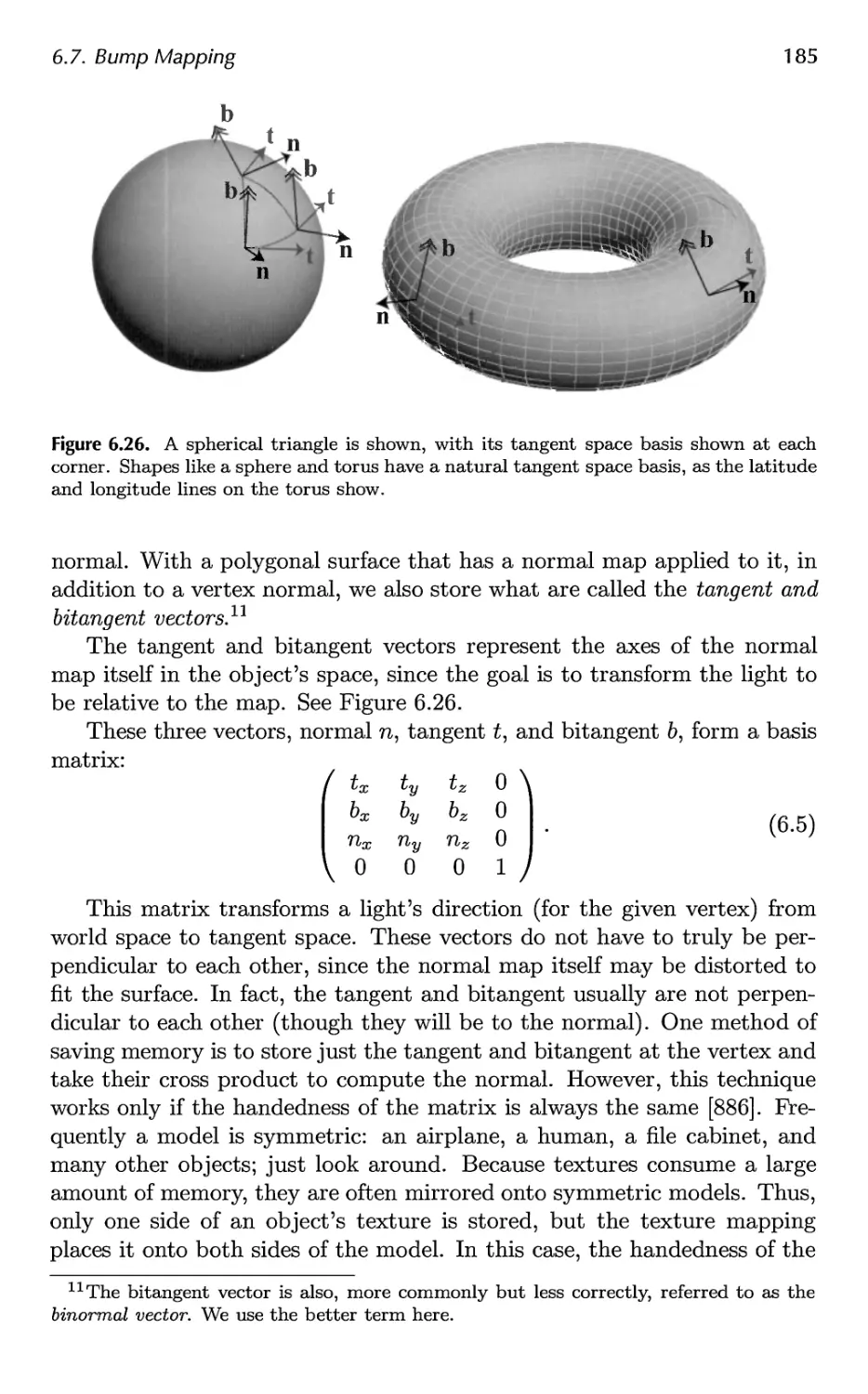
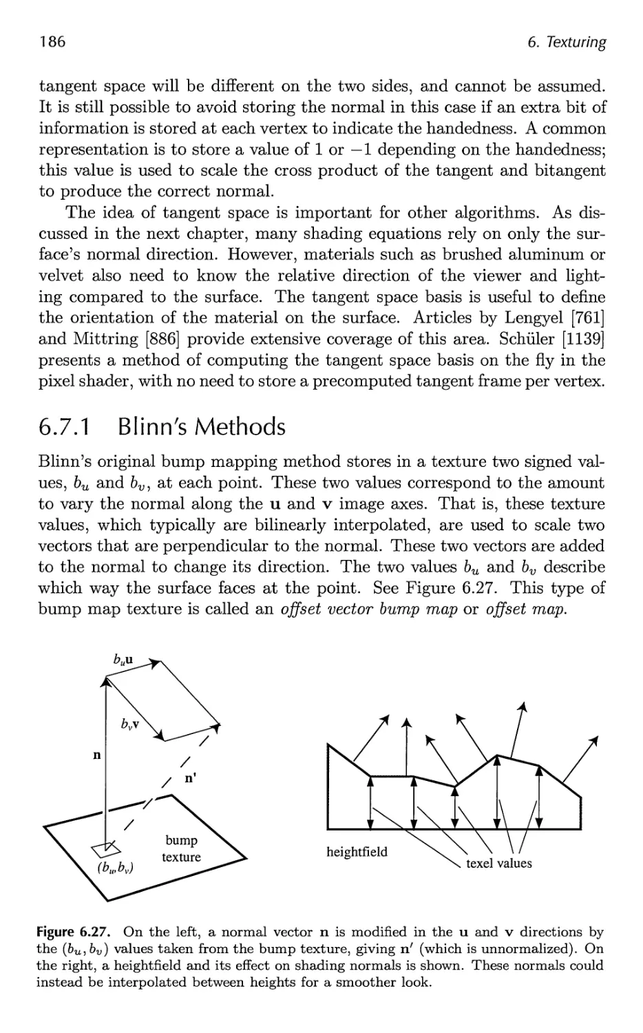
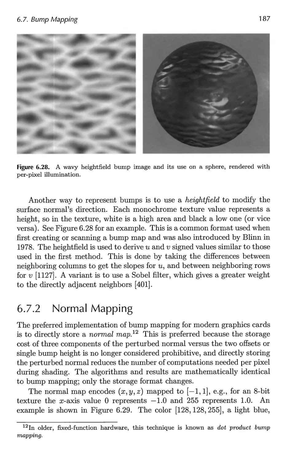
6.7 Bump Mapping 183
7 Advanced Shading 201
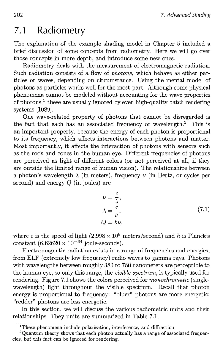
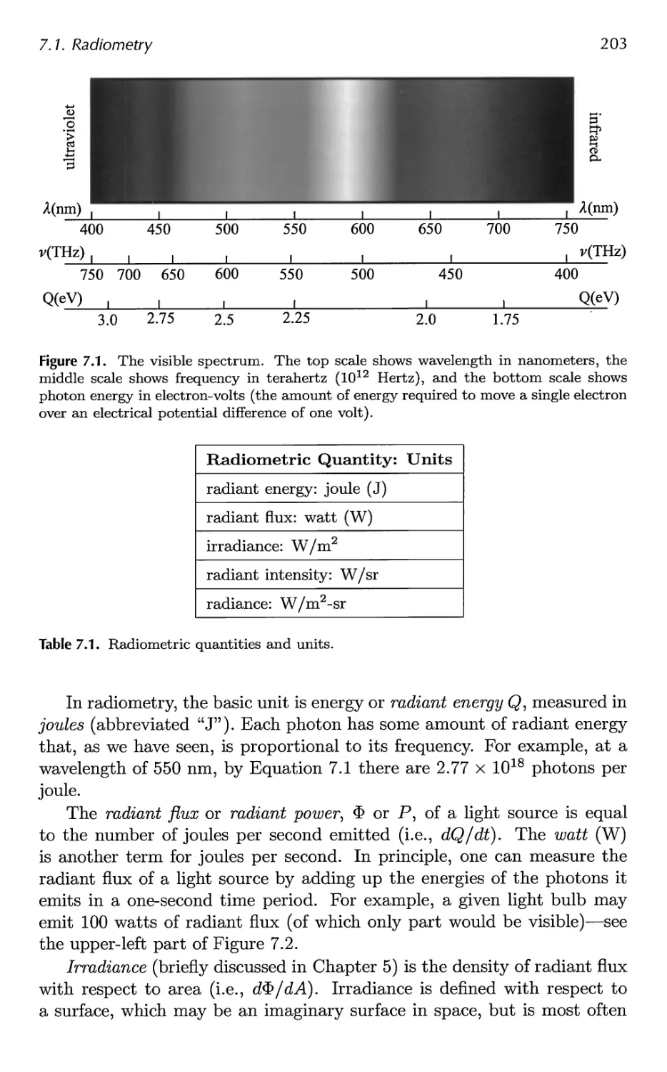
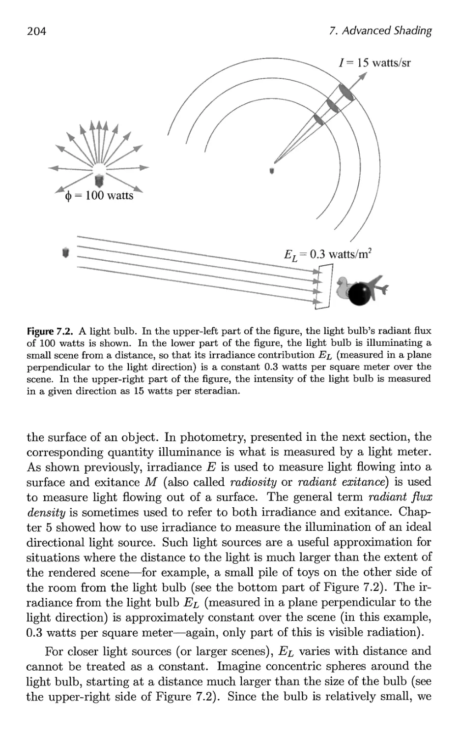
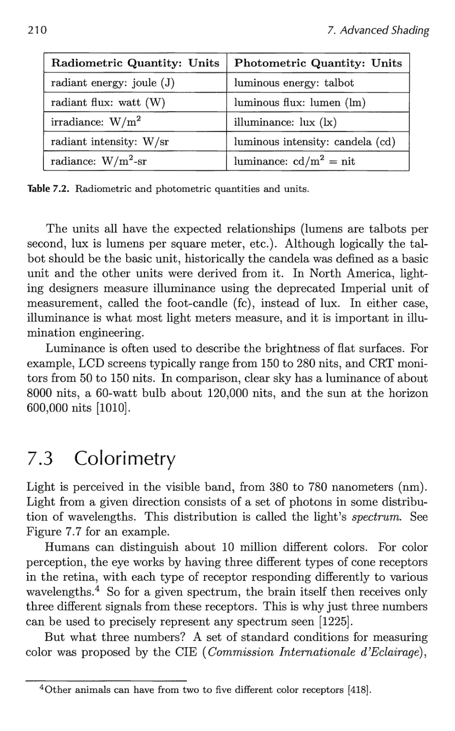
7.1 Radiometry 202
7.2 Photometry 209
7.3 Colorimetry 210
7.4 Light Source Types 217
7.5 BRDF Theory 223
7.6 BRDF Models 251
7.7 BRDF Acquisition and Representation 264
7.8 Implementing BRDFs 269
7.9 Combining Lights and Materials 275
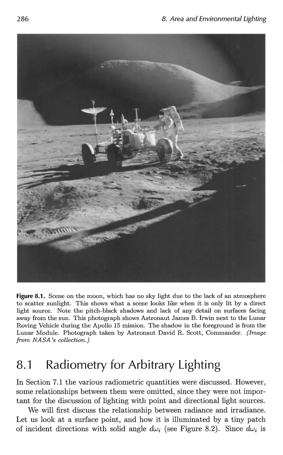
8 Area and Environmental Lighting 285
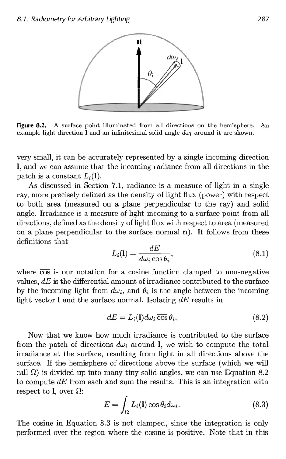
8.1 Radiometry for Arbitrary Lighting 286
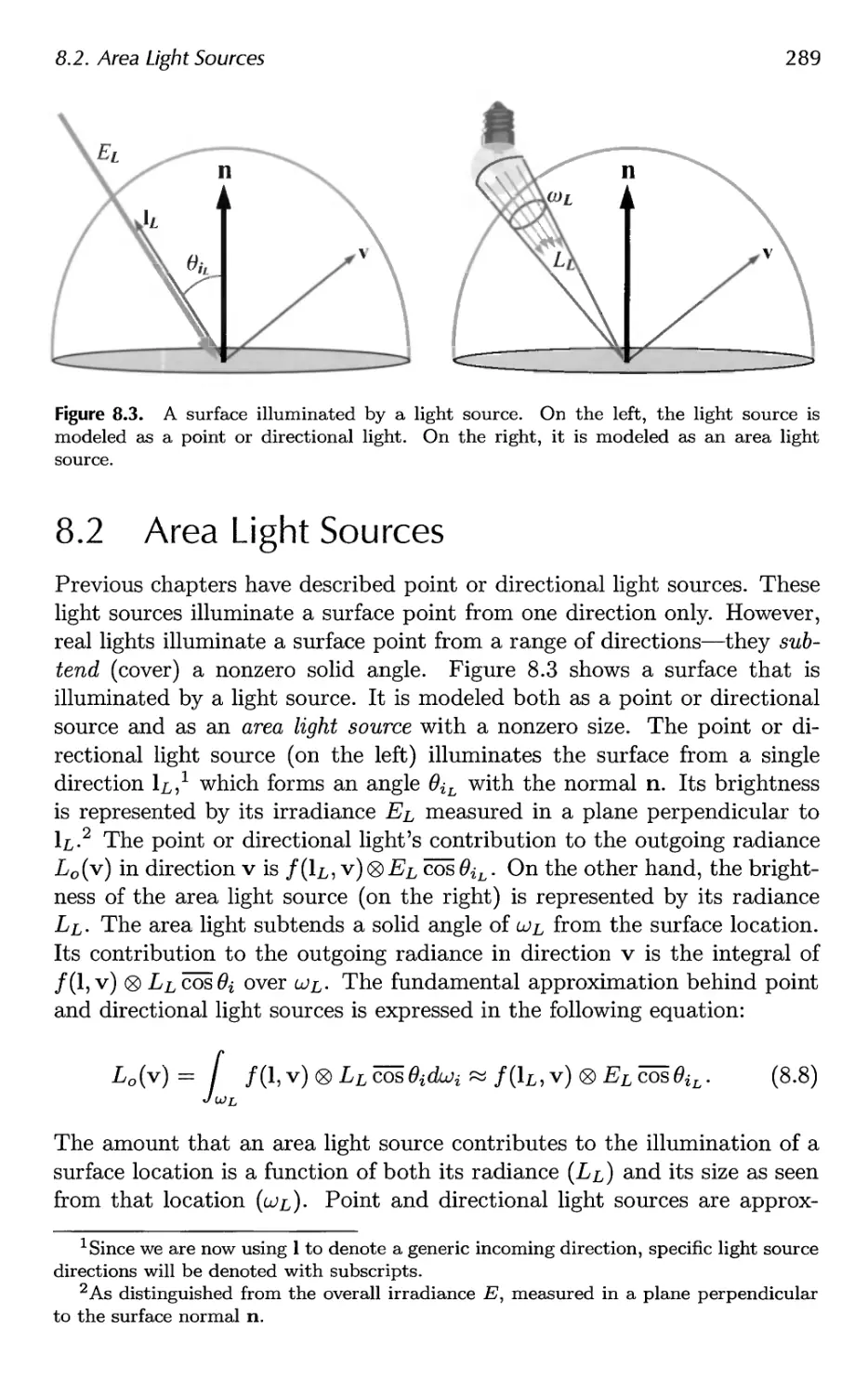
8.2 Area Light Sources 289
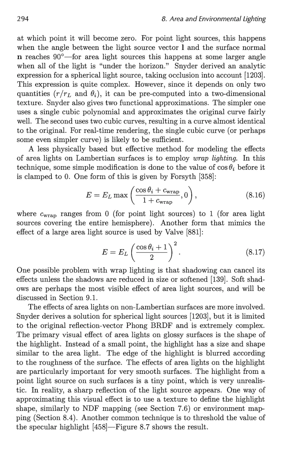
8.3 Ambient Light 295
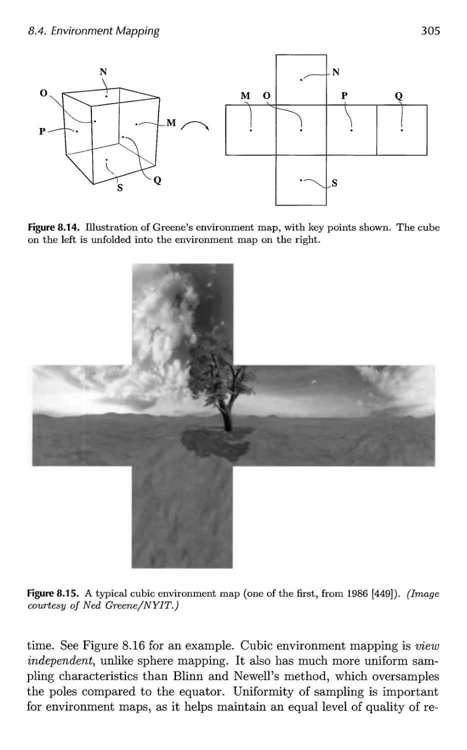
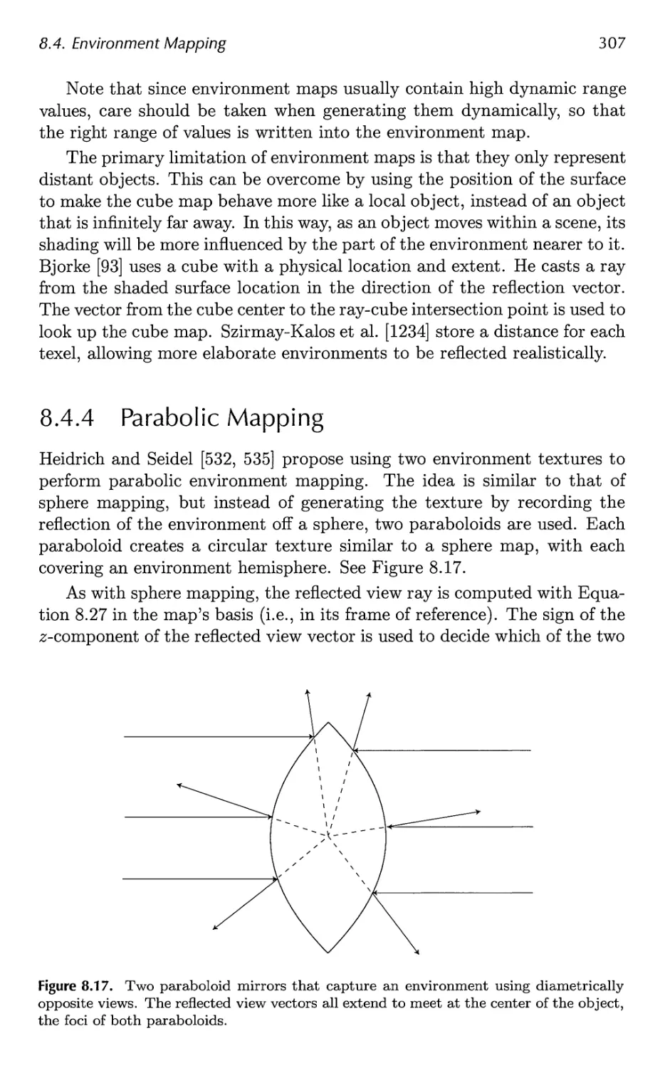
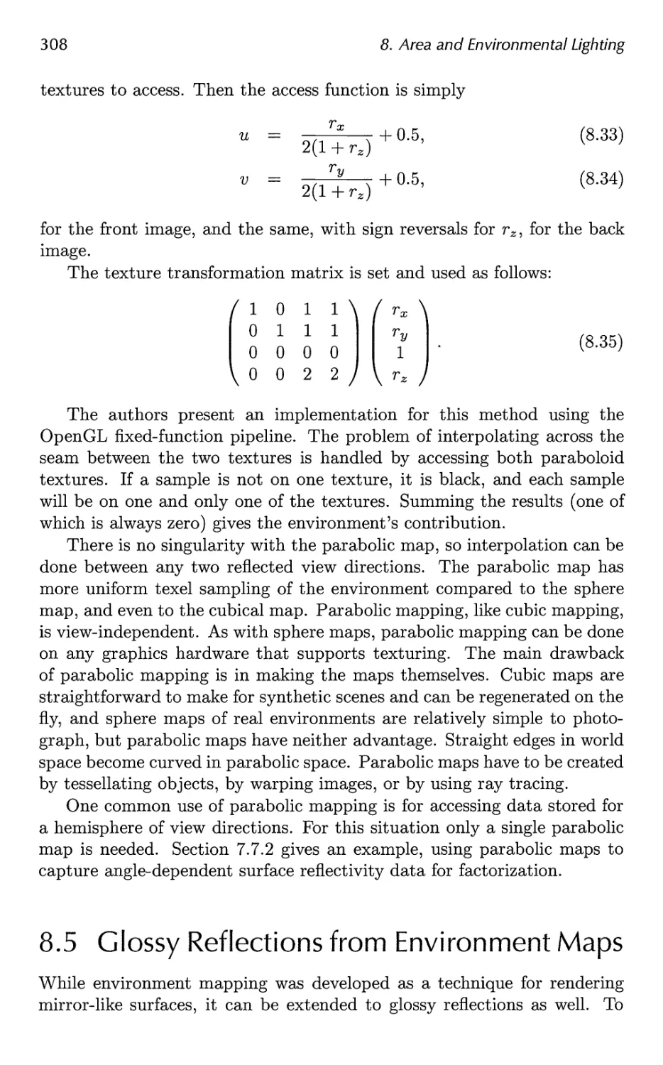
8.4 Environment Mapping 297
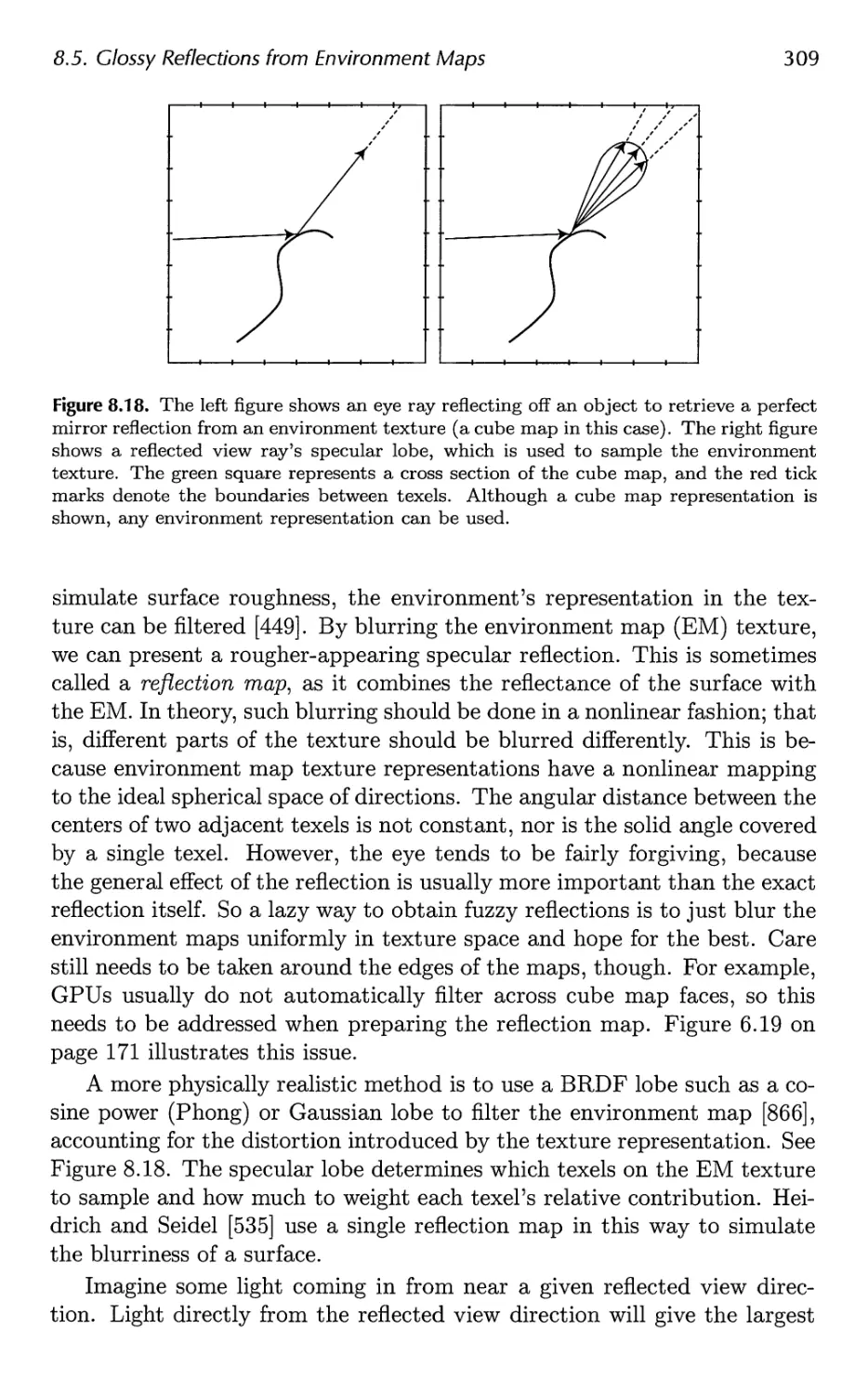
8.5 Glossy Reflections from Environment Maps 308
8.6 Irradiance Environment Mapping 314
9 Global Illumination 327
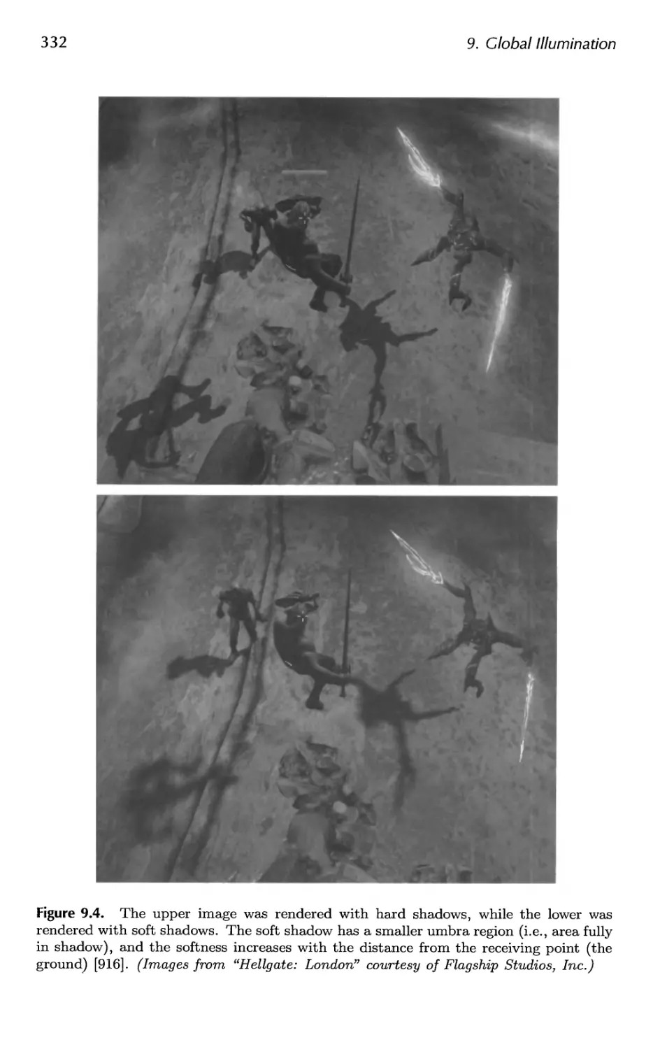
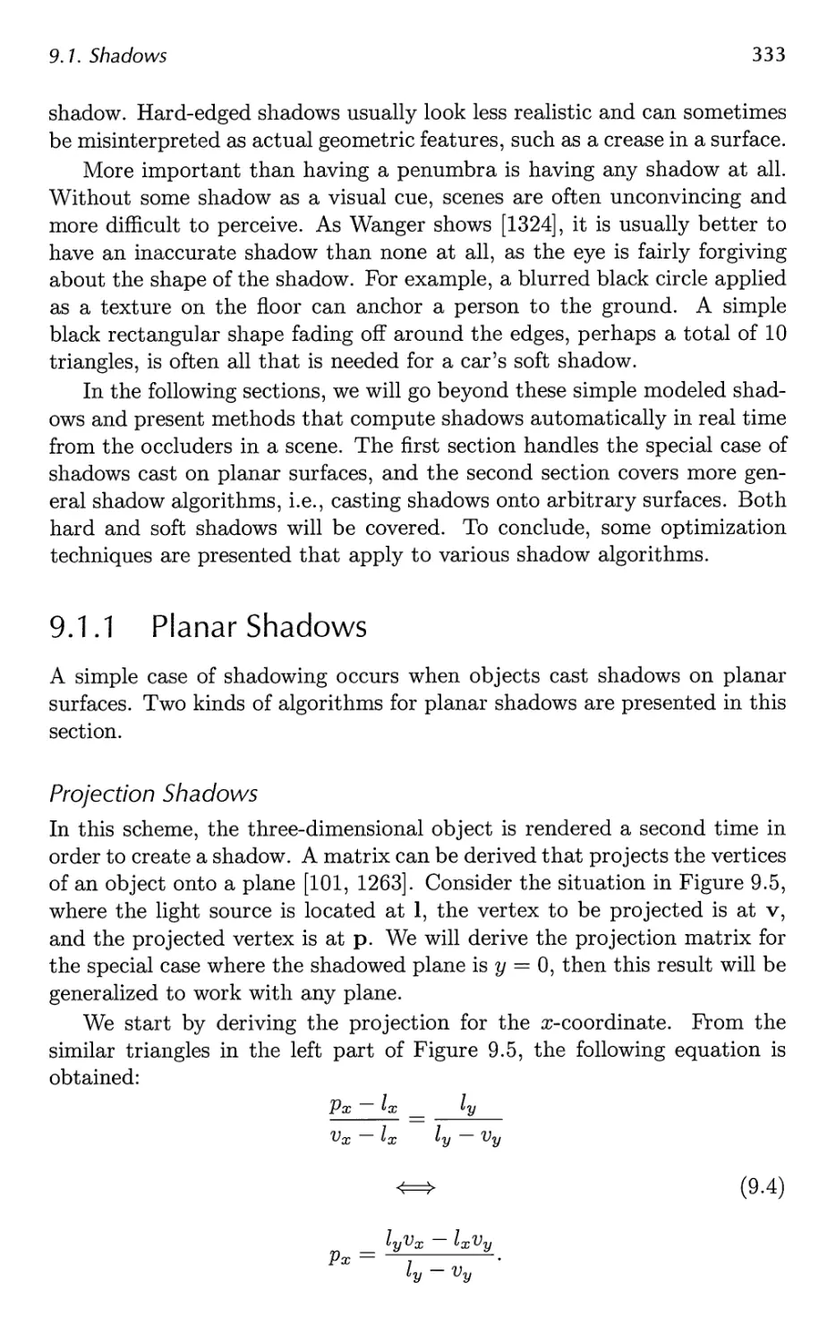
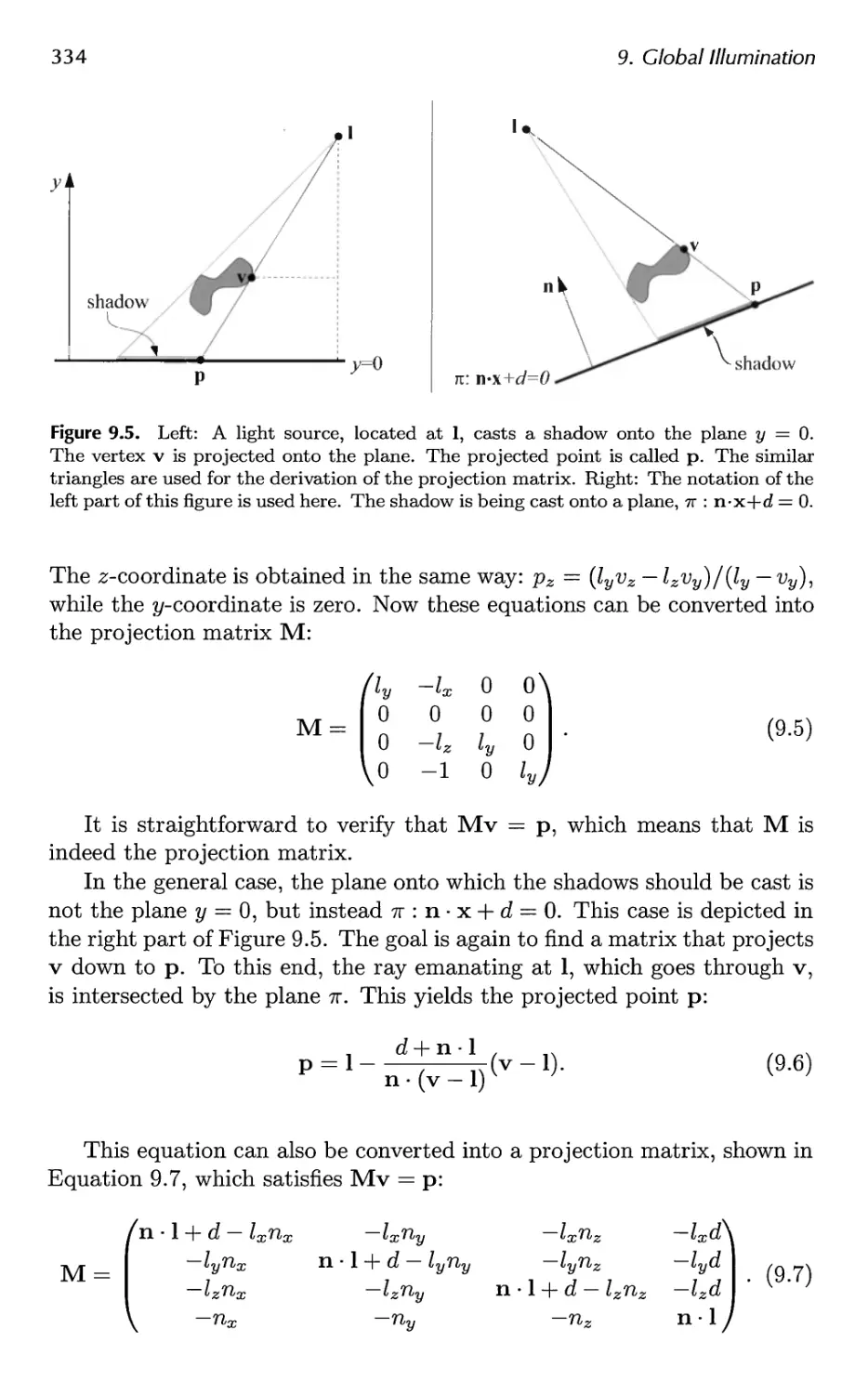
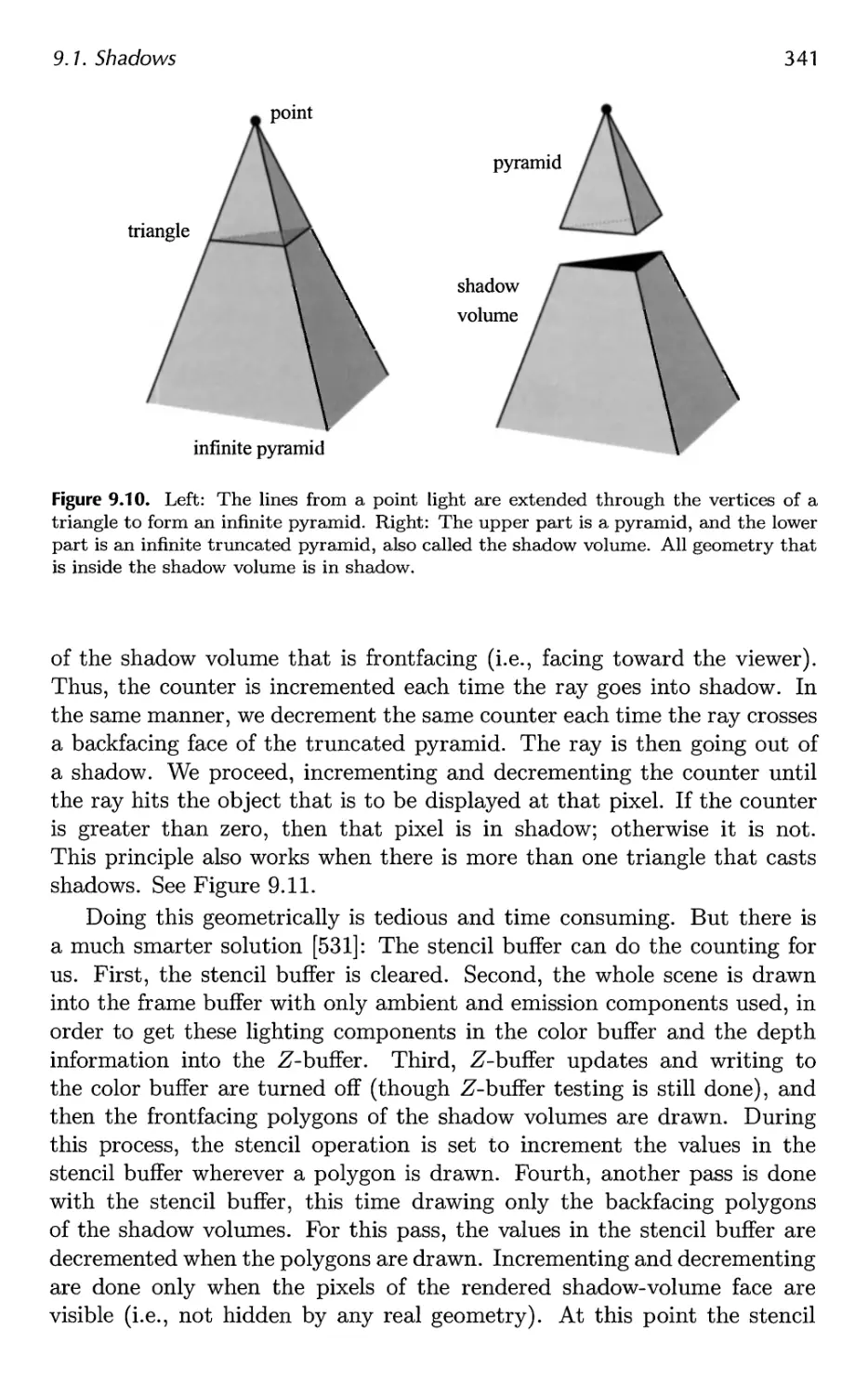
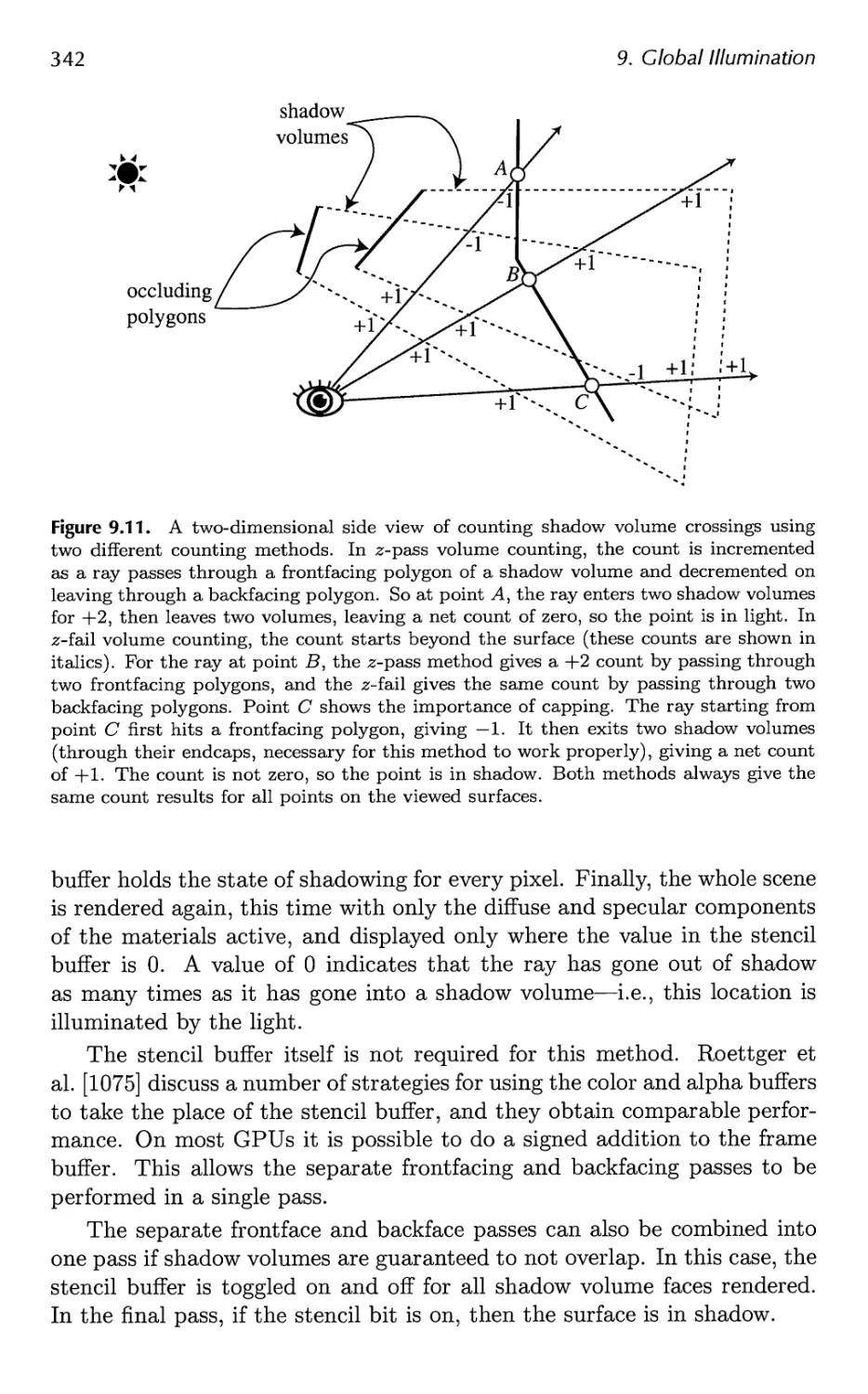
9.1 Shadows 331
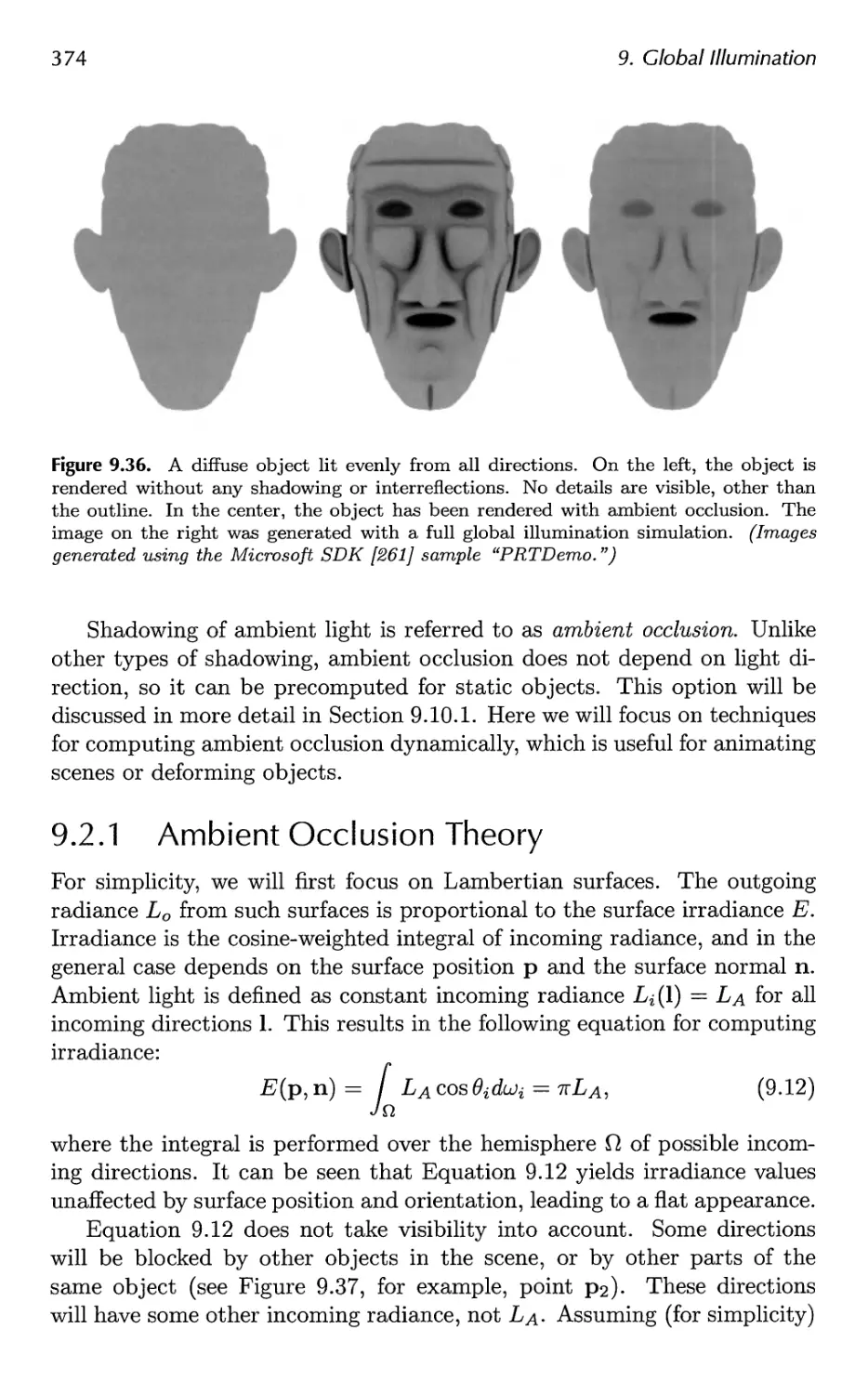
9.2 Ambient Occlusion 373
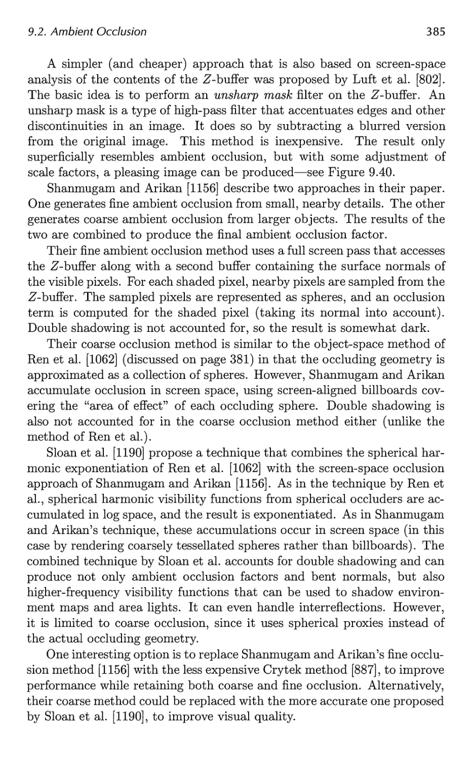
9.3 Reflections 386
9.4 Transmittance 392
9.5 Refractions 396
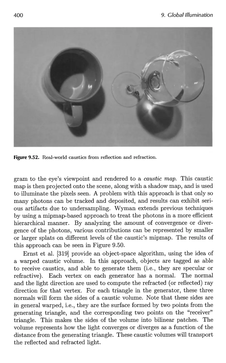
9.6 Caustics 399
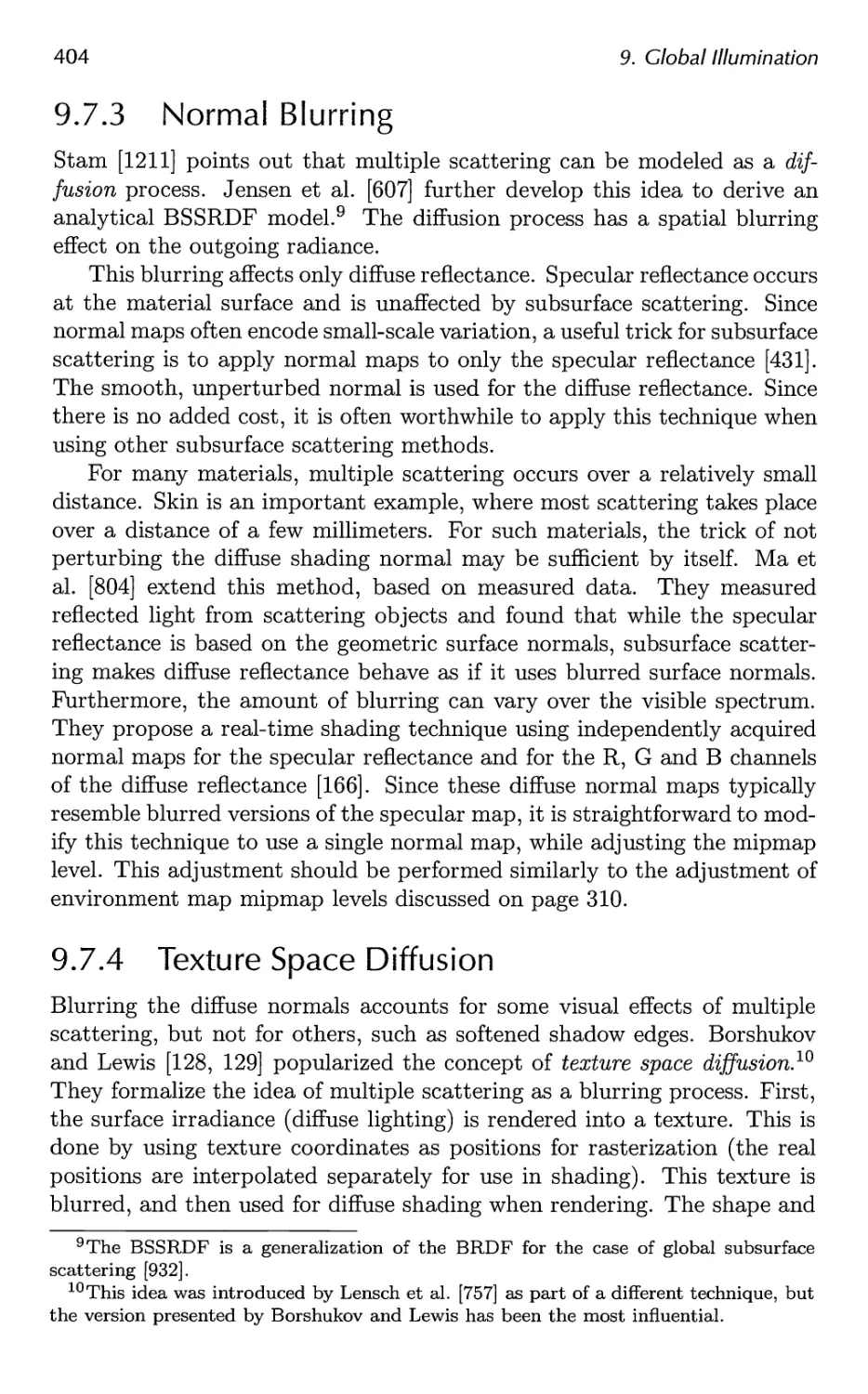
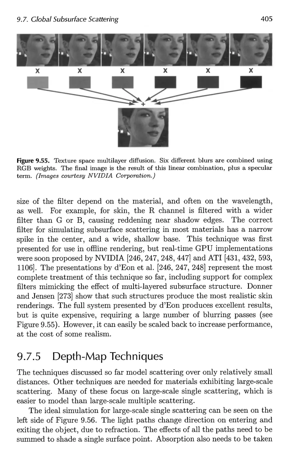
9.7 Global Subsurface Scattering 401
Contents ix
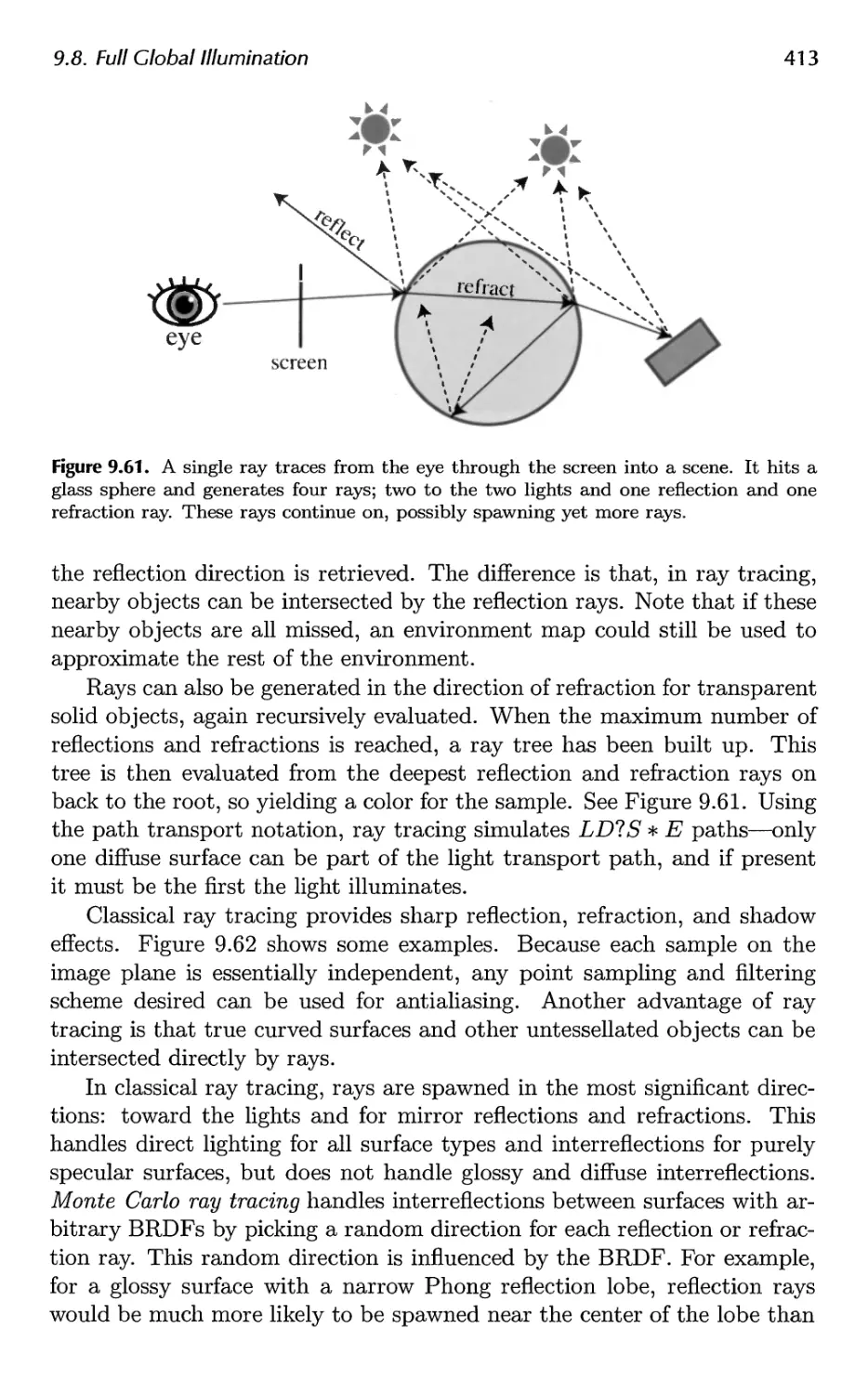
9.8 Full Global Illumination 407
9.9 Precomputed Lighting 417
9.10 Precomputed Occlusion 425
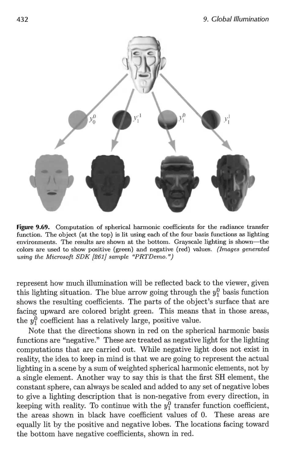
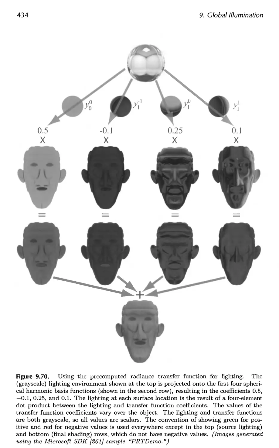
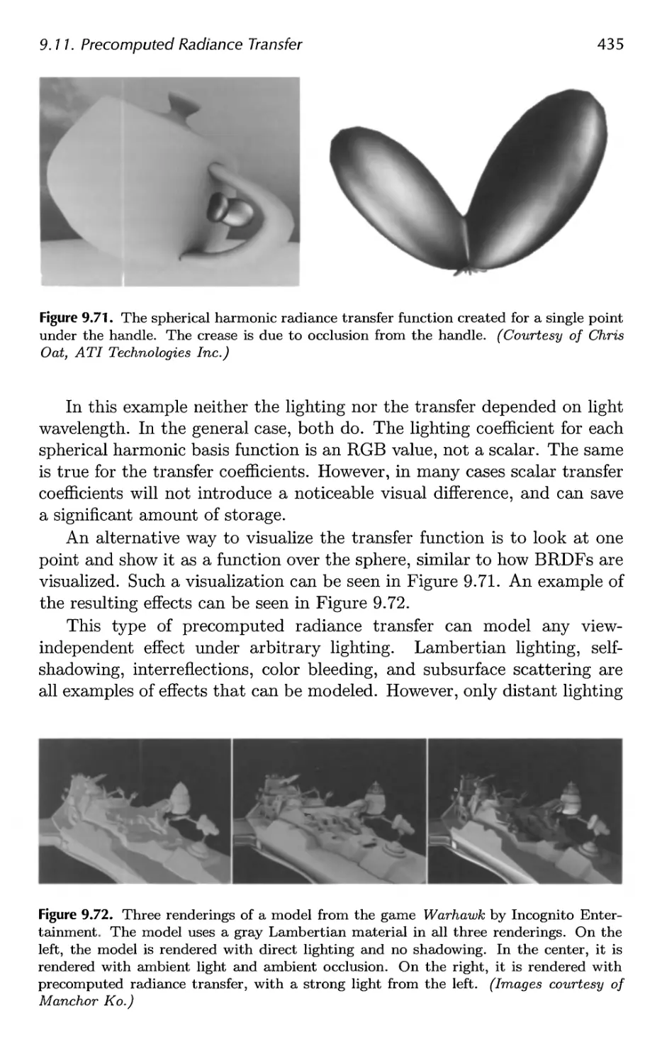
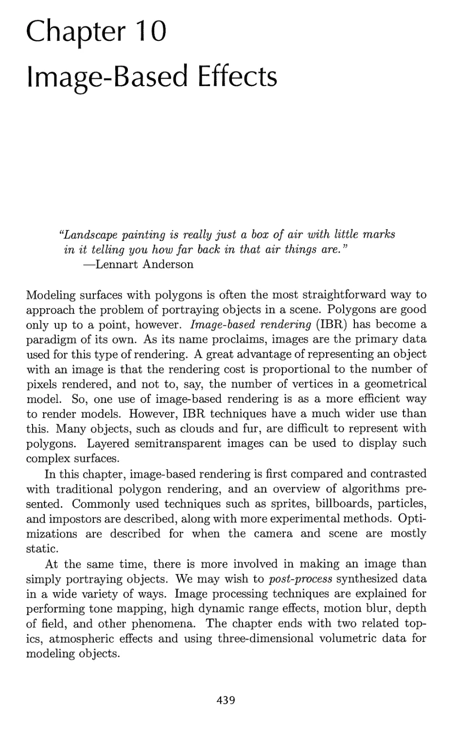
9.11 Precomputed Radiance Transfer 430
10 Image-Based Effects 439
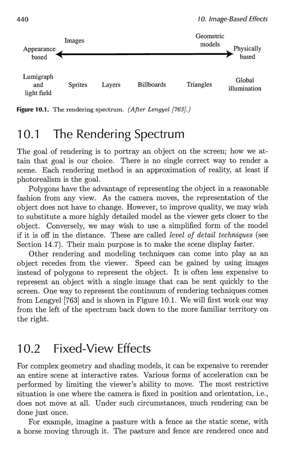
10.1 The Rendering Spectrum 440
10.2 Fixed-View Effects 440
10.3 Skyboxes 443
10.4 Light Field Rendering 444
10.5 Sprites and Layers 445
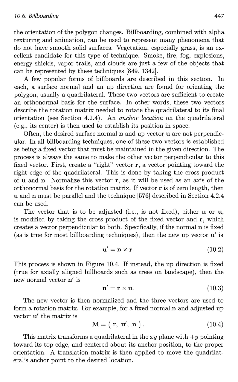
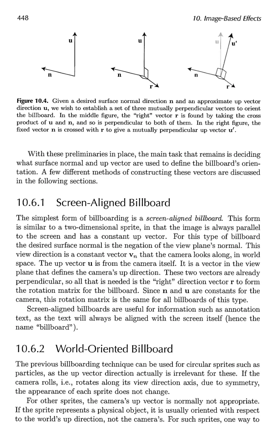
10.6 Billboarding 446
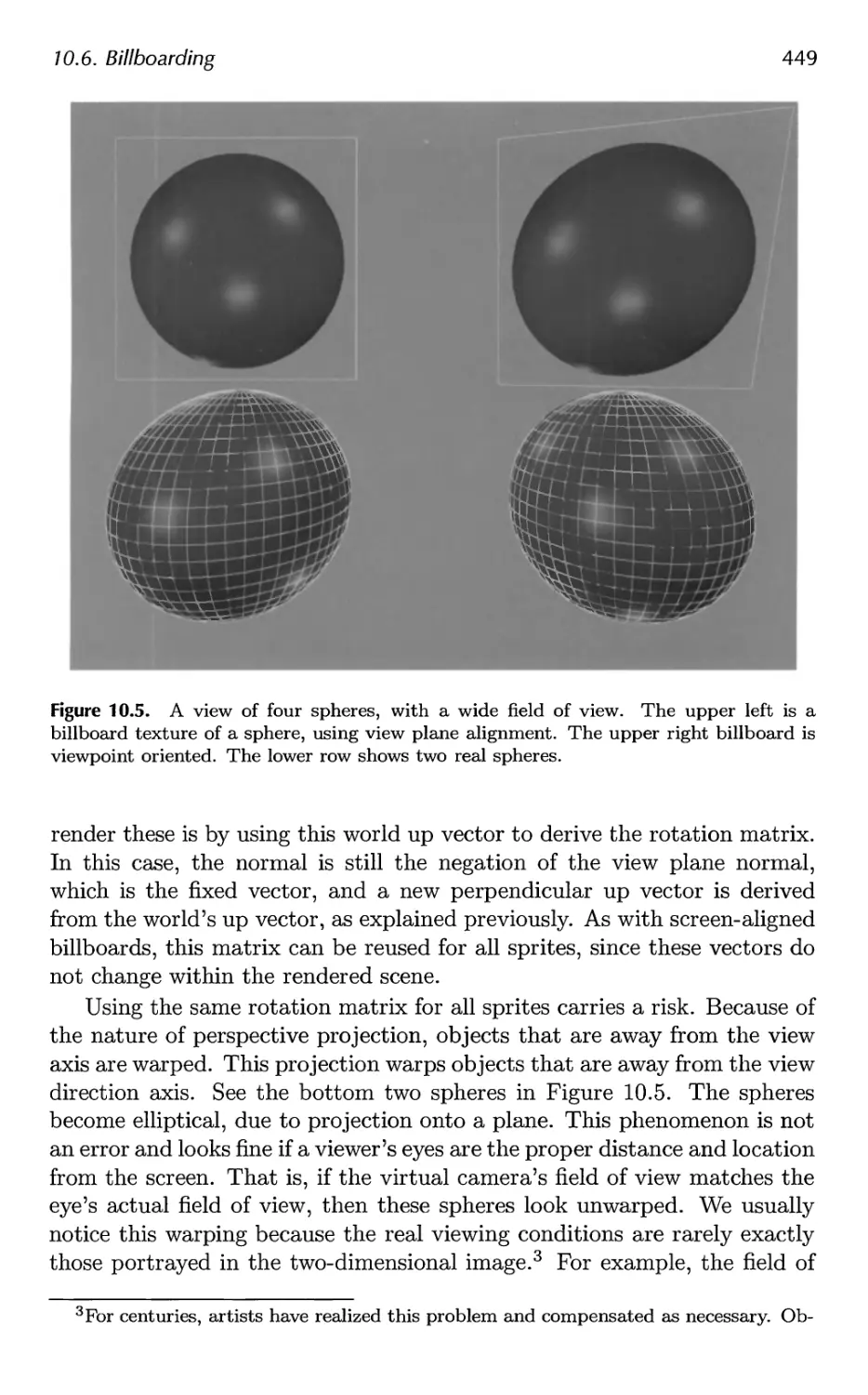
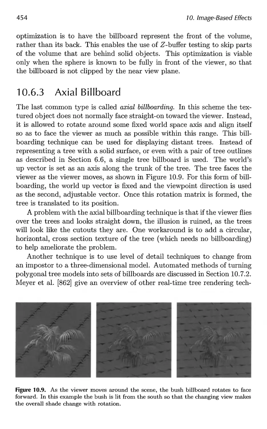
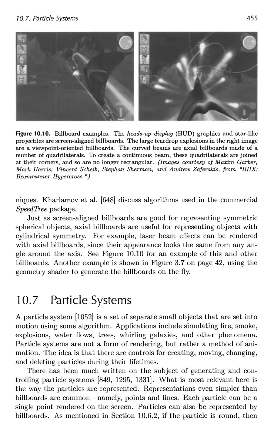
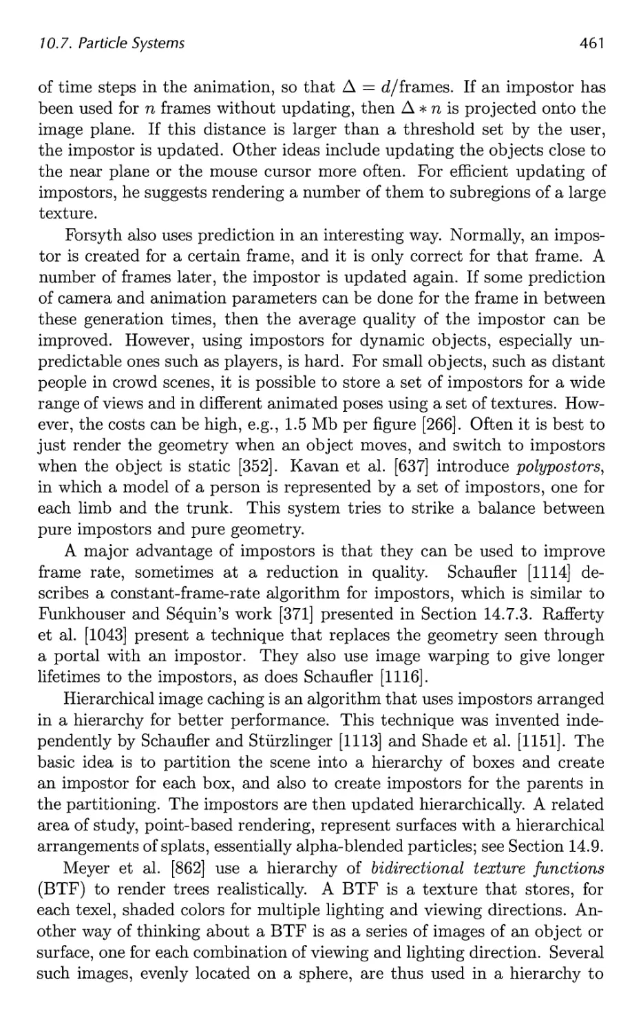
10.7 Particle Systems 455
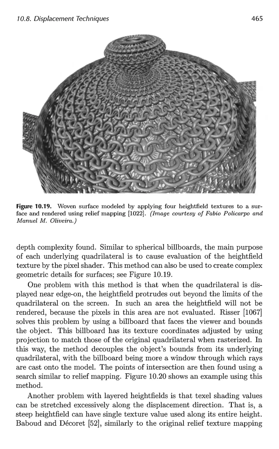
10.8 Displacement Techniques 463
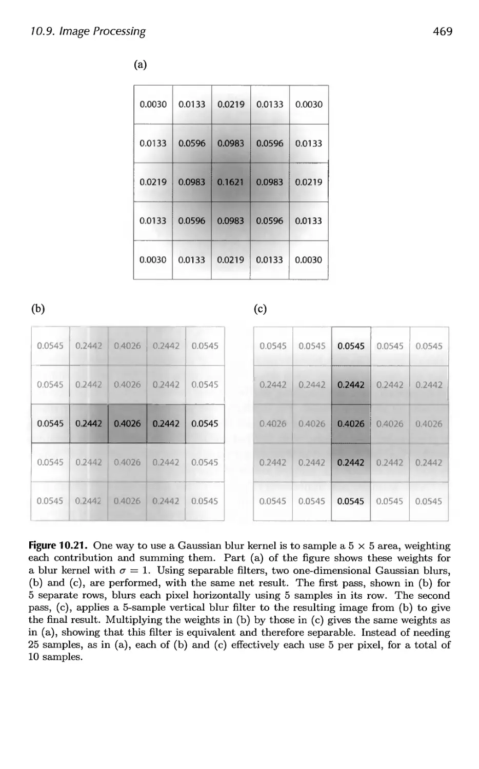
10.9 Image Processing 467
10.10 Color Correction 474
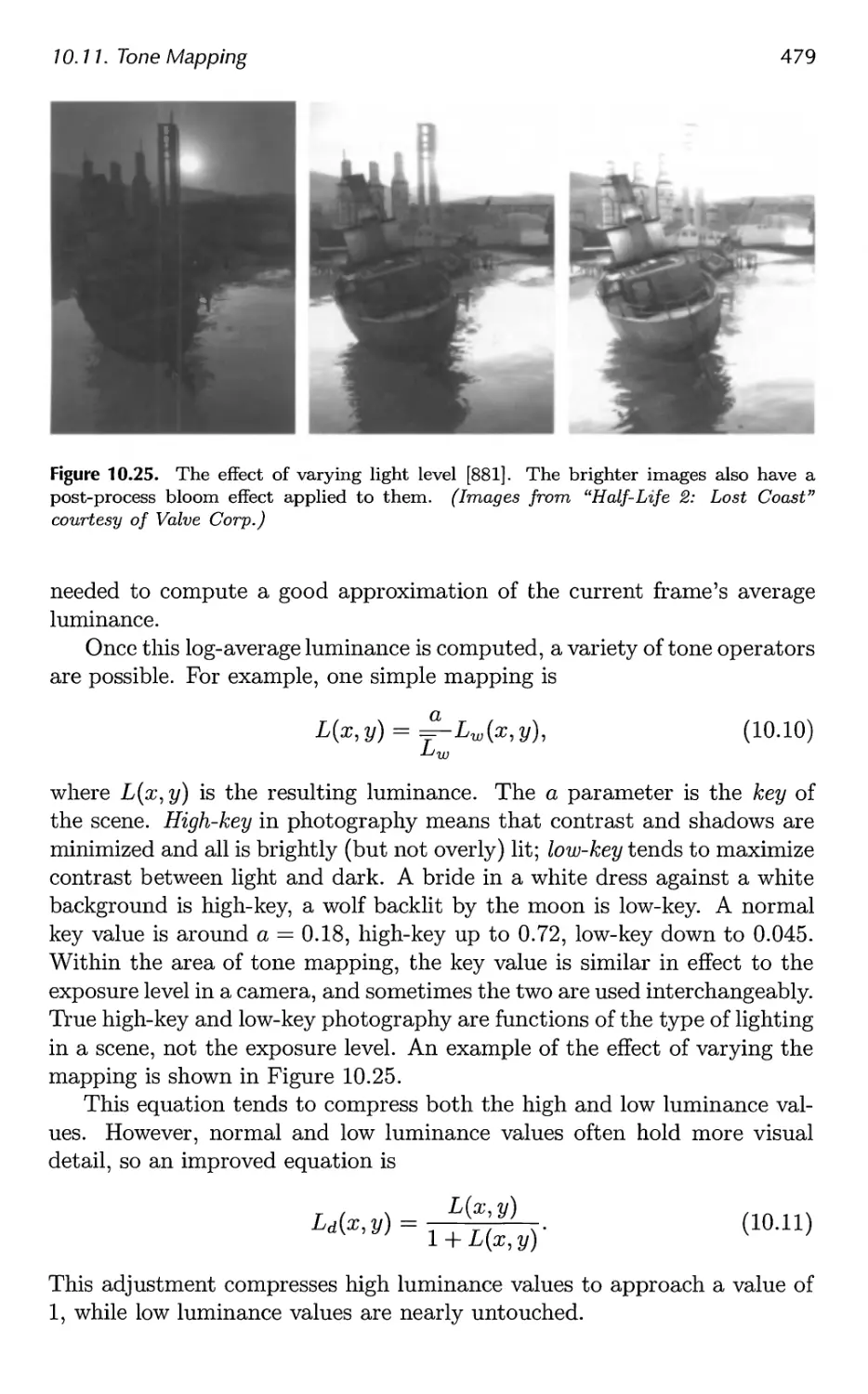
10.11 Tone Mapping 475
10.12 Lens Flare and Bloom 482
10.13 Depth of Field 486
10.14 Motion Blur 490
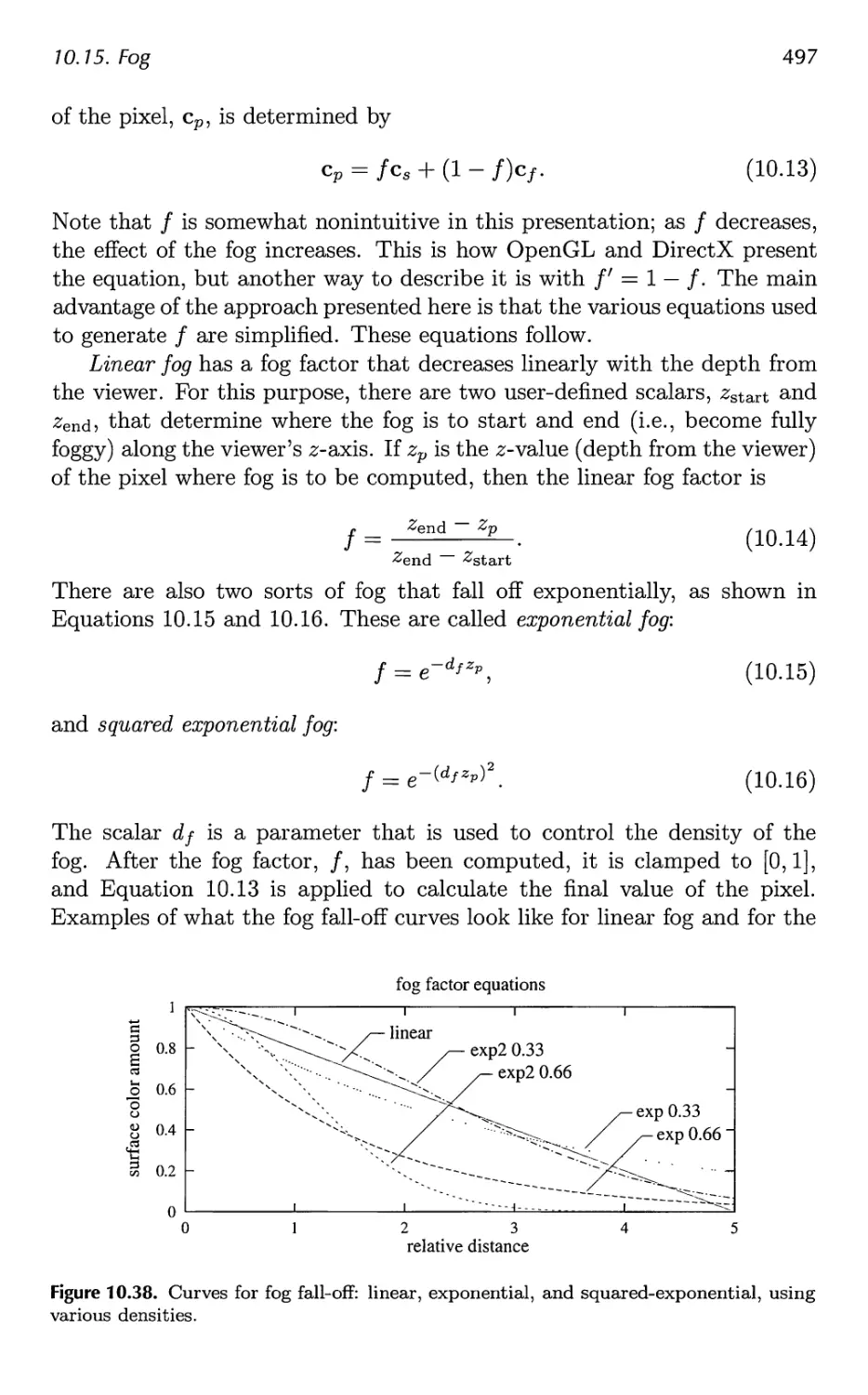
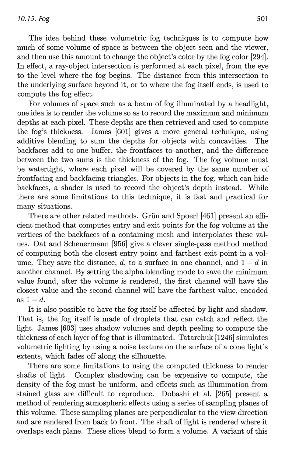
10.15 Fog 496
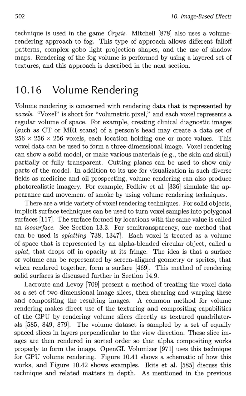
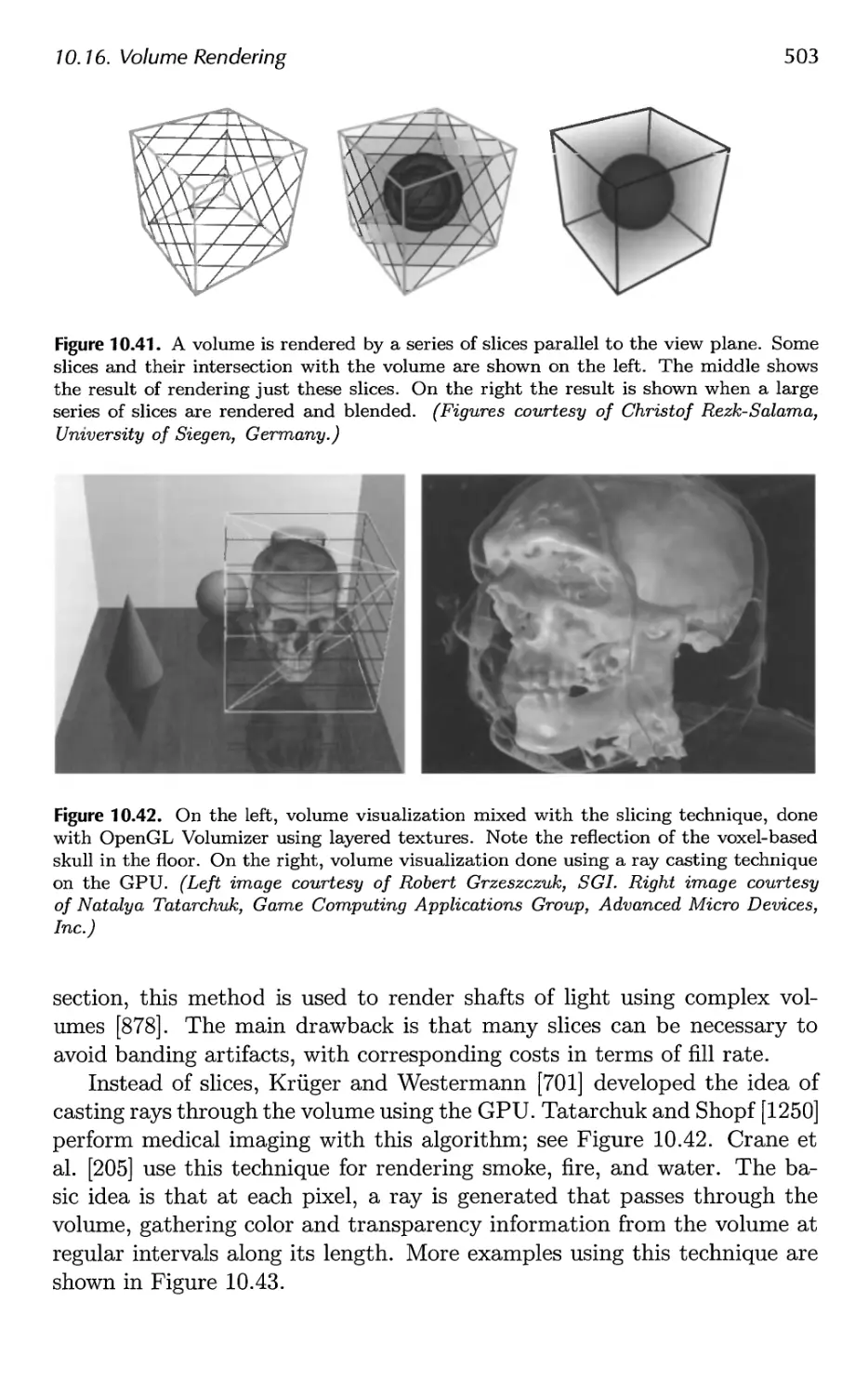
10.16 Volume Rendering 502
11 Non-Photorealistic Rendering 507
11.1 Toon Shading 508
11.2 Silhouette Edge Rendering 510
11.3 Other Styles 523
11.4 Lines 527
12 Polygonal Techniques 531
12.1 Sources of Three-Dimensional Data 532
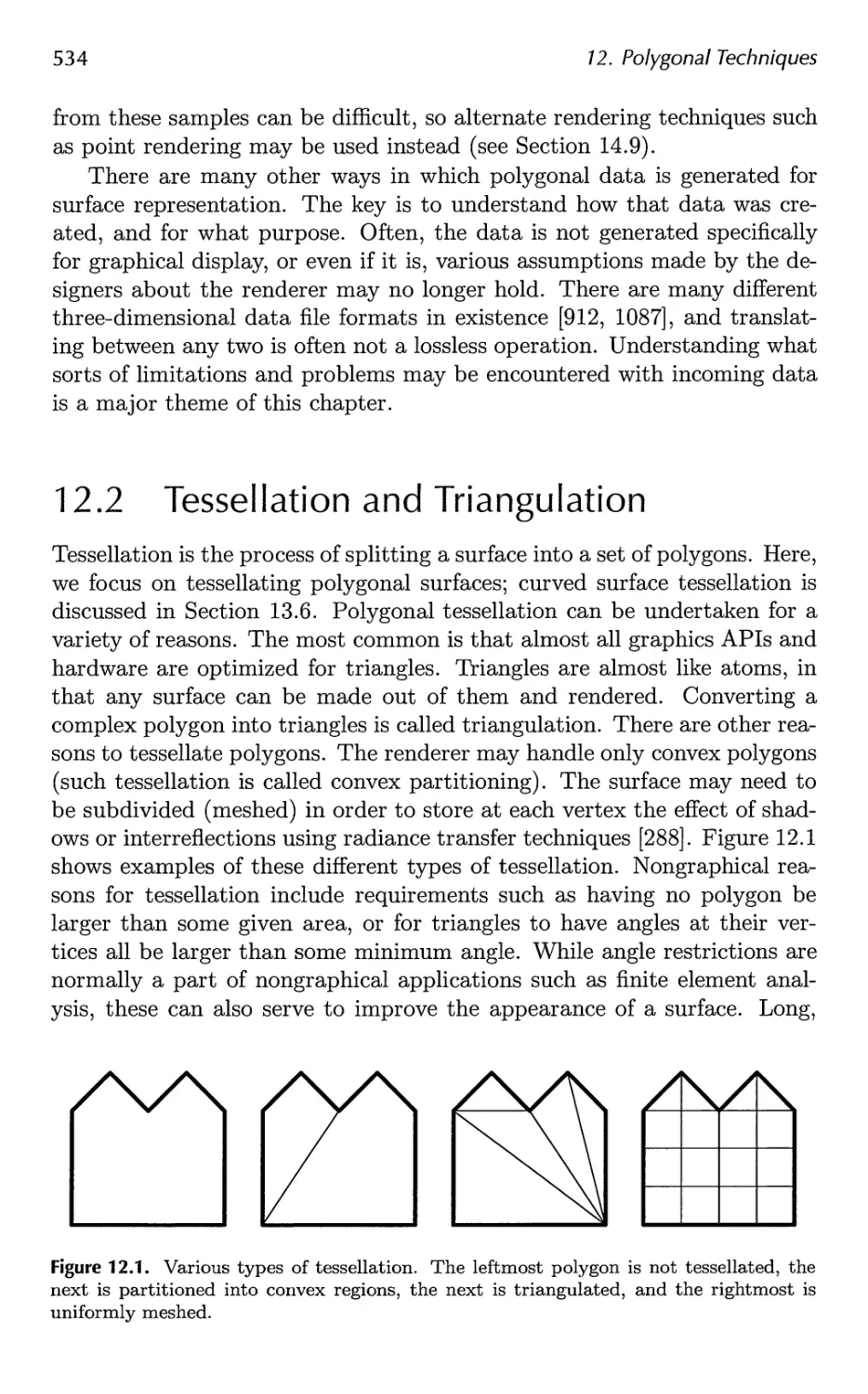
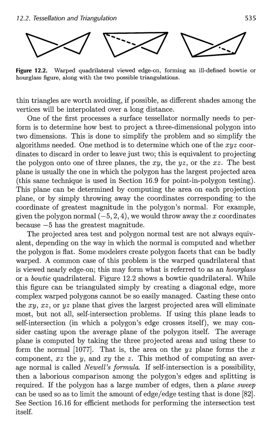
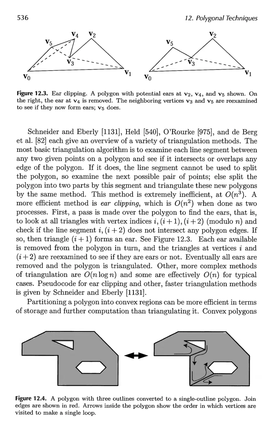
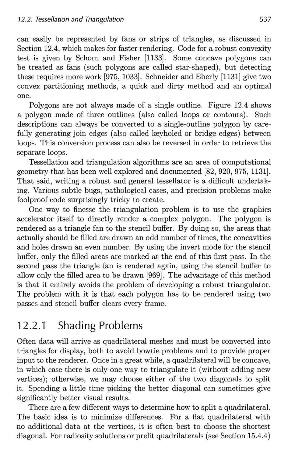
12.2 Tessellation and Triangulation 534
12.3 Consolidation 541
12.4 Triangle Fans, Strips, and Meshes 547
12.5 Simplification 561
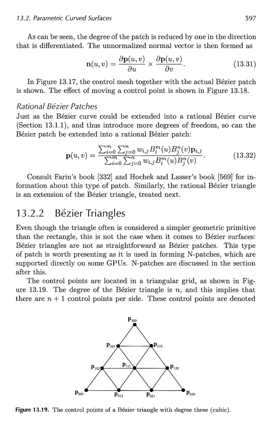
13 Curves and Curved Surfaces 575
13.1 Parametric Curves 576
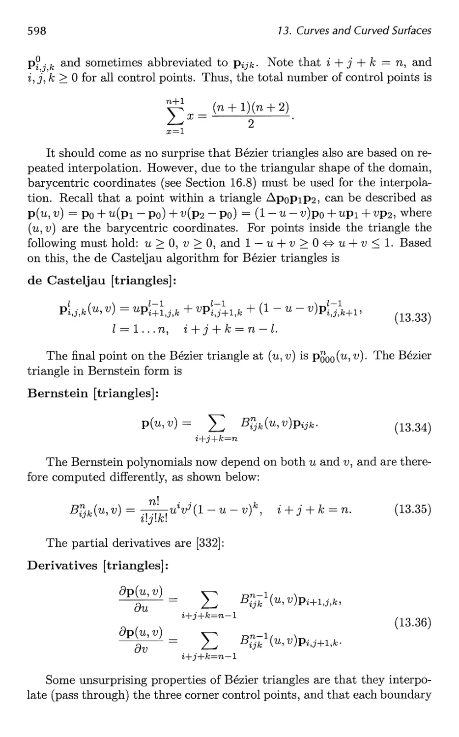
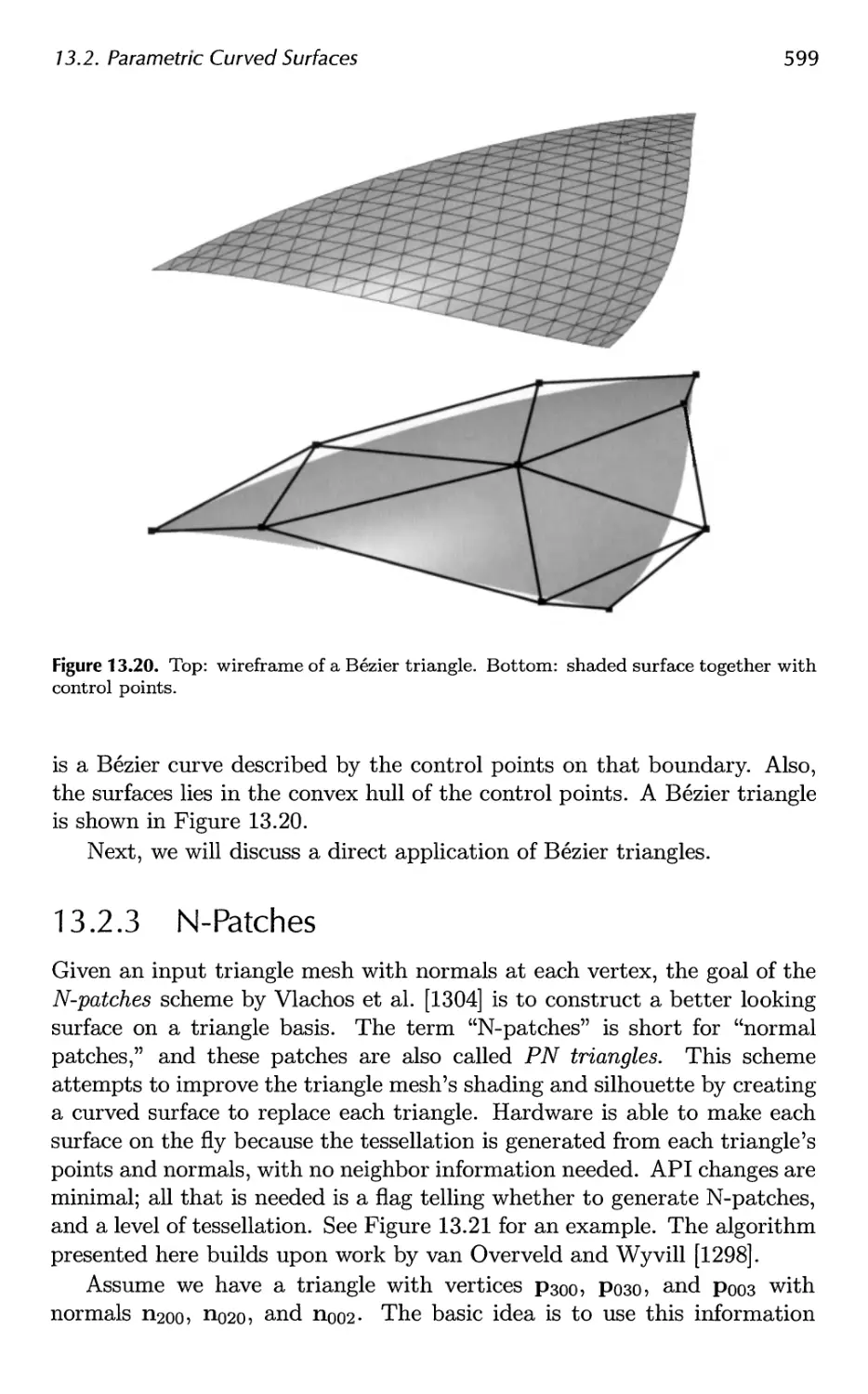
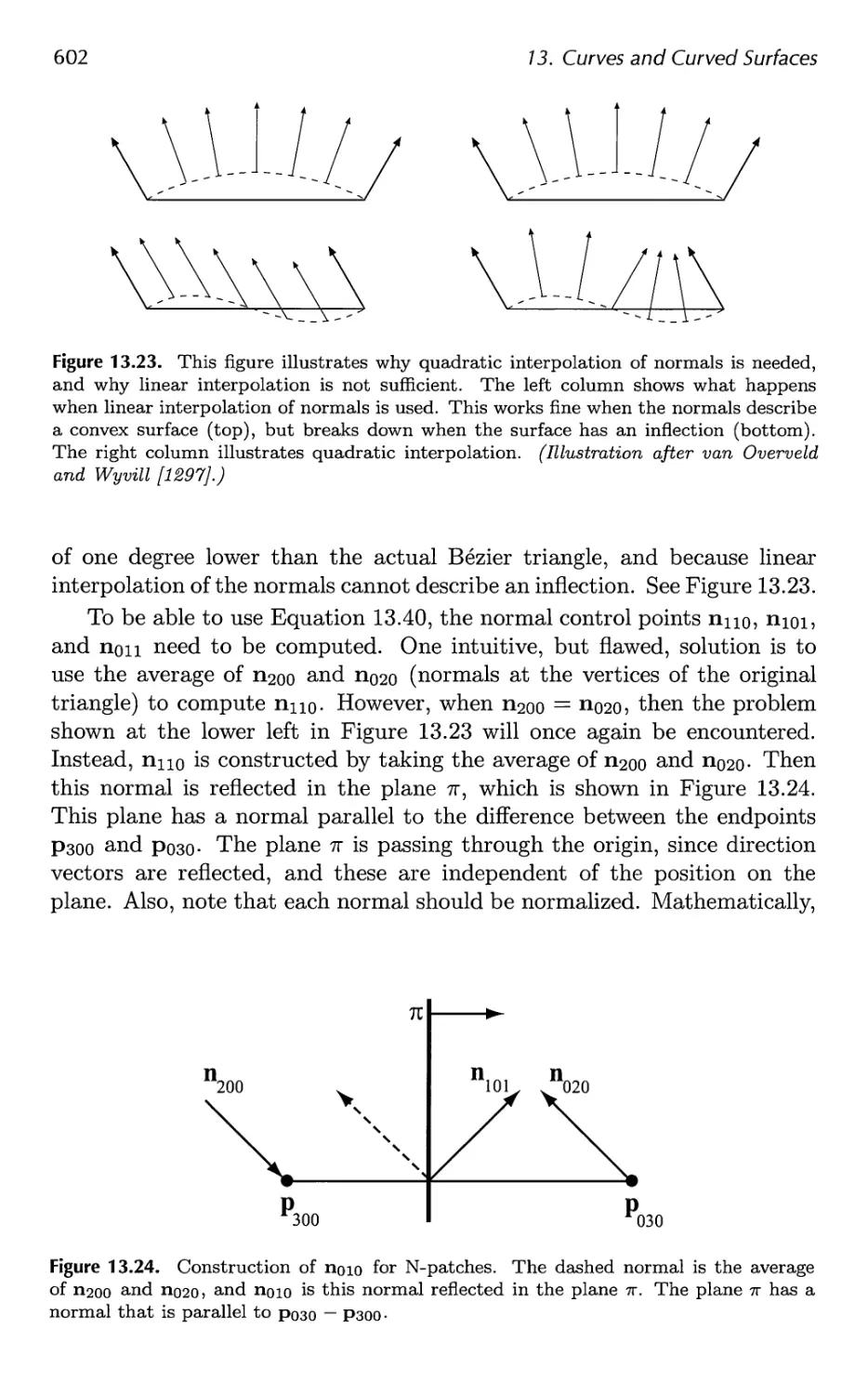
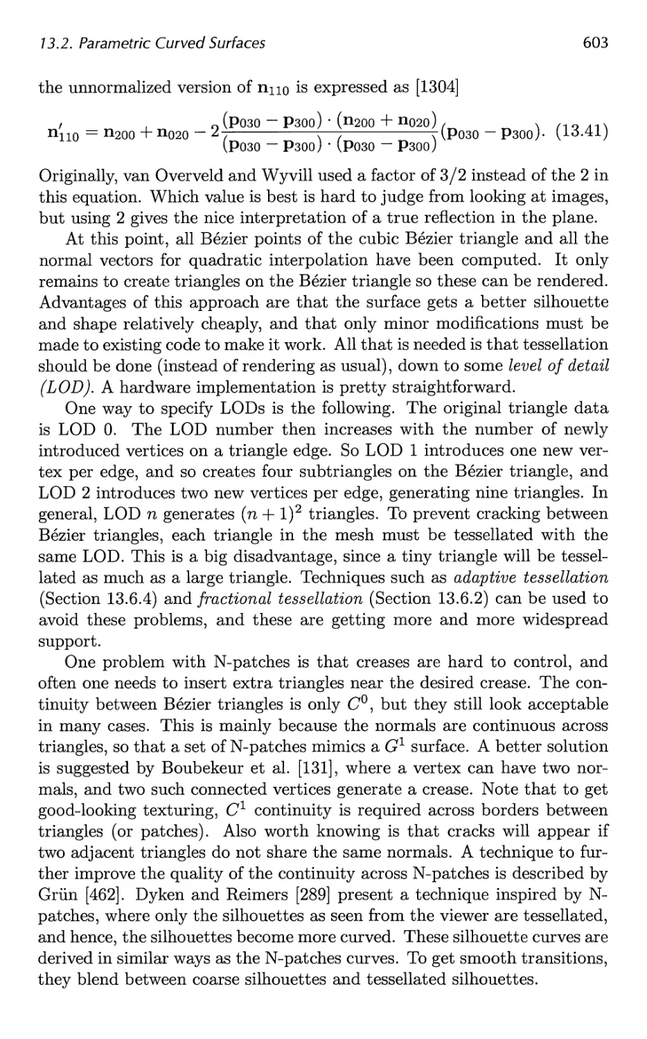
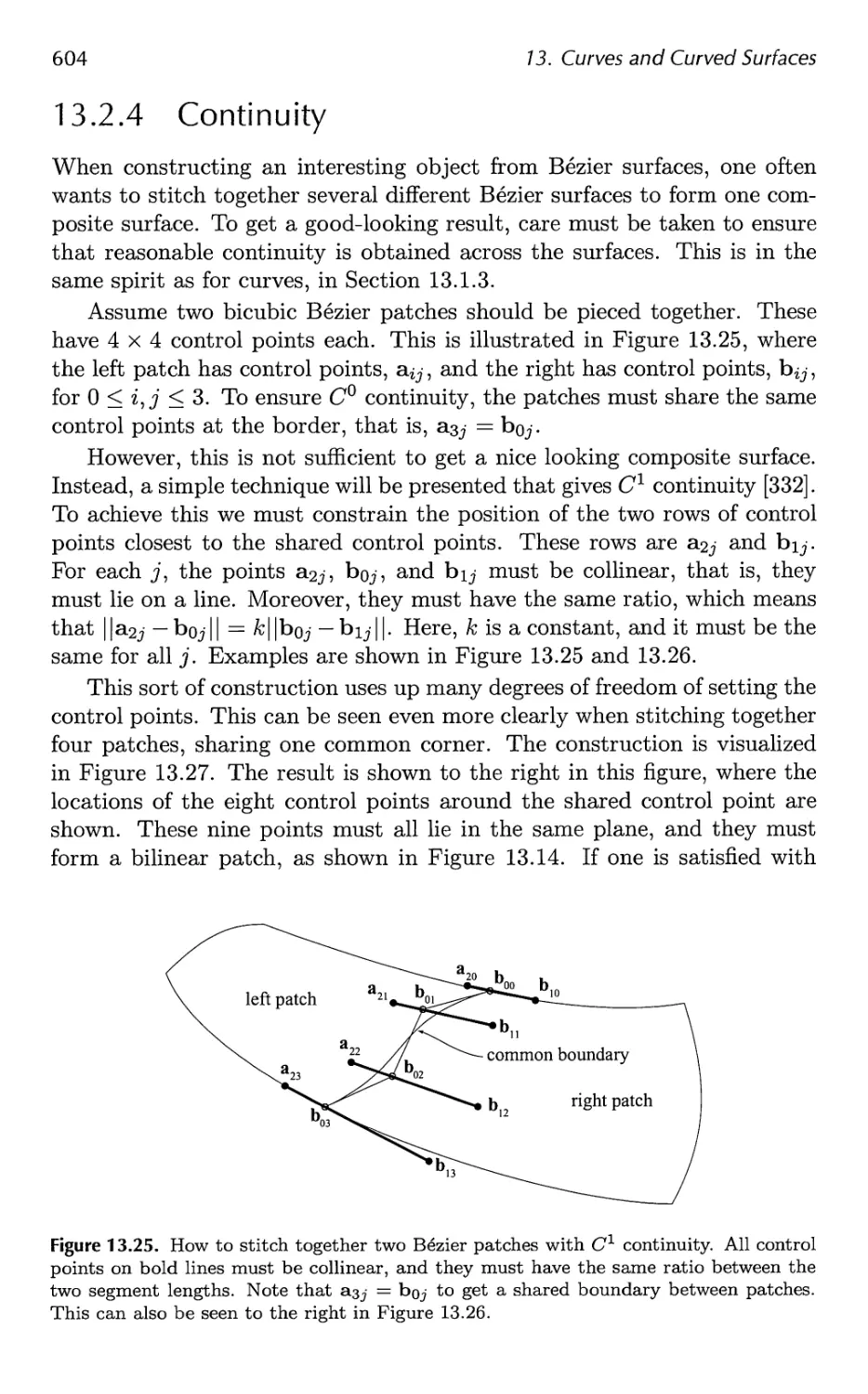
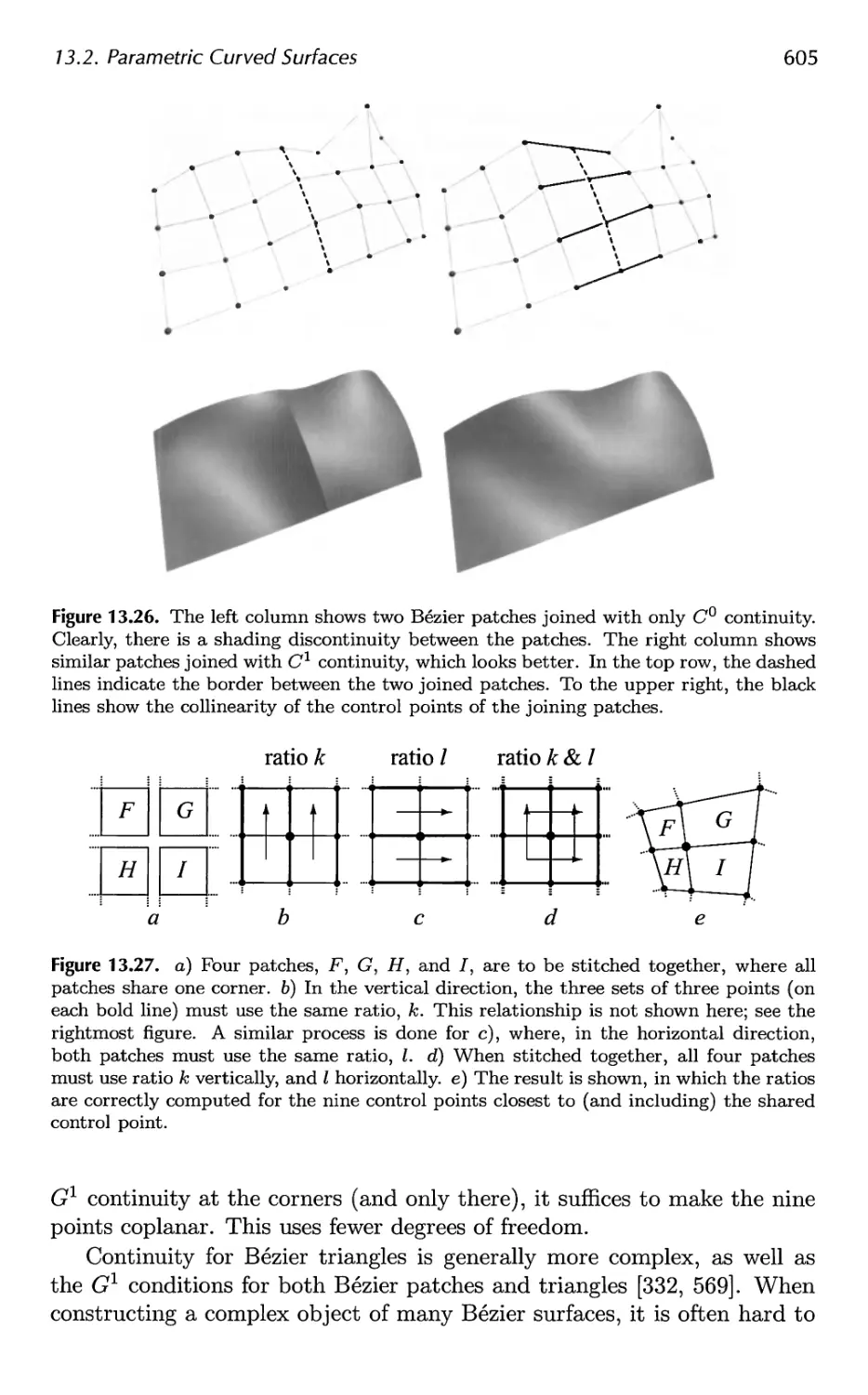
13.2 Parametric Curved Surfaces 592
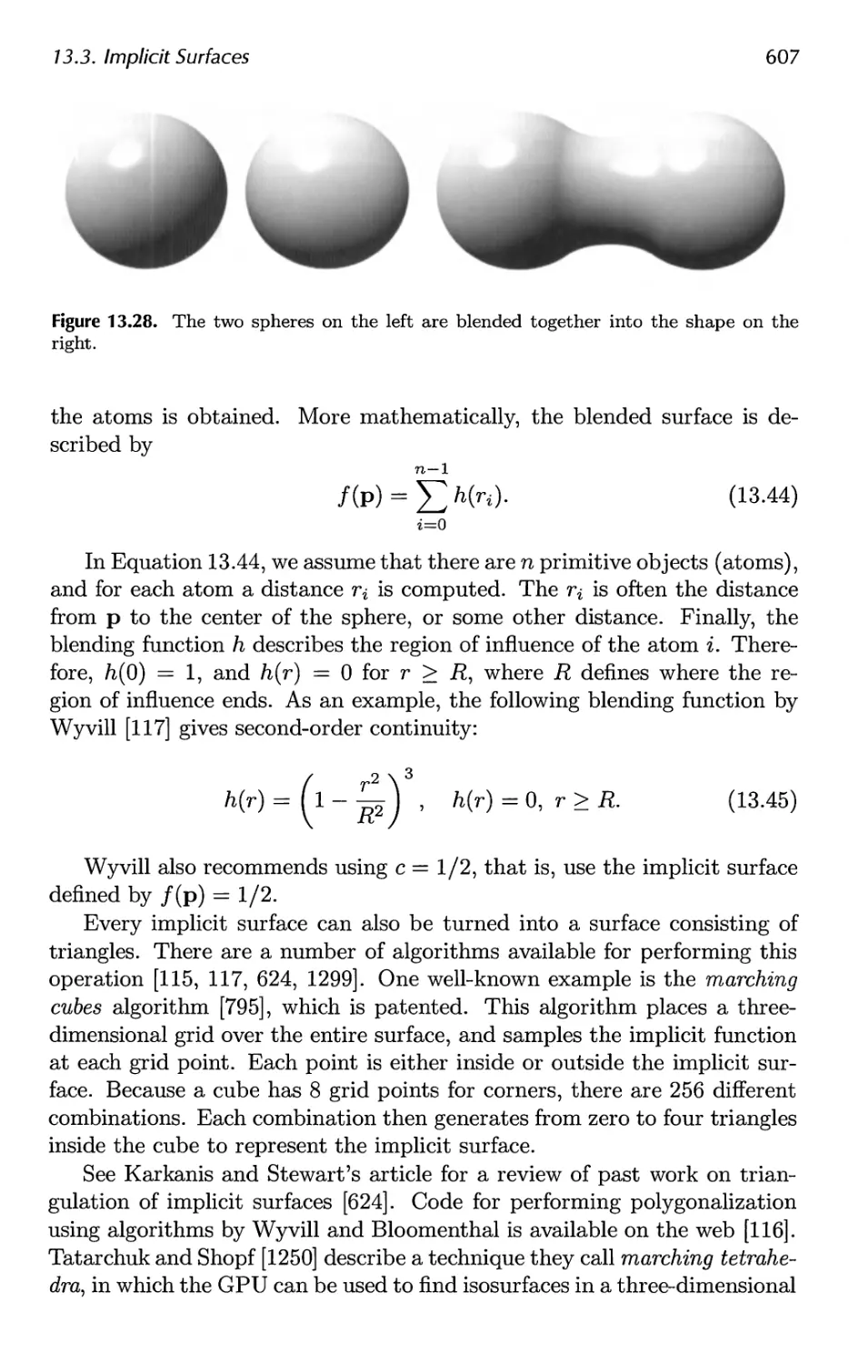
13.3 Implicit Surfaces 606
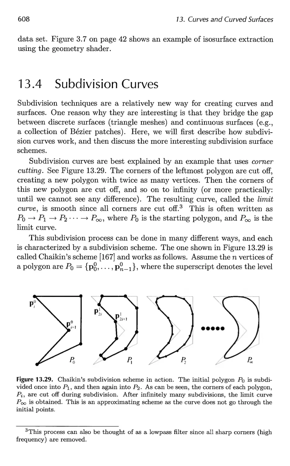
13.4 Subdivision Curves 608
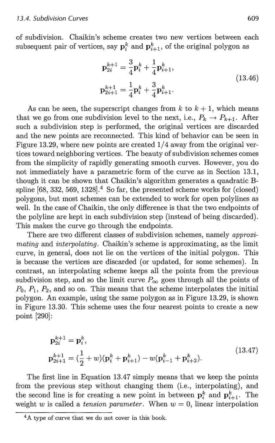
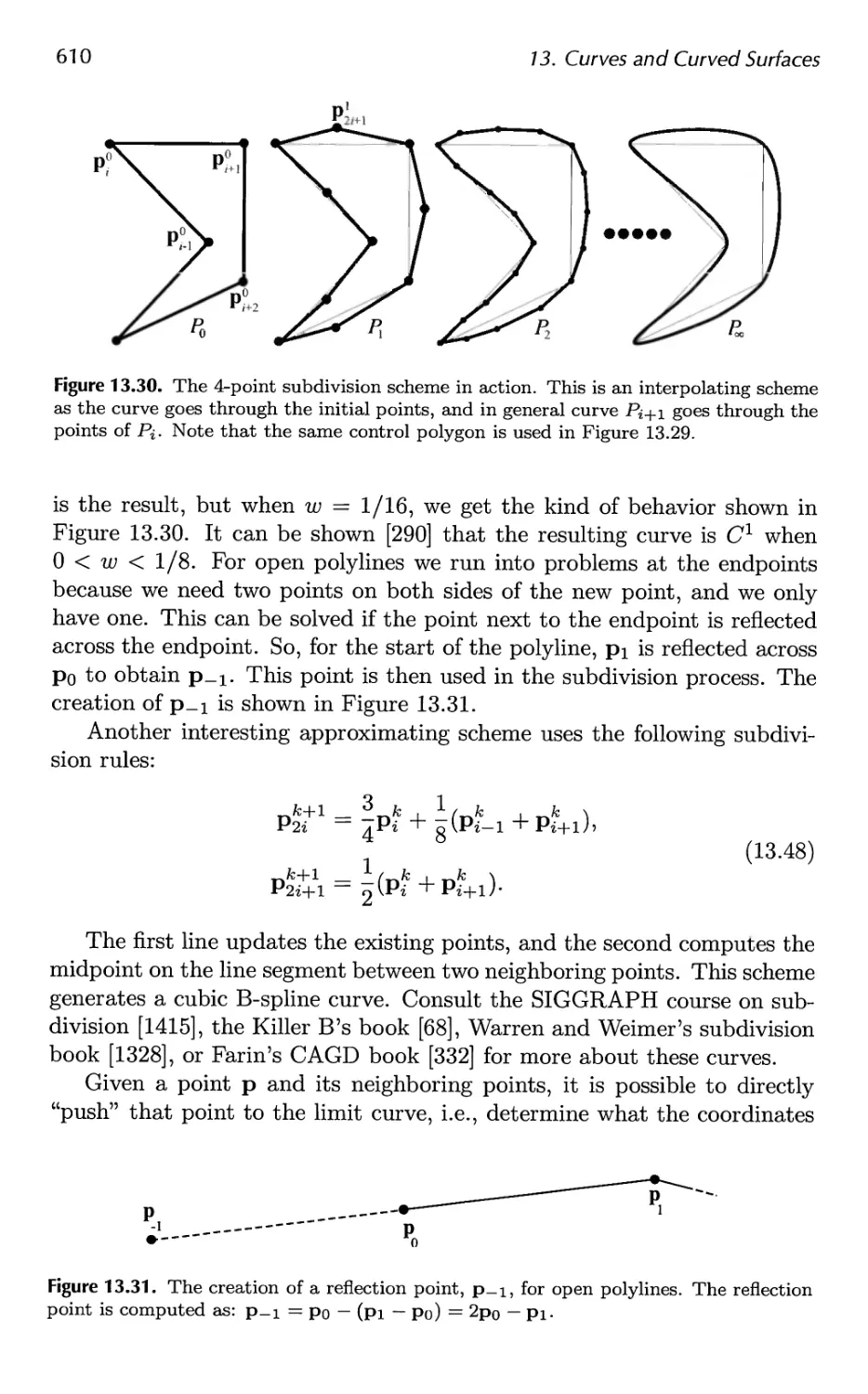
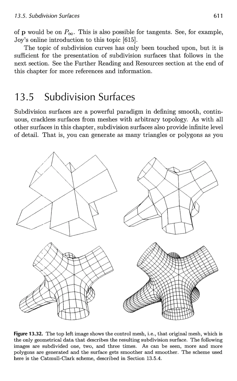
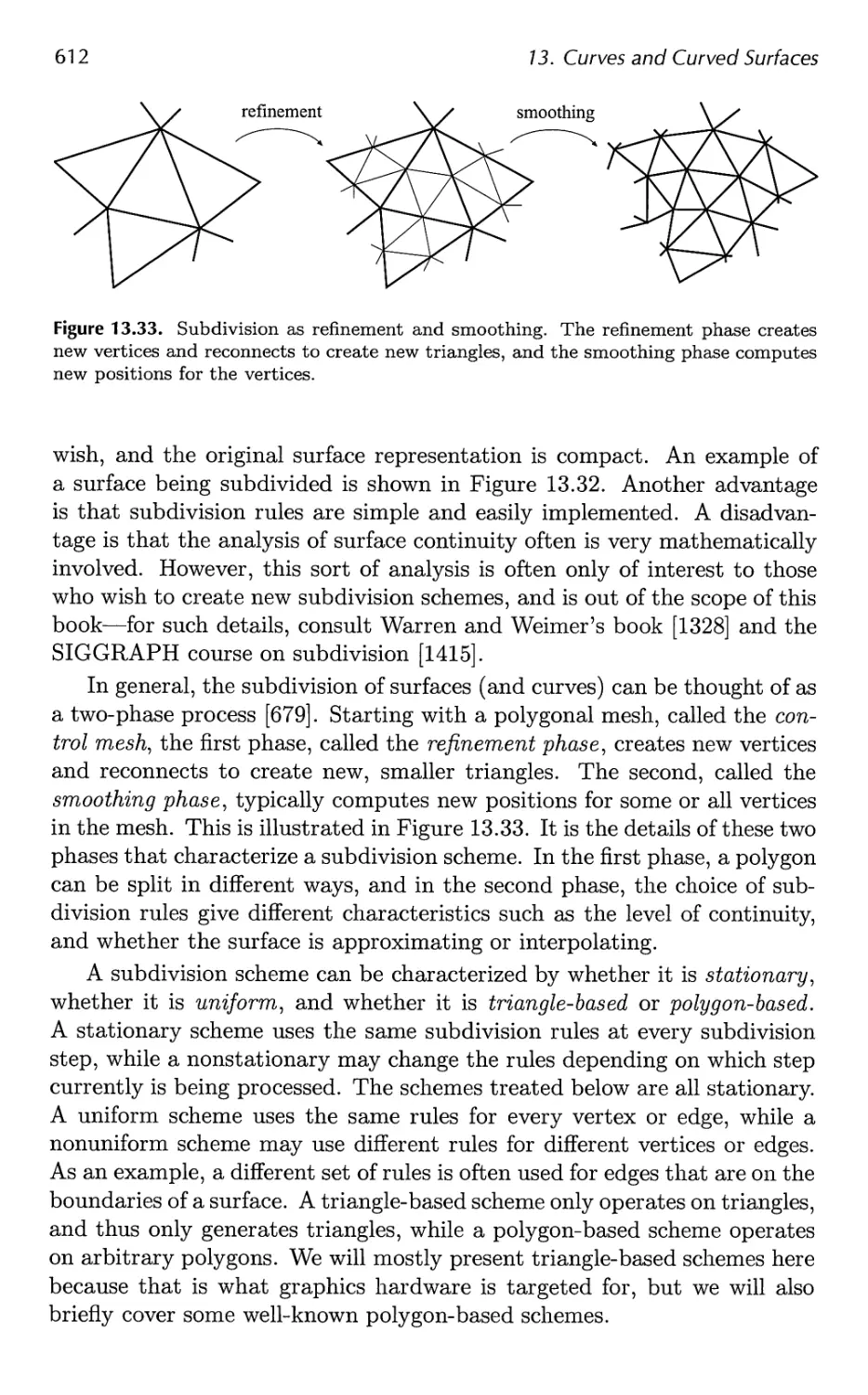
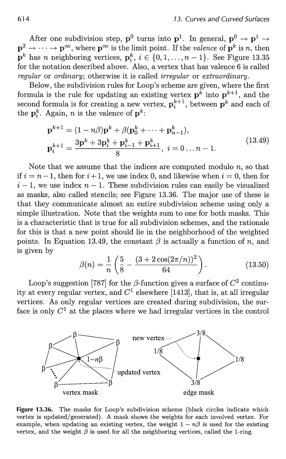
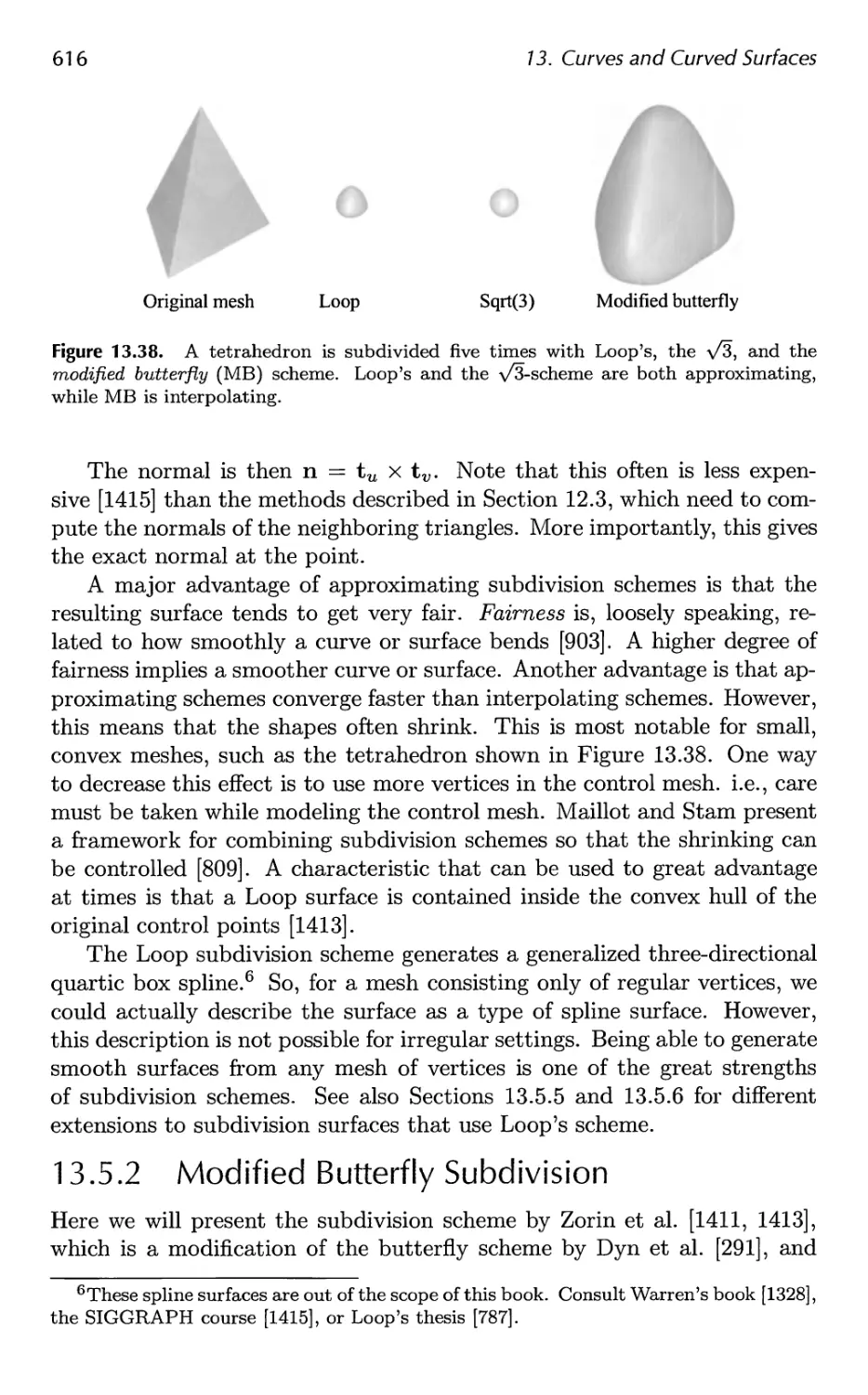
13.5 Subdivision Surfaces 611
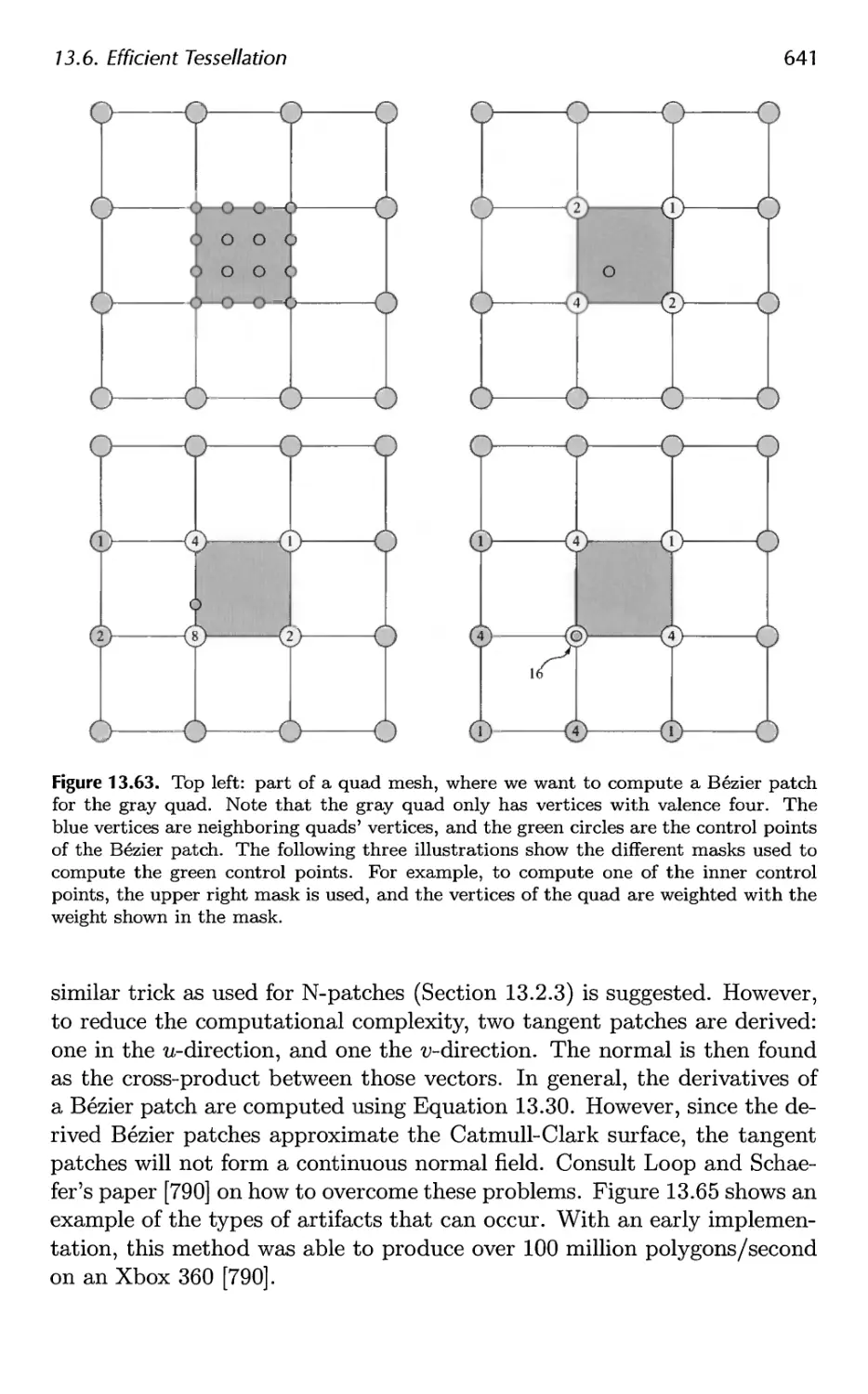
13.6 Efficient Tessellation 629
x Contents
14 Acceleration Algorithms 645
14.1 Spatial Data Structures 647
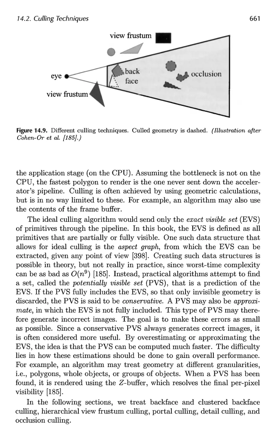
14.2 Culling Techniques 660
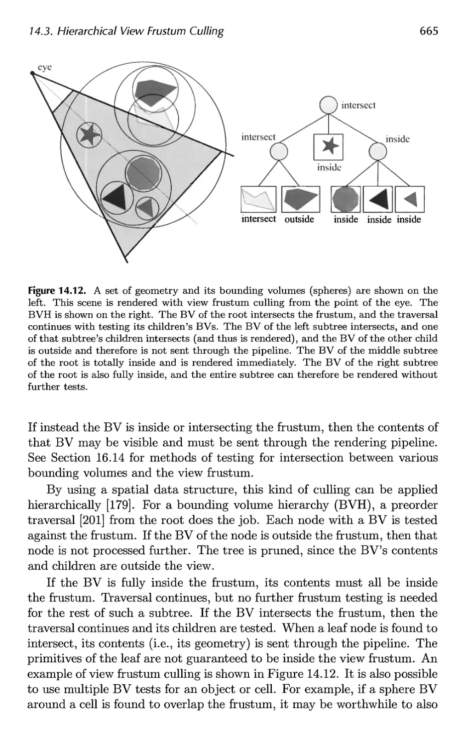
14.3 Hierarchical View Frustum Culling 664
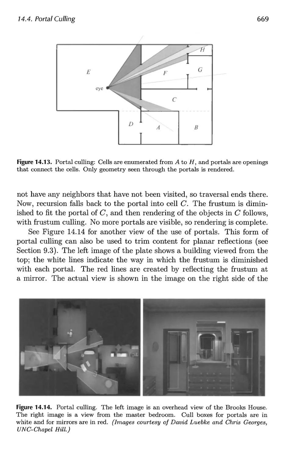
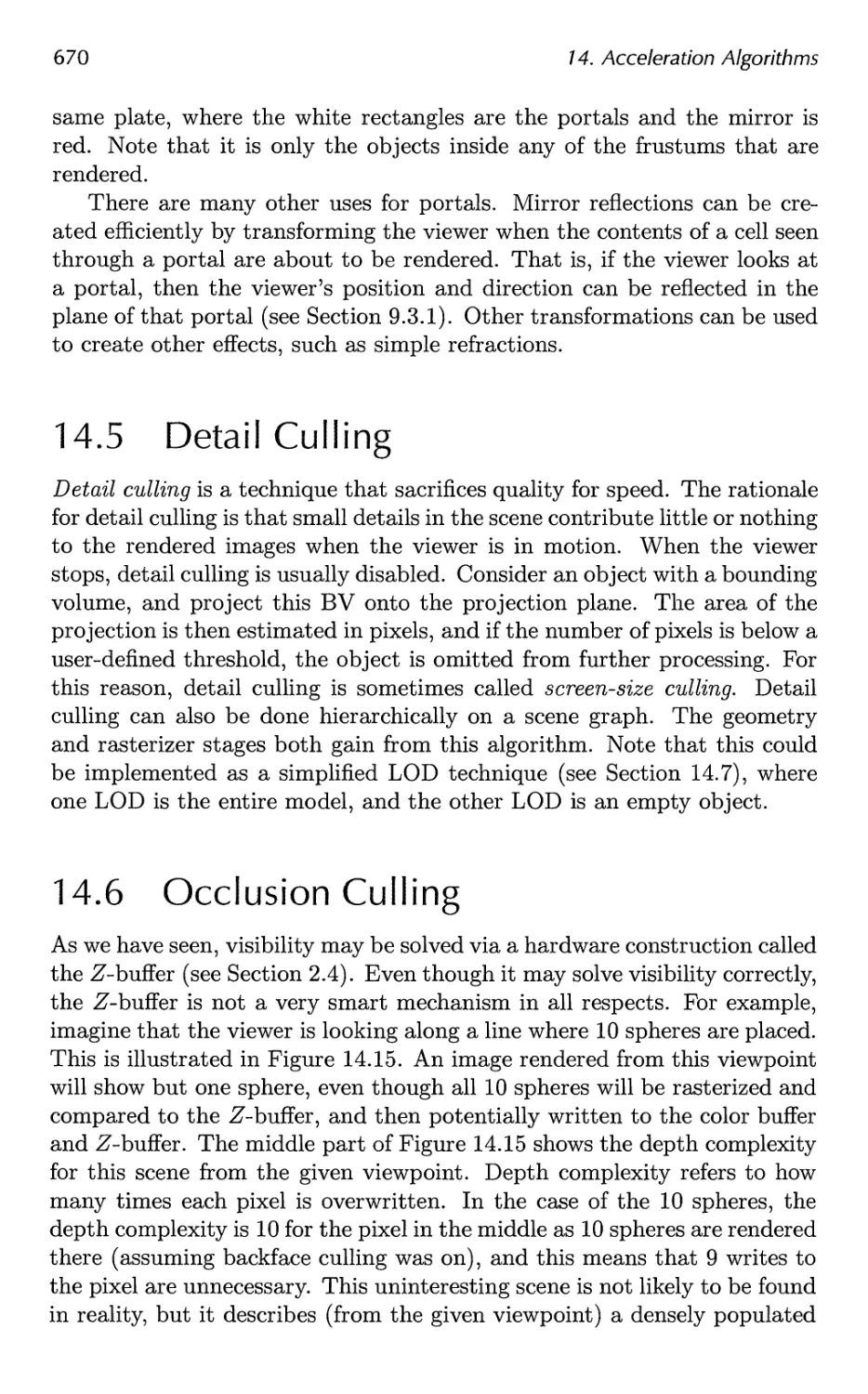
14.4 Portal Culling 667
14.5 Detail Culling 670
14.6 Occlusion Culling 670
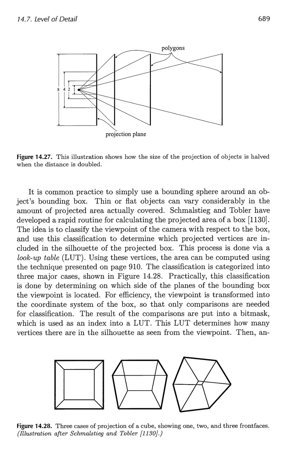
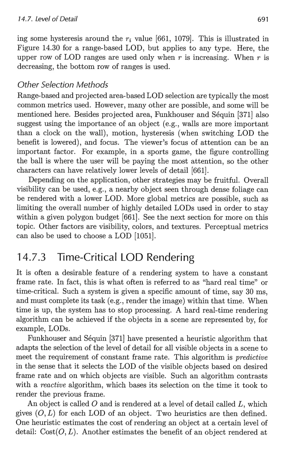
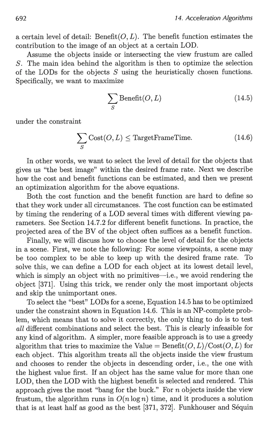
14.7 Level of Detail 680
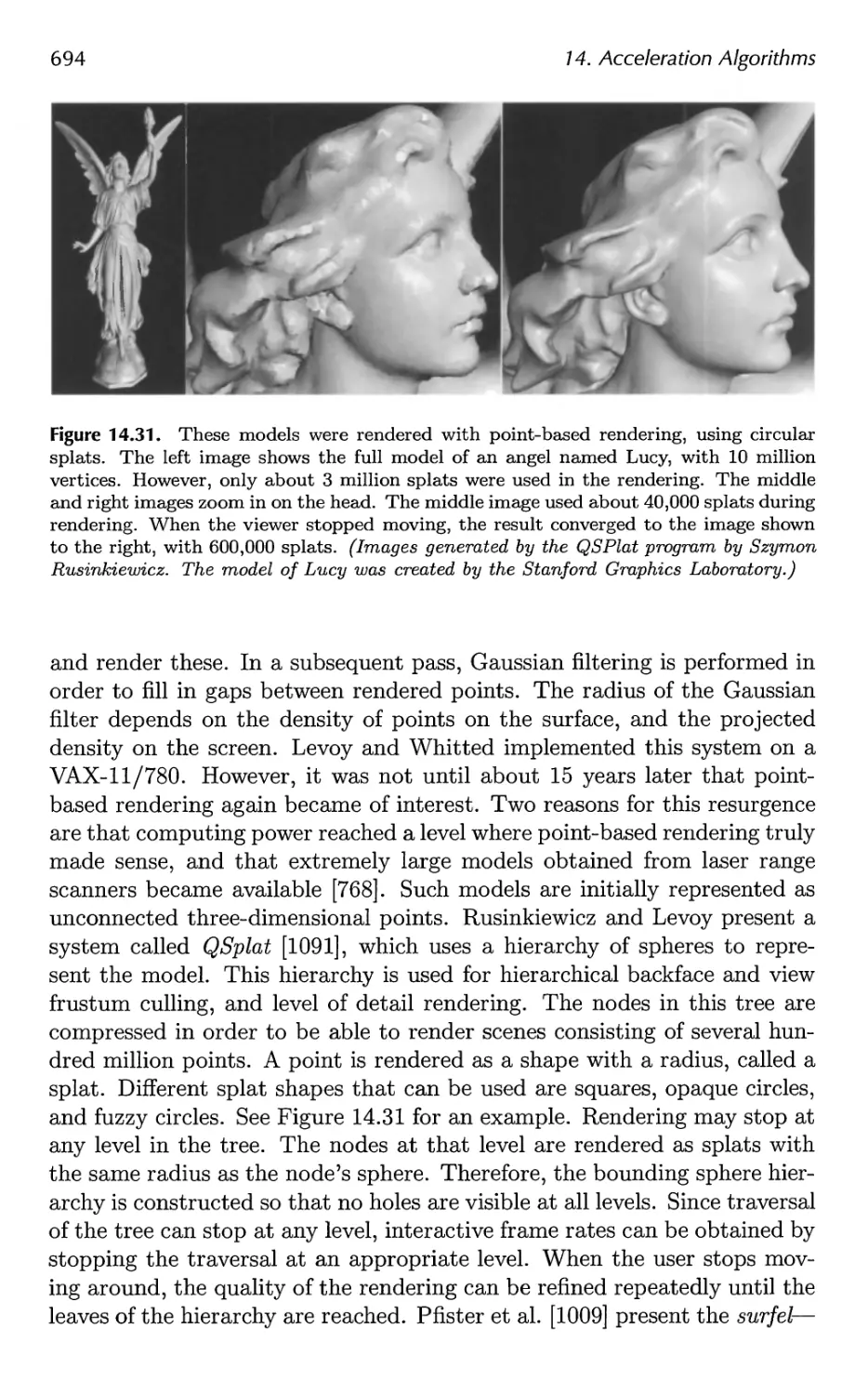
14.8 Large Model Rendering 693
14.9 Point Rendering 693
15 Pipeline Optimization 697
15.1 Profiling Tools 698
15.2 Locating the Bottleneck 699
15.3 Performance Measurements 702
15.4 Optimization 703
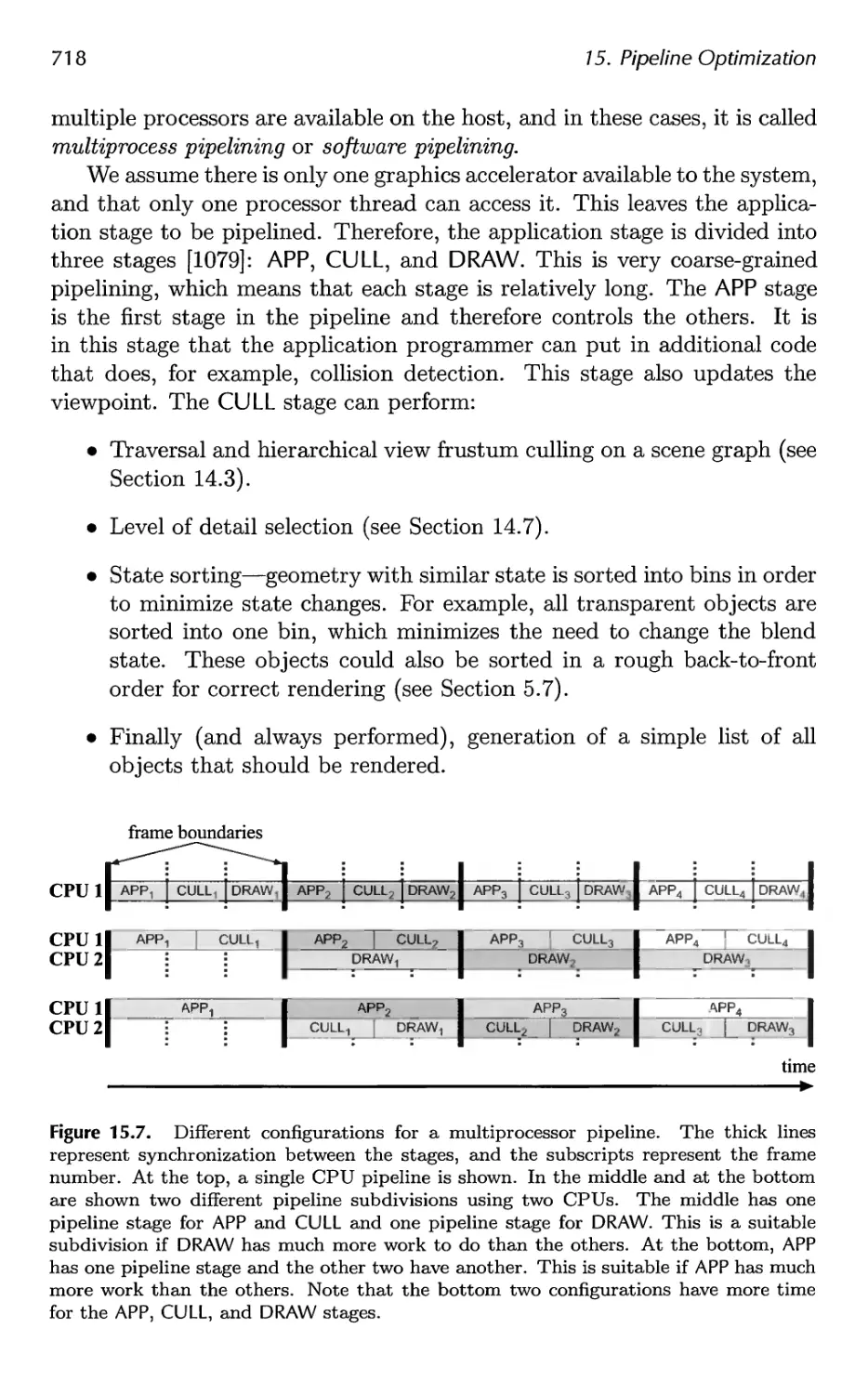
15.5 Multiprocessing 716
16 Intersection Test Methods 725
16.1 Hardware-Accelerated Picking 726
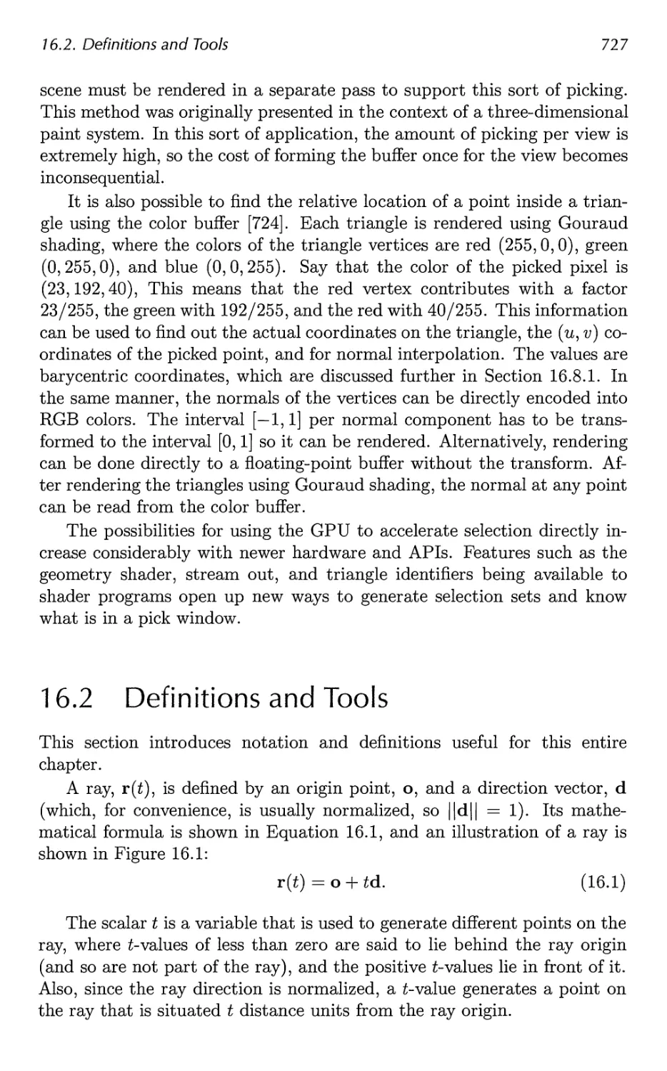
16.2 Definitions and Tools 727
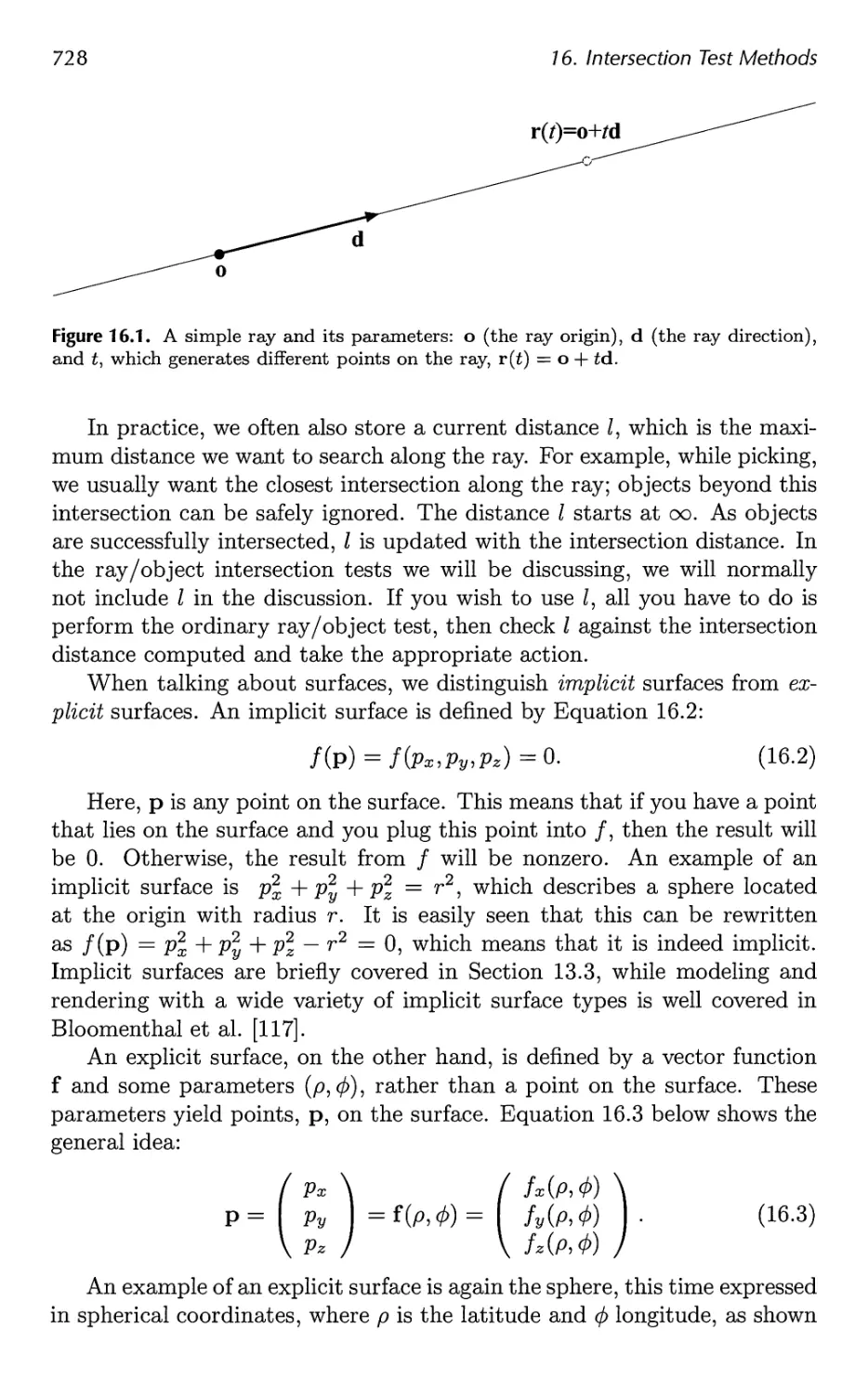
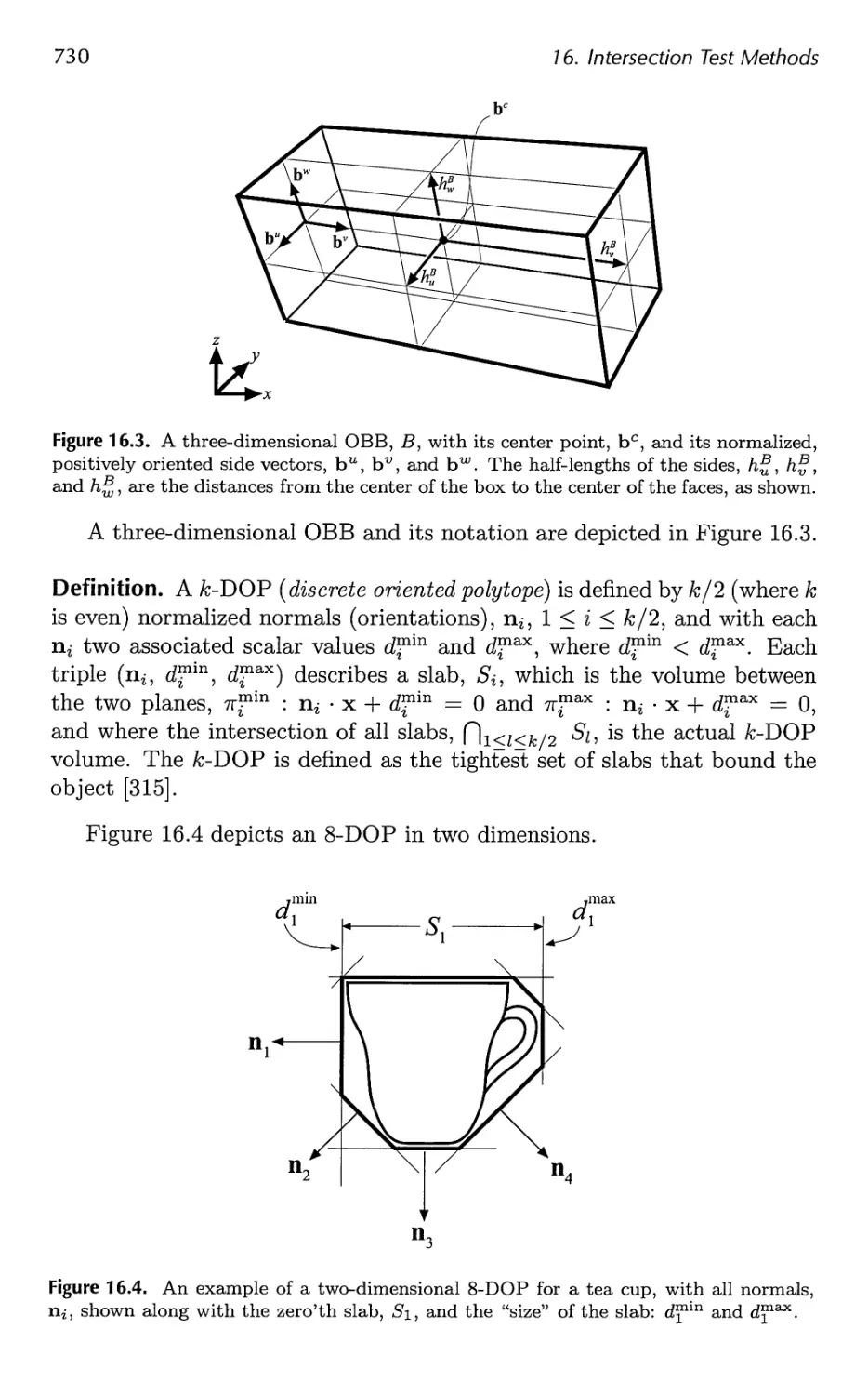
16.3 Bounding Volume Creation 732
16.4 Geometric Probability 735
16.5 Rules of Thumb 737
16.6 Ray/Sphere Intersection 738
16.7 Ray/Box Intersection 741
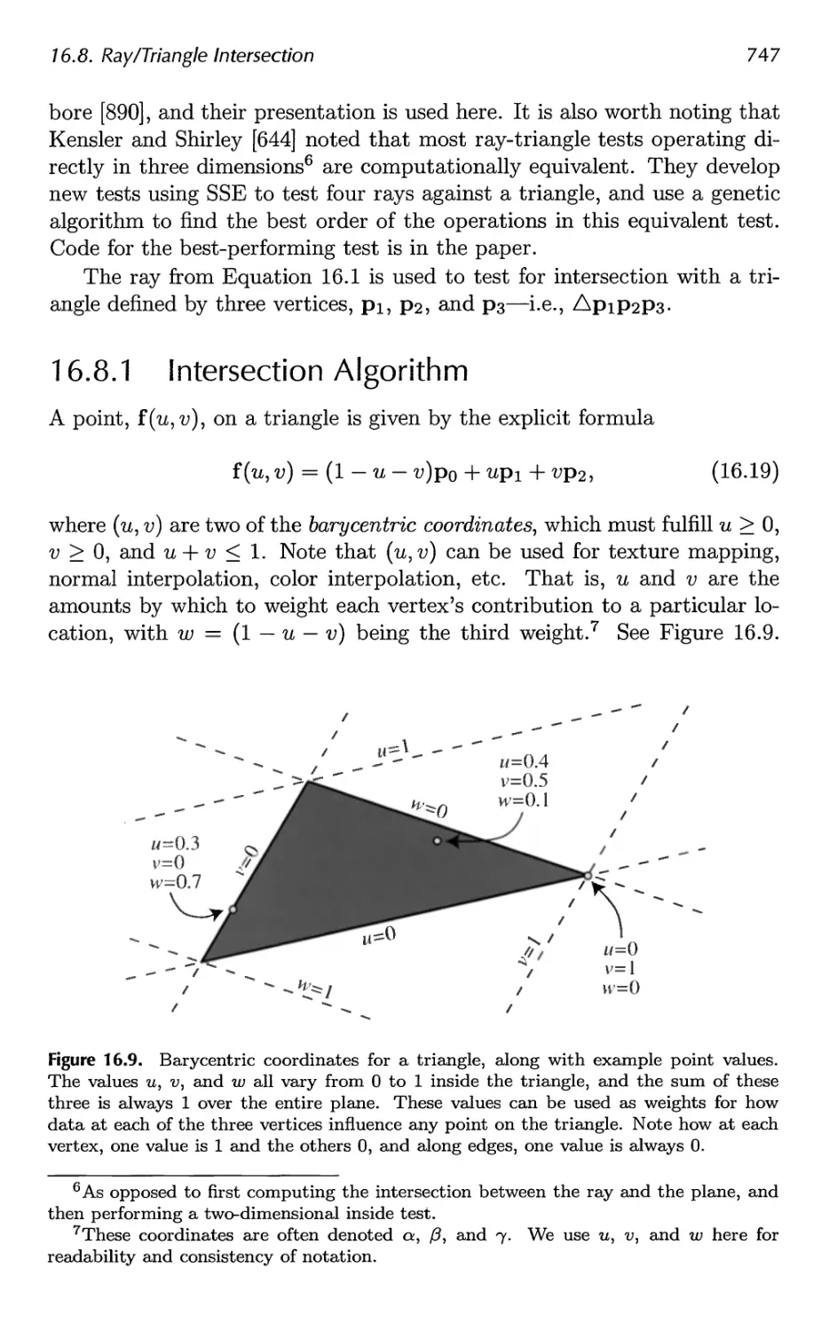
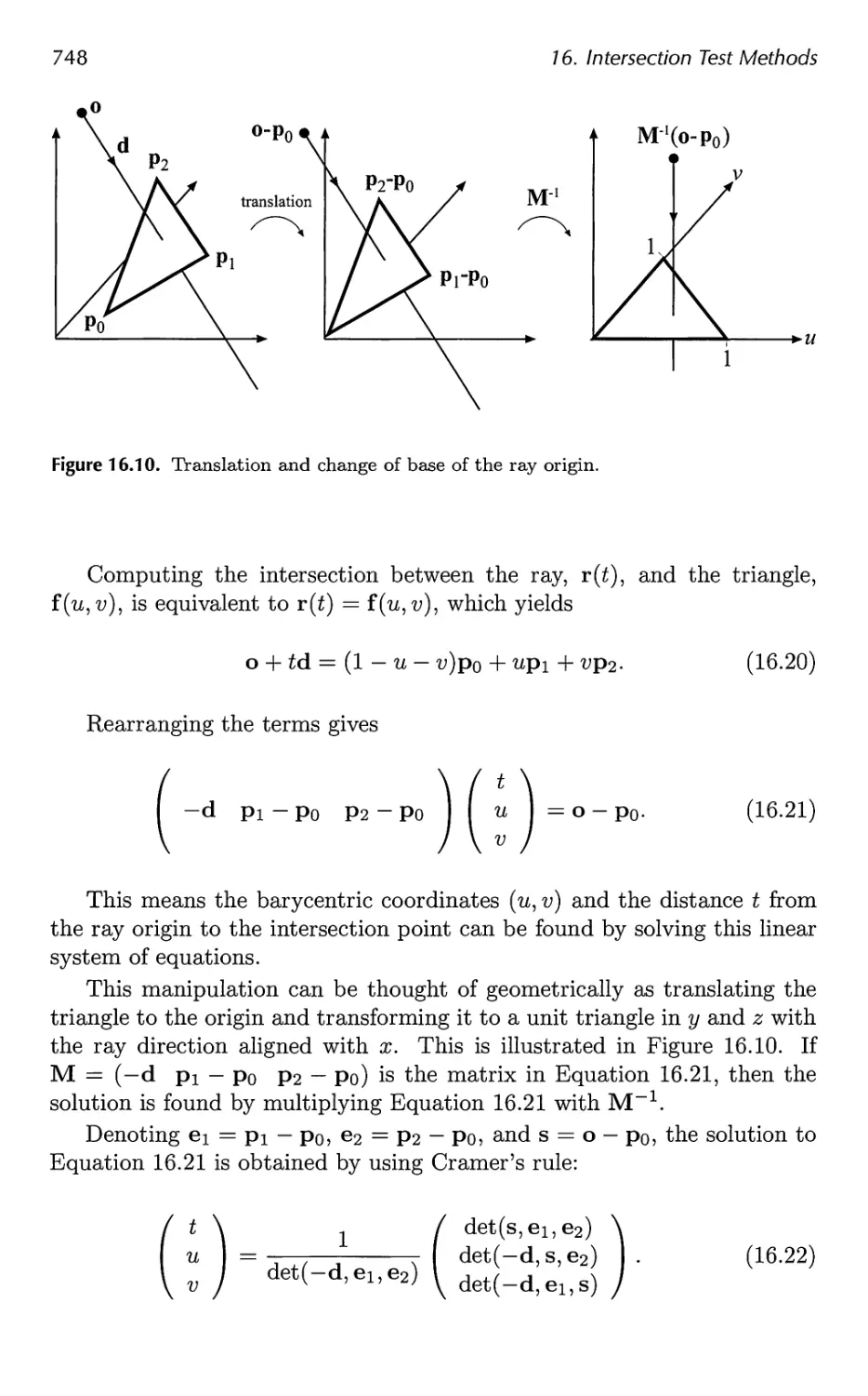
16.8 Ray/Triangle Intersection 746
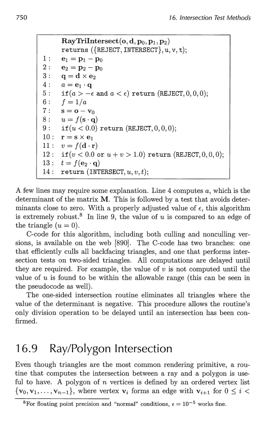
16.9 Ray/Polygon Intersection 750
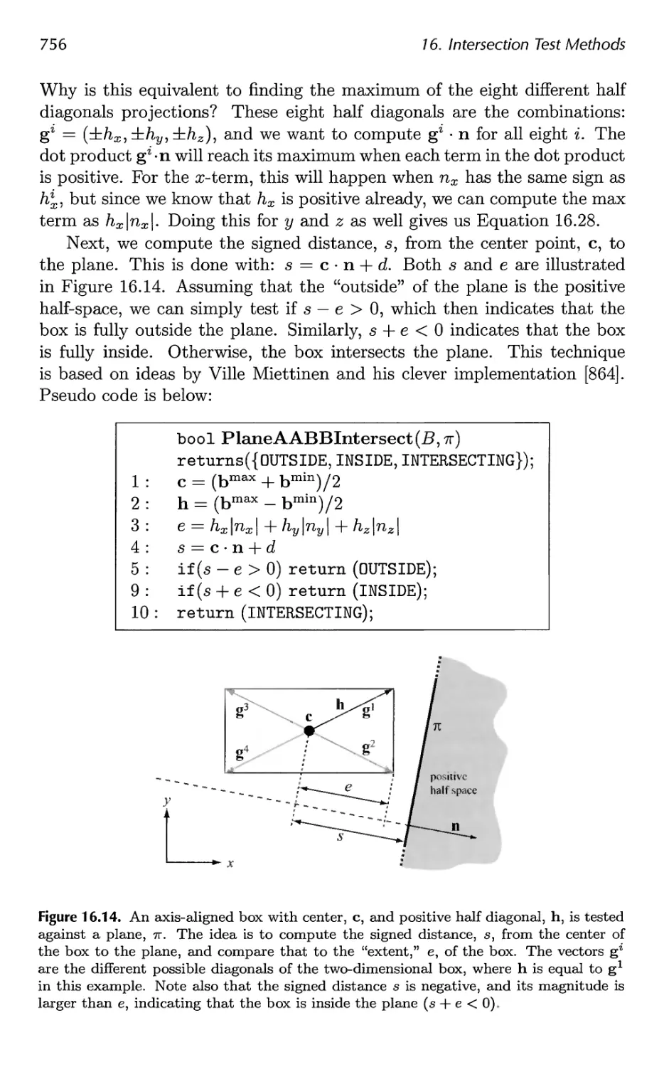
16.10 Plane/Box Intersection Detection 755
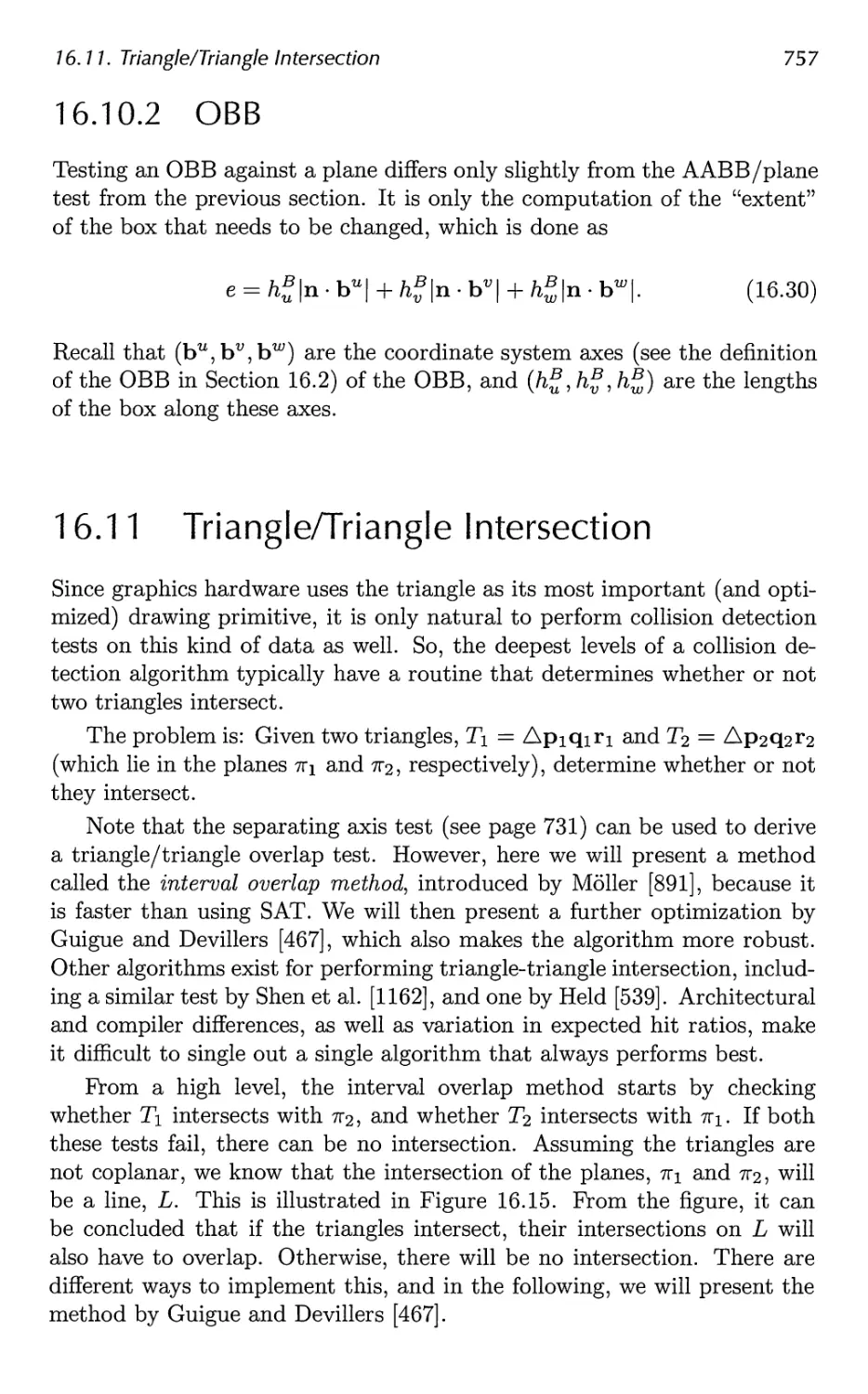
16.11 Triangle/Triangle Intersection 757
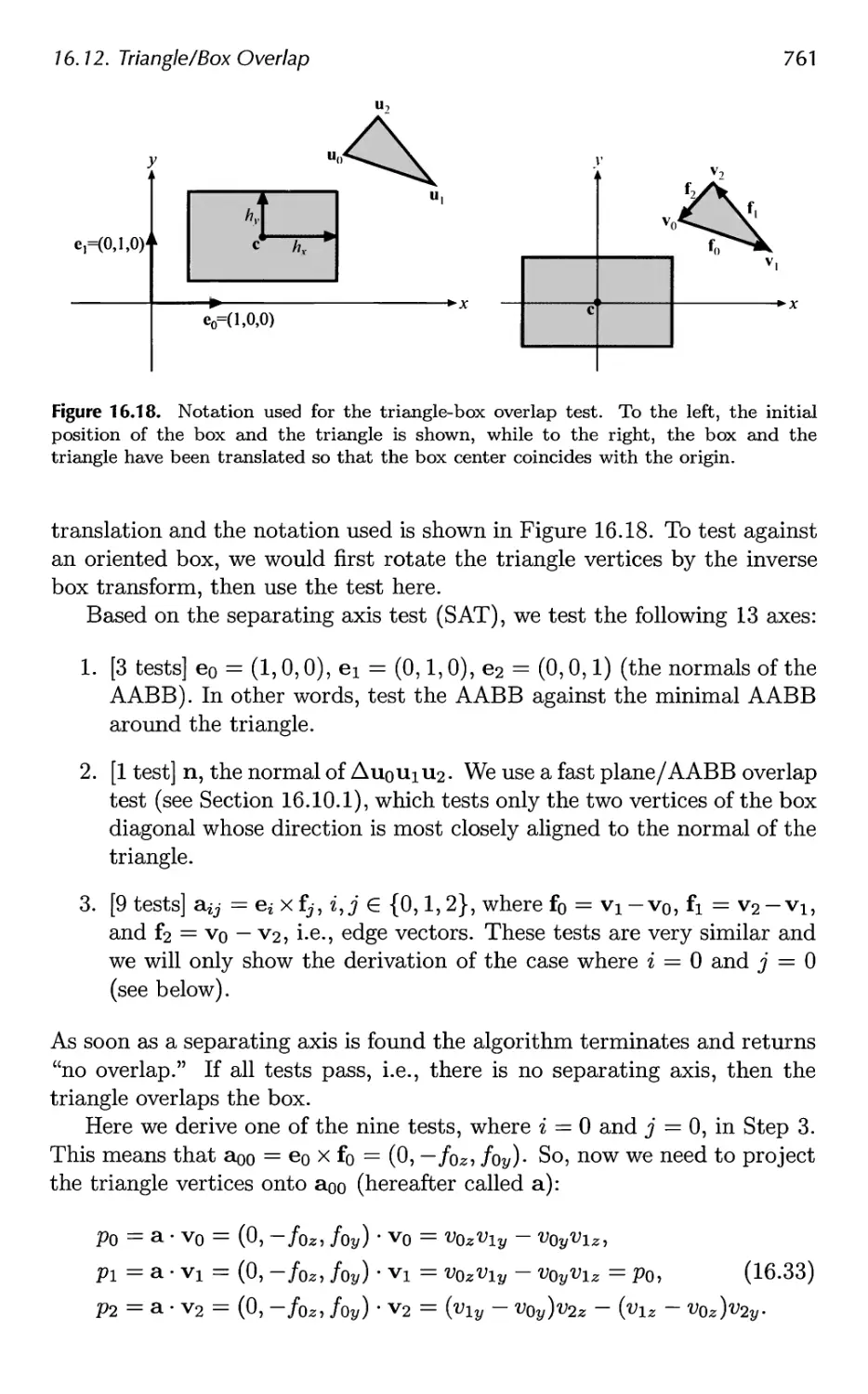
16.12 Triangle/Box Overlap 760
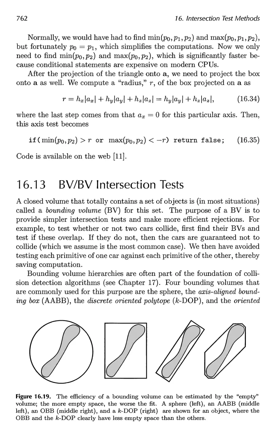
16.13 BV/BV Intersection Tests 762
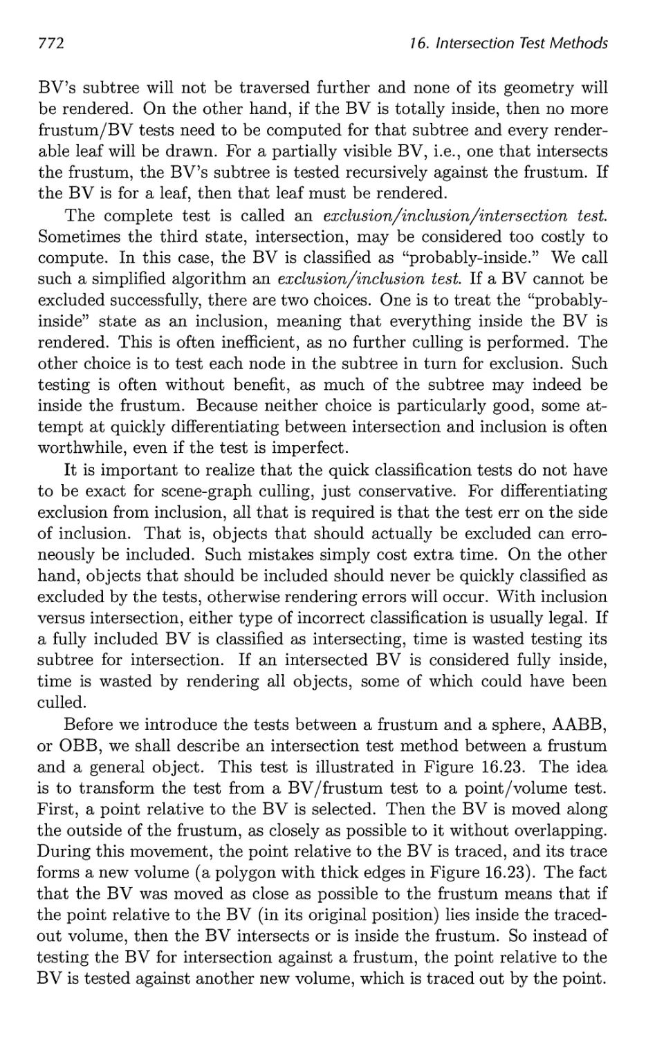
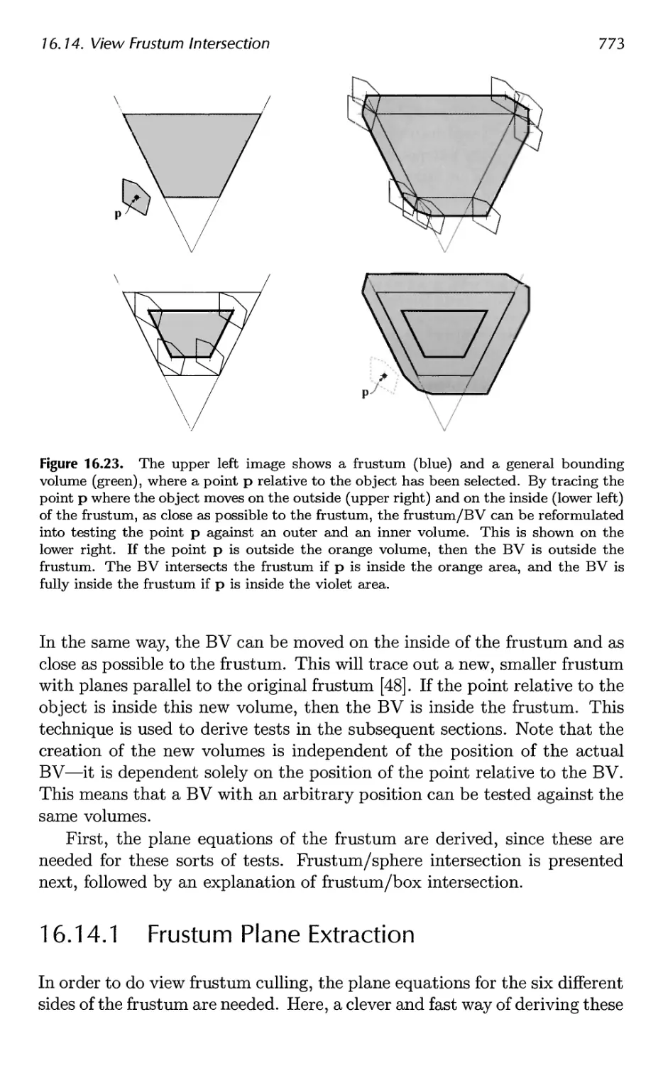
16.14 View Frustum Intersection 771
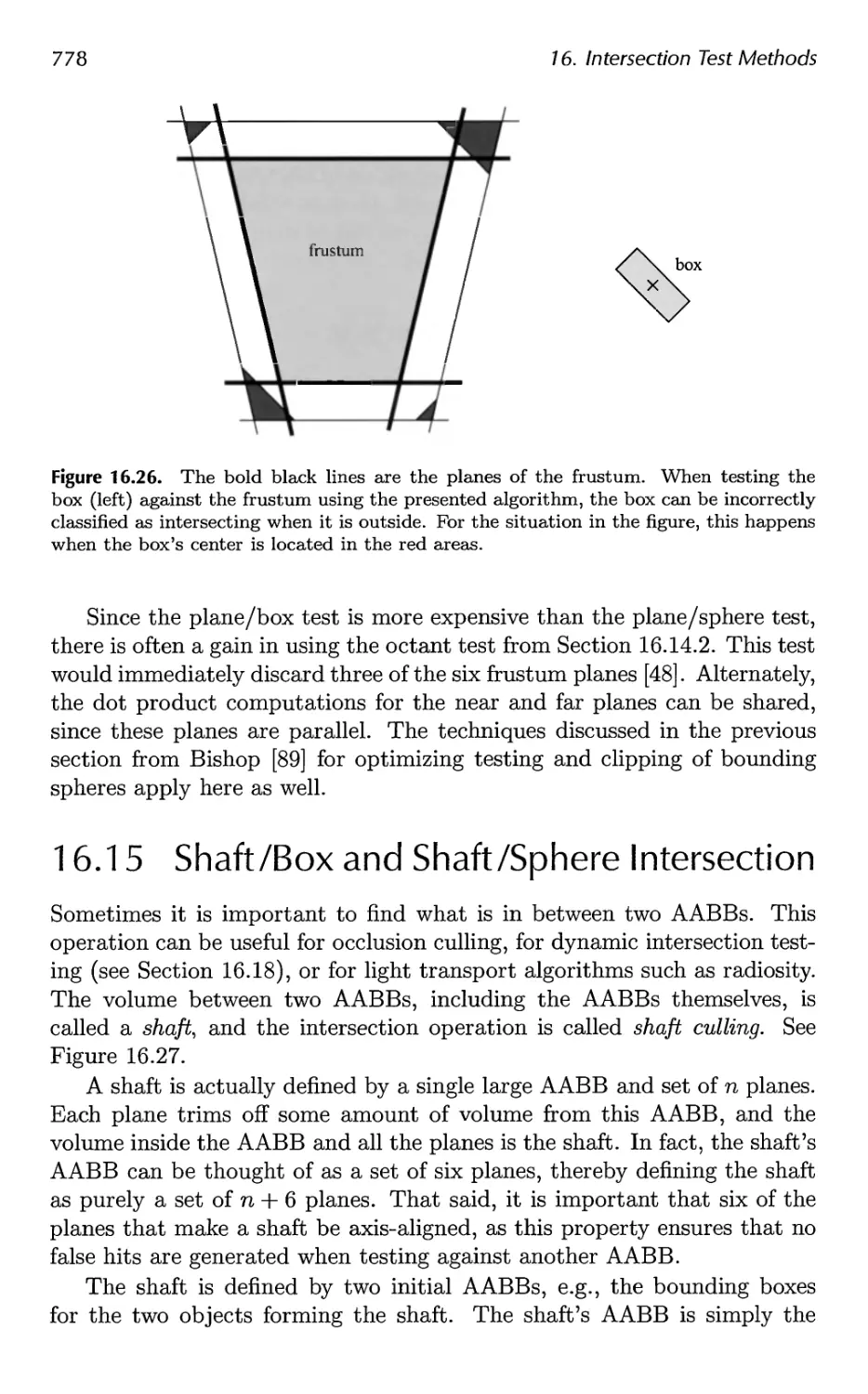
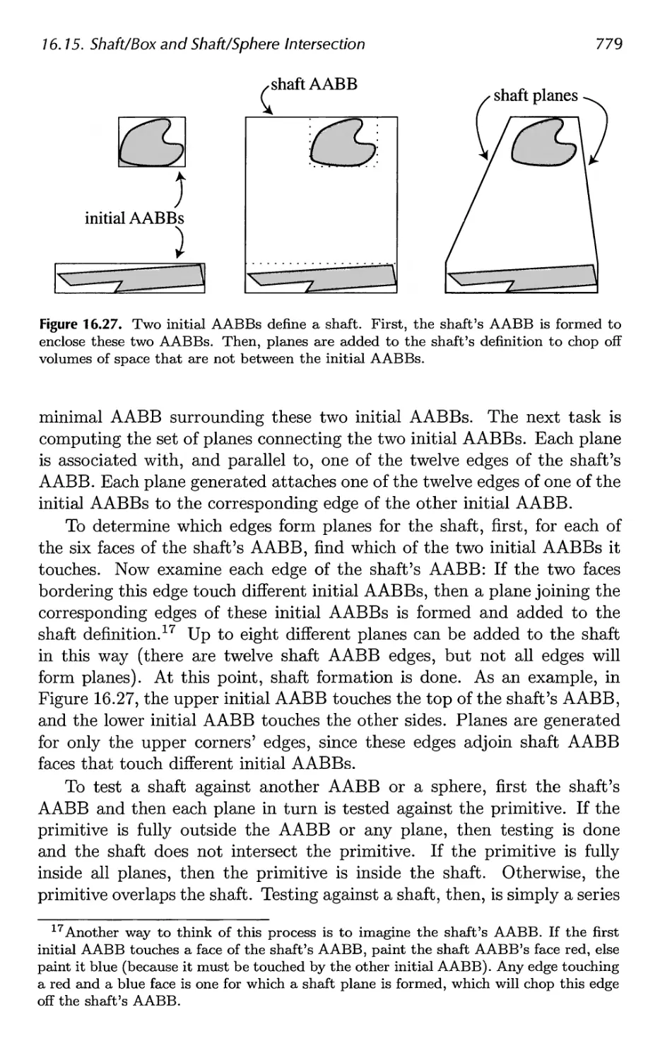
16.15 Shaft/Box and Shaft/Sphere Intersection 778
16.16 Line/Line Intersection Tests 780
16.17 Intersection Between Three Planes 782
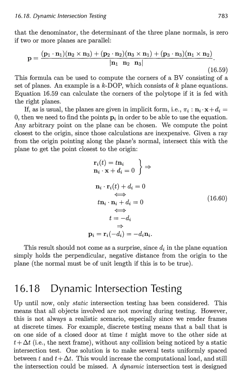
16.18 Dynamic Intersection Testing 783
17 Collision Detection 793
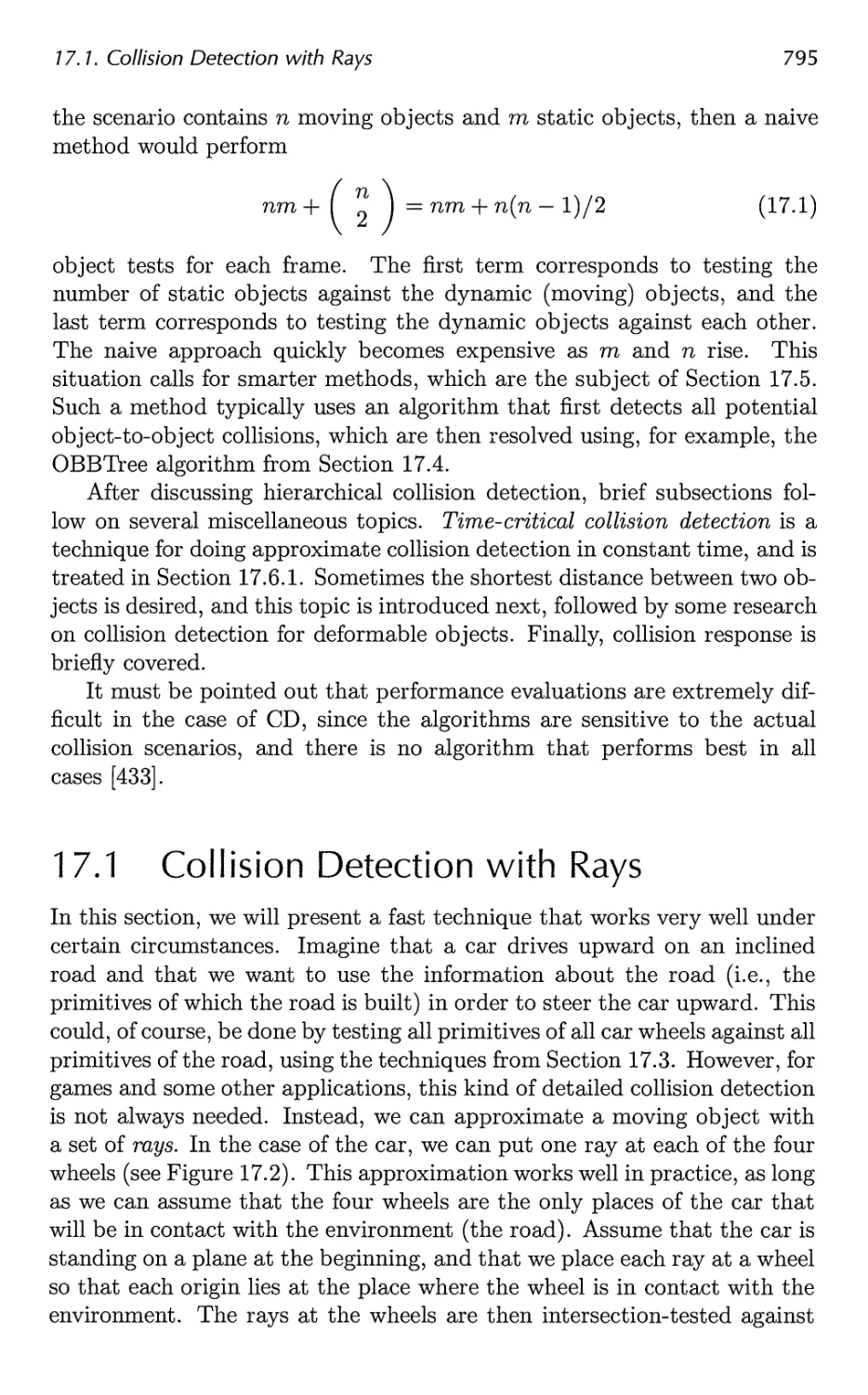
17.1 Collision Detection with Rays 795
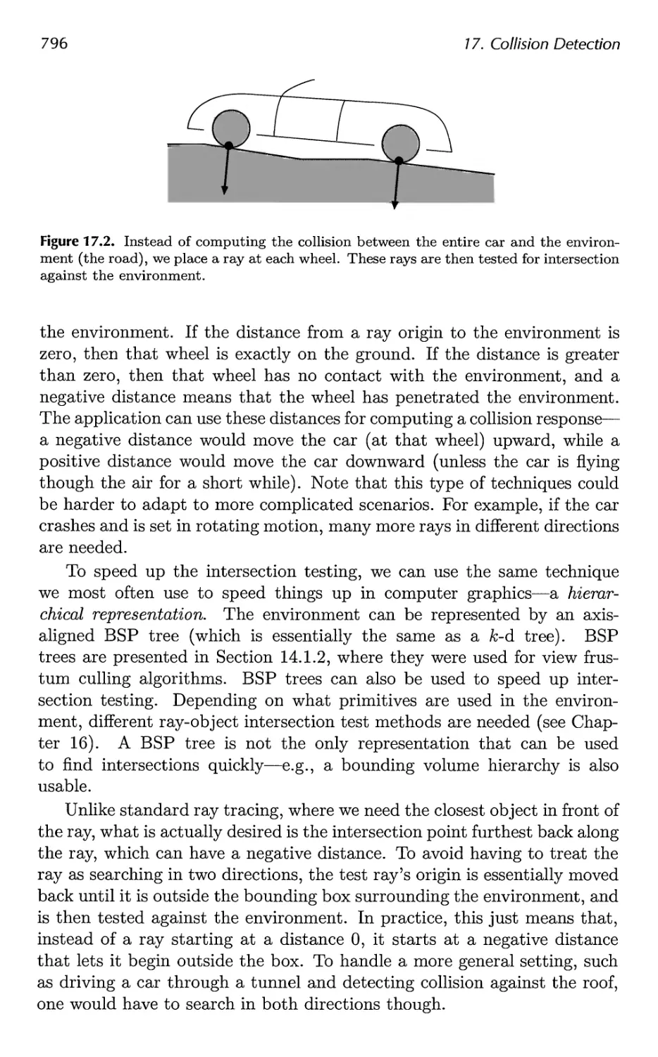
17.2 Dynamic CD using BSP Trees 797
17.3 General Hierarchical Collision Detection 802
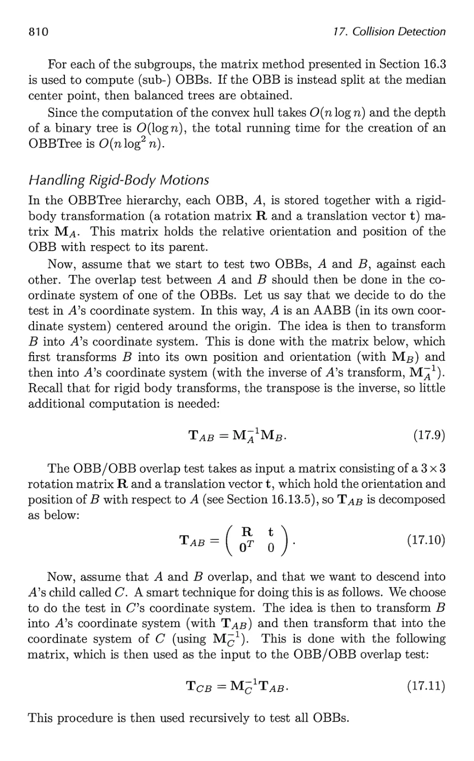
17.4 OBBTree 807
Contents xi
17.5 A Multiple Objects CD System 811
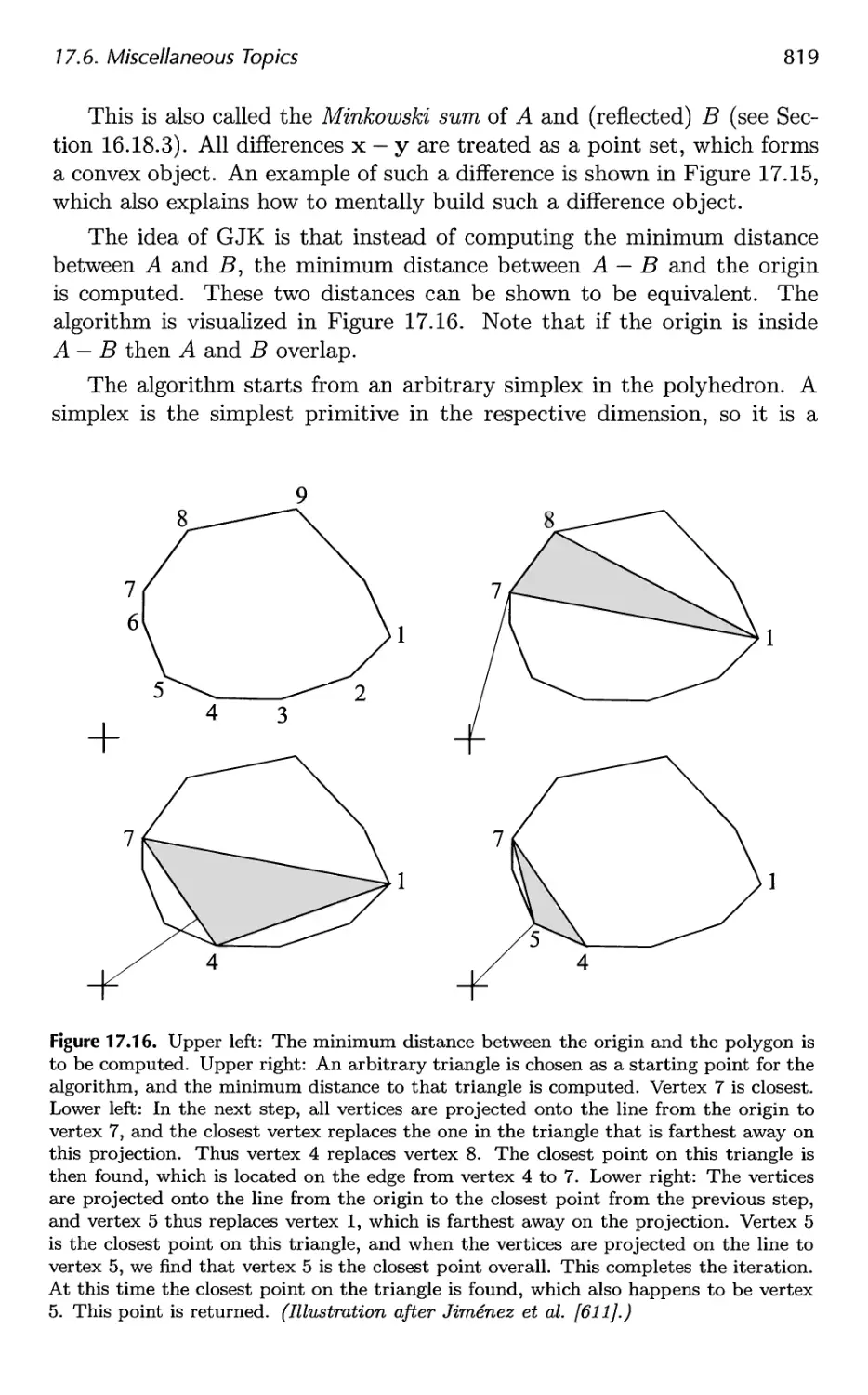
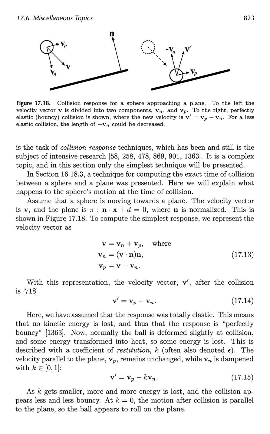
17.6 Miscellaneous Topics 816
17.7 Other Work 826
18 Graphics Hardware 829
18.1 Buffers and Buffering 829
18.2 Perspective-Correct Interpolation 838
18.3 Architecture 840
18.4 Case Studies 859
19 The Future 879
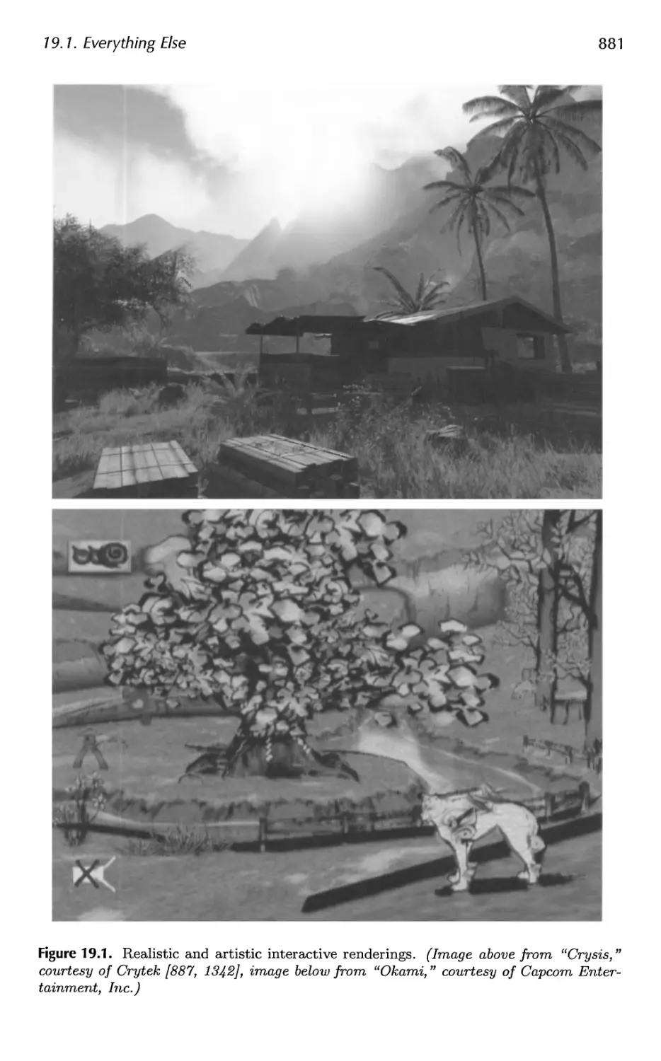
19.1 Everything Else 879
19.2 You 885
A Some Linear Algebra 889
A.l Euclidean Space 889
A.2 Geometrical Interpretation 892
A.3 Matrices 897
A.4 Homogeneous Notation 905
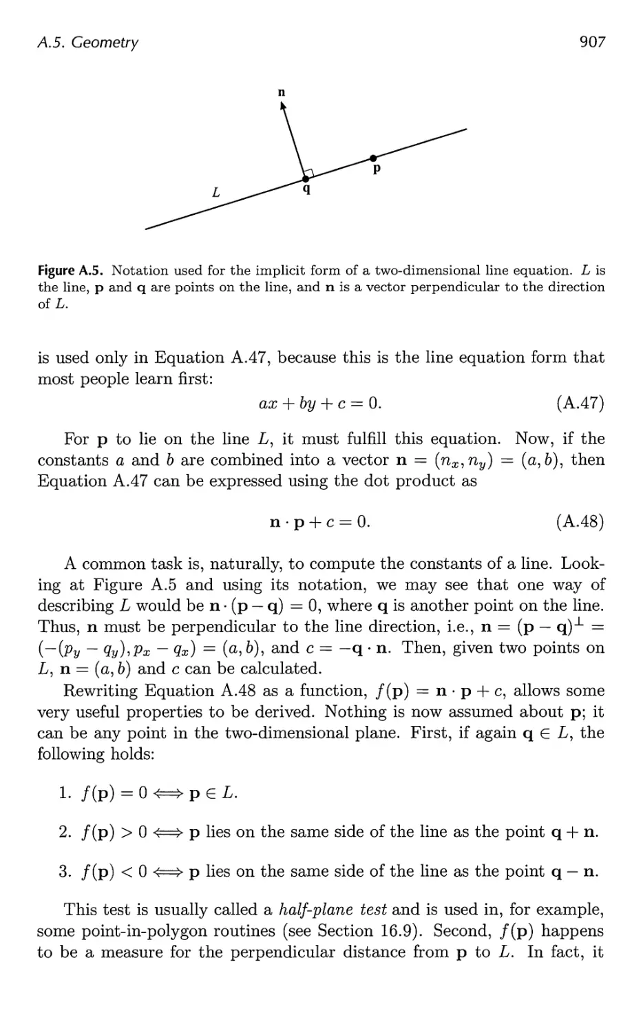
A.5 Geometry 906
B Trigonometry 913
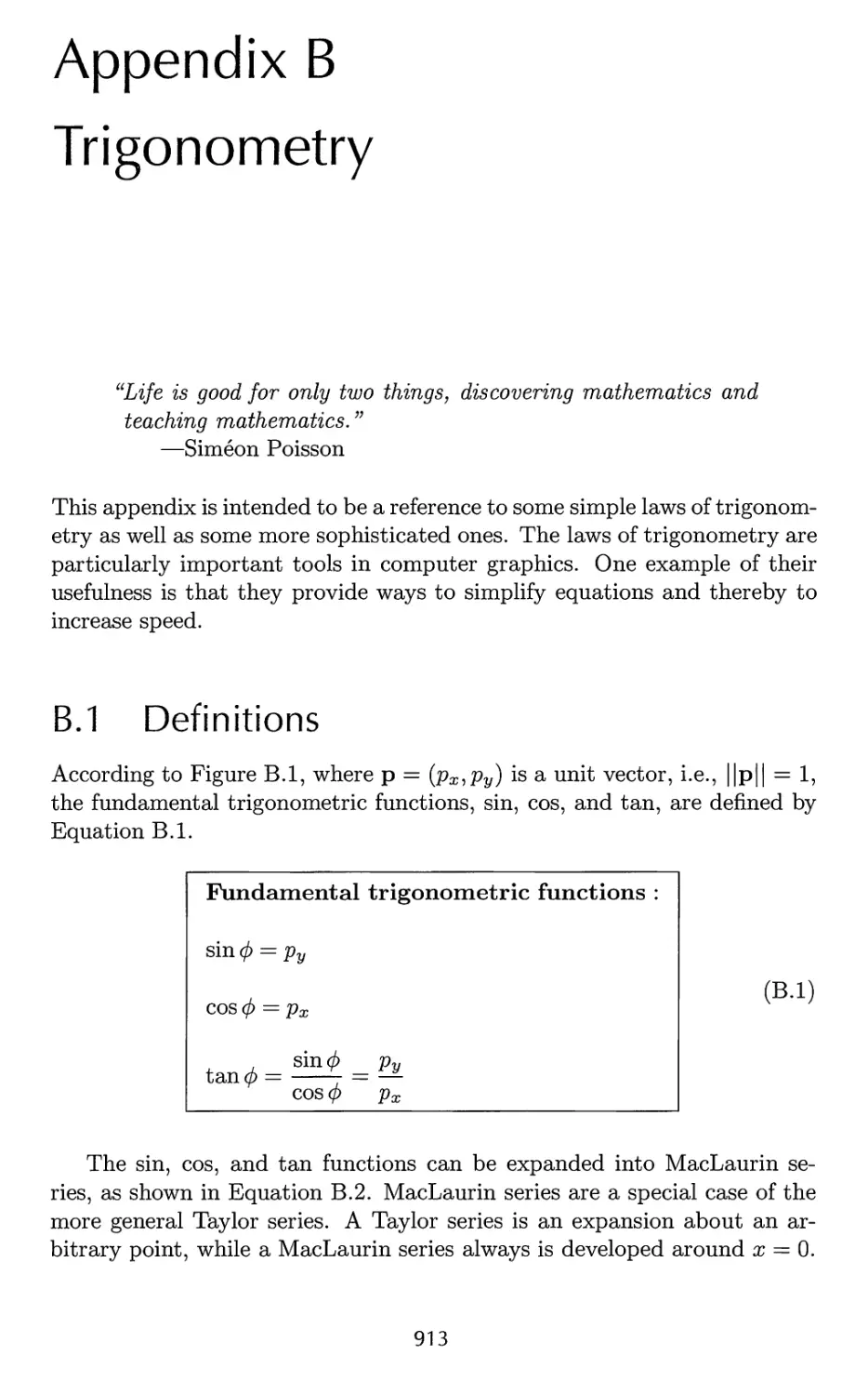
B.l Definitions 913
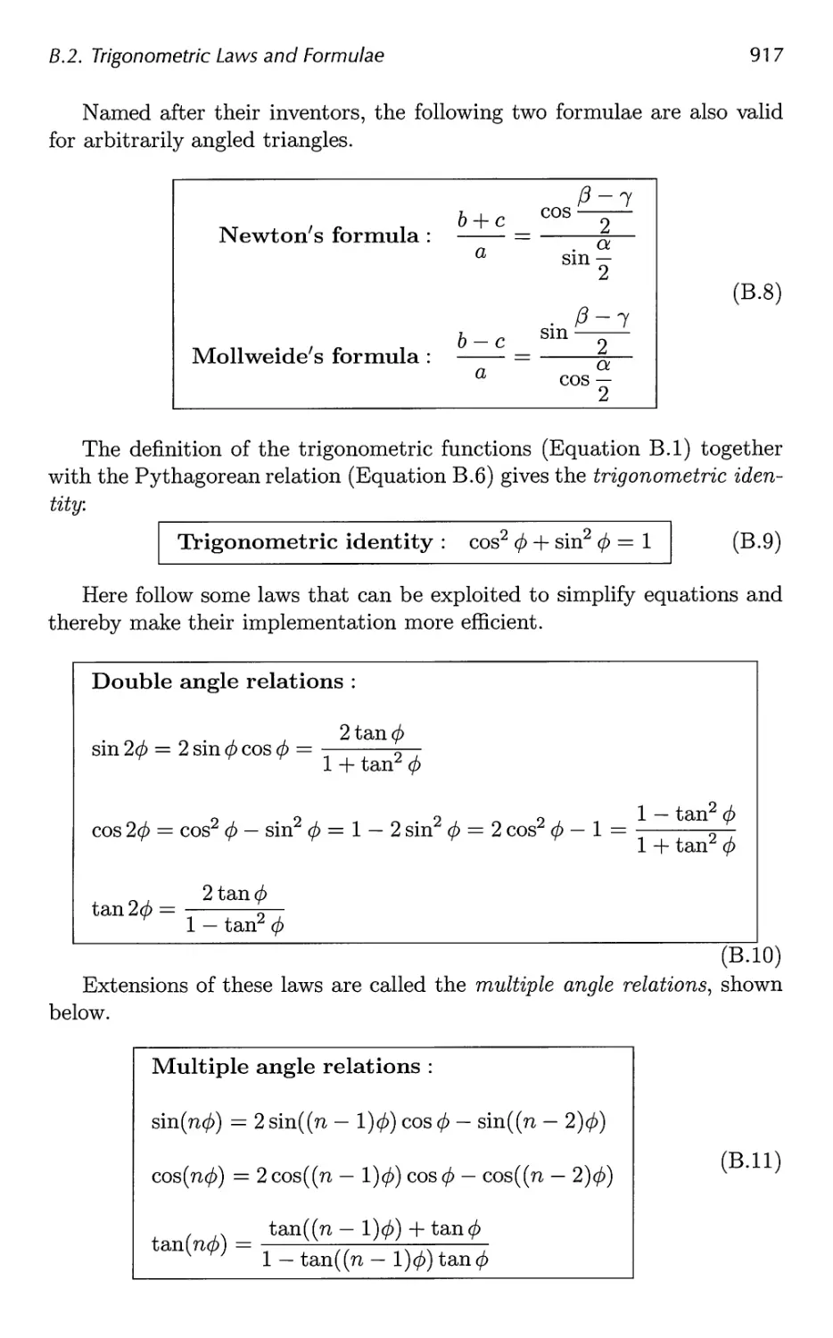
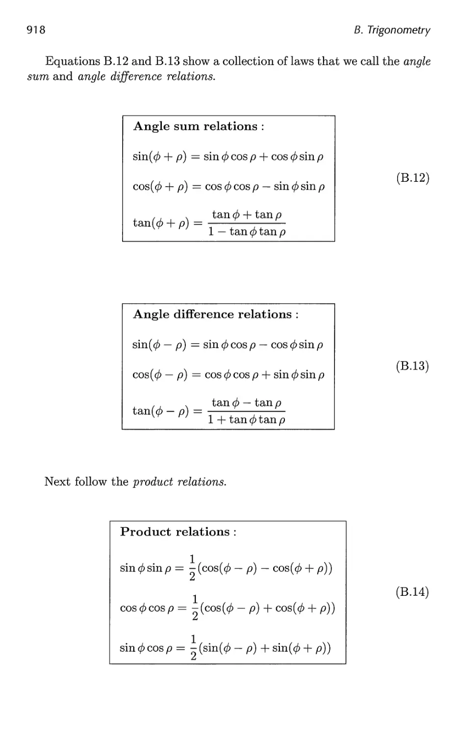
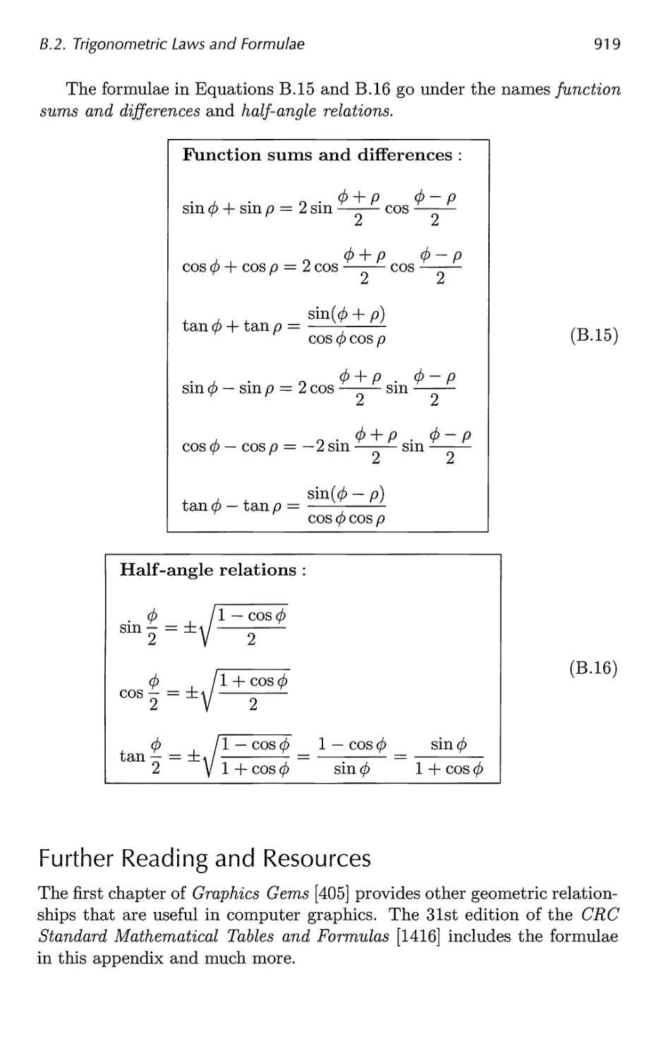
B.2 Trigonometric Laws and Formulae 915
Bibliography 921
Index 1003
Preface
How much has happened in six years! Luckily for us, there has not been a
paradigm shift (yet), but the amount of creative energy that has gone into
the field these past years is incredible. To keep up with this ever-growing
field, we are fortunate this time to be three authors instead of two. Naty
Hoffman joins us this edition. He has years of experience in the field and
has brought a fresh perspective to the book.
Since the second edition in 2002, researchers have produced hundreds
of articles in the area of interactive computer graphics. At one point Naty
filtered through conference proceedings, saving articles he thought were
worth at least a mention. Prom just the research conferences alone the
list grew to over 350 references; this did not include those in journals,
book series like GPU Gems and ShaderX, or web articles. We realized
we had a challenge ahead of us. Even a thorough survey of each area
would make for a book of nothing but surveys. Such a volume would be
exhaustive, but exhausting, and ultimately unsatisfying. Instead, we have
focused on theory, algorithms, and architectures that we felt are key in
understanding the field. We survey the literature as warranted, but with
the goal of pointing you at the most recent work in an area and at resources
for learning more.
This book is about algorithms that create synthetic images fast enough
that the viewer can interact with a virtual environment. We have focused
on three-dimensional rendering and, to a limited extent, on user interaction.
Modeling, animation, and many other areas are important to the process
of making a real-time application, but these topics are beyond the scope of
this book.
We expect you to have some basic understanding of computer graphics
before reading this book, as well as computer science and programming.
Some of the later chapters in particular are meant for implementers of
various complex algorithms. If some section does lose you, skim on through
or look at the references. One of the most valuable services we feel we can
provide is to have you realize what others have discovered and that you do
not yet know, and to give you ways to learn more someday.
We make a point of referencing relevant material wherever possible, as
well as providing a summary of further reading and resources at the end of
XIII
XIV
Preface
most chapters. Time invested in reading papers and books on a particular
topic will almost always be paid back in the amount of implementation
effort saved later.
Because the field is evolving so rapidly, we maintain a website related to
this book at: http://www.realtimerendering.com. The site contains links to
tutorials, demonstration programs, code samples, software libraries, book
corrections, and more. This book's reference section is available there, with
links to the referenced papers.
Our true goal and guiding light while writing this book was simple. We
wanted to write a book that we wished we had owned when we had started
out, a book that was both unified yet crammed with details not found in
introductory texts. We hope that you will find this book, our view of the
world, of some use in your travels.
Acknowledgments
Special thanks go out to a number of people who went out of their way to
provide us with help. First, our graphics architecture case studies would
not have been anywhere as good without the extensive and generous
cooperation we received from the companies making the hardware. Many thanks
to Edvard S0rgard, Borgar Ljosland, Dave Shreiner, and J0rn Nystad at
ARM for providing details about their Mali 200 architecture. Thanks also
to Michael Dougherty at Microsoft, who provided extremely valuable help
with the Xbox 360 section. Masaaki Oka at Sony Computer Entertainment
provided his own technical review of the PLAYSTATION® 3 system case
TM
study, while also serving as the liaison with the Cell Broadband Engine
and RSX® developers for their reviews.
In answering a seemingly endless stream of questions, fact-checking
numerous passages, and providing many screenshots, Natalya Tatarchuk of
ATI/AMD went well beyond the call of duty in helping us out. In addition
to responding to our usual requests for information and clarification,
Wolfgang Engel was extremely helpful in providing us with articles from the
upcoming ShaderX6 book and copies of the difficult-to-obtain ShaderX2
books.1 Ignacio Castano at NVIDIA provided us with valuable support
and contacts, going so far as to rework a refractory demo so we could get
just the right screenshot.
The chapter reviewers provided an invaluable service to us. They
suggested numerous improvements and provided additional insights, helping
us immeasurably. In alphabetical order they are: Michael Ashikhmin,
Dan Baker, Willem de Boer, Ben Diamand, Ben Discoe, Amir Ebrahimi,
1 Check our website; he and we are attempting to clear permissions and make this
two-volume book [307, 308] available for free on the web.
Preface
xv
Christer Ericson, Michael Gleicher, Manny Ko, Wallace Lages, Thomas
Larsson, Gregory Massal, Ville Miettinen, Mike Ramsey, Scott Schaefer,
Vincent Scheib, Peter Shirley, K.R. Subramanian, Mauricio Vives, and
Hector Yee.
We also had a number of reviewers help us on specific sections. Our
thanks go out to Matt Bronder, Christine DeNezza, Prank Fox, Jon Hassel-
gren, Pete Isensee, Andrew Lauritzen, Morgan McGuire, Jacob Munkberg,
Manuel M. Oliveira, Aurelio Reis, Peter-Pike Sloan, Jim Tilander, and
Scott Whitman.
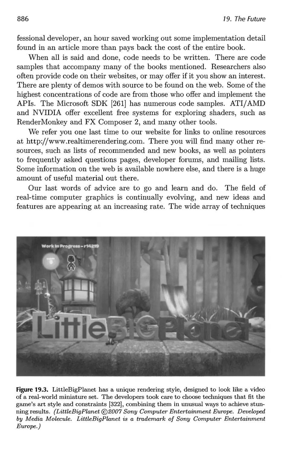
We particularly thank Rex Crowle, Kareem Ettouney, and Francis Pang
from Media Molecule for their considerable help in providing fantastic
imagery and layout concepts for the cover design.
Many people helped us out in other ways, such as answering
questions and providing screenshots. Many gave significant amounts of time
and effort, for which we thank you. Listed alphabetically: Paulo Abreu,
Timo Aila, Johan Andersson, Andreas Baerentzen, Louis Bavoil, Jim Blinn,
Jaime Borasi, Per Christensen, Patrick Conran, Rob Cook, Erwin Coumans,
Leo Cubbin, Richard Daniels, Mark DeLoura, Tony DeRose, Andreas
Dietrich, Michael Dougherty, Bryan Dudash, Alex Evans, Cass Everitt,
Randy Fernando, Jim Ferwerda, Chris Ford, Tom Forsyth, Sam Glassen-
berg, Robin Green, Ned Greene, Larry Gritz, Joakim Grundwall, Mark
Harris, Ted Himlan, Jack Hoxley, John "Spike" Hughes, Ladislav
Kavan, Alicia Kim, Gary King, Chris Lambert, Jeff Lander, Daniel Leaver,
Eric Lengyel, Jennifer Liu, Brandon Lloyd, Charles Loop, David Luebke,
Jonathan Maim, Jason Mitchell, Martin Mittring, Nathan Monteleone,
Gabe Newell, Hubert Nguyen, Petri Nordlund,' Mike Pan, Ivan Pedersen,
Matt Pharr, Fabio Policarpo, Aras Pranckevicius, Siobhan Reddy, Dirk
Reiners, Christof Rezk-Salama, Eric Risser, Marcus Roth, Holly Rush-
meier, Elan Ruskin, Marco Salvi, Daniel Scherzer, Kyle Shubel, Philipp
Slusallek, Torbjorn Soderman, Tim Sweeney, Ben Trumbore, Michal
Valient, Mark Valledor, Carsten Wenzel, Steve Westin, Chris Wyman, Cem
Yuksel, Billy Zelsnack, Fan Zhang, and Renaldas Zioma.
We also thank many others who responded to our queries on public
forums such as GD Algorithms. Readers who took the time to send us
corrections have also been a great help. It is this supportive attitude that
is one of the pleasures of working in this field.
As we have come to expect, the cheerful competence of the people at
A K Peters made the publishing part of the process much easier. For this
wonderful support, we thank you all.
On a personal note, Tomas would like to thank his son Felix and
daughter Elina for making him understand (again) just how fun it can be to play
computer games (on the Wii), instead of just looking at the graphics, and
needless to say, his beautiful wife Eva...
XVI
Preface
Eric would also like to thank his sons Ryan and Evan for their tireless
efforts in finding cool game demos and screenshots, and his wife Cathy for
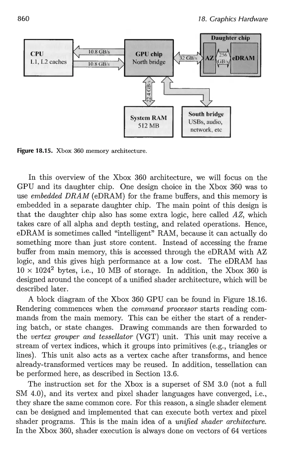
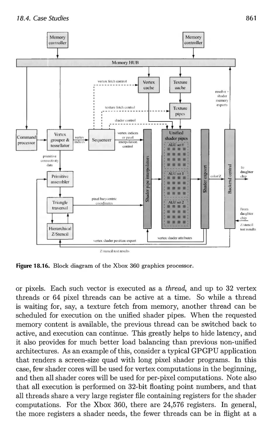
helping him survive it all.
Naty would like to thank his daughter Karen and son Daniel for their
forbearance when writing took precedence over piggyback rides, and his
wife Dorit for her constant encouragement and support.
Tomas Akenine-Moller
Eric Haines
Naty Hoffman
March 2008
Acknowledgements for the Second Edition
One of the most agreeable aspects of writing this second edition has been
working with people and receiving their help. Despite their own
pressing deadlines and concerns, many people gave us significant amounts of
their time to improve this book. We would particularly like to thank
the major reviewers. They are, listed alphabetically: Michael Abrash,
Ian Ashdown, Ulf Assarsson, Chris Brennan, Sebastien Domine, David
Eberly, Cass Everitt, Tommy Fortes, Evan Hart, Greg James, Jan Kautz,
Alexander Keller, Mark Kilgard, Adam Lake, Paul Lalonde, Thomas
Larsson, Dean Macri, Carl Marshall, Jason L. Mitchell, Kasper H0y Nielsen,
Jon Paul Schelter, Jacob Strom, Nick Triantos, Joe Warren, Michael
Wimmer, and Peter Wonka. Of these, we wish to single out Cass Everitt
at NVIDIA and Jason L. Mitchell at ATI Technologies for spending large
amounts of time and effort in getting us the resources we needed. Our
thanks also go out to Wolfgang Engel for freely sharing the contents of
his upcoming book, ShaderX [306], so that we could make this edition as
current as possible.
Prom discussing their work with us, to providing images or other
resources, to writing reviews of sections of the book, many others helped
in creating this edition. They all have our gratitude. These people
include: Jason Ang, Haim Barad, Jules Bloomenthal, Jonathan Blow, Chas.
Boyd, John Brooks, Cem Cebenoyan, Per Christensen, Hamilton Chu,
Michael Cohen, Daniel Cohen-Or, Matt Craighead, Paul Debevec, Joe
Demers, Walt Donovan, Howard Dortch, Mark Duchaineau, Phil Dutre,
Dave Eberle, Gerald Farin, Simon Fenney, Randy Fernando, Jim Ferwerda,
Nickson Fong, Tom Forsyth, Piero Foscari, Laura Fryer, Markus Giegl,
Peter Glaskowsky, Andrew Glassner, Amy Gooch, Bruce Gooch, Simon
Green, Ned Greene, Larry Gritz, Joakim Grundwall, Juan Guardado, Pat
Hanrahan, Mark Harris, Michael Herf, Carsten Hess, Rich Hilmer, Kenneth
Hoff III, Naty Hoffman, Nick Holliman, Hugues Hoppe, Heather Home,
Tom Hubina, Richard Huddy, Adam James, Kaveh Kardan, Paul Keller,
Preface
XVII
David Kirk, Alex Klimovitski, Jason Knipe, Jeff Lander, Marc Levoy,
J.P. Lewis, Ming Lin, Adrian Lopez, Michael McCool, Doug McNabb,
Stan Melax, Ville Miettinen, Kenny Mitchell, Steve Morein, Henry More-
ton, Jerris Mungai, Jim Napier, George Ngo, Hubert Nguyen, Tito Pagan,
Jorg Peters, Tom Porter, Emil Praun, Kekoa Proudfoot, Bernd Raabe,
Ravi Ramamoorthi, Ashutosh Rege, Szymon Rusinkiewicz, Carlo Sequin,
Chris Seitz, Jonathan Shade, Brian Smits, John Spitzer, Wolfgang Strafier,
Wolfgang Stiirzlinger, Philip Taylor, Pierre Terdiman, Nicolas Thibieroz,
Jack Tumblin, Predrik Ulfves, Thatcher Ulrich, Steve Upstill, Alex Vlachos,
Ingo Wald, Ben Watson, Steve Westin, Dan Wexler, Matthias Wloka, Peter
Woytiuk, David Wu, Garrett Young, Borut Zalik, Harold Zatz, Hansong
Zhang, and Denis Zorin. We also wish to thank the journal A CM
Transactions on Graphics for continuing to provide a mirror website for this book.
Alice and Klaus Peters, our production manager Ariel Jaffee, our editor
Heather Holcombe, our copyeditor Michelle M. Richards, and the rest of
the staff at A K Peters have done a wonderful job making this book the
best possible. Our thanks to all of you.
Finally, and most importantly, our deepest thanks go to our families for
giving us the huge amounts of quiet time we have needed to complete this
edition. Honestly, we never thought it would take this long!
Tomas Akenine-Moller
Eric Haines
May 2002
Acknowledgements for the First Edition
Many people helped in making this book. Some of the greatest
contributions were made by those who reviewed parts of it. The reviewers
willingly gave the benefit of their expertise, helping to significantly improve
both content and style. We wish to thank (in alphabetical order) Thomas
Barregren, Michael Cohen, Walt Donovan, Angus Dorbie, Michael
Garland, Stefan Gottschalk, Ned Greene, Ming C. Lin, Jason L. Mitchell, Liang
Peng, Keith Rule, Ken Shoemake, John Stone, Phil Taylor, Ben Trumbore,
Jorrit Tyberghein, and Nick Wilt. We cannot thank you enough.
Many other people contributed their time and labor to this project.
Some let us use images, others provided models, still others pointed out
important resources or connected us with people who could help. In
addition to the people listed above, we wish to acknowledge the help of Tony
Barkans, Daniel Baum, Nelson Beebe, Curtis Beeson, Tor Berg, David
Blythe, Chas. Boyd, Don Brittain, Ian BuUard, Javier Castellar, Satyan
Coorg, Jason Delia Rocca, Paul Diefenbach, Alyssa Donovan, Dave Eberly,
Kells Elmquist, Stuart Feldman, Fred Fisher, Tom Forsyth, Marty Franz,
Thomas Funkhouser, Andrew Glassner, Bruce Gooch, Larry Gritz, Robert
XVIII
Preface
Grzeszczuk, Paul Haeberli, Evan Hart, Paul Heckbert, Chris Hecker,
Joachim Helenklaken, Hugues Hoppe, John Jack, Mark Kilgard, David
Kirk, James Klosowski, Subodh Kumar, Andre LaMothe, Jeff Lander, Jens
Larsson, Jed Lengyel, Predrik Liliegren, David Luebke, Thomas Lundqvist,
Tom McReynolds, Stan Melax, Don Mitchell, Andre Moller, Steve Molnar,
Scott R. Nelson, Hubert Nguyen, Doug Rogers, Holly Rushmeier, Ger-
not Schaufier, Jonas Skeppstedt, Stephen Spencer, Per Stenstrom, Jacob
Strom, Filippo Tampieri, Gary Tarolli, Ken Turkowski, Turner Whitted,
Agata and Andrzej Wojaczek, Andrew Woo, Steve Worley, Brian Yen,
Hans-Philip Zachau, Gabriel Zachmann, and Al Zimmerman. We also wish
to thank the journal A CM Transactions on Graphics for providing a stable
website for this book.
Alice and Klaus Peters and the staff at AK Peters, particularly Carolyn
Artin and Sarah Gillis, have been instrumental in making this book a
reality. To all of you, thanks.
Finally, our deepest thanks go to our families and friends for providing
support throughout this incredible, sometimes grueling, often
exhilarating process.
Tomas Moller
Eric Haines
March 1999
Chapter 1
Introduction
Real-time rendering is concerned with making images rapidly on the
computer. It is the most highly interactive area of computer graphics. An
image appears on the screen, the viewer acts or reacts, and this feedback
affects what is generated next. This cycle of reaction and rendering
happens at a rapid enough rate that the viewer does not see individual images,
but rather becomes immersed in a dynamic process.
The rate at which images are displayed is measured in frames per
second (fps) or Hertz (Hz). At one frame per second, there is little sense of
interactivity; the user is painfully aware of the arrival of each new image.
At around 6 fps, a sense of interactivity starts to grow. An application
displaying at 15 fps is certainly real-time; the user focuses on action and
reaction. There is a useful limit, however. From about 72 fps and up,
differences in the display rate are effectively undetectable.
Watching images flicker by at 60 fps might be acceptable, but an even
higher rate is important for minimizing response time. As little as 15
milliseconds of temporal delay can slow and interfere with interaction [1329].
There is more to real-time rendering than interactivity. If speed was the
only criterion, any application that rapidly responded to user commands
and drew anything on the screen would qualify. Rendering in real-time
normally means three-dimensional rendering.
Interactivity and some sense of connection to three-dimensional space
are sufficient conditions for real-time rendering, but a third element has
become a part of its definition: graphics acceleration hardware. While
hardware dedicated to three-dimensional graphics has been available on
professional workstations for many years, it is only relatively recently that
the use of such accelerators at the consumer level has become possible.
Many consider the introduction of the 3Dfx Voodoo 1 in 1996 the real
beginning of this era [297]. With the recent rapid advances in this market,
add-on three-dimensional graphics accelerators are as standard for home
computers as a pair of speakers. While it is not absolutely required for real-
1
2
/. Introduction
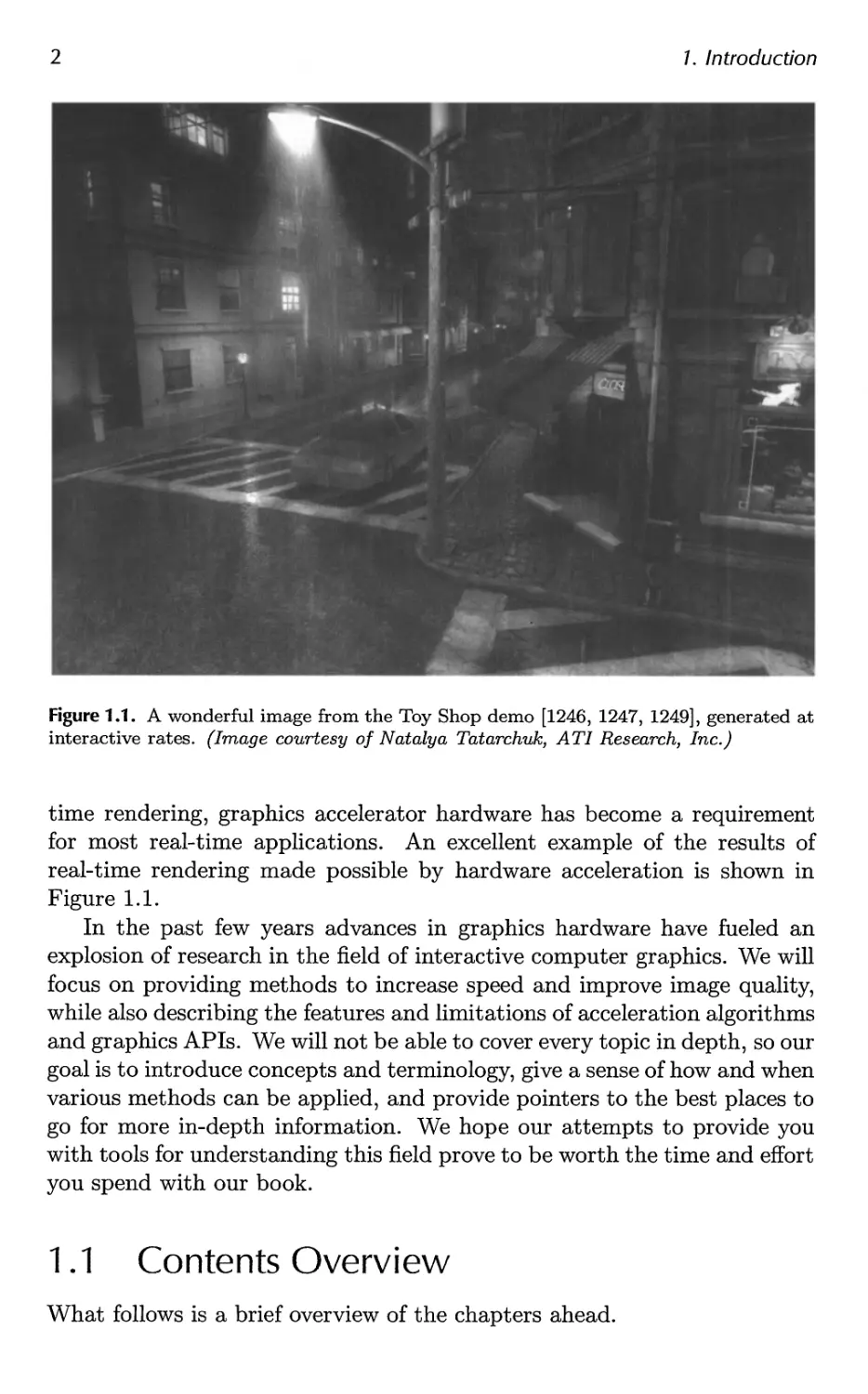
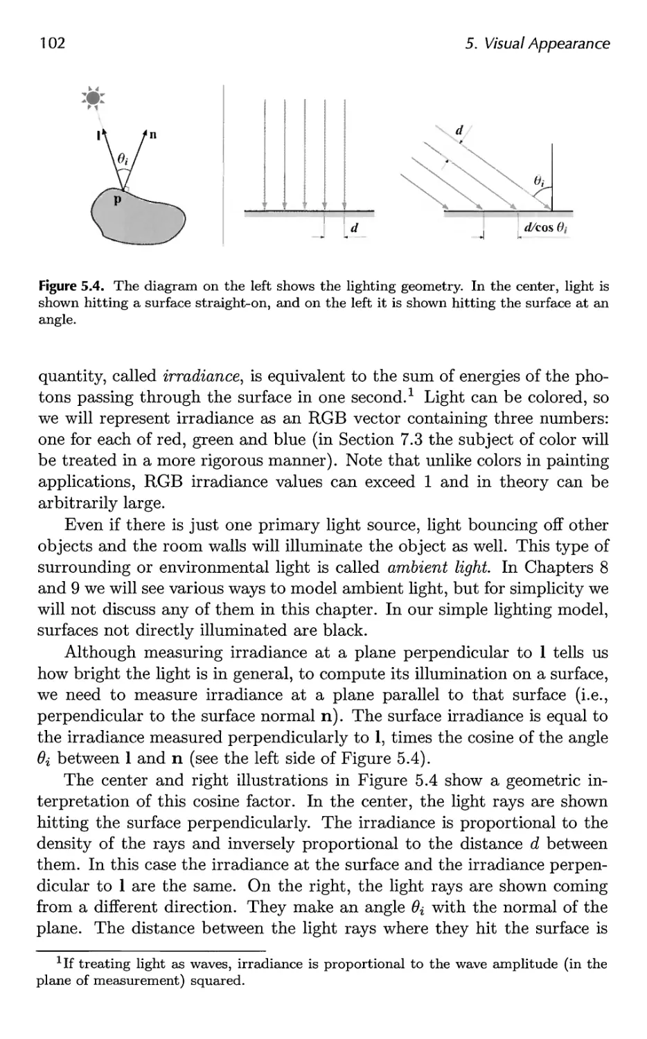
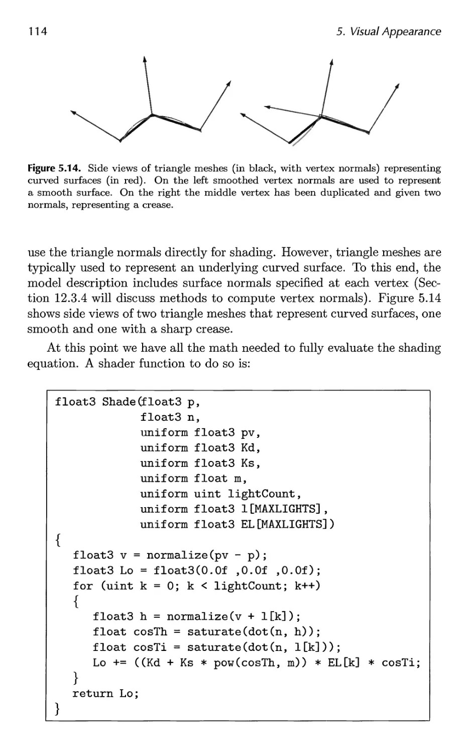
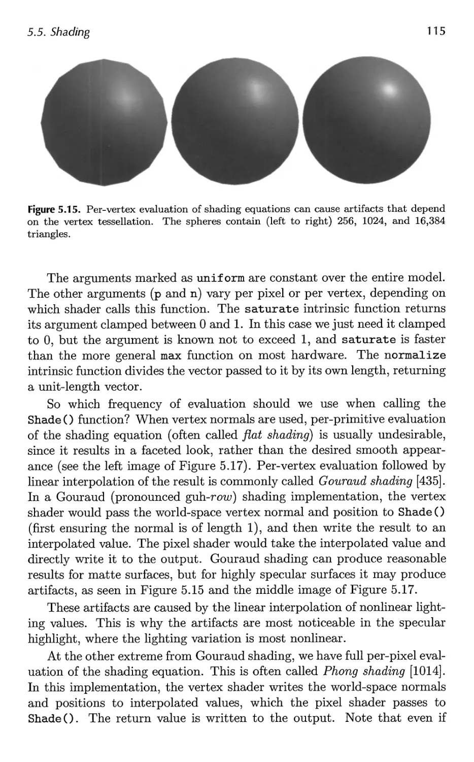
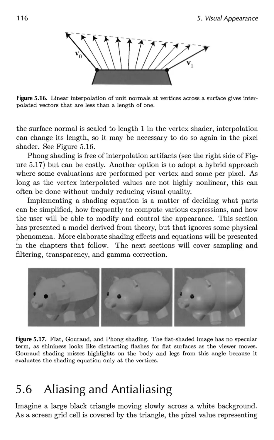
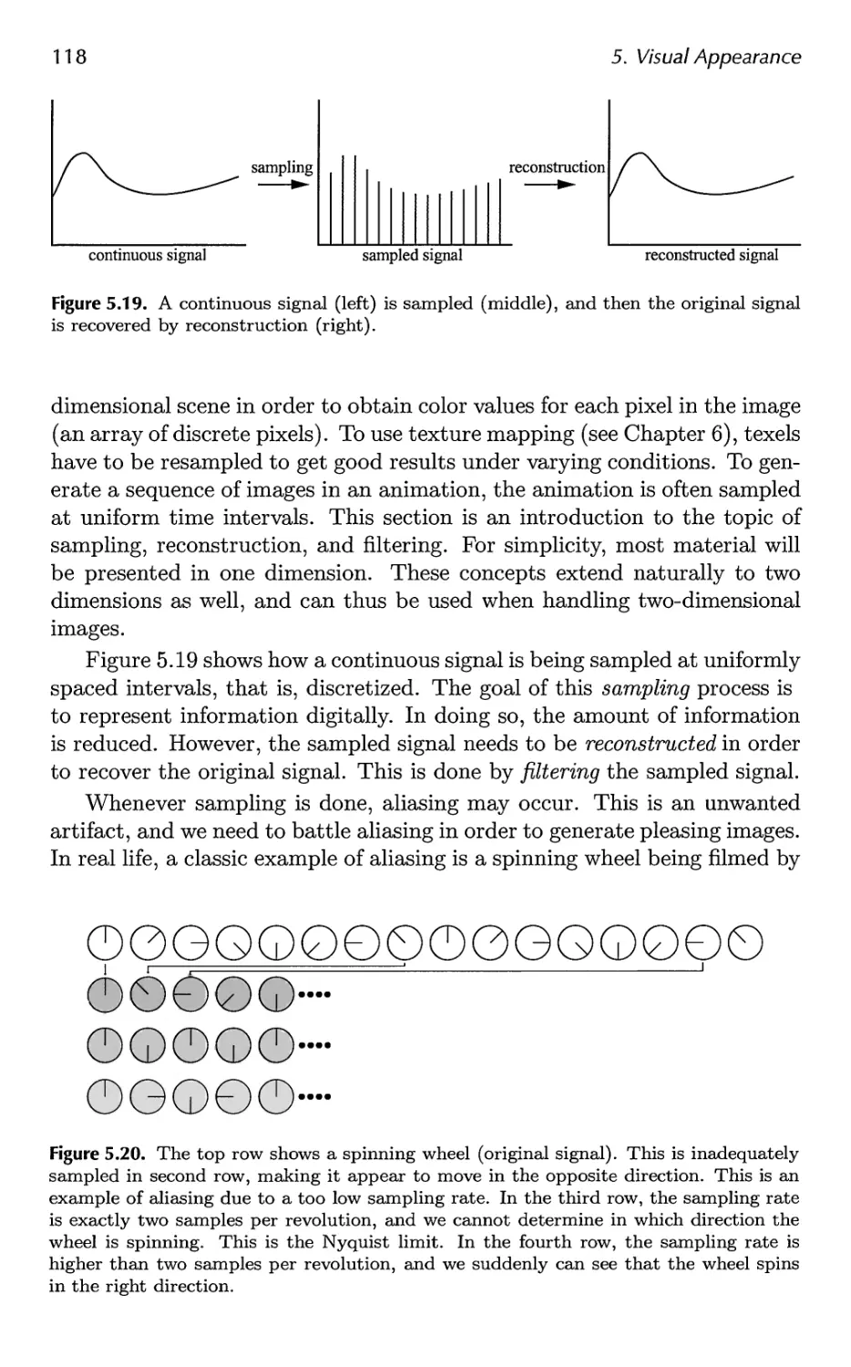
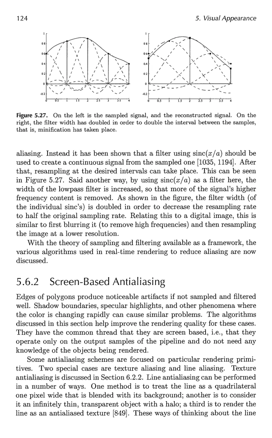
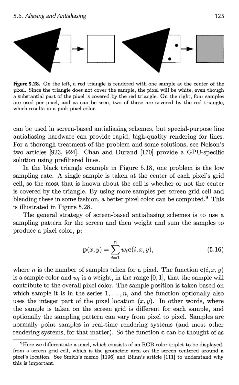
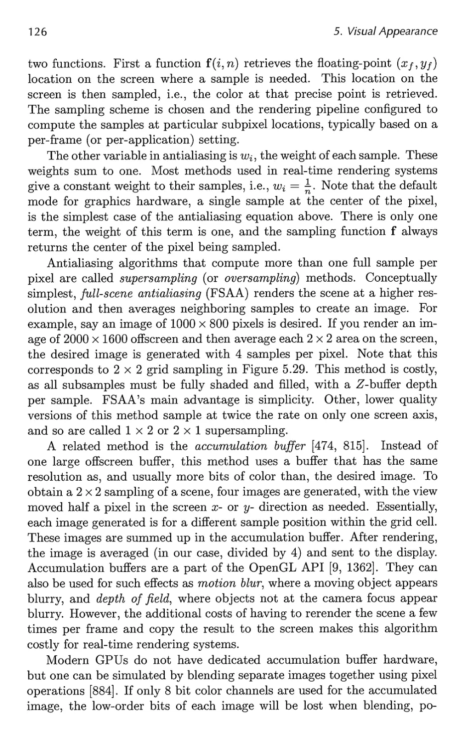
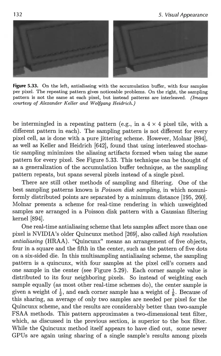
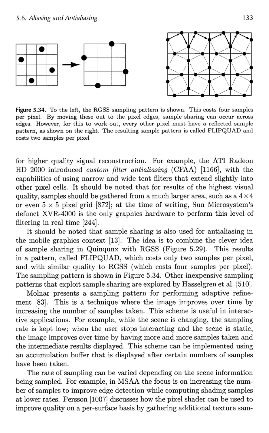
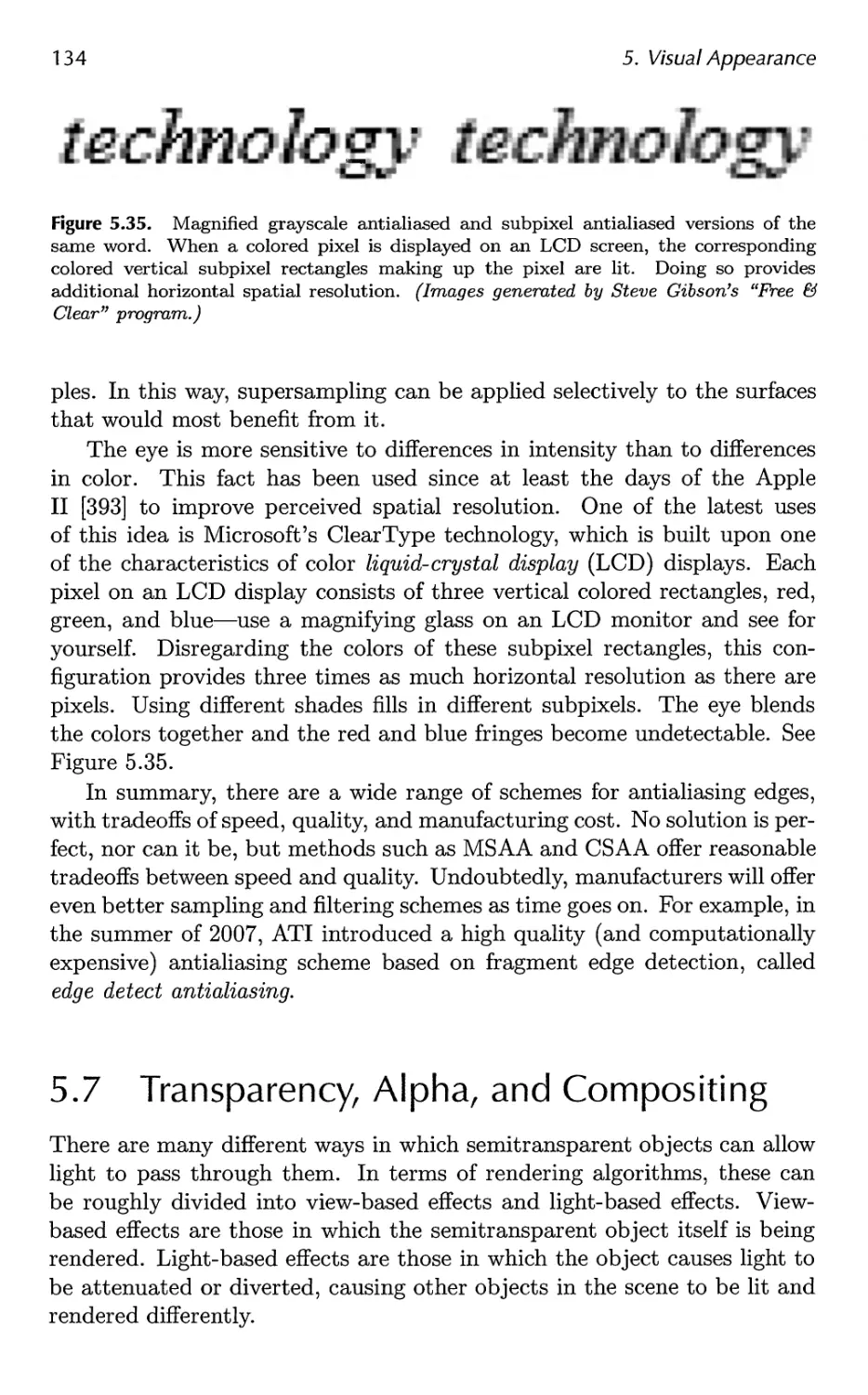
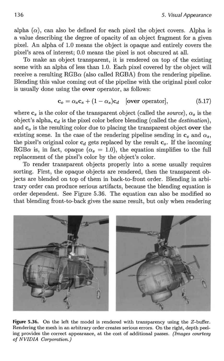
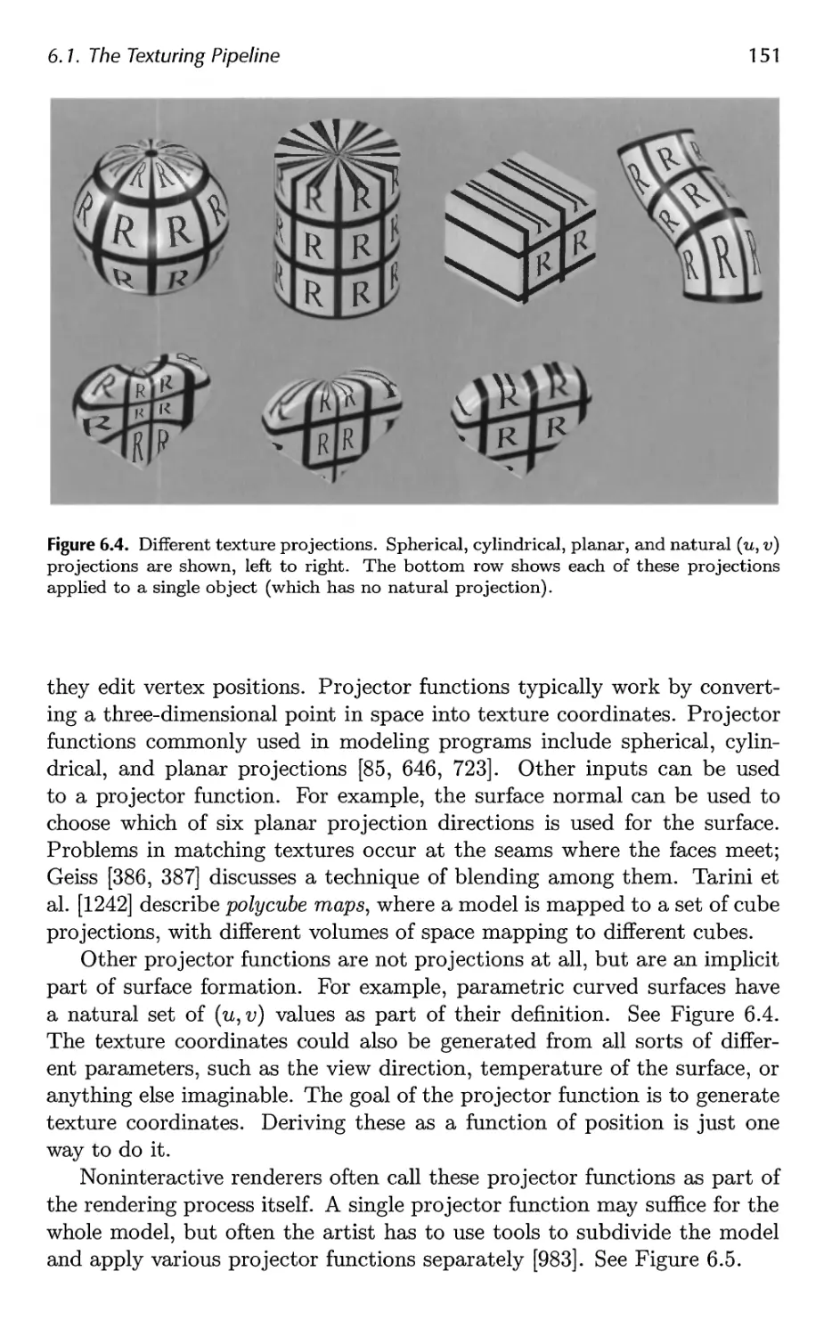
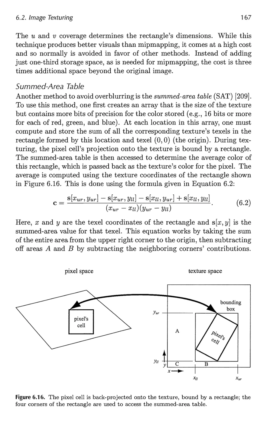
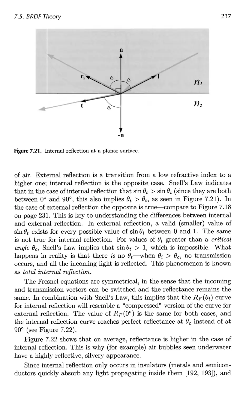
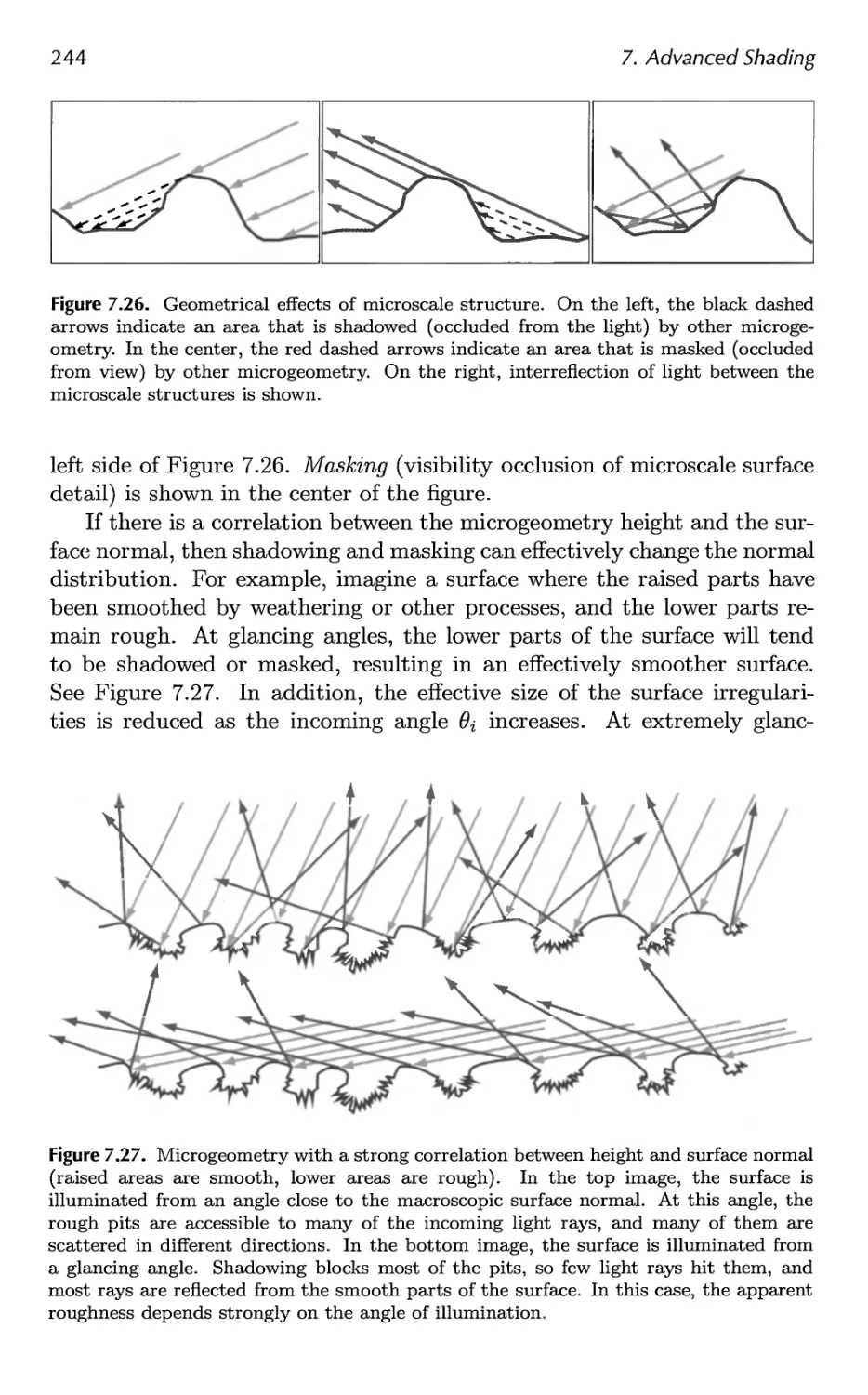
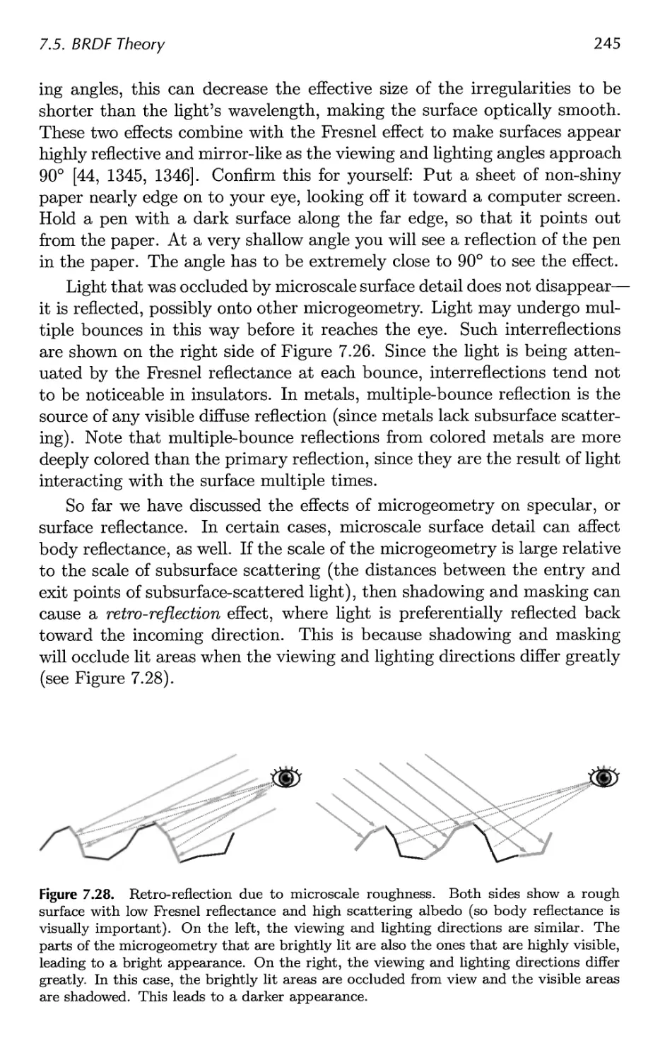
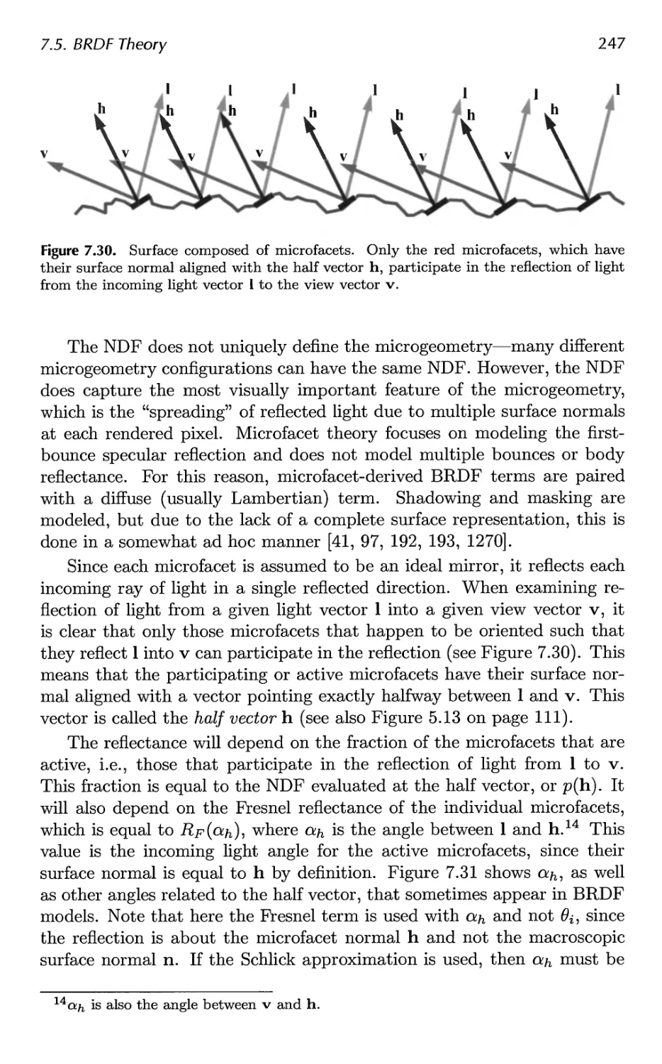
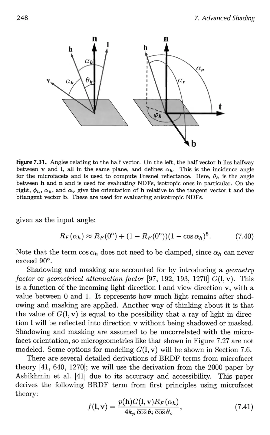
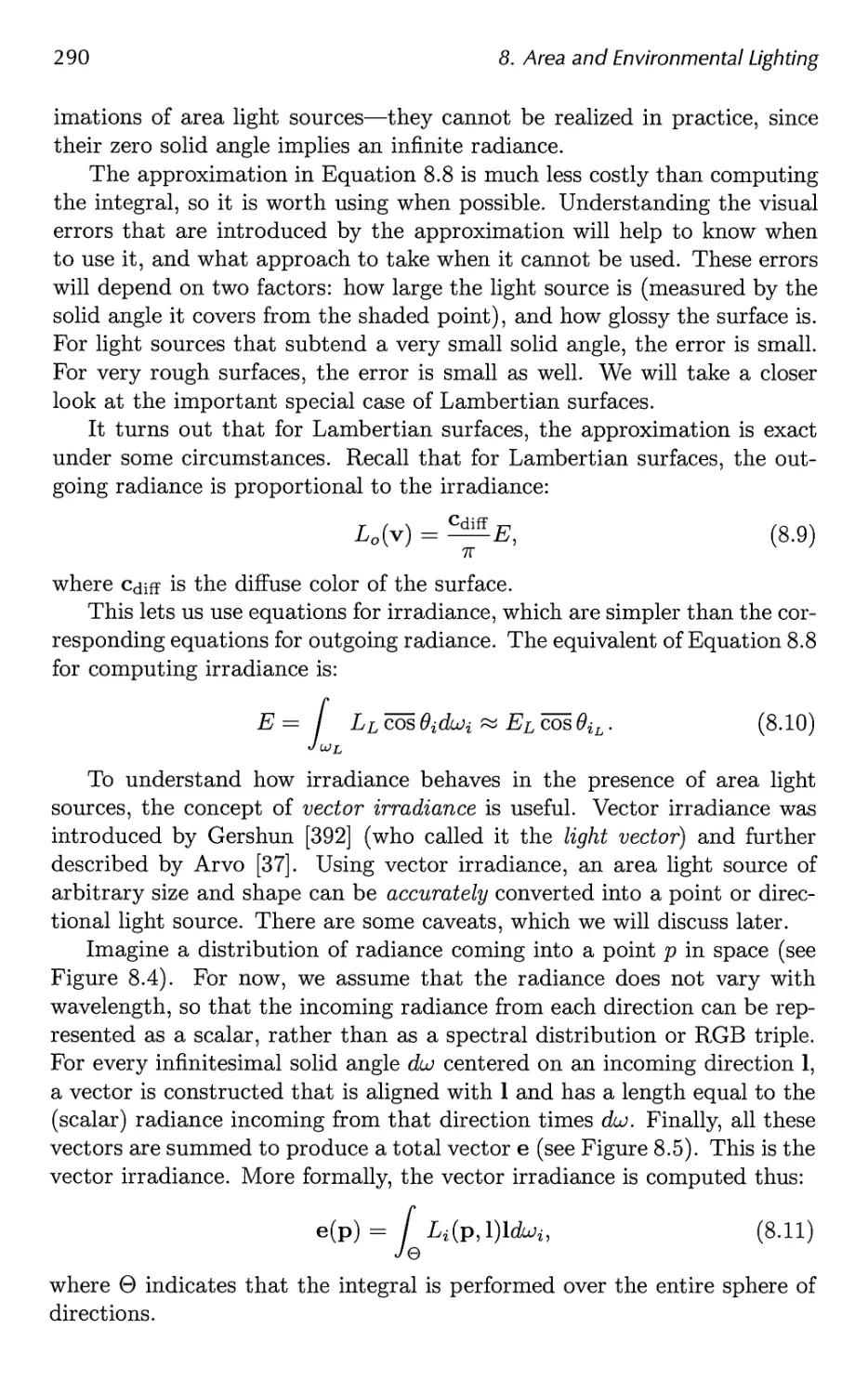
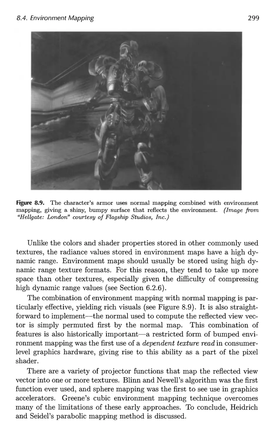
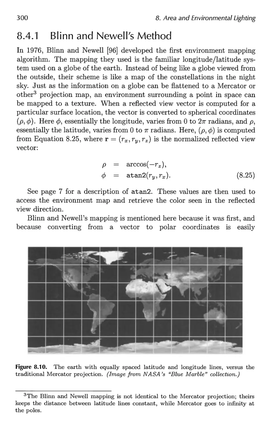
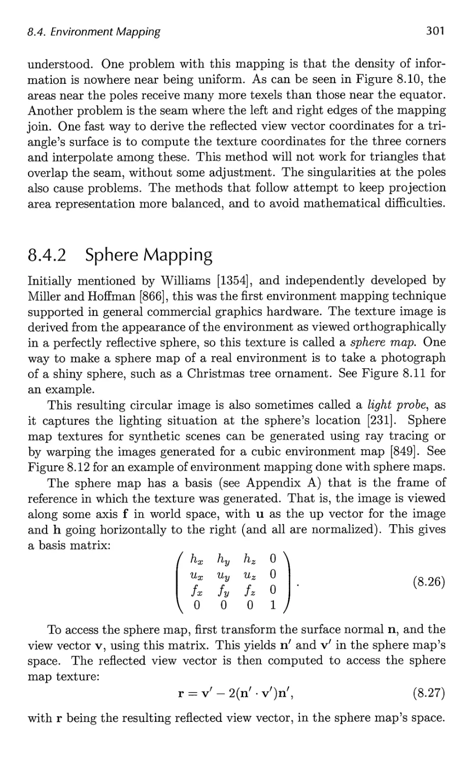
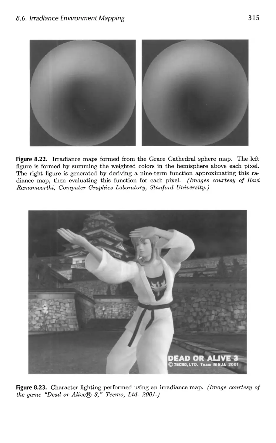
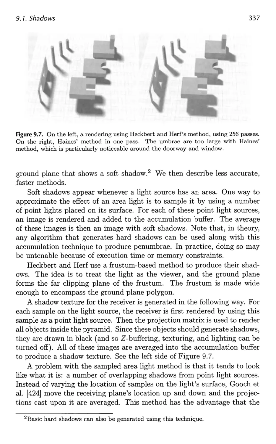
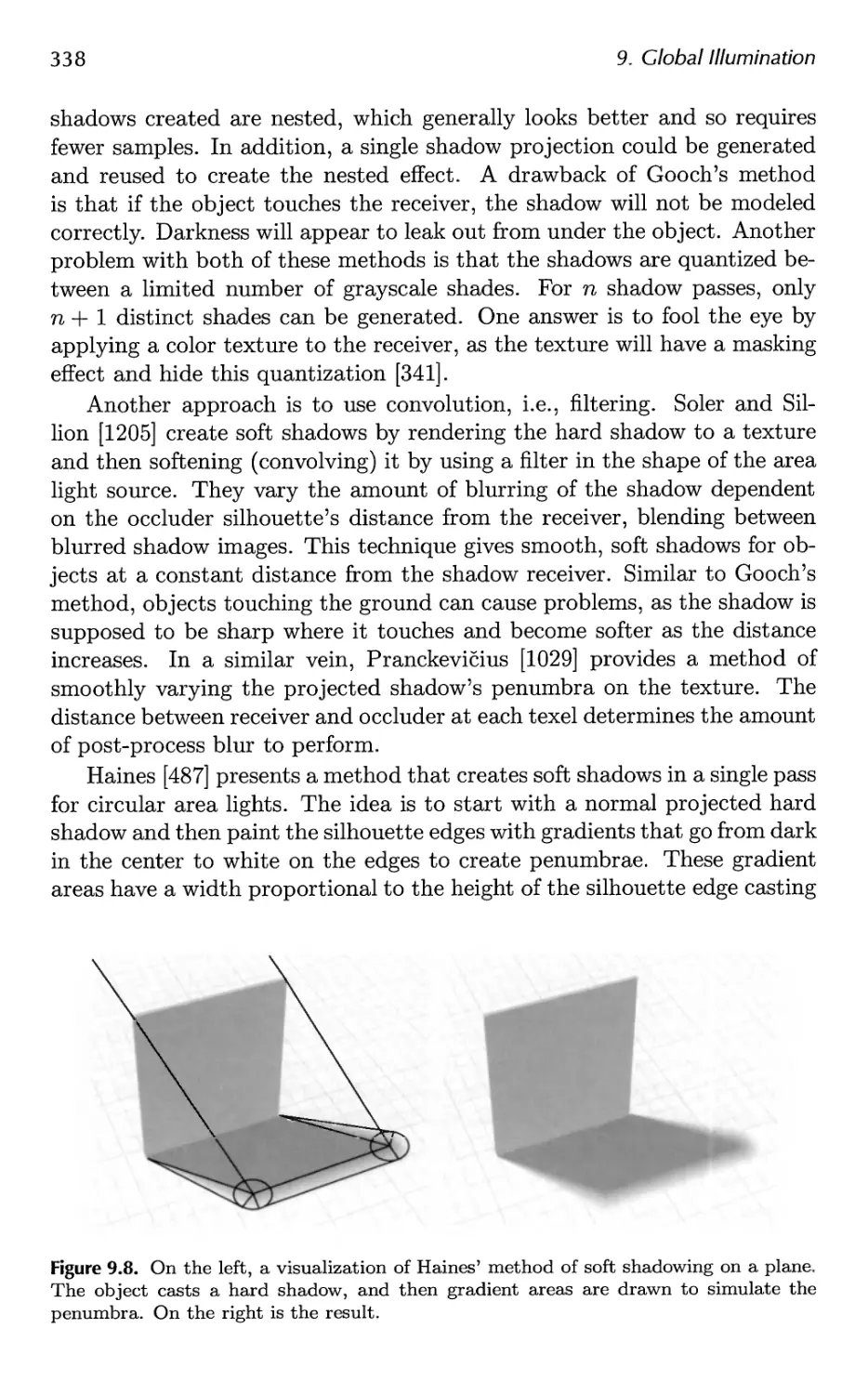
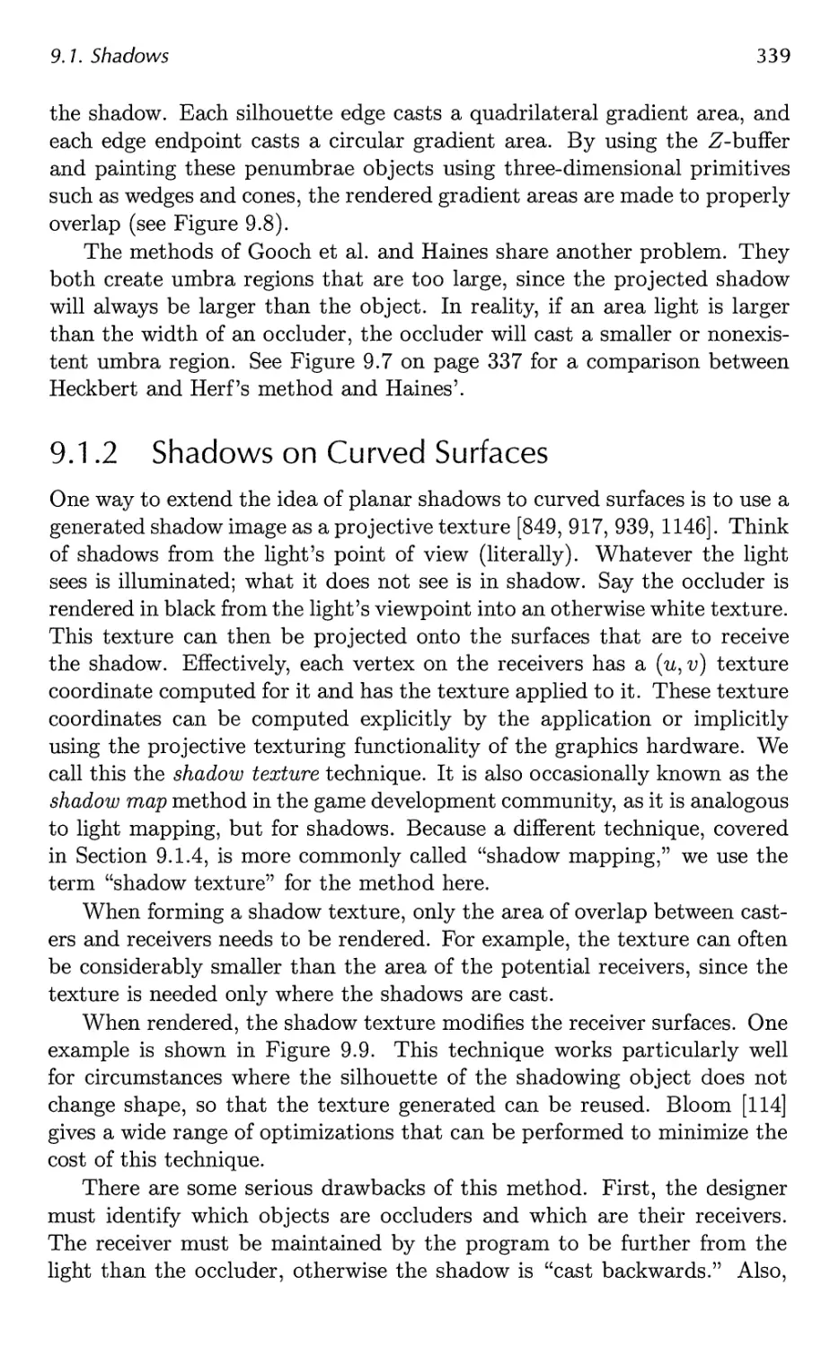
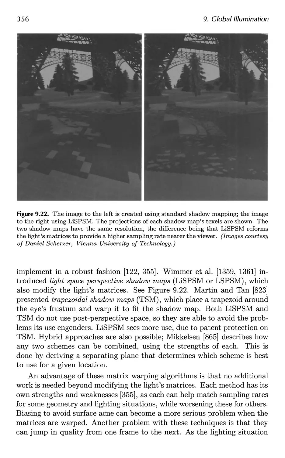
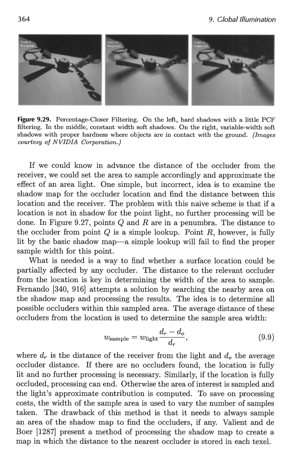
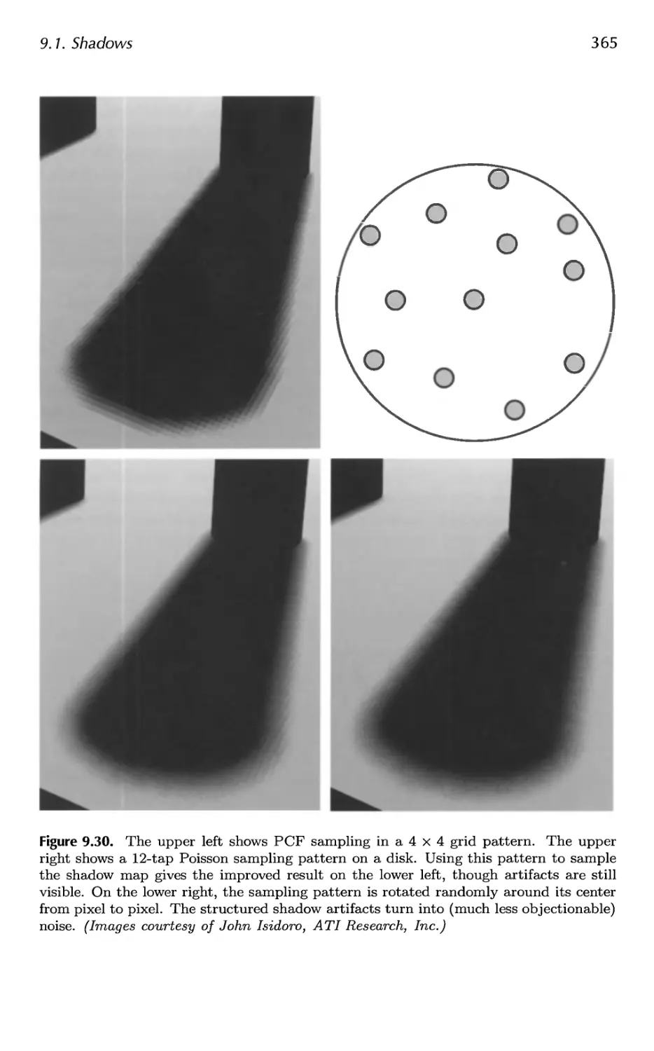
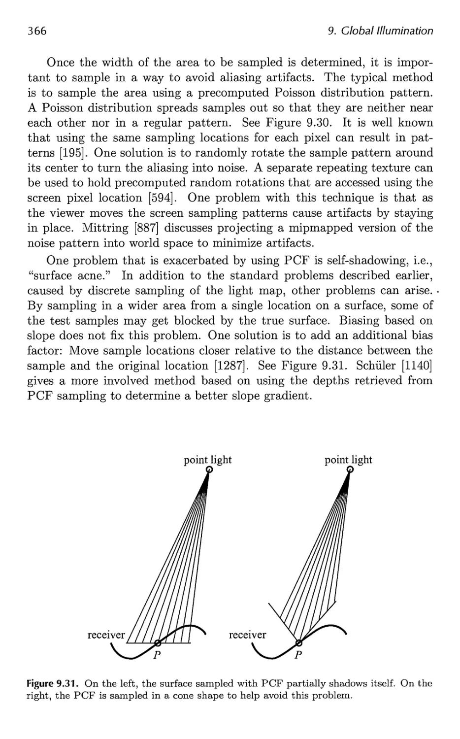
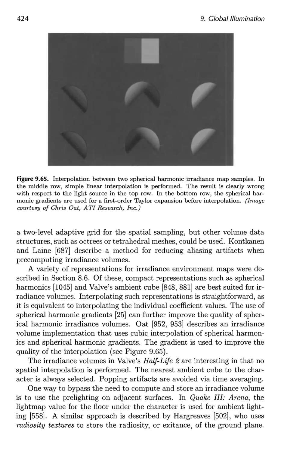
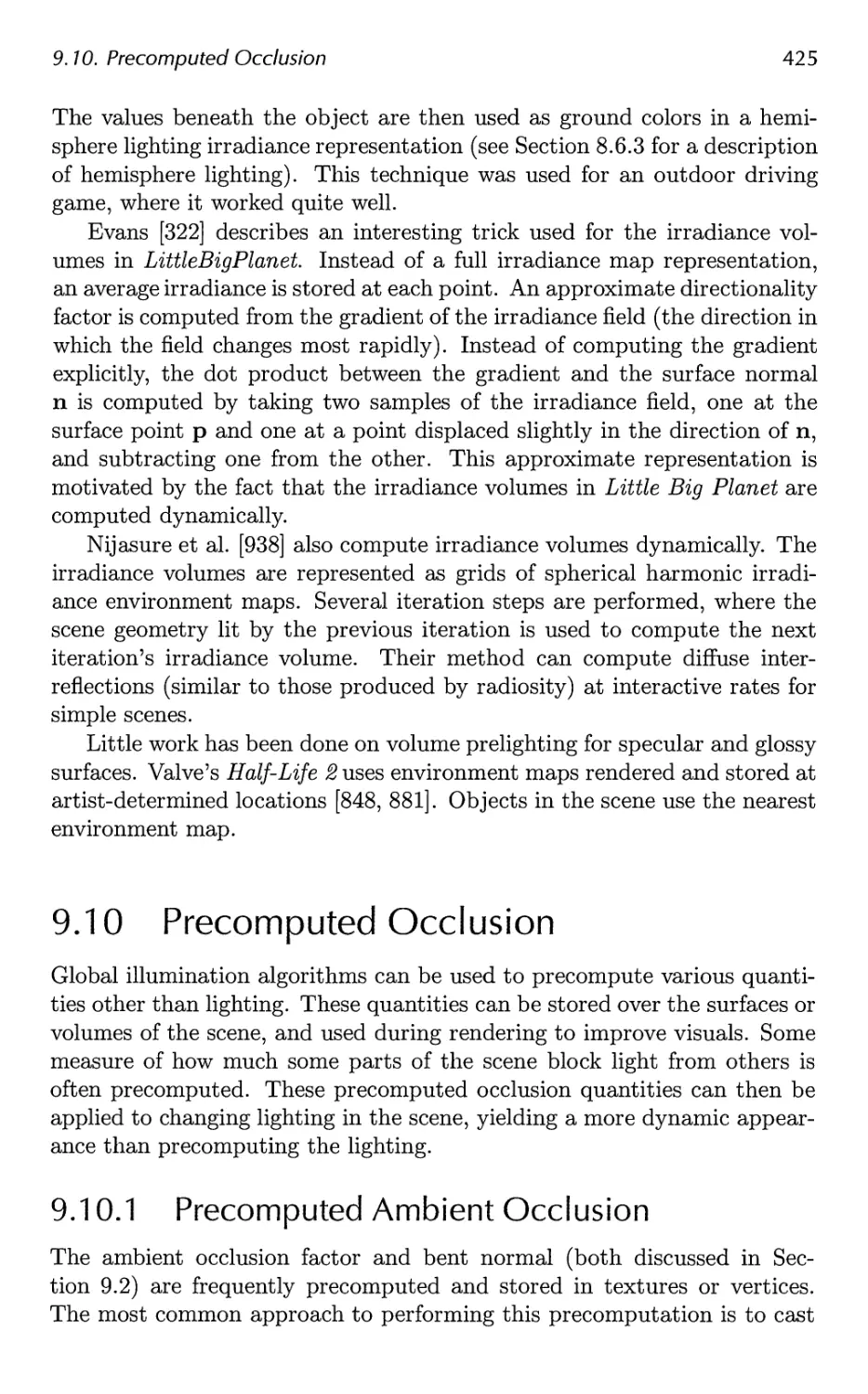
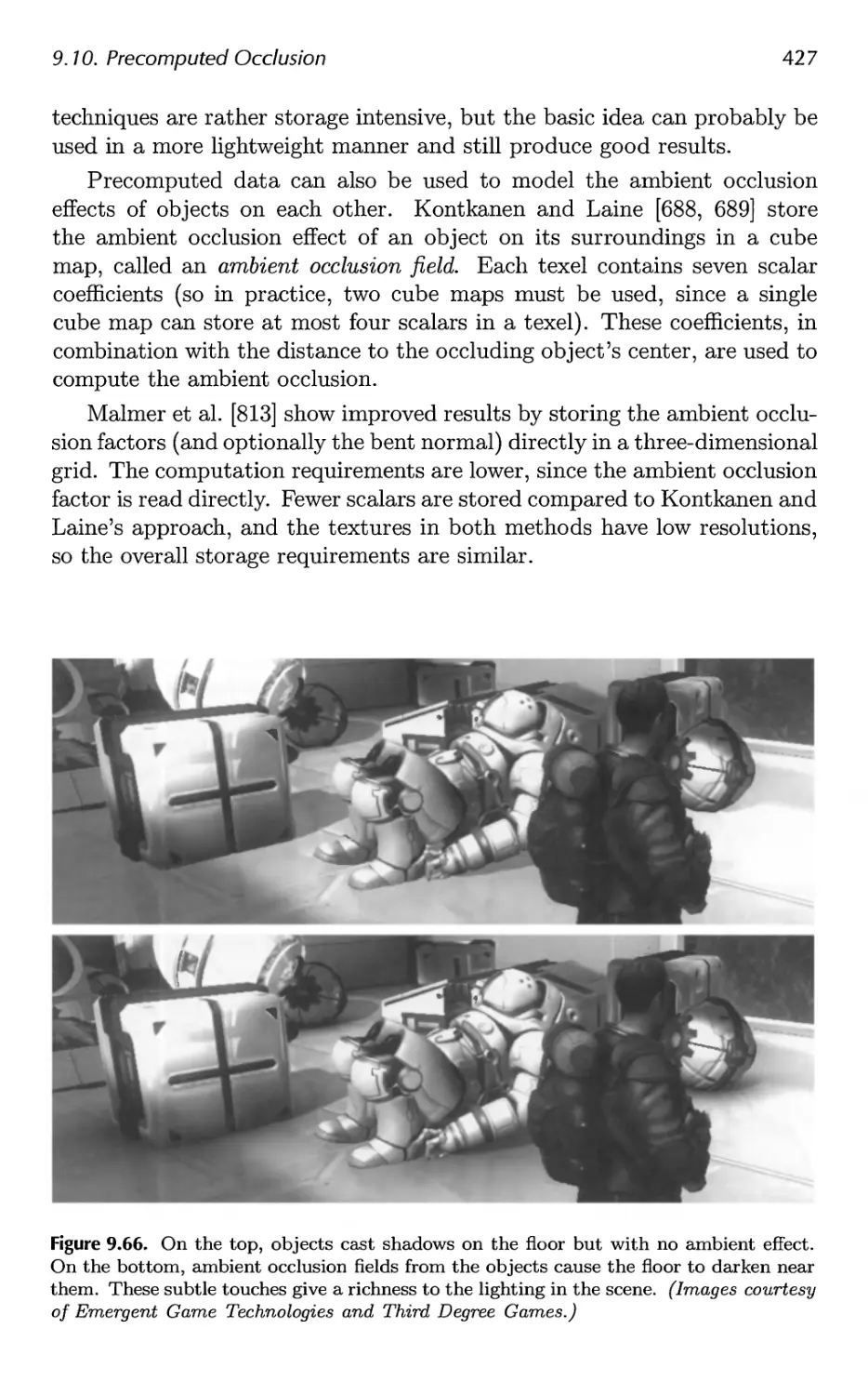
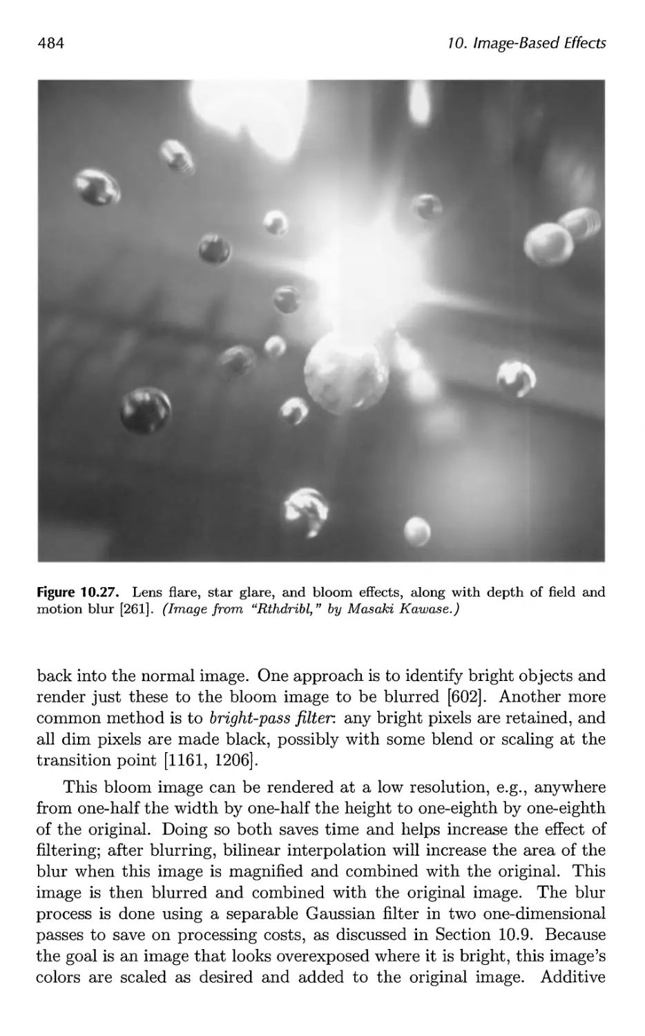
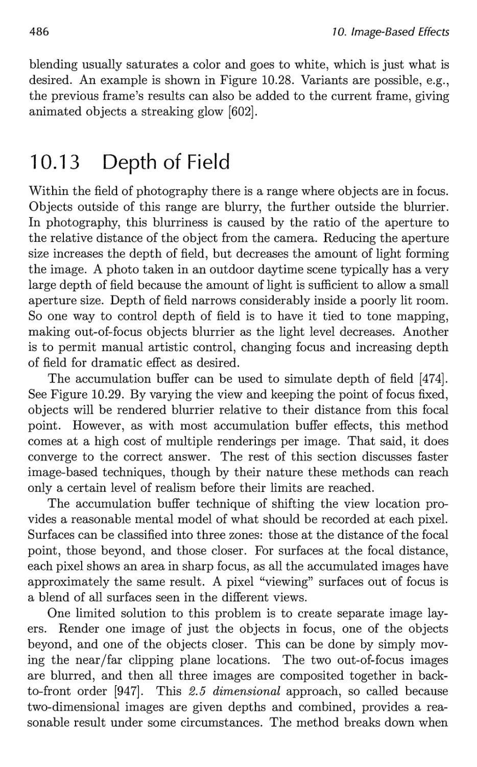
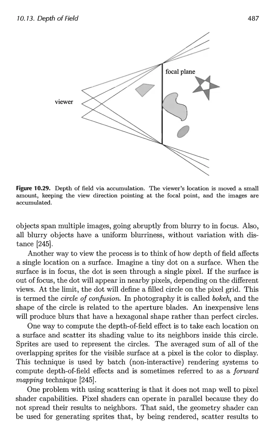
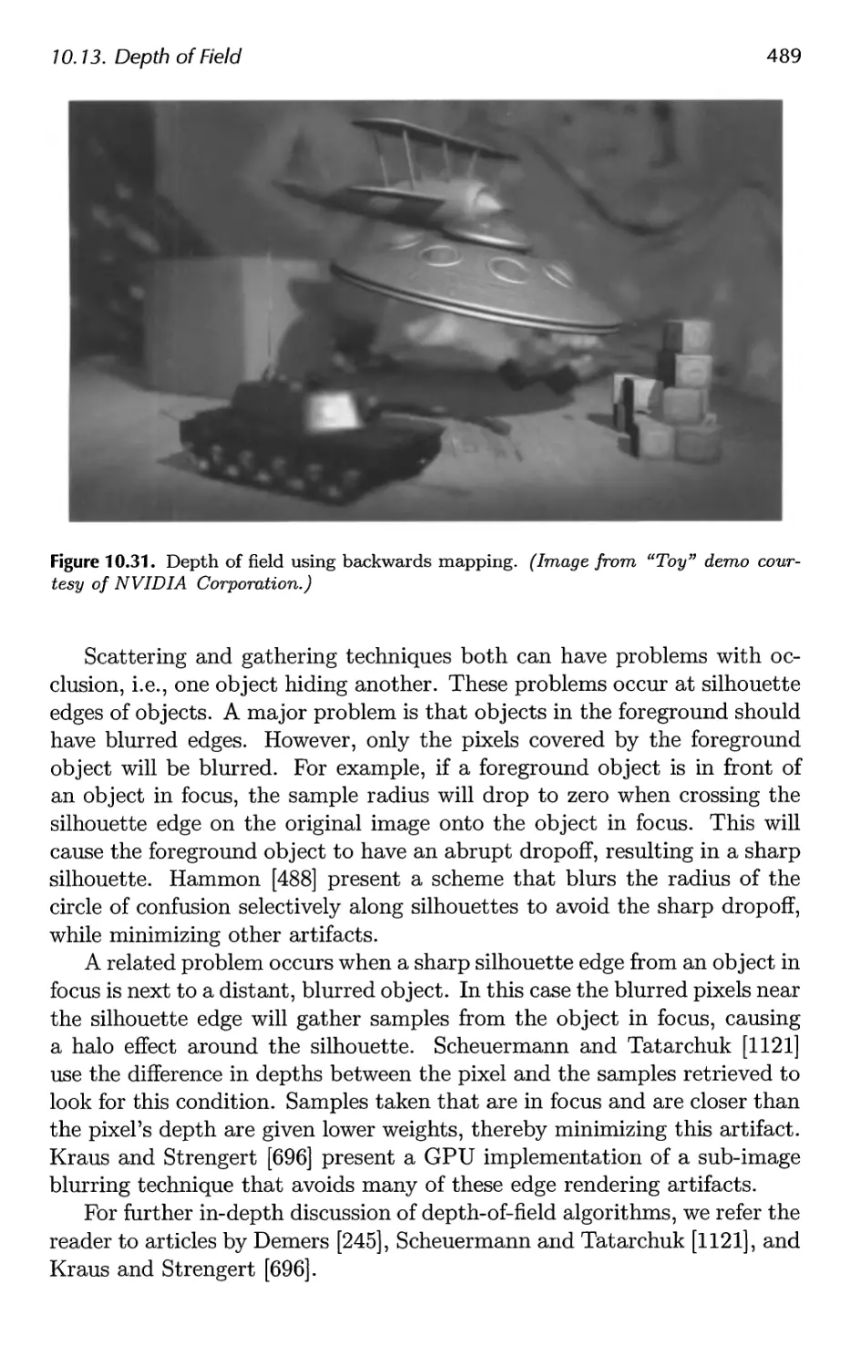
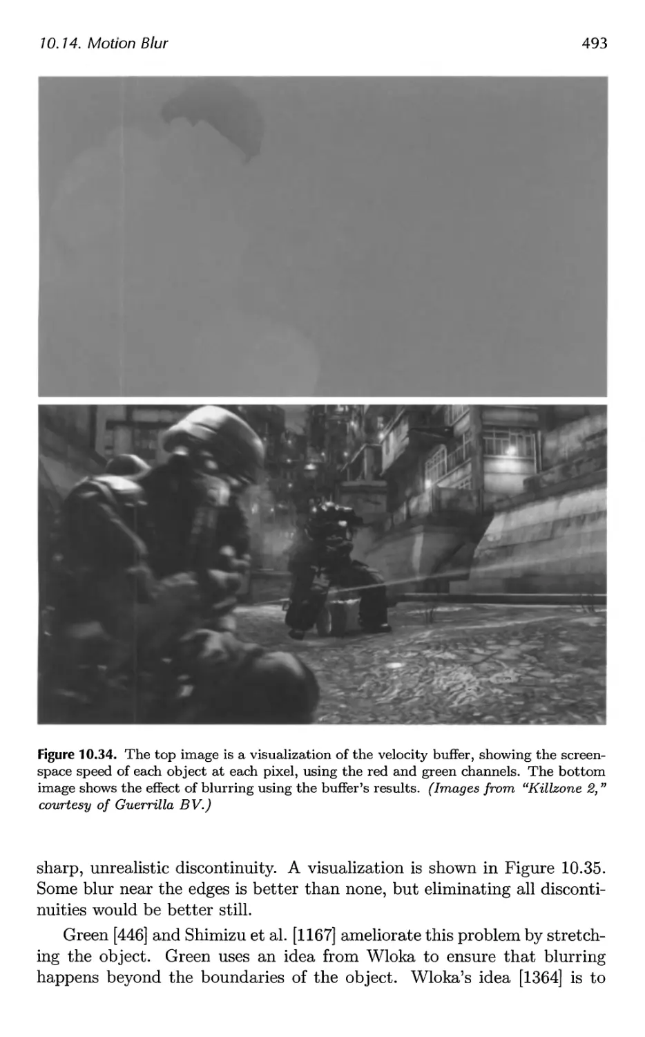
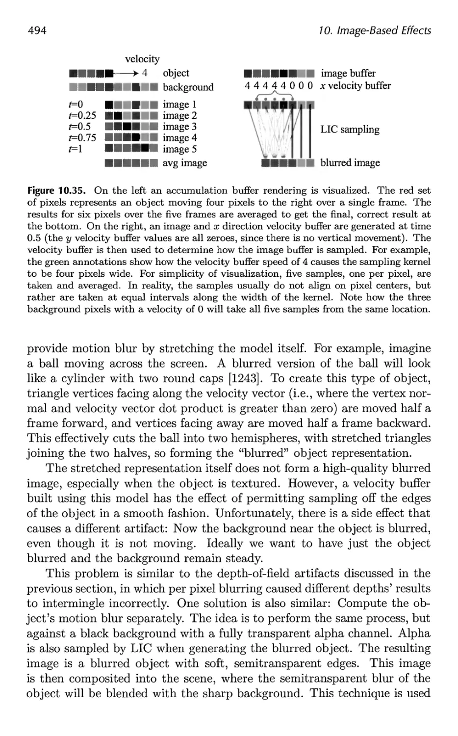
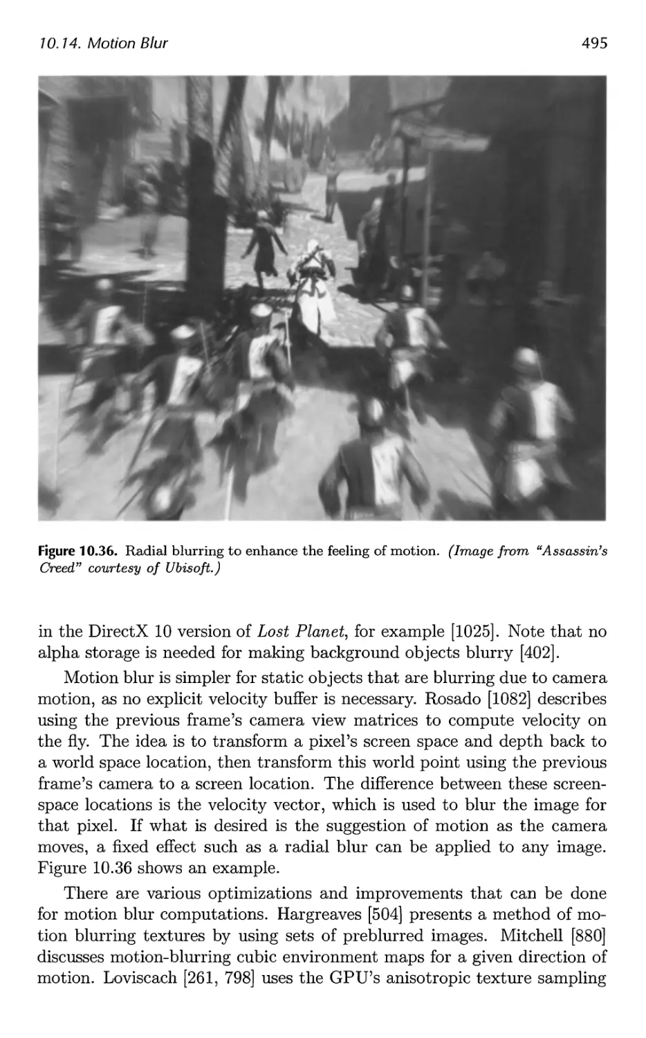
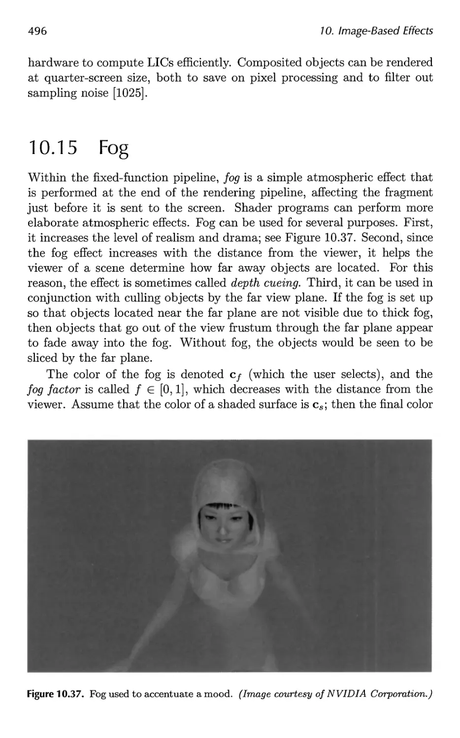
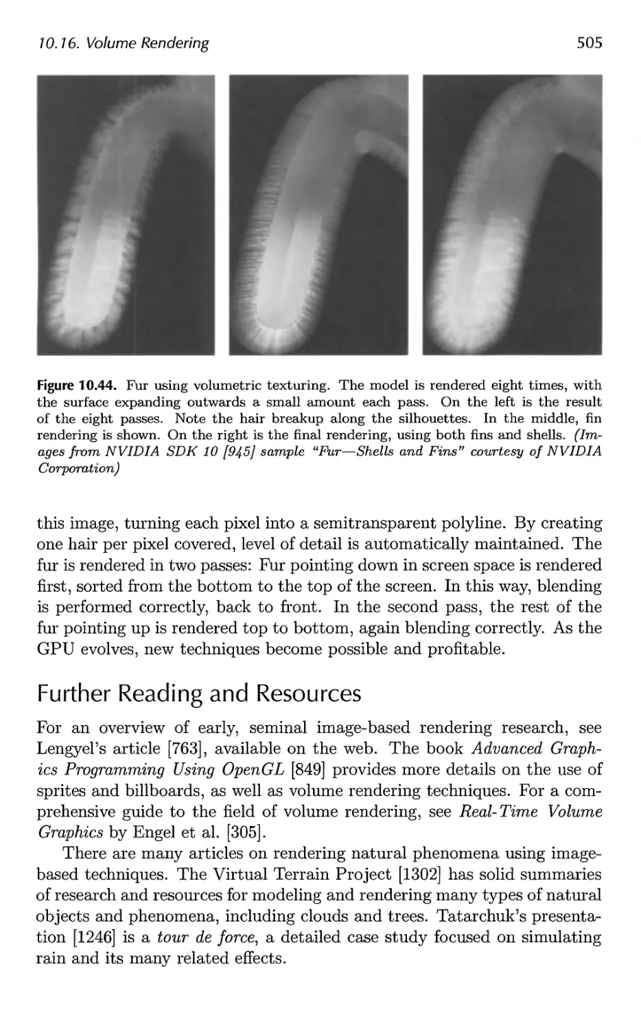
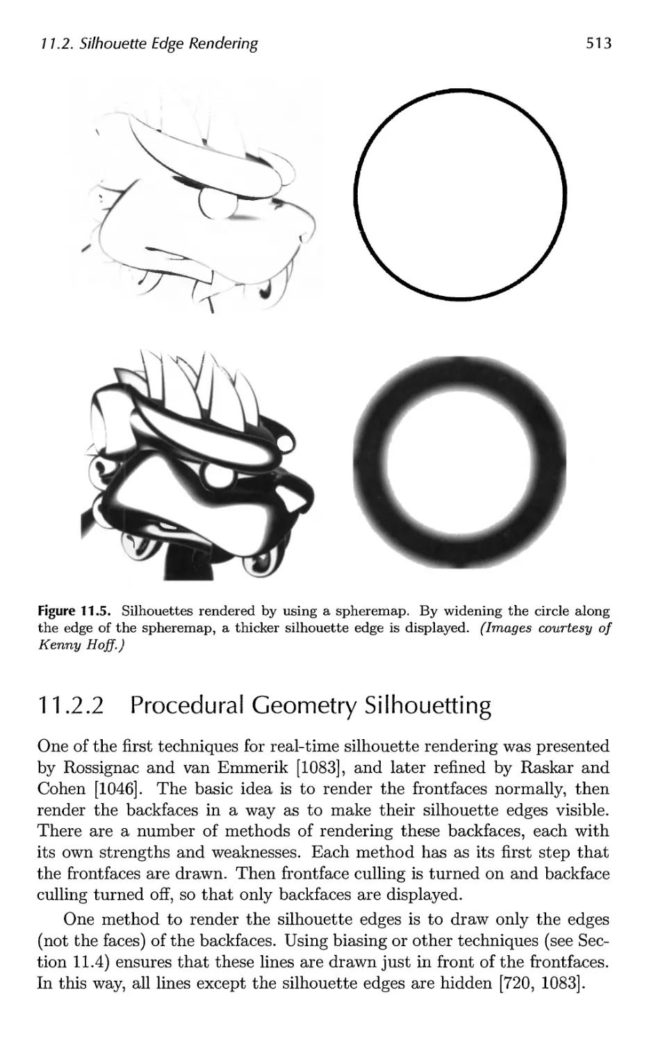
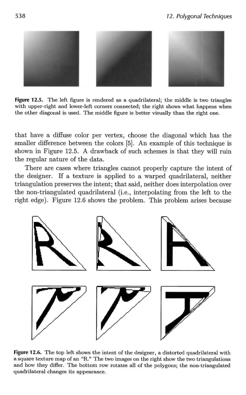
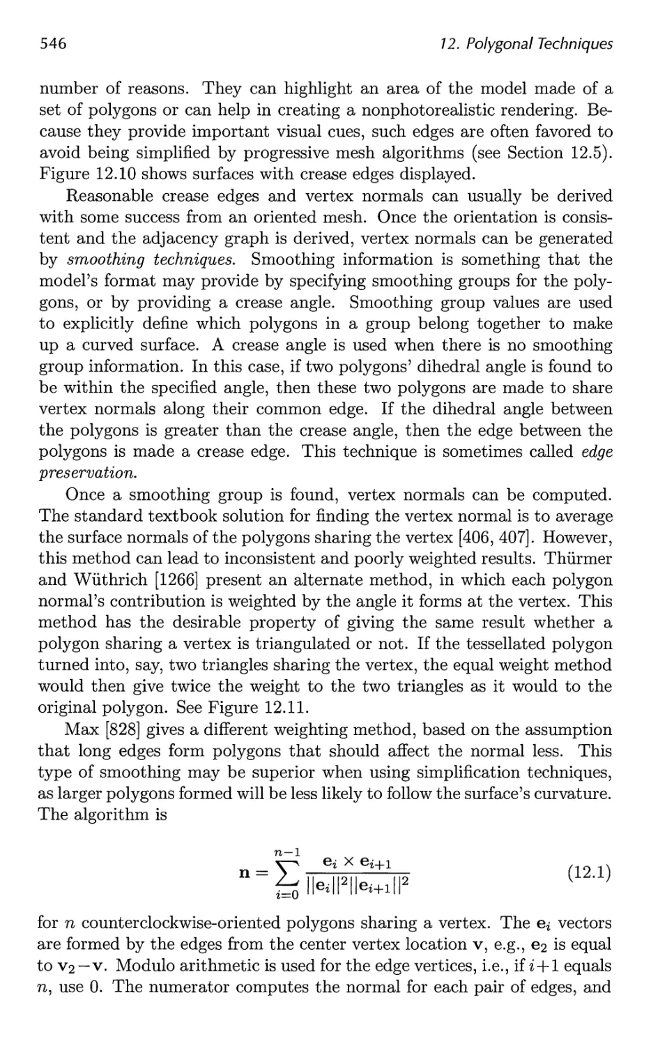
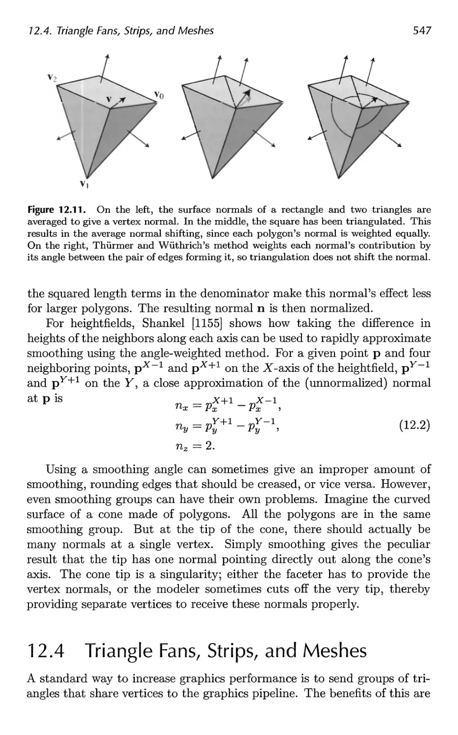
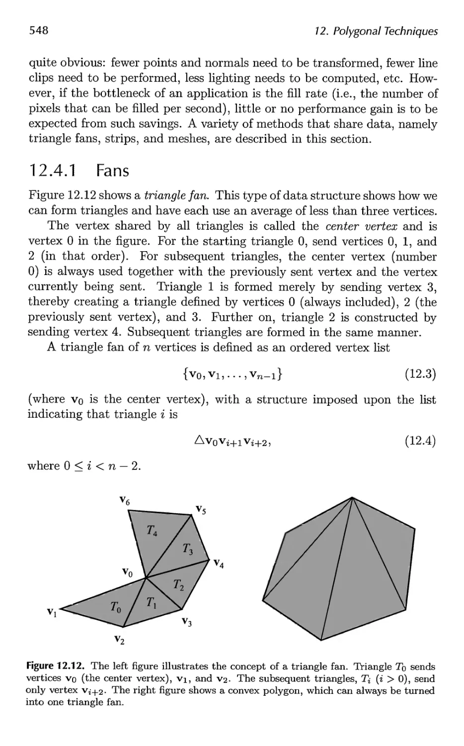
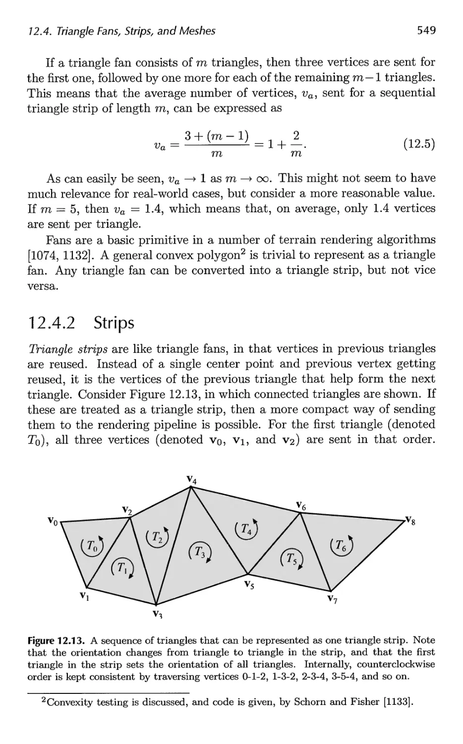
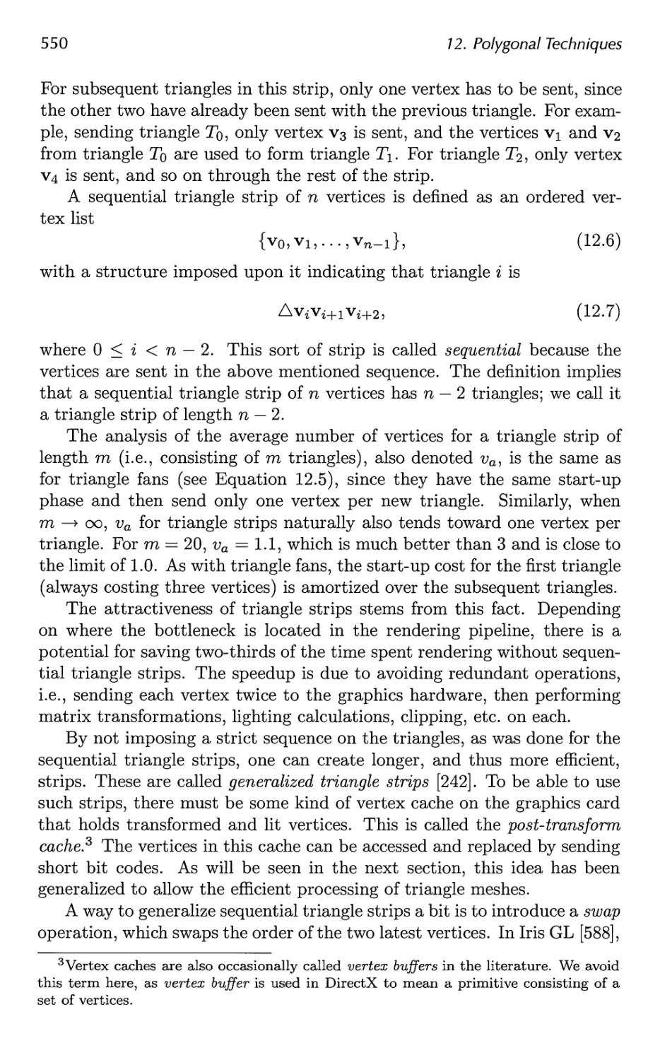
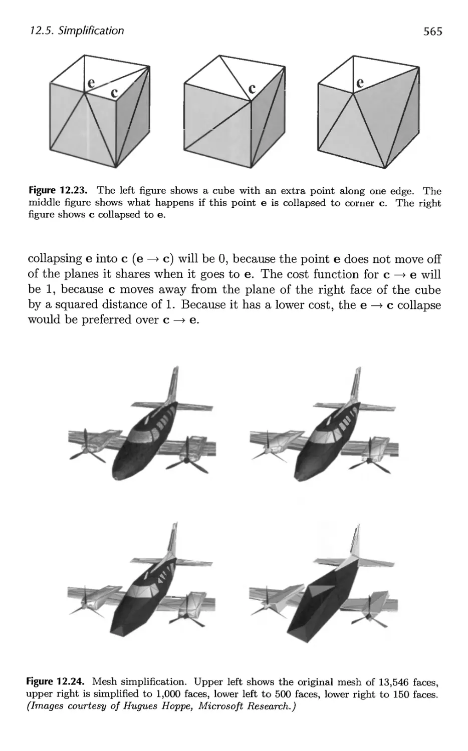
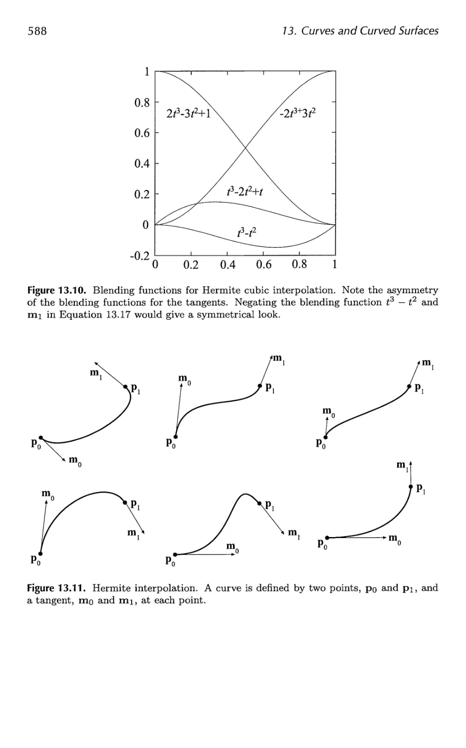
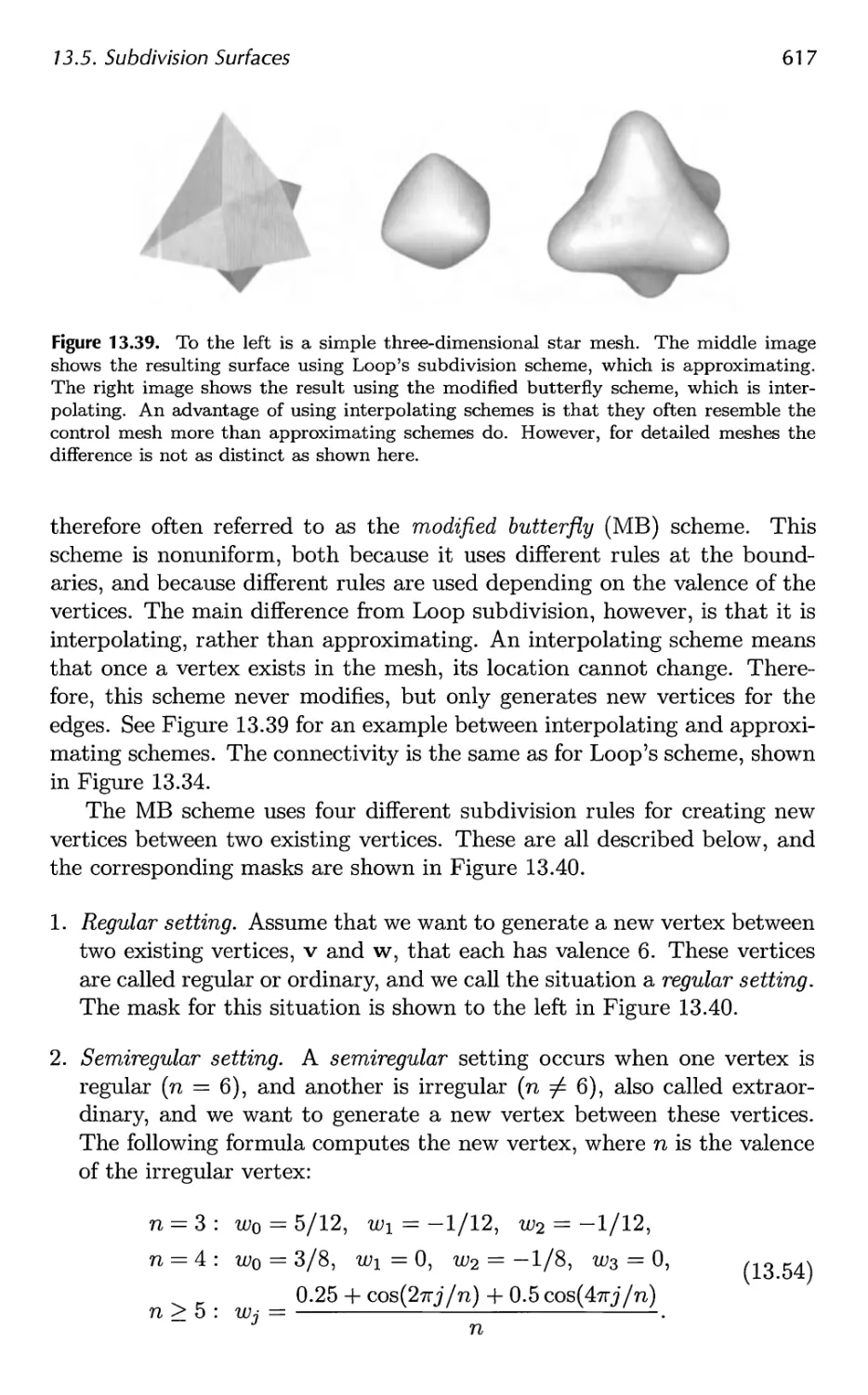
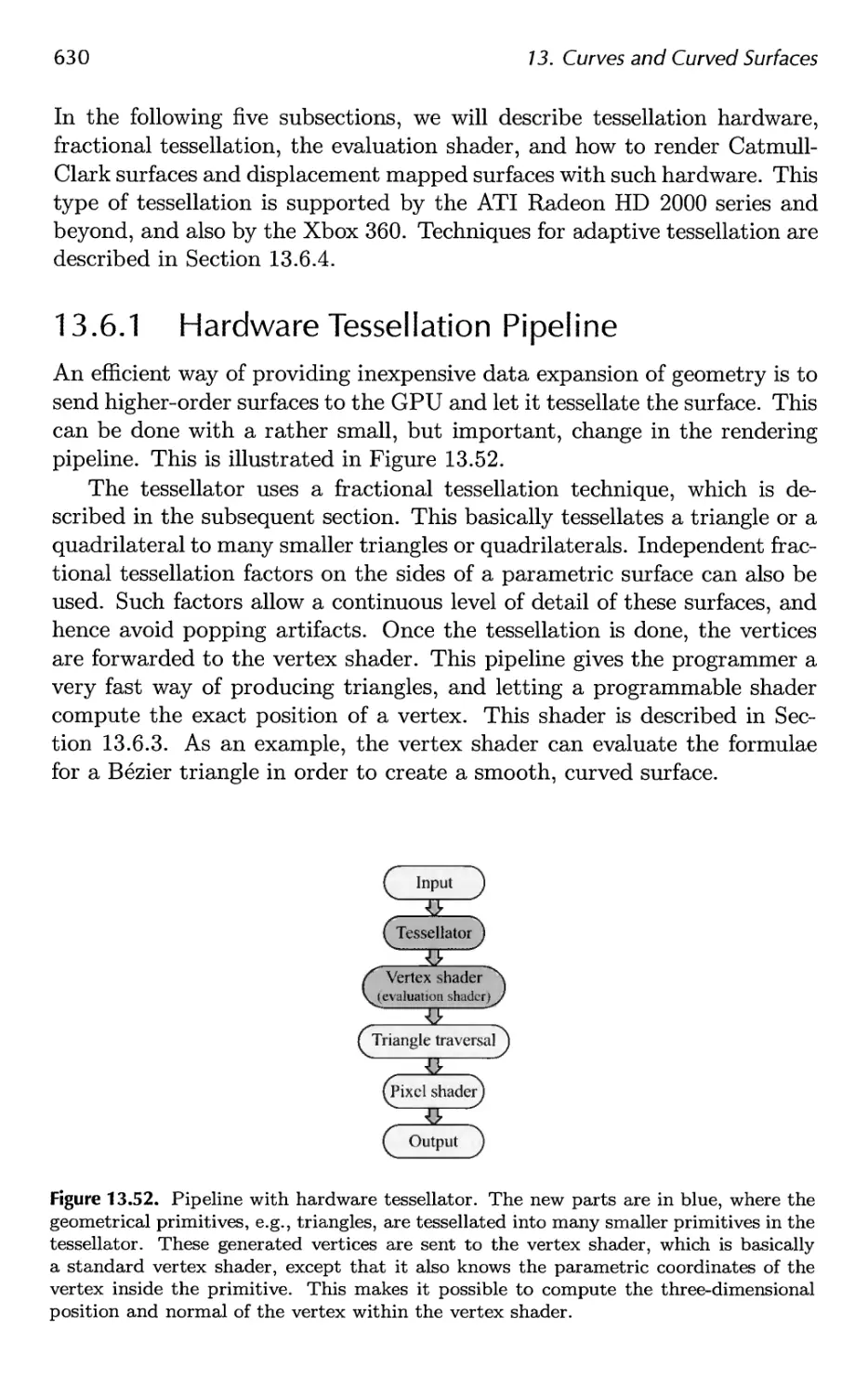
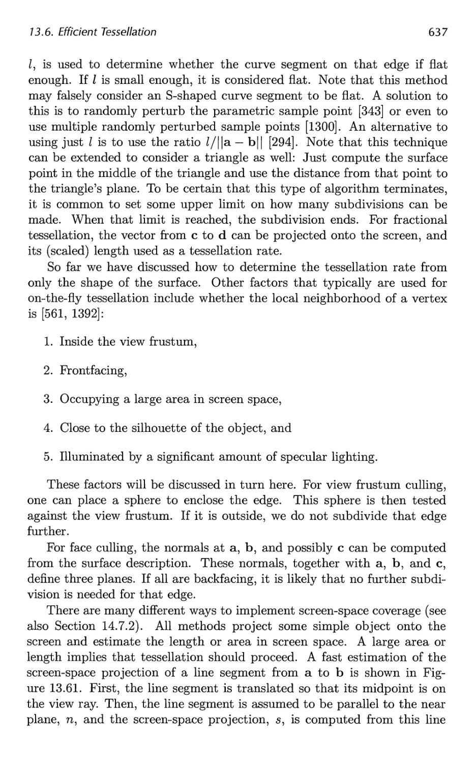
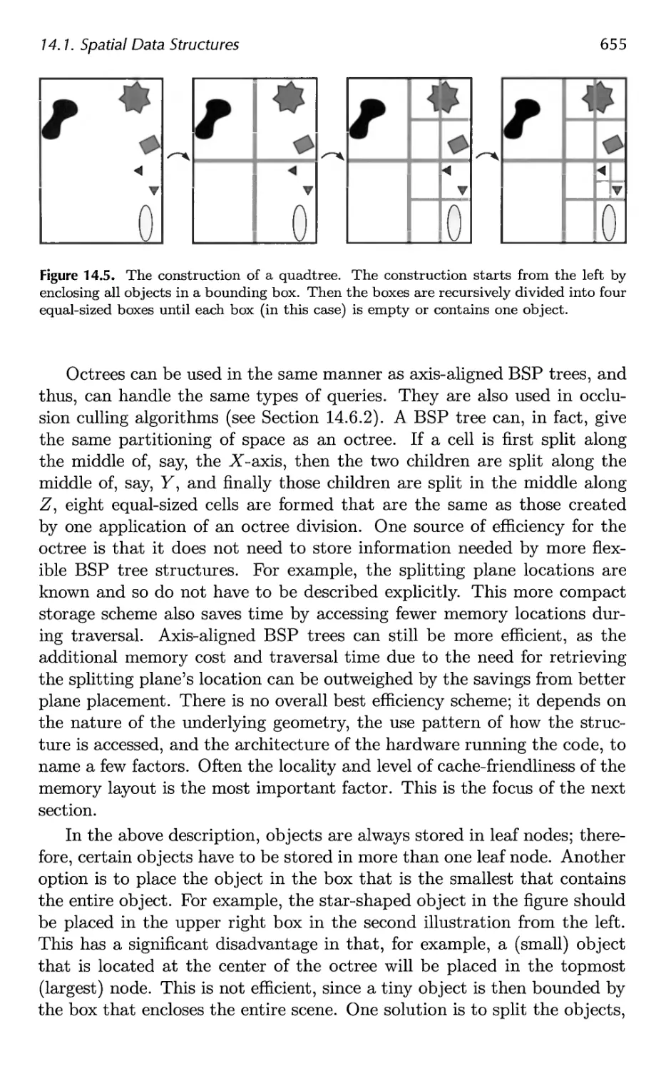
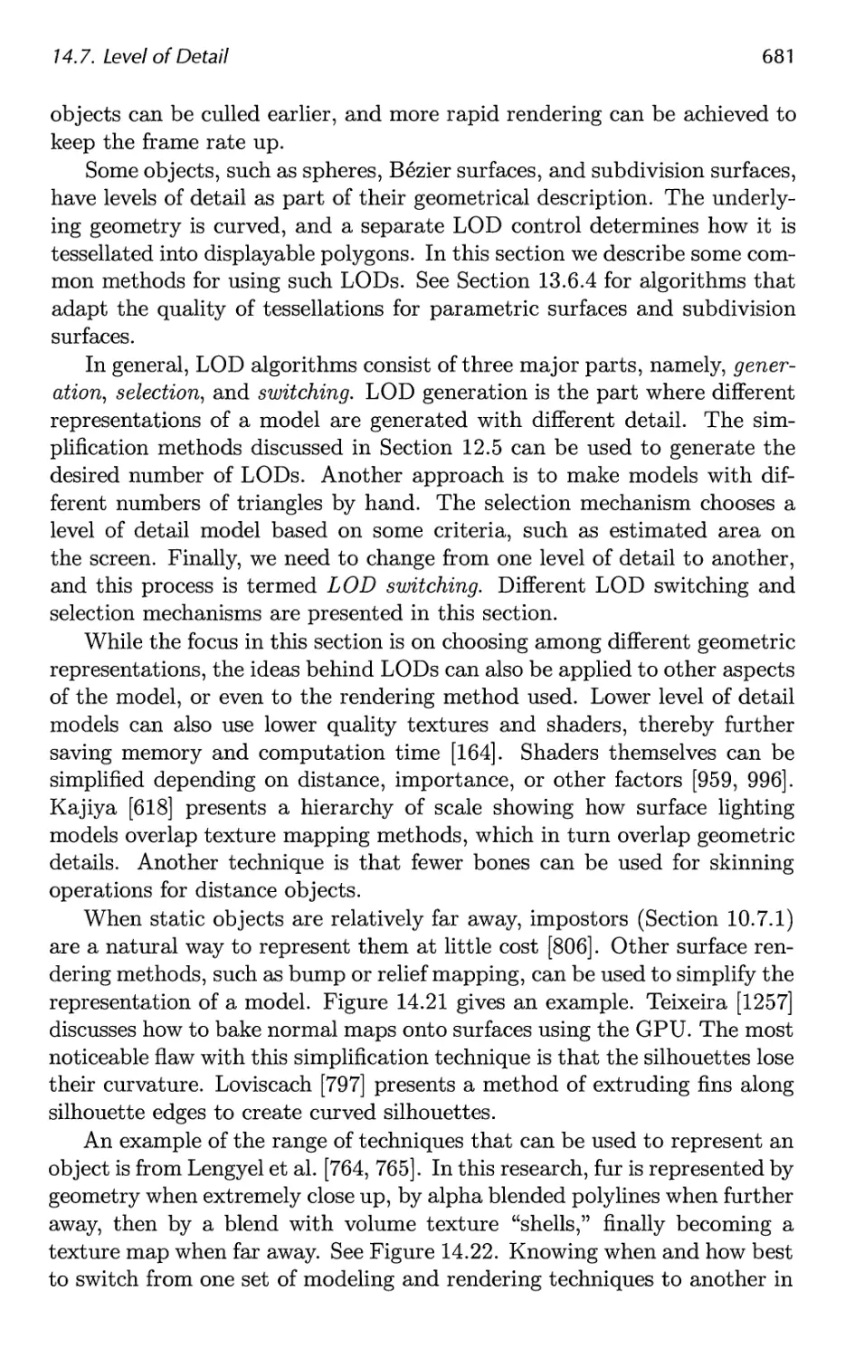
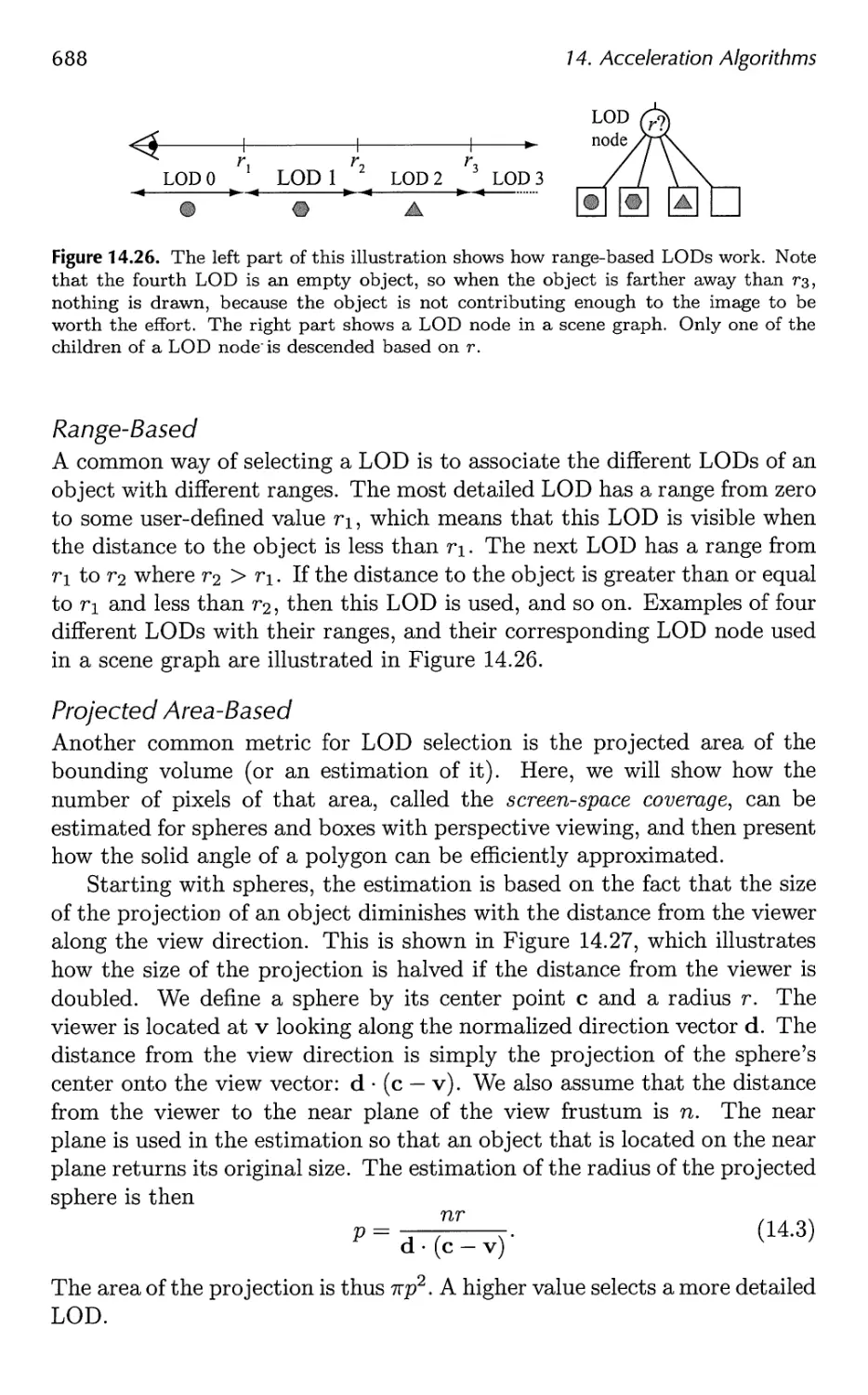
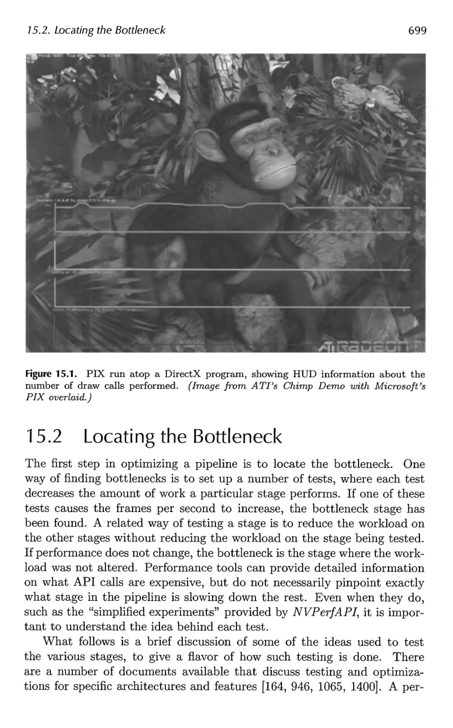
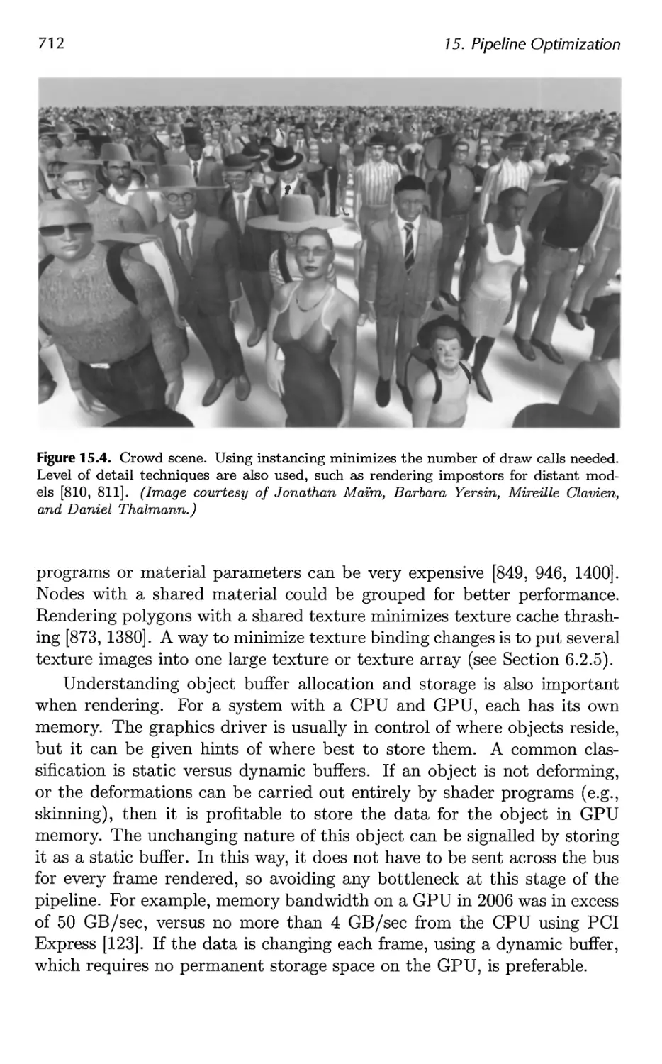
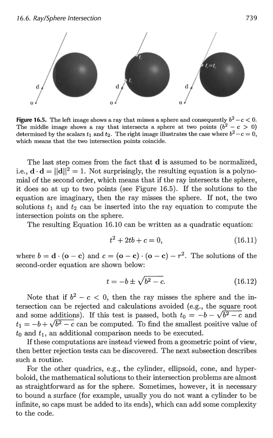
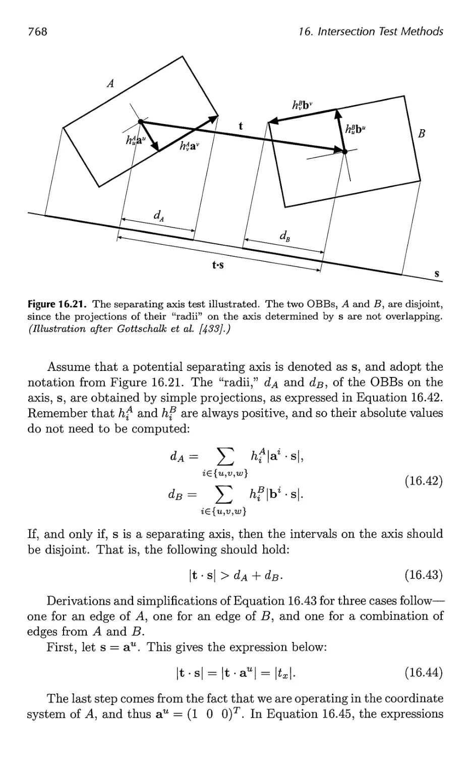
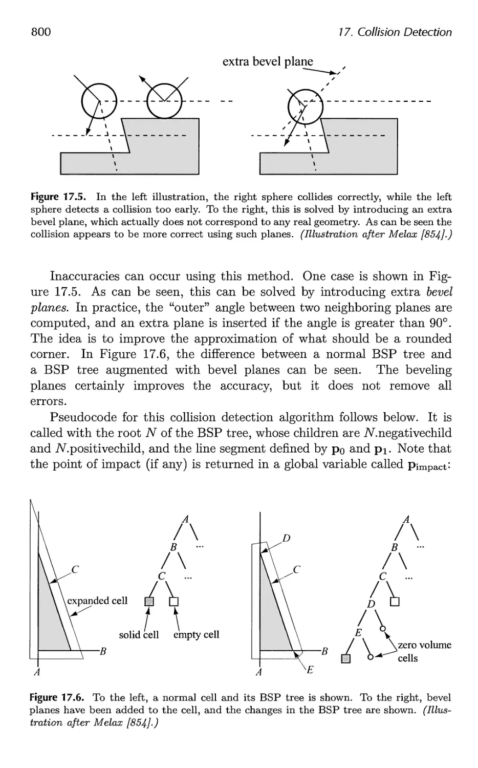
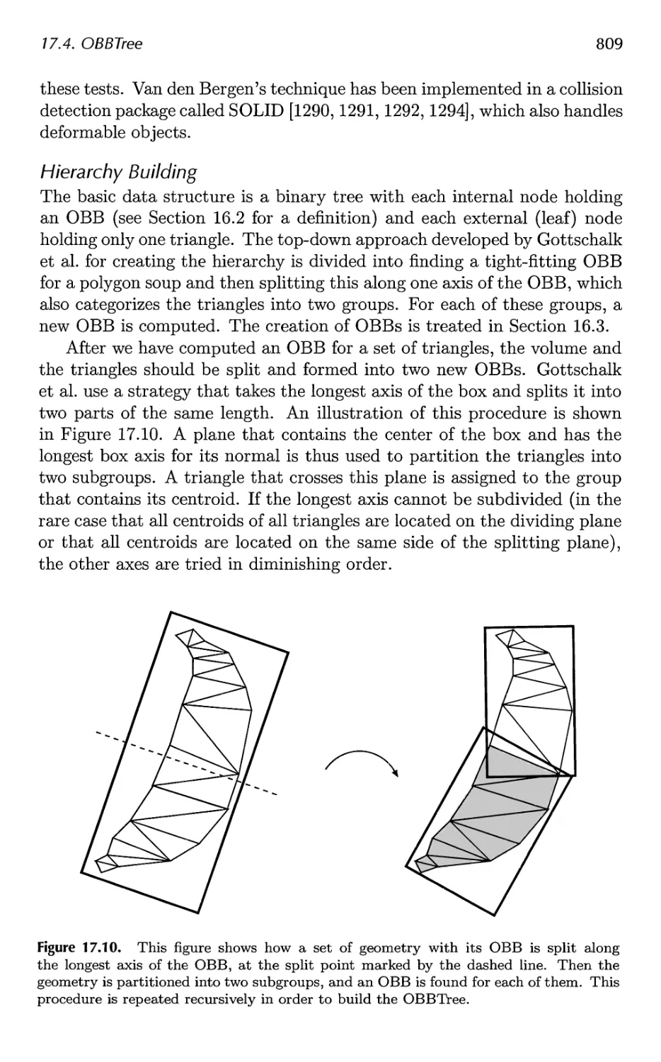
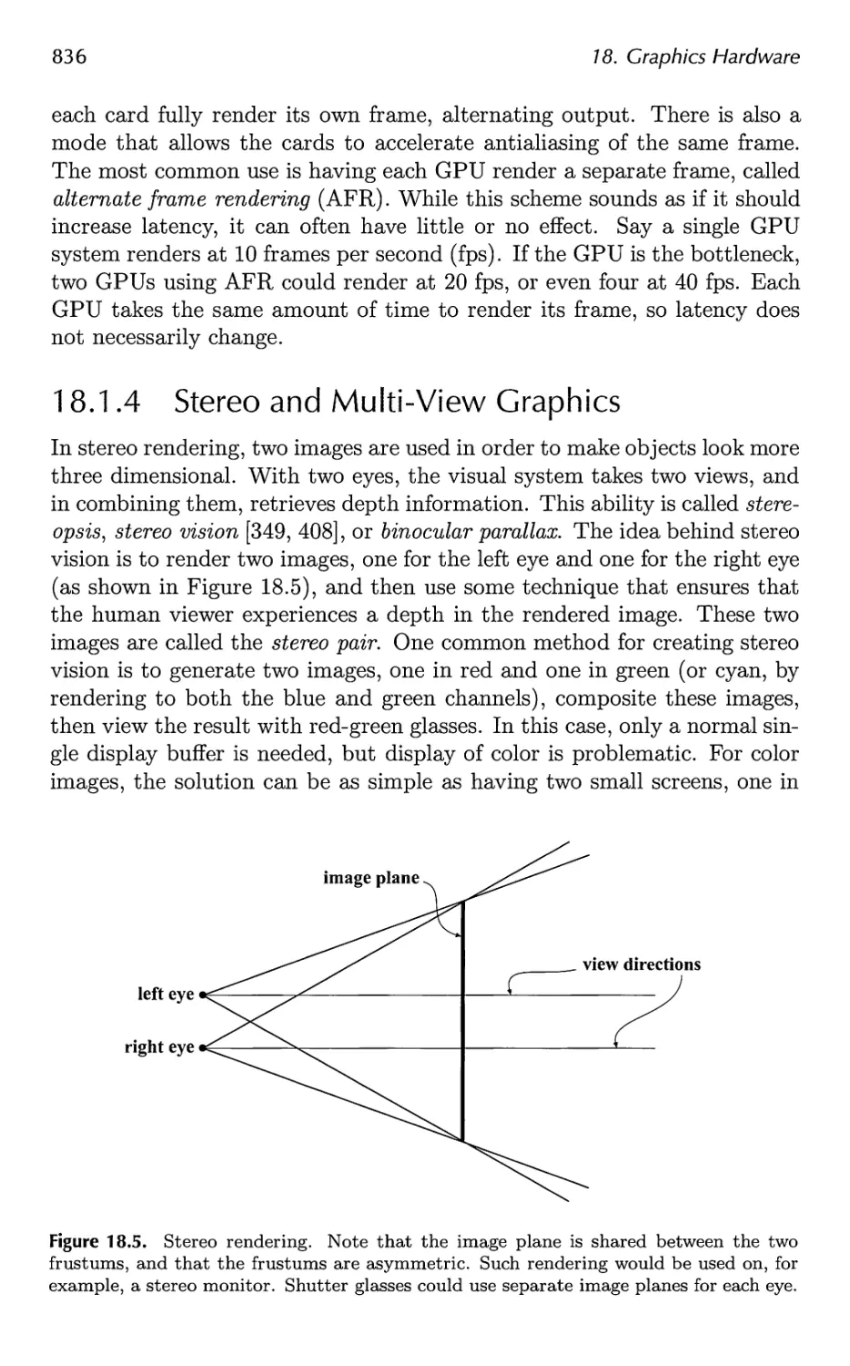
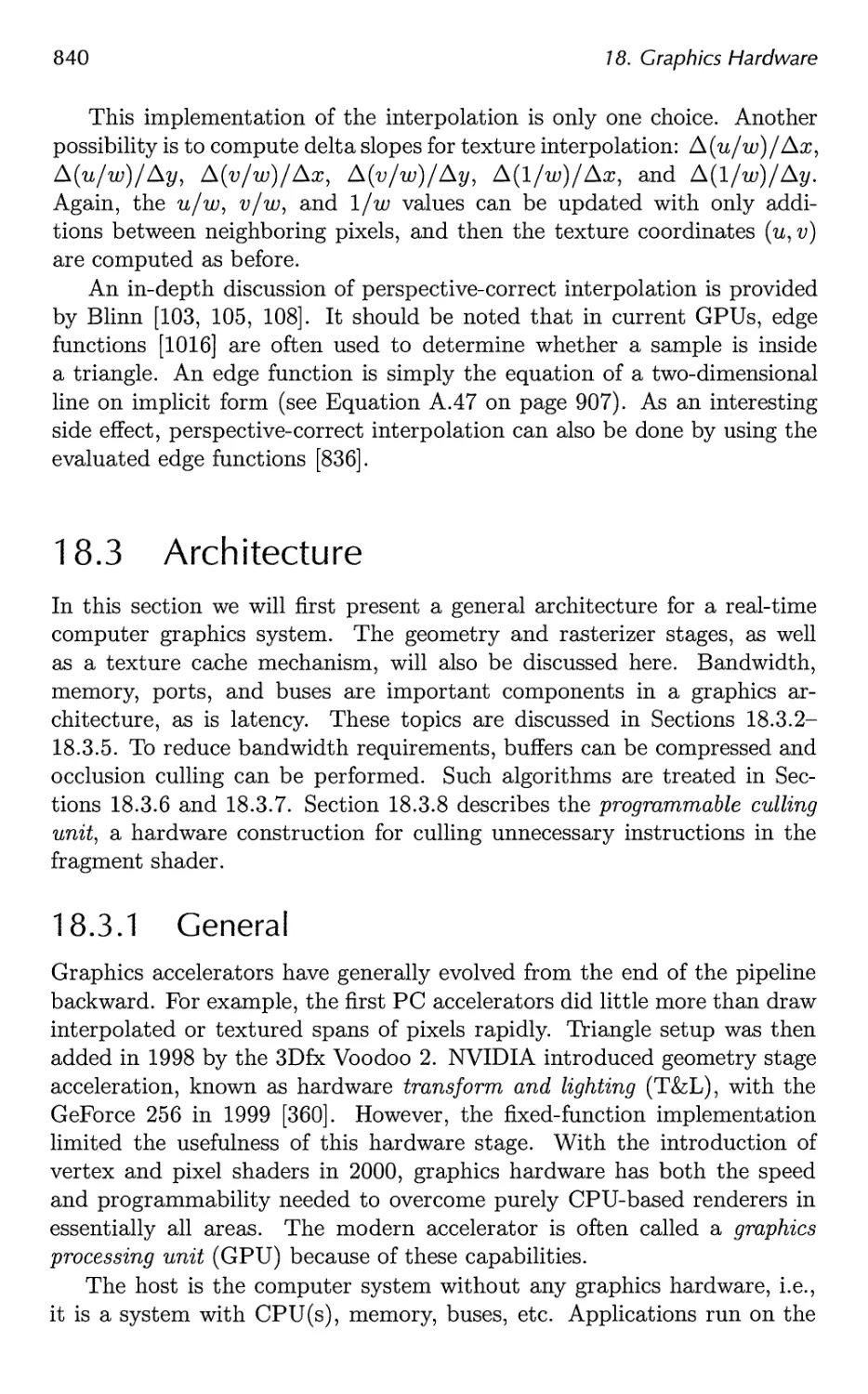
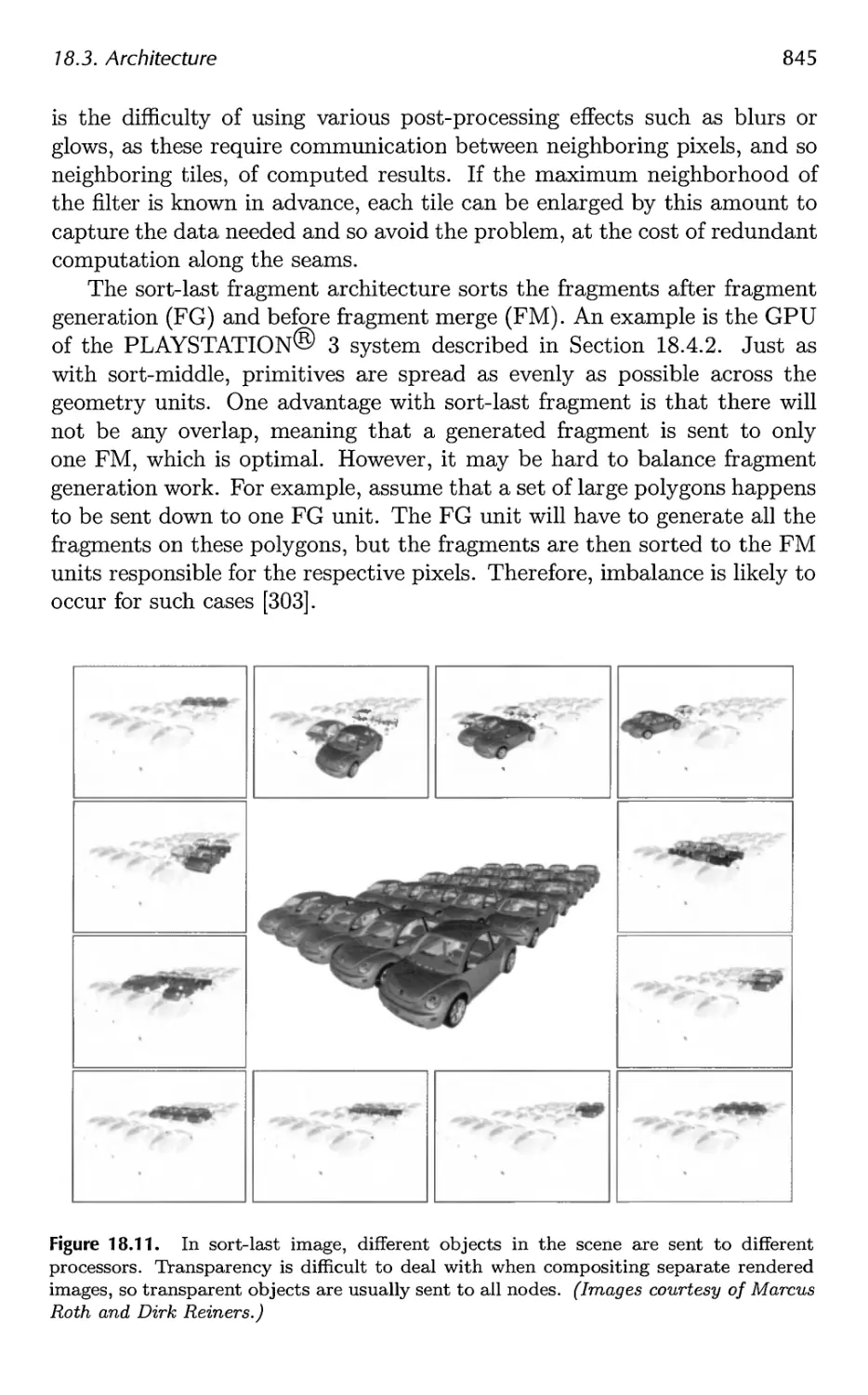
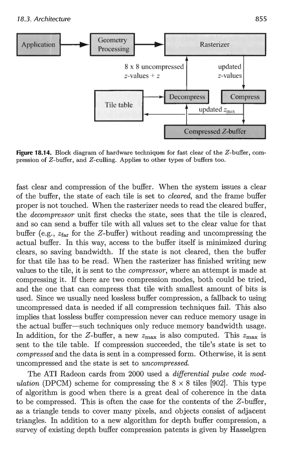
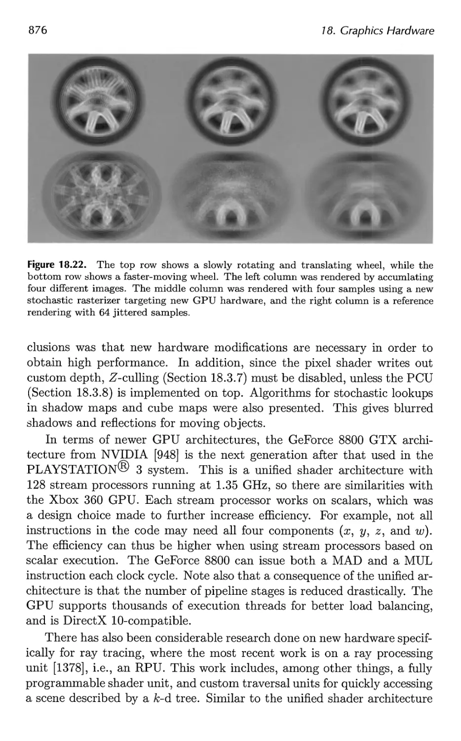
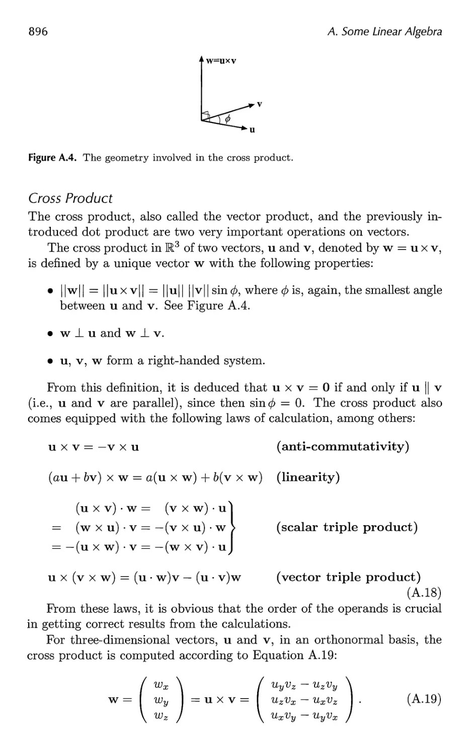
Figure 1.1. A wonderful image from the Toy Shop demo [1246, 1247, 1249], generated at
interactive rates. (Image courtesy of Natalya Tatarchuk, ATI Research, Inc.)
time rendering, graphics accelerator hardware has become a requirement
for most real-time applications. An excellent example of the results of
real-time rendering made possible by hardware acceleration is shown in
Figure 1.1.
In the past few years advances in graphics hardware have fueled an
explosion of research in the field of interactive computer graphics. We will
focus on providing methods to increase speed and improve image quality,
while also describing the features and limitations of acceleration algorithms
and graphics APIs. We will not be able to cover every topic in depth, so our
goal is to introduce concepts and terminology, give a sense of how and when
various methods can be applied, and provide pointers to the best places to
go for more in-depth information. We hope our attempts to provide you
with tools for understanding this field prove to be worth the time and effort
you spend with our book.
1.1 Contents Overview
What follows is a brief overview of the chapters ahead.
7.7. Contents Overview
3
Chapter 2, The Graphics Rendering Pipeline. This chapter deals with the
heart of real-time rendering, the mechanism that takes a scene description
and converts it into something we can see.
Chapter 3, The Graphics Processing Unit. The modern GPU implements
the stages of the rendering pipeline using a combination of fixed-function
and programmable units.
Chapter 4, Transforms. Transforms are the basic tools for manipulating
the position, orientation, size, and shape of objects and the location and
view of the camera.
Chapter 5, Visual Appearance. This chapter begins discussion of the
definition of materials and lights and their use in achieving a realistic surface
appearance. Also covered are other appearance-related topics, such as
providing higher image quality through antialiasing and gamma correction.
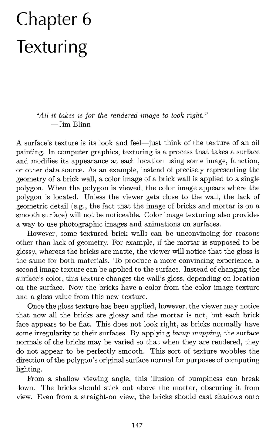
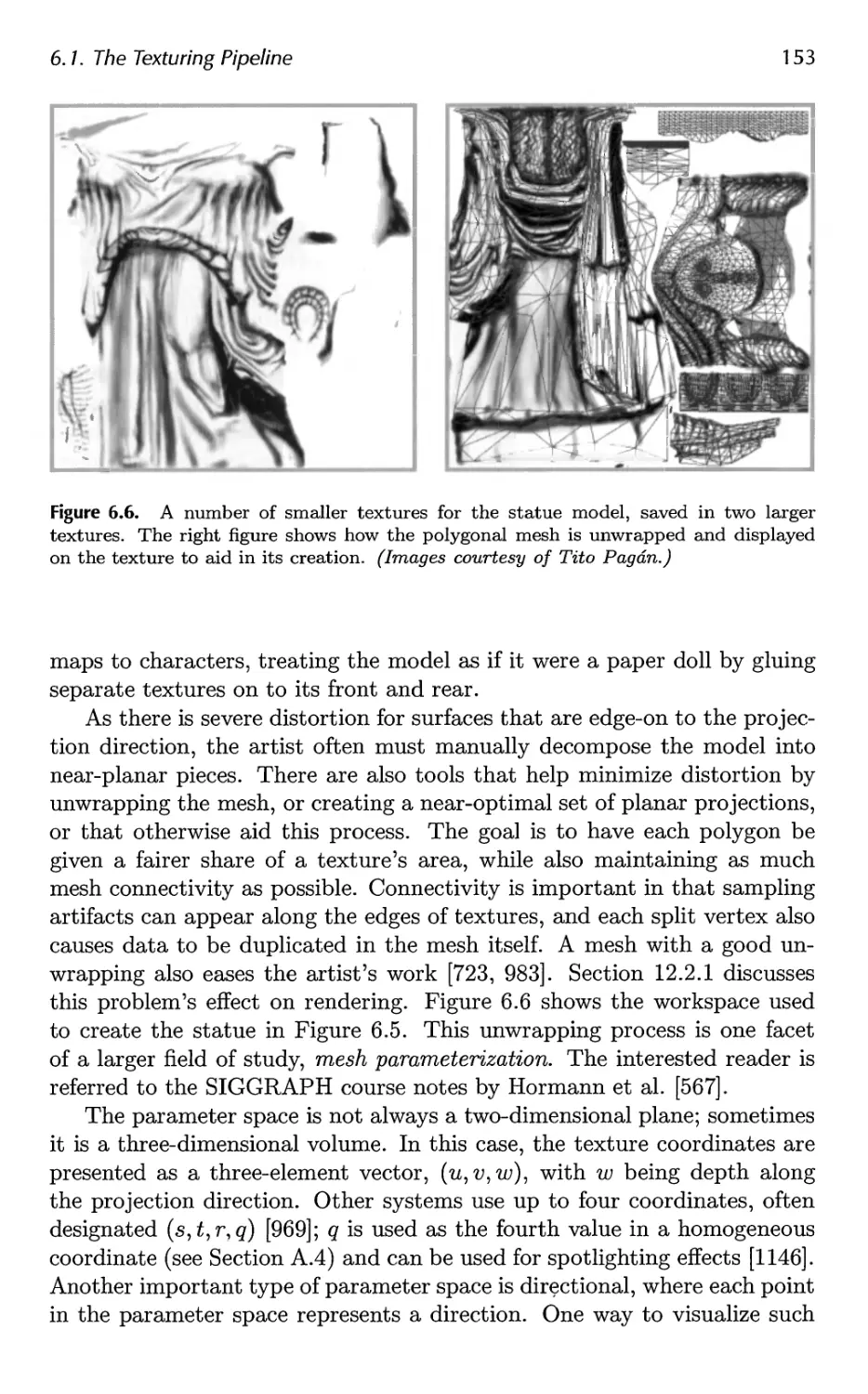
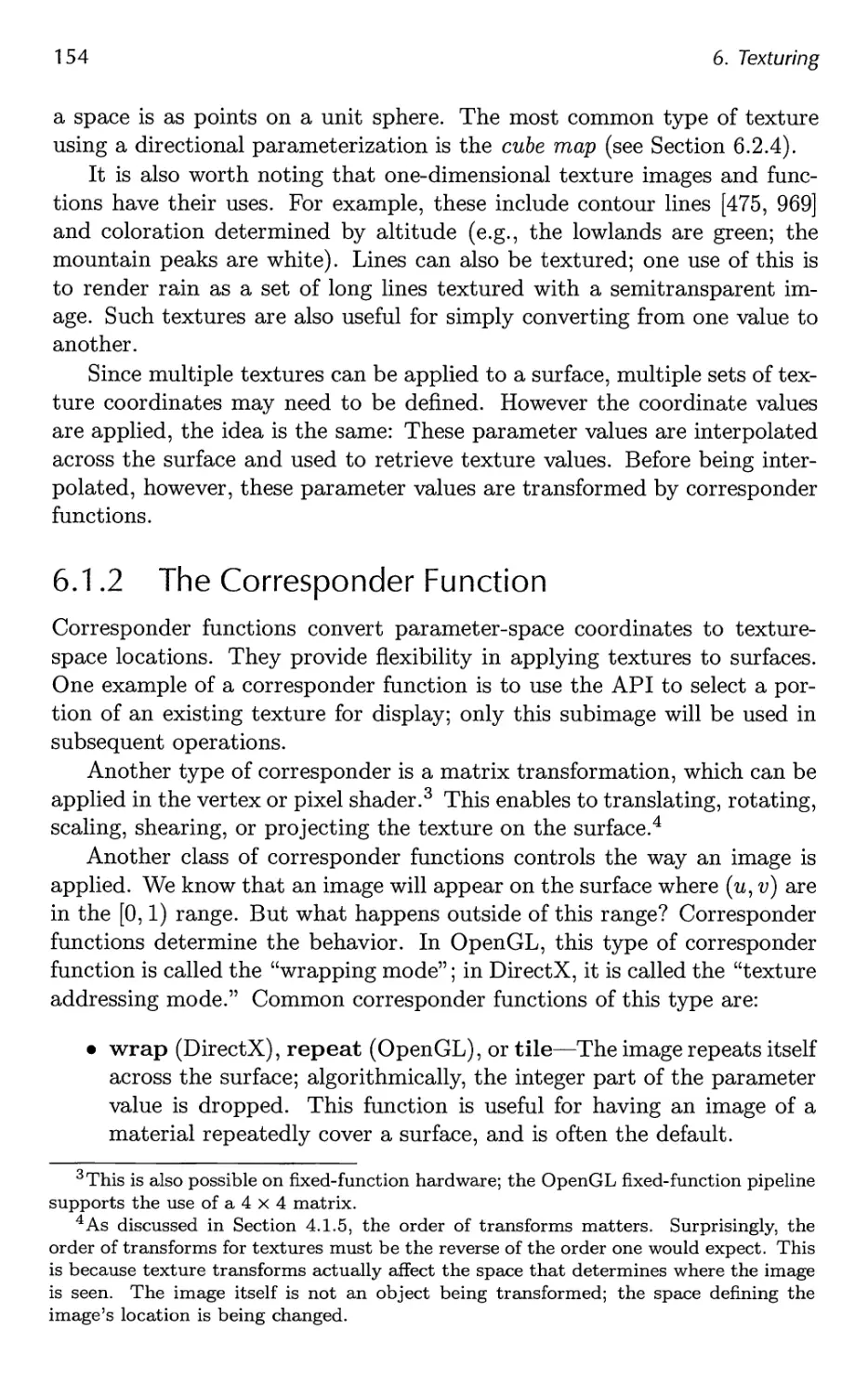
Chapter 6, Texturing. One of the most powerful tools for real-time
rendering is the ability to rapidly access and display data such as images on
surfaces. This chapter discusses the mechanics of this technique, called
texturing, and presents a wide variety of methods for applying it.
Chapter 7, Advanced Shading. This chapter discusses the theory and
practice of correctly representing materials and the use of point light sources.
Chapter 8, Area and Environmental Lighting. More elaborate light sources
and algorithms are explored in this chapter.
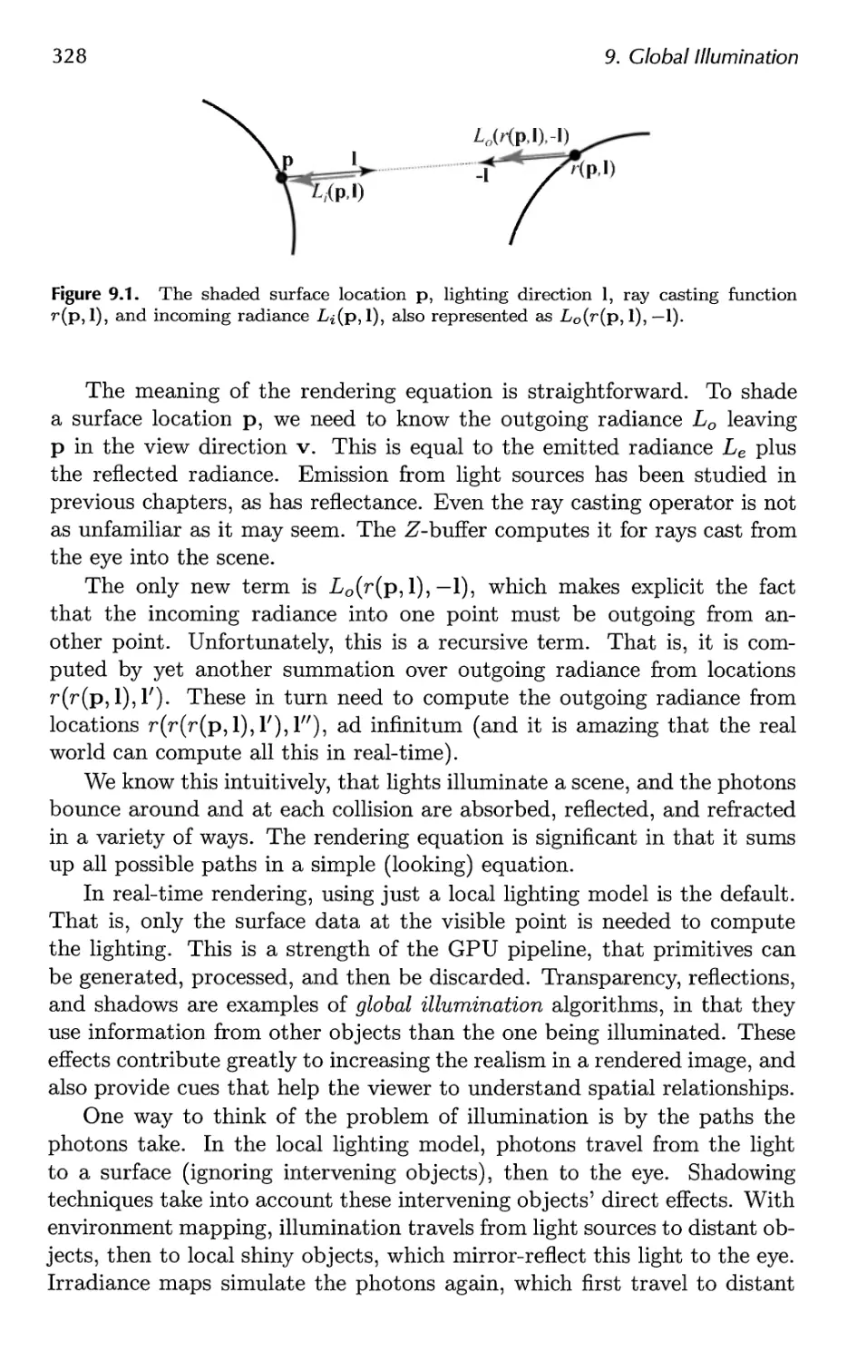
Chapter 9, Global Illumination. Shadow, reflection, and refraction
algorithms are discussed, as well as such topics as radiosity, ray tracing, pre-
computed lighting, and ambient occlusion.
Chapter 10, Image-Based Effects. Polygons are not always the fastest or
most realistic way to describe objects or phenomena such as lens flares or
fire. In this chapter, alternate representations based on using images are
discussed. Post-processing effects such as high-dynamic range rendering,
motion blur, and depth of field are also covered.
Chapter 11, Non-Photorealistic Rendering. Attempting to make a scene
look realistic is only one way of rendering it. This chapter discusses other
styles, such as cartoon shading.
Chapter 12, Polygonal Techniques. Geometric data comes from a wide
range of sources, and sometimes requires modification in order to be
rendered rapidly and well. This chapter discusses polygonal data and ways to
clean it up and simplify it. Also included are more compact representations,
such as triangle strips, fans, and meshes.
4
/. Introduction
Chapter 13, Curves and Curved Surfaces. Hardware ultimately deals in
points, lines, and polygons for rendering geometry. More complex surfaces
offer advantages such as being able to trade off between quality and
rendering speed, more compact representation, and smooth surface generation.
Chapter 14, Acceleration Algorithms. After you make it go, make it go
fast. Various forms of culling and level of detail rendering are covered here.
Chapter 15, Pipeline Optimization. Once an application is running and
uses efficient algorithms, it can be made even faster using various
optimization techniques. This chapter is primarily about finding the bottleneck and
deciding what to do about it. Multiprocessing is also discussed.
Chapter 16, Intersection Test Methods. Intersection testing is important
for rendering, user interaction, and collision detection. In-depth coverage is
provided here for a wide range of the most efficient algorithms for common
geometric intersection tests.
Chapter 17, Collision Detection. Finding out whether two objects touch
each other is a key element of many real-time applications. This chapter
presents some efficient algorithms in this evolving field.
Chapter 18, Graphics Hardware. While GPU accelerated algorithms have
been discussed in the previous chapters, this chapter focuses on components
such as color depth, frame buffers, and basic architecture types. Case
studies of a few representative graphics accelerators are provided.
Chapter 19, The Future. Take a guess (we do).
We have included appendices on linear algebra and trigonometry.
1.2 Notation and Definitions
First, we shall explain the mathematical notation used in this book. For a
more thorough explanation of many of the terms used in this section, see
Appendix A.
1.2.1 Mathematical Notation
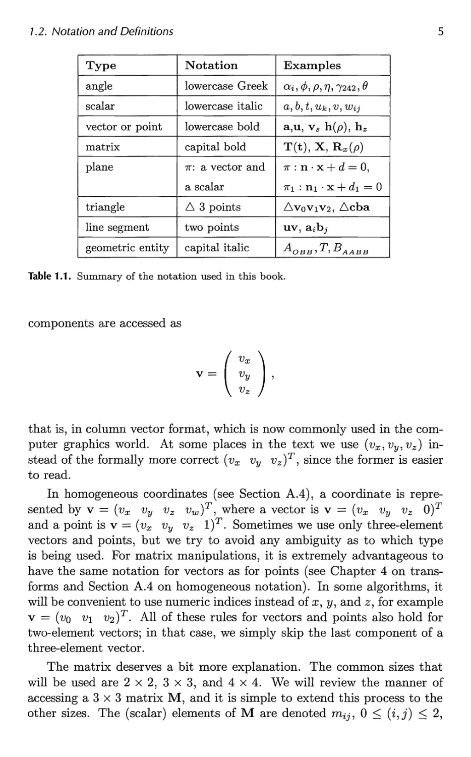
Table 1.1 summarizes most of the mathematical notation we will use. Some
of the concepts will be described at some length here.
The angles and the scalars are taken from M, i.e., they are real
numbers. Vectors and points are denoted by bold lowercase letters, and the
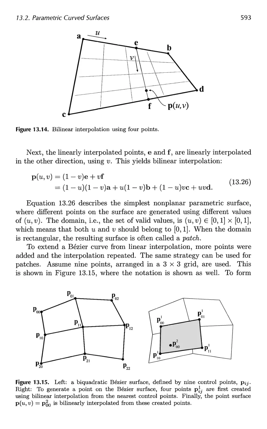
1.2. Notation and Definitions 5
Type
angle
scalar
vector or point
matrix
plane
triangle
line segment
geometric entity
Notation
lowercase Greek
lowercase italic
lowercase bold
capital bold
7r: a vector and
a scalar
A 3 points
two points
capital italic
Examples
a*, <?,P,»7,7242,0
a,b,t,uk,v,Wij
a,u, vs h(p), hz
T(t), X, Rx(p)
7r : n • x + d = 0,
7Ti : ni • x + d\ = 0
AvoviV2, Acba
uv, a^bj
A T R
^OBBi x •>*-*AABB
Table 1.1. Summary of the notation used in this book.
components are accessed as
that is, in column vector format, which is now commonly used in the
computer graphics world. At some places in the text we use (vx,vy,vz)
instead of the formally more correct (vx vy vz)T, since the former is easier
to read.
In homogeneous coordinates (see Section A.4), a coordinate is
represented by v = (vx vy vz vw)T', where a vector is v = (vx vy vz 0)T
and a point is v = (yx vy vz 1)T. Sometimes we use only three-element
vectors and points, but we try to avoid any ambiguity as to which type
is being used. For matrix manipulations, it is extremely advantageous to
have the same notation for vectors as for points (see Chapter 4 on
transforms and Section A.4 on homogeneous notation). In some algorithms, it
will be convenient to use numeric indices instead of x, y, and z, for example
v = (vo vi V2)T. All of these rules for vectors and points also hold for
two-element vectors; in that case, we simply skip the last component of a
three-element vector.
The matrix deserves a bit more explanation. The common sizes that
will be used are 2 x 2, 3 x 3, and 4x4. We will review the manner of
accessing a 3 x 3 matrix M, and it is simple to extend this process to the
other sizes. The (scalar) elements of M are denoted m^-, 0 < (i,j) < 2,
6
/. Introduction
where i denotes the row and j the column, as in Equation 1.2:
m0o moi m02
M = ( raio mn mi2 ) . (1.2)
m2o m2i m22
The following notation, shown in Equation 1.3 for a 3 x 3 matrix, is used to
isolate vectors from the matrix M: mj represents the jth column vector
and m^ represents the ith row vector (in column vector form). As with
vectors and points, indexing the column vectors can also be done with x,
y, z, and sometimes w, if that is more convenient:
M = ( m>0 m,i m}2 ) = (m, my mz ) =
<
(1.3)
\^ /
A plane is denoted tt : n • x + d = 0 and contains its mathematical
formula, the plane normal n and the scalar d. The normal is a vector
describing what direction the plane faces. More generally (e.g., for curved
surfaces), a normal describes this direction for a particular point on the
surface. For a plane the same normal happens to apply to all its points.
7r is the common mathematical notation for a plane. The plane 7r is said
to divide the space into a positive half-space, where n • x + d > 0, and a
negative half-space, where n • x + d < 0. All other points are said to lie in
the plane.
A triangle can be defined by three points vq, vi, and v2 and is denoted
by Av0viv2
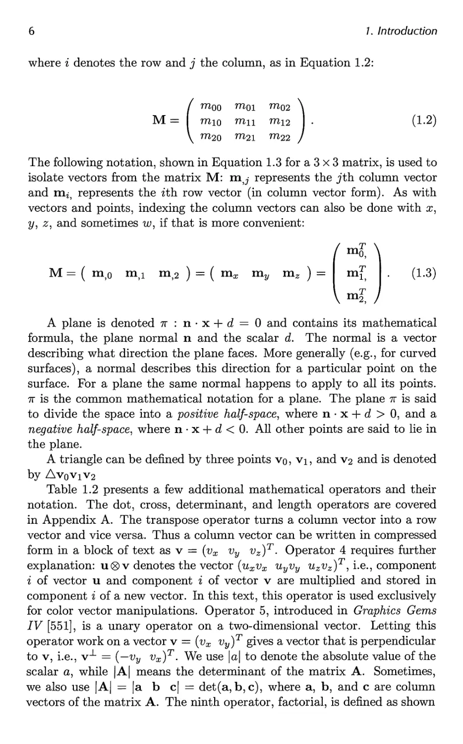
Table 1.2 presents a few additional mathematical operators and their
notation. The dot, cross, determinant, and length operators are covered
in Appendix A. The transpose operator turns a column vector into a row
vector and vice versa. Thus a column vector can be written in compressed
form in a block of text as v = (vx vy vz)T. Operator 4 requires further
explanation: u0v denotes the vector (uxvx uyvy uzvz)T', i.e., component
i of vector u and component i of vector v are multiplied and stored in
component i of a new vector. In this text, this operator is used exclusively
for color vector manipulations. Operator 5, introduced in Graphics Gems
IV [551], is a unary operator on a two-dimensional vector. Letting this
operator work on a vector v = (vx vy)T gives a vector that is perpendicular
to v, i.e., v1- = (—vy vx)T. We use \a\ to denote the absolute value of the
scalar a, while |A| means the determinant of the matrix A. Sometimes,
we also use |A| = |a b c| = det(a, b, c), where a, b, and c are column
vectors of the matrix A. The ninth operator, factorial, is defined as shown
1.2. Notation and Definitions 7
1
2
3
4
5
6
7
8
9
10:
Operator
X
T
V
<g>
JL
1 • 1
1 ¦ 1
II ¦ II
n\
0
Description
dot product
cross product
transpose of the vector v
piecewise vector multiplication
the unary, perp dot product operator
determinant of a matrix
absolute value of a scalar
length (or norm) of argument
factorial
binomial coefficients
Table 1.2. Notation for some mathematical operators.
below, and note that 0! = 1:
n\ = n(n - l)(n - 2) • • • 3 • 2 • 1. (1.4)
The tenth operator, the binomial factor, is defined as shown in
Equation 1.5:
\k) = k\{n-k)V (L5)
Further on, we call the common planes x = 0, y = 0, and z = 0
the coordinate planes or axis-aligned planes. The axes e^ = (1 0 0)T,
e^ = (0 1 0)T, and ez = (0 0 1)T are called main axes or main directions
and often the x-axis, y-axis, and z-axis. This set of axes is often called
the standard basis. Unless otherwise noted, we will use orthonormal bases
(consisting of mutually perpendicular unit vectors; see Appendix A.3.1).
The notation for a range that includes both a and 6, and all numbers in
between is [a, b]. If you want all number between a and 6, but not a and b
themselves, then we write (a, b). Combinations of these can also be made,
e.g., [a, b) means all numbers between a and b including a but not b.
The C-math function atan2(y,x) is often used in this text, and so
deserves some attention. It is an extension of the mathematical function
arctan(x). The main differences between them are that — f < arctan(x) <
^, that 0 < atan2(y, x) < 27r, and that an extra argument has been added
to the latter function. This extra argument avoids division by zero, i.e.,
x = y/x except when x = 0.
8 /. Introduction
1:
2:
3:
Function
atan2(y, x)
cos(0)
log(n)
Description
two-value arctangent
clamped cosine
natural logarithm of n
Table 1.3. Notation for some specialized mathematical functions.
Clamped-cosine, cos(0), is a function we introduce in order to keep
shading equations from becoming difficult to read. If the result of the
cosine function is less than zero, the value returned by clamped-cosine is
zero.
In this volume the notation log(n) always means the natural logarithm,
loge(ra), not the base-10 logarithm, log10(n).
We use a right-hand coordinate system (see Appendix A.2) since this
is the standard system for three-dimensional geometry in the field of
computer graphics.
Colors are represented by a three-element vector, such as (red, green,
blue), where each element has the range [0,1].
1.2.2 Geometrical Definitions
The basic rendering primitives (also called drawing primitives) used by
most graphics hardware are points, lines, and triangles.1
Throughout this book, we will refer to a collection of geometric entities
as either a model or an object A scene is a collection of models comprising
everything that is included in the environment to be rendered. A scene can
also include material descriptions, lighting, and viewing specifications.
Examples of objects are a car, a building, and even a line. In practice, an
object often consists of a set of drawing primitives, but this may not always
be the case; an object may have a higher kind of geometrical representation,
such as Bezier curves or surfaces, subdivision surfaces, etc. Also, objects
can consist of other objects, e.g., we call a car model's door an object or a
subset of the car.
Further Reading and Resources
The most important resource we can refer you to is the website for this
book: http://www.realtimerendering.com. It contains links to the latest
information and websites relevant to each chapter. The field of real-time
rendering is changing with real-time speed. In the book we have attempted
1The only exceptions we know of are Pixel-Planes [368], which could draw spheres,
and the NVIDIA NV1 chip, which could draw ellipsoids.
1.2. Notation and Definitions
9
to focus on concepts that are fundamental and techniques that are unlikely
to go out of style. On the website we have the opportunity to present
information that is relevant to today's software developer, and we have the
ability to keep up-to-date.
Chapter 2
The Graphics
Rendering Pipeline
"A chain is no stronger than its weakest link."
—Anonymous
This chapter presents what is considered to be the core component of
realtime graphics, namely the graphics rendering pipeline, also known simply
as the pipeline. The main function of the pipeline is to generate, or
render, a two-dimensional image, given a virtual camera, three-dimensional
objects, light sources, shading equations, textures, and more. The
rendering pipeline is thus the underlying tool for real-time rendering. The
process of using the pipeline is depicted in Figure 2.1. The locations and
shapes of the objects in the image are determined by their geometry, the
characteristics of the environment, and the placement of the camera in
that environment. The appearance of the objects is affected by material
properties, light sources, textures, and shading models.
The different stages of the rendering pipeline will now be discussed and
explained, with a focus on function and not on implementation.
Implementation details are either left for later chapters or are elements over which
the programmer has no control. For example, what is important to
someone using lines are characteristics such as vertex data formats, colors, and
pattern types, and whether, say, depth cueing is available, not whether
lines are implemented via Bresenham's line-drawing algorithm [142] or via
a symmetric double-step algorithm [1391]. Usually some of these pipeline
stages are implemented in non-programmable hardware, which makes it
impossible to optimize or improve on the implementation. Details of basic
draw and fill algorithms are covered in depth in books such as Rogers [1077].
While we may have little control over some of the underlying hardware,
algorithms and coding methods have a significant effect on the speed and
quality at which images are produced.
11
12
2. The Graphics Rendering Pipeline
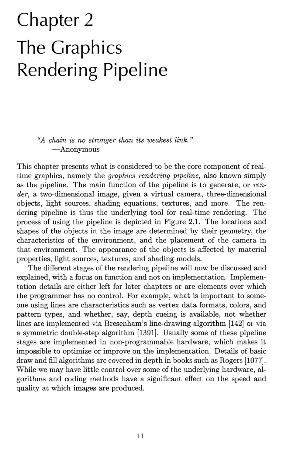
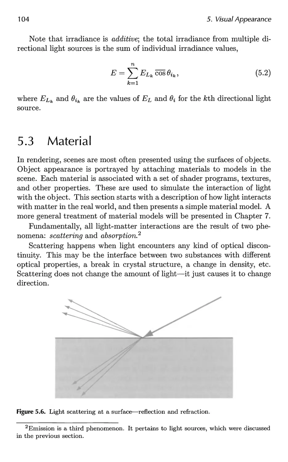
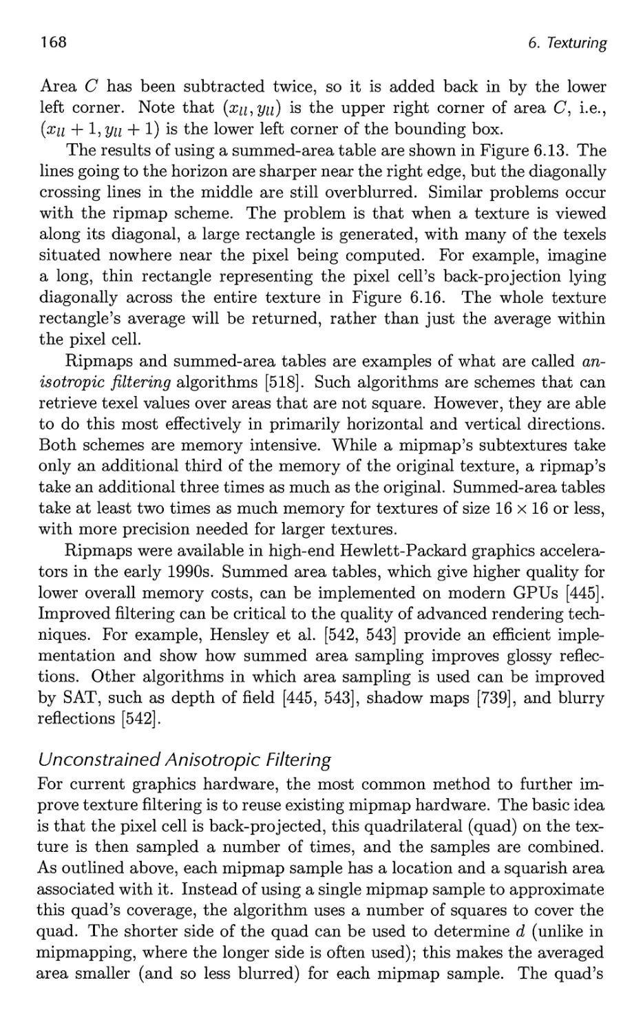
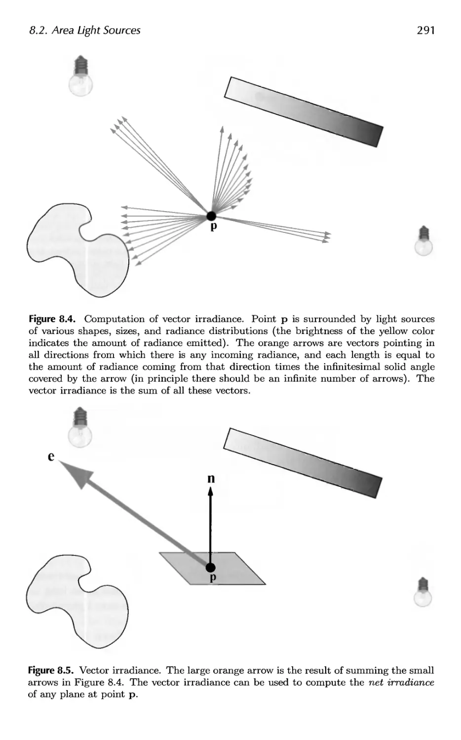
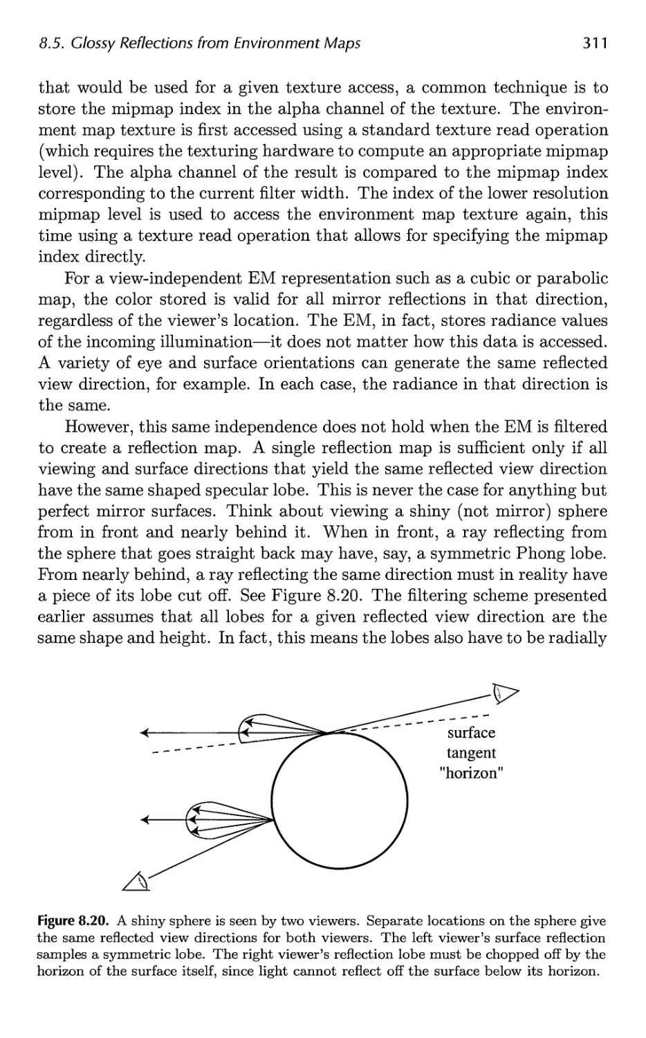
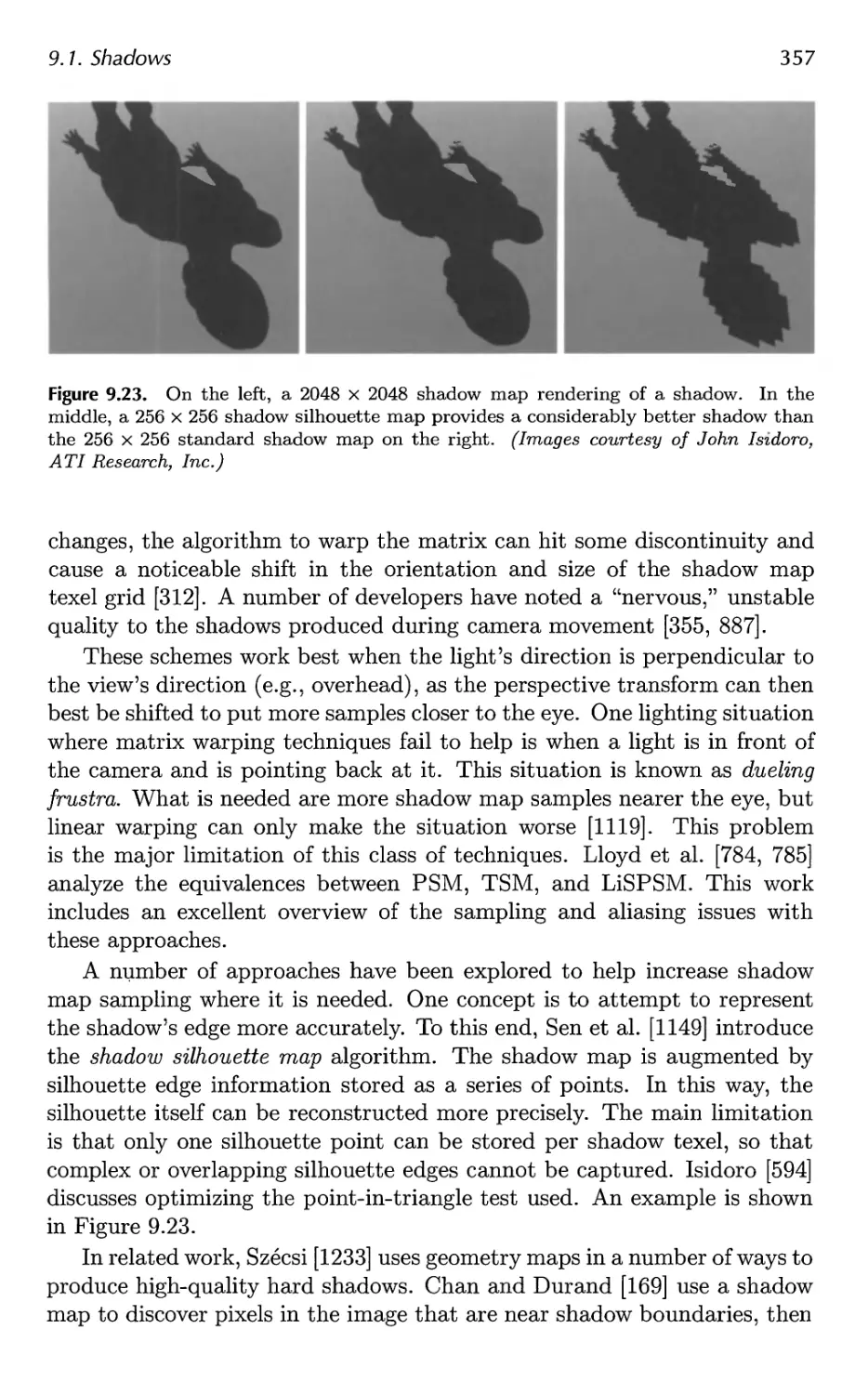
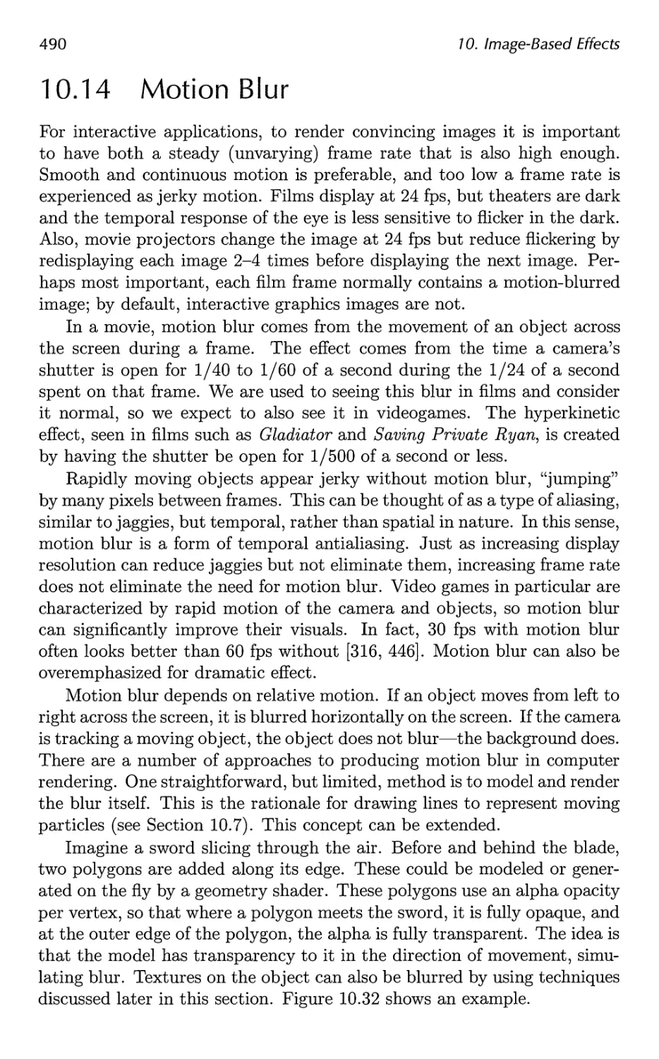
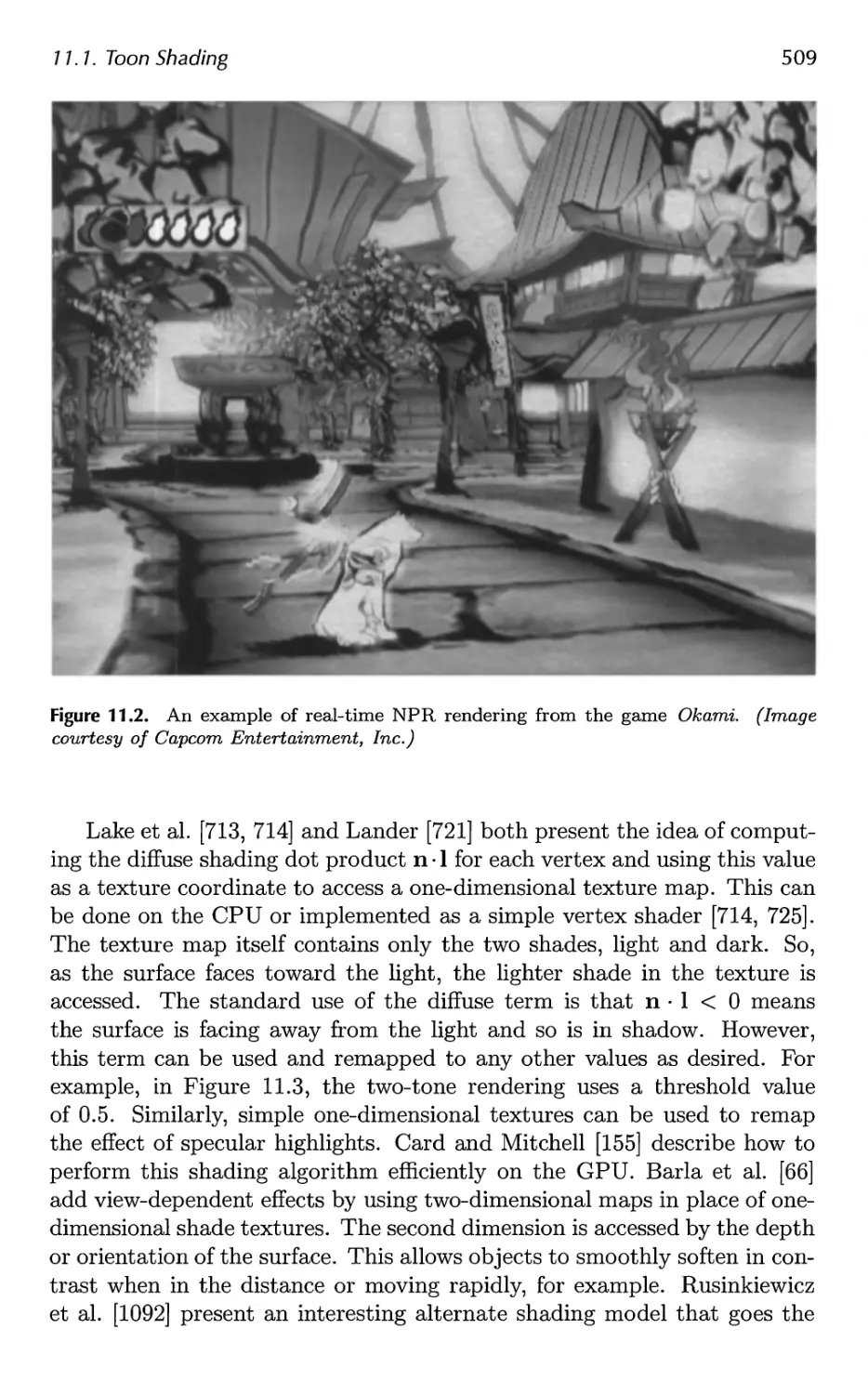
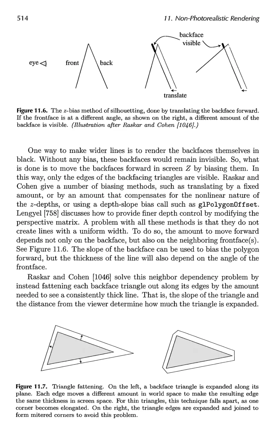
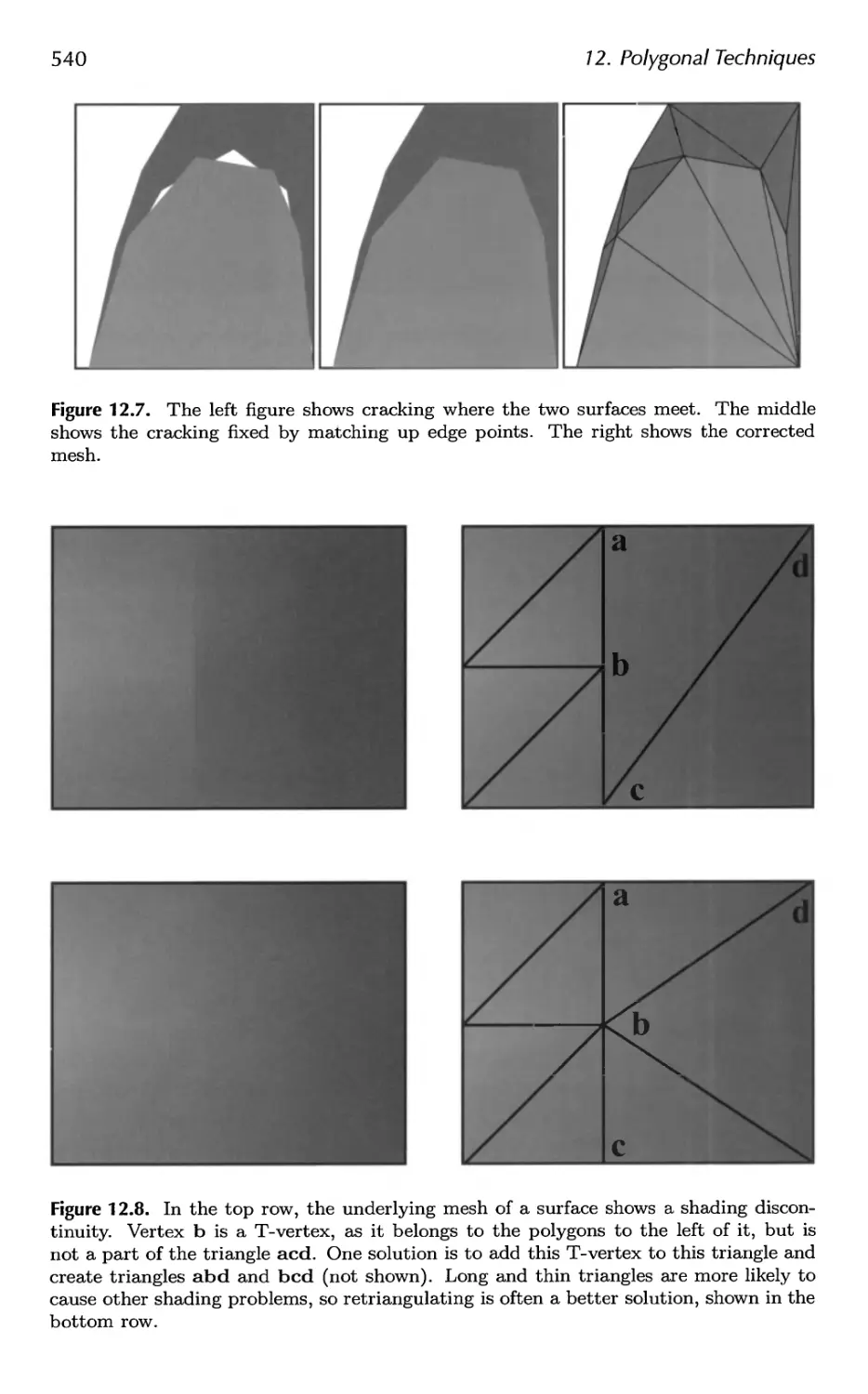
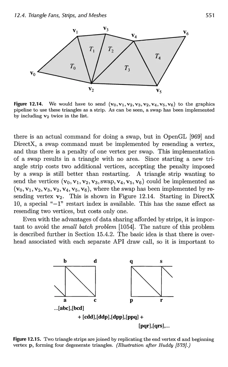
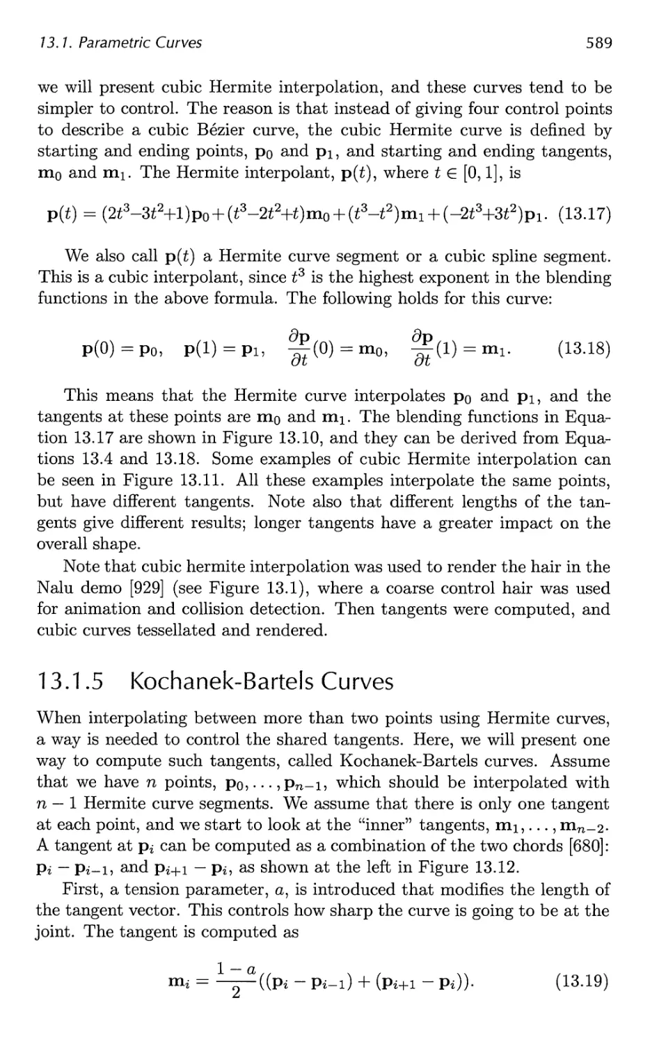
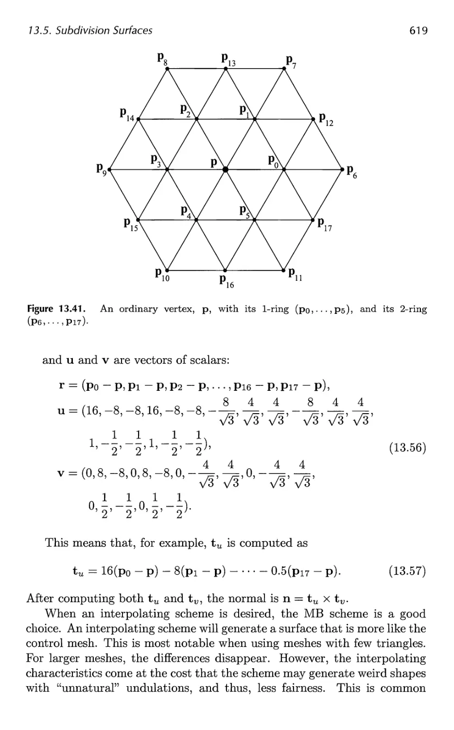
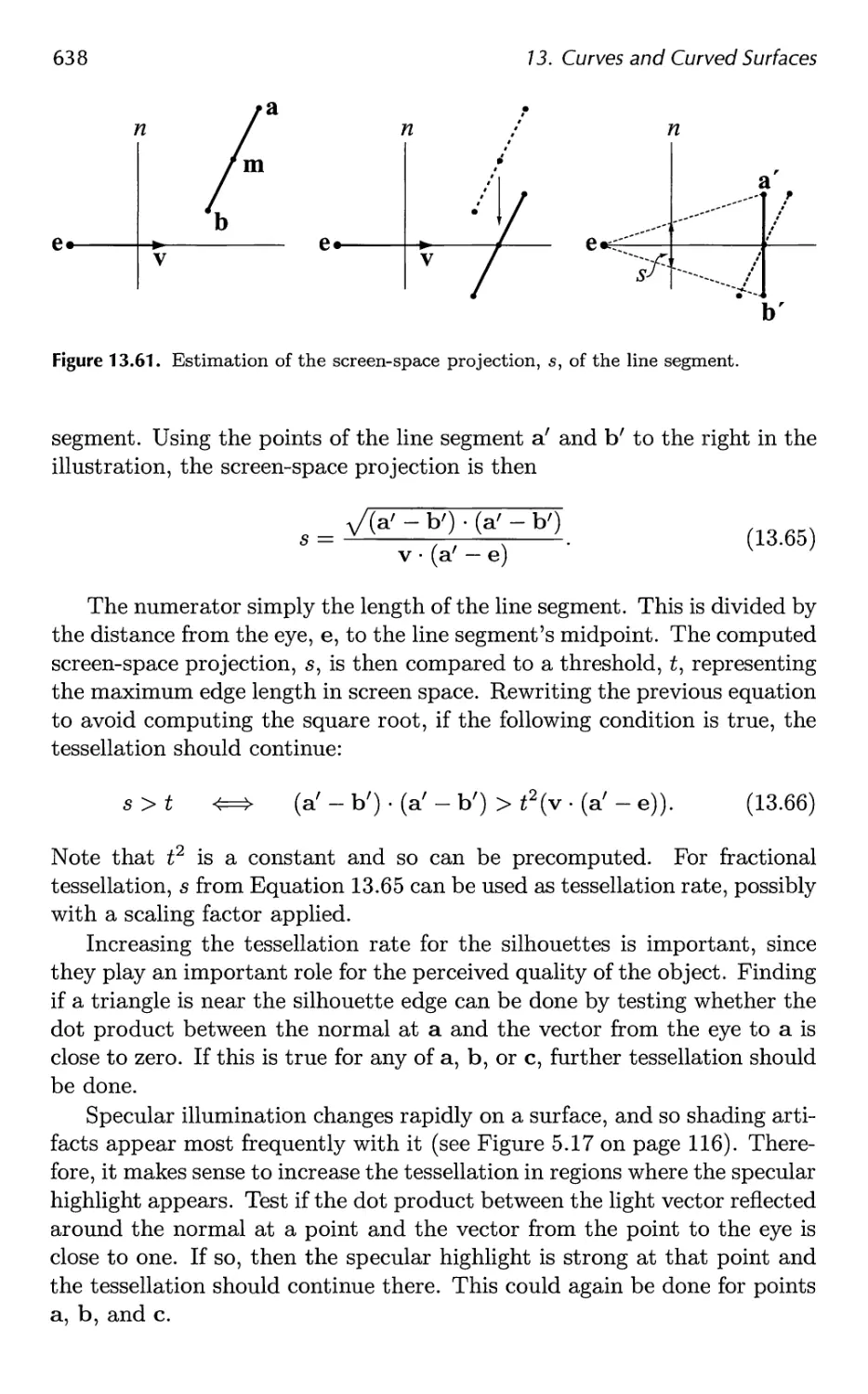
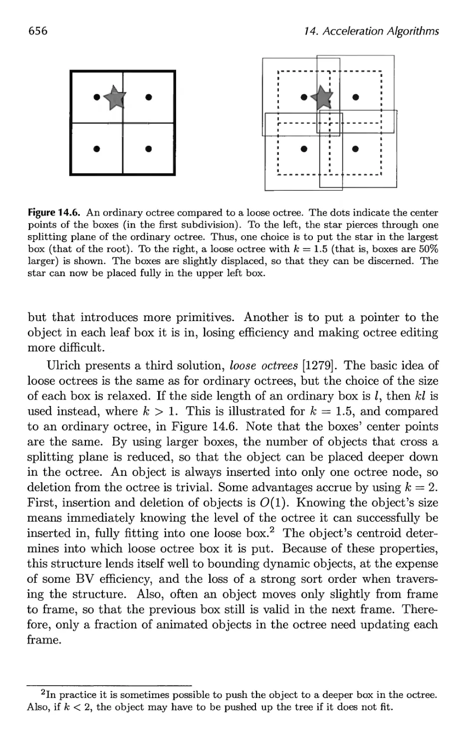
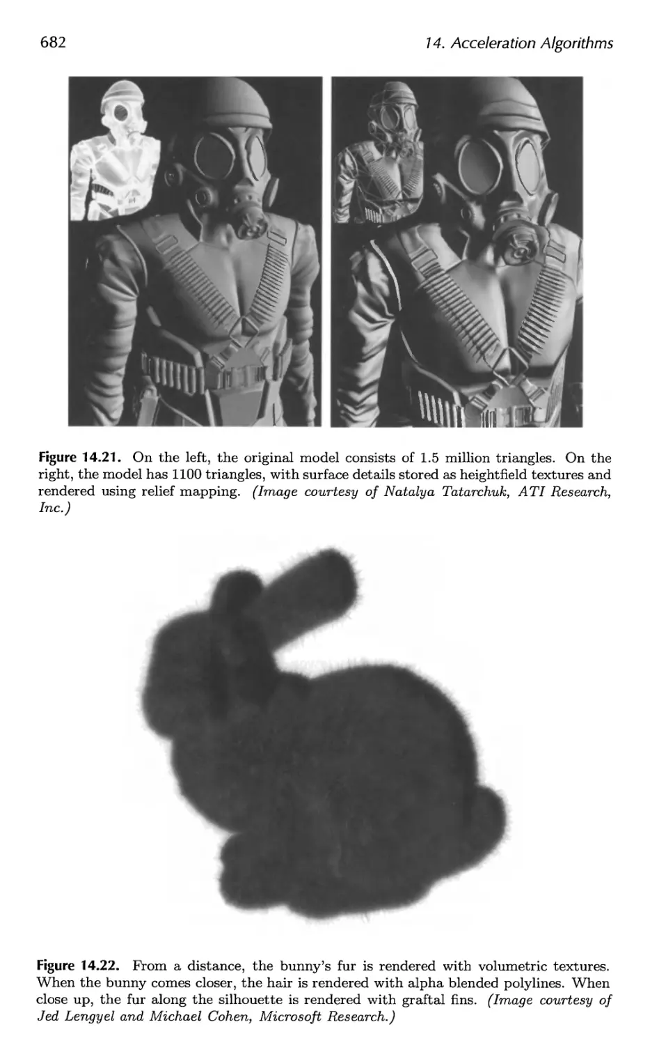
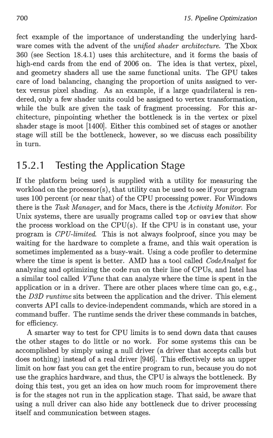
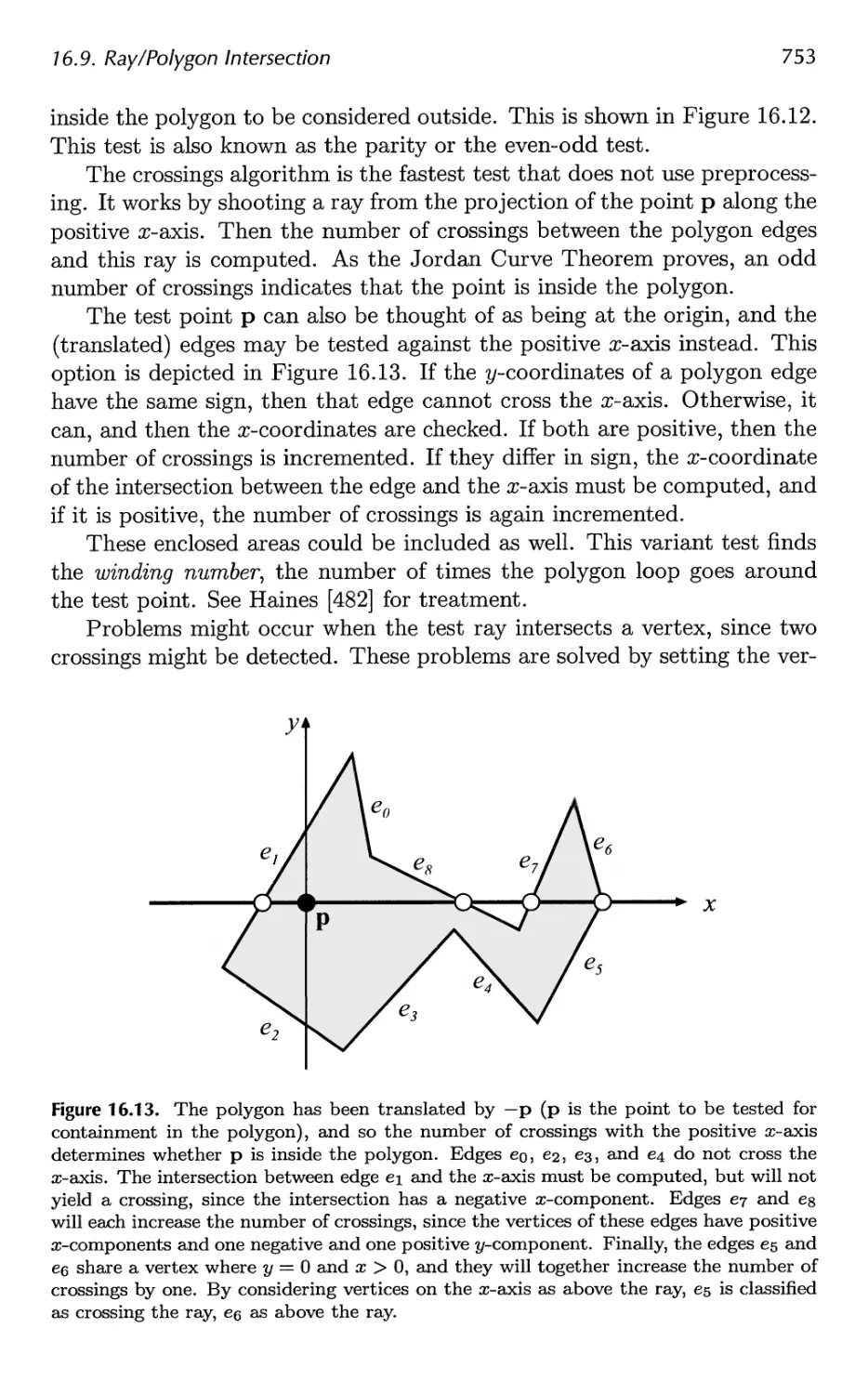
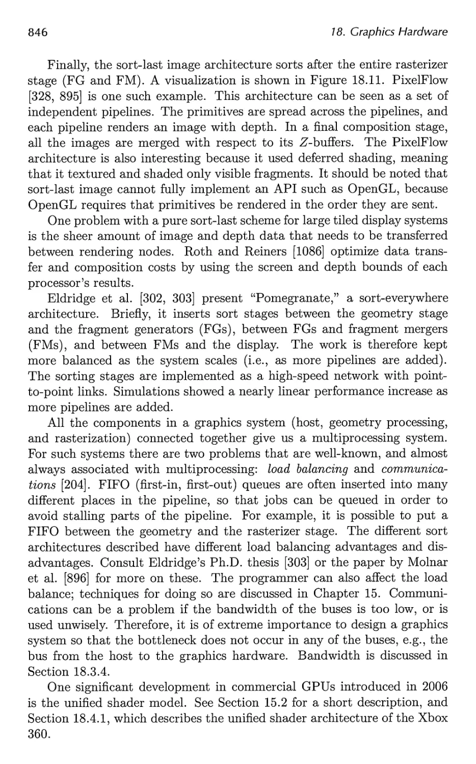
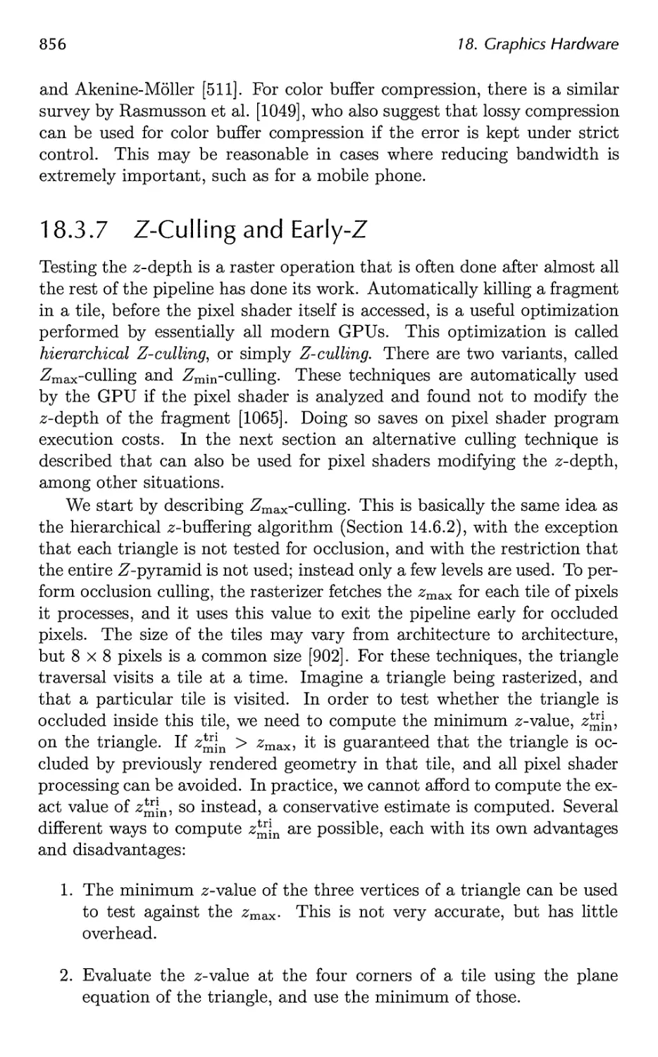
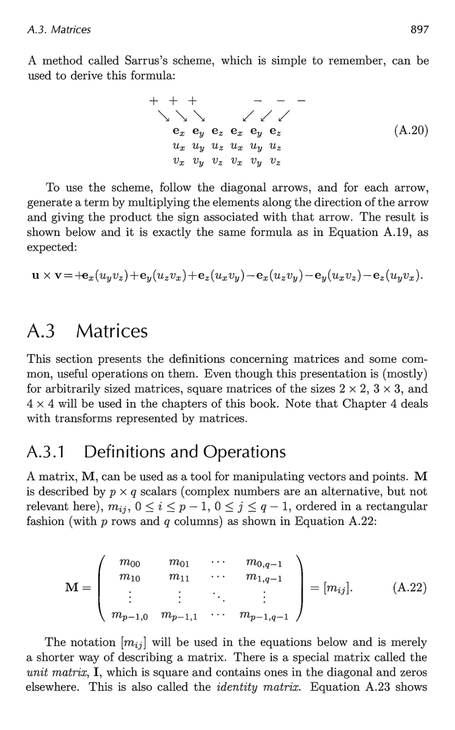
Figure 2.1. In the left image, a virtual camera is located at the tip of the pyramid (where
four lines converge). Only the primitives inside the view volume are rendered. For an
image that is rendered in perspective (as is the case here), the view volume is a frustum,
i.e., a truncated pyramid with a rectangular base. The right image shows what the
camera "sees." Note that the red donut shape in the left image is not in the rendering
to the right because it is located outside the view frustum. Also, the twisted blue prism
in the left image is clipped against the top plane of the frustum.
2.1 Architecture
In the physical world, the pipeline concept manifests itself in many different
forms, from factory assembly lines to ski lifts. It also applies to graphics
rendering.
A pipeline consists of several stages [541]. For example, in an oil
pipeline, oil cannot move from the first stage of the pipeline to the second
until the oil already in that second stage has moved on to the third stage,
and so forth. This implies that the speed of the pipeline is determined by
the slowest stage, no matter how fast the other stages may be.
Ideally, a nonpipelined system that is then divided into n pipelined
stages could give a speedup of a factor of n. This increase in performance
is the main reason to use pipelining. For example, a ski chairlift
containing only one chair is inefficient; adding more chairs creates a proportional
speedup in the number of skiers brought up the hill. The pipeline stages
execute in parallel, but they are stalled until the slowest stage has finished
its task. For example, if the steering wheel attachment stage on a car
assembly line takes three minutes and every other stage takes two minutes,
the best rate that can be achieved is one car made every three minutes; the
other stages must be idle for one minute while the steering wheel
attachment is completed. For this particular pipeline, the steering wheel stage is
the bottleneck, since it determines the speed of the entire production.
This kind of pipeline construction is also found in the context of
realtime computer graphics. A coarse division of the real-time rendering
pipeline into three conceptual stages—application, geometry, and rasterizer—is
shown in Figure 2.2. This structure is the core—the engine of the rendering
2.1. Architecture
13
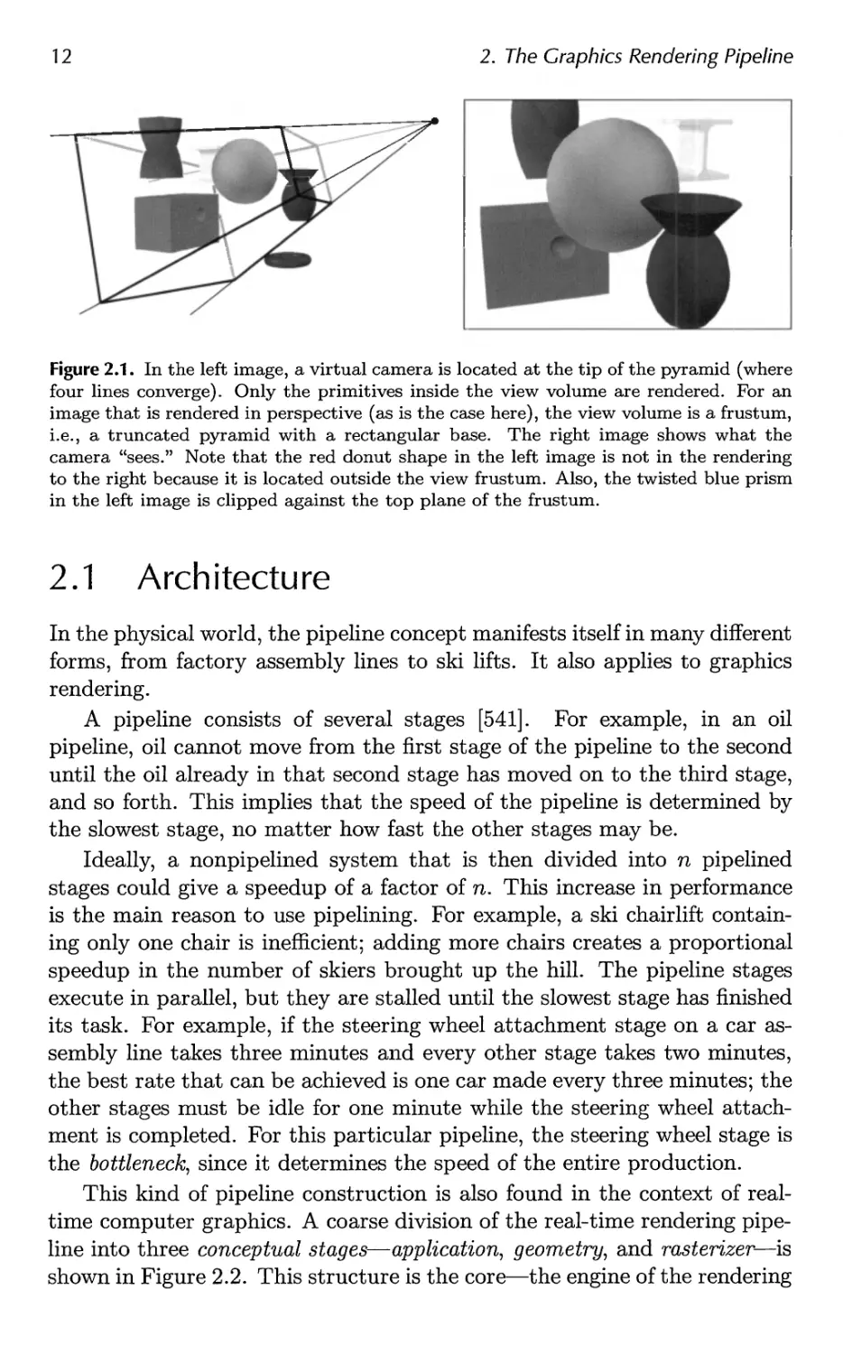
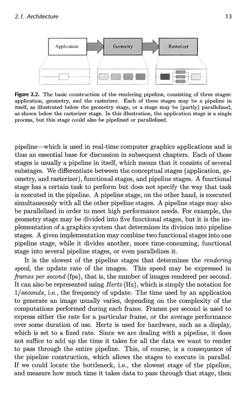
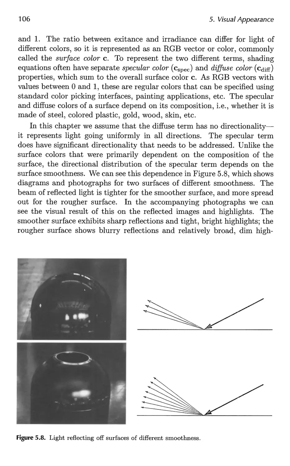
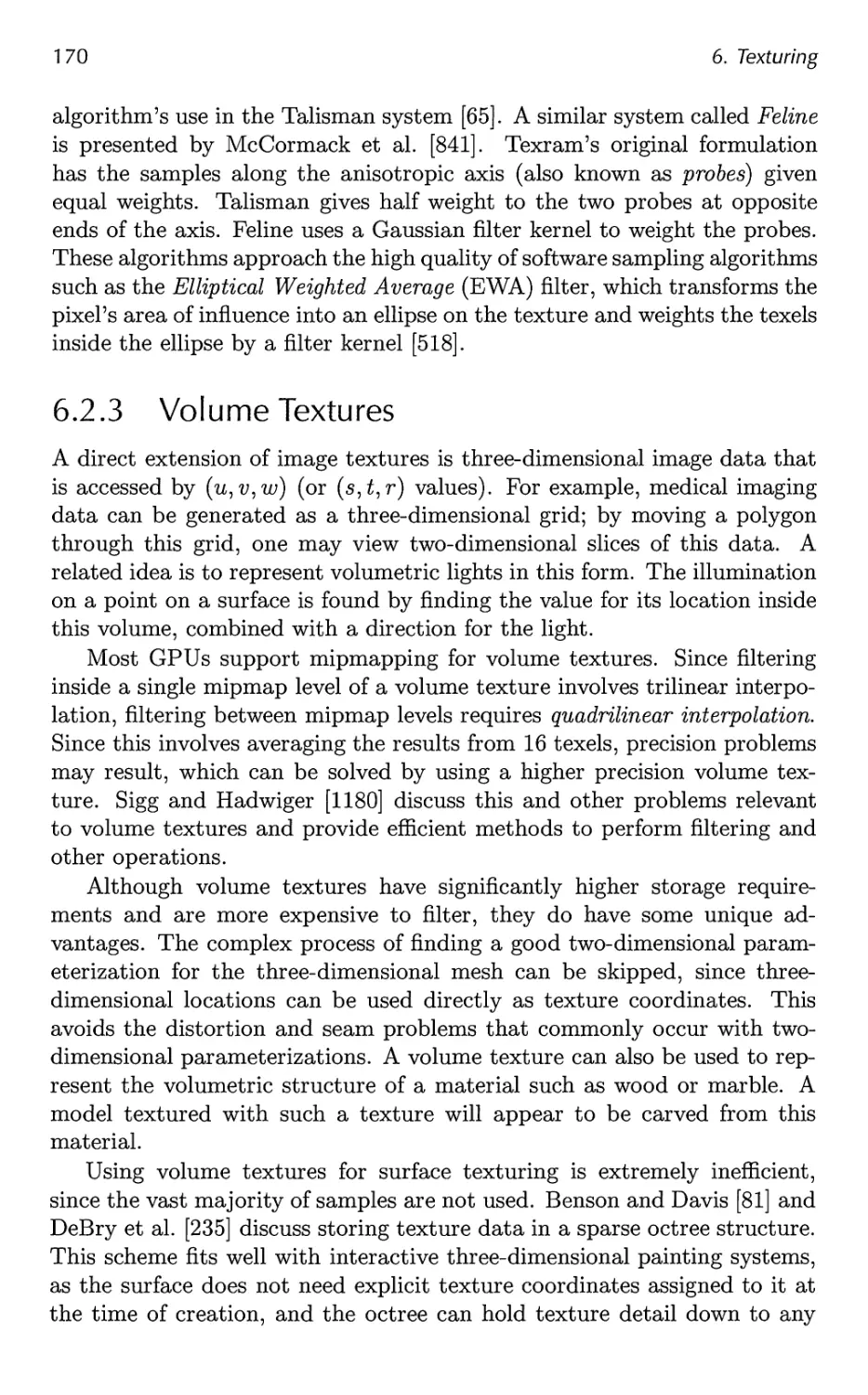
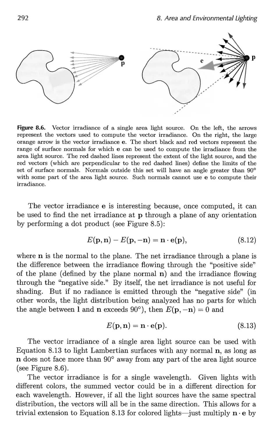
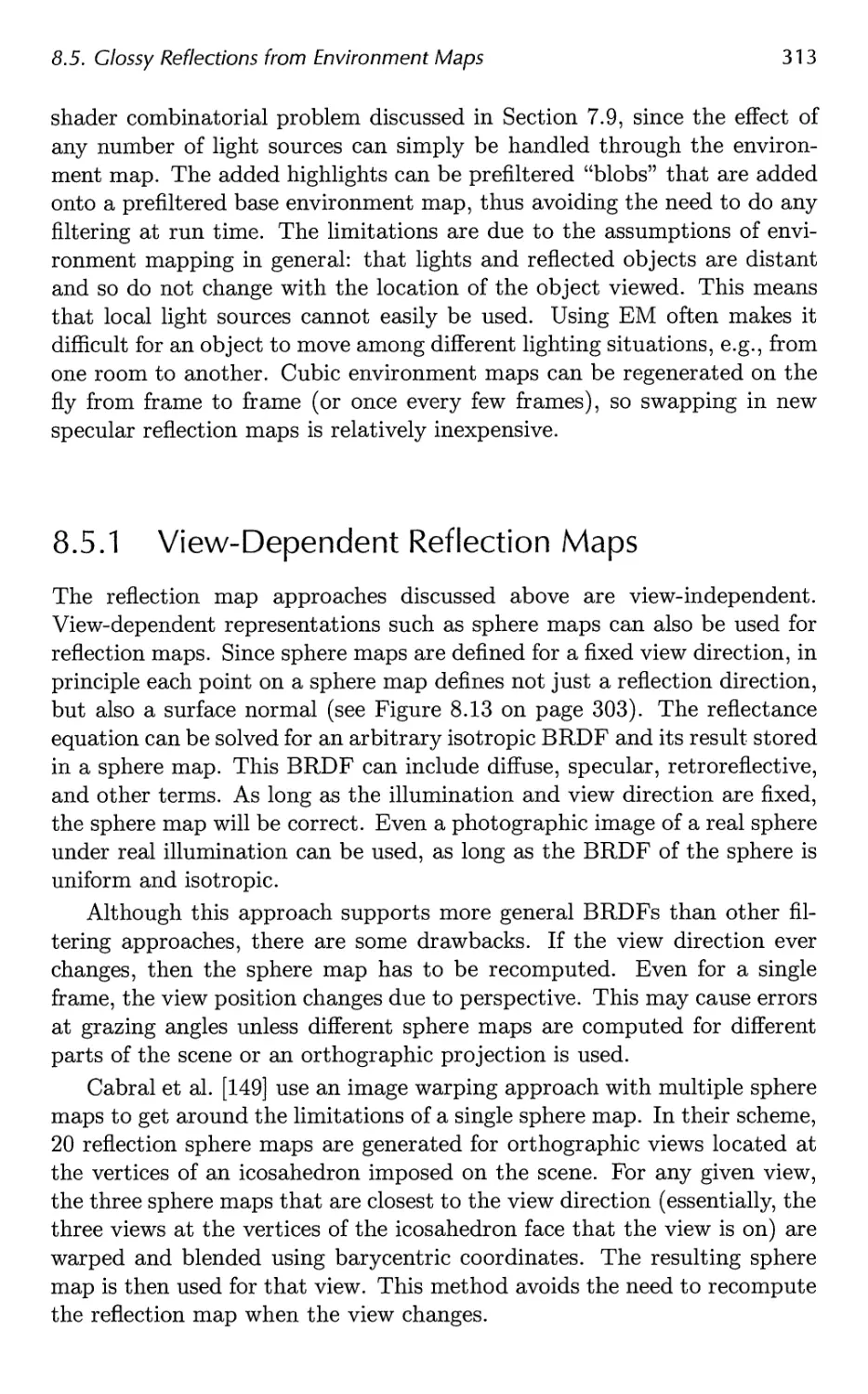
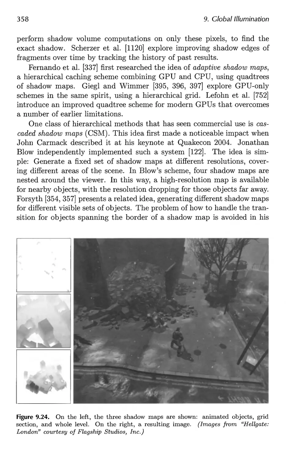
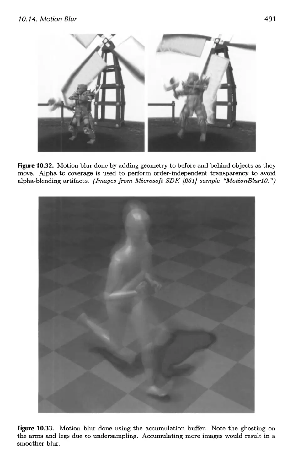
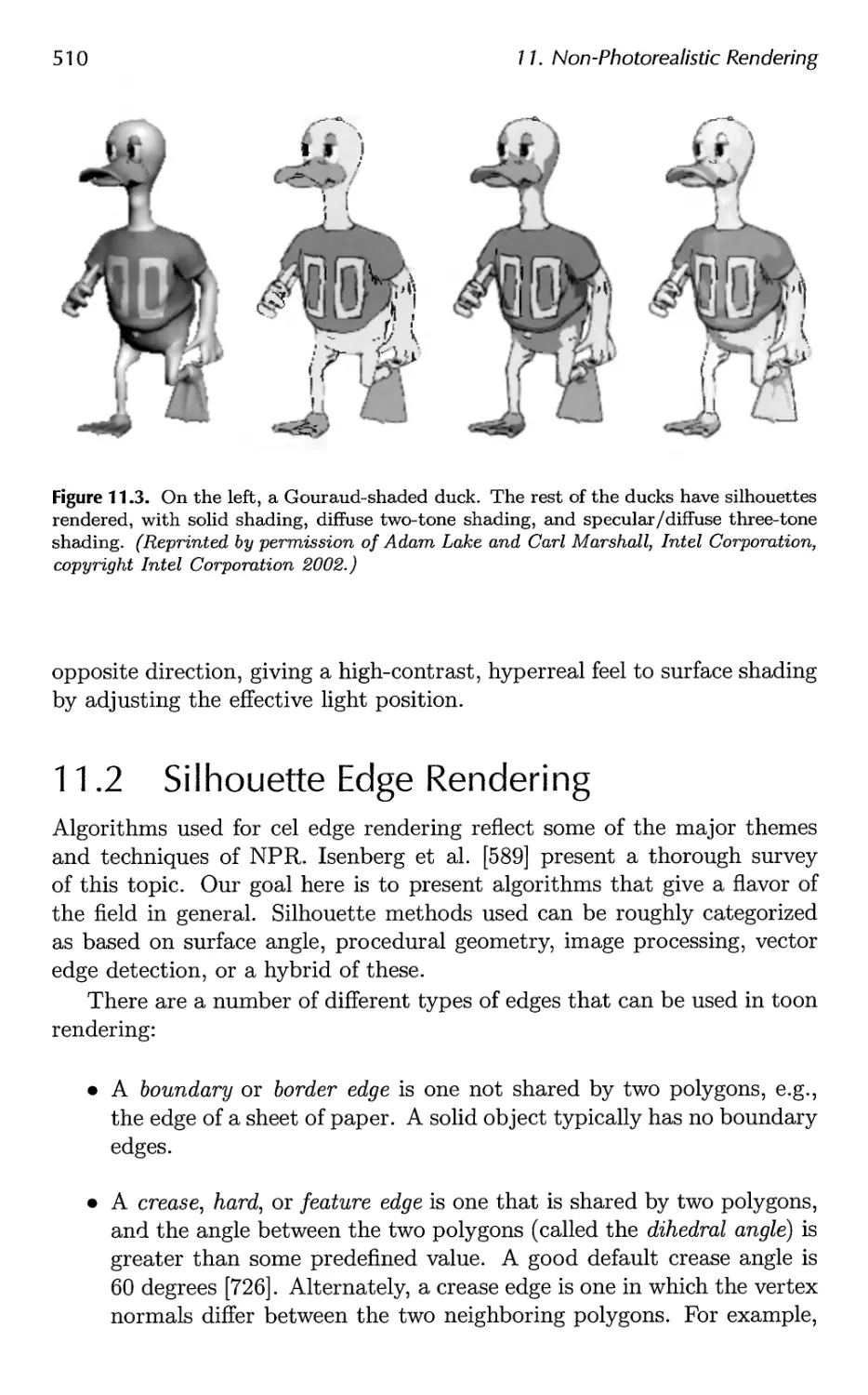
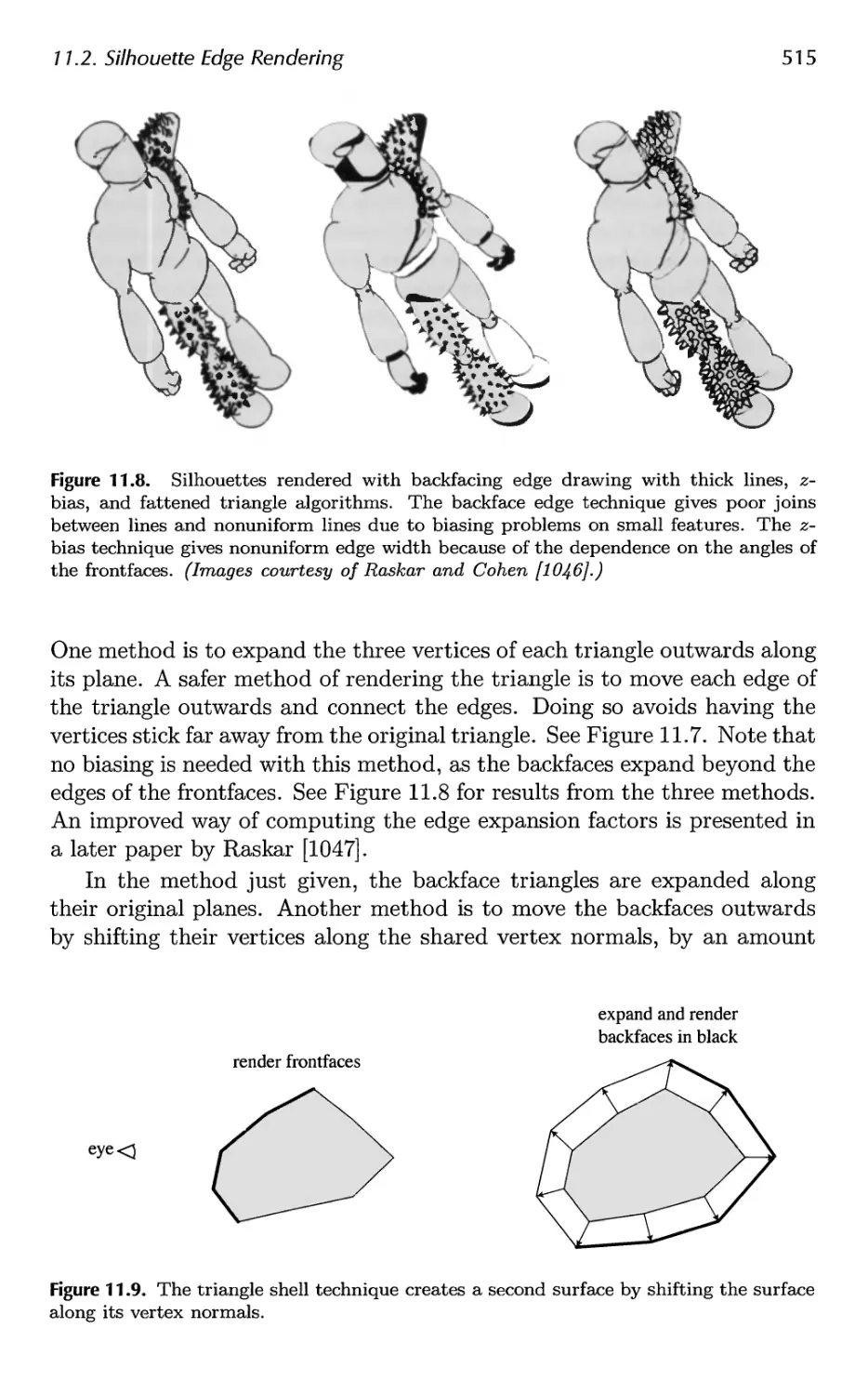
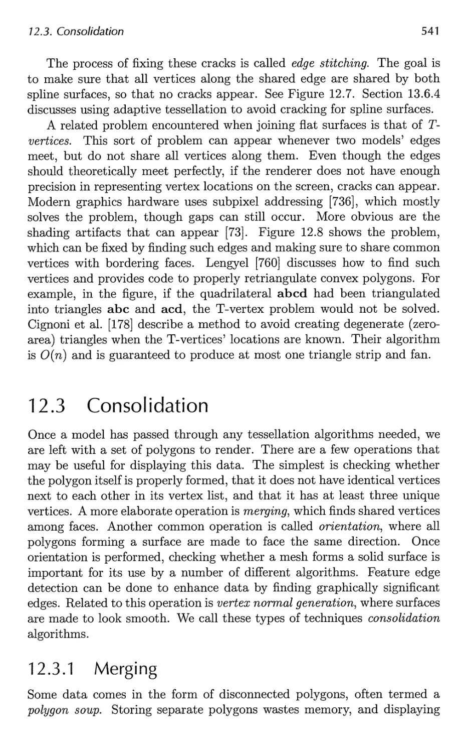
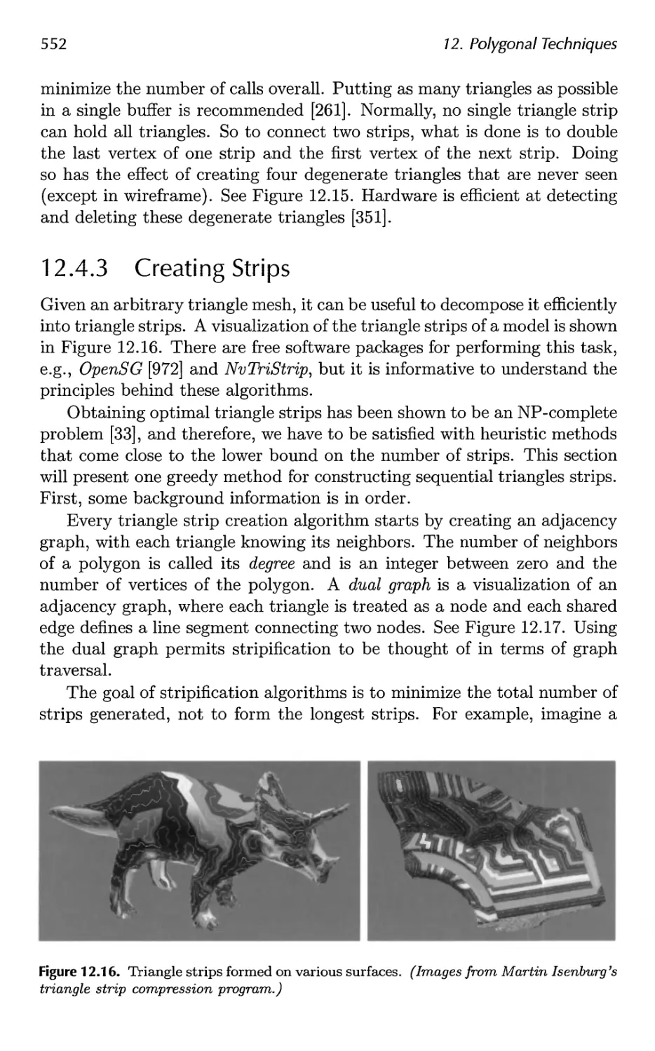
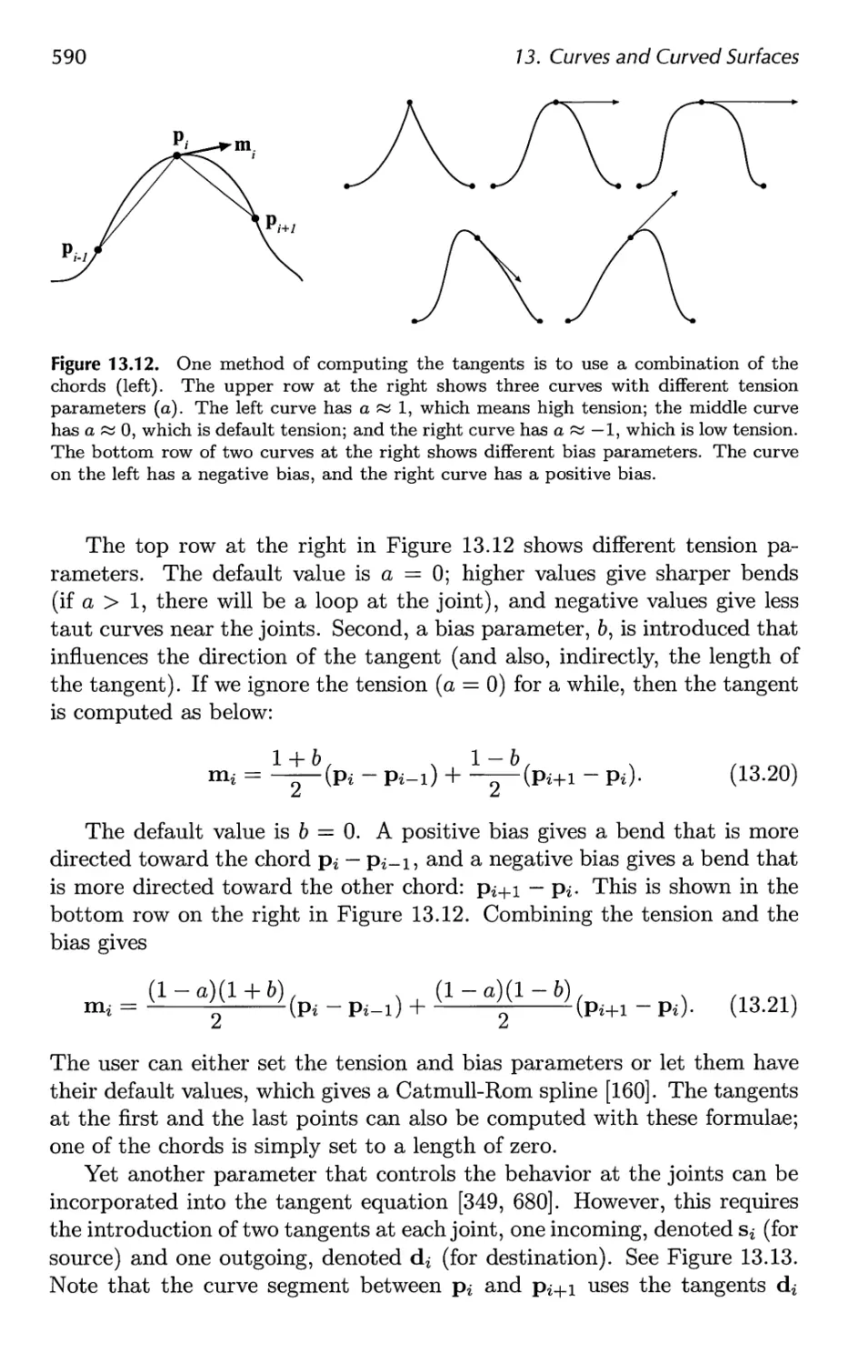
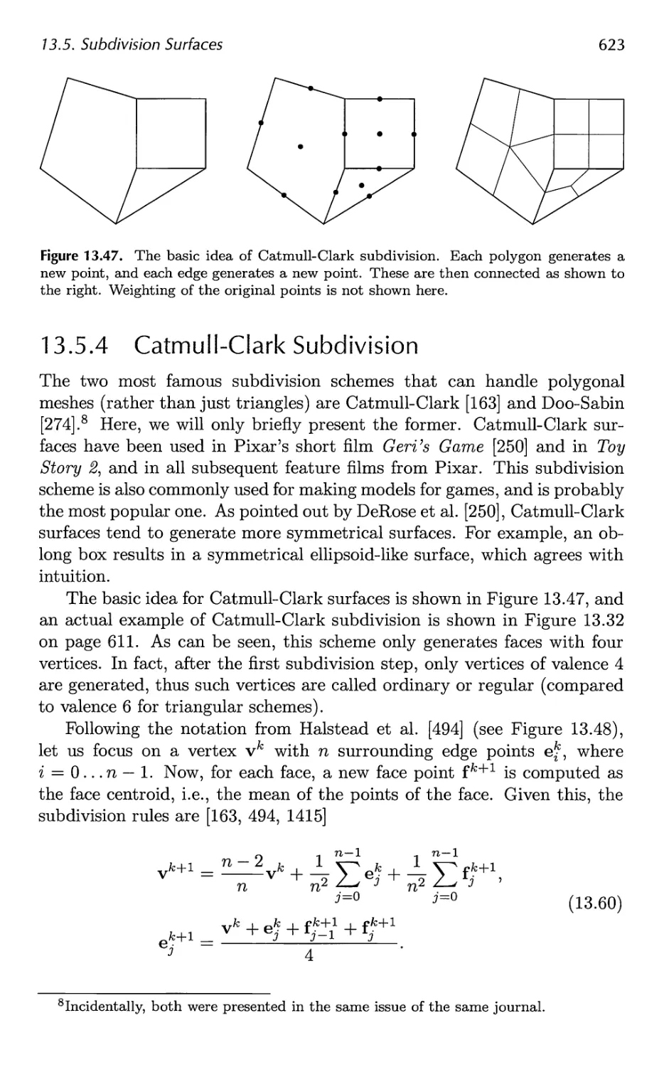
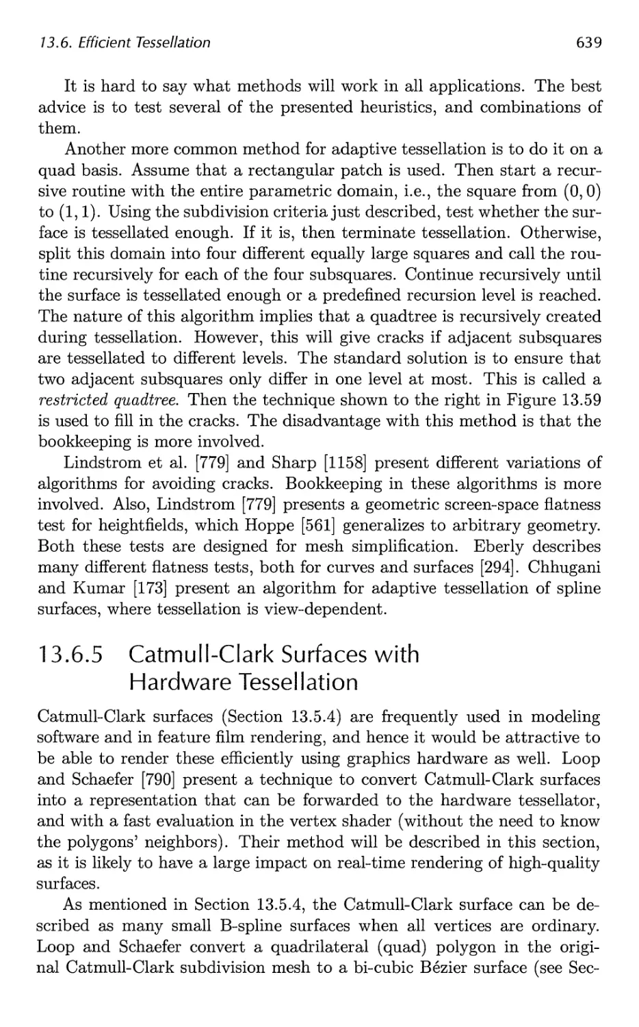
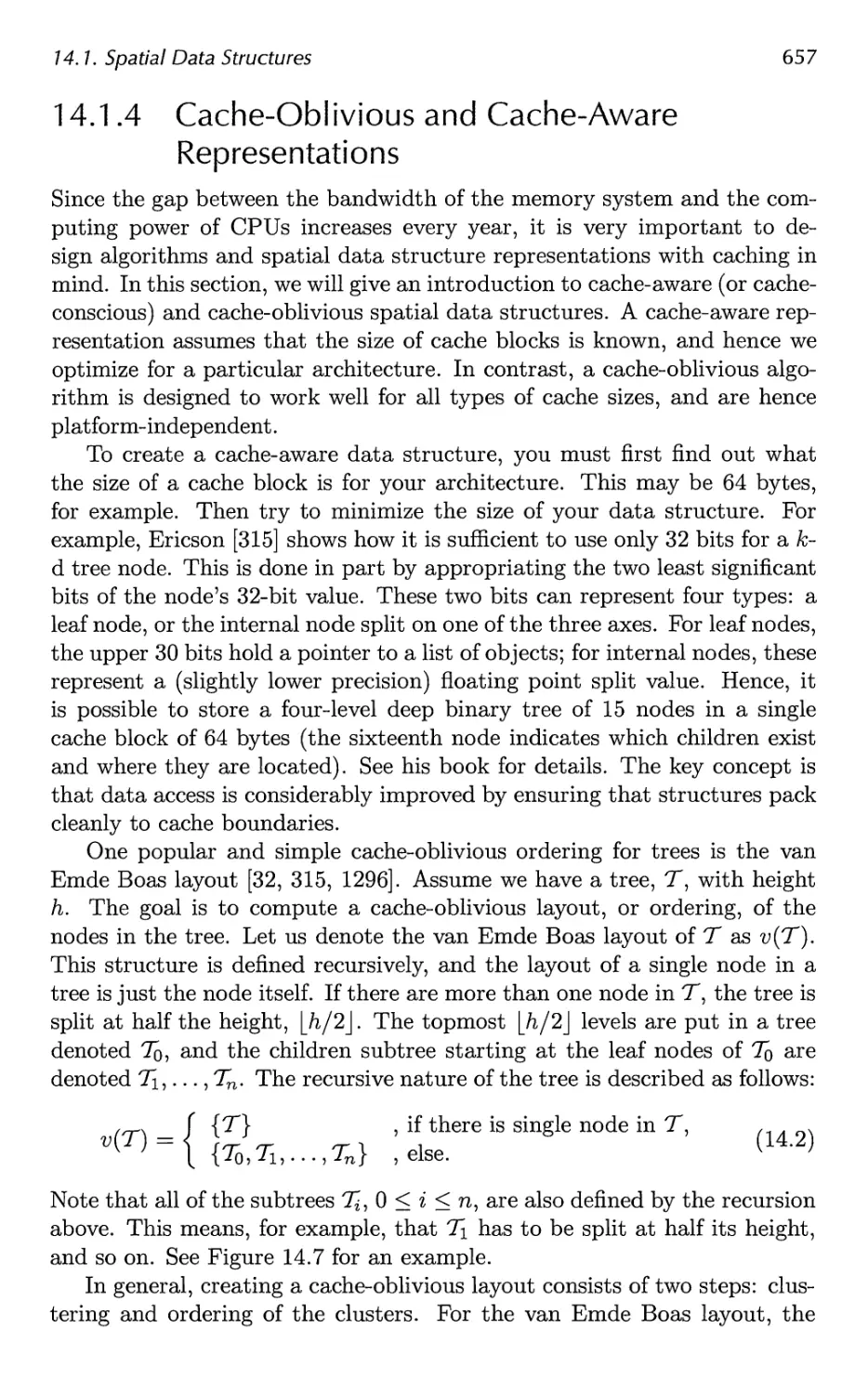
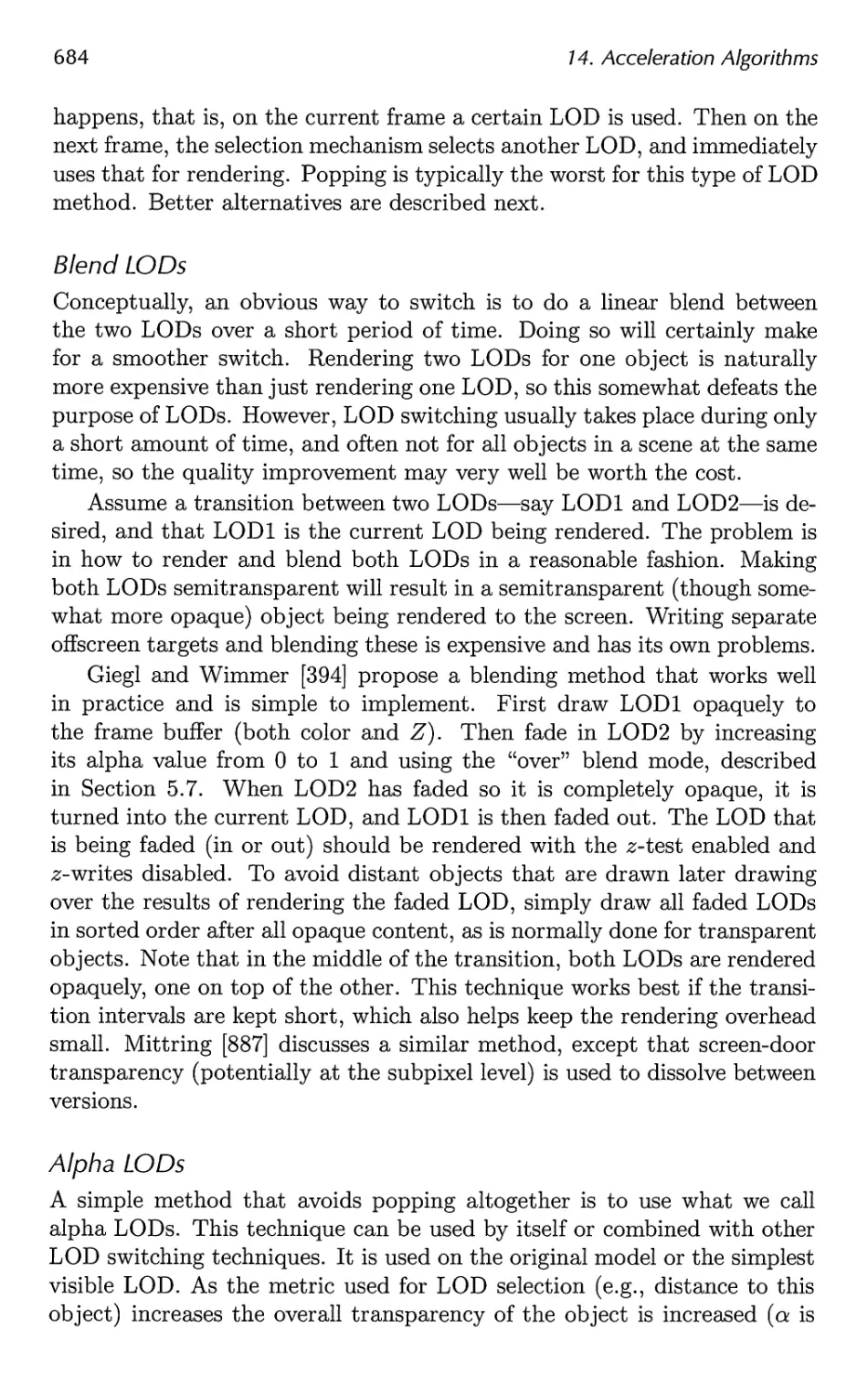
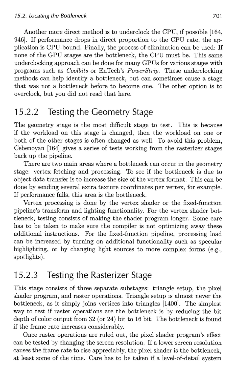
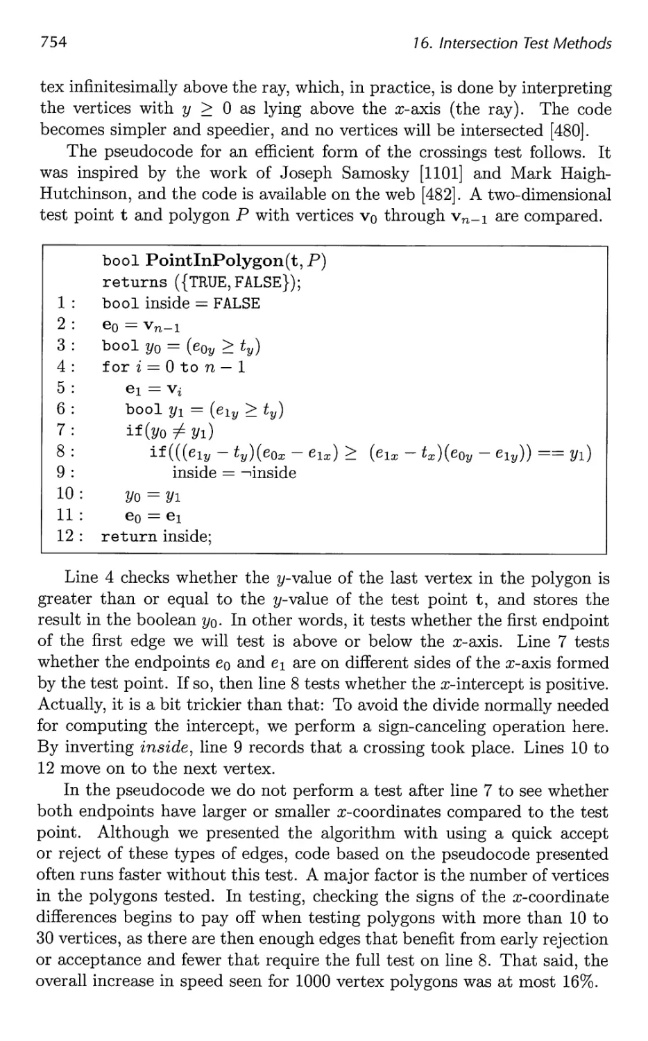
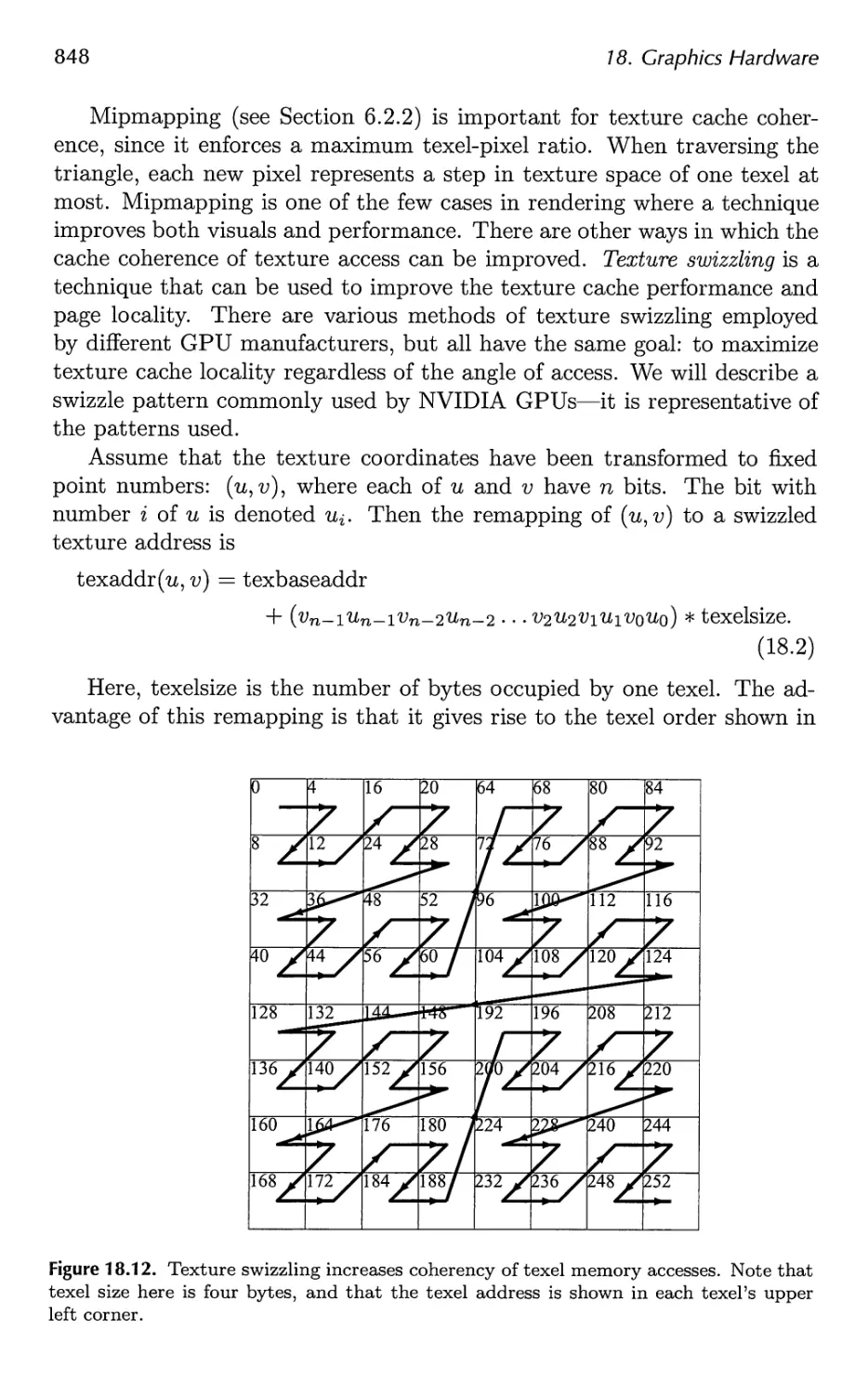
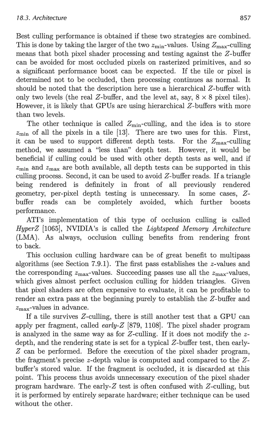
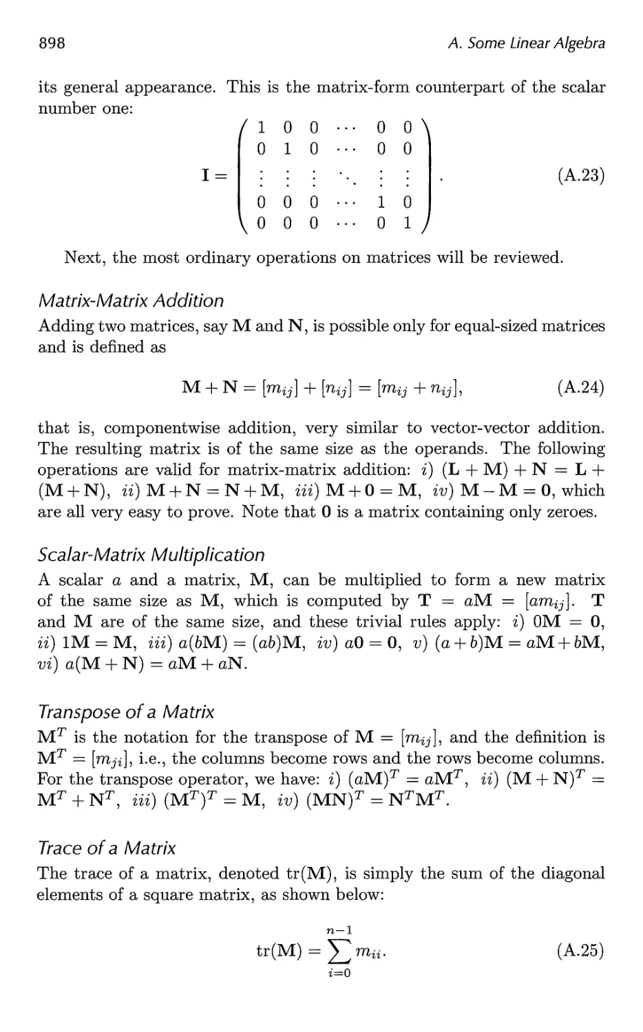
Figure 2.2. The basic construction of the rendering pipeline, consisting of three stages:
application, geometry, and the rasterizer. Each of these stages may be a pipeline in
itself, as illustrated below the geometry stage, or a stage may be (partly) parallelized,
as shown below the rasterizer stage. In this illustration, the application stage is a single
process, but this stage could also be pipelined or parallelized.
pipeline—which is used in real-time computer graphics applications and is
thus an essential base for discussion in subsequent chapters. Each of these
stages is usually a pipeline in itself, which means that it consists of several
substages. We differentiate between the conceptual stages (application,
geometry, and rasterizer), functional stages, and pipeline stages. A functional
stage has a certain task to perform but does not specify the way that task
is executed in the pipeline. A pipeline stage, on the other hand, is executed
simultaneously with all the other pipeline stages. A pipeline stage may also
be parallelized in order to meet high performance needs. For example, the
geometry stage may be divided into five functional stages, but it is the
implementation of a graphics system that determines its division into pipeline
stages. A given implementation may combine two functional stages into one
pipeline stage, while it divides another, more time-consuming, functional
stage into several pipeline stages, or even parallelizes it.
It is the slowest of the pipeline stages that determines the rendering
speed, the update rate of the images. This speed may be expressed in
frames per second (fps), that is, the number of images rendered per second.
It can also be represented using Hertz (Hz), which is simply the notation for
1/seconds, i.e., the frequency of update. The time used by an application
to generate an image usually varies, depending on the complexity of the
computations performed during each frame. Frames per second is used to
express either the rate for a particular frame, or the average performance
over some duration of use. Hertz is used for hardware, such as a display,
which is set to a fixed rate. Since we are dealing with a pipeline, it does
not suffice to add up the time it takes for all the data we want to render
to pass through the entire pipeline. This, of course, is a consequence of
the pipeline construction, which allows the stages to execute in parallel.
If we could locate the bottleneck, i.e., the slowest stage of the pipeline,
and measure how much time it takes data to pass through that stage, then
14
2. The Graphics Rendering Pipeline
we could compute the rendering speed. Assume, for example, that the
bottleneck stage takes 20 ms (milliseconds) to execute; the rendering speed
then would be 1/0.020 = 50 Hz. However, this is true only if the output
device can update at this particular speed; otherwise, the true output rate
will be slower. In other pipelining contexts, the term throughput is used
instead of rendering speed.
EXAMPLE: RENDERING SPEED. Assume that our output device's maximum
update frequency is 60 Hz, and that the bottleneck of the rendering pipeline
has been found. Timings show that this stage takes 62.5 ms to execute.
The rendering speed is then computed as follows. First, ignoring the output
device, we get a maximum rendering speed of 1/0.0625 = 16 fps. Second,
adjust this value to the frequency of the output device: 60 Hz implies that
rendering speed can be 60 Hz, 60/2 = 30 Hz, 60/3 = 20 Hz, 60/4 = 15 Hz,
60/5 = 12 Hz, and so forth. This means that we can expect the rendering
speed to be 15 Hz, since this is the maximum constant speed the output
device can manage that is less than 16 fps. ?
As the name implies, the application stage is driven by the
application and is therefore implemented in software running on general-purpose
CPUs. These CPUs commonly include multiple cores that are capable
of processing multiple threads of execution in parallel. This enables the
CPUs to efficiently run the large variety of tasks that are the
responsibility of the application stage. Some of the tasks traditionally performed
on the CPU include collision detection, global acceleration algorithms,
animation, physics simulation, and many others, depending on the type of
application. The next step is the geometry stage, which deals with
transforms, projections, etc. This stage computes what is to be drawn, how
it should be drawn, and where it should be drawn. The geometry stage
is typically performed on a graphics processing unit (GPU) that contains
many programmable cores as well as fixed-operation hardware. Finally,
the rasterizer stage draws (renders) an image with use of the data that
the previous stage generated, as well as any per-pixel computation
desired. The rasterizer stage is processed completely on the GPU. These
stages and their internal pipelines will be discussed in the next three
sections. More details on how the GPU processes these stages are given in
Chapter 3.
2.2 The Application Stage
The developer has full control over what happens in the application stage,
since it executes on the CPU. Therefore, the developer can entirely
determine the implementation and can later modify it in order to improve
2.3. The Geometry Stage
15
performance. Changes here can also affect the performance of subsequent
stages. For example, an application stage algorithm or setting could
decrease the number of triangles to be rendered.
At the end of the application stage, the geometry to be rendered is
fed to the geometry stage. These are the rendering primitives, i.e., points,
lines, and triangles, that might eventually end up on the screen (or
whatever output device is being used). This is the most important task of the
application stage.
A consequence of the software-based implementation of this stage is
that it is not divided into substages, as are the geometry and raster izer
stages.1 However, in order to increase performance, this stage is often
executed in parallel on several processor cores. In CPU design, this is called
a superscalar construction, since it is able to execute several processes at
the same time in the same stage. Section 15.5 presents various methods
for utilizing multiple processor cores.
One process commonly implemented in this stage is collision detection.
After a collision is detected between two objects, a response may be
generated and sent back to the colliding objects, as well as to a force feedback
device. The application stage is also the place to take care of input from
other sources, such as the keyboard, the mouse, a head-mounted helmet,
etc. Depending on this input, several different kinds of actions may be
taken. Other processes implemented in this stage include texture
animation, animations via transforms, or any kind of calculations that are not
performed in any other stages. Acceleration algorithms, such as
hierarchical view frustum culling (see Chapter 14), are also implemented here.
2.3 The Geometry Stage
The geometry stage is responsible for the majority of the per-polygon and
per-vertex operations. This stage is further divided into the following
functional stages: model and view transform, vertex shading, projection,
clipping, and screen mapping (Figure 2.3). Note again that, depending on the
implementation, these functional stages may or may not be equivalent to
pipeline stages. In some cases, a number of consecutive functional stages
form a single pipeline stage (which runs in parallel with the other pipeline
stages). In other cases, a functional stage may be subdivided into several
smaller pipeline stages.
1 Since a CPU itself is pipelined on a much smaller scale, you could say that the
application stage is further subdivided into several pipeline stages, but this is not relevant
here.
16
2. The Graphics Rendering Pipeline
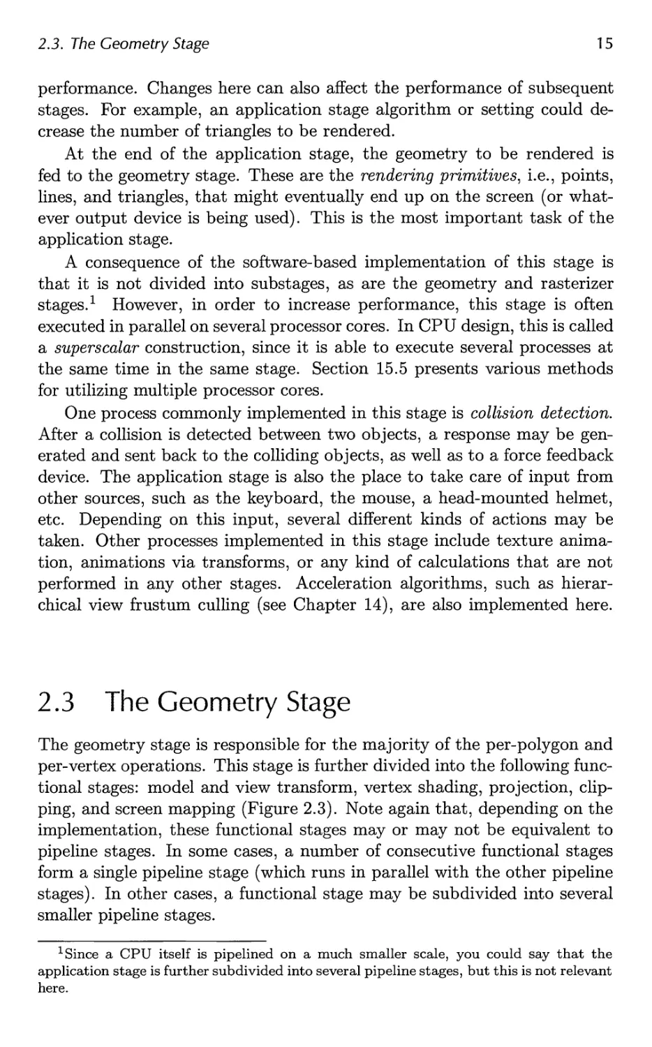
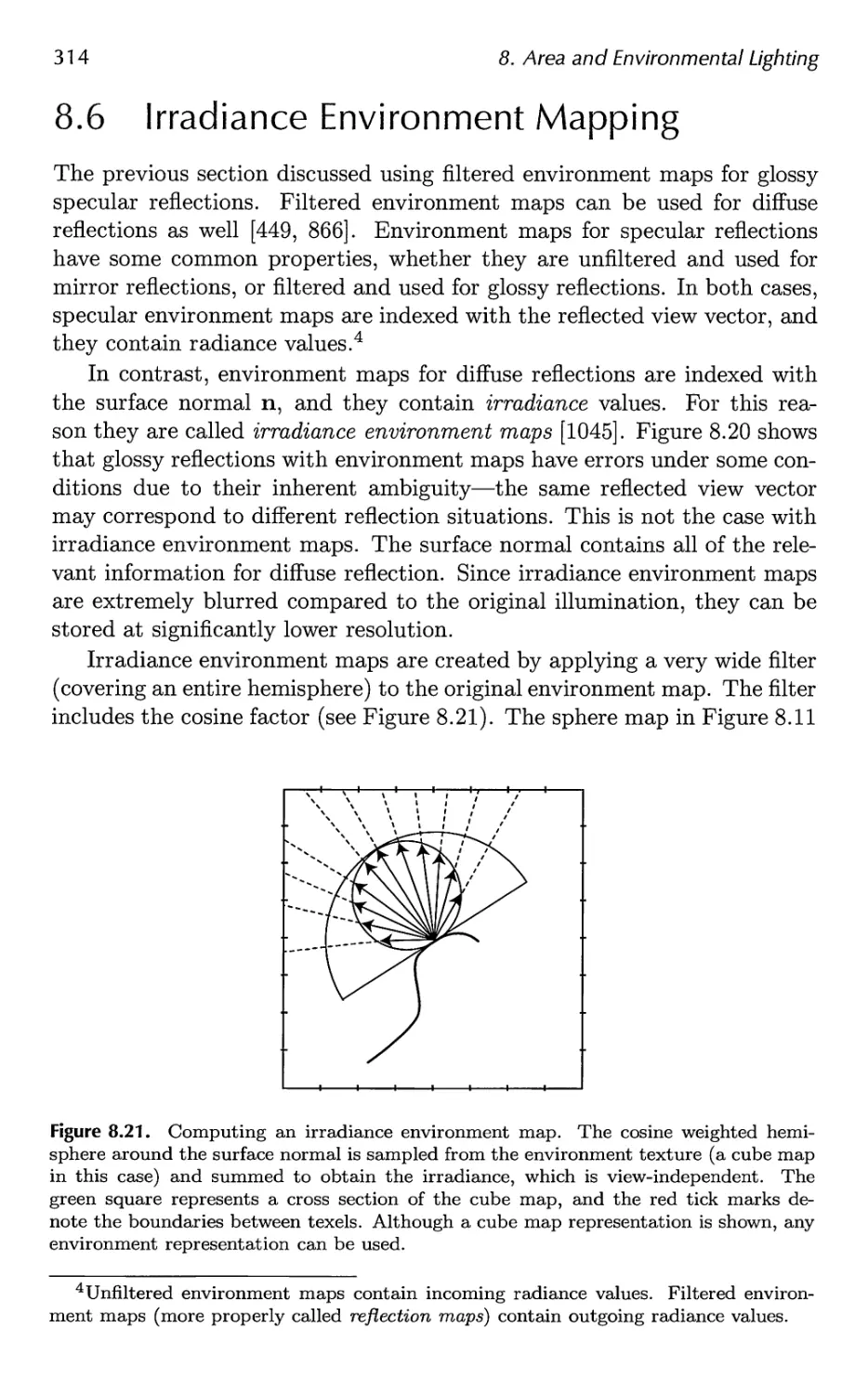
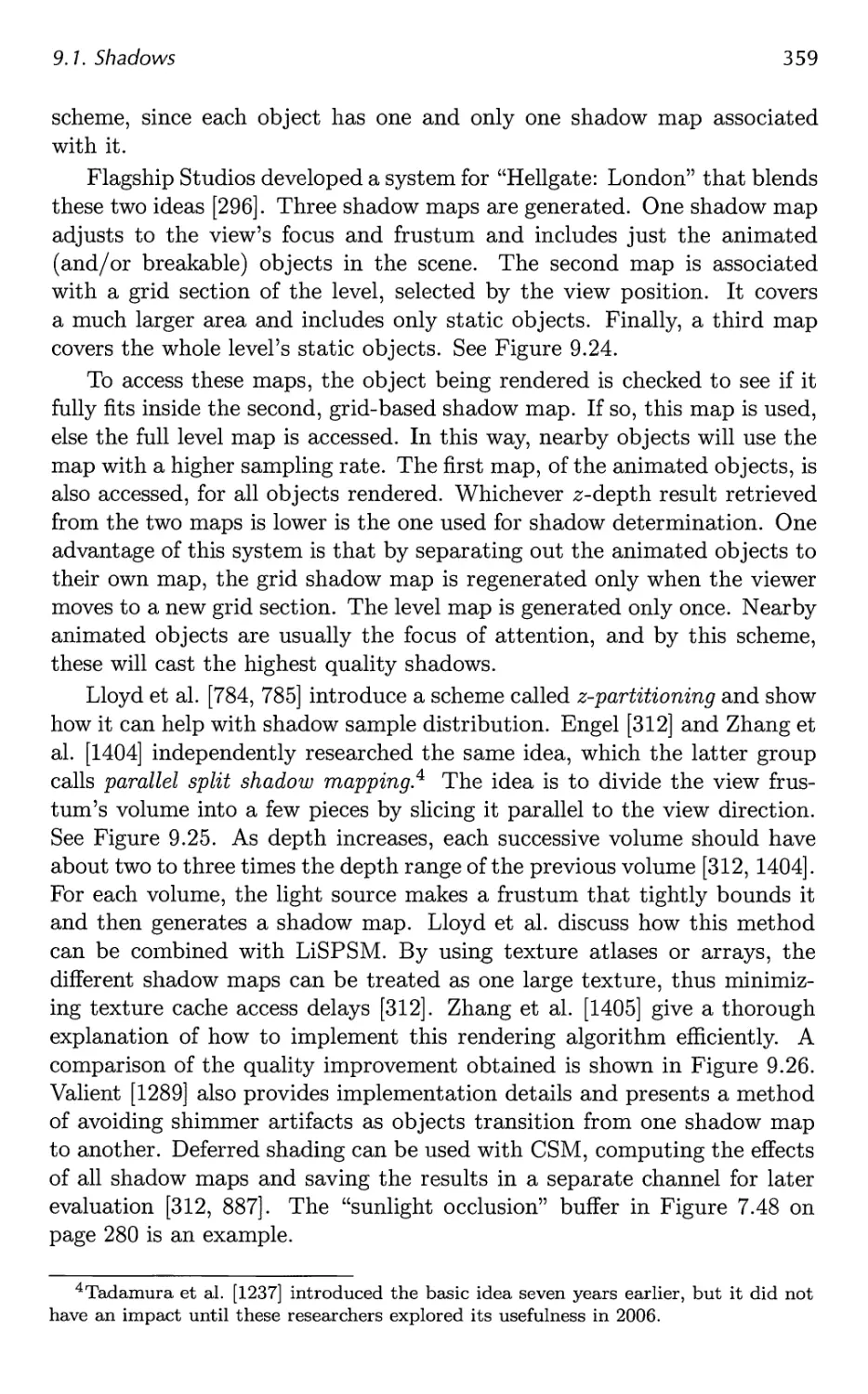
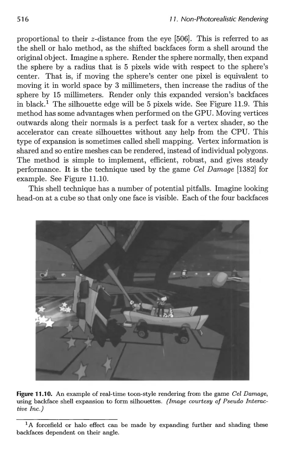
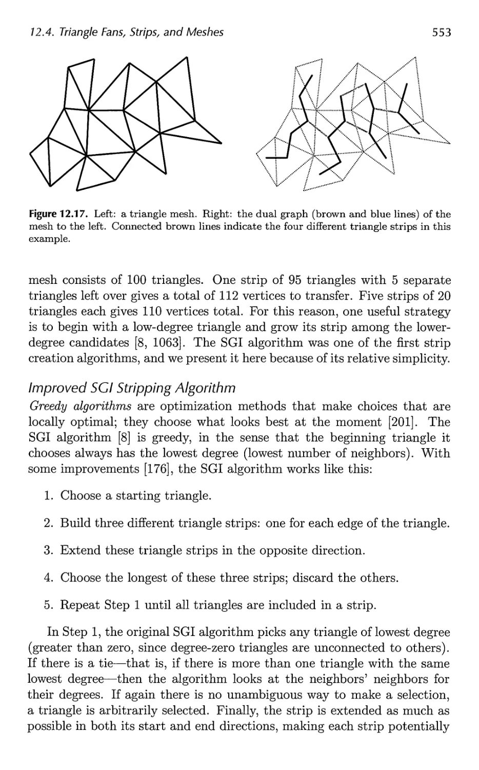
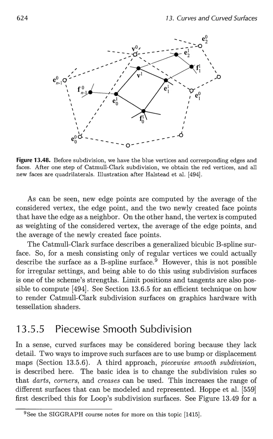
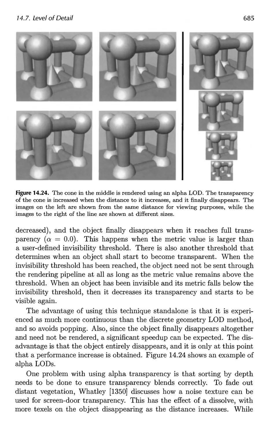
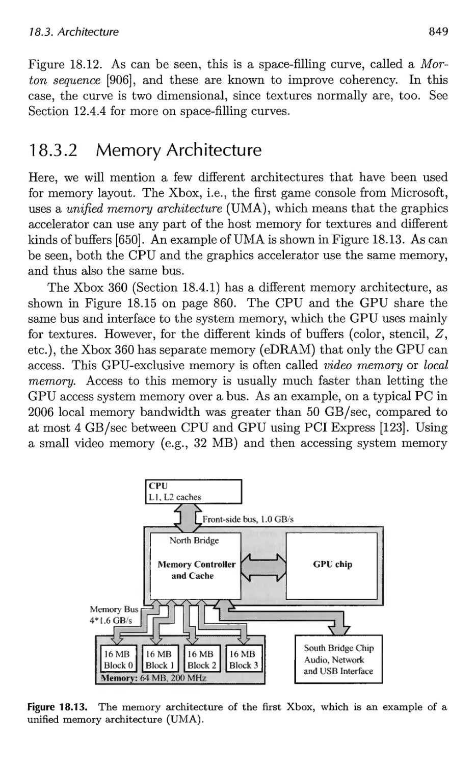
Figure 2.3. The geometry stage subdivided into a pipeline of functional stages.
For example, at one extreme, all stages in the entire rendering pipeline
may run in software on a single processor, and then you could say that your
entire pipeline consists of one pipeline stage. Certainly this was how all
graphics were generated before the advent of separate accelerator chips and
boards. At the other extreme, each functional stage could be subdivided
into several smaller pipeline stages, and each such pipeline stage could
execute on a designated processor core element.
2.3.1 Model and View Transform
On its way to the screen, a model is transformed into several different spaces
or coordinate systems. Originally, a model resides in its own model space,
which simply means that it has not been transformed at all. Each model
can be associated with a model transform so that it can be positioned and
oriented. It is possible to have several model transforms associated with
a single model. This allows several copies (called instances) of the same
model to have different locations, orientations, and sizes in the same scene,
without requiring replication of the basic geometry.
It is the vertices and the normals of the model that are transformed by
the model transform. The coordinates of an object are called model
coordinates, and after the model transform has been applied to these coordinates,
the model is said to be located in world coordinates or in world space. The
world space is unique, and after the models have been transformed with
their respective model transforms, all models exist in this same space.
As mentioned previously, only the models that the camera (or observer)
sees are rendered. The camera has a location in world space and a direction,
which are used to place and aim the camera. To facilitate projection and
clipping, the camera and all the models are transformed with the view
transform. The purpose of the view transform is to place the camera at
the origin and aim it, to make it look in the direction of the negative z-axis,2
with the y-axis pointing upwards and the x-axis pointing to the right. The
actual position and direction after the view transform has been applied are
dependent on the underlying application programming interface (API). The
2 We will be using the — z-axis convention; some texts prefer looking down the +z-axis.
The difference is mostly semantic, as transform between one and the other is simple.
2.3. The Geometry Stage
17
Camera direction
View transform View frustum
x x
Camera
position z z
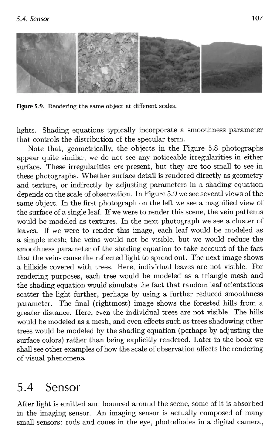
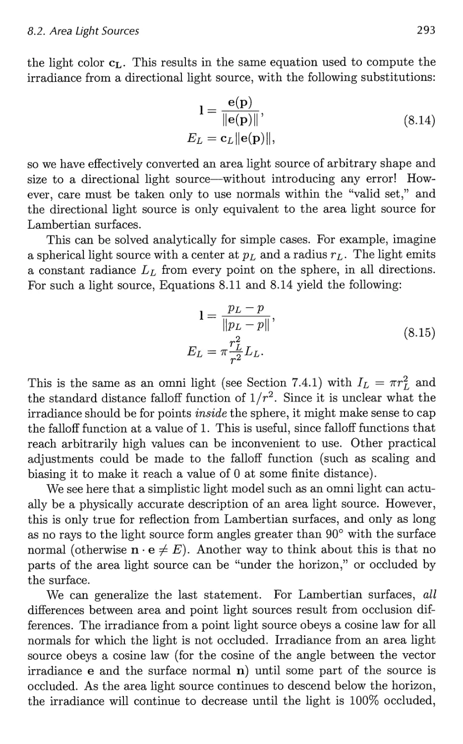
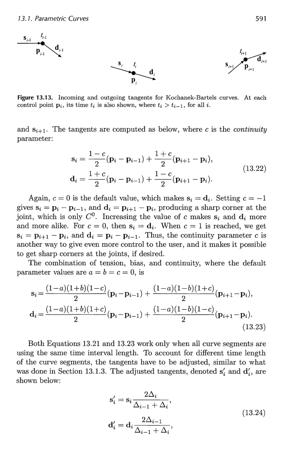
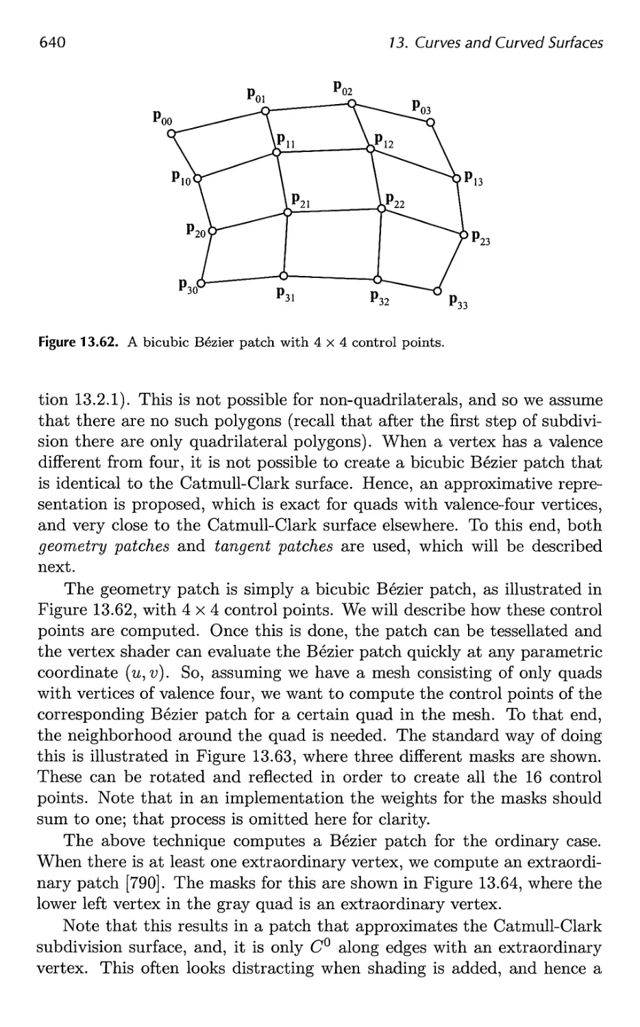
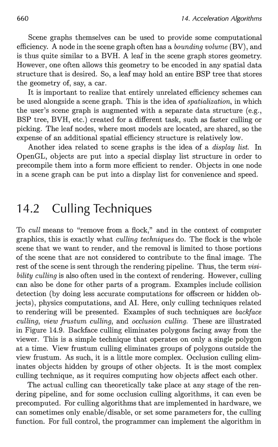
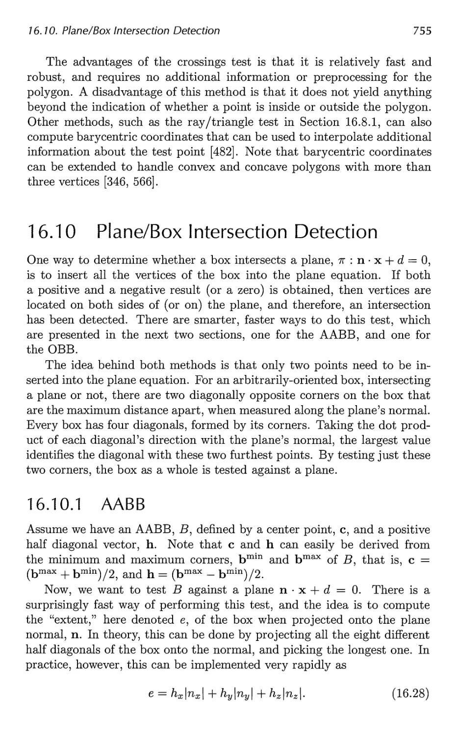
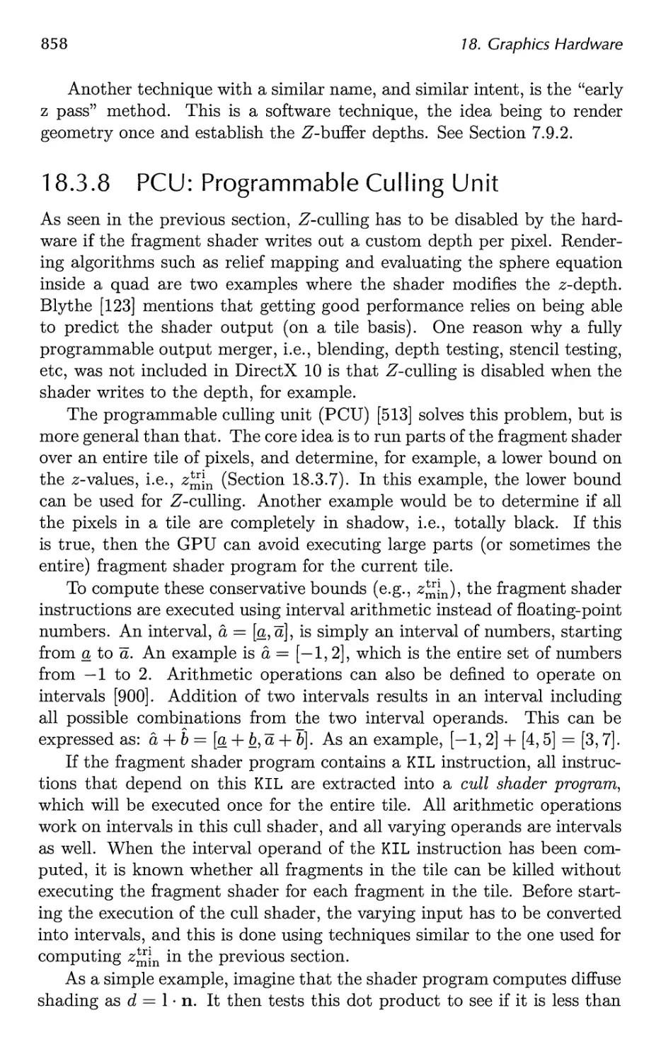
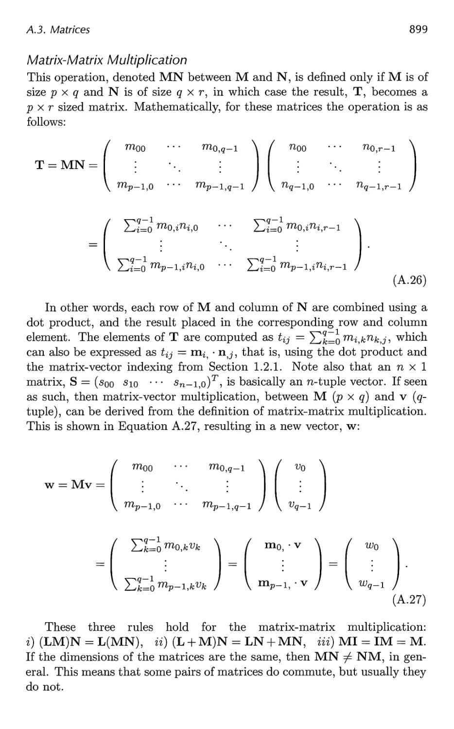
Figure 2.4. In the left illustration, the camera is located and oriented as the user wants
it to be. The view transform relocates the camera at the origin, looking along the
negative z-axis, as shown on the right. This is done to make the clipping and projection
operations simpler and faster. The light gray area is the view volume. Here, perspective
viewing is assumed, since the view volume is a frustum. Similar techniques apply to any
kind of projection.
space thus delineated is called the camera space, or more commonly, the
eye space. An example of the way in which the view transform affects the
camera and the models is shown in Figure 2.4. Both the model transform
and the view transform are implemented as 4 x 4 matrices, which is the
topic of Chapter 4.
2.3.2 Vertex Shading
To produce a realistic scene, it is not sufficient to render the shape and
position of objects, but their appearance must be modeled as well. This
description includes each object's material, as well as the effect of any light
sources shining on the object. Materials and lights can be modeled in any
number of ways, from simple colors to elaborate representations of physical
descriptions.
This operation of determining the effect of a light on a material is known
as shading. It involves computing a shading equation at various points on
the object. Typically, some of these computations are performed during
the geometry stage on a model's vertices, and others may be performed
during per-pixel rasterization. A variety of material data can be stored at
each vertex, such as the point's location, a normal, a color, or any other
numerical information that is needed to compute the shading equation.
Vertex shading results (which can be colors, vectors, texture coordinates,
or any other kind of shading data) are then sent to the rasterization stage
to be interpolated.
Shading computations are usually considered as happening in world
space. In practice, it is sometimes convenient to transform the relevant
entities (such as the camera and light sources) to some other space (such
18
2. The Graphics Rendering Pipeline
as model or eye space) and perform the computations there. This works
because the relative relationships between light sources, the camera, and
the models are preserved if all entities that are included in the shading
calculations are transformed to the same space.
Shading is discussed in more depth throughout this book, most
specifically in Chapters 3 and 5.
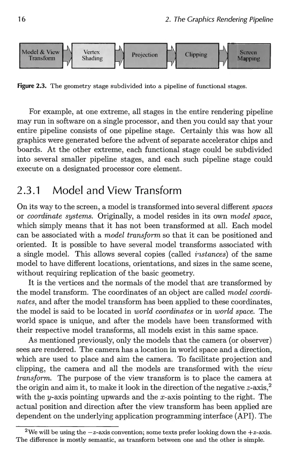
2.3.3 Projection
After shading, rendering systems perform projection, which transforms the
view volume into a unit cube with its extreme points at (—1,-1,-1) and
(1,1, l).3 The unit cube is called the canonical view volume. There are
two commonly used projection methods, namely orthographic (also called
parallel)4 and perspective projection. See Figure 2.5.
Figure 2.5. On the left is an orthographic, or parallel, projection; on the right is a
perspective projection.
3Different volumes can be used, for example 0 < z < 1. Blinn has an interesting
article [102] on using other intervals.
4Actually, orthographic is just one type of parallel projection. For example, there is
also an oblique parallel projection method [516], which is much less commonly used.
2.3. The Geometry Stage
19
The view volume of orthographic viewing is normally a rectangular
box, and the orthographic projection transforms this view volume into
the unit cube. The main characteristic of orthographic projection is that
parallel lines remain parallel after the transform. This transformation is a
combination of a translation and a scaling.
The perspective projection is a bit more complex. In this type of
projection, the farther away an object lies from the camera, the smaller it appears
after projection. In addition, parallel lines may converge at the horizon.
The perspective transform thus mimics the way we perceive objects' size.
Geometrically, the view volume, called a frustum, is a truncated pyramid
with rectangular base. The frustum is transformed into the unit cube as
well. Both orthographic and perspective transforms can be constructed
with 4x4 matrices (see Chapter 4), and after either transform, the models
are said to be in normalized device coordinates.
Although these matrices transform one volume into another, they are
called projections because after display, the ^-coordinate is not stored in
the image generated.5 In this way, the models are projected from three to
two dimensions.
2.3.4 Clipping
Only the primitives wholly or partially inside the view volume need to be
passed on to the rasterizer stage, which then draws them on the screen. A
primitive that lies totally inside the view volume will be passed on to the
next stage as is. Primitives entirely outside the view volume are not passed
on further, since they are not rendered. It is the primitives that are
partially inside the view volume that require clipping. For example, a line that
has one vertex outside and one inside the view volume should be clipped
against the view volume, so that the vertex that is outside is replaced by
a new vertex that is located at the intersection between the line and the
view volume. The use of a projection matrix means that the transformed
primitives are clipped against the unit cube. The advantage of performing
the view transformation and projection before clipping is that it makes the
clipping problem consistent; primitives are always clipped against the unit
cube. The clipping process is depicted in Figure 2.6. In addition to the six
clipping planes of the view volume, the user can define additional clipping
planes to visibly chop objects. An image showing this type of visualization,
called sectioning, is shown in Figure 14.1 on page 646. Unlike the previous
geometry stages, which are typically performed by programmable
processing units, the clipping stage (as well as the subsequent screen mapping
stage) is usually processed by fixed-operation hardware.
5Rather, the ^-coordinate is stored in a Z-buffer. See Section 2.4.
20
2. The Graphics Rendering Pipeline
unit-cube
new vertices
Clipping
x x
new vertex
z z
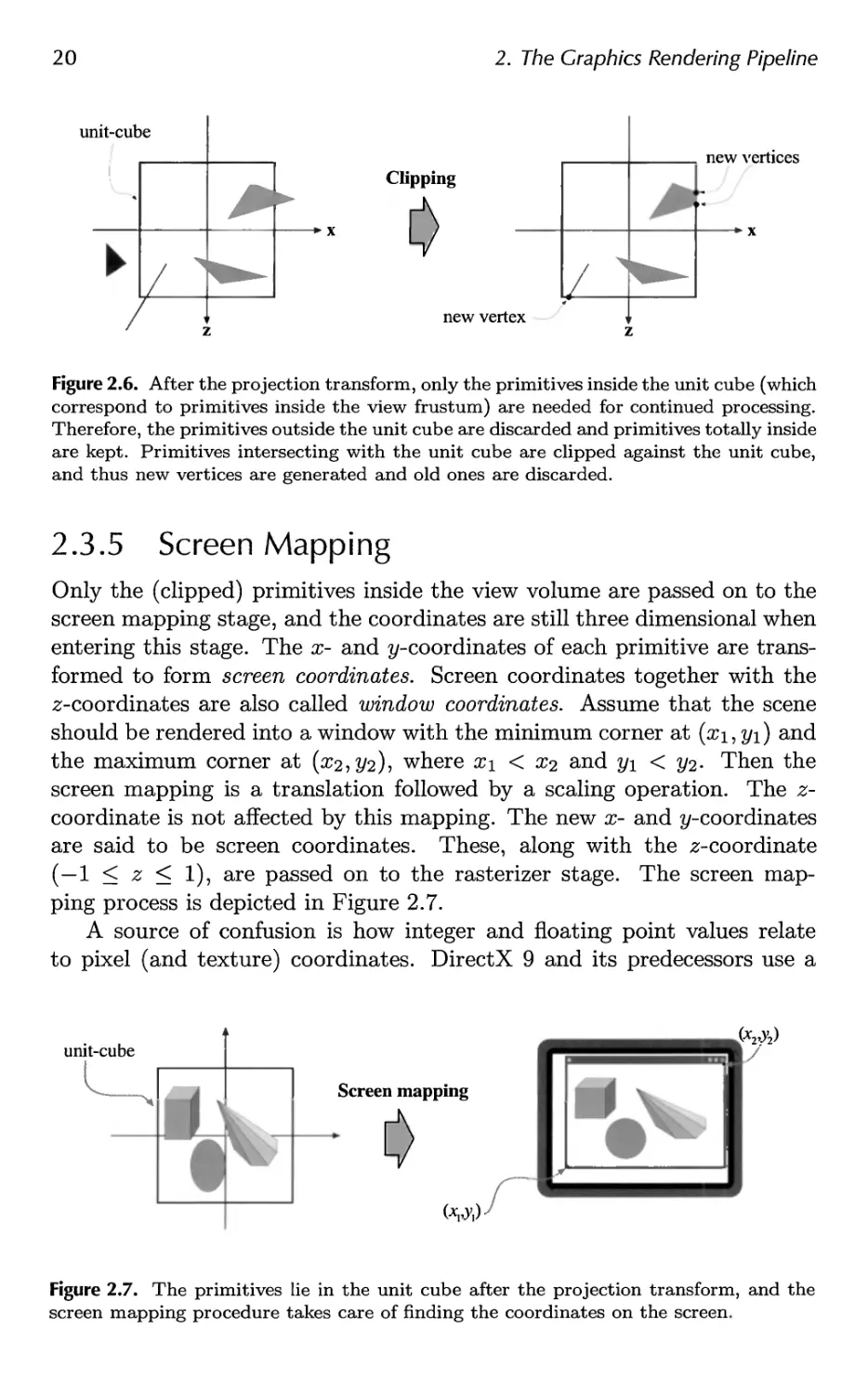
Figure 2.6. After the projection transform, only the primitives inside the unit cube (which
correspond to primitives inside the view frustum) are needed for continued processing.
Therefore, the primitives outside the unit cube are discarded and primitives totally inside
are kept. Primitives intersecting with the unit cube are clipped against the unit cube,
and thus new vertices are generated and old ones are discarded.
2.3.5 Screen Mapping
Only the (clipped) primitives inside the view volume are passed on to the
screen mapping stage, and the coordinates are still three dimensional when
entering this stage. The x- and ^-coordinates of each primitive are
transformed to form screen coordinates. Screen coordinates together with the
z-coordinates are also called window coordinates. Assume that the scene
should be rendered into a window with the minimum corner at (xi,yi) and
the maximum corner at (#2,2/2)? wnere xi < x2 and y\ < 2/2- Then the
screen mapping is a translation followed by a scaling operation. The z-
coordinate is not affected by this mapping. The new x- and ^-coordinates
are said to be screen coordinates. These, along with the z-coordinate
(—1 < z < 1), are passed on to the rasterizer stage. The screen
mapping process is depicted in Figure 2.7.
A source of confusion is how integer and floating point values relate
to pixel (and texture) coordinates. DirectX 9 and its predecessors use a
unit-cube
Screen mapping
(-W)
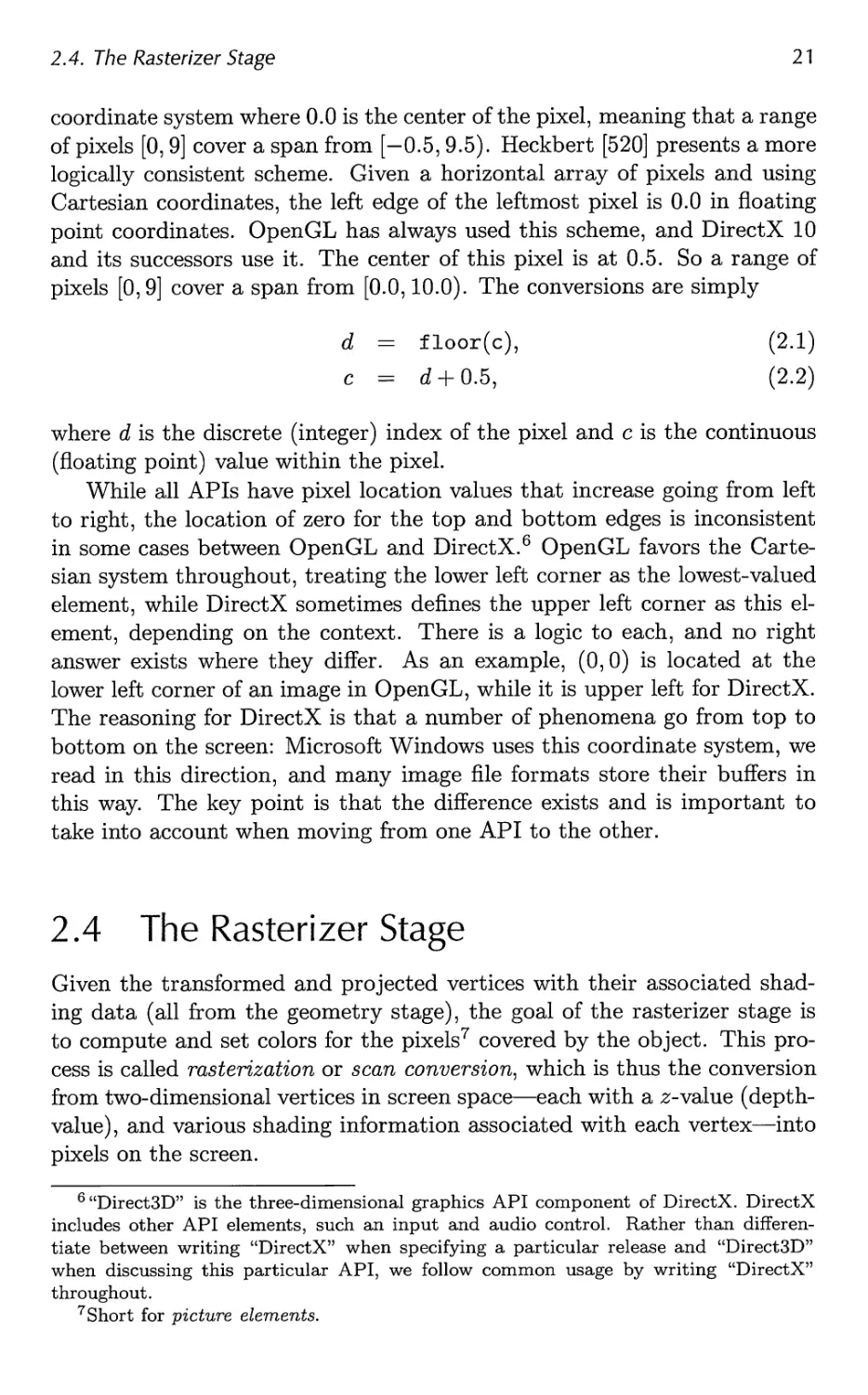
Figure 2.7. The primitives lie in the unit cube after the projection transform, and the
screen mapping procedure takes care of finding the coordinates on the screen.
2.4. The Rasterizer Stage
21
coordinate system where 0.0 is the center of the pixel, meaning that a range
of pixels [0,9] cover a span from [—0.5,9.5). Heckbert [520] presents a more
logically consistent scheme. Given a horizontal array of pixels and using
Cartesian coordinates, the left edge of the leftmost pixel is 0.0 in floating
point coordinates. OpenGL has always used this scheme, and DirectX 10
and its successors use it. The center of this pixel is at 0.5. So a range of
pixels [0,9] cover a span from [0.0,10.0). The conversions are simply
d = floor(c), (2.1)
c = d + 0.5, (2.2)
where d is the discrete (integer) index of the pixel and c is the continuous
(floating point) value within the pixel.
While all APIs have pixel location values that increase going from left
to right, the location of zero for the top and bottom edges is inconsistent
in some cases between OpenGL and DirectX.6 OpenGL favors the
Cartesian system throughout, treating the lower left corner as the lowest-valued
element, while DirectX sometimes defines the upper left corner as this
element, depending on the context. There is a logic to each, and no right
answer exists where they differ. As an example, (0,0) is located at the
lower left corner of an image in OpenGL, while it is upper left for DirectX.
The reasoning for DirectX is that a number of phenomena go from top to
bottom on the screen: Microsoft Windows uses this coordinate system, we
read in this direction, and many image file formats store their buffers in
this way. The key point is that the difference exists and is important to
take into account when moving from one API to the other.
2.4 The Rasterizer Stage
Given the transformed and projected vertices with their associated
shading data (all from the geometry stage), the goal of the rasterizer stage is
to compute and set colors for the pixels7 covered by the object. This
process is called rasterization or scan conversion, which is thus the conversion
from two-dimensional vertices in screen space—each with a z-value (depth-
value), and various shading information associated with each vertex—into
pixels on the screen.
6 "Direct3D" is the three-dimensional graphics API component of DirectX. DirectX
includes other API elements, such an input and audio control. Rather than
differentiate between writing "DirectX" when specifying a particular release and "Direct3D"
when discussing this particular API, we follow common usage by writing "DirectX"
throughout.
7 Short for picture elements.
22
2. The Graphics Rendering Pipeline
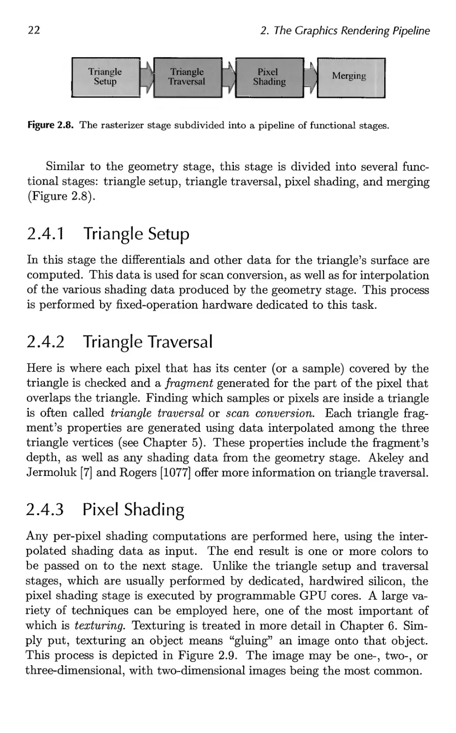
Figure 2.8. The rasterizer stage subdivided into a pipeline of functional stages.
Similar to the geometry stage, this stage is divided into several
functional stages: triangle setup, triangle traversal, pixel shading, and merging
(Figure 2.8).
2.4.1 Triangle Setup
In this stage the differentials and other data for the triangle's surface are
computed. This data is used for scan conversion, as well as for interpolation
of the various shading data produced by the geometry stage. This process
is performed by fixed-operation hardware dedicated to this task.
2.4.2 Triangle Traversal
Here is where each pixel that has its center (or a sample) covered by the
triangle is checked and a fragment generated for the part of the pixel that
overlaps the triangle. Finding which samples or pixels are inside a triangle
is often called triangle traversal or scan conversion. Each triangle
fragment's properties are generated using data interpolated among the three
triangle vertices (see Chapter 5). These properties include the fragment's
depth, as well as any shading data from the geometry stage. Akeley and
Jermoluk [7] and Rogers [1077] offer more information on triangle traversal.
2.4.3 Pixel Shading
Any per-pixel shading computations are performed here, using the
interpolated shading data as input. The end result is one or more colors to
be passed on to the next stage. Unlike the triangle setup and traversal
stages, which are usually performed by dedicated, hardwired silicon, the
pixel shading stage is executed by programmable GPU cores. A large
variety of techniques can be employed here, one of the most important of
which is texturing. Texturing is treated in more detail in Chapter 6.
Simply put, texturing an object means "gluing" an image onto that object.
This process is depicted in Figure 2.9. The image may be one-, two-, or
three-dimensional, with two-dimensional images being the most common.
2.4. The Rasterizer Stage
23
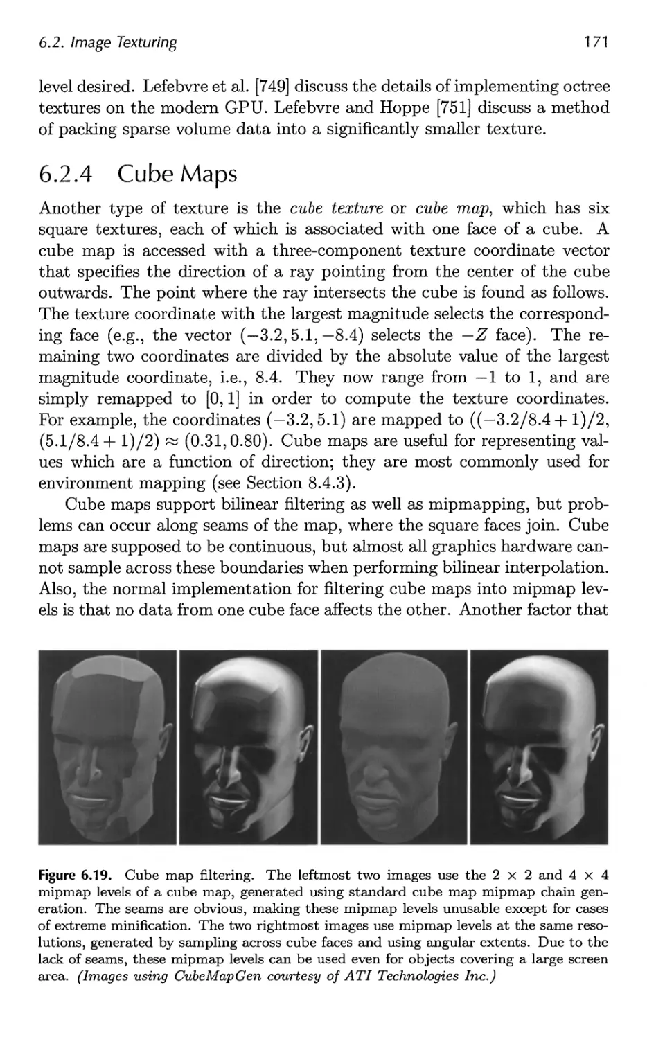
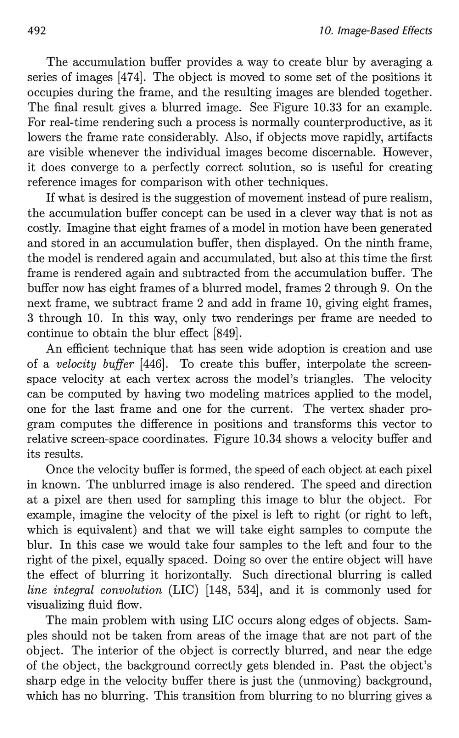
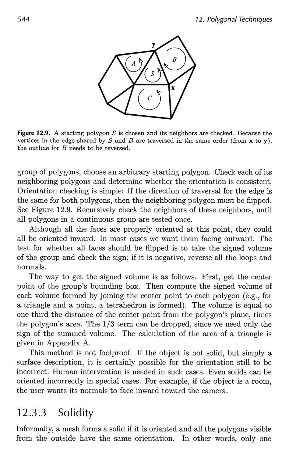
Figure 2.9. A dragon model without textures is shown in the upper left. The pieces in
the image texture are "glued" onto the dragon, and the result is shown in the lower left.
2.4.4 Merging
The information for each pixel is stored in the color buffer, which is a
rectangular array of colors (a red, a green, and a blue component for each
color). It is the responsibility of the merging stage to combine the fragment
color produced by the shading stage with the color currently stored in the
buffer. Unlike the shading stage, the GPU subunit that typically performs
this stage is not fully programmable. However, it is highly configurable,
enabling various effects.
This stage is also responsible for resolving visibility. This means that
when the whole scene has been rendered, the color buffer should contain
the colors of the primitives in the scene that are visible from the point of
view of the camera. For most graphics hardware, this is done with the
Z-buffer (also called depth buffer) algorithm [162].8 A Z-buffer is the same
size and shape as the color buffer, and for each pixel it stores the z-value
from the camera to the currently closest primitive. This means that when a
primitive is being rendered to a certain pixel, the z-value on that primitive
at that pixel is being computed and compared to the contents of the Z-
buffer at the same pixel. If the new z-value is smaller than the z-value
in the Z-buffer, then the primitive that is being rendered is closer to the
camera than the primitive that was previously closest to the camera at
that pixel. Therefore, the z-value and the color of that pixel are updated
8When a Z-buffer is not available, a BSP tree can be used to help render a scene in
back-to-front order. See Section 14.1.2 for information about BSP trees.
24
2. The Graphics Rendering Pipeline
with the z-value and color from the primitive that is being drawn. If the
computed z-value is greater than the z-value in the Z-buffer, then the color
buffer and the Z-buffer are left untouched. The Z-buffer algorithm is very
simple, has 0{n) convergence (where n is the number of primitives being
rendered), and works for any drawing primitive for which a z-value can be
computed for each (relevant) pixel. Also note that this algorithm allows
most primitives to be rendered in any order, which is another reason for its
popularity. However, partially transparent primitives cannot be rendered
in just any order. They must be rendered after all opaque primitives, and
in back-to-front order (Section 5.7). This is one of the major weaknesses
of the Z-buffer.
We have mentioned that the color buffer is used to store colors and
that the Z-buffer stores z-values for each pixel. However, there are other
channels and buffers that can be used to filter and capture fragment
information. The alpha channel is associated with the color buffer and stores
a related opacity value for each pixel (Section 5.7). An optional alpha test
can be performed on an incoming fragment before the depth test is
performed.9 The alpha value of the fragment is compared by some specified
test (equals, greater than, etc.) to a reference value. If the fragment fails to
pass the test, it is removed from further processing. This test is typically
used to ensure that fully transparent fragments do not affect the Z-buffer
(see Section 6.6).
The stencil buffer is an offscreen buffer used to record the locations of
the rendered primitive. It typically contains eight bits per pixel. Primitives
can be rendered into the stencil buffer using various functions, and the
buffer's contents can then be used to control rendering into the color buffer
and Z-buffer. As an example, assume that a filled circle has been drawn
into the stencil buffer. This can be combined with an operator that allows
rendering of subsequent primitives into the color buffer only where the
circle is present. The stencil buffer is a powerful tool for generating special
effects. All of these functions at the end of the pipeline are called raster
operations (ROP) or blend operations.
The frame buffer generally consists of all the buffers on a system, but
it is sometimes used to mean just the color buffer and Z-buffer as a set.
In 1990, Haeberli and Akeley [474] presented another complement to the
frame buffer, called the accumulation buffer. In this buffer, images can be
accumulated using a set of operators. For example, a set of images showing
an object in motion can be accumulated and averaged in order to generate
motion blur. Other effects that can be generated include depth of field,
antialiasing, soft shadows, etc.
9In DirectX 10, the alpha test is no longer part of this stage, but rather a function
of the pixel shader.
2.5. Through the Pipeline
25
When the primitives have reached and passed the rasterizer stage, those
that are visible from the point of view of the camera are displayed on screen.
The screen displays the contents of the color buffer. To avoid allowing the
human viewer to see the primitives as they are being rasterized and sent
to the screen, double buffering is used. This means that the rendering of
a scene takes place off screen, in a back buffer. Once the scene has been
rendered in the back buffer, the contents of the back buffer are swapped
with the contents of the front buffer that was previously displayed on the
screen. The swapping occurs during vertical retrace, a time when it is safe
to do so.
For more information on different buffers and buffering methods, see
Sections 5.6.2 and 18.1.
2.5 Through the Pipeline
Points, lines, and triangles are the rendering primitives from which a model
or an object is built. Imagine that the application is an interactive
computer aided design (CAD) application, and that the user is examining a
design for a cell phone. Here we will follow this model through the entire
graphics rendering pipeline, consisting of the three major stages:
application, geometry, and the rasterizer. The scene is rendered with perspective
into a window on the screen. In this simple example, the cell phone model
includes both lines (to show the edges of parts) and triangles (to show the
surfaces). Some of the triangles are textured by a two-dimensional
image, to represent the keyboard and screen. For this example, shading is
computed completely in the geometry stage, except for application of the
texture, which occurs in the rasterization stage.
Application
CAD applications allow the user to select and move parts of the model. For
example, the user might select the top part of the phone and then move
the mouse to flip the phone open. The application stage must translate the
mouse move to a corresponding rotation matrix, then see to it that this
matrix is properly applied to the lid when it is rendered. Another example:
An animation is played that moves the camera along a predefined path to
show the cell phone from different views. The camera parameters, such
as position and view direction, must then be updated by the application,
dependent upon time. For each frame to be rendered, the application stage
feeds the camera position, lighting, and primitives of the model to the next
major stage in the pipeline—the geometry stage.
Geometry
The view transform was computed in the application stage, along with a
model matrix for each object that specifies its location and orientation. For
26
2. The Graphics Rendering Pipeline
each object passed to the geometry stage, these two matrices are usually
multiplied together into a single matrix. In the geometry stage the vertices
and normals of the object are transformed with this concatenated matrix,
putting the object into eye space. Then shading at the vertices is computed,
using material and light source properties. Projection is then performed,
transforming the object into a unit cube's space that represents what the
eye sees. All primitives outside the cube are discarded. All primitives
intersecting this unit cube are clipped against the cube in order to obtain
a set of primitives that lies entirely inside the unit cube. The vertices then
are mapped into the window on the screen. After all these per-polygon
operations have been performed, the resulting data is passed on to the
rasterizer—the final major stage in the pipeline.
Rasterizer
In this stage, all primitives are rasterized, i.e., converted into pixels in the
window. Each visible line and triangle in each object enters the rasterizer in
screen space, ready to convert. Those triangles that have been associated
with a texture are rendered with that texture (image) applied to them.
Visibility is resolved via the Z-buffer algorithm, along with optional alpha
and stencil tests. Each object is processed in turn, and the final image is
then displayed on the screen.
Conclusion
This pipeline resulted from decades of API and graphics hardware evolution
targeted to real-time rendering applications. It is important to note that
this is not the only possible rendering pipeline; offline rendering pipelines
have undergone different evolutionary paths. Rendering for film production
is most commonly done with micropolygon pipelines [196, 1236]. Academic
research and predictive rendering applications such as architectural previ-
sualization usually employ ray tracing renderers (see Section 9.8.2).
For many years, the only way for application developers to use the
process described here was through a fixed-function pipeline defined by the
graphics API in use. The fixed-function pipeline is so named because the
graphics hardware that implements it consists of elements that cannot be
programmed in a flexible way. Various parts of the pipeline can be set to
different states, e.g., Z-buffer testing can be turned on or off, but there is
no ability to write programs to control the order in which functions are
applied at various stages. The latest (and probably last) example of a
fixed-function machine is Nintendo's Wii. Programmable GPUs make it
possible to determine exactly what operations are applied in various sub-
stages throughout the pipeline. While studying the fixed-function pipeline
provides a reasonable introduction to some basic principles, most new de-
2.5. Through the Pipeline
27
velopment is aimed at programmable GPUs. This programmability is the
default assumption for this third edition of the book, as it is the modern
way to take full advantage of the GPU.
Further Reading and Resources
Blinn's book A Trip Down the Graphics Pipeline [105] is an older book
about writing a software renderer from scratch, but is a good resource for
learning about some of the subtleties of implementing a rendering pipeline.
For the fixed-function pipeline, the venerable (yet frequently updated)
OpenGL Programming Guide (a.k.a., the "Red Book") [969] provides a
thorough description of the fixed-function pipeline and algorithms related
to its use. Our book's website, http://www.realtimerendering.com, gives
links to a variety of rendering engine implementations.
Chapter 3
The Graphics
Processing Unit
"The display is the computer."
—Jen-Hsun Huang
Historically, hardware graphics acceleration has started at the end of the
pipeline, first performing rasterization of a triangle's scanlines. Successive
generations of hardware have then worked back up the pipeline, to the point
where some higher level application-stage algorithms are being committed
to the hardware accelerator. Dedicated hardware's only advantage over
software is speed, but speed is critical.
Over the past decade, graphics hardware has undergone an incredible
transformation. The first consumer graphics chip to include hardware
vertex processing (NVIDIA's GeForce256) shipped in 1999. NVIDIA coined
the term graphics processing unit (GPU) to differentiate the GeForce 256
from the previously available rasterization-only chips, and it stuck [898].
Over the next few years, the GPU evolved from configurable
implementations of a complex fixed-function pipeline to highly programmable "blank
slates" where developers could implement their own algorithms.
Programmable shaders of various kinds are the primary means by which the
GPU is controlled. The vertex shader enables various operations
(including transformations and deformations) to be performed on each vertex.
Similarly, the pixel shader processes individual pixels, allowing complex
shading equations to be evaluated per pixel. The geometry shader allows
the GPU to create and destroy geometric primitives (points, lines,
triangles) on the fly. Computed values can be written to multiple high-precision
buffers and reused as vertex or texture data. For efficiency, some parts
of the pipeline remain configurable, not programmable, but the trend is
towards programmability and flexibility [123].
29
30
3. The Graphics Processing Unit
Figure 3.1. GPU implementation of the rendering pipeline. The stages are color codec-
according to the degree of user control over their operation. Green stages are fully
programmable. Yellow stages are configurable but not programmable, e.g., the clipping
stage can optionally perform culling or add user-defined clipping planes. Blue stages are
completely fixed in their function.
3.1 GPU Pipeline Overview
The GPU implements the geometry and rasterization conceptual pipeline
stages described in Chapter 2. These are divided into several hardware
stages with varying degrees of configurability or programmability.
Figure 3.1 shows the various stages color coded according to how programmable
or configurable they are. Note that these physical stages are split up slightly
differently than the functional stages presented in Chapter 2.
The vertex shader is a fully programmable stage that is typically used
to implement the "Model and View Transform," "Vertex Shading," and
"Projection" functional stages. The geometry shader is an optional, fully
programmable stage that operates on the vertices of a primitive (point, line
or triangle). It can be used to perform per-primitive shading operations,
to destroy primitives, or to create new ones. The clipping, screen mapping,
triangle setup, and triangle traversal stages are fixed-function stages that
implement the functional stages of the same names. Like the vertex and
geometry shaders, the pixel shader is fully programmable and performs the
"Pixel Shading" function stage. Finally, the merger stage is somewhere
between the full programmability of the shader stages and the fixed operation
of the other stages. Although it is not programmable, it is highly
configurable and can be set to perform a wide variety of operations. Of course,
it implements the "Merging" functional stage, in charge of modifying the
color, Z-buffer, blend, stencil, and other related buffers.
Over time, the GPU pipeline has evolved away from hard-coded
operation and toward increasing flexibility and control. The introduction
of programmable shader stages was the most important step in this
evolution. The next section describes the features common to the various
programmable stages.
3.2 The Programmable Shader Stage
Modern shader stages (i.e., those that support Shader Model 4.0, DirectX
10 and later, on Vista) use a common-shader core. This means that the
3.2. The Programmable Shader Stage
31
vertex, pixel, and geometry shaders share a programming model. We
differentiate in this book between the common-shader core, the functional
description seen by the applications programmer, and unified shaders, a
GPU architecture that maps well to this core. See Section 18.4. The
common-shader core is the API; having unified shaders is a GPU feature.
Earlier GPUs had less commonality between vertex and pixel shaders and
did not have geometry shaders. Nonetheless, most of the design elements
for this model are shared by older hardware; for the most part, older
versions' design elements are either simpler or missing, not radically different.
So, for now we will focus on Shader Model 4.0 and discuss older GPUs'
shader models in later sections.
Describing the entire programming model is well beyond the scope of
this book, and there are many documents, books, and websites that
already do so [261, 338, 647, 1084]. However, a few comments are in order.
Shaders are programmed using C-like shading languages such as HLSL, Cg,
and GLSL. These are compiled to a machine-independent assembly
language, also called the intermediate language (IL). Previous shader models
allowed programming directly in the assembly language, but as of DirectX
10, programs in this language are visible as debug output only [123]. This
assembly language is converted to the actual machine language in a
separate step, usually in the drivers. This arrangement allows compatibility
across different hardware implementations. This assembly language can
be seen as defining a virtual machine, which is targeted by the shading
language compiler.
This virtual machine is a processor with various types of registers and
data sources, programmed with a set of instructions. Since many
graphics operations are done on short vectors (up to length 4), the processor
has 4-way SIMD (single-instruction multiple-data) capabilities. Each
register contains four independent values. 32-bit single-precision floating-point
scalars and vectors are the basic data types; support for 32-bit integers has
recently been added, as well. Floating-point vectors typically contain data
such as positions (xyzw), normals, matrix rows, colors (rgba), or texture
coordinates (uvwq). Integers are most often used to represent counters,
indices, or bit masks. Aggregate data types such as structures, arrays,
and matrices are also supported. To facilitate working with vectors, swiz-
zling, the replication of any vector component, is also supported. That
is, a vector's elements can be reordered or duplicated as desired.
Similarly, masking, where only the specified vector elements are used, is also
supported.
A draw call invokes the graphics API to draw a group of primitives,
so causing the graphics pipeline to execute. Each programmable shader
stage has two types of inputs: uniform inputs, with values that remain
constant throughout a draw call (but can be changed between draw calls),
32
3. The Graphics Processing Unit
16 buffers of 128 arrays of
4096 registers 512 textures
Figure 3.2. Common-shader core virtual machine architecture and register layout, under
DirectX 10. The maximum available number is indicated next to each resource. Three
numbers separated by slashes refer to the limits for vertex, geometry, and pixel shaders
(from left to right).
and varying inputs, which are different for each vertex or pixel processed
by the shader. A texture is a special kind of uniform input that once was
always a color image applied to a surface, but that now can be thought of
as any large array of data. It is important to note that although shaders
have a wide variety of inputs, which they can address in different ways,
the outputs are extremely constrained. This is the most significant way
in which shaders are different from programs executing on general-purpose
processors. The underlying virtual machine provides special registers for
the different types of inputs and outputs. Uniform inputs are accessed
via read-only constant registers or constant buffers, so called because their
contents are constant across a draw call. The number of available constant
registers is much larger than the number of registers available for varying
inputs or outputs. This is because the varying inputs and outputs need to
be stored separately for each vertex or pixel, and the uniform inputs are
stored once and reused across all the vertices or pixels in the draw call.
The virtual machine also has general-purpose temporary registers, which
are used for scratch space. All types of registers can be array-indexed
using integer values in temporary registers. The inputs and outputs of the
shader virtual machine can be seen in Figure 3.2.
Operations that are common in graphics computations are efficiently
executed on modern GPUs. Typically, the fastest operations are scalar and
vector multiplications, additions, and their combinations, such as multiply-
add and dot-product. Other operations, such as reciprocal, square root,
3.3. The Evolution of Programmable Shading
33
sine, cosine, exponentiation, and logarithm, tend to be slightly more costly
but still fairly speedy. Texturing operations (see Chapter 6) are efficient,
but their performance may be limited by factors such as the time spent
waiting to retrieve the result of an access. Shading languages expose the
most common of these operations (such as additions and multiplications)
via operators such as * and +. The rest are exposed through intrinsic
functions, e.g., atanO, dot (), logO, and many others. Intrinsic functions
also exist for more complex operations, such as vector normalization and
reflection, cross products, matrix transpose and determinant, etc.
The term flow control refers to the use of branching instructions to
change the flow of code execution. These instructions are used to implement
high-level language constructs such as "if" and "case" statements, as well
as various types of loops. Shaders support two types of flow control. Static
flow control branches are based on the values of uniform inputs. This means
that the flow of the code is constant over the draw call. The primary benefit
of static flow control is to allow the same shader to be used in a variety of
different situations (e.g., varying numbers of lights). Dynamic flow control
is based on the values of varying inputs. This is much more powerful than
static flow control but is more costly, especially if the code flow changes
erratically between shader invocations. As discussed in Section 18.4.2, a
shader is evaluated on a number of vertices or pixels at a time. If the flow
selects the "if" branch for some elements and the "else" branch for others,
both branches must be evaluated for all elements (and the unused branch
for each element is discarded).
Shader programs can be compiled offline before program load or during
run time. As with any compiler, there are options for generating different
output files and for using different optimization levels. A compiled shader
is stored as a string of text, which is passed to the GPU via the driver.
3.3 The Evolution of Programmable Shading
The idea of a framework for programmable shading dates back to 1984 with
Cook's shade trees [194]. A simple shader and its corresponding shade tree
are shown in Figure 3.3. The RenderMan Shading Language [30, 1283] was
developed from this idea in the late 80's and is still widely used today for
film production rendering. Before GPUs supported programmable shaders
natively, there were several attempts to implement programmable shading
operations in real time via multiple rendering passes. The Quake III: Arena
scripting language was the first widespread commercial success in this area
in 1999 [558, 604]. In 2000, Peercy et al. [993] described a system that
translated RenderMan shaders to run in multiple passes on graphics hardware.
They found that GPUs lacked two features that would make this approach
34
3. The Graphics Processing Unit
final color
copper
color
float ka=0.5, ks=0.5;
float roughness 0.1;
float intensity;
color copper=(0.8,0.3,0.1);
intensity = ka*ambient() +
¦specular(normal,view,roughness)
final_color = intensity*copper;
weight of ambient
ambient
component
weight of
specular
component
specular
function
/t\
normal view surface
roughness
Figure 3.3. Shade tree for a simple copper shader, and its corresponding shader language
program. (After Cook [194]-)
very general: the ability to use computation results as texture coordinates
(dependent texture reads), and support for data types with extended range
and precision in textures and color buffers. One of the proposed data types
was a novel (at the time) 16-bit floating point representation. At this
time, no commercially available GPU supported programmable shading,
although most had highly configurable pipelines [898].
In early 2001, NVIDIA's GeForce 3 was the first GPU to support
programmable vertex shaders [778], exposed through DirectX 8.0 and
extensions to OpenGL. These shaders were programmed in an assembly-like
language that was converted by the drivers into microcode on the fly. Pixel
shaders were also included in DirectX 8.0, but pixel shader SM 1.1 fell
short of actual programmability—the very limited "programs" supported
were converted into texture blending states by the driver, which in turn
wired together hardware "register combiners." These "programs" were not
only limited in length (12 instructions or less) but also lacked the two
elements (dependent texture reads1 and float data) that Peercy et al. had
identified as crucial to true programmability.
Shaders at this time did not allow for flow control (branching), so
conditionals had to be emulated by computing both terms and selecting
or interpolating between the results. DirectX defined the concept of a
1The GeForce 3 did support a dependent texture read of sorts, but only in an
extremely limited fashion.
3.3. The Evolution of Programmable Shading
35
Shader Model to distinguish hardware with different shader capabilities.
The GeForce 3 supported vertex shader model 1.1 and pixel shader model
1.1 (shader model 1.0 was intended for hardware that never shipped).
During 2001, GPUs progressed closer to a general pixel shader programming
model. DirectX 8.1 added pixel shader models 1.2 to 1.4 (each meant for
different hardware), which extended the capabilities of the pixel shader
further, adding additional instructions and more general support for
dependent texture reads.
The year 2002 saw the release of DirectX 9.0 including Shader Model 2.0
(and its extended version 2.X), which featured truly programmable vertex
and pixel shaders. Similar functionality was also exposed under OpenGL
using various extensions. Support for arbitrary dependent texture reads
and storage of 16-bit floating point values was added, finally completing
the set of requirements identified by Peercy et al. in 2000 [993]. Limits
on shader resources such as instructions, textures, and registers were
increased, so shaders became capable of more complex effects. Support for
flow control was also added. The growing length and complexity of shaders
made the assembly programming model increasingly cumbersome.
Fortunately, DirectX 9.0 also included a new shader programming language
called HLSL (High Level Shading Language). HLSL was developed by
Microsoft in collaboration with NVIDIA, which released a cross-platform
variant called Cg [818]. Around the same time, the OpenGL ARB
(Architecture Review Board) released a somewhat similar language for OpenGL,
called GLSL [647, 1084] (also known as GLslang). These languages were
heavily influenced by the syntax and design philosophy of the C
programming language and also included elements from the RenderMan Shading
Language.
Shader Model 3.0 was introduced in 2004 and was an incremental
improvement, turning optional features into requirements, further
increasing resource limits and adding limited support for texture reads in vertex
shaders. When a new generation of game consoles was introduced in late
2005 (Microsoft's Xbox 360) and 2006 (Sony Computer Entertainment's
PLAYSTATION® 3 system), they were equipped with Shader Model 3.0-
level GPUs. The fixed-function pipeline is not entirely dead: Nintendo's
Wii console shipped in late 2006 with a fixed-function GPU [207]).
However, this is almost certainly the last console of this type, as even mobile
devices such as cell phones can use programmable shaders (see Section 18.4.3).
Other languages and environments for shader development are available.
For example, the Sh language [837, 838] allows the generation and
combination [839] of GPU shaders through a C++ library. This open-source
project runs on a number of platforms. On the other end of the spectrum,
several visual programming tools have been introduced to allow artists
(most of whom are not comfortable programming in C-like languages) to
36
3. The Graphics Processing Unit
Figure 3.4. A visual shader graph system for shader design. Various operations are
encapsulated in function boxes, selectable on the left. When selected, each function box
has adjustable parameters, shown on the right. Inputs and outputs for each function
box are linked to each other to form the final result, shown in the lower right of the
center frame. (Screenshot from "mental mill," mental images, inc.)
design shaders. Such tools include visual graph editors used to link
predefined shader building blocks, as well as compilers to translate the resulting
graphs to shading languages such as HLSL. A screenshot of one such tool
{mental mill, which is included in NVIDIA's FX Composer 2) is shown in
Figure 3.4. McGuire et al. [847] survey visual shader programming systems
and propose a high-level, abstract extension of the concept.
The next large step in programmability came in 2007. Shader Model
4.0 (included in DirectX 10.0 [123] and also available in OpenGL via
extensions), introduced several major features, such as the geometry shader
and stream output.
Shader Model 4.0 included a uniform programming model for all shaders
(vertex, pixel and geometry), the common-shader core described earlier.
Resource limits were further increased, and support for integer data types
(including bitwise operations) was added. Shader Model 4.0 also is notable
in that it supports only high-level language shaders (HLSL for DirectX and
GLSL for OpenGL)—there is no user-writable assembly language interface,
such as found in previous models.
GPU vendors, Microsoft, and the OpenGL ARB continue to refine and
extend the capabilities of programmable shading. Besides new versions of
existing APIs, new programming models such as NVIDIA's CUD A [211]
and AMD's CTM [994] have been targeted at non-graphics applications.
This area of general-purpose computations on the GPU (GPGPU) is briefly
discussed in Section 18.3.1.
3.3. The Evolution of Programmable Shading
37
3.3.1 Comparison of Shader Models
Although this chapter focuses on Shader Model 4.0 (the newest at time of
writing), often developers need to support hardware that uses older shading
models. For this reason we give a brief comparison between the capabilities
of several recent shading models: 2.0 (and its extended version of 2.X), 3.0
and 4.O.2 A listing of all the differences is beyond the scope of this book;
detailed information is available from the Microsoft Developer Network
(MSDN) and their DirectX SDK [261].
We focus on DirectX here, because of its distinct releases, versus
OpenGL's evolving levels of extensions, some approved by the OpenGL
Architecture Review Board (ARB), some vendor-specific. This extension
system has the advantage that cutting-edge features from a specific
independent hardware vendor (IHV) can be used immediately. DirectX 9 and
earlier support IHV variations by exposing "capability bits" that can be
examined to see if a GPU supports a feature. With DirectX 10, Microsoft has
moved sharply away from this practice and toward a standardized model
that all IHVs must support. Despite the focus here on DirectX, the
following discussion also has relevance to OpenGL, in that the associated
underlying GPUs of the same time periods have the same features.
Table 3.1 compares the capabilities of the various shader models. In
the table, "VS" stands for "vertex shader" and "PS" for "pixel shader"
(Shader Model 4.0 introduced the geometry shader, with capabilities
similar to those of the vertex shader). If neither "VS" nor "PS" appears, the row
applies to both vertex and pixel shaders. Since the virtual machine is 4-way
SIMD, each register can store between one and four independent values.
"Instruction Slots" refers to the maximum number of instructions that the
shader can contain. "Max. Steps Executed" indicates the maximum
number of instructions that can be executed, taking branching and looping into
account. "Temp. Registers" shows the number of general-purpose registers
that are available for storing intermediate results. "Constant Registers"
indicates the number of constant values that can be input to the shader.
"Flow Control, Predication" refers to the ability to compute conditional
expressions and execute loops via branching instructions and predication
(i.e., the ability to conditionally execute or skip an instruction). "Textures"
shows the number of distinct textures (see Chapter 6) that can be accessed
by the shader (each texture may be accessed multiple times). "Integer
Support" refers to the ability to operate on integer data types with bitwise
operators and integer arithmetic. "VS Input Registers" shows the number
of varying input registers that can be accessed by the vertex shader.
"Interpolator Registers" are output registers for the vertex shader and input
2 Shader Models 1.0 through 1.4 were early, limited versions that are no longer actively
used.
38
3. The Graphics Processing Unit
Introduced
VS Instruction Slots
VS Max. Steps Executed
PS Instruction Slots
PS Max. Steps Executed
Temp. Registers
VS Constant Registers
PS Constant Registers
Flow Control, Predication
VS Textures
PS Textures
Integer Support
VS Input Registers
Interpolator Registers
PS Output Registers
SM 2.0/2.X
DX 9.0, 2002
256
65536
> 966
>966
> 12°
> 256a
32
Optionald
None
16
No
16
83
4
SM 3.0
DX 9.0c, 2004
> 512a
65536
> 512a
65536
32
> 256 a
224
Yes
4e
16
No
16
10
4
SM 4.0
DX 10, 2007
4096
oo
> 65536a
oo
4096
14 x 4096 c
14 x 4096 c
Yes
128x512'
128x512'
Yes
16
16/32fl
8
"Minimum requirement (more can be used if available).
bMinimum of 32 texture and 64 arithmetic instructions.
c14 constant buffers exposed (+2 private, reserved for Microsoft/IHVs), each of which
can contain a maximum of 4096 constants.
dVertex shaders are required to support static flow control (based on constant values).
eSM 3.0 hardware typically has very limited formats and no filtering for vertex
textures.
'Up to 128 texture arrays, each of which can contain a maximum of 512 textures.
5Not including 2 color interpolators with limited precision and range.
^Vertex shader outputs 16 interpolators, which the geometry shader can expand
to 32.
Table 3.1. Shader capabilities, listed by DirectX shader model version [123, 261, 946,
1055].
registers for the pixel shader. They are so called because the values output
from the vertex shader are interpolated over the triangle before being sent
to the pixel shader. Finally, "PS Output Registers" shows the number of
registers that can be output from the pixel shader—each one is bound to
a different buffer, or render target.
3.4 The Vertex Shader
The vertex shader is the first stage in the functional pipeline shown in
Figure 3.2. While this is the first stage that does any graphical processing,
it is worth noting that some data manipulation happens before this stage.
In what DirectX calls the input assembler [123, 261], a number of streams
of data can be woven together to form the sets of vertices and primitives
sent down the pipeline. For example, an object could be represented by one
array of positions and one array of colors. The input assembler would create
3.4. The Vertex Shader
39
this object's triangles (or lines or points) by essentially creating vertices
with positions and colors. A second object could use the same array of
positions (along with a different model transform matrix) and a different
array of colors for its representation. Data representation is discussed in
detail in Section 12.4.5. There is also support in the input assembler to
perform instancing. This allows an object to be drawn a number of times
with some varying data per instance, all with a single draw call. The use
of instancing is covered in Section 15.4.2. The input assembler in DirectX
10 also tags each instance, primitive, and vertex with an identifier number
that can be accessed by any of the shader stages that follow. For earlier
shader models, such data has to be added explicitly to the model.
A triangle mesh is represented by a set of vertices and additional
information describing which vertices form each triangle. The vertex shader is
the first stage to process the triangle mesh. The data describing what
triangles are formed is unavailable to the vertex shader; as its name implies,
it deals exclusively with the incoming vertices. In general terms, the vertex
shader provides a way to modify, create, or ignore values associated with
each polygon's vertex, such as its color, normal, texture coordinates, and
position. Normally the vertex shader program transforms vertices from
model space to homogeneous clip space; at a minimum, a vertex shader
must always output this location.
This functionality was first introduced in 2001 with DirectX 8. Because
it was the first stage on the pipeline and invoked relatively infrequently, it
could be implemented on either the GPU or the CPU, which would then
send on the results to the GPU for rasterization. Doing so made the
transition from older to newer hardware a matter of speed, not functionality.
All GPUs currently produced support vertex shading.
A vertex shader itself is very much the same as the common core virtual
machine described earlier in Section 3.2. Every vertex passed in is processed
by the vertex shader program, which then outputs a number of values that
are interpolated across a triangle or line.3 The vertex shader can neither
create nor destroy vertices, and results generated by one vertex cannot be
passed on to another vertex. Since each vertex is treated independently,
any number of shader processors on the GPU can be applied in parallel to
the incoming stream of vertices.
Chapters that follow explain a number of vertex shader effects, such as
shadow volume creation, vertex blending for animating joints, and
silhouette rendering. Other uses for the vertex shader include:
• Lens effects, so that the screen appears fish-eyed, underwater, or
otherwise distorted.
3 Older shader models also supported output of the size of a point sprite particle
object, but sprite functionality is now part of the geometry shader.
40
3. The Graphics Processing Unit
Figure 3.5. On the left, a normal teapot. A simple shear operation performed by
a vertex shader program produces the middle image. On the right, a noise function
creates a field that distorts the model. (Images produced by FX Composer 2, courtesy
of NVIDIA Corporation.)
• Object definition, by creating a mesh only once and having it be
deformed by the vertex shader.
• Object twist, bend, and taper operations.
• Procedural deformations, such as the movement of flags, cloth, or
water [592].
• Primitive creation, by sending degenerate meshes down the pipeline
and having these be given an area as needed. This functionality is
replaced by the geometry shader in newer GPUs.
• Page curls, heat haze, water ripples, and other effects can be done
by using the entire frame buffer's contents as a texture on a screen-
aligned mesh undergoing procedural deformation.
• Vertex texture fetch (available in SM 3.0 on up) can be used to apply
textures to vertex meshes, allowing ocean surfaces and terrain height
fields to be applied inexpensively [23, 703, 887].
Some deformations done using a vertex shader are shown in Figure 3.5.
The output of the vertex shader can be consumed in a number of
different ways. The usual path is for each instance's triangles to then be
generated and rasterized, and the individual pixel fragments produced sent
to the pixel shader program for continued processing. With the
introduction of Shader Model 4.0, the data can also be sent to the geometry shader,
streamed out, or both. These options are the subject of the next section.
3.5 The Geometry Shader
The geometry shader was added to the hardware-accelerated graphics
pipeline with the release of DirectX 10, in late 2006. It is located immediately
3.5. The Geometry Shader
41
after the vertex shader in the pipeline, and its use is optional. While a
required part of Shader Model 4.0, it is not used in earlier shader models.
The input to the geometry shader is a single object and its associated
vertices. The object is typically a triangle in a mesh, a line segment,
or simply a point. In addition, extended primitives can be defined and
processed by the geometry shader. In particular, three additional vertices
outside of a triangle can be passed in, and the two adjacent vertices on a
polyline can be used. See Figure 3.6.
The geometry shader processes this primitive and outputs zero or more
primitives. Output is in the form of points, polylines, and triangle strips.
More than one triangle strip, for example, can be output by a single
invocation of the geometry shader program. As important, no output at all can
be generated by the geometry shader. In this way, a mesh can be selectively
modified by editing vertices, adding new primitives, and removing others.
The geometry shader program is set to input one type of object and
output one type of object, and these types do not have to match. For
example, triangles could be input and their centroids be output as points,
one per triangle input. Even if input and output object types match, the
data carried at each vertex can be omitted or expanded. As an example,
the triangle's plane normal could be computed and added to each output
vertex's data. Similar to the vertex shader, the geometry shader must
output a homogeneous clip space location for each vertex produced.
The geometry shader is guaranteed to output results from primitives
in the same order as they are input. This affects performance, because
if a number of shader units run in parallel, results must be saved and
ordered. As a compromise between capability and efficiency, there is a limit
in Shader Model 4.0 of a total of 1024 32-bit values that can be generated
per execution. So, generating a thousand bush leaves given a single leaf
as input is not feasible and is not the recommended use of the geometry
shader. Tessellation of simple surfaces into more elaborate triangle meshes
is also not recommended [123]. This stage is more about programmatically
modifying incoming data or making a limited number of copies, not about
Figure 3.6. Geometry shader input for a geometry shader program is of some single
type: point, line segment, triangle. The two rightmost primitives, which include vertices
adjacent to the line and triangle objects, can also be used.
42
3. The Graphics Processing Unit
Figure 3.7. Some uses of the geometry shader. On the left, metaball isosurface
tessellation is performed on the fly using the GS. In the middle, fractal subdivision of line
segments is done using the GS and stream out, and billboards are generated by the GS
for display. On the right, cloth simulation is performed by using the vertex and
geometry shader with stream out. (Images from NVIDIA SDK 10 [945] samples courtesy of
NVIDIA Corporation.)
massively replicating or amplifying it. For example, one use is to generate
six transformed copies of data in order to simultaneously render the six
faces of a cube map; see Section 8.4.3. Additional algorithms that can take
advantage of the geometry shader include creating various sized particles
from point data, extruding fins along silhouettes for fur rendering, and
finding object edges for shadow algorithms. See Figure 3.7 for still more.
These and other uses are discussed throughout the rest of the book.
3.5.1 Stream Output
The standard use of the GPU's pipeline is to send data through the vertex
shader, then rasterize the resulting triangles and process these in the pixel
shader. The data always passed through the pipeline and intermediate
results could not be accessed. The idea of stream output was introduced in
Shader Model 4.0. After vertices are processed by the vertex shader (and,
optionally, the geometry shader), these can be output in a stream, i.e.,
an ordered array, in addition to being sent on to the rasterization stage.
Rasterization could, in fact, be turned off entirely and the pipeline then
used purely as a non-graphical stream processor. Data processed in this way
can be sent back through the pipeline, thus allowing iterative processing.
This type of operation is particularly useful for simulating flowing water or
other particle effects, as discussed in Section 10.7.
3.6 The Pixel Shader
After the vertex and geometry shaders perform their operations, the
primitive is clipped and set up for rasterization, as explained in the last chapter.
3.6. The Pixel Shader
43
This section of the pipeline is relatively fixed in its processing steps, not
programmable.4 Each triangle is traversed and the values at the vertices
interpolated across the triangle's area. The pixel shader is the next
programmable stage. In OpenGL this stage is known as the fragment shader,
which in some ways is a better name. The idea is that a triangle covers each
pixel's cell fully or partially, and the material portrayed is opaque or
transparent. The rasterizer does not directly affect the pixel's stored color, but
rather generates data that, to a greater or lesser extent, describes how the
triangle covers the pixel cell. It is then during merging that this fragment's
data is used to modify what is stored at the pixel.
The vertex shader program's outputs effectively become the pixel shader
program's inputs. A total of 16 vectors (4 values each) can be passed from
the vertex shader to the pixel shader in Shader Model 4.O.5 When the
geometry shader is used, it can output 32 vectors to the pixel shader [261].
Additional inputs were added specifically for the pixel shader with the
introduction of Shader Model 3.0. For example, which side of a triangle
is visible was added as an input flag. This knowledge is important for
rendering a different material on the front versus back of each triangle in
a single pass. The screen position of the fragment is also available to the
pixel shader.
The pixel shader's limitation is that it can influence only the fragment
handed it. That is, when a pixel shader program executes, it cannot send its
results directly to neighboring pixels. Rather, it uses the data interpolated
from the vertices, along with any stored constants and texture data, to
compute results that will affect only a single pixel. However, this limitation
is not as severe as it sounds. Neighboring pixels can ultimately be affected
by using image processing techniques, described in Section 10.9.
The one case in which the pixel shader can access information for
adjacent pixels (albeit indirectly) is the computation of gradient or
derivative information. The pixel shader has the ability to take any value and
compute the amount by which it changes per pixel along the x and y
screen axes. This is useful for various computations and texture
addressing. These gradients are particularly important for operations such as
filtering (see Section 6.2.2). Most GPUs implement this feature by
processing pixels in groups of 2 x 2 or more. When the pixel shader
requests a gradient value, the difference between adjacent pixels is returned.
One result of this implementation is that gradient information cannot
be accessed in parts of the shader affected by dynamic flow control—all
the pixels in a group must be processing the same instructions. This
is a fundamental limitation which exists even in offline rendering sys-
4The notable exception is that the pixel shader program can specify what type of
interpolation is used, e.g., perspective corrected or screen space (or none at all).
5In DirectX 10.1 the vertex shader will both input and output 32 vectors.
44
3. The Graphics Processing Unit
terns [31]. The ability to access gradient information is a unique capability
of the pixel shader, not shared by any of the other programmable shader
stages.
Pixel shader programs typically set the fragment color for merging in
the final merging stage. The depth value generated in the rasterization
stage can also be modified by the pixel shader. The stencil buffer value is
not modifiable, but rather is passed through to the merge stage. In SM 2.0
and on, a pixel shader can also discard incoming fragment data, i.e.,
generate no output. Such operations can cost performance, as optimizations
normally performed by the GPU cannot then be used. See Section 18.3.7
for details. Operations such as fog computation and alpha testing have
moved from being merge operations to being pixel shader computations in
SM4.0 [123].
Current pixel shaders are capable of doing a huge amount of processing.
The ability to compute any number of values in a single rendering pass gave
rise to the idea of multiple render targets (MRT). Instead of saving results
of a pixel shader's program to a single color buffer, multiple vectors could
be generated for each fragment and saved to different buffers. These buffers
must be the same dimensions, and some architectures require them each to
have the same bit depth (though with different formats, as needed). The
number of PS output registers in Table 3.1 refers to the number of separate
buffers accessible, i.e., 4 or 8. Unlike the displayable color buffer, there are
other limitations on any additional targets. For example, typically no
antialiasing can be performed. Even with these limitations, MRT functionality
is a powerful aid in performing rendering algorithms more efficiently. If a
number of intermediate results images are to be computed from the same
set of data, only a single rendering pass is needed, instead of one pass per
output buffer. The other key capability associated with MRTs is the ability
to read from these resulting images as textures.
3.7 The Merging Stage
As discussed in Section 2.4.4, the merging stage is where the depths and
colors of the individual fragments (generated in the pixel shader) are
combined with the frame buffer. This stage is where stencil-buffer and Z-buffer
operations occur. Another operation that takes place in this stage is color
blending, which is most commonly used for transparency and compositing
operations (see Section 5.7).
The merging stage occupies an interesting middle point between the
fixed-function stages, such as clipping, and the fully programmable shader
stages. Although it is not programmable, its operation is highly
configurable. Color blending in particular can be set up to perform a large
3.8. Effects
45
number of different operations. The most common are combinations of
multiplication, addition, and subtraction involving the color and alpha
values, but other operations are possible, such as minimum and maximum,
as well as bitwise logic operations. DirectX 10 added the capability to
blend two colors from the pixel shader with the frame buffer color—this
capability is called dual-color blending.
If MRT functionality is employed, then blending can be performed on
multiple buffers. DirectX 10.1 introduced the capability to perform
different blend operations on each MRT buffer. In previous versions, the
same blending operation was always performed on all buffers (note that
dual-color blending is incompatible with MRT).
3.8 Effects
This tour of the pipeline has focused so far on the various programmable
stages. While vertex, geometry, and pixel shader programs are necessary
to control these stages, they do not exist in a vacuum. First, an individual
shader program is not particularly useful in isolation: A vertex shader
program feeds its results to a pixel shader. Both programs must be loaded for
any work to be done. The programmer must perform some matching of the
outputs of the vertex shader to the inputs of the pixel shader. A
particular rendering effect may be produced by any number of shader programs
executed over a few passes. Beyond the shader programs themselves, state
variables must sometimes be set in a particular configuration for these
programs to work properly. For example, the Tenderer's state includes whether
and how the Z-buffer and stencil buffer are each used, and how a fragment
affects the existing pixel value (e.g., replace, add, or blend).
For these reasons, various groups have developed effects languages, such
as HLSL FX, CgFX, and COLLADA FX. An effect file attempts to
encapsulate all the relevant information needed to execute a particular rendering
algorithm [261, 974]. It typically defines some global arguments that can
be assigned by the application. For example, a single effect file might define
the vertex and pixel shaders needed to render a convincing plastic material.
It would expose arguments such as the plastic color and roughness so that
these could be changed for each model rendered, but using the same effect
file.
To show the flavor of an effect file, we will walk through a trimmed-
down example taken from NVIDIA's FX Composer 2 effects system. This
DirectX 9 HLSL effect file implements a very simplified form of Gooch
shading [423]. One part of Gooch shading is to use the surface normal and
compare it to the light's location. If the normal points toward the light, a
warm tone is used to color the surface; if it points away, a cool tone is used.
46
3. The Graphics Processing Unit
Figure 3.8. Gooch shading, varying from a warm orange to a cool blue. (Image produced
by FX Composer 2, courtesy of NVIDIA Corporation.)
Angles in between interpolate between these two user-defined colors. This
shading technique is a form of non-photorealistic rendering, the subject of
Chapter 11. An example of this effect in action is shown in Figure 3.8.
Effect variables are defined at the beginning of the effect file. The
first few variables are "untweakables," parameters related to the camera
position that are automatically tracked for the effect:
float4x4 WorldXf
float4x4 WorldlTXf
float4x4 WvpXf
World;
WorldlnverseTranspose;
WorldViewProjection;
The syntax is type id : semantic. The type f loat4x4 is used for matrices,
the name is user defined, and the semantic is a built-in name. As the
semantic names imply, the WorldXf is the mo del-to-world transform matrix,
the WorldlTXf is the inverse transpose of this matrix, and the WvpXf is
the matrix that transforms from model space to the camera's clip space.
These values with recognized semantics are expected to be provided by the
application and not shown in the user interface.
Next, the user-defined variables are specified:
float3 LampOPos : Position <
string Object = "PointLightO";
string UIName = "Lamp 0 Position";
string Space = "World";
> = {-0.5f, 2.Of, 1.25f};
float3 WarmColor <
string UIName = "Gooch Warm Tone";
string UlWidget = "Color";
> = {1.3f, 0.9f, 0.15f};
3.8. Effects
47
float3 CoolColor <
string UIName = "Gooch Cool Tone";
string UlWidget = "Color";
> = {0.05f, 0.05f, 0.6f};
Here some additional annotations are provided inside the angle brackets
"<>" and then default values are assigned. The annotations are application-
specific and have no meaning to the effect or to the shader compiler. Such
annotations can be queried by the application. In this case the annotations
describe how to expose these variables within the user interface.
Data structures for shader input and output are defined next:
struct appdata {
float3 Position : POSITION;
float3 Normal : NORMAL;
>;
struct vertexOutput {
float4 HPosition
float3 LightVec
float3 WorldNormal
>;
POSITION;
TEXC00RD1;
TEXC00RD2;
The appdata defines what data is at each vertex in the model and so
defines the input data for the vertex shader program. The vertexOutput
is what the vertex shader produces and the pixel shader consumes. The
use of TEXCOORD* as the output names is an artifact of the evolution of the
pipeline. At first, multiple textures could be attached to a surface, so these
additional datafields are called texture coordinates. In practice, these fields
hold any data that is passed from the vertex to the pixel shader.
Next, the various shader program code elements are defined. We have
only one vertex shader program:
vertexOutput std_VS(appdata IN) {
vertexOutput OUT;
float4 No = float4(IN.Normal,0);
OUT.WorldNormal = mul(No,WorldITXf).xyz;
float4 Po = float4(IN.Position,1);
float4 Pw = mul(Po,WorldXf);
OUT.LightVec = (LampOPos - Pw.xyz);
OUT.HPosition = mul(Po,WvpXf);
return OUT;
48
3. The Graphics Processing Unit
This program first computes the surface's normal in world space by using
a matrix multiplication. Transforms are the subject of the next chapter,
so we will not explain why the inverse transpose is used here. The position
in world space is also computed by applying the offscreen transform. This
location is subtracted from the light's position to obtain the direction vector
from the surface to the light. Finally, the object's position is transformed
into clip space, for use by the rasterizer. This is the one required output
from any vertex shader program.
Given the light's direction and the surface normal in world space, the
pixel shader program computes the surface color:
float4 gooch_PS(vertexOutput IN) : COLOR
{
float3 Ln = normalize(IN.LightVec);
float3 Nn = normalize(IN.WorldNormal);
float ldn = dot(Ln,Nn);
float mixer = 0.5 * (ldn + 1.0);
float4 result = lerp(CoolColor, WarmColor, mixer);
return result;
}
The vector Ln is the normalized light direction and Nn the normalized
surface normal. By normalizing, the dot product ldn of these two vectors
then represents the cosine of the angle between them. We want to linearly
interpolate between the cool and warm tones using this value. The function
lerpO expects a mixer value between 0 and 1, where 0 means to use the
CoolColor, 1 the WarmColor, and values in between to blend the two. Since
the cosine of an angle gives a value from [—1,1], the mixer value transforms
this range to [0,1]. This value then is used to blend the tones and produce
a fragment with the proper color. These shaders are functions. An effect
file can consist of any number of functions and can include commonly used
functions from other effects files.
A pass typically consists of a vertex and pixel (and geometry) shader,6
along with any state settings needed for the pass. A technique is a set of
one or more passes to produce the desired effect. This simple file has one
technique, which has one pass:
technique Gooch < string Script = "Pass=p0;n; > {
pass pO < string Script = "Draw=geometry;"; > {
VertexShader = compile vs_2_0 std_VS();
PixelShader = compile ps_2_a gooch_PS();
6 A pass can also have no shaders and control the fixed-function pipeline, in DirectX
9 and earlier.
3.8. Effects
49
Figure 3.9. A wide range of materials and post-processing effects are possible with
programmable shaders. (Images produced by FX Composer 2, courtesy of NVIDIA
Corporation.)
50
3. The Graphics Processing Unit
ZEnable = true;
ZWriteEnable = true;
ZFunc = LessEqual;
AlphaBlendEnable = false;
}
}
These state settings force the Z-buffer to be used in the normal way—
enabled for reading and writing, and passing if the fragment's depth is
less than or equal to the stored ?-depth. Alpha blending is off, as models
using this technique are assumed to be opaque. These rules mean that if
the fragment's z-depth is equal to or closer than whatever was stored, the
computed fragment color is used to replace the corresponding pixel's color.
In other words, standard Z-buffer usage is used.
A number of techniques can be stored in the same effect file. These
techniques are usually variants of the same effect, each targeted at a
different shader model (SM 2.0 versus SM 3.0, for example). A huge range
of effects are possible. Figure 3.9 gives just a taste of the power of the
modern programmable shader pipeline. An effect usually encapsulates
related techniques. Various methods have been developed to manage sets of
shaders [845, 847, 887, 974, 1271].
We are at the end of the tour of the GPU itself. There is much else
the GPU can do, and many ways in which its functions can be used and
combined. Relevant theory and algorithms tuned to take advantage of
these capabilities are the central subjects of this book. With these basics
in place, the focus will move to providing an in-depth understanding of
transforms and visual appearance, key elements in the pipeline.
Further Reading and Resources
David Blythe's paper on DirectX 10 [123] has a good overview of the
modern GPU pipeline and the rationale behind its design, as well as references
to related articles.
Information about programming vertex and pixel shaders alone can
easily fill a book. Our best advice for jumping right in: Visit the ATI [50] and
NVIDIA [944] developer websites for information on the latest techniques.
Their free FX Composer 2 and RenderMonkey interactive shader design
tool suites provide an excellent way to try out shaders, modify them, and
see what makes them tick. Sander [1105] provides an implementation of
the fixed-function pipeline in HLSL for SM 2.0 capable hardware.
To learn the formal aspects of shader programming takes some
work. The OpenGL Shading Language book [1084] picks up where the Red
3.8. Effects
51
Book [969] leaves off, describing GLSL, the OpenGL programmable shading
language. For learning HLSL, the DirectX API continues to evolve with
each new release; for related links and books beyond their SDK, see this
book's website (http://www.realtimerendering.com). O'Rorke's article [974]
provides a readable introduction to effects and effective ways to manage
shaders. The Cg language provides a layer of abstraction, exporting to
many of the major APIs and platforms, while also providing plug-in tools
for the major modeling and animation packages. The Sh metaprogram-
ming language is more abstract still, essentially acting as a C++ library
that works to map relevant graphics code to the GPU.
For advanced shader techniques, read the GPU Gems and ShaderX
series of books as a start. The Game Programming Gems books also have
a few relevant articles. The DirectX SDK [261] has many important shader
and algorithm samples.
Chapter 4
Transforms
"What if angry vectors veer
Round your sleeping head, and form.
There's never need to fear
Violence of the poor world's abstract storm."
—Robert Penn Warren
A transform is an operation that takes entities such as points, vectors, or
colors and converts them in some way. For the computer graphics
practitioner, it is extremely important to master transforms. With them, you
can position, reshape, and animate objects, lights, and cameras. You can
also ensure that all computations are carried out in the same coordinate
system, and project objects onto a plane in different ways. These are only a
few of the operations that can be performed with transforms, but they are
sufficient to demonstrate the importance of the transform's role in real-time
graphics, or, for that matter, in any kind of computer graphics.
A linear transform is one that preserves vector addition and scalar
multiplication. Specifically,
f(x) + f(y)=f(x + y),
fcf(x)=f(jfcx). [ ' }
As an example, f (x) = 5x is a transform that takes a vector and multiplies
each element by five. This type of transform is linear, as any two vectors
multiplied by five and then added will be the same as adding the vectors and
then multiplying. The scalar multiplication condition is clearly fulfilled.
This function is called a scaling transform, as it changes the scale (size) of
an object. The rotation transform is another linear transform that rotates
a vector about the origin. Scaling and rotation transforms, in fact all linear
transforms for 3-element vectors, can be represented using a 3 x 3 matrix.
53
54
4. Transforms
However, this size of matrix is usually not large enough. A function for a
three element vector x such as f (x) = x+ (7,3,2) is not linear. Performing
this function on two separate vectors will add each value of (7,3,2) twice
to form the result. Adding a fixed vector to another vector performs a
translation, e.g., it moves all locations by the same amount. This is a
useful type of transform, and we would like to combine various transforms,
e.g., scale an object to be half as large, then move it to a different location.
Keeping functions in the simple forms used so far makes it difficult to easily
combine them.
Combining linear transforms and translations can be done using an
affine transform, typically stored as a 4 x 4 matrix. An affine transform is
one that performs a linear transform and then a translation. To represent
4-element vectors we use homogeneous notation, denoting points and
directions in the same way (using bold lowercase letters). A direction vector is
represented as v = (vx vy vz 0)T and a point as v = (vx vy vz 1)T.
Throughout the chapter, we will make extensive use of the terminology
explained in Appendix A. You may wish to review this appendix now,
especially Section A.4, page 905, on homogeneous notation.
All translation, rotation, scaling, reflection, and shearing matrices are
affine. The main characteristic of an affine matrix is that it preserves
the parallelism of lines, but not necessarily lengths and angles. An affine
transform may also be any sequence of concatenations of individual affine
transforms.
This chapter will begin with the most essential, basic affine
transforms. These are indeed very basic, and this section could be seen as a
"reference manual" for simple transforms. More specialized matrices are
then described, followed by a discussion and description of quaternions,
a powerful transform tool. Then follows vertex blending and morphing,
which are two simple but more powerful ways of expressing animations
of meshes. Finally, projection matrices are described. Most of these
transforms, their notations, functions, and properties are summarized in
Table 4.1.
Transforms are a basic tool for manipulating geometry. Most graphics
application programming interfaces (APIs) include matrix operations that
implement many of the transforms discussed in this chapter. However, it
is still worthwhile to understand the real matrices and their interaction
behind the function calls. Knowing what the matrix does after such a
function call is a start, but understanding the properties of the matrix
itself will take you further. For example, such an understanding enables
you to discern when you are dealing with an orthogonal matrix, whose
inverse is its transpose (see page 904), making for faster matrix inversions.
Knowledge like this can lead to accelerated code.
4.1. Basic Transforms 55
Notation
T(t)
R*(p)
R
S(s)
HyW
E(h,p,r)
PoW
Pp«
slerp(q,r,i)
Name
translation matrix
rotation matrix
rotation matrix
scaling matrix
shear matrix
Euler transform
orthographic projection
perspective projection
slerp transform
Characteristics
Moves a point.
Affine.
Rotates p radians
around the rr-axis.
Similar notation for
the y- and z-axes.
Orthogonal & affine.
Any rotation matrix.
Orthogonal & affine.
Scales along all x-, y-, and
z-axes according to s.
Affine.
Shears component i by a
factor 5, with respect to
component j.
hj € {#,y, z). Affine.
Orientation matrix given
by the Euler angles
head (yaw), pitch, roll.
Orthogonal & affine.
Parallel projects
onto some plane or to a
volume. Affine. |
Projects with perspective I
onto a plane or to a
volume. I
Creates an interpolated
quaternion with respect to
the quaternions q and f,
and the parameter t. \
Table 4.1. Summary of most of the transforms discussed in this chapter.
4.1 Basic Transforms
This section describes the most basic transforms, such as translation,
rotation, scaling, shearing, transform concatenation, the rigid-body transform,
normal transform (which is not so normal), and computation of inverses.
For the experienced reader, this can be used as a reference manual for
simple transforms, and for the novice, it can serve as an introduction to the
subject. This material is necessary background for the rest of this
chapter and for other chapters in this book. We start with the simplest of
transforms—the translation.
56 4. Transforms
T(5,2,0)
Figure 4.1. The square on the left is transformed with a translation matrix T(5,2,0),
whereby the square is moved 5 distance units to the right and 2 upwards.
4.1.1 Translation
A change from one location to another is represented by a translation
matrix, T. This matrix translates an entity by a vector t = (tx,ty,tz). T is
given below by Equation 4.2:
T(t)=T(tx,ty,tz
11
0
0
0
1
0
0
0
1
tx \
ty
tz
(4.2)
\ 0 0 0 1 /
An example of the effect of the translation transform is shown in Figure 4.1.
It is easily shown that the multiplication of a point p = (px,Py,Pz, 1) with
T(t) yields a new point p' = (px + tx,py + ty,pz + tz, 1), which is clearly
a translation. Notice that a vector v = (vx,vy, vz,0) is left unaffected by
a multiplication by T, because a direction vector cannot be translated.
In contrast, both points and vectors are affected by the rest of the affine
transforms. The inverse of a translation matrix is T_1(t) = T(—t), that
is, the vector t is negated.
4.1.2 Rotation
A rotation transform rotates a vector (position or direction) by a given
angle around a given axis passing through the origin. Like a translation
matrix, it is a rigid-body transform, i.e., it preserves the distances between
points transformed, and preserves handedness (i.e., it never causes left
and right to swap sides). These two types of transforms are clearly useful
in computer graphics for positioning and orienting objects. An
orientation matrix is a rotation matrix associated with a camera view or object
that defines its orientation in space, i.e., its directions for up and forward.
Commonly-used rotation matrices are Rx(0), Ry(0), and Hz(</>), which
4.1. Basic Transforms
57
rotate an entity <j> radians around the #-, y-, and z-axes respectively. They
are given by Equations 4.3-4.5:
R*(0) =
Ry W =
Rz(0) =
/ 1 0 0 0 \
0 cos</> — sin</> 0
0 sin</> cos0 0
\ 0 0 0 1 /
COS(/>
0
— sin</>
0
sine/)
0
COS0
0
/ COS(/>
sin</>
0
V 0
— sm<p
COS0
0
0
0\
0
0
1
o\
0
0
(4.3)
(4.4)
(4.5)
For every 3x3 rotation matrix,1 R, that rotates (j) radians around any
axis, the trace (see page 898 for a definition) is constant independent of
the axis, and is computed as [742]:
tr(R) = 1 + 2 cos <f>.
(4.6)
The effect of a rotation matrix may be seen in Figure 4.4 on page 62. What
characterizes a rotation matrix, R; (</>), besides the fact that it rotates (j>
radians around axis i, is that it leaves all points on the rotation axis, z,
unchanged. Note that R will also be used to denote a rotation matrix
around any axis. The axis rotation matrices given above can be used in
a series of three transforms to perform any arbitrary axis rotation. This
procedure is discussed in Section 4.2.1. Performing a rotation around an
arbitrary axis directly is covered in Section 4.2.4.
All rotation matrices have a determinant of one and are orthogonal ,
easily verified using the definition of orthogonal matrices given on page
904 in Appendix A. This also holds for concatenations of any number of
these transforms. There is another way to obtain the inverse: R~1((/>) =
Ri(—<?), i.e., rotate in the opposite direction around the same axis. Also,
the determinant of a rotation matrix is always one, since the matrix is
orthogonal.
Example: Rotation Around a Point. Assume that we want to rotate
an object by <j> radians around the z-axis, with the center of rotation being
a certain point, p. What is the transform? This scenario is depicted in
1If the bottom row and rightmost column is deleted from a 4 x 4 matrix, a 3 x 3
matrix is obtained.
58
4. Transforms
T(-P)
R^/4)
T(P)
Figure 4.2. Example of rotation around a specific point p.
Figure 4.2. Since a rotation around a point is characterized by the fact
that the point itself is unaffected by the rotation, the transform starts by
translating the object so that p coincides with the origin, which is done
with T(—p). Thereafter follows the actual rotation: Rz(</>). Finally, the
object has to be translated back to its original position using T(p). The
resulting transform, X, is then given by
X = T(p)R,(flT(-p).
(4.7)
?
4.1.3 Scaling
A scaling matrix, S(s) = S(sx,sy,sz), scales an entity with factors sXi sy,
and sz along the #-, y-, and ^-directions respectively. This means that a
scaling matrix can be used to enlarge or diminish an object. The larger the
s^ i G {x, y, z}, the larger the scaled entity gets in that direction. Setting
any of the components of s to 1 naturally avoids a change in scaling in that
direction. Equation 4.8 shows S:
S(s)
0
0
0 0 0 \
Sy 0 0
0 sz 0
0 0 1/
(4.8)
Figure 4.4 on page 62 illustrates the effect of a scaling matrix. The scaling
operation is called uniform if sx = sy = sz and nonuniform otherwise.
Sometimes the terms isotropic and anisotropic scaling are used instead of
uniform and nonuniform. The inverse is S_1(s) = S(l/sx, l/sy, l/sz).
Using homogeneous coordinates, another valid way to create a uniform
scaling matrix is by manipulating matrix element at position (3,3), i.e., the
4.7. Basic Transforms
59
/5 0 0 0\
0 5 0 0
0 0 5 0
\o o o y
s' =
/l 0 0 0 \
0 10 0
0 0 10
y) 0 0 1/5/
element at the lower right corner. This value affects the ^-component of
the homogeneous coordinate, and so scales every coordinate transformed by
the matrix. For example, to scale uniformly by a factor of 5, the elements at
(0,0), (1,1), and (2,2) in the scaling matrix can be set to 5, or the element
at (3,3) can be set to 1/5. The two different matrices for performing this
are shown below:
(4.9)
In contrast to using S for uniform scaling, using S' must always be followed
by homogenization. This may be inefficient, since it involves divides in the
homogenization process; if the element at the lower right (position (3,3))
is 1, no divides are necessary. Of course, if the system always does this
division without testing for 1, then there is no extra cost.
A negative value on one or three of the components of s gives a
reflection matrix, also called a mirror matrix.2 If only two scale factors are
— 1, then we will rotate 7r radians. Reflection matrices usually require
special treatment when detected. For example, a triangle with vertices in a
counterclockwise order will get a clockwise order when transformed by a
reflection matrix. This order change can cause incorrect lighting and back-
face culling to occur. To detect whether a given matrix reflects in some
manner, compute the determinant of the upper left 3x3 elements of the
matrix. If the value is negative, the matrix is reflective.
Example: Scaling in a Certain Direction. The scaling matrix S scales
along only the x-, y-, and z-axes. If scaling should be performed in other
directions, a compound transform is needed. Assume that scaling should
be done along the axes of the orthonormal, right-oriented vectors P, fy,
and P. First, construct the matrix F as below:
fx fy fz q
0 0 0 1
(4.10)
The idea is to make the coordinate system given by the three axes coincide
with the standard axes, then use the standard scaling matrix, and then
transform back. The first step is carried out by multiplying with the
transpose, i.e., the inverse, of F. Then the actual scaling is done, followed by a
transform back. The transform is shown in Equation 4.11:
X = FS(s)FT. (4.11)
?
2 According to some definitions of a reflection matrix, the negative component (s) must
equal — 1.
60
4. Transforms
H»
1
1
Figure 4.3. The effect of shearing the unit square with HXz(s). Both the y- and z-values
are unaffected by the transform, while the a;-value is the sum of the old a:-value and s
multiplied by the z-value, causing the square to be tilted.
4.1.4 Shearing
Another class of transforms is the set of shearing matrices. These can,
for example, be used in games to distort an entire scene in order to
create a psychedelic effect or to create fuzzy reflections by jittering (see
Section 9.3.1). There are six basic shearing matrices,3 and they are denoted
Hxy(s), Hw(s), Hya;(s), Hyz(s), Hzx(s), and Hzy(s). The first subscript
is used to denote which coordinate is being changed by the shear matrix,
while the second subscript indicates the coordinate which does the
shearing. An example of a shear matrix, ~H.xz(s), is shown in Equation 4.12.
Observe that the subscript can be used to find the position of the
parameter 5 in the matrix below; the x (whose numeric index is 0) identifies row
zero, and the z (whose numeric index is 2) identifies column two, and so
the s is located there:
Hxz(s)
/ 1 0 s 0 \
0 10 0
0 0 10
V o o o i J
(4.12)
The effect of multiplying this matrix with a point p yields a point: (px +
sPz Py Pz)T'• Graphically, this is shown for the unit square in Figure 4.3.
The inverse of Hy (s) (shearing the zth coordinate with respect to the jth
coordinate, where i ^ j), is generated by shearing in the opposite direction,
that is, H"-1^) =Hij-(-s).
3 Actually, there are only six shearing matrices, because we shear in planes orthogonal
to the main axes. However, a general shear matrix can shear orthogonally to any plane.
4.1. Basic Transforms
61
Some computer graphics texts [348, 349] use a slightly different kind of
shear matrix:
/ 1 0 s 0 \
0 1 t 0
0 0 10
V 0 0 0 1 J
H' (M) =
(4.13)
Here, however, both subscripts are used to denote that these coordinates
are to be sheared by the third coordinate. The connection between these
two different kinds of descriptions is H^(s,?) = Hifc(s)Hjfc(?), where k is
used as an index to the third coordinate. The right matrix to use is a
matter of taste and API support.
Finally, it should be noted that since the determinant of any shear
matrix |H| = 1, this is a volume preserving transformation.
4.1.5 Concatenation of Transforms
Due to the noncommutativity of the multiplication operation on matrices,
the order in which the matrices occur matters. Concatenation of transforms
is therefore said to be order-dependent.
As an example of order dependency, consider two matrices, S and R.
S(2,0.5,1) scales the x-component by a factor two and the y-component
by a factor 0.5. R2(7r/6) rotates 7r/6 radians counterclockwise around the
z-axis (which points outwards from page of this book). These matrices can
be multiplied in two ways, with the results being totally different. The two
cases are shown in Figure 4.4.
The obvious reason to concatenate a sequence of matrices into a single
one is to gain efficiency. For example, imagine that you have an object that
has several thousand vertices, and that this object must be scaled, rotated,
and finally translated. Now, instead of multiplying all vertices with each
of the three matrices, the three matrices are concatenated into a single
matrix. This single matrix is then applied to the vertices. This composite
matrix is C = TRS. Note the order here: The scaling matrix, S, should
be applied to the vertices first, and therefore appears to the right in the
composition. This ordering implies that TRSp = (T(R(Sp))).4
It is worth noting that while matrix concatenation is order-dependent,
the matrices can be grouped as desired. For example, say that with TRSp
you would like to compute the rigid-body motion transform TR once. It
4 Another valid notational scheme sometimes seen in computer graphics uses matrices
with translation vectors in the bottom row. In this scheme, the order of matrices would
be reversed, i.e., the order of application would read from left to right. Vectors and
matrices in this notation are said to be in row-major form since the vectors are rows. In
this book, we use column-major form.
62
4. Transforms
Figure 4.4. This illustrates the order dependency when multiplying matrices. In the
top row, the rotation matrix Rz(7r/6) is applied followed by a scaling, S(s), where
s = (2,0.5,1). The composite matrix is then S(s)Rz(7r/6). In the bottom row, the
matrices are applied in the reverse order, yielding Rz(7r/6)S(s). The results are clearly
different. It generally holds that MN ^ NM, for arbitrary matrices M and N.
is valid to group these two matrices together, (TR)(Sp), and replace with
the intermediate result. Thus, matrix concatenation is associative.
4.1.6 The Rigid-Body Transform
When a person grabs a solid object, say a pen from a table, and moves it to
another location, perhaps to her shirt pocket, only the object's orientation
and location change, while the shape of the object generally is not affected.
Such a transform, consisting of concatenations of only translations and
rotations, is called a rigid-body transform and has the characteristic of
preserving lengths, angles, and handedness.
Any rigid-body matrix, X, can be written as the concatenation of a
translation matrix, T(t), and a rotation matrix, R. Thus, X has the
appearance of the matrix in Equation 4.14:
X = T(t)R =
/ r00 r0i r02 tx \
rio rn r12 ty
7*20 ^21 7*22 tz
\ 0 0 0 1/
(4.14)
The inverse of X is computed as X"1 = (T(t)R)"1 = R"^^)"1 =
RTT(—t). Thus, to compute the inverse, the upper left 3x3 matrix of R
is transposed, and the translation values of T change sign. These two new
matrices are multiplied together in opposite order to obtain the inverse.
4. h Basic Transforms
63
Another way to compute the inverse of X is to consider R (making R
appear as 3 x 3 matrix) and X in the following notation:
R = (r,0 r,i r|2) =
K\
VlJ
(4.15)
R
0T
Here, 0 is a 3 x 1 column vector filled with zeros. Some simple
calculations yield the inverse in the expression shown in Equation 4.16:
X-1^
ro,
0
ri,
0
r2,
0
-RTt
1
(4.16)
4.1.7 Normal Transform
A single matrix can be used to consistently transform points, lines,
polygons, and other geometry. The same matrix can also transform tangent
vectors following along these lines or on the surfaces of polygons. However,
this matrix cannot always be used to transform one important geometric
property, the surface normal (and also the vertex lighting normal).
Figure 4.5 shows what can happen if this same matrix is used.
Instead of multiplying by the matrix itself, the proper method is to use
the transpose of the matrix's adjoint [156]. Computation of the adjoint is
7/N
polygon
A
normal
incorrect
A
correct
scaled by 0.5 along the * dimension
Figure 4.5. On the left is the original geometry, a polygon and its normal shown from
the side. The middle illustration shows what happens if the model is scaled along the
x- axis by 0.5 and the normal uses the same matrix. The right figure shows the proper
transform of the normal.
64
4. Transforms
described in Section A.3.1. The adjoint is always guaranteed to exist. The
normal is not guaranteed to be of unit length after being transformed, so
typically needs to be normalized.
The traditional answer for transforming the normal is that the transpose
of the inverse is computed [1277]. This method normally works. The full
inverse is not necessary, however, and occasionally cannot be created. The
inverse is the adjoint divided by the original matrix's determinant. If this
determinant is zero, the matrix is singular, and the inverse does not exist.
Even computing just the adjoint for a full 4x4 matrix can be expensive,
and is usually not necessary. Since the normal is a vector, translation will
not affect it. Furthermore, most modeling transforms are affine. They do
not change the w component of the homogeneous coordinate passed in, i.e.,
they do not perform projection. Under these (common) circumstances, all
that is needed for normal transformation is to compute the adjoint of the
upper-left 3x3 components.
Often even this adjoint computation is not needed. Say we know the
transform matrix is composed entirely of a concatenation of translations,
rotations, and uniform scaling operations (no stretching or squashing).
Translations do not affect the normal. The uniform scaling factors
simply change the length of the normal. What is left is a series of rotations,
which always yields a net rotation of some sort, nothing more. A rotation
matrix is defined by the fact that its transpose is its inverse. The transpose
of the inverse can be used to transform normals, and two transposes (or two
inverses) cancel each other out. Put together, the result is that the original
transform itself can also be used directly to transform normals under these
circumstances.
Finally, fully renormalizing the normal produced is not always
necessary. If only translations and rotations are concatenated together, the
normal will not change length when transformed by the matrix, so no
renormalizing is needed. If uniform scalings are also concatenated, the
overall scale factor (if known, or extracted—Section 4.2.3) can be used to
directly normalize the normals produced. For example, if we know that a
series of scalings were applied that makes the object 5.2 times larger, then
normals transformed directly by this matrix are renormalized by dividing
them by 5.2. Alternately, to create a normal transform matrix that would
produce normalized results, the original matrix's 3x3 upper-left could be
divided by this scale factor once.
Note that normal transforms are not an issue in systems where, after
transformation, the surface normal is derived from the triangle (e.g., using
the cross product of the triangle's edges). Tangent vectors are different
than normals in nature, and are always directly transformed by the original
matrix.
4.2. Special Matrix Transforms and Operations
65
4.1.8 Computation of Inverses
Inverses are needed in many cases, for example, when changing back and
forth between coordinate systems. Depending on the available information
about a transform, one of the following three methods of computing the
inverse of a matrix can be used.
• If the matrix is a single transform or a sequence of simple transforms
with given parameters, then the matrix can be computed easily by
"inverting the parameters" and the matrix order. For example, if
M = T(t)R(0), then M"1 = R(-0)T(-t).
• If the matrix is known to be orthogonal, then M_1 = MT, i.e., the
transpose is the inverse. Any sequence of rotations is a rotation, and
so is orthogonal.
• If nothing in particular is known, then the adjoint method
(Equation A.38 on page 902), Cramer's rule, LU decomposition, or
Gaussian elimination could be used to compute the inverse (see
Section A.3.1). Cramer's rule and the adjoint method are generally
preferable, as they have fewer branch operations; "if" tests are good
to avoid on modern architectures. See Section 4.1.7 on how to use
the adjoint to inverse transform normals.
The purpose of the inverse computation can also be taken into account
when optimizing. For example, if the inverse is to be used for transforming
vectors, then only the 3x3 upper left part of the matrix normally needs
to be inverted (see the previous section).
4.2 Special Matrix Transforms and Operations
In this section, a number of matrix transforms and operations that are
essential to real-time graphics will be introduced and derived. First, we
present the Euler transform (along with its extraction of parameters), which
is an intuitive way to describe orientations. Then we touch upon retrieving
a set of basic transforms from a single matrix. Finally, a method is derived
that rotates an entity around an arbitrary axis.
4.2.1 The Euler Transform
This transform is an intuitive way to construct a matrix to orient yourself
(i.e., the camera) or any other entity in a certain direction. Its name comes
from the great Swiss mathematician Leonhard Euler (1707-1783).
66 4. Transforms
y
head
pitch ro11
-z
Figure 4.6. Depicting the way, in terms of the Euler transform, you turn your head,
pitch, and roll. The default view direction is shown, looking along the negative z-axis
with the head oriented along the y-axis.
First, some kind of default view direction must be established. Most
often it lies along the negative z-axis with the head oriented along the y-
axis, as depicted in Figure 4.6. The Euler transform is the multiplication
of three matrices, namely the rotations shown in the figure. More formally,
the transform, denoted E, is given by Equation 4.17:5
E(ft,p,r) = Hz(r)Hx(p)Ry(h). (4.17)
Since E is a concatenation of rotations, it is also clearly orthogonal.
Therefore its inverse can be expressed as E_1 = ET = (RzRxRy)T = R^R^R^,
although it is, of course, easier to use the transpose of E directly.
The Euler angles ft, p, and r represent in which order and how much
the head, pitch, and roll should rotate around their respective axes.6 This
5 Actually, the order of the matrices can be chosen in 24 different ways [1179], but we
choose this one because it is commonly used.
6Sometimes the angles are all called "rolls," e.g., our "head" is the "y-roll" and our
"pitch" is the "x-roll." Also, "head" is sometimes known as "yaw," for example, in flight
simulation.
4.2. Special Matrix Transforms and Operations 67
transform is intuitive and therefore easy to discuss in layperson's language.
For example, changing the head angle makes the viewer shake his head
"no," changing the pitch makes him nod, and rolling makes him tilt his
head sideways. Rather than talking about rotations around the x-, y-, and
z-axes, we talk about altering the head, pitch, and roll. Note that this
transform can orient not only the camera, but also any object or entity
as well. These transforms can be performed using the global axes of the
world's space or relative to a local frame of reference.
When you use Euler transforms, something called gimbal lock may
occur [1176, 1330]. This happens when rotations are made so that one degree
of freedom is lost. For example, say the order of transforms is x/y/z.
Consider a rotation of tt/2 around just the y-axis, the second rotation
performed. Doing so rotates the local z-axis to be aligned with the original
x-axis, so that the final rotation around z is redundant.
Another way to see that one degree of freedom is lost is to set p = n/2
and examine what happens to the Euler matrix E(/i,p, r):
(cosrcos/i—sin r sin/i 0 cosrsin/i+sinr cosh
sinrcos/i+cosr sin/i 0 sin r sin h—cos r cos h
0 1 0
/ cos(r + h) 0 sin(r -\- h) \
= sin(r + /i) 0 -cos(r + h) . (4.18)
Since the matrix is dependent on only one angle (r + h), we conclude that
one degree of freedom has been lost.
While Euler angles are commonly presented as being in x/y/z order
in modeling systems, a rotation around each local axis, other orderings
are feasible. For example, z/x/y is used in animation and z/x/z in both
animation and physics. All are valid ways of specifying three separate
rotations. This last ordering, z/x/z, can be superior for some applications,
as only when rotating n radians around x (a half-rotation) does gimbal lock
occur. That said, by the "hairy ball theorem" gimbal lock is unavoidable,
there is no perfect sequence that avoids it.
While useful for small angle changes or viewer orientation, Euler
angles have some other serious limitations. It is difficult to work with two
sets of Euler angles in combination. For example, interpolation between
one set and another is not a simple matter of interpolating each angle. In
fact, two different sets of Euler angles can give the same orientation, so any
interpolation should not rotate the object at all. These are some of the
reasons that using alternate orientation representations such as quaternions,
discussed later in this chapter, are worth pursuing.
68
4. Transforms
4.2.2 Extracting Parameters from the Euler Transform
In some situations, it is useful to have a procedure that extracts the Euler
parameters, /i, p, and r, from an orthogonal matrix. This procedure is
shown in Equation 4.19:7
/oo
/io
/20
/01
/ll
hi
/02
/12
/22
= R^rJR^R^ft) = E(/i,p,r). (4.19)
Concatenating the three rotation matrices in Equation 4.19 yields
{cosrcos/i — sin r sinp sin fo — sinr cosp cos r sin/i+sinr sinp cos/i \
sin r cos/i+cosr sinp sin/i cosr cosp sin r sin/i — cosr sinp cos/i
—cosp sin/i sinp cos p cos h J
(4.20)
Prom this it is apparent that the pitch parameter is given by sinp = /21.
Also, dividing /01 by /n, and similarly dividing /2o by /22, gives rise to
the following extraction equations for the head and roll parameters:
/01 -sinr
— = = - tan r,
/11 cosr
(4.21)
/20 -sin/i
—— = — = — tan h.
J22 cos h
Thus, the Euler parameters h (head), p (pitch), and r (roll) are extracted
from a matrix F using the function atan2(y,x) (see page 7 in Chapter 1)
as in Equation 4.22:
/i = atan2(-/2o,/22),
p = arcsin(/2i), (4.22)
r = atan2(-/oi,/n).
However, there is a special case we need to handle. It occurs when cosp = 0,
because then /01 = fn = 0, and so the atan2 function cannot be used.
Having cosp = 0 implies that sinp = ±1, and so F simplifies to
(4.23)
The remaining parameters are obtained by arbitrarily setting h = 0 [1265],
and then sinr/cosr = tanr = fio/foo, which gives r = atan2(/io, /oo)-
cos(r ± h)
sin(r dz h)
0
0
0
±1
sin(r =b h)
— cos(r ± h)
0
7The 4x4 matrices have been abandoned for 3x3 matrices, since the latter provide
all the necessary information for a rotation matrix; i.e., the rest of the 4x4 matrix
always contains zeros and a one in the lower right position.
4.2. Special Matrix Transforms and Operations
69
Note that from the definition of arcsin (see Section B.l), — tt/2 < p <
7r/2, which means that if F was created with a value of p outside this
interval, the original parameter cannot be extracted. That ft, p, and r are
not unique means that more than one set of the Euler parameters can be
used to yield the same transform. More about Euler angle conversion can
be found in Shoemake's 1994 article [1179]. The simple method outlined
above can result in problems with numerical instability, which is avoidable
at some cost in speed [992].
Example: Constraining a Transform. Imagine you are holding a
wrench snapped to a screw bolt and to get the screw bolt in place you
have to rotate the wrench around the x-axis. Now assume that your input
device (mouse, VR gloves, space-ball, etc.) gives you an orthogonal
transform for the movement of the wrench. The problem that you encounter
is that you do not want to apply that transform to the wrench, which
supposedly should rotate around only the x-axis. So to restrict the input
transform, called P, to a rotation around the x-axis, simply extract the
Euler angles, ft, p, and r, using the method described in this section, and
then create a new matrix Hx(p). This is then the sought-after transform
that will rotate the wrench around the x-axis (if P now contains such a
movement). ?
4.2.3 Matrix Decomposition
Up to this point we have been working under the assumption that we know
the origin and history of the transformation matrix we are using. This is
often not the case: For example, nothing more than a concatenated matrix
may be associated with some transformed object. The task of retrieving
various transforms from a concatenated matrix is called matrix
decomposition.
There are many reasons to retrieve a set of transformations. Uses
include:
• Extracting just the scaling factors for an object.
• Finding transforms needed by a particular system. For example,
VRML [1310] uses a Transform node (see Section 4.1.5) and does
not allow the use of an arbitrary 4x4 matrix.
• Determining whether a model has undergone only rigid-body
transforms.
• Interpolating between keyframes in an animation where only the
matrix for the object is available.
• Removing shears from a rotation matrix.
70
4. Transforms
We have already presented two decompositions, those of deriving the
translation and rotation matrix for a rigid-body transformation (see
Section 4.1.6) and deriving the Euler angles from an orthogonal matrix
(Section 4.2.2).
As we have seen, it is trivial to retrieve the translation matrix, as we
simply need the elements in the last column of the 4x4 matrix. We can also
determine if a reflection has occurred by checking whether the determinant
of the matrix is negative. To separate out the rotation, scaling, and shears
takes more determined effort.
Fortunately, there are a number of articles on this topic, as well as code
available online. Thomas [1265] and Goldman [414, 415] each present
somewhat different methods for various classes of transformations. Shoemake
[1178] improves upon their techniques for affine matrices, as his algorithm
is independent of frame of reference and attempts to decompose the matrix
in order to obtain rigid-body transforms.
4.2.4 Rotation about an Arbitrary Axis
Sometimes it is convenient to have a procedure that rotates an entity by
some angle around an arbitrary axis. Assume that the rotation axis, r, is
normalized and that a transform should be created that rotates a radians
around r.
To do this, first find two more arbitrary axes of unit length that are
mutually orthogonal with themselves and with r, i.e., orthonormal. These
then form a basis.8 The idea is to change bases (Section A.3.2) from the
standard basis to this new basis, and then rotate a radians around, say,
the x-axis (which then should correspond to r) and finally transform back
to the standard basis [214]. This procedure is illustrated in Figure 4.7.
M
\y
s|
A
MT
r
¦* >jc
Figure 4.7. Rotation about an arbitrary axis, r, is accomplished by finding an
orthonormal basis formed by r, s, and t. We then align this basis with the standard basis so
that r is aligned with the rc-axis. The rotation around the x-axis is performed there,
and finally we transform back.
8An example of a basis is the standard basis, which has the axes ex = (1,0,0),
ey = (0,1,0), and ez = (0,0,1).
4.2. Special Matrix Transforms and Operations
71
The first step is to compute the orthonormal axes of the basis. The first
axis is r, i.e., the one we want to rotate around. We now concentrate on
finding the second axis, s, knowing that the third axis, t, will be the cross
product of the first and the second axis, t = r x s. A numerically stable
way to do this is to find the smallest component (in absolute value) of r,
and set it to 0. Swap the two remaining components, and then negate the
first9 of these. Mathematically, this is expressed as [576]:
(4.24)
This guarantees that s is orthogonal (perpendicular) to r, and that (r, s, t)
is an orthonormal basis. We use these three vectors as the rows in a matrix
as below:
rT
M = I sT I . (4.25)
This matrix transforms the vector r into the x-axis (ex), s into the y-axis,
and t into the z-axis. So the final transform for rotating a radians around
the normalized vector r is then
X = MTRx(a)M. (4.26)
In words, this means that first we transform so that r is the x-axis (using
M), then we rotate a radians around this x-axis (using Rx(a)), and then
we transform back using the inverse of M, which in this case is MT because
M is orthogonal.
Another method for rotating around an arbitrary, normalized axis r by
<j) radians has been presented by Goldman [412]. Here, we simply present
his transform:
R =
(coscj) + (1 — cos (j))rx (1 —cos (j))rxry—rz sine/) (1 — cos (f))rxrz-\-ry sin (A
(1 —cos4>)rxry-\-rz sin4> cos^ + (1 — cos</>)r^ (1 — cos(t))ryrz — rxsmcf) .
(1 — cos(j))rxrz—ry sincj) (1 — cos(j))ryrz+rx sin<j> cos4> + (I —cos(j))r1 )
(4.27)
In Section 4.3.2, we present yet another method for solving this problem,
using quaternions. Also in that section are more efficient algorithms for
related problems, such as rotation from one vector to another.
In fact, either of the nonzero components could be negated.
72
4. Transforms
4.3 Quaternions
Although quaternions were invented back in 1843 by Sir William Rowan
Hamilton as an extension to the complex numbers, it was not until 1985
that Shoemake [1176] introduced them to the field of computer graphics.
Quaternions are a powerful tool for constructing transforms with
compelling features, and in some ways, they are superior to both Euler
angles and matrices, especially when it comes to rotations and orientations.
Given an axis & angle representation, translating to or from a quaternion
is straightforward, while Euler angle conversion in either direction is
challenging. Quaternions can be used for stable and constant interpolation of
orientations, something that cannot be done well with Euler angles.
A complex number has a real and an imaginary part. Each is
represented by two real numbers, the second real number being multiplied by
y/^1. Similarly, quaternions have four parts. The first three values are
closely related to axis of rotation, with the angle of rotation affecting all
four parts (more about this in Section 4.3.2). Each quaternion is
represented by four real numbers, each associated with a different part. Since
quaternions have four components, we choose to represent them as vectors,
but to differentiate them, we put a hat on them: q. We begin with some
mathematical background on quaternions, which is then used to construct
interesting and useful transforms.
4.3.1 Mathematical Background
We start with the definition of a quaternion.
Definition. A quaternion q can be defined in the following ways, all
equivalent.
q = (qv, qw) = iQx + JQy + kqz + qw = qv + qW:
<lv = iqx + JQy + kqz = (qx, qy, qz), (4.28)
i2 = j2 — k2 = —1, jk = —kj = i, ki = —ik = j, ij = —ji — k.
The variable qw is called the real part of a quaternion, q. The imaginary
part is qv, and z, j, and k are called imaginary units. ?
For the imaginary part, q^, we can use all the normal vector
operations, such as addition, scaling, dot product, cross product, and more.
Using the definition of the quaternion, the multiplication operation
between two quaternions, q and f, is derived as shown below. Note that the
multiplication of the imaginary units is noncommutative.
4.3. Quaternions 73
Multiplication :
qr = (iqx + jqy + kqz + qw)(irx + jry + krz + r^,)
= i(Qyrz ~ Qzry + rwqx + gwrx)
+ j(<?zrx - qxrz + r^ + qwry) (4.29)
+ fcferi/ - qyrx + r^g* 4- g^rz)
~~r qwTw qx^x Qy^y Qz^z =
= (qv x rv + rwqv +
As can be seen in this equation, we use both the cross product and the
dot product to compute the multiplication of two quaternions.10 Along
with the definition of the quaternion, the definitions of addition, conjugate,
norm, and an identity are needed:
Addition : q + f = (qv, qw) + (rv,rw) = (q„ + rv, qw + rw).
Conjugate : q* = (qv,qw)* = (-qv,qw).
Norm : n(q) = \/qq* = \/q*q = y/qv • qv + ql (4.30)
^
^ + Qv + «? + 9S
Identity : i = (0,1).
When n(q) = y/qq* is simplified (result shown above), the imaginary parts
cancel out and only a real part remains. The norm is sometimes denoted
||q|| = n(q) [808]. A consequence of the above is that a multiplicative
inverse, denoted by q-1, can be derived. The equation q_1q = qq-1 = 1
must hold for the inverse (as is common for a multiplicative inverse). We
derive a formula from the definition of the norm:
™(q)2 = qq*
<=> (4.31)
qq* =1
n(q)2
This gives the multiplicative inverse as shown below:
Inverse : q_1 = ,^9q*. (4.32)
n(q)2 v J
The formula for the inverse uses scalar multiplication, which is an operation
derived from the multiplication seen in Equation 4.29: sq = (0, s)(qv, qw)
10In fact, the quaternion multiplication is the origin of both the dot product and the
cross product.
74
4. Transforms
= (sqv, sqw), and qs = (qv, qw)(0, s) = (sqv, stf™), which means that
scalar multiplication is commutative: sq = qs = (sqw, sg™).
The following collection of rules are simple to derive from the definitions:
(q*)* = q,
Conjugate rules:
(q + f)* = q*+r*, (4.33)
(qr)*=f*q*.
Norm rules:
n(q*) =n(q),
n(qf) — n(q)n(r).
(4.34)
(4.35)
Laws of Multiplication:
Linearity: p(sq 4- tr) = spq + tpr,
(sp + ?q)f = spr -f iqr.
Associativity: p(qf) = (pq)r-
A unit quaternion, q = (qv, qw), is such that n(q) = 1. Prom this it
follows that q may be written as
q = (sin (f)uq, cos 0) = sin <j>\iq + cos 0, (4.36)
for some three-dimensional vector ug, such that ||u9|| = 1, because
n(q) = n(sin</>ug, cos0) = ysin2 (/>(uq • u9) + cos2 </>
= y sin2 0 -I- cos2 0 = 1 (4.37)
if and only if uq ¦ uq = 1 = ||ug||2. As will be seen in the next section,
unit quaternions are perfectly suited for creating rotations and orientations
in a most efficient way. But before that, some extra operations will be
introduced for unit quaternions.
For complex numbers, a two-dimensional unit vector can be written as
cos (f) + i sin 4> = e1^. The equivalent for quaternions is
q = sin (j)Mq + cos <j> = e^u*. (4.38)
The log and the power functions for unit quaternions follow from
Equation 4.38:
Logarithm : log(q) = log(e^u<?) = (j)\iq.
Power : q* = (sin</>ug + cos^)* = e^tUq = sm((j)t)uq + cos((j)t).
(4.39)
4.3. Quaternions
75
Figure 4.8. Illustration of the rotation transform represented by a unit quaternion,
q = (sin (f)uq, cos cj)). The transform rotates 2<f> radians around the axis uq.
43.2 Quaternion Transforms
We will now study a subclass of the quaternion set, namely those of unit
length, called unit quaternions. The most important fact about unit
quaternions is that they can represent any three-dimensional rotation, and that
this representation is extremely compact and simple.
Now we will describe what makes unit quaternions so useful for rotations
and orientations. First, put the four coordinates of a point or vector p =
(Px Py Pz Pw)T into the components of a quaternion p, and assume that
we have a unit quaternion q = (sin (f>uq, cos </>). Then
qpq"1 (4.40)
rotates p (and thus the point p) around the axis uq by an angle 2<fr. Note
that since q is a unit quaternion, q_1 = q*. This rotation, which clearly
can be used to rotate around any axis, is illustrated in Figure 4.8.
Any nonzero real multiple of q also represents the same transform,
which means that q and — q represent the same rotation. That is, negating
the axis, ug, and the real part, qw, creates a quaternion that rotates exactly
as the original quaternion does. It also means that the extraction of a
quaternion from a matrix can return either q or — q.
Given two unit quaternions, q and f, the concatenation of first applying
q and then f to a quaternion, p (which can be interpreted as a point p),
is given by Equation 4.41:
f (qpq*)r* = (fq)p(fq)* = cpc*. (4.41)
Here, c = rq is the unit quaternion representing the concatenation of the
unit quaternions q and r.
76
4. Transforms
Matrix Conversion
Since some systems have matrix multiplication implemented in hardware
and the fact that matrix multiplication is more efficient than Equation 4.40,
we need conversion methods for transforming a quaternion into a matrix
and vice versa. A quaternion, q, can be converted into a matrix M9, as
expressed in Equation 4.42 [1176, 1177]:
M* =
/ l-s{q2y + q2z)
s(qxqy + qwqz)
s{qxqz - qwqy)
s(qxqy - qwqz)
l-s{q2x + ql)
s(qyqz + qwqx)
0
s{qxqz + q,
s(qyqz ~ q,
l-s{qt
0
>qy)
+ «2y)
o\
0
0
1/
(4.42)
Here, the scalar is s = 2/n(q). For unit quaternions, this simplifies to
M« =
l{qxqy + qwqz)
2(qxqz - qwqy)
V o
2{qxqy - qwqz)
l-2{ql+ql)
z(qyqz + qwqx)
o
2(qxqz + qwqy)
1{qyqz - qwqx)
l-2(<g + <?)
0
0\
0
0
1
(4.43)
)
Once the quaternion is constructed, no trigonometric functions need to be
computed, so the conversion process is efficient in practice.
The reverse conversion, from an orthogonal matrix, M9, into a unit
quaternion, q, is a bit more involved. Key to this process are the following
differences made from the matrix in Equation 4.43:
m2i ~mi2 = ^qwQx,
±qwqz-
m
602
Q
10
(4.44)
• ml
01
The implication of these equations is that if qw is known, the values of the
vector vq can be computed, and thus q derived. The trace (see page 898)
of M.q is calculated by
tr(M*)=4-2s(g2+^ + <?)=4 1-
ql + q2y + q2z
ql + ql + ql + ql
K
qt + qy + qt + qi
n(q)"
(4.45)
This result yields the following conversion for a unit quaternion:
¦Vtr(M*
qx
m.
21
m
12
4qu
qy =
m<\o — m,
fc02
'20
4qu
qz =
ra?n - m.
no
01
4qu
(4.46)
4.3. Quaternions
77
To have a numerically stable routine [1177], divisions by small numbers
should be avoided. Therefore, first set t = q%, — q% — q% — q%, from which it
follows that
m0o =t + 2q2x,
run =t + 2q2
2 (4-47)
m22 =t + 2qz,
u = m0o + rnn + m22 = t + 2qt,
which in turn implies that the largest of moo, win? ^22, and u determine
which of qx, qy, qz, and qw is largest. If qw is largest, then Equation 4.46 is
used to derive the quaternion. Otherwise, we note that the following holds:
Aql = +m0o - mn - rn22 + m33,
4^ =-moo + mn - m22 + m33,
a 2 , (4-48)
4q; = -m0o - rnn + m22 + m33,
4<? = tr(M*).
The appropriate equation of the ones above is then used to compute the
largest of qxi qy, and qz, after which Equation 4.44 is used to calculate the
remaining components of q. Luckily, there is code for this—see the Further
Reading and Resources at the end of this chapter.
Spherical Linear Interpolation
Spherical linear interpolation is an operation that, given two unit
quaternions, q and r, and a parameter t G [0,1], computes an interpolated
quaternion. This is useful for animating objects, for example. It is not as useful
for interpolating camera orientations, as the camera's "up" vector can
become tilted during the interpolation, usually a disturbing effect [349].
The algebraic form of this operation is expressed by the composite
quaternion, s, below:
s(q,f,t) = (fq-1)?q. (4.49)
However, for software implementations, the following form, where slerp
stands for spherical linear interpolation, is much more appropriate:
s(q, r, t) = slerp q, r, t) = m . ;;q + -r^r. 4.50
sin <p sin 0
To compute </>, which is needed in this equation, the following fact can
be used: cos</> = qxrx + qyry + qzrz + qwrw [224]. For t ? [0,1], the
slerp function computes (unique11) interpolated quaternions that together
If and only if q and r are not opposite.
78
4. Transforms
Figure 4.9. Unit quaternions are represented as points on the unit sphere. The function
slerp is used to interpolate between the quaternions, and the interpolated path is a great
arc on the sphere. Note that interpolating from qi to q2 and interpolating from qi to
q3 to q2 are not the same thing, even though they arrive at the same orientation.
constitute the shortest arc on a four-dimensional unit sphere from q (t = 0)
to f (t = 1). The arc is located on the circle that is formed from the
intersection between the plane given by q, f, and the origin, and the four-
dimensional unit sphere. This is illustrated in Figure 4.9. The computed
rotation quaternion rotates around a fixed axis at constant speed. A curve
such as this, that has constant speed and thus zero acceleration, is called
a geodesic curve [263].
The slerp function is perfectly suited for interpolating between two
orientations and it behaves well (fixed axis, constant speed). This is not the
case with when interpolating using several Euler angles. In practice,
computing a slerp directly is an expensive operation involving calling
trigonometric functions. Li [771, 772] provides much faster incremental methods
to compute slerps that do not sacrifice any accuracy.
When more than two orientations, say qo, qi,..., qn-i> are available,
and we want to interpolate from qo to qi to q2, and so on until qn-i, slerp
could be used in a straightforward fashion. Now, when we approach, say,
q^, we would use q^_i and q^ as arguments to slerp. After passing through
q^, we would then use q^ and q^+i as arguments to slerp. This will cause
sudden jerks to appear in the orientation interpolation, which can be seen
in Figure 4.9. This is similar to what happens when points are linearly
interpolated; see the upper right part of Figure 13.2 on page 578. Some
readers may wish to revisit the following paragraph after reading about
splines in Chapter 13.
A better way to interpolate is to use some sort of spline. We introduce
quaternions a^ and a$+i between q^ and q^+i. Spherical cubic interpola-
4.3. Quaternions
79
tion can be defined within the set of quaternions q*, a*, a^+i, and qu+i.
Surprisingly, these extra quaternions are computed as shown below [294]12:
log(qk %-i) + log(q; ^i+i)', ,4 51.
q* exp
The q^, and a^ will be used to spherically interpolate the quaternions using
a smooth cubic spline, as shown in Equation 4.52:
squad(qi5 qi+1, a*, ai+i, t) = ^ ^
slerp(slerp(q*, qi+i, t), slerp(a;, ai+i, ?), 2t(l - t)).
As can be seen above, the squad function is constructed from repeated
spherical interpolation using slerp (see Section 13.1.1 for information on
repeated linear interpolation for points). The interpolation will pass through
the initial orientations q$, i 6 [0,..., n — 1], but not through a^—these are
used to indicate the tangent orientations at the initial orientations.
Rotation from One Vector to Another
A common operation is transforming from one direction s to another
direction t via the shortest path possible. The mathematics of
quaternions simplifies this procedure greatly, and also shows the close
relationship the quaternion has with this representation. First, normalize s and
t. Then compute the unit rotation axis, called u, which is computed as
u = (s x t)/||s x t||. Next, e = s • t = cos(2^) and ||s x t|| = sin(20),
where 20 is the angle between s and t. The quaternion that represents
the rotation from s to t is then q = (sin</>u, cos</>). In fact, simplifying
q = (sin26(s x *)' C0S(I)): using the half-angle relations (see page 919) and
the trigonometric identity (Equation B.9) gives [853]
q=(q^.)=(7^(sxt),^|±l)j. (4.53)
Directly generating the quaternion in this fashion (versus normalizing the
cross product s x t) avoids numerical instability when s and t point in nearly
the same direction [853]. Stability problems appear for both methods when
s and t point in opposite directions, as a division by zero occurs. When
this special case is detected, any axis of rotation perpendicular to s can be
used to rotate to t.
Sometimes we need the matrix representation of a rotation from s to
t. After some algebraic and trigonometric simplification of Equation 4.43,
Shoemake [1176] gives another derivation.
80
4. Transforms
the rotation matrix becomes [893]
R(s,t) =
/ e + hvl
hvxvy + vz
hvxvz - vy
\ o
hvxvy - vz
e + hVy
hvyvz + vx
0
hvxvz + vy
hvyvz - vx
e + hvl
0
o\
0
0
1/
(4.54)
In this equation, we have used the following intermediate calculations:
v = s x t,
e = cos(20) = s • t,
1 - cos(20) 1
(4.55)
h
sin2(2<?)
v • v
1 + e
As can be seen, all square roots and trigonometric functions have
disappeared due to the simplifications, and so this is an efficient way to create
the matrix.
Note that care must be taken when s and t are parallel or near parallel,
because then ||s x t|| « 0. If 4> ~ 0, then we can return the identity matrix.
However, if 2(f> « 7r, then we can rotate tt radians around any axis. This
axis can be found as the cross product between s and any other vector that
is not parallel to s (see Section 4.2.4). Moller and Hughes use Householder
matrices to handle this special case in a different way [893].
Example: Positioning and Orienting a Camera. Assume that the
default position for a virtual camera (or viewpoint) is (0 0 0)T and the
default view direction v is along the negative z-axis, i.e., v = (0 0 — 1)T.
Now, the goal is to create a transform that moves the camera to a new
position p, looking in a new direction w. Start by orienting the camera, which
can be done by rotating the default view direction into the destination view
direction. R(v, w) takes care of this. The positioning is simply done by
translating to p, which yields the resulting transform X = T(p)R(v,w).
In practice, after the first rotation another vector-vector rotation will most
likely be desired to rotate the view's up direction to some desired
orientation. ?
4.4 Vertex Blending
Imagine that an arm of a digital character is animated using two parts, a
forearm and an upper arm, as shown to the left in Figure 4.10. This model
could be animated using rigid-body transforms (Section 4.1.6). However,
then the joint between these two parts will not resemble a real elbow. This
4.4. Vertex Blending
81
K—A
rigid-body
vertex blending
Figure 4.10. An arm consisting of a forearm and an upper arm is animated using rigid-
body transforms of two separate objects to the left. The elbow does not appear realistic.
To the right, vertex blending is used on one single object. The next-to-rightmost arm
illustrates what happens when a simple skin directly joins the two parts to cover the
elbow. The rightmost arm illustrates what happens when vertex blending is used, and
some vertices are blended with different weights: (2/3,1/3) means that the vertex weighs
the transform from the upper arm by 2/3 and from the forearm by 1/3. This figure also
shows a drawback of vertex blending in the rightmost illustration. Here, folding in the
inner part of the elbow is visible. Better results can be achieved with more bones, and
with more carefully selected weights.
is because two separate objects are used, and therefore, the joint consists
of overlapping parts from these two separate objects. Clearly, it would be
better to use just one single object. However, static model parts do not
address the problem of making the joint flexible.
Vertex blending is one possible solution to this problem [770, 1376].
This technique has several other names, such as skinning, enveloping, and
skeleton-sub space deformation. While the exact origin of the algorithm
presented here is unclear, defining bones and having skin react to changes
is an old concept in computer animation [807]. In its simplest form, the
forearm and the upper arm are animated separately as before, but at the
joint, the two parts are connected through an elastic "skin." So, this elastic
part will have one set of vertices that are transformed by the forearm matrix
and another set that are transformed by the matrix of the upper arm. This
results in triangles whose vertices may be transformed by different matrices,
in contrast to using a single matrix per triangle. See Figure 4.10. This basic
technique is sometimes called stitching [1376].
By taking this one step further, one can allow a single vertex to be
transformed by several different matrices, with the resulting locations weighted
and blended together. This is done by having a skeleton of bones for the
animated object, where each bone's transform may influence each vertex
by a user-defined weight. Since the entire arm may be "elastic," i.e., all
vertices may be affected by more than one matrix, the entire mesh is often
called a skin (over the bones). See Figure 4.11. Many commercial model-
82
4. Transforms
i
I
Figure 4.11. A real example of vertex blending. The top left image shows the two bones
of an arm, in an extended position. On the top right, the mesh is shown, with color
denoting which bone owns each vertex. Bottom: the shaded mesh of the arm in a slightly
different position. (Images courtesy of Jeff Lander [717].)
4.4. Vertex Blending
83
ing systems have this same sort of skeleton-bone modeling feature. Despite
their name, bones do not need to necessarily be rigid. For example, Mohr
and Gleicher [889] present the idea of adding additional joints to enable
effects such as muscle bulge. James and Twigg [599] discuss animation
skinning using bones that can squash and stretch.
Mathematically, this is expressed in Equation 4.56, where p is the
original vertex, and u(t) is the transformed vertex whose position depends on
the time t. There are n bones influencing the position of p, which is
expressed in world coordinates. The matrix M$ transforms from the initial
bone's coordinate system to world coordinates. Typically a bone has its
controlling joint at the origin of its coordinate system. For example, a
forearm bone would move its elbow joint to the origin, with an animated
rotation matrix moving this part of the arm around the joint. The B$(?)
matrix is the ith bone's world transform that changes with time to
animate the object, and is typically a concatenation of a number of matrices,
such as the hierarchy of previous bone transforms and the local animation
matrix. One method of maintaining and updating the B$(?) matrix
animation functions is discussed in depth by Woodland [1376]. Finally, Wi is the
weight of bone i for vertex p. The vertex blending equation is
n—1 ra—1
u{t) = ^2wiBi(t)M~1p, where ^^ = 1, Wi>0. (4.56)
i=0 2=0
Each bone transforms a vertex to a location with respect to its own frame
of reference, and the final location is interpolated from the set of
computed points. The matrix Mi is not explicitly shown in some discussions
of skinning, but rather is considered as being a part of B^ (i). We present
it here as it is a useful matrix that is almost always a part of the matrix
concatenation process.
In practice, the matrices B$(?) and M^"1 are concatenated for each
bone for each frame of animation, and each resulting matrix is used to
transform the vertices. The vertex p is transformed by the different bones'
concatenated matrices, and then blended using the weights Wi—thus the
name vertex blending. The weights are nonnegative and sum to one, so
what is occurring is that the vertex is transformed to a few positions and
then interpolated among them. As such, the transformed point u will lie
in the convex hull of the set of points Bi(t)M~1p, for all z = 0.. . n — 1
(fixed t). The normals usually can also be transformed using Equation 4.56.
Depending on the transforms used (e.g., if a bone is stretched or squished
a considerable amount), the transpose of the inverse of the B^^M^"1 may
be needed instead, as discussed in Section 4.1.7.
Vertex blending is well suited for use on the GPU. The set of vertices in
the mesh can be placed in a static buffer that is sent to the GPU one time
84
4. Transforms
and reused. In each frame, only the bone matrices change, with a vertex
shader computing their effect on the stored mesh. In this way, the amount
of data processed on and transferred from the CPU is minimized, allowing
the GPU to efficiently render the mesh. It is easiest if the model's whole
set of bone matrices can be used together; otherwise the model must be
split up and some bones replicated.13
When using vertex shaders, it is possible to specify sets of weights that
are outside the range [0,1] or do not sum to one. However, this makes
Figure 4.12. The left side shows problems at the joints when using linear blend
skinning. On the right, blending using dual quaternions improves the appearance. (Images
courtesy of Ladislav Kavan et al., model by Paul Steed [1218].)
DirectX provides a utility ConvertToIndexedBlendedMesh to perform such splitting.
4.5. Morphing
85
sense only if some other blending algorithm, such as morph targets (see
Section 4.5), is being used.
One drawback of basic vertex blending is that unwanted folding,
twisting, and self-intersection can occur [770]. See Figure 4.12. One of the best
solutions is to use dual quaternions, as presented by Kavan et al. [636].
This technique to perform skinning helps to preserve the rigidity of the
original transforms, so avoiding "candy wrapper" twists in limbs.
Computation is less than 1.5 x the cost for linear skin blending and the results are
excellent, which has led to rapid adoption of this technique. The interested
reader is referred to the paper, which also has a brief survey of previous
improvements over linear blending.
4.5 Morphing
Morphing from one three-dimensional model to another can be useful when
performing animations [16, 645, 743, 744]. Imagine that one model is
displayed at time to and we wish it to change into another model by time t\.
For all times between to and ti, a continuous "mixed" model is obtained,
using some kind of interpolation. An example of morphing is shown in
Figure 4.13.
Morphing consists of two major problems, namely, the vertex
correspondence problem and the interpolation problem. Given two arbitrary
models, which may have different topologies, different number of vertices,
and different mesh connectivity, one usually has to begin by setting up
these vertex correspondences. This is a difficult problem, and there has
been much research in this field. We refer the interested reader to Alexa's
survey [16].
However, if there is a one-to-one vertex correspondence between the
two models, then interpolation can be done on a per-vertex basis. That
is, for each vertex in the first model, there must exist only one vertex in
the second model, and vice versa. This makes interpolation an easy task.
For example, linear interpolation can be used directly on the vertices (see
Section 13.1 for other ways of doing interpolation). To compute a morphed
vertex for time t ? [to, ti], we first compute s = (t — to)/(ti — to), and then
the linear vertex blend,
m= (l-s)p0 + spi, (4.57)
where po and pi correspond to the same vertex but at different times, to
and t\.
An interesting variant of morphing, where the user has more intuitive
control, is often referred to as morph targets or blend shapes [671]. The
basic idea can be explained using Figure 4.14.
86
4. Transforms
Figure 4.13. Vertex morphing. Two locations and normals are defined for every vertex.
In each frame, the intermediate location and normal are linearly interpolated by the
vertex shader. (Images courtesy of NVIDIA Corporation.)
4.5. Morphing
87
neutral
difference vectors
Figure 4.14. Given two mouth poses, a set of difference vectors is computed to control
interpolation, or even extrapolation. In morph targets, the difference vectors are used to
"add" movements onto the neutral face. With positive weights for the difference vectors,
we get a smiling mouth, while negative weights can give the opposite effect.
We start out with a neutral model, which in this case is a face. Let us
denote this model by J\f. In addition, we also have a set of different face
poses. In the example illustration, there is only one pose, which is a smiling
face. In general, we can allow k > 1 different poses, which are denoted Vu
i G [1,..., k]. As a preprocess, the "difference faces" are computed as:
T>i = Vi — AT, i.e., the neutral model is subtracted from each pose.
At this point, we have a neutral model, A/*, and a set of difference poses,
T>i. A morphed model A4 can then be obtained using the following formula:
M=Af + ^2wiVi
(4.58)
This is the neutral model, and on top of that we add the features of the
different poses as desired, using the weights, W{. For Figure 4.14, setting
wi = 1 gives us exactly the smiling face in the middle of the illustration.
Using wi = 0.5 gives us a half-smiling face, and so on. One can also use
negative weights and weights greater than one.
For this simple face model, we could add another face having "sad"
eyebrows. Using a negative weight for the eyebrows could then create
"happy" eyebrows. Since displacements are additive, this eyebrow pose
could be used in conjunction with the pose for a smiling mouth. Morph
targets are a powerful technique that provides the animator with much
control, since different features of a model can be manipulated
independently of the others. Lewis et al. [770] introduce pose-space deformation,
which combines vertex blending and morph targets. Hardware supporting
DirectX 10 can use stream-out and other improved functionality to allow
88
4. Transforms
many more targets to be used in a single model and the effects computed
exclusively on the GPU [793].
A real example of using both skinning and morphing is shown in
Figure 4.15.
Figure 4.15. The Rachel character's facial expressions and movements are controlled by
skinning and vertex morphing, which are accelerated by using graphics hardware
support. (Images by Alex Vlachos, John Isidoro, Dave Gosselin, and Eli Turner; courtesy
of ATI Technologies Inc. and LifeFX.)
4.6. Projections
89
4.6 Projections
Before one can actually render a scene, all relevant objects in the scene must
be projected onto some kind of plane or into some kind of simple volume.
After that, clipping and rendering are performed (see Section 2.3).
The transforms seen so far in this chapter have left the fourth
component, the ^-component, unaffected. That is, points and vectors have
retained their types after the transform. Also, the bottom row in the 4x4
matrices has always been (0 0 0 1). Perspective projection matrices are
exceptions to both of these properties: The bottom row contains vector
and point manipulating numbers, and the homogenization process is often
needed (i.e., w is often not 1, so a division by w is needed to obtain the
nonhomogeneous point). Orthographic projection, which is dealt with first
in this section, is a simpler kind of projection that is also commonly used.
It does not affect the w component.
In this section, it is assumed that the viewer is looking along the
negative z-axis, with the y-axis pointing up and the x-axis to the right. This is
a right-handed coordinate system. Some texts and software, e.g., DirectX,
use a left-handed system in which the viewer looks along the positive z-
axis. Both systems are equally valid, and in the end, the same effect is
achieved.
4.6.1 Orthographic Projection
A characteristic of an orthographic projection is that parallel lines remain
parallel after the projection. Matrix P0, shown below, is a simple
orthographic projection matrix that leaves the x- and y-components of a point
unchanged, while setting the ^-component to zero, i.e., it orthographically
projects onto the plane z = 0:
/ 1 0 0 0 \
Po= 010° (459)
r° 0 0 0 0" [ }
\ 0 0 0 1 /
The effect of this projection is illustrated in Figure 4.16. Clearly, P0 is
non-invertible, since its determinant |P0| = 0. In other words, the
transform drops from three to two dimensions, and there is no way to retrieve
the dropped dimension. A problem with using this kind of orthographic
projection for viewing is that it projects both points with positive and
points with negative z-values onto the projection plane. It is usually
useful to restrict the z-values (and the x- and y-values) to a certain interval,
90
4. Transforms
x
Figure 4.16. Three different views of the simple orthographic projection generated by-
Equation 4.59. This projection can be seen as the viewer is looking along the negative
z-axis, which means that the projection simply skips (or sets to zero) the ^-coordinate
while keeping the x- and y-coordinates. Note that objects on both sides of z = 0 are
projected onto the projection plane.
from, say n (near plane) to / (far plane).14 This is the purpose of the next
transformation.
A more common matrix for performing orthographic projection is
expressed in terms of the six-tuple, (/, r, 6, t, n, /), denoting the left, right,
bottom, top, near, and far planes. This matrix essentially scales and translates
the AABB (Axis-Aligned Bounding Box; see the definition in Section 16.2)
formed by these planes into an axis-aligned cube centered around the
origin. The minimum corner of the AABB is (/, 6, n) and the maximum corner
is (r, t, /). It is important to realize that n > /, because we are looking
down the negative z-axis at this volume of space. Our common sense says
that the near value should be a lower number than the far. OpenGL, which
also looks down the negative z-axis, presents their input near value as less
than far in the orthographic matrix creation call glOrtho, then internally
negates these two values. Another way to think of it is that OpenGL's
near and far values are (positive) distances along the view direction (the
negative z-axis), not z eye coordinate values.
In OpenGL the axis-aligned cube has a minimum corner of (—1, —1, —1)
and a maximum corner of (1,1,1); in DirectX the bounds are (—1, —1,0) to
(1,1,1). This cube is called the canonical view volume and the coordinates
in this volume are called normalized device coordinates. The transformation
14The near plane is also called the front plane or hither, the far plane is also the back
plane or yon.
4.6. Projections
91
Figure 4.17. Transforming an axis-aligned box on the canonical view volume. The box
on the left is first translated, making its center coincide with the origin. Then it is scaled
to get the size of the canonical view volume, shown at the right.
procedure is shown in Figure 4.17. The reason for transforming into the
canonical view volume is that clipping is more efficiently performed there.
After the transformation into the canonical view volume, vertices of the
geometry to be rendered are clipped against this cube. The geometry not
outside the cube is finally rendered by mapping the remaining unit square
to the screen. This orthographic transform for OpenGL is shown here:
P0 = S(s)T(t)
(-
r-l
0
0
V 0
t-b
0
0
0
2
f-n
0
cA
0
0
i)
(i
0
0
V>
0
1
0
0
0
0
1
0
l + r \
2 ,
t + b
f + n
(
\
r-l
0
t-b
0
0
f-n
0
+ 1 \
r-l
t + b
"t^b
f + n
f-n
1
(4.60)
As suggested by this equation, P0 can be written as the concatenation of
a translation, T(t), followed by a scaling matrix, S(s), where s = (2/(r —
0,2/(t - 6), 2/(/ - n)), and t = (-(r + 0/2, -(t + b)/2, -(/ + n)/2). This
matrix is invertible,15 i.e., P'1 = T(-t)S((r - l)/2, (t - b)/2, (/ - n)/2).
If and only if n ^ f, I ^ r, and t ^ 6; otherwise, no inverse exists.
92
4. Transforms
In computer graphics, a left-hand coordinate system is most often used
after projection—i.e., for the viewport, the x-axis goes to the right, y-axis
goes up, and the z-axis goes into the viewport. Because the far value is less
than the near value for the way we defined our A ABB, the orthographic
transform will always include a mirroring transform. To see this, say the
original AABBs is the same size as the goal, the canonical view volume.
Then the AABB's coordinates are (—1, —1,1) for (/, 6, n) and (1,1, —1) for
(r, ?, /). Equation 4.60 yields
Po =
/ 1 0 0 0
0 10 0
0 0-10
\ o o o i
(4.61)
which is a mirroring matrix. It is this mirroring that converts from the
right-handed viewing coordinate system (looking down the negative z-axis)
to left-handed normalized device coordinates.
DirectX maps the z-depths to the range [0,1] instead of OpenGL's
[—1,1]. This can be accomplished by applying a simple scaling and
translation matrix applied after the orthographic matrix, that is,
Mat =
( 1 0 0 0 \
0 10 0
0 0 0.5 0.5
\ 0 0 0 1 )
(4.62)
So the orthographic matrix used in DirectX is
r + l
o[0,l]
V
r-l
0
0
0
0
2
T^b
0
0
0
0
1
7^
0
r-l
t + b
t-b
n
"7^
i
(4.63)
/
which is normally presented in transposed form, as DirectX uses a row-
major form for writing matrices.
4.6.2 Perspective Projection
A much more interesting transform than orthographic projection is
perspective projection, which is used in the majority of computer graphics
applications. Here, parallel lines are generally not parallel after projection;
rather, they may converge to a single point at their extreme. Perspective
4.6. Projections
93
projection plane, z=-d
y
Pz"""\ 7TP
=-d --- $/\
I fe Px
Figure 4.18. The notation used for deriving a perspective projection matrix. The point
p is projected onto the plane z = — d, d > 0, which yields the projected point q. The
projection is performed from the perspective of the camera's location, which in this case
is the origin. The similar triangle used in the derivation is shown for the x-component
at the right.
more closely matches how we perceive the world, i.e., objects further away
are smaller.
First, we shall present an instructive derivation for a perspective
projection matrix that projects onto a plane z — — d: d > 0. We derive from
world space to simplify understanding of how the world-to-view conversion
proceeds. This derivation is followed by the more conventional matrices
used in, for example, OpenGL [970].
Assume that the camera (viewpoint) is located at the origin, and that
we want to project a point, p, onto the plane z = — d, d > 0, yielding a
new point q = (qx,qy, —d). This scenario is depicted in Figure 4.18. From
the similar triangles shown in this figure, the following derivation, for the
x-component of q, is obtained:
Px
-d
Pz
,Px
qx = -d—.
Pz
(4.64)
The expressions for the other components of q are qy = —dpy/pz (obtained
similarly to qx), and qz = —d. Together with the above formula, these give
(4.65)
matrix,
/l 0
0 1
0 0
\ o o
Pp, as shown here:
0 0 \
0 0
1 0
-1/d 0 J
94
4. Transforms
Figure 4.19. The matrix Pp transforms the view frustum into the unit cube, which is
called the canonical view volume.
That this matrix yields the correct perspective projection is confirmed
by the simple verification of Equation 4.66:
q = PpP
( Vx \
Py
Pz
\~Pz/dJ
(-dpx/Pz\
-dPy/Pz
-d
V i J
(4.66)
The last step comes from the fact that the whole vector is divided by the
^-component (in this case -pz/d), in order to get a 1 in the last position.
The resulting z value is always —d since we are projecting onto this plane.
Intuitively, it is easy to understand why homogeneous coordinates
allow for projection. One geometrical interpretation of the homogenization
process is that it projects the point (Vx,Py,Pz) onto the plane w = 1.
As with the orthographic transformation, there is also a perspective
transform that, rather than actually projecting onto a plane (which is non-
invertible), transforms the view frustum into the canonical view volume
described previously. Here the view frustum is assumed to start at z = n
and end at z = /, with 0 > n > f. The rectangle at z = n has the
minimum corner at (/, 6, n) and the maximum corner at (r, t, n). This is shown
in Figure 4.19.
The parameters (Z, r, 6, t, n, /) determine the view frustum of the
camera. The horizontal field of view is determined by the angle between the
left and the right planes (determined by I and r) of the frustum. In the
same manner, the vertical field of view is determined by the angle between
the top and the bottom planes (determined by t and b). The greater the
field of view, the more the camera "sees." Asymmetric frustums can be
created by r ^ -I or t ^ -b. Asymmetric frustums are, for example, used
for stereo viewing (see Section 18.1.4) and in CAVEs [210].
4.6. Projections
95
The field of view is an important factor in providing a sense of the scene.
The eye itself has a physical field of view compared to the computer screen.
This relationship is
0 = 2 arctan(w/(2d)), (4.67)
where </> is the field of view, w is the width of the object perpendicular
to the line of sight, and d is the distance to the object. For example,
a 21-inch monitor is about 16 inches wide, and 25 inches is a minimum
recommended viewing distance [27], which yields a physical field of view
of 35 degrees. At 12 inches away, the field of view is 67 degrees; at 18
inches, it is 48 degrees; at 30 inches, 30 degrees. This same formula can
be used to convert from camera lens size to field of view, e.g., a standard
50mm lens for a 35mm camera (which has a 36mm wide frame size) gives
(j) = 2arctan(36/(2 * 50)) = 39.6 degrees.
Using a narrower field of view compared to the physical setup will lessen
the perspective effect, as the viewer will be zoomed in on the scene. Setting
a wider field of view will make objects appear distorted (like using a wide
angle camera lens), especially near the screen's edges, and will exaggerate
the scale of nearby objects. However, a wider field of view gives the viewer
a sense that objects are larger and more impressive, and has the advantage
of giving the user more information about the surroundings.
The perspective transform matrix that transforms the frustum into a
unit cube is given by Equation 4.68:16
(—, °
\ r — I
2n
0 0
\ 0 0
After applying this transform to a point, we will get another point q =
{QxiQy^Qz^Qw)7'• The u>-component, qW) of this point will (most often) be
nonzero and not equal to one. To get the projected point, p, we need to
divide by qw: p = (qx/qw,qy/qw,qz/qwA)T • The matrix Pp always sees
to it that z — f maps to +1 and z — n maps to —1. After the perspective
transform is performed, clipping and homogenization (division by w) is
done to obtain the normalized device coordinates.
To get the perspective transform used in OpenGL, first multiply with
S(l,l,—1), for the same reasons as for the orthographic transform. This
simply negates the values in the third column of Equation 4.68. After
this mirroring transform has been applied, the near and far values are
16The far plane can also be set to infinity. See Equation 9.8 on page 345 for this form.
r + l
t + b
~T^b
/ + n
f-n
1
0
0
2fn
'f-n
0
(4.68)
96
4. Transforms
entered as positive values, with 0 < ri < /', as they would traditionally
be presented to the user. However, they still represent distances along
the world's negative z-axis, which is the direction of view. For reference
purposes, here is the OpenGL equation:17
OpenGL —
( 2ri
o
o
V o
0
2ri
0
0
t + b
f' + ri
'f'-ri
-1
\
0
0
2/V
'f'-ri ,
0 J
(4.69)
Some APIs (e.g., DirectX) map the near plane to z = 0 (instead of
z — — 1) and the far plane to z = 1. In addition, DirectX uses a left-
handed coordinate system to define its projection matrix. This means
DirectX looks along the positive z-axis and presents the near and far values
as positive numbers. Here is the DirectX equation:
( 2ri n r +1 \
P[0,1]
r-l
0
0
V 0
0
2ri
T^b
0
0
0
0
f'ri
/' -ri f- nf
1 0
r-l
t + b
'T^b
f
(4.70)
DirectX uses row-major form in its documentation, so this matrix is
normally presented in transposed form.
One effect of using a perspective transformation is that the computed
depth value does not vary linearly with the input pz value. For example,
if ri = 10 and /' = 110 (using the OpenGL terminology), when pz is
60 units down the negative z-axis (i.e., the halfway point) the normalized
device coordinate depth value is 0.833, not 0. Figure 4.20 shows the effect
of varying the distance of the near plane from the origin. Placement of
the near and far planes affects the precision of the Z-buffer. This effect is
discussed further in Section 18.1.2.
17So, to test that this really works in the ^-direction, we can multiply PopenGL with
(0,0, —n', 1)T. The z-component of the resulting vector will be —1. If we instead use
the vector (0,0, — /', 1)T, the ^-component will be +1, as expected. A similar test can
be done for P
[o,i]-
4.6. Projections
97
0)
>
U
Q
-1
near=^-——J—~~ ___J _~.~~.~~~A- 'T'.'-'-'-'-'"'"'
/ „'' ,--'' near=10 ...-""
/ /' ,*-' ....--"" near=50
i i i i
-
-
i i i i
20 40 60
distance from near plane
80
100
Figure 4.20. The effect of varying the distance of the near plane from the origin. The
distance /' — nf is kept constant at 100. As the near plane becomes closer to the origin,
points nearer the far plane use a smaller range of the normalized device coordinate depth
space. This has the effect of making the Z-buffer less accurate at greater distances.
Further Reading and Resources
One of the best books for building up one's intuition about matrices in
a painless fashion is Farin and Hansford's The Geometry Toolbox [333].
Another useful work is Lengyel's Mathematics for 3D Game Programming
and Computer Graphics [761]. For a different perspective, many computer
graphics texts, such as Hearn and Baker [516], Shirley [1172], Watt and
Watt [1330], and the two books by Foley et al. [348, 349], also cover matrix
basics. The Graphics Gems series [36, 405, 522, 667, 982] presents various
transform-related algorithms and has code available online for many of
these. Golub and Van Loan's Matrix Computations [419] is the place to
start for a serious study of matrix techniques in general. See: http://www.
realtimerendering.com for code for many different transforms, including
quaternions. More on skeleton-subspace deformation/vertex blending and
shape interpolation can be read in Lewis et al.'s SIGGRAPH paper [770].
Hart et al. [507] and Hanson [498] provide visualizations of quaternions.
Pletinckx [1019] and Schlag [1126] present different ways of interpolating
smoothly between a set of quaternions. Vlachos and Isidoro [1305] derive
formulae for C2 interpolation of quaternions. Related to quaternion
interpolation is the problem of computing a consistent coordinate system along
a curve. This is treated by Dougan [276].
Alexa [16] and Lazarus & Verroust [743] present surveys on many
different morphing techniques.
Chapter 5
Visual Appearance
"A good picture is equivalent to a good deed."
—Vincent Van Gogh
When you render images of three-dimensional models, the models should
not only have the proper geometrical shape, they should also have the
desired visual appearance. In many cases (but not all—see Chapter 11)
the goal is photorealism—an appearance very close to photographs of real
objects. To reach this goal, it is worthwhile to use reality as our guide.
This chapter first discusses some of the ways in which light and materials
behave in the real world. A simple lighting and surface model is used as an
example of how such models can be implemented by using programmable
shaders.
The remainder of the chapter introduces additional techniques that can
be used to give rendered models a realistic appearance. These include
transparency, antialiasing, and compositing.
5.1 Visual Phenomena
When performing a realistic rendering of a scene such as the one in
Figure 5.1, it helps to understand the relevant physical phenomena. These
are:
• Light is emitted by the sun or other sources (natural or artificial).
• Light interacts with objects in the scene; part is absorbed, part is
scattered and propagates in new directions.
• Finally, light is absorbed by a sensor (human eye, electronic sensor,
or film).
In Figure 5.1, we can see evidence of all three phenomena. Light is
emitted from the lamp and propagates directly to the objects in the room.
99
100
5. Visual Appearance
Figure 5.1. A photograph of a room showing a light source and various objects.
The object surfaces absorb some and scatter some into new directions. The
light not absorbed continues to move through the environment,
encountering other objects. A tiny portion of the light traveling through the scene
enters the sensor used to capture the image, in this case the electronic
sensor of a digital camera.
In the following sections we will discuss these phenomena and how they
can be portrayed using the rendering pipeline and GPU shaders from
previous chapters.
5.2 Light Sources
Light is variously modeled as geometric rays, electromagnetic waves, or
photons (quantum particles with some wave properties). Regardless of
how it is treated, light is electromagnetic radiant energy—electromagnetic
energy that travels through space. Light sources emit light, rather than
scattering or absorbing it.
Light sources can be represented in many different ways for rendering
purposes. Here we will discuss a simple light model—more complex and
expressive models will be discussed in Section 7.4 and Chapter 8. Extremely
distant light sources like the sun are simplest to simulate; their light travels
in a single direction that is the same throughout the scene. For this reason
they are called directional lights. For rendering purposes, the directionality
of such a light source is described by the light vector 1, specified in world
space. The vector 1 is always assumed to be of length 1 whenever encoun-
5.2. Light Sources 101
Figure 5.2. The light vector 1 is defined opposite to the direction the light is traveling.
tered in this book. For directional lights, 1 is typically normalized (scaled
to a length of 1) by the application to avoid the need to renormalize it
during shading. The light vector 1 is usually defined pointing in a direction
opposite to the direction the light is traveling (see Figure 5.2). The reason
behind this will become clear shortly.
Besides the light's direction, the amount of illumination it emits also
needs to be specified. The science of measuring light, radiometry, will be
discussed in Section 7.1; this chapter will present only the relevant concepts.
The emission of a directional light source can be quantified by measuring
power through a unit area surface perpendicular to 1 (see Figure 5.3). This
Figure 5.3. Measuring the magnitude of light emitted by a directional light source.
102
5. Visual Appearance
Figure 5.4. The diagram on the left shows the lighting geometry. In the center, light is
shown hitting a surface straight-on, and on the left it is shown hitting the surface at an
angle.
quantity, called irradiance, is equivalent to the sum of energies of the
photons passing through the surface in one second.1 Light can be colored, so
we will represent irradiance as an RGB vector containing three numbers:
one for each of red, green and blue (in Section 7.3 the subject of color will
be treated in a more rigorous manner). Note that unlike colors in painting
applications, RGB irradiance values can exceed 1 and in theory can be
arbitrarily large.
Even if there is just one primary light source, light bouncing off other
objects and the room walls will illuminate the object as well. This type of
surrounding or environmental light is called ambient light. In Chapters 8
and 9 we will see various ways to model ambient light, but for simplicity we
will not discuss any of them in this chapter. In our simple lighting model,
surfaces not directly illuminated are black.
Although measuring irradiance at a plane perpendicular to 1 tells us
how bright the light is in general, to compute its illumination on a surface,
we need to measure irradiance at a plane parallel to that surface (i.e.,
perpendicular to the surface normal n). The surface irradiance is equal to
the irradiance measured perpendicularly to 1, times the cosine of the angle
Oi between 1 and n (see the left side of Figure 5.4).
The center and right illustrations in Figure 5.4 show a geometric
interpretation of this cosine factor. In the center, the light rays are shown
hitting the surface perpendicularly. The irradiance is proportional to the
density of the rays and inversely proportional to the distance d between
them. In this case the irradiance at the surface and the irradiance
perpendicular to 1 are the same. On the right, the light rays are shown coming
from a different direction. They make an angle Oi with the normal of the
plane. The distance between the light rays where they hit the surface is
1If treating light as waves, irradiance is proportional to the wave amplitude (in the
plane of measurement) squared.
5.2. Light Sources
103
Figure 5.5. Irradiance measures light from all incoming directions.
dj cosOi. Since the irradiance is inversely proportional to this distance,
this means that it must be proportional to cos^. This cosine can be easily
computed in a shader by taking the dot product of the two vectors (note
that both 1 and n are always assumed to be of length 1). Here we see why
it is convenient to define the light vector 1 opposite to the light's direction
of travel; otherwise we would have to negate it before performing the dot
product.
E is used in equations for irradiance, most commonly for irradiance
perpendicular to n. We will use El for irradiance perpendicular to 1. Note
that a negative value of the cosine corresponds to the case where light
comes from below the surface. In this case the light does not illuminate
the surface at all, so we will use the cosine clamped to non-negative values
(symbolized by cos):
E = ELcosOi
= ?Lmax(n-l,0). '
In Figures 5.3 and 5.4 all the light is traveling in a constant direction.
However, irradiance in general measures light going in arbitrary directions.
The definition of irradiance is still the same: light energy crossing a unit-
area plane in one second (see Figure 5.5). This quantity has a real-world
device related to it: the light meter. This meter measures irradiance over
a set of wavelengths, multiplied by a perceptual curve for light, and so
gives the perceived amount of light reaching a (small) area oriented in a
particular direction.
104
5. Visual Appearance
Note that irradiance is additive; the total irradiance from multiple
directional light sources is the sum of individual irradiance values,
n
E = ^ELkcoaOik, (5.2)
fc=i
where Elh and 9ik are the values of El and Oi for the kth directional light
source.
5.3 Material
In rendering, scenes are most often presented using the surfaces of objects.
Object appearance is portrayed by attaching materials to models in the
scene. Each material is associated with a set of shader programs, textures,
and other properties. These are used to simulate the interaction of light
with the object. This section starts with a description of how light interacts
with matter in the real world, and then presents a simple material model. A
more general treatment of material models will be presented in Chapter 7.
Fundamentally, all light-matter interactions are the result of two
phenomena: scattering and absorption.2
Scattering happens when light encounters any kind of optical
discontinuity. This may be the interface between two substances with different
optical properties, a break in crystal structure, a change in density, etc.
Scattering does not change the amount of light—it just causes it to change
direction.
Figure 5.6. Light scattering at a surface—reflection and refraction.
2Emission is a third phenomenon. It pertains to light sources, which were discussed
in the previous section.
5.3. Material
105
Figure 5.7. Interactions with reflected and transmitted light.
Absorption happens inside matter and causes some of the light to be
converted into another kind of energy and disappear. It reduces the amount
of light but does not affect its direction.
The most important optical discontinuity in rendering is the interface
between air and object that occurs at a model surface. Surfaces scatter
light into two distinct sets of directions: into the surface (refraction or
transmission) and out of it (reflection); see Figure 5.6 for an illustration.
In transparent objects, the transmitted light continues to travel through
the object. A simple technique to render such objects will be discussed in
Section 5.7; later chapters will contain more advanced techniques. In this
section we will only discuss opaque objects, in which the transmitted light
undergoes multiple scattering and absorption events, until finally some of
it is re-emitted back away from the surface (see Figure 5.7).
As seen in Figure 5.7, the light that has been reflected at the surface
has a different direction distribution and color than the light that was
transmitted into the surface, partially absorbed, and finally scattered back
out. For this reason, it is common to separate surface shading equations
into two terms. The specular term represents the light that was reflected at
the surface, and the diffuse term represents the light which has undergone
transmission, absorption, and scattering.
To characterize the behavior of a material by a shading equation, we
need to represent the amount and direction of outgoing light, based on the
amount and direction of incoming light.
Incoming illumination is measured as surface irradiance. We measure
outgoing light as exitance, which similarly to irradiance is energy per second
per unit area. The symbol for exitance is M. Light-matter interactions are
linear, doubling the irradiance will double the exitance. Exitance divided
by irradiance is a characteristic property of the material. For surfaces
that do not emit light on their own, this ratio must always be between 0
106
5. Visual Appearance
and 1. The ratio between exitance and irradiance can differ for light of
different colors, so it is represented as an RGB vector or color, commonly
called the surface color c. To represent the two different terms, shading
equations often have separate specular color (cspec) and diffuse color (cdiff)
properties, which sum to the overall surface color c. As RGB vectors with
values between 0 and 1, these are regular colors that can be specified using
standard color picking interfaces, painting applications, etc. The specular
and diffuse colors of a surface depend on its composition, i.e., whether it is
made of steel, colored plastic, gold, wood, skin, etc.
In this chapter we assume that the diffuse term has no directionality—
it represents light going uniformly in all directions. The specular term
does have significant directionality that needs to be addressed. Unlike the
surface colors that were primarily dependent on the composition of the
surface, the directional distribution of the specular term depends on the
surface smoothness. We can see this dependence in Figure 5.8, which shows
diagrams and photographs for two surfaces of different smoothness. The
beam of reflected light is tighter for the smoother surface, and more spread
out for the rougher surface. In the accompanying photographs we can
see the visual result of this on the reflected images and highlights. The
smoother surface exhibits sharp reflections and tight, bright highlights; the
rougher surface shows blurry reflections and relatively broad, dim high-
Figure 5.8. Light reflecting off surfaces of different smoothness.
5.4. Sensor
107
Figure 5.9. Rendering the same object at different scales.
lights. Shading equations typically incorporate a smoothness parameter
that controls the distribution of the specular term.
Note that, geometrically, the objects in the Figure 5.8 photographs
appear quite similar; we do not see any noticeable irregularities in either
surface. These irregularities are present, but they are too small to see in
these photographs. Whether surface detail is rendered directly as geometry
and texture, or indirectly by adjusting parameters in a shading equation
depends on the scale of observation. In Figure 5.9 we see several views of the
same object. In the first photograph on the left we see a magnified view of
the surface of a single leaf. If we were to render this scene, the vein patterns
would be modeled as textures. In the next photograph we see a cluster of
leaves. If we were to render this image, each leaf would be modeled as
a simple mesh; the veins would not be visible, but we would reduce the
smoothness parameter of the shading equation to take account of the fact
that the veins cause the reflected light to spread out. The next image shows
a hillside covered with trees. Here, individual leaves are not visible. For
rendering purposes, each tree would be modeled as a triangle mesh and
the shading equation would simulate the fact that random leaf orientations
scatter the light further, perhaps by using a further reduced smoothness
parameter. The final (rightmost) image shows the forested hills from a
greater distance. Here, even the individual trees are not visible. The hills
would be modeled as a mesh, and even effects such as trees shadowing other
trees would be modeled by the shading equation (perhaps by adjusting the
surface colors) rather than being explicitly rendered. Later in the book we
shall see other examples of how the scale of observation affects the rendering
of visual phenomena.
5.4 Sensor
After light is emitted and bounced around the scene, some of it is absorbed
in the imaging sensor. An imaging sensor is actually composed of many
small sensors: rods and cones in the eye, photodiodes in a digital camera,
108
5. Visual Appearance
Figure 5.10. Imaging sensor viewing a scene.
or dye particles in film. Each of these sensors detects the irradiance value
over its surface and produces a color signal. Irradiance sensors themselves
cannot produce an image, since they average light rays from all incoming
directions. For this reason, a full imaging system includes a light-proof
enclosure with a single small aperture (opening) that restricts the directions
from which light can enter and strike the sensors. A lens placed at the
aperture focuses the light so that each sensor only receives light from a
small set of incoming directions. Such a system can be seen in Figure 5.10.
The enclosure, aperture and lens have the combined effect of causing
the sensors to be directionally specific] they average light over a small area
and a small set of incoming directions. Rather than measuring average
irradiance (the density of light flow—from all directions—per surface area),
these sensors measure average radiance. Radiance is the density of light
flow per area and per incoming direction. Radiance (symbolized as L in
equations) can be thought of as the measure of the brightness and color
of a single ray of light. Like irradiance, radiance is represented as an
RGB vector with theoretically unbounded values. Rendering systems also
"measure" (compute) radiance, similarly to real imaging systems. However,
they use a simplified and idealized model of the imaging sensor, which can
be seen in Figure 5.11.
In this model, each sensor measures a single radiance sample, rather
than an average. The radiance sample for each sensor is along a ray that
goes through a point representing the sensor and a shared point p, which
is also the center of projection for the perspective transform discussed in
Section 4.6.2. In rendering systems, the detection of radiance by the sensor
5.4. Sensor
109
Figure 5.11. Idealized computer graphics model of imaging sensor.
is replaced by shader equation evaluation. The purpose of each evaluation is
to compute the radiance along the appropriate ray. The direction of this ray
is represented in the shading equation by the view vector v (see Figure 5.12).
The vector v is always assumed to be of length 1 (i.e., normalized) whenever
encountered in this book.
The relationship between the radiance value at a sensor and the signal
the sensor produces is complex and often nonlinear. It depends on many
factors and can vary as a function of time and spatial location. In addition,
the range of radiance values detected by the sensor is often much larger
than that supported by the display device (especially the "virtual sensor"
used in rendering, which has an almost unlimited range). Scene radiances
need to be mapped to display radiances in an appropriate manner, often
in such a way as to mimic the behavior of physical sensors like film or the
human eye. Relevant techniques will be discussed in Sections 5.8, 10.11,
and 10.12.
Figure 5.12. The view vector, a normalized direction pointing toward the sensor's
location.
110
5. Visual Appearance
There are important differences between physical imaging sensors as
shown in Figure 5.10 and the idealized model shown in Figure 5.11.
Physical sensors measure an average value of radiance over their area, over
incoming directions focused by the lens, and over a time interval; the
evaluation of a shader equation computes radiance in a single ray at a single
instant. The problems caused by these differences, and various solutions
to them, will be discussed in Sections 5.6, 10.13, and 10.14.
5.5 Shading
Shading is the process of using an equation to compute the outgoing
radiance L0 along the view ray, v, based on material properties and light
sources. Many possible shading equations will be discussed in Chapter 7.
Here we will present a relatively simple one as an example, and then discuss
how to implement it using programmable shaders.
The shading equation we will use has diffuse and specular terms. The
diffuse term is simple. From the definitions in the previous section, we
get the diffuse exitance Mdiff as a function of the light's irradiance El, its
direction vector 1 and the diffuse color Cdiff:
Mdiff = Cdiff 0 EL cos 0i, (5.3)
where the 0 symbol is used to denote piecewise vector multiply (the
quantities being multiplied are both RGB vectors).
Since the outgoing diffuse radiance Ldiff is assumed to be the same in
all directions, the following relationship holds (a justification is given in
Section 7.5.1):
Ldiff = ^». (5.4)
7T
Combining Equations 5.3 and 5.4 yields the shading equation for the
diffuse term:
Z/diff = ~J— 0 EL cos 0i. (5.5)
7T
This type of diffuse shading term is also called Lambertian after
Lambert's law, which states that for ideally diffuse surfaces, outgoing radiance
is proportional to cos^. Note that this clamped cosine factor (often
referred to as the n dot I factor, since it is equal to max(n-l, 0)) is not specific
to Lambertian surfaces; as we have seen, it holds for irradiance in general.
The defining characteristic of Lambertian surfaces is that outgoing
radiance is proportional to irradiance. For anyone who has seen Lambertian
shading code, Equation 5.5 should look familiar, except for the 1/tt factor.
This factor is typically folded into the value of El in real time shading
(this is discussed in more detail in Section 7.5).
5.5. Shading
111
Figure 5.13. The half vector forms equal angles (shown in red) with the light and view
vectors.
Similarly to Equation 5.3, the following holds for the specular exitance:
Mspec = Cspec ® EL COS0i- (5.6)
The specular term is more complex than the diffuse term due to its
directional dependence. For specularity, the shading equation uses the half
vector h,3 which is so called because it is halfway between the view vector
v and the light vector 1 (see Figure 5.13). It is computed thus:
1 + v
where the sum of v and 1 is divided by its length ||H-v|| to get a unit-length
result.
The following equation is used to define the distribution of the outgoing
specular radiance Lspec (this is explained in Section 7.6):
^spec(v) = — COS™ flfc-Mspec, (5.8)
where Oh is the angle between h and n (see Figure 5.13).
Note that unlike Ldiff > ^spec depends on v (indirectly via its dependence
on h). I/spec increases when the angle Oh between h and n decreases. The
rapidity of this change depends on the parameter ra, which represents the
surface smoothness. Increasing m causes the specular highlights to be
smaller and brighter. Combining Equations 5.6 and 5.8 yields the shading
equation for the specular term:
^spec(v) = — COS™ 0ftCspec <S> EL COS 0i. (5.9)
3 The significance of the half vector and its use in shading will be explained in more
detail in Section 7.5.6.
112
5. Visual Appearance
The complete shading equation combines the two terms to get the total
outgoing radiance L0:
^o(v) = f —— H COS™ OhCspec J ® ELCOS0i. (5.10)
This shading equation is similar to the "Blinn-Phong" equation, in common
use since it was first presented by Blinn in 1977 [97] :4
Lo(y) = I cos^Cdiff+ cosm^cspec ) ® BL. (5.11)
Bl is used here rather than El because, historically, this equation
has not been used with physical illumination quantities, but with ad hoc
"brightness" values assigned to light sources. The original formulations [97,
1014] had no representation of the light intensity at all. If we take Bl =
El/h, then this is quite similar to our equation, with only two differences:
It lacks the (m + 8)/8 factor, and the specular term is not multiplied by
cos6i. Physical and visual justifications for these differences will be given
in Chapter 7.
5.5.1 Implementing the Shading Equation
Shading equations such as Equation 5.10 are typically evaluated in vertex
and pixel shaders. In this chapter we will focus on a simple implementation
of the shading equation, where the material properties (cdifr, cspec, and
m) are constant across the mesh. The use of textures to vary material
properties will be discussed in Chapter 6.
Equation 5.10 is for a single light source. However, scenes often
contain multiple light sources. Lighting is additive in nature, so we can sum
the contributions of the individual light sources to get the overall shading
equation:
Mv) = ? ( (^f + ^ 55im 0fcfc cspec) ® ELk cosO, (5-12)
where 6hk is the value of 6h for the Arth light source.
Various issues and implementation options relating to multiple light
sources will be discussed in Section 7.9. Here we will use the shader's
4Blinn's paper was actually talking about a different shading equation altogether,
and the "Blinn-Phong" equation was mentioned only briefly in a section discussing
previous work (it is a variant of an equation presented by Phong [1014] two years earlier).
Curiously, the "Blinn-Phong" equation gained rapid acceptance and the paper's main
contribution was all but ignored until the Cook-Torrance paper four years later [192].
5.5. Shading
113
dynamic branching capabilities to loop over the light sources, which is a
simple (but not necessarily optimal) approach.
When designing a shading implementation, the computations need to
be divided according to their frequency of evaluation. The lowest frequency
of evaluation is per-model: Expressions that are constant over the entire
model can be evaluated by the application once, and the results passed to
the graphics API. If the result of the computation is constant over each of
the primitives comprising the model (most usually triangles, but sometimes
quads or line segments), then per-primitive evaluation can be performed.
Per-primitive computations are performed by the geometry shader5 and
the result is reused for all pixels in the primitive. In per-vertex evaluation,
computations are performed in the vertex shader and the results are
linearly interpolated over the triangle for use by the pixel shader. Finally,
the highest frequency of evaluation is per pixel, where the computation is
performed in the pixel shader (the various shader stages were discussed in
Section 3.1).
Separating out the per-model subexpressions of Equation 5.12 results
in
n
L*(v) = Y,((Kd + Ks^m6h*) ® ELkcosOik), (5.13)
where Kd = Cdiff/V and Ks = ((ra + 8)/87r)cspec are computed by the
application. Since we only use directional light sources, 1& and Elh are
constant and can be set once. The remaining variables 6hk and 0ik vary
over the mesh. As we have seen, cos 0ik is computed by performing a
clamped dot product between 1& and n. Similarly, cos 6hk is computed
with a dot product between h^ and n.
The view vector v can be computed from the surface position p and
the view position pv:
llPv -Pll
Following which Equation 5.7 can be used to compute h&. Note that
all points and vectors need to be in a consistent space—here we will use
world space.
The last remaining variable is the surface normal n. Values for n at
various locations are part of the geometric description of the model. Each
triangle has a unique surface normal, and it may seem to make sense to
5Per-primitive computations can also be performed in the vertex shader, as long as
they do not require data from adjacent primitives. This is done by associating each
primitive's properties (e.g., a triangle's normal) with its first vertex and disabling vertex
value interpolation. Disabling interpolation causes the value from the first vertex to be
passed to all pixels in the primitive. DirectX 10 allows disabling interpolation for each
vertex value separately by using the nointerpolate directive; in older APIs this is done
for all vertex values at once by setting the shading mode to "flat."
114
5. Visual Appearance
Figure 5.14. Side views of triangle meshes (in black, with vertex normals) representing
curved surfaces (in red). On the left smoothed vertex normals are used to represent
a smooth surface. On the right the middle vertex has been duplicated and given two
normals, representing a crease.
use the triangle normals directly for shading. However, triangle meshes are
typically used to represent an underlying curved surface. To this end, the
model description includes surface normals specified at each vertex
(Section 12.3.4 will discuss methods to compute vertex normals). Figure 5.14
shows side views of two triangle meshes that represent curved surfaces, one
smooth and one with a sharp crease.
At this point we have all the math needed to fully evaluate the shading
equation. A shader function to do so is:
float3 Shade (float3 p,
{
}
float3 v
float3 Lo
float3 n,
uniform float3 pv,
uniform float3 Kd,
uniform float3 Ks,
uniform float m,
uniform uint lightCount,
uniform float3 1[MAXLIGHTS],
uniform float3 EL[MAXLIGHTS])
= normalize(pv - p);
= float3(0.0f ,0.0f ,0.0f);
for (uint k = 0; k < lightCount; k++)
1
float3
float
float
Lo +=
}
return Lo
h = normalize(v + l[k]);
cosTh = saturate(dot(n, h));
cosTi = saturate(dot(n, l[k]));
((Kd + Ks * pow(cosTh, m)) * EL[k] * cosTi;
9
5.5. Shading
115
Figure 5.15. Per-vertex evaluation of shading equations can cause artifacts that depend
on the vertex tessellation. The spheres contain (left to right) 256, 1024, and 16,384
triangles.
The arguments marked as uniform are constant over the entire model.
The other arguments (p and n) vary per pixel or per vertex, depending on
which shader calls this function. The saturate intrinsic function returns
its argument clamped between 0 and 1. In this case we just need it clamped
to 0, but the argument is known not to exceed 1, and saturate is faster
than the more general max function on most hardware. The normalize
intrinsic function divides the vector passed to it by its own length, returning
a unit-length vector.
So which frequency of evaluation should we use when calling the
Shade () function? When vertex normals are used, per-primitive evaluation
of the shading equation (often called flat shading) is usually undesirable,
since it results in a faceted look, rather than the desired smooth
appearance (see the left image of Figure 5.17). Per-vertex evaluation followed by
linear interpolation of the result is commonly called Gouraud shading [435].
In a Gouraud (pronounced guh-row;) shading implementation, the vertex
shader would pass the world-space vertex normal and position to Shade ()
(first ensuring the normal is of length 1), and then write the result to an
interpolated value. The pixel shader would take the interpolated value and
directly write it to the output. Gouraud shading can produce reasonable
results for matte surfaces, but for highly specular surfaces it may produce
artifacts, as seen in Figure 5.15 and the middle image of Figure 5.17.
These artifacts are caused by the linear interpolation of nonlinear
lighting values. This is why the artifacts are most noticeable in the specular
highlight, where the lighting variation is most nonlinear.
At the other extreme from Gouraud shading, we have full per-pixel
evaluation of the shading equation. This is often called Phong shading [1014].
In this implementation, the vertex shader writes the world-space normals
and positions to interpolated values, which the pixel shader passes to
Shade(). The return value is written to the output. Note that even if
116
5. Visual Appearance
Figure 5.16. Linear interpolation of unit normals at vertices across a surface gives
interpolated vectors that are less than a length of one.
the surface normal is scaled to length 1 in the vertex shader, interpolation
can change its length, so it may be necessary to do so again in the pixel
shader. See Figure 5.16.
Phong shading is free of interpolation artifacts (see the right side of
Figure 5.17) but can be costly. Another option is to adopt a hybrid approach
where some evaluations are performed per vertex and some per pixel. As
long as the vertex interpolated values are not highly nonlinear, this can
often be done without unduly reducing visual quality.
Implementing a shading equation is a matter of deciding what parts
can be simplified, how frequently to compute various expressions, and how
the user will be able to modify and control the appearance. This section
has presented a model derived from theory, but that ignores some physical
phenomena. More elaborate shading effects and equations will be presented
in the chapters that follow. The next sections will cover sampling and
filtering, transparency, and gamma correction.
Figure 5.17. Flat, Gouraud, and Phong shading. The flat-shaded image has no specular
term, as shininess looks like distracting flashes for flat surfaces as the viewer moves.
Gouraud shading misses highlights on the body and legs from this angle because it
evaluates the shading equation only at the vertices.
5.6 Aliasing and Antialiasing
Imagine a large black triangle moving slowly across a white background.
As a screen grid cell is covered by the triangle, the pixel value representing
5.6. Aliasing and Antialiasing
117
Figure 5.18. The upper row shows three images with different levels of antialiasing of
a triangle, a line, and some points. The lower row images are magnifications of the
upper row. The leftmost column uses only one sample per pixel, which means that no
antialiasing is used. The middle column images were rendered with four samples per
pixel (in a grid pattern), and the right column used eight samples per pixel (in a 4 x 4
checkerboard). All images were rendered using InfiniteReality graphics [899].
this cell should smoothly drop in intensity. What typically happens in basic
Tenderers of all sorts is that the moment the grid cell's center is covered, the
pixel color immediately goes from white to black. Standard GPU rendering
is no exception. See the leftmost column of Figure 5.18.
Polygons show up in pixels as either there or not there. Lines drawn
have a similar problem. The edges have a jagged look because of this, and
so this visual artifact is called "the jaggies," which turn into "the crawlies"
when animated. More formally, this problem is called aliasing, and efforts
to avoid it are called antialiasing techniques.6
The subject of sampling theory and digital filtering is large enough to
fill its own book [422, 1035, 1367]. As this is a key area of rendering, the
basic theory of sampling and filtering will be presented. Then, we will focus
on what currently can be done in real time to alleviate aliasing artifacts.
5.6.1 Sampling and Filtering Theory
The process of rendering images is inherently a sampling task. This is
so since the generation of an image is the process of sampling a three-
6 Another way to view this is that the j aggies are not actually due to aliasing—it is
only that the edges are "forced" into the grid formed by the pixels [1330, 1332].
118
5. Visual Appearance
reconstruction
continuous signal sampled signal reconstructed signal
Figure 5.19. A continuous signal (left) is sampled (middle), and then the original signal
is recovered by reconstruction (right).
dimensional scene in order to obtain color values for each pixel in the image
(an array of discrete pixels). To use texture mapping (see Chapter 6), texels
have to be resampled to get good results under varying conditions. To
generate a sequence of images in an animation, the animation is often sampled
at uniform time intervals. This section is an introduction to the topic of
sampling, reconstruction, and filtering. For simplicity, most material will
be presented in one dimension. These concepts extend naturally to two
dimensions as well, and can thus be used when handling two-dimensional
images.
Figure 5.19 shows how a continuous signal is being sampled at uniformly
spaced intervals, that is, discretized. The goal of this sampling process is
to represent information digitally. In doing so, the amount of information
is reduced. However, the sampled signal needs to be reconstructed in order
to recover the original signal. This is done by filtering the sampled signal.
Whenever sampling is done, aliasing may occur. This is an unwanted
artifact, and we need to battle aliasing in order to generate pleasing images.
In real life, a classic example of aliasing is a spinning wheel being filmed by
O0GQO0OOOOOQO0OO
I i : 1
Figure 5.20. The top row shows a spinning wheel (original signal). This is inadequately
sampled in second row, making it appear to move in the opposite direction. This is an
example of aliasing due to a too low sampling rate. In the third row, the sampling rate
is exactly two samples per revolution, and we cannot determine in which direction the
wheel is spinning. This is the Nyquist limit. In the fourth row, the sampling rate is
higher than two samples per revolution, and we suddenly can see that the wheel spins
in the right direction.
sampling
5.6. Aliasing and Antialiasing 119
Figure 5.21. The solid blue line is the original signal, the red circles indicate uniformly
spaced sample points, and the green dashed line is the reconstructed signal. The top
figure shows a too low sample rate. Therefore, the reconstructed signal appears to be
of lower frequency. The bottom shows a sampling rate of exactly twice the frequency
of the original signal, and the reconstructed signal is here a horizontal line. It can be
proven that if the sampling rate is increased ever so slightly, perfect reconstruction is
possible.
a movie camera [404]. Because the wheel spins much faster than the camera
records images, the wheel may appear to be spinning slowly (backwards or
forwards), or may even look like it is not rotating at all. This can be seen
in Figure 5.20. The effect occurs because the images of the wheel are taken
in a series of time steps, and is called temporal aliasing.
Common examples of aliasing in computer graphics are the "j aggies" of
a rasterized line or polygon edge, flickering highlights, and when a texture
with a checker pattern is minified (see Section 6.2.2).
Aliasing occurs when a signal is being sampled at too low a frequency.
The sampled signal then appears to be a signal of lower frequency than the
original. This is illustrated in Figure 5.21. For a signal to be sampled
properly (i.e., so that it is possible to reconstruct the original signal from the
samples), the sampling frequency has to be more than twice the maximum
frequency of the signal to be sampled. This is often called the sampling
theorem, and the sampling frequency is called the Nyquist7 rate [1035, 1367]
or Nyquist limit [1332]. The Nyquist limit is also illustrated in Figure 5.20.
The fact that the theorem uses the term "maximum frequency" implies
that the signal has to be bandlimited, which just means that there are not
any frequencies above a certain limit. Put another way, the signal has to
be smooth enough relative to the spacing between neighboring samples.
A three-dimensional scene is normally never bandlimited when rendered
with point samples. Edges of polygons, shadow boundaries, and other
phenomena produce a signal that changes discontinuously and so produces
frequencies that are essentially infinite [170]. Also, no matter how closely
7After Harry Nyquist [1889-1976], Swedish scientist, who discovered this in 1928.
120
5. Visual Appearance
packed the samples are, objects can still be small enough that they do
not get sampled at all. Thus, it is impossible to entirely avoid aliasing
problems when using point samples to render a scene. However, at times
it is possible to know when a signal is bandlimited. One example is when
a texture is applied to a surface. It is possible to compute the frequency
of the texture samples compared to the sampling rate of the pixel. If this
frequency is lower than the Nyquist limit, then no special action is needed
to properly sample the texture. If the frequency is too high, then schemes
to bandlimit the texture are used (see Section 6.2.2).
Reconstruction
Given a bandlimited sampled signal, we will now discuss how the original
signal can be reconstructed from the sampled signal. To do this, a filter
must be used. Three commonly used niters are shown in Figure 5.22. Note
that the area of the filter should always be one, otherwise the reconstructed
signal can appear to grow or shrink.
In Figure 5.23, the box filter (nearest neighbor) is used to reconstruct
a sampled signal. This is the worst filter to use, as the resulting signal
is a noncontinuous stair case. Still, it is often used in computer graphics
because of its simplicity. As can be seen in the illustration, the box filter is
placed over each sample point, and then scaled so that the topmost point
of the filter coincides with the sample point. The sum of all these scaled
and translated box functions is the reconstructed signal shown to the right.
The box filter can be replaced with any other filter. In Figure 5.24,
the tent filter, also called the triangle filter, is used to reconstruct a
sampled signal. Note that this filter implements linear interpolation between
Figure 5.22. The top left shows the box filter, and the top right the tent filter. The
bottom shows the sine filter (which has been clamped on the rr-axis here).
5.6. Aliasing and Antialiasing
121
Figure 5.23. The sampled signal (left) is reconstructed using the box filter. This is done
by placing the box filter (see Figure 5.22) over each sample point, and scaling it in the
y-direction so that the height of the filter is the same as the sample point. The sum is
the reconstruction signal (right).
Figure 5.24. The sampled signal (left) is reconstructed using the tent filter. The
reconstructed signal is shown to the right.
neighboring sample points, and so it is better than the box filter, as the
reconstructed signal now is continuous.
However, the smoothness of the reconstructed signal using a tent filter
is not very good; there are sudden slope changes at the sample points. This
has to do with the fact that the tent filter is not a perfect reconstruction
filter. To get perfect reconstruction the ideal lowpass filter has to be used.
A frequency component of a signal is a sine wave: sin(27r/), where / is
the frequency of that component. Given this, a lowpass filter removes all
frequency components with frequencies higher than a certain frequency
defined by the filter. Intuitively, the lowpass filter removes sharp features
122
5. Visual Appearance
Figure 5.25. Here, the sine filter is used to reconstruct the signal. The sine filter is the
ideal lowpass filter.
of the signal, i.e., the filter blurs it. The ideal lowpass filter is the sine filter
(Figure 5.22 bottom):
. sin(7rx)
sinca; = . (5.15)
nx
Using the sine filter to reconstruct the signal gives a smoother result, as
shown in Figure 5.25.8
What can be seen is that the sampling process introduces high
frequency components (abrupt changes) in the signal, and the task of the
lowpass filter is to remove these. In fact, the sine filter eliminates all sine
waves with frequencies higher than 1/2 the sampling rate. The sine
function, as presented in Equation 5.15, is the perfect reconstruction filter when
the sampling frequency is 1.0 (i.e., the maximum frequency of the sampled
signal must be smaller than 1/2). More generally, assume the sampling
frequency is fs, that is, the interval between neighboring samples is l/fs- For
such a case, the perfect reconstruction filter is sinc(/sx), and it eliminates
all frequencies higher than fs/2. This is useful when resampling the signal
(next section). However, the filter width of the sine is infinite and also is
negative at times, so it is rarely useful in practice.
There is a useful middle ground between the low-quality box and tent
filters on one hand, and the impractical sine filter on the other. Most widely
used filter functions [872, 941, 1276, 1367] are between these extremes. All
8 The theory of Fourier analysis [1035] explains why the sine filter is the ideal lowpass
filter. Briefly, the reasoning is as follows. The ideal lowpass filter is a box filter in
the frequency domain, which removes all frequencies above the filter width when it is
multiplied with the signal. Transforming the box filter from the frequency domain to
the spatial domain gives a sine function. At the same time, the multiplication operation
is transformed into the convolution function, which is what we have been using in this
section, without actually describing the term.
5.6. Aliasing and Antialiasing
123
of these filter functions have some approximation to the sine function, but
with a limit on how many pixels they influence. The filters that most
closely approximate the sine function have negative values over part of
their domain. For applications where negative filter values are undesirable
or impractical, filters with no negative lobes (often referred to generically
as Gaussian filters, since they either derive from or resemble a Gaussian
curve) are typically used. Section 10.9 discusses filter functions and their
use in more detail.
After using any filter, a continuous signal is obtained. However, in
computer graphics we cannot display continuous signals directly, but we
can use them to resample the continuous signal to another size, i.e., either
enlarging the signal, or diminishing it. This is discussed next.
Resampling
Resampling is used to magnify or minify a sampled signal. Assume that the
original sample points are located at integer coordinates (0,1, 2,...), that
is, with unit intervals between samples. Furthermore, assume that after
resampling we want the new sample points to be located uniformly with an
interval a between samples. For a > 1, minification (downsampling) takes
place, and for a < 1, magnification (upsampling) occurs.
Magnification is the simpler case of the two, so let us start with that.
Assume the sampled signal is reconstructed as shown in the previous
section. Intuitively, since the signal now is perfectly reconstructed and
continuous, all that is needed is to resample the reconstructed signal at the
desired intervals. This process can be seen in Figure 5.26.
However, this technique does not work when minification occurs. The
frequency of the original signal is too high for the sampling rate to avoid
lr lr
Figure 5.26. On the left is the sampled signal, and the reconstructed signal. On the
right, the reconstructed signal has been resampled at double the sample rate, that is,
magnification has taken place.
124
5. Visual Appearance
1 r 1 r
Figure 5.27. On the left is the sampled signal, and the reconstructed signal. On the
right, the filter width has doubled in order to double the interval between the samples,
that is, minification has taken place.
aliasing. Instead it has been shown that a filter using sinc(x/a) should be
used to create a continuous signal from the sampled one [1035, 1194]. After
that, resampling at the desired intervals can take place. This can be seen
in Figure 5.27. Said another way, by using sinc(x/a) as a filter here, the
width of the lowpass filter is increased, so that more of the signal's higher
frequency content is removed. As shown in the figure, the filter width (of
the individual sine's) is doubled in order to decrease the resampling rate
to half the original sampling rate. Relating this to a digital image, this is
similar to first blurring it (to remove high frequencies) and then resampling
the image at a lower resolution.
With the theory of sampling and filtering available as a framework, the
various algorithms used in real-time rendering to reduce aliasing are now
discussed.
5.6.2 Screen-Based Antialiasing
Edges of polygons produce noticeable artifacts if not sampled and filtered
well. Shadow boundaries, specular highlights, and other phenomena where
the color is changing rapidly can cause similar problems. The algorithms
discussed in this section help improve the rendering quality for these cases.
They have the common thread that they are screen based, i.e., that they
operate only on the output samples of the pipeline and do not need any
knowledge of the objects being rendered.
Some antialiasing schemes are focused on particular rendering
primitives. Two special cases are texture aliasing and line aliasing. Texture
antialiasing is discussed in Section 6.2.2. Line antialiasing can be performed
in a number of ways. One method is to treat the line as a quadrilateral
one pixel wide that is blended with its background; another is to consider
it an infinitely thin, transparent object with a halo; a third is to render the
line as an antialiased texture [849]. These ways of thinking about the line
5.6. Aliasing and Antialiasing 12 5
Figure 5.28. On the left, a red triangle is rendered with one sample at the center of the
pixel. Since the triangle does not cover the sample, the pixel will be white, even though
a substantial part of the pixel is covered by the red triangle. On the right, four samples
are used per pixel, and as can be seen, two of these are covered by the red triangle,
which results in a pink pixel color.
can be used in screen-based antialiasing schemes, but special-purpose line
antialiasing hardware can provide rapid, high-quality rendering for lines.
For a thorough treatment of the problem and some solutions, see Nelson's
two articles [923, 924]. Chan and Durand [170] provide a GPU-specific
solution using prefiltered lines.
In the black triangle example in Figure 5.18, one problem is the low
sampling rate. A single sample is taken at the center of each pixel's grid
cell, so the most that is known about the cell is whether or not the center
is covered by the triangle. By using more samples per screen grid cell and
blending these in some fashion, a better pixel color can be computed.9 This
is illustrated in Figure 5.28.
The general strategy of screen-based antialiasing schemes is to use a
sampling pattern for the screen and then weight and sum the samples to
produce a pixel color, p:
n
p(x, y) = ^2 u)ic(i, x, y), (5.16)
i=l
where n is the number of samples taken for a pixel. The function c(i, x, y)
is a sample color and Wi is a weight, in the range [0,1], that the sample will
contribute to the overall pixel color. The sample position is taken based on
which sample it is in the series 1,... ,n, and the function optionally also
uses the integer part of the pixel location (x,y). In other words, where
the sample is taken on the screen grid is different for each sample, and
optionally the sampling pattern can vary from pixel to pixel. Samples are
normally point samples in real-time rendering systems (and most other
rendering systems, for that matter). So the function c can be thought of as
9Here we differentiate a pixel, which consists of an RGB color triplet to be displayed,
from a screen grid cell, which is the geometric area on the screen centered around a
pixel's location. See Smith's memo [1196] and Blinn's article [111] to understand why
this is important.
126
5. Visual Appearance
two functions. First a function f(i,n) retrieves the floating-point (#/,2//)
location on the screen where a sample is needed. This location on the
screen is then sampled, i.e., the color at that precise point is retrieved.
The sampling scheme is chosen and the rendering pipeline configured to
compute the samples at particular subpixel locations, typically based on a
per-frame (or per-application) setting.
The other variable in antialiasing is wi, the weight of each sample. These
weights sum to one. Most methods used in real-time rendering systems
give a constant weight to their samples, i.e., Wi = K Note that the default
mode for graphics hardware, a single sample at the center of the pixel,
is the simplest case of the antialiasing equation above. There is only one
term, the weight of this term is one, and the sampling function f always
returns the center of the pixel being sampled.
Antialiasing algorithms that compute more than one full sample per
pixel are called supersampling (or oversampling) methods. Conceptually
simplest, full-scene antialiasing (FSAA) renders the scene at a higher
resolution and then averages neighboring samples to create an image. For
example, say an image of 1000 x 800 pixels is desired. If you render an
image of 2000 x 1600 offscreen and then average each 2x2 area on the screen,
the desired image is generated with 4 samples per pixel. Note that this
corresponds to 2 x 2 grid sampling in Figure 5.29. This method is costly,
as all subsamples must be fully shaded and filled, with a Z-buffer depth
per sample. FSAA's main advantage is simplicity. Other, lower quality
versions of this method sample at twice the rate on only one screen axis,
and so are called 1 x 2 or 2 x 1 supersampling.
A related method is the accumulation buffer [474, 815]. Instead of
one large offscreen buffer, this method uses a buffer that has the same
resolution as, and usually more bits of color than, the desired image. To
obtain a 2 x 2 sampling of a scene, four images are generated, with the view
moved half a pixel in the screen x- or y- direction as needed. Essentially,
each image generated is for a different sample position within the grid cell.
These images are summed up in the accumulation buffer. After rendering,
the image is averaged (in our case, divided by 4) and sent to the display.
Accumulation buffers are a part of the OpenGL API [9, 1362]. They can
also be used for such effects as motion blur, where a moving object appears
blurry, and depth of field, where objects not at the camera focus appear
blurry. However, the additional costs of having to rerender the scene a few
times per frame and copy the result to the screen makes this algorithm
costly for real-time rendering systems.
Modern GPUs do not have dedicated accumulation buffer hardware,
but one can be simulated by blending separate images together using pixel
operations [884]. If only 8 bit color channels are used for the accumulated
image, the low-order bits of each image will be lost when blending, po-
5.6. Aliasing and Antialiasing
127
1 sample
1 x 2 sample
2xl sample
Quincunx
2x2 grid
2x2 RGSS
4x4 checker
8 rooks
4x4 grid
8x8 checker
8x8 grid
•
•I \m\
?nun
????
nnnn
????
•••••I
•••••i
•••••I
Figure 5.29. A comparison of some pixel sampling schemes. The 2x2 rotated grid
captures more gray levels for the nearly horizontal edge than a straight 2x2 grid.
Similarly, the 8 rooks pattern captures more gray levels for such lines than a 4 x 4 grid,
despite using fewer samples.
128 5. Visual Appearance
tentially causing color banding. Higher-precision buffers (most hardware
supports buffers with 10 or 16 bits per channel) avoid the problem.
An advantage that the accumulation buffer has over FSAA (and over
the A-buffer, which follows) is that sampling does not have to be a uniform
orthogonal pattern within a pixel's grid cell. Each pass is independent
of the others, so alternate sampling patterns are possible. Sampling in
a rotated square pattern such as (0,0.25), (0.5,0), (0.75,0.5), (0.25,0.75)
gives more vertical and horizontal resolution within the pixel. Sometimes
called rotated grid supersampling (RGSS), this pattern gives more levels
of antialiasing for nearly vertical or horizontal edges, which usually are
most in need of improvement. In fact, Naiman [919] shows that humans
are most disturbed by aliasing on near-horizontal and near-vertical edges.
Edges with near 45 degrees slope are next to most disturbing. Figure 5.29
shows how the sampling pattern affects quality.
Techniques such as supersampling work by generating samples that
are fully specified with individually computed shades, depths, and
locations. The cost is high and the overall gains relatively low; in
particular, each sample has to run through a pixel shader. For this reason,
DirectX does not directly support supersampling as an antialiasing method.
Multisampling strategies lessen the high computational costs of these
algorithms by sampling various types of data at differing frequencies. A
multisampling algorithm takes more than one sample per pixel in a single
pass, and (unlike the methods just presented) shares some computations
among the samples. Within GPU hardware these techniques are called
multisample antialiasing (MSAA) and, more recently, coverage sampling
antialiasing (CSAA).
Additional samples are needed when phenomena such as object edges,
specular highlights, and sharp shadows cause abrupt color changes.
Shadows can often be made softer and highlights wider, but object edges remain
as a major sampling problem. MSAA saves time by computing fewer
shading samples per fragment. So pixels might have 4 (x,y) sample locations
per fragment, each with their own color and z-depth, but the shade is
computed only once for each fragment. Figure 5.30 shows some MSAA patterns
used in practice.
If all MSAA positional samples are covered by the fragment, the shading
sample is in the center of the pixel. However, if the fragment covers fewer
positional samples, the shading sample's position can be shifted. Doing so
avoids shade sampling off the edge of a texture, for example. This position
adjustment is called centroid sampling or centroid interpolation and is done
automatically by the GPU, if enabled.10
10Centroid sampling can cause derivative computations to return incorrect values, so
it should be used with care.
5.6. Aliasing and Antialiasing
129
Figure 5.30. MSAA sampling patterns for ATI and NVIDIA graphics accelerators. The
green square is the location of the shading sample, and the red squares are the positional
samples computed and saved. Prom left to right: 2x, 4x, 6x (ATI), and 8x (NVIDIA)
sampling. (Generated by the DSD FSAA Viewer.)
MSAA is faster than a pure supersampling scheme because the fragment
is shaded only once. It focuses effort on sampling the fragment's pixel
coverage at a higher rate and sharing the computed shade. However, actually
storing a separate color and z-depth for each sample is usually unnecessary.
CSAA takes advantage of this observation by storing just the coverage for
the fragment at a higher sampling rate. Each subpixel stores an index to
the fragment with which it is associated. A table with a limited number
of entries^ (four or eight) holds the color and z-depth associated with each
fragment. For example, for a table holding four colors and z-depths, each
subpixel needs only two bits of storage to index into this table. In theory
a pixel with 16 samples could hold 16 different fragments, in which case
CSAA would be unable to properly store the information needed, possibly
resulting in artifacts. For most data types it is relatively rare to have more
than four fragments that are radically different in shade visible in a pixel,
so this scheme performs well in practice.
This idea of separating coverage from shading and depth storage is
similar to Carpenter's A-buffer [157], another form of multisampling. This
algorithm is commonly used in software for generating high-quality
renderings, but at noninter active speeds. In the A-buffer, each polygon rendered
creates a coverage mask for each screen grid cell it fully or partially covers.
See Figure 5.31 for an example of a coverage mask.
Similar to MSAA, the shade for the polygon associated with this
coverage mask is typically computed once at the centroid location on the
fragment and shared by all samples. The z-depth is also computed and
stored in some form. Some systems compute a pair of depths, a minimum
and maximum. Others also retain the slope of the polygon, so that the
exact z-depth can be derived at any sample location, which allows
interpenetrating polygons to be rendered properly [614]. The coverage mask,
shade, z-depth, and other information make up a stored ^-buffer fragment.
A critical way that the A-buffer differs from the Z-buffer is that a
screen grid cell can hold any number of fragments at one time. As they
130
5. Visual Appearance
Figure 5.31. The corner of a polygon partially covers a single screen grid cell
associated with a pixel. The grid cell is shown subdivided into a 4 x 4 subgrid, and those
cells that are considered covered are marked by a 1. The 16-bit mask for this cell is
0000 0111 1111 0111.
collect, fragments can be discarded if they are hidden. For example, if an
opaque fragment A has a coverage mask that fully covers fragment B, and
fragment A has a maximum z-depth less than the minimum z-depth of
B, then fragment B can be safely discarded. Coverage masks can also be
merged and used together. For example, if one opaque fragment covers one
part of a pixel and another opaque fragment covers another, their masks can
be logically ORed together and the larger of their maximum z-depths used
to form a larger area of coverage. Because of this merging mechanism,
fragments are often sorted by z-depth. Depending on the design, such
merging can happen when a fragment buffer becomes filled, or as a final
step before shading and display.
Once all polygons have been sent to the A-buffer, the color to be stored
in the pixel is computed. This is done by determining how much of the
mask of each fragment is visible, and then multiplying this percentage
by the fragment's color and summing the results. See Figure 5.18 for an
example of multisampling hardware in use. Transparency effects, one of
the A-buffer's strengths, are also folded in at this time.
Though this sounds like an involved procedure, many of the
mechanisms for rendering a triangle into a Z-buffer can be reused to implement
the A-buffer in hardware [1362]. Storage and computation requirements are
usually considerably lower than for simple FSAA, as the A-buffer works by
storing a variable number of fragments for each pixel. One problem with
this approach is that there is no upper limit on the number of semitrans-
parent fragments stored. Jouppi & Chang [614] present the Z3 algorithm,
which uses a fixed number of fragments per pixel. Merging is forced to
5.6. Aliasing and Antialiasing
131
• • • •
J • * * J*
L^J Llj I
Figure 5.32. A typical jitter pattern for three pixels, each divided into a 3 x 3 set of
subcells. One sample appears in each subcell, in a random location.
occur when the storage limit is reached. Bavoil et al. [74, 77] generalize
this approach in their fc-buffer architecture. Their earlier paper also has a
good overview of the extensive research that has been done in the field.
While all of these antialiasing methods result in better approximations
of how each polygon covers a grid cell, they have some limitations. As
discussed in the previous section, a scene can be made of objects that are
arbitrarily small on the screen, meaning that no sampling rate can ever
perfectly capture them. So, a regular sampling pattern will always exhibit
some form of aliasing. One approach to avoiding aliasing is to distribute
the samples randomly over the pixel, with a different sampling pattern
at each pixel. This is called stochastic sampling, and the reason it works
better is that the randomization tends to replace repetitive aliasing effects
with noise, to which the human visual system is much more forgiving [404].
The most common kind of stochastic sampling is jittering, a form of
stratified sampling, which works as follows. Assume that n samples are
to be used for a pixel. Divide the pixel area into n regions of equal area,
and place each sample at a random location in one of these regions.11 See
Figure 5.32. The final pixel color is computed by some averaged mean of
the samples. N-rooks sampling is another form of stratified sampling, in
which n samples are placed in an n x n grid, with one sample per row and
column [1169]. Incidently, a form of iV-rooks pattern is used in the Infinite-
Reality [614, 899], as it is particularly good for capturing nearly horizontal
and vertical edges. For this architecture, the same pattern is used per pixel
and is subpixel-centered (not randomized within the subpixel), so it is not
performing stochastic sampling.
AT&T Pixel Machines and Silicon Graphics' VGX, and more recently
ATI's SMOOTHVISION scheme, use a technique called interleaved
sampling. In ATI's version, the antialiasing hardware allows up to 16 samples
per pixel, and up to 16 different user-defined sampling patterns that can
11 This is in contrast to accumulation buffer screen offsets, which can allow random
sampling of a sort, but each pixel has the same sampling pattern.
132
5. Visual Appearance
Figure 5.33. On the left, antialiasing with the accumulation buffer, with four samples
per pixel. The repeating pattern gives noticeable problems. On the right, the sampling
pattern is not the same at each pixel, but instead patterns are interleaved. (Images
courtesy of Alexander Keller and Wolfgang Heidrich.)
be intermingled in a repeating pattern (e.g., in a 4 x 4 pixel tile, with a
different pattern in each). The sampling pattern is not different for every
pixel cell, as is done with a pure jittering scheme. However, Molnar [894],
as well as Keller and Heidrich [642], found that using interleaved
stochastic sampling minimizes the aliasing artifacts formed when using the same
pattern for every pixel. See Figure 5.33. This technique can be thought of
as a generalization of the accumulation buffer technique, as the sampling
pattern repeats, but spans several pixels instead of a single pixel.
There are still other methods of sampling and filtering. One of the
best sampling patterns known is Poisson disk sampling, in which nonuni-
formly distributed points are separated by a minimum distance [195, 260].
Molnar presents a scheme for real-time rendering in which unweighted
samples are arranged in a Poisson disk pattern with a Gaussian filtering
kernel [894].
One real-time antialiasing scheme that lets samples affect more than one
pixel is NVIDIA's older Quincunx method [269], also called high resolution
antialiasing (HRAA). "Quincunx" means an arrangement of five objects,
four in a square and the fifth in the center, such as the pattern of five dots
on a six-sided die. In this multisampling antialiasing scheme, the sampling
pattern is a quincunx, with four samples at the pixel cell's corners and
one sample in the center (see Figure 5.29). Each corner sample value is
distributed to its four neighboring pixels. So instead of weighting each
sample equally (as most other real-time schemes do), the center sample is
given a weight of |, and each corner sample has a weight of |. Because of
this sharing, an average of only two samples are needed per pixel for the
Quincunx scheme, and the results are considerably better than two-sample
FSAA methods. This pattern approximates a two-dimensional tent filter,
which, as discussed in the previous section, is superior to the box filter.
While the Quincunx method itself appears to have died out, some newer
GPUs are again using sharing of a single sample's results among pixels
5.6. Aliasing and Antialiasing
133
o
u
u
u
/ i \ / f
T\ / \ ^T\ / \ ^T
|__^ 1—>» | %^—| _+_j
Figure 5.34. To the left, the RGSS sampling pattern is shown. This costs four samples
per pixel. By moving these out to the pixel edges, sample sharing can occur across
edges. However, for this to work out, every other pixel must have a reflected sample
pattern, as shown on the right. The resulting sample pattern is called FLIPQUAD and
costs two samples per pixel
for higher quality signal reconstruction. For example, the ATI Radeon
HD 2000 introduced custom filter antialiasing (CFAA) [1166], with the
capabilities of using narrow and wide tent filters that extend slightly into
other pixel cells. It should be noted that for results of the highest visual
quality, samples should be gathered from a much larger area, such as a 4 x 4
or even 5x5 pixel grid [872]; at the time of writing, Sun Microsystem's
defunct XVR-4000 is the only graphics hardware to perform this level of
filtering in real time [244].
It should be noted that sample sharing is also used for antialiasing in
the mobile graphics context [13]. The idea is to combine the clever idea
of sample sharing in Quinqunx with RGSS (Figure 5.29). This results
in a pattern, called FLIPQUAD, which costs only two samples per pixel,
and with similar quality to RGSS (which costs four samples per pixel).
The sampling pattern is shown in Figure 5.34. Other inexpensive sampling
patterns that exploit sample sharing are explored by Hasselgren et al. [510].
Molnar presents a sampling pattern for performing adaptive
refinement [83]. This is a technique where the image improves over time by
increasing the number of samples taken. This scheme is useful in
interactive applications. For example, while the scene is changing, the sampling
rate is kept low; when the user stops interacting and the scene is static,
the image improves over time by having more and more samples taken and
the intermediate results displayed. This scheme can be implemented using
an accumulation buffer that is displayed after certain numbers of samples
have been taken.
The rate of sampling can be varied depending on the scene information
being sampled. For example, in MSAA the focus is on increasing the
number of samples to improve edge detection while computing shading samples
at lower rates. Persson [1007] discusses how the pixel shader can be used to
improve quality on a per-surface basis by gathering additional texture sam-
134
5. Visual Appearance
Figure 5.35. Magnified grayscale antialiased and subpixel antialiased versions of the
same word. When a colored pixel is displayed on an LCD screen, the corresponding
colored vertical subpixel rectangles making up the pixel are lit. Doing so provides
additional horizontal spatial resolution. (Images generated by Steve Gibson's "Free &
Clear" program.)
pies. In this way, supersampling can be applied selectively to the surfaces
that would most benefit from it.
The eye is more sensitive to differences in intensity than to differences
in color. This fact has been used since at least the days of the Apple
II [393] to improve perceived spatial resolution. One of the latest uses
of this idea is Microsoft's ClearType technology, which is built upon one
of the characteristics of color liquid-crystal display (LCD) displays. Each
pixel on an LCD display consists of three vertical colored rectangles, red,
green, and blue—use a magnifying glass on an LCD monitor and see for
yourself. Disregarding the colors of these subpixel rectangles, this
configuration provides three times as much horizontal resolution as there are
pixels. Using different shades fills in different subpixels. The eye blends
the colors together and the red and blue fringes become undetectable. See
Figure 5.35.
In summary, there are a wide range of schemes for antialiasing edges,
with tradeoffs of speed, quality, and manufacturing cost. No solution is
perfect, nor can it be, but methods such as MSAA and CSAA offer reasonable
tradeoffs between speed and quality. Undoubtedly, manufacturers will offer
even better sampling and filtering schemes as time goes on. For example, in
the summer of 2007, ATI introduced a high quality (and computationally
expensive) antialiasing scheme based on fragment edge detection, called
edge detect antialiasing.
5.7 Transparency, Alpha, and Compositing
There are many different ways in which semitransparent objects can allow
light to pass through them. In terms of rendering algorithms, these can
be roughly divided into view-based effects and light-based effects. View-
based effects are those in which the semitransparent object itself is being
rendered. Light-based effects are those in which the object causes light to
be attenuated or diverted, causing other objects in the scene to be lit and
rendered differently.
5.7. Transparency, Alpha, and Compositing
135
In this section we will deal with the simplest form of view-based
transparency, in which the semitransparent object acts as a color filter or
constant attenuator of the view of the objects behind it. More elaborate view-
and light-based effects such as frosted glass, the bending of light
(refraction), attenuation of light due to the thickness of the transparent object,
and reflectivity and transmission changes due to the viewing angle are
discussed in later chapters.
A limitation of the Z-buffer is that only one object is stored per pixel.
If a number of transparent objects overlap the same pixel, the Z-buffer
alone cannot hold and later resolve the effect of all the visible objects.
This problem is solved by accelerator architectures such as the A-buffer,
discussed in the previous section. The A-buffer has "deep pixels" that
store a number of fragments that are resolved to a single pixel color after
all objects are rendered. Because the Z-buffer absolutely dominates the
accelerator market, we present here various methods to work around its
limitations.
One method for giving the illusion of transparency is called screen-door
transparency [907]. The idea is to render the transparent polygon with
a checkerboard fill pattern. That is, every other pixel of the polygon is
rendered, thereby leaving the object behind it partially visible. Usually
the pixels on the screen are close enough together that the checkerboard
pattern itself is not visible. The problems with this technique include:
• A transparent object looks best when 50% transparent. Fill patterns
other than a checkerboard can be used, but in practice these are
usually discernable as shapes themselves, detracting from the
transparency effect.
• Only one transparent object can be convincingly rendered on one
area of the screen. For example, if a transparent red object and
transparent green object are rendered atop a blue object, only two of
the three colors can appear on the checkerboard pattern.
That said, one advantage of this technique is its simplicity. Transparent
objects can be rendered at any time, in any order, and no special
hardware (beyond fill pattern support) is needed. The transparency problem
essentially goes away by making all objects opaque. This same idea is used
for antialiasing edges of cutout textures, but at a subpixel level, using a
feature called alpha to coverage. See Section 6.6.
What is necessary for more general and flexible transparency effects is
the ability to blend the transparent object's color with the color of the
object behind it. For this, the concept of alpha blending is needed [143,
281, 1026]. When an object is rendered on the screen, an RGB color and a
Z-buffer depth are associated with each pixel. Another component, called
136 5. Visual Appearance
alpha (a), can also be defined for each pixel the object covers. Alpha is
a value describing the degree of opacity of an object fragment for a given
pixel. An alpha of 1.0 means the object is opaque and entirely covers the
pixel's area of interest; 0.0 means the pixel is not obscured at all.
To make an object transparent, it is rendered on top of the existing
scene with an alpha of less than 1.0. Each pixel covered by the object will
receive a resulting RGBa (also called RGBA) from the rendering pipeline.
Blending this value coming out of the pipeline with the original pixel color
is usually done using the over operator, as follows:
c0 = ascs -f- (1 — as)cd [over operator], (5-17)
where cs is the color of the transparent object (called the source), as is the
object's alpha, c^ is the pixel color before blending (called the destination),
and c0 is the resulting color due to placing the transparent object over the
existing scene. In the case of the rendering pipeline sending in cs and as,
the pixel's original color c^ gets replaced by the result c0. If the incoming
RGBce is, in fact, opaque (as = 1.0), the equation simplifies to the full
replacement of the pixel's color by the object's color.
To render transparent objects properly into a scene usually requires
sorting. First, the opaque objects are rendered, then the transparent
objects are blended on top of them in back-to-front order. Blending in
arbitrary order can produce serious artifacts, because the blending equation is
order dependent. See Figure 5.36. The equation can also be modified so
that blending front-to-back gives the same result, but only when rendering
Figure 5.36. On the left the model is rendered with transparency using the Z-buffer.
Rendering the mesh in an arbitrary order creates serious errors. On the right, depth
peeling provides the correct appearance, at the cost of additional passes. (Images courtesy
of NVIDIA Corporation.)
5.7. Transparency, Alpha, and Compositing
137
the transparent surfaces to a separate buffer, i.e., without any opaque
objects rendered first. This blending mode is called the under operator and is
used in volume rendering techniques [585]. For the special case where only
two transparent surfaces overlap and the alpha of both is 0.5, the blend
order does not matter, and so no sorting is needed [918].
Sorting individual objects by, say, their centroids does not guarantee
the correct sort order. Interpenetrating polygons also cause difficulties.
Drawing polygon meshes can cause sorting problems, as the GPU renders
the polygons in the order given, without sorting.
If sorting is not possible or is only partially done, it is often best to use
Z-buffer testing, but no z-depth replacement, for rendering the transparent
objects. In this way, all transparent objects will at least appear. Other
techniques can also help avoid artifacts, such as turning off culling, or
rendering transparent polygons twice, first rendering backfaces and then
front faces [918].
Other methods of correctly rendering transparency without the
application itself needing to sort are possible. An advantage to the A-buffer
multisampling method described on page 128 is that the fragments can be
combined in sorted order by hardware to obtain high quality transparency.
Normally, an alpha value for a fragment represents either transparency,
the coverage of a pixel cell, or both. A multisample fragment's alpha
represents purely the transparency of the sample, since it stores a separate
coverage mask.
Transparency can be computed using two or more depth buffers and
multiple passes [253, 643, 815]. First, a rendering pass is made so that the
opaque surfaces' z-depths are in the first Z-buffer. Now the transparent
objects are rendered. On the second rendering pass, the depth test is
modified to accept the surface that is both closer than the depth of the
first buffer's stored z-depth, and the farthest among such surfaces. Doing
so renders the backmost transparent object into the frame buffer and the z-
depths into a second Z-buffer. This Z-buffer is then used to derive the next-
closest transparent surface in the next pass, and so on. See Figure 5.37.
The pixel shader can be used to compare z-depths in this fashion and so
perform depth peeling, where each visible layer is found in turn [324, 815].
One initial problem with this approach was knowing how many passes were
sufficient to capture all the transparent layers. This problem is solved using
the pixel draw counter, which tells how many pixels were written during
rendering; when no pixels are rendered by a pass, rendering is done.
Alternatively, peeling could be cut short when the number of pixels rendered
by a pass falls below some minimum.
While depth peeling is effective, it can be slow, as each layer peeled
is a separate rendering pass of all transparent objects. Mark and Proud-
foot [817] discuss a hardware architecture extension they call the "F-buffer"
138
5. Visual Appearance
Figure 5.37. Each depth peel pass draws one of the transparent layers. On the left is
the first pass, showing the layer directly visible to the eye. The second layer, shown in
the middle, displays the second-closest transparent surface at each pixel, in this case the
backfaces of objects. The third layer, on the right, is the set of third-closest transparent
surfaces. Final results can be found on page 394. (Images courtesy of Louis Bavoil.)
that solves the transparency problem by storing and accessing fragments
in a stream. Bavoil et al. [74] propose the ?;-buffer architecture, which also
attacks this problem. Liu et al. [781] and Pangerl [986] explore the use
of multiple render targets to simulate a four-level deep A-buffer.
Unfortunately, the method is limited by the problem of concurrently reading and
writing to the same buffer, which can cause transparent fragments to be
rendered out of order. Liu et al. provide a method to ensure the fragments
are always sorted properly, though at the cost of performance. Nonetheless,
they can still render depth-peeled transparency layers about twice as fast
in overall frame rate. That said, DirectX 10 and its successors do not allow
concurrent read/write from the same buffer, so these approaches cannot be
used with newer APIs.
The over operator can also be used for antialiasing edges. As discussed
in the previous section, a variety of algorithms can be used to find the
approximate percentage of a pixel covered by the edge of a polygon. Instead
of storing a coverage mask showing the area covered by the object, an alpha
can be stored in its place. There are many methods to generate alpha values
that approximate the coverage of an edge, line, or point.
As an example, if an opaque polygon is found to cover 30% of a screen
grid cell, it would then have an alpha of 0.3. This alpha value is then used to
blend the object's edge with the scene, using the over operator. While this
alpha is just an approximation of the area an edge covers, this interpretation
works fairly well in practice if generated properly. An example of a poor
way to generate alphas is to create them for every polygon edge. Imagine
that two adjacent polygons fully cover a pixel, with each covering 50% of it.
If each polygon generates an alpha value for its edge, the two alphas would
5.7. Transparency, Alpha, and Compositing
139
combine to cover only 75% of the pixel, allowing 25% of the background to
show through. This sort of error is avoided by using coverage masks or by
blurring the edges outwards, as discussed in the previous section.
To summarize, the alpha value can represent transparency, edge
coverage, or both (if one multiplies the two alphas together).
EXAMPLE: BLENDING. A teapot is rendered onto a background using
antialiasing techniques. Say that at some pixel the shade of the surface is a
beige, (0.8,0.7,0.1), the background is a light blue, (0.7,0.7,0.9), and the
surface is found to cover 0.6 of the pixel. The blend of these two colors is
0.6(0.8,0.7,0.1) + (1 - 0.6)(0.7,0.7,0.9),
which gives a color of (0.76,0.7,0.42). ?
The over operator turns out to be useful for blending together
photographs or synthetic renderings of objects. This process is called
compositing [143, 1197]. In such cases, the alpha value at each pixel is stored
along with the RGB color value for the object. The alpha channel is
sometimes called the matte and shows the silhouette shape of the object. See
Figure 6.24 on page 182 for an example. This RGBa image can then be
used to blend it with other such elements or against a background.
There are a number of other blending operators besides over [143,1026],
but most are not as commonly used in real-time applications. One
exception is additive blending, where pixel values are simply summed. That is,
c0 = ascs + cd. (5.18)
This blending mode has the advantage of not requiring sorting between
triangles, since addition can be done in any order. It can work well for
glowing effects that do not attenuate the pixels behind them but only
brighten them. However, this mode does not look correct for transparency,
as the opaque surfaces do not appear filtered [849]. For a number of layered
semitransparent surfaces, such as smoke or fire, additive blending has the
effect of saturating the colors of the phenomenon [928].
The most common way to store synthetic RGB a images is with premul-
tiplied alphas (also known as associated alphas). That is, the RGB values
are multiplied by the alpha value before being stored. This makes the
compositing over equation more efficient:
c0 = c's + (1 - aa)cd, (5.19)
where c^ is the premultiplied source channel. Also important, premultiplied
alphas allow cleaner theoretical treatment [1197]. Note that with
premultiplied RGBa values, the RGB components are normally not greater than
the alpha value.
140
5. Visual Appearance
Rendering synthetic images meshes naturally with premultiplied alphas.
An antialiased opaque object rendered over a black background provides
premultiplied values by default. Say a white (1,1,1) polygon covers 40% of
some pixel along its edge. With (extremely precise) antialiasing, the pixel
value would be set to a gray of 0.4—we would save the color (0.4,0.4,0.4)
for this pixel. The alpha value, if stored, would also be 0.4, since this is the
area the polygon covered. The RGBA value would be (0.4,0.4,0.4,0.4),
which is a premultiplied value.
Another way images are stored is with unmultiplied alphas, also known
as unassociated alphas (or even as the mind-bending term nonpremultiplied
alphas). An unmultiplied alpha is just what it says: The RGB value is
not multiplied by the alpha value. This is rarely used in synthetic image
storage, since the final color we see at a pixel is not the shade of the polygon;
it is the shade multiplied by alpha, blended with the background. For
the white polygon example, the unmultiplied color would be (1,1,1,0.4).
This representation has the advantage of storing the polygon's original
color, but this color would always need to be multiplied by the stored
alpha to be displayed correctly. It is normally best to use premultiplied
whenever filtering and blending is performed, as operations such as linear
interpolation do not work correctly using unmultiplied alphas [67, 104].
For image-manipulation applications, an unassociated alpha is useful to
mask a photograph without affecting the underlying image's original data.
Image file formats that support alpha include TIFF (both types of alpha)
and PNG (unassociated alpha only) [912].
A concept related to the alpha channel is chroma-keying [143]. This is a
term from video production, in which actors are filmed against a blue,
yellow, or (increasingly common) green screen and blended with a background.
In the film industry this process is called green-screen or blue-screen
matting. The idea here is that a particular color is designated to be considered
transparent; where it is detected, the background is displayed. This allows
images to be given an outline shape by using just RGB colors—no alpha
needs to be stored. One drawback of this scheme is that the object is either
entirely opaque or transparent at any pixel, i.e., alpha is effectively only
1.0 or 0.0. As an example, the GIF format allows one color (actually, one
palette entry; see Section 18.1.1) to be designated as transparent.
The over operator can be used for rendering semitransparent objects
on top of whatever has been rendered before, e.g., opaque objects and
more distant transparent objects. This works, in the sense that we perceive
something as transparent whenever the objects behind can be seen through
it [554]. But the over operator is more correctly used to represent some
approximation of how much an opaque object covers a pixel's cell. A more
representative formula for how a transparent object acts is to represent it
by a combination of filtering and reflection. To filter, the scene behind the
5.8. Gamma Correction
141
transparent object should be multiplied by the transparent object's spectral
opacity [1348]. For example, a yellow piece of stained glass multiplies the
scene's color by its RGB yellow color. The stained glass itself might reflect
some light toward the eye, a contribution that should then be added in.
To simulate this with alpha blending, we would need to multiply the frame
buffer by one RGB color and then add another RGB color. Doing this in
a single pass cannot be done with regular alpha blending, but is possible
with dual-color blending, added in DirectX 10 (see Section 3.7). Physically
correct transparency is discussed in Sections 7.5.3, 9.4, and 9.5.
One last note on alpha: This channel can be used to store whatever
you like. For image file formats, the stored alpha usually has a specific
meaning, either unmultiplied or premultiplied. During shader
computations, however, the alpha channel is sometimes a convenient place to store
a grayscale specular contribution, power, or other scaling factor. An
understanding of the available blending modes can make a variety of effects
rapid to compute.
5.8 Gamma Correction
Once the pixel values have been computed, we need to display them on
a monitor. In the early years of digital imaging, cathode-ray tube (CRT)
monitors were almost exclusively used. CRT monitors exhibit a power law
relationship between input voltage and display radiance, which turns out to
nearly match the inverse of light sensitivity of the human eye [1028]. The
consequence of this fortunate coincidence is that an encoding proportional
to CRT input voltage is roughly perceptually uniform (the perceptual
difference between a pair of encoded values N and N+1 is roughly constant over
the displayable range). This near-optimal distribution of values minimizes
banding artifacts, which can be particularly bothersome when the number
of distinct values is small (as is the case with color buffers storing 8 bits or
less per channel). Now that CRT displays are rare, perceptual uniformity
is one reason for using power-law encodings. The desire for compatibility
with existing images is another important factor. LCDs have different tone
response curves than CRTs, but hardware adjustments are usually made
to provide compatibility [329, 1157].
The transfer functions that define the relationship between radiance12
and encoded pixel values are slightly modified power curves. It is
customary to characterize such a function by the power curve that most closely
12 Actually, a normalized radiance value that ranges from 0 (for display black level) to
1 (for maximum display radiance).
142
5. Visual Appearance
encoding transfer function
l i 1 r
display transfer function
end-to-end transfer function
0 0.2 0.4 0.6 0.8 1
scene radiance
0 0.2 0.4 0.6 0.8 1
encoded pixel values
0 0.2 0.4 0.6 0.8 1
scene radiance
Figure 5.38. On the left is the function relating normalized scene radiance to encoded
pixel values. In the middle is the function relating encoded pixel values to normalized
display radiance. The concatenation of the two functions gives the end-to-end transfer
function of the imaging system, shown to the right.
approximates it in the 0 to 1 range:
Ixferl^J ~ % j
(5.20)
or more precisely, by the exponent 7 (gamma) of this curve.
Two gamma values are needed to fully characterize an imaging
system. The encoding gamma describes the encoding transfer function, which
is the relationship between scene radiance values captured by an imaging
device (such as a camera) and encoded pixel values. The display gamma
characterizes the display transfer function, which is the relationship
between encoded pixel values and displayed radiance. The product of the
two gamma values is the overall or end-to-end gamma of the imaging
system, which describes the end-to-end transfer function (see Figure 5.38). If
this product were equal to 1, then displayed radiance would be
proportional to captured scene radiance. This might seem ideal, and it would be
if the display could exactly reproduce the viewing conditions of the original
scene. However, in practice there are two significant differences between
the viewing conditions of the original scene and the displayed version. The
first difference is that absolute display radiance values are several orders of
magnitude less than the scene radiance values (due to limitations in
display device technology). The second difference, called the surround effect,
refers to the fact that the original scene radiance values fill the entire field
of view of the observer, while the display radiance values are limited to a
screen surrounded by ambient room illumination. This illumination may
be very dark (as in a movie theater), dim (as in the average television-
watching environment) or bright (as in an office). These two differences in
viewing conditions cause the perceived contrast to be dramatically reduced
compared to the original scene. To counteract this, non-unit end-to-end
5.8. Gamma Correction
143
gamma is used (the recommended value varies from 1.5 for a dark movie
theater to 1.125 for a bright office [1028]), to ensure that the display is
perceptually similar to the original scene.
The relevant gamma for rendering purposes is encoding gamma. Rec.
709 for HDTV uses an encoding gamma of about 0.5 [1028], which is
appropriate for applications using television displays. Personal computers
use a standard called sRGB [1223], which has an encoding gamma of about
0.45.13 This gamma is intended for bright office environments. These
encoding gamma values are designed to work with a display gamma of 2.5
to produce the appropriate end-to-end gamma. This display gamma is
typical of CRT monitors—newer displays include built-in adjustments to
match CRT display gamma for compatibility.14
Example: Gamma Correction. A relative color of (0.3,0.5,0.6) is
computed for a pixel. To display it correctly, each value is raised to a power of
0.45 (1/2.22), giving (0.582,0.732,0.794). For a display with eight bits per
channel, these values are multiplied by 255 to give (148,187,203), which is
stored in the frame buffer. ?
It is the responsibility of the renderer to convert physical radiance
values (computed in the shader) into nonlinear frame buffer values by
applying the appropriate transfer function. In the past this was commonly
neglected, leading to various visual artifacts [107, 459]. The main problem
with neglecting this gamma correction is that shading computations that
are correct for physically linear radiance values are performed on nonlinear
values instead. An example of this can be seen in Figure 5.39.
Figure 5.39. Two overlapping spotlights illuminating a plane. In the left image, the
light values have been combined in a nonlinear space (i.e., gamma correction was not
performed). In the right image, proper gamma correction has resulted in the light values
being combined in linear space. Note the overbrightening of the overlap region in the
left image; the right image is correct.
13 Apple Macintosh computers use an encoding gamma of about 0.55 [1028].
14 At least they do if properly calibrated, which unfortunately is often not the case.
144
5. Visual Appearance
Figure 5.40. On the left, four pixels covered by the edge of a white polygon on a black
(shown as gray) background, with true area coverage shown. If gamma correction is
not performed, the darkening of midtones will cause the perception of the edge to be
distorted, as seen on the right.
Figure 5.41. On the left, the set of antialiased lines are gamma-corrected; in the middle,
the set is partially corrected; on the right, there is no gamma correction. (Images
courtesy of Scott R. Nelson.)
Ignoring gamma correction also affects the quality of antialiased edges.
For example, say a polygon edge covers four screen grid cells (Figure 5.40).
The polygon's normalized radiance is 1 (white); the background's is 0
(black). Left to right, the cells are covered |, |, |, and |. So if we are
using a box filter, we want to represent the normalized scene radiance of the
pixels as 0.125, 0.375, 0.625, and 0.875. The correct approach is to perform
antialiasing in linear space, applying the encoding transfer function to the
four resulting values. If this is not done, the represented scene radiance for
the pixels will be too dark, resulting in a perceived deformation of the edge
as seen in the right side of the figure. This artifact is called roping, because
the edge looks somewhat like a twisted rope [107, 923]. Figure 5.41 shows
this effect.
Fortunately, modern GPUs can be set to automatically apply the
encoding transfer function (typically the sRGB transfer function) when values
are written to the color buffer.15 The first GPUs including this feature did
15 In DirectX the texture sampler call is D3DSAMP_SRGBTEXTURE and the render state is
D3DRS_SRGBWRITEENABLE. DirectX 9's implementation incorrectly converts before
blending, but is fine for opaque surfaces. DirectX 10's works for all cases, converting after
blending.
5.8. Gamma Correction
145
not implement it properly for blending and MSAA antialiasing (both of
which were—incorrectly—performed on nonlinear values), but more recent
hardware has resolved these issues.
Although the GPU is capable of correctly converting linear radiance
values to nonlinear pixel encodings, artifacts will result if the feature is
unused or misused. It is important to apply the conversion at the final
stage of rendering (when the values are written to the display buffer for
the last time), and not before. If post-processing is applied after gamma
correction, post-processing effects will be computed in nonlinear space,
which is incorrect and will often cause visible artifacts. So operations
such as tone mapping (see Section 10.11) can be applied to images to
adjust luminance balance, but gamma correction should always be done
last.
This does not mean that intermediate buffers cannot contain
nonlinear encodings (in fact, this is preferable if the buffers use low-precision
formats, to minimize banding), but then the buffer contents must be
carefully converted back to linear space before computing the post-processing
effect.
Applying the encoding transfer function at the output of the rendering
pipeline is not sufficient—it is also necessary to convert any nonlinear input
values to a linear space as well. Many textures (such as reflectance maps)
contain values between 0 and 1 and are typically stored in a low-bit-depth
format, requiring nonlinear encoding to avoid banding. Fortunately, GPUs
now available can be set to convert nonlinear textures automatically by
configuring them as sRGB textures. As for the output correction discussed
above, the first GPUs to implement sRGB textures did so incorrectly
(performing texture filtering in nonlinear space), but newer hardware
implements the feature properly. As noted in Section 6.2.2, mipmap generation
must also take any nonlinear encoding into account.
Applications used for authoring textures typically store the results in a
nonlinear space, not necessarily the same one used by the GPU for
conversion. Care must be taken to use the correct color space when authoring,
including calibration of the display used. Any photographic textures require
calibration of the camera as well. The Munsell ColorChecker chart [189]
(formerly known as the Macbeth or GretagMacbeth ColorChecker chart)
is a standard color chart that can be quite useful for these calibrations.
Various shader inputs other than textures may be encoded nonlinearly
and require similar conversion before use in shading. Color constants (such
as tint values) are often authored in a nonlinear space; the same may apply
to vertex colors. Care must be taken not to "convert" values already in
linear space!
146
5. Visual Appearance
Further Reading and Resources
A good introduction to lights, color, signal processing, and other topics
discussed in this chapter can be found in Fundamentals of Computer Graphics,
Second Edition [1172] by Shirley et al.
Blinn's article "What Is a Pixel?" [Ill] provides an excellent tour of a
number of areas of computer graphics while discussing different definitions.
Wolberg's book [1367] is an exhaustive guide to sampling and filtering for
computer graphics. Foley et al. cover the topic in some depth in a section
of their classic book [349]. Blinn's Dirty Pixels book [106] includes some
good introductory articles on filtering and antialiasing, as well as articles
on alpha, compositing, and gamma correction.
Shirley has a useful summary of sampling patterns used in computer
graphics [1169]. A summary of practical antialiasing methods for consoles
and PCs is provided by Mitchell [884]. This article also touches on solutions
to problems caused by interlaced television displays. A good quick read that
helps correct the misconception that a pixel is a little square is Smith's
article on the topic [1196], and Smith's tutorials on sampling and filtering
are also of interest [1194, 1195]. Gritz and d'Eon [459] have an excellent
summary of gamma correction issues. Poynton's Digital Video and HDTV:
Algorithms and Interfaces [1028] gives solid coverage of gamma correction
in various media, as well as other color-related topics.
Chapter 6
Texturing
"All it takes is for the rendered image to look right."
—Jim Blinn
A surface's texture is its look and feel—just think of the texture of an oil
painting. In computer graphics, texturing is a process that takes a surface
and modifies its appearance at each location using some image, function,
or other data source. As an example, instead of precisely representing the
geometry of a brick wall, a color image of a brick wall is applied to a single
polygon. When the polygon is viewed, the color image appears where the
polygon is located. Unless the viewer gets close to the wall, the lack of
geometric detail (e.g., the fact that the image of bricks and mortar is on a
smooth surface) will not be noticeable. Color image texturing also provides
a way to use photographic images and animations on surfaces.
However, some textured brick walls can be unconvincing for reasons
other than lack of geometry. For example, if the mortar is supposed to be
glossy, whereas the bricks are matte, the viewer will notice that the gloss is
the same for both materials. To produce a more convincing experience, a
second image texture can be applied to the surface. Instead of changing the
surface's color, this texture changes the wall's gloss, depending on location
on the surface. Now the bricks have a color from the color image texture
and a gloss value from this new texture.
Once the gloss texture has been applied, however, the viewer may notice
that now all the bricks are glossy and the mortar is not, but each brick
face appears to be flat. This does not look right, as bricks normally have
some irregularity to their surfaces. By applying bump mapping, the surface
normals of the bricks may be varied so that when they are rendered, they
do not appear to be perfectly smooth. This sort of texture wobbles the
direction of the polygon's original surface normal for purposes of computing
lighting.
From a shallow viewing angle, this illusion of bumpiness can break
down. The bricks should stick out above the mortar, obscuring it from
view. Even from a straight-on view, the bricks should cast shadows onto
147
148
6. Texturing
Figure 6.1. Texturing. Color, bump, and parallax occlusion texture mapping methods
are used to add complexity and realism to a scene. (Image from "Toyshop" demo
courtesy of Natalya Tatarchuk, ATI Research, Inc.)
the mortar. Parallax and relief mapping use a texture to appear to deform
a flat surface when rendering it. Displacement mapping actually displaces
the surface, creating triangles between the texels. Figure 6.1 shows an
example.
These are examples of the types of problems that can be solved with
textures, using more and more elaborate algorithms. In this chapter,
texturing techniques are covered in detail. First, a general framework of the
texturing process is presented. Next, we focus on using images to texture
surfaces, since this is the most popular form of texturing used in real-time
work. Procedural textures are briefly discussed, and then some common
methods of getting textures to affect the surface are explained.
6.1 The Texturing Pipeline
Texturing, at its simplest, is a technique for efficiently modeling the
surface's properties. One way to approach texturing is to think about what
happens for a single shaded pixel. As seen in the previous chapter, the
color is computed by taking into account the lighting and the material, as
well as the viewer's position. If present, transparency also affects the sam-
6.7. The Texturing Pipeline
149
pie. Texturing works by modifying the values used in the shading equation.
The way these values are changed is normally based on the position on the
surface. So, for the brick wall example, the diffuse color at any point on
the surface is replaced by a corresponding color in the image of a brick
wall, based on the surface location. The pixels in the image texture are
often called texels, to differentiate them from the pixels on the screen. The
gloss texture modifies the gloss value, and the bump texture changes the
direction of the normal, so each of these change the result of the lighting
equation.
Texturing can be described by a generalized texture pipeline. Much
terminology will be introduced in a moment, but take heart: Each piece of
the pipeline will be described in detail. Some steps are not always under
explicit user control, but each step happens in some fashion.
A location in space is the starting point for the texturing process. This
location can be in world space, but is more often in the model's frame of
reference, so that as the model moves, the texture moves along with it.
Using Kershaw's terminology [646], this point in space then has a projector
function applied to it to obtain a set of numbers, called parameter-space
values, that will be used for accessing the texture. This process is called
mapping, which leads to the phrase texture mapping.1 Before these new
values may be used to access the texture, one or more corresponder
functions can be used to transform the parameter-space values to texture space.
These texture-space locations are used to obtain values from the texture,
e.g., they may be array indices into an image texture to retrieve a pixel.
The retrieved values are then potentially transformed yet again by a value
transform function, and finally these new values are used to modify some
property of the surface, such as the material or shading normal. Figure 6.2
shows this process in detail for the application of a single texture. The
reason for the complexity of the pipeline is that each step provides the user
with a useful control.
object parameter texture transformed
space space space texture texture
location coordinates location value value
Figure 6.2. The generalized texture pipeline for a single texture.
1 Sometimes the texture image itself is called the texture map, though this is not
strictly correct.
150 6. Texturing
parameter space >~ image space >- texel color
(0.32,0.29) (81,74) (0.9,0.8,0.7)
Figure 6.3. Pipeline for a brick wall.
Using this pipeline, this is what happens when a polygon has a brick
wall texture and a sample is generated on its surface (see Figure 6.3). The
(x, y, z) position in the object's local frame of reference is found; say it is
(—2.3, 7.1, 88.2). A projector function is then applied to this position. Just
as a map of the world is a projection of a three-dimensional object into
two dimensions, the projector function here typically changes the (x, y, z)
vector into a two-element vector (u,v). The projector function used for
this example is equivalent to an orthographic projection (see Section 2.3.3),
acting something like a slide projector shining the brick wall image onto
the polygon's surface. To return to the wall, a point on its plane could
be transformed into a pair of values ranging from 0 to 1. Say the values
obtained are (0.32,0.29). These parameter-space values are to be used to
find what the color of the image is at this location. The resolution of our
brick texture is, say, 256 x 256, so the corresponder function multiplies
the (u,v) by 256 each, giving (81.92,74.24). Dropping the fractions, pixel
(81, 74) is found in the brick wall image, and is of color (0.9,0.8,0.7). The
original brick wall image is too dark, so a value transform function that
multiplies the color by 1.1 is then applied, giving a color of (0.99,0.88,0.77).
This color is then used in the shading equation as the diffuse color of the
surface.
6.1.1 The Projector Function
The first step in the texture process is obtaining the surface's location and
projecting it into parameter space, usually two-dimensional (u,v) space.
Modeling packages typically allow artists to define (u,v) coordinates per
vertex. These may be initialized from projector functions or from mesh
unwrapping algorithms. Artists can edit (u, v) coordinates in the same way
6.1. The Texturing Pipeline
151
Figure 6.4. Different texture projections. Spherical, cylindrical, planar, and natural (u, v)
projections are shown, left to right. The bottom row shows each of these projections
applied to a single object (which has no natural projection).
they edit vertex positions. Projector functions typically work by
converting a three-dimensional point in space into texture coordinates. Projector
functions commonly used in modeling programs include spherical,
cylindrical, and planar projections [85, 646, 723]. Other inputs can be used
to a projector function. For example, the surface normal can be used to
choose which of six planar projection directions is used for the surface.
Problems in matching textures occur at the seams where the faces meet;
Geiss [386, 387] discusses a technique of blending among them. Tarini et
al. [1242] describe poly cube maps, where a model is mapped to a set of cube
projections, with different volumes of space mapping to different cubes.
Other projector functions are not projections at all, but are an implicit
part of surface formation. For example, parametric curved surfaces have
a natural set of (it, v) values as part of their definition. See Figure 6.4.
The texture coordinates could also be generated from all sorts of
different parameters, such as the view direction, temperature of the surface, or
anything else imaginable. The goal of the projector function is to generate
texture coordinates. Deriving these as a function of position is just one
way to do it.
Noninteractive renderers often call these projector functions as part of
the rendering process itself. A single projector function may suffice for the
whole model, but often the artist has to use tools to subdivide the model
and apply various projector functions separately [983]. See Figure 6.5.
152
6. Texturing
Figure 6.5. How various texture projections are used on a single model. (Images courtesy
of Tito Pagan.)
In real-time work, projector functions are usually applied at the
modeling stage, and the results of the projection are stored at the vertices.
This is not always the case; sometimes it is advantageous to apply the
projection function in the vertex or pixel shader.2 This enables various
effects, including animation (see Section 6.4). Some rendering methods,
such as environment mapping (see Section 8.4), have specialized projector
functions of their own that are evaluated per pixel.
The spherical projection casts points onto an imaginary sphere centered
around some point. This projection is the same as used in Blinn and
Newell's environment mapping scheme (Section 8.4.1), so Equation 8.25 on
page 300 describes this function. This projection method suffers from the
same problems of vertex interpolation described in that section.
Cylindrical projection computes the u texture coordinate the same as
spherical projection, with the v texture coordinate computed as the
distance along the cylinder's axis. This projection is useful for objects that
have a natural axis, such as surfaces of revolution. Distortion occurs when
surfaces are near-perpendicular to the cylinder's axis.
The planar projection is like an x-ray slide projector, projecting along
a direction and applying the texture to all surfaces. It uses orthographic
projection (Section 4.6.1). This function is commonly used to apply texture
2This is also possible on fixed-function graphics hardware; for example, OpenGL's
fixed-function glTexGen routine provides a few different projector functions, including
spherical and planar.
6.1. The Texturing Pipeline
153
Figure 6.6. A number of smaller textures for the statue model, saved in two larger
textures. The right figure shows how the polygonal mesh is unwrapped and displayed
on the texture to aid in its creation. (Images courtesy of Tito Pagan.)
maps to characters, treating the model as if it were a paper doll by gluing
separate textures on to its front and rear.
As there is severe distortion for surfaces that are edge-on to the
projection direction, the artist often must manually decompose the model into
near-planar pieces. There are also tools that help minimize distortion by
unwrapping the mesh, or creating a near-optimal set of planar projections,
or that otherwise aid this process. The goal is to have each polygon be
given a fairer share of a texture's area, while also maintaining as much
mesh connectivity as possible. Connectivity is important in that sampling
artifacts can appear along the edges of textures, and each split vertex also
causes data to be duplicated in the mesh itself. A mesh with a good
unwrapping also eases the artist's work [723, 983]. Section 12.2.1 discusses
this problem's effect on rendering. Figure 6.6 shows the workspace used
to create the statue in Figure 6.5. This unwrapping process is one facet
of a larger field of study, mesh parameterization. The interested reader is
referred to the SIGGRAPH course notes by Hormann et al. [567].
The parameter space is not always a two-dimensional plane; sometimes
it is a three-dimensional volume. In this case, the texture coordinates are
presented as a three-element vector, (u,v,w), with w being depth along
the projection direction. Other systems use up to four coordinates, often
designated (s,t,r,q) [969]; q is used as the fourth value in a homogeneous
coordinate (see Section A.4) and can be used for spotlighting effects [1146].
Another important type of parameter space is directional, where each point
in the parameter space represents a direction. One way to visualize such
154
6. Texturing
a space is as points on a unit sphere. The most common type of texture
using a directional parameterization is the cube map (see Section 6.2.4).
It is also worth noting that one-dimensional texture images and
functions have their uses. For example, these include contour lines [475, 969]
and coloration determined by altitude (e.g., the lowlands are green; the
mountain peaks are white). Lines can also be textured; one use of this is
to render rain as a set of long lines textured with a semitransparent
image. Such textures are also useful for simply converting from one value to
another.
Since multiple textures can be applied to a surface, multiple sets of
texture coordinates may need to be defined. However the coordinate values
are applied, the idea is the same: These parameter values are interpolated
across the surface and used to retrieve texture values. Before being
interpolated, however, these parameter values are transformed by corresponder
functions.
6.1.2 The Corresponder Function
Corresponder functions convert parameter-space coordinates to texture-
space locations. They provide flexibility in applying textures to surfaces.
One example of a corresponder function is to use the API to select a
portion of an existing texture for display; only this subimage will be used in
subsequent operations.
Another type of corresponder is a matrix transformation, which can be
applied in the vertex or pixel shader.3 This enables to translating, rotating,
scaling, shearing, or projecting the texture on the surface.4
Another class of corresponder functions controls the way an image is
applied. We know that an image will appear on the surface where (u,v) are
in the [0,1) range. But what happens outside of this range? Corresponder
functions determine the behavior. In OpenGL, this type of corresponder
function is called the "wrapping mode"; in DirectX, it is called the "texture
addressing mode." Common corresponder functions of this type are:
• wrap (DirectX), repeat (OpenGL), or tile—The image repeats itself
across the surface; algorithmically, the integer part of the parameter
value is dropped. This function is useful for having an image of a
material repeatedly cover a surface, and is often the default.
3This is also possible on fixed-function hardware; the OpenGL fixed-function pipeline
supports the use of a 4 x 4 matrix.
4As discussed in Section 4.1.5, the order of transforms matters. Surprisingly, the
order of transforms for textures must be the reverse of the order one would expect. This
is because texture transforms actually affect the space that determines where the image
is seen. The image itself is not an object being transformed; the space defining the
image's location is being changed.
6.1. The Texturing Pipeline
155
Figure 6.7. Image texture repeat, mirror, clamp, and border functions in action.
• mirror—The image repeats itself across the surface, but is mirrored
(flipped) on every other repetition. For example, the image appears
normally going from 0 to 1, then is reversed between 1 and 2, then
is normal between 2 and 3, then is reversed, etc. This provides some
continuity along the edges of the texture.
• clamp (DirectX) or clamp to edge (OpenGL)—Values outside the
range [0,1) are clamped to this range. This results in the repetition
of the edges of the image texture. This function is useful for avoiding
accidentally taking samples from the opposite edge of a texture when
bilinear interpolation happens near a texture's edge [969].
• border (DirectX) or clamp to border (OpenGL)—Parameter
values outside [0,1) are rendered with a separately defined border color.
This function can be good for rendering decals onto surfaces, for
example, as the edge of the texture will blend smoothly with the border
color.
See Figure 6.7. These corresponder functions can be assigned differently
for each texture axis, e.g., the texture could repeat along the w-axis and be
clamped on the v-axis.
Repeated tiling of a texture is an inexpensive way of adding more visual
detail to a scene. However, this technique often looks unconvincing after
about three repetitions of the texture, as the eye picks out the pattern.
A common solution to avoid such periodicity problems is to combine the
texture values with another, non-tiled, texture. This approach can be
considerably extended, as seen in the commercial terrain rendering system
described by Andersson [23]. In this system, multiple textures are combined
based on terrain type, altitude, slope, and other factors. Texture data is
also tied to where geometric models, such as bushes and rocks, are placed
within the scene.
Another option to avoid periodicity is to use shader programs to
implement specialized corresponder functions that randomly recombine texture
patterns or tiles. Wang tiles are one example of this approach. A Wang
tile set is a small set of square tiles with matching edges. Tiles are selected
156
6. Texturing
randomly during the texturing process [1337]. Lefebvre and Neyret [748]
implement a similar type of corresponder function using dependent texture
reads and tables to avoid pattern repetition.
For real-time work, the last corresponder function applied is implicit,
and is derived from the image's size. A texture is normally applied within
the range [0,1) for u and v. As shown in the brick wall example, by
multiplying parameter values in this range by the resolution of the image, one
may obtain the pixel location. The advantage of being able to specify
(u,v) values in a range of [0,1) is that image textures with different
resolutions can be swapped in without having to change the values stored at
the vertices of the model.
6.1.3 Texture Values
After the corresponder functions are used to produce texture-space
coordinates, the coordinates are used to obtain texture values. For image
textures, this is done by using the texture to retrieve texel information from
the image. This process is dealt with extensively in Section 6.2. Image
texturing constitutes the vast majority of texture use in real-time work,
but procedural functions are sometimes used. In the case of procedural
texturing, the process of obtaining a texture value from a texture-space
location does not involve a memory lookup, but rather the computation of
a function. Procedural texturing is further described in Section 6.3.
The most straightforward texture value is an RGB triplet that is used
to replace or modify the surface colors; similarly, a single grayscale value
could be returned. Another type of data to return is RGBa, as described
in Section 5.7. The a (alpha) value is normally the opacity of the color,
which determines the extent to which the color may affect the pixel. There
are many other types of data that can be stored in image textures, as will
be seen when bump-mapping is discussed in detail (Section 6.7).
The values returned from the texture are optionally transformed before
use. These transformations may be performed in the texturing hardware
or in the shader program. One common example is the remapping of data
from an unsigned range (0 to 1) to a signed range (—1 to 1). Another is
performing a comparison between the texture values and a reference value,
and returning a flag indicating the result of the comparison (often used in
shadow mapping—see Section 9.1.4).
6.2 Image Texturing
In image texturing, a two-dimensional image is effectively glued onto the
surface of a polygon. We have walked through the process of computing
6.2. Image Texturing
157
a texture space location; now we will address the issues and algorithms
for obtaining a texture value from the image texture, given that location.
For the rest of this chapter, the image texture will be referred to simply
as the texture. In addition, when we refer to a pixel's cell here, we mean
the screen grid cell surrounding that pixel. As discussed in Section 5.6.1,
a pixel is actually a displayed color value that can (and should, for better
quality) be affected by samples outside of its associated grid cell.
In this section we particularly focus on methods to rapidly sample and
filter textured images. Section 5.6.2 discussed the problem of aliasing,
especially with respect to rendering edges of objects. Textures can also
have sampling problems, but they occur within the interiors of the triangles
being rendered.
The texture image size used in GPUs is usually 2m x 2n texels, where
m and n are nonnegative integers. Modern GPUs can handle textures
of arbitrary size, which allows a generated image to then be treated as a
texture. Graphics accelerators have different upper limits on texture size.
A typical DirectX 9 laptop allows a maximum of 2048 x 2048, a desktop
40962, and a DirectX 10 machine 81922 texels.
Assume that we have an texture of size 256 x 256 texels and that we
want to use it as a texture on a square. As long as the projected square on
the screen is roughly the same size as the texture, the texture on the square
looks almost like the original image. But what happens if the projected
square covers ten times as many pixels as the original image contains (called
magnification), or if the projected square covers only a small part of the
screen (minification)? The answer is that it depends on what kind of
sampling and filtering methods you use for these two separate cases.
The image sampling and filtering methods discussed in this chapter are
applied to the values read from each texture. However, the desired result
is to prevent aliasing in the final rendered image, which in theory requires
sampling and filtering the final pixel colors. The distinction here is between
filtering the inputs to the shading equation, or its output. As long as the
inputs and output are linearly related (which is true for inputs such as
specular and diffuse colors), then filtering the individual texture values is
equivalent to filtering the final colors. However, many shader input values
with a nonlinear relationship to the output, such as surface normals and
gloss values, are stored in textures. Standard texture filtering methods may
not work well for these textures, resulting in aliasing. Improved methods
for filtering such textures are discussed in Section 7.8.1.
6.2.1 Magnification
In Figure 6.8, a texture of size 48 x 48 texels is textured onto a square, and
the square is viewed rather closely with respect to the texture size, so the
158
6. Texturing
Figure 6.8. Texture magnification of a 48 x 48 image onto 320 x 320 pixels. Left:
nearest neighbor filtering, where the nearest texel is chosen per pixel. Middle: bilinear
filtering using a weighted average of the four nearest texels. Right: cubic filtering using
a weighted average of the 5x5 nearest texels.
underlying graphics system has to magnify the texture. The most common
filtering techniques for magnification are nearest neighbor (the actual filter
is called a box filter—see Section 5.6.1) and bilinear interpolation. There
is also cubic convolution, which uses the weighted sum ofa4x4or5x5
array of texels. This enables much higher magnification quality. Although
native hardware support for cubic convolution (also called bicubic
interpolation) is currently not commonly available, it can be performed in a shader
program.
In the left part of Figure 6.8, the nearest neighbor method is used. One
characteristic of this magnification technique is that the individual texels
may become apparent. This effect is called pixelation and occurs because
the method takes the value of the nearest texel to each pixel center when
magnifying, resulting in a blocky appearance. While the quality of this
method is sometimes poor, it requires only one texel to be fetched per pixel.
In the middle part of the same figure, bilinear interpolation (sometimes
called linear interpolation) is used. For each pixel, this kind of filtering finds
the four neighboring texels and linearly interpolates in two dimensions to
find a blended value for the pixel. The result is blurrier, and much of the
jaggedness from using the nearest neighbor method has disappeared.5
To the right in Figure 6.8, a bicubic filter has been used, and the
remaining blockiness is removed. It should be noted that bicubic filters are
more expensive than bilinear filters.
Returning to the brick texture example on page 150: Without dropping
the fractions, we obtained (pu,Pv) — (81.92,74.24). These fractions are
used in computing the bilinear combination of the four closest pixels, which
thus range from (xi,yb) = (81,74) to (xr,yt) = (82,75). See Figure 6.9 for
5 Looking at these images with eyes squinted has approximately the same effect as a
low-pass filter and reveals the face a bit more.
6.2. Image Texturing 159
(W/)
w—
. .- - -A
- -^
A
V
(Wfc)
Figure 6.9. Notation for bilinear interpolation. The four texels involved are illustrated
by the four squares.
notation. First, the decimal part is computed as: (u\ vf) = (pu — [pu\ ,pv —
\pv\)- This is equal to (u\vf) = (0.92,0.24) for our example. Assuming
we can access the texels' colors in the texture as t(x, y), where x and y are
integers, the bilinearly interpolated color b at (pu,Pv) is
HPu,Pv) = (l - u')(l - v')t(xuyh) + u'(l - v')t(xr,yh)
+ (1 - v!)v't{xuyt) + u'v't(xr,yt).
A common solution to the blurriness that accompanies magnification is
to use detail textures. These are textures that represent fine surface details,
from scratches on a cellphone to bushes on terrain. Such detail is overlaid
onto the magnified texture as a separate texture, at a different scale. The
high-frequency repetitive pattern of the detail texture, combined with the
low-frequency magnified texture, has a visual effect similar to the use of a
single very high resolution texture.
Bilinear interpolation does just that, interpolates linearly in two
directions. However, a linear interpolation is not required. Say a texture
consists of black and white pixels in a checkerboard pattern. Using
bilinear interpolation gives varying grayscale samples across the texture. By
remapping so that, say, all grays lower than 0.4 are black, all grays higher
than 0.6 are white, and those in between are stretched to fill the gap, the
texture looks more like a checkerboard again, while also giving some blend
between texels. See Figure 6.10.
Such remapping is useful in cases where well-defined edges are
important, such as text. One method used is to set an alpha value in the pixel
shader and use alpha testing to threshold the results. That is, if the alpha
value is above a given value, the texture's value is used, else it is not. This
is essentially a cutout texture, described in Section 6.6. However, higher
quality edges can be generated by forming specialized textures made for the
task. Called vector textures, these store information at a texel describing
how the edges cross the grid cell. Qin et al. [1041] discuss previous work and
160 6. Texturing
Figure 6.10. Nearest neighbor, bilinear interpolation, and part way in between by
remapping, using the same 2x2 checkerboard texture. Note how nearest neighbor sampling
gives slightly different square sizes, since the texture and the image grid do not match
perfectly.
propose a method based on computing the distance to the closest cutout
boundary. A related method of using a pixel shader to directly evaluate
Bezier curves is discussed in Section 13.1.2. Nehab and Hoppe [922] present
a fascinating scheme that encodes vector drawings into grid cells and can
then render these elements in a resolution-independent way. Each cell
contains a "texel program," a series of rules defining where each element in
the cell lies, in back-to-front order. The pixel shader program evaluates
each primitive in turn to see its color contribution to the pixel. Such
specialized vector texture techniques can represent complex outlines with high
accuracy. However, they have high storage or computation costs, as well as
other drawbacks (such as not supporting efficient minification) that makes
them unsuitable for many real-time applications [883].
Green [439] presents a much simpler, but surprisingly effective
technique, used by Valve in Team Fortress 2. The technique uses the sampled
distance field data structure introduced by Frisken et al. [364]. A distance
field is a scalar signed field over a space or surface in which an object is
embedded. At any point, the distance field has a value with a magnitude
equal to the distance to the object's nearest boundary point. The sign of
the value is negative for points inside the object and positive for points
outside it. A sampled distance field stores the sampled values of the
distance field at a series of points. These values are linearly interpolated for
rendering. Since the distance field is nearly linear except in the vicinity of
high-curvature boundary areas, this works quite well. Green samples the
distance field (scaled and biased to the 0-to-l range) into an alpha map,
and uses the GPU's built-in support for bilinear linear interpolation and
alpha testing to evaluate the distance field, with no pixel shader
modifications needed. This method can be seen in general as an improved way to
generate alpha maps for alpha test cutouts.
Green also provides simple pixel shader modifications that enable
extensions such as antialiased edges, outlines, and drop shadows (see Figure 6.11
6.2. Image Texturing
161
Figure 6.11. A vector texture used to display crisp text. The original "no trespassing"
sign's data is held in a 64 x 64 distance field. The outline around the text is added
by mapping a particular distance range to the outline color [439]. (Image from "Team
Fortress 2" courtesy of Valve Corp.)
for an example). Sharp corners are smoothed, but optionally can be
preserved by encoding a second distance value in a different texture channel.
6.2.2 Minification
When a texture is minimized, several texels may cover a pixel's cell, as
shown in Figure 6.12. To get a correct color value for each pixel, you
should integrate the effect of the texels influencing the pixel. However,
it is difficult to determine precisely the exact influence of all texels near
a particular pixel, and it is effectively impossible to do so perfectly in
real time.
Because of this limitation, a number of different methods are used in
real-time work. One method is to use the nearest neighbor, which works
exactly as the corresponding magnification filter does, i.e., it selects the
texel that is visible at the very center of the pixel's cell. This filter may
cause severe aliasing problems. In Figure 6.13, nearest neighbor is used in
the top figure. Towards the horizon, artifacts appear because only one of
the many texels influencing a pixel is chosen to represent the surface. Such
artifacts are even more noticeable as the surface moves with respect to the
viewer, and are one manifestation of what is called temporal aliasing.
Another filter often available is bilinear interpolation, again working
exactly as in the magnification filter. This filter is only slightly better than
the nearest neighbor approach for minification. It blends four texels instead
of using just one, but when a pixel is influenced by more than four texels,
the filter soon fails and produces aliasing.
162
6. Texturing
Figure 6.12. Minification: A view of a checkerboard-textured polygon through a row of
pixel cells, showing roughly how a number of texels affect each pixel.
Figure 6.13. The top image was rendered with point sampling (nearest neighbor), the
center with mipmapping, and the bottom with summed area tables.
6.2. Image Texturing
163
Better solutions are possible. As discussed in Section 5.6.1, the problem
of aliasing can be addressed by sampling and filtering techniques. The
signal frequency of a texture depends upon how closely spaced its texels
are on the screen. Due to the Nyquist limit, we need to make sure that the
texture's signal frequency is no greater than half the sample frequency. For
example, say an image is composed of alternating black and white lines,
a texel apart. The wavelength is then two texels wide (from black line to
black line), so the frequency is \. To properly display this texture on a
screen, the frequency must then be at least 2 x |, i.e., at least one pixel
per texel. So, for textures in general, there should be at most one texel per
pixel to avoid aliasing.
To achieve this goal, either the pixel's sampling frequency has to
increase or the texture frequency has to decrease. The antialiasing methods
discussed in the previous chapter give ways to increase the pixel sampling
rate. However, these give only a limited increase in sampling frequency.
To more fully address this problem, various texture minification algorithms
have been developed.
The basic idea behind all texture antialiasing algorithms is the same: to
preprocess the texture and create data structures that will help compute a
quick approximation of the effect of a set of texels on a pixel. For real-time
work, these algorithms have the characteristic of using a fixed amount of
time and resources for execution. In this way, a fixed number of samples
are taken per pixel and combined to compute the effect of a (potentially
huge) number of texels.
Mipmapping
The most popular method of antialiasing for textures is called
mipmapping [1354]. It is implemented in some form on even the most modest
graphics accelerators now produced. "Mip" stands for multum in parvo,
Latin for "many things in a small place"—a good name for a process in
which the original texture is filtered down repeatedly into smaller images.
When the mipmapping minimization filter is used, the original texture
is augmented with a set of smaller versions of the texture before the actual
rendering takes place. The texture (level zero) is downsampled to a
quarter of the original area, with each new texel value often computed as the
average of four neighbor texels in the original texture. The new, level-one
texture is sometimes called a subtexture of the original texture. The
reduction is performed recursively until one or both of the dimensions of the
texture equals one texel. This process is illustrated in Figure 6.14. The set
of images as a whole is often called a mipmap chain.
Two important elements in forming high-quality mipmaps are good
filtering and gamma correction. The common way to form a mipmap level
is to take each 2 x 2 set of texels and average them to get the mip texel value.
164
6. Texturing
Figure 6.14. A mipmap is formed by taking the original image (level 0), at the base
of the pyramid, and averaging each 2x2 area into a texel value on the next level up.
The vertical axis is the third texture coordinate, d. In this figure, d is not linear; it is a
measure of which two texture levels a sample uses for interpolation.
The filter used is then a box filter, one of the worst filters possible. This
can result in poor quality, as it has the effect of blurring low frequencies
unnecessarily, while keeping some high frequencies that cause aliasing [120].
It is better to use a Gaussian, Lanczos, Kaiser, or similar filter; fast, free
source code exists for the task [120, 1141], and some APIs support better
filtering on the GPU itself. Care must be taken filtering near the edges of
textures, paying attention to whether the texture repeats or is a single copy.
Use of mipmapping on the GPU is why square textures with powers-of-two
resolutions are the norm for use on models.
For textures encoded in a nonlinear space (such as most color textures),
ignoring gamma correction when filtering will modify the perceived
brightness of the mipmap levels [121]. As you get farther away from the object
and the uncorrected mipmaps get used, the object can look darker overall,
and contrast and details can also be affected. For this reason, it is
important to convert such textures into linear space, perform all mipmap filtering
in that space, and convert the final results back into nonlinear space for
storage.
As mentioned earlier, some textures have a fundamentally nonlinear
relationship to the final shaded color. Although this poses a problem for
filtering in general, mipmap generation is particularly sensitive to this issue,
since many hundred or thousands of pixels are being filtered. Specialized
mipmap generation methods are often needed for the best results. Such
methods are detailed in Section 7.8.1.
6.2. Image Texturing 165
pixel space texture space
pixel's
cell
v
pixel corner s
translation
Figure 6.15. On the left is a square pixel cell and its view of a texture. On the right is
the projection of the pixel cell onto the texture itself.
The basic process of accessing this structure while texturing is
straightforward. A screen pixel encloses an area on the texture itself. When the
pixel's area is projected onto the texture (Figure 6.15), it includes one or
more texels.6 The goal is to determine roughly how much of the texture
influences the pixel. There are two common measures used to compute d
(which OpenGL calls A, and which is also known as the level of detail). One
is to use the longer edge of the quadrilateral formed by the pixel's cell to
approximate the pixel's coverage [1354]; another is to use as a measure the
largest absolute value of the four differentials du/dx, dv/dx, du/dy, and
dv/dy [666, 1011]. Each differential is a measure of the amount of change in
the texture coordinate with respect to a screen axis. For example, du/dx is
the amount of change in the u texture value along the x-screen-axis for one
pixel. See Williams's original article [1354] or the article by Flavell [345] or
Pharr [1011] for more about these equations. McCormack et al. [840]
discuss the introduction of aliasing by the largest absolute value method, and
they present an alternate formula. Ewins et al. [327] analyze the hardware
costs of several algorithms of comparable quality.
These gradient values are available to pixel shader programs using
Shader Model 3.0 or newer. Since they are based on the differences
between values in adjacent pixels, they are not accessible in sections of the
pixel shader affected by dynamic flow control (see Section 3.6). For texture
reads to be performed in such a section (e.g., inside a loop), the
derivatives must be computed earlier. Note that since vertex shaders cannot
access gradient information, the gradients or the level of detail need to be
computed in the vertex shader itself and supplied to the GPU when doing
vertex texturing.
6Using the pixel's cell boundaries is not strictly correct, but is used here to
simplify the presentation. Texels outside of the cell can influence the pixel's color; see
Section 5.6.1.
166
6. Texturing
The intent of computing the coordinate d is to determine where to
sample along the mipmap's pyramid axis (see Figure 6.14). The goal is a
pixel-to-texel ratio of at least 1:1 in order to achieve the Nyquist rate. The
important principle here is that as the pixel cell comes to include more
texels and d increases, a smaller, blurrier version of the texture is accessed.
The (u, v, d) triplet is used to access the mipmap. The value d is analogous
to a texture level, but instead of an integer value, d has the fractional value
of the distance between levels. The texture level above and the level below
the d location is sampled. The (w, v) location is used to retrieve a bilinearly
interpolated sample from each of these two texture levels. The resulting
sample is then linearly interpolated, depending on the distance from each
texture level to d. This entire process is called trilinear interpolation and
is performed per pixel.
One user control on the d coordinate is the level of detail bias (LOD
bias). This is a value added to d, and so it affects the relative perceived
sharpness of a texture. If we move further up the pyramid to start
(increasing d), the texture will look blurrier. A good LOD bias for any given
texture will vary with the image type and with the way it is used. For
example, images that are somewhat blurry to begin with could use a
negative bias, while poorly filtered (aliased) synthetic images used for texturing
could use a positive bias. The bias can be specified for the texture as a
whole, or per-pixel in the pixel shader. For finer control, the d coordinate
or the derivatives used to compute it can be supplied by the user, in any
shader stage.
The result of mipmapping is that instead of trying to sum all the texels
that affect a pixel individually, precombined sets of texels are accessed
and interpolated. This process takes a fixed amount of time, no matter
what the amount of minification. However, mipmapping has a number of
flaws [345]. A major one is overblurring. Imagine a pixel cell that covers a
large number of texels in the u direction and only a few in the v direction.
This case commonly occurs when a viewer looks along a textured surface
nearly edge-on. In fact, it is possible to need minification along one axis
of the texture and magnification along the other. The effect of accessing
the mipmap is that square areas on the texture are retrieved; retrieving
rectangular areas is not possible. To avoid aliasing, we choose the largest
measure of the approximate coverage of the pixel cell on the texture. This
results in the retrieved sample often being relatively blurry. This effect can
be seen in the mipmap image in Figure 6.13. The lines moving into the
distance on the right show overblurring.
One extension to mipmapping is the ripmap. The idea is to extend the
mipmap to include downsampled rectangular areas as subtextures that can
be accessed [518]. The mipmap is stored 1 x 1, 2 x 2, 4 x 4, etc., but all
possible rectangles are also stored 1x2, 2x4, 2x1, 4x1, 4x2, etc.
6.2. Image Texturing
167
The u and v coverage determines the rectangle's dimensions. While this
technique produces better visuals than mipmapping, it comes at a high cost
and so normally is avoided in favor of other methods. Instead of adding
just one-third storage space, as is needed for mipmapping, the cost is three
times additional space beyond the original image.
Summed-Area Table
Another method to avoid overblurring is the summed-area table (SAT) [209].
To use this method, one first creates an array that is the size of the texture
but contains more bits of precision for the color stored (e.g., 16 bits or more
for each of red, green, and blue). At each location in this array, one must
compute and store the sum of all the corresponding texture's texels in the
rectangle formed by this location and texel (0,0) (the origin). During
texturing, the pixel cell's projection onto the texture is bound by a rectangle.
The summed-area table is then accessed to determine the average color of
this rectangle, which is passed back as the texture's color for the pixel. The
average is computed using the texture coordinates of the rectangle shown
in Figure 6.16. This is done using the formula given in Equation 6.2:
_ s[xur, yur] - s[xur, yu] - s[xq,yur] + s[xu,yq] , .
(xur - xu)(yur - yu)
Here, x and y are the texel coordinates of the rectangle and s[x,y] is the
summed-area value for that texel. This equation works by taking the sum
of the entire area from the upper right corner to the origin, then subtracting
off areas A and B by subtracting the neighboring corners' contributions.
pixel space texture space
Figure 6.16. The pixel cell is back-projected onto the texture, bound by a rectangle; the
four corners of the rectangle are used to access the summed-area table.
168
6. Texturing
Area C has been subtracted twice, so it is added back in by the lower
left corner. Note that (xu,yu) is the upper right corner of area C, i.e.,
(xu + 1, yu + 1) is the lower left corner of the bounding box.
The results of using a summed-area table are shown in Figure 6.13. The
lines going to the horizon are sharper near the right edge, but the diagonally
crossing lines in the middle are still overblurred. Similar problems occur
with the ripmap scheme. The problem is that when a texture is viewed
along its diagonal, a large rectangle is generated, with many of the texels
situated nowhere near the pixel being computed. For example, imagine
a long, thin rectangle representing the pixel cell's back-projection lying
diagonally across the entire texture in Figure 6.16. The whole texture
rectangle's average will be returned, rather than just the average within
the pixel cell.
Ripmaps and summed-area tables are examples of what are called
anisotropic filtering algorithms [518]. Such algorithms are schemes that can
retrieve texel values over areas that are not square. However, they are able
to do this most effectively in primarily horizontal and vertical directions.
Both schemes are memory intensive. While a mipmap's subtextures take
only an additional third of the memory of the original texture, a ripmap's
take an additional three times as much as the original. Summed-area tables
take at least two times as much memory for textures of size 16 x 16 or less,
with more precision needed for larger textures.
Ripmaps were available in high-end Hewlett-Packard graphics
accelerators in the early 1990s. Summed area tables, which give higher quality for
lower overall memory costs, can be implemented on modern GPUs [445].
Improved filtering can be critical to the quality of advanced rendering
techniques. For example, Hensley et al. [542, 543] provide an efficient
implementation and show how summed area sampling improves glossy
reflections. Other algorithms in which area sampling is used can be improved
by SAT, such as depth of field [445, 543], shadow maps [739], and blurry
reflections [542].
Unconstrained Anisotropic Filtering
For current graphics hardware, the most common method to further
improve texture filtering is to reuse existing mipmap hardware. The basic idea
is that the pixel cell is back-projected, this quadrilateral (quad) on the
texture is then sampled a number of times, and the samples are combined.
As outlined above, each mipmap sample has a location and a squarish area
associated with it. Instead of using a single mipmap sample to approximate
this quad's coverage, the algorithm uses a number of squares to cover the
quad. The shorter side of the quad can be used to determine d (unlike in
mipmapping, where the longer side is often used); this makes the averaged
area smaller (and so less blurred) for each mipmap sample. The quad's
6.2. Image Texturing
pixel space
169
texture space
Figure 6.17. Anisotropic filtering. The back-projection of the pixel cell creates a
quadrilateral. A line of anisotropy is formed between the longer sides.
longer side is used to create a line of anisotropy parallel to the longer side
and through the middle of the quad. When the amount of anisotropy is
between 1:1 and 2:1, two samples are taken along this line (see Figure 6.17).
At higher ratios of anisotropy, more samples are taken along the axis.
This scheme allows the line of anisotropy to run in any direction, and so
does not have the limitations that ripmaps and summed-area tables had. It
also requires no more texture memory than mipmaps do, since it uses the
mipmap algorithm to do its sampling. An example of anisotropic filtering
is shown in Figure 6.18.
This idea of sampling along an axis was first introduced by Schilling et
al. with their Texram dynamic memory device [1123]. Barkans describes the
Figure 6.18. Mipmap versus anisotropic filtering. Trilinear mipmapping has been done on
the left, and 16:1 anisotropic filtering on the right, both at a 640 X 450 resolution, using
ATI Radeon hardware. Towards the horizon, anisotropic filtering provides a sharper
result, with minimal aliasing.
170
6. Texturing
algorithm's use in the Talisman system [65]. A similar system called Feline
is presented by McCormack et al. [841]. Texram's original formulation
has the samples along the anisotropic axis (also known as probes) given
equal weights. Talisman gives half weight to the two probes at opposite
ends of the axis. Feline uses a Gaussian filter kernel to weight the probes.
These algorithms approach the high quality of software sampling algorithms
such as the Elliptical Weighted Average (EWA) filter, which transforms the
pixel's area of influence into an ellipse on the texture and weights the texels
inside the ellipse by a filter kernel [518].
6.2.3 Volume Textures
A direct extension of image textures is three-dimensional image data that
is accessed by (u,v,w) (or (s,t,r) values). For example, medical imaging
data can be generated as a three-dimensional grid; by moving a polygon
through this grid, one may view two-dimensional slices of this data. A
related idea is to represent volumetric lights in this form. The illumination
on a point on a surface is found by finding the value for its location inside
this volume, combined with a direction for the light.
Most GPUs support mipmapping for volume textures. Since filtering
inside a single mipmap level of a volume texture involves trilinear
interpolation, filtering between mipmap levels requires quadrilinear interpolation.
Since this involves averaging the results from 16 texels, precision problems
may result, which can be solved by using a higher precision volume
texture. Sigg and Hadwiger [1180] discuss this and other problems relevant
to volume textures and provide efficient methods to perform filtering and
other operations.
Although volume textures have significantly higher storage
requirements and are more expensive to filter, they do have some unique
advantages. The complex process of finding a good two-dimensional
parameterization for the three-dimensional mesh can be skipped, since three-
dimensional locations can be used directly as texture coordinates. This
avoids the distortion and seam problems that commonly occur with two-
dimensional parameterizations. A volume texture can also be used to
represent the volumetric structure of a material such as wood or marble. A
model textured with such a texture will appear to be carved from this
material.
Using volume textures for surface texturing is extremely inefficient,
since the vast majority of samples are not used. Benson and Davis [81] and
DeBry et al. [235] discuss storing texture data in a sparse octree structure.
This scheme fits well with interactive three-dimensional painting systems,
as the surface does not need explicit texture coordinates assigned to it at
the time of creation, and the octree can hold texture detail down to any
6.2. Image Texturing
171
level desired. Lefebvre et al. [749] discuss the details of implementing octree
textures on the modern GPU. Lefebvre and Hoppe [751] discuss a method
of packing sparse volume data into a significantly smaller texture.
6.2.4 Cube Maps
Another type of texture is the cube texture or cube map, which has six
square textures, each of which is associated with one face of a cube. A
cube map is accessed with a three-component texture coordinate vector
that specifies the direction of a ray pointing from the center of the cube
outwards. The point where the ray intersects the cube is found as follows.
The texture coordinate with the largest magnitude selects the
corresponding face (e.g., the vector (—3.2,5.1,-8.4) selects the — Z face). The
remaining two coordinates are divided by the absolute value of the largest
magnitude coordinate, i.e., 8.4. They now range from —1 to 1, and are
simply remapped to [0,1] in order to compute the texture coordinates.
For example, the coordinates (—3.2, 5.1) are mapped to ((—3.2/8.4+ l)/2,
(5.1/8.4+ l)/2) ~ (0.31,0.80). Cube maps are useful for representing
values which are a function of direction; they are most commonly used for
environment mapping (see Section 8.4.3).
Cube maps support bilinear filtering as well as mipmapping, but
problems can occur along seams of the map, where the square faces join. Cube
maps are supposed to be continuous, but almost all graphics hardware
cannot sample across these boundaries when performing bilinear interpolation.
Also, the normal implementation for filtering cube maps into mipmap
levels is that no data from one cube face affects the other. Another factor that
Figure 6.19. Cube map filtering. The leftmost two images use the 2x2 and 4x4
mipmap levels of a cube map, generated using standard cube map mipmap chain
generation. The seams are obvious, making these mipmap levels unusable except for cases
of extreme minification. The two rightmost images use mipmap levels at the same
resolutions, generated by sampling across cube faces and using angular extents. Due to the
lack of seams, these mipmap levels can be used even for objects covering a large screen
area. (Images using CubeMapGen courtesy of ATI Technologies Inc.)
172
6. Texturing
is usually not taken into account by APIs performing cube map filtering
is that the angular size of a texel varies over a cube face. That is, a texel
at the center of a cube face represents a greater visual solid angle than a
texel at the corner.
Specialized tools to preprocess cube maps, such as ATI's CubeMapGen,
take these factors into account when filtering. Neighboring samples from
other faces are used to create the mipmap chain, and the angular extent of
each texel is taken into account. Figure 6.19 shows an example.
6.2.5 Texture Caching
A complex application may require a considerable number of textures. The
amount of fast texture memory varies from system to system, but the
general rule is that it is never enough. There are various techniques for texture
caching, where a balance is sought between the overhead of uploading
textures to memory and the amount of memory taken up by texures at one
time. For example, for textured polygons that are initially far away, the
application may load only the smaller subtextures in a mipmap, since these
are the only levels that will be accessed [1, 118, 359].
Some general advice is to keep the textures small—no larger than is
necessary to avoid magnification problems—and to try to keep polygons
grouped by their use of texture. Even if all textures are always in memory,
such precautions may improve the processor's cache performance.
A least recently used (LRU) strategy is one commonly used in texture
caching schemes and works as follows. Each texture loaded into the
graphics accelerator's memory is given a time stamp for when it was last accessed
to render an image. When space is needed to load new textures, the
texture with the oldest time stamp is unloaded first. Some APIs also allow
a priority to be set for each texture, which is used as a tie-breaker: If the
time stamps of two textures are the same, the lower priority texture is
unloaded first. Setting priorities can help in avoiding unnecessary texture
swapping [1380].
If developing your own texture manager, one useful strategy suggested
by Carmack [374] is to check the texture being swapped out. If it was
used in the current frame, then thrashing is occurring. LRU is a terrible
strategy under these conditions, as every texture will be swapped in during
each frame. Under this condition, change to most recently used (MRU)
until such a time as no textures are swapped out during a frame, then
switch back to LRU.
Loading a texture costs a noticeable amount of time, especially on PC
where conversions to the hardware native format occur "behind the scenes"
as part of the loading process. In a demand-driven system, where a texture
is loaded when it is accessed by a polygon in view, the number of textures
6.2. Image Texturing
173
loaded in each frame can vary considerably. The need for a large number
of textures to be loaded in a single frame makes it difficult to maintain
a constant frame rate. One solution is to use prefetching, where future
needs are anticipated and the texture loading is then spread over a few
frames [118].
For flight simulators and geographical information systems, the image
datasets can be huge. The traditional approach is to break these images
into smaller tiles that hardware can handle. Tanner et al. [899, 1241]
present an improved data structure called the clipmap. The idea is that the
entire dataset is treated as a mipmap, but only a small part of the lower
levels of the mipmap is required for any particular view. For example, if
the viewer is flying above terrain and looking off into the distance, a large
amount of the entire texture may be seen. However, the texture level 0
image is needed for only a small portion of this picture. Since minification
will take place, a different portion of the level 1 image is needed further
out, level 2 beyond that, and so on. By clipping the mipmap structure by
the view, one can identify which parts of the mipmap are needed. An
image made using this technique is shown in Figure 6.20. DirectX 10-capable
GPUs are able to implement clipmapping [945].
Figure 6.20. High resolution terrain mapping accessing a huge image database. Rendered
with clipmapping to reduce the amount of data needed at one time. (Image courtesy of
Aechelon Technology, Inc.)
174
6. Texturing
Cantlay [154] presents a method to automatically determine which
mipmap levels are visually significant to an application such as a game.
For their terrain engine they found that 80% of the memory used by
mipmap textures was never accessed, and so these levels could be
discarded. Forsyth [359] also has a good discussion of these issues. Other
methods to perform texture caching and improve performance are discussed
by Blow [118] and Wright [1380]. Dumont et al. have researched perceptual
rules for weighting how textures are cached [284].
6.2.6 Texture Compression
One solution that directly attacks memory and bandwidth problems and
caching concerns is fixed-rate texture compression [79]. By having hardware
decode compressed textures on the fly, a texture can require less texture
memory and so increase the effective cache size. At least as significant, such
textures are more efficient to use, as they consume less memory bandwidth
when accessed. There are a variety of image compression methods used in
image file formats such as JPEG and PNG [863, 912], but it is costly to
implement decoding for these in hardware. S3 developed a scheme called S3
Texture Compression (S3TC) [1094], which was chosen as a standard for
DirectX and called DXTC, and in DirectX 10, BC (for Block Compression).
It has the advantages of creating a compressed image that is fixed in size,
has independently encoded pieces, and is simple (and therefore fast) to
decode. Each compressed part of the image can be dealt with independently
from the others; there are no shared look-up tables or other dependencies,
which also simplifies decoding.
There are five variants of the DXTC/BC compression scheme, and they
share some common properties. Encoding is done on 4 x 4 texel blocks, also
called tiles. Each block is encoded separately. The encoding is based on
interpolation; for each encoded quantity, two reference values are stored,
and then for each of the 16 texels in the block, an interpolation factor is
given to select a value along the line between the two reference values.
The exact encoding varies between the five variants:
• DXT1 (DirectX 9.0) or BC1 (DirectX 10.0 and above)—Each block
has two 16-bit reference RGB values (5 bits red, 6 green, 5 blue),
and each texel has a 2-bit interpolation factor to select from one of
the reference values or two intermediate values.7 This is the most
compact variant, taking up 8 bytes for the block, or 4 bits per texel.
This represents a 6:1 texture compression ratio, compared to an
uncompressed 24-bit RGB texture.
7An alternate DXT1 mode reserves one of the four possible interpolation factors
for transparent pixels, restricting the number of interpolated values to three—the two
reference values and their average.
6.2. Image Texturing
175
•
DXT3 (DirectX 9.0) or BC2 (DirectX 10.0 and above)—Each block
has RGB data encoded in the same way as a DXT1 block. In addition,
each texel has a 4-bit alpha value stored separately (this is the only
case where data is stored directly and not in interpolated form). A
DXT3 block takes up 16 bytes, or 8 bits per texel. This represents a
4:1 texture compression ratio, compared to an uncompressed 32-bit
RGBA texture.8
DXT5 (DirectX 9.0) or BC3 (DirectX 10.0 and above)—Each block
has RGB data encoded in the same way as a DXT1 block. In addition,
alpha data is encoded using two 8-bit reference values, and a per-
texel 3-bit interpolation factor. Each texel can select either one of
the reference alpha values or one of six intermediate values. A DXT5
block has the same storage requirements as a DXT3 block.9
ATI1 (ATI-specific extension) or BC4 (DirectX 10.0 and above)—
Each block stores a single color channel of data, encoded in the same
way as the alpha data in DXT5. A BC4 block takes up 8 bytes, or 4
bits per texel. This represents a 4:1 texture compression ratio,
compared to an uncompressed 8-bit single-channel texture. This format
is only supported on newer ATI hardware, or DirectX 10.0 hardware
from any vendor.
• ATI2 (ATI-specific extension, also called 3Dc [51]) or BC5 (DirectX
10.0 and above)—Each block stores two color channels of data, each
encoded in the same way as a BC4 block or the alpha data in DXT5.
A BC5 block takes up 16 bytes, or 8 bits per texel. This represents a
4:1 texture compression ratio, compared to an uncompressed 16-bit
two-channel texture. This format is only supported on newer ATI
hardware, or DirectX 10.0 hardware from any vendor.
These compression techniques can be applied to cube or volume
textures, as well as two-dimensional textures.
The main drawback of these compression schemes is that they are lossy.
That is, the original image usually cannot be retrieved from the compressed
version. Only four or eight interpolated values are used to represent 16
pixels. If a tile has a larger number of distinct values in it, there will be
some loss. In practice, these compression schemes generally give acceptable
image fidelity if correctly used.
8 Originally two formats (DXT2 and DXT3) were defined. They were encoded
identically, but DXT2 textures were intended to contain RGB data that had been premulti-
plied by alpha. This convention never saw significant use, and today the DXT3 format
signifier is commonly used regardless of premultiplied alpha.
9DXT4 was defined similarly to DXT2 and was similarly unpopular.
176 6. Texturing
color luminance final image
Figure 6.21. ETC (Ericsson texture compression) encodes the color of a block of pixels
and then modifies the luminance per pixel to create the final texel color.
One of the problems with DXTC is that all the colors used for a block
lie on a straight line in RGB space. For example, DXTC cannot represent
the colors red, green, and blue in one block. Ivanov and Kuzmin [596]
present a similar scheme called color distribution that attacks this
problem. Essentially, they use the colors from the neighbors' blocks in order
to achieve more colors. However, it appears that this scheme needs more
memory accesses during decompression, so it is thus slower to unpack, or
at least uses more memory bandwidth.
For OpenGL ES, another compression algorithm, called Ericsson
texture compression (ETC) [1227] was chosen for inclusion in the API. This
scheme has the same features as S3TC, namely, fast decoding, random
access, no indirect lookups, and fixed rate. It encodes a block of 4 x 4 texels
into 64 bits, i.e., four bits per texel are used. The basic idea is illustrated
in Figure 6.21. Each 2x4 block (or 4 x 2, depending on which gives best
quality) stores a basic color. Each block also selects a set of four constants
from a small static lookup table, and each texel in a block can select to
add one of the values in the selected lookup table. This basically modifies
the luminance per pixel. The image quality is on par with DXTC.
Compression of normal maps (discussed in Section 6.7.2) requires some
care. Compressed formats that were designed for RGB colors usually do
not work well for normal XYZ data. Most approaches take advantage of
the fact that the normal is known to be unit length, and further assume
that its ^-component is positive (a reasonable assumption for tangent-space
normals). This allows for only storing the x- and y-components of a normal.
The z-component is derived on the fly as
nz = yjl-nl-nl- (6.3)
This in itself results in a modest amount of compression, since only
two components are stored, instead of three. Since most GPUs do not
natively support three-component textures, this also avoids the possibility
6.2. Image Texturing
\77
Figure 6.22. Left: the unit normal on a sphere only needs to encode the x- and y-
components. Right: for BC4/3Dc, a box in the ay-plane encloses the normals, and 8x8
normals inside this box can be used per 4x4 block of normals (for clarity, only 4x4
normals are shown here).
of wasting a component (or having to pack another quantity in the fourth
component). Further compression is usually achieved by storing the x- and
y-components in a BC4/3Dc-format texture (see Figure 6.22). Since the
reference values for each block demarcate the minimum and maximum x-
and y-component values, they can be seen as defining a bounding box on
the xy-plane. The three-bit interpolation factors allow for the selection of
eight values on each axis, so the bounding box is divided into an 8 x 8 grid
of possible normals.
On hardware that does not support the BC4/3Dc format, a common
fallback [887] is to use a DXT5-format texture and store the two
components in the green and alpha components (since those are stored with the
highest precision). The other two components are unused.
By using unexploited bit combinations in BC4/3Dc, Munkberg et al.
[908] propose some extra modes that increase the normal quality at the
same bit rate cost. One particularly useful feature is that the aspect ratio
of the box determines the layout of the normal inside a block. For example,
if the box of the normals is more than twice as wide as high, one can use
16x4 normals inside the box instead of 8 x 8 normals. Since this is triggered
by the aspect ratio alone, no extra bits are needed to indicate the normal
layout per block. Further improvements for normal map compression are
also possible. By storing an oriented box and using the aspect ratio trick,
even higher normal map quality can be obtained [910].
Several formats for texture compression of high dynamic range images
have been suggested, as well. Here, each color component is originally
stored using a 16- or 32-bit floating-point number. Most of these schemes
start compression of the data after conversion to a luminance-chrominance
color space. The reason for this is that the component with high dynamic
178
6. Texturing
range is usually only the luminance, while the chrominances can be
compressed more easily. Roimela et al. [1080] present a very fast compressor
and decompressor algorithm, where the chrominances are downsampled,
and the luminance is stored more accurately. Munkberg et al. [909, 911]
store the luminance using a DXTC-inspired variant of the logarithm of the
luminance and introduce shape transforms for efficient chrominance
encodings. Munkberg et al's algorithm produces compressed HDR textures with
better image quality, while Roimela et al's have much simpler hardware
for decompression, and compression is also faster. Both these algorithms
require new hardware. Wang et al. [1323] take another approach, which
reuses the DXTC decompression hardware and stores the content of an
HDR texture in two sets of DXTC textures. This gives real-time
performance today, but with apparent artifacts in some cases [911].
6.3 Procedural Texturing
Performing an image lookup is one way of generating texture values, given
a texture-space location. Another is to evaluate a function, thus defining
a procedural texture.
Although procedural textures are commonly used in offline rendering
applications, image textures are far more common in real-time rendering.
This is due to the extremely high efficiency of the image texturing hardware
in modern GPUs, which can perform many billions of texture accesses
in a second. However, GPU architectures are evolving toward cheaper
computation and (relatively) more costly memory access. This will make
procedural textures more common in real time applications, although they
are unlikely to ever replace image textures completely.
Volume textures are a particularly attractive application for procedural
texturing, given the high storage costs of volume image textures. Such
textures can be synthesized by a variety of techniques. One of the most
common is using one or more noise functions to generate values [295, 1003,
1004, 1005]. See Figure 6.23. Because of the cost of evaluating the noise
function, the lattice points in the three-dimensional array are often pre-
computed and used to interpolate texture values. There are methods that
use the accumulation buffer or color buffer blending to generate these
arrays [849]. Perlin [1006] presents a rapid, practical method for sampling this
noise function and shows some uses. Olano [960] provides noise generation
algorithms that permit tradeoffs between storing textures and performing
computations. Green [448] gives a higher quality method, but one that
is meant more for near-interactive applications, as it uses 50 pixel shader
instructions for a single lookup. The original noise function presented by
Perlin [1003, 1004, 1005] can be improved upon. Cook and DeRose [197]
6.3. Procedural Texturing
179
Figure 6.23. Two examples of real-time procedural texturing using a volume texture.
The marble texture is continuous over the surface, with no mismatches at edges. The
object on the left is formed by cutting a pair of spheres with a plane and using the
stencil buffer to fill in the gap. (Images courtesy of Evan Hart, ATI Technologies Inc.)
present an alternate representation, called wavelet noise, which avoids
aliasing problems with only a small increase in evaluation cost.
Other procedural methods are possible. For example, a cellular texture
is formed by measuring distances from each location to a set of "feature
points" scattered through space. Mapping the resulting closest distances
in various ways, e.g., changing the color or shading normal, creates
patterns that look like cells, flagstones, lizard skin, and other natural textures.
Griffiths [456] discusses how to efficiently find the closest neighbors and
generate cellular textures on the GPU.
Another type of procedural texture is the result of a physical simulation
or some other interactive process, such as water ripples or spreading cracks.
In such cases, procedural textures can produce effectively infinite variability
in reaction to dynamic conditions.
When generating a procedural two-dimensional texture,
parameterization issues can pose even more difficulties than for authored textures, where
stretching or seam artifacts can be manually touched up or worked around.
One solution is to avoid parameterization completely by synthesizing
textures directly onto the surface. Performing this operation on complex sur-
180
6. Texturing
faces is technically challenging and is an active area of research. See Lefeb-
vre and Hoppe [750] for one approach and an overview of past research.
Antialiasing procedural textures is both easier and more difficult than
antialiasing image textures. One one hand, precomputation methods such
as mipmapping are not available. On the other hand, the procedural
texture author has "inside information" about the texture content and so can
tailor it to avoid aliasing. This is particularly the case with procedural
textures created by summing multiple noise functions—the frequency of each
noise function is known, so any frequencies that would cause aliasing can be
discarded (actually making the computation cheaper). Various techniques
exist for antialiasing other types of procedural textures [457, 1085, 1379].
6.4 Texture Animation
The image applied to a surface does not have to be static. For example, a
video source can be used as a texture that changes from frame to frame.
The texture coordinates need not be static, either. In fact, for
environment mapping, they usually change with each frame because of the way
they are computed (see Section 8.4). The application designer can also
explicitly change the texture coordinates from frame to frame. Imagine that
a waterfall has been modeled and that it has been textured with an image
that looks like falling water. Say the v coordinate is the direction of flow.
To make the water move, one must subtract an amount from the v
coordinates on each successive frame. Subtraction from the texture coordinates
has the effect of making the texture itself appear to move forward.
More elaborate effects can be created by modifying the texture
coordinates in the vertex or pixel shader. Applying a matrix to the texture
coordinates10 allows for linear transformations such as zoom, rotation, and
shearing [849, 1377], image warping and morphing transforms [1367], and
generalized projections [475]. By performing other computations on the
texture coordinates, many more elaborate effects are possible, including
waterfalls and animated fire.
By using texture blending techniques, one can realize other animated
effects. For example, by starting with a marble texture and fading in a
flesh texture, one can make a statue come to life [874].
6.5 Material Mapping
A common use of a texture is to modify a material property affecting the
shading equation, for example the equation discussed in Chapter 5:
'This is supported on fixed-function pipelines, as well.
6.6. Alpha Mapping
181
^o(v) = f -J— H — cosm 0hcspec ) ® EL cos Oi. (6.4)
In the implementation of this model in Section 5.5 the material
parameters were accessed from constants. However, real-world objects usually
have material properties that vary over their surface. To simulate such
objects, the pixel shader can read values from textures and use them to
modify the material parameters before evaluating the shading equation.
The parameter that is most often modified by a texture is the diffuse
color Cdifr; such a texture is known as a diffuse color map. The specular
color cspec is also commonly textured, usually as a grayscale value rather
than as RGB, since for most real-world materials cspec is uncolored (colored
metals such as gold and copper are notable exceptions). A texture that
affects cspec is properly called a specular color map. Such textures are
sometimes referred to as gloss maps but this name is more properly applied
to textures that modify the surface smoothness parameter m. The three
parameters Cdiff, cspec, and m fully describe the material in this shading
model; other shading models may have additional parameters that can
similarly be modified by values that are read from textures.
As discussed previously, shading model inputs like Cdifr and cspec have
a linear relationship to the final color output from the shader. Thus,
textures containing such inputs can be filtered with standard techniques, and
aliasing is avoided. Textures containing nonlinear shading inputs, like m,
require a bit more care to avoid aliasing. Filtering techniques that take
account of the shading equation can produce improved results for such
textures. These techniques are discussed in Section 7.8.1.
6.6 Alpha Mapping
The alpha value can be used for many interesting effects. One texture-
related effect is decaling. As an example, say you wish to put a picture of a
flower on a teapot. You do not want the whole picture, but just the parts
where the flower is present. By assigning an alpha of 0 to a texel, you make
it transparent, so that it has no effect. So, by properly setting the decal
texture's alpha, you can replace or blend the underlying surface with the
decal. Typically, a clamp corresponder function is used with a transparent
border to apply a single copy of the decal (versus a repeating texture) to
the surface.
A similar application of alpha is in making cutouts. Say you make a
decal image of a bush and apply it to a polygon in the scene. The principle is
the same as for decals, except that instead of being flush with an underlying
surface, the bush will be drawn on top of whatever geometry is behind it.
182
6. Texturing
Figure 6.24. On the left, the bush texture map and the 1-bit alpha channel map below
it. On the right, the bush rendered on a single polygon; by adding a second copy of the
polygon rotated 90 degrees, we form an inexpensive three-dimensional bush.
In this way, you can render an object with a complex silhouette, using a
single polygon.
In the case of the bush, if you rotate the viewer around it, the illusion
fails, since the bush has no thickness. One answer is to copy this bush
polygon and rotate it 90 degrees along the trunk. The two polygons form an
inexpensive three-dimensional bush, sometimes called a "cross tree" [862],
and the illusion is fairly effective when viewed from ground level. See
Figure 6.24. Pelzer [1000] discusses a similar configuration using three
cutouts to represent grass. In Section 10.6, we discuss a method called
billboarding, which is used to reduce such rendering to a single polygon.
If the viewer moves above ground level, the illusion breaks down as the
bush is seen from above to be two cutouts. See Figure 6.25. To combat this,
more cutouts can be added in different ways—slices, branches, layers—to
provide a more convincing model. Section 10.7.2 discusses one approach
for generating such models. See the images on pages 881 and 882 for more
examples.
Figure 6.25. Looking at the "cross-tree" bush from a bit off ground level, then further
up, where the illusion breaks down.
6.7. Bump Mapping
183
Combining alpha maps and texture animation can produce convincing
special effects, such as flickering torches, plant growth, explosions,
atmospheric effects, etc.
There are several options for rendering objects with alpha maps.
Alpha blending (see Section 5.7) allows for fractional transparency values,
which enables antialiasing the object edges, as well as partially transparent
objects. However, alpha blending requires rendering the blended
polygons after the opaque ones, and in back-to-front order. In addition, fully
transparent pixels are not discarded, so they use merge unit resources and
memory bandwidth.
Alpha testing (conditionally discarding pixels with alpha values below
a given threshold, in the merge unit or pixel shader) enables polygons to
be rendered in any order, and transparent pixels are discarded. However,
the quality is low because only two levels of transparency are available.
In addition, alpha tested edges do not benefit from multisample
antialiasing, since the same alpha value is used for all samples. Alpha testing
displays ripple artifacts under magnification, which can be avoided by pre-
computing the alpha map as a distance field [439] (see also discussion on
page 161).
Alpha to coverage, and the similar feature transparency adaptive
antialiasing, take the transparency value of the fragment and convert this into
how many samples inside a pixel are covered [914]. This idea is similar to
screen-door transparency, described in Section 5.7, but at a subpixel level.
Imagine that each pixel has four sample locations, and that a fragment
covers a pixel, but is 25% transparent (75% opaque), due to the cutout
texture. The alpha to coverage mode makes the fragment become fully
opaque but has it cover only three of the four samples. This mode is useful
for cutout textures for overlapping grassy fronds, for example [648, 1350].
Since each sample drawn is fully opaque, the closest frond will hide
objects behind it in a consistent way along its edges. No sorting is needed to
correctly blend semitransparent edge pixels. Alpha to coverage combines
some of the advantages of both alpha blending and alpha testing.
6.7 Bump Mapping
This section describes a large family of small-scale detail representation
techniques that we collectively call bump mapping. All of these methods are
typically implemented by modifying the per-pixel shading routine. They
give a more three-dimensional appearance than texture mapping alone, but
less than actual geometry.
Detail on an object can be classified into three scales: macro-features
that cover many pixels, meso-features that are a few pixels across, and
184
6. Texturing
micro-features that are substantially smaller than a pixel. These categories
are somewhat fluid, since the viewer may observe the same object at many
distances during an animation or interactive session.
Macro-geometry is represented by vertices and triangles, or other
geometric primitives. When creating a three-dimensional character, the limbs
and head are typically modeled at a macroscale. Micro-geometry is
encapsulated in the shading model, which is commonly implemented in a pixel
shader and uses texture maps as parameters. The shading model used
simulates the interaction of a surface's microscopic geometry; e.g., shiny objects
are microscopically smooth, and diffuse surfaces are microscopically rough.
The skin and clothes of a character appear to have different materials
because they use different shaders, or at least different parameters in those
shaders.
Meso-geometry describes everything between these two scales. It
contains detail that is too complex to efficiently render using individual
polygons, but that is large enough for the viewer to distinguish individual
changes in surface curvature over a few pixels. The wrinkles on a
character's face, musculature details, and folds and seams in his or her clothing,
are mesoscale. A family of methods collectively known as bump mapping
techniques are commonly used for mesoscale modeling. These adjust the
shading parameters at the pixel level in such a way that the viewer
perceives small perturbations away from the base geometry, which actually
remains flat. The main distinctions between the different kinds of bump
mapping are how they represent the detail features. Variables include the
level of realism and complexity of the detail features.
Blinn introduced the idea of encoding mesoscale detail in a two-
dimensional array in 1978 [98]. He observed that a surface appears to have
small-scale detail if, during shading, we substitute a slightly perturbed
surface normal for the true one. He stored the data describing the perturbation
to the surface normal in the array.
So the key idea is that instead of using a texture to change a color
component in the illumination equation, we access a texture to modify the
surface normal. The geometric normal of the surface remains the same; we
merely modify the normal used in the lighting equation. This operation
has no physical equivalent; we perform changes on the surface normal, but
the surface itself remains smooth in the geometric sense. Just as having
a normal per vertex gives the illusion that the surface is smooth between
polygons, modifying the normal per pixel changes the perception of the
polygon surface itself, without modifying its geometry.
For bump mapping, the normal must change direction with respect to
some frame of reference. To do so, a tangent space basis is stored at each
vertex. This frame of reference is used to transform the lights to a surface
location's space (or vice versa) to compute the effect of perturbing the
6.7. Bump Mapping
185
Figure 6.26. A spherical triangle is shown, with its tangent space basis shown at each
corner. Shapes like a sphere and torus have a natural tangent space basis, as the latitude
and longitude lines on the torus show.
normal. With a polygonal surface that has a normal map applied to it, in
addition to a vertex normal, we also store what are called the tangent and
bitangent vectors.11
The tangent and bitangent vectors represent the axes of the normal
map itself in the object's space, since the goal is to transform the light to
be relative to the map. See Figure 6.26.
These three vectors, normal n, tangent t, and bitangent 6, form a basis
matrix:
/ tX ty tZ 0\
(6.5)
^x
bx
nx
0
ty
by
ny
0
tz
bz
nz
0
0
0
0
1
V o o oi/
This matrix transforms a light's direction (for the given vertex) from
world space to tangent space. These vectors do not have to truly be
perpendicular to each other, since the normal map itself may be distorted to
fit the surface. In fact, the tangent and bitangent usually are not
perpendicular to each other (though they will be to the normal). One method of
saving memory is to store just the tangent and bitangent at the vertex and
take their cross product to compute the normal. However, this technique
works only if the handedness of the matrix is always the same [886].
Frequently a model is symmetric: an airplane, a human, a file cabinet, and
many other objects; just look around. Because textures consume a large
amount of memory, they are often mirrored onto symmetric models. Thus,
only one side of an object's texture is stored, but the texture mapping
places it onto both sides of the model. In this case, the handedness of the
11 The bitangent vector is also, more commonly but less correctly, referred to as the
binormal vector. We use the better term here.
186
6. Texturing
tangent space will be different on the two sides, and cannot be assumed.
It is still possible to avoid storing the normal in this case if an extra bit of
information is stored at each vertex to indicate the handedness. A common
representation is to store a value of 1 or —1 depending on the handedness;
this value is used to scale the cross product of the tangent and bitangent
to produce the correct normal.
The idea of tangent space is important for other algorithms. As
discussed in the next chapter, many shading equations rely on only the
surface's normal direction. However, materials such as brushed aluminum or
velvet also need to know the relative direction of the viewer and
lighting compared to the surface. The tangent space basis is useful to define
the orientation of the material on the surface. Articles by Lengyel [761]
and Mittring [886] provide extensive coverage of this area. Schuler [1139]
presents a method of computing the tangent space basis on the fly in the
pixel shader, with no need to store a precomputed tangent frame per vertex.
6.7.1 Blinn's Methods
Blinn's original bump mapping method stores in a texture two signed
values, bu and bv, at each point. These two values correspond to the amount
to vary the normal along the u and v image axes. That is, these texture
values, which typically are bilinearly interpolated, are used to scale two
vectors that are perpendicular to the normal. These two vectors are added
to the normal to change its direction. The two values bu and bv describe
which way the surface faces at the point. See Figure 6.27. This type of
bump map texture is called an offset vector bump map or offset map.
Figure 6.27. On the left, a normal vector n is modified in the u and v directions by
the (bu,bv) values taken from the bump texture, giving n' (which is unnormalized). On
the right, a heightfield and its effect on shading normals is shown. These normals could
instead be interpolated between heights for a smoother look.
6.7. Bump Mapping
187
Figure 6.28. A wavy heightfield bump image and its use on a sphere, rendered with
per-pixel illumination.
Another way to represent bumps is to use a heightfield to modify the
surface normal's direction. Each monochrome texture value represents a
height, so in the texture, white is a high area and black a low one (or vice
versa). See Figure 6.28 for an example. This is a common format used when
first creating or scanning a bump map and was also introduced by Blinn in
1978. The heightfield is used to derive u and v signed values similar to those
used in the first method. This is done by taking the differences between
neighboring columns to get the slopes for u, and between neighboring rows
for v [1127]. A variant is to use a Sobel filter, which gives a greater weight
to the directly adjacent neighbors [401].
6.7.2 Normal Mapping
The preferred implementation of bump mapping for modern graphics cards
is to directly store a normal map.12 This is preferred because the storage
cost of three components of the perturbed normal versus the two offsets or
single bump height is no longer considered prohibitive, and directly storing
the perturbed normal reduces the number of computations needed per pixel
during shading. The algorithms and results are mathematically identical
to bump mapping; only the storage format changes.
The normal map encodes (x,y,z) mapped to [—1,1], e.g., for an 8-bit
texture the x-axis value 0 represents —1.0 and 255 represents 1.0. An
example is shown in Figure 6.29. The color [128,128,255], a light blue,
12In older, fixed-function hardware, this technique is known as dot product bump
mapping.
188
6. Texturing
Figure 6.29. Bump mapping with a normal map. Each color channel is actually a
surface normal coordinate. The red channel is the x deviation; the more red, the more
the normal points to the right. Green is the y deviation, and blue is z. At the right
is an image produced using the normal map. Note the flattened look on the top of the
cube. (Images courtesy of Manuel M. Oliveira and Fabio Policarpo.)
would represent a flat surface for the color mapping shown, i.e., a normal
of [0,0,1].
The normal map representation was originally introduced as the world-
space normal map [182, 652], which is rarely used in practice. In that case,
the perturbation is straightforward: At each pixel, retrieve the normal
from the map and use it directly, along with a light's direction, to compute
the shade at that location on the surface. This works because the normal
map's stored values, where -\-z is up, align with how the square happens
to be oriented. As soon as the square is rotated to another position, this
direct use of the normal map is no longer possible. If the square is not
facing up, one solution could be to generate a new normal map, in which
all the stored normals were transformed to point using the new orientation.
This technique is rarely used, as the same normal map could not then be
used on, say, two walls facing different directions. Even if the normal map
is used but once, the object it is applied to cannot change orientation or
location, or deform in any way.
Normal maps can also be defined in object space. Such normal maps
will remain valid as an object undergoes rigid transformations, but not
any type of deformation. Such normal maps also usually cannot be reused
between different parts of the object, or between objects. Although the
light's direction needs to be transformed into object space, this can be
done in the application stage and does not add any overhead in the shader.
Usually the perturbed normal is retrieved in tangent space, i.e., relative
to the surface itself. This allows for deformation of the surface, as well as
6.7. Bump Mapping
189
maximal reuse of the normal maps. It is also easier to compress tangent
space normal maps, since the sign of the z component (the one aligned with
the unperturbed surface normal) can usually be assumed to be positive.
The downside of tangent-space normal maps is that more transformations
are required for shading, since the reference frame changes over the surface.
To use illumination within a typical shading model, both the surface
and lighting must be in the same space: tangent, object, or world. One
method is to transform each light's direction (as viewed from the vertex)
into tangent space and interpolate these transformed vectors across the
triangle. Other light-related values needed by the shading equation, such
as the half vector (see Section 5.5), could also be transformed, or could be
computed on the fly. These values are then used with the normal from the
normal map to perform shading. It is only the relative direction of the light
from the point being shaded that matters, not their absolute positions in
space. The idea here is that the light's direction slowly changes, so it can be
interpolated across a triangle. For a single light, this is less expensive than
transforming the surface's perturbed normal to world space every pixel.
This is an example of frequency of computation: The light's transform is
computed per vertex, instead of needing a per-pixel normal transform for
the surface.
However, if the application uses more than just a few lights, it is more
efficient to transform the resulting normal to world space. This is done by
using the inverse of Equation 6.5, i.e., its transpose. Instead of interpolating
a large number of light directions across a triangle, only a single transform
is needed for the normal to go into world space. In addition, as we will see
in Chapter 8, some shading models use the normal to generate a reflection
direction. In this case, the normal is needed in world space regardless,
so there is no advantage in transforming the lights into tangent space.
Transforming to world space can also avoid problems due to any tangent
space distortion [887]. Normal mapping can be used to good effect to
increase realism—see Figure 6.30.
Filtering normal maps is a difficult problem, compared to filtering color
textures. In general, the relationship between the normal and the shaded
color is not linear, so standard filtering methods may result in objectionable
aliasing. Imagine looking at stairs made of blocks of shiny white marble.
At some angles, the tops or sides of the stairs catch the light and reflect
a bright specular highlight. However, the average normal for the stairs is
at, say, a 45-degree angle; it will capture highlights from entirely different
directions than the original stairs. When bump maps with sharp specular
highlights are rendered without correct filtering, a distracting sparkle effect
can occur as highlights wink in and out by the luck of where samples fall.
Lambertian surfaces are a special case where the normal map has an
almost linear effect on shading. Lambertian shading is almost entirely a
190
6. Texturing
Figure 6.30. An example of normal map bump mapping used in a game scene. The details
on the player's armor, the rusted walkway surface, and the brick surface of the column
to the left all show the effects of normal mapping. (Image from "Crysis" courtesy of
Crytek.)
dot product, which is a linear operation. Averaging a group of normals
and performing a dot product with the result is equivalent to averaging
individual dot products with the normals:
\ n J n
Note that the average vector is not normalized before use. Equation 6.6
shows that standard filtering and mipmaps almost produce the right result
for Lambertian surfaces. The result is not quite correct because the Lam-
bertian shading equation is not a dot product; it is a clamped dot product—
max(l • n, 0). The clamping operation makes it nonlinear. This will overly
darken the surface for glancing light directions, but in practice this is
usually not objectionable [652]. One caveat is that some texture compression
methods typically used for normal maps (such as reconstructing the z-
component from the other two) do not support non-unit-length normals,
so using non-normalized normal maps may pose compression difficulties.
In the case of non-Lambertian surfaces, it is possible to produce better
results by filtering the inputs to the shading equation as a group, rather
than filtering the normal map in isolation. Techniques for doing so are
discussed in Section 7.8.1.
6.7. Bump Mapping
191
6.7.3 Parallax Mapping
A problem with normal mapping is that the bumps never block each other.
If you look along a real brick wall, for example, at some angle you will not
see the mortar between the bricks. A bump map of the wall will never show
this type of occlusion, as it merely varies the normal. It would be better
to have the bumps actually affect which location on the surface is rendered
at each pixel.
The idea of parallax mapping was introduced in 2001 by Kaneko [622]
and refined and popularized by Welsh [1338]. Parallax refers to the idea
that the positions of objects move relative to one another as the observer
moves. As the viewer moves, the bumps should occlude each other, i.e.,
appear to have heights. The key idea of parallax mapping is to take an
educated guess of what should be seen in a pixel by examining the height
of what was found to be visible.
For parallax mapping, the bumps are stored in a heightfield texture.
When viewing the surface at a given pixel, the heightfield value is retrieved
at that location and used to shift the texture coordinates to retrieve a
different part of the surface. The amount to shift is based on the height
retrieved and the angle of the eye to the surface. See Figure 6.31. The
heightfield values are either stored in a separate texture, or packed in an
unused color or alpha channel of some other texture (care must be taken
when packing unrelated textures together, since this can negatively impact
compression quality). The heightfield values are scaled and biased before
being used to offset the values. The scale determines how high the height-
field is meant to extend above or below the surface, and the bias gives the
"sea-level" height at which no shift takes place. Given a location p,
adjusted heightfield height h, and a normalized view vector v with a height
vz and horizontal component vxy, the new parallax-adjusted position pacjj
view heightfield
Figure 6.31. On the left is the goal: The actual position on the surface is found from
where the view vector pierces the heightfield. Parallax mapping does a first-order
approximation by taking the height at the location on the polygon and using it to find a
new location padj. (After Welsh [1338].)
192
6. Texturing
is
Padj = P+^^. (6.7)
Note that unlike most shading equations, here the space in which the
computation is performed matters—the view vector needs to be in tangent
space.
Though a simple approximation, this shifting works fairly well in
practice if the bump heights change relatively slowly [846]. Nearby neighboring
texels then have about the same heights, so the idea of using the original
location's height as the new location's height is reasonable. However, this
method falls apart at shallow viewing angles. When the view vector is near
the surface's horizon, a small height change results in a large texture
coordinate shift. The approximation fails, as the new location retrieved has
little or no height correlation to the original surface location.
To ameliorate this problem, Welsh [1338] introduced the idea of offset
limiting. The idea is to limit the amount of shifting to never be larger than
the retrieved height. The equation is then
Pidj = P + ft-v*y (6-8)
Note that this equation is faster to compute than the original.
Geometrically, the interpretation is that the height defines a radius beyond which
the position cannot shift. This is shown in Figure 6.32.
At steep angles, this equation is almost the same as the original, since
vz is nearly 1. At shallow angles, the offset becomes limited in its effect.
Visually, this makes the bumpiness lessen at shallow angles, but this is much
better than essentially random sampling of the texture. Problems also
remain with texture swimming as the view changes, or for stereo rendering,
where the viewer simultaneously perceives two viewpoints that must give
consistent depth cues [846].
Figure 6.32. In parallax offset limiting, the offset moves at most the amount of the height
away from the original location, shown as a dashed circular arc. The gray offset shows
the original result, the black the limited result. On the right is a wall rendered with the
technique. (Image courtesy of Terry Welsh.)
6.7. Bump Mapping
193
Even with these drawbacks, parallax mapping with offset limiting costs
just a few additional pixel shader program instructions and gives a
considerable image quality improvement over normal mapping. For these reasons,
it has seen wide use in games and is today considered the practical standard
for bump mapping.
6.7.4 Relief Mapping
Bump mapping does not consider the heightfield itself, and so does not
modify texture coordinates. Parallax mapping provides a simple
approximation of the effect of the heightfield, working on the assumption that the
height at one pixel is similar to the height at another. This assumption
can quickly break down. Also, where the bias (i.e., the "sea-level") is set
affects how the heightfield is displayed. What we want is what is visible at
the pixel, i.e., where the view vector first intersects the heightfield.
Researchers have tackled this problem in a variety of different ways.
All methods perform some approximation of ray tracing along the view
vector until an intersection point is found. In a traditional ray tracer, the
algorithm would walk along the ray through the grid, forming the height
field and checking intersection with the relevant geometry in each grid cell
encountered. GPU-based approaches usually take a different approach,
leveraging the ability of the pixel shader to access texture data.
In computer graphics, just as in other fields, sometimes the time is
ripe for a particular idea. With relief mapping, three sets of researchers
independently developed the idea at about the same time, each without
knowledge of the others' efforts. Brawley and Tatarchuk [138] presented
a straightforward method for finding the intersection, extended later by
with improved root finding [1244, 1248]. Policarpo et al. [1020, 1021] and
McGuire and McGuire [846] independently discovered and explored similar
methods. These algorithms have a variety of names—parallax occlusion
mapping (POM), relief mapping, and steep parallax mapping—but take
essentially the same approach. For brevity, and to differentiate these ray-
tracing related methods from Kaneko and Welsh's single-shift methods, as
a class we will call these "relief mapping" algorithms. What is particularly
interesting about this case of parallel development is that the basic
algorithm of sampling a texture along a ray had actually been discovered 13
years earlier by Patterson et al. [991], which they call inverse displacement
mapping.13 None of the newer researchers had been aware of this work at
13 This problem of multiple names persists today, with "parallax occlusion mapping"
and "relief mapping" being the two popular terms. The name "parallax occlusion
mapping" was rather long, and the word "occlusion" confuses some readers (it does not
refer to shadowing, but to the fact that bumps can occlude each other), so we chose
"relief mapping." Even this name is not ideal, as this term was introduced by Oliveira
194
6. Texturing
Figure 6.33. The green eye ray is projected onto the surface plane, which is sampled at
regular intervals (the violet dots) and the heights are retrieved. The algorithm finds the
first intersection of the eye ray with the black line segments approximating the curved
height field.
the time of their parallel discoveries. There are undoubtedly more little-
remembered nuggets of research originally implemented on the CPU that
are ripe for GPU implementation.
The key idea is to first test a fixed number of texture samples along
the projected vector. More samples are usually generated for view rays at
grazing angles, so that the closest intersection point is not missed [1244,
1248]. Each texture location is retrieved and processed to determine if it
is above or below the heightneld. Once a sample below the heightfield is
found, the amount it is below, and the amount the previous sample is above,
are used to find an intersection location. See Figure 6.33. The location
is then used to shade the surface, using the attached normal map, color
map, etc. Multiple layered heightfields can be used to produce overhangs,
independent overlapping surfaces, and two-sided relief-mapped impostors;
see Section 10.8.
The heightfield tracing approach can also be used to have the bumpy
surface cast shadows onto itself, both hard [1021, 846] and soft [1244, 1248].
See Figure 6.34 for a comparison.
et al. [963] to denote a similar effect, though performed in a different way. Given that
Oliveira worked on both methods and has no problem with reusing the term, we decided
on "relief mapping."
6.7. Bump Mapping
195
Figure 6.34. Parallax mapping compared to relief mapping. On the top of the cube
there is flattening with parallax mapping. Relief mapping is also able to provide self-
shadowing. (Images courtesy of Manuel M. Oliveira and Fabio Policarpo.)
The problem of determining the actual intersection point between the
two regular samples is a root-finding problem. In practice the height-
field is treated more as a depthfield, with the polygon's plane defining
the upper limit of the surface. In this way, the initial point on the plane
is above the heightfield. After finding the last point above, and first
point below, the heightfield's surface, Tatarchuk [1244, 1248] uses a
single step of the secant method to find an approximate solution. Policarpo
et al. [1021] use a binary search between the two points found to hone in
on a closer intersection. Risser et al. [1068] speed convergence by
iterating using a secant method. There is a tradeoff here: Regular sampling
can be done in parallel, while iterative methods need fewer overall texture
accesses but must wait for results and perform slower dependent texture
fetches.
There is critical importance in sampling the heightfield frequently
enough. McGuire and McGuire [846] propose biasing the mipmap lookup
and using anisotropic mipmaps to ensure correct sampling for high-
frequency heightfields, such as those representing spikes or hair. One can
also store the heightfield texture at higher resolution than the normal map.
Finally, some rendering systems do not even store a normal map, preferring
to derive the normal on the fly from the heightfield using a cross filter [23].
Equation 12.2 on page 547 shows the method.
Another approach to increasing both performance and sampling
accuracy is to not initially sample the heightfield at a regular interval, but
instead to try to skip intervening empty space. Donnelly [271] preprocesses
the height field into a set of voxels, storing in each voxel how far away it is
from the heightfield surface. In this way, intervening space can be rapidly
196
6. Texturing
skipped, at the cost of higher storage for each heightfield. Wang [1322]
uses a five-dimensional displacement mapping scheme to hold distances to
the surface from all directions and locations. This allows complex curved
surfaces, self-shadowing, and other effects, at the expense of considerably
larger amounts of memory. Dummer [283] introduces, and Policarpo and
Oliveira [1023] improve upon, the idea of cone step mapping. The concept
here is to also store for each heightfield location a cone radius. This radius
defines an interval on the ray in which there is at most one intersection
with the heightfield. This property allows rapid skipping along the ray
without missing any possible intersections, though at the cost of needing
dependent texture reads. Another drawback is the precomputation needed
to create the cone step map, making the method unusable for dynamically
Figure 6.35. Normal mapping and relief mapping. No self-occlusion occurs with normal
mapping. Relief mapping has problems with silhouettes for repeating textures, as the
polygon is more of a view into the heightfield than a true boundary definition. (Images
courtesy of NVIDIA Corporation.)
6.7. Bump Mapping
197
changing heightfields. Schroeders and Gulik [1134] present quadtree relief
mapping, a hierarchical method to skip over volumes during traversal. Tevs
et al. [1264] use "maximum mipmaps" to allow skipping while minimizing
precomputation costs.
Although this is an active area of research and is highly sensitive to
particular GPU architectures, in preliminary testing, one of the most time-
and space-efficient methods for relief mapping at the time of printing is
Tatarchuk's [1244] linear ray-marching with single-step secant correction.
That said, newer methods, such as cone-stepping and quadtree relief
mapping, were not part of this informal survey. Unquestionably, research will
continue to improve algorithms in this area.
One problem with relief mapping methods is that the illusion breaks
down along the silhouette edges of objects, which will show the original
surface's smooth outlines. See Figure 6.35.
The key idea is that the triangles rendered define which pixels should
be evaluated by the pixel shader program, not where the surface actually
is located. In addition, for curved surfaces, the problem of silhouettes
becomes more involved. One approach is described and developed by Oliveira
and Policarpo [964, 1334], which uses a quadratic silhouette approximation
technique. Jeschke et al. [610] and Dachsbacher et al. [223] both give a more
general and robust method (and review previous work) for dealing with
silhouettes and curved surfaces correctly. First explored by Hirche [552], the
general idea is to extrude each polygon in the mesh outwards and form a
prism. Rendering this prism forces evaluation of all pixels in which the
heightfield could possibly appear. This type of approach is called shell
Figure 6.36. Parallax occlusion mapping, a.k.a. relief mapping, used on a path to make
the stones look more realistic. (Image from "Crysis" courtesy of Crytek.)
198
6. Texturing
mapping, as the expanded mesh forms a separate shell over the original
model. By preserving the nonlinear nature of prisms when intersecting
them with rays, artifact-free rendering of heightfields becomes possible,
though expensive to compute.
To conclude, an impressive use of this type of technique is shown in
Figure 6.36.
6.7.5 Heightfield Texturing
One obvious method of rendering bumps is to model the bumps as true
geometry, in a very fine mesh. A space-efficient alternative is to use the
vertex texture fetch feature (introduced in Shader Model 3.0) to have a
flat meshed polygon access a heightfield texture. The height retrieved from
the texture is used by the vertex shading program to modify the vertex's
location. This method is usually called displacement mapping, and the
heightfield is therefore called a displacement texture in this context.
Using a texture allows for faster manipulation of data for wave simulations
and other animations to apply to the mesh. These techniques can be
expensive in both memory and in processing power, as each vertex in the
mesh requires three additional floating-point numbers, all of which must
be accessed (the less memory touched, the better). For large expanses
(e.g., terrain or ocean rendering [703]), where level of detail techniques can
be brought to bear to keep complexity down, such an approach can be
suitable. See Section 12.5.2. With the evolution of GPUs towards unified
shaders14 and performing tessellation on the fly, the scale appears to be
tipping towards this being the preferred method in general. It is simple
to program and on newer GPUs has few drawbacks. We consider it likely
that this will be the preferred method once the minimum GPU required
for an application supports fast vertex texture access. Szirmay-Kalos and
Umenhoffer [1235] have an excellent, thorough survey of relief mapping and
displacement methods.
While relief and displacement mapping offer additional realism at a
generally reasonable cost, these techniques do have some drawbacks. The
fact that the base surface is unperturbed makes collision detection, and
therefore object interaction, more challenging. For example, if a
displacement map is used to model a rock protruding out of the ground, it will
be additional work to have a character's foot properly stop at the correct
height at this location. Instead of a simple test against a mesh, the mesh
height will also need to be accessed.
Other surfaces than simple quadrilaterals can use displacement
mapping. Its use with subdivision surfaces is discussed in Section 13.5.6. In
14The original vertex texture fetch was slow compared to the pixel shader's. With
unified shaders there is no difference.
6.7. Bump Mapping
199
Section 13.6, we present hardware tessellation where displacement mapping
also can be used.
Further Reading and Resources
Heckbert has written a good survey of the theory of texture mapping [517]
and a more in-depth report on the topic [518]; both are available on the web.
Wolberg's book [1367] is another older but worthwhile work on textures,
particularly in the areas of sampling and filtering. Watt's books [1330,
1331, 1332, 1333] are general texts on computer graphics that have more
information about texturing.
Articles by Geiss [386] and Andersson [23] are excellent resources for
ideas on using traditional and procedural textures to produce complex
surface and terrain effects.
The book Advanced Graphics Programming Using OpenGL [849] has
extensive coverage of various texturing algorithms. While RenderMan is
meant for offline rendering, the RenderMan Companion [1283] has some
relevant material on texture mapping and on procedural textures. For
extensive coverage of three-dimensional procedural textures, see Texturing
and Modeling: A Procedural Approach [295]. The book Advanced Game
Development with Programmable Graphics Hardware [1334] has many details
about implementing relief mapping techniques, as do Tatarchuk's
presentations [1244, 1248].
Visit this book's website, http://www.realtimerendering.com, for many
other resources.
Chapter 7
Advanced Shading
"Let the form of an object be what it may, light, shade, and
perspective will always make it beautiful"
—John Constable
The Gouraud shading model was invented in 1971 [435]. Phong's
specular highlighting equation was introduced around 1975 [1014]. The concept
of applying textures to surfaces was presented a year later by Blinn and
Newell [96]. As part of the standard fixed-function pipeline, these
algorithms were the mainstay of graphics accelerators for years. The advent of
programmable shaders has vastly increased the available options—modern
GPUs can evaluate (almost) arbitrary shading models. This moves the
focus from "what is possible?" to "what are the best choices for this
application?"
An understanding of the underlying physical and psychological
principles pertinent to rendering is important in navigating these choices. The
previous chapters presented the technologies for controlling the graphics
pipeline and the basic theory behind their use. In this chapter some of
the scientific underpinnings of rendering are discussed. Radiometry is
presented first, as this is the core field concerned with the physical transmission
of light. Our perception of color is a purely psychological phenomenon, and
is discussed in the section on colorimetry. A shading model is comprised of
two main parts: the light source and the material model. Sections on both
describe the various options that are available. The final sections detail
methods for the efficient implementation of shading models.
The options covered in this chapter are limited by one basic assumption.
Each light source is assumed to illuminate a surface location from one
direction only—area, ambient, and environment lighting are not covered.
Chapter 8 will describe the theory and practice necessary for the use of
more general types of illumination.
201
202
7. Advanced Shading
7 A Radiometry
The explanation of the example shading model in Chapter 5 included a
brief discussion of some concepts from radiometry. Here we will go over
those concepts in more depth, and introduce some new ones.
Radiometry deals with the measurement of electromagnetic radiation.
Such radiation consists of a flow of photons, which behave as either
particles or waves, depending on circumstance. Using the mental model of
photons as particles works well for the most part. Although some physical
phenomena cannot be modeled without accounting for the wave properties
of photons,1 these are usually ignored by even high-quality batch rendering
systems [1089].
One wave-related property of photons that cannot be disregarded is
the fact that each has an associated frequency or wavelength.2 This is
an important property, because the energy of each photon is proportional
to its frequency, which affects interactions between photons and matter.
Most importantly, it affects the interaction of photons with sensors such
as the rods and cones in the human eye. Different frequencies of photons
are perceived as light of different colors (or not perceived at all, if they
are outside the limited range of human vision). The relationships between
a photon's wavelength A (in meters), frequency v (in Hertz, or cycles per
second) and energy Q (in joules) are
c
A = ^, (7-1)
Q = hv,
where c is the speed of light (2.998 x 10⁸ meters/second) and h is Planck's
constant (6.62620 x 10~34 joule-seconds).
Electromagnetic radiation exists in a range of frequencies and energies,
from ELF (extremely low frequency) radio waves to gamma rays. Photons
with wavelengths between roughly 380 to 780 nanometers are perceptible to
the human eye, so only this range, the visible spectrum, is typically used for
rendering. Figure 7.1 shows the colors perceived for monochromatic (single-
wavelength) light throughout the visible spectrum. Recall that photon
energy is proportional to frequency: "bluer" photons are more energetic;
"redder" photons are less energetic.
In this section, we will discuss the various radiometric units and their
relationships. They units are summarized in Table 7.1.
1 These phenomena include polarization, interference, and diffraction.
2 Quantum theory shows that each photon actually has a range of associated
frequencies, but this fact can be ignored for rendering.
7.7. Radiometry
203
^(nm) , , , , , , , , A(nm)
400 450 500 550 600 650 700 750
KTHz), , , , , , , v(THz)
750 700 650 600 550 500 450 400
Q(eV) , ¦ , , | , Q(eV)
3.0 2.75 2.5 2.25 2.0 1.75
Figure 7.1. The visible spectrum. The top scale shows wavelength in nanometers, the
middle scale shows frequency in terahertz (1012 Hertz), and the bottom scale shows
photon energy in electron-volts (the amount of energy required to move a single electron
over an electrical potential difference of one volt).
Radiometric Quantity:
radiant energy: joule (J)
radiant flux: watt (W)
irradiance: W/m2
radiant intensity: W/sr
radiance: W/m2-sr
Units
Table 7.1. Radiometric quantities and units.
In radiometry, the basic unit is energy or radiant energy Q, measured in
joules (abbreviated "J"). Each photon has some amount of radiant energy
that, as we have seen, is proportional to its frequency. For example, at a
wavelength of 550 nm, by Equation 7.1 there are 2.77 x 10¹⁸ photons per
joule.
The radiant flux or radiant power, $ or P, of a light source is equal
to the number of joules per second emitted (i.e., dQ/di). The watt (W)
is another term for joules per second. In principle, one can measure the
radiant flux of a light source by adding up the energies of the photons it
emits in a one-second time period. For example, a given light bulb may
emit 100 watts of radiant flux (of which only part would be visible)—see
the upper-left part of Figure 7.2.
Irradiance (briefly discussed in Chapter 5) is the density of radiant flux
with respect to area (i.e., d$/dA). Irradiance is defined with respect to
a surface, which may be an imaginary surface in space, but is most often
204
7. Advanced Shading
Figure 7.2. A light bulb. In the upper-left part of the figure, the light bulb's radiant flux
of 100 watts is shown. In the lower part of the figure, the light bulb is illuminating a
small scene from a distance, so that its irradiance contribution El (measured in a plane
perpendicular to the light direction) is a constant 0.3 watts per square meter over the
scene. In the upper-right part of the figure, the intensity of the light bulb is measured
in a given direction as 15 watts per steradian.
the surface of an object. In photometry, presented in the next section, the
corresponding quantity illuminance is what is measured by a light meter.
As shown previously, irradiance E is used to measure light flowing into a
surface and exitance M (also called radiosity or radiant exitance) is used
to measure light flowing out of a surface. The general term radiant flux
density is sometimes used to refer to both irradiance and exitance.
Chapter 5 showed how to use irradiance to measure the illumination of an ideal
directional light source. Such light sources are a useful approximation for
situations where the distance to the light is much larger than the extent of
the rendered scene—for example, a small pile of toys on the other side of
the room from the light bulb (see the bottom part of Figure 7.2). The
irradiance from the light bulb El (measured in a plane perpendicular to the
light direction) is approximately constant over the scene (in this example,
0.3 watts per square meter—again, only part of this is visible radiation).
For closer light sources (or larger scenes), El varies with distance and
cannot be treated as a constant. Imagine concentric spheres around the
light bulb, starting at a distance much larger than the size of the bulb (see
the upper-right side of Figure 7.2). Since the bulb is relatively small, we
7. /. Radiometry
205
assume that all its light is emitted from a point at its center. We want to
examine the light emitted in a particular direction (the orange arrow), so
we construct a narrow cone, its axis along this direction and its apex at
the center of the bulb. Intersecting this cone with the spheres produces
a sequence of patches, increasing in area proportionately to the square of
their distance from the light. Since the radiant flux through the patches is
the same, irradiance decreases by the same proportion:
EL{r) oc 1 (7.2)
The constant of proportionality in Equation 7.2 is a value that does not
change with distance:
EL{r) = ^ (7.3)
I = EL(r)r2.
This quantity, /, is called intensity or radiant intensity. If the distance
r equals 1, then intensity is the same as irradiance—in other words,
intensity is flux density with respect to area on an enclosing radius-1 sphere.
The significance of area on a radius-1 sphere can be seen from an analogy
with the definition of radians: An angle is a set of directions in a plane,
and its size in radians is equal to the length of the arc it intersects on an
enclosing radius-1 circle. A solid angle is a three-dimensional extension of
the concept—a continuous set of directions, measured with steradians
(abbreviated "sr"), which are defined by patch area on a radius-1 sphere [409]
(solid angle is represented by the symbol u). Prom this, we can see that
intensity is actually flux density with respect to solid angle (d$/du>), unlike
irradiance, which is flux density with respect to area. Intensity is measured
in watts per steradian.
The concept of a solid angle is sometimes difficult to grasp, so here is an
analogy that may help. Solid angle has the same relationship to direction
that surface area has to a surface location. Area is the size of a set of
locations, and solid angle is the size of a set of directions.
Most light sources do not emit the same intensity in all directions.
The light bulb in Figure 7.2 emits varying intensities of light in different
directions, as can be seen from the density of arrows in the upper-left part
of the figure. In the upper right, we see that the value of the light bulb's
intensity in the direction represented by the orange arrow is 15 watts per
steradian.
In two dimensions, an angle of 2-ir radians covers the whole unit circle.
Extending this to three dimensions, a solid angle of An steradians would
cover the whole area of the unit sphere. The size of a solid angle of 1
steradian can be seen in Figure 7.3.
206
7. Advanced Shading
Figure 7.3. A cone with a solid angle of one steradian removed from a cutaway view of a
sphere. The shape itself is irrelevant to the measurement; the coverage on the sphere's
surface is the key.
In the last few paragraphs, we assumed that the light source could be
treated as a point. Light sources that have been approximated in this way
are called point lights. Just as directional lights are a useful abstraction
for lights that are far away compared to the size of the scene, point lights
are a useful abstraction for light sources that are far away compared to
the size of the light source. Intensity is useful for measuring the
illumination of a point light source and how it varies with direction. As we
have seen, the irradiance contribution from a point light varies inversely
to the square of the distance between the point light and the illuminated
surface. When is it reasonable to use this approximation? Lambert's Pho-
tometria [716] from 1760 presents the "five-times" rule of thumb. If the
distance from the light source is five times or more that of the light's width,
then the inverse square law is a reasonable approximation and so can be
used.
As seen in Section 5.4, radiance L is what sensors (such as eyes or
cameras) measure, so it is of prime importance for rendering. The purpose
of evaluating a shading equation is to compute the radiance along a given
ray (from the shaded surface point to the camera). Radiance measures the
illumination in a single ray of light—it is flux density with respect to both
area and solid angle (see the left side of Figure 7.4). The metric units of
radiance are watts per square meter per steradian. Radiance is
dApTOjdu'
where dAproj refers to dA projected to the plane perpendicular to the ray.
7.7. Radiometry
207
Figure 7.4. Radiance is power per unit projected area per unit solid angle.
The relationship between dA and dAproj can be seen in the right side of
Figure 7.4, where we see that the projection depends on the cosine of #,
the angle between the ray and the surface normal n:
cosO. (7.5)
Note that Equation 7.5 uses the cos symbol (defined on page 8), which
represents a cosine clamped to zero. Negative cosine values occur when the
projected direction is behind the surface, in which case the projected area
is 0.
A density with respect to two quantities simultaneously is difficult to
visualize. It helps to think of radiance in relation to irradiance or intensity:
L = -^- = ^2i, (7.6)
cL4proj duo
where i?proj refers to irradiance measured in the plane perpendicular to the
ray. Figure 7.5 illustrates these relationships.
The ray exiting the light bulb in the left side of Figure 7.5 has radiance
L. In the middle of the figure we see the relationship between L and the
irradiance i^proj from the light bulb (measured at a surface perpendicular to
the ray). This irradiance is the flux density per area at a surface point—
it represents photons hitting that point from all parts of the light bulb,
covering a range of directions represented by the solid angle uj. As seen
in the right side of Equation 7.6, the radiance L is the density of E per
solid angle. This is computed for a given direction by looking at only
the irradiance contributed by photons arriving from a small solid angle du
around that direction and dividing that irradiance by doj.
On the right side of Figure 7.5 we arrive at radiance "the other way,"
starting with intensity /. Intensity represents all photons from the light
bulb going in a certain direction, from all parts of the light bulb, covering a
208
7. Advanced Shading
Figure 7.5. Radiance, radiance computed from irradiance, and radiance from intensity.
projected area ^4proj- As seen in the left side of Equation 7.6, the radiance
L is the density of / per area. This is computed for a given point by
looking at only the intensity contributed by photons passing through a
small area <L4pr0j around the given direction and dividing that irradiance by
The radiance in an environment can be thought of as a function of
five variables (or six, including wavelength), called the radiance
distribution [288]. Three of the variables specify a location, the other two a
direction. This function describes all light traveling anywhere in space. One
way to think of the rendering process is that the eye and screen define a
point and a set of directions (e.g., a ray going through each pixel), and this
function is evaluated at the eye for each direction. Image-based rendering,
discussed in Section 10.5, uses a related concept, called the light field.
An important property of radiance is that it is not affected by distance
(ignoring atmospheric effects such as fog). In other words, a surface will
have the same radiance regardless of its distance from the viewer. At first
blush, this fact is hard to reconcile with the idea that irradiance falls off
with the square of the distance. What is happening physically is that the
solid angle covered by the light's emitting surface gets smaller as distance
increases. For example, imagine a light source that is square, say some
fluorescent tubes behind a translucent panel. You are sufficiently far away
to use the "five-times" rule. If you double your distance from the light, the
number of photons from the light through a unit surface area goes down
by a factor of four, the square of the distance. However, the radiance from
any point on the light source is the same. It is the fact that the solid angle
of the light source has dropped to about one quarter of its previous value,
proportional to the overall drop in light level.
7.2. Photometry
209
400
450
500 550 600 650
wavelength in nanometers
700 750
Figure 7.6. The photometric curve.
72 Photometry
Radiometry deals purely with physical quantities, without taking account
of human perception. A related field, photometry, is like radiometry,
except that it weights everything by the sensitivity of the human eye. The
results of radiometric computations are converted to photometric units by
multiplying by the CIE photometric curve? a bell-shaped curve centered
around 555 nm that represents the eye's response to various wavelengths
of light [40, 409]. See Figure 7.6. There are many other factors—physical,
psychological, and physiological—that can affect the eye's response to light,
but photometry does not attempt to address these. Photometry is based
on the average measured response of the human eye when the observer has
adapted to normal indoor lighting conditions. The conversion curve and
the units of measurement are the only difference between the theory of
photometry and the theory of radiometry.
Photometry does not deal with the perception of color itself, but rather
with the perception of brightness from light of various wavelengths. For
example, green light appears considerably brighter to the eye than red or
blue light.
Each radiometric quantity has an equivalent metric photometric
quantity. Table 7.2 shows the names and units of each.
3 The full and more accurate name is the "CIE photopic spectral luminous efficiency
curve." The word "photopic" refers to lighting conditions brighter than 3.4 candelas
per square meter—twilight or brighter. Under these conditions the eye's cone cells are
active. There is a corresponding "scotopic" CIE curve, centered around 507 nm, that is
for when the eye has become dark-adapted to below 0.034 candelas per square meter—a
moonless night or darker. The eye's rod cells are active under these conditions.
210
7. Advanced Shading
Radiometric Quantity: Units
radiant energy: joule (J)
radiant flux: watt (W)
irradiance: W/m2
radiant intensity: W/sr
radiance: W/m2-sr
Photometric Quantity: Units
luminous energy: talbot
luminous flux: lumen (lm)
illuminance: lux (lx)
luminous intensity: candela (cd)
luminance: cd/m2 = nit
Table 7.2. Radiometric and photometric quantities and units.
The units all have the expected relationships (lumens are talbots per
second, lux is lumens per square meter, etc.). Although logically the
talbot should be the basic unit, historically the candela was defined as a basic
unit and the other units were derived from it. In North America,
lighting designers measure illuminance using the deprecated Imperial unit of
measurement, called the foot-candle (fc), instead of lux. In either case,
illuminance is what most light meters measure, and it is important in
illumination engineering.
Luminance is often used to describe the brightness of flat surfaces. For
example, LCD screens typically range from 150 to 280 nits, and CRT
monitors from 50 to 150 nits. In comparison, clear sky has a luminance of about
8000 nits, a 60-watt bulb about 120,000 nits, and the sun at the horizon
600,000 nits [1010].
7.3 Colorimetry
Light is perceived in the visible band, from 380 to 780 nanometers (nm).
Light from a given direction consists of a set of photons in some
distribution of wavelengths. This distribution is called the light's spectrum. See
Figure 7.7 for an example.
Humans can distinguish about 10 million different colors. For color
perception, the eye works by having three different types of cone receptors
in the retina, with each type of receptor responding differently to various
wavelengths.4 So for a given spectrum, the brain itself then receives only
three different signals from these receptors. This is why just three numbers
can be used to precisely represent any spectrum seen [1225].
But what three numbers? A set of standard conditions for measuring
color was proposed by the CIE (Commission Internationale d'Eclairage),
Other animals can have from two to five different color receptors [418].
7.3. Colorimetry
211
400
450
500 550 600 650
wavelength in nanometers
700
750
Figure 7.7. The spectrum for a ripe brown banana under white light [409].
and color matching experiments were performed using them. In color
matching, three colored lights are projected on a white screen so that
their colors add together and form a patch. A test color to match is
projected next to this patch. The test color patch is of a single
wavelength from the spectrum. The observer can then change the three
colored lights using knobs calibrated to a range weighted [—1,1] until the
test color is matched. A negative weight is needed to match some test
colors, and such a weight means that the corresponding light is added
instead to the wavelength's test color patch. One set of test results for three
jap
400 450
500 550 600
wavelength in nanometers
650
700
Figure 7.8. The r, g, and b 2-degree color matching curves, from Stiles & Burch (1955).
Values are shown in terms of energy, not the [—1,1] knob range. These color matching
curves are not to be confused with the spectral distributions of the light sources used in
the color matching experiment.
212
7. Advanced Shading
lights, called r, #, and 6, is shown in Figure 7.8. The lights were almost
monochromatic, with the energy distribution of each narrowly clustered
around one of the following wavelengths: r = 645 nm, g = 526 nm, and
b = 444 nm.
What these curves give is a way to convert a spectrum to three values.
Given a single wavelength of light, the three colored light settings can be
read off the graph, the knobs set, and lighting conditions created that will
give an identical sensation from both patches of light on the screen. Given
an arbitrary spectrum, these curves can be multiplied by the spectrum and
the area under each resulting curve (i.e., the integral) gives the relative
amounts to set the colored lights to match the perceived color produced by
the spectrum. Very different spectra can resolve to the same three weights;
in other words, they look the same to an observer. Matching spectra are
called metamers.
The three weighted r, g, and b values cannot directly represent all visible
colors, as their color matching curves have negative weights for various
wavelengths. The CIE proposed three different hypothetical light sources
that did not use monochromatic light. These color matching curves are
denoted af(A), y(A), and z(A), and their spectra are shown in Figure 7.9.
The color matching function y(X) is, in fact, one and the same as the
photometric curve (see page 209), as radiance is converted to luminance
with this curve. Given a surface reflectance and light source, the product
of these two defines a color function C(A), i.e., a spectrum. By again
multiplying this spectrum by a color matching curve and integrating, a
t 1 1 1 1 1 r
400 450 500 550 600 650 700
wavelength in nanometers
Figure 7.9. The Judd-Vos-modified CIE (1978) 2-degree color matching functions. Note
that the two afs are part of the same curve. These color matching curves are not to be
confused with the spectral distributions of the light sources used in the color matching
experiment.
73. Colorimetry
213
single value is computed for each curve:
X
Y =
/•780
/ C(A)x(A)d\,
J38
Jz\
380
780
C(\)y(\)d\,
(7.7)
380
/•780
Z= C(\)z(\)d\.
J380
These X, Y, and Z tristimulus values are weights that define a color in
CIE XYZ space. This three-dimensional space is awkward to work in, so
the plane where X + Y + Z = 1 is used. See Figure 7.10. Coordinates in
this space are called x and y, and are computed as follows:
X
x =
X + Y + Z'
Y
X + Y + Z'
Z
X + Y + Z
(7.8)
x-y.
white
magenta
Figure 7.10. On the left, the RGB color cube is shown in XYZ space, along with its
gamut projection (in violet) and chromaticity diagram (in blue) onto the X + Y + Z = 1
plane. Lines radiating from the origin have a constant chromaticity value, varying
only in luminance. On the right, seven points on the plane X + Y + Z = 1, and so
in xyz coordinates, are projected onto the XY plane (by dropping the z value). The
chromaticity diagram outline is shown for both planes, with the resulting diagram shown
in gray.
214
7. Advanced Shading
Figure 7.11. The chromaticity diagram. The curve is labeled with the corresponding pure
wavelength colors, and a typical gamut is shown with the triangle. (Image generated by a
Java applet from the Computer Science Department, Rochester Institute of Technology.)
The z value gives no additional information, so it is normally omitted.
The plot of the chromaticity coordinates x and y values is known as the
CIE chromaticity diagram. See Figure 7.11. The curved line in the diagram
shows where the colors of the spectrum lie, and the straight line connecting
the ends of the spectrum is called the purple line. Illuminant E, the equal
energy spectrum, is often used to define white, at the point x = y = z = |.
For a computer monitor, the white point is the combination of the three
color phosphors at full intensity, i.e., the brightest white.
Given a color point (#,?/), draw a line from the white point through this
point to the spectral line. The relative distance of the color point compared
to the distance to the edge of the region is the saturation of the color. The
point on the region edge defines the hue of the color.5
The chromaticity diagram describes a plane. The third dimension
needed to fully describe a color is the Y value, luminance. These then
define what is called the xyY coordinate system.
5 Saturation and hue are the commonly used terms for these definitions. The proper
colorimetric terms are excitation purity and dominant wavelength, but these are rarely
used in graphics.
7.3. Colorimetry
215
The chromaticity diagram is important in understanding how color is
used in rendering, and the limits of the rendering system. A computer
monitor presents colors by using some settings of R, G, and B color values.
Each color channel controls some physical phenomenon, e.g., exciting a
phosphor, which in turn emits light in a particular spectrum. By exciting
three phosphors, three spectra are emitted, which are added together and
create a single spectrum that the viewer perceives. The eye's three types
of cones also each have their own color matching functions, i.e., each cone
responds to the incoming spectrum and sends a signal to the brain.
The display system is limited in its ability to present different colors by
the spectra of its three channels. An obvious limitation is in luminance, as a
computer monitor is only so bright, but there are also limits to saturation.
As seen earlier, the r, #, and b color matching system needed to have
negative weights for some of the spectrum colors to be matched. These
colors with negative weights are colors that could not be displayed by a
combination of the three lights. Video displays and printers are limited in
a similar fashion.
The triangle in the chromaticity diagram represents the gamut of a
typical computer monitor. The three corners of the triangle are the most
saturated red, green, and blue colors the monitor can display. An important
property of the chromaticity diagram is that these limiting colors can be
joined by straight lines to show the limits of the monitor as a whole. The
straight lines represent the limits of colors that can be displayed by mixing
these three primaries. See Stone's book [1224] for more information.
Conversion from XYZ to RGB space is linear and can be done with a
matrix [287, 349]:
R\ ( 3.240479 -1.537150 -0.498535 \ /X\
G \ = I -0.969256 1.875992 0.041556 \ \Y . (7.9)
B) \ 0.055648 -0.204043 1.057311 / \Z)
This conversion matrix is for a monitor with a D65 white point, a particular
definition of the "full on" white color produced by the monitor. Some XYZ
values can transform to RGB values that are negative or greater than one.
These are colors that are out of gamut, not reproducible on the monitor.
The inverse RGB to XYZ conversion is
X\ ( 0.412453 0.357580 0.180423 \ (R\
y\ = \ 0.212671 0.715160 0.072169 G . (7.10)
Z) \ 0.019334 0.119193 0.950227 / \BJ
A common conversion is to transform an RGB color to a grayscale
luminance value, which is simply the middle row of the previous equation:
Y = 0.212671^ + 0.715160G + 0.0721695. (7.11)
216
7. Advanced Shading
A few words are in order about this equation. First, in older texts, it is
often given as7 = 0.30i? + 0.59G + 0.115. Poynton [1028] discusses how
this form is based on older NTSC phosphors; the equation given above is
based on modern CRT and HDTV phosphors. This brings us full circle
to the photometric curve shown on page 209. This curve, representing
how a standard observer's eye responds to light of various wavelengths, is
multiplied by the spectra of the three phosphors, and each resulting curve
is integrated. The three resulting weights are what form the luminance
equation above. The reason that a grayscale intensity value is not equal
parts red, green, and blue is because the eye has a different sensitivity to
various wavelengths of light.
The gamut affects the rendering process in a number of ways. The
gamuts and white point locations of monitors vary, both because of the
physical makeup and due to the adjustment of brightness and contrast,
meaning that how a color looks on one monitor will not be the same as
on another. The gamuts of printers differ more still from monitors, so
that there are colors that can display well on one printer, but not another.
Custom inks can be used to print outside the normal gamut, for both
artistic effect and for creating items such as banknotes. Scanners also have
a gamut of colors they can record, and so have similar mismatches and
limitations. Monitor gamuts are always triangles, by the nature of how
they produce colors. Film, print, and other media have gamuts that are
roughly triangular, but with curved edges or other irregularities, due to the
characteristics of the chemicals or inks used to capture color.
While any given spectrum can be precisely represented by an RGB
triplet, it does not follow that using RGB colors for materials and lights
is a precise basis for computations. In other words, multiplying two RGB
colors to obtain an RGB result is not the same as multiplying two spectra
together and then converting the resulting spectrum to RGB. As a simple
thought experiment, imagine a light with a spectrum going from 550 to
700 nm, and a material that has a spectral response of 400 nm to 549
nm. Ignoring red and blue, these two spectra will each convert to RGB
triplets that both have at least some positive green component. When
these two RGB values are multiplied together, the green component in
the result will also be positive. However, the spectra themselves, when
multiplied together, yield an entirely black spectrum, which would have no
green component. That said, while experiments have been done showing
differences when spectra are used instead of RGBs, in practice multiplying
RGBs together works surprisingly well [111].
The CIE XYZ system is useful for precise description, but there are
many other color spaces with different strengths and uses. For example,
CIELUV and CIELAB define color spaces that are more perceptually
uniform [1225]. Color pairs that are perceptibly different by the same amount
7.4. Light Source Types
217
can be up to 20 times different in distance in CIE XYZ space. CIELUV
improves upon this, bringing the ratio down to a maximum of four times.
Other color systems common in computer graphics include HSB {hue,
saturation, brightness) and HLS (hue, lightness, saturation) [349].
CMYK (cyan, magenta, yellow, black) is for the inks used in standard
four-color printing. YUV is the color model used in many video standards,
and represents luminance (Y) and two chroma values. YIQ is a similar
color space used for NTSC television. Dawson [230] gives a good overview
of color display and perception issues concerning real-time applications and
television.
Though colorimetry has strong mathematical underpinnings, the
basis is the perception of color by some set of observers under controlled
conditions. Even under these conditions, observers' genetic, physical, and
mental states affect results. In the real world, there are many more
variables that affect human perception of a color patch, such as the lighting
conditions, the surrounding colors, and past conditions. Some of these
perceptual effects can be put to good use. For example, using red lettering on
a blue background has long been a way to grab attention, because the blue
surrounding color further accentuates the perceived brightness of the red.
Another important effect for computer graphics is that of masking [341]. A
high-frequency, high-contrast pattern laid on an object tends to hide flaws.
In other words, a texture such as a Persian rug will help disguise color
banding and other shading artifacts, meaning that less rendering effort needs to
be expended for such surfaces.
This section has touched on only the basics of color science, primarily to
bring an awareness of the relation of spectra to color triplets and to discuss
the limitations of devices. Stone's book [1224] is a good place to learn about
digital color. Glassner's Principles of Digital Image Synthesis [408, 409]
discusses color theory and perception. Ferwerda's tutorial discusses vision
research relevant to computer graphics [341]. Reinhard's recent book [1060]
gives a thorough overview of the whole area of study.
7.4 Light Source Types
In real-world scenes, light sources can be natural (like the sun), or artificial.
An artificial light source (such as a tungsten filament) is often paired with
a housing that shapes the directional distribution of the emitted light (the
combination of light source and housing is called a luminaire). In rendering
it is common to model the luminaire as a light source with a directional
distribution that implicitly models the effect of the housing.
Directional light sources were discussed in Chapter 5. Directional lights
are the simplest model of a light source—they are fully described by 1 (their
218
7. Advanced Shading
world-space direction vector) and El (their irradiance contribution
measured in a plane perpendicular to 1). Recall that since El varies for different
wavelengths, it is expressed as an RGB vector for rendering purposes.
In Section 7.1 point lights were introduced. Like directional lights, point
lights are an approximation to real light sources. However the assumption
used (that the distance between the light and the illuminated surfaces is
large compared to the size of the light source) is much more likely to be
applicable than the assumption underlying directional lights (that the
distance between the light and the illuminated surfaces is large compared
to the extents of the entire rendered scene). The sun is well modeled as
a directional light source, and perhaps some artificial lights might be far
enough away from the scene to be appropriately represented with
directional lights as well, but most other light sources in a scene will probably
be modeled as point lights.
In this chapter we discuss rendering with lights that are variants of
directional and point lights. Although we will see many options for varying
these lights, there is one thing they all have in common: At a given surface
location, each light source illuminates the surface from one direction only.
In other words, the light source covers a zero solid angle as seen from the
surface point. This is not true for real-world lights, but in most cases the
approximation is good enough. In Section 8.2 we will discuss light sources
that illuminate a surface location from a range of directions.
7.4.1 Omni Lights
Point lights are defined by their position p^ and intensity II- In general,
II varies as a function of direction. Point lights with a constant value for
II are known as omni lights. Like El, II is also expressed as an RGB
vector for rendering.
Shading equations (as we saw in Section 5.5) use the light vector 1 and
the irradiance contribution of the light El (measured in a plane
perpendicular to 1). These can be computed from II and p^ using the following
equations (ps is the surface position):
r= ||pl-Ps||,
7 _ PL - PS
1 ~ ~ . (7.12)
Although El decreasing proportionally to 1/r2 is physically correct for
a point light, it is often preferable to use a different function to describe
how El decreases with distance. Such functions are called distance falloff
7.4. Light Source Types
219
functions. This generalizes the last line in Equation 7.12 to the following:
EL=ILfdist(r). (7.13)
Various distance falloff functions have been in use in computer graphics
for many years. There are various reasons for using a function other than an
inverse square falloff. Alternate falloff functions can provide more control
for lighting the scene to achieve a particular desired appearance. An inverse
square function gets near to 0 with distance, but never quite reaches 0.
Falloff functions that reach a value of 0 at a particular distance can enable
better performance, since the effect of the light on any objects beyond this
distance can be ignored. Unlike inverse square falloff, which gets arbitrarily
large when close to the light source, most falloff functions used in graphics
have a finite value close to the light source. This avoids the (problematic)
need to handle arbitrarily large numbers during shading.
One historically important falloff function is part of the OpenGL and
DirectX fixed-function pipelines:
/dist(r) = ——^- j, (7.14)
sc + sir + sqr2
where sc, si and sq are properties of the light source. This falloff function
was historically not applied to physical values of E or i", but to non-physical
lighting values (typically limited to a 0 to 1 range). Using this function,
physically correct inverse square falloff, as well as other effects, can be
achieved. This function does have the drawback of never reaching 0.
A much simpler distance falloff function is often used in games and
graphical modeling applications:
/dist(r)
1, where r < rstart,
—^- , where rstart < r < rend, (7.15)
'"end '"start
0, where r > rend,
where rstart and rend are properties of the light source. This falloff function
is easy to control and does reach 0 (at rend).
A distance falloff function used by Pixar in film rendering is described
in Barzel's 1997 paper [70]:
1, where r < rc,
/dist(r) = <(77rcVe (7.16)
where r > rc.
This function reaches a desired value fc at a specific distance rc. At
distances closer than rc it gradually approaches a maximum value /max- The
220
7. Advanced Shading
falloff exponent se controls how gradually the function decreases with
distances greater than rc. The constants &o and fci are set to specific values
to ensure a continuous derivative at the transition point: fco = ln(/c//max)
and k\ = se/ko. This falloff function does not reach 0 and is expensive to
compute. An interesting note in Barzel's paper [70] is that, in film
rendering, ad hoc near and far cutoffs are used more often than falloff functions
such as the one in Equation 7.16.
Various other falloff functions are used in real-time rendering
applications, motivated by the need for fine control and fast evaluation.
7.4.2 Spotlights
Unlike omni lights, real light sources have directional variance in their
intensity. Different visual effects can be produced using different functions
to describe how II varies with direction. One important type of effect is
the spotlight Historically, these have been featured in the OpenGL and
DirectX fixed-function pipelines, which use functions based on the cosine
of the angle 6S between a vector s denoting the direction of the spotlight,
and the reversed light vector —1 to the surface. The light vector needs to be
reversed because we define it at the surface as pointing towards the light,
and here we need a vector pointing away from the light. See Figure 7.12.
The spotlight function used in the OpenGL fixed-function pipeline is
ILQ) = {/l-x(cos#s)s~p, where 0a<0u,
1 0, where 0S > 6U.
The function in Equation 7.17 tapers to 0 as the angle between the light
direction and s increases. The tightness of the spotlight is controlled by
Figure 7.12. A spotlight. 0S is the angle from the light's defined direction s to the vector
—1, the direction to the surface. 0P shows the penumbra and 9U the umbra angles defined
for the light. Beyond the umbra angle the spotlight has no effect.
7.4. Light Source Types
221
Figure 7.13. Some types of lights: directional, omni with no falloff, and spotlight with a
smooth transition.
the spotlight's exponent property, sexp. An abrupt cutoff can be specified
by setting the cutoff angle 8U to be less than 90° (this equation does not
allow for values of 6U greater than 90°).6 We call 0U the umbra angle, the
angle at which the intensity reaches 0. The value cos#s is computed as
s • — 1. Note that unlike most cosines in this chapter, all the cosine factors
used in the spotlight equations happen to be undamped (so cosine is used
rather than cos).
The exponent and cutoff behavior in the DirectX fixed-function pipeline
is more flexible:
P'
^Lmax > where cos 6S > cos Q.
_m )t (cos9s-cos0u\Sexp
Il\}) = < hmax 7j jt , where cos(9u < cos0s < cos0p,
1 \ cos 9P — cos 6UJ
0, where cos#5 < cos#n.
(7.18)
The angle 8P defines the penumbra angle of the spotlight, or the angle at
which its intensity starts to decrease. The idea is to create three zones:
an inner cone, where the light's intensity is constant; between inner and
outer cones, where the intensity drops off in some fashion; and beyond the
outer cone, where the light has no effect. Unlike the spotlight function in
Equation 7.17, this function allows for umbra and penumbra angles up to
180°, as long as 6P < 9U. Figure 7.13 shows some light types.
Other spotlight functions can of course be used. For example, the
function between the inner and outer cones could be an S-curve, so providing
continuity between the two cones. Functions can also vary with radial
angle, and can vary over time, e.g., to produce a flickering torch. Real-world
lights have more complex curves describing their behavior. An
interesting description of a system that measures intensity distributions from real
light sources and applies them to rendering can be found in Verbeck and
Greenberg's article [1301].
6 The OpenGL fixed-function pipeline does allow 6U = 180° as a special value that
disables spotlight functionality completely.
222
7. Advanced Shading
Figure 7.14. Projective textured light. The texture is projected onto the teapot and
ground plane and used to modulate the light's contribution within the projection frustum
(it is set to 0 outside the frustum). (Image courtesy of NVIDIA Corporation.)
7A3 Textured Lights
Textures can be used to add visual richness to light sources and allow
for complex intensity distribution or spotlight functions. For lights that
have all their illumination limited to a cone or frustum, projective textures
can be used to modulate the light intensity [849, 1146, 1377]. This allows
for shaped spotlights, patterned lights, and even "slide projector" effects
(Figure 7.14). These lights are often called gobo or cookie lights, after the
terms for the cutouts used in professional theater and film lighting. See
Section 9.1.2 for a discussion of projective mapping being used in a similar
way to cast shadows.
For lights that are not limited to a frustum but illuminate in all
directions, a cube map can be used to modulate the intensity, instead of
a two-dimensional projective texture. One-dimensional textures can be
used to define arbitrary distance falloff functions. Combined with a two-
dimensional angular attenuation map, this can allow for complex
volumetric lighting patterns [256]. A more general possibility is to use three-
dimensional (volume) textures to control the light's falloff [256, 401, 849].
This allows for arbitrary volumes of effect, including light beams. This
technique is memory intensive (as are all volume textures). If the light's
volume of effect is symmetrical along the three axes, the memory footprint
can be reduced eightfold by mirroring the data into each octant.
Textures can be added to any light type to enable additional visual
effects. Textured lights allow for easy control of the illumination by artists,
who can simply edit the texture used.
7.5. BRDF Theory
223
7.4.4 Other Light Sources
Many other lighting options are possible. As long as the shader has 1 and
El values for use in evaluating the shading equation, any method can be
used to compute those values. An interesting example of a powerful and
flexible light source model used in film rendering is given by Barzel [70].
This light source (called an uberlight) is perhaps a bit too costly for most
real-time applications, but it shows the variety of useful effects that can
be achieved. Pellacini and Vidimce [995] discuss GPU implementations of
Barzel's uberlight, as well as other lighting effects.
7.5 BRDF Theory
Section 5.5 described a shading equation for simulating the interaction of
light with a surface. This equation is just one of many possible shading
equations that can be used. In this section we will explain the theory
behind such equations, go over some of the more interesting possibilities,
and finally discuss implementation issues.
7.5.1 The BRDF
When shading a surface, the outgoing radiance in a given direction is
computed, given quantities and directions of incoming light. In radiometry, the
function that is used to describe how a surface reflects light is called the
bidirectional reflectance distribution function (BRDF) [932]. As its name
implies, it is a function that describes how light is reflected from a
surface given two directions—the incoming light direction 1 and outgoing view
direction v.
The precise definition of the BRDF is the ratio between differential
outgoing radiance and differential irradiance:
/ttv)-^. (7.19,
To understand what this means, imagine that a surface is illuminated by
light incoming from a tiny solid angle (set of directions) around 1. This
illumination is measured at the surface as irradiance dE. The surface then
reflects this light in various directions. In any given outgoing direction v,
the radiance dL0 is proportional to the irradiance dE. The ratio between
the two, which depends on 1 and v, is the BRDF. The value of the BRDF
depends also on wavelength, so for rendering purposes it is represented as
an RGB vector.
The discussion in this chapter is restricted to shading with non-area
light sources such as point or directional lights. In this case, the BRDF
224
7. Advanced Shading
definition can be expressed in a non-differential form:
/(l,v) =
El cos 9i'
(7.20)
where El is the irradiance of a light source measured in a plane
perpendicular to the light direction vector 1, and L0(v) is the resulting outgoing
radiance in the direction of the view vector v. The clamped cosine of the
angle 6i between 1 and the surface normal n converts El to irradiance
measured at the surface. It is now straightforward to see how the BRDF fits
into a general shading equation with n non-area lights:
Lo(v) = ^2f(h,v)® ELk cos9ik,
(7.21)
k=i
where k is the index for each light.
The ® symbol (piecewise vector multiply) is used, since both the BRDF
and irradiance are RGB vectors. Since the incoming and outgoing
directions each have two degrees of freedom (a common parameterization is to
use two angles: elevation 6 relative to the surface normal and rotation
(j> about the normal), the BRDF is a function of four scalar variables in
the general case. Isotropic BRDFS are an important special case. Such
BRDFs remain the same when the incoming and outgoing direction are
rotated around the surface normal (keeping the same relative angles between
them). Isotropic BRDFs are functions of three scalar variables. Figure 7.15
shows the variables used in both cases.
The BRDF is defined as radiance (power/(area x solid angle))
divided by irradiance (power/area), so its units are inverse solid angle, or
steradians-1. Intuitively, the BRDF value is the relative amount of energy
reflected in the outgoing direction, given the incoming direction.
Figure 7.15. The BRDF. Azimuth angles <j>i and 4>0 are given with respect to a given
tangent vector t. The relative azimuth angle <j> (used for isotropic BRDFs instead of <j>i
and (f)Q) does not require a reference tangent vector.
7.5. BRDF Theory
225
Figure 7.16. Light interacting with a surface. On the left, we see the subsurface
interactions causing light to be re-emitted away from the entry point. The red and green circles
represent the region covered by a pixel at two different scales of observation. On the
right, all subsurface scattered light is shown emitting from the entry point—the details
of what happens under the surface are ignored.
The BRDF abstracts how light interacts with an object. Section 5.3
discussed the various phenomena that occur: Some light is scattered into
the surface (refraction or transmission), and some light is scattered away
(reflection). In addition, the light transmitted into the object may undergo
absorption and additional scattering, eventually causing some of it to exit
the surface—a phenomena called subsurface scattering. The left side of
Figure 7.16 shows these various types of light-matter interactions.
Figure 7.16 also contains two colored circles that show the areas
covered by a pixel in two cases. The red circle represents a case where the
area covered by a pixel is small compared to the distance between the
entry and exit locations of the subsurface scattered light. In this case, a
BRDF cannot be used to describe the subsurface scattering; instead a more
general equation must be used. This equation is the bidirectional surface
scattering reflectance distribution function (BSSRDF) [932]. The general
BSSRDF encompasses large-scale subsurface scattering by adding incoming
and outgoing locations as inputs to the function. The BSSRDF describes
the relative amount of light that travels along the incoming direction, then
from one point to the other of the surface, then along the outgoing
direction. Techniques for rendering objects that exhibit large-scale subsurface
scattering will be discussed in Section 9.7.
The green circle in the left side of Figure 7.16 represents a case where
each pixel covers a larger area (perhaps the camera is farther away). In
this case, the pixel coverage is large, compared to the scale at which the
subsurface scattering occurs. At this scale reflection, refraction and
subsurface scattering can be approximated as happening at a single point, as
seen in the right side of the figure.
This approximation enables modeling all the light interaction—including
subsurface scattering—with a BRDF. Whether a BRDF can be used
depends both on the surface material (for example, subsurface scattering
occurs over larger distances in wax than in marble) and on the scale of ob-
226
7. Advanced Shading
servation (for example, rendering a close-up of the face of a marble statue
versus a long shot of the entire statue). The original derivation of the
BRDF as an approximation of the BSSRDF [932] defined the BRDF as a
property of uniform surfaces, where the BRDF was assumed to be the same
over the surface. Objects in the real world (and in rendered scenes) rarely
have uniform material properties over their surface; even an object that is
composed of a single material (e.g., a solid gold statue) will have variations
in surface roughness, corroded and dirty spots, etc., which will cause its
visual properties to change from one surface point to the next. A function
that captures BRDF variation based on spatial location is called a spatially
varying BRDF (SVBRDF) or spatial BRDF (SBRDF). Even the general
BSSRDF, as complex as it is, still omits variables that can be important
in the physical world, such as the polarization of the light [1089]. Also,
transmission of light through a surface is not handled, only reflection [409].
To handle transmission, two BRDFs and two BTDFs ("T" for "transmit-
tance") are defined for the surface, one for each side, and so make up the
BSDF ("S" for "scattering"). In practice, these more complex functions
are rarely needed, and a BRDF or SVBRDF is sufficient to model most
surface behavior.
BRDF Characteristics
The laws of physics impose two constraints on any BRDF. The first
constraint is Helmholtz reciprocity, which means that the input and output
angles can be switched and the function value will be the same:
/(l,v) = /(v,l). (7.22)
In practice, BRDFs used in rendering often violate Helmholtz
reciprocity without noticeable artifacts. However, it is a useful tool to use
when determining if a BRDF is physically plausible.
The second constraint is conservation of energy—the outgoing energy
cannot be greater than the incoming energy (not counting glowing
surfaces that emit light, which are handled as a special case). Certain offline
rendering algorithms (e.g., some kinds of ray tracing) require energy
conservation. For real-time rendering, strict energy conservation is not necessary,
but approximate energy conservation is desirable. A surface rendered with
a BRDF that grossly violates energy conservation might look much too
bright, decreasing realism.
The directional-hemispherical reflectance i?(l) is a function related to
the BRDF. It can be used to measure to what degree a BRDF is energy-
conserving. Despite its somewhat daunting name, the
directional-hemispherical reflectance is a simple concept. It measures the amount of light
coming from a given direction that is reflected at all, regardless of
outgoing direction. Essentially, it measures energy loss for a given incoming
7.5. BRDF Theory
227
direction. The input to this function is the incoming direction vector 1,
and its definition is the ratio between differential exitance and differential
irradiance, as shown in Equation 7.23:
Since the discussion is restricted to non-area light sources in this
chapter, a simpler, non-differential definition can be used:
R(l) = p-^-, (7.24)
&L COS &i
where El is the irradiance of a light source measured in a plane
perpendicular to the light direction vector 1, and M is the resulting exitance (recall
that exitance is the same as irradiance, but for outgoing light).
The value of the directional-hemispherical reflectance R(l) must always
be between 0 and 1 (as a result of energy conservation). A reflectance value
of 0 represents a case where all the incoming light is absorbed or otherwise
lost. If all of the light is reflected, the reflectance will be 1. In most cases
it will be somewhere between these two values. Like the BRDF, the values
of i?(l) vary with wavelength, so it is represented as an RGB vector for
rendering purposes. Since each component (R, G and B) is restricted to
lie between 0 and 1, a value of R(l) can be thought of as a regular color.
Note that this restriction does not apply to the values of the BRDF! As a
distribution function, the BRDF can have arbitrarily high values in certain
directions (such as the center of a highlight) if the distribution it describes
is highly non-uniform.
The directional-hemispherical reflectance is closely related to the BRDF.
The relationship between them is presented in Equation 7.25:
R(l) = f /(l, v) cos 0odwo. (7.25)
Jo,
The ft subscript on the integral sign means that the integral is performed
over the hemisphere above the surface (centered on the surface normal n).
Equation 7.25 says that the directional-hemispherical reflectance for a given
incoming direction 1 is equal to the BRDF times the cosine of the angle
between n and 1, integrated over all possible outgoing directions in the
hemisphere. Clamping the cosine to positive values is not necessary here,
since the integration is only performed over the region where the cosine is
positive. Section 8.1 contains further discussion of hemispherical integrals.
The requirement for a BRDF to be energy conserving is simply that
i?(l) be no greater than one for all possible values of 1.
The simplest possible BRDF is Lambertian. The Lambertian BRDF has
a constant value (the cosine factor that distinguishes Lambertian shading is
228
7. Advanced Shading
not part of the BRDF—see Equation 7.21). Lambertian BRDFs are often
used (usually in conjunction with other BRDF terms) in real-time
rendering to represent subsurface scattering. The directional-hemispherical
reflectance of a Lambertian surface is also a constant. Evaluating
Equation 7.25 for a constant value of /(l, v) gives us the following constant value
for the directional-hemispherical reflectance as a function of the BRDF:
fl(l) = 7r/(l,v). (7.26)
The constant reflectance value of a Lambertian BRDF is commonly
referred to as the diffuse colore^. Isolating the BRDF from Equation 7.26
gives us the following result:
/(l,v) = ^L. (7.27)
7T
The 1/7T factor results from the fact that integrating a cosine factor over the
hemisphere yields a value of 7r. Such factors are common in BRDFs. Note
that if we plug the Lambertian BRDF into the shading equation shown in
Equation 7.21, we get
n
L0 (v) = — ® 5^ ^i* cos 6ik. (7.28)
The version of this equation typically used in real-time rendering
applications lacks the 1/it term. This is because real-time applications typically
factor this term into the light's irradiance (effectively using Elj./'k as the
light property indicating color and brightness, instead of ELk). This has
the dual advantages of moving the divide operation out of the shader and
making the shading equation simpler to read. However, this means that
care must be taken when adapting BRDFs from academic papers for use in
real-time shading equations—usually the BRDF will need to be multiplied
by 7r before use.
One way to understand a BRDF is to visualize it with the input
direction held constant. See Figure 7.17. For a given direction of incoming light,
the BRDFs values are displayed for all outgoing directions. The spherical
part around the point of intersection is the diffuse component, since
outgoing radiance has an equal chance of reflecting in any direction. The
ellipsoidal piece is a reflectance lobe, and is from the specular component.
Naturally, such lobes are in the reflection direction from the incoming light,
with the thickness of the lobe corresponding to the fuzziness of the
reflection. By the principle of reciprocity, these same visualizations can also be
thought of as how much each different incoming light direction contributes
to a single outgoing direction.
7.5. BRDF Theory
229
Figure 7.17. Example BRDFs. The solid green line coming from the right of each
figure is the incoming light direction, and the dashed green and white line is the ideal
reflection direction. In the top row, the left figure shows a Lambertian BRDF (a simple
hemisphere). The middle figure shows Blinn-Phong highlighting added to the
Lambertian term. The right figure shows the Cook-Torrance BRDF [192, 1270]. Note how the
specular highlight is not strongest in the reflection direction. In the bottom row, the
left figure shows a close-up of Ward's anisotropic model. In this case, the effect is to tilt
the specular lobe. The middle figure shows the Hapke/Lommel-Seeliger "lunar surface"
BRDF [501], which has strong retroreflection. The right figure shows Lommel-Seeliger
scattering, in which dusty surfaces scatter light toward grazing angles. (Images courtesy
of Szymon Rusinkiewicz, from his "bv" BRDF browser.)
7.5.2 Surface and Body Reflectance
To choose BRDFs for rendering, it is useful to understand the behavior
of light when interacting with real-world objects. To have a clear mental
model of this interaction, it is important to differentiate between the
phenomena that occur at the object's infinitely thin surface, and those
occurring under the surface, in the object's interior (this distinction was briefly
discussed in Section 5.3). When using BRDF representations, surface
phenomena are simulated as surface reflectance, and interior phenomena are
modeled as body reflectance (the term volume reflectance is also sometimes
used). The surface is an optical discontinuity, and as such scatters light
(causes it to change direction) but does not absorb any; all incoming light
is either reflected or transmitted. The object's interior contains matter,
which may absorb some of the light. It may also contain additional optical
discontinuities that will further scatter the light (subsurface scattering).7
7Note that although optical discontinuities require matter, the converse is not true; a
liquid or solid with perfectly uniform density contains no optical discontinuities. Light
travels through such an object without undergoing any scattering, although absorption
230
7. Advanced Shading
This is why it is meaningful to talk about surface transmission and
refraction even in highly absorptive materials. Absorption occurs under the
surface, perhaps very close to it, but never at the surface itself. Surface
reflectance is typically modeled with specular BRDF terms—body reflectance
is modeled with diffuse terms.
7.5.3 Fresnel Reflectance
An object's surface is an interface between two different substances: air
and the object's substance. The interaction of light with a planar
interface between two substances follows the Fresnel equations developed by
Augustin-Jean Fresnel (pronounced freh-neZ) in the 19th century. In
theory, the Fresnel equations require a perfect plane, which of course is not
possible in a real surface. Even if the surface is perfectly flat at the atomic
level (very difficult to achieve!) the atoms themselves form "bumps." In
practice, any irregularities much smaller than the smallest light wavelength
(about 400 nanometers in the case of visible light) have no effect on the
light, so a surface that possesses only such irregularities can be considered
a perfect plane for optical purposes. In Section 7.5.6 we will see how to
apply Fresnel reflectance to rougher surfaces. Note that Fresnel reflectance
is strictly a surface reflectance phenomenon, independent of any body
reflectance phenomena such as absorption.
Recall that optical discontinuities cause light to scatter, or change
direction. An optically planar interface between two substances is a special
case, which scatters each ray of incoming light into exactly two directions:
the ideal reflection direction and the ideal refraction direction (see the left
side of Figure 7.18).
Note that the ideal reflection direction (indicated by the vector r*) forms
the same angle (8i) with the surface normal n as the incoming direction
1. The ideal refraction or transmission vector t forms a different angle (8t)
with the negated surface normal — n. All these vectors are in the same
plane. The amount of light reflected is described by the Fresnel reflectance
Rp, which depends on the incoming angle 0*. Due to conservation of energy,
any light not reflected is transmitted, so the proportion of transmitted flux
to incoming flux is 1 — Rp- The proportion of transmitted-to-incident
radiance, however, is different. Due to differences in projected area and
solid angle between the incident and transmitted rays, the relationship
between the incident and transmitted radiance is
Lt = (l-RF(ei)f-^Li. (7.29)
sin 6t
The reflection vector r^ can be computed from n and 1:
Ti = 2(n • l)n - 1.
(7.30)
7.5. BRDF Theory
231
Figure 7.18. Reflection and refraction at a planar surface. The left side shows the indices
of refraction n\ and ni of the two substances, as well as the radiance and direction of
the incoming, reflected, and refracted rays. The right side shows how the light vector
1 is reflected around the normal n in order to generate r*. First, 1 is projected onto n,
and we get a scaled version of the normal: (n • l)n. Then 1 is negated, and if we add two
times the projected vector, the reflection vector is obtained: r$ = 2(n • l)n — 1.
The right side of Figure 7.18 shows a geometrical construction that explains
Equation 7.30.
Both the Fresnel reflectance Rp and the transmission angle 6t depend
not only on the incoming angle 0^, but also on an optical property of the two
substances called the refractive index or index of refraction. The symbol n is
commonly used to denote refractive index. In this case n\ is the refractive
index of the substance "above" the interface (where the light is initially
propagating) and U2 is the refractive index of the substance "below" the
interface (where the refracted light propagates). The dependence of 6t on
9{, ni, and n2 obeys a simple equation, known as Snell's Law:
ni sin(0i) = n2 sin(0t). (7.31)
The vector t is used in global refraction effects, which are outside the scope
of this chapter; the use of Snell's Law to efficiently compute t will be shown
in Section 9.5.
Snell's Law combined with Equation 7.29 yields a different form for
transmitted radiance:
Lt = {l-RF(6i))T^Li. (7.32)
The Fresnel equations describe the dependence of Rp on 0$, m, and
ri2. Rather than present the equations themselves (which are quite
complicated), we will describe their important characteristics.8
8 The equations can be found in any optics textbook—a good introductory text is
Introduction to Modern Optics by Fowles [361].
232
7. Advanced Shading
External Reflection
External reflection is the case where light reflects from an object's
external surface; in other words, light is in transition from air to the object's
substance (the opposite transition, from object to air, is called internal
reflection and is discussed later).
For a given substance, the Fresnel equations can be interpreted as
defining a reflectance function Rp(0i), dependent only on incoming light angle.
In principle, the value of Rf(0z) varies continuously over the visible
spectrum. For rendering purposes its value is treated as an RGB vector. The
function Rf{0i) has the following characteristics:
• When Oi = 0° (light perpendicular to the surface, or 1 = n) Rp{0i)
has a value that is a property of the substance. This value, Rp(Q°),
can be thought of as the characteristic specular color of the substance.
The case when Oi = 0° is sometimes called normal incidence,
• As Oi increases (the surface is viewed at increasingly glancing angles),
the value of Rp{0i) will tend to increase, reaching a value of 1 for all
frequencies (white) at Oi = 90°.
Figure 7.19 shows Rf(0i) curves for external reflection from a variety
of substances. The curves are highly nonlinear—they barely change until
Oi = 60° or so, and then quickly go to 1. The increase from Rf(0°) to 1 is
mostly monotonic, though some of the substances (most notably aluminum)
do show a slight dip just before going to white.
This increase in reflectance at glancing angles is sometimes called the
Fresnel effect in rendering.9 You can see the Fresnel effect for yourself
with a short experiment. Take a plastic CD case and sit in front of a
bright area like a computer monitor. First hold the CD case close to your
chest, look down at it, and angle it slightly so that it reflects the monitor.
There should be a relatively weak reflection of the monitor on the plastic,
and the CD or cover image should be clearly visible under it. This is
because the characteristic, normal-incidence reflectance of plastic is quite
low. Now raise the CD case up so that it is roughly between your eyes and
the monitor, and again angle it to reflect the monitor. Now the reflection
of the monitor should be much stronger, obscuring whatever is under the
plastic.
Besides their complexity, the Fresnel equations have other properties
that makes their direct use in rendering difficult. They require (possibly
complex) refractive index values sampled over the visible spectrum. The
equations are evaluated for all the sampled frequencies and converted into
RGB values using the methods detailed in Section 7.3.
9 Outside rendering, the term has a different meaning relating to transmission of radio
waves.
7.5. BRDF Theory 233
RF
1 I i i i r
0.9 L
0.8 V
0.7 L-
0.6 \-
0.5 t
0.4 L
0.3 l
0.2 i-
o.i L
o I i ' ¦ ¦ i i i i i
0 10 20 30 40 50 60 70 80 90
angle of incidence 0,-
= copper = aluminum — iron — diamond — glass — water
Figure 7.19. Presnel reflectance for external reflection from a variety of substances.
Since copper and aluminum have significant variation in their reflectance over the visible
spectrum, their reflectance is shown as three separate curves for R, G, and B. Copper's
R curve is highest, followed by G, and finally B (thus its reddish color). Aluminum's B
curve is highest, followed by G, and finally R. Aluminum has a faint bluish tint that is
most noticeable at an incidence angle of about 80°.
The curves in Figure 7.19 suggest a simpler approach based on the
characteristic specular color Rjp(0°). Schlick [1128] gives an approximation
of Presnel reflectance that is fairly accurate for most substances:
Rf(0x) ~ #f(0°) + (1 - Rf(0°))(1 -cosOi)5. (7.33)
This is a simple RGB interpolation between white and Rf(0°). Despite
this, the approximation is reasonably accurate for most materials, as can
be seen in Figure 7.20. Sometimes this equation is modified in practice to
raise the final term to powers other than 5 (4, or even 2). Although this
may reduce accuracy, it is sometimes done for artistic reasons (to modify
the material appearance) or for performance reasons (to simplify the pixel
shader). The Schlick approximation performs less well with substances that
exhibit a noticeable "dip" just before going to white, such as aluminum and
iron. If it is important to precisely capture the color shifts of such materials,
234
7. Advanced Shading
30 40 50 60
angle of incidence 0/
90
= copper ^ aluminum — iron — diamond
glass — water
Figure 7.20. Schlick's approximation to Fresnel reflectance compared to the correct values
for external reflection from a variety of substances (separated into two graphs for clarity).
The solid lines were computed from the full Fresnel equations (in the case of copper and
aluminum, this computation was performed at a dense sampling of frequencies and the
resulting spectral distribution was converted to RGB values). The dotted lines are the
result of Schlick's approximation (computed separately for R, G, and B in the case of
copper and aluminum).
a good course of action may be to precompute Rf^i) values for various
angles into a one-dimensional lookup texture.
When using the Schlick approximation, Rf(0°) is the only parameter
that controls Fresnel reflectance. This is convenient since Rf(0°) has a well-
defined range of valid values (between 0 and 1), is easy to set with standard
color-picking interfaces, and can be textured using texture formats designed
for colors. In addition, reference values for Rf(0°) are available for many
real-world materials. The refractive index can also be used to compute
Rp(0°). It is common to assume that n\ = 1 (a close approximation
for the refractive index of air), and to simply use n instead of ri2 for the
refractive index of the object. This gives the following equation:
Rf(0°)
n-1
n+ 1
(7.34)
7.5. BRDF Theory
235
This equation works even with complex-valued refractive indices if the
magnitude of the (complex) result is used. Note that if the refractive indices
vary significantly over the visible spectrum, the spectral distribution of
Rp(0°) needs to be computed and converted into an RGB vector using the
methods described in Section 7.3.
Typical Fresnel Reflectance Values
Different types of substances will have different ranges of values for Rp(0°).
Substances are divided into three main groups with respect to their optical
properties: insulators (also called dielectrics)] metals (conductors); and
semiconductors, which have properties somewhere in between the first two
groups. Since semiconductors are rarely found in rendered scenes, we will
not discuss them further and will focus on insulators and metals.
Most commonly encountered materials are insulators—water,10 glass,
skin, wood, hair, leather, plastic, stone, concrete, etc. Insulators have
fairly low values for Rf(0°)—usually 0.05 or lower. This low reflectance
at normal incidence makes the Fresnel effect particularly visible for
insulators. The optical properties of insulators rarely vary much over the visible
spectrum, resulting in colorless reflectance values. The Rp(0°) values for
several common insulators are shown in Table 7.3, which includes RGB
values in both linear and sRGB space.11 The Rf(0°) values for other
insulators can be inferred by looking at similar substances in the table. For
unknown insulators, 0.05 is a good default working value. Most substances
of biological origin are close to this value, as well as many others.
Once the light is transmitted into the insulating substance, it may be
further scattered or absorbed. This process is discussed in more detail in
Section 7.5.4. If the material is transparent, the light will continue until
it hits an object surface "from the inside," which is detailed later under
"Internal Reflection."
Metals have high values of Rp(0°)—almost always 0.5 or above. Some
metals have optical properties that vary over the visible spectrum, resulting
in colored reflectance values. The Rp(0o) values for several common metals
are shown in Table 7.4. The ^(0°) values for other metals can be inferred
by looking at similar substances in the table.
10 Pure water has very low conductivity, although most water encountered outside
the laboratory has numerous impurities that cause it to become conductive. These
are usually not present in sufficient quantities to significantly alter the water's optical
properties.
11 When colors such as Rf(0°) are set in digital content creation applications, it is
often convenient to author them in a nonlinear display space such as sRGB and convert
them to linear space before use. This ensures that the colors seen in the color-selection
interface match the colors seen when shading. If such colors are stored in textures,
encoding them nonlinearly also helps maximize bit precision (see Section 5.8 for details).
236
7. Advanced Shading
Insulator
Water
Plastic / Glass (Low)
Plastic High
Glass (High) / Ruby
Diamond
Rf(0°) (Linear)
0.02,0.02,0.02
0.03,0.03,0.03
0.05,0.05,0.05
0.08,0.08,0.08
0.17,0.17,0.17
Rf(0°) (sRGB)
0.15,0.15,0.15
0.21,0.21,0.21
0.24,0.24,0.24
0.31,0.31,0.31
0.45,0.45,0.45
Color
Table 7.3. Values of Rp(0°) for external reflection from various insulators. Various
types of plastic have values ranging from 0.03 to 0.05. There is a greater variance
among different types of glass, ranging from 0.03 to as high as 0.08. Most common
insulators have values close to 0.05—diamond has an unusually high value of Rf(0°)
and is not typical. Recall that these are specular colors; for example, ruby's red color
results from absorption inside the substance and is unrelated to its Presnel reflectance.
Metal
Gold
Silver
Copper
Iron
Aluminum
RF(0°) (Linear)
1.00,0.71,0.29
0.95,0.93,0.88
0.95,0.64,0.54
0.56,0.57,0.58
0.91,0.92,0.92
Rf(0°) (sRGB)
1.00,0.86,0.57
0.98,0.97,0.95
0.98,0.82,0.76
0.77,0.78,0.78
0.96,0.96,0.97
Color
Table 7.4. Values of Rf(0°) for external reflection from various metals. Note that the
actual value for gold is slightly outside the sRGB gamut; the RGB value shown is after
gamut mapping.
Metals immediately absorb any transmitted light, so they do not exhibit
any subsurface scattering or transparency [192, 193].
Since reflectance depends on the refractive indices of the substances on
both sides of the interface, objects will have lower reflectance when viewed
under water (water has a higher refractive index than air), so they will
appear slightly darker. Other factors also contribute to the darkening of
wet materials both above and under water [605].
Internal Reflection
Although external reflection is the most commonly encountered case in
rendering, internal reflection is sometimes important as well. Internal
reflection occurs when light is traveling in the interior of a transparent object
and encounters the object's surface "from the inside" (see Figure 7.21).
The differences between internal and external reflection are due to the
fact that the refractive index for the object's interior is higher than that
7.5. BRDF Theory
237
Figure 7.21. Internal reflection at a planar surface.
of air. External reflection is a transition from a low refractive index to a
higher one; internal reflection is the opposite case. Snell's Law indicates
that in the case of internal reflection that sin 9t > sin 9i (since they are both
between 0° and 90°, this also implies 9t > Q%, as seen in Figure 7.21). In
the case of external reflection the opposite is true—compare to Figure 7.18
on page 231. This is key to understanding the differences between internal
and external reflection. In external reflection, a valid (smaller) value of
sin#? exists for every possible value of sin#; between 0 and 1. The same
is not true for internal reflection. For values of 6i greater than a critical
angle 9C, Snell's Law implies that sin#t > 1, which is impossible. What
happens in reality is that there is no 9t—when 9i > 9C: no transmission
occurs, and all the incoming light is reflected. This phenomenon is known
as total internal reflection.
The Fresnel equations are symmetrical, in the sense that the incoming
and transmission vectors can be switched and the reflectance remains the
same. In combination with Snell's Law, this implies that the Rp(9i) curve
for internal reflection will resemble a "compressed" version of the curve for
external reflection. The value of Rp(0°) is the same for both cases, and
the internal reflection curve reaches perfect reflectance at 9C instead of at
90° (see Figure 7.22).
Figure 7.22 shows that on average, reflectance is higher in the case of
internal reflection. This is why (for example) air bubbles seen underwater
have a highly reflective, silvery appearance.
Since internal reflection only occurs in insulators (metals and
semiconductors quickly absorb any light propagating inside them [192, 193]), and
238
7. Advanced Shading
Figure 7.22. Comparison of internal and external reflectance curves at a glass-air
interface.
insulators have real-valued refractive indices, computation of the critical
angle from the refractive indices or from Rp(0°) is straightforward:
sm0c = — = , (7.35)
ni l + y/RF(Q<>)
The Schlick approximation shown in Equation 7.33 is correct for
external reflection. It can be used for internal reflection if the transmission
angle 8t is substituted for 0$. If the transmission direction vector t has
been computed (e.g., for rendering refractions—see Section 9.5), it can be
used for finding 6t. Otherwise Snell's law could be used to compute 6t from
0i, but that is expensive and requires the index of refraction, which may
not be available. Another option is to modify the Schlick approximation
for use with internal reflection.
7.5.4 Local Subsurface Scattering
Metals and semiconductors quickly absorb any transmitted light, so body
reflectance is not present, and surface reflectance is sufficient to describe
the interaction of light with the object [192, 193]. For insulators, rendering
needs to take account of body reflectance as well.
If the insulator is homogeneous—with few internal discontinuities to
scatter light—then it is transparent.12 Common examples are glass, gem-
12Of course, no real material can be perfectly homogeneous—at the very least, its
constituent atoms will cause discontinuities. In practice, any inhomogeneities much smaller
than the smallest visible light wavelength (about 400 nanometers) can be ignored. A
material possessing only such inhomogeneities can be considered to be optically
homogeneous and will not scatter light traveling through it.
7.5. BRDF Theory
239
stones, crystals, and clear liquids such as water, oil, and wine. Such
substances can partially absorb light traveling though them, but do not change
its direction.13 Transmitted light continues on a straight line through such
objects until it undergoes internal reflection and transmission out of the
object. Techniques for rendering such substances are discussed in Sections 5.7,
9.4, 9.5, and 10.16.
Most insulators (including common substances such as wood, stone,
snow, earth, skin, and opaque plastic—any opaque non-metal) are
heterogeneous—they contain numerous discontinuities, such as air bubbles,
foreign particles, density variations, and structural changes. These will
cause light to scatter inside the substance. As the light travels through
the substance, it may be partially or completely absorbed. Eventually, any
light not absorbed is re-emitted from the surface. To model the reflectance
with a BRDF, it is necessary to assume that the light is re-emitted from
the same point at which it entered. We will call this case local subsurface
scattering. Methods for rendering in cases where this assumption cannot
be made (global subsurface scattering) are discussed in Section 9.7.
The scattering albedo p of a heterogeneous insulator is the ratio between
the energy of the light that escapes a surface compared to the energy of the
light entering into the interior of the material. The value of p is between
0 (all light is absorbed) and 1 (no light is absorbed) and can depend on
wavelength, so p is modeled as an RGB vector for rendering. One way
of thinking about scattering albedo is as the result of a "race" between
absorption and scattering—will the light be absorbed before it has had a
chance to be scattered back out of the object? This is why foam on a
liquid is much brighter than the liquid itself. The process of frothing does
not change the absorptiveness of the liquid, but the addition of numerous
air-liquid interfaces greatly increases the amount of scattering. This causes
most of the incoming light to be scattered before it has been absorbed,
resulting in a high scattering albedo and bright appearance. Fresh snow
is another example of high scattering albedo; there is a lot of scattering
in the interfaces between snow granules and air, but very little absorption,
leading to a scattering albedo of 0.8 or more across the visible spectrum.
White paint is slightly less—about 0.7. Many common substances, such as
concrete, stone, and soil, average between 0.15 and 0.4. Coal is an example
of very low scattering albedo, close to 0.0.
Since insulators transmit most incoming light rather than reflecting it
at the surface, the scattering albedo p is usually more visually important
than the Fresnel reflectance Rp(0i). Since it results from a completely
different physical process than the specular color (absorption in the inte-
13 Although we have seen that light may change its direction when entering or exiting
these substances, it does not change within the substance itself.
240
7. Advanced Shading
rior instead of Presnel reflectance at the surface), p can have a completely
different spectral distribution (and thus RGB color) than Rf(0{). For
example, colored plastic is composed of a clear, transparent substrate with
pigment particles embedded in its interior. Light reflecting specularly will
be uncolored, while light reflecting diffusely will be colored from absorption
by the pigment particles.
Local subsurface scattering is most often modeled as a Lambertian
diffuse term in the BRDF. In this case the directional-hemispherical
reflectance of the diffuse term R^m is set to a constant value, referred to as
the diffuse color c^m ? yielding the following diffuse BRDF term:
/diff(l,v) = ^. (7.36)
7T
What value to choose for Cdiff? It could be set to p, but this does not
account for the fact that only light that is not reflected at the surface is
available to undergo subsurface scattering, so there is an energy tradeoff
between the surface (specular) and body (diffuse) reflectance terms. If the
directional-hemispherical reflectance Rspec of the BRDF's specular term
happens to have a constant value cspec, then it makes sense to set Cdiff =
(1 cspecjP-
The Fresnel effect implies that the surface-body reflectance tradeoff
mentioned above changes with incoming light angle #;. As the specular
reflectance increases at glancing angles, the diffuse reflectance will decrease.
A simple way to account for this is to use the following diffuse term [1169]:
/diff(l,v) = (l-iiF(0i))-. (7.37)
7T
Equation 7.37 results in a uniform distribution of outgoing light; the BRDF
value does not depend on the outgoing direction v. This makes some sense,
since light will typically undergo multiple scattering events before it is re-
emitted, so its outgoing direction will be randomized. However, there are
two reasons to suspect that the outgoing light is not distributed perfectly
uniformly. First, since the diffuse BRDF term in Equation 7.37 varies
by incoming direction, Helmholtz reciprocity implies that it must change
by outgoing direction as well. Second, the light must undergo Fresnel
reflectance on the way out (internal reflection and transmission), which
will impose some directional preference on the outgoing light.
Shirley proposed a diffuse term that addresses the Fresnel effect and
the surface-body reflectance tradeoff, while supporting both energy
conservation and Helmholtz reciprocity [1170]. The derivation assumes that the
Schlick approximation [1128] (Equation 7.33) is used for Fresnel reflectance:
/diff(i,v) = 20?r(1 _2^,(0o)) (i - (i - ^)5) (i - (i - ™e0f) p.
(7.38)
7.5. BRDF Theory
241
Equation 7.38 only applies to optically flat surfaces. A generalized
version that can be used to compute a reciprocal, energy-conserving
diffuse term to match any specular term was proposed by Ashikhmin and
Shirley [42]:
/diff (1, v) = &norm(l ~ #Spec(l))(l ~ i?spec(v))/9, (7.39)
where knorm is a constant computed to ensure energy conservation. Given a
specular BRDF term, using Equation 7.39 to derive a matching diffuse term
is not trivial since in general RspecQ does not have a closed form.
Computation of the normalization constant knorm can also be an involved process
(BRDF term normalization is further discussed in Section 7.6). The
derivation of the diffuse term of the Ashikhmin-Shirley BRDF [42] is an example
of the application of Equation 7.39. Kelemen and Szirmay-Kalos [640] also
derived a diffuse term for their BRDF using Equation 7.39; rather than
attempting to derive a closed form for RSpecQ, their implementation used
precomputed lookup tables.
Theoretical considerations aside, the simple Lambertian term shown in
Equation 7.36 is the most commonly used diffuse term in practice.
7.5.5 Microgeometry
The previous sections discussed material properties relating to the
composition or internal structure of the object, with the surface assumed to be
optically flat. Most real surfaces exhibit some roughness or structure that
affects how light reflects from them. Surface detail modeled by a BRDF is
micro scale—smaller than the visible scale or, in other words, smaller than a
single pixel. Larger details are typically modeled with textures or geometry,
not with BRDFs. As we discussed in Section 5.3, whether surface
structures are considered to be microscale depends on the scale of observation
as much as on the size of the structures themselves.
Since such microgeometry is too small to be seen directly, its effect
is expressed statistically in the way light scatters from the surface. The
microscale structures or irregularities are assumed to be significantly larger
than visible light wavelengths (approximately 400 to 800 nanometers). This
is because structures have no effect on the light if they are much smaller
than visible light wavelengths. If the size is on the same order as the
wavelength, various wave optics effects come into play [44, 515, 1213, 1345,
1346]. Surface detail on this scale is both difficult to model and relatively
rare in rendered scenes, so it will not be further discussed here.
The most important visual effect of the microgeometry is due to the
fact that many surface normals are present at each visible surface point,
rather than a single macroscopic surface normal. Since the reflected light
direction is dependent on the surface normal (recall Equation 7.30), this
242
7. Advanced Shading
Figure 7.23. Light reflecting from two surfaces: a slightly rough surface on the left and
a considerably rougher surface on the right.
causes every incoming light ray to be reflected into many directions; see
Figure 7.23.
Since we cannot see that the microgeometry surface normals and their
directions are somewhat random, it makes sense to model them
statistically, as a distribution. For most surfaces, the distribution of
microgeometry surface normals is a continuous distribution with a strong peak at the
macroscopic surface normal. The "tightness" of this distribution is
determined by surface smoothness. On the right side of Figure 7.23, we see light
reflecting from a surface that is rougher (and thus has its microgeometry
normals clustered less tightly around the overall surface normal) than the
surface on the left side of the figure. Note that the wider distribution of
normals causes the reflected light to "spread" in a wider range of directions.
Figure 7.24. Gradual transition from visible detail to microscale. The sequence of images
goes top row left to right, then bottom row left to right. The surface shape and lighting
are constant; only the scale of the surface detail changes.
7.5. BRDF Theory
243
The visible effect of increasing microscale roughness is greater blurring
of reflected environmental detail. In the case of small, bright light sources,
this blurring results in broader and dimmer specular highlights (highlights
from rougher surfaces are dimmer because the light energy is spread into a
wider cone of directions). This can be seen in the photographs in Figure 5.8
on page 106.
Figure 7.24 shows how visible reflectance results from the aggregate
reflections of the individual microscale surface details. The series of
images shows a curved surface lit by a single light, with bumps that steadily
decrease in scale until in the last image the bumps are all smaller than
a single pixel. It can be seen that statistical patterns in the many small
highlights eventually become details in the shape of the resulting aggregate
highlight. For example, the relative sparsity of individual bump highlights
in the periphery becomes the relative darkness of the aggregate highlight
away from its center.
For most surfaces, the distribution of the microscale surface normals is
isotropic—rotationally symmetrical, or lacking any inherent directionality.
However, some surfaces have microscale structure that is anisotropic. This
results in anisotropic surface normal distributions, and directional blurring
of reflections and highlights (see Figure 7.25).
Some surfaces have highly structured microgeometry, resulting in
interesting microscale normal distributions and surface appearance. Fabrics are
a commonly encountered example—the unique appearance of velvet and
satin is due to the structure of their microgeometry [41].
Although multiple surface normals are the primary effect of
microgeometry on reflectance, other effects can also be important. Shadowing refers to
occlusion of the light source by microscale surface detail, as shown on the
Figure 7.25. On the left, an anisotropic surface (brushed metal). Note the directional
blurring of reflections. On the right, a photomicrograph showing a similar surface. Note
the directionality of the detail. (Photomicrograph courtesy of the Program of Computer
Graphics, Cornell University.)
244
7. Advanced Shading
Figure 7.26. Geometrical effects of microscale structure. On the left, the black dashed
arrows indicate an area that is shadowed (occluded from the light) by other
microgeometry. In the center, the red dashed arrows indicate an area that is masked (occluded
from view) by other microgeometry. On the right, interreflection of light between the
microscale structures is shown.
left side of Figure 7.26. Masking (visibility occlusion of microscale surface
detail) is shown in the center of the figure.
If there is a correlation between the microgeometry height and the
surface normal, then shadowing and masking can effectively change the normal
distribution. For example, imagine a surface where the raised parts have
been smoothed by weathering or other processes, and the lower parts
remain rough. At glancing angles, the lower parts of the surface will tend
to be shadowed or masked, resulting in an effectively smoother surface.
See Figure 7.27. In addition, the effective size of the surface
irregularities is reduced as the incoming angle 8i increases. At extremely glanc-
Figure 7.27. Microgeometry with a strong correlation between height and surface normal
(raised areas are smooth, lower areas are rough). In the top image, the surface is
illuminated from an angle close to the macroscopic surface normal. At this angle, the
rough pits are accessible to many of the incoming light rays, and many of them are
scattered in different directions. In the bottom image, the surface is illuminated from
a glancing angle. Shadowing blocks most of the pits, so few light rays hit them, and
most rays are reflected from the smooth parts of the surface. In this case, the apparent
roughness depends strongly on the angle of illumination.
7.5. BRDF Theory
245
ing angles, this can decrease the effective size of the irregularities to be
shorter than the light's wavelength, making the surface optically smooth.
These two effects combine with the Presnel effect to make surfaces appear
highly reflective and mirror-like as the viewing and lighting angles approach
90° [44, 1345, 1346]. Confirm this for yourself: Put a sheet of non-shiny
paper nearly edge on to your eye, looking off it toward a computer screen.
Hold a pen with a dark surface along the far edge, so that it points out
from the paper. At a very shallow angle you will see a reflection of the pen
in the paper. The angle has to be extremely close to 90° to see the effect.
Light that was occluded by microscale surface detail does not disappear—
it is reflected, possibly onto other microgeometry. Light may undergo
multiple bounces in this way before it reaches the eye. Such interreflections
are shown on the right side of Figure 7.26. Since the light is being
attenuated by the Presnel reflectance at each bounce, interreflections tend not
to be noticeable in insulators. In metals, multiple-bounce reflection is the
source of any visible diffuse reflection (since metals lack subsurface
scattering). Note that multiple-bounce reflections from colored metals are more
deeply colored than the primary reflection, since they are the result of light
interacting with the surface multiple times.
So far we have discussed the effects of microgeometry on specular, or
surface reflectance. In certain cases, microscale surface detail can affect
body reflectance, as well. If the scale of the microgeometry is large relative
to the scale of subsurface scattering (the distances between the entry and
exit points of subsurface-scattered light), then shadowing and masking can
cause a retro-reflection effect, where light is preferentially reflected back
toward the incoming direction. This is because shadowing and masking
will occlude lit areas when the viewing and lighting directions differ greatly
(see Figure 7.28).
Figure 7.28. Retro-reflection due to microscale roughness. Both sides show a rough
surface with low Presnel reflectance and high scattering albedo (so body reflectance is
visually important). On the left, the viewing and lighting directions are similar. The
parts of the microgeometry that are brightly lit are also the ones that are highly visible,
leading to a bright appearance. On the right, the viewing and lighting directions differ
greatly. In this case, the brightly lit areas are occluded from view and the visible areas
are shadowed. This leads to a darker appearance.
246
7. Advanced Shading
Figure 7.29. Photographs of two objects exhibiting non-Lambertian, retro-reflective
behavior due to microscale surface roughness. (Photograph on the right courtesy of
Peter-Pike Sloan.)
This retro-reflection effect will tend to give rough surfaces a flat
appearance (this is why the moon appears as a flat disc and does not look like
a Lambert-shaded sphere). Figure 7.29 shows photographs of two objects
exhibiting this behavior.
7.5.6 Microfacet Theory
Many BRDF models are based on a mathematical analysis of the effects
of microgeometry on reflectance called microfacet theory. Microfacet
theory was developed in its modern form by Torrance and Sparrow [1270]
and was introduced to computer graphics in 1977 by Blinn [97] and again
in 1981 by Cook and Torrance [192, 193]. This theory is based on the
modeling of microgeometry as a collection of microfacets. Each microfacet
is a tiny, flat Fresnel mirror on the surface. In microfacet theory, a
surface is characterized by the distribution of the microfacet surface normals.
This distribution is defined by the surface's normal distribution function, or
NDF. We will use p() to refer to the NDF in equations. The NDF is defined
as the probability distribution function of the microfacet surface normals.
The probability that the surface normal of a given microfacet lies within
an infinitesimal solid angle duo surrounding a candidate direction vector nM
is equal to pin^du. For a function to be a valid NDF, it needs to be
normalized so that it integrates to 1 over the sphere, since the possibility of a
microfacet normal pointing somewhere is 1. Intuitively, the NDF is similar
to a histogram of the microfacet normals; it has high values in directions
where the microfacet normals are more likely to be pointing. Most surfaces
have NDFs that show a strong peak at the macroscopic surface normal n.
In other words, the microfacets are likely to be oriented similarly to the
overall macroscopic surface. Section 7.6 will discuss a few different NDF
models used in rendering.
7.5. BRDF Theory
247
Figure 7.30. Surface composed of microfacets. Only the red microfacets, which have
their surface normal aligned with the half vector h, participate in the reflection of light
from the incoming light vector 1 to the view vector v.
The NDF does not uniquely define the microgeometry—many different
microgeometry configurations can have the same NDF. However, the NDF
does capture the most visually important feature of the microgeometry,
which is the "spreading" of reflected light due to multiple surface normals
at each rendered pixel. Microfacet theory focuses on modeling the first-
bounce specular reflection and does not model multiple bounces or body
reflectance. For this reason, microfacet-derived BRDF terms are paired
with a diffuse (usually Lambertian) term. Shadowing and masking are
modeled, but due to the lack of a complete surface representation, this is
done in a somewhat ad hoc manner [41, 97, 192, 193, 1270].
Since each microfacet is assumed to be an ideal mirror, it reflects each
incoming ray of light in a single reflected direction. When examining
reflection of light from a given light vector 1 into a given view vector v, it
is clear that only those microfacets that happen to be oriented such that
they reflect 1 into v can participate in the reflection (see Figure 7.30). This
means that the participating or active microfacets have their surface
normal aligned with a vector pointing exactly halfway between 1 and v. This
vector is called the half vector h (see also Figure 5.13 on page 111).
The reflectance will depend on the fraction of the microfacets that are
active, i.e., those that participate in the reflection of light from 1 to v.
This fraction is equal to the NDF evaluated at the half vector, or p(h). It
will also depend on the Fresnel reflectance of the individual microfacets,
which is equal to Rp(ah), where ah is the angle between 1 and h.14 This
value is the incoming light angle for the active microfacets, since their
surface normal is equal to h by definition. Figure 7.31 shows ce^, as well
as other angles related to the half vector, that sometimes appear in BRDF
models. Note that here the Fresnel term is used with ah and not 0$, since
the reflection is about the microfacet normal h and not the macroscopic
surface normal n. If the Schlick approximation is used, then an must be
ah is also the angle between v and h.
248
7. Advanced Shading
Figure 7.31. Angles relating to the half vector. On the left, the half vector h lies halfway
between v and 1, all in the same plane, and defines a^. This is the incidence angle
for the microfacets and is used to compute Presnel reflectance. Here, 9^ is the angle
between h and n and is used for evaluating NDFs, isotropic ones in particular. On the
right, (/>h, au, and av give the orientation of h relative to the tangent vector t and the
bitangent vector b. These are used for evaluating anisotropic NDFs.
given as the input angle:
RF(ah) « RF(0°) + (1 - RF(0°))(1 - cose*,,)5. (7.40)
Note that the term cos an does not need to be clamped, since ah can never
exceed 90°.
Shadowing and masking are accounted for by introducing a geometry
factor or geometrical attenuation factor [97, 192, 193, 1270] G(l,v). This
is a function of the incoming light direction 1 and view direction v, with a
value between 0 and 1. It represents how much light remains after
shadowing and masking are applied. Another way of thinking about it is that
the value of G(l, v) is equal to the possibility that a ray of light in
direction 1 will be reflected into direction v without being shadowed or masked.
Shadowing and masking are assumed to be uncorrelated with the micro-
facet orientation, so microgeometries like that shown in Figure 7.27 are not
modeled. Some options for modeling G(l, v) will be shown in Section 7.6.
There are several detailed derivations of BRDF terms from microfacet
theory [41, 640, 1270]; we will use the derivation from the 2000 paper by
Ashikhmin et al. [41] due to its accuracy and accessibility. This paper
derives the following BRDF term from first principles using microfacet
theory:
p(h)G(l,v)flFfa)
7.5. BRDF Theory
249
where kp is calculated thus:15
Kp
J p(h) cos 9hdcvh. (7.42)
Equation 7.42 shows that any scale factors applied to p(h) will apply to kp
as well, so they can be removed without affecting the value of p(h)/kp.
Because of this, it does not matter whether the NDF p() used in Equation 7.41
is normalized.
The NDF p() is usually isotropic—rotationally symmetrical about the
macroscopic surface normal n. In this case, it is a function of just one
variable, the angle 9h between n and h. This simplifies the BRDF slightly
by replacing p(h) with p(9h):
p(9h)G(l,v)RF(ah) (743)
A' } Akp cos Oi cos 0o ' { '
Most of the BRDF models we will see in the next section are either
explicitly derived from microfacet theory or can be interpreted in terms of
it.
Another, more complete surface representation is called height
correlation. This representation gives enough information about the surface
microgeometry to model surfaces such as the one shown in Figure 7.27. It
also gives enough information to correctly model wave optics effects that
occur in microstructures near the scale of light wavelengths [515, 1213].
However, height correlation models are much more complex than micro-
facet models, so they are rarely used in offline rendering, and never in
real-time rendering.
7.5.7 Half Vector versus Reflection Vector
The p(0h) term seen in Equation 7.43 is fairly common, even in BRDFs not
explicitly derived from microfacet theory [42, 43, 1326]. Some BRDFs [710,
1014] contain a superficially similar term, which uses the angle ar
(between the reflection vector r^ and the view vector v) instead of 9h (see
Figure 7.32). The difference between the two terms is significant. The
angle 9^ has a clear physical interpretation—it shows to what extent the
active microfacet normals diverge from the overall macroscopic surface
normal. However, ar has no such physical interpretation.
Although the center of the highlight is present at the same location
in both types of BRDF (9h and ar are both equal to 0 when h = n),
15 Details on the meaning of kp and the derivation of Equation 7.42 can be found in
the paper [41].
250
7. Advanced Shading
Figure 7.32. On the left, the angle $h between the macroscopic surface normal n and the
half vector h is shown. This angle is used in isotropic microfacet BRDFs. In the middle,
the reflection vector r^ and view vector v define the angle ar. This angle is sometimes
used in BRDFs instead of 6^. On the right, an alterative definition of ar, between the
reflected view vector r and 1. Due to symmetry, the same value of ar is obtained.
Figure 7.33. Renderings of a plane and sphere with both reflection-vector-based (on the
left) and half-vector-based (on the right) BRDFs. The top row shows a flat plane with
glancing viewing and lighting angles. The left side shows the circular highlight typical of
reflection-vector-based BRDFs in this situation; the right side shows the narrow highlight
typical of half-vector-based BRDFs. The bottom row shows a sphere; the difference
in highlight shape is far more subtle in this case, where the surface curvature is the
dominating factor, rather than the BRDF.
7.6. BRDF Models
251
Figure 7.34. Photographs of surfaces lit and viewed at glancing angles. These surfaces
clearly exhibit narrow highlights, which the highlights generated by half-vector-based
BRDFs closely resemble. (Photographs courtesy of Elan Ruskin.)
the shape of the highlight may differ significantly. For highly curved
surfaces, there is little difference. For such surfaces, curvature, not BRDF,
primarily determines highlight shape. However, on fiat surfaces, the shape
of the highlight differs greatly between half-vector- and reflection-vector-
based BRDFs. Half-vector-based BRDFs have highlights that become
increasingly elongated at glancing angles, and reflection-vector-based BRDFs
have circular highlights regardless of viewing angle [1124]. Ngan [926, 927]
presents an interesting analysis of the reason behind this difference.
The differing behaviors of reflection-vector- and half-vector-based
BRDFs can be seen in the rendered images of Figure 7.33. Which of these
behaviors is closer to reality? The answer to that question can be seen
in Figure 7.34, which shows three photographs of rough, flat surfaces
under similar viewing and lighting conditions to the top row of Figure 7.33.
The highlight shapes in the photographs clearly resemble the results of the
half-vector-based BRDF, and not the reflection-vector-based BRDF. This
is not surprising, since the former is based on physical principles, while
the latter is not. Aside from the anecdotal evidence of these photographs,
quantitative experimental analysis has also found that half-vector-based
BRDFs match real-world materials more closely than reflection-vector-
based BRDFs [926,927].
7.6 BRDF Models
In most applications BRDFs are represented analytically, as mathematical
equations. Many such models have appeared in the computer graphics
252
7. Advanced Shading
literature, and several good surveys are available [44, 926, 1129, 1170, 1345,
1346]. BRDF models fall into two broad groups: those based on physical
theory [41, 97, 192, 193, 515, 640, 973, 1027, 1213] and those that are
designed to empirically fit a class of surface types [42, 43, 1014, 1326].
Since the empirical BRDF models tend to be simpler, they are more
commonly used in real-time rendering. The first such model used in
rendering was the Lambertian or constant BRDF. Phong introduced the first
specular model to computer graphics in 1975 [1014]. This model is still in
common use; however, it has several drawbacks that merit discussion. The
form in which the Phong lighting model has historically been used (shown
with a single light source for simplicity) is
cosfliCdiff + cosm avcSpec ) ® jBl, where 0* > 0,
Loiy) = { V • ) (7.44)
where Q\ < 0.
The use of Bl rather than El is due to the fact that this form of the
shading equation does not use physical illumination quantities, but rather
uses ad hoc "brightness" values assigned to light sources. Recall from
Section 7.5.4 that effectively Bl = El/tt. Using this and Equation 7.21,
we can transform Equation 7.44 into a BRDF:
m
Cdiff . Cspec COS (Xr
tn ,A ) + =rZ ' where (9i>0, ( .
/(l,v)=^ ix 7r cos 6i (7-45)
where 0i < 0.
Comparing this to Equation 7.36 on page 240 shows that Cdiff is equal
to the directional-hemispherical reflectance of the diffuse term. This is
fortunate—reflectance values make very good BRDF parameters. As a
reflectance value, Cdiff is restricted to values between 0 and 1, so it can be
selected with color-picker interfaces, stored using standard texture formats,
etc. The fact that Cdiff has a clear physical interpretation can also be used
to help select appropriate values for it.
It would be useful to ensure that cSpec is a reflectance value, as well.
To do this, we need to look at the directional-hemispherical reflectance
i?spec of the specular term. However, it turns out that for Equation 7.45,
Rspec is unbounded, increasing to infinity as 9i goes to 90° [769]. This
is unfortunate—it means that the BRDF is much too bright at glancing
angles. The cause of the problem is the division by cos0;. Removing this
division also allows us to remove the conditional term, resulting in a simpler
BRDF:
m
/(l, v) = ?di? + CspecCOS ar
7T 7T
This version of the Phong BRDF is more physically plausible in several
ways—its reflectance does not go to infinity, it is reciprocal, and it lacks
7.6. BRDF Models
253
Figure 7.35. The cutoff in Equation 7.45 when Qi = 90° can cause artifacts, as seen by
the unnatural line towards the bottom right of the figure.
the abrupt cutoff when Oi = 90°. An example of an artifact caused by this
cutoff can be seen in Figure 7.35.
The directional-hemispherical reflectance of the specular term in
Equation 7.46 can now be calculated. It turns out that when 0i = 0, it
reaches a maximum value of 2cspec/(ra + 2). If we divide the specular
term by 2/(ra + 2), then cspec will be equal to the maximum directional-
hemispherical reflectance [586]:
,n x Cdiff , m + 2 —m
/(l, v) = + ——cspec cos ar. (7.47)
7T Z7T
This process of multiplying a BRDF term by a value to ensure that
parameters such as cspec are equivalent to reflectance values is called BDRF
normalization. The value by which the term is divided is called a
normalization factor, and the resulting BRDF is referred to as a normalized BRDF.
Normalized BRDFs have many advantages over non-normalized ones. We
have already discussed the benefits of color parameters being closely related
to reflectance values. In this case cspec is equal to the maximum value of the
directional-hemispherical reflectance of the specular term, which in turn is
closely related to the Fresnel reflectance at normal incidence Rf(0°). Since
Equation 7.47 does not account for the Fresnel effect, using cspec = Rf(®°)
will probably be too dark. Using a value for cspec that is partway between
white and Rf(0°) may work better. If energy conservation is desired (it
can sometimes be a useful guideline to help ensure realism), this can be
guaranteed by ensuring that Cdiff + cspec < 1.
Another important effect of normalization is that now the m
parameter is independent of reflectance and only controls surface roughness. In
254
7. Advanced Shading
Figure 7.36. Graph of unnormalized cosine power term versus angle for various
exponents. Increasing the exponent pulls the curve in, making for a tighter highlight.
However, the height of the curve remains unchanged. This causes the total specularly
reflected energy to decrease.
the non-normalized version of the BRDF, changing m changed both the
amount and distribution of outgoing light. To understand why, see
Figure 7.36. With higher exponents, the width of the curve (and thus the size
of the rendered highlight) decreases; however the peak of the curve (the
brightness at the highlight center) remains the same. The overall energy in
the highlight decreases, since it is related to the integral under this curve.
This behavior was necessary when graphics hardware could not handle
values outside the 0 to 1 range, but, it is avoidable today and is undesirable.
With non-normalized BRDFs, adjusting the surface roughness changes the
reflectance as a side effect. This is bad because the reflectance defines
the perceived specular color. This color defines the "look" of gold, copper,
glass, etc. independent of surface roughness. For example, with a
normalized BRDF an artist can set the overall specular color of a gold statue to
the appropriate value (see Table 7.4) and then paint a roughness map with
detail to show where the statue is smooth and where it is rough. The rough
and smooth areas will both look like gold. If a non-normalized BRDF is
used, then to get the correct gold appearance, the artist would need to
use a second texture controlling the specular color and painstakingly paint
values into it that would compensate for the roughness values. Worse still,
depending on the surface roughness, these values could be very small or
very large, making it difficult or impossible to store them in a texture.
Compare this graph to Figure 7.37, which shows normalized curves.
When the exponent increases (corresponding to a smoother surface), the
size of the highlight decreases, but its brightness increases, keeping the
total reflectance constant. Recall that although reflectance values such as
7.6. BRDF Models
255
Figure 7.37. Graph of normalized cosine power term versus angle for various exponents.
Increasing the exponent not only makes the curve narrower, but also higher. This
increase in height compensates for the decrease in width, keeping the total reflected
energy constant.
R are limited to the 0 to 1 range, BRDF values can (and often do) exceed
1, especially in the case of smooth surfaces.
Figure 7.38 shows a series of spheres rendered with both the original
and normalized Phong BRDFs. The intent is to model spheres that are
the same except for their smoothness, so the specular and diffuse colors are
held constant and m is varied. The images rendered with the normalized
Phong BRDF show the highlight becoming brighter as it narrows, which is
both physically correct and visually convincing. The images rendered with
256
7. Advanced Shading
m = 25 m = 50 m = 75 m=lOO
Normalized Phong BRDF
Figure 7.38. Rendered images of a red plastic sphere. The bottom row of images was
rendered with the normalized Phong BRDF, using cspec = 0.05 (an appropriate value for
plastic). The value of c^iff was set to [0.95,0, 0], for maximum saturation and brightness
without violating energy conservation. The top row of images was rendered with the
original (not normalized) Phong BRDF, using values of cspec and c^iff chosen so that the
two leftmost images match. The value of the smoothness parameter m increases from
right to left, and the other BRDF parameters are held constant for each row. The intent
is to render spheres made of the same substance (red plastic) but of differing surface
smoothness. It can be seen that in the bottom row, the highlight grows much brighter
as it gets narrower, which is the correct behavior—the outgoing light is concentrated in
a narrower cone, so it is brighter. In the top row, the highlight remains equally bright
as it gets narrower, so there is a loss of energy and the surface appears to be getting less
reflective.
the original Phong BRDF do not have this property. The original Phong
BRDF could be used to render the same images as those in the bottom
row, but this would require carefully setting cspec to values that increase
with m—a highly unintuitive process. As discussed earlier, the authoring
problem becomes even worse if values for cspec and m are painted into
textures.
Normalized BRDFs yield the ability to intuitively control physically
meaningful parameters, enabling easy authoring of realistic materials. The
additional rendering cost over a non-normalized version of the same BRDF
is very low, so it is recommended to always use the normalized form. Note
that physically derived BRDFs do not require normalization, since they
have physical parameters by construction.
The normalized version of the Phong BRDF in Equation 7.47 is
significantly improved from the original form, but we can do better. The Phong
BRDF is reflection-vector-based, which (as noted in Section 7.5.7) is un-
7.6. BRDF Models
257
desirable. Fortunately, a half-vector-based variant was proposed by Blinn
in 1977 [97], commonly referred to as the Blinn-Phong BRDF. The BRDF
was originally presented in a non-normalized form, but a normalized form
was derived by Sloan and Hoffman in 2008 [1191]:
c_diff m + 8
7T 87T
/(l, V) = —— + Q^ Cspec COS 0h. (7.48)
Note that to get a similar highlight, the value of m used in the Blinn-Phong
BRDF should be about four times that used for the Phong BRDF [344].
The Blinn-Phong BRDF can also be cheaper to evaluate than the Phong
BRDF in some cases. If both vectors 1 and v are constant, h can be
computed once and reused. In addition, the computation of h requires
fewer operations than r$.
Besides the various benefits of half-vector-based BRDFs discussed in
Section 7.5.7, another advantage is that the form is similar to a microfacet
BRDF. This similarity means that the various expressions can be
interpreted using microfacet theory. For example, the cosine power term can be
interpreted as a normal distribution function (NDF), which gives a clear
physical meaning to the cosine power m—it is a parameter of the micro-
geometry NDF. It is also clear that the BRDF can be extended to include
the Fresnel effect by simply replacing cspec with RpipLh)- This
modification yields a BRDF that has physically meaningful parameters, models the
most important phenomena responsible for the visual appearance of most
materials, and has reasonably low computation and storage requirements:
/(l, v) = ^5 + !!t±lRF(ah) 55sm 6h. (7.49)
7T 07T
Note that after this modification, the energy conservation condition c^iff +
cSpec < 1 no longer applies, and care needs to be taken when setting
parameters if energy conservation is desired. Alternatively, the model could
be further extended by replacing the Lambertian diffuse term with one of
the diffuse terms discussed in Section 7.5.4.
The BRDF in Equation 7.49 is often sufficient for most real-time
rendering needs. However, there are some phenomena it does not model,
and sometimes the need for a different BRDF will arise. For example,
the "cosine term raised to a power" NDF used in the Blinn-Phong BRDF
(sometimes called a Phong lobe) causes a certain falloff in intensity from
the center of the highlight to its periphery, and sometimes highlights with
a different "look" may be desired. The NDF directly controls the
appearance of the highlight, so the effects of changing it can be quite visible. It is
fairly straightforward to modify the Blinn-Phong BRDF by replacing the
cosine power NDF with a different one. The hardest part is computing a
new normalization factor for the specular term.
258
7. Advanced Shading
Various other isotropic NDFs have been proposed in the computer
graphics literature [97, 192, 193, 1270], but these are similar visually to the
cosine power NDF and are more expensive to compute.16 Some materials
exhibit multiscale roughness (different roughnesses at different scales). This
results in NDF curves that appear to be combinations of simpler curves, for
example a low broad curve and a high narrow one. One simple way to
implement such NDFs is to use a sum of appropriately weighted Blinn-Phong
lobes.
Anisotropic NDFs can be used as well. Note that unlike isotropic NDFs,
anisotropic NDFs cannot be evaluated just with the angle 6^] additional
orientation information is needed. In the general case, the half vector h
needs to be transformed into the local frame defined by the normal, tangent
and bitangent vectors (see Figure 7.31 on page 248). The Ward [1326] and
Ashikhmin-Shirley [42, 43] BRDFs both include anisotropic NDFs that
could be reused in a modified Blinn-Phong BRDF.17
A particularly interesting option is to "paint" an arbitrary highlight
shape into a bitmap for use as an NDF [632]. This is known as NDF
mapping and allows for a variety of effects. If care is taken, the result can still
be a physically plausible BRDF [41, 46]. NDFs can also be drawn from
visual inspection of the highlight shapes of real materials [44]. However, since
an NDF map is not a parametric representation, NDF mapping precludes
the texturing of NDF parameters, which is useful for modeling spatially
variant materials.
Pretty much any function over the hemisphere can be used as an NDF.
Usually NDFs are assumed to be normalized so that they integrate to 1
over the hemisphere, but this is not necessary for empirical BRDFs such
as Blinn-Phong, since the specular term needs to be renormalized after
incorporating a new NDF.
Some surfaces are not modeled well with a Blinn-Phong-style BRDF,
regardless of the NDF chosen. For example, extremely anisotropic surfaces
like brushed metal and hair are often best modeled as tightly packed one-
dimensional lines. Kajiya and Kay developed a simple BRDF model for this
case [620], which was given a solid theoretical foundation by Banks [57]. It
is alternately known as "the Kajiya-Kay BRDF" and "the Banks BRDF."
The basic concept is based on the observation that a surface composed
of one-dimensional lines has an infinite number of normals at any given
location, defined by the normal plane perpendicular to the tangent vector t
at that location (t represents the direction of the grooves or fur [764]). The
16It is interesting to note that Blinn [97] proposed the Trowbridge-Reitz NDF as a
replacement for the cosine power NDF because it was cheaper to compute. It was—in
1977. Changes in hardware have now made the cosine power NDF cheaper.
17When implementing the Ward NDF, see the technical report by Walter [1316] that
includes a hardware-friendly form using only dot products.
7.6. BRDF Models
259
Figure 7.39. Shading normals used for the Kajiya-Kay model. A thin fiber is modeled
as a cylinder that has an infinite number of surface normals (shown by the light blue
circular plane) at each shaded point. On the left, the light vector 1 is projected onto the
normal plane, resulting in the vector n^ff. This shading normal is used for computing
the light projection cosine factor cos0^. On the right, the view vector v is projected
onto the normal plane, resulting in the vector nspec- This shading normal is used for
computing the reflection vector r used in the specular BRDF term.
Kajiya-Kay BRDF is essentially identical to the original Phong BRDF once
a shading normal is selected out of this infinite set. Actually, two different
shading normals are used—the diffuse BRDF term uses the projection of
the light vector 1 onto the normal plane, and the specular term uses the
view vector v projected onto the normal plane (see Figure 7.39). One form
of these terms is [533, 628]
55s^ = Vl-(v-t)2,
/ , , x (7.50)
cosa'r = max (y/l - (1 • t) V1 " (v • <02 - (1 • t)(v • t), 0J ,
where cos 6[ and cos a'r are the equivalents of cos 0i and cos ar in the Phong
BRDF, but using the appropriate shading normal, rather than the
geometric surface normal n. The surface normal n is not used, except to simulate
self-shadowing by setting the BRDF value to 0 when the angle between
1 and n exceeds 90°. Although the Kajiya-Kay model was formulated in
terms of the original Phong BRDF, there is no reason that the substitutions
from Equation 7.50 could not be performed with the normalized version.
Presumably, an anisotropic version of the Blinn-Phong BRDF could be
derived using the same principles (most likely projecting the half vector h,
instead of v, onto the normal plane to find the specular shading normal).
It is interesting to interpret the differences between the modified Blinn-
Phong BRDF in Equation 7.49 and other empirical BRDFs in terms of the
full microfacet BRDF in Equation 7.43 (on page 249). To facilitate this
comparison, we will derive a version of the microfacet BRDF that uses a
cosine power NDF:
/(l,v) = (=^U (^^0h) RF(ah). (7.51)
\COSUiCOs0oJ \ 87T /
260
7. Advanced Shading
Equation 7.51 shows the microfacet BRDF grouped into logical terms. Here
is the specular term of the modified Blinn-Phong BRDF, grouped the same
way:
/(l, v) = f7^ 55im 0h] RF(ah). (7.52)
The Fresnel term is identical in both BRDFs. Both BRDFs also have very
similar "NDF terms," each including an exponentiated cosine and a
normalization constant. The small difference between the two normalization
constants is due to different assumptions in the normalization process. In
any case, the difference will be small for all but the roughest surfaces.
The most significant difference between the two BRDFs is the leftmost
term in the microfacet BRDF, which is completely missing in the Blinn-
Phong BRDF. This term includes the geometry factor divided by two cosine
factors. The geometry factor models shadowing and masking, and the
cosine factors in the denominator model the foreshortening of the surface
with respect to the light or camera. We will refer to the combined term as
the visibility term.
The modified Blinn-Phong BRDF has the simplest possible visibility
term, equal to a constant value of 1. This clearly has advantages in terms
of simplicity and evaluation cost—it is worth closer examination to see
if there are any disadvantages. A visibility term of 1 can be interpreted
to mean that the modified Blinn-Phong BRDF has an implicit geometry
factor:
GBf(1,v) =cos6iCos60, (7.53)
which even makes some sense physically. Geometry factors simulate
shadowing and masking effects and tend to decrease at glancing angles. The
implicit geometry factor shown in Equation 7.53 does exhibit this behavior.
However, this decrease happens rapidly as the light or view vector diverges
from the surface normal, and it can be shown that this causes the Blinn-
Phong BRDF to appear dark at glancing angles compared to real surfaces,
particularly smooth metals [925]. For many applications, this will not be
a concern. If it is, then there are several visibility terms proposed in the
graphics literature that can be used to mitigate this problem. Since they
will be more expensive to compute than the empty visibility term of the
modified Blinn-Phong BRDF, they are worth adopting only if they result
in some desired visible change.
The visibility term of the Ward BRDF is equal to l/(cos#; cos0o),18
effectively omitting the geometry factor and ignoring the effects of shadowing
and masking [1326]. The Ward BRDF also does not include a Fresnel term
18Note that the Ward BRDF was originally presented with a different visibility
term [1326], but it was changed to l/(cos 0; cos0o) in a later correction by Diir [280].
This correction has also been adopted by Ward, making it official.
7.6. BRDF Models
261
(it uses a constant specular color instead). Both omissions are motivated by
simplicity and by the fact that these effects tend to work at cross-purposes
(shadowing and masking decrease reflectance at glancing angles, and the
Fresnel effect increases it). In practice, lack of the Fresnel term causes
the Ward BRDF to diverge in appearance from real materials [926]. In
addition, the I/(cos Qi cos 60) visibility term causes the reflectance to go to
infinity at grazing angles, making the surface too bright [925]. For these
reasons, we do not recommend adopting the Ward BRDF's visibility term,
or its lack of a Fresnel term (although as mentioned above, its NDF is
worth considering).
Seeking to find a realistic balance between the "too-dark" effects of
no visibility term (Phong and Blinn-Phong BRDFs) and the "too-bright"
effects of the 1/(cos6i cos90) visibility term (Ward BRDF), Neumann et
al. [925] proposed a new visibility term: l/max(cos^,cos^0). The
specular term of the Ashikhmin-Shirley BRDF [42, 43] used a similar visibility
term: 1/(cos ah m.ax(cos8i, cos 9 0)). Ashikhmin and Premoze [46] propose
dropping the cos ah factor, and replacing the Neumann visibility term with
a more continuous alternative: l/(cos9i + cos0o — cos9i cos0o).
The visibility terms found in empirical BRDFs are designed primarily to
ensure reasonable behavior at glancing angles. Those included in physically
based microfacet BRDF models have explicit geometry factors designed to
model shadowing and masking, divided by cosine terms to model
foreshortening. The most well-known geometry factor was derived by Torrance and
Sparrow [1270], and later introduced to computer graphics (re-derived in a
greatly simplified form) by Blinn [97]:
/ 2cos9hcos90 2cos9hcos9i\
GTs(l, v) = mm 1, = , = . (7.54)
\ cos ah cos ah J
This same geometry factor was later used by Cook and Torrance in their
BRDF model [192, 193]. Kelemen and Szirmay-Kalos derived an
approximation to this geometry factor that is numerically more stable and
significantly cheaper to evaluate [640]. Instead of approximating the geometry
factor by itself, they found a simple approximation to the entire microfacet
visibility term:
GtsM ^ 2 = _J_ = 1
cos 9i cos 90 1 + 1 • v h/ • h' cos2 ah '
where h' is the non-normalized half vector, or 1 + v. It is interesting to note
that when the rightmost form is used, the complete microfacet BRDF can
be factored into two functions, each of which depends on just one variable:
p(9h)/4:kp and RF(ah)/(cos2 ah).
In reality, shadowing and masking depend heavily on the surface
roughness. This has not been accounted for in any of the geometry factors pre-
262
7. Advanced Shading
sented so far. Two roughness-dependent geometry factors from other fields
have been used in computer graphics. A geometry factor introduced by
Sancer [1102] was used by Stam in his diffraction BRDF [1213], and one
introduced by Smith [1193] was used in the HTSG BRDF model [515].
Both of these factors are quite complex and expensive to compute, but
a reasonably cheap approximation to the Smith shadowing function was
introduced by Schlick [1128]:
/ cos 6i \ ( cos90 \ ,„ c.v
GsmithO, V) « [^sei{1_k) + k) {zoseo{l-k) + k) ' (?-56)
where k = ^/2m2/7r. Here m is not the cosine power, but rather the root
mean square (RMS) slope of a Beckmann NDF—published equivalences
between the NDFs [769] can be used to calculate it from the cosine power
if needed.
The 2000 paper by Ashikhmin et al. [41] give a method for deriving a
geometry factor that matches an arbitrary NDF. Since it is based on
integrals that are unlikely to have a closed form in most cases, implementations
of this geometry factor will likely be based on lookup tables.
Ashikhmin [44] analyzes the relative importance of the Fresnel, NDF,
and visibility terms of various microfacet BRDFs. He finds that the NDF
term is by far the most important for determining appearance, followed by
the presence or absence of a Fresnel term. The visibility factor is the least
important of the three.
A physical phenomenon not modeled by the modified Phong BRDF in
Equation 7.49 is the retroreflection seen in certain rough surfaces (as
explained in Figure 7.28 on page 245). Blinn described a BRDF intended
to model such surfaces [100]. Oren and Nayar [973] proposed a different
BRDF targeted at the same problem. The Oren-Nayar BRDF is
particularly interesting since it applies microfacet theory to Lambertian facets. A
simplified version of this BRDF is given as
/(l,v) = ^^(A + 5c^(0)sin(min((9i,6>o))tan(max((9i,6>o))), (7.57)
where (j> is the relative azimuth angle between the projections of the
incoming light direction 1 and the view direction v (see Figure 7.15). A and
B are defined thus:
2
.A = 1-0.5 °
B = 0.45 U
ct22+0-33' (7.58)
cr2 + 0.09'
The intermediate values A and B are computed from <j, the roughness.
The roughness a is defined as the standard deviation of the angle between
7.6. BRDF Models
263
Figure 7.40. Simplified Oren-Nayar, with roughness values (going from left to right)
of 0 (Lambertian), 0.3 (17°), 0.6 (34°), and 1.0 (57°). (Images courtesy of Michal
Valient [1285, 1286].)
the microfacet surface normals and the macroscopic surface normal. It is
measured in radians. According to Oren and Nayar, a a value of 0.52 (30°)
corresponds to a "very rough surface." They show graphs and renderings
for a values up to 0.7 (40°). See Figure 7.40. A visualization of the various
terms is shown in Figure 7.41. When the roughness is zero, the equation
devolves to Cdiff/V, the Lambertian BRDF, Equation 7.36. Oren and Nayar
note that the 0.33 in the term for A can be replaced by 0.57 to better
approximate surface interreflection.
Valient [1285, 1286] presents techniques to rapidly evaluate this
equation on the GPU. For a constant roughness, A and B can be precomputed.
To compute cos(</>), the light and view vectors are projected to the surface's
tangent plane:
Vproj = v-n(n-v),
Wj =l-n(n-l).
(7.59)
cos(0) sin x tan
Rdiff n»l f final
Figure 7.41. Visualization of simplified Oren-Nayar shading. The sin x tan and /
(BRDF) values extend beyond 1 and are visualized using a false-color ramp (black is 0,
red is 1, yellow is 2 and white is 3). (Images courtesy of Michal Valient [1285, 1286].)
264
7. Advanced Shading
The resulting vectors are normalized, and the dot product of these vectors
is then clamped to be non-negative, so computing the cos term. Valient
converts the sin x tan term to a two-dimensional texture lookup, where
the texture coordinates are n • 1 and n • v. Hoxley [314] gives a texture
lookup version and a computed version.
In conclusion, although a large variety of analytic BRDF models exist
in the literature, for most applications, a simple yet reasonably expressive
model such as the one in Equation 7.49 will suffice. In cases where a
different BRDF is desired, pieces of models presented here can be added in
a "mix-and-match" fashion to produce a new analytic BRDF. The Phong
NDF can be extended to a sum of lobes, or an anisotropic NDF can be
used [42, 43, 1326]. Alternatively, the Kajiya-Kay modification [620] can
be applied to convert an isotropic BRDF into an anisotropic one. The
realism of the BRDF can be improved by incorporating visibility terms
that change the behavior at glancing angles. The visibility term derived by
Kelemen and Szirmay-Kalos [640] is particularly worthy of consideration
due to its low cost and physical basis. The Lambertian diffuse term can
be replaced with one that models the tradeoff between surface and body
reflectance (see Section 7.5.4).
This "mixing and matching" can be extended to pieces represented as
lookup tables, since they do not have an analytic closed-form expression.
This might be because the values are manually painted for creative reasons.
NDF maps are one possibility, but there are others. For example, a one-
dimensional lookup table could be used for the Fresnel term, to allow for
hand-painted color shifts at glancing angles. In other cases, BRDF terms
are derived by computing integrals that may not have closed-form solutions,
such as the microfacet geometry term introduced by Ashikhmin et al. [41],
or the reciprocal energy-conserving diffuse term introduced by Shirley et
al. [640, 1170]. Incorporating such lookup tables can make a BRDF more
expressive. However, a lookup table is not something we can modify by a
parameter, so it cannot easily be made to vary over a surface.
The field of possible BRDF models and representations is vast. We have
endeavored to cover the options of most relevance to real-time rendering,
but many others remain. Interested readers are referred to the available
surveys [44, 926, 1129, 1170, 1345, 1346], as well as the second volume of
Glassner's Principles of Digital Image Synthesis [409] and the more recent
Digital Modeling of Material Appearance [275] by Dorsey, Rushmeier, and
Sillion.
7.7 BRDF Acquisition and Representation
In most real-time applications, BRDFs are manually selected and their
parameters set to achieve a desired look. However, sometimes BRDFs are
7.7. BRDF Acquisition and Representation
265
acquired, or measured, directly from actual surfaces. In some cases this
is done to closely match rendered objects to real ones (digital doubles in
film production, or digital reproductions of cultural artifacts). In others,
it may be done to save authoring time. In either case, two problems need
to be solved: how to capture the BRDF data, and once captured, how to
represent it for later rendering.
7.7.1 Acquiring BRDFs
Goniometers, imaging bidirectional reflectometers, and image-based
methods have been used to obtain the reflectance measurements over the
incoming and outgoing angles. Some of these databases are public and
available online, such as those from Cornell University [200], Columbia-
Utrecht [190], and MIT [871]. Ward [1326] discusses measurement in depth,
Kautz et al. [630] give an overview of acquisition techniques, and Marschner
et al. [821] discuss previous work and their own image-based method for
measuring BRDFs, which has been since further refined by Matusik [825]
andNgan [926].
While the previously mentioned techniques measure a single BRDF
function, the capture of spatially varying BRDFs (SVBRDFs) is of more
interest, since real-world objects rarely have uniform reflectance.
Acquisition of SVBRDFS [225, 226, 1255] is an active area of research, especially
from human faces [232, 369, 388, 1349]. Some SVBRDF capture
techniques [232, 377, 495] have been used in commercial applications [2, 1096].
The Columbia-Utrecht database [190] includes some spatially variant
measurements, as well as individual BRDFs.
7.7.2 Representations for Measured BRDFs
The result of a BRDF capture is a large, densely sampled four-dimensional
table (six-dimensional for SVBRDFs). The acquisition process also
unavoidably introduces noise into the data. For these reasons, the raw data
is unsuitable to be used directly for rendering—it must first be converted
into some other representation [1089].
One common method is to select an analytic BRDF and fit its
parameters to the measured data. This results in a very compact representation,
and rendering is reasonably fast. The results are also easy to edit
manually if needed. However, it is not always simple to choose a BRDF for
this purpose, and fitting involves a complex and time-consuming
optimization process. The error introduced can be quite large and depends on the
BRDF model chosen. One way to improve the quality of the results
(although further complicating the fitting process) is to use a weighted sum
of multiple BRDF terms, such as Ward [1326] or Blinn-Phong [97] lobes.
266
7. Advanced Shading
One model that was designed to be used in a multiple-term fitting process
is the Lafortune BRDF [710], which generalizes the calculation of the
reflection vector used in the original Phong model [1014]. This generalization
enables the modeling of retroreflective and anisotropic surfaces. McAllister
et al. used multiple Lafortune terms to render SVBRDFs in real time on a
GPU [830, 831].
Ngan et al. [926] perform a detailed analysis of the errors introduced by
fitting various measured materials to a selection of analytic BRDF models.
For isotropic materials, Ward and Blinn-Phong BRDFs have the highest
errors, most likely due to their lack of a Fresnel term (the original form of
the Blinn-Phong BRDF was used, which does not have a Fresnel term). The
Lafortune BRDF also has fairly high errors, evidently due to the fact that
it is derived from a reflection-vector-based BRDF and shares the problems
of that class of BRDF models (see Section 7.5.7). The best results are
achieved with the HTSG, Cook-Torrance, and Ashikhmin-Shirley BRDFs.
About a third of the measured materials gained significant accuracy from
the addition of a second lobe of the same type—one lobe was sufficient for
the remainder.
Ngan et al. also analyzed several anisotropic materials. Only the Ward
[1326] and Poulin-Fournier [1027] BRDFs were used for fitting. Both of
them did moderately well on surfaces with simple anisotropic reflectance.
Surfaces such as fabrics with complex, periodic microgeometry structure
were not modeled well by any of the analytic BRDFs. For those materials,
Ngan adopted an interesting semi-analytic fitting approach; an arbitrary
microfacet distribution was deduced from the measurements, and then a
BRDF was generated from the microfacet distribution, using the method
introduced by Ashikhmin et al. [41]. This approach resulted in very good
matches to the measured data.
Ashikhmin and Premoze propose [46] a distribution-based BRDF model
that allows for extremely simple BRDF acquisition. A single image of
a sample with known, curved geometry (taken with the light source and
camera positions close to each other) can suffice to capture many materials.
Another way to represent BRDFs is to project them onto orthonor-
mal bases, such as spherical harmonics [1344], spherical wavelets [180, 715,
1135], or Zernike Polynomials [681]. These techniques are focused on
representing the shape of the BRDF as a generic function. Look again at
Figure 7.17: For a given incoming direction, a surface is formed that
represents the reflectance at any outgoing direction. The BRDF surface is
generally changing in a smooth fashion, with few places where it changes
rapidly. This implies that a sum of a few low- and high-frequency functions
can capture the BRDF shape. Such projections are simpler to perform than
fitting to a BRDF or sum of BRDF terms, as no optimization process is
needed. However, many terms are usually needed to achieve a reasonable
7.7. BRDF Acquisition and Representation
267
Figure 7.42. Factorization of a BRDF for gold, using the Cook-Torrance surface
model [192]. The two textures are accessed with the incoming light and outgoing view
directions, respectively, and are multiplied together at each pixel to generate the teapot's
illumination. (Images courtesy of NVIDIA Corporation.)
match to the original function (dozens or hundreds), making these methods
unsuitable for real-time rendering. Section 8.6.1 discusses basis projection
in more detail.
As four-dimensional functions, BRDFs can also be approximated, or
factored, into a sum of products of lower-dimensional functions. If these
functions are one or two dimensional, they can be stored in textures, making
this type of representation amenable to rendering on graphics hardware
(although graphics hardware can use volume textures, the storage cost tends
to be too high to be reasonable). In practice, it has been found that a single
pair of two-dimensional textures is sufficient to give reasonably convincing
results for many materials [625]. See Figure 7.42 for an example. The
basic factorization algorithm and its implementation are explained
thoroughly and clearly by Kautz et al. [631] and Wynn [1389]. We recommend
these articles and the related source code to interested readers. McCool
et al. [835] present a newer factorization technique with some advantages
over the basic factorization algorithm, and also provide code.
The parameterization of the lower-dimensional functions (and thus the
set of values used as coordinates to look up the factored textures when
rendering) needs to be chosen with care so as to minimize the number of
functions needed. A naive parameterization would use the azimuth and
elevation angles 9i and (pi of the incoming light direction as the u and v
coordinates of one texture, and the angles 0o and (j)0 of the outgoing view
direction as the u and v coordinates of the second. In practice, such a
parameterization would yield a poor factorization, requiring a large
number of texture pairs to be summed to approximate the BRDF. Finding a
good re-parameterization is not trivial and may depend on the material.
Rusinkiewicz suggested a parameterization based on the azimuth and
elevation angles of the half vector h and the incoming light vector 1 (l's angles
measured relatively to h) [1090]. This parameterization is naturally aligned
268
7. Advanced Shading
Figure 7.43. Materials rendered using factorization [835], where the BRDF is
approximated by pairs of two-dimensional textures. Prom left to right, the materials are a blue
Krylon latex enamel, satin, and a textured velvet body with garnet red paint on the knot
shape. The paints and velvet are from measured BRDF data [190, 200], and the satin
is computed using the analytic Poulin-Fournier anisotropic reflectance model [1027].
(Images generated by the "brdfview" program by McCool, Ang, and Ahmad.)
to the behavior of real-world surfaces and the features of common analytic
BRDFs. Other parameterizations (also based on the half vector, but in
different ways) are suggested by Stark et al. [1217] and Edwards et al. [298].
If the quantities used as texture coordinates are to be interpolated, this
imposes additional conditions on the parameterization. For example, the
Rusinkiewicz parameterization does not interpolate well—Kautz et al. [625]
suggest several alternatives that do. This is not a concern if the quantities
are to be computed in the pixel shader. Once the parameterization has
been selected, the measured BRDF data can be factored (a fairly time-
consuming process). See Figure 7.43 for some results.
These factorization techniques have two limitations that may be
problematic for most applications: They are not suitable for measured
SVBRDFS, since a separate factorization process needs to be performed
for each location, and the results cannot easily be edited. A recent
paper by Lawrence et al. [740] addresses both of these limitations. Their
method works directly on captured SVBRDF data, decomposing it into a
series of one- or two-dimensional textures. These textures are defined so
as to be suitable for editing. A shade tree is created to combine the
textures and produce the final shaded pixel color. At the top level of the shade
tree, weight textures control the mixing of several basis BRDFs. Each basis
BRDF is decomposed into terms such as specular and diffuse, and each term
is further decomposed using Rusinkiewicz's parameterization [1090]. The
bottom level nodes are editable one-dimensional curves or two-dimensional
maps. The curves control such aspects of the reflectance as isotropic NDFs
and color shifts at glancing angles. The two-dimensional maps are used
for anisotropic NDFs. The weight textures can also be edited, changing
the spatial distribution of the basis BRDFs. This paper is recommended
reading to anyone who needs to render scenes with acquired SVBRDFs.
Basis projections and factorizations have been discussed as
representations for measured BRDFs. They could in theory be used for analytic
7.8. Implementing BRDFs
269
BRDF models as well, perhaps to save computation. In practice, the falling
cost of computation versus the cost of texture lookups on modern hardware,
combined with the many advantages of parametric BRDF representations,
makes this technique unpopular.
7.8 Implementing BRDFs
To incorporate a BRDF model in a rendering system, the BRDF needs
to be evaluated as part of a shading equation. The purpose of a shading
equation is to compute the outgoing radiance L0 from a surface location
into the view direction v. Given a set of n point or directional light sources,
the outgoing radiance is computed thus (repeating Equation 7.21):
n
Lo(v) = ^f(h, v) ® ELk cos0ijfc.
k=l
The cosine factor is computed as the clamped dot product between the
surface normal and the kth. light direction vector:
cos 8ik = max(n-lfe,0). (7-61)
Various methods for computing the value of ?xfc were discussed in
Section 7.4. The computation of the BRDF value /(lfc, v) remains in order to
complete the evaluation of the shading equation.
As we have seen, most BRDFs contain a l/n factor. In many rendering
systems, this factor is folded into El for convenience. When adapting a
radiometrically defined BRDF (such as can be found in academic papers,
or in Section 7.6 of this book) for use in such a rendering system, care must
be taken to multiply the BRDF by n.
The most straightforward way to evaluate any BRDF model that has
an analytic expression, as opposed to being represented by a factorization
or a sum of basis functions, is to simply evaluate the expression in a shader
for each light source (see Equation 7.21 on page 224). Evaluating the full
expression in the pixel shader will give the best visual results, but in some
cases slowly varying subexpressions can be evaluated in the vertex shader
and interpolated. For spatially varying BRDFs, a common approach is to
encode BRDF parameters in textures (see Section 6.5), although in some
cases it might make sense to store them in vertices instead. Since evaluation
of dot products is efficient on graphics hardware, BRDFs intended for
realtime use are usually formulated in terms of cosines of angles between vectors
such as the incoming light vector 1, view vector v, half vector h, surface
normal n, tangent t, or bitangent b. If both vectors are of length 1, the
dot product is equal to the cosine of the angle between the vectors.
270
7. Advanced Shading
In principle, BRDF equations apply in the local frame of the surface
defined by the vectors n, t, and b. In practice, they can be evaluated in
any coordinate system (or more than one) as long as care is taken never
to perform an operation between vectors in different coordinate systems.
Per-pixel BRDF evaluation is often combined with normal mapping. In
principle, normal mapping perturbs the entire local frame, not just the
normal. Isotropic BRDFs rarely require tangent or bitangent vectors, so
perturbing the normal vector is sufficient. When shading with anisotropic
BRDFs, it is important to perturb any tangent or bitangent vectors used.
Anisotropic BRDFs introduce the possibility of per-pixel modification of
the tangent direction—use of textures to perturb both the normal and
tangent vectors is called frame mapping [618]. Frame mapping can enable
effects such as brushed swirls on metal or curly hair.
Some BRDFs are defined as a combination of subexpressions defined
analytically and subexpressions defined by values stored in one- or two-
dimensional data tables (see Section 7.6). These semi-analytic BRDFs are
computed much like fully analytic BRDFs, but with the addition of texture
lookups for the tabulated subexpressions.
Even for fully analytically defined BRDFs, there might be a
performance benefit in extracting a subexpression that is a function of one or two
variables and tabulating its values in a texture for lookup while rendering.
In the past, when computation was costly relative to texture lookups, this
was a very common practice. Now computation is relatively cheap—a rule
of thumb in 2007 was that one texture operation is equivalent to ten
arithmetic operations (or more).19 This number will keep growing as graphics
hardware evolves [1400]. Only the most complex subexpressions will
benefit from being factored into a texture. To avoid losing the parametric
qualities of the BRDF, it is preferable for factored subexpressions to be
independent of the BRDF's parameters.
BRDFs using non-parametric representations are more difficult to
render efficiently. In the case of BRDFs defined as an orthonormal expansion
of bases such as spherical harmonics, rendering is straightforward—just
evaluate the basis functions—but due to the large number of coefficients
computation is likely to be expensive. More importantly, if the BRDF is
spatially varying, then a very large number of texture reads is needed to
read all of the coefficients, further reducing performance.
BRDFs that use factored representations are easier to render, since a
relatively small number of textures are read (usually two). Inverse Shade
Trees [740] use a larger number of textures (about twenty for the examples
given) but most of them are one dimensional. This is still well within
the capabilities of modern accelerators, but the large number of texture
19This holds true for an NVIDIA G80, and it is likely that ATI is similar.
7.8. Implementing BRDFs
271
accesses will cause rendering of such BRDFs to be significantly slower than
most analytic BRDFs. In addition, note that most of the texture accesses
need to be repeated for each light source.
7.8.1 Mipmapping BRDF and Normal Maps
In Section 6.2, we discussed a problem with texture filtering: Mechanisms
such as bilinear filtering and mipmapping are based on the assumption that
the quantity being filtered (which is an input to the shading equation) has
a linear relationship to the final color (the output of the shading equation).
Although this is true for some quantities, such as diffuse and specular
colors, it is not true in general. Artifacts can result from using linear
mipmapping methods on normal maps, or on textures containing nonlinear
BRDF parameters such as cosine powers. These artifacts can manifest as
flickering highlights, or as unexpected changes in surface gloss or brightness
with a change in the surface's distance from the camera.
To understand why these problems occur and how to solve them, it
is important to remember that the BRDF is a statistical description of
the effects of subpixel surface structure. When the distance between the
camera and surface increases, surface structure that previously covered
several pixels may be reduced to subpixel size, moving from the realm of
bump maps into the realm of the BRDF. This transition is intimately tied
to the mipmap chain, which encapsulates the reduction of texture details
to subpixel size.
Let us consider how the appearance of an object such as the cylinder in
Figure 7.44 is modeled for rendering. Appearance modeling always assumes
a certain scale of observation. Macroscale (large scale) geometry is modeled
as triangles, mesoscale (middle scale) geometry is modeled as textures, and
microscale geometry, smaller than a single pixel, is modeled via the BRDF.
Figure 7.44. A shiny, bumpy cylinder, modeled as a cylindrical mesh with a normal map.
(Image courtesy of Patrick Conran, ILM.)
272 7. Advanced Shading
Figure 7.45. Part of the surface from Figure 7.44. The top shows the oriented NDFs, as
well as the underlying surface geometry they implicitly define. The center shows ideal
NDFs collected from the underlying geometry at lower resolutions. The bottom left
shows the result of normal averaging, and the bottom right shows the result of cosine
lobe fitting.
7.8. Implementing BRDFs
273
Given the scale shown in the image, it is appropriate to model the
cylinder as a smooth mesh (macroscale), and represent the bumps with a
normal map (mesoscale). A Blinn-Phong BRDF with a fixed cosine power
is chosen to model the microscale normal distribution function (NDF). This
combined representation models the cylinder appearance well at this scale.
But what happens when the scale of observation changes?
Study Figure 7.45. The black-framed figure at the top shows a small
part of the surface, covered by four normal map texels. For each normal
map texel, the normal is shown as a red arrow, surrounded by the cosine
lobe NDF, shown in black. The normals and NDF implicitly specify an
underlying surface structure, which is shown in cross section. The large
hump in the middle is one of the bumps from the normal map, and the
small wiggles are the microscale surface structure. Each texel in the normal
map, combined with the cosine power, can be seen as collecting the NDF
across the surface area covered by the texel.
The ideal representation of this surface at a lower resolution would
exactly represent the NDFs collected across larger surface areas. The center
of the figure (framed in purple) shows this idealized representation at half
and one quarter of the original resolution. The gray dotted lines show which
areas of the surface are covered by each texel. This idealized representation,
if used for rendering, would most accurately represent the appearance of
the surface at these lower resolutions.
In practice, the representation of the surface at low resolutions is the
responsibility of the lower mipmap levels in the mipmap chain. At the
bottom of the figure, we see two such sets of mipmap levels. On the bottom
left (framed in green) we see the result of averaging and renormalizing
the normals in the normal map, shown as NDFs oriented to the averaged
normals. These NDFs do not resemble the ideal ones—they are pointing
in the same direction, but they do not have the same shape. This will lead
to the object not having the correct appearance. Worse, since these NDFs
are so narrow, they will tend to cause aliasing, in the form of flickering
highlights.
We cannot represent the ideal NDFs directly with the Blinn-Phong
BRDF. However, if we use a gloss map, the cosine power can be varied from
texel to texel. Let us imagine that, for each ideal NDF, we find the rotated
cosine lobe that matches it most closely (both in orientation and overall
width). We store the center direction of this cosine lobe in the normal
map, and its cosine power in the gloss map. The results are shown on the
bottom right (framed in yellow). These NDFs are much closer to the ideal
ones. With this process, the appearance of the cylinder can be represented
much more faithfully than with simple normal averaging, as can be seen in
Figure 7.46.
274
7. Advanced Shading
Figure 7.46. The cylinder from Figure 7.44. On the left, rendered with the original
normal map. In the center, rendered with a much lower-resolution normal map containing
averaged and renormalized normals (as shown in the bottom left of Figure 7.45). On
the right, the cylinder is rendered with textures at the same low resolution, but
containing normal and gloss values fitted to the ideal NDF, as shown in the bottom right of
Figure 7.45. The image on the right is a significantly better representation of the
original appearance. It will also be less prone to aliasing when rendered at low resolutions.
(Image courtesy of Patrick Conran, ILM.)
In general, filtering normal maps in isolation will not produce the best
results. The ideal is to filter the entire surface appearance, represented by
the BRDF, the normal map, and any other maps (gloss map, diffuse color
map, specular color map, etc.). Various methods have been developed to
approximate this ideal.
Toksvig [1267] makes a clever observation, that if normals are averaged
and not renormalized, the length of the averaged normal correlates inversely
with the width of the normal distribution. That is, the more the original
normals point in different directions, the shorter the normal averaged from
them. Assuming that a Blinn-Phong BRDF is used with cosine power m,
Toksvig presents a method to compute a new cosine power ml. Evaluating
the Blinn-Phong BRDF with ml instead of m approximates the spreading
effect of the filtered normals. The equation for computing ml is
m! = „ „ l|nQ''m„ ,,,, (7.62)
||na||+m(l-||na||)
where ||na|| is the length of the averaged normal. Toksvig's method has the
advantage of working with the most straightforward normal mipmapping
scheme (linear averaging without normalization). This feature is
particularly useful for dynamically generated normal maps (e.g., water ripples),
for which mipmap generation must be done on the fly. Note that
common methods of compressing normal maps require reconstructing the z-
component from the other two, so they do not allow for non-unit-length
normals. For this reason, normal maps used with Toksvig's method may
have to remain uncompressed. This issue can be partially compensated for
7.9. Combining Lights and Materials
275
by the ability to avoid storing a separate gloss map, as the normals in the
normal map can be shortened to encode the gloss factor. Toksvig's method
does require a minor modification to the pixel shader to compute a gloss
factor from the normal length.
Conran at ILM [191] proposes a process for computing the effect of
filtered normal maps on specular response. The resulting representation is
referred to as SpecVar maps. SpecVar map generation occurs in two stages.
In the first stage, the shading equation is evaluated at a high spatial
resolution for a number of representative lighting and viewing directions. The
result is an array of shaded colors associated with each high-resolution
surface location. Each entry of this array is averaged across surface locations,
producing an array of shaded colors for each low-resolution texel. In the
second stage a fitting process is performed at each low-resolution texel.
The goal of the fitting process is to find the shading parameters that
produce the closest fit to the array values for the given lighting and viewing
directions. These parameters are stored in texture maps, to be used
during shading. Although the details of the process are specific to Pixar's
RenderMan renderer, the algorithm can also be used to generate mipmap
chains for real-time rendering. SpecVar map generation is
computationally expensive, but it produces very high quality results. This method was
used at ILM for effects shots in several feature films. Figure 7.46 was also
generated using this technique.
Schilling [1124] proposed storing three numbers at each location in the
mipmap, to represent the variance of the normals in the u and v axes.
Unlike the previously discussed methods, this supports extracting anisotropic
NDFs from the normal map. Schilling describes an anisotropic variant of
the Blinn-Phong BRDF using these three numbers. In later work [1125],
this was extended to anisotropic shading with environment maps.
Looking at the ideal lowest-resolution NDF in the middle of Figure 7.45,
we see three distinct lobes, which are only somewhat approximated by the
single Phong lobe on the bottom right. Such multi-lobe NDFs appear when
the normal map contains non-random structure. Several approaches have
been proposed to handle such cases.
Tan et al. [1239, 1240] and Han et al. [496] discuss methods to fit a
mixture of multiple BRDF lobes to a filtered normal map. They demonstrate
significant quality improvement over Toksvig's method, but at the cost of
considerable additional storage and shader computation.
7.9 Combining Lights and Materials
Lighting computations occur in two phases. In the light phase, the light
source properties and surface location are used to compute the light's di-
276
7. Advanced Shading
rection vector 1 and irradiance contribution (measured in a plane
perpendicular to the light source) El • Many different types of light sources can
be defined, leading to different ways to compute 1 and El—see Section 7.4.
In the material phase, the BRDF parameters and surface normal (as well
as the tangent and bitangent, in the case of anisotropic materials) are
found via interpolation or texturing. These values are used to evaluate the
BRDF for 1 and the view vector v. The result of the BRDF evaluation is
multiplied by a cosine factor and by El to produce the outgoing radiance
contributed by the light source. Both phases are repeated for each light
source and the results are summed to produce the total outgoing radiance
for the fragment.
In many real-time applications, numerous light sources of various types
can be applied to surfaces described by a variety of materials. The sheer
number of combinations can pose difficulties. Imagine a game that
supports just three types of light source (point, directional and spot). Each
mesh can be affected by no more than six light sources at once, and can
have one of five material types. In this relatively simple case, there are 420
shader combinations.20 The number of combinations grows rapidly with
every addition—just adding a fourth light type (e.g., a projected texture
light) increases the number of combinations to 1050.21 In real
applications, the number is even higher. Valve's Half-Life 2 has 1920 pixel shader
combinations [848].
In addition, the fact that both the light and material phase need to
be repeated for each light source affecting the object can lead to great
inefficiencies. Imagine a mesh modeling a long hallway, which is lit by
twenty spaced light sources. No location is lit by more than two light
sources, but if dynamic branches are not employed, then all twenty light
sources need to be computed for every pixel.
The most straightforward solution to both problems is to loop over light
sources dynamically in the pixel shader. Unfortunately, dynamic branches
in the pixel shader perform poorly on many GPUs. Even if branches are
reasonably fast, they still introduce some amount of overhead, which may
be unpalatable for performance-sensitive applications.
If dynamic branches are not used, then a different shader needs to
be generated for each possible combination of lights and material type.
Obviously, authoring each combination manually is impractical. A common
solution to this problem is to write a single large shader that is compiled
20There are four possibilities for each of the six light "slots"—point, directional, spot,
and none. This is known in combinatorics as a case of "combinations with repetitions
allowed." In this case, there are 84 possible combinations of lights for each material, for
a total of 420 combinations.
21 As in the previous case, but one more light type increases the number of possible
light combinations per material to 210, for a total of 1050 combinations.
7.9. Combining Lights and Materials
277
Figure 7.47. Lighting a game character. On the left we see the light sources affecting
the character. Arrows symbolize directional light sources and stars symbolize point light
sources. The size indicates brightness. The character is within the area of effect of one
directional light source and four point light sources. On the right we see the
approximation enforced by the game's shaders, which only support up to three directional light
sources and do not support point light sources at all. In this case, the two brightest
lights (the orange directional light source and the bright blue point light source) map to
the first two of the three available slots. The light blue point light source is converted
to a directional source. All other lights (the medium red point light and dim green and
purple point lights) are approximated by a single directional light (the pink arrow).
multiple times, using language features or code preprocessors to create a
different specialized version of the shader each time. This type of shader
is called an iibershader or swpershader [845, 1271]. Ideally one compiled
shader is produced ahead of time for each possible combination, since "on
the fly" compilation may introduce noticeable delays. This is not always
possible—in the case of the game Far Cry, the number of combinations
was too large for an exhaustive compilation. The developers had to find
the combinations used during gameplay and compile just those [887].
One tactic commonly used by game developers is to define a fixed,
cheap lighting model and approximate the actual lighting environment of
each object to fit the model. This reduces the number of combinations
and caps the lighting computations required. For example, imagine that a
game's shaders support only one, two, or three directional lights. All other
types of lights affecting an object are converted into directional lights by
computing 1 and El at the object's center. The two brightest lights (based
on the value of El) are used to fill the first two available lighting slots, and
any remaining lights are combined via a heuristic into a single directional
light, which fills the third slot (see Figure 7.47). Such approximations may
introduce visual artifacts, since they do not precisely represent the scene
lighting. In addition, since the approximation depends on the position of
the lit object, large continuous objects such as the hallway mentioned above
are problematic. Even if the hallway is chopped up into smaller pieces, the
lighting approximation may introduce undesirable discontinuities between
278
7. Advanced Shading
pieces. In addition, if the lights or objects move, then sudden changes in
the approximation may cause popping artifacts.
7.9.1 Multipass Lighting
Multipass lighting is another solution to the problem of combining lights
and materials. Here the idea is to process every light in a separate
rendering pass, using the hardware's additive blending capabilities to sum the
results in the frame buffer. The application determines the set of light
sources affecting each object. Typically, the light sources have distance
attenuation functions that reach 0 at some finite distance. This enables
the application to use bounding volume intersection to narrow the list of
lights affecting each object. This is an 0(mn) process [503, 691], and
performing it efficiently in large scenes is not trivial—relevant techniques are
discussed in Chapter 14. After the set of lights is determined, each object
is rendered once for each light, with a shader that computes the outgoing
radiance contribution for a single light source. Adding a new light source
type requires writing one new shader for each material type. In cases where
the light source illuminates just part of the object, hardware features such
as scissoring, depth bounds, and stencil tests can be used to minimize the
number of pixels processed. In theory, the screen could be cleared to black
and then the lights rendered additively, but in practice an opaque pass is
usually rendered first to lay down an ambient or environment-mapped base
value (see Chapter 8 for more details on ambient lighting and environment
mapping). The overall number of shaders is lower than in an iibershader-
type approach. In our example with four direct light source types, up to
six lights and five material types, a multipass lighting approach requires
25 shaders (one for each combination of material and light type, including
ambient light) instead of 1050.
There are some practical issues with this approach. Multiple blending
passes to the frame buffer use a lot of memory bandwidth, which is a
scarce resource and is becoming relatively scarcer with time. The trend
is that GPU computation resources increase at a much faster rate than
available memory bandwidth [981]. Also, the mesh needs to be processed
multiple times by the vertex shader, and any pixel shader computations
that produce results used by the lighting process (such as texture blending
or relief mapping) need to be repeated for each light source. On a GPU that
does not perform blending correctly on sRGB frame buffers, lights will be
summed in nonlinear space, causing artifacts (see Section 5.8). Nonetheless,
many applications (mostly games) have used this technique to good effect.
7.9. Combining Lights and Materials
279
7.9.2 Deferred Shading
The availability of multiple render targets makes deferred shading a viable
alternative to traditional GPU rendering methods. The basic idea behind
deferred shading is to perform all visibility testing before performing any
lighting computations. In traditional GPU rendering, the Z-buffer
normally shades as it goes. This process can be inefficient, as a single pixel
often contains more than one fragment. Each fragment found to be visible
at the moment it is being rendered has its shade computed. If the fragment
is completely covered by some later fragment, all the time spent computing
its shade is wasted. A rough front-to-back sort of objects can help minimize
this problem, but deferred shading completely resolves it and also solves
the light/material combination issues.
Deferred shading can be done with a Z-buffer by performing a
rendering pass that stores away the attributes of the closest visible surface.
Values saved include the z-depth, normal, texture coordinates, and
material parameters. These values are saved to multiple render targets accessed
by the pixel shader program. This is the only rendering pass needed in
which the objects themselves are sent through the pipeline. The first pass
establishes all geometry and material information for the pixel, so the
objects themselves are no longer needed. The stored buffers are commonly
called G-buffers [1097], short for "geometric buffers." Such buffers are also
sometimes called deep buffers, though this term can also mean storing
multiple surfaces (fragments) per pixel, so we avoid it here. Figure 7.48 shows
typical contents of some G-buffers.
After this point, separate pixel shader programs are used to apply
lighting algorithms or decals, or for post-processing effects, such as motion blur
or depth of field. A pixel shader program is applied with a viewport-filling
quadrilateral (or smaller polygon or object) to drive each computation. By
rendering this quadrilateral, each pixel covered has the pixel shader applied
to it. Pixel shader programs for lighting read the object attributes from the
saved buffers and use these to compute the color of the surface. Multiple
shader programs can be applied in this fashion, with the results added to
the output color buffer as computed.
One advantage of deferred shading over all the previously discussed
approaches has already been mentioned: Fragment shading is done only once
per pixel (per shading program) and so has a predictable upper bound on
rendering cost. Deferred shading also has many of the advantages of
multipass lighting and lacks several of its drawbacks. Geometric transformation
is done only once, in the initial pass, and any computations needed for
lighting are done only once. For example, say that five lights affect a surface,
and each light is computed in a separate pass. If the surface has a normal
map applied to it, the computations to perturb and transform the normal
280
7. Advanced Shading
Figure 7.48. Geometric buffers for deferred shading, in some cases converted to colors
for visualization. Left column: depth map, normal buffer, roughness buffer, sunlight
occlusion [1288]. Right column: texture color (a.k.a. albedo texture), light intensity,
specular intensity, near-final image (without motion blur; see Section 10.14 for the final
image). (Images from "Killzone 2," courtesy of Guerrilla BV.)
will be done for each pixel for each light. With deferred shading, such
computations are performed once per pixel and stored, then used by each
light in turn. This advantage is even greater when relief mapping is used.
Deferred shading also takes advantage of the fact that GPUs render faster
when objects have the same attributes, e.g., share the same surface shader.
7.9. Combining Lights and Materials
281
Since the light shader is separate from the surface shader, each shader can
be used for a longer string of objects, improving efficiency [1410].
Another important advantage has to do with programming and assets
management costs. With the traditional approach, the vertex and pixel
shader programs retrieve each light's and material's parameters and
compute the effect of one on the other. The deferred shading method of
rendering allows a strong separation between lighting and material definition.
In our example application, a deferred shading approach would need 11
shaders (one for each material type to compute the effect of the material
and store the relevant parameters in the G-buffers, plus one for each light
source type) instead of the 25 shaders required by a multipass lighting
approach or the 1050 required by an iibershader approach. The
separation of lighting and material should not be undervalued. This split makes
experimentation simple, as instead of numerous combinations, only one
new shader needs to be added to the system for a new light or material
type [691].
Another advantage of deferred shading is that the time-consuming
process of determining exactly which lights affect which objects is avoided. In
deferred shading, the model is established in space and lights are applied to
it. Shading can be optimized to be computed only in areas where the light
source has any possible effect. Local light sources affect only small areas
of the screen, and various geometric entities and rendering modes can be
used to determine which pixels to shade. For example, point lights can be
treated as spheres and spotlights as cones to determine what pixels they
affect. Only those pixels where surfaces are inside of the volume of effect
need to be shaded [503, 1288]. Even a directional light (e.g., the sun) can
be optimized by marking the stencil buffer on the initial draw to shade
only pixels affected by it [1174]. Local light sources can be culled based on
area of effect or amount of contribution, or can be combined if found to
affect similar areas of the screen [1018]. Fifty or more dynamic lights in a
scene can easily be handled by deferred shading; a traditional renderer can
handle only a fraction of that number at the same frame rate [691].
Deferred shading does have some drawbacks. The video memory
requirements and fill rate costs for the G-buffers are significant, especially
when programming for consoles.22 The most significant technical
limitations are in the areas of antialiasing and transparency. Antialiasing is not
performed and stored for rendered surfaces. To overcome this limitation,
Shishkovtsov [1174] uses an edge-detection method for approximating edge
coverage computations. Supersampling to perform antialiasing is also
possible, but the increase in fill rate makes this approach expensive [1018].
Transparent objects must be drawn using screen-door transparency or ren-
For example, the Xbox 360 has 10 megabytes of render-to-texture memory.
282
7. Advanced Shading
dered into the scene after all deferred shading passes are done, since only
one object per pixel can be stored in the G-buffer. Prom an efficiency
standpoint, if the lighting computations desired are relatively simple,
overall speed can be worse because the costs of writing and reading the render
targets outweigh any gains from deferring lighting computations.
Even with these caveats, deferred shading is a practical rendering
method used in shipping programs. It can handle large numbers of complex
light sources and naturally separates lighting from materials. In deferred
shading, the whole process of rendering becomes a series of post-processing
effects, once the G-buffers are established.
Variants on the G-buffer approach are possible. One problem with
deferred shading is the limitation on what can be stored per pixel. Even
with the greater number of render targets available with newer GPUs,
there is an imbalance in how much is needed at each pixel. Some surfaces
may need only 6 values stored to evaluate their shader formulae, while
others could use 20 or more. To compute and store 20 values for all visible
surfaces is then a waste of bandwidth. One hybrid approach is to save
out some limited set of values, e.g., depth, normal, diffuse, and specular
contributions. Apply lighting, then render the geometry in the scene again,
this time with shaders that draw upon these common results. In this way,
some of the performance increase from deferred shading can be achieved,
while also providing a wider range of shader choices.
For more flexibility and little additional rework to existing code,
another approach is to perform an early z pass. Applications with complex,
expensive shaders and high depth complexity can benefit by performing an
initial pass and establishing the Z-buffer [484, 946, 1065, 1341]. After the
Z-buffer is created, the scene is rendered normally with full shading. In this
way, there is only one shader evaluation performed per pixel, for that of
the closest surface; no time is wasted evaluating shaders for fragments that
are hidden by surfaces rendered later. The cost is that the scene's
geometry is rendered an additional time, though the prepass z-depth rendering
is so simple that it can be extremely rapid. There are some limitations
on pixel shaders for this optimization to work. See Section 18.3.6 for
details. Obtaining and storing the z-depths also turns out to be useful for
other rendering techniques [887, 1341]. For example, fog and soft particle
techniques, discussed in Chapter 10, use the z-depth.
An interesting variant is presented by Zioma [1410]. Instead of first
evaluating the geometry, the areas of effect of local light sources are
rendered to and stored in buffers. Depth peeling can be used to handle storing
the information for overlapping light sources. The scene's geometry is then
rendered, using these stored light representations during shading.
Similar to traditional deferred shading, efficiency is improved by minimizing
switching between shaders. One major advantage that this approach has
7.9. Combining Lights and Materials
283
over deferred shading is that surface materials are not limited by what is
stored in the G-buffers. Also, storing light source descriptions can take
considerably less space than storing a full material description, so memory
and fill rate costs can be reduced.
Further Reading and Resources
A valuable reference for information on BRDFs, global illumination
methods, color space conversions, and much else is Dutre's free online Global
Illumination Compendium [287]. Advanced Global Illumination by Dutre
et al. [288] provides a strong foundation in radiometry. Glassner's
Principles of Digital Image Synthesis [408, 409] discusses the physical aspects of
the interaction of light and matter. The book Color Imaging by Reinhard
et al. [1060] also covers this area, with a focus on the practical use of color
in various fields. Digital Modeling of Material Appearance [275] by Dorsey,
Rushmeier, and Sillion is a comprehensive reference work on all aspects of
modeling material appearance for rendering purposes. Although it is older,
Hall's Illumination and Color in Computer Generated Imagery is a concise
and thorough explanation of illumination and BRDFs in rendering.
Engel's book [314] gives implementations for a wide range of shading
models, including Cook-Torrance, Oren-Nayar, Ashikmin-Shirley, and
others. Since shaders draw so heavily on RenderMan, the two books about
this scene description language [30, 1283] can still be useful for ideas and
inspiration. The book Real-Time Shading by Olano et al. [958], while
predating true shader programming, discusses some BRDF representations in
detail, as well as many other related topics.
Though a relatively new idea, there is already a sizeable literature about
using deferred shading in applications. The interested reader should consult
Koonce [691], Placeres [1018], and Valient [1288] to start; each article has
references to earlier presentations and resources. Please check this book's
website, http://www.realtimerendering.com, for newer works.
For the reader curious to learn still more about light and color,
Introduction to Modern Optics by Fowles [361] is a short and accessible
introductory text. The colorimetry "bible" is Color Science by Wyszecki
and Stiles [1390]. The Physics and Chemistry of Color by Nassau [921]
describes the physical phenomena behind color in great thoroughness and
detail.
Chapter 8
Area and Environmental
Lighting
"Light makes right."
—Andrew Glassner
In Chapter 7 we discussed many aspects of lighting and shading. However,
only the effects of point and directional light sources were presented, thus
limiting surfaces to receiving light from a handful of discrete directions.
This description of lighting is incomplete—in reality, surfaces receive light
from all incoming directions. Outdoors scenes are not just lit by the sun.
If that were true, all surfaces in shadow or facing away from the sun would
be black. The sky is an important source of light, caused by sunlight
scattering from the atmosphere. The importance of sky light can be seen
by looking at a picture of the moon, which lacks sky light because it has
no atmosphere (see Figure 8.1).
On overcast days, at dusk, or at dawn, outdoors lighting is all sky light.
Diffuse, indirect lighting is even more important in indoor scenes. Since
directly visible light sources can cause an unpleasant glare, indoor lighting
is often engineered to be mostly or completely indirect.
The reader is unlikely to be interested in rendering only moonscapes.
For realistic rendering, the effects of indirect and area lights must be taken
into account. This is the topic of the current chapter. Until now, a
simplified form of the radiometric equations has sufficed, since the restriction
of illumination to point and directional lights enabled the conversion of
integrals into summations. The topics discussed in this chapter require the
full radiometric equations, so we will begin with them. A discussion of
ambient and area lights will follow. The chapter will close with techniques for
utilizing the most general lighting environments, with arbitrary radiance
values incoming from all directions.
285
286
8. Area and Environmental Lighting
Figure 8.1. Scene on the moon, which has no sky light due to the lack of an atmosphere
to scatter sunlight. This shows what a scene looks like when it is only lit by a direct
light source. Note the pitch-black shadows and lack of any detail on surfaces facing
away from the sun. This photograph shows Astronaut James B. Irwin next to the Lunar
Roving Vehicle during the Apollo 15 mission. The shadow in the foreground is from the
Lunar Module. Photograph taken by Astronaut David R. Scott, Commander. (Image
from NASA 's collection.)
8.1 Radiometry for Arbitrary Lighting
In Section 7.1 the various radiometric quantities were discussed. However,
some relationships between them were omitted, since they were not
important for the discussion of lighting with point and directional light sources.
We will first discuss the relationship between radiance and irradiance.
Let us look at a surface point, and how it is illuminated by a tiny patch
of incident directions with solid angle duoi (see Figure 8.2). Since dcJi is
8.7. Radiometry for Arbitrary Lighting
287
Figure 8.2. A surface point illuminated from all directions on the hemisphere. An
example light direction 1 and an infinitesimal solid angle dwi around it are shown.
very small, it can be accurately represented by a single incoming direction
1, and we can assume that the incoming radiance from all directions in the
patch is a constant Li(l).
As discussed in Section 7.1, radiance is a measure of light in a single
ray, more precisely defined as the density of light flux (power) with respect
to both area (measured on a plane perpendicular to the ray) and solid
angle. Irradiance is a measure of light incoming to a surface point from all
directions, denned as the density of light flux with respect to area (measured
on a plane perpendicular to the surface normal n). It follows from these
definitions that
Li(l) = , d—„, (8.1)
duji cos &i
where cos is our notation for a cosine function clamped to non-negative
values, dE is the differential amount of irradiance contributed to the surface
by the incoming light from duii, and Oi is the angle between the incoming
light vector 1 and the surface normal. Isolating dE results in
dE = Li(l)duJi cos 9i. (8.2)
Now that we know how much irradiance is contributed to the surface
from the patch of directions dui around 1, we wish to compute the total
irradiance at the surface, resulting from light in all directions above the
surface. If the hemisphere of directions above the surface (which we will
call ft) is divided up into many tiny solid angles, we can use Equation 8.2
to compute dE from each and sum the results. This is an integration with
respect to 1, over ft:
E= Li(\) cos Oidwi. (8.3)
Jn
The cosine in Equation 8.3 is not clamped, since the integration is only
performed over the region where the cosine is positive. Note that in this
288
8. Area and Environmental Lighting
integration, 1 is swept over the entire hemisphere of incoming directions—
it is not a specific "light source direction." The idea is that any incoming
direction can (and usually will) have some radiance associated with it.
Equation 8.3 describes an important relationship between radiance and
irradiance: irradiance is the cosine-weighted integral of radiance over the
hemisphere.
When rendering, we are interested in computing the outgoing radiance
L0 in the view direction v, since this quantity determines the shaded pixel
color. To see how L0 relates to incoming radiance Li, recall the definition
of the BRDF:
Combining this with Equation 8.2 and integrating over the hemisphere
yields the reflectance equation
Lo(v) = / /(l, v) ® Li(l) cosOidwi, (8.5)
where the ® symbol (piecewise vector multiply) is used, since both the
BRDF /(l, v) and the incoming radiance Li(l) vary over the visible
spectrum, which in practice for real-time rendering purposes means that they
are both RGB vectors. This is the full version of the simplified equation
we used in Chapter 7 for point and directional light sources. Equation 8.5
shows that to compute the radiance outgoing in a given direction v, the
incoming radiance times the BRDF times the cosine of the incoming
angle 9i needs to be integrated over the hemisphere above the surface. It
is interesting to compare Equation 8.5 to the simplified version used in
Chapter 7:
n
Lo(y) = X)/(U, v) ® ELk cos0ifc. (8.6)
fc=i
The most commonly used parameterization of the hemisphere uses polar
coordinates (</> and 9). For this parameterization, the differential solid angle
dcj is equal to sin 9d9d<j>, Using this, a double-integral form of Equation 8.5
can be derived, which uses polar coordinates:
L(0o,(j)o)= / / f(0i,<l>i,9o,<l)o)L(0i,<l>i)cos0iSm9id0idfo (8.7)
j^=o Jei=o
The angles 9i, fa, 90, and <j)0 are shown in Figure 7.15 on page 224.
8.2. Area Light Sources
289
Figure 8.3. A surface illuminated by a light source. On the left, the light source is
modeled as a point or directional light. On the right, it is modeled as an area light
source.
8.2 Area Light Sources
Previous chapters have described point or directional light sources. These
light sources illuminate a surface point from one direction only. However,
real lights illuminate a surface point from a range of directions—they
subtend (cover) a nonzero solid angle. Figure 8.3 shows a surface that is
illuminated by a light source. It is modeled both as a point or directional
source and as an area light source with a nonzero size. The point or
directional light source (on the left) illuminates the surface from a single
direction 11,1 which forms an angle 9iL with the normal n. Its brightness
is represented by its irradiance El measured in a plane perpendicular to
\l? The point or directional light's contribution to the outgoing radiance
L0(v) in direction v is /(1l, v) ®El cos 6iL. On the other hand, the
brightness of the area light source (on the right) is represented by its radiance
Ll • The area light subtends a solid angle of lul from the surface location.
Its contribution to the outgoing radiance in direction v is the integral of
/(l, v) 0 Ll cos Oi over col- The fundamental approximation behind point
and directional light sources is expressed in the following equation:
iD(v)= / /(l, v) ® LL cotflidwi «/(1L, v) ® SL cosfliL. (8.8)
Jul
The amount that an area light source contributes to the illumination of a
surface location is a function of both its radiance (Ll) and its size as seen
from that location (wl)- Point and directional light sources are approx-
1 Since we are now using 1 to denote a generic incoming direction, specific light source
directions will be denoted with subscripts.
2 As distinguished from the overall irradiance E, measured in a plane perpendicular
to the surface normal n.
290
8. Area and Environmental Lighting
imations of area light sources—they cannot be realized in practice, since
their zero solid angle implies an infinite radiance.
The approximation in Equation 8.8 is much less costly than computing
the integral, so it is worth using when possible. Understanding the visual
errors that are introduced by the approximation will help to know when
to use it, and what approach to take when it cannot be used. These errors
will depend on two factors: how large the light source is (measured by the
solid angle it covers from the shaded point), and how glossy the surface is.
For light sources that subtend a very small solid angle, the error is small.
For very rough surfaces, the error is small as well. We will take a closer
look at the important special case of Lambertian surfaces.
It turns out that for Lambertian surfaces, the approximation is exact
under some circumstances. Recall that for Lambertian surfaces, the
outgoing radiance is proportional to the irradiance:
L0(v) = ^E, (8.9)
7T
where Cdifr is the diffuse color of the surface.
This lets us use equations for irradiance, which are simpler than the
corresponding equations for outgoing radiance. The equivalent of Equation 8.8
for computing irradiance is:
E= LLCOsOiduJi &ELcos6iL. (8.10)
To understand how irradiance behaves in the presence of area light
sources, the concept of vector irradiance is useful. Vector irradiance was
introduced by Gershun [392] (who called it the light vector) and further
described by Arvo [37]. Using vector irradiance, an area light source of
arbitrary size and shape can be accurately converted into a point or
directional light source. There are some caveats, which we will discuss later.
Imagine a distribution of radiance coming into a point p in space (see
Figure 8.4). For now, we assume that the radiance does not vary with
wavelength, so that the incoming radiance from each direction can be
represented as a scalar, rather than as a spectral distribution or RGB triple.
For every infinitesimal solid angle duj centered on an incoming direction 1,
a vector is constructed that is aligned with 1 and has a length equal to the
(scalar) radiance incoming from that direction times duj. Finally, all these
vectors are summed to produce a total vector e (see Figure 8.5). This is the
vector irradiance. More formally, the vector irradiance is computed thus:
e(p)= f Li(p,l)ldLJi, (8.11)
Je
where G indicates that the integral is performed over the entire sphere of
directions.
8.2. Area Light Sources
291
Figure 8.4. Computation of vector irradiance. Point p is surrounded by light sources
of various shapes, sizes, and radiance distributions (the brightness of the yellow color
indicates the amount of radiance emitted). The orange arrows are vectors pointing in
all directions from which there is any incoming radiance, and each length is equal to
the amount of radiance coming from that direction times the infinitesimal solid angle
covered by the arrow (in principle there should be an infinite number of arrows). The
vector irradiance is the sum of all these vectors.
Figure 8.5. Vector irradiance. The large orange arrow is the result of summing the small
arrows in Figure 8.4. The vector irradiance can be used to compute the net irradiance
of any plane at point p.
292
8. Area and Environmental Lighting
Figure 8.6. Vector irradiance of a single area light source. On the left, the arrows
represent the vectors used to compute the vector irradiance. On the right, the large
orange arrow is the vector irradiance e. The short black and red vectors represent the
range of surface normals for which e can be used to compute the irradiance from the
area light source. The red dashed lines represent the extent of the light source, and the
red vectors (which are perpendicular to the red dashed lines) define the limits of the
set of surface normals. Normals outside this set will have an angle greater than 90°
with some part of the area light source. Such normals cannot use e to compute their
irradiance.
The vector irradiance e is interesting because, once computed, it can
be used to find the net irradiance at p through a plane of any orientation
by performing a dot product (see Figure 8.5):
?(p, n) - JS(p, -n) = n • e(p), (8.12)
where n is the normal to the plane. The net irradiance through a plane is
the difference between the irradiance flowing through the "positive side"
of the plane (defined by the plane normal n) and the irradiance flowing
through the "negative side." By itself, the net irradiance is not useful for
shading. But if no radiance is emitted through the "negative side" (in
other words, the light distribution being analyzed has no parts for which
the angle between 1 and n exceeds 90°), then E(p, —n) = 0 and
?(p,n) = n-e(p). (8.13)
The vector irradiance of a single area light source can be used with
Equation 8.13 to light Lambertian surfaces with any normal n, as long as
n does not face more than 90° away from any part of the area light source
(see Figure 8.6).
The vector irradiance is for a single wavelength. Given lights with
different colors, the summed vector could be in a different direction for
each wavelength. However, if all the light sources have the same spectral
distribution, the vectors will all be in the same direction. This allows for a
trivial extension to Equation 8.13 for colored lights—just multiply n • e by
8.2. Area Light Sources
293
the light color cl- This results in the same equation used to compute the
irradiance from a directional light source, with the following substitutions:
1= e(p)
l|e(p)H' (8.14)
EL = cL||e(p)||,
so we have effectively converted an area light source of arbitrary shape and
size to a directional light source—without introducing any error!
However, care must be taken only to use normals within the "valid set," and
the directional light source is only equivalent to the area light source for
Lambertian surfaces.
This can be solved analytically for simple cases. For example, imagine
a spherical light source with a center at pl and a radius tl . The light emits
a constant radiance Ll from every point on the sphere, in all directions.
For such a light source, Equations 8.11 and 8.14 yield the following:
, _ PL ~ V
EL = 7T^LL.
This is the same as an omni light (see Section 7.4.1) with II = tst\ and
the standard distance falloff function of 1/r2. Since it is unclear what the
irradiance should be for points inside the sphere, it might make sense to cap
the falloff function at a value of 1. This is useful, since falloff functions that
reach arbitrarily high values can be inconvenient to use. Other practical
adjustments could be made to the falloff function (such as scaling and
biasing it to make it reach a value of 0 at some finite distance).
We see here that a simplistic light model such as an omni light can
actually be a physically accurate description of an area light source. However,
this is only true for reflection from Lambertian surfaces, and only as long
as no rays to the light source form angles greater than 90° with the surface
normal (otherwise n • e ^ E). Another way to think about this is that no
parts of the area light source can be "under the horizon," or occluded by
the surface.
We can generalize the last statement. For Lambertian surfaces, all
differences between area and point light sources result from occlusion
differences. The irradiance from a point light source obeys a cosine law for all
normals for which the light is not occluded. Irradiance from an area light
source obeys a cosine law (for the cosine of the angle between the vector
irradiance e and the surface normal n) until some part of the source is
occluded. As the area light source continues to descend below the horizon,
the irradiance will continue to decrease until the light is 100% occluded,
294
8. Area and Environmental Lighting
at which point it will become zero. For point light sources, this happens
when the angle between the light source vector 1 and the surface normal
n reaches 90°—for area light sources this happens at some larger angle
when all of the light is "under the horizon." Snyder derived an analytic
expression for a spherical light source, taking occlusion into account [1203].
This expression is quite complex. However, since it depends on only two
quantities {t/tl and 0$), it can be pre-computed into a two-dimensional
texture. Snyder also gives two functional approximations. The simpler one
uses a single cubic polynomial and approximates the original curve fairly
well. The second uses two cubic curves, resulting in a curve almost identical
to the original. For real-time rendering, the single cubic curve (or perhaps
some even simpler curve) is likely to be sufficient.
A less physically based but effective method for modeling the effects
of area lights on Lambertian surfaces is to employ wrap lighting. In this
technique, some simple modification is done to the value of cos 0{ before it
is clamped to 0. One form of this is given by Forsyth [358]:
E = ELm&X(°0s9i + Cv/rap,o), (8.16)
where cwrap ranges from 0 (for point light sources) to 1 (for area light
sources covering the entire hemisphere). Another form that mimics the
effect of a large area light source is used by Valve [881]:
E = EL(^±l)\ (8.17)
One possible problem with wrap lighting is that shadowing can cancel its
effects unless the shadows are reduced in size or softened [139]. Soft
shadows are perhaps the most visible effect of area light sources, and will be
discussed in Section 9.1.
The effects of area lights on non-Lambertian surfaces are more involved.
Snyder derives a solution for spherical light sources [1203], but it is limited
to the original reflection-vector Phong BRDF and is extremely complex.
The primary visual effect of area lights on glossy surfaces is the shape of
the highlight. Instead of a small point, the highlight has a size and shape
similar to the area light. The edge of the highlight is blurred according
to the roughness of the surface. The effects of area lights on the highlight
are particularly important for very smooth surfaces. The highlight from a
point light source on such surfaces is a tiny point, which is very
unrealistic. In reality, a sharp reflection of the light source appears. One way of
approximating this visual effect is to use a texture to define the highlight
shape, similarly to NDF mapping (see Section 7.6) or environment
mapping (Section 8.4). Another common technique is to threshold the value of
the specular highlight [458]—Figure 8.7 shows the result.
8.3. Ambient Light
295
Figure 8.7. Highlights on smooth objects are sharp reflections of the light source shape.
On the left, this appearance has been approximated by thresholding the highlight value
of a Blinn-Phong shader. On the right, the same object rendered with an unmodified
Blinn-Phong shader for comparison. (Image courtesy of Larry Gritz.)
In principle, the reflectance equation does not distinguish between light
arriving directly from a light source and indirect light that has been
scattered from the sky or objects in the scene. All incoming directions have
radiance, and the reflectance equation integrates over them all. However, in
practice, direct light is usually distinguished by relatively small solid angles
with high radiance values, and indirect light tends to diffusely cover the
rest of the hemisphere with moderate to low radiance values. This provides
good practical reasons to handle the two separately. This is even true for
offline rendering systems—the performance advantages of using separate
techniques tailored to direct and indirect light are too great to ignore.
8.3 Ambient Light
Ambient light is the simplest model of indirect light, where the indirect
radiance does not vary with direction and has a constant value La- Even
such a simple model of indirect light improves visual quality significantly. A
scene with no indirect light appears highly unrealistic. Objects in shadow
or facing away from the light in such a scene would be completely black,
which is unlike any scene found in reality. The moonscape in Figure 8.1
comes close, but even in such scenes some indirect light is bouncing from
nearby objects.
The exact effects of ambient light will depend on the BRDF. For Lam-
bertian surfaces, the constant radiance La results in a constant contribu-
296
8. Area and Environmental Lighting
tion to outgoing radiance, regardless of surface normal n or view
direction v:
L0(v) = —^— ®LAl cosOiduji = cdiff <g> LA> (8.18)
When shading, this constant outgoing radiance contribution is added to
the contributions from direct light sources:
io(v) = ^5. ® | ttLa + Y.ELk cosfli, j . (8.19)
For arbitrary BRDFs, the equivalent equation is
r n
L0(v)=LA / f(l,v)cos6idui + J2f(lk,v)®ELkc5sdik. (8.20)
We define the ambient reflectance itU(v) thus:
Ra(v) = f /(l,v) cos Aid*. (8.21)
Ja
Like any reflectance quantity, Ra(v) has values between 0 and 1 and may
vary over the visible spectrum, so for rendering purposes it is an RGB
color. In real-time rendering applications, it is usually assumed to have a
view-independent, constant value, referred to as the ambient color camb.
For Lambertian surfaces, camb is equal to the diffuse color Cdiff. For other
surface types, camb is usually assumed to be a weighted sum of the diffuse
and specular colors [192, 193]. This tends to work quite well in practice,
although the Fresnel effect implies that some proportion of white should
ideally be mixed in, as well. Using a constant ambient color simplifies
Equation 8.20, yielding the ambient term in its most commonly used form:
n
LQ{y) - camb (8) LA + Ys /(^'v) ® ELk cosOik. (8.22)
k=i
The reflectance equation ignores occlusion—the fact that many surface
points will be blocked from "seeing" some of the incoming directions by
other objects, or other parts of the same object. This reduces realism in
general, but it is particularly noticeable for ambient lighting, which appears
extremely flat when occlusion is ignored. Methods for addressing this will
be discussed in Sections 9.2 and 9.10.1.
8.4. Environment Mapping
297
8.4 Environment Mapping
Since the full reflectance equation is expensive to compute, real-time
rendering tends to utilize simplifying assumptions. In the previous section, we
discussed the assumption (constant incoming radiance) behind the
ambient light model. In this section, the simplifying assumption relates to the
BRDF, rather than the incoming lighting.
An optically flat surface or mirror reflects an incoming ray of light into
one direction, the light's reflection direction r^ (see Section 7.5.3). Similarly,
the outgoing radiance includes incoming radiance from just one direction,
the reflected view vector r. This vector is computed similarly to r^:
r = 2(n-v)n-v. (8.23)
The reflectance equation for mirrors is greatly simplified:
Lo(v) = i?H0o)?i(r), (8.24)
where Rp is the Fresnel term (see Section 7.5.3). Note that unlike the
Fresnel terms in half vector-based BRDFs (which use ah, the angle between
the half vector h and 1 or v), the Fresnel term in Equation 8.24 uses the
angle Oi between v and the surface normal n. If the Schlick approximation
is used for the Fresnel term, mirror surfaces should use Equation 7.33,
rather than Equation 7.40.
If the incoming radiance Li is only dependent on direction, it can be
stored in a two-dimensional table. This enables efficiently lighting a
mirrorlike surface of any shape with an arbitrary incoming radiance distribution,
by simply computing r for each point and looking up the radiance in the
table. Such a table is called an environment map, and its use for rendering is
called environment mapping (EM). Environment mapping was introduced
by Blinn and Newell [96]. Its operation is conceptualized in Figure 8.8.
As mentioned above, the basic assumption behind environment
mapping is that the incoming radiance Li is only dependent on direction. This
requires that the objects and lights being reflected are far away, and that
the reflector does not reflect itself. Since the environment map is a two-
dimensional table of radiance values, it can be interpreted as an image.
The steps of an EM algorithm are:
• Generate or load a two-dimensional image representing the
environment.
• For each pixel that contains a reflective object, compute the normal
at the location on the surface of the object.
• Compute the reflected view vector from the view vector and the
normal.
298
8. Area and Environmental Lighting
projector function converts
reflected view vector (x,y,z)
viewer to texture image (w,v)
reflective
surface environment
texture image
Figure 8.8. Environment mapping. The viewer sees an object, and the reflected view
vector r is computed from v and n. The reflected view vector accesses the environment's
representation. The access information is computed by using some projector function
to convert the reflected view vector's (x, y, z) to (typically) a (u, v) value, which is used
to retrieve texture data.
• Use the reflected view vector to compute an index into the
environment map that represents the incoming radiance in the reflected view
direction.
• Use the texel data from the environment map as incoming radiance
in Equation 8.24.
A potential stumbling block of EM is worth mentioning. Flat surfaces
usually do not work well when environment mapping is used. The problem
with a flat surface is that the rays that reflect off of it usually do not vary
by more than a few degrees. This results in a small part of the EM texture's
being mapped onto a relatively large surface. Normally, the individual tex-
els of the texture become visible, unless bilinear interpolation is used; even
then, the results do not look good, as a small part of the texture is extremely
magnified. We have also been assuming that perspective projection is being
used. If orthographic viewing is used, the situation is much worse for flat
surfaces. In this case, all the reflected view vectors are the same, and so
the surface will get a constant color from some single texel. Other real-time
techniques, such as planar reflections (Section 9.3.1), may be of more use for
flat surfaces.
The term reflection mapping is sometimes used interchangeably with
environment mapping. However, this term has a specific meaning. When
the surface's material properties are used to modify an existing environment
map, a reflection map texture is generated. A simple example: To make a
red, shiny sphere, the color red can be multiplied with an environment map
to create a reflection map. Reflection mapping techniques are discussed in
depth in Section 8.5.
8.4. Environment Mapping
299
Figure 8.9. The character's armor uses normal mapping combined with environment
mapping, giving a shiny, bumpy surface that reflects the environment. (Image from
"Hellgate: London" courtesy of Flagship Studios, Inc.)
Unlike the colors and shader properties stored in other commonly used
textures, the radiance values stored in environment maps have a high
dynamic range. Environment maps should usually be stored using high
dynamic range texture formats. For this reason, they tend to take up more
space than other textures, especially given the difficulty of compressing
high dynamic range values (see Section 6.2.6).
The combination of environment mapping with normal mapping is
particularly effective, yielding rich visuals (see Figure 8.9). It is also
straightforward to implement—the normal used to compute the reflected view
vector is simply permuted first by the normal map. This combination of
features is also historically important—a restricted form of bumped
environment mapping was the first use of a dependent texture read in consumer-
level graphics hardware, giving rise to this ability as a part of the pixel
shader.
There are a variety of projector functions that map the reflected view
vector into one or more textures. Blinn and Newell's algorithm was the first
function ever used, and sphere mapping was the first to see use in graphics
accelerators. Greene's cubic environment mapping technique overcomes
many of the limitations of these early approaches. To conclude, Heidrich
and Seidel's parabolic mapping method is discussed.
300
8. Area and Environmental Lighting
8.4.1 Blinn and Newell's Method
In 1976, Blinn and Newell [96] developed the first environment mapping
algorithm. The mapping they used is the familiar longitude/latitude
system used on a globe of the earth. Instead of being like a globe viewed from
the outside, their scheme is like a map of the constellations in the night
sky. Just as the information on a globe can be flattened to a Mercator or
other3 projection map, an environment surrounding a point in space can
be mapped to a texture. When a reflected view vector is computed for a
particular surface location, the vector is converted to spherical coordinates
(p, (j>). Here </>, essentially the longitude, varies from 0 to 27r radians, and p,
essentially the latitude, varies from 0 to tt radians. Here, (p, </>) is computed
from Equation 8.25, where r = (rx,ry,rz) is the normalized reflected view
vector:
p = arccos(—r2),
(j) = atan2(ry,rx). (8.25)
See page 7 for a description of atan2. These values are then used to
access the environment map and retrieve the color seen in the reflected
view direction.
Blinn and Newell's mapping is mentioned here because it was first, and
because converting from a vector to polar coordinates is easily
Figure 8.10. The earth with equally spaced latitude and longitude lines, versus the
traditional Mercator projection. (Image from NASA's "Blue Marble" collection.)
3The Blinn and Newell mapping is not identical to the Mercator projection; theirs
keeps the distance between latitude lines constant, while Mercator goes to infinity at
the poles.
8.4. Environment Mapping
301
understood. One problem with this mapping is that the density of
information is nowhere near being uniform. As can be seen in Figure 8.10, the
areas near the poles receive many more texels than those near the equator.
Another problem is the seam where the left and right edges of the mapping
join. One fast way to derive the reflected view vector coordinates for a
triangle's surface is to compute the texture coordinates for the three corners
and interpolate among these. This method will not work for triangles that
overlap the seam, without some adjustment. The singularities at the poles
also cause problems. The methods that follow attempt to keep projection
area representation more balanced, and to avoid mathematical difficulties.
8.4.2 Sphere Mapping
Initially mentioned by Williams [1354], and independently developed by
Miller and Hoffman [866], this was the first environment mapping technique
supported in general commercial graphics hardware. The texture image is
derived from the appearance of the environment as viewed orthographically
in a perfectly reflective sphere, so this texture is called a sphere map. One
way to make a sphere map of a real environment is to take a photograph
of a shiny sphere, such as a Christmas tree ornament. See Figure 8.11 for
an example.
This resulting circular image is also sometimes called a light probe, as
it captures the lighting situation at the sphere's location [231]. Sphere
map textures for synthetic scenes can be generated using ray tracing or
by warping the images generated for a cubic environment map [849]. See
Figure 8.12 for an example of environment mapping done with sphere maps.
The sphere map has a basis (see Appendix A) that is the frame of
reference in which the texture was generated. That is, the image is viewed
along some axis f in world space, with u as the up vector for the image
and h going horizontally to the right (and all are normalized). This gives
a basis matrix:
/ hx
ux
Jx
\ o
ky
Uy
fv
0
hz
uz
fz
0
0\
0
0
1)
(8.26)
To access the sphere map, first transform the surface normal n, and the
view vector v, using this matrix. This yields n' and v' in the sphere map's
space. The reflected view vector is then computed to access the sphere
map texture:
r = v/-2(n/-v/)n/, (8.27)
with r being the resulting reflected view vector, in the sphere map's space.
302
8. Area and Environmental Lighting
Figure 8.11. A light probe image used for sphere mapping, formed by photographing
a reflective sphere. This image is of the interior of Grace Cathedral, San Francisco.
(Image courtesy of Paul Debevec, debevec.org.)
Figure 8.12. Specular highlighting. Per-vertex specular is shown on the left,
environment mapping with one light in the middle, and environment mapping of the entire
surrounding scene on the right. (Images courtesy of J.L. Mitchell, M. Tatro, and I.
Bullard.)
8.4. Environment Mapping
303
-bottom of spheremap
Figure 8.13. Given the constant view direction and reflected view vector r in the sphere
map's space, the sphere map's normal n is halfway between these two. For a unit sphere
at the origin, the intersection point h has the same coordinates as the unit normal n.
Also shown is how hy (measured from the origin) and the sphere map texture coordinate
v (not to be confused with the view vector v) are related.
What a reflective sphere does is to show the entire environment on just
the front of the sphere. It maps each reflected view direction to a point
on the two-dimensional image of this sphere. Say we wanted to go the
other direction, that given a point on the sphere map, we would want the
reflected view direction. To do this, we would get the surface normal at
the sphere at that point, and so generate the reflected view direction. So,
to reverse the process and get the location on the sphere from the reflected
view vector, we need to derive the surface normal on the sphere, which will
then yield the (u,v) parameters needed to access the sphere map.
The sphere's normal is the half-angle vector between the reflected view
vector r and the original view vector v, which is (0,0,1) in the sphere
map's space. See Figure 8.13. This normal vector n is simply the sum of
the original and reflected view vectors, i.e., (rx,ry,rz + 1). Normalizing
this vector gives the unit normal:
m =
n
rl+rl + {rz + l)\
r.
m' m
ry rz + 1
m
(8.28)
(8.29)
If the sphere is at the origin and its radius is 1, the unit normal's coordinates
are then also the location h of the normal on the sphere. We do not need
304
8. Area and Environmental Lighting
hz, as (hx, hy) describes a point on the image of the sphere, with each value
in the range [—1,1]. To map this coordinate to the range [0,1) to access
the sphere map, divide each by two and add a half:
m = ^/r2+r2 + (r2 + l)2, (8.30)
u = ^+0.5, (8.31)
2m
v = -^- + 0.5. (8.32)
2m
This equation can even be computed in fixed-function graphics hardware,
using the texture matrix [1383].
Sphere mapping is an improvement over Blinn and Newell's method in a
number of ways. The projector function is simple to implement. There is no
texture seam and only one singularity, located around the edge of the sphere
map. While it is still possible to have triangles that interpolate incorrectly
and produce artifacts, these occur only at shallow grazing angles, around
the silhouette edges of models [849].
There are some other disadvantages to the sphere map. First and
foremost, the texture used captures a view of the environment that is valid
for only a single view direction. The sphere map does capture the entire
environment, so it is possible to compute the EM texture coordinates for
the current viewing direction. However, doing so can result in visual
artifacts, as small parts of the sphere map become magnified due to the new
view, and the singularity around the edge becomes much more noticeable.
If the viewer is to be allowed to change view direction, it is better to use a
view-independent EM, such as those described next.
8.4.3 Cubic Environment Mapping
In 1986, Greene [449] introduced another EM technique. This method is far
and away the most popular EM method implemented in modern graphics
hardware, due to its speed and flexibility. The cubic environment map
(a.k.a. EM cube map) is obtained by placing the camera in the center of
the environment and then projecting the environment onto the sides of a
cube positioned with its center at the camera's location. The images of
the cube are then used as the environment map. In practice, the scene is
rendered six times (one for each cube face) with the camera at the center
of the cube, looking at each cube face with a 90° view angle. This type of
environment map is shown in Figure 8.14. In Figure 8.15, a typical cubic
environment map is shown.
A great strength of Greene's method is that environment maps can
be generated relatively easily by any renderer (versus Blinn and Newell's
method, which uses a spherical projection), and can be generated in real
8.4. Environment Mapping
305
LM
M
rt
O
•-\
.N
P
^r
^S
Q
m
Figure 8.14. Illustration of Greene's environment map, with key points shown. The cube
on the left is unfolded into the environment map on the right.
Figure 8.15. A typical cubic environment map (one of the first, from 1986 [449]). (Image
courtesy of Ned Greene/NY IT.)
time. See Figure 8.16 for an example. Cubic environment mapping is view
independent, unlike sphere mapping. It also has much more uniform
sampling characteristics than Blinn and Newell's method, which oversamples
the poles compared to the equator. Uniformity of sampling is important
for environment maps, as it helps maintain an equal level of quality of re-
306
8. Area and Environmental Lighting
Figure 8.16. A still from the Xbox game Project Gotham Racing. Glare effects from
the headlights make it clear it is nighttime. A cube map of the environment from the
car's location is created, each frame to provide dynamic reflections off the car. (Image
courtesy of Bizarre Creations and Microsoft Corp.)
flection across a surface. Wan et al. [1317, 1318] present a mapping called
the isocube that has a lower sampling rate discrepancy than cube mapping
and accesses the cube map hardware for rapid display.
For most applications, cube mapping provides acceptably high quality
at extremely high speeds. Accessing the cube map is extremely simple—
the reflected view vector r is used directly as a three-component texture
coordinate (it does not even need to be normalized). The only caveat is
that r must be in the same coordinate system that the environment map
is defined in (usually world space).
With the advent of Shader Model 4.0, cube maps can be generated in
a single pass using the geometry shader. Instead of having to form six
different views and run the geometry through the pipeline six times, the
geometry shader replicates incoming data into six separate objects. Each
object is transformed using a different view, and the results are sent to
different faces stored in a texture array [261].
8.4. Environment Mapping
307
Note that since environment maps usually contain high dynamic range
values, care should be taken when generating them dynamically, so that
the right range of values is written into the environment map.
The primary limitation of environment maps is that they only represent
distant objects. This can be overcome by using the position of the surface
to make the cube map behave more like a local object, instead of an object
that is infinitely far away. In this way, as an object moves within a scene, its
shading will be more influenced by the part of the environment nearer to it.
Bjorke [93] uses a cube with a physical location and extent. He casts a ray
from the shaded surface location in the direction of the reflection vector.
The vector from the cube center to the ray-cube intersection point is used to
look up the cube map. Szirmay-Kalos et al. [1234] store a distance for each
texel, allowing more elaborate environments to be reflected realistically.
8.4.4 Parabolic Mapping
Heidrich and Seidel [532, 535] propose using two environment textures to
perform parabolic environment mapping. The idea is similar to that of
sphere mapping, but instead of generating the texture by recording the
reflection of the environment off a sphere, two paraboloids are used. Each
paraboloid creates a circular texture similar to a sphere map, with each
covering an environment hemisphere. See Figure 8.17.
As with sphere mapping, the reflected view ray is computed with
Equation 8.27 in the map's basis (i.e., in its frame of reference). The sign of the
^-component of the reflected view vector is used to decide which of the two
Figure 8.17. Two paraboloid mirrors that capture an environment using diametrically
opposite views. The reflected view vectors all extend to meet at the center of the object,
the foci of both paraboloids.
308
8. Area and Environmental Lighting
textures to access. Then the access function is simply
rx
u =
2(1 + 7-*)
rv
2(1+ rz)
+ 0.5,
+ 0.5,
(8.33)
(8.34)
for the front image, and the same, with sign reversals for rz, for the back
image.
The texture transformation matrix is set and used as follows:
/ 1 0 1 1 \
0 111
0 0 0 0
V 0 0 2 2 J
( rx\
\rz )
(8.35)
The authors present an implementation for this method using the
OpenGL fixed-function pipeline. The problem of interpolating across the
seam between the two textures is handled by accessing both paraboloid
textures. If a sample is not on one texture, it is black, and each sample
will be on one and only one of the textures. Summing the results (one of
which is always zero) gives the environment's contribution.
There is no singularity with the parabolic map, so interpolation can be
done between any two reflected view directions. The parabolic map has
more uniform texel sampling of the environment compared to the sphere
map, and even to the cubical map. Parabolic mapping, like cubic mapping,
is view-independent. As with sphere maps, parabolic mapping can be done
on any graphics hardware that supports texturing. The main drawback
of parabolic mapping is in making the maps themselves. Cubic maps are
straightforward to make for synthetic scenes and can be regenerated on the
fly, and sphere maps of real environments are relatively simple to
photograph, but parabolic maps have neither advantage. Straight edges in world
space become curved in parabolic space. Parabolic maps have to be created
by tessellating objects, by warping images, or by using ray tracing.
One common use of parabolic mapping is for accessing data stored for
a hemisphere of view directions. For this situation only a single parabolic
map is needed. Section 7.7.2 gives an example, using parabolic maps to
capture angle-dependent surface reflectivity data for factorization.
8.5 Glossy Reflections from Environment Maps
While environment mapping was developed as a technique for rendering
mirror-like surfaces, it can be extended to glossy reflections as well. To
8.5. Glossy Reflections from Environment Maps
309
Figure 8.18. The left figure shows an eye ray reflecting off an object to retrieve a perfect
mirror reflection from an environment texture (a cube map in this case). The right figure
shows a reflected view ray's specular lobe, which is used to sample the environment
texture. The green square represents a cross section of the cube map, and the red tick
marks denote the boundaries between texels. Although a cube map representation is
shown, any environment representation can be used.
simulate surface roughness, the environment's representation in the
texture can be filtered [449]. By blurring the environment map (EM) texture,
we can present a rougher-appearing specular reflection. This is sometimes
called a reflection map, as it combines the reflectance of the surface with
the EM. In theory, such blurring should be done in a nonlinear fashion; that
is, different parts of the texture should be blurred differently. This is
because environment map texture representations have a nonlinear mapping
to the ideal spherical space of directions. The angular distance between the
centers of two adjacent texels is not constant, nor is the solid angle covered
by a single texel. However, the eye tends to be fairly forgiving, because
the general effect of the reflection is usually more important than the exact
reflection itself. So a lazy way to obtain fuzzy reflections is to just blur the
environment maps uniformly in texture space and hope for the best. Care
still needs to be taken around the edges of the maps, though. For example,
GPUs usually do not automatically filter across cube map faces, so this
needs to be addressed when preparing the reflection map. Figure 6.19 on
page 171 illustrates this issue.
A more physically realistic method is to use a BRDF lobe such as a
cosine power (Phong) or Gaussian lobe to filter the environment map [866],
accounting for the distortion introduced by the texture representation. See
Figure 8.18. The specular lobe determines which texels on the EM texture
to sample and how much to weight each texel's relative contribution. Hei-
drich and Seidel [535] use a single reflection map in this way to simulate
the blurriness of a surface.
Imagine some light coming in from near a given reflected view
direction. Light directly from the reflected view direction will give the largest
310
8. Area and Environmental Lighting
Figure 8.19. An example of a cube map mip chain filtered with Gaussian lobes of
increasing width. Note that this creates a visual impression of changing surface roughness.
(Images using CubeMapGen courtesy of ATI Technologies Inc.)
contribution, dropping off as the direction to the incoming light
increasingly differs from the reflected view direction. The area of the EM texel
multiplied by the texel's BRDF contribution gives the relative effect of this
texel. This weighted contribution is multiplied by the color of the EM
texel, and the results are summed to compute q. The sum of the weighted
contributions, s, is also computed. The final result, q/s, is the overall color
integrated over the reflected view direction's lobe and is stored in the
resulting reflection map. When combined with a Presnel term, such reflection
maps work well for glossy surfaces.
For surfaces with spatially varying roughness, an effective approach
is to store environment maps filtered with Phong or Gaussian lobes of
different widths in the mipmap levels of a single texture (usually a cube
map) [443, 830, 831]. This works well, since the blurrier maps are stored in
the lower-resolution mipmap levels. ATI's CubeMapGen is an example of
a tool that can generate such mip chains. Figure 8.19 shows an example.
When accessing such mip chains, the index of the mipmap level that
corresponds to the current filter width can be easily computed in the shader.
However, always using this mipmap level may result in aliasing when
minification requires lower-resolution mipmap levels to be used. Ashikhmin and
Ghosh point out [45] that for best results, the indices of the two candidate
mipmap levels (the minification level computed by the texturing hardware
and the level corresponding to the current filter width) should be
compared, and the index of the lower resolution mipmap level used. When
the roughness is constant over a mesh, the texturing hardware can be
configured to perform this mipmap level clamping automatically. However,
when the roughness varies per pixel, this requires the hardware-computed
mipmap index to be accessed in the pixel shader so the comparison can be
performed. Since pixel shaders lack the ability to get the mipmap index
8.5. Glossy Reflections from Environment Maps
311
that would be used for a given texture access, a common technique is to
store the mipmap index in the alpha channel of the texture. The
environment map texture is first accessed using a standard texture read operation
(which requires the texturing hardware to compute an appropriate mipmap
level). The alpha channel of the result is compared to the mipmap index
corresponding to the current filter width. The index of the lower resolution
mipmap level is used to access the environment map texture again, this
time using a texture read operation that allows for specifying the mipmap
index directly.
For a view-independent EM representation such as a cubic or parabolic
map, the color stored is valid for all mirror reflections in that direction,
regardless of the viewer's location. The EM, in fact, stores radiance values
of the incoming illumination—it does not matter how this data is accessed.
A variety of eye and surface orientations can generate the same reflected
view direction, for example. In each case, the radiance in that direction is
the same.
However, this same independence does not hold when the EM is filtered
to create a reflection map. A single reflection map is sufficient only if all
viewing and surface directions that yield the same reflected view direction
have the same shaped specular lobe. This is never the case for anything but
perfect mirror surfaces. Think about viewing a shiny (not mirror) sphere
from in front and nearly behind it. When in front, a ray reflecting from
the sphere that goes straight back may have, say, a symmetric Phong lobe.
From nearly behind, a ray reflecting the same direction must in reality have
a piece of its lobe cut off. See Figure 8.20. The filtering scheme presented
earlier assumes that all lobes for a given reflected view direction are the
same shape and height. In fact, this means the lobes also have to be radially
Figure 8.20. A shiny sphere is seen by two viewers. Separate locations on the sphere give
the same reflected view directions for both viewers. The left viewer's surface reflection
samples a symmetric lobe. The right viewer's reflection lobe must be chopped off by the
horizon of the surface itself, since light cannot reflect off the surface below its horizon.
312
8. Area and Environmental Lighting
symmetric. Beyond the problem at the horizon, most BRDFs do not have
uniform, radially symmetric lobes at all angles; at grazing angles the lobes
often become sharper and thinner. Also, the lengths of the lobes normally
vary with elevation angle.
This effect usually is not noticeable for curved surfaces. However, for
flat surfaces such as floors, radially symmetric filters can introduce
noticeable errors (see Section 7.5.7 for a detailed explanation).
Kautz and McCool address the problem by approximating the BRDF
with multiple lobes, resulting in several reflection maps added
together [626]. Their approach requires an array of reflection maps, one for
each lobe.
McAllister et al. [830, 831] present a method for representing spatially
variant BRDFs (SVBRDFs) with textures containing multiple coefficients
for the Lafortune BRDF [710]. Since Lafortune lobes are generalized Phong
lobes, a single environment map texture can be used where the mipmap
levels are filtered with different Phong cosine exponents. This approach
enables rendering a variety of BRDF effects, including anisotropy and retrore-
flection with environment maps.
Green et al. [443] propose a similar method, which uses Gaussian lobes
instead of Phong lobes. Their fitting process is much faster than
McAllister's. In addition, their approach can be extended to support directional
shadowing of the environment map (see Section 9.10.2).
Colbert and Kfivanek [187, 188] describe a high-quality algorithm that
supports arbitrary BRDFs. It is quite expensive, requiring 20 to 40 reads
from the environment map, but reproduces the effects of integrating over
the environment map with the actual BRDF. Colbert and Kfivanek's
algorithm uses a method called Monte Carlo quadrature with importance
sampling, which is also used in ray tracing. It is based on the idea that
the integral of a function can be approximated by taking random samples,
weighted to occur more often in areas where the function is expected to
have high values.
Filtering environment maps as a pre-process is straightforward, and
tools such as ATI's CubeMapGen are available to assist in this process.
If the environment maps are dynamically generated, efficient filtering can
be difficult. The auto-generated MIP map levels provided by most APIs
may be sufficient for some needs, but can result in artifacts. Kautz et
al. [627] present a technique for rapidly generating filtered parabolic
reflection maps. Hensley et al. [542, 543] present a method to interactively
generate summed-area tables (see Section 6.2.2), which are subsequently
used for high-quality glossy reflections.
An alternative to regenerating the full environment map is to add the
specular highlights from dynamic light sources onto a static base
environment map. This technique can be an alternative way to solve the light-
8.5. Glossy Reflections from Environment Maps
313
shader combinatorial problem discussed in Section 7.9, since the effect of
any number of light sources can simply be handled through the
environment map. The added highlights can be prefiltered "blobs" that are added
onto a prefiltered base environment map, thus avoiding the need to do any
filtering at run time. The limitations are due to the assumptions of
environment mapping in general: that lights and reflected objects are distant
and so do not change with the location of the object viewed. This means
that local light sources cannot easily be used. Using EM often makes it
difficult for an object to move among different lighting situations, e.g., from
one room to another. Cubic environment maps can be regenerated on the
fly from frame to frame (or once every few frames), so swapping in new
specular reflection maps is relatively inexpensive.
8.5.1 View-Dependent Reflection Maps
The reflection map approaches discussed above are view-independent.
View-dependent representations such as sphere maps can also be used for
reflection maps. Since sphere maps are defined for a fixed view direction, in
principle each point on a sphere map defines not just a reflection direction,
but also a surface normal (see Figure 8.13 on page 303). The reflectance
equation can be solved for an arbitrary isotropic BRDF and its result stored
in a sphere map. This BRDF can include diffuse, specular, retroreflective,
and other terms. As long as the illumination and view direction are fixed,
the sphere map will be correct. Even a photographic image of a real sphere
under real illumination can be used, as long as the BRDF of the sphere is
uniform and isotropic.
Although this approach supports more general BRDFs than other
filtering approaches, there are some drawbacks. If the view direction ever
changes, then the sphere map has to be recomputed. Even for a single
frame, the view position changes due to perspective. This may cause errors
at grazing angles unless different sphere maps are computed for different
parts of the scene or an orthographic projection is used.
Cabral et al. [149] use an image warping approach with multiple sphere
maps to get around the limitations of a single sphere map. In their scheme,
20 reflection sphere maps are generated for orthographic views located at
the vertices of an icosahedron imposed on the scene. For any given view,
the three sphere maps that are closest to the view direction (essentially, the
three views at the vertices of the icosahedron face that the view is on) are
warped and blended using barycentric coordinates. The resulting sphere
map is then used for that view. This method avoids the need to recompute
the reflection map when the view changes.
314
8. Area and Environmental Lighting
8.6 Irradiance Environment Mapping
The previous section discussed using filtered environment maps for glossy
specular reflections. Filtered environment maps can be used for diffuse
reflections as well [449, 866]. Environment maps for specular reflections
have some common properties, whether they are unfiltered and used for
mirror reflections, or filtered and used for glossy reflections. In both cases,
specular environment maps are indexed with the reflected view vector, and
they contain radiance values.4
In contrast, environment maps for diffuse reflections are indexed with
the surface normal n, and they contain irradiance values. For this
reason they are called irradiance environment maps [1045]. Figure 8.20 shows
that glossy reflections with environment maps have errors under some
conditions due to their inherent ambiguity—the same reflected view vector
may correspond to different reflection situations. This is not the case with
irradiance environment maps. The surface normal contains all of the
relevant information for diffuse reflection. Since irradiance environment maps
are extremely blurred compared to the original illumination, they can be
stored at significantly lower resolution.
Irradiance environment maps are created by applying a very wide filter
(covering an entire hemisphere) to the original environment map. The filter
includes the cosine factor (see Figure 8.21). The sphere map in Figure 8.11
Figure 8.21. Computing an irradiance environment map. The cosine weighted
hemisphere around the surface normal is sampled from the environment texture (a cube map
in this case) and summed to obtain the irradiance, which is view-independent. The
green square represents a cross section of the cube map, and the red tick marks
denote the boundaries between texels. Although a cube map representation is shown, any
environment representation can be used.
4Unfiltered environment maps contain incoming radiance values. Filtered
environment maps (more properly called reflection maps) contain outgoing radiance values.
8.6. Irradiance Environment Mapping
315
Figure 8.22. Irradiance maps formed from the Grace Cathedral sphere map. The left
figure is formed by summing the weighted colors in the hemisphere above each pixel.
The right figure is generated by deriving a nine-term function approximating this
radiance map, then evaluating this function for each pixel. (Images courtesy of Ravi
Ramamoorthi, Computer Graphics Laboratory, Stanford University.)
Figure 8.23. Character lighting performed using an irradiance map. (Image courtesy of
the game "Dead or Alive® 3," Tecmo, Ltd. 2001.)
316
8. Area and Environmental Lighting
on page 302 has a corresponding irradiance map shown in Figure 8.22.
Figure 8.23 shows an example of an irradiance map in use.
Irradiance environment maps are stored and accessed separately from
the specular environment or reflection map, usually in a view-independent
EM representation such as a cube map. See Figure 8.24. Instead of using
the reflected view vector, the surface normal is used to access the cube map
to retrieve the irradiance. Values retrieved from the irradiance environment
map are multiplied by the diffuse reflectance, and values retrieved from the
specular environment map are multiplied by the specular reflectance. The
Fresnel effect can also be modeled, increasing specular reflectance (and
possibly decreasing diffuse reflectance) at glancing angles [535].
Since the irradiance environment maps use extremely wide filters, it
is difficult to create them efficiently on the fly. King [660] discusses how
to perform convolution on the GPU to create irradiance maps. He was
able to generate irradiance maps at rates of more than 300 fps on 2004-era
hardware.
If a dynamic environment map is rendered only for the purpose of
generating an irradiance environment map, it can have very low resolution.
However, any area light sources may "fall between the texels," causing
them to flicker or drop out completely. To avoid this problem, Wiley [1351]
proposes representing such light sources by large "cards" when rendering
the dynamic environment map.
As in the case of glossy reflections, dynamic light sources can also be
added into prefiltered irradiance environment maps. This allows the
environment map to react dynamically to moving light sources without filtering
Figure 8.24. A cube map and its corresponding filtered irradiance map. (Reprinted with
permission from Microsoft Corporation.)
8.6. Irradiance Environment Mapping
317
the entire environment map. An inexpensive method to do this is given by
Brennan [140]. Imagine an irradiance map for a single light source. In the
direction of the light, the radiance is at a maximum, as the light hits the
surface straight-on. Radiance for a given surface normal direction (i.e., a
given texel) falls off with the cosine of the angle to the light, then is zero
as the surface faces away from the light. The GPU can be used to rapidly
add in this contribution directly to an existing irradiance map. Instead of
rendering a point light to a cube map and filtering the map, the filtered
appearance of the light is represented by an object. This object can be
visualized as a hemisphere centered around the observer, with the pole of the
hemisphere along the light's direction. The hemisphere itself is brightest in
this direction, falling off to zero at its edge. Rendering this object directly
into the cube map gives an irradiance contribution for that light. In this
way, each moving point light in a scene can add its effect to the irradiance
map by rendering its corresponding hemisphere.
As with specular environment maps, it is possible to modify how
irradiance environment maps are accessed, so that they represent local reflections
rather than infinitely far ones. One way to do this is to use a blend of the
normal and the direction from the reference location (the "center" of the
environment map) to the surface location. This gives some variation with
location, while still being affected by the surface normal [947].
8.6.1 Spherical Harmonics Irradiance
Although we have only discussed representing irradiance environment maps
with textures such as cube maps, other representations are possible.
Spherical harmonics (SH) have become popular in recent years as an irradiance
environment map representation. Spherical harmonics are a set of
mathematical functions that can be used to represent functions on the unit sphere
such as irradiance.
Spherical harmonics5 are basis functions: a set of functions that can be
weighted and summed to approximate some general space of functions. In
the case of spherical harmonics, the space is "scalar functions on the unit
sphere." A simple example of this concept is shown in Figure 8.25. Each
of the functions is scaled by a weight or coefficient such that the sum of
the weighted basis functions forms an approximation to the original target
function.
Almost any set of functions can form a basis, but some are more
convenient to use than others. An orthogonal set of basis functions is a set
such that the inner product of any two different functions from the set is
5 The basis functions we discuss here are more properly called "the real spherical
harmonics," since they represent the real part of the complex-valued spherical harmonic
functions.
318 8. Area and Environmental Lighting
Figure 8.25. A simple example of basis functions. In this case, the space is "functions
that have values between 0 and 1 for inputs between 0 and 5." The left side shows
an example of such a function. The middle shows a set of basis functions (each color
is a different function). The right side shows an approximation to the target function,
formed by multiplying each of the basis functions by a weight (the basis functions are
shown scaled by their respective weights) and summing them (the black line shows the
result of this sum, which is an approximation to the original function, shown in gray for
comparison).
zero. The inner product is a more general, but similar, concept to the dot
product. The inner product of two vectors is their dot product, and the
inner product of two functions is defined as the integral of the two functions
multiplied together:
(f>W,fiW)
//,(
x)fj(x)dx,
(8.36)
where the integration is performed over the relevant domain. For the
functions shown in Figure 8.25, the relevant domain is between 0 and 5 on the
cc-axis (note that this particular set of functions is not orthogonal). For
spherical functions the form is slightly different, but the basic concept is
the same:
(/,(n),/,(n)) = / /.(nJ/jCnJdw, (8.37)
Je
where 0 indicates that the integral is performed over the unit sphere.
An orthonormal set is an orthogonal set with the additional condition
that the inner product of any function in the set with itself is equal to 1.
More formally, the condition for a set of functions {/?()} to be orthonormal
is
0, where i ^ j,
1, where i = j.
(fiOJjO)
(8.38)
Figure 8.26 shows a similar example to Figure 8.25, where the basis
functions are orthonormal.
The advantage of an orthonormal basis is that the process to find the
closest approximation to the target function is straightforward. This
process is called basis projection. The coefficient for each basis function is
8.6. Irradiance Environment Mapping 319
Figure 8.26. Orthonormal basis functions. This example uses the same space and target
function as Figure 8.25, but the basis functions have been modified to be orthonormal.
The left side shows the target function, the middle shows the orthonormal set of basis
functions, and the right side shows the scaled basis functions. The resulting
approximation to the target function is shown as a dotted black line, and the original function is
shown in gray for comparison.
simply the inner product of the target function f target () with the
appropriate basis function:
kj — (/target Qj/jO),
/target () ~ J^i/jO-
(8.39)
This is very similar in concept to the "standard basis" introduced in
Section 4.2.4. Instead of a function, the target of the standard basis is a
point's location. Instead of a set of functions, the standard basis is
composed of three vectors. The standard basis is orthonormal by the same
definition used in Equation 8.38. The dot product (which is the inner
product for vectors) of every vector in the set with another vector is zero
(since they are perpendicular to each other), and the dot product of every
vector with itself is one (since they are all unit length). The method of
projecting a point onto the standard basis is also the same: The coefficients
are the result of dot products between the position vector and the basis
vectors. One important difference is that the standard basis exactly
reproduces every point, and a finite set of basis functions only approximates its
target functions. This is because the standard basis uses three basis vectors
to represent a three-dimensional space. A function space has an infinite
number of dimensions, so a finite number of basis functions can only
approximate it. A roughly analogous situation would be to try to represent
three-dimensional points with just the x and y vectors. Projecting a three-
dimensional point onto such a basis (essentially setting its z-coordinate to
0) is an approximation roughly similar to the projection of a function onto
a finite basis.
320
8. Area and Environmental Lighting
Figure 8.27. The first five frequency bands of spherical harmonics. Each spherical
harmonic function has areas of positive values (colored green) and areas of negative
values (colored red). (Spherical harmonic visualizations courtesy of Robin Green.)
Spherical harmonics form an orthonormal basis, and they have several
other advantages. They are rotationally invariant—the result of rotating
the projection of a function is the same as rotating the function and then
projecting it. This means that a function approximated with spherical
harmonics will not change when rotated.
SH basis functions are inexpensive to evaluate. They are simple
polynomials in the x, y and z coordinates of unit-length vectors (in the case
of irradiance environment maps, the coordinates of the surface normal n).
The expressions for the basis functions can be found in several references,
including a presentation by Sloan [1192]. Sloan's presentation is
noteworthy in that it discusses many practical tips for working with spherical
harmonics, including formulae, and in some cases, shader code.
The SH basis functions are arranged in frequency bands—the first basis
function is constant, the next three are linear functions that change very
slowly over the sphere, and the next five represent quadratic functions that
change slightly faster, etc. See Figure 8.27. This means that functions that
are low-frequency (i.e., change slowly over the sphere), such as irradiance
environment maps, are well represented with a relatively small number of
SH coefficients. Ramamoorthi and Hanrahan [1045] showed that irradiance
environment maps can be represented to an accuracy of about 1% with just
the first nine coefficients (note that each coefficient is an RGB vector).
This means that any irradiance environment map can be interpreted
as a spherical function E(n) and projected onto nine RGB coefficients
using Equations 8.37 and 8.39. This is a more compact representation
than a cubic or parabolic map, and during rendering the irradiance can be
reconstructed by evaluating some simple polynomials, instead of accessing
a texture.
8.6. Irradiance Environment Mapping
321
Ramamoorthi and Hanrahan [1045] also show that the SH coefficients
for the incoming radiance function L(l) can be converted into coefficients
for the irradiance function E(n) by multiplying each coefficient with a
constant. This yields a very fast way to filter environment maps into irradiance
environment maps: Project them into the SH basis and then multiply each
coefficient by a constant. For example, this is how King's fast irradiance
filtering implementation [660] works. The basic concept is that the
computation of irradiance from radiance is equivalent to performing an operation
called spherical convolution between the incoming radiance function L(l)
and the clamped cosine function cos(^). Since the clamped cosine function
is rotationally symmetrical about the z-axis, it has only one nonzero
coefficient in each frequency band. The nonzero coefficients correspond to the
basis functions in the center column of Figure 8.27, which are also known
as the zonal harmonics.
The result of performing a spherical convolution between a general
spherical function and a rotationally symmetrical one (such as the clamped
cosine function) is another function over the sphere. This convolution can
be performed directly on the function's SH coefficients. The SH
coefficients of the convolution result is equal to the product (multiplication) of
the coefficients of the two functions, scaled by ^/47r/(2Z + 1) (where I is
the frequency band index). This means that the SH coefficients of the
irradiance function E(n) are equal to the coefficients of the radiance
function L(l) times those of the clamped cosine function cos(^), scaled by
the band constants. The coefficients of cos(#i) beyond the first nine have
small values, which explains why nine coefficients suffice for representing
the irradiance function E(n). SH irradiance environment maps can be
quickly evaluated in this manner. Sloan [1192] describes an efficient GPU
implementation.
There is an inherent approximation here, since although the higher-
order coefficients of E(n) are small, they are not zero. The accuracy of the
approximation can be seen in Figure 8.28. The approximation is
remarkably close, although the "wiggling" of the curve between n/2 and 7r, when
it should be zero, is notable. This "wiggling" is called ringing in signal
processing and typically occurs when a function with a sharp change (like
the clamp to zero at 7r/2) is approximated with a small number of basis
functions. The ringing is not noticeable in most cases, but it can be seen
under extreme lighting conditions as color shifts or bright "blobs" on the
shadowed sides of objects. If the irradiance environment map is only used
to store indirect lighting (as often happens), then ringing is unlikely to be
a problem.
Figure 8.22 on page 315 shows how an irradiance map derived directly
compares to one synthesized by the nine-term function. This function can
be evaluated during rendering with the current surface normal n [1045], or
322
8. Area and Environmental Lighting
1.2
1
0.8
0.6
0.4
0.2
0
-0 2
* 0 jr/4 jt/2 3jt/4 it
Figure 8.28. The clamped cosine function (in red) versus its nine-coefficient spherical
harmonic approximation (in blue). The approximation is quite close. Note the slight
dip below and the rise above zero between tt/2 and n.
can be used to rapidly create a cubic or parabolic map for later use. Such
lighting is inexpensive and gives visually impressive results.
Dynamically rendered cubic environment maps can be projected onto
the SH basis [634, 660, 1045]. Since cubic environment maps are a
discrete representation of the incoming radiance function, the integral over
the sphere in Equation 8.37 becomes a sum over the cube map texels:
kLj=J2fMt})L[t]Mt), (8-40)
t
where t is the index of the current cube map texel, r[t] is the direction vector
pointing to the current texel, fj(r[i\) is the jth SH basis function evaluated
at r[t], L[t] is the radiance stored in the texel, and du[t] is the solid angle
subtended by the texel. Kautz [634], King [660], and Sloan [1192] describe
how to compute duo [t].
To convert the radiance coefficients k^ into irradiance coefficients, they
need to be multiplied by the scaled coefficients of the clamped cosine
function cos(0i):
**y = *WAi = *W E fMt])L[t]Mt], (8.4i)
t
where ksj is the jth coefficient of the irradiance function i?(n), kj^j is the
jth coefficient of the incoming radiance function L(l), and ki— is the jth
coefficient of the clamped cosine function cos(^) scaled by >/47r/(2/ + 1)
(I is the frequency band index).
8.6. Irradiance Environment Mapping
323
Given t and the cube map resolution, the factor k-—.fj(r[t])duj[t] is con-
COS J
stant for each basis function fj(). These basis factors can be precomputed
offline and stored in cube maps, which should be of the same resolution as
the dynamic environment maps that will be rendered. The number of
textures used can be reduced by packing a separate basis factor in each color
channel. To compute an irradiance coefficient for the dynamic cube map,
the texels of the appropriate basis factor map are multiplied with those
of the dynamic cube map and the results summed. King's article [660]on
dynamic irradiance cube maps has implementation details on GPU SH
projection as well.
Dynamic light sources can be added into an existing SH irradiance
environment map, by computing the SH coefHcients of the lights' irradiance
contributions and adding them to the existing coefficients. This avoids the
need to recompute the entire irradiance environment map and is
straightforward to do, since simple analytical expressions exist [444, 634, 1192, 1214]
for the coefficients of point or circular lights, and summing the coefficients
has the same effect as summing the irradiance. Coefficients for light sources
with more complex shapes can be computed by drawing them into an image
that is then numerically projected onto the SH basis [1214].
Rotation of SH coefficients can be quite expensive. Kautz et al. [633]
presented a method to optimize the rotation computations by
decomposing them into rotations about the x and z axes. Green's white paper [444]
discusses this and other rotation methods. Microsoft's DirectX SDK [261]
contains various helper functions for projecting cube maps into SH
coefficients, rotating spherical harmonics, and other operations.
Ramamoorthi and Hanrahan showed [1045] that nine RGB SH
coefficients are needed to accurately represent arbitrary irradiance environment
maps. Often, less precision is needed if the irradiance environment maps
represent indirect lighting, a common situation in interactive applications.
In this case, four coefficients, for the constant basis function and the three
linear basis functions, can often produce good results, since indirect
illumination tends to be low frequency, i.e., change slowly with the angle.
Annen et al. [25] present a method for computing gradients that
describes how the spherical harmonics values vary in space. This can
represent somewhat localized lighting, which is not possible with regular
irradiance environment maps.
8.6.2 Fill Lights
Although irradiance environment maps can represent both direct and
indirect lighting, they are often used for indirect lighting only, with light
sources being used to represent the direct lighting. Light sources can also
be used to represent indirect lighting. This actually has a real-world anal-
324
8. Area and Environmental Lighting
ogy in lighting for film and video, where physical fill lights are often used to
add lighting in shadows. In rendering, fill lights are light sources that are
placed in order to simulate the indirect light in the scene. Specular
contributions are usually not computed for fill lights, so they can be seen as an
irradiance representation. There are several options for the placement of
fill lights. When a fill light is attached to the camera location, it is called
a headlight. Headlights move with the camera and usually do not fall off
with distance.
Another option is to have a fill light that follows a character. This is
usually done as part of a cinematic three-point lighting setup that includes
a key light, which is the primary light for the character; a fill light to fill
in shadowed areas; and a back light or rim light to add lighting around the
outline of the character to make it stand out from the background. Such
lights usually affect only the character they follow and do not illuminate
other objects. One variant that is sometimes used in real-time rendering
applications is to have the fill light direction be exactly opposite from that
of the key light. This has the advantage that the cosine factor computed
for the key light can be simply negated and used for the fill light, which
makes the added cost for the fill light very low [691]. This technique is
sometimes referred to as bidirectional lighting.
A third option is to place fill lights to simulate specific sources of
ambient light in the scene, such as a red fill light placed next to a red wall to
simulate light bouncing off the wall. Such lights typically have a distance
falloff that restricts their effect to a limited part of the scene.
Fill lights usually look better than simple constant ambient terms—
changes in surface orientation affect the lighting, so shadowed areas do not
appear flat. Fill lights are an inexpensive and simple, but nonetheless very
effective, approach to simulating indirect lighting.
8.6.3 Other Irradiance Representations
Although textures and spherical harmonics are the most commonly used
representations for irradiance environment maps, other representations can
be used. Many irradiance environment maps have two dominant colors—a
sky color on the top and a ground color on the bottom. Motivated by this
observation, Parker et al. [989] propose a hemisphere lighting model that
uses just two colors. The upper hemisphere is assumed to emit a uniform
radiance Lsky, and the lower hemisphere is assumed to emit a uniform
radiance Lground. The irradiance integral for this case is
E-
7r ( (1 - - sin0)Lsky + - sin<9LgroUnd ) , where 6 < 90°,
>! i < (8.42)
7r f - sin#Lsky + (1 - - sin0)LgrOund ) > where 6 > 90°,
8.6. Irradiance Environment Mapping
325
where 6 is the angle between the surface normal and the sky hemisphere
axis. Baker and Boyd propose a cheaper approximation (described by
Taylor [1254]):
_ /l + cos<9_ l-cos<9_ \
E = 7T I Lsky H Aground I , (8.43)
which is a linear interpolation between sky and ground using (cos# + l)/2
as the interpolation factor. The approximation is reasonably close and
significantly cheaper, so it is preferable to the full expression for most
applications.
Valve uses an ambient cube representation for irradiance [848, 881]. This
is essentially a weighted blending between six irradiance values specified at
the faces of a cube:
E = Ex + Ey + Ez,
Ex-, nx<0,
Ex+, nx>0,
2)Ey_, n-y<0, (8.44)
Ey+, n-y>0,
Ez-, n-z<0,
Ez+, nz>0,
Ex = {ti- x)
Ey = (n.y)
Ez = (n- z
i2
where x, y, and z are unit-length vectors aligned with the cube axes.
Forsyth [358] presents an inexpensive and flexible lighting model called
the trilight, which includes directional, bidirectional, hemispherical, and
wrap lighting as special cases.
Further Reading and Resources
A valuable reference for information on the radiometry and mathematics
used in this chapter (and much else) is Dutre's free online Global
Illumination Compendium [287].
The work pioneered by Paul Debevec in the area of image-based
lighting is of great interest to anyone who needs to capture environment maps
from actual scenes. Much of this work is covered in a SIGGRAPH 2003
course [233], as well as in the book High Dynamic Range Imaging:
Acquisition, Display, and Image-Based Lighting by Reinhard et al. [1059].
Green's white paper about spherical harmonic lighting [444] gives a
very accessible and thorough overview of spherical harmonic theory and
practice.
Chapter 9
Global Illumination
"If it looks like computer graphics,
it is not good computer graphics."
—Jeremy Birn
Radiance is the final quantity computed by the rendering process. So
far, we have been using the reflectance equation to compute it:
io(p,v)= / /(l,v)(8)Li(p,l)cosM^, (9.1)
where L0(p, v) is the outgoing radiance from the surface location p in the
view direction v; Q is the hemisphere of directions above p; /(l, v) is the
BRDF evaluated for v and the current incoming direction 1; Li(p, 1) is the
incoming radiance into p from 1; 0 is the piecewise vector multiplication
operator (used because both /(l,v) and Li(p, 1) vary with wavelength, so
are represented as RGB vectors); and 9i is the angle between 1 and the
surface normal n. The integration is over all possible 1 in Q.
The reflectance equation is a restricted special case of the full rendering
equation, presented by Kajiya in 1986 [619]. Different forms have been used
for the rendering equation. We will use the following one:
L0(p,v) =Le(p,v)+ / /(l,v)(g)L0(r(p,l),-l)cosM^, (9.2)
where the new elements are Le(p, v) (the emitted radiance from the surface
location p in direction v), and the following replacement:
Li(p,l) = L0(r(p,l),-l). (9.3)
This replacement means that the incoming radiance into location p from
direction 1 is equal to the outgoing radiance from some other point in the
opposite direction —1. In this case, the "other point" is defined by the
ray casting function r(p, 1). This function returns the location of the first
surface point hit by a ray cast from p in direction 1 (see Figure 9.1).
327
328
9. Global Illumination
Figure 9.1. The shaded surface location p, lighting direction 1, ray casting function
r(p,l), and incoming radiance Li(p, 1), also represented as L0{r(p, 1), —1).
The meaning of the rendering equation is straightforward. To shade
a surface location p, we need to know the outgoing radiance L0 leaving
p in the view direction v. This is equal to the emitted radiance Le plus
the reflected radiance. Emission from light sources has been studied in
previous chapters, as has reflectance. Even the ray casting operator is not
as unfamiliar as it may seem. The Z-buffer computes it for rays cast from
the eye into the scene.
The only new term is L0(r(p,l), —1), which makes explicit the fact
that the incoming radiance into one point must be outgoing from
another point. Unfortunately, this is a recursive term. That is, it is
computed by yet another summation over outgoing radiance from locations
r(r(p,l),l/). These in turn need to compute the outgoing radiance from
locations r(r(r(p,l),l/),l//), ad infinitum (and it is amazing that the real
world can compute all this in real-time).
We know this intuitively, that lights illuminate a scene, and the photons
bounce around and at each collision are absorbed, reflected, and refracted
in a variety of ways. The rendering equation is significant in that it sums
up all possible paths in a simple (looking) equation.
In real-time rendering, using just a local lighting model is the default.
That is, only the surface data at the visible point is needed to compute
the lighting. This is a strength of the GPU pipeline, that primitives can
be generated, processed, and then be discarded. Transparency, reflections,
and shadows are examples of global illumination algorithms, in that they
use information from other objects than the one being illuminated. These
effects contribute greatly to increasing the realism in a rendered image, and
also provide cues that help the viewer to understand spatial relationships.
One way to think of the problem of illumination is by the paths the
photons take. In the local lighting model, photons travel from the light
to a surface (ignoring intervening objects), then to the eye. Shadowing
techniques take into account these intervening objects' direct effects. With
environment mapping, illumination travels from light sources to distant
objects, then to local shiny objects, which mirror-reflect this light to the eye.
Irradiance maps simulate the photons again, which first travel to distant
329
Figure 9.2. Some paths and their equivalent notation.
objects, but then light from all these objects is weighted and summed to
compute the effect on the diffuse surface, which in turn is seen by the eye.
Thinking about the different types and combinations of light transport
paths in a more formal manner is helpful in understanding the various
algorithms that exist, and where further research may yield the most benefit.
Heckbert [519] has a notational scheme that is useful for describing the
paths simulated by a technique. Each interaction of a photon along its trip
from the light (L) to the eye (E) can be labeled as diffuse (D) or specular
(S). Categorization can be taken further by adding other surface types,
such as "glossy," meaning shiny but not mirror-like. Figure 9.2 shows some
paths and the equivalent notation. Algorithms can be briefly summarized
Operator
*
+
?
I
0
Description
zero or more
one or more
zero or one
either/or
group
Example
S*
D+
S?
D\SS
(D\S)*
Explanation
zero or more specular bounces
one or more diffuse bounces
zero or one specular bounces
either a diffuse or two specular
bounces
zero or more of diffuse or
specular
Table 9.1. Regular expression notation.
330
9. Global Illumination
by regular expressions, showing what types of interactions they simulate.
See Table 9.1 for a summary of basic notation.
Photons can take various paths from light to eye. The simplest path is
LE, where a light is seen directly by the eye. A basic Z-buffer is L(D\S)E,
or equivalently, LDE\LSE. Photons leave the light, reach a diffuse or
specular surface, and then arrive at the eye. Note that with a basic
rendering system, point lights have no physical representation. Giving lights
geometry would yield a system L(D\S)?E, in which light can also then go
directly to the eye.
If environment mapping is added to the renderer, a compact expression
is a little less obvious. Though Heckbert's notation reads from light to
eye, it is often easier to build up expressions going the other direction.
The eye will first see a specular or diffuse surface, (S\D)E. If the surface
is specular, it could also then, optionally, reflect a (distant) specular or
diffuse surface that was rendered into the environment map. So there is an
additional potential path: ((S\D)?S\D)E. To count in the path where the
eye directly sees the light, add in a ? to this central expression to make it
optional, and cap with the light itself: L((S\D)?S\D)?E}
Note that this expression could be expanded to LE\LSE\LDE\LSSE\
LDSE, which shows all the possible paths individually, or the shorter
L((D\S)?SfE. Each has its uses in understand relationships and limits.
Part of the utility of the notation is in expressing algorithm effects and
being able to build off of them. For example, L(S\D) is what is encoded
when an environment map is generated, and SE is the part that then
accesses this map.
As various global algorithms are introduced in this chapter, their no-
tational equivalent will be presented. The rendering equation itself can be
summarized by the simple expression L(D\S) * E, i.e., photons from the
light can hit zero to nearly infinite numbers of diffuse or specular surfaces
before reaching the eye.
Global illumination research focuses on methods for efficiently
computing light transport along some of these paths. Determining whether light
reaches a surface is one of the most critical factors, and this chapter
begins in this area, discussing shadows and ambient occlusion. A variety of
techniques to perform global reflection, refraction, caustics, and subsurface
scattering follow. Two basic alternate rendering algorithms, radiosity and
ray tracing, are then briefly described.
One of the most common uses of full global illumination algorithms in
real-time rendering is to compute various quantities ahead of time, which
are later used to accelerate the rendering process or improve its quality.
1When building up such paths from the eye, it is often easier on the brain to reverse
the order of the notation, e.g., E(D\S(S\D)?)?L. Either direction is fine; this notation
is meant as a tool, not as an exercise in confusion.
9. /. Shadows
331
The chapter ends with a discussion of the various quantities that can be
precomputed and used in this manner.
9.1 Shadows
Shadows are important elements in creating realistic images and in
providing the user with visual cues about object placement. Here we will present
the most important and popular real-time algorithms for dynamic shadows
and briefly survey the rest as they apply to the themes developed. Various
shadow techniques can usually be mixed as desired in order to maintain
quality while still being efficient.
The terminology used throughout this section is illustrated in
Figure 9.3, where occluders are objects that cast shadows onto receivers. Point
light sources generate only fully shadowed regions, sometimes called hard
shadows. If area or volume light sources are used, then soft shadows are
produced. Each shadow can then have a fully shadowed region, called the
umbra, and a partially shadowed region, called the penumbra. Soft shadows
are recognized by their soft shadow edges. However, it is important to note
that they usually cannot be rendered correctly by just blurring the edges
of a hard shadow with a low-pass filter. As can be seen in Figure 9.4, a
correct soft shadow is sharper the closer the shadow casting geometry is
to the receiver. The umbra region of a soft shadow is not equivalent to a
hard shadow generated by a point light source. Instead, the umbra region
of a soft shadow decreases in size as the light source grows larger, and in
fact, it might even disappear, given a large enough light source and a
receiver far enough from the occluder. Soft shadows are generally preferable
because the soft edges let the viewer know that the shadow is indeed a
Figure 9.3. Shadow terminology: light source, occluder, receiver, shadow, umbra, and
penumbra.
332
9. Global Illumination
Figure 9.4. The upper image was rendered with hard shadows, while the lower was
rendered with soft shadows. The soft shadow has a smaller umbra region (i.e., area fully
in shadow), and the softness increases with the distance from the receiving point (the
ground) [916]. (Images from "Hellgate: London" courtesy of Flagship Studios, Inc.)
9.1. Shadows
333
shadow. Hard-edged shadows usually look less realistic and can sometimes
be misinterpreted as actual geometric features, such as a crease in a surface.
More important than having a penumbra is having any shadow at all.
Without some shadow as a visual cue, scenes are often unconvincing and
more difficult to perceive. As Wanger shows [1324], it is usually better to
have an inaccurate shadow than none at all, as the eye is fairly forgiving
about the shape of the shadow. For example, a blurred black circle applied
as a texture on the floor can anchor a person to the ground. A simple
black rectangular shape fading off around the edges, perhaps a total of 10
triangles, is often all that is needed for a car's soft shadow.
In the following sections, we will go beyond these simple modeled
shadows and present methods that compute shadows automatically in real time
from the occluders in a scene. The first section handles the special case of
shadows cast on planar surfaces, and the second section covers more
general shadow algorithms, i.e., casting shadows onto arbitrary surfaces. Both
hard and soft shadows will be covered. To conclude, some optimization
techniques are presented that apply to various shadow algorithms.
9.1.1 Planar Shadows
A simple case of shadowing occurs when objects cast shadows on planar
surfaces. Two kinds of algorithms for planar shadows are presented in this
section.
Projection Shadows
In this scheme, the three-dimensional object is rendered a second time in
order to create a shadow. A matrix can be derived that projects the vertices
of an object onto a plane [101, 1263]. Consider the situation in Figure 9.5,
where the light source is located at 1, the vertex to be projected is at v,
and the projected vertex is at p. We will derive the projection matrix for
the special case where the shadowed plane is y = 0, then this result will be
generalized to work with any plane.
We start by deriving the projection for the x-coordinate. From the
similar triangles in the left part of Figure 9.5, the following equation is
obtained:
Px ^x by
Vx (>x l>y Vy
<=> (9.4)
Px = j ~ •
Ly Vy
334
9. Global Illumination
Figure 9.5. Left: A light source, located at 1, casts a shadow onto the plane y = 0.
The vertex v is projected onto the plane. The projected point is called p. The similar
triangles are used for the derivation of the projection matrix. Right: The notation of the
left part of this figure is used here. The shadow is being cast onto a plane, it : n-x+d = 0.
The z-coordinate is obtained in the same way: pz = (lyvz — lzVy)/{ly — %)>
while the y-coordinate is zero. Now these equations can be converted into
the projection matrix M:
M =
(ly
0
0
lo
^x
0
-lz
-1
0
0
ly
0
0\
0
0
V
(9.5)
It is straightforward to verify that Mv = p, which means that M is
indeed the projection matrix.
In the general case, the plane onto which the shadows should be cast is
not the plane y = 0, but instead it : n • x + d = 0. This case is depicted in
the right part of Figure 9.5. The goal is again to find a matrix that projects
v down to p. To this end, the ray emanating at 1, which goes through v,
is intersected by the plane 7r. This yields the projected point p:
1
d + n-1
Mv-1)
(v-1).
(9.6)
This equation can also be converted into a projection matrix, shown in
Equation 9.7, which satisfies Mv = p:
M
r
V
1 + d - lx
LyTLx
l>z'ft'x
-nx
T^x
^x^y
n • 1 + d — lyTiy
('z'ft'y
-Thy
LxTlz
LyTlz
n • 1 + d - lznz
-nz
-lxd\
— lyd
-lzd
n-\)
(9.7)
9.7. Shadows
335
As expected, this matrix turns into the matrix in Equation 9.5 if the
plane is y = 0 (that is, n = (0 1 0)T and d = 0).
To render the shadow, simply apply this matrix to the objects that
should cast shadows on the plane 7r, and render this projected object with
a dark color and no illumination. In practice, you have to take measures to
avoid allowing the projected polygons to be rendered beneath the surface
receiving them. One method is to add some bias to the plane we project
upon, so that the shadow polygons are always rendered in front of the
surface. Getting this bias just right is often tricky: too much, and the
shadows start to cover the objects and so break the illusion; too little,
and the ground plane pokes through the shadows, due to precision error.
Biasing solutions are discussed in Section 11.4.
A safer method is to draw the ground plane first, then draw the
projected polygons with the Z-buffer off, then render the rest of the geometry
as usual. The projected polygons are then always drawn on top of the
ground plane, as no depth comparisons are made.
A flaw with projection shadows is that the projected shadows can
fall outside of our plane. To solve this problem, we can use a stencil
buffer. First, draw the receiver to the screen and to the stencil
buffer. Then, with the Z-buffer off, draw the projected polygons only
where the receiver was drawn, then render the rest of the scene
normally.
Projecting the polygons this way works if the shadows are opaque. For
semitransparent shadows, where the underlying surface color or texture can
be seen, more care is needed. A convex object's shadow is guaranteed to
have exactly two (or, by culling backfaces, exactly one) projected polygons
covering each shadowed pixel on the plane. Objects with concavities do
not have this property, so simply rendering each projected polygon as semi-
transparent will give poor results. The stencil buffer can be used to ensure
that each pixel is covered at most once. Do this by incrementing the
stencil buffer's count by each polygon drawn, allowing only the first projected
polygon covering each pixel to be rendered. Alternately, the ground plane
could be drawn, the Z-buffer cleared, and then each successive shadow
polygon is drawn increasingly offset (e.g., using glPolygonOf f set) so that
it is further away than the previous polygon. In this way, each shadowed
pixel is drawn only once [663]. This works, but the ground plane may need
to be redrawn into the Z-buffer (only) to reestablish the correct z-depths,
if needed.
One way to avoid the problems of rendering multiple projected shadow
polygons atop a ground plane is to instead render these polygons to a
texture. This texture is then applied to the ground plane. Essentially, this
texture is a form of a light map. As will be seen, this idea of rendering the
shadow projection to a texture also allows soft shadowing and shadows on
336
9. Global Illumination
Figure 9.6. At the left, a correct shadow is shown, while in the figure on the right, an
antishadow appears, since the light source is below the topmost vertex of the object.
curved surfaces. The major drawback of this technique is that the texture
can become magnified, with a single texel covering multiple pixels.
If the shadow situation does not change from frame to frame, i.e., the
light and shadow casters do not move relative to each other, this texture can
be reused. Most shadow techniques can benefit from reusing intermediate
computed results from frame to frame.
All shadow casters must be between the light and the ground plane
receiver. If the light source is below the topmost point on the object, an
antishadow [101] is generated, since each vertex is projected through the
point of the light source. Correct shadows and antishadows are shown in
Figure 9.6. A similar rendering error as that found with planar reflections
can occur for this kind of shadow generation. For reflections, errors occur
when objects located on the opposite side of the reflector plane are not dealt
with properly. In the case of shadow generation, errors occur when we use
a shadow-casting object that is on the far side of the receiving plane. This
is because an object beyond the shadow receiver does not cast a shadow
on it.
It is certainly possible to explicitly cull and trim shadow polygons to
avoid such artifacts. A simpler method, presented next, is to use the
existing GPU pipeline to perform projection with clipping.
Soft Shadows
Projective shadows can also be made soft, by using a variety of techniques.
Here, we describe an algorithm from Heckbert and Herf [524, 544] that
produces soft shadows. The algorithm's goal is to generate a texture on a
9.7. Shadows
337
Figure 9.7. On the left, a rendering using Heckbert and Herf's method, using 256 passes.
On the right, Haines' method in one pass. The umbrae are too large with Haines'
method, which is particularly noticeable around the doorway and window.
ground plane that shows a soft shadow.2 We then describe less accurate,
faster methods.
Soft shadows appear whenever a light source has an area. One way to
approximate the effect of an area light is to sample it by using a number
of point lights placed on its surface. For each of these point light sources,
an image is rendered and added to the accumulation buffer. The average
of these images is then an image with soft shadows. Note that, in theory,
any algorithm that generates hard shadows can be used along with this
accumulation technique to produce penumbrae. In practice, doing so may
be untenable because of execution time or memory constraints.
Heckbert and Herf use a frustum-based method to produce their
shadows. The idea is to treat the light as the viewer, and the ground plane
forms the far clipping plane of the frustum. The frustum is made wide
enough to encompass the ground plane polygon.
A shadow texture for the receiver is generated in the following way. For
each sample on the light source, the receiver is first rendered by using this
sample as a point light source. Then the projection matrix is used to render
all objects inside the pyramid. Since these objects should generate shadows,
they are drawn in black (and so Z-buffering, texturing, and lighting can be
turned off). All of these images are averaged into the accumulation buffer
to produce a shadow texture. See the left side of Figure 9.7.
A problem with the sampled area light method is that it tends to look
like what it is: a number of overlapping shadows from point light sources.
Instead of varying the location of samples on the light's surface, Gooch et
al. [424] move the receiving plane's location up and down and the
projections cast upon it are averaged. This method has the advantage that the
Basic hard shadows can also be generated using this technique.
338
9. Global Illumination
shadows created are nested, which generally looks better and so requires
fewer samples. In addition, a single shadow projection could be generated
and reused to create the nested effect. A drawback of Gooch's method
is that if the object touches the receiver, the shadow will not be modeled
correctly. Darkness will appear to leak out from under the object. Another
problem with both of these methods is that the shadows are quantized
between a limited number of grayscale shades. For n shadow passes, only
n 4- 1 distinct shades can be generated. One answer is to fool the eye by
applying a color texture to the receiver, as the texture will have a masking
effect and hide this quantization [341].
Another approach is to use convolution, i.e., filtering. Soler and Sil-
lion [1205] create soft shadows by rendering the hard shadow to a texture
and then softening (convolving) it by using a filter in the shape of the area
light source. They vary the amount of blurring of the shadow dependent
on the occluder silhouette's distance from the receiver, blending between
blurred shadow images. This technique gives smooth, soft shadows for
objects at a constant distance from the shadow receiver. Similar to Gooch's
method, objects touching the ground can cause problems, as the shadow is
supposed to be sharp where it touches and become softer as the distance
increases. In a similar vein, Pranckevicius [1029] provides a method of
smoothly varying the projected shadow's penumbra on the texture. The
distance between receiver and occluder at each texel determines the amount
of post-process blur to perform.
Haines [487] presents a method that creates soft shadows in a single pass
for circular area lights. The idea is to start with a normal projected hard
shadow and then paint the silhouette edges with gradients that go from dark
in the center to white on the edges to create penumbrae. These gradient
areas have a width proportional to the height of the silhouette edge casting
Figure 9.8. On the left, a visualization of Haines' method of soft shadowing on a plane.
The object casts a hard shadow, and then gradient areas are drawn to simulate the
penumbra. On the right is the result.
9. /. Shadows
339
the shadow. Each silhouette edge casts a quadrilateral gradient area, and
each edge endpoint casts a circular gradient area. By using the Z-buffer
and painting these penumbrae objects using three-dimensional primitives
such as wedges and cones, the rendered gradient areas are made to properly
overlap (see Figure 9.8).
The methods of Gooch et al. and Haines share another problem. They
both create umbra regions that are too large, since the projected shadow
will always be larger than the object. In reality, if an area light is larger
than the width of an occluder, the occluder will cast a smaller or
nonexistent umbra region. See Figure 9.7 on page 337 for a comparison between
Heckbert and Herf's method and Haines'.
9.1.2 Shadows on Curved Surfaces
One way to extend the idea of planar shadows to curved surfaces is to use a
generated shadow image as a projective texture [849, 917, 939, 1146]. Think
of shadows from the light's point of view (literally). Whatever the light
sees is illuminated; what it does not see is in shadow. Say the occluder is
rendered in black from the light's viewpoint into an otherwise white texture.
This texture can then be projected onto the surfaces that are to receive
the shadow. Effectively, each vertex on the receivers has a (u,v) texture
coordinate computed for it and has the texture applied to it. These texture
coordinates can be computed explicitly by the application or implicitly
using the projective texturing functionality of the graphics hardware. We
call this the shadow texture technique. It is also occasionally known as the
shadow map method in the game development community, as it is analogous
to light mapping, but for shadows. Because a different technique, covered
in Section 9.1.4, is more commonly called "shadow mapping," we use the
term "shadow texture" for the method here.
When forming a shadow texture, only the area of overlap between
casters and receivers needs to be rendered. For example, the texture can often
be considerably smaller than the area of the potential receivers, since the
texture is needed only where the shadows are cast.
When rendered, the shadow texture modifies the receiver surfaces. One
example is shown in Figure 9.9. This technique works particularly well
for circumstances where the silhouette of the shadowing object does not
change shape, so that the texture generated can be reused. Bloom [114]
gives a wide range of optimizations that can be performed to minimize the
cost of this technique.
There are some serious drawbacks of this method. First, the designer
must identify which objects are occluders and which are their receivers.
The receiver must be maintained by the program to be further from the
light than the occluder, otherwise the shadow is "cast backwards." Also,
340
9. Global Illumination
Figure 9.9. Shadow projection. On the left is the scene from the light's view. In the
middle is the occluding object rendered as a shadow texture. On the right, the shadow
texture has been applied. (Images courtesy of Hubert Nguyen.)
occluding objects cannot shadow themselves. The next two sections present
algorithms that generate correct shadows without the need for such
intervention or limitations.
Note that a variety of lighting patterns can be performed by using pre-
built projective textures. A spotlight is simply a square projected texture
with a circle inside of it defining the light. A Venetian blinds effect can
be created by a projected texture consisting of horizontal lines. Shadows
can be made soft by blurring the texture. This type of texture is called
a light attenuation mask, cookie texture, or gobo map. A prebuilt pattern
can be combined with a projected texture created on the fly by simply
multiplying the two textures together. Such lights are discussed further in
Section 7.4.3.
9.1.3 Shadow Volumes
Presented by Heidmann in 1991 [531], a method based on Crow's shadow
volumes [208] can cast shadows onto arbitrary objects by clever use of the
stencil buffer. This technique is also sometimes called volumetric shadows.
To begin, imagine a point and a triangle. Extending the lines from a
point through the vertices of a triangle to infinity yields an infinite pyramid.
The part under the triangle, i.e., the part that does not include the point,
is a truncated infinite pyramid, and the upper part is simply a pyramid.
This is illustrated in Figure 9.10. Now imagine that the point is actually
a point light source. Then, any part of an object that is inside the volume
of the truncated pyramid (under the triangle) is in shadow. This volume
is called a shadow volume.
Say we view some scene and follow a ray from the eye through a pixel
until the ray hits the object to be displayed on screen. While the ray is on
its way to this object, we increment a counter each time it crosses a face
9.1. Shadows
point
pyramid
triangle
shadow
volume
infinite pyramid
Figure 9.10. Left: The lines from a point light are extended through the vertices of a
triangle to form an infinite pyramid. Right: The upper part is a pyramid, and the lower
part is an infinite truncated pyramid, also called the shadow volume. All geometry that
is inside the shadow volume is in shadow.
of the shadow volume that is frontfacing (i.e., facing toward the viewer).
Thus, the counter is incremented each time the ray goes into shadow. In
the same manner, we decrement the same counter each time the ray crosses
a backfacing face of the truncated pyramid. The ray is then going out of
a shadow. We proceed, incrementing and decrementing the counter until
the ray hits the object that is to be displayed at that pixel. If the counter
is greater than zero, then that pixel is in shadow; otherwise it is not.
This principle also works when there is more than one triangle that casts
shadows. See Figure 9.11.
Doing this geometrically is tedious and time consuming. But there is
a much smarter solution [531]: The stencil buffer can do the counting for
us. First, the stencil buffer is cleared. Second, the whole scene is drawn
into the frame buffer with only ambient and emission components used, in
order to get these lighting components in the color buffer and the depth
information into the Z-buffer. Third, Z-buffer updates and writing to
the color buffer are turned off (though Z-buffer testing is still done), and
then the frontfacing polygons of the shadow volumes are drawn. During
this process, the stencil operation is set to increment the values in the
stencil buffer wherever a polygon is drawn. Fourth, another pass is done
with the stencil buffer, this time drawing only the backfacing polygons
of the shadow volumes. For this pass, the values in the stencil buffer are
decremented when the polygons are drawn. Incrementing and decrementing
are done only when the pixels of the rendered shadow-volume face are
visible (i.e., not hidden by any real geometry). At this point the stencil
342
9. Global Illumination
Figure 9.11. A two-dimensional side view of counting shadow volume crossings using
two different counting methods. In z-pass volume counting, the count is incremented
as a ray passes through a frontfacing polygon of a shadow volume and decremented on
leaving through a backfacing polygon. So at point A, the ray enters two shadow volumes
for +2, then leaves two volumes, leaving a net count of zero, so the point is in light. In
z-fail volume counting, the count starts beyond the surface (these counts are shown in
italics). For the ray at point B, the z-pass method gives a +2 count by passing through
two frontfacing polygons, and the z-fail gives the same count by passing through two
backfacing polygons. Point C shows the importance of capping. The ray starting from
point C first hits a frontfacing polygon, giving —1. It then exits two shadow volumes
(through their endcaps, necessary for this method to work properly), giving a net count
of +1. The count is not zero, so the point is in shadow. Both methods always give the
same count results for all points on the viewed surfaces.
buffer holds the state of shadowing for every pixel. Finally, the whole scene
is rendered again, this time with only the diffuse and specular components
of the materials active, and displayed only where the value in the stencil
buffer is 0. A value of 0 indicates that the ray has gone out of shadow
as many times as it has gone into a shadow volume—i.e., this location is
illuminated by the light.
The stencil buffer itself is not required for this method. Roettger et
al. [1075] discuss a number of strategies for using the color and alpha buffers
to take the place of the stencil buffer, and they obtain comparable
performance. On most GPUs it is possible to do a signed addition to the frame
buffer. This allows the separate frontfacing and backfacing passes to be
performed in a single pass.
The separate frontface and backface passes can also be combined into
one pass if shadow volumes are guaranteed to not overlap. In this case, the
stencil buffer is toggled on and off for all shadow volume faces rendered.
In the final pass, if the stencil bit is on, then the surface is in shadow.
occluding
polygons
9.7. Shadows
343
The general algorithm has to be adjusted if the viewer is inside a shadow
volume, as this condition throws off the count. In this case, a value of 0
does not mean a point is in the light. For this condition, the stencil buffer
should be cleared to the number of shadow volumes the viewer starts inside
(instead of 0). Another more serious problem is that the near plane of
the viewer's viewing frustum might intersect one or more shadow volume
planes. If uncorrected, this case invalidates the count for a portion of the
image. This problem cannot be cured by simple count adjustment. The
traditional method to solve this problem is to perform some form of capping
at the near plane [84, 653, 849]. Capping is where additional polygons are
drawn so as to make the object appear solid. However, such methods are
generally not robust and general.
Bilodeau and Songy [87] were the first to present (and patent) an
alternate approach to avoid this near plane clipping problem; Car mack also
independently discovered a similar technique [653] (see Hornus et al. [568]
for the differences). Nonintuitive as it sounds, the idea is to render the
shadow volumes that are obscured by visible surfaces. The first stencil
buffer pass becomes: Render the backfacing shadow volume polygons and
increment the stencil count when the polygon is equal to or farther than the
stored z~depth. In the next stencil pass, render the frontfacing shadow
volume polygons and decrement the count when the polygon is, again, equal
to or farther than the stored z-depth. Because the shadow volumes are
drawn only when the Z-buffer test has failed, they are sometimes called
z-fail shadow volumes, versus z-pass. The other passes are done as
before. In the original algorithm, a point is in shadow because the number
of frontfacing polygons crossed was larger than the number of backfacing
polygons; in this version, the object is in shadow if the number of back-
facing polygons not seen is larger than the number of frontfacing polygons
not seen, something of a logical equivalent. The difference is that now all
shadow volume polygons in front of surfaces, including those that could
encompass the viewer, are not rendered, so avoiding most viewer location
problems. See Figure 9.11.
For the z-pass algorithm, the original triangles generating the
quadrilaterals do not actually need to be rendered to the stencil buffer. These
polygons are always made invisible by the first pass, which will set z-depths
such that these polygons will match and so not be rendered. This is not the
case for the z-fail algorithm. To properly maintain the count, these
originating polygons must be rendered. In addition, the shadow volumes must
be closed up at their far ends, and these far endcaps must be inside the far
plane. The z-fail algorithm has the inverse of the problem that the z-pass
has. In z-pass, it is possible for shadow volumes to penetrate the view
frustum's near plane; in z-fail, shadow volumes can potentially penetrate
the far plane and cause serious shadowing errors. See Figure 9.12.
344
9. Global Illumination
Figure 9.12. The z-pass and z-fail shadow volume methods; z-pass is shown as solid lines
emanating from the occluder, z-fail as dashed lines beyond the receiver. On the left,
if the z-fail method were used for the case shown, the shadow volume would need to
be capped before reaching the far plane. In the middle, z-pass would give an incorrect
count, as it penetrates the near plane. On the right, neither method can work without
some way to avoid the clip by either the near or far plane; depth clamping's effect is
shown on z-fail.
Everitt and Kilgard [326] present two simple, robust solutions to this
problem, one implemented in hardware and the other in software. In
hardware, the solution is called depth clamping. Beginning with the GeForce3,
NVIDIA added the NV_depth_clamp extension. What this does is to no
longer clip objects to the far view plane, but rather to force all objects
that would normally be clipped away by the far plane to instead be drawn
on the far plane with a maximum z-depth. This extension was introduced
specifically to solve the z-fail shadow volume capping problem
automatically. The edge and capping polygons can be projected out an arbitrarily
far distance and will be properly handled by hardware. With this addition,
z-fail shadow volumes become a simple and robust way to generate hard
shadows. The only drawback (besides hardware dependence)3 is that in
some cases, the z-pass will fill less pixels overall, so always using z-fail with
depth clamping may be slower.
Their software solution elegantly uses some of the lesser-known
properties of homogeneous coordinates. Normally, positions are represented as
P = (Px,Py,PzA) in homogeneous coordinates. When the fourth
component, w, is 0, the resulting coordinate (px?Py,Pz,Q) is normally thought of
as a vector. See Section A.4. However, w — 0 can also be thought of as
a point "at infinity" in a given direction. It is perfectly valid to think of
points at infinity in this way, and this is, in fact, used as a matter of course
in environment mapping. The assumption in EM is that the environment is
far enough away to access with just a vector, and for this to work perfectly,
the environment should be infinitely far away.
3 This functionality might be emulated on non-NVIDIA hardware by using a pixel
shader program.
9.1. Shadows
345
When a shadow is cast by an object, the shadow volume planes extend
toward infinity. In practice, they are usually extended some large, finite
distance, but this limitation is not necessary. Given a shadow volume edge
formed by vq and vi and a light at 1, the direction vectors vq — 1 and
vi — 1 can be treated as the two other points (that is, with w — 0) forming
a quadrilateral side of the shadow volume. The GPU works with such
points just fine, transforming and clipping the object to the view frustum.
Similarly, the far cap of the shadow volume for z-fail can be generated by
projecting the triangle out to infinity.
Doing this procedure does not solve anything in and of itself, as the far
plane still will clip the shadow volume, and so the z-fail method will not
work. The other, key part of the software solution is to set the far plane
itself to infinity. In Section 4.6.2, about projection matrices, the near and
far planes are finite, positive numbers. In the limit as the far plane is taken
to infinity, Equation 4.68 on page 95 for the projection matrix becomes
pP =
^ 0 -^ 0^
r — I r — I
2n t + b
0 —- 0
t-b t-b
0 0 1 -In
\ 0 0 1 0 /
(9.8)
Setting the far plane number to infinity loses surprisingly little precision
normally. Say the near plane is 1 meter away and the far plane is 20, and
these map to [—1,1] in z-depth. Moving the far plane to infinity would map
the l-to-20-meter range to [—1, 0.9], with the z-depth values from 20 meters
to infinity mapped to [0.9,1]. The amount of numerical range lost between
the near plane, n, and the original far plane, /, turns out to be only n/f.
In other words, when the distance to the far plane is significantly greater
than to the near plane (which is often the case), moving the far plane to
infinity has little overall effect on precision.
The z-fail method will work with the far plane at infinity. The triangle
closing the shadow volume at infinity will be properly rendered, and nothing
will be clipped against the far plane. For directional lights (i.e., those also
"at infinity") the two quadrilateral points at infinity are even easier to
compute: They are always equal to the direction from the light. This
has the interesting effect that all the points at infinity from directional
lights are the same point. For this case, the side quadrilaterals actually
become triangles, and no cap at infinity is necessary. Both Lengyel [759]
and McGuire [843] discuss implementation details in depth, as well as a
number of other optimizations. Kwoon [705] also has an extremely detailed
presentation on the subject.
346
9. Global Illumination
An example of the shadows that the shadow volume algorithm generates
is shown in Figure 9.13. As can be seen in the analysis image, an area
of concern is the explosion in the number of polygons rendered, and the
corresponding amount of fill rate consumed. Each triangle and each light
create three additional quadrilaterals that must be properly extended and
rendered into the stencil buffer. For solid occluders, only the set of polygons
facing toward (or the set facing away from) the light needs to be used
to create shadow volumes. The z-pass method usually performs faster
than z-fail, so it should be used when the viewer is known to not be in
shadow [1220]. Hornus et al. [568] present a method that first efficiently
tests where the eye's near plane is in shadow, so it then can properly
initialize the state and always use z-pass.
Figure 9.13. Shadow volumes. On the left, a character casts a shadow. On the right,
the extruded triangles of the model are shown. Below, the number of times a pixel is
drawn from the extruded triangles. (Images from Microsoft SDK [261] sample "Shad-
owVolume.")
9. /. Shadows
347
Figure 9.14. Forming a shadow volume using the vertex shader. This process is done
twice, once for each of the two stencil buffer passes. The occluder is shown in the left
figure. In the middle figure, all its edges are sent down as degenerate quadrilaterals,
shown schematically here as thin quadrilaterals. On the right, those edges found by the
vertex shader to be silhouette edges have two of their vertices projected away from the
light, so forming quadrilaterals that define the shadow volume sides. Edges that are not
silhouettes render as degenerate (no area) polygons and so cover no pixels.
To drastically cut down on the number of polygons rendered, the
silhouette edges of the object could be found. Only the silhouette edges need to
generate shadow volume quadrilaterals—a considerable savings. Silhouette
edge detection is discussed in detail in Section 11.2.4.
The vertex shader also offers the ability to create shadow volumes on
the fly. The idea is to send every edge of the object down the pipeline as a
degenerate quadrilateral [137, 141, 506]. The geometric normals of the two
triangles that share the edge are sent with it. Specifically, the two vertices
of one edge of the degenerate quadrilateral get one face's surface normal;
the other edge's vertices get the second face's normal. See Figure 9.14. The
vertex shader then checks these normals against the view direction. If the
vertex's stored normal faces toward the light, the vertex is passed through
unperturbed. If it faces away from the light, the vertex shader projects
the vertex far away along the vector formed by the light's position to the
vertex.
The effect of these two rules is to form silhouette shadow volumes
automatically. For edge quadrilaterals that have both triangle neighbors facing
the light, the quadrilateral is not moved and so stays degenerate, i.e., never
gets displayed. For edge quadrilaterals with both normals facing away, the
entire degenerate quadrilateral is moved far away from the light, but stays
degenerate and so is never seen. Only for silhouette edges is one edge
projected outward and the other remains in place. If a geometry shader is
available, these edge quadrilaterals can be created on the fly, thus saving
storage and processing overall. Stich et al. [1220] describe this technique in
detail, as well as discussing a number of other optimizations and extensions.
The shadow volume algorithm has some advantages. First, it can be
used on general-purpose graphics hardware. The only requirement is a
348
9. Global Illumination
stencil buffer. Second, since it is not image based (unlike the shadow map
algorithm described next), it avoids sampling problems and thus produces
correct sharp shadows everywhere. This can sometimes be a disadvantage.
For example, a character's clothing may have folds that give thin, sharp
shadows that alias badly.
The shadow volume algorithm can be extended to produce visually
convincing soft shadows. Assarsson and Akenine-Moller [49] present a method
called penumbra wedges, in which the projected shadow volume planes are
replaced by wedges. A reasonable penumbra value is generated by
determining the amount a given location is inside a wedge. Forest et al. [350]
improve this algorithm for the case where two separate shadow edges cross,
by blending between overlapping wedges.
There are some serious limitations to the shadow volume technique.
Semitransparent objects cannot receive shadows properly, because the
stencil buffer stores only one object's shadow state per pixel. It is also difficult
to use translucent occluders, e.g., stained glass or other objects that
attenuate or change the color of the light. Polygons with cutout textures also
cannot easily cast shadows.
A major performance problem is that this algorithm burns fill rate, as
shadow volume polygons often cover many pixels many times, and so the
rasterizer becomes a bottleneck. Worse yet, this fill rate load is variable
and difficult to predict. Silhouette edge computation can cut down on
the fill rate, but doing so on the CPU is costly. Lloyd et al. [783] use
culling and clamping techniques to lower fill costs. Another problem is
that curved surfaces that are created by the hardware, such as N-patches,
cannot also generate shadow volumes. These problems, along with the
limitation to opaque, watertight models, and the fact that shadows are
usually hard-edged, have limited the adoption of shadow volumes. The
next method presented is more predictable in cost and can cast shadows
from any hardware-generated surface, and so has seen widespread use.
9.1.4 Shadow Map
In 1978, Williams [1353] proposed that a common Z-buffer-based renderer
could be used to generate shadows quickly on arbitrary objects. The idea
is to render the scene, using the Z-buffer algorithm, from the position of
the light source that is to cast shadows. Note that when the shadow map
is generated, only Z-buffering is required; that is, lighting, texturing, and
the writing of color values into the color buffer can be turned off.
When a single Z-buffer is generated, the light can "look" only in a
particular direction. Under these conditions, the light source itself is either
a distant directional light such as the sun, which has a single view direction,
or some type of spotlight, which has natural limits to its viewing angle.
9. /. Shadows
349
For a directional light, the light's view is set to encompass the viewing
volume that the eye sees, so that every location visible to the eye has a
corresponding location in the light's view volume. For local lights, Arvo
and Aila [38] provide an optimization that renders a spotlight's view volume
to set the image stencil buffer, so that pixels outside the light's view are
ignored during shading.
Each pixel in the Z-buffer now contains the z-depth of the object closest
to the light source. We call the entire contents of the Z-buffer the shadow
map, also sometimes known as the shadow depth map or shadow buffer. To
use the shadow map, the scene is rendered a second time, but this time with
respect to the viewer. As each drawing primitive is rendered, its location
at each pixel is compared to the shadow map. If a rendered point is farther
away from the light source than the corresponding value in the shadow
map, that point is in shadow, otherwise it is not. This technique can be
Figure 9.15. Shadow mapping. On the top left, a shadow map is formed by storing
the depths to the surfaces in view. On the top right, the eye is shown looking at two
locations. The sphere is seen at point va, and this point is found to be located at texel a
on the shadow map. The depth stored there is not (much) less than point va is from the
light, so the point is illuminated. The rectangle hit at point v^ is (much) farther away
from the light than the depth stored at texel 6, and so is in shadow. On the bottom left
is the view of a scene from the light's perspective, with white being further away. On
the bottom right is the scene rendered with this shadow map.
350
9. Global Illumination
Figure 9.16. Shadow mapping problems. On the left there is no bias, so the surface
erroneously shadows itself, in this case producing a Moire pattern. The inset shows a
zoom of part of the sphere's surface. On the right, the bias is set too high, so the shadow
creeps out from under the block object, giving the illusion that the block hovers above
the surface. The shadow map resolution is also too low, so the texels of the map appear
along the shadow edges, giving it a blocky appearance.
implemented by using texture mapping hardware [534, 1146]. Everitt et
al. [325] and Kilgard [654] discuss implementation details. See Figure 9.15.
Advantages of this method are that the cost of building the shadow
map is linear with the number of rendered primitives, and access time is
constant. One disadvantage is that the quality of the shadows depends on
the resolution (in pixels) of the shadow map, and also on the numerical
precision of the Z-buffer.
Since the shadow map is sampled during the comparison, the algorithm
is susceptible to aliasing problems, especially close to points of contact
between objects. A common problem is self-shadow aliasing, often called
"surface acne," in which a polygon is incorrectly considered to shadow
itself. This problem has two sources. One is simply the numerical limits of
precision of the processor. The other source is geometric, from the fact that
the value of a point sample is being used to represent an area's depth. That
is, samples generated for the light are almost never at the same locations
as the screen samples. When the light's stored depth value is compared to
the viewed surface's depth, the light's value may be slightly lower than the
surface's, resulting in self-shadowing. Such errors are shown in Figure 9.16.
Hour cade [570] introduced a different form of shadow mapping that
solves the biasing problem by avoiding depth compares entirely. This
method stores ID numbers instead of depths. Each object or polygon is
given a different ID in the map. When an object is then rendered from the
eye's viewpoint, the ID map is checked and compared at the four
neighboring texels. If no ID matches, the object is not visible to the light and so is
shadowed. With this algorithm, self-shadowing is not possible: Anything
that should shadow itself will never do so, since its ID in the shadowed
9. /. Shadows
351
Figure 9.17. A shadow map samples a surface at discrete locations, shown by the blue
arrows. The gray walls show the shadow map texel boundaries. Within each texel, the
red line represents the distance that the shadow map stores for the surface, i.e., where
it considers the surface to be located. Where the actual surface is below these red (and
dark gray) lines, its distance is greater than the stored depth for that texel, so will
be considered, erroneously, to be in shadow. By using a bias to shift the receiver so
that it is considered above the red texel depth lines, no self-shadowing occurs. (After
Schiller [1138].)
area will match that found in the ID map. Decomposing an object into
convex sub-objects solves the problem, but is often impractical. Even with
proper convex data, an object can fall through the cracks and not cover
any texels, dooming it to always be considered in shadow.
Dietrich [257] and Forsyth [357] describe a hybrid approach with an
ID map and depth buffer. The ID map is used for determining object-to-
object shadowing, and a low-precision depth buffer stores depths for each
object relative to its z-depth extents and is used only for self-shadowing.
Pelzer [999] presents a similar hybrid scheme and provides further
implementation details and code.
For depth shadow maps, if the receiver does not itself cast shadows,
it does not need to be rendered, and the self-shadowing problem can be
avoided. For shadows on occluders, one common method to help Tenderers
avoid (but not always eliminate) this artifact is to introduce a bias factor.
When checking the distance found in the shadow map with the distance of
the location being tested, a small bias is subtracted from the receiver's
distance. See Figure 9.17. This bias could be a constant value [758], but doing
so fails when a light is at a shallow angle to the receiver. A more accurate
method is to use a bias that is proportional to the angle of the receiver to
the light. The more the surface tilts away from the light, the greater the
bias grows, to avoid the problem. This type of bias is called depth-slope
scale bias (or some variant on those words). Schiller [1138, 1140] discusses
this problem and some solutions in depth. Because a slope bias solution
will not fix all sampling problems for triangles inside concavities, these
various bias controls usually have to be hand tweaked for the application;
there are no perfect settings.
352
9. Global Illumination
Too much bias causes a problem called "Peter Panning," in which the
object appears to be slightly above the underlying surface. One method
that helps ameliorate this effect is to make sure the light frustum's near
plane is as far away from the light as possible, and that the far plane is as
close as possible. Doing so increases the effective precision of the Z-buffer.
Another method of avoiding self-shadowing problems is to render only
the backfaces to the shadow map. Called second-depth shadow
mapping [1321], this scheme works well for many situations; by default, most
surfaces have no chance of shadowing themselves. Or, more precisely, the
surfaces that now self-shadow are those that face away from the light, so
it does not matter. The problem cases are when objects are two sided or
in contact with one another. If an object is a two-sided cutout, e.g., a
palm frond or fence, self-shadowing can occur because the backface and
the front face are in the same location. Similarly, if no biasing is performed,
problems can occur near silhouette edges or thin objects, since in these
areas backfaces are close to frontfaces. Also, solid objects must be
"watertight" (manifold and closed), else the object may not fully cast a shadow.
The other problem with second-depth testing is that light leaks can
occur where objects are in contact or interpenetrate. In such cases, the
occluding backface's stored distance is in some places greater than the
sampled receiver's. This problem is in some ways the opposite of self-
shadowing. Problems can also occur in concavities in a solid model.
Careful rendering (e.g., pushing double-sided objects a bit farther away from
the light when building the shadow map), composition (avoiding objects
touching as much as possible), modeling (actually building extra occluder
polygons inside the shadow object to avoid light leaks), and traditional
biasing techniques can give good results. This algorithm is often used in
game development, where content and interactions are under full control
of the creators.
Woo [1374] proposes a general method of avoiding many biasing and
light leak problems by creating an intermediate surface on the fly. Instead
of keeping just the closest depth value, the two closest values are tracked in
separate buffers. For solid objects that do not intersect in space, frontfaces
and backfaces can be rendered to generate the separate buffers. Using two
passes of depth peeling is a general way to generate these buffers [76, 324].
These two buffers are averaged into one, which is then used as the shadow
map. For a solid object, this technique usually creates a shadowing surface
that passes through the middle of the object. For example, a sphere would
create a circle passing through its center and facing the light. However, this
technique can also have problems, such as light leaks and self-shadowing
for thin objects and near silhouette edges. See Figure 9.18. In practice,
the problems seen at j and k are relatively rare and not that noticeable,
especially when using multiple shadow map samples per fragment. By
9.1. Shadows 353
S^
(..
T
intermediate —^v
surface
directional light
III
X la
\ . .
Figure 9.18. Woo's shadow mapping method. A directional light comes from directly
above. The depths from each of the two surfaces closest to the light are combined to
give an intermediate surface that is stored in the shadow map. This surface is shown as
a blue dashed line. The two sets of surfaces on the right have problems due to sampling
limitations. A single surface covers area i, so this intermediate surface is somewhere
behind this part of the surface. At location j, the point may be erroneously found to be
in light if the shadow texel to the left of it is sampled, since this intermediate surface
is farther from the light. Similarly, point k may be incorrectly considered to be in light
because the intermediate surface to its left is more distant.
creating an intermediate surface, we can eliminate most self-shadowing
and light leak problems, at the cost of extra processing.
One other problem that can occur with shadow mapping is that as the
viewer moves, the view volume changes size. This causes the shadow map
generated to vary its view, which in turn causes the shadows to shift slightly
from frame to frame. Koonce [691] and Mittring [887] present the solution
of forcing each succeeding directional shadow map generated to maintain
the same relative texel beam locations in world space. That is, you can
think of the shadow map as imposing a grid frame of reference on the whole
world. As you move, the shadow map is generated for a different window
onto that world. In other words, the view is snapped to a grid to maintain
frame to frame coherence.
Resolution Enhancement
An example of stair-stepping artifacts is shown in Figure 9.19. The shadow
is blocky because each texel of the shadow map covers a large number of
pixels. In this case, the projection of each shadow map texel is stretched
over the surface because the eye is close to the surface but the light is far
away. This type of artifact is called perspective aliasing. Texels also are
stretched on surfaces that are nearly edge-on to the light, but that directly
face the viewer. This problem is called projective aliasing [1119, 1216].
354
9. Global Illumination
Figure 9.19. Perspective aliasing stairstepping artifacts due to the shadow map projection
being magnified.
Blockiness can be decreased by increasing the shadow map resolution, but
at the cost of additional memory and processing. Another useful technique
is to limit the light's view frustum to only those objects in view of the
camera [658] and further restrict this frustum to just the shadow-casting
objects, since shadow receivers outside this frustum are always in light.
At some point, increasing resolution farther or using other simple
optimizations is no longer an option. Similar to how textures are used, ideally
we want one shadow map texel to cover about one pixel. If we have a light
source located at the same position as the eye, the shadow map perfectly
maps one for one with the screen-space pixels (and of course no visible
shadows, since the light illuminates exactly what the eye sees). Say the light
wall •
eye^^
Uoht
walli
Ml
™1
Figure 9.20. The light and the eye focus on a wall. On the left, the light has fewer samples
at the top of the wall than at the bottom, compared to the eye's even distribution. By
shifting the view plane of the light to match that of the eye, the texels again align one
for one.
9.1. Shadows
355
light light
floor floor
Figure 9.21. For an overhead light, on the left the sampling on the floor does not
match the eye's rate. By changing the view direction and projection window, the light's
sampling rate is biased toward having a higher density of texels nearer the eye.
source is a flashlight, held at the chest, pointing at a wall being viewed.
See Figure 9.20. The shadow-map-to-pixel correspondence is close, but the
top of the wall has shadow map texels that are stretched.
To make the shadow map's samples match the eye's, the light's view
and perspective matrices are modified. Specifically, the light's view vector
is made to match the eye's, and the view window is shifted. Normally,
we think of a view as being symmetric, with the view vector in the center
of the frustum. However, the view direction merely defines a view plane.
The window defining the frustum can be shifted, skewed, or rotated on this
plane, creating a quadrilateral that gives a different mapping of world to
view. The quadrilateral is still sampled at regular intervals, as this is the
nature of a linear transform matrix and its use by the GPU. By varying
the view direction and the window's bounds, the sample density can be
changed.
This scheme shows how shifting the view direction and window changes
the distribution of samples. The shift shown improves the sampling rate
along the wall, but does not address the problem of putting more shadow
samples closer to the viewer. Figure 9.21 shows a view shift that creates
more shadow map samples near the eye, where they are needed. For specific
planar targets such as walls and floors, Chong and Gortler [175] show that it
is possible to perfectly match view and light samples. Where the difficulty
comes in is when the entire view frustum's volume is remapped to the
light's space.
As King [658] points out, there are 22 degrees of freedom in mapping
the light's view to the eye's. Exploration of this solution space has led to
a number of different algorithms that attempt to better match the light's
sampling rates to the eye's over the depth range. Stamminger and Dret-
takis first presented perspective shadow mapping (PSM) in 2002 [1216].
Their idea is for each light to attempt to fit its view to a post-perspective
transform of the scene's visible objects. Koslov [692] discusses
implementation issues and solutions. PSM is a difficult approach to understand and
356
9. Clobal Illumination
Figure 9.22. The image to the left is created using standard shadow mapping; the image
to the right using LiSPSM. The projections of each shadow map's texels are shown. The
two shadow maps have the same resolution, the difference being that LiSPSM reforms
the light's matrices to provide a higher sampling rate nearer the viewer. (Images courtesy
of Daniel Scherzer, Vienna University of Technology.)
implement in a robust fashion [122, 355]. Wimmer et al. [1359, 1361]
introduced light space perspective shadow maps (LiSPSM or LSPSM), which
also modify the light's matrices. See Figure 9.22. Martin and Tan [823]
presented trapezoidal shadow maps (TSM), which place a trapezoid around
the eye's frustum and warp it to fit the shadow map. Both LiSPSM and
TSM do not use post-perspective space, so they are able to avoid the
problems its use engenders. LiSPSM sees more use, due to patent protection on
TSM. Hybrid approaches are also possible; Mikkelsen [865] describes how
any two schemes can be combined, using the strengths of each. This is
done by deriving a separating plane that determines which scheme is best
to use for a given location.
An advantage of these matrix warping algorithms is that no additional
work is needed beyond modifying the light's matrices. Each method has its
own strengths and weaknesses [355], as each can help match sampling rates
for some geometry and lighting situations, while worsening these for others.
Biasing to avoid surface acne can become a more serious problem when the
matrices are warped. Another problem with these techniques is that they
can jump in quality from one frame to the next. As the lighting situation
9.1. Shadows
357
Figure 9.23. On the left, a 2048 x 2048 shadow map rendering of a shadow. In the
middle, a 256 x 256 shadow silhouette map provides a considerably better shadow than
the 256 x 256 standard shadow map on the right. (Images courtesy of John Isidoro,
ATI Research, Inc.)
changes, the algorithm to warp the matrix can hit some discontinuity and
cause a noticeable shift in the orientation and size of the shadow map
texel grid [312]. A number of developers have noted a "nervous," unstable
quality to the shadows produced during camera movement [355, 887].
These schemes work best when the light's direction is perpendicular to
the view's direction (e.g., overhead), as the perspective transform can then
best be shifted to put more samples closer to the eye. One lighting situation
where matrix warping techniques fail to help is when a light is in front of
the camera and is pointing back at it. This situation is known as dueling
frustra. What is needed are more shadow map samples nearer the eye, but
linear warping can only make the situation worse [1119]. This problem
is the major limitation of this class of techniques. Lloyd et al. [784, 785]
analyze the equivalences between PSM, TSM, and LiSPSM. This work
includes an excellent overview of the sampling and aliasing issues with
these approaches.
A number of approaches have been explored to help increase shadow
map sampling where it is needed. One concept is to attempt to represent
the shadow's edge more accurately. To this end, Sen et al. [1149] introduce
the shadow silhouette map algorithm. The shadow map is augmented by
silhouette edge information stored as a series of points. In this way, the
silhouette itself can be reconstructed more precisely. The main limitation
is that only one silhouette point can be stored per shadow texel, so that
complex or overlapping silhouette edges cannot be captured. Isidoro [594]
discusses optimizing the point-in-triangle test used. An example is shown
in Figure 9.23.
In related work, Szecsi [1233] uses geometry maps in a number of ways to
produce high-quality hard shadows. Chan and Durand [169] use a shadow
map to discover pixels in the image that are near shadow boundaries, then
358
9. Global Illumination
perform shadow volume computations on only these pixels, to find the
exact shadow. Scherzer et al. [1120] explore improving shadow edges of
fragments over time by tracking the history of past results.
Fernando et al. [337] first researched the idea of adaptive shadow maps,
a hierarchical caching scheme combining GPU and CPU, using quadtrees
of shadow maps. Giegl and Wimmer [395, 396, 397] explore GPU-only
schemes in the same spirit, using a hierarchical grid. Lefohn et al. [752]
introduce an improved quadtree scheme for modern GPUs that overcomes
a number of earlier limitations.
One class of hierarchical methods that has seen commercial use is
cascaded shadow maps (CSM). This idea first made a noticeable impact when
John Carmack described it at his keynote at Quakecon 2004. Jonathan
Blow independently implemented such a system [122]. The idea is
simple: Generate a fixed set of shadow maps at different resolutions,
covering different areas of the scene. In Blow's scheme, four shadow maps are
nested around the viewer. In this way, a high-resolution map is available
for nearby objects, with the resolution dropping for those objects far away.
Forsyth [354, 357] presents a related idea, generating different shadow maps
for different visible sets of objects. The problem of how to handle the
transition for objects spanning the border of a shadow map is avoided in his
Figure 9.24. On the left, the three shadow maps are shown: animated objects, grid
section, and whole level. On the right, a resulting image. (Images from "Hellgate:
London" courtesy of Flagship Studios, Inc.)
9.1. Shadows
359
scheme, since each object has one and only one shadow map associated
with it.
Flagship Studios developed a system for "Hellgate: London" that blends
these two ideas [296]. Three shadow maps are generated. One shadow map
adjusts to the view's focus and frustum and includes just the animated
(and/or breakable) objects in the scene. The second map is associated
with a grid section of the level, selected by the view position. It covers
a much larger area and includes only static objects. Finally, a third map
covers the whole level's static objects. See Figure 9.24.
To access these maps, the object being rendered is checked to see if it
fully fits inside the second, grid-based shadow map. If so, this map is used,
else the full level map is accessed. In this way, nearby objects will use the
map with a higher sampling rate. The first map, of the animated objects, is
also accessed, for all objects rendered. Whichever 2-depth result retrieved
from the two maps is lower is the one used for shadow determination. One
advantage of this system is that by separating out the animated objects to
their own map, the grid shadow map is regenerated only when the viewer
moves to a new grid section. The level map is generated only once. Nearby
animated objects are usually the focus of attention, and by this scheme,
these will cast the highest quality shadows.
Lloyd et al. [784, 785] introduce a scheme called z-partitioning and show
how it can help with shadow sample distribution. Engel [312] and Zhang et
al. [1404] independently researched the same idea, which the latter group
calls parallel split shadow mapping.4 The idea is to divide the view
frustum's volume into a few pieces by slicing it parallel to the view direction.
See Figure 9.25. As depth increases, each successive volume should have
about two to three times the depth range of the previous volume [312,1404].
For each volume, the light source makes a frustum that tightly bounds it
and then generates a shadow map. Lloyd et al. discuss how this method
can be combined with LiSPSM. By using texture atlases or arrays, the
different shadow maps can be treated as one large texture, thus
minimizing texture cache access delays [312]. Zhang et al. [1405] give a thorough
explanation of how to implement this rendering algorithm efficiently. A
comparison of the quality improvement obtained is shown in Figure 9.26.
Valient [1289] also provides implementation details and presents a method
of avoiding shimmer artifacts as objects transition from one shadow map
to another. Deferred shading can be used with CSM, computing the effects
of all shadow maps and saving the results in a separate channel for later
evaluation [312, 887]. The "sunlight occlusion" buffer in Figure 7.48 on
page 280 is an example.
4Tadamura et al. [1237] introduced the basic idea seven years earlier, but it did not
have an impact until these researchers explored its usefulness in 2006.
360
9. Global Illumination
Figure 9.25. On the left, the view frustum from the eye is split into four volumes. On the
right, bounding boxes are created for the volumes, which determine the volume rendered
by each of the four shadow maps for the directional light. (After Engel [312].)
Figure 9.26. On the left, the scene's wide viewable area causes a single shadow map at
a 2048 x 2048 resolution to exhibit perspective aliasing. On the right, four 1024 x 1024
shadow maps placed along the view axis improve quality considerably [1405]. A zoom
of the front corner of the fence is shown in the inset red boxes. (Images courtesy of Fan
Zhang, The Chinese University of Hong Kong.)
9.1. Shadows
361
Overall, this type of algorithm is straightforward to implement, can
cover huge scene areas with reasonable results, is trivial to scale by changing
the number of slices, and is robust. The dueling frusta problem is addressed
by simply sampling closer to the eye, and there are no serious worst-case
problems. This method is used in a growing number of applications that
render large outdoor environments [887].
A limitation of shadow map methods using a single projection is that
the light is assumed to view the scene from somewhere outside of it,
something like a spotlight. Positional lights inside a scene can be represented
by any structure that captures the parts of the scene needed. The usual
approach is to use a six-view cube, similar to cubic environment mapping.
These are called omnidirectional shadow maps. The main challenge for
omnidirectional maps is avoiding artifacts along the seams where two
separate maps meet. King and Newhall [659] analyze the problems in depth
and provide solutions, and Gerasimov [390] provides some implementation
details. Forsyth [355, 357] presents a general multi-frustum partitioning
scheme for omnidirectional lights that also provides more shadow map
resolution where needed.
Using omni shadows with dual paraboloid mapping creates fewer seams,
but normally does not work well, due to non-linear interpolation
problems [1174], i.e., straight edges become curves. Osman et al. [976] attack
the problem by tessellating objects based on distance from the light.
Percentage-Closer Filtering
A simple extension of the shadow map technique can provide pseudo-soft
shadows. This extension can also help ameliorate resolution problems that
cause shadows to look blocky when a single light sample cell covers many
screen pixels. The solution is similar to texture magnification (see
Section 6.2.1). Instead of a single sample being taken off the shadow map,
the four nearest samples are retrieved. The technique does not interpolate
between the depths themselves, but rather the results of their comparisons
with the surface's depth. That is, the surface's depth is compared
separately to the four texel depths, and the point is then determined to be
in light or shadow for each shadow map sample. These results are then
bilinearly interpolated to calculate how much the light actually contributes
to the surface location. This filtering results in an artificially soft shadow.
These penumbrae change, depending on the shadow map's resolution, and
other factors. For example, a higher resolution makes for a narrower
softening of the edges. Still, a little penumbra and smoothing, regardless of how
nonphysical it is, is better than none at all. Sampling four neighboring tex-
els is a common enough operation that support is built into NVIDIA [145]
and ATI [594] GPUs. All GPUs that implement Shader Model 4.0 support
shadow map sampling [123].
362 9. Global Illumination
P QR receiver P qR
Figure 9.27. On the left, the brown lines from the area light source show where penum-
brae are formed. For a single point P on the receiver, the amount of illumination received
could be computed by testing a set of points on the area light's surface and finding which
are not blocked by any occluders. On the right, a point light does not cast a
penumbra. PCF approximates the effect of an area light by reversing the process: At a given
location, it samples over a comparable area on the shadow map to derive a percentage
of how many samples are illuminated. The red ellipse shows the area sampled on the
shadow map. Ideally, the width of this disk is proportional to the distance between the
receiver and occluder.
This idea of retrieving multiple samples from a shadow map and
blending the results is called percentage-closer filtering (PCF) [1053]. Soft
shadows are produced by area lights. The amount of light reaching a location
on a surface is a function of what proportion of the light's area is visible
from the location. PCF attempts to approximate a soft shadow for a point
(or directional) light by reversing the process. Instead of finding the light's
visible area from a surface location, it finds the visibility of the point light
from a set of surface locations near the original location. See Figure 9.27.
The name "percentage-closer filtering" refers to the ultimate goal, to find
the percentage of the samples taken that are visible to the light. This
percentage is how much light then is used to shade the surface.
In PCF, locations are generated nearby to a surface location, at about
the same depth, but at different texel locations on the shadow map. The
key idea is that each location must be individually compared with the
shadow map to see if it is visible. It is these resulting boolean values, lit or
unlit, that are then blended to get a soft shadow. Typical area summation
techniques for textures, such as mipmapping or summed area tables, cannot
be used directly on shadow maps. Such techniques applied to the shadow
map would give an average depth for the occluders over some area, which
9.7. Shadows
363
Figure 9.28. The depth map on the left has edge detection and dilation applied, to create
an edge map, on the right. This map identifies potential penumbra areas. Time is saved
by applying PCF to only these areas and using single samples for the rest. (Images
courtesy of John Isidoro, ATI Research, Inc.)
has little direct correlation to the amount that a receiving point is occluded
from the light. We cannot simply average the depths and compare this
depth to our location. What this means in practice is that each sample
must be evaluated separately (with some potential exceptions, discussed
further on).
Sampling a large number of locations on the shadow map per pixel is
an expensive proposition. Only points that are in the penumbra benefit
from PCF. The problem is knowing which pixels are fully lit or are fully
in shadow. Uralsky [1284] takes a few samples, and if they differ, samples
more. Isidoro [594, 595] uses image processing techniques on the shadow
map to create a bitonal edge map to determine where PCF sampling is
likely to be useful. The costs of processing the map are usually outweighed
by the savings from performing expensive PCF sampling on just a few
locations. See Figure 9.28.
There are numerous variations of how to sample and filter nearby shadow
map locations. Variables include how wide an area to sample, how many
samples to use, the sampling pattern, and how to weight the results. The
width of the area sampled affects how soft the shadow will appear. If the
sampling area's width remains constant, shadows will appear uniformly
soft, all with the same penumbra width. This may be acceptable under
some circumstances, but appears incorrect where there is ground contact
between the occluder and receiver. As shown in Figure 9.29, the shadow
should be sharp at the point of contact and softer as the distance between
occluder and receiver increases.
364
9. Global Illumination
Figure 9.29. Percentage-Closer Filtering. On the left, hard shadows with a little PCF
filtering. In the middle, constant width soft shadows. On the right, variable-width soft
shadows with proper hardness where objects are in contact with the ground. (Images
courtesy of NVIDIA Corporation.)
If we could know in advance the distance of the occluder from the
receiver, we could set the area to sample accordingly and approximate the
effect of an area light. One simple, but incorrect, idea is to examine the
shadow map for the occluder location and find the distance between this
location and the receiver. The problem with this naive scheme is that if a
location is not in shadow for the point light, no further processing will be
done. In Figure 9.27, points Q and R are in a penumbra. The distance to
the occluder from point Q is a simple lookup. Point R, however, is fully
lit by the basic shadow map—a simple lookup will fail to find the proper
sample width for this point.
What is needed is a way to find whether a surface location could be
partially affected by any occluder. The distance to the relevant occluder
from the location is key in determining the width of the area to sample.
Fernando [340, 916] attempts a solution by searching the nearby area on
the shadow map and processing the results. The idea is to determine all
possible occluders within this sampled area. The average distance of these
occluders from the location is used to determine the sample area width:
^sample = flight ~^ ~, (9.9)
where dr is the distance of the receiver from the light and d0 the average
occluder distance. If there are no occluders found, the location is fully
lit and no further processing is necessary. Similarly, if the location is fully
occluded, processing can end. Otherwise the area of interest is sampled and
the light's approximate contribution is computed. To save on processing
costs, the width of the sample area is used to vary the number of samples
taken. The drawback of this method is that it needs to always sample
an area of the shadow map to find the occluders, if any. Valient and de
Boer [1287] present a method of processing the shadow map to create a
map in which the distance to the nearest occluder is stored in each texel.
9.1. Shadows
365
Figure 9.30. The upper left shows PCF sampling in a 4 x 4 grid pattern. The upper
right shows a 12-tap Poisson sampling pattern on a disk. Using this pattern to sample
the shadow map gives the improved result on the lower left, though artifacts are still
visible. On the lower right, the sampling pattern is rotated randomly around its center
from pixel to pixel. The structured shadow artifacts turn into (much less objectionable)
noise. (Images courtesy of John Isidoro, ATI Research, Inc.)
366
9. Clobal Illumination
Once the width of the area to be sampled is determined, it is
important to sample in a way to avoid aliasing artifacts. The typical method
is to sample the area using a precomputed Poisson distribution pattern.
A Poisson distribution spreads samples out so that they are neither near
each other nor in a regular pattern. See Figure 9.30. It is well known
that using the same sampling locations for each pixel can result in
patterns [195]. One solution is to randomly rotate the sample pattern around
its center to turn the aliasing into noise. A separate repeating texture can
be used to hold precomputed random rotations that are accessed using the
screen pixel location [594]. One problem with this technique is that as
the viewer moves the screen sampling patterns cause artifacts by staying
in place. Mittring [887] discusses projecting a mipmapped version of the
noise pattern into world space to minimize artifacts.
One problem that is exacerbated by using PCF is self-shadowing, i.e.,
"surface acne." In addition to the standard problems described earlier,
caused by discrete sampling of the light map, other problems can arise.
By sampling in a wider area from a single location on a surface, some of
the test samples may get blocked by the true surface. Biasing based on
slope does not fix this problem. One solution is to add an additional bias
factor: Move sample locations closer relative to the distance between the
sample and the original location [1287]. See Figure 9.31. Schiller [1140]
gives a more involved method based on using the depths retrieved from
PCF sampling to determine a better slope gradient.
Figure 9.31. On the left, the surface sampled with PCF partially shadows itself. On the
right, the PCF is sampled in a cone shape to help avoid this problem.
9. /. Shadows
367
Variance Shadow Maps
One algorithm that allows filtering of the shadow maps generated is
Donnelly and Lauritzen's variance shadow map (VSM) [272]. The algorithm
stores the depth in one map and the depth squared in another map. MS A A
or other antialiasing schemes can be used when generating the maps. These
maps can be blurred, mipmapped, put in summed area tables [739], or any
other method. The ability to treat these maps as filterable textures is a
huge advantage, as the entire array of sampling and filtering techniques can
be brought to bear when retrieving data from them. Overall this a gives a
noticeable increase in quality for the amount of time spent processing, since
the GPU's optimized hardware capabilities are used efficiently. For
example, while PCF needs more samples (and hence more time) to avoid noise
when generating softer shadows, VSM can work with just a single (high-
quality) sample to determine the entire sample area's effect and produce
a smooth penumbra. This ability means shadows can be made arbitrarily
soft at no additional cost, within the limitations of the algorithm.
To begin, for VSM the depth map is sampled (just once) at the receiver's
location to return an average depth of the closest light occluder. When this
average depth M± (also called the first moment) is greater than the depth
on the shadow receiver t, the receiver is considered fully in light. When
the average depth is less than the receiver's depth, the following equation
is used:
p-{t) = o* + (?-Mlr (9-10)
where pmax is the maximum percentage of samples in light, a2 is the
variance, t is the receiver depth, and Mi is the average (expected) depth in
the shadow map. The depth-squared shadow map's sample M^ (the second
moment) is used to compute the variance:
a2 = M2-M2. (9.11)
The value pmax is an upper bound on the visibility percentage of the
receiver. The actual illumination percentage p cannot be larger than this
value. This upper bound is from Chebychev's inequality, one-tailed version.
The equation attempts to estimate, using probability theory, how much of
the distribution of occluders at the surface location is beyond the surface's
distance from the light. Donnelly and Lauritzen show that for a planar
occluder and planar receiver at fixed depths, p = pmax, so Equation 9.10
can be used as a good approximation of many real shadowing situations.
Myers [915] builds up an intuition as to why this method works. The
variance over an area increases at shadow edges. The greater the difference
in depths, the greater the variance. The (t — Mi)2 term is then a significant
determinant in the visibility percentage. If this value is just slightly above
368
9. Global Illumination
zero, this means the average occluder depth is slightly closer to the light
than the receiver, and pmax is then near 1 (fully lit). This would happen
along the fully lit edge of the penumbra. Moving into the penumbra, the
average occluder depth gets closer to the light, so this term becomes larger
and pmax drops. At the same time the variance itself is changing within the
penumbra, going from nearly zero along the edges to the largest variance
where the occluders differ in depth and equally share the area. These terms
balance out to give a linearly varying shadow across the penumbra. See
Figure 9.32 for a comparison with other algorithms.
Figure 9.32. In the upper left, standard shadow mapping. Upper right, perspective
shadow mapping, increasing the density of shadow map texel density near the viewer.
Lower left, percentage-closer soft shadows, softening the shadows as the occluder's
distance from the receiver increases. Lower right, variance shadow mapping with a constant
soft shadow width, each pixel shaded with a single variance map sample. (Images
courtesy of Nico Hempe, Yvonne Jung, and Johannes Behr.)
9.7. Shadows
369
Figure 9.33. Variance shadow mapping, varying the light distance. (Images from the
NVIDIA SDK 10 [945] samples courtesy of NVIDIA Corporation.)
One significant feature of variance shadow mapping is that it can deal
with the problem of surface bias problems due to geometry in an elegant
fashion. Lauritzen [739] gives a derivation of how the surface's slope is used
to modify the value of the second moment. Bias and other problems from
numerical stability can be a problem for variance mapping. For example,
Equation 9.11 subtracts one large value from another similar value. This
type of computation tends to magnify the lack of accuracy of the underlying
numerical representation. Using floating point textures helps avoid this
problem.
As with PCF, the width of the filtering kernel determines the width
of the penumbra. By finding the distance between the receiver and closest
occluder, the kernel width can be varied, so giving convincing soft shadows.
Mipmapped samples are poor estimators of coverage for a penumbra with
a slowly increasing width, creating boxy artifacts. Lauritzen [739] details
how to use summed-area tables to give considerably better shadows. An
example is shown in Figure 9.33.
One place variance shadow mapping breaks down is along the penum-
brae areas when two or more occluders cover a receiver and one occluder is
close to the receiver. The Chebychev inequality will produce a maximum
light value that is not related to the correct light percentage. Essentially,
the closest occluder, by only partially hiding the light, throws off the
equation's approximation. This results in light bleeding (a.k.a. light leaks),
where areas that are fully occluded still receive light. See Figure 9.34. By
taking more samples over smaller areas, this problem can be resolved, which
essentially turns variance shadow mapping into PCF. As with PCF, speed
and performance trade off, but for scenes with low shadow depth complex-
370
9. Global Illumination
Figure 9.34. On the left, variance shadow mapping applied to a teapot. On the right,
a triangle (not shown) casts a shadow on the teapot, causing objectionable artifacts in
the shadow on the ground. (Images courtesy of Marco Salvi.)
ity, variance mapping works well. Lauritzen [739] gives one artist-controlled
method to ameliorate the problem, which is to treat low percentages as 0%
lit and to remap the rest of the percentage range to 0% to 100%. This
approach darkens light bleeds, at the cost of narrowing penumbrae
overall. While light bleeding is a serious limitation, VSM is excellent for
producing shadows from terrain, since such shadows rarely involve multiple
occluders [887].
The promise of being able to use filtering techniques to rapidly produce
smooth shadows generated much interest in variance shadow mapping; the
main challenge is solving the bleeding problem. Annen et al. [26] introduce
the convolution shadow map. Extending the idea behind Soler and Sillion's
algorithm for planar receivers [1205], the idea is to portray a shadow's effect
as a set of statistical basis functions based on filtering. As with variance
shadow mapping, such maps can be filtered. The method converges to the
correct answer, so the light leak problem is avoided. Salvi [1110] discusses
saving the exponential of the depth into a buffer. An exponential function
approximates the step function that a shadow map performs (i.e., in light
or not), so this can work to significantly reduce bleeding artifacts.
Another element that is a problem for shadow map algorithms in general
is the non-linear way in which the raw z-depth value varies with distance
from the light. Generating the shadow map so that the values stored vary
linearly within the range can also help PCF, but it is particularly
important for variance shadow mapping. Setting the near and far planes of the
lighting frustum as tight as possible against the scene also helps precision
problems [136, 739, 915].
Related Algorithms
Lokovic and Veach [786] present the concept of deep shadow maps, in which
each shadow map texel stores a function of how light drops off with depth.
9.1. Shadows
371
Figure 9.35. Hair rendering using deep opacity maps for shadows [1398]. (Images
courtesy of Cem Yuksel, Texas A&M University.)
This is useful for rendering objects such as hair and clouds, where objects
are either small (and cover only part of each texel) or semitransparent.
Self-shadowing such objects is critical for realism. St. Amour et al. [1210]
use this concept of storing a function to compute penumbrae. Kim and
Neumann [657] introduce a method they call opacity shadow maps that
is suited for the GPU. They generate a set of shadow maps at different
depths from the light, storing the amount of light received at each texel at
each depth. Linear interpolation between the two neighboring depth levels
is then used to compute the amount of obscurance at a point. Nguyen
and Donnelly [929] give an updated version of this approach, producing
images such as Figure 13.1 on page 577. Yuksel and Keyser [1398] improve
efficiency and quality by creating opacity maps that more closely follow the
shape of the model. Doing so allows them to reduce the number of layers
needed, as evaluation of each layer is more significant to the final image.
See Figure 9.35. Ward et al. [1327] provide an excellent in-depth survey of
hair modeling techniques.
In 2003 Chan and Durand [168] and Wyman [1385] simultaneously
presented algorithms that work by using shadow maps and creating
additional geometry along silhouette edges to generate perceptually
convincing penumbrae. The technique of using cones and sheets is similar to
that shown on the right in Figure 9.7 on page 337, but it works for
receivers at any distance. In their paper, Chan and Durand compare their
smoothies technique with Wyman's penumbra maps method. A major
advantage of these algorithms is that a smooth, noiseless penumbra is gen-
372
9. Clobal Illumination
erated that looks convincing. However, as with Haines' method [487],
the umbra regions are overstated, and rendering artifacts occur
wherever two separate shadow edges cross. Arvo et al. [39] and de Boer [234]
each take a different approach, finding silhouette edges via edge detection
and then using image processing techniques to create plausible penum-
brae. By using the depth map to find the distance between occluder
and receiver, they grow variable-width silhouette edges via repeated
filtering operations. Arvo performs this operation in screen space, de Boer
in shadow map space. By using disk sampling to decide whether an edge
should cast a penumbra, de Boer is able to avoid artifacts due to crossing
edges.
Methods like PCF work by sampling the nearby receiver locations.
Ideally we want to determine how much of the area light source is visible from
a single receiver location. In 2006 a number of researchers explored back-
projection using the GPU. The idea is to treat the receiver as a viewer and
the area light source as a screen, and project the occluders back onto it.
A basic element of these algorithms is the micropatch. Each shadow map
texel has a given distance and size; this data can literally be treated as
a tiny polygon for purposes of backprojection. Both Schwarz and Stam-
minger [1142] and Guennebaud et al. [465] summarize previous work and
offer their own improvements. Bavoil et al. [76] take a different approach,
using depth peeling to create a multilayer shadow map.
The challenge is creating a backprojection algorithm that both works
efficiently to determine the amount of light covered by micropatches and
maintains reasonable quality. One concept that has proven useful is a
hierarchical min/max shadow map. While shadow map depths normally
cannot be averaged, the minimum and maximum values at each mipmap
level can be useful. That is, two mipmaps are formed, one saving the largest
z-depth found, and one the smallest. Given a texel location, depth, and
area to be sampled, the mipmaps can be used to rapidly determine fully
lit and fully shadowed conditions. For example, if the texel's z-depth is
greater than the maximum z-depth stored for an area of the mipmap, then
the texel must be in shadow—no further samples are needed. This type
of shadow map makes the task of determining light visibility much more
efficient. In addition, it can be used in place of PCF sampling to create
smooth, noiseless penumbra shadows [262].
9.1.5 Shadow Optimizations
It has already been noted that shadows add to the level of realism of a
rendered image, and that shadows can be used as visual cues to determine
spatial relationships. However, shadows may also incur a great cost, both
9.2. Ambient Occlusion
373
in terms of performance and in memory usage. Some general optimization
strategies for faster shadow generation are presented here.
Since it is fairly difficult to perceive whether a shadow is correct, some
shortcuts can be taken. These simplifications can cause inaccuracies in the
shadows, but given a high enough frame rate, these are often difficult to
notice [114]. One technique is to use a low level of detail model to actually
cast the shadow. Whether this method helps performance is dependent on
the algorithm and the location of the bottleneck (see Chapter 15). Using
a simpler occluder lessens the load on the bus and geometry stage of the
pipeline, as fewer vertices are processed.
You yourself are currently in the shadows of billions of light sources
around the world. Light reaches you from only a few of these. In
realtime rendering, large scenes with multiple lights can become swamped with
computation if all lights are active at all times. Various culling
strategies can also work for lights. For example, the portal culling technique
in Section 14.4 can find which lights affect which cells. Another strategy
is to use lights that drop off with distance and that are made inactive
when beyond some given distance. Alternately, as the distance from a set
of lights increases beyond some value, the lights can be coalesced into a
single light source. One of the great strengths of a deferred shading
system (see Section 7.9.2) is that it can efficiently handle a large number of
lights.
If a light source is inside the view frustum, no object outside this
frustum can cast a shadow that is in the view. Thus, objects outside the
view frustum need not be processed. Note that this is not true in general.
Lights outside the view frustum can have shadows cast by objects outside
the frustum and so affect the image. A bounding volume can be formed by
using the light's area of effect, and this can then be used to avoid
unnecessary shadow generation and rendering by frustum and occlusion culling
(see Section 14.2) [114].
Govindaraju et al. [437] present a number of optimization techniques for
complex models. They use level of detail methods and combine potentially
visible sets with frustum and occlusion culling (see Chapter 14) to save
time overall and improve image quality.
9.2 Ambient Occlusion
When a light source covers a large solid angle, it casts a soft shadow.
Ambient light, which illuminates evenly from all directions (see Section 8.3)
casts the softest shadows. Since ambient light lacks any directional
variation, shadows are especially important—in their absence, objects appear
flat (see left side of Figure 9.36).
374
9. Global Illumination
Figure 9.36. A diffuse object lit evenly from all directions. On the left, the object is
rendered without any shadowing or interreflections. No details are visible, other than
the outline. In the center, the object has been rendered with ambient occlusion. The
image on the right was generated with a full global illumination simulation. (Images
generated using the Microsoft SDK [261] sample "PRTDemo.")
Shadowing of ambient light is referred to as ambient occlusion. Unlike
other types of shadowing, ambient occlusion does not depend on light
direction, so it can be precomputed for static objects. This option will be
discussed in more detail in Section 9.10.1. Here we will focus on techniques
for computing ambient occlusion dynamically, which is useful for animating
scenes or deforming objects.
9.2.1 Ambient Occlusion Theory
For simplicity, we will first focus on Lambertian surfaces. The outgoing
radiance L0 from such surfaces is proportional to the surface irradiance E.
Irradiance is the cosine-weighted integral of incoming radiance, and in the
general case depends on the surface position p and the surface normal n.
Ambient light is defined as constant incoming radiance Li(l) = La for all
incoming directions 1. This results in the following equation for computing
irradiance:
jE?(p, n) = / La cos Oidui = 7rLa, (9.12)
Jo,
where the integral is performed over the hemisphere Q of possible
incoming directions. It can be seen that Equation 9.12 yields irradiance values
unaffected by surface position and orientation, leading to a flat appearance.
Equation 9.12 does not take visibility into account. Some directions
will be blocked by other objects in the scene, or by other parts of the
same object (see Figure 9.37, for example, point P2). These directions
will have some other incoming radiance, not La- Assuming (for simplicity)
9.2. Ambient Occlusion
375
Figure 9.37. An object under ambient illumination. Three points (po3 Pi: and P2) are
shown. On the left, blocked directions are shown as black rays ending in intersection
points (black circles). Unblocked directions are shown as arrows, colored according to
the cosine factor, so arrows closer to the surface normal are lighter. On the right, each
blue arrow shows the average unoccluded direction or bent normal.
that blocked directions have zero incoming radiance results in the following
equation (first proposed by Cook and Torrance [192, 193]):
?(p,n) = LA [ v(p,l)cos6iduu (9.13)
Jn
where i>(p, 1) is a visibility function that equals 0 if a ray cast from p in the
direction of 1 is blocked, and 1 if it is not. The ambient occlusion value5
kA is denned thus:
Mp) = - / v(p,l)cos0i(L)i. (9.14)
k Jn
Possible values for kA range from 0 (representing a fully occluded surface
point, only possible in degenerate cases) to 1 (representing a fully open
surface point with no occlusion). Once kA is defined, the equation for
ambient irradiance in the presence of occlusion is simply
?(p,n) = Mp)7rLA. (9-15)
Note that now the irradiance does change with surface location, since kA
does. This leads to much more realistic results, as seen in the middle of
Figure 9.36. Surface locations in sharp creases will be dark since their value
of kA is low—compare surface locations po and pi in Figure 9.37. The
surface orientation also has an effect, since the visibility function v(p, 1)
is weighted by a cosine factor when integrated. Compare pi to p2 in
Figure 9.37. Both have an unoccluded solid angle of about the same size,
but most of the unoccluded region of pi is around its surface normal, so
5 Since the value increases with visibility, perhaps it would be more proper to call it
ambient visibility, but ambient occlusion is the commonly used term.
376
9. Global Illumination
the cosine factor is relatively high (as can be seen by the brightness of the
arrows). On the other hand, most of the unoccluded region of P2 is off to
one side of the surface normal, with correspondingly lower values for the
cosine factor. For this reason, the value of kA is lower at P2.
Prom this point, we will cease to explicitly show dependence on the
surface location p, for brevity.
9.2.2 Shading with Ambient Occlusion
Shading with ambient occlusion is best understood in the context of the
full shading equation, which includes the effects of both direct and indirect
(ambient) light. Similarly to ambient occlusion, shadows for direct light
sources use the visibility function v(l), but applied directly, rather than in
an integral. To help focus on the relevant terms in the (somewhat large)
shading equations, the terms under discussion will be shown in red. The
shading equation for Lambertian surfaces is
L0(v) = ^0 (kA7rLA +J2v(lk)ELk cos0ifc I , (9.16)
where 1& is the light direction for the kth direct light source, E^k is the
irradiance contribution of that light source (measured in a plane
perpendicular to lfc), and 9ik is the angle between 1/- and the surface normal n.
The ® symbol (piecewise vector multiply) is used, since both Cdiff and the
lighting values are spectral (RGB). The cos function represents a cosine
clamped to non-negative values.
As we have seen in Section 8.3, non-Lambertian surfaces are shaded
with ambient light by defining an ambient color camb that is a blend of the
diffuse and specular colors. The equivalent to Equation 9.16 for arbitrary
BRDFs is
io(v) = &a— ® ttLa + V v(lk)f(lk, v) <g> ELk cos0ifc, (9.17)
7T Z J
where /(l,v) is the BRDF (see Section 7.5).
Ambient occlusion can be used with other types of indirect light besides
constant ambient. ILM uses ambient occlusion with irradiance environment
maps [728]. In addition to fe^, ILM also compute an average unoccluded
direction or bent normal that is used to access the irradiance environment
map, instead of the surface normal. The bent normal is computed as a
cosine-weighted average of unoccluded light directions:
_ /ntt(l)lcosfli&;i
nbent — TTT TTTj J"} [7- \\3.L6)
9.2. Ambient Occlusion
377
The result of the integral is divided by its own length to produce a
normalized result (the notation ||x|| indicates the length of the vector x). See the
right side of Figure 9.37.
The shading equation for applying ambient occlusion to an irradiance
environment map is similar to Equation 9.17, except that the environment
map irradiance E'env(nbent) replaces the ambient irradiance ttLa- We will
use the generic notation E-in(i to represent indirect irradiance from either
ambient light or an irradiance environment map.
Unlike the use of Ua to attenuate a constant ambient light (which is
exact), accessing an irradiance environment map by the bent normal ribent
and attenuating the result by the ambient occlusion factor Ua is an
approximation. However, it produces high-quality results; ILM used it for
several feature films. Pharr [1012] presents an alternative that uses the
GPU's texture filtering hardware to produce a potentially more accurate
result. An area of the original (unfiltered) environment map is dynamically
filtered. The center of the filtered area is determined by the direction of the
bent normal, and its size depends on the value of kA- This technique uses
a texture instruction that takes user-supplied derivatives. Unfortunately,
on most hardware, this instruction is significantly slower than an ordinary
texture access.
ILM [728] sometimes shades direct lights with the bent normal instead
of the surface normal, and attenuates the result by the ambient occlusion
factor instead of using regular shadowing techniques. Lights treated in this
way have some of the visual properties of a large area light.
A similar technique, proposed by Iones et al. [587] is intended to model
the indirect contribution of point or directional lights. This is particularly
useful in environments with dynamic lighting. Imagine a room that is dark
until a character walks in carrying a torch. The direct lighting from the
torch is modeled by a point light using a shadowing technique such as
shadow maps. However, even areas in shadow or facing away from the
torch receive some indirect bounce light from the torch. In the technique
proposed by Iones et al., the indirect contributions of light sources are
modeled by adding them to the indirect irradiance:
(n \ n
E-md+hndJ2E^ I +5>(lk)/(l*,v)®?ifcCOS04lk,
fe=l / fc=l
(9.19)
where the factor &inci is a value between 0 and 1, used to control the relative
intensity of the direct and indirect contributions of the lights. Since this
model is empirical, the value of hmd should be manually set to achieve
visually pleasing results. Note that unlike the direct contributions, the
indirect contributions of the light sources are unaffected by cosine factors.
378
9. Global Illumination
If bent normals are available, it is possible to combine the two previous
techniques by applying the bent normals to the indirect light contributions:
(n \ n
?ind + /cind]P?Lfccos<9-fc J + ]P v(h)f(h, v) <g> ELk cos 6ik,
fc=l / fc=l
(9.20)
where 6'ik is the angle between 1& and the bent normal ribent-
Mittring [887] describes a similar approach used in Crytek's Crysis.
Instead of a bent normal, Crytek uses a blend of the light direction and the
surface normal, and instead of the hiria factor, it uses separate intensity,
color, and distance falloffs for the direct and indirect contributions of the
light source. Otherwise their approach is the same as Equation 9.20.
Although using ambient occlusion to attenuate glossy or specular
environment maps is incorrect, Kozlowski and Kautz [695] show that in some
cases this can work reasonably well. See Section 9.10.2 for more general
approaches to shadowing glossy and specular environment maps.
9.2.3 Visibility and Obscurance
The visibility function v(l) used to compute the ambient occlusion factor
Ua (see Equation 9.14) needs to be carefully defined. For discrete objects,
such as characters or vehicles, it is straightforward to define v(l) based on
whether a ray cast from a surface location in direction 1 intersects any other
part of the same object. However, this does not account for occlusion by
other, nearby objects. Often, the object can be assumed to be placed on
a flat plane for lighting purposes. By including this plane in the visibility
calculation, more realistic occlusion can be achieved. Another benefit is
that the occlusion of the ground plane by the object can be used as a
contact shadow [728].
Unfortunately, the visibility function approach fails for enclosed
geometry. Imagine a scene consisting of a closed room containing various
objects—all surfaces will have a kA value of zero! Empirical approaches,
which attempt to reproduce the look of ambient occlusion without
necessarily simulating physical visibility, tend to work better for closed or
semi-closed geometry. Some of these approaches were inspired by Miller's
concept of accessibility shading [867], which models how nooks and crannies
in a surface capture dirt or corrosion.
Zhukov et al. [1409] introduced the idea of obscurance, which modifies
the ambient occlusion computation by replacing the visibility function v(l)
with a distance mapping function p(l):
kA = - / p(l) cos Oidooi. (9.21)
k Jn
9.2. Ambient Occlusion
379
Unlike v(l), which has only two valid values (1 for no intersection and 0
for an intersection), p{\) is a continuous function of intersection distance.
The value of p(l) is 0 at an intersection distance of 0 and 1 at intersection
distances greater than a specified distance dmax (or no intersection at all).
Intersections beyond dmax do not need to be tested, which can considerably
speed up the computation of fc^.
Although obscurance is nonphysical (despite attempts to justify it on
physical grounds), it is quite effective and practical. One drawback is
that the value of <imax needs to be set by hand to achieve pleasing results.6
Mendez-Feliu et al. [856, 857] extend obscurance to account for color
bleeding as well.
Iones et al. [587] propose a variant of p(l) that asymptotically
approaches 1 as the intersection distance goes to infinity. This has a speed
disadvantage but does not require manually setting a dmax parameter.
9.2.4 Accounting for Interreflections
Although the results produced by ambient occlusion are darker than those
produced by a full global illumination simulation (compare the middle and
right images in Figure 9.36 on page 374), they are visually convincing.
Computing the value of Jza is significantly cheaper than performing a full
global illumination calculation. This is particularly important for dynamic
scenes with deforming objects, where it is preferable to compute Jca in real
time.
The differences between ambient occlusion and global illumination are
due to inter reflections. Equation 9.14 assumes that the radiance in the
blocked directions is zero, while in reality interreflections will introduce a
nonzero radiance from those directions. The effect of this can be seen as
darkening in the creases and pits of the model in the middle of Figure 9.36
(on page 374), compared to the model on the right. This difference can
be addressed by increasing the value of fc^- Using the obscurance distance
mapping function instead of the visibility function (see Section 9.2.3) can
also mitigate this problem, since the obscurance function often has values
greater than 0 for blocked directions.
Accounting for interreflections in a more accurate manner is expensive,
since it requires solving a recursive problem (to shade one point, other
points must first be shaded, and so on). Stewart and Langer [1219]
propose an inexpensive, but surprisingly accurate, solution. It is based on
6This is often the case in computer graphics, where a technique has no direct physical
basis but is "perceptually convincing." The goal is usually a plausible image, so such
techniques are fine to use. Some advantages of methods based on theory are that they
can work automatically and can be improved further by reasoning about how the real
world works.
380
9. Global Illumination
the observation that for Lambertian scenes under diffuse illumination, the
surface locations visible from a given location tend to have similar
radiance. By assuming that the radiance Li from blocked directions is equal to
the outgoing radiance L0 from the currently shaded point, the recursion is
broken and an analytical expression can be found:
WkA :LA. (9.22)
1 - camb(l - &a)
This is equivalent to replacing the ambient occlusion factor fc^ with a new
factor k'A\
«* - i-Jft-*-)- (9-23)
This equation will tend to brighten the ambient occlusion factor, making it
visually closer to the result of a full global illumination solution, including
interreflections. The effect is highly dependent on the value of camb. The
underlying approximation assumes that the ambient color is the same over
the surface. In cases where the ambient color varies, it should be blurred
before use in these equations, so that the results are still somewhat valid.
This blurring can also produce an effect somewhat similar to color bleeding.
Hoffman and Mitchell [555] use this method to illuminate terrain with sky
light.
9.2.5 Dynamic Computation of Ambient Occlusion
For static scenes, the ambient occlusion factor Jza and bent normal ribent
can be precomputed (this will be discussed in more detail in Section 9.10.1).
However, for dynamic scenes or deforming objects, better results can be
achieved by computing these factors dynamically. Methods for doing so
can be grouped into those that operate in object space, and those that
operate in screen space.
Object-Space Methods
Offline methods for computing ambient occlusion usually involve casting
a large number of rays (dozens to hundreds) from each surface point into
the scene and checking for intersection. This is a very expensive operation,
and real-time methods focus on ways to approximate or avoid much of this
computation.
Bunnell [146] computes the ambient occlusion factor Ra and bent
normal ribent by modeling the surface as a collection of disk-shaped elements
placed at the mesh vertices. Disks were chosen since the occlusion of one
disk by another can be computed analytically, avoiding the need to cast
rays. Simply summing the occlusion factors of a disk by all the other
9.2. Ambient Occlusion
381
disks leads to overly dark results due to double-shadowing (if one disk
is behind another, both will be counted as occluding the surface, even
though only the closer of the two should be counted). Bunnell uses a
clever two-pass method to avoid double-shadowing. The first pass
computes ambient occlusion including double-shadowing. In the second pass,
the contribution of each disk is reduced by its occlusion from the first pass.
This is an approximation, but in practice, yields results that are quite
good.
Computing occlusion between each pair of elements is an order 0(n2)
operation, which is too expensive for all but the simplest scenes. The cost
is reduced by using simplified representations for distant surfaces. A
hierarchical tree of elements is constructed, where each node is a disk that
represents the aggregation of the disks below it in the tree. When
performing inter-disk occlusion computations, higher-level nodes are used for more
distant surfaces. This reduces the computation to order O(nlogn), which
is much more reasonable.
Each disk's location, normal, and radius are stored in textures, and
the occlusion computations are performed in fragment shaders. This is
because at the time the technique was developed (2005), GPUs' fragment
shading units possessed significantly higher computation throughput than
their vertex shading units. On modern GPUs with unified shader units,
vertex shaders may be a better choice for this algorithm, since the lowest-
level elements are placed at the vertices.
Bunnell's technique is quite efficient and produces high-quality results—
it was even used by ILM when performing renders for the Pirates of the
Caribbean films [1071].
Hoberock [553] proposes several modifications to Bunnell's algorithm
that improve quality at higher computational expense. A distance
attenuation factor is also proposed, which yields results similar to the obscurance
factor proposed by Zhukov et al. [1409].
Ren et al. [1062] approximate the occluding geometry as a collection
of spheres. The visibility function of a surface point occluded by a single
sphere is represented using spherical harmonics. Such visibility functions
are simple to project onto the spherical harmonic basis. The aggregate
visibility function for occlusion by a group of spheres is the result of
multiplying the individual sphere visibility functions. Unfortunately, multiplying
spherical harmonic functions is an expensive operation. The key idea is to
sum the logarithms of the individual spherical harmonic visibility
functions, and exponentiate the result. This produces the same end result as
multiplying the visibility functions, but summation of spherical harmonic
functions is significantly cheaper than multiplication. The paper shows
that with the right approximations, logarithms and exponentiations can be
performed quickly, yielding an overall speedup.
382
9. Global Illumination
Rather than an ambient occlusion factor, a spherical harmonic visibility
function is computed. The first (order 0) coefficient can be used as the
ambient occlusion factor Ua, and the next three (order 1) coefficients can
be used to compute the bent normal iibent- Higher order coefficients can be
used to shadow environment maps or circular light sources. Since geometry
is approximated as bounding spheres, occlusion from creases and other
small details is not modeled.
Hegeman et al. [530] propose a method that can be used to rapidly
approximate ambient occlusion for trees, grass, or other objects that are
composed of a group of small elements filling a simple volume such as a
sphere, ellipsoid, or slab. The method works by estimating the number
of blockers between the occluded point and the outer boundary of the
volume, in the direction of the surface normal. The method is inexpensive
and produces good results for the limited class of objects for which it was
designed.
Evans [322] describes an interesting dynamic ambient occlusion
approximation method based on distance fields. A distance field is a scalar function
of spatial position. Its magnitude is equal to the distance to the closest
object boundary, and it is negative for points inside objects and positive
for points outside them. Sampled distance fields have many uses in
graphics [364, 439]. Evans' method is suited for small volumetric scenes, since the
signed distance field is stored in a volume texture that covers the extents
of the scene. Although the method is nonphysical, the results are visually
pleasing.
Screen-Space Methods
The expense of object-space methods is dependent on scene complexity.
Spatial information from the scene also needs to be collected into some
data structure that is amenable for processing. Screen-space methods are
independent of scene complexity and use readily available information, such
as screen-space depth or normals.
Crytek developed a screen-space dynamic ambient occlusion approach
used in Crysis [887]. The ambient occlusion is computed in a full-screen
pass, using the Z-buffer as the only input. The ambient occlusion factor
kA of each pixel is estimated by testing a set of points (distributed in a
sphere around the pixel's location) against the Z-buffer. The value of kA
is a function of the number of samples that pass the Z-buffer test (i.e.,
are in front of the value in the Z-buffer). If half or more of the samples
pass, then kA receives a value of l.7 A smaller number of passing samples
7Ideally, samples would be taken only in the hemisphere above the surface. Since
the surface normal is unknown, samples are instead taken over the entire sphere, and
a hemisphere's worth of failing samples (half the total count) are assumed to represent
samples behind the surface normal and so are ignored.
9.2. Ambient Occlusion
383
Figure 9.38. Crytek's ambient occlusion method applied to three surface points (the
yellow circles). For clarity, the algorithm is shown in two dimensions (up is farther
from the camera). In this example, ten samples are distributed over a circle around
each surface point (in actuality, they are distributed over a sphere). Samples failing
the 2-test (which are behind the Z-buffer) are shown in red, and passing samples are
green. Five samples from each set are invalid, since they are not in the hemisphere
above the surface, but it is unknown which ones. Failing samples are more likely to be
invalid, so the number of passing samples is clamped to five and kj\ is a function of
this number divided by five (we ignore the variable sample weights here for simplicity).
The point on the left has more than five passing samples, so it is unoccluded {Ua is 1).
The middle point has three passing samples (one more is outside the object but fails the
z-test anyway, as shown by the red arrow), so kj± is determined from the ratio 3/5. The
point on the right has one passing sample, so the ratio 1/5 is used to compute k&-
results in a lower value for kA—see Figure 9.38. The samples have weights
that decrease with distance from the pixel (similarly to the obscurance
factor [1409]). Note that since the samples are not weighted by a cos#j
factor, the resulting ambient occlusion is theoretically incorrect, but it is
visually convincing nevertheless.
To keep performance reasonable, no more than about 16 samples should
be taken per pixel. However, experiments indicated that as many as 200
samples are needed for good visual quality. To bridge the gap between these
two numbers, the sample pattern is varied for each pixel in a 4 x 4 block
of pixels (giving effectively 16 different sample patterns).8 This converts
the banding artifacts caused by the small number of samples into high-
frequency noise. This noise is then removed with a 4 x 4-pixel post-process
blur. This technique allows each pixel to be affected by its neighbors,
effectively increasing the number of samples. The price paid for this increase
in quality is a blurrier result. A "smart blur" is used that does not blur
across depth discontinuities, to avoid loss of sharpness on edges. An
example using Crytek's ambient occlusion technique is shown in Figure 9.39.
8 The variation is implemented by storing a random direction vector in each texel of
a 4 x 4 texture that is repeated over the screen. At each pixel, a fixed three-dimensional
sample pattern is reflected about the plane, perpendicular to the direction vector.
384
9. Global Illumination
Figure 9.39. The effect of screen-space ambient occlusion is shown in the upper left. The
upper right shows the albedo (diffuse color) without ambient occlusion. In the lower
left the two are shown combined. Specular shading and shadows are added for the final
image, in the lower right. (Images from "Crysis" courtesy of Crytek.)
Figure 9.40. The ^-buffer unsharp mask technique for approximate ambient occlusion.
The image on the left has no ambient occlusion; the image on the right includes an
approximate ambient occlusion term generated with the Z-buffer unsharp mask technique.
(Images courtesy of Mike Pan.)
9.2. Ambient Occlusion
385
A simpler (and cheaper) approach that is also based on screen-space
analysis of the contents of the Z-buffer was proposed by Luft et al. [802].
The basic idea is to perform an unsharp mask filter on the Z-buffer. An
unsharp mask is a type of high-pass filter that accentuates edges and other
discontinuities in an image. It does so by subtracting a blurred version
from the original image. This method is inexpensive. The result only
superficially resembles ambient occlusion, but with some adjustment of
scale factors, a pleasing image can be produced—see Figure 9.40.
Shanmugam and Arikan [1156] describe two approaches in their paper.
One generates fine ambient occlusion from small, nearby details. The other
generates coarse ambient occlusion from larger objects. The results of the
two are combined to produce the final ambient occlusion factor.
Their fine ambient occlusion method uses a full screen pass that accesses
the Z-buffer along with a second buffer containing the surface normals of
the visible pixels. For each shaded pixel, nearby pixels are sampled from the
Z-buffer. The sampled pixels are represented as spheres, and an occlusion
term is computed for the shaded pixel (taking its normal into account).
Double shadowing is not accounted for, so the result is somewhat dark.
Their coarse occlusion method is similar to the object-space method of
Ren et al. [1062] (discussed on page 381) in that the occluding geometry is
approximated as a collection of spheres. However, Shanmugam and Arikan
accumulate occlusion in screen space, using screen-aligned billboards
covering the "area of effect" of each occluding sphere. Double shadowing is
also not accounted for in the coarse occlusion method either (unlike the
method of Ren et al.).
Sloan et al. [1190] propose a technique that combines the spherical
harmonic exponentiation of Ren et al. [1062] with the screen-space occlusion
approach of Shanmugam and Arikan [1156]. As in the technique by Ren et
al., spherical harmonic visibility functions from spherical occluders are
accumulated in log space, and the result is exponentiated. As in Shanmugam
and Arikan's technique, these accumulations occur in screen space (in this
case by rendering coarsely tessellated spheres rather than billboards). The
combined technique by Sloan et al. accounts for double shadowing and can
produce not only ambient occlusion factors and bent normals, but also
higher-frequency visibility functions that can be used to shadow
environment maps and area lights. It can even handle interreflections. However,
it is limited to coarse occlusion, since it uses spherical proxies instead of
the actual occluding geometry.
One interesting option is to replace Shanmugam and Arikan's fine
occlusion method [1156] with the less expensive Crytek method [887], to improve
performance while retaining both coarse and fine occlusion. Alternatively,
their coarse method could be replaced with the more accurate one proposed
by Sloan et al. [1190], to improve visual quality.
386
9. Global Illumination
9.3 Reflections
Environment mapping techniques for providing reflections of objects at a
distance have been covered in Section 8.4 and 8.5, with reflected rays
computed using Equation 7.30 on page 230. The limitation of such techniques
is that they work on the assumption that the reflected objects are located
far from the reflector, so that the same texture can be used by all reflection
rays. Generating planar reflections of nearby objects will be presented in
this section, along with methods for rendering frosted glass and handling
curved reflectors.
9.3.1 Planar Reflections
Planar reflection, by which we mean reflection off a flat surface such as
a mirror, is a special case of reflection off arbitrary surfaces. As often
occurs with special cases, planar reflections are easier to implement and
can execute more rapidly than general reflections.
An ideal reflector follows the law of reflection, which states that the
angle of incidence is equal to the angle of reflection. That is, the angle
between the incident ray and the normal is equal to the angle between the
reflected ray and the normal. This is depicted in Figure 9.41, which
illustrates a simple object that is reflected in a plane. The figure also shows
an "image" of the reflected object. Due to the law of reflection, the
reflected image of the object is simply the object itself, physically reflected
through the plane. That is, instead of following the reflected ray, we could
follow the incident ray through the reflector and hit the same point, but
reflected viewer
geometry
angle of
incidence
angle of reflection
reflector
image
geometry
Figure 9.41. Reflection in a plane, showing angle of incidence and reflection, the reflected
geometry, and the reflector.
9.3. Reflections
387
on the reflected object. The conclusion that can be drawn from this
principle is that a reflection can be rendered by creating a copy of the object,
transforming it into the reflected position, and rendering it from there. To
achieve correct lighting, light sources have to be reflected in the plane as
well, with respect to both position and direction [892, 957].
If for a moment we assume that the reflecting plane has a normal,
n = (0,1,0), and that it goes through the origin, then the matrix that
reflects in this plane is simply this mirror scaling matrix: S(l, — 1,1). For
the general case, we derive the reflection matrix M, given the normal of
the reflector n and some point p on the reflector plane. Since we know
how to reflect in the plane y = 0, the idea is to transform the plane into
y = 0, then perform the simple scaling, and finally transform back. The
concatenation of these matrices yields M.
First, we have to translate the plane so that it passes through the
origin, which is done with a translation matrix: T(—p). Then the normal
of the reflector plane, n, is rotated so that it becomes parallel to the y-
axis: (0,1,0). This can be done with a rotation from n to (0,1,0) using
R(n, (0,1,0)) (see Section 4.3.2). The concatenation of these operations is
called F:
F = R(n,(0,l,0))T(-p). (9.24)
After that, the reflector plane has become aligned with the plane y = 0,
and then scaling, S(l, — 1,1), is performed; finally, we transform back with
F"1. Thus, M is constructed as follows:
M = F_1 S(1,-1,1)TF. (9.25)
Note that this matrix has to be recomputed if the position or orientation
of the reflector surface changes.
The scene is rendered by first drawing the objects to be reflected
(transformed by M), followed by drawing the rest of the scene with the reflector
included. An example of the results of this process appear in Figure 9.42.
An equivalent method is to instead reflect the viewer's position and
orientation through the mirror to the opposite side of the reflector. The advantage
of moving the viewer is that none of the geometry has to be manipulated
before being sent down to form the reflection [492, 849, 957]. In either case,
care must be taken with properly setting backface culling for the reflection
pass, as the use of a reflection matrix will normally flip the sense needed.
The reflector has to be partially transparent, so that the reflection is
visible. As such, the transparency acts like a kind of reflectivity factor; the
reflector appears more reflective with increasing transparency.
However, sometimes the reflections can be rendered incorrectly, as in
the left part of Figure 9.43. This happens because the reflected geometry
can appear at places where there is no reflector geometry. In other words,
388
9. Global Illumination
Figure 9.42. The water reflection is performed by mirroring polygons through the water's
surface and blending them with the textured water polygon. The chandelier and some
other elements are replaced with sets of textured polygons. (Image courtesy of Agata
and Andrzej Wojaczek [agand@aga3d.com], Advanced Graphics Applications Inc.)
Figure 9.43. The left image shows an incorrectly rendered reflection against three
mirrored squares. The right image was rendered with the use of the stencil buffer to mask
out the part where there is visible reflector geometry, which yields a correct reflection.
9.3. Reflections
389
the viewer will figure out the trick, seeing that the reflected objects are
actually real.
To solve the problem, the reflector is first rendered into the stencil
buffer, with the stencil parameters set so that we can write to the screen
only where the reflector is present. Then the reflected geometry is rendered
with stenciling turned on. In this way, the reflected geometry is rendered
only where the stencil buffer is set, i.e., where the reflector exists.
Objects that are on the far side of (i.e., behind) the reflector plane
should not be reflected. This problem can be solved by using the
reflector's plane equation. The simplest method is to set a user-defined clipping
plane. Place the clipping plane so that it coincides with the plane of the
reflector [492]. Using such a clipping plane when rendering the reflected
objects will clip away all reflected geometry that is on the same side as the
viewpoint, i.e., all objects that were originally behind the mirror.
Portal culling methods (Section 14.4) can be used to restrict the amount
of reflected geometry that needs to be fully processed. A mirror on a wall
can be treated as a different kind of portal, "through the looking-glass."
The user-defined clipping plane itself can also help to check if bounding
volumes in the scene are entirely culled out, so that parts of the scene do
not have to be sent down the pipeline at all.
A number of significant global illumination effects and lighting models
are presented by Diefenbach and Badler [253]. We will discuss two here,
glossy reflection and frosted glass. A simple way to enhance the illusion
that the reflector is truly a mirror is to fog the reflected objects seen in it.
This effect is created by having each object fade to black as the distance
from the reflector increases. One way to do this is to render the reflected
objects with a shader program that fades them to black by their distance
from some plane. Another approach is to render the reflected objects to
a texture and a Z-buffer. When the reflector is rendered, its z-depth is
compared to the stored depth. The difference in depths is used to diminish
the contribution of the reflected objects. In this way, no modification of
the other objects' shader is necessary.
The accumulation and stencil buffers can be used together to produce
the effects of fuzzy reflection and frosted glass. The stencil buffer creates
the window into the effect, and the accumulation buffer captures the effect
from jittering the position of the object. Fogging to black is used for the
reflection, fogging to white for the refraction. Examples of these techniques
are shown in Figure 9.44.
While conceptually appealing, using an accumulation buffer is
expensive, as geometry has to be processed multiple times. A considerably faster
way to create a similar effect is to use filtering techniques. The idea is
to render the objects beyond the glass to an image that is then used as a
texture. When the frosted glass is rendered, its shader program samples
390
9. Global Illumination
Figure 9.44. Fuzzy reflections and refractions, done by using the accumulation and
stencil buffers along with fog. (Images courtesy of Paul Diefenbach, window design by
Elsa Schmid.)
Figure 9.45. The upper left and right show the reflection and refraction images generated
from the scene. These are then used by the water's surface as environment map textures,
in the lower left. The lower right shows a similar shader performing refraction [848].
(Images courtesy of Valve Corp.)
9.3. Reflections
391
this texture in a number of locations, thereby giving a blurred effect. See
Section 10.9 for more about such methods.
This idea of having an object (such as the reflector polygon) accessing a
previously stored depth or otherwise compute the distance from some
surface can be used for many other effects. For example, to simulate translu-
cency, the depth between the front and back faces can be mapped to a
one-dimensional texture. Blending and smoothing techniques are needed
to avoid artifacts from any tiny folds in the model [947].
One way to provide reflection and refraction effects in a bump-mapped
surface is given by McTaggart [848]. The scene is reflected using the
technique described earlier in Section 9.3.1. This reflection image is stored for
use as a texture. Similarly, the part of the world seen through the surface
is stored in a texture. The world in front of the reflector is then
rendered normally. The reflector is rendered with a normal map, changing the
reflection and refraction directions. These directions then access the
corresponding image textures to create the appearance of distorted reflection.
See Figure 9.45.
9.3.2 Reflections from Curved Reflectors
Ray tracing is the traditional solution for producing general reflections. See
Section 9.8.2 for details. A reflection ray starts from the viewed location
and picks up and adds in the color in the reflection direction. Ofek and
Rappoport [957] present a technique for sharp, true reflections from convex
and concave reflectors that can be considerably faster. Their observation is
that in a convex reflector (e.g., a sphere), the reflected object is distorted
by the surface, but is otherwise unchanged. That is, each reflected vertex is
reflected by only one point on the reflector (unlike what can happen with a
concave reflector). The curved reflector can be treated like a window into a
mirror world, in a similar manner to the planar reflector. The full
description of this method is fairly involved and has limitations; the interested
reader should see the original paper [957].
Recursive reflections of curved objects in a scene can be performed using
environment mapping [253, 849, 933]. For example, imagine a red and a
blue mirrored ball some distance from each other. Generate an EM for the
red sphere, then generate an EM for the blue while using the red sphere's
EM during its creation. The blue sphere now includes a reflection of the red
sphere, which in turn reflects the world. This recursion should in theory go
on for several steps (until we cannot make out any differences), but this is
expensive. A cheaper version of this computes only one environment map
per frame using the environment maps from the previous frame [360]. This
gives approximate recursive reflections. Figure 9.46 shows some examples
using this technique.
392
9. Global Illumination
Figure 9.46. Recursive reflections, done with environment mapping. (Image courtesy of
Kasper H0y Nielsen.)
Other extensions of the environment mapping technique can enable
more general reflections. Hakura et al. [490] show how a set of EMs can
be used to capture local interreflections, i.e., when a part of an object is
reflected in itself. Such methods are very expensive in terms of texture
memory. Rendering a teapot with ray tracing quality required 100 EMs
of 256 x 256 resolution. Umenhoffer et al. [1282] describe an extension of
environment mapping in which a few of the closest layers of the scene are
stored along with their depths and normals per pixel. The idea is like depth
peeling, but for forming layers of successive environment maps, which they
call layered distance maps. This allows objects hidden from view from the
center point of the EM to be revealed when reflection rays originate from
a different location on the reflector's surface. Accurate multiple reflections
and self-reflections are possible. This algorithm is interesting in that it lies
in a space between environment mapping, image-based rendering, and ray
tracing.
9.4 Transmittance
As discussed in Section 5.7, a transparent surface can be treated as a blend
color or a filter color. When blending, the transmitter's color is mixed with
the incoming color from the objects seen through the transmitter. The
9.4. Transmittance
393
over operator uses the a value as an opacity to blend these two colors.
The transmitter color is multiplied by a, the incoming color by 1 — a, and
the two summed. So, for example, a higher opacity means more of the
transmitter's color and less of the incoming color affects the pixel. While
this gives a visual sense of transparency to a surface [554], it has little
physical basis.
Multiplying the incoming color by a transmitter's filter color is more
in keeping with how the physical world works. Say a blue-tinted filter is
attached to a camera lens. The filter absorbs or reflects light in such a
way that its spectrum resolves to a blue color. The exact spectrum is
usually unimportant, so using the RGB equivalent color works fairly well
in practice. For a thin object like a filter, stained glass, windows, etc., we
simply ignore the thickness and assign a filter color.
For objects that vary in thickness, the amount of light absorption can
be computed using the Beer-Lambert Law:
T = e-a'cd, (9.26)
where T is the transmittance, af is the absorption coefficient, c is the
concentration of the absorbing material, and d is the distance traveled
through the glass, i.e., the thickness. The key idea is that the transmitting
medium, e.g., the glass, absorbs light relative to e~d. While a' and c are
physical values, to make a transmittance filter easy to control, Bavoil [74]
sets the value c to be the least amount of transmittance at some given
thickness, defined to be a maximum concentration of 1.0. These settings
give
T = e_c/duser, (9.27)
so
el = ZMZI. (9.28)
^niser
Note that a transmittance of 0 needs to be handled as a special case. A
simple solution is to add some small epsilon, e.g., 0.000001, to each T. The
effect of color filtering is shown in Figure 9.47.
EXAMPLE: TRANSMITTANCE. The user decides the darkest transmittance
filter color should be (0.3,0.7,0.1) for a thickness of 4.0 inches (the unit
type does not matter, as long as it is consistent). The a' values for these
RGB channels are:
a:
-- -lo4g(0°'3) =0.3010,
a'g = ~lo4g(0°-7) =0.0892, (9.29)
a'h = -y) =0.5756.
394
9. Global Illumination
Figure 9.47. Translucency with different absorption factors. (Images courtesy of Louis
Bavoil.)
In creating the material, the artist sets the concentration down to 0.6,
letting more light through. During shading, thickness of the transmitter is
found to be 1.32 for a fragment. The transmitter filter color is then:
Tr = e-0-3010x°-6xi.32 = 0.7879,
Tg =e-0.0892x0.6xl.32 = 0.9318, (9.30)
Tb =e-0.5756x0.6xl.32 = 0.6339.
The color stored in the underlying pixel is then multiplied by this color
(0.7879, 0.9318, 0.6339), to get the resulting transmitted color. ?
Varying the transmittance by distance traveled can work as a
reasonable approximation for other phenomena. For example, Figure 10.40 on
page 500 shows layered fog using the fog's thickness. In this case, the
incoming light is attenuated by absorption and by out-scattering, where
light bounces off the water particles in the fog in a different direction. In-
scattering, where light from elsewhere in the environment bounces off the
particles toward the eye, is used to represent the white fog.
Computing the actual thickness of the transmitting medium can be
done in any number of ways. A common, general method to use is to first
render the surface where the view ray exits the transmitter. This surface
could be the backface of a crystal ball, or could be the sea floor (i.e., where
the water ends). The z-depth or location of this surface is stored. Then
the transmitter's surface is rendered. In a shader program, the stored z-
depth is accessed and the distance between it and the transmitter's surface
location is computed. This distance is then used to compute the amount
of transmittance for the incoming light, i.e., for the object behind the
transmitter.
This method works if it is guaranteed that the transmitter has one entry
and one exit point per pixel, as with a crystal ball or seabed. For more elab-
9.4. Transmittance
395
orate models, e.g., a glass sculpture or other object with concavities, two
or more separate spans may absorb incoming light. Using depth peeling, as
discussed in Section 5.7, we can render the transmitter surfaces in precise
back-to-front order. As each frontface is rendered, the distance through
the transmitter is computed and used to compute absorption. Applying
each of these in turn gives the proper final transmittance. Note that if all
transmitters are made of the same material at the same concentration, the
shade could be computed once at the end using the summed distances, if
the surface has no reflective component. See Section 10.15 about fog for
related techniques.
Most transmitting media have an index of refraction significantly higher
than that of air. This will cause light to undergo external reflection when
entering the medium, and internal reflection when exiting it. Of the two,
internal reflection will attenuate light more strongly. At glancing angles, all
the light will bounce back from the interface, and none will be transmitted
(total internal reflection). Figure 9.48 shows this effect; objects underwater
are visible when looking directly into the water, but looking farther out,
at a grazing angle, the water's surface mostly hides what is beneath the
waves. There are a number of articles on handling reflection, absorption,
and refraction for large bodies of water [174, 608, 729]. Section 7.5.3 details
how reflectance and transmittance vary with material and angle.
Figure 9.48. Water, taking into account the Presnel effect, where reflectivity increases
as the angle to the transmitter's surface becomes shallow. Looking down, reflectivity
is low and we can see into the water. Near the horizon the water becomes much more
reflective. (Image from "Crysis" courtesy of Crytek.)
396
9. Global Illumination
9.5 Refractions
For simple transmittance, we assume that the incoming light comes from
directly beyond the transmitter. This is a reasonable assumption when the
front and back surfaces of the transmitter are parallel and the thickness
is not great, e.g., for a pane of glass. For other transparent media, the
index of refraction plays an important part. Snell's Law, which describes
how light changes direction when a transmitter's surface is encountered, is
described in Section 7.5.3.
Bee [78] presents an efficient method of computing the refraction vector.
For readability (because n is traditionally used for the index of refraction
in Snell's equation), define N as the surface normal and L as the direction
to the light:
t = (w- k)N - nL, (9.31)
where n = ni/77,2 is the relative index of refraction, and
w = nCL -N),
, - (9.32)
k = v 1 + (w — n)(w + n).
The resulting refraction vector t is returned normalized.
This evaluation can nonetheless be expensive. Oliveira [962] notes that
because the contribution of refraction drops off near the horizon, an
approximation for incoming angles near the normal direction is
t = -cN - L, (9.33)
where c is somewhere around 1.0 for simulating water. Note that the
resulting vector t needs to be normalized when using this formula.
The index of refraction varies with wavelength. That is, a
transparent medium will bend different colors of light at different angles. This
phenomenon is called dispersion, and explains why prisms work and why
rainbows occur. Dispersion can cause a problem in lenses, called chromatic
aberration. In photography, this phenomenon is called purple fringing, and
can be particularly noticeable along high contrast edges in daylight. In
computer graphics we normally ignore this effect, as it is usually an
artifact to be avoided. Additional computation is needed to properly simulate
the effect, as each light ray entering a transparent surface generates a set
of light rays that must then be tracked. As such, normally a single
refracted ray is used. In practical terms, water has an index of refraction of
approximately 1.33, glass typically around 1.5, and air essentially 1.0.
Some techniques for simulating refraction are somewhat comparable to
those of reflection. However, for refraction through a planar surface, it is
not as straightforward as just moving the viewpoint. Diefenbach [252]
discusses this problem in depth, noting that a homogeneous transform matrix
9.5. Refractions
397
Figure 9.49. Refraction and reflection by a glass ball of a cubic environment map, with
the map itself used as a skybox background. (Image courtesy of NVIDIA Corporation.)
is needed to properly warp an image generated from a refracted viewpoint.
In a similar vein, Vlachos [1306] presents the shears necessary to render
the refraction effect of a fish tank.
Section 9.3.1 gave some techniques where the scene behind a refractor
was used as a limited-angle environment map. A more general way to give
an impression of refraction is to generate a cubic environment map from
the refracting object's position. The refracting object is then rendered,
accessing this EM by using the refraction direction computed for the front-
facing surfaces. An example is shown in Figure 9.49. These techniques give
the impression of refraction, but usually bear little resemblance to physical
reality. The refraction ray gets redirected when it enters the transparent
solid, but the ray never gets bent the second time, when it is supposed to
leave this object; this backface never comes into play. This flaw sometimes
does not matter, because the eye is forgiving for what the right appearance
should be.
Oliveira and Brauwers [965] improve upon this simple approximation
by taking into account refraction by the backfaces. In their scheme, the
backfaces are rendered and the depths and normals stored. The front faces
are then rendered and rays are refracted from these faces. The idea is to
find where on the stored backface data these refracted rays fall. Once the
398
9. Global Illumination
Figure 9.50. On the left, the transmitter refracts both nearby objects and the surrounding
skybox [1386]. On the right, caustics are generated via hierarchical maps similar in
nature to shadow maps [1388]. (Images courtesy of Chris Wyman, University of Iowa.)
backface texel is found where the ray exits, the backface's data at that point
properly refracts the ray, which is then used to access the environment map.
The hard part is to find this backface pixel. The procedure they use to trace
the rays is in the spirit of relief mapping (Section 6.7.4). The backface z-
depths are treated like a heightfield, and each ray walks through this buffer
until an intersection is found. Depth peeling can be used for multiple
refractions. The main drawback is that total internal reflection cannot be
handled. Using Heckbert's regular expression notation [519], described at
the beginning of this chapter, the paths simulated are then L(D\S)SSE:
The eye sees a refractive surface, a backface then also refracts as the ray
leaves, and some surface in an environment map is then seen through the
transmitter.
Davis and Wyman [229] take this relief mapping approach a step farther,
storing both back and frontfaces as separate heightfield textures. Nearby
objects behind the transparent object can be converted into color and depth
maps so that the refracted rays treat these as local objects. An example
is shown in Figure 9.50. In addition, rays can have multiple bounces, and
total internal reflection can be handled. This gives a refractive light path of
L(D\S)S + SE. A limitation of all of these image-space refraction schemes
is that if a part of the model is rendered offscreen, the clipped data cannot
refract (since it does not exist).
Simpler forms of refraction ray tracing can be used directly for basic
geometric objects. For example, Vlachos and Mitchell [1303] generate the
refraction ray and use ray tracing in a pixel shader program to find which
wall of the water's container is hit. See Figure 9.51.
9.6. Caustics
399
Figure 9.51. A pool of water. The walls of the pool appear warped, due to refraction
through the water. (Image courtesy of Alex Vlachos, ATI Technologies Inc.)
9.6 Caustics
The type of refraction discussed in the previous section is that of radiance
coming from some surface, traveling through a transmitter, then reaching
the eye. In practice, the computation is reversed: The eye sees the surface
of the transmitter, then the transmitter's surfaces determine what location
and direction are used to sample the radiance. Another phenomenon can
occur, called a caustic, in which light is focused by reflective or refractive
surfaces. A classic example for reflection is the cardioid caustic seen inside
a coffee mug. Refractive caustics are often more noticeable: light focused
through a crystal ornament, a lens, or a glass of water is an everyday
example. See Figure 9.52.
There are two major classes of caustic rendering techniques: image
space and object space. The first class uses images to capture the effect
of the caustic volume [222, 584, 702, 1153, 1234, 1387]. As an example,
Wyman [1388] presents a three-pass algorithm for this approach. In the
first, the scene is rendered from the view of the light, similar to shadow
mapping. Each texel where a refractive or reflective object is seen will cause
the light passing through to be diverted and go elsewhere. This diverted
illumination is tracked; once a diffuse object is hit, the texel location is
recorded as having received illumination. This image with depth is called
the photon buffer. The second step is to treat each location that received
light as a point object. These points represent where light has
accumulated. By treating them as small spheres that drop off in intensity, known
as splats, these primitives are then transformed with a vertex shader pro-
400
9. Global Illumination
Figure 9.52. Real-world caustics from reflection and refraction.
gram to the eye's viewpoint and rendered to a caustic map. This caustic
map is then projected onto the scene, along with a shadow map, and is used
to illuminate the pixels seen. A problem with this approach is that only so
many photons can be tracked and deposited, and results can exhibit
serious artifacts due to undersampling. Wyman extends previous techniques
by using a mipmap-based approach to treat the photons in a more efficient
hierarchical manner. By analyzing the amount of convergence or
divergence of the photons, various contributions can be represented by smaller
or larger splats on different levels of the caustic's mipmap. The results of
this approach can be seen in Figure 9.50.
Ernst et al. [319] provide an object-space algorithm, using the idea of
a warped caustic volume. In this approach, objects are tagged as able
to receive caustics, and able to generate them (i.e., they are specular or
refractive). Each vertex on each generator has a normal. The normal
and the light direction are used to compute the refracted (or reflected) ray
direction for that vertex. For each triangle in the generator, these three
normals will form the sides of a caustic volume. Note that these sides are
in general warped, i.e., they are the surface formed by two points from the
generating triangle, and the corresponding two points on the "receiver"
triangle. This makes the sides of the volume into bilinear patches. The
volume represents how the light converges or diverges as a function of the
distance from the generating triangle. These caustic volumes will transport
the reflected and refracted light.
9.7. Global Subsurface Scattering
401
Figure 9.53. The caustic volumes technique can generate various types of caustics, such
as those from a metallic ring or from the ocean's surface [319].
Caustics are computed in two passes. First the receivers are all rendered
to establish a screen-filling texture that holds their world positions. Then
each of the caustic volumes is rendered in turn. This rendering process
consists of drawing the bounding box for a caustic volume in order to force
evaluation of a set of pixels. The bounding box also limits the number of
pixels that need to be evaluated. At each pixel, a fragment shader program
tests whether the receiver's location is inside the caustic volume. If it is,
the caustic's intensity at the point is computed and accumulated. Caustic
volumes can converge on a location, giving it a high intensity. This process
results in light being added where it focuses.
See Figure 9.53. The right-hand image shows a caustic pattern due to
ocean water. Such caustic patterns from large bodies of water are a special
case that is often handled by particular shaders tuned for the task. For
example, Guardado and Sanchez-Crespo [464] cast a ray from the ocean
bottom straight up to the ocean surface. The surface normal is used to
generate a refraction ray direction. The more this ray's direction deviates,
the less sunlight is assumed to reach the location. This simple shader is
not physically correct—it traces rays in the wrong direction and assumes
the sun is directly overhead—but rapidly provides plausible results.
9.7 Global Subsurface Scattering
When light travels inside a substance, some of it may be absorbed (see
Section 9.4). Absorption changes the light's amount (and possibly its spectral
402
9. Global Illumination
distribution), but not its direction of propagation. Any discontinuities in
the substance, such as air bubbles, foreign particles, density variations, or
structural changes, may cause the light to be scattered. Unlike absorption,
scattering changes the direction, but not the amount, of light. Scattering
inside a solid object is called subsurface scattering. The visual effect of
scattering in air, fog, or smoke is often simply referred to as "fog" in
realtime rendering, though the more correct term is atmospheric scattering.
Atmospheric scattering is discussed in Section 10.15.
In some cases, the scale of scattering is extremely small. Scattered light
is re-emitted from the surface very close to its original point of entry. This
means that the subsurface scattering can be modeled via a BRDF (see
Section 7.5.4). In other cases, the scattering occurs over a distance larger
than a pixel, and its global nature is apparent. To render such effects,
special methods must be used.
9.7.1 Subsurface Scattering Theory
Figure 9.54 shows light being scattered through an object. Scattering
causes incoming light to take many different paths through the object.
Since it is impractical to simulate each photon separately (even for offline
rendering), the problem must be solved probabilistically, by integrating
over possible paths, or by approximating such an integral. Besides scatter-
Figure 9.54. Light scattering through an object. Initially the light transmitted into the
object travels in the refraction direction, but scattering causes it to change direction
repeatedly until it leaves the material. The length of the path through the material
determines the percentage of light lost to absorption.
9.7. Global Subsurface Scattering
403
ing, light traveling through the material also undergoes absorption. The
absorption obeys an exponential decay law with respect to the total travel
distance through the material (see Section 9.4). Scattering behaves
similarly. The probability of the light not being scattered obeys an exponential
decay law with distance.
The absorption decay constants are often spectrally variant (have
different values for R, G, and B). In contrast, the scattering probability constants
usually do not have a strong dependence on wavelength. That said, in
certain cases, the discontinuities causing the scattering are on the order of a
light wavelength or smaller. In these circumstances, the scattering
probability does have a significant dependence on wavelength. Scattering from
individual air molecules is an example. Blue light is scattered more than
red light, which causes the blue color of the daytime sky. A similar effect
causes the blue colors often found in bird feathers.
One important factor that distinguishes the various light paths shown
in Figure 9.54 is the number of scattering events. For some paths, the light
leaves the material after being scattered once; for others, the light is
scattered twice, three times, or more. Scattering paths are commonly grouped
into single scattering and multiple scattering paths. Different rendering
techniques are often used for each group.
9.7.2 Wrap Lighting
For many solid materials, the distances between scattering events are short
enough that single scattering can be approximated via a BRDF. Also, for
some materials, single scattering is a relatively weak part of the total
scattering effect, and multiple scattering predominates—skin is a notable
example. For these reasons, many subsurface scattering rendering techniques
focus on simulating multiple scattering.
Perhaps the simplest of these is wrap lighting [139]. Wrap lighting was
discussed on page 294 as an approximation of area light sources. When
used to approximate subsurface scattering, it can be useful to add a color
shift [447]. This accounts for the partial absorption of light traveling
through the material. For example, when rendering skin, a red color shift
could be used.
When used in this way, wrap lighting attempts to model the effect of
multiple scattering on the shading of curved surfaces. The "leakage" of light
from adjacent points into the currently shaded point softens the transition
area from light to dark where the surface curves away from the light source.
Kolchin [683] points out that this effect depends on surface curvature, and
he derives a physically based version. Although the derived expression is
somewhat expensive to evaluate, the ideas behind it are useful.
404
9. Global Illumination
9.7.3 Normal Blurring
Stam [1211] points out that multiple scattering can be modeled as a
diffusion process. Jensen et al. [607] further develop this idea to derive an
analytical BSSRDF model.9 The diffusion process has a spatial blurring
effect on the outgoing radiance.
This blurring affects only diffuse reflectance. Specular reflectance occurs
at the material surface and is unaffected by subsurface scattering. Since
normal maps often encode small-scale variation, a useful trick for subsurface
scattering is to apply normal maps to only the specular reflectance [431].
The smooth, unperturbed normal is used for the diffuse reflectance. Since
there is no added cost, it is often worthwhile to apply this technique when
using other subsurface scattering methods.
For many materials, multiple scattering occurs over a relatively small
distance. Skin is an important example, where most scattering takes place
over a distance of a few millimeters. For such materials, the trick of not
perturbing the diffuse shading normal may be sufficient by itself. Ma et
al. [804] extend this method, based on measured data. They measured
reflected light from scattering objects and found that while the specular
reflectance is based on the geometric surface normals, subsurface
scattering makes diffuse reflectance behave as if it uses blurred surface normals.
Furthermore, the amount of blurring can vary over the visible spectrum.
They propose a real-time shading technique using independently acquired
normal maps for the specular reflectance and for the R, G and B channels
of the diffuse reflectance [166]. Since these diffuse normal maps typically
resemble blurred versions of the specular map, it is straightforward to
modify this technique to use a single normal map, while adjusting the mipmap
level. This adjustment should be performed similarly to the adjustment of
environment map mipmap levels discussed on page 310.
9.7.4 Texture Space Diffusion
Blurring the diffuse normals accounts for some visual effects of multiple
scattering, but not for others, such as softened shadow edges. Borshukov
and Lewis [128, 129] popularized the concept of texture space diffusion.10
They formalize the idea of multiple scattering as a blurring process. First,
the surface irradiance (diffuse lighting) is rendered into a texture. This is
done by using texture coordinates as positions for rasterization (the real
positions are interpolated separately for use in shading). This texture is
blurred, and then used for diffuse shading when rendering. The shape and
9The BSSRDF is a generalization of the BRDF for the case of global subsurface
scattering [932].
10This idea was introduced by Lensch et al. [757] as part of a different technique, but
the version presented by Borshukov and Lewis has been the most influential.
9.7. Global Subsurface Scattering
405
Figure 9.55. Texture space multilayer diffusion. Six different blurs are combined using
RGB weights. The final image is the result of this linear combination, plus a specular
term. (Images courtesy NVIDIA Corporation.)
size of the filter depend on the material, and often on the wavelength,
as well. For example, for skin, the R channel is filtered with a wider
filter than G or B, causing reddening near shadow edges. The correct
filter for simulating subsurface scattering in most materials has a narrow
spike in the center, and a wide, shallow base. This technique was first
presented for use in offline rendering, but real-time GPU implementations
were soon proposed by NVIDIA [246, 247, 248, 447] and ATI [431, 432, 593,
1106]. The presentations by d'Eon et al. [246, 247, 248] represent the most
complete treatment of this technique so far, including support for complex
filters mimicking the effect of multi-layered subsurface structure. Donner
and Jensen [273] show that such structures produce the most realistic skin
renderings. The full system presented by d'Eon produces excellent results,
but is quite expensive, requiring a large number of blurring passes (see
Figure 9.55). However, it can easily be scaled back to increase performance,
at the cost of some realism.
9.7.5 Depth-Map Techniques
The techniques discussed so far model scattering over only relatively small
distances. Other techniques are needed for materials exhibiting large-scale
scattering. Many of these focus on large-scale single scattering, which is
easier to model than large-scale multiple scattering.
The ideal simulation for large-scale single scattering can be seen on the
left side of Figure 9.56. The light paths change direction on entering and
exiting the object, due to refraction. The effects of all the paths need to be
summed to shade a single surface point. Absorption also needs to be taken
406
9. Global Illumination
Figure 9.56. On the left, the ideal situation, in which light refracts when entering the
object, then all scattering contributions that would properly refract upon leaving the
object are computed. The middle shows a computationally simpler situation, in which
the rays refract only on exit. The right shows a much simpler, and therefore faster,
approximation, where only a single ray is considered.
into account—the amount of absorption in a path depends on its length
inside the material. Computing all these refracted rays for a single shaded
point is expensive even for offline Tenderers, so the refraction on entering
the material is usually ignored, and only the change in direction on exiting
the material is taken into account [607]. This approximation is shown in
the center of Figure 9.56. Since the rays cast are always in the direction of
the light, Hery [547, 548] points out that light space depth maps (typically
used for shadowing) can be used instead of ray casting. Multiple points
(shown in yellow) on the refracted view ray are sampled, and a lookup into
the light space depth map, or shadow map, is performed for each one. The
result can be projected to get the position of the red intersection point. The
sum of the distances from red to yellow and yellow to blue points is used
to determine the absorption. For media that scatter light anisotropically,
the scattering angle also affects the amount of scattered light.
Performing depth map lookups is faster than ray casting, but the
multiple samples required make Hery's method too slow for most real-time
rendering applications. Green [447] proposes a faster approximation, shown
on the right side of Figure 9.56. Instead of multiple samples along the
refracted ray, a single depth map lookup is performed at the shaded point.
Although this method is somewhat nonphysical, its results can be
convincing. One problem is that details on the back side of the object can
show through, since every change in object thickness will directly affect
the shaded color. Despite this, Green's approximation is effective enough
to be used by Pixar for films such as Ratatouille [460]. Pixar refers to
this technique as Gummi Lights. Another problem (shared with Hery's
implementation, but not Pixar's) is that the depth map should not
contain multiple objects, or highly nonconvex objects. This is because it is
9.8. Full Global Illumination
407
assumed that the entire path between the shaded (blue) point and the red
intersection point lies within the object.11
Modeling large-scale multiple scattering in real time is quite difficult,
since each surface point can be influenced by light incoming from any other
surface point. Dachsbacher and Stamminger [218] propose an extension of
the light space depth map method, called translucent shadow maps, for
modeling multiple scattering. Additional information, such as irradiance
and surface normal, is stored in light space textures. Several samples are
taken from these textures (as well as from the depth map) and combined
to form an estimation of the scattered radiance. A modification of this
technique was used in NVIDIA's skin rendering system [246, 247, 248].
Mertens et al. [859] propose a similar method, but using a texture in screen
space, rather than light space.
9.7.6 Other Methods
Several techniques assume that the scattering object is rigid and precal-
culate the proportion of light scattered among different parts of the
object [499, 500, 757]. These are similar in principle to precomputed
radiance transfer techniques (discussed in Section 9.11). Precomputed radiance
transfer can be used to model small- or large-scale multiple scattering on
rigid objects, under low-frequency distant lighting. Isidoro [593] discusses
several practical issues relating to the use of precomputed radiance
transfer for subsurface scattering, and also details how to combine it with other
subsurface scattering methods, such as texture space diffusion.
Modeling large scale multiple scattering is even more difficult in the
case of deforming objects. Mertens et al. [860] present a technique based
on a hierarchical surface representation. Scattering factors are dynamically
computed between hierarchical elements, based on distance. A GPU
implementation is not given. In contrast, Hoberock [553] proposes a GPU-based
method derived from Bunnell's [146] hierarchical disk-based surface model,
previously used for dynamic ambient occlusion.
9.8 Full Global Illumination
So far, this chapter has presented a "piecemeal" approach to solving the
rendering equation. Individual parts or special cases from the rendering
equation were solved with specialized algorithms. In this section, we will
present algorithms that are designed to solve most or all of the rendering
equation. We will refer to these as full global illumination algorithms.
Pixar gets around this problem by using a type of deep shadow map.
408
9. Global Illumination
In the general case, full global illumination algorithms are too
computationally expensive for real-time applications. Why do we discuss them
in a book about real-time rendering? The first reason is that in static or
partially static scenes, full global illumination algorithms can be run as a
pre-process, storing the results for later use during rendering. This is a very
popular approach in games, and will be discussed in detail in Sections 9.9,
9.10 and 9.11.
The second reason is that under certain restricted circumstances, full
global illumination algorithms can be run at rendering time to produce
particular visual effects. This is a growing trend as graphics hardware
becomes more powerful and flexible.
Radiosity and ray tracing are the first two algorithms introduced for
global illumination in computer graphics, and are still in use today. We
will also present some other techniques, including some intended for real
time implementation on the GPU.
9.8.1 Radiosity
The importance of indirect lighting to the appearance of a scene was
discussed in Chapter 8. Multiple bounces of light among surfaces cause a
subtle interplay of light and shadow that is key to a realistic appearance.
Interreflections also cause color bleeding, where the color of an object
appears on adjacent objects. For example, walls will have a reddish tint where
they are adjacent to a red carpet. See Figure 9.57.
Radiosity [427] was the first computer graphics technique developed to
simulate bounced light between diffuse surfaces. There have been whole
books written on this algorithm [40, 183, 1181], but the basic idea is
relatively simple. Light bounces around an environment; you turn a light on
Figure 9.57. Color bleeding. The light shines on the beds and carpets, which in turn
bounce light not only to the eye but to other surfaces in the room, which pick up their
color. (Images generated using the Enlighten SDK courtesy of Geomerics Ltd.)
9.8. Full Global Illumination
409
and the illumination quickly reaches equilibrium. In this stable state, each
surface can be considered as a light source in its own right. When light hits
a surface, it can be absorbed, diffusely reflected, or reflected in some other
fashion (specularly, anisotropically, etc.). Basic radiosity algorithms first
make the simplifying assumption that all indirect light is from diffuse
surfaces. This assumption fails for places with polished marble floors or large
mirrors on the walls, but for most architectural settings this is a reasonable
approximation. The BRDF of a diffuse surface is a simple, uniform
hemisphere, so the surface's radiance from any direction is proportional purely
to the irradiance multiplied by the reflectance of the surface. The outgoing
radiance is then
rE
LSUri = —, (9.34)
7T
where E is the irradiance and r is the reflectance of the surface. Note that,
though the hemisphere covers 27r steradians, the integration of the cosine
term for surface irradiance brings this divisor down to 7r.
To begin the process, each surface is represented by a number of patches
(e.g., polygons, or texels on a texture). The patches do not have to match
one-for-one with the underlying polygons of the rendered surface. There
can be fewer patches, as for a mildly curving spline surface, or more patches
can be generated during processing, in order to capture features such as
shadow edges.
To create a radiosity solution, the basic idea is to create a matrix of
form factors among all the patches in a scene. Given some point or area on
the surface (such as at a vertex or in the patch itself), imagine a hemisphere
above it. Similar to environment mapping, the entire scene can be projected
onto this hemisphere. The form factor is a purely geometric value denoting
the proportion of how much light travels directly from one patch to another.
A significant part of the radiosity algorithm is accurately determining the
form factors between the receiving patch and each other patch in the scene.
The area, distance, and orientations of both patches affect this value.
The basic form of a differential form factor, /^, between a surface point
with differential area, da^, to another surface point with dctj, is
cos <9* cos (^
dfij = ~2—-hijdaj, (9.35)
where 9i and 8j are the angles between the ray connecting the two points
and the two surface normals. If the receiving patch faces away from the
viewed patch, or vice versa, the form factor is 0, since no light can travel
from one to the other. Furthermore, hij is a visibility factor, which is either
0 (not visible) or 1 (visible). This value describes whether the two points
can "see" each other, and d is the distance between the two points. See
Figure 9.58.
410
9. Clobal Illumination
\ dat
da* \
Figure 9.58. The form factor between two surface points.
This formula is not practical since the form factor cannot be computed
between all points in a scene. Instead, larger areas are used, and so
Equation 9.35 has to be integrated. There are a variety of techniques to do
so [288]. As the viewed patch nears the horizon of the receiving patch's
hemisphere its effect lessens, just the same as how a light's effect on a
diffuse surface lessens under the same circumstances.
Another important factor is hij, the visibility between two patches.
If something else partially or fully blocks two patches from seeing each
other, the form factor is correspondingly reduced. Thinking back on the
hemisphere, there is only one opaque surface visible in any given direction.
Calculating the form factor of a patch for a receiving point is equivalent to
finding the area of the patch visible on the hemisphere and then projecting
the hemisphere onto the ground plane. The proportion of the circle on the
ground plane beneath the hemisphere that the patch covers is the patch's
form factor. See Figure 9.59. Called the Nusselt analog, this projection
effectively folds in the cosine term that affects the importance of the viewed
patch to the receiving point.
Given the geometric relations among the various patches, some patches
are designated as being emitters (i.e., lights). Energy travels through the
system, reaching equilibrium. One way used to compute this equilibrium
(in fact, the first way discovered, using heat transfer methods) is to form
a square matrix, with each row consisting of the form factors for a given
patch times that patch's reflectivity. The radiosity equation is then
w
fi-nfn
-7-2/21
-7*1/12
- 7*2/22
\ Tnjnl ^nji
n2
-nfin \ /h\
-7*2/271 ^2
(9.36)
where Vi is the reflectance of patch i, fij the form factor between two
patches (i and j), e$ the initial exitance (i.e., nonzero only for light sources),
and bi the radiosities to be discovered. Performing Gaussian elimination
on this matrix gives the exitance (radiosity) of each patch, so providing the
9.8. Full Global Illumination
Figure 9.59. For a given receiving point, a patch is projected onto the hemisphere, then
onto the ground plane to compute the form factor between the two.
radiance of the surface, since the radiance is constant (i.e., independent of
view angle) for a diffuse material.
A significant amount of research has focused on simplifying the solution
of this matrix. For example, the idea behind the progressive refinement
algorithm is to shoot the light out from the light sources and collect it at each
patch. The patch receiving the most light is then treated like an emitter,
bouncing light back into the environment. The next brightest patch then
shoots its light out, possibly starting to refill the first shot patch with new
energy to shoot. This process continues until some level of diminishing
returns is reached. This algorithm has a number of advantages. Form factors
are created for only one column of the radiosity equation for each patch
shoot, an 0(n) process. After any given shoot step, a preliminary
radiosity solution can be output. This means a usable solution can be rapidly
generated and displayed in seconds or less, with the ability to refine the
solution over time with unused cycles or separate cores. Figure 9.60 shows
an example of an interactive system that takes into account strong indirect
sources of light.
Typically, the radiosity process itself is usually performed off-line.
Coombe and Harris [198] discuss using the GPU to accelerate
computing progressive refinement, but at non-interactive rates. GPUs continue to
get faster, but scenes also get more complex. Regardless of how it is
computed, the resulting illumination is applied to the surfaces by either storing
the amount of light reaching each vertex and interpolating, or by storing
a light map for the surface (see Section 9.9.1 for more details). See Fig-
412
9. Global Illumination
Figure 9.60. On the left, the scene is lit only by direction illumination from the lamp. The
radiosity lighting on the right is computed once per frame. New lightmaps are computed
each frame, containing the diffuse indirect light color along with a vector holding the
approximate overall direction of this illumination. This rough lighting vector allows the
use of normal maps and low-frequency specular effects. (Images generated using the
Enlighten SDK courtesy of Geomerics Ltd.)
ure 12.26 on page 567 for an example of a radiosity solution and page 566
for its underlying mesh.
Classical radiosity can compute interreflections and soft shadows from
area lights in diffuse environments. Using the notation introduced at the
beginning of this chapter, its light transport set is LD * E. It can follow
an effectively unlimited number of diffuse bounces, but it is less well suited
to glossy environments and computing sharp reflections and shadows. For
those effects, ray tracing is typically used, and it is described in the next
section.
9.8.2 Ray Tracing
Ray tracing is a rendering method in which rays are used to determine the
visibility of various elements. The basic mechanism is very simple, and
in fact, functional ray tracers have been written that fit on the back of
a business card [523]. In classical ray tracing, rays are shot from the eye
through the pixel grid into the scene. For each ray, the closest object is
found. This intersection point then can be determined to be illuminated
or in shadow by shooting a ray from it to each light and finding if any
objects are in between. Opaque objects block the light, transparent objects
attenuate it.
Other rays can be spawned from an intersection point. If the surface is
shiny, a ray is generated in the reflection direction. This ray picks up the
color of the first object intersected, which in turn has its intersection point
tested for shadows. This reflection process is recursively repeated until a
diffuse surface is hit or some maximum depth or contribution is reached.
Environment mapping can be thought about as a very simplified version
of ray traced reflections; the ray reflects and the radiance coming from
9.8. Full Global Illumination
413
Figure 9.61. A single ray traces from the eye through the screen into a scene. It hits a
glass sphere and generates four rays; two to the two lights and one reflection and one
refraction ray. These rays continue on, possibly spawning yet more rays.
the reflection direction is retrieved. The difference is that, in ray tracing,
nearby objects can be intersected by the reflection rays. Note that if these
nearby objects are all missed, an environment map could still be used to
approximate the rest of the environment.
Rays can also be generated in the direction of refraction for transparent
solid objects, again recursively evaluated. When the maximum number of
reflections and refractions is reached, a ray tree has been built up. This
tree is then evaluated from the deepest reflection and refraction rays on
back to the root, so yielding a color for the sample. See Figure 9.61. Using
the path transport notation, ray tracing simulates LD7S * E paths—only
one diffuse surface can be part of the light transport path, and if present
it must be the first the light illuminates.
Classical ray tracing provides sharp reflection, refraction, and shadow
effects. Figure 9.62 shows some examples. Because each sample on the
image plane is essentially independent, any point sampling and filtering
scheme desired can be used for antialiasing. Another advantage of ray
tracing is that true curved surfaces and other untessellated objects can be
intersected directly by rays.
In classical ray tracing, rays are spawned in the most significant
directions: toward the lights and for mirror reflections and refractions. This
handles direct lighting for all surface types and interreflections for purely
specular surfaces, but does not handle glossy and diffuse interreflections.
Monte Carlo ray tracing handles interreflections between surfaces with
arbitrary BRDFs by picking a random direction for each reflection or
refraction ray. This random direction is influenced by the BRDF. For example,
for a glossy surface with a narrow Phong reflection lobe, reflection rays
would be much more likely to be spawned near the center of the lobe than
414
9. Global Illumination
Figure 9.62. Three areas where interactive ray tracing can excel. In the upper left image,
true reflections and refractions are computed. The free-form surfaces from the model
are directly ray traced without having to convert them into triangle meshes, allowing
physically precise visualization. In the upper right, volumes are visualized directly via
rays, without the need to explicitly find the surfaces before rendering. The lower image
shows a scene with 1.5 billion potentially visible triangles. It is very costly because of
the many alpha textured leaves. On 16 Opteron cores using untuned code (no SSE)
it runs at about 2 fps (one directional light, 640x480). (Images courtesy of Computer
Graphics Group, Saarland University.)
elsewhere. Weighting the random direction in this way is called importance
sampling.
In the case of glossy surfaces, importance sampling can drastically
reduce the number of rays that need to be cast. The reduction is far more
modest in the case of Lambertian surfaces, where the sampling is essentially
cosine-weighted. Monte Carlo ray tracing fully solves Kajiya's rendering
equation [619], given enough time and rays.
There are two main types of Monte Carlo ray tracing. Path tracing takes
the approach of having a single ray reflect or refract through the scene,
changing direction at each surface intersection. To get a good sampling
9.8. Full Global Illumination
415
of surface illumination, thousands or millions or more rays are shot per
pixel. Distribution ray tracing shoots many fewer rays through each pixel
(perhaps a few dozen), but spawns many random rays from every surface
intersection. See the books by Suffern [1228] and Shirley [1171] for more
on the theory and practice of classical and Monte Carlo ray tracing.
The main problem with ray tracing is simply speed. One reason GPUs
are so fast is that they use coherence efficiently. Each triangle is sent
through the pipeline and covers some number of pixels, and all these related
computations can be shared when rendering a single triangle. Other sharing
occurs at higher levels, such as when a transformed vertex is used to form
more than one triangle or a shader configuration is used for rendering more
than one primitive. In ray tracing, the ray performs a search to find the
closest object. Some caching and sharing of results can be done, but each
ray potentially can hit a different object. Much research has been done on
making the process of tracing rays as efficient as possible [404].
Interactive ray tracing has been possible on a limited basis for some
time. For example, the demo scene [1118] has made real-time programs for
years that have used ray tracing for some or all of the rendering for simple
environments. Because each ray is, by its nature, evaluated independently
from the rest, ray tracing is "embarrassingly parallel," with more
processors being thrown at the problem usually giving a nearly linear performance
increase. Ray tracing also has another interesting feature, that the time
for finding the closest (or for shadows, any) intersection for a ray is
typically order O(logn) for n objects, when an efficiency structure is used. For
example, bounding volume hierarchies (see Section 14.1 for information on
these and other spatial data structures) typically have O(logn) search
behavior. This compares well with the typical 0(n) performance of the basic
Z-buffer, in which all polygons have to be sent down the pipeline.
Techniques such as those discussed in Chapter 10 and 14—hierarchical culling,
level of detail, impostors—can be used to speed up the Z-buffer to give it a
more O(logn) response. With ray tracing, this performance comes with its
efficiency scheme, with minimal user intervention. The problem ray
tracing faces is that, while O(logn) is better in theory than 0(n), in practice
each of these values is multiplied by a different constant, representing how
much time each takes. For example, if ray tracing a single object is 1000
times slower than rendering it with a naive Z-buffer, 1000 log n = n, so at
n = 9119 objects ray tracing's time complexity advantage would allow it
to start to outperform a simplistic Z-buffer renderer.
One advantage of the Z-buffer is its use of coherence, sharing results
to generate a set of fragments from a single triangle. As scene complexity
rises, this factor loses importance. For this reason ray tracing is a viable
alternative for extremely large model visualization. See Figure 14.1 on
page 646. As Wald et al. have shown [1312, 1313], by carefully paying
416
9. Global Illumination
attention to the cache and other architectural features of the CPU, as
well as taking advantage of CPU SIMD instructions, interactive and near-
interactive rates can be achieved. Rays traveling approximately the same
direction can also be bundled in packets and tested together, using a form
of box/frustum testing [133].
A few of the techniques discussed in other sections of this book, such
as relief mapping and image-based caustic rendering, march along rays and
sample the underlying surfaces. These can be thought of as methods of
performing ray/object intersection calculations. However, they arise from
the desire to leverage the GPU's abilities to rapidly access and interpolate
texture data for heightfields. Objects are still rendered one by one, with
each passing through the pipeline and the pixel shader, then performing
these calculations for visible areas of the surface. A more radical approach
is to map ray tracing efficiency structures as a whole to the GPU. Purcell
et al. [1038] were the first to describe how to use a graphics accelerator
to perform ray tracing. This avenue of exploration has led to other
attempts to harness the parallel power of the GPU for ray tracing and other
global illumination algorithms. One place to start is with the article by
Christen [177], who discusses two implementations in some depth.
Ray tracing has its own limitations to work around. For example, the
efficiency structure that reduces the number of ray/object tests needed is
critical to performance. When an object moves or deforms, this structure
needs to be updated to keep efficiency at a maximum, a task that can be
difficult to perform rapidly. There are other issues as well, such as the
cache-incoherent nature of reflection rays. See Wald et al. [1314] for a
summary of some of the successes and challenges in the field of interactive
ray tracing. Priedrich et al. [363] discuss the possibilities of using ray
tracing for game rendering.
9.8.3 Other Global Illumination Techniques
There are many different global illumination techniques for determining the
amount of light reaching a surface and then traveling to the eye. Jensen's
book [606] begins with a good technical overview of the subject.
One well-known algorithm is called irradiance caching or photon
mapping [288]. The concept is to follow photons from the light sources and
deposit them on surfaces. When the camera then views a surface location,
nearby deposits are found and evaluated, to find an approximation of the
indirect illumination. Using Heckbert's notation from the beginning of this
chapter, creating the photon map computes some paths of L(D\S)+.
Sampling from the camera then completes the paths using traditional rendering
methods. Such methods are typically used in offline renderers and produce
highly realistic images.
9.9. Precomputed Lighting
417
Photon mapping is often used together with ray tracing. Ray tracing is
applied in the final gather phase, where rays are shot from each rendered
location to collect indirect illumination (from the photon maps) and direct
illumination (from the light sources).
GPU implementations of these methods have been developed [383, 472,
1039, 1215], but are not yet fast enough to be used in real-time applications.
Rather, the motivation is to speed up offline rendering.
An interesting development is the invention of new global illumination
algorithms designed specifically for the GPU. One of the earliest of these
is "Instant Radiosity" [641], which, despite its name, has little in common
with the radiosity algorithm. The basic idea is simple: Rays are cast
outward from the light sources. For each place where a ray hits, a light source
is placed and rendered with shadows, to represent the indirect illumination
from that surface element. This technique was designed to take advantage
of fixed-function graphics hardware, but it maps well onto programmable
GPUs. Recent extensions [712, 1111, 1147] have been made to this
algorithm to improve performance or visuals.
Other techniques have been developed in the same spirit of representing
bounce lighting with light sources, where the light sources are stored in
textures or splatted on the screen [219, 220, 221, 222].
Another interesting GPU-friendly global illumination algorithm was
proposed by Sloan et al. [1190]. This technique was discussed on page 385
in the context of occlusion, but since it models interreflections as well, it
should be counted as a full global illumination algorithm.
9.9 Precomputed Lighting
The full global illumination algorithms discussed in the previous section
are very costly for all but the simplest scenes. For this reason, they are
usually not employed during rendering, but for offline computations. The
results of these precomputations are then used during rendering.
There are various kinds of data that can be precomputed, but the most
common is lighting information. For precomputed lighting or prelighting
to remain valid, the scene and light sources must remain static.
Fortunately, there are many applications where this is at least partially the case,
enabling the use of precomputed lighting to good effect. Sometimes the
greatest problem is that the static models look much better than the
dynamic (changing) ones.
9.9.1 Simple Surface Prelighting
The lighting on smooth Lambertian surfaces is fully described by a single
RGB value—the irradiance. If the light sources and scene geometry do
418
9. Global Illumination
not change, the irradiance will be constant and can be precomputed ahead
of time. Due to the linear nature of light transport, the effect of any-
dynamic light sources can simply be added on top of the precomputed
irradiance.
In 1997, Quake II by id Software was the first commercial
interactive application to make use of irradiance values precomputed by a global
illumination algorithm. Quake II used texture maps that stored
irradiance values that were precomputed offline using radiosity. Such
textures have historically been called light maps, although they are more
precisely named irradiance maps. Radiosity was a good choice for Quake IPs
precomputation since it is well suited to the computation of irradiance
in Lambertian environments. Also, memory constraints of the time
restricted the irradiance maps to be relatively low resolution, which matched
well with the blurry, low-frequency shadows typical of radiosity solutions.
Born [127] discusses the process of making irradiance map charts using
radiosity techniques.
Irradiance values can also be stored in vertices. This works
particularly well if the geometry detail is high (so the vertices are close together)
or the lighting detail is low. Vertex and texture irradiance can even be
used in the same scene, as can be seen in Figure 9.42 on page 388. The
castle in this figure is rendered with irradiance values that are stored on
vertices over most of the scene. In flat areas with rapid lighting changes
(such as the walls behind the torches) the irradiance is stored in texture
maps.
Precomputed irradiance values are usually multiplied with diffuse color
or albedo maps stored in a separate set of textures. Although the exitance
(irradiance times diffuse color) could in theory be stored in a single set of
maps, many practical considerations rule out this option in most cases. The
color maps are usually quite high frequency and make use of various kinds
of tiling and reuse to keep the memory usage reasonable. The irradiance
data is usually much lower frequency and cannot easily be reused. The
combination of two separate signals consumes much less memory. The low-
frequency irradiance changes also tend to mask repetition resulting from
tiling the color map. A combination of a diffuse color map and an irradiance
map can be seen in Figure 9.63.
Another advantage of storing the irradiance separately from the diffuse
color is that the irradiance can then be more easily changed. Multiple
irradiance solutions could be stored and reused with the same geometry and
diffuse color maps (for example, the same scene seen at night and during
the day). Using texture coordinate animation techniques (Section 6.4) or
projective texturing (Section 7.4.3), light textures can be made to move on
walls—e.g., a moving spotlight effect can be created. Also, light maps can
be recalculated on the fly for dynamic lighting.
9.9. Precomputed Lighting
419
X
Figure 9.63. Irradiance map combined with a diffuse color, or albedo, map. The diffuse
color map on the left is multiplied by the irradiance map in the middle to yield the result
on the right. (Images courtesy of J.L. Mitchell, M. Tatro, and I. Bullard.)
Although additional lights can be added to a precomputed irradiance
solution, any change or addition of geometry invalidates the solution, at least
in theory. In practice, relatively small dynamic objects, such as
characters, can be introduced into the scene and their effect on the precomputed
solution can be either ignored or approximated, e.g., by attenuating the
precomputed irradiance with dynamic shadows or ambient occlusion. The
effect of the precomputed solution on the dynamic objects also needs to be
addressed—some techniques for doing so will be discussed in Section 9.9.3.
Since irradiance maps have no directionality, they cannot be used with
glossy or specular surfaces. Worse still, they also cannot be used with high-
frequency normal maps. These limitations have motivated a search for ways
to store directional precomputed lighting. In cases where indirect lighting
is stored separately, irradiance mapping can still be of interest. Indirect
lighting is weakly directional, and the effects of small-scale geometry can
be modeled with ambient occlusion.
9.9.2 Directional Surface Prelighting
To use low-frequency prelighting information with high-frequency normal
maps, irradiance alone will not suffice. Some directional information must
be stored, as well. In the case of Lambertian surfaces, this information will
represent how the irradiance changes with the surface normal. This is
effectively the same as storing an irradiance environment map at each surface
location. Since irradiance environment maps can be represented with nine
RGB spherical harmonic coefficients, one straightforward approach is to
store those in vertex values or texture maps. To save pixel shader cycles,
these coefficients can be rotated into the local frame at precomputation
time.
Storing nine RGB values at every vertex or texel is very memory
intensive. If the spherical harmonics are meant to store only indirect lighting,
four coefficients may suffice. Another option is to use a different basis
420
9. Global Illumination
Figure 9.64. Half-Life 2 lighting basis. The three basis vectors have elevation angles
of about 26° above the tangent plane, and their projections into that plane are spaced
equally (at 120° intervals) around the normal. They are unit length, and each one is
perpendicular to the other two.
that is optimized for representing functions on the hemisphere, rather than
the sphere. Often normal maps cover only the hemisphere around the
unperturbed surface normal. Hemispherical harmonics [382] can
represent functions over the hemisphere using a smaller number of coefficients
than spherical harmonics. First-order hemispherical harmonics (four
coefficients) should in theory have only slightly higher error than second-order
spherical harmonics (nine coefficients) for representing functions over the
hemisphere.
Valve uses a novel representation [848, 881], which it calls radiosity
normal mapping, in the Half-Life 2 series of games. It represents the
directional irradiance at each point as three RGB irradiance values, sampled in
three directions in tangent space (see Figure 9.64). The coordinates of the
three mutually perpendicular basis vectors in tangent space are
m2 = {!'°'7l}-
At rendering time, the tangent-space normal n is read from the normal
map and the irradiance is interpolated from the three sampled irradiance
mi =
9.9. Precomputed Lighting
421
E(n) = ^ . (9.38)
values (?"0, Ei, and E2):12
2
y^ max(m/c • n, O)2^
;=0
2
y] max(m/c • n, O)2
/c=0
Green [440] points out that shading can be made significantly cheaper if
the following three values are stored in the map instead of the tangent-space
normal:
dk = max(mfe-n,0)2 (g ^
y^ max(mfc • n, 0)2
k=0
for k = 0,1, 2. Then Equation 9.38 simplifies to the following:
E{n) = ^2dkEk. (9.40)
Green describes several other advantages to this representation (some of
them are discussed further in Section 9.10.2). However, it should be noted
that some of the performance savings are lost if the tangent space normal
n is needed for other uses, such as specular lighting, since the normal must
then be reconstructed in the pixel shader. Also, although the required
storage is equivalent in theory to a normal map (both use three numbers), in
practice normal maps are easier to compress. For these reasons, the original
formulation in Equation 9.38 may be preferable for some applications.
The Half-Life 2 representation works well for directional irradiance.
Sloan [1189] found that this representation produces results superior to
low-order hemispherical harmonics.
Another representation of directional irradiance was used by Crytek in
the game Far Cry [887]. Crytek refers to the maps used in its representation
as dot3 lightmaps. The Crytek representation consists of an average light
direction in tangent space, an average light color, and a scalar directionality
factor. The directionality factor expresses to what extent the incoming light
varies in direction. It works to weaken the effect of the n • 1 cosine term
when the incoming light is scattered over the hemisphere.
Vector irradiance (discussed in Section 8.2) can also be used as a
directional irradiance representation for prelighting. During the prelighting
12The formulation given in the GDC 2004 presentation [848] is incorrect; the form in
Equation 9.38 is from a SIGGRAPH 2007 presentation [440].
422
9. Global Illumination
phase, the vector irradiance can be computed by integrating over the
hemisphere around the unperturbed surface normal. Three separate vectors are
computed (one each for R, G and B). During rendering, the perturbed
surface normal can be dotted with the three vectors to produce the R, G, and
B components of the irradiance. The computed irradiance values may be
incorrect due to occlusion effects, but this representation should compare
well with the ones previously discussed.
PDI developed an interesting prelighting representation to render
indirect illumination in the film Shrek 2 [1236]. Unlike the previously discussed
representations, the PDI representation is designed for prelighting bumped
surfaces with arbitrary BRDFs, not just Lambertian surfaces. The PDI
representation consists of the surface irradiance E and three light direction
vectors 1#, 1g, and 1^. These values are sampled in a light gathering phase
that is analogous to the prelighting phase for an interactive application.
Sampling is performed by shooting many rays over the hemisphere of each
sample point and finding the radiance from each intersected surface. No
rays are shot to light sources since only indirect lighting is represented.
The ray casting results are used to compute the surface irradiance E. The
ray directions, weighted by the radiance's R, G, and B components, are
averaged to compute three lighting vectors 1#, 1g, and !#:
1/
Yju lkrI
Ri-k
\Y,kLk,Rh\
»* - nfir^.P (9-41)
1b
\\^2kL^Gh\\
Efc Lk,Bh
where Lk is the radiance from the surface intersected by the kth ray (and
Lk,R, Lk,G, and Lk,B are its R, G and B components). Also, 1& is the kth
ray's direction vector (pointing away from the surface). Each weighted sum
of direction vectors is divided by its own length to produce a normalized
result (the notation ||x|| indicates the length of the vector x).
During final rendering, E, 1#, 1g, and 1# are averaged from nearby
sample points (in an interactive application, they would be individually
interpolated from vertex or texel values). They are then used to light the
surface:
Mv) = E •f(v'1^) ( ^ i n^ax(n-lA,0), (9.42)
a=?g,b max(norig.lA,0)
where L0 (v) is the outgoing radiance resulting from indirect lighting (PDI
computes direct lighting separately). Also, /(v, l\) is the BRDF evaluated
9.9. Precomputed Lighting
423
at the appropriate view and light directions, E\ is a color component (R,
G, or B) of the precomputed irradiance, and norig is the original
unperturbed surface vector (not to be confused with n, the perturbed surface
vector). If normal mapping is not used, then Equation 9.42 can be
simplified somewhat.
A possible lower-cost variant would use just a single lighting direction
(in this case luminance should be used for weighting, instead of the
radiance R, G, or B color components). Another possibility is to optimize
the implementation by scaling the direction vectors by the irradiance and
cosine factor in the prelighting phase, to produce three illumination vectors
iR, iG, and iB:
^ = ( EX i n^> (9'43)
max(norig-lA,0)
for A = R,G,B. Then Equation 9.42 is simplified to
Lo(y)= Y, /(v,lA)max(n-iA,0), (9.44)
X=R,G,B
where l\ is computed by normalizing i\.
Care should be taken when performing this optimization, since the
results of interpolating i#, i^, and i# may not be the same as interpolating
E, I/?, 1g, and 1#. This form of the PDI representation is equivalent to the
RGB vector irradiance representation suggested earlier. Although in
theory this representation is only correct for Lambertian surfaces, PDI reports
good results with arbitrary BRDFs, at least for indirect illumination.
As in the case of simple prelighting, all of these prelighting
representations can be stored in textures, vertex attributes, or a combination of the
two.
9.9.3 Volume Prelighting
Many interactive applications (games in particular) feature a static
environment in which characters and other dynamic objects move about. Surface
prelighting can work well for lighting the static environment, although we
need to factor in the occlusion effects of the characters on the environment.
However, indirect light from the environment also illuminates the dynamic
objects. How can this be precomputed?
Greger et al. [453] proposed the irradiance volume, which represents the
five-dimensional (three spatial and two directional dimensions) irradiance
function with a sparse spatial sampling of irradiance environment maps.
That is, there is a three-dimensional grid in space, and at the grid points
are irradiance environment maps. Dynamic objects interpolate irradiance
values from the closest of these environment maps. Greger et al. used
424
9. Global Illumination
Figure 9.65. Interpolation between two spherical harmonic irradiance map samples. In
the middle row, simple linear interpolation is performed. The result is clearly wrong
with respect to the light source in the top row. In the bottom row, the spherical
harmonic gradients are used for a first-order Taylor expansion before interpolation. (Image
courtesy of Chris Oat, ATI Research, Inc.)
a two-level adaptive grid for the spatial sampling, but other volume data
structures, such as octrees or tetrahedral meshes, could be used. Kontkanen
and Laine [687] describe a method for reducing aliasing artifacts when
precomputing irradiance volumes.
A variety of representations for irradiance environment maps were
described in Section 8.6. Of these, compact representations such as spherical
harmonics [1045] and Valve's ambient cube [848, 881] are best suited for
irradiance volumes. Interpolating such representations is straightforward, as
it is equivalent to interpolating the individual coefBcient values. The use of
spherical harmonic gradients [25] can further improve the quality of
spherical harmonic irradiance volumes. Oat [952, 953] describes an irradiance
volume implementation that uses cubic interpolation of spherical
harmonics and spherical harmonic gradients. The gradient is used to improve the
quality of the interpolation (see Figure 9.65).
The irradiance volumes in Valve's Half-Life 2 are interesting in that no
spatial interpolation is performed. The nearest ambient cube to the
character is always selected. Popping artifacts are avoided via time averaging.
One way to bypass the need to compute and store an irradiance volume
is to use the prelighting on adjacent surfaces. In Quake III: Arena, the
lightmap value for the floor under the character is used for ambient
lighting [558]. A similar approach is described by Hargreaves [502], who uses
radiosity textures to store the radiosity, or exitance, of the ground plane.
9.10. Precomputed Occlusion
425
The values beneath the object are then used as ground colors in a
hemisphere lighting irradiance representation (see Section 8.6.3 for a description
of hemisphere lighting). This technique was used for an outdoor driving
game, where it worked quite well.
Evans [322] describes an interesting trick used for the irradiance
volumes in LittleBigPlanet. Instead of a full irradiance map representation,
an average irradiance is stored at each point. An approximate directionality
factor is computed from the gradient of the irradiance field (the direction in
which the field changes most rapidly). Instead of computing the gradient
explicitly, the dot product between the gradient and the surface normal
n is computed by taking two samples of the irradiance field, one at the
surface point p and one at a point displaced slightly in the direction of n,
and subtracting one from the other. This approximate representation is
motivated by the fact that the irradiance volumes in Little Big Planet are
computed dynamically.
Nijasure et al. [938] also compute irradiance volumes dynamically. The
irradiance volumes are represented as grids of spherical harmonic
irradiance environment maps. Several iteration steps are performed, where the
scene geometry lit by the previous iteration is used to compute the next
iteration's irradiance volume. Their method can compute diffuse inter-
reflections (similar to those produced by radiosity) at interactive rates for
simple scenes.
Little work has been done on volume prelighting for specular and glossy
surfaces. Valve's Half-Life 2 uses environment maps rendered and stored at
artist-determined locations [848, 881]. Objects in the scene use the nearest
environment map.
9.10 Precomputed Occlusion
Global illumination algorithms can be used to precompute various
quantities other than lighting. These quantities can be stored over the surfaces or
volumes of the scene, and used during rendering to improve visuals. Some
measure of how much some parts of the scene block light from others is
often precomputed. These precomputed occlusion quantities can then be
applied to changing lighting in the scene, yielding a more dynamic
appearance than precomputing the lighting.
9.10.1 Precomputed Ambient Occlusion
The ambient occlusion factor and bent normal (both discussed in
Section 9.2) are frequently precomputed and stored in textures or vertices.
The most common approach to performing this precomputation is to cast
426
9. Global Illumination
rays over the hemisphere around each surface location or vertex. The cast
rays may be restricted to a certain distance, and in some cases the
intersection distance may be used in addition to, or instead of, a simple binary
hit/miss determination. The computation of obscurance factors is one
example where intersection distances are used.
The computation of ambient occlusion or obscurance factors usually
includes a cosine weighting factor. The most efficient way to incorporate
this factor is by means of importance sampling. Instead of casting rays
uniformly over the hemisphere and cosine-weighting the results, the
distribution of ray directions is cosine-weighted (so rays are more likely to be
cast closer to the surface normal). Most commercially available modeling
and rendering software packages include an option to precompute ambient
occlusion.
Ambient occlusion precomputations can also be accelerated on the
GPU, using GPU features such as depth maps [1012] or occlusion
queries [362].
Strictly speaking, precomputed ambient occlusion factors are only valid
as long as the scene's geometry does not change. For example, ambient
occlusion factors can be precomputed over a racetrack, and they will stay
valid as the camera moves through the scene. The effect of secondary
bounce lighting for light sources moving through the environment can be
approximated by applying the ambient occlusion factors to the lights, as
discussed in Section 9.2.2. In principle, the introduction of additional
objects (such as cars) invalidates the precomputation. In practice, the simple
approach of precomputing ambient occlusion factors for the track (without
cars), and for each car in isolation, works surprisingly well.
For improved visuals, the ambient occlusion of the track on the cars
(and vice versa) can be approximated by placing each car on a large, flat
plane when performing its ambient occlusion precomputation. The ambient
occlusion factors on the plane can be captured into a texture and projected
onto the track underneath the car [728]. This works well because the track
is mostly flat and the cars are likely to remain in a fixed relationship to the
track surface.
Another reason the simple scheme described above works well is that
the cars are rigid objects. For deformable objects (such as human
characters) the ambient occlusion solution loses its validity as the character
changes pose. Kontkanen and Aila [690] propose a method for
precomputing ambient occlusion factors for many reference poses, and for finding a
correspondence between these and animation parameters, such as joint
angles. At rendering time, they use over 50 coefficients stored at each vertex
to compute the ambient occlusion from the parameters of the current pose
(the computation is equivalent to performing a dot product between two
long vectors). Kirk and Arikan [668] further extend this approach. Both
9.10. Precomputed Occlusion
427
techniques are rather storage intensive, but the basic idea can probably be
used in a more lightweight manner and still produce good results.
Precomputed data can also be used to model the ambient occlusion
effects of objects on each other. Kontkanen and Laine [688, 689] store
the ambient occlusion effect of an object on its surroundings in a cube
map, called an ambient occlusion field. Each texel contains seven scalar
coefficients (so in practice, two cube maps must be used, since a single
cube map can store at most four scalars in a texel). These coefficients, in
combination with the distance to the occluding object's center, are used to
compute the ambient occlusion.
Maimer et al. [813] show improved results by storing the ambient
occlusion factors (and optionally the bent normal) directly in a three-dimensional
grid. The computation requirements are lower, since the ambient occlusion
factor is read directly. Fewer scalars are stored compared to Kontkanen and
Laine's approach, and the textures in both methods have low resolutions,
so the overall storage requirements are similar.
Figure 9.66. On the top, objects cast shadows on the floor but with no ambient effect.
On the bottom, ambient occlusion fields from the objects cause the floor to darken near
them. These subtle touches give a richness to the lighting in the scene. (Images courtesy
of Emergent Game Technologies and Third Degree Games.)
428
9. Global Illumination
Both methods work for rigid objects and can be extended to articulated
objects with small numbers of moving parts. Deformable objects are not
discussed, but they could presumably be approximated in many cases as
articulated objects. An example of the use of such methods can be seen in
Figure 9.66.
9.10.2 Precomputed Directional Occlusion
Similar to ambient occlusion, directional shadowing can also benefit from
precomputed information. Max [827] introduced the concept of horizon
mapping to describe self-occlusion of a heightfield surface. In horizon
mapping, for each point on the surface, the altitude angle of the horizon is
determined for some set of azimuth directions (e.g., eight: north, northeast,
east, southeast, etc.). Soft shadowing can also be supported by tracking
the angular extents of the light source; see the left side of Figure 9.67.
Sloan [1185] describes a horizon mapping implementation on early
graphics hardware. Forsyth [353] gives an alternative implementation that is
better suited to modern GPUs, using volume textures to store the horizon
angles. In the case of a light source (such as the sun) that moves along
a predetermined arc, a single pair of horizon angles suffices [555]. In this
restricted case, it is also straightforward to extend the horizon map concept
to non-heightfield geometry by storing multiple angle intervals [270]; see
the right side of Figure 9.67. An example of horizon mapping used for soft
shadowing of a terrain heightfield can be seen in Figure 9.68.
Figure 9.67. On the left: The horizon angle in the direction of an area light source is
shown in relation to the upper and lower extents of the light source. These values can
be used to generate a partial occlusion value for soft shadowing. On the right: Storing a
sequence of occluded angle intervals, instead of a single horizon angle, enables modeling
non-heightfield geometry.
9.10. Precomputed Occlusion
429
Figure 9.68. A terrain heightfield, lit with normal and horizon mapping. Note the soft
shadows.
Instead of storing horizon angles for some given compass directions, the
set of unoccluded three-dimensional directions as a whole can be modeled
as an elliptical [536, 629] or circular [954, 955] cone (the latter technique
is called ambient aperture lighting). These techniques have lower storage
requirements than horizon maps, but may result in incorrect shadows when
the set of unoccluded directions does not resemble an ellipse or circle. For
example, a flat plane from which tall spikes protrude at regular intervals
has star-shaped, unoccluded direction sets.
Although they can be used for heightfield geometry such as terrain,
the most common use of heightfield shadowing techniques is to model self-
shadowing of bump maps. In this case, large-scale shadowing by (and on)
the geometric meshes must be performed with some other method, such as
shadow maps. Handling shadows separately at macroscale and mesoscale
can lead to higher performance than attempting to model both with the
same approach. The problem with this approach is that it cannot account
for some effects. Imagine a column and floor, both with a brick bump
map. The column will cast a smooth shadow on the floor, unaffected by
the bumps on either object.
The optimized form of the Half-Life 2 lighting basis shown in
Equation 9.39 (on page 421) can be modified to include a directional occlusion
factor [440]. If each of the three stored values is attenuated, based on
occlusion in the direction of its basis vector, the result is similar to ambient
occlusion, but with some directionality. Notably, this is achieved without
further modifying the shader or increasing its cost.
430
9. Global Illumination
Landis [728] describes the concept of reflection occlusion, where a ray
cast in the direction of the reflected view vector is tested for occlusion
against the object or scene. The result is then used to attenuate specular
or glossy environment map reflections. Landis does not describe a way to
accelerate the ray casts, since the technique was not intended for real time
rendering. To compute reflection occlusion in real time, Green et al. [443]
propose precomputing directional visibility functions at various surface
locations and projecting them into a spherical harmonic basis. The spherical
harmonic coefficients are stored in textures or vertices. During rendering,
the visibility function is evaluated for the reflection direction. The result is
then used to attenuate the environment map. For the precomputed
visibility results to remain valid, the object must not deform significantly during
rendering. Kozlowski and Kautz [695] found that this type of directional
occlusion is the most effective occlusion approach for environment maps,
in terms of cost versus perceived realism.
As with lighting, occlusion can also be precomputed over a volume.
Zhou et al. [1407] propose storing shadow fields—directional visibility
sampled on multiple spherical shells—around an object. For low-frequency
shadowing effects, their representation consumes about 380 kilobytes of
storage per object. Only rigid objects are supported, although the method
may be extended to articulated objects by storing a separate shadow field
for each rigid part. This method models the shadowing of one object by
another, but not self-shadowing. Tamura et al. [1238] propose a
more compact representation for the shadow fields, as well as a GPU
implementation.
9.11 Precomputed Radiance Transfer
Precomputed occlusion models how an object blocks incoming light, but it
does not model other global illumination effects, such as interreflection or
subsurface scattering. All these effects together comprise the object's
radiance transfer. The function that represents the transference of incoming
radiance on an object to outgoing radiance is called the transfer function.
The idea behind precomputed radiance transfer (PRT) is that some
representation of the transfer function of the object is computed ahead of time
and stored. At rendering time, the transfer function is applied to the
incoming radiance to generate the outgoing radiance from the object. It is
usually assumed that the scene or object is lit only by distant lighting.13
The incoming radiance then depends only on incoming direction, and not
on position. It is convenient to represent the domain of such functions as
This is the same assumption used in environment mapping.
9.11. Precomputed Radiance Transfer
431
points on the unit sphere. The x/y/z coordinates of these points are also
the coordinates of normalized vectors, which can thus represent directions.
Precomputed radiance transfer techniques require that the incoming
radiance be projected into an appropriate basis. For computation and
storage reasons, the number of basis functions used must be small. This
restricts the possible incoming radiance situations to a low-dimensional
space.
The first precomputed radiance transfer technique, proposed by Sloan
et al. [1186] used the real spherical harmonics for this purpose (see
Section 8.6.1 for more information on this basis). In this technique, the
transfer function is represented as a set of spherical harmonic (SH) coefficients.
The outgoing radiance from each location is assumed to be the same for all
outgoing directions, i.e., the surface is a diffuse reflector, so radiance can
be represented by a single value.
For each location, the transfer function SH coefficients describe how
much illumination is received, dependent on the incoming light's direction.
A more direct way of thinking of this function is to consider each spherical
harmonic element as a lighting situation to be evaluated. See Figure 9.69,
which shows the computation of the transfer function coefficients. At the
top, we see the object for which the transfer function will be computed.
Below it are visualizations of the first four spherical harmonic basis
functions. We will focus on the leftmost one, which is the simplest spherical
harmonic basis function, y$. This function has a constant value over the
sphere. The green color indicates that this value is positive. Light color
is ignored for simplicity, so all values shown are scalars (RGB light will be
discussed later).
Under this type of lighting situation, equal illumination comes from
all directions. Say, by some offline process, we precisely compute the
outgoing radiance from each location due to direct illumination, reflection,
scattering, etc. The leftmost blue arrow shows the result of this lighting
computation, on the bottom left corner of Figure 9.69. We can see that the
computed amount varies over the object. This amount is the coefficient,
i.e., the multiplier, that says how much light reaches the location and is
reflected outward. Locations in crevices are dimmer, and therefore have a
lower coefficient, than those fully exposed. This coefficient is similar to the
ambient occlusion factor, but it takes the entire radiance transfer process
into account, not just occlusion.
Now take the other three spherical harmonic basis functions shown in
Figure 9.69, and treat each as a lighting situation. For example, the third
basis function from the left (yj) can be thought of as lights above and below
the object, fading off toward the horizon. Say this lighting situation is then
perfectly evaluated for the vertices (or, really, any given set of locations)
on the object. The coefficient stored at each location will then perfectly
432
9. Global Illumination
Figure 9.69. Computation of spherical harmonic coefficients for the radiance transfer
function. The object (at the top) is lit using each of the four basis functions as lighting
environments. The results are shown at the bottom. Grayscale lighting is shown—the
colors are used to show positive (green) and negative (red) values. (Images generated
using the Microsoft SDK [261] sample "PRTDemo.")
represent how much illumination will be reflected back to the viewer, given
this lighting situation. The blue arrow going through the y\ basis function
shows the resulting coefficients. The parts of the object's surface that are
facing upward are colored bright green. This means that in those areas,
the y® coefficient has a relatively large, positive value.
Note that the directions shown in red on the spherical harmonic basis
functions are "negative." These are treated as negative light for the lighting
computations that are carried out. While negative light does not exist in
reality, the idea to keep in mind is that we are going to represent the actual
lighting in a scene by a sum of weighted spherical harmonic elements, not by
a single element. Another way to say this is that the first SH element, the
constant sphere, can always be scaled and added to any set of negative lobes
to give a lighting description that is non-negative from every direction, in
keeping with reality. To continue with the t/J transfer function coefficient,
the areas shown in black have coefficient values of 0. These areas are
equally lit by the positive and negative lobes. The locations facing toward
the bottom have negative coefficients, shown in red.
9.11. Precomputed Radiance Transfer
433
Given four coefficients for every location on an object, we can
perfectly represent any lighting situation that is a combination of the four
SH elements shown. It can be mathematically proven that these four
elements can reproduce any distant lighting situation with sufficiently low
frequencies, i.e., where the radiance changes very slowly as a function of
direction. For example, if we wanted to represent a situation where
incoming light was symmetrical around the up-down axis and mostly coming
from below, we might have the coefficients (5.2,0,-3.0,0). This would
represent a situation where light was coming from the direction of the
negative lobe of T/J, since the —3.0 coefficient would make this lobe have a
positive effect. The radiance would be at a maximum for light coming
in directly from below, dropping gradually to a minimum for light
coming directly from above. Four coefficients make for a simple example, but
are too few for most applications. Usually, more coefficients would be
used (e.g., 16 or 25) so that higher-frequency lighting situations can be
represented.
When rendering, we need the spherical harmonic coefficients for the
lighting. These are normally not provided and must be derived from the
lighting. This is done by projecting the lighting onto the spherical harmonic
basis, using the same number of basis functions as the transfer function.
See Figure 9.70. The current lighting environment is at the top. It is
projected against the four spherical harmonic basis functions, resulting in
the four numerical lighting coefficients shown by the blue arrows. Each
coefficient gives some information about the lighting situation. The y§
coefficient shows how bright the lighting is on average. The y^1 coefficient
shows to what extent the lighting from behind the object is brighter than
that from the front. Since it is negative, we see that the lighting from the
front is slightly brighter. The y® coefficient shows that the lighting from
above is significantly brighter than from below. Finally, the y\ coefficient
shows that the lighting from the right is slightly brighter than the lighting
from the left.
The final lighting is the result of a dot product between the lighting
and transfer coefficients.14 In our example this dot product combines two
vectors, each with 4 elements, but in practice the vectors may have 25
elements or more. As shown in the center rows of Figure 9.70, a dot
product means that the precomputed transfer coefficients are multiplied
by the corresponding lighting solutions, then summed as shown by the
purple arrows. The result is the final lighting solution. Since it should
not contain any negative values (if it does, they are clamped), the result is
shown in grayscale and not using the green-red visualization.
14 Mathematically, a dot product between the spherical harmonic coefficients of two
functions is equivalent to integrating the product of the functions.
434
9. Global Illumination
Figure 9.70. Using the precomputed radiance transfer function for lighting. The
(grayscale) lighting environment shown at the top is projected onto the first four
spherical harmonic basis functions (shown in the second row), resulting in the coefficients 0.5,
—0.1, 0.25, and 0.1. The lighting at each surface location is the result of a four-element
dot product between the lighting and transfer function coefficients. The values of the
transfer function coefficients vary over the object. The lighting and transfer functions
are both grayscale, so all values are scalars. The convention of showing green for
positive and red for negative values is used everywhere except in the top (source lighting)
and bottom (final shading) rows, which do not have negative values. (Images generated
using the Microsoft SDK [261] sample "PRTDemo.")
9.11. Precomputed Radiance Transfer
435
Figure 9.71. The spherical harmonic radiance transfer function created for a single point
under the handle. The crease is due to occlusion from the handle. (Courtesy of Chris
Oat, ATI Technologies Inc.)
In this example neither the lighting nor the transfer depended on light
wavelength. In the general case, both do. The lighting coefficient for each
spherical harmonic basis function is an RGB value, not a scalar. The same
is true for the transfer coefficients. However, in many cases scalar transfer
coefficients will not introduce a noticeable visual difference, and can save
a significant amount of storage.
An alternative way to visualize the transfer function is to look at one
point and show it as a function over the sphere, similar to how BRDFs are
visualized. Such a visualization can be seen in Figure 9.71. An example of
the resulting effects can be seen in Figure 9.72.
This type of precomputed radiance transfer can model any view-
independent effect under arbitrary lighting. Lambertian lighting, self-
shadowing, inter reflect ions, color bleeding, and subsurface scattering are
all examples of effects that can be modeled. However, only distant lighting
Figure 9.72. Three renderings of a model from the game Warhawk by Incognito
Entertainment. The model uses a gray Lambertian material in all three renderings. On the
left, the model is rendered with direct lighting and no shadowing. In the center, it is
rendered with ambient light and ambient occlusion. On the right, it is rendered with
precomputed radiance transfer, with a strong light from the left. (Images courtesy of
Manchor Ko.)
436
9. Global Illumination
on rigid objects is supported. Also, any high frequencies in the lighting or
transfer will be blurred.
The distant lighting restriction can be relaxed in some cases. The SH
lighting coefficients can be varied from location to location to simulate local
lighting. However, large-scale effects modeled by the transfer function may
be invalidated, especially if the lighting varies too rapidly. As a simple
example, imagine precomputed radiance transfer on a statue, which models
the shadow cast from the arm onto the body. If a light source moves
between the arm and the body, the precomputed radiance transfer will no
longer be valid. In short, local lighting can usually be modeled to good
effect if some care is taken not to let the light sources get too close to the
object.
Green [444] gives various implementation considerations for computing
and using the transfer function coefficients, as do Ko et al. [677, 678] and
Oat [950]. Isidoro [593] also gives specific considerations for using
precomputed radiance transfer with subsurface scattering.
Techniques have been proposed to render glossy reflections with
precomputed radiance transfer, using either spherical harmonics [633, 754, 1186]
or other bases [442, 782, 1273, 1394]. However, in practice, these techniques
axe extremely costly in terms of computation, storage, or both, so they are
unlikely to be a good fit for most real-time rendering applications.
The basic diffuse precomputed radiance transfer algorithm has been
extended or improved in various ways, some of which are of interest for
real-time rendering. The storage required by the transfer function can be
quite high, including dozens of coefficients sampled over object vertices
or texels. Sloan et al. [1187] propose compressing the radiance transfer
using clustered principal components analysis. This technique speeds up
rendering, as well as saving space, but it may result in artifacts.
A later method proposed by Sloan et al. [1188] enables applying
precomputed radiance transfer to deformable surfaces, as long as the transfer
encodes only local effects. Shadowing and interreflections from small
details such as bumps can be modeled, as well as local scattering effects, such
as translucency.
Sloan [1189] also discusses different possibilities for combining radiance
transfer that has been precomputed at a low spatial resolution with fine-
scale normal maps. He investigates projecting the transferred radiance into
various bases for this purpose and concludes that the Half-Life 2
representation produces better results than low-order hemispherical or spherical
harmonics.
Precomputed radiance transfer usually refers to techniques using
environment lighting. However, some methods have been developed for precom-
puting the response of objects and surfaces to directional or point lights.
Malzbender et al. [814] present a method for encoding the directional illumi-
9.11. Precomputed Radiance Transfer
437
nation of a set of images into a texture consisting of polynomial coefficients
that capture bumpiness, self-shadowing, and interreflection effects. Most
kinds of view-independent effects can be modeled, as long as they are local
(not affected by the large-scale curvature or shape of the surface). The
light directions are parameterized in the tangent space of the surface, so
these textures can be mapped onto arbitrary objects and tiled. Wong et
al. [1368] present a similar technique that uses radial basis functions, rather
than polynomials.
The SIGGRAPH 2005 course [635] on precomputed radiance transfer
provides a good overview of research in the area. Lehtinen [755, 756] gives
a mathematical framework that can be used to analyze the differences
between the various algorithms, and to develop new ones.
Further Reading and Resources
Hasenfratz et al. [508] provide an excellent overview of shadow algorithms
developed up through 2003. Diefenbach's thesis [252] discusses and
contrasts reflection, refraction, and shadow volume techniques in depth, as
well as transparency, light volume filtering, and other techniques. Despite
its age, it provides interesting food for thought. Mittring's article on
developing graphics algorithms for the game Cry sis [887] is a fascinating case
study. It discusses implementation of a number of global phenomena and
many other graphical elements.
A valuable reference for information on BRDFs, global illumination
methods, color space conversions, and much else is Dutre's free online
Global Illumination Compendium [287]. Pharr and Humphrey's book
Physically Based Rendering [1010] is an excellent guide to non-interactive global
illumination algorithms. What is particularly valuable about their work is
that they describe in depth what they found works. Glassner's Principles
of Digital Image Synthesis [408, 409] discusses the physical aspects of the
interaction of light and matter. Advanced Global Illumination by Dutre
et al. [288] provides a foundation in radiometry and on (primarily offline)
methods of solving Kajiya's rendering equation.
Implementing radiosity algorithms is not for the faint of heart. A good
practical introduction is Ashdown's book [40], sadly now out of print. Suf-
fern's book [1228] is an excellent detailed guide for building a basic ray
tracer. Shirley and Morley's book on ray tracing [1171] has less coverage of
the basics, and more about advanced algorithms. The ray tracing book by
Glassner et al. [404], though old, provides some useful material. The
online publication The Ray Tracing News [479] presents articles and describes
resources related to the topic.
Chapter 10
I mage-Based Effects
"Landscape painting is really just a box of air with little marks
in it telling you how far back in that air things are."
—Lennart Anderson
Modeling surfaces with polygons is often the most straightforward way to
approach the problem of portraying objects in a scene. Polygons are good
only up to a point, however. Image-based rendering (IBR) has become a
paradigm of its own. As its name proclaims, images are the primary data
used for this type of rendering. A great advantage of representing an object
with an image is that the rendering cost is proportional to the number of
pixels rendered, and not to, say, the number of vertices in a geometrical
model. So, one use of image-based rendering is as a more efficient way
to render models. However, IBR techniques have a much wider use than
this. Many objects, such as clouds and fur, are difficult to represent with
polygons. Layered semitransparent images can be used to display such
complex surfaces.
In this chapter, image-based rendering is first compared and contrasted
with traditional polygon rendering, and an overview of algorithms
presented. Commonly used techniques such as sprites, billboards, particles,
and impostors are described, along with more experimental methods.
Optimizations are described for when the camera and scene are mostly
static.
At the same time, there is more involved in making an image than
simply portraying objects. We may wish to post-process synthesized data
in a wide variety of ways. Image processing techniques are explained for
performing tone mapping, high dynamic range effects, motion blur, depth
of field, and other phenomena. The chapter ends with two related
topics, atmospheric effects and using three-dimensional volumetric data for
modeling objects.
439
440
70. Image-Based Effects
Geometric
Images , .
a models .
Appearance . Physically
based " —^—i^— ^ based
Global
illumination
Lumigraph
and Sprites Layers Billboards Triangles
light field
Figure 10.1. The rendering spectrum. (After Lengyel [763].)
10.1 The Rendering Spectrum
The goal of rendering is to portray an object on the screen; how we
attain that goal is our choice. There is no single correct way to render a
scene. Each rendering method is an approximation of reality, at least if
photorealism is the goal.
Polygons have the advantage of representing the object in a reasonable
fashion from any view. As the camera moves, the representation of the
object does not have to change. However, to improve quality, we may wish
to substitute a more highly detailed model as the viewer gets closer to the
object. Conversely, we may wish to use a simplified form of the model
if it is off in the distance. These are called level of detail techniques (see
Section 14.7). Their main purpose is to make the scene display faster.
Other rendering and modeling techniques can come into play as an
object recedes from the viewer. Speed can be gained by using images
instead of polygons to represent the object. It is often less expensive to
represent an object with a single image that can be sent quickly to the
screen. One way to represent the continuum of rendering techniques comes
from Lengyel [763] and is shown in Figure 10.1. We will first work our way
from the left of the spectrum back down to the more familiar territory on
the right.
10.2 Fixed-View Effects
For complex geometry and shading models, it can be expensive to rerender
an entire scene at interactive rates. Various forms of acceleration can be
performed by limiting the viewer's ability to move. The most restrictive
situation is one where the camera is fixed in position and orientation, i.e.,
does not move at all. Under such circumstances, much rendering can be
done just once.
For example, imagine a pasture with a fence as the static scene, with
a horse moving through it. The pasture and fence are rendered once and
10.2. Fixed-View Effects
441
the color and Z-buffers stored away. Each frame, these buffers are copied
over to the displayable color and Z-buffer. The horse itself is then all that
needs to be rendered to obtain the final image. If the horse is behind the
fence, the z-depth values stored and copied will obscure the horse. Note
that under this scenario, the horse cannot cast a shadow, since the scene is
unchanging. Further elaboration can be performed, e.g., the area of effect
of the horse's shadow could be determined, and then only this small area of
the static scene would need to be rerendered atop the stored buffers. The
key point is that there are no limits on when or how the color gets set in
an image to be displayed. For a fixed view, much time can be saved by
converting a complex geometric model into a simple set of buffers that can
be reused for a number of frames.
It is common in computer-aided design (CAD) applications that all
modeled objects are static and the view does not change while the user
performs various operations. Once the user has moved to a desired view, the
color and Z-buffers can be stored for immediate reuse, with user interface
and highlighted elements then drawn per frame. This allows the user to
rapidly annotate, measure, or otherwise interact with a complex static
model. By storing additional information in G-buffers, similar to deferred
shading (Section 7.9.2), other operations can be performed. For example, a
three-dimensional paint program can be implemented by also storing object
IDs, normals, and texture coordinates for a given view and converting the
user's interactions into changes to the textures themselves.
A concept related to the static scene is golden thread or adaptive
refinement1 rendering [83, 1044]. The idea is that while the viewer and scene are
not moving, the computer can produce a better and better image as time
goes on. Objects in the scene can be made to look more realistic. Such
higher-quality renderings can be swapped in abruptly or blended in over
a series of frames. This technique is particularly useful in CAD and
visualization applications. There are many different types of refinement that
can be done. One possibility is to use an accumulation buffer to do
antialiasing (see Section 5.6.2) and show various accumulated images along the
way [894]. Another is to perform slower per-pixel shading (e.g., ray
tracing, ambient occlusion, radiosity) off screen and then fade in this improved
image.
Some applications take the idea of a fixed view and static geometry a
step further in order to allow interactive editing of lighting within a film-
quality image. The idea is that the user chooses a view in a scene, then uses
this data for offline processing, which in turn produces a representation of
the scene as a set of G-buffers or more elaborate structures. Such techniques
1This idea is also known as "progressive refinement." We reserve this term for the
radiosity algorithm by the same name.
442
10. I mage-Based Effects
are used in digital film production packages, such as NVIDIA's Sorbetto,
to allow real-time relighting of highly detailed scenes.
Guenter et al. [466] were one of the first groups to explore this area.
They describe a system that allows editing of local lighting model
parameters. It automatically optimizes computations for the current parameter,
giving an increase in rendering speed of as much as 95 times. Gershbein
et al. [391] implement a package that includes BRDF storage and shadow
occlusion. Pellacini et al. [997, 998] describe a modern cinematic
relighting system that is able to also store indirect illumination from multiple
bounces. Ragan-Kelley et al. [1044] present their own package, which keeps
shading samples separate from final pixels. This approach allows them to
perform motion blur, transparency effects, and antialiasing. They also use
adaptive refinement to improve image quality over time. These techniques
closely resemble those used in deferred shading approaches (described in
Section 7.9.2). The primary difference is that here, the techniques are
used to amortize the cost of expensive rendering over multiple frames, and
deferred shading uses them to accelerate rendering within a frame.
An important principle, introduced in Section 7.1, is that for a given
viewpoint and direction there is an incoming radiance. It does not matter
how this radiance is computed or at what distance from the eye it is gener-
Figure 10.2. A panorama of the Mission Dolores, used by QuickTime VR to display a
wide range of views, with three views below, generated from it. Note how the views
themselves are undistorted. (Images courtesy of Ken Turkowski.)
10.3. Sky boxes
443
ated; the eye does not detect distance, only color. Capturing the radiance
in a given direction in the real world can be done by simply2 snapping a
photograph. In the Quicktime VR system [172] a 360-degree panoramic
image surrounds the (unmoving) viewer as a cylindrical image. The image
is usually created from a set of photographs stitched together. As the
camera's orientation changes, the proper part of the image is retrieved, warped,
and displayed. Though limited to a single location, this technique has an
immersive quality compared to a fixed view, because the viewer's head can
turn and tilt. See Figure 10.2. Kim and Hahn [655] and Nielsen [934]
discuss efficient use of cylindrical panoramas on the GPU. It is also possible
to store the distance or other values of each texel's contents and so allow
dynamic objects to interact with the environment.
10.3 Skyboxes
Pick up this book and look just past the left or right edge toward what is
beyond it. Look with just your right eye, then your left. The shift in the
book's edge compared to what is behind it is called the parallax. This effect
is significant for nearby objects, helping us to perceive relative depths as
we move. However, for some group of objects sufficiently far away from
the viewer, there is barely any parallax effect when the viewer moves. In
other words, a distant mountain itself does not normally look appreciably
different if you move a meter, or even a thousand meters. It may be blocked
from view by nearby objects as you move, but take away those objects and
the mountain itself looks the same.
An environment map represents the incoming radiance for a local
volume of space. While such maps are typically used for simulating reflections,
they can also be used directly to represent distant objects in the
surrounding environment. Any view-independent environment map representation
can be used for this purpose; cubic maps are the most common. The
environment map is placed on a mesh centered around the viewer, and
large enough to encompass the rest of the objects in the scene. The exact
shape of the mesh does not matter; a cube is often used. This mesh is
called a sky box. An example is shown in Figure 9.49 on page 397. The
skybox shown in that figure is more like an unconstrained version of a
Quicktime VR panorama. The viewer can look in any direction, but any
movement would destroy the illusion for this scene, as we would detect no
parallax. Environment maps can often contain objects that are relatively
close to the reflective object. The effect works because we normally do not
2 "Simply" is a relative term. Factors such as noise, glare, motion, and depth of field
can make the process of capturing a high-quality photograph a challenge. Computer
graphics has the advantage of full control over these various areas.
444
10. I mage-Based Effects
detect much inaccuracy in reflections. Parallax is much more obvious when
directly viewed. As such, a sky box typically contains only elements such
as the sun, sky, distant (unmoving) clouds, and mountains.
For a skybox to look good, the cube map texture resolution has to be
sufficient, i.e., a texel per screen pixel [1154]. The formula for the necessary
resolution is approximately
. . screen resolution . ^ .
texture resolution = ——— , (10.1)
tan(fov/2) v ;
where fov is the field of view. This formula can be derived from observing
that the texture of one face of the cube map must cover a field of view
(horizontally and vertically) of 90 degrees.
Other shapes than a box surrounding the world are commonly used.
For example, Gehling [385] describes a system in which a flattened dome
is used to represent the sky. This geometric form was found best for
simulating clouds moving overhead. The clouds themselves are represented by
combining and animating various two-dimensional noise textures.
10.4 Light Field Rendering
Radiance can be captured from different locations and directions, at
different times and under changing lighting conditions. In the real world, the
burgeoning field of computational photography explores extracting various
results from such data [1048]. Some purely image-based representations of
an object can be used for modeling. For example, the Lumigraph [429] and
light-field rendering [767] techniques attempt to capture a single object
from a set of viewpoints. Given a new viewpoint, these techniques
perform an interpolation process between stored views in order to create the
new view. This is a complex problem, with a very high data requirement
(tens of megabytes for even small image sets). Related research on surface
light fields [1366] and "Sea of Images" [21] provide useful compression
techniques. The concept is akin to holography, where a two-dimensional array
of views captures the object. A tantalizing aspect of the Lumigraph and
light-field rendering is the ability to capture a real object and be able to
redisplay it from any angle. Any object, regardless of surface and lighting
complexity, can be displayed at a nearly constant rate [1184]. As with the
global illumination end of the rendering spectrum, these techniques
currently have limited use in interactive rendering, but they demarcate what
is possible in the field of computer graphics as a whole.
10.5. Sprites and Layers
445
10.5 Sprites and Layers
One of the simplest image-based rendering primitives is the sprite [384]. A
sprite is an image that moves around on the screen, e.g., a mouse cursor.
The sprite does not have to have a rectangular shape, since some pixels
can be rendered as transparent. For simple sprites, there is a one-to-one
mapping with pixels on the screen. Each pixel stored in the sprite will be
put in a pixel on the screen. Animation can be generated by displaying a
succession of different sprites.
A more general type of sprite is one rendered as an image texture applied
to a polygon that always faces the viewer. The image's alpha channel can
provide full or partial transparency to the various pixels of the sprite. This
type of sprite can have a depth, and so a location in the scene itself, and
can smoothly change size and shape. A set of sprites can also be used
to represent an object from different views. The illusion is fairly weak for
large objects, however, because of the jump when switching from one sprite
to another. That said, an image representation for an object from a given
view can be valid for a number of frames, if the object's orientation and
the view do not change significantly. If the object is small enough on the
screen, storing a large set of views, even for animated objects, is a viable
strategy [266].
One way to think of a scene is as a series of layers, as is commonly
done for two-dimensional eel animation. For example, in Figure 10.3, the
tailgate is in front of the chicken, which is in front of the truck's cab,
which is in front of the road and trees. This layering holds true for a
large set of viewpoints. Each sprite layer has a depth associated with it.
By rendering in a back-to-front order, we can build up the scene without
need for a Z-buffer, thereby saving time and resources. Camera zooms
just make the object larger, which is simple to handle with the same
sprite. Moving the camera in or out actually changes the relative
coverage of foreground and background, which can be handled by changing
each sprite layer's coverage independently. As the viewer moves
perpendicularly to the direction of view, the layers can be moved relative to their
depths.
However, as the view changes, the appearance of the object changes.
For example, viewing a cube straight-on results in a square. As the view
moves, the square appears as a warped quadrilateral. In the same way,
a sprite representing an object can also be warped as its relation to the
view changes. As the view changes, however, new faces of the cube
become visible, invalidating the sprite. At such times, the sprite layer must
be regenerated. Determining when to warp and when to regenerate is one
of the more difficult aspects of image-based rendering. In addition to
surface features appearing and disappearing, specular highlights and shadows
446
10. Image-Based Effects
Figure 10.3. A still from the animation Chicken Crossing, rendered using a Talisman
simulator. In this scene, 80 layers of sprites are used, some of which are outlined and
shown on the left. Since the chicken wing is partially in front of and behind the
tailgate, both were placed in a single sprite. (Reprinted with permission from Microsoft
Corporation.)
can also change, making a system based purely on sprites difficult to use
efficiently.
This layer and image warping process was the basis of the Talisman
hardware architecture espoused by Microsoft in the late 1990s [1204, 1268].
Pure image-layer rendering depends on fast, high-quality image warping,
filtering, and compositing. While such pure systems have serious
drawbacks, the idea of representing a model by one or more image-based
representations has been found to be fruitful. Image-based techniques can
be combined with polygon-based rendering. The following sections discuss
impostors, depth sprites, and other ways of using images to take the place
of polygonal content.
10.6 Billboarding
Orienting a textured polygon based on the view direction is called bill-
boarding, and the polygon is called a billboard [849]. As the view changes,
10.6. Billboarding
447
the orientation of the polygon changes. Billboarding, combined with alpha
texturing and animation, can be used to represent many phenomena that
do not have smooth solid surfaces. Vegetation, especially grass, is an
excellent candidate for this type of technique. Smoke, fire, fog, explosions,
energy shields, vapor trails, and clouds are just a few of the objects that
can be represented by these techniques [849, 1342].
A few popular forms of billboards are described in this section. In
each, a surface normal and an up direction are found for orienting the
polygon, usually a quadrilateral. These two vectors are sufficient to create
an orthonormal basis for the surface. In other words, these two vectors
describe the rotation matrix needed to rotate the quadrilateral to its final
orientation (see Section 4.2.4). An anchor location on the quadrilateral
(e.g., its center) is then used to establish its position in space.
Often, the desired surface normal n and up vector u are not
perpendicular. In all billboarding techniques, one of these two vectors is established
as being a fixed vector that must be maintained in the given direction. The
process is always the same to make the other vector perpendicular to this
fixed vector. First, create a "right" vector r, a vector pointing toward the
right edge of the quadrilateral. This is done by taking the cross product
of u and n. Normalize this vector r, as it will be used as an axis of the
orthonormal basis for the rotation matrix. If vector r is of zero length, then
u and n must be parallel and the technique [576] described in Section 4.2.4
can be used.
The vector that is to be adjusted (i.e., is not fixed), either n or u,
is modified by taking the cross product of the fixed vector and r, which
creates a vector perpendicular to both. Specifically, if the normal n is fixed
(as is true for most billboarding techniques), then the new up vector u' is
u' = n x r. (10.2)
This process is shown in Figure 10.4. If instead, the up direction is fixed
(true for axially aligned billboards such as trees on landscape), then the
new normal vector n' is
n' = r x u. (10.3)
The new vector is then normalized and the three vectors are used to
form a rotation matrix. For example, for a fixed normal n and adjusted up
vector u' the matrix is
M = ( r, u', n ) . (10.4)
This matrix transforms a quadrilateral in the xy plane with +y pointing
toward its top edge, and centered about its anchor position, to the proper
orientation. A translation matrix is then applied to move the
quadrilateral's anchor point to the desired location.
448
10. Image-Based Effects
Figure 10.4. Given a desired surface normal direction n and an approximate up vector
direction u, we wish to establish a set of three mutually perpendicular vectors to orient
the billboard. In the middle figure, the "right" vector r is found by taking the cross
product of u and n, and so is perpendicular to both of them. In the right figure, the
fixed vector n is crossed with r to give a mutually perpendicular up vector u'.
With these preliminaries in place, the main task that remains is deciding
what surface normal and up vector are used to define the billboard's
orientation. A few different methods of constructing these vectors are discussed
in the following sections.
10.6.1 Screen-Aligned Billboard
The simplest form of billboarding is a screen-aligned billboard. This form
is similar to a two-dimensional sprite, in that the image is always parallel
to the screen and has a constant up vector. For this type of billboard
the desired surface normal is the negation of the view plane's normal. This
view direction is a constant vector vn that the camera looks along, in world
space. The up vector u is from the camera itself. It is a vector in the view
plane that defines the camera's up direction. These two vectors are already
perpendicular, so all that is needed is the "right" direction vector r to form
the rotation matrix for the billboard. Since n and u are constants for the
camera, this rotation matrix is the same for all billboards of this type.
Screen-aligned billboards are useful for information such as annotation
text, as the text will always be aligned with the screen itself (hence the
name "billboard").
10.6.2 World-Oriented Billboard
The previous billboarding technique can be used for circular sprites such as
particles, as the up vector direction actually is irrelevant for these. If the
camera rolls, i.e., rotates along its view direction axis, due to symmetry,
the appearance of each sprite does not change.
For other sprites, the camera's up vector is normally not appropriate.
If the sprite represents a physical object, it is usually oriented with respect
to the world's up direction, not the camera's. For such sprites, one way to
70.6. Billboarding
449
Figure 10.5. A view of four spheres, with a wide field of view. The upper left is a
billboard texture of a sphere, using view plane alignment. The upper right billboard is
viewpoint oriented. The lower row shows two real spheres.
render these is by using this world up vector to derive the rotation matrix.
In this case, the normal is still the negation of the view plane normal,
which is the fixed vector, and a new perpendicular up vector is derived
from the world's up vector, as explained previously. As with screen-aligned
billboards, this matrix can be reused for all sprites, since these vectors do
not change within the rendered scene.
Using the same rotation matrix for all sprites carries a risk. Because of
the nature of perspective projection, objects that are away from the view
axis are warped. This projection warps objects that are away from the view
direction axis. See the bottom two spheres in Figure 10.5. The spheres
become elliptical, due to projection onto a plane. This phenomenon is not
an error and looks fine if a viewer's eyes are the proper distance and location
from the screen. That is, if the virtual camera's field of view matches the
eye's actual field of view, then these spheres look unwarped. We usually
notice this warping because the real viewing conditions are rarely exactly
those portrayed in the two-dimensional image.3 For example, the field of
For centuries, artists have realized this problem and compensated as necessary. Ob-
450 W. Image-Based Effects
view plane-aligned viewpoint-oriented
Figure 10.6. A top view of the two billboard alignment techniques. The five billboards
face differently, depending on the method.
view is often made wider than expected viewing conditions, so that more
of the surrounding scene is presented to the user (see Section 4.6.2).
When the field of view and the sprites are small, this warping effect can
often be ignored and a single orientation aligned to the view plane used.
Otherwise, the desired normal needs to equal the vector from the center
of the billboard to the viewer's position. This we call a viewpoint-oriented
billboard. See Figure 10.6. The effect of using different alignments is
shown in Figure 10.5. As can be seen, view plane alignment has the effect
of making the billboard have no distortion, regardless of where it is on
the screen. Viewpoint orientation distorts the sphere image in the same
way in which real spheres are distorted by projecting the scene onto the
plane. For impostors, discussed in Section 10.7.1, viewpoint orientation is
normally more appropriate. Impostors are meant to simulate geometry in
a scene, so the simulation should distort in the same way as real geometry
does.
World-oriented billboarding is useful for rendering many different
phenomena. Guymon [471] and Nguyen [928] both discuss in depth making
convincing flames, smoke, and explosions. One technique is to cluster and
overlap animated sprites in a random and chaotic fashion. Doing so helps
hide the looping pattern of the animated sequences, while also avoiding
making each fire or explosion look the same. Reis [1061] gives a fast method
for also approximating the light-scattering properties of smoke, using
impostors and relief mapping techniques to achieve more convincing results.
For animating billboards, it is beneficial to store all of the animated
frames in the same texture. This reduces the overhead associated with
changing textures. One way of doing so is to use a volume texture to store
the animation, with the z-axis essentially acting as time. By changing the
?-axis to a value between two layers, a blend frame between two images
can be generated. One drawback to this method is that mipmapping will
jects expected to be round, such as the moon, were painted as circular, regardless of
their positions on the canvas [477].
70.6. Bill boarding
451
Figure 10.7. Clouds created by a set of world-oriented impostors. (Images courtesy of
Mark Harris, UNC-Chapel Hill.)
452
10. Image-Based Effects
cause averaging of adjacent frames. Texture arrays (supported by DirectX
10-level hardware) address this problem, although they require two texture
lookups to blend between frames. For GPUs without support for texture
arrays, a commonly used alternative is to pack the animation frames into
a two-dimensional texture as a grid of images.
Dobashi et al. [264] simulate clouds and render them with billboards,
and create shafts of light by rendering concentric semitransparent shells.
Harris and Lastra [505] also use impostors to simulate clouds. See
Figure 10.7. They treat the clouds as three-dimensional objects, in that if a
plane is seen flying into a cloud, the impostor is split into two pieces, one
behind the plane and one in front. It is worth noting that the world up
vector is just one choice for defining an impostor's orientation. For example,
Harris and Lastra use the up vector of the view used to create the impostor
originally. Consistency is maintained as long as the same up vector is used
frame to frame to orient the impostor.
Wang [1319, 1320] details cloud modeling and rendering techniques used
in Microsoft's flight simulator product. Each cloud is formed from 5 to 400
billboards. Only 16 different base sprite textures are needed, as these can
be modified using non-uniform scaling and rotation to form a wide variety
of cloud types. Modifying transparency based on distance from the cloud
center is used to simulate cloud formation and dissipation. To save on
processing, distant clouds are all rendered to a set of eight panorama textures
surrounding the scene, similar to a skybox. The artist sets a number of
parameters to control shading. For example, there are five different cloud
height color levels. The effect of dissipation of light in heavy clouds is
approximated by making the lower altitudes darker. The artist also sets
colors associated with different sun directions. These determine how clouds
look at midday versus sunset.
Billboards are not the only cloud rendering technique possible. For
example, Elinas and Stuerzlinger [304] generate clouds using Gardner's
method of rendering sets of nested ellipsoids that become more
transparent around the viewing silhouettes. Pallister [985] discusses procedurally
generating cloud images and animating these across an overhead sky mesh.
Wenzel [1342] uses a series of planes above the viewer for distant clouds.
As discussed in Sections 5.7 and 6.6, overlapping semitransparent
billboards should be rendered in sorted order, usually with z-depth testing
on but writing off for semitransparent fragments, to perform compositing
correctly. Smoke or fog billboards cause artifacts when they intersect solid
objects. See Figure 10.8. The illusion is broken, as what should be a
volume is seen to be a set of layers. One solution is to have the pixel shader
program check the z-depth of the underlying objects while processing each
billboard. If the underlying object is close to the billboard's depth at a
pixel, then the transparency of the billboard fragment is increased. In this
10.6. Billboarding
453
Figure 10.8. On the left, the areas circled show where intersection artifacts occur due
to the dust cloud billboards intersecting with objects. On the right, the billboards fade
out where they are near objects, avoiding this problem. (Images from NVIDIA SDK
10 [945] sample "Soft Particles" courtesy of NVIDIA Corporation.)
way, the billboard is treated more like a volume and the layer artifact
disappears. Fading linearly with depth can lead to a discontinuity when the
maximum fade distance is reached. An S-curve fadeout function avoids this
problem. Lorach [792, 945] provides more information and implementation
details. Billboards that have their ^-depths modified in this way are called
soft particles.
Fadeout using soft particles solves the problem of billboards intersecting
solid objects. Another problem can occur when explosions move through
scenes or the viewer moves through clouds. In the former case, a billboard
could move in front of an object during an animation. This causes a
noticeable pop if the billboard moves from entirely invisible to fully visible.
Similarly, as the viewer moves through billboards, a billboard can entirely
disappear as it moves in front of the near plane, causing a sudden jump in
what is seen. Umenhoffer et al. [1280, 1281] introduce the idea of
spherical billboards. Essentially, the billboard object is thought of as actually
defining a spherical volume in space. The billboard itself is rendered
ignoring 2-depth read; the purpose of the billboard is purely to make the
pixel shader program execute at locations where the sphere is likely to be.
The pixel shader program computes entrance and exit locations on this
spherical volume and uses solid objects to change the exit depth as needed
and the near clip plane to change the entrance depth. In this way, each
billboard's sphere can be properly faded out.
A slightly different technique was used in Crysis [887, 1341], using box-
shaped volumes instead of spheres to reduce pixel shader cost. Another
454
10. Image-Based Effects
optimization is to have the billboard represent the front of the volume,
rather than its back. This enables the use of Z-buffer testing to skip parts
of the volume that are behind solid objects. This optimization is viable
only when the sphere is known to be fully in front of the viewer, so that
the billboard is not clipped by the near view plane.
10.6.3 Axial Billboard
The last common type is called axial billboarding. In this scheme the
textured object does not normally face straight-on toward the viewer. Instead,
it is allowed to rotate around some fixed world space axis and align itself
so as to face the viewer as much as possible within this range. This bill-
boarding technique can be used for displaying distant trees. Instead of
representing a tree with a solid surface, or even with a pair of tree outlines
as described in Section 6.6, a single tree billboard is used. The world's
up vector is set as an axis along the trunk of the tree. The tree faces the
viewer as the viewer moves, as shown in Figure 10.9. For this form of bill-
boarding, the world up vector is fixed and the viewpoint direction is used
as the second, adjustable vector. Once this rotation matrix is formed, the
tree is translated to its position.
A problem with the axial billboarding technique is that if the viewer flies
over the trees and looks straight down, the illusion is ruined, as the trees
will look like the cutouts they are. One workaround is to add a circular,
horizontal, cross section texture of the tree (which needs no billboarding)
to help ameliorate the problem.
Another technique is to use level of detail techniques to change from
an impostor to a three-dimensional model. Automated methods of turning
polygonal tree models into sets of billboards are discussed in Section 10.7.2.
Meyer et al. [862] give an overview of other real-time tree rendering tech-
Figure 10.9. As the viewer moves around the scene, the bush billboard rotates to face
forward. In this example the bush is lit from the south so that the changing view makes
the overall shade change with rotation.
10.7. Particle Systems
455
Figure 10.10. Billboard examples. The heads-up display (HUD) graphics and star-like
projectiles are screen-aligned billboards. The large teardrop explosions in the right image
are a viewpoint-oriented billboards. The curved beams are axial billboards made of a
number of quadrilaterals. To create a continuous beam, these quadrilaterals are joined
at their corners, and so are no longer rectangular. (Images courtesy of Maxim Garber,
Mark Harris, Vincent Scheib, Stephan Sherman, and Andrew Zaferakis, from "BHX:
Beamrunner Hypercross.")
niques. Kharlamov et al. [648] discuss algorithms used in the commercial
SpeedTree package.
Just as screen-aligned billboards are good for representing symmetric
spherical objects, axial billboards are useful for representing objects with
cylindrical symmetry. For example, laser beam effects can be rendered
with axial billboards, since their appearance looks the same from any
angle around the axis. See Figure 10.10 for an example of this and other
billboards. Another example is shown in Figure 3.7 on page 42, using the
geometry shader to generate the billboards on the fly.
10.7 Particle Systems
A particle system [1052] is a set of separate small objects that are set into
motion using some algorithm. Applications include simulating fire, smoke,
explosions, water flows, trees, whirling galaxies, and other phenomena.
Particle systems are not a form of rendering, but rather a method of
animation. The idea is that there are controls for creating, moving, changing,
and deleting particles during their lifetimes.
There has been much written on the subject of generating and
controlling particle systems [849, 1295, 1331]. What is most relevant here is
the way the particles are represented. Representations even simpler than
billboards are common—namely, points and lines. Each particle can be a
single point rendered on the screen. Particles can also be represented by
billboards. As mentioned in Section 10.6.2, if the particle is round, then
456
10. Image-Based Effects
Figure 10.11. Fireworks using a single screen-aligned, alpha-textured billboard for each
particle, varied in size and shade over time. (From a DirectX demonstration program,
Microsoft.)
the up vector is irrelevant to its display. In other words, all that is needed
is the particle's position to orient it. DirectX supports this by providing a
point sprite primitive,4 thereby eliminating the need for a quadrilateral for
each point. Figure 10.11 shows a simple particle system, a fireworks
display. In addition to an image texture representing a particle, other textures
could be included, such as a normal map. Another rendering technique is
to represent a particle by a line segment drawn from the particle's previous
location to its current location. Axial billboards can be used to display
thicker lines. See Figure 10.43 on page 504 for an example of rain using
lines.
LeGrand [753] discusses implementing particle systems with vertex
shaders. Modern GPUs can also generate animation paths for sprites and
even perform collision detection. A number of researchers use the pixel
shader to generate successive locations for the particles, which the vertex
shader then accesses to generate sprites [665, 682, 737]. Collision
detection with the environment and among particles themselves can also be
performed on the GPU.
DirectX 10 further supports particles by using the geometry shader
and stream output to control the birth and death of particles. This is done
by storing results in a vertex buffer and updating this buffer each frame
entirely on the GPU [261, 387]. An example is shown in Figure 10.12.
In addition to animating explosions, waterfalls, rain, froth, and other
phenomena, particle systems can also be used for rendering. For example,
some trees can be modeled by using particle systems to represent the
geometry, with more particles generated and displayed as the viewer comes
closer to the model.
4DirectX 10 eliminated this primitive, since the same functionality (expanding a
single vertex into a quadrilateral) is supported by the geometry shader.
10.7. Particle Systems
457
Figure 10.12. Particle system used in "Cascades" demo [387]. The water particles have
different representations, dependent on state. (Image courtesy of NVIDIA Corporation.)
10.7.1 Impostors
An impostor5 is a billboard that is created on the fly by rendering a complex
object from the current viewpoint into an image texture, which is mapped
onto the billboard. The rendering is therefore proportional to the number
of pixels the impostor covers on the screen, instead of the number of vertices
or the depth complexity of the object. The impostor can be used for a few
instances of the object or a few frames so that a performance increase is
obtained. In this section different strategies for updating impostors will be
presented.
The impostor image is opaque where the object is present; everywhere
else it is totally transparent. Sometimes, impostors are called sprites. One
of the best uses for impostors is for collections of small static objects [352].
Impostors are also useful for rendering distant objects rapidly. A different
approach is to instead use a very low level of detail model (see Section 14.7).
However, such simplified models often lose shape and color information.
Impostors do not necessarily have this disadvantage, since a higher quality
impostor can be created [20, 1358]. Another advantage is that the texture
image can be lowpass filtered to create an out-of-focus image for a depth-
of-field effect.
5Maciel and Shirley [806] identify several different types of impostors in 1995,
including the one presented in this section. Since that time, the definition of an impostor has
narrowed to the one we use here [352].
458
10. I mage-Based Effects
Figure 10.13. At the left, an impostor is created of the object viewed from the side by
the viewing frustum. The view direction is toward the center, c, of the object, and an
image is rendered and used as an impostor texture. This is shown on the right, where
the texture is applied to a quadrilateral. The center of the impostor is equal to the
center of the object, and the normal (emanating from the center) points directly toward
the viewpoint.
In practice, an impostor should be faster to draw than the object it
represents, and it should closely resemble the object. Also of importance is
that an impostor should be reused for several viewpoints located close
together, and therefore efficiently exploits frame-to-frame coherence. This is
usually the case because the movement of the projected image of an object
diminishes with an increased distance from the viewer. This means that
slowly moving objects that are located far from the viewer are candidates
for this method. Another situation in which impostors can be used is for
objects located close to the viewer that tend to expose the same side to the
viewer as they move [1112].
Before rendering the object to create the impostor image, the viewer is
set to view the center of the bounding box of the object, and the impostor
polygon is chosen so as to point directly toward the viewpoint (at the left
in Figure 10.13). The size of the impostor's quadrilateral is the smallest
rectangle containing the projected bounding box of the object.
An impostor of an object is created by first initializing the alpha channel
of an offscreen buffer to a = 0.0 (i.e., fully transparent). The object is
then drawn into an offscreen image, with the alpha channel set to opaque
(a = 1.0) where the object is present. The pixels that are not written retain
their transparency. Similar to deferred shading, a normal map or other
textures could also be generated and used to later render the impostor.
The impostor image is then used as a texture (or textures) on the
polygon. Once created, the rendering of the impostor starts with placing
the impostor polygon at the center of the bounding box, and orienting the
10.7. Particle Systems
459
Figure 10.14. The angle of a screen pixel is computed as /3SCr = fov/screenres, and the
angle for the texture is computed similarly. Note that these are both approximations as
neither of the angles are constant for all pixels/texels.
polygon so its normal points directly to the viewer (see the image on the
right in Figure 10.13). This is therefore a viewpoint-oriented billboard.
Mapping the texture onto a polygon facing the viewer does not always
give a convincing effect. The problem is that an impostor itself does not
have a thickness, so can show problems when combined with real geometry.
See Figure 10.17 on page 463. Forsyth suggests instead projecting the
texture along the view direction onto the bounding box of the object [352].
This at least gives the impostor a little geometric presence.
The resolution of the texture need not exceed the screen resolution and
so can be computed by Equation 10.5 [1112].
objsize .. .
texres = screenres-— ——— (10.5)
2 • distance • tan(lov/2)
There are many ways in which an impostor may give a bad approximation of
the underlying geometry. This happens when some type of change in view
or object orientation becomes larger than some threshold, and the impostor
is then said to be invalid. One limit to the usefulness of an impostor is its
resolution. If a distant impostor comes closer, the individual pixels of the
texture may become obvious, and so the illusion breaks down. The angles
/?scr, which represents the angle of a pixel, and /?tex> which represents the
angle of a texel of the impostor, can be used to determine when the lifetime
of an impostor has expired. This is illustrated in Figure 10.14. When
Aex > Ajcn there is a possibility that the texels will be clearly visible,
requiring the impostor to be regenerated from the current position of both
the viewer and the object. In this way, the impostor texture adapts to the
screen resolution.
We must also test whether the impostors are valid from the current
point of view. Here we present Schaufler's method [1112, 1113]. The first
observation is that when only the view direction changes, the impostors
need not be updated. The reason is that even though the projection plane
460
70. I mage-Based Effects
b^b^bj seen from Vl
b]^bo*b2 seen from V2
Figure 10.15. The left part illustrates the overestimate of the error angle /3trans, and the
right part shows the overestimate of f3Size. When any of these angles becomes greater
than /3Scr, the impostor needs to be regenerated. The bounding box of the original object
is shown in blue. (Illustration after Schaufler [1112].)
changes as the viewer rotates, the projection itself does not. A viewpoint-
oriented billboard always directly faces the viewer, regardless of the view
direction.
We need to consider regenerating an impostor only when the viewer
moves relative to the impostor. We will look at the two extreme cases,
which are shown in Figure 10.15. The left case in this figure shows how
to compute an error angle called Arans that increases as the viewer moves
sideways (parallel to the plane of the impostor). The apparent displacement
of the object from two such viewpoints is called the parallax. The error
angle is computed by considering how the extreme points on the object's
original bounding box create an angle when the viewer moves. When the
viewer has moved sufficiently far, the impostor will need to be updated
because Arans > Acr-
The right case in Figure 10.15 shows the extreme case when the viewer
moves toward the impostor. This angle is computed by considering how
extreme points on the bounding box project onto the impostor plane when
the viewer moves toward the impostor. Both angles Arans and Aize can
be computed with, for example, the law of cosines (see Section B.2). This
is a different test than that for Aex, as it measures the amount of change
in perspective effect. In conclusion, an impostor needs to be regenerated
every time Aex, Arans, or Aize is greater than /3SCT.
Forsyth [352] gives many practical techniques for using impostors in
games. He suggests that some heuristic be used to update the texture
coordinates (on more complex shapes containing the object) to reduce parallax
errors. Also, when impostors are used for dynamic objects, he suggests a
preprocessing technique that determines the largest distance, d, any vertex
moves during the entire animation. This distance is divided by the number
b^bo seen from Vj
b,^bn seen from V7
10.7. Particle Systems
461
of time steps in the animation, so that A = d/frames. If an impostor has
been used for n frames without updating, then A * n is projected onto the
image plane. If this distance is larger than a threshold set by the user,
the impostor is updated. Other ideas include updating the objects close to
the near plane or the mouse cursor more often. For efficient updating of
impostors, he suggests rendering a number of them to subregions of a large
texture.
Forsyth also uses prediction in an interesting way. Normally, an
impostor is created for a certain frame, and it is only correct for that frame. A
number of frames later, the impostor is updated again. If some prediction
of camera and animation parameters can be done for the frame in between
these generation times, then the average quality of the impostor can be
improved. However, using impostors for dynamic objects, especially
unpredictable ones such as players, is hard. For small objects, such as distant
people in crowd scenes, it is possible to store a set of impostors for a wide
range of views and in different animated poses using a set of textures.
However, the costs can be high, e.g., 1.5 Mb per figure [266]. Often it is best to
just render the geometry when an object moves, and switch to impostors
when the object is static [352]. Kavan et al. [637] introduce polypostors,
in which a model of a person is represented by a set of impostors, one for
each limb and the trunk. This system tries to strike a balance between
pure impostors and pure geometry.
A major advantage of impostors is that they can be used to improve
frame rate, sometimes at a reduction in quality. Schaufler [1114]
describes a const ant-frame-rate algorithm for impostors, which is similar to
Funkhouser and Sequin's work [371] presented in Section 14.7.3. Rafferty
et al. [1043] present a technique that replaces the geometry seen through
a portal with an impostor. They also use image warping to give longer
lifetimes to the impostors, as does Schaufler [1116].
Hierarchical image caching is an algorithm that uses impostors arranged
in a hierarchy for better performance. This technique was invented
independently by Schaufler and Sturzlinger [1113] and Shade et al. [1151]. The
basic idea is to partition the scene into a hierarchy of boxes and create
an impostor for each box, and also to create impostors for the parents in
the partitioning. The impostors are then updated hierarchically. A related
area of study, point-based rendering, represent surfaces with a hierarchical
arrangements of splats, essentially alpha-blended particles; see Section 14.9.
Meyer et al. [862] use a hierarchy of bidirectional texture functions
(BTF) to render trees realistically. A BTF is a texture that stores, for
each texel, shaded colors for multiple lighting and viewing directions.
Another way of thinking about a BTF is as a series of images of an object or
surface, one for each combination of viewing and lighting direction. Several
such images, evenly located on a sphere, are thus used in a hierarchy to
462
10. I mage-Based Effects
represent the tree. Nine BTFs are combined to reconstruct the tree for
a particular view and light direction. At rendering time, they also use a
hierarchy of cube maps to compute shadows on the trees.
10.7.2 Billboard Clouds
A problem with impostors is that the rendered image must continue to face
the viewer. If the distant object is changing its orientation, the impostor
must be recomputed. To model distant objects that are more like the
triangle meshes they represent, Decoret et al. [241] present the idea of a
billboard cloud. A complex model can often be represented by a small
collection of overlapping cutout billboards. A real-world analog is a paper
cut-out model. Billboard clouds can be considerably more convincing that
paper models, as additional information, such as normal or displacement
maps and different materials, can be applied to their surfaces. Cracks
are handled by projecting polygons along the crack onto both billboards.
Decoret et al. present a method of automatically finding and fitting planes
to a given model within some given error tolerance.
This idea of finding a set of planes is more general than the paper
cutout analogy might imply. Billboards can intersect, and cutouts can be
arbitrarily complex. For example, a number of researchers fit billboards to
polygonal tree models [80, 373, 376, 707]. From models with tens of
thousands of triangles, they can create convincing billboard clouds consisting
of less than a hundred textured quadrilaterals. See Figure 10.16. That
said, using billboard clouds can cause a considerable amount of overdraw,
costing fill rate, so it is expensive in other ways. Semitransparent pixels
can also cause visible problems in some situations if the billboards (and
separate objects) are not properly drawn in back-to-front order (for trees,
such problems are usually lost in the noise).
Figure 10.16. On the left, a tree model made of 20,610 triangles. In the middle, the tree
modeled with 78 billboards. The overlapping billboards are shown on the right. (Images
courtesy of Dylan Lacewell, University of Utah.)
10.8. Displacement Techniques
463
Figure 10.17. The upper left image shows a simple scene rendered with geometry. The
upper right image shows what happens if impostors are created and used for the cube,
the cylinder, and the cone. The bottom image shows the result when depth sprites are
used. The depth sprite in the left image uses two bits for depth deviation, while the one
on the right uses eight bits. (Images courtesy of Gemot Schaufler.)
10.8 Displacement Techniques
If the texture of an impostor is augmented with a depth component, this
defines a rendering primitive called a depth sprite or a nailboard [1115]. The
texture image is thus an RGB image augmented with a A parameter for
each pixel, forming an RGB A texture. The A stores the deviation from
the depth sprite polygon to the correct depth of the geometry that the
depth sprite represents. This A channel is essentially a heightfield in view
space. Because depth sprites contain depth information, they are superior
to impostors in that they can help avoid visibility problems. This is
especially evident when the depth sprite polygon penetrates nearby geometry.
Such a case is shown in Figure 10.17. If basic impostors were used, closely
located objects would have to be grouped together and treated as one to
get a reasonable result [1115].
When a depth sprite is rendered, the depth of the depth sprite polygon
is used as an offset for the A-values. Since depth-difference values are
stored in the A-components, a small number of bits can be used to store
464
10. Image-Based Effects
Figure 10.18. Each sphere to the left is rendered as one textured quadrilateral with
depth. To the right, the wire frame of the scene is shown. (Images courtesy of NVIDIA
Corporation.)
these. Typically, 8 to 16 fixed-point bits suffice. Schaufler derives a method
for transforming between different spaces and so obtains correct depths in
the depth buffer [1115]. Pixel shaders are able to perform this algorithm
by varying the z-depth per pixel. See Figure 10.18 for an example.
Shade et al. [1152] also describe a depth sprite primitive, where they
use warping to account for new viewpoints. They introduce a primitive
called a layered depth image, which has several depths per pixel. The
reason for multiple depths is to avoid the gaps that are created due to
deocclusion (i.e., where hidden areas become visible) during the warping.
Related techniques are also presented by Schaufler [1116] and Meyer and
Neyret [861]. To control the sampling rate, a hierarchical representation
called the LDI tree was presented by Chang et al. [171].
Related to depth sprites is relief texture mapping introduced by Oliveira
et al. [963]. The relief texture is an image with a heightfield that represents
the true location of the surface. Unlike a depth sprite, the image is not
rendered on a billboard, but rather is oriented on a quadrilateral in world
space. An object can be defined by a set of relief textures that match at
their seams. In the original CPU-side algorithm, texture warping methods
were used to render these sets of textures. Using the GPU, heightfields can
be mapped onto surfaces and a form of ray tracing can be used to render
them, as discussed at length in Section 6.7.4.
Policarpo and Oliveira [1022] first present a method of displaying relief
texture objects on the GPU. A set of textures on a single quadrilateral
hold the heightfields, and each is rendered in turn. As a simple analogy,
any object formed in an injection molding machine can be formed by two
heightfields. Each heightfield represents a half of the mold. More elaborate
models can be recreated by additional heightfields. Given a particular view
of a model, the number of heightfields needed is equal to the maximum
10.8. Displacement Techniques
465
Figure 10.19. Woven surface modeled by applying four heightfield textures to a
surface and rendered using relief mapping [1022]. (Image courtesy of Fabio Policarpo and
Manuel M. Oliveira.)
depth complexity found. Similar to spherical billboards, the main purpose
of each underlying quadrilateral is to cause evaluation of the heightfield
texture by the pixel shader. This method can also be used to create complex
geometric details for surfaces; see Figure 10.19.
One problem with this method is that when the quadrilateral is
displayed near edge-on, the heightfield protrudes out beyond the limits of the
quadrilateral on the screen. In such an area the heightfield will not be
rendered, because the pixels in this area are not evaluated. Risser [1067]
solves this problem by using a billboard that faces the viewer and bounds
the object. This billboard has its texture coordinates adjusted by using
projection to match those of the original quadrilateral when rasterized. In
this way, the method decouples the object's bounds from its underlying
quadrilateral, with the billboard being more a window through which rays
are cast onto the model. The points of intersection are then found using a
search similar to relief mapping. Figure 10.20 shows an example using this
method.
Another problem with layered heightfields is that texel shading values
can be stretched excessively along the displacement direction. That is, a
steep heightfield can have single texture value used along its entire height.
Baboud and Decoret [52], similarly to the original relief texture mapping
466
10. I mage-Based Effects
Figure 10.20. A scene with 100,000 animated ducks rendered in real time. Each duck
is represented by a single quadrilateral. Each quadrilateral renders a model stored
as two to four heightfields in a single texture, with additional textures used to add
color. Animation is achieved by procedurally warping the input heightfields over time
directly in the shader. In the upper right corner are shown the two heightfields, one in
each channel, that represent the duck's body [1069]. (Images courtesy of Eric Risser,
Columbia University.)
paper, put six heightfields (or, essentially, depthfields) on the surface of
a box and use the box to force computation. They also use a distorted
texture projection to avoid texel stretching. Andujar et al. [24] generalize
the idea of relief impostors by creating an overlapping set of heightfields,
each from a different view, that represent the object from any direction.
During rendering a few (typically three) of these heightfields are selected
and used for display.
Decoret et al. [240] present a taxonomy of rendering errors that may
occur when impostors are used, and they also introduce a new impostor,
called the multi-mesh impostor (MMI). The MMI addresses the different
errors by using several meshes per impostor, and by using both pregenerated
and dynamically updated impostor images. Aliaga and Lastra [20] develop
a constant-frame-rate algorithm, where an automatic preprocessing
technique creates layered depth images that are used to replace distant
geometry during rendering. Wimmer et al. [1358] develop sampling techniques
10.9. Image Processing
467
in order to accurately create a new type of primitive, called point-based
impostors.
Sillion et al. [1182] describe an impostor technique suited for urban
scenery. Distant geometry is replaced with a texture that is mapped onto
a mesh that coarsely follows the geometry it approximates. This type of
primitive is called a textured depth mesh (TDM). Jeschke and Wimmer [609]
describe a process of converting a model or scene to a TDM. Wilson and
Manocha [1356] discuss converting complex models into TDMs from
different viewpoints, sharing data between these representations to save on
processing, memory, and artifacts. Their paper also provides a thorough
overview of related work.
Gu et al. [463] introduce the geometry image. The idea is to
transform an irregular mesh into a square image that holds position values.
The image itself represents a regular mesh, i.e., the triangles formed are
implicit from the grid locations. That is, four neighboring texels in the
image form two triangles. The process of forming this image is
difficult and rather involved; what is of interest here is the resulting image
that encodes the model. The image can be used to generate a mesh,
of course. The interesting feature is that the geometry image can be
mipmapped. Different levels of the mipmap pyramid form simpler versions
of the model. This blurring of the lines between vertex and texel data,
between mesh and image, is a fascinating and tantalizing way to think about
modeling.
10.9 Image Processing
Graphics accelerators have generally been concerned with creating
artificial scenes from geometry and shading descriptions. Image processing is
different, taking an input image and analyzing and modifying it in
various ways. Some forays were made to create fixed-function hardware to
allow graphics accelerators to perform such operations. For example, in
the late 1990s some high-end workstations implemented the OpenGL 1.2
image processing extensions. However, these API calls were not
implemented in consumer-level graphics hardware. Because of limited die space,
IHVs were reluctant to use it for image processing. This desire to avoid
custom solutions spurred efforts to create programmable pipeline elements,
such as pixel shaders. The combination of programmable shaders and the
ability to use an output image as an input texture opened the way to using
the GPU for a wide variety of image processing effects. Such effects can be
combined with image synthesis: Typically, an image is generated and then
one or more image processing operations is performed on it. Performing
image processing after rendering is called post processing.
468
70. Image-Based Effects
There are a few key techniques for post processing using the GPU. A
scene is rendered in some form to an offscreen buffer: color image, z-depth
buffer, etc. This resulting image is then treated as a texture. This texture
is applied to a screen-filling quadrilateral.6 Post processing is performed
by rendering this quadrilateral, as the pixel shader program will be invoked
for every pixel. Most image processing effects rely on retrieving each
image texel's information at the corresponding pixel. Depending on system
limitations and algorithm, this can be done by retrieving the pixel location
from the GPU or by assigning texture coordinates in the range [0,1] to the
quadrilateral and scaling by the incoming image size.
The stage is now set for the pixel shader to access the image data. All
relevant neighboring samples are retrieved and operations are applied to
them. The contribution of the neighbor is weighted by a value depending
on its relative location from the pixel being evaluated. Some operations,
such as edge detection, have a fixed-size neighborhood (for example, 3 x
3 pixels) with different weights (sometimes negative) for each neighbor
and the pixel's original value itself. Each texel's value is multiplied by its
corresponding weight, the results are summed, and the final result is then
output (or processed further).
As discussed in Section 5.6.1, various filter kernels can be used for
reconstruction of a signal. In a similar fashion, filter kernels can be used to
blur the image. A rotation-invariant filter kernel is one that has no
dependency on radial angle for the weight assigned to each contributing texel.
That is, such filter kernels are described entirely by a texel's distance from
the central pixel for the filtering operation. The sine filter, shown in
Equation 5.15 on page 122, is a simple example. The Gaussian filter, the shape
of the well-known bell curve, is a commonly used kernel:
1 *2
Gaussian(x) = j=e 2ct2 > (10.6)
cr2V27T
where x is the distance from the texel's center and a is the standard
deviation. A larger standard deviation makes a wider bell curve. The term
in front of the e keeps the area under the continuous curve equal to 1.
However, this term is irrelevant when forming a discrete filter kernel. The
values computed per texel are summed together over the area, and all
values are then divided by this sum, so that the final weights will sum to 1.
Because of this normalization process, the constant term serves no purpose,
and so often is not shown in filter kernel descriptions. The Gaussian two-
dimensional and one-dimensional niters shown in Figure 10.21 are formed
this way.
6It is not always a single quadrilateral. Because of the way caches work, it can be
faster to tile the screen.
10.9. Image Processing 469
(a)
(b) (c)
Figure 10.21. One way to use a Gaussian blur kernel is to sample a 5 x 5 area, weighting
each contribution and summing them. Part (a) of the figure shows these weights for
a blur kernel with a = 1. Using separable filters, two one-dimensional Gaussian blurs,
(b) and (c), are performed, with the same net result. The first pass, shown in (b) for
5 separate rows, blurs each pixel horizontally using 5 samples in its row. The second
pass, (c), applies a 5-sample vertical blur filter to the resulting image from (b) to give
the final result. Multiplying the weights in (b) by those in (c) gives the same weights as
in (a), showing that this filter is equivalent and therefore separable. Instead of needing
25 samples, as in (a), each of (b) and (c) effectively each use 5 per pixel, for a total of
10 samples.
470
10. Image-Based Effects
A problem with the sine and Gaussian filters is that the functions go
on forever. One expedient is to clamp such filters to a specific diameter or
square area and simply treat anything beyond as having a value of zero.
A sharp dropoff can sometimes cause problems. Cook [195], in his classic
paper on stochastic sampling, presents a truncated Gaussian filter:
Cook(x) = <
x2 W2
e 2ct2 _ g 2ct2 ^ x < w^
(10.7)
0, x > u>,
where w is the radius of interest.7 Beyond this radius, the evaluated number
would be negative, so it is instead set to zero. This filter kernel has a
smoother dropoff than just clamping the Gaussian. Other filtering kernels,
such as Mitchell-Netravali [872], are designed for various properties (such
as blurring or edge sharpening) while avoiding expensive (on the CPU, less
so on a modern GPU) power functions. Bjorke [95], Mitchell et al. [877],
and Rost [1084] each provide some common rotation-invariant filters and
much other information on image processing on the GPU.
The trend for GPUs is that reading texels is the most expensive shader
operation (due to bandwidth costs) and that computations drop in relative
cost as time progresses. One advantage of using the GPU is that built-in
interpolation and mipmapping hardware can be used to help minimize the
number of texels accessed. For example, say the goal is to use a box filter,
i.e., to take the average of the nine texels forming a 3 x 3 grid around
a given texel and display this blurred result. These nine texture samples
would then be weighted and summed together by the pixel shader, which
would then output the blurred result to the pixel.
Nine samples are unnecessary, however. By using bilinear filtering of
a texture, a single texture access can retrieve the weighted sum of up to
four neighboring texels. So the 3x3 grid could be sampled with just four
texture accesses. See Figure 10.22. For a box filter, where the weights are
equal, a single sample could be placed midway among four texels, obtaining
the average of the four. For a filter such as the Gaussian, where the weights
differ in such a way that bilinear interpolation between four samples can be
inaccurate, each sample can still be placed between two texels, but offset
closer to one than the other. For instance, imagine one texel's weight was
0.01 and its neighbor was 0.04. The sample could be put so that it was a
distance of 0.8 from the first, and so 0.2 from the neighbor, and the sample
weight would be 0.05. Alternatively, the Gaussian could be approximated
by using a bilinear interpolated sample for every four texels, finding the
offset that gives the closest approximation to the ideal weights.
7As discussed in the previous paragraph, the unused constant scale factor is not
shown.
10.9. Image Processing
471
-\—\— • T » •
• •• •
•l*l*l I I r I I I*
Figure 10.22. On the left, a box filter is applied by performing nine texture samples
and averaging the contributions together. In the middle, a symmetric pattern of five
samples is used, with the outside samples each representing two texels, and so each is
given twice the weight of the center sample. This type of pattern can be useful for other
filter kernels, where by moving the outside samples between their two texels, the relative
contribution of each texel can be changed. On the right, a more efficient four sample
pattern is used instead. The sample on the upper left interpolates between four texels'
values. The ones on the upper right and lower left each interpolate the values of two
texels. Each sample is given a weight proportional to the number of texels it represents.
Some filtering kernels are separable. Two examples are the Gaussian
and box filters. This means that they can be applied in two separate one-
dimensional blurs. Doing so results in considerably less texel access being
needed overall. The cost goes from d2 to 2d, where d is the kernel diameter
or support [602, 877, 941]. For example, say the box filter is to be applied
in a 5 x 5 area at each pixel in an image. First the image could be filtered
horizontally: The two neighboring texels to the left and two to the right
of each pixel, along with the pixel's value itself, are equally weighted by
0.2 and summed together. The resulting image is then blurred vertically,
with the two neighboring texels above and below averaged with the central
pixel. Instead of having to access 25 texels in a single pass, a total of 10
texels are accessed in two passes. See Figure 10.21. Using the bilinear
filtering technique for sampling, this can be reduced to three texel accesses
per pixel per pass, for a total of six accesses, versus nine for a single-pass
area interpolated approach.
Downsampling is another GPU-related technique commonly used for
blurring. The idea is to make a smaller version of the image to be
manipulated, for example halving the resolution along both axes to make a
quarter-screen image. Depending on the input data and the algorithm's
requirements, the original image may be filtered down in size or simply
sampled or created at this lower resolution. When this image is accessed
to blend into the final, full resolution image, magnification of the texture
will use bilinear interpolation to blend between samples. This gives a
further blurring effect. Performing manipulations on a smaller version of the
original image considerably decreases the overall number of texels accessed.
Also, any filters applied to this smaller image have the net effect of increas-
472
10. Image-Based Effects
ing the relative size of the filter kernel. For example, applying a kernel
with a width of five (i.e., two texels to each side of the central pixel) to the
smaller image is similar in effect to applying a kernel with a width of nine
to the original image. Quality will be lower, but for blurring large areas
of similar color, a common case for many glare effects and other
phenomena, most artifacts will be minimal. The main problem is flickering during
animation [602].
One last process is worth mentioning: ping-pong buffers [951]. This
term is commonly used in GPU image processing. It is simply the idea
of applying operations between two offscreen buffers, each used to hold
intermediate or final results. For the first pass, the first buffer is the input
texture and the second buffer is where output is sent. In the next pass the
roles are reversed, with the second now acting as the input texture and the
first getting reused for output. In this second pass the first buffer's original
contents are overwritten—it is just being reused as temporary storage for
a processing pass.
The field of animation is beyond the scope of this volume, but it should
be noted that the GPU can also assist in performing texture animation
via image processing. For example, James [600] first showed how a variety
of animated effects can be done by modifying textures on the GPU from
frame to frame. That is, a texture image can be modified by a pixel shader
and the result rendered on a surface. Then in the next frame, the result
is modified again by the same pixel shader and rendered. Using one- and
two-dimensional cellular automata rules, effects such as fire, smoke, and
interactive rippling water can be created on a surface. Textures created
can be used to modify the surface color, shading normal, heightfield, or
any other attributes. Many articles have been written about performing
fluid flow animation on the GPU; see Sanders et al. [1108] for a summary of
past work in this area, along with a presentation of their own optimization
technique. Tatarchuk's article on simulating rain [1246] is noteworthy for
its innovative use of a wide range of techniques. Crane et al. [205] discuss
three-dimensional fluid flow, a topic touched upon later in Section 10.16
on volume rendering.
A type of filter that has seen much recent use in graphics and related
fields is the bilateral filter. This filter uses not only the distance between
the texel and central pixel for weighting, but the difference in their values
as well. This results in a "smart blur" that preserves sharp edges. The
recent SIGGRAPH course on the subject [988] is a good overview of the
bilateral filter and its applications.
Pixel shaders can be used in post processing to imitate thermal
imaging [549], reproduce film grain [928], perform edge detection [95, 370, 877],
generate heat shimmer [928] and ripples [28], posterize an image [28], render
clouds [55], simulate VCR playback and rewind [254], and for a huge num-
10.9. Image Processing
473
Figure 10.23. Image processing using pixel shaders. The original image in the upper left
is processed in various ways. The upper right shows a Gaussian difference operation,
the lower left edge shows detection, and lower right a composite of the edge detection
blended with the original image. (Images courtesy of NVIDIA Corporation.)
ber of other operations [95, 600, 875, 876, 941]. See Figure 10.23. These
examples use a color image as the only input. Synthesized images also
come with a Z-buffer, and this data can also be used in post processing,
as well as any other buffers the user cares to generate. For example, the
stencil buffer can be used to perform screen dissolves and other video-like
effects [693].
Rather than continue with an exhaustive (and exhausting) litany of all
possible effects, the sections that follow cover some of the common uses
for image processing on the GPU, along with related areas such as high
dynamic range images.
474
/ 0. Image-Based Effects
10.10 Color Correction
Color correction8 is the process of taking an existing image and using some
function to convert each color to some other color (or not converting at
all). There are many reasons to color correct images or film, e.g., to mimic
the appearance of a specific kind of film stock, provide a coherent look
among elements, or to portray a particular mood or style. Color correction
typically consists of taking a single pixel's RGB value as the input and
applying an algorithm to it to produce a new RGB. Another use is to
accelerate decoding video from, for example, the YUV color space to RGB.
More complex functions that rely on screen position or neighboring pixels
are possible [1148], but most operators use the color of each pixel as the
sole input. Some color correction functions treat each color separately,
i.e., the value of the red input is the only variable that affects the red
output channel. Others use all three channels as inputs that can affect each
output. The RGB to luminance conversion, Equation 7.11 on page 215, is
an example of the latter: All three inputs affect each output channel. In
this case, the output value is the same for all three outputs.
For a simple conversion such as luminance, a pixel shader program can
be applied with a screen-filling quadrilateral and the equation evaluated
directly. Simple formulae can perform basic operations such as scaling the
brightness or modifying saturation [476]. However, color correction
functions can be anything: complex mathematical functions or user-generated
tweaks and modifications. In addition, these functions can be mixed or
used multiple times. The final correction function can therefore be
arbitrarily complex and so be expensive to apply in an interactive setting. On
the GPU, the normal solution for evaluating complex functions is to use a
look-up table (LUT). For a color correction function that has only one input
channel, the table can be one-dimensional. The input acts as the index into
the array, and the output value for that input is stored in the array. In
this way, any arbitrarily complex function for a single channel is reduced
to a constant-time lookup. Implementing this on the GPU is a matter of
storing the array in a texture. Given, say, 256 possible values for the input
color, a 1 x 256 texture is created to hold the output values. A texture
read is then used to access this array to perform the conversion [94].
When a color conversion uses three inputs, a three-dimensional LUT
of size 2563 (more than 16 million texels) is usually out of the question.
If the color conversion function does not change rapidly between
neighboring values, a much smaller LUT array can be used, e.g., a cube of say
323 values. The resolution of the volume depends on the transform's
linearity. The GPU's texture sampling functionality can be used to perform
In film production, often called color grading or color timing.
10.11. Tone Mapping
475
Figure 10.24. Color correction is performed on the scene on the left to create the effect
on the right. By dimming and desaturating the colors, a nighttime effect is produced.
A volume texture is used to transform the colors of the original image [881]. (Images
from "Day of Defeat: Source" courtesy of Valve Corp.)
trilinear interpolation among the neighboring values. Usually such tables
will need to have higher precision than eight bits to avoid banding
artifacts. An example from Valve's color correction system [881] is shown in
Figure 10.24. Selan's article [1148] provides a good description of color
conversion techniques for the GPU.
10.11 Tone Mapping
A computer screen has a certain useful luminance range, while a real image
has a potentially huge luminance range. Tone mapping (also called tone
reproduction) is the process of fitting a wide range of illumination levels
to within the screen's limited gamut [286, 1274]. The fact that the eye
takes time to adjust to rapidly changing lighting conditions, called light
adaptation, can be simulated in real-time rendering by artificially changing
the perception of light. For example, for a person coming out of a tunnel
in a virtual world, the scene could be made to appear bright and washed
out for a second and then fade to normal light and color levels. This
would mimic the perceived feeling of coming out of a real tunnel into the
light [990].
There are many other cases where tone reproduction and the eye's
response play a part. As a demonstration, take a CD jewel case and look
down on it. Aim it to reflect a fluorescent light source (i.e., a light source
that is not painful to view directly). By the Fresnel effect, the reflection
476
10. Image-Based Effects
from the CD case is only about 4% the power of the light itself. Our eyes
rapidly adjust when shifting from the CD to the light, and so we barely
notice this wide disparity.
Older interactive computer rendering systems could not handle color
values outside the 0.0 to 1.0 range. This limited the inputs, as well as the
outputs, of the shading equation to this range. The limitation on input
values was the more restrictive of the two. The fact that any quantity
could not exceed 1 meant that any product of two quantities was always
darker than either. For example, diffuse lighting could darken the diffuse
color texture but never brighten it. These limitations meant that all
quantities had to be carefully tweaked to a narrow brightness range, leading
to washed-out scenes with low contrast and little detail in shadowed
regions. This not only reduced realism, but also made the resulting images
less visually appealing.
Modern GPUs can handle almost arbitrarily high shading values,
allowing for realistic lighting and high contrast images. Since output devices
are still limited in their supported range and precision (8 bits per channel
is typical)9 some form of tone mapping needs to be done on the shaded
values. This mapping can be performed on the fly (as the objects are
rendered) or in a separate full-screen pass. An advantage of tone mapping on
the fly is that low-precision color buffers can be used. However, there are
two disadvantages to on-the-fly tone mapping. One is that in scenes with
high overdraw, the tone mapping step will be performed multiple times per
pixel, which is particularly troublesome if the operator is costly. The other
drawback has to do with alpha-blended objects. Tone mapping should
properly be performed after blending, and doing it on the fly may result in
objectionable artifacts. Performing tone mapping in a separate pass solves
these issues, but does require a high-precision color buffer. Such color
buffers use more memory bandwidth, an increasingly precious resource.
The simplest "tone mapping operator" is to simply clamp the output
values to the displayable range. In many applications where the lighting
and camera are predictable, this can work surprisingly well. An extra
degree of control can be added via an exposure setting that scales the
output colors before they are clamped. Such controls can be set by the
application designers or artists for best visual effect.
In applications where the lighting is not predictable, adaptive tone
mapping techniques that react to the overall illumination in the scene can
produce better results. For first-person games in particular, such mimicry of
the human visual system can lead to a more immersive experience. The
simplest adaptive tone mapping operator is maximum to white [1010]. The
9 Displays with a greater effective contrast and brightness range are available. This
subject is touched upon in Section 18.1.1.
10.11. Tone Mapping
477
largest luminance value found is used to scale the results to a displayable
range. One major drawback of this method is that a single exceptionally
bright pixel in the scene will make the rest of the results all scale to be
extremely dark.
What our eyes most notice are differences in contrast in the area
currently being viewed. Tone mapping operators use each pixel's computed
luminance value to determine the RGB displayed. Such operators can be
global or local in nature. A global algorithm, such as "maximum to white,"
applies the same mapping to all parts of the image. A local algorithm
analyzes each pixel with respect to its neighbors. If a neighbor is extremely
different in luminance value, its effect on the pixel's mapping is minimized,
as only those pixels that are close in luminance are the ones most
noticeable for maintaining contrast. Local tone mapping operators can be quite
effective, but are not often implemented in interactive applications.
Goodnight et al. [426] present a system that implements both global and local
tone operators using pixel shaders.
Global tone mapping operators are less costly in general. There are
effectively two steps: Sample the computed image to determine luminance
levels, then use this information to remap the image as desired. For
example, the "maximum to white" method examines every pixel for the largest
luminance, then scales all pixels by this maximum value. Running through
all pixels in an image can be costly. One method is to perform a number of
passes. The first pass renders a screen-filling quad to a smaller image,
using numerous texture samples to downsize and average the luminance. The
succeeding passes sample this small image to reduce it further, eventually
to a single pixel holding the average luminance [152, 1206]. A variant is
to make a direct rendering of a smaller version of the scene, i.e., a quarter
size or smaller, then average this. This smaller image is useful for post
processing to produce a bloom or glow effect for the brighter pixels in the
image, as discussed in Section 10.12. Other sampling schemes are possible,
such as sampling over fewer pixels or sampling using some conversion other
than the luminance equation [261].
Another approach is to create a histogram of the rendered result's
luminance and use it to create a mapping. A histogram is an array of bins
and is commonly represented as a bar graph, with each bar's height
showing the number of pixels of a given luminance value or range of values.
Histograms can also be created for individual RGB channels. One simple
mapping is histogram equalization [422], which remaps the histogram so
that each display luminance level has a number of bins assigned to it. The
goal is to have each display level have approximately the same number of
pixels associated with it. The effect is to increase contrast among the more
common luminance levels. One problem with this approach is that contrast
can be over-exaggerated. Scheuermann and Hensley [159, 1122] provide an
478
10. Image-Based Effects
efficient method of generating histograms with the GPU by using vertex
texture fetches or rendering to a vertex buffer. They also give an overview
of previous work and alternate methods, as well as implementation details
for histogram equalization and tone mapping operators that avoid contrast
exaggeration.
Valve [881] uses GPU occlusion queries to count the pixels that fall in
a given range of luminance values, building up the luminance histogram
over several frames (time averaging is used to smooth out high-frequency
variations in the results). Systems such as CUDA, which enable writing
from the GPU to different memory locations, can enable the generation of
luminance histograms on the fly, without additional passes.
If the range of input values from the image is relatively low, i.e., it
does not encompass many magnitudes of difference, a simple averaging
and rescaling can work fine to map the image to a displayable range [1206].
Normally, taking the straight average of the luminance values for high
dynamic range images is inadequate for reasonable tone mapping operations,
since a few extremely large values can dominate the average computed. As
summarized by Reinhard et al. [1058], when summing up the pixel values,
it is usually better to take the logarithm of the luminance and average these
values, then convert back, i.e.,
Lw = exp f — ^log(? + Lw{x,y)) I . (10.8)
\ x,y J
Lw is the log-average luminance and Lw(x,y) is the luminance at pixel
(x,y). The S is some tiny value, e.g., 0.0001, just so the logarithm of 0
(undefined) is never attempted for black pixels.
The effect of light adaptation can be applied at this point, if desired.
One method is to use the previous frame's log-aver age luminance along
with this frame's [261]:
Vw = LP:eV + c(Lw-LP:eV). (10.9)
Setting c to, say, 0.04 has the effect of taking 4% of the difference between
the current luminance and the previous luminance and adapting by this
much for the frame.10 The resulting luminance L'w is then used as the
previous luminance in the next frame. This is a simple hack with little
physical basis; other equations are certainly possible [159, 1206]. Such
blending based on previous results can also have the desirable effect of
damping out any statistical noise from one frame to the next. The slowly
changing nature can, in turn, be used to reduce the number of samples
10This equation assumes a constant frame rate. In practice, a term such as 1 -
pow(c, t/30) should be used in place of c, where t is time in seconds and 30 is the fps.
10.17. Tone Mapping
479
Figure 10.25. The effect of varying light level [881]. The brighter images also have a
post-process bloom effect applied to them. (Images from "Half-Life 2: Lost Coast"
courtesy of Valve Corp.)
needed to compute a good approximation of the current frame's average
luminance.
Once this log-average luminance is computed, a variety of tone operators
are possible. For example, one simple mapping is
L(x,y) = ^-Lw(x,y), (10.10)
where L(x, y) is the resulting luminance. The a parameter is the key of
the scene. High-key in photography means that contrast and shadows are
minimized and all is brightly (but not overly) lit; low-key tends to maximize
contrast between light and dark. A bride in a white dress against a white
background is high-key, a wolf backlit by the moon is low-key. A normal
key value is around a = 0.18, high-key up to 0.72, low-key down to 0.045.
Within the area of tone mapping, the key value is similar in effect to the
exposure level in a camera, and sometimes the two are used interchangeably.
True high-key and low-key photography are functions of the type of lighting
in a scene, not the exposure level. An example of the effect of varying the
mapping is shown in Figure 10.25.
This equation tends to compress both the high and low luminance
values. However, normal and low luminance values often hold more visual
detail, so an improved equation is
«*¦»>-TT^J- (ml)
This adjustment compresses high luminance values to approach a value of
1, while low luminance values are nearly untouched.
480
10. Image-Based Effects
Some luminance values can be extremely bright in an image, e.g., the
sun. One solution is to choose a maximum luminance, I/White? and use the
variant equation
Ux,y)(l + $*1)
m™'- i+W ¦ <1012)
which blends between the previous equation and a linear mapping.
While the process of tone mapping sounds complex and time
consuming, the overall effect can cost as little as 1% of total rendering time [1174].
One caveat with non-linear tone mapping (i.e., using any function more
complex than rescaling) is that it can cause problems similar to those
discussed in Section 5.8 on gamma correction. In particular, roping artifacts
along antialiased edges will be more noticeable, and mipmap generation of
textures will not take into account the tone mapping operator used. Pers-
son [1008] discusses how to correct this problem in DirectX 10 by tone
mapping the multisample buffer and then resolving it to the final image.
This section has covered some of the more popular global tone operators
used in interactive applications. The field itself has considerably more
research done in the area of local tone operators, for example. See the
books by Reinhard et al. [1059] and Pharr and Humphreys [1010] for more
information about tone mapping.
10.11.1 High Dynamic Range Imaging and Lighting
Tone mapping is used at the end of the rendering process, when lighting
calculations are done. Lighting calculations themselves can suffer if the
precision of the light source data is not high enough. One problem with
using environment mapping to portray lighting is that the dynamic range
of the light captured is often limited to eight bits per color channel [231].
Directly visible light sources are usually hundreds to thousands of times
brighter than the indirect illumination (bounced light from walls, ceilings,
and other objects in the environment), so eight bits are not enough to
simultaneously capture the full range of incident illumination. For example,
suppose a highly specular object (say a brass candlestick, reflecting 70% of
the light) and a darker specular object (say an ebony statue, reflecting 5%
of the light) use the same environment map (EM). If the EM contains just
the lights in the room, the statue will look good and the candlestick will
not; if the EM contains all the objects in the room, the opposite is true.
This is because the statue is only shiny enough to visibly reflect direct light
sources and little else, while the candlestick will reflect a nearly mirror-like
image of the environment. Even if a single image is used and scaled in some
fashion, the lack of precision will often show up as color banding artifacts.
10.11. Tone Mapping
481
The solution is, at least in theory, simple enough: Use higher precision
environment maps. The acquisition of real-world environment data can be
done with specialized photographic methods and equipment. For example,
a camera might take three photos of the same scene at different exposures,
which are then combined into a single high dynamic range image. The
process of capturing such images is called high dynamic range imaging
(HDRI).
Tone mapping is intimately connected with HDRI, since an HDR image
is not displayable without mapping its values to the display in some fashion.
Tone-mapped images can have a rich visual quality, as detail can be exposed
in areas that might normally be too dark or overexposed. An example is
of a photo taken inside a room, looking out a window. Overall indoor
illumination is normally considerably less than that found outside. Using
HDRI acquisition and tone mapping gives a resulting image that shows
both environments simultaneously. Reinhard et al. [1059] discuss
capture and use of HDR images in computer graphics in their comprehensive
book.
Most image file formats store display pixel values ranging from 0 to 255.
When performing physically accurate simulations, results are computed in
floating point radiance values and then tone mapped and gamma-corrected
for display. Ward [1325] developed the RGBE format to store the computed
values, instead of those finally displayed. RGBE retains the floating-point
accuracy of results by using three 8-bit mantissas for RGB and an 8-bit
exponent for all three values. In this way, the original radiance
computations can be stored at higher precision at little additional cost, just 32 bits
versus the usual 24. DirectX 10 adds a variant format, R9G9B9E5, which
offers greater color precision with a reduced exponent range (5 bits). This
shared-exponent format type is normally used only as an input (texture)
format, due to the difficulty in rapidly determining a good exponent that
works for all three channels. A DirectX 10 compact HDR format that is
supported for output is the R11G11B10_FLOAT format, where R and G
each have 6 bits of mantissa and B has 5, and each channel has a separate
5-bit exponent [123].
In 2003, Industrial Light and Magic released code for its OpenEXR
format [617, 968]. This is a high dynamic range file format that supports
a number of pixel depth formats, including a 16-bit half-precision floating
point format (per channel) that is supported by graphics accelerators.
The term HDR lighting is also loosely used to refer to a wider range
of effects beyond higher precision images. For example, the term is often
used to also mean the glow effect that is created using image post
processing. The section that follows describes a variety of phenomena and their
simulation that provide the viewer with visual cues that some part of the
scene is bright.
482
10. Image-Based Effects
10.12 Lens Flare and Bloom
Lens flare is a phenomenon that is caused by the lens of the eye or camera
when directed at bright light. It consists of a halo and a ciliary corona.
The halo is caused by the radial fibers of the crystalline structure of the
lens. It looks like a ring around the light, with its outside edge tinged
with red, and its inside with violet. The halo has a constant apparent
size, regardless of the distance of the source. The ciliary corona comes
from density fluctuations in the lens, and appears as rays radiating from a
point, which may extend beyond the halo [1208].
Camera lenses can also create secondary effects when parts of the lens
reflect or refract light internally. For example, hexagonal patterns can
appear due to the lens's aperture blades. Streaks of light can also be seen
to smear across a windshield, due to small grooves in the glass [951]. Bloom
is caused by scattering in the lens and other parts of the eye, creating a
glow around the light and dimming contrast elsewhere in the scene. In
video production, the camera captures an image by converting photons
to charge using a charge-coupled device (CCD). Bloom occurs in a video
camera when a charge site in the CCD gets saturated and overflows into
neighboring sites. As a class, halos, coronae, and bloom are called glare
effects.
In reality, most such artifacts are less and less commonly seen as camera
technology improves. However, these effects are now routinely added
digitally to real photos to denote brightness. Similarly, there are limits to the
light intensity produced by the computer monitor, so to give the
impression of increased brightness in a scene or objects, these types of effects are
explicitly rendered. The bloom effect and lens flare are almost interactive
computer graphics cliches, due to their common use. Nonetheless, when
skillfully employed, such effects can give strong visual cues to the viewer;
for example, see Figure 8.16 on page 306.
Figure 10.26 shows a typical lens flare. It is produced by using a set of
textures for the glare effects. Each texture is applied to a square that is
made to face the viewer, so forming a billboard. The texture is treated as
an alpha map that determines how much of the square to blend into the
scene. Because it is the square itself that is being displayed, the square
can be given a color (typically a pure red, green, or blue) for prismatic
effects for the ciliary corona. Where they overlap, these sprites are blended
using an additive effect to get other colors. Furthermore, by animating the
ciliary corona, we create a sparkle effect [649].
To provide a convincing effect, the lens flare should change with the
position of the light source. King [662] creates a set of squares with different
textures to represent the lens flare. These are then oriented on a line going
from the light source position on screen through the screen's center. When
10.12. Lens Flare and Bloom
483
Figure 10.26. A lens flare and its constituent textures. On the right, a halo and a bloom
are shown above, and two sparkle textures below. These textures are given color when
rendered. (Images from a Microsoft DirectX SDK program.)
the light is far from the center of the screen, the sprites are small and
more transparent, becoming larger and more opaque as the light moves
inwards. Maughan [826] varies the brightness of a lens flare by using only
the GPU to compute the occlusion of an onscreen area light source. He
generates a single-pixel intensity texture that is then used to attenuate the
brightness of the effect. Sekulic [1145] renders the light source as a single
polygon, using the occlusion query hardware to give a pixel count of the
area visible (see Section 14.6.1). To avoid GPU stalls from waiting for the
query to return a value to the CPU, the result is used in the next frame to
determine the amount of attenuation. This idea of gathering information
and computing a result for use in the next frame is important, and can be
used with most of the techniques discussed in this section.
Streaks from bright objects or lights in a scene can be performed in a
similar fashion by either drawing semitransparent billboards or performing
post-processing filtering on the bright pixels themselves. Oat [951] discusses
using a steerable filter to produce the streak effect. Instead of filtering
symmetrically over an area, this type of filter is given a direction. Texel
values along this direction are summed together, which produces a streak
effect. Using an image downsampled to one quarter of the width and height,
and two passes using ping-pong buffers, gives a convincing streak effect.
Figure 10.27 shows an example of this technique.
The bloom effect, where an extremely bright area spills over into
adjoining pixels, is performed by combining a number of techniques already
presented. The main idea is to create a bloom image consisting only of the
bright objects that are to be "overexposed," blur this, then composite it
484
70. Image-Based Effects
Figure 10.27. Lens flare, star glare, and bloom effects, along with depth of field and
motion blur [261]. (Image from "Rthdribl," by Masaki Kawase.)
back into the normal image. One approach is to identify bright objects and
render just these to the bloom image to be blurred [602]. Another more
common method is to bright-pass filter, any bright pixels are retained, and
all dim pixels are made black, possibly with some blend or scaling at the
transition point [1161, 1206].
This bloom image can be rendered at a low resolution, e.g., anywhere
from one-half the width by one-half the height to one-eighth by one-eighth
of the original. Doing so both saves time and helps increase the effect of
filtering; after blurring, bilinear interpolation will increase the area of the
blur when this image is magnified and combined with the original. This
image is then blurred and combined with the original image. The blur
process is done using a separable Gaussian filter in two one-dimensional
passes to save on processing costs, as discussed in Section 10.9. Because
the goal is an image that looks overexposed where it is bright, this image's
colors are scaled as desired and added to the original image. Additive
10.12. Lens Flare and Bloom 485
bright-pass
filter and
downsample
two-pass blur
tone map
add original and magnified blur
Figure 10.28. High-dynamic range tone mapping and bloom. The lower image is
produced by using tone mapping on, and adding a post-process bloom to, the original
image [1340]. (Image from Far Cry courtesy of Ubisoft.)
486
10. Image-Based Effects
blending usually saturates a color and goes to white, which is just what is
desired. An example is shown in Figure 10.28. Variants are possible, e.g.,
the previous frame's results can also be added to the current frame, giving
animated objects a streaking glow [602].
10.13 Depth of Field
Within the field of photography there is a range where objects are in focus.
Objects outside of this range are blurry, the further outside the blurrier.
In photography, this blurriness is caused by the ratio of the aperture to
the relative distance of the object from the camera. Reducing the aperture
size increases the depth of field, but decreases the amount of light forming
the image. A photo taken in an outdoor daytime scene typically has a very
large depth of field because the amount of light is sufficient to allow a small
aperture size. Depth of field narrows considerably inside a poorly lit room.
So one way to control depth of field is to have it tied to tone mapping,
making out-of-focus objects blurrier as the light level decreases. Another
is to permit manual artistic control, changing focus and increasing depth
of field for dramatic effect as desired.
The accumulation buffer can be used to simulate depth of field [474].
See Figure 10.29. By varying the view and keeping the point of focus fixed,
objects will be rendered blurrier relative to their distance from this focal
point. However, as with most accumulation buffer effects, this method
comes at a high cost of multiple renderings per image. That said, it does
converge to the correct answer. The rest of this section discusses faster
image-based techniques, though by their nature these methods can reach
only a certain level of realism before their limits are reached.
The accumulation buffer technique of shifting the view location
provides a reasonable mental model of what should be recorded at each pixel.
Surfaces can be classified into three zones: those at the distance of the focal
point, those beyond, and those closer. For surfaces at the focal distance,
each pixel shows an area in sharp focus, as all the accumulated images have
approximately the same result. A pixel "viewing" surfaces out of focus is
a blend of all surfaces seen in the different views.
One limited solution to this problem is to create separate image
layers. Render one image of just the objects in focus, one of the objects
beyond, and one of the objects closer. This can be done by simply
moving the near/far clipping plane locations. The two out-of-focus images
are blurred, and then all three images are composited together in back-
to-front order [947]. This 2.5 dimensional approach, so called because
two-dimensional images are given depths and combined, provides a
reasonable result under some circumstances. The method breaks down when
10.13. Depth of Field
487
focal plane
viewer
Figure 10.29. Depth of field via accumulation. The viewer's location is moved a small
amount, keeping the view direction pointing at the focal point, and the images are
accumulated.
objects span multiple images, going abruptly from blurry to in focus. Also,
all blurry objects have a uniform blurriness, without variation with
distance [245].
Another way to view the process is to think of how depth of field affects
a single location on a surface. Imagine a tiny dot on a surface. When the
surface is in focus, the dot is seen through a single pixel. If the surface is
out of focus, the dot will appear in nearby pixels, depending on the different
views. At the limit, the dot will define a filled circle on the pixel grid. This
is termed the circle of confusion. In photography it is called bokeh, and the
shape of the circle is related to the aperture blades. An inexpensive lens
will produce blurs that have a hexagonal shape rather than perfect circles.
One way to compute the depth-of-field effect is to take each location on
a surface and scatter its shading value to its neighbors inside this circle.
Sprites are used to represent the circles. The averaged sum of all of the
overlapping sprites for the visible surface at a pixel is the color to display.
This technique is used by batch (non-interactive) rendering systems to
compute depth-of-field effects and is sometimes referred to as a forward
mapping technique [245].
One problem with using scattering is that it does not map well to pixel
shader capabilities. Pixel shaders can operate in parallel because they do
not spread their results to neighbors. That said, the geometry shader can
be used for generating sprites that, by being rendered, scatter results to
488
10. Image-Based Effects
/
A
[^
V
\
<T
4
m
>^
/
T
n>
P
(k
\k
K
u>
\
A
\
^1
y
/
/
4J IV f
( i
f^
Vj ,
•
/ "
V
*
^#\
\ J
Figure 10.30. A scatter operation takes a pixel's value and spreads it to the neighboring
area, for example by rendering a circular sprite. In a gather, the neighboring values are
sampled and used to affect a pixel. The GPU's pixel shader is optimized to perform
gather operations via texture sampling.
other pixels. This functionality can be used to aid in computing depth of
field [1025].
Another way to think about circles of confusion is to make the
assumption that the local neighborhood around a pixel has about the same
depth. With this assumption in place, a gather operation can be done.
Pixel shaders are optimized for gathering results from previous
computations. See Figure 10.30. So, one way to perform depth-of-field effects is
to blur the surface at each pixel based on its depth [1204]. The depth
defines a circle of confusion, which is how wide an area should be sampled.
Wloka [1364] gives one scheme to perform this task. The scene is rendered
normally, with no special operations other than storing in the alpha
channel the radius of the circle of confusion. The scene image is post-processed
using filtering techniques to blur it, and blur it again, resulting in a total
of three images: sharp, blurry, and blurrier. Then a pixel shader is used
to access the blur factor and interpolate among the three textures for each
pixel. Multiple textures are needed because of limitations on the ability of
the GPU to access mip levels in mipmaps [245].
The idea behind this technique to use the blur factor to vary the filtering
kernel's size. With modern GPUs, mipmaps or summed-area tables [445,
543] can be used for sampling an area of the image texture. Another
approach is to interpolate between the image and a small, blurry version of
it. The filter kernel size increases with the blurriness, and the blurred image
is given more weight. Sampling artifacts are minimized by using a Poisson-
disk pattern [1121] (see Figure 9.30 on page 365). Gillham [400] discusses
implementation details on newer GPUs. Such gather approaches are also
called backwards mapping or reverse mapping methods. Figure 10.31 shows
an example.
10.13. Depth of Field
489
Figure 10.31. Depth of field using backwards mapping. (Image from "Toy" demo
courtesy of NVIDIA Corporation.)
Scattering and gathering techniques both can have problems with
occlusion, i.e., one object hiding another. These problems occur at silhouette
edges of objects. A major problem is that objects in the foreground should
have blurred edges. However, only the pixels covered by the foreground
object will be blurred. For example, if a foreground object is in front of
an object in focus, the sample radius will drop to zero when crossing the
silhouette edge on the original image onto the object in focus. This will
cause the foreground object to have an abrupt dropoff, resulting in a sharp
silhouette. Hammon [488] present a scheme that blurs the radius of the
circle of confusion selectively along silhouettes to avoid the sharp dropoff,
while minimizing other artifacts.
A related problem occurs when a sharp silhouette edge from an object in
focus is next to a distant, blurred object. In this case the blurred pixels near
the silhouette edge will gather samples from the object in focus, causing
a halo effect around the silhouette. Scheuermann and Tatarchuk [1121]
use the difference in depths between the pixel and the samples retrieved to
look for this condition. Samples taken that are in focus and are closer than
the pixel's depth are given lower weights, thereby minimizing this artifact.
Kraus and Strengert [696] present a GPU implementation of a sub-image
blurring technique that avoids many of these edge rendering artifacts.
For further in-depth discussion of depth-of-field algorithms, we refer the
reader to articles by Demers [245], Scheuermann and Tatarchuk [1121], and
Kraus and Strengert [696].
490
10. Image-Based Effects
10.14 Motion Blur
For interactive applications, to render convincing images it is important
to have both a steady (unvarying) frame rate that is also high enough.
Smooth and continuous motion is preferable, and too low a frame rate is
experienced as jerky motion. Films display at 24 fps, but theaters are dark
and the temporal response of the eye is less sensitive to flicker in the dark.
Also, movie projectors change the image at 24 fps but reduce flickering by
redisplaying each image 2-4 times before displaying the next image.
Perhaps most important, each film frame normally contains a motion-blurred
image; by default, interactive graphics images are not.
In a movie, motion blur comes from the movement of an object across
the screen during a frame. The effect comes from the time a camera's
shutter is open for 1/40 to 1/60 of a second during the 1/24 of a second
spent on that frame. We are used to seeing this blur in films and consider
it normal, so we expect to also see it in videogames. The hyperkinetic
effect, seen in films such as Gladiator and Saving Private Ryan, is created
by having the shutter be open for 1/500 of a second or less.
Rapidly moving objects appear jerky without motion blur, "jumping"
by many pixels between frames. This can be thought of as a type of aliasing,
similar to jaggies, but temporal, rather than spatial in nature. In this sense,
motion blur is a form of temporal antialiasing. Just as increasing display
resolution can reduce j aggies but not eliminate them, increasing frame rate
does not eliminate the need for motion blur. Video games in particular are
characterized by rapid motion of the camera and objects, so motion blur
can significantly improve their visuals. In fact, 30 fps with motion blur
often looks better than 60 fps without [316, 446]. Motion blur can also be
overemphasized for dramatic effect.
Motion blur depends on relative motion. If an object moves from left to
right across the screen, it is blurred horizontally on the screen. If the camera
is tracking a moving object, the object does not blur—the background does.
There are a number of approaches to producing motion blur in computer
rendering. One straightforward, but limited, method is to model and render
the blur itself. This is the rationale for drawing lines to represent moving
particles (see Section 10.7). This concept can be extended.
Imagine a sword slicing through the air. Before and behind the blade,
two polygons are added along its edge. These could be modeled or
generated on the fly by a geometry shader. These polygons use an alpha opacity
per vertex, so that where a polygon meets the sword, it is fully opaque, and
at the outer edge of the polygon, the alpha is fully transparent. The idea is
that the model has transparency to it in the direction of movement,
simulating blur. Textures on the object can also be blurred by using techniques
discussed later in this section. Figure 10.32 shows an example.
10.14. Motion Blur
491
Figure 10.32. Motion blur done by adding geometry to before and behind objects as they
move. Alpha to coverage is used to perform order-independent transparency to avoid
alpha-blending artifacts. (Images from Microsoft SDK [261] sample "MotionBlurlO.")
Figure 10.33. Motion blur done using the accumulation buffer. Note the ghosting on
the arms and legs due to undersampling. Accumulating more images would result in a
smoother blur.
492
10. Image-Based Effects
The accumulation buffer provides a way to create blur by averaging a
series of images [474]. The object is moved to some set of the positions it
occupies during the frame, and the resulting images are blended together.
The final result gives a blurred image. See Figure 10.33 for an example.
For real-time rendering such a process is normally counterproductive, as it
lowers the frame rate considerably. Also, if objects move rapidly, artifacts
are visible whenever the individual images become discernable. However,
it does converge to a perfectly correct solution, so is useful for creating
reference images for comparison with other techniques.
If what is desired is the suggestion of movement instead of pure realism,
the accumulation buffer concept can be used in a clever way that is not as
costly. Imagine that eight frames of a model in motion have been generated
and stored in an accumulation buffer, then displayed. On the ninth frame,
the model is rendered again and accumulated, but also at this time the first
frame is rendered again and subtracted from the accumulation buffer. The
buffer now has eight frames of a blurred model, frames 2 through 9. On the
next frame, we subtract frame 2 and add in frame 10, giving eight frames,
3 through 10. In this way, only two renderings per frame are needed to
continue to obtain the blur effect [849].
An efficient technique that has seen wide adoption is creation and use
of a velocity buffer [446]. To create this buffer, interpolate the screen-
space velocity at each vertex across the model's triangles. The velocity
can be computed by having two modeling matrices applied to the model,
one for the last frame and one for the current. The vertex shader
program computes the difference in positions and transforms this vector to
relative screen-space coordinates. Figure 10.34 shows a velocity buffer and
its results.
Once the velocity buffer is formed, the speed of each object at each pixel
in known. The unblurred image is also rendered. The speed and direction
at a pixel are then used for sampling this image to blur the object. For
example, imagine the velocity of the pixel is left to right (or right to left,
which is equivalent) and that we will take eight samples to compute the
blur. In this case we would take four samples to the left and four to the
right of the pixel, equally spaced. Doing so over the entire object will have
the effect of blurring it horizontally. Such directional blurring is called
line integral convolution (LIC) [148, 534], and it is commonly used for
visualizing fluid flow.
The main problem with using LIC occurs along edges of objects.
Samples should not be taken from areas of the image that are not part of the
object. The interior of the object is correctly blurred, and near the edge
of the object, the background correctly gets blended in. Past the object's
sharp edge in the velocity buffer there is just the (unmoving) background,
which has no blurring. This transition from blurring to no blurring gives a
10.14. Motion Blur
493
Figure 10.34. The top image is a visualization of the velocity buffer, showing the screen-
space speed of each object at each pixel, using the red and green channels. The bottom
image shows the effect of blurring using the buffer's results. (Images from "Killzone 2,"
courtesy of Guerrilla BV.)
sharp, unrealistic discontinuity. A visualization is shown in Figure 10.35.
Some blur near the edges is better than none, but eliminating all
discontinuities would be better still.
Green [446] and Shimizu et al. [1167] ameliorate this problem by
stretching the object. Green uses an idea from Wloka to ensure that blurring
happens beyond the boundaries of the object. Wloka's idea [1364] is to
494
10. Image-Based Effects
velocity
object image buffer
background 44444000 x velocity buffer
image 1
image 2
imaSe 3 LIC sampling
image 4
image 5
avg image blurred image
Figure 10.35. On the left an accumulation buffer rendering is visualized. The red set
of pixels represents an object moving four pixels to the right over a single frame. The
results for six pixels over the five frames are averaged to get the final, correct result at
the bottom. On the right, an image and x direction velocity buffer are generated at time
0.5 (the y velocity buffer values are all zeroes, since there is no vertical movement). The
velocity buffer is then used to determine how the image buffer is sampled. For example,
the green annotations show how the velocity buffer speed of 4 causes the sampling kernel
to be four pixels wide. For simplicity of visualization, five samples, one per pixel, are
taken and averaged. In reality, the samples usually do not align on pixel centers, but
rather are taken at equal intervals along the width of the kernel. Note how the three
background pixels with a velocity of 0 will take all five samples from the same location.
provide motion blur by stretching the model itself. For example, imagine
a ball moving across the screen. A blurred version of the ball will look
like a cylinder with two round caps [1243]. To create this type of object,
triangle vertices facing along the velocity vector (i.e., where the vertex
normal and velocity vector dot product is greater than zero) are moved half a
frame forward, and vertices facing away are moved half a frame backward.
This effectively cuts the ball into two hemispheres, with stretched triangles
joining the two halves, so forming the "blurred" object representation.
The stretched representation itself does not form a high-quality blurred
image, especially when the object is textured. However, a velocity buffer
built using this model has the effect of permitting sampling off the edges
of the object in a smooth fashion. Unfortunately, there is a side effect that
causes a different artifact: Now the background near the object is blurred,
even though it is not moving. Ideally we want to have just the object
blurred and the background remain steady.
This problem is similar to the depth-of-field artifacts discussed in the
previous section, in which per pixel blurring caused different depths' results
to intermingle incorrectly. One solution is also similar: Compute the
object's motion blur separately. The idea is to perform the same process, but
against a black background with a fully transparent alpha channel. Alpha
is also sampled by LIC when generating the blurred object. The resulting
image is a blurred object with soft, semitransparent edges. This image
is then composited into the scene, where the semitransparent blur of the
object will be blended with the sharp background. This technique is used
t=0
t=0.25
t=0.5
t=0.75
t=\
10.14. Motion Blur
495
Figure 10.36. Radial blurring to enhance the feeling of motion. (Image from "Assassin's
Creed" courtesy of Ubisoft.)
in the DirectX 10 version of Lost Planet, for example [1025]. Note that no
alpha storage is needed for making background objects blurry [402].
Motion blur is simpler for static objects that are blurring due to camera
motion, as no explicit velocity buffer is necessary. Rosado [1082] describes
using the previous frame's camera view matrices to compute velocity on
the fly. The idea is to transform a pixel's screen space and depth back to
a world space location, then transform this world point using the previous
frame's camera to a screen location. The difference between these screen-
space locations is the velocity vector, which is used to blur the image for
that pixel. If what is desired is the suggestion of motion as the camera
moves, a fixed effect such as a radial blur can be applied to any image.
Figure 10.36 shows an example.
There are various optimizations and improvements that can be done
for motion blur computations. Hargreaves [504] presents a method of
motion blurring textures by using sets of preblurred images. Mitchell [880]
discusses motion-blurring cubic environment maps for a given direction of
motion. Loviscach [261, 798] uses the GPU's anisotropic texture sampling
496
10. I mage-Based Effects
hardware to compute LICs efficiently. Composited objects can be rendered
at quarter-screen size, both to save on pixel processing and to filter out
sampling noise [1025].
10.15 Fog
Within the fixed-function pipeline, fog is a simple atmospheric effect that
is performed at the end of the rendering pipeline, affecting the fragment
just before it is sent to the screen. Shader programs can perform more
elaborate atmospheric effects. Fog can be used for several purposes. First,
it increases the level of realism and drama; see Figure 10.37. Second, since
the fog effect increases with the distance from the viewer, it helps the
viewer of a scene determine how far away objects are located. For this
reason, the effect is sometimes called depth cueing. Third, it can be used in
conjunction with culling objects by the far view plane. If the fog is set up
so that objects located near the far plane are not visible due to thick fog,
then objects that go out of the view frustum through the far plane appear
to fade away into the fog. Without fog, the objects would be seen to be
sliced by the far plane.
The color of the fog is denoted cy (which the user selects), and the
fog factor is called / G [0,1], which decreases with the distance from the
viewer. Assume that the color of a shaded surface is cs; then the final color
Figure 10.37. Fog used to accentuate a mood. (Image courtesy of NVIDIA Corporation.)
10.15. Fog
497
of the pixel, cp, is determined by
Cp = /cs + (l-/)C/. (10.13)
Note that / is somewhat nonintuitive in this presentation; as / decreases,
the effect of the fog increases. This is how OpenGL and DirectX present
the equation, but another way to describe it is with fr = l — f. The main
advantage of the approach presented here is that the various equations used
to generate / are simplified. These equations follow.
Linear fog has a fog factor that decreases linearly with the depth from
the viewer. For this purpose, there are two user-defined scalars, zstart and
2:end? that determine where the fog is to start and end (i.e., become fully
foggy) along the viewer's z-axis. If zv is the z-value (depth from the viewer)
of the pixel where fog is to be computed, then the linear fog factor is
/ = z™dJzP . (10.14)
¦Zend -^start
There are also two sorts of fog that fall off exponentially, as shown in
Equations 10.15 and 10.16. These are called exponential fog:
f = e-dfZp^ (10.15)
and squared exponential fog:
f = e-(dfzp)\ (1(Ug)
The scalar df is a parameter that is used to control the density of the
fog. After the fog factor, /, has been computed, it is clamped to [0,1],
and Equation 10.13 is applied to calculate the final value of the pixel.
Examples of what the fog fall-off curves look like for linear fog and for the
fog factor equations
0 12 3 4 5
relative distance
Figure 10.38. Curves for fog fall-off: linear, exponential, and squared-exponential, using
various densities.
498
10. I mage-Based Effects
two exponential fog factors appear in Figure 10.38. Of these functions,
the exponential fall-off is physically justifiable, as it is derived from the
Beer-Lambert Law, presented in Section 9.4. Also known as Beer's Law, it
states that the intensity of the outgoing light is diminished exponentially
with distance.
A table (typically stored as a one-dimensional texture) is sometimes
used in implementing these fog functions in GPUs. That is, for each depth,
a fog factor / is computed and stored in advance. When the fog factor at
a given depth is needed, the fog factor is read from the table (or linearly
interpolated from the two nearest table entries). Any values can be put into
the fog table, not just those in the equations above. This allows interesting
rendering styles in which the fog effect can vary in any manner desired [256].
In theory, that is all there is to the fog effect: The color of a pixel is
changed as a function of its depth. However, there are a few simplifying
assumptions that are used in some real-time systems that can affect the
quality of the output.
First, fog can be applied on a vertex level or a pixel level [261]. Applying
it on the vertex level means that the fog effect is computed as part of the
illumination equation and the computed color is interpolated across the
polygon. Pixel-level fog is computed using the depth stored at each pixel.
Pixel-level fog usually gives a better result, though at the cost of extra
computation overall.
The fog factor equations use a value along the viewer's z-axis to
compute their effect. For a perspective view, the z-values are computed in a
nonlinear fashion (see Section 18.1.2). Using these z-values directly in the
fog-factor equations gives results that do not follow the actual intent of the
equations. Using the z-depth and converting back to a distance in linear
space gives a more physically correct result.
Another simplifying assumption is that the z-depth is used as the depth
for computing the fog effect. This is called plane-based fog. Using the z-
vi ewer viewer viewer
Figure 10.39. Use of z-depth versus radial fog. On the left is one view of two objects,
using view-axis-based fog. In the middle, the view has simply been rotated, but in the
rotation, the fog now encompasses object 2. On the right, we see the effect of radial fog,
which will not vary when the viewer rotates.
10.15. Fog
499
depth can cause the unusual effect that the user can see farther into the
fog along the edges of the screen than in the center. A more accurate way
to compute fog is to use the true distance from the viewer to the object.
This is called radial fog, range-based fog, or Euclidean distance fog [534].
Figure 10.39 shows what happens when radial fog is not used. The highest-
quality fog is generated by using pixel-level radial fog.
The traditional fog factor described here is actually an approximation to
scattering and absorption of light in the atmosphere. The depth cue effect
caused by atmospheric scattering is called aerial perspective and includes
many visual effects not modeled by the somewhat simplistic traditional
fog model. The color and intensity of scattered light change with viewing
angle, sun position, and distance in subtle ways. The color of the sky is a
result of the same phenomena as aerial perspective, and can be thought of
as a limit case.
Hoffman and Preetham [556, 557] cover the physics of atmospheric
scattering in detail. They present a model with the simplifying assumption of
constant density of the atmosphere, allowing for a closed-form solution of
the scattering equations and a unified model for sky color and aerial
perspective. This closed form solution enables rapid computation on the GPU
for a variety of atmospheric conditions. Although their model produces
good results for aerial perspective, the resulting sky colors are unrealistic,
due to the simplified atmosphere model [1209].
Sporl [1209] presents a GPU implementation of empirical skylight and
aerial perspective models proposed by Preetham et al. [1032]. Compared
to Hoffman and Preetham's model, the sky colors were found to be
significantly more realistic, for about double the computation cost. However,
only clear skies can be simulated. Although the aerial perspective model is
considerably more costly than Hoffman and Preetham's model, the visual
results are similar, so Sporl suggests combining his skylight implementation
with Hoffman and Preetham's aerial perspective model.
O'Neil [967] implements a physically based skylight model proposed
by Nishita et al. [937] which takes the shape of the earth and variation
in atmospheric density into account. The same model is implemented by
Wenzel [1341, 1342]. Since the full Nishita model is very expensive, the
computation is done onto a low-resolution sky dome texture and distributed
over many frames. For aerial perspective, Wenzel uses a simpler model that
is quicker to compute.
Mitchell [885] and Rohleder & Jamrozik [1073] present image-processing
methods using radial blur to create a beams-of-light effect for backlit
objects (e.g., a skyline with the sun in view).
The atmospheric scattering methods discussed so far handle scattering
of light from only directional light sources. Sun et al. [1229] propose an
analytical model for the more difficult case of a local point light source
500
10. I mage-Based Effects
Figure 10.40. Layered fog. The fog is produced by measuring the distance from a plane
at a given height and using it to attenuate the color of the underlying object. (Image
courtesy of Eric Lengyel.)
and give a GPU implementation. The effects of atmospheric scattering on
reflected surface highlights is also handled. Zhou et al. [1408] extend this
approach to inhomogeneous media.
An area where the medium strongly affects rendering is when viewing
objects underwater. The transparency of coastal water has a transmission
of about (30%, 73%, 63%) in RGB per linear meter [174]. An early,
impressive system of using scattering, absorption, and other effects is presented
by Jensen and Golias [608]. They create realistic ocean water effects in real
time by using a variety of techniques, including the Fresnel term,
environment mapping to vary the water color dependent on viewing angle, normal
mapping for the water's surface, caustics from projecting the surface of
the water to the ocean bottom, simplified volume rendering for godrays,
textured foam, and spray using a particle system. Lanza [729] uses a more
involved approach for godrays that generates and renders shafts of light, a
topic discussed further on in this section.
Other types of fog effects are certainly possible, and many methods
have been explored. Fog can be a localized phenomenon: Swirling wisps of
fog can present their own shape, for example. Such fog can be produced by
overlaying sets of semitransparent billboard images, similar to how clouds
and dust can be represented.
Nuebel [942] provides shader programs for layered fog effects. Lengyel
presents an efficient and robust pixel shader for layered fog [762]. An
example is shown in Figure 10.40. Wenzel [1341, 1342] shows how other
volumes of space can be used and discusses other fog and atmospheric
effects.
10.15. Fog
501
The idea behind these volumetric fog techniques is to compute how
much of some volume of space is between the object seen and the viewer,
and then use this amount to change the object's color by the fog color [294].
In effect, a ray-object intersection is performed at each pixel, from the eye
to the level where the fog begins. The distance from this intersection to
the underlying surface beyond it, or to where the fog itself ends, is used to
compute the fog effect.
For volumes of space such as a beam of fog illuminated by a headlight,
one idea is to render the volume so as to record the maximum and minimum
depths at each pixel. These depths are then retrieved and used to compute
the fog's thickness. James [601] gives a more general technique, using
additive blending to sum the depths for objects with concavities. The
backfaces add to one buffer, the frontfaces to another, and the difference
between the two sums is the thickness of the fog. The fog volume must
be watertight, where each pixel will be covered by the same number of
frontfacing and backfacing triangles. For objects in the fog, which can hide
backfaces, a shader is used to record the object's depth instead. While
there are some limitations to this technique, it is fast and practical for
many situations.
There are other related methods. Grim and Spoerl [461] present an
efficient method that computes entry and exit points for the fog volume at the
vertices of the backfaces of a containing mesh and interpolates these
values. Oat and Scheuermann [956] give a clever single-pass method method
of computing both the closest entry point and farthest exit point in a
volume. They save the distance, d, to a surface in one channel, and 1 — d in
another channel. By setting the alpha blending mode to save the minimum
value found, after the volume is rendered, the first channel will have the
closest value and the second channel will have the farthest value, encoded
as 1 — d.
It is also possible to have the fog itself be affected by light and shadow.
That is, the fog itself is made of droplets that can catch and reflect the
light. James [603] uses shadow volumes and depth peeling to compute the
thickness of each layer of fog that is illuminated. Tatarchuk [1246] simulates
volumetric lighting by using a noise texture on the surface of a cone light's
extents, which fades off along the silhouette.
There are some limitations to using the computed thickness to render
shafts of light. Complex shadowing can be expensive to compute, the
density of the fog must be uniform, and effects such as illumination from
stained glass are difficult to reproduce. Dobashi et al. [265] present a
method of rendering atmospheric effects using a series of sampling planes of
this volume. These sampling planes are perpendicular to the view direction
and are rendered from back to front. The shaft of light is rendered where it
overlaps each plane. These slices blend to form a volume. A variant of this
502
10. I mage-Based Effects
technique is used in the game Cry sis. Mitchell [878] also uses a volume-
rendering approach to fog. This type of approach allows different falloff
patterns, complex gobo light projection shapes, and the use of shadow
maps. Rendering of the fog volume is performed by using a layered set of
textures, and this approach is described in the next section.
10.16 Volume Rendering
Volume rendering is concerned with rendering data that is represented by
voxels. "Voxel" is short for "volumetric pixel," and each voxel represents a
regular volume of space. For example, creating clinical diagnostic images
(such as CT or MRI scans) of a person's head may create a data set of
256 x 256 x 256 voxels, each location holding one or more values. This
voxel data can be used to form a three-dimensional image. Voxel rendering
can show a solid model, or make various materials (e.g., the skin and skull)
partially or fully transparent. Cutting planes can be used to show only
parts of the model. In addition to its use for visualization in such diverse
fields as medicine and oil prospecting, volume rendering can also produce
photorealistic imagery. For example, Fedkiw et al. [336] simulate the
appearance and movement of smoke by using volume rendering techniques.
There are a wide variety of voxel rendering techniques. For solid objects,
implicit surface techniques can be used to turn voxel samples into polygonal
surfaces [117]. The surface formed by locations with the same value is called
an isosurface. See Section 13.3. For semitransparency, one method that
can be used is splatting [738, 1347]. Each voxel is treated as a volume
of space that is represented by an alpha-blended circular object, called a
splat, that drops off in opacity at its fringe. The idea is that a surface
or volume can be represented by screen-aligned geometry or sprites, that
when rendered together, form a surface [469]. This method of rendering
solid surfaces is discussed further in Section 14.9.
Lacroute and Levoy [709] present a method of treating the voxel data
as a set of two-dimensional image slices, then shearing and warping these
and compositing the resulting images. A common method for volume
rendering makes direct use of the texturing and compositing capabilities
of the GPU by rendering volume slices directly as textured
quadrilaterals [585, 849, 879]. The volume dataset is sampled by a set of equally
spaced slices in layers perpendicular to the view direction. These slice
images are then rendered in sorted order so that alpha compositing works
properly to form the image. OpenGL Volumizer [971] uses this technique
for GPU volume rendering. Figure 10.41 shows a schematic of how this
works, and Figure 10.42 shows examples. Ikits et al. [585] discuss this
technique and related matters in depth. As mentioned in the previous
10.16. Volume Rendering
503
Figure 10.41. A volume is rendered by a series of slices parallel to the view plane. Some
slices and their intersection with the volume are shown on the left. The middle shows
the result of rendering just these slices. On the right the result is shown when a large
series of slices are rendered and blended. (Figures courtesy of Christof Rezk-Salama,
University of Siegen, Germany.)
Figure 10.42. On the left, volume visualization mixed with the slicing technique, done
with OpenGL Volumizer using layered textures. Note the reflection of the voxel-based
skull in the floor. On the right, volume visualization done using a ray casting technique
on the GPU. (Left image courtesy of Robert Grzeszczuk, SGI. Right image courtesy
of Natalya Tatarchuk, Game Computing Applications Group, Advanced Micro Devices,
Inc.)
section, this method is used to render shafts of light using complex
volumes [878]. The main drawback is that many slices can be necessary to
avoid banding artifacts, with corresponding costs in terms of fill rate.
Instead of slices, Kriiger and Westermann [701] developed the idea of
casting rays through the volume using the GPU. Tatarchuk and Shopf [1250]
perform medical imaging with this algorithm; see Figure 10.42. Crane et
al. [205] use this technique for rendering smoke, fire, and water. The
basic idea is that at each pixel, a ray is generated that passes through the
volume, gathering color and transparency information from the volume at
regular intervals along its length. More examples using this technique are
shown in Figure 10.43.
504
10. Image-Based Effects
Figure 10.43. Fog and water rendered using volume rendering techniques in conjunction
with fluid simulation on the GPU. (Image on left from "Hellgate: London" courtesy of
Flagship Studios, Inc., image on right courtesy of NVIDIA Corporation [205].)
10.16.1 Related Work
A concept related to using layers of textures for volume rendering method
is volumetric textures, which are volume descriptions that are represented
by layers of two-dimensional, semitransparent textures [861]. Like two-
dimensional textures, volumetric textures can be made to flow along the
surface. They are good for complex surfaces, such as landscape details,
organic tissues, and fuzzy or hairy objects.
For example, Lengyel [764, 765] uses a set of eight textures to represent
fur on a surface. Each texture represents a slice through a set of hairs at a
given distance from the surface. The model is rendered eight times, with
a vertex shader program moving each triangle slightly outwards along its
vertex normals each time. In this way, each successive model depicts a
different height above the surface. Nested models created this way are called
shells. This rendering technique falls apart along the silhouette edges, as
the hairs break up into dots as the layers spread out. To hide this artifact,
the fur is also represented by a different hair texture applied on fins
generated along the silhouette edges. See Figure 10.44. Also see Figure 14.22
on page 682 and Figure 15.1 on page 699.
The idea of silhouette fin extrusion can be used to create visual
complexity for other types of models. For example, Kharlamov et al. [648]
use fins and relief mapping to provide simple tree meshes with complex
silhouettes.
The introduction of the geometry shader made it possible to actually
extrude shaded polyline hair for surfaces with fur. This technique was used
in Lost Planet [1025]. A surface is rendered and values are saved at each
pixel: fur color, length, and angle. The geometry shader then processes
10.16. Volume Rendering
505
Figure 10.44. Fur using volumetric texturing. The model is rendered eight times, with
the surface expanding outwards a small amount each pass. On the left is the result
of the eight passes. Note the hair breakup along the silhouettes. In the middle, fin
rendering is shown. On the right is the final rendering, using both fins and shells.
(Images from NVIDIA SDK 10 [945] sample "Fw—Shells and Fins" courtesy of NVIDIA
Corporation)
this image, turning each pixel into a semitransparent polyline. By creating
one hair per pixel covered, level of detail is automatically maintained. The
fur is rendered in two passes: Fur pointing down in screen space is rendered
first, sorted from the bottom to the top of the screen. In this way, blending
is performed correctly, back to front. In the second pass, the rest of the
fur pointing up is rendered top to bottom, again blending correctly. As the
GPU evolves, new techniques become possible and profitable.
Further Reading and Resources
For an overview of early, seminal image-based rendering research, see
Lengyel's article [763], available on the web. The book Advanced
Graphics Programming Using OpenGL [849] provides more details on the use of
sprites and billboards, as well as volume rendering techniques. For a
comprehensive guide to the field of volume rendering, see Real- Time Volume
Graphics by Engel et al. [305].
There are many articles on rendering natural phenomena using image-
based techniques. The Virtual Terrain Project [1302] has solid summaries
of research and resources for modeling and rendering many types of natural
objects and phenomena, including clouds and trees. Tatarchuk's
presentation [1246] is a tour de force, a detailed case study focused on simulating
rain and its many related effects.
Chapter 11
Non-Photorealistic Rendering
"Using a term like 'nonlinear science' is like referring to the
bulk of zoology as 'the study of nonelephant animals.' "
—Stanislaw Ulam
Photorealistic rendering attempts to make an image indistinguishable from
a photograph. Non-photorealistic rendering (NPR), also called stylistic
rendering, has a wide range of goals. One objective of some forms of NPR
is to create images similar to technical illustrations. Only those details
relevant to the goal of the particular application are the ones that should
be displayed. For example, a photograph of a shiny Ferrari engine may be
Figure 11.1. A variety of non-photorealistic rendering styles applied to a coffee grinder.
(Generated using LiveArt from Viewpoint DataLabs.)
507
508
/ /. Non-Photorealistic Rendering
useful in selling the car to a customer, but to repair the engine, a simplified
line drawing with the relevant parts highlighted may be more meaningful
(as well as cheaper to print).
Another area of NPR is in the simulation of painterly styles and natural
media, e.g., pen and ink, charcoal, watercolor, etc. This is a huge field
that lends itself to an equally huge variety of algorithms that attempt to
capture the feel of various media. Some examples are shown in Figure 11.1.
Two different books give thorough coverage of technical and painterly NPR
algorithms [425, 1226]. Our goal here is to give a flavor of some algorithms
used for NPR in real time. This chapter opens with a detailed discussion of
ways to implement a cartoon rendering style, then discusses other themes
within the field of NPR. The chapter ends with a variety of line rendering
techniques.
11.1 Toon Shading
Just as varying the font gives a different feel to the text, different styles
of rendering have their own mood, meaning, and vocabulary. There has
been a large amount of attention given to one particular form of NPR, eel
or toon rendering. Since this style is identified with cartoons, it has strong
connotations of fantasy and (in the West, at least) childhood. At its
simplest, objects are drawn with solid lines separating areas of different solid
colors. One reason this style is popular is what McCloud, in his classic
book Understanding Comics [834], calls "amplification through
simplification." By simplifying and stripping out clutter, one can amplify the effect
of information relevant to the presentation. For cartoon characters, a wider
audience will identify with those drawn in a simple style.
The toon rendering style has been used in computer graphics for well
over a decade to integrate three-dimensional models with two-dimensional
eel animation. It lends itself well to automatic generation by computer
because it is easily defined, compared to other NPR styles. Games such as
Okami and Cel Damage have used it to good effect. See Figure 11.2.
There are a number of different approaches to toon rendering. For
models with textures and no lighting, a solid-fill cartoon style can be
approximated by quantizing the textures [720]. For shading, the two most
common methods are to fill the polygonal areas with solid (unlit) color or
to use a two-tone approach, representing lit and shadowed areas. Solid
shading is trivial, and the two-tone approach, sometimes called hard
shading, can be performed by remapping traditional lighting equation elements
to different color palettes. This approach is related to the lighting model
work by Gooch et al. [155, 423, 424] for NPR technical illustration. Also,
silhouettes are often rendered in a black color, which amplifies the cartoon
look. Silhouette finding and rendering is dealt with in the next section.
11.1. Toon Shading
509
Figure 11.2. An example of real-time NPR rendering from the game Okami. (Image
courtesy of Capcom Entertainment, Inc.)
Lake et al. [713, 714] and Lander [721] both present the idea of
computing the diffuse shading dot product n • 1 for each vertex and using this value
as a texture coordinate to access a one-dimensional texture map. This can
be done on the CPU or implemented as a simple vertex shader [714, 725].
The texture map itself contains only the two shades, light and dark. So,
as the surface faces toward the light, the lighter shade in the texture is
accessed. The standard use of the diffuse term is that n • 1 < 0 means
the surface is facing away from the light and so is in shadow. However,
this term can be used and remapped to any other values as desired. For
example, in Figure 11.3, the two-tone rendering uses a threshold value
of 0.5. Similarly, simple one-dimensional textures can be used to remap
the effect of specular highlights. Card and Mitchell [155] describe how to
perform this shading algorithm efficiently on the GPU. Barla et al. [66]
add view-dependent effects by using two-dimensional maps in place of one-
dimensional shade textures. The second dimension is accessed by the depth
or orientation of the surface. This allows objects to smoothly soften in
contrast when in the distance or moving rapidly, for example. Rusinkiewicz
et al. [1092] present an interesting alternate shading model that goes the
510
/ /. Non-Photorealistic Rendering
Figure 11.3. On the left, a Gouraud-shaded duck. The rest of the ducks have silhouettes
rendered, with solid shading, diffuse two-tone shading, and specular/diffuse three-tone
shading. (Reprinted by permission of Adam Lake and Carl Marshall, Intel Corporation,
copyright Intel Corporation 2002.)
opposite direction, giving a high-contrast, hyperreal feel to surface shading
by adjusting the effective light position.
11.2 Silhouette Edge Rendering
Algorithms used for eel edge rendering reflect some of the major themes
and techniques of NPR. Isenberg et al. [589] present a thorough survey
of this topic. Our goal here is to present algorithms that give a flavor of
the field in general. Silhouette methods used can be roughly categorized
as based on surface angle, procedural geometry, image processing, vector
edge detection, or a hybrid of these.
There are a number of different types of edges that can be used in toon
rendering:
• A boundary or border edge is one not shared by two polygons, e.g.,
the edge of a sheet of paper. A solid object typically has no boundary
edges.
• A crease, hard, or feature edge is one that is shared by two polygons,
and the angle between the two polygons (called the dihedral angle) is
greater than some predefined value. A good default crease angle is
60 degrees [726]. Alternately, a crease edge is one in which the vertex
normals differ between the two neighboring polygons. For example,
/1.2. Silhouette Edge Rendering
511
Figure 11.4. A box open on the top, with a stripe on the front. The boundary (B),
crease (C), material (M), and silhouette (S) edges are shown.
a cube has crease edges. Crease edges can be further subcategorized
into ridge and valley edges.
• A material edge appears when the two triangles sharing it differ in
material or otherwise cause a change in shading. It also can be an
edge that the artist wishes to always have displayed, e.g., forehead
lines or a line to separate the same colored pants and shirt.
• A silhouette edge is one in which the two neighboring triangles face in
different directions compared to some direction vector, typically one
from the eye.
See Figure 11.4. This categorization is based on common usage within
the literature, but there are some variations, e.g., what we call crease and
material edges are sometimes called boundary edges elsewhere. While our
focus here is toon rendering, there has been research on drawing lines that
represent contours, ridges, and valleys on the surface [236, 616] or highlights
from illumination [237].
For toon rendering, the direction used to define silhouette edges is the
vector from the eye to some point on the edge. In other words, silhouette
edges are those for which one neighboring triangle is frontfacing and the
other is backfacing. Note that this computer graphics definition is a little
different than what is commonly meant by a silhouette, i.e., the outer
512
/ 7. Non-Photorealistic Rendering
boundary of an object. For example, in a side view of a head, the computer
graphics definition includes the edges of the ears.
The definition of silhouette edges can also sometimes include
boundary edges, which can be thought of as joining the front and back faces
of the same triangle (and so in a sense are always silhouette edges). We
define silhouette edges here specifically to not include boundary edges.
Section 12.3 discusses processing polygon data to create connected meshes
with a consistent facing and determining the boundary, crease, and material
edges.
11.2.1 Surface Angle Silhouetting
In a similar fashion to the surface shader in Section 11.1, the dot product
between the direction to the viewpoint and the surface normal can be used
to give a silhouette edge [424]. If this value is near zero, then the surface is
nearly edge-on to the eye and so is likely to be near a silhouette edge. The
technique is equivalent to shading the surface using a spherical environment
map (EM) with a black ring around the edge. See Figure 11.5. In practice,
a one-dimensional texture can be used in place of the environment map.
Marshall [822] performs this silhouetting method by using a vertex shader.
Instead of computing the reflection direction to access the EM, he uses
the dot product of the view ray and vertex normal to access the one-
dimensional texture. Everitt [323] uses the mipmap pyramid to perform
the process, coloring the topmost layers with black. As a surface becomes
edge-on, it accesses these top layers and so is shaded black. Since no vertex
interpolation is done, the edge is sharper. These methods are extremely
fast, since the accelerator does all the work in a single pass, and the texture
filtering can help antialias the edges.
This type of technique can work for some models, in which the
assumption that there is a relationship between the surface normal and the
silhouette edge holds true. For a model such as a cube, this method fails,
as the silhouette edges will usually not be caught. However, by explicitly
drawing the crease edges, such sharp features will be rendered properly,
though with a different style than the silhouette edges. A feature or
drawback of this method is that silhouette lines are drawn with variable width,
depending on the curvature of the surface. Large, flat polygons will turn
entirely black when nearly edge-on, which is usually not the effect desired. In
experiments, Wu found that for the game Cel Damage this technique gave
excellent results for one quarter of the models, but failed on the rest [1382].
11.2. Silhouette Edge Rendering 513
o
Figure 11.5. Silhouettes rendered by using a spheremap. By widening the circle along
the edge of the spheremap, a thicker silhouette edge is displayed. (Images courtesy of
Kenny Hoff.)
11.2.2 Procedural Geometry Silhouetting
One of the first techniques for real-time silhouette rendering was presented
by Rossignac and van Emmerik [1083], and later refined by Raskar and
Cohen [1046]. The basic idea is to render the frontfaces normally, then
render the backfaces in a way as to make their silhouette edges visible.
There are a number of methods of rendering these backfaces, each with
its own strengths and weaknesses. Each method has as its first step that
the frontfaces are drawn. Then frontface culling is turned on and backface
culling turned off, so that only backfaces are displayed.
One method to render the silhouette edges is to draw only the edges
(not the faces) of the backfaces. Using biasing or other techniques (see
Section 11.4) ensures that these lines are drawn just in front of the frontfaces.
In this way, all lines except the silhouette edges are hidden [720, 1083].
514
7 /. Non-Photorealistic Rendering
front
back
backface
visible
eye<3
translate
Figure 11.6. The z-bias method of silhouetting, done by translating the backface forward.
If the front face is at a different angle, as shown on the right, a different amount of the
backface is visible. (Illustration after Raskar and Cohen [1046].)
One way to make wider lines is to render the backfaces themselves in
black. Without any bias, these backfaces would remain invisible. So, what
is done is to move the backfaces forward in screen Z by biasing them. In
this way, only the edges of the backfacing triangles are visible. Raskar and
Cohen give a number of biasing methods, such as translating by a fixed
amount, or by an amount that compensates for the nonlinear nature of
the z-depths, or using a depth-slope bias call such as glPolygonOff set.
Lengyel [758] discusses how to provide finer depth control by modifying the
perspective matrix. A problem with all these methods is that they do not
create lines with a uniform width. To do so, the amount to move forward
depends not only on the backface, but also on the neighboring frontface(s).
See Figure 11.6. The slope of the backface can be used to bias the polygon
forward, but the thickness of the line will also depend on the angle of the
frontface.
Raskar and Cohen [1046] solve this neighbor dependency problem by
instead fattening each backface triangle out along its edges by the amount
needed to see a consistently thick line. That is, the slope of the triangle and
the distance from the viewer determine how much the triangle is expanded.
Figure 11.7. Triangle fattening. On the left, a backface triangle is expanded along its
plane. Each edge moves a different amount in world space to make the resulting edge
the same thickness in screen space. For thin triangles, this technique falls apart, as one
corner becomes elongated. On the right, the triangle edges are expanded and joined to
form mitered corners to avoid this problem.
7 7.2. Silhouette Edge Rendering
515
Figure 11.8. Silhouettes rendered with backfacing edge drawing with thick lines, z-
bias, and fattened triangle algorithms. The backface edge technique gives poor joins
between lines and nonuniform lines due to biasing problems on small features. The z-
bias technique gives nonuniform edge width because of the dependence on the angles of
the frontfaces. (Images courtesy of Raskar and Cohen [1046].)
One method is to expand the three vertices of each triangle outwards along
its plane. A safer method of rendering the triangle is to move each edge of
the triangle outwards and connect the edges. Doing so avoids having the
vertices stick far away from the original triangle. See Figure 11.7. Note that
no biasing is needed with this method, as the backfaces expand beyond the
edges of the frontfaces. See Figure 11.8 for results from the three methods.
An improved way of computing the edge expansion factors is presented in
a later paper by Raskar [1047].
In the method just given, the backface triangles are expanded along
their original planes. Another method is to move the backfaces outwards
by shifting their vertices along the shared vertex normals, by an amount
expand and render
backfaces in black
render frontfaces
eye<3
Figure 11.9. The triangle shell technique creates a second surface by shifting the surface
along its vertex normals.
516
/ /. Non-Photorealistic Rendering
proportional to their z-distance from the eye [506]. This is referred to as
the shell or halo method, as the shifted backfaces form a shell around the
original object. Imagine a sphere. Render the sphere normally, then expand
the sphere by a radius that is 5 pixels wide with respect to the sphere's
center. That is, if moving the sphere's center one pixel is equivalent to
moving it in world space by 3 millimeters, then increase the radius of the
sphere by 15 millimeters. Render only this expanded version's backfaces
in black.1 The silhouette edge will be 5 pixels wide. See Figure 11.9. This
method has some advantages when performed on the GPU. Moving vertices
outwards along their normals is a perfect task for a vertex shader, so the
accelerator can create silhouettes without any help from the CPU. This
type of expansion is sometimes called shell mapping. Vertex information is
shared and so entire meshes can be rendered, instead of individual polygons.
The method is simple to implement, efficient, robust, and gives steady
performance. It is the technique used by the game Cel Damage [1382] for
example. See Figure 11.10.
This shell technique has a number of potential pitfalls. Imagine looking
head-on at a cube so that only one face is visible. Each of the four backfaces
Figure 11.10. An example of real-time toon-style rendering from the game Cel Damage,
using backface shell expansion to form silhouettes. (Image courtesy of Pseudo
Interactive Inc.)
1A forcefield or halo effect can be made by expanding further and shading these
backfaces dependent on their angle.
/ 7.2. Silhouette Edge Rendering
517
forming the silhouette edge will move in the direction of its corresponding
cube face, so leaving gaps at the corners. This occurs because while there
is a single vertex at each corner, each face has a different vertex normal.
The problem is that the expanded cube does not truly form a shell, because
each corner vertex is expanding in a different direction. One solution is to
force vertices in the same location to share a single, new, average vertex
normal. Another technique is to create degenerate geometry at the creases
that then gets expanded into polygons with area [1382].
Shell and fattening techniques waste some fill, since all the backfaces are
rendered. Fattening techniques cannot currently be performed on curved
surfaces generated by the accelerator. Shell techniques can work with
curved surfaces, as long as the surface representation can be displaced
outwards along the surface normals. The z-bias technique works with all
curved surfaces, since the only modification is a shift in z-depth. Other
limitations of all of these techniques is that there is little control over
the edge appearance, semitransparent surfaces are difficult to render with
silhouettes, and without some form of antialiasing the edges look fairly
poor [1382].
One worthwhile feature of this entire class of geometric techniques is
that no connectivity information or edge lists are needed. Each polygon is
processed independently from the rest, so such techniques lend themselves
to hardware implementation [1047]. However, as with all the methods
discussed here, each mesh should be preprocessed so that the faces are
consistent (see Section 12.3).
This class of algorithms renders only the silhouette edges. Other edges
(boundary, crease, and material) have to be rendered in some other fashion.
These can be drawn using one of the line drawing techniques in Section 11.4.
For deformable objects, the crease lines can change over time. Raskar [1047]
gives a clever solution for drawing ridge lines without having to create and
access an edge connectivity data structure. The idea is to generate an
additional polygon along each edge of the triangle being rendered. These
edge polygons are bent away from the triangle's plane by the user-defined
critical dihedral angle that determines when a crease should be visible.
Now if two adjoining triangles are at greater than this crease angle, the
edge polygons will be visible, else they will be hidden by the triangles. For
valley edges, this technique can be performed by using the stencil buffer
and up to three passes.
11.2.3 Silhouetting by Image Processing
The algorithms in the previous section are sometimes classified as image-
based, as the screen resolution determines how they are performed.
Another type of algorithm is more directly image-based, in that it operates
518
/ /. Non-Photorealistic Rendering
entirely on data stored in buffers and does not modify (or even know about)
the geometry in the scene.
Saito and Takahashi [1097] first introduced this G-buffer, concept, which
is also used for deferred shading (Section 7.9.2). Decaudin [238] extended
the use of G-buffers to perform toon rendering. The basic idea is simple:
NPR can be done by performing image processing techniques on various
buffers of information. By looking for discontinuities in neighboring Z-
buffer values, most silhouette edge locations can be found.
Discontinuities in neighboring surface normal values signal the location of
boundary (and often silhouette) edges. Rendering the scene in ambient
colors can also be used to detect edges that the other two techniques may
miss.
Card and Mitchell [155] perform these image processing operations in
real time by first using vertex shaders to render the world space normals
and z-depths of a scene to a texture. The normals are written as a normal
map to the color channels and the most significant byte of z-depths as the
alpha channel.
Once this image is created, the next step is to find the silhouette,
boundary, and crease edges. The idea is to render a screen-filling quadrilateral
with the normal map and the z-depth map (in the alpha channel) and
detect edge discontinuities [876]. The idea is to sample the same texture six
times in a single pass and implement a Sobel edge detection filter [422].
The texture is sampled six times by sending six pairs of texture
coordinates down with the quadrilateral. This filter is actually applied twice to
the texture, once along each axis, and the two resulting images are
composited. One other feature is that the thickness of the edges generated can
be expanded or eroded by using further image processing techniques [155].
See Figure 11.11 for some results.
This algorithm has a number of advantages. The method handles all
primitives, even curved surfaces, unlike most other techniques. Meshes do
not have to be connected or even consistent, since the method is image-
based. From a performance standpoint, the CPU is not involved in creating
and traversing edge lists.
There are relatively few flaws with the technique. For nearly edge-on
surfaces, the z-depth comparison filter can falsely detect a silhouette edge
pixel across the surface. Another problem with z-depth comparison is that
if the differences are minimal, then the silhouette edge can be missed. For
example, a sheet of paper on a desk will usually have its edges missed.
Similarly, the normal map filter will miss the edges of this piece of paper,
since the normals are identical. One way to detect this case is to add a
filter on an ambient or object ID color rendering of the scene [238]. This is
still not foolproof; for example, a piece of paper folded onto itself will still
create undetectable edges where the edges overlap [546].
/1.2. Silhouette Edge Rendering
519
Figure 11.11. The normal map (upper left) and depth map (middle left) have edge
detection applied to their values. The upper right shows edges found by processing the
normal map, the upper middle from the 2-depth map. The image on the lower left is
a thickened composite. The final rendering in the lower right is made by shading the
image with Gooch shading and compositing in the edges. (Images courtesy of Drew
Card and Jason L. Mitchell, ATI Technologies Inc.)
520
/ 7. Non-Photorealistic Rendering
With the z-depth information being only the most significant byte,
thicker features than a sheet of paper can also be missed, especially in
large scenes where the z-depth range is spread. Higher precision depth
information can be used to avoid this problem.
11.2.4 Silhouette Edge Detection
Most of the techniques described so far have the disadvantage of needing
two passes to render the silhouette. For procedural geometry methods, the
second, backfacing pass typically tests many more pixels than it actually
shades. Also, various problems arise with thicker edges, and there is little
control of the style in which these are rendered. Image methods have
similar problems with creating thick lines. Another approach is to detect
the silhouette edges and render them directly. This form of silhouette edge
rendering allows more fine control of how the lines are rendered. Since
the edges are independent of the model, it is possible to create effects
such as having the silhouette jump in surprise while the mesh is frozen in
shock [1382].
A silhouette edge is one in which one of the two neighboring triangles
faces toward the viewer and the other faces away. The test is
(no-v>0)^(ni-v>0), (11.1)
where no and ni are the two triangle normals and v is the view direction
from the eye to the edge (i.e., to either endpoint). For this test to work
correctly, the surface must be consistently oriented (see Section 12.3).
The standard method for finding the silhouette edges in a model is
to loop through the list of edges and perform this test [822]. Lander [726]
notes that a worthwhile technique is to cull out edges that are inside planar
polygons. That is, given a connected triangle mesh, if the two neighboring
triangles for an edge lie in the same plane, do not add this edge to the list
of edges to test for being a silhouette edge. Implementing this test on a
simple clock model dropped the edge count from 444 edges to 256.
There are other ways to improve efficiency of silhouette edge searching.
Buchanan and Sousa [144] avoid the need for doing separate dot product
tests for each edge by reusing the dot product test for each individual
face. Markosian et al. [819] start with a set of silhouette loops and uses a
randomized search algorithm to update this set. For static scenes, Aila and
Miettinen [4] take a different approach, associating a valid distance with
each edge. This distance is how far the viewer can move and still have the
silhouette or interior edge maintain its state. By careful caching, silhouette
recomputation can be minimized.
In an}' model each silhouette always consists of a single closed curve,
called a silhouette loop. It follows that each silhouette vertex must have
/1.2. Silhouette Edge Rendering
521
an even number of silhouette edges [12]. Note that there can be more than
one silhouette curve on a surface. Similarly, a silhouette edge can belong
to only one curve. This does not necessarily mean that each vertex on the
silhouette curve has only two incoming silhouette edges. For example, a
curve shaped like a figure eight has a center vertex with four edges. Once
an edge has been found in each silhouette, this edge's neighbors are tested
to see whether they are silhouette edges as well. This is done repeatedly
until the entire silhouette is traced out.
If the camera view and the objects move little from frame to frame,
it is reasonable to assume that the silhouette edges from previous frames
might still be valid silhouette edges. Therefore, a fraction of these can be
tested to find starting silhouette edges for the next frame. Silhouette loops
are also created and destroyed as the model changes orientation. Hall [493]
discusses detection of these, along with copious implementation details.
Compared to the brute-force algorithm, Hall reported as much as a seven
times performance increase. The main disadvantage is that new silhouette
loops can be missed for a frame or more if the search does not find them.
The algorithm can be biased toward better speed or quality.
Once the silhouettes are found, the lines are drawn. An advantage of
explicitly finding the edges is that they can be rendered with line drawing,
textured impostors (see Section 10.7.1), or any other method desired.
Biasing of some sort is needed to ensure that the lines are properly drawn in
front of the surfaces. If thick edges are drawn, these can also be properly
capped and joined without gaps. This can be done by drawing a screen-
aligned circle at each silhouette vertex [424].
One flaw of silhouette edge drawing is that it accentuates the polygonal
nature of the models. That is, it becomes more noticeable that the model's
silhouette is made of straight lines. Lake et al. [713] give a technique
for drawing curved silhouette edges. The idea is to use different textured
strokes depending on the nature of the silhouette edge. This technique
works only when the objects themselves are given a color identical to the
background; otherwise the strokes may form a mismatch with the filled
areas. A related flaw of silhouette edge detection is that it does not work
for vertex blended, N-patch, or other accelerator-generated surfaces, since
the polygons are not available on the CPU.
Another disadvantage of explicit edge detection is that it is CPU
intensive. A major problem is the potentially nonsequential memory access.
It is difficult, if not impossible, to order faces, edges, and vertices
simultaneously in a manner that is cache friendly [1382]. To avoid CPU
processing each frame, Card and Mitchell [155] use the vertex shader to detect
and render silhouette edges. The idea is to send every edge of the model
down the pipeline as a degenerate quadrilateral, with the two adjoining
triangle normals attached to each vertex. When an edge is found to be
522
7 /. Non-Photorealistic Rendering
part of the silhouette, the quadrilateral's points are moved so that it is no
longer degenerate (i.e., is made visible). This results in a thin quadrilateral
"fin," representing the edge, being drawn. This technique is based on the
same idea as the vertex shader for shadow volume creation, described on
page 347. Boundary edges, which have only one neighboring triangle, can
also be handled by passing in a second normal that is the negation of this
triangle's normal. In this way, the boundary edge will always be flagged
as one to be rendered. The main drawbacks to this technique are a large
increase in the number of polygons sent to through the pipeline, and that
it does not perform well if the mesh undergoes nonlinear transforms [1382].
McGuire and Hughes [844] present work to provide higher-quality fin lines
with endcaps.
If the geometry shader is a part of the pipeline, these additional fin
polygons do not need to be generated on the CPU and stored in a mesh.
The geometry shader itself can generate the fin quadrilaterals as needed.
Other silhouette finding methods exist. For example, Gooch et al. [423]
use Gauss maps for determining silhouette edges. In the last part of
Section 14.2.1, hierarchical methods for quickly categorizing sets of polygons
as front or back facing are discussed. See Hertzman's article [546] or either
NPR book [425, 1226] for more on this subject.
11.2.5 Hybrid Silhouetting
Northrup and Markosian [940] use a silhouette rendering approach that
has both image and geometric elements. Their method first finds a list of
silhouette edges. They then render all the object's triangles and silhouette
edges, assigning each a different ID number (i.e., giving each a unique
color). This ID buffer is read back and the visible silhouette edges are
determined from it. These visible segments are then checked for overlaps
and linked together to form smooth stroke paths. Stylized strokes are then
rendered along these reconstructed paths. The strokes themselves can be
stylized in many different ways, including effects of taper, flare, wiggle,
and fading, as well as depth and distance cues. An example is shown in
Figure 11.12.
Kalnins et al. [621] use this method in their work, which attacks an
important area of research in NPR: temporal coherence. Obtaining a
silhouette is, in one respect, just the beginning. As the object and viewer
move, the silhouette edge changes. With stroke extraction techniques some
coherence is available by tracking the separate silhouette loops. However,
when two loops merge, corrective measures need to be taken or a noticeable
jump from one frame to the next will be visible. A pixel search and "vote"
algorithm is used to attempt to maintain silhouette coherence from frame
to frame.
11.3. Other Styles
523
Figure 11.12. An image produced using Northrup and Markosian's hybrid technique,
whereby silhouette edges are found, built into chains, and rendered as strokes. (Image
courtesy of Lee Markosian.)
11.3 Other Styles
While toon rendering is a popular style to attempt to simulate, there is an
infinite variety of other styles. NPR effects can range from modifying
realistic textures [670, 720, 727] to having the algorithm procedurally generate
geometric ornamentation from frame to frame [623, 820]. In this section,
we briefly survey techniques relevant to real-time rendering.
In addition to toon rendering, Lake et al. [713] discuss using the diffuse
shading term to select which texture is used on a surface. As the diffuse
term gets darker, a texture with a darker impression is used. The
texture is applied with screen-space coordinates to give a hand-drawn look.
A paper texture is also applied in screen space to all surfaces to further
enhance the sketched look. As objects are animated, they "swim" through
the texture, since the texture is applied in screen space. It could be
applied in world space for a different effect. See Figure 11.13. Lander [722]
discusses doing this process with multitexturing. One problem with this
type of algorithm is the shower door effect, where the objects look like they
are viewed through patterned glass during animation. The problem arises
from the textures being accessed by pixel location instead of by surface
coordinates—objects then look somewhat detached from these textures,
since indeed that is the case.
524
/ /. Non-Photorealistic Rendering
Figure 11.13. An image generated by using a palette of textures, a paper texture, and
silhouette edge rendering. (Reprinted by permission of Adam Lake and Carl Marshall,
Intel Corporation, copyright Intel Corporation 2002.)
One solution is obvious: Use texture coordinates on the surface. The
challenge is that stroke-based textures need to maintain a relatively
uniform stroke thickness and density to look convincing. If the texture is
magnified, the strokes appear too thick; if it is minified, the strokes are
either blurred away or are thin and noisy (depending on whether mipmap-
ping is used). Praun et al. [1031] present a real-time method of generating
stroke-textured mipmaps and applying these to surfaces in a smooth
fashion. Doing so maintains the stroke density on the screen as the object's
distance changes. The first step is to form the textures to be used, called
tonal art maps (TAMs). This is done by drawing strokes into the mipmap
levels.2 See Figure 11.14. Care must be taken to avoid having strokes
clump together. With these textures in place, the model is rendered by
interpolating between the tones needed at each vertex. Applying this
technique to surfaces with a lapped texture parameterization [1030] results in
images with a hand-drawn feel. See Figure 11.15.
Card and Mitchell [155] give an efficient implementation of this
technique by using pixel shaders. Instead of interpolating the vertex weights,
they compute the diffuse term and interpolate this per pixel. This is then
used as a texture coordinate into two one-dimensional maps, which yields
per-pixel TAM weights. This gives better results when shading large poly-
2Klein et al. [670] use a related idea in their "art maps" to maintain stroke size for
NPR textures.
11.3. Other Styles
525
Figure 11.14. Tonal art maps (TAMs). Strokes are drawn into the mipmap levels. Each
mipmap level contains all the strokes from the textures to the left and above it. In
this way, interpolation between mip levels and adjoining textures is smooth. (Images
courtesy of Emil Praun, Princeton University.)
Figure 11.15. Two models rendered using tonal art maps (TAMs). The swatches show the
lapped texture pattern used to render each. (Images courtesy of Emil Praun, Princeton
University.)
gons. Webb et al. [1335] present two extensions to TAMs that give better
results, one using a volume texture, which allows the use of color, the other
using a thresholding scheme, which improves antialiasing. Nuebel [943]
gives a related method of performing charcoal rendering. He uses a noise
texture that also goes from dark to light along one axis. The intensity
value accesses the texture along this axis. Lee et al. [747] use TAMs and a
number of other interesting techniques to generate impressive images that
appear drawn by pencil.
With regard to strokes, many other operations are possible than those
already discussed. To give a sketched effect, edges can be jittered [215, 726,
526
7 7. Non-Photorealistic Rendering
Figure 11.16. Two different graftal styles render the Stanford bunny. (Images courtesy
of Bruce Gooch and Matt Kaplan, University of Utah.)
747] or extended beyond their original locations, as seen in the upper right
and lower middle images in Figure 11.1 on page 507.
Girshick et al. [403] discuss rendering strokes along the principal curve
direction lines on a surface. That is, from any given point on a surface,
there is a first principal direction tangent vector that points in the direction
of maximum curvature. The second principal direction is the tangent vector
perpendicular to this first vector and gives the direction in which the surface
is least curved. These direction lines are important in the perception of a
curved surface. They also have the advantage of needing to be generated
only once for static models, since such strokes are independent of lighting
and shading.
Mohr and Gleicher [888] intercept OpenGL calls and perform NPR
effects upon the low-level primitives, creating a variety of drawing styles. By
making a system that replaces OpenGL, existing applications can instantly
be given a different look.
The idea of graftals [623, 820] is that geometry or decal textures can be
added as needed to a surface to produce a particular effect. They can be
controlled by the level of detail needed, by the surface's orientation to the
eye, or by other factors. These can also be used to simulate pen or brush
strokes. An example is shown in Figure 11.16. Geometric graftals are a
form of procedural modeling [295].
This section has only barely touched on a few of the directions NPR
research has taken. See the "Further Reading and Resources" section at
the end of this chapter for where to go for more information. To conclude
this chapter, we will turn our attention to the basic line.
11.4. Lines
527
11.4 Lines
Rendering of simple lines is often considered relatively uninteresting.
However, they are important in fields such as CAD for seeing the underlying
model facets and discerning the object's shape. They are also useful in
highlighting a selected object and in areas such as technical illustration. In
addition, some of the techniques involved are applicable to other problems.
We cover a few useful techniques here; more are covered by McReynolds
and Blythe [849]. Antialiased lines -are briefly discussed in Section 5.6.2.
11.4.1 Edge Highlighting
Edge highlighting is a fixed-view technique useful for rapid interaction with
large models (see Section 10.2). To highlight an object, we draw its edges
in a different color, without having to redraw the whole scene. This is an
extremely fast form of highlighting, since no polygons are rendered. For
example, imagine a blue polygon with gray edges. As the cursor passes
over the polygon, we highlight it by drawing the edges in red, then drawing
gray edges again when the cursor leaves. Since the view is not moving,
the whole scene never has to be redrawn; only the red highlight edges are
drawn on top of the existing image. The idea is that the original gray
edges were drawn properly, so that when a red edge is drawn using the
same geometric description, it should perfectly replace the gray edge.
11.4.2 Polygon Edge Rendering
Correctly rendering edges on top of filled polygons is more difficult than it
first appears. If a line is at exactly the same location as a polygon, how do
we ensure that the line is always rendered in front? One simple solution
is to render all lines with a fixed bias [545]. That is, each line is rendered
slightly closer than it should truly be, so that it will be above the surface.
In practice, the underlying polygon is usually biased away from the viewer.
This works much of the time, but there are problems with this naive
approach. For example, Figure 6.26 on page 185 shows a torus that has
some edge dropouts due to biasing problems. If the fixed bias is too large,
parts of edges that should be hidden appear, spoiling the effect. If polygons
are near edge-on to the viewer, a fixed bias is not enough. Current APIs
provide a separate factor that makes the bias also vary with the slope of the
polygon rendered, thereby helping avoid this particular problem. If API
support is not available, other techniques include changing the projection
matrix: The viewport near and far values could be adjusted [833], or the
z-scale factor could be modified directly [758, 833]. These techniques can
often require hand adjustment to look good.
528
7 7. Non-Photorealistic Rendering
Figure 11.17. Pixel-shader-generated lines. On the left are antialiased single-pixel width
edges; on the right are variable thickness lines with haloing. (Images courtesy of J.
Andreas Bcerentzen.)
Herrell et al. [545] present a scheme that avoids biasing altogether. It
uses a series of steps to mark and clear a stencil buffer, so that edges draw
atop polygons correctly. The drawback of using this method on modern
GPUs is that each polygon must be drawn separately, hindering overall
performance considerably.
Baerentzen et al. [54, 949] present a method that maps well to graphics
hardware. They use a pixel shader that uses the triangle's barycentric
coordinates to determine the distance to the closest edge. If the pixel is
close to an edge, it is drawn with the edge color. Edge thickness can be
any value desired and can be affected by distance. See Figure 11.17. This
method has the further advantage that lines can be antialiased and haloed
(see Section 11.4.4). The main drawback is that silhouette edges are not
antialiased and are drawn half as thick as interior lines.
11.4.3 Hidden-Line Rendering
In normal wireframe drawing, all edges of a model are visible. Hidden-line
rendering treats the model as solid and so draws only the visible lines.
The straightforward way to perform this operation is simply to render the
polygons with a solid fill color the same as the background's and also render
the edges, using a technique from the previous section. Thus the polygons
are painted over the hidden lines. A potentially faster method is to draw
all the filled polygons to the Z-buffer, but not the color buffer, then draw
the edges [849]. This second method avoids unnecessary color fills.
11.4. Lines
529
Figure 11.18. Four line rendering styles. From left to right: wireframe, hidden-line,
obscured-line, and haloed line.
Figure 11.19. Dashed lines are drawn only where the Z-buSer hides the lines.
Lines can also be drawn as partially obscured instead of fully hidden.
For example, hidden lines could appear in light gray instead of not being
drawn at all. To do this, first draw all the edges in the obscured style
desired. Now draw the filled polygons to the Z-buffer only. In this way,
the Z-buffer protects the hidden lines from being drawn upon. Finally,
draw the edges again in the style desired for visible lines.
The method just described has the property that the obscured lines are
rendered overlapped correctly by the visible lines. If this feature is not
necessary, there are other ways to perform the task that are normally more
efficient. One technique is to first draw the surfaces to the Z-buffer. Next,
draw all lines in the visible style. Now reverse the sense of the Z-buffer, so
that only lines that are beyond the current pixel z-depth are drawn. Also
turn off Z-buffer modification, so that these lines drawn do not change any
depth values. Draw the lines again in the obscured style. This method
performs fewer pixel operations, as visible lines are not drawn twice, and
obscured lines do not modify the Z-buffer.
Figure 11.18 shows results for some of the different line rendering
methods discussed here. Figure 11.19 show dashed lines rendered as part of the
user interface.
530
/ 7. Non-Photorealistic Rendering
11.4.4 Haloing
When two lines cross, a common convention is to erase a part of the more
distant line, making the ordering obvious. In computer graphics, this can
be accomplished relatively easily by drawing each line twice, once with a
halo. This method erases the overlap by drawing over it in the background
color. Assume the lines are black and the background white. For each line,
first draw a thick version in the background color, then draw the line itself
normally. A bias or other method will have to be used to ensure that the
thin black line lies atop the thick white background line.
As with hidden-line rendering, this technique can be made more efficient
by first drawing all the white halo lines only to the Z-buffer, then drawing
the black lines normally [849].
A potential problem with haloing is that lines near each other can get
obscured unnecessarily by one line's halo. For example, in Figure 11.18,
if the haloing lines extend all the way to the corners, then near the
corners, the closer lines may halo the lines further away. One solution is to
shorten the lines creating the halos. Because haloing is a technical
illustration convention and not a physical phenomenon, it is difficult to automate
perfectly.
Further Reading and Resources
For inspiration about non-photorealistic and toon rendering, read Scott
McCloud's Understanding Comics [834]. The book by the Gooch's [425] is
a fine guide to NPR algorithms in general, though a little dated. Newer
research can be found in the proceedings of the International Symposium on
Non-Photorealistic Animation and Rendering (NPAR). The book Advanced
Graphics Programming Using OpenGL [849] has chapters on a wide range
of technical illustration and scientific visualization techniques.
This chapter focused on a few methods commonly used for silhouette
edge detection and rendering. A comprehensive, wide-ranging survey of
silhouette edge algorithms is provided by Isenberg et al. [589]. In this same
issue is a survey by Hertzmann [590] of stroke-based rendering techniques.
While this field tends toward methods to aid artists, and to algorithms
that process static images or models, some techniques are applicable to
interactive rendering.
Mitchell et al. [882] provide a case study about how engineers and artists
collaborated to give a distinctive graphic style to the game Team Fortress 2.
This book's website at http://www.realtimerendering.com has pointers
to a number of worthwhile websites, tutorials, demonstration programs,
and code related to NPR.
Chapter 12
Polygonal Techniques
"It is indeed wonderful that so simple a figure as the triangle is
so inexhaustible."
—Leopold Crelle
Up to this point, we have assumed that the model we rendered is available
in exactly the format we need, and with just the right amount of detail. In
reality, we are rarely so lucky. Modelers and data capture devices have their
own particular quirks and limitations, giving rise to ambiguities and errors
within the data set, and so within renderings. This chapter discusses a
variety of problems that are encountered within polygonal data sets, along
with some of the fixes and workarounds for these problems. In addition,
techniques to efficiently render polygonal models are presented.
The overarching goals for polygonal representation (or any other
representation, for that matter) in computer graphics are visual accuracy and
speed. "Accuracy" is a term that depends upon the context: For a machine
part, it may mean that the model displayed falls within some tolerance
range; for an aircraft simulation game, what is important is the overall
impression. The way a model is used is a key differentiator. An engineer
wants to control and position a part in real time and wants every bevel and
chamfer on the machine part visible at every moment. Compare this to a
game, where if the frame rate is high enough, minor errors or inaccuracies
in a given frame are allowable, since they may not occur where attention is
focused, or may disappear in the next frame. In interactive graphics work it
is important to know what the boundaries are to the problem being solved,
since these determine what sorts of techniques can be applied.
The main topics covered in this chapter are tessellation, consolidation,
optimization, and simplification. Polygons can arrive in many different
forms and may have to be split into more tractable primitives, such as
triangles or quadrilaterals; this process is called triangulation or, more generally,
tessellation.1 Consolidation is our term for the process that encompasses
1 "Tessellation" is probably the most frequently misspelled word in computer graphics,
531
532
12. Polygonal Techniques
merging and linking polygonal data, as well as deriving new data, such as
normals, for surface shading. Optimization means grouping and ordering
the polygonal data so it will render more rapidly. Simplification is taking
such linked data and attempting to remove unnecessary or insignificant
features within it.
Triangulation ensures that data is displayable and displayed correctly.
Consolidation further improves data display and often increases speed, by
allowing computations to be shared. Optimization techniques can increase
speed still further. Simplification can provide even more speed by removing
unneeded polygons.
12,1 Sources of Three-Dimensional Data
There are a number of ways a model can be created or generated:
• Directly typing in the geometric description.
• Writing programs that create such data, (this is called procedural
modeling).
• Transforming data found in other forms into surfaces or volumes, e.g.,
taking protein data and converting it into spheres, cylinders, etc.
• Using modeling programs.
• Sampling a real model at various points, using a three-dimensional
digitizer.
• Reconstruction from one or more photographs of the same object
(called photogrammetry; using a pair of photos is called stereopho-
togrammetry).
• Using three-dimensional scanning technologies.
• Using some combination of these techniques.
Our focus is on polygonal data generated by these methods. One
common thread of most of these techniques is that they can represent their
models in polygonal form. Knowing what data sources will be used in an
application is important in determining what sort of data can be expected,
and so in knowing what techniques are applicable.
In the modeling world, there are two main types of modelers: solid-
based and surface-based. Solid-based modelers are usually seen in the area
and "frustum" is a close second.
12.7. Sources of Three-Dimensional Data
533
of computer aided design (CAD), and often emphasize modeling tools that
correspond to actual machining processes, such as cutting, drilling, etc.
Internally, they will have a computational engine that rigorously
manipulates the underlying topological boundaries of the objects. For display and
analysis, such modelers have faceters. A faceter is software that turns the
internal model representation into polygons that can then be displayed. For
example, a model that appears as a sphere internally may be represented
by a center point and a radius, and the faceter could turn it into any
number of triangles or quadrilaterals in order to represent it. Sometimes the
best rendering speedup is the simplest: Turning down the visual accuracy
required when the faceter is employed can increase speed and save storage
space by generating fewer polygons.
An important consideration within CAD work is whether the faceter
being used is designed for graphical rendering. For example, there are
faceters for finite element analysis (FEM), which aim to split the surface
into nearly equal-area triangles; such tessellations are strong candidates for
consolidation and simplification, as they contain much graphically useless
data, while also providing no vertex normals. Similarly, some faceters
produce sets of triangles that are ideal for creating actual physical objects
using stereolithography, but that lack vertex normals and are often ill suited
for fast graphical display.
Surface-based modelers do not have a built-in concept of solidity;
instead, all objects are thought of in terms of their surfaces. Like solid
modelers, they may use internal representations and faceters to display objects
such as spline or subdivision surfaces (see Chapter 13). They may also
allow direct manipulation of surfaces, such as adding or deleting polygons
or vertices. This sort of tool can be used to lower the polygon count of a
model.
There are other types of modelers, such as implicit surface (including
"blobby" metaball) creation systems [117], which work with concepts such
as blends, weights, and fields. These modelers can create impressive organic
effects by generating surfaces that are defined by the solution to some
function f(x,y,z) = 0. Polygonalization techniques are then used to
create sets of polygons for display. See Section 13.3.
Data can also be generated from satellite imagery, by laser scanning,
airborne LIDAR (light detection and ranging) [571], or other three-dimensional
scanners, by various medical scanning devices (in which image slices are
generated and recombined), and by photogrammetry and computational
photography techniques [1048]. Meshes produced are strong candidates for
simplification techniques, as the data is often sampled at regular intervals,
and many samples have a negligible effect on the visual perception of the
data. Some of these techniques generate nothing more than point clouds,
with no inherent connectivity between the points. Reconstructing meshes
534
12. Polygonal Techniques
from these samples can be difficult, so alternate rendering techniques such
as point rendering may be used instead (see Section 14.9).
There are many other ways in which polygonal data is generated for
surface representation. The key is to understand how that data was
created, and for what purpose. Often, the data is not generated specifically
for graphical display, or even if it is, various assumptions made by the
designers about the renderer may no longer hold. There are many different
three-dimensional data file formats in existence [912, 1087], and
translating between any two is often not a lossless operation. Understanding what
sorts of limitations and problems may be encountered with incoming data
is a major theme of this chapter.
12.2 Tessellation and Triangulation
Tessellation is the process of splitting a surface into a set of polygons. Here,
we focus on tessellating polygonal surfaces; curved surface tessellation is
discussed in Section 13.6. Polygonal tessellation can be undertaken for a
variety of reasons. The most common is that almost all graphics APIs and
hardware are optimized for triangles. Triangles are almost like atoms, in
that any surface can be made out of them and rendered. Converting a
complex polygon into triangles is called triangulation. There are other
reasons to tessellate polygons. The renderer may handle only convex polygons
(such tessellation is called convex partitioning). The surface may need to
be subdivided (meshed) in order to store at each vertex the effect of
shadows or interreflections using radiance transfer techniques [288]. Figure 12.1
shows examples of these different types of tessellation. Nongraphical
reasons for tessellation include requirements such as having no polygon be
larger than some given area, or for triangles to have angles at their
vertices all be larger than some minimum angle. While angle restrictions are
normally a part of nongraphical applications such as finite element
analysis, these can also serve to improve the appearance of a surface. Long,
A
W
N
Figure 12.1. Various types of tessellation. The leftmost polygon is not tessellated, the
next is partitioned into convex regions, the next is triangulated, and the rightmost is
uniformly meshed.
12.2. Tessellation and Triangulation
535
Figure 12.2. Warped quadrilateral viewed edge-on, forming an ill-defined bowtie or
hourglass figure, along with the two possible triangulations.
thin triangles are worth avoiding, if possible, as different shades among the
vertices will be interpolated over a long distance.
One of the first processes a surface tessellator normally needs to
perform is to determine how best to project a three-dimensional polygon into
two dimensions. This is done to simplify the problem and so simplify the
algorithms needed. One method is to determine which one of the xyz
coordinates to discard in order to leave just two; this is equivalent to projecting
the polygon onto one of three planes, the xy, the yz, or the xz. The best
plane is usually the one in which the polygon has the largest projected area
(this same technique is used in Section 16.9 for point-in-polygon testing).
This plane can be determined by computing the area on each projection
plane, or by simply throwing away the coordinates corresponding to the
coordinate of greatest magnitude in the polygon's normal. For example,
given the polygon normal (—5,2,4), we would throw away the x coordinates
because —5 has the greatest magnitude.
The projected area test and polygon normal test are not always
equivalent, depending on the way in which the normal is computed and whether
the polygon is flat. Some modelers create polygon facets that can be badly
warped. A common case of this problem is the warped quadrilateral that
is viewed nearly edge-on; this may form what is referred to as an hourglass
or a bowtie quadrilateral. Figure 12.2 shows a bowtie quadrilateral. While
this figure can be triangulated simply by creating a diagonal edge, more
complex warped polygons cannot be so easily managed. Casting these onto
the xy, xz, or yz plane that gives the largest projected area will eliminate
most, but not all, self-intersection problems. If using this plane leads to
self-intersection (in which a polygon's edge crosses itself), we may
consider casting upon the average plane of the polygon itself. The average
plane is computed by taking the three projected areas and using these to
form the normal [1077]. That is, the area on the yz plane forms the x
component, xz the y, and xy the z. This method of computing an
average normal is called NewelVs formula. If self-intersection is a possibility,
then a laborious comparison among the polygon's edges and splitting is
required. If the polygon has a large number of edges, then a plane sweep
can be used so as to limit the amount of edge/edge testing that is done [82].
See Section 16.16 for efficient methods for performing the intersection test
itself.
536
12. Polygonal Techniques
V4 V2
Figure 12.3 Ear clipping. A polygon with potential ears at v2, v4 and v, shown On
— ^6"", i^c cdi a,i V4 is removed. J
to see if they now form ears; v5 does
et a^f??nd Eb6rly [U31]' Hdd [54°]' °'Rourke t975]' ^ de Berg
most ?T ^ !n °TVieW °f a Vari6ty °f trianS^tion methods. The
aC tlT S f10n alg°rithm "t0 6Xamine each line «*"«* between
Z. T.fV6n r^ °* a POlyg°n and See if [t interse^ ^ overlaps any
edge o the polygon. If it does, the line segment cannot be used to split
the polygon so examine the next possible pair of points; else split the
polygon mto two parts by this segment and triangulate these new polygons
more effiamer ^^ ^ ^^ * ^^ inefficient- «* °VH
more efficient method 1S ear clipping, which is 0(n*) when done as two
zzi IT-a r isrde over the poiygon to find the -- ^t
Ick iffhe r " Tth,Vertef indices *> (* + !),« + 2) (modulo n) and
check if the line segment,, (, + 2) does not intersect any polygon edges If
is°'r mo^edr & ?+ ^ f*"8 ^ ^ ^ ^ 12"3" Each ear ^EbE
is removed from the polygon m turn, and the triangles at vertices i and
emoved a^trnei t0 ^ ^ ^ "* ^ °r ^ Eventually a11 ™* ™
removed and the polygon is triangulated. Other, more complex methods
of triangulation are O(nlogn) and some are effectively 0(n) for typS
cases. Pseudocode for ear clipping and other, faster triangulat on meXd
is given by Schneider and Eberly [1131]. memoas
Partitioning a polygon into convex regions can be more efficient in terms
of storage and further computation than triangulating it. Convex polygons
S«™-~^^
visited to make a single loop
12.2. Tessellation and Triangulation
537
can easily be represented by fans or strips of triangles, as discussed in
Section 12.4, which makes for faster rendering. Code for a robust convexity
test is given by Schorn and Fisher [1133]. Some concave polygons can
be treated as fans (such polygons are called star-shaped), but detecting
these requires more work [975, 1033]. Schneider and Eberly [1131] give two
convex partitioning methods, a quick and dirty method and an optimal
one.
Polygons are not always made of a single outline. Figure 12.4 shows
a polygon made of three outlines (also called loops or contours). Such
descriptions can always be converted to a single-outline polygon by
carefully generating join edges (also called key holed or bridge edges) between
loops. This conversion process can also be reversed in order to retrieve the
separate loops.
Tessellation and triangulation algorithms are an area of computational
geometry that has been well explored and documented [82, 920, 975, 1131].
That said, writing a robust and general tessellator is a difficult
undertaking. Various subtle bugs, pathological cases, and precision problems make
foolproof code surprisingly tricky to create.
One way to finesse the triangulation problem is to use the graphics
accelerator itself to directly render a complex polygon. The polygon is
rendered as a triangle fan to the stencil buffer. By doing so, the areas that
actually should be filled are drawn an odd number of times, the concavities
and holes drawn an even number. By using the invert mode for the stencil
buffer, only the filled areas are marked at the end of this first pass. In the
second pass the triangle fan is rendered again, using the stencil buffer to
allow only the filled area to be drawn [969]. The advantage of this method
is that it entirely avoids the problem of developing a robust triangulator.
The problem with it is that each polygon has to be rendered using two
passes and stencil buffer clears every frame.
12.2.1 Shading Problems
Often data will arrive as quadrilateral meshes and must be converted into
triangles for display, both to avoid bowtie problems and to provide proper
input to the renderer. Once in a great while, a quadrilateral will be concave,
in which case there is only one way to triangulate it (without adding new
vertices); otherwise, we may choose either of the two diagonals to split
it. Spending a little time picking the better diagonal can sometimes give
significantly better visual results.
There are a few different ways to determine how to split a quadrilateral.
The basic idea is to minimize differences. For a flat quadrilateral with
no additional data at the vertices, it is often best to choose the shortest
diagonal. For radiosity solutions or prelit quadrilaterals (see Section 15.4.4)
538
12. Polygonal Techniques
Figure 12.5. The left figure is rendered as a quadrilateral; the middle is two triangles
with upper-right and lower-left corners connected; the right shows what happens when
the other diagonal is used. The middle figure is better visually than the right one.
that have a diffuse color per vertex, choose the diagonal which has the
smaller difference between the colors [5]. An example of this technique is
shown in Figure 12.5. A drawback of such schemes is that they will ruin
the regular nature of the data.
There are cases where triangles cannot properly capture the intent of
the designer. If a texture is applied to a warped quadrilateral, neither
triangulation preserves the intent; that said, neither does interpolation over
the non-triangulated quadrilateral (i.e., interpolating from the left to the
right edge). Figure 12.6 shows the problem. This problem arises because
Figure 12.6. The top left shows the intent of the designer, a distorted quadrilateral with
a square texture map of an "R." The two images on the right show the two triangulations
and how they differ. The bottom row rotates all of the polygons; the non-triangulated
quadrilateral changes its appearance.
12.2. Tessellation and Triangulation
539
the image being applied to the surface is to be warped when displayed.
A triangle has only three texture coordinates, so it can establish an afnne
transformation, but not a warp. At most, a basic (u,v) texture on a triangle
can be sheared, not warped. Woo et al. [1375] discuss this problem further.
A number of solutions are possible:
• Warp the texture in advance and reapply this new image.
• Tessellate the surface to a finer mesh; this only lessens the problem.
• Use projective texturing to warp the texture on the fly [518]; this has
the undesirable effect of nonuniform spacing of the texture on the
surface.
• Use a bilinear mapping scheme [518]; this is achievable with additional
data per vertex.
While texture distortion sounds like a pathological case, it happens to
some extent any time the texture data applied does not match the
proportions of the underlying quadrilateral. One extreme case occurs with a
common primitive: the cone. When a texture is applied to the cone and
the cone is faceted, the triangle vertices at the tip of the cone have different
normals. These vertex normals are not shared by the neighboring triangles,
so shading discontinuities occur [485].
Figure 12.6 also shows why rendering using only triangles is usually
better than interpolation across the original polygon: The quadrilateral's
rendering is not rotation-invariant. Such shading will shift around when
animated; triangles' shading and textures at least do not move.
Interpolation on a triangle is, in fact, equivalent to interpolating across the surface
using a triangle's barycentric coordinates (see Section 16.8).
12.2.2 Edge Cracking and T-Vertices
Curved surfaces, discussed in detail in Chapter 13, are usually tessellated
into meshes for rendering. This tessellation is done by stepping along the
spline curves defining the surface and so computing vertex locations and
normals. When we use a simple stepping method, problems can occur
where spline surfaces meet. At the shared edge, the points for both surfaces
need to coincide. Sometimes this may happen, due to the nature of the
model, but often the points generated for one spline curve will not match
those generated by its neighbor. This effect is called edge cracking, and
it can lead to disturbing visual artifacts as the viewer peeks through the
surface. Even if the viewer cannot see through the cracks, the seam is often
visible because of differences in the way the shading is interpolated.
540
12. Polygonal Techniques
Figure 12.7. The left figure shows cracking where the two surfaces meet. The middle
shows the cracking fixed by matching up edge points. The right shows the corrected
mesh.
Figure 12.8. In the top row, the underlying mesh of a surface shows a shading
discontinuity. Vertex b is a T-vertex, as it belongs to the polygons to the left of it, but is
not a part of the triangle acd. One solution is to add this T-vertex to this triangle and
create triangles abd and bed (not shown). Long and thin triangles are more likely to
cause other shading problems, so retriangulating is often a better solution, shown in the
bottom row.
12.3. Consolidation
541
The process of fixing these cracks is called edge stitching. The goal is
to make sure that all vertices along the shared edge are shared by both
spline surfaces, so that no cracks appear. See Figure 12.7. Section 13.6.4
discusses using adaptive tessellation to avoid cracking for spline surfaces.
A related problem encountered when joining flat surfaces is that of T-
vertices. This sort of problem can appear whenever two models' edges
meet, but do not share all vertices along them. Even though the edges
should theoretically meet perfectly, if the renderer does not have enough
precision in representing vertex locations on the screen, cracks can appear.
Modern graphics hardware uses subpixel addressing [736], which mostly
solves the problem, though gaps can still occur. More obvious are the
shading artifacts that can appear [73]. Figure 12.8 shows the problem,
which can be fixed by finding such edges and making sure to share common
vertices with bordering faces. Lengyel [760] discusses how to find such
vertices and provides code to properly retriangulate convex polygons. For
example, in the figure, if the quadrilateral abed had been triangulated
into triangles abc and acd, the T-vertex problem would not be solved.
Cignoni et al. [178] describe a method to avoid creating degenerate (zero-
area) triangles when the T-vertices' locations are known. Their algorithm
is 0(n) and is guaranteed to produce at most one triangle strip and fan.
12.3 Consolidation
Once a model has passed through any tessellation algorithms needed, we
are left with a set of polygons to render. There are a few operations that
may be useful for displaying this data. The simplest is checking whether
the polygon itself is properly formed, that it does not have identical vertices
next to each other in its vertex list, and that it has at least three unique
vertices. A more elaborate operation is merging, which finds shared vertices
among faces. Another common operation is called orientation, where all
polygons forming a surface are made to face the same direction. Once
orientation is performed, checking whether a mesh forms a solid surface is
important for its use by a number of different algorithms. Feature edge
detection can be done to enhance data by finding graphically significant
edges. Related to this operation is vertex normal generation, where surfaces
are made to look smooth. We call these types of techniques consolidation
algorithms.
12.3.1 Merging
Some data comes in the form of disconnected polygons, often termed a
polygon soup. Storing separate polygons wastes memory, and displaying
542
12. Polygonal Techniques
separate polygons is extremely inefficient. For these reasons separate
polygons are usually merged into a polygon mesh. At its simplest, a polygon
mesh consists of a list of vertices and a set of outlines. Each vertex
contains a position and other additional data, such as diffuse and specular
colors, shading normal, texture coordinates, etc. Each polygon outline has
a list of integer indices. Each index is a number from 0 to n — 1, where
n is the number of vertices and so points to a vertex in the list. In this
way, each vertex can be stored just once and shared by any number of
polygons. A triangle mesh is simply a polygon mesh that contains only
triangles.
Given a set of disconnected polygons, merging can be done in any
number of ways. One simple method is to use hashing. Initialize the current
vertex index to zero. For each polygon, attempt to add each of its vertices
in turn to a hash table. If a vertex is not already in the table, store it
there, along with the current vertex index, which is then incremented; also
store the vertex in the final vertex list. If instead the vertex is found in
the hash table, retrieve its stored index. Save the polygon with the indices
used to point to the vertices. Once all polygons are processed, the vertex
and index lists are complete.
Model data sometimes comes in with separate polygons' vertices being
extremely close, but not identical. The process of merging such vertices
is called welding. See Glassner's article [407] for one method of welding
vertices.
There are more elaborate polygon mesh data structures possible. For
example, a cube has 8 vertex positions and 6 face normals. If each necessary
vertex position/normal is stored separately, 24 separate vertices are needed
(4 per face). An alternate way to store this data is to keep two separate
lists, one of positions, one of normals. Then each polygon outline stores
two indices per vertex, selecting the position and normal. Hoppe [562]
discusses memory-efficient ways to share vertex-face information while
retaining surface-surface connectivity.
12.3.2 Orientation
One quality-related problem with model data is face orientation. Some
model data comes in oriented properly, with surface normals either
explicitly or implicitly pointing in the correct directions. For example, in CAD
work, the standard is that the vertices in the polygon outline proceed in
a counterclockwise direction when the front face is viewed. This is called a
right-handed orientation (which is independent of the left-handed or right-
handed viewing or modeling orientation used): Think of the fingers of your
right hand wrapping around the polygon's vertices in counterclockwise
order. Your thumb then points in the direction of the polygon's normal.
12.3. Consolidation
543
There are a number of conditions necessary to ensure that a surface
can be successfully oriented. Each polygon edge should be shared by at
most two polygons in the mesh. For example, if two cubes touched along
an edge and were a part of the same mesh, that edge would be shared by
four polygons. This makes simple orientation computation more difficult.
Also, one-sided objects such as Mobius strips will of course not be able to
be oriented.
Given a reasonable model, here is one approach to orient a polygonal
mesh:
1. Form edge-face structures for all polygons.
2. Sort or hash the edges to find which edges match.
3. Find groups of polygons that touch each other.
4. For each group, flip faces to obtain consistency.
The first step is to create a set of half-edge objects. A half-edge is an
edge of a polygon, with a pointer to its associated face (polygon). Since
an edge is normally shared by two polygons, this data structure is called
a half-edge. Create each half-edge with its first vertex stored before the
second vertex, using sorting order. One vertex comes before another in
sorting order if its ^-coordinate value is smaller. If the ^-coordinates are
equal, then the y-value is used; if these match, then z is used. For example,
vertex (—3,5,2) comes before vertex (—3,6, —8); the —3s match, but 5 < 6.
The goal is to find which edges are identical. Since each edge is stored
such that the first vertex is less than the second, comparing edges is
simply a matter of comparing first to first and second to second vertices; no
permutations such as comparing one edge's first vertex to another's second
vertex are needed. A hash table can be used to find matching edges [8, 407].
If all vertices have previously been merged, so that half-edges use the same
vertex indices, then each half-edge can be matched by putting it on a
temporary list associated with its first vertex index. A vertex has an average
of 6 edges attached to it, making edge matching extremely rapid [1063].
Once the edges are matched, connections among neighboring polygons
are known, forming an adjacency graph. For a triangle mesh, an adjacency
graph can be represented as a list of (up to) three triangle indices
associated with each triangle, its neighbors. Boundary edges can be determined
from adjacency: Any edge that does not have two neighboring polygons
is a boundary edge. The set of polygons that touch each other forms a
continuous group. A single data set can have more than one continuous
group. For example, a teapot can have two groups, the pot and the lid.
The next step is to give the mesh orientation consistency, e.g., we may
want all polygons to have counterclockwise outlines. For each continuous
544
12. Polygonal Techniques
Figure 12.9. A starting polygon S is chosen and its neighbors are checked. Because the
vertices in the edge shared by S and B are traversed in the same order (from x to y),
the outline for B needs to be reversed.
group of polygons, choose an arbitrary starting polygon. Check each of its
neighboring polygons and determine whether the orientation is consistent.
Orientation checking is simple: If the direction of traversal for the edge is
the same for both polygons, then the neighboring polygon must be flipped.
See Figure 12.9. Recursively check the neighbors of these neighbors, until
all polygons in a continuous group are tested once.
Although all the faces are properly oriented at this point, they could
all be oriented inward. In most cases we want them facing outward. The
test for whether all faces should be flipped is to take the signed volume
of the group and check the sign; if it is negative, reverse all the loops and
normals.
The way to get the signed volume is as follows. First, get the center
point of the group's bounding box. Then compute the signed volume of
each volume formed by joining the center point to each polygon (e.g., for
a triangle and a point, a tetrahedron is formed). The volume is equal to
one-third the distance of the center point from the polygon's plane, times
the polygon's area. The 1/3 term can be dropped, since we need only the
sign of the summed volume. The calculation of the area of a triangle is
given in Appendix A.
This method is not foolproof. If the object is not solid, but simply a
surface description, it is certainly possible for the orientation still to be
incorrect. Human intervention is needed in such cases. Even solids can be
oriented incorrectly in special cases. For example, if the object is a room,
the user wants its normals to face inward toward the camera.
12.3.3 Solidity
Informally, a mesh forms a solid if it is oriented and all the polygons visible
from the outside have the same orientation. In other words, only one
12.3. Consolidation
545
side of the mesh is visible. Such polygonal meshes are called closed or
watertight
Knowing an object is solid means backface culling can be used to
improve display efficiency, as discussed in Section 14.2. Solidity is also a
critical property for objects casting shadow volumes (Section 9.1.3) and for
a number of other algorithms. Stereolithography is the process of taking
a computer-generated model and creating a physical prototype, and there,
models without solidity are unusable.
The simplest test for solidity is to check if every polygon edge in the
mesh is shared by exactly two polygons. This test is sufficient for most data
sets. Such a surface is loosely referred to as being manifold, specifically, two-
manifold. Technically, a manifold surface is one without any topological
inconsistencies, such as having three or more polygons sharing an edge or
two or more corners touching each other. A continuous surface forming a
solid is a manifold without boundaries.
12.3.4 Normal Smoothing and Crease Edges
Some polygon meshes form curved surfaces, but the polygon vertices do
not have normal vectors, so they cannot be rendered with the illusion of
curvature. See Figure 12.10.
Many model formats do not provide surface edge information. See
Section 11.2 for the various types of edges. These edges are important for a
Figure 12.10. The object on the left does not have normals per vertex; the one on the
right does.
546
12. Polygonal Techniques
number of reasons. They can highlight an area of the model made of a
set of polygons or can help in creating a nonphotorealistic rendering.
Because they provide important visual cues, such edges are often favored to
avoid being simplified by progressive mesh algorithms (see Section 12.5).
Figure 12.10 shows surfaces with crease edges displayed.
Reasonable crease edges and vertex normals can usually be derived
with some success from an oriented mesh. Once the orientation is
consistent and the adjacency graph is derived, vertex normals can be generated
by smoothing techniques. Smoothing information is something that the
model's format may provide by specifying smoothing groups for the
polygons, or by providing a crease angle. Smoothing group values are used
to explicitly define which polygons in a group belong together to make
up a curved surface. A crease angle is used when there is no smoothing
group information. In this case, if two polygons' dihedral angle is found to
be within the specified angle, then these two polygons are made to share
vertex normals along their common edge. If the dihedral angle between
the polygons is greater than the crease angle, then the edge between the
polygons is made a crease edge. This technique is sometimes called edge
preservation.
Once a smoothing group is found, vertex normals can be computed.
The standard textbook solution for finding the vertex normal is to average
the surface normals of the polygons sharing the vertex [406, 407]. However,
this method can lead to inconsistent and poorly weighted results. Thurmer
and Wiithrich [1266] present an alternate method, in which each polygon
normal's contribution is weighted by the angle it forms at the vertex. This
method has the desirable property of giving the same result whether a
polygon sharing a vertex is triangulated or not. If the tessellated polygon
turned into, say, two triangles sharing the vertex, the equal weight method
would then give twice the weight to the two triangles as it would to the
original polygon. See Figure 12.11.
Max [828] gives a different weighting method, based on the assumption
that long edges form polygons that should affect the normal less. This
type of smoothing may be superior when using simplification techniques,
as larger polygons formed will be less likely to follow the surface's curvature.
The algorithm is
n = g_!^±i (12.1)
U l|e;||2||ei+1||2
for n counterclockwise-oriented polygons sharing a vertex. The e$ vectors
are formed by the edges from the center vertex location v, e.g., e2 is equal
to v2 —v. Modulo arithmetic is used for the edge vertices, i.e., if i+1 equals
n, use 0. The numerator computes the normal for each pair of edges, and
12.4. Triangle Fans, Strips, and Meshes
547
Figure 12.11. On the left, the surface normals of a rectangle and two triangles are
averaged to give a vertex normal. In the middle, the square has been triangulated. This
results in the average normal shifting, since each polygon's normal is weighted equally.
On the right, Thiirmer and Wuthrich's method weights each normal's contribution by
its angle between the pair of edges forming it, so triangulation does not shift the normal.
the squared length terms in the denominator make this normal's effect less
for larger polygons. The resulting normal n is then normalized.
For heightfields, Shankel [1155] shows how taking the difference in
heights of the neighbors along each axis can be used to rapidly approximate
smoothing using the angle-weighted method. For a given point p and four
neighboring points, px_1 and px+1 on the X-axis of the heightfield, py_1
and py+1 on the Y, a close approximation of the (unnormalized) normal
atplS nx=p^-p*-\
nz = 2.
Using a smoothing angle can sometimes give an improper amount of
smoothing, rounding edges that should be creased, or vice versa. However,
even smoothing groups can have their own problems. Imagine the curved
surface of a cone made of polygons. All the polygons are in the same
smoothing group. But at the tip of the cone, there should actually be
many normals at a single vertex. Simply smoothing gives the peculiar
result that the tip has one normal pointing directly out along the cone's
axis. The cone tip is a singularity; either the faceter has to provide the
vertex normals, or the modeler sometimes cuts off the very tip, thereby
providing separate vertices to receive these normals properly.
12.4 Triangle Fans, Strips, and Meshes
A standard way to increase graphics performance is to send groups of
triangles that share vertices to the graphics pipeline. The benefits of this are
548
12. Polygonal Techniques
quite obvious: fewer points and normals need to be transformed, fewer line
clips need to be performed, less lighting needs to be computed, etc.
However, if the bottleneck of an application is the fill rate (i.e., the number of
pixels that can be filled per second), little or no performance gain is to be
expected from such savings. A variety of methods that share data, namely
triangle fans, strips, and meshes, are described in this section.
12.4.1 Fans
Figure 12.12 shows a triangle fan. This type of data structure shows how we
can form triangles and have each use an average of less than three vertices.
The vertex shared by all triangles is called the center vertex and is
vertex 0 in the figure. For the starting triangle 0, send vertices 0,1, and
2 (in that order). For subsequent triangles, the center vertex (number
0) is always used together with the previously sent vertex and the vertex
currently being sent. Triangle 1 is formed merely by sending vertex 3,
thereby creating a triangle defined by vertices 0 (always included), 2 (the
previously sent vertex), and 3. Further on, triangle 2 is constructed by
sending vertex 4. Subsequent triangles are formed in the same manner.
A triangle fan of n vertices is defined as an ordered vertex list
{vo,vi,..,Vn-i} (12.3)
(where vq is the center vertex), with a structure imposed upon the list
indicating that triangle i is
Av0vi+1vi+2, (12.4)
where 0 < i < n — 2.
v2
Figure 12.12. The left figure illustrates the concept of a triangle fan. Triangle To sends
vertices vn (the center vertex), vi, and V2. The subsequent triangles, Ti (i > 0), send
only vertex v^_|_2- The right figure shows a convex polygon, which can always be turned
into one triangle fan.
12.4. Triangle Fans, Strips, and Meshes
549
If a triangle fan consists of m triangles, then three vertices are sent for
the first one, followed by one more for each of the remaining m— 1 triangles.
This means that the average number of vertices, va, sent for a sequential
triangle strip of length m, can be expressed as
Wo=3±(nLzl)=1 + 1
m m
As can easily be seen, va —> 1 as m —>¦ oo. This might not seem to have
much relevance for real-world cases, but consider a more reasonable value.
If m = 5, then va = 1.4, which means that, on average, only 1.4 vertices
are sent per triangle.
Fans are a basic primitive in a number of terrain rendering algorithms
[1074, 1132]. A general convex polygon2 is trivial to represent as a triangle
fan. Any triangle fan can be converted into a triangle strip, but not vice
versa.
12.4.2 Strips
Triangle strips are like triangle fans, in that vertices in previous triangles
are reused. Instead of a single center point and previous vertex getting
reused, it is the vertices of the previous triangle that help form the next
triangle. Consider Figure 12.13, in which connected triangles are shown. If
these are treated as a triangle strip, then a more compact way of sending
them to the rendering pipeline is possible. For the first triangle (denoted
To), all three vertices (denoted vq, vi, and V2) are sent in that order.
Figure 12.13. A sequence of triangles that can be represented as one triangle strip. Note
that the orientation changes from triangle to triangle in the strip, and that the first
triangle in the strip sets the orientation of all triangles. Internally, counterclockwise
order is kept consistent by traversing vertices 0-1-2, 1-3-2, 2-3-4, 3-5-4, and so on.
2Convexity testing is discussed, and code is given, by Schorn and Fisher [1133].
550
12. Polygonal Techniques
For subsequent triangles in this strip, only one vertex has to be sent, since
the other two have already been sent with the previous triangle. For
example, sending triangle To, only vertex V3 is sent, and the vertices vi and V2
from triangle To are used to form triangle T\. For triangle T2, only vertex
V4 is sent, and so on through the rest of the strip.
A sequential triangle strip of n vertices is defined as an ordered
vertex list
{v0,vi,...,vn_i}, (12.6)
with a structure imposed upon it indicating that triangle i is
AviVi+ivi+2, (12.7)
where 0 < i < n — 2. This sort of strip is called sequential because the
vertices are sent in the above mentioned sequence. The definition implies
that a sequential triangle strip of n vertices has n — 2 triangles; we call it
a triangle strip of length n — 2.
The analysis of the average number of vertices for a triangle strip of
length m (i.e., consisting of m triangles), also denoted va, is the same as
for triangle fans (see Equation 12.5), since they have the same start-up
phase and then send only one vertex per new triangle. Similarly, when
m —> co, va for triangle strips naturally also tends toward one vertex per
triangle. For m = 20, va = 1.1, which is much better than 3 and is close to
the limit of 1.0. As with triangle fans, the start-up cost for the first triangle
(always costing three vertices) is amortized over the subsequent triangles.
The attractiveness of triangle strips stems from this fact. Depending
on where the bottleneck is located in the rendering pipeline, there is a
potential for saving two-thirds of the time spent rendering without
sequential triangle strips. The speedup is due to avoiding redundant operations,
i.e., sending each vertex twice to the graphics hardware, then performing
matrix transformations, lighting calculations, clipping, etc. on each.
By not imposing a strict sequence on the triangles, as was done for the
sequential triangle strips, one can create longer, and thus more efficient,
strips. These are called generalized triangle strips [242]. To be able to use
such strips, there must be some kind of vertex cache on the graphics card
that holds transformed and lit vertices. This is called the post-transform
cache.3 The vertices in this cache can be accessed and replaced by sending
short bit codes. As will be seen in the next section, this idea has been
generalized to allow the efficient processing of triangle meshes.
A way to generalize sequential triangle strips a bit is to introduce a swap
operation, which swaps the order of the two latest vertices. In Iris GL [588],
3Vertex caches are also occasionally called vertex buffers in the literature. We avoid
this term here, as vertex buffer is used in DirectX to mean a primitive consisting of a
set of vertices.
12.4. Triangle Fans, Strips, and Meshes
551
v6
Figure 12.14. We would have to send (vo, vi, V2, V3, V2, V4, V5, V6) to the graphics
pipeline to use these triangles as a strip. As can be seen, a swap has been implemented
by including V2 twice in the list.
there is an actual command for doing a swap, but in OpenGL [969] and
DirectX, a swap command must be implemented by resending a vertex,
and thus there is a penalty of one vertex per swap. This implementation
of a swap results in a triangle with no area. Since starting a new
triangle strip costs two additional vertices, accepting the penalty imposed
by a swap is still better than restarting. A triangle strip wanting to
send the vertices (vo, vi, V2, V3,swap, V4, V5, V6) could be implemented as
(vo, vi, V2, V3, V2, V4, V5, V6), where the swap has been implemented by re-
sending vertex V2. This is shown in Figure 12.14. Starting in DirectX
10, a special "—1" restart index is available. This has the same effect as
resending two vertices, but costs only one.
Even with the advantages of data sharing afforded by strips, it is
important to avoid the small batch problem [1054]. The nature of this problem
is described further in Section 15.4.2. The basic idea is that there is
overhead associated with each separate API draw call, so it is important to
a c p r
...[abc],[bcd]
+ [cdd],[ddp],[dpp],[ppq] +
[pqr],[qrs],...
Figure 12.15. Two triangle strips are joined by replicating the end vertex d and beginning
vertex p, forming four degenerate triangles. (Illustration after Huddy [573].)
552
12. Polygonal Techniques
minimize the number of calls overall. Putting as many triangles as possible
in a single buffer is recommended [261]. Normally, no single triangle strip
can hold all triangles. So to connect two strips, what is done is to double
the last vertex of one strip and the first vertex of the next strip. Doing
so has the effect of creating four degenerate triangles that are never seen
(except in wireframe). See Figure 12.15. Hardware is efficient at detecting
and deleting these degenerate triangles [351].
12.4.3 Creating Strips
Given an arbitrary triangle mesh, it can be useful to decompose it efficiently
into triangle strips. A visualization of the triangle strips of a model is shown
in Figure 12.16. There are free software packages for performing this task,
e.g., OpenSG [972] and NvTriStrip, but it is informative to understand the
principles behind these algorithms.
Obtaining optimal triangle strips has been shown to be an NP-complete
problem [33], and therefore, we have to be satisfied with heuristic methods
that come close to the lower bound on the number of strips. This section
will present one greedy method for constructing sequential triangles strips.
First, some background information is in order.
Every triangle strip creation algorithm starts by creating an adjacency
graph, with each triangle knowing its neighbors. The number of neighbors
of a polygon is called its degree and is an integer between zero and the
number of vertices of the polygon. A dual graph is a visualization of an
adjacency graph, where each triangle is treated as a node and each shared
edge defines a line segment connecting two nodes. See Figure 12.17. Using
the dual graph permits stripincation to be thought of in terms of graph
traversal.
The goal of stripification algorithms is to minimize the total number of
strips generated, not to form the longest strips. For example, imagine a
Figure 12.16. Triangle strips formed on various surfaces. (Images from Martin Isenburg's
triangle strip compression program.)
12.4. Triangle Fans, Strips, and Meshes 553
Figure 12.17. Left: a triangle mesh. Right: the dual graph (brown and blue lines) of the
mesh to the left. Connected brown lines indicate the four different triangle strips in this
example.
mesh consists of 100 triangles. One strip of 95 triangles with 5 separate
triangles left over gives a total of 112 vertices to transfer. Five strips of 20
triangles each gives 110 vertices total. For this reason, one useful strategy
is to begin with a low-degree triangle and grow its strip among the lower-
degree candidates [8, 1063]. The SGI algorithm was one of the first strip
creation algorithms, and we present it here because of its relative simplicity.
Improved SCI Stripping Algorithm
Greedy algorithms are optimization methods that make choices that are
locally optimal; they choose what looks best at the moment [201]. The
SGI algorithm [8] is greedy, in the sense that the beginning triangle it
chooses always has the lowest degree (lowest number of neighbors). With
some improvements [176], the SGI algorithm works like this:
1. Choose a starting triangle.
2. Build three different triangle strips: one for each edge of the triangle.
3. Extend these triangle strips in the opposite direction.
4. Choose the longest of these three strips; discard the others.
5. Repeat Step 1 until all triangles are included in a strip.
In Step 1, the original SGI algorithm picks any triangle of lowest degree
(greater than zero, since degree-zero triangles are unconnected to others).
If there is a tie—that is, if there is more than one triangle with the same
lowest degree—then the algorithm looks at the neighbors' neighbors for
their degrees. If again there is no unambiguous way to make a selection,
a triangle is arbitrarily selected. Finally, the strip is extended as much as
possible in both its start and end directions, making each strip potentially
554
72. Polygonal Techniques
longer. The idea behind this method is to catch any low-degree triangles,
so that they do not become isolated.
A linear time algorithm can be implemented by using a priority queue
for finding the starting triangle of each new strip [8]. However, Chow
reports that choosing any arbitrary triangle works almost as well [176].
Gumhold and StraBer report the same for their related geometry
compression algorithm [468]. Steps 2 through 4 guarantee that the longest strip in
the current mesh containing the starting triangle is found.
Xiang et al. [1393] present search algorithms of the dual graph, using
dynamic programming. Reuter et al. [1063] present a variation of the STRIPE
algorithm [321]. By paying careful attention to data locality and neighbor
finding, their results were comparable in quality to software from Xiang et
al. [1393] and about three times as fast to compute. Lord and Brown [794]
provide a good overview of research to date, while also exploring genetic
algorithms for solving the problem.
12.4.4 Triangle Meshes
Triangle fans and strips have their uses, but the trend is to use triangle
meshes as much as possible. Strips and fans allow some data sharing, but
meshes allow full sharing.
The Euler-Poincare formula for connected planar graphs [82], which is
shown in Equation 12.8, helps in determining the average number of vertices
that form a closed mesh:
v-e + f + 2g = 2. (12.8)
Here v is the number of vertices, e is the number of edges, / is the number
of faces,4 and g is the genus. The genus is the number of holes in the
object. As an example, a sphere has genus 0 and a torus has genus 1.
Since every edge has two faces, and every face has at least three edges
(exactly three for triangles), 2e > 3/ holds. Inserting this fact into the
formula and simplifying yields / < 2v — 4. If all faces are triangles, then
2e = 3/ => f = 2v - 4.
For large closed triangle meshes, the rule of thumb then is that the
number of triangles is about equal to twice the number of vertices.
Similarly, each vertex is connected to an average of nearly six triangles (and,
therefore, six edges). What is interesting is that the actual network of
the mesh is irrelevant; a randomly connected triangle mesh has the same
average characteristics as a regular grid of triangles, though the variance
differs. Since the average number of vertices per triangle in a strip
approaches one, every vertex has to be sent twice (on average) if a large mesh
4Each face is assumed to have one loop. If faces can have multiple loops, the formula
becomes v — e + 2/ — I + 2g = 2, where I is the number of loops.
12.4. Triangle Fans, Strips, and Meshes
555
is represented by sequential triangle strips. Furthermore, this implies that
triangle meshes (Section 12.4.4) can be, at most, twice as efficient as
sequential triangle strips. At the limit, triangle meshes can store 0.5 vertices
per triangle.
Note that this analysis holds for only closed meshes. As soon as there
are boundary edges (edges not shared between two polygons), the ratio of
triangles to vertices falls. The Euler-Poincare formula still holds, but the
outer boundary of the mesh has to be considered a separate (unused) face
bordering all exterior edges.
This is the theory. In practice, vertices are transformed by the GPU and
put in a first-in, first-out (FIFO) cache. This FIFO cache is limited in size,
typically holding between 12 and 24 vertices, though it can range from 4 to
32. For example, the PLAYSTATION® 3 system holds about 24 vertices,
depending on the number of bytes per vertex (see Section 18.4.2). If an
incoming vertex is already in this cache, the cached results can be used,
providing a significant performance increase. However, if the triangles in
a triangle mesh are sent down in random order, the cache is unlikely to
be useful. Basic triangle strip algorithms essentially optimize for a cache
size of two, i.e., the last two vertices used. Deering and Nelson [243] first
explored the idea of storing vertex data in a larger FIFO cache by using
additional data to determine which vertices to add to the cache.
Hoppe [564] gives an approach that optimizes the ordering of the
triangles and their vertices for a given cache size. The idea is to create triangle
strips that link together and so optimize cache reuse, then explore local
perturbations of the resulting order for greater efficiency.
This work introduces an important measurement of cache reuse, the
average cache miss ratio (ACMR). This is the average number of vertices
that need to be processed per triangle. It can range from 3 (every vertex
for every triangle has to be reprocessed each time) to 0.5 (perfect reuse
on a large closed mesh; no vertex is reprocessed). If the cache size is as
large as the mesh itself, the ACMR is identical to the vertex per triangle
computations described earlier. For a given cache size and mesh ordering,
the ACMR can be computed precisely, so describing the efficiency of any
given approach for that cache size.
A limitation of Hoppe's method is that the cache size has to be known
in advance. If the assumed cache size is larger than the actual cache size,
the resulting mesh can have significantly less benefit.
Sander et al. [1109] use the idea of a minimum cache size to their
advantage. As discussed in Section 12.4.4, a vertex will have on average about
six neighboring vertices, for a total of vertices. Modern GPUs can hold
at least seven vertices in the cache at the same time. In other words, this
cluster of six triangles can be rendered in any order, since all the vertices
will fit in the cache. This freedom to choose the ordering allows them to
556
12. Polygonal Techniques
Figure 12.18. An illustration of four generations of Hilbert curves. The thin lines
represent the grid, and the bold lines the Hilbert curve. As can be seen, the curve visits
every grid cell, and it is self-similar at all scales. A nice property is that the Hilbert
curve visits every grid cell within 2x2 cells, then within 4x4 cells, then within 8x8
cells, and so on.
explore nearby triangles as the fan attached to a vertex is being output.
The algorithm is more involved than will be explained here, but is fairly
straightforward to implement and is linear time in execution. Another
interesting element of their algorithm is that they attempt to order polygons
essentially from the outside in. By doing so, the object draws faster, as
triangles drawn later are more likely to be hidden by those drawn earlier.
Cache-Oblivious Mesh Layouts
The ideal order for triangles in a mesh is one in which the vertex cache use
is maximized. Solving for different-sized caches may yield different optimal
orderings. For when the target cache size is unknown, cache-oblivious mesh
layout algorithms have been developed that yield orderings that work well,
regardless of size. Such an ordering is sometimes called a universal index
sequence.
An important idea behind this type of algorithm, as well as other related
algorithms, is the concept of a space-filling curve. A space-filling curve is
a single, continuous curve that, without intersecting itself, fills a square or
rectangle containing a uniform grid by visiting every grid cell once. One
example is the Hilbert curve, which is shown in Figure 12.18, and another
is the Peano curve. A space-filling curve can have good spatial coherence,
which means that when walking along the curve, you stay close to the
previously visited points, at all scales. The Hilbert curve is an example of
a curve with good spatial coherence. See Sagan's book [1095] or Voorhies'
article [1309] for more information on this topic.
If a space-filling curve is used to visit the triangles on a triangle mesh,
then one can expect a high hit ratio in the vertex cache. Inspired by this,
Bogomjakov and Gotsman [125] propose two algorithms, recursive cuts
and minimum linear arrangement, for generating good index sequences for
triangle meshes. For cache sizes from about ten and up, these algorithms
consistently outperform Xiang's triangle strip method [1393].
12.4. Triangle Fans, Strips, and Meshes
557
Yoon et al. [1395] develop a fast, approximate metric for whether a
local permutation of the triangle ordering would reduce the number of
cache misses. With this formula in hand, they use a multilevel algorithm
to optimize the mesh. They first coarsen the mesh by clustering groups of
five nearby vertices into a single node. The coarsened adjacency graph is
clustered again, recursively, until five or less vertices are produced. They
then evaluate all possible orderings on these vertices, choosing the best.
Coarsening is then reversed, with each subset of five vertices exhaustively
searched for the best local permutation. Their algorithm works well with
large, out-of-core meshes of hundreds of millions of triangles. There is also
an open source package called OpenCCL that computes cache-oblivious
mesh layouts using algorithms by Yoon et al.
Forsyth [356] and Lin and Yu [777] provide extremely rapid greedy
algorithms that use similar principles. In Forsyth's method, a vertex-triangle
connectivity map is used throughout, which is faster and simpler to
generate than an edge-based adjacency graph. Vertices are given scores based
on their positions in the cache and by the number of unprocessed triangles
attached to them. The triangle with the highest combined vertex score is
processed next. By scoring the three most recently used vertices a little
lower, the algorithm avoids simply making triangle strips and instead
creates patterns similar to a Hilbert curve. By giving higher scores to vertices
with fewer triangles still attached, the algorithm tends to avoid leaving
isolated triangles behind. The average cache miss ratios achieved are
comparable to those of more costly and complex algorithms. Lin and Yu's
method is a little more complex but uses related ideas. For a cache size of
12, the average ACMR for a set of 30 unoptimized models was 1.522; after
optimization, the average dropped below 0.64. This average was lower than
those produced by either Bogomjakov & Gotsman's or Hoppe's algorithms.
Given that the best possible ACMR for an infinitely long triangle strip
is 1.0, universal rendering sequences can almost always outperform pure
triangle strip creation algorithms when it comes to vertex cache reuse.
However, there are other factors that can come into play when deciding on
which data format to use. The next section discusses the data structures
most commonly used on modern GPUs.
12.4.5 Vertex and Index Buffers/Arrays
One efficient way to provide a modern graphics accelerator with model
data is by using what OpenGL calls vertex buffer objects and DirectX calls
vertex buffers. We will go with the DirectX terminology in this section;
most of the concepts map to OpenGL.
The idea of a vertex buffer is to store model data in a contiguous chunk
of memory. A vertex buffer is an array of vertex data in a particular for-
558
12. Polygonal Techniques
mat. The format specifies whether a vertex contains diffuse or specular
colors, a normal, texture coordinates, etc. The size in bytes of a vertex is
called its stride. Alternately, a set of vertex streams can be used. For
example, one stream could hold an array of positions P0P1P2 • • • and another
a separate array of normals 110111112 .... In practice, a single buffer
containing all data for each vertex is generally more efficient on modern GPUs,
but not so much that multiple streams should be avoided [1065]. Multiple
streams can help save storage and transfer time. For example, six house
models with different lighting due to their surroundings could be
represented by six meshes with a different set of illumination colors at each mesh
vertex, merged with a single mesh with positions, normals, and texture
coordinates.
How the vertex buffer is accessed is up to the device's DrawPrimitive
method. The data can be treated as:
1. A list of individual points.
2. A list of unconnected line segments, i.e., pairs of vertices.
3. A single polyline.
4. A triangle list, where each group of three vertices forms a triangle,
e.g., vertices [0,1, 2] form one, [3,4,5] form the next, etc.
5. A triangle fan, where the first vertex forms a triangle with each
successive pair of vertices, e.g., [0,1,2], [0, 2,3], [0,3,4].
6. A triangle strip, where every group of three contiguous vertices forms
a triangle, e.g., [0,1,2], [1,2,3], [2,3,4].
In DirectX 10, triangles and triangle strips can also include adjacent
triangle vertices, for use by the geometry shader (see Section 3.5).
The indices in an index buffer point to vertices in a vertex buffer. The
combination of an index buffer and vertex buffer is used to display the
same types of draw primitives as a "raw" vertex buffer. The difference
is that each vertex in the index/vertex buffer combination needs to be
stored only once in its vertex buffer, versus repetition that can occur in a
vertex buffer without indexing. For example, the triangle mesh structure
can be represented by an index buffer; the first three indices stored in the
index buffer specify the first triangle, the next three the second, etc. See
Figure 12.19 for examples of vertex and index buffer structures.
Which structure to use is dictated by the primitives and the program.
Displaying a simple rectangle is easily done with a vertex buffer using four
vertices as a two-triangle tristrip. One advantage of the index buffer is data
sharing. In the previous section the post-transform cache was explained,
12.4. Triangle Fans, Strips, and Meshes
559
Three triangles, made of vertex positions
Po through p3, and normals n0 through n3
0
The triangles could be rendered through a series of individual calls: begin, p0, n0,
ph nh p2, n2, end, begin, pb nb p3, n3, p2, n2, end, begin, p2, n2, p3, n3, p0, n0, end.
The positions and normals could be put into two separate lists. These two arrays
get treated as a list of triangles, so that each separate trio in the array is a triangle:
array of positions
array of normals
The positions and normals could be put in arrays and every trio define a triangle:
array of positions
array of normals
Po
n0
Pi
ni
P2
n2
Pi
ni
P3
n3
P2
n2
P2
n2
P3
n3
Po
n0
PO Pi P2 P3 PO
n0 iij n2 n3 n0
Each vertex could be put in a single interleaved array, with each separate trio or
every trio (i.e., a tristrip) making a triangle. Here is the array for the tristrip:
Po n0 Pi nj p2 n2 p3 n3 p0 n0
array of vertices
Each vertex could be in a single array, with an index list giving separate triangles:
array of vertices
Po n0 Pi nj p2 n2 p3 n3
012 132 230 1 index array
Each vertex could be in a single array, with an index list defining the triangle strip:
array of vertices
Po n0 Pi nj p2 n2 p3 n3
0 12 3 0 I index array
Figure 12.19. Different ways of defining primitives: separate triangles, or as a vertex
triangle list or triangle strip, or an indexed vertex list or strip.
560
12. Polygonal Techniques
and ways to best use it were described. This vertex cache is available only
when rendering index buffers. See Section 18.4.2 for more about vertex
caches.
Index buffers also avoid the small batch problem, where the API
overhead of processing a single mesh is considerably less than processing a
number of triangle strips. However, separate triangle strips can be stitched
together into larger vertex buffers by duplicating vertices, as discussed in
Section 12.4.
Lastly, the amount of data that needs to be transferred and stored on
the GPU is often smaller when an index buffer is used. The small overhead
of including an indexed array is far outweighed by the savings achieved
by sharing vertices. The index buffer can contain separate triangles or
tristrips stitched together by duplicating vertices. One strategy for saving
space is to find a cache-efficient ordering for the triangle set, then determine
which structure is more space efficient by examining how many tristrips the
ordering forms. The rule is that a set of tristrips with an average of two
triangles or more will take less storage than using an indexed triangle list.
With the DirectX 10 restart index form, this average drops to 1.5 triangles
per tristrip.
An index and vertex buffer provide a way of describing a polygonal
mesh. However, the data is typically stored with the goal of rendering
efficiency, not compact storage. For example, one way to store a cube is to
save its eight corner locations in one array, and its six different normals in
another, along with the six four-index loops that define its faces. This
compact representation is used in many model file formats, such as Wavefront
OBJ and VRML. On the GPU, a vertex buffer would be expanded out
and store 24 different vertices, as each corner location has three separate
normals, depending on the face. The index buffer would store indices (as
triplets or in strips) defining the 12 triangles forming the surface. More
compact schemes are possible by storing the mesh in texture maps and
using the vertex shader's texture fetch mechanism [151], but such usage is
not common.
There are higher-level methods for allocating and using vertex and index
buffers to achieve greater efficiency. For example, a buffer can be stored
on the GPU for use each frame, and multiple instances and variations of
an object can be generated from the same buffer. Section 15.4.2 discusses
such techniques in depth.
Shader Model 4.0 and its ability to output processed vertices to a new
buffer allow more malleable ways to treat vertex buffers. For example, a
vertex buffer describing a triangle mesh could be treated as a simple set
of points in an initial pass. The vertex shader could be used to perform
per-vertex computations as desired, with the results sent to a new vertex
buffer using stream out. On a subsequent pass, this new vertex buffer could
12.5. Simplifica tion
561
be paired with the original index buffer describing the mesh's connectivity,
to further process and display the resulting mesh.
12.5 Simplification
Research into simplification and alternate model descriptions is an active
and wide-ranging field. One area of interest is algorithms to convert surface
features into bump maps [182, 1104]. Sander et al. [1103] use bump maps
and a coarse mesh for the model, but create a higher precision silhouette.
Impostors [806], described in Section 10.7.1, are another form of alternate
rendering of the same model. Sprites and layered depth images can replace
geometry in scenes (see Sections 10.5 and 10.7.1).
Mesh simplification, also known as data reduction or decimation, is the
process of taking a detailed model and reducing its polygon count while
attempting to preserve its appearance. For real-time work normally this
process is done to reduce the number of vertices stored and sent down
the pipeline. This can be important in making the application scalable, as
older machines may need to display lower numbers of polygons [984]. Model
Figure 12.20. On the left is a heightfield of Crater Lake rendered with 200,000 triangles.
The right figure shows this model simplified down to 1000 triangles. The underlying
simplified mesh is shown below. (Images courtesy of Michael Garland.)
562
12. Polygonal Techniques
data may also be received with more tessellation than is necessary for a
reasonable representation. Figure 12.20 gives a sense of how the number
of stored triangles can be reduced by data reduction techniques.
Luebke [800, 801] identifies three types of polygonal simplification:
static, dynamic, and view-dependent. Static simplification is the idea of
creating separate level of detail (LOD) models before rendering begins, and
the renderer chooses among these. This form is covered in Section 14.7.
Batch simplification can also be useful for other tasks, such as providing
coarse meshes for subdivision surfaces to refine [745, 746]. Dynamic
simplification gives a continuous spectrum of LOD models instead of a few
discrete models, and so such methods are referred to as continuous level of
detail (CLOD) algorithms. View-dependent techniques are meant for
models where the level of detail varies within the model. Specifically, terrain
rendering is a case in which the nearby areas in view need detailed
representation while those in the distance are at a lower level of detail. These
two types of simplification are discussed in this section.
12.5.1 Dynamic Simplification
One method of reducing the polygon count is to use an edge collapse
operation. In this operation, an edge is removed by moving its two vertices
to one spot. See Figure 12.21 for an example of this operation in action.
For a solid model, an edge collapse removes a total of two triangles, three
edges, and one vertex. So a closed model with 3000 triangles would have
1500 edge collapses applied to it to reduce it to zero faces. The rule of
thumb is that a closed triangle mesh with v vertices has about 2v faces and
Sv edges. This rule can be derived using the Euler-Poincare formula that
/ — e + i> = 2 for a solid's surface. See Section 12.4.4.
The edge collapse process is reversible. By storing the edge collapses
in order, we can start with the simplified model and reconstruct the
complex model from it. This characteristic is useful for network transmission
of models, in that the edge-collapsed version of the database can be sent
in an efficiently compressed form and progressively built up and displayed
as the model is received [560, 1253]. Because of this feature, this
simplification process is often referred to as view-independent progressive meshing
(VIPM).
In Figure 12.21, u was collapsed into the location of v, but v could
have been collapsed into u. A simplification system limited to just these
two possibilities is using a subset placement strategy. An advantage of
this strategy is that, if we limit the possibilities, we may implicitly encode
the choice actually made [380, 560]. This strategy is faster because fewer
possibilities need to be examined, but it also can yield lower-quality
approximations because a smaller solution space is examined. The DirectX
12.5. Simplification 563
Figure 12.21. On the left is the figure before the uv edge collapse occurs; the right figure
shows point u collapsed into point v, thereby removing triangles A and B and edge uv.
utility library uses this strategy [351], as do most other systems, such as
Melax's [852].
By using an optimal placement strategy, we examine a wider range of
possibilities. Instead of collapsing one vertex into another, both vertices for
an edge are contracted to a new location. Hoppe [560] examines the case
in which u and v both move to some location on the edge; he notes that in
order to improve compression of the final data representation the search can
be limited to checking the midpoint. Another strategy is to limit the new
placement point to anywhere on the edge. Garland and Heckbert [380] solve
a quadratic equation to find an optimal position (which may be located off
of the edge). The advantage of optimal placement strategies is that they
tend to give higher-quality meshes. The disadvantages are extra processing,
code, and memory for recording this wider range of possible placements.
To determine the best point placement, we perform an analysis on the
local neighborhood. This locality is an important and useful feature for
a number of reasons. If the cost of an edge collapse depends on just a
few local variables (e.g., edge length and face normals near the edge), the
cost function is easy to compute, and each collapse affects only a few of its
neighbors. For example, say a model has 3000 possible edge collapses that
are computed at the start. The edge collapse with the lowest cost-function
value is performed. Because it influences only a few nearby triangles and
their edges, only those edge collapse possibilities whose cost functions are
affected by these changes need to be recomputed (say 10 instead of 3000),
and the list requires only a minor bit of resorting. Because an edge-collapse
affects only a few other edge-collapse cost values, a good choice for
maintaining this list of cost values is a heap or other priority queue [1183].
The collapse operation itself is an edit of the model's database. Data
structures for storing these collapses are well-documented [112, 351, 562,
852, 1232]. Each edge collapse is analyzed with a cost function, and the one
with the smallest cost value is performed next. An open research problem
564
12. Polygonal Techniques
Figure 12.22. Example of a bad collapse. On the left is a mesh before collapsing vertex
u into v. On the right is the mesh after the collapse, showing how edges now cross.
is finding the best cost function under various conditions [801].
Depending on the problem being solved, the cost function may make trade-offs
among speed, quality, robustness, and simplicity. It may also be tailored
to maintain surface boundaries, material locations, lighting effect, texture
placement, volume, or other constraints.
Garland and Heckbert [379] introduced the idea that any pair of
vertices, not just edge vertices, can form a pair and be contracted into one
vertex. To limit the numbers of pairs to test, only those vertices within
some distance t of each other can form a pair. This concept of pair
contraction is useful in joining together separate surfaces that may be close to
each other, but are not precisely joined.
Some contractions must be avoided regardless of cost; see the example
in Figure 12.22. These can be detected by checking whether a neighboring
polygon flips its normal direction due to a collapse.
We will present Garland and Heckbert's cost function [379, 380] in order
to give a sense of how such functions work. Because of its efficiency and
reasonable results, it is the cost function used in the DirectX utility library
and a number of other simplification libraries. For a given vertex there
is a set of triangles that share it, and each triangle has a plane equation
associated with it. The cost function for moving a vertex is the sum of the
squared distances between each of these planes and the new location. More
formally,
771
c(v) = 5^(iii-v + di)2
i=l
is the cost function for new location v and m planes, where n is the plane's
normal and d its offset from the origin.
An example of two possible contractions for the same edge is shown
in Figure 12.23. Say the cube is two units long. The cost function for
12.5. Simplifica tion
565
Figure 12.23. The left figure shows a cube with an extra point along one edge. The
middle figure shows what happens if this point e is collapsed to corner c. The right
figure shows c collapsed to e.
collapsing e into c (e —> c) will be 0, because the point e does not move off
of the planes it shares when it goes to e. The cost function for c —> e will
be 1, because c moves away from the plane of the right face of the cube
by a squared distance of 1. Because it has a lower cost, the e —> c collapse
would be preferred over c —» e.
Figure 12.24. Mesh simplification. Upper left shows the original mesh of 13,546 faces,
upper right is simplified to 1,000 faces, lower left to 500 faces, lower right to 150 faces.
(Images courtesy of Hugues Hoppe, Microsoft Research.)
566
12. Polygonal Techniques
This cost function can be modified in various ways. Imagine two
triangles that share an edge that form a very sharp edge, e.g., they are part of a
fish's fin or turbine blade. The cost function for collapsing a vertex on this
edge is low, because a point sliding along one triangle does not move far
from the other triangle's plane. The basic function's cost value is related
to the volume change of removing the feature, but is not a good indicator
of its visual importance. One way to maintain an edge with a sharp crease
is to add an extra plane that includes the edge and has a normal that is
the average of the two triangle normals. Now vertices that move far from
this edge will have a higher cost function [381]. A variation is to weight
the cost function by the change in the areas of the triangles [112].
Another type of extension is to use a cost function based on maintaining
other surface features. For example, the crease and boundary edges of a
model are important in portraying it, so these should be made less likely
to be modified. See Figure 12.24. Other surface features worth preserving
are locations where there are material changes, texture map edges, and
color-per-vertex changes [565]. Radiosity solutions use color per vertex to
record the illumination on a meshed surface and so are excellent
candidates for reduction techniques [560]. The underlying meshes are shown in
Figure 12.25, a comparison of results in Figure 12.26.
The best edge to collapse is the one that makes the least perceptible
change in the resulting image. Lindstrom and Turk [780] use this idea to
produce an image-driven collapse function. Images of the original model
are created from a set of different view directions, say 20 in all. Then all
potential edge collapses are tried for a model and for each one a set of
Figure 12.25. Simplification of radiosity solution. Left is the original mesh (150,983
faces); right is simplified mesh (10,000 faces). (Images courtesy of Hugues Hoppe,
Microsoft Research.)
72.5. Simplifica tion
567
Figure 12.26. Simplification of a radiosity solution, shaded results. (Images courtesy of
Hugues Hoppe, Microsoft Research.)
images is generated and compared to the original. The edge with the least
visual difference is collapsed. This cost function is expensive to compute,
and is certainly not a technique that can be done on the fly. However,
simplification is a process that can be precomputed for later use. The
advantage of the scheme is that it directly evaluates the visual effect of
each collapse, versus the approximations provided by simpler functions.
One serious problem that occurs with most simplification algorithms is
that textures often deviate in a noticeable way from their original
appearance [801]. As edges are collapsed, the underlying mapping of the texture
to the surface can become distorted. A related concept is the idea of
turning a surface's original geometry into a normal map for bump mapping.
Sander et al. [1104] discuss previous work in this area and provide a
solution. Their idea is to split the mesh into reasonable submeshes, each of
which is to give a local texture parameterization. The goal is to treat the
surface position separately from the color and bump information.
Edge-collapse simplification can produce a large number of level of
detail (LOD) models (see Section 14.7) from a single complex model. A
problem found in using LOD models is that the transition can sometimes
be seen if one model instantly replaces another between one frame and
the next [371]. This problem is called "popping." One solution is to use
geomorphs [560] to increase or decrease the level of detail. Since we know
how the vertices in the more complex model map to the simple model, it is
possible to create a smooth transition. See Section 14.7.1 for more details.
One advantage of using VIPM is that a single vertex buffer can be
created once and shared among copies of the same model at different levels
of detail [1232]. However, under the basic scheme, a separate index buffer
568
12. Polygonal Techniques
Figure 12.27. Symmetry problem. The cylinder on the left has 10 flat faces (including
top and bottom). The middle cylinder has 9 flat faces after 1 face is eliminated by
automatic reduction. The right cylinder has 9 flat faces after being regenerated by the
modeler's faceter.
needs to be made for each copy. Another problem is efficiency. Static
LOD models can undergo stripification to improve their display speeds.
For dynamic models, basic VIPM does not take into account the
underlying accelerator hardware. Because the order of collapses determines the
triangle display order, vertex cache coherency is poor. Bloom [113] and
Forsyth [351] discuss a number of practical solutions to improve efficiency
when forming and sharing index buffers.
DeCoro and Tatarchuk [239] present a method of performing
simplification itself using the GPU pipeline, obtaining a 15-22 x increase in
performance over the GPU.
Polygon reduction techniques can be useful, but they are not a panacea.
A talented model maker can create low-polygon-count objects that are
better in quality than those generated by automated procedures. One reason
for this is that most reduction techniques know nothing about visually
important elements or symmetry. For example, the eyes and mouth are the
most important part of the face [852]. A naive algorithm will smooth these
away as inconsequential. The problem of maintaining symmetry is shown
in Figure 12.27.
12.5.2 View-Dependent Simplification
One type of model with unique properties is terrain. The data typically
is represented by uniform heightfield grids. View-independent methods of
simplification can be used on this data, as seen in Figure 12.20 on page 561.
The model is simplified until some limiting criterion is met [378]. Small
surface details can be captured by color or bump map textures. The
resulting static mesh, often called a triangulated irregular network (TIN), is
12.5. Simplifica Hon
569
a useful representation when the terrain area is small and relatively flat in
various areas [1302].
For other outdoor scenes, continuous level of detail techniques can be
used to minimize the number of vertices that must be processed. The idea
is that terrain that is in view and close to the viewer should be shown with
a greater level of detail. One type of algorithm is to use edge collapses and
geomorphing, as described in the previous section, but with a cost function
based on the view [561, 563]. The entire terrain is not represented as a
single mesh, but rather as smaller tiles. This allows techniques such as
frustum culling and potential visible sets to be used to quickly remove tiles
from further consideration.
Another class of algorithms is based on using the underlying structure
of the heightfield grid itself. The method by Lindstrom et al. [779], and
the ROAM scheme by Duchaineau et al. [278, 1278] are two pioneering
papers in this area. While these schemes are relatively inefficient on
modern GPUs, many of the concepts presented are relevant to most terrain
rendering systems.
The idea is to impose a hierarchical structure on the data, then evaluate
this hierarchy and render only the level of complexity needed to sufficiently
represent the terrain. A commonly used hierarchical structure introduced
in ROAM is the triangle binary tree {bintree). Starting with a large right
triangle, with vertices at the corners of the heightfield tile, this triangle
can be subdivided by connecting its centerpoint along the diagonal to the
opposite corner. This splitting process can be done on down to the limit
of the heightfield data. See Figure 12.28. In the ROAM algorithm, an
error bound is created for each triangle. This error bound represents the
maximum amount that the associated terrain heightfield varies from the
plane formed by the triangle. In other words, three points on the heightfield
define a triangle, and all the heightfield samples covered by this triangle are
compared to the triangle's plane and the absolute value of the maximum
difference is the error bound. The vertical error bound and the triangle
Figure 12.28. The triangle bintree. On the left, the heightfield is represented by two
triangles at the topmost level. At each successive level, every triangle is split into two,
with splits shown by the thick lines.
570
12. Polygonal Techniques
Figure 12.29. A ROAM view-dependent subdivision of the terrain. At top, the yellow
dot on the left is the viewer. The blue areas are outside the view frustum, the light
green are inside, and the dark green overlap the frustum's edges. (Images courtesy of
Mark Duchaineau, LLNL.)
together define a pie-shaped wedge of space that contains all the terrain
associated with that triangle.
During run-time, these error bounds are projected on to the view plane
and evaluated for their effect on the rendering. For example, looking edge-
on through a wedge means that the silhouette of the terrain is visible
through that wedge, so a highly tessellated version of the terrain is needed.
Looking top down through the triangular part of the wedge means the
geometry itself is not critical. Due to projection, a distant wedge will have a
smaller projected error, and so will be tessellated less. Blow [119] discusses
improved error metrics for ROAM.
Once the subdivision level of each visible triangle is computed,
tessellation can occur. Crack avoidance and repair is a major part of any terrain
rendering algorithm. That is, if one triangle is highly subdivided and its
neighbors are not, cracks or T-vertices can develop between the levels. The
bintree structure lends itself to avoiding such splits. See Figure 12.29.
12.5. Simplifica Hon
571
There are some useful advantages to the ROAM algorithm. The effect
of each triangle wedge can be used to prioritize which triangles to split
first. This lets a limit be set for the number of triangles rendered. If the
view is slowly and smoothly changing, the previous frame's tessellation can
be used as a starting point to create the current frame, thereby saving
traversal time. Because priority queues are used and the maximum
number of triangles can be specified, the frame rate can be guaranteed. See
Section 14.7.3 for more on the concept of a guaranteed frame rate.
A problem with ROAM is that it tends to work on creating small sets
of triangles for rendering. Hwa et al. [579] describe parts of "ROAM 2.0,"
an algorithm that is a hybrid of the pure CLOD scheme of ROAM mixed
with a discrete LOD system. It takes advantage of the fact that modern
GPUs render more rapidly by having a large number of triangles processed
in a single API call. See Section 15.4.2. A number of schemes focus on
creating tiles and rendering these. One approach is that the heightfield
array is broken up into tiles of, say, 17 x 17 vertices each. For a highly
detailed view, a single tile can be rendered instead of sending individual
triangles or small fans to the GPU. A tile can have multiple levels of detail.
For example, by using only every other vertex in each direction, a 9 x 9 tile
can be formed. Using every fourth vertex gives a 5 x 5 tile, every eighth a
2x2, and finally the four corners a 1 x 1 tile of two triangles. Note that
the original 17 x 17 vertex buffer can be stored on the GPU and reused;
only a different index buffer needs to be provided to change the number of
triangles rendered.
Heuristics similar to those used in ROAM can be used to determine the
level of detail used for each tile. The main challenge for a tiling scheme
is crack repair. For example, if one tile is at 33 x 33 and its neighbor
is at 9 x 9, there will be cracking along the edge where they meet. One
corrective measure is to remove the highly detailed triangles along the edge
and then form sets of triangles that properly bridge the gap between the
two tiles [227, 1201]. Bloom [112] gives a number of general techniques of
welding splits between terrain tiles.
Andersson [23] uses a restricted quadtree to bridge the gaps and lower
the total number of draw calls needed for large terrains. Instead of a
uniform grid of tiles rendered at different resolutions, he uses a quadtree
of tiles. Each tile has the same base resolution of 33 x 33, but each can
cover a different amount of area. The idea of a restricted quadtree is that
each tile's neighbors can be no more than one level of detail different. See
Figure 12.30. This restriction means that there are a limited number of
situations in which the resolution of the neighboring tile differs. Instead of
creating gaps and having additional index buffers rendered to fill these gaps,
the idea is to store all the possible permutations of index buffers that create
a tile that also includes the gap transition triangles. Each index buffer is
572 12. Polygonal Techniques
Figure 12.30. A restricted quadtree of terrain tiles, in which each tile can neighbor tiles
at most one level higher or lower in level of detail. On the left, there are vertices on one
tile but not the other, which would result in cracking. On the right, three of the more
detailed tiles have modified edges to avoid the problem. Each tile is rendered in a single
draw call. In practice, all tiles use 33 x 33 vertices; they are simplified here for visibility.
(After Andersson [23].)
Figure 12.31. Terrain rendering at many levels of detail in action. (Image from the
Frostbite engine courtesy of DICE.)
12.5. Simplifica tion
573
formed by full resolution edges (33 vertices on an edge) and lower level of
detail edges (17 vertices only, since the quadtree is restricted). Because the
quadtree is restricted, only up to two neighboring edges are ever a lower
level of detail. This limitation results in a total of nine different index
buffers to represent all the types of tiles needed. An example of modern
terrain rendering is shown in Figure 12.31.
Research continues in the area of terrain rendering. The Virtual
Terrain Project [1302] has found that Roettger's approach and
implementation [1074] is superior to other CLOD algorithms tested. Bloom [112] uses
VIPM techniques with tiles. Schneider and Westermann [1132] use a
compressed format that is decoded by the vertex shader and explore geomorph-
ing between levels of detail, while maximizing cache coherency. Losasso and
Hoppe [796] present geometry clipmaps for fast rendering of large terrains,
and Asirvatham and Hoppe [47] use this geometry clipmap technique with
GPU vertex texture support to create rings of levels of detail for terrain
meshes. Pangerl [987] and Torchelsen et al. [1269] give related methods for
geometry clipmaps that fit well with the GPU's capabilities.
Further Reading and Resources
Schneider and Eberly [1131] present a wide variety of algorithms
concerning polygons and triangles, along with pseudocode. The OpenGL Utility
Library [969] includes a robust triangulator; this standalone utility library
can be used even if you do not use OpenGL itself.
For translating three-dimensional file formats, the best book is Rule's
3D Graphics File Formats: A Programmer's Reference [1087], which
includes a file translator with source code. Murray and VanRyper's
Encyclopedia of Graphics File Formats [912] includes some information on
three-dimensional file format layout. Open source code such as Blender
import and export a variety of formats.
For more on determining polygon properties such as convexity and
area, see Farin and Hansford's Practical Linear Algebra [333]. Schorn and
Fisher's convexity test code [1133] is robust and fast, and available on the
web.
Tools such as NVIDIA's NvTriStrip can help in forming efficient
triangle strips and index buffers, though they can be slow for extremely large
meshes [1063]. DirectX includes a utility, DSDXOptimizeFaces, for
optimizing indices, based on Hoppe's work [564]. The triangle strip creator in
OpenSG [972] was created by Reuter et al. [1063]. There are a number of
other free optimizers and stripifiers available on the web; see this book's
website at http://www.realtimerendering.com for current links.
Luebke's practical survey [800] is a worthwhile guide to simplification
algorithms. The course notes by Hormann et al. [567] provide an introduc-
574
12. Polygonal Techniques
tion to the complex area of mesh parameterization operations, which are
useful in a number of different fields, including simplification.
The book Level of Detail for 3D Graphics [801] covers simplification and
related topics in depth. Eberly's 3D Game Engine Design book [294]
provides detailed information on his implementation of view-independent
progressive meshing and terrain rendering algorithms. Svarovsky [1232] also
presents a nuts and bolts guide to implementing a VIPM system. Garland
distributes source code for his simplification algorithm [380]. Forsyth [351]
discusses using VIPM techniques efficiently with index buffers. The Virtual
Terrain Project [1302] has an excellent summary of research, and pointers
to many related resources, as well as source code available on request.
Andersson [23] presents a detailed case study of modeling, texturing, and
rendering techniques used for a terrain system.
Chapter 13
Curves and Curved Surfaces
"Where there is matter, there is geometry."
—Johannes Kepler
The triangle is a basic atomic rendering primitive. It is what graphics
hardware is tuned to rapidly turn into lit and textured fragments and put
into the frame buffer. However, objects and animation paths that are
created in modeling systems can have many different underlying geometric
descriptions. Curves and curved surfaces can be described precisely by
equations. These equations are evaluated and sets of triangles are then
created and sent down the pipeline to be rendered.
The beauty of using curves and curved surfaces is at least fourfold:
(1) they have a more compact representation than a set of polygons, (2)
they provide scalable geometric primitives, (3) they provide smoother and
more continuous primitives than straight lines and planar polygons, and
(4) animation and collision detection may become simpler and faster.
Compact curve representation offers a number of advantages for
realtime rendering. First, there is a savings in memory for model storage
(and so some gain in memory cache efficiency). This is especially useful
for game consoles, which typically have little memory compared to a PC.
Transforming curved surfaces generally involves fewer matrix
multiplications than transforming a mesh representing the surface. If the graphics
hardware can accept such curved surface descriptions directly, the amount
of data the host CPU has to send to the graphics hardware is usually much
less than sending a polygon mesh.
Curved model descriptions such as N-patches and subdivision surfaces
have the interesting property that a model with few polygons can be made
more convincing and realistic. The individual polygons are treated as
curved surfaces, so creating more vertices on the surface. The result of
a higher vertex density is better lighting of the surface and silhouette edges
with higher quality.
Another major advantage of curved surfaces is that they are scalable. A
curved surface description could be turned into 2 triangles or 2000. Curved
575
576
13. Curves and Curved Surfaces
surfaces are a natural form of on the fly level of detail modeling: When the
curved object is close, generate more triangles from its equations. Also, if
an application is found to have a bottleneck in the rasterizer, then turning
up the level of detail may increase quality while not hurting performance.
Alternately, if the transform and lighting stage is the bottleneck, the
tessellation rate can be turned down to increase the frame rate. However, with
a unified shader architecture, such as the Xbox 360 (Section 18.4.1), these
types of optimizations do not apply.
In terms of animation, curved surfaces have the advantage that a much
smaller number of points needs to be animated. These points can then
be used to form a curved surface and a smooth surface can be generated.
Also, collision detection can potentially be more efficient and more accurate
[699, 700].
The topic of curves and curved surfaces has been the subject of entire
books [332, 569, 905, 1072, 1328]. Our goal here is to cover curves and
surfaces that are finding common use in real-time rendering. In particular,
a number of surface types are likely to become or have become a part of
graphics APIs and have direct accelerator support.
Curves and surfaces have the potential for making real-time computer
graphics applications faster, simpler to code, and last longer (i.e., survive
a number of generations of graphics hardware). With the advent of
geometry shaders, the programmer even gets control of deriving new primitives
in the shader. A possible problem with using this type of shader can be
that some CPU-side algorithms rely on knowing the exact geometry. For
example, the shadow volume method (Section 9.1.3) needs to use the
silhouette edge of a model in order to generate projected quadrilaterals. If
the CPU is creating these quadrilaterals, a curve description has to also be
evaluated on the CPU to find the silhouette edges. Even with such
limitations, the potential quality and speed improvements offered by curved
surface descriptions makes them useful today, and future graphics hardware
promises to be more powerful and flexible.
13.1 Parametric Curves
In this section we will introduce parametric curves. These are used in many
different contexts and are implemented using a great many different
methods. For real-time graphics, parametric curves are often used to move the
viewer or some object along a predefined path. This may involve changing
both the position and the orientation; however, in this chapter, we
consider only positional paths. See Section 4.3.2 on page 77 for information
on orientation interpolation. Another use could be to render hair, as seen
in Figure 13.1.
13.7. Parametric Curves
577
Figure 13.1. Hair rendering using tessellated cubic curves [929]. (Image from "Nalu"
demo courtesy of NVIDIA Corporation.)
Say you want to move the camera from one point to another in a certain
amount of time, independent of the performance of the underlying
hardware. As an example, assume that the camera should move between these
points in one second, and that the rendering of one frame takes 50 ms. This
means that we will be able to render 20 frames along the way during that
second. On a faster computer, one frame might take only 25 ms, which
would be equal to 40 frames per second, and so we would want to move the
camera to 40 different locations. Finding either set of points is possible to
do with parametric curves.
A parametric curve describes points using some formula as a function of
a parameter t. Mathematically, we write this as p(?), which means that this
function delivers a point for each value of t. The parameter t may belong
to some interval, called the domain, e.g., t G [a, b]. The generated points
are continuous, that is, as e —» 0 then p(t + e) —>• p(t). Loosely speaking,
this means that if e is a very small number, then p(?) and p(t + e) are two
points very close to each other.
In the next section, we will start with an intuitive and geometrical
description of Bezier curves, a common form of parametric curves, and
578
13. Curves and Curved Surfaces
then put this into a mathematical setting. Then we discuss how to use
piece wise Bezier curves and explain the concept of continuity for curves.
In Section 13.1.4 and 13.1.5, we will present two other useful curves, namely
cubic hermites and Kochanek-Bartels splines. Finally, we cover rendering
of Bezier curves using the GPU in Section 13.1.2.
13.1.1 Bezier Curves
Linear interpolation traces out a path, which is a straight line, between two
points, po and pi. This is as simple as it gets. See the left illustration in
Figure 13.2. Given these points, the following function describes a linearly
interpolated point p(?), where t is the curve parameter, and t G [0,1]:
P(*) = Po + t(pi - Po) = (1 - t)p0 + tpi. (13.1)
The parameter t controls where on the line the point p(t) will land;
p(0) = po, p(l) = Pi, and 0 < t < 1 gives us a point on the straight line
between po and pi. So if we would like to move the camera from po to
pi linearly in 20 steps during 1 second, then we would use U = z/(20 - 1),
where i is the frame number (starting from 0).
When you are interpolating between only two points, linear
interpolation may suffice, but for more points on a path, it often does not. For
example, when several points are interpolated, the sudden changes at the
points (also called joints) that connect two segments become unacceptable.
This is shown at the right of Figure 13.2.
To solve this, we take the approach of linear interpolation one step
further, and linearly interpolate repeatedly. By doing this, we arrive at
Figure 13.2. Linear interpolation between two points is the path on a straight line (left).
For seven points, linear interpolation is shown at the upper right, and some sort of
smoother interpolation is shown at the lower right. What is most objectionable about
using linear interpolation are the discontinuous changes (sudden jerks) at the joints
between the linear segments.
13.1. Parametric Curves
579
Figure 13.3. Repeated linear interpolation gives a Bezier curve. This curve is defined
by three control points, a, b, and c. Assuming we want to find the point on the curve
for the parameter t = 1/3, we first linearly interpolate between a and b to get d. Next,
e is interpolated from b and c. The final point, p(l/3) = f is found by interpolating
between d and e.
the geometrical construction of the Bezier (pronounced beh-zee-eh) curve.1
First, to be able to repeat the interpolation, we have to add more points.
For example, three points, a, b, and c, called the control points, could
be used. Say we want to find p(l/3), that is, the point on the curve for
t = 1/3. We compute two new points d and e by linear interpolation from
a & b and b & c using t = 1/3. See Figure 13.3. Finally, we compute f by
linear interpolation from d and e again using t = 1/3. We define p(t) = f.
Using this technique, we get the following relationship:
p(t) = (i-t)d + te
= {1- t)[(l - t)sL + tb] + *[(1 - t)b + tc] (13.2)
= (1 - t)2a + 2(1 - t)tb + t2c,
which is a parabola since the maximum degree of t is two (quadratic). In
fact, given n + 1 control points, it turns out that the degree of the curve is
n. This means that more control points gives more degrees of freedom for
the curve. A second degree curve is also called a quadratic, a third degree
curve is called a cubic, a fourth degree curve is called a quartic, and so on.
This kind of repeated or recursive linear interpolation is often referred
to as the de Casteljau algorithm [332, 569]. An example of what this looks
like when using five control points is shown in Figure 13.4. To generalize,
instead of using points a-f, as in this example, the following notation is
used. The control points are denoted p*, so in the example, po = a,
Pi = b, and P2 = c. Then, after linear interpolation has been applied
k times, intermediate control points p^ are obtained. In our example, we
have Po = d, p} = e, and Pq = f. The Bezier curve for n +1 control points
Us a historical note, the Bezier curves were developed independently by Paul de
Casteljau and Pierre Bezier for use in the French car industry. They are called Bezier
curves because Bezier was able to make his research publicly available before de
Casteljau, even though de Casteljau wrote his technical report before Bezier [332].
580
13. Curves and Curved Surfaces
Figure 13.4. Repeated linear interpolation from five points gives a fourth degree (quartic)
Bezier curve. The curve is inside the convex hull (gray region), of the control points,
marked by black dots. Also, at the first point, the curve is tangent to the line between
the first and second point. The same also holds for the other end of the curve.
can be described with the recursion formula shown below, where p? = p;
are the initial control points:
Pf(t) = (l-*)p?-l(t)+tp^11(t), l^l"^ . (l3.3)
I i = (J ... n — /c.
Note that a point on the curve is described by p(t) = Pq (?). This is not as
complicated as it looks. Consider again what happens when we construct
a Bezier curve from three points; po, pi, and P2, which are equivalent to
neopo? Pi, and p§. Three controls points means that n = 2. To shorten
the formulae, sometimes "(?)" is dropped from the p's. In the first step
k = 1, which gives pj = (1 — ?)po + ^Pi, and p{ = (1 — t)p± -f ?p2. Finally,
for k = 2, we get Pq = (1 — ?)Po + ^Pi, which is the same as sought for
p(t). An illustration of how this works in general is shown in Figure 13.5.
pw-p:
P3 P3
iy X'-y \
Po Pi P2
\-t/ Xt \-t/ \t \-t/ \t
Po Pi \ P]
\-t/ \t \-t/ \t \-t/ Xt \-t/ \t
K p? p^ p? p4°
Figure 13.5. An illustration of how repeated linear interpolation works for Bezier curves.
In this example, the interpolation of a quartic curve is shown. This means there are
five control points, p?, i = 0,1,2,3,4, shown at the bottom. The diagram should be
read from the bottom up, that is, pj is formed from weighting p§ with weight 1 — t and
adding that with pj weighted by t. This goes on until the point of the curve p(t) is
obtained at the top. (Illustration after Goldman [413].)
13.1. Parametric Curves
581
Now that we have the basics in place on how Bezier curves work, we can
take a look at a more mathematical description of the same curves.
Bezier Curves Using Bernstein Polynomials
As seen in Equation 13.2, the quadratic Bezier curve could be described
using an algebraic formula. It turns out that every Bezier curve can be
described with such an algebraic formula, which means that you do not need
to do the repeated interpolation. This is shown below in Equation 13.4,
which yields the same curve as described by Equation 13.3. This description
of the Bezier curve is called the Bernstein form:
n
p(t) = ?l?r(*)Pi- (13.4)
This function contains the Bernstein polynomials,2
B?(t) = Q t\l - *)""* = •j(^h)i*<(l - *)"-*• (13-5)
The first term, the binomial coefficient, in this equation is defined in
Equation 1.5 in Chapter 1. Two basic properties of the Bernstein polynomial
are the following:
W) ? [0,1], when ?G [0,1],
±BH0-i. (136>
i=0
The first formula means that the Bernstein polynomials are in the
interval between 0 to 1 when t also is from 0 to 1. The second formula means
that all the Bernstein polynomial terms in Equation 13.4 sum to one for
all different degrees of the curve (this can be seen in Figure 13.6). Loosely
speaking, this means that the curve will stay "close" to the control points,
Pi. In fact, the entire Bezier curve will be located in the convex hull (see
Section A.5.3) of the control points, which follows from Equations 13.4
and 13.6. This is a useful property when computing a bounding area or
volume for the curve. See Figure 13.4 for an example.
In Figure 13.6 the Bernstein polynomials for n = 1, n = 2, and n = 3
are shown. These are also called blending functions. The case when n = 1
(linear interpolation) is illustrative, in the sense that it shows the curves
y = 1 — t and y = t. This implies that when t = 0, then p(0) = po, and
when t increases, the blending weight for po decreases, while the blending
weight for pi increases by the same amount, keeping the sum of the weights
2The Bernstein polynomials are sometimes called Bezier basis functions.
582
13. Curves and Curved Surfaces
0 0.2 0.4 0.6 0.8 1 0 0.2 0.4 0.6 0.8 1 0 0.2 0.4 0.6 0.8 1
Figure 13.6. Bernstein polynomials for n = 1, n = 2, and n = 3 (left to right). The
left figure shows linear interpolation, the middle quadratic interpolation, and the right
cubic interpolation. These are the blending functions used in the Bernstein form of
Bezier curves. So, to evaluate a quadratic curve (middle diagram) at a certain t-value,
just find the t-value on the a;-axis, and then go vertically until the three curves are
encountered, which gives the weights for the three control points. Note that B™(t) > 0,
when t ? [0,1], and the symmetry of these blending functions: B™(t) = B™_i(l — t).
equal to 1. Finally, when t = 1, p(l) = pi. In general, it holds for
all Bezier curves that p(0) = po and p(l) = pn, that is, the endpoints
are interpolated (i.e., are on the curve). It is also true that the curve is
tangent to the vector pi — po at t = 0, and to pn — pn_i at t = 1. Another
interesting property is that instead of computing points on a Bezier curve,
and then rotating the curve, the control points can first be rotated, and
then the points on the curve can be computed. This is a nice property that
most curves and surfaces have, and it means that a program can rotate the
control points (which are few) and then generate the points on the rotated
curve. This is much faster than doing the opposite.
As an example on how the Bernstein version of the Bezier curve works,
assume that n — 2, i.e., a quadratic curve. Equation 13.4 is then
p(t) = Sgp0 + BfPl + B\p2
= Q «°(i - tfpo + Q ^(i - tyPl + Q t\i - trp* (is.?)
= (l-t)2p0 + 2t(l-?)Pl+t2p2,
which is the same as Equation 13.2. Note that the blending functions
above, (1 — t)2, 2t(l — ?), and t2, are the functions displayed in the middle
of Figure 13.6. In the same manner, a cubic curve is simplified into the
formula below:
p(t) = (1 - t)3p0 + 34(1 - t)2pi + 3t2(l - t)p2 + tsp3. (13.8)
13.1. Parametric Curves
583
This equation can be rewritten in matrix form as
p(t) = (1 t t2 t3)
( 1
-3
3
w
0
3
-6
3
0 0 \
0 0
3 0
-3 l)
/po\
Pi
P2
w
(13.9)
and since it involves dot products (rather than scalar operations, as in
Equation 13.8), it may be more efficient when implementing on a GPU.
Similarly, Wyatt [1384] argues that B-spline curves can be implemented in
a similar way (just a different matrix), but with many advantages, such as
the natural continuity of that type of curve, among other things. We will
not cover B-splines in this text, other than to say they offer local control.
Any Bezier curve can be converted to a B-spline, and any B-spline can
be converted to one or more Bezier curves. Shene's website [1165] and
Andersson's article online [22] give easily accessible overviews of B-splines
and other related curves and surfaces. See Further Reading and Resources
at the end of this chapter for more sources of information.
By collecting terms of the form tk in Equation 13.4, it can be seen that
every Bezier curve can be written in the following form, where the c$ are
points that fall out by collecting terms:
p(t) = J2ti
(13.10)
i=0
It is straightforward to differentiate Equation 13.4, in order to get the
derivative of the Bezier curve. The result, after reorganizing and collecting
terms, is shown below [332]:
dt
p(t)=n'?fB?-1(t)(pi+1-pi).
(13.11)
i=0
The derivative is, in fact, also a Bezier curve, but with one degree lower
than p(t).
One downside of Bezier curves is that they do not pass through all the
control points (except the endpoints). Another problem is that the degree
increases with the number of control points, making evaluation more and
more expensive. A solution to this is to use a simple, low-degree curve
between each pair of subsequent control points, and see to it that this kind
of piecewise interpolation has a high enough degree of continuity. This is
the topic of Sections 13.1.3-13.1.5.
Rational Bezier Curves
While Bezier curves can be used for many things, they do not have that
many degrees of freedom—only the position of the control points can be
584
13. Curves and Curved Surfaces
chosen freely. Also, not every curve can be described by Bezier curves.
For example, the circle is normally considered a very simple shape, but it
cannot be described by one or a collection of Bezier curves. One alternative
is the rational Bezier curve. This type of curve is described by the formula
shown in Equation 13.12:
p(0
(13.12)
The denominator is a weighted sum of the Bernstein polynomials, while
the numerator is a weighted version of the standard Bezier curve
(Equation 13.4). For this type of curve, the user has the weights, wi, as additional
degrees of freedom. More about these curves can be found in Hoschek and
Lasser's [569] and in Farm's book [332]. Farin also describes how a circle
can be described by three rational Bezier curves.
13.1.2 Bounded Bezier Curves on the GPU
A method for rendering Bezier curves on the GPU will be presented [788,
791]. Specifically, the target is "bounded Bezier curves," where the region
between the curve and the straight line between the first and last control
points is filled. There is a surprisingly simple way to do this by rendering
a triangle with a specialized pixel shader.
We use a quadratic, i.e., degree two, Bezier curve, with control points
Po, pi, and p2- See Section 13.1.1. If we set the texture coordinates at
these vertices to t0 = (0,0), ti = (0.5,0), and t2 = (1,1), the texture
coordinates will be interpolated as usual during rendering of the triangle
ApoPiP2. We also evaluate the following scalar function inside the triangle
Po
Figure 13.7. Bounded Bezier curve rendering. Left: The curve is shown in canonical
texture space. Right: The curve is rendered in screenspace. If the condition f(u, v) > 0
is used to kill pixels, then the light blue region will result from the rendering.
73.7. Parametric Curves
585
e
Figure 13.8. An e is represented by a number of straight lines and quadratic Bezier
curves (left). In the middle, this representation has been "tessellated" into a number of
bounded Bezier curves (red and blue), and triangles (green). The final letter is shown
to the right. (Reprinted with permission from Microsoft Corporation.)
for each pixel, where u and v are interpolated texture coordinates:
f(u,v) = u2 -v. (13.13)
The pixel shader then determines whether the pixel is inside (f(u,v) < 0),
or otherwise outside. This is illustrated in Figure 13.7. When rendering a
perspective-projected triangle with this pixel shader, we will get the
corresponding projected Bezier curve. A proof of this is given by Loop and
Blinn [788, 791].
This type of technique can be used to render TrueType fonts, for
example. This is illustrated in Figure 13.8. Loop and Blinn also show how
to render rational quadratic curves and cubic curves, and how do to
antialiasing using this representation.
13.1.3 Continuity and Piecewise Bezier Curves
Assume that we have two Bezier curves that are cubic, that is, defined by
four control points each. The first curve is defined by q*, and the second
by i*i, i = 0,1, 2,3. To join the curves, we could set q3 = ro- This point
is called a joint. However, as shown in Figure 13.9, the joint will not
be smooth using this simple technique. The composite curve formed from
several curve pieces (in this case two) is called a piecewise Bezier curve, and
is denoted p(t) here. Further, assume we want p(0) = qo, p(l) = q3 = ro,
and p(3) = r3. Thus, the times for when we reach qo, q3 = ro, and r3,
are to = 0.0, t\ = 1.0, and t<i — 3.0. See Figure 13.9 for notation. From
the previous section we know that a Bezier curve is defined for t G [0,1],
so this works out fine for the first curve segment defined by the q^'s, since
the time at qo is 0.0, and the time at q3 is 1.0. But what happens when
1.0 < t < 3.0? The answer is simple: We must use the second curve
segment, and then translate and scale the parameter interval from [?1,^2]
586 13. Curves and Curved Surfaces
Figure 13.9. This figure shows from left to right C°, G1, and C1 continuity between two
cubic Bezier curves (four control points each). The top row shows the control points,
and the bottom row the curves, with 10 sample points for the left curve, and 20 for the
right. The following time-point pairs are used for this example: (0.0, qo), (1.0, qs), and
(3.0, ra). With C° continuity, there is a sudden jerk at the join (where q3 = r°). This
is improved with G1 by making the tangents at the join parallel (and equal in length).
Though, since 3.0 — 1.0 ^ 1.0 — 0.0, this does not give C1 continuity. This can be seen
at the join where there is a sudden acceleration of the sample points. To achieve C1,
the right tangent at the join has to be twice as long as the left tangent.
to [0,1]. This is done using the formula below:
t' = ^T- (13-14)
Hence, it is the t' that is fed into the Bezier curve segment defined by the
rVs. This is simple to generalize to stitching several Bezier curves together.
A better way to join the curves is to use the fact that at the first control
point of a Bezier curve the tangent is parallel to qi — qo (see Section 13.1.1).
Similarly, at the last control point the cubic curve is tangent to q3 — q2-
This behavior can be seen in Figure 13.4. So, to make the two curves join
tangentially at the joint, the tangent for the first and the second curve
should be parallel there. Put more formally, the following should hold:
(n - r0) = c(q3 - q2) for c> 0. (13.15)
This simply means that the incoming tangent, q3 — q2, at the joint should
have the same direction as the outgoing tangent, ri —tq.
13.1. Parametric Curves
587
It is possible to achieve even better continuity than that, using in
Equation 13.15 the c defined by Equation 13.16 [332]:
This is also shown in Figure 13.9. If we instead set t<i = 2.0, then
c = 1.0, so when the time intervals on each curve segment are equal, then
the incoming and outgoing tangent vectors should be identical. However,
this does not work when t<i — 3.0. The curves will look identical, but the
speed at which p(t) moves on the composite curve will not be smooth. The
constant c in Equation 13.16 takes care of this.
Some advantages of using piecewise curves are that lower degree curves
can be used, and that the resulting curves will go through a set of points.
In the example above, a degree of three, i.e., a cubic, was used for each
of the two curve segments. Cubic curves are often used for this, as those
are the lowest-degree curves that can describe an S-shaped curve, called
an inflection. The resulting curve p(t) interpolates, i.e., goes through, the
points q0, q3 = r0, and r3.
At this point, two important continuity measures have been introduced
by example. A slightly more mathematical presentation of the continuity
concept for curves follows. For curves in general, we use the Cn notation
to differentiate between different kinds of continuity at the joints. This
means that all the n:th first derivatives should be continuous and nonzero
all over the curve. Continuity of C° means that the segment should join
at the same point, so linear interpolation fulfills this condition. This was
the case for the first example in this section. Continuity of C1 means that
if we derive once at any point on the curve (including joints), the result
should also be continuous. This was the case for the third example in this
section, where Equation 13.16 was used.
There is also a measure that is denoted Gn. Let us look at G1
(geometrical) continuity as an example. For this, the tangent vectors from
the curve segments that meet at a joint should be parallel and have the
same direction, but nothing about the lengths is assumed. In other words,
G1 is a weaker continuity than C1, and a curve that is C1 is always G1
except when the velocities of two curves go to zero at the point where the
curves join and they have different tangents just before the join [349]. The
concept of geometrical continuity can be extended to higher dimensions.
The middle illustration in Figure 13.9 shows G1 -continuity.
13.1.4 Cubic Hermite Interpolation
Bezier curves are very useful in describing the theory behind the
construction of smooth curves, but their use is not always intuitive. In this section,
588
13. Curves and Curved Surfaces
1
0.8
0.6
0.4
0.2
0
•.2
0 0.2 0.4 0.6 0.8 1
Figure 13.10. Blending functions for Hermite cubic interpolation. Note the asymmetry
of the blending functions for the tangents. Negating the blending function t3 — t2 and
mi in Equation 13.17 would give a symmetrical look.
Figure 13.11. Hermite interpolation. A curve is defined by two points, po and pi, and
a tangent, mo and mi, at each point.
~-"\ 1
r 2^-3/2+i\
/
i i
fi-2t2H
l l
1 ^--'
^2f3+3f2
\
i
13.1. Parametric Curves
589
we will present cubic Hermite interpolation, and these curves tend to be
simpler to control. The reason is that instead of giving four control points
to describe a cubic Bezier curve, the cubic Hermite curve is defined by
starting and ending points, po and pi, and starting and ending tangents,
mo and mi. The Hermite interpolant, p(t), where t ? [0,1], is
p(t) = (2t3-3t2+l)po + (^3-2i2+i)mo + (t3-t2)mi + (-2t3+3t2)pi. (13.17)
We also call p(t) a Hermite curve segment or a cubic spline segment.
This is a cubic interpolant, since t3 is the highest exponent in the blending
functions in the above formula. The following holds for this curve:
p(0) = po, p(l)=Pi, ^(0)=mo, ^(l) = mi. (13.18)
This means that the Hermite curve interpolates po and pi, and the
tangents at these points are mo and mi. The blending functions in
Equation 13.17 are shown in Figure 13.10, and they can be derived from
Equations 13.4 and 13.18. Some examples of cubic Hermite interpolation can
be seen in Figure 13.11. All these examples interpolate the same points,
but have different tangents. Note also that different lengths of the
tangents give different results; longer tangents have a greater impact on the
overall shape.
Note that cubic hermite interpolation was used to render the hair in the
Nalu demo [929] (see Figure 13.1), where a coarse control hair was used
for animation and collision detection. Then tangents were computed, and
cubic curves tessellated and rendered.
13.1.5 Kochanek-Bartels Curves
When interpolating between more than two points using Hermite curves,
a way is needed to control the shared tangents. Here, we will present one
way to compute such tangents, called Kochanek-Bartels curves. Assume
that we have n points, po,..., pn-i> which should be interpolated with
n — 1 Hermite curve segments. We assume that there is only one tangent
at each point, and we start to look at the "inner" tangents, mi,..., mn-2-
A tangent at p^ can be computed as a combination of the two chords [680]:
Pi — pi_i, and pi+i — Pi, as shown at the left in Figure 13.12.
First, a tension parameter, a, is introduced that modifies the length of
the tangent vector. This controls how sharp the curve is going to be at the
joint. The tangent is computed as
m* = -y-((p* - Pi_i) + (pi+i - Pi)). (13.19)
590
13. Curves and Curved Surfaces
Figure 13.12. One method of computing the tangents is to use a combination of the
chords (left). The upper row at the right shows three curves with different tension
parameters (a). The left curve has a « 1, which means high tension; the middle curve
has a « 0, which is default tension; and the right curve has a « — 1, which is low tension.
The bottom row of two curves at the right shows different bias parameters. The curve
on the left has a negative bias, and the right curve has a positive bias.
The top row at the right in Figure 13.12 shows different tension
parameters. The default value is a — 0; higher values give sharper bends
(if a > 1, there will be a loop at the joint), and negative values give less
taut curves near the joints. Second, a bias parameter, 6, is introduced that
influences the direction of the tangent (and also, indirectly, the length of
the tangent). If we ignore the tension (a = 0) for a while, then the tangent
is computed as below:
1 + 6. .1 — 6. N ,.,_ rt^x
m, = —— (pi - Pi_i) + —^—(Pi+i - Pi). (13.20)
The default value is 6 = 0. A positive bias gives a bend that is more
directed toward the chord p^ — p;-i, and a negative bias gives a bend that
is more directed toward the other chord: p*+i — p*. This is shown in the
bottom row on the right in Figure 13.12. Combining the tension and the
bias gives
(l-q)(l + 6) (l-q)(l-6)
m* = (pi - pi_i) H (pi+i - Pi). (13.21)
The user can either set the tension and bias parameters or let them have
their default values, which gives a Catmull-Rom spline [160]. The tangents
at the first and the last points can also be computed with these formulae;
one of the chords is simply set to a length of zero.
Yet another parameter that controls the behavior at the joints can be
incorporated into the tangent equation [349, 680]. However, this requires
the introduction of two tangents at each joint, one incoming, denoted s$ (for
source) and one outgoing, denoted d* (for destination). See Figure 13.13.
Note that the curve segment between p* and p^+i uses the tangents d^
13.1. Parametric Curves
591
s '¦-'
Figure 13.13. Incoming and outgoing tangents for Kochanek-Bartels curves. At each
control point p;, its time U is also shown, where U > U-i, for all i.
and Si+i. The tangents are computed as below, where c is the continuity
parameter:
1-c 1 + c
Si = —z— (Pi - Pi-i) H — (Pi+i - Pi),
, , (13.22)
di = —^— (Pi - Pi-i) H 2~(Pi+i - Pi)-
Again, c = 0 is the default value, which makes s^ = d^. Setting c — — 1
gives Si = pi — Pi_i, and d; = pi+i — p*, producing a sharp corner at the
joint, which is only C°. Increasing the value of c makes s$ and d^ more
and more alike. For c = 0, then s$ = d$. When c = 1 is reached, we get
Si = p?+i — p^ and di = Pi — Pi_i. Thus, the continuity parameter c is
another way to give even more control to the user, and it makes it possible
to get sharp corners at the joints, if desired.
The combination of tension, bias, and continuity, where the default
parameter values are a = b = c = 0, is
(l-q)(l+6)(l-c),_ (l-o)(l-6)(l+c)
S» = ^ (Pi-P*-l) "I 2 (Pi+l-Pi),
(l-q)(l+6)(l+c) (l-q)(l-fr)(l-c)
di = 2 (Pt-Pi-i)H 2 iPi+i-Pi)-
(13.23)
Both Equations 13.21 and 13.23 work only when all curve segments are
using the same time interval length. To account for different time length
of the curve segments, the tangents have to be adjusted, similar to what
was done in Section 13.1.3. The adjusted tangents, denoted s^ and d?, are
shown below:
s4 = s.
(13.24)
2A,_!
d< = diA-7TA?
592
13. Curves and Curved Surfaces
where A^ = ti+i — U. This concludes the presentation of Kochanek-Bartels
splines, which gives the user three intuitive parameters, bias, tension, and
continuity, with which to design curves.
13.2 Parametric Curved Surfaces
A natural extension of parametric curves (Section 13.1) is parametric
surfaces. An analogy is that a triangle or polygon is an extension of a line
segment, in which we go from one to two dimensions. Parametric surfaces
can be used to model objects with curved surfaces. A parametric surface is
defined by a small number of control points. Tessellation of a parametric
surface is the process of evaluating the surface representation at a
number of positions, and connecting these to form triangles that approximate
the true surface. This is done because graphics hardware can efficiently
render triangles. At runtime, the surface can then be tessellated into as
many triangles as desired. Thus, parametric surfaces are perfect for
making a tradeoff between quality and speed; more triangles take more time
to render, but give better shading and silhouettes. Another advantage of
parametric surfaces is that the control points can be animated and then the
surface can be tessellated. This is in contrast to animating a large triangle
mesh directly, which can be more expensive.
This section starts by introducing Bezier patches, which are curved
surfaces with rectangular domains. These are also called tensor-product
Bezier surfaces. Then Bezier triangles are presented, which have triangular
domains. An N-patch is a triangular Bezier surface that can replace each
triangle in a triangle mesh. Using N-patches can improve the silhouette and
shading of a coarse mesh. They are presented in Section 13.2.3. Finally,
the topic of continuity is briefly treated in Section 13.2.4.
13.2.1 Bezier Patches
The concept of Bezier curves, introduced in Section 13.1.1, can be extended
from using one parameter to using two parameters, thus forming surfaces
instead of curves. Let us start with extending linear interpolation to
bilinear interpolation. Now, instead of just using two points, we use four
points, called a, b, c, and d, as shown in Figure 13.14. Instead of
using one parameter called t, we now use two parameters (u,v). Using u to
linearly interpolate a & b and c & d gives e and f:
rr*:*!' (13.25)
r = (1 — u)c + ud.
73.2. Parametric Curved Surfaces
593
Figure 13.14. Bilinear interpolation using four points.
Next, the linearly interpolated points, e and f, are linearly interpolated
in the other direction, using v. This yields bilinear interpolation:
p(w, v) = (1 — v)e -f vf
= (1 — u)(l — v)a. -f u(l — v)b + (1 — u)vc + uvd.
(13.26)
Equation 13.26 describes the simplest nonplanar parametric surface,
where different points on the surface are generated using different values
of (u,v). The domain, i.e., the set of valid values, is (u,v) G [0,1] x [0,1],
which means that both u and v should belong to [0,1]. When the domain
is rectangular, the resulting surface is often called a patch.
To extend a Bezier curve from linear interpolation, more points were
added and the interpolation repeated. The same strategy can be used for
patches. Assume nine points, arranged in a 3 x 3 grid, are used. This
is shown in Figure 13.15, where the notation is shown as well. To form
Figure 13.15. Left: a biquadratic Bezier surface, denned by nine control points, pij.
Right: To generate a point on the Bezier surface, four points pj. are first created
using bilinear interpolation from the nearest control points. Finally, the point surface
p(u, v) = Pq0 is bilinearly interpolated from these created points.
594
13. Curves and Curved Surfaces
a biquadratic Bezier patch from these points, we first need to bilinear ly
interpolate four times to create four intermediate points, also shown in
Figure 13.15. Next, the final point on the surface is bilinearly interpolated
from the previously created points.
The repeated bilinear interpolation described above is the extension of
de Casteljau's algorithm to patches. At this point we need to define some
notation. The degree of the surface is n. The control points are pij, where
i and j belong to [0... n]. Thus, (n 4- l)2 control points are used for a
patch of degree n. Note that the control points should be superscripted
with a zero, i.e., p9 •, but this is often omitted, and sometimes we use the
subscript ^ instead of ij when there can be no confusion. The Bezier patch
using de Casteljau's algorithm is described in the equation that follows:
de Casteljau [patches]:
plj(u,v) = (l-u)(l-v)p}y-1 H-^l-^p*-^ + (l-^vp^j+uvp^j^
fc = l...n, z = 0... n — k, j = 0 .. .n — k.
(13.27)
Similar to the Bezier curve, the point at (u, v) on the Bezier patch is
Po 0(u,v). The Bezier patch can also be described in Bernstein form using
Bernstein polynomials, as shown in Equation 13.28:
Bernstein [patches]:
m n m n
P(u,v) = j2B?(u)j2B?(v)Pij = ?X>r»s»p^,
<=0 3=0 i=0j=0
m n / \ / \ '
= ?E (?) u) «*(! - «)m-v(i - vr-iPiJ.
i=0 j=0 ^ / \J /
Note that in Equation 13.28, there are two parameters, m and n, for
the degree of the surface. The "compound" degree is sometimes denoted
m x n. Most often m = n, which simplifies the implementation a bit. The
consequence of, say, m > n is to first bilinearly interpolate n times, and
then linearly interpolate m — n times. This is shown in Figure 13.16. An
interesting interpretation of Equation 13.28 is found by rewriting it as
P(u,V) = ]TBrw??»Pi
(13.29)
m
= ??!>)*(»)•
13.2. Parametric Curved Surfaces
595
Figure 13.16. Different degrees in different directions.
Here, q_i(v) = X)?=o B$(v)Pij for i = 0.. .ra. As can be seen in the
bottom row in Equation 13.29, this is just a Bezier curve when we fix a
v-value. Assuming v = 0.35, the points q^(0.35) can be computed from
a Bezier curve, and then Equation 13.29 describes a Bezier curve on the
Bezier surface, for v = 0.35.
Next, some useful properties of Bezier patches will be presented. By
setting (u,v) = (0,0), (u,v) = (0,1), (u,v) = (1,0), and (u,v) = (1,1)
in Equation 13.28, it is simple to prove that a Bezier patch interpolates,
that is, goes through, the corner control points, po,o> Po,n5 Pn,o? and pn,n.
Also, each boundary of the patch is described by a Bezier curve of degree
n formed by the control points on the boundary. Therefore, the tangents
at the corner control points are defined by these boundary Bezier curves.
Each corner control point has two tangents, one in each of the u and v
directions. As was the case for Bezier curves, the patch also lies within the
convex hull of its control points, and
m n
2=0 j=0
for (u,v) G [0,1] x [0,1]. Finally, rotating the control points and then
generating points on the patch is the same mathematically as (though usually
faster than) generating points on the patch and then rotating these.
Partially differentiating Equation 13.28 gives [332] the equations below:
Derivatives [patches]:
o / \ n m—1
= ™E E Br\n)B^v)[Vi+^ - Piii],
j=0 z=0
o / \ rn n—1
(13.30)
dv . „ . „
1=0 j=0
596
13. Curves and Curved Surfaces
Figure 13.17. Left: control mesh of a 4 x 4 degree Bezier patch. Middle: the actual
quadrilaterals that were generated on the surface. Right: shaded Bezier patch.
Figure 13.18. This set of images shows what happens to a Bezier patch when one vertex
is moved. Most of the change is near the moved control point.
13.2. Parametric Curved Surfaces
597
As can be seen, the degree of the patch is reduced by one in the direction
that is differentiated. The unnormalized normal vector is then formed as
^^ = -Eklx-EkI- (13-31)
In Figure 13.17, the control mesh together with the actual Bezier patch
is shown. The effect of moving a control point is shown in Figure 13.18.
Rational Bezier Patches
Just as the Bezier curve could be extended into a rational Bezier curve
(Section 13.1.1), and thus introduce more degrees of freedom, so can the
Bezier patch be extended into a rational Bezier patch:
p("'")= sz,su«Jflrm?M • (1332)
Consult Farin's book [332] and Hochek and Lasser's book [569] for
information about this type of patch. Similarly, the rational Bezier triangle
is an extension of the Bezier triangle, treated next.
13.2.2 Bezier Triangles
Even though the triangle often is considered a simpler geometric primitive
than the rectangle, this is not the case when it comes to Bezier surfaces:
Bezier triangles are not as straightforward as Bezier patches. This type
of patch is worth presenting as it is used in forming N-patches, which are
supported directly on some GPUs. N-patches are discussed in the section
after this.
The control points are located in a triangular grid, as shown in
Figure 13.19. The degree of the Bezier triangle is n, and this implies that
there are n + 1 control points per side. These control points are denoted
P012 Po;
Figure 13.19. The control points of a Bezier triangle with degree three (cubic).
598
13. Curves and Curved Surfaces
p? • k and sometimes abbreviated to p^k- Note that i + j + k = n, and
i, j, k > 0 for all control points. Thus, the total number of control points is
^ _ (n + l)(n + 2)
Z1X" 2
It should come as no surprise that Bezier triangles also are based on
repeated interpolation. However, due to the triangular shape of the domain,
barycentric coordinates (see Section 16.8) must be used for the
interpolation. Recall that a point within a triangle ApoPiP2, can be described as
p(u, v) = po + w(pi - po) + ^(P2 - Po) = (1 ~ u - v)po + wpi + vp2, where
(u,v) are the barycentric coordinates. For points inside the triangle the
following must hold: u > 0, v > 0, and 1 — u + v>0<^u + v< 1. Based
on this, the de Casteljau algorithm for Bezier triangles is
de Casteljau [triangles]:
Pi,i,*(u, v) = upl^k + vpj~-+lffe + (1 - u - v)plr\\+1,
l = l...n, i + j + k = n — l.
The final point on the Bezier triangle at (u, v) is Pq00(w, v). The Bezier
triangle in Bernstein form is
Bernstein [triangles]:
p(u,v)= Y, Bijk(^v)pijk. (13.34)
i+j+k=n
The Bernstein polynomials now depend on both u and v, and are
therefore computed differently, as shown below:
B?jk{u,v) = ^uivi{l-u-v)\ i+j + k = n. (13.35)
The partial derivatives are [332]:
Derivatives [triangles]:
dp(u,v) _
i-\-j+h=n—l
i+j+k=n—l
(13.36)
Some unsurprising properties of Bezier triangles are that they
interpolate (pass through) the three corner control points, and that each boundary
13.2. Parametric Curved Surfaces
599
Figure 13.20. Top: wireframe of a Bezier triangle. Bottom: shaded surface together with
control points.
is a Bezier curve described by the control points on that boundary. Also,
the surfaces lies in the convex hull of the control points. A Bezier triangle
is shown in Figure 13.20.
Next, we will discuss a direct application of Bezier triangles.
13.2.3 N-Patches
Given an input triangle mesh with normals at each vertex, the goal of the
N-patches scheme by Vlachos et al. [1304] is to construct a better looking
surface on a triangle basis. The term "N-patches" is short for "normal
patches," and these patches are also called PN triangles. This scheme
attempts to improve the triangle mesh's shading and silhouette by creating
a curved surface to replace each triangle. Hardware is able to make each
surface on the fly because the tessellation is generated from each triangle's
points and normals, with no neighbor information needed. API changes are
minimal; all that is needed is a flag telling whether to generate N-patches,
and a level of tessellation. See Figure 13.21 for an example. The algorithm
presented here builds upon work by van Overveld and Wyvill [1298].
Assume we have a triangle with vertices P300, Po305 and P003 with
normals ri2oo> *i020> and noo2- The basic idea is to use this information
600
73. Curves and Curved Surfaces
Figure 13.21. The columns show different levels of detail of the same model. The original
triangle data, consisting of 414 triangles, is shown on the left. The middle model has
3,726 triangles, while the right has 20,286 triangles, all generated with the presented
algorithm. Note how the silhouette and the shading improve. The bottom rows show
the models in wireframe, which reveals that each original triangle generates the same
amount of subtriangles. (Model courtesy of id Software. Image from ATI Technologies
Inc. demo.)
to create a cubic Bezier triangle for each original triangle, and generate as
many triangles as we wish from the Bezier triangle.
To shorten notation, w = 1 — u — v will be used. A cubic Bezier triangle
(see Figure 13.19) is given by
p(w, v) = Y, B%k (u, v)pijk
i+j+k=3
= W3p300 + ^3P030 + W3P003 + 3l?21>P2l0 + 3li2^p201
+ 3m>2pi2o + 3v2typo2i + 3?;w;2poi2 + 3mu2pio2 + 6uvwpm.
(13.37)
To ensure C° continuity at the borders between two N-patch triangles,
the control points on the edge can be determined from the corner
control points and the normals at the respective control point (assuming that
13.2. Parametric Curved Surfaces
601
3P3oo+3Po3o P°30
Figure 13.22. How the Bezier point P210 is computed using the normal 11200 at P3oo>
and the two corner points P300 and po30-
normals are shared between adjacent triangles). Also, to get reasonable
behavior of the surface at the control points, the normals there should be
normals of the surface in Equation 13.37. Therefore, the following strategy
is adopted to compute the six different control points for the borders.
Say that we want to compute P210 using the control points p3oo> P030
and the normal 11200 at P3oo> as illustrated in Figure 13.22. Simply take
the point |p3oo + |po30 and project it in the direction of the normal, P20O5
onto the tangent plane defined by P300 and 11200 [331, 332, 1304]. Assuming
normalized normals, the point P210 is computed as
P210 = ;r (2p3oo + P030 — (1*200 • (P030 — P30o))n2oo) • (13.38)
The other border control points can be computed similarly, so it only
remains to compute the interior control point, pm. This is done as shown
in Equation 13.39, and this choice follows a quadratic polynomial [331, 332]:
Pill = t(P210+P120+P102+P201+P021+P012)-^(P300+P030+P003)- (13.39)
Instead of using Equation 13.36 to compute the two tangents on the
surface, and subsequently the normal, Vlachos et al. [1304] choose to
interpolate the normal using a quadratic scheme, as shown below:
n(u, v) = Y^ Bfjk fa, v)nijk
i+j+k=2
= u2n2oo + ^2n02o + w2n002 + uvnno + uwn101 + vwn011.
(13.40)
This can be thought of as a Bezier triangle of degree two, where the
control points are six different normals. In Equation 13.40, the choice
of the degree, i.e., quadratic, is quite natural, since the derivatives are
602
13. Curves and Curved Surfaces
\\\±U/ \\\lli/
\\Vx\\\ \.U//.\\
Figure 13.23. This figure illustrates why quadratic interpolation of normals is needed,
and why linear interpolation is not sufficient. The left column shows what happens
when linear interpolation of normals is used. This works fine when the normals describe
a convex surface (top), but breaks down when the surface has an inflection (bottom).
The right column illustrates quadratic interpolation. (Illustration after van Overveld
and Wyvill [1297].)
of one degree lower than the actual Bezier triangle, and because linear
interpolation of the normals cannot describe an inflection. See Figure 13.23.
To be able to use Equation 13.40, the normal control points nno, nioi,
and non need to be computed. One intuitive, but flawed, solution is to
use the average of 11200 and 11020 (normals at the vertices of the original
triangle) to compute nno- However, when 11200 = no20, then the problem
shown at the lower left in Figure 13.23 will once again be encountered.
Instead, rino is constructed by taking the average of 11200 and 11020- Then
this normal is reflected in the plane 7r, which is shown in Figure 13.24.
This plane has a normal parallel to the difference between the endpoints
P300 and po3o- The plane n is passing through the origin, since direction
vectors are reflected, and these are independent of the position on the
plane. Also, note that each normal should be normalized. Mathematically,
n
P
r300 1
nm "020
1 Pc
Figure 13.24. Construction of noio for N-patches. The dashed normal is the average
of 11200 and 11020, and noio is this normal reflected in the plane it. The plane 7r has a
normal that is parallel to P030 — P300-
13.2. Pa rametric Curved Surf a ces
603
the unnormalized version of nno is expressed as [1304]
/ , o(P030 — P300) ' (^200 + Ho2o) / x r-\OAt\
nlio = n2oo + n02o - 2^ ^ r(p03o - Psoo)- (13.41)
(P030 — P300j • VP030 — P300J
Originally, van Overveld and Wyvill used a factor of 3/2 instead of the 2 in
this equation. Which value is best is hard to judge from looking at images,
but using 2 gives the nice interpretation of a true reflection in the plane.
At this point, all Bezier points of the cubic Bezier triangle and all the
normal vectors for quadratic interpolation have been computed. It only
remains to create triangles on the Bezier triangle so these can be rendered.
Advantages of this approach are that the surface gets a better silhouette
and shape relatively cheaply, and that only minor modifications must be
made to existing code to make it work. All that is needed is that tessellation
should be done (instead of rendering as usual), down to some level of detail
(LOD). A hardware implementation is pretty straightforward.
One way to specify LODs is the following. The original triangle data
is LOD 0. The LOD number then increases with the number of newly
introduced vertices on a triangle edge. So LOD 1 introduces one new
vertex per edge, and so creates four subtriangles on the Bezier triangle, and
LOD 2 introduces two new vertices per edge, generating nine triangles. In
general, LOD n generates (n+ l)2 triangles. To prevent cracking between
Bezier triangles, each triangle in the mesh must be tessellated with the
same LOD. This is a big disadvantage, since a tiny triangle will be
tessellated as much as a large triangle. Techniques such as adaptive tessellation
(Section 13.6.4) and fractional tessellation (Section 13.6.2) can be used to
avoid these problems, and these are getting more and more widespread
support.
One problem with N-patches is that creases are hard to control, and
often one needs to insert extra triangles near the desired crease. The
continuity between Bezier triangles is only C°, but they still look acceptable
in many cases. This is mainly because the normals are continuous across
triangles, so that a set of N-patches mimics a G1 surface. A better solution
is suggested by Boubekeur et al. [131], where a vertex can have two
normals, and two such connected vertices generate a crease. Note that to get
good-looking texturing, C1 continuity is required across borders between
triangles (or patches). Also worth knowing is that cracks will appear if
two adjacent triangles do not share the same normals. A technique to
further improve the quality of the continuity across N-patches is described by
Griin [462]. Dyken and Reimers [289] present a technique inspired by N-
patches, where only the silhouettes as seen from the viewer are tessellated,
and hence, the silhouettes become more curved. These silhouette curves are
derived in similar ways as the N-patches curves. To get smooth transitions,
they blend between coarse silhouettes and tessellated silhouettes.
604
13. Curves and Curved Surfaces
13.2 A Continuity
When constructing an interesting object from Bezier surfaces, one often
wants to stitch together several different Bezier surfaces to form one
composite surface. To get a good-looking result, care must be taken to ensure
that reasonable continuity is obtained across the surfaces. This is in the
same spirit as for curves, in Section 13.1.3.
Assume two bicubic Bezier patches should be pieced together. These
have 4x4 control points each. This is illustrated in Figure 13.25, where
the left patch has control points, a^-, and the right has control points, b^,
for 0 < z, j < 3. To ensure C° continuity, the patches must share the same
control points at the border, that is, a^j = boj.
However, this is not sufficient to get a nice looking composite surface.
Instead, a simple technique will be presented that gives C1 continuity [332].
To achieve this we must constrain the position of the two rows of control
points closest to the shared control points. These rows are &2J and bij.
For each j, the points a2j, boj, and b^ must be collinear, that is, they
must lie on a line. Moreover, they must have the same ratio, which means
that \\a.2j — bojH = fc||boj — bij||. Here, k is a, constant, and it must be the
same for all j. Examples are shown in Figure 13.25 and 13.26.
This sort of construction uses up many degrees of freedom of setting the
control points. This can be seen even more clearly when stitching together
four patches, sharing one common corner. The construction is visualized
in Figure 13.27. The result is shown to the right in this figure, where the
locations of the eight control points around the shared control point are
shown. These nine points must all lie in the same plane, and they must
form a bilinear patch, as shown in Figure 13.14. If one is satisfied with
Figure 13.25. How to stitch together two Bezier patches with C1 continuity. All control
points on bold lines must be collinear, and they must have the same ratio between the
two segment lengths. Note that a^j = boj to get a shared boundary between patches.
This can also be seen to the right in Figure 13.26.
13.2. Parametric Curved Surfaces
605
Figure 13.26. The left column shows two Bezier patches joined with only C° continuity.
Clearly, there is a shading discontinuity between the patches. The right column shows
similar patches joined with C1 continuity, which looks better. In the top row, the dashed
lines indicate the border between the two joined patches. To the upper right, the black
lines show the collinearity of the control points of the joining patches.
ratio k ratio / ratio k & /
abed e
Figure 13.27. a) Four patches, F, G, H, and /, are to be stitched together, where all
patches share one corner, b) In the vertical direction, the three sets of three points (on
each bold line) must use the same ratio, k. This relationship is not shown here; see the
rightmost figure. A similar process is done for c), where, in the horizontal direction,
both patches must use the same ratio, I. d) When stitched together, all four patches
must use ratio k vertically, and I horizontally, e) The result is shown, in which the ratios
are correctly computed for the nine control points closest to (and including) the shared
control point.
G1 continuity at the corners (and only there), it suffices to make the nine
points coplanar. This uses fewer degrees of freedom.
Continuity for Bezier triangles is generally more complex, as well as
the G1 conditions for both Bezier patches and triangles [332, 569]. When
constructing a complex object of many Bezier surfaces, it is often hard to
——*~
111
——*~
m 1 1
606
13. Curves and Curved Surfaces
see to it that reasonable continuity is obtained across all borders. One
solution to this is to turn to subdivision surfaces, treated in Section 13.5.
Note that C1 continuity is required for good-looking texturing across
borders. For reflections and shading, a reasonable result is obtained with
G1 continuity. C1 or higher gives even better results. An example is shown
in Figure 13.26.
13.3 Implicit Surfaces
To this point, only parametric curves and surfaces have been discussed.
However, another interesting and useful class of surfaces are implicit
surfaces. Instead of using some parameters, say u and v, to explicitly describe
a point on the surface, the following form, called the implicit function,
is used:
f(x,y,z)=f(p)=0. (13.42)
This is interpreted as follows: A point p is on the implicit surface if
the result is zero when the point is inserted into the implicit function /.
Implicit surfaces are often used in intersection testing with rays (see
Sections 16.6-16.9), as they can be simpler to intersect than the corresponding
(if any) parametric surface. Another advantage of implicit surfaces is that
constructive solid geometry algorithms can be applied easily to them, that
is, objects can be subtracted from each other, logically and:ed or or:ed with
each other. Also, objects can be easily blended and deformed.
A simple example is the unit sphere, which has f(x,y,z) = x2 + y2 +
z2 — 1 as its implicit function. Sometimes it is also useful to use isosurfaces
of an implicit function. An isosurface is f(x,y,z) = c, where c is a scalar
function. So, for the unit sphere, /(#, y, z) — 3 describes an isosurface that
is a sphere centered around the origin with a radius of two.
The normal of an implicit surface is described by the partial derivatives,
called the gradient and denoted V/:
To be able to evaluate it, Equation 13.43 must be differentiable, and
thus also continuous.
Blending of implicit surfaces is a nice feature that can be used in what is
often referred to as blobby modeling [99], soft objects, or metaballs [117].
See Figure 13.28 for a simple example. The basic idea is to use several
simple primitives, such as spheres or ellipsoids, and blend these smoothly.
Each sphere can be seen as an atom, and after blending the molecule of
13.3. Implicit Surfaces
607
Figure 13.28. The two spheres on the left are blended together into the shape on the
right.
the atoms is obtained. More mathematically, the blended surface is
described by
n-l
/(p) = J>fa). (13.44)
2 = 0
In Equation 13.44, we assume that there are n primitive objects (atoms),
and for each atom a distance rz- is computed. The r\ is often the distance
from p to the center of the sphere, or some other distance. Finally, the
blending function h describes the region of influence of the atom i.
Therefore, h(0) = 1, and h(r) = 0 for r > R, where R defines where the
region of influence ends. As an example, the following blending function by
Wyvill [117] gives second-order continuity:
(2 \ 3
1 ~ 1&) ' ^ =0'V^R' t13'45)
Wyvill also recommends using c = 1/2, that is, use the implicit surface
defined by /(p) = 1/2.
Every implicit surface can also be turned into a surface consisting of
triangles. There are a number of algorithms available for performing this
operation [115, 117, 624, 1299]. One well-known example is the marching
cubes algorithm [795], which is patented. This algorithm places a three-
dimensional grid over the entire surface, and samples the implicit function
at each grid point. Each point is either inside or outside the implicit
surface. Because a cube has 8 grid points for corners, there are 256 different
combinations. Each combination then generates from zero to four triangles
inside the cube to represent the implicit surface.
See Karkanis and Stewart's article for a review of past work on trian-
gulation of implicit surfaces [624]. Code for performing polygonalization
using algorithms by Wyvill and Bloomenthal is available on the web [116].
Tatarchuk and Shopf [1250] describe a technique they call marching tetrahe-
dra, in which the GPU can be used to find isosurfaces in a three-dimensional
608
13. Curves and Curved Surfaces
data set. Figure 3.7 on page 42 shows an example of isosurface extraction
using the geometry shader.
13.4 Subdivision Curves
Subdivision techniques are a relatively new way for creating curves and
surfaces. One reason why they are interesting is that they bridge the gap
between discrete surfaces (triangle meshes) and continuous surfaces (e.g.,
a collection of Bezier patches). Here, we will first describe how
subdivision curves work, and then discuss the more interesting subdivision surface
schemes.
Subdivision curves are best explained by an example that uses corner
cutting. See Figure 13.29. The corners of the leftmost polygon are cut off,
creating a new polygon with twice as many vertices. Then the corners of
this new polygon are cut off, and so on to infinity (or more practically:
until we cannot see any difference). The resulting curve, called the limit
curve, is smooth since all corners are cut off.3 This is often written as
Pq —> P\ —> Pi ¦ • • —>¦ Poo 5 where Pq is the starting polygon, and P^ is the
limit curve.
This subdivision process can be done in many different ways, and each
is characterized by a subdivision scheme. The one shown in Figure 13.29 is
called Chaikin's scheme [167] and works as follows. Assume the n vertices of
a polygon are Pq = {p[],..., Pn-il? where the superscript denotes the level
Figure 13.29. Chaikin's subdivision scheme in action. The initial polygon Pq is
subdivided once into Pi, and then again into Pi- As can be seen, the corners of each polygon,
Pi, are cut off during subdivision. After infinitely many subdivisions, the limit curve
Poo is obtained. This is an approximating scheme as the curve does not go through the
initial points.
3 This process can also be thought of as a lowpass filter since all sharp corners (high
frequency) are removed.
13.4. Subdivision Curves
609
of subdivision. Chaikin's scheme creates two new vertices between each
subsequent pair of vertices, say p^ and p*+1, of the original polygon as
PL2t+l = \Pi+lPi+l'
(13.46)
As can be seen, the superscript changes from k to k + 1, which means
that we go from one subdivision level to the next, i.e., P& —> Ph+i- After
such a subdivision step is performed, the original vertices are discarded
and the new points are reconnected. This kind of behavior can be seen in
Figure 13.29, where new points are created 1/4 away from the original
vertices toward neighboring vertices. The beauty of subdivision schemes comes
from the simplicity of rapidly generating smooth curves. However, you do
not immediately have a parametric form of the curve as in Section 13.1,
though it can be shown that Chaikin's algorithm generates a quadratic B-
spline [68, 332, 569, 1328].4 So far, the presented scheme works for (closed)
polygons, but most schemes can be extended to work for open polylines as
well. In the case of Chaikin, the only difference is that the two endpoints of
the polyline are kept in each subdivision step (instead of being discarded).
This makes the curve go through the endpoints.
There are two different classes of subdivision schemes, namely
approximating and interpolating. Chaikin's scheme is approximating, as the limit
curve, in general, does not lie on the vertices of the initial polygon. This
is because the vertices are discarded (or updated, for some schemes). In
contrast, an interpolating scheme keeps all the points from the previous
subdivision step, and so the limit curve Poo goes through all the points of
Po, Pi, P2, and so on. This means that the scheme interpolates the initial
polygon. An example, using the same polygon as in Figure 13.29, is shown
in Figure 13.30. This scheme uses the four nearest points to create a new
point [290]:
n/c+l _ k
P2i — Pi '
P&+1 = (\ + ™)(P* + Pi+l) - ™(P?-1 + P*+2)-
(13.47)
The first line in Equation 13.47 simply means that we keep the points
from the previous step without changing them (i.e., interpolating), and
the second line is for creating a new point in between p^ and pf+1. The
weight w is called a tension parameter. When w = 0, linear interpolation
4 A type of curve that we do not cover in this book.
610
13. Curves and Curved Surfaces
Figure 13.30. The 4-point subdivision scheme in action. This is an interpolating scheme
as the curve goes through the initial points, and in general curve Pj+i goes through the
points of Pi. Note that the same control polygon is used in Figure 13.29.
is the result, but when w = 1/16, we get the kind of behavior shown in
Figure 13.30. It can be shown [290] that the resulting curve is C1 when
0 < w < 1/8. For open polylines we run into problems at the endpoints
because we need two points on both sides of the new point, and we only
have one. This can be solved if the point next to the endpoint is reflected
across the endpoint. So, for the start of the polyline, pi is reflected across
Po to obtain p_i. This point is then used in the subdivision process. The
creation of p_i is shown in Figure 13.31.
Another interesting approximating scheme uses the following
subdivision rules:
P2z+1 = TP^+o(ptl+Pt-l)>
5 (13.48)
P^+i^p'+Ph-i)-
The first line updates the existing points, and the second computes the
midpoint on the line segment between two neighboring points. This scheme
generates a cubic B-spline curve. Consult the SIGGRAPH course on
subdivision [1415], the Killer B's book [68], Warren and Weimer's subdivision
book [1328], or Farin's CAGD book [332] for more about these curves.
Given a point p and its neighboring points, it is possible to directly
"push" that point to the limit curve, i.e., determine what the coordinates
p,
Figure 13.31. The creation of a reflection point, p-i, for open polylines. The reflection
point is computed as: p_i = po — (pi — po) = 2po — pi-
13.5. Subdivision Surfaces
611
of p would be on P^. This is also possible for tangents. See, for example,
Joy's online introduction to this topic [615].
The topic of subdivision curves has only been touched upon, but it is
sufficient for the presentation of subdivision surfaces that follows in the
next section. See the Further Reading and Resources section at the end of
this chapter for more references and information.
13.5 Subdivision Surfaces
Subdivision surfaces are a powerful paradigm in defining smooth,
continuous, crackless surfaces from meshes with arbitrary topology. As with all
other surfaces in this chapter, subdivision surfaces also provide infinite level
of detail. That is, you can generate as many triangles or polygons as you
Figure 13.32. The top left image shows the control mesh, i.e., that original mesh, which is
the only geometrical data that describes the resulting subdivision surface. The following
images are subdivided one, two, and three times. As can be seen, more and more
polygons are generated and the surface gets smoother and smoother. The scheme used
here is the Catmull-Clark scheme, described in Section 13.5.4.
612
13. Curves and Curved Surfaces
Figure 13.33. Subdivision as refinement and smoothing. The refinement phase creates
new vertices and reconnects to create new triangles, and the smoothing phase computes
new positions for the vertices.
wish, and the original surface representation is compact. An example of
a surface being subdivided is shown in Figure 13.32. Another advantage
is that subdivision rules are simple and easily implemented. A
disadvantage is that the analysis of surface continuity often is very mathematically
involved. However, this sort of analysis is often only of interest to those
who wish to create new subdivision schemes, and is out of the scope of this
book—for such details, consult Warren and Weimer's book [1328] and the
SIGGRAPH course on subdivision [1415].
In general, the subdivision of surfaces (and curves) can be thought of as
a two-phase process [679]. Starting with a polygonal mesh, called the
control mesh, the first phase, called the refinement phase, creates new vertices
and reconnects to create new, smaller triangles. The second, called the
smoothing phase, typically computes new positions for some or all vertices
in the mesh. This is illustrated in Figure 13.33. It is the details of these two
phases that characterize a subdivision scheme. In the first phase, a polygon
can be split in different ways, and in the second phase, the choice of
subdivision rules give different characteristics such as the level of continuity,
and whether the surface is approximating or interpolating.
A subdivision scheme can be characterized by whether it is stationary,
whether it is uniform, and whether it is triangle-based or polygon-based.
A stationary scheme uses the same subdivision rules at every subdivision
step, while a nonstationary may change the rules depending on which step
currently is being processed. The schemes treated below are all stationary.
A uniform scheme uses the same rules for every vertex or edge, while a
nonuniform scheme may use different rules for different vertices or edges.
As an example, a different set of rules is often used for edges that are on the
boundaries of a surface. A triangle-based scheme only operates on triangles,
and thus only generates triangles, while a polygon-based scheme operates
on arbitrary polygons. We will mostly present triangle-based schemes here
because that is what graphics hardware is targeted for, but we will also
briefly cover some well-known polygon-based schemes.
13.5. Subdivision Surfaces
613
Several different subdivision schemes are presented next. Following
these, two techniques are presented that extend the use of subdivision
surfaces, along with methods for subdividing normals, texture coordinates,
and colors. Finally, some practical algorithms for subdivision and
rendering are presented.
13.5.1 Loop Subdivision
Loop's subdivision scheme [787]5 was the first subdivision scheme for
triangles. It is similar to the last scheme in Section 13.4 in that it is
approximating, and that it updates each existing vertex and creates a new vertex
for each edge. The connectivity for this scheme is shown in Figure 13.34.
As can be seen, each triangle is subdivided into four new triangles, so after
n subdivision steps, a triangle has been subdivided into 4n triangles.
First, let us focus on an existing vertex pfc, where k is the number of
subdivision steps. This means that p° is the vertex of the control mesh.
Figure 13.34. The connectivity of two subdivision steps for schemes such as Loop's and
the modified butterfly scheme (see Section 13.5.2). Each triangle generates four new
triangles.
Figure 13.35. The notation used for Loop's subdivision scheme. The left neighborhood
is subdivided into the neighborhood to the right. The center point pfc is updated and
replaced by pfc+1, and for each edge between pk and p^, a new point is created (p^+1,
i e 1,... ,ra).
A brief overview of Loop's subdivision scheme is also presented by Hoppe et a!. [559].
A7
614
13. Curves and Curved Surfaces
After one subdivision step, p° turns into p1. In general, p° —> p1 —*
p2 —» • • • —* p°°, where p°° is the limit point. If the valence of p^ is n, then
pk has n neighboring vertices, p^, i G {0,1,..., n — 1}. See Figure 13.35
for the notation described above. Also, a vertex that has valence 6 is called
regular or ordinary] otherwise it is called irregular or extraordinary.
Below, the subdivision rules for Loop's scheme are given, where the first
formula is the rule for updating an existing vertex pk into pfc+1, and the
second formula is for creating a new vertex, p/+1, between pk and each of
the p^. Again, n is the valence of pk:
pfc+1 = (l-n/?)pfc+/?(pg + -.. + pti
3pfc + 3p*
P?+1 =
¦Pi-i+P?+i
0...n-l.
(13.49)
Note that we assume that the indices are computed modulo n, so that
if i = n — 1, then for i +1, we use index 0, and likewise when i = 0, then for
i — 1, we use index n — 1. These subdivision rules can easily be visualized
as masks, also called stencils; see Figure 13.36. The major use of these is
that they communicate almost an entire subdivision scheme using only a
simple illustration. Note that the weights sum to one for both masks. This
is a characteristic that is true for all subdivision schemes, and the rationale
for this is that a new point should lie in the neighborhood of the weighted
points. In Equation 13.49, the constant (3 is actually a function of n, and
is given by
1 (h (3 + 2cos(27r/n))2N
P(n) =
64
(13.50)
Loop's suggestion [787] for the /^-function gives a surface of C2
continuity at every regular vertex, and C1 elsewhere [1413], that is, at all irregular
vertices. As only regular vertices are created during subdivision, the
surface is only C1 at the places where we had irregular vertices in the control
p—
new vertex
updated vertex
vertex mask
3/8
edge mask
Figure 13.36. The masks for Loop's subdivision scheme (black circles indicate which
vertex is updated/generated). A mask shows the weights for each involved vertex. For
example, when updating an existing vertex, the weight 1 — n(3 is used for the existing
vertex, and the weight (3 is used for all the neighboring vertices, called the 1-ring.
13.5. Subdivision Surfaces
615
Figure 13.37. A worm subdivided three times with Loop's subdivision scheme.
mesh. See Figure 13.37 for an example of a mesh subdivided with Loop's
scheme. A variant of Equation 13.50, which avoids trigonometric functions,
is given by Warren and Weimer [1328]:
*"> = ^T2) • (13"51)
For regular valences, this gives a C2 surface, and C1 elsewhere. The
resulting surface is hard to distinguish from a regular Loop surface. For a
mesh that is not closed, we cannot use the presented subdivision rules.
Instead, special rules have to be used for such boundaries. For Loop's scheme,
the reflection rules of Equation 13.48 can be used. This is also treated in
Section 13.5.5.
The surface after infinitely many subdivision steps is called the limit
surface. Limit surface points and limit tangents can be computed using
closed form expressions. The limit position of a vertex is computed [559,
1415] using the formula on the first row in Equation 13.49, by replacing
(3(ri) with
7(n) = , 1 3 - (13.52)
U "•" 8(3(n)
Two limit tangents for a vertex pk can be computed by weighting the
immediate neighboring vertices, called the 1-ring or 1-neighborhood, as
shown below [559, 787]:
n—1 n—1
tu = Y^ cos(27ri/n)Po tv = Y^ sin(27rz/n)p*\ (13.53)
2=0 1=0
616
13. Curves and Curved Surfaces
Original mesh Loop Sqrt(3) Modified butterfly
Figure 13.38. A tetrahedron is subdivided five times with Loop's, the \/3, and the
modified butterfly (MB) scheme. Loop's and the \/3-scheme are both approximating,
while MB is interpolating.
The normal is then n = tu x tv. Note that this often is less
expensive [1415] than the methods described in Section 12.3, which need to
compute the normals of the neighboring triangles. More importantly, this gives
the exact normal at the point.
A major advantage of approximating subdivision schemes is that the
resulting surface tends to get very fair. Fairness is, loosely speaking,
related to how smoothly a curve or surface bends [903]. A higher degree of
fairness implies a smoother curve or surface. Another advantage is that
approximating schemes converge faster than interpolating schemes. However,
this means that the shapes often shrink. This is most notable for small,
convex meshes, such as the tetrahedron shown in Figure 13.38. One way
to decrease this effect is to use more vertices in the control mesh, i.e., care
must be taken while modeling the control mesh. Maillot and Stam present
a framework for combining subdivision schemes so that the shrinking can
be controlled [809]. A characteristic that can be used to great advantage
at times is that a Loop surface is contained inside the convex hull of the
original control points [1413].
The Loop subdivision scheme generates a generalized three-directional
quartic box spline.6 So, for a mesh consisting only of regular vertices, we
could actually describe the surface as a type of spline surface. However,
this description is not possible for irregular settings. Being able to generate
smooth surfaces from any mesh of vertices is one of the great strengths
of subdivision schemes. See also Sections 13.5.5 and 13.5.6 for different
extensions to subdivision surfaces that use Loop's scheme.
13.5.2 Modified Butterfly Subdivision
Here we will present the subdivision scheme by Zorin et al. [1411, 1413],
which is a modification of the butterfly scheme by Dyn et al. [291], and
6These spline surfaces are out of the scope of this book. Consult Warren's book [1328],
the SIGGRAPH course [1415], or Loop's thesis [787].
13.5. Subdivision Surfaces
617
Figure 13.39. To the left is a simple three-dimensional star mesh. The middle image
shows the resulting surface using Loop's subdivision scheme, which is approximating.
The right image shows the result using the modified butterfly scheme, which is
interpolating. An advantage of using interpolating schemes is that they often resemble the
control mesh more than approximating schemes do. However, for detailed meshes the
difference is not as distinct as shown here.
therefore often referred to as the modified butterfly (MB) scheme. This
scheme is nonuniform, both because it uses different rules at the
boundaries, and because different rules are used depending on the valence of the
vertices. The main difference from Loop subdivision, however, is that it is
interpolating, rather than approximating. An interpolating scheme means
that once a vertex exists in the mesh, its location cannot change.
Therefore, this scheme never modifies, but only generates new vertices for the
edges. See Figure 13.39 for an example between interpolating and
approximating schemes. The connectivity is the same as for Loop's scheme, shown
in Figure 13.34.
The MB scheme uses four different subdivision rules for creating new
vertices between two existing vertices. These are all described below, and
the corresponding masks are shown in Figure 13.40.
1. Regular setting. Assume that we want to generate a new vertex between
two existing vertices, v and w, that each has valence 6. These vertices
are called regular or ordinary, and we call the situation a regular setting.
The mask for this situation is shown to the left in Figure 13.40.
2. Semiregular setting. A semiregular setting occurs when one vertex is
regular (n = 6), and another is irregular (n ^ 6), also called
extraordinary, and we want to generate a new vertex between these vertices.
The following formula computes the new vertex, where n is the valence
of the irregular vertex:
n = 3: w0 = 5/12, wi =-1/12, w2 = -1/12,
n = 4: wo = 3/8, wx = 0, w2 = -1/8, w3 = 0, (1354)
0.25 -I- cos(2tt3 In) + 0.5 cos(4?rj/n)
n > 5 : Wj = .
J n
618
13. Curves and Curved Surfaces
-1/16 1/8 1/16
vv
1/2—•—1/2
-1/16 1/8 1/16
Figure 13.40. The mask to the left is the "butterfly" mask, which is used when generating
a new vertex between two regular vertices (those with weights 1/2). The mask to the
right shows the weights when one vertex is irregular (the one with weight 1—J2wi), and
one vertex is regular (with weight wo). Note that black circles indicate which vertex is
generated. (Illustration after Zorin et al. [1415].)
Note that we used only the immediate neighborhood of the irregular
vertex to compute the new vertex, as shown in the mask in Figure 13.40.
3. Irregular setting. When an edge connects two vertices, where both
vertices are irregular (n ¦=? 6), we temporarily compute a new vertex for
each of these two vertices using the formula for the semiregular
setting (2). The average of these two vertices is used as the new vertex.
This can happen at only the first subdivision step, because after that
there will be only regular and semiregular settings in the mesh.
Therefore the continuity of this choice does not affect the limit surface. Zorin
et al. [1411] note that this rule generates shapes with better fairness.
4. Boundaries. At boundaries, where an edge in the triangle mesh has only
one triangle connected to it, the interpolating scheme [290] with w =
1/16, described in Section 13.4 (see Figure 13.30 and Equation 13.47)
is used. More types of boundary cases exist—consult the SIGGRAPH
course for more about this [1415]. Implementation details are discussed
by Sharp [1160]. Since this scheme is interpolating, limit positions of
the vertices are the vertices themselves. Limit tangents are more
complex to compute. For extraordinary vertices (n ^ 6), the tangents can
be calculated using Equation 13.53, that is, the same formulae as for
Loop [1413]. For ordinary vertices (n = 6), the 2-ring (also called the
2-neighborhood) is used. The 1-ring and the 2-ring of an ordinary vertex,
p, is shown in Figure 13.41. The tangents vectors, tu and tV) are then
computed as
where r is a vector of the difference vectors p* — p of the entire 2-ring,
13.5. Subdivision Surfaces
619
Figure 13.41. An ordinary vertex, p, with its 1-ring (po>--->P5)> and its 2-ring
(p6,.. • ,P17).
and u and v are vectors of scalars:
(PO - P, Pi ~ P, P2 - P, • • • , Pl6 - P, Pl7 - P),
8 4 4 8 4 4
(16, -8, -8,16, -8, -8, --^, -7f, -7!, --^ -7!, -7=,
1'~2'~2' '"2'"2j' (13-56)
(0,8,-8,0,8,-8,0,-^,-^,0,--^,-^,
.1 1.1 lx
This means that, for example, tu is computed as
tu = 16(p0 - p) - 8(pi - p) 0.5(pi7 - p). (13.57)
After computing both tu and tv, the normal is n = tu x tv.
When an interpolating scheme is desired, the MB scheme is a good
choice. An interpolating scheme will generate a surface that is more like the
control mesh. This is most notable when using meshes with few triangles.
For larger meshes, the differences disappear. However, the interpolating
characteristics come at the cost that the scheme may generate weird shapes
with "unnatural" undulations, and thus, less fairness. This is common
r =
u =
v =
620
13. Curves and Curved Surfaces
Figure 13.42. The cube on the left is subdivided using Loop's scheme (middle), and the
modified butterfly scheme (right). Each face on the cube consists of two triangles. Note
the "unnatural" undulations on the right surface. This is because it is much harder to
interpolate a given set of vertices.
for all interpolating schemes. See Figure 13.42 for a nasty example.
Another disadvantage is that the masks are bigger than those used for
Loop's scheme and the \/3-scheme presented in Section 13.5.3, and thus it
is more expensive to evaluate.
Despite these disadvantages, interpolating schemes such as MB can be
well-suited for real-time rendering work. Meshes for real-time work are
normally not finely tessellated, so an interpolated surface is usually more
intuitive, as it more closely matches the location of the control mesh. The
tradeoff is that fairness problems can occur, but in many cases, minor
adjustments to the underlying mesh can smooth out rippling [1159]. The
MB scheme is C1-continuous all over the surface, even at irregular
vertices [1413]. See Figure 13.38 on page 616, and Figure 13.43 for two
examples. More about this scheme can be found in Zorin's Ph.D. thesis [1413]
and in Sharp's articles [1159, 1160].
Figure 13.43. A worm is subdivided three times with the modified butterfly scheme.
Notice that the vertices are interpolated at each subdivision step.
13.5. Subdivision Surfaces
621
Figure 13.44. Illustration of the \/3-subdivision scheme. A l-to-3 split is performed
instead of a l-to-4 split as for Loop's and the modified butterfly schemes. First, a
new vertex is generated at the center of each triangle. Then, this vertex is connected
to the triangle's three vertices. Finally, the old edges are flipped. (Illustration after
Kobbelt [679].)
13.5.3 V^-Subd ivision
Both Loop's and the MB schemes split each triangle into four new ones,
and so create triangles at a rate of 4nra, where m is the number of triangles
in the control mesh, and n is the number of subdivision steps. A feature of
Kobbelt's \/3-scheme [679] is that it creates only three new triangles per
subdivision step.7 The trick is to create a new vertex (here called mid-
vertex) in the middle of each triangle, instead of one new vertex per edge.
This is shown in Figure 13.44. To get more uniformly shaped triangles,
each old edge is flipped so that it connects two neighboring midvertices.
In the subsequent subdivision step (and in every second subdivision step
thereafter), the shapes of the triangles more resemble the initial triangle
configuration due to this edge flip.
The subdivision rules are shown in Equation 13.58, where pm denotes
the midvertex, computed as the average of the triangle vertices: pa, p&,
and pc. Each of the old vertices, pfc, are updated using the formula in the
second line, where p^ (i = 0.. .n — 1) denotes the immediate neighbors
of pfc, and n is the valence of pk. The subdivision step is denoted by k
as before:
P^+1=(Pa+P6+Pc)A
n-1 (13.58)
pfe+1=(l-n/3)p*+/??>?.
Again, (3 is a function of the valence n, and the following choice of /3(n)
generates a surface that is C2 continuous everywhere except at irregular
7The name stems from the fact that while Loop's and the MB schemes divide each
edge into two new edges per subdivision step, Kobbelt's scheme creates three new edges
per two subdivision steps. Thus the name \/3-subdivision.
622
13. Curves and Curved Surfaces
face mask vertex mask
Figure 13.45. The masks for the \/3-subdivision scheme. As can be seen, the face mask
gives minimal support, since it uses only the three vertices of the triangle. The vertex
mask uses all the vertices in the ring, called the 1-ring, around the vertex.
vertices (n ^ 6), where the continuity is at least C1 [679]:
= 4-2cos(2»/n)
9n
The masks, which are of minimum size, for the \/3-scheme are shown
in Figure 13.45.
The major advantage of this scheme is that it supports adaptive
subdivision in a simpler way, since no extra triangles are needed to avoid cracks.
See Kobbelt's paper [679] for details. Some other advantages of this scheme
are smaller masks, and slower triangle growth rate than Loop's and the MB
scheme. The continuity of this scheme is the same as Loop's.
Disadvantages include that the edge flip introduces a little complexity, and that the
first subdivision step sometimes generates nonintuitive shapes due to the
flip. In Figure 13.46, a worm is subdivided with the \/3-scheme, and in
Figure 13.38 on page 616, a tetrahedron is subdivided.
Figure 13.46. A worm is subdivided three times with the \/3-subdivision scheme.
13.5. Subdivision Surfaces 623
Figure 13.47. The basic idea of Catmull-Clark subdivision. Each polygon generates a
new point, and each edge generates a new point. These are then connected as shown to
the right. Weighting of the original points is not shown here.
13.5.4 Catmull-Clark Subdivision
The two most famous subdivision schemes that can handle polygonal
meshes (rather than just triangles) are Catmull-Clark [163] and Doo-Sabin
[274].8 Here, we will only briefly present the former. Catmull-Clark
surfaces have been used in Pixar's short film GerVs Game [250] and in Toy
Story 2, and in all subsequent feature films from Pixar. This subdivision
scheme is also commonly used for making models for games, and is probably
the most popular one. As pointed out by DeRose et al. [250], Catmull-Clark
surfaces tend to generate more symmetrical surfaces. For example, an
oblong box results in a symmetrical ellipsoid-like surface, which agrees with
intuition.
The basic idea for Catmull-Clark surfaces is shown in Figure 13.47, and
an actual example of Catmull-Clark subdivision is shown in Figure 13.32
on page 611. As can be seen, this scheme only generates faces with four
vertices. In fact, after the first subdivision step, only vertices of valence 4
are generated, thus such vertices are called ordinary or regular (compared
to valence 6 for triangular schemes).
Following the notation from Halstead et al. [494] (see Figure 13.48),
let us focus on a vertex vfc with n surrounding edge points e*, where
i = 0... n — 1. Now, for each face, a new face point ffe+1 is computed as
the face centroid, i.e., the mean of the points of the face. Given this, the
subdivision rules are [163, 494, 1415]
9 1 n~1 1 n~1
n n2 ^—^ 3 n2 ^—' 3
j=0 j=0 (13.60)
ei - 4
'Incidentally, both were presented in the same issue of the same journal.
624
13. Curves and Curved Surfaces
Figure 13.48. Before subdivision, we have the blue vertices and corresponding edges and
faces. After one step of Catmull-Clark subdivision, we obtain the red vertices, and all
new faces are quadrilaterals. Illustration after Halstead et al. [494].
As can be seen, new edge points are computed by the average of the
considered vertex, the edge point, and the two newly created face points
that have the edge as a neighbor. On the other hand, the vertex is computed
as weighting of the considered vertex, the average of the edge points, and
the average of the newly created face points.
The Catmull-Clark surface describes a generalized bicubic B-spline
surface. So, for a mesh consisting only of regular vertices we could actually
describe the surface as a B-spline surface.9 However, this is not possible
for irregular settings, and being able to do this using subdivision surfaces
is one of the scheme's strengths. Limit positions and tangents are also
possible to compute [494]. See Section 13.6.5 for an efficient technique on how
to render Catmull-Clark subdivision surfaces on graphics hardware with
tessellation shaders.
13.5.5 Piecewise Smooth Subdivision
In a sense, curved surfaces may be considered boring because they lack
detail. Two ways to improve such surfaces are to use bump or displacement
maps (Section 13.5.6). A third approach, piecewise smooth subdivision,
is described here. The basic idea is to change the subdivision rules so
that darts, corners, and creases can be used. This increases the range of
different surfaces that can be modeled and represented. Hoppe et al. [559]
first described this for Loop's subdivision surfaces. See Figure 13.49 for a
See the SIGGRAPH course notes for more on this topic [1415].
13.5. Subdivision Surfaces
625
Figure 13.49. The top row shows a control mesh, and the limit surface using the standard
Loop subdivision scheme. The bottom row shows piecewise smooth subdivision with
Loop's scheme. The lower left image shows the control mesh with tagged edges (sharp)
shown in a light gray. The resulting surface is shown to the lower right, with corners,
darts, and creases marked. (Image courtesy of Hugues Hoppe.)
comparison of a standard Loop subdivision surface, and one with piecewise
smooth subdivision.
To actually be able to use such features on the surface the edges that we
want to be sharp are first tagged, so we know where to subdivide differently.
The number of sharp edges coming in at a vertex is denoted s. Then the
vertices are classified into: smooth (s = 0), dart (5 = 1), crease (5 = 2),
and corner (5 > 2). Therefore, a crease is a smooth curve on the surface,
where the continuity across the curve is C°. A dart is a nonboundary
vertex where a crease ends and smoothly blends into the surface. Finally, a
corner is a vertex where three or more creases come together. Boundaries
can be defined by marking each boundary edge as sharp.
626
13. Curves and Curved Surfaces
After classifying the various vertex types, Hoppe et al. use a table to
determine which mask to use for the various combinations. They also
show how to compute limit surface points and limit tangents. Biermann
et al. [86] present several improved subdivision rules. For example, when
extraordinary vertices are located on a boundary, the previous rules could
result in gaps. This is avoided with the new rules. Also, their rules make it
possible to specify a normal at a vertex, and the resulting surface will adapt
to get that normal at that point. DeRose et al. [250] present a technique for
creating soft creases. Basically, they allow an edge to first be subdivided
as sharp a number of times (including fractions), and after that, standard
subdivision is used.
13.5.6 Displaced Subdivision
Bump mapping (Section 6.7) is one way to add detail to otherwise smooth
surfaces. However, this is just an illusionary trick that changes the normal
or local occlusion at each pixel. The silhouette of an object looks the same
with or without bump mapping. The natural extension of bump mapping is
displacement mapping [194], where the surface is displaced. This is usually
done along the direction of the normal. So, if the point of the surface is p,
and its normalized normal is n, then the point on the displaced surface is
s = p + dn. (13.61)
The scalar d is the displacement at the point p. The displacement could
also be vector-valued [698].
In this section, the displaced subdivision surface [745] will be presented.
The general idea is to describe a displaced surface as a coarse control mesh
that is subdivided into a smooth surface that is then displaced along its
normals using a scalar field. In the context of displaced subdivision
surfaces, p in Equation 13.61 is the limit point on the subdivision surface (of
the coarse control mesh), and n is the normalized normal at p, computed
as
n' = pux pv,
n' (13-62)
n~M'
In Equation 13.62, pu and pv are the first-order derivative of the
subdivision surface. Thus, they describe two tangents at p. Lee et al. [745] use
a Loop subdivision surface for the coarse control mesh, and its tangents
can be computed using Equation 13.53. Note that the notation is slightly
different here; we use pu and pv instead of tu and t^. Equation 13.61
describes the displaced position of the resulting surface, but we also need
73.5. Subdivision Surfaces
627
v
1 — 1 2—^-1 l-Ei-2
,/\/\ ,/\/\ A A
1 6 1 1 0 1 -1 0 1
^\/\A/i2\/\A/6 \/\A/6
* 1 -1 -2 -2 1
1 0 0 1 1 1
/\/\ /\/\ /\A
0 -2 0 0 -2 0 -1 -2 1
\/\/m \/\/m \/\A/2
0 1 1 0 1 1
Figure 13.50. The masks for an ordinary vertex in Loop's subdivision scheme. Note that
after using these masks, the resulting sum should be divided as shown. (Illustration
after Lee et al. [745].)
a normal, ns, on the displaced subdivision surface in order to render it
correctly. It is computed analytically as shown below [745]:
su = tt- = Pu + duii + dnn,
ou
sv = — = Pv + dvii + dnv, ^ ' '
ov
XlS = SU X Sy .
To simplify computations, Blinn [98] suggests that the third term can be
ignored if the displacements are small. Otherwise, the following expressions
can be used to compute nu (and similarly nv) [745]:
^¦u = Puu X ~pv ~r Pu X Puv i
_ n„ - (hu ¦ n)n (13.64)
nu 11 /11
Note that nu is not any new notation, it is merely a "temporary"
variable in the computations. For an ordinary vertex (valence n = 6), the
first and second order derivatives are particularly simple. Their masks are
shown in Figure 13.50. For an extraordinary vertex (valence n^6), the
third term in rows one and two in Equation 13.63 is omitted.
The displacement map for one triangle in the coarse mesh is a scalar
field, that is, a heightfield. The storage requirements for one triangle is
one half of (2k -f 1) x (2h + 1), where k is the number of subdivisions that
the displacement map should be able to handle, which depends on the
desired accuracy. The displacement map uses the same parameterization as
the underlying subdivision mesh. So, for example, when one triangle is
subdivided, three new points are created. Displacements for these three
628
13. Curves and Curved Surfaces
Figure 13.51. To the left is a coarse mesh. In the middle, it is subdivided using Loop's
subdivision scheme. The right image shows the displaced subdivision surface. (Image
courtesy Aaron Lee, Henry Moreton, and Hugues Hoppe.)
points are retrieved from the displacement map. This is done for k
subdivision levels. If subdivision continues past this maximum of k levels, the
displacement map is subdivided as well, using Loop's subdivision scheme.
The subdivided displacement, d, is added using Equation 13.61. When the
object is farther away, the displacement map is pushed to the limit points,
and a mipmap pyramid of displacements is built as a preprocess and used.
The resulting displaced subdivision surface is C1 everywhere, except at
extraordinary vertices, where it is C°. Remember that after sufficiently
many subdivision steps, there is only a small fraction of vertices that are
extraordinary. An example is shown in Figure 13.51.
When a displaced surface is far away from the viewer, standard bump
mapping could be used to give the illusion of this displacement. Doing
so saves on geometry processing. Some bump mapping schemes need a
tangent space coordinate system at the vertex, and the following can be
used for that: (b,t,n), where t = pw/||pu|| and b = nxt.
Lee et al. [745] also present how adaptive tessellation and backpatch
culling can be used to accelerate rendering. More importantly, they present
algorithms to derive the control mesh and the displacement field from a
detailed polygon mesh.
13.5.7 Normal, Texture, and Color Interpolation
In this section, we will present different strategies for dealing with normals,
texture coordinates and color per vertex.
As shown for Loop's scheme in Section 13.5.1, and the MB scheme in
Section 13.5.2, limit tangents, and thus, limit normals can be computed
explicitly. This involves trigonometric functions that may be expensive to
evaluate. An approximating technique for the normals of Catmull-Clark
13.6. Efficient Tessellation
629
surfaces is mentioned in Section 13.6.5, where it can be seen that the normal
field is a higher degree "surface" than the actual surface itself. This implies
that merely computing limit normals (which are exact) at the vertices of
the control mesh, and then use the same subdivision scheme used for the
vertices to subdivide the normals is not likely to produce a normal field
with good quality. In addition, such a technique would increase storage,
and it is not obvious whether this is faster.
Assume that each vertex in a mesh has a texture coordinate and a color.
To be able to use these for subdivision surfaces, we also have to create colors
and texture coordinates for each newly generated vertex, too. The most
obvious way to do this is to use the same subdivision scheme as we used
for subdividing the polygon mesh. For example, you can treat the colors as
four-dimensional vectors (RGBA), and subdivide these to create new colors
for the new vertices [1160]. This is a reasonable way to do it, since the color
will have a continuous derivative (assuming the subdivision scheme is at
least C1), and thus abrupt changes in colors are avoided over the surface
The same can certainly be done for texture coordinates [250]. However, care
must be taken when there are boundaries in texture space. For example,
assume we have two patches sharing an edge but with different texture
coordinates along this edge. The geometry should be subdivided with the
surface rules as usual, but the texture coordinates should be subdivided
using boundary rules in this case.
A sophisticated scheme for texturing subdivision surfaces is given by
Piponi and Borshukov [1017].
13.6 Efficient Tessellation
To display a curved surface in a real-time rendering context, we usually
need to create a triangle mesh representation of the surface. This process
is known as tessellation. The simplest form of tessellation is called uniform
tessellation. Assume that we have a parametric Bezier patch, p(u,v), as
described in Equation 13.28. We want to tessellate this patch by computing
11 points per patch side, resulting in 10 x 10 x 2 = 200 triangles. The
simplest way to do this is to sample the uv-space uniformly. Thus, we
evaluate p(u,v) for all (v,k,vi) = (O.lfc, 0.1Z), where both k and I can be
any integer from 0 to 10. This can be done with two nested f or-loops. Two
triangles can be created for the four surface points p(uk,vi), p(uk+i,vi),
p(w/c+i,^+1), and p(ufc,Vi+i).
While this certainly is straightforward, there are faster ways to do it.
Instead of sending tessellated surfaces, consisting of many triangles, over
the bus from the CPU to the GPU, it makes more sense to send the curved
surface representation to the GPU and let it handle the data expansion.
630
13. Curves and Curved Surfaces
In the following five subsections, we will describe tessellation hardware,
fractional tessellation, the evaluation shader, and how to render Catmull-
Clark surfaces and displacement mapped surfaces with such hardware. This
type of tessellation is supported by the ATI Radeon HD 2000 series and
beyond, and also by the Xbox 360. Techniques for adaptive tessellation are
described in Section 13.6.4.
13.6.1 Hardware Tessellation Pipeline
An efficient way of providing inexpensive data expansion of geometry is to
send higher-order surfaces to the GPU and let it tessellate the surface. This
can be done with a rather small, but important, change in the rendering
pipeline. This is illustrated in Figure 13.52.
The tessellator uses a fractional tessellation technique, which is
described in the subsequent section. This basically tessellates a triangle or a
quadrilateral to many smaller triangles or quadrilaterals. Independent
fractional tessellation factors on the sides of a parametric surface can also be
used. Such factors allow a continuous level of detail of these surfaces, and
hence avoid popping artifacts. Once the tessellation is done, the vertices
are forwarded to the vertex shader. This pipeline gives the programmer a
very fast way of producing triangles, and letting a programmable shader
compute the exact position of a vertex. This shader is described in
Section 13.6.3. As an example, the vertex shader can evaluate the formulae
for a Bezier triangle in order to create a smooth, curved surface.
Figure 13.52. Pipeline with hardware tessellator. The new parts are in blue, where the
geometrical primitives, e.g., triangles, are tessellated into many smaller primitives in the
tessellator. These generated vertices are sent to the vertex shader, which is basically
a standard vertex shader, except that it also knows the parametric coordinates of the
vertex inside the primitive. This makes it possible to compute the three-dimensional
position and normal of the vertex within the vertex shader.
13.6. Efficient Tessellation
631
4 4M——————Mi
mm
Figure 13.53. Left: normal tessellation—one factor is used for the rows, and another
for the columns. Right: independent tessellation factors on all four edges. (Illustration
after Moreton [904].)
13.6.2 Fractional Tessellation
To obtain smoother level of detail for parametric surfaces, Moreton
introduced fractional tessellation factors [904]. These factors enable a limited
form of adaptive tessellation, since different tessellation factors can be used
on different sides of the parametric surface. Here, an overview of how these
techniques work will be presented.
In Figure 13.53, constant tessellation factors for rows and columns are
shown to the left, and independent tessellation factors for all four edges
to the right. Note that the tessellation factor of an edge is the number
of points generated on that edge, minus one. In the patch on the right,
the greater of the top and bottom factors is used for both of these edges,
and similarly the greater of the left and right factors is used for those.
Thus, the basic tessellation rate is 4 x 8. For the sides with smaller factors,
triangles are filled in along the edges. Moreton [904] describes this process
in more detail.
•—
•—
•—
—•
•—
4
4.5
• •
^
w
-m—
•
^
w
—•
—•
4.5
Figure 13.54. Top: integer tessellation. Middle: fractional tessellation, with the fraction
to the right. Bottom: fractional tessellation with the fraction in the middle. This
configuration avoids cracks between adjacent patches.
632 13. Curves and Curved Surfaces
Figure 13.55. A patch with the rectangular domain fractionally tessellated. (Illustration
after Moreton [904]-)
The concept of fractional tessellation factors is shown for an edge in
Figure 13.54. For an integer tessellation factor of n, n + 1 points are
generated at k/n, where k = 0,..., n. For a fractional tessellation factor,
r, [~r] points are generated at k/r, where k = 0,..., [r\ • Here, |Y] computes
the ceil of r, which is the closest integer toward — oo, and [r\ computes
the floor, which is the closest integer toward +oo. Then, the rightmost
point is just "snapped" to the rightmost endpoint. As can be seen in the
middle illustration in Figure 13.54, this pattern in not symmetric. This
leads to problems, since an adjacent patch may generate the points in the
other direction, and so give cracks between the surfaces. Moreton solves
this by creating a symmetric pattern of points, as shown at the bottom of
Figure 13.54. See also Figure 13.55 for an example.
Figure 13.56. Fractional tessellation of a triangle, with tessellation factors shown. Note
that the tessellation factors may not correspond exactly to those produced by actual
tessellation hardware. (After Tatarchuk [1252].)
73.6. Efficien t Tessella tion
633
Figure 13.57. Displaced terrain rendering using adaptive fractional tessellation. As can
be seen in the zoomed-in mesh to the right, independent fractional tessellation rates are
used for the edges of the red triangles, which gives us adaptive tessellation. (Images
courtesy of Game Computing Applications Group, Advanced Micro Devices, Inc.)
So far, we have seen methods for tessellating surfaces with a
rectangular domain, e.g., Bezier patches. However, triangles can also be tessellated
using fractions [1252], as shown in Figure 13.56. Similar to the
quadrilaterals, it is also possible to specify an independent fractional tessellation
rate per triangle edge. As mentioned, this enables adaptive tessellation, as
illustrated in Figure 13.57, where displacement mapped terrain is rendered.
Once triangles or quadrilaterals have been created, they can be forwarded
to the next step in the pipeline, which is treated in the next subsection.
13.6.3 Vertex + Evaluation Shader
At this point, the tessellation hardware has created new triangles and
vertices, and each such vertex is forwarded to the vertex shader. However,
the vertex shader now also functions as an evaluation shader. This means
that its task is to compute each vertex position, which may be located on
a curved surface. An example would be to evaluate an N-patch, which is a
Bezier triangle, or to evaluate a Catmull-Clark surface. To make it
possible to evaluate these using tessellation hardware with evaluation shaders,
the subdivision surface must be converted into a representation that does
not require neighboring triangles or quadrilaterals. Such a technique is
described in Section 13.6.5. Another technique is to use displacement
mapping, where each vertex is offset from its tessellated position. This is often
done in direction of the normal, and hence, only a single scalar value is
needed. Such displacements can be done by using a texture fetch in the
vertex shader, or using procedural computations (using noise, for example),
or some other function (e.g., Gerstner waves to create realistic water). An
example is shown in Figure 13.58.
The vertex shader must somehow get information on which surface
location it is about the evaluate. The solution here is simple: The hardware
tessellator simply forwards the parametric coordinates to the vertex shader.
634
13. Curves and Curved Surfaces
Figure 13.58. Left: wireframe of a ninja model. Middle: The model to the left has now
been tessellated with fractional rates on the triangle sides. Right: After tessellation,
each vertex has been displaced. (Images courtesy Game Computing Applications Group,
Advanced Micro Devices, Inc.)
For quadrilaterals, you get a pair of coordinates, (u,v), and in the case of
triangles, this corresponds to the barycentric coordinates of the vertex
inside the original triangle. The barycentric coordinates are (u,v,w), where
w = 1 — u — v.
For the future, the most logical evolution of the pipeline is to add yet
another type of shader just before the hardware tessellator [134]. This
would be a control point shader, and its task would be to compute the
position of the control points of a curved surface before hardware
tessellation. Without this stage, the control points of, say, a Bezier triangle would
have to be computed on the CPU. Another idea is to do the animation of
the low-reslution mesh in a first pass, and output the resulting mesh to
a texture of vertices. In the following pass, the animated model is
tessellated. With a control point shader, you can also add simple animation of
the curved surface.
13.6.4 Adaptive Tessellation
Uniform tessellation gives good results if the sampling rate is high enough.
However, in some regions on a surface there may not be as great a need
for high tessellation as in other regions. This may be because the surface
bends more rapidly in some area and therefore may need higher tessellation
there, while other parts of the surface are almost flat, and only a few
triangles are needed to approximate them. A solution to the problem of
generating unnecessary triangles is adaptive tessellation, which refers to
13.6. Efficient Tessellation
635
Figure 13.59. To the left, a crack is visible between the two regions. This is because
the right has a higher tessellation rate than the left. The problem lies in that the right
region has evaluated the surface where there is a black circle, and the left region has
not. The standard solution is shown to the right.
algorithms that adapt the tessellation rate depending on some measure (for
example curvature, triangle edge length, or some screen size measure). Care
must be taken to avoid cracks that can appear between different tessellated
regions. See Figure 13.59. In this section, we will first describe a three-pass
algorithm for computing adaptive tessellation using tessellation hardware,
fractional rates, and evaluation shaders. Furthermore, we present some
general techniques that can be used to compute fractional tessellation rates
or decide when to terminate further tessellation.
A Three-Pass Technique for Adaptive Tessellation
Tatarchuk [1252] describes a technique for computing the fractional
tessellation factors, and how to instruct the hardware to render tessellated
surfaces using these factors.
In the first pass, the vertices of the original mesh are first displaced
(if such a technique is used). Then, these are transformed into camera
space, rendered out as points into a two-dimensional texture. Here, it is
assumed that each vertex has a unique vertex ID, and the position of the
vertex in the texture is computed from this ID. It is important that each
base triangle here outputs all three vertices, i.e., you cannot use indexed
primitives. The reasons for this will be clear later on. Note that the result
of this pass is only a two-dimensional texture containing the vertices in
camera space.
The second pass computes the fractional tessellation factors, and
outputs them to a two-dimensional texture as well. This pass sends all the
vertices of the original mesh through the pipeline, and we use the vertex ID
to access the transformed vertex in the texture from the first pass. Now,
assume that each vertex shall compute a fractional tessellation factor as
well. The vertices of a triangle, AvqViV2, will be fed to the vertex shader
in order. For the first vertex, vq, we want to compute a tessellation factor,
/o, based on vo and vi. Similarly, f\ should be based on vi and v2, and fc
should be derived from v2 and vq. Since we are using non-indexed prim-
636
13. Curves and Curved Surfaces
itives, we can easily find the transformed edge vertices from the texture
from the first pass by using the vertex ID. When this is done, we compute
a fractional tessellation factor, /$, and write it out to a two-dimensional
texture as well. Techniques for this are described in the next subsection,
called Terminating Adaptive Tessellation. Note that since a tessellation
factor is computed based solely on the edge's two vertices, and because
fractional tessellation is symmetric, there cannot be any cracks with this
technique. The entire system has been designed to avoid such issues.
However, the developer has to take care that edges always are treated with the
same vertex order, because floating-point imprecision may create cracks if
the same order is not preserved.
In the final pass, we use the two textures from the first and second
passes as input data to the tessellation hardware, which automatically uses
on each edge the correct fractional tessellation factor, computed in the
previous pass. After tessellation, the vertex shader program evaluates the
curved surface, possibly with displacement as well, and then the triangles
are rendered. An example of the results is shown in Figure 13.57.
Terminating Adaptive Tessellation
To provide adaptive tessellation, we need to determine when to stop the
tessellation, or equivalently how to compute fractional tessellation factors.
Either you can use only the information of an edge to determine if
tessellation should be terminated, or use information from an entire triangle, or
a combination.
It should also be noted that with adaptive tessellation, one can get
swimming or popping artifacts from frame to frame if the tessellation
factors for a certain edge change too much from one frame to the next. This
may be a factor to take into consideration when computing tessellation
factors as well.
Given an edge, (a, b), with an associated curve, we can try to estimate
how flat the curve is between a and b. See Figure 13.60. The midpoint, m,
in parametric space between a and b, is found, and its three-dimensional
counterpart, c, is computed. Finally, the length, I, between c and its
projection, d, onto the line between a and b, is computed. This length,
c
a*^--———~~ ~~~~d
Figure 13.60. The points a and b have already been generated on this surface. The
question is: Should a new point, that is c, be generated on the surface?
13.6. Efficient Tessellation
637
Z, is used to determine whether the curve segment on that edge if flat
enough. If / is small enough, it is considered flat. Note that this method
may falsely consider an S-shaped curve segment to be flat. A solution to
this is to randomly perturb the parametric sample point [343] or even to
use multiple randomly perturbed sample points [1300]. An alternative to
using just I is to use the ratio Z/||a — b|| [294]. Note that this technique
can be extended to consider a triangle as well: Just compute the surface
point in the middle of the triangle and use the distance from that point to
the triangle's plane. To be certain that this type of algorithm terminates,
it is common to set some upper limit on how many subdivisions can be
made. When that limit is reached, the subdivision ends. For fractional
tessellation, the vector from c to d can be projected onto the screen, and
its (scaled) length used as a tessellation rate.
So far we have discussed how to determine the tessellation rate from
only the shape of the surface. Other factors that typically are used for
on-the-fly tessellation include whether the local neighborhood of a vertex
is [561, 1392]:
1. Inside the view frustum,
2. Front facing,
3. Occupying a large area in screen space,
4. Close to the silhouette of the object, and
5. Illuminated by a significant amount of specular lighting.
These factors will be discussed in turn here. For view frustum culling,
one can place a sphere to enclose the edge. This sphere is then tested
against the view frustum. If it is outside, we do not subdivide that edge
further.
For face culling, the normals at a, b, and possibly c can be computed
from the surface description. These normals, together with a, b, and c,
define three planes. If all are backfacing, it is likely that no further
subdivision is needed for that edge.
There are many different ways to implement screen-space coverage (see
also Section 14.7.2). All methods project some simple object onto the
screen and estimate the length or area in screen space. A large area or
length implies that tessellation should proceed. A fast estimation of the
screen-space projection of a line segment from a to b is shown in
Figure 13.61. First, the line segment is translated so that its midpoint is on
the view ray. Then, the line segment is assumed to be parallel to the near
plane, n, and the screen-space projection, s, is computed from this line
638
13. Curves and Curved Surfaces
,-'
""Sf-
a'
--"'
-»-._ /
•"~~-<
b'
Figure 13.61. Estimation of the screen-space projection, s, of the line segment.
segment. Using the points of the line segment a! and b' to the right in the
illustration, the screen-space projection is then
s =
y/(a! - b') ¦ (a' - b')
v • (a' — e)
(13.65)
The numerator simply the length of the line segment. This is divided by
the distance from the eye, e, to the line segment's midpoint. The computed
screen-space projection, s, is then compared to a threshold, ?, representing
the maximum edge length in screen space. Rewriting the previous equation
to avoid computing the square root, if the following condition is true, the
tessellation should continue:
s>t
(a/-b/)-(a/-b/)>t2(v-(a/-e)).
(13.66)
Note that t2 is a constant and so can be precomputed. For fractional
tessellation, 5 from Equation 13.65 can be used as tessellation rate, possibly
with a scaling factor applied.
Increasing the tessellation rate for the silhouettes is important, since
they play an important role for the perceived quality of the object. Finding
if a triangle is near the silhouette edge can be done by testing whether the
dot product between the normal at a and the vector from the eye to a is
close to zero. If this is true for any of a, b, or c, further tessellation should
be done.
Specular illumination changes rapidly on a surface, and so shading
artifacts appear most frequently with it (see Figure 5.17 on page 116).
Therefore, it makes sense to increase the tessellation in regions where the specular
highlight appears. Test if the dot product between the light vector reflected
around the normal at a point and the vector from the point to the eye is
close to one. If so, then the specular highlight is strong at that point and
the tessellation should continue there. This could again be done for points
a, b, and c.
73.6. Efficient Tessellation
639
It is hard to say what methods will work in all applications. The best
advice is to test several of the presented heuristics, and combinations of
them.
Another more common method for adaptive tessellation is to do it on a
quad basis. Assume that a rectangular patch is used. Then start a
recursive routine with the entire parametric domain, i.e., the square from (0,0)
to (1,1). Using the subdivision criteria just described, test whether the
surface is tessellated enough. If it is, then terminate tessellation. Otherwise,
split this domain into four different equally large squares and call the
routine recursively for each of the four subsquares. Continue recursively until
the surface is tessellated enough or a predefined recursion level is reached.
The nature of this algorithm implies that a quadtree is recursively created
during tessellation. However, this will give cracks if adjacent subsquares
are tessellated to different levels. The standard solution is to ensure that
two adjacent subsquares only differ in one level at most. This is called a
restricted quadtree. Then the technique shown to the right in Figure 13.59
is used to fill in the cracks. The disadvantage with this method is that the
bookkeeping is more involved.
Lindstrom et al. [779] and Sharp [1158] present different variations of
algorithms for avoiding cracks. Bookkeeping in these algorithms is more
involved. Also, Lindstrom [779] presents a geometric screen-space flatness
test for heightfields, which Hoppe [561] generalizes to arbitrary geometry.
Both these tests are designed for mesh simplification. Eberly describes
many different flatness tests, both for curves and surfaces [294]. Chhugani
and Kumar [173] present an algorithm for adaptive tessellation of spline
surfaces, where tessellation is view-dependent.
13.6.5 Catmull-Clark Surfaces with
Hardware Tessellation
Catmull-Clark surfaces (Section 13.5.4) are frequently used in modeling
software and in feature film rendering, and hence it would be attractive to
be able to render these efficiently using graphics hardware as well. Loop
and Schaefer [790] present a technique to convert Catmull-Clark surfaces
into a representation that can be forwarded to the hardware tessellator,
and with a fast evaluation in the vertex shader (without the need to know
the polygons' neighbors). Their method will be described in this section,
as it is likely to have a large impact on real-time rendering of high-quality
surfaces.
As mentioned in Section 13.5.4, the Catmull-Clark surface can be
described as many small B-spline surfaces when all vertices are ordinary.
Loop and Schaefer convert a quadrilateral (quad) polygon in the
original Catmull-Clark subdivision mesh to a bi-cubic Bezier surface (see Sec-
640
13. Curves and Curved Surfaces
Figure 13.62. A bicubic Bezier patch with 4x4 control points.
tion 13.2.1). This is not possible for non-quadrilaterals, and so we assume
that there are no such polygons (recall that after the first step of
subdivision there are only quadrilateral polygons). When a vertex has a valence
different from four, it is not possible to create a bicubic Bezier patch that
is identical to the Catmull-Clark surface. Hence, an approximative
representation is proposed, which is exact for quads with valence-four vertices,
and very close to the Catmull-Clark surface elsewhere. To this end, both
geometry patches and tangent patches are used, which will be described
next.
The geometry patch is simply a bicubic Bezier patch, as illustrated in
Figure 13.62, with 4x4 control points. We will describe how these control
points are computed. Once this is done, the patch can be tessellated and
the vertex shader can evaluate the Bezier patch quickly at any parametric
coordinate (u,v). So, assuming we have a mesh consisting of only quads
with vertices of valence four, we want to compute the control points of the
corresponding Bezier patch for a certain quad in the mesh. To that end,
the neighborhood around the quad is needed. The standard way of doing
this is illustrated in Figure 13.63, where three different masks are shown.
These can be rotated and reflected in order to create all the 16 control
points. Note that in an implementation the weights for the masks should
sum to one; that process is omitted here for clarity.
The above technique computes a Bezier patch for the ordinary case.
When there is at least one extraordinary vertex, we compute an
extraordinary patch [790]. The masks for this are shown in Figure 13.64, where the
lower left vertex in the gray quad is an extraordinary vertex.
Note that this results in a patch that approximates the Catmull-Clark
subdivision surface, and, it is only C° along edges with an extraordinary
vertex. This often looks distracting when shading is added, and hence a
13.6. Efficien t Tessella tion
641
Figure 13.63. Top left: part of a quad mesh, where we want to compute a Bezier patch
for the gray quad. Note that the gray quad only has vertices with valence four. The
blue vertices are neighboring quads' vertices, and the green circles are the control points
of the Bezier patch. The following three illustrations show the different masks used to
compute the green control points. For example, to compute one of the inner control
points, the upper right mask is used, and the vertices of the quad are weighted with the
weight shown in the mask.
similar trick as used for N-patches (Section 13.2.3) is suggested. However,
to reduce the computational complexity, two tangent patches are derived:
one in the it-direction, and one the ^-direction. The normal is then found
as the cross-product between those vectors. In general, the derivatives of
a Bezier patch are computed using Equation 13.30. However, since the
derived Bezier patches approximate the Catmull-Clark surface, the tangent
patches will not form a continuous normal field. Consult Loop and Schae-
fer's paper [790] on how to overcome these problems. Figure 13.65 shows an
example of the types of artifacts that can occur. With an early
implementation, this method was able to produce over 100 million polygons/second
onanXbox360 [790].
642
13. Curves and Curved Surfaces
Figure 13.64. Top left: part of a quad mesh, where we want to compute a Bezier patch
for the gray quad. The lower left vertex in the gray quad is extraordinary, since its
valence is n ^ 4. The blue vertices are neighboring quads' vertices, and the green circles
are the control points of the Bezier patch. The following three illustrations show the
different masks used to compute the green control points.
Figure 13.65. Left: quad structure of a mesh. White quads are ordinary, green have one
extraordinary vertex, and blue have more than one. Mid-left: geometry path
approximation. Mid-right: geometry patches with tangent patches. Note that the obvious shading
artifacts disappeared. Right: true Catmull-Clark surface. (Image courtesy of Charles
Loop and Scott Schaefer, reprinted with permission from Microsoft Corporation.)
73.6. Efficient Tessellation
643
Further Reading and Resources
The topic of curves and surfaces is huge, and for more information, it is
best to consult the books that focus solely on this topic. Mortenson's
book [905] serves as a good general introduction to geometric modeling.
Books by Farin [332, 335], and by Hoschek and Lasser [569] are general
and treat many aspects of Computer Aided Geometric Design (CAGD). For
implicit surfaces, consult the excellent book by Bloomenthal et al. [117].
For much more information on subdivision surfaces, consult Warren and
Heimer's book [1328], and the SIGGRAPH course notes on "Subdivision
for Modeling and Animation" [1415] by Zorin et al.
For spline interpolation, we refer the interested reader to Watt and
Watt [1330], Rogers [1076], and the Killer-B's book [68]. Many
properties of Bernstein polynomials, both for curves and surfaces, are given by
Goldman [416]. Almost everything about triangular Bezier surfaces can be
found in Farm's article [331]. Another class of rational curves and surfaces
is the Non-Uniform Rational B-Splines (NURBS) [334, 1015, 1078].
An easy-to-read article on how to implement a subdivision algorithm
is given by Sharp [1160], which is a follow-up to his article on
subdivision surface theory [1159]. While Kobbelt's \/3-scheme is approximating,
there is also an interpolating \/3-scheme [706]. Proposals for implementing
Loop's subdivision scheme in hardware have been presented by various
researchers [88, 1036]. Biermann et al. [86] present schemes that have normal
control, i.e., that a normal can be set at a vertex and a tangent-plane
continuous surface generated. Many good presentations on continuity analysis
on subdivision surfaces are available [679, 1056, 1328, 1412, 1414, 1415].
See also Stam's paper [1212] on how to evaluate Catmull-Clark surfaces at
arbitrary parameter values using explicit formulae.
There are some different techniques for performing repeated subdivision
or tessellation on the GPU [147, 1175]. Most of these render out vertices
to two-dimensional textures and perform subdivision repeatedly until some
convergence criterion is fulfilled. Loop and Blinn use the GPU to render
piecewise algebraic surfaces, i.e., without any tessellation [789]. This looks
convincing, but on current GPUs, this disables Z-culling (Section 18.3.7)
and any early-Z test.
Chapter 14
Acceleration Algorithms
"Now here, you see, it takes all the running you can do to keep
in the same place. If you want to get somewhere else, you
must run at least twice as fast as that!"
—Lewis Carroll
One of the great myths concerning computers is that one day we will have
enough processing power. Even in a relatively simple application like word
processing, we find that additional power can be applied to all sorts of
features, such as on-the-fly spell and grammar checking, antialiased text
display, voice recognition and dictation, etc.
In real-time rendering, we have at least four performance goals: more
frames per second, higher resolution and sampling rates, more realistic
materials and lighting, and increased complexity. A speed of 60-85 frames per
second is generally considered a fast enough frame rate; see the
Introduction for more on this topic. Even with motion blurring (Section 10.14),
which can lower the frame rate needed for image quality, a fast rate is still
needed to minimize latency when interacting with a scene [1329].
IBM's T221 LCD display offers 3840 x 2400 resolution, with 200 dots
per inch (dpi) [1329]. A resolution of 1200 dpi, 36 times the T221's
density, is offered by many printer companies today. A problem with the
T221 is that it is difficult to update this many pixels at interactive rates.
Perhaps 1600 x 1200 is enough resolution for a while. Even with a limit
on screen resolution, antialiasing and motion blur increase the number of
samples needed for generating high-quality images. As discussed in
Section 18.1.1, the number of bits per color channel can also be increased,
which drives the need for higher precision (and therefore more costly)
computations.
As previous chapters have shown, describing and evaluating an object's
material can be computationally complex. Modeling the interplay of light
645
646
14. Acceleration Algorithms
Figure 14.1. A "reduced" Boeing model with a mere 350 million triangles rendered with
ray tracing. Sectioning is performed by using a user-defined clipping plane. This model
can be rendered at 15 fps without shadows on 16 Opteron cores, using more flexible but
untuned OpenRT ray tracing code. It can also be rendered at about 4 fps at 640 x 480
with shadows, on heavily tuned code on a dual processor. Once camera movement stops,
the image can be progressively enhanced with antialiasing and soft shadowing. (Image
courtesy of Computer Graphics Group, Saarland University. Source 3D data provided
by and used with permission of the Boeing Company.)
and surface can absorb an arbitrarily high amount of computing power.
This is true because an image should ultimately be formed by the
contributions of light traveling down a limitless number of paths from an
illumination source to the eye.
Frame rate, resolution, and shading can always be made more
complex, but there is some sense of diminishing returns to increasing any of
these. There is no real upper limit on scene complexity. The
rendering of a Boeing 777 includes 132,500 unique parts and over 3,000,000
fasteners, which would yield a polygonal model with over 500,000,000
polygons [206]. See Figure 14.1. Even if most of those objects are not seen
due to size or position, some work must be done to determine that this
is the case. Neither Z-buffering nor ray tracing can handle such
models without the use of techniques to reduce the sheer number of
computations needed. Our conclusion: Acceleration algorithms will always be
needed.
In this chapter, a smorgasbord of algorithms for accelerating computer
graphics rendering, in particular the rendering of large amounts of
geometry, will be presented and explained. The core of many such algorithms is
based on spatial data structures, which are described in the next section.
Based on that knowledge, we then continue with culling techniques. These
are algorithms that try to find out which objects are at all visible and need
to be treated further. Level of detail techniques reduce the complexity of
rendering the remaining objects. Finally, systems for rendering very large
models, and point rendering algorithms, are briefly discussed.
14.1. Spatial Data Structures
647
14.1 Spatial Data Structures
A spatial data structure is one that organizes geometry in some n-
dimensional space. Only two- and three-dimensional structures are used
in this book, but the concepts can often easily be extended to higher
dimensions. These data structures can be used to accelerate queries about
whether geometric entities overlap. Such queries are used in a wide variety
of operations, such as culling algorithms, during intersection testing and
ray tracing, and for collision detection.
The organization of spatial data structures is usually hierarchical. This
means, loosely speaking, that the topmost level encloses the level below it,
which encloses the level below that level, and so on. Thus, the structure
is nested and of recursive nature. The main reason for using a
hierarchy is that different types of queries get significantly faster, typically an
improvement from 0{n) to O(logn). It should also be noted that the
construction of most spatial data structures is expensive and is often done as
a preprocess. Lazy evaluation and incremental updates are possible in real
time.
Some common types of spatial data structures are bounding volume
hierarchies (BVHs), variants of binary space partitioning (BSP) trees,
quadtrees, and octrees. BSP trees and octrees are data structures based
on space subdivision. This means that the entire space of the scene is
subdivided and encoded in the data structure. For example, the union of the
space of all the leaf nodes is equal to the entire space of the scene.
Normally the leaf nodes' volumes do not overlap, with the exception of less
common structures such as loose octrees. Most variants of BSP trees are
irregular, which loosely means that the space can be subdivided more
arbitrarily. The octree is regular, meaning that space is split in a uniform
fashion. Though more restrictive, this uniformity can often be a source
of efficiency. A bounding volume hierarchy, on the other hand, is not a
space subdivision structure. Rather, it encloses the regions of the space
surrounding geometrical objects, and thus the BVH need not enclose all
space.
BVHs, BSP trees, and octrees are all described in the following sections,
along with the scene graph, which is a data structure more concerned with
model relationships than with efficient rendering.
14.1.1 Bounding Volume Hierarchies
A bounding volume (BV) is a volume that encloses a set of objects. The
point of a BV is that it should be a much simpler geometrical shape than
the contained objects, so that doing tests using a BV can be done much
faster than using the objects themselves. Examples of BVs are spheres,
axis-aligned bounding boxes (AABBs), oriented bounding boxes (OBBs),
648
14. Acceleration Algorithms
Figure 14.2. The left part shows a simple scene with six objects, each enclosed by a
bounding sphere. The bounding spheres are then grouped together into larger bounding
spheres, until all objects are enclosed by the largest sphere. The right part shows the
bounding volume hierarchy (tree) that is used to represent the object hierarchy on the
left. The BV of the root encloses all objects in the scene.
and &-DOPs (see Section 16.2 for definitions). A BV does not contribute
visually to the rendered image. Instead, it is used as a proxy in place of the
bounded objects, to speed up rendering, selection, and other computations
and queries.
For real-time rendering of three-dimensional scenes, the bounding
volume hierarchy (BVH) is often used for hierarchical view frustum culling
(see Section 14.3). The scene is organized in a hierarchical tree structure,
consisting of a root, internal nodes, and leaves. The topmost node is the
root, which has no parents. A leaf node holds the actual geometry to be
rendered, and it does not have any children. In contrast, an internal node
has pointers to its children. The root is thus an internal node, unless it
is the only node in the tree. Each node, including leaf nodes, in the tree
has a bounding volume that encloses the geometry in its entire subtree—
thus the name bounding volume hierarchy. This means that the root has
a BV that contains the entire scene. An example of a BVH is shown in
Figure 14.2.
The underlying structure of a BVH is a tree, and in the field of
computer science the literature on tree data structures is vast. Here, only a
few important results will be mentioned. For more information, see, for
example, the book Introduction to Algorithms by Cormen et al. [201].
Consider a fc-ary tree, that is, a tree where each internal node has k
children. A tree with only one node (the root) is said to be of height 0.
A leaf node of the root is at height 1, and so on. A balanced tree is a
tree in which all leaf nodes either are at height h or h — 1. In general, the
14.1. Spatial Data Structures
649
height, ft, of a balanced tree is [logfc n\ ? where n is the total number of
nodes (internal and leaves) in the tree.
A full tree is one where all leaf nodes are at the same height, ft. Some
properties of (only) full trees follow. The total number of nodes can be
computed as a geometric sum:
kh+1 — 1
n = k° + A:1 + ... k11'1 + kh = —, -A (14.1)
k — 1
Thus, the number of leaf nodes, Z, is I = kh, and the number of internal
nodes, i, is i = n — I = kk~^. Assuming that only the number of leaf nodes,
/, is known, then the total number of nodes is n = i + I = ^zy- ^or a
binary tree, where k = 2, this gives n = 21 — 1. Note that a higher k gives a
tree with a lower height, which means that it takes fewer steps to traverse
the tree, but it also requires more work at each node. The binary tree is
often the simplest choice, and one that gives good performance. However,
there is evidence that a higher k (e.g., k = 4 or k = 8) gives slightly better
performance for some applications [731]. Using k = 2, k = 4, or k = 8
makes it simple to construct trees; just subdivide along the longest axis for
k = 2, and for the two longest axes for k = 4, and for all axes for k = 8. It
is much more difficult to form optimal trees for other values of A;.
BVHs are also excellent for performing various queries. For example,
assume that a ray should be intersected with a scene, and the first
intersection found should be returned. To use a BVH for this, testing starts at
the root. If the ray misses its BV, then the ray misses all geometry
contained in the BVH. Otherwise, testing continues recursively, that is, the
BVs of the children of the root are tested. As soon as a BV is missed by
the ray, testing can terminate on that subtree of the BVH. If the ray hits
a leaf node's BV, the ray is tested against the geometry at this node. The
performance gains come partly from the fact that testing the ray with the
BV is fast. This is why simple objects such as spheres and boxes are used
as BVs. The other reason is the nesting of BVs, which allows us to avoid
testing large regions of space due to early termination in the tree.
Often the closest intersection, not the first found, is what is desired.
The only additional data needed are the distance and identity of the closest
object found while traversing the tree. The current closest distance is also
used to cull the tree during traversal. If a BV is intersected, but its distance
is beyond the closest distance found so far, then the BV can be discarded.
Normally we do not know which child of a BV is closest without testing,
so we must test all children in arbitrary order. As will be seen, a BSP
tree has an advantage over normal BVHs in that it can guarantee front-
to-back ordering. However, binary BVHs can also achieve this advantage
by keeping track of the axis used to split the set of objects into the two
children [132].
650
14. Acceleration Algorithms
BVHs can be used for dynamic scenes as well [1050]. When an object
contained in a BV has moved, simply check whether it is still contained
in its parent's BV. If it is, then the BVH is still valid. Otherwise, the
object node is removed and the parent's BV recomputed. The node is then
recursively inserted back into the tree from the root. Another method is to
grow the parent's BV to hold the child recursively up the tree as needed.
With either method, the tree can become unbalanced and inefficient as
more and more edits are performed. Another approach is to put a BV
around the limits of movement of the object over some period of time.
This is called a temporal bounding volume [4]. For example, a pendulum
could have a bounding box that enclosed the entire volume swept out by
its motion.
To create a BVH, one must first be able to compute a tight BV around
a set of objects. This topic is treated in Section 16.3 on page 732. Then,
the actual hierarchy of BVs must be created. Strategies for this are treated
in Section 17.3.1 on page 802.
14.1.2 BSP Trees
Binary space partitioning trees, or BSP trees for short, exist as two
noticeably different variants in computer graphics, which we call axis-aligned and
polygon-aligned. The trees are created by using a plane to divide the space
in two, and then sorting the geometry into these two spaces. This division
is done recursively. One interesting property that these trees have is that
if the trees are traversed in a certain way, the geometrical contents of the
tree can be sorted front-to-back from any point of view. This sorting is
approximate for axis-aligned and exact for polygon-aligned BSPs. This is
in contrast to BVHs, which usually do not include any type of sorting.
Axis-Aligned BSP Trees
An axis-aligned BSP tree1 is created as follows. First, the whole scene
is enclosed in an axis-aligned bounding box (AABB). The idea is then to
recursively subdivide that box into smaller boxes. Now, consider a box at
any recursion level. One axis of the box is chosen, and a perpendicular
plane is generated that divides the space into two boxes. Some schemes
fix this partitioning plane so that it divides the box exactly in half; others
allow the plane to vary in position.
An object intersecting the plane can be treated in any number of ways.
For example, it could be stored at this level of the tree, or made a member
of both child boxes, or truly split by the plane into two separate objects.
1A BSP tree that is not polygon-aligned may split the space in any way it wishes.
However, we focus on axis-aligned BSP trees here because this is the most commonly
used variant, and the most practical.
14.1. Spatial Data Structures
651
Storing at the tree level has the advantage that there is only one copy of
the object in the tree, making object deletion straightforward. However,
small objects intersected by the splitting plane become lodged in the upper
levels of the tree, which tends to be inefficient. Placing intersected objects
into both children can give tighter bounds to larger objects, as all objects
percolate down to one or more leaf nodes, but only those they overlap.
A mailboxing scheme (also called timestamping) is then used to mark the
object when it is first encountered when rendering a frame, e.g., with the
number of the frame. When the object is encountered again in another
leaf node, its mailbox is checked and the object ignored if it has already
been sent to the screen for this frame. One disadvantage here is that large
objects could be duplicated into many leaf nodes, costing time and memory.
However, a more important, though subtle, problem is that every object's
timestamp must be both read and written. Doing so can cause the memory
cache to be invalidated and so cause significant slowdowns [864].
Each child box contains some number of objects, and this plane-splitting
procedure is repeated, subdividing each AABB recursively until some
criterion is fulfilled to halt the process. See Figure 14.3 for an example of an
axis-aligned BSP tree.
The axis and placement of the splitting plane is important for
maximizing efficiency. One strategy for splitting a node's box is to cycle through
the axes. That is, at the root, the box is always split along the x-axis, its
children are split along y, the grandchildren along z, then the cycle repeats.
BSP trees using this strategy are sometimes called k-d trees [1099]. An-
Figure 14.3. Axis-aligned BSP tree. In this example, the space partitions are allowed to
be anywhere along the axis, not just at its midpoint. The spatial volumes formed are
labeled A through E. The tree on the right shows the underlying BSP data structure.
Each leaf node represents an area, with that area's contents shown beneath it. Note
that the triangle is in the object list for two areas, C and E, because it overlaps both.
652
14. Acceleration Algorithms
other strategy is to find the largest side of the box and split the box along
this direction. For example, say the box is largest in the y-direction; then
splitting occurs at some plane, y = d, where d is a scalar constant.
Geometric probability theory (see Section 16.4) is also useful in determining a
near-optimal axis and split location. The idea is to avoid splitting objects
as much as possible, along with finding two child nodes that together
minimize the number of objects in a child multiplied by surface area or mean
width of that child.
Aila and Miettinen [4] present an efficient BSP management scheme
for large scenes. The system performs lazy evaluation, subdividing only
those nodes that are visible. This can save work by avoiding computing
splits for parts of the world that are never viewed. It also spreads out
the cost of subdivision over a number of frames. Only those objects that
are smaller than the current node are pushed further down the hierarchy;
larger objects (judged by their diagonal length) remain as direct children
of the node. If the number of small objects in a BSP node is 10 or greater,
the node is subdivided. Geometric probability theory is used to determine
a near-optimal split axis and location. Mailboxing is used to allow an
object cut by a split plane to be in multiple nodes. This approach avoids
small objects getting lodged in the upper levels of the BSP tree, while also
terminating subdivision when it is unlikely to help further.
Rough front-to-back sorting is an example of how axis-aligned BSP trees
can be used. This is useful for occlusion culling algorithms (see Section 14.6
and 18.3.6), as well as for generally reducing pixel shader costs by
minimizing pixel overdraw (see Section 15.4.5). Assume that a node called N
is currently traversed. Here, TV is the root at the start of traversal. The
splitting plane of N is examined, and tree traversal continues recursively
on the side of the plane where the viewer is located. Thus, it is only when
the entire half of the tree has been traversed that we can start to traverse
the other side. This traversal does not give exact front-to-back sorting,
since the contents of the leaf nodes are not sorted, and because objects
may be in many nodes of the tree. However, it gives a rough sorting, which
often is useful. By starting traversal on the other side of a node's plane
when compared to the viewer's position, rough back-to-front sorting can
be obtained. This is useful for transparency sorting (see Section 5.7). This
traversal can also be used to test a ray against the scene geometry. The
ray's origin is simply exchanged for the viewer's location. Another use is
in view frustum culling (Section 14.3).
Polygon-Aligned BSP Trees
The other type of BSP tree is the polygon-aligned form [1, 366, 367, 428].
This data structure is particularly useful for rendering static or rigid
geometry in an exact sorted order. This algorithm was popular for games like
14.1. Spatial Data Structures
653
Figure 14.4. Polygon-aligned BSP tree. Polygons A through G are shown from above.
Space is first split by polygon A, then each half-space is split separately by B and C.
The splitting plane formed by polygon B intersects the polygon in the lower left corner,
splitting it into separate polygons D and E. The BSP tree formed is shown on the right.
Doom, back when there was no hardware Z-buffer. It still has occasional
use, such as for collision detection (see Section 17.2).
In this scheme, a polygon is chosen as the divider, splitting space into
two halves. That is, at the root, a polygon is selected. The plane in which
the polygon lies is used to divide the rest of the polygons in the scene into
two sets. Any polygon that is intersected by the dividing plane is broken
into two separate pieces along the intersection line. Now in each half-
space of the dividing plane, another polygon is chosen as a divider, which
divides only the polygons in its half-space. This is done recursively until all
polygons are in the BSP tree. Creating an efficient polygon-aligned BSP
tree is a time-consuming process, and such trees are normally computed
once and stored for reuse. This type of BSP tree is shown in Figure 14.4.
It is generally best to form a balanced tree, i.e., one where the depth
of each leaf node is the same, or at most off by one. A totally unbalanced
tree is inefficient. An example would be a tree where each selected
splitting polygon divides the space into one empty space, and the other space
contains the rest of the polygons. There are many different strategies for
finding a polygon used for splitting that gives a good tree. One simple
strategy is the least-crossed criterion [366]. First, a number of candidate
polygons are randomly selected. The polygon whose plane splits the fewest
other polygons is used. For a test scene of 1,000 polygons, James [597]
provides empirical evidence that only five polygons need to be tested per
split operation in order to get a good tree. James gives a review of a wide
range of other strategies, as well as providing a new one of his own.
The polygon-aligned BSP tree has some useful properties. One is that,
for a given view, the structure can be traversed strictly from back to front
654
14. Acceleration Algorithms
(or front to back). This is in comparison to the axis-aligned BSP tree,
which normally gives only a rough sorted order. Determine on which side
of the root plane the camera is located. The set of polygons on the far side
of this plane is then beyond the near side's set. Now with the far side's set,
take the next level's dividing plane and determine which side the camera
is on. The subset on the far side is again the subset farthest away from the
camera. By continuing recursively, this process establishes a strict back-
to-front order, and a painter's algorithm can be used to render the scene.
The painter's algorithm does not need a Z-buffer; if all objects are drawn
in a back-to-front order, each closer object is drawn in front of whatever is
behind it, and so no 2-depth comparisons are required.
For example, consider what is seen by a viewer v in Figure 14.4.
Regardless of the viewing direction and frustum, v is to the left of the splitting
plane formed by A. So C, F, and G are behind B, D, and E. Comparing
v to the splitting plane of C, we find G to be on the opposite side of this
plane, so it is displayed first. A test of B's plane determines that E should
be displayed before D. The back-to-front order is then G, C, F, A, E, B,
D. Note that this order does not guarantee that one object is closer to the
viewer than another; rather it provides a strict occlusion order, a subtle
difference. For example, polygon F is closer to v than polygon E, even
though it is farther back in occlusion order.
Other uses for polygon-aligned BSP trees are intersection testing (see
Chapter 16), and collision detection (see Section 17.2).
14.1.3 Octrees
The octree is similar to the axis-aligned BSP tree. A box is split
simultaneously along all three axes, and the split point must be the center of the
box. This creates eight new boxes—hence the name octree. This makes the
structure regular, which can make some queries more efficient.
An octree is constructed by enclosing the entire scene in a minimal
axis-aligned box. The rest of the procedure is recursive in nature and ends
when a stopping criterion is fulfilled. As with axis-aligned BSP trees, these
criteria can include reaching a maximum recursion depth, or obtaining a
certain number of primitives in a box [1098, 1099]. If a criterion is met,
the algorithm binds the primitives to the box and terminates the recursion.
Otherwise, it subdivides the box along its main axes using three planes,
thereby forming eight equal-sized boxes. Each new box is tested and
possibly subdivided again into 2x2x2 smaller boxes. This is illustrated
in two dimensions, where the data structure is called a quadtree, in
Figure 14.5. Quadtrees are the two-dimensional equivalent of octrees, with a
third axis being ignored. They can be useful in situations where there is
little advantage to categorizing the data along all three axes.
14.1. Spatial Data Structures
655
Figure 14.5. The construction of a quadtree. The construction starts from the left by
enclosing all objects in a bounding box. Then the boxes are recursively divided into four
equal-sized boxes until each box (in this case) is empty or contains one object.
Octrees can be used in the same manner as axis-aligned BSP trees, and
thus, can handle the same types of queries. They are also used in
occlusion culling algorithms (see Section 14.6.2). A BSP tree can, in fact, give
the same partitioning of space as an octree. If a cell is first split along
the middle of, say, the X-axis, then the two children are split along the
middle of, say, Y, and finally those children are split in the middle along
Z, eight equal-sized cells are formed that are the same as those created
by one application of an octree division. One source of efficiency for the
octree is that it does not need to store information needed by more
flexible BSP tree structures. For example, the splitting plane locations are
known and so do not have to be described explicitly. This more compact
storage scheme also saves time by accessing fewer memory locations
during traversal. Axis-aligned BSP trees can still be more efficient, as the
additional memory cost and traversal time due to the need for retrieving
the splitting plane's location can be outweighed by the savings from better
plane placement. There is no overall best efficiency scheme; it depends on
the nature of the underlying geometry, the use pattern of how the
structure is accessed, and the architecture of the hardware running the code, to
name a few factors. Often the locality and level of cache-friendliness of the
memory layout is the most important factor. This is the focus of the next
section.
In the above description, objects are always stored in leaf nodes;
therefore, certain objects have to be stored in more than one leaf node. Another
option is to place the object in the box that is the smallest that contains
the entire object. For example, the star-shaped object in the figure should
be placed in the upper right box in the second illustration from the left.
This has a significant disadvantage in that, for example, a (small) object
that is located at the center of the octree will be placed in the topmost
(largest) node. This is not efficient, since a tiny object is then bounded by
the box that encloses the entire scene. One solution is to split the objects,
656
14. Acceleration Algorithms
Figure 14.6. An ordinary octree compared to a loose octree. The dots indicate the center
points of the boxes (in the first subdivision). To the left, the star pierces through one
splitting plane of the ordinary octree. Thus, one choice is to put the star in the largest
box (that of the root). To the right, a loose octree with k = 1.5 (that is, boxes are 50%
larger) is shown. The boxes are slightly displaced, so that they can be discerned. The
star can now be placed fully in the upper left box.
but that introduces more primitives. Another is to put a pointer to the
object in each leaf box it is in, losing efficiency and making octree editing
more difficult.
Ulrich presents a third solution, loose octrees [1279]. The basic idea of
loose octrees is the same as for ordinary octrees, but the choice of the size
of each box is relaxed. If the side length of an ordinary box is Z, then kl is
used instead, where k > 1. This is illustrated for k = 1.5, and compared
to an ordinary octree, in Figure 14.6. Note that the boxes' center points
are the same. By using larger boxes, the number of objects that cross a
splitting plane is reduced, so that the object can be placed deeper down
in the octree. An object is always inserted into only one octree node, so
deletion from the octree is trivial. Some advantages accrue by using k = 2.
First, insertion and deletion of objects is 0(1). Knowing the object's size
means immediately knowing the level of the octree it can successfully be
inserted in, fully fitting into one loose box.2 The object's centroid
determines into which loose octree box it is put. Because of these properties,
this structure lends itself well to bounding dynamic objects, at the expense
of some BV efficiency, and the loss of a strong sort order when
traversing the structure. Also, often an object moves only slightly from frame
to frame, so that the previous box still is valid in the next frame.
Therefore, only a fraction of animated objects in the octree need updating each
frame.
2In practice it is sometimes possible to push the object to a deeper box in the octree.
Also, if k < 2, the object may have to be pushed up the tree if it does not fit.
14.1. Spatial Data Structures
657
14.1.4 Cache-Oblivious and Cache-Aware
Representations
Since the gap between the bandwidth of the memory system and the
computing power of CPUs increases every year, it is very important to
design algorithms and spatial data structure representations with caching in
mind. In this section, we will give an introduction to cache-aware (or cache-
conscious) and cache-oblivious spatial data structures. A cache-aware
representation assumes that the size of cache blocks is known, and hence we
optimize for a particular architecture. In contrast, a cache-oblivious
algorithm is designed to work well for all types of cache sizes, and are hence
platform-independent.
To create a cache-aware data structure, you must first find out what
the size of a cache block is for your architecture. This may be 64 bytes,
for example. Then try to minimize the size of your data structure. For
example, Ericson [315] shows how it is sufficient to use only 32 bits for a k-
d tree node. This is done in part by appropriating the two least significant
bits of the node's 32-bit value. These two bits can represent four types: a
leaf node, or the internal node split on one of the three axes. For leaf nodes,
the upper 30 bits hold a pointer to a list of objects; for internal nodes, these
represent a (slightly lower precision) floating point split value. Hence, it
is possible to store a four-level deep binary tree of 15 nodes in a single
cache block of 64 bytes (the sixteenth node indicates which children exist
and where they are located). See his book for details. The key concept is
that data access is considerably improved by ensuring that structures pack
cleanly to cache boundaries.
One popular and simple cache-oblivious ordering for trees is the van
Emde Boas layout [32, 315, 1296]. Assume we have a tree, T, with height
h. The goal is to compute a cache-oblivious layout, or ordering, of the
nodes in the tree. Let us denote the van Emde Boas layout of T as v(T).
This structure is defined recursively, and the layout of a single node in a
tree is just the node itself. If there are more than one node in T, the tree is
split at half the height, [h/2\. The topmost [h/2\ levels are put in a tree
denoted 7q, and the children subtree starting at the leaf nodes of 7q are
denoted 7i,..., Tn. The recursive nature of the tree is described as follows:
(rr, _ j {T} , if there is single node in T, , .
v^>-{ {T0,Tu...,Tn} ,else. <14^
Note that all of the subtrees 7^, 0 < i < n, are also defined by the recursion
above. This means, for example, that 7i has to be split at half its height,
and so on. See Figure 14.7 for an example.
In general, creating a cache-oblivious layout consists of two steps:
clustering and ordering of the clusters. For the van Emde Boas layout, the
658
14. Acceleration Algorithms
h /
/ T
Figure 14.7. The van Emde Boas layout of a tree, T, is created by splitting the height,
h, of the tree in two. This creates the subtrees, 7o, 7i,.. ., Tn, and each subtree is split
recursively in the same manner until only one node per subtree remains.
clustering is given by the subtrees, and the ordering is implicit in the
creation order. Yoon et al. [1395, 1396] develop techniques that are specifically
designed for efficient bounding volume hierarchies and BSP trees. They
develop a probabilistic model that takes into account both the locality
between a parent and its children, and the spatial locality. The idea is to
minimize cache misses when a parent has been accessed, by making sure
that the children are inexpensive to access. Furthermore, nodes that are
close to each other are grouped closer together in the ordering. A greedy
algorithm is developed that clusters nodes with the highest probabilities.
Generous increases in performance are obtained without altering the
underlying algorithm—it is only the ordering of the nodes in the BVH that
is different.
14.1.5 Scene Graphs
BVHs, BSP trees, and octrees all use some sort of tree as their basic data
structure; it is in how they partition the space and store the geometry
that they differ. They also store geometrical objects, and nothing else, in a
hierarchical fashion. However, rendering a three-dimensional scene is about
so much more than just geometry. Control of animation, visibility, and
other elements are usually performed using a scene graph. This is a user-
oriented tree structure that is augmented with textures, transforms, levels
of detail, render states (material properties, for example), light sources, and
whatever else is found suitable. It is represented by a tree, and this tree
is traversed in depth-first order to render the scene. For example, a light
source can be put at an internal node, which affects only the contents of
its subtree. Another example is when a material is encountered in the tree.
The material can be applied to all the geometry in that node's subtree,
or possibly be overridden by a child's settings. See also Figure 14.26 on
page 688 on how different levels of detail can be supported in a scene
graph. In a sense, every graphics application uses some form of scene
graph, even if the graph is just a root node with a list of children to
display.
LA/2J
[Ml
14.1. Spatial Data Structures
659
Figure 14.8. A scene graph with different transforms M and N applied to internal nodes,
and their respective subtrees. Note that these two internal nodes also point to the same
object, but since they have different transforms, two different objects appear (one is
rotated and scaled).
One way of animating objects is to vary transforms in internal nodes in
the tree. Scene graph implementations then transform the entire contents
of that node's subtree. Since a transform can be put in any internal node,
hierarchical animation can be done. For example, the wheels of a car can
spin, and the car as a whole can move forward.
When several nodes may point to the same child node, the tree structure
is called a directed acyclic graph (DAG) [201]. The term acyclic means that
it must not contain any loops or cycles. By directed, we mean that as two
nodes are connected by an edge, they are also connected in a certain order,
e.g., from parent to child. Scene graphs are often DAGs because they allow
for instantiation, i.e., when we want to make several copies (instances)
of an object without replicating its geometry. An example is shown in
Figure 14.8, where two internal nodes have different transforms applied
to their subtrees. Using instances saves memory, and GPUs can render
multiple copies of an instance rapidly via API calls (see Section 15.4.2).
When objects are to move in the scene, the scene graph has to be
updated. This can be done with a recursive call on the tree structure.
Transforms are updated on the way from the root toward the leaves. The
matrices are multiplied in this traversal and stored in relevant nodes.
However, when transforms have been updated, the BVs are obsolete.
Therefore, the BVs are updated on the way back from the leaves toward the
root. A too-relaxed tree structure complicates these tasks enormously, so
DAGs are often avoided, or a limited form of DAGs is used, where only
the leaf nodes are shared. See Eberly's book [294] for more information on
this topic.
660
14. Acceleration Algorithms
Scene graphs themselves can be used to provide some computational
efficiency. A node in the scene graph often has a bounding volume (BV), and
is thus quite similar to a BVH. A leaf in the scene graph stores geometry.
However, one often allows this geometry to be encoded in any spatial data
structure that is desired. So, a leaf may hold an entire BSP tree that stores
the geometry of, say, a car.
It is important to realize that entirely unrelated efficiency schemes can
be used alongside a scene graph. This is the idea of spatialization, in which
the user's scene graph is augmented with a separate data structure (e.g.,
BSP tree, BVH, etc.) created for a different task, such as faster culling or
picking. The leaf nodes, where most models are located, are shared, so the
expense of an additional spatial efficiency structure is relatively low.
Another idea related to scene graphs is the idea of a display list In
OpenGL, objects are put into a special display list structure in order to
precompile them into a form more efficient to render. Objects in one node
in a scene graph can be put into a display list for convenience and speed.
14.2 Culling Techniques
To cull means to "remove from a flock," and in the context of computer
graphics, this is exactly what culling techniques do. The flock is the whole
scene that we want to render, and the removal is limited to those portions
of the scene that are not considered to contribute to the final image. The
rest of the scene is sent through the rendering pipeline. Thus, the term
visibility culling is also often used in the context of rendering. However, culling
can also be done for other parts of a program. Examples include collision
detection (by doing less accurate computations for offscreen or hidden
objects), physics computations, and AL Here, only culling techniques related
to rendering will be presented. Examples of such techniques are backface
culling, view frustum culling, and occlusion culling. These are illustrated
in Figure 14.9. Backface culling eliminates polygons facing away from the
viewer. This is a simple technique that operates on only a single polygon
at a time. View frustum culling eliminates groups of polygons outside the
view frustum. As such, it is a little more complex. Occlusion culling
eliminates objects hidden by groups of other objects. It is the most complex
culling technique, as it requires computing how objects affect each other.
The actual culling can theoretically take place at any stage of the
rendering pipeline, and for some occlusion culling algorithms, it can even be
precomputed. For culling algorithms that are implemented in hardware, we
can sometimes only enable/disable, or set some parameters for, the culling
function. For full control, the programmer can implement the algorithm in
14.2. Culling Techniques 661
view frustum
eye
view frustum
Figure 14.9. Different culling techniques. Culled geometry is dashed. (Illustration after
Cohen-Or et al. [185].)
the application stage (on the CPU). Assuming the bottleneck is not on the
CPU, the fastest polygon to render is the one never sent down the
accelerator's pipeline. Culling is often achieved by using geometric calculations,
but is in no way limited to these. For example, an algorithm may also use
the contents of the frame buffer.
The ideal culling algorithm would send only the exact visible set (EVS)
of primitives through the pipeline. In this book, the EVS is defined as all
primitives that are partially or fully visible. One such data structure that
allows for ideal culling is the aspect graph, from which the EVS can be
extracted, given any point of view [398]. Creating such data structures is
possible in theory, but not really in practice, since worst-time complexity
can be as bad as 0(n9) [185]. Instead, practical algorithms attempt to find
a set, called the potentially visible set (PVS), that is a prediction of the
EVS. If the PVS fully includes the EVS, so that only invisible geometry is
discarded, the PVS is said to be conservative. A PVS may also be
approximate, in which the EVS is not fully included. This type of PVS may
therefore generate incorrect images. The goal is to make these errors as small
as possible. Since a conservative PVS always generates correct images, it
is often considered more useful. By overestimating or approximating the
EVS, the idea is that the PVS can be computed much faster. The difficulty
lies in how these estimations should be done to gain overall performance.
For example, an algorithm may treat geometry at different granularities,
i.e., polygons, whole objects, or groups of objects. When a PVS has been
found, it is rendered using the Z-buffer, which resolves the final per-pixel
visibility [185].
In the following sections, we treat backface and clustered backface
culling, hierarchical view frustum culling, portal culling, detail culling, and
occlusion culling.
662
14. Acceleration Algorithms
14.2.1 Backface Culling
Imagine that you are looking at an opaque sphere in a scene.
Approximately half of the sphere will not be visible. The obvious conclusion from
this observation is that what is invisible need not be rendered since it does
not contribute to the image. Therefore, the back side of the sphere need
not be processed, and that is the idea behind backface culling. This type
of culling can also be done for whole groups at a time, and so is called
clustered backface culling.
All backfacing polygons that are part of a solid opaque object can be
culled away from further processing, assuming the camera is outside of, and
does not penetrate (i.e., near clip into), the object. A consistently oriented
polygon (see Section 12.3) is backfacing if the projected polygon is known
to be oriented in, say, a counterclockwise fashion in screen space. This test
can be implemented by computing the normal of the projected polygon in
two-dimensional screen space: n = (vi — vo) x (v2 — vo). This normal
will either be (0,0, a) or (0,0, —a), where a > 0. If the negative z-axis is
pointing into the screen, the first result indicates a frontfacing polygon.
This test can also be formulated as a computation of the signed area of
the polygon (see Section A.5.4). Either culling test can be implemented
immediately after the screen-mapping procedure has taken place (in the
geometry stage). Backface culling decreases the load on the rasterizer since
we do not have to scan convert the backfacing polygons. But the load on
the geometry stage might increase because the backface computations are
done there.
Another way to determine whether a polygon is backfacing is to create
a vector from an arbitrary point on the plane in which the polygon lies (one
of the vertices is the simplest choice) to the viewer's position.3 Compute
the dot product of this vector and the polygon's normal. A negative dot
product means that the angle between the two vectors is greater than tt/2
radians, so the polygon is not facing the viewer. This test is equivalent
to computing the signed distance from the viewer's position to the plane
of the polygon (see Section A.5.2). If the sign is positive, the polygon
is frontfacing. Note that the distance is obtained only if the normal is
normalized, but this is unimportant here, as only the sign is of interest.
These culling techniques are illustrated in Figure 14.10.
In the article "Backface Culling Snags" [105], Blinn points out that
these two tests are geometrically the same. Both compute the dot product
between the normal and the vector from a point on the polygon to the eye.
In the test that is done in screen space, the eye has been transformed to
(0, 0, oo), and the dot product is thus only the z-component of the polygon
3For orthographic projections, the vector to the eye position is replaced with the
negative view direction, which is constant for the scene.
14.2. Culling Techniques
663
1
2
3
screen
0
2
0
space
6
5
1
0
4
1
2
3
eye space
eye
Figure 14.10. Two different tests for determining whether a polygon is backfacing. The
left figure shows how the test is done in screen space. The triangle and the quadrilateral
are frontfacing, while the seven-sided polygon is backfacing and can be omitted from
rasterization. The right figure shows how the backface test is done in eye space. Polygon
A is backfacing, while B and C are frontfacing.
vector in screen space. In theory, what differentiates these tests is the space
where the tests are computed—nothing else. In practice, the screen-space
test is often safer, because edge-on polygons that appear to face slightly
backward in eye space can become slightly forward in screen space. This
happens because the eye-space coordinates get rounded off to screen-space
integer pixel or subpixel coordinates.
Using an API such as OpenGL or DirectX, backface culling is normally
controlled with a few functions that either enable backface or frontface
culling or disable all culling. Be aware that a mirroring transform (i.e.,
a negative scaling operation) turns backfacing polygons into frontfacing
ones and vice versa [105] (see Section 4.1.3). Finally, it is worth noting
that DirectX Shader Model 3.0 introduces a register that lets pixel shader
programs know which side of a triangle is visible. Prior to this addition the
main way to display two-sided objects properly was to render them twice,
first culling backfaces then culling frontfaces and reversing the normals.
A common misconception about standard backface culling is that it cuts
the number of polygons rendered by about half. While backface culling will
remove about half of the polygons in many objects, it will provide little
gain for some types of models. For example, the walls, floor, and ceiling
of interior scenes are usually facing the viewer, so there are relatively few
backfaces of these types to cull in such scenes. Similarly, with terrain
rendering often most of the polygons are visible, only those on the back
sides of hills or ravines benefit from this technique.
While backface culling is a simple technique for avoiding rasterizing
individual polygons, it would be even faster if the CPU could decide with
a single test if a whole set of polygons should be sent through the entire
664
14. Acceleration Algorithms
Figure 14.11. Left: a set of polygons and their normals. Middle-left: the normals are
collected (top), and a minimal cone (bottom), defined by one normal n, and a half-angle,
a, is constructed. Middle-right: the cone is anchored at a point a, and truncated so
that it also contains all points on the polygons. Right: a cross section of a truncated
cone. The light gray region on the top is the front facing cone, and the light gray region
at the bottom is the backfacing cone. The points f and b are respectively the apexes of
the front and backfacing cones.
pipeline or not. Such techniques are called clustered backface culling
algorithms. The basic concept that many such algorithms use is the normal
cone [1173]. For some section of a surface, a truncated cone is created
that contains all the normal directions and all the points. See Figure 14.11
for an example. As can be seen, a cone is defined by a normal, n, and
half-angle, a, and an anchor point, a, and some offset distances along the
normal that truncates the cone. In the right part of Figure 14.11, a cross
section of a normal cone is shown. Shirman and Abi-Ezzi [1173] prove that
if the viewer is located in the frontfacing cone, then all faces in the cone
are frontfacing, and similarly for the backfacing cone. There has been
further work in this field by a number of researchers [612, 704, 1103]. Such
techniques are less useful on modern GPUs, where a model is usually
represented by a few complex meshes versus smaller patches. It can be useful
in some situations, such as culling entire backfacing terrain tiles.
14.3 Hierarchical View Frustum Culling
As seen in Section 2.3.4, only primitives that are totally or partially inside
the view frustum need to be rendered. One way to speed up the rendering
process is to compare the bounding volume (BV) of each object to the
view frustum. If the BV is outside the frustum, then the geometry it
encloses can be omitted from rendering. Since these computations are
done within the CPU, this means that the geometry inside the BV does not
need to go through the geometry and the rasterizer stages in the pipeline.
14.3. Hierarchical View Frustum Culling
665
intersect outside inside inside inside
Figure 14.12. A set of geometry and its bounding volumes (spheres) are shown on the
left. This scene is rendered with view frustum culling from the point of the eye. The
BVH is shown on the right. The BV of the root intersects the frustum, and the traversal
continues with testing its children's BVs. The BV of the left subtree intersects, and one
of that subtree's children intersects (and thus is rendered), and the BV of the other child
is outside and therefore is not sent through the pipeline. The BV of the middle subtree
of the root is totally inside and is rendered immediately. The BV of the right subtree
of the root is also fully inside, and the entire subtree can therefore be rendered without
further tests.
If instead the BV is inside or intersecting the frustum, then the contents of
that BV may be visible and must be sent through the rendering pipeline.
See Section 16.14 for methods of testing for intersection between various
bounding volumes and the view frustum.
By using a spatial data structure, this kind of culling can be applied
hierarchically [179]. For a bounding volume hierarchy (BVH), a preorder
traversal [201] from the root does the job. Each node with a BV is tested
against the frustum. If the BV of the node is outside the frustum, then that
node is not processed further. The tree is pruned, since the BVs contents
and children are outside the view.
If the BV is fully inside the frustum, its contents must all be inside
the frustum. Traversal continues, but no further frustum testing is needed
for the rest of such a subtree. If the BV intersects the frustum, then the
traversal continues and its children are tested. When a leaf node is found to
intersect, its contents (i.e., its geometry) is sent through the pipeline. The
primitives of the leaf are not guaranteed to be inside the view frustum. An
example of view frustum culling is shown in Figure 14.12. It is also possible
to use multiple BV tests for an object or cell. For example, if a sphere BV
around a cell is found to overlap the frustum, it may be worthwhile to also
666
14. Acceleration Algorithms
perform the more accurate (though more expensive) box/frustum test if
this box is known to be much smaller than the sphere [1145].
A useful optimization for the "intersects frustum" case is to keep track of
which frustum planes the BV is fully inside [89]. This information, usually
stored as a bitmask, can then be passed with the intersector for testing
children of this BV. Only those planes that intersected the BV need to be
tested against the children. In this way, the root BV will be tested against
6 frustum planes, but as BVs come into view the number of plane/BV tests
done at each child will go down.
View frustum culling operates in the application stage (CPU), which
means that the load on the GPU can often be dramatically reduced. For
large scenes or certain camera views, only a fraction of the scene might
be visible, and it is only this fraction that needs to be sent through the
rendering pipeline. In such cases a large gain in speed can be expected.
View frustum culling techniques exploit the spatial coherence in a scene,
since objects that are located near each other can be enclosed in a BV, and
nearby BVs may be clustered hierarchically.
Other spatial data structures than the BVH can also be used for view
frustum culling. This includes octrees and Binary Space Partitioning (BSP)
trees [1099]. These methods are usually not flexible enough when it comes
to rendering dynamic scenes. That is, it takes too long to update the
corresponding data structures when an object stored in the structure moves
(an exception is loose octrees). But for static scenes, these methods can
perform better than BVHs. Hybrid methods can also be used, e.g., using
BVs to tightly bound the contents of octree nodes. Another approach is to
keep separate structures for static versus dynamic objects.
Polygon-aligned BSP trees are simple to use for view frustum culling. If
the box containing the scene is visible, then the root node's splitting plane
is tested. If the plane intersects the frustum (i.e., if two corners on the
frustum are found to be on opposite sides of the plane [see Section 16.10]),
then both branches of the BSP tree are traversed. If instead, the view
frustum is fully on one side of the plane, then whatever is on the other
side of the plane is culled. Axis-aligned BSP trees and octrees are also
simple to use. Traverse the tree from the root, and test each box in the
tree during traversal. If a box is outside the frustum, traversal for that
branch is terminated.
For view frustum culling, there is a simple technique for exploiting
frame-to-frame coherency.4 If a BV is found to be outside a certain plane
of the frustum in one frame, then (assuming that the viewer does not move
too quickly) it will probably be outside that plane in the next frame too.
So if a BV was outside a certain plane, then an index to this plane is stored
4This is also called temporal coherency.
14.4. Portal Culling
667
(cached) with the BV. In the next frame in which this BV is encountered
during traversal, the cached plane is tested first, and on average a speedup
can be expected [48].
If the viewer is constrained to only translation or rotation around one
axis at a time from frame to frame, then this can also be exploited for
faster frustum culling. When a BV is found to be outside a plane of the
frustum, then the distance from that plane to the BV is stored with the
BV. Now, if the viewer only, say, translates, then the distance to the BV
can be updated quickly by knowing how much the viewer has translated.
This can provide a generous speedup in comparison to a naive view frustum
culler [48].
14.4 Portal Culling
For architectural models, there is a set of algorithms that goes under the
name of portal culling. The first of these were introduced by Airey [5, 6] in
1990. Later, Teller and Sequin [1258, 1259] and Teller and Hanrahan [1260]
constructed more efficient and more complex algorithms for portal culling.
The rationale for all portal-culling algorithms is that walls often act as
large occluders in indoor scenes. Portal culling is thus a type of occlusion
culling, discussed in the next section. We treat portal culling here because
of its importance. This occlusion algorithm uses a view frustum culling
mechanism through each portal (e.g., door or window). When traversing a
portal, the frustum is diminished to fit closely around the portal. Therefore,
this algorithm can be seen as an extension of view frustum culling. Portals
that are outside the view frustum are discarded.
Portal-culling methods preprocess the scene in some way. The scene
is divided into cells that usually correspond to rooms and hallways in a
building. The doors and windows that connect adjacent rooms are called
portals. Every object in a cell and the walls of the cell are stored in a data
structure that is associated with the cell. We also store information on
adjacent cells and the portals that connect them in an adjacency graph. Teller
presents algorithms for computing this graph [1259]. While this technique
worked back in 1992 when it was introduced, for modern complex scenes
automating the process is extremely difficult. For that reason defining cells
and creating the graph is currently done by hand.
Luebke and Georges [799] use a simple method that requires only a
small amount of preprocessing. The only information that is needed is the
data structure associated with each cell, as described above. Rendering
such a scene is accomplished through the following steps:
1. Locate the cell V where the viewer (eye) is positioned.
668
14. Acceleration Algorithms
2. Initialize a two-dimensional bounding box P to the rectangle of the
screen.
3. Render the geometry of the cell V using view frustum culling for
the frustum that emanates from the viewer and goes through the
rectangle P (initially the whole screen).
4. Recurse on portals of the cells neighboring V. For each visible portal
of the current cell, project the portal onto the screen and find the
two-dimensional axis-aligned bounding box (BB) of that projection.
Compute the logical intersection of P and the BB of the portal (which
is done with a few comparisons).
5. For each intersection: If it is empty, then the cell that is connected
via that portal is invisible from the current point of view, and that
cell can be omitted from further processing. If the intersection is not
empty, then the contents of that neighbor cell can be culled against
the frustum that emanates from the viewer and goes though the
(rectangular) intersection.
6. If the intersection was not empty, then the neighboring cells of that
neighbor may be visible, and so we recurse to Step 3 with P being
the intersection BB. Each object may be tagged when it has been
rendered in order to avoid rendering objects more than once.
An optimization that can well be worth implementing is to use the stencil
buffer for more accurate culling. Since the portals are overestimated with
an AABB, the real portal will most likely be smaller. The stencil buffer can
be used to mask away rasterization (e.g., texturing and depth test) outside
that real portal. Similarly, a scissor rectangle around the portal can be
set for the accelerator to increase performance [4]. Stencil and scissor are
particularly useful when dealing with a transparent object seen through
multiple portals. The object should be rendered only once per portal in
order to perform transparency correctly; multiple renderings of the same
object in a portal will give an incorrect result.
The portal culling algorithm is illustrated in Figure 14.13 with an
example. The viewer or eye is located in cell E and therefore rendered together
with its contents. The neighboring cells are C, D, and F. The original
frustum cannot see the portal to cell D and is therefore omitted from further
processing. Cell F is visible, and the view frustum is therefore diminished
so that it goes through the portal that connects to F. The contents of F
are then rendered with that diminished frustum. Then, the neighboring
cells of F are examined—G is not visible from the diminished frustum and
so is omitted, while H is visible. Again, the frustum is diminished with
the portal of if, and thereafter the contents of H are rendered. H does
14A. Portal Culling
669
Figure 14.13. Portal culling: Cells are enumerated from A to 77, and portals are openings
that connect the cells. Only geometry seen through the portals is rendered.
not have any neighbors that have not been visited, so traversal ends there.
Now, recursion falls back to the portal into cell C. The frustum is
diminished to fit the portal of C, and then rendering of the objects in C follows,
with frustum culling. No more portals are visible, so rendering is complete.
See Figure 14.14 for another view of the use of portals. This form of
portal culling can also be used to trim content for planar reflections (see
Section 9.3). The left image of the plate shows a building viewed from the
top; the white lines indicate the way in which the frustum is diminished
with each portal. The red lines are created by reflecting the frustum at
a mirror. The actual view is shown in the image on the right side of the
Figure 14.14. Portal culling. The left image is an overhead view of the Brooks House.
The right image is a view from the master bedroom. Cull boxes for portals are in
white and for mirrors are in red. (Images courtesy of David Luebke and Chris Georges,
UNC-Chapel Hill)
670
14. Acceleration Algorithms
same plate, where the white rectangles are the portals and the mirror is
red. Note that it is only the objects inside any of the frustums that are
rendered.
There are many other uses for portals. Mirror reflections can be
created efficiently by transforming the viewer when the contents of a cell seen
through a portal are about to be rendered. That is, if the viewer looks at
a portal, then the viewer's position and direction can be reflected in the
plane of that portal (see Section 9.3.1). Other transformations can be used
to create other effects, such as simple refractions.
14.5 Detail Culling
Detail culling is a technique that sacrifices quality for speed. The rationale
for detail culling is that small details in the scene contribute little or nothing
to the rendered images when the viewer is in motion. When the viewer
stops, detail culling is usually disabled. Consider an object with a bounding
volume, and project this BV onto the projection plane. The area of the
projection is then estimated in pixels, and if the number of pixels is below a
user-defined threshold, the object is omitted from further processing. For
this reason, detail culling is sometimes called screen-size culling. Detail
culling can also be done hierarchically on a scene graph. The geometry
and rasterizer stages both gain from this algorithm. Note that this could
be implemented as a simplified LOD technique (see Section 14.7), where
one LOD is the entire model, and the other LOD is an empty object.
14.6 Occlusion Culling
As we have seen, visibility may be solved via a hardware construction called
the Z-buffer (see Section 2.4). Even though it may solve visibility correctly,
the Z-buffer is not a very smart mechanism in all respects. For example,
imagine that the viewer is looking along a line where 10 spheres are placed.
This is illustrated in Figure 14.15. An image rendered from this viewpoint
will show but one sphere, even though all 10 spheres will be rasterized and
compared to the Z-buffer, and then potentially written to the color buffer
and Z-buffer. The middle part of Figure 14.15 shows the depth complexity
for this scene from the given viewpoint. Depth complexity refers to how
many times each pixel is overwritten. In the case of the 10 spheres, the
depth complexity is 10 for the pixel in the middle as 10 spheres are rendered
there (assuming backface culling was on), and this means that 9 writes to
the pixel are unnecessary. This uninteresting scene is not likely to be found
in reality, but it describes (from the given viewpoint) a densely populated
14.6. Occlusion Culling
671
10 spheres
depth complexity rendered image
Figure 14.15. An illustration of how occlusion culling can be useful. Ten spheres are
placed in a line, and the viewer is looking along this line (left). The depth complexity
image in the middle shows that some pixels are written to several times, even though
the final image (on the right) only shows one sphere.
Figure 14.16. A simple city example, with a bird's eye view to show the effect of culling.
The middle image shows view frustum culling, while the right shows occlusion culling
and view frustum culling [277].
model. These sorts of configurations are found in real scenes such as those
of a rain forest, an engine, a city, and the inside of a skyscraper. An
example of a Manhattan-style city is shown in Figure 14.16.
Given the examples in the previous paragraph, it seems plausible that
an algorithmic approach to avoid this kind of inefficiency may pay off in
terms of speed. Such approaches go under the name of occlusion culling
algorithms, since they try to cull away (avoid drawing) objects that are
occluded, that is, hidden by other objects in the scene. The optimal
occlusion culling algorithm would select only the objects that are visible. In a
sense, the Z-buffer selects and renders only those objects that are visible,
but not without having to send all objects inside the view frustum through
most of the pipeline. The idea behind efficient occlusion culling algorithms
672
14. Acceleration Algorithms
Figure 14.17. The left figure shows point-based visibility, while the right shows cell-based
visibility, where the cell is a box. As can be seen, the circles are occluded to the left from
the viewpoint. To the right, however, the circles are visible, since rays can be drawn
from somewhere within the cell to the circles without intersecting any occluder.
is to perform some simple tests early on to cull sets of hidden objects. In
a sense, backface culling is a simple form of occlusion culling. If we know
in advance that an object is solid and is opaque, then the backfaces are
occluded by the front faces and so do not need to be rendered.
There are two major forms of occlusion culling algorithms, namely
point-based and cell-based. These are illustrated in Figure 14.17. Point-
based visibility is just what is normally used in rendering, that is, what
is seen from a single viewing location. Cell-based visibility, on the other
hand, is done for a cell, which is a region of the space, normally a box or
a sphere. An invisible object in cell-based visibility must be invisible from
all points within the cell. The advantage of cell-based visibility is that once
it is computed for a cell, it can usually be used for a few frames, as long as
the viewer is inside the cell. However, it is usually more time consuming
to compute than point-based visibility. Therefore, it is often done as a
preprocessing step. Note that point-based and cell-based visibility often
are compared to point and area light sources. For an object to be invisible,
it has to be in the umbra region, i.e., fully occluded.
One can also categorize occlusion culling algorithms into those that
operate in image space, object space, or ray space. Image-space algorithms
do visibility testing in two dimensions after some projection, while object-
space algorithms use the original three-dimensional objects. Ray space [90,
91, 685] methods perform their tests in a dual space. Each point (often
two dimensional) of interest is converted to a ray in this dual space. The
idea is that testing is simpler, more exact, or more efficient in this space.
Pseudocode for one type of occlusion culling algorithm is shown in
Figure 14.18, where the function isOccluded, often called the visibility test,
checks whether an object is occluded. G is the set of geometrical objects
to be rendered, Or is the occlusion representation, and P is a set of
potential occluders that can be merged with Or. Depending on the particular
14.6. Occlusion Culling
673
1:
2
3
4
5
6
7:
8
9
10
11
12
13
14
15
OcclusionCullingAlgorithm(G)
Or =empty
P =empty
for each object g ? G
if (is0ccluded(#,O#))
SkipQ?)
else
Render(g)
Add(#,P)
if (LargeEnough(P))
Update(Oi?,P)
P =empty
end
end
end
Figure 14.18. Pseudocode for a general occlusion culling algorithm. G contains all the
objects in the scene, and Or is the occlusion representation. P is a set of potential
occluders, that are merged into Or when it contains sufficiently many objects. (After
Zhang [1403].)
algorithm, On represents some kind of occlusion information. Or is set
to be empty at the beginning. After that, all objects (that pass the view
frustum culling test) are processed.
Consider a particular object. First, we test whether the object is
occluded with respect to the occlusion representation Or. If it is occluded,
then it is not processed further, since we then know that it will not
contribute to the image. If the object cannot be determined to be occluded,
then that object has to be rendered, since it probably contributes to the
image (at that point in the rendering). Then the object is added to P, and
if the number of objects in P is large enough, then we can afford to merge
the occluding power of these objects into Or. Each object in P can thus
be used as an occluder.
Note that for the majority of occlusion culling algorithms, the
performance is dependent on the order in which objects are drawn. As an
example, consider a car with a motor inside it. If the hood of the car is drawn
first, then the motor will (probably) be culled away. On the other hand,
if the motor is drawn first, then nothing will be culled. Therefore,
performance can be improved by techniques such as rough front-to-back sorting
of the objects by their approximate distance from the viewer and rendering
in this order. Also, it is worth noting that small objects potentially can
be excellent occluders, since the distance to the occluder determines how
674
14. Acceleration Algorithms
much it can occlude. As an example, a matchbox can occlude the Golden
Gate Bridge if the viewer is sufficiently close to the matchbox.
14.6.1 Hardware Occlusion Queries
Modern GPUs support occlusion culling by using a special rendering mode.5
Simply put, the user can query the hardware to find out whether a set of
polygons is visible when compared to the current contents of the Z-buffer.
These polygons most often form the bounding volume (for example, a box
or fc-DOP) of a more complex object. If none of these polygons are visible,
then the object can be culled. The implementation in hardware rasterizes
the polygons of the query and compares their depths to the Z-buffer. A
count of the number of pixels n in which these polygons are visible is
generated, though no pixels are actually modified. If n is zero, all polygons
are occluded (or clipped). Therefore, the occlusion queries operate in
image space. Similar queries are used by the hierarchical Z-buffer algorithm
(Section 14.6.2).
If the pixel count n = 0, and the camera's position is not inside the
bounding volume,6 then the entire bounding volume is completely occluded,
and the contained objects can safely be discarded. If n > 0, then a fraction
of the pixels failed the test. If n is smaller than a threshold number of
pixels, the object could be discarded as being unlikely to contribute much
to the final image [1360]. In this way, speed can be traded for possible loss of
quality. Another use is to let n help determine the LOD (see Section 14.7) of
an object. If n is small, then a smaller fraction of the object is (potentially)
visible, and so a less detailed LOD can be used.
When the bounding volume is found to be obscured, we gain
performance by avoiding sending the complex object through the rendering
pipeline. However, if the test fails, we actually lose a bit of performance as
we spent additional time testing this bounding volume to no benefit.
With such techniques, performance has been reported to be up to twice
as fast as rendering that does not use any occlusion culling [1143]. For
large city scenes or building interiors, gains could be even higher.
The latency of a query is often a relatively long time; often, hundreds or
thousands of polygons can be rendered within this time (see Section 18.3.5
5This type of hardware support was first implemented on a Kubota Pacific Titan
3000 computer with Denali GB graphics hardware [450].
6More precisely, no part of the camera frustum's visible near plane should be inside
the bounding volume. For orthographic views, used in CAD applications, the camera is
normally fully outside of all objects, so this is not a problem. For perspective viewing,
this near-plane case is important. One solution is to be conservative, never testing such
bounding volumes for occlusion.
14.6. Occlusion Culling
675
for more on latency). Hence, this GPU-based occlusion culling method is
worthwhile when the bounding boxes contain a large number of objects
and a relatively large amount of occlusion is occurring.
On HP's VISUALIZE fx hardware (circa 2000), bounding boxes are
created automatically and queried for sufficiently long display lists [213].
It has been shown that using tighter bounding volumes can speed up
rendering. Bartz et al. [69] achieved a 50 percent increase in frame rate using
fc-DOPs (26-DOPs) for mechanical CAD models (where the interiors of the
objects often are complex).
The GPU's occlusion query has been used as the basic building block
for a number of algorithms. Meifiner et al. [851] use occlusion queries in a
hierarchical setting. The scene is represented in a hierarchical data
structure, such as a BVH or octree. First, view frustum culling is used to find
nodes not fully outside the view frustum. These are sorted, based on a
node's center point (for example, the center of a bounding box), in front-
to-back order. The nearest leaf node is rendered without occlusion testing
to the frame buffer. Using the occlusion query, the BVs of subsequent
objects are tested. If a BV is visible, its contents are tested recursively,
or rendered. Klosowski and Silva have developed a constant-frame-rate
algorithm using an occlusion culling algorithm, called the prioritized-layered
projection algorithm [674]. However, at first this was not a conservative
algorithm, i.e., it sacrificed image quality in order to keep a constant frame
rate. Later, they developed a conservative version of the algorithm, using
occlusion queries [675].
The research just described was done with graphics hardware that had a
serious limitation: When an occlusion query was made (which was limited
to a boolean), the CPU's execution was stalled until the query result was
returned. Modern GPUs have adopted a model in which the CPU can send
off any number of queries to the GPU, then periodically check to see if any
results are available. For its part, the GPU performs each query and puts
the result in a queue. The queue check by the CPU is extremely fast, and
the CPU can continue to send down queries or actual renderable objects
without having to stall.
How to effectively use this model of a queue of queries is an active area
of research. The problem is that a query must be done after some actual
geometry has been rendered to the screen, so that the bounding box tested
is more likely to be occluded, but not so late in the rendering process
that the CPU is left waiting for the results of the query. Among other
optimizations, Sekulic [1145] recommends taking advantage of temporal
coherence. Objects are tested for occlusion, but the results are not checked
until the next frame. If an object was found to be occluded in the previous
frame, it is not rendered this frame, but it is tested for occlusion again.
This gives an approximate occlusion test, since an object could be visible
676
14. Acceleration Algorithms
but not rendered for a frame, but with a high frame rate, the problem is
not that serious.
Objects that were visible in the previous frame are handled in a clever
way. First, the object itself is used for the query: The object is rendered
normally, while also issuing a query for visibility. This technique avoids
having to render the test bounding box itself. Next, visible objects do not
need to all issue queries every frame. By having a visible object tested for
occlusion every few frames, fewer occlusion queries need to be dealt with
each frame, at the small cost of occasionally rendering an object that could
have been found to be occluded.
Bittner and Wimmer [92, 1360] wish to avoid any errors from temporal
coherence, while reaping its benefits. Their approach starts with
traversing a hierarchical efficiency structure, rendering objects in a front-to-back
order. Only leaf nodes hold objects in their scheme. Leaf nodes and
previously hidden internal nodes are tested for occlusion. Visibility states from
frame to frame are compared, with changes potentially causing further
hierarchy updates and leaf node renderings. Despite the fact that internal
nodes are also sometimes queried using this approach, the authors'
approach guarantees that the total number of queries will never be greater
than the number of leaf nodes. The major benefit of their technique is
that much rendering time can be saved when internal nodes are found to
be occluded.
The number of queries that are worth performing in a frame is limited,
and each query costs some time. As such, queries should be performed
on objects most likely to be occluded. Kovaleik and Sochor [694] collect
running statistics on queries over a number of frames for each object while
the application is running. The number of frames in which an object was
found to be hidden affects how often it is tested for occlusion in the future.
That is, objects that are visible are likely to stay visible, and so can be
tested less frequently. Hidden objects get tested every frame, if possible,
since these objects are most likely to benefit from occlusion queries. Guthe
et al. [470] likewise explore performing a running statistical analysis, and
their system adapts to the underlying GPU.
The schemes discussed here give a flavor of the potential and problems
with occlusion culling methods. When to use occlusion queries, or most
occlusion schemes in general, is not often clear. If everything is visible, an
occlusion algorithm can only cost additional time, never save it. Rapidly
determining that the algorithm is not helping, and so cutting back on
its fruitless attempts to save time, is one challenge. Another problem is
deciding what set of objects to use as occluders. The first objects rendered
that are inside the frustum must be visible, so spending queries on these is
wasteful. This problem of choosing occluders is a challenge for most of the
algorithms in this section.
14.6. Occlusion Culling
677
Nonetheless, hardware occlusion query systems have proven to be
useful, especially when depth complexity is high. Statistical methods track
whether and when occlusion testing is likely to be effective, so they have
good adaptive properties. Systems based on this basic building block of
the occlusion query are by far the most commonly used occlusion culling
schemes used with modern GPUs. The rest of this section will therefore be
limited to discussion of one algorithm that has been important in its effect
on the GPU's architecture, with a brief survey of the rest.
14.6.2 Hierarchical Z-Buffering
Hierarchical Z-buffering (HZB), an algorithm developed by Greene et al.,
[450, 452] has had a significant influence on occlusion culling research.
Though the CPU-side form presented here is rarely used, the algorithm
is the basis for the GPU hardware method of Z-culling (Section 18.3.7).
The algorithm maintains the scene model in an octree, and a frame's
Z-buffer as an image pyramid, which we call a Z-pyramid—the algorithm
thus operates in image space. The octree enables hierarchical culling of
occluded regions of the scene, and the Z-pyramid enables hierarchical Z-
buffering of individual primitives and bounding volumes. The Z-pyramid
is thus the occlusion representation of this algorithm. Examples of these
data structures are shown in Figure 14.19. Any method can be employed
for organizing scene primitives in an octree, although Greene et al. [450]
recommend a specific algorithm that avoids assigning small primitives to
large octree nodes.
Now we will describe how the Z-pyramid is maintained and how it is
used to accelerate culling. The finest (highest-resolution) level of the Z-
pyramid is simply a standard Z-buffer. At all other levels, each z-value is
the farthest z in the corresponding 2x2 window of the adjacent finer level.
Therefore, each z-value represents the farthest z for a square region of the
screen. Whenever a z-value is overwritten in the Z-buffer, it is propagated
through the coarser levels of the Z-pyramid. This is done recursively until
the top of the image pyramid is reached, where only one z-value remains.
Pyramid formation is illustrated in Figure 14.20.
Hierarchical culling of octree nodes is done as follows. Traverse the
octree nodes in a rough front-to-back order. A bounding box of the octree
is tested against the Z-pyramid using an extended occlusion query
(Section 14.6.1). We begin testing at the coarsest Z-pyramid cell that encloses
the box's screen projection. The box's nearest depth within the cell (znear)
is then compared to the Z-pyramid value, and if znear is farther, the box
is known to be occluded. This testing continues recursively down the Z-
pyramid until the box is found to be occluded, or until the bottom level of
the Z-pyramid is reached, at which point the box is known to be visible.
678
14. Acceleration Algorithms
Figure 14.19. Example of occlusion culling with the HZB algorithm [450, 452], showing
a complex scene (lower right) with the corresponding Z-pyramid (on the left), and
octree subdivision (upper right). By traversing the octree from front-to-back and culling
occluded octree nodes as they are encountered, this algorithm visits only visible octree
nodes and their children (the nodes portrayed at the upper right) and renders only the
polygons in visible boxes. In this example, culling of occluded octree nodes reduces the
depth complexity from 84 to 2.5. (Image courtesy of Ned Greene/Apple Computer.)
IT
4
5
[6
9
5
2
1
1
2
4
3
Tl
i
i
l\
farthest
value
9 2
6l7
farthest
value
m
Figure 14.20. On the left, a 4 x 4 piece of the Z-buffer is shown. The numerical values
are the actual z-values. This is downsampled to a 2 x 2 region where each value is the
farthest (largest) of the four 2x2 regions on the left. Finally, the farthest value of the
remaining four z-values is computed. These three maps compose an image pyramid that
is called the hierarchical Z-buffer.
14.6. Occlusion Culling
679
For visible octree boxes, testing continues recursively down in the octree,
and finally potentially visible geometry is rendered into the hierarchical Z-
buffer. This is done so that subsequent tests can use the occluding power
of previously rendered objects.
14.6.3 Other Occlusion Culling Techniques
There has been a large body of work on occlusion culling techniques. Much
of it has fallen out of favor, due to the performance of GPUs outpacing
CPUs. As such, a brief tour of some schemes are presented here. These are
worth at least some passing knowledge because architectures are constantly
evolving. With the rise of multicore systems, the CPU-side has additional
resources that are difficult to bring directly to bear on rendering itself.
Using one or more cores to perform cell-based visibility testing or other
schemes is certainly conceivable.
The hierarchical occlusion map (HOM) algorithm [1402, 1403], like
hierarchical Z-buffering, is a way of enabling hierarchical image-space culling.
It differs from HZB in that it offers the ability to use approximate
occlusion culling. Each frame a hierarchical depth buffer is built up for occlusion
testing. An opacity threshold is used at each level to determine if enough
of the object about to be drawn is visible. If only a small portion of the
object is potentially visible then the object is culled. As a CPU-driven
system, this algorithm has fallen out of favor.
The idea of occlusion horizons has been used in computer games since
at least 1995 [864]. Wonka and Schmalstieg [1369] and Downs et al. [277]
discuss two variants. This type of algorithm was often used for efficiently
rendering urban environments, that is, cities and villages. By rendering
such scenes front to back, the horizon drawn can be tracked. Any object
found to be both behind and below the current horizon can then be culled.
While its use for cities is dated, Fiedler [342] presents a horizon-based
occlusion culling scheme for mountainous scenes in a GPU-based terrain
rendering system.
The occlusion horizon algorithm is point-based. Cell-based visibility is
sometimes preferable, but is in general much more complex to compute
than point-based visibility. Occluder shrinking is a technique developed
by Wonka et al. [1370] that can use a point-based occlusion algorithm to
generate cell-based visibility. The idea is to extend the validity of point
visibility by shrinking all occluders in the scene by a given amount. They
also present frustum growing [1371, 1372], which is often used in
conjunction with occluder shrinking. Given that the viewer can move and change
orientation at certain speeds, a grown frustum is created that includes all
possible changes in view position and orientation.
680
14. Acceleration Algorithms
Schaufler et al. [1117] uses shafts (Section 16.15) for occlusion culling.
It has been used for visibility preprocessing for walkthroughs in city scenes.
Like occluder shrinking, it is designed to be cell-based, and uses interesting
techniques to fuse occluders. By determining what cells are fully occluded,
a large number of cells and their geometry can quickly be culled away.
An algorithm called "instant visibility" uses occluder shrinking and
frustum growing to compute visibility on the fly, simultaneous to rendering
done on another machine [1371]. The basic idea is to calculate visibility in
parallel to the rendering pipeline on a visibility server, possibly a distinct
computer communicating with the display host over a local network. In
the resulting system, the display host continues rendering new frames while
the visibility server calculates visibility for future frames. Therefore, a
visibility solution is always ready at the start of each frame, and no additional
latency is introduced to the rendering pipeline. With today's multicore
architectures such lookahead schemes become more useful. Allotting more
than one rendering frame to visibility calculations allows for improved
visibility solutions. The instant visibility system combines the advantages of
online visibility processing and cell-based visibility by decoupling visibility
calculations and rendering. Another algorithm for cell-based visibility is
presented by Koltun et al. [684], where they notice that the fusion of several
occluders can be replaced by a much simpler occluder that covers almost
as much. Such a replacement is called a virtual occluder.
Aila and Miettinen [3, 4] implement what they call incremental
occlusion maps (IOM) by combining several different existing algorithms with
new techniques. Their implementation can handle dynamic scenes at
impressive rates. However, it is a complex system to implement.
14.7 Level of Detail
The basic idea of levels of detail (LODs) is to use simpler versions of an
object as it makes less and less of a contribution to the rendered image.
For example, consider a detailed car that may consist of a million
triangles. This representation can be used when the viewer is close to the car.
When the object is farther away, say covering only 200 pixels, we do not
need all one million triangles. Instead, we can use a simplified model that
has only, say, 1000 triangles. Due to the distance, the simplified version
looks approximately the same as the more detailed version. In this way, a
significant performance increase can be expected.
Fog, described in Section 10.15, is often used together with LODs. This
allows us to completely skip the rendering of an object as it enters opaque
fog. Also, the fogging mechanism can be used to implement time-critical
rendering (see Section 14.7.3). By moving the far plane closer to the viewer,
74.7. Level of Detail
681
objects can be culled earlier, and more rapid rendering can be achieved to
keep the frame rate up.
Some objects, such as spheres, Bezier surfaces, and subdivision surfaces,
have levels of detail as part of their geometrical description. The
underlying geometry is curved, and a separate LOD control determines how it is
tessellated into displayable polygons. In this section we describe some
common methods for using such LODs. See Section 13.6.4 for algorithms that
adapt the quality of tessellations for parametric surfaces and subdivision
surfaces.
In general, LOD algorithms consist of three major parts, namely,
generation, selection, and switching. LOD generation is the part where different
representations of a model are generated with different detail. The
simplification methods discussed in Section 12.5 can be used to generate the
desired number of LODs. Another approach is to make models with
different numbers of triangles by hand. The selection mechanism chooses a
level of detail model based on some criteria, such as estimated area on
the screen. Finally, we need to change from one level of detail to another,
and this process is termed LOD switching. Different LOD switching and
selection mechanisms are presented in this section.
While the focus in this section is on choosing among different geometric
representations, the ideas behind LODs can also be applied to other aspects
of the model, or even to the rendering method used. Lower level of detail
models can also use lower quality textures and shaders, thereby further
saving memory and computation time [164]. Shaders themselves can be
simplified depending on distance, importance, or other factors [959, 996].
Kajiya [618] presents a hierarchy of scale showing how surface lighting
models overlap texture mapping methods, which in turn overlap geometric
details. Another technique is that fewer bones can be used for skinning
operations for distance objects.
When static objects are relatively far away, impostors (Section 10.7.1)
are a natural way to represent them at little cost [806]. Other surface
rendering methods, such as bump or relief mapping, can be used to simplify the
representation of a model. Figure 14.21 gives an example. Teixeira [1257]
discusses how to bake normal maps onto surfaces using the GPU. The most
noticeable flaw with this simplification technique is that the silhouettes lose
their curvature. Loviscach [797] presents a method of extruding fins along
silhouette edges to create curved silhouettes.
An example of the range of techniques that can be used to represent an
object is from Lengyel et al. [764, 765]. In this research, fur is represented by
geometry when extremely close up, by alpha blended polylines when further
away, then by a blend with volume texture "shells," finally becoming a
texture map when far away. See Figure 14.22. Knowing when and how best
to switch from one set of modeling and rendering techniques to another in
682
14. Acceleration Algorithms
Figure 14.21. On the left, the original model consists of 1.5 million triangles. On the
right, the model has 1100 triangles, with surface details stored as heightfield textures and
rendered using relief mapping. (Image courtesy of Natalya Tatarchuk, ATI Research,
Inc.)
Figure 14.22. From a distance, the bunny's fur is rendered with volumetric textures.
When the bunny comes closer, the hair is rendered with alpha blended polylines. When
close up, the fur along the silhouette is rendered with graftal fins. (Image courtesy of
Jed Lengyel and Michael Cohen, Microsoft Research.)
14.7. Level of Detail
683
order to maximize frame rate and quality is still an art and an open area
for exploration.
14.7.1 LOD Switching
When switching from one LOD to another, an abrupt model substitution is
often noticeable and distracting. This difference is called popping. Several
different ways to perform this switching will be described here, and they
all have different popping traits.
Discrete Geometry LODs
In the simplest type of LOD algorithm, the different representations are
models of the same object containing different numbers of primitives. This
algorithm is well-suited for modern graphics hardware [801], because these
separate static meshes can be stored in GPU memory and reused (see
Section 18.3.4 and Section 12.4.5). A more detailed LOD has a higher
number of primitives. An example of three LODs of an object is shown
in Figure 14.23. This figure also shows the different LODs at different
distances from the viewer. The switching from one LOD to another just
Figure 14.23. Here, we show three different levels of detail for models of C4 explosives
and a Hunter. Elements are simplified or removed altogether at lower levels of detail.
The small inset images show the simplified models at the relative sizes they might be
used. (Upper row of images courtesy of Crytek; lower row courtesy of Valve Corp.)
684
14. Acceleration Algorithms
happens, that is, on the current frame a certain LOD is used. Then on the
next frame, the selection mechanism selects another LOD, and immediately
uses that for rendering. Popping is typically the worst for this type of LOD
method. Better alternatives are described next.
Blend LODs
Conceptually, an obvious way to switch is to do a linear blend between
the two LODs over a short period of time. Doing so will certainly make
for a smoother switch. Rendering two LODs for one object is naturally
more expensive than just rendering one LOD, so this somewhat defeats the
purpose of LODs. However, LOD switching usually takes place during only
a short amount of time, and often not for all objects in a scene at the same
time, so the quality improvement may very well be worth the cost.
Assume a transition between two LODs—say LOD1 and LOD2—is
desired, and that LOD1 is the current LOD being rendered. The problem is
in how to render and blend both LODs in a reasonable fashion. Making
both LODs semitransparent will result in a semitransparent (though
somewhat more opaque) object being rendered to the screen. Writing separate
offscreen targets and blending these is expensive and has its own problems.
Giegl and Wimmer [394] propose a blending method that works well
in practice and is simple to implement. First draw LOD1 opaquely to
the frame buffer (both color and Z). Then fade in LOD2 by increasing
its alpha value from 0 to 1 and using the "over" blend mode, described
in Section 5.7. When LOD2 has faded so it is completely opaque, it is
turned into the current LOD, and LOD1 is then faded out. The LOD that
is being faded (in or out) should be rendered with the z-test enabled and
z-writes disabled. To avoid distant objects that are drawn later drawing
over the results of rendering the faded LOD, simply draw all faded LODs
in sorted order after all opaque content, as is normally done for transparent
objects. Note that in the middle of the transition, both LODs are rendered
opaquely, one on top of the other. This technique works best if the
transition intervals are kept short, which also helps keep the rendering overhead
small. Mittring [887] discusses a similar method, except that screen-door
transparency (potentially at the subpixel level) is used to dissolve between
versions.
Alpha LODs
A simple method that avoids popping altogether is to use what we call
alpha LODs. This technique can be used by itself or combined with other
LOD switching techniques. It is used on the original model or the simplest
visible LOD. As the metric used for LOD selection (e.g., distance to this
object) increases the overall transparency of the object is increased (a is
14.7. Level of Detail
685
Figure 14.24. The cone in the middle is rendered using an alpha LOD. The transparency
of the cone is increased when the distance to it increases, and it finally disappears. The
images on the left are shown from the same distance for viewing purposes, while the
images to the right of the line are shown at different sizes.
decreased), and the object finally disappears when it reaches full
transparency (a = 0.0). This happens when the metric value is larger than
a user-defined invisibility threshold. There is also another threshold that
determines when an object shall start to become transparent. When the
invisibility threshold has been reached, the object need not be sent through
the rendering pipeline at all as long as the metric value remains above the
threshold. When an object has been invisible and its metric falls below the
invisibility threshold, then it decreases its transparency and starts to be
visible again.
The advantage of using this technique standalone is that it is
experienced as much more continuous than the discrete geometry LOD method,
and so avoids popping. Also, since the object finally disappears altogether
and need not be rendered, a significant speedup can be expected. The
disadvantage is that the object entirely disappears, and it is only at this point
that a performance increase is obtained. Figure 14.24 shows an example of
alpha LODs.
One problem with using alpha transparency is that sorting by depth
needs to be done to ensure transparency blends correctly. To fade out
distant vegetation, Whatley [1350] discusses how a noise texture can be
used for screen-door transparency. This has the effect of a dissolve, with
more texels on the object disappearing as the distance increases. While
686
14. Acceleration Algorithms
the quality is not as good as a true alpha fade, screen-door transparency
means that no sorting is necessary.
CLODs and Ceomorph LODs
The process of mesh simplification can be used to create various LOD
models from a single complex object. Algorithms for performing this
simplification are discussed in Section 12.5.1. One approach is to create a set
of discrete LODs and use these as discussed previously. However, edge
collapse methods have an interesting property that allows other ways of
making a transition between LODs.
A model has two fewer polygons after each edge collapse operation is
performed. What happens in an edge collapse is that an edge is shrunk
until its two endpoints meet and it disappears. If this process is animated, a
smooth transition occurs between the original model and its slightly
simplified version. For each edge collapse, a single vertex is joined with another.
Over a series of edge collapses, a set of vertices move to join other vertices.
By storing the series of edge collapses, this process can be reversed, so that
a simplified model can be made more complex over time. The reversal of
an edge collapse is called a vertex split. So one way to change the level of
detail of an object is to precisely base the number of polygons visible on
the LOD selection value. At 100 meters away, the model might consist of
1000 polygons, and moving to 101 meters, it might drop to 998 polygons.
Such a scheme is called a continuous level of detail (CLOD) technique.
There is not, then, a discrete set of models, but rather a huge set of models
available for display, each one with two less polygons than its more
complex neighbor. While appealing, using such a scheme in practice has some
drawbacks. Not all models in the CLOD stream look good. Polygonal
meshes, which can be rendered much more rapidly than single triangles,
are more difficult to use with CLOD techniques than with static models.
If there are a number of the same objects in the scene, then each CLOD
object needs to specify its own specific set of triangles, since it does not
match any others. Bloom [113] and Forsyth [351] discuss solutions to these
and other problems.
In a vertex split, one vertex becomes two. What this means is that
every vertex on a complex model comes from some vertex on a simpler
version. Geomorph LODs [560] are a set of discrete models created by
simplification, with the connectivity between vertices maintained. When
switching from a complex model to a simple one, the complex model's
vertices are interpolated between their original positions and those of the
simpler version. When the transition is complete, the simpler level of detail
model is used to represent the object. See Figure 14.25 for an example of a
transition. There are a number of advantages to geomorphs. The individual
static models can be selected in advance to be of high quality, and easily
14.7. Level of Detail
687
Figure 14.25. The left and right images show a low detail model and a higher detail
model. The image in the middle shows a geomorph model interpolated approximately
halfway between the left and right models. Note that the cow in the middle has equally
many vertices and triangles as the model to the right. (Images generated using Melax's
"Polychop" simplification demo [852].)
can be turned into polygonal meshes. Like CLOD, popping is also avoided
by smooth transitions. The main drawback is that each vertex needs to be
interpolated; CLOD techniques usually do not use interpolation, so the set
of vertex positions themselves never changes. Another drawback is that
the objects always appear to be changing, which may be distracting. This
is especially true for textured objects. Sander and Mitchell [1107] describe
a system in which geomorphing is used in conjunction with static, GPU-
resident vertex and index buffers.
A related idea called fractional tessellation has been finding its way onto
hardware. In such schemes, the tessellation factor for a curved surface can
be set to any floating point number, and so a popping can be avoided.
Fractional tessellation has been used for Bezier patches, and displacement
mapping primitives. See Section 13.6.2 for more on these techniques.
14.7.2 LOD Selection
Given that different levels of detail of an object exist, a choice must be
made for which one of them to render, or which ones to blend. This is
the task of LOD selection, and a few different techniques for this will be
presented here. These techniques can also be used to select good occluders
for occlusion culling algorithms.
In general, a metric, also called the benefit function, is evaluated for the
current viewpoint and the location of the object, and the value of this metric
picks an appropriate LOD. This metric may be based on, for example, the
projected area of the bounding volume (BV) of the object or the distance
from the viewpoint to the object. The value of the benefit function is
denoted r here. See also Section 13.6.4 on how to rapidly estimate the
projection of a line onto the screen.
688
14. Acceleration Algorithms
<
Y Y Y
LOD 0 l LOD 1 2 LOD 2 3 LOD 3
O O A
Figure 14.26. The left part of this illustration shows how range-based LODs work. Note
that the fourth LOD is an empty object, so when the object is farther away than r3,
nothing is drawn, because the object is not contributing enough to the image to be
worth the effort. The right part shows a LOD node in a scene graph. Only one of the
children of a LOD node* is descended based on r.
Range-Based
A common way of selecting a LOD is to associate the different LODs of an
object with different ranges. The most detailed LOD has a range from zero
to some user-defined value r*i, which means that this LOD is visible when
the distance to the object is less than T\. The next LOD has a range from
r\ to r2 where T2 > t\ . If the distance to the object is greater than or equal
to ri and less than r2, then this LOD is used, and so on. Examples of four
different LODs with their ranges, and their corresponding LOD node used
in a scene graph are illustrated in Figure 14.26.
Projected Area-Based
Another common metric for LOD selection is the projected area of the
bounding volume (or an estimation of it). Here, we will show how the
number of pixels of that area, called the screen-space coverage, can be
estimated for spheres and boxes with perspective viewing, and then present
how the solid angle of a polygon can be efficiently approximated.
Starting with spheres, the estimation is based on the fact that the size
of the projection of an object diminishes with the distance from the viewer
along the view direction. This is shown in Figure 14.27, which illustrates
how the size of the projection is halved if the distance from the viewer is
doubled. We define a sphere by its center point c and a radius r. The
viewer is located at v looking along the normalized direction vector d. The
distance from the view direction is simply the projection of the sphere's
center onto the view vector: d • (c — v). We also assume that the distance
from the viewer to the near plane of the view frustum is n. The near
plane is used in the estimation so that an object that is located on the near
plane returns its original size. The estimation of the radius of the projected
sphere is then
P=, r y (14-3)
d • (c — v)
The area of the projection is thus irp2. A higher value selects a more detailed
LOD.
14.7. Level of Detail
polygons
689
projection plane
Figure 14.27. This illustration shows how the size of the projection of objects is halved
when the distance is doubled.
It is common practice to simply use a bounding sphere around an
object's bounding box. Thin or flat objects can vary considerably in the
amount of projected area actually covered. Schmalstieg and Tobler have
developed a rapid routine for calculating the projected area of a box [1130].
The idea is to classify the viewpoint of the camera with respect to the box,
and use this classification to determine which projected vertices are
included in the silhouette of the projected box. This process is done via a
look-up table (LUT). Using these vertices, the area can be computed using
the technique presented on page 910. The classification is categorized into
three major cases, shown in Figure 14.28. Practically, this classification
is done by determining on which side of the planes of the bounding box
the viewpoint is located. For efficiency, the viewpoint is transformed into
the coordinate system of the box, so that only comparisons are needed
for classification. The result of the comparisons are put into a bitmask,
which is used as an index into a LUT. This LUT determines how many
vertices there are in the silhouette as seen from the viewpoint. Then, an-
@^
Figure 14.28. Three cases of projection of a cube, showing one, two, and three frontfaces.
(Illustration after Schmalstieg and Tobler [1130].)
690
14. Acceleration Algorithms
_ occluder
v_
viewer s '
Figure 14.29. The geometry involved in the estimation of the solid angle.
other lookup is used to actually find the silhouette vertices. After they
have been projected to the screen, the area is computed. Source code is
available on the web.
To select a good occluder, Coorg and Teller [199] estimate the solid
angle that a polygon subtends. This can also be used for LOD selection.
Their approximation is
a(n'v) ma a\
r = ~^. (14.4)
Here, a is the area of the polygon, n is the normal of the polygon, v is the
view direction vector, and d is the vector from the viewpoint to the center
of the polygon. Both v and n are assumed to be normalized. The geometry
involved is shown in Figure 14.29. The higher the value of r, the higher
benefit. The solid angle approximation estimates the benefit because the
larger the area, the larger the value, and the value is inversely proportional
to the distance to the polygon. Also, the maximum value is reached when
the viewer looks at a polygon "head-on," and the value decreases with an
increasing angle between the polygon normal and the view direction [199].
However, this property is mostly useful for occluder selection and not for
LOD selection.
Hysteresis
Unnecessary popping can occur if the metric used to determine which LOD
to use varies from frame to frame around some value, r*. A rapid cycling
back and forth between levels can occur. This can be solved by introduc-
lncreasing r
LOD 0 LOD 1 LOD 2 LOD 3
decreasing r
Figure 14.30. The gray areas illustrate the hysteresis regions for the LOD technique.
14.7. Level of Detail
691
ing some hysteresis around the Ti value [661, 1079]. This is illustrated in
Figure 14.30 for a range-based LOD, but applies to any type. Here, the
upper row of LOD ranges are used only when r is increasing. When r is
decreasing, the bottom row of ranges is used.
Other Selection Methods
Range-based and projected area-based LOD selection are typically the most
common metrics used. However, many other are possible, and some will be
mentioned here. Besides projected area, Funkhouser and Sequin [371] also
suggest using the importance of an object (e.g., walls are more important
than a clock on the wall), motion, hysteresis (when switching LOD the
benefit is lowered), and focus. The viewer's focus of attention can be an
important factor. For example, in a sports game, the figure controlling
the ball is where the user will be paying the most attention, so the other
characters can have relatively lower levels of detail [661].
Depending on the application, other strategies may be fruitful. Overall
visibility can be used, e.g., a nearby object seen through dense foliage can
be rendered with a lower LOD. More global metrics are possible, such as
limiting the overall number of highly detailed LODs used in order to stay
within a given polygon budget [661]. See the next section for more on this
topic. Other factors are visibility, colors, and textures. Perceptual metrics
can also be used to choose a LOD [1051].
14.7.3 Time-Critical LOD Rendering
It is often a desirable feature of a rendering system to have a constant
frame rate. In fact, this is what often is referred to as "hard real time" or
time-critical. Such a system is given a specific amount of time, say 30 ms,
and must complete its task (e.g., render the image) within that time. When
time is up, the system has to stop processing. A hard real-time rendering
algorithm can be achieved if the objects in a scene are represented by, for
example, LODs.
Funkhouser and Sequin [371] have presented a heuristic algorithm that
adapts the selection of the level of detail for all visible objects in a scene to
meet the requirement of constant frame rate. This algorithm is predictive
in the sense that it selects the LOD of the visible objects based on desired
frame rate and on which objects are visible. Such an algorithm contrasts
with a reactive algorithm, which bases its selection on the time it took to
render the previous frame.
An object is called O and is rendered at a level of detail called L, which
gives (O, L) for each LOD of an object. Two heuristics are then defined.
One heuristic estimates the cost of rendering an object at a certain level of
detail: Cost(0, L). Another estimates the benefit of an object rendered at
692
14. Acceleration Algorithms
a certain level of detail: Benefit(O, L). The benefit function estimates the
contribution to the image of an object at a certain LOD.
Assume the objects inside or intersecting the view frustum are called
S. The main idea behind the algorithm is then to optimize the selection
of the LODs for the objects S using the heuristically chosen functions.
Specifically, we want to maximize
^Benefit(0,L) (14.5)
s
under the constraint
Y^ Cost(0, L) < TargetPrameTime. (14.6)
s
In other words, we want to select the level of detail for the objects that
gives us "the best image" within the desired frame rate. Next we describe
how the cost and benefit functions can be estimated, and then we present
an optimization algorithm for the above equations.
Both the cost function and the benefit function are hard to define so
that they work under all circumstances. The cost function can be estimated
by timing the rendering of a LOD several times with different viewing
parameters. See Section 14.7.2 for different benefit functions. In practice, the
projected area of the BV of the object often suffices as a benefit function.
Finally, we will discuss how to choose the level of detail for the objects
in a scene. First, we note the following: For some viewpoints, a scene may
be too complex to be able to keep up with the desired frame rate. To
solve this, we can define a LOD for each object at its lowest detail level,
which is simply an object with no primitives—i.e., we avoid rendering the
object [371]. Using this trick, we render only the most important objects
and skip the unimportant ones.
To select the "best" LODs for a scene, Equation 14.5 has to be optimized
under the constraint shown in Equation 14.6. This is an NP-complete
problem, which means that to solve it correctly, the only thing to do is to test
all different combinations and select the best. This is clearly infeasible for
any kind of algorithm. A simpler, more feasible approach is to use a greedy
algorithm that tries to maximize the Value = Benefit(O, L)/Cost(0, L) for
each object. This algorithm treats all the objects inside the view frustum
and chooses to render the objects in descending order, i.e., the one with
the highest value first. If an object has the same value for more than one
LOD, then the LOD with the highest benefit is selected and rendered. This
approach gives the most "bang for the buck." For n objects inside the view
frustum, the algorithm runs in O(nlogn) time, and it produces a solution
that is at least half as good as the best [371, 372]. Funkhouser and Sequin
14.8. Large Model Rendering
693
also exploit frame-to-frame coherence for speeding up the sorting of the
values.
More information about LOD management and the combination of LOD
management and portal culling can be found in Punkhouser's Ph.D.
thesis [372]. Maciel and Shirley [806] combine LODs with impostors and
present an approximately constant-time algorithm for rendering outdoor
scenes. The general idea is that a hierarchy of different representations
(some LODs, hierarchical impostors, etc.) of an object is used. Then the
tree is traversed in some fashion to give the best image given a certain
amount of time. Mason and Blake [824] present an incremental
hierarchical LOD selection algorithm. Again, the different representations of
an object can be arbitrary. Eriksson et al. [317] present hierarchical level
of details (HLODs). Using these, a scene can be rendered with constant
frame rate as well, or rendered such that the rendering error is bounded.
Wimmer and Schmalstieg present analytic formulae for selecting balanced
choices of the polygon count for continuous levels of detail [1357]. They
use Lagrange multipliers to solve the same problem Funkhouser and Sequin
solved for managing static LODs [371].
14.8 Large Model Rendering
So far it has been implied that the model that is rendered fits into the
main memory of the computer. This may not always be the case. One
example is to render a model of the earth. This is a complex topic, and
so we only point to some relevant literature. Very briefly, several nested
data structures are used. Often a quadtree-like data structure is used to
cover the surface of the earth [228, 330]. Inside each leaf node different
data structures can be used, depending on its contents. Also, in order
to maintain a reasonable frame rate, areas that are about to come into
view are paged in from disk just before they are needed. The quadtree is
used for that as well. The combination of different acceleration algorithms
is nontrivial. Aliaga et al. [17, 18, 19] have combined several algorithms
for extremely large scenes. Section 6.2.5 discusses clip-mapping, a related
technique for managing large textures. Dietrich et al. [255] provide an
excellent overview of work in this field as a whole.
14.9 Point Rendering
In 1985, Levoy and Whitted wrote a pioneering technical report [766] where
they suggested the use of points as a new primitive used to render
everything. The general idea is to represent a surface using a large set of points
694
14. Acceleration Algorithms
Figure 14.31. These models were rendered with point-based rendering, using circular
splats. The left image shows the full model of an angel named Lucy, with 10 million
vertices. However, only about 3 million splats were used in the rendering. The middle
and right images zoom in on the head. The middle image used about 40,000 splats during
rendering. When the viewer stopped moving, the result converged to the image shown
to the right, with 600,000 splats. (Images generated by the QSPlat program by Szymon
Rusinkiewicz. The model of Lucy was created by the Stanford Graphics Laboratory.)
and render these. In a subsequent pass, Gaussian filtering is performed in
order to fill in gaps between rendered points. The radius of the Gaussian
filter depends on the density of points on the surface, and the projected
density on the screen. Levoy and Whitted implemented this system on a
VAX-11/780. However, it was not until about 15 years later that point-
based rendering again became of interest. Two reasons for this resurgence
are that computing power reached a level where point-based rendering truly
made sense, and that extremely large models obtained from laser range
scanners became available [768]. Such models are initially represented as
unconnected three-dimensional points. Rusinkiewicz and Levoy present a
system called QSplat [1091], which uses a hierarchy of spheres to
represent the model. This hierarchy is used for hierarchical backface and view
frustum culling, and level of detail rendering. The nodes in this tree are
compressed in order to be able to render scenes consisting of several
hundred million points. A point is rendered as a shape with a radius, called a
splat. Different splat shapes that can be used are squares, opaque circles,
and fuzzy circles. See Figure 14.31 for an example. Rendering may stop at
any level in the tree. The nodes at that level are rendered as splats with
the same radius as the node's sphere. Therefore, the bounding sphere
hierarchy is constructed so that no holes are visible at all levels. Since traversal
of the tree can stop at any level, interactive frame rates can be obtained by
stopping the traversal at an appropriate level. When the user stops
moving around, the quality of the rendering can be refined repeatedly until the
leaves of the hierarchy are reached. Pfister et al. [1009] present the surf el—
14.9. Point Rendering
695
a surface element. A surfel is also a point-based primitive. An octree is
used to store the sampled surfels (position, normal, filtered texels). During
rendering, the surfels are projected onto the screen, and subsequently, a
visibility splatting algorithm is used to fill in any holes created.
Baerentzen [53] discusses using point-based models as substitutes for
objects in the distance. When triangles in a model each cover a pixel or less,
points can be faster to render as there is no triangle setup or interpolation.
Botsch et al. [130] use deferred shading techniques along with an elliptical
weighted average (EWA) filter to efficiently provide high quality.
Further Reading and Resources
The Inventor Mentor [1343] discusses the way scene graphs operate.
Abrash's (now free) book [1] offers a thorough treatment of the use of
polygon-based BSP trees and their application in games such as Doom and
Quake. A thorough treatment of BSP trees and their history is also given by
James [597]. Though the focus is collision detection, Ericson's book [315]
has relevant material about forming and using various space subdivision
schemes. A number of different view frustum culling optimizations (and
their combinations) are presented by Assarsson and Moller [48].
There is a wealth of literature about occlusion culling. Two good
starting places for early work on algorithms are the visibility surveys by Cohen-
Or et al. [185] and Durand [285]. Aila and Miettinen [4] describe the
architecture of a commercial, state-of-the-art culling system. An excellent
resource for information on levels of detail is the book Level of Detail for
3D Graphics by Luebke et al. [801]. A recent overview of research in the
area of rendering massive models is presented by Dietrich et al. [255].
Chapter 15
Pipeline Optimization
"We should forget about small efficiencies, say about 97% of the
time: Premature optimization is the root of all evil."
—Donald Knuth
As we saw in Chapter 2, the process of rendering an image is based on a
pipelined architecture with three conceptual stages: application, geometry,
and rasterizer. At any given moment, one of these stages, or the
communication path between them, will always be the bottleneck—the slowest
stage in the pipeline. This implies that the bottleneck stage sets the limit
for the throughput, i.e., the total rendering performance, and so is a prime
candidate for optimization.
Optimizing the performance of the rendering pipeline resembles the
process of optimizing a pipelined processor (CPU) [541] in that it consists
mainly of two steps. First, the bottleneck of the pipeline is located. Second,
that stage is optimized in some way; and after that, step one is repeated if
the performance goals have not been met. Note that the bottleneck may
or may not be located at the same place after the optimization step. It is
a good idea to put only enough effort into optimizing the bottleneck stage
so that the bottleneck moves to another stage. Several other stages may
have to be optimized before this stage becomes the bottleneck again. For
this reason, effort should not be wasted on over-optimizing a stage.
The location of the bottleneck may change within a frame. At one
moment the geometry stage may be the bottleneck because many tiny triangles
are rendered. Later in the frame the rasterizer could be the bottleneck
because triangles covering large parts of the screen are rendered. So, when
we talk about, say, the rasterizer stage being the bottleneck, we mean it is
the bottleneck most of the time during that frame.
Another way to capitalize on the pipelined construction is to recognize
that when the slowest stage cannot be optimized further, the other stages
can be made to work just as much as the slowest stage. This will not change
performance, since the speed of the slowest stage will not be altered, but the
697
698
15. Pipeline Optimization
extra processing can be used to improve image quality. For example, say
that the bottleneck is in the application stage, which takes 50 milliseconds
(ms) to produce a frame, while the others each take 25 ms. This means
that without changing the speed of the rendering pipeline (50 ms equals
20 frames per second), the geometry and the rasterizer stages could also
do their work in 50 ms. For example, we could use a more sophisticated
lighting model or increase the level of realism with shadows and reflections,
assuming that this does not increase the workload on the application stage.
Pipeline optimization is a process in which we first maximize the
rendering speed, then allow the stages that are not bottlenecks to consume as
much time as the bottleneck. That said, this idea does not apply for newer
architectures such as the Xbox 360, which automatically load-balance
computational resources (more on this in a moment).
This exception is an excellent example of a key principle. When reading
this chapter, the dictum
KNOW YOUR ARCHITECTURE
should always be in the back of your mind, since optimization techniques
vary greatly for different architectures. A related dictum is, simply,
"Measure."
15.1 Profiling Tools
There are a number of worthwhile tools available for profiling use of the
graphics accelerator and CPU. Such tools are useful both for locating
bottlenecks and for optimizing. Examples include PIX for Windows (for
DirectX), gDEBugger (for OpenGL), NVIDIA's NVPerfKit suite of tools,
ATI's GPU P erf Studio [1401], and Apple's OpenGL Profiler.
As an example, PIX for Windows provides real-time performance
evaluation by providing counters for a wide variety of data, such as the number
of draw calls, state changes, texture and shader calls, CPU and GPU idle
time, locks on various resources, read and write I/O, the amount of
memory used, etc. This data can be displayed overlaid on the application itself.
Figure 15.1 was rendered with this technique.
PIX can capture all the DirectX calls made within a given frame for
later analysis or playback. Examining this stream can show whether and
where unnecessary API calls are being made. PIX can also be used for
pixel debugging, showing the frame buffer history for a single pixel.
While these tools can provide developers with most of the information
they need, sometimes other data is needed that does not fit the mold.
Pelzer [1001] presents a number of useful techniques to display debugging
information.
15.2. Locating the Bottleneck
699
Figure 15.1. PIX run atop a DirectX program, showing HUD information about the
number of draw calls performed. (Image from ATI's Chimp Demo with Microsoft's
PIX overlaid.)
15.2 Locating the Bottleneck
The first step in optimizing a pipeline is to locate the bottleneck. One
way of finding bottlenecks is to set up a number of tests, where each test
decreases the amount of work a particular stage performs. If one of these
tests causes the frames per second to increase, the bottleneck stage has
been found. A related way of testing a stage is to reduce the workload on
the other stages without reducing the workload on the stage being tested.
If performance does not change, the bottleneck is the stage where the
workload was not altered. Performance tools can provide detailed information
on what API calls are expensive, but do not necessarily pinpoint exactly
what stage in the pipeline is slowing down the rest. Even when they do,
such as the "simplified experiments" provided by NVPerfAPI, it is
important to understand the idea behind each test.
What follows is a brief discussion of some of the ideas used to test
the various stages, to give a flavor of how such testing is done. There
are a number of documents available that discuss testing and
optimizations for specific architectures and features [164, 946, 1065, 1400]. A per-
700
15. Pipeline Optimization
feet example of the importance of understanding the underlying
hardware comes with the advent of the unified shader architecture. The Xbox
360 (see Section 18.4.1) uses this architecture, and it forms the basis of
high-end cards from the end of 2006 on. The idea is that vertex, pixel,
and geometry shaders all use the same functional units. The GPU takes
care of load balancing, changing the proportion of units assigned to
vertex versus pixel shading. As an example, if a large quadrilateral is
rendered, only a few shader units could be assigned to vertex transformation,
while the bulk are given the task of fragment processing. For this
architecture, pinpointing whether the bottleneck is in the vertex or pixel
shader stage is moot [1400]. Either this combined set of stages or another
stage will still be the bottleneck, however, so we discuss each possibility
in turn.
15.2.1 Testing the Application Stage
If the platform being used is supplied with a utility for measuring the
workload on the processor (s), that utility can be used to see if your program
uses 100 percent (or near that) of the CPU processing power. For Windows
there is the Task Manager, and for Macs, there is the Activity Monitor. For
Unix systems, there are usually programs called top or osview that show
the process workload on the CPU(s). If the CPU is in constant use, your
program is CPU-limited. This is not always foolproof, since you may be
waiting for the hardware to complete a frame, and this wait operation is
sometimes implemented as a busy-wait. Using a code profiler to determine
where the time is spent is better. AMD has a tool called CodeAnalyst for
analyzing and optimizing the code run on their line of CPUs, and Intel has
a similar tool called VTune that can analyze where the time is spent in the
application or in a driver. There are other places where time can go, e.g.,
the DSD runtime sits between the application and the driver. This element
converts API calls to device-independent commands, which are stored in a
command buffer. The runtime sends the driver these commands in batches,
for efficiency.
A smarter way to test for CPU limits is to send down data that causes
the other stages to do little or no work. For some systems this can be
accomplished by simply using a null driver (a driver that accepts calls but
does nothing) instead of a real driver [946]. This effectively sets an upper
limit on how fast you can get the entire program to run, because you do not
use the graphics hardware, and thus, the CPU is always the bottleneck. By
doing this test, you get an idea on how much room for improvement there
is for the stages not run in the application stage. That said, be aware that
using a null driver can also hide any bottleneck due to driver processing
itself and communication between stages.
15.2. Locating the Bottleneck
701
Another more direct method is to underclock the CPU, if possible [164,
946]. If performance drops in direct proportion to the CPU rate, the
application is CPU-bound. Finally, the process of elimination can be used: If
none of the GPU stages are the bottleneck, the CPU must be. This same
underclocking approach can be done for many GPUs for various stages with
programs such as Coolbits or EnTech's PowerStrip. These underclocking
methods can help identify a bottleneck, but can sometimes cause a stage
that was not a bottleneck before to become one. The other option is to
overdock, but you did not read that here.
15.2.2 Testing the Geometry Stage
The geometry stage is the most difficult stage to test. This is because
if the workload on this stage is changed, then the workload on one or
both of the other stages is often changed as well. To avoid this problem,
Cebenoyan [164] gives a series of tests working from the rasterizer stages
back up the pipeline.
There are two main areas where a bottleneck can occur in the geometry
stage: vertex fetching and processing. To see if the bottleneck is due to
object data transfer is to increase the size of the vertex format. This can be
done by sending several extra texture coordinates per vertex, for example.
If performance falls, this area is the bottleneck.
Vertex processing is done by the vertex shader or the fixed-function
pipeline's transform and lighting functionality. For the vertex shader
bottleneck, testing consists of making the shader program longer. Some care
has to be taken to make sure the compiler is not optimizing away these
additional instructions. For the fixed-function pipeline, processing load
can be increased by turning on additional functionality such as specular
highlighting, or by changing light sources to more complex forms (e.g.,
spotlights).
15.2.3 Testing the Rasterizer Stage
This stage consists of three separate substages: triangle setup, the pixel
shader program, and raster operations. Triangle setup is almost never the
bottleneck, as it simply joins vertices into triangles [1400]. The simplest
way to test if raster operations are the bottleneck is by reducing the bit
depth of color output from 32 (or 24) bit to 16 bit. The bottleneck is found
if the frame rate increases considerably.
Once raster operations are ruled out, the pixel shader program's effect
can be tested by changing the screen resolution. If a lower screen resolution
causes the frame rate to rise appreciably, the pixel shader is the bottleneck,
at least some of the time. Care has to be taken if a level-of-detail system
702
75. Pipeline Optimization
is in place. A smaller screen is likely to also simplify the models displayed,
lessening the load on the geometry stage.
Another approach is the same as that taken with vertex shader
programs, to add more instructions to see the effect on execution speed. Again,
it is important to determine that these additional instructions were not
optimized away by the compiler.
15.3 Performance Measurements
Before delving into different ways of optimizing the performance of the
graphics pipeline, a brief presentation of performance measurements will
be given. One way to express the performance of the geometry stage is
in terms of vertices per second. As in the geometry stage, one way to
express the fill rate of the rasterizer stage is in terms of pixels per second
(or sometimes texels per second).
Note that graphics hardware manufacturers often present peak rates,
which are at best hard to reach. Also, since we are dealing with a pipelined
system, true performance is not as simple as listing these kinds of numbers.
This is because the location of the bottleneck may move from one time to
another, and the different pipeline stages interact in different ways during
execution. It is educational to find out what the peak rates represent, and
try to duplicate them: Usually you will find the bus getting in the way,
but the exercise is guaranteed to generate insights into the architecture like
nothing else can.
When it comes to measuring performance for CPUs, the trend has been
to avoid IPS (instructions per second), FLOPS (floating point operations
per second), gigahertz, and simple short benchmarks. Instead, the
preferred method is to use clock cycle counters [1], or to measure wall clock
times for a range of different, real programs [541], and then compare the
running times for these. Following this trend, most independent
benchmarks instead measure the actual frame rate in fps for a number of given
scenes, and for a number of different screen resolutions, antialiasing
settings, etc. Many graphics-heavy games include a benchmarking mode or
have one created by a third party, and these benchmarks are commonly
used in comparing GPUs.
To be able to see the potential effects of pipeline optimization, it is
important to measure the total rendering time per frame with double
buffering disabled, i.e., in single-buffer mode. This is because with double
buffering turned on, swapping of the buffers occurs only in
synchronization with the frequency of the monitor, as explained in the example in
Section 2.1. Other benchmarking tips and numerous optimizations are
provided in NVIDIA's [946] and ATI's guides [1400].
15.4. Optimization
703
15.4 Optimization
Once a bottleneck has been located, we want to optimize that stage to boost
the performance. Optimizing techniques for the application, geometry, and
rasterizer stages are presented next. Some of these optimizations trade off
quality for speed, and some are just clever tricks for making the execution
of a certain stage faster.
15.4.1 Application Stage
The application stage is optimized by making the code faster and the
memory accesses of the program faster or fewer. Detailed code optimization is
out of the scope of this book, and optimization techniques usually differ
from one CPU manufacturer to another.
One of the first steps to take is to turn on the optimization flags for the
compiler. There are usually a number of different flags, and you will have
to check which of these apply to your code. Make few assumptions about
what optimization options to use. For example, setting the compiler to
"minimize code size" instead of "optimizing for speed" may result in faster
code because memory caching performance is improved. Also, if possible,
try different compilers, as these are optimized in different ways, and some
are markedly superior.
For code optimization, it is crucial to locate the place in the code where
most of the time is spent. A good code profiler is key in finding these code
hot spots, where most time is spent. Optimization efforts are then made
in these places. Such locations in the program are often inner loops, pieces
of the code that are executed many times each frame.
The basic rule of optimization is to try a variety of tactics: Reexamine
algorithms, assumptions, and code syntax, trying as many variants as
possible. CPU architecture and compiler performance often limit the user's
ability to form an intuition about how to write the fastest code, so question
your assumptions and keep an open mind. For example, Booth [126] shows
a piece of code in which a seemingly useless array access actually feeds the
cache and speeds the overall routine by 25 percent.
A cache is a small fast-memory area that exists because there is usually
much coherence in a program, which the cache can exploit. That is, nearby
locations in memory tend to be accessed one after another (spatial locality),
and code is often accessed sequentially. Also, memory locations tend to be
accessed repeatedly (temporal locality), which the cache also exploits [282].
Processor caches are fast to access, second only to registers for speed. Many
fast algorithms work to access data as locally (and as little) as possible.
Registers and local caches form one end of the memory hierarchy, which
extends next to dynamic random access memory (DRAM), then to storage
704
15. Pipeline Optimization
on hard disks. At the one end are small amounts of very expensive and
very fast memory, at the other are large amounts of slow and cheap storage.
Between each level of the hierarchy the speed drops by some noticeable
factor. For example, processor registers are usually accessed in one clock
cycle, while LI cache memory is accessed in a few cycles. Each change
in level has an increase in latency in this way. The one level change to
be avoided if at all possible is accessing the hard disk, which can have
hundreds of thousands of cycles of latency. Sometimes latency can be
hidden by the architecture. Section 18.4.2 describes this technique for the
PLAYSTATION® 3 system, but it is always a factor that must be taken
into account.
Below we address memory issues and then present tricks and methods
for writing fast code. These considerations apply to most pipelined CPUs
with a memory hierarchy and a cache at the topmost level(s). The rules are
constantly changing, though, so it helps to know your target architecture
well. Also, keep in mind that the hardware will change, so some
optimizations made now may eventually become useless or counterproductive.
Memory Issues
The memory hierarchy can be a major source of slowdown on CPU
architectures, much more than inefficiency in computation. Years ago the
number of arithmetic instructions was the key measure of an algorithm's
efficiency; now the key is memory access patterns. Below is a list of pointers
that should be kept in consideration when programming.
• Assume nothing when it comes to the system memory routines (or
anything else, for that matter). For example, if you know the
direction of a copy, or that no overlap of source and destination occurs,
an assembly loop using the largest registers available is the quickest
way to do a copy. This is not necessarily what the system's memory
routines provide.
• Data that is accessed sequentially in the code should also be stored
sequentially in memory. For example, when rendering a triangle mesh,
store texture coordinate #0, normal #0, color #0, vertex #0, texture
coordinate #1, normal #1, etc., sequentially in memory if they are
accessed in that order.
• Avoid pointer indirection, jumps, and function calls, as these may
significantly decrease the performance of the cache. You get pointer
indirection when you follow a pointer to another pointer and so on.
This is typical for linked lists and tree structures; use arrays instead,
as possible. McVoy and Staelin [850] show a code example that
follows a linked list through pointers. This causes cache misses for data
15.4. Optimization
705
both before and after, and their example stalls the CPU more than
100 times longer than it takes to follow the pointer (if the cache
could provide the address of the pointer). Smits [1200] notes how
flattening a pointer-based tree into a list with skip pointers
considerably improves hierarchy traversal. Using a van Emde Boas layout is
another way to help avoid cache misses—see Section 14.1.4.
• The default memory allocation and deletion functions may be slow
on some systems, so it is often better to allocate a large pool of
memory at start-up for objects of the same size, and then use your
own allocation and free routines for handling the memory of that
pool [72, 550]. Libraries such as Boost provide pool allocation. That
said, for languages with garbage collection, such as C# and Java,
pools can actually reduce performance.
• Better yet, try to avoid allocating or freeing memory altogether within
the rendering loop, e.g., allocate scratch space once, and have stacks,
arrays, and other structures only grow (using a variable or flags to
note which elements should be treated as deleted).
• On PCs, aligning frequently used data structures to multiples of
exactly 32 bytes can noticeably improve overall performance by using
cache lines optimally [1144]. Check the cache line size on your
computer; on Pentium IVs, the LI (level 1) cache line size is 64 bytes,
and the L2 (level 2) cache line size is 128 bytes; so for these, it is
better to align to either 64 or 128 bytes. On an AMD Athlon, the
cache line size is 64 bytes for both LI and L2. Compiler options
can help, but it helps to design your data structures with alignment,
called padding, in mind. Tools such as VTune and CodeAnalyst for
Windows and Linux and the open-source Valgrind for Linux can help
identify caching bottlenecks.
• Try different organizations of data structures. For example, Hecker
[525] shows how a surprisingly large amount of time was saved by
testing a variety of matrix structures for a simple matrix multiplier.
An array of structures,
struct Vertex {float x,y,z;}
Vertex myvertices [1000];
or a structure of arrays,
struct VertexChunk {float x[1000],y[1000],z [1000] ;}
VertexChunk myvertices;
706
15. Pipeline Optimization
may work better for a given architecture. This second structure is
better for using SIMD commands, but as the number of vertices goes
up, the chance of a cache miss increases. As the array size increases,
a hybrid scheme,
struct Vertex4 {float x[4] ,y [4] ,z[4];}
Vertex4 myvertices[250] ;
may be the best choice that works well with existing code.
Code Issues
The list that follows gives some techniques for writing fast code that are
particularly relevant to computer graphics. Such methods vary with the
compiler and the evolving CPU, but most of the following have held for
some years.
• Single Instruction Multiple Data (SIMD) instruction sets, such as
Intel's SSE series, AMD's 3DNow! series, and the AIM Alliance's Al-
tiVec, could be used in many situations with great performance gains.
Typically, 2-4 elements can be computed in parallel, which is perfect
for vector operations. Alternately, four tests can be done in parallel.
For example, Ericson [315] provides SIMD tests for comparing four
separate pairs of objects simultaneously for overlap.
• Using float-to-long conversion is slow on Pentiums, due to
compliance with the C ANSI standard. A custom assembly language routine
can save significant time (while sacrificing ANSI compliance) [251,
664]. Intel added SSE instructions for integer truncation and other
operations to improve performance [347].
• Avoid using division as much as possible. Such instructions can take
2.5 or more times longer to execute than multiplying [591]. For
example, take normalizing a three-dimensional vector. Conceptually,
this is done by dividing all elements in the vector by the length of the
vector. Instead of dividing three times, it is faster to compute 1/d,
where d is the length of the vector, and then multiply all elements by
this factor.
• Math functions such as sin, cos, tan, exp, arcsin, etc., are expensive
and should be used with care. If lower precision is acceptable,
develop or use approximate routines (possibly using SIMD instructions)
where only the first few terms in the MacLaurin or Taylor series (see
Equation B.2) are used. Since memory accesses can be expensive on
modern CPUs, this is strongly preferred over using lookup tables.
15.4. Optimization
707
• Conditional branches are often expensive, though most processors
have branch prediction, which means as long as the branches can be
consistently predicted, the cost can be low. However, a mispredicted
branch is often very expensive on some architectures, especially those
with deep pipelines.
• Unroll small loops in order to get rid of the loop overhead. However,
this makes the code larger and thus may degrade cache performance.
Also, branch prediction usually works well on loops. Sometimes the
compiler can do the loop unrolling for you.
• Use inline code for small functions that are called frequently.
• Lessen floating-point precision when reasonable. For example, on
an Intel Pentium, floating-point division normally takes 39 cycles at
80 bits of precision, but only 19 cycles at 32 bits (however, at any
precision, division by a power of 2 takes around 8 cycles) [126]. When
choosing float instead of double, remember to attach an f at the
end of constants. Otherwise, they, and whole expressions, may be cast
to double. So float x=2.42f; may be faster than float x=2.42;.
• Lower precision is also better because less data is then sent down the
graphics pipeline. Graphics computations are often fairly forgiving.
If a normal vector is stored as three 32-bit floats, it has enough
accuracy to point from Earth to a rock on Mars with sub-centimeter
precision [1207]. This level of precision is usually a bit more than is
needed.
• Virtual methods, dynamic casting, (inherited) constructors, and
passing structs by value have some efficiency penalties. In one case
reported to us, 40% of the time spent in a frame was used on the
virtual inheritance hierarchy that managed models. Blinn [109] presents
techniques for avoiding overhead for evaluating vector expressions in
C++.
15.4.2 API Calls
Throughout this book we have given advice based on general trends in
hardware. For example, indexed vertex buffers (in OpenGL, vertex buffer
objects) are usually the fastest way to provide the accelerator with
geometric data (see Section 12.4.5). This section deals with some of the features
of the API and how to use them to best effect.
One problem touched upon in Section 12.4.2 that we would like to revisit
here is the small batch problem. This is by far the most significant factor
708
15. Pipeline Optimization
affecting performance in modern APIs. DirectX 10 had specific changes in
its design to combat this bottleneck, improving performance by a factor of
2x [1066], but its effect is still significant. Simply put, a few large meshes
are much more efficient to render than many small ones. This is because
there is a fixed-cost overhead associated with each API call, a cost paid for
processing a primitive, regardless of size. For example, Wloka [1365] shows
that drawing two (relatively small) triangles per batch was a factor of 375 x
away from the maximum throughput for the GPU tested. Instead of 150
million triangles per second, the rate was 0.4 million, for a 2.7 GHz CPU.
This rate dropped to 0.1 million, 1500 x slower, for a 1.0 GHz CPU. For a
scene rendered consisting of many small and simple objects, each with only
a few triangles, performance is entirely CPU-bound by the API; the GPU
has no ability to increase it. That is, the processing time on the CPU for
the draw call is greater than the amount of time the GPU takes to actually
draw the mesh, so the GPU is starved.
G80 Polys/clock as Mesh size increases
(no updates) 575MHz
Figure 15.2. Batching performance benchmarks for an Intel Core 2 Duo 2.66 GHz CPU
using an NVIDIA G80 GPU, running DirectX 10. Batches of varying size were run and
timed under different conditions. The "Low" conditions are for triangles with just the
position and a constant-color pixel shader; the other set of tests is for reasonable meshes
and shading. "Single" is rendering a single batch many times. "Instancing" reuses
the mesh data and puts the per-instance data in a separate stream. "Constants" is a
DirectX 10 method where instance data is put in constant memory. As can be seen, small
batches hurt all methods, but instancing gives proportionally much faster performance.
At a few hundred polygons, performance levels out, as the bottleneck becomes how fast
vertices are retrieved from the vertex buffer and caches. (Graph courtesy of NVIDIA
Corporation.)
15.4. Optimization
709
Back in 2003, the breakpoint where the API was the bottleneck was
about 130 triangles per object. The breakpoint for NVIDIA's GeForce 6
and 7 series with typical CPUs is about 200 triangles per draw call [75].
In other words, when batches have 200 triangles or less (and the triangles
are not large or shaded in a complex fashion), the bottleneck is the API on
the CPU side; an infinitely fast GPU would not change this performance,
since the GPU is not the bottleneck under these conditions. A slower GPU
would of course make this breakpoint lower. See Figure 15.2 for more recent
tests.
Wloka's rule of thumb, borne out by others, is that "You get X batches
per frame." and that X depends on the CPU speed. This is a maximum
number of batches given the performance of just the CPU; batches with a
large number of polygons or expensive rasterization, making the GPU the
bottleneck, lower this number. This idea is encapsulated in his formula:
where B is the number of batches per second for a 1 GHz CPU, C is GHz
rating of the current CPU, U is the amount of the CPU that is dedicated
to calling the object API, F is the target frame rate in fps, and X is
the computed number of batches callable per frame. Wloka gives B as a
constant of 25,000 batches per second for a 1 GHz CPU at 100% usage.
This formula is approximate, and some API and driver improvements can
be done to lower the impact of the CPU on the pipeline (which may increase
B). However, with GPUs increasing in speed faster than CPUs (about
3.0 — 3.7x for GPUs versus 2.2x for CPUs over an eighteen month span),
the trend is toward each batch containing more triangles, not less. That
said, a few thousand polygons per mesh is enough to avoid the API being
the bottleneck and keep the GPU busy.
Example: Batches per Frame. For a 3.7 GHz CPU, a budget of 40% of
the CPU's time spent purely on object API calls, and a 60 fps frame rate,
the formula evaluates to
_ 25000 batches/GHz x 3.7 GHz x 0.40 usage
60 fps = 616 batches/frame
For this configuration, usage budget, and goals, the CPU limits the
application to roughly 600 batches that can be sent to the GPU each frame.
?
There are a number of ways of ameliorating the small batch problem,
and they all have the same goal: fewer API calls. The basic idea of batching
is to combine a number of objects into a single object, so needing only one
API call to render the set.
710
15. Pipeline Optimization
Figure 15.3. Vegetation instancing. All objects the same color in the lower image are
rendered in a single draw call [1340]. (Image from CryEnginel courtesy of Crytek.)
15.4. Optimization
711
Combining can be done one time and the buffer reused each frame for
sets of objects that are static. For dynamic objects, a single buffer can be
filled with a number of meshes. The limitation of this basic approach is
that all objects in a mesh need to use the same set of shader programs, i.e.,
the same material. However, it is possible to merge objects with different
colors, for example, by tagging each object's vertices with an identifier.
This identifier is used by a shader program to look up what color is used
to shade the object. This same idea can be extended to other surface
attributes. Similarly, textures attached to surfaces can also hold identifiers
as to which material to use. Light maps of separate objects need to be
combined into texture atlases or arrays [961].
However, such practices can be taken too far. Adding branches and
different shading models to a single pixel shader program can be costly.
Sets of fragments are processed in parallel. If all fragments do not take
the same branch, then both branches must be evaluated for all fragments.
Care has to be taken to avoid making pixel shader programs that use an
excessive number of registers. The number of registers used influences the
number of fragments that a pixel shader can handle at the same time in
parallel. See Section 18.4.2.
The other approach to minimize API calls is to use some form of
instancing. Most APIs support the idea of having an object and drawing it
a number of times in a single call. So instead of making a separate API
call for each tree in a forest, you make one call that renders many copies
of the tree model. This is typically done by specifying a base model and
providing a separate data structure that holds information about each
specific instance desired. Beyond position and orientation, other attributes
could be specified per instance, such as leaf colors or curvature due to the
wind, or anything else that could be used by shader programs to affect the
model. Lush jungle scenes can be created by liberal use of instancing. See
Figure 15.3. Crowd scenes are a good fit for instancing, with each character
appearing unique by having different body parts from a set of choices.
Further variation can be added by random coloring and decals [430]. Instancing
can also be combined with level of detail techniques [158, 279, 810, 811].
See Figure 15.4 for an example.
In theory, the geometry shader could be used for instancing, as it can
create duplicate data of an incoming mesh. In practice, this method is often
slower than using instancing API commands. The intent of the geometry
shader is to perform local, small scale amplification of data [1311].
Another way for the application to improve performance is to minimize
state changes by grouping objects with a similar rendering state (vertex and
pixel shader, texture, material, lighting, transparency, etc.) and rendering
them sequentially. When changing the state, there is sometimes a need
to wholly or partially flush the pipeline. For this reason, changing shader
712
15. Pipeline Optimization
Figure 15.4. Crowd scene. Using instancing minimizes the number of draw calls needed.
Level of detail techniques are also used, such as rendering impostors for distant
models [810, 811]. (Image courtesy of Jonathan Maim, Barbara Yersin, Mireille Clavien,
and Daniel Thalmann.)
programs or material parameters can be very expensive [849, 946, 1400].
Nodes with a shared material could be grouped for better performance.
Rendering polygons with a shared texture minimizes texture cache
thrashing [873, 1380]. A way to minimize texture binding changes is to put several
texture images into one large texture or texture array (see Section 6.2.5).
Understanding object buffer allocation and storage is also important
when rendering. For a system with a CPU and GPU, each has its own
memory. The graphics driver is usually in control of where objects reside,
but it can be given hints of where best to store them. A common
classification is static versus dynamic buffers. If an object is not deforming,
or the deformations can be carried out entirely by shader programs (e.g.,
skinning), then it is profitable to store the data for the object in GPU
memory. The unchanging nature of this object can be signalled by storing
it as a static buffer. In this way, it does not have to be sent across the bus
for every frame rendered, so avoiding any bottleneck at this stage of the
pipeline. For example, memory bandwidth on a GPU in 2006 was in excess
of 50 GB/sec, versus no more than 4 GB/sec from the CPU using PCI
Express [123]. If the data is changing each frame, using a dynamic buffer,
which requires no permanent storage space on the GPU, is preferable.
15.4. Optimization
713
15.4.3 Geometry Stage
The geometry stage is responsible for transforms, lighting, clipping,
projection, and screen mapping. Transforms and lighting are processes that
can be optimized relatively easily; the rest are difficult or impossible to
optimize. Transform, lighting, projection, clipping, and screen-mapping
operations can also all gain from using lower precision data when feasible.
The previous chapters discussed ways to reduce the number of vertices
and drawing primitives that have to pass through the (entire) pipeline.
Simplifying the models so they have fewer vertices lowers transfer and
vertex transform costs. Techniques such as frustum and occlusion culling avoid
sending the full primitive itself down the pipeline. Adding such large-scale
techniques can entirely change performance characteristics of the
application and so are worth trying early on in development.
There are further optimizations that can be done for those objects that
are visible and need a certain level of resolution. As discussed in
Section 12.4.5, using index and vertex buffers is usually more space efficient
than storing single triangles or triangle strips. Doing so saves space and
memory, and bus transfer time. Section 12.4.4 has an extensive discussion
of cache-oblivious layout algorithms, where the vertices are ordered in a
fashion that maximizes cache reuse, so saving processing time.
To save both memory and time spent accessing it, choose as low a
precision as possible (without rendering artifacts) on vertices, normals,
colors, and other shading parameters. There is sometimes a choice between
half, single, and double floating-point precision. Note also that some
formats may be faster than others because of what is used internally in the
hardware—use a native format.
Another way to decrease memory use is to store the vertex data in
a compressed form. Deering [243] discusses such techniques in depth.
Calver [150] presents a variety of schemes that use the vertex shader for
decompression. Zarge [1400] notes that data compression can also help
align vertex formats to cache lines. Purnomo et al. [1040] combine
simplification and vertex quantization techniques, and optimize the mesh for a
given target mesh size, using an image-space metric.
15.4.4 Lighting
The effect of elements of lighting can be computed per vertex, per pixel, or
both. Lighting computations can be optimized in several ways. First, the
types of light sources being used should be considered. Is lighting needed for
all polygons? Sometimes a model only requires texturing, or texturing with
colors at the vertices, or simply colors at the vertices. If light sources are
static with respect to geometry, then the diffuse and ambient lighting can be
714
15. Pipeline Optimization
precomputed and stored as colors at the vertices. Doing so is often referred
to as "baking" on the lighting. A more elaborate form of prelighting is to
use radiosity methods to precompute the diffuse global illumination in a
scene (see Section 9.8.1). Such illumination can be stored as colors at the
vertices or as light maps (see Section 9.9.1).
The number of light sources influences the performance of the
geometry stage. More light sources mean less speed. Also, two-sided lighting
may be more expensive than one-sided lighting. When using fixed-function
distance attenuation on the light sources, it is useful, and hardly
noticeable, to turn off/on light sources on a per-object basis, depending on the
distance from the object to the light sources. When the distance is great
enough, turn off the light source. A common optimization is to cull based
on distance from the light, rendering only those objects affected by the
local light source. Another way to lessen work is to disable lighting and
instead use an environment map (see Section 8.5). With a large number of
light sources, deferred shading techniques can help limit computations and
avoid state changes (see Section 7.9.2).
15.4.5 Rasterizer Stage
The rasterizer stage can be optimized in a variety of ways. For closed (solid)
objects and for objects that will never show their backfaces (for example,
the back side of a wall in a room), backface culling should be turned on (see
Section 14.2.1). For a closed object, this reduces the number of triangles
to be rasterized by approximately 50 percent.
Another technique is to turn off Z-buffering at certain times. For
example, after the frame buffer has been cleared, any background image can
be drawn without the need for depth testing. If every pixel on the screen
is guaranteed to be covered by some object (e.g., the scene is indoors, or
a background sky image is in use), the color buffer does not need to be
cleared. Similarly, make sure to enable blend modes only when useful. If
the Z-buffer is being used, on some systems it costs no additional time to
also access the stencil buffer. This is because the 8-bit stencil buffer value
is stored in the same word as the 24-bit z-depth value [651].
Remember to use native texture and pixel formats, i.e., use the formats
that the graphics accelerator uses internally to avoid a possible expensive
transform from one format to another [186]. Another technique commonly
used is texture compression. Such textures are faster to send to texture
memory if they are compressed before they are sent to the graphics
hardware, and faster to send over the bus from memory to the GPU. Another
advantage of compressed textures is that they improve cache usage since
they use less memory. This gives better performance. See also Section 6.2.5.
One useful technique is to use different pixel shader programs,
depending on the distance of the object from the viewer. For example, with three
15.4. Optimization
715
Figure 15.5. The depth complexity of the scene on the left is shown on the right. (Images
created using NVPerfHUD from NVIDIA Corporation.)
flying saucer models in a scene, the closest might have an elaborate bump
map for surface details that the two further away do not need. In addition,
the farthest saucer might have specular highlighting simplified or removed
altogether, both to simplify computations and to reduce speckling artifacts
from under sampling.
To understand the behavior of a program, and especially the load on
the rasterizer, it is useful to visualize the depth complexity, which is the
number of times a pixel is touched. Figure 15.5 shows an example. One
simple method of generating a depth complexity image is to use a call
like OpenGL's glBlendFunc(GLJONE,GL_ONE), with Z-buffering disabled.
First, the image is cleared to black. All objects in the scene are then
rendered with the color (0,0,1). The effect of the blend function setting
is that for each primitive rendered, the values of the written pixels will
increase by (0,0,1). A pixel with a depth complexity of 0 is then black and
a pixel of depth complexity 255 is full blue (0,0,255).
A two-pass approach can be used to count the number of pixels that
pass or fail the Z-buffer depth tests. In the first pass, enable Z-buffering
and use the method above to count the pixels that have passed the depth
test. To count the number of pixels that fail the depth test, increment
the stencil buffer upon depth buffer failure. Alternately, render with Z-
buffering off to obtain the depth complexity, and then subtract the first-pass
results.
These methods can serve to determine the average, minimum, and
maximum depth complexity in a scene; the number of pixels per primitive
(assuming that the number of primitives that have made it to the scene
is known); and the number of pixels that pass and fail the depth tests.
These numbers are useful for understanding the behavior of a real-time
graphics application and determining where further optimization may be
worthwhile.
716
15. Pipeline Optimization
Depth complexity tells how many surfaces cover each pixel. The amount
of pixel overdraw is related to how many surfaces actually were rendered.
Say two polygons cover a pixel, so the depth complexity is two. If the
farther polygon is drawn first, the nearer polygon overdraws it, and the
amount of overdraw is one. If the nearer is drawn first, the farther polygon
fails the depth test and is not drawn, so there is no overdraw. For a random
set of opaque polygons covering a pixel, the average number of draws is the
harmonic series [203]:
If(n) = l + i +i + ... + i. (15.2)
The logic behind this is that the first polygon rendered is one draw. The
second polygon is either in front or behind the first, a 50/50 chance. The
third polygon can have one of three positions compared to the first two,
giving one chance in three of it being frontmost. As n goes to infinity,
lim H(n) =ln(n)+7, (15.3)
n—»oo
where 7 = 0.57721... is the Euler-Mascheroni constant. Overdraw rises
rapidly when depth complexity is low, but quickly tapers off. For example,
a depth complexity of 4 gives an average of 2.08 draws, 11 gives 3.02 draws,
but it takes a depth complexity of 12,367 to reach an average of 10.00 draws.
There is a performance gain in roughly sorting and then drawing the
scene in front-to-back order (near to far) [164]. This is because the
occluded objects that are drawn later will not write to the color or Z-buffers
(i.e., overdraw is reduced). Also, the pixel fragment can be rejected by
occlusion culling hardware before even reaching the pixel shader program
(see Section 18.3.6).
Another technique is useful for surfaces with complex pixel shader
programs. The "early z pass" technique renders the Z-buffer first, then the
whole scene is rendered normally. This method can be useful for avoiding
unnecessary pixel shader evaluation, since only the visible surface has its
pixel shader evaluated. However, drawing in a rough front-to-back order,
as provided by a BSP tree traversal or explicit sort, can provide much of
the same benefit without the need for this extra pass. This technique is
discussed further in Section 7.9.2.
15.5 Multiprocessing
Multiprocessor computers can be broadly classified into message-passing
architectures and shared memory multiprocessors. In message-passing
designs, each processor has its own memory area, and messages are sent
15.5. Multiprocessing
717
Figure 15.6. Two different ways of utilizing multiple processors. At the top we show
how three processors (CPUs) are used in a multiprocessor pipeline, and at the bottom
we show parallel execution on three CPUs. One of the differences between these two
implementations is that lower latency can be achieved if the configuration at the bottom
is used. On the other hand, it may be easier to use a multiprocessor pipeline. The ideal
speedup for both of these configurations is linear, i.e., using n CPUs would give a speedup
of n times.
between the processors to communicate results. Shared memory
multiprocessors are just as they sound; all processors share a logical address space
of memory among themselves. Most popular multiprocessor systems use
shared memory, and most of these have a symmetric multiprocessing (SMP)
design. SMP means that all the processors are identical. A multicore PC
system is an example of a symmetric multiprocessing architecture.
Here, we will present two methods for utilizing multiple processors for
real-time graphics. The first method—multiprocessor pipelining, also called
temporal parallelism—will be covered in more detail than the second—
parallel processing, also called spatial parallelism. These two methods are
illustrated in Figure 15.6. Multiprocessor pipelining and parallel processing
can also be combined, but little research has been done in this area. For
this discussion, we assume that a multiprocessor computer is available, but
do not go into details about different types of multiprocessors.
15.5.1 Multiprocessor Pipelining
As we have seen, pipelining is a method for speeding up execution by
dividing a job into certain pipeline stages that are executed in parallel. The
result from one pipeline stage is passed on to the next. The ideal speedup
is n times for n pipeline stages, and the slowest stage (the bottleneck)
determines the actual speedup. Up to this point, we have seen
pipelining used to run the application, geometry processing, and rasterization in
parallel for a single-CPU system. This technique can also be used when
718
15. Pipeline Optimization
multiple processors are available on the host, and in these cases, it is called
multiprocess pipelining or software pipelining.
We assume there is only one graphics accelerator available to the system,
and that only one processor thread can access it. This leaves the
application stage to be pipelined. Therefore, the application stage is divided into
three stages [1079]: APP, CULL, and DRAW. This is very coarse-grained
pipelining, which means that each stage is relatively long. The APP stage
is the first stage in the pipeline and therefore controls the others. It is
in this stage that the application programmer can put in additional code
that does, for example, collision detection. This stage also updates the
viewpoint. The CULL stage can perform:
• Traversal and hierarchical view frustum culling on a scene graph (see
Section 14.3).
• Level of detail selection (see Section 14.7).
• State sorting—geometry with similar state is sorted into bins in order
to minimize state changes. For example, all transparent objects are
sorted into one bin, which minimizes the need to change the blend
state. These objects could also be sorted in a rough back-to-front
order for correct rendering (see Section 5.7).
• Finally (and always performed), generation of a simple list of all
objects that should be rendered.
frame boundaries
CPU1
CPU1
CPU 2
CPU1
CPU 2
time
^
Figure 15.7. Different configurations for a multiprocessor pipeline. The thick lines
represent synchronization between the stages, and the subscripts represent the frame
number. At the top, a single CPU pipeline is shown. In the middle and at the bottom
are shown two different pipeline subdivisions using two CPUs. The middle has one
pipeline stage for APP and CULL and one pipeline stage for DRAW. This is a suitable
subdivision if DRAW has much more work to do than the others. At the bottom, APP
has one pipeline stage and the other two have another. This is suitable if APP has much
more work than the others. Note that the bottom two configurations have more time
for the APP, CULL, and DRAW stages.
15.5. Multiprocessing
719
The DRAW stage takes the list from the CULL stage and issues all
graphics calls in this list. This means that it simply walks through the
list and feeds the geometry stage, which in turn feeds the rasterizer stage.
Figure 15.7 shows some examples of how this pipeline can be used.
If one processor is available, then all three stages are run on that CPU.
If two CPUs are available, then APP and CULL can be executed on one
CPU and DRAW on the other. Another configuration would be to execute
APP on one processor and CULL and DRAW on the other. Which is the
best depends on the workloads for the different stages. Finally, if the host
has three CPUs, then each stage can be executed on a separate CPU. This
possibility is shown in Figure 15.8.
The advantage of this technique is that the throughput, i.e., the
rendering speed, increases. The downside is that, compared to parallel processing,
the latency is greater. Latency, or temporal delay, is the time it takes from
the polling of the user's actions to the final image [1329]. This should not
be confused with frame rate, which is the number of frames displayed per
second. For example, say the user is using a head-mounted display. The
determination of the head's position may take 50 milliseconds to reach the
CPU, then it takes 15 milliseconds to render the frame. The latency is then
65 milliseconds from initial input to display. Even though the frame rate
is 66.7 Hz (1/0.015 seconds), interactivity will feel sluggish because of the
delay in sending the position changes to the CPU. Ignoring any delay due
to user interaction (which is a constant under both systems),
multiprocessing has more latency than parallel processing because it uses a pipeline.
As is discussed in detail in the next section, parallel processing breaks up
the frame's work into pieces that are run concurrently.
In comparison to using a single CPU on the host, multiprocessor
pipelining gives a higher frame rate and the latency is about the same or a little
greater due to the cost of synchronization. The latency increases with
CPU1
CPU 2
CPU 3
frame 1 frame 2
finished finished
CPU1
CPU 2
CPU 3
Figure 15.8. At the top, a three-stage pipeline is shown. In comparison to the
configurations in Figure 15.7, this configuration has more time for each pipeline stage. The
bottom illustration shows a way to reduce the latency: The CULL and the DRAW are
overlapped with FIFO buffering in between.
720
15. Pipeline Optimization
the number of stages in the pipeline. For a well-balanced application the
speedup is n times for n CPUs.
One technique for reducing the latency is to update the viewpoint and
other latency-critical parameters at the end of the APP stage [1079]. This
reduces the latency by (approximately) one frame. Another way to reduce
latency is to execute CULL and DRAW overlapped. This means that the
result from CULL is sent over to DRAW as soon as anything is ready for
rendering. For this to work, there has to be some buffering, typically a
FIFO, between those stages. The stages are stalled on empty and full
conditions; i.e., when the buffer is full, then CULL has to stall, and when
the buffer is empty, DRAW has to stall. The disadvantage is that techniques
such as state sorting cannot be used to the same extent, since primitives
have to be rendered as soon as they have been processed by CULL. This
latency reduction technique is visualized in Figure 15.8.
The pipeline in this figure uses a maximum of three CPUs, and the
stages have certain tasks. However, this technique is in no way limited to
this configuration—rather, you can use any number of CPUs and divide
the work in any way you want. The key is to make a smart division of the
entire job to be done so that the pipeline tends to be balanced. For example,
multiprocessor pipelining has been used to speed up the occlusion culling
algorithm in Section 14.6 using a different pipeline stage division than the
one presented here [1403]. Multiprocessor pipelining has also been used by
Funkhouser [372] to speed up LOD management (see Section 14.7.3) and
portal culling (Section 14.4).
The multiprocessor pipelining technique requires a minimum of
synchronization in that it needs to synchronize only when switching frames.
In all kinds of multiprocessing systems, there are many factors to consider
when it comes to data sharing, data exclusion, multibuffering, and more.
Details on these topics can be found in Rohlf and Herman's paper [1079].
15.5.2 Parallel Processing
The most apparent disadvantage of using a multiprocessor pipeline
technique is that the latency tends to increase. For some applications, such as
flight simulators, first person shooters, etc., this is not acceptable. When
moving the viewpoint, you usually want instant (next-frame) response, but
when the latency is long this will not happen. That said, it all depends:
If multiprocessing raised the frame rate from 30 fps with 1 frame latency
to 60 fps with 2 frames latency, the extra frame delay would then cause no
additional latency.
If multiple processors are available, one can try to parallelize the code
instead, which may result in shorter latency. To do this, the program
must possess the characteristics of parallelism. This means that, for a
75.5. Multiprocessing
721
program with no or a small amount of parallelism, there is no gain in
parallelizing the program—a parallel version may even become slower due
to the overhead involved in extra synchronization, etc. However, many
programs and algorithms do have a large amount of parallelism and can
therefore benefit.
There are several different methods for parallelizing an algorithm.
Assume that n processors are available. Using static assignment [212], the
total work package, such as the traversal of an acceleration structure, is
divided into n work packages. Each processor then takes care of a work
package, and all processors execute their work packages in parallel. When
all processors have completed their work packages, it may be necessary to
merge the results from the processors. For this to work, the workload must
be highly predictable. When that is not the case, dynamic assignment
algorithms that adapt to different workloads may be used [212]. These use
one or more work pools. When jobs are generated, they are put into the
work pools. CPUs can then fetch one or more jobs from the queue when
they have finished their current job. Care must be taken so that only one
CPU can fetch a particular job, and so that the overhead in maintaining
the queue does not damage performance. Larger jobs mean that the
overhead for maintaining the queue becomes less of a problem, but, on the
other hand, if the jobs are too big, then performance may degrade due to
imbalance in the system—i.e., one or more CPUs may starve.
As for the multiprocessor pipeline, the ideal speedup for a parallel
program running on n processors would be n times. This is called linear
speedup. Even though linear speedup rarely happens, actual results can
sometimes be very close to it.
In Figure 15.6 on page 717, both a multiprocessor pipeline and a parallel
processing system with three CPUs are shown. Temporarily assume that
these should do the same amount of work for each frame and that both
configurations achieve linear speedup. This means that the execution will
run three times faster in comparison to serial execution (i.e., on a single
CPU). Furthermore, we assume that the total amount of work per frame
takes 30 ms, which would mean that the maximum frame rate on a single
CPU would be 1/0.03 « 33 frames per second.
The multiprocessor pipeline would (ideally) divide the work into three
equal-sized work packages and let each of the CPUs be responsible for one
work package. Each work package should then take 10 ms to complete.
If we follow the work flow through the pipeline, we will see that the first
CPU in the pipeline does work for 10 ms (i.e., one-third of the job) and
then sends it on to the next CPU. The first CPU then starts working on
the first part of the next frame. When a frame is finally finished, it has
taken 30 ms for it to complete, but since the work has been done in parallel
in the pipeline, one frame will be finished every 10 ms. So the latency is
722
15. Pipeline Optimization
30 ms, and the speedup is a factor of three (30/10), resulting in 100 frames
per second.
Now, a parallel version of the same program would also divide the jobs
into three work packages, but these three packages will execute at the same
time on the three CPUs. This means that the latency will be 10 ms, and
the work for one frame will also take 10 ms. The conclusion is that the
latency is much shorter when using parallel processing than when using a
multiprocessor pipeline. However, parallel processing often does not map
to hardware constraints. For example, DirectX 10 and earlier allow only
one thread to access the GPU at a time, so parallel processing for the
DRAW stage is more difficult [1057].
Example: Valve's Game Engine Pipeline. Valve reworked their engine
to take advantage of multicore systems. They found a mix of coarse and
fine-grained threading worked well. Coarse-grained threading is where an
entire subsystem, such as artificial intelligence or sound, is handled by a
core. Fine-grained uses parallel processing to split a single task among a
set of cores. For the tasks related to rendering, their new pipeline acts as
follows [1057]:
1. Construct scene rendering lists for multiple scenes in parallel (world,
water reflections, and TV monitors).
2. Overlap graphics simulations (particles, ropes).
3. Compute character skeletal transformations for all characters in all
scenes in parallel.
4. Compute shadows for all characters in parallel.
5. Allow multiple threads to draw in parallel (which required a rewrite
of low-level graphics libraries). ?
Further Reading and Resources
Though a little dated, Cebenoyan's article [164] gives an overview of how
to find the bottleneck and techniques to improve efficiency. NVIDIA's
extensive guide [946] covers a wide range of topics, and ATI's newer
presentation [1400] provides a number of insights into some of the subtleties
of various architectures. Some of the better optimization guides for C++
are Fog's [347] and Isensee's [591], free on the web.
There are a number of tools that make the task of performance tuning
and debugging much simpler. These include Microsoft's PIX, NVIDIA's
NVPerfHUD, ATI's GPU PerfStudio, and gDEBugger for OpenGL. See
http://www.realtimerendering.com for a current list. Zarge et al. [1401]
75.5. Multiprocessing
723
discusses GPU P erf Studio and optimizing performance specifically for
DirectX 10. Futuremark's SDMark benchmarking suites provides information
about the capabilities of your PC system, while also being entertaining to
watch.
Issues that arise in the design of a parallel graphics API are treated
by Igehy et al. [581]. See the book Parallel Computer Architecture: A
Hardware/Software Approach [212] for more information on parallel
programming.
Chapter 16
Intersection Test Methods
"I'll sit and see if that small sailing cloud
Will hit or miss the moon."
—Robert Frost
Intersection testing is often used in computer graphics. We may wish to
click the mouse on an object, or to determine whether two objects collide,
or to make sure we maintain a constant height off the floor for our viewer
as we navigate a building. All of these operations can be performed with
intersection tests. In this chapter, we cover the most common ray/object
and object/object intersection tests.
In interactive computer graphics applications, it is often desirable to
let the user select a certain object by picking (clicking) on it with the
mouse or any other input device. Naturally, the performance of such an
operation needs to be high. One picking method, supported by OpenGL, is
to render all objects into a tiny pick window. All the objects that overlap
the window are returned in a list, along with the minimum and maximum
z-depth found for each object. This sort of system usually has the added
advantage of being able to pick on lines and vertices in addition to surfaces.
This pick method is always implemented entirely on the host processor and
does not use the graphics accelerator. Some other picking methods do use
the graphics hardware, and are covered in Section 16.1.
Intersection testing offers some benefits that OpenGL's picking method
does not. Comparing a ray against a triangle is normally faster than
sending the triangle through OpenGL, having it clipped against a pick window,
then inquiring whether the triangle was picked. Intersection testing
methods can compute the location, normal vector, texture coordinates, and
other surface data. Such methods are also independent of API support (or
lack thereof).
The picking problem can be solved efficiently by using a bounding
volume hierarchy (see Section 14.1.1). First, we compute the ray from the
camera's position through the pixel that the user picked. Then, we
recursively test whether this ray hits a bounding volume of the hierarchy. If at
725
726
16. Intersection Test Methods
any time the ray misses a bounding volume (BV), then that subtree can be
discarded from further tests, since the ray will not hit any of its contents.
However, if the ray hits a BV, its children's BVs must be tested as well.
Finally, the recursion may end in a leaf that contains geometry, in which
case the ray must be tested against each primitive in the geometry node.
As we have seen in Section 14.3, view frustum culling is a means for
efficiently discarding geometry that is outside the view frustum. Tests
that decide whether a bounding volume is totally outside, totally inside, or
partially inside a frustum are needed to use this method.
In collision detection algorithms (see Chapter 17), which are also built
upon hierarchies, the system must decide whether or not two primitive
objects collide. These primitive objects include triangles, spheres, axis-
aligned bounding boxes (AABBs), oriented bounding boxes (OBBs), and
discrete oriented polytopes (/c-DOPs).
In all of these cases, we have encountered a certain class of problems
that require intersection tests. An intersection test determines whether two
objects, A and B, intersect, which may mean that A is totally inside B
(or vice versa), that the boundaries of A and B intersect, or that they are
totally disjoint. However, sometimes more information may be needed, such
as the closest intersection point, the distance to this intersection point, etc.
In this chapter, a set of fast intersection test methods is identified and
studied thoroughly. We not only present the basic algorithms, but also
give advice on how to construct new and efficient intersection test
methods. Naturally, the methods presented in this chapter are also of use in
offline computer graphics applications. For example, the algorithms
presented in Sections 16.6 through 16.9 can be used in ray tracing and global
illumination programs.
After briefly covering hardware-accelerated picking methods, this
chapter continues with some useful definitions, followed by algorithms for
forming bounding volumes around primitives. Rules of thumb for constructing
efficient intersection test methods are presented next. Finally, the bulk of
the chapter is made up of a cookbook of intersection test methods.
16.1 Hardware-Accelerated Picking
There are a few hardware-accelerated picking methods worth mentioning.
One method was first presented by Hanrahan and Haeberli [497]. To
support picking, the scene is rendered with each polygon having a unique color
value that is used as an identifier. The image formed is stored offscreen and
is then used for extremely rapid picking. When the user clicks on a pixel,
the color identifier is looked up in this image and the polygon is
immediately identified. The major disadvantage of this method is that the entire
16.2. Definitions and Tools
727
scene must be rendered in a separate pass to support this sort of picking.
This method was originally presented in the context of a three-dimensional
paint system. In this sort of application, the amount of picking per view is
extremely high, so the cost of forming the buffer once for the view becomes
inconsequential.
It is also possible to find the relative location of a point inside a
triangle using the color buffer [724]. Each triangle is rendered using Gouraud
shading, where the colors of the triangle vertices are red (255,0,0), green
(0,255,0), and blue (0,0,255). Say that the color of the picked pixel is
(23,192,40), This means that the red vertex contributes with a factor
23/255, the green with 192/255, and the red with 40/255. This information
can be used to find out the actual coordinates on the triangle, the (w, v)
coordinates of the picked point, and for normal interpolation. The values are
barycentric coordinates, which are discussed further in Section 16.8.1. In
the same manner, the normals of the vertices can be directly encoded into
RGB colors. The interval [—1,1] per normal component has to be
transformed to the interval [0,1] so it can be rendered. Alternatively, rendering
can be done directly to a floating-point buffer without the transform.
After rendering the triangles using Gouraud shading, the normal at any point
can be read from the color buffer.
The possibilities for using the GPU to accelerate selection directly
increase considerably with newer hardware and APIs. Features such as the
geometry shader, stream out, and triangle identifiers being available to
shader programs open up new ways to generate selection sets and know
what is in a pick window.
16.2 Definitions and Tools
This section introduces notation and definitions useful for this entire
chapter.
A ray, r(t), is defined by an origin point, o, and a direction vector, d
(which, for convenience, is usually normalized, so ||d|| = 1). Its
mathematical formula is shown in Equation 16.1, and an illustration of a ray is
shown in Figure 16.1:
r(t) = o + td. (16.1)
The scalar Ms a variable that is used to generate different points on the
ray, where t-values of less than zero are said to lie behind the ray origin
(and so are not part of the ray), and the positive t-values lie in front of it.
Also, since the ray direction is normalized, a t-value generates a point on
the ray that is situated t distance units from the ray origin.
728
76. Intersection Test Methods
Figure 16.1. A simple ray and its parameters: o (the ray origin), d (the ray direction),
and ?, which generates different points on the ray, r(t) = o + td.
In practice, we often also store a current distance /, which is the
maximum distance we want to search along the ray. For example, while picking,
we usually want the closest intersection along the ray; objects beyond this
intersection can be safely ignored. The distance I starts at oo. As objects
are successfully intersected, I is updated with the intersection distance. In
the ray/object intersection tests we will be discussing, we will normally
not include I in the discussion. If you wish to use Z, all you have to do is
perform the ordinary ray/object test, then check I against the intersection
distance computed and take the appropriate action.
When talking about surfaces, we distinguish implicit surfaces from
explicit surfaces. An implicit surface is defined by Equation 16.2:
f(p)=f(Px,Py,Pz)=Q. (16-2)
Here, p is any point on the surface. This means that if you have a point
that lies on the surface and you plug this point into /, then the result will
be 0. Otherwise, the result from / will be nonzero. An example of an
implicit surface is p^ + p^ + pi = r2, which describes a sphere located
at the origin with radius r. It is easily seen that this can be rewritten
as /(p) = p\ + Py + Pz ~ r2 ~ 0> which means that it is indeed implicit.
Implicit surfaces are briefly covered in Section 13.3, while modeling and
rendering with a wide variety of implicit surface types is well covered in
Bloomenthal et al. [117].
An explicit surface, on the other hand, is defined by a vector function
f and some parameters (p, 0), rather than a point on the surface. These
parameters yield points, p, on the surface. Equation 16.3 below shows the
general idea:
/ Px \ ( fx(p,4>) \
P= \ Py \ =f(p,0)= fy(p^) . (16.3)
\Pz J \ fzM) )
An example of an explicit surface is again the sphere, this time expressed
in spherical coordinates, where p is the latitude and (j) longitude, as shown
76.2. Definitions and Tools
729
Figure 16.2. A three-dimensional AABB, A, with its extreme points, amin and amax,
and the axes of the standard basis.
in Equation 16.4:
f(p,«
r sin p cos c
r sin p sin <;
rcosp
(16.4)
As another example, a triangle, AvqViV2, can be described in explicit form
like this: t{u,v) = (1 — u — v)vo + uv\ + W2, where u > 0, v > 0 and
w + v < 1 must hold.
Finally, we shall give definitions of three bounding volumes, namely the
AABB, the OBB, and the &-DOP, used extensively in this and the next
chapter.
Definition. An axis-aligned bounding box1 (also called a rectangular box),
AABB for short, is a box whose faces have normals that coincide with the
standard basis axes. For example, an AABB A is described by two
diagonally opposite points, amin and amax, where af1111 < a™ax, Vi G {x,y, z).
Figure 16.2 contains an illustration of a three-dimensional AABB
together with notation.
Definition. An oriented bounding box, OBB for short, is a box whose faces
have normals that are all pairwise orthogonal—i.e., it is an AABB that is
arbitrarily rotated. An OBB, B, can be described by the center point of
the box, bc, and three normalized vectors, bu, bv, and b™, that describe
the side directions of the box. Their respective positive half-lengths are
denoted h^ , h„ , and h^, which is the distance from bc to the center of the
respective face.
xIn fact, neither the AABB nor OBB needs to be used as a BV, but can act as a pure
geometric box. However, these names are widely accepted.
16. Intersection Test Methods
Figure 16.3. A three-dimensional OBB, ??, with its center point, bc, and its normalized,
positively oriented side vectors, bu, hv, and hw. The half-lengths of the sides, h^f, h^,
and /i^, are the distances from the center of the box to the center of the faces, as shown.
A three-dimensional OBB and its notation are depicted in Figure 16.3.
Definition. A fc-DOP (discrete oriented polytope) is defined by k/2 (where k
is even) normalized normals (orientations), n^, 1 < i < k/2, and with each
n^ two associated scalar values d™m and df18*, where d™m < d™ax. Each
triple (iii, df1111, df1^) describes a slab, Si, which is the volume between
the two planes, ivf1™ : n* • x + dfin = 0 and Tif1^ : n* • x + dzmax = 0,
and where the intersection of all slabs, rii<z<fc/2 ^ 1S ^ne actual k-DOP
volume. The fc-DOP is defined as the tightest set of slabs that bound the
object [315].
Figure 16.4 depicts an 8-DOP in two dimensions.
Figure 16.4. An example of a two-dimensional 8-DOP for a tea cup, with all normals,
rii, shown along with the zero'th slab, Si, and the "size" of the slab: d™in and d™3-*.
16.2. Definitions and Tools
731
A separating axis specifies a line in which two objects that do not
overlap (are disjoint) have projections onto that line that also do not overlap.
Similarly, where a plane can be inserted between two three-dimensional
objects, that plane's normal defines a separating axis. An important tool
for intersection testing [433, 451] follows, one that works for convex
polyhedra such as AABBs, OBBs, and &-DOPs. It is an aspect of the separating
hyperplane theorem [135].2
Separating Axis Test (SAT). For any two arbitrary, convex, disjoint
polyhedra, A and ??, there exists at least one separating axis where the projections
of the polyhedra, which form intervals on the axis, are also disjoint. This
does not hold if one object is concave. For example, the walls of a well and
a bucket inside may not touch, but no plane can divide them.
Furthermore, if A and B are disjoint, then they can be separated by an axis that
is orthogonal (i.e., by a plane that is parallel) to either
1. A face of A,
2. A face of B, or
3. An edge from each polyhedron (e.g., cross product).
This test is illustrated for two boxes in Figure 16.21 on page 768. Note
that the definition of a convex polyhedron is very liberal here. A line
segment and a convex polygon such as a triangle are also convex polyhedra
(though degenerate, since they enclose no volume). A line segment A does
not have a face, so the first test disappears. This test is used in deriving the
box/line segment overlap test in Section 16.7.2, the triangle/box overlap
test in Section 16.12, and the OBB/OBB overlap test in Section 16.13.5.
To return to the discussion of methods that can be brought to bear, a
common technique for optimizing intersection tests is to make some simple
calculations early on that can determine whether the ray or object totally
misses the other object. Such a test is called a rejection test, and if the
test succeeds, the intersection is said to be rejected.
Another approach often used in this chapter is to project the three-
dimensional objects onto the "best" orthogonal plane (xy, xz, or yz), and
solve the problem in two dimensions instead.
Finally, due to numerical imprecision, we often use a very small
number in the intersection tests. This number is denoted e (epsilon), and its
value will vary from test to test. However, often an epsilon is chosen that
works for the programmer's problem cases (what Press et al. [1034] call a
"convenient fiction"), as opposed to doing careful roundoff error analysis
2This test is sometimes known as the "separating axis theorem" in computer graphics,
a misnomer we helped promulgate in previous editions. It is not a theorem itself, but is
rather a special case of the separating hyperplane theorem.
732
16. Intersection Test Methods
and epsilon adjustment. Such code used in another setting may well break
because of differing conditions. Ericson's book [315] discusses the area of
numerical robustness in depth in the context of geometric computation.
This caveat firmly in place, we sometimes do attempt to provide epsilons
that are at least reasonable starting values for "normal" data, small scale
(say less than 100, more than 0.1) and near the origin.
16.3 Bounding Volume Creation
Given a collection of objects, finding a tight fitting bounding volume is
important to minimizing intersection costs. The chance that an arbitrary
ray will hit any convex object is proportional to that object's surface area
(see Section 16.4). Minimizing this area increases the efficiency of any
intersection algorithm, as a rejection is never slower to compute than an
intersection. In contrast, it is often better to minimize the volume of each
BV for collision detection algorithms. This section briefly covers methods
of finding optimal or near-optimal bounding volumes given a collection of
polygons.
AABB and k-DOP Creation
The simplest bounding volumes to create is an AABB. Take the minimum
and maximum extents of the set of polygon vertices along each axis and
the AABB is formed. The &-DOP is an extension of the AABB: Project
the vertices onto each normal, n^, of the fc-DOP, and the extreme values
(min,max) of these projections are stored in dlmin and dlmay.. These two
values define the tightest slab for that direction. Together, all such values
define a minimal /c-DOP.
Sphere Creation
Bounding sphere formation is not as straightforward as determining slab
extents. There are a number of algorithms that perform this task, and
these have speed versus quality tradeoffs. A fast, constant-time single pass
algorithm is to form an AABB for the polygon set and then use the center
and the diagonal of this box to form the sphere. This sometimes gives a
poor fit, and the fit can often be improved by another quick pass: Starting
with the center of the AABB as the center of the sphere BV, go through
all vertices once again and find the one that is farthest from this center
(comparing against the square of the distance so as to avoid taking the
square root). This is then the new radius.
Ritter [1070] presents a simple algorithm that creates a near-optimal
bounding sphere. The idea is to find the vertex that is at the minimum
and the vertex at the maximum along each of the x, y, and z axes. For
16.3. Bounding Volume Creation
733
these three pairs of vertices, find the pair with the largest distance between
them. Use this pair to form a sphere with its center at the midpoint
between them and a radius equal to the distance to them. Go through all
the other vertices and check their distance d to the center of the sphere. If
the vertex is outside the sphere's radius r, move the sphere's center toward
the vertex by (d — r)/2, set the radius to (d + r)/2, and continue. This
step has the effect of enclosing the vertex and the existing sphere in a new
sphere. After this second time through the list, the bounding sphere is
guaranteed to enclose all vertices. Code is available on the web.
Welzl [1339] presents a more complex algorithm, which is implemented
by Eberly [294, 1131] and Ericson [315], with code on the web. This
algorithm is expected to be linear for a randomized list of vertices
(randomization helps find a good sphere quickly on average). The idea is to find a
supporting set of points defining a sphere. A sphere can be defined by a
set of two, three, or four points on its surface. When a vertex is found to
be outside the current sphere, its location is added to the supporting set
(and possibly old support vertices removed from the set), the new sphere
is computed, and the entire list is run through again. This process repeats
until the sphere contains all vertices. While more complex than the
previous methods, this algorithm guarantees that an optimal bounding sphere
is found.
OBB Creation
OBB formation, with its arbitrary basis orientation, is even more involved
than finding a reasonable bounding sphere. One method by Gottschalk [434]
will be presented, followed by a brief explanation of another method by
Eberly [294].
It has been shown that a tight-fitting OBB enclosing an object can
be found by computing an orientation from the triangles of the convex
hull [433, 434]. The convex hull is used because it avoids using points in
the interior of the object that should not affect the orientation of the box.
Also, an integration is performed over each triangle of the convex hull. This
is done since using the vertices of the convex hull can make for bad-fitting
boxes, if, for example, several vertices clump in a small region. Here, we
will present the formulae for computing a good-fit OBB using a statistical
method. The derivation is found in Gottschalk's Ph.D. thesis [434].
First, the convex hull of an object must be computed. This can be
done with, for example, the Quickhull algorithm [62]. This gives us, say,
n triangles defined as Apfcqfcrfc, where pfc, qfc, and rk are the vertices of
triangle &, 0 < k < n. We also denote the area of triangle k as afc, and the
total area of the convex hull as aH = Y^k=o ak- Furthermore, the centroid
of triangle i is ml = (p2 + q* + rl)/3, that is, the mean of the vertices.
The centroid of the whole convex hull, mH, is the weighted mean of the
734
16. Intersection Test Methods
triangle centroids, as shown in Equation 16.5:
n-l
mH = -^^akmk. (16.5)
a k=o
With the use of these definitions, we will present a formula that
computes a 3 x 3 covariance matrix, C, whose eigenvectors (see Section A.3.1
on how to compute the eigenvectors) are the direction vectors for a good-fit
box:
^ n—1 ? \
aH ^ 12
^ fc=o
0<z,j <3. (16.6)
After computing C, the eigenvectors are computed and normalized.
These vectors are the direction vectors, au, a?, and a™, of the OBB. We
must next find the center and the half-lengths of the OBB. This is done
by projecting the points of the convex hull onto the direction vectors and
finding the minimum and maximum along each direction. These will
determine the size and position of the box, i.e., will fully specify the OBB
according to its definition (see Section 16.2).
When computing the OBB, the most demanding operation is the convex
hull computation, which takes O(nlogn) time, where n is the number of
primitives of the object. The basis calculation takes, at most, linear time,
and the eigenvector computation takes constant time, which means that
computing an OBB for a set of n triangles takes 0(n log n) time.
Eberly [294] presents a method for computing a minimum-volume OBB
using a minimization technique. An advantage is that the convex hull need
not be computed. This is an iterative algorithm, and so the initial guess of
the box determines how fast the solution converges to the minimum box.
For a box with the axes au, av, and a™, the points are projection onto
these axes. The min, fe^in, and max, ?^ax, along au are found. Then A;^in,
fc^ax, &min> and ^max are computed similarly. The center of this box is then
c ^min ~ ""max u , ""min ' ""max v ¦ "'min ~ amax w /-i/? rj\
A A Zi
The half-lengths of the sides of the box are then hi = (klmaK — klmin)/2,
for I ? {u, v,w}. Eberly samples the set of possible directions of the box,
and uses the axes whose box is smallest as a starting point for the numeric
minimizer. Then Powell's direction set method [1034] is used to find the
minimum volume box. Eberly has code for this operation on the web [294].
16.4. Geometric Probability
735
16.4 Geometric Probability
Common geometric operations include whether a plane or ray intersects an
object, and whether a point is inside it. A related question is what is the
relative probability that a point, ray, or plane intersects an object. The
relative probability of a random point in space being inside an object is
fairly obvious: It is directly proportional to the volume of the object. So a
1x2x3 box is 6 times as likely to contain a randomly chosen point as is
a 1 x 1 x 1 box.
For an arbitrary ray in space, what is the relative chance of it
intersecting one object versus another? This question is related to another question:
What is the average number of pixels covered by an object when using an
orthographic projection? An orthographic projection can be thought of as
a set of parallel rays in the view volume, with a ray traveling through each
pixel. Given a randomly oriented object, the number of pixels covered is
equal to the number of rays intersecting the object.
An informal solution by Nienhuys [935] for convex objects is as follows:
1. Imagine an equilateral triangle being randomly oriented and then
projected onto a plane a huge number of times. The ratio of the
triangle's average projection area divided by its actual surface area
is some constant (though unknown) value /.
2. All triangles, at the limit,3 can be tessellated into equilateral triangles
of varying size, so / is the same ratio for all shapes of triangles.
3. All convex objects can be tessellated into triangles, at the limit.
4. All (non-degenerate) convex objects have a depth complexity of 2
from any angle.
5. A sphere is a convex object, and its surface area is 47rr2.
6. A sphere's orthographic projection is always a circle with area nr2.
So a sphere's projected area is always \ of its surface area. That is, / = \
for a sphere, and also for any convex object, by the reasoning in the steps
presented.
A sphere has a depth complexity of 2, so there are always two points on
the sphere projected to one point on the projected circle. This allows us to
know what / for a triangle is: | times a depth complexity of 2, i.e., / = |.
This means that any polygon projects an average surface area equal to |
of its actual surface area.
3 Meaning that an infinite number of equilateral triangles can be used to tessellate an
arbitrary triangle.
736
76. Intersection Test Methods
So for our original question, a 1 x 1 x 1 box has a surface area of 6 and
the 1x2x3 box has a surface area of 22. Therefore, the second box is
22/6 « 3.67 times as likely to be hit by an arbitrary ray as the first box.
This metric is referred to as the surface area heuristic (SAH) [35, 805,
1314] in the ray tracing literature, as it is important in forming efficient
visibility structures for data sets. One use is in comparing bounding volume
efficiency. For example, a sphere has a relative probability of 1.57 (tt/2)
of being hit by a ray, compared to an inscribed cube (i.e., a cube with its
corners touching the sphere). Similarly, a cube has a relative probability
of 1.91 (6/7r) of being hit, versus a sphere inscribed inside it.
This type of probability measurement can be useful in areas such as
level of detail computation. For example, imagine a long and thin object
that covers many fewer pixels than a rounder object, yet both have the
same bounding sphere size. Knowing this in advance from the area of its
bounding box, the long and thin object may be assigned a different screen
area for when it changes its level of detail.
It may also be useful to know the relative probability of a plane
intersecting one convex object versus another. Similar to surface area, the
chance of a plane intersecting a box is directly proportional to the sum of
the extents of the box in three dimensions [1136]. This sum is called the
object's mean width. For example, a cube with an edge length of 1 has a
mean width of 1 + 1 + 1 = 3. A box's mean width is proportional to its
chance of being hit by a plane. So a 1 x 1 x 1 box has a measure of 3, and
a 1 x 2 x 3 box a measure of 6, meaning that the second box is twice as
likely to be intersected by an arbitrary plane.
However, this sum is larger than the true geometric mean width, which
is the average projected length of an object along a fixed axis over the set
of all possible orientations. There is no easy relationship (such as surface
area) among different convex object types for mean width computation. A
sphere of diameter d has a geometric mean width of d, since the sphere
spans this same length for any orientation. We will leave this topic by
simply stating that multiplying the sum of a box's dimensions (i.e., its
mean width) by 0.5 gives its geometric mean width, which can be compared
directly to a sphere's diameter. So the lxlxl box with measure 3 has
a geometric mean width of 3 x 0.5 = 1.5. A sphere bounding this box
has a diameter of y/S = 1.732. Therefore a sphere surrounding a cube is
1.732/1.5 = 1.155 times as likely to be intersected by an arbitrary plane. It
is worth noting that the best-fitting sphere around an object can in some
cases be smaller than the sphere whose surface encloses all the object's
bounding box corners.
These relationships are useful for determining the benefits of various
algorithms. Frustum culling is a prime candidate, as it involves intersecting
planes with bounding volumes. The relative benefits of using a sphere
16.5. Rules of Thumb
737
versus a box for a bounding volume can be computed. Another use is for
determining whether and where to best split a BSP node containing objects,
so that frustum culling performance becomes better (see Section 14.1.2).
16.5 Rules of Thumb
Before we begin studying the specific intersection methods, here are some
rules of thumb that can lead to faster, more robust, and more exact
intersection tests. These should be kept in mind when designing, inventing, and
implementing an intersection routine:
• Perform computations and comparisons early on that might trivially
reject or accept various types of intersections to obtain an early escape
from further computations.
• If possible, exploit the results from previous tests.
• If more than one rejection or acceptance test is used, then try
changing their internal order (if possible), since a more efficient test may
result. Do not assume that what appears to be a minor change will
have no effect.
•
•
Postpone expensive calculations (especially trigonometric functions,
square roots, and divisions) until they are truly needed (see
Section 16.8 for an example of delaying an expensive division).
The intersection problem can often be simplified considerably by
reducing the dimension of the problem (for example, from three
dimensions to two dimensions or even to one dimension). See Section 16.9
for an example.
• If a single ray or object is being compared to many other objects at
a time, look for precalculations that can be done just once before the
testing begins.
• Whenever an intersection test is expensive, it is often good to start
with a sphere or other simple BV around the object to give a first
level of quick rejection.
• Make it a habit always to perform timing comparisons on your
computer, and use real data and testing situations for the timings.
• Finally, try to make your code robust. This means it should work for
all special cases and that it will be insensitive to as many floating
point precision errors as possible. Be aware of any limitations it
738
16. Intersection Test Methods
may have. For more information about numerical and geometrical
robustness, we refer to Ericson's book [315].
Finally, we emphasize on the fact that it is hard to determine whether
there is a "best" algorithm for a particular test. For evaluation, random
data with a set of different, predetermined hit rates are often used, but
this shows only part of the truth. However, the algorithm will get used in
real scenarios, e.g., in a game, and it is best evaluated in that context, and
the more test scenes, the better understanding of performance issues you
get. Furthermore, algorithms tend to behave differently on different CPU
architectures, and that is also something that needs to be examined if the
algorithm should work well over several platforms.
16.6 Ray/Sphere Intersection
Let us start with a mathematically simple intersection test—namely, that
between a ray and a sphere. As we will see later, the straightforward
mathematical solution can be made faster if we begin thinking in terms of
the geometry involved [480].
16.6.1 Mathematical Solution
A sphere can be defined by a center point, c, and a radius, r. A more
compact implicit formula (compared to the one previously introduced) for
the sphere is then
/(p) = ||p-c||-r = 0, (16.8)
where p is any point on the sphere's surface. To solve for the intersections
between a ray and a sphere, the ray r(t) simply replaces p in Equation 16.8
to yield
f(r(t)) = \\r(t) - c|| - r = 0. (16.9)
Using Equation 16.1, that r(t) = o + td, Equation 16.9 is simplified as
follows:
\\r(t) -c|| -r = 0
||o + td-c|| =r
<=>
(o + td - c) • (o + td - c) = r2 (16.10)
<=>
t2(d • d) + 2t(d • (o - c)) + (o - c) • (o - c) - r2 = 0
t2 + 2t(d • (o - c)) + (o - c) • (o - c) - r2 = 0.
76.6. Ray/Sphere Intersection
739
Figure 16.5. The left image shows a ray that misses a sphere and consequently b2 — c < 0.
The middle image shows a ray that intersects a sphere at two points (b2 — c > 0)
determined by the scalars t\ and ?2- The right image illustrates the case where b2 — c — 0,
which means that the two intersection points coincide.
The last step comes from the fact that d is assumed to be normalized,
i.e., d • d = ||d||2 = 1. Not surprisingly, the resulting equation is a
polynomial of the second order, which means that if the ray intersects the sphere,
it does so at up to two points (see Figure 16.5). If the solutions to the
equation are imaginary, then the ray misses the sphere. If not, the two
solutions t\ and t<i can be inserted into the ray equation to compute the
intersection points on the sphere.
The resulting Equation 16.10 can be written as a quadratic equation:
t2 + 2tb + c = 0, (16.11)
where b = d • (o — c) and c = (o — c) • (o — c) — r2. The solutions of the
second-order equation are shown below:
t = -b ± a/62 - c. (16.12)
Note that if b2 — c < 0, then the ray misses the sphere and the
intersection can be rejected and calculations avoided (e.g., the square root
and some additions). If this test is passed, both to = —b— \Jb2 — c and
t\ = —b+ y/b2 — c can be computed. To find the smallest positive value of
?0 and ?1, an additional comparison needs to be executed.
If these computations are instead viewed from a geometric point of view,
then better rejection tests can be discovered. The next subsection describes
such a routine.
For the other quadrics, e.g., the cylinder, ellipsoid, cone, and hyper-
boloid, the mathematical solutions to their intersection problems are almost
as straightforward as for the sphere. Sometimes, however, it is necessary
to bound a surface (for example, usually you do not want a cylinder to be
infinite, so caps must be added to its ends), which can add some complexity
to the code.
740
76. Intersection Test Methods
16.6.2 Optimized Solution
For the ray/sphere intersection problem, we begin by observing that
intersections behind the ray origin are not needed (this is normally the case in
picking, etc.). Therefore, a vector 1 = c — o, which is the vector from the
ray origin to the center of the sphere, is computed. All notation that is
used is depicted in Figure 16.6. Also, the squared length of this vector is
computed, I2 = 1 • 1. Now if I2 < r2, this implies that the ray origin is
inside the sphere, which, in turn, means that the ray is guaranteed to hit the
sphere and we can exit if we want to detect only whether or not the ray hits
the sphere; otherwise, we proceed. Next, the projection of 1 onto the ray
direction, d, is computed: s = Id. Now, here comes the first rejection test:
If s < 0 and the ray origin is outside the sphere, then the sphere is behind
the ray origin and we can reject the intersection. Otherwise, the squared
distance from the sphere center to the projection is computed using the
Pythagorean theorem (Equation B.6): m2 = I2 — s2. The second rejection
test is even simpler than the first: If m2 > r2 the ray will definitely miss
the sphere and the rest of the calculations can safely be omitted. If the
sphere and ray pass this last test, then the ray is guaranteed to hit the
sphere and we can exit if that was all we were interested in finding out.
To find the real intersection points, a little more work has to be done.
First, the squared distance q2 = r2 — m2 (see Figure 16.6) is calculated.4
Since m2 <= r2, q2 is greater than or equal to zero, and this means that
Q = VT can be computed. Finally, the distances to the intersections
are t = s ± q, whose solution is quite similar to that of the second-order
Figure 16.6. The notation for the geometry of the optimized ray /sphere intersection.
In the left figure, the ray intersects the sphere in two points, where the distances are
t = s±q along the ray. The middle case demonstrates a rejection made when the sphere
is behind the ray origin. Finally, at the right, the ray origin is inside the sphere, in which
case the ray always hits the sphere.
4The scalar r2 could be computed once and stored within the data structure of the
sphere in an attempt to gain further efficiency. In practice such an "optimization" may
be slower, as more memory is then accessed, a major factor for algorithm performance.
76.7. Ray/Box Intersection
741
equation obtained in the previous mathematical solution section. If we
are interested in only the first, positive intersection point, then we should
use t\ — s — q for the case where the ray origin is outside the sphere and
t2 = s + q when the ray origin is inside. The true intersection point(s) are
found by inserting the t-value(s) into the ray equation (Equation 16.1).
Pseudocode for the optimized version is shown in the box below. The
routine returns a boolean value that is REJECT if the ray misses the sphere
and INTERSECT otherwise. If the ray intersects the sphere, then the
distance, t, from the ray origin to the intersection point along with the
intersection point, p, are also returned.
1
2
3
4
5
6
7
8
9
10
RaySpherelntersect (o, d, c, r)
returns ({REJECT, INTERSECT}, t, p)
1 = c — o
s = ld
I2 = 1 • 1
if (5 < 0 and I2 > r2) return (REJECT, 0, 0);
m2 = I2 - s2
if(ra2 > r2) return (REJECT, 0, 0);
q = yfr2 — m2
±±(l2 >r2)t = s-q
else t = s + q
: return (INTERSECT, t, 0 + td);
Note that after line 3, we can test whether p is inside the sphere and, if
all we want to know is whether the ray and sphere intersect, the routine can
terminate if they do so. Also, after line 6, the ray is guaranteed to hit the
sphere. If we do an operation count (counting adds, multiplies, compares,
etc.), we find that the geometric solution, when followed to completion, is
approximately equivalent to the algebraic solution presented earlier. The
important difference is that the rejection tests are done much earlier in the
process, making the overall cost of this algorithm lower on average.
Optimized geometric algorithms exist for computing the intersection
between a ray and some other quadrics and hybrid objects. For example,
there are methods for the cylinder [216, 539, 1163], cone [539, 1164],
ellipsoid, capsule (a cylinder with spherical caps), and lozenge (a box with
cylindrical sides and spherical corners) [294].
16.7 Ray/Box Intersection
Three methods for determining whether a ray intersects a solid box are
given below. The first handles both AABBs and OBBs. The second is
742
16. Intersection Test Methods
often faster, but deal with only the simpler A ABB. The third is based
on the separating axis test on page 731, and handles only line segments
versus AABBs. Here, we use the definitions and notation of the BVs from
Section 16.2.
16.7.1 Slabs Method
One scheme for ray/AABB intersection is based on Kay and Kajiya's slab
method [480, 639], which in turn is inspired by the Cyrus-Beck line clipping
algorithm [217].
We extend this scheme to handle the more general OBB volume. It
returns the closest positive t-value (i.e., the distance from the ray origin o
to the point of intersection, if any exists). Optimizations for the AABB will
be treated after we present the general case. The problem is approached
by computing all t-values for the ray and all planes belonging to the faces
of the OBB. The box is considered as a set of three slabs,5 as illustrated
in two dimensions in the left part of Figure 16.7. For each slab, there is
a minimum and a maximum t-value, and these are called if1111 and tf13*,
Vi G {w, v, w}. The next step is to compute the variables in Equation 16.14:
j.min T~ic.__/.i.min j-min j.min\
z — max^u ,zv , zw )
(16.14)
traax = min(Cax, Cax> Cax)
Figure 16.7. The left figure shows a two-dimensional OBB (oriented bounding box)
formed by two slabs, while the right shows two rays that are tested for intersection with
the OBB. All t-values are shown, and they are subscripted with u for the green slab and
with v for the other. The extreme t-values are marked with boxes. The left ray hits the
OBB since tmin < imax, and the right ray misses since ?max < tmin.
A slab is two parallel planes, which are grouped for faster computations.
76.7. Ray/Box Intersection
743
Now, the clever test: If tmm < tmax, then the ray intersects the box;
otherwise it misses. The reader should convince himself of this by inspecting
the illustration on the right side of Figure 16.7.
Pseudocode for the ray/OBB intersection test, between an OBB (A) and
a ray (described by Equation 16.1) follows. The code returns a boolean
indicating whether or not the ray intersects the OBB (INTERSECT or REJECT),
and the distance to the intersection point (if it exists). Recall that for an
OBB A, the center is denoted ac, and au, av, and a™ are the normalized
side directions of the box; hu, hv, and hw are the positive half-lengths (from
the center to a box face).
1 :
2:
1 3:
4:
5:
6:
7:
8:
9:
10
11
12
13
14
15
16
17
RayOBBIntersect(o, d, A)
returns ({REJECT, INTERSECT}, t);
tmin = -co
traax = oo
p = ac — o
for each i ? {w, v,w}
e = a1 • p
/ = a* ¦ d
if (l/l > c)
*i = (e + K)/f
t2 = (e - K)/f
: if(*i >t2) swap(*i,t2);
: if(ti > tmin) tmin = ti
: if(*2 <?max) tma* = t2
: if (tmin > tmax) return (REJECT, 0);
: if (tmax < 0) return (REJECT, 0);
: else if ( - e - hi > 0 or - e + hi < 0) return (REJECT, 0);
: if(tmin > 0) return (INTERSECT, tmin);
: else return (INTERSECT, tmax);
Line 7 checks whether the ray direction is not perpendicular to the normal
direction of the slab currently being tested. In other words, it tests whether
the ray is not parallel to the slab planes and so can intersect them. Note
that e is a very small number here, on the order of 10~20, simply to avoid
overflow when the division occurs. Lines 8 and 9 show a division by /; in
practice, it is usually faster to compute 1/f once and multiply by this value,
since division is often expensive. Line 10 ensures that the minimum of t\
and t2 is stored in ?i, and consequently, the maximum of these is stored in
t2. In practice, the swap does not have to be made; instead lines 11 and 12
can be repeated for the branch, and ti and t2 can change positions there.
Should line 13 return, then the ray misses the box, and similarly, if line 14
744
16. Intersection Test Methods
returns, then the box is behind the ray origin, line 15 is executed if the
ray is parallel to the slab (and so cannot intersect it); it tests if the ray is
outside the slab. If so, then the ray misses the box and the test terminates.
For even faster code, Haines discusses a way of unwrapping the loop and
thereby avoiding some code [480].
There is an additional test not shown in the pseudocode that is worth
adding in actual code. As mentioned when we defined the ray, we usually
want to find the closest object. So after line 15, we could also test whether
tmm > /, where I is the current ray length. If the new intersection is not
closer, the intersection is rejected. This test could be deferred until after
the entire ray/OBB test has been completed, but it is usually more efficient
to try for an early rejection inside the loop.
There are other optimizations for the special case of an OBB that is
an A ABB. Lines 5 and 6 change to e = pi and f = d{, which makes the
test faster. Normally the amm and amax corners of the A ABB are used
on lines 8 and 9, so the addition and subtraction is avoided. Kay and
Kajiya [639] and Smits [1200] note that line 7 can be avoided by allowing
division by 0 and interpreting the processor's results correctly. Williams et
al. [1352] provide implementation details to handle division by 0 correctly,
along with other optimizations. Woo [1373] introduced an optimization
where only three candidate planes are identified and tested against.
A generalization of the slabs method can be used to compute the
intersection of a ray with a fc-DOP, frustum, or any convex polyhedron; code is
available on the web [481].
16.7.2 Line Segment/Box Overlap Test
In this section, it will be shown that the separating axis test on page 731
can be used to determine whether a line segment overlaps an AABB [454].
The line segment has finite length in contrast to a ray. Assume the line
segment is defined by a center (mean of the two endpoints) c and a half
vector w. Furthermore, both the AABB, denoted B, and the line segment
have been translated so the AABB's origin is (0,0,0). Also, the size of the
box is (2hx, 2hy, 2hz), i.e., h is the half vector of the box. This is shown in
Figure 16.8.
It is normally most effective to first test against an axis that is
orthogonal to a face of both objects to be tested. Since the line segment does not
have a face, it does not generate any test. The box generates three axes to
test: (1,0,0), (0,1,0), and (0,0,1). Finally, the axes formed from the cross
product between line segment direction and the box axes should be tested.
The test for the axis (1,0, 0) is shown below, and Figure 16.8 shows this
as well. The other two axes are similar:
\cx\ > \wx\ + hx.
(16.16)
76.7. Ray/Box Intersection
745
Figure 16.8. Left: The x-axis is tested for overlap between the box and the line segment.
Right: The a-axis is tested. Note that hy\wz\ + hz\wy\ and \cywz — czwy\ are shown in
this illustration as if w is normalized. When this is not the case, then both the shown
values should be scaled with llwll. See text for notation.
If this test is true then the line segment and the box do not overlap.
The cross product axis a = w x (1,0, 0) = (0,wz,—wy) is tested as
follows. The extent of the box projected onto a. is hy\wz\ + hz\wy\. Next
we need to find the projected length of the line segment, and the projection
of the line segment center. The projection of the line segment direction w
onto a is zero, since w • (w x (1,0,0)) = 0. The projection of c onto a is
c • a = c • (0, wz, —wy) = cywz — czwy. Thus, the test becomes
\CyWZ — CZWy\ > hy\WZ\ + IlZ\Wy\. (16.17)
Again, if this test is true, then there is no overlap. The other two cross
product axes are similar.
The routine is summarized below:
1
2
3
4
5
6
7
8
9
10
RayAABBOverlap(c, w, B)
returns ({OVERLAP, DISJOINT});
Vx = \WX\
Vy = \Wy\
vz = \wz\
±±(\cx\ > vx + hx) return DISJOINT;
if (\cy\ >vy + hy) return DISJOINT;
if (\cz\ >vz + hz) return DISJOINT;
if (\cyWz — czwy\ > hyvz + hzVy) return DISJOINT;
if (\cxwz — czwx\ > hxvz + hzvx) return DISJOINT;
if (\cxwy — cywx\ > hxvy + kyvx) return DISJOINT;
: return OVERLAP;
746
16. Intersection Test Methods
In terms of code, this routine is fast, but it has the disadvantage of not
being able to return the intersection distance.
16.7.3 Ray Slope Method
In 2007 Eisemann et al. [301] presented a method of intersecting boxes that
appears to be faster than previous methods. Instead of a three-dimensional
test, the ray is tested against three projections of the box in two dimensions.
The key idea is that for each two-dimensional test, there are two box corners
that define the extreme extents of what the ray "sees," akin to the silhouette
edges of a model. To intersect this projection of the box, the slope of the
ray must be between the two slopes defined by the ray's origin and these
two points. If this test passes for all three projections, the ray must hit
the box. The method is extremely fast because some of the comparison
terms rely entirely on the ray's values. By computing these terms once,
the ray can then efficiently be compared against a large number of boxes.
This method can return just whether the box was hit, or can also return
the intersection distance, at a little additional cost.
16.8 Ray/Triangle Intersection
In real-time graphics libraries and APIs, triangle geometry is usually stored
as a set of vertices with associated normals, and each triangle is defined
by three such vertices. The normal of the plane in which the triangle lies
is often not stored, in which case it must be computed if needed. There
exist many different ray/triangle intersection tests, and many of them first
compute the intersection point between the ray and the triangle's plane.
Thereafter, the intersection point and the triangle vertices are projected
on the axis-aligned plane (xy, yz, or xz) where the area of the triangle
is maximized. By doing this, we reduce the problem to two dimensions,
and we need only decide whether the (two-dimensional) point is inside
the (two-dimensional) triangle. Several such methods exist, and they have
been reviewed and compared by Haines [482], with code available on the
web. See Section 16.9 for one popular algorithm using this technique. A
wealth of algorithms have been evaluated for different CPU architectures,
compilers, and hit ratios [803], and it could not be concluded that there is
a single best test in all cases.
Here, the focus will be on an algorithm that does not presume that
normals are precomputed. For triangle meshes, this can amount to significant
memory savings, and for dynamic geometry, we do not need to recompute
any extra data, such as the plane equation of the triangle every frame. This
algorithm, along with optimizations, was discussed by Moller and Trum-
16.8. Ray/Triangle Intersection
747
bore [890], and their presentation is used here. It is also worth noting that
Kensler and Shirley [644] noted that most ray-triangle tests operating
directly in three dimensions6 are computationally equivalent. They develop
new tests using SSE to test four rays against a triangle, and use a genetic
algorithm to find the best order of the operations in this equivalent test.
Code for the best-performing test is in the paper.
The ray from Equation 16.1 is used to test for intersection with a
triangle denned by three vertices, pi, p2, and P3—i.e., AP1P2P3.
16.8.1 Intersection Algorithm
A point, f(i?,f), on a triangle is given by the explicit formula
f (u, v) = (1 - u - i>)po + wpi + vp2, (16.19)
where (it, v) are two of the barycentric coordinates, which must fulfill u > 0,
v > 0, and u + v < 1. Note that (it, v) can be used for texture mapping,
normal interpolation, color interpolation, etc. That is, u and v are the
amounts by which to weight each vertex's contribution to a particular
location, with w = (1 — u — v) being the third weight.7 See Figure 16.9.
Figure 16.9. Barycentric coordinates for a triangle, along with example point values.
The values w, v, and w all vary from 0 to 1 inside the triangle, and the sum of these
three is always 1 over the entire plane. These values can be used as weights for how
data at each of the three vertices influence any point on the triangle. Note how at each
vertex, one value is 1 and the others 0, and along edges, one value is always 0.
6 As opposed to first computing the intersection between the ray and the plane, and
then performing a two-dimensional inside test.
7These coordinates are often denoted a, (3, and 7. We use u, v, and w here for
readability and consistency of notation.
748
16. Intersection Test Methods
M-^o-Pq)
Figure 16.10. Translation and change of base of the ray origin.
Computing the intersection between the ray, r(t), and the triangle,
f(ix,v), is equivalent to r(t) = f(u,v), which yields
o + td = (1 - u - i>)po + wpi + ^P2-
Rearranging the terms gives
-d pi - po P2 - Po
(16.20)
(16.21)
This means the barycentric coordinates (u, v) and the distance t from
the ray origin to the intersection point can be found by solving this linear
system of equations.
This manipulation can be thought of geometrically as translating the
triangle to the origin and transforming it to a unit triangle in y and z with
the ray direction aligned with x. This is illustrated in Figure 16.10. If
M = (—d pi — po P2 — Po) is the matrix in Equation 16.21, then the
solution is found by multiplying Equation 16.21 with M_1.
Denoting ei = pi — po, &2 = P2 — Po5 and s = o — po, the solution to
Equation 16.21 is obtained by using Cramer's rule:
det(-d,ei,e2)
det(s,ei,e2)
det(-d,s, e2)
det(—d, ei,s)
(16.22)
16.8. Ray/Triangle Intersection
749
Prom linear algebra, we know that det(a, b, c) = |a b c| = — (axc)-b =
— (c x b) • a. Equation 16.22 can therefore be rewritten as
t \ 1 / (s x ei) -e2 \ 1 ( re2 \
u )=- r (dxe2)s = qs , (16.23)
y j (dxe2).ei ^ (sxei).d ) q-ex ^ r.d J
where q = d x e2 and r = s x ei. These factors can be used to speed up
the computations.
If you can afford some extra storage, this test can be reformulated
in order to reduce the number of computations. Equation 16.23 can be
rewritten as
(s x ei) -e2
(d x e2) • s
(dxe2)'ei V (sxei)-d
(ei x e2) • s
(s x d) • e2
-(ei x e2) • d I / ,x
v L ZJ \ —(s x d) • ei
(16.24)
where n = ei xei is the unnormalized normal of the triangle, and hence
constant (for static geometry), and m = sxd. If we store po, ei, e2, and n
for each triangle, we can avoid many ray triangle intersection computations.
Most of the gain comes from avoiding a cross product. It should be noted
that this defies the original idea of the algorithm, namely to store minimal
information with the triangle. However, if speed is of utmost concern,
this may a reasonable alternative. The tradeoff is whether the savings
in computation is outweighed by the additional memory accesses. Only
careful testing can ultimately show what is fastest.
16.8.2 Implementation
The algorithm is summarized in the pseudocode below. Besides returning
whether or not the ray intersects the triangle, the algorithm also returns
the previously-described triple (u,v,i). The code does not cull backfacing
triangles, and it returns intersections for negative t-values, but these can
be culled too, if desired.
750 16. Intersection Test Methods
1 :
2:
3:
4:
5:
6:
7:
8:
9:
10
11
12
13
14
Ray Trilnter sect (o, d, po, Pi, P2)
returns ({REJECT, INTERSECT}, u, v, t);
ei = Pi - Po
e2 = P2 - Po
q = d x e2
a = ei • q
if (a > —e and a < e) return (REJECT, 0, 0,0);
/ = 1/*
s = 0 - v0
w = /(s • q)
if (u < 0.0) return (REJECT, 0, 0,0);
: r = s x ei
: i; = /(d.r)
: if(v <0.0 or u + v> 1.0) return (REJECT, 0, 0,0);
: * = /(e2-q)
: return (INTERSECT, w,u,t);
A few lines may require some explanation. Line 4 computes a, which is the
determinant of the matrix M. This is followed by a test that avoids
determinants close to zero. With a properly adjusted value of e, this algorithm
is extremely robust.8 In line 9, the value of u is compared to an edge of
the triangle (u = 0).
C-code for this algorithm, including both culling and nonculling
versions, is available on the web [890]. The C-code has two branches: one
that efficiently culls all backfacing triangles, and one that performs
intersection tests on two-sided triangles. All computations are delayed until
they are required. For example, the value of v is not computed until the
value of u is found to be within the allowable range (this can be seen in
the pseudocode as well).
The one-sided intersection routine eliminates all triangles where the
value of the determinant is negative. This procedure allows the routine's
only division operation to be delayed until an intersection has been
confirmed.
16.9 Ray/Polygon Intersection
Even though triangles are the most common rendering primitive, a
routine that computes the intersection between a ray and a polygon is
useful to have. A polygon of n vertices is defined by an ordered vertex list
{vo, vi,..., vn_i}, where vertex v$ forms an edge with v^+i for 0 < i <
8For floating point precision and "normal" conditions, e = 10-5 works fine.
76.9. Ray/Polygon Intersection
751
n — 1 and the polygon is closed by the edge from vn_i to vq. The plane of
the polygon9 is denoted 7rp : np • x + dp = 0.
We first compute the intersection between the ray (Equation 16.1) and
7TP, which is easily done by replacing x by the ray. The solution is presented
below:
Up • (o -f- td) + dp = 0
-dP-np.o <16-26)
rip d
If the denominator |np • d| < e, where e is a very small number,10 then
the ray is considered parallel to the polygon plane and no intersection
occurs.11 Otherwise, the intersection point, p, of the ray and the polygon
plane is computed: p = o + td, where the t-value is that from
Equation 16.26. Thereafter, the problem of deciding whether p is inside the
polygon is reduced from three to two dimensions. This is done by
projecting all vertices and p to one of the xy-, xz-, or yz-planes where the area of
the projected polygon is maximized. In other words, the coordinate
component that corresponds to max(|nP}a;|, |nPj2/|, |nPj^|) can be skipped and
the others kept as two-dimensional coordinates. For example, given a
normal (0.6,-0.692,0.4), the y component has the largest magnitude, so all
y coordinates are ignored. Note that this component information could
be precomputed once and stored within the polygon for efficiency. The
topology of the polygon and the intersection point is conserved during this
projection (assuming the polygon is indeed flat; see Section 12.2 for more
on this topic). The projection procedure is shown in Figure 16.11.
The question left is whether the two-dimensional ray/plane intersection
point p is contained in the two-dimensional polygon. Here, we will review
just one of the more useful algorithms—the "crossings" test. Haines [482]
and Schneider and Eberly [1131] provide extensive surveys of two-
dimensional, point-in-polygon strategies. A more formal treatment can
be found in the computational geometry literature [82, 975, 1033]. Lagae
and Dutre [711] provide a fast method for ray/quadrilateral intersection
based on the Moller and Trumbore ray/triangle test. Walker [1315]
provides a method for rapid testing of polygons with more than 10 vertices.
Nishita et al. [936] discuss point inclusion testing for shapes with curved
edges.
9This plane can be computed from the vertices on the fly or stored with the polygon,
whichever is most convenient. It is sometimes called the supporting plane of the polygon.
10An epsilon of 10-20 or smaller can work, as the goal is to avoid overflowing when
dividing.
11 We ignore the case where the ray is in the polygon's plane.
752
16. Intersection Test Methods
y
Figure 16.11. Orthographic projection of polygon vertices and intersection point p onto
the xy-plane, where the area of the projected polygon is maximized. This is an example
of using dimension reduction to obtain simpler calculations.
16.9.1 The Crossings Test
The crossings test is based on the Jordan Curve Theorem, a result from
topology. Prom it, a point is inside a polygon if a ray from this point in an
arbitrary direction in the plane crosses an odd number of polygon edges.
The Jordan Curve Theorem actually limits itself to non-self-intersecting
loops. For self-intersecting loops, this ray test causes some areas visibly
Figure 16.12. A general polygon that is self-intersecting and concave, yet all of its
enclosed areas are not considered inside (only yellow areas are inside). Vertices are
marked with large, black dots. Three points being tested are shown, along with their
test rays. According to the Jordan Curve Theorem, a point is inside if the number
of crossings with the edges of the polygon is odd. Therefore, the uppermost and the
bottommost points are inside (one and three crossings, respectively). The two middle
points each cross two edges and are thus, because of self-intersection, considered outside
the polygon.
16.9. Ray/Polygon Intersection
753
inside the polygon to be considered outside. This is shown in Figure 16.12.
This test is also known as the parity or the even-odd test.
The crossings algorithm is the fastest test that does not use
preprocessing. It works by shooting a ray from the projection of the point p along the
positive x-axis. Then the number of crossings between the polygon edges
and this ray is computed. As the Jordan Curve Theorem proves, an odd
number of crossings indicates that the point is inside the polygon.
The test point p can also be thought of as being at the origin, and the
(translated) edges may be tested against the positive x-axis instead. This
option is depicted in Figure 16.13. If the y-coordinates of a polygon edge
have the same sign, then that edge cannot cross the x-axis. Otherwise, it
can, and then the x-coordinates are checked. If both are positive, then the
number of crossings is incremented. If they differ in sign, the x-coordinate
of the intersection between the edge and the x-axis must be computed, and
if it is positive, the number of crossings is again incremented.
These enclosed areas could be included as well. This variant test finds
the winding number, the number of times the polygon loop goes around
the test point. See Haines [482] for treatment.
Problems might occur when the test ray intersects a vertex, since two
crossings might be detected. These problems are solved by setting the ver-
Figure 16.13. The polygon has been translated by —p (p is the point to be tested for
containment in the polygon), and so the number of crossings with the positive x-axis
determines whether p is inside the polygon. Edges eo, e2, e3, and e& do not cross the
x-axis. The intersection between edge e\ and the x-axis must be computed, but will not
yield a crossing, since the intersection has a negative x-component. Edges ey and e%
will each increase the number of crossings, since the vertices of these edges have positive
x-components and one negative and one positive y-component. Finally, the edges es and
eQ share a vertex where y = 0 and x > 0, and they will together increase the number of
crossings by one. By considering vertices on the x-axis as above the ray, es is classified
as crossing the ray, ee as above the ray.
754
16. Intersection Test Methods
tex infinitesimally above the ray, which, in practice, is done by interpreting
the vertices with y > 0 as lying above the x-axis (the ray). The code
becomes simpler and speedier, and no vertices will be intersected [480].
The pseudocode for an efficient form of the crossings test follows. It
was inspired by the work of Joseph Samosky [1101] and Mark Haigh-
Hutchinson, and the code is available on the web [482]. A two-dimensional
test point t and polygon P with vertices vq through vn_i are compared.
1 :
2:
3:
4:
5:
6:
7:
8:
9:
10
11
12
bool PointInPolygon(t,P)
returns ({TRUE,FALSE});
bool inside = FALSE
eo = vn_i
bool 2/0 = (e0y > ty)
for i = 0 to n — 1
ei = v*
bool ?/i = (e±y > ty)
if (2/0 / 2/1)
if (((ely - ty)(e0x - eix) > (eix - tx)(e0y - eiy)) == yi)
inside = -"inside
: 2/o = 2/i
: e0 = ei
: return inside;
Line 4 checks whether the y-value of the last vertex in the polygon is
greater than or equal to the y-value of the test point t, and stores the
result in the boolean yo. In other words, it tests whether the first endpoint
of the first edge we will test is above or below the x-axis. Line 7 tests
whether the endpoints eo and e\ are on different sides of the a;-axis formed
by the test point. If so, then line 8 tests whether the ^-intercept is positive.
Actually, it is a bit trickier than that: To avoid the divide normally needed
for computing the intercept, we perform a sign-canceling operation here.
By inverting inside, line 9 records that a crossing took place. Lines 10 to
12 move on to the next vertex.
In the pseudocode we do not perform a test after line 7 to see whether
both endpoints have larger or smaller x-coordinates compared to the test
point. Although we presented the algorithm with using a quick accept
or reject of these types of edges, code based on the pseudocode presented
often runs faster without this test. A major factor is the number of vertices
in the polygons tested. In testing, checking the signs of the x-coordinate
differences begins to pay off when testing polygons with more than 10 to
30 vertices, as there are then enough edges that benefit from early rejection
or acceptance and fewer that require the full test on line 8. That said, the
overall increase in speed seen for 1000 vertex polygons was at most 16%.
16.10. Plane/Box Intersection Detection
755
The advantages of the crossings test is that it is relatively fast and
robust, and requires no additional information or preprocessing for the
polygon. A disadvantage of this method is that it does not yield anything
beyond the indication of whether a point is inside or outside the polygon.
Other methods, such as the ray/triangle test in Section 16.8.1, can also
compute barycentric coordinates that can be used to interpolate additional
information about the test point [482]. Note that barycentric coordinates
can be extended to handle convex and concave polygons with more than
three vertices [346, 566].
16.10 Plane/Box Intersection Detection
One way to determine whether a box intersects a plane, tv : n • x + d = 0,
is to insert all the vertices of the box into the plane equation. If both
a positive and a negative result (or a zero) is obtained, then vertices are
located on both sides of (or on) the plane, and therefore, an intersection
has been detected. There are smarter, faster ways to do this test, which
are presented in the next two sections, one for the AABB, and one for
the OBB.
The idea behind both methods is that only two points need to be
inserted into the plane equation. For an arbitrarily-oriented box, intersecting
a plane or not, there are two diagonally opposite corners on the box that
are the maximum distance apart, when measured along the plane's normal.
Every box has four diagonals, formed by its corners. Taking the dot
product of each diagonal's direction with the plane's normal, the largest value
identifies the diagonal with these two furthest points. By testing just these
two corners, the box as a whole is tested against a plane.
16.10.1 AABB
Assume we have an AABB, ??, defined by a center point, c, and a positive
half diagonal vector, h. Note that c and h can easily be derived from
the minimum and maximum corners, bmm and bmax of B, that is, c =
(bmax + bmin)/2, and h = (bmax - bmin)/2.
Now, we want to test B against a plane n • x + d = 0. There is a
surprisingly fast way of performing this test, and the idea is to compute
the "extent," here denoted e, of the box when projected onto the plane
normal, n. In theory, this can be done by projecting all the eight different
half diagonals of the box onto the normal, and picking the longest one. In
practice, however, this can be implemented very rapidly as
e = hx\nx\ + hy\ny\ + hz\nz\.
(16.28)
756
16. Intersection Test Methods
Why is this equivalent to finding the maximum of the eight different half
diagonals projections? These eight half diagonals are the combinations:
g2 = (±/ia;, ±/iy, ±/i^), and we want to compute g1 • n for all eight i. The
dot product g* n will reach its maximum when each term in the dot product
is positive. For the x-term, this will happen when nx has the same sign as
hx, but since we know that hx is positive already, we can compute the max
term as /i^ln^. Doing this for y and z as well gives us Equation 16.28.
Next, we compute the signed distance, s, from the center point, c, to
the plane. This is done with: s = c • n + d. Both s and e are illustrated
in Figure 16.14. Assuming that the "outside" of the plane is the positive
half-space, we can simply test if 5 — e > 0, which then indicates that the
box is fully outside the plane. Similarly, s + e < 0 indicates that the box
is fully inside. Otherwise, the box intersects the plane. This technique
is based on ideas by Ville Miettinen and his clever implementation [864].
Pseudo code is below:
bool PlaneAABBIntersect(jB,7r)
returns({OUTSIDE, INSIDE, INTERSECTING});
1 : c = (bmax + bmin)/2
2 : h = (bmax - bmin)/2
3: e = hx\nx\ + hy\ny\ + hz\nz\
4 : s = C-X1 + d
5 : if (5 - e > 0) return (OUTSIDE);
9 : if (s + e < 0) return (INSIDE);
10 : return (INTERSECTING);
Figure 16.14. An axis-aligned box with center, c, and positive half diagonal, h, is tested
against a plane, tt. The idea is to compute the signed distance, s, from the center of
the box to the plane, and compare that to the "extent," e, of the box. The vectors gl
are the different possible diagonals of the two-dimensional box, where h is equal to g1
in this example. Note also that the signed distance s is negative, and its magnitude is
larger than e, indicating that the box is inside the plane (5 + e < 0).
76.Z7. Triangle/Triangle Intersection
757
16.10.2 OBB
Testing an OBB against a plane differs only slightly from the AABB/plane
test from the previous section. It is only the computation of the "extent"
of the box that needs to be changed, which is done as
e = /if |n • bu| + /if |n • bv\ + /if |n • bw\. (16.30)
Recall that (bu,bv,b™) are the coordinate system axes (see the definition
of the OBB in Section 16.2) of the OBB, and (/if, /if, /if) are the lengths
of the box along these axes.
16.11 Triangle/Triangle Intersection
Since graphics hardware uses the triangle as its most important (and
optimized) drawing primitive, it is only natural to perform collision detection
tests on this kind of data as well. So, the deepest levels of a collision
detection algorithm typically have a routine that determines whether or not
two triangles intersect.
The problem is: Given two triangles, Ti = Apiqiri and T2 = Ap2q2i*2
(which lie in the planes -k\ and 7T2, respectively), determine whether or not
they intersect.
Note that the separating axis test (see page 731) can be used to derive
a triangle/triangle overlap test. However, here we will present a method
called the interval overlap method, introduced by Moller [891], because it
is faster than using SAT. We will then present a further optimization by
Guigue and Devillers [467], which also makes the algorithm more robust.
Other algorithms exist for performing triangle-triangle intersection,
including a similar test by Shen et al. [1162], and one by Held [539]. Architectural
and compiler differences, as well as variation in expected hit ratios, make
it difficult to single out a single algorithm that always performs best.
Prom a high level, the interval overlap method starts by checking
whether T\ intersects with 7T2, and whether T2 intersects with m. If both
these tests fail, there can be no intersection. Assuming the triangles are
not coplanar, we know that the intersection of the planes, 7Ti and 7T2, will
be a line, L. This is illustrated in Figure 16.15. From the figure, it can
be concluded that if the triangles intersect, their intersections on L will
also have to overlap. Otherwise, there will be no intersection. There are
different ways to implement this, and in the following, we will present the
method by Guigue and Devillers [467].
758
76. Intersection Test Methods
Figure 16.15. Triangles and the planes in which they lie. Intersection intervals are
marked in red in both figures. Left: The intervals along the line L overlap, as well as
the triangles. Right: There is no intersection; the two intervals do not overlap.
In this implementation, there is heavy use of 4 x 4 determinants from
four three-dimensional vectors, a, b, c, and d:
[a, b, c, d] = -
«x
ay
az
1
ox
by
bz
1
Cx
Cy
Cz
1
dx
dy
dz
1
= (d-a)-((b-a)x(c-a)). (16.31)
Note that we do not use the standard notation for determinants
(Section A.3.1), because the vectors are three dimensional, but the determinant
is 4 x 4. Geometrically, Equation 16.31 has an intuitive interpretation. The
cross product, (b — a) x (c — a), can be seen as computing the normal of
a triangle, Aabc. By taking the dot product between this normal and the
vector from a to d, we get a value that is positive if d is in the positive
half space of the triangle's plane, Aabc. An alternative interpretation is
that the sign of the determinant tells us whether a screw in the direction of
b — a turns in the same direction as indicated by d — c. This is illustrated
in Figure 16.16.
Figure 16.16. Illustration of the screw a vector b — a in the direction of d — c.
16.11. Triangle/Triangle Intersection
759
Figure 16.17. Two intersecting triangles with their intersection shown on the line of
intersection, L. The intervals on L are also shown and are represented by i, j, k, and I.
Now, with interval overlap methods, we first test whether T\ intersects
with 7T2, and vice versa. This can be done using the specialized
determinants from Equation 16.31 by evaluating [p2> q2> r2? Pi]» [P2? 02? T2, qi], and
[p2,q2,1*2,1*1]. The first test is equivalent to computing the normal of T2,
and then testing which half-space the point pi is in. If the signs of these
determinants are the same and non-zero, there can be no intersection, and
the test ends. If all are zero, the triangles are coplanar, and a separate test
is performed to handle this case. Otherwise, we continue testing whether
T2 intersects with 7Ti, using the same type of test.
Guigue and Devillers assume that no triangle vertex or edge is exactly
on the plane of the other triangle. If this occurs, they perturb the vertices
in such a way that the intersection with L is preserved. The algorithm then
proceeds by changing the order of the triangle vertices so that pi (P2) is
the only vertex that lies in that half space. At the same time, the other
vertices (q2 and Y2) are swapped so that pi "sees" the vertices P2, q2,
and r2 in counterclockwise order (and similarly for P2). The vertex order
has been arranged in this way in Figure 16.17. Let us denote the scalar
intersections on L with i, j, /c, and /, for the edges Piqi, Pii*i, P2q2, and
P2r2- This is also shown in Figure 16.17. These scalars form two intervals,
I\ = [i, j] and I2 = [&, Z], on L. If I\ overlaps with I^, then the two triangles
intersect, and this occurs only if k < j and i < I. To implement k < j, we
can use the sign test of the determinant (Equation 16.31), and note that
j is derived from piri, and k from P2q2- Using the interpretation of the
"screw test" of the determinant computation, we can conclude that k < j
if [pi,qi,P2>q2] < 0. The final test then becomes
[Pi,qi,P2,q2] <0 and [pi,ri,r2,p2] < 0. (16.32)
760
16. Intersection Test Methods
The entire test starts with six determinant tests, and the first three share
the first arguments, so there is a lot to gain in terms of shared computations.
In principle, the determinant can be computed using many smaller 2x2
sub determinants (see Section A.3.1), and when these occur in more than
one 4x4 determinant, the computations can be shared. There is code on
the web for this test [467], and it is also possible to augment the code to
compute the actual line segment of intersection.
If the triangles are coplanar, they are projected onto the axis-aligned
plane where the areas of the triangles are maximized (see Section 16.9).
Then, a simple two-dimensional triangle-triangle overlap test is performed.
First, test all closed edges (i.e., including endpoints) of T\ for intersection
with the closed edges of T2. If any intersection is found, the triangles
intersect. Otherwise, we must test whether T\ is totally contained in T<i
or vice versa. This can be done by performing a point-in-triangle test (see
Section 16.8) for one vertex of T\ against T2, and vice versa.
Robustness problems may arise when the triangles are nearly coplanar
or when an edge is nearly coplanar to the other triangle (especially when
the edge is close to an edge of the other triangle). To handle these cases in
a reasonable way, a user-defined constant, EPSILON (e), can be used.12 For
example, if |[p2,q2,r2,pi]| < e, then we move pi so that [P2,q2,r2,pi] =
0. Geometrically, this means that if a point is "close enough" to the other
triangle's plane, it is considered to be on the plane. The same is done for
the points of the other triangle, as well. The source code does not handle
degenerate triangles (i.e., lines and points). To do so, those cases should
be detected first and then handled as special cases.
16.12 Triangle/Box Overlap
This section presents an algorithm for determining whether a triangle
intersects an axis-aligned box. Such a test can be used to build voxel-spaces,
test triangles against boxes in collision detection, and test polygons against
canonical view volumes (see Section 4.6), and thus potentially eliminate the
need for calls to clipping and lighting routines, etc.
Green and Hatch [441] present an algorithm that can determine whether
an arbitrary polygon overlaps a box. Akenine-Moller [11] developed a faster
method that is based on the separating axis test (page 731), and which we
present here.
We focus on testing an axis-aligned bounding box (AABB), defined by
a center c, and a vector of half lengths, h, against a triangle A110U1U2.
To simplify the tests, we first move the box and the triangle so that the
box is centered around the origin, i.e., v$ = u^ — c, i G {0,1,2}. This
12For floating point precision, e = 10-6 works for "normal" data.
16.12. Triangle/Box Overlap
761
e,=(0,1,0)4
e0=(l,0,0)
Figure 16.18. Notation used for the triangle-box overlap test. To the left, the initial
position of the box and the triangle is shown, while to the right, the box and the
triangle have been translated so that the box center coincides with the origin.
translation and the notation used is shown in Figure 16.18. To test against
an oriented box, we would first rotate the triangle vertices by the inverse
box transform, then use the test here.
Based on the separating axis test (SAT), we test the following 13 axes:
1. [3 tests] e0 = (1,0,0), ei = (0,1,0), e2 = (0,0,1) (the normals of the
AABB). In other words, test the AABB against the minimal AABB
around the triangle.
2. [1 test] n, the normal of AuoUiu2. We use a fast plane/AABB overlap
test (see Section 16.10.1), which tests only the two vertices of the box
diagonal whose direction is most closely aligned to the normal of the
triangle.
3. [9 tests] aij = ei x fj, i, j ? {0,1,2}, where fo = vi — vq, fi = v2 — vi,
and f2 = vq — V2, i.e., edge vectors. These tests are very similar and
we will only show the derivation of the case where i = 0 and j = 0
(see below).
As soon as a separating axis is found the algorithm terminates and returns
"no overlap." If all tests pass, i.e., there is no separating axis, then the
triangle overlaps the box.
Here we derive one of the nine tests, where i = 0 and j = 0, in Step 3.
This means that aoo = eo x fo = (0, — foz, foy). So, now we need to project
the triangle vertices onto aoo (hereafter called a):
P0 = a • V0 = (0, -f0z, foy) • V0 = VozVly - VQyViz,
pi = a • vi = (0, -/0z, foy) • vi = v0zviy - voyViz = Po, (16.33)
p2 = a • V2 = (0, -foz, foy) • V2 = (Vly - VQy)v2z ~ (Viz - V0z)v2y.
762
16. Intersection Test Methods
Normally, we would have had to find min(po?Pi5P2) and max(po,Pi,P2),
but fortunately po = pi, which simplifies the computations. Now we only
need to find min(po,P2) and max(po,P2), which is significantly faster
because conditional statements are expensive on modern CPUs.
After the projection of the triangle onto a, we need to project the box
onto a as well. We compute a "radius," r, of the box projected on a as
r = hx\ax\ + hy\ay\ + hz\az\ = hy\ay\ + hz\az\, (16.34)
where the last step comes from that ax = 0 for this particular axis. Then,
this axis test becomes
if (min(po,P2) > r or max(po,P2) < — t) return false; (16.35)
Code is available on the web [11].
16.13 BV/BV Intersection Tests
A closed volume that totally contains a set of objects is (in most situations)
called a bounding volume (BV) for this set. The purpose of a BV is to
provide simpler intersection tests and make more efficient rejections. For
example, to test whether or not two cars collide, first find their BVs and
test if these overlap. If they do not, then the cars are guaranteed not to
collide (which we assume is the most common case). We then have avoided
testing each primitive of one car against each primitive of the other, thereby
saving computation.
Bounding volume hierarchies are often part of the foundation of
collision detection algorithms (see Chapter 17). Four bounding volumes that
are commonly used for this purpose are the sphere, the axis-aligned
bounding box (AABB), the discrete oriented polytope (fc-DOP), and the oriented
Figure 16.19. The efficiency of a bounding volume can be estimated by the "empty"
volume; the more empty space, the worse the fit. A sphere (left), an AABB (middle
left), an OBB (middle right), and a /e-DOP (right) are shown for an object, where the
OBB and the /c-DOP clearly have less empty space than the others.
16.13. BV/BV Intersection Tests
763
bounding box (OBB). A fundamental operation is to test whether or not
two bounding volumes overlap. Methods of testing overlap for the AABB,
the /c-DOP, and the OBB are presented in the following sections. See
Section 16.3 for algorithms that form BVs around primitives.
The reason for using more complex BVs than the sphere and the AABB
is that more complex BVs often have a tighter fit. This is illustrated in
Figure 16.19. Other bounding volumes are possible, of course. For example,
cylinders, ellipsoids, and capsules are sometimes used as bounding volumes
for objects. Also, a number of spheres can be placed to enclose a single
object [572, 1137].
16.13.1 Sphere/Sphere Intersection
For spheres, the intersection test is simple and quick: Compute the
distance between the two spheres' centers and then reject if this distance is
greater than the sum of the two spheres' radii. Otherwise, they intersect.
In implementing this algorithm the squared distances of the various
quantities are used, since all that is desired is the result of the comparison. In
this way, computing the square root (an expensive operation) is avoided.
Ericson [315] gives SSE code for testing four separate pairs of spheres
simultaneously.
bool Sphere_intersect(ci,ri,C2,r2)
returns({OVERLAP, DISJOINT});
1 : h = ci - c2
2 : d2 = h • h
3 : if (d2 > (n + r2)2) return (DISJOINT);
4: return (OVERLAP);
16.13.2 Sphere/Box Intersection
An algorithm for testing whether a sphere and an AABB intersect was
first presented by Arvo [34] and is surprisingly simple. The idea is to
find the point on the AABB that is closest to the sphere's center, c. One-
dimensional tests are used, one for each of the three axes of the AABB. The
sphere's center coordinate for an axis is tested against the bounds of the
AABB. If it is outside the bounds, the distance between the sphere center
and the box along this axis (a subtraction) is computed and squared. After
we have done this along the three axes, the sum of these squared distances
is compared to the squared radius, r2, of the sphere. If the sum is less
than the squared radius, the closest point is inside the sphere, and the box
764
16. Intersection Test Methods
overlaps. As Arvo shows, this algorithm can be modified to handle hollow
boxes and spheres, as well as axis-aligned ellipsoids.
Larsson et al. [734] present some variants of this algorithm, including a
considerably faster SSE vectorized version. Their insight is to use simple
rejection tests early on, either per axis or all at the start. The rejection
test is to see if the center-to-box distance along an axis is greater than the
radius. If so, testing can end early, since the sphere then cannot possibly
overlap with the box. When the chance of overlap is low, this early rejection
method is noticeably faster. What follows is the QRI (quick rejections
intertwined) version of their test. The early out tests are at lines 4 and 7,
and can be removed if desired.
1
2
3
4
5
6
7
8
9
10
bool Sphere A ABB_intersect(c,r, A)
returns({OVERLAP, DISJOINT});
d = 0
for each i G {x, y, z)
if ((e = a- afn) < 0)
if (e < -r)return (DISJOINT);
d = d + e2;
else if ((e = c* - afax) > 0)
if (e > r)return (DISJOINT);
d = d + e2;
if (d > r2) return (DISJOINT);
: return (OVERLAP);
For a fast vectorized (using SSE) implementation, Larsson et al. propose
to eliminate the majority of the branches. The insight is to evaluate lines
3 and 6 simultaneously using the following expression:
e = max(afn - a, 0) + maxfe - a™ax)). (16.38)
Normally, we would then update d as d = d + e2. However, using SSE, we
can evaluate Equation 16.38 for x, y, and z in parallel. Pseudo code for
the full test is given below.
bool SphereAABB.intersect(c,r,^4)
returns({OVERLAP, DISJOINT});
1 : e = (max(a™in - cx, 0), max(a^in - cy, 0), max(a™in - cz, 0))
2 : e = e + (max(cx - a^ax), max(cy - a^ax), max(c2 - a^ax))
3 : d = e • e
4 : if (d > r2) return (DISJOINT);
6 : return (OVERLAP);
Note that lines 1 and 2 can be implemented using a parallel SSE max
function. Even though there are no early outs in this test, it is still faster
76.13. BV/BV Intersection Tests
765
than the other techniques. This is because branches have been eliminated
and parallel computations used.
Another approach to SSE is to vectorize the object pairs. Ericson [315]
presents SIMD code to compare four spheres with four AABBs at the same
time.
For sphere/OBB intersection, first transform the sphere's center into
the OBB's space. That is, use the OBB's normalized axes as the basis
for transforming the sphere's center. Now this center point is expressed in
terms of the OBB's axes, so the OBB can be treated as an A ABB. The
sphere/AABB algorithm is then used to test for intersection.
16.13.3 AABB/AABB Intersection
An AABB is, as its name implies, a box whose faces are aligned with the
main axis directions. Therefore, two points are sufficient to describe such a
volume. Here we use the definition of the AABB presented in Section 16.2.
Due to their simplicity, AABBs are commonly employed both in
collision detection algorithms and as bounding volumes for the nodes in a scene
graph. The test for intersection between two AABBs, A and B, is trivial
and is summarized below:
1
2
3
4
bool AABB_intersect(A,i?)
returns({OVERLAP, DISJOINT});
for each i G {x, y, z}
±f(afn > bf™ or bfn > afa*)
return (DISJOINT);
return (OVERLAP);
Lines 1 and 2 loop over all three standard axis directions x, y, and z.
Ericson [315] provides SSE code for testing four separate pairs of AABBs
simultaneously.
Another approach to SSE is to vectorize the object pairs. Ericson [315]
presents SIMD code to compare four spheres with four AABBs at the same
time.
16.13.4 ?-DOP/?-DOP Intersection
The bounding volume called a discrete orientation poly tope or fc-DOP was
named by Klosowski et al. [672]. A /c-DOP is a convex polytope13 whose
faces are determined by a small, fixed set of k normals, where the outward
half-space of the normals is not considered part of the BV. Kay and Kajiya
were the first to introduce this kind of BV, and they used them in the
13A (convex) polytope is the convex hull of a finite set of points (see Section A.5.3).
766
16. Intersection Test Methods
context of ray tracing. Also, they called the volume between two oppositely
oriented normals on parallel planes a bounding slab and used these to keep
the intersection cost down (see Section 16.7.1). This technique is used for
the &-DOPs for the same reason. As a result the intersection test consists
of only k/2 interval overlap tests. Klosowski et al. [672] have shown that,
for moderate values of fc, the overlap test for two /c-DOPs is an order of a
magnitude faster than the test for two OBBs. In Figure 16.4 on page 730,
a simple two-dimensional &-DOP is depicted. Note that the A ABB is a
special case of a 6-DOP where the normals are the positive and negative
main axis directions. Also note that as k increases, the BV increasingly
resembles the convex hull, which is the tightest-fitting convex BV.
The intersection test that follows is simple and extremely fast, inexact
but conservative. If two /c-DOPs, A and B (superscripted with indices A
and jB), are to be tested for intersection, then test all pairs of slabs (SA, Sf)
for overlap; si = SfClS-3 is a one-dimensional interval overlap test, which is
solved with ease.14 If at any time Si = 0 (i.e., the empty set), then the BVs
are disjoint and the test is terminated. Otherwise, the slab overlap tests
continues. If and only if all Si ^ 0, 1 < % < k/2, then the BVs are considered
to be overlapping. According to the separating axis test (see Section 16.2),
one also needs to test an axis parallel to the cross product of one edge from
each fc-DOP. However, these tests are often omitted because they cost more
than they give back in performance. Therefore, if the test below returns
that the /c-DOPs overlap, then they might actually be disjoint. Here is the
pseudocode for the fc-DOP/fc-DOP overlap test:
kDOP_intersect(df min,..., d^fn,
7i4,max M,max 7.B,min iB,m'm
al ' ' * ' ' ak/2 ' al »* * ' ' ak/2 >
rB,max 7.D,max\
al ' ' ' ' » ak/2 )
returns({OVERLAP, DISJOINT});
1 : for each i G {1, ...,fc/2}
2 : if (^ > d^ or di > di' ) \
3 : return (DISJOINT);
4 : return (OVERLAP);
Note that only k scalar values need to be stored with each instance of
the fc-DOP (the normals, n^, are stored once for all &-DOPs since they
are static). If the fc-DOPs are translated by tA and ts, respectively, the
test gets a tiny bit more complicated. Project tA onto the normals, n^,
e.g., pf = tA - iii (note that this is independent of any A;-DOP in particular
14 This is indeed an example of dimension reduction as the rules of thumb
recommended. Here, a three-dimensional slab test is simplified into a one-dimensional interval
overlap test.
16.13. BV/BV Intersection Tests
767
and therefore needs to be computed only once for each tA or tB) and add
pf to df,min and df,max in the if-statement. The same is done for tB. In
other words, a translation changes the distance of the /c-DOP along each
normal's direction.
16.13.5 OBB/OBB Intersection
In this section, a fast routine by Gottschalk et al. [433, 434] will be derived
for testing whether two OBBs, A and J3, overlap. The algorithm uses
the separating axis test, and is about an order of magnitude faster than
previous methods, which use closest features or linear programming. The
definition of the OBB may be found in Section 16.2.
The test is done in the coordinate system formed by A's center and
axes. This means that the origin is ac = (0,0,0) and that the main axes in
this coordinate system are au = (1,0,0), a.v = (0,1,0), and a™ = (0,0,1).
Moreover, B is assumed to be located relative to A, with a translation t
and a rotation (matrix) R.
According to the separating axis test, it is sufficient to find one axis that
separates A and B to be sure that they are disjoint (do not overlap). Fifteen
axes have to be tested: three from the faces of A, three from the faces of
B, and 3-3 = 9 from combinations of edges from A and B. This is shown
in two dimensions in Figure 16.20. As a consequence of the orthonormality
of the matrix A = (an a.v a™), the potential separating axes that should
be orthogonal to the faces of A are simply the axes an, av, and s.w. The
same holds for B. The remaining nine potential axes, formed by one edge
each from both A and B, are then cu = a2 x b-7, Vz G {u, v,w} and
Mj e {u,v,w}.
Figure 16.20. To determine whether two OBBs A and B overlap, the separating axis
test can be used. Here, it is shown in two dimensions. The separating axes should be
orthogonal to the faces of A and B. The axes m and n are orthogonal to the faces of A,
and p and q are orthogonal to the faces of B. The OBBs are then projected onto the
axes. If both projections overlap on all axes, then the OBBs overlap; otherwise, they do
not. So it is sufficient to find one axis that separates the projections in order to know
that the OBBs do not overlap. In this example, the n axis is the only axis that separates
the projections.
768
76. Intersection Test Methods
l«b"
ts
Figure 16.21. The separating axis test illustrated. The two OBBs, A and B, are disjoint,
since the projections of their "radii" on the axis determined by s are not overlapping.
(Illustration after Gottschalk et al. [433].)
Assume that a potential separating axis is denoted as s, and adopt the
notation from Figure 16.21. The "radii," gU and dg, of the OBBs on the
axis, s, are obtained by simple projections, as expressed in Equation 16.42.
Remember that hf and hf are always positive, and so their absolute values
do not need to be computed:
d,A
ds '-
E
i(z{u,v,w }
h
E
ftflb'-sl
(16.42)
i?{u,v,w}
If, and only if, s is a separating axis, then the intervals on the axis should
be disjoint. That is, the following should hold:
|t • s| > d>A + d>B-
(16.43)
Derivations and simplifications of Equation 16.43 for three cases follow—
one for an edge of A, one for an edge of B, and one for a combination of
edges from A and B.
First, let s = a.u. This gives the expression below:
It-sl = It-au| = \t~
(16.44)
The last step comes from the fact that we are operating in the coordinate
system of A, and thus a.u = (1 0 0)T. In Equation 16.45, the expressions
16.13. BV/BV Intersection Tests
769
(16.45)
for cIa and ds are simplified:
dA= Y, tf\J-B\ = E ^|a*-au| = ^,
dB= Y, hf\hi-s\= E h?\hi-*u\
i?{u,v,w} i?{u,v,w}
= h*\bux\ + hf\b"x\ + h5\b?\ = h*\r00\ + h*\r01\ + h*\r02\.
The resulting equation for cU comes from the orthonormality of A, and
in the last step in the derivation of ds, note that
n>o r0i r02
R= | rio rn r12 | = (bu bv b™), (16.46)
r2o r21 r22
since R is the relative rotation matrix. The disjointedness test for the axis
1 = a.u becomes
1**1 > K + A« Nol + h?|roi| + h^M, (16.47)
and if this expression is true, then ^4 and B are disjoint. Similar test
expressions are derived in the same manner for s = a.v and s = a™.
Second, let s = bu, for which the derivation follows:
|t. s| = |t • bu\ = \txbux + tyb% + tzbuz\ = \txr00 + tyr10 + tzr2ol .
dA= Y, *<V-s| = E fc.V-btt|
i?{u,v,w} i€:{u,v,w}
= ^"1 + KK\ + h?\buz\ = h?\rm\ + K\rw\ + ht\r2o\,
dB= Y hf\bi-B\ = Y h?\W-hu\=h*.
iE{u,v,w} i?{u,v,w}
This leads to the disjointedness test in Equation 16.49 for s = bu:
\txr00 + Vio + tzr2o\ > K\rm\ + h$\r10\ + fc?|r20| + hf - (16.49)
Again, for the remaining axes, bv and b™, similar tests are derived in
the same manner.
770
16. Intersection Test Methods
Finally, the separating axis could be a combination of an edge from
each OBB. As an example, the axis is chosen as s = aw x bv. This gives
|t ¦ s| = |t-(au xb")| = |t-(0,-6^6J)|
= \tzbvy - tvbvz\ = \tzru - tyr21\,
dA= J2 h?\ai-s\= E *,V • (att x b")|
i(z{u,v,w} i?{u,v,w}
= J2 ht\bv-(auxai)\ = h^\bv-aw\ + h^\bv-av\
i€{u,v,w}
= h?\bvz\ + ht\bvy\ = h?\r21\ + ^|ru|, (16'50)
dB= Y, hf\W-s\= J2 ^f|b* • (au x b»)|
iE{u,v,w} iE{u,v,w}
= J2 ftf|au-(bixb")|=/i^|au.bu'| + /if|au-bu|
= h*\b™\+hl\bux\=h*\r02\ + h*\rw\.
The resulting test becomes
\tzru - tyr21\ > h*\r2i\ + h^\rn\ + A*|r02| + ft*|r0o|. (16.51)
Disjointedness tests for the remaining axes, formed by c2-7 = a2 x b-7, Vz G
{u, v,w} and Vj ? {u,v,w}, are derived analogously.
Once again, if any of these 15 tests is positive, the OBBs are disjoint
(A fl B = 0). The maximum number of operations (reported to be around
180, or 240 if the transform of B into A's coordinate system is included)
[434] occurs when the OBBs overlap (A D B ^ 0). However, in most cases,
the routine may terminate earlier because a separating axis has been found.
Gottschalk et al. [433] point out that the absolute values of the elements
of R are used four times and could therefore be computed once and reused
for more rapid code.
Note that testing the axes in different orders has an impact on
performance. To get a good average result for two OBBs, A and i?, one should
first test the three axes au, av, and a™. The main reasons for this are that
they are orthogonal and thus reject the overlap faster, and that they are
the simplest tests [1088]. After these have been tested, the axes of B could
be tested, followed by the axes formed from the axes of A and B.
Depending on the application, it may be worthwhile to add a quick
rejection test before beginning the actual OBB/OBB test. The enclosing
16.14. View Frustum Intersection
77\
sphere for an OBB is centered at the OBB's center bc, and the sphere's
radius is computed from the OBB's half-lengths hu, hv, and hw. Then the
sphere/sphere intersection test (Section 16.13.1) can be used for a possible
quick rejection.
16.14 View Frustum Intersection
As has been seen in Section 14.3, hierarchical view frustum culling is
essential for rapid rendering of a complex scene. One of the few operations
called during bounding-volume-hierarchy cull traversal is the intersection
test between the view frustum and a bounding volume. These operations
are thus critical to fast execution. Ideally, they should determine whether
the BV is totally inside (inclusion), totally outside (exclusion), or whether
it intersects the frustum.
To review, a view frustum is a pyramid that is truncated by a near
and a far plane (which are parallel), making the volume finite. In fact, it
becomes a polyhedron. This is shown in Figure 16.22, where the names of
the six planes, near, far, left, right, top, and bottom also are marked. The
view frustum volume defines the parts of the scene that should be visible
and thus rendered (in perspective for a pyramidal frustum).
The most common bounding volumes used for internal nodes in a
hierarchy (e.g., a scene graph) and for enclosing geometry are spheres, AABBs,
and OBBs. Therefore frustum/sphere and frustum/AABB/OBB tests will
be discussed and derived here.
To see why we need the three return results outside/inside/intersect,
we will examine what happens when traversing the bounding volume
hierarchy. If a BV is found to be totally outside the view frustum, then that
Truncation
right
bottom
Infinite pyramid View frustum
Figure 16.22. The illustration on the left is an infinite pyramid, which then is cropped
by the parallel near and far planes in order to construct a view frustum. The names of
the other planes are also shown, and the position of the camera is at the apex of the
pyramid.
772
16. Intersection Test Methods
BV's subtree will not be traversed further and none of its geometry will
be rendered. On the other hand, if the BV is totally inside, then no more
frustum/BV tests need to be computed for that subtree and every render-
able leaf will be drawn. For a partially visible BV, i.e., one that intersects
the frustum, the BV's subtree is tested recursively against the frustum. If
the BV is for a leaf, then that leaf must be rendered.
The complete test is called an exclusion/inclusion/intersection test
Sometimes the third state, intersection, may be considered too costly to
compute. In this case, the BV is classified as "probably-inside." We call
such a simplified algorithm an exclusion/inclusion test. If a BV cannot be
excluded successfully, there are two choices. One is to treat the "probably-
inside" state as an inclusion, meaning that everything inside the BV is
rendered. This is often inefficient, as no further culling is performed. The
other choice is to test each node in the subtree in turn for exclusion. Such
testing is often without benefit, as much of the subtree may indeed be
inside the frustum. Because neither choice is particularly good, some
attempt at quickly differentiating between intersection and inclusion is often
worthwhile, even if the test is imperfect.
It is important to realize that the quick classification tests do not have
to be exact for scene-graph culling, just conservative. For differentiating
exclusion from inclusion, all that is required is that the test err on the side
of inclusion. That is, objects that should actually be excluded can
erroneously be included. Such mistakes simply cost extra time. On the other
hand, objects that should be included should never be quickly classified as
excluded by the tests, otherwise rendering errors will occur. With inclusion
versus intersection, either type of incorrect classification is usually legal. If
a fully included BV is classified as intersecting, time is wasted testing its
subtree for intersection. If an intersected BV is considered fully inside,
time is wasted by rendering all objects, some of which could have been
culled.
Before we introduce the tests between a frustum and a sphere, AABB,
or OBB, we shall describe an intersection test method between a frustum
and a general object. This test is illustrated in Figure 16.23. The idea
is to transform the test from a BV/frustum test to a point/volume test.
First, a point relative to the BV is selected. Then the BV is moved along
the outside of the frustum, as closely as possible to it without overlapping.
During this movement, the point relative to the BV is traced, and its trace
forms a new volume (a polygon with thick edges in Figure 16.23). The fact
that the BV was moved as close as possible to the frustum means that if
the point relative to the BV (in its original position) lies inside the traced-
out volume, then the BV intersects or is inside the frustum. So instead of
testing the BV for intersection against a frustum, the point relative to the
BV is tested against another new volume, which is traced out by the point.
16.14. View Frustum Intersection
773
Figure 16.23. The upper left image shows a frustum (blue) and a general bounding
volume (green), where a point p relative to the object has been selected. By tracing the
point p where the object moves on the outside (upper right) and on the inside (lower left)
of the frustum, as close as possible to the frustum, the frustum/BV can be reformulated
into testing the point p against an outer and an inner volume. This is shown on the
lower right. If the point p is outside the orange volume, then the BV is outside the
frustum. The BV intersects the frustum if p is inside the orange area, and the BV is
fully inside the frustum if p is inside the violet area.
In the same way, the BV can be moved on the inside of the frustum and as
close as possible to the frustum. This will trace out a new, smaller frustum
with planes parallel to the original frustum [48]. If the point relative to the
object is inside this new volume, then the BV is inside the frustum. This
technique is used to derive tests in the subsequent sections. Note that the
creation of the new volumes is independent of the position of the actual
BV—it is dependent solely on the position of the point relative to the BV.
This means that a BV with an arbitrary position can be tested against the
same volumes.
First, the plane equations of the frustum are derived, since these are
needed for these sorts of tests. Frustum/sphere intersection is presented
next, followed by an explanation of frustum/box intersection.
16.14.1 Frustum Plane Extraction
In order to do view frustum culling, the plane equations for the six different
sides of the frustum are needed. Here, a clever and fast way of deriving these
774
16. Intersection Test Methods
is presented. Assume that the view matrix is V and that the projection
matrix is P. The composite transform is then M = PV. A point s (where
sw = 1) is transformed into t as t = Ms. At this point, t may have tw ^ 1
due to, for example, perspective projection. Therefore, all components in
t are divided by tw in order to obtain a point u with uw = 1. For points
inside the view frustum, it holds that — 1 < Ui < 1, for i G x,y,z, i.e.,
the point u is inside a unit cube.15 From this equation, the planes of the
frustum can be derived, which is shown next.
Focus for a moment on the volume on the right side of the left plane of
the unit-cube, for which — 1 < ux. This is expanded below:
-\<ux <=> -1<^ ^=> tx+tw>0
(m0, ¦ s) + (m3? • s) > 0 ^=> (m0, 4- m3j) • s > 0.
(16.52)
In the derivation, m^ denotes the z:th row in M. The last step (mo, +
1*13,) • s > 0 is, in fact, denoting a (half) plane equation of the left plane of
the view frustum. This is so because the left plane in the unit cube has been
transformed back to world coordinates. Also note that sw = 1, which makes
the equation a plane. To make the normal of the plane point outwards
from the frustum, the equation must be negated (as the original equation
described the inside of the unit cube). This gives — (m3?+mo,)-(x, y,z,l) =
0 for the left plane of the frustum (where we use (x, ?/, z, 1) instead to use
a plane equation of the form: ax + bx + ex + d = 0). To summarize, all the
planes are
-(m3) + m0,)
-(m3, -m0,)
-(m3) + mij
-(m3, -mi,)
-(m3> + m2,)
-(m3, -m2|)
(x,y,z,l) = 0 [left],
(x,y,z, 1) =0 [right],
(xy y, z, 1) = 0 [bottom],
(x,y,z,l) = 0 [top],
(x,y,z,l) = 0 [near],
(x,y,z,l) = 0 [far].
(16.53)
Code for doing this in OpenGL and DirectX is available on the web [455].
16.14.2 Frustum/Sphere Intersection
A frustum for an orthographic view is a box, so the overlap test in this case
becomes a sphere/OBB intersection and can be solved using the algorithm
presented in Section 16.13.2. To further test whether the sphere is entirely
inside the box, we treat the box as hollow when we are finding the closest
15This is for the OpenGL type of projection matrices (see Section 4.6). For DirectX,
the same holds, except that 0 < uz < 1.
16.14. View Frustum Intersection
775
Figure 16.24. At the left, a frustum and a sphere are shown. The exact frustum/sphere
test can be formulated as testing p against the orange and violet volumes in the middle
figure. At the right is a reasonable approximation of the volumes in the middle. If the
center of the sphere is located outside a rounded corner, but inside all outer planes, it
will be incorrectly classified as intersecting, even though it is outside the frustum.
point. For a full presentation of this modified algorithm, along with code,
see Arvo [34].
Following the method for deriving a frustum/BV test, we select the
origin of the sphere as the point p to trace. This is shown in Figure 16.24.
If the sphere, with radius r, is moved along the inside and along the outside
of the frustum and as close to the frustum as possible, then the trace of
p gives us the volumes that are needed to reformulate the frustum/sphere
test. The actual volumes are shown in the middle segment of Figure 16.24.
As before, if p is outside the orange volume, then the sphere is outside the
frustum. If p is inside the violet area, then the sphere is completely inside
the frustum. If the point is inside the orange area, the sphere intersects the
frustum sides planes. In this way, the exact test can be done. However, for
the sake of efficiency we use the approximation that appears on the right
side of Figure 16.24. Here, the orange volume has been extended so as to
avoid the more complicated computations that the rounded corners would
require. Note that the outer volume consists of the planes of the frustum
moved r distance units outwards in the direction of the frustum plane
normal, and that the inner volume can be created by moving the planes of
the frustum r distance units inwards in the direction of the frustum plane
normals.
Assume that the plane equations of the frustum are such that the
positive half-space is located outside of the frustum. Then, an actual
implementation would loop over the six planes of the frustum, and for each
frustum plane, compute the signed distance from the sphere's center to the
plane. This is done by inserting the sphere center into the plane
equation. If the distance is greater than the radius r, then the sphere is outside
the frustum. If the distances to all six planes are less than — r, then the
776
7 6. Intersection Test Methods
Figure 16.25. The left figure shows how a three-dimensional frustum is divided into eight
octants. The other figure shows a two-dimensional example, where the sphere center c is
in the upper right octant. The only planes that then need to be considered are the right
and the far planes (thick black lines). Note that the small sphere is in the same octant
as the large sphere. This technique also works for arbitrary objects, but the following
condition must hold: The minimum distance, d, from the frustum center to the frustum
planes must be larger than the radius of a tight bounding sphere around the object. If
that condition is fulfilled, then the bounding sphere can be used to find the octant.
sphere is inside the frustum; otherwise the sphere intersects it.16 To make
the test more accurate, it is possible to add extra planes for testing if
the sphere is outside. However, for the purposes of quickly culling out
scene-graph nodes, occasional false hits simply cause unnecessary
testing, not algorithm failure, and this additional testing will cost more time
overall.
Most frustums are symmetric around the view direction, meaning that
the left plane is the right plane reflected around the view direction. This
also holds for the bottom and top planes. To reduce the number of planes
that must be tested for a symmetric frustum, an octant test can be added
to the previous view frustum test [48]. For this test, the frustum is divided
into eight octants, much as an octree is subdivided (see Figure 16.25).
When that has been done, we need to test against only the three outer
planes of the octant that the sphere center is in. This means that we can
actually halve the number of planes that need to be tested. While it was
found that this test did not improve the performance of a frustum/sphere
test, since the sphere/plane test is already so fast, it could be extended
and used for arbitrary objects (see the right side of Figure 16.25). As will
be seen in the next sections, this test can be used to speed up the frustum
tests for AABBs and OBBs.
16 More correctly, we say that the sphere intersects the frustum, but the sphere center
may be located in the rounded corners shown in Figure 16.24. This would mean that
the sphere is outside the frustum but we report it to be intersecting. Still, this is
conservatively correct.
16.14. View Frustum Intersection
777
Bishop et al. [89] discuss the following clever optimization for using
sphere culling in a game engine. This useful technique can apply to any
hierarchical frustum culling scheme, regardless of BV type. If a BV is found
to be fully inside a certain frustum plane, then its children are also inside
this plane. This means that this plane test can be omitted for all children,
which can result in faster overall testing.
16.14.3 Frustum/Box Intersection
If the view's projection is orthographic (i.e., the frustum has a box shape),
precise testing can be done using OBB/OBB intersection testing (see
Section 16.13.5). For general frustum/box intersection testing there is a simple
exclusion/inclusion/intersection test that is inexact but conservative. This
test is similar to the frustum/sphere test in that the OBB or AABB
bounding box is checked against the six view frustum planes. If all corner points
of the bounding box are outside of one such plane, the bounding box is
guaranteed to be outside the frustum. However, instead of checking all
corner points (in the worst case) with each plane equation, we can use the
smarter test presented in Section 16.10.
The algorithm tests the box against each of the six frustum planes in
turn. If the box is outside one such plane, the box is outside the frustum
and the test is terminated. If the box is inside all six planes, then the box
is inside the frustum, else it is considered as intersecting the frustum (even
though it might actually be slightly outside—see below). Pseudocode for
this is shown below, where 7r\ i = 0... 5, are the six frustum planes and B
is the AABB. As can be seen, the core of this algorithm is the plane/box
test from Section 16.10.
bool FrusturaAABBIntersect(7r°,..., 7r5, B)
returns({OUTSIDE, INSIDE, INTERSECTING});
intersecting = false;
for k = 0 to 5
result =PlaneAABBIntersect(5,7T/c)
if (result == OUTSIDE) return OUTSIDE;
elseif (result == INTERSECTING) intersecting = true;
if (intersecting == true) return INTERSECTING;
else return INSIDE;
Similar to the frustum/sphere algorithm, this test suffers from
classifying boxes as intersecting that are actually fully outside. Those kinds of
errors are shown in Figure 16.26. An exclusion/inclusion approach that
does not have this problem is to use the separating axis test (found in
Section 16.13) to derive an intersection routine.
778
16. Intersection Test Methods
Figure 16.26. The bold black lines are the planes of the frustum. When testing the
box (left) against the frustum using the presented algorithm, the box can be incorrectly
classified as intersecting when it is outside. For the situation in the figure, this happens
when the box's center is located in the red areas.
Since the plane/box test is more expensive than the plane/sphere test,
there is often a gain in using the octant test from Section 16.14.2. This test
would immediately discard three of the six frustum planes [48]. Alternately,
the dot product computations for the near and far planes can be shared,
since these planes are parallel. The techniques discussed in the previous
section from Bishop [89] for optimizing testing and clipping of bounding
spheres apply here as well.
16.15 Shaft/Box and Shaft/Sphere Intersection
Sometimes it is important to find what is in between two AABBs. This
operation can be useful for occlusion culling, for dynamic intersection
testing (see Section 16.18), or for light transport algorithms such as radiosity.
The volume between two AABBs, including the AABBs themselves, is
called a shaft, and the intersection operation is called shaft culling. See
Figure 16.27.
A shaft is actually defined by a single large A ABB and set of n planes.
Each plane trims off some amount of volume from this A ABB, and the
volume inside the A ABB and all the planes is the shaft. In fact, the shaft's
A ABB can be thought of as a set of six planes, thereby defining the shaft
as purely a set of n + 6 planes. That said, it is important that six of the
planes that make a shaft be axis-aligned, as this property ensures that no
false hits are generated when testing against another A ABB.
The shaft is defined by two initial AABBs, e.g., the bounding boxes
for the two objects forming the shaft. The shaft's A ABB is simply the
16.15. Shaft/Box and Shaft/Sphere Intersection
779
initial AABBs
Figure 16.27. Two initial AABBs define a shaft. First, the shaft's AABB is formed to
enclose these two AABBs. Then, planes are added to the shaft's definition to chop off
volumes of space that are not between the initial AABBs.
minimal AABB surrounding these two initial AABBs. The next task is
computing the set of planes connecting the two initial AABBs. Each plane
is associated with, and parallel to, one of the twelve edges of the shaft's
AABB. Each plane generated attaches one of the twelve edges of one of the
initial AABBs to the corresponding edge of the other initial AABB.
To determine which edges form planes for the shaft, first, for each of
the six faces of the shaft's AABB, find which of the two initial AABBs it
touches. Now examine each edge of the shaft's AABB: If the two faces
bordering this edge touch different initial AABBs, then a plane joining the
corresponding edges of these initial AABBs is formed and added to the
shaft definition.17 Up to eight different planes can be added to the shaft
in this way (there are twelve shaft AABB edges, but not all edges will
form planes). At this point, shaft formation is done. As an example, in
Figure 16.27, the upper initial AABB touches the top of the shaft's AABB,
and the lower initial AABB touches the other sides. Planes are generated
for only the upper corners' edges, since these edges adjoin shaft AABB
faces that touch different initial AABBs.
To test a shaft against another AABB or a sphere, first the shaft's
AABB and then each plane in turn is tested against the primitive. If the
primitive is fully outside the AABB or any plane, then testing is done
and the shaft does not intersect the primitive. If the primitive is fully
inside all planes, then the primitive is inside the shaft. Otherwise, the
primitive overlaps the shaft. Testing against a shaft, then, is simply a series
17Another way to think of this process is to imagine the shaft's AABB. If the first
initial AABB touches a face of the shaft's AABB, paint the shaft AABB's face red, else
paint it blue (because it must be touched by the other initial AABB). Any edge touching
a red and a blue face is one for which a shaft plane is formed, which will chop this edge
off the shaft's AABB.
.shaftAABB , . ,
( / shaft planes ¦
780
16. Intersection Test Methods
of plane/AABB (Section 16.10) or plane/sphere (Section 16.14.2) tests.
While it is possible for false hits to be generated when doing shaft/sphere
testing, shaft/box testing is exact.
Haines and Wallace discuss optimizations for shaft formation and culling,
and code is available on the web [483, 486].
16.16 Line/Line Intersection Tests
In this section, both two- and three-dimensional line/line intersection tests
will be derived and examined. Lines, rays, and line segments will be
intersected, and methods that are both fast and elegant will be described.
16.16.1 Two Dimensions
First Method
From a theoretical viewpoint, this first method of computing the
intersection between a pair of two-dimensional lines is truly beautiful. Consider
two lines, i*i(s) = oi -f-sdi and r2(?) = o2 +?d2. Since a-a-1 =0 (the perp
dot product [551] from Section 1.2.1), the intersection calculations between
ri(s) and r2(t) become elegant and simple. Note that all vectors are two
dimensional in this subsection:
1 :
ri(s)=r2(t)
2:
oi + sdi = o2 + td2
3:
4:
f sdi • d^- = (o2
\ td2 . d^ = (oi -
-oi)-d?
o2) . d^
(o2 - oi) • d^-
di • djj-
(oi - o2) • dj-
dodf
(16.55)
If di • d^ = 0, then the lines are parallel and no intersection occurs. For
lines of infinite length, all values of s and t are valid, but for line segments
(with normalized directions), say of length l\ and l2 (starting at s — 0 and
t — 0 and ending at s = l\ and t = l2), we have a valid intersection if and
only if 0 < s < l\ and 0 < t < l2. Or, if you set Oi = pi and di = p2 — pi
(meaning that the line segment starts at pi and ends at P2) and do likewise
for r2 with startpoints and endpoints qi and q2, then a valid intersection
occurs if and only if 0 < s < 1 and 0 < t < 1. For rays with origins, the
76.76. Line/Line Intersection Tests
781
valid range is s > 0 and t > 0. The point of intersection is obtained either
by plugging s into ri or by plugging t into r2.
Second Method
Antonio [29] describes another way of deciding whether two line segments
(i.e., of finite length) intersect by doing more compares and early
rejections and by avoiding the expensive calculations (divisions) in the previous
formulae. This method is therefore faster. The previous notation is used
again, i.e., the first line segment goes from pi to P2 and the second from qi
toq2. This means ri(5) = pi+«s(p2 — pi) and r2(t) = qi+t(q2 — qi). The
result from Equation 16.55 is used to obtain a solution to ri(s) = ^(t)-
( _ — c • a-1 _ c • a-1 _ d
S= ba^ = !TbI = J'
< (16.56)
_ c•bx _ e
I *-a-b-L-.f
In Equation 16.56, a = q2 — qi, b = P2 — pi, c = pi — qi, d = c • a-1,
e = c • b-1, and / = a • b-1. The simplification step for the factor s comes
from the fact that a-1 • b = —bx • a and a • bx = b-1 • a. If a • bx = 0, then
the lines are collinear. Antonio [29] observes that the denominators for
both s and t are the same, and that, since s and t are not needed explicitly,
the division operation can be omitted. Define s — d/f and t = e/f. To
test if 0 < s < 1 the following code is used:
l:if(/>0)
2 : if (d < 0 or d > f) return N0_INTERSECTI0N;
3:else
4: if(d>0 or d< f) return N0_INTERSECTI0N;
After this test, it is guaranteed that 0 < s < 1. The same is then
done for t = e/f (by replacing d by e in the code). If the routine has not
returned after this test, the line segments do intersect, since the lvalue is
then also valid.
Source code for an integer version of this routine is available on the
web [29], and is easily converted for use with floating point numbers.
16.16.2 Three Dimensions
Say we want to compute in three dimensions the intersection between two
lines (defined by rays, Equation 16.1). The lines are again called ri(s) =
01 + sdi and T2(t) = 02+ M2, with no limitation on the value of t. The
three-dimensional counterpart of the perp dot product is, in this case, the
782
16. Intersection Test Methods
cross product, since a x a = 0, and therefore the derivation of the three-
dimensional version is very similar to that of the two-dimensional version.
The intersection between two lines is derived below:
1: ri(s)=r2(*)
2 : oi + sdi = o2 + td2
sdi xd2 = (o2 — oi) x d2
td2 xdi = (oi - o2) x di
3:
s(di x d2) • (di x d2) = ((o2 - ox) x d2) • (di x d2) (16.58)
xdi) = ((oi -o2) xdi)
det(o2 - oi, d2, di x d2)
4 ¦
?(d2 x di) • (d2 x di) = ((oi - o2) x di) • (d2 x di)
s =
t =
||dixd2||2
det(o2 — oi, di, di x d2)
||dixd2||2
Step 3 comes from subtracting oi (o2) from both sides and then
crossing with d2 (di), and Step 4 is obtained by dotting with di x d2 (d2 x di).
Finally, Step 5, the solution, is found by rewriting the right sides as
determinants (and changing some signs in the bottom equation) and then by
dividing by the term located to the right of s (t).
Goldman [411] notes that if the denominator ||di x d2||2 equals 0, then
the lines are parallel. He also observes that if the lines are skew (i.e., they
do not share a common plane), then the s and t parameters represent the
points of closest approach.
If the lines are to be treated like line segments, with lengths l\ and
Z2 (assuming the direction vectors di and d2 are normalized), then check
whether 0 < s < l\ and 0 < t < Z2 both hold. If not, then the intersection
is rejected.
Rhodes [1064] gives an in-depth solution to the problem of intersecting
two lines or line segments. He gives robust solutions that deal with special
cases, and he discusses optimizations and provides source code.
16.17 Intersection Between Three Planes
Given three planes, each described by a normalized normal vector, n^, and
an arbitrary point on the plane, p^, i = 1, 2, and 3, the unique point, p, of
intersection between those planes is given by Equation 16.59 [410]. Note
16.18. Dynamic Intersection Testing
783
that the denominator, the determinant of the three plane normals, is zero
if two or more planes are parallel:
(pi • ni)(n2 x n3) + (P2 • n2)(n3 x m) + (p3 • n3)(ni x n2)
P= i 1 •
|ni n2 n3|
(16.59)
This formula can be used to compute the corners of a BV consisting of a
set of planes. An example is a &-DOP, which consists of k plane equations.
Equation 16.59 can calculate the corners of the poly tope if it is fed with
the right planes.
If, as is usual, the planes are given in implicit form, i.e., 7T; : n^ -x + g^ =
0, then we need to find the points p; in order to be able to use the equation.
Any arbitrary point on the plane can be chosen. We compute the point
closest to the origin, since those calculations are inexpensive. Given a ray
from the origin pointing along the plane's normal, intersect this with the
plane to get the point closest to the origin:
Ti(t) = tUi
iii'X. + di = 0
n* 'Ti(i) + di = 0
^ n (16-6°)
trii ¦ Ui + di = 0 v J
t = —di
Pi = *i(—di) = —dilli.
This result should not come as a surprise, since di in the plane equation
simply holds the perpendicular, negative distance from the origin to the
plane (the normal must be of unit length if this is to be true).
16.18 Dynamic Intersection Testing
Up until now, only static intersection testing has been considered. This
means that all objects involved are not moving during testing. However,
this is not always a realistic scenario, especially since we render frames
at discrete times. For example, discrete testing means that a ball that is
on one side of a closed door at time t might move to the other side at
t + At (i.e., the next frame), without any collision being noticed by a static
intersection test. One solution is to make several tests uniformly spaced
between t and t + At. This would increase the computational load, and still
the intersection could be missed. A dynamic intersection test is designed
784
76. Intersection Test Methods
to cope with this problem. This section provides an introduction to the
topic. More information can be found in Ericson's [315] and Eberly's [294]
books.
Methods such as shaft culling (Section 16.15) can be used to aid in
intersection testing of moving AABBs. The object moving through space
is represented by two AABBs at different times, and these two AABBs are
joined by a shaft. However, intersection algorithms usually become simpler
and faster if the moving object is contained in a bounding sphere. In fact,
it is often worthwhile to use a set of a few spheres to tightly bound and
represent the moving object [1137].
One principle that can be applied to dynamic intersection testing
situations where only translations (not rotations) take place is the fact that
motion is relative. Assume object A moves with velocity v^ and object B
with velocity vg, where the velocity is the amount an object has moved
during the frame. To simplify calculations, we instead assume that A is
moving and B is still. To compensate for B's velocity, A's velocity is then:
v = va — v#. As such, only one object is given a velocity in the algorithms
that follow.
16.18.1 Sphere/Plane
Testing a sphere dynamically against a plane is simple. Assume the sphere
has its center at c and a radius r. In contrast to the static test, the sphere
also has a velocity v during the entire frame time At. So, in the next frame,
the sphere will be located at e = c -j- At v. For simplicity, assume At is
1 and that this frame starts at time 0. The question is: Has the sphere
collided with a plane it : n • x -f d = 0 during this time?
The signed distance, sc, from the sphere's center to the plane is
obtained by plugging the sphere center into the plane equation. Subtracting
the sphere radius from this distance gives how far (along the plane normal)
the sphere can move before reaching the plane. This is illustrated in
Figure 16.28. A similar distance, se, is computed for the endpoint e. Now, if
the sphere centers are on the same side of the plane (tested as scse > 0),
and if \sc\ > r and |se| > r, then an intersection cannot occur, and the
sphere can safely be moved to e. Otherwise, the sphere position and the
exact time when the intersection occurs is obtained as follows [420]. The
time when the sphere first touches the plane is t, where t is computed as
*=i*?^. (16.61)
The sphere center is then located at c + tv. A simple collision response
at this point would be to reflect the velocity vector v around the plane
normal, and move the sphere using this vector: (1 — t)r, where 1 — t is the
16.18. Dynamic Intersection Testing
785
r®<
Figure 16.28. The notation used in the dynamic sphere/plane intersection test. The
middle sphere shows the position of the sphere at the time when collision occurs. Note
that sc and se are both signed distances.
remaining time to the next frame from the collision, and r is the reflection
vector.
16.18.2 Sphere/Sphere
Testing two moving spheres A and B for intersection turns out to be
equivalent to testing a ray against a static sphere—a surprising result. This
equivalency is shown by performing two steps. First, use the principle of
relative motion to make sphere B become static. Then, a technique is
borrowed from the frustum/sphere intersection test (Section 16.14.2). In that
test, the sphere was moved along the surface of the frustum to create a
larger frustum. By extending the frustum outwards by the radius of the
sphere, the sphere itself could be shrunk to a point. Here, moving one
sphere over the surface of another sphere results in a new sphere that is
the sum of the radii of the two original spheres.18 So, the radius of sphere
A is added to the radius of B to give B a new radius. Now we have the
situation where sphere B is static and is larger, and sphere A is a point
moving along a straight line, i.e., a ray. See Figure 16.29.
As this basic intersection test was already presented in Section 16.6, we
will simply present the final result:
(vab • vAB)t2 + 2(1 • vAB)t + 1 • 1 - (rA + rB)2 = 0. (16.62)
In this equation, wAB = vA — vB, and 1 = cA — cB, where c^ and cB
are the centers of the spheres.
18This discussion assumes that the spheres do not overlap to start; the intersections
computed by the algorithm here computes where the outsides of the two spheres first
touch.
786
76. Intersection Test Methods
Figure 16.29. The left figure shows two spheres moving and colliding. In the center
figure, sphere B has been made static by subtracting its velocity from both spheres.
Note that the relative positions of the spheres at the collision point remains the same.
On the right, the radius r& of sphere A is added to B and subtracted from itself, making
the moving sphere A into a ray.
This gives a, 6, and c:
a= (vAB -vab),
6 = 2(l.vAB), (16.63)
c = 1 • 1 — (rA+rB)2,
which are values used in the quadratic equation
at2 + bt + c = 0. (16.64)
The two roots are computed by first computing
q = -1(6 + sign(fc)V&2-4ac). (16.65)
Here, sign(fr) is +1 when b > 0, else —1. Then the two roots are
*o = -j
_ c (16-66)
q'
This form of solving the quadratic is not what is normally presented in
textbooks, but Press et al. note that it is more numerically stable [1034].
The smallest value in the range [to, ti] that lies within [0,1] (the time
of the frame) is the time of first intersection. Plugging this t-value into
pA(t)=cA+tvA,
Pb(*J = cb +tvB
yields the location of each sphere at the time of first contact. The main
difference of this test and the ray/sphere test presented earlier is that the
ray direction vab is not normalized here.
16.18. Dynamic Intersection Testing
787
16.18.3 Sphere/Polygon
Dynamic sphere/plane intersection was simple enough to visualize directly.
That said, sphere/plane intersection can be converted to another form in
a similar fashion as done with sphere/sphere intersection. That is, the
moving sphere can be shrunk to a moving point, so forming a ray, and the
plane expanded to a slab the thickness of the sphere's diameter. The key
idea used in both tests is that of computing what is called the Minkowski
sum of the two objects. The Minkowski sum of a sphere and a sphere is
a larger sphere equal to the radius of both. The sum of a sphere and a
plane is a plane thickened in each direction by the sphere's radius. Any
two volumes can be added together in this fashion, though sometimes the
result is difficult to describe. For dynamic sphere/polygon testing the idea
is to test a ray against the Minkowski sum of the sphere and polygon.
Intersecting a moving sphere with a polygon is somewhat more involved
than sphere/plane intersection. Schroeder gives a detailed explanation of
this algorithm, and provides code on the web [1137]. We follow his
presentation here, making corrections as needed, then show how the Minkowski
sum helps explain why the method works.
If the sphere never overlaps the plane, then no further testing is done.
The sphere/plane test presented previously finds when the sphere first
intersects the plane. This intersection point can then be used in performing
a point in polygon test (Section 16.9). If this point is inside the polygon,
the sphere first hits the polygon there and testing is done.
However, this hit point can be outside the polygon but the sphere's
body can still hit a polygon edge or point while moving further along its
path. If a sphere collides with the infinite line formed by the edge, the first
point of contact p on the sphere will be radius r away from the center:
(ct-p).(c?-p)=r2, (16.68)
where ct = c + tv. The initial position of the sphere is c, and its
velocity is v. Also, the vector from the sphere's center to this point will be
perpendicular to the edge:
(ct - P) • (Pi - Po) = 0. (16.69)
Here, po and pi are the vertices of the polygon edge. The hit point's
location p on the edge's line is defined by the parametric equation
P = Po + d(pi-Po), (16.70)
where d is a relative distance from po, and d ? [0,1] for points on the edge.
The variables to compute are the time t of the first intersection with
the edge's line and the distance d along the edge. The valid intersection
788
16. Intersection Test Methods
Figure 16.30. Notation for the intersection test of a moving sphere and a polygon edge.
(After Schroeder [1137].)
range for t is [0,1], i.e., during this frame's duration. If t is discovered to
be outside this range, the collision does not occur during this frame. The
valid range for d is [0,1], i.e., the hit point must be on the edge itself, not
beyond the edge's endpoints. See Figure 16.30.
This set of two equations and two unknowns gives
CL — f^ee'^ss ^es'
0 = 2(/Ceg/Ces fceefogsji (16.71)
C = kee\kgg ~ r J ~ k,eg->
where
and
fCee — Ke • Ke, ™eg — -^e " **-g 5
/CgS — Kg • KS, tCgg — Kg ' Kg, (ID. / Zj
rZgS = Kg ' Ks, Kss = Ks • Ks,
ke = Pi - P0,
k5 = po - c, (16.73)
ks = e — c = v.
Note that k5 = v, the velocity vector for one frame, since e is the
destination point for the sphere. This gives a, 6, and c, which are the
variables of the quadratic equation in Equation 16.64 on page 786, and so
solved for to and t\ in the same fashion.
This test is done for each edge of the polygon, and if the range [?o,?i]
overlaps the range [0,1], then the edge's line is intersected by the sphere
in this frame at the smallest value in the intersection of these ranges. The
sphere's center c* at first intersection time t is computed and yields a
distance
d=(ct-Po)-k,t (16J4)
16.18. Dynamic Intersection Testing 789
which needs to be in the range [0,1]. If d is not in this range, the edge is
considered missed.19 Using this d in Equation 16.70 gives the point where
the sphere first intersects the edge. Note that if the point of first
intersection is needed, then all three edges must be tested against the sphere, as
the sphere could hit more than one edge.
The sphere/edge test is computationally complex. One optimization for
this test is to put an A ABB around the sphere's path for the frame and
test the edge as a ray against this box before doing this full test. If the
line segment does not overlap the AABB, then the edge cannot intersect
the sphere [1137].
If no edge is the first point of intersection for the sphere, further testing
is needed. Recall that the sphere is being tested against the first point of
contact with the polygon. A sphere may eventually hit the interior or an
edge of a polygon, but the tests given here check only for first intersection.
The third possibility is that the first point of contact is a polygon vertex.
So, each vertex in turn is tested against the sphere. Using the concept of
relative motion, testing a moving sphere against a static point is exactly
equivalent to testing a sphere against a moving point, i.e., a ray. Using the
ray/sphere intersection routine in Section 16.6 is then all that is needed.
To test the ray c* = c + tv against a sphere centered at po with radius,
r, results can be reused from the previous edge computations to solve t, as
follows:
(X z= rCss,
b=-2kgs, (16.75)
c = ^99 — r •
Using this form avoids having to normalize the ray direction for
ray/sphere intersection. As before, solve the quadratic equation shown
in Equation 16.64 and use the lowest valid root to compute when in the
frame the sphere first intersects the vertex. The point of intersection is the
vertex itself, of course.
In truth, this sphere/polygon test is equivalent to testing a ray
(represented by the center of the sphere moving along a line) against the
Minkowski sum of the sphere and polygon. This summed surface is one
in which the vertices have been turned into spheres of radius r, the edges
into cylinders of radius r, and the polygon itself raised and lowered by r
to seal off the object. See Figure 16.31 for a visualization of this. This is
the same sort of expansion as done for frustum/sphere intersection
(Section 16.14.2). So the algorithm presented can be thought of as testing a
19In fact, the edge could be hit by the sphere, but the hit point computed here would
not be where contact is actually made. The sphere will first hit one of the vertex
endpoints, and this test follows next.
790
16. Intersection Test Methods
Figure 16.31. In the left figure, a sphere moves towards a polygon. In the right figure,
a ray shoots at an "inflated" version of the polygon. The two intersection tests are
equivalent.
ray against this volume's parts: First, the polygon facing the ray is tested,
then the edge cylinders are tested against the ray, and finally, the vertex
spheres are tested.
Thinking about this puffy object gives insight as to why a polygon is
most efficiently tested by using the order of area, then edges, then vertices.
The polygon in this puffy object that faces the sphere is not covered by the
object's cylinders and spheres, so testing it first will give the closest possible
intersection point without further testing. Similarly, the cylinders formed
by the edges cover the spheres, but the spheres cover only the insides of
the cylinders. Hitting the inside of the cylinder with a ray is equivalent to
finding the point where the moving sphere last hits the corresponding edge,
a point we do not care about. The closest cylinder exterior intersection (if
one exists) will always be closer than the closest sphere intersection. So,
finding a closest intersection with a cylinder is sufficient to end testing
without needing to check the vertex spheres. It is much easier (at least for
us) to think about testing order when dealing with a ray and this puffy
object than the original sphere and polygon.
Another insight from this puffy object model is that, for polygons with
concavities, a vertex at any concave location does not have to be tested
against the moving sphere, as the sphere formed at such a vertex is not
16.18. Dynamic Intersection Testing
791
visible from the outside. Efficient dynamic sphere/object intersection tests
can be derived by using relative motion and the transformation of a moving
sphere into a ray by using Minkowski sums.
16.18.4 Dynamic Separating Axis Method
The separating axis test (SAT) on page 731 is very useful in testing convex
polyhedrons, e.g., boxes and triangles, against each other. This can be
extended quite easily to dynamic queries as well [124, 292, 315, 1131].
Remember that the SAT method tests a set of axes to see whether the
projections of the two objects onto these axes overlap. If all projections
on all axes overlap, then the objects overlap as well. The key to solving
the problem dynamically is to move the projected interval of the moving
object with a speed of (v • a)/(a • a) (see Equation A. 17) on the axis,
a [124]. Again, if there is overlap on all tested axes, then the dynamic
objects overlap, otherwise they do not. See Figure 16.32 for an illustration
of the difference between the stationary SAT and the dynamic SAT.
Eberly [292], using an idea by Ron Levine, also computes the actual time
of intersection between A and B. This is done by computing times when
they just start to overlap, tSi and when they stop overlapping (because the
intervals have moved "through" each other), te. The hit between A and
B occurs at the largest of all the tss for all the axes. Likewise, the end
of overlapping occurs at the smallest of all the tes. Optimizations include
detecting when the intervals are nonoverlapping at t = 0 and also moving
apart. Also, if at any time the largest ts is greater than the smallest te,
then the objects do not overlap, and so the test is terminated. This is
similar to the ray/box intersection test in Section 16.7.1. Eberly has code
for a wide range of tests between convex polyhedra, including box/box,
triangle/box, and triangle/triangle.
GO '"""-"[I]
Figure 16.32. Left: the stationary SAT illustrated for an axis a. A and B do not overlap
on this axis. Right: the dynamic SAT illustrated. A moves and the projection of its
interval on a is tracked during the movement. Here, the two objects overlap on axis a.
792
76. Intersection Test Methods
Figure 16.33. A line swept sphere (LSS) and rectangle swept sphere (RSS).
Further Reading and Resources
Ericson's Real-Time Collision Detection [315] and Eberly's 3D Game
Engine Design [294] cover a wide variety of object/object intersection tests,
hierarchy traversal methods, and much else, and also include source code.
Schneider and Eberly's Geometric Tools for Computer Graphics [1131]
provides many practical algorithms for two- and three-dimensional geometric
intersection testing. Practical Linear Algebra [333] is a good source for
two-dimensional intersection routines and many other geometric
manipulations useful in computer graphics. The Graphics Gems series [36, 405,
522, 667, 982] includes many different kinds of intersection routines, and
reusable code is available on the web. The free Maxima [829] software is
good for manipulating equations and deriving formulae. This book's
website includes a page, http://www.realtimerendering.com/int, summarizing
resources available for many object/object intersection tests.
Other bounding volumes of possible interest are line swept spheres
(LSS) and rectangle swept spheres (RSS). These are also called capsules
and lozenges, respectively, and are shown in Figure 16.33. For these BVs it
is a relatively quick operation to compute the minimum distance.
Therefore, they are often used in tolerance verification applications, where one
wants to verify that two (or more) objects are at least a certain distance
apart. Eberly [294] and Larsen et al. [730] derive formulae and efficient
algorithms for these types of bounding volumes.
Chapter 17
Collision Detection
"To knock a thing down, especially if it is cocked at an arrogant
angle, is a deep delight to the blood."
—George Santayana
Collision detection (CD) is a fundamental and important ingredient in
many computer graphics applications. Areas where CD plays a vital role
include virtual manufacturing, CAD/CAM, computer animation, physically
based modeling, games, flight and vehicle simulators, robotics, path and
motion planning (tolerance verification), assembly, and almost all virtual
reality simulations. Due to its huge number of uses, CD has been and still
is a subject of extensive research.
Collision detection is part of what is often referred to as collision
handling, which can be divided into three major parts: collision detection,
collision determination, and collision response. The result of collision
detection is a boolean saying whether two or more objects collide, while
collision determination finds the actual intersections between objects; finally,
collision response determines what actions should be taken in response to
the collision of two objects.
In Section 17.1 we discuss simple and extremely fast collision detection
techniques. The main idea is to approximate a complex object using a set of
lines. These lines are then tested for intersection with the primitives of the
environment. This technique is often used in games. Another
approximative method is described in Section 17.2, where a BSP tree representation
of the environment is used, and a cylinder may be used to describe a
character. However, all objects cannot always be approximated with lines or
cylinders, and some applications may require more accurate tests.
Imagine, for example, that we want to determine whether a three-
dimensional hand collides with (grabs) a three-dimensional cup of tea,
where both objects are represented by triangles. How can this be done
efficiently? Certainly, each triangle of the hand can be tested for
intersection with each triangle of the cup of tea using the triangle/triangle
intersection tests from Section 16.11. But in the case where the two objects
793
794
17. Collision Detection
Figure 17.1. On the left, collision detection and response computed for many barrels
colliding against themselves and the environment. On the right, more chaos. (Image on
the left courtesy of Crytek, on the right courtesy of Valve Corp.)
are far from each other, an algorithm should report this quickly, which
would be impossible with such exhaustive testing. Even when the objects
are close together, exhaustive testing is not efficient. There is a need for
algorithms that handle these cases rapidly. It is easy to think of more
complex scenarios for collision detection, and one such example is shown in
Figure 17.1.
Section 17.3 deals with a general, hierarchical bounding volume collision
detection algorithm. One particular implementation based on OBBs is then
presented in Sections 17.4. The following features are characteristics that
are desirable for most CD systems.
• They achieve interactive rates with models consisting of a large
number of polygons, both when the models are far from each other and
when they are in close proximity.
• They handle polygon soups, i.e., general polygon models with no
restrictions such as convexity or the availability of adjacency
information.
• The models can undergo rigid-body motion, i.e., rotation plus
translation, or even more general types of deformation.
• They provide efficient bounding volumes (BVs), in that they try to
create tight fitting volumes for a set of geometry. Small BVs improve
the performance of algorithms that determine whether there are
collisions between two objects. The creation of the BVs should also be
fast.
Since a scenario may contain tens or hundreds of moving objects, a
good CD system must be able to cope with such situations as well. If
77.7. Collision Detection with Rays
795
the scenario contains n moving objects and m static objects, then a naive
method would perform
nm+( 9 ) =nm + n(n- l)/2 (17-1)
object tests for each frame. The first term corresponds to testing the
number of static objects against the dynamic (moving) objects, and the
last term corresponds to testing the dynamic objects against each other.
The naive approach quickly becomes expensive as m and n rise. This
situation calls for smarter methods, which are the subject of Section 17.5.
Such a method typically uses an algorithm that first detects all potential
object-to-object collisions, which are then resolved using, for example, the
OBBTree algorithm from Section 17.4.
After discussing hierarchical collision detection, brief subsections
follow on several miscellaneous topics. Time-critical collision detection is a
technique for doing approximate collision detection in constant time, and is
treated in Section 17.6.1. Sometimes the shortest distance between two
objects is desired, and this topic is introduced next, followed by some research
on collision detection for deformable objects. Finally, collision response is
briefly covered.
It must be pointed out that performance evaluations are extremely
difficult in the case of CD, since the algorithms are sensitive to the actual
collision scenarios, and there is no algorithm that performs best in all
cases [433].
1 7.1 Collision Detection with Rays
In this section, we will present a fast technique that works very well under
certain circumstances. Imagine that a car drives upward on an inclined
road and that we want to use the information about the road (i.e., the
primitives of which the road is built) in order to steer the car upward. This
could, of course, be done by testing all primitives of all car wheels against all
primitives of the road, using the techniques from Section 17.3. However, for
games and some other applications, this kind of detailed collision detection
is not always needed. Instead, we can approximate a moving object with
a set of rays. In the case of the car, we can put one ray at each of the four
wheels (see Figure 17.2). This approximation works well in practice, as long
as we can assume that the four wheels are the only places of the car that
will be in contact with the environment (the road). Assume that the car is
standing on a plane at the beginning, and that we place each ray at a wheel
so that each origin lies at the place where the wheel is in contact with the
environment. The rays at the wheels are then intersection-tested against
796
77. Collision Detection
Figure 17.2. Instead of computing the collision between the entire car and the
environment (the road), we place a ray at each wheel. These rays are then tested for intersection
against the environment.
the environment. If the distance from a ray origin to the environment is
zero, then that wheel is exactly on the ground. If the distance is greater
than zero, then that wheel has no contact with the environment, and a
negative distance means that the wheel has penetrated the environment.
The application can use these distances for computing a collision response—
a negative distance would move the car (at that wheel) upward, while a
positive distance would move the car downward (unless the car is flying
though the air for a short while). Note that this type of techniques could
be harder to adapt to more complicated scenarios. For example, if the car
crashes and is set in rotating motion, many more rays in different directions
are needed.
To speed up the intersection testing, we can use the same technique
we most often use to speed things up in computer graphics—a
hierarchical representation. The environment can be represented by an axis-
aligned BSP tree (which is essentially the same as a A;-d tree). BSP
trees are presented in Section 14.1.2, where they were used for view
frustum culling algorithms. BSP trees can also be used to speed up
intersection testing. Depending on what primitives are used in the
environment, different ray-object intersection test methods are needed (see
Chapter 16). A BSP tree is not the only representation that can be used
to find intersections quickly—e.g., a bounding volume hierarchy is also
usable.
Unlike standard ray tracing, where we need the closest object in front of
the ray, what is actually desired is the intersection point furthest back along
the ray, which can have a negative distance. To avoid having to treat the
ray as searching in two directions, the test ray's origin is essentially moved
back until it is outside the bounding box surrounding the environment, and
is then tested against the environment. In practice, this just means that,
instead of a ray starting at a distance 0, it starts at a negative distance
that lets it begin outside the box. To handle a more general setting, such
as driving a car through a tunnel and detecting collision against the roof,
one would have to search in both directions though.
77.2. Dynamic CD using BSP Trees 797
C
i ¦
solid cell empty cell
Figure 17.3. To the left is some geometry (blue) seen from above. Its BSP tree is shown
in the middle. To test this tree against a circle with origin at p, the BSP tree is grown
outwards with the circle's radius, and then the point p can instead be tested against
the grown BSP tree. This is shown to the right. Notice that the corners should really
be rounded, so this is an approximation that the algorithm introduces.
17.2 Dynamic CD using BSP Trees
Here, the collision detection algorithm by Melax [854, 855] will be
presented. It determines collisions between the geometry described by a BSP
tree (see Section 14.1.2), and a collider that can be either a sphere, a
cylinder, or the convex hull of an object. It also allows for dynamic collision
detection. For example, if a sphere moves from a position po at frame n to
Pi at frame n + 1, the algorithm can detect if a collision occurs anywhere
along the straight line path from po to pi. The presented algorithm has
been used in commercial games, where a character's geometry was
approximated by a cylinder.
The standard BSP tree can be tested against a line segment very
efficiently. A line segment can represent a point (particle) that moves from
po to pi. There may be several intersections, but the first one (if any)
represents the collision between the point and the geometry represented in
the BSP tree. Note that, in this case, the BSP tree is surface aligned, not
axis-aligned. That is, each plane in the tree is coincident with a wall, floor,
or ceiling in the scene. This is easily extended to handle a sphere, with
radius r, that moves from po to pi instead of a point. Instead of testing
the line segment against the planes in the BSP tree nodes, each plane is
moved a distance r along the plane normal direction (see Section 16.18 for
similar ways of recasting intersection tests). This sort of plane adjustment
is illustrated in Figure 17.3. This is done for every collision query on the fly,
so that one BSP tree can be used for spheres of any size. Assuming a plane
is 7r : n-x+d = 0, the adjusted plane is n' : n-x + <i±r = 0, where the sign
of r depends on which side of the plane you continue testing/traversing in
search of a collision. Assuming that the character is supposed to be in the
798
77. Collision Detection
positive half-space of the plane, i.e., where n • x + d > 0, we would have
to subtract the radius r from d. Note then that the negative half-space is
considered "solid," i.e., something that the character cannot step through.
A sphere does not approximate a character in a game very well.1 The
convex hull of the vertices of a character or a cylinder surrounding the
character does a better job. In order to use these other bounding volumes,
d in the plane equation has to be adjusted differently. To test a moving
convex hull of a set of vertices, S, against a BSP tree, the scalar value in
Equation 17.2 below is added to the d-value of the plane equation [854]:
-max(n- (v» - p0)). (17.2)
Vies
The minus sign, again, assumes that characters are in the positive half-
space of the planes. The point po can be any point found suitable to be
used as a reference point. For the sphere, the center of the sphere was
implicitly chosen. For a character, a point close to the feet may be chosen,
or perhaps a point at the navel. Sometimes this choice simplifies equations
(as the center of a sphere does). It is this point po that is tested against
the adjusted BSP tree. For a dynamic query, that is, where the character
moves from one point to another during one frame, this point po is used
as the starting point of the line segment. Assuming that the character is
moved with a vector w during one frame, the endpoint of the line segment
is pi = po + w.
The cylinder is perhaps even more useful because it is faster to test
and still approximates a character in a game fairly well. However, the
derivation of the value that adjusts the plane equation is more involved.
What we do in general for this algorithm is that we recast the testing of a
bounding volume (sphere, convex hull, and cylinder, in this case) against
a BSP tree into testing a point, po, against the adjusted BSP tree. This is
basically the same as Minkowski sums (Section 16.18.3 and 17.6.2). Then,
to extend this to a moving object, the point po is replaced by testing with
a line segment from po to the destination point pi
We derive such a test for a cylinder, whose properties are shown to the
top left in Figure 17.4, where the reference point, po, is at the bottom
center of the cylinder. Figure 17.4(b) shows what we want to solve: testing
the cylinder against the plane it. In Figure 17.4(c), we move the plane
7r so that it barely touches the cylinder. The distance, e, from po to the
moved plane is computed. This distance, e, is then used in Figure 17.4(d)
to move the plane tt into its new position irf. Thus, the test has been
reduced to testing po against 7r'. The e-value is computed on the fly for
each plane each frame. In practice, a vector is first computed from po to
Schroeder notes that a few spheres can work [1137].
77.2. Dynamic CD using BSP Trees
a)
799
d)
n s>
Figure 17.4. Figure (a) shows a cylinder with height h, radius r, and reference point po-
The sequence (b)-(d) then shows how testing a plane, 7r, against a cylinder (shown from
the side) can be recast into testing a point po against a new plane n'.
the point t, where the moved plane touches the cylinder. This is shown in
Figure 17.4(c). Next, e is computed as
e = |n- (t-p0)|.
(17.3)
Now all that remains is to compute t. The z-component (i.e., cylinder
axis direction) oft is simple; if nz > 0, then tz = poz, i.e., the z-component
of po- Else, tz = poz + h. These tz values correspond to the bottom and
top of the cylinder. If nx and ny are both zero (e.g., for a floor or ceiling),
then we can use any point on the caps of the cylinder. A natural choice is
(tx,ty) = (Px>Py), the center of the cylinder cap. Otherwise, for an n not
vertical, the following choice gives a point on the rim of the cylinder cap:
^x
rnx
aM
+ nl
V^
+«s
+ Px,
+ Py.
(17.4)
That is, we project the plane normal onto the xy-plane, normalize it, and
then scale by r to land on the rim of the cylinder.
800
77. Collision Detection
Figure 17.5. In the left illustration, the right sphere collides correctly, while the left
sphere detects a collision too early. To the right, this is solved by introducing an extra
bevel plane, which actually does not correspond to any real geometry. As can be seen the
collision appears to be more correct using such planes. (Illustration after Melax [854]-)
Inaccuracies can occur using this method. One case is shown in
Figure 17.5. As can be seen, this can be solved by introducing extra bevel
planes. In practice, the "outer" angle between two neighboring planes are
computed, and an extra plane is inserted if the angle is greater than 90°.
The idea is to improve the approximation of what should be a rounded
corner. In Figure 17.6, the difference between a normal BSP tree and
a BSP tree augmented with bevel planes can be seen. The beveling
planes certainly improves the accuracy, but it does not remove all
errors.
Pseudocode for this collision detection algorithm follows below. It is
called with the root N of the BSP tree, whose children are iV.negativechild
and iV.positivechild, and the line segment defined by po and pi. Note that
the point of impact (if any) is returned in a global variable called Pimpact-
A A
A A
B - B •••
A A
c ... c ...
cell d D D ?
/ \ /\
solid cell empty cell E V
1 \3:
G o-*^ cells
zero volume
Figure 17.6. To the left, a normal cell and its BSP tree is shown. To the right, bevel
planes have been added to the cell, and the changes in the BSP tree are shown.
(Illustration after Melax [854]-)
17.2. Dynamic CD using BSP Trees
801
1
2
3
4
5
6
7
8
9
10
11
12
13
14
HitCheckBSP(iV, p0, pi)
returns ({TRUE, FALSE});
if (not isSolidCell(iV)) return FALSE;
else if (isSolidCell(JV))
Pimpact = P0
return TRUE;
end
hit = FALSE;
if (clipLineInside(7V shift out,po,Pi,&wo, &Wi))
hit = HitCheckBSP(A^.negativechild, w0, wi);
if (hit) pi = Pimpact
end
if(clipLineOutside(iV shift in, po,Pi,&wo,&Wi))
hit | = HitCheckBSP(A^.positivechild, Wo, wi);
end
return hit;
The function isSolidCell returns TRUE if we have reached a leaf, and
we are on the solid side (as opposed to the empty). See Figure 17.3 for
an illustration of empty and solid cells. The function clipLinelnside
returns TRUE if part of the line segment (defined by the movement path
vo and vi) is inside the node's shifted plane, that is, in the negative half-
space. It also clips the line against the node's shifted plane, and returns
w0«-
i
w0f-
w,
'Pi
' wt
Figure 17.7. To the left, the line segment defined by po and pi is clipped against a plane
defined by a normal n. The dynamic adjustments of this plane is shown as dashed lines.
The functions clipLinelnside and clipLineOutside returns the line segments defined
by wo and wi. Note that all three lines should have the same y-coordinates, but they
are shown like this for clarity. To the right, an example is shown that explains why the
lines should be clipped as shown to the left. The node A in the BSP tree belongs to
both the triangle on the left and on the right. Therefore, it is necessary to move its
plane in both directions.
802
17. Collision Detection
the resulting line segment in wo and wi. The function clipLineDutside
is similar. Note also that the line segments returned by clipLineInside
and clipLineOutside overlap each other. The reason for this is shown in
Figure 17.7, as well as how the line is clipped. Line 9 sets vi = Pimpact,
and this is simply an optimization. If a hit has been found, and thus a
potential impact point, pimpact, then nothing beyond this point need to be
tested since we want the first point of impact. On Lines 7 and 11, TV is
shifted "out" versus "in." These shifts refer to the adjusted plane equations
derived earlier for spheres, convex hulls, and cylinders.
Melax has shown that this algorithm is between 2.5 and 3.5 times more
expensive than an algorithm not using dynamically adjusted planes. This
is so because there is overhead in computing the proper adjustments, and
also the BSP tree gets larger due to the bevel planes. Even though this
slowdown may seem serious, Melax points out that it is not so bad in
context. A frame typically takes 33,000 /is (giving 30 fps) to compute,
and his most expensive collision query takes 66 fis. The advantage of this
scheme is that only a single BSP tree is needed to test all characters and
objects. The alternative would be to store different BSP trees for each
different radius and object type.
17.3 General Hierarchical Collision Detection
This section will present some general ideas and methods that are used
in collision detection algorithms for detecting collisions between two given
models. These algorithms have the four features listed on page 794.
Common denominators of these algorithms are:
• They build a representation of each model hierarchically using
bounding volumes.
• The high-level code for a collision query is similar, regardless of the
kind of BV being used.2
• A simple cost function can be used to trim, evaluate, and compare
performance.
These points are treated in the following three subsections.
1 7.3.1 Hierarchy Building
Initially, a model is represented by a number of primitives, which in our
case are polygon soups, where all polygons with more than three vertices
2However, BV-BV overlap tests and primitive-primitive overlap tests are different
depending on what BVs and primitives are used.
17.3. General Hierarchical Collision Detection
803
are decomposed into triangles (see Section 12.2). Then, since each model
should be represented as a hierarchy of some kind of bounding volumes,
methods must be developed that build such hierarchies with the desired
properties. A hierarchy that is commonly used in the case of collision
detection algorithms is a data structure called a fe-ary tree, where each
node may have at most A: children (see Section 14.1). Many algorithms use
the simplest instance of the fc-ary tree, namely the binary tree, where k = 2.
At each internal node, there is a BV that encloses all of its children in its
volume, and at each leaf are one or more primitives (which in our case are
triangles). The bounding volume of an arbitrary node (either an internal
node or a leaf), A, is denoted Abv, and the set of children belonging to A
is denoted Ac.
There are three main ways to build a hierarchy: a bottom-up method,
an incremental tree-insertion, or a top-down approach. In order to create
efficient, tight structures, typically the areas or the volumes of the BVs
are minimized wherever possible [63, 417, 672, 966]. For CD, it makes
more sense to minimize volume since a BV is tested against another BV.
The first of these methods, bottom-up, starts by combining a number of
primitives and finding a BV for them. These primitives should be located
close together, which can be determined by using the distance between
the primitives. Then, either new BVs can be created in the same way,
or existing BVs can be grouped with one or more BVs constructed in a
similar way, thus yielding a new, larger parent BV. This is repeated until
only one BV exists, which then becomes the root of the hierarchy. In this
way, closely located primitives are always located near each other in the
bounding volume hierarchy. Barequet et al. present BOXTREE [63], a data
structure for performing ray tracing and collision detection, where the tree
is built from the bottom up.
The incremental tree-insertion method starts with an empty tree. Then
all other primitives and their BVs are added one at a time to this tree. This
Figure 17.8. On the left, a binary tree with three nodes is shown. We assume that only
one primitive is stored at each leaf. Now we wish to insert a new node, named N. This
node has a bounding volume (BV) and a primitive that BV encloses. Therefore, the
node will be inserted as a leaf node. In this example, say we find that the total tree
volume is smaller if we insert N at the node called C (rather than at B). Then a new
parent node P is created that encloses both C and the new node N.
804
17. Collision Detection
is illustrated in Figure 17.8. To make an efficient tree, an insertion point
in the tree must be found. This point should be selected so that the total
tree volume increase is minimized. A simple method for doing this is to
descend to the child that gives a smaller increase in the tree. This kind
of algorithm typically takes O(nlogn) time. Randomizing the ordering
in which primitives are inserted can improve tree formation [417]. For
more sophisticated methods, see Omohundro's work [966]. Little is known
about incremental tree-insertion in the context of collision detection, but
it has been used with good results in ray tracing [417] and in intersection
queries [966], so it probably works well for collision detection, too.
The top-down approach, which is used by the majority of hierarchy
construction algorithms, starts by finding a BV for all primitives of the
model, which then acts as the root of the tree. Then a divide-and-conquer
strategy is applied, where the BV is first split into k or fewer parts. For each
such part, all included primitives are found, and then a BV is created in the
same manner as for the root, i.e., the hierarchy is created recursively. It is
most common to find some axis along which the primitives should be split,
and then to find a good split point on this axis. In Section 16.4 geometric
probability is discussed, and this can be used when searching for a good split
point, which will result in better BVHs. Note that a potential advantage
of the top-down approach is that a hierarchy can be created lazily, i.e., on
an as-needed basis. This means that we construct the hierarchy only for
those parts of the scene where it is actually needed. But since this building
process is performed during runtime, whenever a part of the hierarchy is
created, the performance may go down significantly. This is not acceptable
for applications such as games with real-time requirements, but may be a
great time and memory saver for CAD applications or off-line calculations
such as path planning, animation, and more.
One challenge for CD algorithms is to find tight-fitting bounding
volumes and hierarchy construction methods that create balanced and efficient
trees. Note that balanced trees are expected to perform best on average
in all cases, since the depth of every leaf is the same (or almost the same).
This means that it takes an equal amount of time to traverse the hierarchy
down to any leaf (i.e., a primitive), and that the time of a collision query
will not vary depending on which leaves are accessed. In this sense, a
balanced tree is optimal. However, this does not mean that it is best for all
inputs. For example, if part of a model will seldom or never be queried for
a collision, then those parts can be located deep in an unbalanced tree, so
that the parts that are queried most often are closer to the root [434]. The
details of this procedure for an OBB tree is described on page 809.
Note also that several spatial data structures are described in relation
to accelerations algorithms in Section 14.1, and that BV creation is treated
in Section 16.3.
17.3. General Hierarchical Collision Detection
805
1 7.3.2 Collision Testing between Hierarchies
Usually there are two different situations that we want to detect at
different times. First, we might only be interested in whether or not the two
models collide, and then the method may terminate whenever a pair of
triangles has been found to overlap. Second, we might want all pairs of
overlapping triangles reported. The solution to the first problem is called
collision detection, while the solution to the second is called collision
determination. Here, pseudocode is given that solves the first problem. The
second situation can be solved with small alterations of the given code, and
will be discussed later.
A and B are two nodes in the model hierarchies, which at the first call
are the roots of the models. Abv and Bbv are used to access the BV of
the appropriate node. Recall that Ac is the set of children nodes of A, and
that Ta is used to denote the triangle of a leaf node (in the pseudocode,
only one triangle per node is assumed). The basic idea is, when overlap is
detected, to open a (larger) box and recursively test its contents.
1
2
3
4
5
6
7
8
9
10
11
12
13
14
15
16
17
18
19
FindFirstHitCD(A, B)
returns ({TRUE, FALSE});
if (isLeaf (A) and isLeaf (B))
ii(overlap(TA,Ts)) return TRUE;
else if (isNotLeaf (A) and isNotLeaf (B))
if (overla.-p(ABv, BBv))
if (Volume(A) > Volume(?))
for each child C G Ac
FindFirstHitCD(C,?)
else
for each child C G Bc
FindFirstHitCD(A,C)
else if (isLeaf (A) and isNotLeaf (B))
if (overlap^, BBv))
for each child C G Bc
FindFirstHitCD(C,A)
else
if(overlap(TB,yW))
for each child C G Ac
FindFirstHitCD(C,?)
return FALSE;
As can be seen in this pseudocode, there are portions of code that could
be shared, but it is presented like this to show how the algorithm works.
Some lines deserve some attention. Lines 1-2 take care of the case where
both nodes are leaves. Lines 3-10 handle the case where both nodes are in-
806
77. Collision Detection
ternal nodes. The consequence of the comparison Volume (A) > Volume (B)
is that the node with the largest volume is descended. The idea behind such
a test is to get the same tree traversal for the calls FindFirstHitCD(A, B)
and for FindFirstHitCD(5, A), so that traversal becomes deterministic.
This is important if the first collision detected has a special status (early
end, collision response, etc.). Perhaps even more important is that this
tends to give better performance, as the largest box is traversed first at
each step. Another idea is to alternate between descending A and B. This
avoids the volume computation, and so could be faster. Alternatively, the
volume can be precomputed for rigid bodies, but this requires extra
memory per node. Also, note for many BVs the actual volume need not be
computed, since it suffices with a computation that preserves the "volume
order." As an example, for sphere it suffices to compare the radii.
To find all pairs of triangles that collide, this pseudocode is modified in
the following way. The pairs of triangles that the algorithm finds are stored
in a global list, L, which begins empty. Then Line 2 requires modification:
If the test is passed, the program should add the triangle pair to L (instead
of returning). When recursion ends, all the collision are found in L.
17.3.3 Cost Function
The function t in Equation 17.7 below was first introduced (in a slightly
different form, without the last term) as a framework for evaluating the
performance of hierarchical BV structures in the context of acceleration
algorithms for ray tracing [1336]. It has since been used to evaluate the
performance of CD algorithms as well [433], and it has been augmented by
the last term to include a new cost specific to some systems [672, 699] that
might have a significant impact on performance. This cost results from the
fact that if a model is undergoing a rigid-body motion, then its BV and
parts or all of its hierarchy might have to be recomputed, depending on
the motion and the choice of BV:
t = nvcv + npcp + nucu. (17.7)
Here, the parameters are
nv : number of BV/BV overlap tests
cv : cost for a BV/BV overlap test
np : number of primitive pairs tested for overlap
cp : cost for testing whether two primitives overlap
nu : number of BVs updated due to the model's motion
cu : cost for updating a BV
Creating a better hierarchical decomposition of a model would result in
lower values of nVy np, and nu. Creating better methods for determining
17.4. OBBTree
807
whether two BVs or two triangles overlap would lower cv and cp. However,
these are often conflicting goals, because changing the type of BV in order
to use a faster overlap test usually means that we get looser-fitting volumes.
Examples of different bounding volumes that have been used in the
past are spheres [572], axis-aligned bounding boxes (AABBs) [537, 1290],
oriented bounding boxes (OBBs) [433], k-DOPs (discrete oriented poly-
topes) [672, 686, 1399], pie slices [63], spherical shells [699, 700] (which
provide a good fit for Bezier patches), line swept spheres (LSSs), rectangle
swept spheres (RSSs) [730], and QuOSPOs (which combines the
advantages of OBBs and A;-DOPs) [514]. Spheres are the fastest to transform,
and the overlap test is also fast, but they provide quite a poor fit. AABBs
normally provide a better fit and a fast overlap test, and they are a good
choice if there is a large amount of axially aligned geometry in a model
(as is the case in most architectural models). OBBs have a much better
fit, but slower overlap tests. The fit of the A:-DOPs are determined by the
parameter k—higher values of k give a better fit, slower overlap testing,
and poorer transform speed. For more information on /c-DOPTrees, we
refer the reader to the work by Klosowski et al. [538, 672, 673].
There are obviously many parameters to fine tune in order to get good
performance, and that is the focus of the following section on the OBBTree.
17.4 OBBTree
In this section, we will present the OBBTree, first developed by Gottschalk
et al. [433], which is a data structure that has influenced the CD field
substantially.3
The OBBTree was designed to perform especially well if parallel close
proximity, where two surfaces are very close and nearly parallel, is found
during collision detection. These kinds of situations often occur in tolerance
analysis and in virtual prototyping.
Choice of Bounding Volume
As the name of the OBBTree algorithm implies, the bounding volume used
is the oriented bounding box, the OBB. One reason for this choice is that
both the AABB (axis-aligned bounding box) and the sphere, which were
commonly used in previous CD algorithms, provide quite a poor fit in
general. That is, they contain much empty space compared to the geometry
they are holding. The convergence of the OBB to the underlying geometry
of the models was generally better than that for either AABBs or spheres.
3In 1981, Ballard [56] did similar work in two dimensions for computing intersections
between curves, so his work was a precursor to the OBBTree.
808
17. Collision Detection
Figure 17.9. At the left are two OBBs (^4 and B) that are to be tested for overlap with
an OBB/OBB overlap test that omits the last nine axis tests. If this is interpreted
geometrically, then the OBB/OBB overlap test is approximated with two AABB-AABB
overlap tests. The middle illustration shows how B is bounded by an AABB in the
coordinate system of A. C and A overlap, so the test continues on the right. Here, A
is enclosed with an AABB in the coordinate system of B. B and D are reported not to
overlap. So, testing ends here. However, in three dimensions, D and B could overlap as
well, and still A and B need not overlap due to the remaining axis tests. In such cases,
A and B would erroneously be reported to overlap.
Another reason is that Gottschalk et al. developed a new method for
determining whether two OBBs overlap. This method is about a magnitude
faster than previous methods. The speed of this test mainly is because the
OBBs are transformed so that one of them becomes an AABB centered
around the origin. The actual transform (presented below in Section 17.4)
takes 63 operations, and the OBB/OBB test may exit early due to one
of the 15 axis tests. After the transformation, an exit after the first axis
test takes 17 operations, and an exit after the last axis would take 180
operations.4 OBB/OBB overlap testing is treated in Section 16.13.5.
In terms of the performance evaluation framework of Section 17.3.3,
the preceding reasoning means that nv and np are lower for OBBs than for
AABBs and spheres.
Van den Bergen has suggested a simple technique for speeding up the
overlap test between two OBBs [1290, 1292]: Simply skip the last nine axis
tests that correspond to a direction perpendicular to one edge of the first
OBB and one edge of the second OBB. This test is often referred to as SAT
lite. Geometrically, this can be thought of as doing two AABB/AABB tests,
where the first test is done in the coordinate system of the first OBB and
the other is done in the coordinate system of the other. This is illustrated
in Figure 17.9. The shortened OBB/OBB test (which omits the last nine
axis tests) will sometimes report two disjoint OBBs as overlapping. In these
cases, the recursion in the OBBTree will go deeper than necessary. The
reason for using such extensive recursion is that it was found that these
last nine axis tests culled away only a small proportion of the overlaps.
The net result was that the average performance was improved by skipping
Extra arithmetic error testing would take nine additional operations.
17.4. OBBTree
809
these tests. Van den Bergen's technique has been implemented in a collision
detection package called SOLID [1290,1291, 1292, 1294], which also handles
deformable objects.
Hierarchy Building
The basic data structure is a binary tree with each internal node holding
an OBB (see Section 16.2 for a definition) and each external (leaf) node
holding only one triangle. The top-down approach developed by Gottschalk
et al. for creating the hierarchy is divided into finding a tight-fitting OBB
for a polygon soup and then splitting this along one axis of the OBB, which
also categorizes the triangles into two groups. For each of these groups, a
new OBB is computed. The creation of OBBs is treated in Section 16.3.
After we have computed an OBB for a set of triangles, the volume and
the triangles should be split and formed into two new OBBs. Gottschalk
et al. use a strategy that takes the longest axis of the box and splits it into
two parts of the same length. An illustration of this procedure is shown
in Figure 17.10. A plane that contains the center of the box and has the
longest box axis for its normal is thus used to partition the triangles into
two subgroups. A triangle that crosses this plane is assigned to the group
that contains its centroid. If the longest axis cannot be subdivided (in the
rare case that all centroids of all triangles are located on the dividing plane
or that all centroids are located on the same side of the splitting plane),
the other axes are tried in diminishing order.
Figure 17.10. This figure shows how a set of geometry with its OBB is split along
the longest axis of the OBB, at the split point marked by the dashed line. Then the
geometry is partitioned into two subgroups, and an OBB is found for each of them. This
procedure is repeated recursively in order to build the OBBTree.
810
77. Collision Detection
For each of the subgroups, the matrix method presented in Section 16.3
is used to compute (sub-) OBBs. If the OBB is instead split at the median
center point, then balanced trees are obtained.
Since the computation of the convex hull takes 0(n log n) and the depth
of a binary tree is O(logra), the total running time for the creation of an
OBBTreeis 0(nlog2n).
Handling Rigid-Body Motions
In the OBBTree hierarchy, each OBB, A, is stored together with a rigid-
body transformation (a rotation matrix R and a translation vector t)
matrix Ma- This matrix holds the relative orientation and position of the
OBB with respect to its parent.
Now, assume that we start to test two OBBs, A and ?, against each
other. The overlap test between A and B should then be done in the
coordinate system of one of the OBBs. Let us say that we decide to do the
test in A's coordinate system. In this way, A is an AABB (in its own
coordinate system) centered around the origin. The idea is then to transform
B into A's coordinate system. This is done with the matrix below, which
first transforms B into its own position and orientation (with M#) and
then into A's coordinate system (with the inverse of A's transform, M^1).
Recall that for rigid body transforms, the transpose is the inverse, so little
additional computation is needed:
Tab=M^Mb. (17.9)
The OBB/OBB overlap test takes as input a matrix consisting of a 3 x 3
rotation matrix R and a translation vector t, which hold the orientation and
position of B with respect to A (see Section 16.13.5), so Tab is decomposed
as below:
T.B=(0RT I). (17.10)
Now, assume that A and B overlap, and that we want to descend into
A's child called C. A smart technique for doing this is as follows. We choose
to do the test in C's coordinate system. The idea is then to transform B
into A's coordinate system (with Tab) and then transform that into the
coordinate system of C (using M^1). This is done with the following
matrix, which is then used as the input to the OBB/OBB overlap test:
TCb=Mc1Tab. (17.11)
This procedure is then used recursively to test all OBBs.
17.5. A Multiple Objects CD System
811
Miscellaneous
The FindFirstHitCD pseudocode for collision detection between two
hierarchical trees, as presented in Section 17.3.2, can be used on two trees
created with the preceding algorithms. All that needs to be exchanged is
the overlap () function, which should point to a routine that tests two
OBBs for overlap.
All algorithms involved in OBBTree have been implemented in a free
software package called RAPID (Robust and Accurate Polygon Interference
Detection) [433].
17.5 A Multiple Objects CD System
Consider an old-style clock consisting of springs and cog-wheels. Say this
clock is represented as a detailed, three-dimensional model in the computer.
Now imagine that the clock's movements are to be simulated using collision
detection. The spring is wound and the clock's motion is simulated as
collisions are detected and responses are generated. Such a system would
require collision detection between possibly hundreds of pairs of objects.
The previously described algorithms that detect collisions between only one
pair of objects (two-body collision detection). A brute-force search of all
possible collision pairs is incredibly inefficient and so is impractical under
these circumstances.
Here, we will describe a two-level collision detection system [181, 574,
775] that is targeted at large-scale environments with multiple objects in
motion. The first level of this system reports potential collisions among
all the objects in the environment. These results are then sent to the
second level, which performs exact collision detection between each pair of
objects. The OBBTree algorithm from Section 17.4 (or any other method
that detects collisions between two objects) can be used for this task.
17.5.1 Broad Phase Collision Detection
The goal of the first level is to minimize the number of calls to the second
level in the collision detection system. This means that we want to report as
few potential object/object collisions as possible. At this level, the testing
is done on a higher level (i.e., on the object level), and therefore this is
often called broad phase collision detection.
Most algorithms for this start by enclosing each object in a BV, and
then apply some technique to find all BV/BV pairs that overlap. A simple
approach is to use an axis-aligned bounding box (AABB) for each object.
To avoid recomputing this AABB for an object undergoing rigid-body
motion, the AABB is adjusted to be a fixed cube large enough to contain the
812
17. Collision Detection
object in any arbitrary orientation. The fixed cubes are used to determine
rapidly which pairs of objects are totally disjoint in terms of these bounding
volumes. Sometimes it may be better to use dynamically resized AABBs.
Instead of fixed cubes, spheres can be used. This is reasonable, since the
sphere is the perfect BV with which to enclose an object at any orientation.
An algorithm for spheres is presented by Kim et al. [656]. Yet another
approach is to use the convex hull or any other convex polyhedron, using
for example the Lin-Canny algorithm [773, 774] or the V-clip [870] instead
of fixed cubes. In the following, we describe two algorithms for broad phase
CD: sweep-and-prune, and using grids. An entirely different method is to
use the loose octree presented in Section 14.1.3.
Sweep-and-Prune
We assume that each object has an enclosing A ABB. In the sweep-and-
prune technique [60, 774, 1363], the temporal coherence, which often is
present in typical applications, is exploited. Temporal coherence means
that objects undergo relatively small (if any) changes in their position and
orientation from frame to frame (and so it is also called frame-to-frame
coherence).
Lin [774] points out that the overlapping bounding box problem in three
dimensions can be solved in 0(n log2 n-\- k) time (where k is the number of
pairwise overlaps), but it can be improved upon by exploiting coherence and
so can be reduced to 0{n + k). However, this assumes that the animation
has a fair amount of temporal coherence.
If two AABBs overlap, all three one-dimensional intervals (formed by
the startpoints and endpoints of AABBs) in each main axis direction must
also overlap. Here, we will describe how all overlaps of a number of one-
dimensional intervals can be detected efficiently when the frame-to-frame
coherency is high (which is what we can expect in a reasonable application).
Given that solution, the three-dimensional problem for AABBs is solved
by using the one-dimensional algorithm for each of the three main axes.
Assume that n intervals (along a particular axis) are represented by
Si and e^, where si < e$ and 0 < i < n. These values are sorted in one
list in increasing order. This list is then swept from start to end. When a
startpoint Si is encountered, the corresponding interval is put into an active
interval list. When an endpoint is encountered, the corresponding interval
is removed from the active list. Now, if the startpoint of an interval is
encountered while there are intervals in the active list, then the encountered
interval overlaps all intervals in the list. This is shown in Figure 17.11.
This procedure would take O(nlogn) to sort all the intervals, plus 0(n)
to sweep the list and 0(k) to report k overlapping intervals, resulting in
an 0(n log n + k) algorithm. However, due to temporal coherence, the lists
are not expected to change very much from frame to frame, and so a bubble
17.5. A Multiple Objects CD System 813
(a) (b)
h \ \ h
-\
-M—I I 1 h—
Sy ex s3 s4 e3 s2 e4
H—h
Figure 17.11. At the top, the interval I4 is encountered (at the point marked (a)) when
there is only one interval in the active list (I3), so it is concluded that I4 and I3 overlap.
When I2 is encountered, I4 is still in the active list (since e^ has not been encountered
yet), and so I4 and I2 also overlap. When e^ is encountered, I4 is removed (at the point
marked (b)) from the active list. At the bottom, I2 has moved to the right, and when
the insertion sort finds that S2 and €4 need to change places, it can also be concluded
that I2 and I4 do not overlap any longer. (Illustration after Witkin et al. [1363].)
sort or insertion sort [676] can be used with great efficiency after the first
pass has taken place. These sorting algorithms sort nearly-sorted lists in
an expected time of 0(n).
Insertion sort works by building up the sorted sequence incrementally.
We start with the first number in the list. If we consider only this entry,
then the list is sorted. Next, we add the second entry. If the second entry
is smaller than the first, then we change places of the first and the second
entries; otherwise, we leave them be. We continue to add entries, and we
change the places of the entries, until the list is sorted. This procedure is
repeated for all objects that we want to sort, and the result is a sorted list.
To use temporal coherence to our advantage, we keep a boolean for each
interval pair. For large models, this may not be practical, as it implies an
0(n2) storage cost. A specific boolean is TRUE if the pair overlaps and
FALSE otherwise. The values of the booleans are initialized at the first
step of the algorithm when the first sorting is done. Assume that a pair
of intervals were overlapping in the previous frame, and so their boolean
was TRUE. Now, if the startpoint of one interval exchanges places with
the endpoint of the other interval, then the status of this interval pair is
inverted, which in this case means that their boolean is then FALSE and
they do not overlap anymore. The same goes in the other direction, i.e., if
814
17. Collision Detection
a boolean was FALSE, then it becomes TRUE when one startpoint changes
place with one endpoint. This is also illustrated in Figure 17.11.
So we can create a sorted list of intervals for all three main axes and
use the preceding algorithm to find overlapping intervals for each axis.
If all three intervals for a pair overlap, their AABBs (which the intervals
represent) also overlap; otherwise, they do not. The expected time is linear,
which results in an 0(n + &)-expected-time sweep-and-prune algorithm,
where, again, k is the number of pairwise overlaps. This makes for fast
overlap detection of the AABBs. Note that this algorithm can deteriorate
to the worst of the sorting algorithm, which may be 0(n2). This can
happen when clumping occurs; a common example is when a large number
of objects are lying on a floor, for example. If the z-axis is pointing in the
normal direction of the floor, we get clumping on the z-axis. One solution
would be to skip the z-axis entirely and only perform the testing on the x-
and y-axes [315]. In many cases, this works well.
Grids
While grids and hierarchical grids are best known as data structures for
ray tracing acceleration, they can also be used for broad phase collision
detection [1275]. In its simplest form, a grid is just an n-dimensional array
of non-overlapping grid cells that cover the entire space of the scene. Each
cell is therefore a box, where all boxes have the same size. From a high
level, broad phase CD with a grid starts with insertion of all the objects'
BVs in our scene into the grid. Then, if two objects are associated with the
same grid cell, we immediately know that the BVs of these two objects are
likely to overlap. Hence, we perform a simple BV/BV overlap test, and if
they collide, we can proceed to the second level of the CD system. To the
left in Figure 17.12, a two-dimensional grid with four objects is shown.
To obtain good performance, it is important to choose a reasonable grid
cell size. This problem is illustrated to the right in Figure 17.12. One idea
is to find the largest object in the scene, and make the grid cell size big
enough to fit that object at all possible orientations [315]. In this way, all
objects will overlap at most eight cells in the case of a three-dimensional
grid.
Storing a large grid can be quite wasteful, especially if significant
portions of the grid are left unused. Therefore, it has been suggested that
spatial hashing should be used instead [315, 1261, 1275]. In general, each
grid cell is mapped to an index in a hash table. All objects overlapping
with a grid cell are inserted into the hash table, and testing can continue
as usual. Without spatial hashing, we need to determine the size of the
AABB enclosing the entire scene before memory can be allocated for the
grid. We also must limit where objects can move, so they do not leave
these bounds. These problems are avoided altogether with spatial hash-
17.5. A Multiple Objects CD System
815
Figure 17.12. Left: a low-resolution two-dimensional grid with four objects. Note that
since the ellipse and the star overlap a shared grid cell, these objects have to be tested
using a BV/BV test. In this case, they do not collide. The triangle and the star also
overlap a shared grid cell, and they do in fact collide. Right: a higher-resolution grid.
As can be seen, the star overlaps with many grid cells, which can make this procedure
expensive. Also note that there are many smaller objects where clumping occurs, and
this is another possible source of inefficiency.
ing, as objects can immediately be inserted into the hash table, no matter
where they are located.
As illustrated in Figure 17.12, it is not always optimal to use the same
grid cell size in the entire grid. Therefore, we can instead turn to
hierarchical grids. In this case, several different nested grids with different cell
sizes are used, and an object is inserted in only the grid where the object's
BV is (just) smaller than the grid cell. If the difference in grid cell size
between adjacent levels in the hierarchical grid is exactly two, this structure
is quite similar to an octree. There are many details worth knowing about
when implementing grids and hierarchical grids for CD, and we refer to the
excellent treatment of this topic by Ericson [315].
17.5.2 Summary
The outline of the two-level collision detection system is summarized below,
and depicted in Figure 17.13.
• First, using the sweep-and-prune algorithm or a grid-based technique,
all pairs of objects whose BVs overlap are detected and stored in the
pair list.
• Second, the object pairs are sent to exact collision detection
algorithms, such as the OBBTree.
• Finally, the results from collision detection are forwarded and taken
care of by the application, so that action (collision response) can
be taken.
816
17. Collision Detection
Object transformations
Simulation
Broad-phase
collision
detection
Collision
Response
Overlapping pairs
Exact Collision
Detection
(OBBTree and
?-DOPTree)
J Colliding pairs
Figure 17.13. The outline of the collision detection system. The overlapping object pairs
found by the first level broad phase CD algorithm are reported to the exact CD system,
which, in turn, reports true collisions to a part of the system that should compute the
collision response. Finally, all objects are treated by the simulation, where objects get
their transforms, for example. (After Cohen et al. [181].)
1 7.6 Miscellaneous Topics
In this section, short introductions will be given for a number of different
topics of interest: time-critical collision detection, distance queries, collision
detection of arbitrarily deformable models, and finally, collision response.
17.6.1 Time-Critical Collision Detection
Assume that a certain game engine is rendering a scene in 7 ms when the
viewer looks at a single wall, but that the rendering takes 15 ms when the
viewer is looking down a long corridor. Clearly, this will give very
different frame rates, which is usually disturbing to the user. One rendering
algorithm that attempts to achieve constant frame rate is presented in
Section 14.7.3. Here, another approach, called time-critical collision detection,
is taken, which can be used if the application uses CD as well. It is called
"time-critical" because the CD algorithm is given a certain time frame, say
9 ms, to complete its task, and it must finish within this time. Another
reason to use such algorithms for CD is that it is very important for the
perceived causality [977, 978], e.g., detecting whether one object causes
another to move. So, returning to our example, assume that we set the
goal that each frame (including CD) should take at most 20 ms, that is,
50 frames per second. With a time-critical collision detection algorithm,
17.6. Miscellaneous Topics
817
Figure 17.14. Depth-first (left) versus breadth-first (right) traversal. Depth-first traversal
is often used in collision detection when traversing the bounding volume hierarchies, but
for time-critical CD, breadth-first traversal is used.
we can see to it that the collision detection part of the rendering engine
uses what time is left, up to 20 ms. For example, if a frame uses 15 ms for
rendering, the CD part can use only 5 ms.
The following algorithm was introduced by Hubbard [572]. The idea
is to traverse the bounding volume hierarchies in breadth-first order. This
means that all nodes at one level in the tree are visited before descending
to the next level. This is in contrast to depth-first traversal, which traverses
the shortest way to the leaves (as done in the pseudocode in Section 17.3.2).
These two traversals are illustrated in Figure 17.14. The reason for using
breadth-first traversal is that both the left and the right subtree of a node
are visited, which means that BVs which together enclose the entire object
are visited. With depth-first traversal, we might only visit the left subtree
because the algorithm might run out of time. When we do not know
whether we have time to traverse the whole tree, it is at least better to
traverse a little of both subtrees.
The algorithm first finds all pairs of objects whose BVs overlap, using,
for example, the algorithm in Section 17.5.1. These pairs are put in a
queue, called Q. The next phase starts by taking out the first BV pair
from the queue. Their children BVs are tested against each other and if
they overlap, the children pairs are put at the end of the queue. Then the
testing continues with the next BV pair in the queue, until either the queue
is empty (in which case all of the tree has been traversed) or until we run
out of time [572].
Another related approach is to give each BV pair a priority and sort
the queue on this priority. This priority can be based on factors such as
visibility, eccentricity, distance, etc. Dingliana and O'Sullivan describe
algorithms for computing approximate collision response and approximate
collision contact determination [259]. This is needed for time-critical CD
since the time may run out before the tree traversal has finished. Men-
doza and O'Sullivan present a time-critical CD algorithm for deformable
objects [858].
818
17. Collision Detection
1 7.6.2 Distance Queries
In certain applications one wants to test whether an object is at least a
certain distance from an environment. For example, when designing new
cars, there has to be enough space for different sized passengers to be able to
seat themselves comfortably. Therefore, a virtual human of different sizes
can be tried against the car seat and the car, to see if he can be seated
without bumping into the car. Preferably, the passengers should be able
to seat themselves and still be at least, say, 10 cm apart from some of the
car's interior elements. This sort of testing is called tolerance verification.
This can be used for path planning, i.e., how an object's collision-free path
from one point to another can be determined algorithmically. Given the
acceleration and velocity of an object, the minimum distance can be used
to estimate a lower bound on the time to impact. In this way, collision
detection can be avoided until that time [774]. Another related query is of
the penetration depth, that is, finding out how far two objects have moved
into each other. This distance can be used to move the objects back just
enough so that they do not penetrate any longer, and then an appropriate
collision response can be computed at that point.
One of the first practical approaches that compute the minimum
distance between convex polyhedra is called GJK, after its inventors; Gilbert,
Johnson and Keerthi [399]. An overview of this algorithm will be given
in this section. This algorithm computes the minimum distance between
two convex objects, A and B. To do this, the difference object (sometimes
called the sum object) between A and B is used [1291]:
A - B = {x - y : x G A, y e B).
(17.12)
reflected B / \
+
d
origin
Figure 17.15. To the left, two convex objects A and B are shown. To construct A — B,
first move A and B so that one reference point is at the origin (already done at the left).
Then B is reflected, as shown in the middle, and the chosen reference point on B is put
on the surface of A and then the reflected B is swept around A. This creates A — B, to
the right. The minimum distance, d, is shown both on the left and the right.
77.6. Miscellaneous Topics
819
This is also called the Minkowski sum of A and (reflected) B (see
Section 16.18.3). All differences x — y are treated as a point set, which forms
a convex object. An example of such a difference is shown in Figure 17.15,
which also explains how to mentally build such a difference object.
The idea of GJK is that instead of computing the minimum distance
between A and B, the minimum distance between A — B and the origin
is computed. These two distances can be shown to be equivalent. The
algorithm is visualized in Figure 17.16. Note that if the origin is inside
A — B then A and B overlap.
The algorithm starts from an arbitrary simplex in the polyhedron. A
simplex is the simplest primitive in the respective dimension, so it is a
Figure 17.16. Upper left: The minimum distance between the origin and the polygon is
to be computed. Upper right: An arbitrary triangle is chosen as a starting point for the
algorithm, and the minimum distance to that triangle is computed. Vertex 7 is closest.
Lower left: In the next step, all vertices are projected onto the line from the origin to
vertex 7, and the closest vertex replaces the one in the triangle that is farthest away on
this projection. Thus vertex 4 replaces vertex 8. The closest point on this triangle is
then found, which is located on the edge from vertex 4 to 7. Lower right: The vertices
are projected onto the line from the origin to the closest point from the previous step,
and vertex 5 thus replaces vertex 1, which is farthest away on the projection. Vertex 5
is the closest point on this triangle, and when the vertices are projected on the line to
vertex 5, we find that vertex 5 is the closest point overall. This completes the iteration.
At this time the closest point on the triangle is found, which also happens to be vertex
5. This point is returned. (Illustration after Jimenez et al. [611].)
820
7 7. Collision Detection
triangle in two dimensions, and a tetrahedron in three dimensions. Then
the point on this simplex closest to the origin is computed. Van den Bergen
shows how this can be done by solving a set of linear equations [1291, 1292].
A vector is then formed starting at the origin and ending at the nearest
point. All vertices of the polyhedron are projected onto this vector, and
the one with the smallest projection distance from the origin is chosen to
be a new vertex in the updated simplex. Since a new vertex is added to
the simplex, an existing vertex in the simplex must be removed. The one
whose projection is farthest away is deleted. At this point, the minimum
distance to the updated simplex is computed, and the algorithm iterates
through all vertices again until the algorithm cannot update the simplex
any longer. The algorithm terminates in a finite number of steps for two
polyhedra [399]. The performance of this algorithm can be improved using
many techniques, such as incremental computation and caching [1291].
Van den Bergen describes a fast and robust implementation of
GJK [1291, 1292]. GJK can also be extended to compute penetration
depth [153, 1293]. GJK is not the only algorithm for computing minimum
distance; there are many others, such as the Lin-Canny algorithm [773],
V-Clip [870], PQP [730] SWIFT [299], and SWIFT++ [300] (which also
computes distance between concave rigid bodies).
17.6.3 Deformable Models
So far, the main focus of this section has been on either static models or
rigid-body animated models. Obviously, there are other sorts of motion,
such as waves on the water or a piece of cloth swaying in the wind. This
type of motion is generally not possible to describe using rigid bodies, and
instead, one can treat each vertex as being an independent vector function
over time. Collision detection for such models is generally more expensive,
and some initial research is presented here.
Assuming that the mesh connectivity stays the same for an object
during deformation, it is possible to design clever algorithms that exploit this
property. Such deformation is what would happen to a piece of cloth in
the wind (unless it is somehow torn apart). As a preprocess, an initial
hierarchical bounding volume (BV) tree is built. Instead of actually
rebuilding the tree when deformation has taken place, the bounding volumes
are simply refitted to the deformed geometry [731, 1290]. By using AABBs,
which are fast to recompute, this operation is pretty efficient (as compared
to OBBs). In addition, merging k children AABBs into a parent AABB
is also quick and gives an optimal parent AABB. However, in general, any
type of BV can be used. Van den Bergen organizes his tree so that all BVs
are allocated and placed in an array, where a node always is placed so that
its index is lower than its child nodes [1290, 1292]. In this way, a bottom-
77.6. Miscellaneous Topics
821
Figure 17.17. The hybrid bottom-up/top-down tree update method. The upper levels
are updated using a bottom-up strategy, and only those nodes deeper down in the tree
that are reached during a tree traversal are updated using a top-down method.
up update can be done by traversing the array from the end backwards,
recomputing each BV at each node. This means that the BVs of the leaves
are recomputed first, and then their parents' BVs are recomputed using
the newly computed BVs, and so on back to the root of the tree. This sort
of refit operation is reported to be about ten times as fast as rebuilding the
tree from scratch [1290].
However, it has been noted that, in general, few BVs in a tree need to
be updated. This is because most of them are not used during a collision
query. A hybrid bottom-up/top-down tree update has therefore been
proposed [731]. The idea is to use a bottom-up update for the higher levels
(including the root), which means that only the upper BVs will be updated
each frame. The rationale for this is that the upper levels often prune away
most geometry. These updated upper levels are tested for overlap with the
other tree (also possibly deforming and updated). For nodes that do not
overlap, we can skip the updating of their subtrees, and so save much
effort. On the other hand, for nodes that do overlap, a top-down strategy
is used for updating nodes in their subtrees as they are needed during a
tree traversal. Bottom-up could also be used for these, but top-down was
found to be more effective [731]. Good results were achieved when the first
n/2 upper levels were updated with a bottom-up method, and the lower
ra/2 levels with a top-down method. This is shown in Figure 17.17. To
update a node top-down, the node records which vertices its entire subtree
holds, and this list is traversed and a minimal BV is computed. When
using top-down update, overlap testing is done as soon as a BV has been
updated, so that the traversal can be terminated if no overlap is found.
This, again, gives more efficiency. Initial tests show that this method is
four to five times faster than van den Bergen's method [731].
822
77. Collision Detection
Sometimes, one can create more efficient algorithms when there is some
known information about the type of deformation. For example, if a model
is deformed using morphing (see Section 4.5), then you can morph (i.e.,
blend) the BVs in a bounding volume hierarchy in the same way that you
morph the actual geometry [732]. This does not create optimal BVs during
morphing, but they are guaranteed to always contain the morphed
geometry. This update can also be done in a top-down manner, i.e., only where
it is needed. This technique can be used for AABBs, k-DOPs, and spheres.
Computing a morphed BV from k different BVs costs 0(&), but usually k
is very low and can be regarded as a constant. James and Pai [598] present
a framework with a reduced deformation model, which is described by a
combination of displacement fields. This provide for generous increases in
performance. Ladislav and Zara present similar CD techniques for skinned
models [708].
However, when the motion is completely unstructured and has breaking
objects, these methods do not work. Some recent techniques attempt to
track how well a subtree in a BVH fits the underlying geometry, and only
rebuilds them as needed using some heuristics [733, 1397].
Another general method for deformable objects first computes minimal
AABBs around two objects to be tested for collision [1199]. If they overlap,
the overlap AABB region is computed, which simply is the intersection
volume of the AABBs. It is only inside this overlap region that a collision
can occur. A list of all triangles inside this region is created. An octree
(see Section 14.1.3) that surrounds the entire scene is then used. The idea
is then to insert triangles into the octree's nodes, and if triangles from both
objects are found in a leaf node, then these triangles are tested against each
other. Several optimizations are possible. First, the octree does not need
to be built explicitly. When a node gets a list of triangles, the triangles
are tested against the eight children nodes, and eight new triangle lists are
created. This recursion ends at the leaves, where triangle/triangle testing
can take place. Second, this recursion can end any time the triangle list has
triangles from only one of the objects. To avoid testing a triangle pair more
than once, a checklist is kept that tracks the tested pairs. The efficiency
of this method may break down when an overlap region is very large, or
there are many triangles in an overlap region.
1 7.6.4 Collision Response
Collision response is the action that should be taken to avoid (abnormal)
interpenetration of objects. Assume, for example, that a sphere is moving
toward a cube. When the sphere first hits the cube, which is determined
by collision detection algorithms, we would like the sphere to change its
trajectory (e.g., velocity direction), so it appears that they collided. This
77.6. Miscellaneous Topics 823
Figure 17.18. Collision response for a sphere approaching a plane. To the left the
velocity vector v is divided into two components, vn, and vp. To the right, perfectly-
elastic (bouncy) collision is shown, where the new velocity is v' = vp — vn. For a less
elastic collision, the length of —vn could be decreased.
is the task of collision response techniques, which has been and still is the
subject of intensive research [58, 258, 478, 869, 901, 1363]. It is a complex
topic, and in this section only the simplest technique will be presented.
In Section 16.18.3, a technique for computing the exact time of collision
between a sphere and a plane was presented. Here we will explain what
happens to the sphere's motion at the time of collision.
Assume that a sphere is moving towards a plane. The velocity vector
is v, and the plane is7r:n-x + d = 0, where n is normalized. This is
shown in Figure 17.18. To compute the simplest response, we represent the
velocity vector as
vn + vp, where
(v • n)n, (17.13)
v- vn.
With this representation, the velocity vector, v', after the collision
is [718]
v'=Vp-Vn. (17.14)
Here, we have assumed that the response was totally elastic. This means
that no kinetic energy is lost, and thus that the response is "perfectly
bouncy" [1363]. Now, normally the ball is deformed slightly at collision,
and some energy transformed into heat, so some energy is lost. This is
described with a coefficient of restitution, k (often also denoted e). The
velocity parallel to the plane, vp, remains unchanged, while vn is dampened
with ke [0,1]:
v/ = vp-fcvn. (17.15)
As k gets smaller, more and more energy is lost, and the collision
appears less and less bouncy. At k = 0, the motion after collision is parallel
to the plane, so the ball appears to roll on the plane.
Vp
824
17. Collision Detection
More sophisticated collision response is based on physics, and involves
creating a system of equations that is solved using an ordinary
differential equation (ODE) solver. In such algorithms, a point of collision and
a normal at this point is needed. The interested reader should consult
the SIGGRAPH course notes by Witkin et al. [1363] and the paper by
Dingliana et al. [258]. Also, O'Sullivan and Dingliana present experiments
that show that it is hard for a human to judge whether a collision response
is correct [977, 978]. This is especially true when more dimensions are
involved (i.e., it is easier in one dimension than in three). To produce a
real-time algorithm, they found that when there was not time enough to
compute an accurate response, a random collision response could be used.
These were found to be as believable as more accurate responses.
1 7.6.5 GPU-Based Collision Detection
It has been long known that rasterization can be used detect collisions
[1168]. The major difference between what has been described so far in
this chapter is that algorithms based on GPUs are often performed in
image space. This is in contrast to the techniques operating directly on the
geometry.
There is a wealth of algorithms for performing CD on the GPU, and
here we will present only one of the algorithms, called CULLIDE [436]. The
basic idea is to use occlusion queries (see Section 14.6.1) to perform a test
that determines whether an object, 0, is "fully visible" (i.e., not colliding
with) another set of objects, S. Recall that an occlusion query is usually
used with a less-or-equal depth test. The occlusion query can count the
number of fragments that pass the depth test, and if no fragments pass,
then we can be certain that the rendered object (or its bounding box) is
occluded with respect to the contents of the depth buffer.
For collision detection, we are instead interested in finding objects that
definitely do not overlap with other objects. Govindaraju et al. suggest
that this is done by reversing the depth test, so that we use greater-or-
equal, and writing to the depth buffer is turned off. If both the front and
the back faces of an object are rendered, and no fragment pass the depth
test, we can conclude that the object is fully visible with respect to the
depth buffer. In this way, we test for overlap in the depth direction, and
in the image plane.
Next, we describe how this test can be used to implement a broad-phase
collision detection algorithm on the GPU. Assume there are n objects,
denoted Oi, 1 < i < n. That Oi does not collide with any other object simply
means that it does not collide with any of the objects, Oi,..., 02_i, nor
with any of O^+i,..., On. This can be formulated as an efficient rendering
algorithm. In a first pass, the objects are rendered in order, and we test
77.6. Miscellaneous Topics
825
Figure 17.19. To the left, two triangles are shown on top of the pixel grid. In the middle,
the triangles have been rendered using standard rasterization (with one sample at the
center of each pixel), and as can be seen no overlap between the triangles is detected.
To the right the triangles have been rasterized conservatively, so that each pixel that
overlaps with a triangle is visited. This correctly detects the true geometric overlap.
whether each object is fully visible with respect to the objects already
rendered. So, when 0{ is being rendered, this means that we test it against
Oi,..., Oi-i. In the second pass, we render the objects in reversed order,
and this means that Oi now is tested against 0$+i,..., On. This type of
rendering is done using orthographic projection, and typically it is done
once for each axis (x, y, and z). In other words, the objects are evaluated
from six views. If any pair overlaps from all six it is likely they may collide.
The result is a small set of objects that can potentially collide, and this
set is often called a potentially colliding set (PCS). This test can also be
improved by using another object level, i.e., by splitting each object into
a set of smaller sub-objects and continue with similar testing there. In
the end, the remaining objects or triangles in the PCS are tested for true
overlap by the CPU.
It should be noted that the performance and accuracy of these types of
image-space algorithms is influenced by the screen resolution, and in the
case of CULLIDE, also the accuracy of the depth buffer. In general, with a
higher resolution, we will get better accuracy and fewer objects in the PCS,
but this will also affect the fill rate requirements, and vice versa. For truly
correct results, we also need a conservative rasterizer [509]. The reason for
this is that the rasterizer usually only samples the geometry at the center
of the pixel. What is needed for collision detection is a rasterizer that
visits every pixel that is overlapping (ever so slightly) with the geometry
being rendered. An example of when standard rasterization can go wrong
is shown in Figure 17.19. Note that this problem can be ameliorated by
using a higher resolution, but the problem cannot be completely avoided.
Govindaraju et al. [438] have extended the CULLIDE system so that
it also can handle self-collision detection (for deformable objects) using a
new visibility testing algorithm. Georgii et al. [389] use depth peeling to
detect possible collision in the depth direction, and a mipmap hierarchy
of bounding boxes to further prune the PCS. In the end a sparse texture
826
77. Collision Detection
is packed into smaller representation, and read back to the CPU for exact
polygon-polygon testing. Collisions between objects can truly deform the
objects simply by painting the colliding areas onto the texture [1381].
17.7 Other Work
The OBBTree algorithm has been extended by Eberly to handle dynamic
collision detection [294]. This work is briefly described in IEEE CG&A [89].
Algorithms for collision detection of extremely large models (millions of
triangles) have been presented by Wilson et al. [1355]. They combine BVHs
of spheres, AABBs, and OBBs, with a data structure called the overlap
graph, lazy creation of BVHs, temporal coherence, and more, into a system
called IMMPACT. Storing a bounding volume hierarchy may use much
memory, and so Gomez presents some methods for compressing an AABB
tree [421].
Frisken et al. [365] present a framework for soft bodies, where
collisions, impact forces, and contact determination can be computed efficiently.
Their framework is based on adaptively sampled distance fields (ADFs),
which is a relatively new shape representation [364].
Baraff and Witkin [59] and Hughes et al. [575] present collision detection
algorithms for objects undergoing polynomial deformation. Another more
general system for arbitrary deformable objects is presented by Ganovelli et
al. [375]. Related to his are algorithms for response and collision detection
for cloth. This is treated by Baraff and Witkin [61], Courshesnes et al. [202],
and Volino and Magnenat-Thalmann [1307, 1308]. Another complex
phenomenon is CD of hair. Hadap and Magnenat-Thalmann [473] treat hair
as a continuum, which makes it possible to simulate hair relatively quickly.
Distance queries have been extended to handle concave objects by Quin-
lan [1042], and Ehmann and Lin also handle concave objects by
decomposing an object into convex parts [300]. Kawachi and Suzuki present
another algorithm for computing the minimum distance between concave
parts [638].
Further Reading and Resources
See this book's website, http://www.realtimerendering.com, for the latest
information and free software in this rapidly evolving field. One of the best
resources for CD is Ericson's book Real-Time Collision Detection [315],
which also includes much code. The collision detection book by van den
Bergen [1294] has a particular focus on GJK and the SOLID CD software
system, included with the book. An extensive survey of collision detection
17.7. Other Work
827
algorithms was presented by Lin and Gottschalk [776] in 1998. More
recent surveys are given by Jimenez and Torras [611], and by O'Sullivan et
al. [979]. Teschner et al. present a survey of CD algorithms for deformable
objects [1262]. Schneider and Eberly present algorithms for computing the
distance between many different primitives in their book on geometrical
tools [1131].
More information on spatial data structures can be found in
Section 14.1. Beyond Ericson's more approachable book [315], Samet's
books [1098, 1099, 1100] are extremely comprehensive reference works on
spatial data structures.
For an overview of dynamic CD, i.e., continuous CD, we refer to Zhang
et al's paper [1406], which also present a new algorithm based on a
conservative Taylor model and temporal culling.
For an overview, Hecker has a set of four theoretical and practical
tutorials on collision response and the physics involved [526, 527, 528, 529].
Lander also has a good introduction to the physics of collision response
for accurately simulating a pool table [719]. Books by Millington [868],
Erleben et al. [318], and Eberly [293] are comprehensive guides to the field.
Chapter 18
Graphics Hardware
"Thermal issues are going to force parallelism extraction into
the software domain, and that transition will result in a more
homogeneous computing environment. The current strategy of
CPU execution separated from GPU execution by DirectX or
OpenGL will be replaced by a massive number of similar cores
executing an instruction set that works well for a wide variety
of applications, including graphics. The question will not be
heterogenous versus homogeneous, it will be a question of whose
cores win the hearts and minds of software developers."
—Gabe Newell, Valve, 2007
Despite the fact that graphics hardware is evolving at a rapid pace, there
are some general concepts and architectures that are commonly used in its
design. Our goal in this chapter is to give an understanding of the various
hardware elements of a graphics system and how they relate to one another.
Other parts of the book discuss these in terms of their use with particular
algorithms. Here, we discuss hardware on its own terms. We begin by
discussing how the contents of the color buffer get displayed on the monitor.
The various different buffers that can be a part of a real-time rendering
system are then discussed. After that, perspective-correct interpolation is
described. We continue with an overview of graphics architecture concepts,
followed by three case studies of specific graphics systems.
18.1 Buffers and Buffering
In Section 2.4, we saw that the colors of the pixels are located in a color
buffer. Visible primitives affect these pixels. Here, we will use a simple
model to describe how the contents of the color buffer end up on the
monitor. The memory of the frame buffer may be located in the same memory
as the CPU uses for its tasks, in dedicated frame-buffer memory, or in video
829
830
18. Graphics Hardware
Figure 18.1. A simple display system: The color buffer is scanned by the video controller,
which fetches the colors of the pixels. These colors are in turn used to control the
intensities on the output device.
memory that can contain any GPU data but is not directly accessible to
the CPU. The color buffer is a part of the frame buffer. It is in some way
connected to a video controller, that, in turn, is connected to the
monitor. This is illustrated in Figure 18.1. The video controller often includes
a digital-to-analog converter (DAC), since if an analog display device is
used, the digital pixel value must be converted to an analog equivalent.
Because digital-to-analog conversion operates on every pixel of each frame,
this system must be able to deal with high bandwidths. CRT-based
displays are analog devices, and hence need analog input. LCD-based displays
are digital devices, but can usually take both analog and digital input.
Personal computers use the digital visual interface (DVT) or DisplayPort
digital interfaces, while consumer electronics devices such as game systems and
televisions commonly use the high-definition multimedia interface (HDMI)
standard.
The rate at which a cathode ray tube (CRT) monitor updates the image
is typically between 60 and 120 times per second (Hertz). The job of the
video controller is to scan through the color buffer, scanline by scanline, at
the same rate as the monitor, and to do this in synchronization with the
beam of the monitor. During a single refresh of the image, the colors of the
pixels in the color buffer are used to control the intensities of the monitor
beam. Note that the electron beam usually moves in a left-to-right and
up-to-down manner. Because of this, the beam does not contribute to the
image on the screen when it moves from the right side to the left. This is
called the horizontal retrace. Related to this is the line rate or horizontal
refresh rate, the amount of time it takes to complete one entire left-right-left
cycle. The vertical retrace is the movement of the beam from the bottom
to the upper left corner, i.e., its return to position to begin the next frame.
This is shown in Figure 18.2. The vertical refresh rate is the number of
times per second the monitor performs this process. Most viewers notice
flicker at rates less than 72 Hz (see Section 10.14 for more information on
this).
18.1. Buffers and Buffering
831
Figure 18.2. The horizontal and vertical retraces of a monitor. The color buffer shown
here has five scanlines of pixels. The scanning of the lines starts at the upper left
corner and proceeds one scanline at a time. At the end of a scanline it stops scanning
and moves to the line below the current line. This passage is called horizontal retrace.
When the bottom right corner is reached, the scanning ends and moves back to the
upper left corner in order to be able to scan the next frame. This movement is called
vertical retrace.
A liquid crystal display (LCD) usually updates at 60 Hertz. CRTs need
a higher refresh rate because the phosphor begins to dim as soon as the
electron beam passes it. LCD cells transmit light continuously, so do not
normally require higher refresh rates. They also do not need retrace time.
The concept of vertical sync still applies to LCDs, in the sense that the
effective update rate is affected by the speed at which frames are generated.
See Section 2.1 for how these rates interact.
Related to this topic is interlacing. Computer monitors are typically
noninterlaced, or what is commonly known as progressive scan. In
television, the horizontal lines are interlaced, so that during one vertical refresh,
the odd numbered lines are drawn, and during the next one, the even
numbered lines are drawn. Filtering computer animation for television is
nontrivial [230, 1202].
18.1.1 The Color Buffer
The color buffer usually has a few color modes, based on the number of
bytes representing the color. These modes include:
• High color: two bytes per pixel, of which 15 or 16 bits are used for
the color, giving 32,768 or 65,536 colors, respectively.
• True color or RGB color: three or four bytes per pixel, of which 24
bits are used for the color, giving 16, 777, 216 « 16.8 million different
colors.
The high color mode has 16 bits of color resolution to use. Typically,
this amount is split into at least 5 bits each for red, green, and blue,
giving 32 levels of color. This leaves one bit, which is usually given to the
green channel, resulting in a 5-6-5 division. The green channel is chosen
because it has the largest luminance effect on the eye, and so requires
greater precision.
832
18. Graphics Hardware
Figure 18.3. As the rectangle is shaded from white to black, banding appears. Although
each grayscale bar has a solid intensity level, each can appear to be darker on the left
and lighter on the right due to Mach banding.
High color has a speed advantage over true color. This is because two
bytes of memory per pixel may usually be accessed more quickly than three
or four bytes per pixel. That said, the use of high color mode is fading out
for desktop graphics. However, some laptop displays use 18 bits for color,
i.e., six bits per color component.1 In addition, mobile devices, such as
mobile phones and portable game consoles, also often use 16 or 18 bits for
color, but can also use as many as 24 bits per pixel.
With 32 or 64 levels of color in each channel, it is possible to discern
differences in adjacent color levels. The human visual system further
magnifies the differences due to a perceptual phenomenon called Mach
banding [408, 491]. See Figure 18.3. Dithering [64, 349] can lessen the effect by
trading spatial resolution for increased effective color resolution.
True color uses 24 bits of RGB2 color, one byte per color channel.
Internally, these colors may be stored as 24 or 32 bits. A 32-bit representation
can be present for speed purposes, because data access is optimized for
groups of four bytes. On some systems the extra 8 bits can also be used to
store an alpha channel (see Section 5.7), giving the pixel an RGBA value.
The 24-bit color (no alpha) representation is also called the packed pixel
format, which can save frame buffer memory in comparison to its 32-bit,
unpacked counterpart. Using 24 bits of color is almost always acceptable
for real-time rendering. It is still possible to see banding of colors, but
much less likely than with only 16 bits.
Monitors can have more than 8 bits per channel. For example, Bright-
Side Technologies, acquired by Dolby in 2007, uses a lower resolution array
of LED backlights to enhance their LCD monitors. Doing so gives their
display about 10 times the brightness and 100 times the contrast of a typical
monitor [1150]. These displays are commercially available, but currently
target certain high-end markets, such as medical imaging and film post-
production.
-"¦The MacBook and MacBook Pro display may be in this class, as in 2007 a lawsuit
was brought alleging false claims of displaying 8 bits per channel [930].
2 On PC systems, the ordering is often reversed to BGR.
18.1. Buffers and Buffering
833
18.1.2 Z-Buffering
Depth resolution is important because it helps avoid rendering errors. For
example, say you modeled a sheet of paper and placed it on a desk, ever
so slightly above the desk's surface.3 With precision limits of the z-depths
computed for the desk and paper, the desk can poke through the paper at
various spots. This problem is sometimes called z-fighting.
As we saw in Section 2.4, the Z-buffer (also called the depth buffer)
can be used to resolve visibility. This kind of buffer typically has 24 bits
per pixel. For orthographic viewing, the corresponding world space
distance values are proportional to the z-value, and so the depth resolution is
uniform. For example, say the world space distance between the near and
far planes is 100 meters, and the Z-buffer stores 16 bits per pixel. This
means that the distance between any adjacent depth values is the same,
100 meters/216, i.e., about 1.5 millimeters.
However, for perspective viewing, this is not the case; the distribution
is non-uniform. After applying the perspective transform (Equations 4.68-
4.70), a point v = (vx,vy,vz,vw) is obtained. Next, division by vw is
done, giving (vx/vw,vy/vw,vz/vw, 1). The value vz/vw is mapped from its
valid range (e.g., [0,1] for DirectX) to the range [0, 2b — 1] and is stored
in the Z-buffer, where b is the number of bits. The characteristics of the
perspective transform matrix result in greater precision for objects closer
to the viewer (see page 97). This is especially true when there is a large
difference between the near and the far values. When the near value is
close to the far value, the precision tends to be uniform over the depth.
To return to the paper and desk example, this change in precision can
mean that as the viewer moves farther away from the paper, the desk
poke-through problem occurs more frequently.
18.1.3 Single, Double, and Triple Buffering
In Section 2.4, we mentioned that double buffering is used in order for
the viewer not to see the actual rendering of the primitives. Here, we will
describe single, double, and even triple buffering.
Assume that we have only a single buffer. This buffer has to be the
one that is currently shown to the viewer. As polygons for a frame are
drawn, we will see more and more of them as the monitor refreshes—an
unconvincing effect. Even if our frame rate is equal to the monitor's update
rate, single buffering has problems. If we decide to clear the buffer or draw
a large polygon, then we will briefly be able to see the actual partial changes
3If the paper were placed exactly at the same height as the desk, i.e., the paper
and desk were made coplanar, then there would be no right answer without additional
information about their relationship. This problem is due to poor modeling and cannot
be resolved by better z precision.
834
18. Graphics Hardware
Single Buffering
buffer 0
frame 0
frame 1
frame 2
frame 3
Double Buffering frame 0
buffer 0
buffer 1 back
frame 1
frame 2
frame 3
back
back
back
Triple Buffering frame 0
buffer 0
buffer 1
frame 1
frame 2 frame 3
back
back
buffer 2 back
back • • • •
Figure 18.4. For single buffering, the front buffer is always shown. For double buffering,
buffer 0 is first in front and buffer 1 is in the back. Then they swap from front-to-back
and vice versa for each frame. Triple buffering works by having a pending buffer as
well. Here, a buffer is first cleared, and rendering to it is begun (pending). Second,
the system continues to use the buffer for rendering until the image has been completed
(back). Finally, the buffer is shown (front).
to the color buffer as the beam of the monitor passes those areas that are
being drawn. Sometimes called tearing, because the image displayed looks
as if it were briefly ripped in two, this is not a desirable feature for real-time
graphics.4
To avoid the visibility problem, double buffering is commonly used. In
this scheme, a finished image is shown in the front buffer, while an
offscreen back buffer contains the scene that is currently being drawn. The
back buffer and the front buffer are then swapped by the graphics driver,
typically during vertical retrace to avoid tearing. The swap does not have
to occur during retrace; instantly swapping is useful for benchmarking a
rendering system, but is also used in many applications because it
maximizes frame rate. Immediately after the swap, the (new) back buffer is
then the recipient of graphics commands, and the new front buffer is shown
to the user. This process is shown in Figure 18.4. For applications that
control the whole screen, the swap is normally implemented using a color
buffer flipping technique [204], also known as page flipping. This means
that the front buffer is associated with the address of a special register.
This address points to the pixel at the position (0, 0), which may be at the
4On some ancient systems, like the old Amiga, you could actually test where the
beam was and so avoid drawing there, thus allowing single buffering to work.
18.1. Buffers and Buffering
835
lower or upper left corner. When buffers are swapped, the address of the
register is changed to the address of the back buffer.
For windowed applications, the common way to implement swapping is
to use a technique called BLT swapping [204] or, simply, blitting.
The double buffer can be augmented with a second back buffer, which
we call the pending buffer. This is called triple buffering [832]. The pending
buffer is similar to the back buffer in that it is also offscreen, and in that
it can be modified while the front buffer is being displayed. The pending
buffer becomes part of a three-buffer cycle. During one frame, the pending
buffer can be accessed. At the next swap, it becomes the back buffer, where
the rendering is completed. Then it becomes the front buffer and is shown
to the viewer. At the next swap, the buffer again turns into a pending
buffer. This course of events is visualized at the bottom of Figure 18.4.
Triple buffering has one major advantage over double buffering. Using
it, the system can access the pending buffer while waiting for the vertical
retrace. With double buffering, a swap can stall the graphics pipeline.
While waiting for the vertical retrace so a swap can take place, a double-
buffered construction must simply be kept waiting. This is so because the
front buffer must be shown to the viewer, and the back buffer must remain
unchanged because it has a finished image in it, waiting to be shown. The
drawback of triple buffering is that the latency increases up to one entire
frame. This increase delays the reaction to user inputs, such as keystrokes
and mouse or joystick moves. Control can become sluggish because these
user events are deferred after the rendering begins in the pending buffer.
Some hardcore game players will even turn off vertical sync and accept
tearing in order to minimize latency [1329].
In theory, more than three buffers could be used. If the amount of time
to compute a frame varies considerably, more buffers give more balance
and an overall higher display rate, at the cost of more potential latency.
To generalize, multibuffering can be thought of as a ring structure. There
is a rendering pointer and a display pointer, each pointing at a different
buffer. The rendering pointer leads the display pointer, moving to the next
buffer when the current rendering buffer is done being computed. The only
rule is that the display pointer should never be the same as the rendering
pointer.
A related method of achieving additional acceleration for PC graphics
accelerators is to use SLI mode. Back in 1998 3dfx used SLI as an acronym
for scanline interleave, where two graphics chipsets run in parallel, one
handling the odd scanlines, the other the even. NVIDIA (who bought 3dfx's
assets) uses this abbreviation for an entirely different way of connecting two
(or more) graphics cards, called scalable link interface. ATI/AMD calls it
CrossFire X. This form of parallelism divides the work by either splitting
the screen into two (or more) horizontal sections, one per card, or by having
836
18. Graphics Hardware
each card fully render its own frame, alternating output. There is also a
mode that allows the cards to accelerate antialiasing of the same frame.
The most common use is having each GPU render a separate frame, called
alternate frame rendering (AFR). While this scheme sounds as if it should
increase latency, it can often have little or no effect. Say a single GPU
system renders at 10 frames per second (fps). If the GPU is the bottleneck,
two GPUs using AFR could render at 20 fps, or even four at 40 fps. Each
GPU takes the same amount of time to render its frame, so latency does
not necessarily change.
18.1 A Stereo and Multi-View Graphics
In stereo rendering, two images are used in order to make objects look more
three dimensional. With two eyes, the visual system takes two views, and
in combining them, retrieves depth information. This ability is called stere-
opsis, stereo vision [349, 408], or binocular parallax. The idea behind stereo
vision is to render two images, one for the left eye and one for the right eye
(as shown in Figure 18.5), and then use some technique that ensures that
the human viewer experiences a depth in the rendered image. These two
images are called the stereo pair. One common method for creating stereo
vision is to generate two images, one in red and one in green (or cyan, by
rendering to both the blue and green channels), composite these images,
then view the result with red-green glasses. In this case, only a normal
single display buffer is needed, but display of color is problematic. For color
images, the solution can be as simple as having two small screens, one in
image plane
__ view directions
Figure 18.5. Stereo rendering. Note that the image plane is shared between the two
frustums, and that the frustums are asymmetric. Such rendering would be used on, for
example, a stereo monitor. Shutter glasses could use separate image planes for each eye.
18.1. Buffers and Buffering
837
front of each (human) eye, in a head-mounted display. Another hardware
solution is the use of shutter glasses, in which only one eye is allowed to
view the screen at a time. Two different views can be displayed by rapidly
alternating between eyes and synchronizing with the monitor [210].
For these latter forms of stereography, two separate display buffers are
needed. When viewing is to take place in real time, double buffering is
used in conjunction with stereo rendering. In this case, there have to be
two front and two back buffers (one set for each eye), so the color buffer
memory requirement doubles.
Other technologies that provide full color without the need for glasses
are possible. Such displays are therefore often called auto stereoscopic [267].
The basic idea is to modify the display surface in some way. One technique
is covering the LCD with a plastic sheet of vertical (or near vertical) lenses
(half cylinders) or prisms that refract the light so that alternating pixel
columns are directed toward the left and right eyes. These displays are
called lenticular displays. Another mechanism is to place black vertical
stripes (which may be implemented as another LCD) a small distance in
front of the LCD to mask out alternating columns from each eye. These
are called parallax barrier displays.
So far, only stereo rendering have been considered, where two views are
displayed. However, it is possible to build displays with many more views as
well. There are commercial displays with nine views, and research displays
with more than 80 views. In general, these displays are often called multi-
view displays. The idea is that such displays also can provide another type
of depth cue called motion parallax. This means that the human viewer
can move the head to, say, the left, in order to look "around a corner." In
addition, it makes it easier for more than one person to look at the display.
Systems for three-dimensional TV and video have been built, and
standardization work is proceeding for defining how TV and video signals will
be sent for a wide variety of displays. The transition from black-and-white
TVs to color was a large step forward for TV, and it may be that the
transition to three-dimensional TV could be as large. When rendering to
these displays, it is simple to use brute force techniques: Either just
render each image in sequence, or put a number of graphics cards into the
computer, and let each render one image. However, there is clearly a lot
of coherency among these images, and by rendering a triangle to all views
simultaneously and using a sorted traversal order, texture cache content
can be exploited to a great extent, which speeds up rendering [512].
18.1.5 Buffer Memory
Here, a simple example will be given on how much memory is needed
for the different buffers in a graphics system. Assume that we have a
838
18. Graphics Hardware
color buffer of 1280 x 1024 pixels with true colors, i.e., 8 bits per color
channel. With 32 bits per color, this would require 1280 x 1024 x 4 = 5
megabytes (MB). Using double buffering doubles this value to 10 MB. Also,
let us say that the Z-buffer has 24 bits per pixel and a stencil buffer of 8
bits per (these usually are paired to form a 32 bit word). The Z-buffer
and stencil buffer would then need 5 MB of memory. This system would
therefore require 10 + 5 = 15 MB of memory for this fairly minimal set
of buffers. Stereo buffers would double the color buffer size. Note that
under all circumstances, only one Z-buffer and stencil buffer are needed,
since at any moment they are always paired with one color buffer active
for rendering. When using supersampling or multisampling techniques to
improve quality, the amount of buffer memory increases further. Using,
say, four samples per pixel increases most buffers by a factor of four.
18.2 Perspective-Correct Interpolation
The fundamentals of how perspective-correct interpolation is done in a
rasterizer will briefly be described here. This is important, as it forms
the basis of how rasterization is done so that textures look and behave
correctly on primitives. As we have seen, each primitive vertex, v, is per-
spectively projected using any of Equations 4.68-4.70. A projected vertex,
p = {pxw,pyw,pzw,w), is obtained. We use w = pw here to simplify the
presentation. After division by w we obtain (px,Py,PzA)- Recall that
— 1 < Pz < 1 for the OpenGL perspective transform. However, the stored
z-value in the Z-buffer is in [0,26 — 1], where b is the number of bits in
the Z-buffer. This is achieved with a simple translation and scale of pz.
Also, each vertex may have a set of other parameters associated with it,
e.g., texture coordinates (u,v), fog, and color, c.
The screen position (px,Py>Pz) can be correctly interpolated linearly
over the triangle, with no need for adjustment. In practice, this is often
done by computing delta slopes: ^ and ^. These slopes represent how
much the pz value differs between two adjacent pixels in the x- and y-
directions, respectively. Only a simple addition is needed to update the
pz value when moving from one pixel to its neighbor. However, it is
important to realize that the colors and especially texture coordinates cannot
normally be linearly interpolated. The result is that improper
foreshortening due to the perspective effect will be achieved. See Figure 18.6 for
a comparison. To solve this, Heckbert and Moreton [521] and Blinn [103]
show that 1/w and (u/w,v/w) can be linearly interpolated. Then the
interpolated texture coordinates are divided by the interpolated 1/w to get
the correct texture location. That is, (u/w, v/w)/(l/w) = (u, v). This type
of interpolation is called hyperbolic interpolation, because a graph of the
18.2. Perspective-Correct Interpolation
839
Figure 18.6. A textured quadrilateral consists of two triangles. To the left, linear
interpolation is used over each triangle, and to the right, perspective-correct interpolation is
used. Notice how linear interpolation ruins the three-dimensional effect.
interpolated value versus position forms a hyperbola. It is also called
rational linear interpolation, because a numerator and denominator are linearly
interpolated.
As an example, assume a triangle should be rasterized, and that each
vertex is
\ l Ui Vi]
r» = P;,—>—,— • (18-1)
|_ Wi Wi Wi\
Here, p^ = (pix,Piy,Piz) is the point after projection and division by its
^-component, which is denoted Wi. The (ui,Vi) are texture coordinates at
the vertices. This is shown in Figure 18.7. To find the coordinates of a pixel
on the horizontal scanline shown in gray, one must first linearly interpolate
ro and ri to get r3, and also linearly interpolate r2 and ri to get r^. Then
linear interpolation of r3 and r^ can be used to find a r vertex for each
pixel on the gray scanline. The interpolated p-values are correct as is. The
other interpolated surface values (u/w, v/w) are multiplied by a computed
value w to obtain (u,v). To obtain w itself the linearly interpolated value
1/w is used, with a division done per pixel to compute w = l/(l/w).
D 1 wo vo
wn wn wn
Figure 18.7. A triangle being rasterized. The vectors i*j are linearly interpolated over
the triangle.
840
18. Graphics Hardware
This implementation of the interpolation is only one choice. Another
possibility is to compute delta slopes for texture interpolation: A(u/w)/Ax,
A{u/w)/Ay, A(v/w)/Ax, A(v/w)/Ay, A(l/w)/Ax, and A(l/w)/Ay.
Again, the u/w, v/w, and 1/w values can be updated with only
additions between neighboring pixels, and then the texture coordinates (ii, v)
are computed as before.
An in-depth discussion of perspective-correct interpolation is provided
by Blinn [103, 105, 108]. It should be noted that in current GPUs, edge
functions [1016] are often used to determine whether a sample is inside
a triangle. An edge function is simply the equation of a two-dimensional
line on implicit form (see Equation A.47 on page 907). As an interesting
side effect, perspective-correct interpolation can also be done by using the
evaluated edge functions [836].
18.3 Architecture
In this section we will first present a general architecture for a real-time
computer graphics system. The geometry and rasterizer stages, as well
as a texture cache mechanism, will also be discussed here. Bandwidth,
memory, ports, and buses are important components in a graphics
architecture, as is latency. These topics are discussed in Sections 18.3.2-
18.3.5. To reduce bandwidth requirements, buffers can be compressed and
occlusion culling can be performed. Such algorithms are treated in
Sections 18.3.6 and 18.3.7. Section 18.3.8 describes the programmable culling
unit, a hardware construction for culling unnecessary instructions in the
fragment shader.
18.3.1 General
Graphics accelerators have generally evolved from the end of the pipeline
backward. For example, the first PC accelerators did little more than draw
interpolated or textured spans of pixels rapidly. Triangle setup was then
added in 1998 by the 3Dfx Voodoo 2. NVIDIA introduced geometry stage
acceleration, known as hardware transform and lighting (T&L), with the
GeForce 256 in 1999 [360]. However, the fixed-function implementation
limited the usefulness of this hardware stage. With the introduction of
vertex and pixel shaders in 2000, graphics hardware has both the speed
and programmability needed to overcome purely CPU-based Tenderers in
essentially all areas. The modern accelerator is often called a graphics
processing unit (GPU) because of these capabilities.
The host is the computer system without any graphics hardware, i.e.,
it is a system with CPU(s), memory, buses, etc. Applications run on the
18.3. Architecture
841
host, i.e., on the CPU(s). The interface between the application and the
graphics hardware is called a driver.
The GPU is often thought of in different terms than the CPU. A GPU
is not a serial processor like the CPU, but is rather a dataflow or stream
processor. It is the appearance of data at the beginning of the pipeline
that causes computation to occur, and a limited set of inputs is needed to
perform the computation. This different processing model lends itself in
particular to problems where each datum is affected by only nearby data.
One active area of research is how to apply the GPU to non-rendering
problems of this type, such as fluid flow computation and collision
detection. This form of computation is called general purpose computation
on the GPU, abbreviated as GPGPU. AMD's CTM [994] and NVIDIA's
CUD A [211] are toolkits that aid the programmer in using the GPU for
non-graphical applications, as well as alternative rendering methods such
as ray tracing. Other architectures, such as Intel's Larrabee [1221], aim
to provide graphics acceleration using CPU-centric processors with texture
samplers. The Larrabee architecture is expected to be able to attack a
wider range of problems that can benefit from parallelization.
Pipelining and Parallelization
Two ways to achieve faster processing in graphics hardware are pipelining
and parallelism. These techniques are most often used in conjunction with
each other. See Section 2.1 for the basics of pipelining. When discussing
pipelining in this section, we do not mean the conceptual or the functional
stages, but rather the physical pipeline stages, i.e., the actual blocks built
in silicon that are executed in parallel. It is worth repeating that
dividing a certain function (for example, the lighting computation of a vertex)
into n pipeline stages ideally gives a performance increase of n. In general,
graphics hardware for polygon rendering is much simpler to pipeline than
a CPU. For example, the Intel Pentium IV has 20 pipeline stages, which
should be compared to NVIDIA's GeForce3, which has 600-800 stages
(depending on which path is taken). The reasons for this are many, including
that the CPU is operation-driven, while most of the GPU is data-driven,
that pixels are rendered independent of each other, and that some parts of
the GPU are highly specialized and fixed-function (not programmable).
The clock frequency of a CPU is often much higher than that of a
graphics accelerator, but this hardly touches the huge advantage that modern
accelerators have over the CPU when used correctly. CPUs typically have
much higher clock frequencies because, among other reasons, CPU
designers spend much more time on optimizing the blocks. One reason for this is
because CPUs have tens of pipeline stages, compared to hundreds or
thousands for GPUs. Also, for GPUs, the clock frequency is most often not the
842
18. Graphics Hardware
Geometry Rasterizer
stage stage
Figure 18.8. The general architecture for a high-performance, parallel computer graphics
architecture. Each geometry unit (G) processes (i.e., transforms, projects, etc.) a portion
of the geometry to be rendered, and each rasterizer unit (R) takes care of a portion of
the pixel calculations.
bottleneck—rather, memory bandwidth is.5 Another reason why graphics
algorithms can run fast in hardware is that it is relatively simple to predict
what memory accesses will be done, and so efficient memory prefetching
can be achieved. The majority of memory accesses are reads, which also
simplifies and improves performance. Also note that a CPU cannot
tolerate long latencies (when an instruction is executed, the result is usually
desired immediately), whereas a graphics accelerator can tolerate longer
latencies, as long as sufficiently many primitives can be rendered per second.
In addition, in the beginning of the 21st century, the most complex GPUs
surpassed the most complex PC CPUs in terms of number of transistors.
In conclusion, if the same chip area is used to build a dedicated graphics
accelerator as a standard CPU, hardware rendering is at least 100 times
faster than using software rendering with the CPU [816].
The other way of achieving faster graphics is to parallelize, and this
can be done in both the geometry and the rasterizer stages. The idea
is to compute multiple results simultaneously and then merge these at a
later stage. In general, a parallel graphics architecture has the appearance
shown in Figure 18.8. The result of the graphics database traversal is sent
to a number of geometry units (G's) that work in parallel. Together, these
geometry units do the geometry-stage work of the rendering pipeline (see
Section 2.3), and forward their results to a set of rasterizer units (R's),
which together implement the rasterizer stage in the rendering pipeline.
However, since multiple results are computed in parallel, some kind of
sorting must be done, so that the parallel units together render the image
that the user intended. Specifically, the sorting needed is from model space
to screen space (see Section 2.3.1 and 2.4). It should be noted that the
5In fact, memory bandwidth is most often the bottleneck for CPUs as well. However,
CPU company marketing departments have found that a high clock frequency number
is what sells best.
18.3. Architecture
843
5
o
o
Figure 18.9. Taxonomy of parallel graphics architectures. A is the application, G is the
geometry stage, then follows the rasterizer comprised of FG, which is fragment
generation, and FM, which is fragment merging. The architectures are (left to right): sort-
first, sort-middle, sort-last fragment, and sort-last image. (Illustration after Eldridge et
al [302].)
G's and R's may be identical units, i.e., unified shader cores, capable of
executing both geometry and per-pixel processing, and switching between
these. See Section 18.4.1 on how the Xbox 360 uses unified shaders. Even
if this is the case, it is important to understand where this sorting takes
place.
Molnar et al. [896] present a taxonomy for parallel architectures, based
on where in the parallel rendering pipeline the sort occurs. Eldridge et
al. [302] present a slight variation of this taxonomy, and we follow their
notation here. The sort can occur anywhere in the pipeline, which gives rise
to four different classes of parallel architectures, as shown in Figure 18.9.
These are called sort-first, sort-middle, sort-last fragment, and sort-last
image. The rasterizer stage is comprised of two internal stages, namely,
fragment generation (FG) and fragment merge (FM). FG generates the
actual locations inside a primitive, and forwards these to FM, which merges
the result, using the Z-buffer. Shading is not shown, but is, in general, done
either at the end of FG, or in the beginning of FM. Also note that there
may be, for example, twice as many FGs as there are geometry units. Any
configuration is possible.
A sort-first-based architecture sorts primitives before the geometry
stage. The strategy is to divide the screen into a set of regions, and the
primitives inside a region are sent to a complete pipeline that "owns" that
region. See Figure 18.10. A primitive is initially processed enough to know
which region(s) it needs to be sent—this is the sorting step. Sort-first
844
18. Graphics Hardware
Figure 18.10. Sort-first splits the screen into separate tiles and assigns a processor to
each tile, as shown here. A primitive is then sent to the processors whose tiles they
overlap. This is in contrast to sort-middle architecture, which needs to sort all triangles
after geometry processing has occurred. Only after all triangles have been sorted can
per-pixel rasterization start. (Images courtesy of Marcus Roth and Dirk Reiners.)
is the least explored architecture for a single machine [303, 896]. It is a
scheme that does see use when driving a system with multiple screens or
projectors forming a large display, as a single computer is dedicated to each
screen [1086]. A system called Chromium [577] has been developed, which
can implement any type of parallel rendering algorithm using a cluster of
workstations. For example, sort-first and sort-last can be implemented
with high rendering performance.
The Mali 200 (Section 18.4.3) is a sort-middle architecture. Geometry
processors are given arbitrary sets of primitives, with the goal of load-
balancing the work. Also, each rasterizer unit is responsible for a screen-
space region, here called a tile. This may be a rectangular region of pixels,
or a set of scanlines, or some other interleaved pattern (e.g., every eighth
pixel). Once a primitive is transformed to screen coordinates, sorting
occurs to route the processing of this primitive to the rasterizer units (FGs
and FMs) that are responsible for that tile of the screen. Note that a
transformed triangle or mesh may be sent to several rasterizer units if it
overlaps more than one tile. One limitation of these tiling architectures
18.3. Architecture
845
is the difficulty of using various post-processing effects such as blurs or
glows, as these require communication between neighboring pixels, and so
neighboring tiles, of computed results. If the maximum neighborhood of
the filter is known in advance, each tile can be enlarged by this amount to
capture the data needed and so avoid the problem, at the cost of redundant
computation along the seams.
The sort-last fragment architecture sorts the fragments after fragment
generation (FG) and before fragment merge (FM). An example is the GPU
of the PLAYSTATION® 3 system described in Section 18.4.2. Just as
with sort-middle, primitives are spread as evenly as possible across the
geometry units. One advantage with sort-last fragment is that there will
not be any overlap, meaning that a generated fragment is sent to only
one FM, which is optimal. However, it may be hard to balance fragment
generation work. For example, assume that a set of large polygons happens
to be sent down to one FG unit. The FG unit will have to generate all the
fragments on these polygons, but the fragments are then sorted to the FM
units responsible for the respective pixels. Therefore, imbalance is likely to
occur for such cases [303].
Figure 18.11. In sort-last image, different objects in the scene are sent to different
processors. Transparency is difficult to deal with when compositing separate rendered
images, so transparent objects are usually sent to all nodes. (Images courtesy of Marcus
Roth and Dirk Reiners.)
846
18. Graphics Hardware
Finally, the sort-last image architecture sorts after the entire rasterizer
stage (FG and FM). A visualization is shown in Figure 18.11. PixelFlow
[328, 895] is one such example. This architecture can be seen as a set of
independent pipelines. The primitives are spread across the pipelines, and
each pipeline renders an image with depth. In a final composition stage,
all the images are merged with respect to its Z-buffers. The PixelFlow
architecture is also interesting because it used deferred shading, meaning
that it textured and shaded only visible fragments. It should be noted that
sort-last image cannot fully implement an API such as OpenGL, because
OpenGL requires that primitives be rendered in the order they are sent.
One problem with a pure sort-last scheme for large tiled display systems
is the sheer amount of image and depth data that needs to be transferred
between rendering nodes. Roth and Reiners [1086] optimize data
transfer and composition costs by using the screen and depth bounds of each
processor's results.
Eldridge et al. [302, 303] present "Pomegranate," a sort-everywhere
architecture. Briefly, it inserts sort stages between the geometry stage
and the fragment generators (FGs), between FGs and fragment mergers
(FMs), and between FMs and the display. The work is therefore kept
more balanced as the system scales (i.e., as more pipelines are added).
The sorting stages are implemented as a high-speed network with point-
to-point links. Simulations showed a nearly linear performance increase as
more pipelines are added.
All the components in a graphics system (host, geometry processing,
and rasterization) connected together give us a multiprocessing system.
For such systems there are two problems that are well-known, and almost
always associated with multiprocessing: load balancing and
communications [204]. FIFO (first-in, first-out) queues are often inserted into many
different places in the pipeline, so that jobs can be queued in order to
avoid stalling parts of the pipeline. For example, it is possible to put a
FIFO between the geometry and the rasterizer stage. The different sort
architectures described have different load balancing advantages and
disadvantages. Consult Eldridge's Ph.D. thesis [303] or the paper by Molnar
et al. [896] for more on these. The programmer can also affect the load
balance; techniques for doing so are discussed in Chapter 15.
Communications can be a problem if the bandwidth of the buses is too low, or is
used unwisely. Therefore, it is of extreme importance to design a graphics
system so that the bottleneck does not occur in any of the buses, e.g., the
bus from the host to the graphics hardware. Bandwidth is discussed in
Section 18.3.4.
One significant development in commercial GPUs introduced in 2006
is the unified shader model. See Section 15.2 for a short description, and
Section 18.4.1, which describes the unified shader architecture of the Xbox
360.
18.3. Architecture
847
Texture Access
The performance increase in terms of pure computations has grown
exponentially for many years. While processors have continued to increase in
speed at a rate in keeping with Moore's Law, and graphics pipelines have
actually exceeded this rate [735], memory bandwidth and memory latency
have not kept up. Bandwidth is the rate at which data can be transferred,
and latency is the time between request and retrieval. While the
capability of a processor has been going up 71% per year, DRAM bandwidth is
improving about 25%, and latency a mere 5% [981]. For NVIDIA's 8800
architecture [948], you can do about 14 floating-point operations per texel
access.6 Chip density rises faster than available bandwidth, so this ratio
will only increase [1400]. In addition, the trend is to use more and more
textures per primitive. Reading from texture memory is often the main
consumer of bandwidth [10]. Therefore, when reading out texels from memory,
care must be taken to reduce the bandwidth used and to hide latency.
To save bandwidth, most architectures use caches at various places in
the pipeline, and to hide latency, a technique called prefetching is often
used. Caching is implemented with a small on-chip memory (a few
kilobytes) where the result of recent texture reads are stored, and access is very
fast [489, 582, 583]. This memory is shared among all textures currently in
use. If neighboring pixels need to access the same or closely located texels,
they are likely to find these in the cache. This is what is done for standard
CPUs, as well. However, reading texels into the cache takes time, and most
often entire cache blocks (e.g., 32 bytes) are read in at once.
So, if a texel is not in the cache, it may take relatively long before it can
be found there. One solution employed by GPUs today to hide this latency
is to keep many fragments in flight at a time. Say the shader program is
about to execute a texture lookup instruction. If only one fragment is kept
in flight, we need to wait until the texels are available in the texture cache,
and this will keep the pipeline idle. However, assume that we can keep
100 fragments in flight at a time. First, fragment 0 will request a texture
access. However, since it will take many clock cycles before the requested
data is in the cache, the GPU executes the same texture lookup instruction
for fragment 1, and so on for all 100 fragments. When these 100 texture
lookup instructions have been executed, we are back at processing fragment
0. Say a dot product instruction, using the texture lookup as an argument,
follows. At this time, it is very likely that the requested data is in the
cache, and processing can continue immediately. This is a common way
of hiding latency in GPUs. This is also the reason why a GPU has many
registers. See the Xbox 360 description in Section 18.4.1 for an example.
6This ratio was obtained using 520 GFLOPS as the computing power, and 38.4 billion
texel accesses per second. It should be noted that these are peak performance numbers.
848
18. Graphics Hardware
Mipmapping (see Section 6.2.2) is important for texture cache
coherence, since it enforces a maximum texel-pixel ratio. When traversing the
triangle, each new pixel represents a step in texture space of one texel at
most. Mipmapping is one of the few cases in rendering where a technique
improves both visuals and performance. There are other ways in which the
cache coherence of texture access can be improved. Texture swizzling is a
technique that can be used to improve the texture cache performance and
page locality. There are various methods of texture swizzling employed
by different GPU manufacturers, but all have the same goal: to maximize
texture cache locality regardless of the angle of access. We will describe a
swizzle pattern commonly used by NVIDIA GPUs—it is representative of
the patterns used.
Assume that the texture coordinates have been transformed to fixed
point numbers: (u,v), where each of u and v have n bits. The bit with
number i of u is denoted ui. Then the remapping of (u,v) to a swizzled
texture address is
texaddr(ii, v) = texbaseaddr
+ (vn-iun-ivn-2Un-2 • • • V2U2V1U1V0U0) * texelsize.
(18.2)
Here, texelsize is the number of bytes occupied by one texel. The
advantage of this remapping is that it gives rise to the texel order shown in
Figure 18.12. Texture swizzling increases coherency of texel memory accesses. Note that
texel size here is four bytes, and that the texel address is shown in each texel's upper
left corner.
18.3. Architecture
849
Figure 18.12. As can be seen, this is a space-filling curve, called a
Morton sequence [906], and these are known to improve coherency. In this
case, the curve is two dimensional, since textures normally are, too. See
Section 12.4.4 for more on space-filling curves.
18.3.2 Memory Architecture
Here, we will mention a few different architectures that have been used
for memory layout. The Xbox, i.e., the first game console from Microsoft,
uses a unified memory architecture (UMA), which means that the graphics
accelerator can use any part of the host memory for textures and different
kinds of buffers [650]. An example of UMA is shown in Figure 18.13. As can
be seen, both the CPU and the graphics accelerator use the same memory,
and thus also the same bus.
The Xbox 360 (Section 18.4.1) has a different memory architecture, as
shown in Figure 18.15 on page 860. The CPU and the GPU share the
same bus and interface to the system memory, which the GPU uses mainly
for textures. However, for the different kinds of buffers (color, stencil, Z,
etc.), the Xbox 360 has separate memory (eDRAM) that only the GPU can
access. This GPU-exclusive memory is often called video memory or local
memory. Access to this memory is usually much faster than letting the
GPU access system memory over a bus. As an example, on a typical PC in
2006 local memory bandwidth was greater than 50 GB/sec, compared to
at most 4 GB/sec between CPU and GPU using PCI Express [123]. Using
a small video memory (e.g., 32 MB) and then accessing system memory
Figure 18.13. The memory architecture of the first Xbox, which is an example of a
unified memory architecture (UMA).
850
18. Graphics Hardware
using the GPU is called Turbo Cache by NVIDIA and HyperMemory by
ATI/AMD.
Another somewhat less unified layout is to have dedicated memory for
the GPU, which can then be used for textures and buffers in any way
desired, but cannot be used directly by the CPU. This is the approach taken
by the architecture of the PLAYSTATION® 3 system (Section 18.4.2),
which uses a local memory for scene data and for textures.
18.3.3 Ports and Buses
A port is a channel for sending data between two devices, and a bus is a
shared channel for sending data among more than two devices. Bandwidth
is the term used to describe throughput of data over the port or bus, and
is measured in bytes per second, b/s. Ports and buses are important in
computer graphics architecture because, simply put, they glue together
different building blocks. Also important is that bandwidth is a scarce
resource, and so a careful design and analysis must be done before building
a graphics system. An example of a port is one that connects the CPU
with the graphics accelerator, such as PCI Express (PCIe) used in PCs.
Since ports and buses both provide data transfer capabilities, ports are
often referred to as buses, a convention we will follow here.
Many objects in a scene do not appreciably change shape from frame
to frame. Even a human character is typically rendered with a set of
unchanging meshes that use GPU-side vertex blending at the joints. For
this type of data, animated purely by modeling matrices and vertex shader
programs, it is common to use static vertex buffers, which are placed in
video memory (sometimes called local memory), i.e., dedicated graphics
memory. Doing so makes for fast access by the GPU. For vertices that
are updated by the CPU each frame, dynamic vertex buffers are used, and
these are placed in system memory that can be accessed over a bus, such
as PCI Express. This is the main reason why vertex buffers are so fast.
Another nice property of PCI Express is that queries can be pipelined, so
that several queries can be requested before results return.
18.3.4 Memory Bandwidth
Next, we will present a simplified view of memory bandwidth usage between
the CPU and the GPU, and the bandwidth usage for a single fragment. We
say simplified, because there are many factors, such as caching and DMA,
that are hard to take into account.
To begin, let us discuss a theoretical model for the bandwidth used by
a single fragment on its way through the pixel pipeline. Let us assume
that the bandwidth usage consists of three terms, namely, jBc, which is the
18.3. Architecture
851
bandwidth usage to the color buffer, Bz, which is the bandwidth usage to
the depth buffer (Z-buffer), and Bt, which is bandwidth usage to textures.
The total bandwidth usage, B, is then
B = BC + Bz + Bt. (18.3)
Recall that the average depth complexity, here denoted d, is the number of
times a pixel is covered by. The average overdraw, here denoted o(d), is the
number of times a pixel has its contents written. Both depth complexity
and overdraw are covered in Section 15.4.5. The average overdraw can be
modeled as a Harmonic series, as shown in Equation 15.2, and this equation
is repeated here for clarity:
<*0 = l + ! + ! + " + 5- (18-4)
The interesting thing is that if there are d triangles covering a pixel, then
one will write to o(d) of these. In terms of depth buffer bandwidth, Bz,
this means that there will d depth buffer reads (costing Zr bytes each),
but only o(d) depth buffer writes (costing Zw bytes each). This can be
summarized as
Bz = dx Zr + o(d) x Zw. (18.5)
For blending operations, one may also need to read the color buffer (Cr),
but we assume this is not part of the common case. However, there will be
as many color buffer writes as depth buffer writes, so Bc = o(d) x Cw, where
Cw is the cost (in bytes) of writing the color of a single pixel. Since most
scenes are textured, one or more texture reads (Tr) may also occur. Some
architectures may perform texturing before the depth test, which means
Bt — d x Tr. However, in the following, we assume that texture reads are
done after the depth test, which means that Bt = o(d) x Tr. Together, the
total bandwidth cost is then [13]
B = dx Zr + o(d) x (Zw + CW + Tr). (18.6)
With trilinear mipmapping, each Tr may cost 8 x 4 = 32, i.e., eight texel
accesses costing four bytes each. If we assume that four textures are
accessed per pixel, then Tr = 128 bytes. We also assume Cw> %v> &rid Zw
each cost four bytes. Assuming a target depth complexity of d = 6 gives
o(d) ~ 2.45, which means a pixel costs
6 = 6x4 + 2.45 x (4 + 4 + 128) « 357 bytes per pixel. (18.7)
However, we can also take a texture cache (Section 18.3.1) into account,
and this reduces the ???-cost quite a bit. With a texture cache miss rate
852
18. Graphics Hardware
m, Equation 18.6 is refined to
b = dx Zr + o(d) x (Zw + Cw + m x Tr)
= dx Zr + o(d) x Zw+ o{d) x Cw + o(d) x mxTr
> v ' V v ' V v '
depth buffer, Bz color buffer, Bc texture read, Bt
= Bd + Bc + Bt. (18.8)
This equation is what we call the rasterization equation. Hakura and Gupta
uses m = 0.25, which means that on every fourth texel access, we get a
miss in the cache. Now, let us use this formula for an example where,
again, d = 6 and o « 2.45. This gives Bc = 2.45 x 4 = 9.8 bytes, and
Bz = 6 x 4 + 2.45 x4 = 33.8 bytes. The texture bandwidth usage becomes:
Bt = 2.45 x 4 x 8 x 4 x 0.25 = 78.4 bytes. This sums to b = 33.8+9.8+78.4 =
122 bytes, which is a drastic reduction compared to the previous example
(357 bytes).
A cost of 122 bytes per pixel may seem small, but put in a real context,
it is not. Assume that we render at 72 frames per second at 1920 x 1200
resolution. This gives
72 x 1920 x 1200 x 122 bytes/s « 18.8 Gbytes/s. (18.9)
Next, assume that the clock of the memory system is running at 500
MHz. Also, assume that a type of memory called DDRAM is used. Now,
256 bits can be accessed per clock from DDRAM, as opposed to 128 bits
for SDRAM. Using DDRAM gives
256
500Mhz x — « 15.6 Gbytes/s. (18.10)
8
As can be seen here, the available memory bandwidth (15.6 GB/s) is almost
sufficient for this case, where the per-pixel bandwidth usage is 18.8 GB/s.
However, the figure of 18.8 GB/s is not truly realistic either. The depth
complexity could be higher, and buffers with more bits per component can
be used (i.e., floating-point buffers, etc.). In addition, the screen resolution
could be increased, even more textures could be accessed, better texture
filtering (which costs more memory accesses) could be used, multisampling
or super sampling may be used, etc. Furthermore, we have only looked at
memory bandwidth usage for fragment processing. Reading vertices and
vertex attributes into the GPU also uses up bandwidth resources.
On top of that, the usage of bandwidth is never 100% in a real system.
It should now be clear that memory bandwidth is extremely important in
a computer graphics system, and that care must be taken when designing
the memory subsystem. However, it is not as bad as it sounds. There are
18.3. Architecture
853
many techniques for reducing the number of memory accesses, including a
texture cache with prefetching, texture compression, and the techniques in
Sections 18.3.6 and 18.3.7. Another technique often used is to put several
memory banks that can be accessed in parallel. This also increases the
bandwidth delivered by the memory system.
Let us take a look at the bus bandwidth from the CPU to the GPU.
Assume that a vertex needs 56 bytes (3x4 for position, 3 x 4 for normal, and
4 x 2 x 4 for texture coordinates). Then, using an indexed vertex array,
an additional 6 bytes per triangle are needed to index into the vertices.
For large closed triangle meshes, the number of triangles is about twice
the number of vertices (see Equation 12.8 on page 554). This gives (56 +
6 x 2)/2 = 34 bytes per triangle. Assuming a goal of 300 million triangles
per second, a rate of 10.2 Gbytes per second is needed just for sending the
triangles from the CPU to the graphics hardware. Compare this to PCI
Express 1.1 with 16 lanes of data (a commonly used version in 2007), which
can provide a peak (and essentially unreachable) rate of 4.0 GBytes/sec in
one direction.
These numbers imply that the memory system of a GPU and the
corresponding algorithms should be designed with great care. Furthermore, the
needed bus bandwidth in a graphics system is huge, and one should design
the buses with the target performance in mind.
18.3.5 Latency
In general, the latency is the time between making the query and receiving
the result. As an example, one may ask for the value at a certain address
in memory, and the time it takes from the query to getting the result is
the latency. In a pipelined system with n pipeline stages, it takes at least
n clock cycles to get through the entire pipeline, and the latency is thus
n clock cycles. This type of latency is a relatively minor problem. As an
example, we will examine an older GPU, where variables such as the effect
of shader program length are less irrelevant. The GeForce3 accelerator has
600-800 pipeline stages and is clocked at 233 MHz. For simplicity, assume
that 700 pipeline stages are used on average, and that one can get through
the entire pipeline in 700 clock cycles (which is ideal). This gives 700/(233-
106) « 3-10-6 seconds = 3 microseconds (/xs). Now assume that we want to
render the scene at 50 Hz. This gives 1/50 seconds = 20 milliseconds (ms)
per frame. Since 3 jis is much smaller than 20 ms (about four magnitudes),
it is possible to pass through the entire pipeline many times per frame.
More importantly, due to the pipelined design, results will be generated
every clock cycle, that is, 233 million times per second. On top of that,
as we have seen, the architectures are often parallelized. So, in terms of
rendering, this sort of latency is not often much of a problem. There is also
854
18. Graphics Hardware
the latency when requesting access to texel data. One technique for hiding
this type of latency is described on page 847.
A different type of latency is that from reading back data from GPU to
CPU. A good mental model is to think of the GPU and CPU as separate
computers working asynchronously, with communication between the two
taking some effort. Latency from changing the direction of the flow of
information can seriously hurt performance. When data is read back from
the accelerator, the pipeline often has to be flushed before the read. During
this time, the CPU is idle. An example of a read-back mechanism that does
not produce a stall is the occlusion query. See Section 14.6.1. For occlusion
testing, the mechanism is to perform the query and then occasionally check
the GPU to see if the results of the query are available. While waiting for
the results, other work can then be done on both the CPU and GPU.
18.3.6 Buffer Compression
As can be seen in Equation 18.8, there are several components adding up
to the bandwidth traffic. To obtain an efficient GPU architecture, one
needs to work on all fronts to reduce bandwidth usage. Even for occluded
triangles, there is still a substantial amount of Z-buffer bandwidth (dxZr).
In addition, it would be advantageous to reduce the bandwidth traffic to
other buffers, such as color and stencil, as well. In this section, we will
present techniques to compress and decompress these types of buffers on
the fly, i.e., as images are being rendered. This includes algorithms for
rapidly clearing the contents of the buffers. Automatic GPU occlusion
culling (called Z-culling), compression and decompression of buffers, and
rapid clears are typically implemented in the same subsystem in hardware,
since they share some parts of the implementation. For clarity, we present
buffer compression and fast clears together with the system first, and then
discuss Z-culling.
Central to these algorithms is on-chip storage or a cache, which we
call the tile table, with additional information stored for each tile, i.e.,
rectangle, of pixels in the buffer. A block diagram of this algorithm is
shown in Figure 18.14, where we consider only Z-buffer compression, for
simplicity. However, this general architecture applies to other buffers, such
as color and stencil, as well. Each element in the tile table stores the status
of, say, an 8 x 8 tile of pixels in the frame buffer. This includes a state
and the maximum z-value, zmax (and possibly zm[n as well—more about
that in Section 18.3.7), for the tile. As will be seen later, the zmax can be
used for occlusion culling. The state of each tile can be either compressed,
uncompressed, or cleared. In general there could also be different types of
compressed blocks. For example, one compressed mode might compress
down to 25% and another to 50%. These modes are used to implement a
18.3. Architecture
855
Figure 18.14. Block diagram of hardware techniques for fast clear of the Z-buffer,
compression of Z-buffer, and Z-culling. Applies to other types of buffers too.
fast clear and compression of the buffer. When the system issues a clear
of the buffer, the state of each tile is set to cleared, and the frame buffer
proper is not touched. When the rasterizer needs to read the cleared buffer,
the decompressor unit first checks the state, sees that the tile is cleared,
and so can send a buffer tile with all values set to the clear value for that
buffer (e.g., Zfar for the Z-buffer) without reading and uncompressing the
actual buffer. In this way, access to the buffer itself is minimized during
clears, so saving bandwidth. If the state is not cleared, then the buffer
for that tile has to be read. When the rasterizer has finished writing new
values to the tile, it is sent to the compressor, where an attempt is made at
compressing it. If there are two compression modes, both could be tried,
and the one that can compress that tile with smallest amount of bits is
used. Since we usually need lossless buffer compression, a fallback to using
uncompressed data is needed if all compression techniques fail. This also
implies that lossless buffer compression never can reduce memory usage in
the actual buffer—such techniques only reduce memory bandwidth usage.
In addition, for the Z-buffer, a new /?max is also computed. This ?max is
sent to the tile table. If compression succeeded, the tile's state is set to
compressed and the data is sent in a compressed form. Otherwise, it is sent
uncompressed and the state is set to uncompressed.
The ATI Radeon cards from 2000 used a differential pulse code
modulation (DPCM) scheme for compressing the 8x8 tiles [902]. This type
of algorithm is good when there is a great deal of coherence in the data
to be compressed. This is often the case for the contents of the Z-buffer,
as a triangle tends to cover many pixels, and objects consist of adjacent
triangles. In addition to a new algorithm for depth buffer compression, a
survey of existing depth buffer compression patents is given by Hasselgren
856
18. Graphics Hardware
and Akenine-Moller [511]. For color buffer compression, there is a similar
survey by Rasmusson et al. [1049], who also suggest that lossy compression
can be used for color buffer compression if the error is kept under strict
control. This may be reasonable in cases where reducing bandwidth is
extremely important, such as for a mobile phone.
18.3.7 Z-CullingandEarly-Z
Testing the z-depth is a raster operation that is often done after almost all
the rest of the pipeline has done its work. Automatically killing a fragment
in a tile, before the pixel shader itself is accessed, is a useful optimization
performed by essentially all modern GPUs. This optimization is called
hierarchical Z-culling, or simply Z-culling. There are two variants, called
^max-culling and zTmin-culling. These techniques are automatically used
by the GPU if the pixel shader is analyzed and found not to modify the
z-depth of the fragment [1065]. Doing so saves on pixel shader program
execution costs. In the next section an alternative culling technique is
described that can also be used for pixel shaders modifying the z-depth,
among other situations.
We start by describing Zmax-culling. This is basically the same idea as
the hierarchical z-buffering algorithm (Section 14.6.2), with the exception
that each triangle is not tested for occlusion, and with the restriction that
the entire Z-pyramid is not used; instead only a few levels are used. To
perform occlusion culling, the rasterizer fetches the zmax for each tile of pixels
it processes, and it uses this value to exit the pipeline early for occluded
pixels. The size of the tiles may vary from architecture to architecture,
but 8x8 pixels is a common size [902]. For these techniques, the triangle
traversal visits a tile at a time. Imagine a triangle being rasterized, and
that a particular tile is visited. In order to test whether the triangle is
occluded inside this tile, we need to compute the minimum z-value, ^|n,
on the triangle. If z^\n > zmax, it is guaranteed that the triangle is
occluded by previously rendered geometry in that tile, and all pixel shader
processing can be avoided. In practice, we cannot afford to compute the
exact value of z^\n, so instead, a conservative estimate is computed. Several
different ways to compute zj?jn are possible, each with its own advantages
and disadvantages:
1. The minimum z-value of the three vertices of a triangle can be used
to test against the zmax. This is not very accurate, but has little
overhead.
2. Evaluate the z-value at the four corners of a tile using the plane
equation of the triangle, and use the minimum of those.
18.3. Architecture
857
Best culling performance is obtained if these two strategies are combined.
This is done by taking the larger of the two zm[n-values. Using Zmax-culling
means that both pixel shader processing and testing against the Z-buffer
can be avoided for most occluded pixels on rasterized primitives, and so
a significant performance boost can be expected. If the tile or pixel is
determined not to be occluded, then processing continues as normal. It
should be noted that the description here use a hierarchical Z-buffer with
only two levels (the real Z-buffer, and the level at, say, 8x8 pixel tiles).
However, it is likely that GPUs are using hierarchical Z-buffers with more
than two levels.
The other technique is called Zmin-culling, and the idea is to store
zm[n of all the pixels in a tile [13]. There are two uses for this. First,
it can be used to support different depth tests. For the Zmax-culling
method, we assumed a "less than" depth test. However, it would be
beneficial if culling could be used with other depth tests as well, and if
Zmin and zmax are both available, all depth tests can be supported in this
culling process. Second, it can be used to avoid Z-buffer reads. If a triangle
being rendered is definitely in front of all previously rendered
geometry, per-pixel depth testing is unnecessary. In some cases, Z-
buffer reads can be completely avoided, which further boosts
performance.
ATI's implementation of this type of occlusion culling is called
HyperZ [1065], NVIDIA's is called the Lightspeed Memory Architecture
(LMA). As always, occlusion culling benefits from rendering front
to back.
This occlusion culling hardware can be of great benefit to multipass
algorithms (see Section 7.9.1). The first pass establishes the 2-values and
the corresponding zmax-values. Succeeding passes use all the zmax-values,
which gives almost perfect occlusion culling for hidden triangles. Given
that pixel shaders are often expensive to evaluate, it can be profitable to
render an extra pass at the beginning purely to establish the Z-buffer and
^max-values in advance.
If a tile survives Z-culling, there is still another test that a GPU can
apply per fragment, called early-Z [879, 1108]. The pixel shader program
is analyzed in the same way as for Z-culling. If it does not modify the z-
depth, and the rendering state is set for a typical Z-buffer test, then early-
Z can be performed. Before the execution of the pixel shader program,
the fragment's precise z-depth value is computed and compared to the Z-
buffer's stored value. If the fragment is occluded, it is discarded at this
point. This process thus avoids unnecessary execution of the pixel shader
program hardware. The early-Z test is often confused with Z-culling, but
it is performed by entirely separate hardware; either technique can be used
without the other.
858
18. Graphics Hardware
Another technique with a similar name, and similar intent, is the "early
z pass" method. This is a software technique, the idea being to render
geometry once and establish the Z-buffer depths. See Section 7.9.2.
18.3.8 PCU: Programmable Culling Unit
As seen in the previous section, Z-culling has to be disabled by the
hardware if the fragment shader writes out a custom depth per pixel.
Rendering algorithms such as relief mapping and evaluating the sphere equation
inside a quad are two examples where the shader modifies the z-depth.
Blythe [123] mentions that getting good performance relies on being able
to predict the shader output (on a tile basis). One reason why a fully
programmable output merger, i.e., blending, depth testing, stencil testing,
etc, was not included in DirectX 10 is that Z-culling is disabled when the
shader writes to the depth, for example.
The programmable culling unit (PCU) [513] solves this problem, but is
more general than that. The core idea is to run parts of the fragment shader
over an entire tile of pixels, and determine, for example, a lower bound on
the z-values, i.e., z^\n (Section 18.3.7). In this example, the lower bound
can be used for Z-culling. Another example would be to determine if all
the pixels in a tile are completely in shadow, i.e., totally black. If this
is true, then the GPU can avoid executing large parts (or sometimes the
entire) fragment shader program for the current tile.
To compute these conservative bounds (e.g., z^\n), the fragment shader
instructions are executed using interval arithmetic instead of floating-point
numbers. An interval, a = [a, a], is simply an interval of numbers, starting
from a to a. An example is a = [—1, 2], which is the entire set of numbers
from —1 to 2. Arithmetic operations can also be defined to operate on
intervals [900]. Addition of two intervals results in an interval including
all possible combinations from the two interval operands. This can be
expressed as: a + b = [a + 6, a + &]. As an example, [—1,2] + [4,5] = [3,7].
If the fragment shader program contains a KIL instruction, all
instructions that depend on this KIL are extracted into a cull shader program,
which will be executed once for the entire tile. All arithmetic operations
work on intervals in this cull shader, and all varying operands are intervals
as well. When the interval operand of the KIL instruction has been
computed, it is known whether all fragments in the tile can be killed without
executing the fragment shader for each fragment in the tile. Before
starting the execution of the cull shader, the varying input has to be converted
into intervals, and this is done using techniques similar to the one used for
computing z^m in the previous section.
As a simple example, imagine that the shader program computes diffuse
shading as d = 1 • n. It then tests this dot product to see if it is less than
18.4. Case Studies
859
zero (facing away from the light). If so, the program sends a KIL command,
which terminates the fragment if the dot product is less than zero. Assume
that the interval result of the dot product is [—1.2, —0.3]. This means that
all possible combinations of the light vectors, 1, and the normals, n, for the
fragments in the current tile evaluate to a negative dot product. The tile
is then culled because the diffuse shading is guaranteed to be zero.
Assume that the tile size is 8 x 8 pixels, and that the cull shader
program uses four7 times [513] as many instructions as the fragment shader
program. This is so because evaluating the cull shader is done using interval
arithmetic, which is more costly than using plain floating-point arithmetic.
In this case, it is possible to get a 16 x speedup (in theory) for tiles that can
be culled, since the cull shader is only evaluated once for a tile and then
ends the execution. For tiles that cannot be culled, there is actually a slight
slowdown, since you need to execute the PCU's cull shader program once,
and then the normal 8x8 pixel shader programs. Overall the performance
gains are significant, with a 1.4-2.1 times speedup. Currently there are no
commercial implementations available, but the PCU solves an important
problem. It allows programmers to use more general shader programs (e.g.,
modified z-depth) while maintaining performance. A research
implementation shows that the size of a simple fragment shader unit increases by
less than 10% in terms of gates. It should be straightforward to add PCU
hardware to a unified shader architecture.
18.4 Case Studies
In this section, three different graphics hardware architectures will be
presented. The Xbox 360 is described first, followed by the PLAYSTATION® 3
system architecture. Finally, an architecture that targets mobile devices,
called Mali, is presented.
18.4.1 Case Study: Xbox 360
The Xbox 360 is a game console built by Microsoft with a graphics hardware
solution by ATI/AMD [268]. It is built around the memory architecture
illustrated in Figure 18.15. The main GPU chip also acts as a memory
controller (often called the north bridge), so the CPU accesses the system
memory through the GPU chip. So, in a sense this is a kind of a unified
memory architecture (UMA). However, as can be seen, there is also memory
that only the GPU can access.
7The exact number is somewhere between two and four per instruction. However,
the cull shader program is often shorter than the actual fragment shader program.
860
18. Graphics Hardware
Figure 18.15. Xbox 360 memory architecture.
In this overview of the Xbox 360 architecture, we will focus on the
GPU and its daughter chip. One design choice in the Xbox 360 was to
use embedded DRAM (eDRAM) for the frame buffers, and this memory is
embedded in a separate daughter chip. The main point of this design is
that the daughter chip also has some extra logic, here called AZ, which
takes care of all alpha and depth testing, and related operations. Hence,
eDRAM is sometimes called "intelligent" RAM, because it can actually do
something more than just store content. Instead of accessing the frame
buffer from main memory, this is accessed through the eDRAM with AZ
logic, and this gives high performance at a low cost. The eDRAM has
10 x 10242 bytes, i.e., 10 MB of storage. In addition, the Xbox 360 is
designed around the concept of a unified shader architecture, which will be
described later.
A block diagram of the Xbox 360 GPU can be found in Figure 18.16.
Rendering commences when the command processor starts reading
commands from the main memory. This can be either the start of a
rendering batch, or state changes. Drawing commands are then forwarded to
the vertex grouper and tessellator (VGT) unit. This unit may receive a
stream of vertex indices, which it groups into primitives (e.g., triangles or
lines). This unit also acts as a vertex cache after transforms, and hence
already-transformed vertices may be reused. In addition, tessellation can
be performed here, as described in Section 13.6.
The instruction set for the Xbox is a superset of SM 3.0 (not a full
SM 4.0), and its vertex and pixel shader languages have converged, i.e.,
they share the same common core. For this reason, a single shader element
can be designed and implemented that can execute both vertex and pixel
shader programs. This is the main idea of a unified shader architecture.
In the Xbox 360, shader execution is always done on vectors of 64 vertices
18.4. Case Studies
861
Figure 18.16. Block diagram of the Xbox 360 graphics processor.
or pixels. Each such vector is executed as a thread, and up to 32 vertex
threads or 64 pixel threads can be active at a time. So while a thread
is waiting for, say, a texture fetch from memory, another thread can be
scheduled for execution on the unified shader pipes. When the requested
memory content is available, the previous thread can be switched back to
active, and execution can continue. This greatly helps to hide latency, and
it also provides for much better load balancing than previous non-unified
architectures. As an example of this, consider a typical GPGPU application
that renders a screen-size quad with long pixel shader programs. In this
case, few shader cores will be used for vertex computations in the beginning,
and then all shader cores will be used for per-pixel computations. Note also
that all execution is performed on 32-bit floating point numbers, and that
all threads share a very large register file containing registers for the shader
computations. For the Xbox 360, there are 24,576 registers. In general,
the more registers a shader needs, the fewer threads can be in flight at a
862
18. Graphics Hardware
time. This concept will be discussed in detail in the next case study, on
the PLAYSTATION® 3 system.
The sequencer (Figure 18.16) receives vertex indices from the VGT. Its
core task is to schedule threads for execution. Depending on what needs
to be processed, this is done by sending vertex and pixel vectors to units
such as the vertex cache, the texture pipes, or the unified shader pipes.
In the unified shader pipes unit, there are three sets of ALUs (arithmetic
logic units), each consisting of 16 small shader cores. One such set of cores
can execute one operation on a vertex vector (64 entries) or pixel vector
(64 entries) over four clock cycles. Each shader core can execute one vector
operation and one scalar operation per cycle.
After a vertex or pixel shader program has been executed, the results
are forwarded to the shader export If a vertex shader has been executed,
all the outputs, such as transformed vertex coordinates and texture
coordinates, are "exported" back into the primitive assembler. The primitive
assembler obtains how a triangle is connected from the VGT (through a
deep FIFO), and "imports" the transformed vertices from the shader export
unit. Note that FIFO buffers are there to avoid stalls during operations
with long latency. Then it performs triangle setup, clipping, and
viewport culling. The remaining information is then forwarded to the triangle
traversal unit, which operates on 8 x 8 tiles. The reason to work with
tiles is that texture caching is more efficient, and buffer compression and
various Z-culling techniques can be used. Tiles are sent to the hierarchical
Z/stencil unit, where Z-culling (see Section 18.3.7) and early stencil
rejection are done. This unit stores 11 bits for depth (zmax) and one bit for
stencil per 16 samples in the depth buffer. Each quad is tested against the
^max for occlusion, and up to 16 quads can be accepted/rejected per cycle.
Surviving 2x2 pixels quads are sent back to the triangle traversal unit.
Since the ALU sets can handle a vector of 64 pixels at a time, the triangle
traversal unit packs 16 quads (i.e., 16 x 2 x 2) into a vector. Note that
there can be quads from different primitives in a vector. A similar process
is used in the PLAYSTATION® 3 system, and will be explained further
in that section.
A vector of quad fragments with their barycentric coordinates is then
sent to the shader pipe interpolators, which perform all vertex attribute
interpolation, and place these values into the register file of the unified
shader.
The texture cache is a 32 kB four-way set associative cache that stores
uncompressed texture data. The texture pipes retrieve texels from the
texture cache, and can compute 16 bilinear filtered samples per cycle. So,
trilinear mipmapping then runs at half the speed, but this still amounts to
eight trilinear filtered samples per clock. Adaptive anisotropic filtering is
also handled here.
18.4. Case Studies
863
When the unified shaders have executed a pixel shader program for a 64
entry vector, it "exports" the pixel shader outputs, which typically consist
of color. Two quads (2x2x2 pixels) can be handled per cycle. Depth can
also be exported (but this is seldom done), which costs an extra cycle. The
backend central groups pixel quads and reorders them to best utilize the
eDRAM bandwidth. Note that at this point, we have "looped through"
the entire architecture. The execution starts when triangles are read from
memory, and the unified shader pipes executes a vertex shader program for
the vertices. Then, the resulting information is rerouted back to the setup
units and then injected into the unified shader pipes, in order to execute a
pixel shader program. Finally, pixel output (color + depth) is ready to be
sent to the frame buffer.
The daughter chip of the Xbox 360 performs merging operations, and
the available bandwidth is 32 GB/s. Eight pixels, each with four samples,
can be sent per clock cycle. A sample stores a representation of a 32-bit
color and uses lossless Z-compression for depth. Alternatively, 16 pixels can
be handled if only depth is used. This can be useful for shadow volumes
and when rendering out depth only, e.g., for shadow mapping or as a pre-
pass for deferred shading. In the daughter chip, there is extra logic (called
"AZ" in Figure 18.15) for handling alpha blending, stencil testing, and
depth testing. When this has been done, there are 256 GB/s available
directly to the DRAM memory in the daughter chip.
As an example of the great advantage of this design, we consider alpha
blending. Usually, one first needs to read the colors from the color buffer,
then blend the current color (generated by a pixel shader), and then send
it back to the color buffer. With the Xbox 360 architecture, the generated
color is sent to the daughter chip, and the rest of the communication is
handled inside that chip. Since depth compression also is used and performed
in the daughter chip, similar advantages accrue.
When a frame has been rendered, all the samples of the pixels reside
in the eDRAM in the daughter chip. The back buffer needs to be sent to
main memory, so it can be displayed onscreen. For multi-sampled buffers,
the downsampling is done by the AZ unit in the daughter chip, before it is
sent over the bus to main memory.
18.4.2 Case Study: The PLAYSTATION® 3 System
The PLAYSTATION 3 system8 is a game system built by Sony Computer
Entertainment. The architecture of the PLAYSTATION 3 system can be
TM
seen in Figure 18.17. The Cell Broadband Engine was developed by
8 "PlayStation," "PLAYSTATION," and the "PS" Family logo are registered
trademarks and "Cell Broadband Engine" is a trademark of Sony Computer Entertainment
Inc. The "Blu-ray Disc" and "Blu-ray Disc" logos are trademarks.
864
18. Graphics Hardware
Figure 18.17. PLAYSTATION 3 architecture. (Illustration after Perthuis [1002].)
Sony Computer Entertainment in partnership with IBM and Toshiba, and
is the CPU (central processing unit) of the system. The RSX®, developed
by NVIDIA, serves as the GPU (graphics processing unit).
As can be seen, the memory of the PLAYSTATION 3 system is split
into two separate pools. Main memory consists of 256MB of Rambus-
developed XDR memory, connected to the Cell Broadband Engine. The
RSX has its own pool of 256 MB of GDDR3 memory. Although the GDDR3
memory operates at a higher frequency, the XDR memory operates at a
higher bandwidth due to its ability to transfer eight bits over each pin in
a clock cycle (as opposed to two bits for GDDR3). The Cell Broadband
TM
Engine and RSX can access each other's memory over the FlexIO
interface (also developed by Rambus) connecting the two, although the full
bandwidth can only be used when the RSX is accessing main memory. The
Cell Broadband Engine accesses video memory at lower data rates,
especially when reading from video memory. For this reason, PLAYSTATION 3
application developers try to have the Cell Broadband Engine read from
video memory as little as possible. The south bridge chip, also connected
to the Cell Broadband Engine via FlexIO, is used to access a variety of
I/O devices. These include Blu-Ray Disc and magnetic drives, wireless
game controllers, and network access devices. Video and audio outputs are
connected to the RSX.
The PLAYSTATION 3® GPU: The RSX®
We will start with a description of the GPU. The RSX is essentially a
modified GeForce 7800. The block diagram of the GPU is shown in
Figure 18.18.
The geometry stage of the PLAYSTATION 3 system, located on the
top half of Figure 18.18, supports programmable vertex shaders. It has
18.4. Case Studies
865
Figure 18.18. RSX architecture.
eight vertex shader (geometry) units) that execute programs in parallel
on multiple vertices, enabling a throughput of eight instructions (including
compound multiply-add instructions) per clock. These units support vertex
shader model 3.0 (see Section 3.3.1), and have access to the same constants
and textures.
There are four caches in the geometry stage, one for textures and three
for vertices. The vertex shader units share a small (2 kilobytes) LI texture
cache. Any misses go to the L2 texture cache, which is shared between the
vertex and pixel shader units. The vertex cache before the vertex shader
units is called Pre T&L (transform and lighting), and the one immediately
after the vertex shader units is called Post T&L. Pre T&L has 4 kilobytes of
866
18. Graphics Hardware
storage, and Post T&L has, in practice, storage for roughly 24 vertices. The
task of the Pre T&L vertex cache is to avoid redundant memory fetches.
When a vertex that is needed for a triangle can be found in the Pre T&L
vertex cache, the memory fetch for that vertex data can be avoided. The
Post T&L vertex cache, on the other hand, is there to avoid processing
the same vertex with the vertex shader more than once. This can happen
because a vertex is, on average, shared by six other triangles. Both these
caches can improve performance tremendously.
Due to the memory requirements of a shaded vertex located in the
Post T&L vertex cache, it may take quite some time to fetch it from
that cache. Therefore, a Primitive Assembly cache is inserted after the
Post T&L vertex cache. This cache can store only four fully shaded
vertices, and its task is to avoid fetches from the Post T&L vertex cache.
For example, when rendering a triangle strip, two vertices from the
previous triangle are used, along with another new vertex, to create a new
triangle. If those two vertices already are located in the Primitive
Assembly cache, only one vertex is fetched from the Post T&L. It should
be noted, however, that as with all caches, the hit rate is not perfect,
so when the desired data is not in the cache, it needs to be fetched or
recomputed.
When all the vertices for a triangle have been assembled in the Primitive
Assembly cache, they are forwarded to the cull, clip, and setup block. This
block implements clipping, triangle setup, and triangle traversal, so it can
be seen as straddling the boundary between the geometry and
rasterization stages. In addition, the cull, clip, and setup block also implements two
types of culling: backface culling (discussed in Section 14.2), and Z-culling
(described in Section 18.3.7). Since this block generates all the fragments
that are inside a triangle, the PLAYSTATION 3 system can be seen as a
sort-last fragment architecture when only the GPU is taken into
consideration. As we shall see, usage of the Cell Broadband Engine can introduce
another level of sorting, making the PLAYSTATION 3 system a hybrid of
sort-first and sort-last fragment.
Fragments are always generated in 2 x 2-pixel units called quads. All
the pixels in a quad must belong to the same triangle. Each quad is sent to
one of six quad pixel shader (rasterizer) units. Each of these units processes
all the pixels in a quad simultaneously, so these units can be thought of as
comprising 24 pixel shader units in total. However, in practice, many of the
quads will have some invalid pixels (pixels that are outside the triangle),
especially in scenes composed of many small triangles. These invalid pixels
are still processed by the quad pixel shader units, and their shading results
are discarded. In the extreme case where each quad has one valid pixel,
this inefficiency can decrease pixel shader throughput by a factor of four.
See McCormack et al.'s paper [842] for different rasterization strategies.
18.4. Case Studies
867
The pixel shader microcode is arranged into passes, each of which
contains a set of computations that can be performed by a quad pixel shader
unit in one clock cycle. A pixel shader will execute some number of passes,
proportional to the shader program length. A quad pixel shader unit
contains a texture processor that can do one texture read operation (for the
four pixels in a quad), as well as two arithmetic processors, each of which
can perform up to two vector operations (totaling a maximum vector width
of four) or one scalar operation. Possible vector operations include
multiply, add, multiply-add, and dot product. Scalar operations tend to be more
complex, like reciprocal square root, exponent, and logarithm. There is also
a branch processor that can perform one branch operation. Since there are
many scheduling and dependency restrictions, it is not to be expected that
each pass will fully utilize all the processors.
The pixel shader is run over a batch of quads. This is handled by the
quad dispatch unit, which sends the quads through the quad pixel shader
units, processing the first pixel shader pass for all the quads in a batch.
Then the second pass is processed for all quads, and so on, until the pixel
shader is completed. This arrangement has the dual advantages of allowing
very long pixel shaders to be executed, and hiding the very long latencies
common to texture read operations. Latency is hidden because the result of
a texture read for a given quad will not be required until the next pass, by
which time hundreds of quads will have been processed, giving the texture
read time to complete.
The quad's state is held in a buffer. Since the state includes the values
of temporary variables, the number of quads in a batch is inversely
proportional to the memory required to store the state of the temporary registers.
This will depend on the number and precision of the registers, which can
be specified as 32-floats or 16-bit half floats.
Batches are typically several hundred pixels in size. This can cause
problems with dynamic flow control. If the conditional branches do not
go the same way for all the pixels in the batch, performance can degrade
significantly. This means that dynamic conditional branching is only
efficient if the condition remains constant over large portions of the screen.
As discussed is Section 3.6, processing pixels in quads also enables the
computation of derivatives, which has many applications.
Each quad pixel shader unit has a 4 kilobyte LI texture cache that
is used to provide texel data for texture read operations. Misses go to
the L2 texture cache, which is shared between the vertex and pixel shader
units. The L2 texture cache is divided into 96 kilobytes for textures in main
memory, and 48 kilobytes for textures in video memory. Texture reads from
main memory go through the Cell Broadband Engine, resulting in higher
latency. This latency is why more L2 cache space is allocated for main
memory. The RSX® also supports texture swizzling to improve cache
868
18. Graphics Hardware
coherence, using the pattern shown in Figure 18.12. See Section 18.3.1 for
more information on texture caching.
After the pixel shader is run, the final color of each fragment is sent to
the fragment crossbar, where the fragments are sorted and distributed to
the merge units, whose task it is to merge the fragment color and depth
with the pixel values in the color and Z-buffer. Thus it is here that alpha
blending, depth testing, stencil testing, alpha testing, and writing to the
color buffer and the Z-buffer occur. The merge units in the RSX can be
configured to support up to 4 x multisampling, in which case the color and
Z-buffers will contain multiple values for each pixel (one per sample).
The merge units also handle Z-compression and decompression. Both
the color buffer and Z-buffer can be configured to have a tiled memory
architecture. Either buffer can be in video or main memory, but in practice,
most games put them in video memory. Tiling is roughly similar to texture
swizzling, in that memory ordering is modified to improve coherence of
memory accesses. However, the reordering is done on a coarser scale. The
exact size of a tile depends on the buffer format and whether it is in video
or main memory, but it is on the order of 32 x 32 pixels.
The PLAYSTATION® 3 CPU: The Cell Broadband Engine™
While the RSX® is fundamentally similar to GPUs found in other systems,
the Cell Broadband Engine is more unusual and is perhaps a sign of future
developments in rendering systems. The architecture of the Cell Broadband
Engine can be seen in Figure 18.19.
Besides a conventional PowerPC processor (the PowerPC Processor
Element, or PPE), the Cell Broadband Engine contains eight additional Syn-
Figure 18.19. Cell Broadband Engine architecture. (Illustration after Perthuis [1002].)
18A. Case Studies
869
ergistic Processor Element (SPE) cores. Each SPE contains a memory
controller and Synergistic Processor Unit (SPU). The SPE is commonly
referred to as an SPU, but this acronym properly refers only to the
computational core of the SPE. In the Cell Broadband Engine processors used
in the PLAYSTATION 3 system, one of the SPEs has been disabled, so
only seven can be used.9 The SPEs are different from processors that
are designed to run general-purpose code. Each SPE has 256 kilobytes of
local storage that is directly addressed by the processor. Main memory,
video memory, or the local storage of other SPEs cannot be directly
addressed by the SPE. The only way for an SPE to process data stored at
such locations is to transfer it into its local storage via DMA (direct
memory access). Each SPE is a "pure SIMD" processor. All registers are 16
bytes in width; there are no scalar registers or scalar instruction variants.
All memory accesses are 16 bytes wide and must be to addresses that are
aligned to 16 bytes. Smaller or unaligned accesses are emulated via multiple
instructions.
The SPEs were designed in this way because their role is not to run
general-purpose code—that is the role of the PPE. The SPEs are intended
to be used for computation-intensive tasks while the PPE performs more
general code and orchestrates the activities of the SPEs. An SPE can
access all of its local storage at full speed without any cache misses (there is
no cache) or other penalties. A new memory access can be initiated at a
throughput of one per clock cycle, with its results available five clock cycles
later. An SPE can also perform multiple DMA transfers concurrently with
processing. This enables an SPE to efficiently perform localized
computations on large data sets by working on subsets of data. While the current
subset is being processed, the next subset is being transferred in, and the
results of processing the previous subset are being transferred out.
The SPE can issue two instructions per clock, one of which is an
arithmetic instruction, while the other is a "support" instruction such as load,
store, branch, data shuffle, etc. The execution of all instructions (except
double-precision floating point operations) is fully pipelined, so a similar
instruction can be issued again on the next clock. To enable operation at
high frequencies, the execution units are highly pipelined, so that many
commonly used instructions have six-clock latencies. However, the large
register file (128 registers) means that techniques such as loop unrolling
and software pipelining can be used extensively to hide these latencies. In
9This is a common maneuver to improve yield in high-volume chips. The advantage is
that if any one of the eight SPEs has a defect, the chip is still viable. Unfortunately, for
compatibility reasons, this means that even a Cell Broadband Engine with no defects
must have one of its SPEs disabled to be used in the PLAYSTATION 3 system. It
should be noted that one additional SPE is reserved for the use of the operating system,
leaving six for application use.
870
18. Graphics Hardware
practice, highly efficient operation can be achieved for most computation-
intensive tasks.
A common use for the SPEs in PLAYSTATION 3 games is to perform
rendering-related tasks. For example, Sony Computer Entertainment's
EDGE library performs triangle culling and vertex skinning. Other
vertex operations are often offloaded from the RSX® onto the SPEs. The
SPEs are not restricted by the "one vertex at a time" model of the
vertex shader on the RSX, so it can perform other types of processing. This
can include computations similar to those performed by a GPU geometry
shader, as well as more general processing. For this reason, the SPEs can be
seen as implementing part of the geometry stage. The results of these
computations will need to be sorted to keep them in the original order, which
makes the PLAYSTATION 3 system a hybrid sort-first (for the SPEs) /
sort-last fragment (for the RSX) architecture.
The EIB (Element Interconnect Bus) is a ring bus that connects the
PPE, the SPEs, and the memory and I/O controllers. It is an extremely
fast bus, capable of sustaining over 200 gigabytes per second in bandwidth.
The PLAYSTATION 3 system is an interesting case because of the
inclusion of the Cell Broadband Engine. GPUs have been becoming more
"CPU-like" for several years, as programmable shaders have become more
general. The Cell Broadband Engine is an example of a CPU that is
somewhat "GPU-like" due to its inclusion of heterogeneous processing units
optimized for localized computations.
The Game Developers Conference 2005 presentation by Mallinson and
DeLoura [812] contains additional interesting information about the Cell
Broadband Engine processor. Full Cell Broadband Engine documentation
is available on IBM's website [165].
18.4.3 Case Study: Mali 200
In this section, the Mali 200 architecture from ARM will be described. This
architecture is different from the Xbox 360 and the PLAYSTATION® 3
system in two major ways. First, the target is not desktop PCs nor game
consoles, but rather mobile devices, such as mobile phones or portable game
consoles. Since these are powered by batteries, and you want long use time
on the battery, it is important to design an energy-efficient architecture,
rather than just one with high performance. In the mobile context, the
focus is therefore both on energy efficiency and on performance. Second,
this architecture is what we call a tiling architecture, and this has certain
important implications for the mobile context. The mobile phone is now
one of the most widespread devices with rendering capabilities [13], and
the potential impact of graphics on these is therefore huge. The Mali 200
architecture is fully compliant with the OpenGL ES 2.0 API, which has
18.4. Case Studies
871
Figure 18.20. Overview of the Mali 200 tiling architecture, targeted toward mobile
devices. The TC block is the texture cache.
been designed specifically for handheld devices. This API supports both
programmable vertex and pixel shaders using GLSL (OpenGL Shading
Language).
A tile in this case is simply a 16 x 16 pixel region10 of the frame buffer.
The major difference with this type of architecture is that a per-pixel
processing unit (including rasterizer, pixel shaders, blending, etc.) works on
only a single tile at a time, and when this tile is finished, it will never
be touched again during the current frame. While this may sound
awkward, it actually gives several advantages, as explained later. The first
tiling architecture was Pixel-Planes 5 [368], and that system has some
high-level similarities to the Mali 200. Other tiling architectures include
the PowerVR-based KYRO II and MBX/SGX GPUs from Imagination
Technologies.
The core idea of tiling architectures is to first perform all geometry
processing, so that the screen-space position of each rendering primitive is
found. At the same time, a tile list, containing pointers to all the primitives
overlapping a tile, is built for each tile in the frame buffer. When this
sorting has been done, the set of primitives overlapping a tile is known, and
therefore, one can render all the primitives in a tile and output the result
to an external frame buffer. Then the next tile is rasterized, and so on,
until the entire frame has been rendered. Conceptually, this is how every
tiling architecture works, and hence, these are sort-middle architectures.
An outline of the architecture is presented in Figure 18.20. As can be
seen, the rendering primitives are first read from memory, and geometry
processing with programmable vertex shaders commences. In most GPUs,
Other tile sizes may be used in other tiling architectures.
872
18. Graphics Hardware
the output from the vertex shader is forwarded to the rasterizer stage.
With the Mali 200, this output is written back to memory. The vertex
processing unit is heavily pipelined, and this pipeline is single-threaded,
allowing that processing of one vertex to start every cycle.
The Tiling unit (Figure 18.20) performs backface and viewport culling
first, then determines which tiles a primitive overlaps. It stores pointers to
these primitives in each corresponding tile list. The reason it is possible
to process one tile at a time is that all primitives in the scene need to be
known before rasterization can begin. This may be signaled by requesting
that the front and back buffers be swapped. When this occurs for a tiling
architecture, all geometry processing is basically done, and the results are
stored in external memory. The next step is to start per-pixel processing of
the triangles in each tile list, and while this is done, the geometry processing
can commence working on the next frame. This processing model implies
that there is more latency in a tiling architecture.
At this point, fragment processing is performed, and this includes
triangle traversal (finding which pixels/samples are inside a triangle), and
pixel shader execution, blending, and other per-pixel operations. The
single most important feature of a tiling architecture is that the frame buffer
(including color, depth, and stencil, for example) for a single tile can be
stored in very fast on-chip memory, here called the on-chip tile buffer. This
is affordable because the tiles are small (16 x 16 pixels). Bigger tile sizes
make the chip larger, and hence less suitable for mobile phones. When
all rendering has finished to a tile, the desired output (usually color, and
possibly depth) of the tile is copied to an off-chip frame buffer (in external
memory) of the same size as the screen. This means that all accesses to
the frame buffer during per-pixel processing is essentially for free. Avoiding
using the external buses is highly desirable, because this use comes with
a high cost in terms of energy [13]. This design also means that buffer
compression techniques, such as the ones described in Section 18.3.6, are
of no relevance here.
To find which pixels or samples are inside a triangle, the Mali 200
employs a hierarchical testing scheme. Since the triangle is known to overlap
with the 16 x 16 pixel tile, testing starts against the four 8x8 pixel subtiles.
If the triangle is found not to overlap with a subtile, no further testing, nor
any processing, is done there. Otherwise, the testing continues down until
the size of a subtile is 2 x 2 pixels. At this scale, it is possible to compute
approximations of the derivatives on any variable in the fragment shader.
This is done by simply subtracting in the x- and ^-directions. The Mali
200 architecture also performs hierarchical depth testing, similar to the
Z-max culling technique described in Section 18.3.7, during this
hierarchical triangle traversal. At the same time, hierarchical stencil culling and
alpha culling are done. If a tile survives Z-culling, Mali computes individ-
18.4. Case Studies
873
ual fragment z-depths and performs early-Z testing as possible to avoid
unnecessary fragment processing.
The next step is to start with per-fragment processing, and the Mali
200 can have 128 fragments in flight at the same time. This is a common
technique to hide the latency in the system. For example, when fragment
0 requests a texel, it will take awhile before that data is available in the
texture cache, but in the meantime, another 127 pixels can request access
to other texels, as well. When it is time to continue processing fragment 0,
the texel data should be available.
To reduce texture bandwidth, there is a texture cache with hardware
decompression units for ETC [1227] (see Section 6.2.6), which is a texture
compression algorithm. ETC is part of OpenGL ES 2.0. Also, as another
cost-efficient technique, compressed textures are actually stored in
compressed form in the cache, as opposed to decompressing them and then
putting the texels in the cache. This means that when a request for a texel
is made, the hardware reads out the block from the cache and then
decompresses it on the fly. Most other architectures appear to store the texels in
uncompressed form in the cache.
The Mali 200 architecture was designed from the ground up with screen-
space antialiasing in mind, and it implements the rotated-grid supersam-
pling (RGSS) scheme described on page 128, using four samples per pixel.
This means that the native mode for is 4x antialiasing. Another important
consequence of a tiling architecture is that screen-space antialiasing is more
affordable. This is because filtering is done just before the tile leaves the
GPU and is sent out to the external memory. Hence, the frame buffer in
external memory needs to store only a single color per pixel. A standard
architecture would need a frame buffer to be four times as large (which
gives you less memory for textures, etc.). For a tiling architecture, you
need to increase only the on-chip tile buffer by four times, or effectively use
smaller display tiles (half the width and height of a processing tile).
The Mali 200 can also selectively choose to use either multisampling
or supersampling on a batch of rendering primitives. This means that
the more expensive supersampling approach, where you execute the pixel
shader for each sample, can be used when it is really needed. An example
would be rendering a textured tree with alpha mapping (see Section 6.6),
where you need high quality sampling to avoid disturbing artifacts. For
these primitives, supersampling could be enabled. When this complex
situation ends and simpler objects are to be rendered, one can switch back
to using the less expensive multisampling approach. In addition, there is a
16 x antialiasing mode as well, where the contents of 2 x 2 pixels, each with
four samples, are filtered down into a single color before they are written to
the external frame buffer. See Figure 18.21 for an example of an antialiased
rendering using the Mali 200 architecture.
874
18. Graphics Hardware
Figure 18.21. Two images rendered using the Mali 200 architecture for mobile devices,
using the OpenGL ES 2.0 API. Rotated-grid supersampling (with four samples per
pixel) is used to increase the image quality, and the antialiasing effect can be seen in
the zoomed inset in the left image. The planet was rendered using pixel shader
programs implementing a variety of techniques, including parallax mapping, environment
mapping, and a full lighting equation. (Images courtesy of ARM.)
When all triangles have been rasterized, and per-pixel processing has
finished for a tile, the desired content (color and possibly depth) of the
on-chip tile buffer is copied out to the frame buffer in external memory.
The Mali 200 has two on-chip tile buffers, so once rendering has finished
into on-chip tile buffer 1, processing of the next tile into on-chip tile buffer
2 can start, while the content of tile buffer 1 is written to external memory.
Low-level power saving techniques, such as clock gating, are also heavily
used in this architecture. This basically means that unused or inactive parts
of the pipeline are shut down in order to preserve energy.
As we have seen here, the Mali 200 is not designed as a unified shader
architecture. Keeping the size of the hardware down is another important
design factor for mobile graphics hardware, and the Mali 200 hardware
designers found that their vertex shader unit occupies less than 30% of the
gates, as compared to a fragment shader unit. Hence, if you can keep the
vertex shader and fragment shader units reasonably busy, you have a very
cost-effective architecture.
An advantage of the tiling architecture, in general, is that it is inherently
designed for rendering in parallel. For example, more fragment-processing
units could be added, where each unit is responsible for independently
rendering to a single tile at a time. A disadvantage of tiling architectures
is that the entire scene data needs to be sent to the graphics hardware and
stored in local memory. This places an upper limit on how large a scene
can be rendered. Note that more complex scenes can be rendered with
a multipass approach. Assume that in the first pass, 30,000 triangles are
18.4. Case Studies
875
rendered, and the Z-buffer is saved out to the local memory. Now, in the
second pass, another 30,000 triangles are rendered. Before the per-pixel
processing of a tile starts, the Z-buffer, and possibly the color buffer (and
stencil) for that tile, is read into the on-chip tile buffer external memory.
This multipass method comes at a cost of more bandwidth usage, and
so there is an associated performance hit. Performance could also drop
in some pathological cases. For example, say there are many different and
long pixel shader programs for small triangles that are to be executed inside
a tile. Switching long shader programs often comes with a significant cost.
Such situations seldom happen with normal content.
More and more mobile phones are being equipped with special-purpose
hardware for three-dimensional graphics. Energy-efficient architectures
such as the one described here will continue to be important, since even
with a "miracle" battery (lasting long), the heat has to dissipate through
the cover of the phone. Too much heat will be inconvenient for the user.
This suggests that there is much research to be done for mobile graphics,
and that fundamental changes in the core architecture should be
investigated.
18.4.4 Other Architectures
There are many other three-dimensional graphics architectures that have
been proposed and built over the years. Two major systems, Pixel-Planes
and PixelFlow, have been designed and built by the graphics group at
the University of North Carolina, Chapel Hill. Pixel-Planes was built in
the late 1980s [368] and was a sort-middle architecture with tile-based
rendering. PixelFlow [328, 895, 897] was an example of a sort-last image
architecture with deferred shading and programmable shading. Recently,
the group at UNC also has developed the WarpEngine [1024], which is
a rendering architecture for image-based rendering. The primitives used
are images with depth. Owens et al. describe a stream architecture for
polygon rendering, where the pipeline work is divided in time, and each
stage is run in sequence using a single processor [980]. This architecture
can be software programmed at all pipeline stages, giving high flexibility.
The SHARP architecture developed at Stanford uses ray tracing as its
rendering algorithm [10].
The REYES software rendering architecture [196] used in RenderMan
has used stochastic rasterization for a long time now. This technique is
more efficient for motion blur and depth-of-field rendering, among other
advantages. Stochastic rasterization is not trivial to simply move over
to the GPU. However, some research on a new architecture to perform
this algorithm has been done, with some of the problems solved [14]. See
Figure 18.22 for an example of motion blur rendering. One of the con-
876
18. Graphics Hardware
Figure 18.22. The top row shows a slowly rotating and translating wheel, while the
bottom row shows a faster-moving wheel. The left column was rendered by accumlating
four different images. The middle column was rendered with four samples using a new
stochastic rasterizer targeting new GPU hardware, and the right column is a reference
rendering with 64 jittered samples.
elusions was that new hardware modifications are necessary in order to
obtain high performance. In addition, since the pixel shader writes out
custom depth, Z-culling (Section 18.3.7) must be disabled, unless the PCU
(Section 18.3.8) is implemented on top. Algorithms for stochastic lookups
in shadow maps and cube maps were also presented. This gives blurred
shadows and reflections for moving objects.
In terms of newer GPU architectures, the GeForce 8800 GTX
architecture from NVIDIA [948] is the next generation after that used in the
PLAYSTATION® 3 system. This is a unified shader architecture with
128 stream processors running at 1.35 GHz, so there are similarities with
the Xbox 360 GPU. Each stream processor works on scalars, which was
a design choice made to further increase efficiency. For example, not all
instructions in the code may need all four components (x, y, z, and w).
The efficiency can thus be higher when using stream processors based on
scalar execution. The GeForce 8800 can issue both a MAD and a MUL
instruction each clock cycle. Note also that a consequence of the unified
architecture is that the number of pipeline stages is reduced drastically. The
GPU supports thousands of execution threads for better load balancing,
and is DirectX 10-compatible.
There has also been considerable research done on new hardware
specifically for ray tracing, where the most recent work is on a ray processing
unit [1378], i.e., an RPU. This work includes, among other things, a fully
programmable shader unit, and custom traversal units for quickly accessing
a scene described by a A;-d tree. Similar to the unified shader architecture
18.4. Case Studies
877
for GPUs, the RPU also works on executing threads, and may switch
between these quickly to hide latency, etc.
Further Reading and Resources
A great resource is the set of course notes on computer graphics
architectures by Akeley and Hanrahan [10] and Hwu and Kirk [580]. Owens [981]
discusses trends in hardware properties and how they affect architecture.
The annual SIGGRAPH/Eurographics Workshop on Graphics Hardware
and SIGGRAPH conference proceedings are good sources for more
information. The book Advanced Graphics Programming Using OpenGL [849]
discusses ways of creating stereo pairs. The book Mobile 3D Graphics
by Pulli et al. [1037] thoroughly covers programming in OpenGL ES and
M3G, a graphics API for Java ME. A survey on GPUs for handhelds [15]
also describes some trends in the mobile field, as well as differences and
similarities between desktop GPUs and mobile GPUs.
Check this book's website, http://www.realtimerendering.com, for
information on benchmarking tests and results, as well as other hardware-related
links.
Chapter 19
The Future
"Pretty soon, computers will be fast."
—Billy Zelsnack
"Prediction is difficult, especially of the future."
—Niels Bohr or Yogi Berra
"The best way to predict the future is to create it."
—Alan Kay
"I program my home computer,
beam myself into the future."
—Kraftwerk
There are two parts to the future: you and everything else. This chapter is
about both. First, we will make some predictions, a few of which may even
come true. More important is the second part of this chapter, about where
you could go next. It is something of an extended Further Reading and
Resources section, but it also discusses ways to proceed from here—sources
of information, conferences, programming tools, etc.
19.1 Everything Else
One yardstick of progress is how closely interactive applications can
approach offline rendered images. Films such as Pixar's Ratatouille and PDFs
Shrek series use render farms chock full of racks of CPUs, around 3100 cores
in all, each with access to 16 GB of memory. For example, for Ratatouille,
a single frame took an average of 6.5 hours, though complex shots could
take tens of hours. One constraint is the number of primitives. Scenes
with swarms of rats have hundreds of millions of hairs in them [1093]. All
the assets—models, textures, shaders, precomputed lighting—totaled 5
terabytes, all of which had to be available to the network at all times. At one
879
880
19. The Future
point, network traffic was a major bottleneck for the film Cars, not CPU
processing power [613].
Going from 300+ minutes per frame to 30 frames per second is a
challenge. On one level, current games can claim levels of visual complexity
near that of Toy Story. This perhaps is not quite true, as the texture
detail, geometry tessellation, and amount of sampling per pixel is higher
in Toy Story than in any game. RenderMan is a microgeometry
Tenderer at heart, with each surface chopped into polygons smaller than a
pixel [31, 196]. Such fine tessellations are rarely used in interactive
applications because of the cost. Effective resolution, in terms of total number
of samples taken per pixel multiplied by total number of pixels, is a
magnitude or two higher in films than at playable frame rates for video games.
That said, a case can be made that for some shots, at relatively low
resolution (so that antialiasing can be used), Toy Story complexity has been
achieved.
Say that with the latest GPUs we are only a factor of 100 away from
achieving a decent frame rate at a fine level of detail and shading for most
scenes. Moore's Law gives an acceleration rate of 2 times every 1.5 years, or,
more usefully, about 10 times every 5 years [1198]. So by this measure, we
are only a decade away from achieving this goal. Unfortunately, it does not
appear that processor speed will be the main constraint on computing in
the future. Bandwidth is increasing by only around 25% per year, a rise of
a little more than 3 times every 5 years. This makes a hundred-fold increase
take about 20 years instead of 10, as long as some other bottleneck does
not appear. Also, the goal line has moved: Ratatouille took 420 times the
computing resources that Toy Story did [613]. On one level, it is incredible
to see what has been done in the area of interactive rendering, such as
Figures 19.1 and 19.2. On another, there is still a lot more processing that
can be done.
Graphics helps sell games, and games help sell chips. One of the best
features of real-time rendering from a chipmaker's marketing perspective is
that graphics eats huge amounts of processing power and other resources.
As discussed at the beginning of Chapter 14, hardware constraints such as
frame rate, resolution, and color depth all can grow to some extent. The
direction that is essentially unbounded is complexity. By complexity, we
mean both the number of objects in a scene and the way these objects are
rendered. Ignoring all other directions for growth, this single factor makes
graphics a bottomless pit for processing power to fill. The depth complexity
of scenes will rise, primitives will get smaller, illumination models will
become more complex, and so on. First, build a model of the place where
you are right now, down to the tiniest details, and then create shaders
that create a photorealistic rendering of that environment. Add shadows,
then glossy reflections. Now, model the surroundings with the same detail.
19.1. Everything Else
881
Figure 19.1. Realistic and artistic interactive renderings. (Image above from "Crysis,"
courtesy of Crytek [887, 134-2], image below from "Okami," courtesy of Capcom
Entertainment, Inc.)
882
19. The Future
Figure 19.2. How many effects can you identify? (© 2008 EA Digital Illusions CE
AB [23].)
Then, add additional light transport paths for indirect lighting. Soon, any
real-time rendering system will be a nonreal-time system.
So, we promised some predictions. "Faster and better" is a simple one
to make. One simple possibility is that the Z-buffer triangle rasterization
pipeline will continue to rule the roost. All but the simplest games use the
GPU for rendering. Even if tomorrow some incredible technique supplanted
the current pipeline, one that was a hundred times faster and that consisted
19.1. Everything Else
883
of downloading a system patch, it could still take years for the industry
to move to this new technology. The catch would be whether the new
technology could use exactly the same APIs as the existing ones. If not,
adoption could take awhile. A complex game costs tens of millions of dollars
and takes years to make. The target platforms are chosen, which informs
decisions about everything from the algorithms and shaders used, to the
size and complexity of artwork produced. Beyond that, the tools needed
to work with or produce these elements need to be made. The momentum
that the current pipeline has behind it gives it a number of years of life,
even with a miracle occurring.
The way in which special purpose features are added to peripheral
hardware, which then later gets folded into the main CPU, is referred to as the
wheel of reincarnation [913]. The interesting question is whether the GPU
pipeline will evolve to perform more general algorithms by itself, will
continue to complement the CPU's capabilities, or will evolve in some other
direction entirely. There are a few foreseeable paths, along with any hybrids
among them.
If the wheel of reincarnation turns, a possible future is something along
the lines of AMD's Fusion and Intel's Nehalem projects [1222]. ATI and
AMD merged in the latter half of 2006. Their Fusion project and Intel's
Nehalem look to be aimed at putting one or more CPU cores and a GPU
on the same chip. CPUs and GPUs are comparable in size, so replacing
one CPU core with a GPU makes sense. Such a design has a number of
advantages, such as lower latency and overall lower power consumption.
However, it seems aimed more at the mobile market, where small size and
lower wattage matter more.
Intel's Larrabee project is thought to be aimed more squarely at high
performance, along with broader GPGPU-type computational
functionality [1221, 1256]. Larrabee appears to be a GPU with more of the feel of
a CPU that has access to texture samplers. Larrabee products may have
from 16 to 24 cores and attach to a main processor via a second generation
PCI Express bus.
Back in 2006, Intel promised 80 cores on a chip by 2011 [697]. Whether
they reach this goal or not is irrelevant. The key is that the number of
cores is only going to rise, and they will be used in interesting new ways, as
the preceding projects attest. Another Intel initiative (and AMD certainly
is aiming the same direction) is what they call terascale computing [1221,
1256], using multicore to provide a teranop of performance and a terabyte
of bandwidth on computationally intensive problems. The GPU already
has elements that are massively parallel. One algorithm that immediately
comes to mind when the words "massive parallelism" are spoken is ray
tracing. GPGPU languages such as AMD's CTM [994] and NVIDIA's
CUD A [211] make writing a ray tracer that takes advantage of the GPU
884
19. The Future
much easier. NVIDIA, Intel, IBM, and others are actively researching ray
tracing. Intel considers ray tracing a key computational area [1221, 1256].
The major advantages and drawbacks of ray tracing are discussed in
Section 9.8.2. Ray tracing does scale well, at least for 8 or even 16 cores,
but nothing is as simple as it seems. Currently, ray tracing can
outperform the Z-buffer for some very large models, but such rendering is a
relatively small niche, compared to the computer games industry. Ray
tracing is also radically different than established APIs in a number of
areas, so it faces a serious delay in adoption, even if proven to be
superior.
As GPUs and CPUs continue on their convergence collision course,
GPGPU (which was primarily distinguished by the use of GPUs for non-
graphical applications) has come full circle, with the GPU being used to
perform graphics computations in ways that do not resemble the
traditional pipeline. New techniques for illumination and rendering are
continually being developed, which take advantage of the GPU's parallel
processing power. One recent example is the fc-buffer [74, 75, 77], proposed
by Bavoil et al. for efficient order-independent rendering of translucent
objects.
Somewhere in between the evolutionary path of yet more Z-buffered
triangles and the revolutionary options of ray tracing or some as-yet unknown
algorithm, the micropolygon-based REYES rendering system [31, 196] (first
used for Pixar's RenderMan) occupies an intriguing middle ground. It has
many commonalities with the current GPU pipeline. For example, both
use a Z-buffer for visibility. Micropolygons have the potential to be more
efficient than triangle rasterization in scenes where most of the triangles are
under one pixel in size. Like ray tracing, REYES is also "embarrassingly
parallel," but in an entirely different way. It treats each object separately,
dices it into grids of micropolygons, then shades and merges these [31, 196].
It uses stochastic rasterization, a technique that can be performed by
graphics hardware (Section 18.4.4). Ray tracing is performed only when no other
option will work. This system is battle-tested, having been used for the
majority of film rendering over the last twenty years. Other studios have
implemented essentially the same algorithm. It is almost as ubiquitous
for film rendering as Z-buffered triangles are for games. At the current
speed of around 0.0006 fps, five orders of magnitude are needed to have
it perform at 60 fps. In making an estimation, let's say that the speed
gains already achieved by GPUs are balanced out by the slower memory
bandwidth growth rate. In other words, ignore reality, so that we can use
our Moore's Law yardstick. Using the 5 years per factor of 10 rule for
Moore's Law, this puts us at 2033 for interactive Ratatouille. And there
will also be colonies on Mars, underwater cities, and personal jet packs.
And cake.
19.2. You
885
19.2 You
So, while you and your children's children are waiting for the next big
thing to take over the world, what do you do in the meantime? Program,
of course: discover new algorithms, create applications, design new
hardware, or whatever else you enjoy doing. In this section, we cover various
resources we have found to be useful in keeping on top of the field of
realtime rendering.
This book does not exist in a vacuum; it draws upon a huge number of
sources of information. If you are interested in a particular algorithm, track
down the original sources. Journal and conference articles in computer
graphics are usually not utterly mysterious, especially now that you have
read this book. Go and get them. Most articles are available for download
from the authors, and services such as the ACM Digital Library have a huge
amount of new and older information available at reasonable subscription
rates.
There are many resources that can help you keep abreast of the field. In
the area of research, the SIGGRAPH annual conference is a premier venue
for new ideas, but hardly the only one. Other technical gatherings, such
as the various Eurographics conferences and workshops, the Symposium on
Interactive 3D Graphics and Games, and the Graphics Interface conference,
publish a significant amount of material relevant to real-time rendering.
Particularly noteworthy are the Eurographics Symposium on Rendering and
the Eurographics/SIGGRAPH Graphics Hardware forum. Of course, one
of the best ways to stay in touch is actually to attend these conferences.
There are also many excellent field-specific conferences, such as the Game
Developers Conference (GDC). Meeting people and exchanging ideas face
to face is rewarding on many levels.
There are a number of journals that publish technical articles, such as
IEEE Computer Graphics and Applications, the journal of graphics tools,
ACM Transactions on Graphics (which now includes the SIGGRAPH
proceedings as an issue), and IEEE Transactions on Visualization and
Computer Graphics, to mention a few.
The most significant trend in the past few years has been the
proliferation of books in the area of interactive rendering. Beyond some excellent
texts in various fields, edited collections of articles have appeared. Prime
examples are the GPU Gems series [339, 931, 1013] and the ShaderX
series [306, 307, 308, 309, 310, 311, 313]. Also noteworthy are the Game
Programming Gems series [249], though in recent years this series truly
has become more about game programming as a whole. All these books
allow game developers to present their algorithms without having to write
a formal conference paper. They also allow academics to discuss technical
details about their work that do not fit into a research paper. For a pro-
886
19. The Future
fessional developer, an hour saved working out some implementation detail
found in an article more than pays back the cost of the entire book.
When all is said and done, code needs to be written. There are code
samples that accompany many of the books mentioned. Researchers also
often provide code on their websites, or may offer if it you show an interest.
There are plenty of demos with source to be found on the web. Some of the
highest concentrations of code are from those who offer and implement the
APIs. The Microsoft SDK [261] has numerous code samples. ATI/AMD
and NVIDIA offer excellent free systems for exploring shaders, such as
Render Monkey and FX Composer 2, and many other tools.
We refer you one last time to our website for links to online resources
at http://www.realtimerendering.com. There you will find many other
resources, such as lists of recommended and new books, as well as pointers
to frequently asked questions pages, developer forums, and mailing lists.
Some information on the web is available nowhere else, and there is a huge
amount of useful material out there.
Our last words of advice are to go and learn and do. The field of
real-time computer graphics is continually evolving, and new ideas and
features are appearing at an increasing rate. The wide array of techniques
Figure 19.3. LittleBigPlanet has a unique rendering style, designed to look like a video
of a real-world miniature set. The developers took care to choose techniques that fit the
game's art style and constraints [322], combining them in unusual ways to achieve
stunning results. (LittleBigPlanet ©2007 Sony Computer Entertainment Europe. Developed
by Media Molecule. LittleBigPlanet is a trademark of Sony Computer Entertainment
Europe.)
19.2. You
887
employed can seem daunting, but you do not need to implement a laundry
list of buzzwords-du-jour to get good results. Cleverly combining a small
number of techniques, based on the constraints and visual style of your
application, can result in amazing visuals (see Figure 19.3).
Even areas that seem old and well established are worth revisiting;
computer architectures change, and what worked (or did not work) a few years
ago may no longer apply. What makes real-time rendering a qualitatively
different field from other areas of computer graphics is that it provides
different tools and has different goals. Today, hardware-accelerated shading,
filtering, stencil buffering, and other operations change the relative costs
of algorithms, and so change our ways of doing things.
This edition comes 34 years after one of the milestone papers in the field
of computer graphics, "A Characterization of Ten Hidden-Surface
Algorithms" by Sutherland, Sproull, and Schumacker, published in 1974 [1231].
Their 55-page paper is an incredibly thorough comparison of ten
different algorithms. What is interesting is that the algorithm described as
"ridiculously expensive," the brute-force technique not even dignified with
What do you want to do next? (Image from "Assassin's Creed," courtesy of
Ubisoft.)
888
19. The Future
a researcher's name, and mentioned only in the appendices, is what is now
called the Z-buffer.1 This eleventh hidden surface technique won out
because it was easy to implement in hardware and because memory densities
went up and costs went down. The research done by Sutherland et al. was
perfectly valid for its time. As conditions change, so do the algorithms.
It will be exciting to see what happens in the years to come. How will it
feel when we look back on this current era of rendering technology? No
one knows, and each person can have a significant effect on the way the
future turns out. There is no one future, no course that must occur. You
create it.
1In fairness, Sutherland was the advisor of the inventor of the Z-bufTer, Ed Catmull,
whose thesis discussing this concept would be published a few months later [161].
Appendix A
Some Linear Algebra
BOOK I. DEFINITIONS.
A point is that which has no part.
A line is a breadthless length.
The extremities of a line are points.
A straight line is a line which lies evenly with the points on
itself.
—The first four definitions from Elements by Euclid [320]
This appendix deals with the fundamental concepts of linear algebra that
are of greatest use for computer graphics. Our presentation will not be as
mathematically abstract and general as these kinds of descriptions often
are, but will rather concentrate on what is most relevant. For the
inexperienced reader, it can be seen as a short introduction to the topic, and for
the more experienced one, it may serve as a review.
We will start with an introduction to the Euclidean spaces. This may
feel abstract at first, but in the section that follows, these concepts are
connected to geometry, bases, and matrices. So bite the bullet during the
first section, and reap the rewards in the rest of the appendix and in many
of the other chapters of this book.
If you are uncertain about the notation used in this book, take a look
at Section 1.2.
A.1 Euclidean Space
The n-dimensional real Euclidean space is denoted Rn. A vector v in this
space is an n-tuple, that is, an ordered list of real numbers:1
1Note that the subscripts start at 0 and end at n — 1, a numbering system that
follows the indexing of arrays in many programming languages, such as C and C++.
This makes it easier to convert from formula to code. Some computer graphics books
and linear algebra books start at 1 and end at n.
889
890
A. Some Linear Algebra
v G
Vi
\vn-lj
with Vi G '.
0,...,n- 1.
(A.1)
The vector can also be presented as a row vector, but most computer
graphics book use column vectors, in what is called the column-major form.
We call vo, • • • ,vn-i the elements, the coefficients, or the components of
the vector v. All bold lowercase letters are vectors that belong to Rn, and
italicized lowercase letters are scalars that belong to R. As an example, a
two-dimensional vector is v = (^o,^i)T ? R2- For vectors in a Euclidean
space there exist two operators, addition and multiplication by a scalar,
which work as might be expected:
u + v
and
f u0 \
+
( V° )
/ u0 + v0 \
Ui +Vi
GR
\Un-lJ \Vn-lJ \Un-l + Vn-iJ
( au0 \
au\
Gl
r
(m
ultiplication
by a
n (addition)
(A.2)
scalar). (A.3)
\awn_i/
The "G Rn" simply means that addition and multiplication by a scalar
yields vectors of the same space. As can be seen, addition is done
componentwise, and multiplication is done by multiplying all elements in the
vector with the scalar a.
A series of rules hold for Euclidean space.2 Addition of vectors in a
Euclidean space also works as might be expected:
(i) (u + v) + w = u + (v + w) (associativity)
(ii) u + v = v + u (commutativity).
(A.4)
There is a unique vector, called the zero vector, which is 0 = (0, 0,..., 0)
with n zeros, such that
(Hi) 0 + v = v (zero identity).
(A.5)
2 Actually, these are the definition of Euclidean space.
A. 7. Euclidean Space
891
There is also a unique vector — v = (—vo, —vi,..., —vn-i) such that
(iv) v + (—v) = 0 (additive inverse). (A.6)
Rules for multiplication by a scalar work as follows:
(i) (ab)u = a(bu)
(ii) (a 4- b)u = au + 6u (distributive law)
(A.7)
(Hi) a(u + v) = au + av (distributive law)
(iv) lu = u.
For a Euclidean space we may also compute the dot product* of two
vectors u and v. The dot product is denoted u • v, and its definition is
shown below:
n-l
u • v = 2\. uivi (dot product). (A.8)
i=0
For the dot product we have the rules:
(i) u • u > 0, with u • u = 0 if and only if u = (0, 0,..., 0) = 0
(ii) (u + v)-w = u-w + v-w
(Hi) (au) • v = a(u • v)
(iv) u • v = v • u (commutativity)
(v) u • v = 0 <^=> u _L v.
(A.9)
The last formula means that if the dot product is zero then the vectors
are orthogonal (perpendicular). The norm of a vector, denoted ||u||, is a
nonnegative number that can be expressed using the dot product:
|u|| = Vu^=^(?r=o«?) (norm). (A.10)
3 Also called inner (dot) product or scalar product.
892
A. Some Linear Algebra
The following rules hold for the norm:
(i) ||u||=0<^u=(0,0,...,0) = 0
(ii) \\au\\ = \a\\\u\\
(Hi) ||u +v|| < ||u|| + ||v|| (triangle inequality)
(iv) |u • v| < ||u||||v|| (Cauchy—Schwartz inequality).
(A.11)
The next section shows how we can use the theory in this section by
interpreting everything geometrically.
A.2 Geometrical Interpretation
Here, we will interpret the vectors (from the previous section) geometrically.
For this, we first need to introduce the concepts of linear independence and
the basis.4
If the only scalars to satisfy Equation A. 12 below are v$ = v\ = ... =
vn-i = 0, then the vectors, uq, ... un_i, are said to be linearly independent.
Otherwise, the vectors are linearly dependent:
v0u0 H h vn_iun_i = 0 (A.12)
For example, the vectors uo = (4, 3) and ui = (8, 6) are not linearly
independent, since vo = 2 and v\ — — 1 (among others) satisfy Equation A.12.
Only vectors that are parallel are linearly dependent.
If a set of n vectors, uo,..., un_i G Mn, is linearly independent and any
vector v G M71 can be written as
n-l
v = ^^ViUi, (A.13)
z=0
then the vectors uo,...,un_i are said to span Euclidean space Rn. If,
in addition, vo,... ,vn-i are uniquely determined by v for all v G Rn,
then uo,..., un_i is called a basis of Rn. What this means is that every
vector can be described uniquely by n scalars (v$,v\,... ,^n-i) and the
basis vectors uq, ..., un_i. The dimension of the space is n, if n is the
largest number of linearly independent vectors in the space.
4 Note that the concepts of linear independence and the basis can be used without
any geometry.
A.2. Geometrical Interpretation
893
Figure A.1. A three-dimensional vector v = (fch^i,^) expressed in the basis formed by
uq, ui, U2 in M3. Note that this is a right-handed system.
An example of a linearly independent basis is uo = (4,3) and ui =
(2,6). This spans R2, as any vector can be expressed as a unique
combination of these two vectors. For example, (—5,-6) is described by vo = — 1
and vi = —0.5 and no other combinations of vo and v\.
To completely describe a vector, v, one should use Equation A. 13, that
is, using both the vector components, V{ and the basis vectors, u^. That
often becomes impractical, and therefore the basis vectors are often omitted
in mathematical manipulation when the same basis is used for all vectors.
If that is the case, then v can be described as
(vo\
Vl
\Vn-lJ
(A.14)
which is exactly the same vector description as in Expression A.l, and so
this is the one-to-one mapping of the vectors in Section A.l onto
geometrical vectors.5 An illustration of a three-dimensional vector is shown in
Figure A.l. A vector v can either be interpreted as a point in space or as a
directed line segment (i.e., a direction vector). All rules from Section A.l
apply in the geometrical sense, too. For example, the addition and the
scaling operators from Equation A.2 are visualized in Figure A.2. A basis
can also have different "handedness." A three-dimensional, right-handed
basis is one in which the x-axis is along the thumb, the y-axis is along
index-finger, and the z-axis is along the middle finger. If this is done with
the left hand, a left-handed basis is obtained. See page 901 for a more
formal definition of "handedness."
The norm of a vector (see Equation A. 10) can be thought of as the
length of the vector. For example, the length of a two-dimensional vector,
In mathematics, this is called an isomorphism.
894
A. Some Linear Algebra
Figure A.2. Vector-vector addition is shown in the two figures on the left. They are
called the head-to-tail axiom and the parallelogram rule. The two rightmost figures show
scalar-vector multiplication for a positive and a negative scalar, a and —a, respectively.
u, is ||u|| = ^/uq + u\, which is basically the Pythagorean theorem. To
create a vector of unit length, i.e., of length one, the vector has to be
normalized. This can be done by dividing by the length of the vector:
q = it^ttP, where q is the normalized vector, which also is called a unit
vector.
For R2 and M3, or two- and three-dimensional space, the dot product
can also be expressed as below, which is equivalent to Expression A.8:
u-v = ||u|| ||v||cos0 (dot product) (A.15)
Here, (f> (shown at the left in Figure A.3) is the smallest angle between u
and v. Several conclusions can be drawn from the sign of the dot product,
assuming that both vectors have non-zero length. First, u-v = 0<^>u_Lv,
i.e., u and v are orthogonal (perpendicular) if their dot product is zero.
Second, if u • v > 0, then it can seen that 0 < 4> < |, and likewise if
u • v < 0 then § < 4> < tt.
Now we will go back to the study of basis for a while, and introduce
a special kind of basis that is said to be orthonormal. For such a basis,
consisting of the basis vectors uo,..., un_i, the following must hold:
I Hi . (A-ie)
This means that every basis vector must have a length of one, i.e.,
||u^|| = 1, and also that each pair of basis vectors must be orthogonal, i.e.,
the angle between them must be tt/2 radians (90°). In this book, we mostly
use two- and three-dimensional orthonormal bases. If the basis vectors are
mutually perpendicular, but not of unit length, then the basis is called
orthogonal. Orthonormal bases do not have to consist of simple vectors.
For example, in precomputed radiance transfer techniques the bases often
are either spherical harmonics or wavelets. In general, the vectors are
U?; • U,
A.2. Geometrical Interpretation
895
Figure A.3. The left figure shows the notation and geometric situation for the dot
product. In the rightmost figure, orthographic projection is shown. The vector u is
orthogonally (perpendicularly) projected onto v to yield w.
exchanged for functions, and the dot product is augmented to work on
these functions. Once that is done, the concept of orthonormality applies
as above. See Section 8.6.1 for more information about this.
Let p = (po? • • • ,Pn-i)i then for an orthonormal basis it can also be
shown that pi = p • u*. This means that if you have a vector p and
a basis (with the basis vectors uo,..., un_i), then you can easily get the
elements of that vector in that basis by taking the dot product between the
vector and each of the basis vectors. The most common basis is called the
standard basis, where the basis vectors are denoted e^. The ith basis vector
has zeroes everywhere except in position i, which holds a one. For three
dimensions, this means eo = (1,0,0), ei = (0,1,0), and e2 = (0,0,1). We
also denote these vectors ex, ey, and ez, since they are what we normally
call the #-, the y-, and the z-axes.
A very useful property of the dot product is that it can be used to
project a vector orthogonally onto another vector. This orthogonal
projection (vector), w, of a vector u onto a vector v is depicted on the right in
Figure A.3.
For arbitrary vectors u and v, w is determined by
w = (rrni) v = (—)v = tv> (A-17)
VIMI / Vv-v/
where t is a scalar. The reader is encouraged to verify that Expression A. 17
is indeed correct, which is done by inspection and the use of Equation A. 15.
The projection also gives us an orthogonal decomposition of u, which is
divided into two parts, w and (u — w). It can be shown that wl (u — w),
and of course u = w + (u — w) holds. An additional observation is that
if v is normalized, then the projection is w = (u • v)v. This means that
||w|| = |u • v|, i.e., the length of w is the absolute value of the dot product
between u and v.
896
A. Some Linear Algebra
Figure A.4. The geometry involved in the cross product.
Cross Product
The cross product, also called the vector product, and the previously
introduced dot product are two very important operations on vectors.
The cross product in M3 of two vectors, u and v, denoted by w = u x v,
is defined by a unique vector w with the following properties:
• 11w| | = ||u x v|| = I |u| I I |v| I sin </>, where <j> is, again, the smallest angle
between u and v. See Figure A.4.
• wlu and w _L v.
• u, v, w form a right-handed system.
Prom this definition, it is deduced that u x v = 0 if and only if u || v
(i.e., u and v are parallel), since then sin</> = 0. The cross product also
comes equipped with the following laws of calculation, among others:
u x v = —v x u (anti-commutativity)
(au + 6v) x w = a(u x w) -f- b(v x w) (linearity)
(u x v) • w = (v x w) • u]
= (w x u) • v = — (v x u) • w )
= —(u x w) • v = —(w x v) • u J
(scalar triple product)
u x (v x w) = (u • w)v — (u • v)w (vector triple product)
(A.18)
Prom these laws, it is obvious that the order of the operands is crucial
in getting correct results from the calculations.
For three-dimensional vectors, u and v, in an orthonormal basis, the
cross product is computed according to Equation A.19:
uyvz — uzv.
hyUz
zuy
= u x v =
uzvx - uxvz
(A.19)
A. 3. Matrices
897
A method called Sarrus's scheme, which is simple to remember, can be
used to derive this formula:
Gx Gy Gz Qx Qy Gz
l^x Uy Uz Ux l^y Uz
VX Vy Vz Vx Vy Vz
(A.20)
To use the scheme, follow the diagonal arrows, and for each arrow,
generate a term by multiplying the elements along the direction of the arrow
and giving the product the sign associated with that arrow. The result is
shown below and it is exactly the same formula as in Equation A. 19, as
expected:
u x v = ^x(uyvz)+ey(uzvx)+ez(uxVy)-ex(uzVy)-ey(uxvz)-ez(uyVx).
A.3 Matrices
This section presents the definitions concerning matrices and some
common, useful operations on them. Even though this presentation is (mostly)
for arbitrarily sized matrices, square matrices of the sizes 2 x 2, 3 x 3, and
4x4 will be used in the chapters of this book. Note that Chapter 4 deals
with transforms represented by matrices.
A.3.1 Definitions and Operations
A matrix, M, can be used as a tool for manipulating vectors and points. M
is described by p x q scalars (complex numbers are an alternative, but not
relevant here), m^-, 0 < i < p — 1, 0 < j < g — 1, ordered in a rectangular
fashion (with p rows and q columns) as shown in Equation A.22:
M =
/ moo rn01 • • • mo,g-i \
mio mn • • • rnijq-i
\ TTV-1,0 "V-1,1 *'' mp_i,9_i /
(A.22)
The notation [rriij] will be used in the equations below and is merely
a shorter way of describing a matrix. There is a special matrix called the
unit matrix, I, which is square and contains ones in the diagonal and zeros
elsewhere. This is also called the identity matrix. Equation A.23 shows
898
A. Some Linear Algebra
its general appearance. This is the matrix-form counterpart of the scalar
number one:
/ 1 0 0
0 1 0
0 0 0
\ 0 0 0
0 0 \
0 0
1 0
0 1/
(A.23)
Next, the most ordinary operations on matrices will be reviewed.
Matrix-Matrix Addition
Adding two matrices, say M and N, is possible only for equal-sized matrices
and is defined as
M + N = [rriij] + [n„] = [m^- + n^],
(A.24)
that is, componentwise addition, very similar to vector-vector addition.
The resulting matrix is of the same size as the operands. The following
operations are valid for matrix-matrix addition: i) (L + M) + N = L +
(M + N), m) M + N = N + M, m)M + 0 = M, iv) M - M = 0, which
are all very easy to prove. Note that 0 is a matrix containing only zeroes.
Scalar-Matrix Multiplication
A scalar a and a matrix, M, can be multiplied to form a new matrix
of the same size as M, which is computed by T = aM = [arriij]. T
and M are of the same size, and these trivial rules apply: i) 0M = 0,
m)1M = M, Hi) a(bM) = {ab)M, iv)aO = 0, v) (a + 6)M = aM + 6M,
vi) a(M + N) = aM + aN.
Transpose of a Matrix
MT is the notation for the transpose of M = [m^], and the definition is
MT = [rriji], i.e., the columns become rows and the rows become columns.
For the transpose operator, we have: i) (aM)T = aMT, ii) (M + N)T =
MT + NT, Hi) (MT)T = M, iv) (MN)T = NTMT.
Trace of a Matrix
The trace of a matrix, denoted tr(M), is simply the sum of the diagonal
elements of a square matrix, as shown below:
tr(M) = 5^m«.
(A.25)
i=0
A3. Matrices
899
Matrix-Matrix Multiplication
This operation, denoted MN between M and N, is defined only if M is of
size p x q and N is of size q x r, in which case the result, T, becomes a
p x r sized matrix. Mathematically, for these matrices the operation is as
follows:
T = MN
m00
fy-1,0
™>Q,q-l
m.
•p— l,g— 1
™00
ttg-1,0
™0,r-l
^g—l,r—1
E*"1
0 ^0,^,0
Eg—1
i=0 m0,ini,r-l
Eq—1
i=0 mp-ijUifl
2^fi=0 'mp—l,ini^—1
(A.26)
In other words, each row of M and column of N are combined using a
dot product, and the result placed in the corresponding row and column
element. The elements of T are computed as Uj = Efc=om^n^J' which
can also be expressed as Uj = m^ • n?J, that is, using the dot product and
the matrix-vector indexing from Section 1.2.1. Note also that annxl
matrix, S = (soo 5io • • • Sn-i,o)T, is basically an n-tuple vector. If seen
as such, then matrix-vector multiplication, between M (p x q) and v (q-
tuple), can be derived from the definition of matrix-matrix multiplication.
This is shown in Equation A.27, resulting in a new vector, w:
= Mv =
moo
m0,q-i
vo
"V-1,0 * ' " mp-l,q-l J \ Vq~l
ELo mo,kVk \ / m0, • v
yr^q-1
T,l=omP-hkVk J \ mP-i,-v
/ ^0
V Wq-1
(A.27)
These three rules hold for the matrix-matrix multiplication:
i)(LM)N = L(MN), ii) (L + M)N = LN + MN, Hi) MI = IM = M.
If the dimensions of the matrices are the same, then MN ^ NM, in
general. This means that some pairs of matrices do commute, but usually they
do not.
900
A. Some Linear Algebra
Determinant of a Matrix
The determinant is defined only for square matrices, and in the general
case, the definition is recursive or defined via permutations [742]. Here,
the focus will be on determinants for 2 x 2 and 3x3 matrices, since those
are the ones most often needed in computer graphics.
The determinant of M, written |M|, for these matrices appears in
Equation A.28 and A.29:
|M| =
^00 TOoi
raio mn
= moomn - raoiraio
(A.28)
moo rriQi m02
|M| = | raio mn mi2 | (A.29)
m2o m2i m22
= moomiira22 + m0imi2m20 + m02mi0m2i
- ra02miim20 - m0imi0m22 - m0omi2ra2i
In these two equations, a certain pattern can be distinguished: The positive
terms are the elements multiplied in the diagonals from the top downwards
to the right and the negative terms are the elements in the diagonals from
the top downwards to the left, where a diagonal continues on the opposite
side if an edge is crossed. Note that if the top row in M is replaced
by ex ey ez, the middle row by and the bottom row by
vx vy vz, the cross product u x v is obtained according to Sarrus's scheme
(see Section A.2 on the cross product).
Another useful way to compute the determinant for 3x3 matrices is to
use the dot and the cross product as in Equation A.30, which is reminiscent
of the column vector indexing introduced in Section 1.2.1:
IMI = |m
m
,i m,2| = \mx
m2
= (mx x m.y) • mz (A.30)
The following notation is also used for determinants:
|M| = det(M) = det(ma;,my,m^).
(A.31)
Observe that the scalar triple product from Equation A. 18 can be
applied to Equation A.30; that is, if the vectors are rotated, the determinant
remains unchanged, but changing the places of two vectors will change the
sign of the determinant.
If n x n is the size of M, then the following apply to determinant
calculations: i) (M"1! = 1/|M|, ii) |MN| = |M| |N|, Hi) |aM| =
an|M|, iv) |MT| = |M|. Also, if all elements of one row (or one column)
A3. Matrices
901
are multiplied by a scalar, a, then a|M| is obtained, and if two rows (or
columns) coincide (i.e., the cross product between them is zero), then |M| =
0. The same result is obtained if any row or column is composed entirely
of zeroes.
The orientation of a basis can be determined via determinants. A basis
is said to form a right-handed system, also called a positively oriented basis,
if its determinant is positive. The standard basis has this property, since
(ex x ey) • ez = (0,0,1) • ez
1 > 0. If the
determinant is negative, the basis is called negatively oriented or is said to
be forming a left-handed system.
Some geometrical interpretations of the determinant are given in
Section A. 5.
Ad joints
The adjoint6 is another form of a matrix that can sometimes be useful. In
particular, it is a matrix that is useful for transforming surface normals, as
discussed in Section 4.1.7. It is also a first step in computing the inverse of
a matrix. We start by defining the subdeterminant (also called cofactor)
d™ of an n x n matrix M as the determinant that is obtained by deleting
row i and column j and then taking the determinant of the resulting (n —
1) x (n — 1) matrix. An example of computing the subdeterminant d™ of
a 3 x 3 matrix is shown in Equation A.32:
7M
202
raio mn
m2o rn2i
(A.32)
For a 3 x 3 matrix, the adjoint is then
adj(M)
^00
-doi
do2
-dio
dn
-du
d20
-<ki
d22
(A.33)
where we have left out the superscript M of the subdeterminants for clarity.
Note the signs and the order in which the subdeterminants appear. If we
want to compute the adjoint A of an arbitrary sized matrix M, then the
component at position (i,j) is
(-l)<i+''>4
M
(A.34)
6Sometimes the adjoint has another definition than the one presented here, i.e., the
adjoint of a matrix M = [rriij] is denoted M* = [mJT], where rnjl is the complex
conjugate.
902
A. Some Linear Algebra
Inverse of a Matrix
The multiplicative inverse of a matrix, M, denoted M_1, which is dealt
with here, exists only for square matrices with |M| ^ 0. If all elements
of the matrix under consideration are real scalars, then it suffices to show
that MN = I and NM = I, where then N = M_1. The problem can also
be stated thus: If u = Mv and a matrix N exists such that v = Nu, then
N = M-1.
The inverse of a matrix can be computed either implicitly or explicitly.
If the inverse is to be used several times, then it is more economical to
compute M_1 explicitly, i.e., to get a representation of the inverse as an
array ofnxn real numbers. On the other hand, if only a linear system
of the type u = Mv needs to be solved (for v), then an implicit method,
like Cramer's rule, can be used. For a linear system of the type Mv = 0,
|M| = 0 is a requirement if there is to be a solution, v.
Using Cramer's rule to solve u = Mv gives v = M_1u, but not M-1
explicitly. Equation A.35 shows the general solution for the elements of v:
Vi =
IMI'
v~
(A.35)
di = |m?0 m,i ... m5i_i u m^+i ... m,n_i|.
The terms di are thus computed as |M|, except that column i is replaced by
u. For a 3 x 3 system, the solution obtained by Cramer's rule is presented
below:
1 /det(u,my,m2)\
— det(maj,u,ma) . (A.36)
1 I \det(mx,my,u)J
Many terms in this equation can be factorized using the scalar triple
product rule and then reused for faster calculation. For example, this is
done in Section 16.8 when computing the intersection between a ray and a
triangle.
For a 2 x 2 matrix, M, the explicit solution is given by Equation A.37,
and as can be seen, it is very simple to implement, since |M| = raoo^n —
moimio:
r-i _ 1 ( ran -raoi
M-i = _l/ """ "*U1 . (A.37)
|M| V _mio moo )
For the general case, the adjoint from the previous section can be used:
M-1 = ^adj(M). (A.38)
In fact, this is Cramer's rule expressed differently to get the inverse
matrix explicitly.
A3. Matrices
903
However, for larger sizes than 4x4, there are no simple formulae,
and Cramer's rule also becomes infeasible for matrices larger than 4x4.
Gaussian elimination is then the method of preference, and it can be used
to solve for u = Mv => v = M_1u—that is, an implicit solution, as is the
case for Cramer's rule. However, Gaussian elimination can also be used to
compute the matrix M_1 explicitly. Consider the system in Equation A.39,
where u and v are arbitrary vectors of the same dimension as M and I (the
identity matrix):
Mu = Iv. (A.39)
Performing Gaussian elimination on this system until M has been
transformed into the identity matrix I means that the right side identity matrix
has become the inverse M_1. Thus, u and v are, in fact, not of any
particular use; they are merely means for expressing Equation A.39 in a
mathematically sound way.
LU decomposition is another method that can be used to compute the
inverse efficiently. However, a discussion of Gaussian elimination and LU
decomposition is beyond the scope of this text. Virtually any book on
linear algebra [741, 742] or numerical methods books, such as the one by
Press et al. [1034], describe these methods.
Some important rules of computation for the inverse of matrices are:
i) (M-1)7 = (MT)-\ ii) (MN)"1 = N^M"1.
Eigenvalue and Eigenvector Computation
The solution to the eigenvalue problem has a large range of uses. For
example, one application area is the computation of tight bounding volumes
(see Section 17.4). The problem is stated as follows:
Ax = Ax, (A.40)
where A is a scalar.7 The matrix A has to be square (say of size nxn), and
x/0, then, if x fulfills this equation, x is said to be an eigenvector to A,
and A is its belonging eigenvalue. Rearranging the terms of Equation A.40
yields Equation A.41:
(AI - A)x = 0. (A.41)
This equation has a solution if and only if pa (A) = det(AI — A) = 0,
where the function PaW is called the characteristic polynomial to A. The
eigenvalues, Ao,...,An_i, are thus solutions to PaW = 0. Focus for a
while on a particular eigenvalue A; to A. Then x* is its corresponding
eigenvector if (A^I —A)x$ = 0, which means that once the eigenvalues have
been found, the eigenvectors can be found via Gaussian elimination.
7We use A (even though this is not consistent with our notation) because that is what
most texts use.
904
A. Some Linear Algebra
Some theoretical results of great use are: i) tr(A) = Yh=o a™ =
J27=o ^' ^) det(A) = Yl™=0 ^*' ^) ^ ^ *s rea^ (consists of only
real values) and is symmetric, i.e., A = AT, then its eigenvalues are real
and the different eigenvectors are orthogonal.
Orthogonal Matrices
Here, we will shed some light on the concept of an orthogonal matrix, its
properties, and its characteristics. A square matrix, M, with only real
elements is orthogonal if and only if MMT = MTM = I. That is, when
multiplied by its transpose, it yields the identity matrix.
The orthogonality of a matrix, M, has some significant implications
such as: i) |M| = ±1, ii) M_1 = MT, Hi) MT is also orthogonal,
iv) ||Mu|| = ||u||, v) Mu ± Mv <?> u J_ v, vi) if M and N are
orthogonal, so is MN.
The standard basis is orthonormal because the basis vectors are
mutually orthogonal and of length one. Using the standard basis as a matrix,
we can show that the matrix is orthogonal:8 E = (e^ ey ez) = I, and
ITI = I.
To clear up some possible confusion, an orthogonal matrix is not the
same as an orthogonal vector set (basis). Informally, the difference is that
an orthogonal matrix must consist of normalized vectors. A set of vectors
may be mutually perpendicular, and so be called an orthogonal vector set.
However, if these are inserted into a matrix either as rows or columns,
this does not automatically make the matrix orthogonal, if the vectors
themselves are not normalized. An orthonormal vector set (basis), on the
other hand, always forms an orthogonal matrix if the vectors are inserted
into the matrix as a set of rows or columns. A better term for an orthogonal
matrix would be an orthonormal matrix, since it is always composed of an
orthonormal basis, but even mathematics is not always logical.
A.3.2 Change of Base
Assume we have a vector, v, in the standard basis (see Section 1.2.1),
described by the coordinate axes ex, ey, and ez. Furthermore, we have
another coordinate system described by the arbitrary basis vectors f^, fy,
and lz (which must be noncoplanar, i.e., \ix fy iz\ ^ 0). How can v be
expressed uniquely in the basis described by fx, fy, and fz? The solution is
given below, where w is v expressed in the new basis, described by F [741]:
Fw = ( fx fy f2 ) w = v
<=> (A.42)
w = F_1v.
8Note that the basis is orthonormal, but the matrix is orthogonal, though they mean
the same thing.
A.4. Homogeneous Notation
905
A special situation occurs if the matrix F is orthogonal, which implies
that the inverse is easily obtained by F_1 = FT. Therefore, Equation A.42
simplifies to Equation A.43:
(A.43)
Orthogonal coordinate system changes are the most common ones in
the context of computer graphics.
A.4 Homogeneous Notation
This section is probably the most important in this chapter, since it
influences many areas of computer graphics and is almost never treated in a
common linear algebra book.
A point describes a location in space, while a vector describes a direction
and has no location. Using 3x3 matrices (or 2 x 2 for two dimensions), it is
possible to perform linear transformations such as rotations, scalings, and
shears on coordinates. However, translation cannot be performed using
such matrices. This lack is unimportant for vectors, for which translation
has no meaning, but translation is meaningful for points.
Homogeneous notation is useful for transforming both vectors and
points, and includes the ability to perform translation only on points.
It augments 3x3 matrices to the size of 4 x 4, and three-dimensional
points and vectors get one more element. So a homogeneous vector is
P — {Px,Py>Pz,Pw)> As will soon be made clear, pw = 1 for points, and
pw — 0 for vectors. For projections, other values can be used for pw (see
Section 4.6). When pw ^ 0 and pw ^ 1, then the actual point is obtained
through homogenization, where all components are divided by pw. This
means the point {px/Pw)Py/Pw,Pz/Pw, 1) is obtained.
Equation A.44 shows how a 3 x 3 matrix, M, is augmented (in the
simplest case) into the homogeneous form:
M4X4 =
/ m0o raoi rn02 0 \
mio mn mi2 0
m2o rn2i m22 0
\ 0 0 0 1 J
(A.44)
Rotation, scaling, and shear matrices can replace M in this equation,
and affect both vectors and points, as they should. A translation, however,
uses the additional elements of the augmented matrix to obtain the goal of
906
A. Some Linear Algebra
the foundation. A typical translation matrix, T, which translates a point
by a vector, t, is shown in Equation A.45:
/ 1 0 0
T= ° 1 °
0 0 1
\ 0 0 0
The combination of a linear transform followed by a translation is called
an affine transform.
It is quickly verified that a vector v = (vx,vy, vz, 0) is unaffected by the
Tv transform due to the fact that its last element is 0. If the point p =
(PxiPyiPz, 1) is transformed as Tp, the result is (px + tx,Py + tyiPz + tzA),
i.e., p translated by t.
Matrix-matrix multiplications (and thus concatenations of
homogeneous matrices) and matrix-vector multiplications are carried out
precisely as usual. In Chapter 4, many kinds of different homogeneous
transforms will be introduced and thoroughly dissected.
A.5 Geometry
This section is concerned with presenting some useful geometrical
techniques that are used extensively in, for example, Chapter 16.
A.5.1 Lines
Two-Dimensional Lines
For two-dimensional lines, there are two main mathematical descriptions:
the implicit form and the explicit form. The latter is parametric, and a
typical equation for it is Equation A.46:
r(t) = o + td. (A.46)
Here, o is a point on the line, d is the direction vector of the line, and
t is a parameter that can be used to generate different points, r, on the
line.9
The implicit form is different in that it cannot generate points explicitly.
Assume, instead, that on our line of interest, called L, any point can be
described by p = (px,Py) — (x,y), where the latter coordinate notation
tx \
\y . (A.45)
Lz I
1 /
9 The points are named r here because in other chapters the line is usually referred
to as a ray.
A.5. Geometry
907
Figure A.5. Notation used for the implicit form of a two-dimensional line equation. L is
the line, p and q are points on the line, and n is a vector perpendicular to the direction
of L.
is used only in Equation A.47, because this is the line equation form that
most people learn first:
ax + by + c = 0. (A.47)
For p to lie on the line L, it must fulfill this equation. Now, if the
constants a and b are combined into a vector n = (nx,ny) = (a, 6), then
Equation A.47 can be expressed using the dot product as
n • p + c = 0. (A.48)
A common task is, naturally, to compute the constants of a line.
Looking at Figure A.5 and using its notation, we may see that one way of
describing L would be n • (p — q) =0, where q is another point on the line.
Thus, n must be perpendicular to the line direction, i.e., n = (p — q)1- =
(~(Py ~ %)->Vx — Qx) = (a, 6), and c = —q • n. Then, given two points on
L, n = (a, b) and c can be calculated.
Rewriting Equation A.48 as a function, /(p) = n • p + c, allows some
very useful properties to be derived. Nothing is now assumed about p; it
can be any point in the two-dimensional plane. First, if again q G L, the
following holds:
1. /(P) = 0^peL.
2. /(p) > 0 <^=> p lies on the same side of the line as the point q + n.
3. /(p) < 0 <=> p lies on the same side of the line as the point q — n.
This test is usually called a half-plane test and is used in, for example,
some point-in-polygon routines (see Section 16.9). Second, /(p) happens
to be a measure for the perpendicular distance from p to L. In fact, it
908
A. Some Linear Algebra
turns out that the signed distance, fs, is found by using Equation A.49:
/,(P) = jj^- (A.49)
If ||n|| = 1, that is, n is normalized, then fs(p) = /(p)-
Three-Dimensional Lines
In three dimensions, the implicit form of a line is often expressed as the
intersection between two nonparallel planes. An explicit form is shown in
Equation A.50. This equation is heavily used in computing the intersection
between a line (or ray) and a three-dimensional surface:
r(t) = o + ?d. (A.50)
This is exactly the same equation used for the two-dimensional line, except
that the points and the direction vector are now three dimensional.
The distance from a point p to r(t) can be computed by first projecting
p onto r(t), using Equation A. 17. Assuming d is normalized, this is done
by computing the vector w = ((p — o) • d)d. Then the sought-for distance
is ||(p-o)-w||.
A.5.2 Planes
Since the three-dimensional plane is a natural extension of the two-
dimensional line, it can be expected that the plane has similar properties
as the line. In fact, any hyperplane, which is the name for a plane of an
arbitrary dimension, has these similar characteristics. Here, the discussion
will be limited to the three-dimensional plane.
First, the plane can be described in both explicit and implicit form.
Equation A.51 shows the explicit form of the three-dimensional plane:
p(it, v) = o + us + vt. (A.51)
Here, o is a point lying on the plane, s and t are direction vectors that
span the plane (i.e., they are noncollinear), and u and v are parameters
that generate different points on the plane. The normal of this plane is
s x t.
The implicit equation for the plane, called 7r, shown in Equation A.52,
is identical to Equation A.48, with the exception that the plane equation
is augmented with an extra dimension, and c has been renamed to d:
n-p + d = 0. (A.52)
Again, n is the normal of the plane, p is any point on the plane, and
d is a constant that determines part of the position of the plane. As was
AS. Geometry
909
shown previously, the normal can be computed using two direction vectors,
but it can naturally also be obtained from three noncollinear points, u, v,
and w, lying on the plane, as n = (u — w) x (v — w). Given n and a point
q on the plane, the constant is computed as d = — n • q. The half-plane
test is equally valid. By denoting /(p) = n • p + d, the same conclusions
can be drawn as for the two-dimensional line; that is,
1. /(p) -0^p€^.
2. /(p) > 0 <=> p lies on the same side of the plane as the point q + n.
3. /(p) < 0 ^=> p lies on the same side of the plane as the point q — n.
The signed distance from an arbitrary point p to 7r is obtained by
exchanging the two-dimensional parts of Equation A.49 for their three-
dimensional counterparts for the plane. Also, it is very easy to interpret
the meaning of d using the signed distance formula. This requires inserting
the origin, 0, into that formula; /s(0) = d, which means that d is the
shortest (signed) distance from the origin to the plane.
A.5.3 Convex Hull
For a set of points, the convex hull is defined as the smallest set that satisfies
the condition that the straight line between any two points in the set is
totally included in the set as well. This holds for any dimension.
In two dimensions, the construction of the convex hull is intuitively
illustrated by the rubberband/nail scheme. Imagine that the points are
nails in a table, and that a rubber band is held in such a way that its
interior includes all nails. The rubber band is then released, and now the
Figure A.6. The rubberband/nail scheme in action. The left figure shows the rubber
band before it has been released and the right figure shows the result after. Then the
rubber band is a representation of the convex hull of the nails.
910
A. Some Linear Algebra
rubber band is, in fact, the convex hull of the nails. This is illustrated in
Figure A. 6.
The convex hull has many areas of use; the construction of bounding
volumes is one. The convex hull is, by its definition, the smallest convex
volume for a set of points, and is therefore attractive for those computations.
Algorithms for computing the convex hull in two and three dimensions can
be found in, for example, books by de Berg et al. [82] or O'Rourke [975].
A fast algorithm, called QuickHull, is presented by Barber et al. [62].
A.5.4 Miscellaneous
Area Calculation
A parallelogram defined by two vectors, u and v, starting at the origin,
has the area ||u x v|| = ||u|| ||v|| sin0, as shown in Figure A.7.
If the parallelogram is divided by a line from u to v, two triangles are
formed. This means that the area of each triangle is half the area of the
parallelogram. So, if a triangle is given by three points, say p, q, and r,
its area is
Area(Apqr) = i||(p - r) x (q - r)||. (A.53)
The signed area of a general two-dimensional polygon can be computed
by [975, 1081]
1 n—1
Area(P) = - ^(z^+i - yiXi+i), (A.54)
1 i=o
Figure A.7. Left figure: a parallelogram whose area is computed by multiplying the
length of the base (||u||) with the height (||v|| sin</>). Right figure: the volume of a
parallelepiped is given by (u x v) • w.
A.5. Geometry
911
where n is the number of vertices, and where i is modulo n, so that xn = xo,
etc. This area can be computed with fewer multiplies and potentially more
accuracy (though needing a wider range of indices for each term) by the
following formula [1230]:
1 n—1
Area(P) = - ^(xi(yi+i - yi-i)). (A.55)
1 i=o
The sign of the area is related to the order in which the outline of the
polygon is traversed; positive means counterclockwise.
Volume Calculation
The scalar triple product, from Equation A. 18, is sometimes also called the
volume formula. Three vectors, u, v and w, starting at the origin, form a
solid, called a parallelepiped, whose volume is given by the equation that
follows. The volume and the notation are depicted in Figure A.7:
Volume(u, v, w) = (u x v) • w = det(u, v, w) (A.56)
This is a positive value only if the vectors form a positively oriented
basis. The formula intuitively explains why the determinant of three
vectors is zero if the vectors do not span the entire space R3: In that case,
the volume is zero, meaning that the vectors must lie in the same plane (or
one or more of them may be the zero vector).
Further Reading and Resources
For a more thorough treatment of linear algebra, the reader is directed to,
for example, the books by Lawson [741] and Lax [742]. Hutson and Pym's
book [578] gives an in-depth treatment of all kinds of spaces (and more). A
lighter read is Farin and Hansford's Practical Linear Algebra [333], which
builds up a geometric understanding for transforms, eigenvalues, and much
else.
The 30th edition of the CRC Standard Mathematical Tables and
Formulas [1416] is a recent major update of this classic reference. Much of the
material in this appendix is included, as well as a huge amount of other
mathematical knowledge.
Appendix B
Trigonometry
"Life is good for only two things, discovering mathematics and
teaching mathematics."
—Simeon Poisson
This appendix is intended to be a reference to some simple laws of
trigonometry as well as some more sophisticated ones. The laws of trigonometry are
particularly important tools in computer graphics. One example of their
usefulness is that they provide ways to simplify equations and thereby to
increase speed.
B.1 Definitions
According to Figure B.l, where p = (px,Py) is a unit vector, i.e., ||p|| = 1,
the fundamental trigonometric functions, sin, cos, and tan, are defined by
Equation B.l.
Fundamental
sin</> =
COS(j) =
tan</> =
= Py
= Px
sine/)
COS(p
trigonometric
Py_
Px
functions :
(B.l)
The sin, cos, and tan functions can be expanded into MacLaurin
series, as shown in Equation B.2. MacLaurin series are a special case of the
more general Taylor series. A Taylor series is an expansion about an
arbitrary point, while a MacLaurin series always is developed around x = 0.
913
914
B. Trigonometry
Figure B.l. The geometry for the definition of the sin, cos, and tan functions is shown
to the left. The right-hand part of the figure shows px = cos <j> and py = sin </>, which
together traces out the circle.
MacLaurin series are beneficial because they clarify the origins of some of
the derivatives (shown in Equation set B.4).
MacLaurin series :
am^0_|r + |r_|f + ... + (_1)--±_ + ...
«-*-14 + $4 + - + «-1)"^I + -
tan, = ,4 + f + ... + (-ir-1^^)S2^-
"1 + ...
(B.2)
The two first series hold for —oo < <j> < oo, the last one for —7r/2 <
<j> < 7r/2 and Bn is the nth Bernoulli number.1
The inverses of the trigonometric functions, arcsin, arccos, and arctan,
are defined as in Equation B.3.
Inverses of trigonometric
Py
Px
Py_
Px
= sin 4> <=$ (j) =
= cos (p O 4> -
= tan $ o $ z
arcsin py,
= arccos pXj
= arctan —,
Px
functions :
-l<Py
-1 <Px
—oo <
<1,
<1,
P]L<
Px ~~
-*<
2 -
o<4>
oo, -
0
<
7T
~2
<
7T
<
7T
2
<S>
<
TT
2
(B.3)
¦'•The Bernoulli numbers can be generated with a recursive formula, where Bo = 1
and then for k> 1, J^jZo [•) Bj = °-
B.2. Trigonometric Laws and Formulae
915
Figure B.2. A right triangle and its notation.
The derivatives of the trigonometric functions and their inverses are
summarized below.
Trigonometric derivatives :
dsmc/)
dcoscj)
d<f> =
dt&ncf)
d<t> =
d arcsin t
dt
darccos t
Jt
d arctan t
Jt
cos</>
— sine/)
— 1 ! f nn^ rh
0 . — i I tan cp
cosz q>
1
v7!^
l
VT^?
l
l + t2
(B.4)
B.2 Trigonometric Laws and Formulae
We begin with some fundamental laws about right triangles. To use the
notation from Figure B.2, the following laws apply:
916
B. Trigonometry
Right triangle
sin a =
cos a =
tana =
a
c
b
c
sin a
cos a
laws :
a
b
(B.5)
Pythagorean relation : c2 = a2 + b2
(B.6)
For arbitrarily angled triangles, the following well-known rules are valid,
using the notation from Figure B.3.
Law of sines :
Law of cosines :
Law of tangents :
sin a sin f3 sin 7
a b c
c2 = a2 -\-b2 — 2ab cos 7
a + 0
a + b tan^—
a-b~ . ol- (3
tan^
(B.7)
Figure B.3. An arbitrarily angled triangle and its notation.
B.2. Trigonometric Laws and Formulae
917
Named after their inventors, the following two formulae are also valid
for arbitrarily angled triangles.
Newton's formula :
b + c
cos -
0-7
sin -
2
b - c sin ——
Mollweide's formula : = —
a
cos —
2
(B.8)
The definition of the trigonometric functions (Equation B.l) together
with the Pythagorean relation (Equation B.6) gives the trigonometric
identity:
' " ' (B.9)
Trigonometric identity : cos2 0 + sin 0=1
Here follow some laws that can be exploited to simplify equations and
thereby make their implementation more efficient.
Double angle relations :
2tan0
sin 20 = 2 sin 0 cos (j) =
1 + tan2«
cos 20 = cos2 0 — sin 0 = 1 — 2 sin 0 = 2 cos2 0 — 1 =
1 — tan2 0
1 + tan2 0
tan 20:
2tan0
1 - tan2 0
(B.10)
Extensions of these laws are called the multiple angle relations, shown
below.
Multiple angle relations :
sin(n0) = 2 sin((n — 1)0) cos 0 — sin((n -
cos(n0) = 2 cos((n — 1)0) cos 0 — cos((n
, ;X tan((n — 1)0) + tan0
tan(n0) = ^-77 -—r
v YJ l-tan((n- 1)0) tan 0
-2)0)
-2)0)
(B.ll)
918
B. Trigonometry
Equations B.12 and B.13 show a collection of laws that we call the angle
sum and angle difference relations.
Angle sum
sin(</> +
cos((j) +
tan(0 -f
p) =
p) =
p) =
relations :
sin <p cos p + cos <p sin p
cos <p cos p — sin 0 sin p
tan 0 + tan p
1 — tan 4> tan p
(B.12)
Angle
sin(0 -
cos(</> -
tan(0 -
difference relations :
- p) = sin (p cos p — cos (p sin p
- p) — cos 0 cos p -f sin cp sin p
tan (p — tan p
1 + tan <p tan p
(B.13)
Next follow the product relations.
Product relations :
sin (p sin p = -(cos(0 -
cos (p cos p = -(cos((/> -
sin ^ cos p = - (sin(0 -
-p)-cos(0 + p))
-p) + cos((? + p))
-p)+sin((/> + p))
(B.14)
B.2. Trigonometric Laws and Formulae
919
The formulae in Equations B.15 and B.16 go under the names function
sums and differences and half-angle relations.
Function sums and differences :
. . . (j)-\r p 4> — p
sin (j) + sin p = 2 sm —-— cos —-—
4) + p 4> — p
COS (j) + COS p = 2 COS —-— COS —-—
tan (j> + tan p ¦
sin((/> + p)
cos (j> cos p
. , . 0 <t> + P . 0-P
sm <p — sm p = 2 cos —-— sm —-—
n . </> + p , 6 — p
cos <p — cos p = —2 sm —-— sm —-—
tan (j) — tan p ¦
sm{(f> - p)
cos <)> cos p
(B.15)
Half-angle relations :
. (j) , /1 — COS (j)
sm2 = ±y^r~
(j) . /1 + COS 0
C0S2=±V^^
0 , /1 — cos <i 1 — cos 0
2 V 1 + cos 0 sm 0
sin0
1 + COS (j)
(B.16)
Further Reading and Resources
The first chapter of Graphics Gems [405] provides other geometric
relationships that are useful in computer graphics. The 31st edition of the CRC
Standard Mathematical Tables and Formulas [1416] includes the formulae
in this appendix and much more.
Bibliography
[1] Abrash, Michael, Michael Abrash's Graphics Programming Black Book, Special
Edition, The Coriolis Group, Inc., Scottsdale, Arizona, 1997. Cited on p. 172, 652,
695, 702
[2] Aguru Images, Inc. website, http://www.aguruimages.com/ Cited on p. 265
[3] Aila, T., and V. Miettinen, Umbra Reference Manual, Hybrid Holding Ltd.,
Helsinki, Finland, October 2000. Cited on p. 680
[4] Aila, Timo, and Ville Miettinen, "dPVS: An Occlusion Culling System for Massive
Dynamic Environments," IEEE Computer Graphics and Applications, vol. 24, no.
2, pp. 86-97, March 2004. Cited on p. 520, 650, 652, 668, 680, 695
[5] Airey, John M., John H. Rohlf, and Frederick P. Brooks Jr., "Towards Image
Realism with Interactive Update Rates in Complex Virtual Building Environments,"
Computer Graphics (1990 Symposium on Interactive 3D Graphics), vol. 24, no.
2, pp. 41-50, March 1990. Cited on p. 538, 667
[6] Airey, John M., Increasing Update Rates in the Building Walkthrough System
with Automatic Model-Space Subdivision and Potentially Visible Set Calculations,
Ph.D. Thesis, Technical Report TR90-027, Department of Computer Science,
University of North Carolina at Chapel Hill, July 1990. Cited on p. 667
[7] Akeley, K., and T. Jermoluk, "High-Performance Polygon Rendering," Computer
Graphics (SIGGRAPH '88 Proceedings), pp. 239-246, August 1988. Cited on p.
22
[8] Akeley, K., P. Haeberli, and D. Burns, tomesh.c, a C-program on the SGI
Developer's Toolbox CD, 1990. Cited on p. 543, 553, 554
[9] Akeley, Kurt, "RealityEngine Graphics," Computer Graphics (SIGGRAPH 93
Proceedings), pp. 109-116, August 1993. Cited on p. 126
[10] Akeley, Kurt, and Pat Hanrahan, "Real-Time Graphics Architectures," Course
CS448A Notes, Stanford University, Fall 2001. Cited on p. 847, 875, 877
[11] Akenine-Moller, Tomas, "Fast 3D Triangle-Box Overlap Testing," journal of
graphics tools, vol. 6, no. 1, pp. 29-33, 2001. Cited on p. 760, 762
[12] Akenine-Moller, Tomas, and Ulf Assarsson, "On the Degree of Vertices in a Shadow
Volume Silhouette," journal of graphics tools, vol. 8, no. 4, pp. 21-24, 2003. Cited
on p. 521
[13] Akenine-Moller, Tomas, and Jacob Strom, "Graphics for the Masses: A Hardware
Rasterization Architecture for Mobile Phones," ACM Transactions on Graphics,
vol. 22, no. 3, pp. 801-808, 2003. Cited on p. 133, 851, 857, 870, 872
[14] Akenine-Moller, Tomas, Jacob Munkberg, and Jon Hasselgren, "Stochastic
Rasterization using Time-Continuous Triangles," Graphics Hardware, pp. 7-16, August
2007. Cited on p. 875
922
Bibliography
[15] Akenine-Moller, Tomas, and Jacob Strom, "Graphics Processing Units for Hand-
helds," to appear in Proceedings of the IEEE, special issue on Edge Computing,
2008. Cited on p. 877
[16] Alexa, Marc, "Recent Advances in Mesh Morphing," Computer Graphics Forum,
vol. 21, no. 2, pp. 173-197, 2002. Cited on p. 85, 97
[17] Aliaga, D., J. Cohen, H. Zhang, R. Bastos, T. Hudson, and C. Erikson, "Power
Plant Walkthrough: An Integrated System for Massive Model Rendering,"
Technical Report TR no. 97-018, Computer Science Department, University of North
Carolina at Chapel Hill, 1997. Cited on p. 693
[18] Aliaga, D., J. Cohen, A. Wilson, H. Zhang, C. Erikson, K. Hoff, T. Hudson, W.
Stiirzlinger, E. Baker, R. Bastos, M. Whitton, F. Brooks Jr., and D. Manocha, "A
Framework for the Real-Time Walkthrough of Massive Models," Technical Report
UNC TR no. 98-013, Computer Science Department, University of North Carolina
at Chapel Hill, 1998. Cited on p. 693
[19] Aliaga, D., J. Cohen, A. Wilson, E. Baker, H. Zhang, C. Erikson, K. Hoff, T.
Hudson, W. Stiirzlinger, R. Bastos, M. Whitton, F. Brooks, and D. Manocha, "MMR:
An Interactive Massive Model Rendering System Using Geometric and Image-
Based Acceleration," Proceedings 1999 Symposium on Interactive 3D Graphics,
pp. 199-206, April 1999. Cited on p. 693
[20] Aliaga, Daniel G., and Anselmo Lastra, "Automatic Image Placement to Provide
A Guaranteed Frame Rate," Computer Graphics (SIGGRAPH 1999 Proceedings),
pp. 307-316, August 1999. Cited on p. 457, 466
[21] Aliaga, Daniel G., Thomas Funkhouser, Dimah Yanovsky, and Ingrid Carlbom,
"Sea of Images," Proceedings of IEEE Visualization, pp. 331-338, 2002. Cited on
p. 444
[22] Andersson, Fredrik, "Bezier and B-Spline Technology," M.Sc. Thesis, Ume0a Uni-
versitet, 2003. Cited on p. 583
[23] Andersson, Johan, "Terrain Rendering in Frostbite Using Procedural Shader
Splatting," SIGGRAPH 2007 Advanced Real-Time Rendering in 3D Graphics
and Games course notes, 2007. Cited on p. 40, 155, 195, 199, 571, 572, 574, 882
[24] Andujar, Carlos, Javier Boo, Pere Brunet, Mart a Fair en, Isabel Navazo, Pere
Pau Vazquez, and Alvar Vinacua, "Omni-directional Relief Impostors," Computer
Graphics Forum, vol. 26, no. 3, pp. 553-560, 2007. Cited on p. 466
[25] Annen, Thomas, Jan Kautz, Fredo Durand, and Hans-Peter Seidel, "Spherical
Harmonic Gradients for Mid-Range Illumination," Eurographics Symposium on
Rendering (2004), PP- 331-336, June 2004. Cited on p. 323, 424
[26] Annen, Thomas, Tom Mertens, Philippe Bekaert, Hans-Peter Seidel, and Jan
Kautz, "Convolution Shadow Maps," Eurographics Symposium on Rendering
(2007), 51-60, June 2007. Cited on p. 370
[27] Ankrum, Dennis R., "Viewing Distance at Computer Workstations," WorkPlace
Ergonomics, pp. 10-12, Sept./Oct. 1996. Cited on p. 95
[28] Ansari, Marwan Y., "Image Effects with DirectX 9 Pixel Shaders," in Engel,
Wolfgang, ed., ShaderX2: Shader Programming Tips and Tricks with DirectX 9,
Wordware, pp. 481-518, 2004. Cited on p. 472
[29] Antonio, Franklin, "Faster Line Segment Intersection," in David Kirk, ed.,
Graphics Gems III, Academic Press, pp. 199-202, 1992. Cited on p. 781
[30] Apodaca, Anthony A., and Larry Gritz, Advanced RenderMan: Creating CGI for
Motion Pictures, Morgan Kaufmann, 1999. Cited on p. 33, 283
Bibliography
923
[31] Apodaca, Anthony A., "How PhotoRealistic RenderMan Works," in Advanced
RenderMan: Creating CGI for Motion Pictures, Morgan Kaufmann, 1999. Also
in SIGGRAPH 2000 Advanced RenderMan 2: To RIJNFINITY and Beyond
course notes, 2000. Cited on p. 44, 880, 884
[32] Arge, L., G. S. Brodal, and R. Fagerberg, "Cache-Oblivious Data Structures,"
Chapter 34 in Handbook of Data Structures, CRC Press, 2005. Cited on p. 657
[33] Arkin, Esther M., Martin Held, Joseph S. B. Mitchell, and Steven S. Skiena,
"Hamiltonian Triangulations for Fast Rendering," The Visual Computer, vol. 12,
no. 9, pp. 429-444, 1996. Cited on p. 552
[34] Arvo, James, "A Simple Method for Box-Sphere Intersection Testing," in Andrew
S. Glassner, ed., Graphics Gems, Academic Press, pp. 335-339, 1990. Cited on p.
763, 775
[35] Arvo, James, "Ray Tracing with Meta-Hierarchies," SIGGRAPH '90 Advanced
Topics in Ray Tracing course notes, Volume 24, 1990. Cited on p. 736
[36] Arvo, James, ed., Graphics Gems II, Academic Press, 1991. Cited on p. 97, 792
[37] Arvo, James, "The Irradiance Jacobian for Partially Occluded Polyhedral
Sources," Computer Graphics (SIGGRAPH 94 Proceedings), pp. 343-350, July
1994. Cited on p. 290
[38] Arvo, Jukka, and Timo Aila, "Optimized Shadow Mapping Using the Stencil
Buffer," journal of graphics tools, vol. 8, no. 3, pp. 23-32, 2003. Also collected
in [71]. Cited on p. 349
[39] Arvo, Jukka, Mika Hirvikorpi, and Joonas Tyystyjarvi, "Approximate Soft
Shadows Using an Image-Space Flood-Fill Algorithm," Computer Graphics Forum, vol.
23, no. 3, pp. 271-280, 2004. Cited on p. 372
[40] Ashdown, Ian, Radiosity: A Programmer's Perspective, John Wiley & Sons, Inc.,
1994. Cited on p. 209, 408, 437
[41] Ashikhmin, Michael, Simon Premoze, and Peter Shirley, "A Microfacet-Based
BRDF Generator," Computer Graphics (SIGGRAPH 2000 Proceedings), pp. 67-
74, July 2000. Cited on p. 243, 247, 248, 249, 252, 258, 262, 264, 266
[42] Ashikhmin, Michael, and Peter Shirley, "An Anisotropic Phong Light Reflection
Model," Technical Report UUCS-00-014, Computer Science Department,
University of Utah, June 2000. Cited on p. 241, 249, 252, 258, 261, 264
[43] Ashikhmin, Michael, Simon Premoze, and Peter Shirley, "An Anisotropic Phong
BRDF Model," journal of graphics tools, vol. 5, no. 2, pp. 25-32, 2000. Cited on
p. 249, 252, 258, 261, 264
[44] Ashikhmin, Michael, "Microfacet-based BRDFs," SIGGRAPH 2001 State of the
Art in Modeling and Measuring of Surface Reflection course notes, August 2001.
Cited on p. 241, 245, 252, 258, 262, 264
[45] Ashikhmin, Michael, Abhijeet Ghosh, "Simple Blurry Reflections with
Environment Maps," journal of graphics tools, vol. 7, no. 4, pp. 3-8, 2002. Cited on p.
310
[46] Ashikhmin, Michael, and Simon Premoze, "Distribution-based BRDFs," 2007.
http://www.cs.utah.edu/~premoze/dbrdf Cited on p. 258, 261, 266
[47] Asirvatham, Arul, and Hugues Hoppe, "Terrain Rendering Using GPU-Based
Geometry Clipmaps," in Matt Pharr, ed., GPU Gems 2, Addison-Wesley, pp. 27-45,
2005. Cited on p. 573
924
Bibliography
[48] Assarsson, Ulf, and Tomas Moller, "Optimized View Frustum Culling Algorithms
for Bounding Boxes," journal of graphics tools, vol. 5, no. 1, pp. 9-22, 2000. Cited
on p. 667, 695, 773, 776, 778
[49] Assarsson, Ulf, and Tomas Akenine-Moller, "A Geometry-based Soft Shadow
Volume Algorithm using Graphics Hardware," ACM Transactions on Graphics (SIG-
GRAPH 2003), vol. 22, no. 3, pp. 511-520, 2003. Cited on p. 348
[50] ATI developer website, http://ati.amd.com/developer/index.html Cited on p. 50
[51] ATI, "3Dc White Paper," ATI website, http://ati.de/products/radeonx800/
3DcWhitePaper.pdf Cited on p. 175
[52] Baboud, Lionel, and Xavier Decoret "Rendering Geometry with Relief Textures,"
Graphics Interface 2006, pp. 195-201, 2006. Cited on p. 465
[53] Baerentzen, J. Andreas, "Hardware-Accelerated Point Generation and Rendering
of Point-Based Impostors," journal of graphics tools, vol. 10, no. 2, pp. 1-12, 2005.
Cited on p. 695
[54] Baerentzen, J. Andreas, Steen L. Nielsen, Mikkel Gj0l, Bent D. Larsen, and Niels
J0rgen Christensen, "Single-pass Wireframe Rendering," SIGGRAPH 2006
Technical Sketch, 2006. Cited on p. 528
[55] Bahnassi, Homam, and Wessam Bahnassi, "Volumetric Clouds and Mega-
Particles," in Engel, Wolfgang, ed., ShaderX5, Charles River Media, pp. 295-302,
2006. Cited on p. 472
[56] Ballard, Dana H., "Strip Trees: A Hierarchical Representation for Curves,"
Graphics and Image Processing, vol. 24, no. 5, pp. 310-321, May 1981. Cited on p. 807
[57] Banks, David, "Illumination in Diverse Codimensions," Computer Graphics
(SIGGRAPH 94 Proceedings), pp. 327-334, July 1994. Cited on p. 258
[58] Baraff, D., "Curved Surfaces and Coherence for Non-Penetrating Rigid Body
Simulation," Computer Graphics (SIGGRAPH '90 Proceedings), pp. 19-28, August
1990. Cited on p. 823
[59] Baraff, D., and A. Witkin, "Dynamic Simulation of Non-Penetrating Flexible
Objects," Computer Graphics (SIGGRAPH '92 Proceedings), pp. 303-308, July
1992. Cited on p. 826
[60] Baraff, D., Dynamic Simulation of Non-Penetrating Rigid Bodies, PhD thesis,
Technical Report 92-1275, Computer Science Department, Cornell University,
1992. Cited on p. 812
[61] Baraff, David, and Andrew Witkin, "Large Steps in Cloth Simulation," Computer
Graphics (SIGGRAPH 98 Proceedings), pp. 43-54, July 1998. Cited on p. 826
[62] Barber, C.B., D.P. Dobkin, and H. Huhdanpaa, "The Quickhull Algorithm for
Convex Hull," Geometry Center Technical Report GCG53, July 1993. Cited on
p. 733, 910
[63] Barequet, G., B. Chazelle, L.J. Guibas, J.S.B. Mitchell, and A. Tal, "BOXTREE:
A Hierarchical Representation for Surfaces in 3D," Computer Graphics Forum,
vol. 15, no. 3, pp. 387-396, 1996. Cited on p. 803, 807
[64] Barkans, Anthony C, "Color Recovery: True-Color 8-Bit Interactive Graphics,"
IEEE Computer Graphics and Applications, vol. 17, no. 1, pp. 67-77, Jan./Feb.
1997. Cited on p. 832
[65] Barkans, Anthony C, "High-Quality Rendering Using the Talisman Architecture,"
ACM SIGGRAPH/Eurographics Workshop on Graphics Hardware Los Angeles,
CA, pp. 79-88, August 1997. Cited on p. 170
Bibliography
925
[66] Barla, Pascal, Joelle Thollot, and Lee Markosian, "X-Toon: An extended toon
shader," International Symposium on Non-Photorealistic Animation and
Rendering (NPAR), 2006. Cited on p. 509
[67] Barrett, Sean, "Blend Does Not Distribute Over Lerp," Game Developer
Magazine, vol. 11, no. 10, pp. 39-41, November 2004. Cited on p. 140
[68] Bartels, Richard H., John C. Beatty, and Brian A. Barsky, An Introduction to
Splines for use in Computer Graphics & and Geometric Modeling, Morgan Kauf-
mann, 1987. Cited on p. 609, 610, 643
[69] Bartz, Dirk, James T. Klosowski, and Dirk Staneker, "/c-DOPs as Tighter
Bounding Volumes for Better Occlusion Performance," Visual Proceedings (SIGGRAPH
2001), p. 213, August 2001. Cited on p. 675
[70] Barzel, Ronen, "Lighting Controls for Computer Cinematography" journal of
graphics tools, vol. 2, no. 1, pp. 1-20, 1997. Cited on p. 219, 220, 223
[71] Barzel, Ronen, ed., Graphics Tools—The jgt Editors' Choice, A K Peters Ltd.,
2005. Cited on p. 923, 928, 931, 948, 953, 968, 971, 972, 985, 989, 991, 993, 994
[72] Batov, Vladimir, "A Quick and Simple Memory Allocator," Dr. Dobbs's Portal,
January 1, 1998. Cited on p. 705
[73] Baum, Daniel R., Stephen Mann, Kevin P. Smith, and James M. Winget,
"Making Radiosity Usable: Automatic Preprocessing and Meshing Techniques for the
Generation of Accurate Radiosity Solutions," Computer Graphics (SIGGRAPH
'91 Proceedings), pp. 51-60, July 1991. Cited on p. 541
[74] Bavoil, Louis, Steven P. Callahan, Aaron Lefohn, Joao L.D. Comba, and Claudio
T. Silva, "Multi-Fragment Effects on the GPU using the /c-Buffer," ACM
Symposium on Interactive 3D Graphics and Games (I3D 2007), pp. 97-104, 2007. Cited
on p. 131, 138, 393, 884
[75] Bavoil, Louis, "Efficient Multi-Fragment Effects on GPUs," Masters Thesis, School
of Computing, University of Utah, May 2007. Cited on p. 709, 884
[76] Bavoil, Louis, Steven P. Callahan, and Claudio T. Silva, "Robust Soft Shadow
Mapping with Depth Peeling," journal of graphics tools, to appear, 2008. Cited
on p. 352, 372
[77] Bavoil, Louis, and Kevin Myers, "Deferred Rendering using a Stencil Routed K-
Buffer," in Wolfgang Engel, ed., ShaderX6, Charles River Media, pp. 189-198,
2008. Cited on p. 131, 884
[78] Bee, Xavier, "Faster Refraction Formula, and Transmission Color Filtering," in
Eric Haines, ed., Ray Tracing News, vol. 10, no. 1, January 1997. Cited on p. 396
[79] Beers, Andrew C, Maneesh Agrawala, and Navin Chaddha, "Rendering from
Compressed Textures," Computer Graphics (SIGGRAPH 96 Proceedings), pp.
373-378, August 1996. Cited on p. 174
[80] Behrendt, S., C. Colditz, O. Franzke, J. Kopf, and O. Deussen, "Realistic
Realtime Rendering of Landscapes Using Billboard Clouds," Computer Graphics
Forum, vol. 24, no. 3, pp. 507-516, 2005. Cited on p. 462
[81] Benson, David, and Joel Davis, "Octree Textures," ACM Transactions on
Graphics (SIGGRAPH 2002), vol. 21, no. 3, pp. 785-790, July 2002. Cited on p. 170
[82] de Berg, M., M. van Kreveld, M. Overmars, and O. Schwarzkopf, Computational
Geometry—Algorithms and Applications, second edition, Springer-Verlag, Berlin,
2000. Cited on p. 535, 536, 537, 554, 751, 910
926
Bibliography
[83] Bergman, L. D., H. Fuchs, E. Grant, and S. Spach, "Image Rendering by
Adaptive Refinement," Computer Graphics (SIGGRAPH '86 Proceedings), pp. 29-37,
August 1986. Cited on p. 133, 441
[84] Bestimt, Jason, and Bryant Freitag, "Real-Time Shadow Casting Using Shadow
Volumes," Gamasutra, Nov. 1999. Cited on p. 343
[85] Bier, Eric A., and Kenneth R. Sloan, Jr., "Two-Part Texture Mapping," IEEE
Computer Graphics and Applications, vol. 6, no. 9, pp. 40-53, September 1986.
Cited on p. 151
[86] Biermann, Henning, Adi Levin, and Denis Zorin, "Piecewise Smooth Subdivision
Surface with Normal Control," Computer Graphics (SIGGRAPH 2000
Proceedings), pp. 113-120, July 2000. Cited on p. 626, 643
[87] Bilodeau, Bill, with Mike Songy, "Real Time Shadows," Creativity '99, Creative
Labs Inc. sponsored game developer conferences, Los Angeles, California, and
Surrey, England, May 1999. Cited on p. 343
[88] Bischoff, Stephan, Leif P. Kobbelt, and Hans-Peter Seidel, "Towards Hardware
Implementation of Loop Subdivision," ACM SIGGRAPH/Eurographics
Workshop on Graphics Hardware, pp. 41-50, 2000. Cited on p. 643
[89] Bishop, L., D. Eberly, T. Whitted, M. Finch, and M. Shantz, "Designing a PC
Game Engine," IEEE Computer Graphics and Applications, pp. 46-53, Jan./Feb.
1998. Cited on p. 666, 777, 778, 826
[90] Bittner, Jiff, and Jan Pfikryl, "Exact Regional Visibility using Line Space
Partitioning," Technical Report TR-186-2-01-06, Institute of Computer Graphics and
Algorithms, Vienna University of Technology, March 2001. Cited on p. 672
[91] Bittner, Jiff, Peter Wonka, and Michael Wimmer, "Visibility Preprocessing for
Urban Scenes using Line Space Subdivision," Pacific Graphics 2001, pp. 276-284,
October 2001. Cited on p. 672
[92] Bittner, J., M. Wimmer, H. Piringer, W. Purgathofer, "Coherent Hierarchical
Culling: Hardware Occlusion Queries Made Useful," Computer Graphics Forum,
vol. 23 no. 3, pp. 615-624, 2004. Cited on p. 676
[93] Bjorke, Kevin, "Image-Based Lighting," in Randima Fernando, ed., GPU Gems,
Addison-Wesley, pp. 308-321, 2004. Cited on p. 307
[94] Bjorke, Kevin, "Color Controls," in Randima Fernando, ed., GPU Gems, Addison-
Wesley, pp. 363-373, 2004. Cited on p. 474
[95] Bjorke, Kevin, "High-Quality Filtering," in Randima Fernando, ed., GPU Gems,
Addison-Wesley, pp. 391-424, 2004. Cited on p. 470, 472, 473
[96] Blinn, J.F., and M.E. Newell, "Texture and reflection in computer generated
images," Communications of the ACM, vol. 19, no. 10, pp. 542-547, October 1976.
Cited on p. 201, 297, 300
[97] Blinn, James F., "Models of Light Reflection for Computer Synthesized Pictures,"
ACM Computer Graphics (SIGGRAPH '77 Proceedings), pp. 192-198, July 1977.
Cited on p. 112, 246, 247, 248, 252, 257, 258, 261, 265
[98] Blinn, James, "Simulation of wrinkled surfaces," Computer Graphics
(SIGGRAPH '78 Proceedings), pp. 286-292, August 1978. Cited on p. 184, 627
[99] Blinn, James F., "A Generalization of Algebraic Surface Drawing," ACM
Transactions on Graphics, vol. 1, no. 3, pp. 235-256, 1982. Cited on p. 606
[100] Blinn, James F., "Light Reflection Functions for Simulation of Clouds and Dusty
Surfaces," Computer Graphics (SIGGRAPH '82 Proceedings), pp. 21-29, August
1982. Cited on p. 262
Bibliography
927
[101] Blinn, Jim, "Me and My (Fake) Shadow," IEEE Computer Graphics and
Applications, vol. 8, no. 1, pp. 82-86, January 1988. Also collected in [105]. Cited on
p. 333, 336
[102] Blinn, Jim, "A Trip Down the Graphics Pipeline: Line Clipping," IEEE Computer
Graphics and Applications, vol. 11, no. 1, pp. 98-105, January 1991. Also collected
in [105]. Cited on p. 18
[103] Blinn, Jim, "Hyperbolic Interpolation," IEEE Computer Graphics and
Applications, vol. 12, no. 4, pp. 89-94, July 1992. Also collected in [105]. Cited on p. 838,
840
[104] Blinn, Jim, "Image Compositing—Theory," IEEE Computer Graphics and
Applications, vol. 14, no. 5, pp. 83-87, September 1994. Also collected in [106]. Cited
on p. 140
[105] Blinn, Jim, Jim Blinn's Corner: A Trip Down the Graphics Pipeline, Morgan
Kaufmann, 1996. Cited on p. 27, 662, 663, 840, 927
[106] Blinn, Jim, Jim Blinn's Corner: Dirty Pixels, Morgan Kaufmann, 1998. Cited on
p. 146, 927
[107] Blinn, Jim, "A Ghost in a Snowstorm," IEEE Computer Graphics and
Applications, vol. 18, no. 1, pp. 79-84, Jan/Feb 1998. Also collected in [110], Chapter 9.
Cited on p. 143, 144
[108] Blinn, Jim, "W Pleasure, W Fun," IEEE Computer Graphics and Applications,
vol. 18, no. 3, pp. 78-82, May/June 1998. Also collected in [110], Chapter 10.
Cited on p. 840
[109] Blinn, Jim, "Optimizing C++ Vector Expressions," IEEE Computer Graphics &
Applications, vol. 20, no. 4, pp. 97-103, 2000. Also collected in [110], Chapter 18.
Cited on p. 707
[110] Blinn, Jim, Jim Blinn's Corner: Notation, Notation, Notation, Morgan
Kaufmann, 2002. Cited on p. 927
[111] Blinn, Jim, "What Is a Pixel?" IEEE Computer Graphics and Applications, vol.
25, no. 5, pp. 82-87, September/October 2005. Cited on p. 125, 146, 216
[112] Bloom, Charles, "View Independent Progressive Meshes (VIPM)," June 5, 2000.
Cited on p. 563, 566, 571, 573
[113] Bloom, Charles, "VIPM Advanced Topics," Oct. 30, 2000. Cited on p. 568, 686
[114] Bloom, Charles, "Advanced Techniques in Shadow Mapping," June 3, 2001. Cited
on p. 339, 373
[115] Bloomenthal, Jules, "Polygonization of Implicit Surfaces," Computer-Aided
Geometric Design, vol. 5, no. 4, pp. 341-355, 1988. Cited on p. 607
[116] Bloomenthal, Jules, "An Implicit Surface Polygonizer," in Paul S. Heckbert, ed.,
Graphics Gems IV, Academic Press, pp. 324-349, 1994. Cited on p. 607
[117] Bloomenthal, Jules, ed., Introduction to Implicit Surfaces, Morgan Kaufmann,
1997. Cited on p. 502, 533, 606, 607, 643, 728
[118] Blow, Jonathan, "Implementing a Texture Caching System," Game Developer,
vol. 5, no. 4, pp. 46-56, April 1998. Cited on p. 172, 173, 174
[119] Blow, Jonathan, "Terrain Rendering at High Levels of Detail," Game Developers
Conference, March 2000. http://www.bolt-action.com/dl_papers.html Cited on p.
570
120] Blow, Jonathan, "Mipmapping, Part 1," Game Developer, vol. 8, no. 12, pp. 13-
17, Dec. 2001. Cited on p. 164
928
Bibliography
[121] Blow, Jonathan, "Mipmapping, Part 2," Game Developer, vol. 9, no. 1, pp. 16-19,
Jan. 2002. Cited on p. 164
[122] Blow, Jonathan, "Happycake Development Notes: Shadows," article on website.
http://number-none.com/happycake/notes_8/index.html Cited on p. 356, 358
[123] Blythe, David, "The Direct3D 10 System," ACM Transactions on Graphics, vol.
25, no. 3, pp. 724-734, July 2006. Cited on p. 29, 31, 36, 38, 41, 44, 50, 361, 481,
712, 849, 858
[124] Bobic, Nick, "Advanced Collision Detection Techniques," Gamasutra, March 2000.
Cited on p. 791
[125] Bogomjakov, Alexander, and Craig Gotsman, "Universal Rendering Sequences
for Transparent Vertex Caching of Progressive Meshes," Graphics Interface 2001,
Ottawa, Canada, pp. 81-90, June 2001. Cited on p. 556
[126] Booth, Rick, Inner Loops, Addison-Wesley, 1997. Cited on p. 703, 707
[127] Born, Florian, "Implementing Radiosity for a Light Map Precomputation Tool," in
Engel, Wolfgang, ed., ShaderX4, Charles River Media, pp. 499-512, 2005. Cited
on p. 418
[128] Borshukov, George, and J. P. Lewis, "Realistic Human Face Rendering for 'The
Matrix Reloaded'," SIGGRAPH 2003 Technical Sketch, 2003. Cited on p. 404
[129] Borshukov, George, and J. P. Lewis, "Fast Subsurface Scattering," SIGGRAPH
2005 Digital Face Cloning course notes, 2005. Cited on p. 404
[130] Botsch, Mario, Alexander Hornung, Matthias Zwicker, and Leif Kobbelt, "High-
Quality Surface Splatting on Today's GPUs," Eurographics Symposium on Point-
Based Graphics 2005, pp. 17-24, June 2005. Cited on p. 695
[131] Boubekeur, Tamy, Patrick Reuter, and Christophe Schlick, "Scalar Tagged PN
Triangles," Eurographics 2005, short presentation, pp. 17-20, September 2005.
Cited on p. 603
[132] Boulos, Solomon, and Eric Haines, "Ray-Box Sorting," in Eric Haines, ed., Ray
Tracing News, vol. 19, no. 1, September 2006. Cited on p. 649
[133] Boulos, Solomon, Dave Edwards, J Dylan Lacewell, Joe Kniss, Jan Kautz, Ingo
Wald, and Peter Shirley, "Packet-based Whitted and Distribution Ray Tracing,"
Graphics Interface 2007, pp. 177-184, 2007. Cited on p. 416
[134] Boyd, Chas, "The Future of DirectX," Game Developer's Conference, 2007. Cited
on p. 634
[135] Boyd, Stephen, and Lieven Vandenberghe, Convex Optimization, Cambridge
University Press, 2004. Freely downloadable, http://www.stanford.edu/~boyd/
cvxbook/ Cited on p. 731
136] Brabec, Stefan, Thomas Annen, and Hans-Peter Seidel, "Practical Shadow
Mapping," journal of graphics tools, vol. 7, no. 4, pp. 9-18, 2002. Also collected in [71].
Cited on p. 370
137] Brabec, Stefan, and Hans-Peter Seidel, "Shadow Volumes on Programmable
Graphics Hardware," Computer Graphics Forum, vol. 22, no. 3, pp. 433-440,
Sept. 2003. Cited on p. 347
138] Brawley, Zoe, and Natalya Tatarchuk, "Parallax Occlusion Mapping: Self-
Shadowing, Perspective-Correct Bump Mapping Using Reverse Height Map
Tracing," in Wolfgang Engel, ed., ShaderX3, Charles River Media, pp. 135-154,
November 2004. Cited on p. 193
Bibliography
929
[139] Bredow, Rob, "Pur in Stuart Little," SIGGRAPH 2000 Advanced RenderMan 2:
To RIJNFINITY and Beyond course notes, July 2000. Cited on p. 294, 403
[140] Brennan, Chris, "Diffuse Cube Mapping," in Wolfgang Engel, ed., ShaderX, Word-
ware, pp. 287-289, May 2002. Cited on p. 317
[141] Brennan, Chris, "Shadow Volume Extrusion using a Vertex Shader," in Wolfgang
Engel, ed., ShaderX, Wordware, pp. 188-194, May 2002. Cited on p. 347
[142] Bresenham, J.E., "Algorithm for Computer Control of a Digital Plotter," IBM
Systems Journal, vol. 4, no. 1, pp. 25-30, 1965. Cited on p. 11
[143] Brinkmann, Ron, The Art and Science of Digital Compositing, Morgan Kauf-
mann, 1999. Cited on p. 135, 139, 140
[144] Buchanan, J.W., and M.C. Sousa, "The edge buffer: A Data Structure for Easy
Silhouette Rendering," Proceedings of the First International Symposium on Non-
photorealistic Animation and Rendering (NPAR), pp. 39-42, June 2000. Cited
on p. 520
[145] Bunnell, Michael, and Fabio Pellacini "Shadow Map Antialiasing," in Randima
Fernando, ed., GPU Gems, Addison-Wesley, pp. 167-183, 2004. Cited on p. 361
[146] Bunnell, Michael, "Dynamic Ambient Occlusion and Indirect Lighting," in Matt
Pharr, ed., GPU Gems 2, Addison-Wesley, pp. 223-233, 2005. Cited on p. 380,
407
[147] Bunnell, Michael, "Adaptive Tessellation of Subdivision Surfaces with
Displacement Mapping," in Matt Pharr, ed., GPU Gems 2, Addison-Wesley, pp. 109-122,
2005. Cited on p. 643
[148] Cabral, Brian, and Leith (Casey) Leedom "Imaging Vector Fields Using Line
Integral Convolution," Computer Graphics (SIGGRAPH 93 Proceedings), pp. 263-
270, August 1993. Cited on p. 492
[149] Cabral, Brian, Marc Olano, and Phillip Nemec, "Reflection Space Image Based
Rendering," Computer Graphics (SIGGRAPH 99 Proceedings), pp. 165-170,
August 1999. Cited on p. 313
[150] Calver, Dean, "Vertex Decompression Using Vertex Shaders," in Wolfgang Engel,
ed., ShaderX, Wordware, pp. 172-187, May 2002. Cited on p. 713
[151] Calver, Dean, "Accessing and Modifying Topology on the GPU," in Engel,
Wolfgang, ed., ShaderX3, Charles River Media, pp. 5-19, 2004. Cited on p. 560
[152] Calver, Dean, "Deferred Lighting on PS 3.0 with High Dynamic Range," in Engel,
Wolfgang, ed., ShaderX3, Charles River Media, pp. 97-105, 2004. Cited on p. 477
[153] Cameron, S., "Enhancing GJK: Computing Minimum and Penetration Distance
Between Convex Polyhedra," International Conference on Robotics and
Automation, pp. 3112-3117, 1997. Cited on p. 820
[154] Cantlay, Iain, "Mipmap Level Measurement," in Matt Pharr, ed., GPU Gems 2,
Addison-Wesley, pp. 437-449, 2005. Cited on p. 174
[155] Card, Drew, and Jason L. Mitchell, "Non-Photorealistic Rendering with Pixel and
Vertex Shaders," in Wolfgang Engel, ed., ShaderX, Wordware, pp. 319-333, May
2002. Cited on p. 508, 509, 518, 521, 524
[156] Carling, Richard, "Matrix Inversion," in Andrew S. Glassner, ed., Graphics Gems,
Academic Press, pp. 470-471, 1990. Cited on p. 63
[157] Carpenter, Loren, "The A-buffer, an Antialiased Hidden Surface Method,"
Computer Graphics (SIGGRAPH '84 Proceedings), pp. 103-108, July 1984. Cited on
p. 129
930
Bibliography
[158] Carucci, Francesco, "Inside Geometry Instancing," in Matt Pharr, ed., GPU Gems
2, Addison-Wesley, pp. 47-67, 2005. Cited on p. 711
[159] Carucci, Francesco, "HDR meets Black&White 2," in Wolfgang Engel, ed.,
ShaderX6, Charles River Media, pp. 199-210, 2008. Cited on p. 477, 478
[160] Catmull, E., and R. Rom, "A Class of Local Interpolating Splines," Computer
Aided Geometric Design, edited by R. Barnhill and R. Riesenfeld, Academic Press,
pp. 317-326, 1974. Cited on p. 590
[161] Catmull, E., A Subdivision Algorithm for Computer Display of Curved Surfaces,
Ph.D. Thesis, University of Utah, December 1974. Cited on p. 888
[162] Catmull, Edwin, "Computer Display of Curved Surfaces," Proceedings of the IEEE
Conference on Computer Graphics, Pattern Recognition and Data Structures, Los
Angeles, pp. 11-17, May 1975. Cited on p. 23
[163] Catmull, E., and J. Clark, "Recursively Generated B-Spline Surfaces on
Arbitrary Topological Meshes," Computer-Aided Design, vol. 10, no. 6, pp. 350-355,
September 1978. Cited on p. 623
[164] Cebenoyan, Cem, "Graphics Pipeline Performance," in Randima Fernando, ed.,
GPU Gems, Addison-Wesley, pp. 473-486, 2004. Cited on p. 681, 699, 701, 716,
722
[165] "Cell Broadband Engine resource center," IBM. Cited on p. 870
[166] Chabert, Charles-Felix, Wan-Chun Ma, Tim Hawkins, Pieter Peers, and Paul
Debevec, "Fast Rendering of Realistic Faces with Wavelength Dependent Normal
Maps," Poster at SIGGRAPH 2007, 2007. Cited on p. 404
[167] Chaikin, G., "An Algorithm for High Speed Curve Generation," Computer
Graphics and Image Processing, vol. 4, no. 3, 1974. Cited on p. 608
[168] Chan, Eric, and Fredo Durand, "Rendering Fake Soft Shadows with Smoothies,"
Eurographics Symposium on Rendering (2003), pp. 208-218, June 2003. Cited on
p. 371
[169] Chan, Eric, and Fredo Durand, "An Efficient Hybrid Shadow Rendering
Algorithm," Eurographics Symposium on Rendering (2004), PP- 185-196, June 2004.
Cited on p. 357
[170] Chan, Eric, and Fredo Durand, "Fast Prefiltered Lines," in Matt Pharr, ed., GPU
Gems 2, Addison-Wesley, pp. 345-359, 2005. Cited on p. 119, 125
[171] Chang, Chun-Fa, Gary Bishop, Anselmo Lastra, "LDI Tree: A Hierarchical
Representation for Image-based Rendering," Computer Graphics (SIGGRAPH 99
Proceedings), pp. 291-298, August, 1999. Cited on p. 464
[172] Chen, S. E., "Quicktime VR—An Image-Based Approach to Virtual Environment
Navigation," Computer Graphics (SIGGRAPH 95 Proceedings), pp. 29-38,
August 1995. Cited on p. 443
[173] Chhugani, Jatin, and Subodh Kumar, "View-dependent Adaptive Tessellation of
Spline Surfaces," Proceedings 2001 Symposium on Interactive 3D Graphics, pp.
59-62 March 2001. Cited on p. 639
[174] Chi, Yung-feng, "True-to-Life Real-Time Animation of Shallow Water on Todays
GPUs," in Engel, Wolfgang, ed., ShaderX4, Charles River Media, pp. 467-480,
2005. Cited on p. 395, 500
[175] Chong, Hamilton Y. and Steven J. Gortler, "A Lixel for every Pixel," Eurographics
Symposium on Rendering (2004), PP- 167-172, June 2004. Cited on p. 355
Bibliography
931
[176] Chow, Mike M., "Using Strips for Higher Game Performance," Presentation at
Meltdown X99. Cited on p. 553, 554
[177] Christen, Martin, "Implementing Ray Tracing on the GPU," in Engel, Wolfgang,
ed., ShaderX4, Charles River Media, pp. 409-427, 2005. Cited on p. 416
[178] Cignoni, P., C. Montani, and R. Scopigno, "Triangulating Convex Polygons
Having T-Vertices," journal of graphics tools, vol. 1, no. 2, pp. 1-4, 1996. Also collected
in [71]. Cited on p. 541
[179] Clark, James H., "Hierarchical Geometric Models for Visible Surface Algorithms,"
Communications of the ACM, vol. 19, no. 10, pp. 547-554, October 1976. Cited
on p. 665
[180] Claustres, Luc, Loic Barthe, and Mathias Paulin, "Wavelet Encoding of BRDFs
for Real-Time Rendering," Graphics Interface 2007, pp. 169-176, 2007. Cited on
p. 266
[181] Cohen, Jonathan D., Ming C. Lin, Dinesh Manocha, and Madhave Ponamgi, "I-
COLLIDE: An Interactive and Exact Collision Detection System for Large-Scaled
Environments," Proceedings 1995 Symposium on Interactive 3D Graphics, pp.
189-196, 1995. Cited on p. 811, 816
[182] Cohen, Jonathan D., Marc Olano, and Dinesh Manocha, "Appearance-Preserving
Simplification," Computer Graphics (SIGGRAPH 98 Proceedings), pp. 115-122,
July 1998. Cited on p. 188, 561
[183] Cohen, Michael F., and John R. Wallace, Radiosity and Realistic Image Synthesis,
Academic Press Professional, Boston, 1993. Cited on p. 408
[184] Cohen-Or, Daniel, Yiorgos Chrysanthou, Fredo Durand, Ned Greene, Vladlen Kul-
ton, and Claudio T. Silva, "Visibility, Problems, Techniques and Applications,"
Course SO notes at SIGGRAPH 2001, 2001. Cited on p.
[185] Cohen-Or, Daniel, Yiorgos Chrysanthou, Claudio T. Silva, and Fredo Durand,
"A Survey of Visibility for Walkthrough Applications," IEEE Transactions on
Visualization and Computer Graphics, vol. 9, no. 3, pp. 412-431, July-Sept. 2003.
Cited on p. 661, 695
[186] Cok, Keith, Roger Corron, Bob Kuehne, Thomas True, "Developing Efficient
Graphics Software: The Yin and Yang of Graphics," Course 6 notes at
SIGGRAPH 2000, 2000. Cited on p. 714
[187] Colbert, Mark, and Jaroslav Kfivanek, "GPU-Based Importance Sampling," in
Hubert Nguyen, ed., GPU Gems 3, Addison-Wesley, pp. 459-475, 2007. Cited on
p. 312
[188] Colbert, Mark, and Jaroslav Kfivanek, "Real-time Shading with Filtered
Importance Sampling," SIGGRAPH 2007 Technical Sketch, 2007. Cited on p. 312
[189] Munsell ColorChecker Chart, X-Rite, Incorporated, Cited on p. 145
[190] Columbia-Utrecht Reflectance and Texture Database (CUReT). Cited on p. 265,
268
[191] Conran, Patrick, "SpecVar Maps: Baking Bump Maps into Specular Response,"
SIGGRAPH 2005 Technical Sketch, 2005. Cited on p. 275
[192] Cook, Robert L., and Kenneth E. Torrance, "A Reflectance Model for Computer
Graphics," Computer Graphics (SIGGRAPH '81 Proceedings), pp. 307-316, July
1981. Cited on p. 112, 229, 236, 237, 238, 246, 247, 248, 252, 258, 261, 267, 296,
375
932
Bibliography
[193] Cook, Robert L., and Kenneth E. Torrance, "A Reflectance Model for Computer
Graphics," ACM Transactions on Graphics, vol. 1, no. 1, pp. 7-24, January 1982.
Cited on p. 236, 237, 238, 246, 247, 248, 252, 258, 261, 296, 375
[194] Cook, Robert L., "Shade Trees," Computer Graphics (SIGGRAPH '84
Proceedings), pp. 223-231, July 1984. Cited on p. 33, 34, 626
[195] Cook, Robert L., "Stochastic Sampling in Computer Graphics," ACM
Transactions on Graphics, vol. 5, no. 1, pp. 51-72, January 1986. Cited on p. 132, 366,
470
[196] Cook, Robert L., Loren Carpenter, and Edwin Catmull, "The Reyes Image
Rendering Architecture," Computer Graphics (SIGGRAPH '87 Proceedings), pp. 95-
102, July 1987. Cited on p. 26, 875, 880, 884
[197] Cook, Robert L., and Tony DeRose, "Wavelet Noise," A CM Transactions on
Graphics (SIGGRAPH 2005), vol. 24, no. 3, pp. 803-811, 2005. Cited on p. 178
[198] Coombe, Greg, and Mark Harris, "Global Illumination using Progressive
Refinement Radiosity," in Matt Pharr, ed., GPU Gems 2, Addison-Wesley, pp. 635-647,
2005. Cited on p. 411
[199] Coorg, S., and S. Teller, "Real-Time Occlusion Culling for Models with Large
Occluders," Proceedings 1997 Symposium on Interactive 3D Graphics, pp. 83-90,
April 1997. Cited on p. 690
[200] Cornell University Program of Computer Graphics Measurement Data. Cited on
p. 265, 268
[201] Cormen, T.H., C.E. Leiserson, and R. Rivest, Introduction to Algorithms, MIT
Press, Inc., Cambridge, Massachusetts, 1990. Cited on p. 553, 648, 659, 665
[202] Courshesnes, Martin, Pascal Volino, and Nadia Magnenat Thalmann, "Versatile
and Efficient Techniques for Simulating Cloth and Other Deformable Objects,"
Computer Graphics (SIGGRAPH 95 Proceedings), pp. 137-144, August 1995.
Cited on p. 826
[203] Cox, Michael, and Pat Hanrahan, "Pixel Merging for Object-Parallel Rendering:
a Distributed Snooping Algorithm," ACM SIGGRAPH Symposium on Parallel
Rendering, pp. 49-56, Nov. 1993. Cited on p. 716
[204] Cox, Michael, David Sprague, John Danskin, Rich Ehlers, Brian Hook, Bill
Lorensen, and Gary Tarolli, "Developing High-Performance Graphics
Applications for the PC Platform," Course 29 notes at SIGGRAPH 98, 1998. Cited on
p. 834, 835, 846
[205] Crane, Keenan, Ignacio Llamas, and Sarah Tariq, "Real-Time Simulation and
Rendering of 3D Fluids," in Hubert Nguyen, ed., GPU Gems 3, Addison-Wesley,
pp. 633-675, 2007. Cited on p. 472, 503, 504
[206] Cripe, Brian and Thomas Gaskins, "The Direct Model Toolkit: Meeting the 3D
Graphics Needs of Technical Applications," Hewlett-Packard Journal, pp. 19-27,
May 1998. Cited on p. 646
[207] Croal, N'Gai, "Geek Out: Xbox Uber-Boss Robbie Bach Takes a Shot At
Nintendo's 'Underpowered' Wii. Does He Manage to Score a Bulls-Eye, or Is He Just
Shooting Blanks?," Newsweek's "Level Up" blog. Cited on p. 35
[208] Crow, Franklin C, "Shadow Algorithms for Computer Graphics," Computer
Graphics (SIGGRAPH '77 Proceedings), pp. 242-248, July 1977. Cited on p.
340
[209] Crow, Franklin C, "Summed-Area Tables for Texture Mapping," Computer
Graphics (SIGGRAPH '84 Proceedings), pp. 207-212, July 1984. Cited on p.
167
Bibliography
933
[210] Cruz-Neira, Carolina, Daniel J. Sandin, and Thomas A. DeFanti, "Surround-
screen Projection-based Virtual Reality: The Design and Implementation of the
CAVE," Computer Graphics (SIGGRAPH 93 Proceedings), pp. 135-142, August
1993. Cited on p. 94, 837
"NVIDIA CUDA Homepage," NVIDIA website, 2007. http://developer.nvidia.
com/cuda Cited on p. 36, 841, 883
Culler, David E., and Jaswinder Pal Singh, with Anoop Gupta, Parallel Computer
Architecture: A Hardware/Software Approach, Morgan Kaufmann, 1998. Cited
on p. 721, 723
Cunnif, R., "Visualize fx Graphics Scalable Architecture," HotSD Proceedings,
ACM SIGGRAPH/Eurographics Workshop on Graphics Hardware, Switzerland,
August 2000. Cited on p. 675
Cunningham, Steve, "3D Viewing and Rotation using Orthonormal Bases," in
Andrew S. Glassner, ed., Graphics Gems, Academic Press, pp. 516-521, 1990.
Cited on p. 70
Curtis, Cassidy, "Loose and Sketchy Animation," SIGGRAPH 98 Technical
Sketch, p. 317, 1998. Cited on p. 526
Cychosz, J.M. and W.N. Waggenspack Jr., "Intersecting a Ray with a Cylinder,"
in Paul S. Heckbert, ed., Graphics Gems IV, Academic Press, pp. 356-365, 1994.
Cited on p. 741
Cyrus, M., and J. Beck, "Generalized two- and three-dimensional clipping,"
Computers and Graphics, vol. 3, pp. 23-28, 1978. Cited on p. 742
Dachsbacher, Carsten, and Marc Stamminger, "Translucent Shadow Maps,"
Eurographics Symposium on Rendering (2003), pp. 197-201, June 2003. Cited on p.
407
Dachsbacher, Carsten, and Marc Stamminger, "Reflective Shadow Maps," ACM
Symposium on Interactive 3D Graphics and Games (I3D 2005), pp. 203-231,
2005. Cited on p. 417
Dachsbacher, Carsten, and Marc Stamminger, "J3: Interactive Indirect
Illumination," in Engel, Wolfgang, ed., ShaderX4, Charles River Media, pp. 235-246,
2005. Cited on p. 417
Dachsbacher, Carsten, and Marc Stamminger, "Splatting of Indirect
Illumination," ACM Symposium on Interactive 3D Graphics and Games (I3D 2006), pp.
93-100, March 2006. Cited on p. 417
Dachsbacher, Carsten, and Marc Stamminger, "Splatting of Diffuse and Glossy
Indirect Illumination," in Engel, Wolfgang, ed., ShaderX5, Charles River Media,
pp. 373-387, 2006. Cited on p. 399, 417
Dachsbacher, C, and N. Tatarchuk, "Prism Parallax Occlusion Mapping with
Accurate Silhouette Generation," Poster at ACM Symposium on Interactive 3D
Graphics and Games (I3D 2007), 2007. Cited on p. 197
Dam, Erik B., Martin Koch, and Martin Lillholm, "Quaternions, Interpolation and
Animation," Technical Report DIKU-TR-98/5, Department of Computer Science,
University of Copenhagen, July 1998. Cited on p. 77
Dana, Kristin J., Bram van Ginneken, Shree K. Nayar, and Jan J. Koenderink
"Reflectance and Texture of Real-World Surfaces," ACM Transactions on
Graphics, vol. 18, no. 1, pp. 1-34, 1999. Cited on p. 265
"BRDF/BTF measurement device," in Proceedings of ICCV 2001, vol. 2, pp.
460-466, 2001. Cited on p. 265
934 Bibliography
[227] Dallaire, Chris, "Binary Triangle Trees for Terrain Tile Index Buffer Generation,"
Gamasutra, December 21, 2006. Cited on p. 571
[228] Davis, Douglass, William Ribarsky, T.Y. Kiang, Nickolas Faust, and Sean Ho,
"Real-Time Visualization of Scalably Large Collections of Heterogeneous
Objects," IEEE Visualization, pp. 437-440, 1999. Cited on p. 693
[229] Davis, Scott T., and Chris Wyman, "Interactive Refractions with Total Internal
Reflection," Graphics Interface 2007, pp. 185-190, 2007. Cited on p. 398
[230] Dawson, Bruce, "What Happened to My Colours!?!" Game Developers
Conference, pp. 251-268, March 2001. http://www.gdconf.com/archives/proceedings/
2001/prog_papers.html Cited on p. 217, 831
[231] Debevec, Paul E., "Rendering Synthetic Objects into Real Scenes: Bridging
Traditional and Image-Based Graphics with Global Illumination and High Dynamic
Range Photography," Computer Graphics (SIGGRAPH 98 Proceedings), pp. 189-
198, July 1998. Cited on p. 301, 480
[232] Debevec, Paul E., "Acquiring the Reflectance Field of a Human Face," Computer
Graphics (SIGGRAPH 2000 Proceedings), pp. 145-156, July 2000. Cited on p.
265
[233] Debevec, Paul, Rod Bogart, Frank Vitz, and Greg Ward, "HDRI and Image-Based
Lighting," Course 19 notes at SIGGRAPH 2003, 2003. Cited on p. 325
[234] de Boer, Willem H., "Smooth Penumbra Transitions with Shadow Maps," journal
of graphics tools, vol. 11, no. 2, pp. 59-71, 2006. Cited on p. 372
[235] DeBry, David (grue), Jonathan Gibbs, Devorah DeLeon Petty, and Nate Robins,
"Painting and Rendering Textures on Unparameterized Models," ACM
Transactions on Graphics (SIGGRAPH 2002), vol. 21, no. 3, pp. 763-768, July 2002.
Cited on p. 170
[236] DeCarlo, Doug, Adam Finkelstein, and Szymon Rusinkiewicz, "Interactive
Rendering of Suggestive Contours with Temporal Coherence," The 3rd International
Symposium on Non-Photorealistic Animation and Rendering (NPAR 2004), PP-
15-24, June 2004. Cited on p. 511
[237] DeCarlo, Doug, and Szymon Rusinkiewicz, "Highlight Lines for Conveying
Shape," International Symposium on Non-Photorealistic Animation and
Rendering (NPAR), August 2007. Cited on p. 511
[238] Decaudin, Philippe, "Cartoon-Looking Rendering of 3D-Scenes," Technical
Report INRIA 2919, Universite de Technologie de Compiegne, France, June 1996.
Cited on p. 518
[239] DeCoro, Christopher, and Natalya Tatarchuk, "Implementing Real-Time Mesh
Simplification Using the GPU," in Wolfgang Engel, ed., ShaderX6, Charles River
Media, pp. 29-39, 2008. Cited on p. 568
[240] Decoret, Xavier, Gemot Schaufler, Frangois Sillion, and Julie Dorsey, "Multi-
layered Impostors for Accelerated Rendering," Computer Graphics Forum, vol.
18, no. 3, pp. 61-72, 1999. Cited on p. 466
[241] Decoret, Xavier, Fredo Durand, Frangois Sillion, and Julie Dorsey, "Billboard
Clouds for Extreme Model Simplification," ACM Transactions on Graphics
(SIGGRAPH 2003), vol. 22, no. 3, pp. 689-696, 2003. Cited on p. 462
[242] Deering, Michael F., and Scott R. Nelson, "Leo: A System for Cost Effective 3D
Shaded Graphics," Computer Graphics (SIGGRAPH 93 Proceedings), pp. 101-
108, August 1993. Cited on p. 550
Bibliography 935
Deering, Michael, "Geometry Compression," Computer Graphics (SIGGRAPH
95 Proceedings), pp. 13-20, August 1995. Cited on p. 555, 713
Deering, Michael, and David Naegle, "The SAGE Graphics Architecture," ACM
Transactions on Graphics (SIGGRAPH 2002), vol. 21, no. 3, pp. 683-692, July
2002. Cited on p. 133
Demers, Joe, "Depth of Field: A Survey of Techniques," in Randima Fernando,
ed., GPU Gems, Addison-Wesley, pp. 375-390, 2004. Cited on p. 487, 488, 489
d'Eon, Eugene, and David Luebke, "Advanced Techniques for Realistic Real-Time
Skin Rendering," in Hubert Nguyen, ed., GPU Gems 3, Addison-Wesley, pp. 293-
347, 2007. Cited on p. 405, 407
d'Eon, Eugene, David Luebke, and Eric Enderton, "Efficient Rendering of Human
Skin," Eurographics Symposium on Rendering (2007), 147-157, June 2007. Cited
on p. 405, 407
d'Eon, Eugene, "NVIDIA Demo Team Secrets—Advanced Skin Rendering,"
Game Developers Conference, March 2007. http://developer.nvidia.com/object/
gdc-2007.htm Cited on p. 405, 407
DeLoura, Mark, ed., Game Programming Gems, Charles River Media, 2000. Cited
on p. 885
DeRose, T., M. Kass, and T. Truong, "Subdivision Surfaces in Character
Animation," Computer Graphics (SIGGRAPH 98 Proceedings), pp. 85-94, July 1998.
Cited on p. 623, 626, 629
de Castro Lopo, Erik, Faster Floating Point to Integer Conversions, 2001. Cited
on p. 706
Diefenbach, Paul J., "Pipeline Rendering: Interaction and Realism through
Hardware-based Multi-pass Rendering," Ph.D. Thesis, University of
Pennsylvania, 1996. Cited on p. 396, 437
Diefenbach, Paul J., and Norman I. Badler, "Multi-Pass Pipeline Rendering:
Realism for Dynamic Environments," Proceedings 1997 Symposium on Interactive
3D Graphics, pp. 59-70, April 1997. Cited on p. 137, 389, 391
Diepstraten, Joachim, "Simulating the Visual Effects of a Video Recording
System," in Engel, Wolfgang, ed., ShaderX4, Charles River Media, pp. 269-274,
2005. Cited on p. 472
Dietrich, Andreas, Enrico Gobbetti, and Sung-Eui Yoon, "Massive-Model
Rendering Techniques," IEEE Computer Graphics and Applications, vol. 27, no. 6, pp.
20-34, November/December 2007. Cited on p. 693, 695
Dietrich, Sim, "Attenuation Maps," in Mark DeLoura, ed., Game Programming
Gems, Charles River Media, pp. 543-548, 2000. Cited on p. 222, 498
Dietrich, D. Sim, Jr., "Practical Priority Buffer Shadows," in Mark DeLoura, ed.,
Game Programming Gems 2, Charles River Media, pp. 481-487, 2001. Cited on
p. 351
Dingliana, John, and Carol O'Sullivan, "Graceful Degradation of Collision
Handling in Physically Based Animation," Computer Graphics Forum, vol. 19, no. 3,
pp. 239-247, 2000. Cited on p. 823, 824
Dingliana, John, and Carol O'Sullivan, "Collisions and Adaptive Level of Detail,"
Visual Proceedings (SIGGRAPH 2001), p. 156, August 2001. Cited on p. 817
Dippe, Mark A. Z., and Erling Henry Wold, "Antialiasing Through Stochastic
Sampling," Computer Graphics (SIGGRAPH '85 Proceedings), pp. 69-78, July
1985. Cited on p. 132
936
Bibliography
[261] "The DirectX Software Development Kit," Microsoft, November 2007. Cited on
p. 31, 37, 38, 43, 45, 51, 306, 323, 346, 374, 432, 434, 456, 477, 478, 484, 491, 495,
498, 552, 886
[262] Dmitriev, Kirill, and Yury Uralsky, "Soft Shadows Using Hierarchical Min-Max
Shadow Maps," Game Developers Conference, March 2007. http://developer.
nvidia.com/object/gdc-2007.htm Cited on p. 372
[263] Do Carmo, Manfred P., Differential Geometry of Curves and Surfaces, Prentice-
Hall, Inc., Englewoods Cliffs, New Jersey, 1976. Cited on p. 78
[264] Dobashi, Yoshinori, Kazufumi Kaneda, Hideo Yamashita, Tsuyoshi Okita, and To-
moyuki Nishita, "A Simple, Efficient Method for Realistic Animation of Clouds,"
Computer Graphics (SIGGRAPH 2000 Proceedings), pp. 19-28, July 2000. Cited
on p. 452
[265] Dobashi, Yoshinori, Tsuyoshi Yamamoto, and Tomoyuki Nishita, "Interactive
Rendering of Atmospheric Scattering Effects Using Graphics Hardware," Graphics
Hardware (2002), pp. 1-10, 2002. Cited on p. 501
[266] Simon Dobbyn, John Hamill, Keith O'Conor, and Carol O'Sullivan, "Geopostors:
A Real-time Geometry/Impostor Crowd Rendering System," A CM SIGGRAPH
2005 Symposium on Interactive 3D Graphics and Games, pp. 95-102, August
2005. Cited on p. 445, 461
[267] Dodgson, N. A., "Autostereoscopic 3D Displays," IEEE Computer, vol. 38, no. 8,
pp. 31-36, 2005. Cited on p. 837
[268] Doggett, Michael, "Xenos: Xbox 360 GPU," GDC-Europe 2005, 2005. Cited on
p. 859
[269] Domine, Sebastien, "OpenGL Multisample," Game Developers Conference, March
2002. http://developer.nvidia.com/object/gdc_ogl_multisample.html Cited on p.
132
[270] Donnelly, William, and Joe Demers, "Generating Soft Shadows Using Occlusion
Interval Maps," in Randima Fernando, ed., GPU Gems, Addison-Wesley, pp. 205-
215, 2004. Cited on p. 428
[271] Donnelly, William, "Per-Pixel Displacement Mapping with Distance Functions,"
in Matt Pharr, ed., GPU Gems 2, Addison-Wesley, pp. 123-136, 2005. Cited on
p. 195
[272] Donnelly, William, and Andrew Lauritzen, "Variance Shadow Maps," Proceedings
2006 Symposium on Interactive 3D Graphics, pp. 161-165, 2006. Cited on p. 367
[273] Donner, Craig, and Henrik Wann Jensen, "Light Diffusion in Multi-Layered
Translucent Materials," ACM Transactions on Graphics (SIGGRAPH 2005), vol.
24, no. 3, pp. 1032-1039, 2005. Cited on p. 405
[274] Doo, D., and M. Sabin, "Behaviour of Recursive Division Surfaces Near
Extraordinary Points," Computer-Aided Design, vol. 10, no. 6, pp. 356-360, September
1978. Cited on p. 623
[275] Dorsey, Julie, Holly Rushmeier, and Frangois Sillion, Digital Modeling of Material
Appearance, Morgan Kaufmann, 2007. Cited on p. 264, 283
[276] Dougan, Carl, "The Parallel Transport Frame," in Mark DeLoura, ed., Game
Programming Gems 2, Charles River Media, pp. 215-219, 2001. Cited on p. 97
[277] Downs, Laura, Tomas Moller, and Carlo Sequin, "Occlusion Horizons for Driving
through Urban Scenery," Proceedings 2001 Symposium on Interactive 3D
Graphics, pp. 121-124, March 2001. Cited on p. 671, 679
Bibliography
937
[278] Duchaineau, Mark A., Murray Wolinsky, David E. Sigeti, Mark C. Miller, Charles
Aldrich, and Mark B. Mineev-Weinstein, "ROAMing Terrain: Real-time
Optimally Adapting Meshes," IEEE Visualization '97, pp. 81-88, 1997. Cited on p.
569
[279] Dudash, Bryan, "Animating Crowd Rendering," in Hubert Nguyen, ed., GPU
Gems 3, Addison-Wesley, pp. 39-52, 2007. Cited on p. 711
[280] Diir, Arne, "An Improved Normalization for the Ward Reflectance Model," journal
of graphics tools, vol. 11, no. 1, pp. 51-59, 2006. Cited on p. 260
[281] Duff, Tom, "Compositing 3-D Rendered Images," Computer Graphics (SIG-
GRAPH '85 Proceedings), pp. 41-44, July 1985. Cited on p. 135
[282] Duffy, Joe, "CLR Inside Out," MSDN Magazine, vol. 21, no. 10, September 2006.
Cited on p. 703
[283] Dummer, Jonathan, "Cone Step Mapping: An Iterative Ray-Heightfield
Intersection Algorithm," website, 2006. http://www.lonesock.net/papers.html Cited on p.
196
[284] Dumont, Reynald, Fabio Pellacini, and James A. Ferwerda, "A Perceptually-Based
Texture Caching Algorithm for Hardware-Based Rendering," 12th Eurographics
Workshop on Rendering, pp. 246-253, June 2001. Cited on p. 174
[285] Durand, Fredo, 3D Visibility: Analytical Study and Applications, Ph.D. Thesis,
Universite Joseph Fourier, Grenoble, July 1999. Cited on p. 695
[286] Durand, Fredo, and Julie Dorsey, "Interactive Tone Mapping," 11th Eurographics
Workshop on Rendering, pp. 219-230, June 2000. Cited on p. 475
[287] Dutre, Philip, Global Illumination Compendium, 1999. Cited on p. 215, 283, 325,
437
[288] Dutre, Philip, Kavita Bala, and Philippe Bekaert, Advanced Global Illumination,
second edition, A K Peters Ltd., 2006. Cited on p. 208, 283, 410, 416, 437, 534
[289] Dyken, C, and M. Reimers, "Real-time Linear Silhouette Enhancement,"
Mathematical Methods for Curves and Surfaces, pp. 145-156, 2005. Cited on p. 603
[290] Dyn, Nira, David Levin, and John A. Gregory, "A 4-point Interpolatory
Subdivision Scheme for Curve Design," Computer Aided Geometric Design, vol. 4, no. 4,
pp. 257-268, 1987. Cited on p. 609, 610, 618
[291] Dyn, Nira, David Levin, and John A. Gregory, "A Butterfly Subdivision Scheme
for Surface Interpolation with Tension Control," A CM Transactions on Graphics,
vol. 9, no. 2, pp. 160-169, April 1990. Cited on p. 616
[292] Eberly, David, "Testing for Intersection of Convex Objects: The Method of
Separating Axes," Technical Report, Magic Software, 2001. http://www.geometrictools.
com Cited on p. 791
[293] Eberly, David, Game Physics, Morgan Kaufmann, 2003. Cited on p. 827
[294] Eberly, David, 3D Game Engine Design, Second Edition: A Practical
Approach to Real-Time Computer Graphics, Morgan Kaufmann, 2006. http://www.
geometrictools.com/ Cited on p. 79, 501, 574, 637, 639, 659, 733, 734, 741, 784,
792, 826
[295] Ebert, David S., John Hart, Bill Mark, F. Kenton Musgrave, Darwyn Peachey,
Ken Perlin, and Steven Worley, Texturing and Modeling: A Procedural Approach,
third edition, Morgan Kaufmann, 2002. Cited on p. 178, 199, 526
[296] Ebrahimi, Amir. Personal communication, 2008. Cited on p. 359
938
Bibliography
[297] Eccles, Allen, "The Diamond Monster 3Dfx Voodoo 1," Gamespy Hall of Fame,
2000. Cited on p. 1
[298] Edwards, Dave, Solomon Boulos, Jared Johnson, Peter Shirley, Michael
Ashikhmin, Michael Stark, and Chris Wyman, "The Halfway Vector Disk for
BRDF Modeling," ACM Transactions on Graphics, vol. 25, no. 1, pp. 1-18, 2006.
Cited on p. 268
[299] Ehmann, Stephen A., and Ming C. Lin, "Accelerated Proximity Queries Between
Convex Polyhedra Using Multi-Level Voronoi Marching," IEEE/RSJ
International Conference on Intelligent Robots and Systems 2000, pp. 2101-2106, 2000.
Cited on p. 820
[300] Ehmann, Stephen A., and Ming C. Lin, "Accurate and Fast Proximity Queries
Between Polyhedra Using Convex Surface Decomposition," Computer Graphics
Forum, vol. 20, no. 3, pp. C500-C510, 2001. Cited on p. 820, 826
[301] Eisemann, Martin, Marcus Magnor, Thorsten Grosch, and Stefan Miiller, "Fast
Ray/Axis-Aligned Bounding Box Overlap Tests using Ray Slopes," journal of
graphics tools, vol. 12, no. 4, pp. 35-46, 2007. Cited on p. 746
[302] Eldridge, Matthew, Homan Igehy, and Pat Hanrahan, "Pomegranate: A Fully
Scalable Graphics Architecture," Computer Graphics (SIGGRAPH 2001
Proceedings), pp. 443-454, July 2000. vol. 11, no. 6, pp. 290-296, 1995. Cited on p. 843,
846
[303] Eldridge, Matthew, Designing Graphics Architectures around Scalability and
Communication, Ph.D. Thesis, Stanford University, June 2001. Cited on p. 844,
845, 846
[304] Elinas, Pantelis, and Wolfgang Stuerzlinger, "Real-time Rendering of 3D Clouds,"
journal of graphics tools, vol. 5, no. 4, pp. 33-45, 2000. Cited on p. 452
[305] Engel, Klaus, Markus Hadwiger, Joe M. Kniss, Christof Rezk-Salama, and Daniel
Weiskopf, Real-Time Volume Graphics, A K Peters Ltd., 2006. Cited on p. 505
[306] Engel, Wolfgang, ed., ShaderX, Wordware, May 2002. Cited on p. xvi, 885
[307] Engel, Wolfgang, ed., ShaderX2: Introduction & Tutorials with DirectX 9, Word-
ware, 2004. Cited on p. xiv, 885
[308] Engel, Wolfgang, ed., ShaderX2: Shader Programming Tips & Tricks with
DirectX 9, Wordware, 2004. Cited on p. xiv, 885, 949
[309] Engel, Wolfgang, ed., ShaderX3, Charles River Media, November 2004. Cited on
p. 885, 997
[310] Engel, Wolfgang, ed., ShaderX4, Charles River Media, 2005. Cited on p. 885
[311] Engel, Wolfgang, ed., ShaderX5, Charles River Media, 2006. Cited on p. 885, 943
[312] Engel, Wolfgang, "Cascaded Shadow Maps," in Engel, Wolfgang, ed., ShaderX5,
Charles River Media, pp. 197-206, 2006. Cited on p. 357, 359, 360
[313] Engel, Wolfgang, ed., ShaderX6, Charles River Media, 2008. Cited on p. 885
[314] Engel, Wolfgang, ed., Programming Vertex, Geometry, and Pixel Shaders, Second
Edition, Charles River Media, 2008. Cited on p. 264, 283
[315] Ericson, Christer, Real-Time Collision Detection, Morgan Kaufmann, 2005. Cited
on p. 657, 695, 706, 730, 732, 733, 738, 763, 765, 784, 791, 792, 814, 815, 826, 827
[316] Ericson, Christer, "More Capcom/CEDEC bean-spilling," realtimecollisiondetec-
tion.net blog. http://realtimecollisiondetection.net/blog/?p=35 Cited on p. 490
[317] Eriksson, Carl, Dinesh Manocha, William V. Baxter III, Proceedings 2001
Symposium on Interactive 3D Graphics, pp. 111-120, March 2001. Cited on p. 693
Bibliography
939
[318] Erleben, Kenny, Jon Sporring, Knud Henriksen, and Henrik Dohlmann, Physics
Based Animation, Charles River Media, 2005. Cited on p. 827
[319] Ernst, Manfred, Tomas Akenine-Moller, and Henrik Wann Jensen, "Interactive
Rendering of Caustics Using Interpolated Warped Volumes," Graphics Interface
2005, pp. 87-96, May 2005. Cited on p. 400, 401
[320] Euclid (original translation by Heiberg, with introduction and commentary by
Sir Thomas L. Heath), The Thirteen Books of EUCLID'S ELEMENTS, Second
Edition, Revised with Additions, Volume I (Books I, II), Dover Publications, Inc.,
1956. Cited on p. 889
[321] Evans, Francine, Steven Skiena, and Amitabh Varshney, "Optimizing Triangle
Strips for Fast Rendering," IEEE Visualization '96, pp. 319-326, 1999. Cited on
p. 554
[322] Evans, Alex, "Fast Approximations for Global Illumination on Dynamic Scenes,"
SIGGRAPH 2006 Advanced Real-Time Rendering in 3D Graphics and Games
course notes, 2006. Cited on p. 382, 425, 886
[323] Everitt, Cass, "One-Pass Silhouette Rendering with GeForce and GeForce2,"
NVIDIA White Paper, June 2000. http://developer.nvidia.com Cited on p. 512
[324] Everitt, Cass, "Interactive Order-Independent Transparency," NVIDIA White
Paper, May 2001. http://developer.nvidia.com Cited on p. 137, 352
[325] Everitt, Cass, Ashu Rege, and Cem Cebenoyan, "Hardware Shadow Mapping,"
NVIDIA White Paper, December 2001. http://developer.nvidia.com Cited on p.
350
[326] Everitt, Cass, and Mark Kilgard, "Practical and Robust Stenciled Shadow
Volumes for Hardware-Accelerated Rendering," NVIDIA White Paper, March 2002.
http://developer.nvidia.com Cited on p. 344
[327] Ewins, Jon P., Marcus D. Waller, Martin White, and Paul F. Lister, "MIP-Map
Level Selection for Texture Mapping," IEEE Transactions on Visualization and
Computer Graphics, vol. 4, no. 4, pp. 317-329, Oct.-Dec. 1998. Cited on p. 165
[328] Eyles, J., S. Molnar, J. Poulton, T. Greer, A. Lastra, N. England, and L. West-
over, "PixelFlow: The Realization," ACM SIGGRAPH'/Eurographics Workshop
on Graphics Hardware Los Angeles, CA, pp. 57-68, August 1997. Cited on p. 846,
875
[329] Fairchild, Mark D. and David R. Wyble, "Colorimetric Characterization of the
Apple Studio Display (Flat Panel LCD)," Technical Report, RIT Munsell Color
Science Laboratory, July, 1998. Cited on p. 141
[330] Falby, John S., Michael J. Zyda, David R. Pratt, and Randy L. Mackey,
"NPSNET: Hierarchical Data Structures for Real-Time Three-Dimensional
Visual Simulation," Computers & Graphics, vol. 17, no. 1, pp 65-69, 1993. Cited
on p. 693
[331] Farin, Gerald, "Triangular Bernstein-Bezier Patches," Computer Aided Geometric
Design, vol. 3, no. 2, pp. 83-127, 1986. Cited on p. 601, 643
[332] Farin, Gerald, Curves and Surfaces for Computer Aided Geometric Design—A
Practical Guide, Fourth Edition (First Edition, 1988), Academic Press Inc., 1996.
Cited on p. 576, 579, 583, 584, 587, 595, 597, 598, 601, 604, 605, 609, 610, 643
[333] Farin, Gerald E., and Dianne Hansford, Practical Linear Algebra: A Geometry
Toolbox, A K Peters Ltd., 2004. Cited on p. 97, 573, 792, 911
[334] Farin, Gerald E., NURBS: From Projective Geometry to Practical Use, 2nd
edition, A K Peters Ltd., 1999. Cited on p. 643
940
Bibliography
[335] Farin, Gerald, and Dianne Hansford, The Essentials of CAGD, A K Peters Ltd.,
2000. Cited on p. 643
[336] Fedkiw, Ronald, Jos Stam, and Henrik Wann Jensen, "Visual Simulation of
Smoke," Computer Graphics (SIGGRAPH 2001 Proceedings), pp. 15-22, August
2001. Cited on p. 502
[337] Fernando, Randima, Sebastian Fernandez, Kavita Bala, and Donald P. Greenberg,
"Adaptive Shadow Maps," Computer Graphics (SIGGRAPH 2001 Proceedings),
pp. 387-390, August 2001. Cited on p. 358
[338] Fernando, Randima, and Mark J. Kilgard, The Cg Tutorial: The Definitive Guide
to Programmable Real-Time Graphics, Addison-Wesley, 2003. Cited on p. 31
[339] Fernando, Randima, ed., GPU Gems, Addison-Wesley, 2004. Cited on p. 885
[340] Fernando, Randima, "Percentage-closer Soft Shadows," SIGGRAPH 2005
Technical Sketch, 2005. Cited on p. 364
[341] Ferwerda, James, "Elements of Early Vision for Computer Graphics," IEEE
Computer Graphics and Applications, vol. 21, no. 5, pp. 22-33, September/October
2001. Cited on p. 217, 338
[342] Fiedler, Glenn, "Terrain Occlusion Culling with Horizons," in Andrew Kirmse,
ed., Game Programming Gems J±, Charles River Media, pp. 515-527, 2004. Cited
on p. 679
[343] de Figueiredo, L.H., "Adaptive Sampling of Parametric Curves," in Alan Paeth,
ed., Graphics Gems V, Academic Press, pp. 173-178, 1995. Cited on p. 637
[344] Fisher, F., and A. Woo, "R.E versus N.H Specular Highlights," in Paul S. Heck-
bert, ed., Graphics Gems IV, Academic Press, pp. 388-400, 1994. Cited on p.
257
[345] Flavell, Andrew, "Run Time Mip-Map Filtering," Game Developer, vol. 5, no. 11,
pp. 34-43, November 1998. Cited on p. 165, 166
[346] Floater, Michael, Kai Hormann, and Geza Kos, "A General Construction of Ba-
rycentric Coordinates over Convex Polygons," Advances in Computational
Mathematics, vol. 24, no. 1-4, pp. 311-331, January 2006. Cited on p. 755
[347] Fog, Agner, Optimizing software in C++, 2007. Cited on p. 706, 722
[348] Foley, J.D., A. van Dam, S.K. Feiner, J.H. Hughes, and R.L. Philips, Introduction
to Computer Graphics, Addison-Wesley, 1993. Cited on p. 61, 97
[349] Foley, J.D., A. van Dam, S.K. Feiner, and J.H. Hughes, Computer Graphics:
Principles and Practice, Second Edition in C, Addison-Wesley, 1995. Cited on p.
61, 77, 97, 146, 215, 217, 587, 590, 832, 836
[350] Forest, Vincent, Loic Barthe, and Mathias Paulin, "Realistic Soft Shadows by
Penumbra-Wedges Blending," Graphics Hardware (2006), pp. 39-48, 2006. Cited
on p. 348
[351] Forsyth, Tom, "Comparison of VIPM Methods," in Mark DeLoura, ed., Game
Programming Gems 2, Charles River Media, pp. 363-376, 2001. Cited on p. 552,
563, 568, 574, 686
[352] Forsyth, Tom, "Impostors: Adding Clutter," in Mark DeLoura, ed., Game
Programming Gems 2, Charles River Media, pp. 488-496, 2001. Cited on p. 457, 459,
460, 461
[353] Forsyth, Tom, "Self-Shadowing Bumpmap Using 3D Texture Hardware," journal
of graphics tools, vol. 7, no. 4, pp. 19-26, 2002. Cited on p. 428
Bibliography
941
[354] Forsyth, Tom, "Making Shadow Buffers Robust Using Multiple Dynamic
Frustums," in Wolfgang Engel, ed., ShaderX4, Charles River Media, pp. 331-346,
2005. Cited on p. 358
[355] Forsyth, Tom, "Extremely Practical Shadows," Game Developers Conference,
March 2006. http://www.eelpi.gotdns.org/papers/papers.html Cited on p. 356,
357, 361
[356] Forsyth, Tom, "Linear-Speed Vertex Cache Optimisation," website, September
2006. http://www.eelpi.gotdns.org/papers/papers.html Cited on p. 557
[357] Forsyth, Tom, "Shadowbuffers," Game Developers Conference, March 2007. http:
//www.eelpi.gotdns.org/papers/papers.html Cited on p. 351, 358, 361
[358] "The Trilight: A Simple General-Purpose Lighting Model for Games," website,
March 2007. http://www.eelpi.gotdns.org/papers/papers.html Cited on p. 294,
325
[359] "Knowing Which Mipmap Levels are Needed," website, August 2007. http://www.
eelpi. got dns. or g/blog. wiki. html- [ [Knowingwhichmipmaple velsareneeded] ] C i ted
on p. 172, 174
[360] Fosner, Ron, "All Aboard Hardware T Sz L," Game Developer, vol. 7, no. 4, pp.
30-41, April 2000. Cited on p. 391, 840
[361] Fowles, Grant R., Introduction to Modern Optics, Second Edition, Holt, Reinhart,
and Winston, 1975. Cited on p. 231, 283
[362] Franklin, Dustin, "Hardware-Based Ambient Occlusion," in Engel, Wolfgang, ed.,
ShaderX4, Charles River Media, pp. 91-100, 2005. Cited on p. 426
[363] Friedrich, Heiko, Johannes Giinther, Andreas Dietrich, Michael Scherbaum, Hans-
Peter Seidel, and Philipp Slusallek, Exploring the Use of Ray Tracing for Future
Games, SIGGRAPH Video Game Symposium 2006, 2006. Cited on p. 416
[364] Frisken, Sarah, Ronald N. Perry, Alyn P. Rockwood, and Thouis R. Jones, "Adap-
tively Sampled Distance Fields: A General Representation of Shape for Computer
Graphics," Computer Graphics (SIGGRAPH 2000 Proceedings), pp. 249-254,
July 2000. Cited on p. 160, 382, 826
[365] Frisken, Sarah, and Ronald N. Perry, "A Computationally Efficient Framework
for Modeling Soft Body Impact," Visual Proceedings (SIGGRAPH 2001), p. 160,
August 2001. Cited on p. 826
[366] Fuchs, H., Z.M. Kedem, and B.F. Naylor, "On Visible Surface Generation by A
Priori Tree Structures," Computer Graphics (SIGGRAPH '80 Proceedings), pp.
124-133, July 1980. Cited on p. 652, 653
[367] Fuchs, H., G.D. Abram, and E.D. Grant, "Near Real-Time Shaded Display of
Rigid Objects," Computer Graphics (SIGGRAPH '83 Proceedings), pp. 65-72,
July 1983. Cited on p. 652
[368] Fuchs, H., J. Poulton, J. Eyles, T. Greer, J. Goldfeather, D. Ellsworth, S. Molnar,
G. Turk, B. Tebbs, and L. Israel, "Pixel-Planes 5: A Heterogeneous
Multiprocessor Graphics System Using Processor-Enhanced Memories," Computer Graphics
(SIGGRAPH '89 Proceedings), pp. 79-88, July 1989. Cited on p. 8, 871, 875
[369] Fuchs, Martin, Volker Blanz, Hendrik Lensch, and Hans-Peter Seidel, "Reflectance
from Images: A Model-Based Approach for Human Faces," IEEE Transactions
on Visualization and Computer Graphics, vol. 11, no. 3, pp. 296-305, May-June.
2005. Cited on p. 265
[370] Fung, James, "Computer Vision on the GPU," in Matt Pharr, ed., GPU Gems 2,
Addison-Wesley, pp. 649-666, 2005. Cited on p. 472
942 Bibliography
Punkhouser, Thomas A., and Carlo H. Sequin, "Adaptive Display Algorithm for
Interactive Frame Rates During Visualization of Complex Virtual Environments,"
Computer Graphics (SIGGRAPH 93 Proceedings), pp. 247-254, August 1993.
Cited on p. 461, 567, 691, 692, 693
Funkhouser, Thomas A., Database and Display Algorithms for Interactive
Visualization of Architectural Models, Ph.D. Thesis, University of California, Berkeley,
1993. Cited on p. 692, 693, 720
Fuhrmann, Anton L., Eike Umlauf, and Stephan Mantler, "Extreme Model
Simplification for Forest Rendering," Eurographics Workshop on Natural Phenomena
(2005), pp. 57-66, 2005. Cited on p. 462
Game Development Algorithms mailing list archives. Cited on p. 172
Ganovelli, Fabio, John Dingliana, and Carol O'Sullivan, "BucketTree: Improving
Collision Detection between Deformable Objects," Spring Conference in
Computer Graphics (SCCG2000), pp. 156-163, 2000. Cited on p. 826
Garcia, Ismael, Mateu Sbert, and Lazlo Szirmay-Kalos, "Tree Rendering with
Billboard Clouds," Third Hungarian Conference on Computer Graphics and
Geometry, pp., 2005. Cited on p. 462
Gardner, Andrew, Chris Tchou, Tim Hawkins, and Paul Debevec, "Linear Light
Source Reflectometry," ACM Transactions on Graphics (SIGGRAPH 2003), vol.
22, no. 3, pp.749-758, 2003. Cited on p. 265
Garland, Michael, and Paul S. Heckbert, "Fast Polygonal Approximation of
Terrains and Height Fields," Technical Report CMU-CS-95-181, Carnegie Mellon
University, 1995. Cited on p. 568
Garland, Michael, and Paul S. Heckbert, "Surface Simplification Using Quadric
Error Metrics," Proceedings of SIGGRAPH 97, pp. 209-216, August 1997. Cited
on p. 564
Garland, Michael, and Paul S. Heckbert, "Simplifying Surfaces with Color and
Texture using Quadric Error Metrics," IEEE Visualization 98, pp. 263-269, July
1998. Cited on p. 562, 563, 564, 574
Garland, Michael, "Quadric-Based Polygonal Surface Simplification," Ph.D.
thesis, Technical Report CMU-CS-99-105, Carnegie Mellon University, 1999. Cited
on p. 566
Gautron, Pascal, Jaroslav Kfivanek, Sumanta Pattanaik, and Kadi Bouatouch, "A
Novel Hemispherical Basis for Accurate and Efficient Rendering," Eurographics
Symposium on Rendering (2004), pp. 321-330, June 2004. Cited on p. 420
Gautron, Pascal, Jaroslav Kfivanek, Kadi Bouatouch, and Sumanta Pattanaik,
"Radiance Cache Splatting: A GPU-Friendly Global Illumination Algorithm,"
Rendering Techniques 2005: 16th Eurographics Workshop on Rendering, pp. 55-
64, June-July 2005. Cited on p. 417
Geczy, George, "2D Programming in a 3D World: Developing a 2D Game Engine
Using DirectX 8 Direct3D," Gamasutra, June 2001. Cited on p. 445
Gehling, Michael, "Dynamic Skyscapes," Game Developer Magazine, vol. 13, no.
3, pp. 23-33, March 2006. Cited on p. 444
Geiss, Ryan, "Generating Complex Procedural Terrains Using the GPU," in
Hubert Nguyen, ed., GPU Gems 3, Addison-Wesley, pp. 7-37, 2007. Cited on p. 151,
199
Geiss, Ryan, and Michael Thompson, "NVIDIA Demo Team Secrets—Cascades,"
Game Developers Conference, March 2007. http://developer.nvidia.com/object/
gdc-2007.htm Cited on p. 151, 456, 457
Bibliography
943
Georghiades, Athinodoros S., "Recovering 3-D Shape and Reflectance from a Small
Number of Photographs," Eurographics Symposium on Rendering (2003), pp.
230-240, June 2003. Cited on p. 265
Georgii, Joachim, Jens Kriiger, and Riidiger Westermann, "Interactive GPU-based
Collision Detection," Proceedings of IADIS Computer Graphics and Visualization,
pp. 3-10, 2007. Cited on p. 825
Gerasimov, Philipp, "Omnidirectional Shadow Mapping," in Randima Fernando,
ed., GPU Gems, Addison-Wesley, pp. 193-203, 2004. Cited on p. 361
Gershbein, Reid, and Pat Hanrahan, "A Fast Relighting Engine for Interactive
Cinematic Lighting Design," Computer Graphics (SIGGRAPH 2000 Proceedings),
pp. 353-358, July 2000. Cited on p. 442
Gershun, Arun, "The Light Field," Moscow, 1936, translated by P. Moon and
G. Timoshenko, Journal of Mathematics and Physics, vol. 18, no. 2, pp. 51-151,
1939. Cited on p. 290
Gibson, Steve, "The Origins of Sub-Pixel Font Rendering," web article, http://
www.grc.com/ctwho.htm Cited on p. 134
Giegl, Markus, and Michael Wimmer, "Unpopping: Solving the Image-Space
Blend Problem for Smooth Discrete LOD Transition," Computer Graphics
Forum, vol. 26, no. 1, pp. 46-49, March 2007. Cited on p. 684
Giegl, Markus, and Michael Wimmer, "Queried Virtual Shadow Maps," ACM
Symposium on Interactive 3D Graphics and Games (I3D 2007), pp. 65-72, 2007.
Similar article in [311]. Cited on p. 358
Giegl, Markus, and Michael Wimmer, "Fitted Virtual Shadow Maps," Graphics
Interface 2007, pp. 159-168, 2007. Cited on p. 358
Giegl, Markus, "Fitted Virtual Shadow Maps and Shadow Fog," in Wolfgang
Engel, ed., ShaderX6, Charles River Media, pp. 275-300, 2008. Cited on p. 358
Gigus, Z., J. Canny, and R. Seidel, "Efficiently Computing and Representing
Aspect Graphs of Polyedral Objects," IEEE Transactions On Pattern Analysis and
Machine Intelligence, vol. 13, no. 6, pp. 542-551, 1991. Cited on p. 661
Gilbert, E., D. Johnson, and S. Keerthi, "A Fast Procedure for Computing the
Distance between Complex Objects in Three-Dimensional Space," IEEE Journal
of Robotics and Automation, vol. 4, no. 2, pp. 193-203, April 1988. Cited on p.
818, 820
Gillham, David, "Real-time Depth-of-Field Implemented with a Postprocessing-
Only Technique," in Wolfgang Engel, ed., ShaderX5, Charles River Media, pp.
163-175, 2006. Cited on p. 488
Ginsburg, Dan, and Dave Gosselin, "Dynamic Per-Pixel Lighting Techniques,"
in Mark DeLoura, ed., Game Programming Gems 2, Charles River Media, pp.
452-462, 2001. Cited on p. 187, 222
Ginsburg, Dan, "Ruby: Dangerous Curves," Game Developers Conference, March
2005. http://ati.amd.com/developer/techreports.html Cited on p. 495
Girshick, Ahna, Victoria Interrante, Steve Haker, and Todd Lemoine, "Line
Direction Matters: An Argument for the Use of Principal Directions in 3D Line
Drawings," Proceedings of the First International Symposium on Non-photorealistic
Animation and Rendering (NPAR), pp. 43-52, June 2000. Cited on p. 526
[404] Glassner, Andrew S., ed., An Introduction to Ray Tracing, Academic Press Inc.,
London, 1989. Cited on p. 119, 131, 415, 437
944
Bibliography
[405] Glassner, Andrew S., ed., Graphics Gems, Academic Press, 1990. Cited on p. 97,
792, 919
[406] Glassner, Andrew S., "Computing Surface Normals for 3D Models," in Andrew
S. Glassner, ed., Graphics Gems, Academic Press, pp. 562-566, 1990. Cited on p.
546
[407] Glassner, Andrew, "Building Vertex Normals from an Unstructured Polygon List,"
in Paul S. Heckbert, ed., Graphics Gems IV, Academic Press, pp. 60-73, 1994.
Cited on p. 542, 543, 546
[408] Glassner, Andrew S., Principles of Digital Image Synthesis, vol. 1, Morgan Kauf-
mann, 1995. Cited on p. 217, 283, 437, 832, 836
[409] Glassner, Andrew S., Principles of Digital Image Synthesis, vol. 2, Morgan Kauf-
mann, 1995. Cited on p. 205, 209, 211, 217, 226, 264, 283, 437
[410] Goldman, Ronald, "Intersection of Three Planes," in Andrew S. Glassner, ed.,
Graphics Gems, Academic Press, p. 305, 1990. Cited on p. 782
[411] Goldman, Ronald, "Intersection of Two Lines in Three-Space," in Andrew S.
Glassner, ed., Graphics Gems, Academic Press, p. 304, 1990. Cited on p. 782
[412] Goldman, Ronald, "Matrices and Transformations," in Andrew S. Glassner, ed.,
Graphics Gems, Academic Press, pp. 472-475, 1990. Cited on p. 71
[413] Goldman, Ronald, "Some Properties of Bezier Curves," in Andrew S. Glassner,
ed., Graphics Gems, Academic Press, pp. 587-593, 1990. Cited on p. 580
[414] Goldman, Ronald, "Recovering the Data from the Transformation Matrix," in
James Arvo, ed., Graphics Gems II, Academic Press, pp. 324-331, 1991. Cited
on p. 70
[415] Goldman, Ronald, "Decomposing Linear and Afline Transformations," in David
Kirk, ed., Graphics Gems III, Academic Press, pp. 108-116, 1992. Cited on p. 70
[416] Goldman, Ronald, "Identities for the Univariate and Bivariate Bernstein Basis
Functions," in Alan Paeth, ed., Graphics Gems V, Academic Press, pp. 149-162,
1995. Cited on p. 643
[417] Goldsmith, Jeffrey, and John Salmon, "Automatic Creation of Object Hierarchies
for Ray Tracing," IEEE Computer Graphics and Applications, vol. 7, no. 5, pp.
14-20, May 1987. Cited on p. 803, 804
[418] Goldsmith, Timothy H., "What Birds See," Scientific American, pp. 69-75, July
2006. Cited on p. 210
[419] Golub, Gene, and Charles Van Loan, Matrix Computations, Third Edition, Johns
Hopkins University Press, 1996. Cited on p. 97
[420] Gomez, Miguel, "Simple Intersection Tests for Games," Gamasutra, October 1999.
Cited on p. 784
[421] Gomez, Miguel, "Compressed Axis-Aligned Bounding Box Trees," in Mark De-
Loura, ed., Game Programming Gems 2, Charles River Media, pp. 388-393, 2001.
Cited on p. 826
[422] Gonzalez, Rafael C, and Richard E. Woods, Digital Image Processing, Third
Edition, Addison-Wesley, 1992. Cited on p. 117, 477, 518
[423] Gooch, Amy, Bruce Gooch, Peter Shirley, and Elaine Cohen, "A Non-
Photorealistic Lighting Model for Automatic Technical Illustration," Computer
Graphics (SIGGRAPH 98 Proceedings), pp. 447-452, July 1998. Cited on p. 45,
508, 522
Bibliography 945
Gooch, Bruce, Peter-Pike J. Sloan, Amy Gooch, Peter Shirley, and Richard Riesen-
feld, "Interactive Technical Illustration," Proceedings 1999 Symposium on
Interactive 3D Graphics, pp. 31-38, April 1999. Cited on p. 337, 508, 512, 521
Gooch, Bruce or Amy, and Amy or Bruce Gooch, Non-Photorealistic Rendering,
A K Peters Ltd., 2001. Cited on p. 508, 522, 530
Goodnight, Nolan, Rui Wang, Cliff Woolley, and Greg Humphreys, "Interactive
Time-Dependent Tone Mapping Using Programmable Graphics Hardware,"
Eurographics Symposium on Rendering (2003), pp. 26-37, June 2003. Cited on p.
477
Goral, Cindy M., Kenneth E. Torrance, Donald P. Greenberg, and Bennett Bat-
taile, "Modelling the Interaction of Light Between Diffuse Surfaces," Computer
Graphics (SIGGRAPH '84 Proceedings), pp. 212-222, July 1984. Cited on p. 408
Gordon, Dan, and Shuhong Chen, "Front-to-back display of BSP trees," IEEE
Computer Graphics and Applications, vol. 11, no. 5, pp. 79-85, September 1991.
Cited on p. 652
Gortler, Steven J., Radek Grzeszczuk, Richard Szeliski, and Michael F. Cohen,
"The Lumigraph," Computer Graphics (SIGGRAPH 96 Proceedings), pp. 43-54,
August, 1996. Cited on p. 444
Gosselin, David R., Pedro V. Sander, and Jason L. Mitchell, "Drawing a Crowd,"
in Engel, Wolfgang, ed., ShaderX3, Charles River Media, pp. 505-517, 2004.
Cited on p. 711
Gosselin, David R., "Real Time Skin Rendering," Game Developers Conference,
March 2004. ati.amd.com/developer/gdc/Gosselin_skin.pdf Cited on p. 404, 405
Gosselin, David R., Pedro V. Sander, and Jason L. Mitchell, "Real-Time Texture-
Space Skin Rendering," in Engel, Wolfgang, ed., ShaderX3, Charles River Media,
pp. 171-183, 2004. Cited on p. 405
Gottschalk, S., M.C. Lin, and D. Manocha, "OBBTree: A Hierarchical Structure
for Rapid Interference Detection," Computer Graphics (SIGGRAPH 96
Proceedings), pp. 171-180, August, 1996. Cited on p. 731, 733, 767, 768, 770, 795, 806,
807, 811
Gottschalk, Stefan, Collision Queries using Oriented Bounding Boxes, Ph.D.
Thesis, Department of Computer Science, University of North Carolina at Chapel Hill,
1999. Cited on p. 733, 767, 770, 804
Gouraud, H., "Continuous Shading of Curved Surfaces," IEEE Transactions on
Computers, vol. C-20, pp. 623-629, June 1971. Cited on p. 115, 201
Govindaraju, N. K., S. Redon, M. C. Lin, and D. Manocha, "CULLIDE:
Interactive Collision Detection between Complex Models in Large Environments using
Graphics Hardware," Graphics Hardware (2003), pp. 25-32, 2003. Cited on p. 824
Govindaraju, Naga K., Brandon Lloyd, Sung-Eui Yoon, Avneesh Sud, and Di-
nesh Manocha, "Interactive Shadow Generation in Complex Environments," ACM
Transactions on Graphics (SIGGRAPH 2003), vol. 22, no. 3, pp. 501-510, 2003.
Cited on p. 373
Govindaraju, N. K., M. C. Lin, and D. Manocha, "Quick-CULLIDE: Fast Inter-
and Intra-Object Collision Culling Using Graphics Hardware," IEEE Virtual
Reality, pp. 59-66, 2005. Cited on p. 825
Green, Chris, "Improved Alpha-Tested Magnification for Vector Textures and
Special Effects," SIGGRAPH 2007 Advanced Real-Time Rendering in 3D Graphics
and Games course notes, 2007. Cited on p. 160, 161, 183, 382
946
Bibliography
[440] Green, Chris, "Efficient Self-Shadowed Radiosity Normal Mapping," SIGGRAPH
2007 Advanced Real-Time Rendering in 3D Graphics and Games course notes,
2007. Cited on p. 421, 429
[441] Green, D., and D. Hatch, "Fast Polygon-Cube Intersection Testing," in Alan
Paeth, ed., Graphics Gems V, Academic Press, pp. 375-379, 1995. Cited on
p. 760
[442] Green, Paul, Jan Kautz, Wojciech Matusik, and Fredo Durand, "View-Dependent
Precomputed Light Transport Using Nonlinear Gaussian Function
Approximations," ACM Symposium on Interactive 3D Graphics and Games (I3D 2006), pp.
7-14, March 2006. Cited on p. 436
[443] Green, Paul, Jan Kautz, and Fredo Durand, "Efficient Reflectance and Visibility
Approximations for Environment Map Rendering," Computer Graphics Forum,
vol. 26, no. 3, pp. 495-502, 2007. Cited on p. 310, 312, 430
[444] Green, Robin, "Spherical Harmonic Lighting: The Gritty Details," Game
Developers Conference, March 2003. http://www.research.scea.com/gdc2003/
spherical-harmonic-lighting.pdf Cited on p. 323, 325, 436
[445] Green, Simon, "Summed Area Tables using Graphics Hardware," Game
Developers Conference, March 2003. http://developer.nvidia.com/object/GDC_2003_
Presentations.html Cited on p. 168, 488
[446] Green, Simon, "Stupid OpenGL Shader Tricks," Game Developers
Conference, March 2003. http://developer.nvidia.com/docs/IO/8230/
GDC2003_OpenGLShaderTricks.pdf Cited on p. 490, 492, 493
[447] Green, Simon, "Real-Time Approximations to Subsurface Scattering," in Randima
Fernando, ed., GPU Gems, Addison-Wesley, pp. 263-278, 2004. Cited on p. 403,
405, 406
[448] Green, Simon, "Implementing Improved Perlin Noise," in Matt Pharr, ed., GPU
Gems 2, Addison-Wesley, pp. 409-416, 2005. Cited on p. 178
[449] Greene, Ned, "Environment Mapping and Other Applications of World
Projections," IEEE Computer Graphics and Applications, vol. 6, no. 11, pp. 21-29,
November 1986. Cited on p. 304, 305, 309, 314
[450] Greene, Ned, Michael Kass, and Gavin Miller, "Hierarchical Z-Buffer Visibility,"
Computer Graphics (SIGGRAPH 93 Proceedings), pp. 231-238, August 1993.
Cited on p. 674, 677, 678
[451] Greene, Ned, "Detecting Intersection of a Rectangular Solid and a Convex
Polyhedron," in Paul S. Heckbert, ed., Graphics Gems IV, Academic Press, pp. 74-82,
1994. Cited on p. 731
[452] Greene, Ned, Hierarchical Rendering of Complex Environments, Ph.D. Thesis,
University of California at Santa Cruz, Report no. UCSC-CRL-95-27, June 1995.
Cited on p. 677, 678
[453] Greger, Gene, Peter Shirley, Philip M. Hubbard, and Donald P. Greenberg, "The
Irradiance Volume," IEEE Computer Graphics and Applications, vol. 18, no. 2,
pp. 32-43, Mar./Apr. 1998. Cited on p. 423
[454] Gregory, Arthur, Ming C. Lin, Stefan Gottschalk, and Russell Taylor, "H-Collide:
A Framework for Fast and Accurate Collision Detection for Haptic Interaction,"
Proceedings of Virtual Reality Conference 1999, pp. 38-45, 1999. Cited on p. 744
[455] Gribb, Gil, and Klaus Hartmann, "Fast Extraction of Viewing Frustum Planes
from the World-View-Projection Matrix," June 2001. Cited on p. 774
Bibliography 947
[456] Griffiths, Andrew, "Real-time Cellular Texturing," in Engel, Wolfgang, ed.,
ShaderX5, Charles River Media, pp. 519-532, 2006. Cited on p. 179
[457] Gritz, Larry, "Shader Antialiasing," in Advanced RenderMan: Creating CGI for
Motion Pictures, Morgan Kaufmann, 1999. Also (as "Basic Antialiasing in Shading
Language") in SIGGRAPH 99 Advanced RenderMan: Beyond the Companion
course notes, 1999. Cited on p. 180
[458] Gritz, Larry, "The Secret Life of Lights and Surfaces," in Advanced RenderMan:
Creating CGI for Motion Pictures, Morgan Kaufmann, 1999. Also in SIGGRAPH
2000 Advanced RenderMan 2: To RLINFINITY and Beyond course notes, 2000.
Cited on p. 294
[459] Gritz, Larry, and Eugene d'Eon, "The Importance of Being Linear," in Hubert
Nguyen, ed., GPU Gems 3, Addison-Wesley, pp. 529-542, 2007. Cited on p. 143,
146
[460] Gronsky, Stefan, "Lighting Food," SIGGRAPH 2007 Anyone Can Cook—Inside
Ratatouille }s Kitchen course notes, 2007. Cited on p. 406
[461] Griin, Holger, and Marco Spoerl, "Ray-Traced Fog Volumes," in Engel, Wolfgang,
ed., ShaderX4, Charles River Media, pp. 143-155, 2005. Cited on p. 501
[462] Griin, Holger, "Smoothed N-Patches," in Engel, Wolfgang, ed., ShaderX5,
Charles River Media, pp. 5-22, 2006. Cited on p. 603
[463] Gu, Xianfeng, Steven J. Gortler, Hugues Hoppe, "Geometry Images," ACM
Transactions on Graphics (SIGGRAPH 2002), vol. 21, no. 3, pp. 355-361, 2002. Cited
on p. 467
[464] Guardado, Juan, and Daniel Sanchez-Crespo, "Rendering Water Caustics," in
Randima Fernando, ed., GPU Gems, Addison-Wesley, pp. 31-62, 2004. Cited on
p. 401
[465] Guennebaud, Gael, Loi'c Barthe, and Mathias Paulin, "High-Quality Adaptive
Soft Shadow Mapping," Computer Graphics Forum, vol. 26, no. 3, pp. 525-533,
2007. Cited on p. 372
[466] Guenter, Brian, Todd Knoblock, and Erik Ruf, "Specializing Shaders," Computer
Graphics (SIGGRAPH 95 Proceedings), pp. 343-350, August 1995. Cited on p.
442
[467] Guigue, Philippe, and Olivier Devillers, "Fast and Robust Triangle-Triangle
Overlap Test using Orientation Predicates," journals of graphics tools, vol. 8, no. 1,
pp. 25-42, 2003. Cited on p. 757, 760
[468] Gumhold, Stefan, and Wolfgang Strafier, "Real Time Compression of Triangle
Mesh Connectivity," Computer Graphics (SIGGRAPH 98 Proceedings), pp. 133-
140, August 1998. Cited on p. 554
[469] Guthe, Stefan, Stefan Roettger, Andreas Schieber, Wolfgang Strasser, Thomas
Ertl, "High-Quality Unstructured Volume Rendering on the PC Platform," ACM
SIGGRAPH/Eurographics Workshop on Graphics Hardware, pp. 1-8, 2002. Cited
on p. 502
[470] Guthe, Stefan, Akos Balazs, and Reinhard Klein, "Near Optimal Hierarchical
Culling: Performance Driven Use of Hardware Occlusion Queries," Eurographics
Symposium on Rendering (2006), pp. 207-214, June 2006. Cited on p. 676
[471] Guymon, Mel, "Pyro-Techniques: Playing with Fire," Game Developer, vol. 7, no.
2, pp. 23-27, Feb. 2000. Cited on p. 450
[472] Hachisuka, Toshiya, "High-Quality Global Illumination Rendering Using
Rasterization," in Matt Pharr, ed., GPU Gems 2, Addison-Wesley, pp. 615-633, 2005.
Cited on p. 417
948
Bibliography
[473] Hadap, Sunil, and Nadia Magnenat-Thalmann, "Modeling Dynamic Hair as a
Continuum," Computer Graphics Forum, vol. 20, no. 3, pp. 329-338, 2001. Cited
on p. 826
[474] Haeberli, P., and K. Akeley, "The Accumulation Buffer: Hardware Support for
High-Quality Rendering," Computer Graphics (SIGGRAPH '90 Proceedings), pp.
309-318, August 1990. Cited on p. 24, 126, 486, 492
[475] Haeberli, Paul, and Mark Segal, "Texture Mapping as a Fundamental Drawing
Primitive," Jfth Eurographics Workshop on Rendering, pp. 259-266, June 1993.
Cited on p. 154, 180
[476] Haeberli, Paul, "Matrix Operations for Image Processing," Grafica Obscura
website, November 1993. http://www.graficaobscura.com/matrix/index.html Cited on
p. 474
[477] Hagen, Margaret A., "How to Make a Visually Realistic 3D Display," Computer
Graphics, vol. 25, no. 2, pp. 76-81, April 1991. Cited on p. 450
[478] Hahn, James K., "Realistic Animation of Rigid Bodies," Computer Graphics
(SIGGRAPH '88 Proceedings), pp. 299-308, 1988. Cited on p. 823
[479] Haines, Eric, ed., The Ray Tracing News. Cited on p. 437
[480] Haines, Eric, "Essential Ray Tracing Algorithms," Chapter 2 in Andrew Glassner,
ed., An Introduction to Ray Tracing, Academic Press Inc., London, 1989. Cited
on p. 738, 742, 744, 754
[481] Haines, Eric, "Fast Ray-Convex Polyhedron Intersection," in James Arvo, ed.,
Graphics Gems II, Academic Press, pp. 247-250, 1991. Cited on p. 744
[482] Haines, Eric, "Point in Polygon Strategies," in Paul S. Heckbert, ed., Graphics
Gems IV, Academic Press, pp. 24-46, 1994. Cited on p. 746, 751, 753, 754, 755
[483] Haines, Eric, and John Wallace, "Shaft Culling for Efficient Ray-Traced Ra-
diosity," in P. Brunet and F.W. Jansen, eds., Photorealistic Rendering in
Computer Graphics (Proceedings of the Second Eurographics Workshop on Rendering),
Springer-Verlag, pp. 122-138, 1994. Cited on p. 780
[484] Haines, Eric, and Steven Worley, "Fast, Low-Memory Z-buffering when Performing
Medium-Quality Rendering," journal of graphics tools, vol. 1, no. 3, pp. 1-6, 1996.
Cited on p. 282
[485] Haines, Eric, "The Curse of the Monkey's Paw," in Eric Haines, ed., Ray Tracing
News, vol. 10, no. 2, June 1997. Cited on p. 539
[486] Haines, Eric, "A Shaft Culling Tool," journal of graphics tools, vol. 5, no. 1, pp.
23-26, 2000. Also collected in [71]. Cited on p. 780
[487] Haines, Eric, "Soft Planar Shadows Using Plateaus," journal of graphics tools,
vol. 6, no. 1, pp. 19-27, 2001. Also collected in [71]. Cited on p. 338, 372
[488] Hammon, Earl, Jr., "Practical Post-Processing Depth of Field," in Hubert Nguyen,
ed., GPU Gems 3, Addison-Wesley, pp. 583-605, 2007. Cited on p. 489
[489] Hakura, Ziyad S., and Anoop Gupta, "The Design and Analysis of a Cache
Architecture for Texture Mapping," 24th International Symposium of Computer
Architecture (ISCA), pp. 108-120, June 1997. Cited on p. 847
[490] Hakura, Ziyad S., John M. Snyder, and Jerome E. Lengyel, "Parameterized
Environment Maps," Proceedings 2001 Symposium on Interactive 3D Graphics, pp.
203-208, March 2001. Cited on p. 392
[491] Hall, Roy, Illumination and Color in Computer Generated Imagery, Springer-
Verlag, 1989. Cited on p. 832
Bibliography
949
[492] Hall, Tim, "A how to for using OpenGL to Render Mirrors,"
comp.graphics.api.opengl newsgroup, August 1996. Cited on p. 387, 389
[493] Hall, Tom, "Silhouette Tracking," website, May 2003. http://www.geocities.com/
tom_j_hall Cited on p. 521
[494] Halstead, Mark, Michal Kass, and Tony DeRose, "Efficient, Fair Interpolation
using Catmull-Clark Surfaces," Computer Graphics (SIGGRAPH 93 Proceedings),
pp. 35-44, August 1994. Cited on p. 623, 624
[495] Han, Jefferson Y., and Ken Perlin, "Measuring Bidirectional Texture Reflectance
with a Kaleidoscope," ACM Transactions on Graphics (SIGGRAPH 2003), vol.
22, no. 3, pp.741-748, 2003. Cited on p. 265
[496] Han, Charles, Bo Sun, Ravi Ramamoorthi, and Eitan Grinspun, "Frequency
Domain Normal Map Filtering," ACM Transactions on Graphics (SIGGRAPH
2007), vol. 26, no. 3, 28:1-28:11, July, 2007. Cited on p. 275
[497] Hanrahan, P., and P. Haeberli, "Direct WYSIWYG Painting and Texturing on 3D
Shapes," Computer Graphics (SIGGRAPH '90 Proceedings), pp. 215-223, August
1990. Cited on p. 726
[498] Hanson, Andrew J., Visualizing Quaternions, Morgan Kaufmann, 2006. Cited on
p. 97
[499] Hao, Xuejun, Thomas Baby, and Amitabh Varshney, "Interactive Subsurface
Scattering for Translucent Meshes," ACM Symposium on Interactive 3D Graphics
(I3D 2003), pp. 75-82, 2003. Cited on p. 407
[500] Hao, Xuejun, and Amitabh Varshney, "Real-Time Rendering of Translucent
Meshes," A CM Transactions on Graphics, vol. 23, no. 2, pp. 120-142, 2004. Cited
on p. 407
[501] Hapke, B., "A Theoretical Photometric Function for the Lunar Surface," J.
Geophysical Research, vol. 68, no. 15, 1 August 1963. Cited on p. 229
[502] Hargreaves, Shawn, " Hemisphere Lighting With Radiosity Maps," Gamasutra,
Aug. 2003. Also collected in [308]. Cited on p. 424
[503] Hargreaves, Shawn, "Deferred Shading," Game Developers Conference, March
2004. http://www.talula.demon.co.uk/DeferredShading.pdf Cited on p. 278, 281
[504] Hargreaves, Shawn, "Detail Texture Motion Blur," in Engel, Wolfgang, ed.,
ShaderX3, Charles River Media, pp. 205-214, 2004. Cited on p. 495
[505] Harris, Mark J., and Anselmo Lastra, "Real-Time Cloud Rendering," Computer
Graphics Forum, vol. 20, no. 3, pp. 76-84, 2001. Cited on p. 452
[506] Hart, Evan, Dave Gosselin, and John Isidoro, "Vertex Shading with Direct3D and
OpenGL," Game Developers Conference, March 2001. http://www.ati.com/na/
pages/resource_centre/dev_rel/techpapers.html Cited on p. 347, 516
[507] Hart, John C, George K. Francis, and Louis H. Kauffman, "Visualizing
Quaternion Rotation," A CM Transactions on Graphics, vol. 13, no. 3, pp. 256-276, 1994.
Cited on p. 97
[508] Hasenfratz, Jean-Marc, Marc Lapierre, Nicolas Holzschuch, Francois Sillion, "A
Survey of Real-time Soft Shadows Algorithms," Computer Graphics Forum, vol.
22, no. 4, pp. 753-774, Dec. 2003. Cited on p. 437
[509] Hasselgren, J., T. Akenine-Moller, and L. Ohlsson, "Conservative Rasterization,"
in Matt Pharr, ed., GPU Gems 2, Addison-Wesley, pp. 677-690, 2005. Cited on
p. 825
950
Bibliography
[510] Hasselgren, J., T. Akenine-Moller, and S. Laine, "A Family of Inexpensive
Sampling Schemes," Computer Graphics Forum, vol. 24, no.4, pp. 843-848, 2005.
Cited on p. 133
[511] Hasselgren, J., and T. Akenine-Moller, "Efficient Depth Buffer Compression,"
Graphics Hardware, pp. 103-110, 2006. Cited on p. 856
[512] Hasselgren, J., and T. Akenine-Moller, "An Efficient Multi-View Rasterization
Architecture," Eurographics Symposium on Rendering, pp. 61-72, June 2006. Cited
on p. 837
[513] Hasselgren, J., and T. Akenine-Moller, "PCU: The Programmable Culling Unit,"
ACM Transactions on Graphics, vol. 26, no. 3, pp. 92.1-91.20, 2007. Cited on p.
858, 859
[514] He, Taosong, "Fast Collision Detection Using QuOSPO Trees," Proceedings 1999
Symposium on Interactive 3D Graphics, pp. 55-62, April 1999. Cited on p. 807
[515] He, Xiao D., Kenneth E. Torrance, Frangois X. Sillion, and Donald P. Green-
berg, "A Comprehensive Physical Model for Light Reflection," Computer
Graphics (SIGGRAPH '91 Proceedings), pp. 175-186, July 1991. Cited on p. 241, 249,
252, 262
[516] Hearn, Donald, and M. Pauline Baker, Computer Graphics with OpenGL, Third
Edition, Prentice-Hall, Inc., Englewoods Cliffs, New Jersey, 2003. Cited on p. 18,
97
[517] Heckbert, Paul, "Survey of Texture Mapping," IEEE Computer Graphics and
Applications, vol. 6, no. 11, pp. 56-67, November 1986. Cited on p. 199
[518] Heckbert, Paul S., "Fundamentals of Texture Mapping and Image Warping,"
Report no. 516, Computer Science Division, University of California, Berkeley, June
1989. Cited on p. 166, 168, 170, 199, 539
[519] Heckbert, Paul S., "Adaptive Radiosity Textures for Bidirectional Ray Tracing,"
Computer Graphics (SIGGRAPH '90 Proceedings), pp. 145-154, August 1990.
Cited on p. 329, 398
[520] Heckbert, Paul S., "What Are the Coordinates of a Pixel?" in Andrew S. Glassner,
ed., Graphics Gems, Academic Press, pp. 246-248, 1990. Cited on p. 21
[521] Heckbert, Paul S., and Henry P. Moreton, "Interpolation for Polygon Texture
Mapping and Shading," State of the Art in Computer Graphics: Visualization
and Modeling, Springer-Verlag, pp. 101-111, 1991. Cited on p. 838
[522] Heckbert, Paul S., ed., Graphics Gems IV, Academic Press, 1994. Cited on p. 97,
792
[523] Heckbert, Paul S., "A Minimal Ray Tracer," in Paul S. Heckbert, ed., Graphics
Gems IV, Academic Press, pp. 375-381, 1994. Cited on p. 412
[524] Heckbert, Paul S., and Michael Herf, Simulating Soft Shadows with Graphics
Hardware, Technical Report CMU-CS-97-104, Carnegie Mellon University,
January 1997. Cited on p. 336
[525] Hecker, Chris, "More Compiler Results, and What To Do About It," Game
Developer, pp. 14-21, August/September 1996. Cited on p. 705
[526] Hecker, Chris, "Physics, The Next Frontier," Game Developer, pp. 12-20,
October/November 1996. Cited on p. 827
[527] Hecker, Chris, "Physics, Part 2: Angular Effects," Game Developer, pp. 14-22,
December/January 1997. Cited on p. 827
Bibliography
951
[528] Hecker, Chris, "Physics, Part 3: Collision Response," Game Developer, pp. 11-18,
February/March 1997. Cited on p. 827
[529] Hecker, Chris, "Physics, Part 4: The Third Dimension," Game Developer, pp.
15-26, June 1997. Cited on p. 827
[530] Hegeman, Kyle, Simon Premoze, Michael Ashikhmin, and George Drettakis,
"Approximate Ambient Occlusion for Trees," ACM Symposium on Interactive 3D
Graphics and Games (I3D 2006), pp. 41-48, March 2006. Cited on p. 382
[531] Heidmann, Tim, "Real shadows, real time," Iris Universe, no. 18, pp. 23-31,
Silicon Graphics Inc., November 1991. Cited on p. 340, 341
[532] Heidrich, Wolfgang, and Hans-Peter Seidel, "View-independent Environment
Maps," ACM SIGGRAPH'/Eurographics Workshop on Graphics Hardware, pp.
39-45, August 1998. Cited on p. 307
[533] Heidrich, Wolfgang, and Hans-Peter Seidel, "Efficient Rendering of Anisotropic
Surfaces Using Computer Graphics Hardware," Image and Multi-dimensional
Digital Signal Processing Workshop (IMDSP), 1998. Cited on p. 259
[534] Heidrich, Wolfgang, Riidifer Westermann, Hans-Peter Seidel, and Thomas Ertl,
"Applications of Pixel Textures in Visualization and Realistic Image Synthesis,"
Proceedings 1999 Symposium on Interactive 3D Graphics, pp. 127-134, April 1999.
Cited on p. 350, 492, 499
[535] Heidrich, Wolfgang, and Hans-Peter Seidel, "Realistic, Hardware-accelerated
Shading and Lighting," Computer Graphics (SIGGRAPH 99 Proceedings), pp.
171-178, August 1999. Cited on p. 307, 309, 316
[536] Heidrich, Wolfgang, Katja Daubert, Jan Kautz, and Hans-Peter Seidel,
"Illuminating Micro Geometry Based on Precomputed Visibility," Computer Graphics
(SIGGRAPH 2000 Proceedings), pp. 455-464, July 2000. Cited on p. 429
[537] Held, M., J.T. Klosowski, and J.S.B. Mitchell, "Evaluation of Collision
Detection Methods for Virtual Reality Fly-Throughs," Proceedings of the 7th Canadian
Conference on Computational Geometry, pp. 205-210, 1995. Cited on p. 807
[538] Held, M., J.T. Klosowski, and J.S.B. Mitchell, "Real-Time Collision Detection
for Motion Simulation within Complex Environments," Visual Proceedings
(SIGGRAPH 96), p. 151, August 1996. Cited on p. 807
[539] Held, Martin, "ERIT—A Collection of Efficient and Reliable Intersection Tests,"
journal of graphics tools, vol. 2, no. 4, pp. 25-44, 1997. Cited on p. 741, 757
[540] Held, Martin, "FIST: Fast Industrial-Strength Triangulation," submitted for
publication, 1998. Cited on p. 536
[541] Hennessy, John L., and David A. Patterson, Computer Architecture: A
Quantitative Approach, Second Edition, Morgan Kaufmann, 1996. Cited on p. 12, 697,
702
[542] Hensley, Justin, and Thorsten Scheuermann, "Dynamic Glossy Environment
Reflections Using Summed-Area Tables," in Engel, Wolfgang, ed., ShaderX4,
Charles River Media, pp. 187-200, 2005. Cited on p. 168, 312
[543] Hensley, Justin, Thorsten Scheuermann, Greg Coombe, Montek Singh, and
Anselmo Lastra, "Fast Summed-Area Table Generation and its Applications,"
Computer Graphics Forum, vol. 24, no. 3, pp. 547-555, 2005. Cited on p. 168,
312, 488
[544] Herf, M., and P.S. Heckbert, "Fast Soft Shadows," Visual Proceedings
(SIGGRAPH 96), p. 145, August 1996. Cited on p. 336
952
Bibliography
[545] Herrell, Russ, Joe Baldwin, and Chris Wilcox, "High-Quality Polygon Edging,"
IEEE Computer Graphics and Applications, vol. 15, no. 4, pp. 68-74, July 1995.
Cited on p. 527, 528
[546] Hertzmann, Aaron, "Introduction to 3D Non-Photorealistic Rendering:
Silhouettes and Outlines," SIGGRAPH 99 Non-Photorealistic Rendering course notes,
1999. Cited on p. 518, 522
[547] Hery, Christophe, "On Shadow Buffers," Stupid RenderMan/RAT Tricks,
SIGGRAPH 2002 RenderMan Users Group meeting, 2002. Cited on p. 406
[548] Hery, Christophe, "Implementing a Skin BSSRDF (or Several)," SIGGRAPH 2003
RenderMan, Theory and Practice course notes, 2003. Cited on p. 406
[549] Hicks, Odell, "A Simulation of Thermal Imaging," in Engel, Wolfgang, ed.,
ShaderX3, Charles River Media, pp. 169-170, 2004. Cited on p. 472
[550] Hill, Steve, "A Simple Fast Memory Allocator," in David Kirk, ed., Graphics
Gems HI, Academic Press, pp. 49-50, 1992. Cited on p. 705
[551] Hill, F.S., Jr., "The Pleasures of 'Perp Dot' Products," in Paul S. Heckbert, ed.,
Graphics Gems IV, Academic Press, pp. 138-148, 1994. Cited on p. 6, 780
[552] Hirche, Johannes, Alexander Ehlert, Stefan Guthe, and Michael Doggett,
"Hardware Accelerated Per-Pixel Displacement Mapping," Graphics Interface 2000, pp.
153-158, 2004. Cited on p. 197
[553] Hoberock, Jared, and Yuntao Jia, "High-Quality Ambient Occlusion," in Hubert
Nguyen, ed., GPU Gems 3, Addison-Wesley, pp. 257-274, 2007. Cited on p. 381,
407
[554] Hoffman, Donald D., Visual Intelligence, W.W. Norton &; Company, 2000. Cited
on p. 140, 393
[555] Hoffman, Naty, and Kenny Mitchell, "Photorealistic Terrain Lighting in Real
Time," Game Developer, vol. 8, no. 7, pp. 32-41, July 2001. More detailed version
in Game Developers Conference, pp. 357-367, March 2001. Also collected in [1272].
http://www.gdconf.com/archives/proceedings/2001/prog_papers.html Cited on p.
380, 428
[556] Hoffman, Naty, and Arcot J. Preetham, "Rendering Outdoor Light Scattering
in Real Time," Game Developers Conference, March 2002. http://ati.amd.com/
developer/dx9/ATI-LightScattering.pdf Cited on p. 499
[557] Hoffman, Naty, and Arcot J. Preetham, "Real-Time Light Atmosphere Interaction
for Outdoor Scenes," in Lander, Jeff, ed., Graphics Programming Methods, Charles
River Media, pp. 337-352, 2003. Cited on p. 499
[558] Hook, Brian, "The Quake 3 Arena Rendering Architecture," Game Developers
Conference, March 1999. http://www.gamasutra.com/features/index_video.htm
Cited on p. 33, 424
[559] Hoppe, H., T. DeRose, T. Duchamp, M. Halstead, H. Jin, J. McDonald, J.
Schweitzer, and W. Stuetzle, "Piecewise Smooth Surface Reconstruction,"
Computer Graphics (SIGGRAPH 94 Proceedings), pp. 295-302, July 1994. Cited on
p. 613, 615, 624
[560] Hoppe, Hugues, "Progressive Meshes," Computer Graphics (SIGGRAPH 96
Proceedings), pp. 99-108, August 1996. Cited on p. 562, 563, 566, 567, 686
[561] Hoppe, Hugues, "View-Dependent Refinement of Progressive Meshes," Computer
Graphics (SIGGRAPH 97 Proceedings), pp. 189-198, August 1997. Cited on p.
569, 637, 639
Bibliography
953
[562] Hoppe, Hugues, "Efficient Implementation of Progressive Meshes," Computers
and Graphics, vol. 22, no. 1, pp. 27-36, 1998. Cited on p. 542, 563
[563] Hoppe, Hugues, "Smooth View-Dependent Level-of-Detail Control and Its
Application to Terrain Rendering," IEEE Visualization 1998, pp. 35-42, Oct. 1998.
Cited on p. 569
[564] Hoppe, Hugues, "Optimization of Mesh Locality for Transparent Vertex Caching,"
Computer Graphics (SIGGRAPH 99 Proceedings), pp. 269-276, August 1999.
Cited on p. 555, 573
[565] Hoppe, Hugues, "New Quadric Metric for Simplifying Meshes with Appearance
Attributes," IEEE Visualization 1999, pp. 59-66, October 1999. Cited on p. 566
[566] Hormann, K., and M. Floater, 'Mean Value Coordinates for Arbitrary Planar
Polygons," ACM Transactions on Graphics, vol. 25, no. 4, no. 1424-1441, October
2006. Cited on p. 755
[567] Hormann, Kai, Bruno Levy, and Alia Sheffer, "Mesh Parameterization: Theory
and Practice," Course 2 notes at SIGGRAPH 2007, 2007. Cited on p. 153, 573
[568] Hornus, Samuel, Jared Hoberock, Sylvain Lefebvre, and John Hart, "ZP+:
Correct Z-pass Stencil Shadows," ACM Symposium on Interactive 3D Graphics and
Games (I3D 2005), pp. 195-202, 2005. Cited on p. 343, 346
[569] Hoschek, Josef, and Dieter Lasser, Fundamentals of Computer Aided Geometric
Design, A.K. Peters Ltd., 1993. Cited on p. 576, 579, 584, 597, 605, 609, 643
[570] Hourcade, J.C., and A. Nicolas, "Algorithms for Antialiased Cast Shadows,"
Computers and Graphics, vol. 9, no. 3, pp. 259-265, 1985. Cited on p. 350
[571] Hu, Jinhui, Suya You, and Ulrich Neumann, "Approaches to Large-Scale Urban
Modeling," IEEE Computer Graphics and Applications, vol. 23, no. 6, pp. 62-69,
November/December 2003. Cited on p. 533
[572] Hubbard, Philip M., "Approximating Polyhedra with Spheres for Time-Critical
Collision Detection," ACM Transactions on Graphics, vol. 15, no. 3, pp. 179-210,
1996. Cited on p. 763, 807, 817
[573] Huddy, Richard, "The Efficient Use of Vertex Buffers," NVIDIA White Paper,
November 2000. http://developer.nvidia.com Cited on p. 551
[574] Hudson, T., M. Lin, J. Cohen, S. Gottschalk, and D. Manocha, "V-COLLIDE:
Accelerated collision detection for VRML," Proceedings of VRML '97, Monterey,
California, February 1997. Cited on p. 811
[575] Hughes, M., M. Lin, D. Manocha, and C. Dimattia, "Efficient and Accurate
Interference Detection for Polynomial Deformation," Proceedings of Computer
Animation, Geneva, Switzerland, pp. 155-166, 1996. Cited on p. 826
[576] Hughes, John F., and Tomas Moller, "Building an Orthonormal Basis from a Unit
Vector," journal of graphics tools, vol. 4, no. 4, pp. 33-35, 1999. Also collected
in [71]. Cited on p. 71, 447
[577] Humphreys, Greg, Mike Houston, Ren Ng, Randall Frank, Sean Ahem, Peter D.
Kirchner, and James t. Klosowski, "Chromium: A Stream-Processing Framework
for Interactive Rendering on Clusters," ACM Transactions on Graphics, vol. 21,
no. 3, pp. 693-702, July 2002. Cited on p. 844
[578] Hutson, V., and J.S. Pym, Applications of Functional Analysis and Operator
Theory, Academic Press, London, 1980. Cited on p. 911
[579] Hwa, Lok M., Mark A. Duchaineau, and Kenneth I. Joy, "Adaptive 4-8 Texture
Hierarchies," Visualization '04 conference, pp. 219-226, 2004. Cited on p. 571
954
Bibliography
[580] Hwu, Wen-Mei, and David Kirk, "Programming Massively Parallel Processors,"
Course ECE 498 AL1 Notes, ECE Illinois, Fall 2007. Cited on p. 877
[581] Igehy, Homan, Gordon Stoll, and Pat Hanrahan, "The Design of a Parallel
Graphics Interface," Computer Graphics (SIGGRAPH 98 Proceedings), pp. 141-150,
July 1998. Cited on p. 723
[582] Igehy, Homan, Matthew Eldridge, and Kekoa Proudfoot, "Prefetching in a
Texture Cache Architecture," ACM SIGGRAPH/Eurographics Workshop on
Graphics Hardware, pp. 133-142, August 1998. Cited on p. 847
[583] Igehy, Homan, Matthew Eldridge, and Pat Hanrahan, "Parallel Texture Caching,"
ACM SIGGRAPH'/Eurographics Workshop on Graphics Hardware, pp. 95-106,
August 1999. Cited on p. 847
[584] Ihrke, Ivo, Gemot Ziegler, Art Tevs, Christian Theobalt, Marcus Magnor, and
Hans-Peter Seidel, "Eikonal Rendering: Efficient Light Transport in Refractive
Objects," ACM Transactions on Graphics, vol. 26, no. 3, article 59, 2007. Cited
on p. 399
[585] Ikits, Milan, Joe Kniss, Aaron Lefohn, and Charles Hansen, "Volume Rendering
Techniques," in Randima Fernando, ed., GPU Gems, Addison-Wesley, pp. 667-
692, 2004. Cited on p. 137, 502
[586] Immel, David S., Michael F. Cohen, and Donald P. Greenberg, "A Radiosity
Method for Non-diffuse Environments," Computer Graphics (SIGGRAPH '86
Proceedings), pp. 133-142, August 1986. Cited on p. 253
[587] Iones, Andrei, Anton Krupkin, Mateu Sbert, and Sergei Zhukov, "Fast, Realistic
Lighting for Video Games," IEEE Computer Graphics and Applications, vol. 23,
no. 3, pp. 54-64, May 2003. Cited on p. 377, 379
[588] Iris Graphics Library Programming Guide, Silicon Graphics Inc., 1991. Cited on
p. 550
[589] Isenberg, Tobias, Bert Freudenberg, Nick Halper, Stefan Schlechtweg, and Thomas
Strothotte, "A Developer's Guide to Silhouette Algorithms for Polygonal Models,"
IEEE Computer Graphics and Applications, vol. 23, no. 4, pp. 28-37, July/August
2003. Cited on p. 510, 530
[590] Hertzmann, Aaron, "A Survey of Stroke-Based Rendering," IEEE Computer
Graphics and Applications, vol. 23, no. 4, pp. 70-81, July/August 2003. Cited on
p. 530
[591] Isensee, Pete, "C++ Optimization Strategies and Techniques," 2007. Cited on p.
706, 722
[592] Isidoro, John, Alex Vlachos, and Chris Brennan, "Rendering Ocean Water," in
Wolfgang Engel, ed., ShaderX, Wordware, pp. 347-356, May 2002. Cited on p. 40
[593] Isidoro, John, "Next Generation Skin Rendering," Game Tech Conference, 2004.
http://www.game-tech.com/Talks/SkinRendering.pdf Cited on p. 405, 407, 436
[594] Isidoro, John, "Shadow Mapping: GPU-based Tips and Techniques," Game
Developers Conference, March 2006. http://ati.amd.com/developer/gdc/2006/
Isidoro-ShadowMapping.pdf Cited on p. 357, 361, 363, 366
[595] Isidoro, John, "Edge Masking and Per-Texel Depth Extent Propagation For
Computation Culling During Shadow Mapping," in Wolfgang Engel, ed., ShaderX5,
Charles River Media, pp. 239-248, 2006. Cited on p. 363
[596] Ivanov, D. V., and Y. P. Kuzmin, "Color Distribution—A New Approach to
Texture Compression," Computer Graphics Forum, vol. 19, no. 3, pp. 283-289, 2000.
Cited on p. 176
Bibliography
955
[597] James, Adam, Binary Space Partitioning for Accelerated Hidden Surface Removal
and Rendering of Static Environments, Ph.D. Thesis, University of East Anglia,
August 1999. Cited on p. 653, 695
[598] James, Doug L., and Dinesh K. Pai, "BD-Tree: Output-Sensitive Collision
Detection for Reduced Deformable Models," ACM Transactions on Graphics,vol. 23,
no. 3, pp. 393-398, August 2004. Cited on p. 822
[599] James, Doug L., and Christopher D. Twigg, "Skinning Mesh Animations," ACM
Transactions on Graphics (SIGGRAPH 2004), vol. 23, no. 3, pp. 399-407, August,
2004. Cited on p. 83
[600] James, Greg, "Operations for Hardware Accelerated Procedural Texture
Animation," in Mark DeLoura, ed., Game Programming Gems 2, Charles River Media,
pp. 497-509, 2001. Cited on p. 472, 473
[601] James, Greg, "Rendering Objects as Thick Volumes," in Engel, Wolfgang, ed.,
ShaderX2: Shader Programming Tips and Tricks with DirectX 9, Wordware, pp.
89-106, 2004. Cited on p. 501
[602] James, Greg, and John ORorke, "Real-Time Glow," in Randima Fernando, ed.,
GPU Gems, Addison-Wesley, pp. 343-362, 2004. Cited on p. 471, 472, 484, 486
[603] James, Robert, "True Volumetric Fog," in Lander, Jeff, ed., Graphics
Programming Methods, Charles River Media, pp. 353-366, 2003. Cited on p. 501
[604] Jaquays, Paul, and Brian Hook, Quake 3: Arena Shader Manual, Revision 12,
December 1999. Cited on p. 33
[605] Jensen, Henrik Wann, Justin Legakis, and Julie Dorsey, "Rendering of Wet
Materials," 10th Eurographics Workshop on Rendering, pp. 273-282, June 1999. Cited
on p. 236
[606] Jensen, Henrik Wann, Realistic Image Synthesis Using Photon Mapping, A.K.
Peters Ltd., 2001. Cited on p. 416
[607] Jensen, Henrik Wann, Stephen R. Marschner, Marc Levoy, and Pat Hanrahan,
"A Practical Model for Subsurface Light Transport," Computer Graphics
(SIGGRAPH 2001 Proceedings), pp. 511-518, August 2001. Cited on p. 404, 406
[608] Jensen, Lasse Staff, and Robert Golias, "Deep-Water Animation and Rendering,"
Gamasutra, Sept. 2001. Cited on p. 395, 500
[609] Jeschke, Stefan, and Michael Wimmer, "Textured Depth Meshes for Real-Time
Rendering of Arbitrary Scenes," 13th Eurographics Workshop on Rendering, pp.
181-190, June 2002. Cited on p. 467
[610] Jeschke, Stefan, Stephan Mantler, Michael Wimmer, "Interactive Smooth and
Curved Shell Mapping," Eurographics Symposium on Rendering (2007), pp. 351-
360, June 2007. Cited on p. 197
[611] Jimenez, P., and Thomas C. Torras, "3D Collision Detection: A Survey,"
Computers & Graphics, vol. 25, pp. 269-285, 2001. Cited on p. 819, 827
[612] Johannsen, Andreas, and Michael B. Carter, "Clustered Backface Culling,"
journal of graphics tools, vol. 3, no. 1, pp. 1-14, 1998. Cited on p. 664
[613] Johnson, Carolyn Y., "Making a Rat's Tale," Boston Globe website, July 9,
2007. http://www.boston.com/business/technology/articles/2007/07/09/making_
a_rats_tale/ Cited on p. 880
[614] Jouppi, Norman P., and Chun-Fa Chang, "Z3: An Economical
Hardware Technique for High-Quality Antialiasing and Transparency," ACM
SIGGRAPH/Eurographics Workshop on Graphics Hardware, pp. 85-93, August 1999.
Cited on p. 129, 130, 131
956
Bibliography
[615] Joy, Kenneth L, On-Line Geometric Modeling Notes, Cited on p. 611
[616] Judd, Tilke, Fredo Durand, and Edward Adelson, "Apparent Ridges for Line
Drawing," ACM Transactions on Graphics, vol. 26, no. 3, article 19, 2007. Cited
on p. 511
[617] Kainz, Florian, Rod Bogart, and Drew Hess, "The OpenEXR File Format," in
Randima Fernando, ed., GPU Gems, Addison-Wesley, pp. 425-444, 2004. Cited
on p. 481
[618] Kajiya, James T., "Anisotropic Reflection Models," Computer Graphics
(SIGGRAPH '85 Proceedings), pp. 15-21, July 1985. Cited on p. 270, 681
[619] Kajiya, James T., "The Rendering Equation," Computer Graphics (SIGGRAPH
'86 Proceedings), pp. 143-150, August 1986. Cited on p. 327, 414
[620] Kajiya, James T., and Timothy L. Kay, "Rendering Fur with Three Dimensional
Textures," Computer Graphics (SIGGRAPH '89 Proceedings), pp. 271-280, July
1989. Cited on p. 258, 264
[621] Kalnins, Robert D., Philip L. Davidson, Lee Markosian, and Adam Finkelstein,
"Coherent Stylized Silhouettes," ACM Transactions on Graphics (SIGGRAPH
2003), vol. 22, no. 3, pp. 856-861, 2003. Cited on p. 522
[622] Kaneko, Tomomichi, Toshiyuki Takahei, Masahiko Inami, Naoki Kawakami, Ya-
suyuki Yanagida, Taro Maeda, and Susumu Tachi, "Detailed Shape
Representation with Parallax Mapping," ICAT 2001, Tokyo, pp. 205-208, Dec. 2001. Cited
on p. 191
[623] Kaplan, Matthew, Bruce Gooch, and Elaine Cohen, "Interactive Artistic
Rendering," Proceedings of the First International Symposium on Non-photorealistic
Animation and Rendering (NPAR), pp. 67-74, June 2000. Cited on p. 523, 526
[624] Karkanis, Tasso, and A. James Stewart, "Curvature-Dependent Triangulation of
Implicit Surfaces," IEEE Computer Graphics and Applications, vol. 22, no. 2, pp.
60-69, March 2001. Cited on p. 607
[625] Kautz, Jan, and M.D. McCool, "Interactive Rendering with Arbitrary BRDFs
using Separable Approximations," 10th Eurographics Workshop on Rendering,
pp. 281-292, June 1999. Cited on p. 267, 268
[626] Kautz, Jan, and M.D. McCool, "Approximation of Glossy Reflection with Pre-
filtered Environment Maps," Graphics Interface 2000, pp. 119-126, May 2000.
Cited on p. 312
[627] Kautz, Jan, P.-P. Vazquez, W. Heidrich, and H.-P. Seidel, "A Unified Approach
to Prefiltered Environment Maps," 11th Eurographics Workshop on Rendering,
pp. 185-196, June 2000. Cited on p. 312
[628] Kautz, Jan, and Hans-Peter Seidel, "Towards Interactive Bump Mapping with
Anisotropic Shift-Variant BRDFs," ACM SIGGRAPH/Eurographics Workshop
on Graphics Hardware, pp. 51-58, 2000. Cited on p. 259
[629] Kautz, Jan, Wolfgang Heidrich, and Katja Daubert, "Bump Map Shadows for
OpenGL Rendering," Technical Report MPII20004-001, Max-Planck-Institut fur
Informatik, Saarbrucken, Germany, 2000. Cited on p. 429
[630] Kautz, Jan, Chris Wynn, Jonathan Blow, Chris Blasband, Anis Ahmad, and
Michael McCool, "Achieving Real-Time Realistic Reflectance, Part 1" Game
Developer, vol. 8, no. 1, pp. 32-37, January 2001. Cited on p. 265
[631] Kautz, Jan, Chris Wynn, Jonathan Blow, Chris Blasband, Anis Ahmad, and
Michael McCool, "Achieving Real-Time Realistic Reflectance, Part 2" Game
Developer, vol. 8, no. 2, pp. 38-44, February 2001. Cited on p. 267
Bibliography 957
Kautz, Jan, "Rendering with Handcrafted Shading Models," in Dante Treglia, ed.,
Game Programming Gems 3, Charles River Media, pp. 477-484, 2002. Cited on
p. 258
Jan, Kautz, Peter-Pike Sloan, and John Snyder, "Fast, Arbitrary BRDF
Shading for Low-Frequency Lighting using Spherical Harmonics," 13th Eurographics
Workshop on Rendering, pp. 291-296, June 2002. Cited on p. 323, 436
Kautz, Jan, "SH Light Representations," SIGGRAPH 2005 Precomputed
Radiance Transfer: Theory and Practice course notes, 2005. Cited on p. 322, 323
Kautz, Jan, Jaakko Lehtinen, and Peter-Pike Sloan, "Precomputed Radiance
Transfer: Theory and Practice," Course 18 notes at SIGGRAPH 2005, 2005.
Cited on p. 437
Kavan, Ladislav, Steven Collins, Jiff Zara, and Carol O'Sullivan, "Skinning with
Dual Quaternions," ACM Symposium on Interactive 3D Graphics and Games
(I3D 2007), pp. 39-46, 2007. Cited on p. 85
Kavan, Ladislav, Simon Dobbyn, Steven Collins, Jiff Zara, Carol O'Sullivan.
"Polypostors: 2D Polygonal Impostors for 3D Crowds," ACM Symposium on
Interactive 3D Graphics and Games (I3D 2008), pp. 149-156, February 2008. Cited
on p. 461
Kawachi, Katsuaki, and Hirosama Suzuki, "Distance Computation between Non-
convex Polyhedra at Short Range Based on Discrete Voronoi Regions," IEEE
Geometric Modeling and Processing, pp. 123-128, April 2000. Cited on p. 826
Kay, T.L., and J.T. Kajiya, "Ray Tracing Complex Scenes," Computer Graphics
(SIGGRAPH '86 Proceedings), pp. 269-278, August 1986. Cited on p. 742, 744
Kelemen, Csaba, and Lazlo Szirmay-Kalos, "A Microfacet Based Coupled
Specular-Matte BRDF Model with Importance Sampling," Eurographics 2001,
short presentation, pp. 25-34, September 2001. Cited on p. 241, 248, 252, 261,
264
Keller, Alexander, "Instant Radiosity," Proceedings of SIGGRAPH 97, pp. 49-56,
August 1997. Cited on p. 417
Keller, Alexander, and Wolfgang Heidrich, "Interleaved Sampling," 12th
Eurographics Workshop on Rendering, pp. 266-273, June 2001. Cited on p. 132
Kelley, Michael, Kirk Gould, Brent Pease, Stephanie Winner, and Alex Yen,
"Hardware Accelerated Rendering of CSG and Transparency," Computer
Graphics (SIGGRAPH 94 Proceedings), pp. 177-184, July 1994. Cited on p. 137
Kensler, Andrew, and Peter Shirley, "Optimizing Ray-Triangle Intersection via
Automated Search," Symposium on Interactive Ray Tracing, pp. 33-38, 2006.
Cited on p. 747
Kent, James R., Wayne E. Carlson, and Richard E. Parent, "Shape transformation
for polyhedral objects," Computer Graphics (SIGGRAPH '92 Proceedings), pp.
47-54, 1992. Cited on p. 85
Kershaw, Kathleen, A Generalized Texture-Mapping Pipeline, M.S. Thesis,
Program of Computer Graphics, Cornell University, Ithaca, New York, 1992. Cited
on p. 149, 151
Kessenich, John, Dave Baldwin, and Radi Rost, "The OpenGL Shading
Language," Cited on p. 31, 35
Kharlamov, Alexander, Iain Cantlay, and Yury Stepanenko, "Next-Generation
SpeedTree Rendering," in Hubert Nguyen, ed., GPU Gems 3, Addison-Wesley,
pp. 69-92, 2007. Cited on p. 183, 455, 504
958
Bibliography
[649] Kilgard, Mark, "Fast OpenGL-rendering of Lens Flares," Cited on p. 482
[650] Kilgard, Mark J., "Realizing OpenGL: Two Implementations of One
Architecture," ACM SIG'GRAPH/Eurographics Workshop on Graphics Hardware, Los
Angeles, California, pp. 45-55, August 1997. Cited on p. 849
[651] Kilgard, Mark J., "Creating Reflections and Shadows Using Stencil Buffers,"
Game Developers Conference, March 1999. http://developer.nvidia.com Cited
on p. 714
[652] Kilgard, Mark J., "A Practical and Robust Bump-mapping Technique for Today's
GPUs," Game Developers Conference, March 2000. http://developer.nvidia.com
Cited on p. 188, 190
[653] Kilgard, Mark J., "More Advanced Hardware Rendering Techniques," Game
Developers Conference, March 2001. http://developer.nvidia.com Cited on p. 343
[654] Kilgard, Mark J., "Shadow Mapping with Today's OpenGL Hardware," CEDEC,
2001. Cited on p. 350
[655] Kim, Dongho, and James K. Hahn, "Hardware-Assisted Rendering of Cylindrical
Panoramas," journal of graphics tools, vol. 7, no. 4, pp. 33-42, 2005. Cited on p.
443
[656] Kim, Dong-Jin, Leonidas J. Guibas, and Sung-Yong Shin, "Fast Collision
Detection Among Multiple Moving Spheres," IEEE Transactions on Visualization and
Computer Graphics, vol. 4, no. 3., July/September 1998. Cited on p. 812
[657] Kim, Tae-Yong, and Ulrich Neumann, "Opacity Shadow Maps," Proceedings of
Eurographics Rendering Workshop 2001, pp. 177-182, 2001. Cited on p. 371
[658] King, Gary, "Shadow Mapping Algorithms," GPU Jackpot presentation, Oct.
2004. Cited on p. 354, 355
[659] King, Gary, and William Newhall, "Efficient Omnidirectional Shadow Maps," in
Engel, Wolfgang, ed., ShaderX3, Charles River Media, pp. 435-448, 2004. Cited
on p. 361
[660] King, Gary, "Real-Time Computation of Dynamic Irradiance Environment Maps,"
in Matt Pharr, ed., GPU Gems 2, Addison-Wesley, pp. 167-176, 2005. Cited on
p. 316, 321, 322, 323
[661] King, Yossarian, "Never Let 'Em See You Pop—Issues in Geometric Level of
Detail Selection," in Mark DeLoura, ed., Game Programming Gems, Charles River
Media, pp. 432-438, 2000. Cited on p. 691
[662] King, Yossarian, "2D Lens Flare," in Mark DeLoura, ed., Game Programming
Gems, Charles River Media, pp. 515-518, 2000. Cited on p. 482
[663] King, Yossarian, "Ground-Plane Shadows," in Mark DeLoura, ed., Game
Programming Gems, Charles River Media, pp. 562-566, 2000. Cited on p. 335
[664] King, Yossarian, "Floating-Point Tricks: Improving Performance with IEEE
Floating Point," in Mark DeLoura, ed., Game Programming Gems 2, Charles
River Media, pp. 167-181, 2001. Cited on p. 706
[665] Kipfer, Peter, Mark Segal, and Riidiger Westermann, "UberFlow: A GPU-based
Particle Engine," SIG GRAPH/Eurographics Workshop on Graphics Hardware,
pp. 115-122, 2004. Cited on p. 456
[666] Kirk, David B., and Douglas Voorhies, "The Rendering Architecture of the DN-
10000VS," Computer Graphics (SIGGRAPH '90 Proceedings), pp. 299-307,
August 1990. Cited on p. 165
[667] Kirk, David, ed., Graphics Gems HI, Academic Press, 1992. Cited on p. 97, 792
Bibliography 959
Kirk, Adam G., and Okan Arikan, "Real-Time Ambient Occlusion for Dynamic
Character Skins," ACM Symposium on Interactive 3D Graphics and Games (I3D
2007), pp. 47-52 , 2007. Cited on p. 426
Kirmse, Andrew, ed., Game Programming Gems 4-> Charles River Media, 2004.
Cited on p. 990
Klein, Allison W., Wilmot Li, Michael M. Kazhdan, Wagner T. Correa, Adam
Finkelstein, and Thomas A. Funkhouser, "Non-Photorealistic Virtual
Environments," Computer Graphics (SIGGRAPH 2000 Proceedings), pp. 527-534, July
2000. Cited on p. 523, 524
Kleinhuis, Christian, "Morph Target Animation Using DirectX," in Engel,
Wolfgang, ed., ShaderX4, Charles River Media, pp. 39-45, 2005. Cited on p. 85
Klosowski, J.T., M. Held, J.S.B. Mitchell, H. Sowizral, and K. Zikan, "Efficient
Collision Detection Using Bounding Volume Hierarchies of k-DOPs," IEEE
Transactions on Visualization and Computer Graphics, vol. 4, no. 1, 1998. Cited on p.
765, 766, 803, 806, 807
Klosowski, James T., Efficient Collision Detection for Interactive 3D Graphics
and Virtual Environments, Ph.D. Thesis, State University of New York at Stony
Brook, May 1998. Cited on p. 807
Klosowski, James T., and Claudio T. Silva, "The Prioritized-Layered Projection
Algorithm for Visible Set Estimation," IEEE Transactions on Visualization and
Computer Graphics, vol. 6, no. 2, pp. 108-123, April/June 2000. Cited on p. 675
Klosowski, James T., and Claudio T. Silva, "Efficient Conservative Visibility
Culling Using The Prioritized-Layered Projection Algorithm," IEEE Transactions
on Visualization and Computer Graphics, vol. 7, no. 4, pp. 365-379, 2001. Cited
on p. 675
Knuth, Donald E., The Art of Computer Programming: Sorting and Searching,
vol. 3, Second Edition, Addison-Wesley, 1998. Cited on p. 813
Ko, Jerome, Manchor Ko, and Matthias Zwicker, "Practical Methods for a PRT-
based Shader Using Spherical Harmonics," in Wolfgang Engel, ed., ShaderX6,
Charles River Media, pp. 355-381, 2008. Cited on p. 436
Ko, Manchor, and Jerome Ko, "Practical Methods for a PRT-based Shader
Using Spherical Harmonics," GDC 2008 Core Techniques & Algorithms in Shader
Programming tutorial, 2008. http://www.coretechniques.info/ Cited on p. 436
Kobbelt, Leif, "\/3-Subdivision," Computer Graphics (SIGGRAPH 2000
Proceedings), pp. 103-112, July 2000. Cited on p. 612, 621, 622, 643
Kochanek, Doris H.U., and Richard H. Bartels, "Interpolating Splines with Local
Tension, Continuity, and Bias Control," Computer Graphics (SIGGRAPH '84
Proceedings), pp. 33-41, July 1984. Cited on p. 589, 590
Koenderink, Jan J., Andrea J. van Doom, and Marigo Stavridi, "Bidirectional
Reflection Distribution Function Expressed in Terms of Surface Scattering Modes,"
in Proceedings of ECCV 2001, vol. 2, pp. 28-39, 1996. Cited on p. 266
Kolb, Andreas, Lutz Latta, and Christof Rezk-Salama, "Hardware-based
Simulation and Collision Detection for Large Particle Systems,"
SIGGRAPH/Eurographics Workshop on Graphics Hardware, pp. 123-131, 2004.
Cited on p. 456
Konstantin, Kolchin, "Curvature-Based Shading of Translucent Materials, such as
Human Skin," GRAPHITE 2007, pp. 239-242, 2007. Cited on p. 403
960
Bibliography
[684] Koltun, Vladlen, Yiorgos Chrysanthou, and Daniel Cohen-Or, "Virtual Occluders:
An Efficient Intermediate PVS representation," 11th Eurographics Workshop on
Rendering, pp. 59-70, June 2000. Cited on p. 680
[685] Koltun, Vladlen, Yiorgos Chrysanthou, and Daniel Cohen-Or, "Hardware-
Accelerated From-Region Visibility using a Dual Ray Space," 12th Eurographics
Workshop on Rendering, pp. 204-214, June 2001. Cited on p. 672
[686] Konecny, Petr, Bounding Volumes in Computer Graphics, M.S. Thesis, Faculty
of Informatics, Masaryk University, Brno, April 1998. Cited on p. 807
[687] Kontkanen, Janne, and Samuli Laine, "Sampling Precomputed Volumetric
Lighting," journal of graphics tools, vol. 11, no. 3, pp. 1-16, 2006. Cited on p. 424
[688] Kontkanen, Janne, and Samuli Laine, "Ambient Occlusion Fields," ACM
Symposium on Interactive 3D Graphics and Games (I3D 2005), pp. 41-48, 2005. Cited
on p. 427
[689] Kontkanen, Janne, and Samuli Laine, "Ambient Occlusion Fields," in Engel,
Wolfgang, ed., ShaderX4, Charles River Media, pp. 101-108, 2005. Cited on p. 427
[690] Kontkanen, Janne, and Timo Aila, "Ambient Occlusion for Animated Characters,"
Eurographics Symposium on Rendering (2006), 343-348, June 2006. Cited on p.
426
[691] Koonce, Rusty, "Deferred Shading in Tabula Rasa" in Hubert Nguyen, ed., GPU
Gems 3, Addison-Wesley, pp. 429-457, 2007. Cited on p. 278, 281, 283, 324, 353
[692] Koslov, Simon, "Perspective Shadow Maps: Care and Feeding," in Randima
Fernando, ed., GPU Gems, Addison-Wesley, pp. 217-244, 2004. Cited on p. 355
[693] Kovach, Peter, "Inside Direct3D: Stencil Buffers," Gamasutra, August 2000. Cited
on p. 473
[694] Kovaleik, Vit, and Jifi Sochor, "Occlusion Culling with Statistically Optimized
Occlusion Queries," WSCG 2005, 2005. Cited on p. 676
[695] Kozlowski, Oscar, and Jan Kautz, "Is Accurate Occlusion of Glossy Reflections
Necessary?," Proceedings of Symposium on Applied Perception in Graphics and
Visualization 2007, pp. 91-98, July 2007. Cited on p. 378, 430
[696] Kraus, Martin, and Magnus Strengert, "Depth-of-Field Rendering by Pyramidal
Image Processing," Computer Graphics Forum, vol. 26, no. 3, pp. 645-654, 2007.
Cited on p. 489
[697] Krazit, Tom, "Intel Pledges 80 Cores in Five Years," CNET News.com, September
26, 2006. http://www.news.com/Intel-pledges-80-cores-in-five-years/2100-1006_
3-6119618.html Cited on p. 883
[698] Krishnamurthy, V., and M. Levoy, "Fitting Smooth Surfaces to Dense Polygon
Meshes," Computer Graphics (SIGGRAPH 96 Proceedings), pp. 313-324, August,
1996. Cited on p. 626
[699] Krishnan, S., A. Pattekar, M.C. Lin, and D. Manocha, "Spherical Shell: A Higher
Order Bounding Volume for Fast Proximity Queries," Proceedings of Third
International Workshop on Algorithmic Foundations of Robotics, pp. 122-136, 1998.
Cited on p. 576, 806, 807
[700] Krishnan, S., M. Gopi, M. Lin, D. Manocha, and A. Pattekar, "Rapid and
Accurate Contact Determination between Spline Models using ShellTrees," Computer
Graphics Forum, vol. 17, no. 3, pp. 315-326, 1998. Cited on p. 576, 807
[701] Kriiger, Jens, and Riidiger Westermann, "Acceleration Techniques for GPU-based
Volume Rendering," IEEE Visualization 2003, pp. 287-292, 2003. Cited on p. 503
Bibliography
961
[702] Kriiger, Jens, Kai Burger, and Riidiger Westermann, "Interactive Screen-Space
Accurate Photon Tracing on GPUs," Eurographics Symposium on Rendering
(2006), pp. 319-329, June 2006. Cited on p. 399
[703] Kryachko, Yuri, "Using Vertex Texture Displacement for Realistic Water
Rendering," in Matt Pharr, ed., GPU Gems 2, Addison-Wesley, pp. 283-294, 2005. Cited
on p. 40, 198
[704] Kumar, Subodh, and Dinesh Manocha, "Hierarchical Visibility Culling for Spline
Models," Graphics Interface 96, Toronto, Canada, pp. 142-150, May 1996. Cited
on p. 664
[705] Kwoon, Hun Yen, "The Theory of Stencil Shadow Volumes," in Engel, Wolfgang,
ed., ShaderX2: Introduction & Tutorials with DirectX 9, Wordware, pp. 197-278,
2004. Cited on p. 345
[706] Labsik, U., and G. Greiner, "Interpolatory \/3-Subdivision," Computer Graphics
Forum, vol. 19, no. 3, pp. 131-138, 2000. Cited on p. 643
[707] Lacewell, J. Dylan, Dave Edwards, Peter Shirley, and William B. Thompson,
"Stochastic Billboard Clouds for Interactive Foliage Rendering," journal of
graphics tools, vol. 11, no. 1, pp. 1-12, 2006. Cited on p. 462
[708] Ladislav, Kavan, and Zara Jiri, "Fast Collision Detection for Skeletally Deformable
Models," Computer Graphics Forum, vol. 24, no. 3, p. 363-372, 2005. Cited on p.
822
[709] Lacroute, Philippe, and Marc Levoy, "Fast Volume Rendering Using a Shear-Warp
Factorization of the Viewing Transformation," Computer Graphics (SIGGRAPH
94 Proceedings), pp. 451-458, July 1994. Cited on p. 502
[710] Lafortune, Eric P. F., Sing-Choong Foo, Kenneth E. Torrance, and Donald P.
Greenberg, "Non-Linear Approximation of Reflectance Functions," Computer
Graphics (SIGGRAPH 97 Proceedings), pp. 117-126, August 1997. Cited on
p. 249, 266, 312
[711] Ares Lagae, Ares, and Philip Dutre "An Efficient Ray-Quadrilateral Intersection
Test," journal of graphics tools, vol. 10, no. 4, pp. 23-32, 2005. Cited on p. 751
[712] Laine, Samuli, Hannu Saransaari, Janne Kontkanen, Jaakko Lehtinen, Timo Aila,
"Incremental Instant Radiosity for Real-Time Indirect Illumination," Eurographics
Symposium on Rendering (2007), 277-286, June 2007. Cited on p. 417
[713] Lake, Adam, Carl Marshall, Mark Harris, and Marc Blackstein, "Stylized
Rendering Techniques for Scalable Real-time Animation," Proceedings of the First
International Symposium on Non-photorealistic Animation and Rendering (NPAR),
pp. 13-20, June 2000. Cited on p. 509, 521, 523
[714] Lake, Adam, "Cartoon Rendering Using Texture Mapping and Programmable
Vertex Shaders," in Mark DeLoura, ed., Game Programming Gems 2, Charles
River Media, pp. 444-451, 2001. Cited on p. 509
[715] Lalonde, Paul, and Alain Fournier, "A Wavelet Representation of Reflectance
Functions," IEEE Transactions on Visualization and Computer Graphics, vol. 3,
no. 4, pp. 329-336, Oct. 2003. Cited on p. 266
[716] Lambert, J. H., Photometria, 1760. English translation by D. L. DiLaura,
Illuminating Engineering Society of North America, 2001. Cited on p. 206
[717] Lander, Jeff, "Skin Them Bones: Game Programming for the Web Generation,"
Game Developer, vol. 5, no. 5, pp. 11-16, May 1998. Cited on p. 82
[718] Lander, Jeff, "Collision Response: Bouncy, Trouncy, Fun," Game Developer, vol.
6, no. 3, pp. 15-19, March 1999. Cited on p. 823
962
Bibliography
[719] Lander, Jeff, "Physics on the Back of a Cocktail Napkin," Game Developer, vol.
6, no. 9, pp. 17-21, September 1999. Cited on p. 827
[720] Lander, Jeff, "Under the Shade of the Rendering Tree," Game Developer
Magazine, vol. 7, no. 2, pp. 17-21, Feb. 2000. Cited on p. 508, 513, 523
[721] Lander, Jeff, "Shades of Disney: Opaquing a 3D World," Game Developer
Magazine, vol. 7, no. 3, pp. 15-20, March 2000. Cited on p. 509
[722] Lander, Jeff, "Return to Cartoon Central," Game Developer Magazine, vol. 7, no.
8, pp. 9-14, August 2000. Cited on p. 523
[723] Lander, Jeff, "That's a Wrap: Texture Mapping Methods," Game Developer
Magazine, vol. 7, no. 10, pp. 21-26, October 2000. Cited on p. 151, 153
[724] Lander, Jeff, "Haunted Trees for Halloween," Game Developer Magazine, vol. 7,
no. 11, pp. 17-21, November 2000. Cited on p. 727
[725] Lander, Jeff, "Graphics Programming and the Tower of Babel," Game Developer,
vol. 8, no. 3, pp. 13-16, March 2001. Cited on p. 509
[726] Lander, Jeff, "Images from Deep in the Programmer's Cave," Game Developer,
vol. 8, no. 5, pp. 23-28, May 2001. Cited on p. 510, 520, 526
[727] Lander, Jeff, "The Era of Post-Photorealism," Game Developer, vol. 8, no. 6, pp.
18-22, June 2001. Cited on p. 523
[728] Landis, Hayden, "Production-Ready Global Illumination," SIGGRAPH 2002
RenderMan in Production course notes, July 2002. Cited on p. 376, 377, 378,
426, 430
[729] Lanza, Stefano, "Animation and Rendering of Underwater God Rays," in Engel,
Wolfgang, ed., ShaderX5, Charles River Media, pp. 315-327, 2006. Cited on p.
395, 500
[730] Larsen, E., S. Gottschalk, M. Lin, and D. Manocha, "Fast proximity queries with
swept sphere volumes," Technical Report TR99-018, Department of Computer
Science, University of North Carolina, 1999. Cited on p. 792, 807, 820
[731] Larsson, Thomas, and Tomas Akenine-Moller, "Collision Detection for
Continuously Deforming Bodies," Eurographics 2001, short presentation, pp. 325-333,
September 2001. Cited on p. 649, 820, 821
[732] Larsson, Thomas, and Tomas Akenine-Moller, "Efficient Collision Detection for
Models Deformed by Morphing," The Visual Comptuer, vol. 19, no. 2-3, pp. 164-
174, 2003. Cited on p. 822
[733] Larsson, Thomas, and Tomas Akenine-Moller, "A Dynamic Bounding Volume
Hierarchy for Generalized Collision Detection," Comptuers & Graphics, vol. 30,
no. 3, pp. 451-460, 2006. Cited on p. 822
[734] Larsson, Thomas, Tomas Akenine-Moller, and Eric Lengyel, "On Faster Sphere-
Box Overlap Testing," journal of graphics tools, vol. 12, no. 1, pp. 3-8, 2007.
Cited on p. 764
[735] Lastra, Anselmo, "All the Triangles in the World," Cornell Workshop on
Rendering, Perception, and Measurement, April 1999. Cited on p. 847
[736] Lathrop, Olin, David Kirk, and Doug Voorhies, "Accurate Rendering by Subpixel
Addressing," IEEE Computer Graphics and Applications, vol. 10, no. 5, pp. 45-53,
September 1990. Cited on p. 541
[737] Latta, Lutz, "Massively Parallel Particle Systems on the GPU," in Engel,
Wolfgang, ed., ShaderX3, Charles River Media, pp. 119-133, 2004. Cited on p. 456
Bibliography
963
[738] Laur, David, and Pat Hanrahan, "Hierarchical Splatting: A Progressive
Refinement Algorithm for Volume Rendering," Computer Graphics (SIGGRAPH '91
Proceedings), pp. 285-288, July 1991. Cited on p. 502
[739] Lauritzen, Andrew, "Summed-Area Variance Shadow Maps," in Hubert Nguyen,
ed., GPU Gems 3, Addison-Wesley, pp. 157-182, 2007. Cited on p. 168, 367, 369,
370
[740] Lawrence, Jason, Aner Ben-Artzi, Christopher DeCoro, Wojciech Matusik,
Hanspeter Pfister, Ravi Ramamoorthi, and Szymon Rusinkiewicz, "Inverse Shade
Trees for Non-Parametric Material Representation and Editing," ACM
Transactions on Graphics, vol. 25, no. 3, pp. 735-745, July 2006. Cited on p. 268, 270
[741] Lawson, Terry, Linear Algebra, John Wiley & Sons, Inc., 1996. Cited on p. 903,
904, 911
[742] Lax, Peter D., Linear Algebra, John Wiley & Sons, Inc., 1997. Cited on p. 57,
900, 903, 911
[743] Lazarus, F., and A. Verroust, "Three-Dimensional Metamorphosis: A Survey"
The Visual Computer, vol. 14, pp. 373-389, 1998. Cited on p. 85, 97
[744] Lee, Aaron W. F., David Dobkin, Wim Sweldens, and Peter Schroder, "Multireso-
lution mesh morphing," Computer Graphics (SIGGRAPH 1999 Proceedings), pp.
343-350, 1999. Cited on p. 85
[745] Lee, Aaron, Henry Moreton, and Hugues Hoppe, "Displaced Subdivision
Surfaces," Computer Graphics (SIGGRAPH 2000 Proceedings), pp. 85-94, July 2000.
Cited on p. 562, 626, 627, 628
[746] Lee, Aaron, "Building Your Own Subdivision Surfaces," Gamasutra, September
8, 2000. Cited on p. 562
[747] Lee, Hyunjun, Sungtae Kwon, and Seungyong Lee, "Real-time pencil
rendering," International Symposium on Non-Photorealistic Animation and Rendering
(NPAR), 2006. Cited on p. 525, 526
[748] Lefebvre, Sylvain, and Fabrice Neyret, "Pattern Based Procedural Textures,"
ACM Symposium on Interactive 3D Graphics (I3D 2003), pp. 203-212, 2003.
Cited on p. 156
[749] Lefebvre, Sylvain, Samuel Hornus, and Fabrice Neyret, "Octree Textures on the
GPU," in Matt Pharr, ed., GPU Gems 2, Addison-Wesley, pp. 595-613, 2005.
Cited on p. 171
[750] Lefebvre, Sylvain, and Hugues Hoppe, "Appearance-Space Texture Synthesis,"
ACM Transactions on Graphics, vol. 25, no. 3, pp. 541-548, July 2006. Cited on
p. 180
[751] Lefebvre, Sylvain, and Hugues Hoppe, "Perfect Spatial Hashing," ACM
Transactions on Graphics, vol. 25, no. 3, pp. 579-588, July 2006. Cited on p. 171
[752] Lefohn, Aaron E., Shubhabrata Sengupta, and John D. Owens, "Resolution-
matched Shadow Maps," A CM Transactions on Graphics, vol. 20, no. 4, pp.
20:1-20:17, October 2007. Cited on p. 358
[753] LeGrand, Scott, "Compendium of Vertex Shader Tricks," in Wolfgang Engel, ed.,
ShaderX, Wordware, pp. 228-231, May 2002. Cited on p. 456
[754] Lehtinen, Jaakko, and Jan Kautz, "Matrix Radiance Transfer," ACM Symposium
on Interactive 3D Graphics (I3D 2003), pp. 59-64, 2003. Cited on p. 436
[755] Lehtinen, Jaakko, "Theory and Algorithms for Efficient Physically-Based
Illumination," Ph.D. Thesis, Helsinki University of Technology (Espoo, Finland), 2007.
Cited on p. 437
964
Bibliography
[756] Lehtinen, Jaakko, "A Framework for Precompiled and Captured Light
Transport," ACM Transactions on Graphics, vol. 26, no. 4, pp. 13:1-13:22, 2007. Cited
on p. 437
[757] Lensch, Hendrik P. A., Michael Goesele, Philippe Bekaert, Jan Kautz, Marcus A.
Magnor, Jochen Lang, and Hans-Peter Seidel, "Interactive Rendering of
Translucent Objects," Pacific Graphics 2002, pp. 214-224, October 2002. Cited on p.
404, 407
[758] Lengyel, Eric, "Tweaking a Vertex's Projected Depth Value," in Mark DeLoura,
ed., Game Programming Gems, Charles River Media, pp. 361-365, 2000. Cited
on p. 351, 514, 527
[759] Lengyel, Eric, "The Mechanics of Robust Stencil Shadows," Gamasutra, October
11, 2002. Cited on p. 345
[760] Lengyel, Eric, "T-Junction Elimination and Retriangulation," in Dante Treglia,
ed., Game Programming Gems 3, Charles River Media, pp. 338-343, 2002. Cited
on p. 541
[761] Lengyel, Eric, Mathematics for 3D Game Programming and Computer Graphics,
Second Edition, Charles River Media, 2003. Cited on p. 97, 186
[762] Lengyel, Eric, "Unified Distance Formulas for Halfspace Fog," journal of graphics
tools, vol. 12, no. 2, pp. 23-32, 2007. Cited on p. 500
[763] Lengyel, Jerome, "The Convergence of Graphics and Vision," Computer, pp. 46-
53, July 1998. Cited on p. 440, 505
[764] Lengyel, Jerome, "Real-Time Fur," 11th Eurographics Workshop on Rendering,
pp. 243-256, June 2000. Cited on p. 258, 504, 681
[765] Lengyel, Jed, Emil Praun, Adam Finkelstein, and Hugues Hoppe, "Real-Time
Fur over Arbitrary Surfaces," Proceedings 2001 Symposium on Interactive 3D
Graphics, pp. 59-62 March 2001. Cited on p. 504, 681
[766] Levoy, Marc, and Turner Whitted, The Use of Points as a Display Primitive,
Technical Report 85-022, Computer Science Department, University of North
Carolina at Chapel Hill, January, 1985. Cited on p. 693
[767] Levoy, Marc, and Pat Hanrahan, "Light Field Rendering," Computer Graphics
(SIGGRAPH 96 Proceedings), pp. 31-42, August, 1996. Cited on p. 444
[768] Levoy, Marc, Kari Pulli, Brian Curless, Szymon Rusinkiewicz, David Roller,
Lucas Pereira, Matt Ginzton, Sean Anderson, James Davis, Jeremy Ginsberg, and
Jonathan Shade, "The Digital Michelangelo Project: 3D scanning of large
statues," Computer Graphics (SIGGRAPH 2000 Proceedings), pp. 131-144, July
2000. Cited on p. 694
[769] Lewis, Robert R., "Making Shaders More Physically Plausible," Computer
Graphics Forum, vol. 13, no. 2, pp. 109-120, 1994. Cited on p. 252, 262
[770] Lewis, J.P., Matt Cordner, and Nickson Fong, "Pose Space Deformation: A Unified
Approach to Shape Interpolation and Skeleton-Driven Deformation," Computer
Graphics (SIGGRAPH 2000 Proceedings), pp. 165-172, July 2000. Cited on p.
81, 85, 87, 97
[771] Li, Xin, "To Slerp, or Not to Slerp," Game Developer, vol. 13, no. 7, pp. 17-23,
August 2006. Cited on p. 78
[772] Li, Xin, "iSlerp: An incremental approach of Slerp," journal of graphics tools, vol.
12, no. 1, pp. 1-6, 2007. Cited on p. 78
Bibliography
965
[773] Lin, M.C., and J. Canny, "Efficient algorithms for incremental distance
computation," IEEE Conference on Robotics and Automation, pp. 1008-1014, 1991. Cited
on p. 812, 820
[774] Lin, M.C., Efficient Collision Detection for Animation and Robotics, Ph.D.
Thesis, University of California, Berkeley, 1993. Cited on p. 812, 818
[775] Lin, M.C., D. Manocha, J. Cohen, and S. Gottschalk, "Collision Detection:
Algorithms and Applications," Proceedings of Algorithms for Robotics Motion and
Manipulation, Jean-Paul Laumond and M. Overmars, eds., A.K. Peters Ltd., pp.
129-142, 1996. Cited on p. 811
[776] Lin, M.C., and S. Gottschalk, "Collision Detection between Geometric Models:
A Survey," Proceedings of IMA Conference on Mathematics of Surfaces, 1998.
Cited on p. 827
[777] Lin, Gang, and Thomas P.-Y. Yu, "An Improved Vertex Caching Scheme for 3D
Mesh Rendering," IEEE Trans, on Visualization and Computer Graphics, vol. 12,
no. 4, pp. 640-648, 2006. Cited on p. 557
[778] Lindholm, Erik, Mark Kilgard, and Henry Moreton, "A User-Programmable
Vertex Engine," Computer Graphics (SIGGRAPH 2001 Proceedings), pp. 149-158,
August 2001. Cited on p. 34
[779] Lindstrom, P., D. Roller, W. Ribarsky, L.F. Hodges, N. Faust, and G.A. Turner,
"Real-Time, Continuous Level of Detail Rendering of Height Fields," Computer
Graphics (SIGGRAPH 96 Proceedings), pp. 109-118, August 1996. Cited on p.
569, 639
[780] Lindstrom, Peter, and Greg Turk, "Image-Driven Simplification," ACM
Transactions on Graphics, vol. 19, no. 3, pp. 204-241, July 2000. Cited on p. 566
[781] Liu, Baoquan, Li-Yi Wei, Ying-Qing Xu, "Multi-Layer Depth Peeling via
Fragment Sort," Technical Report MSR-TR-2006-81, Microsoft Research Asia, 2006.
Cited on p. 138
[782] Liu, Xinguo, Peter-Pike Sloan, Heung-Yeung Shum, and John Snyder, "All-
Frequency Precomputed Radiance Transfer for Glossy Objects," Eurographics
Symposium on Rendering (2004), PP- 337-344, June 2004. Cited on p. 436
[783] Lloyd, D. Brandon, Jeremy Wendt, Naga K. Govindaraju, and Dinesh Manocha
"CC Shadow Volumes," Eurographics Symposium on Rendering (2004), PP- 197—
206, June 2004. Cited on p. 348
[784] Lloyd, Brandon, David Tuft, Sung-Eui Yoon, and Dinesh Manocha, "Warping and
Partitioning for Low Error Shadow Maps," Eurographics Symposium on Rendering
(2006), pp. 215-226, June 2006. Cited on p. 357, 359
[785] Lloyd, Brandon, "Logarithmic Perspective Shadow Maps," Ph.D. Thesis, Dept.
of Computer Science, University of North Carolina at Chapel Hill, August 2007.
Cited on p. 357, 359
[786] Lokovic, Tom, and Eric Veach, "Deep Shadow Maps," Computer Graphics
(SIGGRAPH 2000 Proceedings), pp. 385-392, July 2000. Cited on p. 370
[787] Loop, C, Smooth Subdivision Based on Triangles, Master's Thesis, Department
of Mathematics, University of Utah, August 1987. Cited on p. 613, 614, 615, 616
[788] Loop, Charles, and Jim Blinn, "Resolution Independent Curve Rendering using
Programmable Graphics Hardware," ACM Transactions on Graphics, vol. 24, no.
3, pp. 1000-1009, 2005. Cited on p. 584, 585
[789] Loop, Charles, and Jim Blinn, "Real-Time GPU Rendering Piecewise Algebraic
Surfaces," ACM Transactions on Graphics, vol. 25, no. 3, pp. 664-670, 2006.
Cited on p. 643
966
Bibliography
[790] Loop, Charles, and Scott Schaefer, "Approximating Catmull-Clark Subdivision
Surfaces with Bicubic Patches," Microsoft Research Technical Report, MSR-TR-
2007-44, 2007. Cited on p. 639, 640, 641
[791] Loop, Charles, and Jim Blinn, "Rendering Vector Art on the GPU," in Hubert
Nguyen, ed., GPU Gems 3, Addison-Wesley, pp. 543-561, 2007. Cited on p. 584,
585
[792] Lorach, Tristan, "Soft Particles," NVIDIA White Paper, January 2007. http://
developer.download.nvidia.com/whitepapers/2007/SDK10/SoftParticles_hi.pdf
Cited on p. 453
[793] Lorach, Tristan, "DirectX 10 Blend Shapes: Breaking the Limits," in Hubert
Nguyen, ed., GPU Gems 3, Addison-Wesley, pp. 53-67, 2007. Cited on p. 88
[794] Lord, Kieren, and Ross Brown, "Using Genetic Algorithms to Optimise Triangle
Strips," GRAPHITE 2005, pp. 169-176, 2005. Cited on p. 554
[795] Lorensen, William E., and Harvey E. Cline, "Marching Cubes: A High
Resolution 3D Surface Construction Algorithm," Computer Graphics (SIGGRAPH '87
Proceedings), pp. 163-169, July 1987. Cited on p. 607
[796] Losasso, F., and H. Hoppe, "Geometry Clipmaps: Terrain Rendering using Nested
Regular Grids," ACM Transactions on Graphics, vol. 23, no. 3, pp. 769-776, 2004.
Cited on p. 573
[797] Loviscach, Jorn, "Silhouette Geometry Shaders," in Engel, Wolfgang, ed.,
ShaderX3, Charles River Media, pp. 49-56, 2004. Cited on p. 681
[798] Loviscach, J., "Motion Blur for Textures by Means of Anisotropic Filtering,"
Eurographics Symposium on Rendering (2005), pp. 7-14, June-July 2005. Cited on
p. 495
[799] Luebke, David P., and Chris Georges, "Portals and Mirrors: Simple, Fast
Evaluation of Potentially Visible Sets," Proceedings 1995 Symposium on Interactive 3D
Graphics, pp. 105-106, April 1995. Cited on p. 667
[800] Luebke, David P., "A Developer's Survey of Polygonal Simplification Algorithms,"
IEEE Computer Graphics & Applications, vol. 21, no. 3, pp. 24-35, May/June
2001. Cited on p. 562, 573
[801] Luebke, David, Level of Detail for 3D Graphics, Morgan Kaufmann, 2002. Cited
on p. 562, 564, 567, 574, 683, 695
[802] Luft, Thomas, Carsten Colditz, and Oliver Deussen, "Image Enhancement by
Unsharp Masking the Depth Buffer," ACM Transactions on Graphics, vol. 25,
no. 3, pp. 1206-1213, July 2006. Cited on p. 385
[803] Lofstedt, Marta, and Tomas Akenine-Moiler, "An Evaluation Framework for Ray-
Triangle Intersection Algorithms," journal of graphics tools, vol. 10, no. 2, pp.
13-26, 2005. Cited on p. 746
[804] Ma, Wan-Chun, Tim Hawkins, Pieter Peers, Charles-Felix Chabert, Malte Weiss,
and Paul Debevec, "Rapid Acquisition of Specular and Diffuse Normal Maps from
Polarized Spherical Gradient Illumination," Eurographics Symposium on
Rendering (2007), pp. 183-194, June 2007. Cited on p. 404
[805] MacDonald, J.D., and K.S. Booth, "Heuristics for Ray Tracing using Space
Subdivision," Visual Computer, vol. 6, no.6, pp. 153-165, 1990. Cited on p. 736
[806] Maciel, P., and P. Shirley, "Visual Navigation of Large Environments Using
Textured Clusters," Proceedings 1995 Symposium on Interactive 3D Graphics, pp.
96-102, 1995. Cited on p. 457, 561, 681, 693
Bibliography
967
[807] Magnenat-Thalmann, Nadia, Richard Laperriere, and Daniel Thalmann, "Joint-
Dependent Local Deformations for Hand Animation and Object Grasping,"
Graphics Interface '88, pp. 26-33, June 1988. Cited on p. 81
[808] Maillot, Patrick-Giles, "Using Quaternions for Coding 3D Transformations," in
Andrew S. Glassner, ed., Graphics Gems, Academic Press, pp. 498-515, 1990.
Cited on p. 73
[809] Maillot, Jerome, and Jos Stam, "A Unified Subdivision Scheme for Polygonal
Modeling," Computer Graphics Forum, vol. 20, no. 3, pp. 471-479, 2001. Cited
on p. 616
[810] Maim, Jonathan, and Daniel Thalmann, "Improved Appearance Variety for
Geometry Instancing," in Wolfgang Engel, ed., ShaderX6, Charles River Media, pp.
17-28, 2008. Cited on p. 711, 712
[811] Maim, Jonathan, Barbara Yersin, and Daniel Thalmann, "Unique Instances for
Crowds," IEEE Computer Graphics & Applications, to appear, vol. 9, 2008. Cited
on p. 711, 712
[812] Mallinson, Dominic, and Mark DeLoura, "CELL: A New Platform for Digital
Entertainment," Game Developers Conference, March 2005. http://www.research.
scea.com/research/html/CellGDC05/index.html Cited on p. 870
[813] Maimer, Mattias, Predrik Maimer, Ulf Assarsson and Nicolas Holzschuch, "Fast
Precomputed Ambient Occlusion for Proximity Shadows," journal of graphics
tools, vol. 12, no. 2, pp. 59-71, 2007. Cited on p. 427
[814] Malzbender, Tom, Dan Gelb, and Hans Wolters, "Polynomial Texture Maps,"
Computer Graphics (SIGGRAPH 2001 Proceedings), pp. 519-528, August 2001.
Cited on p. 436
[815] Mammen, Abraham, "Transparency and Antialiasing Algorithms Implemented
with the Virtual Pixel Maps Technique," IEEE Computer Graphics &
Applications, vol. 9, no. 4, pp. 43-55, July 1989. Cited on p. 126, 137
[816] Mark, Bill, "Background and Future of Real-Time Procedural Shading," in
Approaches for Procedural Shading on Graphics Hardware, Course 27 notes at
SIGGRAPH 2000, 2000. Cited on p. 842
[817] Mark, William R., and Kekoa Proudfoot, "The F-Buffer: A Rasterization-Order
FIFO Buffer for Multi-Pass Rendering," ACM SIGGRAPH/Eurographics
Workshop on Graphics Hardware, pp. 57-63, August 2001. Cited on p. 137
[818] Mark, William R., R. Steven Glanville, Kurt Akeley, and Mark J. Kilgard, "Cg: A
System for Programming Graphics Hardware in a C-like Language," ACM
Transactions on Graphics (SIGGRAPH 2003), vol. 22, no. 3, pp. 896-907, 2003. Cited
on p. 35
[819] Markosian, Lee, Michael A. Kowalski, Samuel J. Trychin, Lubomir D. Bourdev,
Daniel Goldstein, and John F. Hughes, "Real-Time Nonphotorealistic Rendering,"
Computer Graphics (SIGGRAPH 97 Proceedings), pp. 415-420, August 1997.
Cited on p. 520
[820] Markosian, Lee, Barbara J. Meier, Michael A. Kowalski, Loring S. Holden, J.D.
Northrup, and John F. Hughes, "Art-based Rendering with Continuous Levels of
Detail," Proceedings of the First International Symposium on Non-photorealistic
Animation and Rendering (NPAR), pp. 59-66, June 2000. Cited on p. 523, 526
[821] Marschner, Stephen R., Stephen H. Westin, Eric P.F. Lafortune, and Kenneth E.
Torrance, "Image-based Bidirectional Reflectance Distribution Function
Measurement," Applied Optics, vol. 39, no. 16, June 2000. Cited on p. 265
968
Bibliography
[822] Marshall, Carl S., "Cartoon Rendering: Real-time Silhouette Edge Detection and
Rendering," in Mark DeLoura, ed., Game Programming Gems 2, Charles River
Media, pp. 436-443, 2001. Cited on p. 512, 520
[823] Martin, Tobias, and Tiow-Seng Tan, "Anti-aliasing and Continuity with
Trapezoidal Shadow Maps," Eurographics Symposium on Rendering (2004), pp. 153-
160, June 2004. Cited on p. 356
[824] Mason, Ashton E. W., and Edwin H. Blake, "Automatic Hierarchical Level Of
Detail Optimization in Computer Animation," Computer Graphics Forum, vol.
16, no. 3, pp. 191-199, 1997. Cited on p. 693
[825] Matusik, Wojciech, Hanspeter Pfister, Matt Brand, and Leonard McMillan, "A
Data-Driven Reflectance Model," A CM Transactions on Graphics (SIGGRAPH
2003), vol. 22, no. 3, pp. 759-769, 2003. Cited on p. 265
[826] Maughan, Chris, "Texture Masking for Faster Lens Flare," in Mark DeLoura, ed.,
Game Programming Gems 2, Charles River Media, pp. 474-480, 2001. Cited on
p. 483
[827] Max, Nelson L., "Horizon Mapping: Shadows for Bump-Mapped Surfaces," The
Visual Computer, vol. 4, no. 2, pp. 109-117, 1988. Cited on p. 428
[828] Max, Nelson L., "Weights for Computing Vertex Normals from Facet Normals,"
journal of graphics tools, vol. 4, no. 2, pp. 1-6, 1999. Also collected in [71]. Cited
on p. 546
[829] "Maxima for Symbolic Computation Program," Cited on p. 792
[830] McAllister, David K., Anselmo A. Lastra, and Wolfgang Heidrich, "Efficient
Rendering of Spatial Bi-directional Reflectance Distribution Functions," Graphics
Hardware (2002), pp. 79-88, 2002. Cited on p. 266, 310, 312
[831] McAllister, David, "Spatial BRDFs," in Randima Fernando, ed., GPU Gems,
Addison-Wesley, pp. 293-306, 2004. Cited on p. 266, 310, 312
[832] McCabe, Dan, and John Brothers, "DirectX 6 Texture Map Compression," Game
Developer, vol. 5, no. 8, pp. 42-46, August 1998. Cited on p. 835
[833] McClellan, Matt, and Kipp Owens, "Alternatives to Using Z-Bias to Fix Z-
Fighting Issues," Intel Corporation website, 2006. http://softwarecommunity.mtel.
com/articles/eng/1688.htm Cited on p. 527
[834] McCloud, Scott, Understanding Comics: The Invisible Art, Harper Perennial,
1994. Cited on p. 508, 530
[835] McCool, Michael D., Jason Ang, and Anis Ahmad, "Homomorphic Factorization
of BRDFs for High-performance Rendering," Computer Graphics (SIGGRAPH
2001 Proceedings), pp. 171-178, August 2001. Cited on p. 267, 268
[836] McCool, Michael D., Chris Wales, and Kevin Moule, "Incremental and
Hierarchical Hilbert Order Edge Equation Polygon Rasterization," Graphics Hardware, pp.
65-72, 2001. Cited on p. 840
[837] McCool, Michael D., Zheng Qin, and Tiberiu S. Popa, "Shader Metaprogram-
ming," ACM SIGGRAPH/Eurographics Workshop on Graphics Hardware, pp.
57-68, September 2002. revised version. Cited on p. 35
[838] McCool, Michael, and Stefanus Du Toit, Metaprogramming GPUs with Sh, A K
Peters Ltd., 2004. Cited on p. 35
[839] McCool, Michael D., Stefanus Du Toit, Tiberiu S. Popa, Bryan Chan, and Kevin
Moule, "Shader Algebra," ACM Transactions on Graphics (SIGGRAPH 2004),
vol. 23, no. 3, pp. 787-795, August, 2004. Cited on p. 35
Bibliography
969
[840] McCormack, Joel, Bob McNamara, Christopher Gianos, Larry Seiler, Norman P.
Jouppi, Ken Corell, Todd Dutton, and John Zurawski, "Implementing Neon: A
256-Bit Graphics Accelerator," IEEE Micro, vol. 19, no. 2, pp. 58-69, March/April
1999. Cited on p. 165
[841] McCormack, Joel, Ronald Perry, Keith I. Farkas, and Norman P. Jouppi,
"Feline: Fast Elliptical Lines for Anisotropic Texture Mapping," Computer Graphics
(SIGGRAPH 99 Proceedings), pp. 243-250, August 1999. Cited on p. 170
[842] McCormack, Joel, and Robert McNamara, "Tiled Polygon Traversal Using Half-
Plane Edge Functions," ACM SIGGRAPH/Eurographics Workshop on Graphics
Hardware, pp. 15-22, 2000. Cited on p. 866
[843] McGuire, Morgan, "Efficient Shadow Volume Rendering," in Randima Fernando,
ed., GPU Gems, Addison-Wesley, pp. 137-166, 2004. Cited on p. 345
[844] McGuire, Morgan, and John F. Hughes, "Hardware-Determined Feature Edges,"
The 3rd International Symposium on Non-Photorealistic Animation and
Rendering (NPAR 2004), PP- 35-47, June 2004. Cited on p. 522
[845] McGuire, Morgan, "The SuperShader," in Wolfgang Engel, ed., ShaderX4,
Charles River Media, pp. 485-498, 2005. Cited on p. 50, 277
[846] McGuire, Morgan, and Max McGuire, "Steep Parallax Mapping," Poster at ACM
Symposium on Interactive 3D Graphics and Games (I3D 2005), 2005. Cited on
p. 192, 193, 194, 195
[847] McGuire, Morgan, George Stathis, Hanspeter Pfister, and Shriram Krishnamurthi,
"Abstract Shade Trees," ACM Symposium on Interactive 3D Graphics and Games
(I3D 2006), pp. 79-86, March 2006. Cited on p. 36, 50
[848] McTaggart, Gary, "Half-Life 2/Valve Source Shading," Game Developers
Conference, March 2004. http://www2.ati.com/developer/gdc/D3DTutoriallO_
Half-Life2_Shading.pdf Cited on p. 276, 325, 390, 391, 420, 421, 424, 425
[849] McReynolds, Tom, and David Blythe, Advanced Graphics Programming Using
OpenGL, Morgan Kaufmann, 2005. Cited on p. 124, 139, 178, 180, 199, 222, 301,
304, 339, 343, 387, 391, 446, 447, 455, 492, 502, 505, 527, 528, 530, 712, 877
[850] McVoy, Larry, and Carl Staelin, "lmbench: Portable tools for performance
analysis," Proceedings of the USENIX 1996 Annual Technical Conference, San Diego,
pp. 120-133, January 1996. Cited on p. 704
[851] Meifiner, Michael, Dirk Bartz, Tobias Hiittner, Gordon Miiller, and Jens
Einighammer, Generation of Subdivision Hierarchies for Efficient Occlusion
Culling of Large Polygonal Models, Technical Report WSI-99-13, WSI/GRIS,
University of Tbingen, 1999. Cited on p. 675
[852] Melax, Stan, "A Simple, Fast, and Effective Polygon Reduction Algorithm," Game
Developer, vol. 5, no. 11, pp. 44-49, November 1998. Cited on p. 563, 568, 687
[853] Melax, Stan, "The Shortest Arc Quaternion," in Mark DeLoura, ed., Game
Programming Gems, Charles River Media, pp. 214-218, 2000. Cited on p. 79
[854] Melax, Stan, "Dynamic Plane Shifting BSP Traversal," Graphics Interface 2000,
Canada, pp. 213-220, May 2000. Cited on p. 797, 798, 800
[855] Melax, Stan, "BSP Collision Detection as Used in MDK2 and NeverWinter
Nights," Gamasutra, March 2001. Cited on p. 797
[856] Mendez-Feliu, Alex, Mateu Sbert, and Jordi Cata, "Real-Time Obscurances with
Color Bleeding," Spring Conference in Computer Graphics (SCCG2003), pp. 171-
176, 2003. Cited on p. 379
970
Bibliography
Mendez-Feliu, Alex, Mateu Sbert, Jordi Cata, Nicolau Sunyer, and Sergi Fun-
tane, "Real-Time Obscurances with Color Bleeding," in Engel, Wolfgang, ed.,
ShaderX4, Charles River Media, pp. 121-133, 2005. Cited on p. 379
Mendoza, Cesar, and Carol O'Sullivan, "Interruptible Collision Detection for De-
formable Objects," Computer and Graphics, vol. 30, no 2., pp. 432-438, 2006.
Cited on p. 817
Mertens, Tom, Jan Kautz, Philippe Bekaert, Hans-Peter Seidel, and Frank Van
Reeth, "Efficient Rendering of Local Subsurface Scattering," Pacific Graphics
2003, pp. 51-58, October 2003. Cited on p. 407
Mertens, Tom, Jan Kautz, Philippe Bekaert, Hans-Peter Seidel, and Frank Van
Reeth, "Interactive Rendering of Translucent Deformable Objects," Eurographics
Symposium on Rendering (2003), pp. 130-140, June 2003. Cited on p. 407
Meyer, Alexandre, and Fabrice Neyret, "Interactive Volumetric Textures," 9th
Eurographics Workshop on Rendering, pp. 157-168, July 1998. Cited on p. 464,
504
Meyer, Alexandre, Fabrice Neyret, and Pierre Poulin, "Interactive Rendering of
Trees with Shading and Shadows," 12th Eurographics Workshop on Rendering,
pp. 182-195, June 2001. Cited on p. 182, 454, 461
Miano, John, Compressed Image File Formats: JPEG, PNG, GIF, XBM, BMP,
Addison-Wesley, 1999. Cited on p. 174
Miettinen, Ville. Personal communication, 2007. Cited on p. 651, 679, 756
Mikkelsen, Morten S., "Separating-Plane Perspective Shadow Mapping," journal
of graphics tools, vol. 12, no. 3, pp. 43-54, 2007. Cited on p. 356
Miller, Gene S., and C. Robert Hoffman, "Illumination and Reflection Maps:
Simulated Objects in Simulated and Real Environments," SIGGRAPH '84 Advanced
Computer Graphics Animation course notes, 1984. Cited on p. 301, 309, 314
Miller, Gavin, "Efficient Algorithms for Local and Global Accessibility Shading,"
Computer Graphics (SIGGRAPH 94 Proceedings), pp. 319-326, July 1994. Cited
on p. 378
Millington, Ian, Game Physics Engine Development, Morgan Kaufmann, 2007.
Cited on p. 827
Mirtich, Brian, and John Canny, "Impulse-Based Simulation of Rigid-Bodies,"
Proceedings 1995 Symposium on Interactive 3D Graphics, pp. 181-188, 1995.
Cited on p. 823
Mirtich, Brian, "V-Clip: fast and robust polyhedral collision detection," ACM
Transactions on Graphics, vol. 17, no. 3, pp. 177-208, July 1998. Cited on p. 812,
820
MIT Anisotropic BRDF Measurement Data. Cited on p. 265
Mitchell, D., and A. Netravali, "Reconstruction Filters in Computer Graphics,"
Computer Graphics (SIGGRAPH '88 Proceedings), pp. 239-246, August 1988.
Cited on p. 122, 133, 470
Mitchell, Jason L., "Optimizing Direct3D Applications for Hardware
Acceleration," Gamasutra, December 5, 1997. Cited on p. 712
Mitchell, Jason L., Michael Tatro, and Ian Bullard, "Multitexturing in DirectX
6," Game Developer, vol. 5, no. 9, pp. 33-37, September 1998. Cited on p. 180
Mitchell, Jason L., "Advanced Vertex and Pixel Shader Techniques," European
Game Developers Conference, London, September 2001. http://www.users.qwest.
net/^jlmitchelll Cited on p. 473
Bibliography
971
[876] Mitchell, Jason L. "Image Processing with 1.4 Pixel Shaders in Direct3D," in
Wolfgang Engel, ed., ShaderX, Wordware, pp. 258-269, May 2002. Cited on p.
473, 518
[877] Mitchell, Jason L., Marwan Y. Ansari, and Evan Hart, "Advanced Image
Processing with DirectX 9 Pixel Shaders," in Engel, Wolfgang, ed., ShaderX2: Shader
Programming Tips and Tricks with DirectX 9, Wordware, pp. 439-468, 2004.
Cited on p. 470, 471, 472
[878] Mitchell, Jason L., "Light Shaft Rendering," in Engel, Wolfgang, ed., ShaderX3,
Charles River Media, pp. 573-588, 2004. Cited on p. 502, 503
[879] Mitchell, Jason L., and Pedro V. Sander, "Applications of Explicit Early-Z
Culling," Real-Time Shading Course, SIGGRAPH 2004, 2004. Cited on p. 502,
857
[880] Mitchell, Jason, "Motion Blurring Environment Maps," in Engel, Wolfgang, ed.,
ShaderX4, Charles River Media, pp. 263-268, 2005. Cited on p. 495
[881] Mitchell, Jason, Gary McTaggart, and Chris Green, "Shading in Valve's Source
Engine," SIGGRAPH 2006 Advanced Real-Time Rendering in 3D Graphics and
Games course notes, 2006. Cited on p. 294, 325, 420, 424, 425, 475, 478, 479
[882] Mitchell, Jason L., Moby Prancke, and Dhabih Eng, "Illustrative Rendering in
Team Fortress 2," International Symposium on Non-Photorealistic Animation and
Rendering, 2007, pp. 71-76, 2007. Collected in [1251]. Cited on p. 530
[883] Mitchell, Jason L., "Graphics Research and the Game Developer," I3D 2008 Game
Developer RoundTable, February 2008. Cited on p. 160
[884] Mitchell, Kenny, "Real-Time Full Scene Anti-Aliasing for PCs and Consoles,"
Game Developers Conference, pp. 537-543, March 2001. http://www.gdconf.com/
archives/proceedings/2001/prog_papers.html Cited on p. 126, 146
[885] Mitchell, Kenny, "Volumetric Light Scattering as a Post-Process," in Hubert
Nguyen, ed., GPU Gems 3, Addison-Wesley, pp. 275-285, 2007. Cited on p.
499
[886] Mittring, Martin, "Triangle Mesh Tangent Space Calculation," in Engel,
Wolfgang, ed., ShaderX4, Charles River Media, pp. 77-89, 2005. Cited on p. 185,
186
[887] Mittring, Martin, "Finding Next Gen-CryEngine 2," SIGGRAPH 2007 Advanced
Real-Time Rendering in 3D Graphics and Games course notes, 2007. Cited on p.
40, 50, 177, 189, 277, 282, 353, 357, 359, 361, 366, 370, 378, 382, 385, 421, 437,
453, 684, 881
[888] Mohr, Alex, and Michael Gleicher, "Non-Invasive, Interactive, Stylized
Rendering," Proceedings 2001 Symposium on Interactive 3D Graphics, pp. 59-62 March
2001. Cited on p. 526
[889] Mohr, Alex, and Michael Gleicher, "Building Efficient, Accurate Character Skins
From Examples," ACM Transactions on Graphics (SIGGRAPH 2003), vol. 22,
no. 3, pp. 562-568, 2003. Cited on p. 83
[890] Moller, Tomas, and Ben Trumbore, "Fast, Minimum Storage Ray-Triangle
Intersection," journal of graphics tools, vol. 2, no. 1, pp. 21-28, 1997. Also collected
in [71]. Cited on p. 747, 750
[891] Moller, Tomas, "A Fast Triangle-Triangle Intersection Test," journal of graphics
tools, vol. 2, no. 2, pp. 25-30, 1997. Cited on p. 757
972 Bibliography
Moller, Tomas, Real-Time Algorithms and Intersection Test Methods for
Computer Graphics, Ph.D. Thesis, Technology, Technical Report no. 341, Department
of Computer Engineering, Chalmers University of Technology, October 1998. Cited
on p. 387
Moller, Tomas, and John F. Hughes, "Efficiently Building a Matrix to Rotate One
Vector to Another," journal of graphics tools, vol. 4, no. 4, pp. 1-4, 1999. Also
collected in [71]. Cited on p. 80
Molnar, Steven, "Efficient Supersampling Antialiasing for High-Performance
Architectures," TR91-023, Department of Computer Science, The University of
North Carolina at Chapel Hill, 1991. Cited on p. 132, 441
Molnar, S., J. Eyles, and J. Poulton, "PixelFlow: High-Speed Rendering Using
Image Composition," Computer Graphics (SIGGRAPH '92 Proceedings), pp. 231-
240, July 1992. Cited on p. 846, 875
Molnar, S., M. Cox, D. Ellsworth, and H. Fuchs, "A Sorting Classification of
Parallel Rendering," IEEE Computer Graphics and Applications, vol. 14, no. 4,
pp. 23-32, July 1994. Cited on p. 843, 844, 846
Molnar, S., "The PixelFlow Texture and Image Subsystem," in the Proceedings of
the 10th Eurographics Workshop on Graphics Hardware, Maastricht, Netherlands,
pp. 3-13, August 28-29, 1995. Cited on p. 875
Monk, Thomas, "7 Years of Graphics," Accelenation website, 2006. http://
accelenation.com/7ac.id. 123.1 Cited on p. 29, 34
Montrym, J., D. Baum, D. Dignam, and C. Migdal, "InfiniteReality: A Real-
Time Graphics System," Computer Graphics (SIGGRAPH 97 Proceedings), pp.
293-302, August 1997. Cited on p. 117, 131, 173
Moore, R. E., Interval Analysis, Prentice-Hall, 1966. Cited on p. 858
Moore, Matthew, and Jane Wilhelms, "Collision Detection and Response for
Computer Animation," Computer Graphics (SIGGRAPH '88 Proceedings), pp. 289-
298, August 1988. Cited on p. 823
Morein, Steve, "ATI Radeon HyperZ Technology," ACM
SIGGRAPH/Eurographics Workshop on Graphics Hardware, Hot3D Proceedings,
Switzerland, August 2000. Cited on p. 855, 856
Moreton, Henry P., and Carlo H. Sequin, "Functional Optimization for Fair
Surface Design," Computer Graphics (SIGGRAPH '92 Proceedings), pp. 167-176,
July 1992. Cited on p. 616
Moreton, Henry, "Watertight Tessellation using Forward Differencing," ACM
SIGGRAPH/Eurographics Workshop on Graphics Hardware, pp. 25-132, August
2001. Cited on p. 631, 632
Mortenson, Michael E., Geometric Modeling, Second Edition, John Wiley & Sons,
1997. Cited on p. 576, 643
Morton, G.M., "A Computer Oriented Geodetic Data Base and a New Technique
in File Sequencing," Technical Report, IBM, Ottawa, Ontario, March 1, 1966.
Cited on p. 849
Mueller, Carl, "Architectures of Image Generators for Flight Simulators," TR95-
015, Department of Computer Science, The University of North Carolina at Chapel
Hill, 1995. Cited on p. 135
Munkberg, Jacob, Tomas Akenine-Moller, and Jacob Strom, "High Quality
Normal Map Compression," Graphics Hardware, pp. 95-101, 2006. Cited on p. 177
Bibliography
973
[909] Munkberg, Jacob, Petrik Clarberg, Jon Hasselgren and Tomas Akenine-Moller,
"High Dynamic Range Texture Compression for Graphics Hardware," ACM
Transactions on Graphics, vol. 25, no. 3, pp. 698-706, 2006. Cited on p. 178
[910] Munkberg, Jacob, Ola Olsson, Jacob Strom, and Tomas Akenine-Moller, "Tight
Frame Normal Map Compression," Graphics Hardware, pp. 37-40, 2007. Cited
on p. 177
[911] Munkberg, Jacob, Petrik Clarberg, Jon Hasselgren and Tomas Akenine-Moller,
"Practical HDR Texture Compression," to appear in Computer Graphics Forum,
2008. Cited on p. 178
[912] Murray, James D., and William VanRyper, Encyclopedia of Graphics File
Formats, Second Edition, O'Reilly &; Associates, 1996. Cited on p. 140, 174, 534,
573
[913] Myer, T.H., and I.E. Sutherland, "On the Design of Display Processors,"
Communications of the ACM, vol. 11, no. 6, pp. 410-414, June 1968. Cited on p.
883
[914] Myers, Kevin, "Alpha-to-Coverage in Depth," in Engel, Wolfgang, ed., ShaderX5,
Charles River Media, pp. 69-74, 2006. Cited on p. 183
[915] Myers, Kevin, "Variance Shadow Mapping," NVIDIA White Paper,
2007. http://developer.download.nvidia.com/SDK/10/direct3d/Source/
VarianceShadowMapping/Doc/VarianceShadowMapping.pdf Cited on p.
367, 370
[916] Myers, Kevin, Randima (Randy) Fernando, and Louis Bavoil, "Integrating
Realistic Soft Shadows into Your Game Engine," NVIDIA White Paper, February
2008. http://news.developer.nvidia.com/2008/02/integrating-rea.html Cited on p.
332, 364
[917] Nagy, Gabor, "Real-Time Shadows on Complex Objects," in Mark DeLoura, ed.,
Game Programming Gems, Charles River Media, pp. 567-580, 2000. Cited on p.
339
[918] Nagy, Gabor, "Convincing-Looking Glass for Games," in Mark DeLoura, ed.,
Game Programming Gems, Charles River Media, pp. 586-593, 2000. Cited on
p. 137
[919] Naiman, Avi C, "Jagged edges: when is filtering needed?," ACM Transaction on
Graphics, vol. 14, no. 4, pp. 238-258, 1998. Cited on p. 128
[920] Narkhede, Atul, and Dinesh Manocha, "Fast Polygon Triangulation Based on
Seidel's Algorithm," in Alan Paeth, ed., Graphics Gems V, Academic Press, pp.
394-397, 1995. Improved code at: Cited on p. 537
[921] Nassau, Kurt, The Physics and Chemistry of Color: The Fifteen Causes of Color,
second edition, John Wiley & Sons, Inc., 2001. Cited on p. 283
[922] Nehab, Diego, and Hugues Hoppe, "Texel Programs for Random-Access An-
tialiased Vector Graphics," Microsoft Research Technical Report, MSR-TR-2007-
95, July 2007. Cited on p. 160
[923] Nelson, Scott R., "Twelve characteristics of correct antialiased lines," journal of
graphics tools, vol. 1, no. 4, pp. 1-20, 1996. Cited on p. 125, 144
[924] Nelson, Scott R., "High quality hardware line antialiasing," journal of graphics
tools, vol. 2, no. 1, pp. 29-46, 1997. Cited on p. 125
[925] Neumann, Lazlo, Attila Neumann, and Lazlo Szirmay-Kalos, "Compact Metallic
Reflectance Models," Computer Graphics Forum, vol. 18, no. 3, pp. 161-172, 1999.
Cited on p. 260, 261
974
Bibliography
[926] Ngan, Addy, Fredo Durand, and Wojciech Matusik, "Experimental Analysis of
BRDF Models," Eurographics Symposium on Rendering (2005), 117-126, June-
July 2005. Cited on p. 251, 252, 261, 264, 265, 266
[927] Ngan, Addy, Acquisition and Modeling of Material Appearance, Ph.D. Thesis,
Massachusetts Institute of Technology, 2006. Cited on p. 251
[928] Nguyen, Hubert, "Fire in the 'Vulcan' Demo," in Randima Fernando, ed., GPU
Gems, Addison-Wesley, pp. 87-105, 2004. Cited on p. 139, 450, 472
[929] Nguyen, Hubert, and William Donnelly, "Hair Animation and Rendering in the
Nalu Demo," in Matt Pharr, ed., GPU Gems 2, Addison-Wesley, pp. 361-380,
2005. Cited on p. 371, 577, 589
[930] Nguyen, Tuan, "Apple Sued for Deceptive MacBook and MacBook Pro
Advertising," DailyTech, May 18, 2007. Cited on p. 832
[931] Hubert Nguyen, ed., GPU Gems 3, Addison-Wesley, 2007. Cited on p. 885
[932] Nicodemus, F.E., J.C. Richmond, J.J. Hsia, I.W. Ginsberg, and T. Limperis,
"Geometric Considerations and Nomenclature for Reflectance," National Bureau
of Standards (US), October 1977. Cited on p. 223, 225, 226, 404
[933] Nielsen, Kasper H0y, Real-Time Hardware-Based Photorealistic Rendering,
Master's Thesis, Informatics and Mathematical Modeling, The Technical University
of Denmark, 2000. Cited on p. 391
[934] Nielsen, Frank, "Interactive Image Segmentation Based on GPU Cellular
Automata," in Engel, Wolfgang, ed., ShaderX5, Charles River Media, pp. 543-552,
2006. Cited on p. 443
[935] Nienhuys, Han-Wen, Jim Arvo, and Eric Haines, "Results of Sphere in Box Ratio
Contest," in Eric Haines, ed., Ray Tracing News, vol. 10, no. 1, January 1997.
Cited on p. 735
[936] Nishita, Tomoyuki, Thomas W. Sederberg, and Masanori Kakimoto, "Ray
Tracing Trimmed Rational Surface Patches," Computer Graphics (SIGGRAPH '90
Proceedings), pp. 337-345, August 1990. Cited on p. 751
[937] Nishita, Tomoyuki, Takao Sirai, Katsumi Tadamura, and Eihachiro Nakamae,
"Display of The Earth Taking into Account Atmospheric Scattering," Computer
Graphics (SIGGRAPH 93 Proceedings), pp. 175-182, August 1993. Cited on p.
499
[938] Nijasure, Mangesh, Sumanta N. Pattanaik, and Vineet Goel, "Real-Time Global
Illumination on GPUs," journal of graphics tools, vol. 10, no. 2, pp. 55-71, 2005.
Cited on p. 425
[939] Nguyen, Hubert, "Casting Shadows on Volumes," Game Developer, vol. 6, no. 3,
pp. 44-53, March 1999. Cited on p. 339
[940] Northrup, J.D., and Lee Markosian, "Artistic Silhouettes: A Hybrid Approach,"
Proceedings of the First International Symposium on Non-photorealistic
Animation and Rendering (NPAR), pp. 31-37, June 2000. Cited on p. 522
[941] Novosad, Justin, "Advanced High-Quality Filtering," in Matt Pharr, ed., GPU
Gems 2, Addison-Wesley, pp. 417-435, 2005. Cited on p. 122, 471, 473
[942] Nuebel, Markus, "Introduction to Different Fog Effects," in Wolfgang Engel, ed.,
ShaderX2: Introductions and Tutorials with DirectX 9, Wordware, pp. 151-179,
2003. Cited on p. 500
[943] Nuebel, Markus, "Hardware-Accelerated Charcoal Rendering," in Engel,
Wolfgang, ed., ShaderX3, Charles River Media, pp. 195-204, 2004. Cited on p. 525
Bibliography
975
[944] NVIDIA developer website, http://developer.nvidia.com Cited on p. 50
[945] NVIDIA SDK 10. http://developer.nvidia.com Cited on p. 42, 173, 369, 453, 505
[946] NVIDIA Corporation, "NVIDIA GPU Programming Guide," NVIDIA developer
website, 2005. http://developer.nvidia.com/object/gpu_programming_guide.html
Cited on p. 38, 282, 699, 700, 701, 702, 712, 722
[947] NVIDIA Corporation, "GPU Programming Exposed: The Naked Truth Behind
NVIDIA's Demos," Exhibitor Tech Talk, SIGGRAPH 2005. http://developer.
nvidia.com/object/siggraph_2005_presentations.html Cited on p. 317, 391, 486
[948] NVIDIA Corporation, "GeForce 8800 GPU Architecture Overview," Technical
brief, TB-02787-001^v01, 2006. Cited on p. 847, 876
[949] NVIDIA Corporation, "Solid Wireframe," White Paper, WP-03014-001_v01,
February 2007. http://developer.download.nvidia.com/SDK/10/direct3d/samples.
html Cited on p. 528
[950] Oat, Chris, "Adding Spherical Harmonic Lighting to the Sushi Engine," Game
Developers Conference, March 2004. http://developer.download.nvidia.com/SDK/
10/direct3d/samples.html Cited on p. 436
[951] Oat, Chris, "A Steerable Streak Filter," in Engel, Wolfgang, ed., ShaderX3,
Charles River Media, pp. 341-348, 2004. Cited on p. 472, 482, 483
[952] Oat, Chris, "Irradiance Volumes for Games," Game Developers Conference, March
2005. http://www.ati.com/developer/gdc/GDC2005_PracticalPRT.pdf Cited on p.
424
[953] Oat, Chris, "Irradiance Volumes for Real-time Rendering," in Engel, Wolfgang,
ed., ShaderX5, Charles River Media, pp. 333-344, 2006. Cited on p. 424
[954] Oat, Christopher, and Pedro V. Sander, "Ambient Aperture Lighting,"
SIGGRAPH 2006 Advanced Real-Time Rendering in 3D Graphics and Games course
notes, 2006. Cited on p. 429
[955] Oat, Christopher, and Pedro V. Sander, "Ambient Aperture Lighting," ACM
Symposium on Interactive 3D Graphics and Games (I3D 2007), pp. 61-64, 2007.
Cited on p. 429
[956] Oat, Christopher, and Thorsten Scheuermann, "Computing Per-Pixel Object
Thickness in a Single Render Pass," in Wolfgang Engel, ed., ShaderX6, Charles
River Media, pp. 57-62, 2008. Cited on p. 501
[957] Ofek, E., and A. Rappoport, "Interactive Reflections on Curved Objects,"
Computer Graphics (SIGGRAPH 98 Proceedings), pp. 333-342, July 1998. Cited on
p. 387, 391
[958] Olano, Marc, John Hart, Wolfgang Heidrich, and Michael McCool, Real-Time
Shading, A K Peters Ltd., 2002. Cited on p. 283
[959] Olano, Marc, Bob Kuehne, and Maryann Simmons, "Automatic Shader Level of
Detail," ACM SIGGRAPH'/Eurographics Workshop on Graphics Hardware, pp.
7-14, 2003. Cited on p. 681
[960] Olano, Marc, "Modified Noise for Evaluation on Graphics Hardware," ACM
SIGGRAPH/Eurographics Workshop on Graphics Hardware, pp. 105-110, July 2005.
Cited on p. 178
[961] Olick, Jon, "Segment Buffering," in Matt Pharr, ed., GPU Gems 2, Addison-
Wesley, pp. 69-73, 2005. Cited on p. 711
[962] Oliveira, Gustavo, "Refractive Texture Mapping, Part Two," Gamasutra,
November 2000. Cited on p. 396
976
Bibliography
[963] Oliveira, Manuel M., Gary Bishop, and David McAllister, "Relief Texture
Mapping," Computer Graphics (SIGGRAPH 2000 Proceedings), pp. 359-368, July
2000. Cited on p. 194, 464
[964] Oliveira, Manuel M., and Fabio Policarpo, "An Efficient Representation for Surface
Details," UFRGS Technical Report RP-351, January 26, 2005. Cited on p. 197
[965] Oliveira, Manuel M., and Maicon Brauwers, "Real-Time Refraction Through De-
formable Objects," ACM Symposium on Interactive 3D Graphics and Games (I3D
2007), pp. 89-96, 2007. Cited on p. 397
[966] Omohundro, Stephen M., "Five Balltree Construction Algorithms," Technical
Report no. 89-063, International Computer Science Institute, 1989. Cited on p. 803,
804
[967] O'Neil, Sean, "Accurate Atmospheric Scattering," in Matt Pharr, ed., GPU Gems
2, Addison-Wesley, pp. 253-268, 2005. Cited on p. 499
[968] OpenEXR File Format, Cited on p. 481
[969] OpenGL Architecture Review Board, M. Woo, J. Neider, T. Davis, and D.
Shreiner, OpenGL Programming Guide, Sixth Edition, Addison-Wesley, 2007.
Cited on p. 27, 51, 153, 154, 155, 537, 551, 573
[970] OpenGL Architecture Review Board, OpenGL Reference Manual, Fourth Edition,
Addison-Wesley, 2004. Cited on p. 93
[971] OpenGL Volumizer Programmer's Guide, Silicon Graphics Inc., 1998. Cited on p.
502
[972] OpenSG scene graph system. Cited on p. 552, 573
[973] Oren, Michael, and Shree K. Nayar, "Generalization of Lambert's Reflectance
Model," Computer Graphics (SIGGRAPH 94 Proceedings), pp. 239-246, July
1994. Cited on p. 252, 262
[974] ORorke, John, "Integrating Shaders into Applications," in Randima Fernando,
ed., GPU Gems, Addison-Wesley, pp. 601-615, 2004. Cited on p. 45, 50, 51
[975] O'Rourke, Joseph, Computational Geometry in C, Second Edition, Cambridge
University Press, Cambridge, 1998. Cited on p. 536, 537, 751, 910
[976] Osman, Brian, Mike Bukowski, and Chris McEvoy, "Practical Implementation of
Dual Paraboloid Shadow Maps," ACM SIGGRAPH Symposium on Video Games
(Sandbox 2006), pp. 103-106, 2006. Cited on p. 361
[977] O'Sullivan, Carol, and John Dingliana, "Real vs. Approximate Collisions: When
Can We Tell the Difference?," Visual Proceedings (SIGGRAPH 2001), p. 249,
August 2001. Cited on p. 816, 824
[978] O'Sullivan, Carol, and John Dingliana, "Collisions and Perception," ACM
Transactions on Graphics, vol. 20, no. 3, pp. 151-168, 2001. Cited on p. 816, 824
[979] O'Sullivan, Carol, John Dingliana, Fabio Ganovelli, and Garet Bradshaw, "T6:
Collision Handling for Virtual Environments," Eurographics 2001 Tutorial
proceedings, 2001. Cited on p. 827
[980] Owens, John D., William J. Dally, Ujval J. Kapasi, Scott Rixner, Peter Matt-
son, Ben Mowery, "Polygon Rendering on a Stream Architecture," ACM
SIGGRAPH/Eurographics Workshop on Graphics Hardware, pp. 23-32, June 2000.
Cited on p. 875
[981] Owens, John, "Streaming Architectures and Technology Trends," in Matt Pharr,
ed., GPU Gems 2, Addison-Wesley, pp. 457-470, 2005. Cited on p. 278, 847, 877
Bibliography
977
[982] Paeth, Alan W., ed., Graphics Gems V, Academic Press, 1995. Cited on p. 97,
792
[983] Pagan, Tito, "Efficient UV Mapping of Complex Models," Game Developer, vol.
8, no. 8, pp. 28-34, August 2001. Cited on p. 151, 153
[984] Pallister, Kim, and Dean Macri, "Building Scalable 3D Games for the PC," Gama-
sutra, November 1999. Cited on p. 561
[985] Pallister, Kim, "Generating Procedural Clouds Using 3D Hardware," in Mark
DeLoura, ed., Game Programming Gems 2, Charles River Media, pp. 463-473,
2001. Cited on p. 452
[986] Pangerl, David, "ZT-Buffer Algorithm," in Wolfgang Engel, ed., ShaderX5,
Charles River Media, pp. 151-157, 2006. Cited on p. 138
[987] Pangerl, David, "Quantized Ring Clipping," in Wolfgang Engel, ed., ShaderX6,
Charles River Media, pp. 133-140, 2008. Cited on p. 573
[988] Paris, Sylvain, Pierre Kornprobst, Jack Tumblin, and Fredo Durand, "A
Gentle Introduction to Bilateral Filtering and Its Applications," Course 13 notes at
SIGGRAPH 2007, 2007. Cited on p. 472
[989] Parker, Steven, William Martin, Peter-Pike J. Sloan, Peter Shirley, Brian Smits,
Charles Hansen, "Interactive Ray Tracing," Proceedings 1999 Symposium on
Interactive 3D Graphics, pp. 119-134, April 1999. Cited on p. 324
[990] Pattanaik, S., J. Tumblin, H. Yee, and D. Greenberg, "Time-Dependent Visual
Adaptation for Fast, Realistic Image Display," Computer Graphics (SIGGRAPH
2000 Proceedings), pp. 47-54, July 2000. Cited on p. 475
[991] Patterson, J.W., S.G. Hoggar, and J.R. Logie, "Inverse Displacement Mapping,"
Computer Graphics Forum, vol. 10 no. 2, pp. 129-139, March 1991. Cited on p.
193
[992] Paul, Richard P.C., Robot Manipulators: Mathematics, Programming, and
Control, MIT Press, Cambridge, Mass., 1981. Cited on p. 69
[993] Peercy, Mark S., Marc Olano, John Airey, and P. Jeffrey Ungar, "Interactive
Multi-Pass Programmable Shading," Computer Graphics (SIGGRAPH 2000
Proceedings), pp. 425-432, July 2000. Cited on p. 33, 35
[994] Peercy, Mark S., Mark Segal, and Derek Gerstmann, "A Performance-Oriented
Data Parallel Virtual Machine for GPUs," SIGGRAPH 2006 Technical Sketch,
2006. Cited on p. 36, 841, 883
[995] Pellacini, Fabio, and Kiril Vidimce, "Cinematic Lighting," in Randima Fernando,
ed., GPU Gems, Addison-Wesley, pp. 167-183, 2004. Cited on p. 223
[996] Pellacini, Fabio, "User-Configurable Automatic Shader Simplification," ACM
Transactions on Graphics (SIGGRAPH 2005), vol. 24, no. 3, pp. 445-452,
August, 2005. Cited on p. 681
[997] Pellacini, Fabio, Kiril Vidimce, Aaron Lefohn, Alex Mohr, Mark Leone, and John
Warren, "Lpics: a Hybrid Hardware-Accelerated Relighting Engine for Computer
Cinematography," ACM Transactions on Graphics (SIGGRAPH 2005), vol. 24,
no. 3, pp. 464-470, August, 2005. Cited on p. 442
[998] Pellacini, Fabio, Milos Hasan, and Kavita Bala, "Interactive Cinematic Relighting
with Global Illumination," in Hubert Nguyen, ed., GPU Gems 3, Addison-Wesley,
pp. 183-202, 2007. Cited on p. 442
[999] Pelzer, Kurt, "Combined Depth and ID-Based Shadow Buffers," in Kirmse,
Andrew, ed., Game Programming Gems 4, Charles River Media, pp. 411-425, 2004.
Cited on p. 351
978
Bibliography
[1000] Pelzer, Kurt, "Rendering Countless Blades of Waving Grass," in Randima
Fernando, ed., GPU Gems, Addison-Wesley, pp. 107-121, 2004. Cited on p. 182
[1001] Pelzer, Kurt, "Indicator Materials," in Engel, Wolfgang, ed., ShaderX4, Charles
River Media, pp. 513-521, 2005. Cited on p. 698
[1002] Perthuis, Cedric, "Introduction to the graphics pipeline of the PS3," Eurographics
2006, Graphics Meets Games Talks, 2006. Cited on p. 864, 868
[1003] Perlin, Ken, "An Image Synthesizer," Computer Graphics (SIGGRAPH '85
Proceedings), pp. 287-296, July 1985. Cited on p. 178
[1004] Perlin, Ken, and Eric M. Hoffert, "Hypertexture," Computer Graphics
(SIGGRAPH '89 Proceedings), pp. 253-262, July 1989. Cited on p. 178
[1005] Perlin, Ken, "Improving Noise," ACM Transactions on Graphics (SIGGRAPH
2002), vol. 21, no. 3, pp. 681-682, 2002. Cited on p. 178
[1006] Perlin, Ken, "Implementing Improved Perlin Noise," in Randima Fernando, ed.,
GPU Gems, Addison-Wesley, pp. 73-85, 2004. Cited on p. 178
[1007] Persson, Emil, "Selective Supersampling," in Engel, Wolfgang, ed., ShaderX5,
Charles River Media, pp. 177-183, 2006. Cited on p. 133
[1008] Persson, Emil, "Post-Tonemapping Resolve for High-Quality HDR Anti-aliasing
in D3D10," in Wolfgang Engel, ed., ShaderX6, Charles River Media, pp. 161-164,
2008. Cited on p. 480
[1009] Pfister, Hans-Peter, Matthias Zwicker, Jeroen van Barr, and Markus Gross,
"Surfels: Surface Elements as Rendering Primitives," Computer Graphics
(SIGGRAPH 2000 Proceedings), pp. 335-342, July 2000. Cited on p. 694
[1010] Pharr, Matt, and Greg Humphreys, Physically Based Rendering: From Theory
to Implementation, Morgan Kaufmann, 2004. Cited on p. 210, 437, 476, 480
[1011] Pharr, Matt, "Fast Filter Width Estimates with Texture Maps," in Randima
Fernando, ed., GPU Gems, Addison-Wesley, pp. 417-424, 2004. Cited on p. 165
[1012] Pharr, Matt, and Simon Green, "Ambient Occlusion," in Randima Fernando,
ed., GPU Gems, Addison-Wesley, pp. 279-292, 2004. Cited on p. 377, 426
[1013] Pharr, Matt, ed., GPU Gems 2, Addison-Wesley, 2005. Cited on p. 885
[1014] Phong, Bui Tuong, "Illumination for Computer Generated Pictures,"
Communications of the ACM, vol. 18, no. 6, pp. 311-317, June 1975. Cited on p. 112, 115,
201, 249, 252, 266
[1015] Piegl, L., and W. Tiller, The NURBS Book, Springer-Verlag, Berlin/Heidelberg,
Second Edition, 1997. Cited on p. 643
[1016] Pineda, Juan, "A Parallel Algorithm for Polygon Rasterization," Computer
Graphics (SIGGRAPH '88 Proceedings), pp. 17-20, August 1988. Cited on p.
840
[1017] Piponi, Dan, and George Borshukov, "Seamless Texture Mapping of
Subdivision Surfaces by Model Pelting and Texture Blending," Computer Graphics
(SIGGRAPH 2000 Proceedings), pp. 471-478, July 2000. Cited on p. 629
[1018] Placeres, Frank Puig, "Overcoming Deferred Shading Drawbacks," in Wolfgang
Engel, ed., ShaderX5, Charles River Media, pp. 115-130, 2006. Cited on p. 281,
283
[1019] Pletinckx, Daniel, "Quaternion calculus as a basic tools in computer graphics,"
The Visual Computer, vol. 5, pp. 2-13, 1989. Cited on p. 97
[1020] Policarpo, Fabio, "Relief Mapping in a Pixel Shader using Binary Search,"
Technical report, September 2004. Cited on p. 193
Bibliography
979
[1021] Policarpo, Fabio, Manuel M. Oliveira, and Joao L.D. Comba, "Real-Time Relief
Mapping on Arbitrary Polygonal Surfaces," ACM Symposium on Interactive 3D
Graphics and Games (I3D 2005), pp. 155-162, April 2005. Cited on p. 193, 194,
195
[1022] Policarpo, Fabio, and Manuel M. Oliveira, "Relief Mapping of Non-Height-Field
Surface Details," ACM Symposium on Interactive 3D Graphics and Games (I3D
2006), pp. 55-62, March 2006. Cited on p. 464, 465
[1023] Policarpo, Fabio, and Manuel M. Oliveira, "Relaxed Cone Stepping for Relief
Mapping," in Hubert Nguyen, ed., GPU Gems 3, Addison-Wesley, pp. 409-428,
2007. Cited on p. 196
[1024] Popescu, Voicu, John Eyles, Anselmo Lastra, Joshua Steinhurst, Nick England,
and Lars Nyland, "The WarpEngine: An Architecture for the Post-Polygonal
Age," Computer Graphics (SIGGRAPH 2000 Proceedings), pp. 433-442, July
2000. Cited on p. 875
[1025] Porcino, Nick, "Lost Planet Parallel Rendering," Meshula.net website, October
2007. http://meshula.net/wordpress/?p=124 Cited on p. 488, 495, 496, 504
[1026] Porter, Thomas, and Tom Duff, "Compositing digital images," Computer
Graphics (SIGGRAPH '84 Proceedings), pp. 253-259, July 1984. Cited on p. 135, 139
[1027] Poulin, P., and A. Fournier, "A Model for Anisotropic Reflection," Computer
Graphics (SIGGRAPH '90 Proceedings), pp. 273-282, August 1990. Cited on p.
252, 266, 268
[1028] Poynton, Charles, Digital Video and HDTV: Algorithms and Interfaces, Morgan
Kaufmann, 2003. Related resource: Gamma FAQ. Cited on p. 141, 143, 146, 216
[1029] Pranckevicius, Aras, "Soft Projected Shadows," in Wolfgang Engel, ed.,
ShaderX4, Charles River Media, pp. 279-288, 2005. Cited on p. 338
[1030] Praun, Emil, Adam Finkelstein, and Hugues Hoppe, "Lapped Textures,"
Computer Graphics (SIGGRAPH 2000 Proceedings), pp. 465-470, July 2000. Cited
on p. 524
[1031] Praun, Emil, Hugues Hoppe, Matthew Webb, and Adam Finkelstein,
"Realtime Hatching," Computer Graphics (SIGGRAPH 2001 Proceedings), pp. 581-
586, August 2001. Cited on p. 524
1032] Preetham, Arcot J., Peter Shirley, and Brian Smitsc, "A Practical Analytic Model
for Daylight," Computer Graphics (SIGGRAPH 99 Proceedings), pp. 91-100,
August 1999. Cited on p. 499
1033] Preparata, F.P., and M.I. Shamos, Computational Geometry: An Introduction,
Springer-Verlag, 1985. Cited on p. 537, 751
[1034] Press, William H., Saul A. Teukolsky, William T. Vetterling, and Brian P. Flan-
nery, "Numerical Recipes in C," Cambridge University Press, Cambridge, 1992.
Cited on p. 731, 734, 786, 903
[1035] Proakis, John G., and Dimitris G. Manolakis, Digital Signal Processing:
Principles, Algorithms, and Applications, Third Edition, Macmillan Publishing Co.,
1995. Cited on p. 117, 119, 122, 124
[1036] Pulli, Kari, and Mark Segal, "Fast Rendering of Subdivision Surfaces," 7th
Eurographics Workshop on Rendering, pp. 61-70, June 1996. Cited on p. 643
1037] Pulli, Kari, Tomi Aarnio, Ville Miettinen, Kimmo Roimela, Jani Vaarala, Mobile
3D Graphics: with OpenGL ES and M3G, Morgan Kaufmann, 2007. Cited on p.
877
980
Bibliography
[1038] Purcell, Timothy J., Ian Buck, William R. Mark, and Pat Hanrahan, "Ray
Tracing on Programmable Graphics Hardware," ACM Transactions on Graphics (SIG-
GRAPH 2002), vol. 21, no. 3, pp. 703-712, July 2002. Cited on p. 416
[1039] Purcell, Timothy J., Craig Donner, Mike Cammarano, Henrik Wann Jensen,
and Pat Hanrahan, "Photon Mapping on Programmable Graphics Hardware,"
SIG GRAPH/Eurographics Workshop on Graphics Hardware, pp. 41-50, 2003.
Cited on p. 417
[1040] Purnomo, Budirijanto, Jonathan Bilodeau, Jonathan D. Cohen, and Subodh
Kumar, "Hardware-Compatible Vertex Compression Using Quantization and
Simplification," Graphics Hardware, pp. 53-61, 2005. Cited on p. 713
[1041] Qin, Zheng, Michael D. McCool, and Craig S. Kaplan, "Real-Time Texture-
Mapped Vector Glyphs," ACM Symposium on Interactive 3D Graphics and
Games (I3D 2006), pp. 63-69, 2006. Cited on p. 159
[1042] Quinlan, S., "Efficient distance computation between non-convex objects," IEEE
Conference on Robotics and Automation, pp. 3324-3329, 1994. Cited on p. 826
[1043] Rafferty, Matthew, Daniel Aliaga, Voicu Popescu, and Anselmo Lastra, "Images
for Accelerating Architectural Walkthroughs," IEEE Computer Graphics and
Applications, vol. 18, no. 6, pp. 38-45, Nov./Dec. 1998. Cited on p. 461
[1044] Ragan-Kelley, Jonathan, Charlie Kilpatrick, Brian W. Smith, Doug Epps, "The
Lightspeed Automatic Interactive Lighting Preview System," ACM Transactions
on Graphics (SIGGRAPH 2007), vol. 26, no. 3, 25:1-25:11, July, 2007. Cited on
p. 441, 442
[1045] Ramamoorthi, Ravi, and Pat Hanrahan, "An Efficient Representation for Irradi-
ance Environment Maps," Computer Graphics (SIGGRAPH 2001 Proceedings),
pp. 497-500, August 2001. Cited on p. 314, 320, 321, 322, 323, 424
[1046] Raskar, Ramesh, and Michael Cohen, "Image Precision Silhouette Edges,"
Proceedings 1999 Symposium on Interactive 3D Graphics, pp. 135-140, April 1999.
Cited on p. 513, 514, 515
[1047] Raskar, Ramesh, "Hardware Support for Non-photorealistic Rendering," ACM
SIGGRAPH'/Eurographics Workshop on Graphics Hardware, pp. 41-46, 2001.
Cited on p. 515, 517
[1048] Raskar, Ramesh, and Jack Tumblin, Computational Photography: Mastering
New Techniques for Lenses, Lighting, and Sensors, A K Peters Ltd., 2007. Cited
on p. 444, 533
[1049] Rasmusson, J., J. Hasselgren, and T. Akenine-Moller, "Exact and Error-Bounded
Approximate Color Buffer Compression and Decompression," Graphics Hardware,
pp. 41-48, 2007. Cited on p. 856
[1050] Ratcliff, John W., "Sphere Trees for Fast Visibility Culling, Ray Tracing, and
Range Searching," in Mark DeLoura, ed., Game Programming Gems 2, Charles
River Media, pp. 384-387, 2001. Cited on p. 650
[1051] Reddy, Martin, Perceptually Modulated Level of Detail for Virtual Environments,
Ph.D. Thesis, University of Edinburgh, 1997. Cited on p. 691
[1052] Reeves, William T., "Particle Systems—A Technique for Modeling a Class of
Fuzzy Objects," ACM Transactions on Graphics, vol. 2, no. 2, pp. 91-108, April
1983. Cited on p. 455
[1053] Reeves, William T., David H. Salesin, and Robert L. Cook, "Rendering An-
tialiased Shadows with Depth Maps," Computer Graphics (SIGGRAPH '87
Proceedings), pp. 283-291, July 1987. Cited on p. 362
Bibliography
981
[1054] Rege, Ashu, "Optimization for DirectX 9 Graphics," Game Developers
Conference, March 2004. http://developer.nvidia.com/object/optimizations_for_dx9.html
Cited on p. 551
[1055] Rege, Ashu, "Shader Model 3.0," NVIDIA Developer Technology Group,
2004. ftp://download.nvidia.com/developer/presentations/2004/GPU_Jackpot/
Shader_Model_3.pdf Cited on p. 38
[1056] Reif, Ulrich, "A Unified Approach to Subdivision Algorithms Near Extraordinary
Vertices," Computer Aided Geometric Design, vol. 12, no. 2, pp. 153-174, 1995.
Cited on p. 643
[1057] Reimer, Jeremy, "Valve goes multicore," ars technica website, Nov. 5, 2006.
http://arstechnica.com/articles/paedia/cpu/valve-multicore.ars Cited on p. 722
[1058] Reinhard, Erik, Mike Stark, Peter Shirley, and James Ferwerda, "Photographic
Tone Reproduction for Digital Images," A CM Transactions on Graphics (SIG-
GRAPH 2002), vol. 21, no. 3, pp. 267-276, July 2002. Cited on p. 478
[1059] Reinhard, Erik, Greg Ward, Sumanta Pattanaik, and Paul Debevec, High
Dynamic Range Imaging: Acquisition, Display, and Image-Based Lighting, Morgan
Kaufmann, 2006. Cited on p. 325, 480, 481
[1060] Reinhard, Erik, Erum Arif Khan, Ahmet Oguz Akyiiz, and Garrett Johnson
Color Imaging: Fundamentals and Applications, A K Peters Ltd., 2008. Cited on
p. 217, 283
[1061] Reis, Aurelio, "Per-Pixel Lit, Light Scattering Smoke," in Engel, Wolfgang, ed.,
ShaderX5, Charles River Media, pp. 287-294, 2006. Cited on p. 450
[1062] Ren, Zhong Ren, Rui Wang, John Snyder, Kun Zhou, Xinguo Liu, Bo Sun,
Peter-Pike Sloan, Hujun Bao, Qunsheng Peng, and Baining Guo, "Real-Time Soft
Shadows in Dynamic Scenes using Spherical Harmonic Exponentiation," ACM
Transactions on Graphics, vol. 25, no. 3, pp. 977-986, July 2006. Cited on p. 381,
385
[1063] Reuter, Patrick, Johannes Behr, and Marc Alexa, "An Improved Adjacency Data
Structure for Fast Triangle Stripping," journal of graphics tools, vol. 10, no. 2, pp.
41-50, 2005. Cited on p. 543, 553, 554, 573
[1064] Rhodes, Graham, "Fast, Robust Intersection of 3D Line Segments," in Mark
DeLoura, ed., Game Programming Gems 2, Charles River Media, pp. 191-204,
2001. Cited on p. 782
[1065] Riguer, Guennadi, "Performance Optimization Techniques for ATI
Graphics Hardware with DirectX 9.0," ATI whitepaper, 2002. http://ati.amd.com/
developer/dx9/ATI-DX9_Optimization.pdf Cited on p. 282, 558, 699, 856, 857
[1066] Riguer, Guennadi, "DirectX 10: porting, performance, and "gotchas","
Game Developers Conference, March 2007. http://developer.amd.com/assets/
Riguer-DX10_tips_and_tricks_for_print.pdf Cited on p. 708
[1067] Risser, Eric, "True Impostors," in Hubert Nguyen, ed., GPU Gems 3, Addison-
Wesley, pp. 481-490, 2007. Cited on p. 465
[1068] Risser, Eric, Musawir Shah, and Sumanta Pattanaik, "Faster Relief Mapping
Using the Secant Method," journal of graphics tools, vol. 12, no. 3, pp. 17-24,
2007. Cited on p. 195
[1069] Risser, Eric, "Truer Impostors," Game Developers Conference, February 2008.
http://www.ericrisser.com/ Cited on p. 466
[1070] Ritter, Jack, "An Efficient Bounding Sphere," in Andrew S. Glassner, ed.,
Graphics Gems, Academic Press, pp. 301-303, 1990. http://www.graphicsgems.org Cited
on p. 732
982
Bibliography
[1071] Robertson, Barbara, "Shades of Davy Jones," CGSociety Technology Focus, 22
December 2006. Cited on p. 381
[1072] Rockwood, Alyn, and Peter Chambers, "Interactive Curves and Surfaces: A
Multimedia Tutorial on CAGD," Morgan Kaufmann, 1996. Cited on p. 576
[1073] Rohleder, Pawel, and Maciej Jamrozik, "Sunlight with Volumetric Light Rays,"
ShaderX6, Charles River Media, pp. 325-330, 2008. Cited on p. 499
[1074] Rottger, Stefan, Wolfgang Heidrich, Philipp Slusallek, Hans-Peter Seidel, "Real-
Time Generation of Continuous Levels of Detail for Height Fields," Proc. 6th Int.
Conf. in Central Europe on Computer Graphics and Visualization, pp. 315-322,
1998. Cited on p. 549, 573
[1075] Rottger, Stefan, Alexander Irion, and Thomas Ertl, "Shadow Volumes
Revisited," 10th International Conference in Central Europe on Computer Graphics,
Visualization and Computer Vision 2002 (WSCG), pp. 373-379. Cited on p. 342
[1076] Rogers, David F., Mathematical Elements for Computer Graphics, Second
Edition, McGraw-Hill, 1989. Cited on p. 643
[1077] Rogers, David F., Procedural Elements for Computer Graphics, Second Edition,
McGraw-Hill, 1998. Cited on p. 11, 22, 535
[1078] Rogers, David F., An Introduction to NURBS: With Historical Perspective,
Morgan Kaufmann, 2000. Cited on p. 643
[1079] Rohlf, J., and J. Helman, "IRIS Performer: A High Performance
Multiprocessing Toolkit for Real-Time 3D Graphics," Computer Graphics (SIGGRAPH 94
Proceedings), pp. 381-394, July 1994. Cited on p. 691, 718, 720
[1080] Roimela, Kimmo, Tomi Aarnio ,and Joonas Itaranta, "High Dynamic Range
Texture Compression," ACM Transactions on Graphics, vol. 25, no. 3, pp. 707-
712, 2006. Cited on p. 178
[1081] Rokne, Jon, "The Area of a Simple Polygon," in James Arvo, ed., Graphics Gems
II, Academic Press, pp. 5-6, 1991. Cited on p. 910
[1082] Rosado, Gilberto, "Motion Blur as a Post-Processing Effect," in Hubert Nguyen,
ed., GPU Gems 3, Addison-Wesley, pp. 575-581, 2007. Cited on p. 495
[1083] Rossignac, J., and M. van Emmerik, M., "Hidden contours on a frame-buffer,"
7th Eurographics Workshop on Computer Graphics Hardware, pp. 188-204, 1992.
Cited on p. 513
[1084] Rost, Randi J., OpenGL Shading Language (2nd Edition), Addison-Wesley, 2006.
Cited on p. 31, 35, 50, 470
^1085] Rost, Randi J., "Antialiasing Procedural Shaders," in OpenGL Shading Language
(2nd Edition), Addison-Wesley, 2006. Cited on p. 180
1086] Roth, Marcus, and Dirk Reiners, "Sorted Pipeline Image Composition,"
Eurographics Symposium on Parallel Graphics and Visualization (EGPGV 2006), pp.
119-126, 2006. Cited on p. 844, 846
1087] Rule, Keith, 3D Graphics File Formats: A Programmer's Reference, Addison-
Wesley, 1996. Cited on p. 534, 573
1088] Rundberg, Peter, An Optimized Collision Detection Algorithm, M.S. Thesis,
Department of Computer Engineering, Chalmers University of Technology,
Gothenburg, 1999. Cited on p. 770
1089] Rusinkiewicz, Szymon, "A Survey of BRDF Representation for Computer
Graphics," written for CS348C, Stanford University, 1997. Cited on p. 202, 226, 265
Bibliography
983
[1090] Rusinkiewicz, Szymon, "A New Change of Variables for Efficient BRDF
Representation," 9th Eurographics Workshop on Rendering, pp. 11-22, June-July 1998.
Cited on p. 267, 268
[1091] Rusinkiewicz, Szymon, and Marc Levoy, "QSplat: A Multiresolution Point
Rendering System for Large Meshes," Computer Graphics (SIGGRAPH 2000
Proceedings), pp. 343-352, July 2000. Cited on p. 694
[1092] Rusinkiewicz, Szymon, Michael Burns, and Doug DeCarlo, "Exaggerated
Shading for Depicting Shape and Detail," ACM Transactions on Graphics, vol. 25, no.
3, July 2006. Cited on p. 509
[1093] Ryu, David, "500 Million and Counting: Hair Rendering on Ratatouille," Pixar
Technical Memo 07-09, May 2007. Cited on p. 879
[1094] "S3TC DirectX 6.0 Standard Texture Compression," S3 Inc., 1998. Cited on p.
174
[1095] Sagan, Hans, Space-Filling Curves, Springer-Verlag, 1994. Cited on p. 556
[1096] "Reflectance Field Rendering of Human Faces in Spider-Man 2" Sagar, Mark,
John Monos, John Schmidt, Dan Ziegler, Sing-choong Foo, Remington Scott, Jeff
Stern, Chris Waegner, Peter Nofz, Tim Hawkins, and Paul Debevec, SIGGRAPH
2004 Technical Sketch, 2004. Cited on p. 265
[1097] Saito, Takafumi, and Tokiichiro Takahashi, "Comprehensible Rendering of 3-D
Shapes," Computer Graphics (SIGGRAPH '90 Proceedings), pp. 197-206, August
1990. Cited on p. 279, 518
[1098] Samet, Hanan, Applications of Spatial Data Structures: Computer Graphics,
Image Processing and GIS, Addison-Wesley, 1989. Cited on p. 654, 827
[1099] Samet, Hanan, The Design and Analysis of Spatial Data Structures, Addison-
Wesley, 1989. Cited on p. 651, 654, 666, 827
[1100] Samet, Hanan, Foundations of Multidimensional and Metric Data Structures,
Morgan Kaufmann, 2006. Cited on p. 827
[1101] Samosky, Joseph, SectionView: A system for interactively specifying and
visualizing sections through three-dimensional medical image data, M.S. Thesis,
Department of Electrical Engineering and Computer Science, Massachusetts Institute of
Technology, 1993. Cited on p. 754
[1102] Sancer, M. I., "Shadow Corrected Electromagnetic Scattering from Randomly
Rough Surfaces," IEEE Transactions on Antennas and Propagation, vol. 17, no.
5, pp. 577-585, September 1969. Cited on p. 262
[1103] Sander, Pedro V., Xianfeng Gu, Steven J. Gortler, Hugues Hoppe, and John
Snyder, "Silhouette Clipping," Computer Graphics (SIGGRAPH 2000 Proceedings),
pp. 327-334, July 2000. Cited on p. 561, 664
[1104] Sander, Pedro V., John Snyder, Steven J. Gortler, and Hugues Hoppe, "Texture
Mapping Progressive Meshes," Computer Graphics (SIGGRAPH 2001
Proceedings), pp. 409-416, August 2001. Cited on p. 561, 567
[1105] Sander, Pedro V., "A Fixed Function Shader in HLSL," ATI Research, October
2003. http://www2.ati.com/misc/samples/dx9/FixedFuncShader.pdf Cited on p.
50
[1106] Sander, Pedro V., David Gosselin, and Jason L. Mitchell, "Real-Time Skin
Rendering on Graphics Hardware," SIGGRAPH 2004 Technical Sketch, 2004. Cited
on p. 405
984 Bibliography
[11071 Sander, Pedro V., and Jason L. Mitchell, "Progressive Buffers: View-dependent
Geometry and Texture LOD Rendering," SIGGRAPH 2006 Advanced Real-Time
Rendering in 3D Graphics and Games course notes, 2006. Cited on p. 687
[1108] Sander, Pedro V., Natalya Tatarchuk, and Jason L. Mitchell, "Explicit Early-Z
Culling for Efficient Fluid Flow Simulation," in Engel, Wolfgang, ed., ShaderX5,
Charles River Media, pp. 553-564, 2006. Cited on p. 472, 857
[11091 Sander, Pedro V., Diego Nehab, and Joshua Barczak, "Fast Triangle Reordering
for Vertex Locality and Reduced Overdraw," ACM Transactions on Graphics, vol.
26, no. 3, article 89, 2007. Cited on p. 555
[1110] Salvi, Marco, "Rendering Filtered Shadows with Exponential Shadow Maps," in
Engel, Wolfgang, ed., ShaderX6, Charles River Media, pp. 257-274, 2008. Cited
on p. 370
fill 11 Saransaari, Hannu, "Incremental Instant Radiosity," in Wolfgang Engel, ed.,
ShaderX6, Charles River Media, pp. 381-392, 2008. Cited on p. 417
[11121 Schaufler, Gemot, "Dynamically Generated Impostors," GI Workshop on
"Modeling—Virtual Worlds—Distributed Graphics, D.W. Fellner, ed., Infix Ver-
lag, pp. 129-135, November 1995. Cited on p. 458, 459, 460
[11131 Schaufler, G., and W. Stiirzlinger, "A Three Dimensional Image Cache for Virtual
Reality," Computer Graphics Forum, vol. 15, no. 3, pp. 227-236, 1996. Cited on
p. 459, 461
[11141 Schaufler, Gemot, "Exploiting Frame to Frame Coherence in a Virtual Reality
System," VRAIS '96, Santa Clara, California, pp. 95-102, April 1996. Cited on
p. 461
[1115] Schaufler, Gemot, "Nailboards: A Rendering Primitive for Image Caching in
Dynamic Scenes," Eurographics Rendering Workshop 1997, pp. 151-162, 1997.
Cited on p. 463, 464
[1116] Schaufler, Gemot, "Per-Object Image Warping with Layered Impostors," 9th
Eurographics Workshop on Rendering, pp. 145-156, June-July 1998. Cited on p.
461, 464
[11171 Schaufler, Gemot, Julie Dorsey, Xavier Decoret, and Frangois Sillion,
"Conservative Volumetric Visibility with Occluder Fusion," Computer Graphics
(SIGGRAPH 2000 Proceedings), pp. 229-238, July 2000. Cited on p. 680
[11181 Scheib, Vincent, "Introduction to Demos &; The Demo Scene," Gamasutra,
February 2001. Cited on p. 415
[1119] Scherzer, Daniel, "Robust Shadow Maps for Large Environments," Central
European Seminar on Computer Graphics 2005, pp. 15-22, 2005. Cited on p. 353,
357
[11201 Scherzer, Daniel, Stefan Jeschke, and Michael Wimmer, "Pixel-Correct Shadow
Maps with Temporal Reprojection and Shadow Test Confidence," Eurographics
Symposium on Rendering (2007), 45-50, June 2007. Cited on p. 358
[11211 Scheuermann, Thorsten, and Natalya Tatarchuk, "Improved Depth-of-Field
Rendering," in Engel, Wolfgang, ed., ShaderX3, Charles River Media, pp. 363-377,
2004. Related article on website, http://www.ati.com/developer/techpapers.html
Cited on p. 488, 489
[1122] Scheuermann, T., and J. Hensley, "Efficient Histogram Generation Using
Scattering on GPUs," ACM SIGGRAPH Symposium on Interactive 3D Graphics and
Games, pp. 33-37, 2007. Cited on p. 477
Bibliography
985
[1123] Schilling, Andreas, G. Knittel, and Wolfgang Strafier, "Texram: A Smart
Memory for Texturing," IEEE Computer Graphics and Applications, vol. 16, no. 3, pp.
32-41, May 1996. Cited on p. 169
[1124] Schilling, Andreas, "Towards Real-Time Photorealistic Rendering: Challenges
and Solutions," ACM SIG GRAPH/Eurographics Workshop on Graphics
Hardware Los Angeles, CA, pp. 7-16, August 1997. Cited on p. 251, 275
[1125] Schilling, Andreas, "Antialiasing of Environment Maps," Computer Graphics
Forum, vol. 20, no. 1, pp. 5-11, March 2001. Cited on p. 275
[1126] Schlag, John, "Using Geometric Constructions to Interpolate Orientations with
Quaternions," in James Arvo, ed., Graphics Gems II, Academic Press, pp. 377-
380, 1991. Cited on p. 97
[1127] Schlag, John, "Fast Embossing Effects on Raster Image Data," in Paul S. Heck-
bert, ed., Graphics Gems IV, Academic Press, pp. 433-437, 1994. Cited on p.
187
[1128] Schlick, Christophe, "An Inexpensive BDRF Model for Physically based
Rendering," Computer Graphics Forum, vol. 13, no. 3, Sept. 1994, pp. 149-162. Cited
on p. 233, 240, 262
[1129] Schlick, Christophe, "A Survey of Shading and Reflectance Models," Computer
Graphics Forum, vol. 13, no. 2, June 1994, pp. 121-131. Cited on p. 252, 264
[1130] Schmalstieg, Dieter, and Robert F. Tobler, "Fast Projected Area Computation
for Three-Dimensional Bounding Boxes," journal of graphics tools, vol. 4, no. 2,
pp. 37-43, 1999. Also collected in [71]. Cited on p. 689
[1131] Schneider, Philip, and David Eberly, Geometric Tools for Computer Graphics,
Morgan Kaufmann, 2003. Cited on p. 536, 537, 573, 733, 751, 791, 792, 827
[1132] Schneider, Jens, and Riidiger Westermann, "GPU-Friendly High-Quality Terrain
Rendering," Journal of WSCG, vol. 14, no. 1-3, pp. 49-56, 2006. Cited on p. 549,
573
[1133] Schorn, Peter and Frederick Fisher, "Testing the Convexity of Polygon," in Paul
S. Heckbert, ed., Graphics Gems IV, Academic Press, pp. 7-15, 1994. Cited on p.
537, 549, 573
[1134] Schroders, M.F.A., and R.V. Gulik, "Quadtree Relief Mapping," ACM SIG-
GRAPH/Eurographics Workshop on Graphics Hardware, pp. 61-66, 2006. Cited
on p. 197
[1135] Schroder, Peter, and Wim Sweldens, "Spherical Wavelets: Efficiently
Representing Functions on the Sphere," Computer Graphics (SIGGRAPH 95 Proceedings),
pp. 161-172, August 1995. Cited on p. 266
[1136] Schroder, Peter, "What Can We Measure?" SIGGRAPH 2006 Discrete
Differential Geometry course notes, 2006. Cited on p. 736
[1137] Schroeder, Tim, "Collision Detection Using Ray Casting," Game Developer, vol.
8, no. 8, pp. 50-56, August 2001. Cited on p. 763, 784, 787, 788, 789, 798
[1138] Schiiler, Christian, "Eliminating Surface Acne with Gradient Shadow Mapping,"
in Wolfgang Engel, ed., ShaderX4, Charles River Media, pp. 289-297, 2005. Cited
on p. 351
[1139] Schiiler, Christian, "Normal Mapping without Precomputed Tangents," in Engel,
Wolfgang, ed., ShaderX5, Charles River Media, pp. 131-140, 2006. Cited on p.
186
986
Bibliography
[1140] Schiiler, Christian, "Multisampling Extension for Gradient Shadow Maps," in
Wolfgang Engel, ed., ShaderX5, Charles River Media, pp. 207-218, 2006. Cited
on p. 351, 366
[1141] Schumacher, Dale A., "General Filtered Image Rescaling," in David Kirk, ed.,
Graphics Gems III, Academic Press, pp. 8-16, 1992. Cited on p. 164
[1142] Schwarz, Michael, and Marc Stamminger, "Bitmask Soft Shadows," Computer
Graphics Forum, vol. 26, no. 3, pp. 515-524, 2007. Cited on p. 372
[1143] Scott, N., D. Olsen, and E. Gannett, "An Overview of the VISUALIZE fx
Graphics Accelerator Hardware," Hewlett-Packard Journal, pp. 28-34, May 1998. Cited
on p. 674
[1144] Sears, Chris, "The Elements of Cache Programming Style," Proceedings of the
4th Annual Linux Showcase and Conference, October 2000. Cited on p. 705
[1145] Sekulic, Dean, "Efficient Occlusion Culling," in Randima Fernando, ed., GPU
Gems, Addison-Wesley, pp. 487-503, 2004. Cited on p. 483, 666, 675
[1146] Segal, M., C. Korobkin, R. van Widenfelt, J. Foran, and P. Haeberli, "Fast
Shadows and Lighting Effects Using Texture Mapping," Computer Graphics (SIG-
GRAPH '92 Proceedings), pp. 249-252, July 1992. Cited on p. 153, 222, 339, 350
[1147] Segovia, Benjamin, Jean-Claude Iehl, Richard Mitanchey, and Bernard Peroche,
"Bidirectional Instant Radiosity," Eurographics Symposium on Rendering (2006),
pp.389-397 , June 2006. Cited on p. 417
[1148] Selan, Jeremy, "Using Lookup Tables to Accelerate Color Transformations," in
Matt Pharr, ed., GPU Gems 2, Addison-Wesley, pp. 381-408, 2005. Cited on p.
474, 475
[1149] Sen, Pradeep, Mike Cammarano, and Pat Hanrahan, "Shadow Silhouette Maps,"
ACM Transactions on Graphics (SIGGRAPH 2003), vol. 22, no. 3, pp. 521-526,
2003. Cited on p. 357
[1150] Seetzen, Helge, Wolfgang Heidrich, Wolfgang Stuerzlinger, Greg Ward, Lome
Whitehead, Matthew Trentacoste, Abhijeet Ghosh, and Andrejs Vorozcovs, "High
Dynamic Range Display Systems," ACM Transactions on Graphics (SIGGRAPH
2004), vol. 23, no. 3, pp. 760-768, August, 2004. Cited on p. 832
[1151] Shade, J., D. Lischinski, D. Salesin, T. DeRose, and J. Snyder, "Hierarchical
Image Caching for Accelerated Walkthroughs of Complex Environments," Computer
Graphics (SIGGRAPH 96 Proceedings), pp. 75-82, August 1996. Cited on p. 461
[1152] Shade, J., Steven Gortler, Li-Wei He, and Richard Szeliski, "Layered Depth
Images," Computer Graphics (SIGGRAPH 98 Proceedings), pp. 231-242, July
1998. Cited on p. 464
[1153] Shah, Musawir A., Jaakko Konttinen, and Sumanta Pattanaik, "Caustics
Mapping: An Image-space Technique for Real-time Caustics," IEEE Transactions on
Visualization and Computer Graphics, vol. 13, no. 2, pp. 272-280, Mar.-Apr. 2007.
Cited on p. 399
[1154] Shankel, Jason, "Rendering Distant Scenery with Skyboxes," in Mark DeLoura,
ed., Game Programming Gems 2, Charles River Media, pp. 416-420, 2001. Cited
on p. 444
[1155] Shankel, Jason, "Fast Heightfield Normal Calculation," in Dante Treglia, ed.,
Game Programming Gems 3, Charles River Media, pp. 344-348, 2002. Cited on
p. 547
[1156] Shanmugam, Perumaal, and Okan Arikan, "Hardware Accelerated Ambient
Occlusion Techniques on GPUs," ACM Symposium on Interactive 3D Graphics and
Games (I3D 2007), pp. 73-80, 2007. Cited on p. 385
Bibliography
987
[1157] Sharma, Gaurav, "Comparative Evaluation of Color Characterization and Gamut
of LCDs versus CRTs," Proc. SPIE: Color Imaging: Device Independent Color,
Color Hard Copy, and Applications VII, January 2002, vol. 4663, pp. 177-186.
Cited on p. 141
[1158] Sharp, Brian, "Implementing Curved Surface Geometry," Game Developer, vol.
6, no. 6, pp. 42-53, June 1999. Cited on p. 639
[1159] Sharp, Brian, "Subdivision Surface Theory," Game Developer, vol. 7, no. 1, pp.
34-42, January 2000. Cited on p. 620, 643
[1160] Sharp, Brian, "Implementing Subdivision Surface Theory," Game Developer, vol.
7, no. 2, pp. 40-45, February 2000. Cited on p. 618, 620, 629, 643
[1161] Shastry, Anirudh S., "High Dynamic Range Rendering," GameDev.net website,
2004. http://www.gamedev.net/reference/articles/article2108.asp Cited on p. 484
[1162] Shen, Hao, Pheng Ann Heng, and Zesheng Tang, "A Fast Triangle-Triangle
Overlap Test Using Signed Distances," journals of graphics tools, vol. 8, no. 1, pp.
17-24, 2003. Cited on p. 757
[1163] Shene, Ching-Kuang, "Computing the Intersection of a Line and a Cylinder,"
in Paul S. Heckbert, ed., Graphics Gems IV, Academic Press, pp. 353-355, 1994.
Cited on p. 741
[1164] Shene, Ching-Kuang, "Computing the Intersection of a Line and a Cone," in
Alan Paeth, ed., Graphics Gems V, Academic Press, pp. 227-231, 1995. Cited on
p. 741
[1165] Shene, Ching-Kuang, "CS3621 Introduction to Computing with Geometry
Notes," Michigan Technological University, website, 2007. http://www.cs.mtu.
edu/~shene/COURSES/cs3621/NOTES/notes.html Cited on p. 583
[1166] Shilov, Anton, Yaroslav Lyssenko, and Alexey Stepin, "Highly Defined: ATI
Radeon HD 2000 Architecture Review," Xbit Laboratories website, August 2007.
http://www.xbitlabs.com/articles/video/display/r600-architecture_8.html Cited
on p. 133
[1167] Shimizu, Clement, Amit Shesh, and Baoquan Chen, "Hardware Accelerated
Motion Blur Generation Clement Shimizu," University of Minnesota Computer
Science Department Technical Report 2003-01. Cited on p. 493
[1168] Shinya, M., and M-C Forgue, "Interference Detection through Rasterization,"
The Journal of Visualization and Computer Animation, vol. 2, no. 3, pp. 132-
134, 1991. Cited on p. 824
[1169] Shirley, Peter, Physically Based Lighting Calculations for Computer Graphics,
Ph.D. Thesis, University of Illinois at Urbana Champaign, December 1990. Cited
on p. 131, 146, 240
[1170] Shirley, Peter, Helen Hu, Brian Smits, Eric Lafortune, "A Practitioners'
Assessment of Light Reflection Models," Pacific Graphics '97, pp. 40-49, October 1997.
Cited on p. 240, 252, 264
[1171] Shirley, Peter, and R. Keith Morley, Realistic Ray Tracing, Second Edition, A.K.
Peters Ltd., 2003. Cited on p. 415, 437
[1172] Shirley, Peter, Michael Ashikhmin, Michael Gleicher, Stephen Marschner, Erik
Reinhard, Kelvin Sung, William Thompson, and Peter Willemsen, Fundamentals
of Computer Graphics, Second Edition, A.K. Peters Ltd., 2005. Cited on p. 97,
146
[1173] Shirman, Leon A., and Salim S. Abi-Ezzi, "The Cone of Normals Technique for
Fast Processing of Curved Patches," Computer Graphics Forum, vol. 12, no. 3,
pp. 261-272, 1993. Cited on p. 664
988
Bibliography
[1174] Shishkovtsov, Oles, "Deferred Shading in S.T.A.L.K.E.R.," in Matt Pharr, ed.,
GPU Gems 2, Addison-Wesley, pp. 143-166, 2005. Cited on p. 281, 361, 480
[1175] Shiue, Le-Jeng, Ian Jones, and Jorg Peters, "A Realtime GPU Subdivision
Kernel," ACM Transactions on Graphics, vol. 24, no. 3, pp. 1010-1015, 2005. Cited
on p. 643
[1176] Shoemake, Ken, "Animating Rotation with Quaternion Curves," Computer
Graphics (SIGGRAPH '85 Proceedings), pp. 245-254, July 1985. Cited on p.
67, 72, 76, 79
[1177] Shoemake, Ken, "Quaternions and 4x4 Matrices," in James Arvo, ed., Graphics
Gems II, Academic Press, pp. 351-354, 1991. Cited on p. 76, 77
[1178] Shoemake, Ken, "Polar Matrix Decomposition," in Paul S. Heckbert, ed.,
Graphics Gems IV, Academic Press, pp. 207-221, 1994. Cited on p. 70
[1179] Shoemake, Ken, "Euler Angle Conversion," in Paul S. Heckbert, ed., Graphics
Gems IV, Academic Press, pp. 222-229, 1994. Cited on p. 66, 69
[1180] Sigg, Christian, and Markus Hadwiger, "Fast Third-Order Texture Filtering," in
Matt Pharr, ed., GPU Gems 2, Addison-Wesley, pp. 313-329, 2005. Cited on p.
170
[1181] Sillion, Frangois, and Claude Puech, Radiosity and Global Illumination, Morgan
Kaufmann, 1994. Cited on p. 408
[1182] Sillion, Frangois, G. Drettakis, and B. Bodelet, "Efficient Impostor Manipulation
for Real-Time Visualization of Urban Scenery," Computer Graphics Forum, vol.
16, no. 3, pp. 207-218, 1997. Cited on p. 467
[1183] Skiena, Steven, The Algorithm Design Manual, Springer Verlag, 1997. Cited on
p. 563
[1184] Sloan, Peter-Pike, Michael F. Cohen, and Steven J. Gortler, "Time Critical Lu-
migraph Rendering," Proceedings 1997 Symposium on Interactive 3D Graphics,
pp. 17-23, April 1997. Cited on p. 444
[1185] Sloan, Peter-Pike J., and Michael F. Cohen, "Interactive Horizon Mapping," 11th
Eurographics Workshop on Rendering, pp. 281-286, June 2000. Cited on p. 428
[1186] Sloan, Peter-Pike, Jan Kautz, and John Snyder, "Precomputed Radiance
Transfer for Real-Time Rendering in Dynamic, Low-Frequency Lighting Environments,"
ACM Transactions on Graphics (SIGGRAPH 2002), vol. 21, no. 3, pp. 527-536,
July 2002. Cited on p. 431, 436
[1187] Sloan, Peter-Pike, Jesse Hall, John Hart, and John Snyder, "Clustered
Principal Components for Precomputed Radiance Transfer," A CM Transactions on
Graphics (SIGGRAPH 2003), vol. 22, no. 3, pp. 382-391, 2003. Cited on p. 436
[1188] Sloan, Peter-Pike, Ben Luna, and John Snyder, "Local, Deformable Precomputed
Radiance Transfer," ACM Transactions on Graphics (SIGGRAPH 2005), vol. 24,
no. 3, pp. 1216-1224, August, 2005. Cited on p. 436
1189] Sloan, Peter-Pike, "Normal Mapping for Precomputed Radiance Transfer," ACM
Symposium on Interactive 3D Graphics and Games (I3D 2006), pp. 23-26, March
2006. Cited on p. 421, 436
[1190] Sloan, Peter-Pike, Naga K. Govindaraju, Derek Nowrouzezahrai, and John
Snyder, "Image-Based Proxy Accumulation for Real-Time Soft Global Illumination,"
Pacific Graphics 2007, pp. 97-105, October 2007. Cited on p. 385, 417
1191] Sloan, Peter-Pike. Personal communication, 2008. Cited on p. 257
Bibliography
989
[1192] Sloan, Peter-Pike, "Stupid Spherical Harmonics (SH) Tricks," Game Developers
Conference, February 2008. http://www.ppsloan.org/publications/ Cited on p.
320, 321, 322, 323
[1193] Smith, Bruce G., "Geometrical Shadowing of a Random Rough Surface," IEEE
Transactions on Antennas and Propagation, vol. 15, no. 5, pp. 668-671, September
1967. Cited on p. 262
[1194] Smith, Alvy Ray, Digital Filtering Tutorial for Computer Graphics, Technical
Memo 27, revised March 1983. Cited on p. 124, 146
[1195] Smith, Alvy Ray, Digital Filtering Tutorial, Part II, Technical Memo 44, revised
May 1983. Cited on p. 146
[1196] Smith, Alvy Ray, "A Pixel is Not a Little Square, a Pixel is Not a Little Square,
a Pixel is Not a Little Square! (And a Voxel is Not a Little Cube)," Technical
Memo 6, Microsoft Research, July 1995. Cited on p. 125, 146
[1197] Smith, Alvy Ray, and James F. Blinn, "Blue Screen Matting," Computer
Graphics (SIGGRAPH 96 Proceedings), pp. 259-268, August 1996. Cited on p. 139
[1198] Smith, Alvy Ray, "The Stuff of Dreams," Computer Graphics World, pp. 27-29,
July 1998. Cited on p. 880
[1199] Smith, Andrew, Yoshifumi Kitamura, Haruo Takemura, and Fumio Kishino, "A
Simple and Efficient Method for Accurate Collision Detection Among Deformable
Polyhedral Objects in Arbitrary Motion," IEEE Virtual Reality Annual
International Symposium, pp. 136-145, 1995. Cited on p. 822
[1200] Smits, Brian, "Efficiency Issues for Ray Tracing," journal of graphics tools, vol.
3, no. 2, pp. 1-14, 1998. Also collected in [71]. Cited on p. 705, 744
[1201] Snook, Greg, "Simplified Terrain Using Interlocking Tiles," in Mark DeLoura,
ed., Game Programming Gems 2, Charles River Media, pp. 377-383, 2001. Cited
on p. 571
[1202] Snyder, John, Ronen Barzel, and Steve Gabriel, "Motion Blur on Graphics
Workstations," in David Kirk, ed., Graphics Gems III, Academic Press, pp. 374-382,
1992. Cited on p. 831
[1203] Snyder, John, "Area Light Sources for Real-Time Graphics," Microsoft Research
Technical Report, MSR-TR-96-11 Microsoft Research, March 1996. Cited on p.
294
[1204] Snyder, John, and Jed Lengyel, "Visibility Sorting and Compositing without
Splitting for Image Layer Decompositions," Computer Graphics (SIGGRAPH 98
Proceedings), pp. 219-230, July 1998. Cited on p. 446, 488
[1205] Soler, Cyril, and Francois Sillion, "Fast Calculation of Soft Shadow Textures
Using Convolution," Computer Graphics (SIGGRAPH 98 Proceedings), pp. 321-
332, July 1998. Cited on p. 338, 370
[1206] Sousa, Tiago, "Adaptive Glare," in Engel, Wolfgang, ed., ShaderX3, Charles
River Media, pp. 349-355, 2004. Cited on p. 477, 478, 484
[1207] Sowizral, Henry, Kevin Rushforth, and Michael Deering, The Java 3D API
Specification, Addison Wesley, 1997. Cited on p. 707
[1208] Spencer, Greg, Peter Shirley, Kurt Zimmerman, and Donald Greenberg,
"Physically-Based Glare Effects for Digital Images," Computer Graphics
(SIGGRAPH 95 Proceedings), pp. 325-334, August 1995. Cited on p. 482
[1209] Sporl, Marco, "A Practical Analytic Model for Daylight with Shaders," in Engel,
Wolfgang, ed., ShaderX3, Charles River Media, pp. 597-610, 2004. Cited on p.
499
990
Bibliography
[1210] St. Amour, Jean-Francois, Eric Paquette, Pierre Poulin, and Philippe Beaudoin
"Real-Time Soft Shadows Using the PDSM Technique," in Wolfgang Engel, ed.,
ShaderX4, Charles River Media, pp. 299-311, 2005. Cited on p. 371
[1211] Stam, Jos, "Multiple Scattering as a Diffusion Process," 6th Eurographics
Workshop on Rendering, pp. 41-50, June 1995. Cited on p. 404
[1212] Stam, Jos, "Exact Evaluation of Catmull-Clark Subdivision Surfaces at Arbitrary
Parameter Values," Computer Graphics (SIGGRAPH 98 Proceedings), pp. 395-
404, July 1998. Cited on p. 643
[1213] Stam, Jos, "Diffraction Shaders," Computer Graphics (SIGGRAPH 99
Proceedings), pp. 101-110, August 1999. Cited on p. 241, 249, 252, 262
[1214] Stamate, Vlad, "Reduction of Lighting Calculations Using Spherical Harmonics,"
in Engel, Wolfgang, ed., ShaderX3, Charles River Media, pp. 251-262, 2004. Cited
on p. 323
[1215] Stamate, Vlad, "Real Time Photon Mapping Approximation on the GPU," in
Wolfgang Engel, ed., ShaderX6, Charles River Media, pp. 393-400, 2008. Cited
on p. 417
[1216] Stamminger, Marc, and George Drettakis, "Perspective Shadow Mapping," A CM
Transactions on Graphics (SIGGRAPH 2002), vol. 21, no. 3, pp. 557-562, July
2002. Related article in [669]. Cited on p. 353, 355
[1217] Stark, Michael M., James Arvo, and Brian Smits, "Barycentric Parameteriza-
tions for Isotropic BRDFs," IEEE Transactions on Visualization and Computer
Graphics, vol. 11, no. 2, pp. 126-138, Mar. 2005. Cited on p. 268
[1218] Steed, Paul, Animating Real-Time Game Characters, Charles River Media, 2002.
Cited on p. 84
[1219] Stewart, A.J., and M.S. Langer, "Towards Accurate Recovery of Shape from
Shading Under Diffuse Lighting," IEEE Trans, on Pattern Analysis and Machine
Intelligence, vol. 19, no. 9, Sept. 1997, pp. 1020-1025. Cited on p. 379
[1220] Stich, Martin, Carsten Wachter, and Alexander Keller, "Efficient and Robust
Shadow Volumes Using Hierarchical Occlusion Culling and Geometry Shaders,"
in Hubert Nguyen, ed., GPU Gems 3, Addison-Wesley, pp. 239-256, 2007. Cited
on p. 346, 347
[1221] Stokes, Jon, "Clearing up the confusion over Intel's Larrabee, part II,"
Ars Technica website, June 4, 2007. http://arstechnica.com/news.ars/post/
20070604-clearing-up-the-confusion-over-intels-larrabee-part-ii.html Cited on p.
841, 883, 884
[1222] Stokes, Jon, "Intel talks Penryn, Nehalem at IDF," Ars Technica
website, September 18, 2007. http://arstechnica.com/news.ars/post/
20070918-intel-talks-penryn-nehalem-at-idf.html Cited on p. 883
[1223] Stokes, Michael, Matthew Anderson, Srinivasan Chandrasekar, and Ricardo
Motta, "A Standard Default Color Space for the Internet—sRGB," Version 1.10,
Nov. 1996. Cited on p. 143
[1224] Stone, Maureen, A Field Guide to Digital Color, A K Peters Ltd., August 2003.
Cited on p. 215, 217
[1225] Stone, Maureen, "Representing Colors as Three Numbers," IEEE Computer
Graphics and Applications, vol. 25, no. 4, pp. 78-85, July/August 2005. Cited on
p. 210, 216
[1226] Strothotte, Thomas, and Stefan Schlechtweg Non-Photorealistic Computer
Graphics: Modeling, Rendering, and Animation, Morgan Kaufmann, 2002. Cited
on p. 508, 522
Bibliography
991
[1227] Strom, Jacob, and Tomas Akenine-Moller, "iPACKMAN: High-Quality, Low-
Complexity Texture Compression for Mobile Phones," Graphics Hardware, pp.
63-70, 2005. Cited on p. 176, 873
[1228] Suffern, Kevin, Ray Tracing from the Ground Up, A K Peters Ltd., 2007. Cited
on p. 415, 437
[1229] Sun, Bo, Ravi Ramamoorthi, Srinivasa Narasimhan, and Shree Nayar, "A
Practical Analytic Single Scattering Model for Real Time Rendering," ACM
Transactions on Graphics (SIGGRAPH 2005), vol. 24, no. 3, pp. 1040-1049, 2005. Cited
on p. 499
[1230] Sunday, Dan, "Area of Triangles and Polygons (2D and 3D)," Geometry
Algorithms, com, 2001. Also collected in [71] as "Fast Polygon Area and Newell Normal
Computation." Cited on p. 911
[1231] Sutherland, Ivan E., Robert F. Sproull, and Robert F. Schumacker, "A
Characterization of Ten Hidden-Surface Algorithms," Computing Surveys, vol. 6, no. 1,
March 1974. Cited on p. 887
[1232] Svarovsky, Jan, "View-Independent Progressive Meshing," in Mark DeLoura, ed.,
Game Programming Gems, Charles River Media, pp. 454-464, 2000. Cited on p.
563, 567, 574
[1233] Szecsi, Laszlo, "Alias-Free Hard Shadows with Geometry Maps," in Wolfgang
Engel, ed., ShaderX5, Charles River Media, pp. 219-237, 2006. Cited on p. 357
[1234] Szirmay-Kalos, Laszlo, Barnabas Aszodi, and Istvan Lazanyi, "Ray Tracing
Effects without Tracing Rays," in Engel, Wolfgang, ed., ShaderX4, Charles River
Media, pp. 397-407, 2005. Cited on p. 307, 399
[1235] Szirmay-Kalos, Laszlo, and Umenhoffer, Tamas, "Displacement Mapping on the
GPU—State of the Art," Computer Graphics Forum, vol. 27, no. 1, 2008. Cited
on p. 198
[1236] Tabellion, Eric, and Arnauld Lamorlette, "An Approximate Global Illumination
System for Computer Generated Films," ACM Transactions on Graphics
(SIGGRAPH 2004), vol. 23, no. 3, pp. 469-476, August, 2004. Cited on p. 26, 422
[1237] Tadamura, Katsumi, Xueying Qin, Guofang Jiao, and Eihachiro Nakamae,
"Rendering Optimal Solar Shadows Using Plural Sunlight Depth Buffers," Computer
Graphics International 1999, pp. 166, 1999. Cited on p. 359
[1238] Tamura, Naoki, Henry Jonah, Bing-Yu Chen, and Tomoyuki Nishita, "A
Practical and Fast Rendering Algorithm for Dynamic Scenes Using Adaptive Shadow
Fields," Pacific Graphics 2006, pp. 702-712, October 2006. Cited on p. 430
[1239] Tan, Ping, Stephen Lin, Long Quan, Baining Guo, and Heung-Yeung Shum,
"Multiresolution Reflectance Filtering," Rendering Techniques 2005: 16th
Eurographics Workshop on Rendering, pp. 111-116, June-July 2005. Cited on p. 275
[1240] Tan, Ping, Stephen Lin, Long Quan, Baining Guo, and Harry Shum, "Filtering
and Rendering of Resolution-Dependent Reflectance Models," IEEE Transactions
on Visualization and Computer Graphics, vol. 14, no. 2, pp. 412-425, Mar.-Apr.
2008. Cited on p. 275
[1241] Tanner, Christopher C, Christopher J. Migdal, and Michael T. Jones, "The
Clipmap: A Virtual Mipmap," Computer Graphics (SIGGRAPH 98 Proceedings),
pp. 151-158, July 1998. Cited on p. 173
[1242] Tarini, Marco, Kai Hormann, Paolo Cignoni, and Claudio Montani, "PolyCube-
Maps," ACM Transactions on Graphics (SIGGRAPH 2004), vol. 23, no. 3, pp.
853-860, August, 2004. Cited on p. 151
992
Bibliography
[1243] Tatarchuk, Natalya, Chris Brennan, Alex Vlachos, and John Isidoro,
"Motion Blur Using Geometry and Shading Distortion," in Engel, Wolfgang, ed.,
ShaderX2: Shader Programming Tips and Tricks with DirectX 9, Wordware,
pp. 299-308, 2004. Cited on p. 494
[1244] Tatarchuk, Natalya, "Dynamic Parallax Occlusion Mapping with Approximate
Soft Shadows," SIGGRAPH 2006 Advanced Real-Time Rendering in 3D Graphics
and Games course notes, 2006. Cited on p. 193, 194, 195, 197, 199
[1245] Tatarchuk, Natalya, Chris Oat, Pedro V. Sander, Jason L. Mitchell, Carsten
Wenzel, and Alex Evans, SIGGRAPH 2006 Advanced Real-Time Rendering in
3D Graphics and Games course notes, 2006. Cited on p. 997
[1246] Tatarchuk, Natalya, "Artist-Directable Real-Time Rain Rendering in City
Environments," SIGGRAPH 2006 Advanced Real-Time Rendering in 3D Graphics
and Games course notes, 2006. Cited on p. 2, 472, 501, 505
[1247] Tatarchuk, Natalya, "Rendering Multiple Layers of Rain with a Postprocessing
Composite Effect," in Engel, Wolfgang, ed., ShaderX5, Charles River Media, pp.
303-313, 2006. Cited on p. 2
[1248] Tatarchuk, Natalya, "Practical Parallax Occlusion Mapping with Approximate
Soft Shadows for Detailed Surface Rendering," SIGGRAPH 2006 Advanced Real-
Time Rendering in 3D Graphics and Games course notes, 2006. Cited on p. 193,
194, 195, 199
[1249] Tatarchuk, Natalya, "ATI: ToyShop," Best of Eurographics Animation Festival,
Eurographics, September 2006. http://www.ati.com/developer/techpapers.html
Cited on p. 2
[1250] Tatarchuk, Natalya, and Jeremy Shopf, "Real-Time Medical Visualization with
FireGL," SIGGRAPH 2007, AMD Technical Talk, August 2007. Cited on p. 503,
607
[1251] Tatarchuk, Natalya, Christopher Oat, Jason L. Mitchell, Chris Green, Johan
Andersson, Martin Mittring, Shanon Drone, and Nico Galoppo, SIGGRAPH 2007
Advanced Real-Time Rendering in 3D Graphics and Games course notes, 2007.
Cited on p. 971
[1252] Tatarchuk, Natalya, "Real-Time Tessellation on GPU," SIGGRAPH 2007
Advanced Real-Time Rendering in 3D Graphics and Games course notes, 2007. Cited
on p. 632, 633, 635
[1253] Taubin, Gabriel, Andre Gueziec, William Horn, and Francis Lazarus,
"Progressive Forest Split Compression," Computer Graphics (SIGGRAPH 98
Proceedings), pp. 123-132, July 1998. Cited on p. 562
[1254] Taylor, Philip, "Per-Pixel Lighting," In Driving DirectX web column, November
2001. http://msdn2.microsoft.com/en-us/library/ms810494.aspx Cited on p. 325
[1255] Tchou, Chris, Jessi Stumpfel, Per Einarsson, Marcos Fajardo, and Paul Debevec,
"Unlighting the Parthenon," SIGGRAPH 2004 Technical Sketch, 2004. Cited on
p. 265
[1256] Team Beyond3D, "Intel Presentation Reveals the Future of the CPU-GPU War,"
Beyond3D.com website, 11th Apr 2007. http://www.beyond3d.com/content/
articles/31/ Cited on p. 883, 884
[1257] Teixeira, Diogo, "Baking Normal Maps on the GPU," in Hubert Nguyen, ed.,
GPU Gems 3, Addison-Wesley, pp. 491-512, 2007. Cited on p. 681
[1258] Teller, Seth J., and Carlo H. Sequin, "Visibility Preprocessing For Interactive
Walkthroughs," Computer Graphics (SIGGRAPH '91 Proceedings), pp. 61-69,
July 1991. Cited on p. 667
Bibliography
993
[1259] Teller, Seth J., Visibility Computations in Densely Occluded Polyhedral
Environments, Ph.D. Thesis, Department of Computer Science, University of Berkeley,
1992. Cited on p. 667
[1260] Teller, Seth, and Pat Hanrahan, "Global Visibility Algorithms for Illumination
Computations," Computer Graphics (SIGGRAPH 94 Proceedings), pp. 443-450,
July 1994. Cited on p. 667
[1261] Teschner, M., B. Heidelberger, M. Mueller, D. Pomeranets, and M. Gross,
"Optimized Spatial Hashing for Collision Detection of Deformable Objects," Vision,
Modeling, Visualization, pp. 47-54, November 2003. Cited on p. 814
[1262] Teschner, M., S. Kimmerle, B. Heidelberger, G. Zachmann, L. Raghupathi, A.
Fuhrmann, M. Cani, F. Faure, N. Magnenat-Thalmann, W. Strasser, and P.
Volino, "Collision Detection for Deformable Objects," Computer Graphics Forum,
vol. 24, no. 1, pp. 61-81 , 2005. Cited on p. 827
[1263] Tessman, Thant, "Casting Shadows on Flat Surfaces," Iris Universe, pp. 16-19,
Winter 1989. Cited on p. 333
[1264] Tevs, A., I. Ihrke, and H.-P. Seidel, "Maximum Mipmaps for Fast, Accurate, and
Scalable Dynamic Height Field Rendering," ACM Symposium on Interactive 3D
Graphics and Games (I3D 2008), pp. 183-190, February 2008. Cited on p. 197
[1265] Thomas, Spencer W., "Decomposing a Matrix into Simple Transformations," in
James Arvo, ed., Graphics Gems II, Academic Press, pp. 320-323, 1991. Cited
on p. 68, 70
[1266] Thiirmer, Grit, and Charles A. Wiithrich, "Computing Vertex Normals from
Polygonal Facets," journal of graphics tools, vol. 3, no. 1, pp. 43-46, 1998. Also
collected in [71]. Cited on p. 546
[1267] Toksvig, Michael, "Mipmapping Normal Maps," journal of graphics tools, vol.
10, no. 3, pp. 65-71, 2005. Cited on p. 274
[1268] Torborg, J., and J.T. Kajiya, "Talisman: Commodity Realtime 3D Graphics for
the PC," Computer Graphics (SIGGRAPH 96 Proceedings), pp. 353-363, August
1996. Cited on p. 446
[1269] Rafael P. Torchelsen, Rafael P., Joao L. D. Comba, and Rui Bastos, "Practical
Geometry Clipmaps for Rendering Terrains in Computer Games," in Wolfgang
Engel, ed., ShaderX6, Charles River Media, pp. 103-114, 2008. Cited on p. 573
[1270] Torrance, K., and E. Sparrow, "Theory for Off-Specular Reflection From
Roughened Surfaces," J. Optical Society of America, vol. 57, September 1967. Cited on
p. 229, 246, 247, 248, 258, 261
[1271] Trapp, Matthias, and Jiirgen Dollner, "Automated Combination of Real-Time
Shader Programs," Eurographics 2007, short presentation, pp. 53-56, September
2007. Cited on p. 50, 277
[1272] Treglia, Dante, ed., Game Programming Gems 3, Charles River Media, 2002.
Cited on p. 952
[1273] Tsai, Yu-Ting, and Zen-Chung Shih, "All-Frequency Precomputed Radiance
Transfer using Spherical Radial Basis Functions and Clustered Tensor
Approximation," ACM Transactions on Graphics, vol. 25, no. 3, pp. 967-976, July 2006.
Cited on p. 436
[1274] Tumblin, Jack, J.K. Hodgins, and B. Guenter, "Two Methods for Display of
High Contrast Images," ACM Transactions on Graphics, vol. 18, no. 1, pp. 56-
94, January 1999. Cited on p. 475
994 Bibliography
[1275] Turk, Greg, Interactive Collision Detection for Molecular Graphics, Technical
Report TR90-014, University of North Carolina at Chapel Hill, 1990. Cited on p.
814
[1276] Turkowski, Ken, "Filters for Common Resampling Tasks," in Andrew S. Glass-
ner, ed., Graphics Gems, Academic Press, pp. 147-165, 1990. Cited on p. 122
[1277] Turkowski, Ken, "Properties of Surface-Normal Transformations," in Andrew S.
Glassner, ed., Graphics Gems, Academic Press, pp. 539-547, 1990. Cited on p. 64
[1278] Turner, Bryan, "Real-Time Dynamic Level of Detail Terrain Rendering with
ROAM," Gamasutra, April 2000. Cited on p. 569
[1279] Ulrich, Thatcher, "Loose Octrees," in Mark DeLoura, ed., Game Programming
Gems, Charles River Media, pp. 444-453, 2000. Cited on p. 656
[1280] Umenhoffer, Tamas, Lazlo Szirmay-Kalos, Gabor Szijarto, "Spherical Billboards
and Their Application to Rendering Explosions," Graphics Interface 2006, pp.
57-63, 2006. Cited on p. 453
[1281] Umenhoffer, Tamas, Laszlo Szirmay-Kalos and Gabor Szijarto, "Spherical
Billboards for Rendering Volumetric Data," in Engel, Wolfgang, ed., ShaderX5,
Charles River Media, pp. 275-285, 2006. Cited on p. 453
[1282] Umenhoffer, Tamas, Gustavo Patow, and Lazlo Szirmay-Kalos, "Robust Multiple
Specular Reflections and Refractions," in Hubert Nguyen, ed., GPU Gems 3,
Addison-Wesley, pp. 387-407, 2007. Cited on p. 392
[1283] Upstill, S., The RenderMan Companion: A Programmer's Guide to Realistic
Computer Graphics, Addison-Wesley, 1990. Cited on p. 33, 199, 283
[1284] Uralsky, Yury, "Efficient Soft-Edged Shadows Using Pixel Shader Branching," in
Matt Pharr, ed., GPU Gems 2, Addison-Wesley, pp. 269-282, 2005. Cited on p.
363
[1285] Valient, Michal, "Accelerated Real-Time Rendering," M.Sc. Thesis, Comenius
University, Bratislava, Slovakia, 2003. Cited on p. 263
[1286] Valient, Michal, "Advanced Lighting and Shading with Direct3D 9," in Engel,
Wolfgang, ed., ShaderX2 : Introductions&cTutorialswithDirectX9, Wordware,
pp. 83-150, 2004. Cited on p. 263
[1287] Valient, Michal, and Willem H. de Boer, "Fractional-Disk Soft Shadows," in
Engel, Wolfgang, ed., ShaderX3, Charles River Media, pp. 411-424, 2004. Cited
on p. 364, 366
[1288] Valient, Michal, "Deferred Rendering in Killzone," Develop Conference,
Brighton, July 2007. Cited on p. 280, 281, 283
[1289] Valient, Michal, "Stable Rendering of Cascaded Shadow Maps," in Wolfgang
Engel, ed., ShaderX6, Charles River Media, pp. 231-238, 2008. Cited on p. 359
[1290] van den Bergen, G., "Efficient Collision Detection of Complex Deformable Models
Using AABB Trees," journal of graphics tools, vol. 2, no. 4, pp. 1-13, 1997. Also
collected in [71]. Cited on p. 807, 808, 809, 820, 821
[1291] van den Bergen, G., "A Fast and Robust GJK Implementation for Collision
Detection of Convex Objects," journal of graphics tools, vol. 4, no. 2, pp. 7-25,
1999. Cited on p. 809, 818, 820
[1292] van den Bergen, Gino, Collision Detection in Interactive 3D Computer
Animation, Ph.D. Thesis, Eindhoven University of Technology, 1999. Cited on p. 808,
809, 820
Bibliography
995
[1293] van den Bergen, Gino, "Proximity Queries and Penetration Depth Computation
on 3D Game Objects," Game Developers Conference, pp. 821-837, March 2001.
http://www.win.tue.nl/~gino/solid/gdc2001depth.pdf Cited on p. 820
[1294] van den Bergen, Gino, Collision Detection in Interactive 3D Environments,
Morgan Kaufmann, 2003. Cited on p. 809, 826
[1295] van der Burg, John, "Building an Advanced Particle System," Gamasutra, June
2000. Cited on p. 455
[1296] van Emde Boas, P., R. Kaas, and E. Zijlstra, "Design and Implementation of
an Efficient Priority Queue," Mathematical Systems Theory, vol. 10, no. 1, pp.
99-127, 1977. Cited on p. 657
[1297] van Overveld, C.V.A.M., and B. Wyvill, "Phong Normal Interpolation
Revisited," ACM Transaction on Graphics, vol. 16, no. 4, pp. 397-419, October 1997.
Cited on p. 602
[1298] van Overveld, C.V.A.M., and B. Wyvill, "An Algorithm for Polygon Subdivision
Based on Vertex Normals," Computer Graphics International '97, pp. 3-12, June
1997. Cited on p. 599
[1299] Velho, Luiz, "Simple and Efficient Polygonization of Implicit Surfaces," journal
of graphics tools, vol. 1, no. 2, pp. 5-24, 1996. Cited on p. 607
[1300] Velho, Luiz, and Luiz Henrique de Figueiredo, "Optimal Adaptive Polygonal
Approximation of Parametric Surfaces," Technical Report CS-96-23, University
of Waterloo, 1996. Cited on p. 637
[1301] Verbeck, Channing, and Donald P. Greenberg, "A Comprehensive Light Source
Description for Computer Graphics," IEEE Computer Graphics & Applications,
vol. 4, no. 7, pp. 66-75, 1984. Cited on p. 221
[1302] Virtual Terrain Project website, http://www.vterrain.org Cited on p. 505, 569,
573, 574
[1303] Vlachos, Alex, and Jason L. Mitchell, "Refraction Mapping in Liquid
Containers," in Mark DeLoura, ed., Game Programming Gems, Charles River Media, pp.
594-600, 2000. Cited on p. 398
[1304] Vlachos, Alex, Jorg Peters, Chas Boyd, and Jason L. Mitchell, "Curved PN
Triangles," ACM Symposium on Interactive 3D Graphics 2001, pp. 159-166, 2001.
Cited on p. 599, 601, 603
[1305] Vlachos, Alex, and John Isidoro, "Smooth C2 Quaternion-based Flythrough
Paths," in Mark DeLoura, ed., Game Programming Gems 2, Charles River Media,
pp. 220-227, 2001. Cited on p. 97
[1306] Vlachos, Alex, "Approximating Fish Tank Refractions," in Mark DeLoura, ed.,
Game Programming Gems 2, Charles River Media, pp. 402-405, 2001. Cited on
p. 397
[1307] Volino, Pascal, and Nadia Magnenat Thalmann, "Collision and Self-Collision
Detection: Efficient and Robust Solutions for Highly Deformable Surfaces,"
Eurographics Workshop on Animation and Simulation '95, pp. 55-65, September
1995. Cited on p. 826
[1308] Volino, Pascal, and Nadia Magnenat Thalmann, "Implementing Fast Cloth
Simulation with Collision Response," Computer Graphics International 2000, pp.
257-268, June 2000. Cited on p. 826
[1309] Voorhies, Douglas, "Space-Filling Curves and a Measure of Coherence," in James
Arvo, ed., Graphics Gems II, Academic Press, pp. 26-30, 1991. Cited on p. 556
996
Bibliography
[1310] International Standard ISO/IEC 14772-1:1997 (VRML). Cited on p. 69
[1311] Walbourn, Chuck, ed., "Introduction to Direct3D 10," Course 5 notes at SIG-
GRAPH 2007, 2007. Cited on p. 711
[1312] Wald, Ingo, Philipp Slusallek, and Carsten Benthin, "Interactive Distributed
Ray-Tracing of Highly Complex Models," 12th Eurographics Workshop on
Rendering, pp. 274-285, June 2001. Cited on p. 415
[1313] Wald, Ingo, Carsten Benthin, Markus Wagner, and Philipp Slusallek, "Interactive
Rendering with Coherent Ray-Tracing," Computer Graphics Forum, vol. 20, no.
3, pp. 153-164, 2001. Cited on p. 415
[1314] Wald, Ingo, William R. Mark, Johannes Gunther, Solomon Boulos, Thiago Ize,
Warren Hunt, Steven G. Parker, and Peter Shirley, "State of the Art in Ray
Tracing Animated Scenes," State of the Art Reports, EUROGRAPHICS 2007,
pp. 89-116, September 2007. Cited on p. 416, 736
[1315] Walker, R., and J. Snoeyink, "Using CSG Representations of Polygons for
Practical Point-in-Polygon Tests," Visual Proceedings (SIGGRAPH 97), p. 152, August
1997. Cited on p. 751
[1316] Walter, Bruce, "Notes on the Ward BRDF," Technical Report PCG-05-06,
Program of Computer Graphics, Cornell University, Ithaca, New York, 2005. Cited
on p. 258
[1317] Wan, Liang, Tien-Tsin Wong, and Chi-Sing Leung, "Isocube: Exploiting the
Cubemap Hardware," IEEE Transactions on Visualization and Computer
Graphics, vol. 13, no. 4, pp. 720-731, July 2007. Cited on p. 306
[1318] Wan, Liang, Tien-Tsin Wong, Chi-Sing Leung, and Chi-Wing Pu, "Isocube: A
Cubemap with Uniformly Distributed and Equally Important Texels," in Wolfgang
Engel, ed., ShaderX6, Charles River Media, pp. 83-92, 2008. Cited on p. 306
[1319] Wang, Niniane, "Realistic and Fast Cloud Rendering," journal of graphics tools,
vol. 9, no. 3, pp. 21-40, 2004. Cited on p. 452
[1320] Wang, Niniane, "Let There Be Clouds!" Game Developer Magazine, vol. 11, no.
1, pp. 34-39, January 2004. Cited on p. 452
[1321] Wang, Yulan, and Steven Molnar, "Second-depth Shadow Mapping," TR94-019,
Department of Computer Science, The University of North Carolina at Chapel
Hill, 1994. Cited on p. 352
[1322] Wang, X., X. Tong, S. Lin, S. Hu, B. Guo, and H.-Y. Shum, "Generalized
Displacement Maps," Eurographics Symposium on Rendering (2004), PP- 227-233,
June 2004. Cited on p. 196
[1323] Wang, L., X. Wang, P. Sloan, L. Wei, Xin Tong, and B. Guo, "Rendering from
Compressed High Dynamic Range Textures on Programmable Graphics
Hardware," I3D, pp. 17-23, 2007. Cited on p. 178
[1324] Wanger, Leonard, "The effect of shadow quality on the perception of spatial
relationships in computer generated imagery," Computer Graphics (1992 Symposium
on Interactive 3D Graphics), vol. 25, no. 2, pp. 39-42, 1992. Cited on p. 333
[1325] Ward, Greg, "Real Pixels," in James Arvo, ed., Graphics Gems II, Academic
Press, pp. 80-83, 1991. Cited on p. 481
[1326] Ward, Gregory, "Measuring and Modeling Anisotropic Reflection," Computer
Graphics (SIGGRAPH '92 Proceedings), pp. 265-272, July 1992. Cited on p. 249,
252, 258, 260, 264, 265, 266
Bibliography 997
[1327] Ward, Kelly, Florence Bertails, Tae-Yong Kim, Stephen R. Marschner, Marie-
Paule Cani, and Ming Lin, "A Survey on Hair Modeling: Styling, Simulation,
and Rendering," IEEE Transactions on Visualization and Computer Graphics
(TVCG), vol. 13, no. 2, pp. 213234, March/April 2007. Cited on p. 371
[1328] Warren, Joe, and Henrik Weimer, Subdivision Methods for Geometric Design: A
Constructive Approach, Morgan Kaufmann, 2001. Cited on p. 576, 609, 610, 612,
615, 616, 643
[1329] Watson, Benjamin, and David Luebke, "The Ultimate Display: Where Will All
the Pixels Come From?" Computer, pp. 54-61, August 2005. Cited on p. 1, 645,
719, 835
[1330] Watt, Alan, and Mark Watt, Advanced Animation and Rendering Techniques—
Theory and Practice, Addison-Wesley, 1992. Cited on p. 67, 97, 117, 199, 643
[1331] Watt, Alan, 3D Computer Graphics, Second Edition, Addison-Wesley, 1993.
Cited on p. 199, 455
[1332] Watt, Alan, and Fabio Policarpo, The Computer Image, Addison-Wesley, 1998.
Cited on p. 117, 119, 199
[1333] Watt, Alan, and Fabio Policarpo, 3D Games: Real-Time Rendering and Software
Technology, Addison-Wesley, 2001. Cited on p. 199
[1334] Watt, Alan, and Fabio Policarpo, Advanced Game Development with
Programmable Graphics Hardware, A K Peters Ltd., 2005. Cited on p. 197, 199
[1335] Webb, Matthew , Emil Praun, Adam Finkelstein, and Hugues Hoppe, "Fine
tone control in hardware hatching," 2nd International Symposium on Non-
Photorealistic Animation and Rendering (NPAR), pp. 53-58, June 2002. Cited
on p. 525
[1336] Weghorst, H., G. Hooper, and D. Greenberg, "Improved Computational Methods
for Ray Tracing," ACM Transactions on Graphics, vol. 3, no. 1, pp. 52-69, 1984.
Cited on p. 806
[1337] Wei, Li-Yi, "Tile-Based Texture Mapping," in Matt Pharr, ed., GPU Gems 2,
Addison-Wesley, pp. 189-199, 2005. Cited on p. 156
[1338] Welsh, Terry, "Parallax Mapping with Offset Limiting: A Per-Pixel
Approximation of Uneven Surfaces," Infiscape Corp., 2004. Also collected in [309]. Cited on
p. 191, 192
[1339] Welzl, Emo, "Smallest Enclosing Disks (Balls and Ellipsoids)," in H. Maurer,
ed., New Results and New Trends in Computer Science, LNCS 555, 1991. Cited
on p. 733
[1340] Wenzel, Carsten, "Far Cry and DirectX," Game Developers Conference,
March 2005. http://ati.amd.com/developer/gdc/D3DTutorial08_FarCryAndDX9.
pdf Cited on p. 485, 710
[1341] Wenzel, Carsten, "Real-Time Atmospheric Effects in Games," SIGGRAPH 2006
Advanced Real-Time Rendering in 3D Graphics and Games course notes, 2006.
Cited on p. 282, 453, 499, 500
[1342] Wenzel, Carsten, "Real-time Atmospheric Effects in Games Revisited," Game
Developers Conference, March 2007. Related article in [1245]. http://ati.amd.com/
developer/gdc/2007/D3DTutorial_Crytek.pdf Cited on p. 447, 452, 499, 500, 881
[1343] Wernecke, Josie, The Inventor Mentor, Addison-Wesley, 1994. Cited on p. 695
[1344] Westin, Stephen H., James R. Arvo, and Kenneth E. Torrance, "Predicting
Reflectance Functions from Complex Surfaces," Computer Graphics (SIGGRAPH
'92 Proceedings), pp. 255-264, July 1992. Cited on p. 266
998
Bibliography
[1345] Westin, Stephen H., Hongsong Li, and Kenneth E. Torrance, "A Field Guide
to BRDF Models," Research Note PCG-04-01, Cornell University Program of
Computer Graphics, January 2004. Cited on p. 241, 245, 252, 264
[1346] Westin, Stephen H., Hongsong Li, and Kenneth E. Torrance, "A Comparison of
Four BRDF Models," Research Note PCG-04-02, Cornell University Program of
Computer Graphics, April 2004. Cited on p. 241, 245, 252, 264
[1347] Westover, Lee, "Footprint Evaluation for Volume Rendering," Computer
Graphics (SIGGRAPH '90 Proceedings), pp. 367-376, August 1990. Cited on p. 502
[1348] Wexler, Daniel, Larry Gritz, Eric Enderton, and Jonathan Rice,
"GPU-Accelerated High-Quality Hidden Surface Removal," ACM
SIGGRAPH/Eurographics Workshop on Graphics Hardware, pp. 7-14, 2005.
Cited on p. 141
[1349] Weyrich, Tim, Wojciech Matusik, Hanspeter Pfister, Bernd Bickel, Craig Donner,
Chien Tu, Janet McAndless, Jinho Lee, Addy Ngan, Henrik Wann Jensen, and
Markus Gross, "Analysis of Human Faces Using a Measurement-Based Skin
Reflectance Model," ACM Transactions on Graphics, vol. 25, no. 3, pp. 1013-1024,
July 2006. Cited on p. 265
[1350] Whatley, David "Towards Photorealism in Virtual Botany," in Matt Pharr, ed.,
GPU Gems 2, Addison-Wesley, pp. 7-45, 2005. Cited on p. 183, 685
[1351] Wiley, Abe, and Thorsten Scheuermann, "The Art and Technology of Whiteout,"
SIGGRAPH 2007, AMD Technical Talk, August 2007. Cited on p. 316
[1352] Williams, Amy, Steve Barrus, R. Keith Morley, and Peter Shirley, "An Efficient
and Robust Ray-Box Intersection Algorithm," journal of graphics tools, vol. 10,
no. 1, pp. 49-54, 2005. Cited on p. 744
[1353] Williams, Lance, "Casting Curved Shadows on Curved Surfaces," Computer
Graphics (SIGGRAPH '78 Proceedings), pp. 270-274, August 1978. Cited on
p. 348
[1354] Williams, Lance, "Pyramidal Parametrics," Computer Graphics, vol. 7, no. 3,
pp. 1-11, July 1983. Cited on p. 163, 165, 301
[1355] Wilson, A, E. Larsen, D. Manocha, and M.C. Lin, "Partitioning and Handling
Massive Models for Interactive Collision Detection," Computer Graphics Forum,
vol. 18, no. 3, pp. 319-329, 1999. Cited on p. 826
[1356] Wilson, Andy, and Dinesh Manocha, "Simplifying Complex Environments
using Incremental Textured Depth Meshes," ACM Transactions on Graphics
(SIGGRAPH 2003), vol. 22, no. 3, pp. 678-688, 2003. Cited on p. 467
[1357] Wimmer, Michael, and Dieter Schmalstieg, "Load balancing for smooth LODs,"
Technical Report TR-186-2-98-31, Institute of Computer Graphics and
Algorithms, Vienna University of Technology, December 1998. Cited on p. 693
[1358] Wimmer, Michael, Peter Wonka, and Frangois Sillion, "Point-Based Impostors
for Real-Time Visualization," 12th Eurographics Workshop on Rendering, pp.
163-176, June 2001. Cited on p. 457, 466
[1359] Wimmer, Michael, Daniel Scherzer, and Werner Purgathofer, "Light Space
Perspective Shadow Maps," Eurographics Symposium on Rendering (2004), PP- 143-
151, June 2004. Cited on p. 356
[1360] Wimmer, Michael, and Jiff Bittner, "Hardware Occlusion Queries Made Useful,"
in Matt Pharr, ed., GPU Gems 2, Addison-Wesley, pp. 91-108, 2005. Cited on p.
674, 676
Bibliography
999
[1361] Wimmer, Michael, and Daniel Scherzer, "Robust Shadow Mapping with Light-
Space Perspective Shadow Maps," in Wolfgang Engel, ed., ShaderX4, Charles
River Media, pp. 313-330, 2005. Cited on p. 356
[1362] Winner, Stephanie, Mike Kelley, Brent Pease, Bill Rivard, and Alex Yen,
"Hardware Accelerated Rendering of Antialiasing Using a Modified A-Buffer Algorithm,"
Computer Graphics (SIGGRAPH 97 Proceedings), pp. 307-316, August 1997.
Cited on p. 126, 130
[1363] Witkin, Andrew, David Baraff, and Michael Kass, "Physically Based Modeling,"
Course 25 notes at SIGGRAPH 2001, 2001. Cited on p. 812, 813, 823, 824
[1364] Wloka, Matthias, "Implementing Motion Blur &; Depth of Field using DirectX
8," Meltdown 2001, July 2001. Cited on p. 488, 493
[1365] Wloka, Matthias, "Batch, Batch, Batch: What Does It Really Mean?" Game
Developers Conference, March 2003. http://developer.nvidia.com/docs/IO/8230/
BatchBatchBatch.pdf Cited on p. 708
[1366] Wood, Daniel N., Daniel I. Azuma, Ken Aldinger, Brian Curless, Tom Duchamp,
David H. Salesin, and Werner Stuetzle, "Surface Light Fields for 3D
Photography," Computer Graphics (SIGGRAPH 2000 Proceedings), pp. 287-296, July
2000. Cited on p. 444
[1367] Wolberg, George, Digital Image Warping, IEEE Computer Society Press, 1990.
Cited on p. 117, 119, 122, 146, 180, 199
[1368] Wong, Tien-Tsin, Chi-Sing Leung, and Kwok-Hung Choy, "Lighting Precompu-
tation Using the Relighting Map," in Engel, Wolfgang, ed., ShaderX3, Charles
River Media, pp. 379-392, 2004. Cited on p. 437
[1369] Wonka, Peter, and Dieter Schmalstieg, "Occluder Shadows for Fast Walkthroughs
of Urban Environments," Computer Graphics Forum, vol. 18, no. 3, pp. 51-60,
1999. Cited on p. 679
[1370] Wonka, Peter, Michael Wimmer, and Dieter Schmalstieg, "Visibility
Preprocessing with Occluder Fusion for Urban Walkthroughs," 11th Eurographics Workshop
on Rendering, pp. 71-82, June 2000. Cited on p. 679
[1371] Wonka, Peter, Michael Wimmer, and Frangois X. Sillion, "Instant Visibility,"
Computer Graphics Forum, vol. 20, no. 3, pp. 411-421, 2001. Cited on p. 679, 680
[1372] Wonka, Peter, Occlusion Culling for Real-Time Rendering of Urban
Environments, Ph.D. Thesis, The Institute of Computer Graphics and Algorithms, Vienna
University of Technology, June, 2001. Cited on p. 679
[1373] Woo, Andrew, "Fast Ray-Box Intersection," in Andrew S. Glassner, ed., Graphics
Gems, Academic Press, pp. 395-396, 1990. Cited on p. 744
[1374] Woo, Andrew, "The Shadow Depth Map Revisited," in David Kirk, ed., Graphics
Gems III, Academic Press, pp. 338-342, 1992. Cited on p. 352
[1375] Woo, Andrew, Andrew Pearce, and Marc Ouellette, "It's Really Not a Rendering
Bug, You See...," IEEE Computer Graphics and Applications, vol. 16, no. 5, pp.
21-25, September 1996. Cited on p. 539
[1376] Woodland, Ryan, "Filling the Gaps—Advanced Animation Using Stitching and
Skinning," in Mark DeLoura, ed., Game Programming Gems, Charles River
Media, pp. 476-483, 2000. Cited on p. 81, 83
[1377] Woodland, Ryan, "Advanced Texturing Using Texture Coordinate Generation,"
in Mark DeLoura, ed., Game Programming Gems, Charles River Media, pp. 549-
554, 2000. Cited on p. 180, 222
1000
Bibliography
[1378] Woop, Sven, Jorg Schmittler, and Philipp Slusallek, "RPU: A Programmable
Ray Processing Unit for Realtime Ray Tracing," ACM Transactions on Graphics,
vol. 24, no. 3, pp. 434-444, August, 2005. Cited on p. 876
[1379] Worley, Steven, "Advanced Antialiasing," in Texturing and Modeling: A
Procedural Approach, third edition, Morgan Kaufmann, 2002. Cited on p. 180
[1380] Wright, Richard, "Understanding and Using OpenGL Texture Objects," Gama-
sutra, July 23, 1999. Cited on p. 172, 174, 712
[1381] Wrotek, Pawel, Alexander Rice, Morgan McGuire, "Real-Time Collision
Deformations using Graphics Hardware," journal of graphics tools, vol. 10, no. 4, pp.
1-22, 2005. Cited on p. 826
[1382] Wu, David. Personal communication, 2002. Cited on p. 512, 516, 517, 520, 521,
522
[1383] Wyatt, Rob, "Hardware Accelerated Spherical Environment Mapping using
Texture Matrices," Gamasutra, August 2000. Cited on p. 304
[1384] Wyatt, Rob, "Curves on the RSX," Insomniac Games presentation, 2007. Cited
on p. 583
[1385] Wyman, Chris, and Charles Hansen, "Penumbra Maps: Approximate Soft
Shadows in Real-Time," Eurographics Symposium on Rendering (2003), pp. 202-207,
June 2003. Cited on p. 371
[1386] Wyman, Chris, "Interactive Image-Space Refraction of Nearby Geometry,"
GRAPHITE 2005, pp. 205-211, November 2005. Cited on p. 398
[1387] Wyman, Chris, "Interactive Refractions and Caustics Using Image-Space
Techniques," in Engel, Wolfgang, ed., ShaderX5, Charles River Media, pp. 359-371,
2006. Cited on p. 399
[1388] Wyman, Chris, "Hierarchical Caustic Maps," ACM Symposium on Interactive
3D Graphics and Games (I3D 2008), pp. 163-172, February 2008. Cited on p.
398, 399
[1389] Wynn, Chris, "Real-Time BRDF-based Lighting using Cube-Maps," NVIDIA
White Paper, 2001. http://developer.nvidia.com Cited on p. 267
[1390] Wyszecki, Giinther, and W. S. Stiles, Color Science: Concepts and Methods,
Quantitative Data and Formulae, second edition, John Wiley & Sons, Inc., 1982.
Cited on p. 283
[1391] Wyvill, Brian, "Symmetric Double Step Line Algorithm," in Andrew S. Glassner,
ed., Graphics Gems, Academic Press, pp. 101-104, 1990. Cited on p. 11
[1392] Xia, Julie C, Jihad El-Sana, and Amitabh Varshney, "Adaptive Real-Time Level-
of-detail-based Rendering for Polygonal Objects," IEEE Transactions on
Visualization and Computer Graphics, vol. 3, no. 2, June 1997. Cited on p. 637
[1393] Xiang, X., M. Held, and J.S.B. Mitchell, "Fast and Effective Stripification
of Polygonal Surface Models," Proceedings 1999 Symposium on Interactive 3D
Graphics, pp. 71-78, April 1999. Cited on p. 554, 556
[1394] Kun Xu, Kun, Yun-Tao Jia, Hongbo Fu, Shimin Hu, and Chiew-Lan Tai,
"Spherical Piecewise Constant Basis Functions for All-Frequency Precomputed Radiance
Transfer," IEEE Transactions on Visualization and Computer Graphics, vol. 14,
no. 2, pp. 454-467, Mar .-Apr. 2008. Cited on p. 436
[1395] Yoon, Sung-Eui, Peter Lindstrom, Valerio Pascucci, and Dinesh Manocha
"Cache-oblivious Mesh Layouts," ACM Transactions on Graphics, vol. 24, no.
3, pp. 886-893, July 2005. Cited on p. 557, 658
Bibliography
1001
[1396] Yoon, Sung-Eui, and Dinesh Manocha "Cache-Efficient Layouts of Bounding
Volume Hierarchies," Computer Graphics Forum, vol. 25, no. 3, pp. 853-857,
2006. Cited on p. 658
[1397] Yoon, Sung-Eui, Sean Curtis, and Dinesh Manocha, "Ray Tracing Dynamic
Scenes using Selective Restructuring," Eurographics Symposium on Rendering
(2007), pp. 73-84, June 2007. Cited on p. 822
[1398] Yuksel, Cem, and John Keyser, "Deep Opacity Maps," Computer Graphics
Forum, vol. 27, no. 2, 2008. Cited on p. 371
[1399] Zachmann, Gabriel, "Rapid Collision Detection by Dynamically Aligned DOP-
TVees," Proceedings of IEEE Virtual Reality Annual International Symposium—
VRAIS '98, Atlanta, Georgia, pp. 90-97, March 1998. Cited on p. 807
[1400] Zarge, Jonathan, and Richard Huddy, "Squeezing Performance out of your
Game with ATI Developer Performance Tools and Optimization Techniques,"
Game Developers Conference, March 2006. http://ati.amd.com/developer/gdc/
2006/GDC06-ATI_Session-Zarge-PerfTools.pdf Cited on p. 270, 699, 700, 701,
702, 712, 713, 722, 847
[1401] Zarge, Jonathan, Seth Sowerby, and Guennadi Riguer "AMD DirectX 10
Performance Tools and Techniques," in Wolfgang Engel, ed., ShaderX6, Charles River
Media, pp. 557-582, 2008. Cited on p. 698, 722
[1402] Zhang, H., D. Manocha, T. Hudson, and K.E. Hoff III, "Visibility Culling using
Hierarchical Occlusion Maps," Computer Graphics (SIGGRAPH 97 Proceedings),
pp. 77-88, August 1997. Cited on p. 679
[1403] Zhang, Hansong, Effective Occlusion Culling for the Interactive Display of
Arbitrary Models, Ph.D. Thesis, Department of Computer Science, University of North
Carolina at Chapel Hill, July 1998. Cited on p. 673, 679, 720
[1404] Zhang, Fan, Hanqiu Sun, Leilei Xu, and Kit-Lun Lee, "Parallel-Split Shadow
Maps for Large-Scale Virtual Environments," ACM International Conference on
Virtual Reality Continuum and Its Applications 2006, pp. 311-318, June 2006.
Cited on p. 359
[1405] Zhang, Fan, Hanqiu Sun, and Oskari Nyman, "Parallel-Split Shadow Maps on
Programmable GPUs," in Hubert Nguyen, ed., GPU Gems 3, Addison-Wesley,
pp. 203-237, 2007. Cited on p. 359, 360
[1406] Zhang, X., S. Redon, M. Lee, and Y.J. Kim, "Continuous Collision Detection for
Articulated Models using Taylor Models and Temporal Culling," ACM
Transactions on Graphics, vol. 26, no. 3, article 15, 2007. Cited on p. 827
[1407] Zhou, Kun, Yaohua Hu, Stephen Lin, Baining Guo, and Heung-Yeung Shum,
"Precomputed Shadow Fields for Dynamic Scenes," ACM Transactions on
Graphics (SIGGRAPH 2005), vol. 24, no. 3, pp. 1196-1201, 2005. Cited on p. 430
[1408] Zhou, Kun, Qiming Hou, Minmin Gong, John Snyder, Baining Guo, and Heung-
Yeung Shum, "Fogshop: Real-Time Design and Rendering of Inhomogeneous,
Single-Scattering Media," Pacific Graphics 2007, pp. 116-125, October 2007.
Cited on p. 500
[1409] Zhukov, Sergei, Andrei Iones, Grigorij Kronin, "An Ambient Light Illumination
Model," 9th Eurographics Workshop on Rendering, pp. 45-56, June-July 1998.
Cited on p. 378, 381, 383
[1410] Zioma, Renaldas, "Better Geometry Batching Using Light Buffers," in Engel,
Wolfgang, ed., ShaderX4, Charles River Media, pp. 5-16, 2005. Cited on p. 281,
282
1002
Bibliography
[1411] Zorin, Denis, Peter Schroder, and Wim Sweldens, "Interpolating Subdivision for
Meshes with Arbitrary Topology," Computer Graphics (SIGGRAPH 96
Proceedings), pp. 189-192, August 1996. Cited on p. 616, 618
[1412] Zorin, Denis, Ck Continuity of Subdivision Surfaces, Caltech CS-TR-96-23, 1996.
Cited on p. 643
[1413] Zorin, Denis, Stationary Subdivision and Multiresolution Surface
Representations, Ph.D. thesis, Caltech CS-TR-97-32, 1997. Cited on p. 614, 616, 618, 620
[1414] Zorin, Denis, "A Method for Analysis of Cl-Continuity of Subdivision Surfaces,"
SIAM Journal of Numerical Analysis, vol. 37, no. 5, pp. 1677-1708, 2000. Cited
on p. 643
[1415] Zorin, Denis, Peter Schroder, Tony DeRose, Leif Kobbelt, Adi Levin, and Wim
Sweldens, "Subdivision for Modeling and Animation," Course notes at
SIGGRAPH 2000, 2000. Cited on p. 610, 612, 615, 616, 618, 623, 624, 643
[1416] Zwillinger, Dan, "CRC Standard Mathematical Tables and Formulas," 31st
Edition, CRC Press, 2002. Cited on p. 911, 919
Index
1 - ring , 614 , 615
2 - ring , 618
2.5 dimensions , 486
3DNow , 706
.A - buffer , see buffer
AABB , 650 , 729 , 731 , 760 , 762 , 807
creation , 732
orthographic projection , 90
plane/box intersection , 755 - 756
ray/box intersection , 741 - 746
AABB/AABB intersection , see
intersection testing
AABB/plane intersection , see intersection
testing
AABB/ray intersection , see intersection
testing
AABB/sphere intersection , see
intersection testing
absorption , 104
acceleration algorithms , 15 , 533 , 645 - 695 ,
806 , see also optimization
accessibility shading , 378
accumulation buffer , see buffer
adaptive refinement , 133 , 441
adjacency graph , 543
adjoint , see matrix
AFR , 836
albedo texture , 280
aliasing , 117 , 118
crawlies , 117
jaggies , 117 , 119
perspective , 353
projective , 353
self - shadow , 350
shadow map , 350
temporal , 119 , 161
texture , 161 , 166
alpha , 136 , 137 - 141 , 146 , 181 - 183
blending , 135 - 136 , 183
channel , 24 , 139 , 140 , 182 , 832
1003
LOD , see level of detail
mapping , see texturing
premultiplied , 139 - 140
unmultiplied , 140
alpha test , 24
alpha to coverage , 135 , 183 , 491
alternate frame rendering , 836
AltiVec , 706
ambient
aperture lighting , 429
color , 296
cube , 325 , 424
light , 102 , 295 - 296
occlusion
dynamic , 373 - 385
field , 427
precomputed , 425 - 427
reflectance , 296
term , see lighting model
angle difference relations , see
trigonometry
angle sum relations , see trigonometry
animation , 77 , 81 , 180 , 659
eel , 508
impostor , 461
particle system , 455
sprite , 445
subdivision , 643
texture , see texturing
vertex blending , see transform
anisotropic
filtering , see texturing , minification
reflection , see BRDF
scaling , see transform , scaling ,
nonuniform
anti - shadow , see shadow
antialiasing , 116 - 134 , 146
coverage sampling , 128 - 129
custom filter , 133
edge , 138
edge detect , 134
1004
Index
full - scene , 126
HRAA , 132
jittering , 131
line , 124
multisampling , 128 - 132 , 137
AT - rooks , 131
Quincunx , 132
RGSS , 128
screen based , 124 - 134 , 183
supersampling , 126 , 126
rotated grid , 128 , 873
texture , see texturing , minification
application stage , see pipeline
approximating
subdivision curve , see curves ,
subdivision
subdivision surface , see surfaces ,
subdivision
arccos , see trigonometry
arcsin , see trigonometry
arctan , see trigonometry
area calculation , 910 - 911
parallelogram , 910
triangle , 910
artistic rendering , see non - photorealistic
rendering
Ashikhmin model , see BRDF
aspect graph , see spatial data structure
Assassin's Creed , 495 , 887
atan2 , 7 , 68
atmospheric scattering , 499
autostereoscopic , 837
average cache miss ratio , 555
axis - aligned bounding box , see AABB
axis - aligned BSP tree , see spatial data
structure , BSP tree
B - spline , see curves , and surfaces
Bezier
curves , see curves
patch , see surfaces
triangle , see surfaces
back buffer , see buffer
back plane , 90 n
backface culling , see culling
backprojection , 372
backwards mapping , 488
baking , 537 , 681
balancing the pipeline , see pipeline
banding artifacts , 128 , 217 , 832
bandlimited signal , see sampling
bandwidth , 847 , 850 - 853
bus , 853
memory , 842 , 850 - 852
barycentric coordinates , 539 , 747 - 748
basis , 185 , 301 , 892 - 894
functions , 317
orthogonal , 317
orthonormal , 318
orientation , 901
orthogonal , 894
orthonormal , 894 - 895 , 904
projection , 318 , 431
standard , 7 , 70 , 319 , 895 , 904
tangent space , 628
batch , 709
BC , see texturing , compression
Beer's Law , see Beer - Lambert Law
Beer - Lambert Law , 393 , 498
bell curve , 468
benchmarking , 834
bent normal , 375 - 378
Bernoulli number , 914
Bernstein
form
Bezier curve , 581
Bezier patch , 594
Bezier triangle , 598
polynomial , 581 , 594
Bezier triangle , 598
bevel plane , 800
BGR , 832 n
bias , 335
bias factor , see shadow , shadow map
bias parameter , see curves
bidirectional reflectance distribution
function , see BRDF
bidirectional texture function , 461
bilateral filter , 472
bilinear interpolation , see interpolation
billboard , 446 ~ 462 , 500 , see also impostor
axial , 454 - 455 , 456
cloud , 462
particle , 455 , 456
screen - aligned , 448
spherical , 454
world oriented , 448 - 454
binary space partitioning tree , see spatial
data structure , BSP tree
binary tree , see tree
binocular parallax , 836
binormal vector , 185
bintree , 569 - 570
biquadratic surface , see surfaces
bitangent vector , 185 , 258 , 269
bitmask , 689
blend shapes , see transform , morph
targets
Index
1005
blending , 24
additive , 139 , 486
function , 581 , 582 , 588 , 589
implicit surface , 607
operations , see texturing
surfaces , see surfaces , implicit
Blinn and Newell's environment mapping ,
see environment mapping
Blinn lighting equation , see lighting
equation and BRDF
blitting , 835
blocking , see stage blocking
bloom , 482
BLT swapping , see blitting
blue - screen matting , 140
blur , 468 - 472
radial , 495 , 499
bokeh , 487
Boost , 705
border , see texturing
bottleneck , 12 , 697 , 699 - 702 , 846
bottom - up , see collision detection
bounded Bezier curve , see curves
bounding volume , 647 , 762 , 763
creation , 732 - 734
hierarchy , see spatial data structure
temporal , 650
bowtie , see polygon
box/plane intersection , see intersection
testing
box/ray intersection , see intersection
testing
box/sphere intersection , see intersection
testing
BOXTREE , 803
BRDF , 223 - 275
acquisition , 265
anisotropic , 229
Ashikhmin - Shirley , 241 , 258 , 261 ,
266
Banks , see BRDF , Kajiya - Kay
basis projection , 266 - 267
Blinn , 311
Blinn - Phong , 229 , 257 , 266
Cook - Torrance , 229 , 261 , 266
Cook - Torrance model , 267
databases , 265
diffraction , 262
environment map , 308 - 313
factorization , 267 - 268
fitting to measured data , 265 - 266
Hapke model , 229
HTSG , 266
HTSG model , 262
implementing , 269 - 275
isotropic , 224
Kajiya - Kay , 258
Lafortune , 266
Lambertian , 110 , 227 , 229
Lommel - Seeliger model , 229
lunar , 229
normalization , 253
Oren - Nayar , 262
Phong , 229 , 252 , 311
Poulin - Fournier , 266
re - parameterization , 267
reflectance lobe , 228 , 229 , 309 - 312
specular lobe , 228 , 229 , 309 - 312
theoretical models , 251 - 264
visibility term , 260
Ward , 258 , 260 , 266
breadth - first traversal , 817
BrightSide , 832
BSDF , 226
BSP tree , see spatial data structure
BSSRDF , 225 , 404
BTDF , 226
buffer
A - buffer , 129 - 131 , 135
accumulation , 24
antialiasing , 126 - 128 , 131 - 133
depth of field , 486
glossy effects , 389
motion blur , 492
soft shadow , 337
back , 25 , 834
color , 23 , 829 - 831 , 831 - 832
compression' , 854 - 856
deep , 279
double , 25 , 834 - 835 , 835
dual depth , 137
dynamic , 712
frame , 24 , 829
front , 25 , 834
G - buffer , 279 , 441 , 518
identification , 522 , 726
memory , 837 - 838
pending , 835
photon , 399
single , 702 , 833 - 834
static , 712
stencil , 24 , 44 , 838
glossy effects , 389
projection shadow , 335
reflection , 387 - 389
shadow volume , 340 - 348
stereo , 836 - 837
triple , 835 - 836
1006
Index
Z - buffer , 23 - 24 , 44 , 833 , 838 , 854 ,
888
compression , 854 - 856
hierarchical , see culling
shadow map , 348
bump mapping , 147 , 183 - 199
dot product , 187 n
heightfield , 186 - 187
normal map , 176 , 187 - 190 , 270 , 271 ,
419 , 567
offset vector , 186
bus , 850
bus bandwidth , see bandwidth
BV , see bounding volume
BV/BV intersection , see intersection
testing
BVH , see spatial data structure ,
bounding volume hierarchy
C° - continuity , see continuity
C1 - continuity , see continuity
cache , 703
memory , 172 , 704
post T&L , 865
post - transform , 550 , 866
pre T&L , 865
primitive assembly , 866
texture , 172 - 174 , 847 - 849 , 853 , 867
thrashing , 712
vertex , 550 , 865 - 866
cache - oblivious mesh , see triangle mesh
CAD , 441
CAGD , 643
camera gamma , see encoding gamma
camera space , 17
canonical view volume , 18 , 90
capability bits , 37
capping , 343
Cars , 880
cartoon rendering , see shading , toon
cathode - ray tube , see CRT
Catmull - Clark subdivision , see surfaces ,
subdivision
Cat mull - Rom spline , see curves
caustics , 399 - 401
ceil , 632
Cel Damage , 508 , 512 , 516
eel rendering , see shading , toon
cell , see culling , portal
TM
Cell Broadband Engine , 868 - 870
PPE , 868
SPE , 869
cell - based visibility , 672 , 679 , 680
central differencing , see differencing
scheme
centroid , 733
CFAA , see antialiasing , custom filter
Cg , 31 , 51
CgFX , 45
Chaikin subdivision , see curves ,
subdivision
change of base , see matrix
character animation , see transform ,
vertex blending
charcoal , 508
chroma - keying , 140
chromatic aberration , 396
chromaticity , 214
diagram , 214
Chromium , 844
CIE , 210 , 212
CIE chromaticity diagram , 214 - 215
CIE XYZ , 213 - 217
CIELAB , 216
CIELUV , 216
ciliary corona , 482
circle of confusion , 487
clamp , see texturing
ClearType , 134
clipmap , see texturing
geometry , 573
clipping , 19
clipping plane , 19
user - defined , 19 , 389
clock gating , 874
CLOD , see level of detail , continuous
closed model , 545
clouds , 371 , 452
CMYK , 217
Cn - continuity , see continuity
code optimization , see optimization
code profiler , 703
CodeAnalyst , 700 , 705
cofactor , see matrix , subdeterminant
coherence
frame - to - frame , 458 , 666 , 693
collision detection , 812 , 813
spatial , 556 , 666
temporal , see coherence ,
frame - to - frame
COLLADA FX , 45
collision detection , 15 , 793 - 827
bottom - up , 803 , 821
bounding volume , 807
hierarchy , 802 , 803
broad phase , 811 - 815 , 824 - 826
cost function , 806 - 807
Index
1007
CULLIDE , 824
deformable , 820 - 822
distance queries , 818 - 820
dynamic , 797 - 802 , 826
GJK , 818
GPU - based , 824 - 826
grids , 814 - 815
hierarchical , 802 - 807
grids , 815
hierarchy building , 802 - 804
incremental tree - insertion , 803 - 804
multiple objects , 811 - 815
OBBTree , 807 - 811
parallel close proximity , 807
pseudocode , 805
RAPID , 811
rigid - body motion , 794 , 810
SOLID , 809 , 826
sweep - and - prune , 812 - 814
time - critical , 795 , 816 - 817
top - down , 803 , 804 , 821
OBBTree , 809 - 810 , 826
with rays , 795 - 796
collision determination , 793
collision handling , 793
collision response , 784 , 793 , 817 , 822 - 824
elastic , 823
restitution , 823
color , 8 , 146 , 210 - 217
bleeding , 408
buffer , see buffer
correction , 474 - 475
matching , 210 - 213
mode , 831
high color , 831 - 832
true color , 831 - 832
perception , 217
colorimetry , 210 - 217
combine functions , see texturing ,
blending operations
common - shader core , 30 , 36
communication , 846
compositing , 139 , 146
compression , see texturing , see buffer ,
Z - buffer , 854
computational photography , 444 , 533
Computer Aided Geometric Design , 643
concatenation , see transform
consolidation , see polygonal techniques
constant buffer , 32
constant register , 32
constructive solid geometry , 606
continuity , see also curves and surfaces
C° , 587 , 600 , 604
C1 , 587 , 604 , 606
Cn , 587
G1 , 587 , 605 , 606
Gn , 587
continuity parameter , see curves
continuous signal , see sampling
contour , see polygon
contour lines , 154
contouring artifacts , see banding artifacts
control mesh , 612
control points , 579
convex hull , 733 , 765 , 766 , 798 , 810 ,
909 - 910
Bezier curve , 581
Bezier patch , 595
Bezier triangle , 599
Loop , 616
convex region , see polygon
convolution , 122
spherical , 321
Cook - Torrance model , see BRDF
cookie , 222 , 340
Coolbits , 701
coordinate system
left - handed , 89 , 92
right - handed , 89 , 542 , 893
corner cutting , 608
corona , see ciliary corona
cos , see trigonometry
counterclockwise vertex order , 59 , 542 ,
543 , 662
coverage mask
A - buffer , 129
CPU , 864
CPU - limited , 700
cracking , 539 - 541 , 632
Bezier triangle , 603
fractional tessellation , 631
N - patch , 603
polygon edge , 539 - 541
quadtree , 639
terrain , 570
tessellation , 635
Cramer's rule , see matrix , inverse
crawlies , see aliasing , 117
crease , 625
critical angle , 237
cross product , 73 n , 896 - 897
notation , 7
CrossFire X , 835
crossings test , see intersection testing
CRT , 141 , 830 - 831
phosphors , 216
1008
Index
Crysis , 190 , 197 , 378 , 382 , 384 , 395 , 437 ,
453 , 502 , 881
CSAA , see antialiasing , coverage sampling
CSG , 606
CSM , see shadow , map , cascaded
CTM , 36 , 841 , 883
cube map , 154 , 171
cube texture , 171
cube/polygon intersection , see
intersection testing
CubeMapGen , 172 , 310 , 312
cubic convolution , see texturing ,
magnification
cubic curve , see curves
cubic environment mapping , see
environment mapping
CUDA , 36 , 478 , 841 , 883
culling , 660 - 680
approximate visibility , 679
backface , 662 - 664 , 714
orientation consistency , 59
PLAYSTATION® 3 , 866
clustered backface , 664
detail , 670
early - Z , 643 , 857 - 858 , 873
frontface , 663
hardware occlusion query , 674 - 677
hierarchical Z - buffering , 677 - 679
hierarchical view frustum , 664 ~ 667 ,
718 , 771
image - space , 672 , 674 , 677 , 679
incremental occlusion maps , 680
object - space , 672
occlusion , 652 , 670 - 680 , 720
hardware , 856 - 857
PLAYSTATION® 3 , 866
representation , 672
portal , 461 , 667 - 670 , 720
programmable , 858 - 859
ray - space , 672
shaft occlusion , 680
view frustum , 664 - 667 , 718 , 771
Z , 643 , 677 , 854 , 856 - 857 , 858 , 862 ,
866 , 872 , 876
Zmax , 856 - 857
Zmin , 857
curve segment , 589
curved surfaces , see surfaces
curves
B - spline , 609 , 610
Bezier , 578 - 583
Bernstein , 581 - 583
de Casteljau , 579
derivative , 583
rational , 583 - 584
bias parameter , 590
bounded Bezier , 584 - 585
Catmull - Rom spline , 590
continuity , 585 - 587
continuity parameter , 591
cubic , 579 , 582 , 589
degree , 579
GPU rendering , 584 - 585
Hermite , 587 - 589 , 589
Kochanek - Bartels , 589 - 592
parametric , 576 - 592
piecewise , 585
quadratic , 579 , 581 , 582
quartic , 579
S - shaped , 587 , 637
spline , 589 , 643
subdivision , 608 - 611
approximating , 609
Chaikin , 608
interpolating , 609
limit , 608
tension parameter , 589 , 609
cylinder , 798 - 799
D3D runtime , 700
DAC , see digital - to - analog converter
DAG , see directed acyclic graph
dart , 625
data reduction , see simplification , 561
dataflow , 841
Day of Defeat: Source , 475
DDRAM , 852
de Casteljau
Bezier curves , 579
Bezier patches , 594
Bezier triangles , 598
decaling , 181
decimation , see simplification , 561
deferred shading , see shading
demo scene , 415
dependent texture read , see texture
depth
buffer , see buffer , Z - buffer and
^ - buffer
clamp , 344
complexity , 282 , 670 , 671 , 715 , 716 ,
851
cueing , 496
of field , 126 , 484 , 486 - 489
peeling , 136 , 137 , 282 , 352 , 372 , 392 ,
395 , 398 , 501 , 825
sprite , see impostor
Index
1009
determinant , see matrix
notation , 7
dielectric , 235
difference object , 818
differential pulse code modulation , 855
diffuse color , 228 , 240
diffuse term , 105
diffusion , 404
texture space , 404
digital visual interface , 830
digital - to - analog converter , 830
dihedral angle , 510 , 517 , 546
dimension reduction , see intersection
testing
direct memory access , see DMA
Direct3D , 21 n
directed acyclic graph , 659
direction
principal , 526
directional light , see light , source ,
directional
directional occlusion
precomputed , 428 - 430
discrete geometry LOD , see level of detail
discrete oriented polytope , see fc - DOP
discretized signal , see sampling
displaced subdivision , see surfaces ,
subdivision
displacement mapping , 148 , 196 , 198 - 199 ,
626 , 627 , 633
display gamma , 142
display hardware , 829 - 831
display list , 660
DisplayPort , 830
distance attenuation , see lighting equation
distance fields , 160 , 382 , 826
distance queries , see collision detection
dithering , 832
division , 706
DMA , 869
domain , 577
rectangular , 593
triangular , 598
Doom , 653 , 695
dot product , 73 n , 891 , 894
notation , 7
dots per inch , 645
double angle relations , see trigonometry
double buffer , see buffer
downsampling , 123 , 471 , 483
DRAM , 703
draw call , 31
driver , see graphics , driver
dual - color blending , 45 , 141
dueling frusta , 357
DVI , 830
DXTC , see texturing , compression
dynamic
intersection testing , see intersection
testing
separating axis test , see intersection
testing , separating axis test
dynamic buffer , see buffer , dynamic
dynamically adjusted BSP tree , see
spatial data structure , BSP
tree
ear clipping , 536
early z pass , 282 , 716 , 858
early - Z cullingr see culling
edge , 510 - 512 , see also line
border , 510
boundary , 510 , 511 , 518 , 522 , 543 ,
566
bridge , 537
collapse , see simplification
crease , 510 , 511 , 517 , 518 , 546 , 566 ,
603
detection
Sobel , 518
feature , 510
hard , 510
highlighting , see line
join , 537
keyholed , 537
material , 511 , 511
preservation , 546
ridge , 511 , 517
stitching , see polygon
valley , 511 , 517
eigenvalue , see matrix
eigenvector , see matrix
elastic collision response , see collision
response
electron beam , 830
EM , see environment mapping
EMBM , see bump mapping , environment
map
emissive term , see lighting model
encoding gamma , 142
energy efficiency , 870
enveloping , see transform , vertex blending
environment map bump mapping , see
bump mapping
environment mapping , 297 - 313
Blinn and Newell's method ,
300 - 301 , 304
BRDF , see BRDF
1010
Index
cubic , 304 - 307 , 316
filtering , 308 - 313
irradiance , ' 314 - 325 , 423
limitations of , 298 , 313
parabolic mapping , 307 - 308 , 361
silhouette rendering , 512
sphere mapping , 301 - 304
with normal mapping , 299
Ericsson Texture Compression , see
texturing , compression
ETC , see texturing , compression , Ericsson
Euclidean space , 889 - 892
Euler angles , 55 , 66 , 69 , 78
Euler transform , see transform
Euler - Mascheroni constant , 716
Euler - Poincare formula , 554 , 562
EVS , see exact visible set
EWA , 170
exact visible set , 661
exitance , 105 , 204 , 411
explicit surface , see surfaces
extraordinary vertex , 614
eye space , 17 , 26
faceter , 533
factorization , see BRDF
fairness , 616
falloff function , 219 , 293
false shadow , see shadow
fan , see triangle fan
Far Cry , 277 , 421 , 485 , 710
far plane , 90 , 96 , 771
Feline , 170
FIFO , 719 , 720 , 846
fill bounded , see fill limited
fill rate , 702
film frame rate , 490
filter
rotation - invariant , 468
separable , 471 , 484
steerable , 483
filtering , 117 , 117 - 124 , 132 , 468
box filter , 120 , 144
Gaussian filter , 123 , 132 , 468 , 484
kernel , 471
lowpass filter , 121 , 124
nearest neighbor , 120
sine filter , 122 - 123 , 468
support , 471
television , 831
tent filter , 120
triangle filter , 120
fin , 504 , 522
final gather , 417
first principal direction , 526
five times rule , 206
fixed - function pipeline , see pipeline ,
fixed - function
fixed - view effects , 440 - 443
flat shading , see shading
FLIPQUAD , 133
floor , 632
flow control , 33
dynamic , 33
static , 33
fluorescence , see light , emission
flush , see pipeline
fog , 496 - 502
color , 496
exponential , 497
factor , 496
glossy reflection , 389
linear , 497
pixel level , 498
radial , 499
vertex level , 498
volumetric , 501
force feedback , 15
form factor , 409
forward differencing , see differencing
scheme
forward mapping , 487
fps , 702
fragment , 22 , 137
A - buffer , 129
generation , 843
merge , 843
shader , see pixel , shader
frame
buffer , see buffer
map , 270
rate , 1 , 719
constant , 461 , 691 - 692
frame - to - frame coherence , see coherence
frames per second , 13
Fresnel effect , 232
Fresnel equations , 230
Fresnel reflectance , 230
Schlick approximation , 233 , 247 , 297
front buffer , see buffer
Frostbite , 882
frosted glass , 389
frustum , 19 , 771
intersection , see intersection testing
plane extraction , 773 - 774
frustum/object intersection , see
intersection testing
FSAA , see antialiasing , full - scene
Index
101
Fusion , 883
FX Composer , 36 , 40 , 45 , 46 , 49 , 50 , 886
G?1 - continuity , see continuity
gamma correction , 141 - 145 , 146 , 164
gamut , 215 - 216 , 236
sRGB , 236
gather operation , 488
Gaussian elimination , see matrix , inverse
genus , 554
geodesic curve , 78
geometric sum , 649
geometrical attenuation factor , see
geometry , factor
geometry
factor , 248
patch , 640
shader , 29 , 40 - 42 , 113 , 306 , 467 ,
487 , 490 , 504 , 522 , 558 , 576 ,
700 , 711 , 727
particles , 456
shadows , 347
stage , see pipeline
unit , 842
PLAYSTATION® 3 , 865
geomorph LOD , see level of detail
gimbal lock , see transform , Euler
GJK , see collision detection
glare effects , 482
global illumination , 328 , 389 , 416 , 444
full , 407
glow , 481
glPolygonOffset , 335 , 514
GLSL , 31 , 35 , 51 , 871
GLslang , 35
Gn - continuity , see continuity
gobo , 222 , 340 , 502
golden thread , 441
goniometer , 265
Gooch shading , 45 , 519
Gouraud shading , see shading
GPGPU , 36 , 841 , 861 , 883
GPU , 14 , 840 , 864 , see also hardware
gradient
pixel , 43 , 165
graftals , 526
graphics
driver , 700 , 712 , 834 , 841
processing unit , see GPU
rendering pipeline , see pipeline
graphics processing unit , see GPU
grayscale
conversion to , 215 - 216
greedy algorithm , 553
green - screen matting , 140
grids , see collision detection
hair , 371 , 504 - 505
hairy ball theorem , 67
half vector , 111 , 247
half - angle relations , see trigonometry
half - edge , 543
Half - Life 2 , 276 , 420 , 421 , 424 , 425 , 429 ,
436
Half - Life 2: Lost Coast , 479
half - plane
test , 907 , 909
half - space , 6
halo , 482
haloing , see line
handedness , 893
left - handed basis , 893 , 901
right - handed basis , 893 , 901
hard real time , 691
hardware
GeForce 256 , 29 , 840
GeForce 7800 , 864
GeForce 8800 , 876
GeForce256 , 840
GeForce3 , 34 , 344 , 841 , 853
InfiniteReality , 117 , 131
Mali , 844
Mali architecture , 870 - 875
MBX/SGX , 871
Pixel - Planes , 8 n , 871 , 875
PixelFlow , 846 , 875
PLAYSTATION® 3 , 845 , 850 ,
863 - 870
Pomegranate , 846
PowerVR , 871
Radeon , 169 , 855
Radeon HD 2000 , 133 , 630
Talisman , 170 , 446
VISUALIZE fx , 675
Voodoo 1 , 1
Voodoo 2 , 840
Wii , 26 , 35
Xbox , 849
Xbox 360 , 849 , 859 - 863
harmonic series , 716
HDMI , 830
HDR , 480 - 481
HDRI , 481
HDTV , 143
phosphors , 216
He's lighting model , see lighting model
head , 66 , 68
headlight , 324
1012
Index
heads - up display , 455
height correlation , 249
heightfield , 463 - 466 , 569 , see also bump
mapping
terrain , 568 , 569
Hellgate: London , 299 , 332 , 358 , 359 , 504
Helmholtz reciprocity , 226 , 240
hemisphere lighting , 324 , 425
Hermite curves , see curves
Hermite interpolation , see interpolation
Hertz , 13
hidden line rendering , see line
hierarchical
Z - buffering , see culling
image caching , see impostor
occlusion map , see culling , HOM
algorithm
spatial data structure , see spatial
data structure
view frustum culling , see culling , see
culling
hierarchical grids , see collision detection
hierarchy building , see collision detection
high color mode , see color
high dynamic range imaging , see HDRI
high level shading language , see HLSL
high - definition multimedia interface , 830
highlighting
selection , 527
Hilbert curve , 556
histogram , 477
hither , 90 n
HLS , 217
HLSL , 31 , 35 , 51
HLSL FX , 45
homogeneous notation , 5 , 54 , 58 , 153 ,
905 - 906
homogenization , 59 , 89 , 905
horizon mapping , 428
horizontal refresh rate , see refresh rate
horizontal retrace , see retrace
hourglass , see polygon
HSB , 217
HUD , 455
hue , 214
hyperbolic interpolation , see interpolation
HyperZ , 857
hysteresis , see level of detail
HZB culling , see culling , hierarchical
Z - buffering
IBR , see image - based rendering
IHV , 37
Illuminant E , 214
image
geometry , 467
processing , 467 - 473
pyramid , 677 , 678
size , see texturing
image - based rendering , 208 , 439
imaging sensor , 107 - 110
IMMPACT , 826
implicit surface , see surfaces
importance sampling , 414 , 426
impostor , 450 , 457 - 462 , 693
depth sprite , 463 - 464
hierarchical image caching , 461
layered depth image , 464
multimesh , 466
point - based , 467
sprite , 457
incandescence , see light , emission
incremental occlusion maps , see culling
incremental tree - insertion , see collision
detection
index buffer , see vertex buffer , 558 - 561
index of refraction , 231
indexed vertex buffer , see vertex , buffer
inflection , 587
inline code , 707
inner product , 317
input assembler , 38
instance , 16 , 659
instancing , 39 , 711
insulator , 235
intensity , 205
interactivity , 1
interface , see hardware
interlacing , 831
interleaved sampling , 131
intermediate language , 31
interpolating
subdivision curve , see curves ,
subdivision
subdivision surface , see surfaces ,
subdivision
interpolation , 643
barycentric , 747
bicubic , 158
bilinear , 158 - 159 , 161 , 592 - 593
centroid , 128
Hermite , 587 - 592
hyperbolic , 838
linear , 578
perspective - correct , 838 - 840
quadrilinear , 170
rational linear , 839
Index
1013
repeated , 598
bilinear , 594
linear , 578 - 581
rotation invariant , 539
trilinear , 166
intersection testing , 725 - 792
fc - DOP/fc - DOP , 765 - 767
fc - DOP/ray , 744
AABB/AABB , 765
box/plane , 755 - 757
box/ray , 741 - 746
ray slope , 746
slabs method , 742 - 744
BV/BV , 762 - 771
convex polyhedron/ray , 744
crossings test , 752 - 755
dimension reduction , 737
dynamic , 783 - 791 , 797 - 802
dynamic separating axis test , see
intersection testing , separating
axis test
dynamic sphere/plane , 784 - 785
dynamic sphere/polygon , 787 - 791
dynamic sphere/sphere , 785 - 786
frustum , 771 - 778
frustum/box , 777 - 778
frustum/ray , 744
frustum/sphere , 774 - 777
hardware - accelerated , 726 - 727
interval overlap method , 757 - 760
line/line , 780 - 782
OBB/OBB , 767 - 771
SAT lite , 808
octant test , 776 , 778
picking , 725 - 726
plane/ray , 751
polygon/ray , 750 - 755
rejection test , 731
rules of thumb , 737 - 738
separating axis , 731
separating axis test , 731 , 744 , 757 ,
760 , 761 , 766 , 767 , 777
dynamic , 791
lite , 808
shaft/box , 778 - 780
sphere/box , 763 - 765
sphere/ray , 738 - 741
sphere/sphere , 763
static , 783
three planes , 782 - 783
triangle/box , 760 - 762
triangle/ray , 746 - 750
triangle/triangle , 757 - 760
interval arithmetic , 858
interval overlap method , see intersection
testing
intrinsic functions , 33
inverse displacement mapping , see
texturing , relief
irradiance , 102 , 203 , 314 , 409
map , see environment mapping
volume , 423
irregular vertex , 614
isocube , 306
isosurface , 502 , 606 , 607
isotropic scaling , see transform , scaling ,
uniform
jaggies , see aliasing , 117
Java ME , 877
jittering , 60 , see antialiasing , 389
joint , 578 , 585 , 587 , 590
Jordan curve theorem , 752
joule , 203
fc - ary tree , see tree
k - d tree , see spatial data structure
fc - DOP , 675 , 730 , 731 , 744 , 762 , 765 , 783 ,
807
collision detection , 807
creation , 732
key , 479
Killzone 2 , 280 , 493
Kochanek - Bartels curves , see curves
LAB , 216
Lafortune model , see BRDF
Lambert's law , 110
Lambertian shading , see BRDF ,
Lambertian
Nehalem , 883
latency , 1 , 704 , 717 , 719 - 721 , 835 , 842 ,
847 , 853 - 854 , 861
occlusion query , 674
latitude , 300 , 728
law of cosines , see trigonometry
law of sines , see trigonometry
law of tangents , see trigonometry
layered depth image , see impostor
layered distance map , 392
lazy creation , 804
LCD , 134 , 830 - 831
LDI , see impostor , layered depth image
least - crossed criterion , 653
left - handed , see coordinate system
basis , see handedness
lens flare , 482
lenticular display , 837
1014
Index
level of detail , 576 , 680 - 693 , 718 , 720
alpha , 684 - 686
benefit function , 687 , 692
bias , 166 , see also texturing
blend , 684
continuous , 562 , 569 , 571 , 573 , 630 ,
686
cost function , 691
discrete geometry , 683
fractional tessellation , 631
generation , 681
geomorph , 686 - 691
hysteresis , 690 - 691
N - patch , 603
popping , 567 , 683 , 684 , 685
projected area - based , 688 - 690
range - based , 688
selection , 681 , 687 - 691
simplification , 567
subdivision surface , 611
switching , 681 , 683 - 687
time - critical , 680 , 691 - 693
LIC , see line , integral convolution
LIDAR , 533
light
absorption , 393
adaptation , 475 , 478
attenuation mask , 340
back , 324
baking on , 714
bidirectional , 324
bleeding , 369
field , 208
fill , 324
key , 324
leak , 352 - 353 , 369 , 370
mapping , see texturing
meter , 103 , 204 , 210
probe , 301
rim , 324
source , 100 - 104 , 713
area , 289 - 295 , 331 , 337
directional , 100
point , 206
spot , 220
spotlight , 418
volume , 331
three - point , 324
vector , 100
light - field rendering , 444
lighting equation , 146 , see also BRDF
Phong , 201
Lightspeed Memory Architecture , 857
limit
curve , 608 , 610
surface , 615
tangent , 618
Lindstrom , 569
line , 19 , 527 - 530 , 906 - 908 , see also edge
drawing , 11
edge highlighting , 527
haloing , 528 , 530
hidden - line rendering , 528 - 529
integral convolution , 492
polygon edge rendering , 527 - 528
three - dimensional , 908
explicit , 908
implicit , 908
two - dimensional , 906 - 908
explicit , 906
implicit , 906
line/line intersection , see intersection
testing
linear algebra , 889 - 911
linear independence , 892 - 893
linear interpolation , see interpolation
linear speedup , 721
LiSPSM , see shadow , map , light space
perspective
LittleBigPlanet , 425 , 886
LMA , 857
load balance , 846
load balancing , 861
local frame , 258
local lighting model , see lighting model
LOD , see levels of detail
log , 8
longitude , 300 , 728
look - up table , 474 , 689
loop , see silhouette , see polygon
Loop subdivision , see surfaces ,
subdivision
loop unrolling , 707
loose octree , see spatial data structure
lossy compression , see texturing ,
compression
Lost Planet , 495 , 504
LSPSM , see shadow , map , light space
perspective
LU decomposition , see matrix , inverse
Lumigraph , 444
luminaire , 217
luminance , 212 , 215
luminescence , see light , emission
LUT , see look - up table
LUV , 216
Index
1015
M3G , 877
Mobius strips , 543
Macbeth Color Checker , see Munsell
ColorChecker
Mach banding , 832 , 832
MacLaurin series , see trigonometry
macroscale , 107 , 184 , 271
magnification , see texturing
mailboxing , 651
main axes , 7
manifold , 352 , 545
map
caustic , 400
marching cubes , 607
marching tetrahedra , 607
mask , 614
masking
perceptual , 217
shader , 31
material , 104 - 107
matrix , 897 - 905 , see also transform
addition , 898
adjoint , 901 - 902
change of base , 904 - 905
column - major , 61 n , 890
definition , 897
determinant , 59 , 900 - 901
eigenvalue , 903 - 904
eigenvector , 734 , 903 - 904
homogeneous form , 905
identity , 897 , 903 , 904
multiplication , 899
orthogonal , 65 , 68 , 76 , 904
rotation , 57 , 66
row - major , 61 n , 92
scalar multiplication , 898
subdeterminant , 901
trace , 57 , 76 , 898
transpose , 59 , 898
notation , 7
matte , 139
MB subdivision , see surfaces , subdivision ,
modified butterfly
MBX/SGX , see hardware
mean width , 736
memory
allocation , 705
architecture , 849 - 850
bandwidth , see bandwidth
bank , 853
dynamic random access , 703
optimization , see optimization
tiled , 868
UMA , 849
unified , see unified memory
architecture
memory hierarchy , 703
mental mill , 36
merging
pixel , 23 - 25
merging stage , 23 - 24 , 44 - 45
mesh , see polygon
mesh parameterization , 153
mesoscale , 107 , 183 - 184 , 271
message - passing architecture , see
multiprocessing
metaball , 42 , 533 , 606
metal , 235
metamers , 212
microfacets , 246 - 249
microgeometry , 241 - 246
masking , 244
shadowing , 243
micropatch , 372
micropolygon , 26
microscale , 107 , 184 , 241 , 271
minification , see texturing
Minkowski sum , 787 , 789 , 791 , 798 , 819
mipmap chain , 163
mipmapping , see texturing , minification
mirror transform , see transform , reflection
model space , 16 , 842
modeler , 532 - 533 , 535 , 547
solid , 532 - 533
surface , 533
modified butterfly subdivision , see
surfaces , subdivision
modulate , see texturing , blending
operations
Mollweide's formula , see trigonometry
monitor , 141 , 830 - 831
gamut , 216
Moore's Law , 880
morph targets , see transform
morphing , see transform
Morton sequence , 849
mosaicing , see texturing , tiling
motion blur , 126 , 490 - 496
motion parallax , 837
MRT , 44
MSAA , see antialiasing , multisampling
multi - view rendering , 836 - 837
multicore , 717
multipass lighting , 278
multipass rendering , 857
multiple angle relations , see trigonometry
1016
Index
multiprocessing , 716 - 722 , 846
dynamic assignment , 721
message - passing , 716
parallel , 720 - 722
pipeline , 717 - 720
shared memory multiprocessor , 716
static assignment , 721
symmetric , 717
multisampling , see antialiasing
multitexturing , see texturing
multum in parvo , 163
Munsell Color Checker , 145
N - patch , see surfaces
nailboard , see impostor , depth sprite
NDF , see normal , distribution function
near plane , 90 , 96 , 688 , 771
nearest neighbor , see texturing and
filtering
negatively oriented , see handedness ,
left - handed basis
Nehalem , 883
Newell's formula , 535
Newton's formula , see trigonometry
node , 648 - 649
internal , 648
leaf , 648
root , 648
noise function , see texturing
non - photorealistic rendering , 507 - 526
stylistic rendering , 507
noncommutativity , 61 , 72 , 899
norm of vector , see vector
normal
cone , 664
distribution function , 246 , 273
map , 258
incidence , 232
map , see bump mapping
transform , see transform
normal - patches , see surfaces , N - patch
normalize vector , see vector
normalized device coordinates , 19 , 90
north bridge , 859 , 860
NPR , see non - photorealistic rendering
AT - rooks sampling , 131
NTSC , 217
phosphors , 216
NURBS , see surfaces
Nusselt analog , 410
NV_depth_clamp , 344
NvTriStrip , 552 , 573
Nyquist limit , see sampling
OBB , 729 - 730 , 731 , 762 , 807
collision detection , 807 - 809
plane/box intersection , 757
ray/box intersection , 742 - 744
OBB/OBB intersection , see intersection
testing
OBB/plane intersection , see intersection
testing
OBB/ray intersection , see intersection
testing
OBBTVee , see collision detection
obscurance , 378 , 379 , 381 , 383 , 426
occluder , 673
shrinking , 679
virtual , 680
occluding power , 673
occlusion
culling , see culling
horizons , see culling
reflection , 430
octant test , see intersection testing
octree , see spatial data structure
octree texture , 171
Okami , 508 , 509 , 881
omni light , 218
opacity
spectral , 141
OpenEXR format , 481
OpenGL ARB , 37
OpenGL ES , 176 , 870 , 873 , 877
OpenRT , 646
OpenSG , 552 , 573
optimal placement , see simplification
optimization
application stage , 703 - 707
code , 703 - 707
geometry stage , 713 - 714
lighting , 713 - 714
memory , 704 - 707
pipeline , 697 - 723
pixel shader , 711 , 716 , 857
rasterizer stage , 714
vertex shader , 711
ordinary vertex , 614
Oren and Nayar model , see BRDF
orientation , 56 , 65 , see polygon
oriented bounding box , see OBB
orthogonal
decomposition , 895
vectors , 891
outline , see polygon , with multiple
outlines
over operator , 136 - 140 , 393 , 684
overblurring , 166
Index
1017
overclock , 701
overdraw , 851
oversampling , see supersampling
packed pixel format , 832
padding , 705
page flipping , 834
painter's algorithm , 654
painterly rendering , 508
parabola , 579
parabolic mapping , see environment
mapping
paraboloid mapping , see environment
mapping
parallax , 443 , 460 , 460
barrier display , 837
mapping , 191 - 193
occlusion mapping , see texturing ,
relief
parallel
close proximity , see collision
detection
graphics , 723 , 842
processing , see multiprocessing
projection , see projection ,
orthographic
parallelism , 720
spatial , 717
temporal , 717
parameter space values , see texturing
parametric
curves , see curves
surfaces , see surfaces
particle , 39 n
soft , 452 - 454
system , 455 - 456
patch , 593
path planning , 818
PCF , see percentage - closer filtering
PCI Express , 712 , 849 , 850 , 883
PCIe , 850
PCU , see culling , programmable , 876
PDI , 422
Peano curve , 556
pen and ink , 508
pending buffer , see buffer
penetration depth , 818
penumbra , see shadow -
penumbra map , see shadow , map ,
penumbra method
penumbra wedge , 348
per - polygon operations , see per - vertex
operations
per - vertex operations , 15
percentage - closer filtering , 361 - 366
performance measurement , 702
perp dot product , 6 , 780 , 781
perspective projection , see projection
perspective - correct interpolation , see
interpolation
Peter Panning , 352
Phong lighting equation , see lighting
equation and BRDF
Phong lobe , 257
Phong shading , see shading
phosphor , 214 - 216
phosphorescence , see light , emission
photogrammetry , 532 , 533
photometric curve , 209 , 212 , 216
photometry , 209 - 210
photon mapping , 399 , 416
photons , 202
photorealistic rendering , 440 , 507
pick window , see intersection testing
picking , 725 - 726 , 728 , 740
piecewise
Bezier curves , see curves
smooth subdivision , see surfaces ,
subdivision
ping - pong buffers , 4?2 , 483
pipeline , 11 - 27 , 697 - 723
application stage , 12 , 14 ~ 15 , 697
conceptual stages , 12
fixed - function , 26 , 201 , 220 , 467 ,
496 , 701
lighting , 219
flush , 711 , 854
functional stages , 13
geometry stage , 12 , 15 - 20 , 697
rasterizer stage , 12 , 21 - 25 , 697
software , 718
speedup , 12
stage , 12 - 14 , 841 - 842
Pirates of the Caribbean , 381
pitch , 66 , 68
pixel , 21 n , 125 n
overdraw , 716
processor , see pixel , shader
shader , 29 , 42 ~ 44 , 137
depth sprite , 464
PLAYSTATION® 3 , 866 - 868
Pixel - Planes , see hardware
pixelation , 158
PixelFlow , see hardware
pixels per second , 702
Planck's constant , 202
plane , 6 , 908 - 909
axis - aligned , 7
1018
Index
coordinate , 7
explicit , 908
implicit , 908
sweep , 535
plane/AABB intersection , see intersection
testing
plane/box intersection , see intersection
testing
plane/OBB intersection , see intersection
testing
plane/ray intersection , see intersection
testing
PLAYSTATION® 3 , 35
PLAYSTATION® 3 , see hardware
PN triangle , see surfaces , N - patch
point , 893 , 905 , 906
point clouds , 533
point rendering , 534 , 693 - 695
point - based visibility , 672
pointer indirection , 704
Poisson disk , 132 , 365 , 366 , 488
polycube maps , 151
polygon
area , 910 - 911
bowtie , 535
contour , 537
convex region , 536
degree , 552
edge cracking , see cracking
edge stitching , 541
edges for joining outlines , 537
hourglass , 535
loop , 537
mesh , 542
orientation , 542 - 544
sorting , 136 - 137 , 654 , 715 - 716
soup , 541 , 794 , 802 , 809
star - shaped , 537
T - vertex , 541
with multiple outlines , 537
polygon - aligned BSP tree , see spatial
data structure , BSP tree
polygon/cube intersection , see
intersection testing
polygon/ray intersection , see intersection
testing
polygonal techniques , 531 - 574
consolidation , 531 , 541 - 547
merging , 541 - 542
simplification , see simplification
smoothing , 545 - 547
tessellation , 531 , 534 - 541 , 681
triangulation , 531 , 534 - 537 , 538
polygonalization , 533
polypostor , 461
polytope , 765 n
POM , 193
Pomegranate , see hardware
popping , see level of detail
port , 850
portal culling , see culling
positively oriented , see handedness ,
right - handed basis
post processing , 467
post T&L vertex cache , see cache
potentially visible set , 373 , 661
Poulin - Fournier model , see BRDF
PowerStrip , 701
PowerVR , see hardware
pre T&L vertex cache , see cache
pre - order traversal , 665
precision , 713
color , 167 , 831
depth , 350
floating point , 707
half , 481 , 713
subpixel , 541
precomputed lighting , 417 - 425
precomputed radiance transfer , 407 ,
430 - 437
prefetch , 842
texture , 173 , 847 - 849 , 853
prelighting , 417 , 537
preshaded , 537
printer gamut , 216
probability
geometric , 735 - 737
procedural modeling , 199 , 526 , 532
procedural texturing , see texturing
processor
stream , 841
product relations , see trigonometry
programmable culling , see
culling , programmable
progressive refinement , 411 , 441 n
progressive scan , 831
projected area , 409
projection , 18 - 19 , 89 - 97
3D polygon to 2D , 751
3D triangle to 2D , 746
bounding volume , 688 - 691
cylindrical , 152
orthogonal vector , 895
orthographic , 18 - 19 , 55 , 89 - 92
parallel , see projection , orthographic
perspective , 18 , 19 , 55 , 92 - 97 , 833
planar , 152
spherical , 152
Index
projective texturing , see texturing
projector function , see texturing
proxy object , 648
PRT , see precomputed radiance transfer
PSM , see shadow , map , perspective
purple fringing , 396
PVS , see potentially visible set
Pythagorean relation , see trigonometry
quadratic curve , see curves
quadratic equation , 739 , 786
quadtree , see spatial data structure , 654
Quake , 695
Quake II , 418
Quake III , 33 , 424
quartic curve , see curves
quaternion , 67 , 72 - 80
addition , 73
conjugate , 73 , 74
definition , 72
dual , 85
identity , 73
imaginary units , 72
inverse , 73
laws of multiplication , 74
logarithm , 74
matrix conversion , 76 - 77
multiplication , 73
norm , 73 , 74
power , 74
slerp , 77 - 79
spherical linear interpolation , 77 - 78
spline interpolation , 78 - 79
transforms , 75 - 80
unit , 74 , 75
R11G11B10 float format , 481
R9G9B9E5 format , 481
radian , 205
radiance , 108 , 206 - 208 , 212 , 311 , 316 ,
409 , 411 , 442
radiance distribution , 208
radiance transfer , 430
radiant
energy , 203
exitance , see exitance
flux , 203
intensity , see intensity
power , 203
radiometry , 101
radiosity , see exitance , 408 - 412 , 537
equation , 410
normal mapping , 420
simplification , 566
1019
range - based fog , see fog
RAPID , see collision detection
raster operations , 24
rasterization equation , 852
rasterizer
perspective - correct , 838
stage , see pipeline
unit , 842
PLAYSTATION® 3 , 866
Ratatouille , 406 , 879 , 880 , 884
rational
Bezier curve , see curves , Bezier
Bezier patch , see surfaces , Bezier
linear interpolation , see
interpolation
ray , 727 - 728
tracing , 26 , 301 , 412 , 412 - 416 , 437 ,
736 , 804 , 806 , 814 , 841 , 875 ,
876 , 883 , 884
Monte Carlo , 413
reflection , 391
ray/object intersection , see intersection
testing
reciprocity , 226
reconstruction , 118 , 120 - 123
refinement phase , see surfaces , subdivision
reflectance
anisotropic , 243
body , 229
directional - hemispherical , 226
equation , 288 , 327
isotropic , 243
lobe , see BRDF
surface , 229
volume , see reflectance , body
reflection , 105 , 228 , 229 , 386 - 392
curved , 391 - 392
environment mapping , 298 , 301 , 307
equation , see reflectance , equation
external , 232
glossy , 389
internal , 232 , 236
total , 237 , 395 , 398
law of , 386
map , 309 - 312
mapping , 298
occlusion , 430
planar , 386 - 391 , 669
transform , 59 , 387
reflectometer , 265
refraction , 105 , 135 , 396 - 401
glossy , 389
image - space , 398
refractive index , see index of refraction
1020
Index
refresh rate
horizontal , 830
vertical , 830
register combiners , 34
regular
setting , 617
vertex , 614
rejection test , see intersection testing
relief texture mapping , see texturing
render target , 38
rendering
equation , 327 - 328 , 414
spectrum , 440
speed , 13 , 14
state , 711
RenderMan , 33 , 35 , 199 , 275 , 283 , 875 ,
880 , 884
RenderMonkey , 50 , 886
repeat , see texturing
repeated linear interpolation , see
interpolation
replace , see texturing , blending operations
resampling , 123 - 124
restitution , see collision response
retrace
horizontal , 830
vertical , 25 , 830 , 834
retro - reflection , 245
reverse mapping , 488
REYES , 875 , 884
RGB , 156
color cube , 213
color mode , see color , mode , true
color
to grayscale , 215
RGBA , 136 , 139 , 832
texture , 156
RGBE format , 481
RGSS , 128
right triangle laws , see trigonometry -
right - handed , see coordinate system
basis , see handedness
rigid - body
transform , see transform
ripmap , see texturing , minincation
ROAM , 569
roll , 66 , 68
ROP , 24
roping , 144
rotation , see transform
RSX® , see hardware ,
PLAYSTATION® 3
S3 texture compression , see texturing ,
compression
S3TC , see texturing , compression
sampling , 117 - 125 , 128 , see also
antialiasing
bandlimited signal , 119 - 120
centroid , 128
continuous signal , 118
discretized signal , 118
Nyquist limit , 119 , 163 , 166
pattern , 128 , 146
stochastic , 131
stratified , 131
theorem , 119
Sarrus's scheme
cross product , 897
determinant , 900
SAT , see intersection testing , separating
axis test
saturation , 214
SBRDF , see SVBRDF
scalable link interface , 835
scalar product , see dot product
scaling , see transform
scan conversion , 21 , 22
scanline , 830
interleave , 835
scanner gamut , 216
scatter operation , 487
scattering , 104
multiple , 403
single , 403
scattering albedo , 239 - 241
scene graph , see spatial data structure
screen
coordinates , 20
mapping , 20
space , 842
space coverage , 637 , 688
SDRAM , 852
Sea of Images , 444
second - order equation , 739
sectioning , 19
self - shadowing , see aliasing
semi - regular setting , 617
sensor , see imaging sensor
separating axis test , see intersection
testing
separating hyperplane theorem , 731
SGI algorithm , see triangle strip
Sh , 35 , 51
shade tree , 33
Index
1021
shader
unified , see unified shader
architecture
Shader Model , 35
shading , 17 , 110 - 116
deferred , 279 - 283 , 373 , 442 , 846 , 875
equation , 17 , 149
flat , 113 , 115
Gouraud , 115
hard , 508
language , 31
mode , 113
Phong , 115
pixel , 22 , see also pixel shader
problems , 537 - 539
texture palette , 523 - 525
toon , 508 - 510
vertex , 17 - 18 , see vertex shader
shadow , 331 - 373
anti - shadow , 336
buffer , 349
depth map , 349
field , 430
hard , 331
map , 339 , 348 , 348 - 372
adaptive , 358
bias , 350 - 353
cascaded , 358 - 361
convolution , 370
deep , 370 , 407
hierarchical , 372
light space perspective , 356
minmax , 372
omnidirectional , 361
opacity , 371
parallel split , 359
penumbra , 371
perspective , 355
second depth , 352
silhouette , 357
trapezoidal , 356
variance , 367 - 370
on curved surfaces , 339 - 340
optimization , 372 - 373
penumbra , 331 , 337
planar , 333 - 339
soft , 336 - 339
projection , 333 - 336
soft , 331 - 333 , 336 - 340 , 348 ,
361 - 372 , 412
texture , 339
umbra , 331 , 339
volume , 340 - 348
shaft , 778
shaft occlusion culling , see culling
shape blending , see transform , morph
targets
shared memory multiprocessor , see
multiprocessing
shear , see transform
shell , 504
shell mapping , 198 , 516
shortest arc , 78
shower door effect , 523
Shrek , 879
Shrek 2 , 422
silhouette , 338 , 510 - 522 , 626 , 638
backface rendered , 513 - 517
bias rendered , 513
detection
hardware , 347
edge detection , 520 - 522
environment mapped , 512
fattening , 514 - 515
halo , 516
hybrid , 522
image , 517 - 520
loop , 520 , 522
procedural geometry , 513 - 517
shadow volume , 347
shell , 515 - 517
SIMD , 31 , 37
simplex , 819
simplification , 532 , 561 - 573 , 681 , 713
cost function , 563 - 566
edge collapse , 562 - 564
level of detail , 567
optimal placement , 563
reversibility , 562
sin , see trigonometry
single buffer , see buffer
skeleton - subspace deformation , see
transform , vertex blending
skinning , see transform , vertex blending
skybox , 443 - 444 , 452
slab , 730 , 742 n , 766
slabs method , see intersection testing
slerp , see quaternion
SLI , 835
small batch problem , 551 , 560 , 708
smoothies , 371
smoothing , see polygonal techniques
smoothing phase , see surfaces , subdivision
SMOOTHVISION , 131
SMP , 717
Snell's Law , 231 , 237
Sobel edge detection , 518
software pipelining , see multiprocessing
1022
Index
SOLID , see collision detection , SOLID
solid , 544
angle , 205 , 690
volume of , 544
Sorbetto , 442
sort , 652
bubble sort , 813
insertion sort , 813
space , 842
Sort - Everywhere , 846
sort - first , 843 , 843
PLAYSTATION® 3 , 866
sort - last , 843
sort - last fragment , 845
PLAYSTATION® 3 , 866
sort - last image , 846
PixelFlow , 846
sort - middle , 843 , 844 , 871 , 875
Mali , 844
south bridge , 860 , 864
space subdivision , 647
space - filling curve , 556 , 849
span , 892
spatial data structure , 647 - 660
aspect graph , 661
bounding volume hierarchy , 647 ,
647 - 650 , 725 , 762
BSP tree , 647 , 650 - 654 , 666 , 796
axis - aligned , 650 - 652
collision detection , 796
dynamically adjusted , 797 - 802
polygon - aligned , 652 - 654
cache - aware , 657 - 658
cache - oblivious , 657 - 658
collision testing , 805 - 806
hierarchical , 647
hierarchy building , 802 - 804
irregular , 647
fc - d tree , 651 , 876
loose octree , 656
octree , 647 , 654 - 656 , 666 , 677 , 822
quadtree , 654
restricted , 571 , 639
regular , 647
scene graph , 658 - 660 , 660 , 670 , 688
LOD , 688
triangle binary tree , 569 - 570
spatial relationship , 328
spatialization , 660
TM
SPE , see Cell Broadband Engine , SPE
spectrum , 210 , 211 , 212 , 214 - 215
visible , 202
specular
highlight , see highlight
light map , see texturing
lobe , see BRDF
term , 105
SpecVar maps , 275
SpeedTree , 455
sphere , 533 , 807
formula , 728 , 729 , 738
sphere mapping , see environment
mapping
sphere/box intersection , see intersection
testing
sphere/frustum intersection , see
intersection testing
sphere/plane intersection , see intersection
testing , dynamic
sphere/ray intersection , see intersection
testing
sphere/sphere intersection , see
intersection testing , dynamic ,
see intersection testing
spherical
coordinates , 300 , 728
harmonics , 266 , 317 - 323 , 381 , 424 ,
430 , 894
gradients , 323 , 424
linear interpolation , see quaternion
splat , 399 , 461 , 502 , 694 - 695
spline
curves , see curves
surfaces , see surfaces
sprite , 39 n , 445 ~ 446 > see a^so impostor
layered , 445
point , 456
TM
SPU , see Cell Broadband Engine , SPU
sRGB , 143 - 145 , 235 , 236
SSE , 706 , 763 - 765
stage
blocking , 720
starving , 720
star - shaped polygon , see polygon
starving , see stage starving
state
changes , 711 , 718
sorting , 718
static buffer , see buffer , static
static intersection testing , see intersection
testing
stationary subdivision , see surfaces ,
subdivision
stencil , 614
buffer , see buffer
steradian , 205
stereo
buffer , see buffer
Index
1023
rendering , 836 - 837
vision , 836
stereolithography , 533 , 545
stereophotogrammetry , 532
stereopsis , 836
stitching , see polygon , edge stitching
stochastic sampling , 131
stream output , 42 , 456 , 560
stride , 558
strip , see triangle strip
stroke , 525 - 526
stylistic rendering , see non - photorealistic
rendering
subdeterminant , see matrix
subdivision
curves , see curves
surfaces , see surfaces
subpixel addressing , 541
subsurface scattering , 225
global , 401 - 407
local , 238 - 241
subtexture , see texturing
sum object , 818
summed - area table , see texturing ,
minification
superscalar , 15
supershader , 277
supporting plane , 751 n
surface
acne , 350 , 356 , 366
area
heuristic , 736
light fields , 444
surfaces
B - spline , 624
Bezier patch , 592 - 597
Bernstein , 594
de Casteljau , 594
degree , 594
derivatives , 595
rational , 597
Bezier triangle , 597 - 599 , 600
Bernstein , 598
de Casteljau , 598
degree , 597
derivatives , 598
biquadratic , 594
continuity , 604 - 606
explicit , 728 - 729
sphere , 728 , 729
triangle , 729 , 747
implicit , 606 - 608 , 728
blending , 606
derivatives , 606
sphere , 738
N - patch , 592 , 599 - 603
shadows , 348
NURBS , 643
parametric , 151 , 592 - 603
spline , 539 , 616
subdivision , 611 - 629
VS , 621 - 622
approximating , 613
Catmull - Clark , 623 - 624
color interpolation , 629
displaced , 626 - 628
interpolating , 617
limit position , 615
limit surface , 615
limit tangents , 615
Loop , 613 - 616 , 617 , 620 - 622 ,
624 , 626 - 628 , 643
mask , 614
modified butterfly , 613 , 616 ,
616 - 620 , 621 , 622 , 628
normal interpolation , 628 - 629
piecewise smooth , 624 - 626
polygon - based , 612
refinement phase , 612
smoothing phase , 612
stationary , 612
stencil , 614
texture interpolation , 629
triangle - based , 612
uniform , 612
tensor product , 592
tessellation , see tessellation
surfel , 694
surround effect , 142
SVBRDF , 226
swap
buffer , 25 , 834 , 835
strip , see triangle strip
sweep - and - prune , see collision detection
swizzling , 31 , see texturing
synchronization
monitor , 702 , 830 , 835 , 837
T221 display , 645
TAM , see tonal art map
tan , see trigonometry
tangent
patch , 640
space , see basis
vector , 185 , 589
taxonomy
parallel architectures , 843
1024
Index
Taylor series , see trigonometry
Team Fortress 2 , 160 , 161
tearing , 834
technical illustration , 507 , 508 , 527 , 530
television
color space , 217
temporal
aliasing , see aliasing , temporal
coherence , 522 , see coherence ,
frame - to - frame
delay , 1
temporary register , 32
tension parameter , see curves
tensor product surfaces , see surfaces
tessellation , 629 - 641 , see also polygonal
techniques , tessellation
adaptive , 633 - 639
evaluation shader , 633 - 634
fractional , 631 - 633 , 687
surface , 592
uniform , 629
texel , 149
Texram , 169
text , 159 , 585
texture
coordinates , 47
cube map , 171
dependent read , 34 , 35 , 196 , 299
displacement , 198
lapped , 524
lookup , 508
matrix , 154 n , 304 , 308
palette , see shading
periodicity , 155
space , 149
volume , 170 - 171
volumetric , 504
textured depth mesh , 467
texturing , 22 , 147 - 199
alpha mapping , 156 , 181 - 183 , 447 ,
482
animation , 180 , 183 , 418
antialiasing , see antialiasing
bandwidth , see bandwidth
border , 155
bump mapping , see bump mapping
cache , see cache
cellular , 179
clamp , 155
clipmap , 173
compression , 174 - 178 , 853
Ericsson , 873
lossy , 175
normal , 176 - 177
corresponder function , 149 , 154 - 156
decaling , 181
detail , 159
diffuse color map , 181
distortion , 538 - 539
environment mapping , see
environment mapping
filtering , see texturing , sampling and
filtering
gloss map , 181
image , 156 - 178
image size , 157
level of detail bias , 166
light mapping , 339 , 411 , 417 - 419
dot3 , 421
magnification , 157 , 157 - 161
bilinear interpolation , 158
cubic convolution , 158
nearest neighbor , 158
minification , 157 , 161 - 170
anisotropic filtering , 168 - 169
bilinear interpolation , 161
Elliptical Weighted Average , 170
level of detail , 165
mipmapping , 163 - 166
nearest neighbor , 161
quadrilinear interpolation , 170
ripmap , 166 , 168
summed - area table , 167 - 168
trilinear interpolation , 166
mirror , 155
noise , 178 , 444
one - dimensional , 154
pipeline , 148 - 156
prefetch , see prefetch
procedural , 178 - 180
projective , 222 , 539
projector function , 149 - 154
relief , 193 - 198 , 199 , 280 , 398 , 450 ,
464 - 465 , 504 , 681 , 682
repeat , 154
specular color map , 181
subtexture , 163
swizzling , 848 - 849
tiling , 712
value transform function , 149
vector , 159
wrap , 154
three plane intersection , see intersection
testing
throughput , 14 , 697 , 719
tile , 871
screen , 844 , 854
texture , see texturing
Index
1025
tile table , 854
tiled memory , see memory
tiled rasterization , see rasterizer
tiling , see texturing
time - critical rendering , 691
timestamping , 651
timing , 14 , 737
TIN , 568
tolerance verification , 818
tonal art maps , 524
tone mapping , 475 - 481
tone reproduction , 475
toon rendering , see shading
top - down , see collision detection
Torrance - Sparrow model , see BRDF
Toy Story , 880
trace of matrix , see matrix
transfer function , 141 , 430
display , 142
encoding , 142
end - to - end , 142
transform , 53 , 905 , see also matrix
affine , 54 , 64 , 906
angle preserving , 62
bounded , see transform , limited
concatenation of , 61 - 62
constraining a , 69
decomposition , 69 - 70
Euler , 65 - 69
extracting parameters , 68 - 69
gimbal lock , 67
inverse , 56 - 60 , 62 , 63 , 65 , 66 , 71 ,
902 - 903 , 905
adjoint method , 65
Cramer's rule , 65 , 748 , 902 - 903
Gaussian elimination , 65 , 903
LU decomposition , 65
length preserving , 62
linear , 53
mirror , see transform , reflection
model , 16 - 17
morph targets , 85 - 89
morphing , 85 - 89
normal , 63 - 64
orthographic , see projection
perspective , see projection
quaternion , 76
reflection , 59 , 663
rigid - body , 56 , 62 - 63 , 70 , 80
collision detection , 810
rotation , 56 - 58
about an arbitrary axis , 70 - 71
from one vector to another , 79 - 80
rotation around a point , 57
scaling , 58 - 59
anisotropic , see transform ,
scaling , nonuniform
isotropic , see transform , scaling ,
uniform
nonuniform , 58
uniform , 58
shear , 60 - 61
translation , 56
vertex blending , 80 - 85 , 87 , 97 , 850
enveloping , 81
skeleton - subspace deformation , 81
skinning , 81
view , 16 - 17
volume preserving , 61
translation , see transform
transmission , 105
transparency , 135 - 141 , 389 , 718
screen - door , 135 , 685
sorting , 136 , 652
transparency adaptive antialiasing , 183
tree
balanced , 648 , 804 , 810
binary , 649 , 803
full , 649
fc - ary tree , 648 , 803
trees
rendering , 181 - 182 , 454 - 456 ,
461 - 462
triangle
area , 910
degree , 552
fan , 537 , 548 - 549
formula , 729 , 747
mesh , 542 , 554 - 557
cache - oblivious , 556 - 557
universal , 556 - 557
setup , 22 , 840
strip , 549 - 551
creating , 552 - 554
generalized , 550
sequential , 550
swap , 550
traversal , 22 , 862
triangle/triangle intersection , see
intersection testing
triangulated irregular network , 568
triangulation , see polygonal techniques
trigonometry , 913 - 919
angle difference relations , 918
angle sum relations , 918
arccos , 914 - 915
arcsin , 914 - 915
arctan , 914 - 915
1026
Index
cos , 913
derivatives of functions , 915
double angle relations , 917
formulae , 915 - 919
function sums &; differences , 919
functions , 913 - 915
half - angle relations , 919
inverses of functions , 914
law of cosines , 916
law of sines , 916
law of tangents , 916
MacLaurin series , 914
Mollweide's formula , 917
multiple angle relations , 917
Newton's formula , 917
product relations , 918
Pythagorean relation , 916
right triangle laws , 915
sin , 913
tan , 913
Taylor series , 913
trigonometric identity , 917
trilight , 325
trilinear interpolation , see interpolation
triple buffer , see buffer
tristimulus values , 213
true color mode , see color
TSM , see shadow , map , trapezoidal
T - vertex , see polygon
two - and - half - dimensions , see 2|D
uberlight , 223
ubershader , 277 , 278 , 281
UMA , see unified memory architecture
umbra , see shadow
under operator , 137
underclock , 701
unified memory architecture , 849 , 849 ,
859
unified shader architecture , 31 n , 700 , 846 ,
860 , 860
uniform tessellation , see tessellation
unsharp mask , 385
upsampling , 123
valence , 614
Valgrind , 705
van Emde Boas layout , 657
vector , 889 - 890
addition , 890 , 893
geometrical , 893 , 905 , 906
irradiance , 290 , 421
length , 893
norm , 891 - 893
notation , 7
normalize , 894
product , see cross product
scalar multiplication , 890 , 893
zero , 890 - 891
velocity buffer , 492 - 496
vertex
array , see vertex , buffer , see vertex ,
buffer
buffer , 550 , 557 - 561 , 707
cache , see cache
correspondence , 85
processor , see vertex , shader
shader , 29 , 38 - 40
animation , 40
data compression , 713
effects , 39
particle systems , 456
PLAYSTATION® 3 , 864 - 866
shadows , 347
skinning , 83 - 85
vertex blending , 83 - 85
stream , 558
texture , 40 , 165 , 198 , 198 n
vertical
refresh rate , see refresh rate
retrace , see retrace
sync , see synchronization , monitor
vertices per second , 702
video
color space , 217
controller , 830
memory , 830 , 849
view
frustum culling , see culling
ray , 110
transform , see transform
vector , 109
view - independent progressive meshing ,
562
VIPM , 562
visibility test , 672
Vista , 30
visual appearance , 99
visual phenomena , 99 - 100
volume
calculation
parallelepiped - box , 911
rendering , 502 - 505
solid , see solid
volumetric shadows , see shadow
voxel , 502 , 760
VSM , see shadow , map , variance
VTune , 700 , 705
Wang tiles , 155
Ward model , see BRDF
watercolor , 508
watertight model , 545
watt , 203
wavelets , 179 , 266 , 894
W - buffer , see buffer
welding vertices , 542
wheel of reincarnation , 883
white point , 214
Wii , see hardware
winding number , 753
window coordinates , 20
wireframe , 528 , 529
Woo's method , see intersection testing
world space , 16 , 17 , 833
wrap , see texturing , repeat
wrap lighting , 294 , 403
Xbox , see hardware
Xbox 360 , 35 , see hardware
yaw , 66 n
YIQ , 217
yon , 90 n
YUV , 217 , 474
Z - buffer , see buffer
Z - compression , 854 - 856
z - fighting , 833 n
Z - max culling , see culling
Z - min culling , see culling
zonal harmonics , 321
^ - partitioning , 359
Z - pyramid , 677
Real-Time
Rendering
Third Edition
Tomas Akenine-Moller
.,j Haines
Naty Hoffman
Thoroughly revised, this third edition focuses on modern techniques used to generate
synthetic three-dimensional images in a fraction of a second. With the advent of
programmable shaders, a wide variety of new algorithms have arisen and evolved over
the past few years. This edition discusses current, practical rendering methods used in
games and other applications. It also presents a solid theoretical framework and relevant
mathematics for the field of interactive computer graphics, all in an approachable style.
New chapters provide broad coverage of the field, such as:
• The Graphics Processing Unit • Area and Environmental Lighting
• Image-Based Effects • Acceleration Algorithms
• Curves and Curved Surfaces
With topics including:
• Ambient Occlusion
• Displacement Mapping
• Deferred Shading
High Dynamic Range Imaging and Lighting
Global Subsurface Scattering
PlayStation 3 and Xbox 360 Console Case Studies
Praise for
"Real-Time Rendering has been a required reference for professional graphics practitioners
for nearly a decade.This latest edition is as relevant as ever, covering topics from essential
mathematical foundations to advanced techniques used by today's cutting edge games."
—Gabe Newell, President, Valve
"Real-Time Rendering provides a solid introduction to the essential techniques every
graphics programmer should know. It also serves as a great reference for finding
relevant publications and is a joy to read."
—Martin Mittring, Lead graphics programmer, Crytek
"\ can't think of any higher praise for a book than the fact that
it's always on my desk and within easy reach, and Real-Time
Rendering, 2nd Edition is one of the few books that qualifies for
that distinction There's no doubt that this is a must-have
volume for any graphics programmer."
—Herb Marselas, Ensemble Studios
One of my favorite graphics books is Real-Time Rendering.
... If you only get one graphics book, get this one."
—Ron Fosner, author of Real-Time
Shader Programming
ISBN 978-1-56881-424-7
H
A K Peters, Ltd.
Sackboys and Sackgirls
from
M
LittleBTGPIanet'
781568"814247l