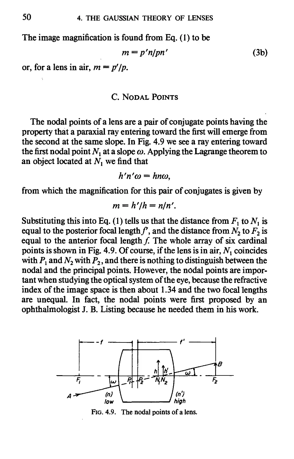
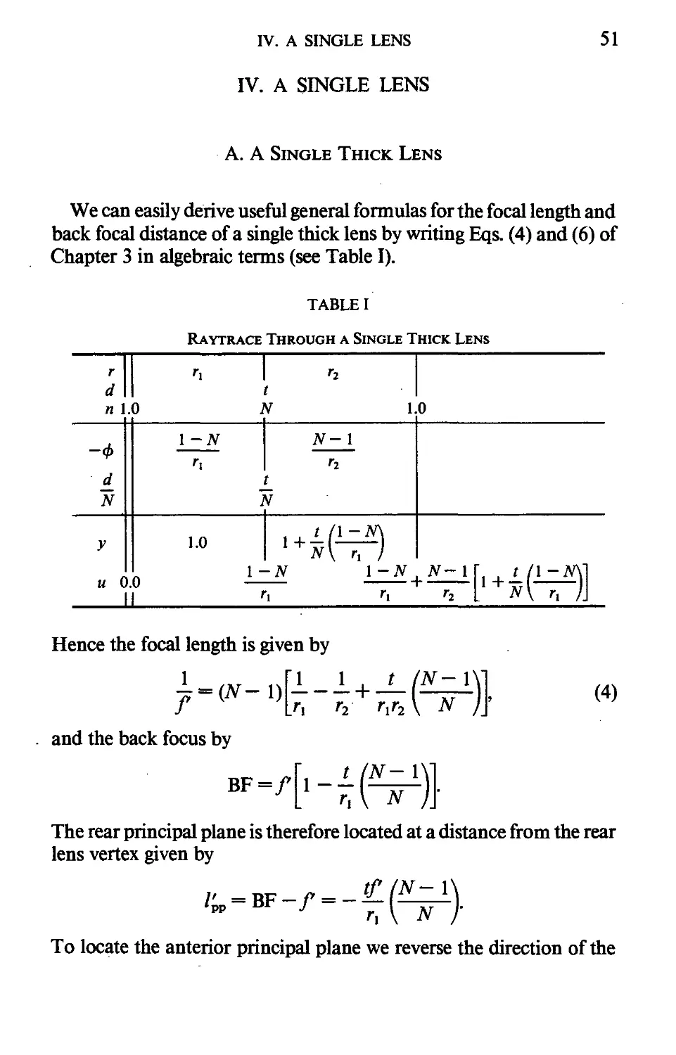
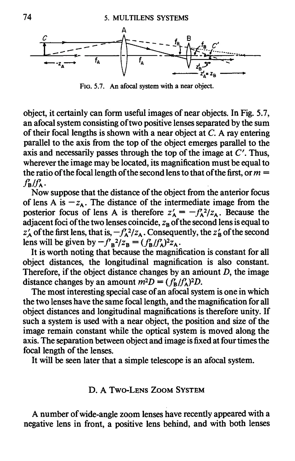
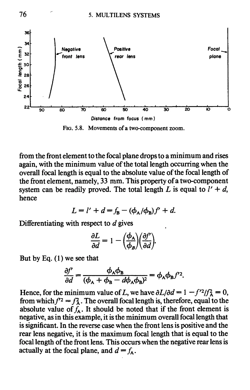
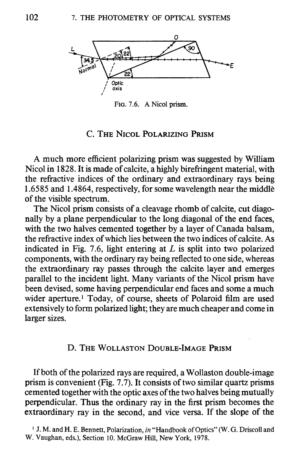
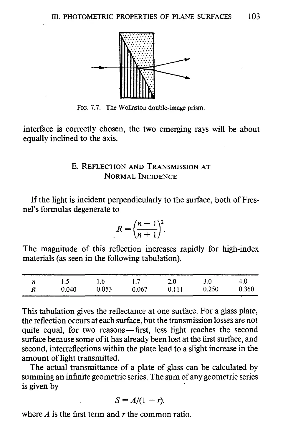
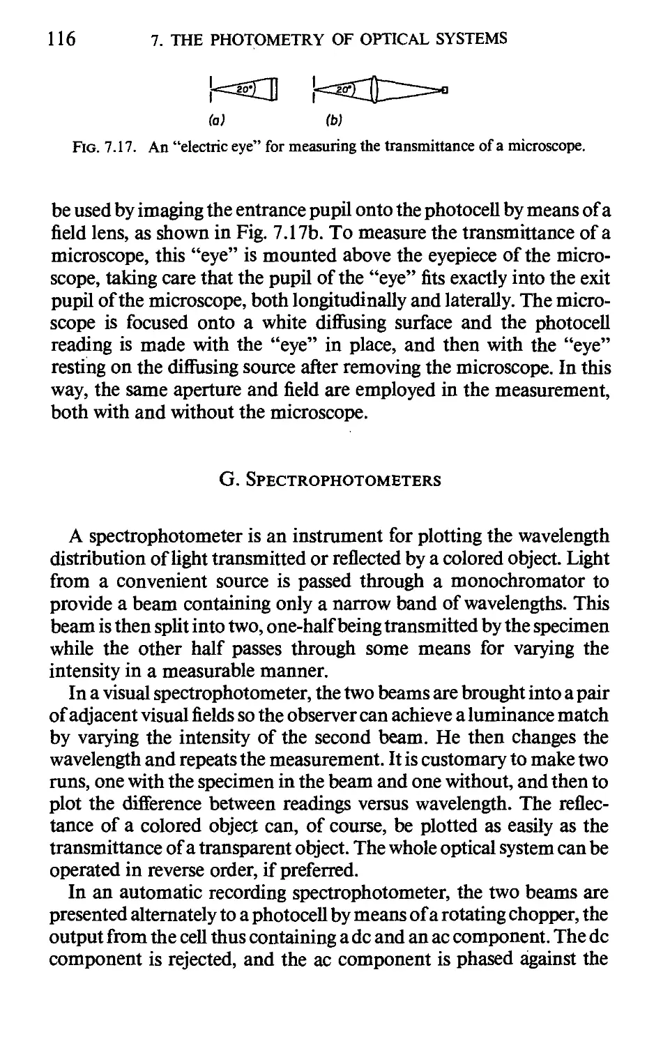
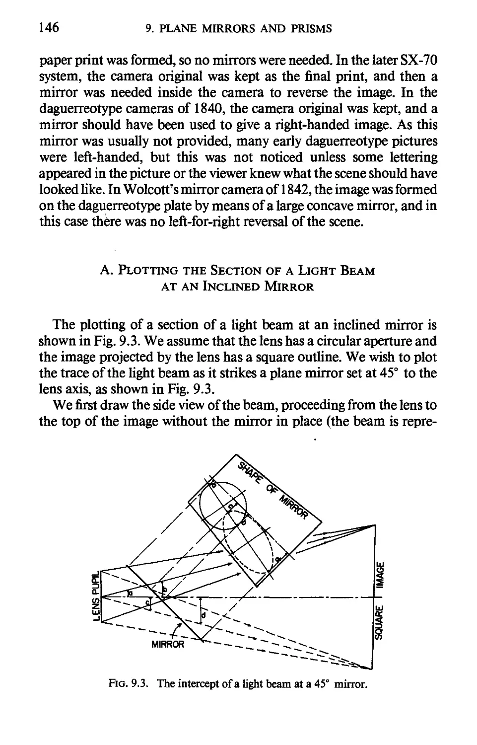
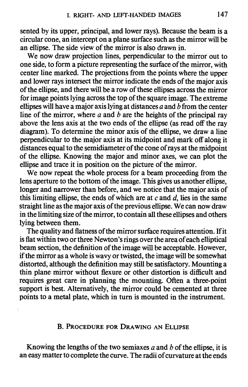
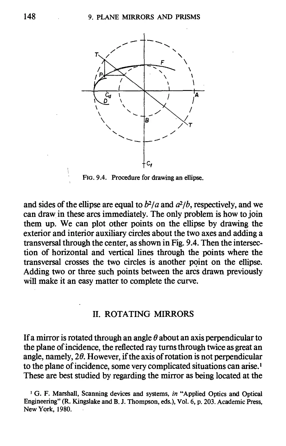
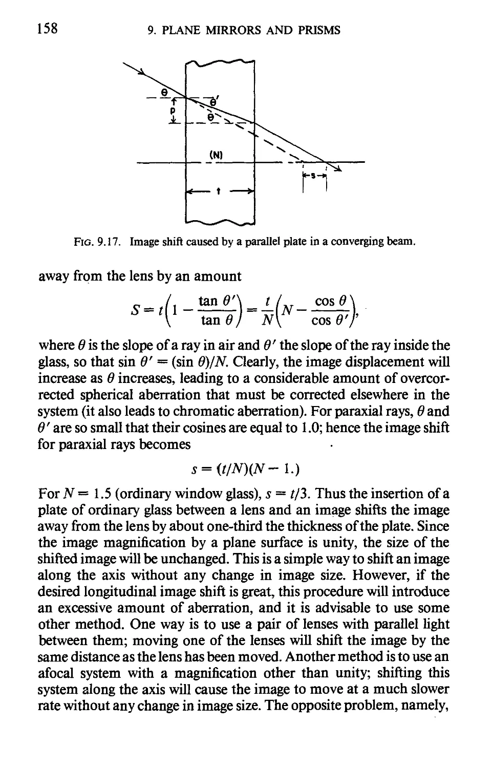
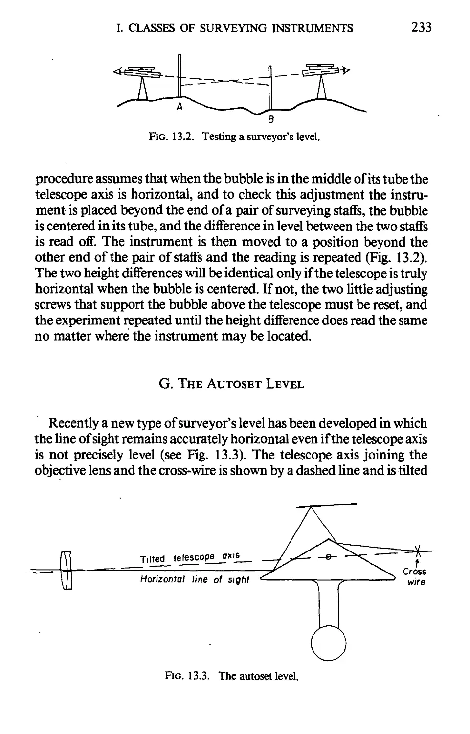
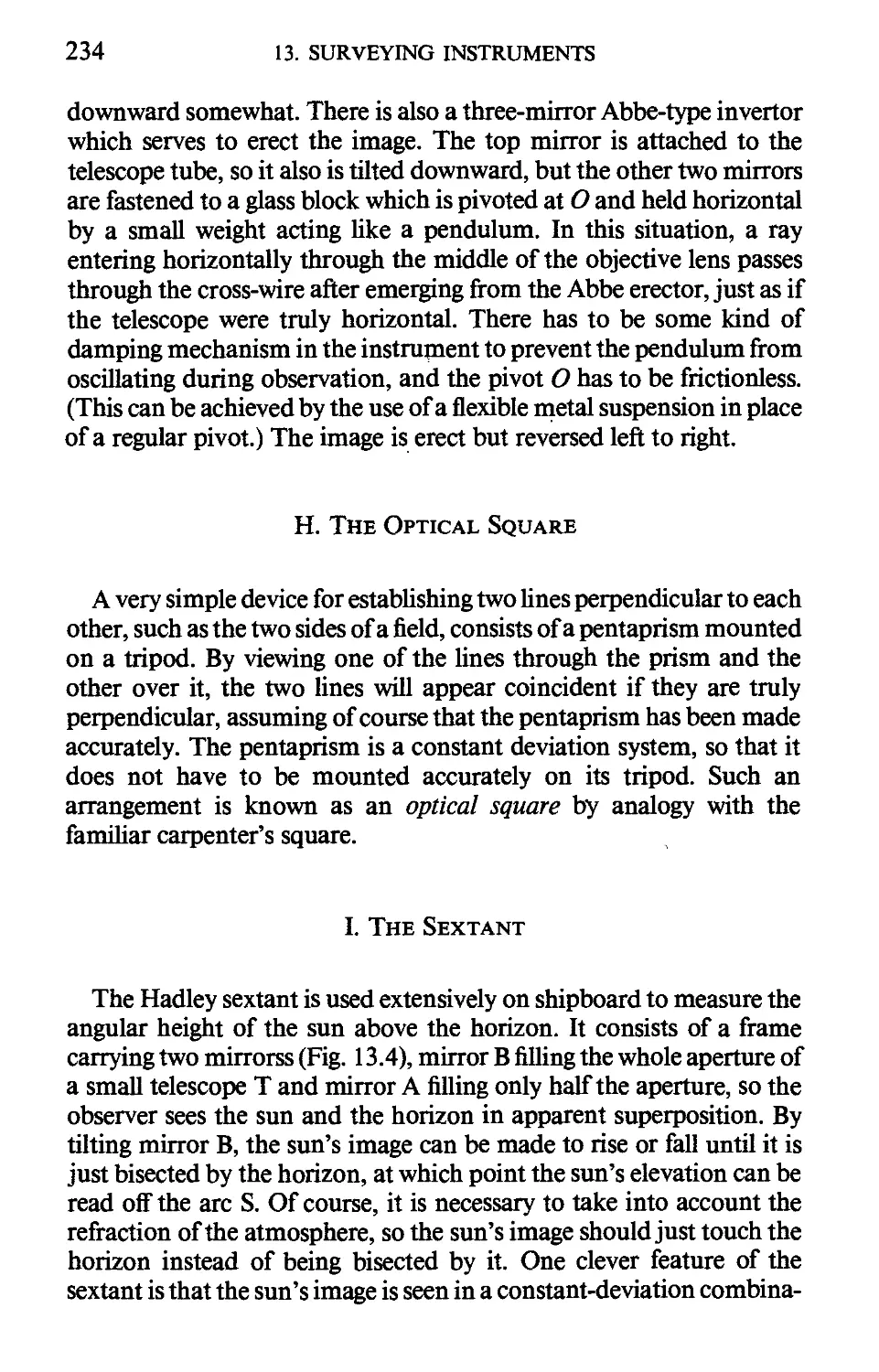
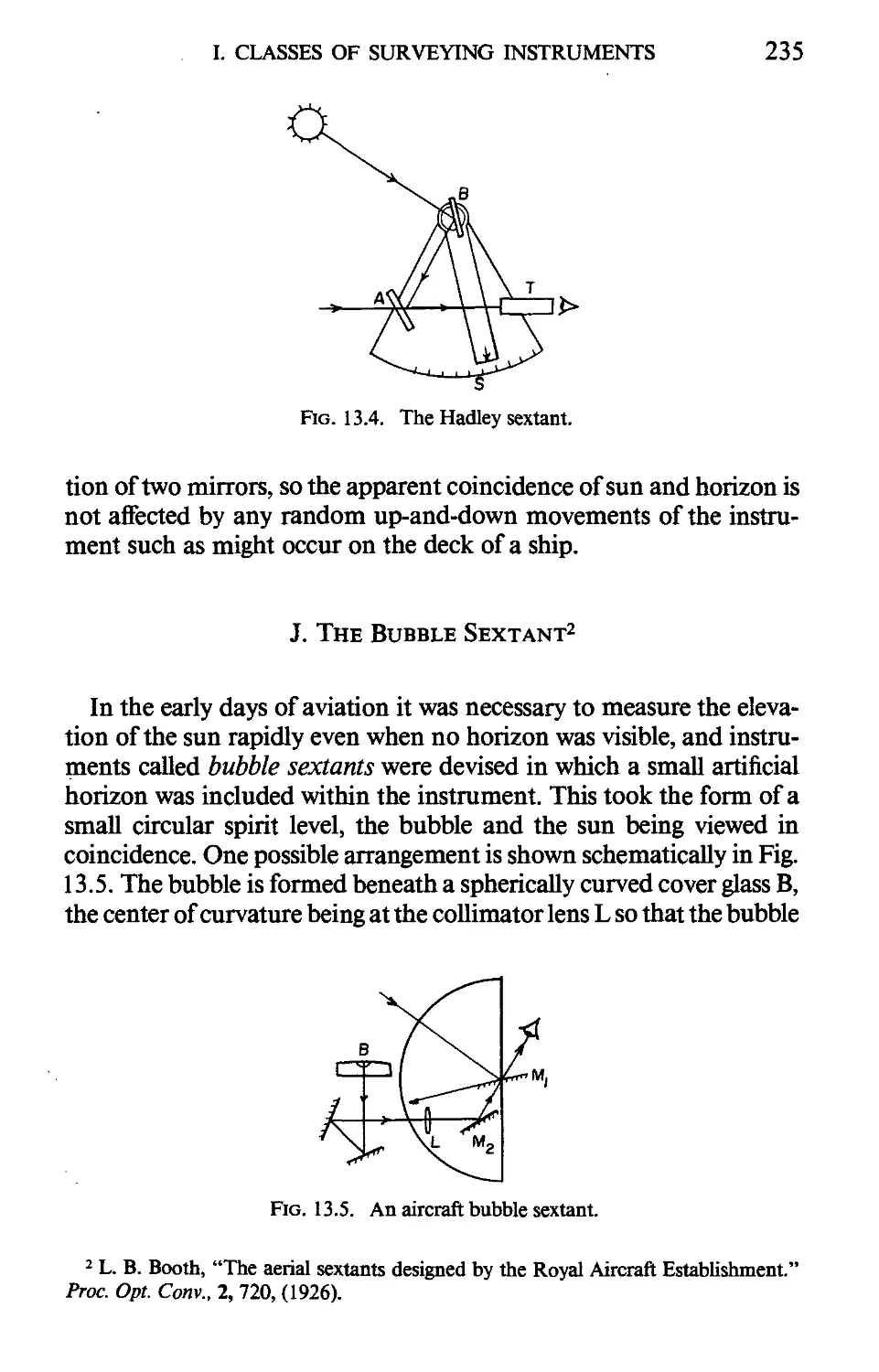
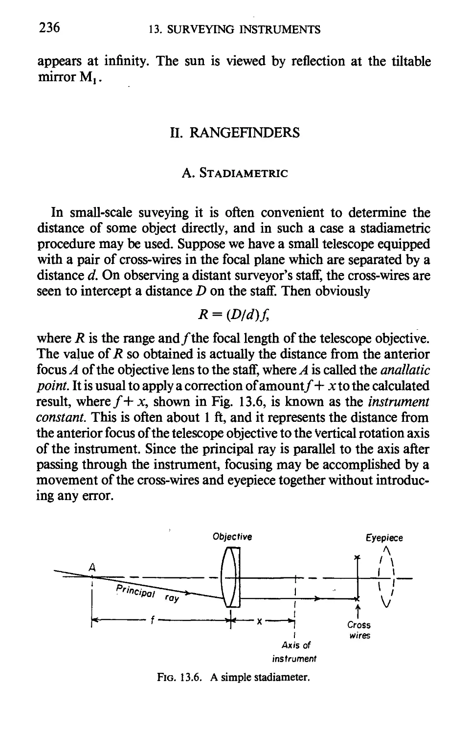
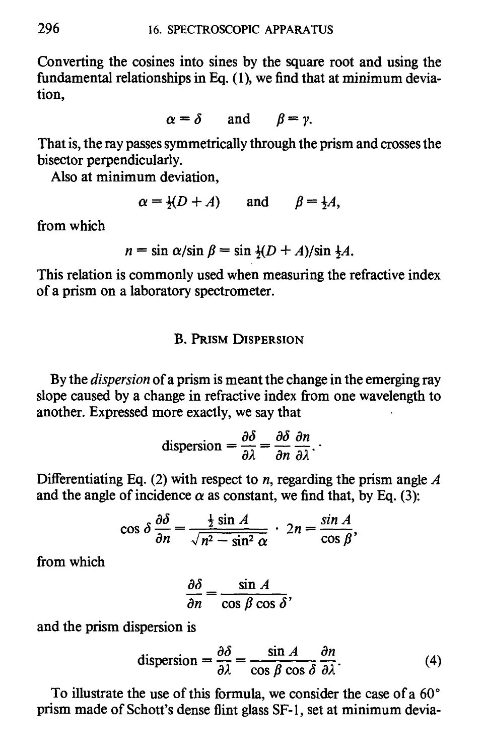
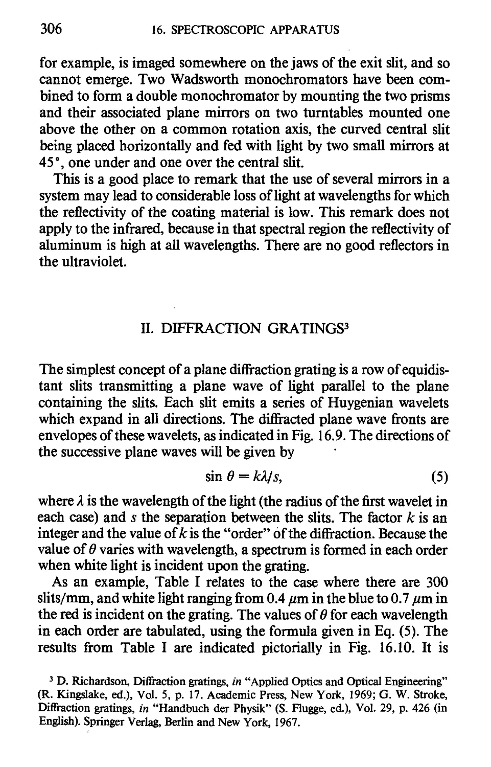
/


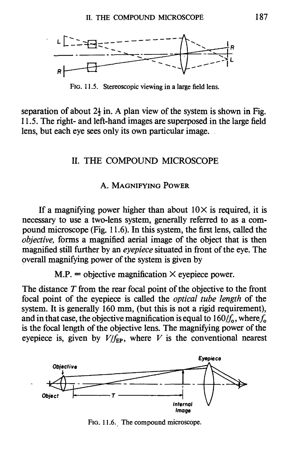
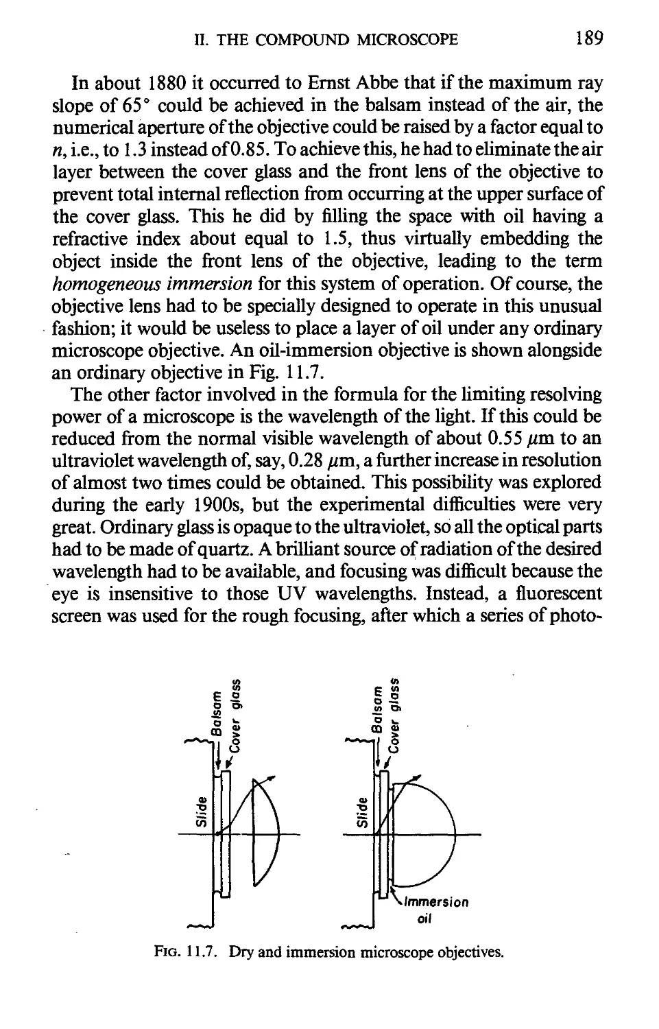
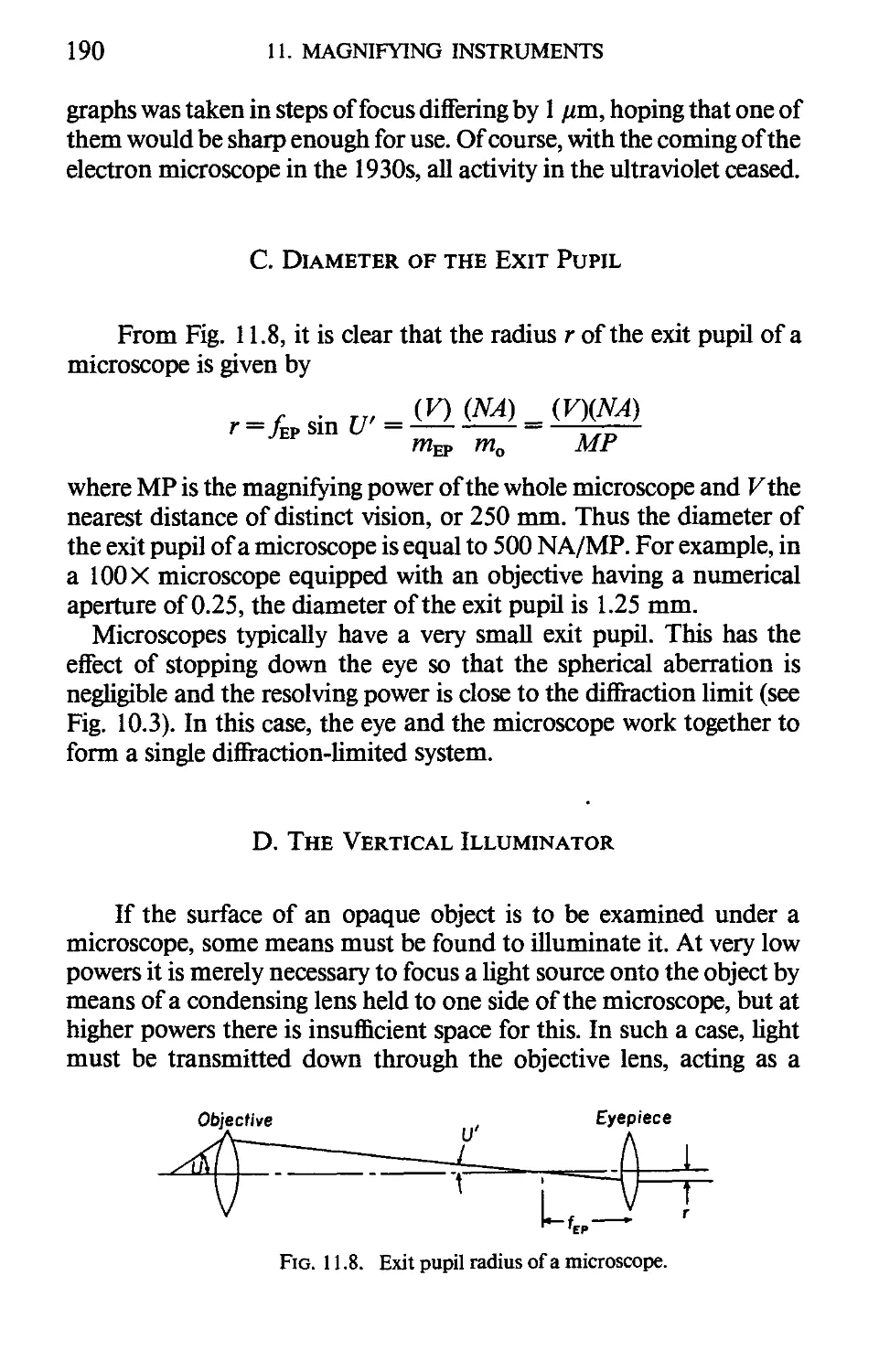


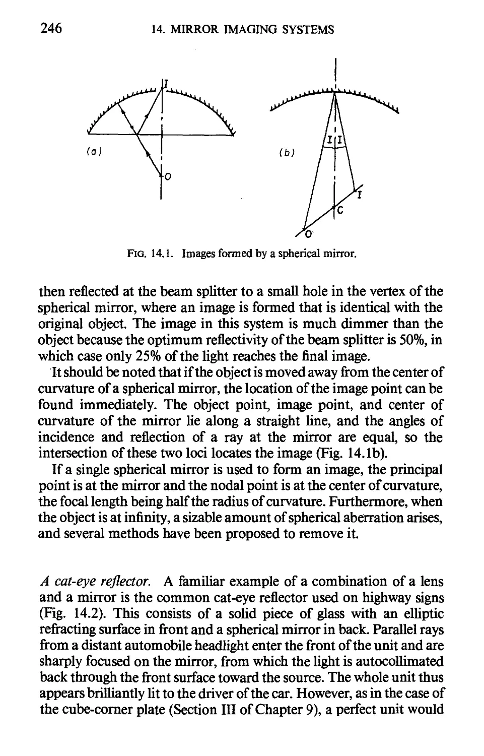


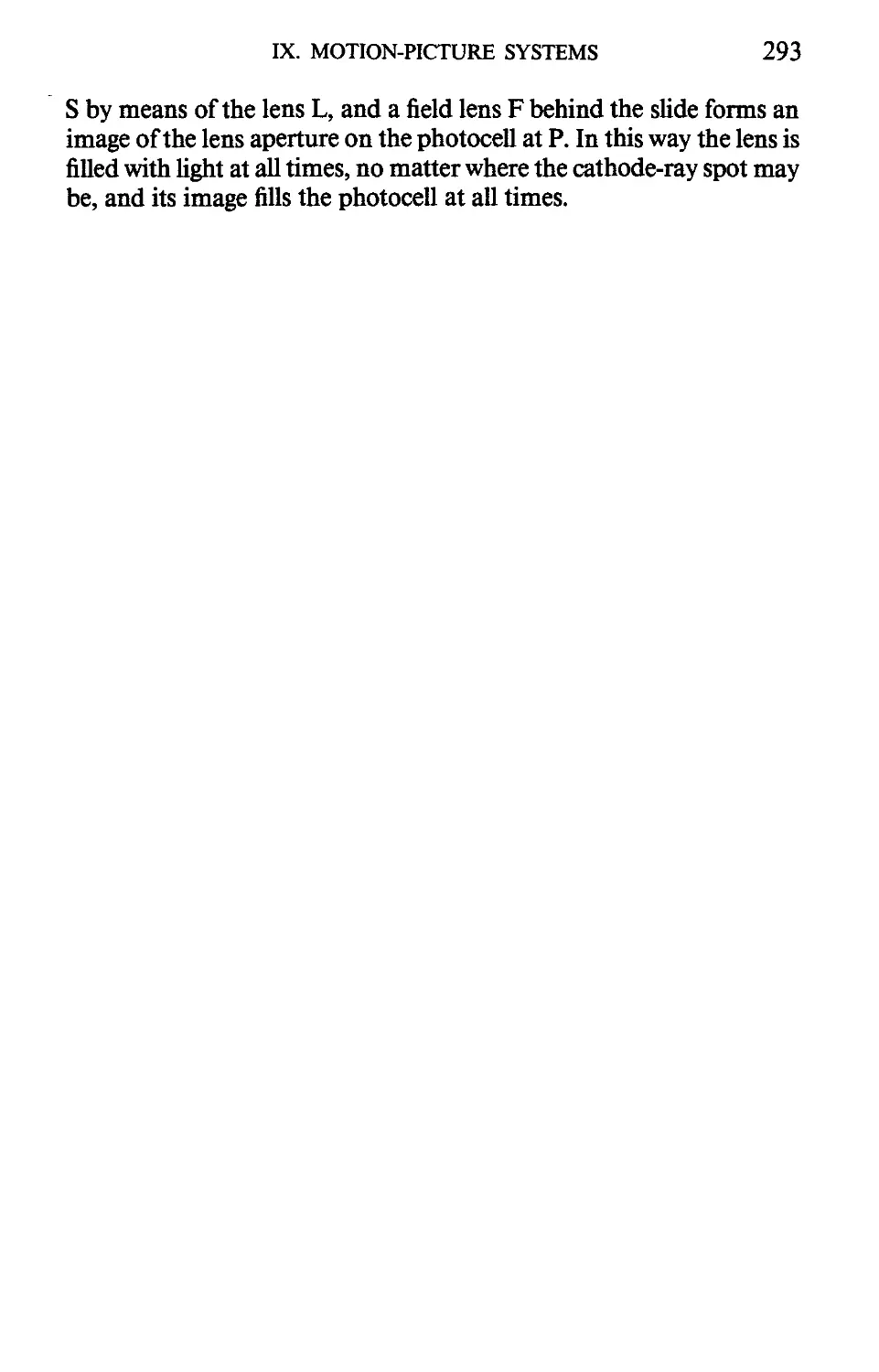


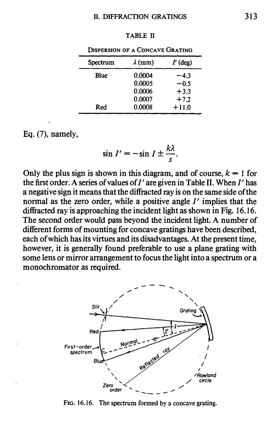


Текст
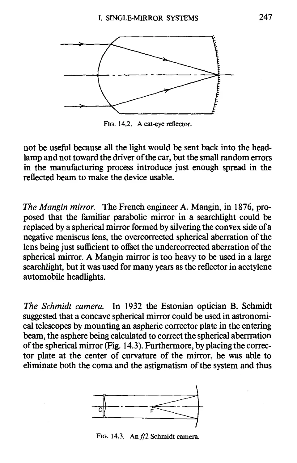
Optical System Design
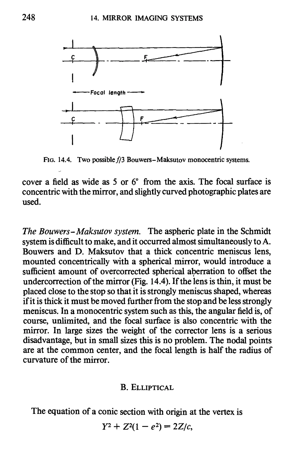
RUDOLF KINGSLAKE
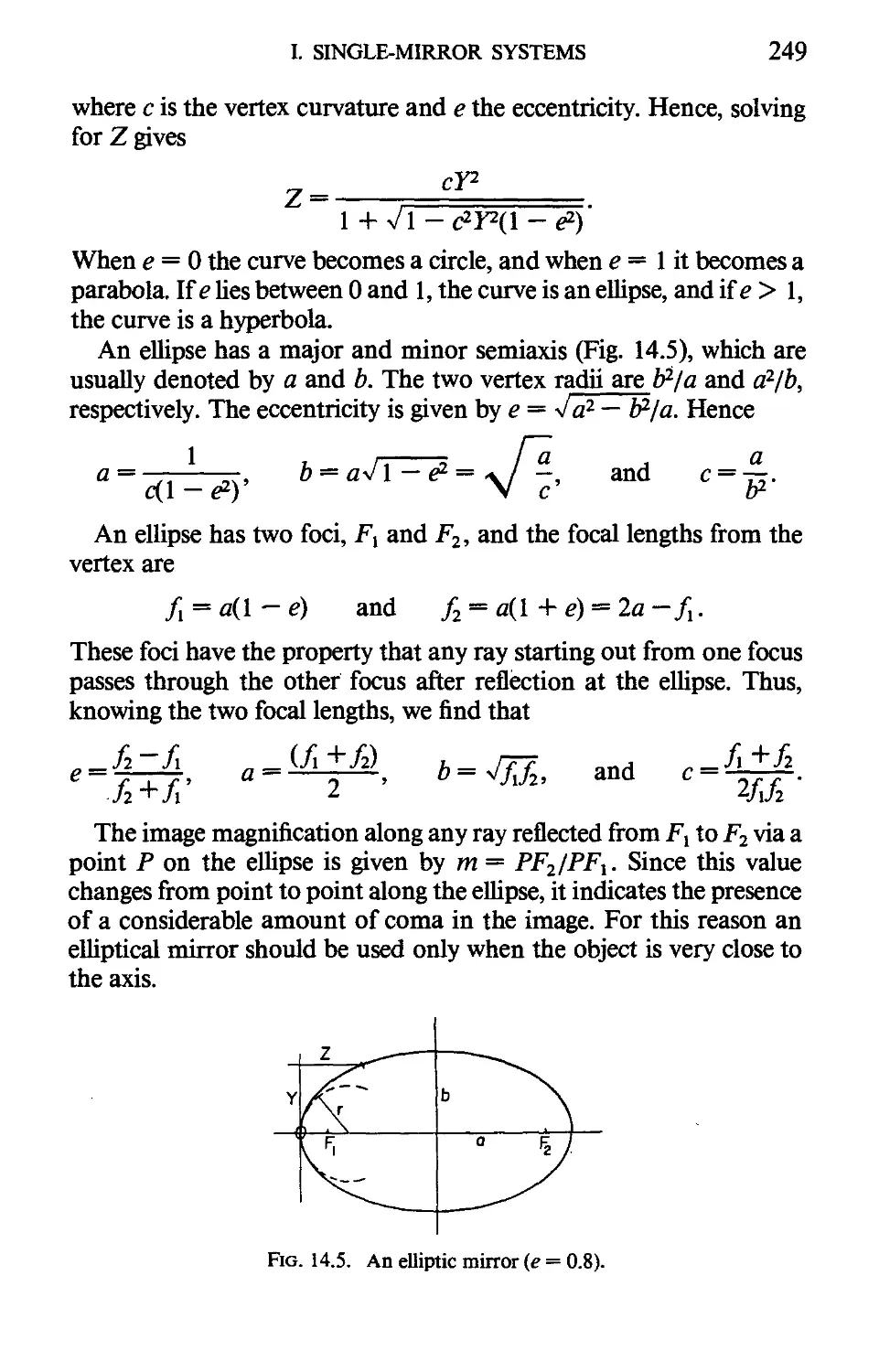
Institute of Optics
University of Rochester
Rochester, New York
ACADEMIC PRESS, INC.
Harcourt Brace Jovanovich, Publishers
Orlando San Diego New York
Austin London Montreal Sydney
Tokyo Toronto
Copyright © 1983, by Academic Press, Inc.
all rights reserved.
no part of this publication may be reproduced or
transmitted in any form or by any means, electronic
or mechanical, including photocopy, recording, or any
information storage and retrieval system, without
permission in writing from the publisher.
ACADEMIC PRESS, INC.
Orlando, Florida 32887
United Kingdom Edition published by
ACADEMIC PRESS, INC. (LONDON) LTD.
24/28 Oval Road, London NW1 7DX
Library of Congress Cataloging in Publication Data
Kingslake, Rudolf.
Optical system design.
Bibliography: p.
Includes index.
1. Optics. 2. Optical instruments. I. Title.
QC371.K52 1983 535'.33 83-9997
ISBN 0-12-408660-8
PRINTED IN THE UNITED STATES OF AMERICA
85 86 87 88 9 8 7 6 5
Contents
Preface a.
1. Optical Systems
I. DESIGN AND PRODUCTION
II. OPTICAL MATERIALS 2
III. LENS MANUFACTURE 3
2. Light and Images
I. THE NATURE OF LIGHT 7
II. THE LAW OF REFRACTION 10
III. A PERFECT OPTICAL SYSTEM 13
IV. LENS ABERRATIONS 21
V. FIBER OPTICS 22
3. Ray-Tracing Procedures
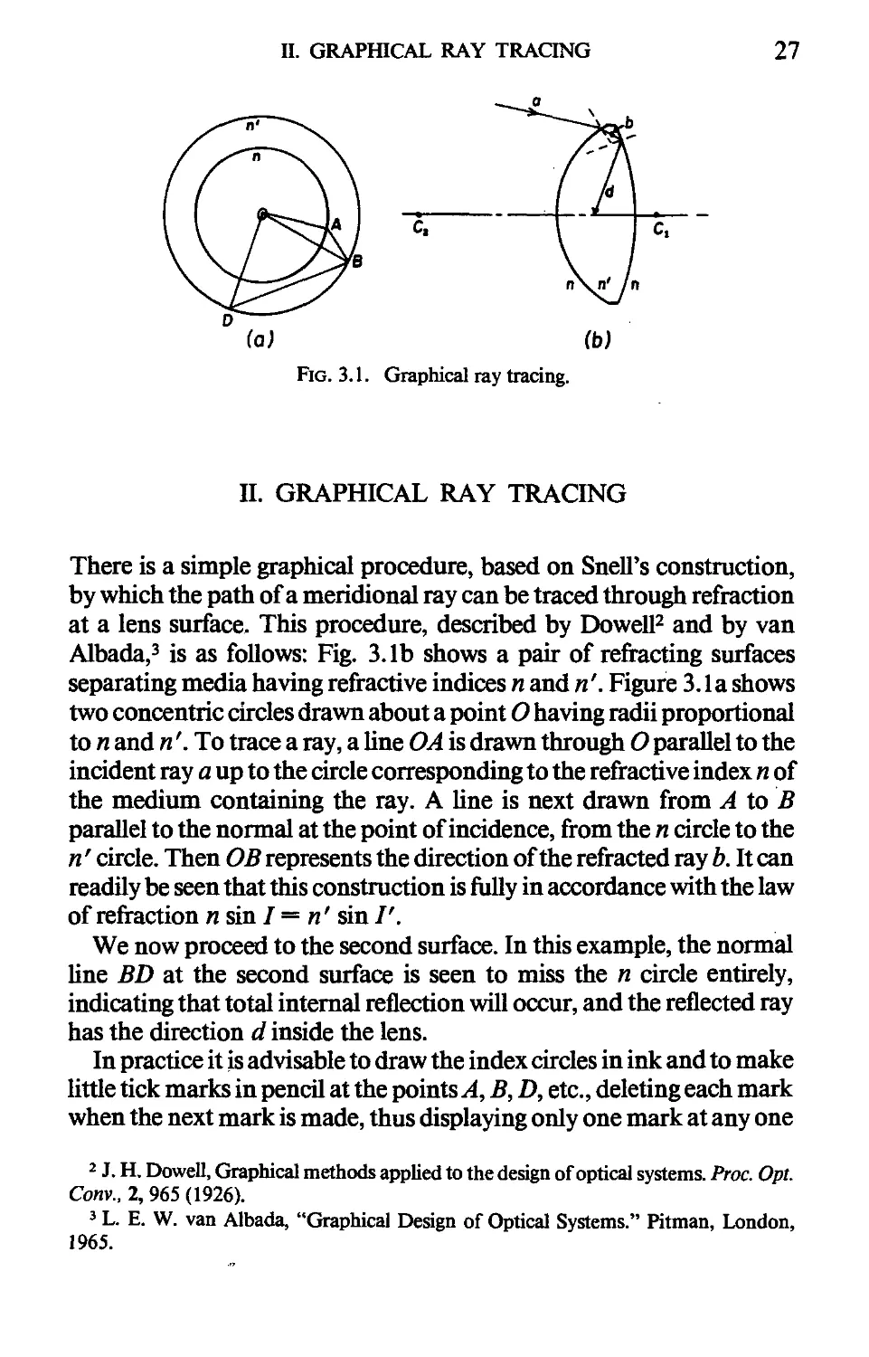
I. TYPES OF RAYS 26
II. GRAPHICAL RAY TRACING 27
Ш. MERIDIONAL RAY TRACING 28
IV. PARAXIAL RAYS 30
V. CURVED MIRRORS 36
VI. MAGNIFICATION AND THE LAGRANGE THEOREM 36
VII. THE FRESNEL LENS 38
vi CONTENTS
4. The Gaussian Theory of Lenses
I. INTRODUCTION 40
II. THE FOUR CARDINAL POINTS 40
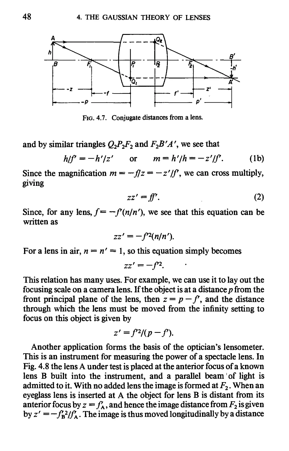
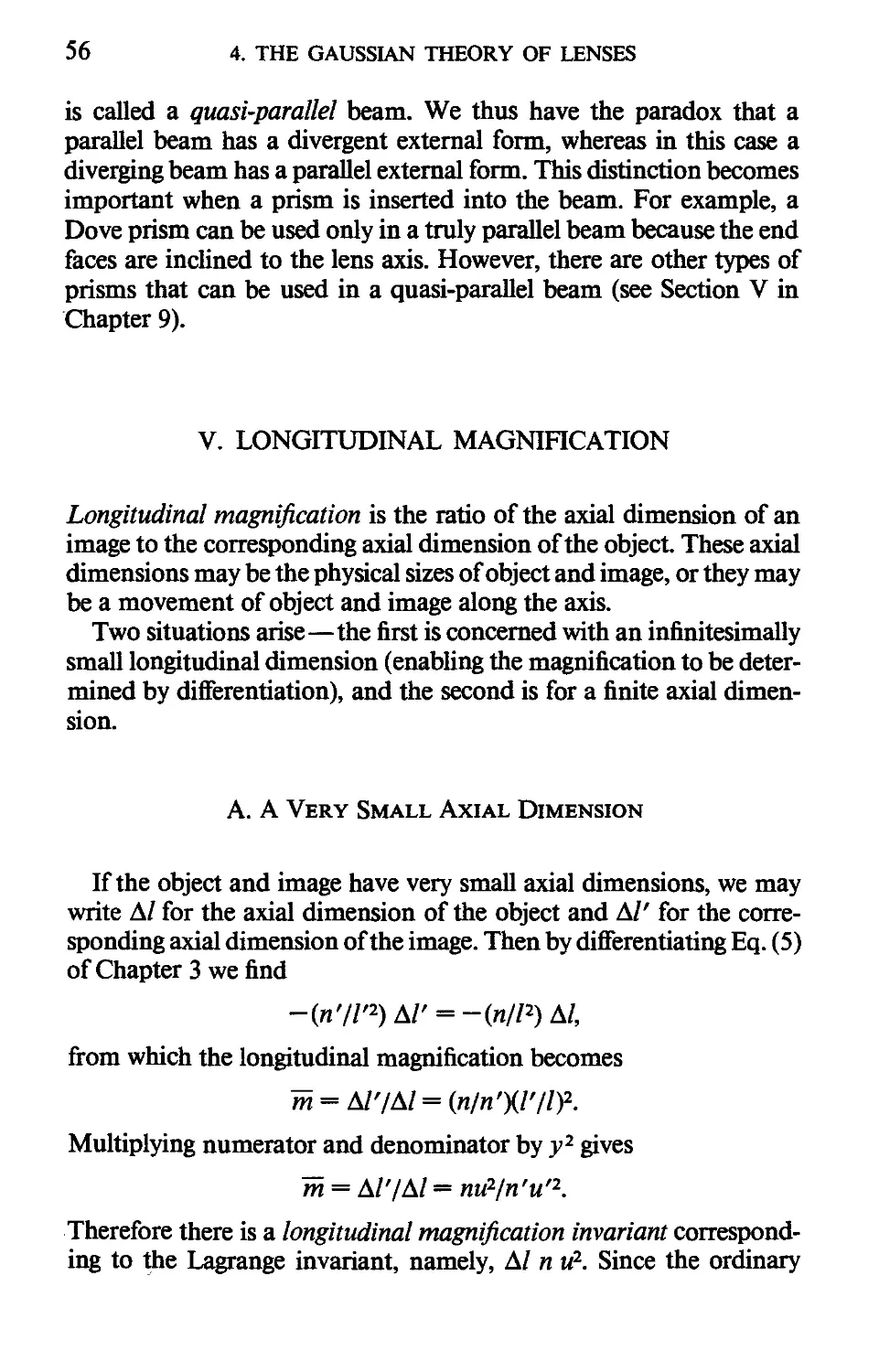
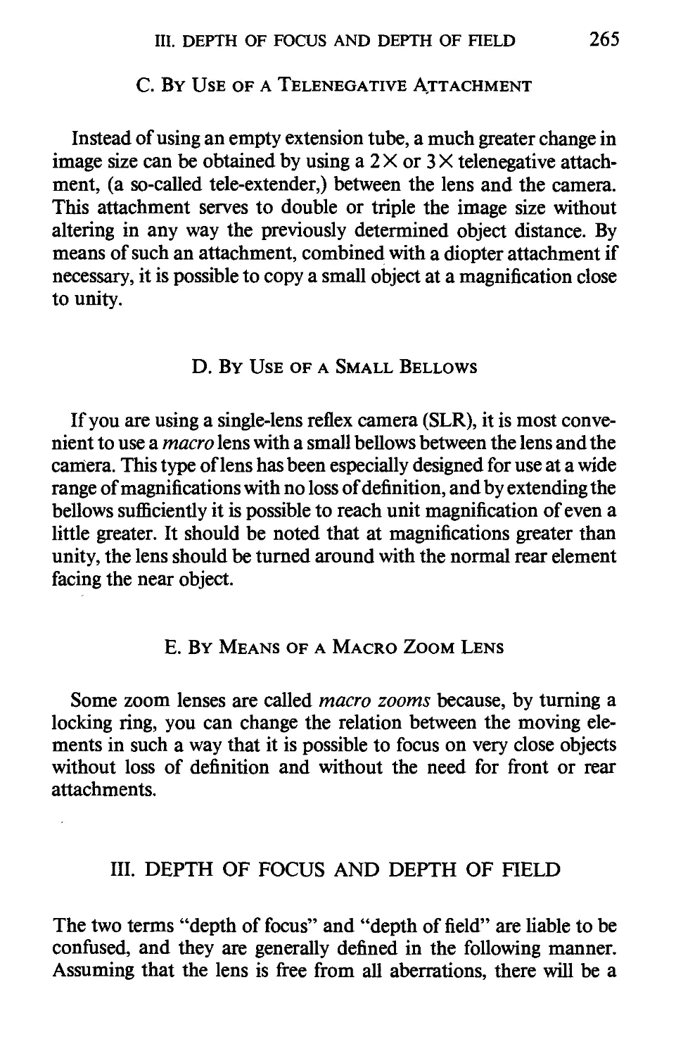
Ш. CONJUGATE DISTANCE RELATIONSHIPS 47
IV. A SINGLE LENS 51
V. LONGITUDINAL MAGNIFICATION 56
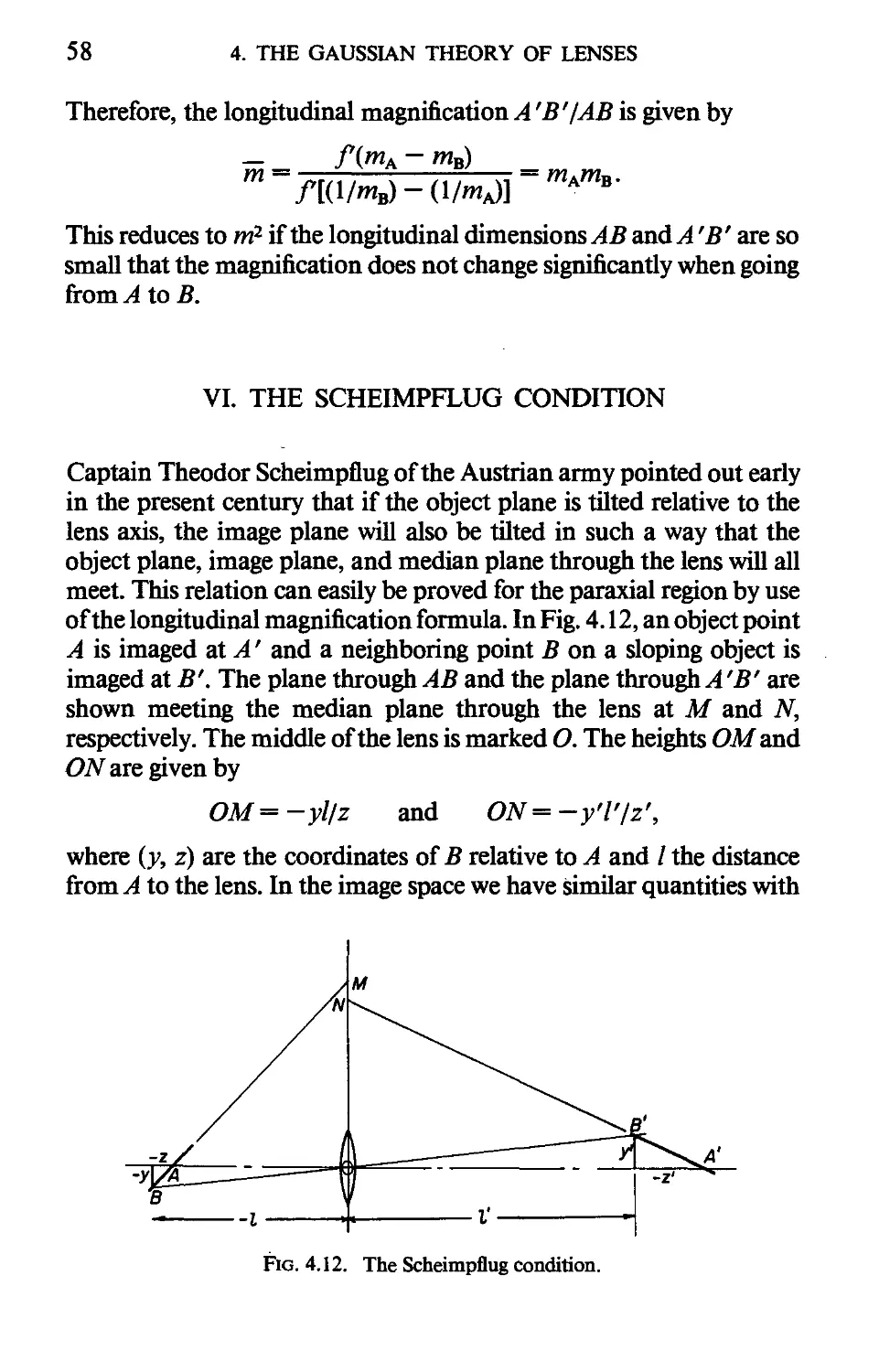
VI. THE SCHEIMPFLUG CONDITION 58
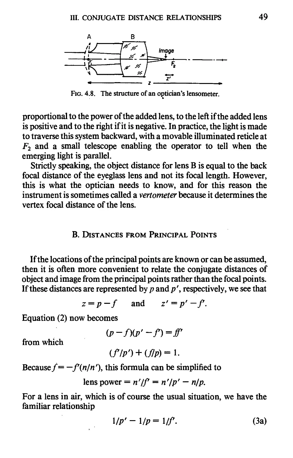
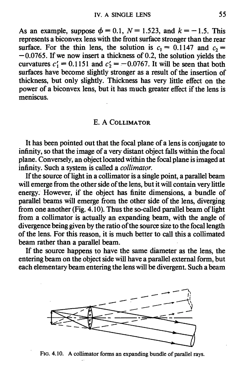
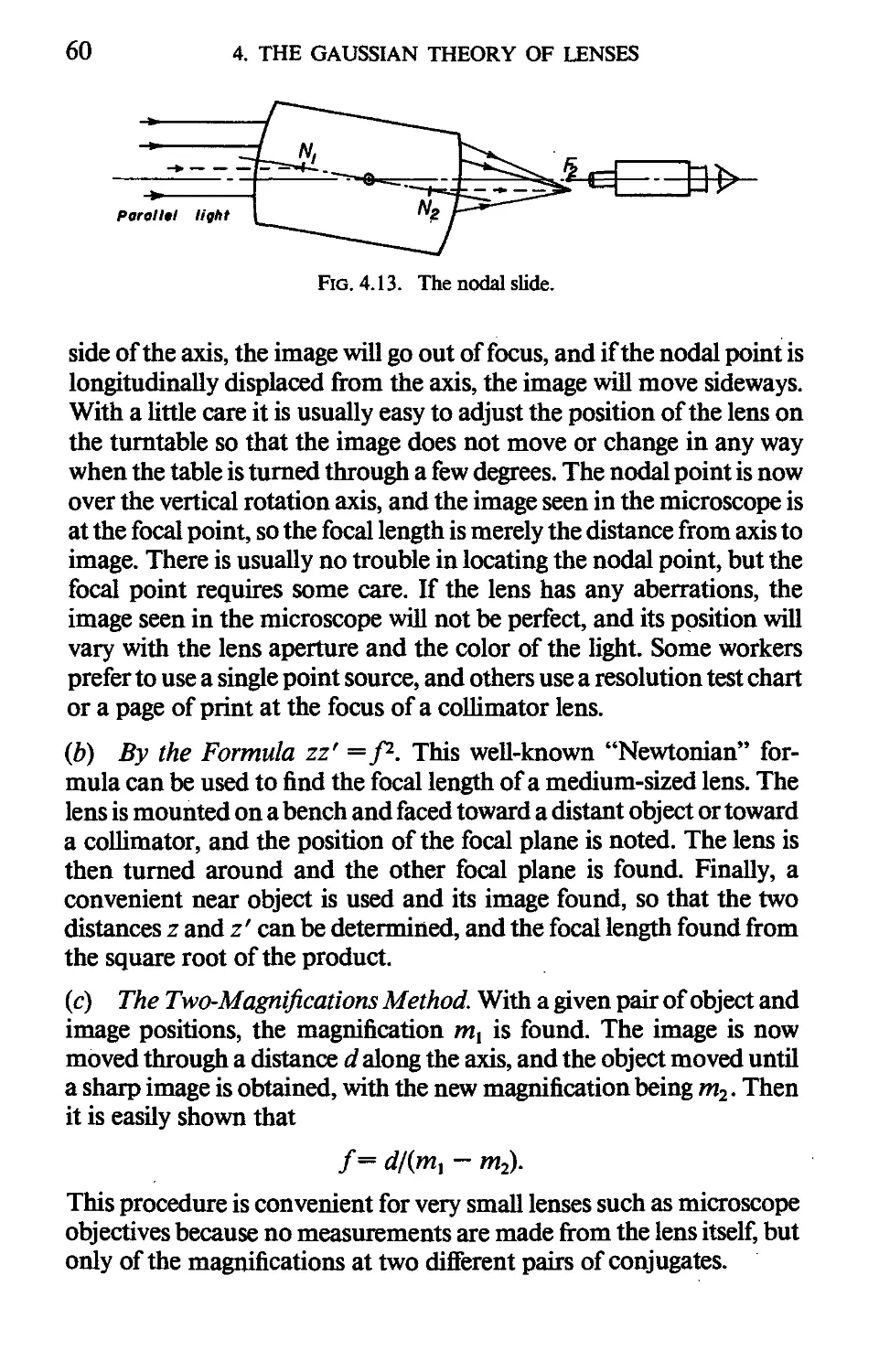
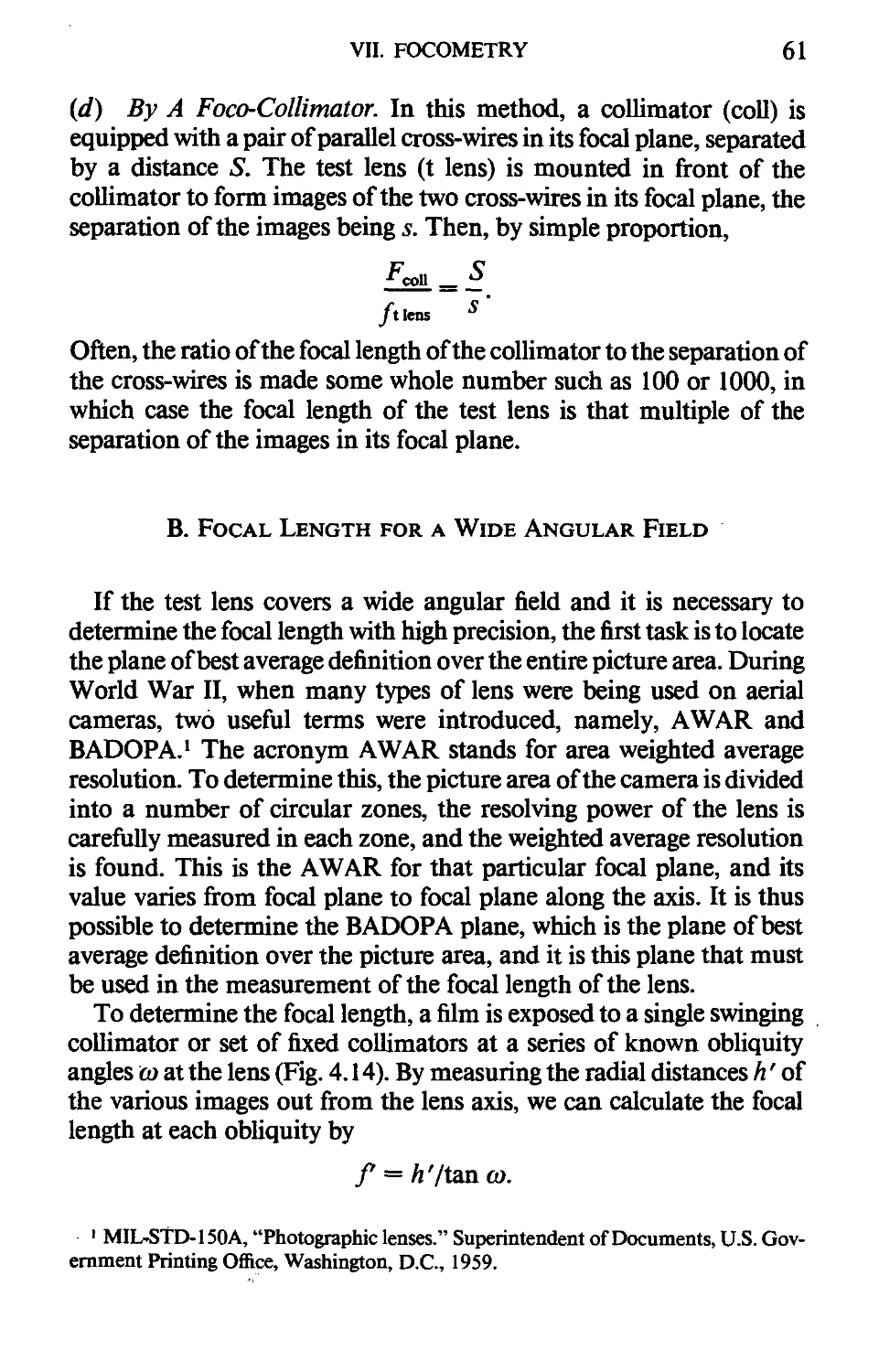
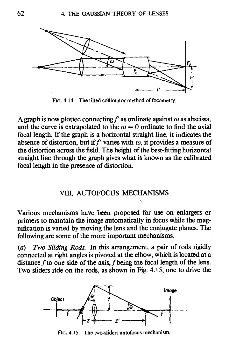
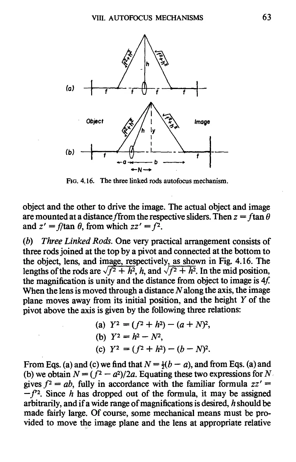
VII. FOCOMETRY 59
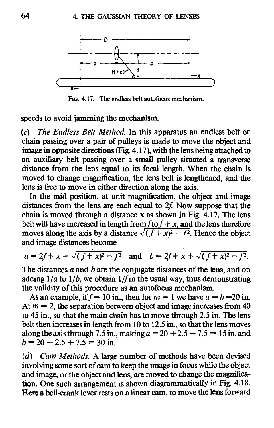
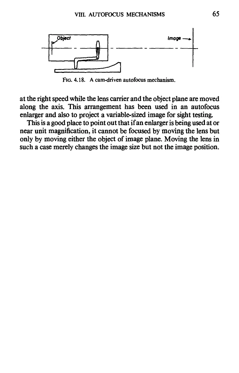
VIII. AUTOFOCUS MECHANISMS 62
5. Multilens Systems
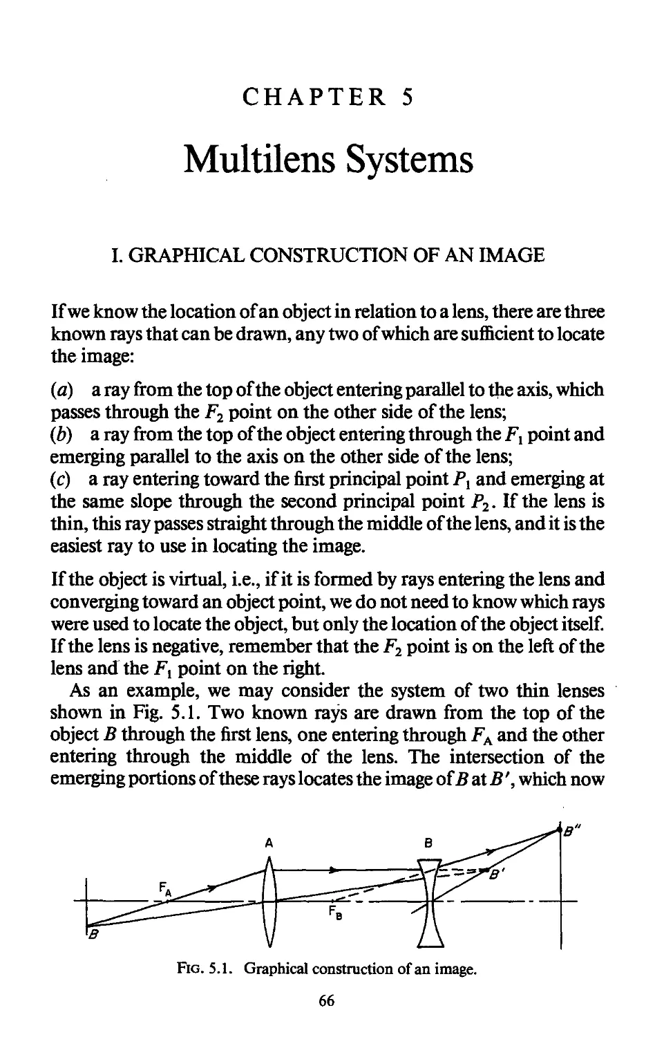
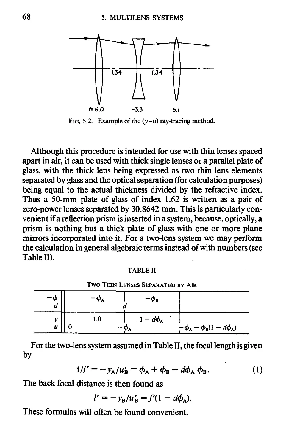
I. GRAPHICAL CONSTRUCTION OF AN IMAGE 66
II. RAY TRACING THROUGH A SYSTEM OF SEPARATED THIN
LENSES 67
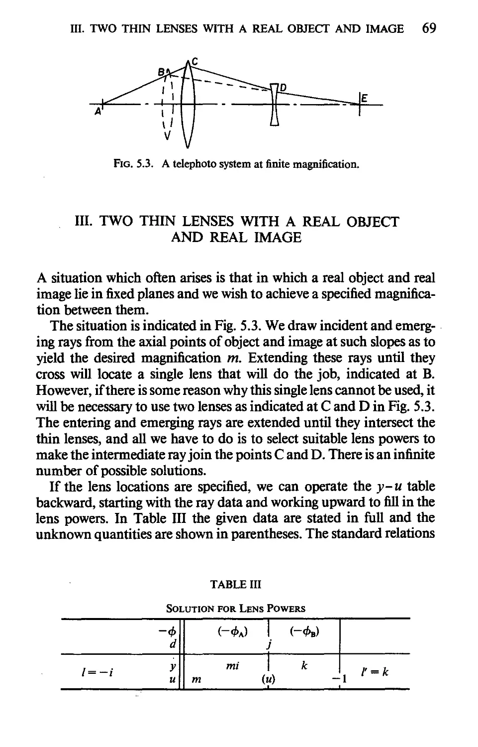
III. TWO THIN LENSES WITH A REAL OBJECT AND REAL
IMAGE 69
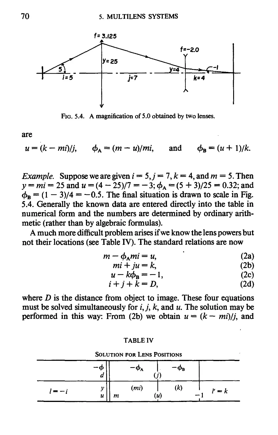
IV. THE MATRIX APPROACH TO PARAXIAL RAYS 77
V. CYLINDRICAL LENSES 80
6. Oblique Beams
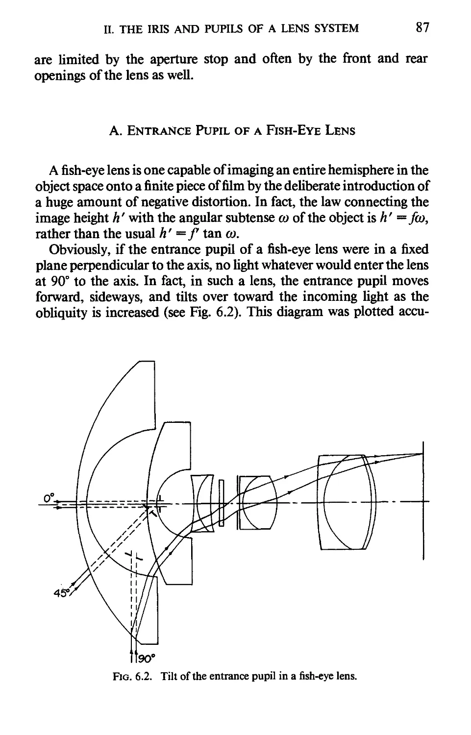
I. MERIDIONAL RAYS 84
II. THE IRIS AND PUPILS OF A LENS 86
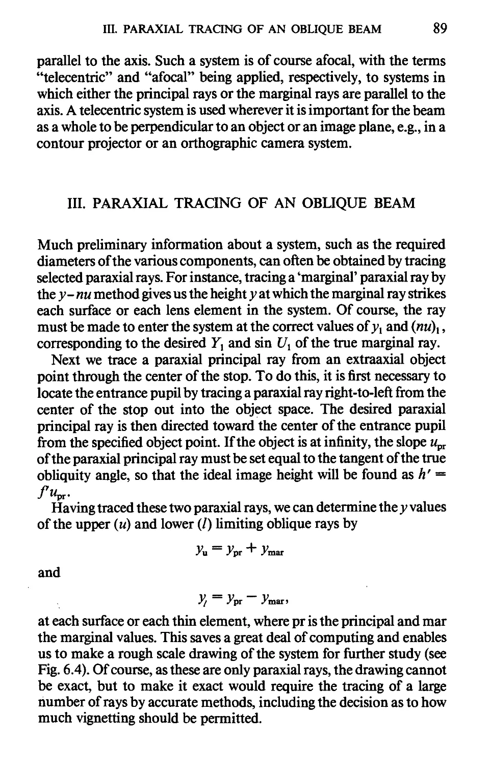
Ш. PARAXIAL TRACING OF AN OBLIQUE BEAM 89
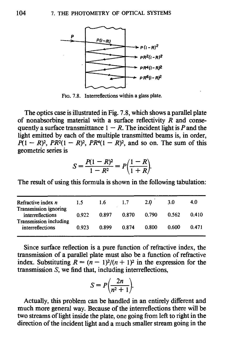
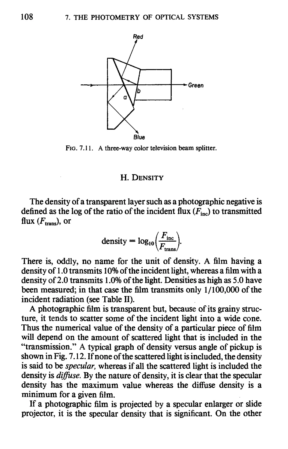
7. The Photometry of Optical Systems
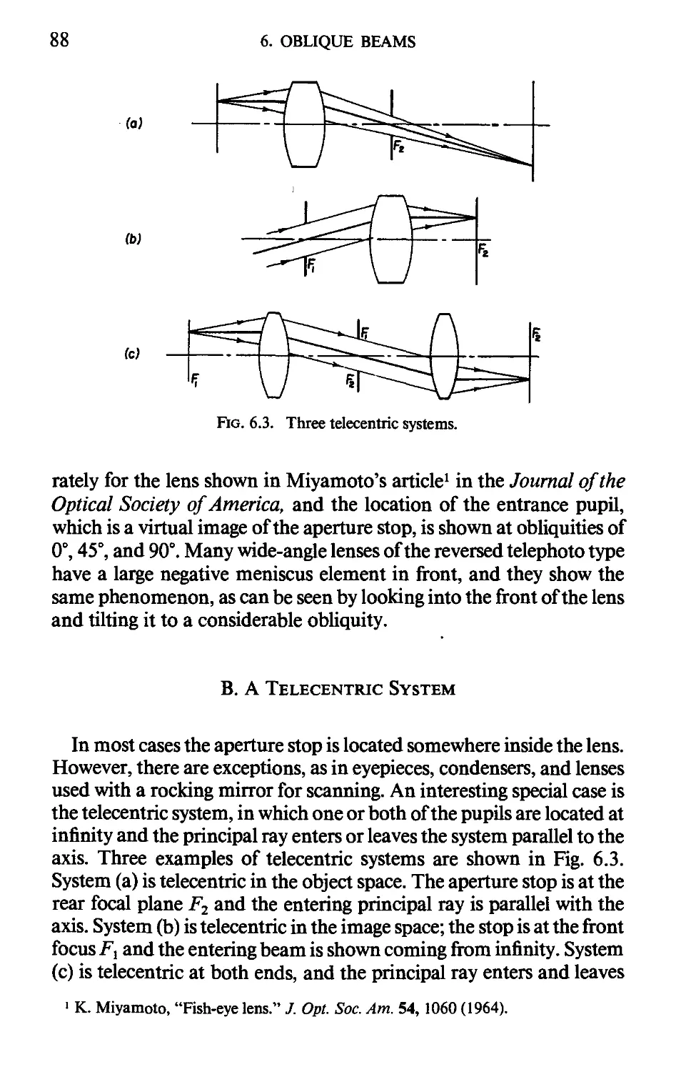
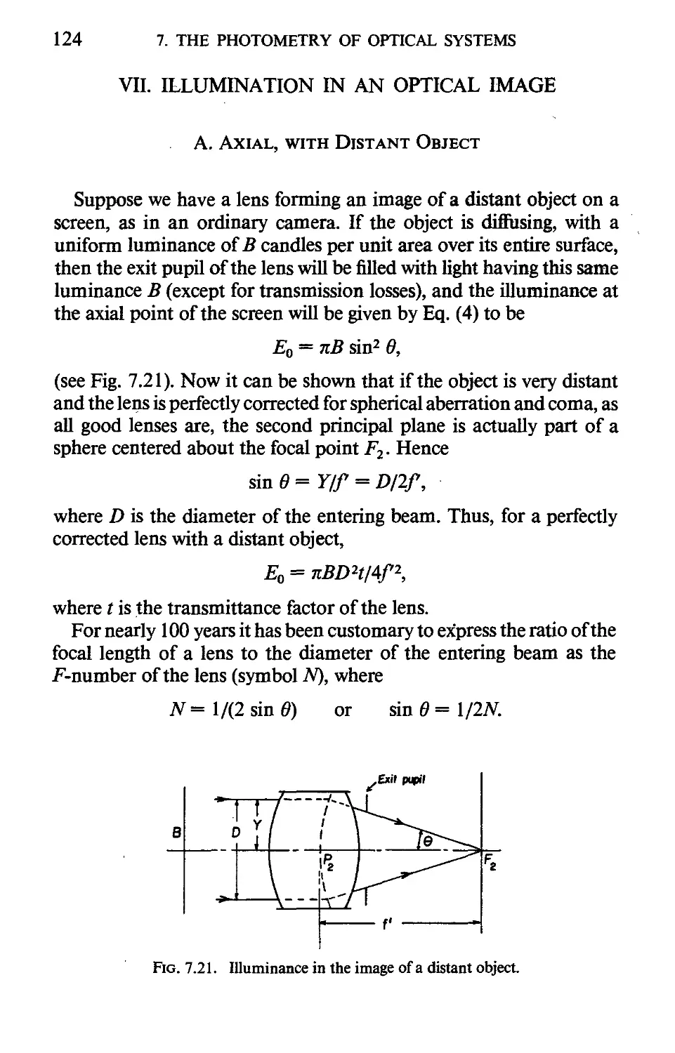
I. INTRODUCTION 92
II. PHOTOMETRIC DEFINITIONS 93
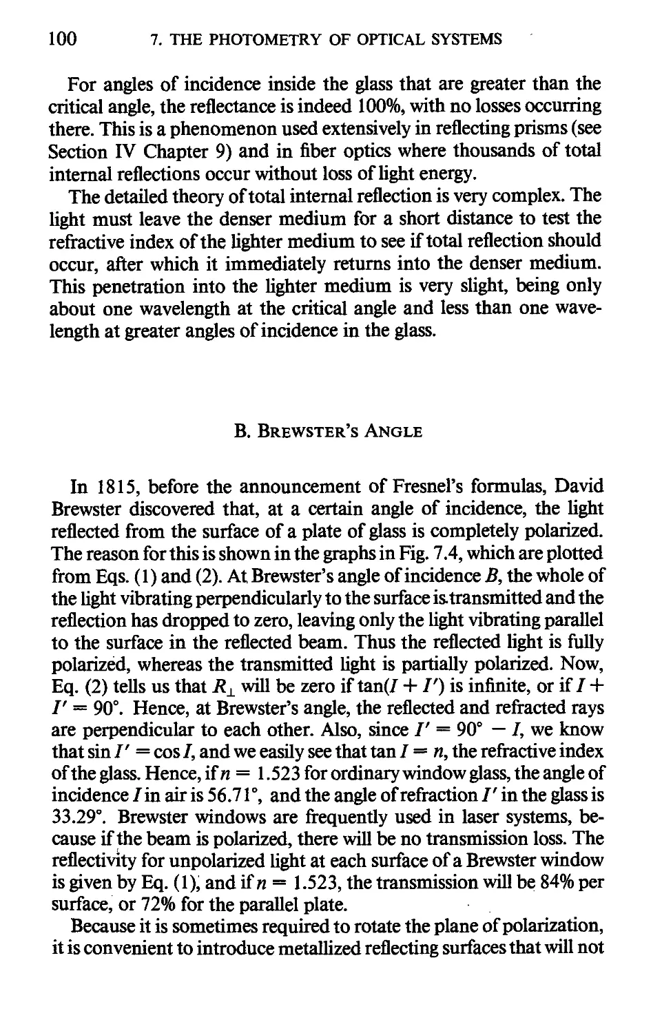
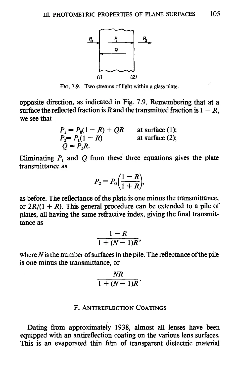
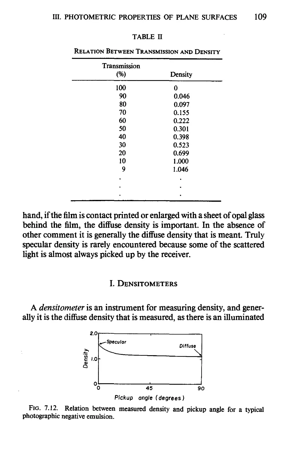
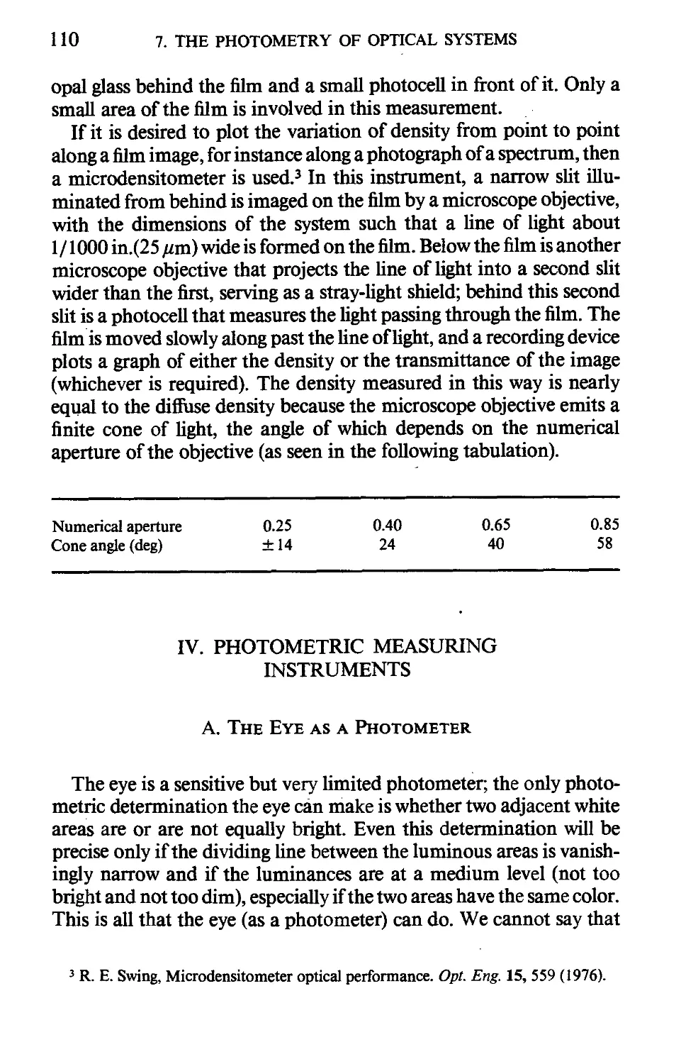
Ш. PHOTOMETRIC PROPERTIES OF PLANE SURFACES 98
IV. PHOTOMETRIC MEASURING INSTRUMENTS 110
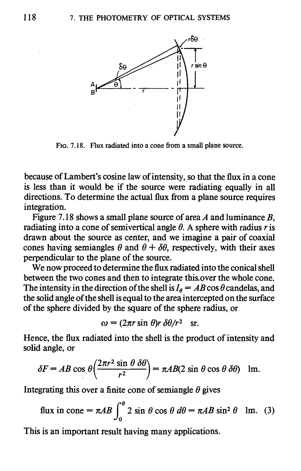
V. THE FLUX EMITTED BY A PLANE SOURCE 117
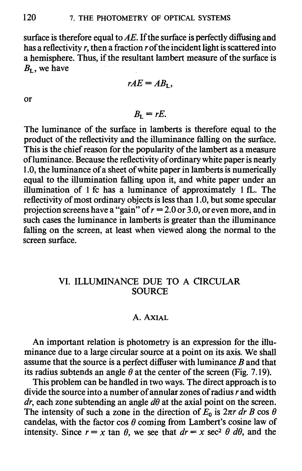
VI. ILLUMINANCE DUE TO A CIRCULAR SOURCE 120
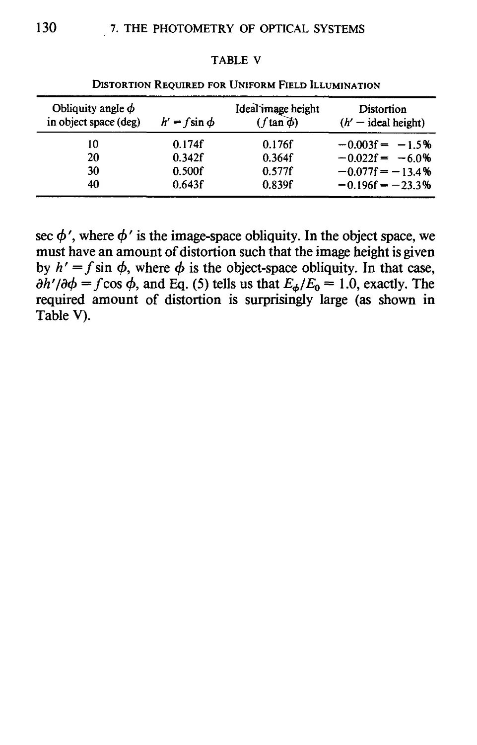
VII. ILLUMINATION IN AN OPTICAL IMAGE 124
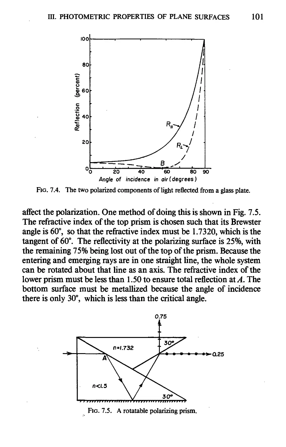
8. Projection Systems
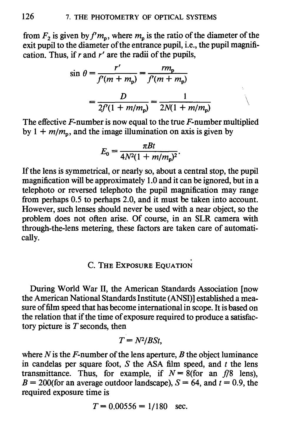
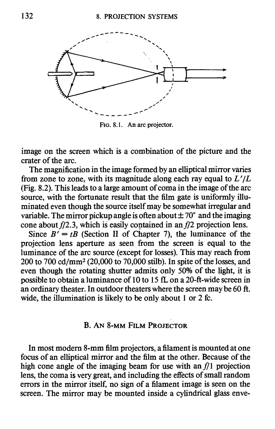
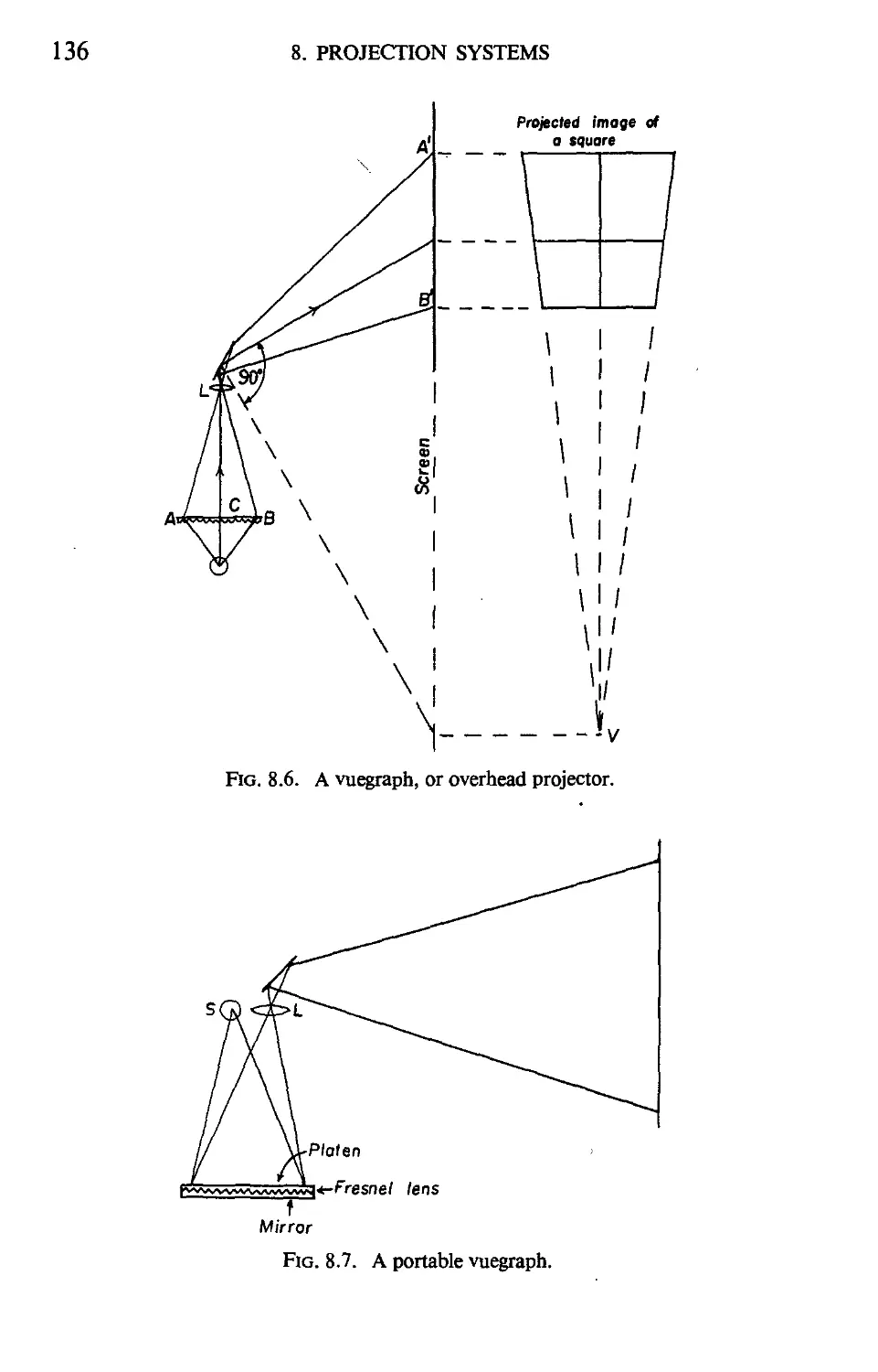
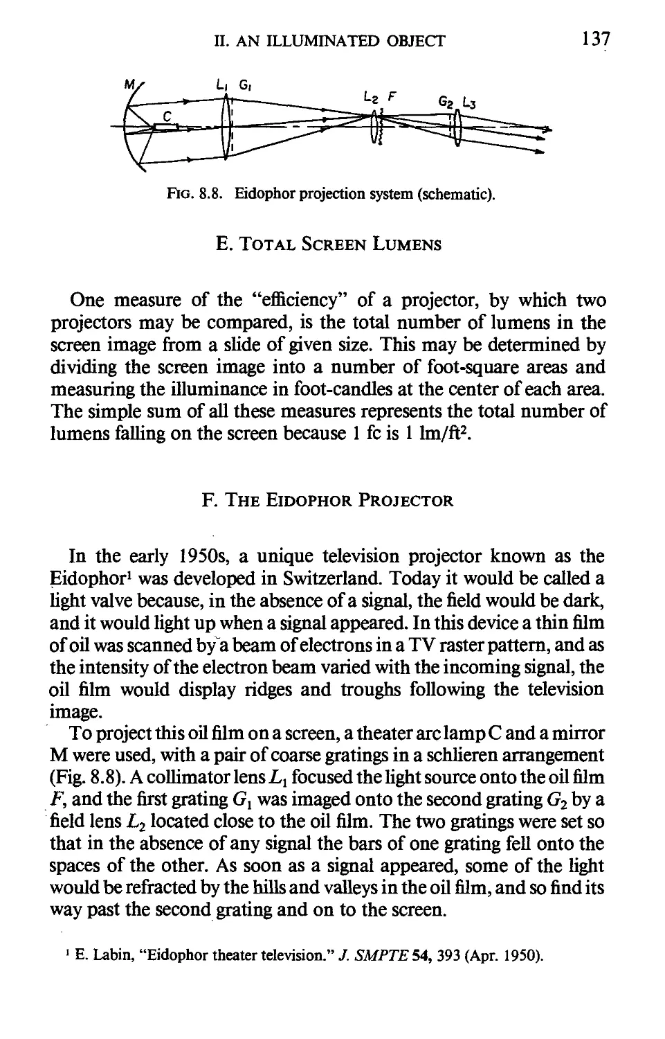
I. A SELF-LUMINOUS OBJECT 131
II. AN ILLUMINATED OBJECT 131
CONTENTS vii
Ш. PROJECTION SCREENS 138
IV. STEREOSCOPIC PROJECTION 140
V. CONTOUR PROJECTORS 141
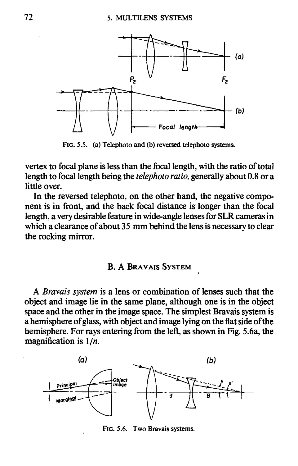
9. Plane Mirrors and Prisms
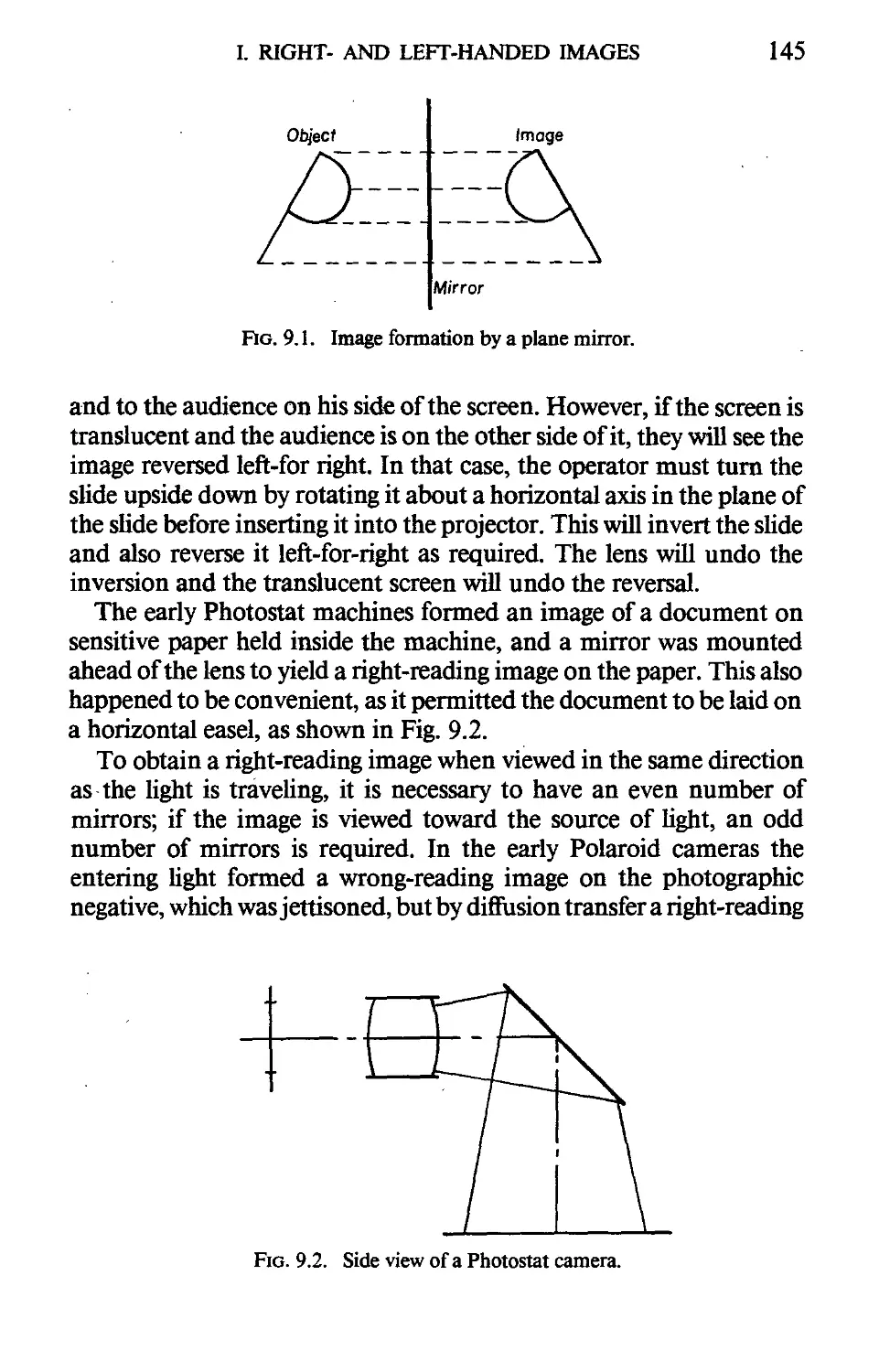
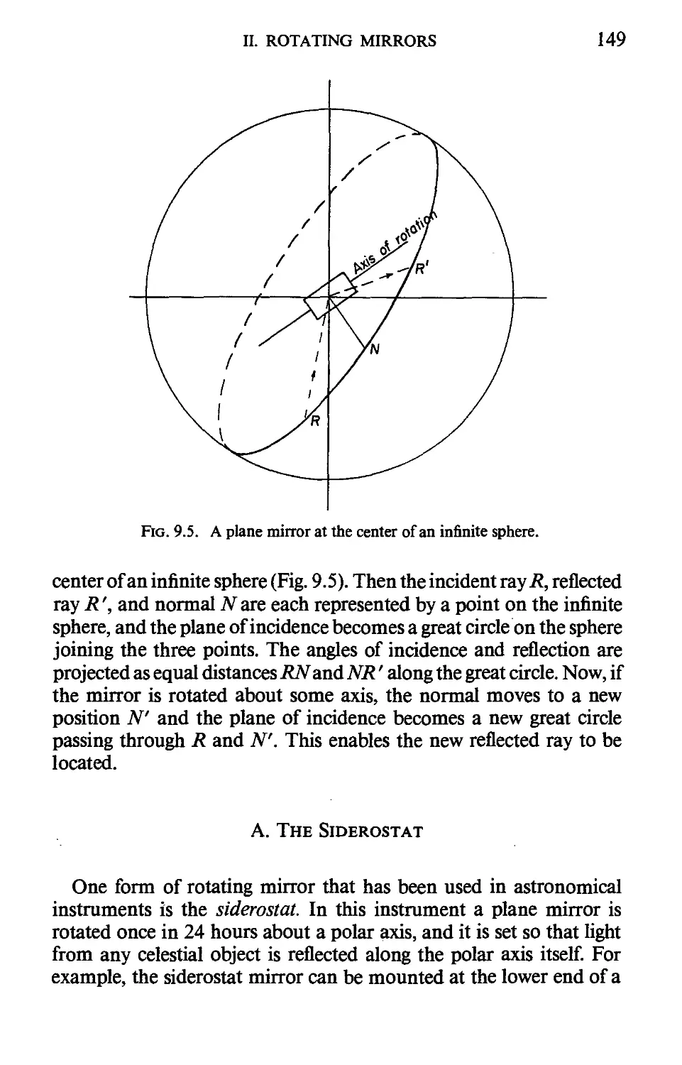
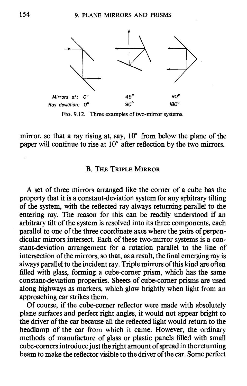
I. RIGHT- AND LEFT-HANDED IMAGES 144
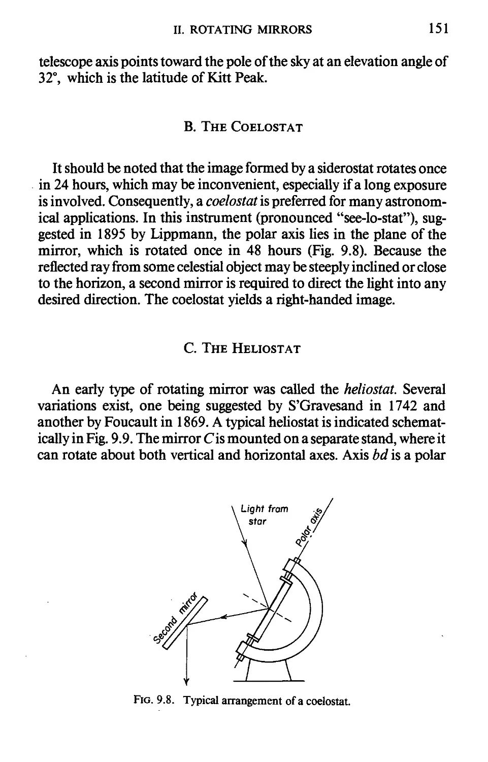
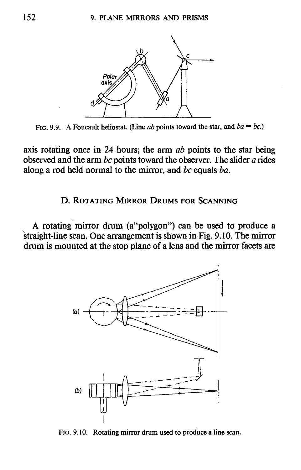
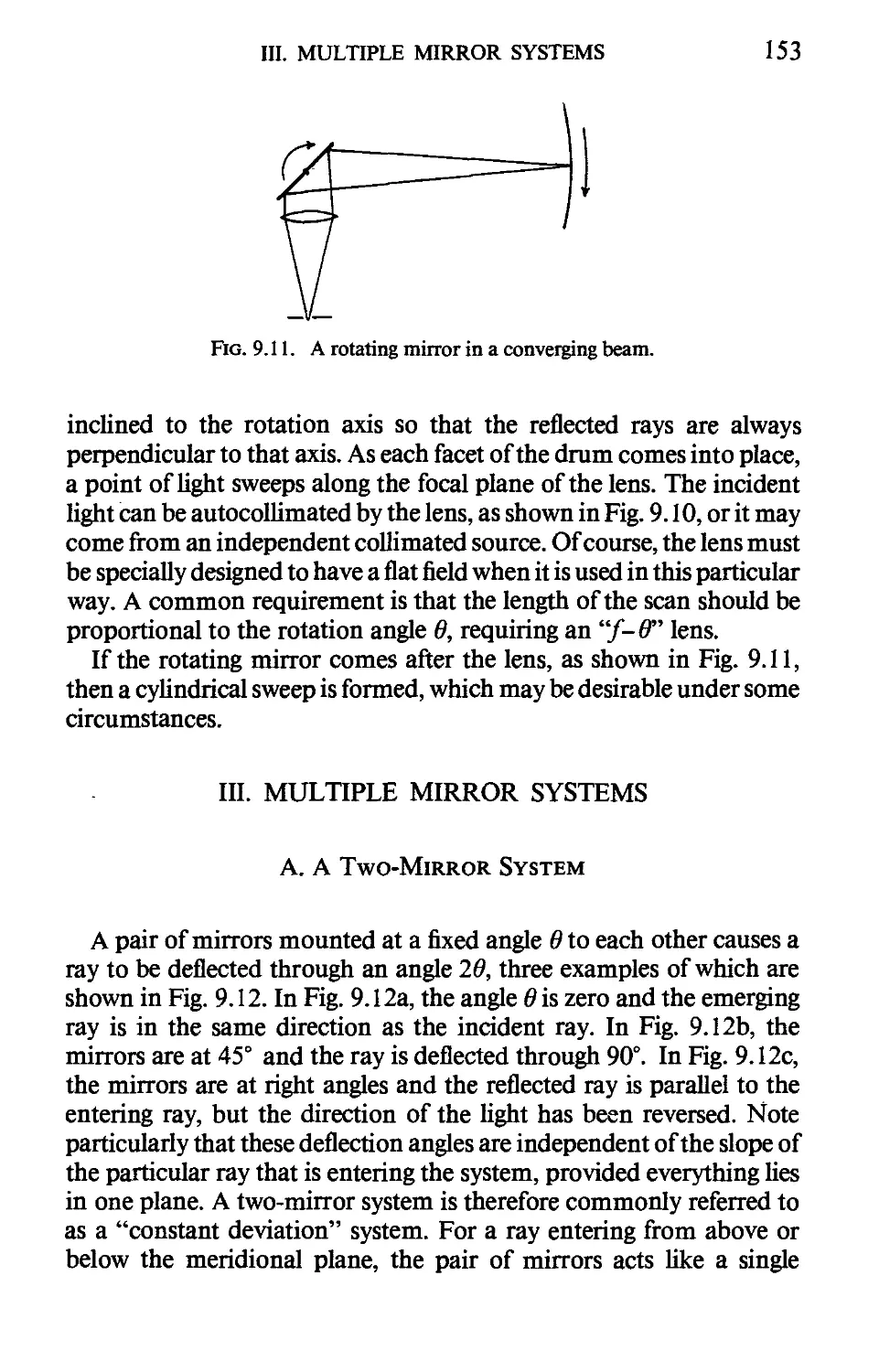
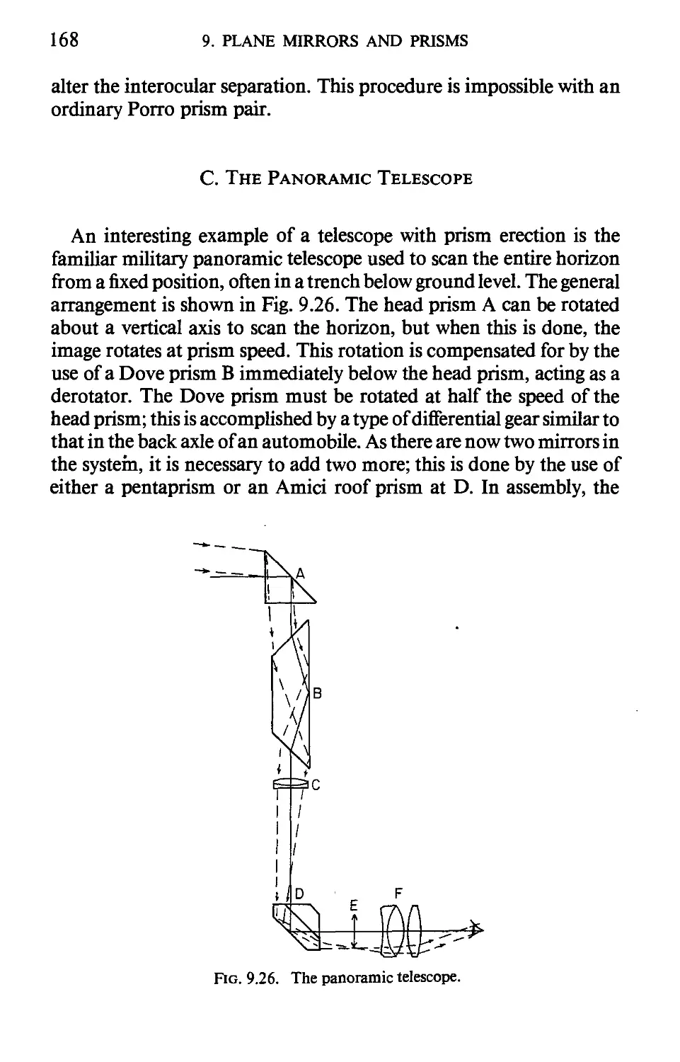
II. ROTATING MIRRORS 148
III. MULTIPLE MIRROR SYSTEMS 153
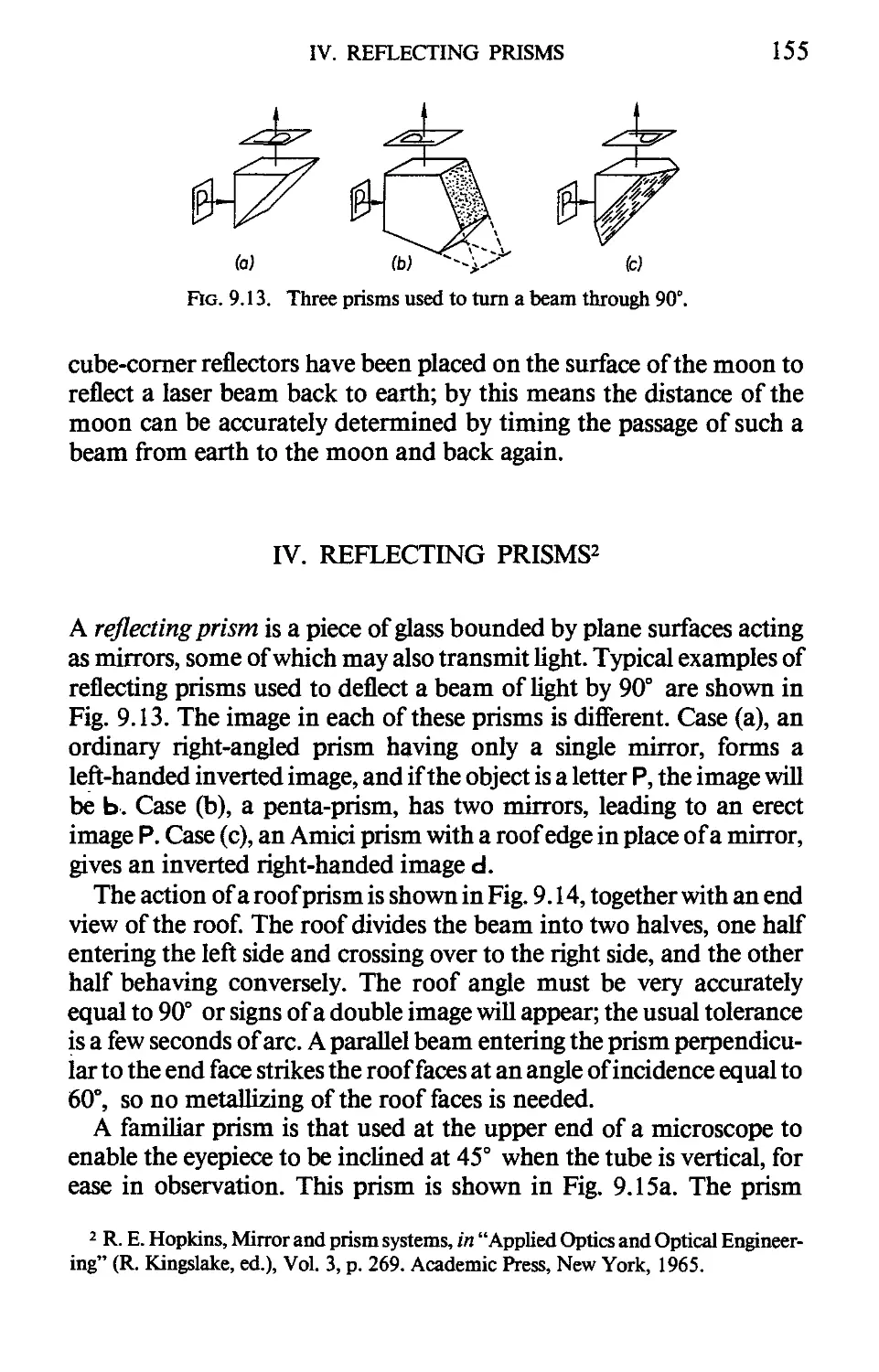
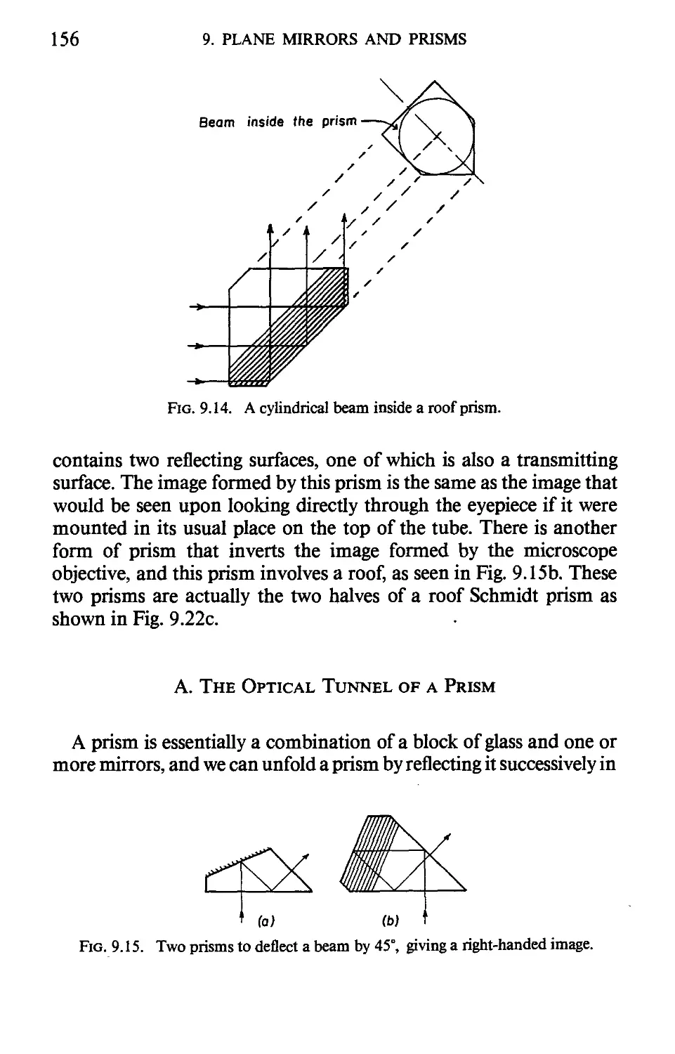
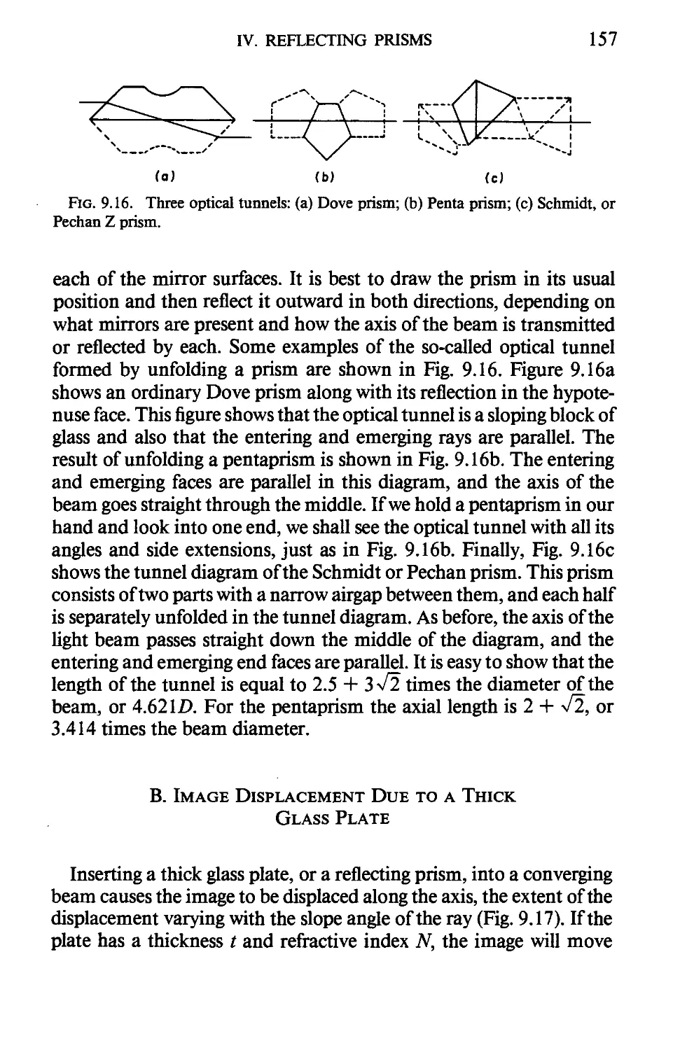
IV. REFLECTING PRISMS 155
V. IMAGE ROTATORS 161
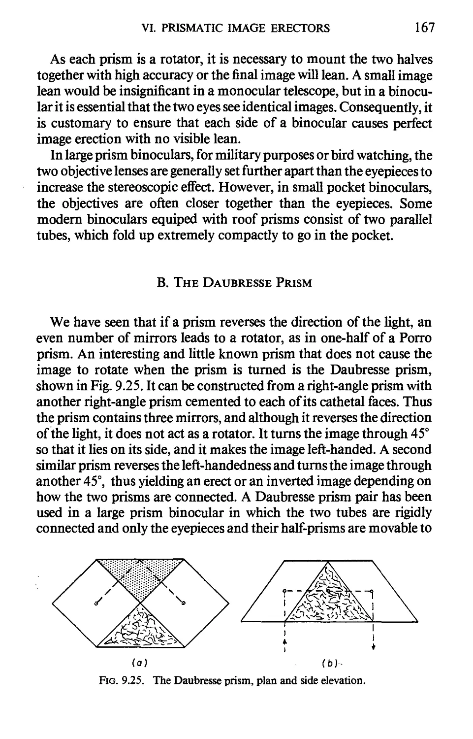
VI. PRISMATIC IMAGE ERECTORS 164
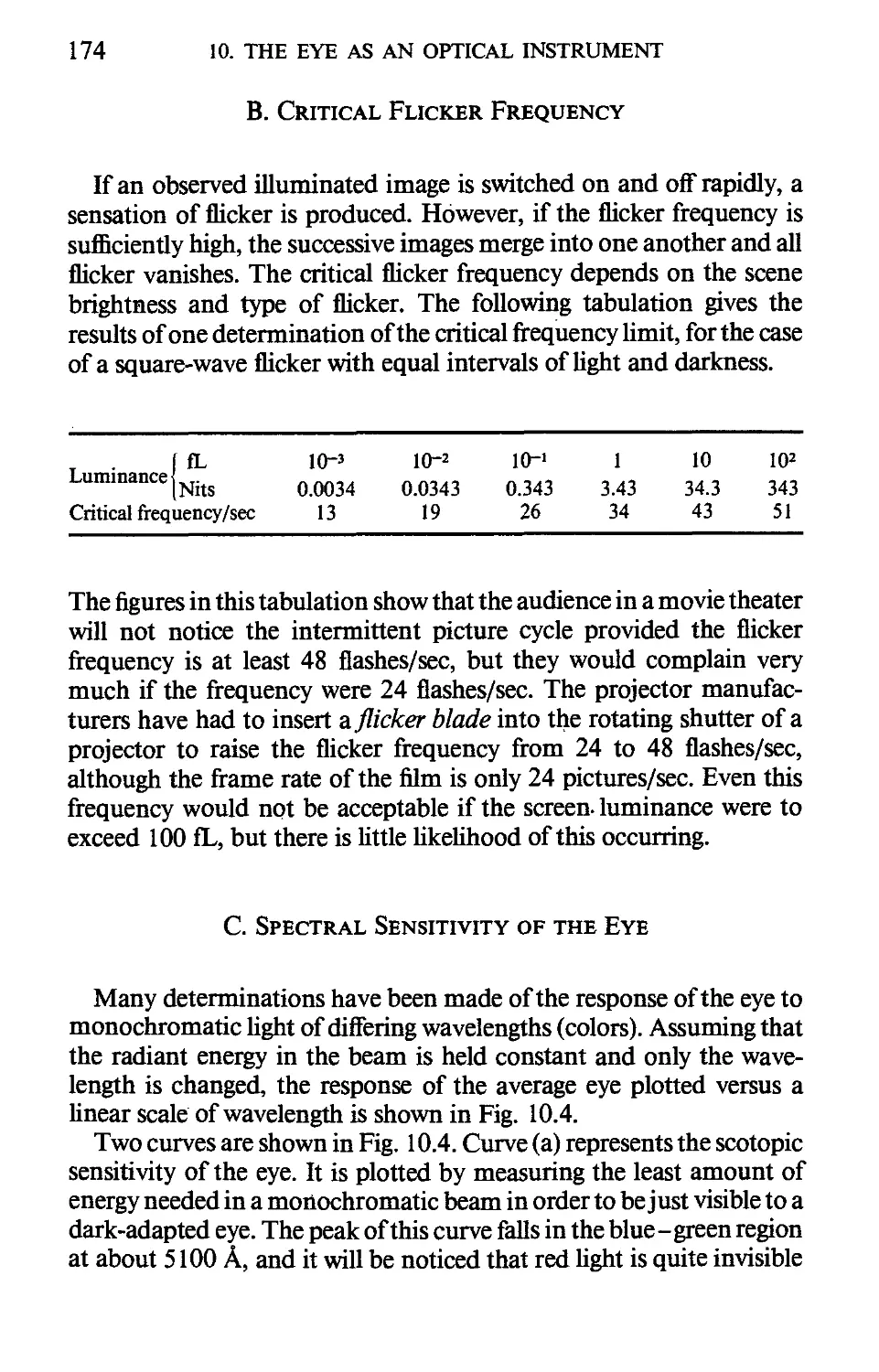
10. The Eye as an Optical Instrument
I. DIMENSIONS 170
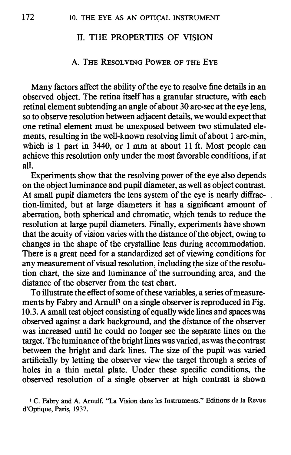
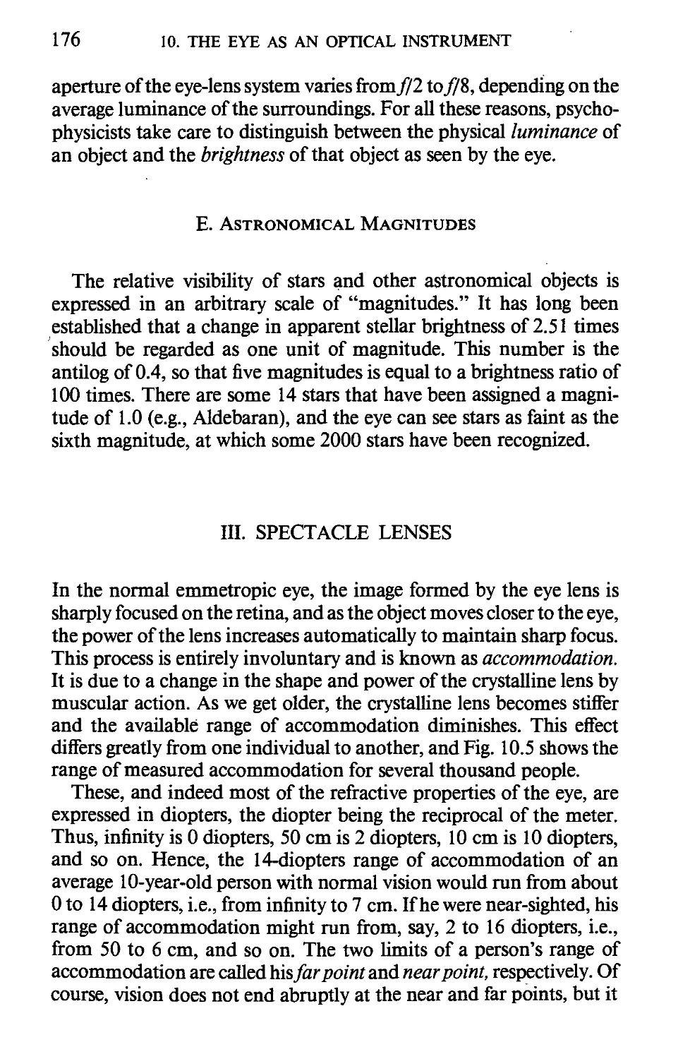
II. THE PROPERTIES OF VISION 172
III. SPECTACLE LENSES 176
IV. STEREOSCOPIC VISION 180
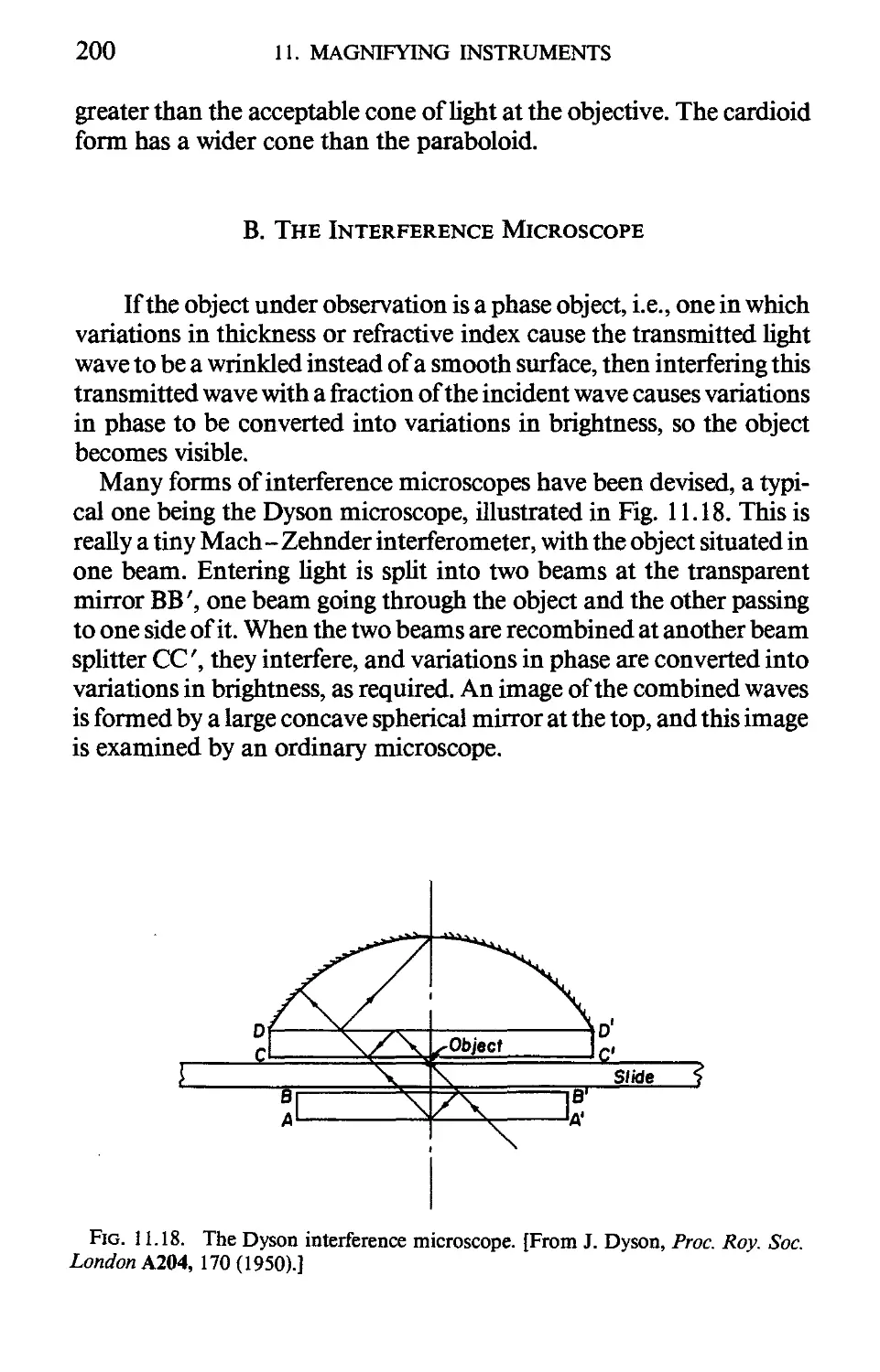
11. Magnifying Instruments
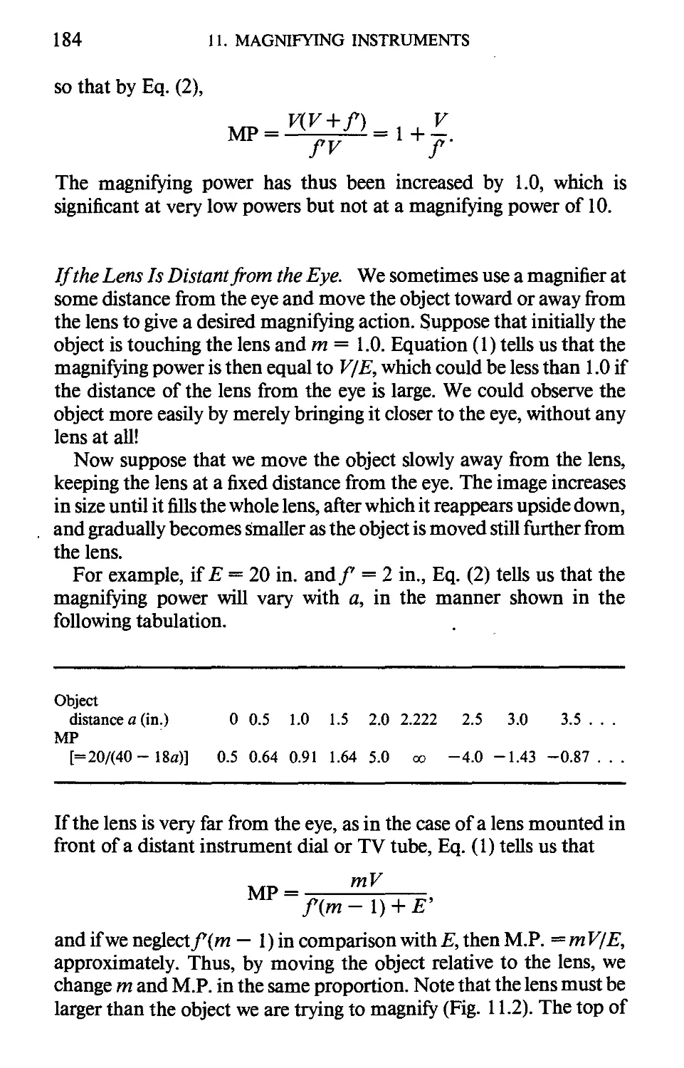
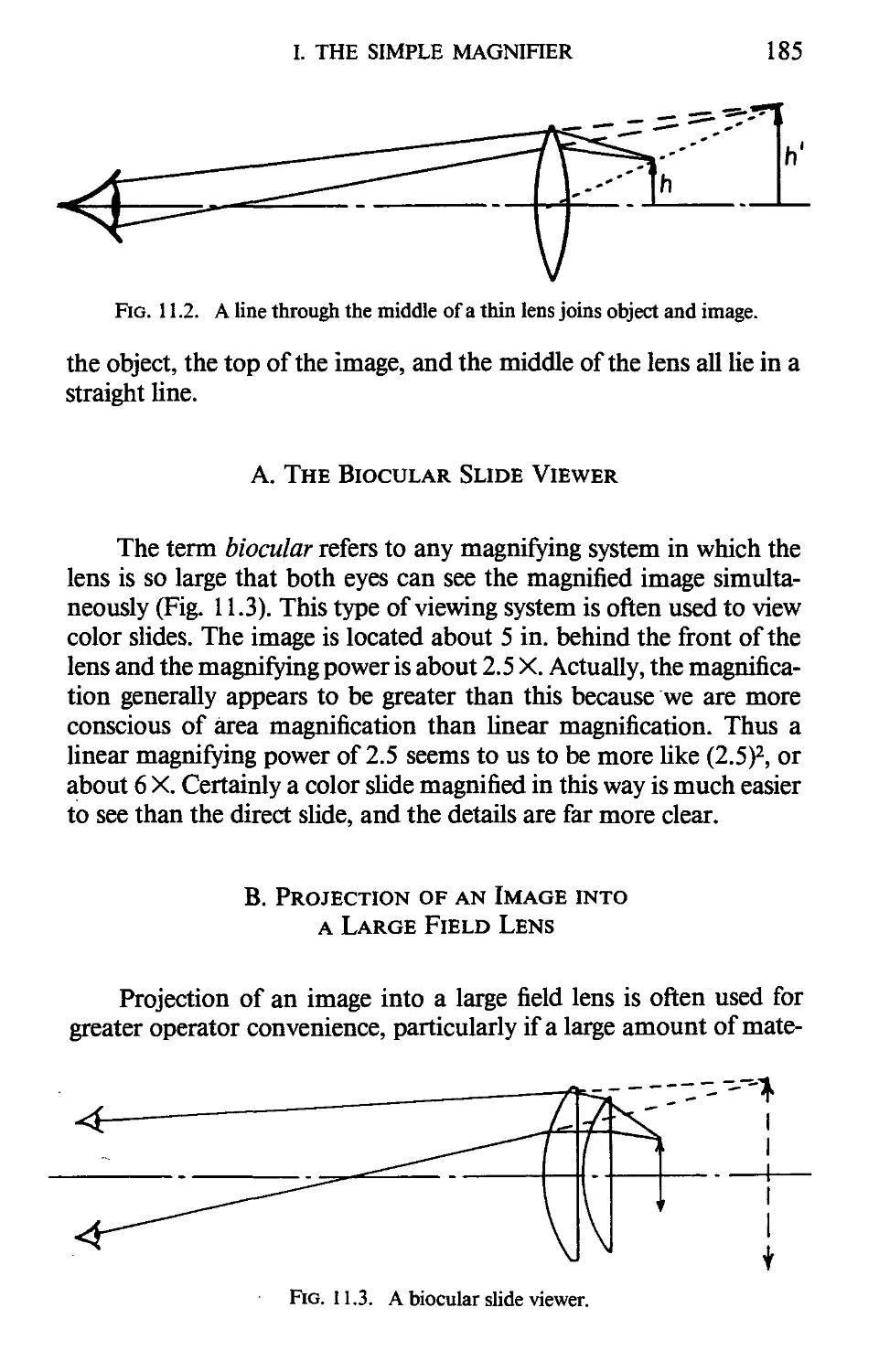
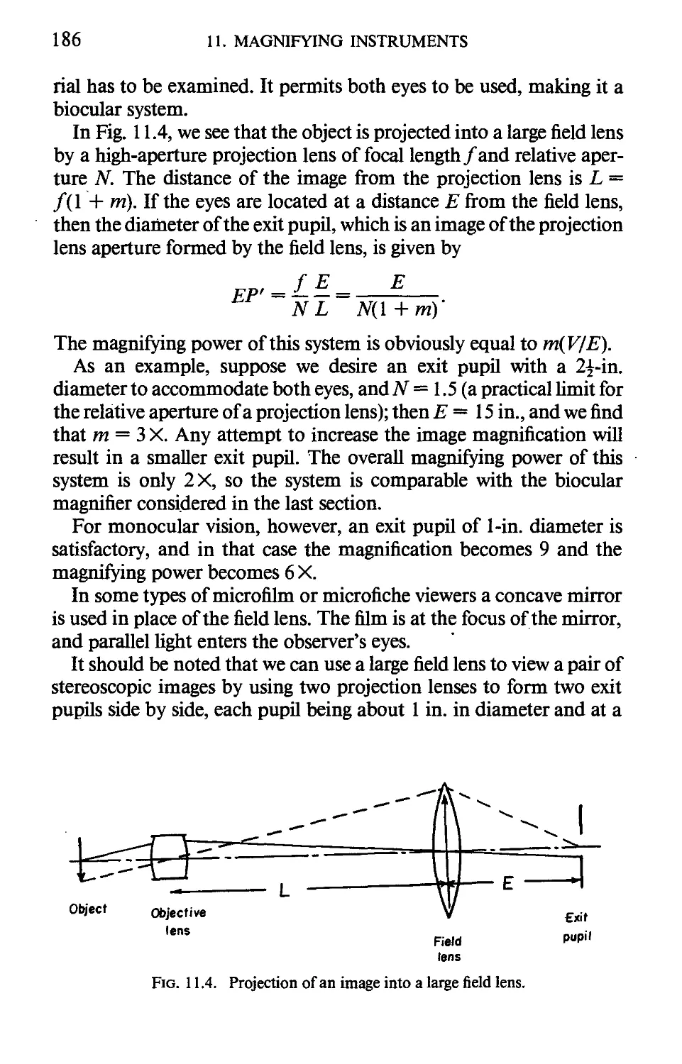
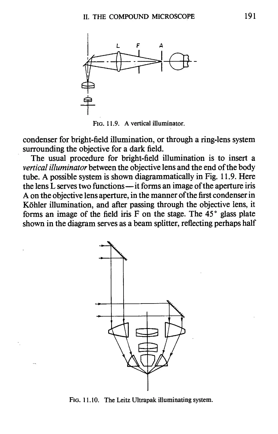
I. THE SIMPLE MAGNIFIER 182
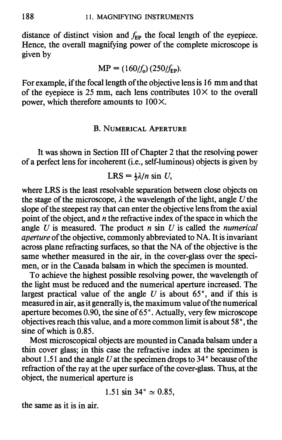
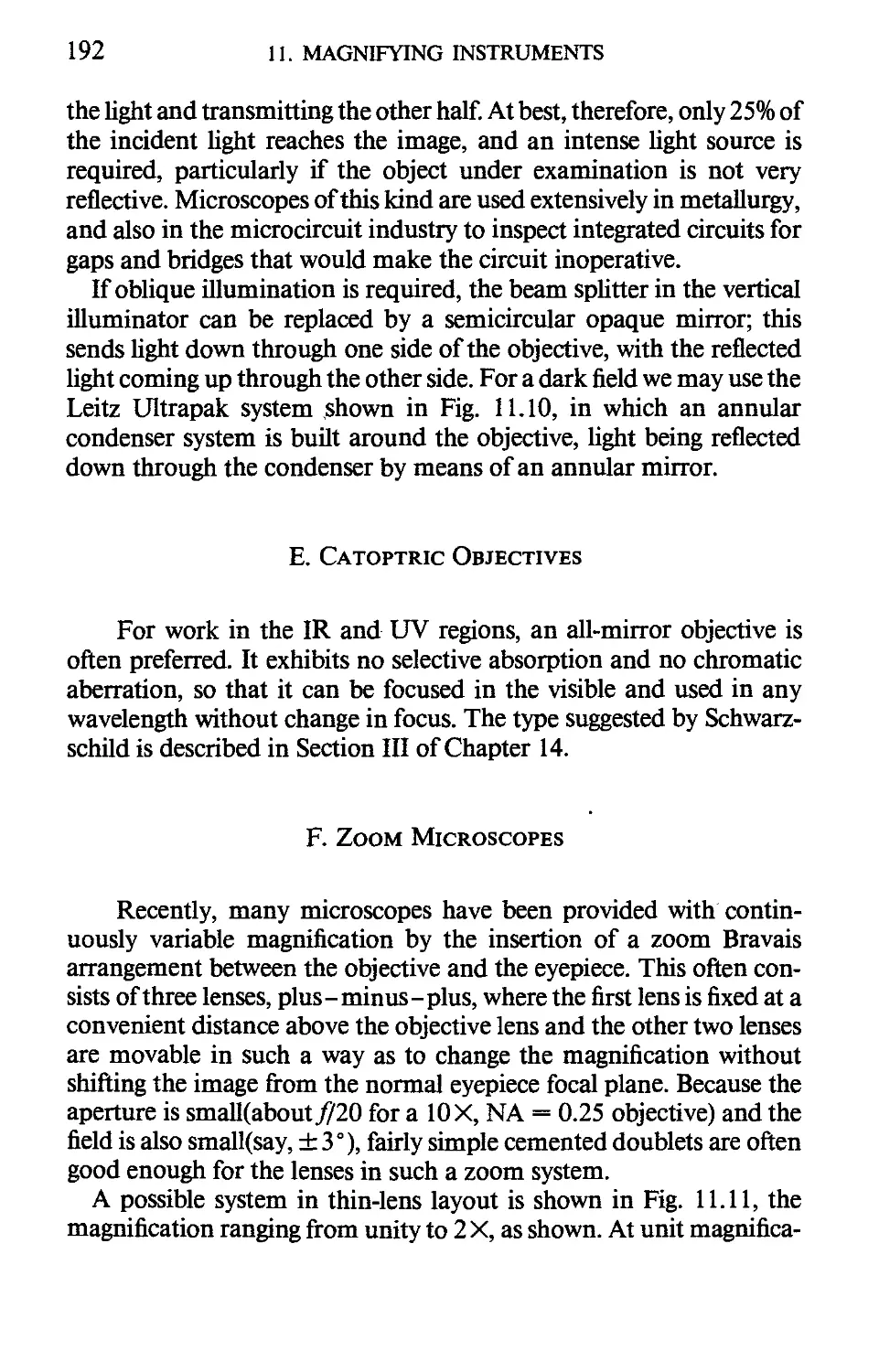
II. THE COMPOUND MICROSCOPE 187
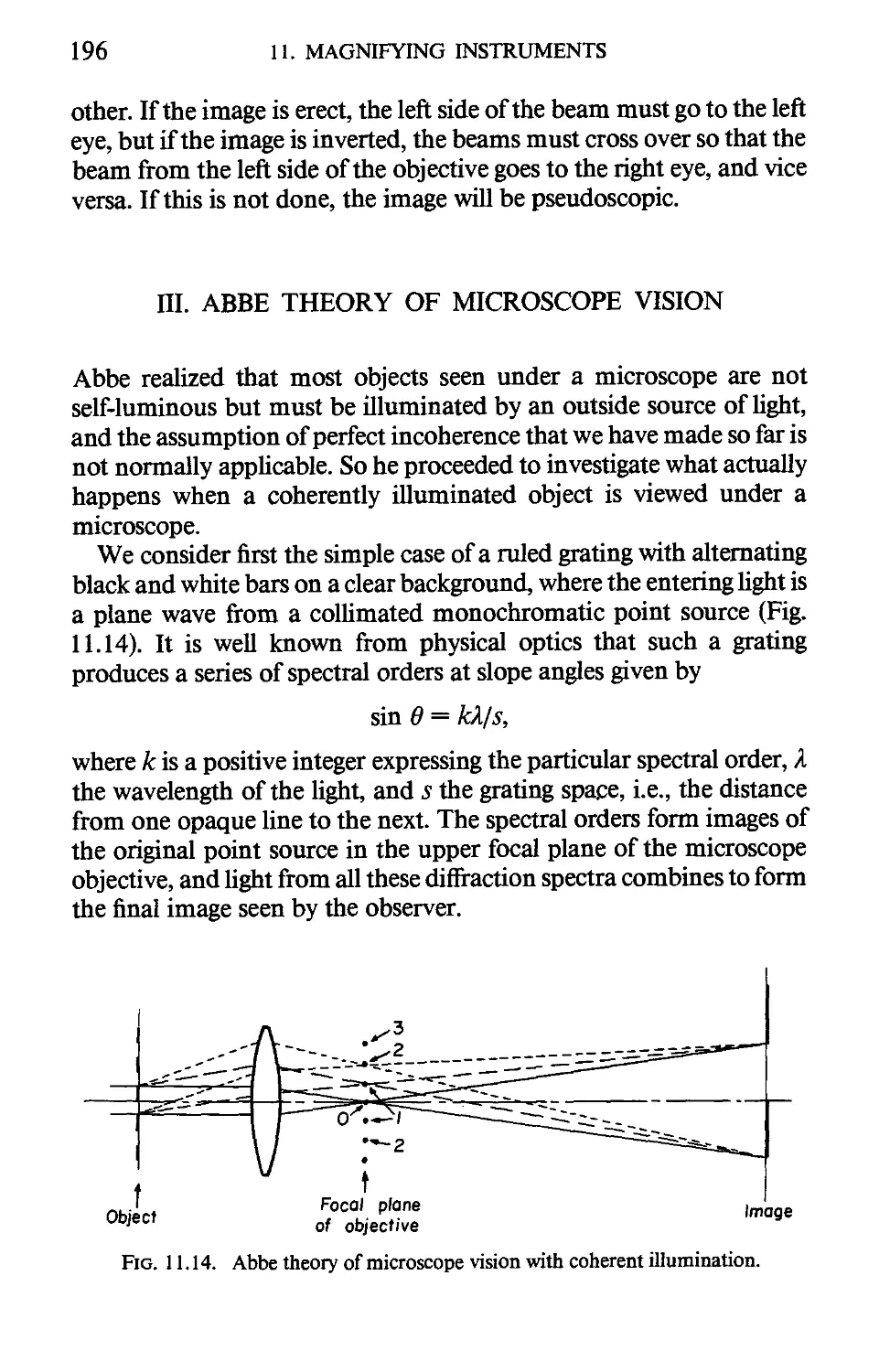
Ш. ABBE THEORY OF MICROSCOPE VISION 196
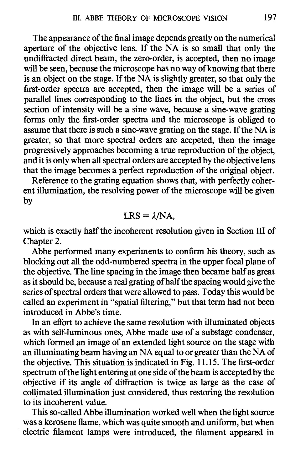
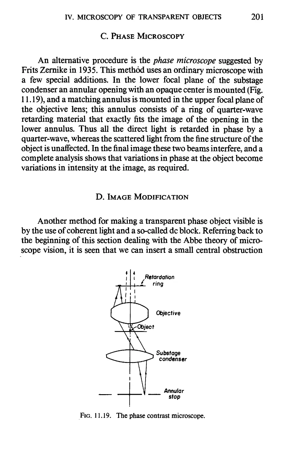
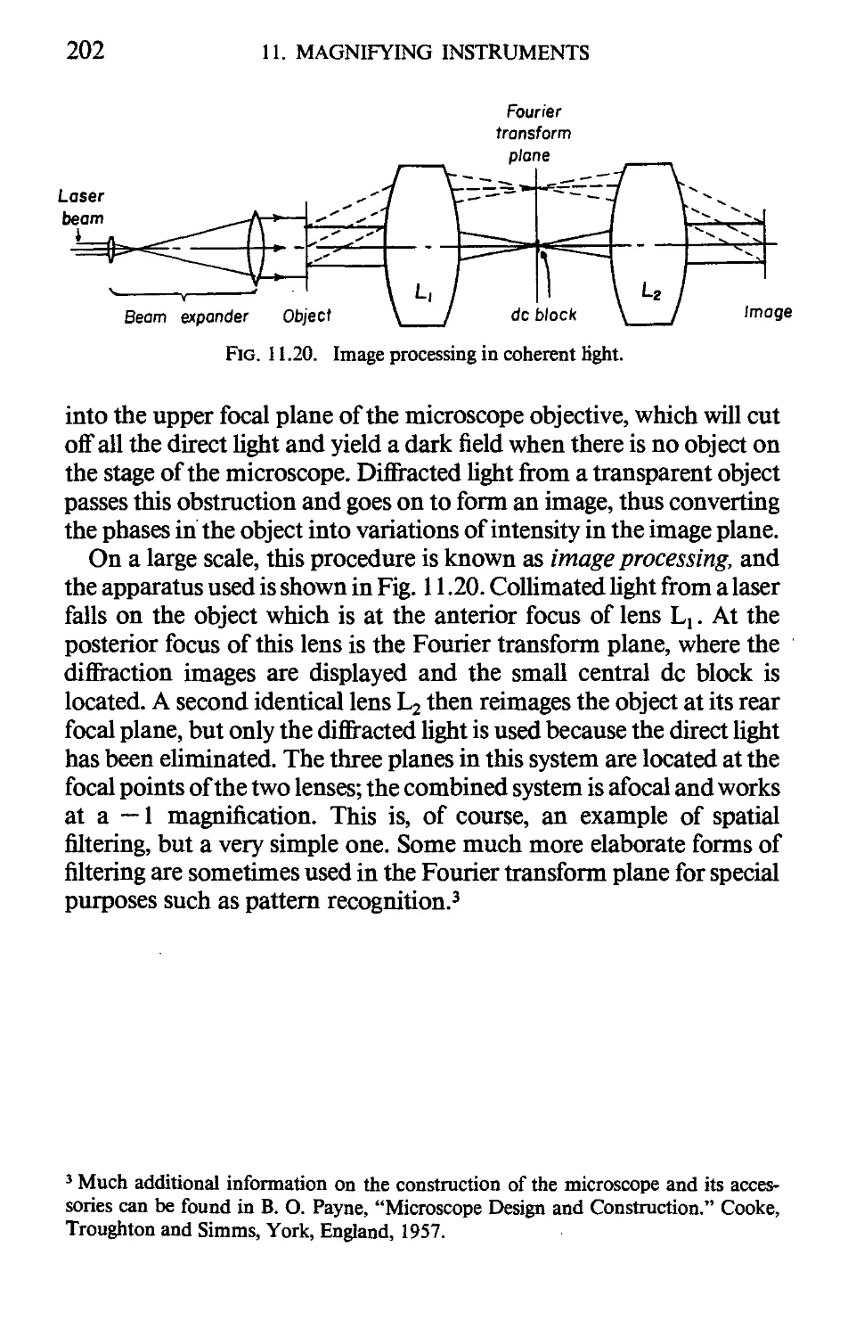
IV. MICROSCOPY OF TRANSPARENT OBJECTS 199
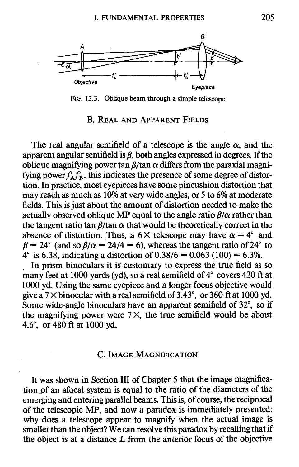
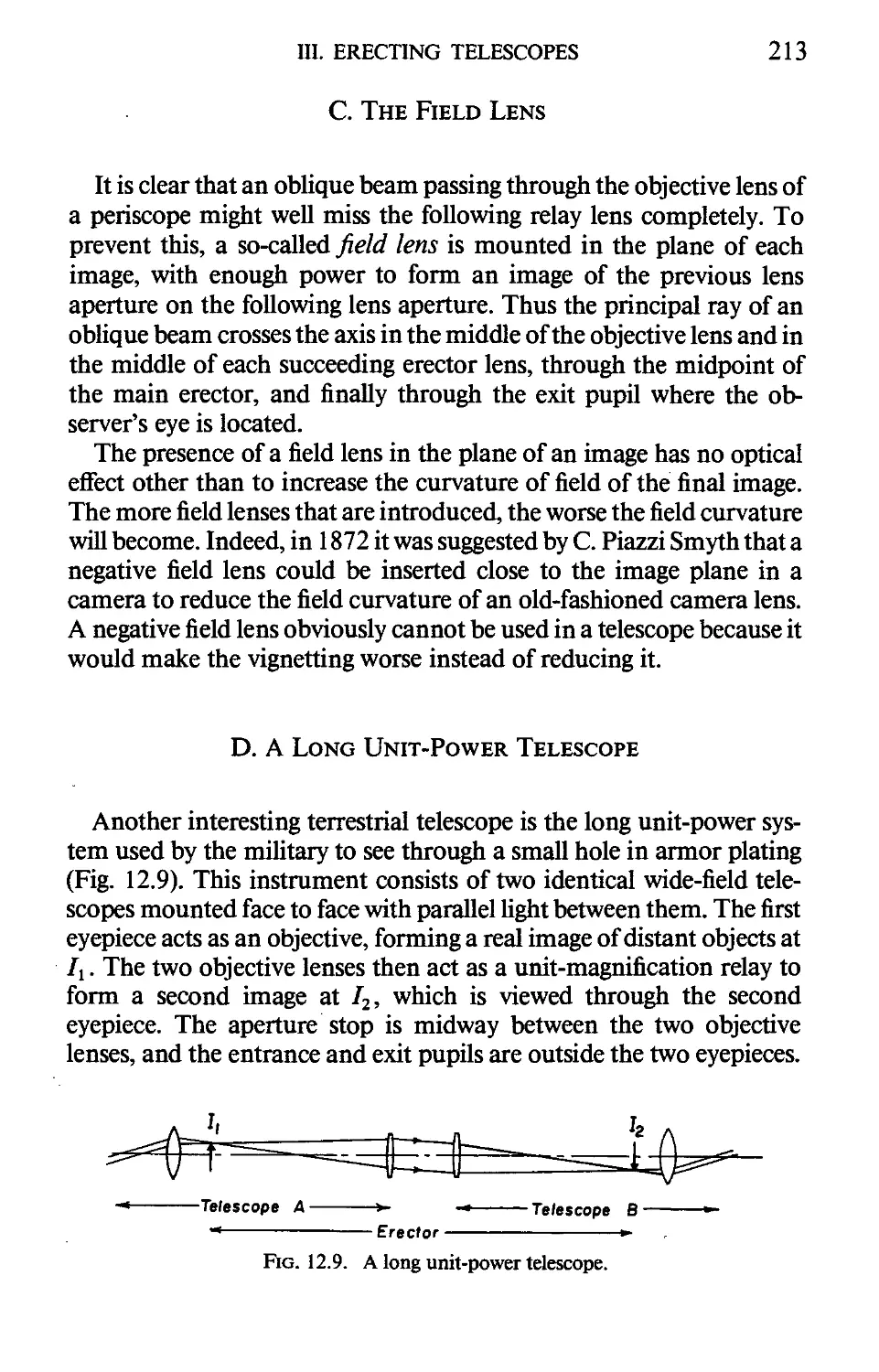
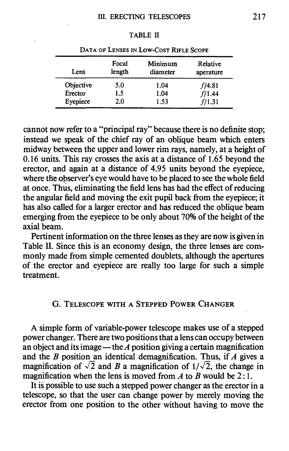
12. The Telescope
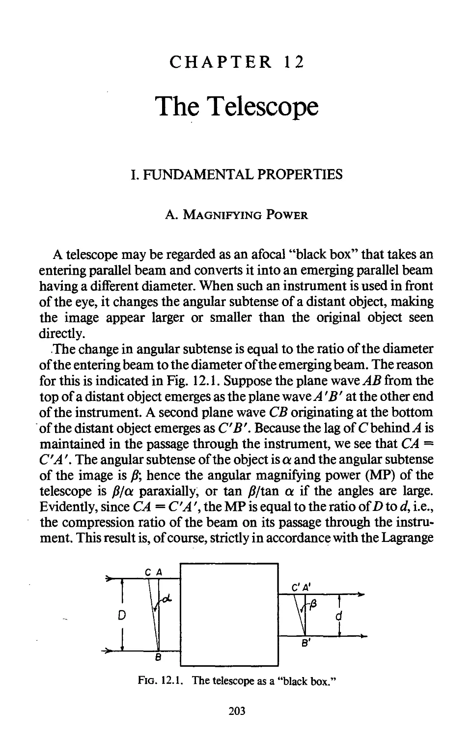
I. FUNDAMENTAL PROPERTIES 203
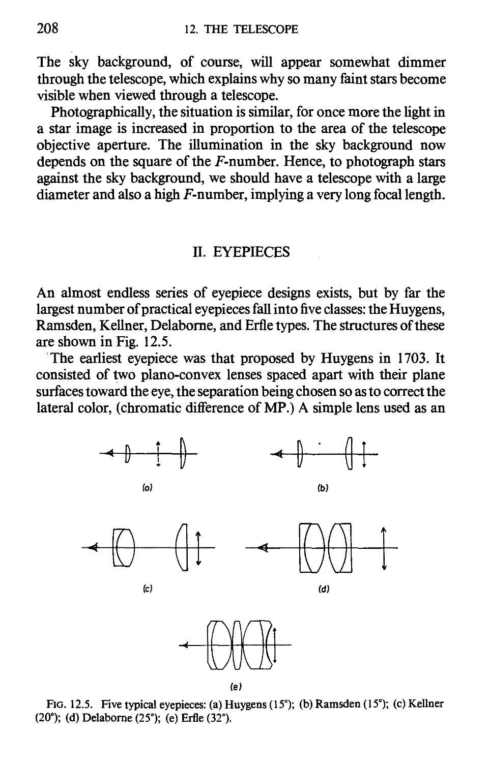
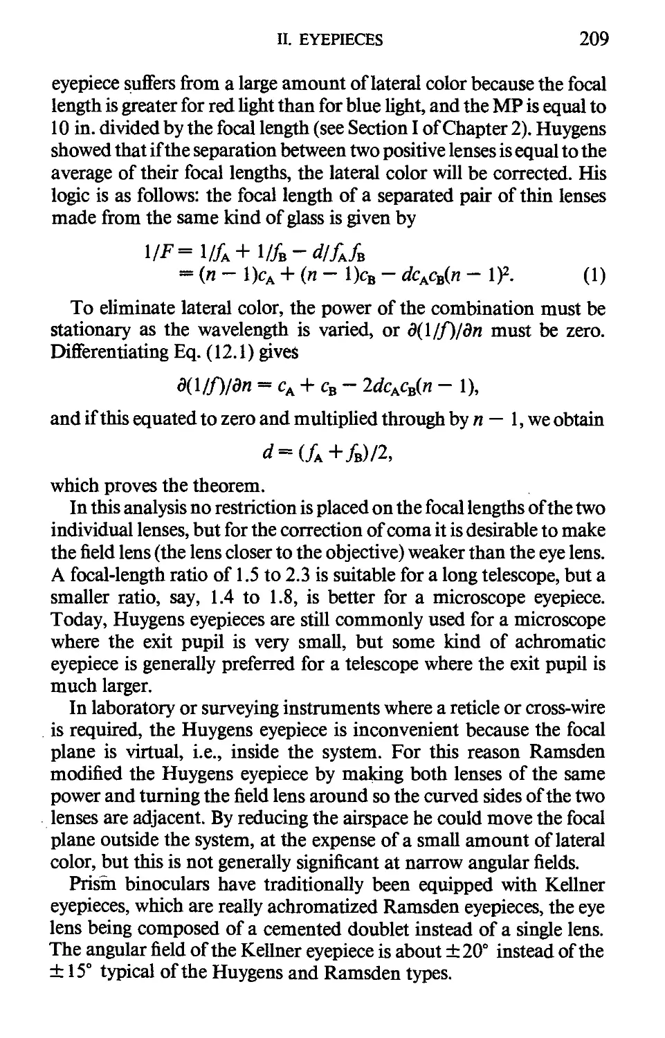
II. EYEPIECES 208
Ш. ERECTING TELESCOPES 210
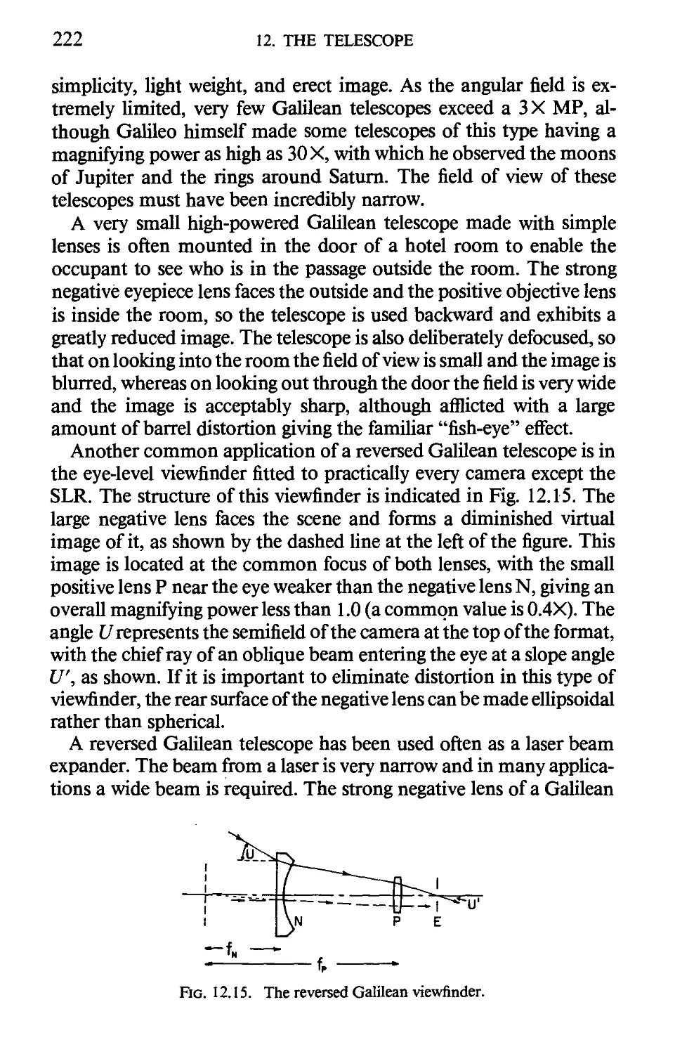
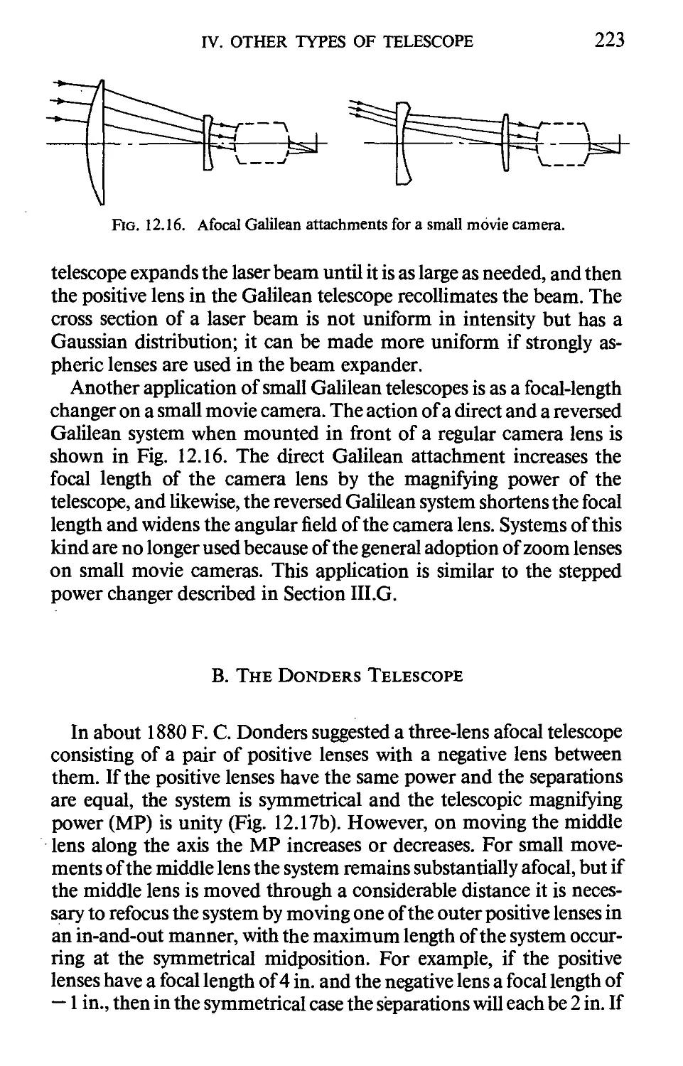
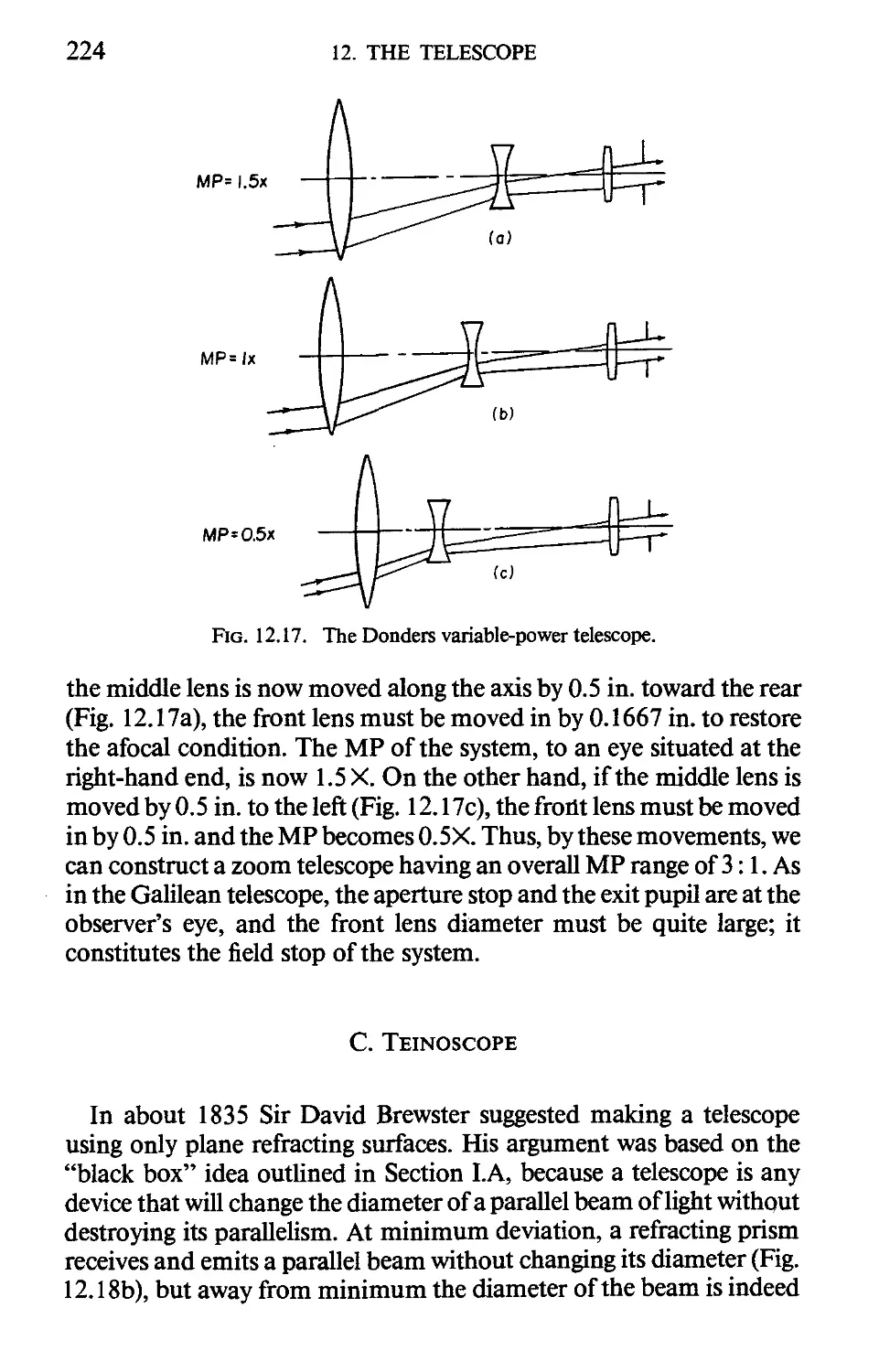
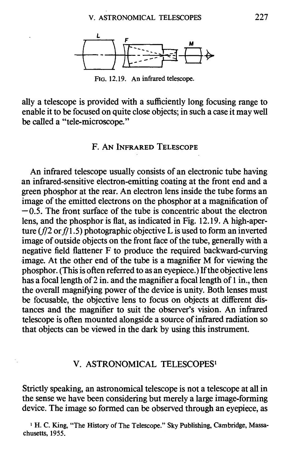
IV. OTHER TYPES OF TELESCOPES 221
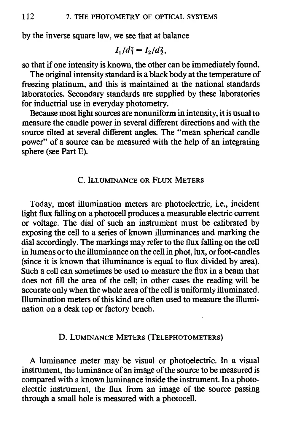
V. ASTRONOMICAL TELESCOPES 227
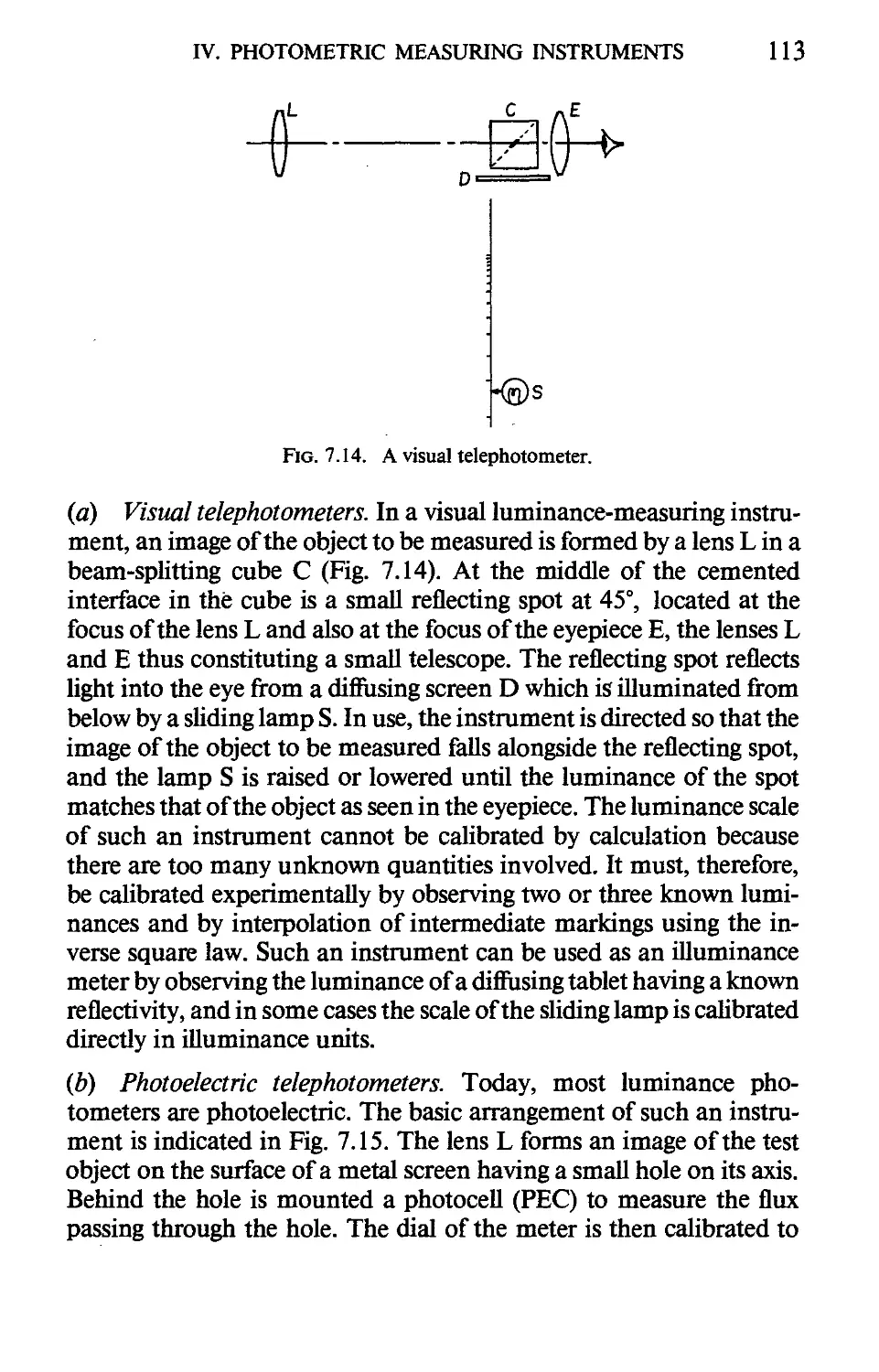
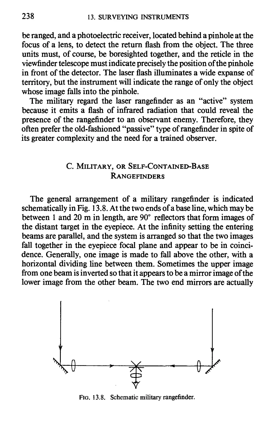
13. Surveying Instruments
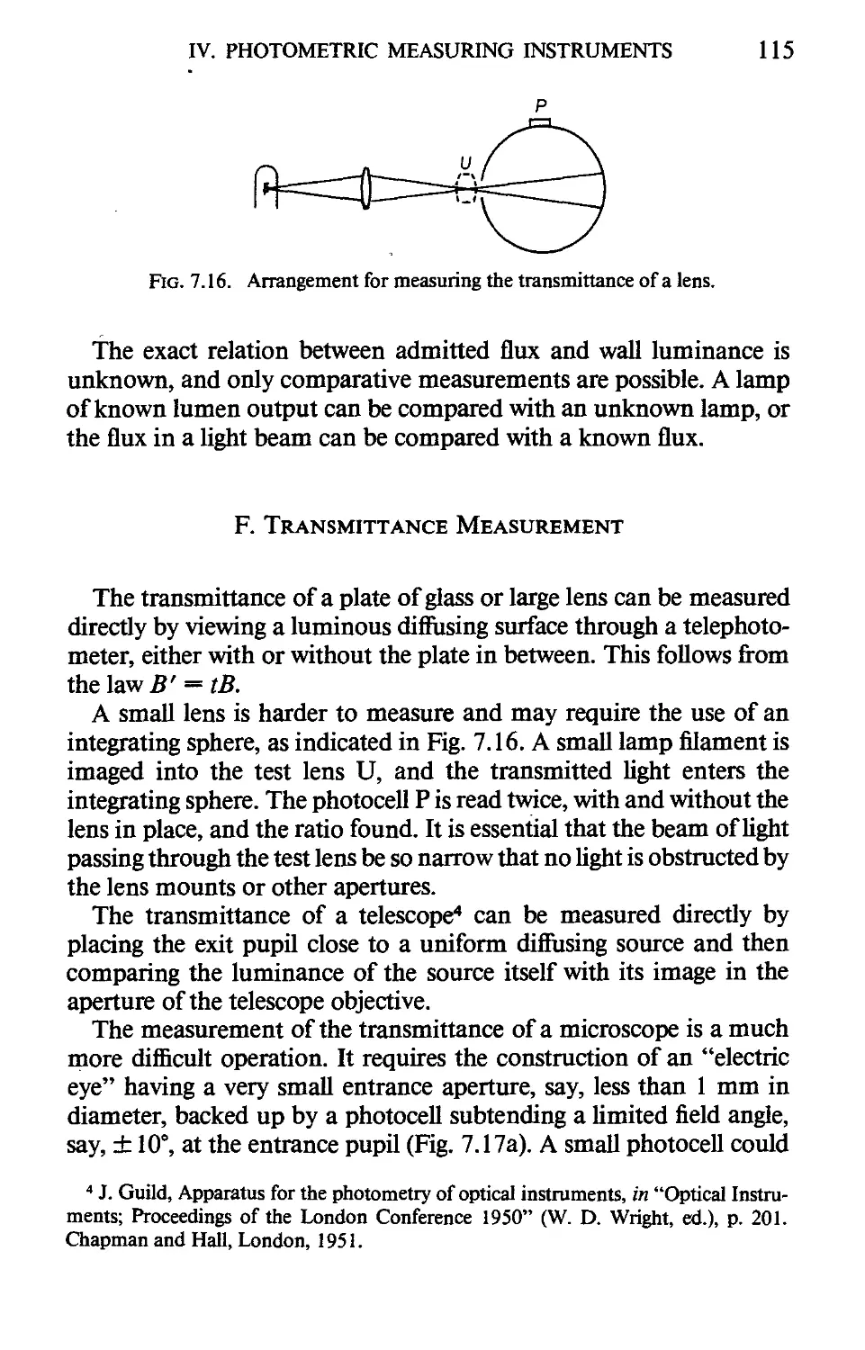
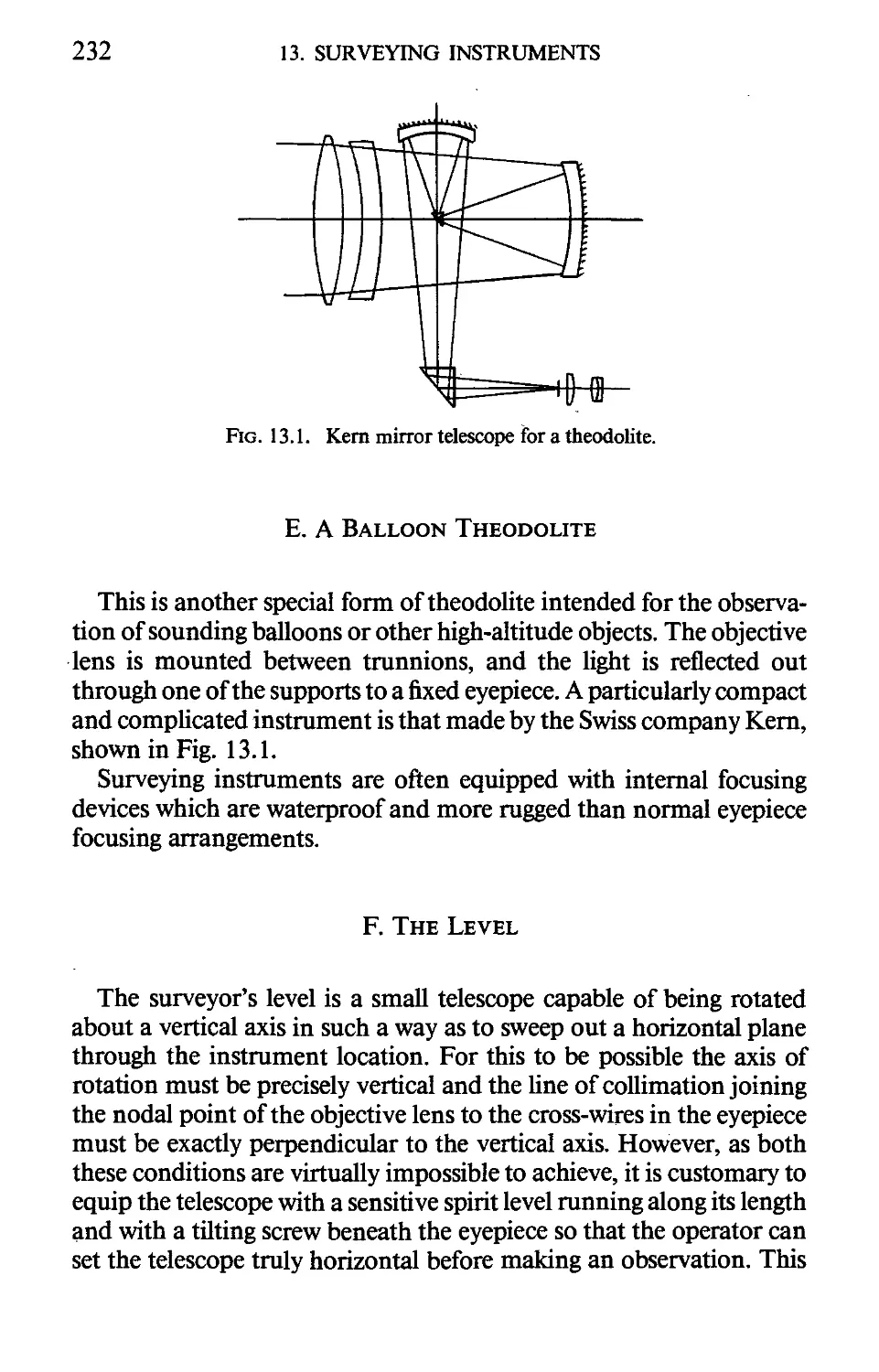
I. CLASSES OF SURVEYING INSTRUMENTS 230
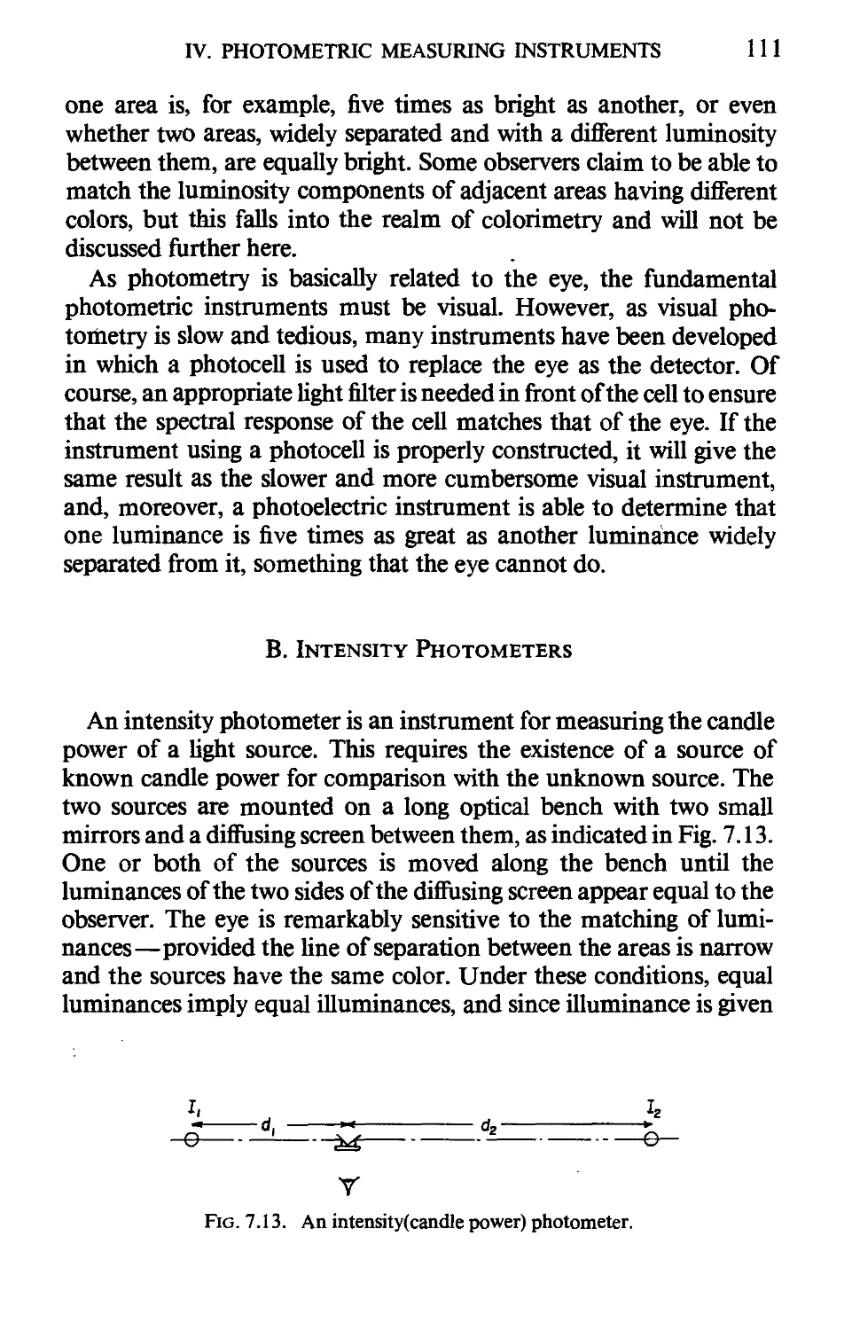
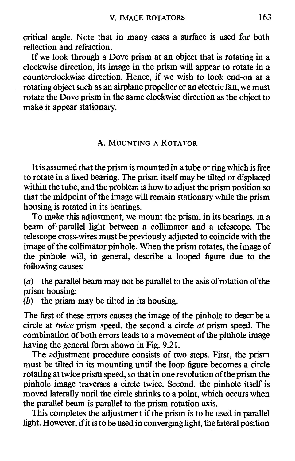
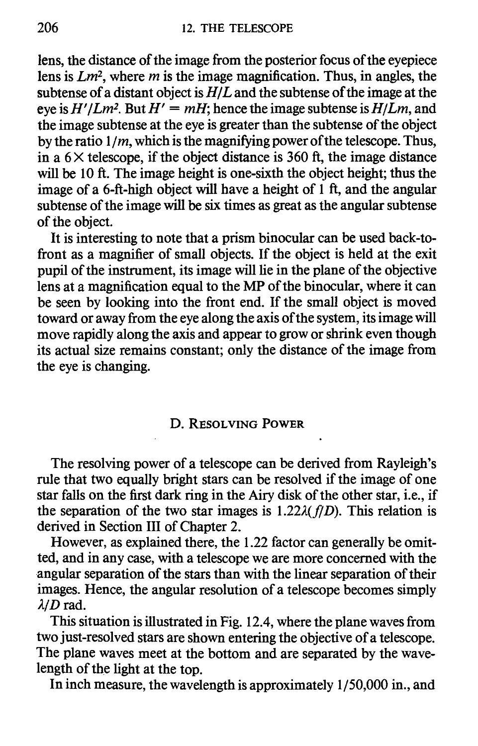
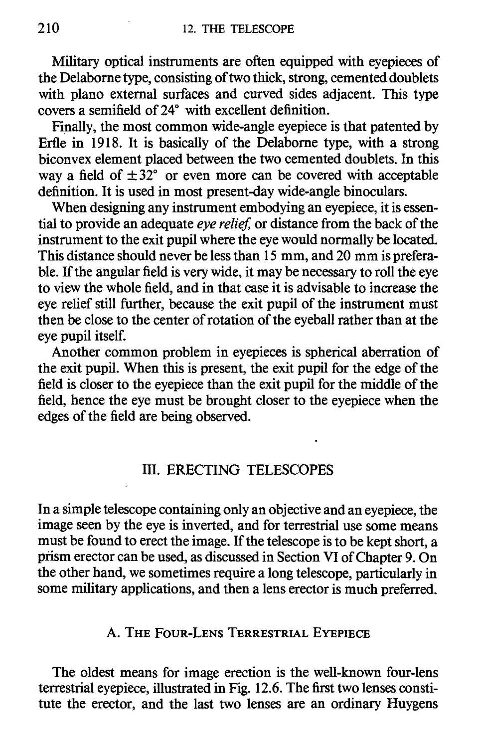
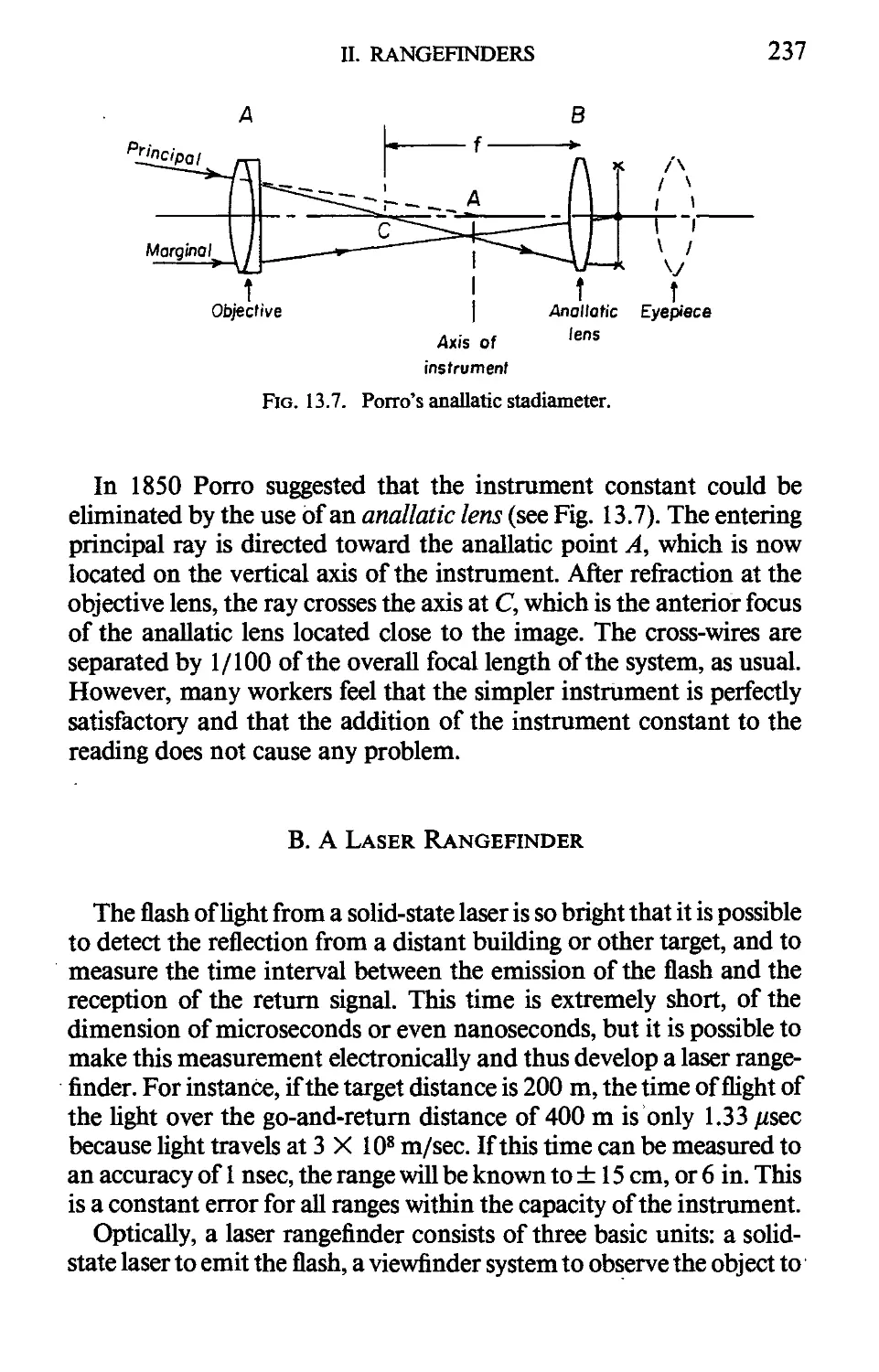
II. RANGEFINDERS 236
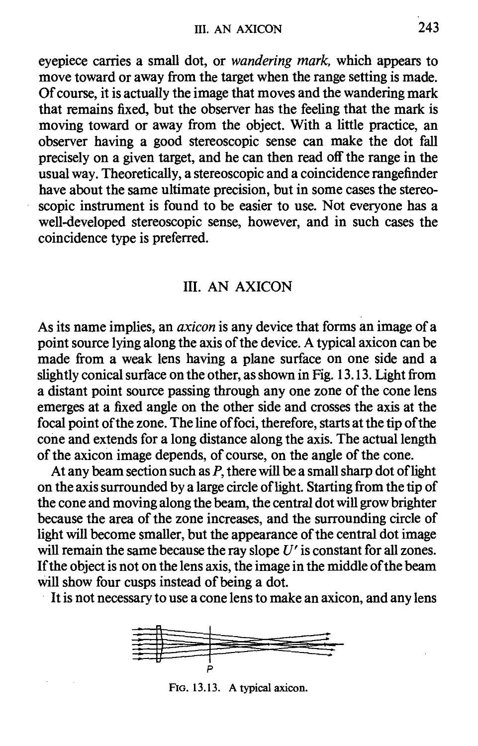
Ш. AN AXICON 243
viii CONTENTS
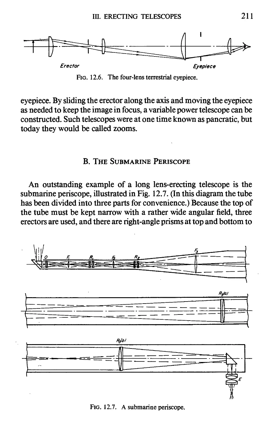
14. Mirror Imaging Systems
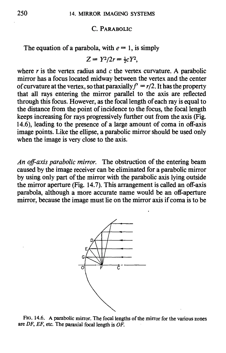
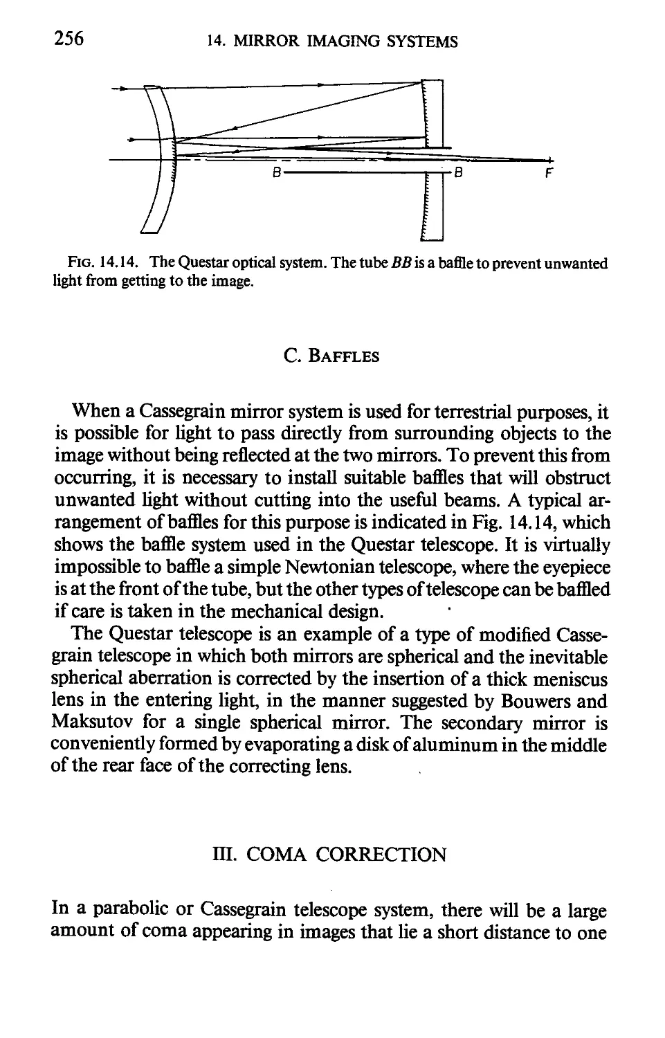
I. SINGLE-MIRROR SYSTEMS 245
II. TWO-MIRROR SYSTEMS 253
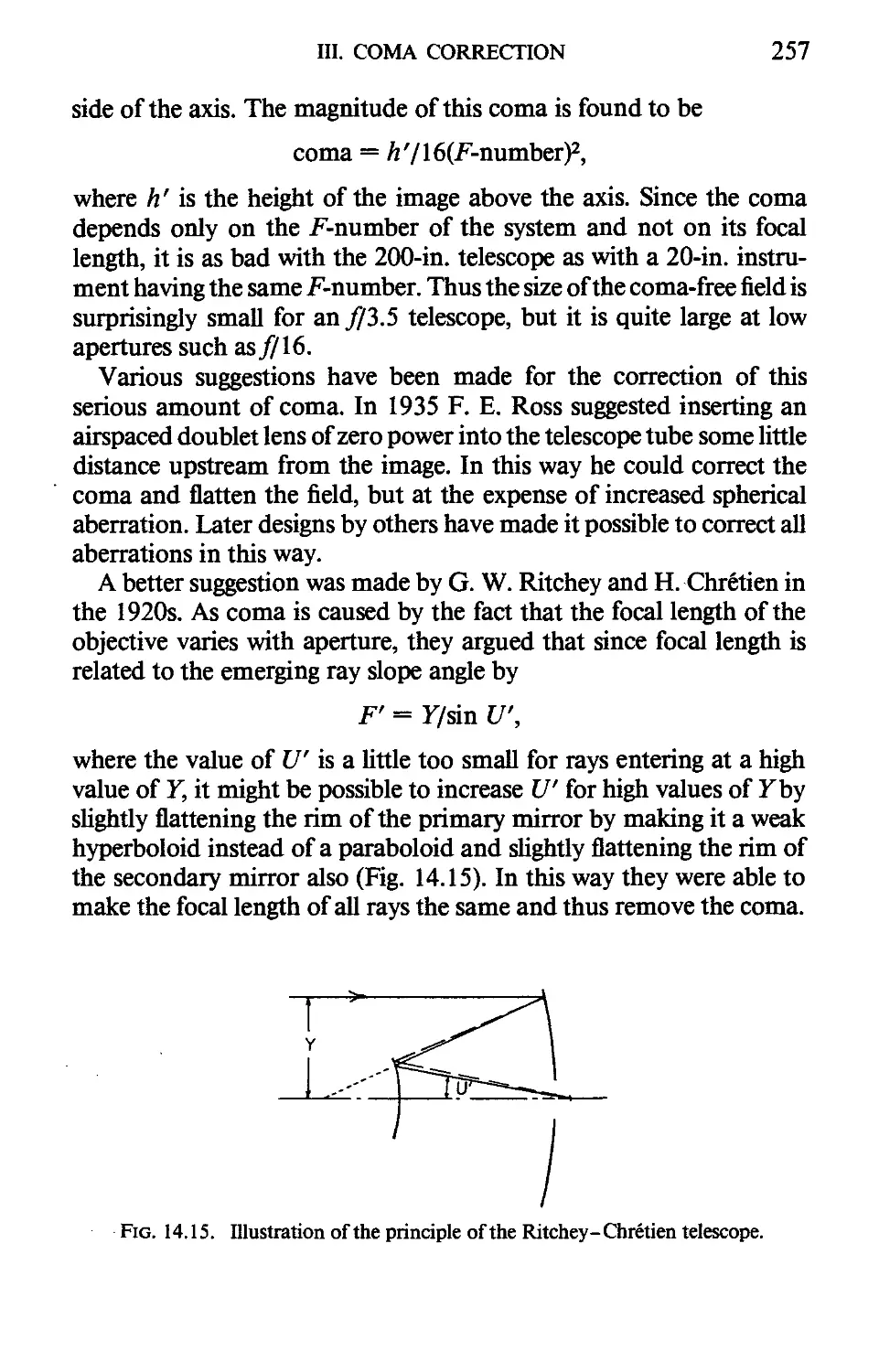
III. COMA CORRECTION 256
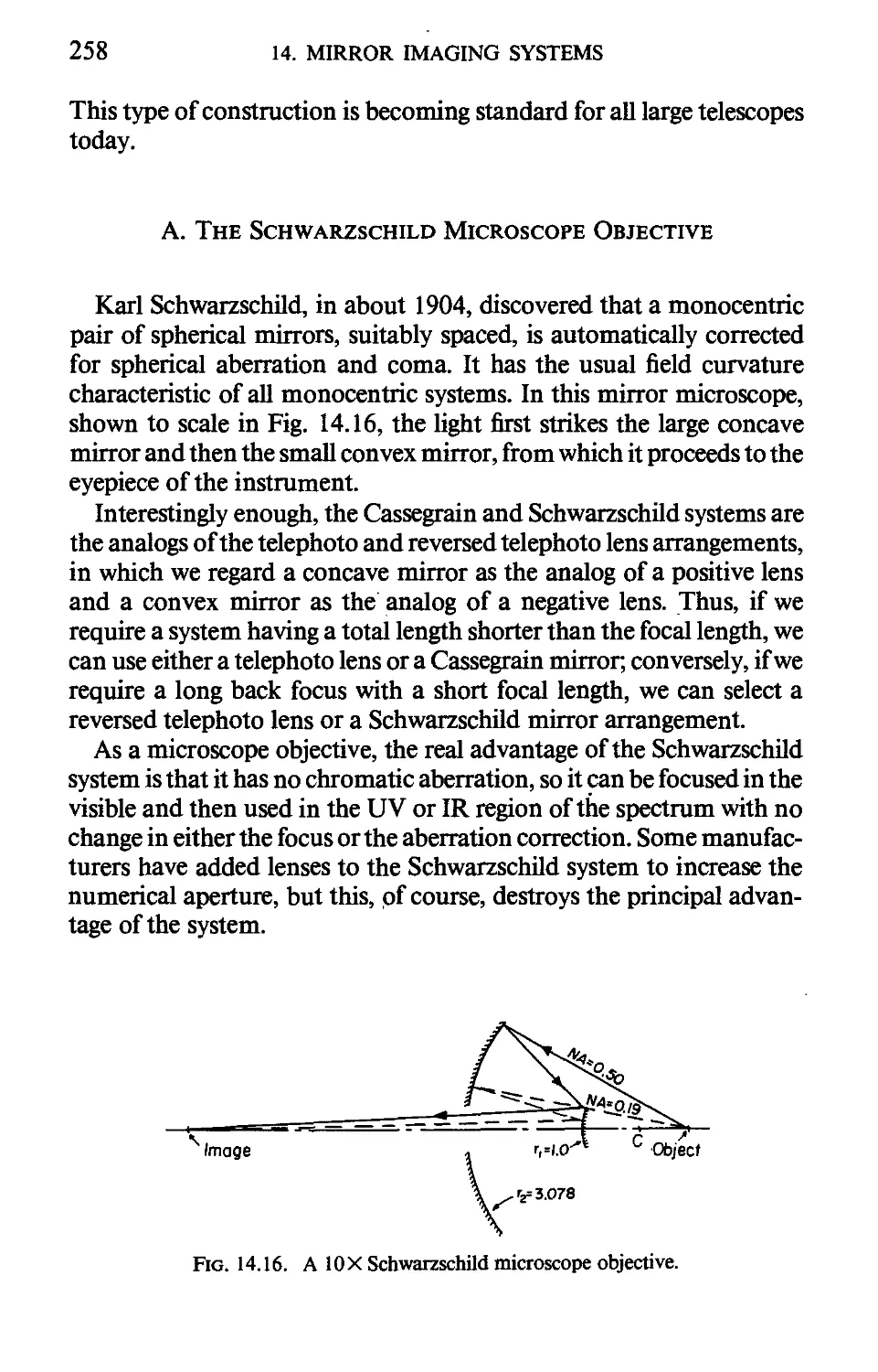
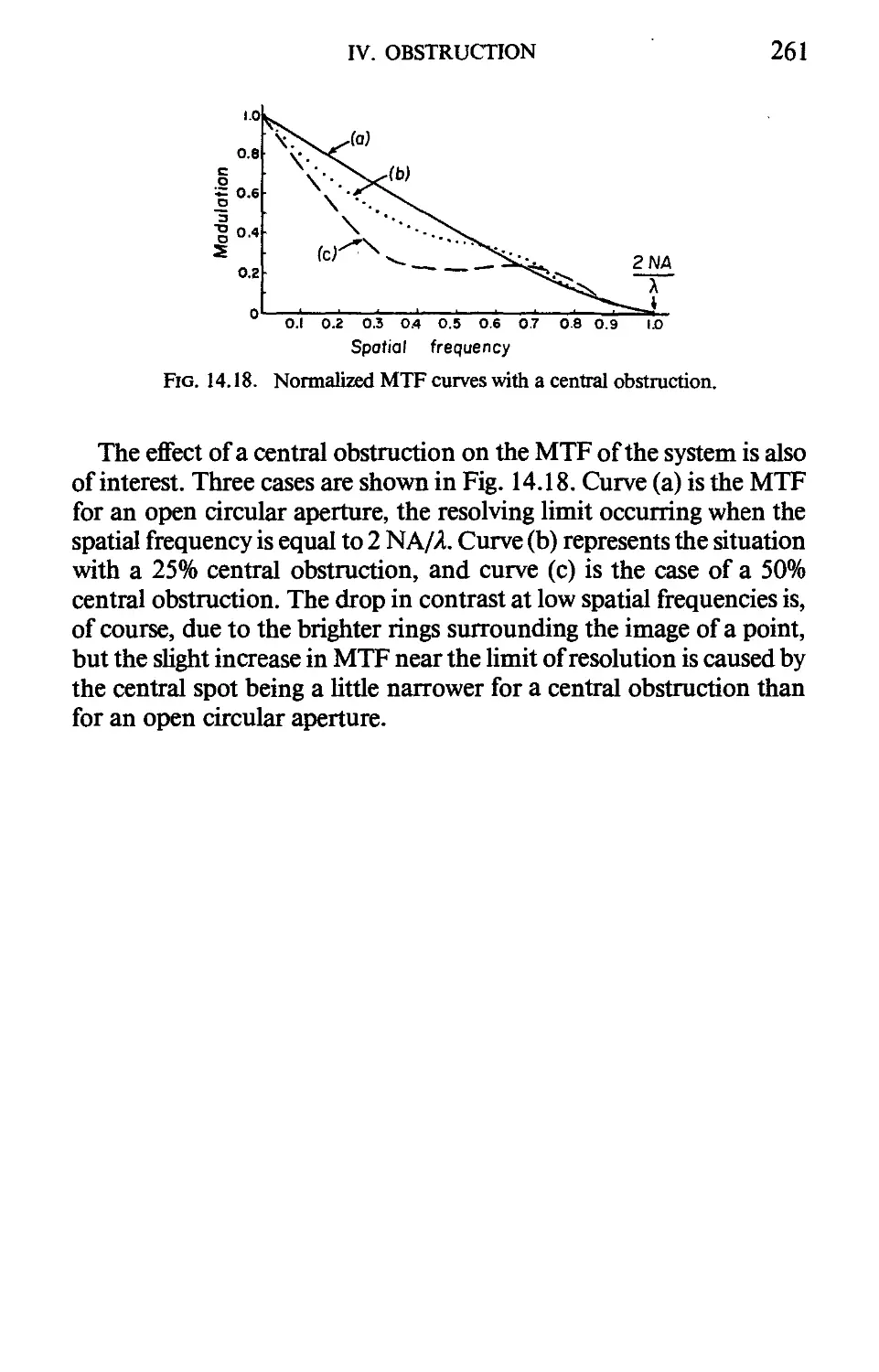
IV. OBSTRUCTION 259
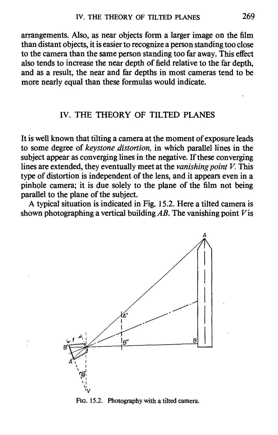
15. Photographic Optics
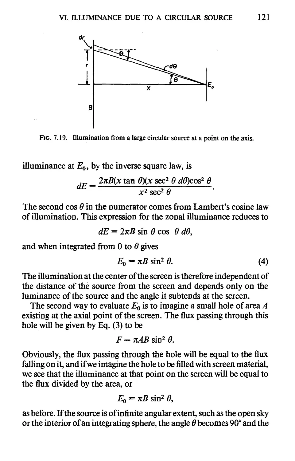
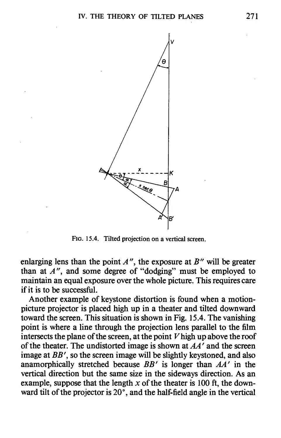
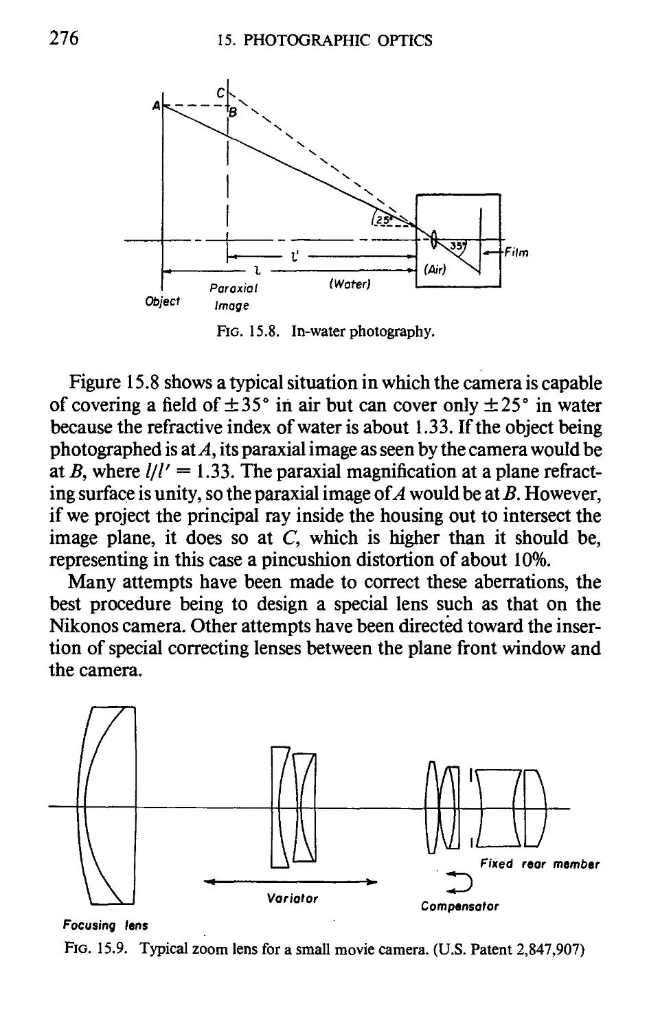
I. PERSPECTIVE EFFECTS IN PHOTOGRAPHY 262
II. FOCUSING ON A NEAR OBJECT 263
III. DEPTH OF FOCUS AND DEPTH OF FIELD 265
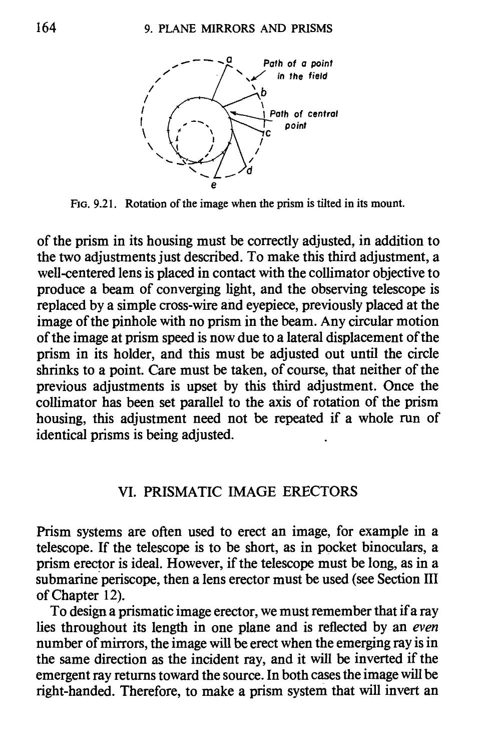
IV. THE THEORY OF TILTED PLANES 269
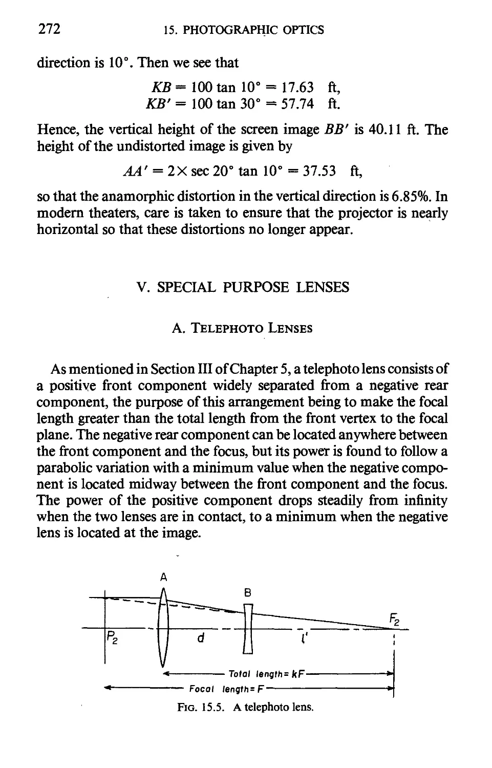
V. SPECIAL PURPOSE LENSES 272
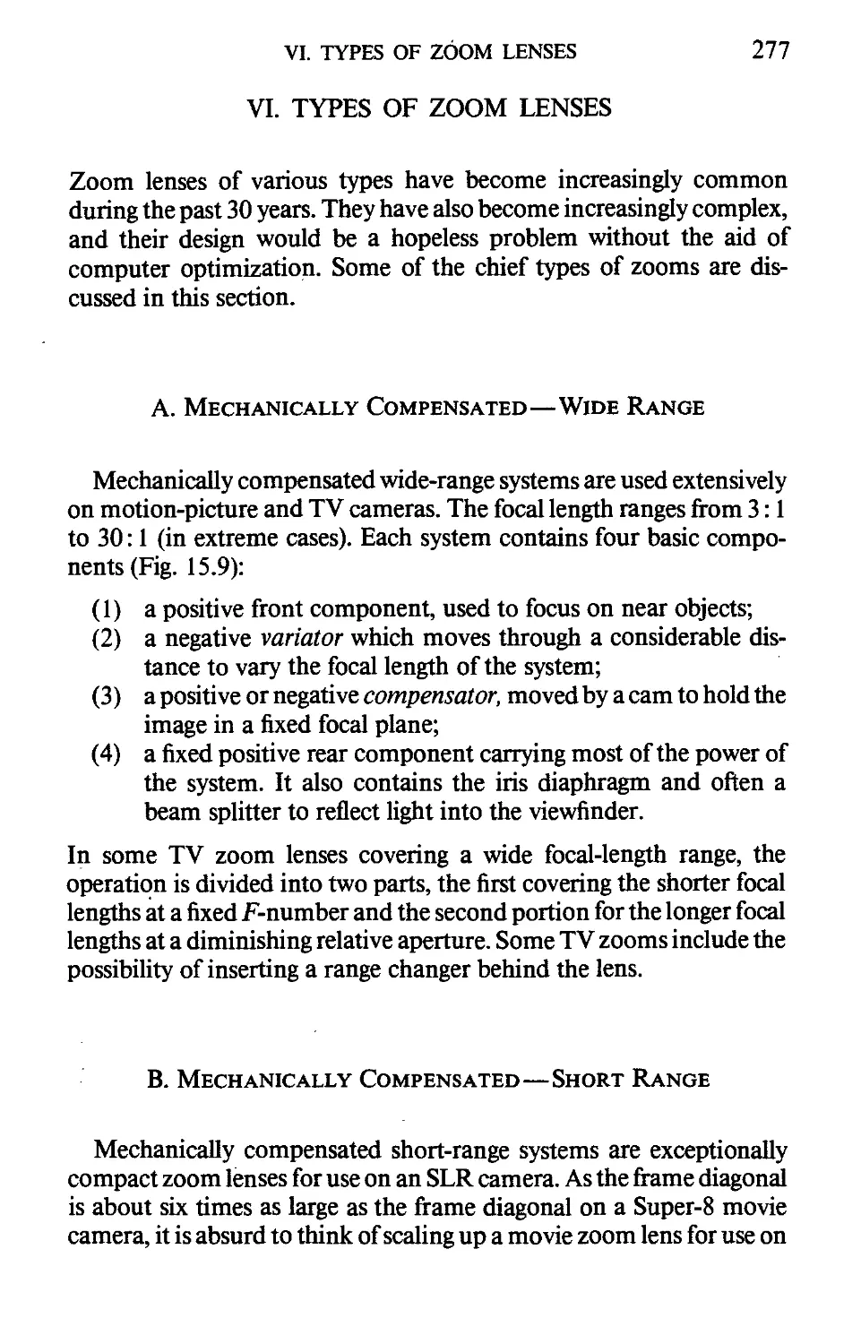
VI. TYPES OF ZOOM LENSES 277
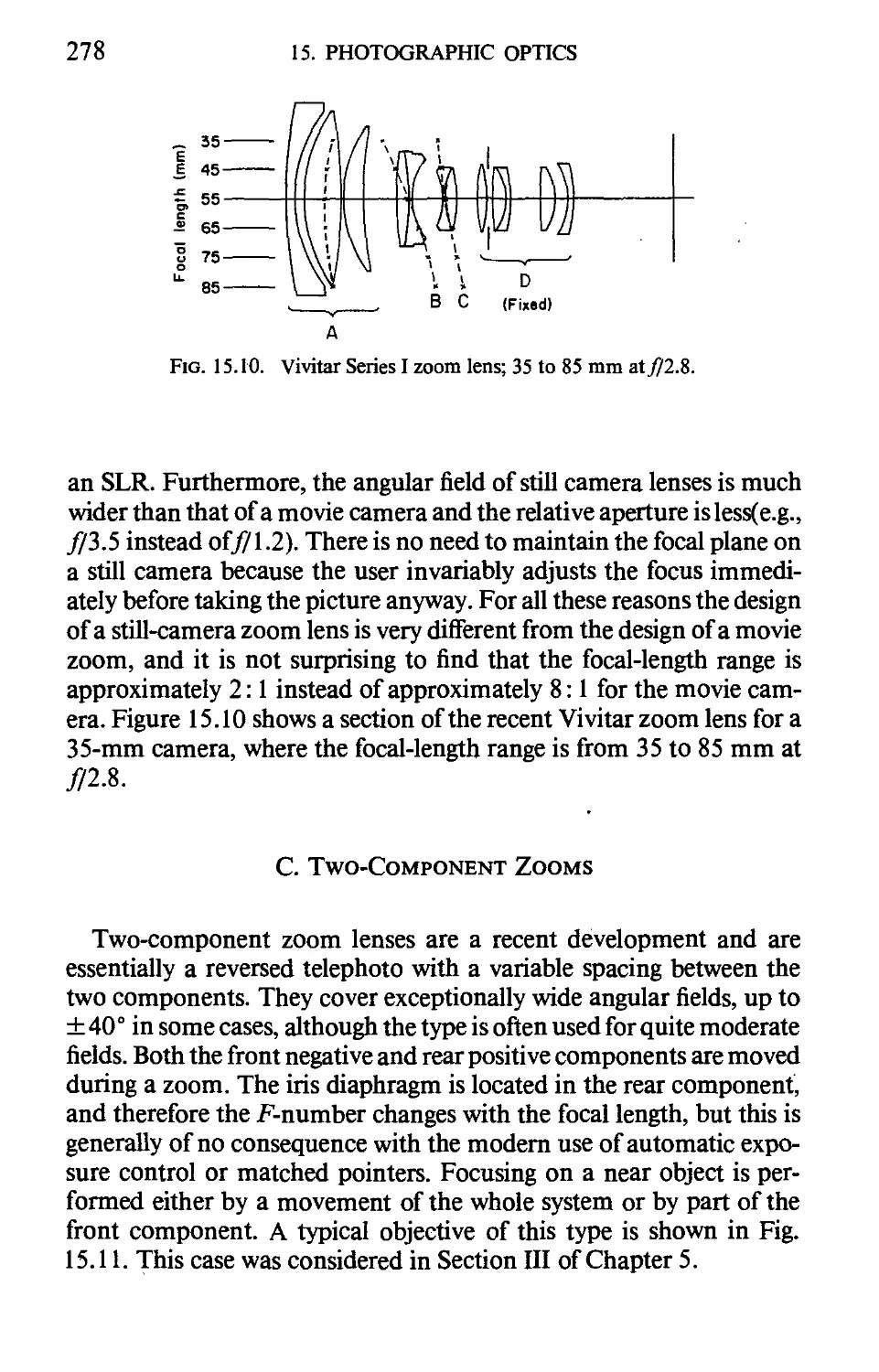
VII. SPECIFYING A PHOTOGRAPHIC OBJECTIVE 280
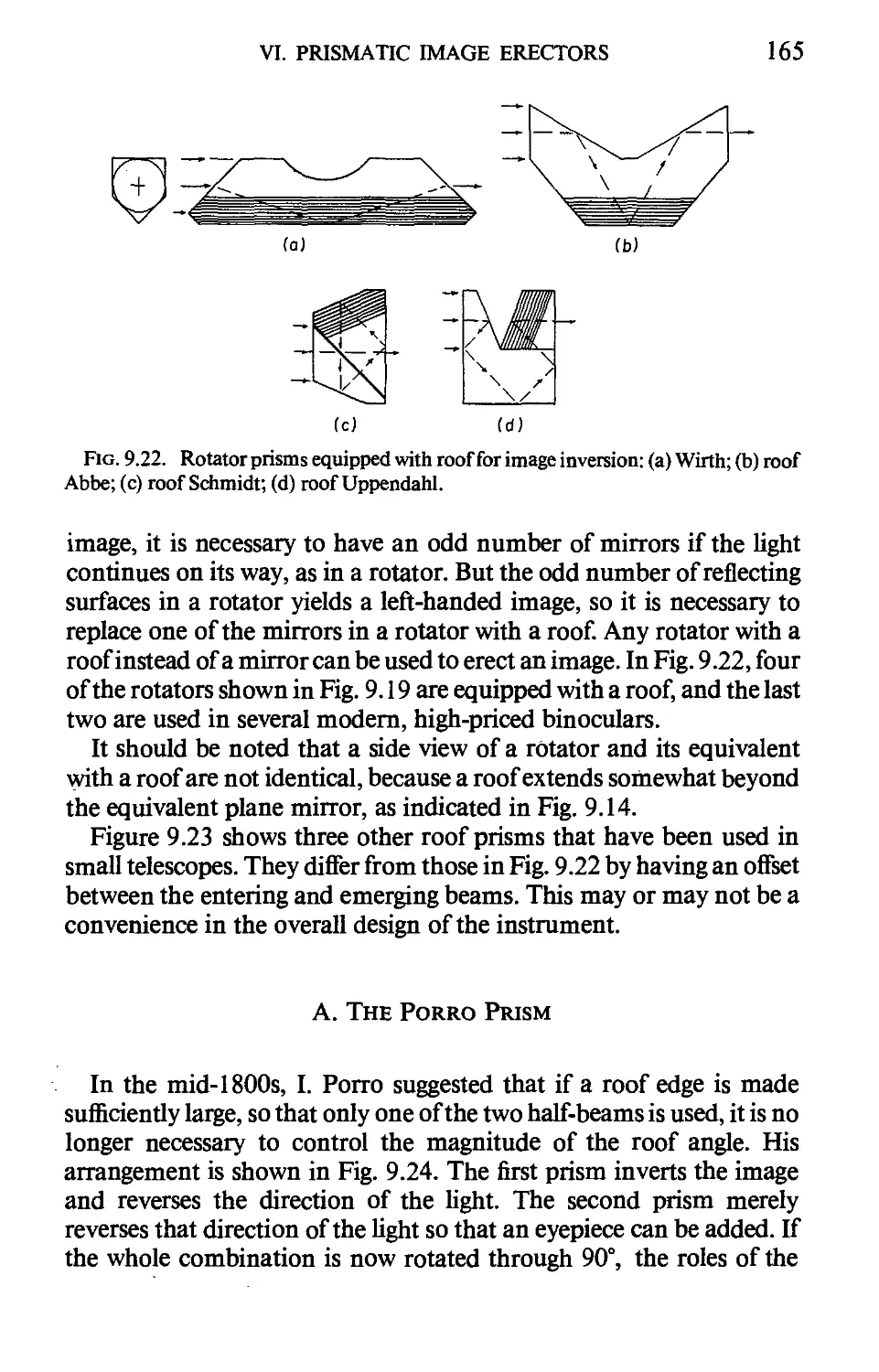
VIII. PANORAMIC OR SLIT CAMERAS 281
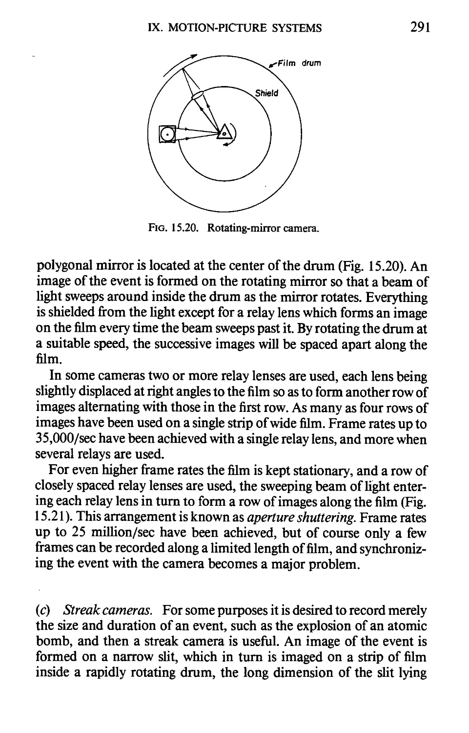
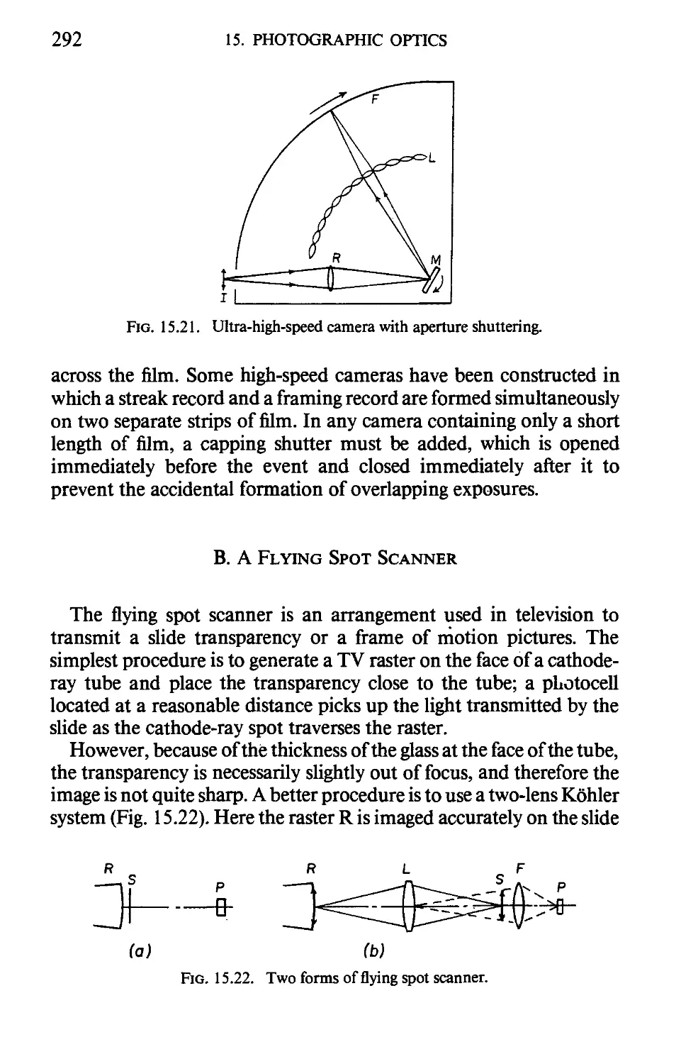
IX. MOTION-PICTURE SYSTEMS 286
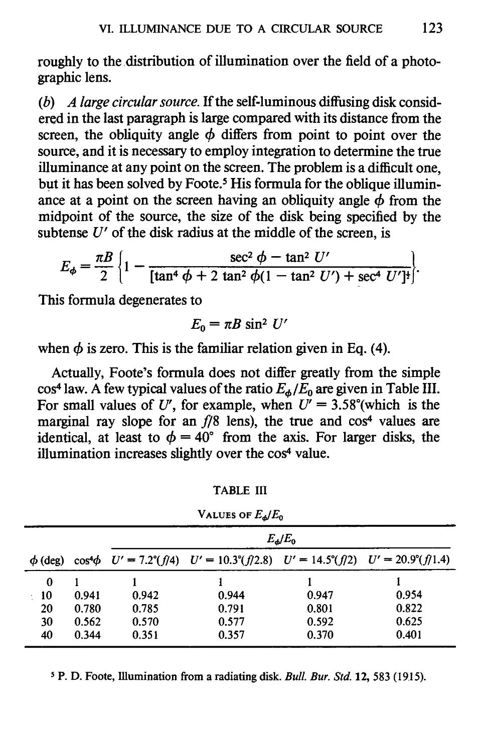
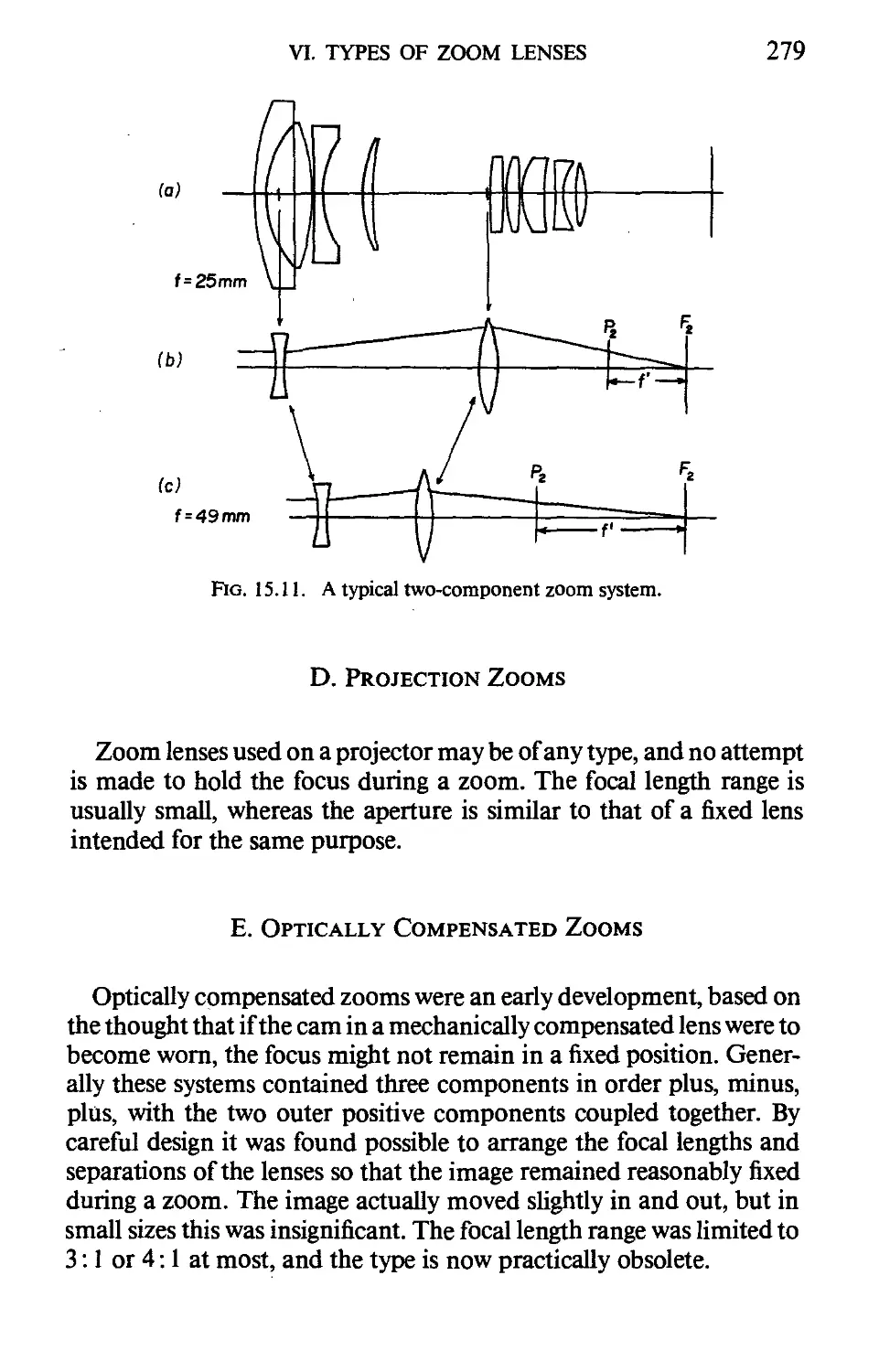
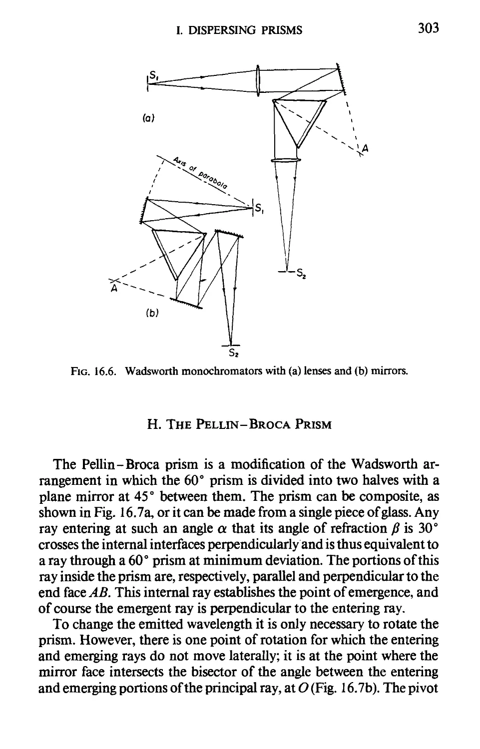
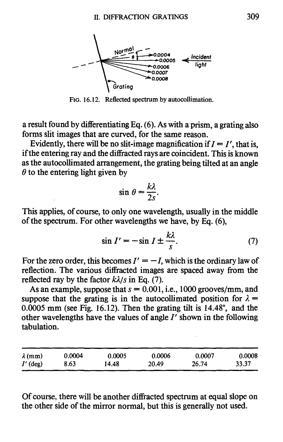
16. Spectroscopic Apparatus
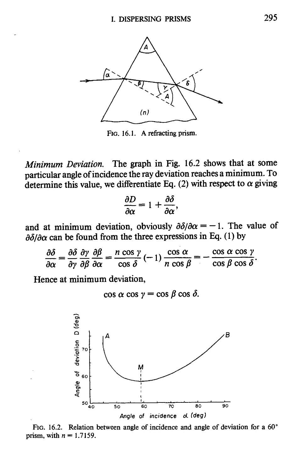
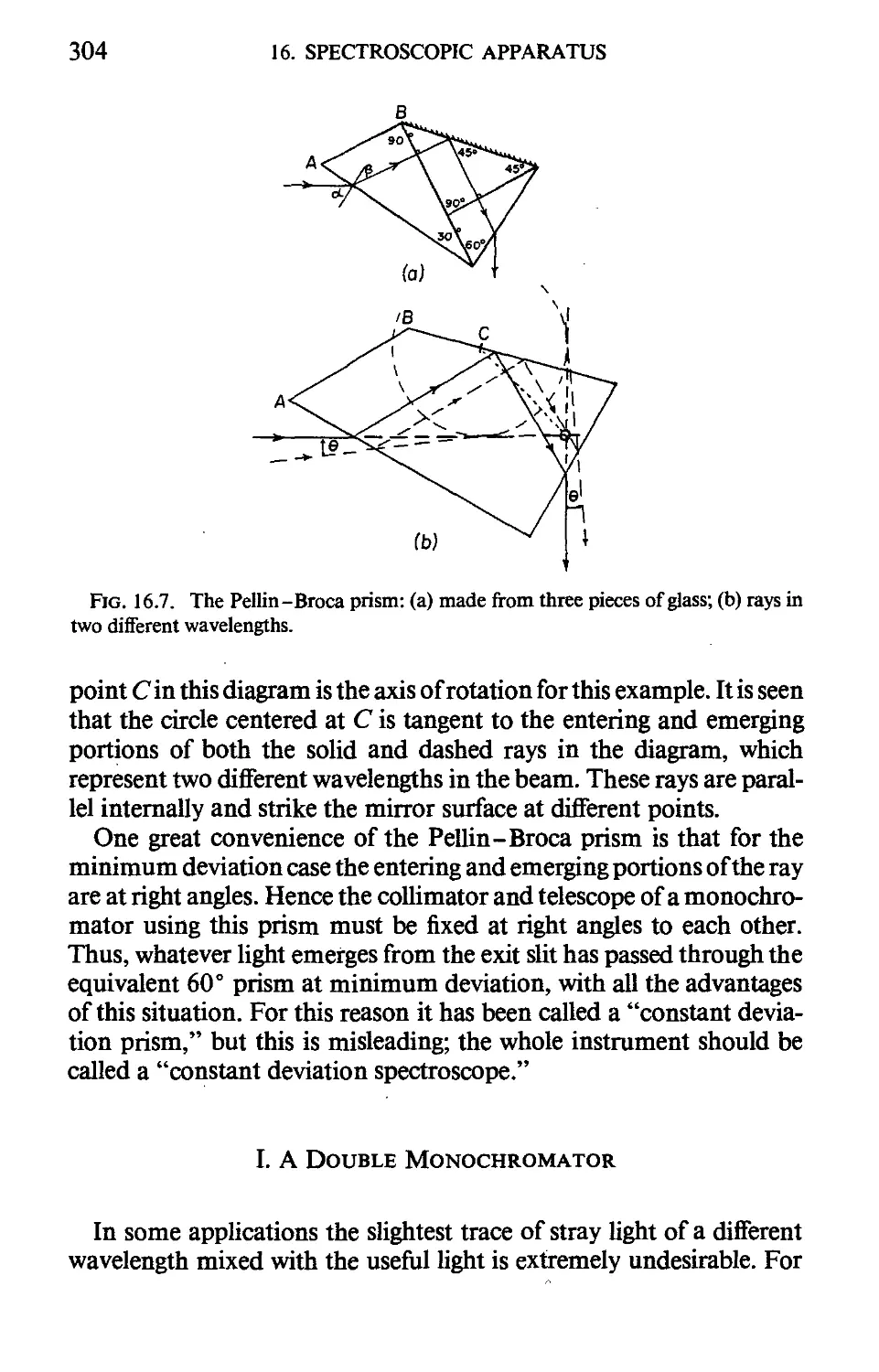
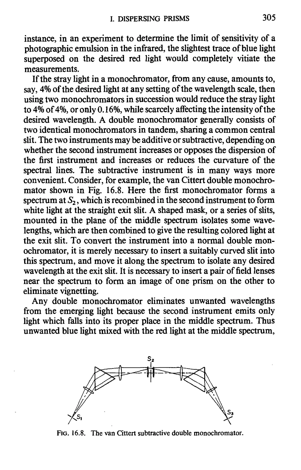
I. DISPERSING PRISMS 294
II. DIFFRACTION GRATINGS 306
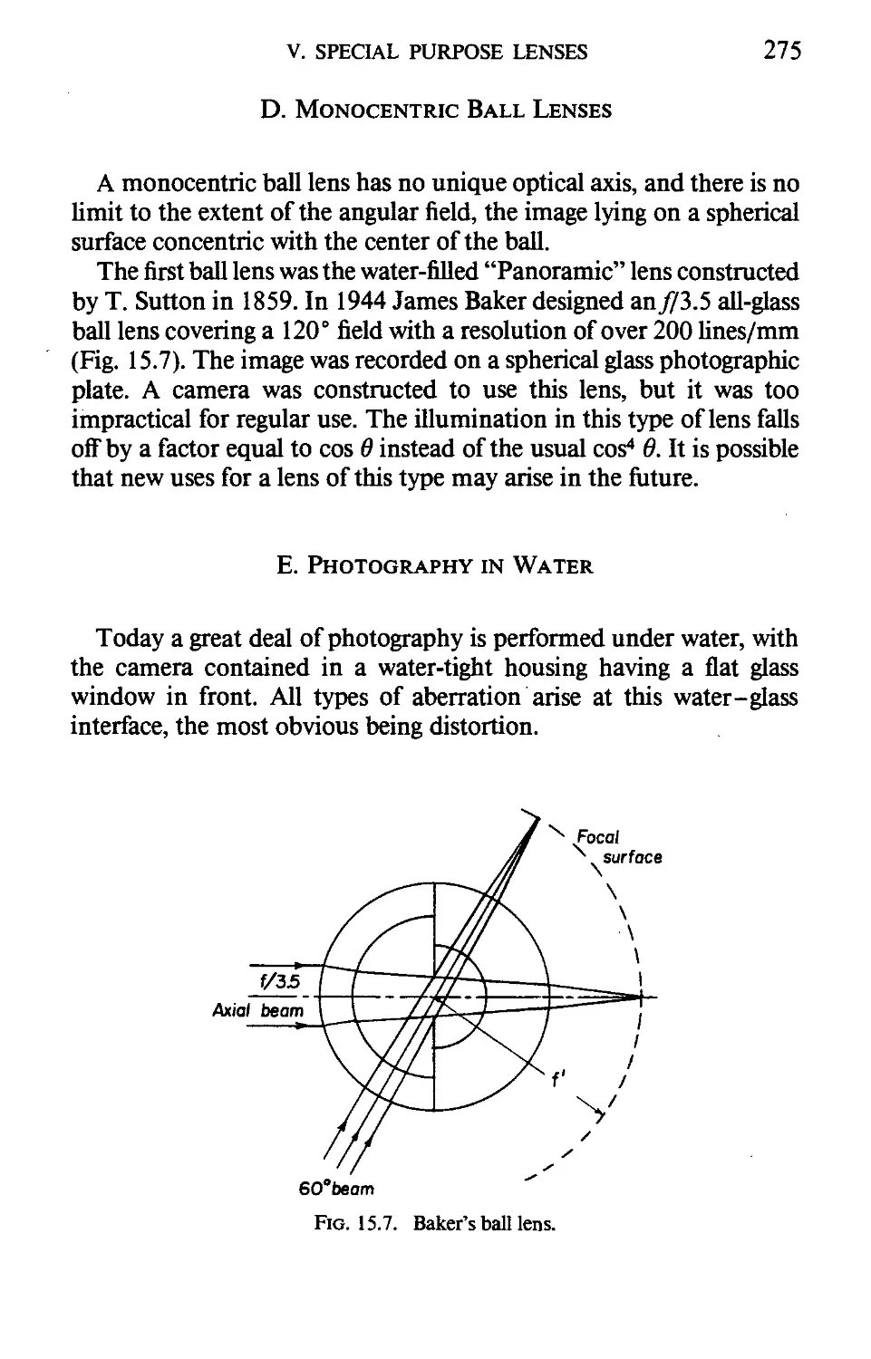
Index 3i5
Preface
It often happens in industrial and government laboratories that an electrical
or mechanical engineer is required to design an optical system to perform
some particular function. He then needs a basic knowledge of optics,
especially geometrical, and a clear understanding of the flow of light
through an optical system. The purpose of this book is to provide this basic
information, enabling a nonoptical engineer to tackle his unfamiliar
problem.
Several standard types of optical instrument are described in detail be-
because they are so often used alone or in combination to form more compli-
complicated systems. Some degree of familiarity with physical optics, diffraction,
and coherence is also required because of the importance of phenomena
resulting from the finite wavelength of light. These matters receive consid-
consideration wherever they arise in the discussion of a problem.
This book represents an expansion of undergraduate and summer-school
courses in geometrical optics and system design given by the author in the
Institute of Optics at the University of Rochester. No attempt has been
made to include lens design; that has been dealt with in the author's "Lens
Design Fundamentals" (Academic Press, 1978).
It is clearly impossible to explain every conceivable situation in a single
volume, and the reader will need to refer frequently to more specialized
sources. Much of this additional information will be found in the nine
volumes published since 1965 by Academic Press, and the future volumes
of "Applied Optics and Optical Engineering." Other useful sources are the
regular issues of the journals Optical Engineering, published by SPIE, and
Applied Optics, published by the Optical Society of America. Excellent
further references are Warren Smith's book "Modern Optical Engineer-
Engineering" (McGraw Hill, 1966), and "Military Standardization Handbook 141:
Optical Design" (Defense Supply Agency, Washington, 1963). For work
in the infrared, "The Infrared Handbook," edited by W. L. Wolfe and G.
J. Zissis (ERIM, Ann Arbor, 1979) will be found useful.
CHAPTER 1
Optical Systems
I. DESIGN AND PRODUCTION
The production of an optical system, whether a unique instrument or
a mass-production item, necessarily follows three well-defined stages:
(a) system layout, (b) lens design, and (c) optical engineering.
In the first of these stages, the structure of the system is defined so
that it will meet the customer's requirements and perform its desired
function. The system designer must be highly skilled in optics, knowl-
knowledgeable as to the availability of components, and aggressive in keep-
keeping costs to a reasonable level. He is ultimately responsible for the
entire project.
When the structure of the system has been established, the lens
designer takes over and fills in the details of each lens or other optical
component that will be required. Finally, the optical engineer is called
in to design the mechanical parts and to decide how everything is to be
made, either in-house or purchased from an outside supplier. He must
also set up a time schedule and plan the various test procedures that
will be used before the release of the instrument to the customer. In a
small establishment these three functions may be combined in a single
individual, whereas in a large company each function may be the
responsibility of a whole group. Nevertheless, all persons involved
must work together to ensure that the job is completed on time, that
the costs are kept to a minimum, and that the system will operate
reliably and satisfactorily.
Besides these people, there will be the usual departments for esti-
estimating, drafting, factory planning, cost accounting, etc., which apply
to everything that is undertaken in the establishment, but the three
functions listed above apply particularly to the design of an optical
system. In this book only the first of these functions will be consid-
considered.1
1 The functions of the lens designer are discussed in "Lens Design Fundamentals" by
Kingslake (Academic Press, 1978). Optical engineering is covered broadly in the series
of volumes entitled "Applied Optics and Optical Engineering," edited by Kingslake
(vol. 1 -6) and by Shannon-Wyant (vol. 7-9) (Academic Press, 1965-1983).
1
2 1. OPTICAL SYSTEMS
An optical system is an assembly of components working together to
produce a desired result. This may be as simple as forming an image
having a specified brightness and size at a given location, or it may be a
complex system involving some or all of the following features:
A) light sources, lamps, lasers, LEDs;
B) radiation detectors, photocells, thermocouples, photographic
emulsions;
C) lenses and curved mirrors for image formation;
D) plane mirrors and prisms to deflect light or rotate an image;
E) projection and display devices, screens, light valves, CRTs,
liquid crystals;
F) thin films;
G) polarizers and retardation plates;
(8) chromatic and achromatic niters;
(9) beamsplitters;
A0) image scanners, mirrors, polygons, acoustooptics;
A1) image tubes, IR, UV, x ray, light amplifiers;
A2) television tubes, Vidicons, Orthicons;
A3) charge-coupled devices;
A4) Pockels and Kerr cells;
A5) gratings and prisms to form a spectrum;
A6) fibers, face plates, waveguides;
A7) integrated optics;
A8) image processing, pattern recognition, spatial filtering;
A9) stereoscopy, photogrammetry;
B0) interferometers, holograms;
B1) motion-picture equipment, sound recording and reproduc-
reproduction.
II. OPTICAL MATERIALS
Most lenses are made of optical glass, several hundred types of which
are produced regularly by many manufacturers around the world; all
necessary data about these can be found in the makers' catalogs.
Millions of lenses are made every year by injection molding of plastic
materials, but unfortunately, the range of available types of plastic is
severely limited and the refractive indices are generally low. The high
III. LENS MANUFACTURE 3
temperature-coefficients of expansion and refractive index can also
present problems. Occasionally, crystalline materials such as quartz,
sapphire, or lithium fluoride are used, either because of their hardness
or their transparency in the ultraviolet. Such materials as silicon and
germanium are used in the infrared because of their transparency in
that region, but these materials are likely to be opaque in the visible
region, and lenses made from them are difficult to test and adjust. It
has often been proposed that a lens be made of a thin shell, spherical or
aspheric, filled with liquid, but thermal effects and the possibility of
leakage render this rather impractical. All in all, glass provides the
greatest range of useful materials in the wavelength range from 0.36 to
2.5 fim.
Recently, experiments have been started on the making of lenses
with materials having either a longitudinal or a transverse gradient of
refractive index. Both types have their uses, and work has been
undertaken on the routine fabrication of suitable materials. If these
become practical, they will replace aspheric surfaces in lenses. Gra-
Gradient-index (GRIN) rods are already common, and gradient optical
fibers are being used as communication channels between cities that
are many miles apart.
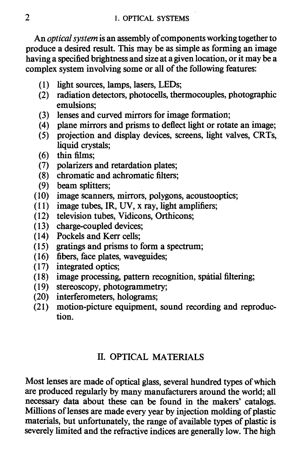
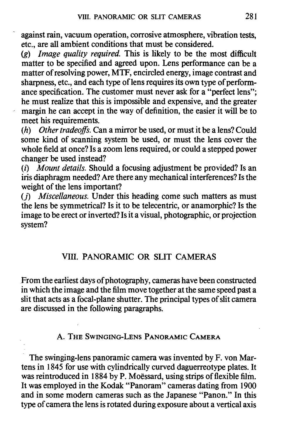
III. LENS MANUFACTURE*-"
To make a lens having spherical surfaces, a suitable piece of material is
molded into a circular form, and the surface radii are generated by the
use of a diamond-studded tool of ring shape, as indicated in Fig. 1.1a.
The lens surfaces are then lapped with loose emery on an iron tool
shaped to the desired curve, the tool being the reverse of the desired
lens surface. The tool is oscillated back and forth while the lens is
rotated about a vertical axis, with the most irregular motion producing
the best approach to a perfect spherical surface (Fig. 1.1b). After
lapping is complete, the surfaces are polished with a pitch-covered
tool, using cerium oxide or rouge as a polishing agent.
The difference between lapping and polishing is that in the former
operation the abrasive grains are loose and free to roll over and chip the
2 F. Twyman, "Prism and Lens Making." Hilger and Watts, London, 1952.
3 D. F. Home, "Optical Production Technology." Crane Russak, New York, 1972.
4 A. S. DeVany, "Master Optical Techniques." Wiley, New York, 1981.
1. OPTICAL SYSTEMS
Ш
Fig. 1.1. (a) Curve generation, (b) Lapping and polishing.
glass, whereas in the latter the grains are stuck into the surface of the
pitch and tend to scrape or "sandpaper" the glass surface. The polish-
polishing process can be speeded up by the application of high pressure and
rapid relative movement of the tool and the glass.
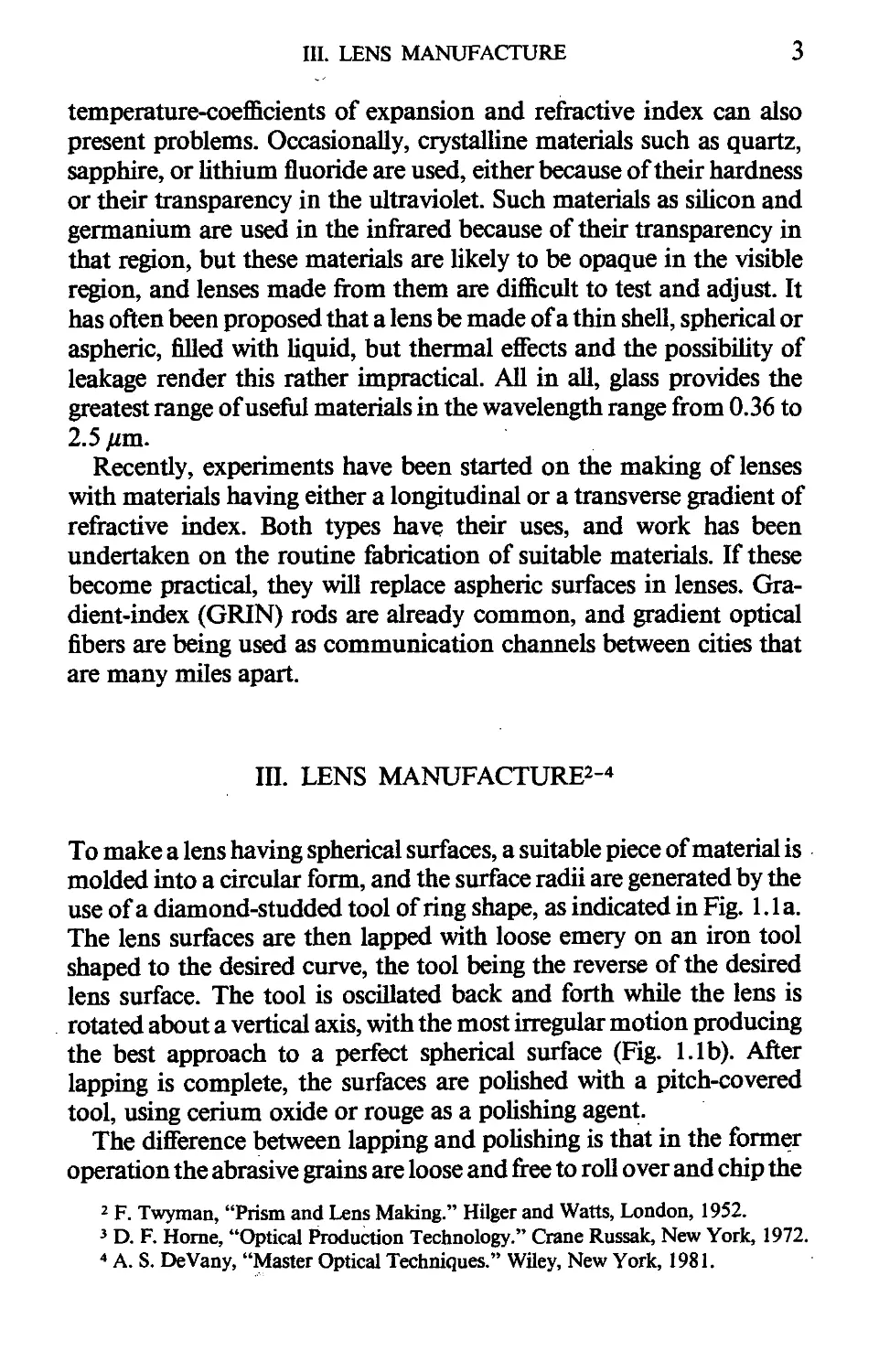
A. Centering and Edging
After grinding and polishing is complete, a lens is edged to the
required diameter by rotating it about an axis containing the centers of
curvature of the two surfaces. The completed lens elements are then
mounted in a metal cell so that all the elements share a common axis
(Fig. 1.2a). Failure to do this will result in very poor image quality,
which can be caused by a decentered element or even by a slightly
tilted surface (Fig. 1.2b). Centering and mounting lenses is the most
difficult part of the manufacturing process.
B. Aspheric Surfaces
Any attempt to generate an aspheric surface of revolution by normal
methods will result in a spherical surface unless some means are found
to restrict the relative motion of the units. Many companies are
developing ways to manufacture aspheric surfaces, but the problem is
complex and such lenses are liable to be very expensive.5 Not the least
of these problems is the development of a test procedure to determine
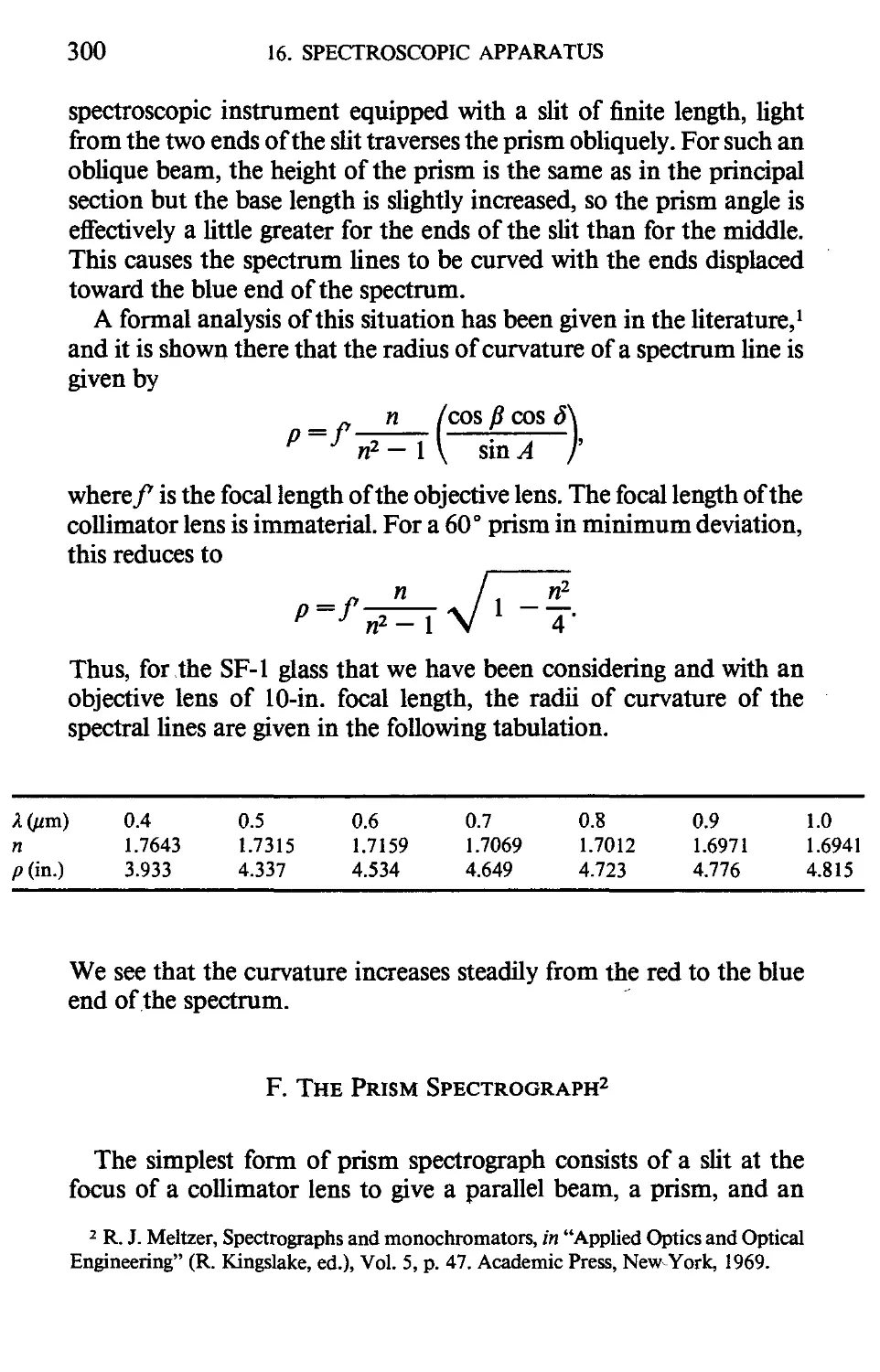
5 R. R. Shannon, "Aspheric surfaces," in "Applied Optics and Optical Engineering"
(R. R. Shannon and J. С Wyant, eds.), Vol. 8, p. 55. Academic Press, New York, 1980.
III. LENS MANUFACTURE
(а) (Ы
Fig. 1.2. (a) A centered lens, (b) A lens with one element tilted and displaced.
whether the surface generated is the correct one or if it is so far from the
desired shape as to introduce intolerable aberrations into the image.
An aspheric surface has its own unique axis which must be mounted so
that it lies in the axis formed by the centers of curvature of all the other
surfaces in the system. Plastic lenses can be molded with an aspheric
surface as easily as with a spherical surface, but the mold must be
correctly formed and this is as difficult as making an aspheric lens.
However, once the mold has been made, tested, and found to be
correct, thousands of lenses can be produced with very little difficulty.
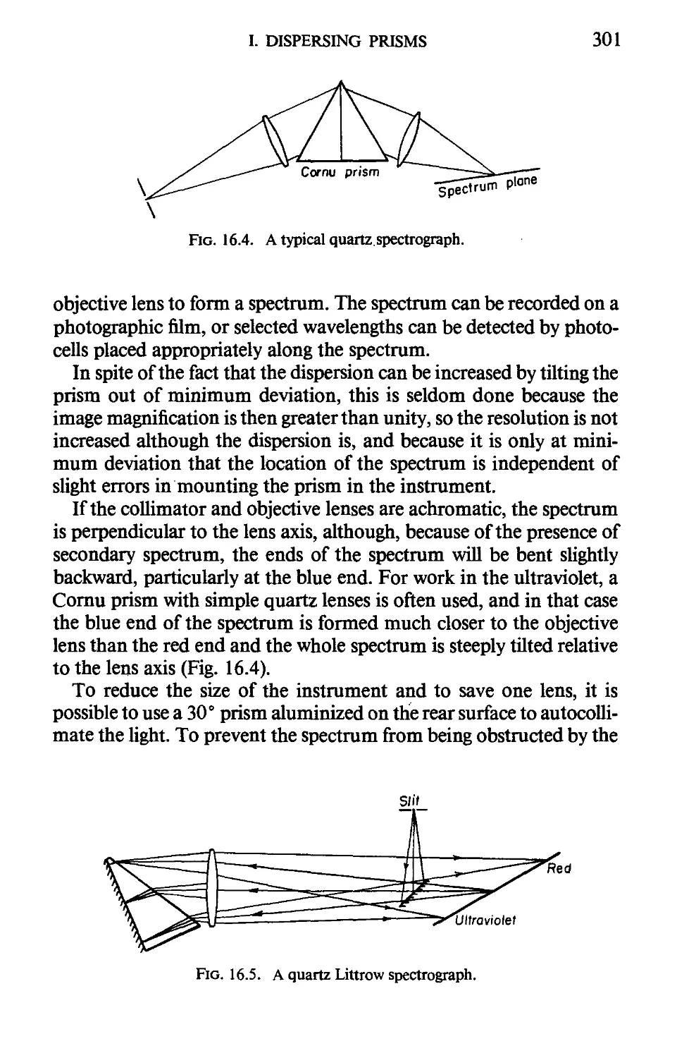
Rather than making the whole lens out of plastic materials it has been
proposed to deposit a thin layer of plastic material on a polished glass
substrate and mold the layer to the desired aspheric shape.
A cylindrical surface can be ground and polished to a circular
section by ordinary methods, provided the grinding and polishing
tools are prevented from rotating. A cylindrical lens can be made very
long and cut into sections after completion, with each section then
being edge-ground to the required diameter.
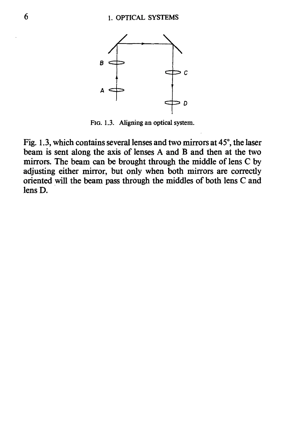
С Aligning an Optical System
An important step in the manufacture of an optical system is the
alignment of a series of lenses and mirrors in the housing. The usual
procedure is to employ a small milliwatt gas laser, which emits a
narrow parallel beam, and to make a small ink dot in the middle of
each lens in the system. By sending the laser beam along the system
axis, it is readily seen whether the beam passes through all the ink dots.
Finer tuning may be required later if the image shows signs of coma on
the axis, which obviously should not be there.
The laser procedure is particularly useful if plane mirrors are used
within a system to deflect a beam. For instance, in the system shown in
1. OPTICAL SYSTEMS
\
\
Fig. 1.3. Aligning an optical system.
Fig. 1.3, which contains several lenses and two mirrors at 45°, the laser
beam is sent along the axis of lenses A and В and then at the two
mirrors. The beam can be brought through the middle of lens С by
adjusting either mirror, but only when both mirrors are correctly
oriented will the beam pass through the middles of both lens С and
lens D.
CHAPTER 2
Light and Images
I. THE NATURE OF LIGHT
Light is a wave motion traveling through space or other transparent
medium that is able to affect the eye and certain artificial detectors to
form an image. The principal sources of light are the sun, sunlight
reflected from surrounding objects, tungsten lamps, carbon arcs,
lasers, gas discharge tubes, and fluorescent and phosphorescent mate-
materials excited by electrons or UV radiation. The principal detectors of
radiation are eyes, thermal detectors, photocells, and photographic
emulsions. Some detectors merely respond to radiation, whereas
others retain an image for further study.
Light waves have a frequency lying between 7.5 X 10¹⁴ vibrations/
sec for violet light and 4 X 10¹⁴ vibrations/sec for deep red light. The
wavelength, or distance from crest to crest, is found by dividing the
velocity of light C X 1010 cm/sec in empty space) by the frequency;
thus in air the wavelength of violet light is about 0.4 цт (micrometer)
and in red light it is about 0.75 /mi. In glass or other transparent media
the wavelength and the velocity are reduced by a factor known as the
refractive index of the material. Refractive indices range from as low as
1.33 for water to as high as 4.0 for germanium in the infrared. Few
transparent materials have refractive indices exceeding 2.0, although
diamond has an index of about 2.5. Ordinary window glass has a
refractive index of about 1.52.
A measure of light waves that is particularly useful to infrared
spectroscopists is the wave number, or number of waves in a centime-
centimeter. This ranges from 25,000 for violet light to about 13,000 for red
light. In the far infrared region the wave numbers become smaller and
more manageable; for instance, at a wavelength of 0.1 mm the wave
number is 100, and at 1 mm it has dropped to 10.
8 2. LIGHT AND IMAGES
A. Polarized Light
Light is a transverse wave motion, and it is possible by suitable
means to cause the vibrations to lie in one direction only. Such
plane-polarized light has many interesting properties. Ordinary light
can be regarded as a mixture of vibrations lying in all possible orienta-
orientations.
Since 1808 it has been known that light becomes partially polarized
when it is obliquely reflected from glass or other nonmetallic material.
It is also partially polarized by internal strain in glass and by some
transparent crystals, and this latter property is employed in Polaroid
material, which is used extensively to polarize light in instruments.
Some crystals, such as calcite, are strongly birefringent; they have
entirely different refractive indices for light vibrating parallel and
perpendicular to the optic axis of the crystal, and prisms made of
calcite have been used for 150 years to polarize a beam of light.
Two polarizing prisms, or Polaroid sheets, can be used in succession
to vary the intensity of a beam of light in a quantitative manner. If the
two polarizers are set with their vibration directions parallel, the first
polarizer reduces the intensity of the light to half, because half is lost by
reflection or absorption, but the second polarizer has no further effect
on the intensity. However, when the second polarizer, which is often
called the analyzer, is rotated about the axis of the beam, the intensity
of the transmitted light varies as the cos2 of the angle between the two
polarizing directions and becomes completely dark when the polariz-
polarizing directions are at right angles. This property is quite quantitatively
accurate and can be used for making photometric measurements.
If three polarizers are used in succession, the first two determine the
maximum transmittance of the assembly, and the third serves to
reduce this maximum to zero when the second and third polarizers are
crossed.
B. Rays and Waves
Although light is known to be a wave motion, it is often more
convenient to consider only the paths along which light travels. These
paths are known as rays, and in a homogeneous medium they are
I. THE NATURE OF LIGHT 9
straight lines. However, the ray concept is basically a mathematical
fiction, and the highly convenient ray treatment of imaging systems
necessarily ignores all wave-related phenomena such as polarization,
difiraction, interference, and scattering. We can readily determine the
location and brightness of an image by ray methods, but if we wish to
study the fine structure and distribution of light within an image, we
must resort to a wave treatment of the situation, and this is generally a
far more difficult operation. The study of ray phenomena is known as
geometrical optics, and the study of light waves constitutes physical
optics.
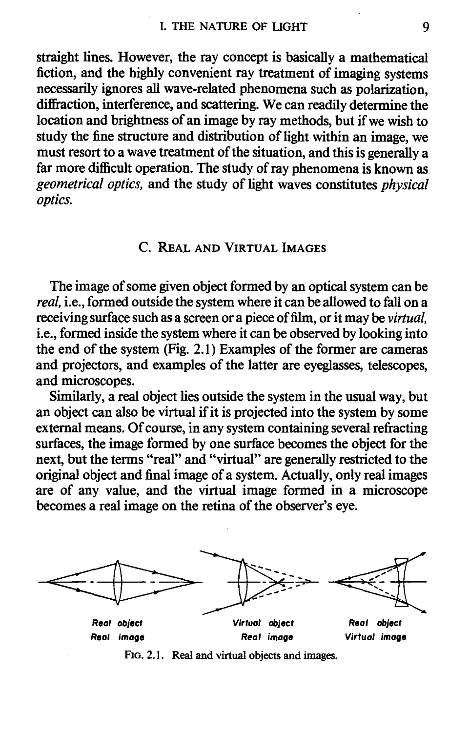
С Real and Virtual Images
The image of some given object formed by an optical system can be
real, i.e., formed outside the system where it can be allowed to fall on a
receiving surface such as a screen or a piece of film, or it may be virtual,
i.e., formed inside the system where it can be observed by looking into
the end of the system (Fig. 2.1) Examples of the former are cameras
and projectors, and examples of the latter are eyeglasses, telescopes,
and microscopes.
Similarly, a real object lies outside the system in the usual way, but
an object can also be virtual if it is projected into the system by some
external means. Of course, in any system containing several refracting
surfaces, the image formed by one surface becomes the object for the
next, but the terms "real" and "virtual" are generally restricted to the
original object and final image of a system. Actually, only real images
are of any value, and the virtual image formed in a microscope
becomes a real image on the retina of the observer's eye.
Real object Virtual object Real object
Real image Real image Virtual image
Fig. 2.1. Real and virtual objects and images.
10 2. LIGHT AND IMAGES
D. Object Space and Image Space
Considered naively, the object space and the image space of a lens
system are those spaces containing the object and image, respectively.
This is fine if the object and image are real, but if they are virtual, it
becomes somewhat confusing. We may regard the object space, no
matter where the object itself may be located, as the space containing
the incident rays, and likewise the image space as the space containing
the emerging rays. Alternatively, we can regard the object space as the
space containing the object, but if the object is virtual, we must
postulate that the object and image spaces overlap each other to
infinity in both directions—a concept that some people find hard to
accept. Of course, in a spherical mirror, for example, the entering and
reflected rays necessarily lie on the same side of the mirror, and
therefore the object and image spaces must be considered to overlap,
and the confusion cannot be avoided.
II. THE LAW OF REFRACTION
Let us consider a plane wave front, in a parallel beam of light, that is
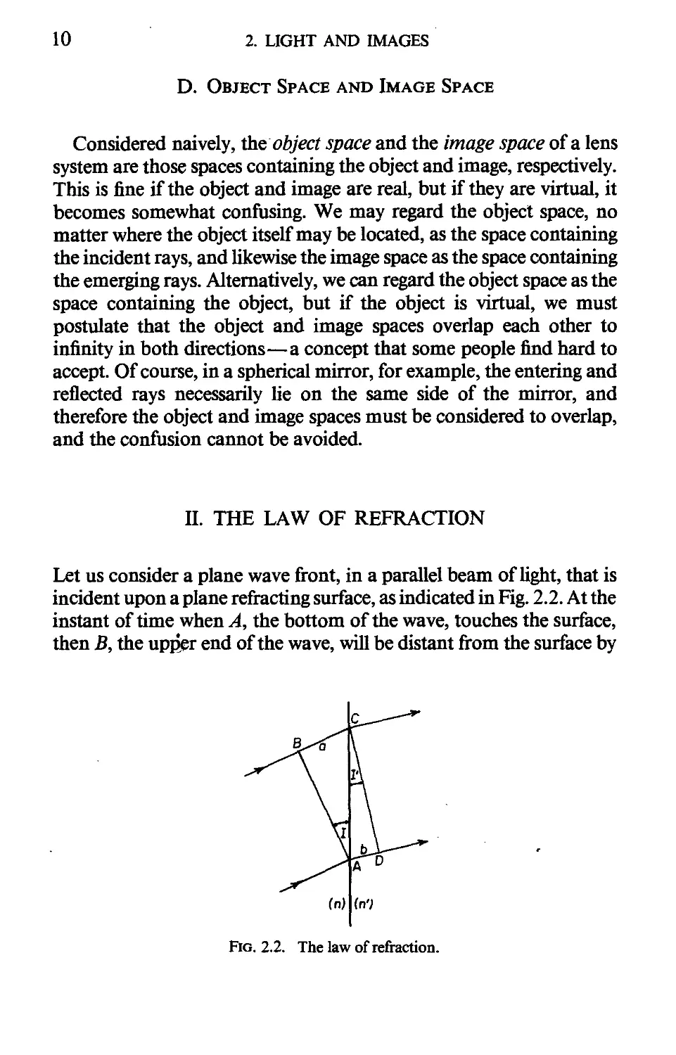
incident upon a plane refracting surface, as indicated in Fig. 2.2. At the
instant of time when A, the bottom of the wave, touches the surface,
then B, the upper end of the wave, will be distant from the surface by
Fig. 2.2. The law of refraction.
II. THE LAW OF REFRACTION 11
an amount a. While В moves to С in the left-hand medium, the lower
end of the wave moves from A to D in the right-hand medium, a
distance b. Because the velocity of light is different on the two sides of
the refracting surface, a will not be equal to b; in fact, a/b is equal to the
ratio of the two refractive indices n'/n.
Turning now to angles, the angle of incidence /between the incident
ray and the normal to the surface at the point of incidence, and the
corresponding angle of refraction /', are related by
sin/ ВС /AD ВС a n'
sin /' AC I AC AD b n'
hence
n sin/ = n' sin/'.
This is the well-known law of refraction, first stated in this form by
Descartes in 1637, although a geometrical construction for the direc-
direction of the refracted ray had been given by W. Snell in 1621; it is often
referred to as SnelFs law. This law underlies all considerations of
optical systems based on ray paths.
As already mentioned, a ray is a purely mathematical concept, and
it represents the path along which a light wave will travel. The rays are
everywhere perpendicular to the wave fronts, and because of the
symmetry of the law of refraction, we can assume that light can travel
in either direction along a ray.
A. Total Internal Reflection
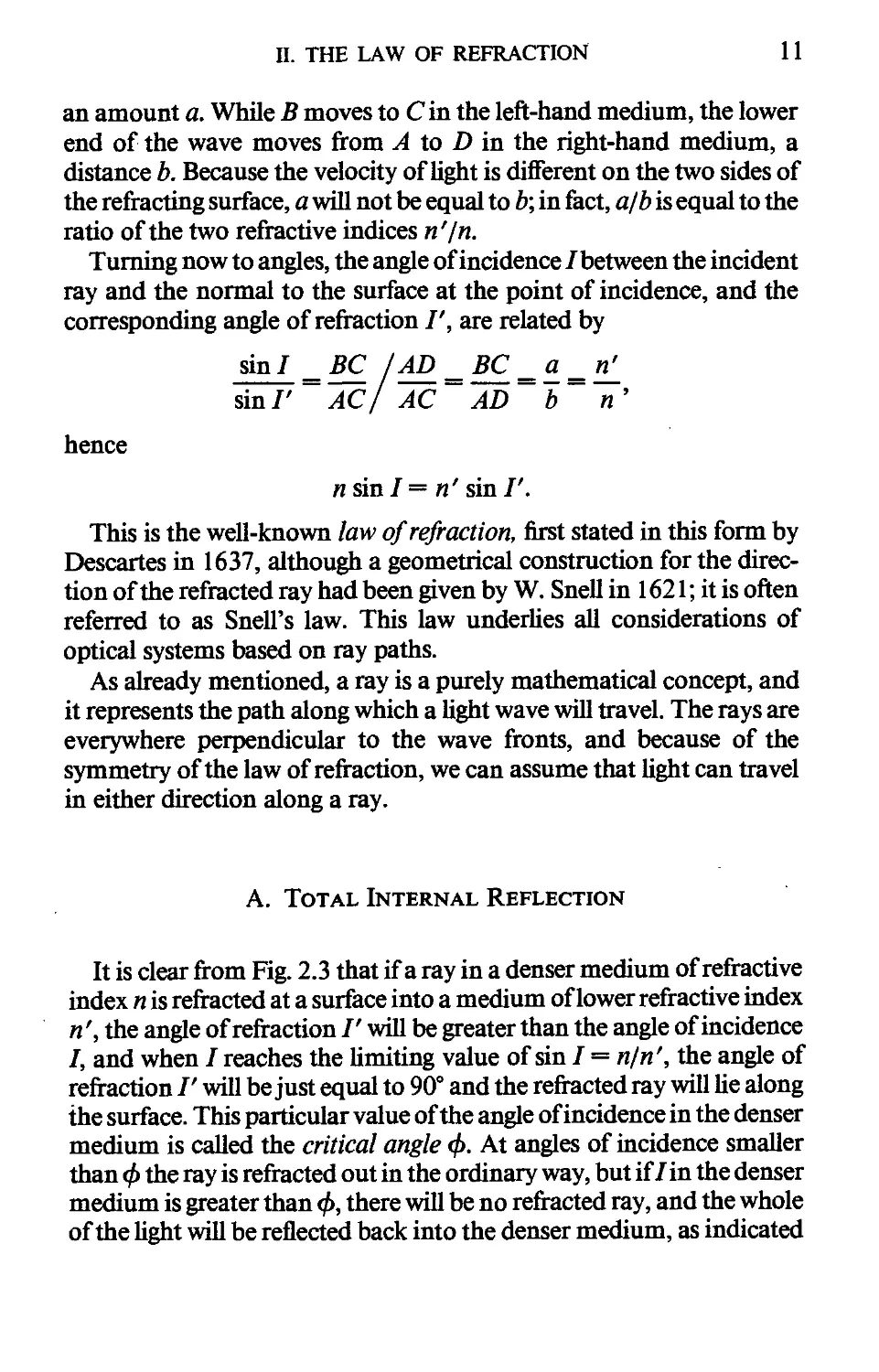
It is clear from Fig. 2.3 that if a ray in a denser medium of refractive
index n is refracted at a surface into a medium of lower refractive index
n', the angle of refraction /' will be greater than the angle of incidence
/, and when / reaches the limiting value of sin / = n/n', the angle of
refraction /' will be just equal to 90° and the refracted ray will lie along
the surface. This particular value of the angle of incidence in the denser
medium is called the critical angle ф. At angles of incidence smaller
than ф the ray is refracted out in the ordinary way, but if/in the denser
medium is greater than ф, there will be no refracted ray, and the whole
of the light will be reflected back into the denser medium, as indicated
12
2. LIGHT AND IMAGES
Air
-••-. Gloss n=/.523
4
Fig. 2.3. Refraction and the critical angle.
by the dashed ray in Fig. 2.3. This subject is discussed much more fully
in Chapter VII, Section IIIA.
B. Interpolation of Refractive Indices
Optical glass catalogs give refractive index data for a large number of
wavelengths, from 0.365 цт in the near ultraviolet to 1.014 цт in the
infrared. However, it is sometimes necessary to interpolate between
the given wavelengths, and for this purpose a formula connecting
refractive index with wavelength is needed. In the catalog of the Schott
Optical Glass Company, a six-term formula is used of the form
n2 = Ao + At*2 + А2/Л2 + Л3/Л4 + AJk6 + A5/A8.
A)
All six coefficients Ao to A5 are given explicitly to eight significant
figures for each type of glass. The terms with A in the numerator
become large in the infrared, and those with A in the denominator
become large in the ultraviolet. The index of most glasses rises rapidly
in the UV but drops only slowly in the IR, which explains why in Eq.
A) four UV terms are used with only one in the IR.
Some other interpolation equations have been proposed, but to
apply them it is necessary to solve for the various coefficients by use of
an appropriate number of stated refractive indices at known wave-
wavelengths.
III. A PERFECT OPTICAL SYSTEM 13
III. A PERFECT OPTICAL SYSTEM
A perfect optical system is one in which all the light rays from an object
point on one side of the system pass through a single image point on
the other side of the system. The emerging wave front is then spherical,
and the optical paths from object to image are all equal. The optical
path is the sum of the products nD along each ray, where л is the
refractive index of any portion of the ray path and D the length of that
portion.
In the case of a nonperfect system, the optical paths will not all be
equal nor will all the rays pass through a single image point, and the
emerging wave front will not be spherical. We can express the quality
of such an image by the scatter of the emerging rays or by stating the
maximum difference between the various possible optical paths from
object point to image point. Lord Rayleigh found that if the optical
path difference (often referred to as OPD) is everywhere less than a
quarter of the wavelength of the light, the image will not be noticeably
imperfect; this is commonly known as the Rayleigh limit of permissi-
permissible imperfection in an image.
A. The Airy Disk
It is shown in books on physical optics that the image formed by a
perfect optical system at the center of curvature of the emerging
spherical wave front is not a point, as geometrical optics suggests, but
instead it is a tiny circular spot of light surrounded by a series of very
faint rings of light having rapidly diminishing intensities. This image
structure is called an Airy disk after the man who first worked out its
properties in 1834. Theoretically, the succession of concentric rings
goes on forever, but after two or three rings the intensity becomes so
low that they are no longer visible.
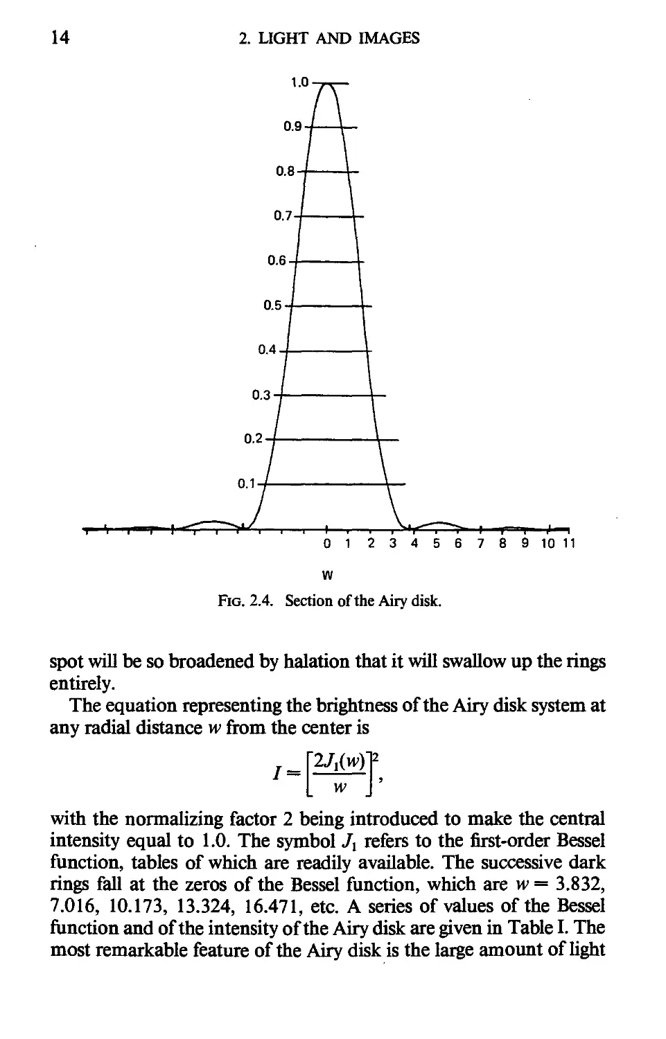
A graph of the light intensity across the Airy disk is shown in Fig.
2.4. It is seen that the central spot is enormously brighter than even the
first ring, the brightness of which is only about ^ of the brightness of
the central spot, while the other rings are even fainter still. It is
therefore virtually impossible to photograph an Airy disk, for if the
exposure is adjusted to record the central spot, the rings will not be
recorded, and if the exposure is set to photograph the rings, the central
14
2. LIGHT AND IMAGES
1.0-
01 23456789 10 11
W
Fig. 2.4. Section of the Airy disk.
spot will be so broadened by halation that it will swallow up the rings
entirely.
The equation representing the brightness of the Airy disk system at
any radial distance w from the center is
.
J'
with the normalizing factor 2 being introduced to make the central
intensity equal to 1.0. The symbol Jx refers to the first-order Bessel
function, tables of which are readily available. The successive dark
rings fall at the zeros of the Bessel function, which are w = 3.832,
7.016, 10.173, 13.324, 16.471, etc. A series of values of the Bessel
function and of the intensity of the Airy disk are given in Table I. The
most remarkable feature of the Airy disk is the large amount of light
III. A PERFECT OPTICAL SYSTEM
TABLE I
Values of the Bessel Function and of the Intensity of
the Airy Disk
15
w
0.0
0.5
1.0
1.5
2.0
2.5
3.0
3.5
4.0
4.5
5.0
5.5
6.0
0.0
0.242
0.440
0.558
0.577
0.497
0.339
0.137
-0.066
-0.231
-0.328
-0.341
-0.277
Intensity
1.0
0.939
0.775
0.553
0.333
0.158
0.0511
0.0062
0.0011
0.0106
0.0172
0.0154
0.0085
w
6.5
7.0
7.5
8.0
8.5
9.0
9.5
10.0
10.5
11.0
11.5
12.0
12.5
-0.154
-0.005
0.135
0.235
0.273
0.245
0.161
0.044
-0.079
-0.177
-0.228
-0.223
-0.165
Intensity
0.0022
0.0000
0.0013
0.0034
0.0041
0.0030
0.0012
0.0000
0.0002
0.0010
0.0016
0.0014
0.0007
energy in the outer rings. The Table II lists the radii of the successive
rings and their relative brightness, and also the amount of energy
remaining outside each dark ring. The actual physical value of the
radius of any particular ring can be found from the formula
radius of ring = w(M'/nD) = (w/7r)A(.F-number),
where D is the diameter of the lens aperture, /' the distance of the
TABLE II
Values of Various Parameters Related to the Airy Disk
Ring
Center
First dark
First bright
Second dark
Second bright
Third dark
Third bright
Fourth dark
Radius of ring
w
0.0
3.832
5.136
7.016
8.417
10.173
11.620
13.324
Relative
intensity
1.0
—
0.0175
0.0042
0.0016
—
Amount of light
in ring (%)
83.9
7.1
2.8
1.5
—
Light remaining
outside the ring
(%)
16.1
—
9.0
6.2
_
4.7
16. 2. LIGHT AND IMAGES
image from the lens, and A the wavelength of the light. Thus, for
example, the radius of the first dark ring for a perfect f/4.5 lens in
sodium-Z) light with a distant object is found to be 0.0032 mm, or
3.2 /дп.
The effective diameter of the central spot is usually stated to be
about 70% of the diameter of the first dark ring; thus in the visible
region it can be assumed to be about equal to the F-number of the lens
expressed in micrometers. This amounts to a diameter of 4.5 fira in the
example given. In the infrared, where the wavelength is so much
greater, the effective diameter of the central spot becomes quite large,
e.g., 38 цт for an f/4.5 lens at lOfim in the IR. This explains why
optical elements intended for use in the infrared "window" at 10 fim
can have sizable surface errors that would be quite inadmissable in the
visible region.
The special case of a central obstruction leading to an annular lens
aperture is discussed in Chapter 14. This situation often arises in a
mirror system such as a Cassegrain telescope.
B. A Diffraction-Limited Lens
A lens in which the aberrations are so small that the image of a point
is no larger than the Airy disk is often referred to as being diffraction
limited. Very few real lenses can make this claim-over their whole field,
but many are diffraction limited on the lens axis. Since aberrations are
scaled in proportion to the focal length, whereas diffraction effects
depend only on the relative aperture (F-number) of the lens, many
lenses are diffraction limited when the focal length is short but not
when they are made to a longer focal length. Microscope objectives are
invariably diffraction limited but, again, only because their focal
length is quite small.
С Resolving Power of a Perfect Lens
Lord Rayleigh considered that two equally bright stars could be just
resolved by a perfect telescope if the image of one star fell on the first
dark ring of the Airy disk of the other star. Thus, he considered that the
III. A PERFECT OPTICAL SYSTEM 17
least resolvable separation (LRS) of the two star images in the focal
plane of the telescope is given by
LRS' = —
where D is the diameter of the lens aperture and /' the image distance
from the lens. Actually, this is somewhat pessimistic and we can safely
ignore the factor of 1.22. Expressed in terms of U', which is the slope
angle of the steepest ray that can pass from the lens to the axial image
point, we see that sin U' = \D/V, hence
LRS' = ±A/sin U'.
Because the magnification is m = (и sin U)/(n' sin U'), where n' = 1
for air, we see that the least resolvable separation in the object is given
by
LRS = LRS'//n - \X/n sin U.
In microscopy the product n sin U is called the numerical aperture in
the object space, and correspondingly we may regard the numerical
aperture in the image space as being equal to n' sin ?/'. In this
notation, the least resolvable separation in either the object space or
the image space is given by half the wavelength divided by the numeri-
numerical aperture in that space.
D. Modulation Transfer Function
As its name implies, the modulation transfer function (MTF) of a
lens is a measure of its ability to form a faithful image of a given object.
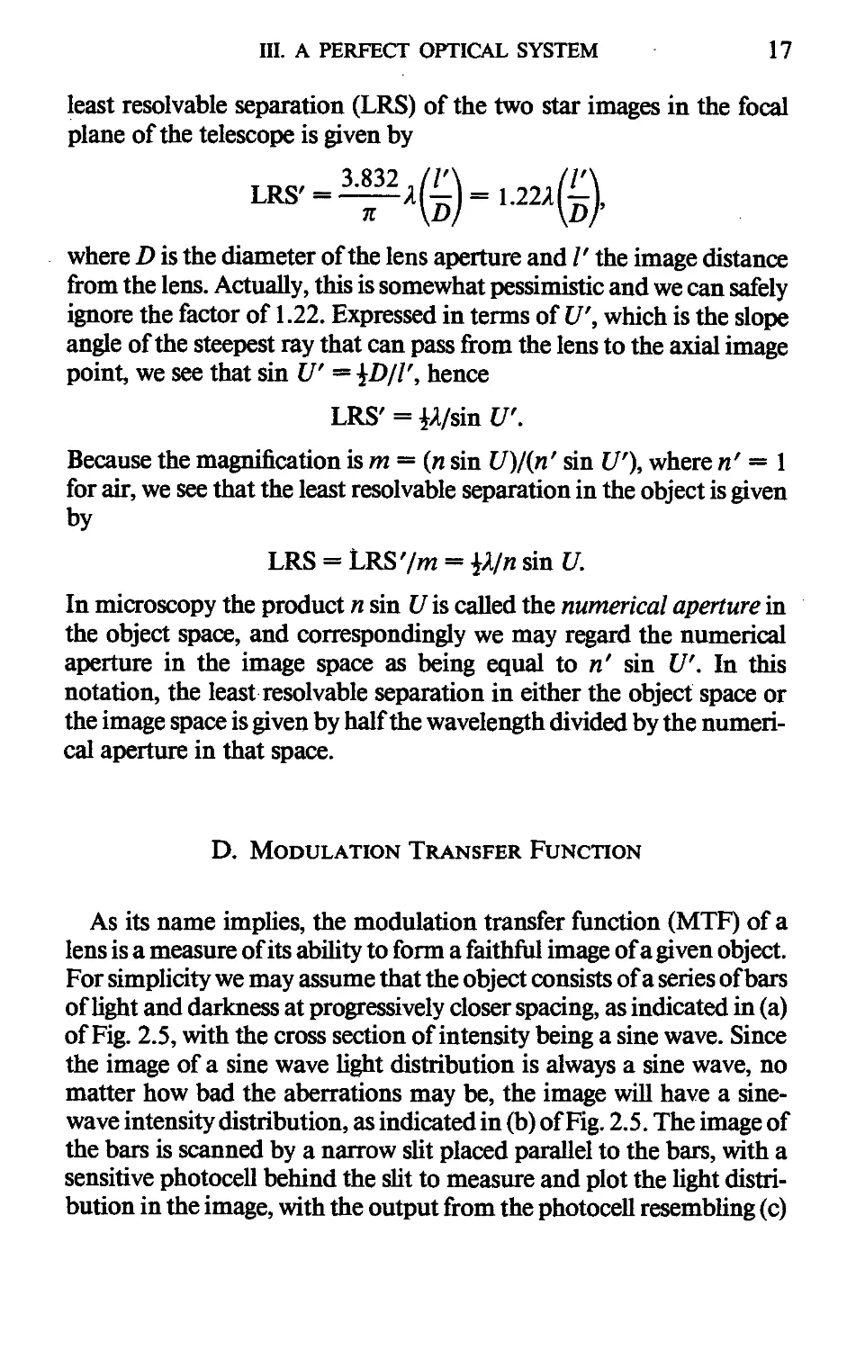
For simplicity we may assume that the object consists of a series of bars
of light and darkness at progressively closer spacing, as indicated in (a)
of Fig. 2.5, with the cross section of intensity being a sine wave. Since
the image of a sine wave light distribution is always a sine wave, no
matter how bad the aberrations may be, the image will have a sine-
wave intensity distribution, as indicated in (b) of Fig. 2.5. The image of
the bars is scanned by a narrow slit placed parallel to the bars, with a
sensitive photocell behind the slit to measure and plot the light distri-
distribution in the image, with the output from the photocell resembling (c)
18
2. LIGHT AND IMAGES
Fig. 2.5. Modulation transfer.
of Fig. 2.5. When the bars are coarse and widely spaced, the lens has no
difficulty in accurately reproducing them, but as the bars get closer
together, diffraction and aberrations in the lens cause some light to
stray from the bright bars into the dark spaces between them, with the
result that the light bars get dimmer and the dark spaces get brighter,
until eventually there is nothing to distinguish light from darkness and
all resolution is lost.
From the photocell response it is possible t6 plot a graph connecting
image contrast with line frequency, where contrast is the intensity
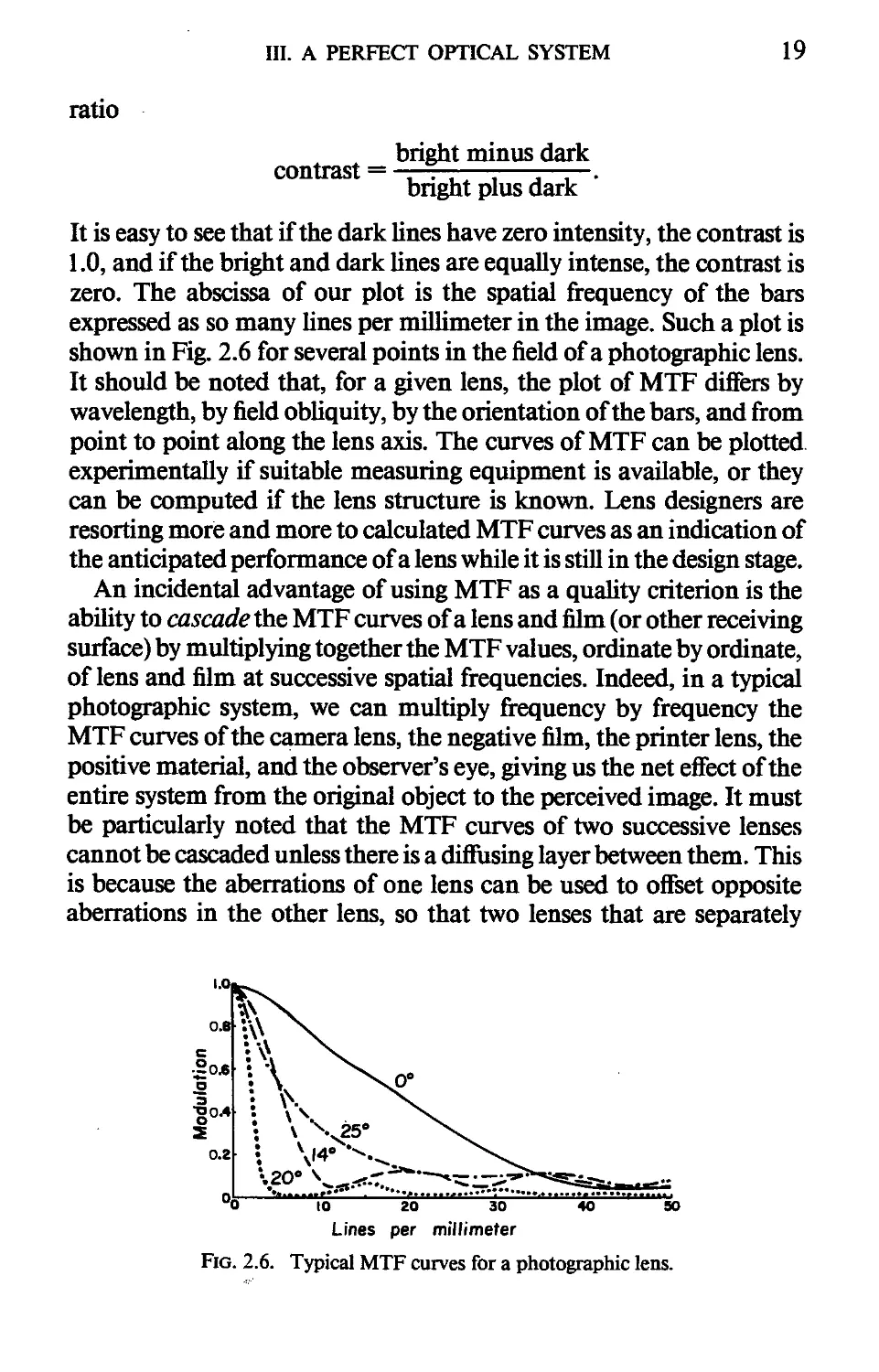
III. A PERFECT OPTICAL SYSTEM 19
ratio
bright minus dark
contrast = , . . ^ .—. . .
bright plus dark
It is easy to see that if the dark lines have zero intensity, the contrast is
1.0, and if the bright and dark lines are equally intense, the contrast is
zero. The abscissa of our plot is the spatial frequency of the bars
expressed as so many lines per millimeter in the image. Such a plot is
shown in Fig. 2.6 for several points in the field of a photographic lens.
It should be noted that, for a given lens, the plot of MTF differs by
wavelength, by field obliquity, by the orientation of the bars, and from
point to point along the lens axis. The curves of MTF can be plotted
experimentally if suitable measuring equipment is available, or they
can be computed if the lens structure is known. Lens designers are
resorting more and more to calculated MTF curves as an indication of
the anticipated performance of a lens while it is still in the design stage.
An incidental advantage of using MTF as a quality criterion is the
ability to cascade the MTF curves of a lens and film (or other receiving
surface) by multiplying together the MTF values, ordinate by ordinate,
of lens and film at successive spatial frequencies. Indeed, in a typical
photographic system, we can multiply frequency by frequency the
MTF curves of the camera lens, the negative film, the printer lens, the
positive material, and the observer's eye, giving us the net effect of the
entire system from the original object to the perceived image. It must
be particularly noted that the MTF curves of two successive lenses
cannot be cascaded unless there is a diffusing layer between them. This
is because the aberrations of one lens can be used to offset opposite
aberrations in the other lens, so that two lenses that are separately
Lines per millimeter
Fig. 2.6. Typical MTF curves for a photographic lens.
20
2. LIGHT AND IMAGES
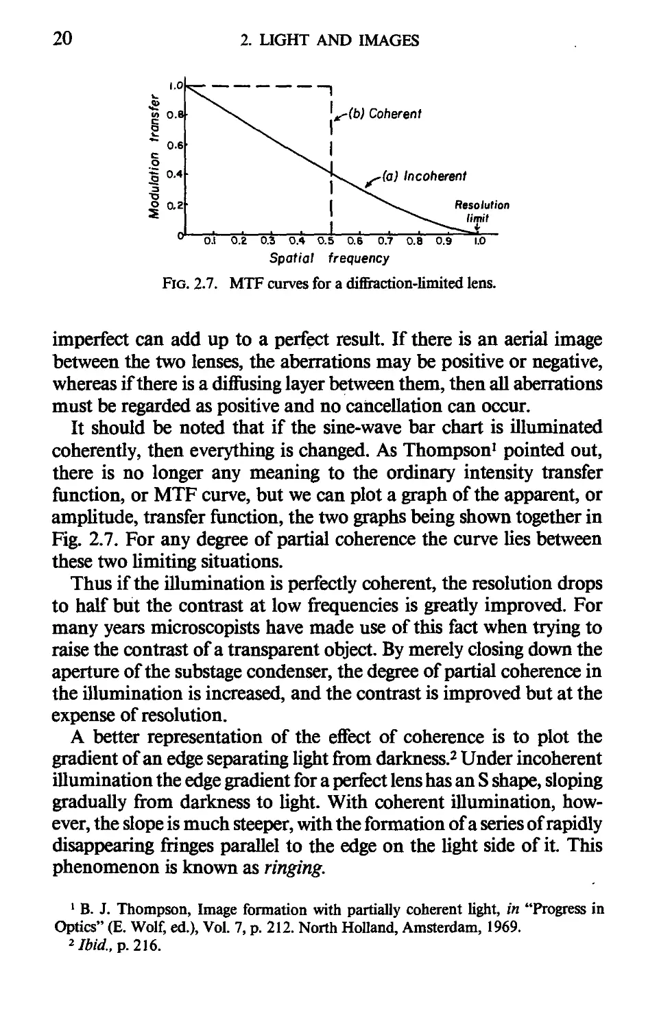
1.0
к.
ю 0.8
2
*~ 0.6
s
Iм
о 0.Z
_ 1
. . . .
o.i о.г о.з o.4 о.:
trtb) Coherent
ч s~(a) Incoherent
«^^ Resolution
> 0.6 0.7 0.8 0.9 1.0
Spatial frequency
Fig. 2.7. MTF curves for a diflraction-limited lens.
imperfect can add up to a perfect result. If there is an aerial image
between the two lenses, the aberrations may be positive or negative,
whereas if there is a diffusing layer between them, then all aberrations
must be regarded as positive and no cancellation can occur.
It should be noted that if the sine-wave bar chart is illuminated
coherently, then everything is changed. As Thompson1 pointed out,
there is no longer any meaning to the ordinary intensity transfer
function, or MTF curve, but we can plot a graph of the apparent, or
amplitude, transfer function, the two graphs being shown together in
Fig. 2.7. For any degree of partial coherence the curve lies between
these two limiting situations.
Thus if the illumination is perfectly coherent, the resolution drops
to half but the contrast at low frequencies is greatly improved. For
many years microscopists have made use of this fact when trying to
raise the contrast of a transparent object. By merely closing down the
aperture of the substage condenser, the degree of partial coherence in
the illumination is increased, and the contrast is improved but at the
expense of resolution.
A better representation of the effect of coherence is to plot the
gradient of an edge separating light from darkness.2 Under incoherent
illumination the edge gradient for a perfect lens has an S shape, sloping
gradually from darkness to light. With coherent illumination, how-
however, the slope is much steeper, with the formation of a series of rapidly
disappearing fringes parallel to the edge on the light side of it. This
phenomenon is known as ringing.
1 B. J. Thompson, Image formation with partially coherent light, in "Progress in
Optics" (E. Wolf, ed.), Vol. 7, p. 212. North Holland, Amsterdam, 1969.
2 Ibid., p. 216.
IV. LENS ABERRATIONS 21
IV. LENS ABERRATIONS
There are seven well-established classes of aberrations, each of which
contains a series of orders varying with the lens aperture and the
angular field. The seven basic aberrations are as follows:
(a) Chromatic. Since the refractive index of all transparent materials
varies with wavelength, all the properties of a lens that depend on
refractive index will necessarily vary with wavelength. The simplest of
these is the location of an axial image point along the axis. If the
position of this image varies with wavelength, the lens is said to suffer
from chromatic aberration. A lens in which two wavelengths have
been united at a common image point is said to be achromatic,
whereas if three or more wavelengths have been united, it is said to be
apochromatic.
(b) Lateral color. A related but quit© separate aberration is con-
concerned with a variation with wavelength of the height of an image
above the axis, causing colored fringes to surround images far out in
the field and to disappear on axis. This aberration is called lateral color,
transverse chromatic aberration, or chromatic difference of magnifica-
magnification.
(c) Spherical. Spherical aberration exists if the position of an axial
image varies from zone to zone along the axis. Even though the
marginal and paraxial images may coincide, there may still be a
residual of zonal spherical aberration.
{d) Coma. This is an analogous aberration in which the height of an
image above the axis varies from zone to zone of the lens.
It should be noted that these four aberrations are analogous, in the
sense that (a) and (b) represent a variation of image position and image
height from one wavelength to another, and (c) and (d) represent a
variation of image position and image height from one lens zone to
another.
(e) Distortion. Distortion is present in a lens if the height of the image
above the axis is not proportional to the height of the object above the
axis, i.e., if the magnification varies across the field. If the object is at
infinity, distortion is present if the focal length varies with obliquity.
A symmetrical system is such that, if one side is rotated through 180°
about the center of the stop, it will fall exactly on the other side. This
22 2. LIGHT AND IMAGES
implies unit magnification also. In such a system, the three transverse
aberrations—coma, distortion, and lateral color—are automatically
corrected.
(/) Field curvature. If the image of a plane object perpendicular to
the axis does not lie in a plane perpendicular to the axis, then the lens is
said to have a curved field. This is regarded as inward curving if the
image is concave toward the lens, and backward curving if it is convex
toward the lens.
(g) Astigmatism. This is a more subtle aberration in which the image
of an off-axis point appears as a pair of focal lines, one line being radial
to the field and the other tangential to it. The field curvature will
obviously be different for radial and for tangential focal lines. A lens in
which astigmatism is corrected at one point in the field is said to be
stigmatic at that field point, and if that point lies in the focal plane, the
lens is said to be an anastigmat.
Since, with a distant object, the focal length of a lens is a measure of
image size, we can regard coma as a variation of focal length with
aperture and distortion as a variation of focal length with obliquity.
V. FIBER OPTICS
An optical fiber is a long thread of glass having an approximately
circular section that transmits light along its length by a process of
repeated total internal reflection at the surface. No light is lost at total
reflection, with the only loss being that due either to absorption in the
glass itself or to dirt or grease on the surface of the fiber. To prevent the
latter loss it is customary to clad'the fiber with glass or plastic of a lower
refractive index than that of the fiber.
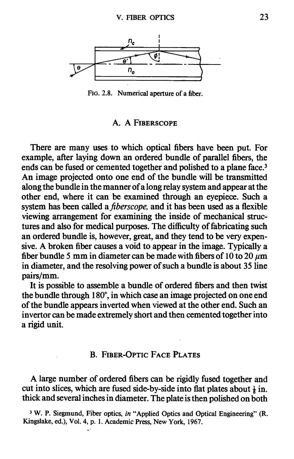
The numerical aperture of the fiber is the sine of the slope angle в of
the steepest entering ray that is just at the point of total internal
reflection inside the fiber. In Fig. 2.8 it is seen that if ф is the critical
angle, then sin ф = tiJuq, where щ is the refractive index of the fiber
and nc that of the cladding material. The numerical aperture sin в is
therefore equal to
sin в = щ sin в' = Uq cos ф = A^Vl — sin2</>
Thus if the index of the fiber is 1.55 and that ofthe cladding is 1.50, the
numerical aperture will be 0.39.
23
Fig. 2.8. Numerical aperture of a fiber.
A. A FlBERSCOPE
There are many uses to which optical fibers have been put. For
example, after laying down an ordered bundle of parallel fibers,, the
ends can be fused or cemented together and polished to a plane face.3
An image projected onto one end of the bundle will be transmitted
along the bundle in the manner of a long relay system and appear at the
other end, where it can be examined through an eyepiece. Such a
system has been called afiberscope, and it has been used as a flexible
viewing arrangement for examining the inside of mechanical struc-
structures and also for medical purposes. The difficulty of fabricating such
an ordered bundle is, however, great, and they tend to be very expen-
expensive. A broken fiber causes a void to appear in the image. Typically a
fiber bundle 5 mm in diameter can be made with fibers of 10 to 20 fim
in diameter, and the resolving power of such a bundle is about 35 line
pairs/mm.
It is possible to assemble a bundle of ordered fibers and then twist
the bundle through 180°, in which case an image projected on one end
of the bundle appears inverted when viewed at the other end. Such an
invertor can be made extremely short and then cemented together into
a rigid unit.
B. Fiber-Optic Face Plates
A large number of ordered fibers can be rigidly fused together and
cut into slices, which are fused side-by-side into flat plates about ? in.
thick and several inches in diameter. The plate is then polished on both
3 W. P. Siegmund, Fiber optics, in "Applied Optics and Optical Engineering" (R.
Kingslake, ed.), Vol. 4, p. 1. Academic Press, New York, 1967.
24 2. LIGHT AND IMAGES
sides and used as the end window of a cathode-ray tube. The phosphor
is deposited on the inside of the plate, and a piece of photographic film
can be pressed against the outer face of the window to record the
image. The illumination on the film transmitted by such a face plate
can be 20 to 40 times as great as when a lens is used to image the
phosphor on the film in the ordinary way.
C. Communication Fibers4
In the last 10 years or so, means have been found to make fibers in
which the absorption loss is around 1 dB/km. [A decibel (dB) is
defined as a transmission of @.1)* = 0.79; 2 dB is 0.63, and so on, to
10 dB, a transmittance of 0.1.] The real problem with very long fibers is
that the time taken for the transmission of a signal via the different
possible paths through the fiber varies, so that a rapid sequence of
pulses fed into the fiber at one end comes out as a continuous stream at
the other end and all information is lost. To prevent this, fibers are
being made with a radial gradient of refractive index having a para-
parabolic cross section of index. In this way the light is transmitted by
refraction rather than reflection, and in the near infrared the time of
transit is the same for all possible paths. The number of possible paths
can also be reduced by making the fiber very thin, i.e., of dimensions
comparable to the wavelength of the light, in which case the fiber
becomes a wave guide. Using light as a carrier wave, a large number of
telephone and TV messages can be transmitted over a single fiber with
no possibility of interference by ambient electrical disturbances.
D. Selfoc GRIN Rods
Selfoc GRIN rods are a recent development by a Japanese company.
A rod 1 or 2 mm thick is made with a radial gradient of refractive index
(hence GRIN), and rays of light inside such a rod are curved, oscillat-
oscillating from one side to the other like a sine wave. Such a rod has the
property of forming a succession of images wherever the curved rays
4 D. B. Keck and R. E. Love, Fiber optics for communications, in "Applied Optics
and Optical Engineering" (R. Kingslake and B. J. Thompson, eds.), Vol. 6, p. 439.
Academic Press, New York, 1980.
V. HBER OPTICS 25
cross each other. These images are successively inverted, then erect,
then inverted, etc., at a longitudinal separation of several Millimeters.
Thus if the rod is cut to the correct length and the ends polished, it acts
like a lens, forming an erect or an inverted image as required.
CHAPTER 3
Ray-Tracing Procedures
I. TYPES OF RAYS
Geometrical optics is based on the concept of rays of light, which are
assumed to be straight lines in any homogeneous medium and which
are bent at a surface separating two media having differing refractive
indices. We often need to trace the path of a ray through an optical
system, which will generally contain a succession of refracting or
reflecting surfaces separated by given distances along the axis. A rough
graphical procedure is available for rapid ray tracing, but for more
precision it is necessary to use a set of trigonometric formulas executed
in succession.
Rays in general fall into three classes: meridional, paraxial, and
skew. Meridional rays lie in the meridian plane, which is the plane
containing the lens axis and an object point lying to one side of the
axis. If the object point lies on the axis, all rays are necessarily
meridional.
Paraxial rays lie throughout their length extremely close to the
optical axis. The image formed by paraxial rays is deemed to be the
image, and if any image departs from the paraxial image, this is
regarded as an aberration. Paraxial ray-tracing formulas are purely
algebraic, whereas the formulas for tracing real rays involve trigono-
trigonometric functions.
Skew rays, on the other hand, do not lie in the meridian plane, but
they pass in front of or behind it and pierce the meridian plane at the
diapoint. A skew ray never intersects the lens axis. Skew rays are much
more difficult to trace than meridional rays, and we shall not refer to
them again.1
1 R. Kingslake, "Lens Design Fundamentals," p. 145. Academic Press, New York,
1978.
26
II. GRAPHICAL RAY TRACING 27
Fig. 3.1. Graphical ray tracing.
II. GRAPHICAL RAY TRACING
There is a simple graphical procedure, based on Snell's construction,
by which the path of a meridional ray can be traced through refraction
at a lens surface. This procedure, described by Dowell2 and by van
Albada,3 is as follows: Fig. 3.1b shows a pair of refracting surfaces
separating media having refractive indices n and n'. Figure 3. la shows
two concentric circles drawn about a point О having radii proportional
to n and n'. To trace a ray, a line О A is drawn through О parallel to the
incident ray a up to the circle corresponding to the refractive index n of
the medium containing the ray. A line is next drawn from A to В
parallel to the normal at the point of incidence, from the n circle to the
n' circle. Then OB represents the direction of the refracted ray b. It can
readily be seen that this construction is fully in accordance with the law
of refraction n sin / = n' sin /'.
We now proceed to the second surface. In this example, the normal
line BD at the second surface is seen to miss the n circle entirely,
indicating that total internal reflection will occur, and the reflected ray
has the direction d inside the lens.
In practice it is advisable to draw the index circles in ink and to make
little tick marks in pencil at the points A, B, D, etc., deleting each mark
when the next mark is made, thus displaying only one mark at any one
2 J. H. Dowell, Graphical methods applied to the design of optical systems. Proc. Opt.
Com., 2, 965 A926).
3 L. E. W. van Albada, "Graphical Design of Optical Systems." Pitman, London,
1965.
28 3. RAY-TRACING PROCEDURES
time. It is unnecessary to draw the radial lines from О to A, to B, etc.,
for the tick marks are quite sufficient. Changes in the lens can be made
at any time by overlaying a sheet of tracing paper and drawing the
altered lens upon it. After two or three changes have been made, the
original design will have disappeared, and only the changed system will
be visible.
The precision of this procedure is not high, say about 1 mm in
position and about Г in direction. The graphical procedure has the
great advantage that the lens diameters and thicknesses can be watched
continuously as the ray proceeds, to ensure that the dimensions of the
system are realistic. Furthermore, the procedure can be operated in
reverse, so that we can determine the radius of curvature of a surface
that will send a ray into any desired direction. Graphical ray tracing of
this kind is perfectly adequate for the design of condensers, magnifiers,
and field lenses, but it is not good enough if aberrations are to be
determined and corrected.
III. MERIDIONAL RAY TRACING
We define a meridional ray by its slope angle U, which is reckoned
positive if a counterclockwise rotation takes us from axis to ray, and by
its perpendicular distance Q from the surface vertex. The distance Q is
reckoned positive if the ray passes above the surface vertex.
We define a spherical refracting surface by its radius of curvature r,
which is considered positive if the center of curvature lies to the right of
the surface, and by the refractive indices и and n' of the media lying to
left and right of the surface, respectively. The distance measured along
the axis from one surface to the next is given by d and is reckoned
positive if the light is proceeding from left to right.
The first step in the ray-tracing process is to calculate the angle of
incidence /between ray and normal, and this is reckoned positive if a
counterclockwise rotation takes us from the normal to the ray. All the
data of the incident ray are expressed by plain symbols, and the
corresponding data for the refracted ray are given in primed symbols.
Figure 3.2a shows that for a spherical surface with radius r =
PC = AC, the line CNbeing drawn parallel to the ray
Q = r sin / — r sin U,
III. MERIDIONAL RAY TRACING
29
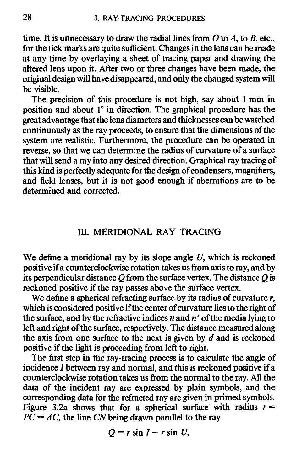
T
Fig. 3.2. Refraction of a meridional ray: (a) at a sphere; (b) at a plane.
from which
sin I = (Q/r) + sin U,
A)
or sin / = Qc + sin U if the surface curvature с is given instead of its
radius r.
We next apply the law of refraction to determine the angle of
refraction /':
sin/' = (и/и') sin /.
The third ray-tracing equation is found from the obvious fact that the
central angle PCA in Fig. 3.2a is the same for both the entering and
emerging rays, or
PCA = I- U=I'-U',
from which
l/'= U+r-I.
The final equation is found by adding primes to the first relation,
giving
Q' - /-(sin /' - sin V).
With these four equations we can determine the U' and Q' of the
refracted ray, given the С/and Q of the incident ray and the data of the
surface: r, n, and и'.
These equations are perfectly general provided that the radius of
curvature of the surface is finite. They obviously cannot be applied to a
plane surface because then, in the fourth equation, we find that
/' = U', and r is infinite, so we have the product of oo X 0, which is
indeterminate. Therefore, for a plane we must develop a separate set of
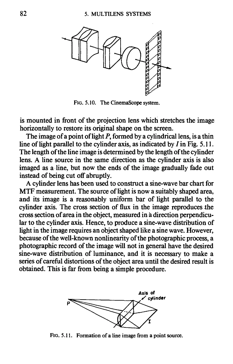
30 3. RAY-TRACING PROCEDURES
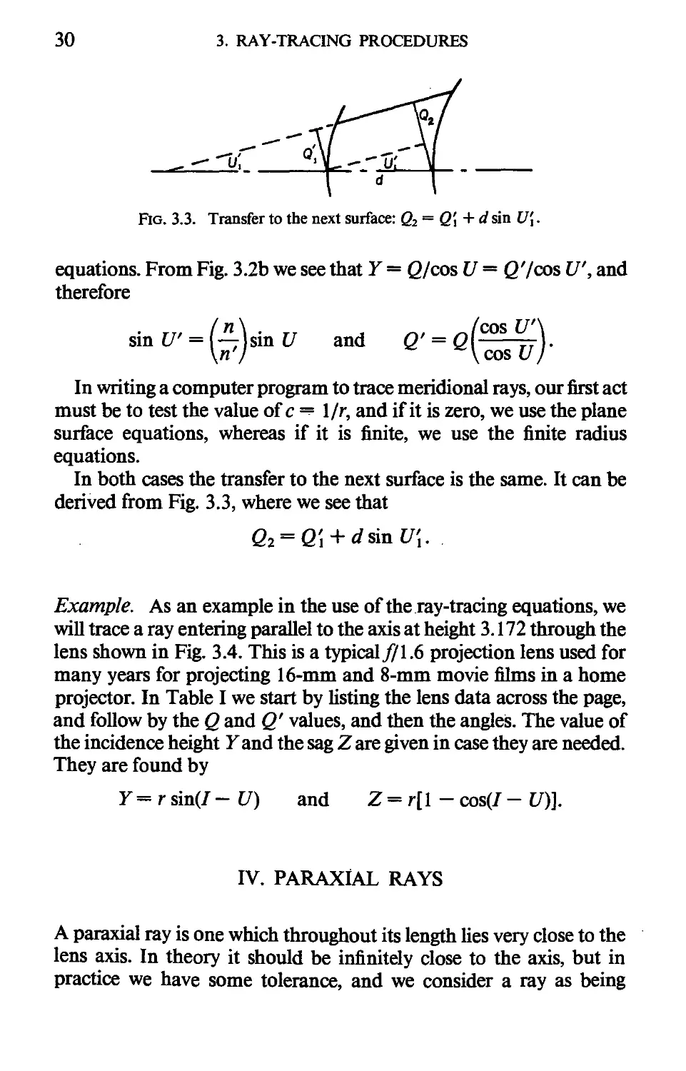
d
Fig. 3.3. Transfer to the next surface: Q2 = Q\ + d sin U\.
equations. From Fig. 3.2b we see that Y = Q/cos U = Q'/cos Uf, and
therefore
In writing a computer program to trace meridional rays, our first act
must be to test the value of с — 1/r, and if it is zero, we use the plane
surface equations, whereas if it is finite, we use the finite radius
equations.
In both cases the transfer to the next surface is the same. It can be
derived from Fig. 3.3, where we see that
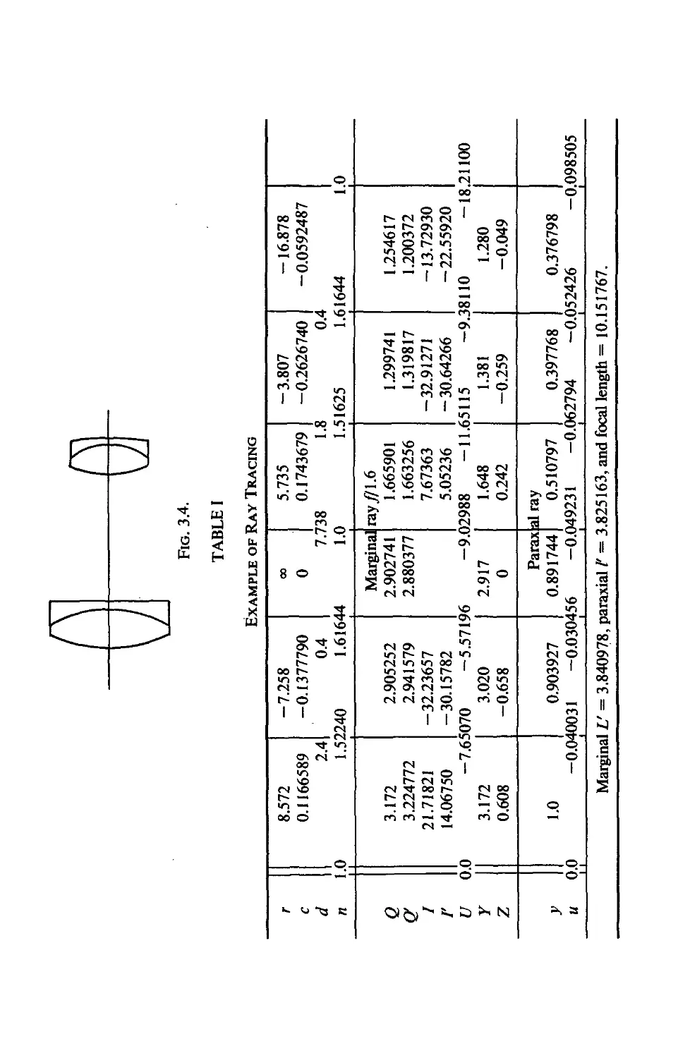
Example. As an example in the use of the ray-tracing equations, we
will trace a ray entering parallel to the axis at height 3.172 through the
lens shown in Fig. 3.4. This is a typical.//1.6 projection lens used for
many years for projecting 16-mm and 8-mm movie films in a home
projector. In Table I we start by listing the lens data across the page,
and follow by the Q and Q' values, and then the angles. The value of
the incidence height У and the sag Z are given in case they are needed.
They are found by
Y = r sin(/ - U) and Z = r[ 1 - cos(/ - [/)].
IV. PARAXIAL RAYS
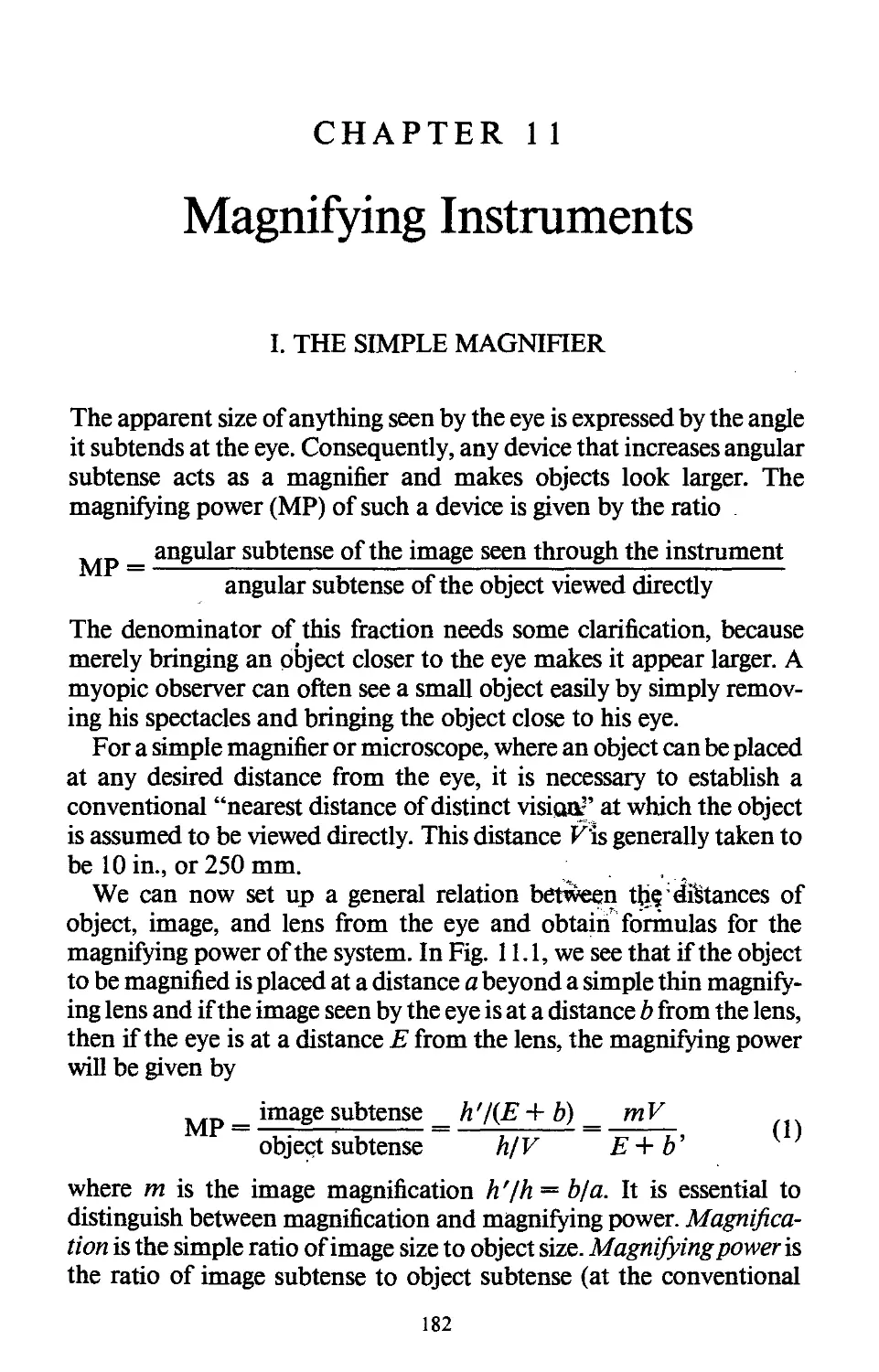
A paraxial ray is one which throughout its length lies very close to the
lens axis. In theory it should be infinitely close to the axis, but in
practice we have some tolerance, and we consider a ray as being
Fig. 3.4.
TABLE I
Example of Ray Tracing
r
с
d
n
1.0
8.572
0.1166589
2.4
-7.258
-0.1377790
0.4
1.52240
1.61644
7.738
1.0
5.735 -3.807 -16.878
0.1743679 -0.2626740 -0.0592487
1.8 0.4
1.51625 1.61644 \.O
Q
Q
I
Г
U
Y
Z
0.0
3.172 2.905252
3.224772 2.941579
21.71821 -32.23657
14.06750 -30.15782
-7.65070 -5.57196
3.172 3.020
0.608 -0.658
Marginal
2.902741
2.880377
ray//1.6
1.665901
1.663256
7.67363
5.05236
1.299741
1.319817
-32.91271
-30.64266
-9.02988 -11.65115
1.254617
1.200372
-13.72930
-22.55920
-9.38110
2.917
0
1.648
0.242
1.381
-0.259
-18.21100
1.280
-0.049
У
и
0.0
11
Parax al ray
1.0
0.903927
0.891744
0.510797
0.397768
0.376798
-0.040031
-0.030456
-0.049231 -0.062794 -0.052426
-0.098505
Marginal U = 3.840978, paraxial /' = 3.825163, and focal length = 10.151767.
32
3. RAY-TRACING PROCEDURES
-I
t'
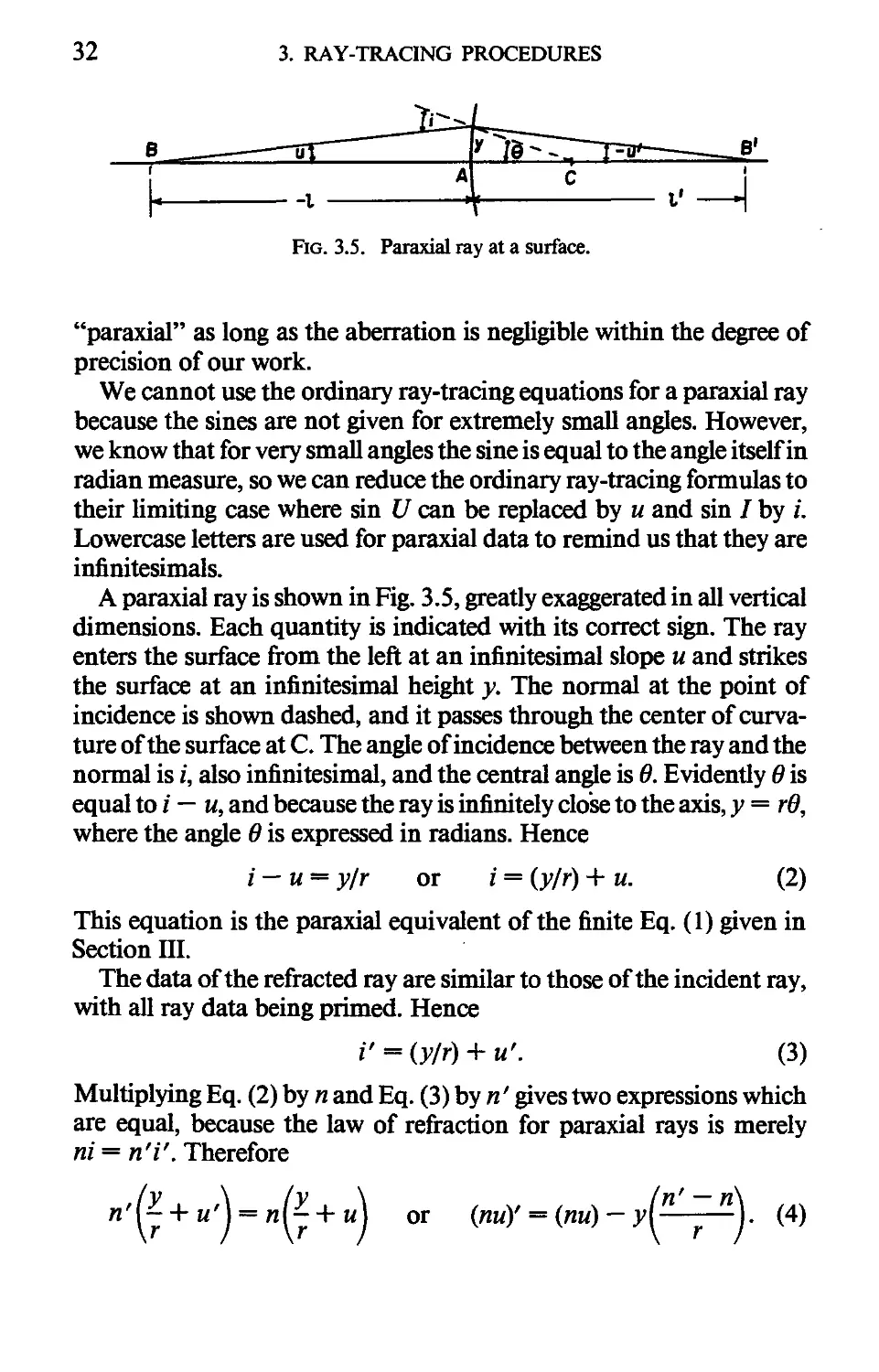
Fig. 3.5. Paraxial ray at a surface.
"paraxial" as long as the aberration is negligible within the degree of
precision of our work.
We cannot use the ordinary ray-tracing equations for a paraxial ray
because the sines are not given for extremely small angles. However,
we know that for very small angles the sine is equal to the angle itself in
radian measure, so we can reduce the ordinary ray-tracing formulas to
their limiting case where sin U can be replaced by и and sin / by /.
Lowercase letters are used for paraxial data to remind us that they are
infinitesimals.
A paraxial ray is shown in Fig. 3.5, greatly exaggerated in all vertical
dimensions. Each quantity is indicated with its correct sign. The ray
enters the surface from the left at an infinitesimal slope и and strikes
the surface at an infinitesimal height y. The normal at the point of
incidence is shown dashed, and it passes through the center of curva-
curvature of the surface at С The angle of incidence between the ray and the
normal is i, also infinitesimal, and the central angle is в. Evidently в is
equal to / — u, and because the ray is infinitely close to the axis, у = гв,
where the angle в is expressed in radians. Hence
/ - и = y/r or i = (y/r) + u. B)
This equation is the paraxial equivalent of the finite Eq. A) given in
Section III.
The data of the refracted ray are similar to those of the incident ray,
with all ray data being primed. Hence
i' - (У/г) + и'. C)
Multiplying Eq. B) by n and Eq. C) by n' gives two expressions which
are equal, because the law of refraction for paraxial rays is merely
ni = n'i'. Therefore
ог
D)
IV. PARAXIAL RAYS 33
This is a relation between the slope of the entering paraxial ray and the
slope of the emerging ray for a single refracting surface. Note that the
angles of incidence and refraction have disappeared; they are merely
auxiliaries and need not be calculated.
Another important relation is also shown in Fig. 3.5. If/and /' are
the distances from the surface to the points where the incident and
refracted rays cross the lens axis, then
у = —lu = —I'u'; hence и = —(y/l) and u' = —{y/l').
The quantities /and /' are called the intersection lengths of the ray, and
they have the usual signs of negative to the left of the surface and
positive to the right.
If we divide Eq. D) by у we obtain
from which
Now all the paraxial angles have disappeared, and they are all merely
auxiliaries. This relation shows that all paraxial rays emerging from a
given object point pass through the same image point. This is certainly
not true of finite rays. We can readily calculate the value of/', given /
and the surface data, by
/' = •
where ф is the surface power, given by in' — n)/r. A small pocket
calculator equipped with a reciprocal key is a convenient means for
using this equation. The transfer to the next surface is extremely
simple, because /2 = /{ — d.
A. Paraxial Ray with All Angles
There are, of course, other ways to trace a paraxial ray. For instance,
we can trace a paraxial ray with all the angles by using these equations
34 3. RAY-TRACING PROCEDURES
in order: given the / and у of the incident ray, we have
и = -y/l,
u' - /' - Ш,
/' = -y/u',
with the transfer
I2 = l\-d.
These equations can be collected together to give
or
и' — (су+ и) — — су, where с = —.
The transfer is now
y2 = у i + du[. F)
B. The y-nu Method for Tracing Paraxial Rays
In many ways the most useful procedure for tracing paraxial rays is
to use Eq. E) for the refraction and Eq. F) for the transfer. Both these
expressions are of the same form, namely, "the new value is equal to
the old value plus the product of the other variable times a constant."
The truth of this can be seen by
y2 = yi+(nuYl(d/n).
To trace a ray by this method, we start by tabulating the constants—ф
and d/n across the page, followed by the values of у and nu in order,
calculated and recorded in a zig-zag fashion, with the initial у and nu
being given. The calculation ends with the determination of the image
IV. PARAXIAL RAYS
35
r\
IZJ
Fig. 3.6.
distance /' by
image distance — —
last у
lastM'
As an example, we will use this procedure to trace a paraxial ray from
infinity through the cemented doublet lens shown in Fig. 3.6. The
figures to be recorded are shown in Table II. As before, any data
referring to the surfaces are written in the columns and data referring
to the spaces between surfaces are written between the columns.
Having entered the values of yx and (им),, we find {nu)\ = (nuJ by
TABLE II
Tracing of a Paraxial Ray from Infinity
through a Cemented Doublet Lens
r 7.3895 | -5.1784 | -16.2225
d И 1.05 0.4
n 1.0 1.517 1.649
1.0
n')/r
d/n
-0.0699641 0.02549041 -0.0400061
( 6921555 0.2425712
У
пи 0
2.0
1.903148
1.880973
-0.1399282
/'=11.28584
/'=12.0
-0.0914162 -0.1666667
и 0
У/г
1 + и
-0.0922400 -0.0554373 -0.1666667
0.2706543
0.2706543
-0.3675166
-0.4597566
-0.1159484
-0.1713857
21.68255
20.63255
34.32977
33.92977
11.28585
36
3. RAY-TRACING PROCEDURES
adding the product of yt and the number over it, namely, —фи to the
given value of (им),. This simple process is repeated twice for each
surface in the lens, once for the refraction and once for the transfer.
Any starting data can be used provided that the у is equal to the
product of / and — w; some workers always use yx = 1.0.
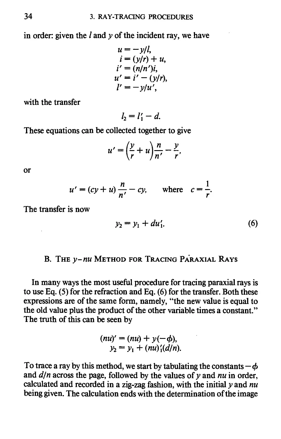
V. CURVED MIRRORS
A concave or convex reflecting surface can be included in a lens system
when tracing rays. The rule is to list the surfaces in succession in the
order in which the light strikes them, with the correct axial separation d
and refractive index и between the surfaces (Table HI). Note particu-
particularly that if the light is traveling from right to left, both the separation
and the refractive index must be entered with a negative sign. Other
than this there is no distinction between a lens and a mirror. An
example of a paraxial ray traced through the catadioptric system is
shown in Fig. 3.7.
Fig. 3.7. Ray tracing through a catadioptric system.
VI. MAGNIFICATION AND THE
LAGRANGE THEOREM
An image magnification is the transverse dimension of the image
divided by the transverse dimension of the object. For a single spheri-
VI. MAGNIFICATION AND THE LAGRANGE THEOREM 37
TABLE III
Tracing a Paraxial Ray
through a catadioptic system"
г
d
n
5.0 I 6.993 | 10.0 | 1.645 |
-0.35 -4.0 5.286 0.6
-1.0 -1.545 -1.0 1.0 1.545 \.O
f
-Ф
d/n
0.109000 -0.0779350 -0.2
-0.3313066 0
.2265372 4.0 5.286 0.3883495
/' = 0.00006
/' = 4.37605
У
nu
2.0 I 2.049385 2.282510 0.177515 0.000026
0.0 0.218000 0.0582812 -0.3982208-0.4570327 -0.4570327
" The sign of nu depends both on the sign of и and the sign of u. Otherwise the sign of и remains
the same as usual, namely, that a ray sloping downwards from left to right has a negative value of
u.
cal surface it is easy to develop a formula for the paraxial magnifica-
magnification, and this can readily be extended to apply to a complete system.
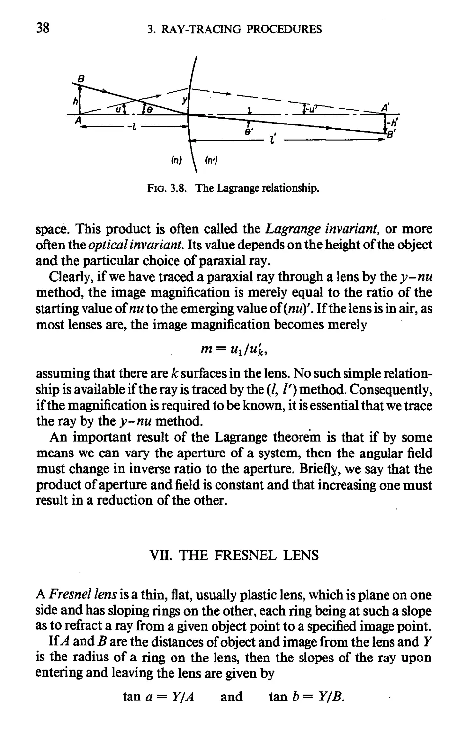
In Fig. 3.8, suppose that an axial object points is imaged at A' by a
single refracting surface. Then a small object of height h erected at A
will be imaged at A' with height h'. The magnification is, of course,
m = h'/h.
To relate h and h', we trace a paraxial ray from B, the top of the
object, to the surface vertex and on to the top of the image at B'. The
angles of incidence and refraction of this ray are в and в', respectively.
Therefore
0 = -h/l and 0' = -h'/l'.
We now multiply в by yn and в' by yn'. Then, because the law of
refraction for paraxial rays is пв = п'в', we obtain
nh(y/l) = n'h'(
which can be further simplified since y/l = —u and y/1' = — w', giving
finally
h'n'u'' = hnu.
This relation is known as the theorem ofLagrange.
For a complete system, it is clear that n\ is identical with n2, h\ is
identical with h2, u\ is identical with u2, etc., throughout the system.
We therefore conclude that the product hnu is invariant for all the
spaces between surfaces, including the object space and the image
38
3. RAY-TRACING PROCEDURES
Fig. 3.8. The Lagrange relationship.
space. This product is often called the Lagrange invariant, or more
often the optical invariant. Its value depends on the height of the object
and the particular choice of paraxial ray.
Clearly, if we have traced a paraxial ray through a lens by the y-nu
method, the image magnification is merely equal to the ratio of the
starting value of им to the emerging value of (им)'. If the lens is in air, as
most lenses are, the image magnification becomes merely
m = uju'k,
assuming that there are к surfaces in the lens. No such simple relation-
relationship is available if the ray is traced by the (/, /') method. Consequently,
if the magnification is required to be known, it is essential that we trace
the ray by the у- пи method.
An important result of the Lagrange theorem is that if by some
means we can vary the aperture of a system, then the angular field
must change in inverse ratio to the aperture. Briefly, we say that the
product of aperture and field is constant and that increasing one must
result in a reduction of the other.
VII. THE FRESNEL LENS
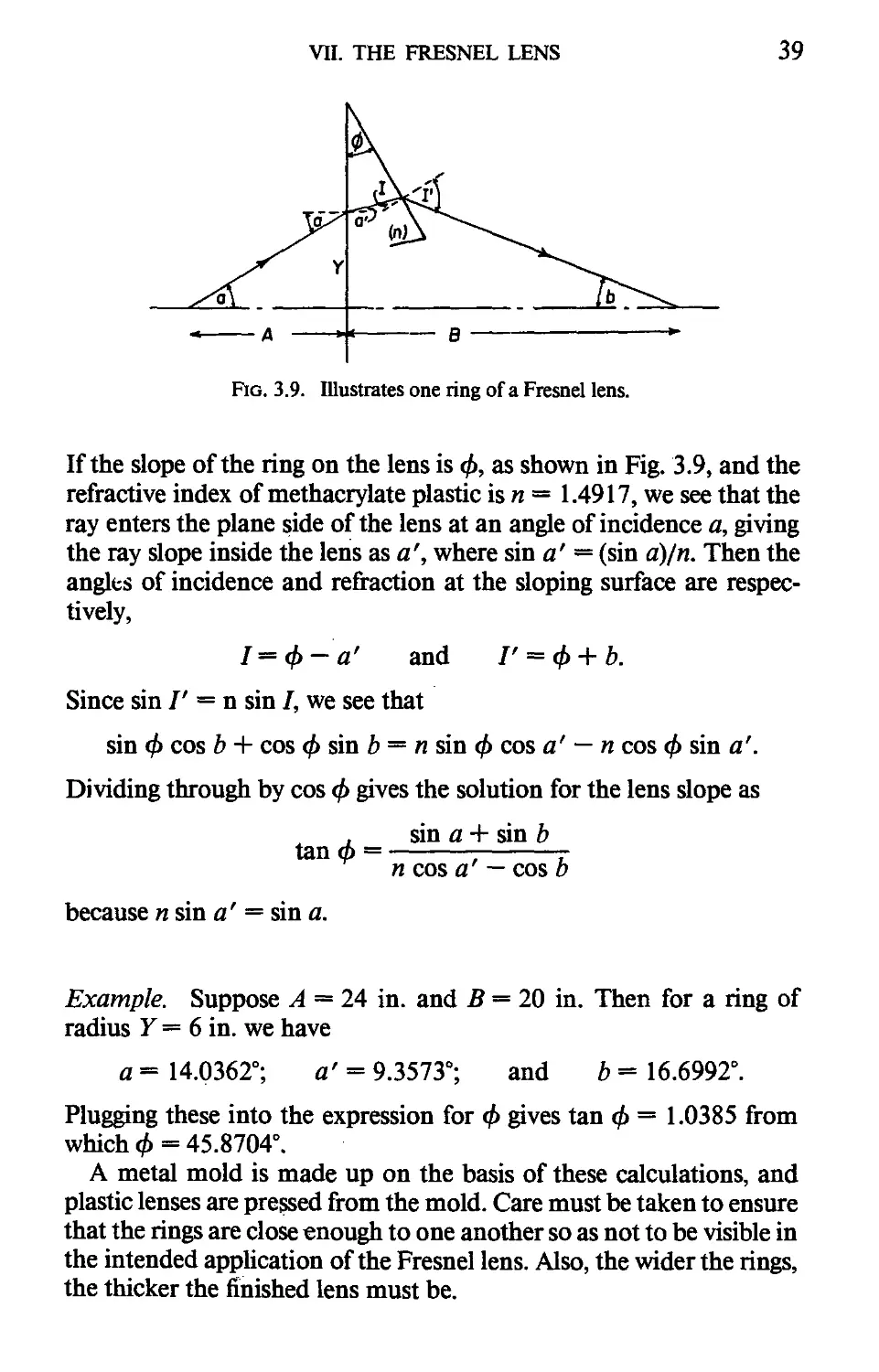
A Fresnel lens is a thin, flat, usually plastic lens, which is plane on one
side and has sloping rings on the other, each ring being at such a slope
as to refract a ray from a given object point to a specified image point.
If A and В are the distances of object and image from the lens and Y
is the radius of a ring on the lens, then the slopes of the ray upon
entering and leaving the lens are given by
tan a = Y/A and tan b = Y/B.
VII. THE FRESNEL LENS
39
Fig. 3.9. Illustrates one ring of a Fresnel lens.
If the slope of the ring on the lens is ф, as shown in Fig. 3.9, and the
refractive index of methacrylate plastic is n — 1.4917, we see that the
ray enters the plane side of the lens at an angle of incidence a, giving
the ray slope inside the lens as a', where sin a' — (sin a)/n. Then the
angles of incidence and refraction at the sloping surface are respec-
respectively,
1=ф-а' and Г = ф + Ь.
Since sin /' = n sin /, we see that
sin ф cos b + cos ф sin b = n sin ф cos a' — n cos ф sin a'.
Dividing through by cos ф gives the solution for the lens slope as
sin a + sin b
tan ф ¦¦
n cos a' — cos b
because n sin a' = sin a.
Example. Suppose A = 24 in. and Б = 20 in. Then for a ring of
radius Y = 6 in. we have
а= 14.0362°; a' = 9.3573°; and b= 16.6992°.
Plugging these into the expression for ф gives tan ф = 1.0385 from
which ф = 45.8704°.
A metal mold is made up on the basis of these calculations, and
plastic lenses are pressed from the mold. Care must be taken to ensure
that the rings are close enough to one another so as not to be visible in
the intended application of the Fresnel lens. Also, the wider the rings,
the thicker the finished lens must be.
CHAPTER 4
The Gaussian Theory
of Lenses
I. INTRODUCTION
Prior to the time of C. F. Gauss A777 -1855), the term focal length had
meaning only for a very thin lens, it being the distance from the lens to
the "focus" where images of distant objects were formed. Before the
invention of photography in the 1830s, all practical lenses were thin
enough for this concept of focal length to be quite adequate. However,
with the introduction of the Petzval Portrait lens in 1839, some
extension of this concept became necessary.
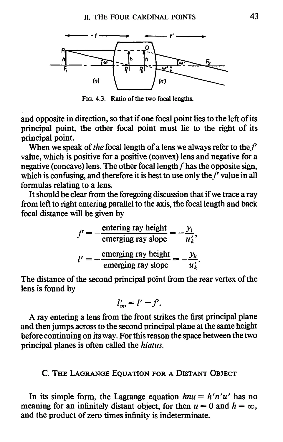
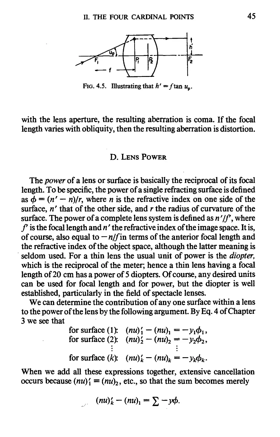
II. THE FOUR CARDINAL POINTS
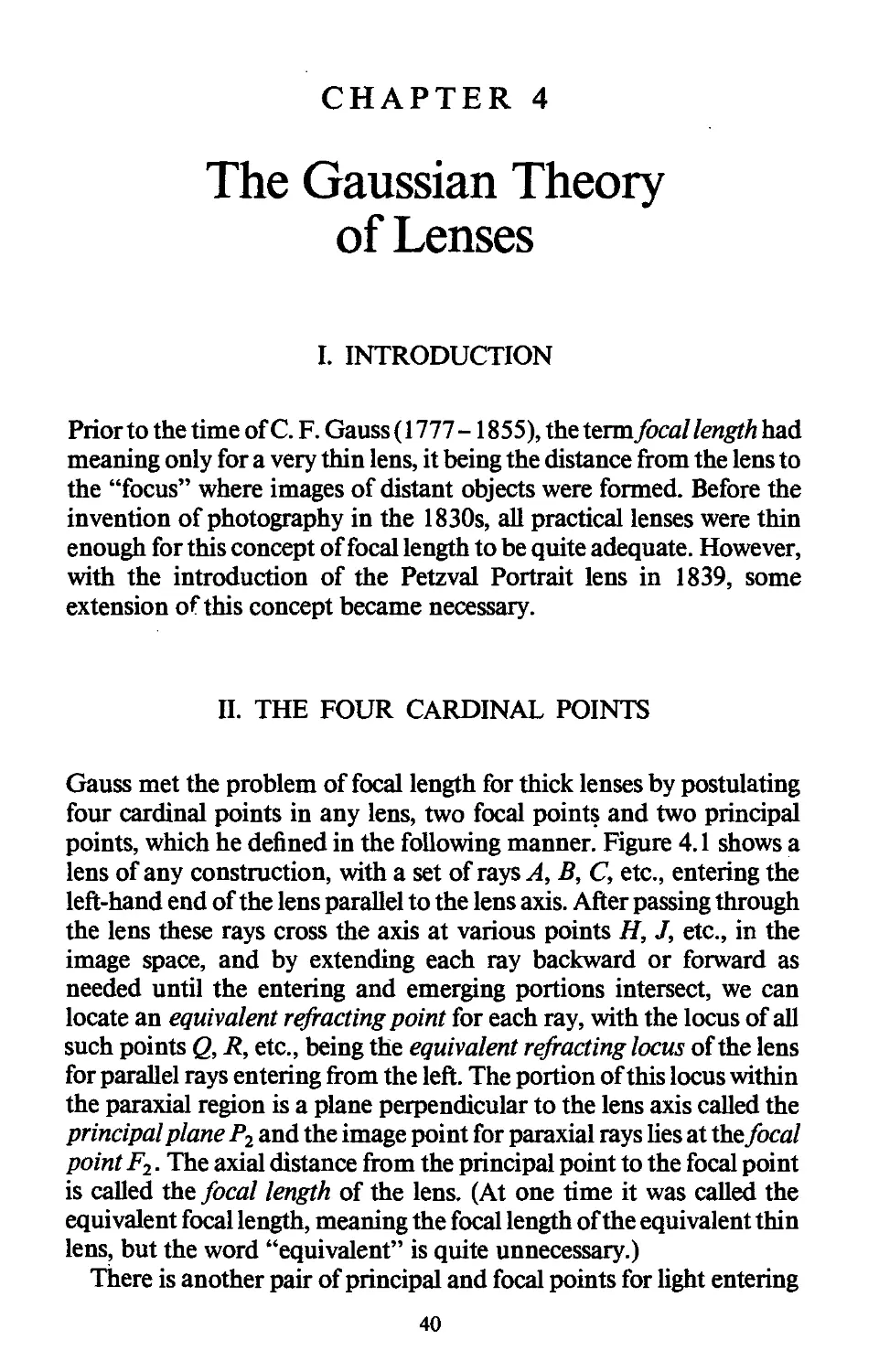
Gauss met the problem of focal length for thick lenses by postulating
four cardinal points in any lens, two focal points and two principal
points, which he defined in the following manner. Figure 4.1 shows a
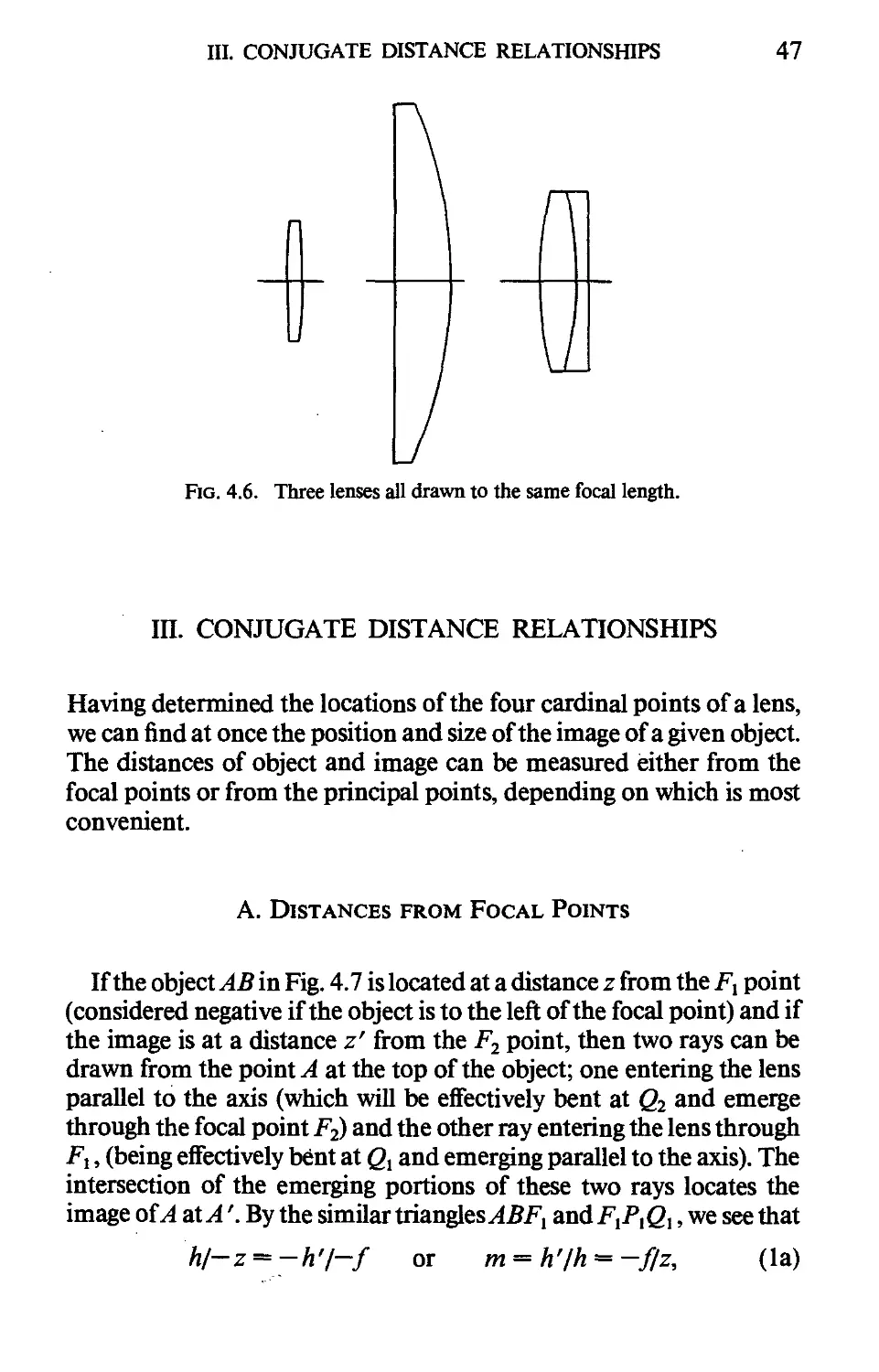
lens of any construction, with a set of rays А, В, С, etc., entering the
left-hand end of the lens parallel to the lens axis. After passing through
the lens these rays cross the axis at various points H, J, etc., in the
image space, and by extending each ray backward or forward as
needed until the entering and emerging portions intersect, we can
locate an equivalent refracting point for each ray, with the locus of all
such points Q, R, etc., being the equivalent refracting locus of the lens
for parallel rays entering from the left. The portion of this locus within
the paraxial region is a plane perpendicular to the lens axis called the
principal plane P2 and the image point for paraxial rays lies at the focal
point F2. The axial distance from the principal point to the focal point
is called the focal length of the lens. (At one time it was called the
equivalent focal length, meaning the focal length of the equivalent thin
lens, but the word "equivalent" is quite unnecessary.)
There is another pair of principal and focal points for light entering
40
П. THE FOUR CARDINAL POINTS
41
Fig. 4.1. The equivalent refracting locus of a lens for a set of rays entering from the
left parallel to the axis.
the lens parallel to the axis from the right and emerging to the left. The
complete set of four cardinal points Fl,Pl,P2, and F2 is shown in Fig.
4.2.
A. Relation between Principal Planes
Working purely from the formal definitions for the cardinal points,
we can derive several relations which are of considerable importance
in geometrical optics. The first of these is that the two principal planes
are images of each other at unit magnification (see Fig. 4.2). In this
diagram a paraxial ray A enters from the left parallel to the axis. It is
effectively bent at Q in the second principal plane (following Gauss's
definitions), and it emerges through the second focal point F2. An-
Another paraxial ray В enters parallel to the axis from the right in the
same straight line as the first ray. This second ray is effectively bent at R
in the Px plane and emerges through the first focal point Fx. By
reversing the arrows on this second ray, we end up with two rays
entering through R and emerging through Q. This makes Q an image
Fig. 4.2. The principal planes as unit planes.
42 4. THE GAUSSIAN THEORY OF LENSES
of R and vice versa. In Fig. 4.2 both the object and image points are
virtual, but other systems could be drawn in which one or both of the
principal points fell outside the system instead of inside. Because R
and Q are at the same height above the axis, the magnification for this
conjugate pair is +1.0. For this reason the principal planes are often
called the unit planes of a lens. It must be emphasized that the cardinal
points and focal length are all paraxial properties of a lens.
B. Relation between the Focal Lengths
We can now proceed to determine the relation between the two focal
lengths of a lens system. Suppose we place a small object at the anterior
focal point Ft, as shown in Fig, 4.3, and draw two rays from the top of
this object into the lens. The first ray enters parallel to the axis and
emerges through F2 at the right. The second ray enters the lens toward
the first principal point Px, and therefore it must emerge through P2,
because P2 is an image of Pj. How about the direction of this emerging
ray? Since the small object h is located in the anterior focal plane, all
rays originating at any point in the object must emerge as a parallel
beam at the other end of the lens, because the focal plane is conjugate
to infinity. Consequently, our second ray must emerge through P2
parallel to the emergent portion of the first ray. If the slope of the
second ray on entry is со and on emergence is со', as shown in Fig. 4.3,
we see that
со = -h/f and со' = h/f,
from which со'/со = —f/f.
To obtain a second expression for со'/со, we move the small object
along the axis until it falls on the anterior principal plane at Pt. The
image is now at P2, and the magnification is unity. Applying the
Lagrange equation to this pair of conjugates we see that
hnco = hn'co',
hence со '/со = п/п', where и and n' are the refractive indices of object
space and image space, respectively. Combining the two values of
со'/со gives
~f/f = n/n' or f=-f(n/n').
For a lens in air, therefore, the two focal lengths are equal in magnitude
II. THE FOUR CARDINAL POINTS 43
Fig. 4.3. Ratio of the two focal lengths.
and opposite in direction, so that if one focal point lies to the left of its
principal point, the other focal point must lie to the right of its
principal point.
When we speak of the focal length of a lens we always refer to the/
value, which is positive for a positive (convex) lens and negative for a
negative (concave) lens. The other focal length/ has the opposite sign,
which is confusing, and therefore it is best to use only the/ value in all
formulas relating to a lens.
It should be clear from the foregoing discussion that if we trace a ray
from left to right entering parallel to the axis, the focal length and back
focal distance will be given by
entering ray height yx
emerging ray slope и 'к'
emerging ray height _ yk
ii
emerging ray slope u'k
The distance of the second principal point from the rear vertex of the
lens is found by
«pp * j •
A ray entering a lens from the front strikes the first principal plane
and then jumps across to the second principal plane at the same height
before continuing on its way. For this reason the space between the two
principal planes is often called the hiatus.
C. The Lagrange Equation for a Distant Object
In its simple form, the Lagrange equation hnu = h'n'u' has no
meaning for an infinitely distant object, for then и = 0 and h = oo,
and the product of zero times infinity is indeterminate.
44
4. THE GAUSSIAN THEORY OF LENSES
Fig. 4.4. The Lagrange relationship for a distant object.
To interpret the Lagrange equation for a distant object, we refer to
Fig. 4.4. The point A represents an object point that is distant but not
infinitely distant. Then
h'n'u' = (h/l)n(lu).
In the limit when / becomes infinite, the ratio h/l becomes equal to
tan Mp and the product lu becomes equal to — y, where у is the height at
which the ray enters the lens. Thus, since y/u' = —f, we find
h' = -(и/и') tan МрОУм') = (и/и/)/ tan «„,
where Wp is the slope of an entering parallel beam of light. For a lens in
air, therefore, the image height for an infinitely distant object is equal
to the product of the focal length and the tangent of the angular
subtense of the object. Paraxially, the tangent is equal to the angle in
radians.
Another way of looking at this is seen in Fig. 4.5, where the anterior
focal length/= —(n/n')f, hence
A ray entering at slope tip through the anterior focal point emerges
parallel to the axis at a height h' on the other side of the lens.
We thus have two expressions for focal length, each of which
consists of a length divided by an angle. They are
f—yJW
and
The first of these relationships is used to compute the focal length after
tracing a paraxial ray, whereas the second expression provides a simple
and unambiguous definition of focal length. This will be used later in
Section VII.
Both these formulas refer to paraxial rays. If the focal length varies
II. THE FOUR CARDINAL POINTS
45
Fig. 4.5. Illustrating that h' =/tan «p.
with the lens aperture, the resulting aberration is coma. If the focal
length varies with obliquity, then the resulting aberration is distortion.
D. Lens Power
The power of a lens or surface is basically the reciprocal of its focal
length. To be specific, the power of a single refracting surface is defined
as ф = (и' — ri)/r, where и is the refractive index on one side of the
surface, и' that of the other side, and r the radius of curvature of the
surface. The power of a complete lens system is defined as n 'If, where
f is the focal length and и' the refractive index of the image space. It is,
of course, also equal to — n/fm terms of the anterior focal length and
the refractive index of the object space, although the latter meaning is
seldom used. For a thin lens the usual unit of power is the diopter,
which is the reciprocal of the meter; hence a thin lens having a focal
length of 20 cm has a power of 5 diopters. Of course, any desired units
can be used for focal length and for power, but the diopter is well
established, particularly in the field of spectacle lenses.
We can determine the contribution of any one surface within a lens
to the power of the lens by the following argument. By Eq. 4 of Chapter
3 we see that
for surface A): (им) J — (им), = — Ухфх,
for surface B): (имJ — (имJ = —угФг->
for surface (fc): (nu)'k — (nu)k = —укфк.
When we add all these expressions together, extensive cancellation
occurs because (им){ = (имJ, etc., so that the sum becomes merely
(nu)k - (им), = ? -уф.
46 4. THE GAUSSIAN THEORY OF LENSES
Dividing through by yx gives
(nu)'k (пи)г у
Ух Ух L Ух
So far the expression is perfectly general. We now consider the
special case of an infinitely distant object, for which щ is zero. Further-
Furthermore, for such an object (— nu) 'kfyx is the lens power P. Hence the lens
power is given by
This tells us that the contribution of a single surface to the power of the
lens is equal to the surface power ф multiplied by the ratio of the height
of the ray at the surface divided by its height of entry into the lens. If a
ray drops before striking a surface, that surface contributes less than its
own power to the power of the system, and conversely, if the ray rises at
the surface, that surface contributes more than its power to the system.
In the limit when у = 0 at a surface, that surface makes no contribu-
contribution to the lens power, whether it is convex, concave, or plane. Indeed,
it could well be made of ground glass, because the image falls on the
surface itself in such a case.
This law leads to a ready explanation of many effects in lenses. For
instance, it shows why increasing the thickness of a biconvex lens
reduces its power and increases its focal length, but increasing the
thickness of a meniscus lens reduces the negative contribution of the
concave surface and therefore increases the lens power.
It should be noted particularly that if the image is formed in a
material other than air, the focal length is still given by.f = —yt /u'k,
but the lens power is now equal to n'/f. Only when the image is
formed in air is the power equal to the reciprocal of the focal length.
However, this is by far the most common situation, and in very few
instances is the image formed in a material other than air.
Do not be confused by the appearance of a lens in a drawing. Just
because it is thick does not make it strong. Figure 4.6 shows three
lenses which all have the same focal length. The first is thin and small,
the second is large and thick, and the third is an ordinary achromatic
doublet. As a good example of this effect, turn ahead to Figure 12.5, in
which five eyepieces of different types are all drawn to the same focal
length, yet example (e) looks as though it must be much stronger than
example (a) because it is thicker and larger.
III. CONJUGATE DISTANCE RELATIONSHIPS
47
ГП
VII
Fig. 4.6. Three lenses all drawn to the same focal length.
III. CONJUGATE DISTANCE RELATIONSHIPS
Having determined the locations of the four cardinal points of a lens,
we can find at once the position and size of the image of a given object.
The distances of object and image can be measured either from the
focal points or from the principal points, depending on which is most
convenient.
A. Distances from Focal Points
If the object AB in Fig. 4.7 is located at a distance z from the Fx point
(considered negative if the object is to the left of the focal point) and if
the image is at a distance z' from the F2 point, then two rays can be
drawn from the point A at the top of the object; one entering the lens
parallel to the axis (which will be effectively bent at Q2 and emerge
through the focal point F2) and the other ray entering the lens through
Ft, (being effectively bent at Q, and emerging parallel to the axis). The
intersection of the emerging portions of these two rays locates the
image ofA at A'. By the similar triangles ABFX and F,P,<2i, we see that
hl-z^-h'l-f or m = h'/h'=-f/z, (la)
48
4. THE GAUSSIAN THEORY OF LENSES
Fig. 4.7. Conjugate distances from a lens.
and by similar triangles 62^2^2 ап<* F2B'A', we see that
h/f = -h'/zr or m-h'/h--z'/f. (lb)
Since the magnification m = —f/z = —z'/f, we can cross multiply,
giving
zz'-JST. B)
Since, for any lens,/= —f(n/n'), we see that this equation can be
written as
zz' = -Pin/n').
For a lens in air, n — n'= 1, so this equation simply becomes
zz' = -f2.
This relation has many uses. For example, we can use it to lay out the
focusing scale on a camera lens. If the object is at a distance ;> from the
front principal plane of the lens, then z = p—f, and the distance
through which the lens must be moved from the infinity setting to
focus on this object is given by
z'=Pl{p-f).
Another application forms the basis of the optician's lensometer.
This is an instrument for measuring the power of a spectacle lens. In
Fig. 4.8 the lens A under test is placed at the anterior focus of a known
lens В built into the instrument, and a parallel beam' of light is
admitted to it. With no added lens the image is formed at F2. When an
eyeglass lens is inserted at A the object for lens В is distant from its
anterior focus by z = fA, and hence the image distance from F2 is given
by z' = —Ув2/Л • The image is thus moved longitudinally by a distance
III. CONJUGATE DISTANCE RELATIONSHIPS 49
Fig. 4.8. The structure of an optician's lensometer.
proportional to the power of the added lens, to the left if the added lens
is positive and to the right if it is negative. In practice, the light is made
to traverse this system backward, with a movable illuminated reticle at
F2 and a small telescope enabling the operator to tell when the
emerging light is parallel.
Strictly speaking, the object distance for lens В is equal to the back
focal distance of the eyeglass lens and not its focal length. However,
this is what the optician needs to know, and for this reason the
instrument is sometimes called a vertometer because it determines the
vertex focal distance of the lens.
B. Distances from Principal Points
If the locations of the principal points are known or can be assumed,
then it is often more convenient to relate the conjugate distances of
object and image from the principal points rather than the focal points.
If these distances are represented by p and p', respectively, we see that
z = p—f and z'=p'—f.
Equation B) now becomes
from which
(f/Pf) + (f/p) = 1.
Because/= —f(n/n'), this formula can be simplified to
lens power = n'/f = n'/p' — n/p.
For a lens in air, which is of course the usual situation, we have the
familiar relationship
I/P' ~ I/P = I//- Ca)
50
4. THE GAUSSIAN THEORY OF LENSES
The image magnification is found from Eq. A) to be
m=p'n/pn'
or, for a lens in air, m — p'/p.
Cb)
C. Nodal Points
The nodal points of a lens are a pair of conjugate points having the
property that a paraxial ray entering toward the first will emerge from
the second at the same slope. In Fig. 4.9 we see a ray entering toward
the first nodal point iV, at a slope со. Applying the Lagrange theorem to
an object located at Nt we find that
h'n'co = hnco,
from which the magnification for this pair of conjugates is given by
m = h'/h = и/и'.
Substituting this into Eq. A) tells us that the distance from F, to iV, is
equal to the posterior focal length/, and the distance from N2 to F2 is
equal to the anterior focal length/ The whole array of six cardinal
points is shown in Fig. 4.9. Of course, if the lens is in air, iV, coincides
with Px and N2 with P2, and there is nothing to distinguish between the
nodal and the principal points. However, the nodal points are impor-
important when studying the optical system of the eye, because the refractive
index of the image space is then about 1.34 and the two focal lengths
are unequal. In fact, the nodal points were first proposed by an
ophthalmologist J. B. Listing because he needed them in his work.
Fig. 4.9. The nodal points of a lens.
IV. A SINGLE LENS
IV. A SINGLE LENS
51
A. A Single Thick Lens
We can easily derive useful general formulas for the focal length and
back focal distance of a single thick lens by writing Eqs. D) and F) of
Chapter 3 in algebraic terms (see Table I).
TABLE I
Raytrace Through a Single Thick Lens
Hence the focal length is given by
and the back focus by
The rear principal plane is therefore located at a distance from the rear
lens vertex given by
и _BF p- tf(N~l
To locate the anterior principal plane we reverse the direction of the
52 4. THE GAUSSIAN THEORY OF LENSES
ray, giving
hence
z
The separation between the two principal planes is often called the
hiatus, represented by the symbol Z. Its value is found by
If a lens is fairly thin, we may neglect the t inside the bracket, and in
this case
Thus, if N = 1.5, the hiatus is approximately equal to one-third the
thickness of the lens.
B. A Thin Lens
A strictly "thin" lens, i.e., one having zero thickness, is of course a
purely mathematical fiction. However, the simplicity and convenience
of the thin-lens concept is so great that we often speak of "thin lenses"
as being those in which the thickness effects are negligible within the
precision of our work. Now we assume that the principal planes
coalesce within the lens itself, and the conjugate distances are mea-
measured "from the lens." A thin lens is specified completely by its focal
length and diameter, whereas if its shape is important, we add the radii
of curvature and the refractive index.
Writing t = 0 in Eq. D) tells us that the power of a thin lens is given
by
IV. A SINGLE LENS 53
where the <?'s are the surface powers. Because the ray height у is the
same at both surfaces in a thin lens, we merely add the surface powers
to determine the lens power. We cannot do this if the lens has a finite
thickness.
С Simplified Case of a Thin Lens with Real Conjugates
The most common situation in real life by far is that in which a
positive lens is used to form a real image of a real object. For this
special case we can simplify Eq. C) by ignoring signs and writing the
object and image distances as a and b and the magnification as m, with
all three quantities being regarded as simple positive numbers. When
we do this we find that
product b
'¦> m = -'¦>
sum a
b=f(l+m);
а
and
D
ab
a + b
= /(l"
= n 4- h
The two middle equations are read: "Object distance is 1 plus l/m
focal lengths" and "Image distance is 1 plus m focal lengths." Famil-
Familiarity with these relations enables one to make rapid mental calcula-
calculations of image distances and magnification.
For example, if a 4-in. lens is required to form an image at a
magnification of six times, these formulas tell us that the object
distance must be a = 4 X 7/6 = 4.67 in. and the image distance b =
4 X 7 = 28 in. Similarly, if we know that the object and image
distances are, respectively, 30 and 5 in., we see that the focal length of
the lens must be C0 X 5)/CO + 5) = 4.29 in. We can use these
equations for a thick lens if we remember that the distances a and b
must be measured from the two principal planes.
The last of these formulas is particularly useful in designing a printer
to produce prints of a standard size from a variety of negative sizes.
Thus, knowing that the object-to-image distance is D and the required
54 4. THE GAUSSIAN THEORY OF LENSES
magnification is m, we can at once determine the required focal length
by d
" ~ 2 + m
If we are using a thick lens, we must remember to subtract the hiatus
from the value of D before making the calculation.
It is sometimes useful, for example in the design of some types of
zoom lenses, to invert Eq. E) and solve for the magnification that will
result when a lens of known focal length is used between given object
and image planes. Then
m = ±fc - 1 ± V|fc2 - it, where к = D/f.
Then, when/* and m are known, the distances a and b can be found by
the ordinary formulas. It should be noticed that the two values of m
given by this formula are reciprocals, so that when a given lens is used
between fixed object and image planes, the lens may occupy either of
two positions, giving magnifications equal to m and l/m, respectively.
This feature has been used in some types of variable-power telescopes
(see Chapter 12, Section III.G).
D. Insertion of Thickness into a Thin Lens
Suppose we have designed a system that includes a thin lens of
power ф, refractive index N, and two surface curvatures cx and c2. We
now wish to replace this by a thick lens of thickness t, having the same
focal length and the same ratio of radii к = r2lrl = c, /c2. For the thin
lens, the surface curvatures were
C = l C = kC
For the thick lens we have
ф = (N- l)\c[ -c'2 + jj(N- ljcjcjl with к = °-±.
The solution to this quadratic is
2kt{N-\)IN
IV. A SINGLE LENS 55
As an example, suppose ф = 0.1, JV= 1.523, and k = —1.5. This
represents a biconvex lens with the front surface stronger than the rear
surface. For the thin lens, the solution is c, = 0.1147 and c2 —
—0.0765. If we now insert a thickness of 0.2, the solution yields the
curvatures c\ — 0.1151 and c'2 = -0.0767. It will be seen that both
surfaces have become slightly stronger as a result of the insertion of
thickness, but only slightly. Thickness has very little effect on the
power of a biconvex lens, but it has much greater effect if the lens is
meniscus.
E. A Collimator
It has been pointed out that the focal plane of a lens is conjugate to
infinity, so that the image of a very distant object falls within the focal
plane. Conversely, an object located within the focal plane is imaged at
infinity. Such a system is called a collimator.
If the source of light in a collimator is a single point, a parallel beam
will emerge from the other side of the lens, but it will contain very little
energy. However, if the object has finite dimensions, a bundle of
parallel beams will emerge from the other side of the lens, diverging
from one another (Fig. 4.10). Thus the so-called parallel beam of light
from a collimator is actually an expanding beam, with the angle of
divergence being given by the ratio of the source size to the focal length
of the lens. For this reason, it is much better to call this a collimated
beam rather than a parallel beam.
If the source happens to have the same diameter as the lens, the
entering beam on the object side will have a parallel external form, but
each elementary beam entering the lens will be divergent. Such a beam
Fig. 4.10. A collimator forms an expanding bundle of parallel rays.
56 4. THE GAUSSIAN THEORY OF LENSES
is called a quasi-parallel beam. We thus have the paradox that a
parallel beam has a divergent external form, whereas in this case a
diverging beam has a parallel external form. This distinction becomes
important when a prism is inserted into the beam. For example, a
Dove prism can be used only in a truly parallel beam because the end
faces are inclined to the lens axis. However, there are other types of
prisms that can be used in a quasi-parallel beam (see Section V in
Chapter 9).
V. LONGITUDINAL MAGNIFICATION
Longitudinal magnification is the ratio of the axial dimension of an
image to the corresponding axial dimension of the object. These axial
dimensions may be the physical sizes of object and image, or they may
be a movement of object and image along the axis.
Two situations arise—the first is concerned with an infinitesimally
small longitudinal dimension (enabling the magnification to be deter-
determined by differentiation), and the second is for a finite axial dimen-
dimension.
A. A Very Small Axial Dimension
If the object and image have very small axial dimensions, we may
write A/ for the axial dimension of the object and A/' for the corre-
corresponding axial dimension of the image. Then by differentiating Eq. E)
of Chapter 3 we find
-in'II'2) M' = ~(n/P) M,
from which the longitudinal magnification becomes
Multiplying numerator and denominator by y2 gives
т = АГ/А1 = пи2/п'и'2.
Therefore there is a longitudinal magnification invariant correspond-
corresponding to the Lagrange invariant, namely, Д/ n и2. Since the ordinary
V. LONGITUDINAL MAGNIFICATION 57
magnification m = nu/n 'u', we see that
m = (n'/n)m2.
For a lens in air, the fact that m = m2 tells us that longitudinal
magnification is always positive, so that if the object moves from left to
right, the image must move from left to right also. On the other hand,
for a mirror, the signs of и and n' are equal and opposite, so that when
the object moves from left to right the image must move from right to
left.
If the ordinary magnification is large, as in a microscope objective,
the longitudinal magnification will be very large, which explains the
small depth of field noticed in a microscope. On the other hand, in a
camera the magnification is small, so the longitudinal magnification is
very small, accounting for the great depth of field noticed in most
cameras.
B. A Large Axial Dimension
If the longitudinal dimensions of object and image are large, we
can still derive a useful expression for the longitudinal magnification.
In Fig. 4.11 the magnifications of the objects at A and В are related to
their image distances z'A and zB from the rear focal point of the lens by
z'a = ~fmA and z'B = -fmB.
When the object moves from A to B, the change in image distance
A'B' is therefore given by
A'B' = {zA-zB)=f(mA-mb).
The corresponding change in the object distance AB is similarly
AB
¦ \тв тА
z'b
Fig. 4.11. Longitudinal magnification.
58
4. THE GAUSSIAN THEORY OF LENSES
Therefore, the longitudinal magnification A 'B'/AB is given by
_ _ f(mA - mB)
ТП rr-
This reduces to m2 if the longitudinal dimensions AB and A 'B' are so
small that the magnification does not change significantly when going
from A to B.
VI. THE SCHEIMPFLUG CONDITION
Captain Theodor Scheimpflug of the Austrian army pointed out early
in the present century that if the object plane is tilted relative to the
lens axis, the image plane will also be tilted in such a way that the
object plane, image plane, and median plane through the lens will all
meet. This relation can easily be proved for the paraxial region by use
of the longitudinal magnification formula. In Fig. 4.12, an object point
A is imaged at A' and a neighboring point В on a sloping object is
imaged at B'. The plane through AB and the plane through A 'B' are
shown meeting the median plane through the lens at M and N,
respectively. The middle of the lens is marked O. The heights QMand
ON are given by
OM = -yl/z and ON = -y'l'/z',
where (y, z) are the coordinates of В relative to A and / the distance
from A to the lens. In the image space we have similar quantities with
Fig. 4.12. The Scheimpflug condition.
VII. FOCOMETRY 59
primes. Since y' = my and /' = ml and since (by the longitudinal
magnification rule) z' = m2z, we see that OM = ON, and this at once
bears out Scheimpflug's rule. Although we have proved this only for
the paraxial region, it actually holds well over a considerable field
angle. This subject is discussed much more fully in Section IV of
Chapter 15.
VII. FOCOMETRY
Focometry is the name given to the process of measuring the focal
length of an actual lens. Two cases immediately arise: Are we to
consider only the axial image point, or must we determine the location
of the best average focal plane within the entire picture area? In the
latter case, the measurement involves two parts—first the determina-
determination of the location of the best average focal plane, and then the
determination of the focal length to that focal plane. Furthermore, it
must be remembered that if the lens has distortion, the focal length will
vary across the field.
This is a good place to point out that in most cases the focal length of
a lens need not be known with any degree of precision. The ordinary
camera owner could not care less what the actual focal length of his
lens is; a rough value is quite close enough. Many lenses such as
microscope objectives are not marked with the focal length at all. The
only time the focal length of a camera lens must be known with high
precision is with lenses used for photogrammetry i.e., the making of
maps from aerial photographs.
A. Focal Length to an Axial Image
Several methods are available for measuring the focal length of a
lens when the axial image is all that matters. They are as follows:
(a) The Nodal Slide. The nodal slide is a piece of apparatus in which
the lens to be tested is mounted on a turntable over a vertical axis of
rotation. The image formed by the lens of a distant object is observed
through a low-power microscope, and when the turntable is rotated
through a small angle, the image moves by the same amount that the
N2 point moves (Fig. 4.13). Thus, if the nodal point is displaced to one
60 4. THE GAUSSIAN THEORY OF LENSES
Paralltl
Fig. 4.13. The nodal slide.
side of the axis, the image will go out of focus, and if the nodal point is
longitudinally displaced from the axis, the image will move sideways.
With a little care it is usually easy to adjust the position of the lens on
the turntable so that the image does not move or change in any way
when the table is turned through a few degrees. The nodal point is now
over the vertical rotation axis, and the image seen in the microscope is
at the focal point, so the focal length is merely the distance from axis to
image. There is usually no trouble in locating the nodal point, but the
focal point requires some care. If the lens has any aberrations, the
image seen in the microscope will not be perfect, and its position will
vary with the lens aperture and the color of the light. Some workers
prefer to use a single point source, and others use a resolution test chart
or a page of print at the focus of a collimator lens.
(b) By the Formula zz' =f2. This well-known "Newtonian" for-
formula can be used to find the focal length of a medium-sized lens. The
lens is mounted on a bench and faced toward a distant object or toward
a collimator, and the position of the focal plane is noted. The lens is
then turned around and the other focal plane is found. Finally, a
convenient near object is used and its image found, so that the two
distances z and z' can be determined, and the focal length found from
the square root of the product.
(c) The Two-Magnifications Method. With a given pair of object and
image positions, the magnification /n, is found. The image is now
moved through a distance d along the axis, and the object moved until
a sharp image is obtained, with the new magnification being m2. Then
it is easily shown that
/= d/{mx - m2).
This procedure is convenient for very small lenses such as microscope
objectives because no measurements are made from the lens itself, but
only of the magnifications at two different pairs of conjugates.
VII. FOCOMETRY 61
(d) By A Foco-Collimator. In this method, a collimator (coll) is
equipped with a pair of parallel cross-wires in its focal plane, separated
by a distance S. The test lens (t lens) is mounted in front of the
collimator to form images of the two cross-wires in its focal plane, the
separation of the images being s. Then, by simple proportion,
/tlens S
Often, the ratio of the focal length of the collimator to the separation of
the cross-wires is made some whole number such as 100 or 1000, in
which case the focal length of the test lens is that multiple of the
separation of the images in its focal plane.
B. Focal Length for a Wide Angular Field
If the test lens covers a wide angular field and it is necessary to
determine the focal length with high precision, the first task is to locate
the plane of best average definition over the entire picture area. During
World War II, when many types of lens were being used on aerial
cameras, two useful terms were introduced, namely, AWAR and
BADOPA.1 The acronym AWAR stands for area weighted average
resolution. To determine this, the picture area of the camera is divided
into a number of circular zones, the resolving power of the lens is
carefully measured in each zone, and the weighted average resolution
is found. This is the AWAR for that particular focal plane, and its
value varies from focal plane to focal plane along the axis. It is thus
possible to determine the BADOPA plane, which is the plane of best
average definition over the picture area, and it is this plane that must
be used in the measurement of the focal length of the lens.
To determine the focal length, a film is exposed to a single swinging
collimator or set of fixed collimators at a series of known obliquity
angles со at the lens (Fig. 4.14). By measuring the radial distances h' of
the various images out from the lens axis, we can calculate the focal
length at each obliquity by
f = h'/Un<o.
1 MIL-STD-150A, "Photographic lenses." Superintendent of Documents, U.S. Gov-
Government Printing Office, Washington, D.C., 1959.
62
4. THE GAUSSIAN THEORY OF LENSES
Fig. 4.14. The tilted collimator method of focometry.
A graph is now plotted connecting/1 as ordinate against w as abscissa,
and the curve is extrapolated to the со = 0 ordinate to find the axial
focal length. If the graph is a horizontal straight line, it indicates the
absence of distortion, but if/ varies with w, it provides a measure of
the distortion across the field. The height of the best-fitting horizontal
straight line through the graph gives what is known as the calibrated
focal length in the presence of distortion.
VHI. AUTOFOCUS MECHANISMS
Various mechanisms have been proposed for use on enlargers or
printers to maintain the image automatically in focus while the mag-
magnification is varied by moving the lens and the conjugate planes. The
following are some of the more important mechanisms.
(a) Two Sliding Rods. In this arrangement, a pair of rods rigidly
connected at right angles is pivoted at the elbow, which is located at a
distance/to one side of the axis,/being the focal length of the lens.
Two sliders ride on the rods, as shown in Fig. 4.15, one to drive the
Object
Image
Fig. 4.15. The two-sliders autofocus mechanism.
VIII. AUTOFOCUS MECHANISMS
63
fa)
(b)
Fig. 4.16. The three linked rods autofocus mechanism.
object and the other to drive the image. The actual object and image
are mounted at a distance/from the respective sliders. Then z = /tan 0
and z' =f/tan 0, from which zz' =p.
(b) Three Linked Rods. One very practical arrangement consists of
three rods joined at the top by a pivot and connected at the bottom to
the object, lens, and image, respectively, as shown in Fig. 4.16. The
lengths of the rods are sip + h2, h, and V/2 + h2. In the mid position,
the magnification is unity and the distance from object to image is 4/
When the lens is moved through a distance N along the axis, the image
plane moves away from its initial position, and the height Y of the
pivot above the axis is given by the following three relations:
(a) Y2 = (p + h2) -(a
(b) Y2 = h2- N2,
(c) Y2 = (p + h2) - (b - NJ.
From Eqs. (a) and (c) we find that N = $(b — a), and from Eqs. (a) and
(b) we obtain N = (P — a2) 12a. Equating these two expressions for 2V
gives/2 = ab, fully in accordance with the familiar formula zz' =
—f2. Since h has dropped out of the formula, it may be assigned
arbitrarily, and if a wide range of magnifications is desired, h should be
made fairly large. Of course, some mechanical means must be pro-
provided to move the image plane and the lens at appropriate relative
64 4. THE GAUSSIAN THEORY OF LENSES
I fir-
—»x
X"—
Fig. 4.17. The endless belt auto focus mechanism.
speeds to avoid jamming the mechanism.
(c) The Endless Belt Method. In this apparatus an endless belt or
chain passing over a pair of pulleys is made to move the object and
image in opposite directions (Fig. 4.17), with the lens being attached to
an auxiliary belt passing over a small pulley situated a transverse
distance from the lens equal to its focal length. When the chain is
moved to change magnification, the lens belt is lengthened, and the
lens is free to move in either direction along the axis.
In the mid position, at unit magnification, the object and image
distances from the lens are each equal to 2f. Now suppose that the
chain is moved through a distance x as shown in Fig. 4.17. The lens
belt will have increased in length from/to/+ x, and the lens therefore
moves along the axis by a distance V(/+ xf —p. Hence the object
and image distances become
a = 2/+ x - V(/+ xf -p and b = 2/+ x + V(/+ xf -p.
The distances a and b are the conjugate distances of the lens, and on
adding I/a to l/b, we obtain l//in the usual way, thus demonstrating
the validity of this procedure as an autofocus mechanism.
As an example, if/= 10 in., then for m = 1 we have a — b =20 in.
At m — 2, the separation between object and image increases from 40
to 45 in., so that the main chain has to move through 2.5 in. The lens
belt then increases in length from 10 to 12.5 in., so that the lens moves
along the axis through 7.5 in., making a = 20 + 2.5 — 7.5 = 15 in. and
b = 20 + 2.5 + 7.5 = 30 in.
(d) Cam Methods. A large number of methods have been devised
involving some sort of cam to keep the image in focus while the object
and image, or the object and lens, are moved to change the magnifica-
magnification. One such arrangement is shown diagrammatically in Fig. 4.18.
Here a bell-crank lever rests on a linear cam, to move the lens forward
УТИ. AUTOFOCUS MECHANISMS
65
Image-
Fig. 4.18. A cam-driven autofocus mechanism.
at the right speed while the lens carrier and the object plane are moved
along the axis. This arrangement has been used in an autofocus
enlarger and also to project a variable-sized image for sight testing.
This is a good place to point out that if an enlarger is being used at or
near unit magnification, it cannot be focused by moving the lens but
only by moving either the object of image plane. Moving the lens in
such a case merely changes the image size but not the image position.
CHAPTER 5
Multilens Systems
I. GRAPHICAL CONSTRUCTION OF AN IMAGE
If we know the location of an object in relation to a lens, there are three
known rays that can be drawn, any two of which are sufficient to locate
the image:
(a) a ray from the top of the object entering parallel to the axis, which
passes through the F2 point on the other side of the lens;
(b) a ray from the top of the object entering through the Fx point and
emerging parallel to the axis on the other side of the lens;
(c) a ray entering toward the first principal point P, and emerging at
the same slope through the second principal point P2. If the lens is
thin, this ray passes straight through the middle of the lens, and it is the
easiest ray to use in locating the image.
If the object is virtual, i.e., if it is formed by rays entering the lens and
converging toward an object point, we do not need to know which rays
were used to locate the object, but only the location of the object itself.
If the lens is negative, remember that the F2 point is on the left of the
lens and the F, point on the right.
As an example, we may consider the system of two thin lenses
shown in Fig. 5.1. Two known rays are drawn from the top of the
object В through the first lens, one entering through FA and the other
entering through the middle of the lens. The intersection of the
emerging portions of these rays locates the image of В at В', which now
Fig. 5.1. Graphical construction of an image.
66
II. RAY TRACING THROUGH SEPARATED THIN LENSES
67
becomes the object for the second lens. One ray through the second
lens is already available; it is the ray between the lenses parallel to the
axis which emerges through the FB point of the second lens. The other
ray joins B' to the midpoint of lens В and passes on. These two rays
cross at B", which is the final image of B.
II. RAY TRACING THROUGH A SYSTEM OF
SEPARATED THIN LENSES
We can readily adapt the familiar y-nu method of tracing a paraxial
ray to the case of a succession of thin lenses separated by air, with each
lens being denned by its power and diameter only. The formulas to be
used are
и' = и — уф and y2 — Yi + (d'u'\ •
As before, у represents the height of incidence of the ray at each thin
lens and и the slope of the ray between lenses. The lens powers are
represented by ф and their separations by d. The calculation is per-
performed in columns, one for each thin lens (see Table I). The lens
system being traced is shown in Fig. 5.2.
TABLE I
Tracing a Ray Through a Series of Thin Lenses
f
6.0
-3.3
5.1
-Ф
d
-0.166667
1.34
0.30303 -0.19607
1.34
1.0
0.77666
0.86869
0.0
-0.16667
/' = 8.546
f = 9.838
0.06868 -0.10164
No refractive indices are entered and only the lens powers and separations are
required. The five significant figures used here represents a reasonable practical value.
The computation proceeds as in Section IVB Chapter 3, with each figure being the
sum of the previous figure plus the product of the other dimension with the number
immediately above it. The example given here assumes an object at infinity in order
to calculate the focal length and the back focal distance. Of course, any object distance
may be used, with the initial value of у being usually assigned as 1.0, and the initial и
being given by «, = -y,//,.
68
5. MULTILENS SYSTEMS
134
1.34
LA
V
и 6.0
-3.3 5./
Fig. 5.2. Example of the (у- и) ray-tracing method.
Although this procedure is intended for use with thin lenses spaced
apart in air, it can be used with thick single lenses or a parallel plate of
glass, with the thick lens being expressed as two thin lens elements
separated by glass and the optical separation (for calculation purposes)
being equal to the actual thickness divided by the refractive index.
Thus a 50-mm plate of glass of index 1.62 is written as a pair of
zero-power lenses separated by 30.8642 mm. This is particularly con-
convenient if a reflection prism is inserted in a system, because, optically, a
prism is nothing but a thick plate of glass with one or more plane
mirrors incorporated into it. For a two-lens system we may perform
the calculation in general algebraic terms instead of with numbers (see
Table II).
TABLE II
Two Thin Lenses Separated by Air
"Фа I ~Фв
d
1.0
~Ф\
For the two-lens system assumed in Table II, the focal length is given
by
1// = -
The back focal distance is then found as
A)
These formulas will often be found convenient.
III. TWO THIN LENSES WITH A REAL OBJECT AND IMAGE 69
Fig. 5.3. A telephoto system at finite magnification.
HI. TWO THIN LENSES WITH A REAL OBJECT
AND REAL IMAGE
A situation which often arises is that in which a real object and real
image lie in fixed planes and we wish to achieve a specified magnifica-
magnification between them.
The situation is indicated in Fig. 5.3. We draw incident and emerg-
emerging rays from the axial points of object and image at such slopes as to
yield the desired magnification m. Extending these rays until they
cross will locate a single lens that will do the job, indicated at B.
However, if there is some reason why this single lens cannot be used, it
will be necessary to use two lenses as indicated at С and D in Fig. 5.3.
The entering and emerging rays are extended until they intersect the
thin lenses, and all we have to do is to select suitable lens powers to
make the intermediate ray join the points С and D. There is an infinite
number of possible solutions.
If the lens locations are specified, we can operate the y-u table
backward, starting with the ray data and working upward to fill in the
lens powers. In Table 1П the given data are stated in full and the
unknown quantities are shown in parentheses. The standard relations
TABLE III
Solution for Lens Powers
(~Фа) I (-6.)
j
mi I k
m (и)
-1
70
5. MULTILENS SYSTEMS
f = 3./25
Fig. 5.4. A magnification of 5.0 obtained by two lenses.
are
— и) I mi, and
(м + I)/к.
Example. Suppose we are given i — 5,j — 7, к = 4, and m = 5. Then
y = mi = 25 and и = D - 25)/7 = - 3; фА = E + 3)/25 = 0.32; and
фв = A — 3)/4 = —0.5. The final situation is drawn to scale in Fig.
5.4. Generally the known data are entered directly into the table in
numerical form and the numbers are determined by ordinary arith-
arithmetic (rather than by algebraic formulas).
A much more difficult problem arises if we know the lens powers but
not their locations (see Table IV). The standard relations are now
m — <f>Kmi = u,
mi +ju = k,
и-кфв = -1,
i+j + k = D,
Ba)
Bb)
Bc)
Bd)
where D is the distance from object to image. These four equations
must be solved simultaneously for i,j, k, and u. The solution may be
performed in this way: From Bb) we obtain и = (к — mi)/j, and
TABLE IV
Solution for Lens Positions
I
U)
~Фв
(mi) | (fc)
m (u)
-1
III. TWO THIN LENSES WITH A REAL OBJECT AND IMAGE 71
substituting this into Ba) gives
к = —jm + mi — тцфК. Bе)
Substituting и into Bc) gives
*"»
and lastly from Bd) we obtain
k-D-i-j. Bg)
From Be) and Bf) we find, after some reduction, that
._ 1+т]тфъ
тф + тф-гщфф'
whereas from Be) and Bg) we obtain
._ j{\+m)-D
Equating Bh) and Bi) gives us a quadratic for j, namely,
+
а Фв
Having solved this for j, we obtain / by Bh) or Bi), and then к from
Bg).
Example. From the previous example we found that m = 5, D = 16,
and фА = 0.32 and фц = —0.5. Inserting these values into Bj) gives
; = 9 or 7. From Bi) we find that / = 4.5238 or 5.0, and then from Bd)
we obtain к = 2.4762 or 4.0. The second solution is the one we used
previously, whereas the first solution is new.
A. Telephoto and Reversed Telephoto Systems
Telephoto and reversed telephoto systems are used extensively in
photography, and each consists of a widely separated positive and
negative component (see Fig. 5.5). It will be seen that in the telephoto
system, with the positive lens in front, the total length from front
72
5. MULTILENS SYSTEMS
Focal length
Fig. 5.5. (a) Telephoto and (b) reversed telephoto systems.
vertex to focal plane is less than the focal length, with the ratio of total
length to focal length being the telephoto ratio, generally about 0.8 or a
little over.
In the reversed telephoto, on the other hand, the negative compo-
component is in front, and the back focal distance is longer than the focal
length, a very desirable feature in wide-angle lenses for SLR cameras in
which a clearance of about 35 mm behind the lens is necessary to clear
the rocking mirror.
B. A Bravais System
A Bravais system is a lens or combination of lenses such that the
object and image lie in the same plane, although one is in the object
space and the other in the image space. The simplest Bravais system is
a hemisphere of glass, with object and image lying on the flat side of the
hemisphere. For rays entering from the left, as shown in Fig. 5.6a, the
magnification is \/n.
Object
Imoge
Fig. 5.6. Two Bravais systems.
III. TWO THIN LENSES WITH A REAL OBJECT AND IMAGE 73
TABLE V
A Bravais System
d
У
и
-m
m(d + B) В
B-m(d+B)
d
-1
I
Other Bravais systems can be constructed from two lenses spaced
apart. Such a system is shown in Fig. 5.6b, with the magnification
being given by the ratio of the entering ray slope и to the emerging
slope u' (see Table V). Hence
В(т - 1)
md(d + B)
and фв•
A -m)(d + B)
dB
Example. As an example, suppose d=2,B = 2, and m — 3. Then
фА = ? and фв 2.0.
Bravais systems of this kind are sometimes made with cylindrical
surfaces. These give an anamorphic magnification in one meridian
only, and they are intended to be used in front of a camera or enlarger
lens. It is obvious that the umnagnified image in the null meridian and
the magnified image in the power meridian must be made to fall into
the same plane, and hence a Bravais system of cylinders is necessary.
Ordinary Bravais systems made with spherical surfaces have been
proposed for use in a film printer to take care of the occasional need for
some unusual magnification not provided by the lenses normally
available for the printer.
С Afocal Systems
An afocal system is one in which parallel light both enters and
emerges from the system. The focal and principal points are, therefore,
all at infinity, and the focal length is infinite.
Although such a system cannot produce a real image of a distant
5. MULTILENS SYSTEMS
Fig. 5.7. An afocal system with a near object.
object, it certainly can form useful images of near objects. In Fig. 5.7,
an afocal system consisting of two positive lenses separated by the sum
of their focal lengths is shown with a near object at C. A ray entering
parallel to the axis from the top of the object emerges parallel to the
axis and necessarily passes through the top of the image at C. Thus,
wherever the image may be located, its magnification must be equal to
the ratio of the focal length of the second lens to that of the first, or m =
/в/Л-
Now suppose that the distance of the object from the anterior focus
of lens A is — zA. The distance of the intermediate image from the
posterior focus of lens A is therefore z'A= —fA2/zA. Because the
adjacent foci of the two lenses coincide, zB of the second lens is equal to
z'A of the first lens, that is, —fA2/zA. Consequently, the zB of the second
lens will be given by -/B2/zB = (/b/№a-
It is worth noting that because the magnification is constant for all
object distances, the longitudinal magnification is also constant.
Therefore, if the object distance changes by an amount D, the image
distance changes by an amount m2D = (/b/ZaJ^-
The most interesting special case of an afocal system is one in which
the two lenses have the same focal length, and the magnification for all
object distances and longitudinal magnifications is therefore unity. If
such a system is used with a near object, the position and size of the
image remain constant while the optical system is moved along the
axis. The separation between object and image is fixed at four times the
focal length of the lenses.
It will be seen later that a simple telescope is an afocal system.
D. A Two-Lens Zoom System
A number of wide-angle zoom lenses have recently appeared with a
negative lens in front, a positive lens behind, and with both lenses
III. TWO THIN LENSES WITH A REAL OBJECT AND IMAGE 75
being moved to vary the focal length and hold the image in a fixed
position. The range of focal lengths in these systems is usually small,
say about 2:1, but they can be made to cover exceptionally wide
angular fields. They are much more compact than other types of zoom
systems.
It should be noted that, in any two-lens system with a variable lens
separation, the back focus varies linearly with the focal length. This is
easily seen by expressing /' and/ as functions of the separation rfand
then eliminating d between the two expressions. Thus we have
1// = Фа + ФвA - #a)
and
Equating the two values of 1 — й?фА gives
/'=/b ~
Example. As an example we may quote from a recent patent in which
the focal lengths of the lens components were — 33 mm and + 29 mm,
respectively, and the separation varied from 36 to 23 mm between
adjacent principal planes, although of course the real lenses contained
several elements and were quite thick (see Table VI). The distances
given in Table VI are plotted in Fig. 5.8. A similar system will be
shown in Fig. 15.11. It is interesting to note that the "total length"
TABLE VI
A Two-Component Zoom System"
Focal length
/'
24
26
28
30
32
34
35
Separation
ft.
35.875
32.808
30.179
27.900
25.906
24.147
23.345
Back focus
/'
50.091
51.848
53.606
55.364
57.121
58.879
59.758
Total length
d+l'
85.966
84.656
83.785
83.264
83.027
83.026
83.103
All dimensions are in millimeters.
76 5. MULTILENS SYSTEMS
36
34
I"
? 30
I 28
о 36
24
22
Negative \ Positive Focal^
front lens \ rear lens plane
90 80 TO 60 50 40 30 20 Ю
Distance from focus ( mm)
Fig. 5.8. Movements of a two-component zoom.
from the front element to the focal plane drops to a minimum and rises
again, with the minimum value of the total length occurring when the
overall focal length is equal to the absolute value of the focal length of
the front element, namely, 33 mm. This property of a two-component
system can be readily proved. The total length L is equal to /' + d,
hence
Differentiating with respect to d gives
dd
But by Eq. A) we see that
dd (фА "*" Фв ~~ ^"i
Hence, for the minimum value of L, we have dL/dd = 1 —f'2/J\ = 0,
from which/2 = f%. The overall focal length is, therefore, equal to the
absolute value o{fA. It should be noted that if the front element is
negative, as in this example, it is the minimum overall focal length that
is significant. In the reverse case when the front lens is positive and the
rear lens negative, it is the maximum focal length that is equal to the
focal length of the front lens. This occurs when the negative rear lens is
actually at the focal plane, and d—fK.
IV. THE MATRIX APPROACH TO PARAXIAL RAYS 77
IV. THE MATRIX APPROACH TO PARAXIAL RAYS12
It has been pointed out by Gauss and others that the similarity between
the paraxial equations for nu and у suggests a simple matrix formula-
formulation for these relations.
The rules of matrix algebra are simple. Suppose we have two
simultaneous equations in x and у such as
A = ax + by,
B = cx + dy.
Then in matrix notation we can write
Furthermore, the product of two matrices is another matrix, of which
the elements are
I» 4* *J L
ае + eg af+ eh
be + dg bf+ dh
To apply matrix notation to the case of a paraxial ray through a lens,
we note that, for the first lens surface,
In matrix notation these formulas become
1 —ф
0 1
C)
This square matrix is known as the refraction matrix for the first
surface. The transfer to the next surface is performed by
and y2 = yl
1 W. Brower, "Matrix Methods in Optical Instrument Design." Benjamin, New
York, 1964.
2 H. Kogelnik, "Paraxial ray propagation," in "Applied Optics and Optical Engineer-
Engineering" (R. R. Shannon and J. С Wyant, eds.), Vol. 7, p. 156. Academic Press, New York,
1979.
78 5. MULTILENS SYSTEMS
which in matrix notation becomes
This square matrix is known as the transfer matrix from surface 1 to
surface 2. But the last matrix here is the left side of Eq. C). Substituting
this into the last relation gives
\nuJ
Уг
1 0
1
Ух
We can verify this by multiplying the two square matrices together.
This gives
Г(««J] = Г i
L Jb J \_Ш
which correctly represents the two equations
(nuJ = i
(им).
We can extend this argument to a system containing any number к
of surfaces, giving
Xnu)'k
1
(t/nYk-y
т
transfer
from
(ft:-1) to it
1 -ф,
'k-X
refraction
at
surface к — 1
The product of all the square matrices, taken in order, is another
square matrix which is a pure property of the lens. It can be written as
В -А
-D С
IV. THE MATRIX APPROACH TO PARAXIAL RAYS 79
with the property that the determinant of this matrix, ВС — AD,
equals 1.0. The four quantities A, B, C, and D are called the Gauss
constants of the lens. Неге Л is the lens power, В the ratio of the front
focal distance to the front focal length, and С the ratio of the back focal
distance to the rear focal length. We find D by (ВС — I)/A. Knowing
the four elements of this matrix, we can immediately find the values of
(nu)'k and yk for any ray defined by its entering values of (им), and y,.
As an example we will take the doublet in Section IVB of Chapter 3.
We find that for this lens the Gauss constants are
A = 0.0833332 = 1//,
В = 0.9800774 FF/f,
С = 0.9404865 =BF/f,
D = - 0.9390067 = (ВС - 1 )/A.
Using this matrix, if (им), = 0.02 and j>, = 1.0, for example, then we
find that (nu)'3 = -0.063732 and y3 = 0.959267, both agreeing per-
perfectly with the results of a direct paraxial ray trace.
In practice it is generally easiest to find the lens power and the
positions of the focal points by tracing right-to-left and left-to-right
paraxial rays through the lens and then determine the Gauss constants
by their meanings given above. Then for any ray defined by its (им),
and уi we have for the emerging ray
'k = B(nu)l-Ayl,
A. A Single Thick Lens
Since ф! = №— 1)//-, and ф2 = A — N)/r2, we see that the Gauss
constants of a single thick lens are:
В=\-(ЦЩф2,
С=1-ШЮФ1,
D = -(t/N).
Example. Suppose r, = 5.0 and r2 = —10.0 for a biconvex lens, with
t = 1.5 and N= 1.523. Then (N- 1)/W= 0.343401, hence l/f =
80 5. MULTILENS SYSTEMS
0.151512. This gives
/ = 6.600137,
FF= -6.260163,
BF= 5.920189,
Hence
lpp = 0.339974,
l'pp = -0.679948,
and the Gauss constants are
A = 0.151512,
В = 0.948490,
С = 0.896980,
D = -0.984898,
with ВС - AD = 1.0 (as it should).
B. A Succession of Separated Thin Lenses
If we apply the matrix notation to a succession of thin lenses
separated by air, the refraction matrix becomes [J "",*] for each thin
lens, and the transfer matrix becomes [ld ?] for each space between
lenses. Thus, for a system of two thin lenses, we have
1 Oil -фА
d Ф l .
Since the product of these three matrices must be equal to [_?D ~?],
for two thin lenses we have
V. CYLINDRICAL LENSES
A cylindrical lens has a cylindric surface on one side and usually a
plane surface on the other side, although biconvex and biconcave
V. CYLINDRICAL LENSES
81
Object
Side r-~~ZZ
view
Image
Top
view
Fig. 5.9. Anamorphic imagery with two cylinder lenses.
cylindrical lenses have been made. In this case it is essential that the
cylinder axes on the two sides be strictly parallel, for the slightest
rotation of one axis relative to the other precludes the possibility of
good imagery.
A cylindrical lens has a power meridian and a null meridian, which
are perpendicular to each other. Looking at a cylinder lens end-on
gives the appearance of a piano convex lens, while looking at it from
the side gives the impression of a plate of glass.
A pair of cylindrical lenses with their axes at right angles has been
used to distort an image anamorphically, as shown in Fig. 5.9. An
oblique view of the system is shown at the top, with plan and elevation
views below. In the side view, only the first lens has any power, whereas
in the plan view only the second lens is operative. As a result, a square
object is imaged as a tall rectangle (the height being greater than the
height of the object), whereas its width is less than the width of the
object.
Another application of cylindrical lenses to compress or stretch an
image anamorphically has been employed in the CinemaScope system
of motion picture photography and projection, shown schematically
in Fig. 5.10. A reversed Galilean telescope, made entirely of cylindrical
surfaces with all their cylinder axes vertical, is mounted in front of an
ordinary movie camera lens. The attachment compresses the image in
its power meridian without any effect in the null meridian, thus a
square object is imaged as a narrow rectangle in the horizontal direc-
direction with no change in the vertical meridian. A similar anamorphoser
82
5. MULTILENS SYSTEMS
Fig. 5.10. The CinemaScope system.
is mounted in front of the projection lens which stretches the image
horizontally to restore its original shape on the screen.
The image of a point of light P, formed by a cylindrical lens, is a thin
line of light parallel to the cylinder axis, as indicated by / in Fig. 5.11.
The length of the line image is determined by the length of the cylinder
lens. A line source in the same direction as the cylinder axis is also
imaged as a line, but now the ends of the image gradually fade out
instead of being cut off abruptly.
A cylinder lens has been used to construct a sine-wave bar chart for
MTF measurement. The source of light is now a suitably shaped area,
and its image is a reasonably uniform bar of light parallel to the
cylinder axis. The cross section of flux in the image reproduces the
cross section of area in the object, measured in a direction perpendicu-
perpendicular to the cylinder axis. Hence, to produce a sine-wave distribution of
light in the image requires an object shaped like a sine wave. However,
because of the well-known nonlinearity of the photographic process, a
photographic record of the image will not in general have the desired
sine-wave distribution of luminance, and it is necessary to make a
series of careful distortions of the object area until the desired result is
obtained. This is far from being a simple procedure.
Axis of
/ cylinder
Fig. 5.11. Formation of a line image from a point source.
V. CYLINDRICAL LENSES 83
A. Crossed Cylinders
If two thin cylindrical lenses having powers фА and ф^, where
фА > фв, are crossed perpendicularly, the result is the combination of
a sphere with power <^ and a cylinder of power фА — фъ, with the axis
of the equivalent cylinder being the same as the axis of the original
cylinder фА. If the cylinders are crossed at some angle other than 90°,
the result is still equivalent to a sphere plus a cylinder, but the whole
calculation is now quite complicated.3
3 L. С Martin, "Applied Optics," Vol. 1, p. 288. Pitman, London, 1930.
CHAPTER 6
Oblique Beams
I. MERIDIONAL RAYS
A. Axial Rays
So far we have considered only axial beams through a lens, i.e.,
beams of light that are symmetrical about the lens axis, with the object
point being on the axis and either in front of the lens (real) or behind it
(virtual).
If the object is at infinity, the entering slope angle of the marginal ray
is zero and its height of incidence is given by the focal length of the lens
divided by twice the F-number. Hence
C/, = 0 and Yl =f/2N,
where N is the F-number of the lens.
If the object is at a finite distance, the extreme marginal ray is
defined by its entering slope angle and its initial Q value:
. 1 1
Sm ' twice the effective F-number 2N(l + 1/w)'
and
Qi= — Lsin J7,.
Here N is the infinity F-number and m the image magnification
(considered positive for a real image). We are assuming that the pupil
magnification is unity. Notice that these starting data for a near object
do not depend on the focal length of the lens; only the object distance,
F-number, and magnification are significant.
84
I. MERIDIONAL RAYS
B. Oblique Rays
85
We must now consider an oblique beam passing through a lens from
an object point lying to one side of the axis, a so-called extraaxial
object point. We know where the object is located, but we need further
information to determine the highest and lowest oblique rays that will
pass through the system. In many lenses there is an aperture stop (often
an iris diaphragm) somewhere in the lens that limits the size of oblique
beams passing through it. Once the location of the aperture stop is
known, its diameter can be found from the extreme axial ray passing
through the system.
С Vignetting
At small obliquity, the highest and lowest rays passing through the
lens are usually those that strike the top and bottom of the aperture
stop. However, at greater obliquities, the extreme upper and lower rays
are often limited by the front and rear lens opernings, respectively (see
Fig. 6.1). The failure of an oblique beam to fill the aperture stop is
known as vignetting, and it leads to a lowering of the image illumina-
illumination at increasing distances out from the axis. In some lenses, the front
and rear openings have been deliberately enlarged to reduce the
vignetting, but it is customary in many lenses to make these openings
Marginal
Fig. 6.1. Vignetting.
86 6. OBLIQUE BEAMS
just large enough to pass the extreme marginal ray, and then vignetting
begins at very small obliquities.
D. Principal and Chief Rays
The ray that passes through the middle of the aperture stop from an
extraaxial object point is called the principal ray of an oblique beam.
The ray that enters the lens midway between the highest and lowest
rays of an oblique beam is called the chief ray of the beam. Obviously,
in the absence of vignetting, the principal ray and the chief ray are
identical, and the most desirable position for the iris in any lens is
where the chief ray crosses the axis inside the lens, as indicated in Fig.
6.1. Unfortunately, it often happens in photographic objectives that,
because of the particular arrangement of lens elements and airspaces,
this is not always possible, and in such a case the principal ray and the
chief ray may be quite different. When the iris diaphragm is stopped
down to a small aperture, only the principal ray remains.
II. THE IRIS AND PUPILS OF A LENS SYSTEM
By analogy with the human eye, the limiting aperture that determines
how large a beam shall pass through a lens is called the iris, and the
image of the iris as seen from the object space is called the pupil of the
lens. Actually, in any real lens there are two pupils—the entrance
pupil being the image of the iris in the object space and the exit pupil
being its image in the image space. The iris and two pupils of a lens are
therefore all images of each other. Remember that these are paraxial
images and they exhibit no vignetting; hence a paraxial principal ray
enters a system through the middle of the entrance pupil, passes
through the middle of the aperture stop (iris), and leaves through the
middle of the exit pupil.
At higher obliquities, the pupils are liable to move longitudinally,
laterally, and even become tilted by an amount depending on the
obliquity, and it then becomes useless to speak of the pupils at all.
However, in all cases the highest and lowest rays of an oblique beam
П. THE IRIS AND PUPILS OF A LENS SYSTEM
87
are limited by the aperture stop and often by the firont and rear
openings of the lens as well.
A. Entrance Pupil of a Fish-Eye Lens
A fish-eye lens is one capable of imaging an entire hemisphere in the
object space onto a finite piece of film by the deliberate introduction of
a huge amount of negative distortion. In fact, the law connecting the
image height h' with the angular subtense со of the object is h' —fco,
rather than the usual h'—f tan со.
Obviously, if the entrance pupil of a fish-eye lens were in a fixed
plane perpendicular to the axis, no light whatever would enter the lens
at 90° to the axis. In fact, in such a lens, the entrance pupil moves
forward, sideways, and tilts over toward the incoming light as the
obliquity is increased (see Fig. 6.2). This diagram was plotted accu-
T9O"
Fig. 6.2. Tilt of the entrance pupil in a fish-eye lens.
88
6. OBLIQUE BEAMS
(a)
(b)
(c)
Fig. 6.3. Three telecentric systems.
rately for the lens shown in Miyamoto's article1 in the Journal of the
Optical Society of America, and the location of the entrance pupil,
which is a virtual image of the aperture stop, is shown at obliquities of
0°, 45°, and 90°. Many wide-angle lenses of the reversed telephoto type
have a large negative meniscus element in front, and they show the
same phenomenon, as can be seen by looking into the front of the lens
and tilting it to a considerable obliquity.
B. A Telecentric System
In most cases the aperture stop is located somewhere inside the lens.
However, there are exceptions, as in eyepieces, condensers, and lenses
used with a rocking mirror for scanning. An interesting special case is
the telecentric system, in which one or both of the pupils are located at
infinity and the principal ray enters or leaves the system parallel to the
axis. Three examples of telecentric systems are shown in Fig. 6.3.
System (a) is telecentric in the object space. The aperture stop is at the
rear focal plane F2 and the entering principal ray is parallel with the
axis. System (b) is telecentric in the image space; the stop is at the front
focus Fj and the entering beam is shown coming from infinity. System
(c) is telecentric at both ends, and the principal ray enters and leaves
1 K. Miyamoto, "Fish-eye lens." J. Opt. Soc. Am. 54, 1060 A964).
III. PARAXIAL TRACING OF AN OBLIQUE BEAM 89
parallel to the axis. Such a system is of course afocal, with the terms
"telecentric" and "afocal" being applied, respectively, to systems in
which either the principal rays or the marginal rays are parallel to the
axis. A telecentric system is used wherever it is important for the beam
as a whole to be perpendicular to an object or an image plane, e.g., in a
contour projector or an orthographic camera system.
III. PARAXIAL TRACING OF AN OBLIQUE BEAM
Much preliminary information about a system, such as the required
diameters of the various components, can often be obtained by tracing
selected paraxial rays. For instance, tracing a 'marginal' paraxial ray by
the у- пи method gives us the height у at which the marginal ray strikes
each surface or each lens element in the system. Of course, the ray
must be made to enter the system at the correct values of yx and (nu)x,
corresponding to the desired У, and sin Ux of the true marginal ray.
Next we trace a paraxial principal ray from an extraaxial object
point through the center of the stop. To do this, it is first necessary to
locate the entrance pupil by tracing a paraxial ray right-to-left from the
center of the stop out into the object space. The desired paraxial
principal ray is then directed toward the center of the entrance pupil
from the specified object point. If the object is at infinity, the slope Mpr
of the paraxial principal ray must be set equal to the tangent of the true
obliquity angle, so that the ideal image height will be found as h' =
p
Having traced these two paraxial rays, we can determine the у values
of the upper (w) and lower (/) limiting oblique rays by
J>u = Урт + Утаг
and
У, = Урт ~ Утаг>
at each surface or each thin element, where pr is the principal and mar
the marginal values. This saves a great deal of computing and enables
us to make a rough scale drawing of the system for further study (see
Fig. 6.4). Of course, as these are only paraxial rays, the drawing cannot
be exact, but to make it exact would require the tracing of a large
number of rays by accurate methods, including the decision as to how
much vignetting should be permitted.
90
6. OBLIQUE BEAMS
Marginal
f*7 f = -2 f = 3.4
Fig. 6.4. An oblique paraxial beam through a system of thin lenses.
Example. As an example we shall consider an imaginary system
consisting of three separated thin elements with an aperture stop, as
shown in Fig. 6.4. The ray-tracing data are shown in Table I:
TABLE I
An Oblique Paraxial Beam Through a Lens
f
-2
(stop)
3.4
-Ф
d
-0.142857
0.5
-0.294118
30
0.5
1.1
У
и 0
1.35227
.772726
Paraxial f/4 ray:
0.869317 I 1.081817
/' = 8.65454
-0.193181 0.193181 0.193181 -0.125/'= 10.81816
Right-to-left stop ray:
0
-0.425
и .064286
-0.05
0.125
0.10
, = -6.6111
1-1.165716
Paraxial principal ray at l(f
1 |
-0.137143
0.301716
,.907533
tan 10° = «„,. 0.176327 0.342858 0.274287 0.274287 0.185547
0.186
-2.518
0.636
-0.909
Upper rim ray
0.869 | 1.384
Lower rim ray
-0.869 I -0.780
(The upper and lower rim rays are shown in position.) We must now
calculate the required F-numbers of the lens elements to see if it is
possible to construct the system. The results are listed in the following
tabulation.
III. PARAXIAL TRACING OF AN OBLIQUE BEAM 91
Minimum
Lens aperture Focal length F-number
1 5.04 7.0 1.39
2 1.82 -2.0 1.10
3 2.77 3.4 1.23
It is clear from this analysis that all the lens elements, and especially
the middle lens, must have an impossibly large aperture to avoid
vignetting. For a practical system, we could reduce either the relative
aperture or the angular field, or we could deliberately introduce some
vignetting. The latter possibility is the most practical.
CHAPTER 7
The Photometry of Optical
Systems
I. INTRODUCTION
With any optical instrument, a quantitative knowledge of the flow of
light from object to image is of the greatest importance. It enables us to
determine the illumination falling on the film in a camera, for in-
instance, or the brightness of a star seen in a telescope, or an image
projected on a screen. We live in a world of light, and we can see
surrounding objects only if they have sufficient brightness.
We cannot see "light"; if we could, the entire night sky would be
bright, as a large amount of light from the sun is streaming past the
earth all night. We can see only the source from which the light comes.
Thus our response to light is entirely different from our response to
sound. We can be in a room full of sound and have no idea where it
originates. Our ears can distinguish high notes from low notes, and
even different types of sound, whereas our eyes can detect only the
resultant mixture of wavelengths which we refer to as the "color" of
the object.
A. Radiometry and Photometry
It is essential to distinguish carefully between the basic concepts of
radiometry and photometry. Photometry is concerned only with the
integrated effect of all the wavelengths to which the eye is sensitive, i.e.,
from about 0.4 to about 0.75 цт. The basic unit of photometry is that
of brightness, or more strictly luminance, because the eye responds
only to brightness. On the other hand, radiometry is concerned with
the emission and detection of radiant energy, taken wavelength by
wavelength through the entire radiation spectrum from the extreme
ultraviolet to the extreme infrared, with the detectors being generally
responsive to radiant power, which is expressed in watts. In this
92
II. PHOTOMETRIC DEHNITIONS 93
chapter we shall consider only photometric concepts, assume that the
light is "white," and leave problems of color aside for separate consid-
consideration.
II. PHOTOMETRIC DEFINITIONS
There are four basic concepts in photometry that must be clearly
differentiated and understood. Two of these relate to the emission of
light, one to the flow of light from a source to a receiver, and the last to
the effect of light on a receiving surface.
A. Luminance
The concept of luminance (B), formerly called brightness, is basic to
all photometry because the eye responds only to luminance. An object
having a high luminance looks bright to our eyes, and conversely, an
object having a low luminance looks dim to our eyes. The apparent
brightness of an object depends on three factors—the luminance of
the object, the size of the pupils of our eyes, and our state of adapta-
adaptation. If we have been in a dark room for some time, our eyes become
dark adapted, and even dim objects appear bright. On the other hand,
after being in bright sunlight for some time our eyes become bright
adapted, and upon going indoors everything looks dark, but gradually
we find we can see more and more as our eyes lose their bright
adaptation.
The fundamental unit of luminance is the stilb, which is defined as
one-sixtieth of the luminance of a black body at the temperature of
freezing platinum, i.e., about 1770°C. If a luminous surface is diffusing
(i.e., not shiny), then its luminance is independent of both the area of
the surface and the angle of view. Indeed, the constancy of luminance
with angle provides the criterion for regarding a surface as being
diffusing. If a surface is shiny, or partially specular, we cannot draw
any useful conclusions about its luminance, because the luminance of
such a surface varies with the direction of view and the presence of light
sources above the surface which are partially reflected by it.
The luminance of a surface is a physical property of the surface and
does not depend on how it is viewed; indeed, it may not be viewed at all
94 7. THE PHOTOMETRY OF OPTICAL SYSTEMS
and yet retain its luminance. Viewed from the end of the highway, all
the street lamps in a row appear equally bright to our eyes, although
the distant lamps appear small and the nearer lamps large. The
luminance of a source is quite independent of the size of the source,
provided it is uniform over its area. The concept of luminance is not
confined to a plane solid surface; the sun, which consists of a ball of
glowing gas, has a very high luminance of about 200,000 stilb. A bright
spot on the surface of the full moon has a luminance of about 0.25
stilb, with the reflectance (albedo) of the moon being about 17%. A
sheet of white paper under fairly bright indoor lighting has a lumi-
luminance of about 0.017 stilb, and under full noon sunlight outdoors may
reach about 3.5 stilb. The filament of a tungsten projection lamp may
have an effective luminance of 2500 stilb.
It will be seen that the stilb is a fairly bright unit, suitable for
measuring light sources. If we are concerned with much dimmer
luminances such as some illuminated objects, a more convenient unit
is the nit, which is defined as one ten-thousandth of a stilb, so that 0.25
stilb is 2500 nit.
B. Intensity
The unit of intensity (I) is the candela (formerly candle power). The
intensity of a source is a measure of its ability to illuminate other
objects. If we limit the area of our black body at the temperature of
freezing platinum to 1 cm2, its intensity will be 60 candelas (cd) in a
direction perpendicular to the surface. In any other direction the
projected area will be less in proportion to the cosine of the angle from
the normal and so will the intensity of the source. This is known as
Lambert's cosine law of intensity. The intensity of a source also
depends directly on its area. Thus,
I = BA cos в,
where A is the area of the source, В its luminance, and в the angle of
view. If A is 1 cm2, В1 stilb, and в zero, then the intensity is 1 cd. Thus
we may regard the stilb as such a luminance that its intensity is
1 cd/cm2 of projected area.
The intensity of an ordinary domestic light bulb varies with direc-
direction. The average intensity over a complete sphere is called the mean
spherical candle power, and it is this which measures the ability of the
II. PHOTOMETRIC DEFINITIONS 95
source to fill a room with light. Many ceiling luminaires for room
lighting give light only downward, and the intensity varies consider-
considerably with direction. The intensity of a searchlight to anyone standing
in the beam could be several million candelas, but this quickly drops to
zero as the observer moves out of the beam.
С Flux
Light flux (F) is a measure of the amount of light radiated by a
source into a given solid angle. The unit of flux is the lumen (lm)
defined as the amount of flux radiated by a point source having an
intensity of 1 candela into a cone having a solid angle of 1 steradian
(sr). The dimensions of flux are those of power (the rate of flow of
energy). (Note: The steradian is defined in a manner analogous to the
radian in plane angles. The radian is the angle at the center of a circular
arc when the length of the arc is equal to the radius of the circle. The
steradian is the solid angle at the center of a sphere when the area
intercepted by the solid angle on the surface of the sphere is equal to
the square of the radius of the sphere. The plane angle of a semicircle is
n rad; the solid angle of a hemisphere is In sr.)
D. Illuminance
When light falls on an object, it causes that object to be illuminated.
This process is called illumination, and the quantity of the illumina-
illumination is called illuminance (E). The unit of illuminance is the phot,
which represents the illuminance produced by 1 lm of light falling on
1 cm2 of a plane surface. The phot is actually a high level of illumin-
illuminance, and for ordinary circumstances a more convenient unit is the
lux, which is the illuminance produced when 1 lm falls on a m2 of a
plane surface. Therefore, there are 10,000 lux in 1 phot.
E. The Inverse Square Law
Suppose a small source having an intensity / cd is at a distance d
from a perpendicular screen having a small area A (Fig. 7.1). The solid
96 7. THE PHOTOMETRY OF OPTICAL SYSTEMS
Fig. 7.1. The inverse square law.
angle со subtended by the screen at the source isA/d2 sr, hence the flux
in the beam is IA/d2 lm. To determine the illuminance on the screen
we must divide the flux by the area of the screen; hence the illumin-
illuminance is equal to E = lid2. If/is in candelas and d is in centimeters, the
illuminance will be in phots. Similarly, if the distance dis in meters,
the illuminance will be in lux. Thus we see that, for a reasonably small
source, the illuminance falls oflFas the square of the distance from the
source. This is known as the inverse square law of illumination. At one
time the illuminance at a distance of 1 m from a small source of 1
candle power was called a meter-candle, but the modern term is lumen
per square meter (i.e., lux). Similarly, at a distance of 1 cm the
illuminance was called a centimeter-candle, but it is now called a
lumen per square centimeter, or phot.
There is another Lambert's cosine law for illumination. If a parallel
beam containing F lumens falls obliquely on a plane surface, the area
on which the light falls is increased by the cosine of the angle of
incidence в. Thus the illuminance is given by
„ .Fcosfl
where A is the cross-sectional area of the incident beam.
F. Photometric Units in the English System
Unfortunately, in the English system of units there are no specific
photometric units corresponding to the stilb, lux, etc., in the metric
system. Instead, we have to express a given luminance as so many
candles per square foot, and an illuminance as so many lumens per
square foot (formerly foot-candles). The conversion factors between
the English and the metric units depend on the number of square
centimeters in one square foot(929) or the number of square feet in
one square meterA0.8). Thus 1 stilb is equal to 929 candles/ft2 and
II. PHOTOMETRIC DEFINITIONS 97
there are 929 foot-candles (fc) in 1 phot. The candela and the lumen
are the same in both systems of units.
G. The Luminance of an Aerial Image
If we look at a uniform diffusing surface through a window or lens,
the image that we see will have a luminance equal to the luminance of
the surface multiplied by the transmittance of the window or lens.
In Fig. 7.2, we are looking at a points of the surface in each case, but
at different angles. However, it is a property of a diffusing surface that
its luminance is independent of the angle under which it is viewed;
hence the luminance at A is the same no matter what kind of optical
system may lie between the surface and our eyes. Thus, including a
transmittance factor /, we see that
B' = tB,
where В is the luminance of the diffusing surface and В' the luminance
of the image that we see. Although this relation can be proved mathe-
mathematically, it may well be regarded as a fundamental axiom of pho-
photometry.
If we use a lens to form an image of a bright object on the pupil of
our eye, the whole aperture of the lens appears to have the same
luminance as the source of light, only reduced by the transmittance
factor of the lens. This is called the Maxwellian view. Similarly, if we
look at some object through a telescope, the image that we see will have
the same luminance as the object, only reduced by the transmittance
factor of the telescope. Under no circumstances can the image seen in a
telescope be brighter than the original object. If we look at the moon
through a telescope, we get the impression that the image is much
brighter than the object, but if we open the other eye and look at the
moon directly past the telescope, we see that the real moon is brighter
\
Fig. 7.2. The luminance of a diffusing surface, seen through a window or a lens.
98 7. THE PHOTOMETRY OF OPTICAL SYSTEMS
than its image in the telescope. The explanation of this effect is that the
telescope accepts more total energy than the unaided eye, which leads
to a sensation of dazzle because the image of the moon is so much
larger than the original moon.
III. PHOTOMETRIC PROPERTIES OF
PLANE SURFACES
A. Fresnel's Formulas and Total Reflection
In 1823 Fresnel developed two remarkable formulas giving the
fraction of light reflected at the surface of a sheet of glass at various
angles of incidence. If the external angle of incidence in air is /and the
internal angle in the glass /', then sin / = n sin /', where n is the
refractive index of the glass. Fresnel's formulas are as follows:
(a) for light vibrating in a direction parallel to the surface,
(b) for light vibrating perpendicular to the surface,
For ordinary unpolarized light we take the average of these two
reflectances. In Fig. 7.3, we see two graphs relating the reflectance with
the angles of incidence, the angle in air (Fig. 3b) on the right-hand
graph and the angle inside the glass (Fig. 7.3a) on the left-hand graph.
It will be seen that, for a refractive index of 1.523, for ordinary window
glass, the reflectance remains fairly constant up to an angle of inci-
incidence (in air) of about 40°, after which it rises at an increasing rate to
become 100% at / = 90° at grazing incidence.
Figure 7.3a is important because it shows that the reflection remains
fairly constant up to an angle of incidence /' in the glass of about 25°,
after which it rises rapidly, reaching 100% at an angle of incidence /' of
41.041°, the sine of/' then being equal to \/n. From then on the
reflection remains 100% for all angles of incidence; this is known as
total internal reflection. The angle of incidence in the glass at which the
III. PHOTOMETRIC PROPERTIES OF PLANE SURFACES
99
100
20 40 60 80 90
Angle of incidence (degrees)
Fig. 7.3. Variation of reflectivity with angle of incidence.
reflection first reaches 100% is the critical angle. For angles of inci-
incidence less than the critical angle the light is partially reflected, as
indicated in Table I. These data are shown plotted in Fig. 7.3.
TABLE I
Reflection from a Glass Surface"
Angle of incidence /'
inside the glass (deg)
0
5
10
15
20
25
30
35
37
38
39
40
41
41.041
Angle of refraction /
in air (deg)
0
7.63
15.34
23.22
31.39
40.06
49.60
60.88
66.43
69.66
73.43
78.23
87.68
90.00
' For this table, n = 1.523
Reflectivity R
(%)
4.30
4.30
4.31
4.35
4.49
4.89
6.03
9.75
13.67
17.10
22.71
33.60
79.43
100.00
100 7. THE PHOTOMETRY OF OPTICAL SYSTEMS
For angles of incidence inside the glass that are greater than the
critical angle, the reflectance is indeed 100%, with no losses occurring
there. This is a phenomenon used extensively in reflecting prisms (see
Section IV Chapter 9) and in fiber optics where thousands of total
internal reflections occur without loss of light energy.
The detailed theory of total internal reflection is very complex. The
light must leave the denser medium for a short distance to test the
refractive index of the lighter medium to see if total reflection should
occur, after which it immediately returns into the denser medium.
This penetration into the lighter medium is very slight, being only
about one wavelength at the critical angle and less than one wave-
wavelength at greater angles of incidence in the glass.
B. Brewster's Angle
In 1815, before the announcement of Fresnel's formulas, David
Brewster discovered that, at a certain angle of incidence, the light
reflected from the surface of a plate of glass is completely polarized.
The reason for this is shown in the graphs in Fig. 7.4, which are plotted
from Eqs. A) and B). At Brewster's angle of incidence B, the whole of
the light vibrating perpendicularly to the surface is. transmitted and the
reflection has dropped to zero, leaving only the light vibrating parallel
to the surface in the reflected beam. Thus the reflected light is fully
polarized, whereas the transmitted light is partially polarized. Now,
Eq. B) tells us that R± will be zero if tan(/ + /') is infinite, or if / +
/' = 90°. Hence, at Brewster's angle, the reflected and refracted rays
are perpendicular to each other. Also, since /' = 90° — 7, we know
that sin /' = cos /, and we easily see that tan / = n, the refractive index
of the glass. Hence, if и = 1.523 for ordinary window glass, the angle of
incidence /in air is 56.7 Г, and the angle of refraction /' in the glass is
33.29°. Brewster windows are frequently used in laser systems, be-
because if the beam is polarized, there will be no transmission loss. The
reflectivity for unpolarized light at each surface of a Brewster window
is given by Eq. A), and if и = 1.523, the transmission will be 84% per
surface, or 72% for the parallel plate.
Because it is sometimes required to rotate the plane of polarization,
it is convenient to introduce metallized reflecting surfaces that will not
III. PHOTOMETRIC PROPERTIES OF PLANE SURFACES
101
S
20 40 60 80 90
Angle of incidence in air (degrees)
Fig. 7.4. The two polarized components of light reflected from a glass plate.
affect the polarization. One method of doing this is shown in Fig. 7.5.
The refractive index of the top prism is chosen such that its Brewster
angle is 60°, so that the refractive index must be 1.7320, which is the
tangent of 60°. The reflectivity at the polarizing surface is 25%, with
the remaining 75% being lost out of the top of the prism. Because the
entering and emerging rays are in one straight line, the whole system
can be rotated about that line as an axis. The refractive index of the
lower prism must be less than 1.50 to ensure total reflection at A. The
bottom surface must be metallized because the angle of incidence
there is only 30°, which is less than the critical angle.
0.75
* «>-u25
Fig. 7.5. A rotatable polarizing prism.
102 7. THE PHOTOMETRY OF OPTICAL SYSTEMS
О
/ Optic
/ axis
Fig. 7.6. A Nicol prism.
С The Nicol Polarizing Prism
A much more efficient polarizing prism was suggested by William
Nicol in 1828. It is made of calcite, a highly birefringent material, with
the refractive indices of the ordinary and extraordinary rays being
1.6585 and 1.4864, respectively, for some wavelength near the middle
of the visible spectrum.
The Nicol prism consists of a cleavage rhomb of calcite, cut diago-
diagonally by a plane perpendicular to the long diagonal of the end faces,
with the two halves cemented together by a layer of Canada balsam,
the refractive index of which lies between the two indices of calcite. As
indicated in Fig. 7.6, light entering at L is split into two polarized
components, with the ordinary ray being reflected to one side, whereas
the extraordinary ray passes through the calcite layer and emerges
parallel to the incident light. Many variants of the Nicol prism have
been devised, some having perpendicular end faces and some a much
wider aperture.1 Today, of course, sheets of Polaroid film are used
extensively to form polarized light; they are much cheaper and come in
larger sizes.
D. The Wollaston Double-Image Prism
If both of the polarized rays are required, a Wollaston double-image
prism is convenient (Fig. 7.7). It consists of two similar quartz prisms
cemented together with the optic axes of the two halves being mutually
perpendicular. Thus the ordinary ray in the first prism becomes the
extraordinary ray in the second, and vice versa. If the slope of the
1 J. M. and H. E. Bennett, Polarization, in "Handbook of Optics" (W. G. Driscoll and
W. Vaughan, eds.), Section 10. McGraw Hill, New York, 1978.
III. PHOTOMETRIC PROPERTIES OF PLANE SURFACES
103
Fig. 7.7. The Wollaston double-image prism.
interface is correctly chosen, the two emerging rays will be about
equally inclined to the axis.
E. Reflection and Transmission at
Normal Incidence
If the light is incident perpendicularly to the surface, both of Fres-
nel's formulas degenerate to
n- IV
n+ 1/'
The magnitude of this reflection increases rapidly for high-index
materials (as seen in the following tabulation).
n
R
1.5
0.040
1.6
0.053
1.7
0.067
2.0
0.111
3.0
0.250
4.0
0.360
This tabulation gives the reflectance at one surface. For a glass plate,
the reflection occurs at each surface, but the transmission losses are not
quite equal, for two reasons—first, less light reaches the second
surface because some of it has already been lost at the first surface, and
second, interreflections within the plate lead to a slight increase in the
amount of light transmitted.
The actual transmittance of a plate of glass can be calculated by
summing an infinite geometric series. The sum of any geometric series
is given by
where A is the first term and r the common ratio.
104
7. THE PHOTOMETRY OF OPTICAL SYSTEMS
Fig. 7.8. Interreflections within a glass plate.
The optics case is illustrated in Fig. 7.8, which shows a parallel plate
of nonabsorbing material with a surface reflectivity R and conse-
consequently a surface transmittance 1 — R. The incident Ught is P and the
light emitted by each of the multiple transmitted beams is, in order,
Д1 - R)\ PR2(l - RJ, PR*(l - Rf, and so on. The sum of this
geometric series is
S~
_
\-r
\-R2 P\\+R.f
The result of using this formula is shown in the following tabulation:
Refractive index n
Transmission ignoring
interreflections
Transmission including
interreflections
1.5
0.922
0.923
1.6
0.897
0.899
1.7
0.870
0.874
2.0
0.790
0.800
3.0
0.562
0.600
4.0
0.410
0.471
Since surface reflection is a pure function of refractive index, the
transmission of a parallel plate must also be a function of refractive
index. Substituting R= (n— lJ/(n + IJ in the expression for the
transmission S, we find that, including interreflections,
S = P
Actually, this problem can be handled in an entirely different and
much more general way. Because of the interreflections there will be
two streams of light inside the plate, one going from left to right in the
direction of the incident light and a much smaller stream going in the
III. PHOTOMETRIC PROPERTIES OF PLANE SURFACES 105
(I) 12)
Fig. 7.9. Two streams of light within a glass plate.
opposite direction, as indicated in Fig. 7.9. Remembering that at a
surface the reflected fraction is R and the transmitted fraction is 1 — R,
we see that
i>, = P0(l ~R) + QR at surface A);
P2=P1(l-R) at surface B);
Eliminating Px and Q from these three equations gives the plate
transmittance as
Р2 = Ро
as before. The reflectance of the plate is one minus the transmittance,
or 2i?/(l + R). This general procedure can be extended to a pile of
plates, all having the same refractive index, giving the final transmit-
transmittance as
1 -R
where Nis the number of surfaces in the pile. The reflectance of the pile
is one minus the transmittance, or
NR
F. Antireflection Coatings
Dating from approximately 1938, almost all lenses have been
equipped with an antireflection coating on the various lens surfaces.
This is an evaporated thin film of transparent dielectric material
106
7. THE PHOTOMETRY OF OPTICAL SYSTEMS
which, if properly applied, has the effect of reducing the reflectivity of
the surface, and hence improving the transmittance because no light is
lost at a transparent layer. Reduction of surface reflection has two
advantages—it improves the light transmission and reduces the
brightness of ghost images caused by interreflections between the lens
surfaces.
The action of an antireflection coating is indicated in Fig. 7.10.
Incident light(ray b) is reflected at the upper surface of the coating and
also at the interface between the coating and the substrate(ray a). If the
refractive index of the coating material is equal to the square root of
the refractive index of the substrate, the intensity of the two reflected
beams will be equal. Furthermore, if the optical thickness of the
coating is equal to one-quarter of the wavelength of the light, the phase
of the upper reflection will be opposite to the phase of the interface
reflection, and the two reflected beams will interfere and produce
darkness at JR.
It is harder to understand why the transmission is increased by an
antireflection coating. There will be two beams in the transmitted
light, ray b passing directly through the coating and ray a, reflected
twice, once at the coating-substrate interface and again at the upper
surface of the coating where it suffers a 180° phase reversal. Conse-
Consequently, when these two beams meet at T, they will be in phase and
their intensities will add, whereas in the reflected beam at R the two
beams are in opposite phase and so lead to destructive interference.
Because the effect of the coating depends on the wavelength of the
Out of phase
(dork)
Fig. 7.10. Action of an antireflection coating.
III. PHOTOMETRIC PROPERTIES OF PLANE SURFACES 107
light, it is perfectly effective at only one wavelength; however, it is
almost as effective at other wavelengths throughout the visible spec-
spectrum. For a greater degree of reflection reduction, a multilayer coating
is often used, which is more effective throughout the spectrum and also
more effective if the square root of the substrate index lies outside the
range of refractive indices of available coating materials.
G. Beam Splitters
In many instrumental applications it is desired to divide a beam of
light into two separate beams emerging in different directions. In
parallel light, the simplest form of beam splitter is a plate of glass set at
45° in the beam, with one surface of the plate made reflective by
depositing on it a thin transparent layer of metal, or better, a multi-
multilayer dielectric coating which can either be achromatic or can divide
the spectrum between the two beams, sending one color one way and
its complementary color the other way.
Trouble may arise if a thick beam splitter is used in converging light.
The reflected beam may show a double image and the transmitted
beam exhibit astigmatism. It has been proposed to form a weak convex
surface on the rear of a beam splitter to correct the aberrations of the
transmitted beam, or alternatively, to follow the beam splitter with a
meniscus lens element.2 These effects can be eliminated by making the
beam splitter very thin (a stretched pellicle reflector is often used). A
better arrangement is to deposit the reflective material on the hypote-
hypotenuse of a 45° prism and then cement an identical prism to it, thus
forming a beam-splitting cube. It is necessary to include the effect of
the thick glass plate in the design of the lens using the cube.
In cameras for color television it is necessary to divide a beam three
ways, with dichroic reflectors to send the red, green, and blue compo-
components of the image into three separate Vidicon tubes. A possible
arrangement is shown in Fig. 7.11. A dichroic film on surface a reflects
blue light and transmits the rest. Another Mm at b reflects red and
transmits green. Care must be taken to see that the glass path in each of
the three beams is the same length, so that its aberrational effect can be
designed into the relay or zoom lens used in the camera.
2 V. J. Doherty and D. Shafer, Simple method of correcting the aberration of a
beamsplitter in converging light. Proc. SPIE 237, 195 A980).
108
7. THE PHOTOMETRY OF OPTICAL SYSTEMS
Red
Green
Blue
Fig. 7.11. A three-way color television beam splitter.
H. Density
The density of a transparent layer such as a photographic negative is
defined as the log of the ratio of the incident flux (ГЫс) to transmitted
flux CFfcaJ, ОГ
density = log
10
There is, oddly, no name for the unit of density. A film having a
density of 1.0 transmits 10% of the incident light, whereas a film with a
density of 2.0 transmits 1.0% of the light. Densities as high as 5.0 have
been measured; in that case the film transmits only 1/100,000 of the
incident radiation (see Table II).
A photographic film is transparent but, because of its grainy struc-
structure, it tends to scatter some of the incident light into a wide cone.
Thus the numerical value of the density of a particular piece of film
will depend on the amount of scattered light that is included in the
"transmission." A typical graph of density versus angle of pickup is
shown in Fig. 7.12. If none of the scattered light is included, the density
is said to be specular, whereas if all the scattered light is included the
density is diffuse. By the nature of density, it is clear that the specular
density has the maximum value whereas the diffuse density is a
minimum for a given film.
If a photographic film is projected by a specular enlarger or slide
projector, it is the specular density that is significant. On the other
III. PHOTOMETRIC PROPERTIES OF PLANE SURFACES
109
TABLE II
Relation Between Transmission and Density
Transmission
(%)
100
90
80
70
60
50
40
30
20
10
9
Density
0
0.046
0.097
0.155
0.222
0.301
0.398
0.523
0.699
1.000
1.046
hand, if the film is contact printed or enlarged with a sheet of opal glass
behind the film, the diffuse density is important. In the absence of
other comment it is generally the difiuse density that is meant. Truly
specular density is rarely encountered because some of the scattered
light is almost always picked up by the receiver.
I. Densitometers
A densitometer is an instrument for measuring density, and gener-
generally it is the difiuse density that is measured, as there is an illuminated
45 90
Pickup angle (degrees)
Fig. 7.12. Relation between measured density and pickup angle for a typical
photographic negative emulsion.
110 7. THE PHOTOMETRY OF OPTICAL SYSTEMS
opal glass behind the film and a small photocell in front of it. Only a
small area of the film is involved in this measurement.
If it is desired to plot the variation of density from point to point
along a film image, for instance along a photograph of a spectrum, then
a microdensitometer is used.3 In this instrument, a narrow slit illu-
illuminated from behind is imaged on the film by a microscope objective,
with the dimensions of the system such that a line of light about
1/1000 in.B5 цта) wide is formed on the film. Below the film is another
microscope objective that projects the line of light into a second slit
wider than the first, serving as a stray-light shield; behind this second
slit is a photocell that measures the light passing through the film. The
film is moved slowly along past the line of light, and a recording device
plots a graph of either the density or the transmittance of the image
(whichever is required). The density measured in this way is nearly
equal to the dimise density because the microscope objective emits a
finite cone of light, the angle of which depends on the numerical
aperture of the objective (as seen in the following tabulation).
Numerical aperture 0.25 0.40 0.65 0.85
Cone angle (deg) ±14 24 40 58
IV. PHOTOMETRIC MEASURING
INSTRUMENTS
A. The Eye as a Photometer
The eye is a sensitive but very limited photometer; the only photo-
photometric determination the eye can make is whether two adjacent white
areas are or are not equally bright. Even this determination will be
precise only if the dividing line between the luminous areas is vanish-
ingly narrow and if the luminances are at a medium level (not too
bright and not too dim), especially if the two areas have the same color.
This is all that the eye (as a photometer) can do. We cannot say that
3 R. E. Swing, Microdensitometer optical performance. Opt. Eng. 15, 559 A976).
IV. PHOTOMETRIC MEASURING INSTRUMENTS 111
one area is, for example, five times as bright as another, or even
whether two areas, widely separated and with a different luminosity
between them, are equally bright. Some observers claim to be able to
match the luminosity components of adjacent areas having different
colors, but this falls into the realm of colorimetry and will not be
discussed further here.
As photometry is basically related to the eye, the fundamental
photometric instruments must be visual. However, as visual pho-
photometry is slow and tedious, many instruments have been developed
in which a photocell is used to replace the eye as the detector. Of
course, an appropriate light filter is needed in front of the cell to ensure
that the spectral response of the cell matches that of the eye. If the
instrument using a photocell is properly constructed, it will give the
same result as the slower and more cumbersome visual instrument,
and, moreover, a photoelectric instrument is able to determine that
one luminance is five times as great as another luminance widely
separated from it, something that the eye cannot do.
B. Intensity Photometers
An intensity photometer is an instrument for measuring the candle
power of a light source. This requires the existence of a source of
known candle power for comparison with the unknown source. The
two sources are mounted on a long optical bench with two small
mirrors and a diffusing screen between them, as indicated in Fig. 7.13.
One or both of the sources is moved along the bench until the
luminances of the two sides of the diffusing screen appear equal to the
observer. The eye is remarkably sensitive to the matching of lumi-
luminances—provided the line of separation between the areas is narrow
and the sources have the same color. Under these conditions, equal
luminances imply equal illuminances, and since illuminance is given
Y
Fig . 7.13. An intensity(candle power) photometer.
112 7. THE PHOTOMETRY OF OPTICAL SYSTEMS
by the inverse square law, we see that at balance
so that if one intensity is known, the other can be immediately found.
The original intensity standard is a black body at the temperature of
freezing platinum, and this is maintained at the national standards
laboratories. Secondary standards are supplied by these laboratories
for inductrial use in everyday photometry.
Because most light sources are nonuniform in intensity, it is usual to
measure the candle power in several different directions and with the
source tilted at several different angles. The "mean spherical candle
power" of a source can be measured with the help of an integrating
sphere (see Part E).
С Illuminance or Flux Meters
Today, most illumination meters are photoelectric, i.e., incident
light flux falling on a photocell produces a measurable electric current
or voltage. The dial of such an instrument must be calibrated by
exposing the cell to a series of known illuminances and marking the
dial accordingly. The markings may refer to the flux falling on the cell
in lumens or to the illuminance on the cell in phot, lux, or foot-candles
(since it is known that illuminance is equal to flux divided by area).
Such a cell can sometimes be used to measure the flux in a beam that
does not fill the area of the cell; in other cases the reading will be
accurate only when the whole area of the cell is uniformly illuminated.
Illumination meters of this kind are often used to measure the illumi-
illumination on a desk top or factory bench.
D. Luminance Meters (Telephotometers)
A luminance meter may be visual or photoelectric. In a visual
instrument, the luminance of an image of the source to be measured is
compared with a known luminance inside the instrument. In a photo-
photoelectric instrument, the flux from an image of the source passing
through a small hole is measured with a photocell.
IV. PHOTOMETRIC MEASURING INSTRUMENTS
С
113
Fig. 7.14. A visual telephotometer.
(a) Visual telephotometers. In a visual luminance-measuring instru-
instrument, an image of the object to be measured is formed by a lens L in a
beam-splitting cube С (Fig. 7.14). At the middle of the cemented
interface in the cube is a small reflecting spot at 45°, located at the
focus of the lens L and also at the focus of the eyepiece E, the lenses L
and E thus constituting a small telescope. The reflecting spot reflects
light into the eye from a diffusing screen D which is illuminated from
below by a sliding lamp S. In use, the instrument is directed so that the
image of the object to be measured falls alongside the reflecting spot,
and the lamp S is raised or lowered until the luminance of the spot
matches that of the object as seen in the eyepiece. The luminance scale
of such an instrument cannot be calibrated by calculation because
there are too many unknown quantities involved. It must, therefore,
be calibrated experimentally by observing two or three known lumi-
luminances and by interpolation of intermediate markings using the in-
inverse square law. Such an instrument can be used as an illuminance
meter by observing the luminance of a diffusing tablet having a known
reflectivity, and in some cases the scale of the sliding lamp is calibrated
directly in illuminance units.
ib) Photoelectric telephotometers. Today, most luminance pho-
photometers are photoelectric. The basic arrangement of such an instru-
instrument is indicated in Fig. 7.15. The lens L forms an image of the test
object on the surface of a metal screen having a small hole on its axis.
Behind the hole is mounted a photocell (PEC) to measure the flux
passing through the hole. The dial of the meter is then calibrated to
114 7. THE PHOTOMETRY OF OPTICAL SYSTEMS
Fig. 7.15. A photoelectric telephotometer.
read luminance directly. In use, some kind of viewfinder is required to
ensure that the instrument is measuring the desired point on the
object. This may consist of a beam splitter В which reflects an image of
the scene into the focal plane of an eyepiece E, with a little circle on a
reticle in the focal plane indicating the exact location of the hole in
front of the photocell. In some instruments the dial of the electric
meter appears in the eyepiece field so that the observer can read off the
luminance of any part of the scene without removing the instrument
from his eye.
It should be remarked that both these instruments assume the truth
of the relation В' ~ tB and that the luminance of an image is propor-
proportional to the actual luminance of the object.
E. The Integrating Sphere
The integrating sphere is a familiar piece of laboratory equipment. It
consists of a large hollow sphere lined with highly reflective diffusing
white paint, with the property that any flux admitted into the sphere
becomes uniformly distributed over the entire sphere wall and the
luminance so produced is strictly proportional to the admitted flux.
The flux may come from a lamp whose lumen output is to be mea-
measured or from an admitted beam of light from an outside source such as
a slide projector. The luminance of the sphere wall can be measured by
means of a telephotometer looking through a small hole in the wall or
by a photocell set in the sphere wall in such a position that no direct
flux falls on it. In order that the proportionality is accurate, it is
essential that any holes in the sphere wall are very small (less than 2%
of the sphere area) and that there are no obstructions inside the sphere.
The effect of lamp holders, etc., can be minimized by painting them
with the same paint used on the sphere wall.
IV. PHOTOMETRIC MEASURING INSTRUMENTS 115
P
Fig. 7.16. Arrangement for measuring the transmittance of a lens.
the exact relation between admitted flux and wall luminance is
unknown, and only comparative measurements are possible. A lamp
of known lumen output can be compared with an unknown lamp, or
the flux in a light beam can be compared with a known flux.
F. Transmittance Measurement
The transmittance of a plate of glass or large lens can be measured
directly by viewing a luminous diffusing surface through a telephoto-
meter, either with or without the plate in between. This follows from
the law B' = tB.
A small lens is harder to measure and may require the use of an
integrating sphere, as indicated in Fig. 7.16. A small lamp filament is
imaged into the test lens U, and the transmitted light enters the
integrating sphere. The photocell P is read twice, with and without the
lens in place, and the ratio found. It is essential that the beam of light
passing through the test lens be so narrow that no light is obstructed by
the lens mounts or other apertures.
The transmittance of a telescope4 can be measured directly by
placing the exit pupil close to a uniform diffusing source and then
comparing the luminance of the source itself with its image in the
aperture of the telescope objective.
The measurement of the transmittance of a microscope is a much
more difficult operation. It requires the construction of an "electric
eye" having a very small entrance aperture, say, less than 1 mm in
diameter, backed up by a photocell subtending a limited field angle,
say, ± 10°, at the entrance pupil (Fig. 7.17a). A small photocell could
4 J. Guild, Apparatus for the photometry of optical instruments, in "Optical Instru-
Instruments; Proceedings of the London Conference 1950" (W. D. Wright, ed.), p. 201.
Chapman and Hall, London, 1951.
116 7. THE PHOTOMETRY OF OPTICAL SYSTEMS
(a) (b)
Fig. 7.17. An "electric eye" for measuring the transmittance of a microscope.
be used by imaging the entrance pupil onto the photocell by means of a
field lens, as shown in Fig. 7.17b. To measure the transmittance of a
microscope, this "eye" is mounted above the eyepiece of the micro-
microscope, taking care that the pupil of the "eye" fits exactly into the exit
pupil of the microscope, both longitudinally and laterally. The micro-
microscope is focused onto a white diffusing surface and the photocell
reading is made with the "eye" in place, and then with the "eye"
resting on the diffusing source after removing the microscope. In this
way, the same aperture and field are employed in the measurement,
both with and without the microscope.
G. Spectrophotometers
A spectrophotometer is an instrument for plotting the wavelength
distribution of light transmitted or reflected by a colored object. Light
from a convenient source is passed through a monochromator to
provide a beam containing only a narrow band of wavelengths. This
beam is then split into two, one-half being transmitted by the specimen
while the other half passes through some means for varying the
intensity in a measurable manner.
In a visual spectrophotometer, the two beams are brought into a pair
of adjacent visual fields so the observer can achieve a luminance match
by varying the intensity of the second beam. He then changes the
wavelength and repeats the measurement. It is customary to make two
runs, one with the specimen in the beam and one without, and then to
plot the difference between readings versus wavelength. The reflec-
reflectance of a colored object can, of course, be plotted as easily as the
transmittance of a transparent object. The whole optical system can be
operated in reverse order, if preferred.
In an automatic recording spectrophotometer, the two beams are
presented alternately to a photocell by means of a rotating chopper, the
output from the cell thus containing a dc and an ac component. The dc
component is rejected, and the ac component is phased against the
V. THE FLUX EMITTED BY A PLANE SOURCE 117
rotating chopper so that it can be used to drive both the means for
varying the beam intensity and the recording pen in the у direction.
The graph paper is moved in the jc direction by the wavelength drum of
the monochromator.
H. Photographic Exposure Meters
A simple hand-held exposure meter such as the well-known Weston
instrument measures the average luminance of the scene, limited, it is
hoped, to the angular field that will be accepted by the camera. A slide
rule is supplied with the instrument by means of which the exposure
time can be calculated for any given film speed and stop aperture. It
may be necessary to make various corrections (such as the change in
the effective F-number with a near object) and reasonable assumptions
as to the lens transmittance. A meter mounted on top of the camera
serves the same purpose.
A through-the-lens meter is an entirely different matter. This meter
does not measure the object luminance; instead it measures the illumi-
illumination that will fall on the film, thus determining the correct exposure
time without needing any adjustments. In many SLR cameras the film
speed dial is mounted on top of the shutter speed control, and a
photocell mounted above the ground-glass screen measures the illumi-
illumination there. By matching pointers, or by some other device, the
correct exposure is immediately determined. In automatic cameras
the stop aperture is adjusted electrically to give the right exposure for
any рге-set shutter speed.
V. THE FLUX EMITTED BY A PLANE
SOURCE
A. Flux Radiated into a Cone
We have seen that the flux radiated into a cone from a point source is
F = Ico, where /is the intensity of the source in candelas and со is the
solid angle of the cone in steradians (the flux then being in lumens).
However, the intensity of a plane source falls off at increasing angles
118
7. THE PHOTOMETRY OF OPTICAL SYSTEMS
Se
ran в
Fig. 7.18. Flux radiated into a cone from a small plane source.
because of Lambert's cosine law of intensity, so that the flux in a cone
is less than it would be if the source were radiating equally in all
directions. To determine the actual flux from a plane source requires
integration.
Figure 7.18 shows a small plane source of area A and luminance B,
radiating into a cone of semivertical angle в. A sphere with radius r is
drawn about the source as center, and we imagine a pair of coaxial
cones having semiangles в and в + SO, respectively, with their axes
perpendicular to the plane of the source.
We now proceed to determine the flux radiated into the conical shell
between the two cones and then to integrate this.over the whole cone.
The intensity in the direction of the shell is Ig = AB cos в candelas, and
the solid angle of the shell is equal to the area intercepted on the surface
of the sphere divided by the square of the sphere radius, or
со = Bnr sin в)г дв/r2 sr.
Hence, the flux radiated into the shell is the product of intensity and
solid angle, or
x* ли J2nr2smeSff
SF = AB cos 0
¦ V r2
= 7tABB sin 0 cos в SO) lm.
Integrating this over a finite cone of semiangle в gives
гв
flux in cone = nAB 2 sin в cos в dd = nAB sin2 в lm. C)
Jo
This is an important result having many applications.
V. THE FLUX EMITTED BY A PLANE SOURCE 119
B. The Lambert
By writing в — 90°, we see that the flux radiated by a small plane
source into a complete hemisphere is given by
F=nAB lm.
The term used to express the amount of flux radiated into a hemi-
hemisphere is the lambert (L) and it is denned as the flux radiated into a
hemisphere by 1 cm2 of a diffusing surface having a luminance of 1
stilb. Thus, if the surface area is A cm2 and its luminance is В stilb, the
hemisphere radiation is given by
F = nAB =АВЬ lm,
where Bb is the surface luminance in lamberts, and BL = nB.
If the unit of length is the meter, the unit of luminance is the nit and
the total radiation is in meter-lamberts (mL) or apostilbs. In the
English system, the unit of luminance is the candle per square foot and
the total hemisphere radiation is in foot-lamberts (fL).
Over the years the true significance of the lambert has been lost, and
it is now customary to regard the lambert as just another unit of
luminance, where the number of lamberts is n times the ordinary
luminance in candles per unit area. Thus a surface having a luminance
of, say, 200 candles/ft2 is said to have a luminance of 200л = 628 fL.
The lambert concept is strictly applicable to a diffusing surface, but
it is common to have the luminance of a partially specular surface such
as a projection screen expressed in foot-lamberts.
It is useful to remember that there are 929 cm2 in 1 ft2, and hence the
foot-lambert is only slightly larger than the millilambert. The latter
term is often used in scientific literature as a unit of luminance,
although the foot-lambert is more common in this country.
С The Luminance of an Illuminated Surface
We must now determine the relation between the illuminance
falling on a surface and the luminance resulting from this illumina-
illumination.
Suppose a plane receiving surface of area A is under an illuminance
of E lumens per square unit. The total number of lumens falling on the
120 7. THE PHOTOMETRY OF OPTICAL SYSTEMS
surface is therefore equal to AE. If the surface is perfectly diffusing and
has a reflectivity r, then a fraction r of the incident light is scattered into
a hemisphere. Thus, if the resultant lambert measure of the surface is
BL, we have
rAE = ABb,
or
Bh = rE.
The luminance of the surface in lamberts is therefore equal to the
product of the reflectivity and the illuminance falling on the surface.
This is the chief reason for the popularity of the lambert as a measure
of luminance. Because the reflectivity of ordinary white paper is nearly
1.0, the luminance of a sheet of white paper in lamberts is numerically
equal to the illumination falling upon it, and white paper under an
illumination of 1 fc has a luminance of approximately 1 fL. The
reflectivity of most ordinary objects is less than 1.0, but some specular
projection screens have a "gain" of r = 2.0 or 3.0, or even more, and in
such cases the luminance in lamberts is greater than the illuminance
falling on the screen, at least when viewed along the normal to the
screen surface.
VI. ILLUMINANCE DUE TO A CIRCULAR
SOURCE
A. Axial
An important relation is photometry is an expression for the illu-
illuminance due to a large circular source at a point on its axis. We shall
assume that the source is a perfect diffuser with luminance В and that
its radius subtends an angle в at the center of the screen (Fig. 7.19).
This problem can be handled in two ways. The direct approach is to
divide the source into a number of annular zones of radius r and width
dr, each zone subtending an angle dB at the axial point on the screen.
The intensity of such a zone in the direction of Eo is 2nr dr В cos в
candelas, with the factor cos в coming from Lambert's cosine law of
intensity. Since r = x tan в, we see that dr = x sec2 в dd, and the
VI. ILLUMINANCE DUE TO A CIRCULAR SOURCE
121
dr
4
r
1
Fig. 7.19. Illumination from a large circular source at a point on the axis.
illuminance at Eo, by the inverse square law, is
= 2nB(x tan 0)(x sec2 0 u?0)cos2 0
x2sec20
The second cos 0 in the numerator comes from Lambert's cosine law
of illumination. This expression for the zonal illuminance reduces to
dE = 2nB sin 0 cos Odd,
and when integrated from 0 to 0 gives
Eo = nB sin2 0. D)
The illumination at the center of the screen is therefore independent of
the distance of the source from the screen and depends only on the
luminance of the source and the angle it subtends at the screen.
The second way to evaluate Eo is to imagine a small hole of area A
existing at the axial point of the screen. The flux passing through this
hole will be given by Eq. C) to be
F = nAB sin2 0.
Obviously, the flux passing through the hole will be equal to the flux
falling on it, and if we imagine the hole to be filled with screen material,
we see that the illuminance at that point on the screen will be equal to
the flux divided by the area, or
Eo = nB sin2 0,
as before. If the source is of infinite angular extent, such as the open sky
or the interior of an integrating sphere, the angle 0 becomes 90° and the
122
7. THE PHOTOMETRY OF OPTICAL SYSTEMS
illuminance becomes
Eo = nB =
so that the illuminance is then numerically equal to the luminance of
the source in lamberts, independent of the distance of the screen from
the source. Thus there is no inverse square law if the source is of
infinite extent.
B. Oblique
(a) A small source; the cos4 law. If a plane diffusing self-luminous
source of light is small compared with its distance from a screen placed
parallel to the source, it is easy to see that the illumination on the
screen will be a maximum on the axis of the source and will diminish at
increasing obliquity angles ф.
In Fig. 7.20, we see that if X is the axial distance from source to
screen, the oblique distance at angle ф is X sec ф, and by the inverse
square law, the illumination at angle ф will be inversely proportional
to (Xsec фу. In addition to this loss, there are two Lambert's cosine
laws that have to be taken into account, one at the source and the other
at the screen. The net result is that
Еф = Eo cos4 ф.
This is the well-known cos4 law of illumination.
Since we can regard the exit pupil of a lens as being a diffusing disk,
at least to first approximation, we see that the cos4 law can be applied
Fig. 7.20. The cos4 law.
VI. ILLUMINANCE DUE TO A CIRCULAR SOURCE 123
roughly to the distribution of illumination over the field of a photo-
photographic lens.
(b) A large circular source. If the self-luminous diffusing disk consid-
considered in the last paragraph is large compared with its distance from the
screen, the obliquity angle ф differs from point to point over the
source, and it is necessary to employ integration to determine the true
illuminance at any point on the screen. The problem is a difficult one,
but it has been solved by Foote.5 His formula for the oblique illumin-
illuminance at a point on the screen having an obliquity angle ф from the
midpoint of the source, the size of the disk being specified by the
subtense U' of the disk radius at the middle of the screen, is
= тгЯ f sec2 ф - tan2 U' j
* 2 1 [tan4 ф + 2 tan2 фA - tan2 V) + sec4 ?/']*}'
This formula degenerates to
Eo = nB sin2 U'
when ф is zero. This is the familiar relation given in Eq. D).
Actually, Foote's formula does not differ greatly from the simple
cos4 law. A few typical values of the ratio Еф/Е0 are given in Table III.
For small values of U, for example, when U = 3.58°(which is the
marginal ray slope for an ./78 lens), the true and cos4 values are
identical, at least to ф = 40° from the axis. For larger disks, the
illumination increases slightly over the cos4 value.
TABLE III
Values of Еф/Е0
Еф1Е0
<Hdeg)
0
10
20
30
40
«**
1
0.941
0.780
0.562
0.344
V = 7.2°(//4) V =
1
0.942
0.785
0.570
0.351
1O.3V/2.8) U'
1
0.944
0.791
0.577
0.357
= 14.5°(//;
1
0.947
0.801
0.592
0.370
!) ?/' = 20.9°(//1.4)
1
0.954
0.822
0.625
0.401
5 P. D. Foote, Illumination from a radiating disk. Bull. Bur. Std. 12, 583 A915).
124 7. THE PHOTOMETRY OF OPTICAL SYSTEMS
VII. ILLUMINATION IN AN OPTICAL IMAGE
A. Axial, with Distant Object
Suppose we have a lens forming an image of a distant object on a
screen, as in an ordinary camera. If the object is diffusing, with a
uniform luminance of В candles per unit area over its entire surface,
then the exit pupil of the lens will be filled with light having this same
luminance В (except for transmission losses), and the illuminance at
the axial point of the screen will be given by Eq. D) to be
EQ — nB sin2 в,
(see Fig. 7.21). Now it can be shown that if the object is very distant
and the lens is perfectly corrected for spherical aberration and coma, as
all good lenses are, the second principal plane is actually part of a
sphere centered about the focal point F2. Hence
sin 0 = Y/f = D/2f,
where D is the diameter of the entering beam. Thus, for a perfectly
corrected lens with a distant object,
Eo = nBD2t/4f2,
where t is the transmittance factor of the lens.
For nearly 100 years it has been customary to express the ratio of the
focal length of a lens to the diameter of the entering beam as the
F-number of the lens (symbol N), where
N=1/B sin 0) or sin 0 = 1/2N.
Exit pupil
Fig. 7.21. Illuminance in the image of a distant object
VII. ILLUMINATION IN AN OPTICAL IMAGE
125
TABLE IV
Some Well-Known Fractions of a Stop
Fraction
Whole
Half
Third
Quarter
Sixth
Area ratio
2 (or 0.5)
&2 = 1.414
tfl = 1.260
^2= 1.189
V2 = 1.122
Diameter ratio
1.414 (or 0.707)
1.189 (orO.841)
1.122 (or 0.891)
1.091 (or 0.917)
1.059 (or 0.944)
Hence, the expression for the image illuminance becomes
Eo = nBt/AN2.
Since photographic exposure is proportional to the product of illumi-
illumination and time, it will be inversely proportional to the square of N.
Thus, halving the F-number, say, from 5.6 to 2.8, will require one-
quarter the exposure time to produce the same density on the film.
It is common among photographers to refer to certain "fractions of a
stop." A whole stop is an aperture change to one which has double or
half the aperture area, or a factor of V2 or 1/V2 times the aperture
diameter. Other well-known fractions of a stop are shown in Table IV.
B. Axial, with Near Object
Figure 7.22 illustrates the situation existing when the object is close
to the lens. The image is now at a distance from F2 given by mf, where
m is the image magnification. Similarly, the distance of the exit pupil
From infinity
Object
Image
ЕР EP'
Fig. 7.22. Illuminance in the image of a near object.
126 7. THE PHOTOMETRY OF OPTICAL SYSTEMS
from F2 is given by fnip, where /Wp is the ratio of the diameter of the
exit pupil to the diameter of the entrance pupil, i.e., the pupil magnifi-
magnification. Thus, if r and r' are the radii of the pupils,
r' _ rmp
D
2f(l+m/mp) 2N(l+m/mp)
The effective F-number is now equal to the true F-number multiplied
by 1 + m/nip, and the image illumination on axis is given by
_ _ nBt
°~ 4Щ1 +т/трУ
If the lens is symmetrical, or nearly so, about a central stop, the pupil
magnification will be approximately 1.0 and it can be ignored, but in a
telephoto or reversed telephoto the pupil magnification may range
from perhaps 0.5 to perhaps 2.0, and it must be taken into account.
However, such lenses should never be used with a near object, so the
problem does not often arise. Of course, in an SLR camera with
through-the-lens metering, these factors are taken care of automati-
automatically.
С The Exposure Equation
During World War II, the American Standards Association [now
the American National Standards Institute (ANSI)] established a mea-
measure of film speed that has become international in scope. It is based on
the relation that if the time of exposure required to produce a satisfac-
satisfactory picture is Г seconds, then
T = WIBSt,
where N is the F-number of the lens aperture, В the object luminance
in candelas per square foot, 5 the ASA film speed, and t the lens
transmittance. Thus, for example, if N = 8(for an f/S lens),
В = 200(for an average outdoor landscape), S = 64, and t = 0.9, the
required exposure time is
7=0.00556=1/180 sec.
VII. ILLUMINATION IN AN OPTICAL IMAGE 127
A well-known rule of thumb states that for an average outdoor scene in
bright sunlight, the exposure time will be about equal to the reciprocal
of the ASA film speed atf/\6. This fits directly into the exposure
equation, because a scene luminance of 200 is about equal to the
square of 16 (=256).
In Germany and some other European countries, film speeds are
expressed in the DIN system. The relation between speeds in the DIN
and ASA systems is logarithmic, being
5bm-101ogS'ASA+l,
so that an ASA speed of 400 becomes 27 in the DIN system, and ASA
64 becomes DIN 19, and so on.
At one time, many camera lenses were marked in the so-called
Uniform Scale (U.S.) system. The virtue of this system was that the
exposure would have to be directly proportional to the U.S. number
rather than to its square, with the conversion factor between the F
system and the U.S. system being
F-number = 4VU.S. number
or
U.S. number = (F-numberJ/16.
Thus//4 becomes U.S. 1, and//16 is U.S. 16.
D. The T-Stop System
In professional motion-picture photography, it is necessary to en-
ensure that a scene taken through a variety of dhTerent lenses will always
have the same density, at least in the middle of the field. For this
reason, such lenses are often engraved with photometrically-deter-
photometrically-determined aperture markings in which the lens transmittance is embodied
in the stop number by use of the so-called Г-stop, where
Г-stop = (F-number)/ -ft,
so that the exposure equation becomes
Time T= (Т-питЪетУ/BS.
The need for Г-stops has largely disappeared as a result of the universal
use of antireflection coatings and color-free glass; they are still needed
128 7. THE PHOTOMETRY OF OPTICAL SYSTEMS
in special cases such as when a beam splitter is included in the optical
system, the effective transmittance then being perhaps only 0.5 or less.
E. Stray Light in Lenses
Stray(unwanted) light in an optical image comes from two indepen-
independent sources. It may arise from mechanical scattering on the inside of
the lens barrel or from the ground rims of the lens elements; it may also
arise from interreflections between pairs of lens surfaces. In the latter
case, since the surfaces are spherical and highly polished, a series of
images of a bright source such as the sun is formed, even if the source
itself is outside the picture area. These so-called ghost images are often
seen in motion pictures or television; they all lie on a line joining the
bright source to the middle of the picture area. Most of these ghost
images will be out of focus, and in any case they are afflicted with every
possible aberration and appear as irregular blobs of light.
Occasionally, when a lens is stopped down to a very small aperture,
an image of the iris diaphragm is formed by reflection in the middle of
the picture. This image may be in focus, or it may be so out of focus
that only a vague patch of light is formed. This is generally called aflare
spot.
If the stray light does not form any recognizable ghost images or flare
spots, it is generally referred to as veiling glare. This has the effect of
lowering the overall contrast of the image. It can be measured by
forming an image of the inside of a light box with a black absorbent
disk in the middle of the opposite wall. A comparison of the illumin-
illuminance in the image of the disk with that of the light background provides
a measure of the amount of veiling glare present in the image.
The application of antireflection coatings to the lens surfaces has the
effect of greatly reducing the brightness of all these effects that are due
to interreflections between lens surfaces, and this is perhaps the princi-
principal reason why lenses are always coated. Lens coating, of course, has
no effect on stray light arising from scattering inside the lens barrel,
and this must be reduced by the judicious application of suitable
baffles and by lining the lens barrel with black absorbent material. The
sources of this kind of stray light can be located by placing the eye at a
point in the image which should be dark and looking back into the
VII. ILLUMINATION IN AN OPTICAL IMAGE 129
lens. Stray light in a slide projector can be located by looking back into
the projector from a point just outside the projected picture area.
F. Oblique Image Illumination
So far, we have confined our attention to a point on the axis of the
lens. At points away from the axis the illumination falls off, and if the
exit pupil of the lens were a small circle of constant diameter, the cos4
law would be accurately applicable in the image space. More usually
the exit pupil is no longer a circle at higher obliquities, and in most
lenses it changes its size, shape, and location as the obliquity increases.
Put briefly, the image illumination is given by the product of object
luminance, lens transmittance, cosine of the obliquity angle in the
image space, and solid angle subtended by the exit pupil at the
particular point in the field.
If the obliquity angle in the object space is under consideration, then
we must take into account also the distortion in the image, in addition
to the other factors of vignetting, cos4 law, and distortion of the
entrance pupil. It can be shown6 that in the absence of vignetting and
pupil distortion, the combined effect of image distortion and the cos4
effect is given by
Еф _P sin ф cos ф
Eo h'dBh'/дф) ' ()
where ф is the obliquity angle in the object space,/the focal length of
the lens, h' the image height, and dh'/дф the rate of change of image
height with obliquity angle ф (in radians) in the object space.
It is interesting to note that, with a distant object and in the absence
of distortion, h' =/tan ф, so that dh'/дф =/sec2 ф, and the ratio
Еф/Е0 becomes merely cos4 ф, where ф is the obliquity angle in the
object space.
If a lens is to have uniform illumination across the field (assuming
uniform object luminance and no vignetting), then in the image space
we must have an exit pupil distortion such that the solid angle sub-
subtended by the exit pupil at the particular field point is proportional to
6 R. Kingslake, Illumination in optical images, in "Applied Optics and Optical
Engineering" (R. Kingslake, ed.), Vol. 2, p. 214. Academic Press, New York, 1965.
130 7. THE PHOTOMETRY OF OPTICAL SYSTEMS
TABLE V
Distortion Required for Uniform Field Illumination
Obliquity angle ф IdeaThnage height Distortion
in object space (deg) h' = /sin ф (/tan ф) (h' — ideal height)
10 0.174f
20 0.342f
30 0.500f
40 0.643f
sec ф', where ф' is the image-space obliquity. In the object space, we
must have an amount of distortion such that the image height is given
by h' =/sin ф, where ф is the object-space obliquity. In that case,
dh'/дф =/cos ф, and Eq. E) tells us that Еф/Е0 = 1A exactly. The
required amount of distortion is surprisingly large (as shown in
Table V).
0.176f
0.364f
0.577f
0.839f
-0.003f=
-0.022f=
-0.077f =
-0.196f =
-1.5%
-6.0%
-13.4%
-23.3%
CHAPTER 8
Projection Systems
I. A SELF-LUMINOUS OBJECT
A self-luminous object such as a cathode ray tube display can be
projected onto a screen by means of a lens, but only at a considerable
loss in brightness. Suppose В is the source luminance, m the image
magnification, and N the F-number of the projection lens with trans-
mittance t. Then if mp = 1, the screen illuminance will be given by
E = nBt/4N2(l +mJ.
For example, if nB = 5000 fL, t = 0.85, N = 2 for an f/2 lens, and
m = 5, then the screen illuminance is found to be E = 7.4 fc. If the
screen is made of white paper, the image luminance will be about
7.1 fL a huge drop from the original tube luminance of 5000 fL. This
can be helped by the use of a semispecular screen, but still the result is
disappointingly low. This problem arises in projection television,
where three tubes are often employed (one for each color), projected in
register by high-aperture Schmidt mirror systems.
II. AN ILLUMINATED OBJECT
A. An Arc Projector
Professional motion picture projectors employ an arc source (either
carbon or xenon) which is imaged into the film gate by a condenser
lens, or more often by a concave elliptical mirror (Fig. 8.1), with the arc
at one focus of the ellipse and the film gate at the other. The arc source
may have an effective diameter of only 5 or 6 mm, and with a mirror
magnification of five times, the image of the arc just fills the film gate
having an area of 16 X 22 mm. The projection lens then forms an
131
132 8. PROJECTION SYSTEMS
Fig. 8.1. An arc projector.
image on the screen which is a combination of the picture and the
crater of the arc.
The magnification in the image formed by an elliptical mirror varies
from zone to zone, with its magnitude along each ray equal to L'/L
(Fig. 8.2). This leads to a large amount of coma in the image of the arc
source, with the fortunate result that the film gate is uniformly illu-
illuminated even though the source itself may be somewhat irregular and
variable. The mirror pickup angle is often about ± 70° and the imaging
cone about f/2.3, which is easily contained in an f/2 projection lens.
Since B' = tB (Section II of Chapter 7), the luminance of the
projection lens aperture as seen from the screen is equal to the
luminance of the arc source (except for losses). This may reach from
200 to 700 cd/mm2 B0,000 to 70,000 stilb). In spite of the losses, and
even though the rotating shutter admits only 50% of the light, it is
possible to obtain a luminance of 10 to 15 fL on a 20-ft-wide screen in
an ordinary theater. In outdoor theaters where the screen may be 60 ft.
wide, the illumination is likely to be only about 1 or 2 fc.
B. An 8-mm Film Projector
In most modern 8-mm film projectors, a filament is mounted at one
focus of an elliptical mirror and the film at the other. Because of the
high cone angle of the imaging beam for use with anf/l projection
lens, the coma is very great, and including the effects of small random
errors in the mirror itself, no sign of a filament image is seen on the
screen. The mirror may be mounted inside a cylindrical glass enve-
II. AN ILLUMINATED OBJECT
133
Fig. 8.2. Image magnification at an elliptic mirror.
lope, or may constitute the back of the envelope in the manner of a
sealed beam automobile headlamp.
С A Slide Projector
Slide projectors for home and lecture purposes, and many 16-mm
film projectors, employ a filament lamp as source and a two-stage
relay illumination system similar to the Kohler illumination in a
microscope. A condenser lens forms an image of the lamp filament in
the aperture of the projection lens, which in turn forms an image of
the slide on the screen (Fig. 8.3). The slide must be placed close to the
condenser so that it will be uniformly illuminated, and only the
projection lens need be corrected for aberrations. As always, the
illumination in the screen image will depend on the luminance of
the light source and the angle subtended at the screen by the image of
the filament in the projection lens aperture. If the projection lens is not
filled with light, obviously the dark portions will contribute nothing to
the screen illumination. Therefore, it is the aim of the projector
designer to use as bright a source as possible and magnify it so that it
will fill as much of the projection lens aperture as possible.
Fig. 8.3. A slide projector.
134
8. PROJECTION SYSTEMS
Unfortunately, these two requirements are somewhat contradic-
contradictory, because the filament will have the highest luminance if it is made
small and compact, which then calls for a high condenser magnifica-
magnification. In practice, the greatest condenser magnification that can be
obtained in an ordinary slide projector is about 4X, which is often
insufficient to fill the projection lens aperture completely. However,
this is an advantage, because the spherical aberration of the condenser
causes the filament image to wander sideways from point to point over
the slide, and a little leeway leads to a more uniform illumination
across the screen. Clearly, there would be no advantage in replacing the
standard ^3.5 projection lens with anf/2.8 lens if the original lens is
not filled with light.
It is worth noting that the beam of light emerging from the con-
condenser consists of a uniformly illuminated central cone with an in-
increasingly nonuniform and broad surrounding area, culminating in a
sharp image of the filament at /(see Fig. 8.4). Thus the slide or film to
be projected should be inserted into the central cone, and as the
brightness of the cone increases toward its tip, the film should be
inserted as far down the cone as possible without encroaching on the
nonuniform surrounding area.
Recently some small and very bright lamps have been made by the
addition of iodine inside a quartz envelope, which is run almost red
hot. The iodine combines with the tungsten vapor from the hot
filament, but eventually the tungsten iodide vapor comes into contact
with the filament, where it is decomposed and deposits its tungsten
back onto the filament and liberates the iodine. This cycle continues as
long as the lamp is lit, thus preventing the deposition of tungsten on
the inside of the envelope that occurs in the older type of lamp. The
filament in these tungsten iodine lamps is often a single helical coil
lying along the axis of the system, the lamp being surrounded by a deep
elliptical reflector that is filled with light and acts as the "source" in the
Fig. 8.4. The beam emerging from the condenser of a slide projector.
II. AN ILLUMINATED OBJECT
135
Elliptic
mirror
Condenser Projection
lens aperture
Fig. 8.5. Use of a tungsten iodine lamp in a slide projector.
projection system (Fig. 8.5). A very weak condenser lens is sufficient to
image the mirror aperture into the projection lens aperture.
D. The Vuegraph, or Overhead Projector
A recent development, which is especially useful in classrooms or
lecture halls, is the so-called vuegraph, or overhead projector (Fig. 8.6).
In this instrument a small light source (often a tungsten iodine lamp) is
imaged by a Fresnel condenser С into a projection lens L. Close to the
condenser is a glass platen on which the lecturer can write or place a
previously made transparency. Above the projection lens is a mirror at
45°, to project the image onto a vertical screen behind the lecturer's
head. Rays from the top of the platen at A go to the screen at A' and
from BXoB', so that the image will be erect on the screen if it appears
upright to the lecturer when facing the audience.
If the mirror is tilted above 45°, to raise the image on the screen for
increased visibility to the audience, the image becomes keystoned,
with a vanishing point at V where a line drawn at right angles to the
axis of the beam strikes the screen. This form of distortion is com-
commonly seen when a vuegraph is used, but most audiences accept it as
inevitable.
There is a type of portable vuegraph in which the lamp S is mounted
alongside the projection lens L (Fig. 8.7). A Fresnel lens and a plane
mirror are placed immediately below the platen, to autocollimate the
light and form an image of the lamp filament in the projection lens
aperture. One result of this arrangement is that if the transparency, or
the lecturer's pencil, is raised above the platen, a double image will be
seen, one image caused by light coming down from the lamp and the
other by light rising toward the projection lens.
136
8. PROJECTION SYSTEMS
Projected image of
a square
l"
4—-A
Fig. 8.6. A vuegraph, or overhead projector.
Fig. 8.7. A portable vuegraph.
м.
П. AN ILLUMINATED OBJECT
Ц G,
137
Fig. 8.8. Eidophor projection system (schematic).
E. Total Screen Lumens
One measure of the "efficiency" of a projector, by which two
projectors may be compared, is the total number of lumens in the
screen image from a slide of given size. This may be determined by
dividing the screen image into a number of foot-square areas and
measuring the illuminance in foot-candles at the center of each area.
The simple sum of all these measures represents the total number of
lumens falling on the screen because 1 fc is 1 lm/ft2.
F. The Eidophor Projector
In the early 1950s, a unique television projector known as the
Eidophor1 was developed in Switzerland. Today it would be called a
light valve because, in the absence of a signal, the field would be dark,
and it would light up when a signal appeared. In this device a thin film
of oil was scanned by a beam of electrons in a TV raster pattern, and as
the intensity of the electron beam varied with the incoming signal, the
oil film would display ridges and troughs following the television
image.
To project this oil film on a screen, a theater arc lamp С and a mirror
M were used, with a pair of coarse gratings in a schlieren arrangement
(Fig. 8.8). A collimator lens Lx focused the light source onto the oil film
F, and the first grating Gt was imaged onto the second grating G2 by a
field lens L2 located close to the oil film. The two gratings were set so
that in the absence of any signal the bars of one grating fell onto the
spaces of the other. As soon as a signal appeared, some of the light
would be refracted by the hills and valleys in the oil film, and so find its
way past the second grating and on to the screen.
1 E. Labin, "Eidophor theater television." J. SMPTE 54, 393 (Apr. 1950).
138
8. PROJECTION SYSTEMS
III. PROJECTION SCREENS
A. Opaque
The simplest projection screen is, of course, a plain white diffusing
surface, which will appear equally bright when viewed from any
distance or at any angle. This is quite satisfactory provided the image is
bright enough for comfortable viewing.
However, in many cases, it is desired to redistribute the light in such
a way as to increase the screen luminance for some regions of the
audience while reducing it for others. This is referred to as screen gain.
For instance, a metallized or beaded screen has the effect of greatly
increasing the luminance for viewers located close to the projector
while reducing the luminance when the screen is viewed from a steeper
angle.
A more recent procedure is to cover the screen with fine vertical
grooves that scatter light laterally but not vertically, so that, whereas a
fairly extended audience can view the screen comfortably, it would
appear dim to anyone situated above or below the average audience
level. A graphical plot of these screen types is shown in Fig. 8.9.
A curved screen. By far the brightest means of projecting images for
observation is to mount the projector at or close to the center of
curvature of a metallized concave spherical surface. The viewer then
stands close to the projector, and the image appears intensely bright,
even if sunlight is falling obliquely on the screen. The larger the screen
\ ¦
\
-Beaded
'*¦••..
V)
Lenticular
(horizontal)
.••¦"
—
Lenticular (vertical! i
_
*.
tO
Viewing angle (degrees)
Fig. 8.9. Typical examples of screen gain.
III. PROJECTION SCREENS
139
the dimmer the image, but a large screen has the advantage of giving
the viewer some latitude in placing his eyes to receive the maximum
screen luminance.
B. Translucent
For many purposes, for instance in a microfilm or microfiche
viewer, it is highly desirable to use a translucent screen with the
projector on one side and the viewer on the other. Many problems
arise, however, depending on the degree of diffusion in the screen
material.
If the diffusion is small. If the amount of diffusion is small, as with
slightly ground glass, the situation is indicated in Fig. 8.10a. The
observer sees a bright "hot spot" surrounding the projection lens
which moves around if he moves his head sideways. (Of course, if there
were no diffusion, he would be looking directly at the projection lens
aperture.)
The hot spot can be enlarged by the use of a field lens mounted in
front of the translucent screen (Fig. 8.10b). A Fresnel lens works well,
but the grooves must be narrow enough not to be visible to the
observer. The field lens forms a real image of the projection lens, and if
Fig. 8.10. Translucent projection screens.
140 8. PROJECTION SYSTEMS
the observer's eye is placed within the image, the screen will appear
intensely bright, but if he moves his eye even slightly outside the limits
of this exit pupil, the image win immediately disappear. The more
diffusion that is used in the screen, the larger this exit pupil becomes,
and the easier the system will be to use, but the dimmer the image will
appear.
If the diffusion is large. If the degree of diffusion on the screen is
sufficiently large, no field lens is needed, and the hot spot becomes
large enough to cover the whole screen, but the image becomes
relatively dim (Fig. 8.10c). This is generally the most satisfactory
arrangement. However, ambient light now becomes a problem, be-
because it is scattered back into the observer's eyes from the screen, and
he soon finds that he must work in a darkened room. Placing a layer of
neutral-density glass close to the screen often helps, because the image
has to traverse the layer once whereas the ambient light has to traverse
it twice. Home television receivers often have a neutral-density face-
faceplate for this reason.
IV. STEREOSCOPIC PROJECTION
A stereoscopic pair of positive transparencies can be viewed by projec-
projection if some means is provided to ensure that each eye sees only its
correct image, even though the two pictures are superposed on the
screen.
In the colored anaglyph process, for example, one projected image is
colored red and the other with the complementary blue-green. Simi-
Similarly colored filters are worn by the viewer in the form of spectacles, so
that the right eye sees only the right-hand image and the left eye only
the left-hand image. Present-day stereo projection is performed with
polarizing filters in front of the projection lenses, the viewers wearing
similar polarizing filters in front of their eyes. By setting the Polaroids
at 45 ° to the horizontal, it is immaterial which way round the filters are
worn, but they must not be turned upside down or a pseudoscopic
image will result. The screen must be metallized to prevent depolari-
depolarization of the images.
It is not generally realized that stereoscopic projection is quite
V. CONTOUR PROJECTORS 141
different from viewing stereo prints on paper. In projection the room is
dark and only the light portions of the images are seen; on paper the
background is light and only the dark lines are visible. In projecting a
colored anaglyph, the background is colored red or green, and each
image is viewed through the same colored filter. On paper, however,
one image may be printed in green ink and viewed through a red filter
to make it visible, and vice versa.
In stereo projection, the correct three-dimensional reconstruction is
seen only if the observer is located at the center of perspective of the
scene, somewhere around the middle of the audience. If the viewer is
too close to the screen, the depth effect is diminished, and if he is too
far from the screen, the third dimension is exaggerated. Some -D"
movies have been produced for public viewing, but the result was
satisfactory for only a small group of viewers near the center of
perspective, and most people were not happy at having to wear
cardboard spectacles while watching the movie.
V. CONTOUR PROJECTORS
A contour (or profile) projector is an instrument for projecting a
magnified image of a small mechanical part upon a drawing of the
part, to check its dimensions. Common magnifications are 5 X, 10X,
20 X, 50 X, and 100 X. The magnification ratio must be maintained
exactly, and no distortion is permitted in the lenses. The optical system
is invariably telecentric, with an aperture of/710 or/716, and a turret of
lenses is used to vary the magnification. The virtue of a telecentric
system is that the size of the projected image does not alter if the image
is slightly out of focus (Fig. 8.11). As always in telecentric systems, the
Object \J ^^^SSSfe^ Screen
Lens
Fig. 8.11. A telecentric lens in a contour projector.
142
8. PROJECTION SYSTEMS
^linage
Object
Fig. 8.12. A typical 5 X contour projector.
diameter of the lens aperture must be greater than the diameter of the
object. The condenser lens near the lamp, providing collimated light,
must also be larger than the largest object to be projected.
The final image is generally projected on a ground glass screen,
sometimes equipped with a Fresnel lens to brighten up the outer parts
of the screen. As shown in Fig. 8.12, the projected image is upside
down but correct as viewed by the operator standing behind the object.
A more elaborate contour projector was developed by the Eastman
Kodak Company soon after World War II. It is shown diagrammati-
cally in Fig. 8.13. A long symmetrical telecentric relay was mounted
Object
Telecentric
slop
Fig. 8.13. The Kodak 14-in. contour projector.
V. CONTOUR PROJECTORS 143
behind the object, to provide a working distance of about 7 in. and
erect the projected image on the screen. A turret of six projection
lenses was provided, from 10 X to 100X, and the working distance of
these lenses could be quite small, as the relay provided the needed long
working distance at the object holder. A telecentric stop was placed at
the middle of the relay and another after each of the projection lenses.
The screen diameter was 14 in.
CHAPTER 9
Plane Mirrors and Prisms
I. RIGHT- AND LEFT-HANDED IMAGES
If an object is placed in front of a plane mirror, each point in the object
will be imaged, along the normal to the mirror, at the same distance
behind the mirror as the object is in front. In this way a virtual image of
the whole object is formed in the mirror. A side view of the situation is
shown in Fig. 9.1. When you look at your image in a mirror, every-
everything remains the same except that your image is reversed along the
line of sight. Your left side is imaged at the left and your head is imaged
at the top; the only difference is that the person in the mirror appears to
be left-handed (if you are right-handed). We say that the hand of the
image has been reversed by the mirror. When you look in the mirror of
your car and watch another car coming up behind, you see that the
driver of the other vehicle is sitting at the left side just as you are, and
you do not notice anything peculiar until you look at his number plate,
which you find is reversed, so that
PGS-693
appears as
In the printing industry, lead type must be in "looking-glass lan-
language" so that when it is inked and pressed on paper the lettering will
come out correctly. Printers use the terms "right-reading" and
"wrong-reading" to describe these two situations. In lithography, for
example, a right-reading document is inked and rolled against a rubber
roller, where it becomes wrong-reading. The image on the roller is then
transferred by pressure onto a sheet of paper passing under the roller,
thus a right-reading copy of the original document is produced.
When using a slide projector, the operator stands behind the projec-
projector to insert the slides. He first orients the slide so that it reads correctly
as he sees it, and he must then turn it upside down, i.e., he must rotate
it in its own plane through 180° before inserting it into the projector,
because the lens in the projector will turn the image through another
180° on the screen. The image will then appear right-reading to him
144
I. RIGHT- AND LEFT-HANDED IMAGES
145
Object
Image
Mirror
Fig. 9.1. Image formation by a plane mirror.
and to the audience on his side of the screen. However, if the screen is
translucent and the audience is on the other side of it, they will see the
image reversed left-for right. In that case, the operator must turn the
slide upside down by rotating it about a horizontal axis in the plane of
the slide before inserting it into the projector. This will invert the slide
and also reverse it left-for-right as required. The lens will undo the
inversion and the translucent screen will undo the reversal.
The early Photostat machines formed an image of a document on
sensitive paper held inside the machine, and a mirror was mounted
ahead of the lens to yield a right-reading image on the paper. This also
happened to be convenient, as it permitted the document to be laid on
a horizontal easel, as shown in Fig. 9.2.
To obtain a right-reading image when viewed in the same direction
as the light is traveling, it is necessary to have an even number of
mirrors; if the image is viewed toward the source of light, an odd
number of mirrors is required. In the early Polaroid cameras the
entering light formed a wrong-reading image on the photographic
negative, which was jettisoned, but by diffusion transfer a right-reading
Fig. 9.2. Side view of a Photostat camera.
146
9. PLANE MIRRORS AND PRISMS
paper print was formed, so no mirrors were needed. In the later SX-70
system, the camera original was kept as the final print, and then a
mirror was needed inside the camera to reverse the image. In the
daguerreotype cameras of 1840, the camera original was kept, and a
mirror should have been used to give a right-handed image. As this
mirror was usually not provided, many early daguerreotype pictures
were left-handed, but this was not noticed unless some lettering
appeared in the picture or the viewer knew what the scene should have
looked like. In Wolcott's mirror camera of 1842, the image was formed
on the daguerreotype plate by means of a large concave mirror, and in
this case there was no left-for-right reversal of the scene.
A. Plotting the Section of a Light Beam
at an Inclined Mirror
The plotting of a section of a light beam at an inclined mirror is
shown in Fig. 9.3. We assume that the lens has a circular aperture and
the image projected by the lens has a square outline. We wish to plot
the trace of the light beam as it strikes a plane mirror set at 45° to the
lens axis, as shown in Fig. 9.3.
We first draw the side view of the beam, proceeding from the lens to
the top of the image without the mirror in place (the beam is repre-
MIRROR
Fig. 9.3. The intercept of a light beam at a 45° mirror.
I. RIGHT- AND LEFT-HANDED IMAGES 147
sented by its upper, principal, and lower rays). Because the beam is a
circular cone, an intercept on a plane surface such as the mirror will be
an ellipse. The side view of the mirror is also drawn in.
We now draw projection lines, perpendicular to the mirror out to
one side, to form a picture representing the surface of the mirror, with
center line marked. The projections from the points where the upper
and lower rays intersect the mirror indicate the ends of the major axis
of the ellipse, and there will be a row of these ellipses across the mirror
for image points lying across the top of the square image. The extreme
ellipses will have a major axis lying at distances a and b from the center
line of the mirror, where a and b are the heights of the principal ray
above the lens axis at the two ends of the ellipse (as read off the ray
diagram). To determine the minor axis of the ellipse, we draw a line
perpendicular to the major axis at its midpoint and mark off along it
distances equal to the semidiameter of the cone of rays at the midpoint
of the ellipse. Knowing the major and minor axes, we can plot the
ellipse and trace it in position on the picture of the mirror.
We now repeat the whole process for a beam proceeding from the
lens aperture to the bottom of the image. This gives us another ellipse,
longer and narrower than before, and we notice that the major axis of
this limiting ellipse, the ends of which are at с and d, lies in the same
straight line as the major axis of the previous ellipse. We can now draw
in the limiting size of the mirror, to contain all these ellipses and others
lying between them.
The quality and flatness of the mirror surface requires attention. If it
is flat within two or three Newton's rings over the area of each elliptical
beam section, the definition of the image will be acceptable. However,
if the mirror as a whole is wavy or twisted, the image will be somewhat
distorted, although the definition may still be satisfactory. Mounting a
thin plane mirror without flexure or other distortion is difficult and
requires great care in planning the mounting. Often a three-point
support is best. Alternatively, the mirror could be cemented at three
points to a metal plate, which in turn is mounted in the instrument.
B. Procedure for Drawing an Ellipse
Knowing the lengths of the two semiaxes a and b of the ellipse, it is
an easy matter to complete the curve. The radii of curvature at the ends
148
9. PLANE MIRRORS AND PRISMS
-C,
Fig. 9.4. Procedure for drawing an ellipse.
and sides of the ellipse are equal to IP/a and a2/b, respectively, and we
can draw in these arcs immediately. The only problem is how to join
them up. We can plot other points on the ellipse by drawing the
exterior and interior auxiliary circles about the two axes and adding a
transversal through the center, as shown in Fig. 9.4. Then the intersec-
intersection of horizontal and vertical lines through the points where the
transversal crosses the two circles is another point on the ellipse.
Adding two or three such points between the arcs drawn previously
will make it an easy matter to complete the curve.
II. ROTATING MIRRORS
If a mirror is rotated through an angle в about an axis perpendicular to
the plane of incidence, the reflected ray turns through twice as great an
angle, namely, 26. However, if the axis of rotation is not perpendicular
to the plane of incidence, some very complicated situations can arise.1
These are best studied by regarding the mirror as being located at the
1 G. F. Marshall, Scanning devices and systems, in "Applied Optics and Optical
Engineering" (R. Kingslake and B. J. Thompson, eds.), Vol. 6, p. 203. Academic Press,
New York, 1980.
II. ROTATING MIRRORS
149
Fig. 9.5. A plane mirror at the center of an infinite sphere.
center of an infinite sphere (Fig. 9.5). Then the incident ray R, reflected
ray R', and normal Nare each represented by a point on the infinite
sphere, and the plane of incidence becomes a great circle on the sphere
joining the three points. The angles of incidence and reflection are
projected as equal distances .RNand NR' along the great circle. Now, if
the mirror is rotated about some axis, the normal moves to a new
position N' and the plane of incidence becomes a new great circle
passing through R and N'. This enables the new reflected ray to be
located.
A. The Siderostat
One form of rotating mirror that has been used in astronomical
instruments is the siderostat. In this instrument a plane mirror is
rotated once in 24 hours about a polar axis, and it is set so that light
from any celestial object is reflected along the polar axis itself. For
example, the siderostat mirror can be mounted at the lower end of a
150
9. PLANE MIRRORS AND PRISMS
/To pole of sky
Fig. 9.6. A siderostatic telescope.
telescope, with the telescope tube pointing toward the pole of the sky
#nd rotating once in 24 hours, carrying the plane mirror with it. This
arrangement permits an easy and convenient location of the eyepiece
inside a building, with a downward viewing position for the observer
(see Fig. 9.6).
Of course, the siderostat can be mounted at the top of the telescope,
as has been done in the large McMath solar telescope on Kitt Peak in
Arizona (Fig. 9.7). In this case, only the siderostat mirror is rotated; the
telescope itself is partly above ground and partly underground and the
Ж siderostat mirror
'Polar axis
-48-in. mirror
in. solar image
Fig. 9.7. The McMath solar telescope at Kitt Peak.
П. ROTATING MIRRORS 151
telescope axis points toward the pole of the sky at an elevation angle of
32°, which is the latitude of Kitt Peak.
B. The Coelostat
It should be noted that the image formed by a siderostat rotates once
in 24 hours, which may be inconvenient, especially if a long exposure
is involved. Consequently, a coelostat is preferred for many astronom-
astronomical applications. In this instrument (pronounced "see-lo-stat"), sug-
suggested in 1895 by Lippmann, the polar axis lies in the plane of the
mirror, which is rotated once in 48 hours (Fig. 9.8). Because the
reflected ray from some celestial object may be steeply inclined or close
to the horizon, a second mirror is required to direct the light into any
desired direction. The coelostat yields a right-handed image.
C. The Heliostat
An early type of rotating mirror was called the heliostat. Several
variations exist, one being suggested by S'Gravesand in 1742 and
another by Foucault in 1869. A typical heliostat is indicated schemat-
schematically in Fig. 9.9. The mirror Cis mounted on a separate stand, where it
can rotate about both vertical and horizontal axes. Axis bd is a polar
Fig. 9.8. Typical arrangement of a coelostat.
152
9. PLANE MIRRORS AND PRISMS
L\
Fig. 9.9. A Foucault heliostat. (Line ab points toward the star, and ba = be.)
axis rotating once in 24 hours; the arm ab points to the star being
observed and the arm be points toward the observer. The slider a rides
along a rod held normal to the mirror, and be equals ba.
D. Rotating Mirror Drums for Scanning
A rotating mirror drum (a"polygon") can be used to produce a
straight-line scan. One arrangement is shown in Fig. 9.10. The mirror
drum is mounted at the stop plane of a lens and the mirror facets are
<w
Fig. 9.10. Rotating mirror drum used to produce a line scan.
III. MULTIPLE MIRROR SYSTEMS 153
Fig. 9.11. A rotating mirror in a converging beam.
inclined to the rotation axis so that the reflected rays are always
perpendicular to that axis. As each facet of the drum comes into place,
a point of light sweeps along the focal plane of the lens. The incident
light can be autocollimated by the lens, as shown in Fig. 9.10, or it may
come from an independent collimated source. Of course, the lens must
be specially designed to have a flat field when it is used in this particular
way. A common requirement is that the length of the scan should be
proportional to the rotation angle в, requiring an "/-0" lens.
If the rotating mirror comes after the lens, as shown in Fig. 9.11,
then a cylindrical sweep is formed, which may be desirable under some
circumstances.
III. MULTIPLE MIRROR SYSTEMS
A. A Two-Mirror System
A pair of mirrors mounted at a fixed angle в to each other causes a
ray to be deflected through an angle 20, three examples of which are
shown in Fig. 9.12. In Fig. 9.12a, the angle в is zero and the emerging
ray is in the same direction as the incident ray. In Fig. 9.12b, the
mirrors are at 45° and the ray is deflected through 90°. In Fig. 9.12c,
the mirrors are at right angles and the reflected ray is parallel to the
entering ray, but the direction of the light has been reversed. Note
particularly that these deflection angles are independent of the slope of
the particular ray that is entering the system, provided everything lies
in one plane. A two-mirror system is therefore commonly referred to
as a "constant deviation" system. For a ray entering from above or
below the meridional plane, the pair of mirrors acts like a single
154
9. PLANE MIRRORS AND PRISMS
Mirrors at: 0° 45° 90°
Ray deviation: 0° 90° /80°
Fig. 9.12. Three examples of two-mirror systems.
mirror, so that a ray rising at, say, 10° from below the plane of the
paper will continue to rise at 10° after reflection by the two mirrors.
B. The Triple Mirror
A set of three mirrors arranged like the corner of a cube has the
property that it is a constant-deviation system for any arbitrary tilting
of the system, with the reflected ray always returning parallel to the
entering ray. The reason for this can be readily understood if an
arbitrary tilt of the system is resolved into its three components, each
parallel to one of the three coordinate axes where the pairs of perpen-
perpendicular mirrors intersect. Each of these two-mirror systems is a con-
constant-deviation arrangement for a rotation parallel to the line of
intersection of the mirrors, so that, as a result, the final emerging ray is
always parallel to the incident ray. Triple mirrors of this kind are often
filled with glass, forming a cube-corner prism, which has the same
constant-deviation properties. Sheets of cube-corner prisms are used
along highways as markers, which glow brightly when hght from an
approaching car strikes them.
Of course, if the cube-corner reflector were made with absolutely
plane surfaces and perfect right angles, it would not appear bright to
the driver of the car because all the reflected light would return to the
headlamp of the car from which it came. However, the ordinary
methods of manufacture of glass or plastic panels filled with small
cube-corners introduce just the right amount of spread in the returning
beam to make the reflector visible to the driver of the car. Some perfect
IV. REFLECTING PRISMS 155
(a) (b) p
Fig. 9.13. Three prisms used to turn a beam through 90°.
cube-comer reflectors have been placed on the surface of the moon to
reflect a laser beam back to earth; by this means the distance of the
moon can be accurately determined by timing the passage of such a
beam from earth to the moon and back again.
IV. REFLECTING PRISMS2
A reflecting prism is a piece of glass bounded by plane surfaces acting
as mirrors, some of which may also transmit light. Typical examples of
reflecting prisms used to deflect a beam of light by 90° are shown in
Fig. 9.13. The image in each of these prisms is different. Case (a), an
ordinary right-angled prism having only a single mirror, forms a
left-handed inverted image, and if the object is a letter P, the image will
be b. Case (b), a penta-prism, has two mirrors, leading to an erect
image P. Case (c), an Amici prism with a roof edge in place of a mirror,
gives an inverted right-handed image d.
The action of a roof prism is shown in Fig. 9.14, together with an end
view of the roof. The roof divides the beam into two halves, one half
entering the left side and crossing over to the right side, and the other
half behaving conversely. The roof angle must be very accurately
equal to 90° or signs of a double image will appear; the usual tolerance
is a few seconds of arc. A parallel beam entering the prism perpendicu-
perpendicular to the end face strikes the roof faces at an angle of incidence equal to
60°, so no metallizing of the roof faces is needed.
A familiar prism is that used at the upper end of a microscope to
enable the eyepiece to be inclined at 45° when the tube is vertical, for
ease in observation. This prism is shown in Fig. 9.15a. The prism
2 R. E. Hopkins, Mirror and prism systems, in "Applied Optics and Optical Engineer-
Engineering" (R. Kingslake, ed.), Vol. 3, p. 269. Academic Press, New York, 1965.
156
9. PLANE MIRRORS AND PRISMS
Beam inside the prism
Fig. 9.14. A cylindrical beam inside a roof prism.
contains two reflecting surfaces, one of which is also a transmitting
surface. The image formed by this prism is the same as the image that
would be seen upon looking directly through the eyepiece if it were
mounted in its usual place on the top of the tube. There is another
form of prism that inverts the image formed by the microscope
objective, and this prism involves a roof, as seen in Fig. 9.15b. These
two prisms are actually the two halves of a roof Schmidt prism as
shown in Fig. 9.22c.
A. The Optical Tunnel of a Prism
A prism is essentially a combination of a block of glass and one or
more mirrors, and we can unfold a prism by reflecting it successively in
(a) (b)
Fig. 9.15. Two prisms to deflect a beam by 45°, giving a right-handed image.
IV. REFLECTING PRISMS 157
(b) (c)
Fig. 9.16. Three optical tunnels: (a) Dove prism; (b) Penta prism; (c) Schmidt, or
Pechan Z prism.
each of the mirror surfaces. It is best to draw the prism in its usual
position and then reflect it outward in both directions, depending on
what mirrors are present and how the axis of the beam is transmitted
or reflected by each. Some examples of the so-called optical tunnel
formed by unfolding a prism are shown in Fig. 9.16. Figure 9.16a
shows an ordinary Dove prism along with its reflection in the hypote-
hypotenuse face. This figure shows that the optical tunnel is a sloping block of
glass and also that the entering and emerging rays are parallel. The
result of unfolding a pentaprism is shown in Fig. 9.16b. The entering
and emerging faces are parallel in this diagram, and the axis of the
beam goes straight through the middle. If we hold a pentaprism in our
hand and look into one end, we shall see the optical tunnel with all its
angles and side extensions, just as in Fig. 9.16b. Finally, Fig. 9.16c
shows the tunnel diagram of the Schmidt or Pechan prism. This prism
consists of two parts with a narrow airgap between them, and each half
is separately unfolded in the tunnel diagram. As before, the axis of the
light beam passes straight down the middle of the diagram, and the
entering and emerging end faces are parallel. It is easy to show that the
length of the tunnel is equal to 2.5 + 3>/2 times the diameter of the
beam, or 4.62ID. For the pentaprism the axial length is 2 + -Jl, or
3.414 times the beam diameter.
B. Image Displacement Due to a Thick
Glass Plate
Inserting a thick glass plate, or a reflecting prism, into a converging
beam causes the image to be displaced along the axis, the extent of the
displacement varying with the slope angle of the ray (Fig. 9.17). If the
plate has a thickness t and refractive index N, the image will move
158
9. PLANE MIRRORS AND PRISMS
Fig. 9.17. Image shift caused by a parallel plate in a converging beam.
away from the lens by an amount
tang'
tang
t I cos в
" N\ cos в'''
where в is the slope of a ray in air and в' the slope of the ray inside the
glass, so that sin в' — (sin 6)/N. Clearly, the image displacement will
increase as в increases, leading to a considerable amount of overcor-
rected spherical aberration that must be corrected elsewhere in the
system (it also leads to chromatic aberration). For paraxial rays, в and
в' are so small that their cosines are equal to 1.0; hence the image shift
for paraxial rays becomes
s = (t/N)(N- 1.)
For N — 1.5 (ordinary window glass), s = t/3. Thus the insertion of a
plate of ordinary glass between a lens and an image shifts the image
away from the lens by about one-third the thickness of the plate. Since
the image magnification by a plane surface is unity, the size of the
shifted image will be unchanged. This is a simple way to shift an image
along the axis without any change in image size. However, if the
desired longitudinal image shift is great, this procedure will introduce
an excessive amount of aberration, and it is advisable to use some
other method. One way is to use a pair of lenses with parallel light
between them; moving one of the lenses will shift the image by the
same distance as the lens has been moved. Another method is to use an
afocal system with a magnification other than unity; shifting this
system along the axis will cause the image to move at a much slower
rate without any change in image size. The opposite problem, namely,
IV. REFLECTING PRISMS 159
to change the size of an image without moving it along the axis, can be
solved by the use of a zoom lens of some kind.
С Prism Angle Errors
If a prism angle is in error by a small amount e, the reflected ray
inside the prism is deviated by 2e, and after emerging into the air this
error becomes increased by a factor n, which is the refractive index of
the glass. In the case of a roof prism, an error in the roof angle by e
results in an external error of 3e in each half-beam, or 6e altogether. If
the roof prism is located close to the image, this image doubling might
not be noticed, but if the roof prism is a long way from the image, it
might generate a noticeable doubling, particularly because the eye-
eyepiece increases the angular doubling by its magnifying power, and the
eye can detect details subtending about 2 arc-min. Thus if the roof
angle error is 2 arc-sec, the prism doubling will be 12 sec, and if the
eyepiece power is six times, this becomes 72 arc-sec, or just over 1 min.
Although this would probably not be noticeable, it certainly indicates
how accurately the angle of a roof must be produced.
D. The Prism Autocollimator3
A convenient instrument for detecting and measuring the errors of
prism angles is the autocollimator, shown in Fig. 9.18. Suppose that a
right-angled prism is mounted in front of an autocollimating tele-
telescope, with the telescope axis approximately perpendicular to the
hypotenuse face of the prism. Three reflected images will be seen in the
eyepiece. One of these, C, is faint and is caused by reflection at the
hypotenuse face, whereas the other two, A and B, are caused by total
reflection at the cathetal faces bounding the right angle. The separation
between images A and В is six times the error of the right angle, and the
lateral displacement of С from the line joining A and В is twice the
"pyramid error," i.e., the angle between the hypotenuse face and the
line of intersection of the cathetal faces. If the system were a true
geometrical prism, this angle would be zero, and the presence of a
3 В. К. Johnson, "Optics and Optical Instruments," p. 189. Dover, New York, 1960.
160
9. PLANE MIRRORS AND PRISMS
ft)
Fig. 9.18. The prism-testing autocollimator.
finite angle indicates that the so-called prism is really a section of a long
thin pyramid. Many of the angles of a prism are either unimportant or
can be cancelled by appropriate tilt or displacement of the prism in
mounting, but nothing can be done to eliminate pyramid error, other
than to introduce an equal and opposite pyramid error somewhere else
in the system.
Another way to detect and measure the pyramid error in a right-an-
right-angled prism is to mount the prism on its ground face on the table of a
spectrometer, with the collimator and telescope nearly in line and the
slit horizontal. Two images are seen, one is the Dove-prism image
formed by light passing through the prism, and the other is formed by
reflection from the outside of the hypotenuse face. When pyramid
error is present, one of these images is raised while the other is
depressed, and the vertical separation of these images can be read offa
scale in the eyepiece of the telescope. If pyramid error is absent, the two
images coincide and appear as a single image of the slit.
E. Tracking Images through
Lenses and Mirrors
If a beam of light strikes one or more plane mirrors, we can follow its
path by drawing a letter P on a card and moving it (in imagination)
along the beam. Whenever an inverting lens is encountered, the card
must be rotated through 180° in its own plane. When a mirror is
encountered, the card must be tilted so as to lie in the plane of the
V. IMAGE ROTATORS
161
mirror, and then allowed to continue in the reflected beam, so that
now the back of the card leads the way. The next mirror again reverses
the card, forming a right-handed image which may be erect or in-
inverted. For example, between the two surfaces of a roof, the card, and
therefore the image, is turned through a right angle by the first mirror,
so that the image lies on its side and is left-handed. The second mirror
of the roof completes the inversion and reverses the left-handedness.
Some imaging systems involving plane mirrors can be laid out by a
paper-folding process. A strip of paper is cut with the lens aperture at
one end, the image diameter at the other, and the length of the paper
equal to the distance from lens to image. The paper strip is then folded
as required by the problem, each fold representing the position and
size of a plane mirror.
V. IMAGE ROTATORS
In some instruments, such as microfilm readers, it is necessary to be
able to rotate an image about its midpoint. This is usually accom-
accomplished by inserting a rotator somewhere in the optical path. Five
possible forms of an image rotator are shown in Fig. 9.19. The essential
requirements are that the axes of the entering and emerging beams
@)
(b)
(c)
(d)
\
(e)
Fig. 9.19. Five prisms for image rotation: (a) Dove prism (one mirror); (b) Abbe К
prism (three mirrors); (c) Taylor V prism (three mirrors); (d) Schmidt or Pechan Z prism
(five mirrors); (e) Uppendahl M prism (five mirrors).
162
9. PLANE MIRRORS AND PRISMS
h
р
Fig. 9.20. Effect of rotating a Dove prism about the line of sight. (The reflecting
hypotenuse is shown shaded.)
must lie in the same straight line, which constitutes the axis of rotation
of the device, and there must be an odd number of reflecting surfaces.
The simplest rotator is the Dove prism, shown in Fig. 9.19a. The
light is refracted at the sloping end face and bent down to the reflecting
base, after which it is again refracted at the rear surface. The end angles
can have any value, but they must be equal to each other; 45° is usual,
but 40° prisms are common and more compact.
To understand why a Dove prism acts as a rotator, consider Fig.
9.20, in which an end view of the prism is shown in a series of angular
positions. The object in each case is a letter P, and the reflecting base of
the prism is indicated by shading. The figure shows that the image
rotates in the same direction as the prism is turned, but at twice prism
speed, so that when the prism has been turned through 90°, the image
is completely inverted. Note that, because of the odd number of
reflections, the image is left-handed, and another mirror must be
included somewhere in the system to yield a final right-handed image.
The same argument can be applied to the other rotators shown in Fig.
9.19, which have three or five reflecting surfaces. Note that prisms (a)
and (c) have sloping end faces and consequently can be used only in
parallel light; a converging beam becomes highly astigmatic if it is
refracted at a sloping glass surface. Prism (b), the so-called Abbe or К
prism, can be constructed from three plane mirrors instead of a solid
glass prism; this is particularly useful if a large system is required where
a prism would be impractical. The Schmidt, Pechan, or Z prism,
shown in part (d), is the most used rotator because of its compactness
and its perpendicular end faces that permit it to be used in a converging
beam if required. The narrow air film makes mounting difficult.
Prisms (b) and (e) must be composed of two parts cemented together,
taking care that glass of the same refractive index is used for both parts.
Surfaces shown shaded in Fig. 9.19 must be aluminized or silvered
because reflection occurs there at angles of incidence less than the
V. IMAGE ROTATORS 163
critical angle. Note that in many cases a surface is used for both
reflection and refraction.
If we look through a Dove prism at an object that is rotating in a
clockwise direction, its image in the prism will appear to rotate in a
counterclockwise direction. Hence, if we wish to look end-on at a
rotating object such as an airplane propeller or an electric fan, we must
rotate the Dove prism in the same clockwise direction as the object to
make it appear stationary.
A. Mounting a Rotator
It is assumed that the prism is mounted in a tube or ring which is free
to rotate in a fixed bearing. The prism itself may be tilted or displaced
within the tube, and the problem is how to adjust the prism position so
that the midpoint of the image will remain stationary while the prism
housing is rotated in its bearings.
To make this adjustment, we mount the prism, in its bearings, in a
beam of parallel light between a collimator and a telescope. The
telescope cross-wires must be previously adjusted to coincide with the
image of the collimator pinhole. When the prism rotates, the image of
the pinhole will, in general, describe a looped figure due to the
following causes:
(a) the parallel beam may not be parallel to the axis of rotation of the
prism housing;
(b) the prism may be tilted in its housing.
The first of these errors causes the image of the pinhole to describe a
circle at twice prism speed, the second a circle at prism speed. The
combination of both errors leads to a movement of the pinhole image
having the general form shown in Fig. 9.21.
The adjustment procedure consists of two steps. First, the prism
must be tilted in its mounting until the loop figure becomes a circle
rotating at twice prism speed, so that in one revolution of the prism the
pinhole image traverses a circle twice. Second, the pinhole itself is
moved laterally until the circle shrinks to a point, which occurs when
the parallel beam is parallel to the prism rotation axis.
This completes the adjustment if the prism is to be used in parallel
light. However, if it is to be used in converging light, the lateral position
164 9. PLANE MIRRORS AND PRISMS
Path of a point
in the field
\
I Path of central
point
e
Fig. 9.21. Rotation of the image when the prism is tilted in its mount.
of the prism in its housing must be correctly adjusted, in addition to
the two adjustments just described. To make this third adjustment, a
well-centered lens is placed in contact with the collimator objective to
produce a beam of converging light, and the observing telescope is
replaced by a simple cross-wire and eyepiece, previously placed at the
image of the pinhole with no prism in the beam. Any circular motion
of the image at prism speed is now due to a lateral displacement of the
prism in its holder, and this must be adjusted out until the circle
shrinks to a point. Care must be taken, of course, that neither of the
previous adjustments is upset by this third adjustment. Once the
collimator has been set parallel to the axis of rotation of the prism
housing, this adjustment need not be repeated if a whole run of
identical prisms is being adjusted.
VI. PRISMATIC IMAGE ERECTORS
Prism systems are often used to erect an image, for example in a
telescope. If the telescope is to be short, as in pocket binoculars, a
prism erector is ideal. However, if the telescope must be long, as in a
submarine periscope, then a lens erector must be used (see Section III
of Chapter 12).
To design a prismatic image erector, we must remember that if a ray
lies throughout its length in one plane and is reflected by an even
number of mirrors, the image will be erect when the emerging ray is in
the same direction as the incident ray, and it will be inverted if the
emergent ray returns toward the source. In both cases the image will be
right-handed. Therefore, to make a prism system that will invert an
VI. PRISMATIC IMAGE ERECTORS
165
(d)
Fig. 9.22. Rotator prisms equipped with roof for image inversion: (a) Wirth; (b) roof
Abbe; (c) roof Schmidt; (d) roof Uppendahl.
image, it is necessary to have an odd number of mirrors if the light
continues on its way, as in a rotator. But the odd number of reflecting
surfaces in a rotator yields a left-handed image, so it is necessary to
replace one of the mirrors in a rotator with a roof. Any rotator with a
roof instead of a mirror can be used to erect an image. In Fig. 9.22, four
of the rotators shown in Fig. 9.19 are equipped with a roof, and the last
two are used in several modern, high-priced binoculars.
It should be noted that a side view of a rotator and its equivalent
with a roof are not identical, because a roof extends somewhat beyond
the equivalent plane mirror, as indicated in Fig. 9.14.
Figure 9.23 shows three other roof prisms that have been used in
small telescopes. They differ from those in Fig. 9.22 by having an offset
between the entering and emerging beams. This may or may not be a
convenience in the overall design of the instrument.
A. The Porro Prism
In the mid-1800s, I. Porro suggested that if a roof edge is made
sufficiently large, so that only one of the two half-beams is used, it is no
longer necessary to control the magnitude of the roof angle. His
arrangement is shown in Fig. 9.24. The first prism inverts the image
and reverses the direction of the light. The second prism merely
reverses that direction of the light so that an eyepiece can be added. If
the whole combination is now rotated through 90°, the roles of the
166
9. PLANE MIRRORS AND PRISMS
(Ь) (с)
Fig. 9.23. Three roof prisms with offset beam: (a) Moller; (b) Hensoldt; (c) Leman.
prisms are reversed. At 45°, the first prism rotates the image through
90° and the second prism rotates it through an additional 90°, making
180° in all. Thus, as the combination is rotated, the action of the
prisms continually changes, but the result is the same.
„Objective
Porro
f prisms
Eyepiece
Fig. 9.24. Porro prism system used in a prism binocular.
VI. PRISMATIC IMAGE ERECTORS 167
As each prism is a rotator, it is necessary to mount the two halves
together with high accuracy or the final image will lean. A small image
lean would be insignificant in a monocular telescope, but in a binocu-
binocular it is essential that the two eyes see identical images. Consequently, it
is customary to ensure that each side of a binocular causes perfect
image erection with no visible lean.
In large prism binoculars, for military purposes or bird watching, the
two objective lenses are generally set further apart than the eyepieces to
increase the stereoscopic effect. However, in small pocket binoculars,
the objectives are often closer together than the eyepieces. Some
modern binoculars equiped with roof prisms consist of two parallel
tubes, which fold up extremely compactly to go in the pocket.
B. The Daubresse Prism
We have seen that if a prism reverses the direction of the light, an
even number of mirrors leads to a rotator, as in one-half of a Porro
prism. An interesting and little known prism that does not cause the
image to rotate when the prism is turned is the Daubresse prism,
shown in Fig. 9.25. It can be constructed from a right-angle prism with
another right-angle prism cemented to each of its cathetal faces. Thus
the prism contains three mirrors, and although it reverses the direction
of the light, it does not act as a rotator. It turns the image through 45°
so that it lies on its side, and it makes the image left-handed. A second
similar prism reverses the left-handedness and turns the image through
another 45°, thus yielding an erect or an inverted image depending on
how the two prisms are connected. A Daubresse prism pair has been
used in a large prism binocular in which the two tubes are rigidly
connected and only the eyepieces and their half-prisms are movable to
(a) (b)~
Fig. 9.25. The Daubresse prism, plan and side elevation.
168
9. PLANE MIRRORS AND PRISMS
alter the interocular separation. This procedure is impossible with an
ordinary Porro prism pair.
С The Panoramic Telescope
An interesting example of a telescope with prism erection is the
familiar military panoramic telescope used to scan the entire horizon
from a fixed position, often in a trench below ground level. The general
arrangement is shown in Fig. 9.26. The head prism A can be rotated
about a vertical axis to scan the horizon, but when this is done, the
image rotates at prism speed. This rotation is compensated for by the
use of a Dove prism В immediately below the head prism, acting as a
derotator. The Dove prism must be rotated at half the speed of the
head prism; this is accomplished by a type of differential gear similar to
that in the back axle of an automobile. As there are now two mirrors in
the system, it is necessary to add two more; this is done by the use of
either a pentaprism or an Amici roof prism at D. In assembly, the
Fig. 9.26. The panoramic telescope.
VI. PRISMATIC IMAGE ERECTORS 169
Dove prism is rotated until the image is erect, after which the gears are
meshed and the image remains erect permanently.
Figure 9.26 shows a typical arrangement, with the addition of a
small 3?X telescope to magnify the image. The true field at ±5° is
shown by dashed lines, the apparent field being ±17° at the eye. The
Dove derotator В is mounted ahead of the objective lens because it
must be used in parallel light. Because angles will be read off the two
rotations in this instrument, great care must be taken to mount the
Dove prism accurately, so that the point in the middle of the field
remains fixed.
CHAPTER 10
The Eye as an Optical
Instrument
I. DIMENSIONS
The human eye (Fig. 10.1) is similar to a little camera, complete with
lens, automatic focusing, automatic diaphragm control, a sensitive
receiving surface curved to fit the curved field of the lens, and a full
range of color sensitivity. The resolving power of the eye is, for most
people, about 2 arc-min. or 1 in 1700. This means that under favorable
circumstances most people might expect to see the millimeter mark-
markings on a ruler at a distance of about 5? ft.
The combination of eye and brain has many remarkable properties.
In bright light the sensitivity of the system to light becomes automati-
automatically reduced so you will not be dazzled; this is known as light
adaptation. On the other hand, after spending some time in a dark
room, the sensitivity of the system greatly improves, so that after a few
minutes many things that were invisible at first can now be seen. This
is known as dark adaptation.
Another automatic visual compensation is concerned with image
motion across the retina. If we move our eyes or head rapidly from side
to side, the image of surrounding objects sweeps across the retina, yet
we detect no motion of the objects themselves. There is an automatic
feedback mechanism which tells the brain that the objects are actually
stationary even though the images are moving. We can upset this
mechanism by looking through a lens; in this case the objects do
appear to move when we turn our head sideways.
The dimensions of the visual system have been determined by many
observers. According to Gullstrand, the dimensions of the average
relaxed eye are as follows:
focal lengths: anterior 17.1 mm; posterior 22.8 mm;
principal points: anterior 1.35 mm behind vertex;
posterior 1.60 mm behind vertex;
lens power: 58.6 diopters (cornea 43 diopters; lens 15.6 diopters).
170
I. DIMENSIONS
171
Fig. 10.1. Longitudinal section of human eye.
A. The Pupil Diameter of the Eye
One of the obvious involuntary properties of our eyes is the auto-
automatic variation in pupil diameter depending on the amount of light
entering the eye. Assuming a very wide angular field of view with a
definite luminance, many observers have plotted a graph of pupil
diameter versus field luminance, as shown in Fig. 10.2. Of course, if
the field is narrow and seen against a dark background, we would not
expect the pupil diameter to shrink by the amount shown.
As indicated in Fig. 10.2, the largest and smallest average pupils are
about 8 mm and 2 mm in diameter, respectively, and represent an
area ratio of about 16 to 1. This by no means compensates for the
million-to-one ratio of the brightest sunlight to the darkest starlight to
which the eye is sensitive.
i-
!6
I*
Г
io id* io кг2 кг1 i io ioo iooo
Field luminance (foot- lamberfs)
Fig. 10.2. Pupil diameter versus field luminance.
172 10. THE EYE AS AN OPTICAL INSTRUMENT
II. THE PROPERTIES OF VISION
A. The Resolving Power of the Eye
Many factors affect the ability of the eye to resolve fine details in an
observed object. The retina itself has a granular structure, with each
retinal element subtending an angle of about 30 arc-sec at the eye lens,
so to observe resolution between adjacent details, we would expect that
one retinal element must be unexposed between two stimulated ele-
elements, resulting in the well-known resolving limit of about 1 arc-min,
which is 1 part in 3440, or 1 mm at about 11 ft. Most people can
achieve this resolution only under the most favorable conditions, if at
all.
Experiments show that the resolving power of the eye also depends
on the object luminance and pupil diameter, as well as object contrast.
At small pupil diameters the lens system of the eye is nearly diffrac-
diffraction-limited, but at large diameters it has a significant amount of
aberration, both spherical and chromatic, which tends to reduce the
resolution at large pupil diameters. Finally, experiments have shown
that the acuity of vision varies with the distance of the object, owing to
changes in the shape of the crystalline lens during accommodation.
There is a great need for a standardized set of viewing conditions for
any measurement of visual resolution, including the size of the resolu-
resolution chart, the size and luminance of the surrounding area, and the
distance of the observer from the test chart.
To illustrate the effect of some of these variables, a series of measure-
measurements by Fabry and Arnulf on a single observer is reproduced in Fig.
10.3. A small test object consisting of equally wide lines and spaces was
observed against a dark background, and the distance of the observer
was increased until he could no longer see the separate lines on the
target. The luminance of the bright lines was varied, as was the contrast
between the bright and dark lines. The size of the pupil was varied
artificially by letting the observer view the target through a series of
holes in a thin metal plate. Under these specific conditions, the
observed resolution of a single observer at high contrast is shown
1 C. Fabry and A. Arnulf, "La Vision dans les Instruments." Editions de la Revue
d'Optique, Paris, 1937.
II. THE PROPERTIES OF VISION
173
(Л 4
. ГСГ FL
0 12 3 4 5 6
Pupil diameter (mm.)
Fig. 10.3. Resolving power of the eye.
graphically in Fig. 10.3. If the experimental conditions had been
changed—for instance, if the test object had been observed against a
bright background—everything would be different because the pupil
diameter would then have depended on the luminance of the back-
background.
The bottom of the graph in Fig. 10.3 shows in dashed lines what the
resolution would have been if the eye were diffraction-limited. It is
clear that the eye is nearly perfect for a pupil diameter of 1 mm or less,
but it is very far from perfect at higher pupil diameters. When the
contrast in the target is lowered, all the curves move upward and the
resolving power rapidly diminishes.
In very dim light, our ability to see an object at all drops rapidly.
This explains the so-called night glass effect, where the use of a 7X
binocular with a large exit pupil helps enormously in detecting distant
objects under twilight conditions. Although the object actually appears
dimmer when seen through the binoculars, the fact that it appears
larger makes all the difference.
It is essential to distinguish between seeing and resolving. The eye
can see a star subtending an angle of much less than an arc-sec, but it
cannot resolve two stars separated by such a small angle.
174 10. THE EYE AS AN OPTICAL INSTRUMENT
B. Critical Flicker Frequency
If an observed illuminated image is switched on and off rapidly, a
sensation of flicker is produced. However, if the flicker frequency is
sufficiently high, the successive images merge into one another and all
flicker vanishes. The critical flicker frequency depends on the scene
brightness and type of flicker. The following tabulation gives the
results of one determination of the critical frequency limit, for the case
of a square-wave flicker with equal intervals of light and darkness.
Luminance
fL
Nits
Critical frequency/sec
10-3
0.0034
13
10-2
0.0343
19
10-'
0.343
26
1
3.43
34
10
34.3
43
102
343
51
The figures in this tabulation show that the audience in a movie theater
will not notice the intermittent picture cycle provided the flicker
frequency is at least 48 flashes/sec, but they would complain very
much if the frequency were 24 flashes/sec. The projector manufac-
manufacturers have had to insert a flicker blade into the rotating shutter of a
projector to raise the flicker frequency from 24 to 48 flashes/sec,
although the frame rate of the film is only 24 pictures/sec. Even this
frequency would not be acceptable if the screen, luminance were to
exceed 100 fL, but there is little likelihood of this occurring.
С Spectral Sensitivity of the Eye
Many determinations have been made of the response of the eye to
monochromatic light of differing wavelengths (colors). Assuming that
the radiant energy in the beam is held constant and only the wave-
wavelength is changed, the response of the average eye plotted versus a
linear scale of wavelength is shown in Fig. 10.4.
Two curves are shown in Fig. 10.4. Curve (a) represents the scotopic
sensitivity of the eye. It is plotted by measuring the least amount of
energy needed in a monochromatic beam in order to be just visible to a
dark-adapted eye. The peak of this curve falls in the blue-green region
at about 5100 A, and it will be noticed that red light is quite invisible
II. THE PROPERTIES OF VISION
175
I.U
n о
visibility
э о с
Relative
0 J
(ft
i
/
/
/ /
У
0.5
X
л
/
\
\
\ 1
\
\
\(b)
\
\
0.6
0.7
Wavelength (jum)
Fig. 10.4. Visibility curves of a normal eye.
under these conditions. Indeed, at sufficiently low levels of illumina-
illumination, our color sense virtually disappears, and "all cats are grey in the
dark."
Curve (b) in Fig. 10.4 is called the photopic curve, and it represents
the response of the eye at everyday levels of illumination, with a peak
at about 5550 A. It is plotted by a process of heterochromatic pho-
photometry, in which the luminance component of a monochromatic
colored area is matched visually against an adjacent white area of
variable luminance. This type of observation requires much practice
to obtain consistent results, and it is indeed a philosophical question as
to whether it is possible in principle to make such a match. At fairly
low levels of luminance the response of the eye falls between these two
curves. The loss of color vision at low luminance levels is known as the
Purkinje effect.
D. Apparent Brightness of an Object
The apparent brightness of an object, as seen by the eye, depends on
several factors, principally the retinal illumination and the state of
adaptation of the eye. The retinal illumination, in turn, depends on the
luminance of the object and the diameter of the eye pupil. The relative
176 10. THE EYE AS AN OPTICAL INSTRUMENT
aperture of the eye-lens system varies from j/2 tof/S, depending on the
average luminance of the surroundings. For all these reasons, psycho-
physicists take care to distinguish between the physical luminance of
an object and the brightness of that object as seen by the eye.
E. Astronomical Magnitudes
The relative visibility of stars and other astronomical objects is
expressed in an arbitrary scale of "magnitudes." It has long been
established that a change in apparent stellar brightness of 2.51 times
should be regarded as one unit of magnitude. This number is the
antilog of 0.4, so that five magnitudes is equal to a brightness ratio of
100 times. There are some 14 stars that have been assigned a magni-
magnitude of 1.0 (e.g., Aldebaran), and the eye can see stars as faint as the
sixth magnitude, at which some 2000 stars have been recognized.
III. SPECTACLE LENSES
In the normal emmetropic eye, the image formed by the eye lens is
sharply focused on the retina, and as the object moves closer to the eye,
the power of the lens increases automatically to maintain sharp focus.
This process is entirely involuntary and is known as accommodation.
It is due to a change in the shape and power of the crystalline lens by
muscular action. As we get older, the crystalline lens becomes stiffer
and the available range of accommodation diminishes. This effect
differs greatly from one individual to another, and Fig. 10.5 shows the
range of measured accommodation for several thousand people.
These, and indeed most of the refractive properties of the eye, are
expressed in diopters, the diopter being the reciprocal of the meter.
Thus, infinity is 0 diopters, 50 cm is 2 diopters, 10 cm is 10 diopters,
and so on. Hence, the 14-diopters range of accommodation of an
average 10-year-old person with normal vision would run from about
0 to 14 diopters, i.e., from infinity to 7 cm. If he were near-sighted, his
range of accommodation might run from, say, 2 to 16 diopters, i.e.,
from 50 to 6 cm, and so on. The two limits of a person's range of
accommodation are called his farpoint and near point, respectively. Of
course, vision does not end abruptly at the near and far points, but it
III. SPECTACLE LENSES
177
ь
10
80
20 30 40 50 60 70
Age (yeqrsj
Fig. 10.5. Drop in accommodation with advancing years.
gradually deteriorates, and the person requires larger print to be able to
read comfortably beyond his normal distance limits. However, these
limits become fairly definite when we try to read very small print.
If a person's far point is closer than infinity, we say that he is
near-sighted, or myopic, by so many diopters. To move the far point
back to infinity requires the use of a negative spectacle lens of the
necessary power. Thus, if his far point is 50 cm from the eye, a —2
diopter lens is required. The error is caused by the eye lens being too
strong by 2 diopters, and adding a negative spectacle lens will weaken it
to the normal emetropic condition.
On the other hand, in some eyes the lens is too weak. This is seldom
discovered in childhood because the available range of accommoda-
accommodation is great enough to overcome the error unconsciously. Far-sighted-
Far-sightedness, or hyperopia, sometimes becomes evident at age 20 or later by the
vision becoming blurred, even for objects at a great distance, when the
person is tired, and a conscious effort is required to bring them into
focus. The addition of a suitable positive spectacle lens brings every-
everything into focus once more. Thus, for example, if a person's near point
is at 10 cm and he has 12 diopters of accommodation, his far point will
be at 2 diopters "beyond infinity," and a +2 diopter spectacle lens
brings the far point back to infinity and moves the near point from 10
to 12 diopters A0 to 8 cm) from his eye.
Problems in accommodation and refractive errors can be solved by
the use of a scale of distances in diopters, as shown in the following
tabulation.
Diopters 0 1 2 3 4 5 6 7 8 9 10 11 12 13 14
Distance (cm) oo 100 50 33 25 20 17 14 12 11 10 9 8 Ц 7
178 10. THE EYE AS AN OPTICAL INSTRUMENT
The line drawn over the diopter scale indicates a myopic person with
10 diopters of accommodation; his far point is at 2 diopters and his
near point 12 diopters. Because he has 2 diopters of myopia, he needs a
—2 diopter spectacle lens. This lens has the property of moving the
entire line by 2 diopters to the left, so that it would now run from 0 to
10 diopters. If he were to wear a +2 diopter eyeglass lens, the line
would move by 2 diopters to the right, i.e., from 4 to 14 diopters B5 to
1\ cm). On the other hand, for a hyperopic person having 10 diopters
of accommodation and 2 diopters of hyperopia, the line extends to the
left beyond the infinity point, and he needs to wear a+2 diopter lens to
bring his vision back to normal.
When a person becomes so old that his range of accommodation is
seriously reduced, he needs to wear eyeglass lenses for reading, al-
although he may not need them for distant vision. Suppose he has 2
diopters of accommodation and 1 diopter of hyperopia; he can now
see sharply from infinity to 1 m, but this is not close enough for
comfortable reading. By wearing a+2 lens, his accommodation range
is moved to the right, and he can now see clearly from 1 to 3 diopters,
i.e., from 100 to 33 cm. He would probably prefer a somewhat
stronger lens for close work, say + 3D, in which case his range of sharp
definition would extend from 2 to 4 diopters E0 to 25 cm).
A. Multifocal Lenses •
Today, most old people wear multifocal (bifocal or trifocal) lenses in
which selected areas of the lens have additional power for reading.
Two diopters BD) represents a convenient addition in the lower half of
a bifocal, or 1 diopter addition in each segment of a trifocal lens. The
upper area of the lens contains whatever power the person needs to see
clearly at infinity, and this may be positive, negative, or even zero
power.
Eyeglass lenses are generally manufactured with a fixed power on
one surface and whatever power is needed on the other. A person
requiring + ID for distant vision and + 3D for reading might have a
— 5D curve on the rear face of his lenses with a+6D upper and a + 8D
lower segment on the front face. A person with, say, 5 diopters of
myopia might have a +1D curve on the front and a—6D curve on the
back of his eyeglass lenses.
III. SPECTACLE LENSES 179
Some progress is being made in the development of eyeglass lenses
having a progressively increasing power from top to bottom so that
they act as a continuously variable multifocal lens. It seems that the
decentered aspheric surface necessary for this introduces a large
amount of astigmatism which is difficult, if not impossible, to correct.
B. Toric Lenses
Many people suffer from some degree of astigmatism in the middle
of their visual field, mainly due to the pressure of the eyelid on the soft
cornea. The result is that vertical and horizontal lines cannot be
focused simultaneously. The cure for this refractive error is to use
eyeglass lenses that have different powers in different orientations,
with the meridians of maximum and minimum power being mutually
perpendicular. At one time this was achieved by grinding a spherical
surface on one face of the lens and a cylindrical surface on the other,
but today a toric surface is ground on one face and a spherical (or
bifocal) surface on the other.
A toric is a surface with different curvatures in perpendicular merid-
meridians, examples being the bowl of a teaspoon or the rim of an automo-
automobile tire. Thus, if a person has 0.5 diopters of astigmatism and no other
error, his eyeglass lens may have a 5-diopter surface in front and a toric
surface on the back with a power of—5 diopters in one meridian and
either — 5^ or—4? diopters of power in the other meridian, according
to his needs. Most people are very sensitive to even small amounts of
astigmatism, and the powers and directions of the two principal
meridians must be determined with great care.
The personnel of the spectacle industry include the optometrist, who
measures the errors of a person's vision, and the optician, who makes
the eyeglasses and mounts them in a suitable frame, in accordance
with the optometrist's prescription. There is also the ophthalmologist,
a medical doctor qualified to perform eye surgery, who commonly
measures errors in vision also. The old term oculist has no particular
connotation.
The capabilities of the eyeglass industry are truly remarkable.
Where else would you find anyone capable of producing a pair of thin,
light-weight lenses, cut to shape and mounted in a frame, with bifocal
or trifocal powers on one side of each lens and possibly differing toric
180 10. THE EYE AS AN OPTICAL INSTRUMENT
surfaces on the other side, and make the whole apparatus in a few days
and sell it at a profit for under $100? Injection-molded plastic lenses
are becoming increasingly popular in eyeglasses; they are light in
weight and surprisingly robust. For those who can wear them, hard
and soft contact lenses are now available; these rest in contact with the
cornea under the eyelids and require no frame to hold them.
Removal of the crystalline lens to cure cataract causes the eye to lose
some 16 diopters of power, and a very strong eyeglass lens is usually
required. Of course, if the patient is normally near-sighted, his post-
cataract spectacles would not have to be so strong, and some highly
myopic patients find that they can see better after surgery than before.
Contact lenses are particularly beneficial for after-cataract patients.
Recently, some success has been achieved by implanting a plastic lens
into the eye itself to replace the eye lens that was removed in the
cataract operation.
IV. STEREOSCOPIC VISION
When we look at some object with both eyes open, each retina receives
a slightly different image of the object, and the brain combines these
two images to yield a sensation of depth. This effect is incredibly
sensitive, and the slightest difference between the two images results in
a depth sensation. Careful measurements have shown that the stereo
acuity of the eyes is about 10 arc-sec, so that objects subtending 1 in
20,000 at the eyes produce some depth sensation. If the interocular
separation is, say, 65 mm, the furthest object capable of depth sensa-
sensation is at a distance of 20,000 X .065 = 1300 m. Of course, this limit
can be increased by artificially increasing the stereoscopic base, as with
a stereoscopic rangefinder.
A peculiar effect is observed if a close object is observed through a
pair of prismatic rhombs placed in front of the eyes so as to increase or
reduce the effective separation of the eyes. If the rhombs are turned
outward so as to increase the effective interocular separation, near
objects appear to be too small, an effect known as dwarfism. The
reason is that the convergence of the eyes must be increased as a result
of the increased interocular separation, so our brain tells us that the
object is closer than it really is. Because the angular subtense of the
object is not changed by the rhombs, we get the feeling that the object
IV. STEREOSCOPIC VISION 181
must be smaller than it really is. The converse is equally striking, and if
the rhombs are turned inward so as to reduce the effective interocular
separation, near objects appear larger than real, an effect known as
giantism.
The images seen by our two eyes can be recorded photographically
by the use of a stereo camera equipped with two lenses spaced apart,
forming two slightly dissimilar images on the film. After printing, and
rotating each print through 180° to erect the images, the two pictures
are presented to the two eyes by means of a stereoscope. Ideally, the
separation of the camera and stereoscope lenses should be equal to the
observer's interocular separation (nominally 2\ in.) and the focal
lengths of the camera and stereoscope lenses should be identical.
However, most practical cameras and stereoscopes depart somewhat
from these ideal conditions, resulting in some degree of three-dimen-
three-dimensional distortion. This is often considered desirable if it leads to a
moderate increase in the depth sensation.
Some stereoscopic periscopes have been constructed. Two objective
lenses are spaced apart and the two beams are polarized perpendicu-
perpendicularly to each other. The two beams are then combined into a single
relay system that goes right through to the eyepiece end of the instru-
instrument. At this point, a beam splitter divides the beam into two parts for
the two eyes, and by the use of polarizing niters, each eye is made to see
only its appropriate original image. Some light is lost by this process
because a pair of parallel polarizers transmits less than 50% of the light,
but the saving in having only one relay system for both eyes is
considerable.
CHAPTER 1 1
Magnifying Instruments
I. THE SIMPLE MAGNIFIER
The apparent size of anything seen by the eye is expressed by the angle
it subtends at the eye. Consequently, any device that increases angular
subtense acts as a magnifier and makes objects look larger. The
magnifying power (MP) of such a device is given by the ratio
_ angular subtense of the image seen through the instrument
angular subtense of the object viewed directly
The denominator of this fraction needs some clarification, because
merely bringing an object closer to the eye makes it appear larger. A
myopic observer can often see a small object easily by simply remov-
removing his spectacles and bringing the object close to his eye.
For a simple magnifier or microscope, where an object can be placed
at any desired distance from the eye, it is necessary to establish a
conventional "nearest distance of distinct vision?' at which the object
is assumed to be viewed directly. This distance Fis generally taken to
be 10 in., or 250 mm. ,
We can now set up a general relation between tjje.; distances of
object, image, and lens from the eye and obtain formulas for the
magnifying power of the system. In Fig. 11.1, we see that if the object
to be magnified is placed at a distance a beyond a simple thin magnify-
magnifying lens and if the image seen by the eye is at a distance b from the lens,
then if the eye is at a distance E from the lens, the magnifying power
will be given by
_ image subtense _ h'/(E + b) _ mV
object subtense njv E + b'
where m is the image magnification h'/h = b/a. It is essential to
distinguish between magnification and magnifying power. Magnifica-
Magnification is the simple ratio of image size to object size. Magnifying power is
the ratio of image subtense to object subtense (at the conventional
182
I. THE SIMPLE MAGNfflER 183
Magnified
virtual image
Fig. 11.1. Magnifying power of a lens.
distance V). Magnifying power thus involves object and image dis-
distances as well as their sizes.
It was shown in Section II of Chapter 4 that l/a — \/b = l/f. Hence,
solving for m gives
m =f/(f -a) or m = (b +f)/f.
In the ordinary use of a magnifier, to make a small object look larger,
the image magnification is not known, so we eliminate it, giving the
two alternative expressions:
Vf
if the object distance a is known, MP = „ , '„ ; B)
af + E(f-a)
if the image distance b is known, MP = , . C)
j (b + L)
Several special cases may now be considered.
If the Eye Is Close to the Lens. This is by far the most common
situation. Here, E = 0, b = oo, and the object is at the focus of the lens,
so a=f. Thus, Eq. A1.2) tells us that
Vf V
Thus the magnifying power of a simple lens used in this way is merely
equal to 10 in. divided by the focal length of the lens. An eye loupe
having a focal length of 3 in. is labeled 3.3 X, and a high-power pocket
magnifier of 1-in. focal length is labeled 10X. Microscope eyepieces
are also labeled by this system.
A slight gain in magnifying power can be obtained by accommodat-
accommodating the eye to a distance F while using the lens. Then E = 0 and b = V,
184 11. MAGNIFYING INSTRUMENTS
so that by Eq. B),
_, | V
The magnifying power has thus been increased by 1.0, which is
significant at very low powers but not at a magnifying power of 10.
If the Lens Is Distant from the Eye. We sometimes use a magnifier at
some distance from the eye and move the object toward or away from
the lens to give a desired magnifying action. Suppose that initially the
object is touching the lens and m = 1.0. Equation A) tells us that the
magnifying power is then equal to VIE, which could be less than 1.0 if
the distance of the lens from the eye is large. We could observe the
object more easily by merely bringing it closer to the eye, without any
lens at all!
Now suppose that we move the object slowly away from the lens,
keeping the lens at a fixed distance from the eye. The image increases
in size until it fills the whole lens, after which it reappears upside down,
and gradually becomes smaller as the object is moved still further from
the lens.
For example, if E = 20 in. and/' = 2 in., Eq. B) tells us that the
magnifying power will vary with a, in the manner shown in the
following tabulation.
Object
distance a (in.) 0 0.5 1.0 1.5 2.0 2.222 2.5 3.0 3.5...
MP
[=20/D0 - 18a)] 0.5 0.64 0.91 1.64 5.0 oo -4.0 -1.43 -0.87 . . .
If the lens is very far from the eye, as in the case of a lens mounted in
front of a distant instrument dial or TV tube, Eq. A) tells us that
mp= mV
f(m - 1) + E'
and if we neglect/"(m — 1) in comparison with E, then M.P. = m V/E,
approximately. Thus, by moving the object relative to the lens, we
change m and M.P. in the same proportion. Note that the lens must be
larger than the object we are trying to magnify (Fig. 11.2). The top of
I. THE SIMPLE MAGNIFIER
185
h'
Fig. 11.2. A line through the middle of a thin lens joins object and image.
the object, the top of the image, and the middle of the lens all lie in a
straight line.
A. The Biocular Slide Viewer
The term biocular refers to any magnifying system in which the
lens is so large that both eyes can see the magnified image simulta-
simultaneously (Fig. 11.3). This type of viewing system is often used to view
color slides. The image is located about 5 in. behind the front of the
lens and the magnifying power is about 2.5 X. Actually, the magnifica-
magnification generally appears to be greater than this because we are more
conscious of area magnification than linear magnification. Thus a
linear magnifying power of 2.5 seems to us to be more like B.5J, or
about 6 X. Certainly a color slide magnified in this way is much easier
to see than the direct slide, and the details are far more clear.
В. Projection of an Image into
a Large Field Lens
Projection of an image into a large field lens is often used for
greater operator convenience, particularly if a large amount of mate-
Fig. 11.3. A biocular slide viewer.
186
11. MAGNIFYING INSTRUMENTS
rial has to be examined. It permits both eyes to be used, making it a
biocular system.
In Fig. 11.4, we see that the object is projected into a large field lens
by a high-aperture projection lens of focal length/and relative aper-
aperture N. The distance of the image from the projection lens is L =
/A + m). If the eyes are located at a distance E from the field lens,
then the diameter of the exit pupil, which is an image of the projection
lens aperture formed by the field lens, is given by
= nI =
The magnifying power of this system is obviously equal to miV/E).
As an example, suppose we desire an exit pupil with a 2^-in.
diameter to accommodate both eyes, and N= 1.5 (a practical limit for
the relative aperture of a projection lens); then E — 15 in., and we find
that m = 3 X. Any attempt to increase the image magnification will
result in a smaller exit pupil. The overall magnifying power of this
system is only 2X, so the system is comparable with the biocular
magnifier considered in the last section.
For monocular vision, however, an exit pupil of 1-in. diameter is
satisfactory, and in that case the magnification becomes 9 and the
magnifying power becomes 6 X.
In some types of microfilm or microfiche viewers a concave mirror
is used in place of the field lens. The film is at the focus of the mirror,
and parallel light enters the observer's eyes.
It should be noted that we can use a large field lens to view a pair of
stereoscopic images by using two projection lenses to form two exit
pupils side by side, each pupil being about 1 in. in diameter and at a
Object
Objective
lens
Fig. 11.4. Projection of an image into a large field lens.
II. THE COMPOUND MICROSCOPE
187
Fig. 11.5. Stereoscopic viewing in a large field lens.
separation of about 2| in. A plan view of the system is shown in Fig.
11.5. The right- and left-hand images are superposed in the large field
lens, but each eye sees only its own particular image.
II. THE COMPOUND MICROSCOPE
A. Magnifying Power
If a magnifying power higher than about 10 X is required, it is
necessary to use a two-lens system, generally referred to as a com-
compound microscope (Fig. 11.6). In this system, the first lens, called the
objective, forms a magnified aerial image of the object that is then
magnified still further by an eyepiece situated in front of the eye. The
overall magnifying power of the system is given by
M.P. = objective magnification X eyepiece power.
The distance T from the rear focal point of the objective to the front
focal point of the eyepiece is called the optical tube length of the
system. It is generally 160 mm, (but this is not a rigid requirement),
and in that case, the objective magnification is equal to 160/fo, whereX
is the focal length of the objective lens. The magnifying power of the
eyepiece is, given by V/fEP, where V is the conventional nearest
Eyepiece
Objective
*
Object
Internal
Image
Fig. 11.6. The compound microscope.
188 11. MAGNIFYING INSTRUMENTS
distance of distinct vision and fEP the focal length of the eyepiece.
Hence, the overall magnifying power of the complete microscope is
given by
MP = A60//o)B50//EP).
For example, if the focal length of the objective lens is 16 mm and that
of the eyepiece is 25 mm, each lens contributes 10 X to the overall
power, which therefore amounts to 100 X.
B. Numerical Aperture
It was shown in Section III of Chapter 2 that the resolving power
of a perfect lens for incoherent (i.e., self-luminous) objects is given by
LRS = \kjn sin U,
where LRS is the least resolvable separation between close objects on
the stage of the microscope, Я the wavelength of the light, angle [/the
slope of the steepest ray that can enter the objective lens from the axial
point of the object, and n the refractive index of the space in which the
angle U is measured. The product n sin U is called the numerical
aperture of the objective, commonly abbreviated to NA. It is invariant
across plane refracting surfaces, so that the NA of the objective is the
same whether measured in the air, in the cover-glass over the speci-
specimen, or in the Canada balsam in which the specimen is mounted.
To achieve the highest possible resolving power, the wavelength of
the light must be reduced and the numerical aperture increased. The
largest practical value of the angle U is about 65°, and if this is
measured in air, as it generally is, the maximum value of the numerical
aperture becomes 0.90, the sine of 65°. Actually, very few microscope
objectives reach this value, and a more common limit is about 58°, the
sine of which is 0.85.
Most microscopical objects are mounted in Canada balsam under a
thin cover glass; in this case the refractive index at the specimen is
about 1.51 and the angle C/at the specimen drops to 34° because of the
refraction of the ray at the uper surface of the cover-glass. Thus, at the
object, the numerical aperture is
1.51 sin 34° ^0.85,
the same as it is in air.
II. THE COMPOUND MICROSCOPE
189
In about 1880 it occurred to Ernst Abbe that if the maximum ray
slope of 65° could be achieved in the balsam instead of the air, the
numerical aperture of the objective could be raised by a factor equal to
n, i.e., to 1.3 instead of 0.85. To achieve this, he had to eliminate the air
layer between the cover glass and the front lens of the objective to
prevent total internal reflection from occurring at the upper surface of
the cover glass. This he did by filling the space with oil having a
refractive index about equal to 1.5, thus virtually embedding the
object inside the front lens of the objective, leading to the term
homogeneous immersion for this system of operation. Of course, the
objective lens had to be specially designed to operate in this unusual
fashion; it would be useless to place a layer of oil under any ordinary
microscope objective. An oil-immersion objective is shown alongside
an ordinary objective in Fig. 11.7.
The other factor involved in the formula for the limiting resolving
power of a microscope is the wavelength of the light. If this could be
reduced from the normal visible wavelength of about 0.55 цт to an
ultraviolet wavelength of, say, 0.28 pim, a further increase in resolution
of almost two times could be obtained. This possibility was explored
during the early 1900s, but the experimental difficulties were very
great. Ordinary glass is opaque to the ultraviolet, so all the optical parts
had to be made of quartz. A brilliant source of radiation of the desired
wavelength had to be available, and focusing was difficult because the
eye is insensitive to those UV wavelengths. Instead, a fluorescent
screen was used for the rough focusing, after which a series of photo-
$
4
е
о
V.
о
со
¦в
55
W
О)
¦К
J
Immersion
oil
Fig. 11.7. Dry and immersion microscope objectives.
190 11. MAGNIFYING INSTRUMENTS
graphs was taken in steps of focus differing by 1 цт, hoping that one of
them would be sharp enough for use. Of course, with the coming of the
electron microscope in the 1930s, all activity in the ultraviolet ceased.
С Diameter of the Exit Pupil
From Fig. 11.8, it is clear that the radius r of the exit pupil of a
microscope is given by
JEF mEP m0 MP
where MP is the magnifying power of the whole microscope and Fthe
nearest distance of distinct vision, or 250 mm. Thus the diameter of
the exit pupil of a microscope is equal to 500 NA/MP. For example, in
a 100X microscope equipped with an objective having a numerical
aperture of 0.25, the diameter of the exit pupil is 1.25 mm.
Microscopes typically have a very small exit pupil. This has the
effect of stopping down the eye so that the spherical aberration is
negligible and the resolving power is close to the diffraction limit (see
Fig. 10.3). In this case, the eye and the microscope work together to
form a single diffraction-limited system.
D. The Vertical Illuminator
If the surface of an opaque object is to be examined under a
microscope, some means must be found to illuminate it. At very low
powers it is merely necessary to focus a light source onto the object by
means of a condensing lens held to one side of the microscope, but at
higher powers there is insufficient space for this. In such a case, light
must be transmitted down through the objective lens, acting as a
Fig. 11.8. Exit pupil radius of a microscope.
II. THE COMPOUND MICROSCOPE
191
Fig. 11.9. A vertical illuminator.
condenser for bright-field illumination, or through a ring-lens system
surrounding the objective for a dark field.
The usual procedure for bright-field illumination is to insert a
vertical illuminator between the objective lens and the end of the body
tube. A possible system is shown diagrammatically in Fig. 11.9. Here
the lens L serves two functions—it forms an image of the aperture iris
A on the objective lens aperture, in the manner of the first condenser in
Kohler illumination, and after passing through the objective lens, it
forms an image of the field iris F on the stage. The 45° glass plate
shown in the diagram serves as a beam splitter, reflecting perhaps half
Fig. 11.10. The Leitz Ultrapak illuminating system.
192 11. MAGNIFYING INSTRUMENTS
the light and transmitting the other half. At best, therefore, only 25% of
the incident light reaches the image, and an intense light source is
required, particularly if the object under examination is not very
reflective. Microscopes of this kind are used extensively in metallurgy,
and also in the microcircuit industry to inspect integrated circuits for
gaps and bridges that would make the circuit inoperative.
If oblique illumination is required, the beam splitter in the vertical
illuminator can be replaced by a semicircular opaque mirror; this
sends light down through one side of the objective, with the reflected
light coming up through the other side. For a dark field we may use the
Leitz Ultrapak system shown in Fig. 11.10, in which an annular
condenser system is built around the objective, light being reflected
down through the condenser by means of an annular mirror.
E. Catoptric Objectives
For work in the IR and UV regions, an all-mirror objective is
often preferred. It exhibits no selective absorption and no chromatic
aberration, so that it can be focused in the visible and used in any
wavelength without change in focus. The type suggested by Schwarz-
schild is described in Section III of Chapter 14.
F. Zoom Microscopes
Recently, many microscopes have been provided with contin-
continuously variable magnification by the insertion of a zoom Bravais
arrangement between the objective and the eyepiece. This often con-
consists of three lenses, plus-minus-plus, where the first lens is fixed at a
convenient distance above the objective lens and the other two lenses
are movable in such a way as to change the magnification without
shifting the image from the normal eyepiece focal plane. Because the
aperture is smallCabout^IO for a 10 X, NA = 0.25 objective) and the
field is also small(say, ±3°), fairly simple cemented doublets are often
good enough for the lenses in such a zoom system.
A possible system in thin-lens layout is shown in Fig. 11.11, the
magnification ranging from unity to 2 X, as shown. At unit magnifica-
II. THE COMPOUND MICROSCOPE
193
Objective Zoom Brovois System
Fig. 11.11. Arrangement of a zoom microscope.
Image
tion, the ray emerging from the zoom system must continue along its
incident path with no change in slope angle. As an example, we will
assume that the focal lengths of the three lenses are 60, —10.5, and
30 mm, respectively, and that the first fixed lens is at 130 mm from the
eyepiece focal plane. If the diameter of the final image is 15 mm and if
the objective lens is a 16-mm f/2 lens with a numerical aperture of
0.25, then the oblique beam is as shown in Fig. 11.11b. The marginal
ray is shown at an exaggerated distance from the axis by dashed lines;
the shaded area represents the true oblique beam to scale. Figure
11.11a shows the situation when the zoom system is set at 2 X magnifi-
magnification. The dashed lines show that the emerging ray from the zoom
now has half the slope angle at which it entered the zoom, since m =
ux/u'k. The positions of the two lenses at a series of magnifications are
indicated in Fig. 11.12, which shows that the negative lens moves to
the right while the rear positive lens moves to the left. To make a linear
scale of magnification, two cams must be used, but the rear lens can be
2.0
с 18
О
1 '¦"
I 1.4
о
5 ,.г
i.o
f=60
U-IO.5
изо
130 120 110 100 90 80
Distance from image (mm)
Fig. 11.12. Lens movements in a zoom microscope.
194 11. MAGNIFYING INSTRUMENTS
moved linearly if preferred, in which case only one cam is required. In
practice, the user adjusts the magnification by inspection rather than
by reading from a scale, and he is not concerned with whether the scale
is uniformly divided.
G. Photomicrography1
Photographing small objects under a microscope is often quite
difficult. Uniformity of illumination over the field is, of course, neces-
necessary, and a flat-field objective lens must be used. The eyepiece of the
microscope can be merely omitted if a small picture is desired, as on
35-mm film, or a projection eyepiece can be used to enlarge the image.
This may be the ordinary eyepiece supplied with the microscope, or it
may be a special negative lens called a projection eyepiece, which is not
really an eyepiece at all. Both forms are illustrated in Fig. 11.13. In
either case, it is necessary to focus the projected image with great care
on the film, and the focus setting is usually different from that required
by eye because the eye looks at a collimated image, whereas the film
requires a sharply focused image at a close distance. The negative
projection eyepiece is generally preferred as it tends to help flatten the
field.
In any photomicrographic procedure, depth of focus is of para-
paramount importance. Stopping down the aperture-of the objective lens
increases the depth but tends to enlarge the diffraction image and so
reduce the resolving power of the system. Some degree of compromise
is therefore required.
H. MlCROPHOTOGRAPHY2
Photomicrography and microphotography are very different pro-
procedures, although the names are similar and often confused. Micro-
photography is the process of forming a tiny image of a pattern or
message by working backward through a microscope; the object is
placed at the eyepiece end of the tube and the photographic film on the
1 R. P. Loveland, "Photomicrography," Vols. 1 and 2. Wiley, New York, 1970.
2 G. W. W. Stevens, "Microphotography", 2nd ed. Wiley, New York, 1968.
II. THE COMPOUND MICROSCOPE
195
Fig. 11.13.
crography.
Use of a positive (a) and a negative (b) projection eyepiece for photomi-
stage of the microscope, with the illuminant at the eye end. Focusing of
the image on the fflm is the main problem, and sometimes the piece of
film is pressed up against a small hole in a metal plate, so that once a
good focus has been established, as the result of many trials, other
microphotographs can be made without further focusing. Micro-
Microimages of this kind have been used in the integrated circuit industry
and also for secret messages in wartime, where a whole message has
been placed on a single period mark in a letter.
I. Binocular Microscopes
Because we generally prefer to use both eyes when observing an
object through a microscope, many arrangements for binocular view-
viewing have been devised over the years. These generally involve a beam
splitter and prisms forming identical images in the two eyepieces.
For stereoscopic viewing of relatively large objects, two independent
erecting microscopes are often mounted together at a convenient angle
and focused on the object. Means must be provided for varying the
interpupillary separation, and some manufacturers include a zoom
power changer in each half.
For high magnifications, it is usual to divide the beam emerging
from a single objective lens into two halves by the sharp edge of a
prism, where the left side goes to one eye and the right side goes to the
196
11. MAGNIFYING INSTRUMENTS
other. If the image is erect, the left side of the beam must go to the left
eye, but if the image is inverted, the beams must cross over so that the
beam from the left side of the objective goes to the right eye, and vice
versa. If this is not done, the image will be pseudoscopic.
III. ABBE THEORY OF MICROSCOPE VISION
Abbe realized that most objects seen under a microscope are not
self-luminous but must be illuminated by an outside source of light,
and the assumption of perfect incoherence that we have made so far is
not normally applicable. So he proceeded to investigate what actually
happens when a coherently illuminated object is viewed under a
microscope.
We consider first the simple case of a ruled grating with alternating
black and white bars on a clear background, where the entering light is
a plane wave from a collimated monochromatic point source (Fig.
11.14). It is well known from physical optics that such a grating
produces a series of spectral orders at slope angles given by
sin в = кЛ/s,
where к is a positive integer expressing the particular spectral order, A
the wavelength of the light, and s the grating space, i.e., the distance
from one opaque line to the next. The spectral orders form images of
the original point source in the upper focal plane of the microscope
objective, and light from all these diffraction spectra combines to form
the final image seen by the observer.
Focal plane
of objective
Image
Fig. 11.14. Abbe theory of microscope vision with coherent illumination.
III. ABBE THEORY OF MICROSCOPE VISION 197
The appearance of the final image depends greatly on the numerical
aperture of the objective lens. If the NA is so small that only the
undiffracted direct beam, the zero-order, is accepted, then no image
will be seen, because the microscope has no way of knowing that there
is an object on the stage. If the NA is slightly greater, so that only the
first-order spectra are accepted, then the image will be a series of
parallel lines corresponding to the lines in the object, but the cross
section of intensity will be a sine wave, because a sine-wave grating
forms only the first-order spectra and the microscope is obliged to
assume that there is such a sine-wave grating on the stage. If the NA is
greater, so that more spectral orders are accpeted, then the image
progressively approaches becoming a true reproduction of the object,
and it is only when all spectral orders are accepted by the objective lens
that the image becomes a perfect reproduction of the original object.
Reference to the grating equation shows that, with perfectly coher-
coherent illumination, the resolving power of the microscope will be given
by
LRS = A/NA,
which is exactly half the incoherent resolution given in Section III of
Chapter 2.
Abbe performed many experiments to confirm his theory, such as
blocking out all the odd-numbered spectra in the upper focal plane of
the objective. The line spacing in the image then became half as great
as it should be, because a real grating of half the spacing would give the
series of spectral orders that were allowed to pass. Today this would be
called an experiment in "spatial filtering," but that term had not been
introduced in Abbe's time.
In an effort to achieve the same resolution with illuminated objects
as with self-luminous ones, Abbe made use of a substage condenser,
which formed an image of an extended light source on the stage with
an illuminating beam having an NA equal to or greater than the NA of
the objective. This situation is indicated in Fig. 11.15. The first-order
spectrum of the light entering at one side of the beam is accepted by the
objective if its angle of diffraction is twice as large as the case of
colhmated illumination just considered, thus restoring the resolution
to its incoherent value.
This so-called Abbe illumination worked well when the light source
was a kerosene flame, which was quite smooth and uniform, but when
electric filament lamps were introduced, the filament appeared in
198
11. MAGNIFYING INSTRUMENTS
Fig. 11.15. Use of Abbe illumination to double the resolving power of a microscope.
sharp focus in the plane of the object. To eliminate this difficulty, A.
Kohler, in 1893, suggested using a two-stage illuminating system
similar to that of an ordinary slide projector (Fig. 11.16). A large
condenser lens is used to form an image of the lamp filament in the
aperture of the substage condenser, which in turn forms an image of
the first condenser on the stage. Under these conditions the first
condenser would provide a uniformly illuminated disk of light in the
plane of the object being examined.
Two iris diaphragms are usually added to the Kohler system, one at
the first condenser, to control the size of the disk of light on the stage
and thus eliminate stray light, and the other at the substage condenser,
to control the numerical aperture of the illuminating beam. This latter
diaphragm controls the degree of coherence of the illuminant, with the
result that, if the aperture is reduced, the contrast in the image is
increased (at the expense of resolution). The reason for this is shown by
the two MTF curves in Fig. 2.7.
This is a good place to mention that a microscope is not always used
to obtain the ultimate in resolving power. Often a simple increase in
Object
Substage
condenser
condenser
Fig. 11.16. The Kohler illuminating system.
IV. MICROSCOPY OF TRANSPARENT OBJECTS 199
size is all that is required, and if the object is transparent, as biological
specimens nearly always are, an increase in contrast is much more
useful than an increase in resolution. The practical microscopist
spends much time adjusting the iris diaphragms in his instrument,
changing their diameter and moving them sideways, in an effort to see
as much as possible of the object on the stage.
IV. MICROSCOPY OF TRANSPARENT OBJECTS
A. Dark Field Illumination
It is one of the unfortunate facts of microscopy that most biologi-
biological objects in thin section are transparent. However, they are not like a
piece of jelly, but do have some internal structure, and the problem is
to make this structure visible. Some specimens are susceptible to
differential staining by suitable dyes; in other cases ultraviolet light can
be used to detect structures that absorb some wavelengths more than
others. One of the more successful procedures is to use dark-field
illumination, in which the object is made to scatter light into the
microscope objective while none of the direct light can enter it.
If the numerical aperture of the objective is small, all that is neces-
necessary is to place an opaque stop in the middle of the substage condenser
aperture, making sure that the stop is large enough to cut out all the
direct light that might enter the objective. For objectives of higher
aperture a special condenser is necessary, two forms of which are
available, the paraboloid and the cardioid (Fig. 11.17). These con-
condensers emit a hollow beam of light, the inside cone angle of which is
(a) (b)
Fig. 11.17. Two types of dark-field condenser.
200
11. MAGNIFYING INSTRUMENTS
greater than the acceptable cone of light at the objective. The cardioid
form has a wider cone than the paraboloid.
B. The Interference Microscope
If the object under observation is a phase object, i.e., one in which
variations in thickness or refractive index cause the transmitted light
wave to be a wrinkled instead of a smooth surface, then interfering this
transmitted wave with a fraction of the incident wave causes variations
in phase to be converted into variations in brightness, so the object
becomes visible.
Many forms of interference microscopes have been devised, a typi-
typical one being the Dyson microscope, illustrated in Fig. 11.18. This is
really a tiny Mach - Zehnder interferometer, with the object situated in
one beam. Entering light is split into two beams at the transparent
mirror BB', one beam going through the object and the other passing
to one side of it. When the two beams are recombined at another beam
splitter CC, they interfere, and variations in phase are converted into
variations in brightness, as required. An image of the combined waves
is formed by a large concave spherical mirror at the top, and this image
is examined by an ordinary microscope.
Fig. 11.18. The Dyson interference microscope. [From J. Dyson, Proc. Roy. Soc.
London МЫ, 170A950).]
IV. MICROSCOPY OF TRANSPARENT OBJECTS
C. Phase Microscopy
201
An alternative procedure is the phase microscope suggested by
Frits Zeraike in 1935. This method uses an ordinary microscope with
a few special additions. In the lower focal plane of the substage
condenser an annular opening with an opaque center is mounted (Fig.
11.19), and a matching annulus is mounted in the upper focal plane of
the objective lens; this annulus consists of a ring of quarter-wave
retarding material that exactly fits the image of the opening in the
lower annulus. Thus all the direct light is retarded in phase by a
quarter-wave, whereas the scattered light from the fine structure of the
object is unaffected. In the final image these two beams interfere, and a
complete analysis shows that variations in phase at the object become
variations in intensity at the image, as required.
D. Image Modification
Another method for making a transparent phase object visible is
by the use of coherent light and a so-called dc block. Referring back to
the beginning of this section dealing with the Abbe theory of micro-
microscope vision, it is seen that we can insert a small central obstruction
Retardation
ring
Objective
Substage
condenser
Annular
stop
Fig. 11.19. The phase contrast microscope.
202
11. MAGNIFYING INSTRUMENTS
Fourier
transform
plane
Laser
Beam expander Object \ / deblock
Fig. 1L20. Image processing in coherent light.
Image
into the upper focal plane of the microscope objective, which will cut
off all the direct light and yield a dark field when there is no object on
the stage of the microscope. Diffracted light from a transparent object
passes this obstruction and goes on to form an image, thus converting
the phases in the object into variations of intensity in the image plane.
On a large scale, this procedure is known as image processing, and
the apparatus used is shown in Fig. 11.20. Collimated light from a laser
falls on the object which is at the anterior focus of lens L,. At the
posterior focus of this lens is the Fourier transform plane, where the
diffraction images are displayed and the small central dc block is
located. A second identical lens L2 then reimages the object at its rear
focal plane, but only the diffracted light is used because the direct light
has been eliminated. The three planes in this system are located at the
focal points of the two lenses; the combined system is afocal and works
at a — 1 magnification. This is, of course, an example of spatial
filtering, but a very simple one. Some much more elaborate forms of
filtering are sometimes used in the Fourier transform plane for special
purposes such as pattern recognition.3
3 Much additional information on the construction of the microscope and its acces-
accessories can be found in B. O. Payne, "Microscope Design and Construction." Cooke,
Troughton and Simms, York, England, 1957.
CHAPTER 12
The Telescope
I. FUNDAMENTAL PROPERTIES
A. Magnifying Power
A telescope may be regarded as an afocal "black box" that takes an
entering parallel beam and converts it into an emerging parallel beam
having a different diameter. When such an instrument is used in front
of the eye, it changes the angular subtense of a distant object, making
the image appear larger or smaller than the original object seen
directly.
The change in angular subtense is equal to the ratio of the diameter
of the entering beam to the diameter of the emerging beam. The reason
for this is indicated in Fig. 12.1. Suppose the plane wave AB from the
top of a distant object emerges as the plane wave А'В' at the other end
of the instrument. A second plane wave CB originating at the bottom
of the distant object emerges as C'B'. Because the lag of СЬепйкЫ is
maintained in the passage through the instrument, we see that CA =
С А'. The angular subtense of the object is a and the angular subtense
of the image is fi; hence the angular magnifying power (MP) of the
telescope is fi/a paraxially, or tan /?/tan a if the angles are large.
Evidently, since CA = С A', the MP is equal to the ratio of D to d, i.e.,
the compression ratio of the beam on its passage through the instru-
instrument. This result is, of course, strictly in accordance with the Lagrange
3 1
1
D
,1
С i
\
\
в
Fig.
12.1
. The telescope as a
203
C'A1
\
-/3
B1
"black box.
1 '
d
204 12. THE TELESCOPE
Fig. 12.2. The simple telescope.
theorem, which states that the product of aperture and field must be
constant.
The simplest form of telescope consists of two positive lenses sepa-
separated by the sum of their focal lengths, so there is a common focal
point somewhere between them (Fig. 12.2). An oblique ray entering
through Fj at a slope angle a runs parallel to the axis between the
lenses and emerges through^ at angle 0. The ratio of tan fi to tan a is
thus equal to fA/fb, which gives the MP, negative in this case because
the image is inverted. The first lens A is called the objective because it
faces the object, and the second lens В is called the eyepiece because it
is close to the eye.
If we draw an oblique beam of light filling the objective lens, we
obtain the situation shown in Fig. 12.3. The internal image lies at the
common focal point F of the two lenses. The principal ray of the
oblique beam passes through the middle of the objective lens, which
therefore serves as both the aperture stop and the entrance pupil of the
system. The exit pupil is at EP', where the principal ray crosses the axis
after passing through the system; EP' is, of course, a real image of the
objective lens formed by the eyepiece, and this is where we must place
our eye if we wish to see the whole image. For this reason EP' is
sometimes called the eyepoint. The size of the field of view is limited by
the diameter of the eyepiece, and often a metal ring is placed at the
internal real image to form a sharp edge to the field; this ring then
becomes the field stop of the system.
Since the ratio of the diameter of the entrance pupil to that of the
exit pupil is equal to the MP of the telescope, this provides a conve-
convenient way to determine the MP of a large astronomical telescope. In
such a case the diameter of the objective lens is, of course, known, and
the diameter of the exit pupil can be conveniently measured by a little
glass scale set at the focus of a magnifying lens, the instrument being
known as a dynameter, or power measurer. Thus, for example, if the
diameter of the objective lens is 30 in. and the measured diameter of
the exit pupil 0.25 in., the MP of the telescope is 120X.
I. FUNDAMENTAL PROPERTIES 205
8
Eyepiece
Fig. 12.3. Oblique beam through a simple telescope.
B. Real and Apparent Fields
The real angular semifield of a telescope is the angle a, and the
apparent angular semifield is fl, both angles expressed in degrees. If the
oblique magnifying power tan /?/tan a differs from the paraxial magni-
magnifying power f/Js, this indicates the presence of some degree of distor-
distortion. In practice, most eyepieces have some pincushion distortion that
may reach as much as 10% at very wide angles, or 5 to 6% at moderate
fields. This is just about the amount of distortion needed to make the
actually observed oblique MP equal to the angle ratio PI a rather than
the tangent ratio tan /?/tan a that would be theoretically correct in the
absence of distortion. Thus, a 6X telescope may have a = 4° and
P - 24° (and so P/a = 24/4 = 6), whereas the tangent ratio of 24° to
4° is 6.38, indicating a distortion of 0.38/6 = 0.063 A00) = 6.3%.
In prism binoculars it is customary to express the true field as so
many feet at 1000 yards (yd), so a real semifield of 4° covers 420 ft at
1000 yd. Using the same eyepiece and a longer focus objective would
give a 7 X binocular with a real semifield of 3.43°, or 360 ft at 1000 yd.
Some wide-angle binoculars have an apparent semifield of 32°, so if
the magnifying power were 7 X, the true semifield would be about
4.6°, or 480 ft at 1000 yd.
С Image Magnification
It was shown in Section III of Chapter 5 that the image magnifica-
magnification of an afocal system is equal to the ratio of the diameters of the
emerging and entering parallel beams. This is, of course, the reciprocal
of the telescopic MP, and now a paradox is immediately presented:
why does a telescope appear to magnify when the actual image is
smaller than the object? We can resolve this paradox by recalling that if
the object is at a distance L from the anterior focus of the objective
206 12. THE TELESCOPE
lens, the distance of the image from the posterior focus of the eyepiece
lens is Lm2, where m is the image magnification. Thus, in angles, the
subtense of a distant object is H/L and the subtense of the image at the
eye is H'/Lm2. But H' = mH; hence the image subtense is H/Lm, and
the image subtense at the eye is greater than the subtense of the object
by the ratio 1 /m, which is the magnifying power of the telescope. Thus,
in a 6X telescope, if the object distance is 360 ft, the image distance
will be 10 ft. The image height is one-sixth the object height; thus the
image of a 6-ft-high object will have a height of 1 ft, and the angular
subtense of the image will be six times as great as the angular subtense
of the object.
It is interesting to note that a prism binocular can be used back-to-
front as a magnifier of small objects. If the object is held at the exit
pupil of the instrument, its image will lie in the plane of the objective
lens at a magnification equal to the MP of the binocular, where it can
be seen by looking into the front end. If the small object is moved
toward or away from the eye along the axis of the system, its image will
move rapidly along the axis and appear to grow or shrink even though
its actual size remains constant; only the distance of the image from
the eye is changing.
D. Resolving Power
The resolving power of a telescope can be derived from Rayleigh's
rule that two equally bright stars can be resolved if the image of one
star falls on the first dark ring in the Airy disk of the other star, i.e., if
the separation of the two star images is 1.22Я( f/D). This relation is
derived in Section III of Chapter 2.
However, as explained there, the 1.22 factor can generally be omit-
omitted, and in any case, with a telescope we are more concerned with the
angular separation of the stars than with the linear separation of their
images. Hence, the angular resolution of a telescope becomes simply
A/Z> rad.
This situation is illustrated in Fig. 12.4, where the plane waves from
two just-resolved stars are shown entering the objective of a telescope.
The plane waves meet at the bottom and are separated by the wave-
wavelength of the light at the top.
In inch measure, the wavelength is approximately 1/50,000 in., and
I. FUNDAMENTAL PROPERTIES
207
Fig. 12.4. Two stars at the limit of resolution.
if the aperture diameter D is in inches, the resolving power becomes
1/E0,000 D) rad = 4/D arc-sec
because there are 206,000 sec in a radian. This is known as Dawes' rule
and is borne out by small telescopes. However, because of atmospheric
turbulence, it is rare that an astronomical telescope can resolve better
than about 1 arc-sec, and the larger the telescope the more trouble it
has with atmospheric turbulence. It has been said that an aperture of
about 8 in. is best from the point of view of resolution.
When a large telescope is placed in orbit in space, we may hope to
achieve resolutions approaching Dawes' rule, but the mirror must be
made with an accuracy far exceeding the ordinary quarter-wave limit.
The mirror will no longer be subject to gravitational distortion and
atmospheric absorption in the ultraviolet will not be a problem. The
space vehicle must be locked onto the stars with an accuracy compara-
comparable to the desired angular resolution to prevent blurring of the image
during a long exposure.
E. Brightness of Telescopic Images
We saw in Section II of Chapter 7 that the luminance of an extended
object is the same whether we look at it directly or through an optical
instrument (B' = tB). On the other hand, the image of a star is a point
under all conditions of magnification, and starlight therefore piles up
on a single retinal detector element in proportion to the area of the
telescope objective. Thus if we view a star through a 4-in. diameter
telescope, the star will appear brighter in proportion to 42/0.252,
assuming that the pupil diameter is 0.25 in. under night viewing
conditions. Thus, the star will appear to be 250 times as bright when
seen through the telescope as compared with direct naked-eye vision.
208
12. THE TELESCOPE
The sky background, of course, will appear somewhat dimmer
through the telescope, which explains why so many faint stars become
visible when viewed through a telescope.
Photographically, the situation is similar, for once more the light in
a star image is increased in proportion to the area of the telescope
objective aperture. The illumination in the sky background now
depends on the square of the F-number. Hence, to photograph stars
against the sky background, we should have a telescope with a large
diameter and also a high .F-number, implying a very long focal length.
II. EYEPIECES
An almost endless series of eyepiece designs exists, but by far the
largest number of practical eyepieces fall into five classes: the Huygens,
Ramsden, Kellner, Delaborne, and Erfle types. The structures of these
are shown in Fig. 12.5.
The earliest eyepiece was that proposed by Huygens in 1703. It
consisted of two plano-convex lenses spaced apart with their plane
surfaces toward the eye, the separation being chosen so as to correct the
lateral color, (chromatic difference of MP.) A simple lens used as an
(a)
(b)
(c)
(d)
(e)
Fig. 12.5. Five typical eyepieces: (a) Huygens A5°); (b) Ramsden A5°); (c) Kellner
B0°); (d) Delabome B5°); (e) Erfle C2°).
II. EYEPIECES 209
eyepiece suffers from a large amount of lateral color because the focal
length is greater for red light than for blue light, and the MP is equal to
10 in. divided by the focal length (see Section I of Chapter 2). Huygens
showed that if the separation between two positive lenses is equal to the
average of their focal lengths, the lateral color will be corrected. His
logic is as follows: the focal length of a separated pair of thin lenses
made from the same kind of glass is given by
- (и - l)cA + (л - l)cB - dcAcB(n - If. A)
To eliminate lateral color, the power of the combination must be
stationary as the wavelength is varied, or d(l/f)/dn must be zero.
Differentiating Eq. A2.1) gives
d(l/f)/dn = cA + cB- 2dcAcB(n - 1),
and if this equated to zero and multiplied through by n — 1, we obtain
which proves the theorem.
In this analysis no restriction is placed on the focal lengths of the two
individual lenses, but for the correction of coma it is desirable to make
the field lens (the lens closer to the objective) weaker than the eye lens.
A focal-length ratio of 1.5 to 2.3 is suitable for a long telescope, but a
smaller ratio, say, 1.4 to 1.8, is better for a microscope eyepiece.
Today, Huygens eyepieces are still commonly used for a microscope
where the exit pupil is very small, but some kind of achromatic
eyepiece is generally preferred for a telescope where the exit pupil is
much larger.
In laboratory or surveying instruments where a reticle or cross-wire
is required, the Huygens eyepiece is inconvenient because the focal
plane is virtual, i.e., inside the system. For this reason Ramsden
modified the Huygens eyepiece by making both lenses of the same
power and turning the field lens around so the curved sides of the two
lenses are adjacent. By reducing the airspace he could move the focal
plane outside the system, at the expense of a small amount of lateral
color, but this is not generally significant at narrow angular fields.
Prism binoculars have traditionally been equipped with Kellner
eyepieces, which are really achromatized Ramsden eyepieces, the eye
lens being composed of a cemented doublet instead of a single lens.
The angular field of the Kellner eyepiece is about ±20° instead of the
± 15° typical of the Huygens and Ramsden types.
210 12. THE TELESCOPE
Military optical instruments are often equipped with eyepieces of
the Delabome type, consisting of two thick, strong, cemented doublets
with piano external surfaces and curved sides adjacent. This type
covers a semifield of 24° with excellent definition.
Finally, the most common wide-angle eyepiece is that patented by
Erfle in 1918. It is basically of the Delaborne type, with a strong
biconvex element placed between the two cemented doublets. In this
way a field of ±32° or even more can be covered with acceptable
definition. It is used in most present-day wide-angle binoculars.
When designing any instrument embodying an eyepiece, it is essen-
essential to provide an adequate eye relief, or distance from the back of the
instrument to the exit pupil where the eye would normally be located.
This distance should never be less than 15 mm, and 20 mm is prefera-
preferable. If the angular field is very wide, it may be necessary to roll the eye
to view the whole field, and in that case it is advisable to increase the
eye relief still further, because the exit pupil of the instrument must
then be close to the center of rotation of the eyeball rather than at the
eye pupil itself.
Another common problem in eyepieces is spherical aberration of
the exit pupil. When this is present, the exit pupil for the edge of the
field is closer to the eyepiece than the exit pupil for the middle of the
field, hence the eye must be brought closer to the eyepiece when the
edges of the field are being observed.
HI. ERECTING TELESCOPES
In a simple telescope containing only an objective and an eyepiece, the
image seen by the eye is inverted, and for terrestrial use some means
must be found to erect the image. If the telescope is to be kept short, a
prism erector can be used, as discussed in Section VI of Chapter 9. On
the other hand, we sometimes require a long telescope, particularly in
some military applications, and then a lens erector is much preferred.
A. The Four-Lens Terrestrial Eyepiece
The oldest means for image erection is the well-known four-lens
terrestrial eyepiece, illustrated in Fig. 12.6. The first two lenses consti-
constitute the erector, and the last two lenses are an ordinary Huygens
III. ERECTING TELESCOPES
211
Erector Eyepiece
Fig. 12.6. The four-lens terrestrial eyepiece.
eyepiece. By sliding the erector along the axis and moving the eyepiece
as needed to keep the image in focus, a variable power telescope can be
constructed. Such telescopes were at one time known as pancratic, but
today they would be called zooms.
B. The Submarine Periscope
An outstanding example of a long lens-erecting telescope is the
submarine periscope, illustrated in Fig. 12.7. (In this diagram the tube
has been divided into three parts for convenience.) Because the top of
the tube must be kept narrow with a rather wide angular field, three
erectors are used, and there are right-angle prisms at top and bottom to
Fig. 12.7. A submarine periscope.
212
12. THE TELESCOPE
give a horizontal view through a vertical tube. At the top of the tube,
after the prism, is an objective lens О covering a field of perhaps ±4°
and forming a real image of distant objects at Ft. This image is relayed
by a small unit-magnification erector R^ at F2 and again by another
erector R2 to form an enlarged image at F3. After this comes the very
long main erector consisting of two widely separated components
R3(a) and R3(b), as shown. The final image is formed in the focal plane
of the eyepiece E. With an overall magnifying power of six times, the
apparent field would be about ±24°.
In some examples there is only one upper erector, and there are two
long erectors situated in the wider part of the tube. The principle is,
however, the same.
In some periscopes the magnifying power can be reduced to 1.5 X
and the true field increased to ± 16° by the insertion of a small reversed
Galilean telescope above the top objective lens. The entrance pupil of
this added system is located below the top negative component, as
indicated in Fig. 12.8.
Reversed
Galilean
telescope
to expand
the field
Fig. 12.8. The top of a submarine periscope, with and without a field expander.
III. ERECTING TELESCOPES 213
С The Field Lens
It is clear that an oblique beam passing through the objective lens of
a periscope might well miss the following relay lens completely. To
prevent this, a so-called field lens is mounted in the plane of each
image, with enough power to form an image of the previous lens
aperture on the following lens aperture. Thus the principal ray of an
oblique beam crosses the axis in the middle of the objective lens and in
the middle of each succeeding erector lens, through the midpoint of
the main erector, and finally through the exit pupil where the ob-
observer's eye is located.
The presence of a field lens in the plane of an image has no optical
effect other than to increase the curvature of field of the final image.
The more field lenses that are introduced, the worse the field curvature
will become. Indeed, in 1872 it was suggested by C. Piazzi Smyth that a
negative field lens could be inserted close to the image plane in a
camera to reduce the field curvature of an old-fashioned camera lens.
A negative field lens obviously cannot be used in a telescope because it
would make the vignetting worse instead of reducing it.
D. A Long Unit-Power Telescope
Another interesting terrestrial telescope is the long unit-power sys-
system used by the military to see through a small hole in armor plating
(Fig. 12.9). This instrument consists of two identical wide-field tele-
telescopes mounted face to face with parallel light between them. The first
eyepiece acts as an objective, forming a real image of distant objects at
7,. The two objective lenses then act as a unit-magnification relay to
form a second image at I2, which is viewed through the second
eyepiece. The aperture stop is midway between the two objective
lenses, and the entrance and exit pupils are outside the two eyepieces.
-Telescope A »- - Telescope B-
•" Erector *¦
Fig. 12.9. A long unit-power telescope.
214 12. THE TELESCOPE
Since an exit pupil of 2 or 3 mm in diameter is adequate to fill the
observer's eye pupil, the entrance pupil of the telescope also will be
only 2 or 3 mm in diameter, because the overall magnifying power of
the system is unity. Thus, the instrument can be used behind a small
hole in armor plating and still cover a wide field, which may reach 60°
or more in diameter if the two telescopes are equipped with wide-angle
eyepieces. Unit-power systems of this kind have been made with a
length of 6 or 8 ft, both for military applications and to observe inside a
closed space in industrial applications.
A similar system has been used in the Gullstrand ophthalmoscope
for observing the retina of a patient's eye. The structure of this
instrument is indicated in Fig. 12.10. An erect image of the patient's
pupil is formed on the doctor's pupil, and an inverted image of the
patient's retina is formed on the doctor's retina, which he will see as an
upright image. In this way, the doctor can view the whole of the
patient's retina at once, or photograph it if need be. Light is provided
by imaging an illuminated slit on the patient's pupil via a beam
splitter, as shown. To avoid back-reflection which would lower the
image contrast, the slit image is usually formed to one side of the
portion of the patient's pupil used by the instrument. This is, of course,
determined by the size of the erector lens.
E. The Borescope
The borescope is a long narrow telescope intended for use in the
examination of the inside of tubes such as gun barrels or the fuel tubes
in an atomic reactor. Most borescopes consist of a number of unit-
magnification relay units, each perhaps 3 or 4 ft long, which can be
„ .. . Objective Erector
Patient '
Fig. 12.10. Scheme of the Gullstrand ophthalmoscope.
III. ERECTING TELESCOPES 215
0 _ R
,s *¦—i
1
p
\
[ -
Fig. 12.11. Borescope with telecentric relay.
coupled together to build up the necessary total length. A wide-angle
eyepiece О in front forms a real image of the tube wall, which is relayed
down to the final eyepiece E, where it can be studied by the observer.
To eliminate the necessity for field lenses at the intermediate image
planes, the relays are often constructed of unit-magnification afocal
units used in a telecentric mode (Fig. 12.11). The length of each unit is
four times the focal length of the relay lenses; there is an image at each
end and the effective stop is in the middle. Thus the principal ray of an
oblique beam enters and leaves each relay unit parallel to the axis and
no field lenses are needed.
At the front end, the objective, really an eyepiece with a small
entrance pupil, forms a ring-shaped image of a section of the tube wall
with a round hole in the center. This unwanted central part of the field
is often filled by a plane mirror set at 45° to give a perpendicular view
of any part of the tube wall requiring special study. The tube is
illuminated by a lamp mounted in front of this 45° mirror. Focusing is
accomplished by moving the eyepiece in and out.
F. The Common Rifle Scope
The common rifle scope consists of an objective lens with a reticle or
cross-wire at its focus, an erector lens working at about unit magnifica-
magnification, and a large eyepiece. The exit pupil is located as far from the
eyepiece as possible to avoid injury due to the recoil of the rifle when
fired.
To eliminate vignetting over a moderately wide field, a field lens is
introduced at or near the plane of the first image to form an image of
the objective lens aperture on the erector lens, so that the principal ray
crosses the axis at the middle of the objective (the entrance pupil), the
middle of the erector (an internal pupil), and finally at the eyepoint
(the exit pupil).
A typical rifle scope is illustrated in Fig. 12.12a, in which the focal
216
12. THE TELESCOPE
Fig. 12.12. Two types of rifle scope.
length of the objective lens is 5 units, of the erector 1.5 units, and of the
eyepiece 2 units. Since the erector is working at unit magnification, the
overall magnifying power of the system is 2.5 X, and assuming thin
lenses, the length from objective to eyepiece is 13 units. As shown, the
true field is ± 5.2° (tan = 0.09) and the apparent field is ±12.7° (tan =
0.225). The eye relief, or distance from the eyepiece to the exit pupil, is
3.33 units. Pertinent data of the four lenses are listed in Table I. In
practice, of course, the thin lenses assumed in the table would be
replaced by properly designed achromats, and the erector and eyepiece
would probably be made of two cemented doublets placed close
together. The field lens could be a single element because it contributes
nothing to the aberration correction.
For a rifle scope of minimum cost, it is customary to omit the field
lens and greatly reduce the angular field, as shown in Fig. 12.12b. Also,
to minimize the vignetting, the erector lens is often made as large as the
objective lens. In this example the angular field has been reduced to
±2.9° (tan = 0.05) and the apparent field to ±7.1° (tan = 0.125). At
this obliquity the upper rim ray enters at a height of 0.52, which is the
aperture of the axial beam, but the lower rim ray enters at a height of
only —0.2 in order to strike the erector at the same height of 0.52. We
Lens
Objective
Field
Erector
Eyepiece
TABLE I
Data of Lenses in Rifle Scope
Focal
length
5.0
1.88
1.5
2.0
Minimum
diameter
1.04
0.90
0.62
1.92
Relative,
aperature
//4.81
//2.08
//2.40
//1.04
III. ERECTING TELESCOPES 217
TABLE II
Data of Lenses in Low-Cost Rifle Scope
Focal Minimum Relative
Lens length diameter aperature
Objective 5.0 1.04 //4.81
Erector 1.5 1.04 //1.44
Eyepiece 2.0 1.53 //1.31
cannot now refer to a "principal ray" because there is no definite stop;
instead we speak of the chief ray of an oblique beam which enters
midway between the upper and lower rim rays, namely, at a height of
0.16 units. This ray crosses the axis at a distance of 1.65 beyond the
erector, and again at a distance of 4.95 units beyond the eyepiece,
where the observer's eye would have to be placed to see the whole field
at once. Thus, eliminating the field lens has had the effect of reducing
the angular field and moving the exit pupil back from the eyepiece; it
has also called for a larger erector and has reduced the oblique beam
emerging from the eyepiece to be only about 70% of the height of the
axial beam.
Pertinent information on the three lenses as they are now is given in
Table II. Since this is an economy design, the three lenses are com-
commonly made from simple cemented doublets, although the apertures
of the erector and eyepiece are really too large for such a simple
treatment.
G. Telescope with a Stepped Power Changer
A simple form of variable-power telescope makes use of a stepped
power changer. There are two positions that a lens can occupy between
an object and its image—the A position giving a certain magnification
and the В position an identical demagnification. Thus, if A gives a
magnification of -fl and В a magnification of 1/V2, the change in
magnification when the lens is moved from A to В would be 2:1.
It is possible to use such a stepped power changer as the erector in a
telescope, so that the user can change power by merely moving the
erector from one position to the other without having to move the
218
12. THE TELESCOPE
Field lens Erector Image Eyepiece
Fig. 12.13. Telescope with a (a) 5 X and (b) 10 X stepped power changer.
eyepiece. To maintain a constant exit pupil, we can place a stop at the
position of the erector in its low-magnification setting, and we must
then choose a field lens that images the objective lens aperture into this
stop at the high-magnification setting (Fig. 12.13).
As an example, consider a telescope in which the two magnifying
powers are 5X and 10X. Assuming that the focal length of the
objective lens is 8 cm and the erector magnification is VI and 1/VI at
the two positions, then the eyepiece focal length must be 8 VI/10 =
1.131 cm. If the erector focal length is 2 cm, its conjugate distances
must be 2A + VI) and 2A + 1/V2), respectively.
To determine the power of the field lens, we set up the front end of
the high-power system in reverse order, starting at the fixed stop and
ending at the objective lens, leaving the power of the field lens to be
filled in later (as shown in Table III). The ray shown in this table is a
paraxial principal ray traced from the middle of the stop as far as it will
TABLE III
Determination of the Field-Lens Power
Stop
Erector
Field lens
Objective
-Ф
d
-0.5
1.414214
-0.125
3.414214
8.0
0
и -0.1 -0.1
-0.1414214 | -0.2414214 | 0
-0.0292893 0.0301777
III. ERECTING TELESCOPES 219
go, namely, to the у of the field lens. As this ray must pass through the
middle of the objective lens, the value of u' must be equal to y/8 =
0.0301777. Hence, the power of the field lens is given by @.0292893 +
0.0301777)/@.2414214) = 0.2463203, and the problem is solved.
As a check, we may now set up the whole system, still in reverse
order, and trace a principal ray and a marginal ray at each of the two
possible positions of the erector. The height of entry of the reverse
marginal ray is assumed to be 0.15 cm at either power, and the
apparent angular field is ±0.3. Lastly, at each erector position the
heights of the upper and lower rim rays have been found by
Supper = Pprin + Упшг and tfower = Ур™ ~ Утаг >
and the two rays have been added to the diagrams in Fig. 12.13. The
ray traces are shown in Table IV. Pertinent information on the four
lenses as they are now is given in Table V. The exit pupil diameter is
3 mm and the entrance pupil diameter is therefore 30 mm at the high
power and 15 mm at the low power. The angular fields are
tan-'@.03) = ± 1.72° at high power and tan-40.06) = ±3.43° at low
power. The apparent field is thus about ±17° at either power. The
strongest lens is the erector and it would call for very careful design.
The shift of the erector from one position to the other is only 20/ -Jl —
14.14 mm. The eyepiece diameter is a little larger than its focal length,
but this is usual in eyepieces. The objective aperture of/72.7 is exces-
excessive, and it is clear that the exit pupil should be made smaller than
3 mm in such a telescope.
Another form of stepped power changer is a low-power afocal
Galilean telescope that can be inserted, when required, into a parallel
beam of light at any convenient place in a system. The power changer
at the top of a submarine periscope shown in Fig. 12.8 is an example of
this arrangement. Of course, the Galilean telescope can be inserted
into the beam with the positive lens in front, in which case it will have
the effect of increasing the MP and reducing the angular field of the
instrument. Sometimes the Galilean telescope is mounted into a
hollow box which can be indexed around through 180° in order that
the power changer can be inserted either way round, or indeed at 90°
rotation both lenses can be removed from the system. In this way, if the
Galilean telescope has a magnifying power of \/2, we have three
stepped powers available, namely, 0.7, 1.0, and 1.4 times the basic
power of the instrument.
TABLE IV"
Paraxial Rays through a Two-Power Telescope
-Ф
d
У
и
У
и
UR
LR
d
У
и
У
и
UR
LR
0.3
II
||
0
0 3
1
II
0.
Exit pupil
0
0
0.15
0.15
-0.15
0
0.15
0.15
-0.15
Eyepiece
-0.883883
1.50627 1.13137
0.4519
0.3 -0.0994
0.15
0 -0.1326
0.602
0.302
1.50627 1.13137
0.4519
0.3 -0.0994
0
0.15
-0.1326
0.602
0.302
Image
0
Stop
0
High-power system
3.41421 1.
Principal ray
0.3394
0
Erector
-0.5
1421
-0.1406
-0.0994 -0.0994
Marginal ray
0
-0.4527
-0.6402
-0.1326 -O.i326
Upper and lower rim rays
0.339
0.339
-0.453
0.453
Low-power system
-0.781
0.500
3.41421 0
Principal ray
0.3394
0
0
-0.0994 -0.0994
Marginal ray
0 1 -0.4527
-0.1326 -0.
Upper and lower rim rays
0.339
0.339
-0.453
0.453
-0.4527
1326
-0.453
0.453
3
Field lens
-0.246320
41421
-0.24
-0.0291
0
0.1875
-0.24
-0.24
4.82843
-0.48
-0.0994
0.(
0
i937
-0.48
-0.48
8.0
0.03
0.1875
8.0
0.0188
|
0.0937
Objective
-0.125
0
0.03
1.5
0
1.5
-1.5
-0.3294
0.06
0.75
0
0.421
-1.079
0 All numbers are rounded off to four significant figures.
IV. OTHER TYPES OF TELESCOPE
TABLE V
Data of Lenses jn a Rifle Scope
221
Lens
Objective
Field
Erector
Eyepiece
Focal
length (mm)
80.0
40.6
20.0
11.3
Clear
aperture (mm)
30.0
9.6
14.1
12.1
Relative
aperture
//2.7
//4.2
//1.4
//0.93
IV. OTHER TYPES OF TELESCOPE
A. The Galilean Telescope
In a Galilean telescope a positive objective lens is followed by a
negative eyepiece. The path of an oblique beam through the system is
shown in Fig. 12.14, giving an erect image. The figure shows that the
aperture stop and exit pupil now coincide at the pupil of the user's eye,
and the entrance pupil is the virtual image of the eye formed by the
instrument at a point behind the observer's head. The field stop is now
the objective lens aperture, and the field of view will have a fuzzy edge
because the entrance pupil is so far from the field stop. Galilean
telescopes have been used extensively as small terrestrial telescopes,
opera glasses, telescopic spectacles, and sports glasses, because of then-
Entrance
pupil
Fig. 12.14. The Galilean telescope.
222 12. THE TELESCOPE
simplicity, light weight, and erect image. As the angular field is ex-
extremely limited, very few Galilean telescopes exceed a 3 X MP, al-
although Galileo himself made some telescopes of this type having a
magnifying power as high as 30 X, with which he observed the moons
of Jupiter and the rings around Saturn. The field of view of these
telescopes must have been incredibly narrow.
A very small high-powered Galilean telescope made with simple
lenses is often mounted in the door of a hotel room to enable the
occupant to see who is in the passage outside the room. The strong
negative eyepiece lens faces the outside and the positive objective lens
is inside the room, so the telescope is used backward and exhibits a
greatly reduced image. The telescope is also deliberately defocused, so
that on looking into the room the field of view is small and the image is
blurred, whereas on looking out through the door the field is very wide
and the image is acceptably sharp, although afflicted with a large
amount of barrel distortion giving the familiar "fish-eye" effect.
Another common application of a reversed Galilean telescope is in
the eye-level viewfinder fitted to practically every camera except the
SLR. The structure of this viewfinder is indicated in Fig. 12.15. The
large negative lens faces the scene and forms a diminished virtual
image of it, as shown by the dashed line at the left of the figure. This
image is located at the common focus of both lenses, with the small
positive lens P near the eye weaker than the negative lens N, giving an
overall magnifying power less than 1.0 (a common value is 0.4X). The
angle [/represents the semifield of the camera at the top of the format,
with the chief ray of an oblique beam entering the eye at a slope angle
U', as shown. If it is important to eliminate distortion in this type of
viewfinder, the rear surface of the negative lens can be made ellipsoidal
rather than spherical.
A reversed Galilean telescope has been used often as a laser beam
expander. The beam from a laser is very narrow and in many applica-
applications a wide beam is required. The strong negative lens of a Galilean
Fig. 12.15. The reversed Galilean viewfinder.
IV. OTHER TYPES OF TELESCOPE 223
Fig. 12.16. Afocal Galilean attachments for a small movie camera.
telescope expands the laser beam until it is as large as needed, and then
the positive lens in the Galilean telescope recollimates the beam. The
cross section of a laser beam is not uniform in intensity but has a
Gaussian distribution; it can be made more uniform if strongly as-
pheric lenses are used in the beam expander.
Another application of small Galilean telescopes is as a focal-length
changer on a small movie camera. The action of a direct and a reversed
Galilean system when mounted in front of a regular camera lens is
shown in Fig. 12.16. The direct Galilean attachment increases the
focal length of the camera lens by the magnifying power of the
telescope, and likewise, the reversed Galilean system shortens the focal
length and widens the angular field of the camera lens. Systems of this
kind are no longer used because of the general adoption of zoom lenses
on small movie cameras. This application is similar to the stepped
power changer described in Section III.G.
B. The Donders Telescope
In about 1880 F. С Donders suggested a three-lens afocal telescope
consisting of a pair of positive lenses with a negative lens between
them. If the positive lenses have the same power and the separations
are equal, the system is symmetrical and the telescopic magnifying
power (MP) is unity (Fig. 12.17b). However, on moving the middle
lens along the axis the MP increases or decreases. For small move-
movements of the middle lens the system remains substantially afocal, but if
the middle lens is moved through a considerable distance it is neces-
necessary to refocus the system by moving one of the outer positive lenses in
an in-and-out manner, with the maximum length of the system occur-
occurring at the symmetrical midposition. For example, if the positive
lenses have a focal length of 4 in. and the negative lens a focal length of
— 1 in., then in the symmetrical case the separations will each be 2 in. If
224
12. THE TELESCOPE
Л
MP= l.5x
MP=/x
MP'0.5x
Fig. 12.17. The Donders variable-power telescope.
the middle lens is now moved along the axis by 0.5 in. toward the rear
(Fig. 12.17a), the front lens must be moved in by 0.1667 in. to restore
the afocal condition. The MP of the system, to an eye situated at the
right-hand end, is now 1.5 X. On the other hand, if the middle lens is
moved by0.5 in. to the left (Fig. 12.17c), the front lens must be moved
in by 0.5 in. and the MP becomes 0.5X. Thus, by these movements, we
can construct a zoom telescope having an overall MP range of 3:1. As
in the Galilean telescope, the aperture stop and the exit pupil are at the
observer's eye, and the front lens diameter must be quite large; it
constitutes the field stop of the system.
С Teinoscope
In about 1835 Sir David Brewster suggested making a telescope
using only plane refracting surfaces. His argument was based on the
"black box" idea outlined in Section I.A, because a telescope is any
device that will change the diameter of a parallel beam of light without
destroying its parallelism. At minimum deviation, a refracting prism
receives and emits a parallel beam without changing its diameter (Fig.
12.18b), but away from minimum the diameter of the beam is indeed
IV. OTHER TYPES OF TELESCOPE
225
(d)
Fig. 12.18. Beam compression caused by a 30° prism of refractive index 1.60.
changed (Figs. 12.18 a and c). Consequently, if we look at a distant
scene through a refracting prism and turn the prism out of minimum
deviation, we see the scene deviated laterally and highly colored, but
also stretched or compressed in a direction perpendicular to the
refracting edge of the prism. The apparent size of the scene in the
perpendicular direction is unaffected, leading to what is known as
anamorphic distortion.
However, as Brewster pointed out, both the deviation and the color
fringing can be removed by the use of a second prism following the
first, one prism being turned clockwise and the other counterclockwise
through such angles as to keep the image in its original direction (Fig.
12.18d). An anamorphic system of this kind has been used to decom-
decompress the anamorpbically compressed image on the film in the Cine-
maScope system of motion pictures. Prismatic anamorphotes are not
suitable for wide angular fields, but they cause little trouble in projec-
projection systems. At wide field angles some signs of color fringing appear at
the edges of the field; this can be removed by achromatizing the
prisms.
Brewster also suggested that the anamorphic distortion could be
eliminated by the use of two sets of tilting prisms used in succession,
226 12. THE TELESCOPE
mounted at right angles to one another, so that the image would be
stretched or compressed equally in the two perpendicular meridians,
making what we would now call a zoom telescope.
i D. Endoscopes
Endoscope is a generic term covering a wide variety of optical
systems intended to enable a surgeon to observe diseased structures
through natural or artificial apertures in the human body. For many
years endoscopes were little periscopes made up of a series of relay and
field lenses, with a small electric bulb at the far end to provide
illumination inside the body, and an eyepiece at the near end. Prior to
the introduction of antireflection coatings in the 1930s, the numerous
interreflections between lens surfaces caused such a huge amount of
stray light that the image was almost unrecognizable. Even with coated
lenses the loss of light was still serious, considering how little light was
available anyway.
Since about 1958 endoscopes have been constructed with an or-
ordered fiber-optic bundle to conduct the image to the eyepiece, instead
of the series of little lenses used previously. A small objective lens and
an Amici prism at the lower end form an image on the end of the fiber
bundle and the eyepiece is focused on the other end to observe the
image. Instead of a tiny electric lamp as a source of illumination, a set
of thicker fibers surrounding the imaging bundle is used to conduct
light from a large external light source down the tube. This new
endoscope structure has led to a vast improvement in image quality
and brightness, so it is now even possible to make color movies of
internal organs through the instrument.
E. Is It a Telescope or a Microscope?
Doubt sometimes arises as to whether a given instrument is a small
telescope or a large microscope. The criterion to be adopted is usually
whether or not you have access to the object. If you can get as close as
you please to the object, then your magnifying instrument must be
regarded as a microscope. On the other hand, if the object is inaccessi-
inaccessible and at a fixed distance from the observer, then the instrument must
be regarded as a telescope. The meaning of "magnifying power" in the
two cases must be carefully defined if it is to be significant. Occasion-
V. ASTRONOMICAL TELESCOPES 227
L
M
Fig. 12.19. An infrared telescope.
ally a telescope is provided with a sufficiently long focusing range to
enable it to be focused on quite close objects; in such a case it may well
be called a "tele-microscope."
F. An Infrared Telescope
An infrared telescope usually consists of an electronic tube having
an infrared-sensitive electron-emitting coating at the front end and a
green phosphor at the rear. An electron lens inside the tube forms an
image of the emitted electrons on the phosphor at a magnification of
—0.5. The front surface of the tube is concentric about the electron
lens, and the phosphor is flat, as indicated in Fig. 12.19. A high-aper-
high-aperture (f/2 or/71-5) photographic objective L is used to form an inverted
image of outside objects on the front face of the tube, generally with a
negative field flattener F to produce the required backward-curving
image. At the other end of the tube is a magnifier M for viewing the
phosphor. (This is often referred to as an eyepiece.) If the objective lens
has a focal length of 2 in. and the magnifier a focal length of 1 in., then
the overall magnifying power of the device is unity. Both lenses must
be focusable, the objective lens to focus on objects at different dis-
distances and the magnifier to suit the observer's vision. An infrared
telescope is often mounted alongside a source of infrared radiation so
that objects can be viewed in the dark by using this instrument.
V. ASTRONOMICAL TELESCOPES1
Strictly speaking, an astronomical telescope is not a telescope at all in
the sense we have been considering but merely a large image-forming
device. The image so formed can be observed through an eyepiece, as
1 H. C. King, "The History of The Telescope." Sky Publishing, Cambridge, Massa-
Massachusetts, 1955.
228 12. THE TELESCOPE
in any small telescope, or it can be photographed (with or without the
aid of an image intensifier), or it can be made to fall on the slit of a
spectrograph, or on a photometer, or a television camera, or any other
suitable receiver.
In all large telescopes the primary image former is a concave mirror,
but in smaller telescopes, say up to about 6 inches in diameter, an
objective lens is often used. The relative advantages of a mirror and a
lens are discussed at the beginning of Chapter 14.
The largest refracting telescopes are the Yerkes D0-in.) and the Lick
C6-in.), both made by the Alvan Clarks in the 1890s. With a focal
length of, say, 60 ft, the telescope tube is very long, and it must be
pivoted about its center for mechanical balance, so the eyepiece or
photographic plate holder or spectrograph will rise and fall some 30 ft
when going from the horizon to the zenith. This problem is usually
overcome by the use of a rising floor that can be set at any convenient
height by the operator.
Because the whole sky and everything in it rotates once every 24
hours about a point in the sky which is an extension of the earth's axis
of rotation, most astronomical telescopes are mounted on a rotating
polar axis directed toward the pole of the sky, which is near but not
exactly coincident with the star Polaris. The telescope must also have a
second axis of rotation perpendicular to the polar axis known as the
declination axis so that it can be directed toward any desired point in
the sky. Such a mounting is called equatorial. Recently, a very large
and heavy Russian telescope was mounted with horizontal and verti-
vertical rotation axes like a theodolite; this is called an altazimuth mount.
To follow any particular stellar object it is necessary to rotate the
telescope about both axes simultaneously, and a digital computer is
employed to produce the desired motions in real time.
A. The Coronagraph
The coronagraph was developed by B. Lyot in 1931 in an effort to
observe the solar corona without a total eclipse. The problem is that
the sun's luminance is about a million times brighter than the corona,
and the slightest amount of stray light from the sun will entirely drown
the faint light from the corona.
Lyot's achievement was to find ways to eliminate all traces of stray
V. ASTRONOMICAL TELESCOPES 229
Eyepiece
Objective
Fig. 12.20. A coronagraph.
light in the instrument. His telescope was constructed on the plan
indicated in Fig. 12.20. A black metal occulting disk was placed in the
focal plane of the objective to block out the direct image of the sun
formed by that lens. The image of the corona surrounding the sun's
image would, of course, pass the occulting disk and be relayed to the
eyepiece by the erector lens. Unfortunately, there are several sources of
stray light besides direct light that had to be eliminated, the largest
being diffraction at the rim of the objective lens. Lyot removed this
source by placing a field lens immediately behind the occulting disk, to
form an image of the rim of the objective lens on an annular shield
shaped like a washer, the hole in the shield being a little smaller than
the image of the objective-lens aperture. This served effectively to
block out diffraction at the rim. The next source of stray light was an
image of the sun caused by two reflections within the objective lens
itself; this was blocked by a small metal stop placed where this image is
formed. The last source of stray light to be considered was scatter at the
polished surfaces of the objective lens, and Lyot found that this could
be removed by polishing the lens surfaces for several times as long as
usual. For the objective lens he used a single element of selected
borosilicate crown glass with no trace of bubbles or striae; the aberra-
aberrations of this simple lens were corrected in the erector after the direct
image of the sun had been removed by the occulting disk.
CHAPTER 13
Surveying Instruments
I. CLASSES OF SURVEYING INSTRUMENTS
Large-scale land surveying is generally performed by first establishing
a horizontal base line of known length with great care and accuracy.
An easily identifiable distant point, such as a hilltop, is next chosen,
the angles between the base line and this point measured at each end of
the base, and a triangle constructed with the distant point at its apex.
The triangle is then projected down to a sea-level plane for map
making. The lengths of the sides are calculated, and they in turn serve
as the bases of other triangles until the whole area has been covered.
The topographic details within each triangle are filled in later, either by
local surveying or from aerial photographs. The original surveyed
points, called bench marks, act as known locations to determine the
scale and tilt of aerial photographs. In some cases, surveyors make use
of rangefinding devices to determine the distance of a remote object,
but these are not always sufficiently precise, except for topographic
work.
An independent branch of surveying is concerned with the determi-
determination of heights above sea level and the plotting of contour lines. This
process is known as leveling, and again it is now generally performed
by using stereoscopic pairs of aerial photographs.
Classical surveying instruments fall into several classes. The sim-
simplest is the plane table. Next comes the surveyor's transit and the more
elaborate and precise theodolite. Lastly comes the surveyor's level,
which is a device for sweeping out a horizontal plane in space. Besides
these, we can include the various types of sextants, which are hand-
handheld angle-measuring devices.
A. The Plane Table
The plane table is a horizontal drafting board mounted on a tripod
along with a movable alidade consisting of a straightedge on which is
230
I. CLASSES OF SURVEYING INSTRUMENTS 231
mounted a simple pair of sights or small telescope. The measured base
line is first marked on the drawing paper to scale, sights are made on a
distant object, (such as a church tower), from each end of the base line,
and lines are ruled along the straightedge to close the triangle. Other
conspicuous objects are then sighted, and more triangles are drawn in.
Plane-table work is obviously not very accurate, but it is quick and
convenient for small-scale detailed surveys on fairly level ground.
B. The Transit
A transit is a small telescope mounted on a tripod, with vertical and
horizontal axes so that the telescope can be sighted on any desired
object. A horizontal angle scale is provided so that azimuth angles can
be read off, generally to an accuracy of 1 arc-min. Transits are often
used for plotting highways and lot lines, where their accuracy is quite
adequate.
С The Theodolite1
The name "theodolite" is generally reserved for a much larger and
more precise form of transit, equipped with two divided circles to read
angles in both azimuth and elevation, often to an accuracy of 1 arc-sec.
Theodolites are used for large-scale surveys and for establishing pri-
primary triangles over a wide area of land.
D. The Cinetheodolite
This is a special-purpose instrument used to track a fast-moving
object such as a rocket. Photographs of the target are made on motion-
picture film at a fixed rate, and the altitude and azimuth readings are
recorded on each frame. A small telescope is provided so that an
observer can keep the instrument sighted on the moving target.
1 H. E. Torberg, W. J. Rowan, and J. R. Vyce, "Optical instruments for metrology,"
in "Handbook of Optics" (W. G. Driscoll and W. Vaughan, eds.), Section 16. McGraw
Hill, New York, 1978.
232
13. SURVEYING INSTRUMENTS
Fig. 13.1. Kern mirror telescope for a theodolite.
E. A Balloon Theodolite
This is another special form of theodolite intended for the observa-
observation of sounding balloons or other high-altitude objects. The objective
lens is mounted between trunnions, and the light is reflected out
through one of the supports to a fixed eyepiece. A particularly compact
and complicated instrument is that made by the Swiss company Kern,
shown in Fig. 13.1.
Surveying instruments are often equipped with internal focusing
devices which are waterproof and more rugged than normal eyepiece
focusing arrangements.
F. The Level
The surveyor's level is a small telescope capable of being rotated
about a vertical axis in such a way as to sweep out a horizontal plane
through the instrument location. For this to be possible the axis of
rotation must be precisely vertical and the line of collimation joining
the nodal point of the objective lens to the cross-wires in the eyepiece
must be exactly perpendicular to the vertical axis. However, as both
these conditions are virtually impossible to achieve, it is customary to
equip the telescope with a sensitive spirit level running along its length
and with a tilting screw beneath the eyepiece so that the operator can
set the telescope truly horizontal before making an observation. This
I. CLASSES OF SURVEYING INSTRUMENTS
233
Fig. 13.2. Testing a surveyor's level.
procedure assumes that when the bubble is in the middle of its tube the
telescope axis is horizontal, and to check this adjustment the instru-
instrument is placed beyond the end of a pair of surveying staffs, the bubble
is centered in its tube, and the difference in level between the two staffs
is read off. The instrument is then moved to a position beyond the
other end of the pair of staffs and the reading is repeated (Fig. 13.2).
The two height differences will be identical only if the telescope is truly
horizontal when the bubble is centered. If not, the two little adjusting
screws that support the bubble above the telescope must be reset, and
the experiment repeated until the height difference does read the same
no matter where the instrument may be located.
G. The Autoset Level
Recently a new type of surveyor's level has been developed in which
the line of sight remains accurately horizontal even if the telescope axis
is not precisely level (see Fig. 13.3). The telescope axis joining the
objective lens and the cross-wire is shown by a dashed line and is tilted
Tilted telescope oxis_
Horizonial line of sight
Fig. 13.3. The autoset level.
234 13. SURVEYING INSTRUMENTS
downward somewhat. There is also a three-mirror Abbe-type invertor
which serves to erect the image. The top mirror is attached to the
telescope tube, so it also is tilted downward, but the other two mirrors
are fastened to a glass block which is pivoted at О and held horizontal
by a small weight acting like a pendulum. In this situation, a ray
entering horizontally through the middle of the objective lens passes
through the cross-wire after emerging from the Abbe erector, just as if
the telescope were truly horizontal. There has to be some kind of
damping mechanism in the instrument to prevent the pendulum from
oscillating during observation, and the pivot О has to be frictionless.
(This can be achieved by the use of a flexible metal suspension in place
of a regular pivot.) The image is erect but reversed left to right.
H. The Optical Square
A very simple device for establishing two lines perpendicular to each
other, such as the two sides of a field, consists of a pentaprism mounted
on a tripod. By viewing one of the lines through the prism and the
other over it, the two lines will appear coincident if they are truly
perpendicular, assuming of course that the pentaprism has been made
accurately. The pentaprism is a constant deviation system, so that it
does not have to be mounted accurately on its tripod. Such an
arrangement is known as an optical square by analogy with the
familiar carpenter's square.
I. The Sextant
The Hadley sextant is used extensively on shipboard to measure the
angular height of the sun above the horizon. It consists of a frame
carrying two mirrorss (Fig. 13.4), mirror В filling the whole aperture of
a small telescope T and mirror A filling only half the aperture, so the
observer sees the sun and the horizon in apparent superposition. By
tilting mirror B, the sun's image can be made to rise or fall until it is
just bisected by the horizon, at which point the sun's elevation can be
read off the arc S. Of course, it is necessary to take into account the
refraction of the atmosphere, so the sun's image should just touch the
horizon instead of being bisected by it. One clever feature of the
sextant is that the sun's image is seen in a constant-deviation combina-
I. CLASSES OF SURVEYING INSTRUMENTS
235
Fig. 13.4. The Hadley sextant.
tion of two mirrors, so the apparent coincidence of sun and horizon is
not affected by any random up-and-down movements of the instru-
instrument such as might occur on the deck of a ship.
J. The Bubble Sextant2
In the early days of aviation it was necessary to measure the eleva-
elevation of the sun rapidly even when no horizon was visible, and instru-
instruments called bubble sextants were devised in which a small artificial
horizon was included within the instrument. This took the form of a
small circular spirit level, the bubble and the sun being viewed in
coincidence. One possible arrangement is shown schematically in Fig.
13.5. The bubble is formed beneath a spherically curved cover glass B,
the center of curvature being at the collimator lens L so that the bubble
Fig. 13.5. An aircraft bubble sextant.
2 L. B. Booth, "The aerial sextants designed by the Royal Aircraft Establishment."
Proc. Opt. Com., 2, 720, A926).
236
13. SURVEYING INSTRUMENTS
appears at infinity. The sun is viewed by reflection at the tiltable
mirror Mj.
II. RANGEHNDERS
A. Stadiametric
In small-scale suveying it is often convenient to determine the
distance of some object directly, and in such a case a stadiametric
procedure may be used. Suppose we have a small telescope equipped
with a pair of cross-wires in the focal plane which are separated by a
distance d. On observing a distant surveyor's staff, the cross-wires are
seen to intercept a distance D on the staff. Then obviously
R = (D/d)f,
where R is the range and/the focal length of the telescope objective.
The value of R so obtained is actually the distance from the anterior
focus A of the objective lens to the staff, where A is called the anallatic
point. It is usual to apply a correction of amount/+ x to the calculated
result, where/+ x, shown in Fig. 13.6, is known as the instrument
constant. This is often about 1 ft, and it represents the distance from
the anterior focus of the telescope objective to the Vertical rotation axis
of the instrument. Since the principal ray is parallel to the axis after
passing through the instrument, focusing may be accomplished by a
movement of the cross-wires and eyepiece together without introduc-
introducing any error.
Axis of
instrument
Fig. 13.6. A simple stadiameter.
II. RANGEFINDERS
237
Princi
t t
Anallatic Eyepiece
Axis of lens
instrument
Fig. 13.7. Potto's anallatic stadiameter.
In 1850 Porro suggested that the instrument constant could be
eliminated by the use of an anallatic lens (see Fig. 13.7). The entering
principal ray is directed toward the anallatic point A, which is now
located on the vertical axis of the instrument. After refraction at the
objective lens, the ray crosses the axis at C, which is the anterior focus
of the anallatic lens located close to the image. The cross-wires are
separated by 1/100 of the overall focal length of the system, as usual.
However, many workers feel that the simpler instrument is perfectly
satisfactory and that the addition of the instrument constant to the
reading does not cause any problem.
B. A Laser Rangefinder
The flash of light from a solid-state laser is so bright that it is possible
to detect the reflection from a distant building or other target, and to
measure the time interval between the emission of the flash and the
reception of the return signal. This time is extremely short, of the
dimension of microseconds or even nanoseconds, but it is possible to
make this measurement electronically and thus develop a laser range-
finder. For instance, if the target distance is 200 m, the time of flight of
the light over the go-and-return distance of 400 m is only 1.33 /isec
because light travels at 3 X 10⁸ m/sec. If this time can be measured to
an accuracy of 1 nsec, the range will be known to ± 15 cm, or 6 in. This
is a constant error for all ranges within the capacity of the instrument.
Optically, a laser rangefinder consists of three basic units: a solid-
state laser to emit the flash, a viewfinder system to observe the object to
238
13. SURVEYING INSTRUMENTS
be ranged, and a photoelectric receiver, located behind a pinhole at the
focus of a lens, to detect the return flash from the object. The three
units must, of course, be boresighted together, and the reticle in the
viewfinder telescope must indicate precisely the position of the pinhole
in front of the detector. The laser flash illuminates a wide expanse of
territory, but the instrument will indicate the range of only the object
whose image falls into the pinhole.
The military regard the laser rangefinder as an "active" system
because it emits a flash of infrared radiation that could reveal the
presence of the rangefinder to an observant enemy. Therefore, they
often prefer the old-fashioned "passive" type of rangefinder in spite of
its greater complexity and the need for a trained observer.
С Military, or Self-Contained-Base
Rangefinders
The general arrangement of a military rangefinder is indicated
schematically in Fig. 13.8. At the two ends of a base line, which may be
between 1 and 20 m in length, are 90° reflectors that form images of
the distant target in the eyepiece. At the infinity setting the entering
beams are parallel, and the system is arranged so that the two images
fall together in the eyepiece focal plane and appear to be in coinci-
coincidence. Generally, one image is made to fall above the other, with a
horizontal dividing line between them. Sometimes the upper image
from one beam is inverted so that it appears to be a mirror image of the
lower image from the other beam. The two end mirrors are actually
\
\
Fig. 13.8. Schematic military rangefinder.
II. RANGEHNDERS 239
-M
Fig. 13.9. Right-hand side of rangefinder when focused on a near object.
pentaprisms or pentamirrors which effect a constant 90° deviation of
the light even if they are seriously displaced from their correct posi-
positions. The two mirrors indicated diagrammatically in the eyepiece
focal plane are actually parts of a complex coincidence-prism assem-
assembly.
When the instrument is focused on a near object, the left-hand beam
is unchanged, but the right-hand beam is tilted through an angle в (Fig.
13.9), which is such that
в = D/R rad = 3438 D/R arc-min,
where D is the base length and R the distance of the object being
measured. The image formed by the right-hand half of the instrument
is displaced laterally in the focal plane by a distance d=JB, and the
observer brings the two images back into coincidence either by chang-
changing the slope angle of the beam or by displacing the image laterally.
Both these possible procedures have been used in actual rangefinders.
The main difficulty is the smallness of the angle в, which may be only a
few afc-min, and the extreme accuracy with which it must be mea-
measured. The tolerance on в is a few arc-sec, at the most, and the
tolerance on the lateral image displacement d is only a few thou-
thousandths of an inch.
The angle в can be measured by
(a) tilting the end mirror through an angle в/2;
(b) tilting a small-angle glass wedge in a parallel beam;
(c) rotating a pair of small-angle wedges about the lens axis through
equal angles in opposite directions.
Alternatively, the lateral image displacement d can be measured
directly by
240 13. SURVEYING INSTRUMENTS
(d) moving the objective lens laterally through a distance d;
(e) tilting a parallel glass plate in a converging beam;
(/) sliding a glass wedge along a converging beam.
The two simple procedures (a) and (d) are far too imprecise for military
applicatons, although they have been employed in camera range-
finders where the value of в is large and the required precision is low.
Methods (b) and (e) are quite practical, and they have the advantage
that they are most sensitive when в is the smallest, i.e., for very distant
objects.
Method (b). Suppose, for example, that the rangefinder base is 3 m
long; then the angle в to be compensated is given by the following
tabulation.
Range (m) 10,000 5,000 1,000 500
Angle в (arc-min) 1.03 2.06 10.31 20.63
Assuming that the tilting prism is made of glass having a refractive
index equal to 1.523, then the necessary tilt of the prism from its initial
symmetrical position to cause a deviation of 22 arc-min is shown
(approximately) in the following tabulation.
Prism angle (deg) 1 2 3
Maximum tilt (deg) 45 36 31
Method (e). Figure 13.10 shows that when a converging beam passes
through a tilted parallel glass plate, the image will be displaced laterally
by
S=t
cos /'
where t is the thickness of the plate. Assuming that the objective lens
has a focal length of 50 cm and the refractive index of the plate is
1.523, the lateral image displacement corresponding to an object at
500-m distance would be about 3 mm, obtainable in any of the ways
shown in the following tabulation.
II. RANGEFINDERS
241
L__L
Fig. 13.10. Lateral image displacement caused by a tilted glass plate in a converging
beam.
Plate thickness (mm)
Tilt angle (deg)
15
30
20
23
25
19
Method (/). Method (f) is shown in Fig. 13.11. A glass wedge that
deviates the light through an angle fi is moved along the converging
beam from the right-hand objective toward the image. The angular
deviation of the light remains constant but the lateral displacement of
the image in the focal plane diminishes in a linear manner as the wedge
is moved along from the lens to the image. Thus, for example, if the
rangefinder base is 1 m and the focal length of the objective lens is
40 cm, then to cover ranges from 50 to 500 m the angular deviation of
the wedge must be about /? = 78 arc-min. Assuming these conditions,
the lateral displacement of the image is shown in Table I. This type of
construction has been used extensively in 1-m hand-held rangefinders.
The range scale is attached to and moves with the sliding wedge in
front of a magnifying lens placed conveniently close to the main
eyepiece.
plane
Fig. 13.11. The sliding wedge method for displacing an image laterally.
242 13. SURVEYING INSTRUMENTS
TABLE I
Typical Data for a One-Meter Rangefinder
Range
(m)
500
200
100
50
Angular
displacement
в (min)
6.88
17.19
34.38
68.75
Lateral shift
of image = d(cm)
0.08
0.20
0.40
0.80
Distance from
wedge to image
(cm)
3.50
8.75
17.50
35.00
Method (c). If the method of oppositely rotating wedges is used a pair
of glass wedges, each of which deflects the beam through an angle ф, is
placed in series in a parallel beam. Looking end-on at the wedges, we
may represent each angular deflection as a vector (Fig. 13.12). Thus,
when the wedges are rotated about the lens axis by equal amounts in
opposite directions, the combined deflection remains in a constant
orientation but varies in magnitude from 2ф to the left to 2ф to the
right, or 4ф altogether. Thus a maximum deflection of Г can be
obtained by the use of two wedges, each of which provides a deviation
of 15 агс-min. The wedges are rotated by a gearing similar to the
differential gear in an automobile, and of course the range scale is
highly nonlinear. This arrangement is used in some of the most precise
military rangefinders.
D. Stereoscopic
If the two images in a self-contained-base rangefinder are brought to
the two eyes separately instead of being combined in a single eyepiece,
a stereoscopic.rangefinder is formed. A reticle in the focal plane of each
-20
Fig. 13.12. Vector representation of a pair of oppositely rotating wedges.
III. AN AXICON 243
eyepiece carries a small dot, or wandering mark, which appears to
move toward or away from the target when the range setting is made.
Of course, it is actually the image that moves and the wandering mark
that remains fixed, but the observer has the feeling that the mark is
moving toward or away from the object. With a little practice, an
observer having a good stereoscopic sense can make the dot fall
precisely on a given target, and he can then read off the range in the
usual way. Theoretically, a stereoscopic and a coincidence rangefinder
have about the same ultimate precision, but in some cases the stereo-
stereoscopic instrument is found to be easier to use. Not everyone has a
well-developed stereoscopic sense, however, and in such cases the
coincidence type is preferred.
III. AN AXICON
As its name implies, an axicon is any device that forms an image of a
point source lying along the axis of the device. A typical axicon can be
made from a weak lens having a plane surface on one side and a
slightly conical surface on the other, as shown in Fig. 13.13. Light from
a distant point source passing through any one zone of the cone lens
emerges at a fixed angle on the other side and crosses the axis at the
focal point of the zone. The line of foci, therefore, starts at the tip of the
cone and extends for a long distance along the axis. The actual length
of the axicon image depends, of course, on the angle of the cone.
At any beam section such as P, there will be a small sharp dot of light
on the axis surrounded by a large circle of light. Starting from the tip of
the cone and moving along the beam, the central dot will grow brighter
because the area of the zone increases, and the surrounding circle of
light will become smaller, but the appearance of the central dot image
will remain the same because the ray slope U' is constant for all zones.
If the object is not on the lens axis, the image in the middle of the beam
will show four cusps instead of being a dot.
It is not necessary to use a cone lens to make an axicon, and any lens
p
Fig. 13.13. A typical axicon.
244 13. SURVEYING INSTRUMENTS
having a sufficiently large amount of spherical aberration may be used.
In that case, the emerging ray slope U' will not remain constant, and
the appearance of the central dot image will change from point to
point along the axis.
An axicon has been used to provide a line of light to test the
straightness of a lathe bed or the alignment of the bearings for the shaft
of a ship propeller, but today the beam from a small gas laser is
generally used instead.
A variety of axicon-like mirror systems has been developed for
special purposes, with names Шее "reflaxicon" and "waxicon." A
summary of these has been given by Ferguson.3
3 T. R. Ferguson et al, "Conical element nomenclature, use, and metrology." Opt.
Eng. 21,959 A982).
CHAPTER 14
Mirror Imaging Systems
Reflective optical systems in which a concave mirror, or a combina-
combination of lenses and mirrors, is used to form an image are becoming
increasingly common. The chief reason for this is the weight and cost
of the piece of optical glass required to make a large lens. Conse-
Consequently, the limit in size for a lens system is about a 10- or 12-in.
diameter, although plastic lenses can be made considerably larger. A
mirror, of course, can be made of any suitable material, including
metals, because the light does not penetrate the material but is re-
reflected from its surface. Thus there is no limit to the size of a mirror,
which may be as small as a few millimeters in diameter or as large as
20 ft. A mirror also possesses no chromatic aberrations of any kind, so
it can be focused in the visible and used in the UV or IR with no change
in focus and no variation in the aberration correction.
A mirror is much weaker than a lens, and the aberrations of a mirror
are likely to be as small as one-quarter of the aberrations of a compara-
comparable lens. The ancient term "catoptric" refers to an all-mirror system,
whereas the term "catadioptric" refers to a system containing both
mirrors and lenses.
I. SINGLE-MIRROR SYSTEMS
A. Spherical
The most perfect optical system, which has no aberrations of any
kind, is a spherical mirror with an object point at its center of curva-
curvature. The image is also at the center of curvature. The object and image
can be separated by a beam splitter, as in Dyson's device for increasing
the working distance of a microscope (Fig. 14.1a). Light from the
object, located at the center of curvature of the mirror, passes through
the thin plane beam splitter, is reflected at the spherical mirror, and is
245
246 14. MIRROR IMAGING SYSTEMS
(a)
Fig. 14.1. Images formed by a spherical mirror.
then reflected at the beam splitter to a small hole in the vertex of the
spherical mirror, where an image is formed that is identical with the
original object. The image in this system is much dimmer than the
object because the optimum reflectivity of the beam splitter is 50%, in
which case only 25% of the light reaches the final image.
It should be noted that if the object is moved away from the center of
curvature of a spherical mirror, the location of the image point can be
found immediately. The object point, image point, and center of
curvature of the mirror lie along a straight line, and the angles of
incidence and reflection of a ray at the mirror are equal, so the
intersection of these two loci locates the image (Fig. 14.1b).
If a single spherical mirror is used to form an image, the principal
point is at the mirror and the nodal point is at the center of curvature,
the focal length being half the radius of curvature. Furthermore, when
the object is at infinity, a sizable amount of spherical aberration arises,
and several methods have been proposed to remove it.
A cat-eye reflector. A familiar example of a combination of a lens
and a mirror is the common cat-eye reflector used on highway signs
(Fig. 14.2). This consists of a solid piece of glass with an elliptic
refracting surface in front and a spherical mirror in back. Parallel rays
from a distant automobile headlight enter the front of the unit and are
sharply focused on the mirror, from which the light is autocollimated
back through the front surface toward the source. The whole unit thus
appears brilliantly lit to the driver of the car. However, as in the case of
the cube^corner plate (Section III of Chapter 9), a perfect unit would
I. SINGLE-MIRROR SYSTEMS
247
Fig. 14.2. A cat-eye reflector.
not be useful because all the light would be sent back into the head-
headlamp and not toward the driver of the car, but the small random errors
in the manufacturing process introduce just enough spread in the
reflected beam to make the device usable.
The Mangin mirror. The French engineer A. Mangin, in 1876, pro-
proposed that the familiar parabolic mirror in a searchlight could be
replaced by a spherical mirror formed by silvering the convex side of a
negative meniscus lens, the overcorrected spherical aberration of the
lens being just sufficient to offset the undercorrected aberration of the
spherical mirror. A Mangin mirror is too heavy to be used in a large
searchlight, but it was used for many years as the reflector in acetylene
automobile headlights.
The Schmidt camera. In 1932 the Estonian optician B. Schmidt
suggested that a concave spherical mirror could be used in astronomi-
astronomical telescopes by mounting an aspheric corrector plate in the entering
beam, the asphere being calculated to correct the spherical aberrration
of the spherical mirror (Fig. 14.3). Furthermore, by placing the correc-
corrector plate at the center of curvature of the mirror, he was able to
eliminate both the coma and the astigmatism of the system and thus
Fig. 14.3. An f/2 Schmidt camera.
248
14. MIRROR IMAGING SYSTEMS
-Focal length -
Fig. 14.4. Two possible f/3 Bouwers-Maksutov monocentnc systems.
cover a field as wide as 5 or 6° from the axis. The focal surface is
concentric with the mirror, and slightly curved photographic plates are
used.
The Bouwers-Maksutov system. The aspheric plate in the Schmidt
system is difficult to make, and it occurred almost simultaneously to A.
Bouwers and D. Maksutov that a thick concentric meniscus lens,
mounted concentrically with a spherical mirror, would introduce a
sufficient amount of overcorrected spherical aberration to offset the
undercorrection of the mirror (Fig. 14.4). If the lens is thin, it must be
placed close to the stop so that it is strongly meniscus shaped, whereas
if it is thick it must be moved further from the stop and be less strongly
meniscus. In a monocentric system such as this, the angular field is, of
course, unlimited, and the focal surface is also concentric with the
mirror. In large sizes the weight of the corrector lens is a serious
disadvantage, but in small sizes this is no problem. The nodal points
are at the common center, and the focal length is half the radius of
curvature of the mirror.
B. Elliptical
The equation of a conic section with origin at the vertex is
Y2 + Z\\- e2) = 2Z/c,
I. SINGLE-MIRROR SYSTEMS
249
where с is the vertex curvature and e the eccentricity. Hence, solving
for Z gives
cY2
When e = 0 the curve becomes a circle, and when e — 1 it becomes a
parabola. If e lies between 0 and 1, the curve is an ellipse, and if e > 1,
the curve is a hyperbola.
An ellipse has a major and minor semiaxis (Fig. 14.5), which are
usually denoted by a and b. The two vertex radii are Ы/а and a2/b,
respectively. The eccentricity is given by e = Va2 — bP-ja. Hence
1
and
An ellipse has two foci, F, and F2, and the focal lengths from the
vertex are
and
/2 = a(l + e) = 2a -/,.
These foci have the property that any ray starting out from one focus
passes through the other focus after reflection at the ellipse. Thus,
knowing the two focal lengths, we find that
ana
Ш.
The image magnification along any ray reflected from Fx to F2 via a
point P on the ellipse is given by m = PF2/PFi. Since this value
changes from point to point along the ellipse, it indicates the presence
of a considerable amount of coma in the image. For this reason an
elliptical mirror should be used only when the object is very close to
the axis.
Fig. 14.5. An elliptic mirror (e = 0.8).
250 14. MIRROR IMAGING SYSTEMS
С Parabolic
The equation of a parabola, with e— 1, is simply
where r is the vertex radius and с the vertex curvature. A parabolic
mirror has a focus located midway between the vertex and the center
of curvature at the vertex, so that paraxially/ = r/2. It has the property
that all rays entering the mirror parallel to the axis are reflected
through this focus. However, as the focal length of each ray is equal to
the distance from the point of incidence to the focus, the focal length
keeps increasing for rays progressively further out from the axis (Fig.
14.6), leading to the presence of a large amount of coma in off-axis
image points. Like the ellipse, a parabolic mirror should be used only
when the image is very close to the axis.
An off-axis parabolic mirror. The obstruction of the entering beam
caused by the image receiver can be eliminated for a parabolic mirror
by using only part of the mirror with the parabolic axis lying outside
the mirror aperture (Fig. 14.7). This arrangement is called an off-axis
parabola, although a more accurate name would be an off-aperture
mirror, because the image must lie on the mirror axis if coma is to be
Fig. 14.6. A parabolic mirror. The focal lengths of the mirror for the various zones
are DF, EF, etc. The paraxial focal length is OF.
I. SINGLE-MIRROR SYSTEMS 251
С F
Fig. 14.7. An off-axis parabolic mirror.
avoided. Thus, three or more off-axis mirrors can be cut from one large
parabolic mirror, as indicated in Fig. 14.8. Alternatively, a group of
separate small mirrors could be polished at one time by mounting
them in a ring around the axis of the polishing block.
There are many uses for an off-axis parabolic mirror, two of which
are given in the following list.
(a) A schlieren system. An imaging system for observing the
schlieren, or compression waves, in a wind tunnel involves two identi-
identical off-axis parabolic mirrors, as indicated in Fig. 14.9. An illuminated
slit at S, is collimated by the first mirror to form a parallel beam in the
tunnel and then reimaged by the second mirror at S2 where an opaque
bar blocks off the direct light. Any variation in the refractive index of
the air in the tunnel causes the light to be slightly deflected so that it
misses the opaque bar and becomes visible to the eye at E. If the object
in the tunnel is roughly at the focus of the second mirror, the image of
the striations will be at infinity, and a camera can be substituted for the
eye without any focusing problems.
It should be noted that the axes of the parabolic mirrors pass through
the slits Sy and iS2 and lie parallel to the parallel light in the tunnel. The
two mirrors must be in the Z configuration shown in Fig. 14.10b so
that the coma of one mirror will be cancelled by that of the other. This
constitutes a symmetrical system, referred to in Section IV of Chapter
2 when describing the various aberrations. If the mirrors were arranged
Fig. 14.8. Cutting several off-axis mirrors from one large paraboloid.
252
14. MIRROR IMAGING SYSTEMS
S,
Axis of parabola )
Fig. 14.9. A schlieren system for a wind tunnel.
as in Fig. 14.10a, the two comas would add, giving a useless image
atF2.
(b) The Wadsworth Mirror Monochromator. The Wadsworth mon-
ochromator, described in Section I of Chapter 16, is often constructed
with concave mirrors instead of lenses so that the image remains in
focus for all wavelengths. A pair of identical off-axis parabolic mirrors
is used, and in the Z arrangement shown in Fig. 16.6, the coma of one
mirror cancels that of the other, giving a sharp image of the slit in the
spectrum lines at the second slit.
(c) A head-up display. A head-up display, or HUD, is a means for
providing an airplane pilot with alphanumeric or other data from a
cathode-ray display without the necessity for him to lower his gaze
from the distant scene.
The display is projected onto a large transparent parabolic mirror M
located between the windshield and the pilot's head, as indicated in
Fig. 14.11. The material to be displayed is formed on the face of a small
CRT С located above the pilot's head, and it is relayed by a lens L to
/x"
\Z
\7
(a)
-V
(b)
Fig. 14.10. A pair of off-axis parabolic mirrors, where (a) the comas add; (b) the
comas cancel.
II. TWO-MIRROR SYSTEMS 253
С
Fig. 14.11. A typical head-up display.
the focus of the concave mirror at I, from which it is projected as a
collimated beam to the pilot's eyes. The exit pupil P of the system,
within which his eyes must be located, is an image of the relay-lens
aperture formed by the parabolic mirror, and it should be as large as
possible to give the pilot the maximum freedom in the location of his
head. There is inevitably some degree of distortion in the displayed
image, and when the pilot moves his head sideways the image appears
to "squirm." Attempts have been made to use some other shape for the
mirror but without much success.
D. Hyperbolic
The equation of a hyperbola is the same as that of an ellipse except
that the eccentricity is now greater than 1.0 instead of less. A convex
hyperboloid resembles an ellipsoid except that now one of the two foci
is virtual; this arrangement is employed in the Cassegrain telescope. A
concave hyperbolic mirror is used in the Ritchey- Chretien telescope
system (see Section HI).
II. TWO-MIRROR SYSTEMS
Since the time of Newton, reflecting telescopes have usually contained
two mirrors—a large concave primary mirror to receive the parallel
light from a distant object and a smaller secondary mirror. For a long
254
14. MIRROR IMAGING SYSTEMS
time the preferred form was the Gregorian, in which the primary was a
paraboloid and the secondary a concave ellipsoid; this yielded an erect
image that was necessary for terrestrial observation. Much later the
Cassegrain form became universal for astronomical purposes because
of its greater compactness and smaller obstruction. In this case the
secondary was a convex hyperboloid, an exceedingly difficult form to
fabricate.
A comparison of the three basic mirror telescope systems (all at the
same focal length) is shown in Fig. 14.12. In part (a) is the Newtonian
form, with a parabolic mirror and a small diagonal flat to place the
image outside the tube. The obstruction caused by the diagonal is
minimal, but the system is very long and it is used mainly by amateurs.
The Gregorian is shown in (b), where the relative apertures of the two
mirrors P and S are f/2 and f/1.5, respectively, and the diameter
obstruction caused by the secondary is 50%. Lastly, with the Casse-
Cassegrain form (c), the relative apertures of the mirrors shown are f/2 and
f/3, respectively, leading to an obstruction of only 25%. By temporar-
temporarily removing the secondary mirror, observations can be made at the
prime focus F, where the high relative aperture is useful for photo-
photographing faint extended objects in the sky.
Fig. 14.12. Astronomical reflecting telescopes: (a) Newtonian, (b) Gregorian, (c)
Cassegrain.
II. TWO-MIRROR SYSTEMS 255
A. The Dall-Kirkham Telescope
Amateur telescope makers have great difficulty in fabricating a
telescope of the Cassegrain type, mainly because of the impossibility of
properly testing a convex hyperboloid mirror. For this reason the
arrangement suggested by Dall and Kirkham is often preferred. In this
system the primary mirror is elliptical, which can be conveniently
tested in the workshop by placing a small source at one focus and a
knife-edge at the other, and the convex secondary is spherical, which
can be tested by Newton's rings in the ordinary way. The only objec-
objection to this system is the greatly increased coma. After all, as Ritchey
and Chretien pointed out, the edge curvature of a paraboloid must be
weakened to correct the coma, but in the Dall-Kirkham form the
edge of the primary is steeper than in a parabola.
B. Laser-Beam Expander
It is possible to construct a Cassegrain laser-beam expander from
two parabolic mirrors, one small and convex and the other large and
concave (Fig. 14.13). For example, if the first mirror has a radius of 4.0,
separated by a distance of 18 from a second mirror of radius 10.0, then
we have an afocal system with a magnifying power of 10. Since a laser
beam has a Gaussian cross section, it has been suggested that aspheric
forms differing from a paraboloid be used to equalize the beam
intensity across its width. It should be noted that with this arrangement
the central one-tenth of the beam is missing.
Fig. 14.13. A 10X Cassegrain-type laser-beam expander.
256
14. MIRROR IMAGING SYSTEMS
Fig. 14.14. The Questar optical system. The tube BB is a baffle to prevent unwanted
light from getting to the image.
C. Baffles
When a Cassegrain mirror system is used for terrestrial purposes, it
is possible for light to pass directly from surrounding objects to the
image without being reflected at the two mirrors. To prevent this from
occurring, it is necessary to install suitable baffles that will obstruct
unwanted light without cutting into the useful beams. A typical ar-
arrangement of baffles for this purpose is indicated in Fig. 14.14, which
shows the baffle system used in the Questar telescope. It is virtually
impossible to baffle a simple Newtonian telescope, where the eyepiece
is at the front of the tube, but the other types of telescope can be baffled
if care is taken in the mechanical design.
The Questar telescope is an example of a type of modified Casse-
Cassegrain telescope in which both mirrors are spherical and the inevitable
spherical aberration is corrected by the insertion of a thick meniscus
lens in the entering light, in the manner suggested by Bouwers and
Maksutov for a single spherical mirror. The secondary mirror is
conveniently formed by evaporating a disk of aluminum in the middle
of the rear face of the correcting lens.
III. COMA CORRECTION
In a parabolic or Cassegrain telescope system, there will be a large
amount of coma appearing in images that lie a short distance to one
III. COMA CORRECTION 257
side of the axis. The magnitude of this coma is found to be
coma = /z'/ieCF-numberJ,
where h' is the height of the image above the axis. Since the coma
depends only on the F-number of the system and not on its focal
length, it is as bad with the 200-in. telescope as with a 20-in. instru-
instrument having the same F-number. Thus the size of the coma-free field is
surprisingly small for an .#3.5 telescope, but it is quite large at low
apertures such as./716.
Various suggestions have been made for the correction of this
serious amount of coma. In 1935 F. E. Ross suggested inserting an
airspaced doublet lens of zero power into the telescope tube some little
distance upstream from the image. In this way he could correct the
coma and flatten the field, but at the expense of increased spherical
aberration. Later designs by others have made it possible to correct all
aberrations in this way.
A better suggestion was made by G. W. Ritchey and H. Chretien in
the 1920s. As coma is caused by the fact that the focal length of the
objective varies with aperture, they argued that since focal length is
related to the emerging ray slope angle by
F' = У/sin U',
where the value of U' is a little too small for rays entering at a high
value of Y, it might be possible to increase U' for high values of У by
slightly flattening the rim of the primary mirror by making it a weak
hyperboloid instead of a paraboloid and slightly flattening the rim of
the secondary mirror also (Fig. 14.15). In this way they were able to
make the focal length of all rays the same and thus remove the coma.
Fig. 14.15. Illustration of the principle of the Ritchey-Chretien telescope.
258 14. MIRROR IMAGING SYSTEMS
This type of construction is becoming standard for all large telescopes
today.
A. The Schwarzschild Microscope Objective
Karl Schwarzschild, in about 1904, discovered that a monocentric
pair of spherical mirrors, suitably spaced, is automatically corrected
for spherical aberration and coma. It has the usual field curvature
characteristic of all monocentric systems. In this mirror microscope,
shown to scale in Fig. 14.16, the light first strikes the large concave
mirror and then the small convex mirror, from which it proceeds to the
eyepiece of the instrument.
Interestingly enough, the Cassegrain and Schwarzschild systems are
the analogs of the telephoto and reversed telephoto lens arrangements,
in which we regard a concave mirror as the analog of a positive lens
and a convex mirror as the analog of a negative lens. Thus, if we
require a system having a total length shorter than the focal length, we
can use either a telephoto lens or a Cassegrain mirror; conversely, if we
require a long back focus with a short focal length, we can select a
reversed telephoto lens or a Schwarzschild mirror arrangement.
As a microscope objective, the real advantage of the Schwarzschild
system is that it has no chromatic aberration, so it can be focused in the
visible and then used in the UV or IR region of the spectrum with no
change in either the focus or the aberration correction. Some manufac-
manufacturers have added lenses to the Schwarzschild system to increase the
numerical aperture, but this, of course, destroys the principal advan-
advantage of the system.
Fig. 14.16. A 10X Schwarzschild microscope objective.
IV. OBSTRUCTION 259
IV. OBSTRUCTION
One of the problems in using a mirror to form an image is that the
image receiver, be it a Mm, an eyepiece, a television tube, or a
photocell, is located within the entering beam, and it necessarily
obstructs some of the entering radiation. However, this is not as bad as
it might seem, for even if the diameter of the obstruction were as large
as half the diameter of the mirror, it would only block out one-quarter
of the light, which amounts to 0.42 of a stop, so that if the mirror had
an aperture off/4, the 50% obstruction would reduce it only to ./74.6.
However, a more serious effect of the obstruction is that the first bright
ring of the Airy disk is considerably brightened and the MTF at low
frequencies is noticeably lower than for the unobstructed aperture.
It is shown in books on physical optics1 that the expression for the
amplitude of the light at a radial distance r out from the lens axis, in the
absence of all aberrations, is given by
Ux{w)lw,
where w = 2nar/Xl. Here a is the radius of the lens aperture and /the
distance from the lens to the image. The intensity of the light at the
point r is given by the square of the amplitude, as stated in Section III
of Chapter 2. The factor 2 is merely a normalizing factor to make the
central intensity equal to 1.0.
When there is a central obstruction having a diameter equal to a
fraction e of the lens aperture, we merely subtract the amplitude
corresponding to the obstruction from that of the open aperture,
remembering that the amount of light in the obstruction is less than
that in the open aperture by a factor of e2. Hence, the amplitude with
the central obstruction in place becomes
2/,(w) jU.jew)-]
w Y ew i
and the intensity is the square of this amount. The term w refers to the
value of 2nar/Xl for the open aperture.
As an example, we will calculate the distribution of light in the Airy
disk for a 50% obstruction, noting that, as usual, the intensity is the
square of the amplitude. Then, since e is equal to 0.50, we find that the
1 M. Born and E. Wolf, "Principles of Optics," 2nd ed., p. 416. Pergamon, Oxford,
1964; also Macmillan,, New York, 1964.
260
14. MIRROR IMAGING SYSTEMS
intensity is
\ux{w)-mw)f
and the normalizing factor to yield unit intensity at the central spot
becomes 16/9 = 1.7778.
Three graphs are shown in Fig. 14.17. They represent (a) a single
marginal zone of the lens with e = 1 (this is merely a graph of Д); (b)
the usual graph for the open area of the lens; and (c) the graph for the
50% obstruction. It is not difficult to plot these graphs if tables of Bessel
functions are available.
Notice that for a single narrow zone of the lens the central spot is
fairly narrow but the rings are very bright and extend a long way out
from the axis. However, as more and more of the aperture is exposed,
the central spot widens slightly but the rings rapidly become fainter,
and for the fully open aperture, the rings have almost disappeared.
1.0
0.9
0.8
0.7
0.6
0.5
-2?
_c
| о.з
0.2
O.I
¦: Л.'
¦'••¦ \/ \
123456789 10 II 12
Value of w
Fig. 14.17. Airy disk with a central obstruction.
IV. OBSTRUCTION
261
O.I 0.2 0.3 0.4 0.5 0.6 0.7 OB 0.9
Spofiol frequency
Fig. 14.18. Normalized MTF curves with a central obstruction.
The effect of a central obstruction on the MTF of the system is also
of interest. Three cases are shown in Fig. 14.18. Curve (a) is the MTF
for an open circular aperture, the resolving limit occurring when the
spatial frequency is equal to 2 NA/Л. Curve (b) represents the situation
with a 25% central obstruction, and curve (c) is the case of a 50%
central obstruction. The drop in contrast at low spatial frequencies is,
of course, due to the brighter rings surrounding the image of a point,
but the slight increase in MTF near the limit of resolution is caused by
the central spot being a little narrower for a central obstruction than
for an open circular aperture.
CHAPTER 15
Photographic Optics
I. PERSPECTIVE EFFECTS IN PHOTOGRAPHY
A picture, whether printed on paper or projected on a screen, is a
two-dimensional representation of a three-dimensional object, and it
will "look right" only if the viewer is located at such a position that
objects in the picture subtend the same angles at his eye as the original
objects subtended at the camera. This point is known as the center of
perspective of the scene.
Consider the case of a portrait taken with a short-focus lens. To
make the person appear reasonably large on the film, the photographer
moves up close to the subject, whose nose is then appreciably closer to
the camera than his ears. As a result, his nose will appear unduly large
in the picture and his ears unduly small. This effect is commonly called
wide-angle distortion because the short-focus lens is used to cover a
wide angle of field. However, this distortion will disappear if the
picture is viewed from its correct center of perspective, which may be
uncomfortably close to the picture.
In the opposite case, when a long-focus camera lens is used, the
photographer must stand at a considerable distance from the subject,
and then close objects will appear too small when compared with
distant objects. This picture must be viewed from a considerable
distance if it is to appear natural.
It is worth noting that an 8 X 10-in. print made from a 35-mm
negative and viewed from a distance of 15 in. subtends approximately
the same angle as the original film subtended at a lens of 45-mm
focal length. Similarly, a color slide projected on a screen and viewed
from a distance of three times the width of the image subtends the
same angle as at a camera lens of approximately a 100-mm focal
length. If realism is important, the photographer should take care to
use the right lens for whatever viewing conditions will be used for the
final picture. If a color slide is taken with a 50-mm lens and projected
with a lens of 5-in. focal length, the center of perspective in the
262
II. FOCUSING ON A NEAR OBJECT 263
audience will be at 40% of the distance of the screen from the projector,
or a little closer than the midpoint of the audience.
II. FOCUSING ON A NEAR OBJECT
Most 35-mm cameras today are equipped with lenses that can be
focused on an object lying anywhere between infinity and about 10
focal lengths distant, representing an image magnification ranging
from zero to about 0.1 X. Thus a typical 50-mm lens can be focused
down to 0.5 m B0 in.) and a 100-mm lens to about 1 m D0 in.). For
mechanical reasons, many large long-focus lenses can be moved
through only about 15 to 20 mm, representing a closest object at a
distance of perhaps 15 to 20 ft.
Several possible procedures are available for focusing on closer
objects to obtain a higher image magnification. Some of these are
discussed in the following paragraphs.
A. By Use of Diopter Attachments
Adding a thin meniscus lens of U, 2-, or 3-diopters power in front of
the camera lens shortens the focusing distance appreciably. We can
calculate the new object distance by the rule that
1 diopter power 1
focusing distance 39.4 focus scale setting'
all distances being in inches. This formula was used to calculate the
values in Table I. (This is a good place to warn the user that while the
1D and 2D attachments are generally quite satisfactory, the 3D attach-
attachment may show signs of distortion and lateral color, even when the
main lens is stopped down considerably.)
B. By Means of an Extension Tube
Many manufacturers provide a series of extension tubes of differing
thickness that can be inserted between a camera and its lens. The
264 15. PHOTOGRAPHIC OPTICS
TABLE
I
Focusing Distance Using Diopter Lenses
Focus scale
setting (ft.)
00
50
25
15
10
8
6
5
4
3
2
Actual
focusing distance
with diopter lens (in.)
ID
39.4
36.9
34.8
32.3
29.6
27.9
25.5
23.8
21.6
18.8
14.9
2D
19.7
19.0
18.5
17.7
16.9
16.3
15.5
14.8
14.0
12.7
10.8
3D
13.1
12.8
12.6
12.2
11.8
11.5
11.1
10.8
10.3
9.6
8.5
object distance p is now related to the focal length^ the thickness of the
extension tube E, and the focus scale setting s on the camera by
_ Jsf+Eis-
p-f[
Thus, for example, suppose that/= 50 mm, E = 15 mm, and s = oo.
Then to calculate the object distance p, we must divide the numerator
and denominator by s, giving
p =f+f2/E = 217 mm (8.5 in.).
Again, if we wish to use a lens with a 1-ft focal length to focus on an
object 10 ft away, using an extension tube 1 in. thick, we can deter-
determine the lens setting by the second formula, giving s = 35.4 ft.
Of course, it is perfectly possible to combine an extension tube with
a diopter attachment. For example, a 100-mm lens set at 1-m focusing
distance will focus sharply on an object at 1000 mm. Adding a 2D
attachment permits focusing at 333 mm. With a 15-mm extension
tube instead of the diopter attachment, the focusing distance becomes
480 mm; with both the extension tube and the 2D attachment, the
focusing distance drops to 270 mm, giving an image magnification of
1/2.7, or 0.37 X.
III. DEPTH OF FOCUS AND DEPTH OF HELD 265
С By Use of a Telenegative Attachment
Instead of using an empty extension tube, a much greater change in
image size can be obtained by using a 2X or 3 X telenegative attach-
attachment, (a so-called tele-extender,) between the lens and the camera.
This attachment serves to double or triple the image size without
altering in any way the previously determined object distance. By
means of such an attachment, combined with a diopter attachment if
necessary, it is possible to copy a small object at a magnification close
to unity.
D. By Use of a Small Bellows
If you are using a single-lens reflex camera (SLR), it is most conve-
convenient to use a macro lens with a small bellows between the lens and the
camera. This type of lens has been especially designed for use at a wide
range of magnifications with no loss of definition, and by extending the
bellows sufficiently it is possible to reach unit magnification of even a
little greater. It should be noted that at magnifications greater than
unity, the lens should be turned around with the normal rear element
facing the near object.
E. By Means of a Macro Zoom Lens
Some zoom lenses are called macro zooms because, by turning a
locking ring, you can change the relation between the moving ele-
elements in such a way that it is possible to focus on very close objects
without loss of definition and without the need for front or rear
attachments.
III. DEPTH OF FOCUS AND DEPTH OF HELD
The two terms "depth of focus" and "depth of field" are liable to be
confused, and they are generally defined in the following manner.
Assuming that the lens is free from all aberrations, there will be a
266
15. PHOTOGRAPHIC OPTICS
certain plane in the object space that is precisely conjugate to the film
plane in the image space. This is known as the focused plane in the
object. Because the observer's eyes have a limited acuity, there will be a
small amount of tolerable blur in a photograph that the average
observer will be unable to distinguish from sharp imagery. Thus a
point object may be imaged as a small circle of confusion on the film
before the observer can detect that the image is not perfectly sharp.
The depth of focus of a lens is the distance along the lens axis in the
image space from the plane of sharp definition to the place where the
image of a point source just reaches this permissible circle of confu-
confusion. Similarly, the depth of field of a lens is the corresponding distance
of an object point from the focused plane in the object space before its
image reaches the permissible circle of confusion in the film plane.
To make these matters more specific, it is clear that the depth of
focus is obviously equal to the product of the diameter c' of the
permissible circle of confusion on the film and the F-number N of the
lens. This distance is the same whether the image is just within or just
beyond the film plane.
In the object space things are more complicated because objects
lying beyond the focused plane may at times extend to infinity before
their image becomes significantly out of focus on the film, whereas
near objects soon reach a limit to their acceptable distance from the
focused plane. The situation is indicated in Fig. 15.1. This diagram is
based on the fact that everything lying in the focused plane will be
imaged sharply on the film, including the projection of a near or far
object into that plane from the open aperture of the camera lens. Thus,
if Ь, is the far depth of field, D2 the near depth, с the diameter of the
acceptable circle of confusion in the focused plane, and A the diameter
of the lens aperture, then it is clear that
c/A = A /(s + A) - D2/(s - D2),
plane
Fig. 15.1. Depth of field diagram.
lens
III. DEPTH OF FOCUS AND DEPTH OF FIELD 267
where s is the distance of the focused plane from the lens. From these
relations we see that the far and near depths of field are, respectively,
Dl = cs/(A-c) and D2 = cs/(A + c). A)
The far depth D1 is clearly larger than the near depth D2, and it would
become infinite if A = с The limiting distances from the camera are
L, = s + A = AsliA - c) and L2 = s - D2 = As/(A + c).
B)
We now consider what happens when a picture is viewed by an
observer. We find that most people are incapable of distinguishing
between a perfect point and a small circle of confusion that subtends
about 2 arc-min A in 1700) at the eye. This is the subtense of 1 mm at a
distance of 1.7 m E? ft)! Three cases that arise for the observer are
discussed in the following paragraphs.
Case 1. The eye is at the center of perspective. Having the eye at the
center of perspective is the same as if the eye were at the center of
perspective of the original scene, so с = s/1700. The limiting distances
then become
L, = 170QAs/AША - s) and L2 = 1700,4s/( 1ША + s).
Thus, in this case, the depth of field depends only on the distance of the
subject and the linear diameter of the aperture of the camera lens. For
example, a 2-in. lens at f/2 has a linear aperture of 1 in., so that if
s = 10 ft, we find that
L, = 129 in. = 10.8 ft and L2 = 112 in. = 9.3 ft.
Case 2. If the observer is not at the center of perspective. If the
observer is not at the center of perspective, we must start with the
observer and follow the sequence of events back to the camera and
finally to the original scene. For example, suppose we have a 2-in.
camera lens making a negative 1 X 1^ in. in size, which is enlarged
onto a print of 4 X 6 in. This print is now viewed by an observer from a
distance of 15 in. Assuming that his resolving power is 1 /1700, the size
of the acceptable circle of confusion on the print will be 15/1700 =
0.0088 in., and because the enlargement ratio was 4X, the circle of
confusion on the film must have been c' = 0.0022 in. Projected back
268 15. PHOTOGRAPHIC OPTICS
into the original object plane, we see that
с = c'(s/f) = 0.132 in.
From Eq. B) we see that if the lens aperture A = 1 in. (f/2) and s = 120
in. then
L, = 138 in. = 11.5 ft, and L2 = 106 in. = 8.8 ft.
The depth of field is now nearly twice as great as it was in the first
example because the observer of the print is about twice as far as he
should be from the picture. The center of perspective of the picture is
actually at 2 in. from the negative, or 8 in. from the print.
Case 3. A fixed circle of confusion on the film. In the case where c'
has a fixed value, often assumed to be 1/30 mm, we have
c = c'(s/f) and A=f/N,
where N is the F-number of the lens. Then
Ll=
\-(Nsc'IP) and Ll l+(Nsc'/PY C)
These formulas assume that the viewer is located at a distance from the
picture equal to ПООтс', where c' is the diameter of the circle of
confusion on the negative and m the enlargement ratio between the
negative and the final picture. Thus, for the example in case 2, the
observer should be at a distance of 1700 X 4 X 1/30 mm, which is
about 9 in. from the print. This is very close to the center of perspec-
perspective, but closer than most observers would care to be. After all, the 2-in.
camera lens covers a field diagonal of about ±24°, and this is wider
than the average viewer's ability to study a picture in comfort.
A. Effect of Lens Aberrations
Since spherical and chromatic aberrations in a lens have the effect of
increasing the depth of focus, they also increase the depth of field.
Indeed, the uncorrected lens in a simple box camera turns out to have
a greater depth of field than it would have if the lens were well
corrected, and such a camera need not be provided with any focusing
IV. THE THEORY OF TILTED PLANES
269
arrangements. Also, as near objects form a larger image on the film
than distant objects, it is easier to recognize a person standing too close
to the camera than the same person standing too far away. This effect
also tends to increase the near depth of field relative to the far depth,
and as a result, the near and far depths in most cameras tend to be
more nearly equal than these formulas would indicate.
IV. THE THEORY OF TILTED PLANES
It is well known that tilting a camera at the moment of exposure leads
to some degree of keystone distortion, in which parallel lines in the
subject appear as converging lines in the negative. If these converging
lines are extended, they eventually meet at the vanishing point V. This
type of distortion is independent of the lens, and it appears even in a
pinhole camera; it is due solely to the plane of the film not being
parallel to the plane of the subject.
A typical situation is indicated in Fig. 15.2. Here a tilted camera is
shown photographing a vertical building AB. The vanishing point Fis
Fig. 15.2. Photography with a tilted camera.
270
15. PHOTOGRAPHIC. OPTICS
found at the intersection of the plane of the film A 'B' and a vertical
line drawn through the camera lens. The vanishing point is the
conjugate of an infinitely distant point on the building if it were
extended upward indefinitely.
It is not difficult to "rectify" converging parallels during printing by
tilting the enlarger easel through the same angle в by which the original
camera was tilted. This process is equivalent to projecting the negative
back onto a plane parallel to the original object but much closer to the
camera, as at A"B" in Fig. 15.2. Redrawn for the more familiar case of
a vertical enlarger with a tilted easel, Fig. 15.2 becomes Fig. 15.3. The
necessary tilt of the easel is found by joining the vanishing point Fon
the negative to the enlarging lens, and now the distance between the
negative and the enlarging lens must be equal to the focal length/of the
original camera lens. Hence, the focal length of the enlarger lens must
be shorter than the focal length of the camera lens by an amount
depending on the enlargement required. Thus, if the camera had a
4-in. lens and a 3X enlargement is desired, the enlarger must be
equipped with a 3-in. lens. Failure to meet this condition results in
some degree of anamorphic distortion, because the easel would not
have the same slope as the original camera.
One further point should be mentioned. To obtain sharp imagery
throughout the entire easel, it is necessary to tilt the enlarger lens
slightly, so that the planes of the negative, lens, and easel all meet at the
point S in accordance with the Scheimpflug condition(see Section V of
Chapter 4). This tilt is not great, but it makes an enormous difference
to the sharpness of the final print. As the point B" is closer to the
Fig. 15.3. Arrangement of an enlarger for "rectifying" a keystoned negative.
IV. THE THEORY OF TILTED PLANES
271
Fig. 15.4. Tilted projection on a vertical screen.
enlarging lens than the point A", the exposure at B" will be greater
than at A", and some degree of "dodging" must be employed to
maintain an equal exposure over the whole picture. This requires care
if it is to be successful.
Another example of keystone distortion is found when a motion-
picture projector is placed high up in a theater and tilted downward
toward the screen. This situation is shown in Fig. 15.4. The vanishing
point is where a line through the projection lens parallel to the film
intersects the plane of the screen, at the point Fhigh up above the roof
of the theater. The undistorted image is shown at AA' and the screen
image at BB', so the screen image will be slightly keystoned, and also
anamorphically stretched because BB' is longer than AA' in the
vertical direction but the same size in the sideways direction. As an
example, suppose that the length x of the theater is 100 ft, the down-
downward tilt of the projector is 20°, and the half-field angle in the vertical
272
15. PHOTOGRAPHIC OPTICS
direction is 10°. Then we see that
KB =100 tan 10° = 17.63 ft,
KB' = 100 tan 30° = 57.74 ft.
Hence, the vertical height of the screen image BB' is 40.11 ft. The
height of the undistorted image is given by
^' = 2Xsec20°tanl0° = 37.53 ft,
so that the anamorphic distortion in the vertical direction is 6.85%. In
modern theaters, care is taken to ensure that the projector is nearly
horizontal so that these distortions no longer appear.
V. SPECIAL PURPOSE LENSES
A. Telephoto Lenses
As mentioned in Section III of Chapter 5, a telephoto lens consists of
a positive front component widely separated from a negative rear
component, the purpose of this arrangement being to make the focal
length greater than the total length from the front vertex to the focal
plane. The negative rear component can be located anywhere between
the front component and the focus, but its power is found to follow a
parabolic variation with a minimum value when the negative compo-
component is located midway between the front component and the focus.
The power of the positive component drops steadily from infinity
when the two lenses are in contact, to a minimum when the negative
lens is located at the image.
Fig. 15.5. A telephoto lens.
V. SPECIAL PURPOSE LENSES
273
Suppose the overall focal length is F and the telephoto ratio, or ratio
of the total length to the focal length, is k, as indicated in Fig. 15.5.
Then we know that
Da)
and
But /' + d - kF = F( 1 - d<j>A) + d, from which
f
dF
f
Jk d + Щ-к)'
Substituting Db) in Da) gives
/b =
d(d-kF)
Db)
Dc)
To find the minimum value of/g, we differentiate Dc), giving
a/B 2d-kF ...
¦—; = ~^r. 7T = 0, from which d =
dd F(l~k)
As an example, suppose F = 10 and к = 0.8. Then
lOd
/a =
JA d + 2
These values are plotted in Fig. 15.6.
and /B =
f
Fig
8
7
6
5
3
2
1
°O
. 15.6.
/
12 3 4 5
d
_ —
\
\rfB
V
6 7 8
Focal lengths of the components of a telephoto lens
274 15. PHOTOGRAPHIC OPTICS
В. Reversed Telephoto Lenses
A lens of the reversed telephoto type has a large negative component
in front and a much smaller positive component behind, just the
opposite of the telephoto type of construction. It has the advantage of
an exceptionally long back focus, usually longer than the focal length.
Reversed telephoto lenses are universally employed for all the wide-
angle lenses on an SLR camera because of the space needed to clear the
45° rocking mirror in the camera. Indeed, with a focal length of
18 mm and a back focus of 35 mm, the rear principal plane is about
midway between the back of the lens and the film.
The front negative component of a reversed telephoto lens is invari-
invariably of a meniscus shape, and it serves to widen the angular field; the
system as a whole tends to favor both a high aperture and a wide field.
The only reasons why a reversed telephoto type is not used for every
application are its large size and the high cost of the many lens
elements necessary to correct all the aberrations.
С Fish-Eye Lenses
The name "fish-eye lens" was coined by R. W. Wood, who realized
that a fish looking upward in water would see a circular area of water
surface which would contain an image of the entire sky. The name has
been applied more recently to a class of extreme wide-angle lenses
having enough barrel distortion to image a complete 180 ° in the object
space on a finite circle of film. The law connecting the angular field in
the object space with the size of the image is
h'=fd @ in radians),
instead of the usual distortionless law h' =f tan в.
The earliest application of a fish-eye lens was in sky photography by
meteorologists, who wished to record the entire cloud cover in a single
picture. Such lenses were then called "sky lenses." Today fish-eye
pictures are common in magazines and elsewhere when a full 180° of a
scene is desired. The tilt of the entrance pupil of a fish-eye lens is
discussed in Section II of Chapter 6.
V. SPECIAL PURPOSE LENSES
D. Monocentric Ball Lenses
275
A monocentric ball lens has no unique optical axis, and there is no
limit to the extent of the angular field, the image lying on a spherical
surface concentric with the center of the ball.
The first ball lens was the water-filled "Panoramic" lens constructed
by T. Sutton in 1859. In 1944 James Baker designed anf/3.5 all-glass
ball lens covering a 120° field with a resolution of over 200 lines/mm
(Fig. 15.7). The image was recorded on a spherical glass photographic
plate. A camera was constructed to use this lens, but it was too
impractical for regular use. The illumination in this type of lens falls
off by a factor equal to cos в instead of the usual cos4 6. It is possible
that new uses for a lens of this type may arise in the future.
E. Photography in Water
Today a great deal of photography is performed under water, with
the camera contained in a water-tight housing having a flat glass
window in front. All types of aberration arise at this water-glass
interface, the most obvious being distortion.
Axial beam
60Qbeam
Fig. 15.7. Baker's ball lens.
276
15. PHOTOGRAPHIC OPTICS
••- Film
Fig. 15.8. In-water photography.
Figure 15.8 shows a typical situation in which the camera is capable
of covering a field of ±35° in air but can cover only ±25° in water
because the refractive index of water is about 1.33. If the object being
photographed is at A, its paraxial image as seen by the camera would be
at B, where ///' = 1.33. The paraxial magnification at a plane refract-
refracting surface is unity, so the paraxial image of A would be at B. However,
if we project the principal ray inside the housing out to intersect the
image plane, it does so at C, which is higher than it should be,
representing in this case a pincushion distortion of about 10%.
Many attempts have been made to correct these aberrations, the
best procedure being to design a special lens such as that on the
Nikonos camera. Other attempts have been directed toward the inser-
insertion of special correcting lenses between the plane front window and
the camera.
Г7
L\
Fixed rear member
Compensator
Varialor
Focusing lens
Fig. 15.9. Typical zoom lens for a small movie camera. (U.S. Patent 2,847,907)
VI. TYPES OF ZOOM LENSES 277
VI. TYPES OF ZOOM LENSES
Zoom lenses of various types have become increasingly common
during the past 30 years. They have also become increasingly complex,
and their design would be a hopeless problem without the aid of
computer optimization. Some of the chief types of zooms are dis-
discussed in this section.
A. Mechanically Compensated—Wide Range
Mechanically compensated wide-range systems are used extensively
on motion-picture and TV cameras. The focal length ranges from 3:1
to 30:1 (in extreme cases). Each system contains four basic compo-
components (Fig. 15.9):
A) a positive front component, used to focus on near objects;
B) a negative variator which moves through a considerable dis-
distance to vary the focal length of the system;
C) a positive or negative compensator, moved by a cam to hold the
image in a fixed focal plane;
D) a fixed positive rear component carrying most of the power of
the system. It also contains the iris diaphragm and often a
beam splitter to reflect light into the viewfinder.
In some TV zoom lenses covering a wide focal-length range, the
operation is divided into two parts, the first covering the shorter focal
lengths at a fixed ^-number and the second portion for the longer focal
lengths at a diminishing relative aperture. Some TV zooms include the
possibility of inserting a range changer behind the lens.
B. Mechanically Compensated—Short Range
Mechanically compensated short-range systems are exceptionally
compact zoom lenses for use on an SLR camera. As the frame diagonal
is about six times as large as the frame diagonal on a Super-8 movie
camera, it is absurd to think of scaling up a movie zoom lens for use on
278
15. PHOTOGRAPHIC OPTICS
Fig. 15.10. Vivitar Series I zoom lens; 35 to 85 mm at.#2.8.
an SLR. Furthermore, the angular field of still camera lenses is much
wider than that of a movie camera and the relative aperture is less(e.g.,
//Ъ.5 instead of/71.2). There is no need to maintain the focal plane on
a still camera because the user invariably adjusts the focus immedi-
immediately before taking the picture anyway. For all these reasons the design
of a still-camera zoom lens is very different from the design of a movie
zoom, and it is not surprising to find that the focal-length range is
approximately 2:1 instead of approximately 8:1 for the movie cam-
camera. Figure 15.10 shows a section of the recent Vivitar zoom lens for a
35-mm camera, where the focal-length range is from 35 to 85 mm at
//2.8.
С Two-Component Zooms
Two-component zoom lenses are a recent development and are
essentially a reversed telephoto with a variable spacing between the
two components. They cover exceptionally wide angular fields, up to
± 40° in some cases, although the type is often used for quite moderate
fields. Both the front negative and rear positive components are moved
during a zoom. The iris diaphragm is located in the rear component,
and therefore the F-number changes with the focal length, but this is
generally of no consequence with the modern use of automatic expo-
exposure control or matched pointers. Focusing on a near object is per-
performed either by a movement of the whole system or by part of the
front component. A typical objective of this type is shown in Fig.
15.11. This case was considered in Section III of Chapter 5.
VI. TYPES OF ZOOM LENSES
279
(a)
Fig. 15.11. A typical two-component zoom system.
D. Projection Zooms
Zoom lenses used on a projector may be of any type, and no attempt
is made to hold the focus during a zoom. The focal length range is
usually small, whereas the aperture is similar to that of a fixed lens
intended for the same purpose.
E. Optically Compensated Zooms
Optically compensated zooms were an early development, based on
the thought that if the cam in a mechanically compensated lens were to
become worn, the focus might not remain in a fixed position. Gener-
Generally these systems contained three components in order plus, minus,
plus, with the two outer positive components coupled together. By
careful design it was found possible to arrange the focal lengths and
separations of the lenses so that the image remained reasonably fixed
during a zoom. The image actually moved slightly in and out, but in
small sizes this was insignificant. The focal length range was limited to
3:1 or 4:1 at most, and the type is now practically obsolete.
280 15. PHOTOGRAPHIC OPTICS
VII. SPECIFYING A PHOTOGRAPHIC OBJECTIVE
If a photographic lens is to be designed and constructed for some
particular application, there are several important factors on which it
is essential for the buyer and seller to agree, otherwise the lens may not
meet the customer's requirements. It is particularly important that the
purchaser should not overspecify, as every particular requirement that
he may list renders the problem more difficult, the product more
expensive, and lengthens the time required to design and make the
lens. Every number that is stated must be accompanied by its toler-
tolerance, as nothing can be made to exact dimensions, and if the customer
does not state his tolerances, someone will invent them for him, and
they may not be at all what the customer requires.
Some of the factors to be considered are as follows:
(a) Simple specification—distant object (or image). The simple facts
to be stated here are the desired focal length, angular field, and relative
aperture (F-number).
(b) Simple specification —finite magnification. If a lens is to be used
at finite magnification, it is of no significance to state the focal length or
the angular field because these terms are meaningless. What must be
stated is the distance from object to image, the sizes of object and
image, and the effective .F-number in either the object or the image
space.
Following these simple specifications, other factors of importance are
as follows:
(c) Wavelength region. The range of wavelengths to be under control
must be known, and also the anticipated transmittance over this
wavelength range.
(d) Field coverage. It is necessary to specify if the field is to be flat or
curved, what the distortion tolerance is, and the permitted variation in
illumination over the field (vignetting, cos4 law).
(e) The number of lenses required and the anticipated cost per lens.
This requirement dictates whether low-cost glass, or even plastic
materials, must be considered, the number of surfaces on a block, the
possibility of using aspheric surfaces, and the lead time before lenses
start being delivered to the customer.
(/) Ambient conditions. Temperature range, hostile environment,
neutron flux, tropical atmosphere, underwater usage, protection
VIII. PANORAMIC OR SLIT CAMERAS 281
against rain, vacuum operation, corrosive atmosphere, vibration tests,
etc., are all ambient conditions that must be considered.
(g) Image quality required. This is likely to be the most difficult
matter to be specified and agreed upon. Lens performance can be a
matter of resolving power, MTF, encircled energy, image contrast and
sharpness, etc., and each type of lens requires its own type of perform-
performance specification. The customer must never ask for a "perfect lens";
he must realize that this is impossible and expensive, and the greater
margin he can accept in the way of definition, the easier it will be to
meet his requirements.
(h) Other tradeoffs. Can a mirror be used, or must it be a lens? Could
some kind of scanning system be used, or must the lens cover the
whole field at once? Is a zoom lens required, or could a stepped power
changer be used instead?
(/) Mount details. Should a focusing adjustment be provided? Is an
iris diaphragm needed? Are there any mechanical interferences? Is the
weight of the lens important?
(J) Miscellaneous. Under this heading come such matters as must
the lens be symmetrical? Is it to be telecentric, or anamorphic? Is the
image to be erect or inverted? Is it a visual, photographic, or projection
system?
VIII. PANORAMIC OR SLIT CAMERAS
From the earliest days of photography, cameras have been constructed
in which the image and the film move together at the same speed past a
slit that acts as a focal-plane shutter. The principal types of slit camera
are discussed in the following paragraphs.
A. The Swinging-Lens Panoramic Camera
The swinging-lens panoramic camera was invented by F. von Mar-
Martens in 1845 for use with cylindrically curved daguerreotype plates. It
was reintroduced in 1884 by P. Moessard, using strips of flexible film.
It was employed in the Kodak "Panoram" cameras dating from 1900
and in some modern cameras such as the Japanese "Panon." In this
type of camera the lens is rotated during exposure about a vertical axis
282
15. PHOTOGRAPHIC OPTICS
(a) I
I
eo'
40* 20"
Fig. 15.12. The swinging-lens panoramic camera.
through the rear nodal point, the film being supported on a fixed
cylindrical track centered about the vertical rotation axis of the lens. A
tubular "funnel" joins the rear of the lens to a slit close to the film, the
movement of the slit past the film acting as a focal-plane shutter (Fig.
15.12a). The exposure can be controlled by altering the rate of rotation
of the lens about its axis, varying the F-number of the lens, or adjusting
the width of the slit.
The definition in this type of camera is excellent because the lens has
only to cover a field as wide as the vertical height of the slit, but
the image is distorted in both the horizontal and vertical directions.
The reason for this is indicated in Fig. 15.12b. The horizontal length of
the finished picture is given Ъу/ф instead of the usual/tan ф, where ф
is the horizontal field angle, and the vertical dimension of the image is
proportional to/instead of/sec ф. As a result, what should be a
rectangle, as shown by dashed lines in Fig. 15.12c, is actually shortened
and contracted at the ends, as shown by the solid lines.
B. The Rotating Camera
The rotating camera was originated by J. R. Johnson in 1862 under
the name of the "Pantoscopic" camera. The whole apparatus'rotates
VIII. PANORAMIC OR SLIT CAMERAS 283
on its tripod about a vertical axis, and the film is driven past a slit in the
focal plane at the same rate as the image is moving. The gearing to
drive the film is chosen to suit the focal length of the lens and the
distance of the object. A popular example of this type of camera was
the Circut, dating from 1904.
С The Aerial Slit Camera
In an aerial slit camera the lens axis points vertically downward
toward the ground, and the image passes across a transverse slit in the
focal plane as the airplane moves forward. The film is moved forward
at such a rate that the image and film stay locked together during
exposure. The film velocity depends, of course, on the speed of the
airplane, the focal length of the lens, and the height of the plane above
the ground, and in hilly country the velocity of the film must be
continually adjusted to keep up with changes in the height of the
terrain. This is performed automatically by electronic means that
monitor the passage of ground details past a number of slits backed up
by photocells.
Stereoscopic pictures can be made in this way by the use of two
lenses mounted side by side in front of a single slit with one lens slightly
ahead of the other. In this way the image of a detail on the ground is
recorded on one side of the film before it is recorded on the other side
and the distance that the airplane has moved between the two expo-
exposures constitutes the stereoscopic base. For viewing, one image is
presented to the right eye and the other to the left.
D. The Race-Track Camera
A special form of slit camera is used to record the finish of a horse
race. The camera is mounted high up above the track, looking
obliquely downward, and a vertical slit is placed in the focal plane to
record only events occurring along the finish line. The film is made to
travel horizontally past the slit at about the speed of the image of the
horses, although horses close to the camera will appear to move faster
than those at the other side of the track. The important point is that
any vertical line drawn across the completed film represents the finish
line at a particular moment of time, hence a time scale can be drawn
284
15. PHOTOGRAPHIC OPTICS
along the length of the film. The images of the horses will appear
somewhat distorted because their legs will have moved between the
times that their heads and their tails cross the finish line. A vertical
mirror at the other side of the track permits the horses at that side to be
photographed even though they are hidden behind those on the near
side of the track.
E. Scanning Copy Cameras
In some microfilm cameras a moving document is photographed on
a moving film traveling in the opposite direction with the ratio of the
two movements equal to the magnification ratio of the lens (Fig.
15.13). A wide slit is inserted in the beam in front of either the
document or the film to limit the extent of the document being
photographed at any one time.
If an erecting lens is used at unit magnification between document
and copy, it is possible to arrange matters so that the lens system moves
between fixed document and copy planes, as in some machines for
Document
Copy
Inverting
¦ 0-
tens
fa)
Fig. 15.13. Scanning copy cameras.
VIII. PANORAMIC OR SLIT CAMERAS 285
copying a mask on a silicon wafer in the integrated circuit industry. A
variety of different imaging arrangements have been used in copying
machines of the Xerox type.
F. Orthographic Photography
It is occasionally necessary to make an orthographic photograph of
some object, i.e., a photograph in which the beams of light are every-
everywhere perpendicular to the mean plane through the object. Such a
system must be telecentric in the object space.
If the field is small, it may be possible to find an existing telecentric
lens that would meet the need. However, such lenses are rare, and it is
generally easier to mount a large plano-convex field lens, often of
plastic material, in front of the object and then place the camera at the
rear focus of the field lens (Fig. 15.14).
If the object is larger than any available field lens, it may be
necessary to use a scanning slit camera. The camera is moved along a
horizontal track with a film moving at the correct speed behind a
vertical slit in the image plane of the lens. After each scan the camera is
moved down a small distance and another scan is made. If an erect-
image lens is used, the whole film can be used as it comes out of the
camera, but if an inverting lens is used, it is necessary to print each strip
separately and to mount the strips in proper order to build up the
complete scene.
Fig. 15.14. Orthographic photography.
286 15. PHOTOGRAPHIC OPTICS
IX. MOTION-PICTURE SYSTEMS
In an ordinary motion-picture camera, a long strip of film, ranging
from 8 to 70 mm in width, is mounted at the focus of a lens. One frame
of film is exposed briefly to the image, and then a shutter obstructs the
light while the film is moved rapidly to the next frame. The film is then
held stationary during the next exposure and the cycle is repeated
many times a second. Motion-picture film is perforated along one or
both sides and each frame is represented by a fixed number of perfora-
perforation holes. For example, in the standard 35-mm film used in theaters,
there are four perforations to a frame, each frame being 16 X 22 mm
in size. In 8- and 16-mm film there is only one hole per frame. The
larger films are moved by an intermittent sprocket or some other
suitable mechanism, whereas the smaller amateur films are generally
moved by a simple claw or pusher device.
Ordinary intermittent motion-picture cameras are capable of frame
rates up to perhaps 300 frames/sec, although the standard rates are 16
or 18 frames/sec for silent film or 24 for sound film. Movie projectors
are generally limited to the standard frame rates.
The greatest care must be taken in all motion-picture equipment,
cameras, printers, and projectors to ensure that the film remains
absolutely stationary during exposure. The sprocket holes in the film
and the various intermittent film movements must be equally precise
to prevent any jiggle of the picture that would be disturbing to the
audience.
A. High-Speed Cameras1
For frame rates higher than about 300/sec, the ordinary intermittent
film movement becomes impractical, and various arrangements have
been devised to cause the image to move continuously at the same
speed as the film is moving in the camera, so that the next frame
brightens up while the previous frame is fading out. The separation of
the images along the film must, of course, be equal to the sprocket-hole
spacing, which is 0.75 in. A9.05 mm) for 35-mm film, 0.3 in.
! A. Dubovik, "Photographic Recording of High-Speed Processes." Wiley, New
York, 1981.
IX. MOTION-PICTURE SYSTEMS
287
G.62 mm) for 16-mm film, 0.167 in. D.23 mm) for Super-8 film, and
0.15 in. C.81 mm) for 8-mm film.
(a) Rotating prism types. The procedure generally adopted in a
nonintermittent high-speed camera is to mount a rotating polygonal
glass prism between the lens and the film. Each pair of opposite faces in
such a polygon acts like a tilting parallel plate, and when the prism
rotates in a clockwise direction, the image moves downward, and the
film is made to follow the image at the same linear speed. The situation
with an eight-sided prism is indicated in Fig. 15.15. In (a) the prism
surfaces are shown perpendicular to the beam, and the image is
centered on the axis at Fx. After the prism has rotated through 22.5°,
the edges A and В come to the axis, and the beam from the lens is split
into two equal parts, one-half forming the fading image Fl while the
other half forms the incoming image F2. Soon Fx disappears entirely
and only F2 is exposed. No shutter is needed in this case, although it is
desirable to cut off the light at the extreme ends of each exposure
because the image motion gradually speeds up and begins to be faster
than the film, causing blurring of the picture.
(a)
(b)
Fig. 15.15. A refracting polygon in a movie camera.
288
15. PHOTOGRAPHIC OPTICS
Fig. 15.16. Geometry of a ray passing through a thick glass plate.
The reason for this is seen in Fig. 15.16, where a tilted parallel plate
is indicated behind a lens. If the tilt angle is в and the refractive index is
N, then the image shift S is given by
= ,(tan в - tan 0')cos в
cos
J ! cos 01
1 r;
[ N cos 0 J
For a very small tilt of the plate, this expression reduces to its paraxial
form, and
which is less than the accurate value S. The gradual increase in Sas the
tilt is increased is shown graphically in Fig. 15.17, which refers to a
с
о
2 8.
True value S
0 10 20 30 40
Angular tilt of plate (deg)
Fig. 15.17. Values of S and s for a 20-mm-thick plate of index 1.523.
IX. MOTION-PICTURE SYSTEMS
289
plate 20 mm thick having a refractive index equal to 1.523. Evidently,
in such a case, the plate should not be allowed to turn through an angle
greater than approximately 15°, or blurring starts to occur. Another
problem, not shown in these diagrams, is that the image gradually
becomes distorted in shape at increasing tilt angles, which is another
reason for using a shutter to cut off the light between frames.
The design of a camera or projector using a polygonal prism requires
some care. The faces of the prism must be large enough to cover the
whole frame on the film, and the thickness must be such that s will be
equal to the frame height when в is equal to half the angle between
facets. These conditions enable the refractive index to be determined
for any given number of facets on the prism. The more facets that are
used, the better the image quality will be, and the slower must be the
angular speed of the prism. But a large prism requires a long space
between the back of the lens and the film, so either a lens having a long
back focus (such as the lens from an SLR camera) must be used or a
relay must be employed to reimage the first image onto the film. Both
Fig. 15.18. Optical system of the Hycam camera (Red Lake Corporation): 1.
objective lens; 2. aperture plate; 3. first field lens; 5. compensating polygon; 6. shutter; 8.
second field lens; 9. relay lens; 11. image on film; 12-13. viewfinder eyepiece.
290
15. PHOTOGRAPHIC OPTICS
these procedures have been used in commercial high-speed cameras.
Frame rates up to 10,000/sec have been achieved on 16-mm film, the
limit being reached when it is no longer possible to unwind and rewind
the film fast enough without damage to the film. Often a large part of
the film in a camera is used up in merely reaching the maximum speed,
before attempting to record the event which is to be photographed.
Originally the rotating prism and the film drive mechanism were on
separate shafts connected by gearing, but recently it has been found
possible to mount both drives, and also a shutter, on the same shaft by
inserting fixed prisms in the optical path, as shown in Fig. 15.18.
If fewer facets are used to make a smaller prism requiring a smaller
back focal clearance, it is necessary to include shutters between succes-
successive prism faces to cut off the light as soon as the image quality begins
to deteriorate. Such an arrangement for a square prism is indicated in
Fig. 15.19.
(b) Rotating mirror types. For faster frame rates, a short length of
film is mounted inside a drum and a rapidly rotating three- or six-sided
Fig. 15.19. A four-sided rotating prism with cutoff shields.
IX. MOTION-PICTURE SYSTEMS 291
drum
Fig. 15.20. Rotating-mirror camera.
polygonal mirror is located at the center of the drum (Fig. 15.20). An
image of the event is formed on the rotating mirror so that a beam of
light sweeps around inside the drum as the mirror rotates. Everything
is shielded from the light except for a relay lens which forms an image
on the film every time the beam sweeps past it. By rotating the drum at
a suitable speed, the successive images will be spaced apart along the
film.
In some cameras two or more relay lenses are used, each lens being
slightly displaced at right angles to the film so as to form another row of
images alternating with those in the first row. As many as four rows of
images have been used on a single strip of wide film. Frame rates up to
35,000/sec have been achieved with a single relay lens, and more when
several relays are used.
For even higher frame rates the film is kept stationary, and a row of
closely spaced relay lenses are used, the sweeping beam of light enter-
entering each relay lens in turn to form a row of images along the film (Fig.
15.21). This arrangement is known as aperture shuttering. Frame rates
up to 25 million/sec have been achieved, but of course only a few
frames can be recorded along a limited length of film, and synchroniz-
synchronizing the event with the camera becomes a major problem.
(c) Streak cameras. For some purposes it is desired to record merely
the size and duration of an event, such as the explosion of an atomic
bomb, and then a streak camera is useful. An image of the event is
formed on a narrow slit, which in turn is imaged on a strip of film
inside a rapidly rotating drum, the long dimension of the slit lying
292
15. PHOTOGRAPHIC OPTICS
Fig. 15.21. Ultra-high-speed camera with aperture shuttering.
across the film. Some high-speed cameras have been constructed in
which a streak record and a framing record are formed simultaneously
on two separate strips of film. In any camera containing only a short
length of film, a capping shutter must be added, which is opened
immediately before the event and closed immediately after it to
prevent the accidental formation of overlapping exposures.
B. A Flying Spot Scanner
The flying spot scanner is an arrangement used in television to
transmit a slide transparency or a frame of motion pictures. The
simplest procedure is to generate a TV raster on the face of a cathode-
ray tube and place the transparency close to the tube; a photocell
located at a reasonable distance picks up the light transmitted by the
slide as the cathode-ray spot traverses the raster.
However, because of the thickness of the glass at the face of the tube,
the transparency is necessarily slightly out of focus, and therefore the
image is not quite sharp. A better procedure is to use a two-lens Kohler
system (Fig. 15.22). Here the raster R is imaged accurately on the slide
¦>&-
(a) (b)
Fig. 15.22. Two forms of flying spot scanner.
IX. MOTION-PICTURE SYSTEMS 293
S by means of the lens L, and a field lens F behind the slide forms an
image of the lens aperture on the photocell at P. In this way the lens is
filled with light at all times, no matter where the cathode-ray spot may
be, and its image fills the photocell at all times.
CHAPTER 16
Spectroscopic Apparatus
I. DISPERSING PRISMS
Dispersing prisms have been used in spectroscopic apparatus for over a
century and are still used in preference to gratings because of their ease
of manufacture if only a single spectral order is required and if the
prism material is transparent to the range of wavelengths under inves-
investigation. The necessary formulas for determining the dispersion and
resolving power of a prism follow.1
A. Prism Deviation
It is clear from Fig. 16.1, which shows a single ray passing through a
prism, that
sin fi = (sin a)/n,
7 = A-/S, A)
sin 5 = n sin y.
The ray deviation is
D = a + д - A, B)
where A is the prism angle, n its refractive index, and a, fi, y, and S the
successive values of the angles of incidence and refraction at the two
surfaces of the prism.
If we are given the prism angle A and the angle of incidence a, we
can determine the angle of emergence 5 at the second surface by
sin S = n svo(A — /?) = sin A sin2 — sin2 a — cos A sin a. C)
A plot of the relation between deviation and the angle of incidence in a
typical prism is shown in Fig. 16.2.
1 R. Kingslake, Dispersing prisms, in "Applied Optics and Optical Engineering" (R.
Kingslake, ed.), Vol. 5, p. 12. Academic Press, New York, 1969.
294
I. DISPERSING PRISMS
295
Fig. 16.1. A refracting prism.
Minimum Deviation. The graph in Fig. 16.2 shows that at some
particular angle of incidence the ray deviation reaches a minimum. To
determine this value, we differentiate Eq. B) with respect to a giving
да да'
and at minimum deviation, obviously dS/da = — l. The value of
дд/да can be found from the three expressions in Eq. A) by
дд _дб ду dfi _n cos у cos a _ _ cos a cos у
да ду dfi да cos д n cos /? cos fi cos S'
Hence at minimum deviation,
cos a cos у = cos 0 cos 6.
40 50 60 70 80 90
Angle of incidence d. fdegj
Fig. 16.2. Relation between angle of incidence and angle of deviation for a 60°
prism, with n = 1.7159.
296 16. SPECTROSCOPIC APPARATUS
Converting the cosines into sines by the square root and using the
fundamental relationships in Eq. A), we find that at minimum devia-
deviation,
a = 8 and fi = y.
That is, the ray passes symmetrically through the prism and crosses the
bisector perpendicularly.
Also at minimum deviation,
a = &D + A) and Д = ±4,
from which
n = sin a/sin ft = sin #D + A)/sin %
This relation is commonly used when measuring the refractive index
of a prism on a laboratory spectrometer.
B. Prism Dispersion
By the dispersion of a prism is meant the change in the emerging ray
slope caused by a change in refractive index from one wavelength to
another. Expressed more exactly, we say that
дд дд dn
dispersion = - = --.•
Differentiating Eq. B) with respect to n, regarding the prism angle A
and the angle of incidence a as constant, we find that, by Eq. C):
»дд i sin A sin A
cos о — = • 2n = -,
дп л/и2-sin2 a cosy?
from which
dS _ sin A
dn cos/?cos <T
and the prism dispersion is
,. . дд sin A dn ...
dispersion = — = s -z -r. D)
dX cos /3 cos д дХ
To illustrate the use of this formula, we consider the case of a 60°
prism made of Schott's dense flint glass SF-1, set at minimum devia-
I. DISPERSING PRISMS 297
tion for the wavelength 0.60 /лп. Using the interpolation formula
given in Schott's catalog, we can determine the refractive index of this
glass for a series of wavelengths, and by differentiating the formula we
can also calculate the successive values of дп/дЛ as shown in the
following tabulation.
Л (/mi) 0.4 0.5 0.6 0.7 0.8 0.9 1.0
Refractive index я 1.76427 1.73152 1.71589 1.70692 1.70115 1.69712 1.69409
дп/дЛ -0.50159 -0.21274 -0.11433 -0.07021 -0.04740 -0.03450 -0.02676
As the prism is set at minimum deviation for the wavelength
0.60 цт, we find from the above formulas that the fixed value of a is
59.0866 °, and this is also the value of 6 at Я = 0.60 цт.
For substitution in Eq. D), we see that sin A/cos fi ~ 1A aQd hence
for this case,
dispersion = —- sec 8.
дл
The value of S at each wavelength has to be determined by Eq. C),
giving the values in the following tabulation.
<J(deg) 64.9726 60.8740 59.0866 58.0995 57.4778 57.0494 56.7303
sec 5 2.3638 2.0545 1.9465 1.8923 1.8600 1.8385 1.8229
dispersion -1.1856 -0.4371 -0.2225 -0.1329 -0.0882 -0.0634 -0.0488
Dispersion is equal to the product of the values of sec д and the values
ofdn/дЛ. The units for the last row of values are radians/'fim. They can,
of course, be converted into any other units if desired.
С Prism Magnification
We saw in Section III of Chapter 3 that the width of a parallel beam
refracted at a single plane surface is given by
D_ _ cos a
~d~ cosy?'
298
16. SPECTROSCOPIC APPARATUS
and hence, after the two faces of a refracting prism, the width of the
parallel beam is given by
D _ cos a cos у
d cos p cos S'
This tells us that at minimum deviation the prism magnification is
unity, and if we place the prism in front of our eye, the image that we
see will have the same shape as the object, although it will be deviated
to one side and highly colored because of the deviation and dispersion
of the prism.
D. Resolving Power of a Prism
Assuming a diffraction-limited optical system, an infinitely narrow
slit, and perfectly parallel light passing through the prism, it is custom-
customary to define the resolving power (RP) of the prism as
RP = X/dX,
where X is the wavelength of the light and dX the wavelength separation
between two adjacent spectral lines that are just resolved by the
instrument.
The situation is illustrated in Fig. 16.3. We assume that the width of
the refracted beam is limited by the objective lens.and that the prism is
larger than necessary to accommodate the whole beam.
By diffraction theory, the angular resolution of the objective lens is
Xjw radians, hence
X/w-
:ТТ • dX,
Limiting
aperture
Fig. 16.3. The resolving power of a prism.
I. DISPERSING PRISMS 299
where dS is the angular separation of the just resolved spectral lines
having wavelengths A and A + dX. Hence the resolving power is given
by
The RP of the prism is therefore equal to the product of the dispersion
of the prism and the width w of the emerging beam.
ByEq.D)
дд _ sin A /dn
dk cos fi cos S
and as w/cos Sis the slant length s of the beam on the prism face, we see
that
A _ sin A /dn\
~dk~ ~ Scos7? \Щ
If the prism is in minimum deviation, which is the usual situation,
= \A and the RP becomes
A „ . 1 /dn
2s sin \A is the difference between the longest and shortest paths within
the prism, namely, D2 — Dx. Therefore the RP is given by
As an example, to resolve the two sodium lines requires an RP of
980. If the prism is made of Schott's SF-1 glass, the value ofdn/дЛ at the
sodium wavelength is about 0.12; hence the difference D2 — A must
be not less than 8170 /im, or, say, 9 mm. A prism of 60° angle and
~ 0.5 in. on a side made of this glass should easily resolve the sodium
lines.
E. Curvature of Spectrum Lines
So far we have considered only events occurring in the principal
section of a prism perpendicular to the refracting edge. However, in a
300 16. SPECTROSCOPIC APPARATUS
spectroscopic instrument equipped with a slit of finite length, light
from the two ends of the slit traverses the prism obliquely. For such an
oblique beam, the height of the prism is the same as in the principal
section but the base length is slightly increased, so the prism angle is
effectively a little greater for the ends of the slit than for the middle.
This causes the spectrum lines to be curved with the ends displaced
toward the blue end of the spectrum.
A formal analysis of this situation has been given in the literature,1
and it is shown there that the radius of curvature of a spectrum line is
given by
a n /cos В cos 5\
P=f-^-X[ sin л }
where/ is the focal length of the objective lens. The focal length of the
collimator lens is immaterial. For a 60° prism in minimum deviation,
this reduces to
Thus, for the SF-1 glass that we have been considering and with an
objective lens of 10-in. focal length, the radii of curvature of the
spectral lines are given in the following tabulation.
Х(цт) 0.4 0.5 0.6 0.7 0.8 0.9 1.0
n 1.7643 1.7315 1.7159 1.7069 1.7012 1.6971 1.6941
/>(in.) 3.933 4.337 4.534 4.649 4.723 4.776 4.815
We see that the curvature increases steadily from the red to the blue
end of the spectrum.
F. The Prism Spectrograph2
The simplest form of prism spectrograph consists of a slit at the
focus of a collimator lens to give a parallel beam, a prism, and an
2 R. J. Meltzer, Spectrographs and monochromators, in "Applied Optics and Optical
Engineering" (R. Kingslake, ed.), Vol. 5, p. 47. Academic Press, New-York, 1969.
I. DISPERSING PRISMS
301
plone
Fig. 16.4. A typical quartz, spectrograph.
objective lens to form a spectrum. The spectrum can be recorded on a
photographic film, or selected wavelengths can be detected by photo-
photocells placed appropriately along the spectrum.
In spite of the fact that the dispersion can be increased by tilting the
prism out of minimum deviation, this is seldom done because the
image magnification is then greater than unity, so the resolution is not
increased although the dispersion is, and because it is only at mini-
minimum deviation that the location of the spectrum is independent of
slight errors in mounting the prism in the instrument.
If the collimator and objective lenses are achromatic, the spectrum
is perpendicular to the lens axis, although, because of the presence of
secondary spectrum, the ends of the spectrum will be bent slightly
backward, particularly at the blue end. For work in the ultraviolet, a
Cornu prism with simple quartz lenses is often used, and in that case
the blue end of the spectrum is formed much closer to the objective
lens than the red end and the whole spectrum is steeply tilted relative
to the lens axis (Fig. 16.4).
To reduce the size of the instrument and to save one lens, it is
possible to use a 30° prism aluminized on the rear surface to autocolli-
mate the light. To prevent the spectrum from being obstructed by the
Red
Ultraviolet
Fig. 16.5. A quartz Littrow spectrograph.
302 16. SPECTROSCOPIC APPARATUS
incident light, the slit is raised slightly above the plane of the emerging
light, and a small mirror is inserted near the slit to bend the beam
through a right angle, as shown in Fig. 16.5. Such an arrangement is
known as a Littrow spectrograph. The objection to this arrangement is
that stray light caused by reflection from the lens and prism surfaces
often falls on the film, and if the light is of a wavelength to which the
film is particularly sensitive, it may give a false impression of the
spectrum being examined. Coating the surfaces and slightly tilting the
lens can help matters somewhat.
G. A Prism Monochromator
A prism spectrograph can be converted into a source of monochro-
monochromatic light by placing an exit slit at the desired wavelength in the plane
of the spectrum. However, it is generally desired to vary the wave-
wavelength of the emitted light without moving either slit, and in that case
the Littrow arrangement is particularly convenient because it is merely
necessary to rotate the aluminized half-prism to cause the spectrum to
traverse the exit slit and thus vary the emitted wavelength. Either a line
source or a continuous white-light source can be used. If a line source is
used, the spectral lines will be curved, and a curved exit slit is required.
Because the curvature varies with wavelength, the exit slit should be
made to fit a line in about the middle of the spectrum, with the hope
that it will not be too far off at the two ends.
If for any reason the Littrow arrangement is undesirable, the Wads-
worth system may be used. In this arrangement the 60° prism is
mounted on a turntable with a plane mirror, the axis of rotation being
at A, the intersection of the mirror and the bisector of the prism, as
indicated in Fig. 16.6. Rotating the turntable causes the spectrum to
traverse the exit slit in such a way that whatever wavelength is emitted,
that is the wavelength which has passed through the prism in mini-
minimum deviation, so the width of the slit image remains constant
throughout the spectrum. Lenses can be used for the coUimator and
objective, but for use over a wide spectral range it is better to use
mirrors, because the inevitable secondary spectrum of a lens would
cause most of the wavelengths to be slightly out of focus. The mirrors
are off-axis paraboloids, and the instrument can be used in the UV or
IR spectral regions if desired.
I. DISPERSING PRISMS
303
(b)
Fig. 16.6. Wadsworth monochromators with (a) lenses and (b) mirrors.
H. The Pellin-Broca Prism
The Pellin-Broca prism is a modification of the Wadsworth ar-
arrangement in which the 60° prism is divided into two halves with a
plane mirror at 45° between them. The prism can be composite, as
shown in Fig. 16.7a, or it can be made from a single piece of glass. Any
ray entering at such an angle a that its angle of refraction Д is 30°
crosses the internal interfaces perpendicularly and is thus equivalent to
a ray through a 60° prism at minimum deviation. The portions of this
ray inside the prism are, respectively, parallel and perpendicular to the
end face AB. This internal ray establishes the point of emergence, and
of course the emergent ray is perpendicular to the entering ray.
To change the emitted wavelength it is only necessary to rotate the
prism. However, there is one point of rotation for which the entering
and emerging rays do not move laterally; it is at the point where the
mirror face intersects the bisector of the angle between the entering
and emerging portions of the principal ray, at О (Fig. 16.7b). The pivot
304
16. SPECTROSCOPIC APPARATUS
В
(Ы
Fig. 16.7. The Pellin-Вгоса prism: (a) made from three pieces of glass; (b) rays in
two different wavelengths.
point С in this diagram is the axis of rotation for this example. It is seen
that the circle centered at С is tangent to the entering and emerging
portions of both the solid and dashed rays in the diagram, which
represent two different wavelengths in the beam. These rays are paral-
parallel internally and strike the mirror surface at different points.
One great convenience of the Pellin-Broca prism is that for the
minimum deviation case the entering and emerging portions of the ray
are at right angles. Hence the collimator and telescope of a monochro-
mator using this prism must be fixed at right angles to each other.
Thus, whatever light emerges from the exit slit has passed through the
equivalent 60° prism at minimum deviation, with all the advantages
of this situation. For this reason it has been called a "constant devia-
deviation prism," but this is misleading; the whole instrument should be
called a "constant deviation spectroscope."
I. A Double Monochromator
In some applications the slightest trace of stray light of a different
wavelength mixed with the useful light is extremely undesirable. For
I. DISPERSING PRISMS 305
instance, in an experiment to determine the limit of sensitivity of a
photographic emulsion in the infrared, the slightest trace of blue light
superposed on the desired red light would completely vitiate the
measurements.
If the stray light in a monochromator, from any cause, amounts to,
say, 4% of the desired light at any setting of the wavelength scale, then
using two monochromators in succession would reduce the stray light
to 4% of 4%, or only 0.16%, while scarcely affecting the intensity of the
desired wavelength. A double monochromator generally consists of
two identical monochromators in tandem, sharing a common central
slit. The two instruments may be additive or subtractive, depending on
whether the second instrument increases or opposes the dispersion of
the first instrument and increases or reduces the curvature of the
spectral lines. The subtractive instrument is in many ways more
convenient. Consider, for example, the van Cittert double monochro-
monochromator shown in Fig. 16.8. Here the first monochromator forms a
spectrum at S2, which is recombined in the second instrument to form
white light at the straight exit slit. A shaped mask, or a series of slits,
mounted in the plane of the middle spectrum isolates some wave-
wavelengths, which are then combined to give the resulting colored light at
the exit slit. To convert the instrument into a normal double mon-
monochromator, it is merely necessary to insert a suitably curved slit into
this spectrum, and move it along the spectrum to isolate any desired
wavelength at the exit slit. It is necessary to insert a pair of field lenses
near the spectrum to form an image of one prism on the other to
eliminate vignetting.
Any double monochromator eliminates unwanted wavelengths
from the emerging light because the second instrument emits only
light which falls into its proper place in the middle spectrum. Thus
unwanted blue light mixed with the red light at the middle spectrum,
Fig. 16.8. The van Cittert subtractive double monochromator.
306 16. SPECTROSCOPIC APPARATUS
for example, is imaged somewhere on the jaws of the exit slit, and so
cannot emerge. Two Wadsworth monochromators have been com-
combined to form a double monochromator by mounting the two prisms
and their associated plane mirrors on two turntables mounted one
above the other on a common rotation axis, the curved central slit
being placed horizontally and fed with light by two small mirrors at
45 °, one under and one over the central slit.
This is a good place to remark that the use of several mirrors in a
system may lead to considerable loss of light at wavelengths for which
the reflectivity of the coating material is low. This remark does not
apply to the infrared, because in that spectral region the reflectivity of
aluminum is high at all wavelengths. There are no good reflectors in
the ultraviolet.
II. DIFFRACTION GRATINGS3
The simplest concept of a plane diffraction grating is a row of equidis-
equidistant slits transmitting a plane wave of light parallel to the plane
containing the slits. Each slit emits a series of Huygenian wavelets
which expand in all directions. The diffracted plane wave fronts are
envelopes of these wavelets, as indicated in Fig. 16.9. The directions of
the successive plane waves will be given by
sin в = kk/s, E)
where Л is the wavelength of the light (the radius of the first wavelet in
each case) and s the separation between the slits. The factor к is an
integer and the value of A: is the "order" of the diffraction. Because the
value of в varies with wavelength, a spectrum is formed in each order
when white light is incident upon the grating.
As an example, Table I relates to the case where there are 300
slits/mm, and white light ranging from 0.4 /дп in the blue to 0.7 /mi in
the red is incident on the grating. The values of в for each wavelength
in each order are tabulated, using the formula given in Eq. E). The
results from Table I are indicated pictorially in Fig. 16.10. It is
3 D. Richardson, Diffraction gratings, in "Applied Optics and Optical Engineering"
(R. Kingslake, ed.), Vol. 5, p. 17. Academic Press, New York, 1969; G. W. Stroke,
Diffraction gratings, in "Handbuch der Physik" (S. Flugge, ed.), Vol. 29, p. 426 (in
English). Springer Verlag, Berlin and New York, 1967.
II. DIFFRACTION GRATINGS
307
Fig. 16.9. The first two spectral orders in one wavelength.
immediately evident that there will be some degree of overlapping
between the successive orders, particularly when к is large, only the
first order shown here being free from overlapping. For this reason, the
first order is used in most applications, although there is greater
dispersion in the higher orders.
TABLE I
Angular Spread of Successive Spectral Orders
я
0.0004
0.0005
0.0006
0.0007
к= 1
6.9
8.6
10.4
12.1
к = 2
13.9
17.4
21.1
24.8
0(deg)
к-Ъ
21.1
26.7
32.7
39.0
А: = 4
28.7
36.9
46.1
57.1
к=4
Fig. 16.10. The extent of the first four spectral orders, from A = 0.0004 to
0.0007 mm, with s = 0.00333 mm.
308
16. SPECTROSCOPIC APPARATUS
Fig. 16.11. Incident light at an angle to a grating.
If the incident plane light wave is inclined to the grating by an angle
of incidence /, the angle of diffraction /' is related to the angle of
incidence by
s(sm I + sin /') = a + b = kk,
F)
where a and b are the distances of the entering and emerging wave
fronts from the first slit. The situation is indicated in Fig. 16.11.
So far, the discussion has been restricted to a transmission grating,
but the same arguments can be applied to a reflecting grating ruled on
a layer of aluminum evaporated on a glass substrate. Such a grating
acts like a mirror so far as the zero order is concerned, the diffracted
orders lying on both sides of the reflected zero order, with the blue ends
of the spectra closest to the zero order and the red ends further out; the
second and higher orders, of course, fall beyond the first order spectra,
as usual.
A. Image Magnification
As with a prism, a diffraction grating can form images that are wider
or narrower than the original slit, the image magnification being given
by
дГ
COS /
COS /'
II. DIFFRACTION GRATINGS 309
(|9M
Grating
Fig. 16.12. Reflected spectrum by autocollimation.
a result found by differentiating Eq. F). As with a prism, a grating also
forms slit images that are curved, for the same reason.
Evidently, there will be no slit-image magnification if/ = /', that is,
if the entering ray and the diffracted rays are coincident. This is known
as the autocollimated arrangement, the grating being tilted at an angle
в to the entering light given by
sin0 = -.
This applies, of course, to only one wavelength, usually in the middle
of the spectrum. For other wavelengths we have, by Eq. F),
kX
sin/' = -sin/±—. G)
For the zero order, this becomes /' = —/, which is the ordinary law of
reflection. The various diffracted images are spaced away from the
reflected ray by the factor кЛ/s in Eq. G).
As an example, suppose that s — 0.001, i.e., 1000 grooves/mm, and
suppose that the grating is in the autocollimated position for A =
0.0005 mm (see Fig. 16.12). Then the grating tilt is 14.48°, and the
other wavelengths have the values of angle /' shown in the following
tabulation.
Я (mm) 0.0004 0.0005 0.0006 0.0007 0.0008
/'(deg) 8.63 14.48 20.49 26.74 33.37
Of course, there will be another diffracted spectrum at equal slope on
the other side of the mirror normal, but this is generally not used.
310 16. SPECTROSCOPIC APPARATUS
В. Dispersion
The angular dispersion of a grating is found by differentiating Eq. G)
with respect to wavelength. Because / is constant, we have
dispersion = dl'/dX = k/s cos /'.
C. Resolving Power
The resolving power of a grating, as for a prism, is given by RP =
X/dX, where dX is the just resolved difference between two adjacent
spectral lines at a wavelength equal to X. To find its magnitude, we refer
to Rayleigh's rule that two adjacent line images will just be separated if
one image falls on the first dark ring of the other. The angular
resolution is then equal to XIA rad, where A is the diameter of the lens
aperture. Referring to Fig. 16.13, we see that for a grating
A=Ns cos /',
where iVis the number of lines in the grating and s the line separation.
Equating Rayleigh's resolution to the dispersion, we obtain
X _ ЫХ
Ns cos /' s cos /''
from which the RP becomes
X/dX = Nk,
which is the simple product of the number of grooves in the grating
and the order of the spectrum. If Wis the width of the grating, W = Ns,
and since к = s(sin / + sin I')/X by Eq. G), we see that the RP becomes
X iVXsin I + sin /') W
TX=~ X = T
As the maximum possible value of sin / + sin /' is 2.0, it is clear that
the maximum possible RP of a 6-in. grating at X = 0.0005 mm is
600,000, regardless of the spectral order or the number of grooves in
the grating.
II. DIFFRACTION GRATINGS
311
Fig. 16.13. Angular resolution of a plane grating.
D. Blaze
By suitably shaping the grooves in a grating, it is possible to direct
most if not all of the light into one specific direction, which, of course,
is made to coincide with the desired diffraction image. Thus, for
example, in the autocollimated case, the grooves should be perpendic-
perpendicular to the incident light, hence they should be flat and inclined to the
face of the grating by an angle в = / (see Fig. 16.14). Such a grating is
said to be blazed for this particular application. A transmission grating
can also be blazed, but the blaze angle must be much larger.
Fig. 16.14. A blazed reflecting grating. The blaze angle is в.
312 16. SPECTROSCOPIC APPARATUS
Grating-
Mirror
Fig. 16.15. The Ebert-Fastie monochromator.
E. A Plane-Grating Spectrograph
A typical spectrograph equipped with a plane reflecting grating is
the Ebert-Fastie arrangement shown in Fig. 16.15. The large concave
mirror serves as the collimator and image former, with the grating set
at a suitable angle in between. The grating is thus nearly in the
autocollimated position, and the slit-image magnification is very close
to unity. The instrument can be converted into a monochromator by
installing an exit slit at the middle of the spectrum; rotating the grating
will then cause the spectrum to traverse the exit slit and let any desired
wavelength pass through it. Both slits should be curved about the
middle axis of the mirror, as indicated in Fig. 16.15. Several other
possible applications of a plane grating are described in the literature.
F. A Concave Grating ¦
It occurred to H. A. Rowland that by ruling the grating on a concave
substrate the focusing action and the dispersion could be combined in
a single unit (Fig. 16.16). It is easily shown that the slit and the spectral
images in all wavelengths fall on a circle called the Rowland circle; the
center of curvature of the grating also lies on this circle.
In Fig. 16.16 the reflected ray from the mirror is shown; this
constitutes the zero-order spectrum. The effect of the grating is to
generate two series of spectra, first-order, second-order, etc., on both
sides of the reflected ray (only one first-order spectrum is shown in this
diagram). The grating blaze would, of course, be adjusted to send as
much light as possible into this order.
In this illustration, the angle of incidence is 20° and there are
assumed to be 667 grooves/mm on the grating, i.e., s = 0.0015 mm.
Then the angles of diffraction, measured from the normal, are given in
II. DIFFRACTION GRATINGS
TABLE II
Dispersion of a Concave Grating
313
Spectrum
Blue
Red
Я (mm)
0.0004
0.0005
0.0006
0.0007
0.0008
/' (deg)
-4.3
-0.5
+3.3
+7.2
+ 11.0
Eq. G), namely,
kX
sin/' = —sin I± —.
Only the plus sign is shown in this diagram, and of course, к = 1 for
the first order. A series of values of/' are given in Table II. When /' has
a negative sign it means that the diflFracted ray is on the same side of the
normal as the zero order, while a positive angle /' implies that the
diffracted ray is approaching the incident light as shown in Fig. 16.16.
The second order would pass beyond the incident light. A number of
different forms of mounting for concave gratings have been described,
each of which has its virtues and its disadvantages. At the present time,
however, it is generally found preferable to use a plane grating with
some lens or mirror arrangement to focus the light into a spectrum or a
monochromator as required.
Fig. 16.16. The spectrum formed by a concave grating.
314
16. SPECTROSCOPIC APPARATUS
G. Acousto-Optic Devices
It was shown by Debye and Sears, in about 1932, that a supersonic
wave train traveling through a liquid can be used as a phase grating, to
deviate or disperse light. The arrangement is illustrated diagrammati-
cally in Fig. 16.17. If the liquid layer is thin, it acts like an ordinary
plane diffraction grating, but if it is thick, the situation becomes very
complicated and the liquid layer acts more like x-ray Bragg diffraction
in a crystal. For a thin liquid layer the angle of diffraction в is given by
sin в = kA/A, as in an ordinary grating, where к is an integer, к the
wavelength of the light, and Л the wavelength of the sound in the
liquid. The fact that the sound waves are moving rapidly in a trans-
transverse direction introduces a Doppler shift into the acoustic grating.
The higher the intensity of the sound, the more orders of diffraction are
generated.
As an example, the velocity v of sound in water is about 5000 ft/sec,
and at a supersonic frequency/of 150 million/sec A50 MHz), the
acoustic wavelength will be given by Л = v/f= 0.01 mm, or 10 /an. А
light wave entering perpendicular to the cell with a wavelength Я =
0.0005 mm will be diffracted through an angle в equal to ±2.86° for
the first order, ± 5.74° for the second order, and so on. The velocity of
sound in glass is about 11,000 ft/sec, and it is even higher in other
materials. Hence, extremely high sonic frequencies are required for
acousto-optic devices to be really practical, and it is reported that
frequencies up to 3 billion Hz have been generated in the laboratory.
Nevertheless, in spite of these difficulties, such devices are becoming
commercially available.
Absorber
к=-2
Transducer
Fig. 16.17. An acousto-optical grating.
Index
Abbe, oil-immersion objective, 189
theory of microscope vision, 196
Aberrations,
effect on depth of field, 268
of a lens, 21
Accommodation of the eye, 176
Acoustooptic devices, 314
Adaptation, visual, 93, 170
Afocal Galilean attachments, 223
Afocal systems, 73
Airy disk, 13
with central obstruction, 260
Aligning an optical system, 5
Altazimuth mounting, 228
Ambient light on a screen, 140
Anaglyph, colored, 140
Anallatic point, 236
Anamorphic systems, 81
prismatic, 225
Antireflection coatings, 105
Aperture, relative (f-number), 124
Aperture shuttering, in high-speed camera, 291
Apostilb, 119
Apparent brightness of an object, 93, 175
ASA film speed system, 126
Aspheric surfaces, 4
Astigmatism, 22
visual, 179
Attachments, diopter, 263
Autocollimator, prism testing by, 159
Autofocus mechanisms, 62
Autoset level, 233
AWAR, 61
Axicon, 243
alignment with an, 244
BADOPA plane, 61
Baffles, in mirror systems, 256
Balloon theodolite, 232
Beam section at a tilted mirror, 146
Beam splitters, for color television, 107
pellicle, 107
Bifocal spectacles, 178
Binocular microscopes, 195
Binoculars, field of view, 205
Biocular magnifier, 185
Birefringent materials, 8
Blaze, of a grating, 311
Borescope, 214
telecentric relay, 215
Bouwers-Maksutov system, 248
Bravais system, 72
Brewster, polarizing angle, 100
prism, 224
teinoscope, 224
Brightness, of object seen by eye, 175
of telescopic images, 207
vs. luminance, 176
Bubble sextant, 235
Calibrated focal length, 62
Camera, aerial slit, 283
motion-picture, 286
optics, 262
Polaroid, 145
racetrack, 283
rotating-mirror, 290
315
316
INDEX
rotating panoramic, 282
rotating-prism, 287
scanning copy, 284
Schmidt, 247
slit, 281
streak, 291
swinging-lens panoramic, 281
telecentric, for orthographic photography,
285
Candela, 94
Candle-power photometers, 111
Cardinal points, 40
Cardioid condenser, 199
Catadioptric systems, 245
raytracing through, 37
Cataract spectacles, 180
Cat-eye reflector, 246
Catoptric microscope objectives, 192
Catoptric systems, 245
Center of perspective, 262
Central obstruction in mirror systems, 259
Chief ray, 86
CinemaScope system, 81
Cinetheodolite, 231
Circle of confusion, 266
Circular source, 120
Coating, antireflection, 105
dichroic, 107
Coelostat, 151
Collimator, 55
Coma, 21
correction of, in a telescope, 256
of elliptical mirror, 132, 249
of parabolic mirror, 250
Communication fibers, 24
Condenser, in slide projector, 133
Conjugate distances, of a thin lens, 53
relation between, 47
Constant deviation spectroscope, 304
Constant deviation system of two mirrors, 153
Contour projector, 141
Coronagraph, 228
Cos4 law, 122
Critical angle, 11, 99
Critical flicker frequency, 174
Crystals, optical, 3
Curvature of spectrum lines, 299
Curved mirror, raytracing at, 36
Curved screen, 138
Cylinders, crossed, 83
Cylindrical surfaces, 5
D
Daguerreotypes, image inversion in, 146
Dark field illumination, 199
Dawes' rule, 207
Densitometers, 109
Density, 108
Depth of field, 265
Diapoint, 26
Diffuse density, 108
Diffusing surface, 93
DIN film-speed system, 127
Diopter, 45, 176
attachments, 263
Dispersion, of a grating, 310
of a prism, 296
Displacement of image by a parallel plate,
longitudinal, 157
transverse, 241, 288
Distortion, anamorphic, 225
when rectifying keystone, 220
with a cylindrical Bravais system, 73
curvilinear, 21
effect on oblique illumination, 129
in a panoramic camera, 282
keystone, 269
vanishing point, 269
of a telescope eyepiece, 205
wide-angle, 262
Double monochromator, 304
Dynameter, 204
Dyson, interference microscope, 200
relay for a microscope objective, 245
Ebert-Fastie spectograph, 312
Edge gradient, 20
Ellipse, drawing an, 147
Endoscopes, 226
Entrance pupil, 86
of fish-eye lens, 87
Equatorial mounting, 228
Equivalent refracting locus, 40
Erecting telescopes, 210
Errors, in mounting a rotator, 163
in prism angles, 159
Exit pupil, 86
of a microscope, 190
INDEX
317
of a telescope, 210
spherical aberration of, 210
Exposure equation, 126
Exposure meters, 117
Extension tubes, 263
Eye, accommodation, 176
adaptation, 170
as a photometer, 110
as an optical instrument, 170
dark adaptation of, 170
dimensions of, 170
far point, 176
near point, 176
pupil diameter, 171
resolving power, 172
spectral sensitivity, 174
stereo acuity of, 180
wavelength sensitivity, 174
Eye-level viewfinder, 222
Eyepieces, 208
Delaborne, 208
Erfle, 208
four-lens terrestrial, 210
Huygens', 208
Kellner, 208
military, 210
Ramsden, 208
Eyepoint, of a microscope, 190
of a telescope, 204
Eye relief, 210
'F-0' lens, 153, 274
Fiber optics, 22
communication channel, 24
endoscopes, 226
face-plates, 23
image invertor, 23
wave-guides, 24
Fiberscope, 23
Field curvature, 22
Field, depth of, 265
Field flattener, see Lens, Smyth
Film projector, 8mm, 132
Flare spot, 128
Flicker, 174
Flux, 95
measurement of, 112
radiated into a cone, 117
Flux meters, 112
Flying spot scanner, 292
F-number, effective, 84
of a lens, 124
Focal lengths, 40
calibrated, 62
measurement of, 59
relation between, 42
Focal points, 40
Foco-collimator, 61
Focometry, 59
Focus, depth of, 265
Focusing a camera on a near object, 263
Foot-candle, 96
Foote's formula for oblique illumination,
123
Fourier transform plane, 202
Fractions of a stop, 125
Frequency of light waves, 7
Fresnel, formulas for reflection, 98
Galilean telescope, 221
Galilean viewfinder, 222
Gauss theory of lenses, 40
Ghost images, 128
Glass, optical, 2
Gradient index, materials, 3
GRIN rods, 24
Graphical image construction with thin lenses,
66
Grating, diffraction, 306
blaze, 311
concave, 312
dispersion, 310
magnification, 308
resolving power, 310
GRIN rods, 3
Gullstrand ophthalmoscope, 214
H
Hadley's sextant, 234
Head-up display, 252
Heliostat, 151
318
INDEX
Hiatus, 52
High-speed cameras, 286
Homogeneous immersion, 189
Hot spot, with translucent screen, 139
'Hycam' camera, 289
Hyperopia (far sight), 177
Intensity, 94
measurement of, 111
Internal reflection, 11
Interpolation of refractive indices, 12
Inverse square law, 95
Iris and pupils, 86
of a telescope, 204
Illuminance, 95
from a circular source, 120
measurement of, 112
Illuminance meters, 112
Illumination, Abbe, for a microscope, 197
dark field, 199
in an optical image, 124
Kohler, for a microscope, 198
for a slide projector, 133
Illuminator, vertical, 190
Image, contrast, 19
displacement by a parallel plate, 157
in a large field lens, 185
left-handed, 144
real, 9
right-reading, 144
virtual, 9
stray light in, 128
wrong-reading, 144
Image brightness, to the eye, 175
in a telescope, 207
Image contrast, 19
Image erector, prismatic, 164
Image illuminance, distant object, 124
near object, 125
Image inversion, in a slide projector, 144
Image invertor, fiber optic, 23
prismatic, 164
Image lean, in prism binocular, 167
Image magnification, in afocal system, 205
Image processing, 202
Image rotators, 161
mounting of, 163
Image shift, methods for producing, 158
Image space, 10
Image tracking through lenses and mirrors, 160
Immersion objectives, 189
Infrared, materials, 3
telescope, 227
Integrating sphere, 114
Keystone distortion, 269
in overhead projector, 135
rectification of, 270
Lagrange theorem, distant object, 43
near object, 37
Lambert, cosine law of illumination, 96
cosine law of intensity, 94
unit of radiated flux, 119
Lambertian diffuser, 93
Laser beam, expander, 222, 255
used for alignment, 5, 244
Laser rangefinder, 237
Lateral color, 21
of eyepieces, 208
Left- and right-handed images, 144
Lens, anallatic, 237
anastigmat, 22
ball, see Sutton's panoramic
centering and edging, 4
contact, 180
cylindrical, 80
crossed, 83
in Bravais system, 73
used to make a sine-wave bar chart, 82
diamond grinding of, 3
diffraction limited, 16
erecting, 210
in telescope, 210
field, at translucent screen, 139
image projection into, 186
in a telescope, 213
in orthographic photography, 285
of an eyepiece, 209
fish-eye, 274
entrance pupil of, 87
INDEX
319
Fresnel, 38
liquid-filled, 3
monocentric, 275
photographic, 280
plastic, aspheric, 5
reversed telephoto, 71, 274
Ross, for coma correction, 257
sky, see fish-eye
spectacle, 176
Smyth, 213
surface power, 45
Sutton's panoramic, 275
telecentric, in contour projectors, 141
telephoto, 71, 272
thick single, 51
thin, 52
raytracing through separated, 67
toric, 179
zoom, 277
mechanically compensated, 277
optically compensated, 279
two-component, 74, 278
Lens erector in a telescope, 210
Lens manufacture, 3
Lens power, 45
Lensometer, 49
Level, autoset, 233
surveyor's 232
Light and color, 92
detectors of, 7
nature of, 7
polarized, 8
sources of, 7
wavelength, 7
Light adaptation of eye, 170
Littrow spectrograph, 302
Longitudinal magnification, 56
Lumen, 95
Luminance, 93
measurement of, 112
of an aerial image, 97
of an illuminated surface, 119
vs. brightness, 176
Luminance meters, 112
Lux, 95
Lyot stop, in coronagraph, 229
M
Macro lens, 265
Macro zoom, 265
Magnification, 36
in a telescope, 205
in an afocal system, 74
longitudinal, 56
of a grating, 308
of a prism, 297
Magnifying instruments, 182
Magnifying power, 182
of a microscope, 187
of a telescope, 203
Magnitude of stars, 176
Maksutov-Bouwers systems, 248
Maksutov Cassegrain system, 256
Materials, optical, 2
Matrix theory of paraxial rays, 77
Maxwellian view, 97
Mean spherical candle power, 94
Meridional rays, 26
tracing of, 28
Meter-candle, 96
Microdensitometer, 110
Microphotography, 194
Microscope, 187
binocular, 195
compound, 187
interference, 200
spatial filtering in, 197
tube length, 187
Zernike phase, 201
zoom, 192
Microscope objective, numerical aperture of,
188
oil immersion, 189
Schwarzschild, 258
Microscopy, of transparent objects, 199
ultraviolet, 189
Military rangefinder, 238
Mirror, beam section on a tilted, 146
conic-section, 248
elliptical, 248
hyperbolic, 253
Mangin, 247
off-axis paraboloid. 250
parabolic. 250
plane, flatness tolerance of, 147
flexure, 147
triple, 154
rotating, 148
spherical, 245
Mirror drum for scanning, 152
320
INDEX
Mirror imaging systems, 245
Mirror microscope objectives, 258
Mirror scanners, 152
Mirror systems, central obstruction in, 259
Modulation transfer function, 17
cascading, 19
coherent, 20
with central obstruction, 261
Monochromator, 302
Littrow, 302
van Cittert double, 305
Wadsworth, 252, 303
Mounting an image rotator, 163
MTF, see Modulation transfer function
Multifocal spectacles, 178
Multi-lens systems, 66
Multiple mirror systems, 153
Myopia (near sight), 177
N
Near object, focusing on a, 263
Nearest distance of distinct vision, 182
Night-glass effect, 173
Nit, 94
Nodal points, 50
of a mirror, 246
Nodal slide, 59
Numerical aperture, 17
of a fiber, 22
of a microscope objective, 188
О
Object space, 10
Objects, real, 9
virtual, 9
Oblique beams, 85
paraxial tracing of, 89
Oblique image illumination, 129
Obstruction, in mirror systems, 259
Oil-immersion microscope objective, 189
OPD, see Optical path difference
Ophthalmoscope, Gullstrand, 214
Optical fibers, 22
Optical Invariant, 38
Optical path difference, 13
Optical square, 234
Optical system components, 2
alignment, 5
design and production, 1
Optical tunnel, 156
Orthographic photography, 285
Overhead projector, 135
Panoramic camera, 281
Paraboloid condenser, dark field, 199
Parallel beam, 55
Parallel plate, image displacement by,
longitudinal, 157
transverse, 241, 288
Paraxial rays, 26
matrix theory of, 77
tracing, 30
Perfect optical system, 13
resolving power of, 16
Periscopes, 211
stereoscopic, 181
Perspective, in photography, 262
Phase microscopy, 201
Phot, 95
Photographic exposure meters, 117
Photographic lens, specifying a, 280
Photographic optics, 262
Photography, underwater, 275
Photometric definitions, 93
Photometric measuring instruments, 110
Photometry of optical systems, 92
Photomicrography, 194
Photostat machine, 145
Pile of plates, 105
Plane grating spectrograph, 312
Plane surfaces, photometry of, 98
Plane-table surveying, 230
Polarization by reflection, 100
Polarized light, 8
Polaroid cameras, image inversion in,
145
Polaroid sheet material, 8
Polygon mirror scanners, 152
Polygon, reflecting, 152
transmitting, 287
Power changers, stepped, 217
Power of a lens, 45
INDEX
321
Principal planes, 40
relation between, 41
Principal points, 40
Principal ray, 86
Prism angle errors, 159
Prism autocollimator, 159
Prism binoculars, field of view of, 205
used as a magnifier, 206
Prism, Brewster, 224
double-image, 102
Nicol, 102
Prism monochromator, 302
Prism spectrograph, 300
Prismatic image erectors, 164
Prisms, dispersing, 294
curvature of spectrum lines, 299
deviation, 294
dispersion, 296
magnification, 297
minimum deviation, 295
Pellin-Broca, 303
resolving power, 298
Prisms, reflecting, 155
Abbe, 161
Amici roof, 155
cube-comer, 154
Daubresse, 167
Dove, 161
rotating object seen through, 163
erecting, 164
for image rotation, 161
Hensoldt, 166
inclined eyepiece, 155
Leman, 166
Moller, 166
optical tunnel of, 156
Pechan, 161
penta, 155
Porro, 165
right-angled, 155
roof, 155
Schmidt, 161
Taylor, 161
Uppendahl, 161
Wirth, 165
Projection, stereoscopic, 140
three-dimensional, 140
with illuminated object, 131
with self-luminous object, 131
zoom lenses for, 279
Projection screens, 138
Projector, arc, 131
contour, 141
Eidophor, 137
Kodak contour, 142
slide, 133
image inversion in, 144
Pupil diameter of eye, 171
Pupils, entrance and exit, 86
of a telescope, 204
Purkinje effect, 175
Pyramid error of a prism, 159
Quartz, spectrograph, 301
Quasi-parallel beam, 56
'Questar', optical system of, 256
Radiometry and photometry, 92
Rangefinders, 236
laser, 237
military, 238
self-contained-base, 238
stadiametric, 236
stereoscopic, 242
Rayleigh limit of optical path difference, 13
Rays and waves, 8
types of, 26
Ray tracing, 27
at a curved mirror, 36
graphical, 27
meridional, 28
paraxial, 30
through separated thin lenses, 67
Real and virtual images, 9
Rectification of keystone distortion, 270
Reflaxicon, 244
Reflection, at a glass surface, 98
at normal incidence, 103
total internal, 11, 98
Refraction, law of, 10
Refractive index, 7
interpolation of, 12
Resolving power, eye, 172
grating, 310
322
INDEX
microscope, 188
perfect lens, 16
prism, 298
telescope, 206
Rifle scope, 215
Rim rays, upper and lower, 85
Roof edge, precision needed in, 159
Rotators, 161
mounting a, 163
Rowland circle, 312
photographs, 181
projection, 140
rangefinder, 242
viewing in a field lens, 187
vision, 180
Stigmatic image, 22
Stilb, 93
Stray light in images, 128
Surface reflection, 98
Surveying instruments, 230
Surveyor's level, 232
Swinging collimator, for focometry, 61
Symmetrical systems, 21
Scanners, mirror, 152
Scheimpflug condition, 58
in a rectifying enlarger, 270
Schlieren system, 251
Schwarzschild microscope objective, 258
Screen, curved, 138
diffusing, 139
opaque, 138
projection, 138
translucent, 139
Screen gain, 120, 138
Screen lumens, measurement of, 137
Selfoc GRIN rods, 24
Sextant, 234
Shifting an image along axis, 158
Siderostat, 149
Sine-wave bar chart,
made by cylindrical lens, 82
used for MTF measurement, 17
Skew rays, 26
Slide viewer, biocular, 185
Snell's law, 11
Spectacle lenses, 176
Spectrograph, grating, 312
prism, 300
Spectrophotometers, 116
Spectroscopic apparatus, 294
Specular density, 108
Stadiametric rangefinder, 236
Stellar magnitudes, 176
Stepped power changer, 217
Steradian, 95
Stereoscopic, aerial slit camera, 283
binoculars, 167
microscope, 195
periscope, 181
Teinoscope, 224
Telecentric systems, 88
Tele-extender, 265
Tele-microscope, 227
Telenegative attachment, 265
Telephoto system at finite magnification, 69
Telephotometers, photoelectric, 113
visual, 113
Telescope, 203
astronomical, 227
Cassegrain, 254
coma correction in, 256
Dall-Kirkham, 255
declination axis of, 228
Donders, 223
erecting, 210
field stop, 204
fields, real and apparent, 205
Galilean, 221
as a power changer, 219
mounted in hotel room door, 222
used in front of camera lens, 223
used in submarine periscope, 212
Gregorian, 254
image brightness in, 207
infrared, 227
McMath Solar, 150
Newtonian, 254
pancratic, 211
panoramic, 168
polar axis of, 228
resolving power of, 206
Ritchey-Chretien, 257 ¦
INDEX
323
siderostatic, 150
space, 20V
unit-power, 213
with stepped power changer, 218
zoom, 211
Theodolite, 231
Thickness, insertion of, 54
Through-the-lens metering, 117
Tilted planes, 58
theory of, 269
Tilted projection, 271
Total internal reflection, 11, 98
Tracking an image through lenses and mirrors,
160
Transit, surveyor's, 231
Transmission at normal incidence, 103
Transmittance measurement, 115
Transparent objects under a microscope, 199
Trifocal spectacles, 178
Г-stop system, 127
Tube length of microscope, 187
Tungsten iodine lamps, 134
Two-mirror systems, 153, 253
Unit planes, 42
U.S. aperture designation, 127
Veiling glare, 128
Vertometer, 49
Viewfinder, Galilean, 222
Vignetting, 85
Virtual objects and images, 9
Vision, properties of, 172
Visual brightness, 175
Vuegraph, 135
W
Wave number, 7
Waveguides, fiber-optic, 24
Waves and rays, 8
Waxicon, 244
'Ultrapak' illuminator, 191
Y-nu method for tracing paraxial rays, 34