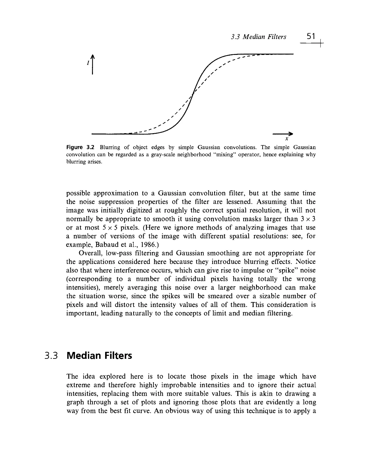
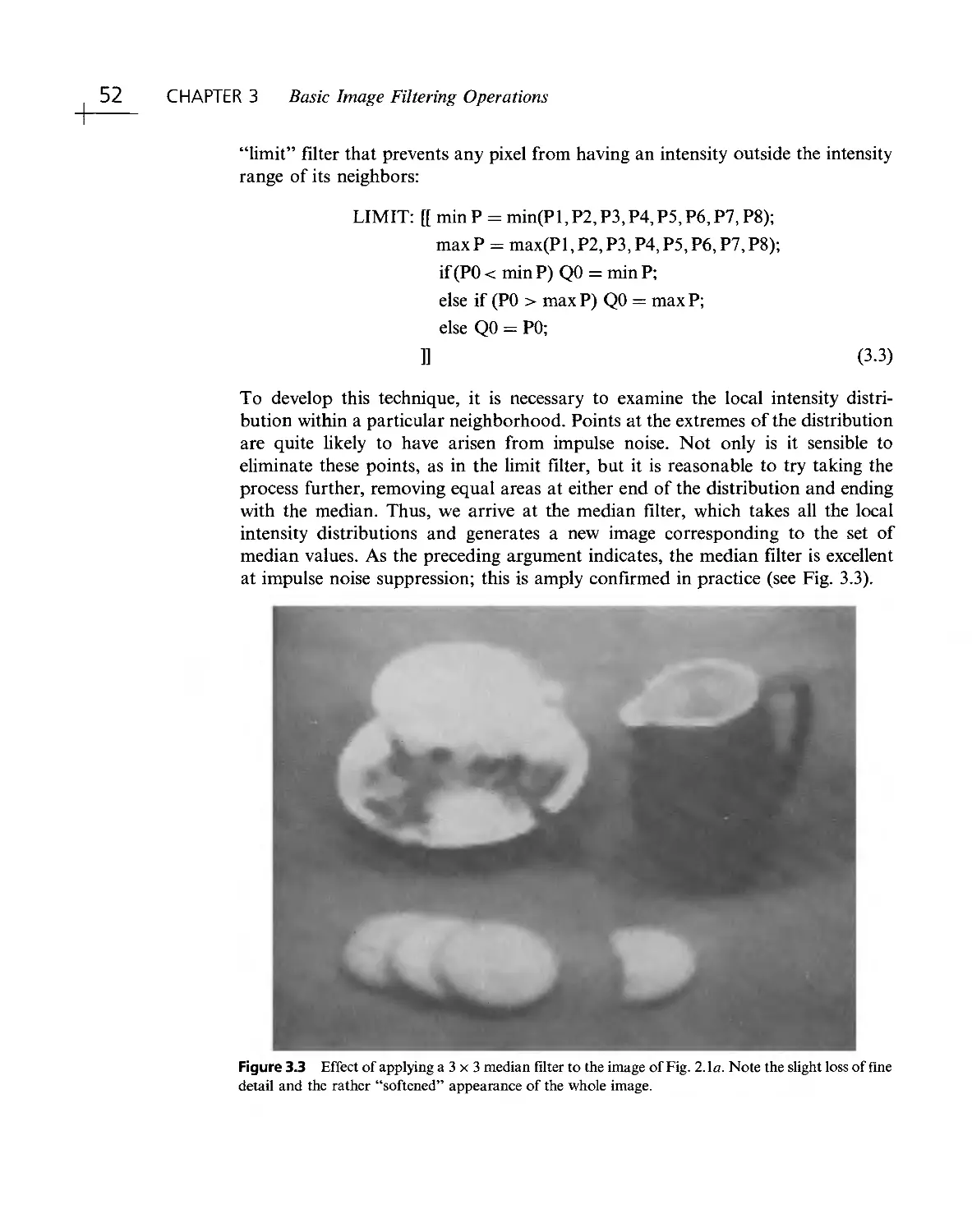
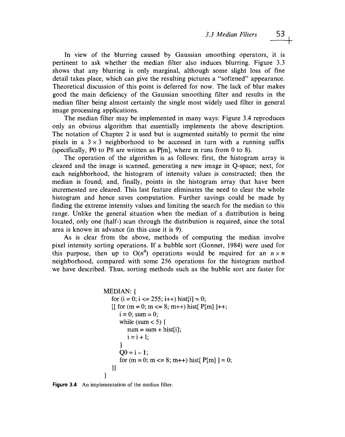
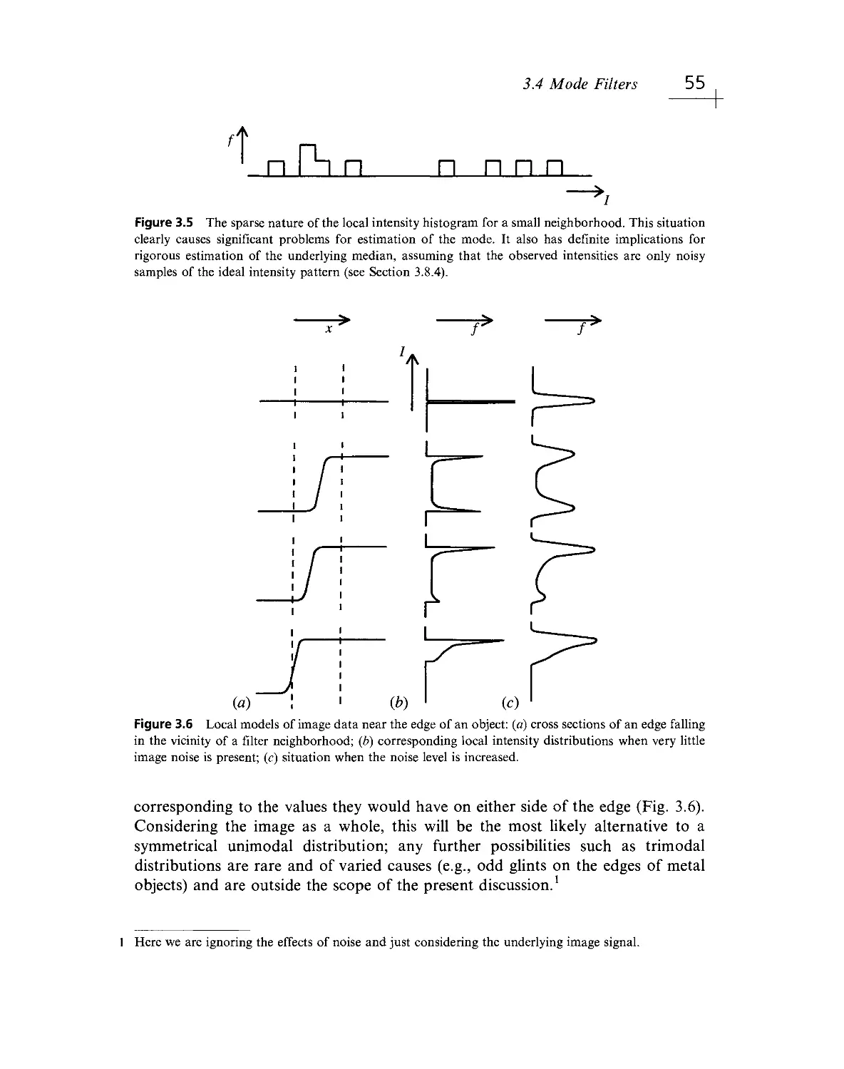
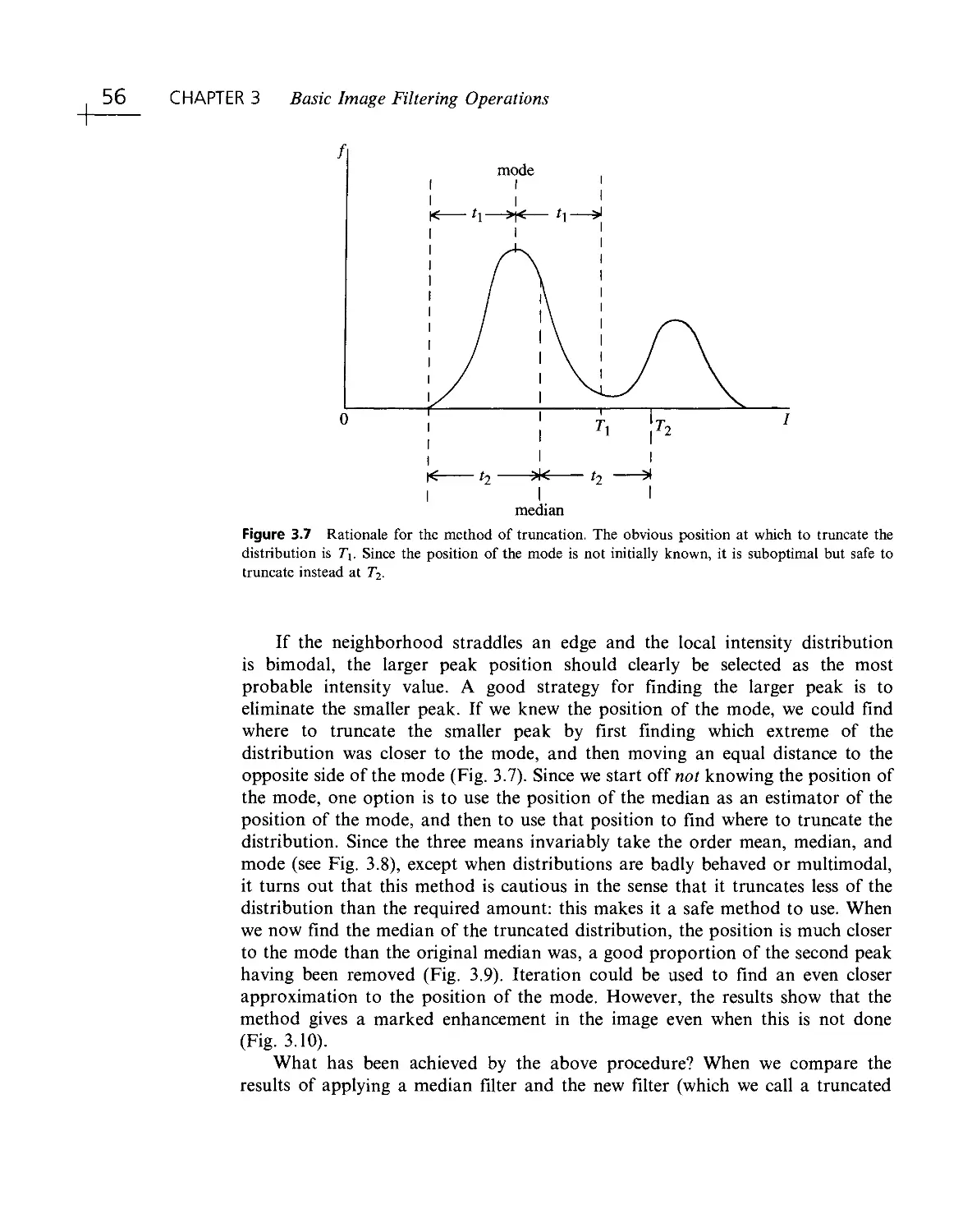
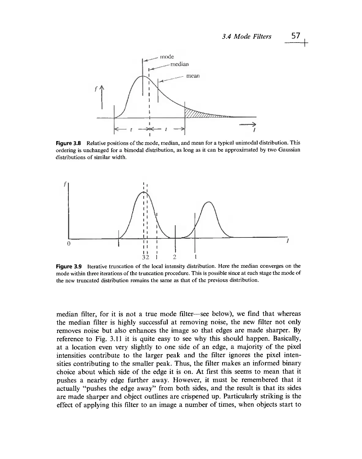
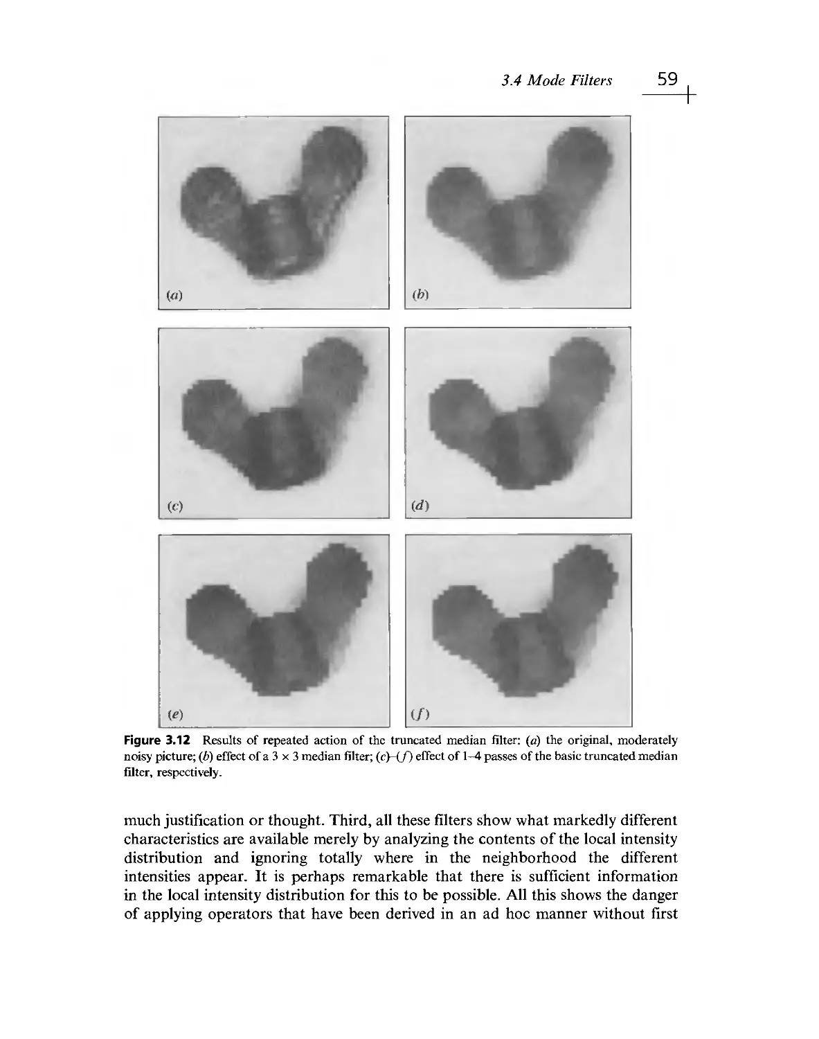
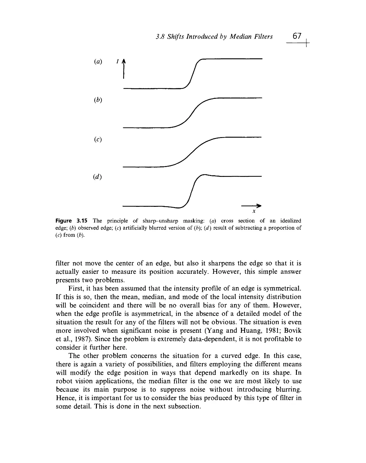
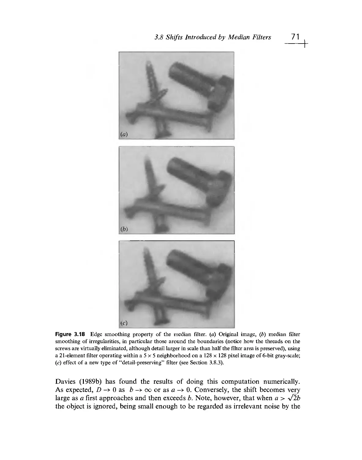
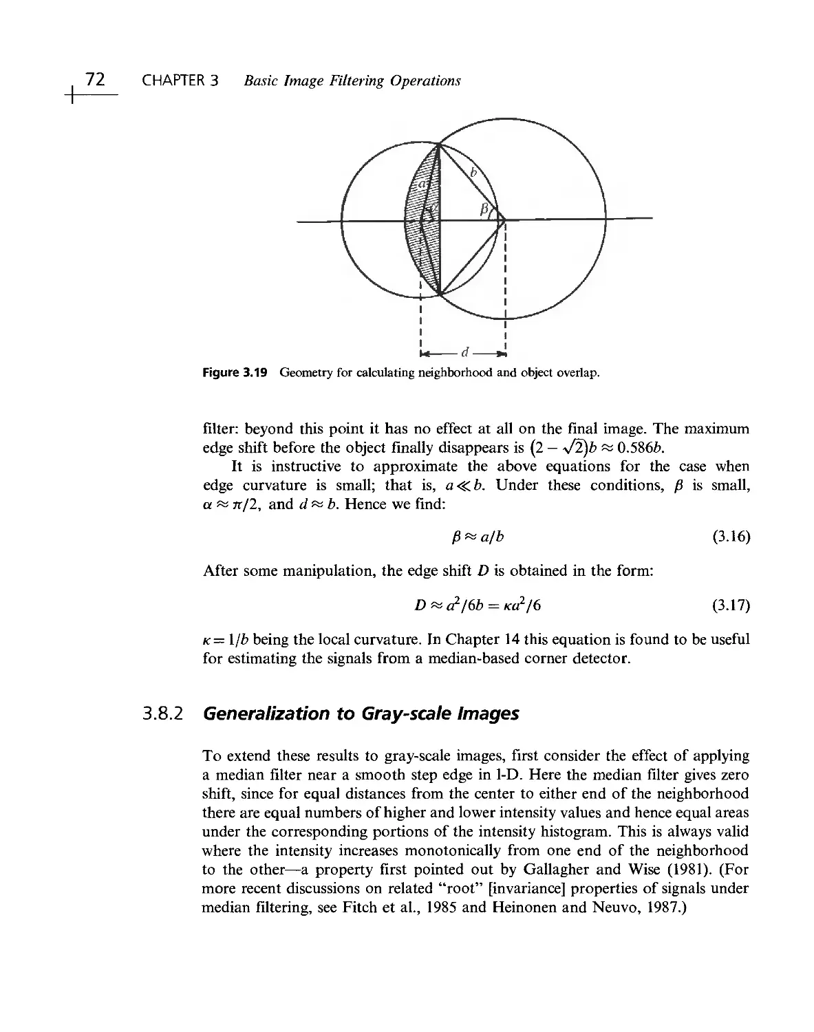
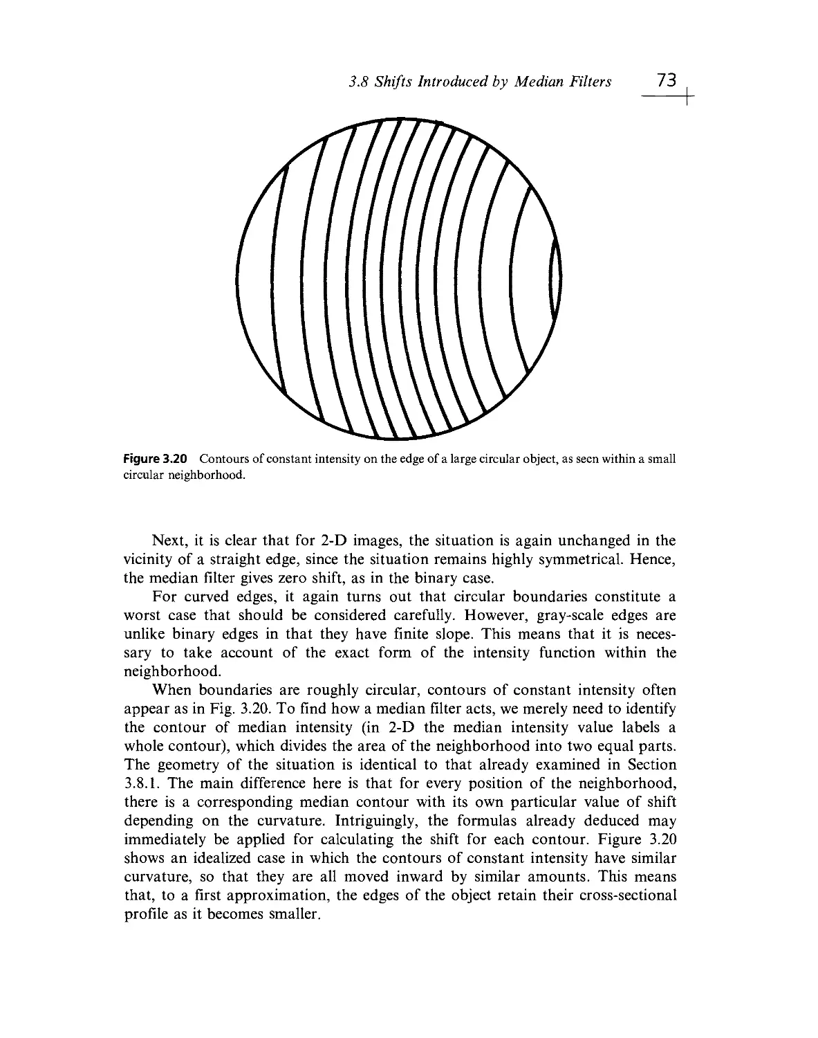
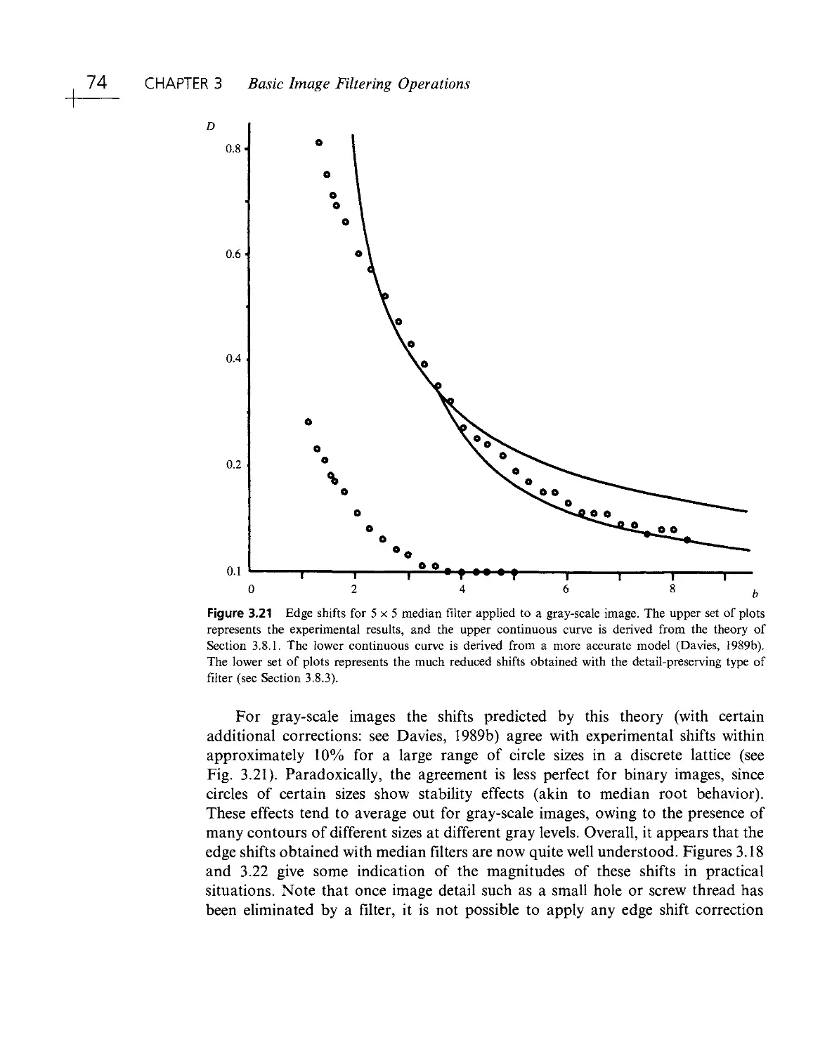
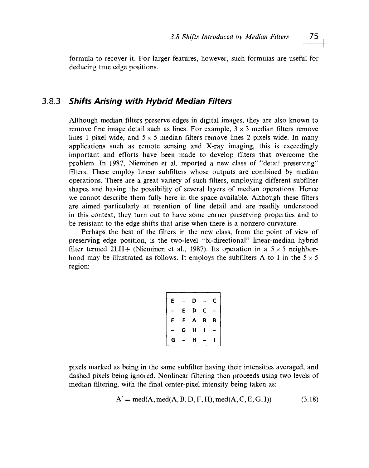
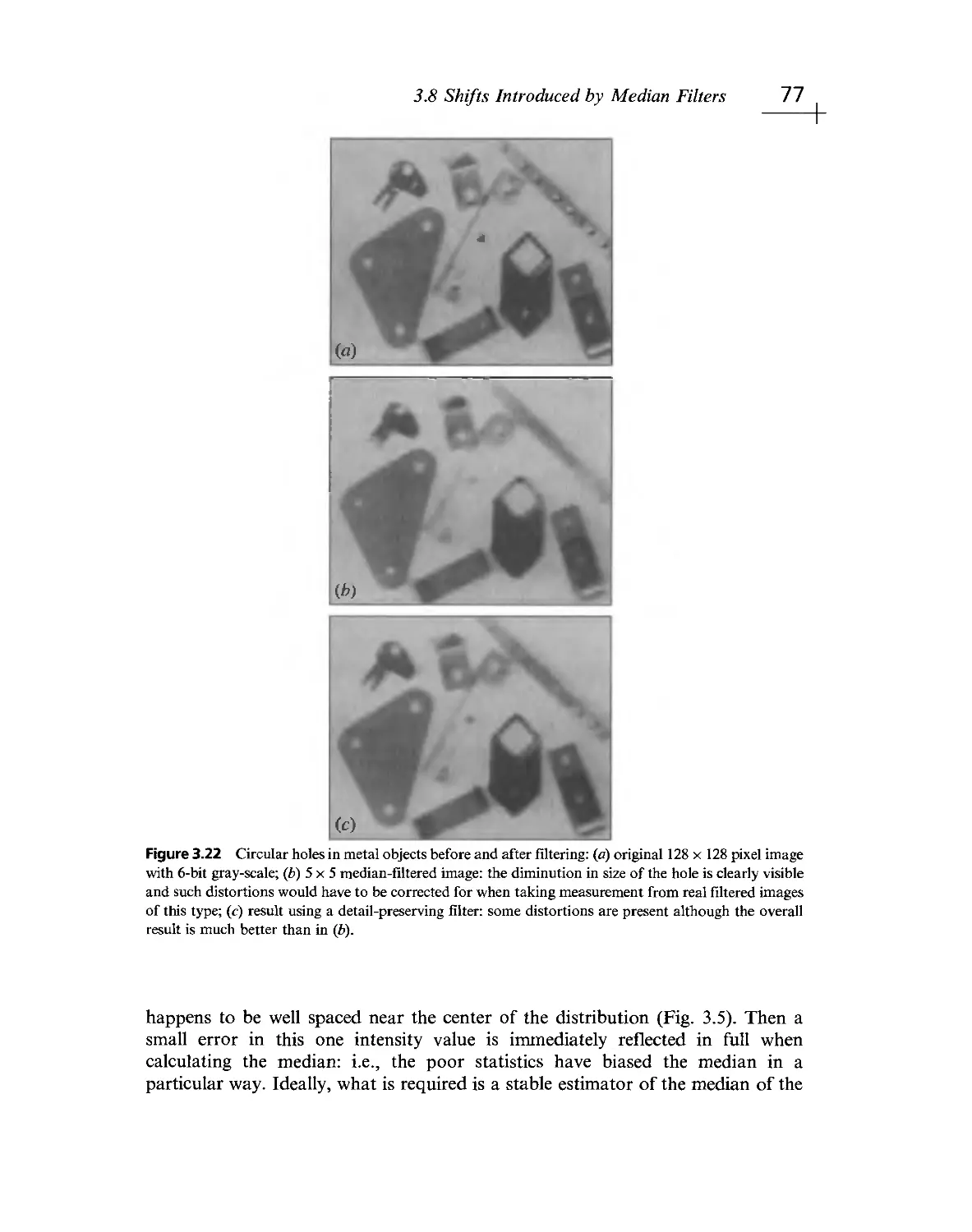
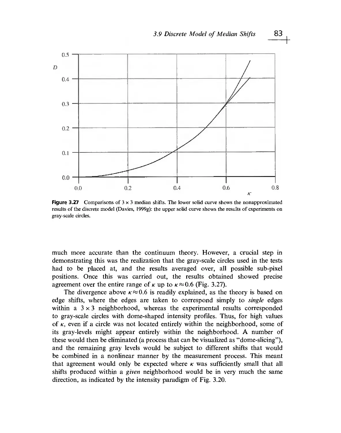
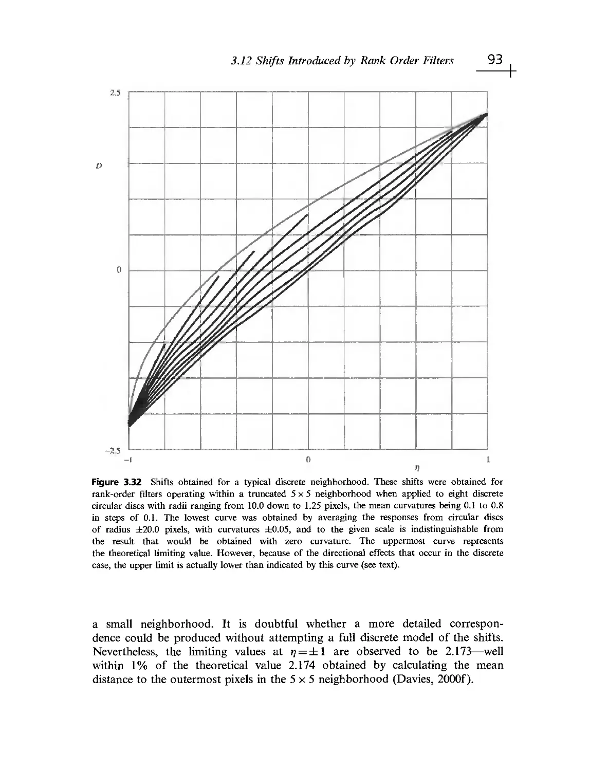
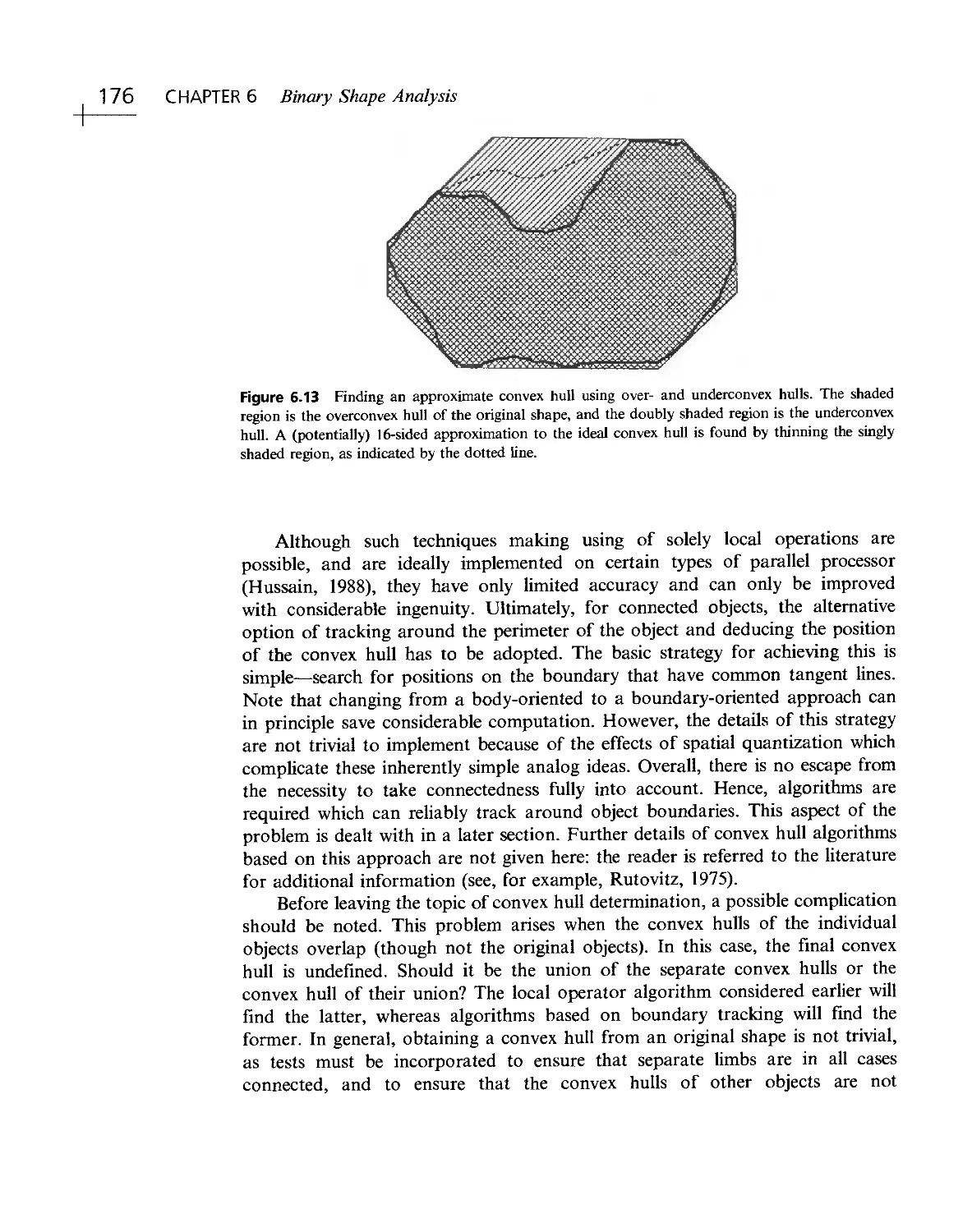
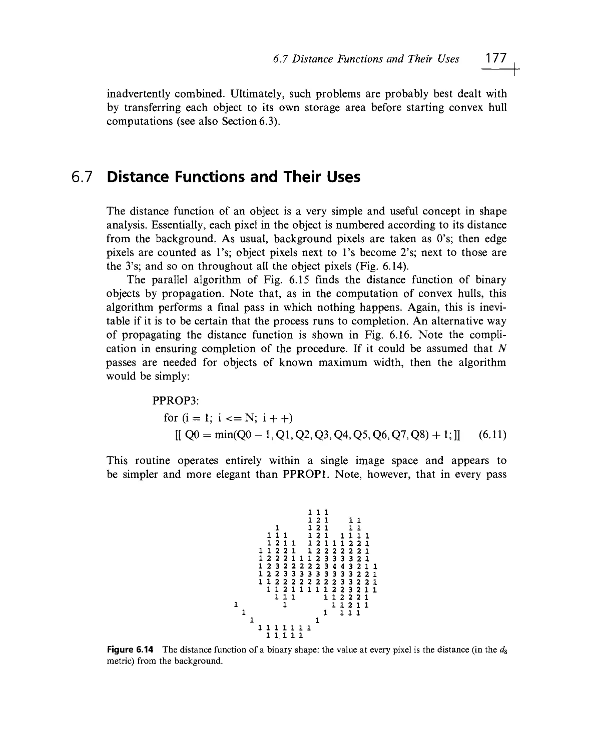
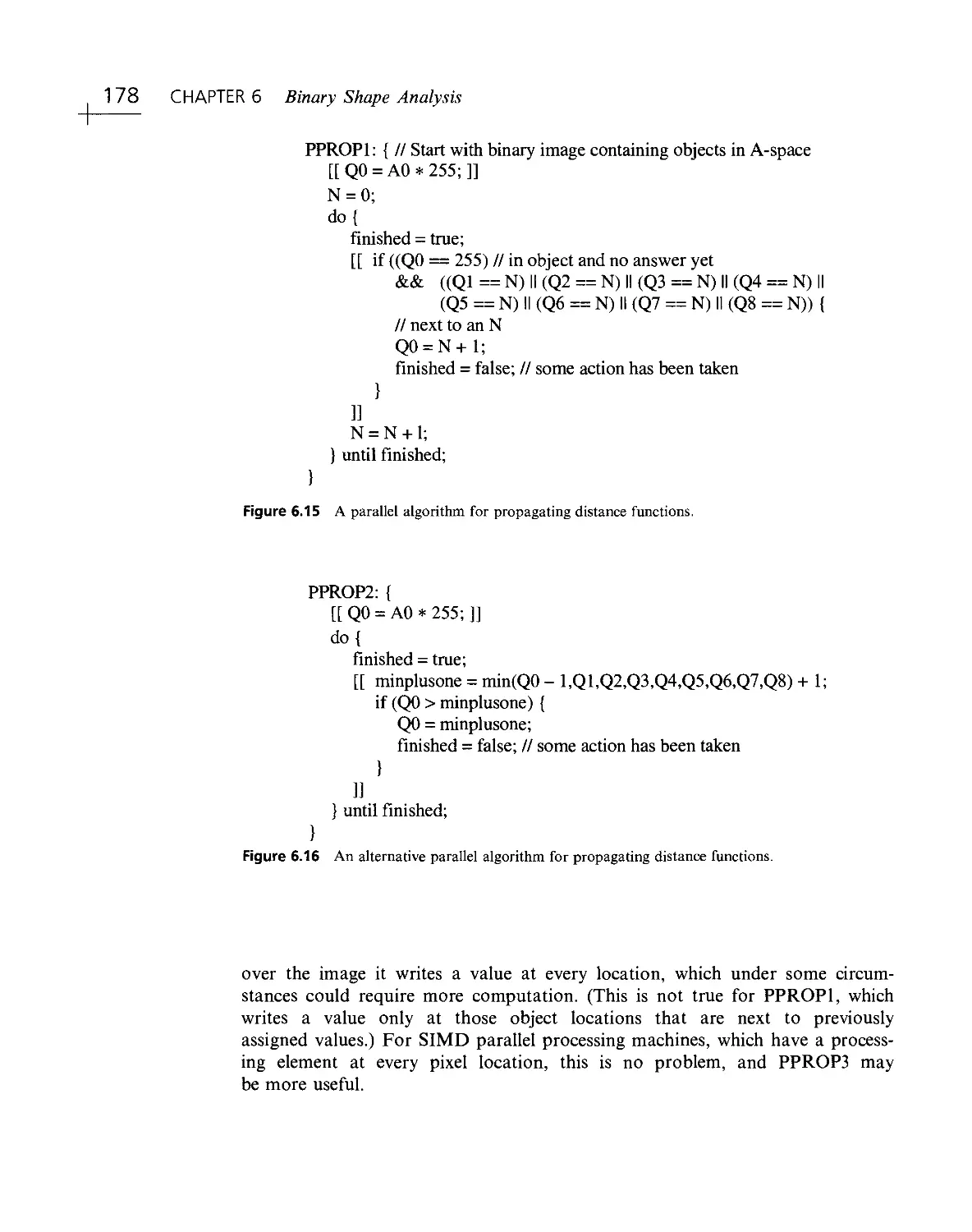
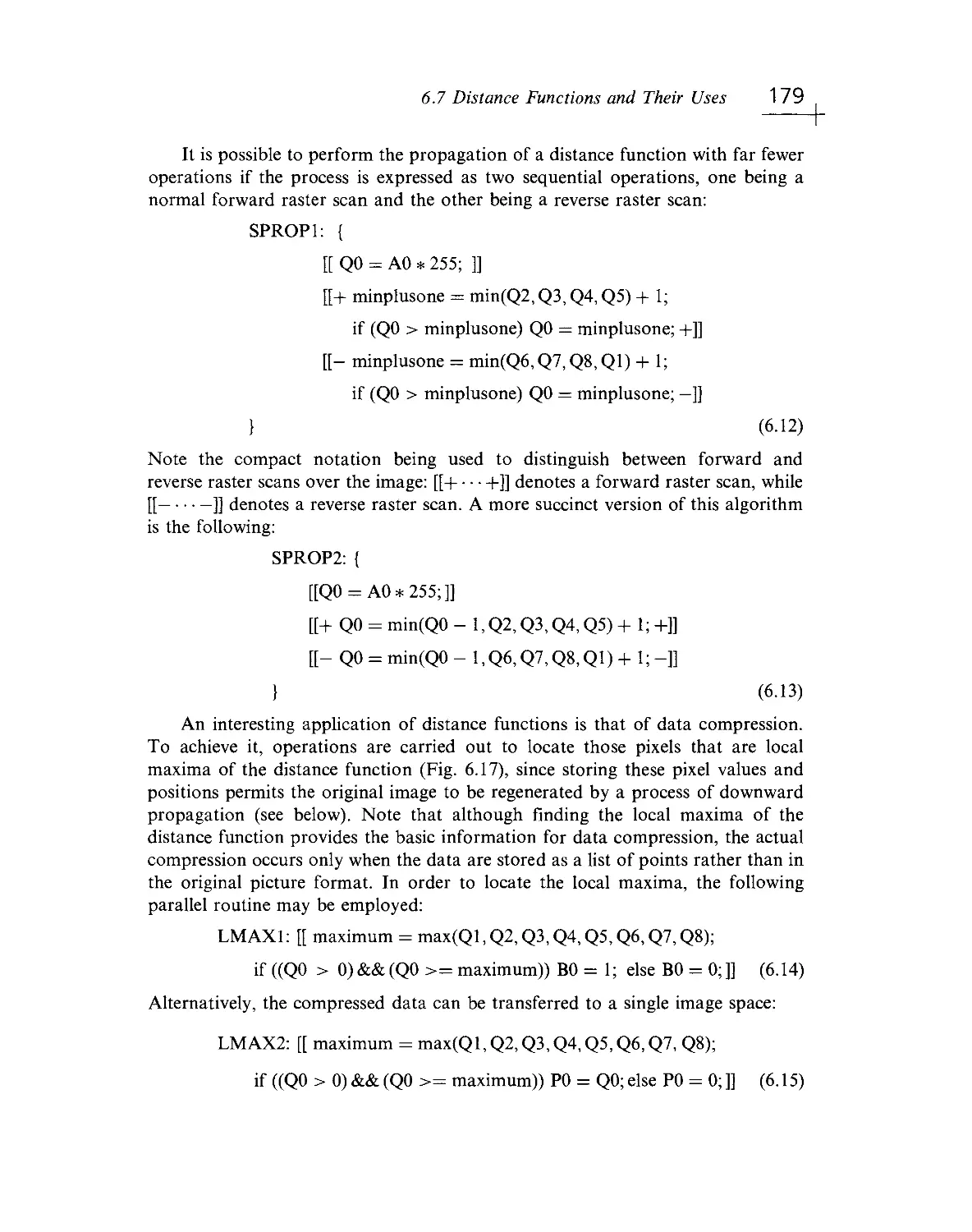
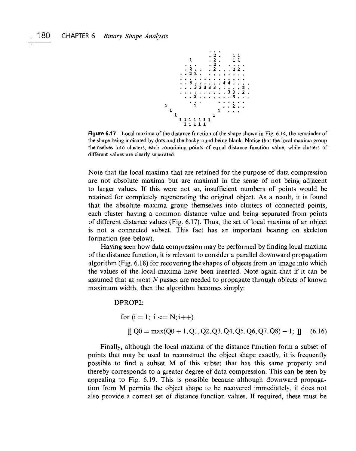
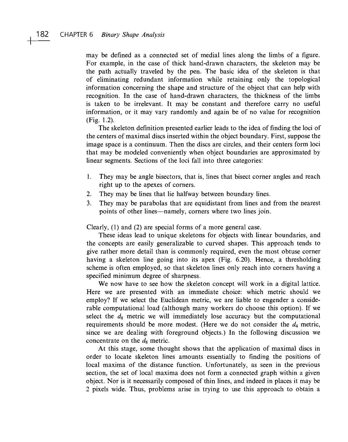
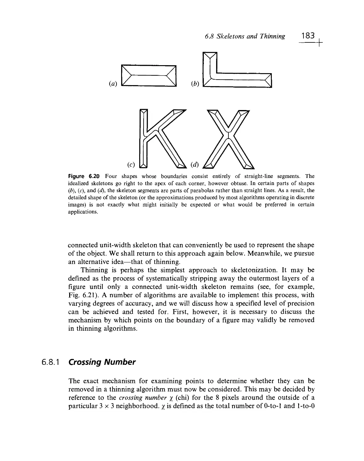
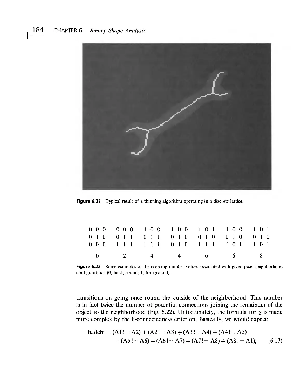
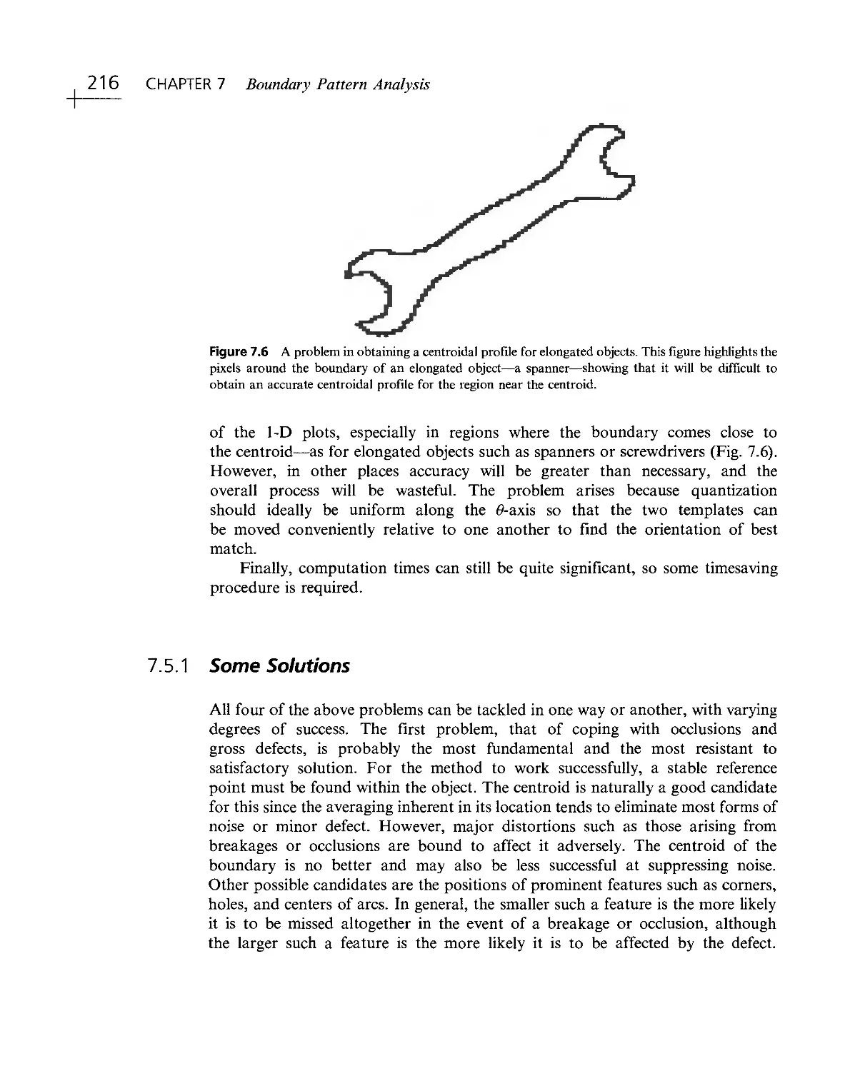
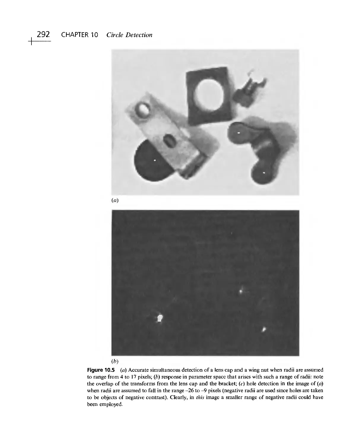
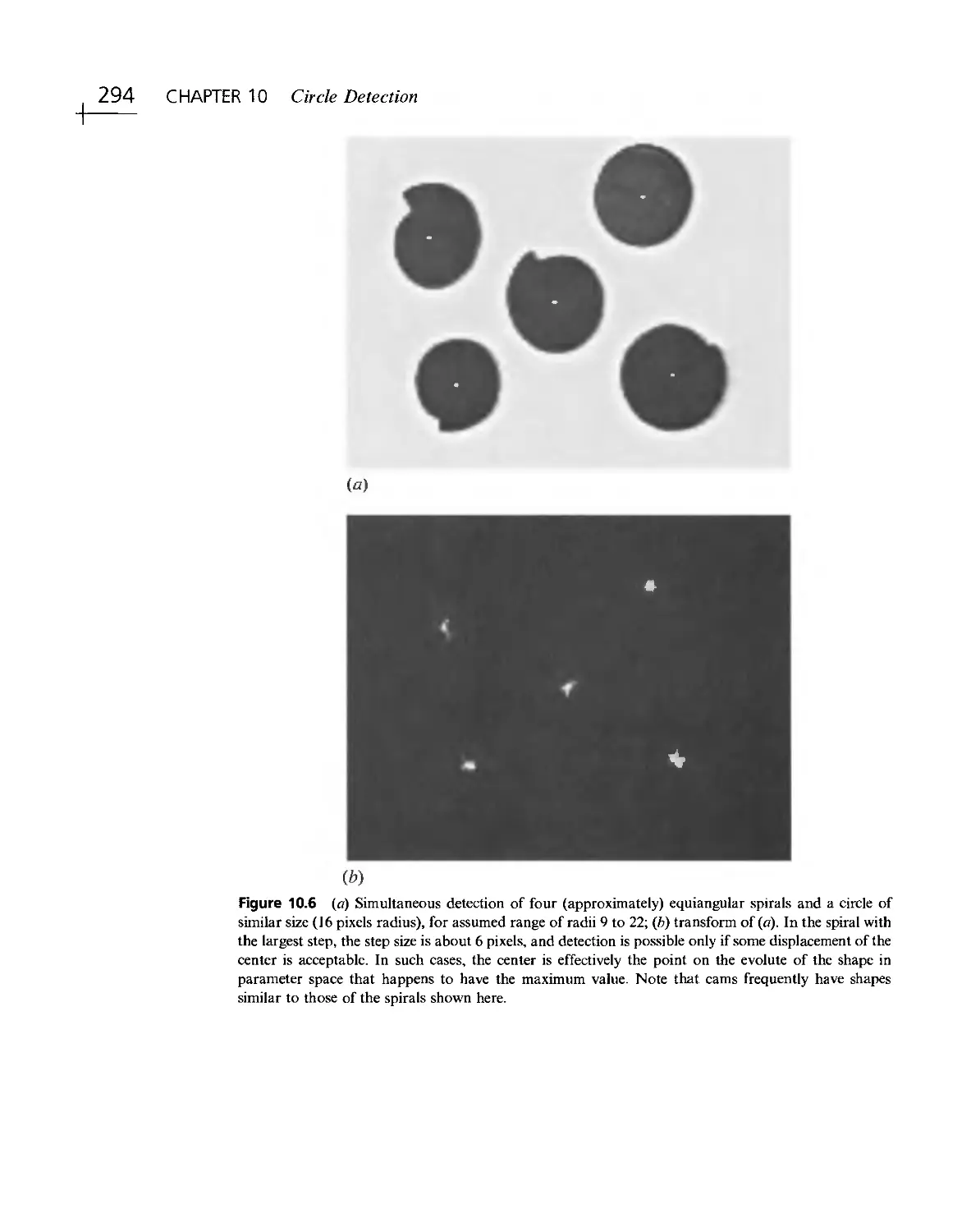
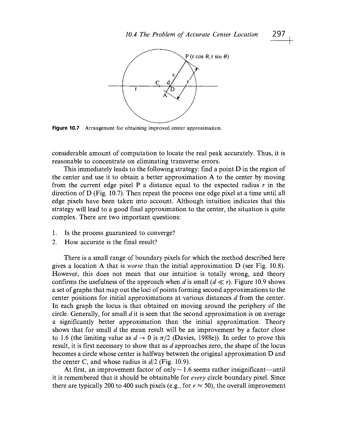
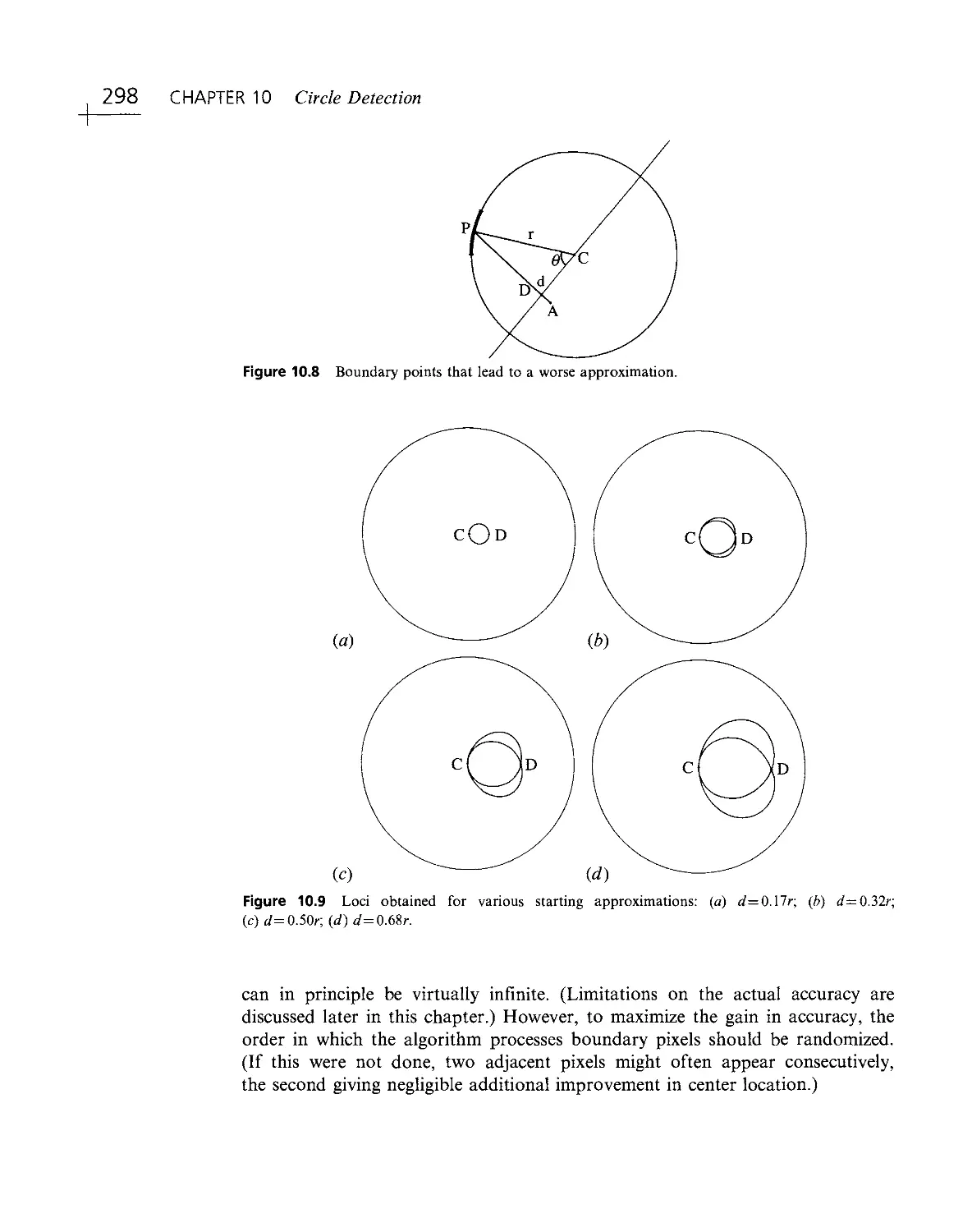
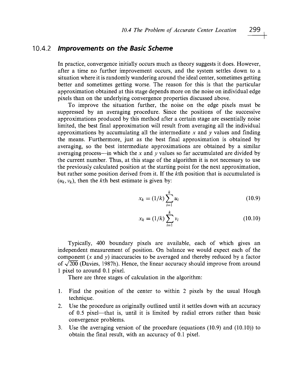
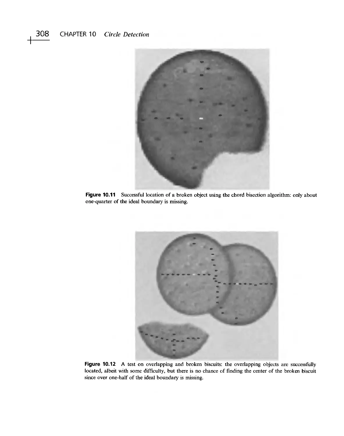
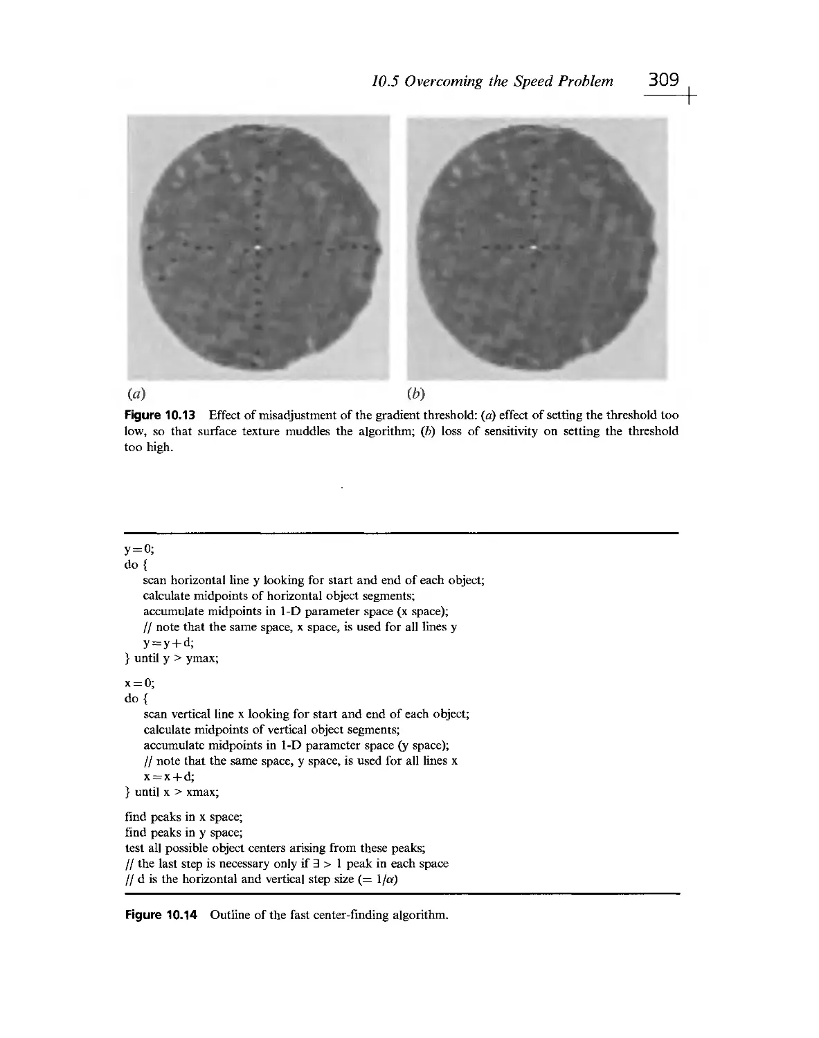
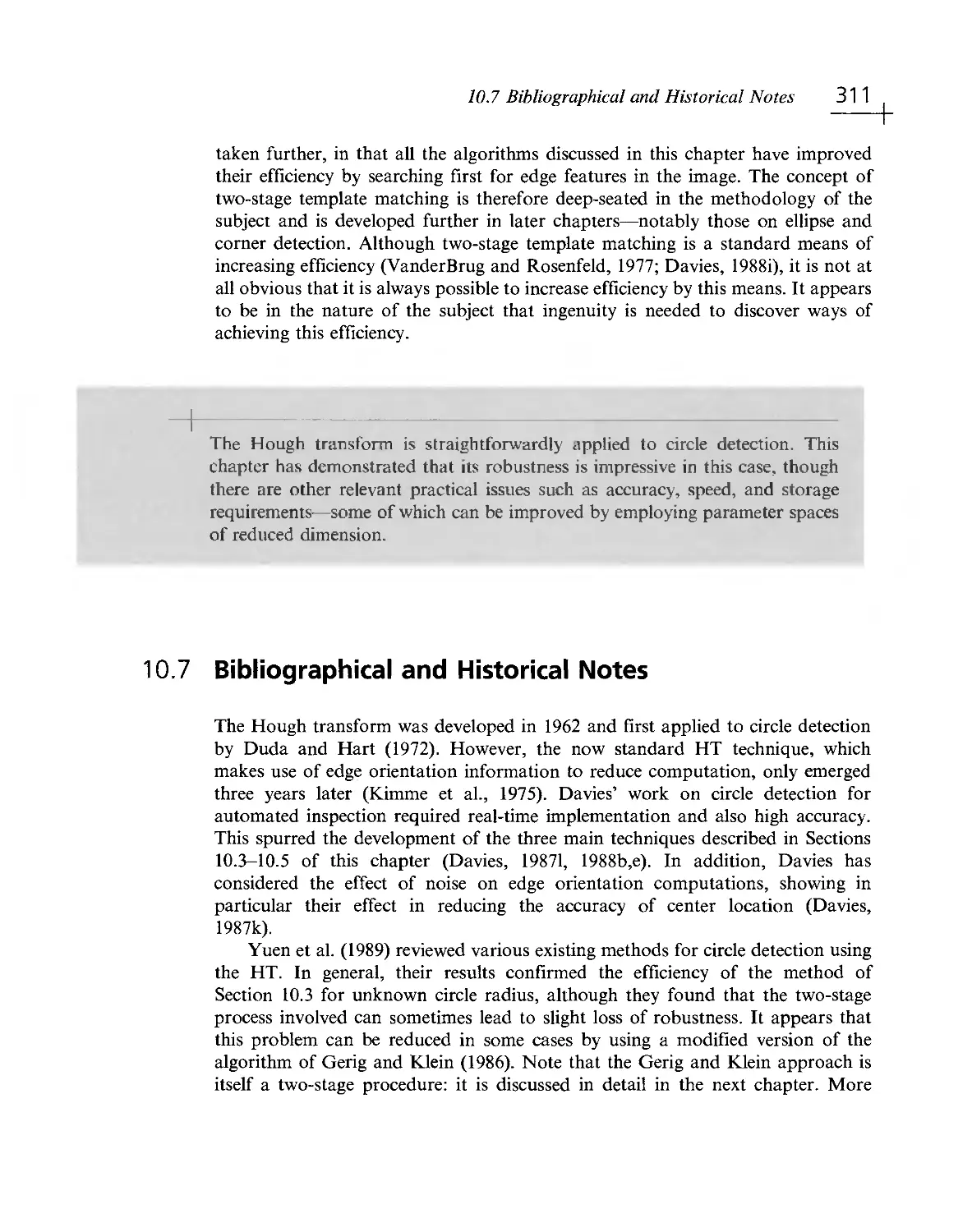
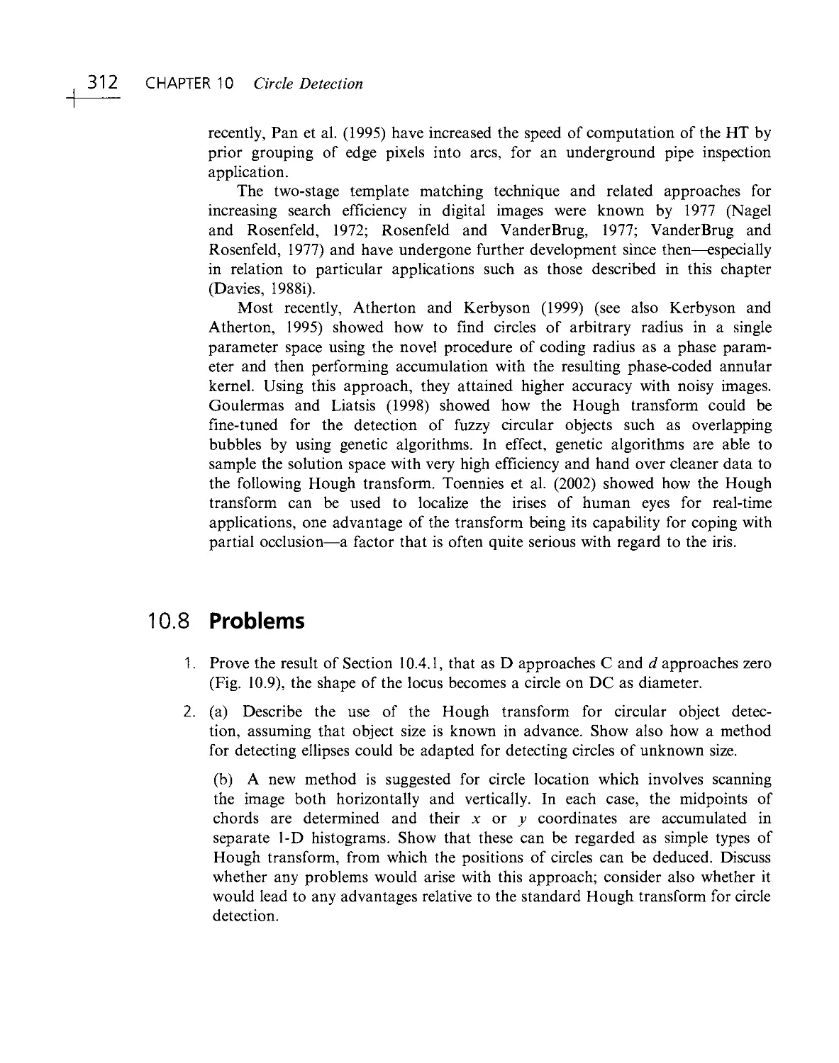
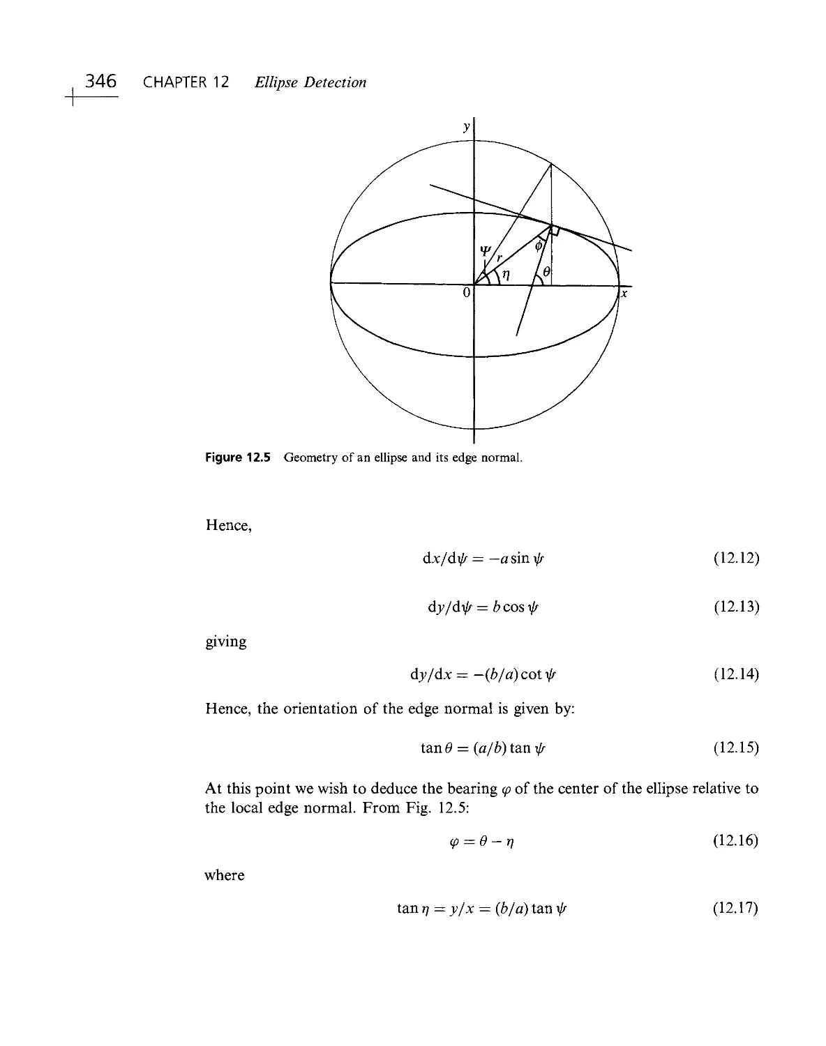
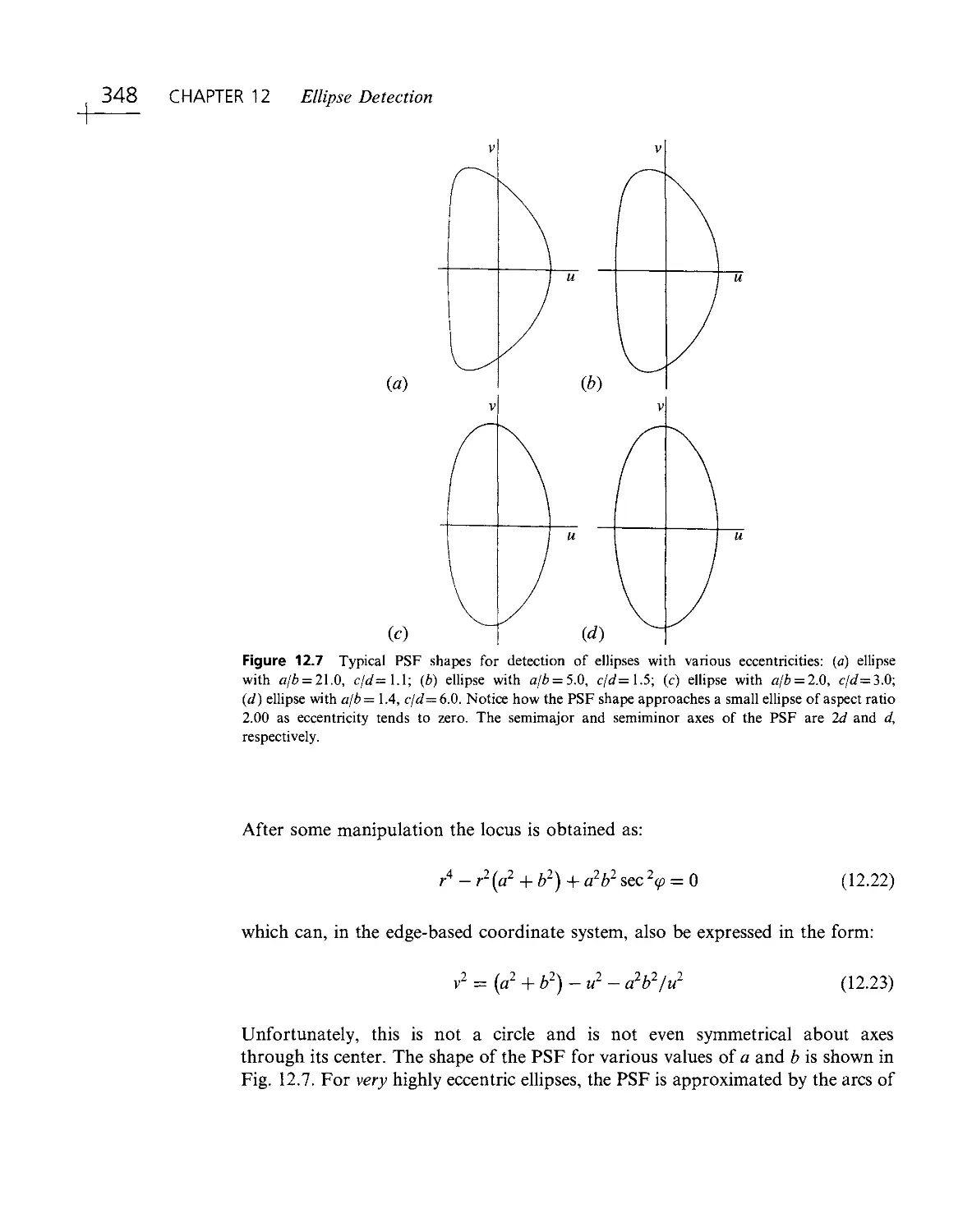
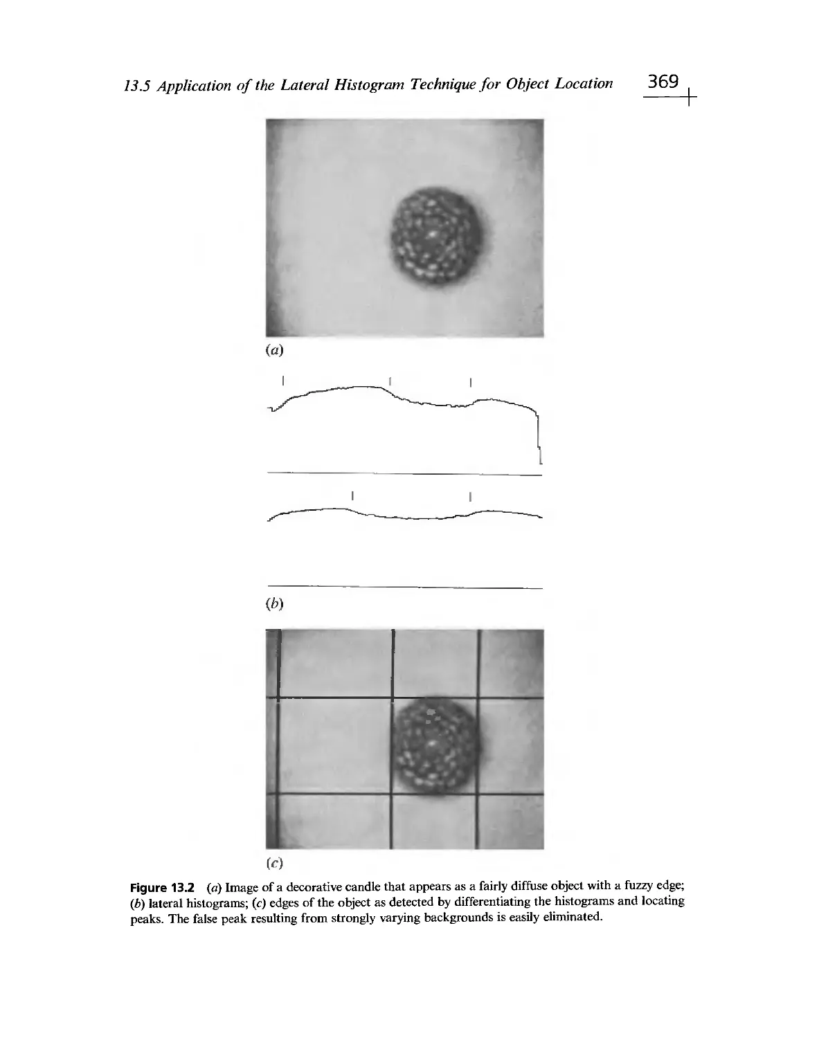
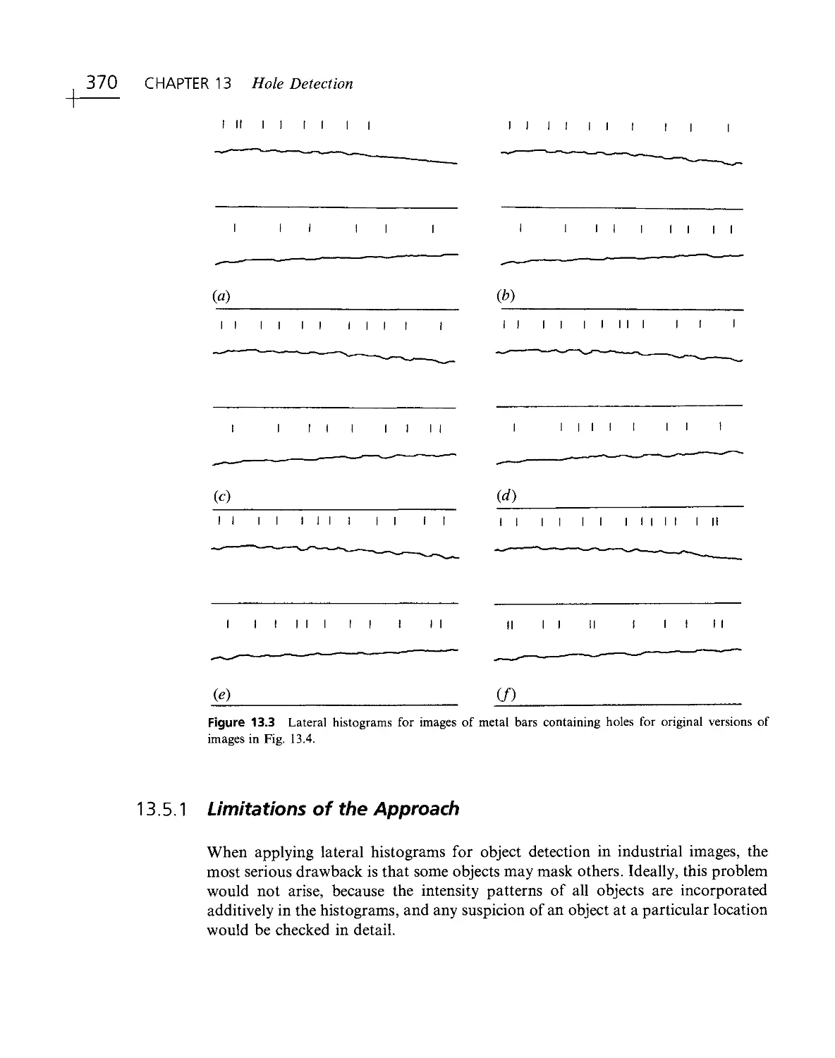
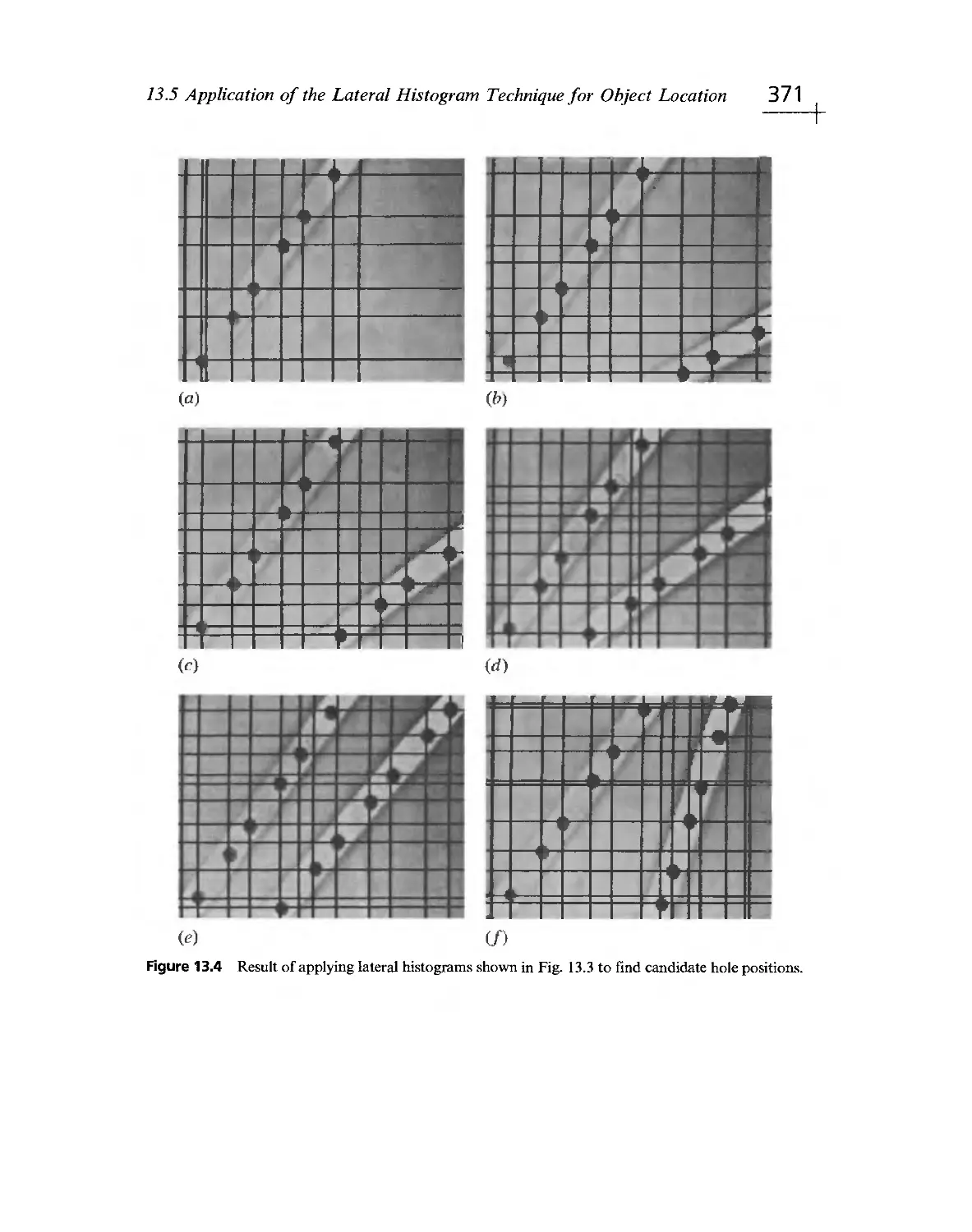
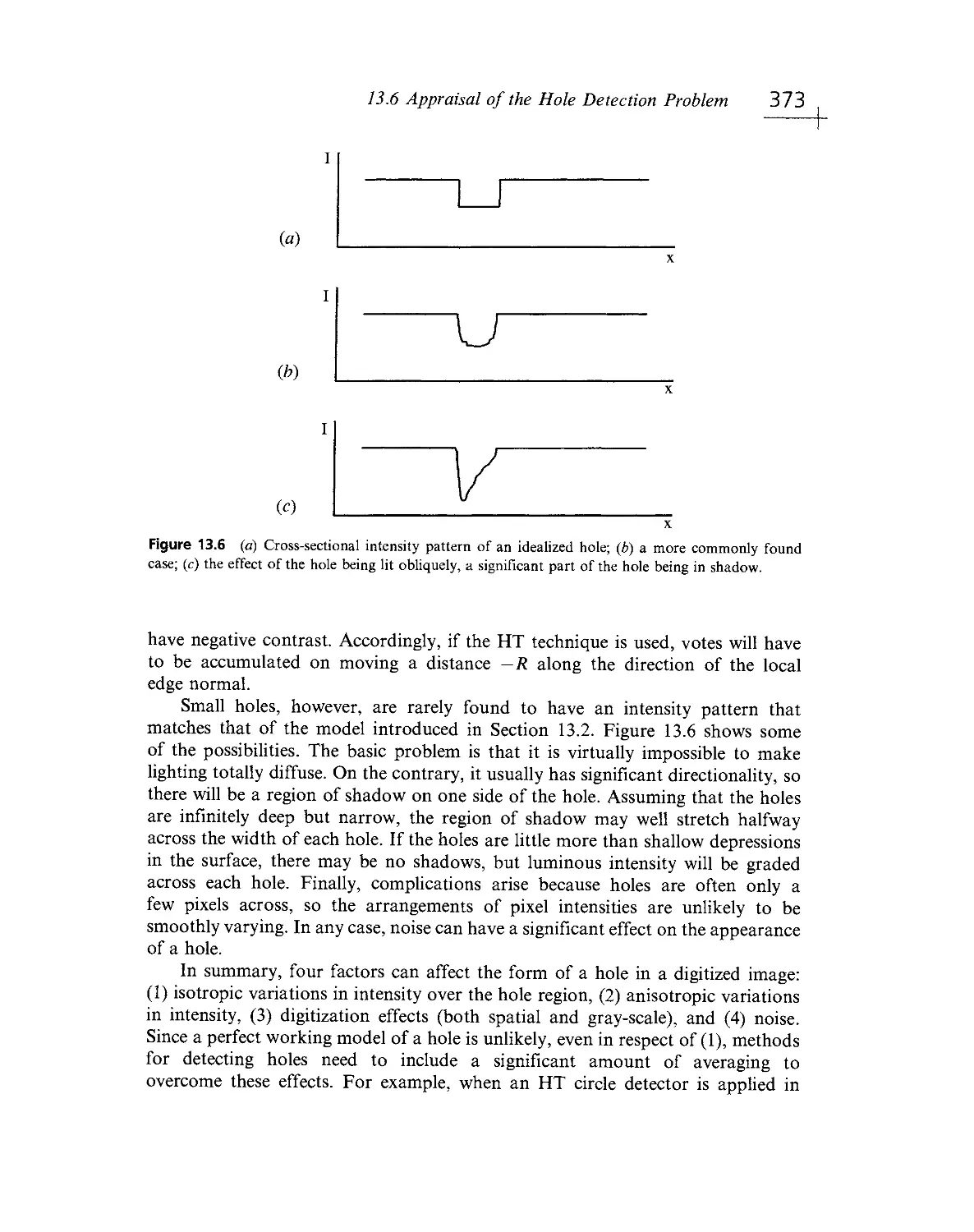
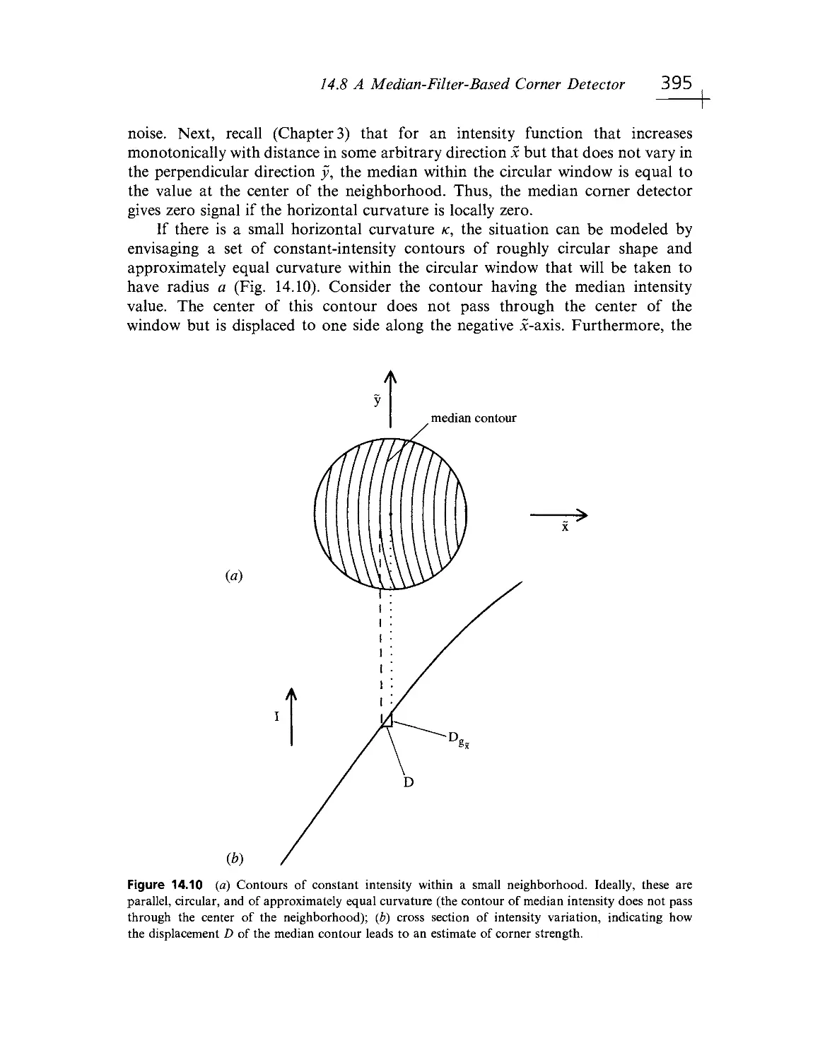
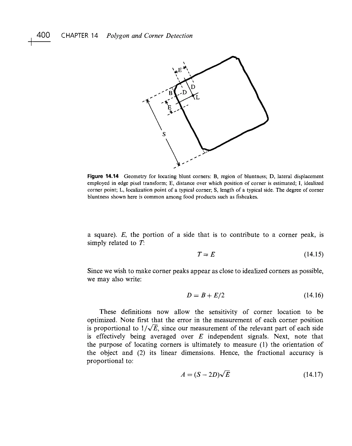
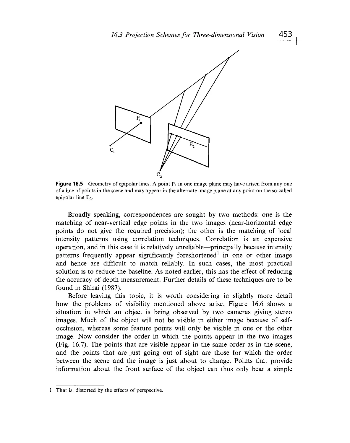
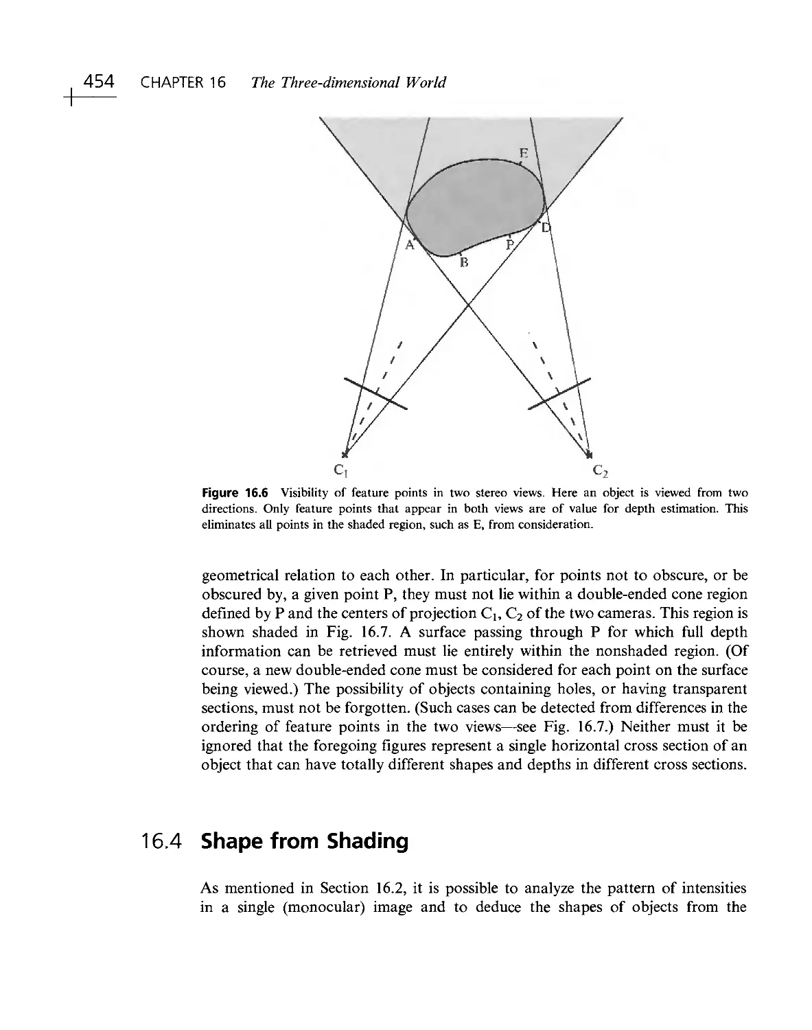
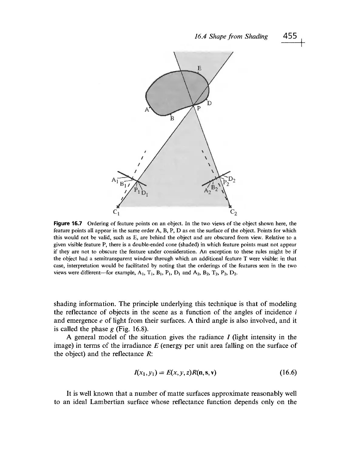
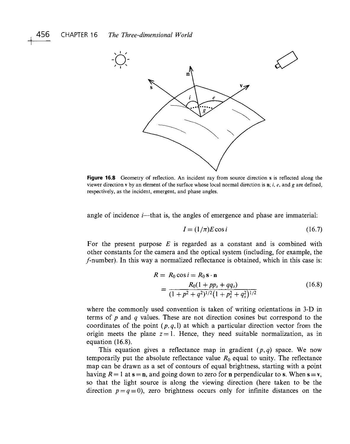
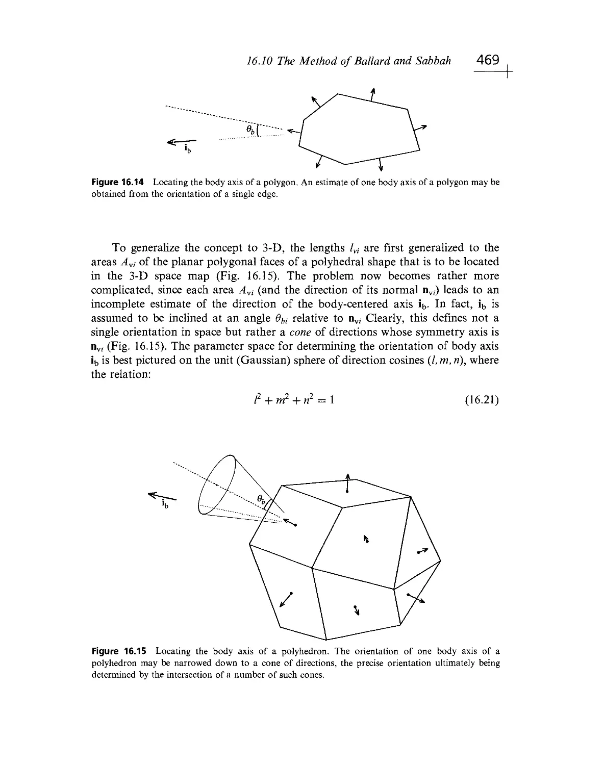
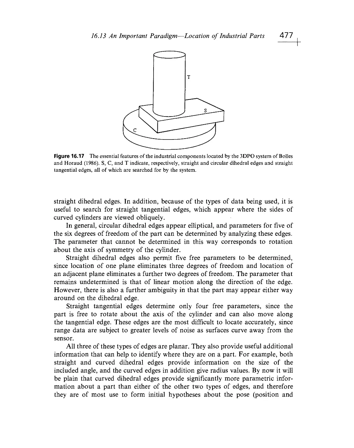
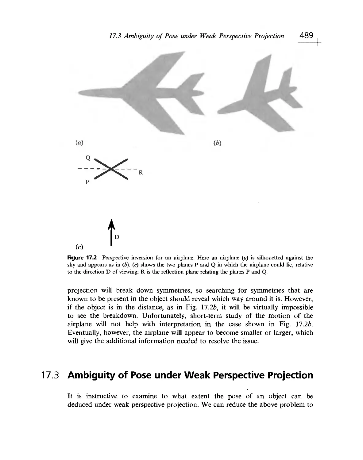
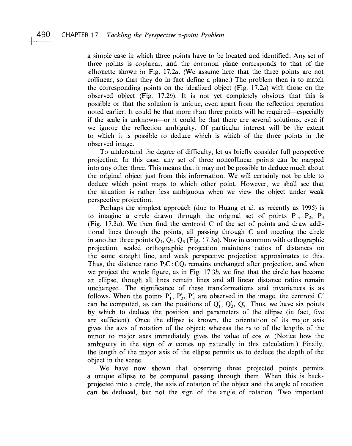
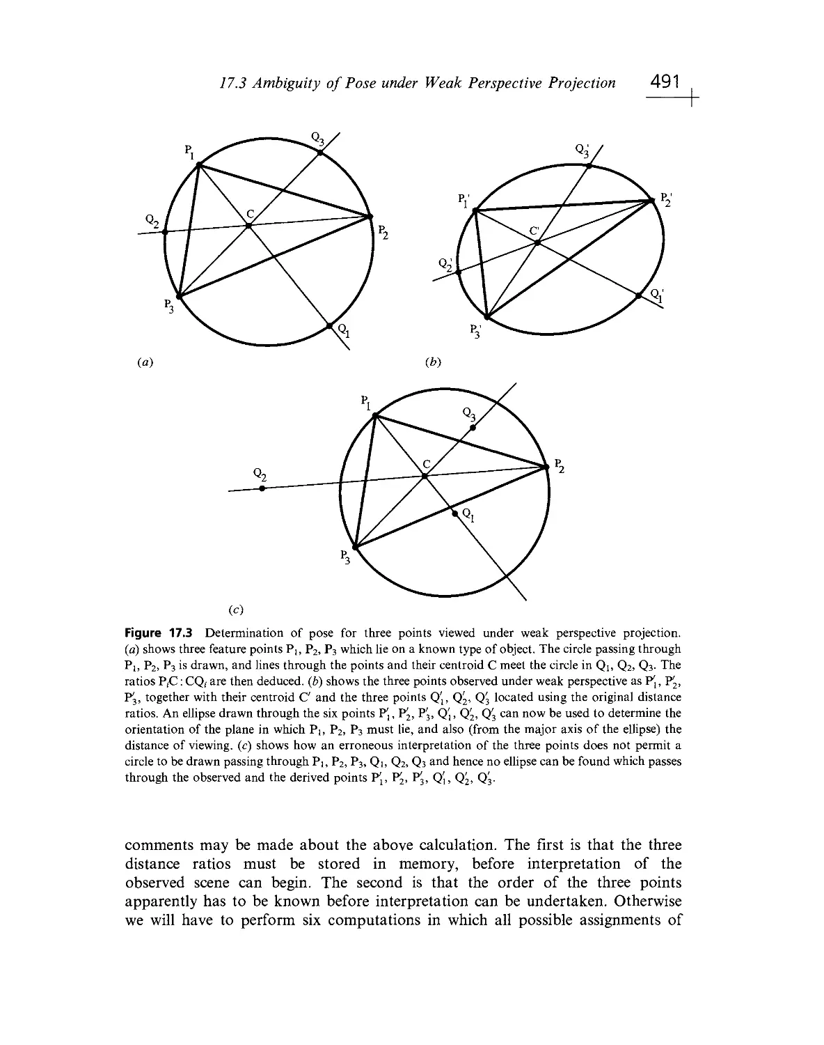
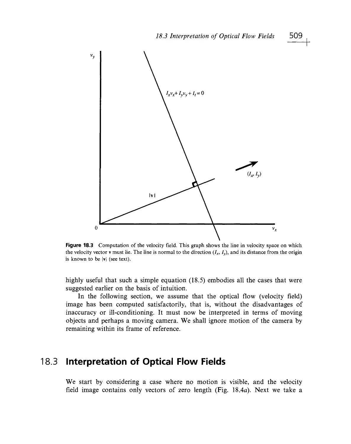
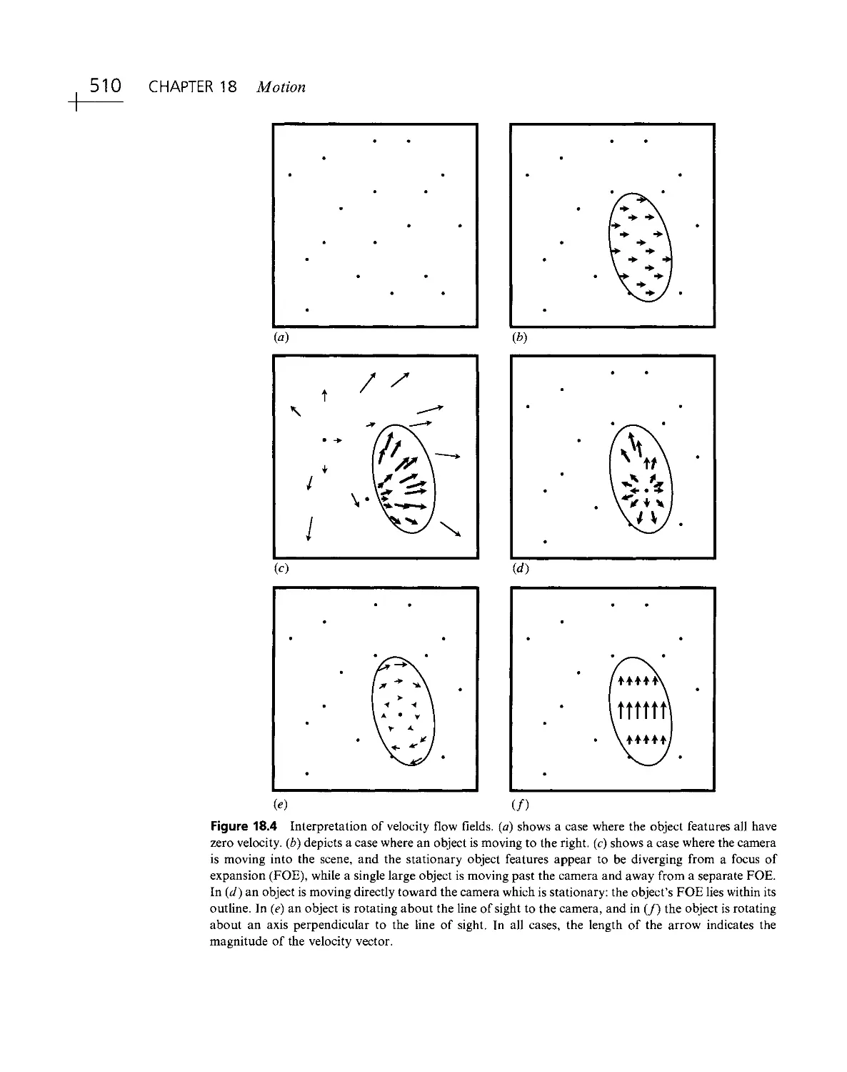
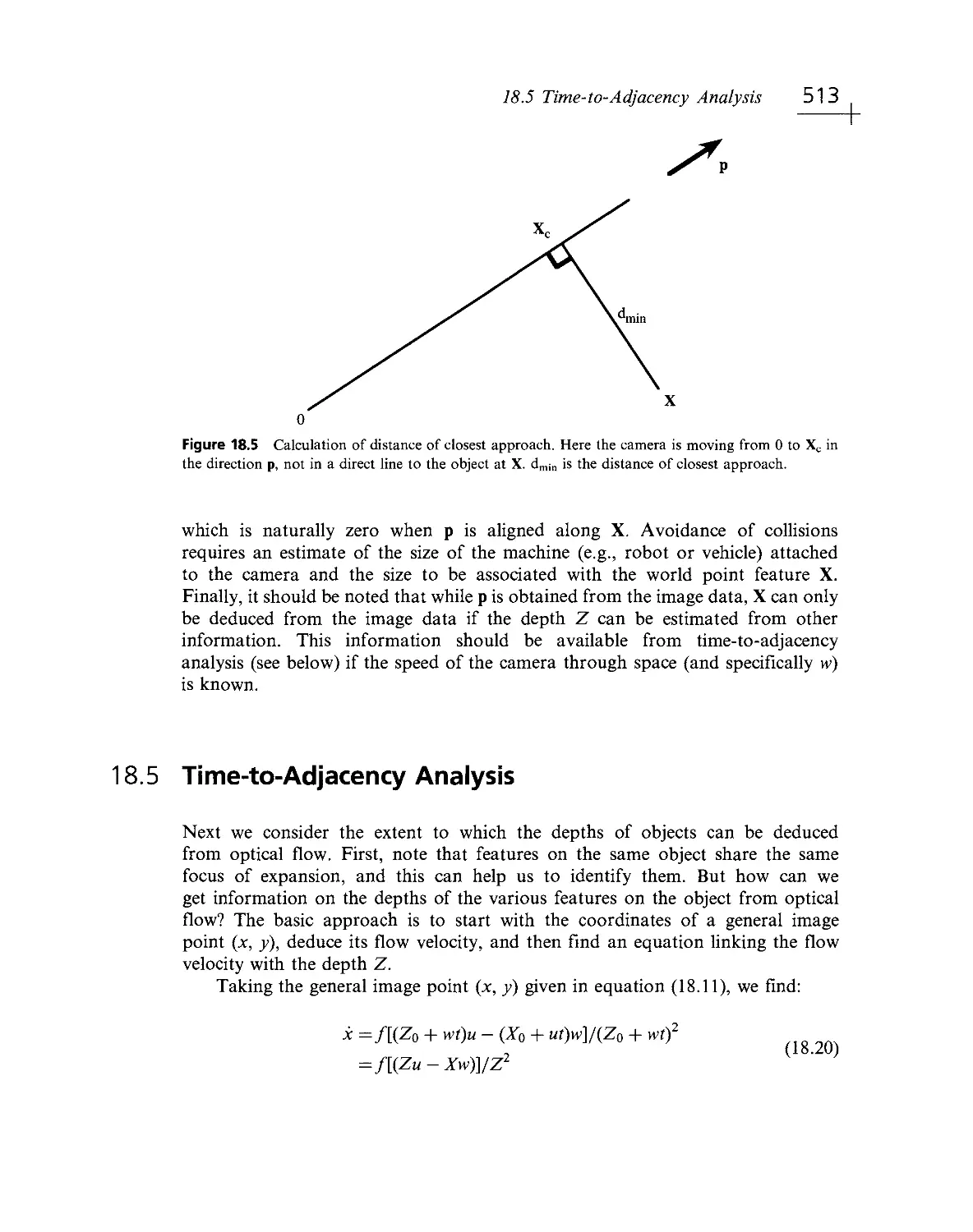
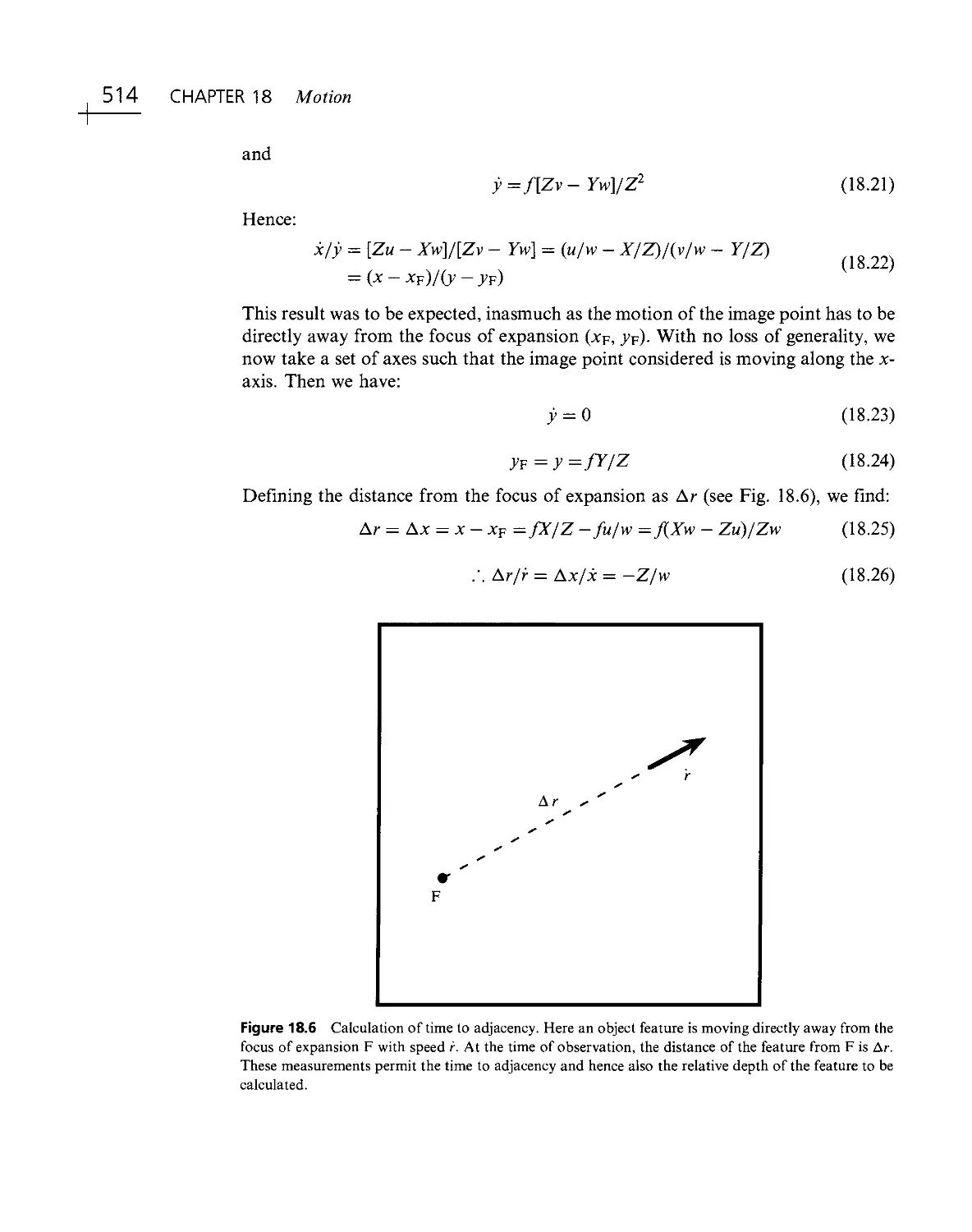
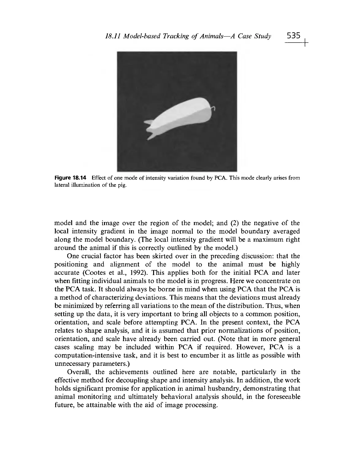
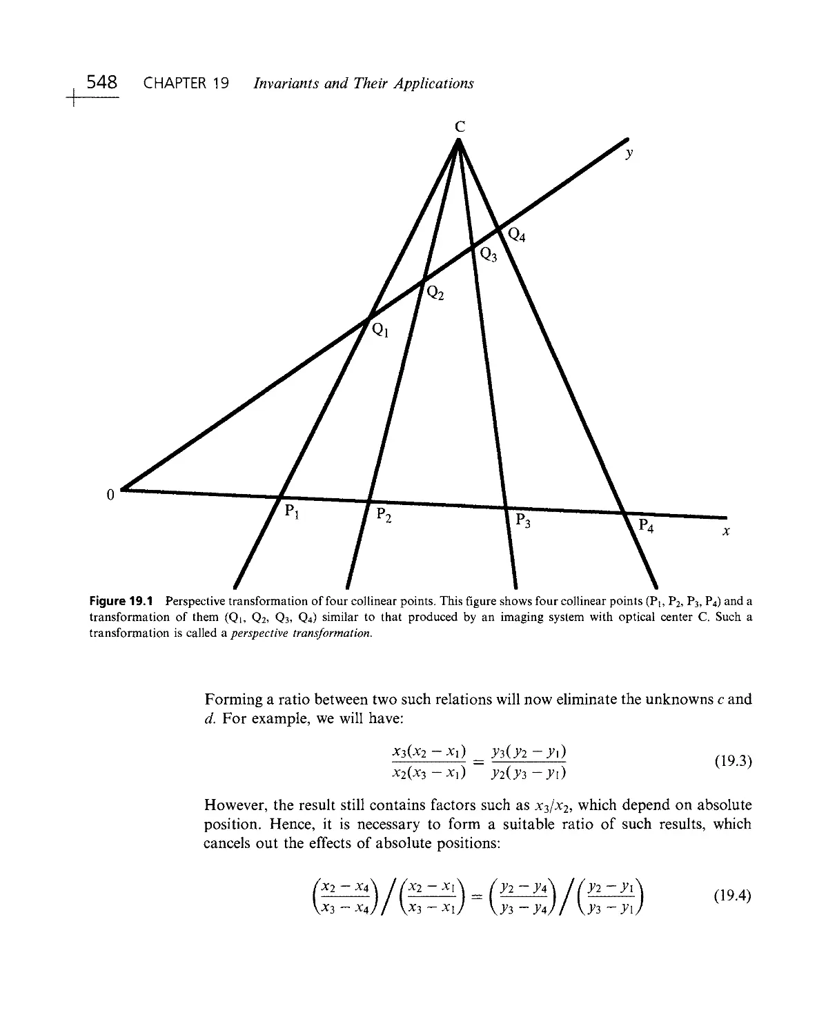
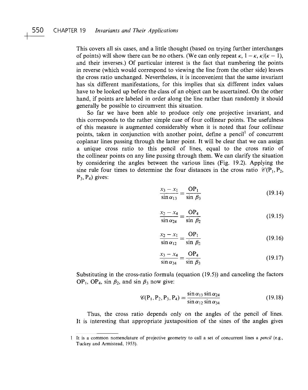
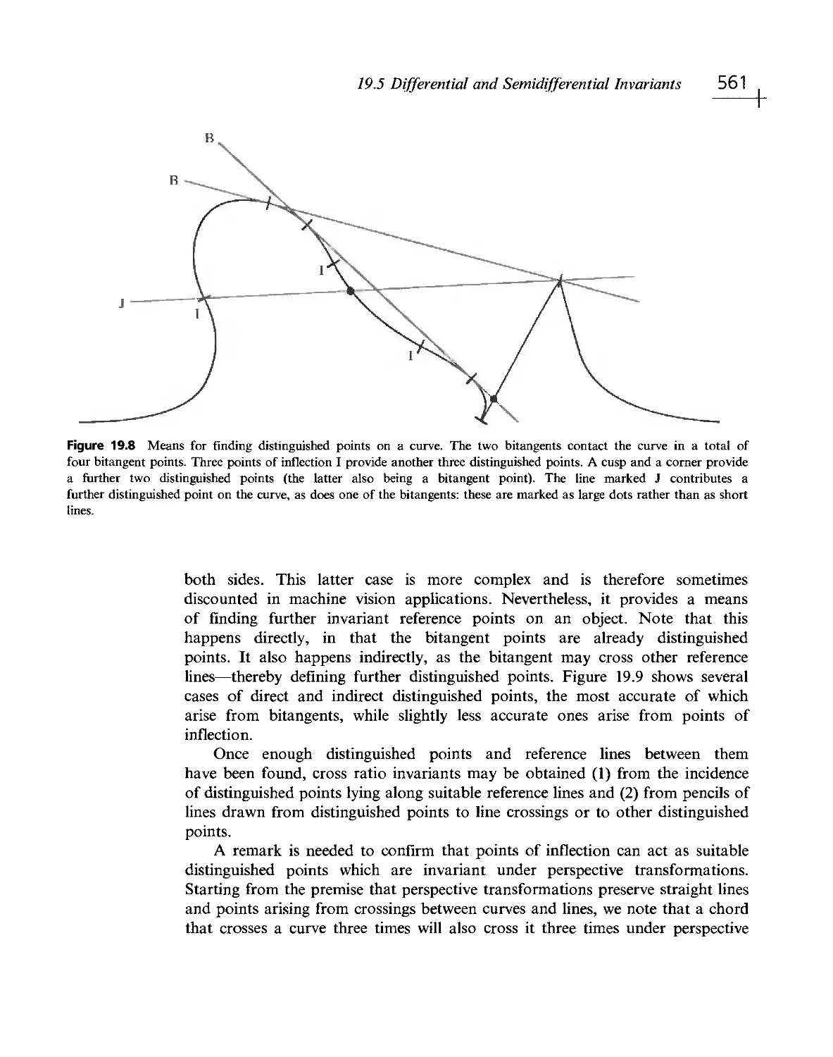
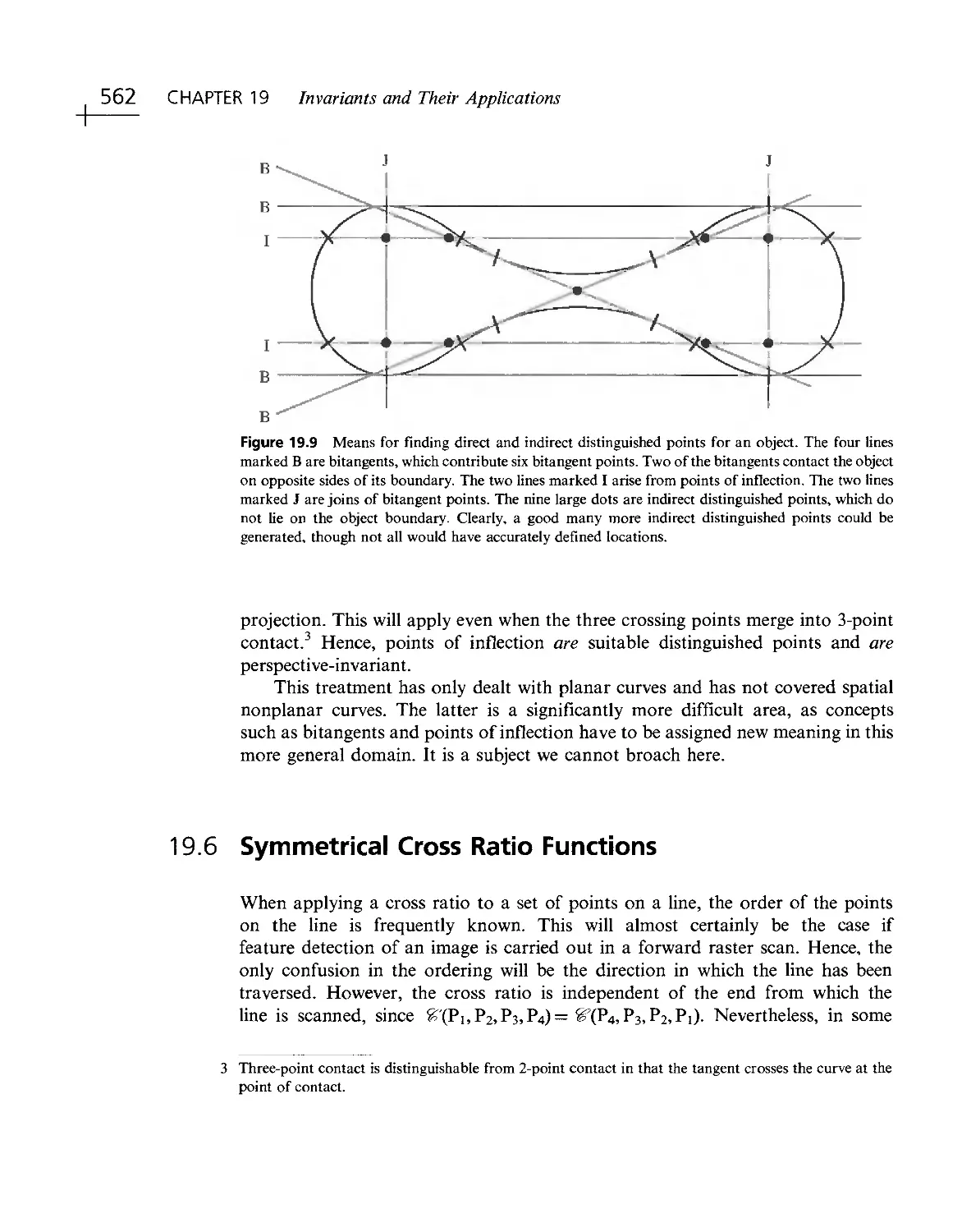
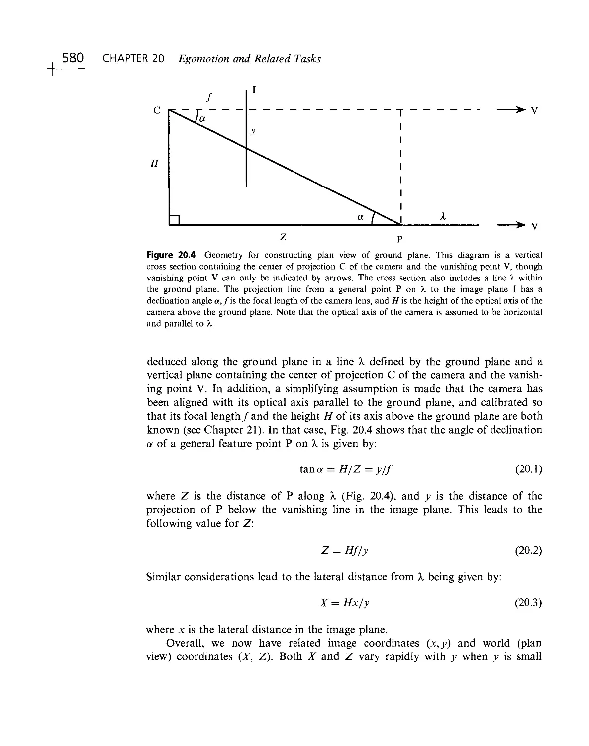
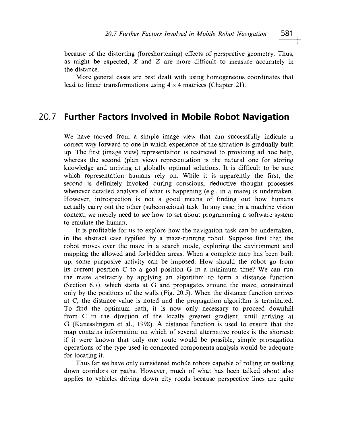
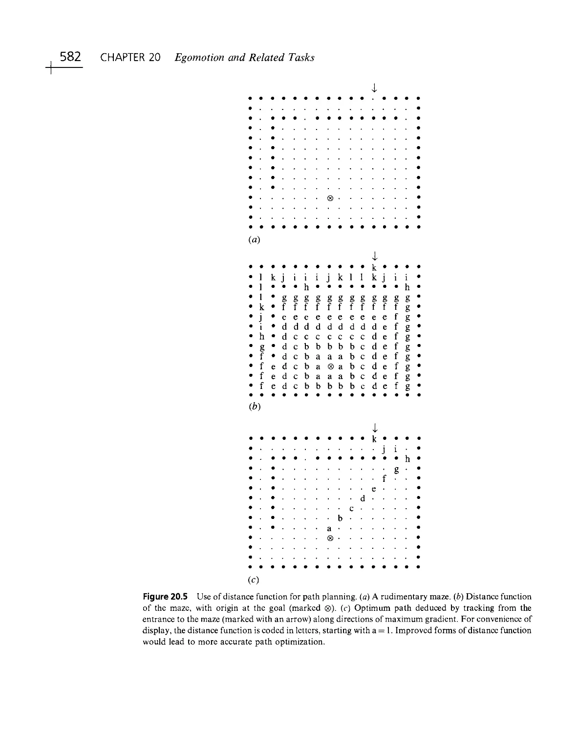
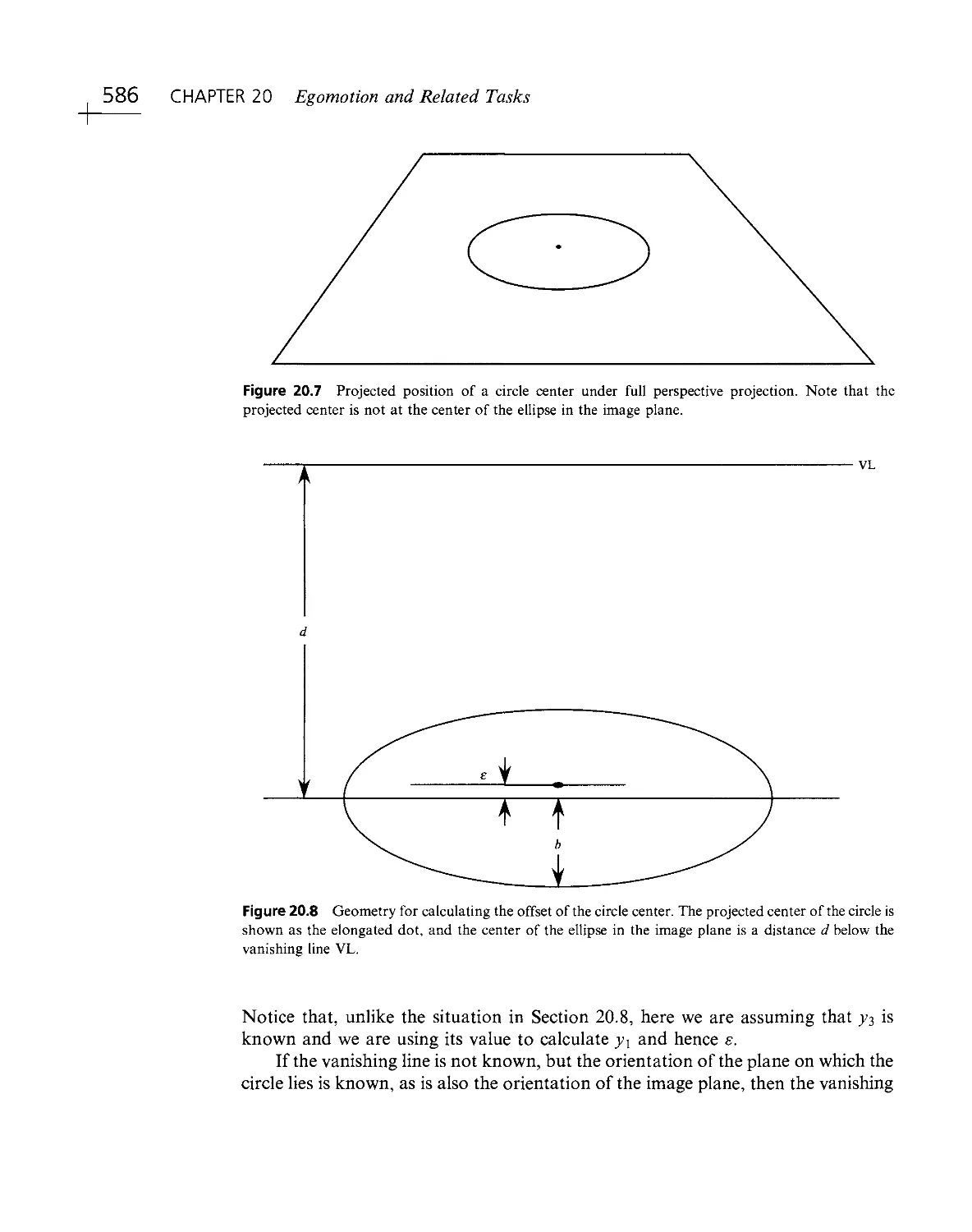
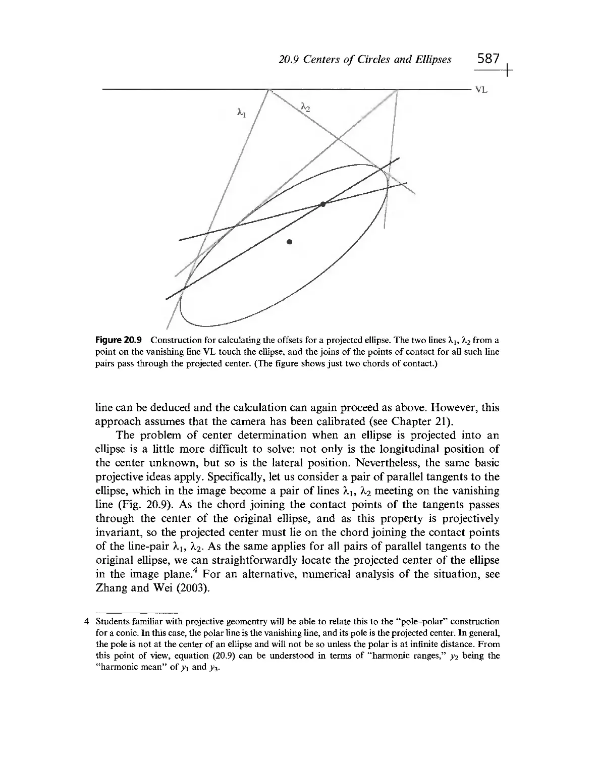
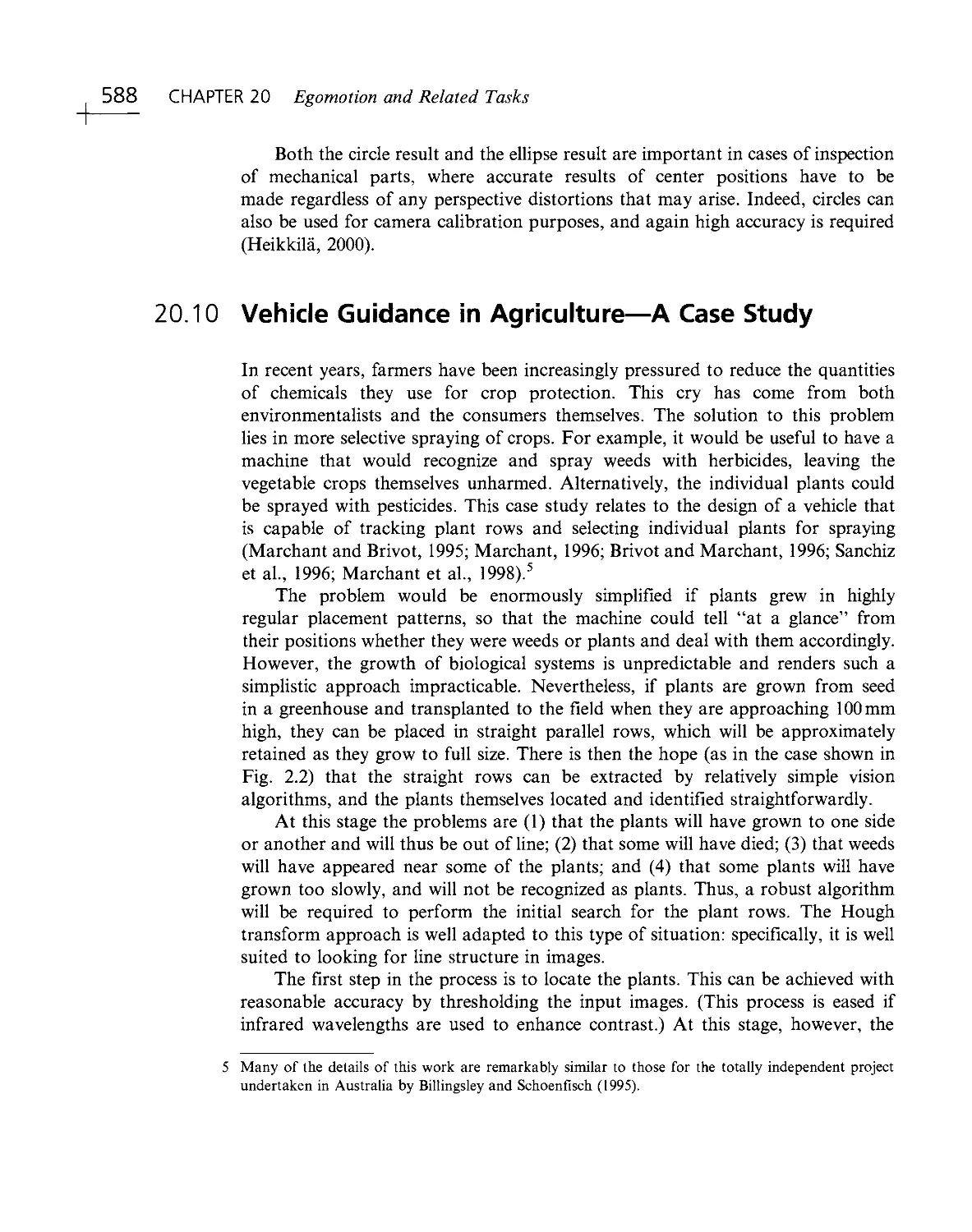
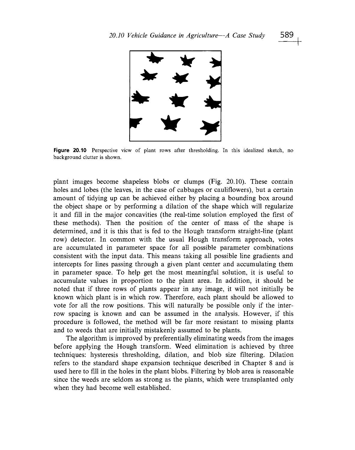
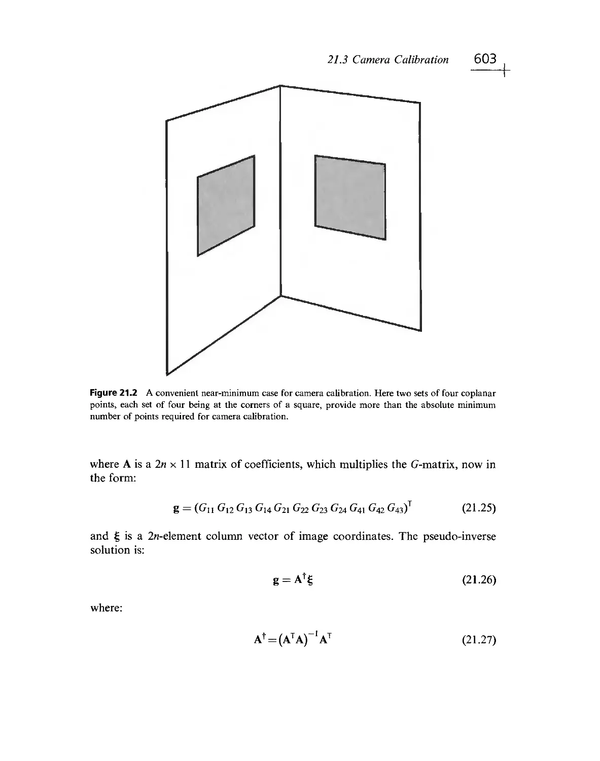
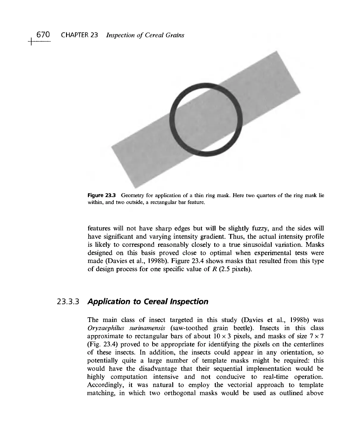
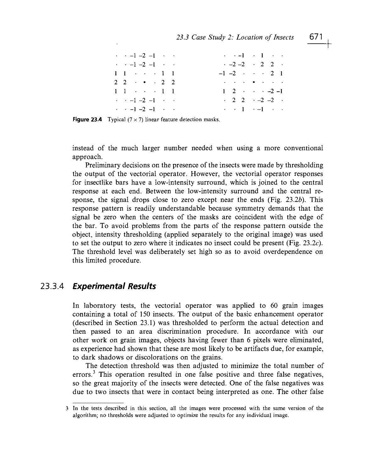
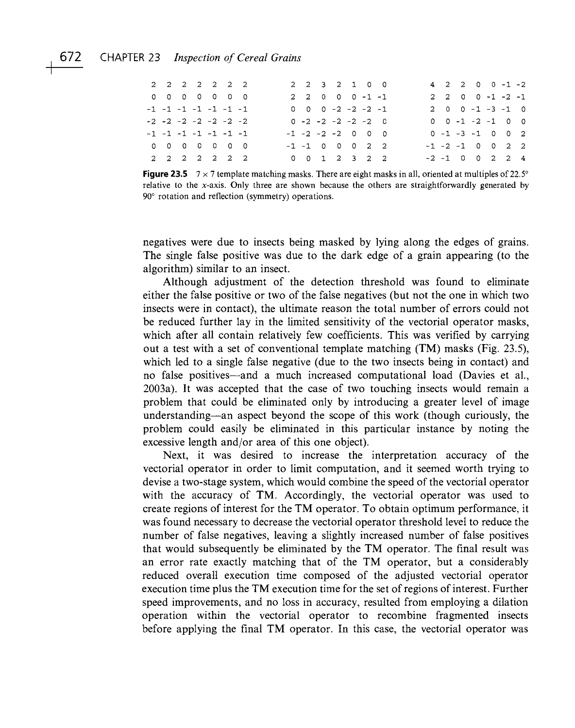
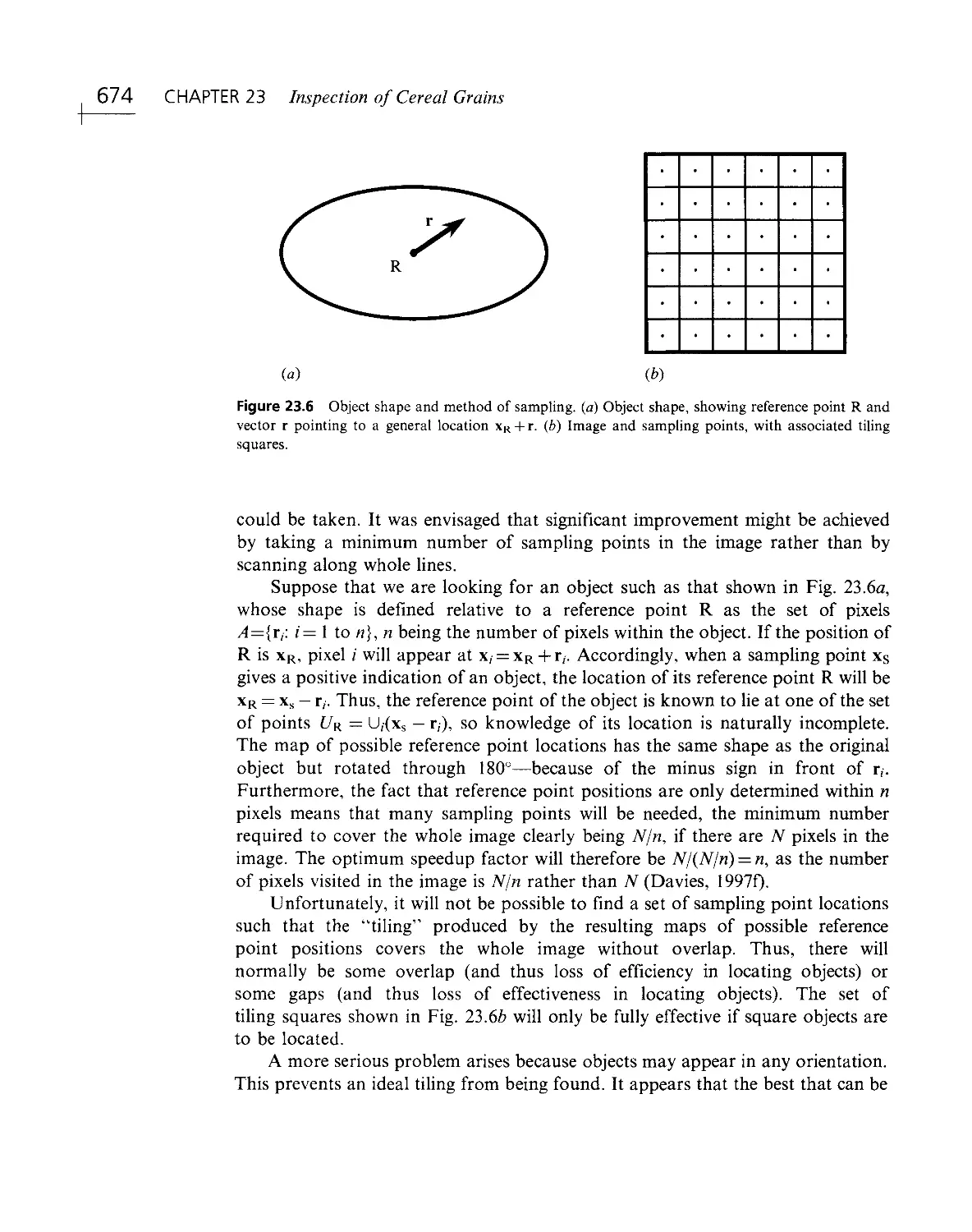
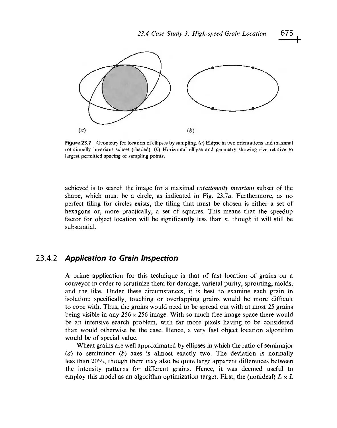
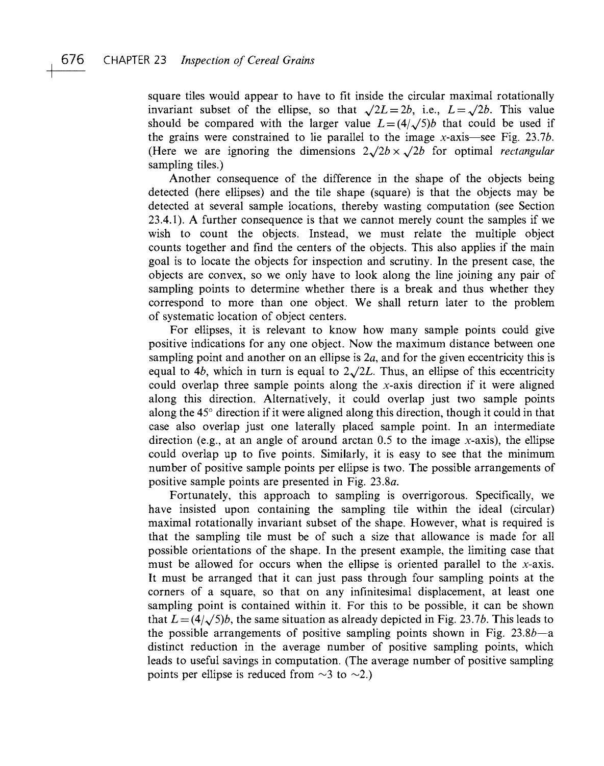
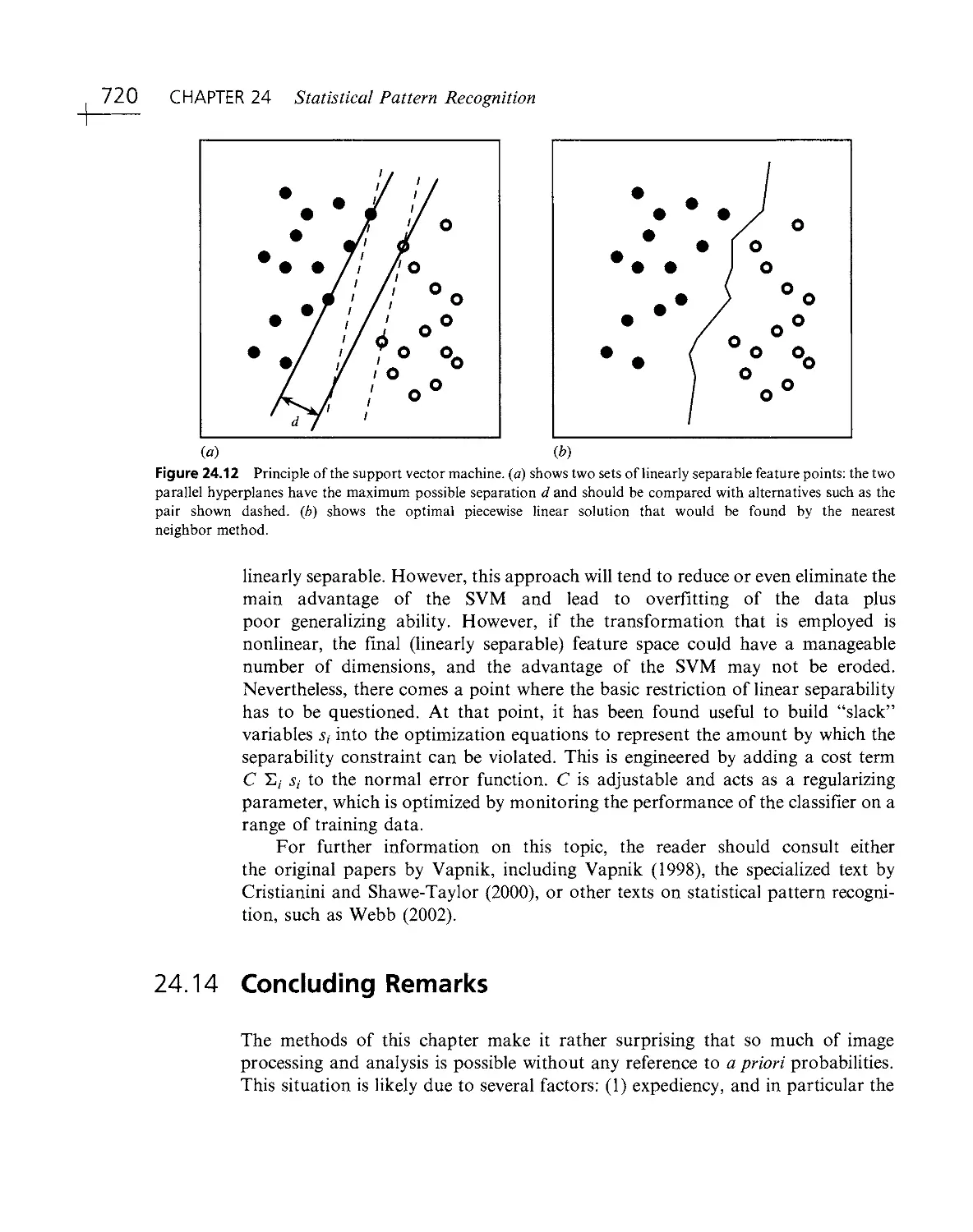
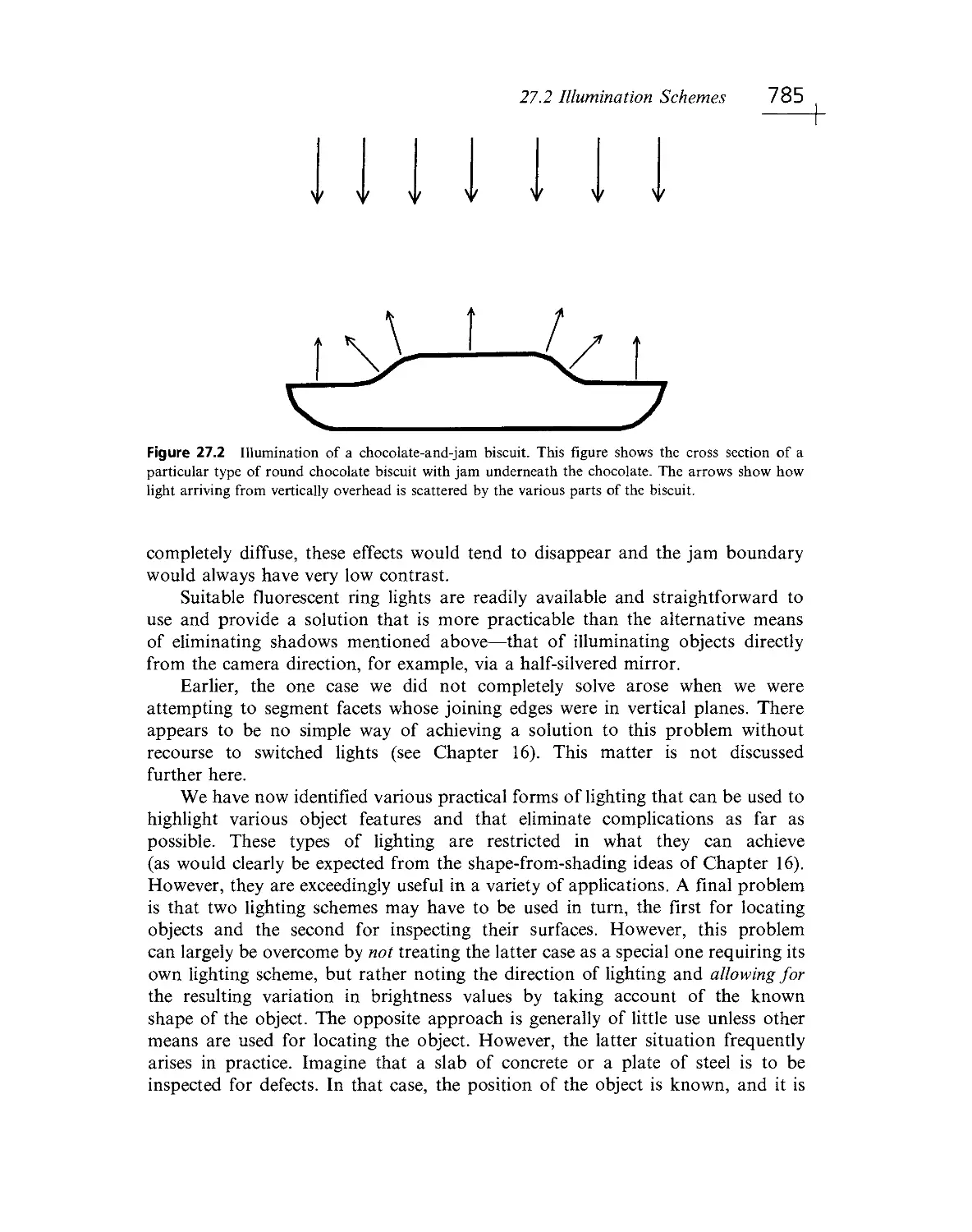
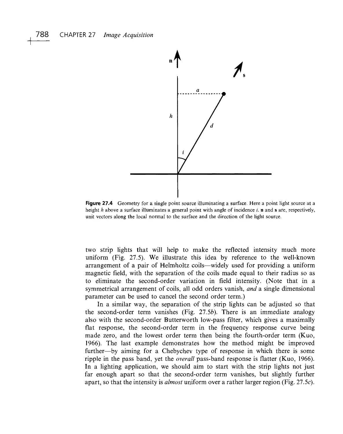
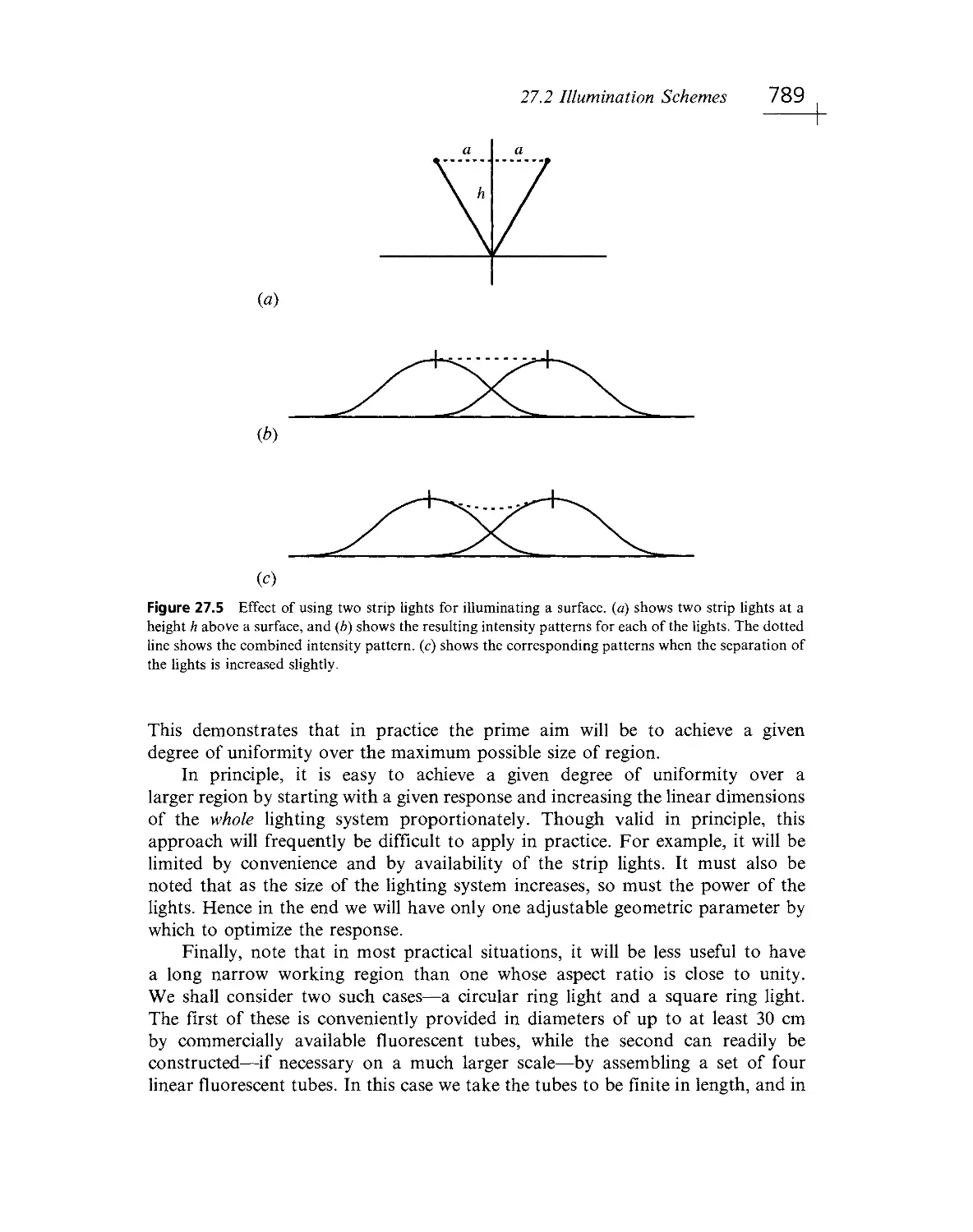
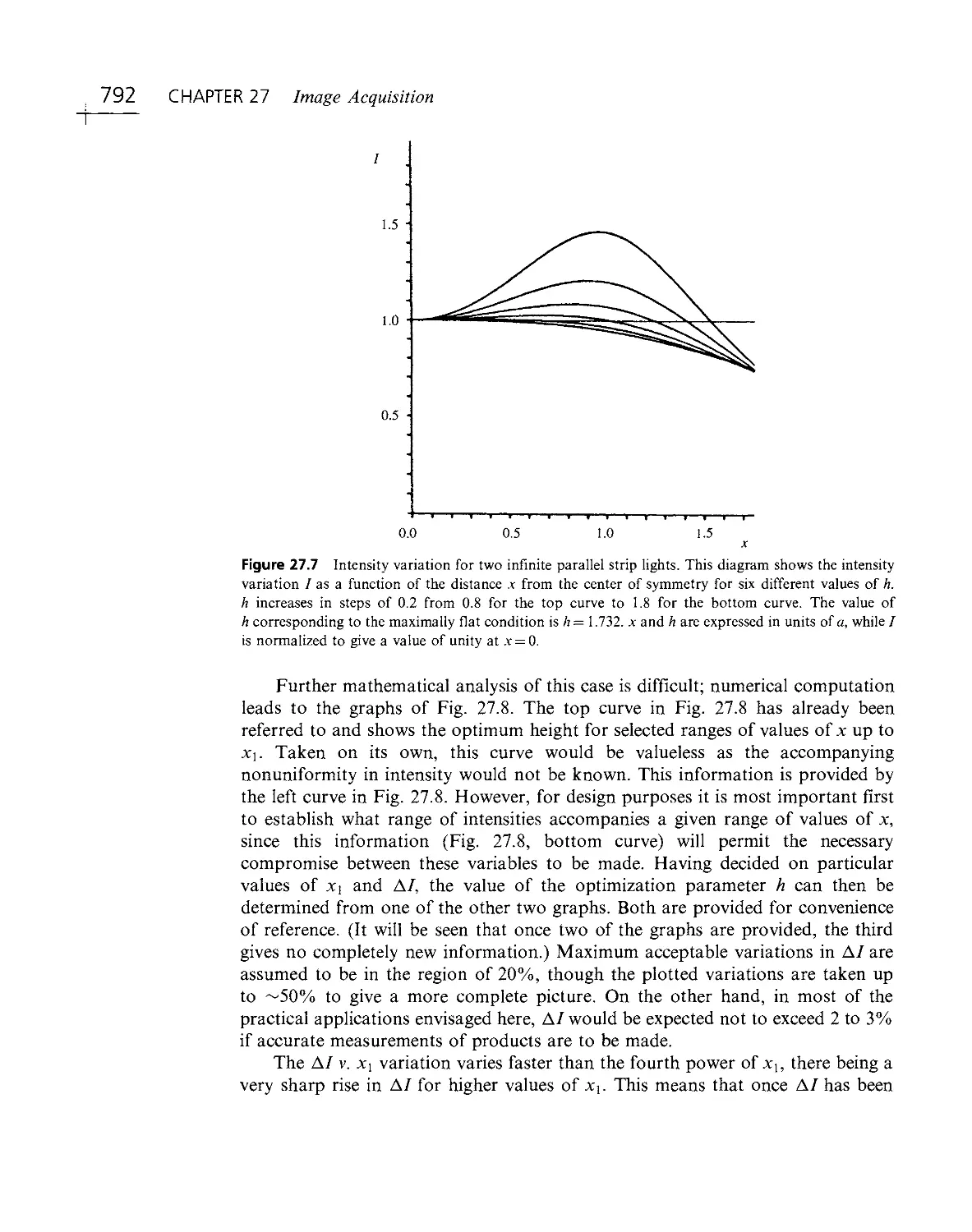
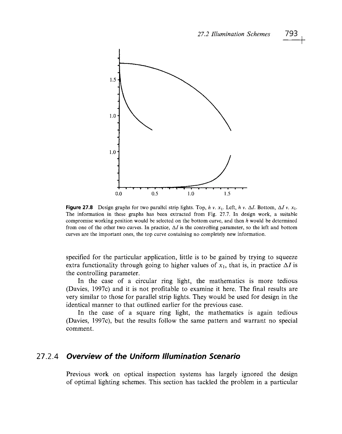
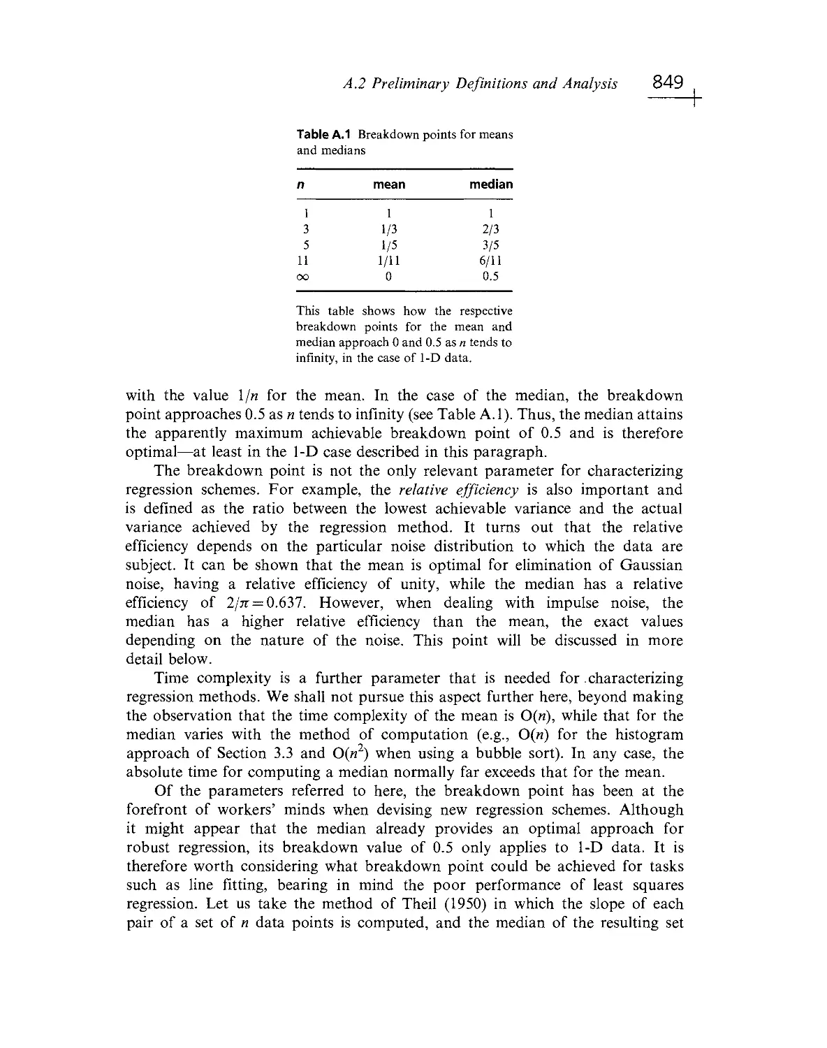
/


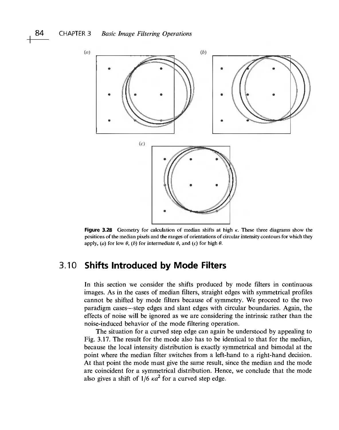


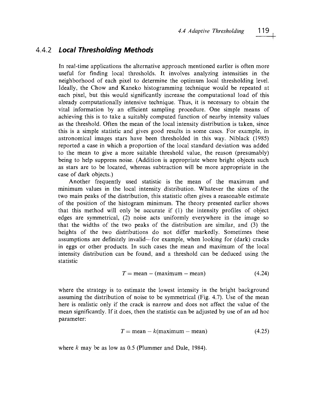
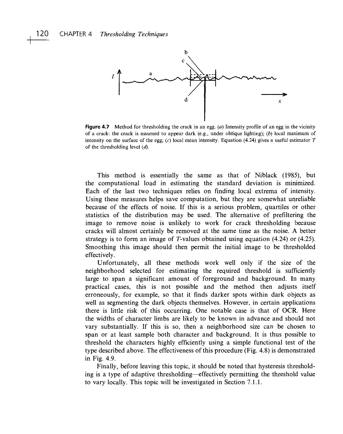


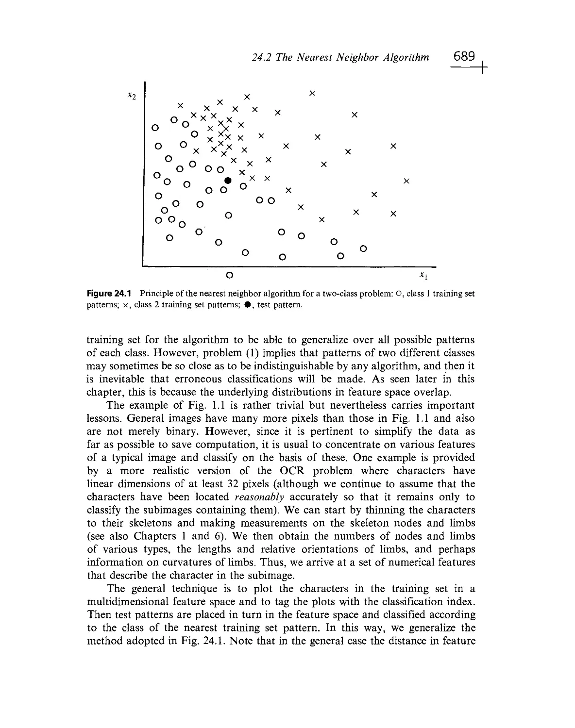


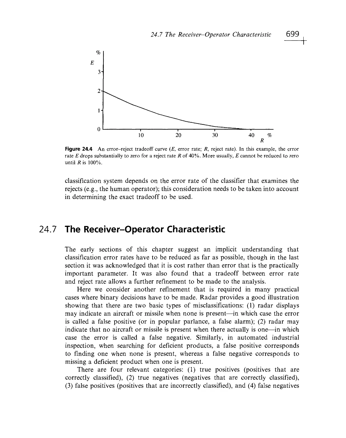


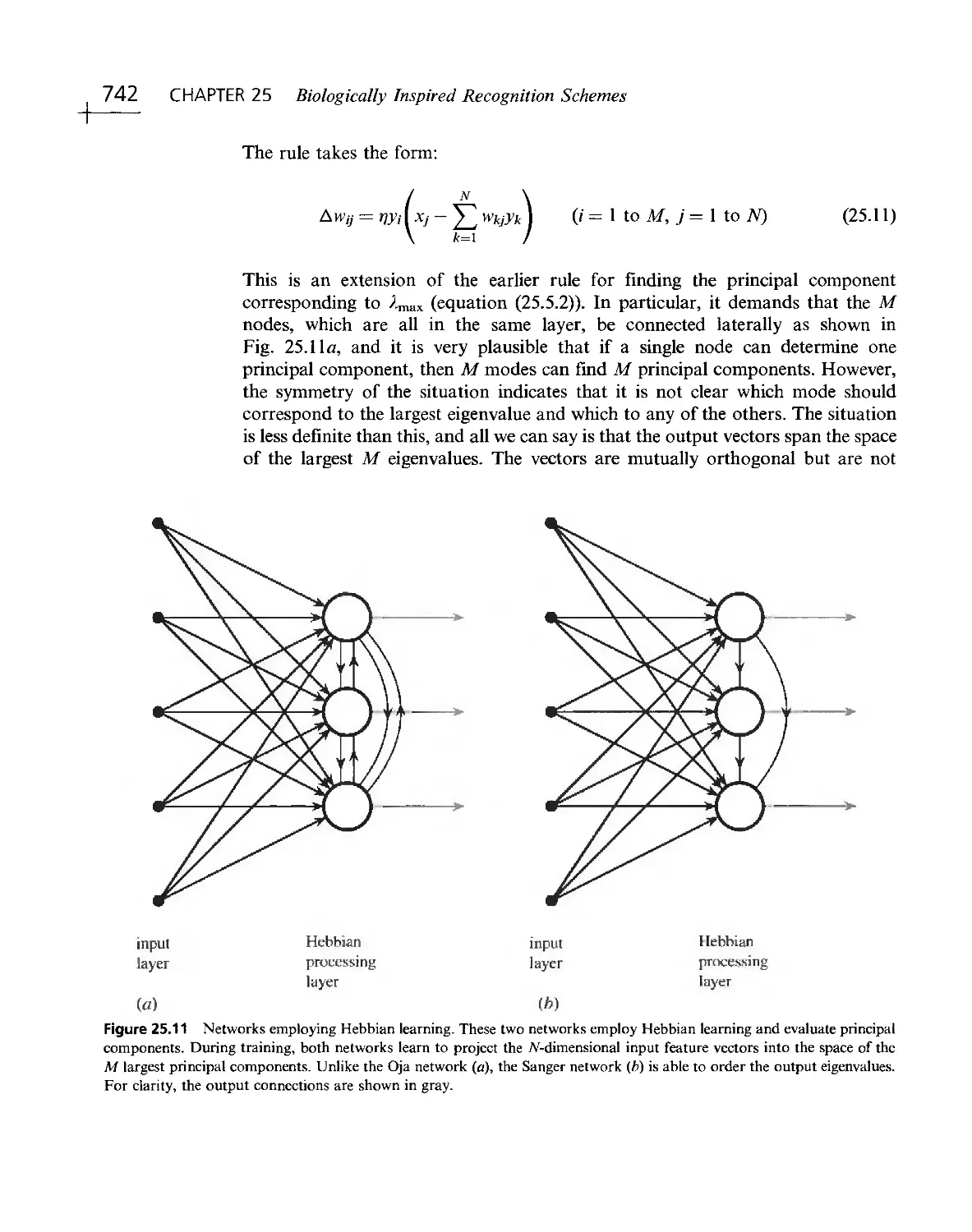


Текст
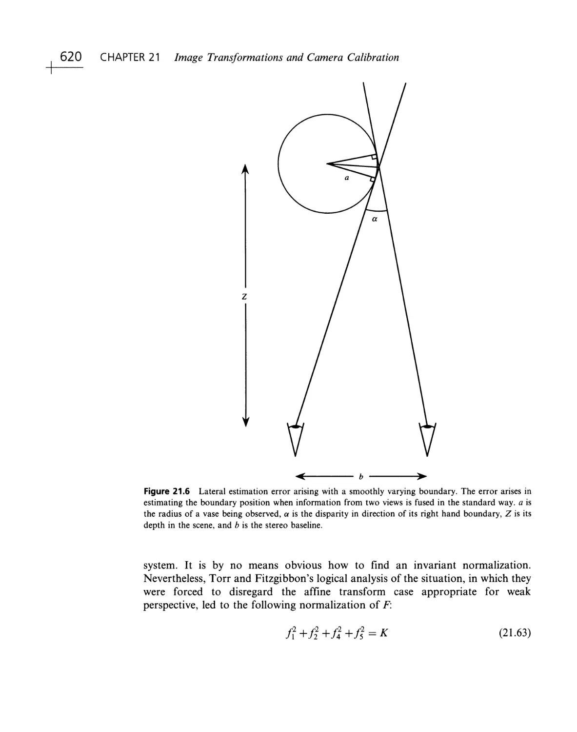
^LSEV'"^ I Thiirf Edition
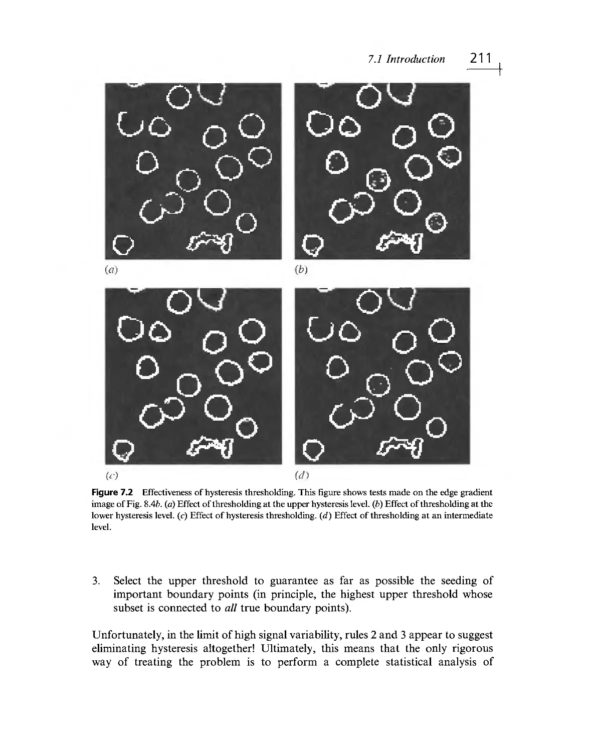
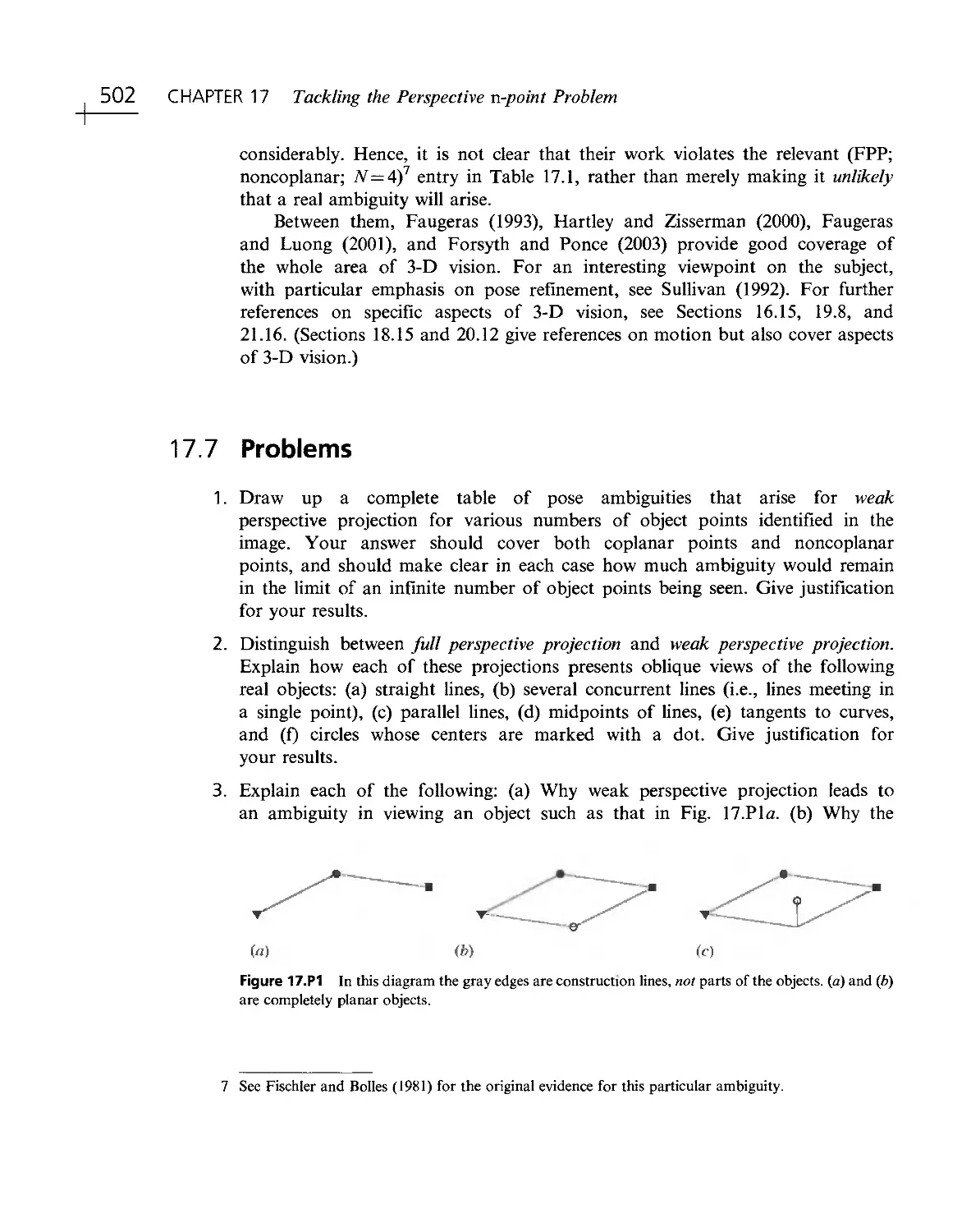
E.R. DAVIES
MACHINE
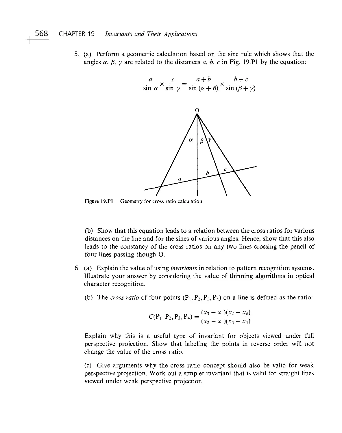
ViSID
Theory
Algorith
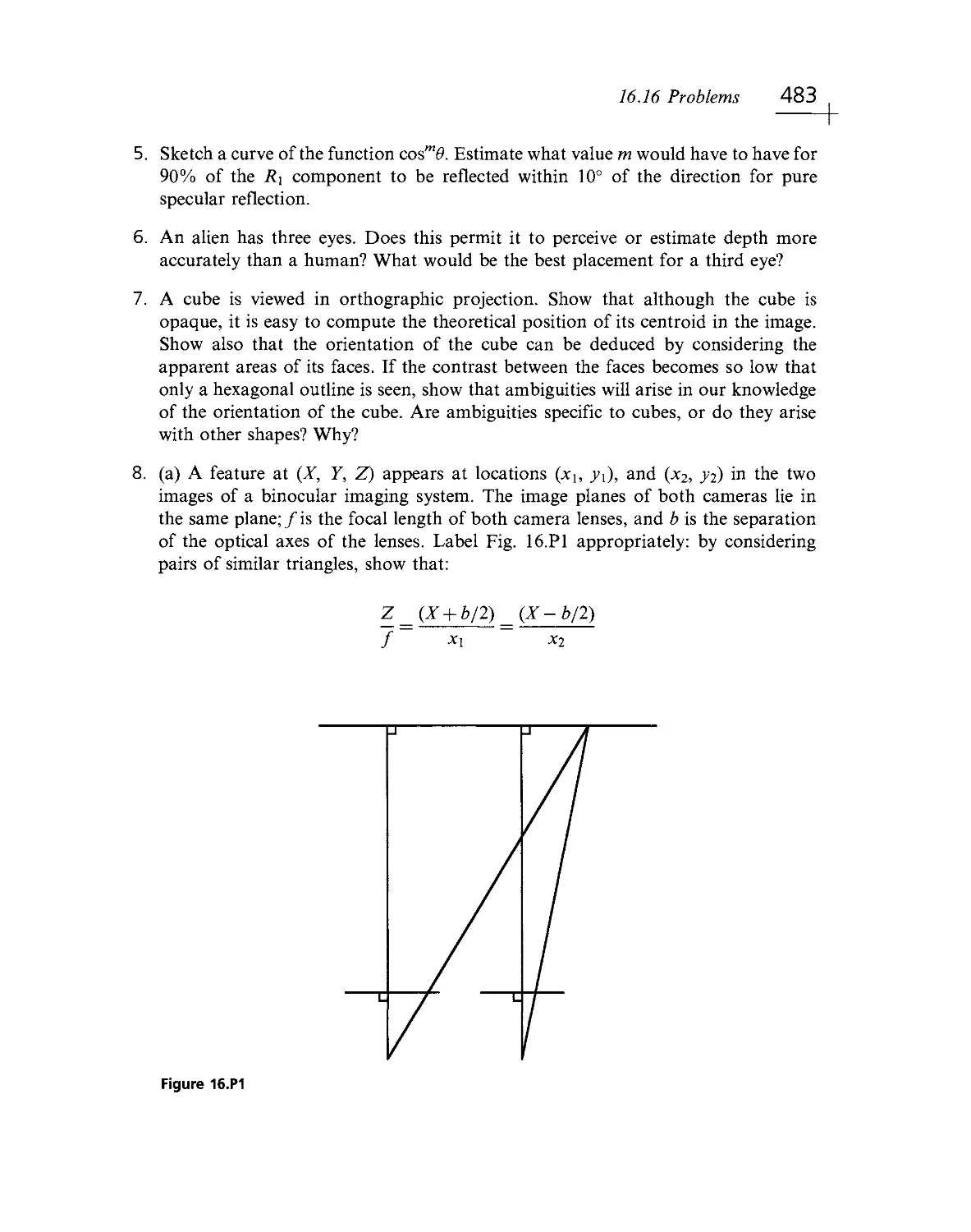
Elsevier Third Edition
E. R. DAVIES
MACHINE
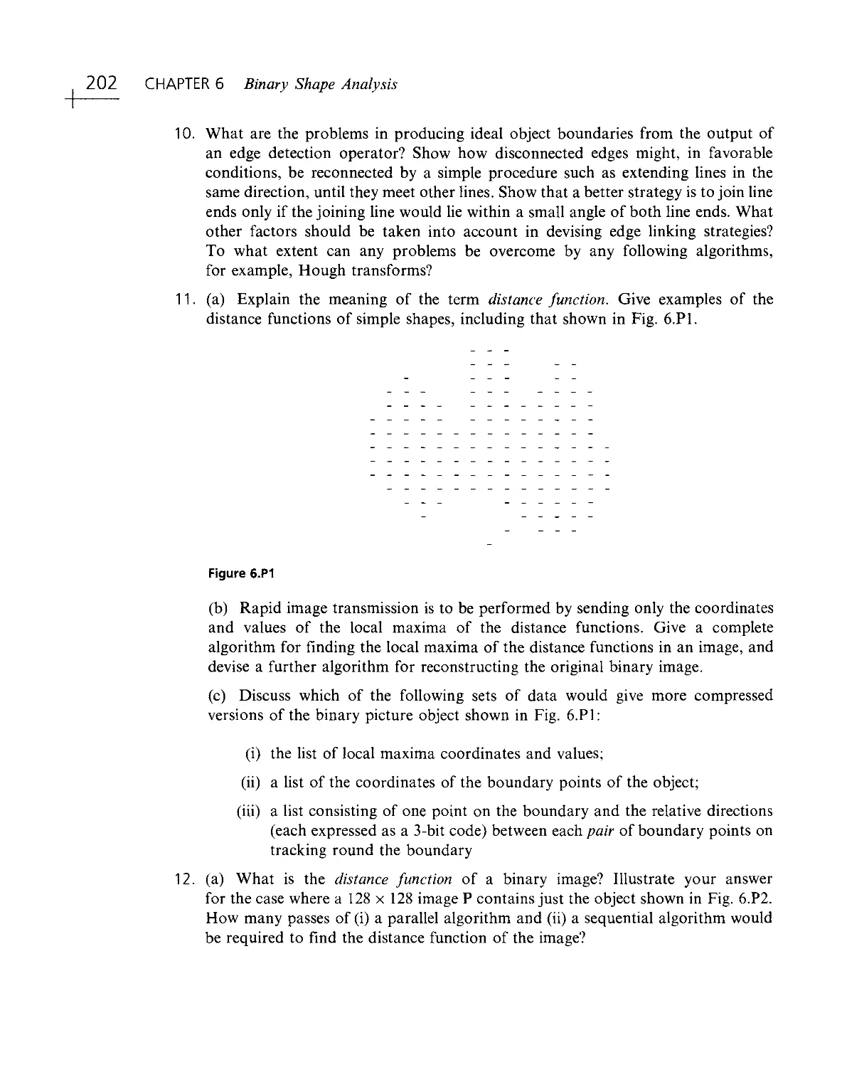
VISION
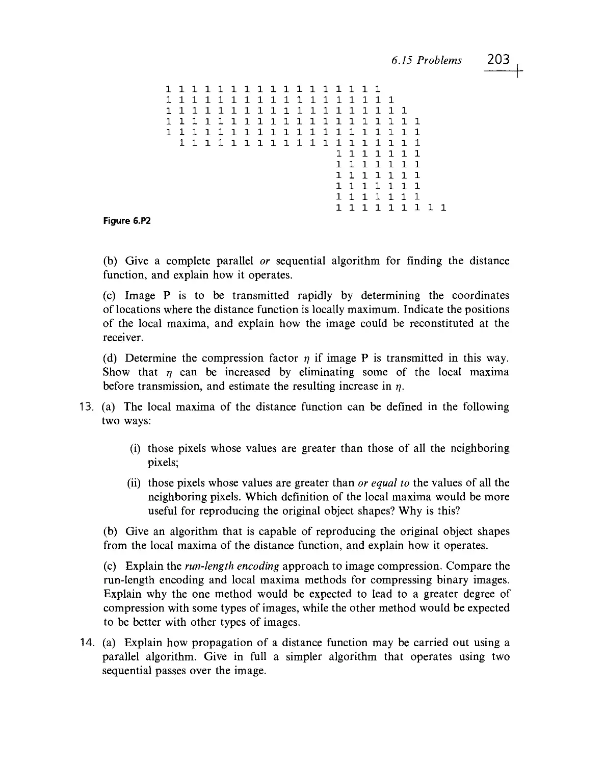
Theory
Algorithms
Practicalities
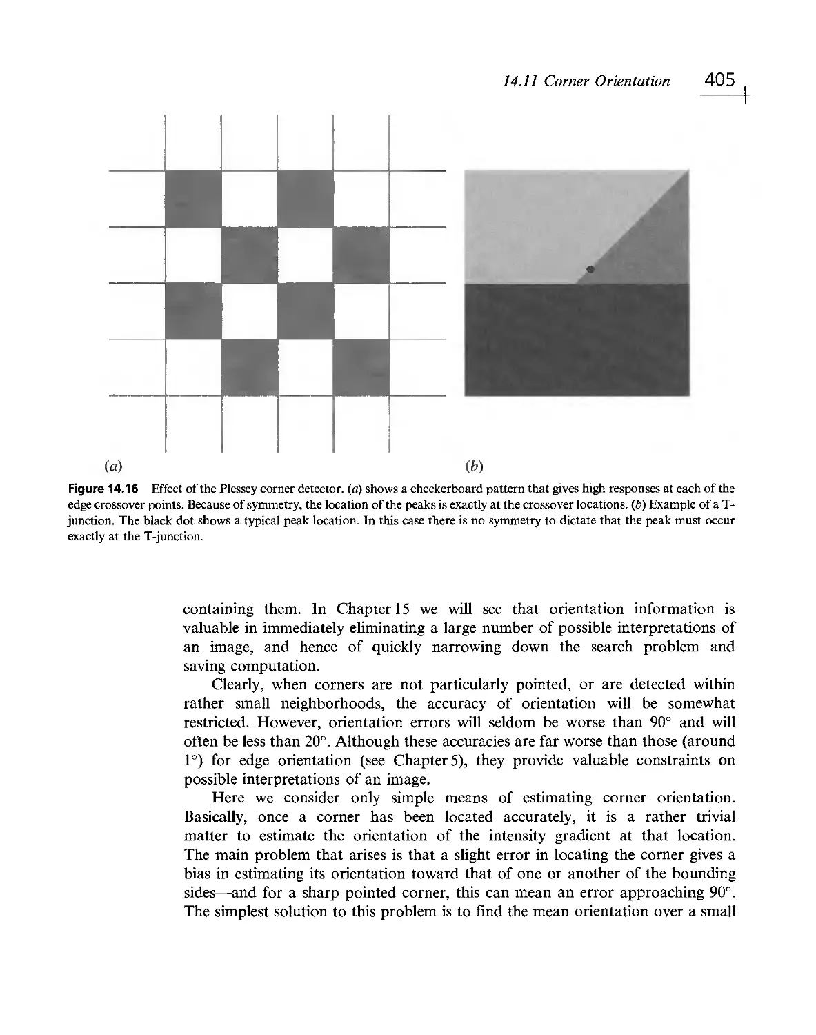
.1'Sii":i''i'R;::, .
- < ivjl MvpnolDgy
About the Author
Professor E.R. Da vies graduated from Oxford University in 1963 with a First
Class Honours degree in Physics. After 12 years research in soUd state physics,
he became interested in vision and is currently professor of machine vision at
Royal Holloway, University of London. He has worked on image filtering,
shape analysis, edge detection, Hough transforms, robust pattern matching, and
artificial neural networks and is involved in algorithm design for inspection,
surveillance, real- time vision, and a number of industrial applications. He has
published over 180 papers and two books— Electronics, Noise and Signal Recovery
(1993), and Image Processing for the Food Industry (2000)— as well as the
present volume. Professor Davies is on the Editorial Boards of Real- Time Imaging,
Pattern Recognition Letters and Imaging Science. He holds a DSc at the University
of London and is a Fellow of the Institute of Physics (UK) and the Institution of
Electrical Engineering (USA), and a Senior Member of the Institute of Electrical
and Electronics Engineering (USA). He is on the Executive Committees of the
British Machine Vision Association and the lEE Visual Information Engineering
Professional Network.
Foreword
An important focus of advances in mechatronics and robotics is the addition of
sensory inputs to systems with increasing "intelligence." Without doubt, sight is
the "sense of choice." In everyday life, whether driving a car or threading a needle,
we depend first on sight. The addition of visual perception to machines promises
the greatest improvement and at the same time presents the greatest challenge.
Until relatively recently, the volume of data in the images that make up a video
stream has been a serious deterrent to progress. A single frame of very modest
resolution might occupy a quarter of a megabyte, so the task of handling thirty or
more such frames per second requires substantial computer resources.
Fortunately, the computer and communications industries' investment in
entertainment has helped address this challenge. The transmission and processing
of video signals are an easy justification for selling the consumer increased
computing speed and bandwidth. A digital camera, capable of video capture, has
already become a fashion accessory as part of a mobile phone. As a result, video
signals have become more accessible to the serious engineer. But the task of
acquiring a visual image is just the tip of the iceberg.
While generating sounds and pictures is a well- defined process (speech
generation is a standard "accessibility" feature of Windows), the inverse task of
recognizing connected speech is still at an unfinished state, a quarter of a century
later, as any user of "dictation" software will attest. Still, analyzing sound is not
even in the same league with analyzing images, particularly when they are of real-
world situations rather than staged pieces with synthetic backgrounds and artificial
lighting.
The task is essentially one of data reduction. From the many megabytes of the
image stream, the required output might be a simple "All wheel nuts are in place"
or "This tomato is ripe." But images tend to be noisy, objects that look sharp to
the eye can have broken edges, boundaries can be fuzzy, and straight lines can be
illusory. The task of image analysis demands a wealth of background know- how
and mathematical analytic tools.
Roy Davies has been developing that rich background for well over two
decades. At the time of the UK Robotics Initiative, in the 1980s, Roy had formed a
relationship with the company United Biscuits. We fellow researchers might well
have been amused by the task of ensuring that the blob of jam on a "Jaffacake"
had been placed centrally beneath the enrobing chocolate. However, the funding of
XXIII
XXIV Foreword
the then expensive vision acquisition and analysis equipment, together with the
spur of a practical target of real economic value, gave Roy a head start that made
us all envious.
Grounded in that research is the realization that human image analysis is a
many- layered process. It starts with simple graphical processing, of the sort that
our eyes perform without our conscious awareness. Contrasts are enhanced;
changes are emphasized and brought to our attention. Next we start to code the
image in terms of lines, the curves of the horizon or of a face, boundaries between
one region and another that a child might draw with a crayon. Then we have to
"understand" the shape - is it a broken biscuit, or is one biscuit partly hidden by
another? If we are comparing a succession of images, has something moved? What
action should we take?
Machine vision must follow a similar, multilayered path. Roy has captured the
essentials with clear, well- illustrated examples. He demonstrates filters that by
convolution can smooth or sharpen an image. He shows us how to wield the tool of
the Hough transform for locating lines and boundaries that are made indistinct by
noise. He throws in the third dimension with stereo analysis, structured lighting,
and optical flow. At every step, however, he drags us back to the world of reality by
considering some practical task. Then, with software examples, he challenges us to
try it for ourselves.
The easy access to digital cameras, video cameras, and streaming video in all its
forms has promoted a tidal wave of would- be applications. But an evolving and
substantial methodology is still essential to underpin the "art" of image processing.
With this latest edition of his book, Roy continues to surf the crest of that wave.
John Billingsley
University of Southern Queensland
Preface
Preface to the third edition
The first edition came out in 1990, and was welcomed by many researchers and
practitioners. However, in the space of 14 years the subject has moved on at a
seemingly accelerating rate, and topics which hardly deserved a mention in the first
edition had to be considered very seriously for the second and more recently for the
third edition. It seemed particularly important to bring in significant amounts of
new material on mathematical morphology, 3- D vision, invariance, motion
analysis, artificial neural networks, texture analysis. X- ray inspection and foreign
object detection, and robust statistics. There are thus new chapters or appendices
on these topics, and these have been carefully integrated with the existing material.
The greater proportion of this new material has been included in Parts 3 and 4.
So great has been the growth in work on 3- D vision and motion— coupled with
numerous applications on (for example) surveillance and vehicle guidance— that
the original single chapter on 3- D vision has had to be expanded into the set of six
chapters on 3- D vision and motion forming Part 3. In addition, Part 4 encompasses
an increased range of chapters whose aim is to cover both applications and all the
components needed for design of real- time visual pattern recognition systems.
In fact, it is difficult to design a logical ordering for all the chapters— particularly
in Part 4— as the topics interact with each other at a variety of different levels—
theory, algorithms, methodologies, practicalities, design constraints, and so on.
However, this should not matter, as the reader will be exposed to the essential
richness of the subject, and his/her studies should be amply rewarded by increased
understanding and capability.
A typical final- year undergraduate course on vision for Electronic Engineering
or Computer Science students might include much of the work of Chapters 1 to 10
and 14 to 16, and a selection of sections from other chapters, according to
requirements. For MSc or PhD research students, a suitable lecture course might
go on to cover Part 3 in depth, including some chapters in Part 4 and also the
appendix on robust statistics, ' with many practical exercises being undertaken on
1 The importance of this appendix should not be underestimated once one gets onto serious work, though
this will probably be outside the restrictive environment of an undergraduate syllabus.
XXV
XXVi Preface
an image analysis system. Here much will depend on the research program being
undertaken by each individual student. At this stage the text will have to be used
more as a handbook for research, and, indeed, one of the prime aims of the volume
is to act as a handbook for the researcher and practitioner in this important area.
As mentioned above, this book leans heavily on experience I have gained
from working with postgraduate students: in particular I would like to express
my gratitude to Barry Cook, Mark Edmonds, Simon Barker, Daniel Celano,
Barrel Greenhill, Derek Charles, and Mark Sugrue, all of whom have in their
own ways helped to shape my view of the subject. In addition, it is a special
pleasure to recall very many rewarding discussions with my colleagues Zahid
Hussain, Ian Hannah, Dev Patel, David Mason, Mark Bateman, Tieying Lu,
Adrian Johnstone, and Piers Plummer; the last two named having been particularly
prolific in generating hardware systems for implementing my research group's
vision algorithms.
The author owes a debt of gratitude to John Billingsley, Kevin Bowyer, Farzin
Deravi, Cornelia Fermuller, Martial Hebert, Majid Mirmehdi, Qiang Ji, Stan
Sclaroff, Milan Sonka, Ellen Walker, and William G. Wee, all of whom read a
draft of the manuscript and made a great many insightful comments and
suggestions. The author is particularly sad to record the passing of Professor Azriel
Rosenfeld before he could complete his reading of the last few chapters, having
been highly supportive of this volume in its various editions. Finally, I am indebted
to Denise Penrose of Elsevier Science for her help and encouragement, without
which this third edition might never have been completed.
Supporting Materials:
Morgan Kaufmann's website for the book contains resources to help
instructors teach courses using this text. Please check the publishers' website for
more information:
www.textbooks.elsevier.com
E.R. DAVIES
Royal Holloway,
University of London
Preface to the first edition
Over the past 30 years or so, machine vision has evolved into a mature subject
embracing many topics and applications: these range from automatic (robot)
assembly to automatic vehicle guidance, from automatic interpretation of
documents to verification of signatures, and from analysis of remotely sensed
images to checking of fingerprints and human blood cells; currently, automated
visual inspection is undergoing very substantial growth, necessary improvements in
Preface XXVii
quality, safety and cost- effectiveness being the stimulating factors. With so much
ongoing activity, it has become a difficult business for the professional to keep up
with the subject and with relevant methodologies: in particular, it is difficult for
him to distinguish accidental developments from genuine advances. It is the
purpose of this book to provide background in this area.
The book was shaped over a period of 10- 12 years, through material I have
given on undergraduate and postgraduate courses at London University and
contributions to various industrial courses and seminars. At the same time, my
own investigations coupled with experience gained while supervising PhD and
postdoctoral researchers helped to form the state of mind and knowledge that is
now set out here. Certainly it is true to say that if I had had this book 8, 6, 4, or
even 2 years ago, it would have been of inestimable value to myself for solving
practical problems in machine vision. It is therefore my hope that it will now be of
use to others in the same way. Of course, it has tended to follow an emphasis
that is my own— and in particular one view of one path towards solving automated
visual inspection and other problems associated with the application of vision in
industry. At the same time, although there is a specialism here, great care has
been taken to bring out general principles— including many applying throughout
the field of image analysis. The reader will note the universality of topics such as
noise suppression, edge detection, principles of illumination, feature recognition,
Bayes' theory, and (nowadays) Hough transforms. However, the generalities lie
deeper than this. The book has aimed to make some general observations and
messages about the limitations, constraints, and tradeoffs to which vision
algorithms are subject. Thus there are themes about the effects of noise, occlusion,
distortion, and the need for built- in forms of robustness (as distinct from less
successful ad hoc varieties and those added on as an afterthought); there are also
themes about accuracy, systematic design, and the matching of algorithms and
architectures. Finally, there are the problems of setting up lighting schemes
which must be addressed in complete systems, yet which receive scant attention
in most books on image processing and analysis. These remarks will indicate that
the text is intended to be read at various levels— a factor that should make it
of more lasting value than might initially be supposed from a quick perusal of
the Contents.
Of course, writing a text such as this presents a great difficulty in that it is
necessary to be highly selective: space simply does not allow everything in a subject
of this nature and maturity to be dealt with adequately between two covers. One
solution might be to dash rapidly through the whole area mentioning everything
that comes to mind, but leaving the reader unable to understand anything in detail
or to achieve anything having read the book. However, in a practical subject of this
nature this seemed to me a rather worthless extreme. It is just possible that the
emphasis has now veered too much in the opposite direction, by coming down to
practicalities (detailed algorithms, details of lighting schemes, and so on):
individual readers will have to judge this for themselves. On the other hand, an
XXViii Preface
author has to be true to himself and my view is that it is better for a reader or
student to have mastered a coherent series of topics than to have a mish- mash of
information that he is later unable to recall with any accuracy. This, then, is my
justification for presenting this particular material in this particular way and for
reluctantly omitting from detailed discussion such important topics as texture
analysis, relaxation methods, motion, and optical flow.
As for the organization of the material, I have tried to make the early part of
the book lead into the subject gently, giving enough detailed algorithms (especially
in Chapters 2 and 6) to provide a sound feel for the subject— including especially
vital, and in their own way quite intricate, topics such as connectedness in binary
images. Hence Part 1 provides the lead- in, although it is not always trivial material
and indeed some of the latest research ideas have been brought in (e.g., on
thresholding techniques and edge detection). Part 2 gives much of the meat of the
book. Indeed, the (book) literature of the subject currently has a significant gap in
the area of intermediate- level vision; while high- level vision (AI) topics have long
caught the researcher's imagination, intermediate- level vision has its own
difficulties which are currently being solved with great success (note that the
Hough transform, originally developed in 1962, and by many thought to be a very
specialist topic of rather esoteric interest, is arguably only now coming into its
own). Part 2 and the early chapters of Part 3 aim to make this clear, while Part 4
gives reasons why this particular transform has become so useful. As a whole, Part
3 aims to demonstrate some of the practical applications of the basic work covered
earlier in the book, and to discuss some of the principles underlying
implementation: it is here that chapters on lighting and hardware systems will be found. As
there is a limit to what can be covered in the space available, there is a
corresponding emphasis on the theory underpinning practicalities. Probably this is
a vital feature, since there are many applications of vision both in industry and
elsewhere, yet listing them and their intricacies risks dwelling on interminable
detail, which some might find insipid; furthermore, detail has a tendency to date
rather rapidly. Although the book could not cover 3- D vision in full (this topic
would easily consume a whole volume in its own right), a careful overview of this
complex mathematical and highly important subject seemed vital. It is therefore no
accident that Chapter 16 is the longest in the book. Finally, Part 4 asks questions
about the limitations and constraints of vision algorithms and answers them by
drawing on information and experience from earlier chapters. It is tempting to call
the last chapter the Conclusion. However, in such a dynamic subject area any such
temptation has to be resisted, although it has still been possible to draw a good
number of lessons on the nature and current state of the subject. Clearly, this
chapter presents a personal view but I hope it is one that readers will find
interesting and useful.
Acknowledgments
The author would like to credit the following sources for permission to reproduce
tables, figures and extracts of text from earlier publications:
The Committee of the Alvey Vision Club for permission to reprint portions of the
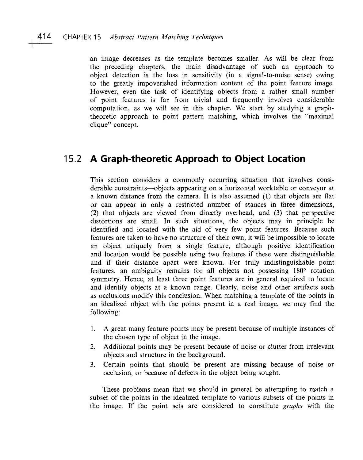
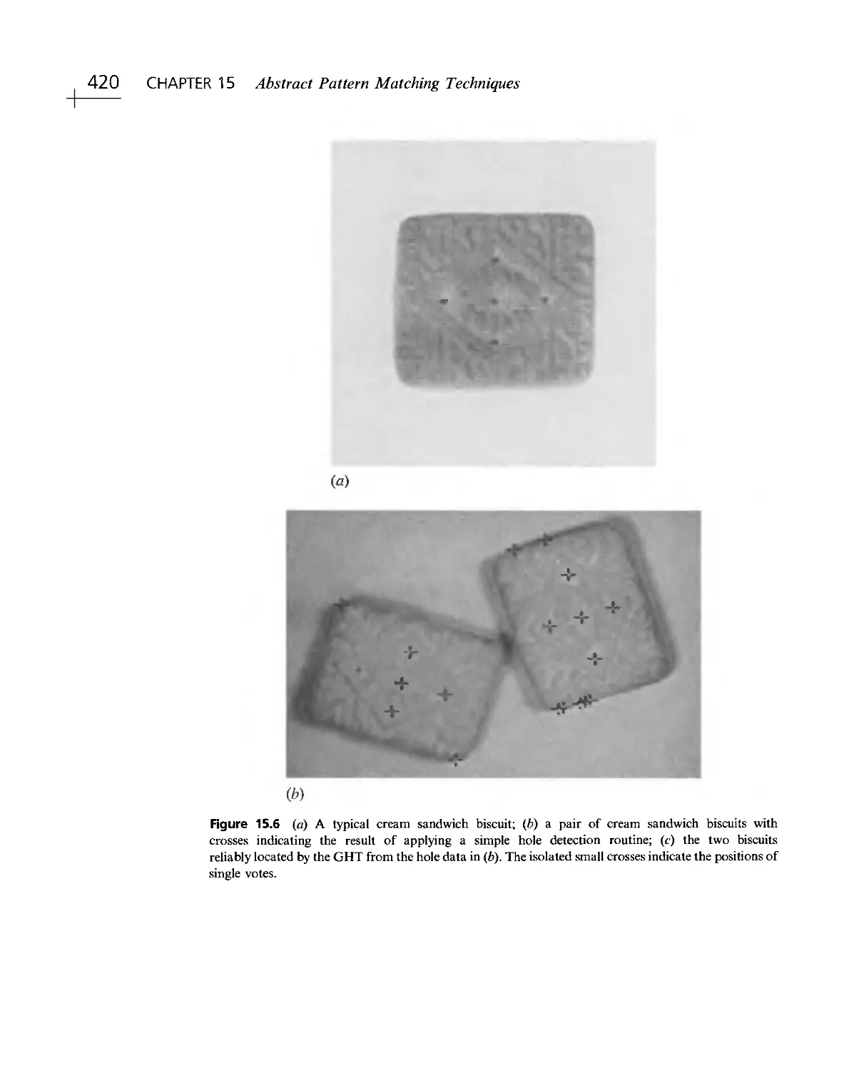
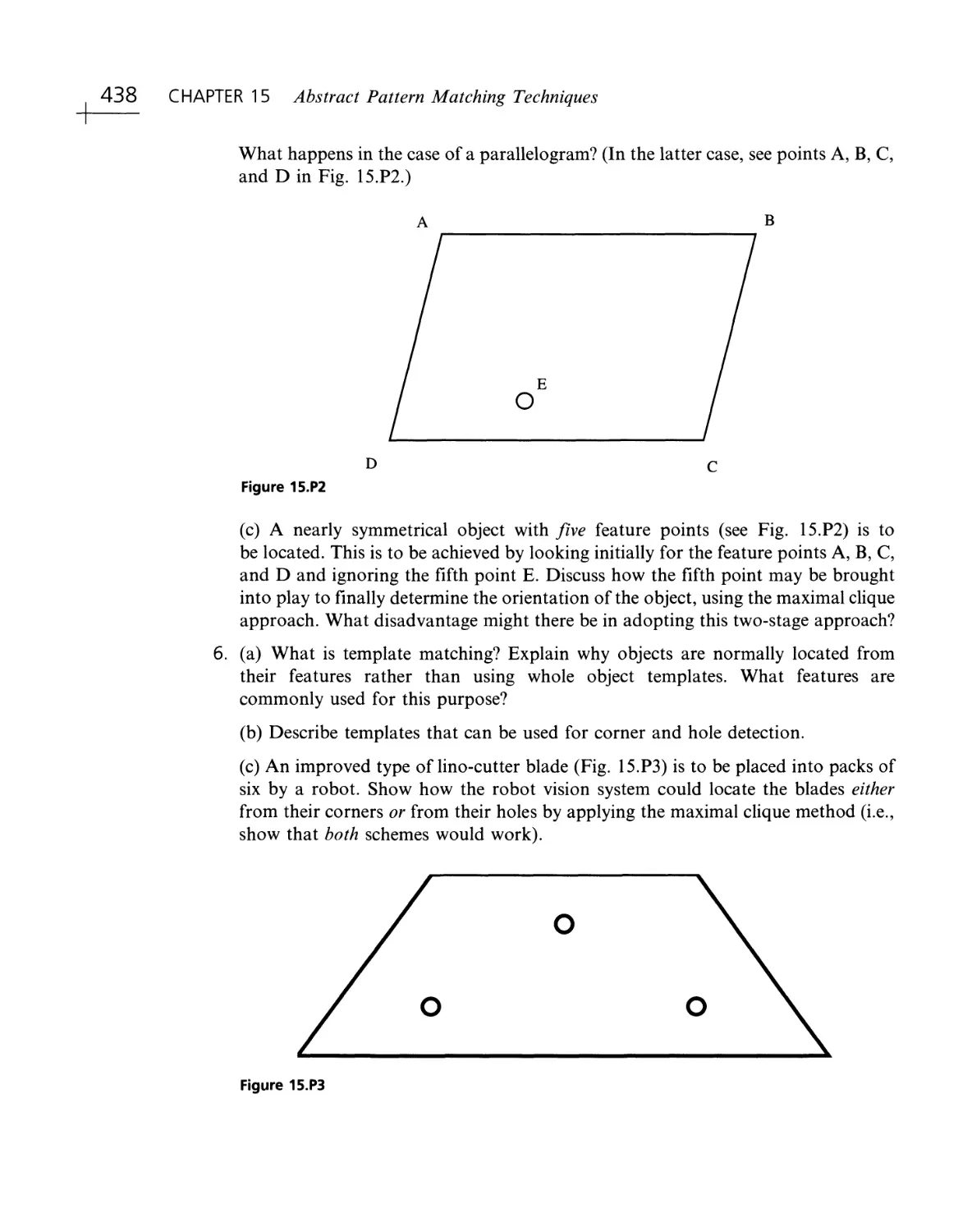
following paper as text in Chapter 15 and as Figs. 15.1, 15.2, 15.6:
Davies, E.R. (1988g).
CEP Consultants Ltd (Edinburgh) for permission to reprint portions of the
following paper as text in Chapter 19:
Davies, E.R. (1987a).
Portions of the following papers from Pattern Recognition and Signal Processing
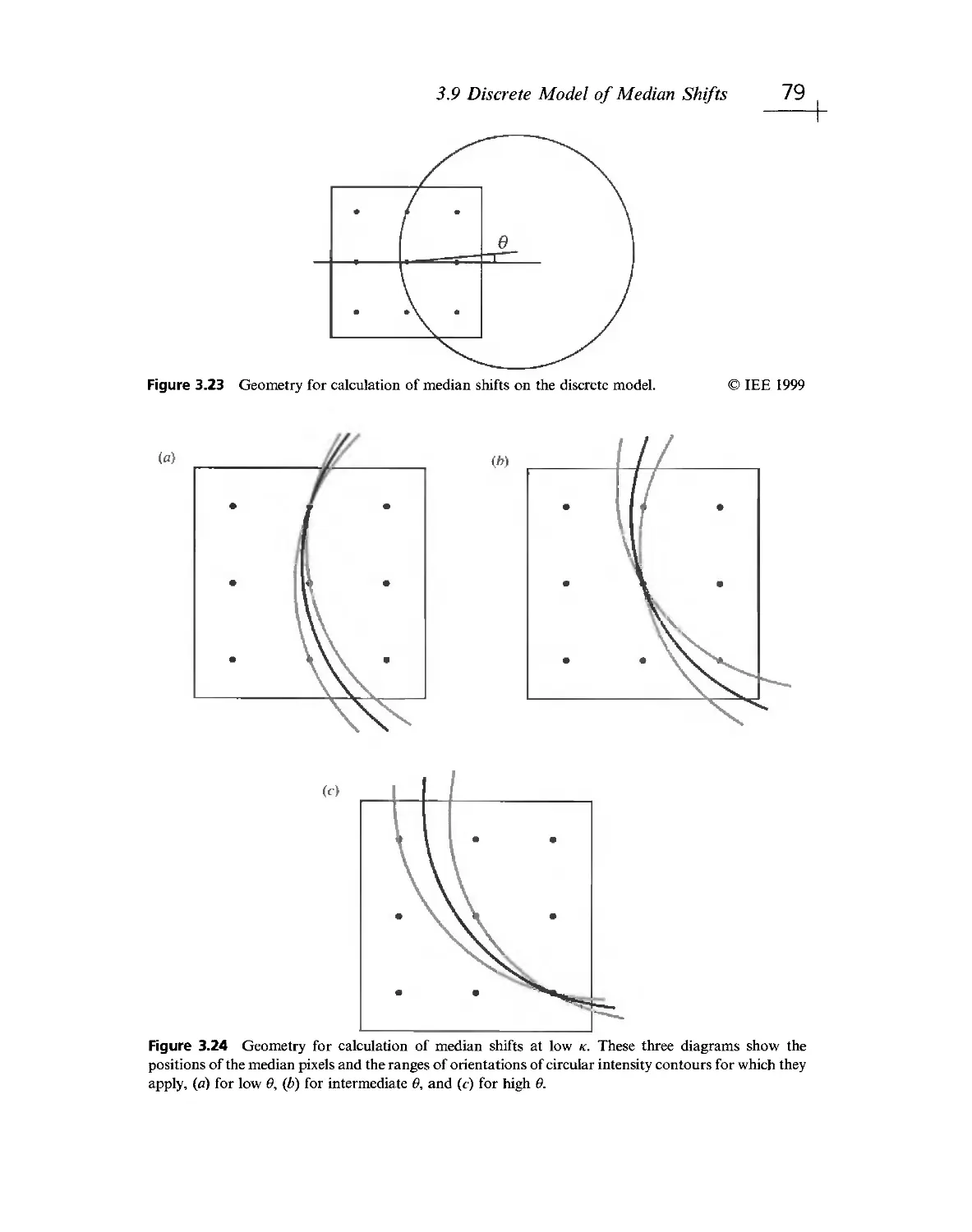
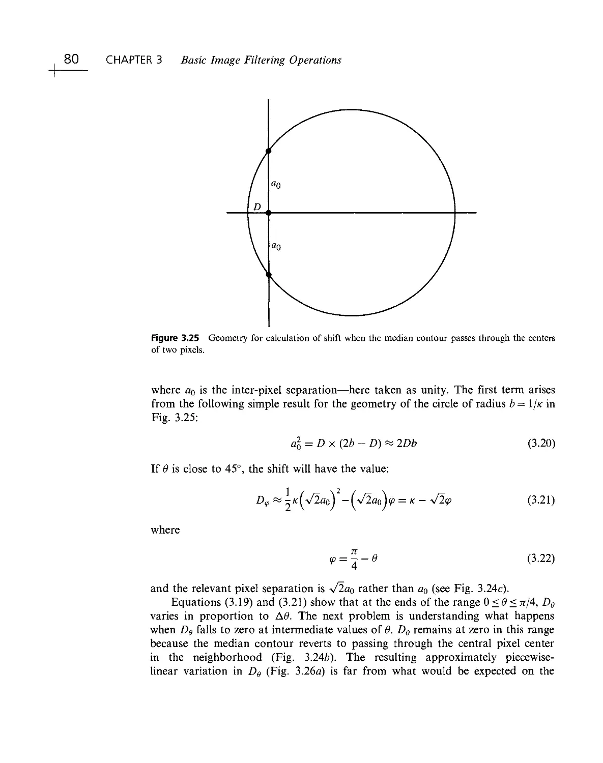
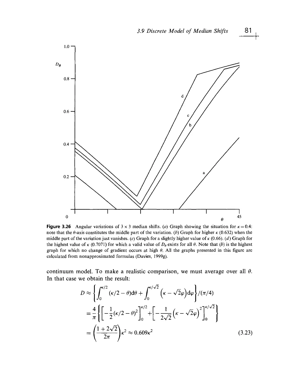
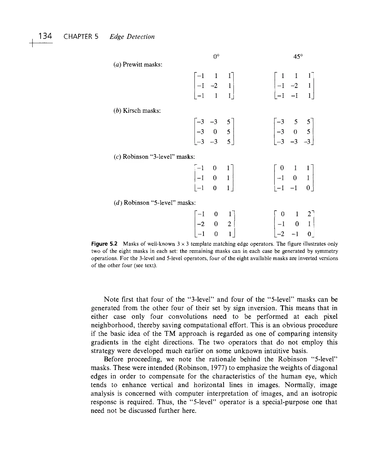
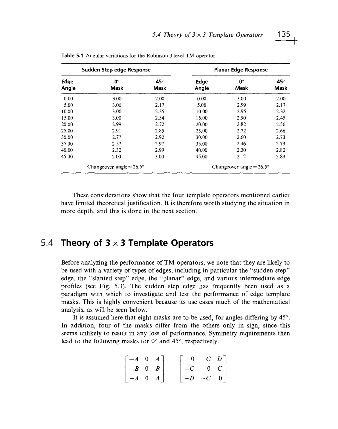
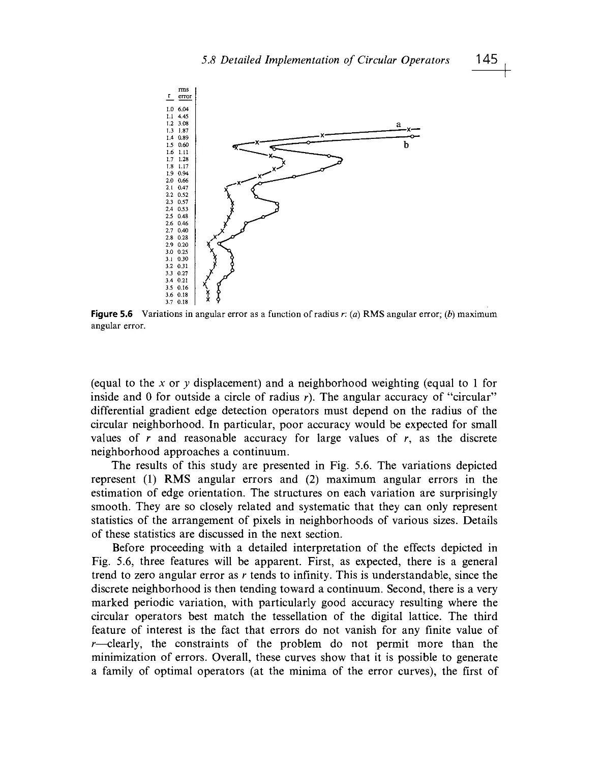
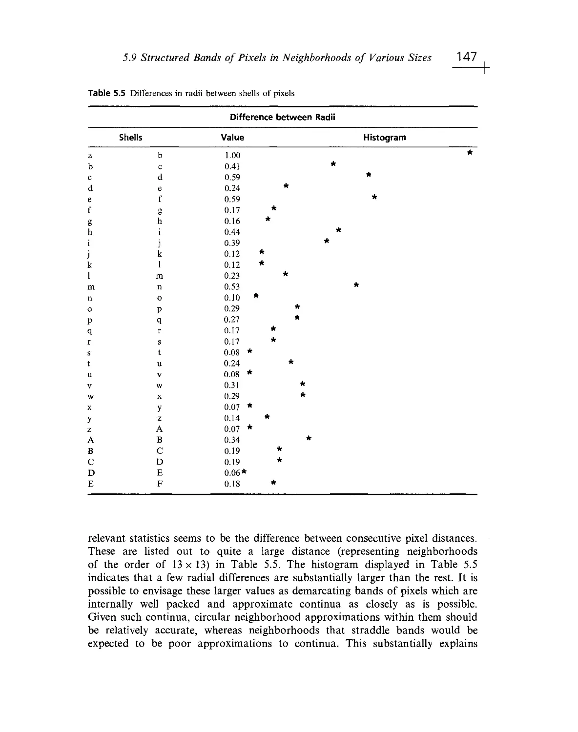
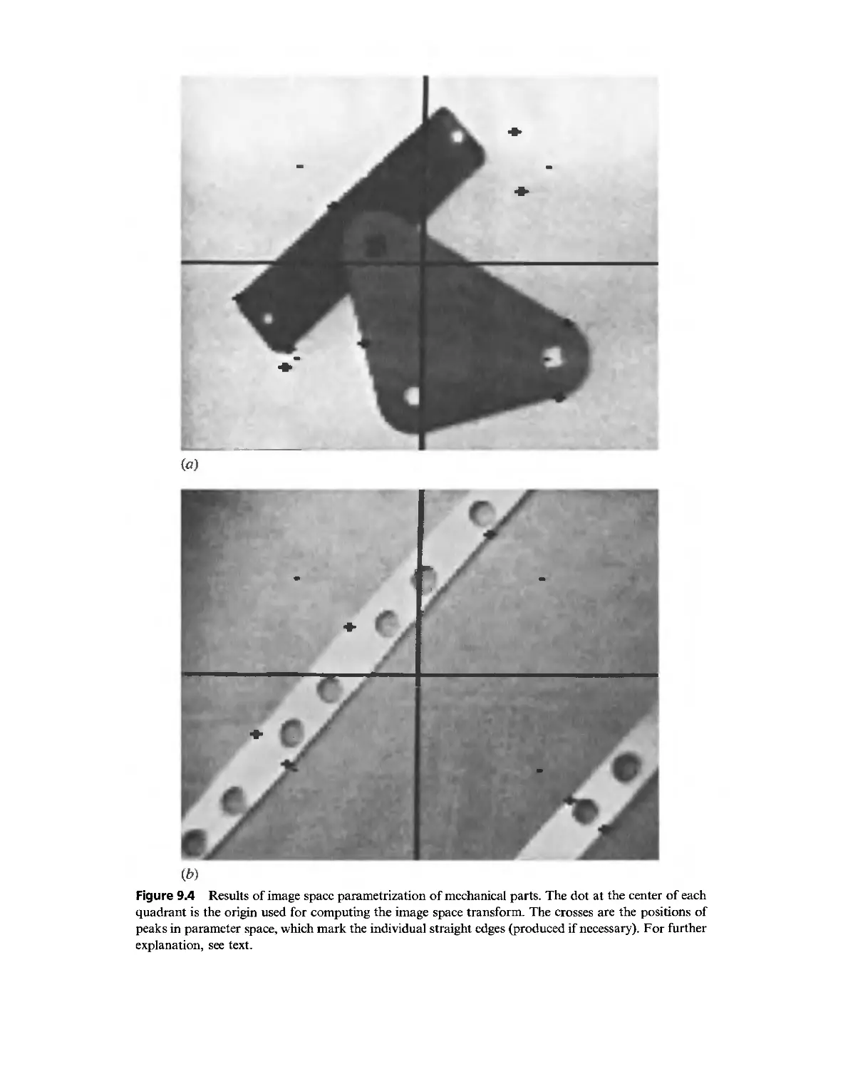
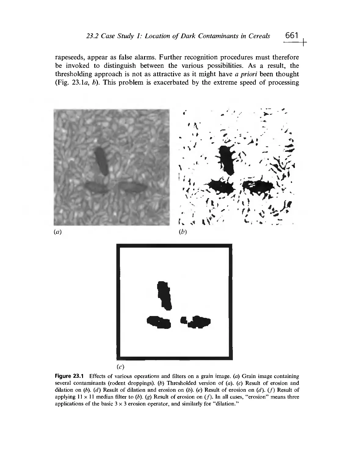
as text in Chapters 3, 5, 9- 15, 23, 24 and tables 5.1, 5.2, 5.3 and as Figs. 3.7, 3.9,
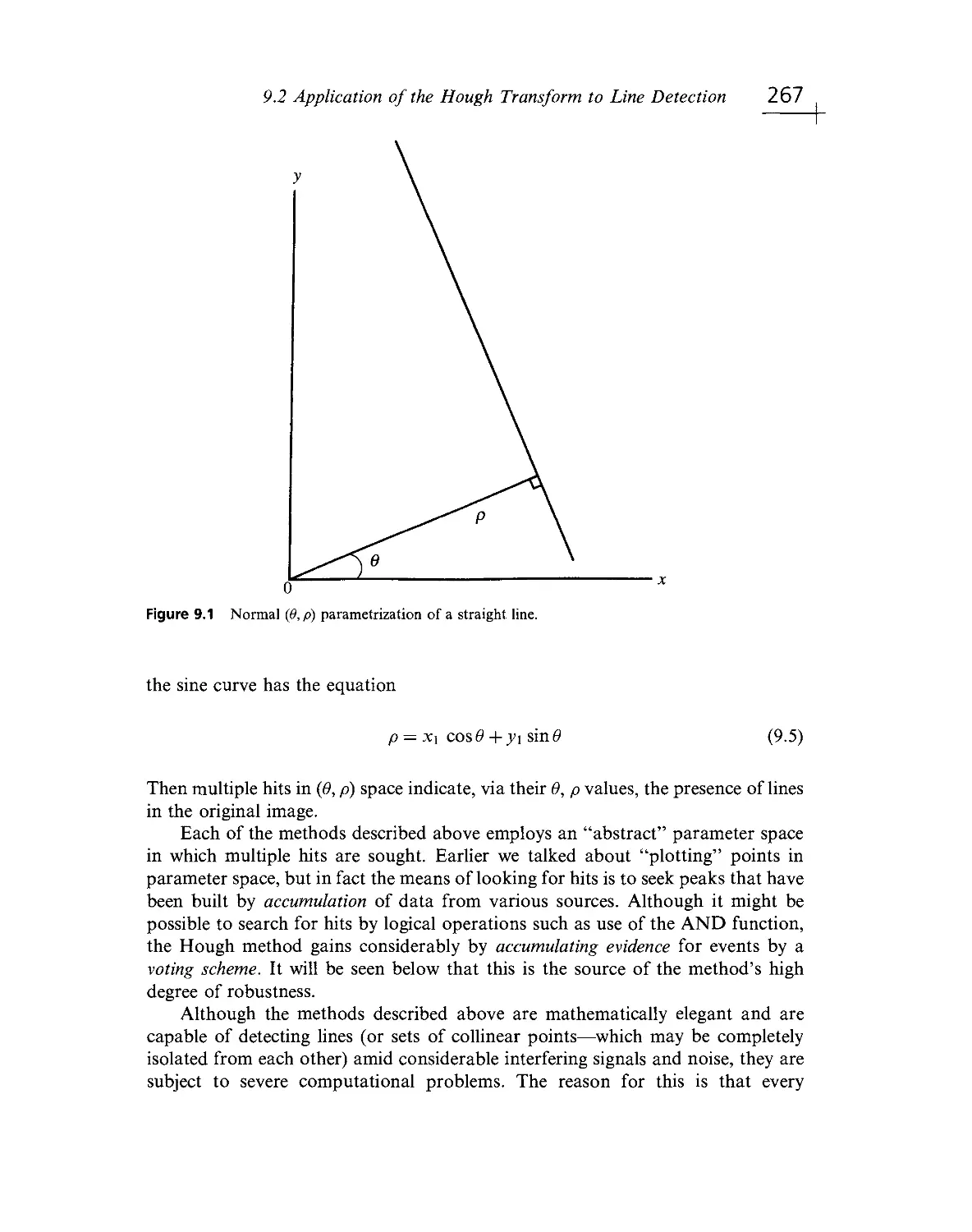
3.11, 3.12, 3.13, 3.17, 3, 18, 3.19, 3.20, 3.21, 3.22, 5.2, 5.3, 5.4, 5.8, 9.1, 9.2, 9.3, 9.4,
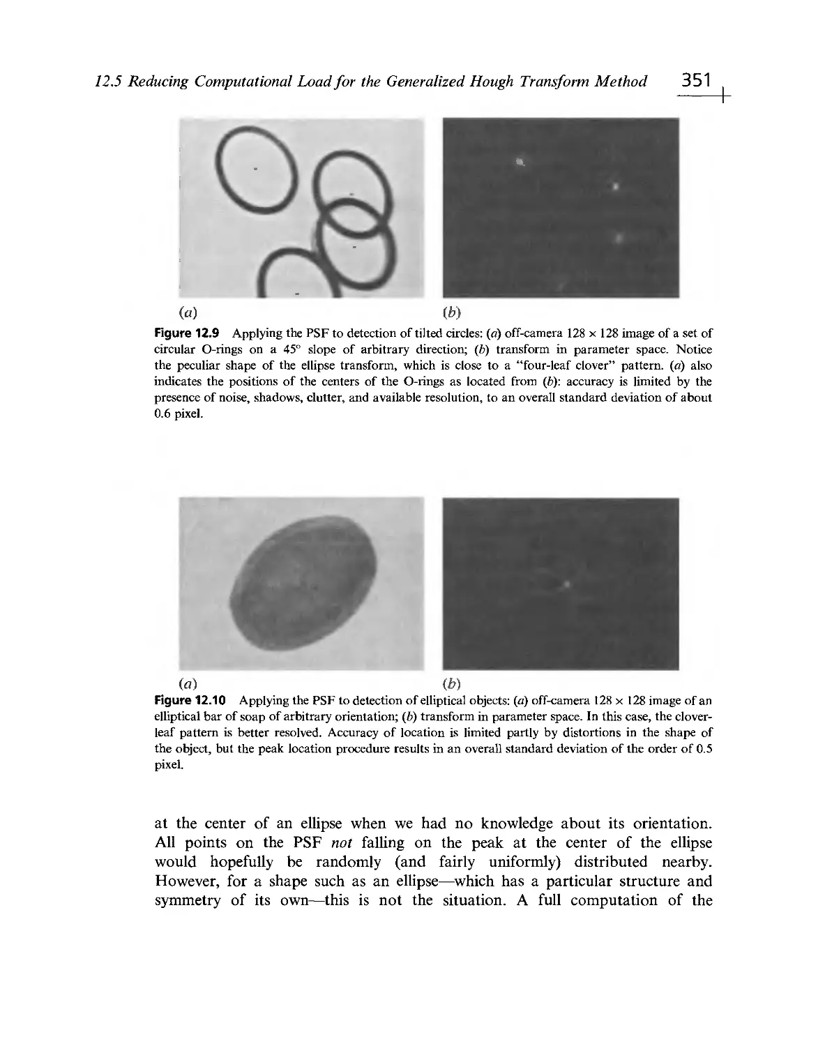
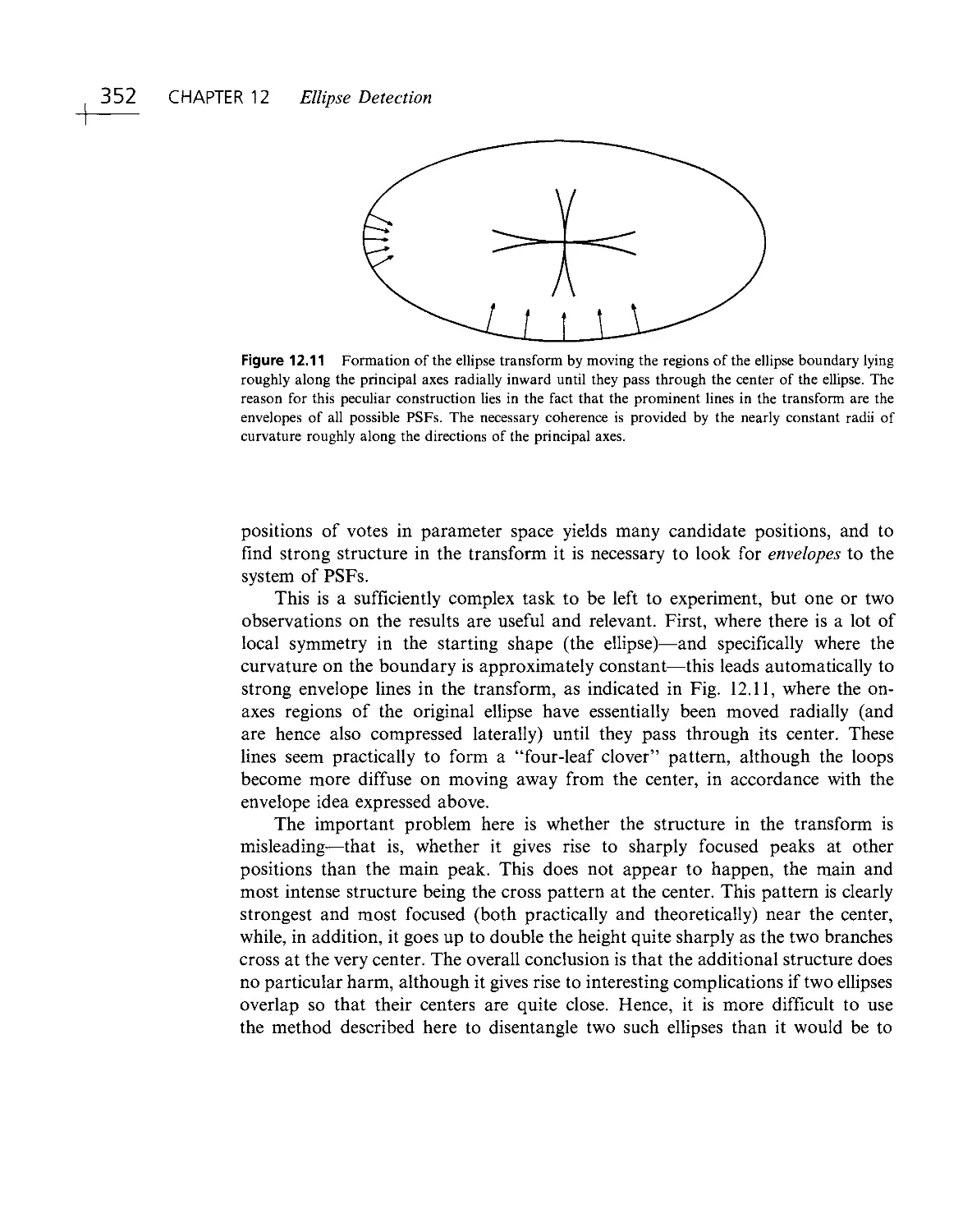
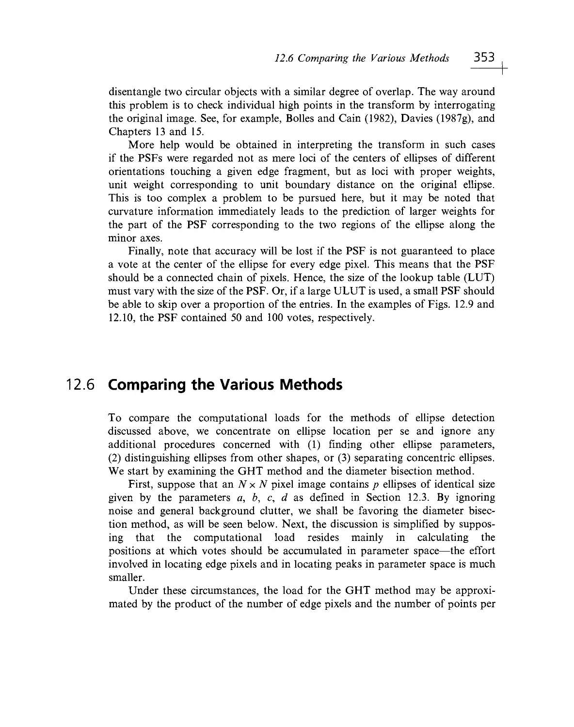
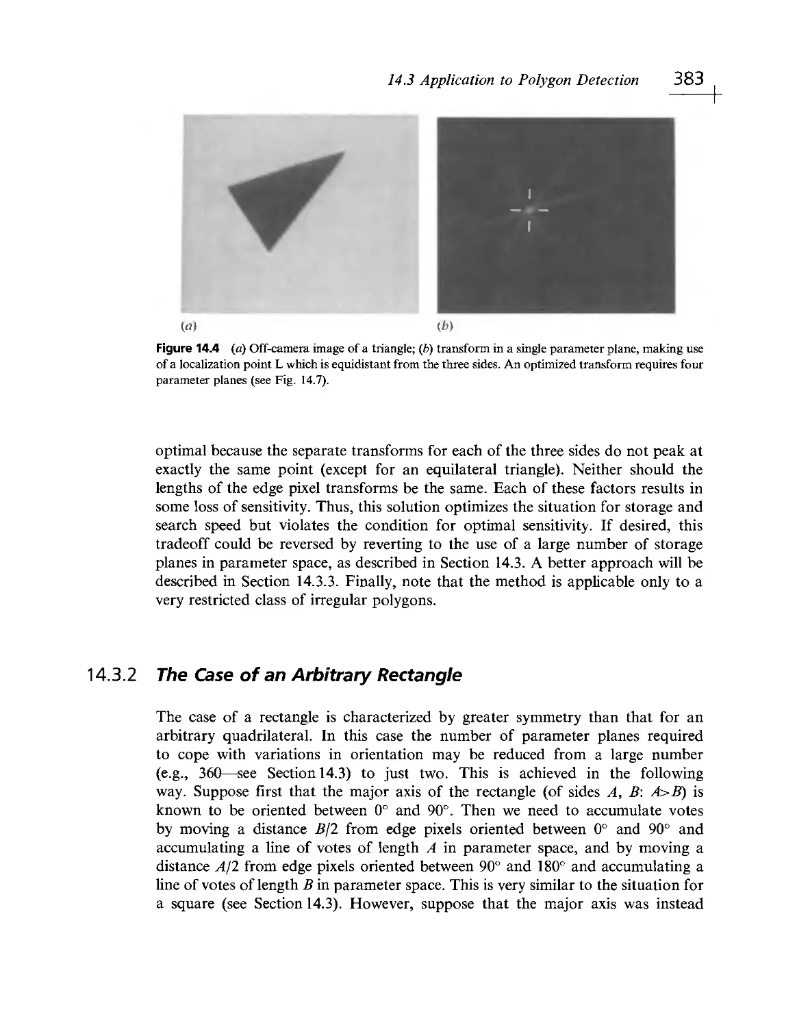
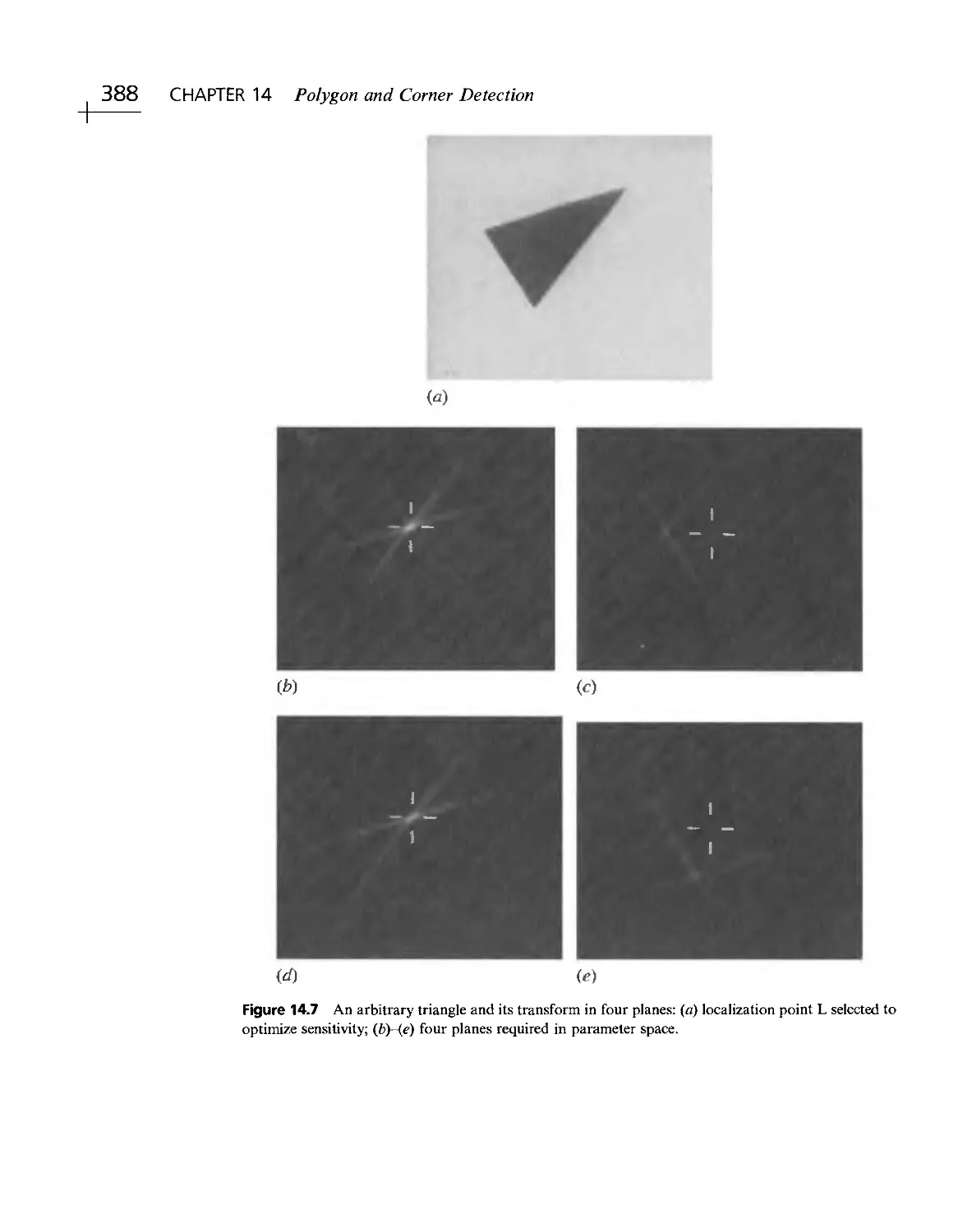
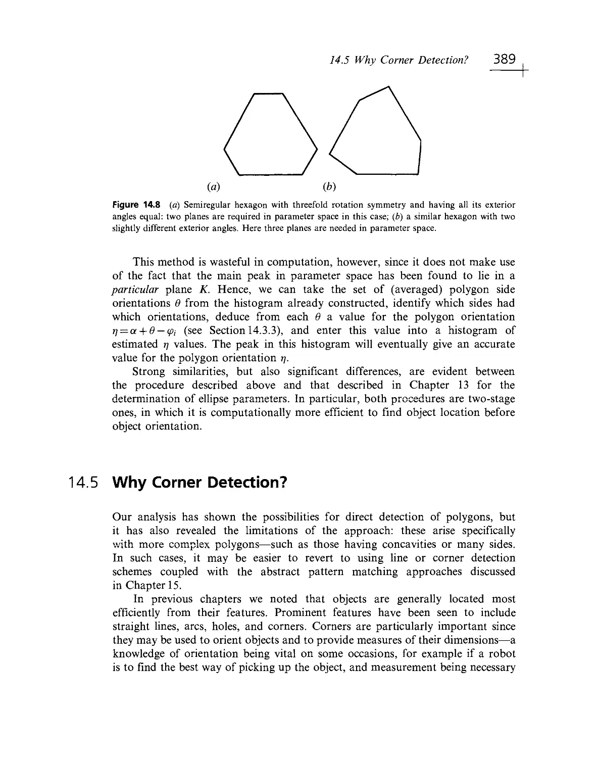
10.4- 10.14, 11.1, 11.3- 11.11, 12.5- 12.11, 13.1- 13.5, 14.1- 14.3, 14.6, 14.7, 14.8,
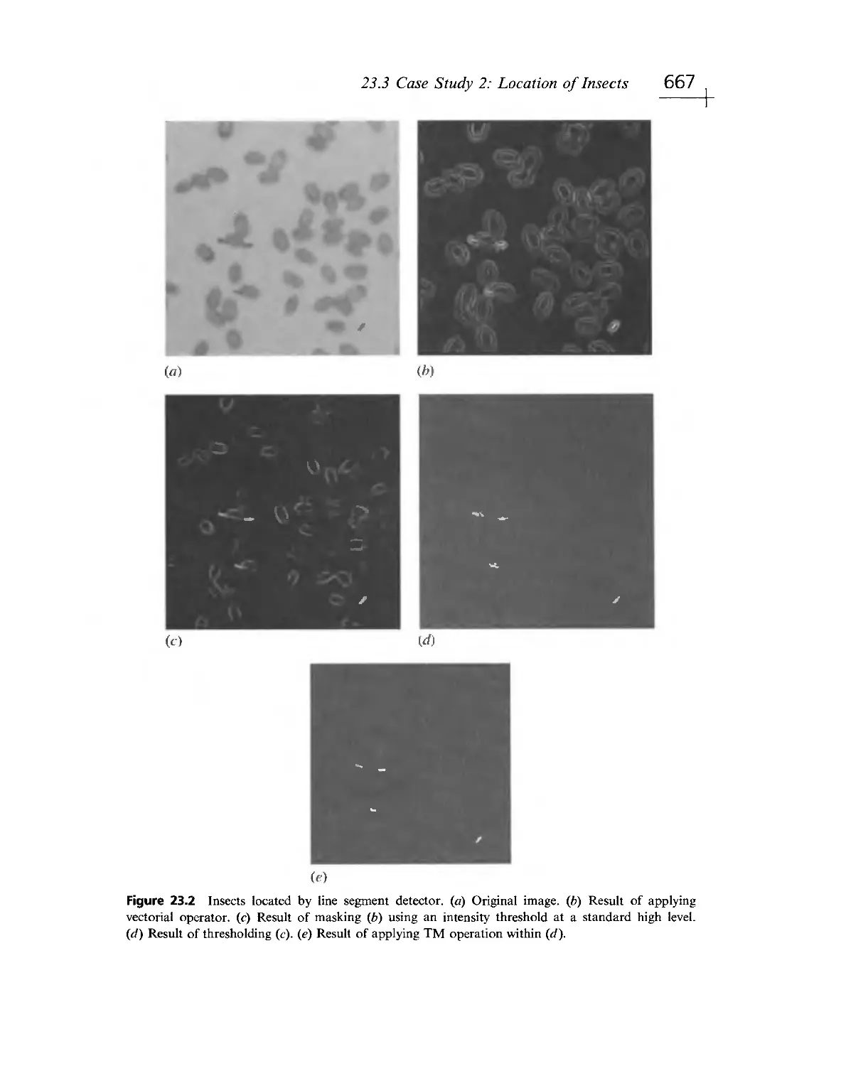
15.8, 23.2, 23.5:
Davies, E.R. (1986a, c, 1987c, d, g, k, l, 1988b, c, e, f, 1989 a- d).
Portions of the following papers from Image and Vision Computing as text in
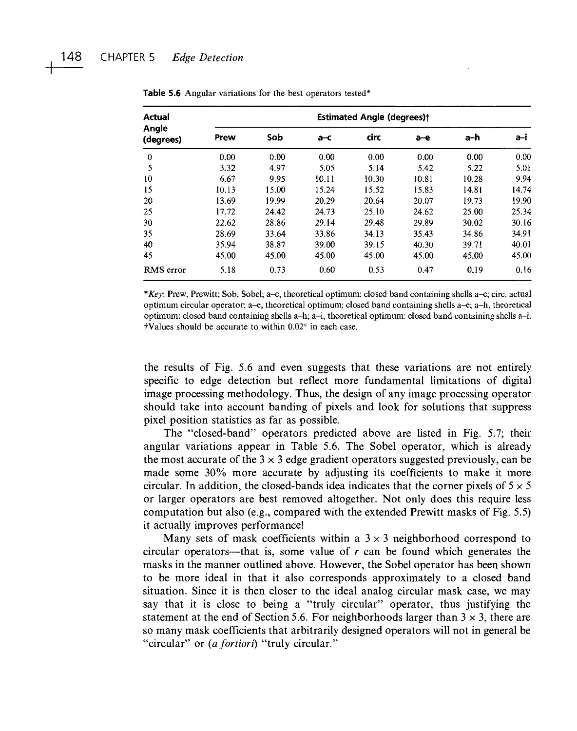
Chapter 5, as Tables 5.4, 5.5, 5.6 and as Figs. 3.33, 5.1, 5.5, 5.6, 5.7:
Davies, E.R. (1984b, 1987e)
Figures 5, 9; and about 10% of the text in the following paper:
Davies, E.R., Bateman, M., Mason, D.R., Chambers, J. and Ridgway, C.
(2003). "Design of efficient line segment detectors for cereal grain
inspection." Pattern Recogn. Lett., 24, nos. 1- 3, 421- 436.
Figure 4 of the following article:
Davies, E.R. (1987) "Visual inspection, automatic (robotics)", in
Encyclopedia of Physical Science and Technology, Vol. 14, Academic Press,
pp. 360- 377.
XXIX
XXX Acknowledgments
About 4% of the text in the following paper:
Davies, E.R. (2003). "An analysis of the geometric distortions produced by
median and related image processing filters." Advances in Imaging and
Electron Physics, 126, Academic Press, pp. 93- 193.
The above five items reprinted with permission from Elsevier.
lEE for permission to reprint portions of the following papers from the lEE
Proceedings and Colloquium Digests as text in Chapters 14, 22, 25, and as Figs.
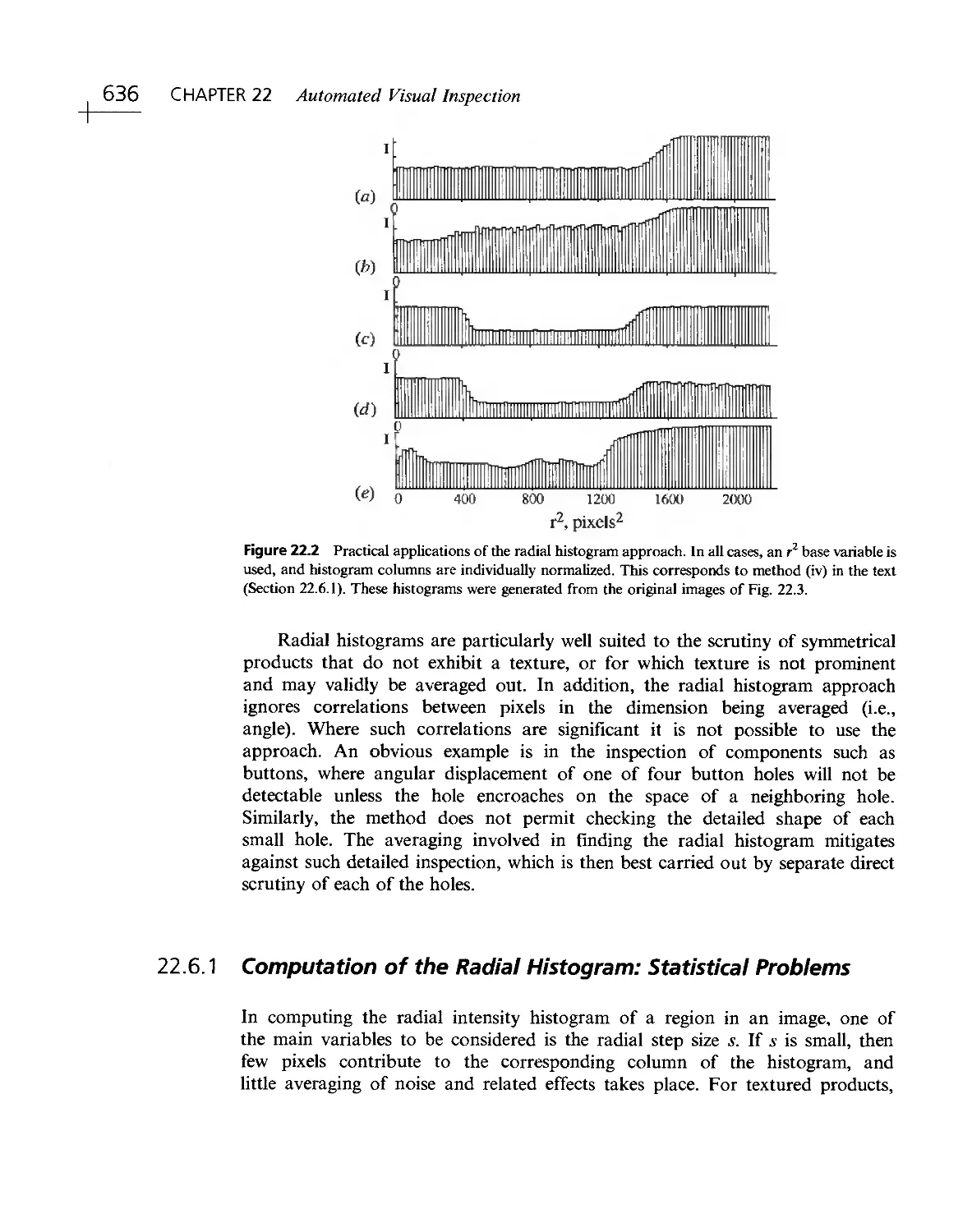
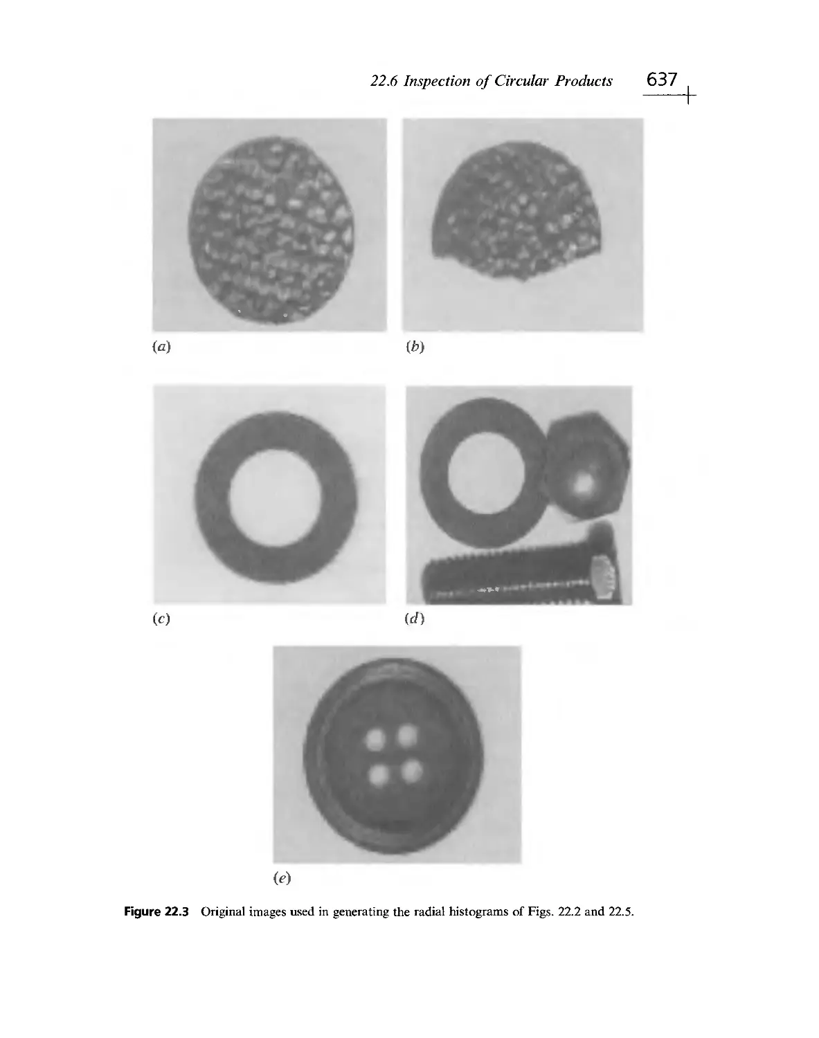
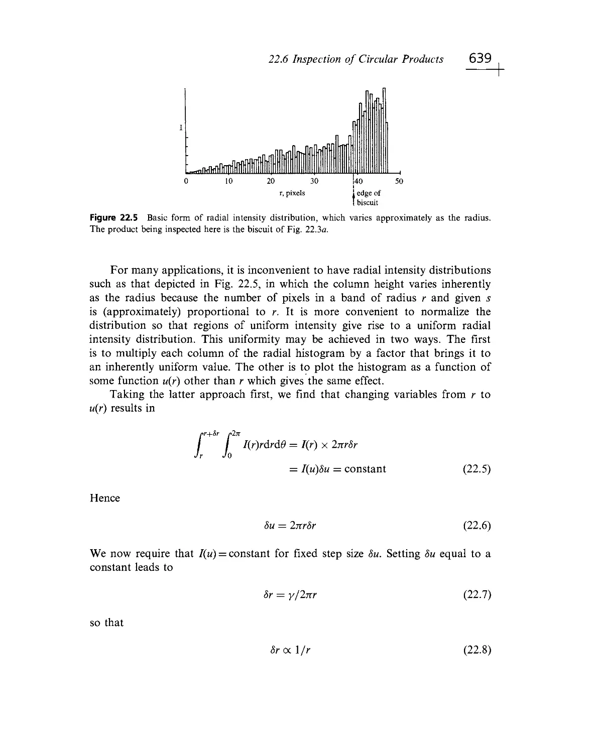
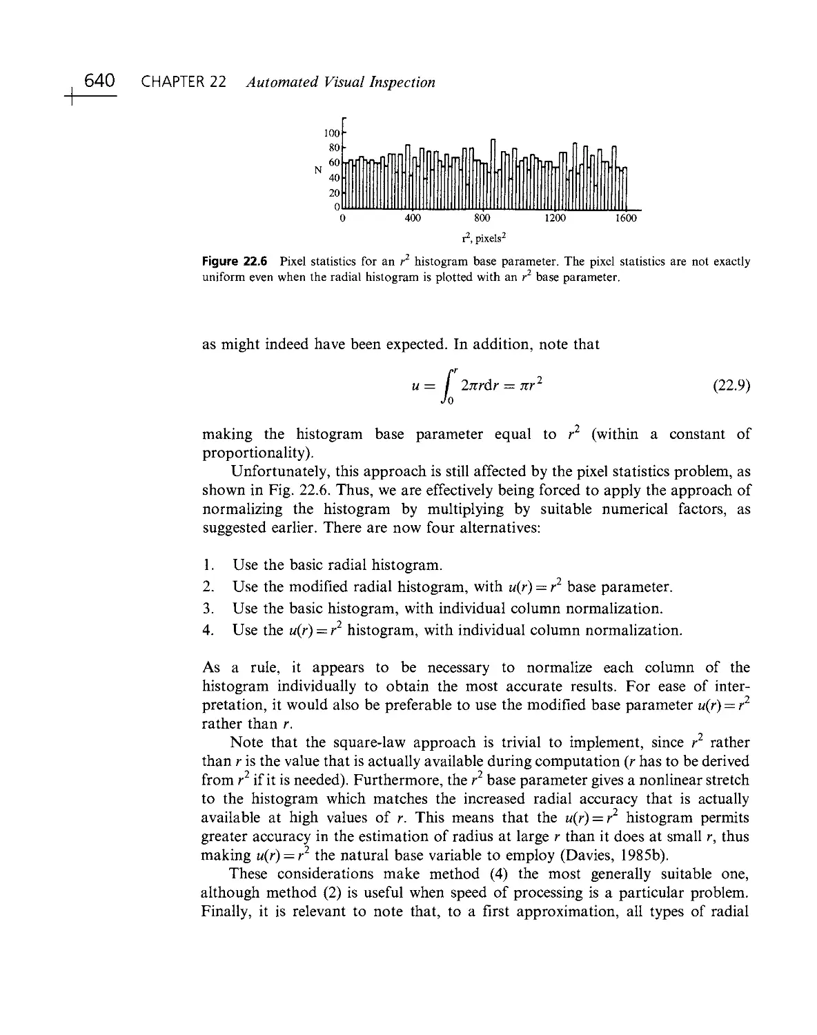
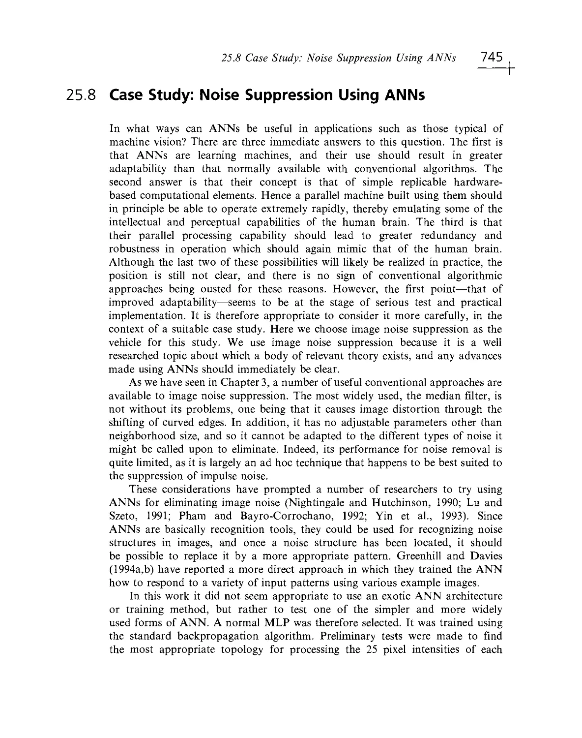
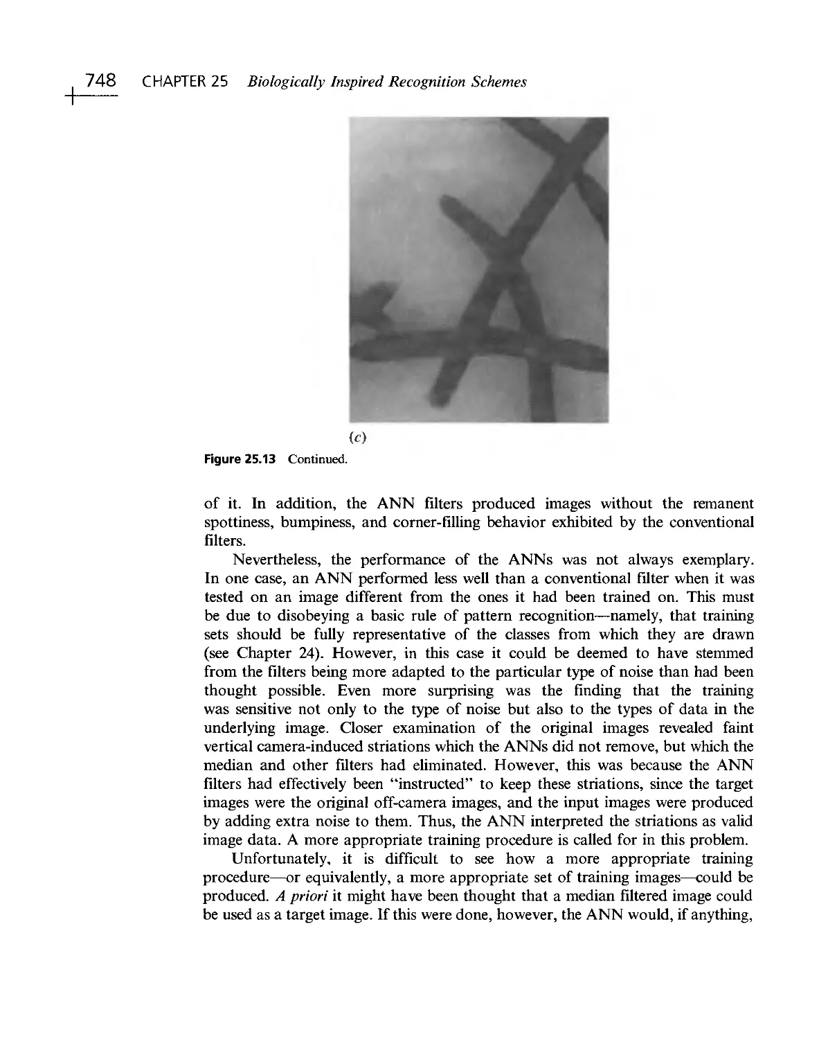
14.13- 14.15, 22.2- 22.6, 25.13:
Davies, E.R. (1985b, 1988a)
Davies, E.R. and Johnstone, A.I.C. (1989)
Greenhill, D. and Davies, E.R. (1994b)
and
Figures 1- 5; and about 44% of the text in the following paper:
Davies, E.R. (1997). Principles and design graphs for obtaining uniform
illumination in automated visual inspection. Proc. 6th lEE Int. Conf. on
Image Processing and its Applications, Dublin (14- 17 July), lEE Conf
Publication no. 443, pp. 161- 165.
Table 1; and about 95% of the text in the following paper:
Davies, E.R. (1997). Algorithms for inspection: constraints, tradeoffs and the
design process. lEE Digest no. 1997/041, Colloquium on Industrial
Inspection, lEE (10 Feb.), pp. 6/1- 5.
Figure 1; and about 35% of the text in the following paper:
Davies, E.R., Bateman, M., Chambers, J. and Ridgway, С (1998). Hybrid
non- linear filters for locating speckled contaminants in grain. lEE Digest no.
1998/284, Colloquium on Non- Linear Signal and Image Processing, lEE (22
May), pp. 12/1- 5.
Table 1; Figures 4- 8; and about 15% of the text in the following paper:
Davies, E.R. (1999). Image distortions produced by mean, median and mode
filters. lEE Proc. Vision Image Signal Processing, 146, no. 5, 279- 285.
Figure 1; and about 45% of the text in the following paper:
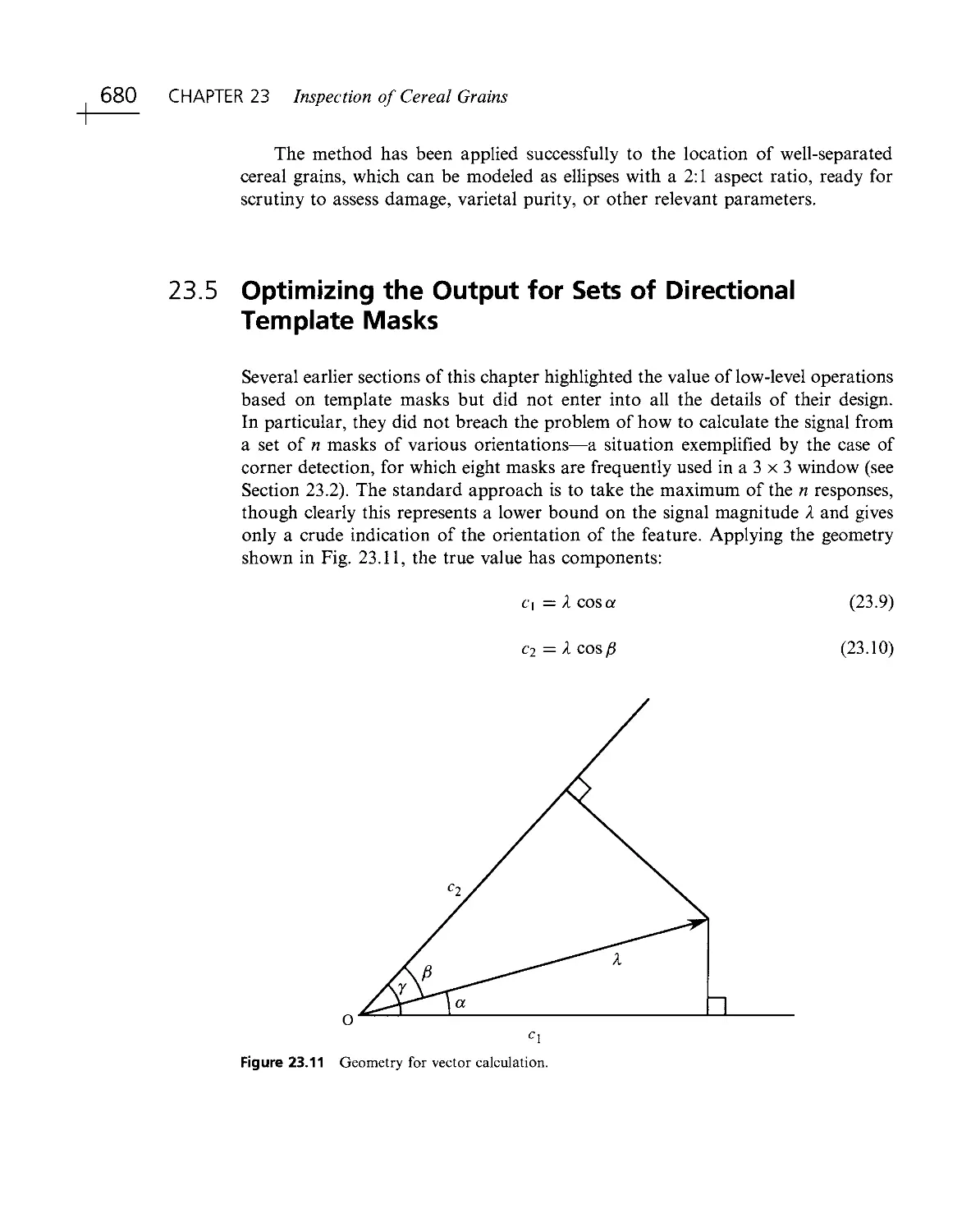
Davies, E.R. (2000). Obtaining optimum signal from set of directional
template masks. Electronics Lett., 36, no. 15, 1271- 1272.
Acknowledgments XXXI
Figures 1- 3; and about 90% of the text in the following paper:
Davies, E.R. (2000). Resolution of problem with use of closing for texture
segmentation. Electronics Lett., 36, no. 20, 1694- 1696.
IEEE for permission to reprint portions of the following paper as text in Chapter
14 and as Figs. 3.5, 3.6, 3.8, 3.12, 14.4, 14.5:
Davies, E.R. (1984a, 1986d).
IFS Publications Ltd for permission to reprint portions of the following paper
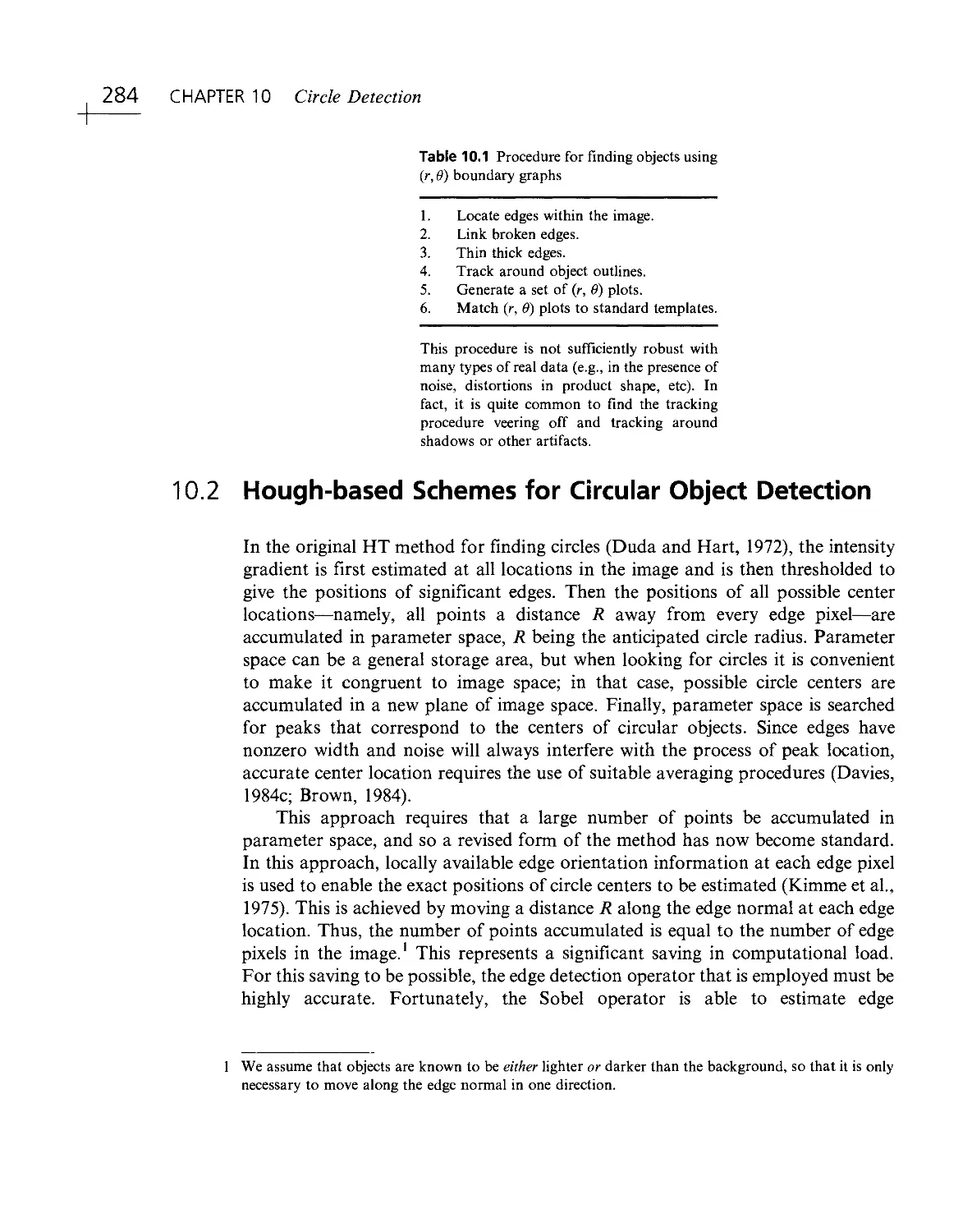
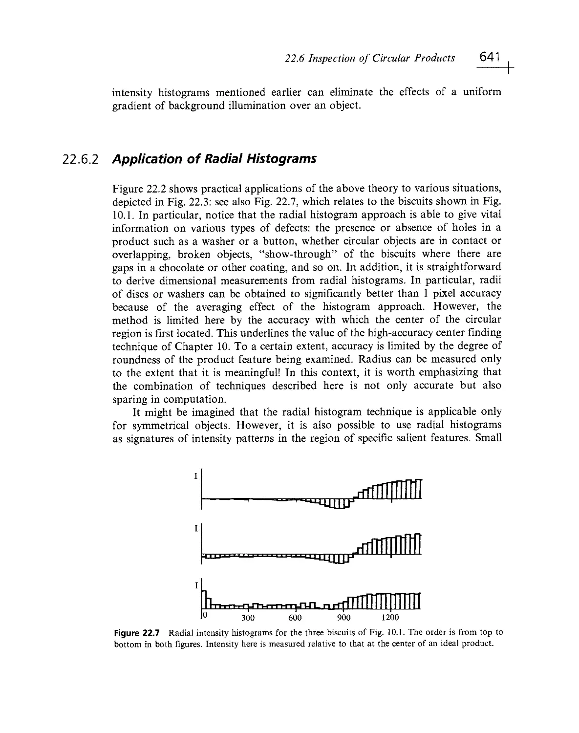
as text in Chapter 22 and as Figs. 10.1, 10.2, 22.7:
Davies, E.R. (1984c).
The Council of the Institution of Mechanical Engineers for permission to reprint
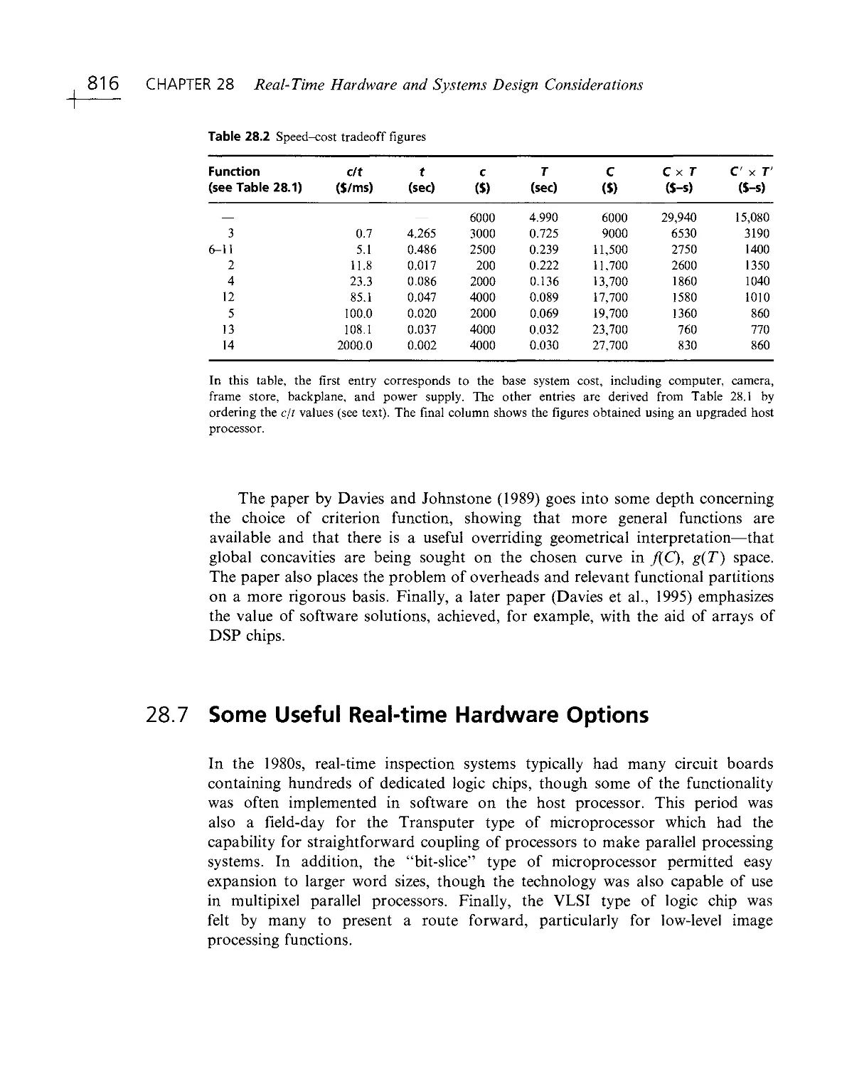
portions of the following paper as Tables 28.1, 28.2:
Davies. E.R. and Johnstone, A.I.C. (1986).
MCB University Press (Emerald Group) for permission to reproduce Plate 1 of
the following paper as Fig. 22.8:
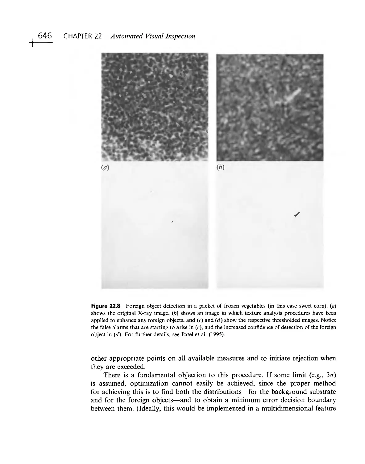
Patel, D., Davies, E.R. and Hannah, I. (1995).
Pergamon (Elsevier Science Ltd) for permission to reprint portions of the
following articles as text in Chapters 6, 7 and as Figs. 3.16, 6.7, 6.24:
Davies, E.R. and Plummer, A.P.N. (1981).
Davies, E.R. (1982).
Royal Swedish Academy of Engineering Sciences for permission to reprint portions
of the following paper as text in Chapter 22 and as Fig. 7.4:
Davies, E.R. (19871).
World Scientific for permission to reprint:
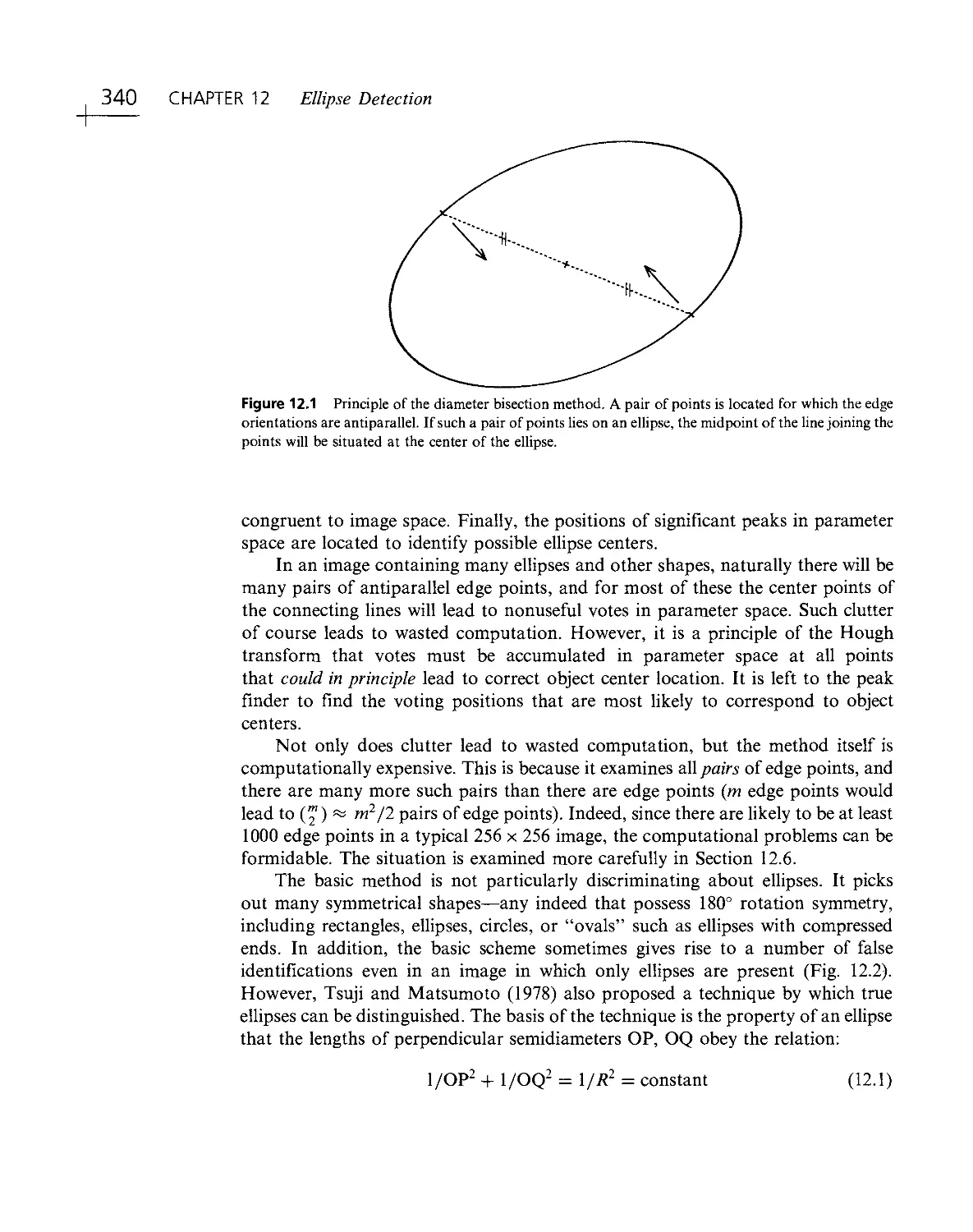
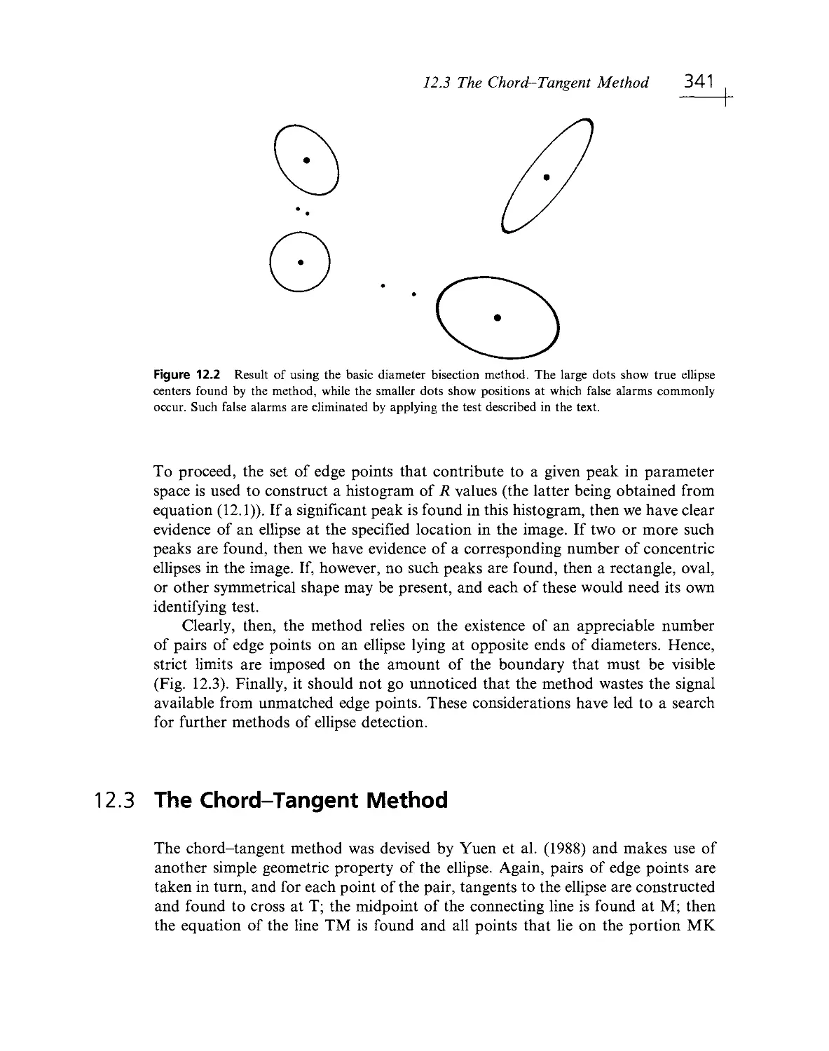
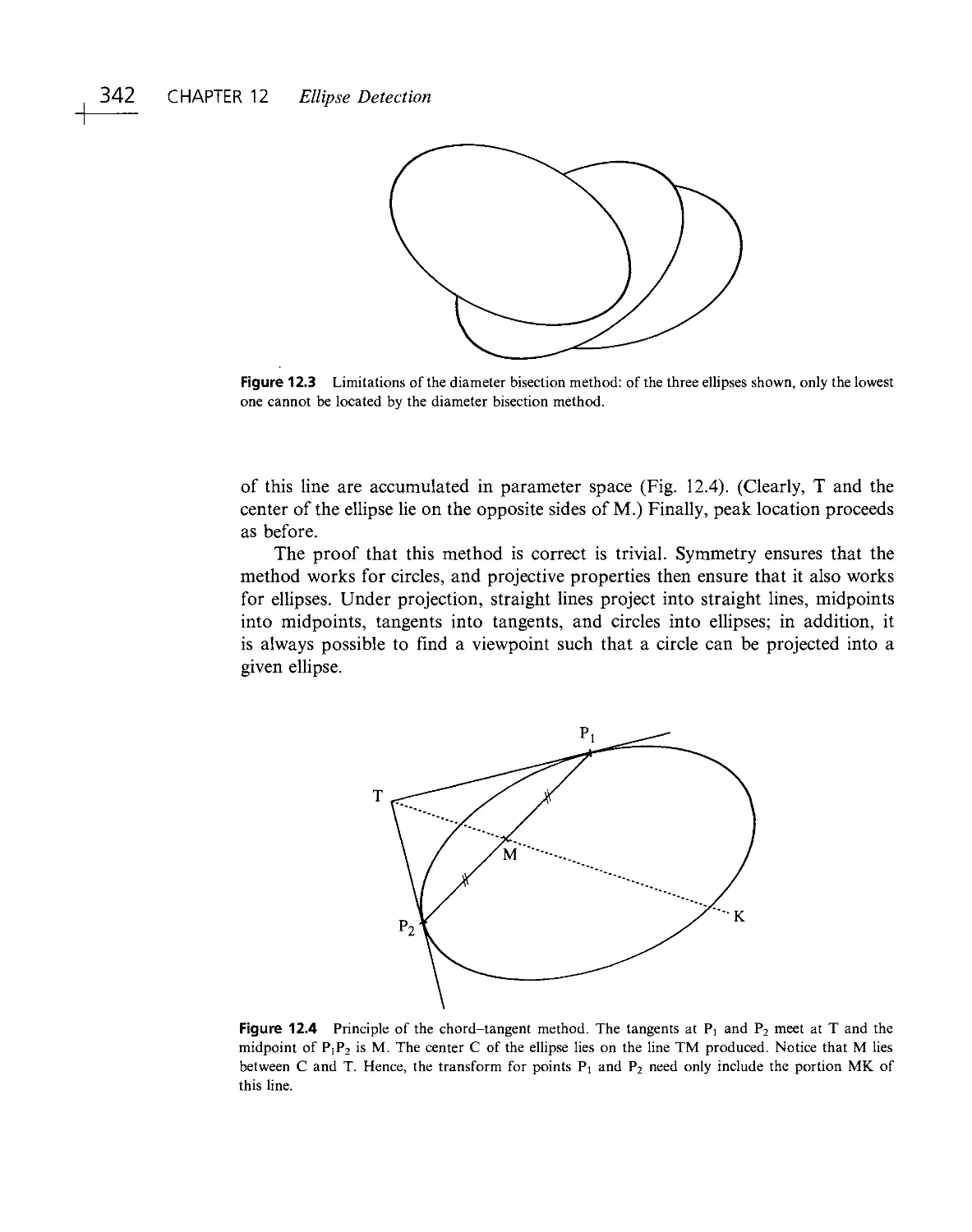
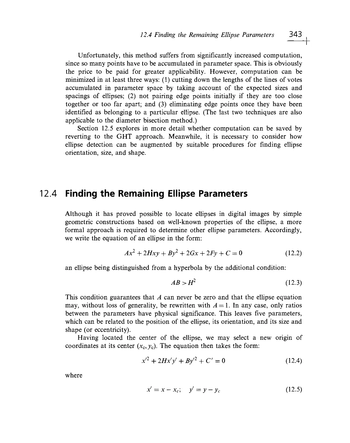
Figures 2.7(a, b), 3.4- 3.6, 10.4, 12.1- 12.3, 14.1; plus about 3 pp. of text extracted
from p. 49 et seq; about 1 p. of text extracted from p. 132 et seq; about 2 pp. of text
extracted from p. 157 et seq; about 3 pp. of text extracted from p. 187 et seq; about
7 pp. of text extracted from p. 207 et seq; about 3 pp. of text extracted from p. 219
et seq, in the following book:
Davies, E.R. (2000). Image Processing for the Food Industry.
in all cases excluding text which originated from earlier publications
XXXii Acknowledgments
The Royal Photographic Society for permission to reprint:
Table 1; figures 1, 2, 7, 9; and about 40% of the text in the following paper:
Davies, E.R. (2000). A generalized model of the geometric distortions
produced by rank- order filters. Imaging Science Journal, 48, no. 3, 121- 130.
Figures 4(b, e, h), 5(b), 14(a, b, c) in the following paper:
Charles, D. and Davies, E.R. (2004). Mode filters and their effectiveness for
processing colour images. Imaging Science Journal, 52, no. 1, 3- 25.
EURASIP for permission to reprint:
Figures 1- 7; and about 65% of the text in the following paper:
Davies, E.R. (1998). Rapid location of convex objects in digital images.
Proc. EUSIPCO'98, Rhodes, Greece (8- 11 Sept.), pp. 589- 592.
Figure 1; and about 30% of the text in the following paper:
Davies, E.R., Mason, D.R., Bateman, M., Chambers, J. and Ridgway, С
(1998). Linear feature detectors and their application to cereal inspection.
Proc. EUSIPCO'98, Rhodes, Greece (8- 11 Sept.), pp. 2561- 2564.
CRC Press for permission to reprint:
Table 1; Figures 8, 10, 12, 15- 17; and about 15% of the text in the following
chapter:
Davies (2003): Chapter 7 in Cho, H. (ed.) (2003). Opto- Mechatronic Systems
Handbook.
Springer- Verlag for permission to reprint:
about 4% of the text in the following chapter:
Davies, E.R. (2003). Design of object location algorithms and their use for
food and cereals inspection. Chapter 15 in Graves, M. and Batchelor, E.G.
(eds.) (2003). Machine Vision Techniques for Inspecting Natural Products,
393- 420.
Unicom Seminars Ltd. for permission to reprint:
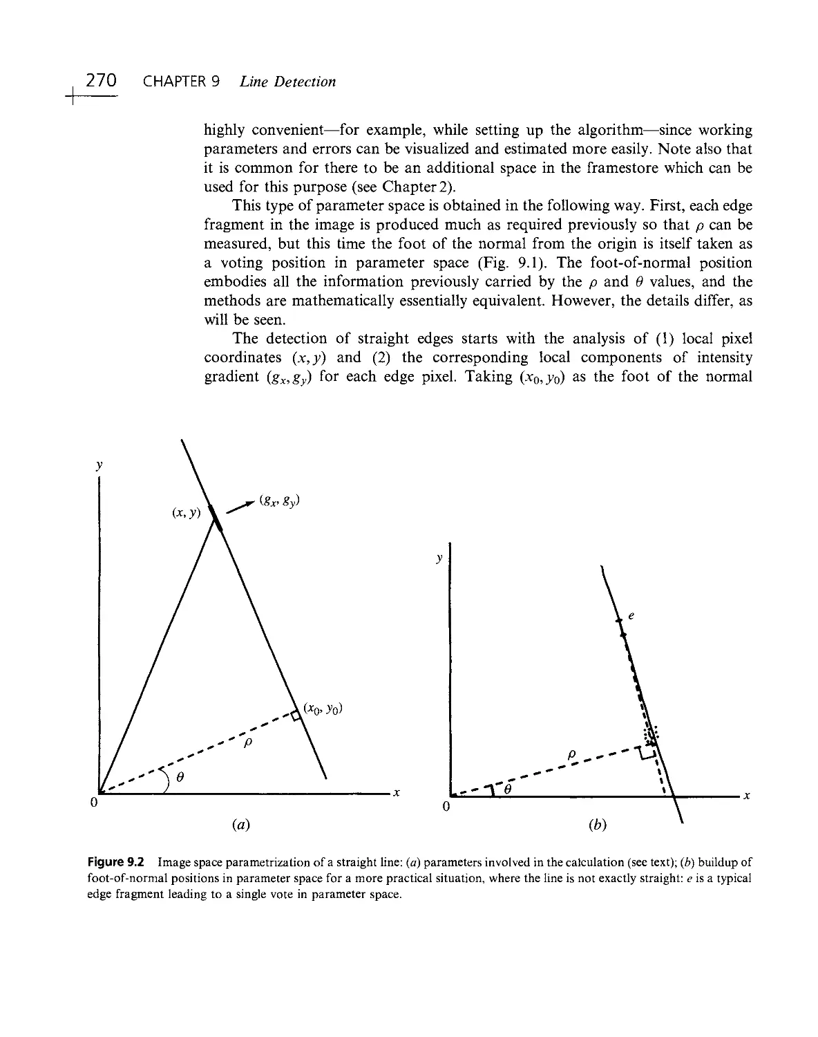
Portions of the following paper as text in Chapter 22 and as Figs. 9.2, 10.3, 12.3,
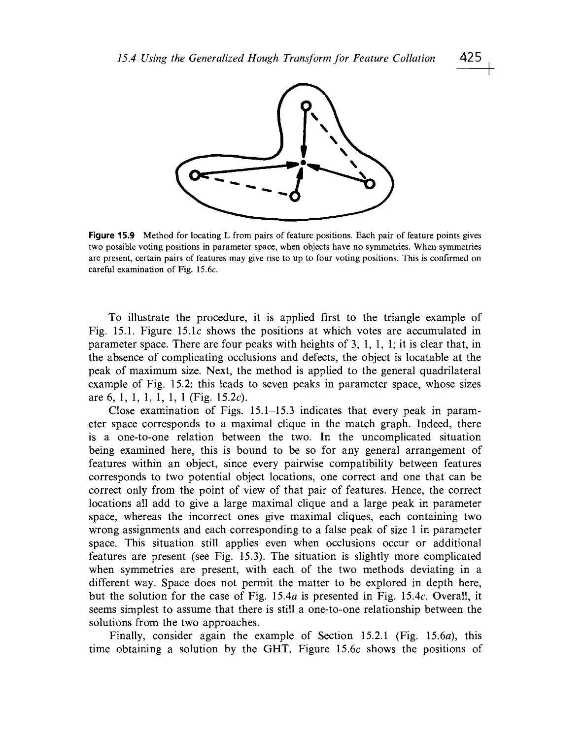
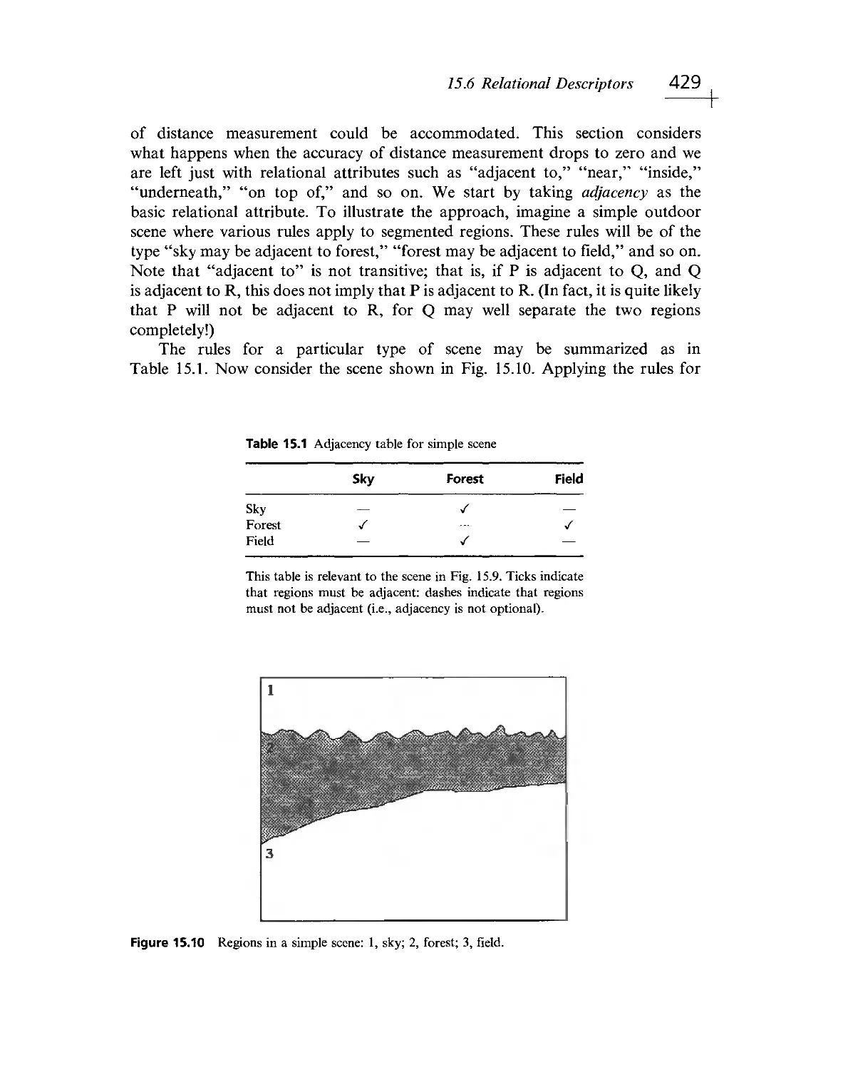
14.15, 15.9:
Davies, E.R. (1988h).
Acknowledgments XXXii
Royal Hollow ay, University of London for permission to reprint:
Extracts from the following examination questions, written by E.R. Davies:
EL333/01/2, 4- 6; EL333/98/2; EL333/99/2, 3, 5, 6; EL385/97/2; PH4760/04/
1- 5; PH5330/98/3, 5; PH5330/03/1- 5.
University of London for permission to reprint:
Extracts from the following examination questions, written by E.R. Davies:
PH385/92/2, 3; PH385/93/1- 3; PH385/94/1- 4; PH385/95/4; PH385/96/3, 6;
PH433/94/3, 5; PH433/96/2, 5.
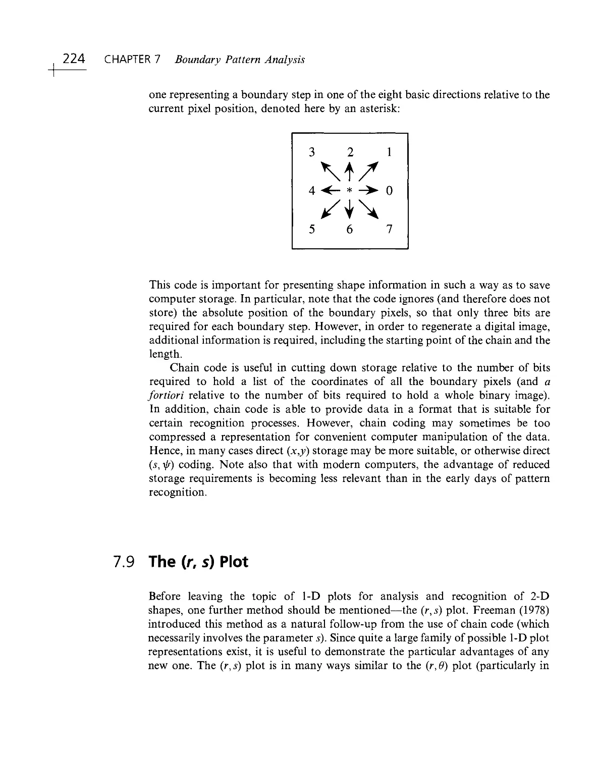
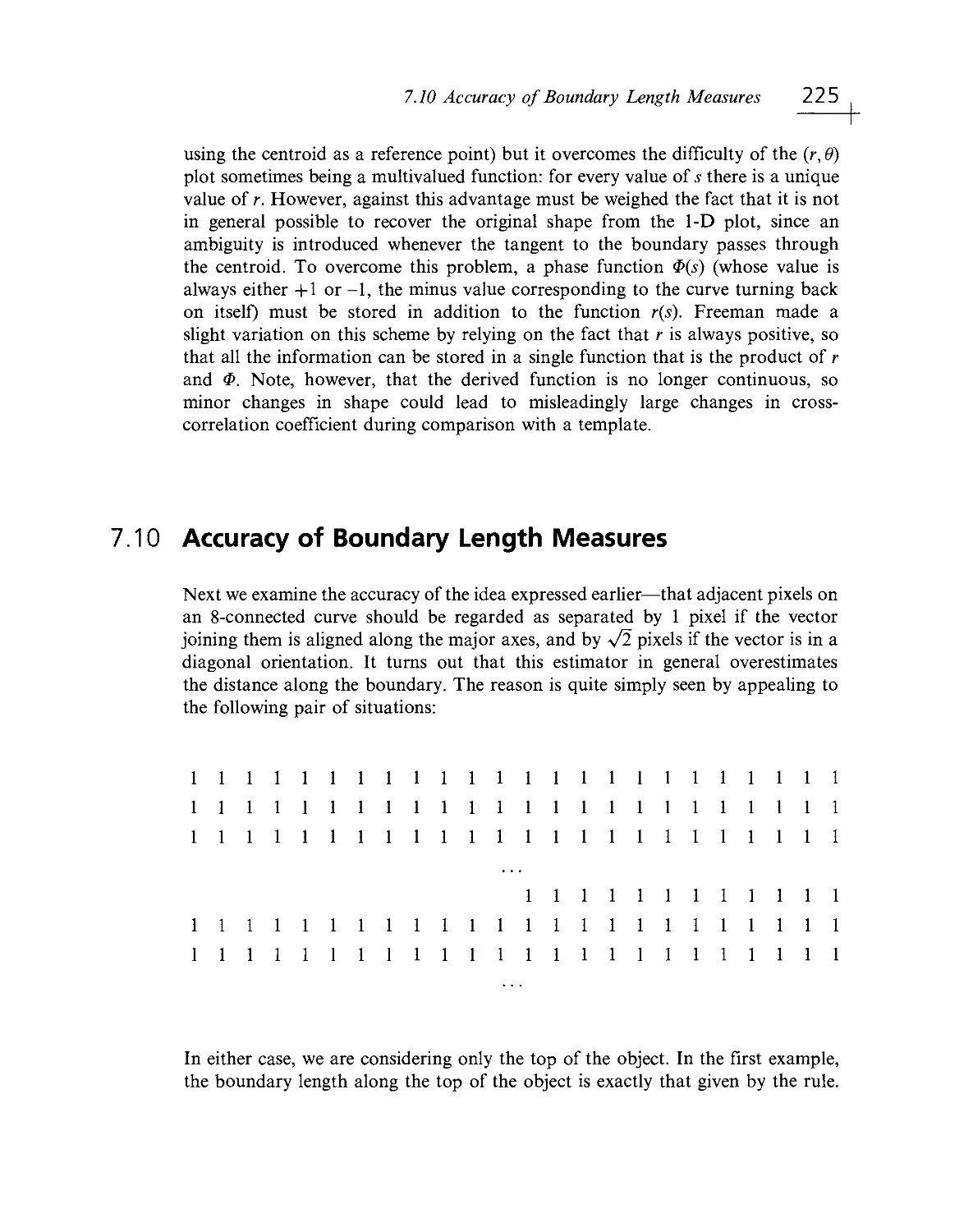
CHAPTER 1
Vision, the Challenge
1.1 Introduction— The Senses
Of the five senses— vision, hearing, smell, taste, and touch— vision is undoubtedly
the one that we have come to depend upon above ail others, and indeed the one
that provides most of the data we receive. Not only do the input pathways from
the eyes provide megabits of information at each glance, but the data rate for
continuous viewing probably exceed 10 megabits per second. However, much of
this information is redundant and is compressed by the various layers of the visual
cortex, so that the higher centers of the brain have to interpret abstractly only a
small fraction of the data. Nonetheless, the amount of information the higher
centers receive from the eyes must be at least two orders of magnitude greater than
all the information they obtain from the other senses.
Another feature of the human visual system is the ease with which
interpretation is carried out. We see a scene as it is— trees in a landscape, books
on a desk, widgets in a factory. No obvious deductions are needed, and no overt
effort is required to interpret each scene. In addition, answers are effectively
immediate and are normally available within a tenth of a second. Just now and
again some doubt arises— for example, a wire cube might be "seen" correctly or
inside out. This and a host of other optical illusions are well known, although for
the most part we can regard them as curiosities— irrelevant freaks of nature.
Somewhat surprisingly, it turns out that illusions are quite important, since they
reflect hidden assumptions that the brain is making in its struggle with the huge
amounts of complex visual data it is receiving. We have to bypass this topic here
(though it surfaces now and again in various parts of this book). However, the
important point is that we are for the most part unaware of the complexities of
vision. Seeing is not a simple process: it is just that vision has evolved over millions
of years, and there was no particular advantage in evolution giving us any
indication of the difficulties of the task. (If anything, to have done so would have
cluttered our minds with worthless information and quite probably slowed our
reaction times in crucial situations.)
CHAPTER 1 Vision, the Challenge
Thus, ignorance of the process of human vision abounds. However, being by
nature inventive, the human species is now trying to get machines to do much of
its work. For the simplest tasks there should be no particular difficulty in
mechanization, but for more complex tasks the machine must be given our
prime sense, that of vision. Efforts have been made to achieve this, sometimes in
modest ways, for well over 30 years. At first such tasks seemed trivial, and schemes
were devised for reading, for interpreting chromosome images, and so on. But
when such schemes were challenged with rigorous practical tests, the problems
often turned out to be more difficult. Generally, researchers react to their discovery
that apparent "trivia" are getting in the way by intensifying their efforts and
applying great ingenuity. This was certainly the case with some early efforts at
vision algorithm design. Hence, it soon became plain that the task is a complex
one, in which numerous fundamental problems confront the researcher, and the
ease with which the eye can interpret scenes has turned out to be highly deceptive.
Of course, one way in which the human visual system surpasses the machine is
that the brain possesses some 10'° cells (or neurons), some of which have well over
10, 000 contacts (or synapses) with other neurons. If each neuron acts as a type of
microprocessor, then we have an immense computer in which all the processing
elements can operate concurrently. Probably, the largest single man- made
computer still contains less than 100 million processing elements, so the majority
of the visual and mental processing tasks that the eye- brain system can perform in
a flash have no chance of being performed by present- day man- made systems.
Added to these problems of scale is the problem of how to organize such a large
processing system and how to program it. Clearly, the eye- brain system is partly
hard- wired by evolution, but there is also an interesting capability to program it
dynamically by training during active use. This need for a large parallel processing
system with the attendant complex control problems clearly illustrates that
machine vision must indeed be one of the most difficult intellectual problems
to tackle.
So what are the problems involved in vision that make it apparently so easy
for the eye and yet so difficult for the machine? In the next few sections we attempt
to answer this question.
1.2 The Nature of Vision
1.2.1 The Process of Recognition
This section illustrates the intrinsic difficulties of implementing machine vision,
starting with an extremely simple example— that of character recognition. Consider
the set of patterns shown in Fig. 1.1a. Each pattern can be considered as a set of
1.2 The Nature of Vision
Щ.
Ф)
(4) (5> (6)
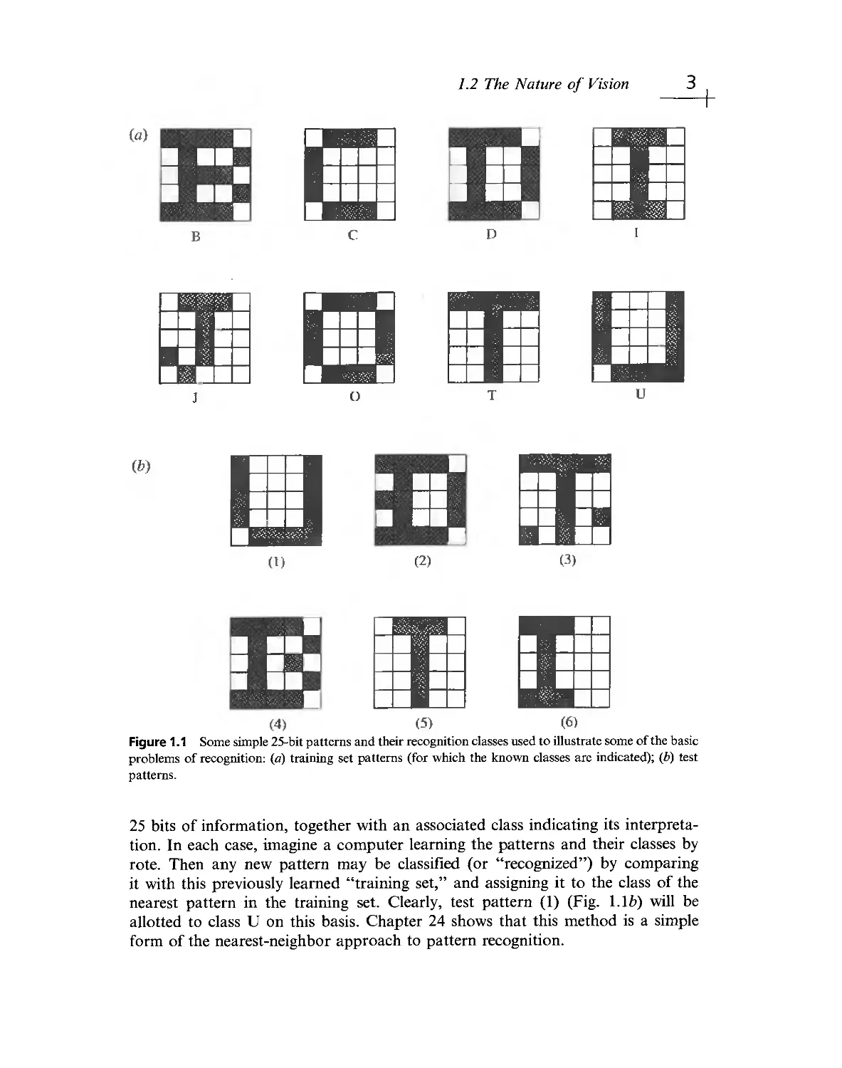
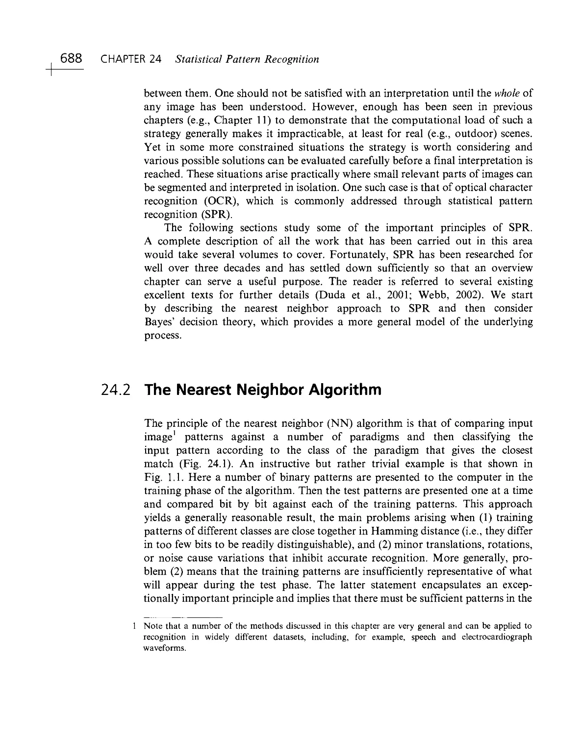
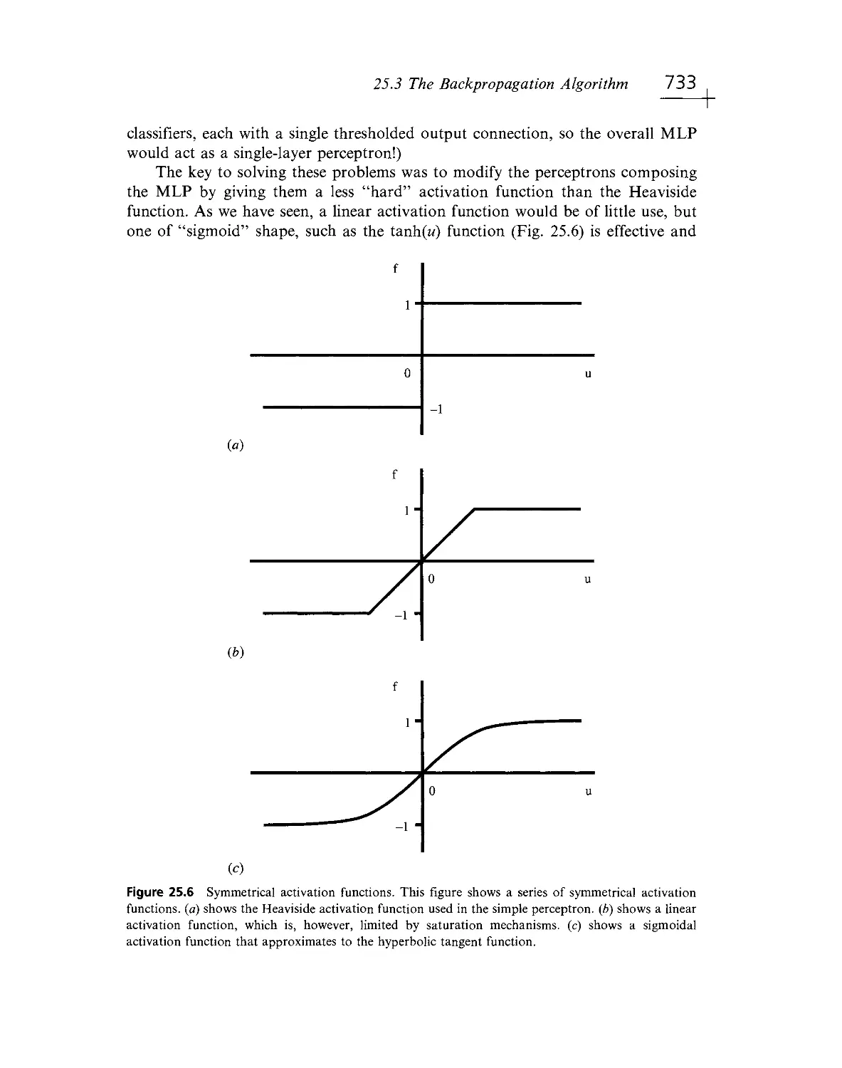
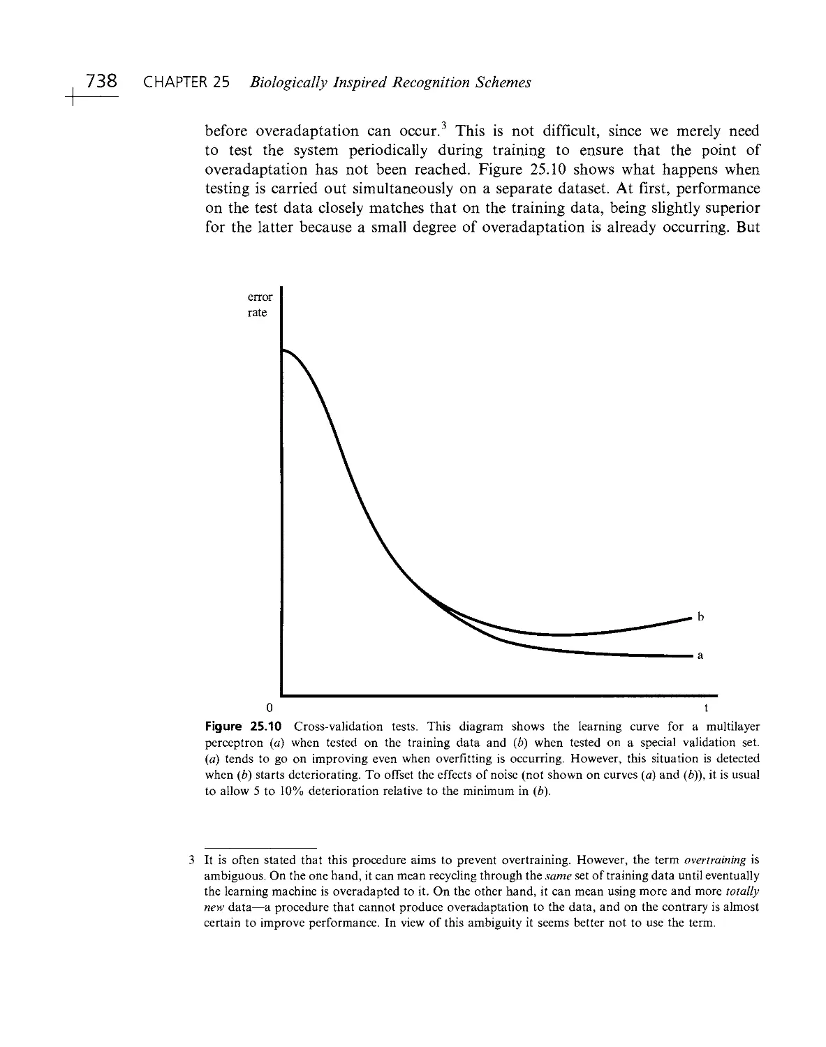
Figure 1.1 Some simple 25- bit patterns and tlieir recognition classes used to illustrate some of the basic
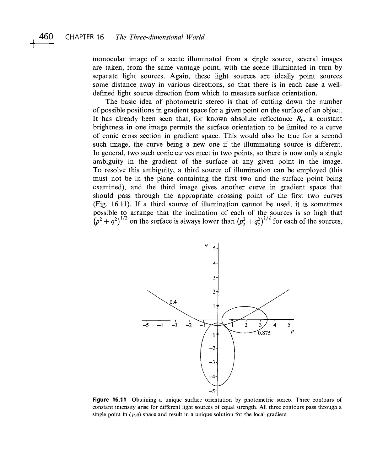
problems of recognition; (a) training set patterns (for whicli the known classes are indicated); (b) test
patterns.
25 bits of information, together with an associated class indicating its
interpretation. In each case, imagine a computer learning the patterns and their classes by
rote. Then any new pattern may be classified (or "recognized") by comparing
it with this previously learned "training set, " and assigning it to the class of the
nearest pattern in the training set. Clearly, test pattern (1) (Fig. I ЛЬ) will be
allotted to class U on this basis. Chapter 24 shows that this method is a simple
form of the nearest- neighbor approach to pattern recognition.
CHAPTER 1 Vision, the Challenge
The scheme we have outhned in Fig. 1.1 seems straightforward and is indeed
highly effective, even being able to cope with situations where distortions of the test
patterns occur or where noise is present: this is illustrated by test patterns (2) and
(3). However, this approach is not always foolproof. First, in some situations
distortions or noise is so excessive that errors of interpretation arise. Second,
patterns may not be badly distorted or subject to obvious noise and, yet, are
misinterpreted: this situation seems much more serious, since it indicates an
unexpected limitation of the technique rather than a reasonable result of noise or
distortion. In particular, these problems arise where the test pattern is displaced or
erroneously oriented relative to the appropriate training set pattern, as with test
pattern (6).
As will be seen in Chapter 24, a powerful principle is operative here, indicating
why the unlikely limitation we have described can arise: it is simply that there are
insufficient training set patterns and that those that are present are insufficiently
representative of what will arise during tests. Unfortunately, this presents a major
difficulty inasmuch as providing enough training set patterns incurs a serious
storage problem, and an even more serious search problem when patterns are
tested. Furthermore, it is easy to see that these problems are exacerbated as
patterns become larger and more real. (Obviously, the examples of Fig. 1.1 are far
from having enough resolution even to display normal type fonts.) In fact, a
combinatorial explosion' takes place. Forgetting for the moment that the patterns
of Fig. 1.1 have familiar shapes, let us temporarily regard them as random bit
patterns. Now the number of bits in these N x Ж patterns is N'^, and the number of
possible patterns of this size is 2^: even in a case where N = 20, remembering all
these patterns and their interpretations would be impossible on any practical
machine, and searching systematically through them would take impracticably
long (involving times of the order of the age of the universe). Thus, it is not only
impracticable to consider such brute- force means of solving the recognition
problem, but also it is effectively impossible theoretically. These considerations
show that other means are required to tackle the problem.
1.2.2 Tackling the Recognition Problem
An obvious means of tackling the recognition problem is to normalize the images
in some way. Clearly, normalizing the position and orientation of any 2- D picture
object would help considerably. Indeed, this would reduce the number of degrees of
1 This is normally taken to mean that one or more parameters produce fast- varying (often exponential)
effects that "explode" as the parameters increase by modest amounts.
1.2 The Nature of Vision
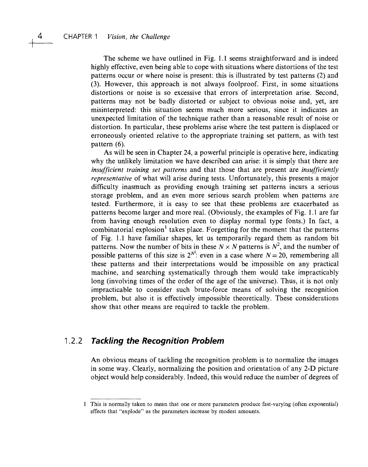
Figure 1.2 Use of thinning to regularize character shapes. Here character shapes of different Hmb
widths— or even varying limb widths— are reduced to stick figures or skeletons. Thus, irrelevant
information is removed, and at the same time recognition is facilitated.
freedom by three. Methods for achieving this involve centralizing the objects—
arranging that their centroids are at the center of the normalized image— and
making their major axes (deduced by moment calculations, for example) vertical or
horizontal. Next, we can make use of the order that is known to be present in the
image— and here it may be noted that very few patterns of real interest are
indistinguishable from random dot patterns. This approach can be taken further: if
patterns are to be nonrandom, isolated noise points may be eliminated. Ultimately,
all these methods help by making the test pattern closer to a restricted set of
training set patterns (although care has to be taken to process the training set
patterns initially so that they are representative of the processed test patterns).
It is useful to consider character recognition further. Here we can make
additional use of what is known about the structure of characters— namely, that
they consist of limbs of roughly constant width. In that case, the width carries
no useful information, so the patterns can be thinned to stick figures (called
skeletons— see Chapter 6). Then, hopefully, there is an even greater chance that the
test patterns will be similar to appropriate training set patterns (Fig. 1.2). This
process can be regarded as another instance of reducing the number of degrees of
freedom in the image, and hence of helping to minimize the combinatorial
explosion— or, from a practical point of view, to minimize the size of the training
set necessary for effective recognition.
Next, consider a rather different way of looking at the problem. Recognition
is necessarily a problem of discrimination— that is, of discriminating between
patterns of different classes. In practice, however, considering the natural variation
of patterns, including the effects of noise and distortions (or even the effects of
breakages or occlusions), there is also a problem of generalizing over patterns of
the same class. In practical problems a tension exists between the need to
discriminate and the need to generalize. Nor is this a fixed situation. Even for the
character recognition task, some classes are so close to others (n's and A's will be
similar) that less generalization is possible than in other cases. On the other hand,
extreme forms of generalization arise when, for example, an A is to be recognized
as an A whether it is a capital or small letter, or in italic, bold, or other form of
font— even if it is handwritten. The variability is determined largely by the training
set initially provided. What we emphasize here, however, is that generalization is
as necessary a prerequisite to successful recognition as is discrimination.
CHAPTER 1 Vision, the Challenge
G
R
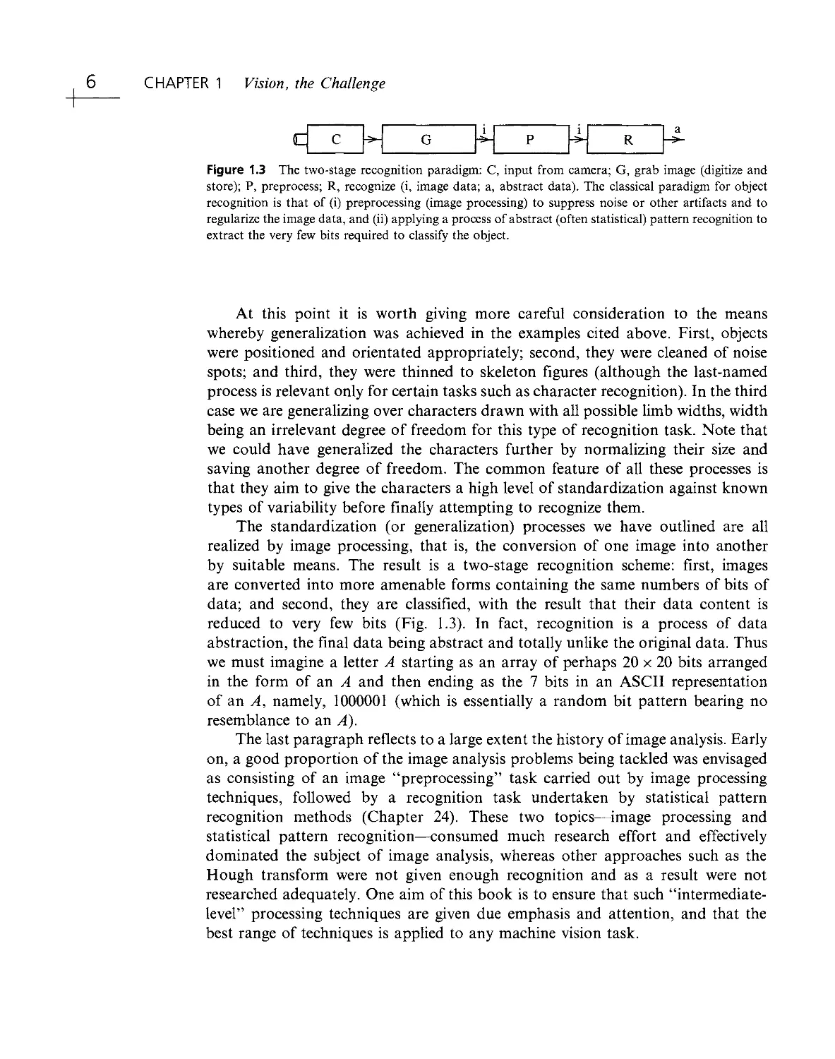
Figure 1.3 The two- stage recognition paradigm: C, input from camera; G, grab image (digitize and
store); P, preprocess; R, recognize (i, image data; a, abstract data). The classical paradigm for object
recognition is that of (i) preprocessing (image processing) to suppress noise or other artifacts and to
regularize the image data, and (ii) applying a process of abstract (often statistical) pattern recognition to
extract the very few bits required to classify the object.
At this point it is worth giving more careful consideration to the means
whereby generaUzation was achieved in the examples cited above. First, objects
were positioned and orientated appropriately; second, they were cleaned of noise
spots; and third, they were thinned to skeleton figures (although the last- named
process is relevant only for certain tasks such as character recognition). In the third
case we are generalizing over characters drawn with all possible limb widths, width
being an irrelevant degree of freedom for this type of recognition task. Note that
we could have generalized the characters further by normalizing their size and
saving another degree of freedom. The common feature of all these processes is
that they aim to give the characters a high level of standardization against known
types of variability before finally attempting to recognize them.
The standardization (or generalization) processes we have outlined are all
realized by image processing, that is, the conversion of one image into another
by suitable means. The result is a two- stage recognition scheme: first, images
are converted into more amenable forms containing the same numbers of bits of
data; and second, they are classified, with the result that their data content is
reduced to very few bits (Fig. 1.3). In fact, recognition is a process of data
abstraction, the final data being abstract and totally unlike the original data. Thus
we must imagine a letter A starting as an array of perhaps 20 x 20 bits arranged
in the form of an A and then ending as the 7 bits in an ASCII representation
of an A, namely, 1000001 (which is essentially a random bit pattern bearing no
resemblance to an A).
The last paragraph reflects to a large extent the history of image analysis. Early
on, a good proportion of the image analysis problems being tackled was envisaged
as consisting of an image "preprocessing" task carried out by image processing
techniques, followed by a recognition task undertaken by statistical pattern
recognition methods (Chapter 24). These two topics— image processing and
statistical pattern recognition— consumed much research effort and effectively
dominated the subject of image analysis, whereas other approaches such as the
Hough transform were not given enough recognition and as a result were not
researched adequately. One aim of this book is to ensure that such "intermediate-
level" processing techniques are given due emphasis and attention, and that the
best range of techniques is applied to any machine vision task.
1.2 The Nature of Vision
7
1, 2.3 Object Location
The problem tackled in the preceding section— that of character recognition— is a
highly constrained one. In many practical applications, it is necessary to search
pictures for objects of various types rather than just interpreting a small area of
a picture.
The search task can involve prodigious amounts of computation and is also
subject to a combinatorial explosion. Imagine the task of searching for a letter E'm
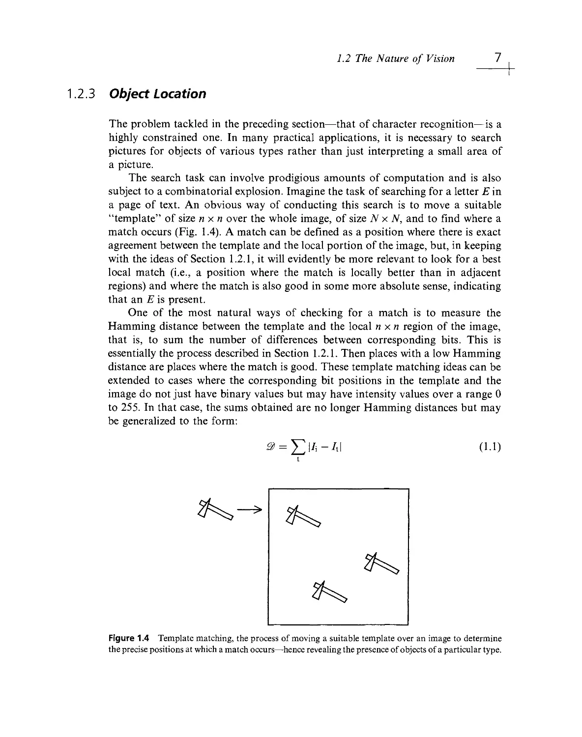
a page of text. An obvious way of conducting this search is to move a suitable
"template" of size nxn over the whole image, of size N x N, and to find where a
match occurs (Fig. 1.4). A match can be defined as a position where there is exact
agreement between the template and the local portion of the image, but, in keeping
with the ideas of Section 1.2.1, it will evidently be more relevant to look for a best
local match (i.e., a position where the match is locally better than in adjacent
regions) and where the match is also good in some more absolute sense, indicating
that an E is present.
One of the most natural ways of checking for a match is to measure the
Hamming distance between the template and the local n xn region of the image,
that is, to sum the number of differences between corresponding bits. This is
essentially the process described in Section 1.2.1. Then places with a low Hamming
distance are places where the match is good. These template matching ideas can be
extended to cases where the corresponding bit positions in the template and the
image do not just have binary values but may have intensity values over a range 0
to 255. In that case, the sums obtained are no longer Hamming distances but may
be generalized to the form:
= J2^i- iA
(1.1)
Figure 1.4 Template matching, the process of moving a suitable template over an image to determine
the precise positions at which a match occurs— hence revealing the presence of objects of a particular type.
8 CHAPTER 1 Vision, the Challenge
where Д is the local template value, I\ is the local image value, and the sum is
taken over the area of the template. This makes template matching practicable in
many situations; the possibilities are examined in more detail in subsequent
chapters.
We referred earlier to a combinatorial explosion in this search problem too.
The reason this arises is as follows. First, when a 5 x 5 template is moved over an
N X N image in order to look for a match, the number of operations required is of
the order of 5^Ж^, totaling some 1 million operations for a 256 x 256 image. The
problem is that when larger objects are being sought in an image, the number of
operations increases in proportion to the square of the size of the object, the total
number of operations being jVV when an и x и template is used.^ For a 30 x 30
template and a 256 x 256 image, the number of operations required rises to some
60 million. The time it takes to achieve this on any conventional computer will be
many seconds— well away from the requirements of real- time^ operation.
Next, recall that, in general, objects may appear in many orientations in an
image (E's on a printed page are exceptional). If we imagine a possible 360
orientations (i.e., one per degree of rotation), then a corresponding number of
templates will in principle have to be applied in order to locate the object. This
additional degree of freedom pushes the search effort and time to enormous levels,
so far away from the possibility of real- time implementation that new approaches
must be found for tackling the task. Fortunately, many researchers have applied
their minds to this problem, and as a result we now have many ideas for tackling it.
Perhaps the most important general means of saving effort on this sort of scale is
that of two- stage (or multistage) template matching. The principle is to search for
objects via their features. For example, we might consider searching for £"s by
looking for characters that have horizontal line segments within them. Similarly,
we might search for hinges on a manufacturer's conveyor by looking first for the
screw holes they possess. In general, it is useful to look for small features, since they
require smaller templates and hence involve significantly less computation, as we
have demonstrated. This means that it may be better to search for £"s by looking
for corners instead of horizontal line segments.
Unfortunately, noise and distortions give rise to problems if we search for
objects via small features; there is even a risk of missing the object altogether.
Hence, it is necessary to collate the information from a number of such features.
This is the point where the many available methods start to differ from each other.
How many features should be collated? Is it better to take a few larger features
Note that, in general, a template will be larger than the object it is used to search for, because some
background will have to be included to help demarcate the object.
A commonly used phrase meaning that the information has to be processed as it becomes available. This
contrasts with the many situations (such as the processing of images from space probes) where the
information may be stored and processed at leisure.
1.2 The Nature of Vision
than a lot of smaller ones? And so on. Also, we have not fully answered the
question of what types of features are the best to employ. These and other
questions are considered in the following chapters.
Indeed, in a sense, these questions are the subject of this book. Search is one
of the fundamental problems of vision, yet the details and the application of the
basic idea of two- stage template matching give the subject much of its richness:
to solve the recognition problem the dataset needs to be explored carefully.
Clearly, any answers will tend to be data- dependent, but it is worth exploring
to what extent generalized solutions to the problem are possible.
1.2.4 Scene Analysis
The preceding subsection considered what is involved in searching an image for
objects of a certain type. The result of such a search is likely to be a list of
centroid coordinates for these objects, although an accompanying list of
orientations might also be obtained. The present subsection considers what is
involved in scene analysis— the activity we are continually engaged in as we walk
around, negotiating obstacles, finding food, and so on. Scenes contain a
multitude of objects, and it is their interrelationships and relative positions that
matter as much as identifying what they are. There is often no need for a search
per se, and we could in principle passively take in what is in the scene. However,
there is much evidence (e.g., from analysis of eye movements) that the eye- brain
system interprets scenes by continually asking questions about what is there. For
example, we might ask the following questions: Is this a lamppost? How far
away is it? Do I know this person? Is it safe to cross the road? And so on. Our
purpose here is not to dwell on these human activities or to indulge in long
introspection about them but merely to observe that scene analysis involves
enormous amounts of input data, complex relationships between objects within
scenes, and, ultimately, descriptions of these complex relationships. The latter no
longer take the form of simple classification labels, or Usts of object coordinates,
but have a much richer information content. Indeed, a scene will, to a first
approximation, be better described in English than as a list of numbers. It seems
likely that a much greater combinatorial explosion is involved in determining
relationships between objects than in merely identifying and locating them. Hence
all sorts of props must be used to aid visual interpretation: there is considerable
evidence of this in the human visual system, where contextual information and
the availability of immense databases of possibilities clearly help the eye to a very
marked degree.
Note also that scene descriptions may initially be at the level of factual content
but will eventually be at a deeper level— that of meaning, significance, and
1 о CHAPTER 1 Vision, the Challenge
relevance. However, we shall not be able to delve further into these areas in
this book.
1.2.5 Vision as Inverse Graphics
It has often been said that vision is "merely" inverse graphics. There is a certain
amount of truth in this statement. Computer graphics is the generation of images
by computer, starting from abstract descriptions of scenes and knowledge of
the laws of image formation. Clearly, it is difficult to quarrel with the idea that
vision is the process of obtaining descriptions of sets of objects, starting from
sets of images and knowledge of the laws of image formation. (Indeed, it is
good to see a definition that explicitly brings in the need to know the laws of
image formation, since it is all too easy to forget that this is a prerequisite when
building descriptions incorporating heuristics that aid interpretation.)
This similarity in formulation of the two processes, however, hides some
fundamental points. First, graphics is a "feedforward" activity; that is, images can
be produced in a straightforward fashion once sufficient specification about the
viewpoint and the objects, and knowledge of the laws of image formation, has
been obtained. True, considerable computation may be required, but the process is
entirely determined and predictable. The situation is not so straightforward for
vision because search is involved and there is an accompanying combinatorial
explosion. Indeed, certain vision packages incorporate graphics or CAD
(computer- aided design) packages (Tabandeh and Fallside, 1986) which are inserted into
feedback loops for interpretation. The graphics package is then guided iteratively
until it produces an acceptable approximation to the input image, when its input
parameters embody the correct interpretation. (There is a close parallel here with
the problem of designing analog- to- digital converters by making use of digital- to-
analog converters). Hence it seems inescapable that vision is intrinsically more
complex than graphics.
We can clarify the situation somewhat by noting that, as a scene is observed,
a 3- D environment is compressed into a 2- D image and a considerable amount of
depth and other information is lost. This can lead to ambiguity of interpretation of
the image (both a helix viewed end- on and a circle project into a circle), so the 3- D
to 2- D transformation is many- to- one. Conversely, the interpretation must be one-
to- many, meaning that many interpretations are possible, yet we know that only
one can be correct. Vision involves not merely providing a list of all possible
interpretations but providing the most likely one. Some additional rules or
constraints must therefore be involved in order to determine the single most likely
interpretation. Graphics, in contrast, does not have these problems, for it has
been shown to be a many- to- one process.
1.3 From Automated Visual Inspection to Surveillance 11
1.3 From Automated Visual Inspection to Surveillance
So far we have considered the nature of vision but not the possible uses of
man- made vision systems. There is in fact a great variety of applications for
artificial vision systems— including, of course, all of those for which we employ our
visual senses. Of particular interest in this book are surveillance, automated
inspection, robot assembly, vehicle guidance, traffic monitoring and control,
biometric measurement, and analysis of remotely sensed images. By way of
example, fingerprint analysis and recognition have long been important
applications of computer vision, as have the counting of red blood cells, signature
verification and character recognition, and aeroplane identification (both from
aerial silhouettes and from ground surveillance pictures taken from satellites). Face
recognition and even iris recognition have become practical possibilities, and
vehicle guidance by vision will in principle soon be sufficiently reliable for urban
use."* However, among the main applications of vision considered in this book are
those of manufacturing industry— particularly, automated visual inspection and
vision for automated assembly.
In the last two cases, much the same manufactured components are viewed by
cameras: the difference lies in how the resulting information is used. In assembly,
components must be located and oriented so that a robot can pick them up and
assemble them. For example, the various parts of a motor or brake system need to
be taken in turn and put into the correct positions, or a coil may have to be
mounted on a TV tube, an integrated circuit placed on a printed circuit board, or a
chocolate placed into a box. In inspection, objects may pass the inspection station
on a moving conveyor at rates typically between 10 and 30 items per second, and
it has to be ascertained whether they have any defects. If any defects are detected,
the offending parts will usually have to be rejected: that is the feedforward solution.
In addition, a feedback solution may be instigated— that is, some parameter may
have to be adjusted to control plant further back down the production line. (This is
especially true for parameters that control dimensional characteristics such as
product diameter.) Inspection also has the potential for amassing a wealth of
information, useful for management, on the state of the parts coming down the
line: the total number of products per day, the number of defective products per
day, the distribution of sizes of products, and so on. The important feature of
artificial vision is that it is tireless and that all products can be scrutinized and
measured. Thus, quality control can be maintained to a very high standard.
In automated assembly, too, a considerable amount of on- the- spot inspection can
be performed, which may help to avoid the problem of complex assemblies being
4 Whether the pubhc will accept this, with all its legal implications, is another matter, although it is worth
noting that radar blind- landing aids for aircraft have been in wide use for some years. As discussed
further in Chapter 18, last- minute automatic action to prevent accidents is a good compromise.
12 CHAPTER 1 Vision, the Challenge
rejected, or having to be subjected to expensive repairs, because (for example) a
proportion of screws were threadless and could not be inserted properly.
An important feature of most industrial tasks is that they take place in real
time: if applied, machine vision must be able to keep up with the manufacturing
process. For assembly, this may not be too exacting a problem, since a robot may
not be able to pick up and place more than one item per second— leaving the vision
system a similar time to do its processing. For inspection, this supposition is rarely
valid: even a single automated line (for example, one for stoppering bottles) is able
to keep up a rate of 10 items per second (and, of course, parallel lines are able to
keep up much higher rates). Hence, visual inspection tends to press computer
hardware very hard. Note in addition that many manufacturing processes operate
under severe financial constraints, so that it is not possible to employ expensive
multiprocessing systems or supercomputers. Great care must therefore be taken
in the design of hardware accelerators for inspection applications. Chapter 28
aims to give some insight into these hardware problems.
Finally, we return to our initial discussion about the huge variety of
applications of machine vision— and it is interesting to note that, in a sense,
surveillance tasks are the outdoor analogs of automated inspection. They have
recently been acquiring close to exponentially increasing application; as a result,
they have been included in this volume, not as an afterthought but as an expanding
area wherein the techniques used for inspection have acquired a new injection of
vitality. Note, however, that in the process they have taken in whole branches
of new subject matter, such as motion analysis and perspective invariants (see
Part 3). It is also interesting that such techniques add a new richness to such
old topics as face recognition (Section 24.12.1).
1.4 What This Book Is About
The foregoing sections have examined the nature of machine vision and have
briefly considered its applications and implementation. Clearly, implementing
machine vision involves considerable practical difficulties, but, more important,
these practical difficulties embody substantial fundamental problems, including
various mechanisms giving rise to excessive processing load and time. With
ingenuity and care practical problems may be overcome. However, by definition,
truly fundamental problems cannot be overcome by any means— the best that
we can hope for is that they be minimized following a complete understanding of
their nature.
Understanding is thus a cornerstone for success in machine vision. It is often
difficult to achieve, since the dataset (i.e., all pictures that could reasonably be
expected to arise) is highly variegated. Much investigation is required to determine
1.4 What This Book Is About 13
the nature of a given dataset, including not only the objects being observed but
also the noise levels, and degrees of occlusion, breakage, defect, and distortion that
are to be expected, and the quality and nature of lighting schemes. Ultimately,
sufficient knowledge might be obtained in a useful set of cases so that a good
understanding of the miUeu can be attained. Then it remains to compare
and contrast the various methods of image analysis that are available. Some
methods will turn out to be quite unsatisfactory for reasons of robustness, accuracy
or cost of implementation, or other relevant variables: and who is to say in
advance what a relevant set of variables is? This, too, needs to be ascertained and
defined. Finally, among the methods that could reasonably be used, there will be
competition: tradeoffs between parameters such as accuracy, speed, robustness,
and cost will have to be worked out first theoretically and then in numerical
detail to find an optimal solution. This is a complex and long process in a situation
where workers have usually aimed to find solutions for their own particular (often
short- term) needs. Clearly, there is a need to raise practical machine vision from
an art to a science. Fortunately, this process has been developing for some years,
and it is one of the aims of this book to throw additional light on the problem.
Before proceeding further, we need to fit one or two more pieces into the
jigsaw. First, there is an important guiding principle: if the eye can do it, so can
the machine. Thus, if an object is fairly well hidden in an image, but the eye can
still see it, then it should be possible to devise a vision algorithm that can also
find it. Next, although we can expect to meet this challenge, should we set our
sights even higher and aim to devise algorithms that can beat the eye? There
seems no reason to suppose that the eye is the ultimate vision machine: it has
been built through the vagaries of evolution, so it may be well adapted for
finding berries or nuts, or for recognizing faces, but ill- suited for certain other
tasks. One such task is that of measurement. The eye probably does not need to
measure the sizes of objects, at a glance, to better than a few percent accuracy.
However, it could be distinctly useful if the robot eye could achieve remote size
measurement, at a glance, and with an accuracy of say 0.001%. Clearly, it is
worth noting that the robot eye will have some capabilities superior to those of
biological systems. Again, this book aims to point out such possibilities where
they exist.
Machine Vision
Machine vision is the study of methods and techniques whereby artificial vision
systems can be constructed and usefully employed in practical applications.
As such, it embraces both the science and engineering of vision.
14 CHAPTER 1 Vision, the Challenge
Finally, it is good to have a working definition of machine vision (see box).^ Its
study includes not only the software but also the hardware environment and image
acquisition techniques needed to apply it. As such, it differs from computer vision,
which appears from most books on the subject to be the realm of the possible
design of the software, without too much attention on what goes into an integrated
vision system (though modern books on computer vision usually say a fair amount
about the "nasty realities" of vision, such as noise elimination and occlusion
analysis).
1.5 The Following Chapters
On the whole the early chapters of the book (Chapters 2- 4) cover rather simple
concepts, such as the nature of image processing, how image processing
algorithms may be devised, and the restrictions on intensity thresholding techniques.
The next four chapters (Chapters 5- 8) discuss edge detection and some fairly
traditional binary image analysis techniques. Then, Chapters 9- 15 move on to
intermediate- level processing, which has developed significantly in the past two
decades, particularly in the use of transform techniques to deduce the presence of
objects. Intermediate- level processing is important in leading to the inference of
complex objects, both in 2- D (Chapter 15) and in 3- D (Chapter 16). It also enables
automated inspection to be undertaken efficiently (Chapter 22). Chapter 24
expands on the process of recognition that is fundamental to many inspection
and other processes— as outlined earlier in this chapter. Chapters 27 and 28,
respectively, outline the enabling technologies of image acquisition and vision
hardware design, and, finally, Chapter 29 reiterates and highlights some of the
lessons and topics covered earlier in the book.
To help give the reader more perspective on the 29 chapters, the main text has
been divided into five parts: Part 1 (Chapters 2- 8) is entitled Low- Level Vision,
Part 2 (Chapters 9- 15) Intermediate- Level Vision, Part 3 (Chapters 16- 21) 3- D
Vision and Motion, Part 4 (Chapters 22- 28) Toward Real- Time Pattern
Recognition Systems, and Part 5 (Chapter 29) Perspectives on Vision. The heading
Toward Real- Time Pattern Recognition Systems is used to emphasize real- world
applications with immutable data flow rates, and the need to integrate all the
necessary recognition processes into reliable working systems. The purpose of
Part 5 is to obtain a final analytic view of the topics already encountered.
5 Interestingly, this definition is much broader than that of Batchelor (2003) who relates the subject to
manufacturing in general and inspection and assembly in particular.
1.6 Bibliographical Notes 1 5
Although the sequence of chapters follows the somewhat logical order just
described, the ideas outlined in the previous section— understanding of the visual
process, constraints imposed by realities such as noise and occlusion, tradeoffs
between relevant parameters, and so on— are mixed into the text at relevant
junctures, as they reflect all- pervasive issues.
Finally, many other topics would ideally have been included in the book, yet
space did not permit it. The chapter bibliographies, the main list of references,
and the indexes are intended to compensate in some measure for some of these
deficiencies.
1.6 Bibliographical Notes
This chapter introduces the reader to some of the problems of machine vision,
showing the intrinsic difficulties but not at this stage getting into details. For
detailed references, the reader should consult the later chapters. Meanwhile, some
background on the world of pattern recognition can be obtained from Duda et al.
(2001). In addition, some insight into human vision can be obtained from the
fascinating monograph by Hubel (1995).
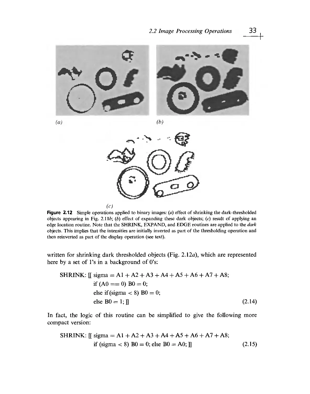
Images and Imaging Operations
Images are at the core of vision, and there are many ways— from simple to
sophisticated— ^to process and analyze them. This chapter concentrates on simple
algorithms, which nevertheless need to be treated carefully, for important subtleties
need to be learned. Above all, the chapter aims to show that quite a lot can be achieved
with such algorithms, which can readily be programmed and tested by the reader.
Look out for:
the different types of images— binary, gray- scale, and color,
a useful, compact notation for presenting image processing operations,
basic pixel operations— clearing, copying, Inverting, thresholding,
basic window operations— shifting, shrinking, expanding,
gray- scale brightening and contrast- stretching operations,
binary edge location and noise removal operations,
multi- image and convolution operations.
the distinction between sequential and parallel operations, and complications
that can arise in the sequential case.
* problems that arise around the edge of the image.
Though elementary, this chapter provides the basic methodology for the whole
of Part 1 and much of Part 2 of the book, and its importance should not be
underestimated; neither should the subtleties be ignored. Full understanding at this
stage will save many complications later, when one is programming more
sophisticated algorithms. In particular, obvious fundamental difficulties arise when
applying a sequence of window operations to the same original image.
18
CHAPTER 2
Images and Imaging Operations
p'ix'ellated, a. picture broken into a regular tiling
pXx'^lated, a. pixie- like, crazy, deranged
2.1 Introduction
This chapter focuses on images and simple image processing operations and
is intended to lead to more advanced image analysis operations that can be used
for machine vision in an industrial environment. Perhaps the main purpose of
the chapter is to introduce the reader to some basic techniques and notation
that will be of use throughout the book. However, the image processing
algorithms introduced here are of value in their own right in disciplines ranging
from remote sensing to medicine, and from forensic to military and scientific
apphcations.
The images discussed in this chapter have already been obtained from
suitable sensors: the sensors are covered in a later chapter. Typical of such images
is that shown in Fig. 2. la. This is a gray- tone image, which at first sight appears
to be a normal "black and white" photograph. On closer inspection, however, it
becomes clear that it is composed of a large number of individual picture cells,
or pixels. In fact, the image is a 128 x 128 array of pixels. To get a better feel
for the limitations of such a digitized image. Fig. 2.\b shows a section that has
been enlarged so that the pixels can be examined individually. A threefold
magnification factor has been used, and thus the visible part of Fig. 2.1^; contains
only a 42 X 42 array of pixels.
It is not easy to see that these gray- tone images are digitized into a
grayscale containing just 64 gray levels. To some extent, high spatial resolution
compensates for the lack of gray- scale resolution, and as a result we cannot at
once see the difference between an individual shade of gray and the shade it
19
20 CHAPTER 2 Images and Imaging Operations
(ci)
Ф)
Figure 2.1 Typical gray- scale images: (a) gray- scale image digitized into a 128 x 128 array of pixels;
Ф) section of image shown in (o) subjected to threefold linear magnification: the individual pixels are
now clearly visible.
2.1 Introduction 21
would have had in an ideal picture. In addition, when we look at the magnified
section of image in Fig. 2.\b, it is difficult to understand the significance of
the individual pixel intensities— the whole is becoming lost in a mass of small
parts. Older television cameras typically gave a gray- scale resolution that was
accurate only to about one part in 50, corresponding to about 6 bits of useful
information per pixel. Modern solid- state cameras commonly give less noise
and may allow 8 or even 9 bits of information per pixel. However, it is often
not worthwhile to aim for such high gray- scale resolutions, particularly when
the result will not be visible to the human eye, and when, for example, there is
an enormous amount of other data that a robot can use to locate a particular
object within the field of view. Note that if the human eye can see an object
in a digitized image of particular spatial and gray- scale resolution, it is in
principle possible to devise a computer algorithm to do the same thing.
Nevertheless, there is a range of applications for which it is valuable to
retain good gray- scale resolution, so that highly accurate measurements can
be made from a digital image. This is the case in many robotic applications,
where high- accuracy checking of components is critical. More will be said
about this subject later. In addition, in Part 2 we will see that certain techniques
for locating components efficiently require that local edge orientation be
estimated to better than 1°, and this can be achieved only if at least 6 bits
of gray- scale information are available per pixel.
2.1.1 Gray- Scale versus Color
Returning now to the image of Fig. 2.la, we might reasonably ask whether
it would be better to replace the gray- scale with color, using an RGB (red,
green, blue) color camera and three digitizers for the three main colors. Two
aspects of color are important for the present discussion. One is the intrinsic
value of color in machine vision: the other is the additional storage and
processing penalty it might bring. It is tempting to say that the second aspect is
of no great importance given the cheapness of modern computers which have
both high storage and high speed. On the other hand, high- resolution images
can arrive from a collection of CCTV cameras at huge data rates, and it will be
many years before it will be possible to analyze all the data arriving from such
sources. Hence, if color adds substantially to the storage and processing load,
its use will need to be justified.
The potential of color in helping with many aspects of inspection, surveillance,
control, and a wide variety of other applications including medicine (color
plays a crucial role in images taken during surgery) is enormous. This potential
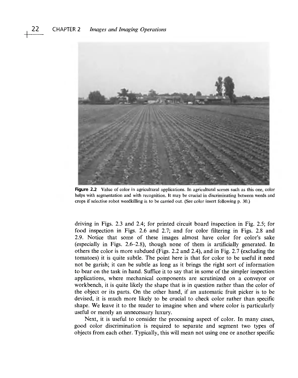
is illustrated with regard to agriculture in Fig. 2.2; for robot navigation and
22
CHAPTER 2 Images and Imaging Operations
Figure 2.2 Value of color in agricultural applications. In agricultural scenes such as this one, color
helps with segmentation and with recognition. It may be crucial in discriminating between weeds and
crops if selective robot weedkilling is to be carried out. (See color insert following p. 30.)
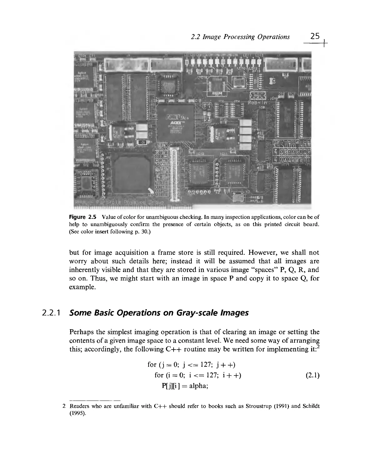
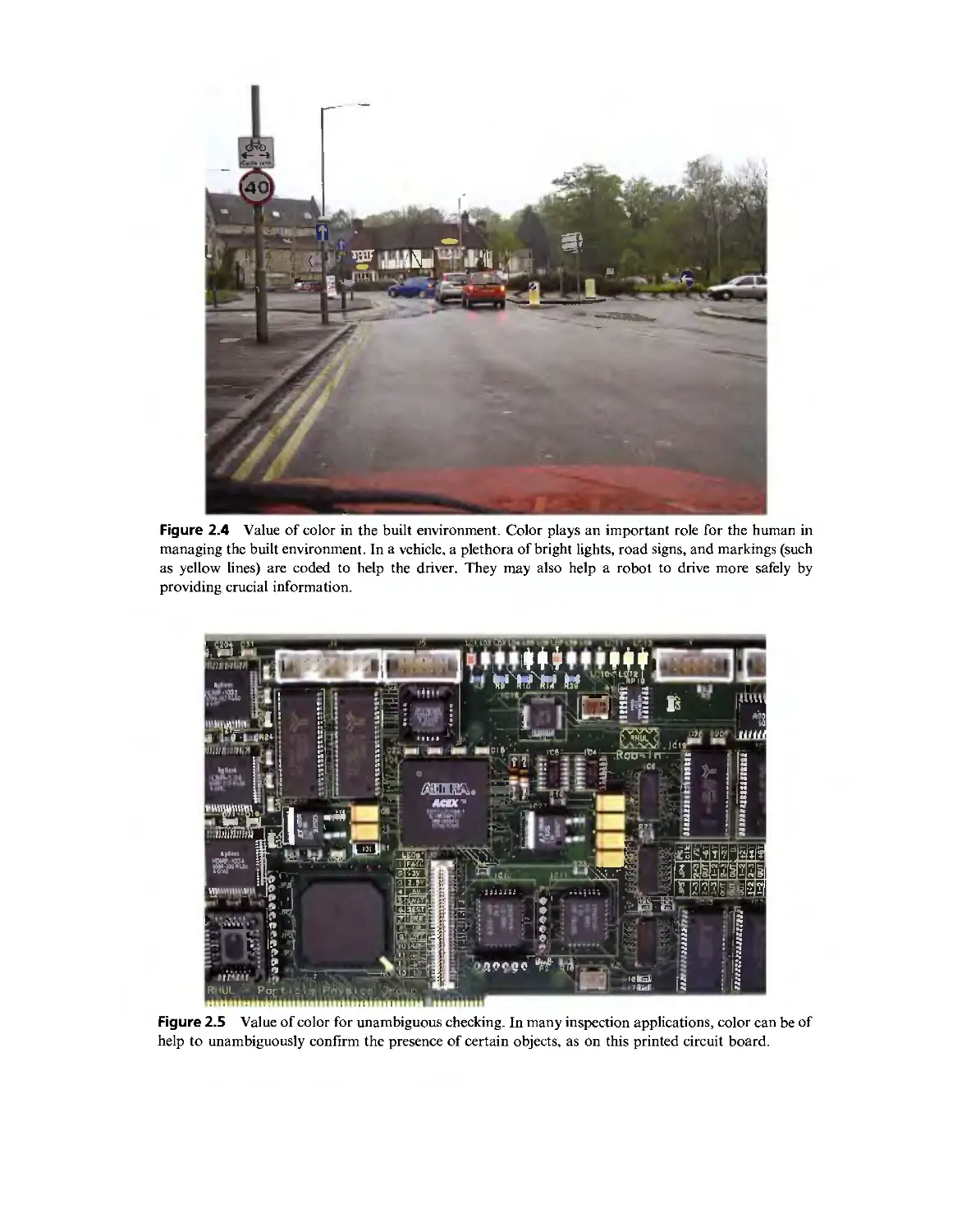
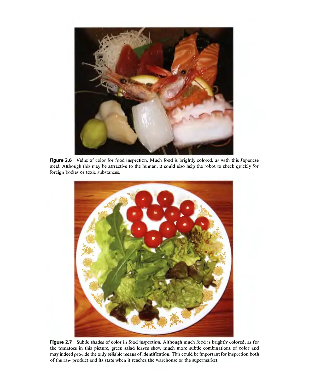
driving in Figs. 2.3 and 2.4; for printed circuit board inspection in Fig. 2.5; for
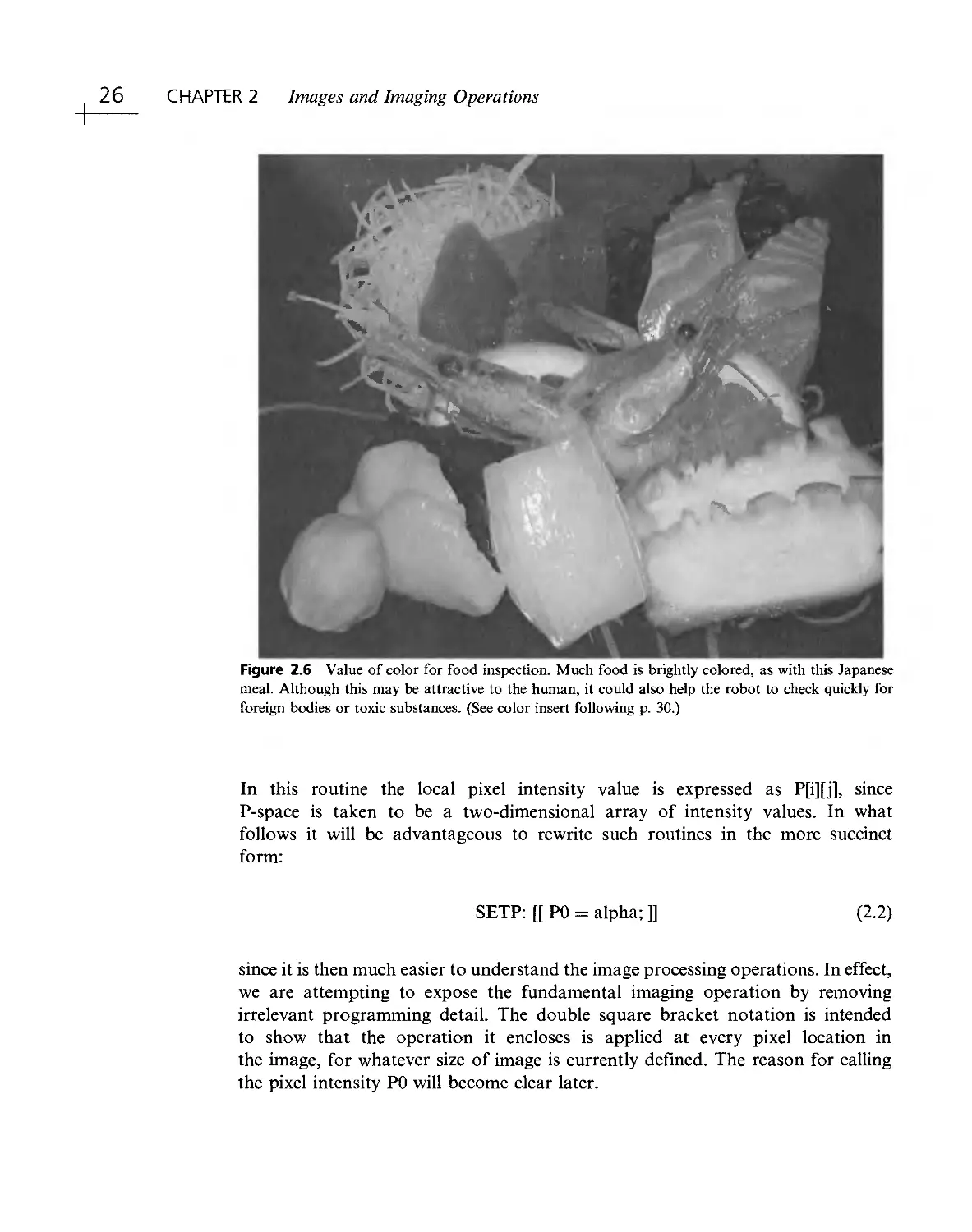
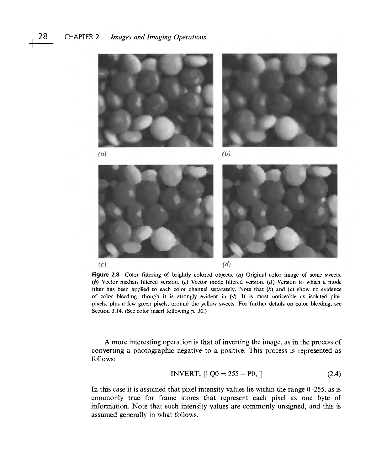
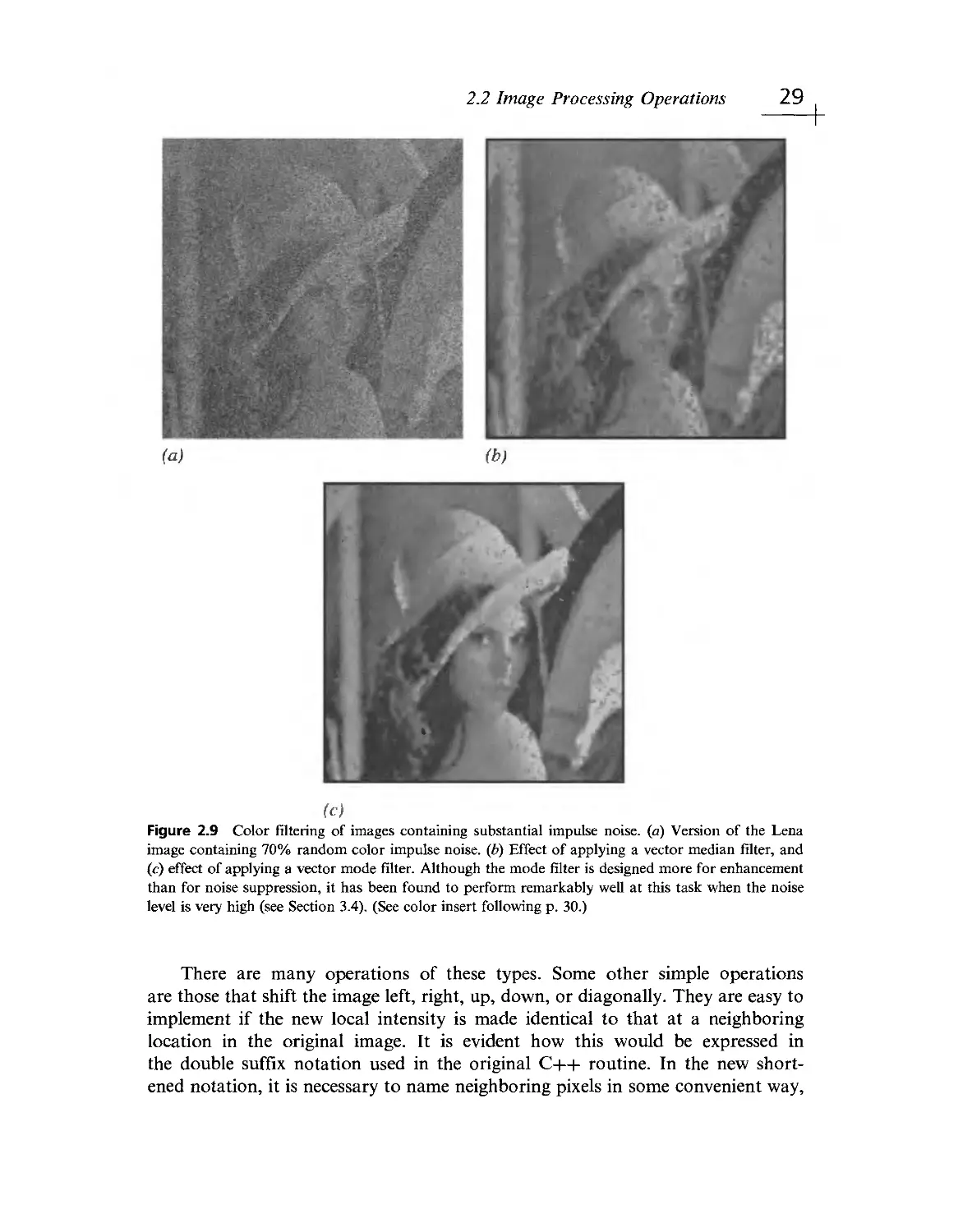
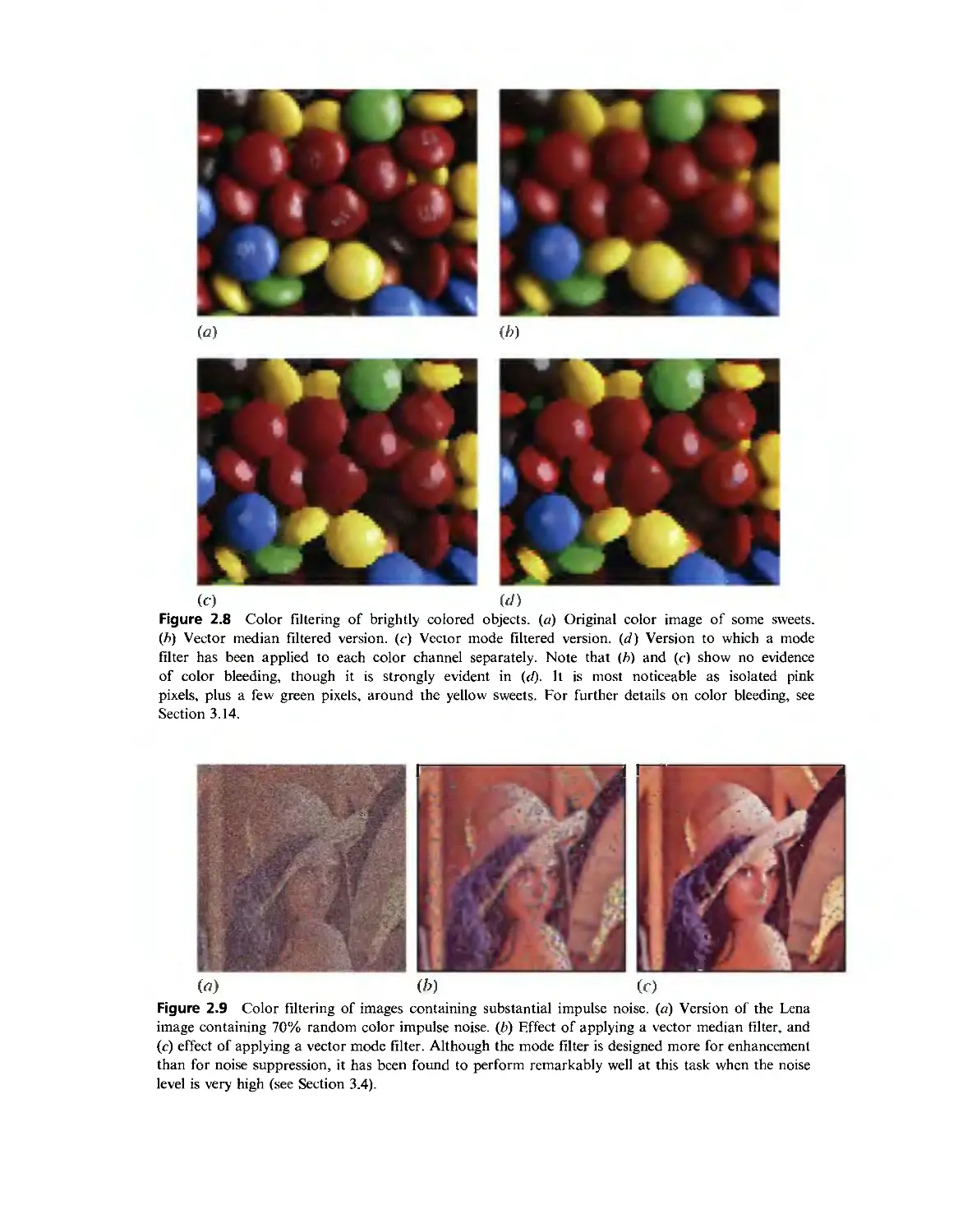
food inspection in Figs. 2.6 and 2.7; and for color filtering in Figs. 2.8 and
2.9. Notice that some of these images almost have color for color's sake
(especially in Figs. 2.6- 2.8), though none of them is artificially generated. In
others the color is more subdued (Figs. 2.2 and 2.4), and in Fig. 2.7 (excluding the
tomatoes) it is quite subtle. The point here is that for color to be useful it need
not be garish; it can be subtle as long as it brings the right sort of information
to bear on the task in hand. Suffice it to say that in some of the simpler inspection
applications, where mechanical components are scrutinized on a conveyor or
workbench, it is quite likely the shape that is in question rather than the color of
the object or its parts. On the other hand, if an automatic fruit picker is to be
devised, it is much more likely to be crucial to check color rather than specific
shape. We leave it to the reader to imagine when and where color is particularly
useful or merely an unnecessary luxury.
Next, it is useful to consider the processing aspect of color. In many cases,
good color discrimination is required to separate and segment two types of
objects from each other. Typically, this will mean not using one or another specific
2.1 Introduction
23
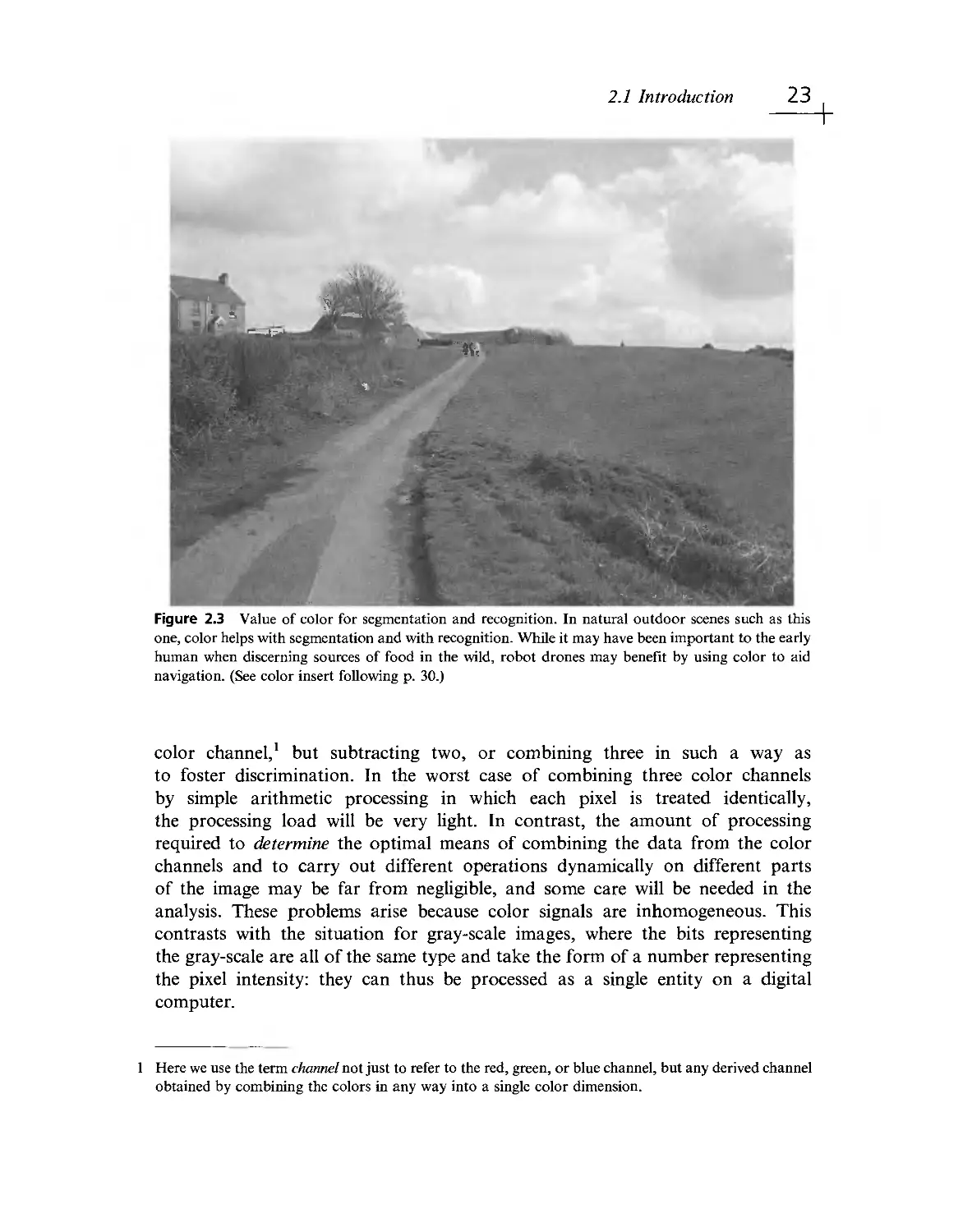
Figure 2.3 Value of color for segmentation and recognition. In natural outdoor scenes such as this
one, color helps with segmentation and with recognition. While it may have been important to the early
human when discerning sources of food in the wild, robot drones may benefit by using color to aid
navigation. (See color insert following p. 30.)
color channel, ' but subtracting two, or combining three in such a way as
to foster discrimination. In the worst case of combining three color channels
by simple arithmetic processing in which each pixel is treated identically,
the processing load will be very light. In contrast, the amount of processing
required to determine the optimal means of combining the data from the color
channels and to carry out different operations dynamically on different parts
of the image may be far from negligible, and some care will be needed in the
analysis. These problems arise because color signals are inhomogeneous. This
contrasts with the situation for gray- scale images, where the bits representing
the gray- scale are all of the same type and take the form of a number representing
the pixel intensity: they can thus be processed as a single entity on a digital
computer.
1 Here we use the term channel not just to refer to the red, green, or blue channel, but any derived channel
obtained by combining the colors in any way into a single color dimension.
24
CHAPTER 2 Images and Imaging Operations
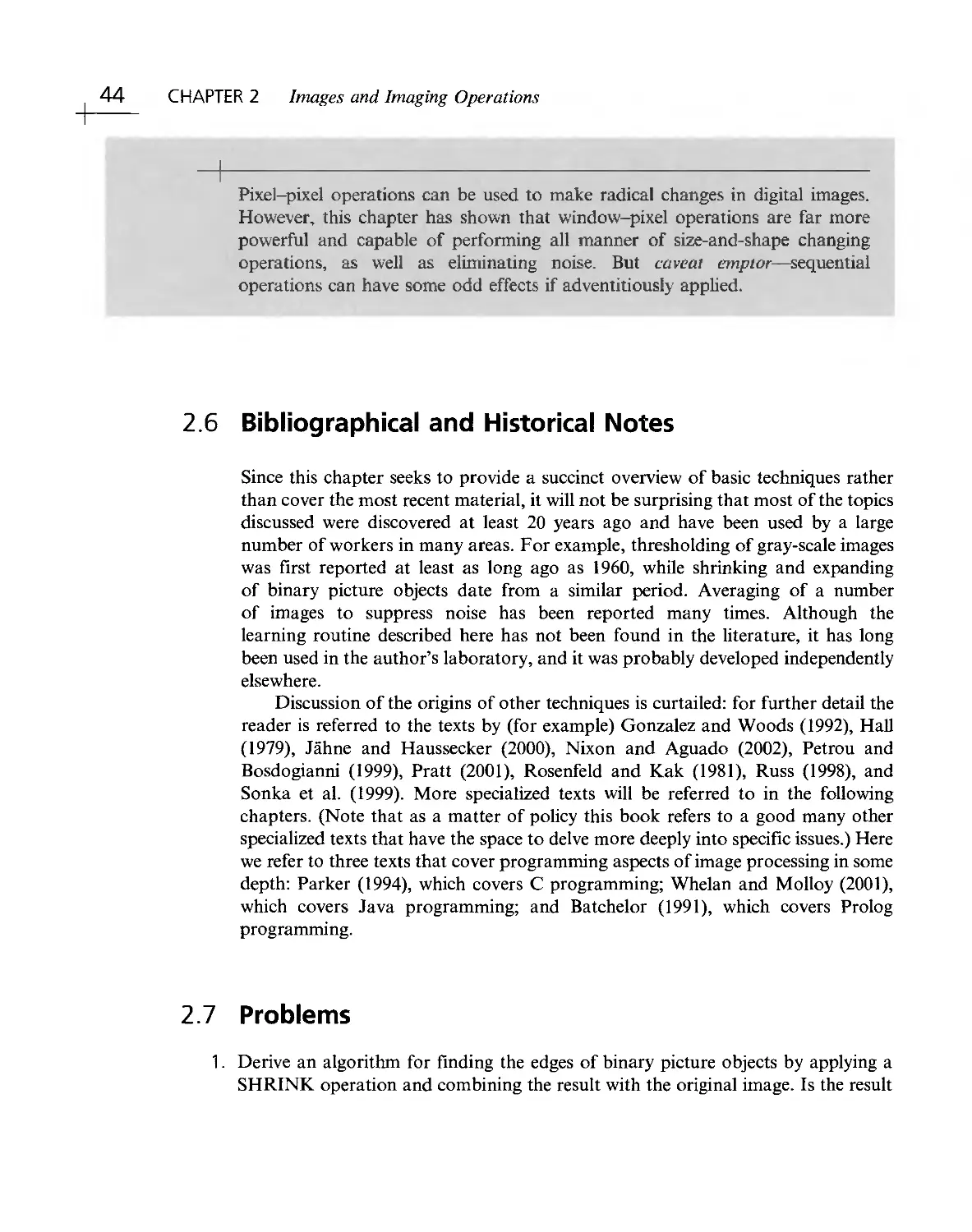
Figure 2.4 Value of color in the built environment. Color plays an important role for the human in
managing the built environment. In a vehicle, a plethora of bright lights, road signs, and markings (such
as yellow lines) are coded to help the driver. They may also help a robot to drive more safely by
providing crucial information. (See color insert following p. 30.)
2.2 Image Processing Operations
The images of Figs 2.1 and 2.11a are considered in some detail here,
including some of the many image processing operations that can be performed
on them. The resolution of these images reveals a considerable amount of detail
and at the same time shows how it relates to the more "meaningful" global
information. This should help to show how simple imaging operations contribute
to image interpretation.
When performing image processing operations, we start with an image in
one storage area and generate a new processed image in another storage area.
In practice these storage areas may either be in a special hardware unit called
a frame store that is interfaced to the computer, or else they may be in the main
memory of the computer or on one of its discs. In the past, a special frame store
was required to store images because each image contains a good fraction of a
megabyte of information, and this amount of space was not available for
normal users in the computer main memory. Today this is less of a problem.
2.2 Image Processing Operations 25
Figure 2.5 Value of color for unambiguous checking. In many inspection applications, color can be of
help to unambiguously confirm the presence of certain objects, as on this printed circuit board.
(See color insert following p. 30.)
but for image acquisition a frame store is still required. However, we shall not
worry about such details here; instead it will be assumed that all images are
inherently visible and that they are stored in various image "spaces" P, Q, R, and
so on. Thus, we might start with an image in space P and copy it to space Q, for
example.
2.2.1 Some Basic Operations on Gray- scale Images
Perhaps the simplest imaging operation is that of clearing an image or setting the
contents of a given image space to a constant level. We need some way of arranging
this; accordingly, the following C++ routine may be written for implementing it:^
for(j = 0; j<=127; j + +)
for(i = 0; i<:=127; i + +)
P[j][i] = alpha;
(2.1)
2 Readers who are unfamiliar with C++ should refer to books such as Stroustrup (1991) and Schildt
(1995).
26 CHAPTER 2 Images and Imaging Operations
Figure 2.6 Value of color for food inspection. Much food is brightly colored, as with this Japanese
meal. Although this may be attractive to the human, it could also help the robot to check quickly for
foreign bodies or toxic substances. (See color insert following p. 30.)
In this routine the local pixel intensity value is expressed as P[i][j], since
P- space is taken to be a two- dimensional array of intensity values. In what
follows it will be advantageous to rewrite such routines in the more succinct
form:
SET?: [[ PO = alpha; ]]
(2.2)
since it is then much easier to understand the image processing operations. In effect,
we are attempting to expose the fundamental imaging operation by removing
irrelevant programming detail. The double square bracket notation is intended
to show that the operation it encloses is applied at every pixel location in
the image, for whatever size of image is currently defined. The reason for calling
the pixel intensity PO will become clear later.
2.2 Image Processing Operations
27
Figure 2.7 Subtle shades of color in food inspection. Although much food is brightly colored, as for
the tomatoes in this picture, green salad leaves show much more subtle combinations of color and
may indeed provide the only reliable means of identification. This could be important for inspection
both of the raw product and its state when it reaches the warehouse or the supermarket. (See color insert
following p. 30.)
Another simple imaging operation is to copy an image from one space
to another. This is achieved, without changing the contents of the original space
P, by the routine:
COPY: [[ QO = PO; ]]
(2.3)
Again, the double bracket notation indicates a double loop that copies each
individual pixel of P- space to the corresponding location in Q- space.
28 CHAPTER 2 Images and Imaging Operations
Figure 2.8 Color filtering of brightly colored objects, (a) Original color image of some sweets.
Ф) Vector median filtered version, (c) Vector mode filtered version, {d) Version to which a mode
filter has been applied to each color channel separately. Note that {b) and (c) show no evidence
of color bleeding, though it is strongly evident in {d). It is most noticeable as isolated pink
pixels, plus a few green pixels, around the yellow sweets. For further details on color bleeding, see
Section 3.14. (See color insert following p. 30.)
A more interesting operation is that of inverting the image, as in the process of
converting a photographic negative to a positive. This process is represented as
follows:
INVERT: [[ QO = 255 - PO; ]]
(2.4)
In this case it is assumed that pixel intensity values lie within the range 0- 255, as is
commonly true for frame stores that represent each pixel as one byte of
information. Note that such intensity values are commonly unsigned, and this is
assumed generally in what follows.
2.2 Image Processing Operations 29
Figure 2.9 Color filtering of images containing substantial impulse noise, (a) Version of the Lena
image containing 70% random color impulse noise, (b) Effect of applying a vector median filter, and
(c) effect of applying a vector mode filter. Although the mode filter is designed more for enhancement
than for noise suppression, it has been found to perform remarkably well at this task when the noise
level is very high (see Section 3.4), (See color insert following p. 30.)
There are many operations of these types. Some other simple operations
are those that shift the image left, right, up, down, or diagonally. They are easy to
implement if the new local intensity is made identical to that at a neighboring
location in the original image. It is evident how this would be expressed in
the double suffix notation used in the original C++ routine. In the new
shortened notation, it is necessary to name neighboring pixels in some convenient way.
30 CHAPTER 2 Images and Imaging Operations
Figure 2.10 Contrast- stretching: effect of increasing the contrast in the image of Fig. 2. la by a factor
of two and adjusting the mean intensity level appropriately. The interior of the jug can now be seen more
easily. Note, however, that there is no additional information in the new image.
and we here employ a commonly used numbering scheme:
P4
P5
P6
P3
PO
P7
P2
PI
P8
with a similar scheme for other image spaces. With this notation, it is easy to
express a left shift of an image as follows:
LEFT: [[00 = PI;]]
Similarly, a shift down to the bottom right is expressed as:
DOWNR: [[ QO = P4; ]]
(2.5)
(2.6)
2.2 Image Processing Operations 31
(Note that the shift appears in a direction opposite to that which one might at
first have suspected.)
It will now be clear why PO and QO were chosen for the basic notation of pixel
intensity: the "0" denotes the central pixel in the "neighborhood" or "window, "
and corresponds to zero shift when copying from one space to another.
A whole range of possible operations is associated with modifying images
in such a way as to make them more satisfactory for a human viewer. For
example, adding a constant intensity makes the image brighter:
BRIGHTEN: [[ QO = PO + beta; ]] (2.7)
and the image can be made darker in the same way. A more interesting operation is
to stretch the contrast of a dull image:
STRETCH: [[ QO = PO * gamma + beta; ]] (2.8)
where gamma >1. In practice (as for Fig. 2.10) it is necessary to ensure that
intensities do not result that are outside the normal range, for example, by using
an operation of the form:
STRETCH: [[ QQ = PO * gamma + beta;
if (QQ < 0) QO = 0;
elseif (QQ>255)Q0:- 255;
else QO = QQ; ]] (2.9)
Most practical situations demand more sophisticated transfer functions— either
nonlinear or piecewise Hnear— but such complexities are ignored here.
A further simple operation that is often applied to gray- scale images is that of
thresholding to convert to a binary image. This topic is covered in more detail later
in this chapter since it is widely used to detect objects in images. However, our
purpose here is to look on it as another basic imaging operation. It can be
implemented using the routine
THRESH: [[ if (PO > thresh) АО = 1; else АО := 0; ]] (2.10)
The first few letters of the alphabet (A, B, C, ...) are used consistently to denote binary image spaces,
and later letters (P, Q, R, ...) to denote gray- scale images. In software, these variables are assumed to be
predeclared, and in hardware (e.g., frame store) terms they are taken to refer to dedicated memory
spaces containing only the necessary 1 or 8 bits per pixel. The intricacies of data transfer between
variables of different types are important considerations which are not addressed in detail here: it is
sufficient to assume that both АО = PO and PO = АО correspond to a single- bit transfer, except that in the
latter case the top 7 bits are assigned the value 0.
32
CHAPTER 2 Images and Imaging Operations
(a) (h)
Figure 2.11 Thresholding of gray- scale images: (a) 128 x 128 pixel gray- scale image of a collection of
parts; (b) effect of thresholding the image.
If, as often happens, objects appear as dark objects on a light background, it is
easier to visualize the subsequent binary processing operations by inverting the
thresholded image using a routine such as
INV: [[ АО = 1 - АО; ]]
(2.11)
However, it would be more usual to combine the two operations into a single
routine of the form:
INVTHRESH: [[ if (PO > thresh) АО = 0; else АО = 1; ]]
(2.12)
To display the resulting image in a form as close as possible to the original, it can
be reinverted and given the full range of intensity values (intensity values 0 and 1
being scarcely visible):
INVDISPLAY: [[ RO = 255 * (1 - AG); ]]
(2.13)
Figure 2.11 shows the effect of these two operations.
2.2.2 Basic Operations on Binary Images
Once the image has been thresholded, a wide range of binary imaging operations
becomes possible. Only a few such operations are covered here, with the aim of
being instructive rather than comprehensive. With this in mind, a routine may be
2.2 Image Processing Operations 33
ъ°Х v>''-
Ш)
(b)
(c)
Figure 2.12 Simple operations applied to binary images: (o) effect of shrinking the dark- thresholded
objects appearing in Fig. 2.1 li; (b) effect of expanding these dark objects; (c) result of applying an
edge location routine. Note that the SHRINK, EXPAND, and EDGE routines are applied to the dark
objects. This implies that the intensities are initially inverted as part of the thresholding operation and
then reinverted as part of the display operation (see text).
written for shrinking dark thresholded objects (Fig. 2.12a), which are represented
here by a set of I's in a background of O's:
SHRINK: [[ Sigma = АЦ- A2 + A3 + A4 + A5 + A6 + A7 + A8;
if (АО == 0) BO = 0;
else if (sigma < 8) BO = 0;
else BO = 1;]] (2.14)
In fact, the logic of this routine can be simplified to give the following more
compact version:
SHRINK: [[ Sigma = Al + A2 + A3 + A4 + A5 + A6 + A7 + AS;
if (sigma < 8) BO = 0; else BO = AG; ]]
(2.15)
34 CHAPTER 2 Images and Imaging Operations
Note that the process of shrinking"* dark objects also expands light objects,
including the light background. It also expands holes in dark objects. The
opposite process, that of expanding dark objects (or shrinking light ones), is
achieved (Fig. 2.\2b) with the routine:
EXPAND: [[ sigma = Al + A2 + A3 + A4 + A5 + A6 + A7 + A8;
if (Sigma > 0) BO = 1; else BO = АО; ]] (2.16)
Each of these routines employs the same technique for interrogating neighboring
pixels in the original image: as will be apparent on numerous occasions in this
book, the sigma value is a useful and powerful descriptor for 3x3 pixel
neighborhoods. Thus, "if (sigma > 0)" can be taken to mean "if next to a dark
object, " and the consequence can be read as "then expand it." Similarly,
"if (sigma< 8)" can be taken to mean "if next to a light object" or "if next to
light background, " and the consequence can be read as "then expand the light
background into the dark object."
The process of finding the edge of a binary object has several possible
interpretations. Clearly, it can be assumed that an edge point has a sigma value
in the range 1- 7 inclusive. However, it may be defined as being within the object,
within the background, or in either position. Taking the definition that the edge
of an object has to lie within the object (Fig. 2.12c), the following edge- finding
routine for binary images results:
EDGE: [[ sigma = Al + A2 + A3 + A4 + A5 + A6 + A7 + AS;
if (sigma == 8) BO = 0; else BO = АО; ]] (2.17)
This strategy amounts to canceling out object pixels that are not on the edge. For
this and a number of other algorithms (including the SHRINK and EXPAND
algorithms already encountered), a thorough analysis of exactly which pixels
should be set to 1 and 0 (or which should be retained and which eliminated),
involves drawing up tables of the form:
EDGE
АО
0
1
sigma
0to7
0
1
8
0
0
4 The processes of shrinking and expanding are also widely known by the respective terms erosion and
dilation. (See also Chapter 8.)
2.2 Image Processing Operations 35
This reflects the fact that algorithm specification includes a recognition phase and
an action phase. That is, it is necessary first to locate situations within an image
where (for example) edges are to be marked or noise eliminated, and then action
must be taken to implement the change.
Another function that can usefully be performed on binary images is the
removal of "salt and pepper" noise, that is, noise that appears as a light spot on a
dark background or a dark spot on a light background. The first problem to be
solved is that of recognizing such noise spots; the second is the simpler one of
correcting the intensity value. For the first of these tasks, the sigma value is
again useful. To remove salt noise (which has binary value 0 in our convention),
we arrive at the following routine:
SALT: [[ Sigma = Al + A2 + A3 + A4 + A5 + A6 + A7 + A8;
if (Sigma == 8) BO = 1; else BO = АО; ]] (2.18)
which can be read as leaving the pixel intensity unchanged unless it is proven
to be a salt noise spot. The corresponding routine for removing pepper noise
(binary value 1) is:
PEPPER: [[ Sigma = A1+ A2 + A3 + A4 + A5 + A6 + A7 + A8;
if (sigma == 0) BO = 0; else BO = АО; ]] (2.19)
Combining these two routines into one operation (Fig. 2.13a) gives:
NOISE: [[ Sigma = Al + A2 + A3 + A4 + A5 + A6 + A7 + A8;
if (sigma == 0) BO = 0;
else if (sigma ==8) B0= 1;
else BO = АО; ]] (2.20)
The routine can be made less stringent in its specification of noise pixels, so that
it removes spurs on objects and background. This is achieved (Fig. 2.l3b) by a
variant such as
NOIZE: [[ sigma = Al + A2 + A3 + A4 + A5 + A6 + A7 + A8;
if (sigma < 2) BO = 0;
else if (sigma > 6) BO = 1;
else BO = АО;]] (2.21)
36
CHAPTER 2 Images and Imaging Operations
&» о -
(a)
№)
Figure 2.13 Simple binary noise removal operations: (a) result of applying a "salt and pepper" noise
removal operation to the thresholded image in Fig. 2.1 li; (b) result of applying a less stringent
noise removal routine: this is effective in cutting down the jagged spurs that appear on some of the
objects.
As before, if any doubt about the algorithm exists, its specification should be set up
rigorously— in this case with the following table:
Sigma
NOIZE
Oor 1
2 to 6
7 or 8
АО
Many other simple operations can usefully be applied to binary images, some
of which are dealt with in Chapter 6. Meanwhile, we should consider the use of
common logical operations such as NOT, AND, OR, EXOR. The NOT function
is related to the inversion operation described earlier, in that it produces the
complement of a binary image:
This has the same action as
NOT: [[ BO = ! АО; ]]
INV [[ BO = 1 - АО; ]]
(2.22)
(2.23)
The other logical operations operate on two or more images to produce a third
image. This may be illustrated for the AND operation:
AND: [[ CO = АО && BO; ]]
(2.24)
2.2 Image Processing Operations 37
This has the effect of masking off those parts of A- space that are not within a
certain region defined in B- space (or locating those objects that are visible in both
A- space and B- space).
2.2.3 Noise Suppression by Image Accumulation
The AND routine combines information from two or more images to generate a
third image. It is frequently useful to average gray- scale images in a similar way in
order to suppress noise. A routine for achieving this is:
AVERAGE: [[ RO = (PO + Q0)/2; ]] (2.25)
This idea can be developed so that noisy images from a TV camera or other
input device are progressively averaged until the noise level is low enough for
useful application. It is, of course, well known that it is necessary to average 100
measurements to improve the signal- to- noise ratio by a factor of 10: that is, the
signal- to- noise ratio is multiplied only by the square root of the number of
measurements averaged. Since whole- image operations are computationally
costly, it is usually practicable to average only up to 16 images. To achieve this
the routine shown in Fig. 2.14 is applied. Note that overflow from the usual single
byte per pixel storage limit will prevent this routine from working properly if
the input images do not have low enough intensities. Sometimes, it may be
permissible to reserve more than one byte of storage per pixel. If this is not
possible, a useful technique is to employ the "learning" routine of Fig. 2.15. The
action of this routine is somewhat unusual, for it retains one- sixteenth of the
last image obtained from the camera and progressively lower portions of all
earlier images. The effectiveness of this technique can be seen in Fig. 2.16.
ADDAVG: {
[[P0 = 0;]]
for(i= 1; i<= 16; i++) {
input(Q); // obtain new image in Q- space
[[PO = PO + QO;]]
}
[[P0 = P0/16;]]
}
Figure 2.14 Routine for averaging a set of input images.
38
CHAPTER 2 Images and Imaging Operations
LEARNAVG: {
input(P); // obtain new image in P- space
for (i = 1; i <= 15; i++) {
input(Q); // obtain new image in Q- space
[[P0 = (P0*15 + Q0 + 8)/16;]]
}
}
Figure 2.15 Alternative "learning" routine for averaging images.
Figure 2.16 Noise suppression by averaging a number of images using the LEARNAVG routine of
Fig. 2.15. Note that this is highly effective at removing much of the noise and does not introduce
any blurring. (Clearly this is true only if, as here, there is no camera or object motion.) Compare this
image with that of Fig. l.\a for which no averaging was used.
Note that in this last routine 8 is added before dividing by 16 in order to
offset rounding errors. If accuracy is not to suffer, this is a vital feature of most
imaging routines that involve small- integer arithmetic. Surprisingly, this problem is
seldom referred to in the literature, although it must account for many attempts
2.3 Convolutions and Point Spread Functions 39
at perfectly good algorithm strategies that mysteriously turn out not to work well
in practice!
2.3 Convolutions and Point Spread Functions
Convolution is a powerful and widely used technique in image processing and
other areas of science. Because it appears in many applications throughout this
book, it is useful to introduce it at an early stage. We start by defining the
convolution of two functions/(x) and g{x) as the integral:
/oo
Дм)^(х - u)du (2.26)
- oo
The action of this integral is normally described as the result of applying a point
spread function g{x) to all points of a function f{x) and accumulating the
contributions at every point. It is significant that if the point spread function (PSF)
is very narrow, ^ then the convolution is identical to the original function/(x). This
makes it natural to think of the function/(x) as having been spread out under the
influence of g(x). This argument may give the impression that convolution
necessarily blurs the original function, but this is not always so if, for example, the
PSF has a distribution of positive and negative values.
When convolution is applied to digital images, the above formulation changes
in two ways: (1) a double integral must be used in respect of the two dimensions;
and (2) integration must be changed into discrete summation. The new form of the
convolution is:
F{x, y) ^fix, y) * g{x, y) = J2J1 /('■' f>S(^ - '■' У - J) (2.27)
where g is now referred to as a spatial convolution mask. When convolutions are
performed on whole images, it is usual to restrict the sizes of masks as far as
possible in order to save computation. Thus, convolution masks are seldom
larger than 15 pixels square, and 3x3 masks are typical. The fact that the mask has
to be inverted before it is applied is inconvenient for visualizing the process of
convolution. In this book we therefore present only preinverted masks of the form:
h{x, y) ^ g{- x, - y) (2.28)
5 Formally, it can be a delta function, which is infinite at one point and zero elsewhere while having an
integral of unity.
40 CHAPTER 2 Images and Imaging Operations
Convolution can then be calculated using the more intuitive formula:
Fix, y) = J2Лf^^ + ^'У +J^^^'^ J^
i J
(2.29)
Clearly, this involves multiplying corresponding values in the modified mask and
the neighborhood under consideration. Reexpressing this result for a 3x3
neighborhood and writing the mask coefficients in the form:
h4 h3 h2
h5 ho hi
h6 h7 h8
the algorithm can be obtained in terms of our earlier notation;
CONVOLV: [[ QO = PO * hO + PI * hl+ P2 * h2 + P3 * h3 + P4 * h4
+P5 * h5 + P6 * h6 + P7 * h7 + P8 * h8; ]] (2.30)
We are now in a position to apply convolution to a real situation. At this
stage we merely extend the ideas of the previous section, attempting to suppress
noise by averaging not over corresponding pixels of different images, but over
nearby pixels in the same image. A simple way of achieving this is to use the
convolution mask:
1
9
'1 1 1
1 1 1
1 1 1
where the number in front of the mask weights all the coefficients in the mask
and is inserted to ensure that applying the convolution does not alter the mean
intensity in the image. As hinted earlier, this particular convolution has the
effect of blurring the image as well as reducing the noise level (Fig. 2.17). More will
be said about this in the next chapter.
Convolutions are linear operators and are the most general spatially invariant
linear operators that can be applied to a signal such as an image. Note that
linearity is often of interest in that it permits mathematical analysis to be
performed that would otherwise be intractable.
2.4 Sequential versus Parallel Operations
41
Figure 2.17 Noise suppression by neighborhood averaging achieved by convolving the original image
of Fig. 2.1a with a uniform mask within a 3 x 3 neighborhood. Note that noise is suppressed only at the
expense of introducing significant blurring.
2.4 Sequential versus Parallel Operations
Most of the operations defined so far have started with an image in one space
and finished with an image in a different space. Usually, P- space was used for
an initial gray- scale image and Q- space for the processed image, or A- space
and B- space for the corresponding binary images. This may seem somewhat
inconvenient, since if routines are to act as interchangeable modules that can be
applied in any sequence, it will be necessary to interpose restoring routines^
between modules:
RESTORE: [[ PO = QO; ]]
(2.31)
6 Restoring is not actually necessary within a sequence of routines if the computer is able to keep track of
where the currently useful images are stored and to modify the routines accordingly. Nonetheless, it can
be a particular problem when it is wished to see a sequence of operations as they occur, using a frame
store with only one display space.
42 CHAPTER 2 Images and Imaging Operations
Unfortunately, many of the operations cannot work satisfactorily if we do not
use separate input and output spaces in this way. This is because they are
inherently "parallel processing" routines. This term is used in as much as these
are the types of processes that would be performed by a parallel computer
possessing a number of processing elements equal to the number of pixels in the
image, so that all the pixels are processed simultaneously. If a serial computer is to
simulate the operation of a parallel computer, then it must have separate input and
output image spaces and rigorously work in such a way that it uses the original
image values to compute the output pixel values. This means that an operation
such as the following cannot be an ideal parallel process:
BADSHRINK: [[ sigma = A1+ A2 + A3 + A4 + A5 + A6 + A7 + A8;
if (Sigma < 8) АО = 0; else АО = АО; ]] (2.32)
This is so because, when the operation is half completed, the output pixel intensity
will depend not only on some of the unprocessed pixel values but also on some
values that have already been processed. For example, if the computer makes a
normal (forward) TV raster scan through the image, the situation at a general point
in the scan will be
V
V
X
V
X
X
V
X
X
where the ticked pixels have already been processed and the others have not. As a
result, the BADSHRINK routine will shrink all objects to nothing!
A much simpler illustration is obtained by attempting to shift an image to the
right using the following routine:
BADSHIFT: [[ PO = P5; ]] (2.33)
All this achieves is to fill up the image with values corresponding to those off its
left edge, ' whatever they are assumed to be. Thus, we have shown that the
BADSHIFT process is inherently parallel.
7 Note that when the computer is performing a 3 x 3 (or larger) window operation, it has to assume some
value for off- image pixel intensities. Usually, whatever value is selected will be inaccurate, and so the
final processed image will contain a border that is also inaccurate. This will be so whether the off- image
pixel addresses are trapped in software or in specially designed circuitry in the frame store.
2.5 Concluding Remarks 43
As will be seen later, some processes are inherently sequential— that is, the
processed pixel has to be returned immediately to the original image space.
Meanwhile, note that not all of the routines described so far need to be restricted
rigorously to parallel processing. In particular, all single- pixel routines (essentially,
those that only refer to the single pixel in a 1 x 1 neighborhood) can validly be
performed as if they were sequential in nature. Such routines include the following
inverting, intensity adjustment, contrast stretching, thresholding, and logical
operations:
INVERT: [[ PO = 255 - PO; ]] (2.34)
BRIGHTEN: [[ PO = PO + beta; ]] (2.35)
STRETCH: [[ PO = PO * gamma + beta; ]] (2.36)
THRESH: [[ if (PO > thresh) PO = 1; else PO = 0; ]] (2.37)
NOT: [[ АО = ! АО; ]] (2.38)
AND: [[ АО = АО && ВО; ]] (2.39)
These remarks are intended to act as a warning. It may well be safest to design
algorithms that are exclusively parallel processes unless there is a definite need to
make them sequential. Later we will see how this need can arise.
2.5 Concluding Remarks
This chapter has introduced a compact notation for representing imaging
operations and has demonstrated some basic parallel processing routines.
The following chapter extends this work to see how noise suppression can be
achieved in gray- scale images. This leads to more advanced image analysis
work that is directly relevant to machine vision applications. In particular.
Chapter 4 studies in more detail the thresholding of gray- scale images, building
on the work of Section 2.2.1, while Chapter 6 studies object shape analysis in
binary images.
44 CHAPTER 2 Images and Imaging Operations
Pixel- pixel operations can be used to make radical changes in digital images.
However, this chapter has shown that window- pixel operations are far more
powerful and capable of performing all manner of size- and- shape changing
operations, as well as eliminating noise. But caveat emptor— sequential
operations can have some odd effects if adventitiously applied.
2.6 Bibliographical and Historical Notes
Since this chapter seeks to provide a succinct overview of basic techniques rather
than cover the most recent material, it will not be surprising that most of the topics
discussed were discovered at least 20 years ago and have been used by a large
number of workers in many areas. For example, thresholding of gray- scale images
was first reported at least as long ago as 1960, while shrinking and expanding
of binary picture objects date from a similar period. Averaging of a number
of images to suppress noise has been reported many times. Although the
learning routine described here has not been found in the literature, it has long
been used in the author's laboratory, and it was probably developed independently
elsewhere.
Discussion of the origins of other techniques is curtailed: for further detail the
reader is referred to the texts by (for example) Gonzalez and Woods (1992), Hall
(1979), Jahne and Haussecker (2000), Nixon and Aguado (2002), Petrou and
Bosdogianni (1999), Pratt (2001), Rosenfeld and Как (1981), Russ (1998), and
Sonka et al. (1999). More specialized texts will be referred to in the following
chapters. (Note that as a matter of policy this book refers to a good many other
specialized texts that have the space to delve more deeply into specific issues.) Here
we refer to three texts that cover programming aspects of image processing in some
depth: Parker (1994), which covers С programming; Whelan and Molloy (2001),
which covers Java programming; and Batchelor (1991), which covers Prolog
programming.
2.7 Problems
1. Derive an algorithm for finding the edges of binary picture objects by applying a
SHRINK operation and combining the result with the original image. Is the result
2 J Problems 45
the same as that obtained using the edge- finding routine (2.17)? Prove your
statement rigorously by drawing up suitable algorithm tables as in Section 2.2.2.
2. In a certain frame store, each off- image pixel can be taken to have either the value 0
or the intensity for the nearest image pixel. Which will give the more meaningful
results for (a) shrinking, (b) expanding, and (c) blurring convolution?
3. Suppose the NOISE and NOIZE routines of Section 2.2.2 were reimplemented as
sequential algorithms. Show that the action of NOISE would be unchanged,
whereas NOIZE would produce very odd effects on some binary images.
Figure 2.2 Value of color in agricultural applications. In agricultural scenes such as this one, color
helps with segmentation and with recognition. It may be crucial in discriminating between weeds and
crops if selective robot weedkilling is to be carried out.
Figure 2.3 Value of color for segmentation and recognition. In natural outdoor scenes such as this
one, color helps with segmentation and with recognition. While it may have been important to the early
human when discerning sources of food in the wild, robot drones may benefit by using color to aid
navigation.
Figure 2.4 Value of color in the built environment. Color plays an important role for the human in
managing the built environment. In a vehicle, a plethora of bright lights, road signs, and markings (such
as yellow lines) are coded to help the driver. They may also help a robot to drive more safely by
providing crucial information.
Figure 2.5 Value of color for unambiguous checking. In many inspection applications, color can be of
help to unambiguously confirm the presence of certain objects, as on this printed circuit board.
Figure 2.6 Value of color for food inspection. Much food is brightly colored, as with this Japanese
meal. Although this may be attractive to the human, it could also help the robot to check quickly for
foreign bodies or toxic substances.
Figure 2.7 Subtle shades of color in food inspection. Although much food is brightly colored, as for
the tomatoes in this picture, green salad leaves show much more subtle combinations of color and
may indeed provide the only reliable means of identification. This could be important for inspection both
of the raw product and its state when it reaches the warehouse or the supermarket.
(с) (tJ)
Figure 2.8 Color filtering of brightly colored objects, (a) Original color image of some sweets.
(h) Vector median filtered version, (c) Vector mode filtered version, (d) Version to which a mode
filter has been applied to each color channel separately. Note that (h) and (c) show no evidence
of color bleeding, though it is strongly evident in (</). It is most noticeable as isolated pink
pixels, plus a few green pixels, around the yellow sweets. For further details on color bleeding, see
Section 3.14.
(й) (b) (c)
Figure 2.9 Color filtering of images containing substantial impulse noise, (a) Version of the Lena
image containing 70% random color impulse noise, (b) Effect of applying a vector median filter, and
(c) effect of applying a vector mode filter. Although the mode filter is designed more for enhancement
than for noise suppression, it has been found to perform remarkably well at this task when the noise
level is very high (see Section 3.4).
Basic Image Filtering Operations
Image filtering involves the application of window operations that achieve useful
effects, such as noise removal or image enhancement. This chapter deals particularly
with what can be achieved with quite basic approaches, such as application of local
mean, median, or mode filters to digital images. The focus is on gray- scale images,
though some aspects of color processing are also covered.
Look out for:
■ what can be achieved by low- pass filtering in the spatial frequency domain.
m how the same process can be carried out by convolution in the spatial domain.
■ the problem of impulse noise and what can be achieved with a limiting filter.
■ the value of median, mode, and rank order filters.
■ how computational load can be reduced.
■ what can be achieved by sharp- unsharp masking.
■ the distinction between image enhancement and image restoration.
■ the distortions produced by standard filters— mean, Gaussian, median, mode, and
rank order filters.
This chapter delves into the properties of a variety of standard types of filters in order
to show what they can achieve and what their limitations are. The edge shifts
produced by most of these filters are small but predictable, and therefore correctable
in principle. The exception is the rank order filter, for which the shifts can be large—
but then this is the advantage of this type of filter and is at the core of mathematical
morphology (see Chapter 8).
46
с HAPTER 3
Basic Image Filtering Operations
3.1 Introduction
In this chapter the discussion is extended to noise suppression and enhancement in
gray- scale images. Although these types of operations can for the most part be
avoided in industrial applications of vision, it is useful to examine them in some
depth because of their wide use in a variety of other image processing applications
and because they set the scene for much of what follows. In addition, some
fundamental issues come to light which are of vital importance.
It has already been seen that noise can arise in real images; hence it is
necessary to have sound techniques for suppressing it. Commonly, in electrical
engineering applications, noise is removed by means of low- pass or other filters
that operate in the frequency domain (Rosie, 1966). Applying these filters to 1- D
time- varying analog signals is straightforward, since it is necessary only to place
them at suitable stages in the sequence of black boxes through which the
signals pass. For digital signals, the situation is more complicated, since first the
frequency transform of the signal must be computed, then the low- pass filter
applied, and finally the signal obtained from the modified transform by
converting back to the time domain. Thus, two Fourier transforms have to be computed,
although modifying the signal while it is in the frequency domain is a
straightforward task (Fig. 3.1). It is by now well known that the amount of processing
involved in computing a discrete Fourier transform of a signal represented by N
samples is of order N- ^ (we shall write this as 0(Ж^)), and that the amount of
computation can be cut down to 0(N logjN) by employing the fast Fourier
transform (FFT) (Gonzalez and Woods, 1992). This then becomes a practical
approach for the elimination of noise.
When applying these ideas to images, we must first note that the signal is a
spatial rather than a time- varying quantity and must be filtered in the spatial
frequency domain. Mathematically, this makes no real difference, but there are
nevertheless significant problems. First, there is no satisfactory analog shortcut.
47
48
CHAPTER 3 Basic Image Filtering Operations
(a)
Fourier
transform
■^-
X
■>-
(inverse)
Fourier
transform
- >^
(b)
- >-
- >-
Figure 3.1 Low- pass filtering for noise suppression; s, spatial domain; /, spatial frequency domain;
X, multiplication by low- pass characteristic; *, convolution with Fourier transform of low- pass
characteristics, (o) Low- pass filtering achieved most simply, by a process of multiplication in the
(spatial) frequency domain; (b) low- pass filtering achieved by a process of convolution. Note that (a)
may require more computation overall because of the two Fourier transforms that have to be
performed.
and the whole process has to be carried out digitally. (Here we ignore optical
processing methods despite their obvious power, speed, and high resolution,
because they are by no means trivial to marry with digital computer technology;
also, while there is much ongoing research in this area, it is difficult to anticipate
the future position with any accuracy.) Second, for an N x N pixel image, the
number of operations required to compute a Fourier transform is 0{N^) and the
FFT only reduces this to 0(N^ log2 N), so the amount of computation is quite
considerable. (Here it is assumed that the 2- D transforms are implemented
by successive passes of 1- D transforms: see Gonzalez and Woods, 1992.) Note also
that two Fourier transforms are required for the purpose of noise suppression
(Fig. 3.1). Nevertheless, in many imaging applications it is worth proceeding in
this way, not only so that noise can be removed but also so that TV scan lines and
other artifacts can be filtered out. This situation particularly applies in remote
sensing and space technology. However, in industrial applications the emphasis
is always on real- time processing; in many cases, therefore, it is not practicable to
remove noise by spatial frequency domain operations. A secondary problem is
that low- pass filtering is suited to removing Gaussian noise but distorts the image
if it is used to remove impulse noise.
Section 3.2 discusses Gaussian smoothing in both the spatial frequency
and the spatial domains. The subsequent three sections introduce median
filters, mode filters, and then general rank order filters, and contrast their main
properties and uses. In Section 3.6 consideration is given to reducing
computational load— with particular reference to the median filter. Section 3.7 introduces
the sharpH- unsharp masking technique, which provides a rather simple route
to image enhancement. Then follow a number of sections that concentrate on
the edge shifts produced by the various filters. In the case of the median filter,
the discrete theory (Section 3.9) is much more exact than the continuum
model (Section 3.8). All edge shifts are quite small, except for rank order filters
3.2 Noise Suppression by Gaussian Smoothing 49
(Section 3.12); these are treated fairly fully because of their relevance to widely
used morphological operators (Chapter 8) where the shifts are turned to
advantage.
3.2 Noise Suppression by Gaussian Smoothing
Low- pass filtering is normally thought of as the elimination of signal components
with high spatial frequencies; it is therefore natural to carry it out in the
spatial frequency domain. Nevertheless, it is possible to implement it directly
in the spatial domain. That this is possible is due to the well- known fact
(Rosie, 1966) that multiplying a signal by a function in the spatial frequency
domain is equivalent to convolving it with the Fourier transform of the function
in the spatial domain (Fig. 3.1). If the final convolving function in the
spatial domain is sufficiently narrow, then the amount of computation
involved will not be excessive. In this way, a satisfactory implementation of the
low- pass filter can be sought. It now remains to find a suitable convolving
function.
If the low- pass filter is to have a sharp cutoff, then its transform in image
space will be oscillatory. An extreme example is the sine (sin x/x) function, which
is the spatial transform of a low- pass filter of rectangular profile (Rosie, 1966).
It turns out that oscillatory convolving functions are unsatisfactory since they can
introduce halos around objects, hence distorting the image quite grossly. Marr
and Hildreth (1980) suggested that the right types of filters to apply to images
are those that are well behaved (nonoscillatory) both in the frequency and in
the spatial domain. Gaussian filters are able to fulfill this criterion optimally: they
have identical forms in the spatial and spatial frequency domains. In 1- D these
forms are
fix) = [1/(2^0- 2)1/2] exp[- xV(2o- 2)] (3.1)
Fico) = ехр(- а^о//2) (3.2)
Thus, the type of spatial convolving operator required for the purpose of noise
suppression by low- pass filtering is one that approximates to a Gaussian profile.
Many such approximations appear in the literature; these vary with the size of
the neighborhood chosen and in the precise values of the convolution mask
coefficients.
One of the most common masks is the following one, first introduced in
Chapter 2, which is used more for simplicity of computation than for its fidelity to a
50 CHAPTER 3 Basic Image Filtering Operations
Gaussian profile:
1
9
'1 1 1
1 1 1
1 1 1
Another commonly used mask, which approximates more closely to a Gaussian
profile, is the following:
1
1 2 1
2 4 2
1 2 1
In both cases, the coefficients that precede the mask are used to weight all the
mask coefficients. As mentioned in Section 2.2.3, these weights are chosen so that
applying the convolution to an image does not affect the average image intensity.
These two convolution masks probably account for over 80% of all discrete
approximations to a Gaussian. Notice that as they operate within a 3 x 3
neighborhood, they are reasonably narrow and hence incur a relatively small
computational load.
Let us next study the properties of this type of operator, deferring for now
consideration of Gaussian operators in larger neighborhoods. First, imagine
such an operator applied to a noisy image whose intensity is inherently
uniform. Then clearly noise is suppressed, as it is now averaged over 9 pixels.
This averaging model is obvious for the first of the two masks above but in fact
applies equally to the second mask, once it is accepted that the averaging effect is
differently distributed in accordance with the improved approximation to a
Gaussian profile.
Although this example shows that noise is suppressed, it will be plain that
the signal is also affected. This problem arises only where the signal is initially
nonuniform. Indeed, if the image intensity is constant, or if the intensity map
approximates to a plane, there is again no problem. However, if the signal is
uniform over one part of a neighborhood and rises in another part of it, as is
bound to occur adjacent to the edge of an object, then the object will make itself
felt at the center of the neighborhood in the filtered image (see Fig. 3.2). As a
result, the edges of objects become somewhat blurred. Looking at the operator
as a "mixing operator" that forms a new picture by mixing together the intensities
of pixels fairly close to each other, it is intuitively obvious why blurring occurs.
It is also apparent, from a spatial frequency viewpoint, why blurring
should occur. Basically, we are aiming to give the signal a sharp cutoff in the
spatial frequency domain, and as a result it will become slightly blurred in the
spatial domain. Clearly, the blurring effect can be reduced by using the narrowest
3.3 Median Filters 51
Figure 3.2 Blurring of object edges by simple Gaussian convolutions. The simple Gaussian
convolution can be regarded as a gray- scale neighborhood "mixing" operator, hence explaining why
blurring arises.
possible approximation to a Gaussian convolution filter, but at the same time
the noise suppression properties of the filter are lessened. Assuming that the
image was initially digitized at roughly the correct spatial resolution, it will not
normally be appropriate to smooth it using convolution masks larger than 3x3
or at most 5x5 pixels. (Here we ignore methods of analyzing images that use
a number of versions of the image with different spatial resolutions: see, for
example, Babaud et al., 1986.)
Overall, low- pass filtering and Gaussian smoothing are not appropriate for
the applications considered here because they introduce blurring effects. Notice
also that where interference occurs, which can give rise to impulse or "spike" noise
(corresponding to a number of individual pixels having totally the wrong
intensities), merely averaging this noise over a larger neighborhood can make
the situation worse, since the spikes will be smeared over a sizable number of
pixels and will distort the intensity values of all of them. This consideration is
important, leading naturally to the concepts of limit and median filtering.
3.3 Median Filters
The idea explored here is to locate those pixels in the image which have
extreme and therefore highly improbable intensities and to ignore their actual
intensities, replacing them with more suitable values. This is akin to drawing a
graph through a set of plots and ignoring those plots that are evidently a long
way from the best fit curve. An obvious way of using this technique is to apply a
52
CHAPTER 3 Basic Image Filtering Operations
"limit" filter that prevents any pixel from having an intensity outside the intensity
range of its neighbors:
LIMIT: [[ min P = min(Pl, P2, P3, P4, P5, P6, P7, P8);
maxP = max(Pl, P2, P3, P4, P5, P6, P7, P8);
if (PO < min P) QO = min P;
else if (PO > max P) QO = max P;
else QO = PO;
]] (3.3)
To develop this technique, it is necessary to examine the local intensity
distribution within a particular neighborhood. Points at the extremes of the distribution
are quite likely to have arisen from impulse noise. Not only is it sensible to
eliminate these points, as in the limit filter, but it is reasonable to try taking the
process further, removing equal areas at either end of the distribution and ending
with the median. Thus, we arrive at the median filter, which takes all the local
intensity distributions and generates a new image corresponding to the set of
median values. As the preceding argument indicates, the median filter is excellent
at impulse noise suppression; this is amply confirmed in practice (see Fig. 3.3).
Figure 3.3 Effect of applying a 3 x 3 median filter to the image of Fig. 2. la. Note the slight loss of fine
detail and the rather "softened" appearance of the whole image.
3.3 Median Filters 53
In view of the blurring caused by Gaussian smoothing operators, it is
pertinent to ask whether the median filter also induces blurring. Figure 3.3
shows that any blurring is only marginal, although some slight loss of fine
detail takes place, which can give the resulting pictures a "softened" appearance.
Theoretical discussion of this point is deferred for now. The lack of blur makes
good the main deficiency of the Gaussian smoothing filter and results in the
median filter being almost certainly the single most widely used filter in general
image processing applications.
The median filter may be implemented in many ways: Figure 3.4 reproduces
only an obvious algorithm that essentially implements the above description.
The notation of Chapter 2 is used but is augmented suitably to permit the nine
pixels in a 3x3 neighborhood to be accessed in turn with a running suffix
(specifically, PO to P8 are written as P[m], where m runs from 0 to 8).
The operation of the algorithm is as follows: first, the histogram array is
cleared and the image is scanned, generating a new image in Q- space; next, for
each neighborhood, the histogram of intensity values is constructed; then the
median is found; and, finally, points in the histogram array that have been
incremented are cleared. This last feature eliminates the need to clear the whole
histogram and hence saves computation. Further savings could be made by
finding the extreme intensity values and limiting the search for the median to this
range. Unlike the general situation when the median of a distribution is being
located, only one (half- ) scan through the distribution is required, since the total
area is known in advance (in this case it is 9).
As is clear from the above, methods of computing the median involve
pixel intensity sorting operations. If a bubble sort (Gonnet, 1984) were used for
this purpose, then up to 0{n^) operations would be required for an и x и
neighborhood, compared with some 256 operations for the histogram method
we have described. Thus, sorting methods such as the bubble sort are faster for
MEDIAN: {
for (i = 0; i <= 255; i++) hist[i] = 0;
[[ for (m = 0; m <= 8; m++) hist[ P[m] ]++;
i = 0; sum = 0;
while (sum < 5) {
sum = sum + hist[i];
i = i + 1;
}
Q0 = i- 1;
for (m = 0; m <= 8; m++) hist[ P[m] ] = 0;
]]
}
Figure 3.4 An implementation of the median filter.
54 CHAPTER 3 Basic Image Filtering Operations
small neighborhoods where и is 3 or 4 but not for neighborhoods where n is
greater than about 5, or where pixel intensity values are more restricted.
Much of the discussion of the median filter in the literature is concerned with
saving computation (Narendra, 1978; Huang et al., 1979; Danielsson, 1981).
In particular, it has been observed that, on proceeding from one neighborhood
to the next, relatively few new pixels are encountered. Thus, the new median
value can be found by updating the old value rather than starting from scratch
(Huang et al., 1979).
3.4 Mode Filters
Having considered the mean and the median of the local intensity distribution
as candidate intensity values for noise smoothing filters, we also find it relevant
to consider the mode of the distribution. Indeed, we might imagine that this is,
if anything, more important than the mean or the median, since the mode
represents the most probable value of any distribution.
A tedious problem arises, however, as soon as we attempt to apply this idea.
The local intensity distribution is calculated from relatively few pixel intensity
values (Fig. 3.5). This means that instead of a smooth intensity distribution whose
mode is easily located, we are almost certain to have a multimodal distribution
whose highest point does not indicate the position of the underlying mode. Clearly,
the distribution needs to be smoothed out considerably before the mode
is computed. Another tedious problem is that the width of the distribution
varies widely from neighborhood to neighborhood (e.g., from close to zero to
close to 256), so that it is difficult to know quite how much to smooth the
distribution in any instance. For these reasons, it is likely to be better to choose an
indirect measure of the position of the mode rather than to attempt to measure
it directly.
The position of the mode can be estimated with reasonable accuracy once
the median has been located (Davies, 1984a, 1988c). To understand the technique,
it is necessary to consider how local intensity distributions of various sorts arise
in practical situations. At most positions in an image, variations in pixel intensity
are generated by steady changes in background illumination, or by steady
variations in surface orientation, or else by noise. Thus, a symmetrical unimodal
local intensity distribution is to be expected. It is well known that the mean,
median, and mode are coincident in such cases. More problematic is what
happens to the intensity variation near the edge of an object in the image. Here the
local intensity distribution is unlikely to be symmetrical, and, more important, it
may not even be unimodal. In fact, near an edge the distribution is in general
inherently bimodal, since the neighborhood contains pixels with intensities
3.4 Mode Filters
55
pA
n
lb.
EL
П П П П
Figure 3.5 The sparse nature of the local intensity histogram for a small neighborhood. This situation
clearly causes significant problems for estimation of the mode. It also has definite implications for
rigorous estimation of the underlying median, assuming that the observed intensities are only noisy
samples of the ideal intensity pattern (see Section 3.8.4).
(a) ; ' (b) (c)
Figure 3.6 Local models of image data near the edge of an object: (a) cross sections of an edge falling
in the vicinity of a filter neighborhood; (b) corresponding local intensity distributions when very little
image noise is present; (c) situation when the noise level is increased.
corresponding to the values they would have on either side of the edge (Fig. 3.6).
Considering the image as a whole, this will be the most likely alternative to a
symmetrical unimodal distribution; any further possibilities such as trimodal
distributions are rare and of varied causes (e.g., odd glints on the edges of metal
objects) and are outside the scope of the present discussion.'
1 Here we are ignoring the effects of noise and just considering the underlying image signal.
56
CHAPTER 3 Basic Image Filtering Operations
median
Figure 3.7 Rationale for the method of truncation. The obvious position at which to truncate the
distribution is Tj. Since the position of the mode is not initially known, it is suboptimal but safe to
truncate instead at Г2.
If the neighborhood straddles an edge and the local intensity distribution
is bimodal, the larger peak position should clearly be selected as the most
probable intensity value. A good strategy for finding the larger peak is to
eliminate the smaller peak. If we knew the position of the mode, we could find
where to truncate the smaller peak by first finding which extreme of the
distribution was closer to the mode, and then moving an equal distance to the
opposite side of the mode (Fig. 3.7). Since we start off no; knowing the position of
the mode, one option is to use the position of the median as an estimator of the
position of the mode, and then to use that position to find where to truncate the
distribution. Since the three means invariably take the order mean, median, and
mode (see Fig. 3.8), except when distributions are badly behaved or multimodal,
it turns out that this method is cautious in the sense that it truncates less of the
distribution than the required amount: this makes it a safe method to use. When
we now find the median of the truncated distribution, the position is much closer
to the mode than the original median was, a good proportion of the second peak
having been removed (Fig. 3.9). Iteration could be used to find an even closer
approximation to the position of the mode. However, the results show that the
method gives a marked enhancement in the image even when this is not done
(Fig. 3.10).
What has been achieved by the above procedure? When we compare the
results of applying a median filter and the new filter (which we call a truncated
3.4 Mode Filters
57
. ^ mode
■ median
Figure 3.8 Relative positions of the mode, median, and mean for a typical unimodal distribution. This
ordering is unchanged for a bimodal distribution, as long as it can be approximated by two Gaussian
distributions of similar width.
Figure 3.9 Iterative truncation of the local intensity distribution. Here the median converges on the
mode within three iterations of the truncation procedure. This is possible since at each stage the mode of
the new truncated distribution remains the same as that of the previous distribution.
median filter, for it is not a true mode filter— see below), we find that whereas
the median filter is highly successful at removing noise, the new filter not only
removes noise but also enhances the image so that edges are made sharper. By
reference to Fig. 3.11 it is quite easy to see why this should happen. Basically,
at a location even very slightly to one side of an edge, a majority of the pixel
intensities contribute to the larger peak and the filter ignores the pixel
intensities contributing to the smaller peak. Thus, the filter makes an informed binary
choice about which side of the edge it is on. At first this seems to mean that it
pushes a nearby edge further away. However, it must be remembered that it
actually "pushes the edge away" from both sides, and the result is that its sides
are made sharper and object outlines are crispened up. Particularly striking is the
effect of applying this filter to an image a number of times, when objects start to
58
CHAPTER 3 Basic Image Filtering Operations
Figure 3.10 Effect of a single application of 3 x 3 truncated median filter to the image of Fig. 2.1a.
Figure 3.11 Image enhancement performed by the mode filter. Here the onset of the edge is pushed
laterally by the action of the mode filter within one neighborhood. Since the same happens from the
other side within an adjacent neighborhood, the actual position of the edge is unchanged in first order.
The overall effect is to shaфen the edge.
become segmented into regions of fairly uniform intensity (Fig. 3.12). The
complete algorithm for achieving this is outlined in Fig. 3.13.
We have dealt with this problem at some length for several reasons. First, it
seems that the mode filter has not hitherto received the attention it deserves.
Second, the median filter seems to be used fairly universally, often without very
3.4 Mode Filters
59
(«)
Ф)
«)
(d)
(«)
(Л
Figure 3.12 Results of repeated action of the truncated median filter: (a) the original, moderately
noisy picture; ф) effect of a 3 x 3 median filter; (c)- (/) effect of 1- 4 passes of the basic truncated median
filter, respectively.
much justification or thought. Third, all these filters show what markedly different
characteristics are available merely by analyzing the contents of the local intensity
distribution and ignoring totally where in the neighborhood the different
intensities appear. It is perhaps remarkable that there is sufficient information
in the local intensity distribution for this to be possible. All this shows the danger
of applying operators that have been derived in an ad hoc manner without first
60 CHAPTER 3 Basic Image Filtering Operations
do { // as many passes over image as necessary
do { // for each pixel
compute local intensity distribution;
do { // iterate to improve estimate of mode
find minimum, median, and maximum intensity values;
decide from which end local intensity distribution should be truncated;
deduce where local intensity distribution should be truncated;
truncate local intensity distribution;
find median of truncated local intensity distribution;
} until median sufficiently close to mode of local distribution;
transfer estimate of mode to output image space;
} until all pixels processed;
} until sufficient enhancement of image;
Figure 3.13 Outline of algorithm for implementing the truncated median filter. In this algorithm
(i) The outermost and innnermost loops can normally be omitted (i.e., they need to be executed once
only), (ii) The final estimate of the position of the mode can be performed by simple averaging instead
of computing the median: this has been found to save computation with negligible loss of accuracy,
(iii) Instead of the minimum and maximum intensity values, the positions of the outermost octiles
(for example) may be used to give more stable estimates of the extremes of the local intensity
distribution.
making a specification of what is required and then designing an operator with
the required characteristics. In fact, it appears that if we want a filter that has
maximum impulse noise suppression capability, then we should use a median
filter; and if we want a filter that enhances images by sharpening edges, then we
should use a mode or truncated median filter. (Note that the truncated median
filter should in some ways be an improvement on the mode filter in that it is more
cautious when very close to an edge transition, where noise prevents an exact
judgement from being made as to which side of the edge a pixel is on: see Davies,
1984a, 1988c.)
While considering enhancement, attention has been restricted to filters based
on the local intensity distribution; many filters enhance images without the aid of
the local intensity distribution (Lev et al., 1977; Nagao and Matsuyama, 1979), but
they are not within the scope of this chapter. Note that the method of "sharps-
unsharp masking" (Section 3.7) performs an enhancement function, although its
main purpose is to restore images that have inadvertently become blurred, for
example, by a hazy atmosphere or defocussed camera.
Finally, although this section has concentrated on the gray- scale properties of
mode filters, Charles and Davies (2003a, 2004) have recently shown how to devise
versions of the mode filter that operate on color images. Typical results are shown
in Fig. 2.8. In addition, Fig. 2.9 shows that the mode filter has the hitherto
unexpected property of being able to eliminate very large amounts of impulse noise
from images— significantly more than a median filter— in spite of being designated
as an image enhancement filter.
3.6 Reducing Computational Load
61
3.5 Rank Order Filters
The principle employed in rank order filters is to take all the intensity values in a
given neighborhood; place these in order of increasing value; and finally select
the rth of the n values and return this value as the filter local output value.
Clearly, n rank order filters can be specified in terms of the value r that is used, but
these filters are all intrinsically nonlinear; that is, the output intensity cannot be
expressed as a linear sum of the component intensities within the neighborhood.
In particular, the median filter (for which r = {n+ l)/2, and which is only defined
if n is odd^) does not normally give the same output image as a mean filter. Indeed,
it is well known that the mean and median of a distribution are in general only
coincident for symmetrical distributions. Note that minimum and maximum
filters (corresponding to r=l and r = n, respectively) are also often classed as
morphological filters (see Chapter 8).
3.6 Reducing Computational Load
Significant efforts have been made to speed the operation of the Gaussian filter
since implementations in large neighborhoods require considerable amounts of
computation (Wiejak et al., 1985), For example, smoothing images using a 30 x 30
Gaussian convolution mask in an image of 256 x 256 pixels involves 64 milUon
basic operations. For such a basic operation as smoothing, this is unacceptable.
However, the amount of computation can be cut down drastically, since a 2- D
Gaussian convolution can be factorized into two 1- D Gaussian convolutions which
can be applied in turn:
exp(- rV2o- ^) = exp(- xV2o- ^)exp(- jV2fT^)
(3.4)
The decomposition is rigorously provable and is not an approximation; we
shall refer to this below in the context of the median filter. Meanwhile, the
decompositions for the two 3x3 Gaussian filters we met earlier are:
1 1 1
1 1 1
1 1 1
1
3
"Г
1
1
^[1 1 1]
(3.5)
2 If n is even, the mean of the central two values in the distribution is usually taken as representing the
median.
62
CHAPTER 3 Basic Image Filtering Operations
and
1
1 2 1
2 4 2
1 2 1
1
4
"Г
7
1
[1 2 1]
(3.6)
Overall, this approach replaces a single и x и operator whose load is 0(n )
with two operators of load 0(n), and for и > 3 there are always worthwhile
savings. Ignoring scanning and other overheads we are summarize the situation
in Table 3.1, the final column of which represents the saving factor.
It turns out that it is not possible to decompose the median filter in the
same way without making approximations. However, it is quite common to try to
perform a similar function by applying two 1- D median filters in turn (Narendra,
1978). Although the effect is similar in its outlier rejection properties to the
corresponding 2- D median filter, by appealing to specific examples of image data
it is simple to show that the two are not formally equivalent. An instance in which
the same effect is obtained by a 3 x 3 median filter or by 3 x 1 and 1 x 3 median
filters applied in either order is the following:
0 0 0 0 0 0
0 0 10 0 0
original image segment: 0 0 0 10 0
0 10 0 10
0 0 0 0 0 0
In this case, all the I's immediately disappear after applying аЗхЗогаЗх1ога
1 X 3 median filter. In the following instance, the situation is slightly more complex:
0 0 0 0 0 0
0 0 1 12 0
0 0 2 2 0 0
0 0 0 0 0 0
original image segment:
Table 3.1 Savings achieved by factorizing an n x n
Gaussian operator
n
1
3
5
7
9
11
13
15
2n
2
6
10
14
18
22
26
30
n^
1
9
25
49
81
121
169
225
n/2
0.5
1.5
2.5
3.5
4.5
5.5
6.5
7.5
3.6 Reducing Computational Load 63
0 0 0 0 0 0
. . r- , 0 0 0 10 0
after applying a 3 x 3 filter: q о 0 1 0 0
0 0 0 0 0 0
after applying a 3 x 1 and then a 1 x 3 filter:
000000 000000
001110 001100
002200 001100
000000 000000
after applying a 3 x 1 and then a 1 x 3 filter:
000000 000000
001100 001100
001100 001100
000000 000000
The following case tests the situation more thoroughly and is one of the
simplest for which the three final image segments are all different:
0 0 0 0 0 0
0 0 0 10 0
original image segment: 0 0 1110
0 0 10 0 0
0 0 0 0 0 0
0 0 0 0 0 0
0 0 0 0 0 0
after applying a 3 x 3 filter: 0 0 0 10 0
0 0 0 0 0 0
0 0 0 0 0 0
after applying a 3 x 1 and then a 1 x 3 filter:
000000 000000
000000 000000
001110 000000
000000 000000
000000 000000
64 CHAPTER 3 Basic Image Filtering Operations
after applying a 1 x 3 and then a 3 x 1 filter:
000000 000000
000100 000000
001100 001100
001000 000000
000000 000000
In general, spots and streaks not more than one pixel wide are eliminated quite
effectively by the original or by the separated forms of the filter. Larger filters
should effectively eliminate wider spots and streaks, although exact functional
equivalence between the original and its separated forms is not to be expected, as
has been indicated.
Finally, the problem of inexact decomposition is not an exclusive property
of nonlinear filters: many linear filters cannot be decomposed exactly either,
because the number of independent coefficients in an и x и mask is n^ which is
much greater than the number in an и x 1 or 1 x и component mask.
3.6.1 A Bit- based Method for Fast Median Filtering
A number of other means have been employed to speed the operation of the
median filter. Of especial interest is the bit- based method of Ataman et al. (1980),
since it is surprisingly simple, yet highly effective. Space does not permit a full
account of the method to be given here, so a simplified version retaining the same
main underlying principle is given.
The basic idea derives from the observation that only the most significant bit
(MSB) of each of the original numbers is relevant for computing the MSB of the
median. This suggests that it ought to be possible to determine the median in a
number of operations of the order of the number of bits required to represent the
original numbers. Since pixel intensities are frequently represented by just 6 to 8
bits of data, this makes the idea a particularly attractive one for further
development in image processing applications.
To proceed, the discussion is specialized to the case where the numbers
involved are the N pixel intensities within a given neighborhood, each represented
by L bits, and t is the number of the median in the ordered sequence of
the pixel intensities (so that t = N/2+ 1). Bits are here labeled from the MSB to
the LSB in the order 1, 2, ..., L in which they will be examined. Finally,
p{r) denotes the number of pixels for which the rth bit is 1, while the first r — l
bits are identical to those of the median (as so far determined during the
processing).
3.7 Sharp- Unsharp Masking 65
In this notation, the MSB of the median will be 1 if/>(!) is at least t and 0
otherwise:
if (p(l) >= t) median[l] = 1; else median[l] = 0; (3.7)
It is relevant to what follows to note that if p{\)< t, this identifies p{\) pixel
intensities as being greater than the median: otherwise none is so identified.
This simple result is somewhat tricky to generalize; in fact, it is now
necessary to restate the problem. At any stage, let us denote by the variable G the
number of pixel intensities that have already been shown to be greater than the
median. Let us also imagine that we are making a trial to determine whether,
after considering the rth bit, this number should be increased. If G+p{r) is at
least t, then the additional pixels which contribute to the value of/>(r) (having rth
bit equal to 1) ensure that the rth bit of the median is 1, but we are prevented
from knowing any more about the number of pixels that have intensities
greater than the median. However, \i G+p{f) is less than t, then (a) we know that
median[r] is 0, and (b) we have identified additional p{r) pixel intensities that are
larger than the median. This can be written algorithmically in the form:
if (G + p(r) >= t) median[r] = 1;
else {median[r] = 0; G = G + p(r);}; (3.8)
Clearly, the processing terminates when all bits have been examined.
The overall algorithm now appears as in Fig. 3.14. Note that p{r) will have to
be a (C++) function requiring separate declaration, in accordance with the
definition given earlier. If the whole algorithm including p{r) is expressed in
C++, then it is unlikely to be significantly faster than other relevant methods.
However, if it is written in machine code or implemented partly in suitable
hardware, then it should achieve its potential speed. This is ultimately due to the
problem of bit packing and unpacking, which certain high- level languages are
unable to handle efficiently.
3.7 Sharp- Unsharp Masking
When images are blurred either before or as part of the process of acquisition, it is
frequently possible to restore them substantially to their ideal state. Properly,
this is achieved by making a model of the blurring process and applying an
inverse transformation that is intended exactly to cancel the blurring. This is a
complex task to carry out rigorously, but in some cases a rather simple method
called sharp- unsharp masking is able to produce significant improvement
(Gonzalez and Woods, 1992). This technique involves first obtaining an even
66 CHAPTER 3 Basic Image Filtering Operations
t = N/2 + l;
G = 0;
r = 0;
do{
r = r+ 1;
if (G + p(r) >= t) median[r] - 1;
else { median[r] = 0; G = G + p(r) }
} until r = L;
/* It is assumed that p(r) has already been implemented as a software or hardware
function */
Figure 3.14 The complete bit- based median algorithm.
more blurred version of the image (e.g., with the aid of a Gaussian filter) and then
subtracting this image from the original:
UNSHARP: {
[[ QO = (PO * 4 + (PI + P3 + P5 + P7) * 2 + P2 + P4 + P6 + P8)/16; ]]
[[ PO = PO * (1 + alpha) - QO * alpha; ]] } (3.9)
The principle of the technique is illustrated in Fig. 3.15 and its effect is seen
in Fig. 3.16. Unfortunately, this particular technique is difficult to set up
rigorously, since the amount of artificial blurring to apply and the proportion
of the blurred image to subtract are rather arbitrary quantities and are usually
adjusted by eye. (The value of alpha is typically 1/4.) Thus, the method is in
practice better categorized under the heading "enhancement" than as
"restoration, " for it is not the precise mathematical technique normally understood by the
latter term. With regard to such enhancement techniques. Hall (1979) states:
"Much of the art of enhancement is knowing when to stop."
3.8 Shifts Introduced by Median Filters
Despite knowledge of the main characteristics of the different types of filters, some
factors remain unknown. In particular, it is often important (especially when
making precision measurements on manufactured components) to ensure that
noise is removed in such a way that object locations and sizes are unchanged. It
is necessary to examine how the various filters satisfy this criterion. Actually, we
seem to have answered this question already when we pointed out that the mode
filter operates by pushing back edges equally from both sides. Not only does this
3.8 Shifts Introduced by Median Filters 67
(a) I A
ib)
(c)
id)
Figure 3.15 The principle of sharp- unsharp masking: (a) cross section of an idealized
edge; {b) observed edge; (c) artificially blurred version of (6); {d) result of subtracting a proportion of
(c) from {b).
filter not move the center of an edge, but also it sharpens the edge so that it is
actually easier to measure its position accurately. However, this simple answer
presents two problems.
First, it has been assumed that the intensity profile of an edge is symmetrical.
If this is so, then the mean, median, and mode of the local intensity distribution
will be coincident and there will be no overall bias for any of them. However,
when the edge profile is asymmetrical, in the absence of a detailed model of the
situation the result for any of the filters will not be obvious. The situation is even
more involved when significant noise is present (Yang and Huang, 1981; Bovik
et al., 1987). Since the problem is extremely data- dependent, it is not profitable to
consider it further here.
The other problem concerns the situation for a curved edge. In this case,
there is again a variety of possibilities, and filters employing the different means
will modify the edge position in ways that depend markedly on its shape. In
robot vision applications, the median filter is the one we are most likely to use
because its main purpose is to suppress noise without introducing blurring.
Hence, it is important for us to consider the bias produced by this type of filter in
some detail. This is done in the next subsection.
68 CHAPTER 3 Basic Image Filtering Operations
y.a)
Figure 3.16 8Ьагр- ип5Ьаф masking:
8Ьагр- ип5Ьаф masking.
(a) original.
slightly blurred image; (b) improvement after
3.8.1 Continuum Model of Median Shifts
This section focuses on the case of a continuous image (i.e., a nondiscrete lattice),
assuming (1) that the image is binary, (2) that neighborhoods are exactly circular,
and (3) that images are noise- free. To proceed, we notice that binary edges have
symmetrical cross sections, wherever straight edges extend this symmetry into 2- D.
Hence, applying a median filter in a (symmetrical) circular neighborhood
cannot pull a straight edge to one side or the other.
3.8 Shifts Introduced by Median Filters 69
(a)
(b) f
(c) /
id) f
Figure 3.17 Variation in local intensity distribution with position of neighborhood: (a) neighborhood
of radius a overlapping a dark circular object of radius b; {b)- (d) intensity distributions / when the
separations of the centers are, respectively, less than, equal to, or greater than the distance d for which
the object bisects the area of the neighborhood.
Now consider what happens when the filter is applied to an edge that is not
straight. If, for example, the edge is circular, the local intensity distribution will
contain two peaks whose relative sizes will vary with the precise position of the
neighborhood (Fig. 3.17). At some position, the sizes of the two peaks will be
identical. This happens when the center of the neighborhood is at a unique
distance from the center of a circular object; this is the position at which the output
of the median filter changes from dark to light (or vice versa). Thus, the median
filter produces an inward shift toward the center of a circular object (or the center
of curvature), whether the object is dark on a light background or light on a dark
background.
Next suppose that the edge is irregular with several "bumps" (i.e.,
prominences or indentations) within the filter neighborhood. The filter will now tend to
average out the bumps and straighten the edge, because it acts in such a way as to
70 CHAPTER 3 Basic Image Filtering Operations
form a boundary on which the amounts of dark and Hght within the
neighborhood are equalized (Fig. 3.18). This means that the edge will be locally biased but
only by a reduced amount, since the various bumps will tend to pull the final edge
in opposite directions. On the other hand, if there is one gross bump within the
neighborhood— that is if the curvature has the same sign and is roughly constant
at all points on the edge within the filter neighborhood— then all these parts of the
edge will act in consort and it will be pulled sideways a significant amount by
the filter. Thus, a circular section of the boundary constitutes a worst- case
situation, for which the filter produces the largest bias in the position of the edge. It
is clearly worth finding the size of the worst- case shift, and for this reason we
concentrate our attention on circular objects, in the knowledge that all other
shapes will give less serious shifts and distortions.
The worst- case calculation is a matter of elementary geometry: we need to
find at what distance d from the center of a circular object (of radius b) the area
of a circular neighborhood (of radius a) is bisected by the object boundary.
From Fig. 3.19 the area of the sector of angle 2p is pb^ whereas the area of
the triangle of angle 2p is b^ sin p cos /6. Hence, the area of the segment shown
shaded is:
B = b^{P- smPcosp) (3.10)
Making a similar calculation of the area Л of a circular segment of radius a and
angle 2a, we may deduce the area of overlap (Fig. 3.19) between the circular
neighborhood of radius a and the circular object of radius b as:
C=A+B (3.11)
For a median filter this is equal to 7ra^/2. Hence:
F = a^{a - sin a cos a) + b^(p - sin p cos P) - 7га^/2 = 0 (3.12)
where
a^ = b^ + cf- 2bd COS p (3.13)
and
a^ +d^ - 2adcosa (3.14)
To solve this set of equations, we take a given value of d, deduce values of a
and p, calculate the value of F, and then adjust the value of J until F=0. Since dis
the modified value of b obtained after filtering, the shift produced by the filtering
process is:
D = b- d (3.15)
3.8 Shifts Introduced by Median Filters 71
Figure 3.18 Edge smoothing property of the median filter, (a) Original image, ф) median filter
smoothing of irregularities, in particular those around the boundaries (notice how the threads on the
screws are virtually eliminated, although detail larger in scale than half the filter area is preserved), using
a 21- element filter operating within a 5 x 5 neighborhood on a 128 x 128 pixel image of 6- bit gray- scale;
(c) effect of a new type of "detail- preserving" filter (see Section 3.8.3).
Davies (1989b) has found the results of doing this computation numerically.
As expected, Z) - > 0 as fe - > oo or as a - > 0. Conversely, the shift becomes very
large as a first approaches and then exceeds b. Note, however, that when a > л/2Ь
the object is ignored, being small enough to be regarded as irrelevant noise by the
72 CHAPTER 3 Basic Image Filtering Operations
Figure 3.19 Geometry for calculating neighborhood and object overlap.
filter: beyond this point it has no effect at all on the final image. The maximum
edge shift before the object finally disappears is (2 — \/7)b ^ 0.586fe.
It is instructive to approximate the above equations for the case when
edge curvature is small; that is, a<^b. Under these conditions, )3 is small,
a f» 7Г/2, and d^b. Hence we find:
^^a/b (3.16)
After some manipulation, the edge shift D is obtained in the form:
D^c^l6b = Kc^l6 (3.17)
#c= Xjb being the local curvature. In Chapter 14 this equation is found to be useful
for estimating the signals from a median- based corner detector.
3.8.2 Generalization to Gray- scale Images
To extend these results to gray- scale images, first consider the effect of applying
a median filter near a smooth step edge in 1- D. Here the median filter gives zero
shift, since for equal distances from the center to either end of the neighborhood
there are equal numbers of higher and lower intensity values and hence equal areas
under the corresponding portions of the intensity histogram. This is always valid
where the intensity increases monotonically from one end of the neighborhood
to the other— a property first pointed out by Gallagher and Wise (1981). (For
more recent discussions on related "root" [invariance] properties of signals under
median filtering, see Fitch et al., 1985 and Heinonen and Neuvo, 1987.)
3.8 Shifts Introduced by Median Filters 73
Figure 3, 20 Contours of constant intensity on the edge of a large circular object, as seen within a small
circular neighborhood.
Next, it is clear that for 2- D images, the situation is again unchanged in the
vicinity of a straight edge, since the situation remains highly symmetrical. Hence,
the median filter gives zero shift, as in the binary case.
For curved edges, it again turns out that circular boundaries constitute a
worst case that should be considered carefully. However, gray- scale edges are
unlike binary edges in that they have finite slope. This means that it is
necessary to take account of the exact form of the intensity function within the
neighborhood.
When boundaries are roughly circular, contours of constant intensity often
appear as in Fig. 3.20. To find how a median filter acts, we merely need to identify
the contour of median intensity (in 2- D the median intensity value labels a
whole contour), which divides the area of the neighborhood into two equal parts.
The geometry of the situation is identical to that already examined in Section
3.8.1. The main difference here is that for every position of the neighborhood,
there is a corresponding median contour with its own particular value of shift
depending on the curvature. Intriguingly, the formulas already deduced may
immediately be applied for calculating the shift for each contour. Figure 3.20
shows an idealized case in which the contours of constant intensity have similar
curvature, so that they are all moved inward by similar amounts. This means
that, to a first approximation, the edges of the object retain their cross- sectional
profile as it becomes smaller.
74 CHAPTER 3 Basic Image Filtering Operations
0.6
0.4
0.2
0.1
0
о о
t ** * t
T
T
Figure 3.21 Edge shifts for 5 x 5 median filter applied to a gray- scale image. The upper set of plots
represents the experimental results, and the upper continuous curve is derived from the theory of
Section 3.8.1. The lower continuous curve is derived from a more accurate model (Davies, 1989b).
The lower set of plots represents the much reduced shifts obtained with the detail- preserving type of
filter (see Section 3.8.3).
For gray- scale images the shifts predicted by this theory (with certain
additional corrections: see Davies, 1989b) agree with experimental shifts within
approximately 10% for a large range of circle sizes in a discrete lattice (see
Fig. 3.21). Paradoxically, the agreement is less perfect for binary images, since
circles of certain sizes show stability effects (akin to median root behavior).
These effects tend to average out for gray- scale images, owing to the presence of
many contours of different sizes at different gray levels. Overall, it appears that the
edge shifts obtained with median filters are now quite well understood. Figures 3.18
and 3.22 give some indication of the magnitudes of these shifts in practical
situations. Note that once image detail such as a small hole or screw thread has
been eliminated by a filter, it is not possible to apply any edge shift correction
3.8 Shifts Introduced by Median Filters
75
formula to recover it. For larger features, however, such formulas are useful for
deducing true edge positions.
3.8.3 Shifts Arising with Hybrid Median Filters
Although median filters preserve edges in digital images, they are also known to
remove fine image detail such as lines. For example, 3x3 median filters remove
lines 1 pixel wide, and 5x5 median filters remove lines 2 pixels wide. In many
applications such as remote sensing and X- ray imaging, this is exceedingly
important and efforts have been made to develop filters that overcome the
problem. In 1987, Nieminen et al. reported a new class of "detail preserving"
filters. These employ linear subfilters whose outputs are combined by median
operations. There are a great variety of such filters, employing different subfilter
shapes and having the possibility of several layers of median operations. Hence
we cannot describe them fully here in the space available. Although these filters
are aimed particularly at retention of line detail and are readily understood
in this context, they turn out to have some corner preserving properties and to
be resistant to the edge shifts that arise when there is a nonzero curvature.
Perhaps the best of the filters in the new class, from the point of view of
preserving edge position, is the two- level "bi- directional" linear- median hybrid
filter termed 2LH+ (Nieminen et al., 1987). Its operation in a 5 x 5
neighborhood may be illustrated as follows. It employs the subfilters A to I in the 5 x 5
region:
E
-
F
-
G
-
E
F
G
-
D
D
A
H
H
- С
С -
В В
1 -
- 1
pixels marked as being in the same subfilter having their intensities averaged, and
dashed pixels being ignored. Nonlinear filtering then proceeds using two levels of
median filtering, with the final center- pixel intensity being taken as:
A' = med(A, med(A, B, D, F, H), med(A, C, E, G, I))
(3.18)
76 CHAPTER 3 Basic Image Filtering Operations
Here we ignore the line- preserving properties of this filter and concentrate on
its corner- preserving, low- edge- shift characteristics. It is quite easy to see that
the 5x5 regions
00000 00000
00000 00000
0 0 111 0 0 10 0
0 0 111 0 1110
0 0 111 11111
are preserved by this filter, although these examples represent limiting cases that
could be disrupted by minor amounts of noise or slight changes of orientation.
Thus, the filter seems guaranteed to preserve corners only if the internal angle is
greater than 135°. This figure should be compared with the 180° obtained using
similar arguments for the normal median filter in 5 x 5 regions such as
0 0 0 11
0 0 0 11
0 0 111
0 0 111
0 0 111
Figure 3.21 shows plots obtained with this filter under the same conditions as
for the 5x5 median filters. It always gives at least a fourfold improvement in
edge shift over that for the median filter, and this performance improves with
increasing radius of curvature b until there is zero shift for b > A. (Note that Z; = 4 is
approximately the figure that would be expected from the corner angle of 135°
noted above, within a 5x5 neighborhood.) Hence, such detail- preserving
filters improve the situation dramatically but do not completely overcome
the underlying problem described earlier. In addition, this improvement may
not have been obtained without cost, since in some cases the filter seems to
insert structure where none exists (Davies, 1989b). The result is to cast some doubt
on the usefulness of this type of filter in all possible situations. Nevertheless,
its effect on real images appears to be generally very good (see Figs 3.18c
and 3.22c).
3.8.4 Problems with Statistics
Thus far it has been seen that computations of the position of the mode are
made more difficult because of the sparse statistics of the local intensity
distribution. This also affects the median calculation. Suppose the median value
3.8 Shifts Introduced by Median Filters
77
MK \
^^^
Figure 3.22 Circular holes in metal objects before and after filtering: (a) original 128 x 128 pixel image
with 6- bit gray- scale; (b) 5x5 median- filtered image: the diminution in size of the hole is clearly visible
and such distortions would have to be corrected for when taking measurement from real filtered images
of this type; (c) result using a detail- preserving filter: some distortions are present although the overall
result is much better than in (b).
happens to be well spaced near the center of the distribution (Fig. 3.5). Then a
small error in this one intensity value is immediately reflected in full when
calculating the median: i.e., the poor statistics have biased the median in a
particular way. Ideally, what is required is a stable estimator of the median of the
78 CHAPTER 3 Basic Image Filtering Operations
underlying distribution. Thus, the distribution should be made smoother before
arriving at a specific value for the median. In practice, this procedure adds
significant computational load to the filter calculation and is commonly not
carried out. As a consequence, the median filter tends to result in runs of constant
intensity, thereby giving images the "softened" appearance noted earlier. This is
apparent on studying the following 1- D example:
orginal: 00100112122123343223
filtered: 700001 1 122222333322?
Although histogram smoothing is not commonly carried out, some workers
have felt it necessary to adjust the relative weights of the various pixels in the
neighborhood according to their distance from the central pixel (Akey and
Mitchell, 1984). This mimics what happens for a Gaussian filter and
is theoretically necessary, although it is not generally implemented. However,
recently further developments have been recorded on this front (e.g., see Charles
and Davies, 2003b).
3.9 Discrete Model of Median Shifts
To produce a discrete model we need to recognize explicitly the positions of
the pixels within the chosen neighborhood. We approximate by assuming that the
intensity of any pixel is the mean intensity over the whole pixel and is represented
by a sample positioned at the center of the pixel. We start by examining
the case of a 3x3 neighborhood, and proceed by taking the underlying
analog intensity variation to have contours of curvature к, as shown in Fig. 3.20.
Following what happened in the continuum case, it will not matter whether the
contours of constant intensity are those of a step edge or those of a slowly varying
slant edge; it is what happens at the median contour that determines the shift
that arises.
The starting point is that zero shift occurs for л: = 0. Next, if к is even
minutely greater than zero, the center pixel will not necessarily be the median
pixel. Consider the case when the circular median intensity contour passes
close to the center of the neighborhood at a small angle в to the positive x- axis
(Figs. 3.23 and 3.24a). In that case, the filter will produce a definite shift,
whose value is:
Вв^- ка1- аов = ^к- в (3.19)
3.9 Discrete Model of Median Shifts
79
Figure 3.23 Geometry for calculation of median shifts on the discrete model.
' lEE 1999
(a)
(c)
Figure 3.24 Geometry for calculation of median shifts at low к. These three diagrams show the
positions of the median pixels and the ranges of orientations of circular intensity contours for which they
apply, (o) for low в, Ф) for intermediate в, and (c) for high в.
80
CHAPTER 3 Basic Image Filtering Operations
Figure 3.25 Geometry for calculation of shift when the median contour passes through the centers
of two pixels.
where aq is the inter- pixel separation— here taken as unity. The first term arises
from the following simple result for the geometry of the circle of radius b = l/к in
Fig. 3.25:
al = Dx{2b- D)^ 2Db
If в is close to 45°, the shift will have the value:
1 / ^ ч2
D^ ^ - к(л/2ао) - (л/2ао)(р = к - 4l.(p
(3.20)
(3.21)
where
^ = 4- '
(3.22)
and the relevant pixel separation is л/2ао rather than aq (see Fig. 3.24c).
Equations (3.19) and (3.21) show that at the ends of the range 0 < 6» < 7r/4, D»
varies in proportion to A^. The next problem is understanding what happens
when Dg falls to zero at intermediate values of Q. Dg remains at zero in this range
because the median contour reverts to passing through the central pixel center
in the neighborhood (Fig. 3.24^;). The resulting approximately piecewise-
linear variation in Dg (Fig. 3.26a) is far from what would be expected on the
3.9 Discrete Model of Median Shifts 81
1.0— 1
Figure 3.26 Angular variations of 3 x 3 median shifts, (a) Graph showing the situation for к = 0.4:
note that the 9- axis constitutes the middle part of the variation, (b) Graph for higher к (0.632) when the
middle part of the variation just vanishes, (c) Graph for a slightly higher value of jc (0.66). (d) Graph for
the highest value of jc (0.7071) for which a valid value of D^ exists for all в. Note that (b) is the highest
graph for which no change of gradient occurs at high в. All the graphs presented in this figure are
calculated from nonapproximated formulas (Davies, 1999g).
continuum model. To make a realistic comparison, we must average over all 9.
In that case we obtain the result:
/ {k/2 - в)йв + (к- V2(p)d(p
D
/(^/4)
1 1"^^ Г 1 / \2l'''
^1+2л^^
2л-
0.609к^
(3.23)
82 CHAPTER 3 Basic Image Filtering Operations
This shows that D follows a quadratic rather than a linear law at low values of
K, unlike the situation for the continuum model. However, for high values of л:, the
variation would be expected to revert to a linear model. This should occur when к
reaches such high values that the range of values of 0 for which Dg = 0 falls to zero.
At that stage the whole variation of De with в should rise bodily as в increases
further (Fig. 3.26). Equating to zero the values of Dg and D^ given by the
approximate equations (3.19) and (3.21), we deduce that this should happen for
values of к above about (\/2— 1)7г/2?»0.8. (The accurate value is 0.632— see
below.)
Perhaps the most surprising thing is that this hardly happens for a 3 x 3
neighborhood (Figs. 3.26 and 3.27). For the necessary high values of л:, the median
contour fails to reach all the outermost pixels in the neighborhood and there are
orientations for which the contour represents an object that is eliminated entirely
by the median filter. Averaging over all в is then not meaningful: here we do not
consider such cases further.
There is one problem with the above interpretation— that for quite high values
of к one other pixel separation than a^ and - JlaQ becomes important. This value is
aQJ'Jl (Fig. 3.28c). This leads to the following equation taking over from equation
(3.21) at high values of ft
D^ w (ao/V2) +- ^(ao/V2) - (^0/^2)^
To understand in detail when this happens, we should compare Figs. 3.24c and
3.28c. The changeover from one situation to the other occurs when an extreme
intensity contour passes through the following three pixel centers: (— 1, 0), (0, - 1),
(1, - 1). Such a contour will have a radius Z> = [(3/2)2 + (l/2)2]'/2 = V2^« 1.581,
leading to a curvature л: ^^ 0.632. Curiously, this is the same value as that (noted
above) for which the value zero for Dg drops out of consideration— as is seen by
considering Fig. 3.24b, when we find that both extreme intensity contours pass
through (1, 0), (0, 0), and (1, - 1).
Finally, exact formulas (Davies, 1999g) are used in place of the approximate
results of equations (3.19)- (3.23) to produce the Dg graphs in Fig. 3.26 and the
average graph in Fig. 3.27.
3.9.1 Generalization to Gray- scale Images
In this section, we consider the results of experiments carried out to check the
predictions of the discrete theory. It turned out that the discrete theory was
3.9 Discrete Model of Median Shifts 83
D
Figure 3.27 Comparisons of 3 x 3 median shifts. The lower solid curve shows the nonapproximated
results of the discrete model (Davies, I999g): the upper solid curve shows the results of experiments on
gray- scale circles.
much more accurate than the continuum theory. However, a crucial step in
demonstrating this was the reahzation that the gray- scale circles used in the tests
had to be placed at, and the results averaged over, all possible sub- pixel
positions. Once this was carried out, the results obtained showed precise
agreement over the entire range of л- up to #c«0.6 (Fig. 3.27).
The divergence above к ^0.6 is readily explained, as the theory is based on
edge shifts, where the edges are taken to correspond simply to single edges
within a 3 X 3 neighborhood, whereas the experimental results corresponded
to gray- scale circles with dome- shaped intensity profiles. Thus, for high values
of K, even if a circle was not located entirely within the neighborhood, some of
its gray- levels might appear entirely within the neighborhood. A number of
these would then be eliminated (a process that can be visualized as "dome- slicing"),
and the remaining gray levels would be subject to different shifts that would
be combined in a nonHnear manner by the measurement process. This meant
that agreement would only be expected where к was sufficiently small that all
shifts produced within a given neighborhood would be in very much the same
direction, as indicated by the intensity paradigm of Fig. 3.20.
84
CHAPTER 3 Basic Image Filtering Operations
(n)
ib)
\c)
Figure 3.28 Geometry for calculation of median shifts at high к. These three diagrams show the
positions of the median pixels and the ranges of orientations of circular intensity contours for which they
apply, (o) for low в, (b) for intermediate в, and (c) for high в.
3.10 Shifts Introduced by Mode Filters
In this section we consider the shifts produced by mode filters in continuous
images. As in the cases of median filters, straight edges with symmetrical profiles
cannot be shifted by mode filters because of symmetry. We proceed to the two
paradigm cases— step edges and slant edges with circular boundaries. Again, the
effects of noise will be ignored as we are considering the intrinsic rather than the
noise- induced behavior of the mode filtering operation.
The situation for a curved step edge can again be understood by appealing to
Fig. 3.17. The result for the mode also has to be identical to that for the median,
because the local intensity distribution is exactly symmetrical and bimodal at the
point where the median filter switches from a left- hand to a right- hand decision.
At that point the mode must give the same result, since the median and the mode
are coincident for a symmetrical distribution. Hence, we conclude that the mode
also gives a shift of 1/6 ксР' for a curved step edge.
3.10 Shifts Introduced by Mode Filters 85
Next, we calculate edge shifts in the case where smoothly varying intensity
functions exist or— within the confines of a small neighborhood— appear to be
smoothly varying. In this case the calculation is especially simple (Davies,
1997c). Using the geometry of Fig. 3.20, we consider the intensity pattern within
a circular neighborhood C. Of all the circular intensity contours appearing
within C, the one possessing the most frequently occurring intensity, as selected
by a mode filter, is the longest. This is the one (M) whose ends are at opposite ends
of a diameter of С To estimate the shift in this case, all we need to do is to calculate
the position of M and determine its distance from the center of C. To proceed, we
use the well- known formula relating the lengths of parts of intersecting chords of a
circle, which gives:^
a^ = D{2b - D)^ IDb (3.25)
Hence:
D:=^- Ka^ (3.26)
That is there is a right shift of the contour, toward the local center of curvature,
of 1/2 ка^. If we regard this set of contours as forming part of a gray- scale edge
profile, then the mode filter shifts the edge through 1/2 ка^ toward the center of
curvature.
A comment is needed on the marked difference between the cases of step
edges and linear intensity profiles. This is all the more interesting as the median
filter produces identical shifts of 1/6 ка^, for the two profiles (see Table 3.2).
Of all the cases listed in Table 3.2, the outstanding one is the large shift for a
mode filter operating on a hnear intensity profile. Special in this case is that the
result relies on a single extreme contour length rather than an average of lengths
Table 3.2 Summary
Edge
Type
Step
Intermediate
Linear
of edge
shifts for neighborhood
Mean
1/6 КС?
~ 1/7 ка^
\1Ъкс?
averaging
filters
Filter
Median
1/6 ка^
1/6 Ki?
© lEE [1999]
Mode
1/6 KO^
1/2 KO^
1/2 ка^
3 This equation is a more general form of equation (3.20), as a can have any value; the proof follows
similarly, on replacing Uq by a in Fig. 3.22.
86 CHAPTER 3 Basic Image Filtering Operations
amounting to an area measure. Hence, it is not surprising that the mode filter
gives an exceptionally large shift in this case.
Finally, we note that edge shifts are not avoided merely by choosing an
alternative method of neighborhood averaging, but rather that they are intrinsic to
the averaging process and can be avoided only by specially designed operators
(e.g., see Greenhill and Davies, 1994a).
3.11 Shifts Introduced by Mean and Gaussian Filters
In this section, we consider the shifts produced by mean and Gaussian filters
in continuous images. As in the cases of median and mode filters, straight
edges with symmetrical profiles cannot be shifted by mean and Gaussian filters,
because of symmetry. We again consider the two paradigm cases— step edges and
slant edges with circular boundaries. Again, we will ignore the effects of noise
because we are considering the intrinsic rather than the noise- induced behavior
of the filters.
The situation for a curved step edge can again be understood by appealing
to Fig. 3.17. It is identical to that for the median and mode filters, and it
follows because of the symmetry of the local intensity distribution at the
point where the filter switches from a left- hand to a right- hand decision. At that
point the mean filter must give the same result, since all three statistics coincide
for a symmetrical distribution. Hence, it also gives a shift of 1/6 кс^ for a curved
step edge.
In the case of a smoothly varying slant edge, the result for the mean filter
has to be calculated by integrating over the area of the neighborhood. The results
cannot be obtained by intuitive or simple geometric or intuitive arguments, and
here we merely quote the shift for the mean filter as being 1/8 ка^.
These considerations complete the entries in Table 3.2. The results for
Gaussian filters do not differ substantially from those for mean filters but have to
be obtained by integration, taking account of the Gaussian weighting function
(Davies, 1991b). All such filters have similar shifting effects because they
all incorporate a measure of signal averaging. The shifting effect is not avoided
simply by employing a different central- seeking statistic to perform the averaging.
3.12 Shifts Introduced by Rank Order Filters
This section focuses on rank order filters (Bovik et al., 1983), which form a whole
family of filters that can be applied to digital images— often in combination with
3.12 Shifts Introduced by Rank Order Filters 87
other filters of the family— in order to give a variety of effects (Goetcherian, 1980;
Hodgson et al., 1985). Other notable members of the family are max and min
filters. Because rank order filters generalize the concept of the median filter, it is
relevant to study the types of distortions they produce on straight and curved
intensity contours. These filters are of central importance in the design of filters
for morphological image analysis and measurement. In addition, they have some
advantages when used for this purpose in that they help to suppress noise (Harvey
and Marshall, 1995) (though the effect vanishes in the special cases of max and min
filters).
Section 3.12.1 examines the reasons underlying the shifts produced by
rank order filters and makes calculations of their extent for rectangular
neighborhoods. Section 3.12.2 generalizes these results to circular neighborhoods.
Section 3.12.3 examines the extent to which the theoretical predictions of the
previous sections are borne out in practice by measurements of the shifts
produced by 5 x 5 rank order filters on circular discs of varying sizes. It will be
taken as axiomatic that the application of rank order filters produces edge shifts
on real images (they are well attested in the case of max, min, and median filters).
The main question to be answered here is the exact numerical extent of these shifts
and how they may be modeled for general rank order filters.
3.12.1 Shifts in Rectangular Neighborhoods
In common with previous work in this area we concentrate here on the ideal
noiseless case, in which the filter operates within a small neighborhood, over
which the signal is basically a monotonically increasing intensity function in
some direction. The most complex intensity variation that will be considered is
that in which the intensity contours are curved with curvature к. In spite of
this simplified configuration, it will be found that valuable statements can be
made about the level of distortion likely to be produced in practice by rank order
filters.
Because of the complexity of the calculations that arise in the case of rank
order filters, which involve an additional parameter vis- a- vis the median filter,
it is worth studying their properties first for the simple case of rectangular
neighborhoods (Davies, 2000f). Let us presume that a rank order filter is being
applied in a situation in which straight intensity contours are aligned parallel to the
short sides of a rectangular neighborhood, which we initially take to be a 1 x и
array of pixels (Fig. 3.29). In this case, we can assume without loss of generality
that the successive pixels within the neighborhood will have increasing values of
intensity. We next take the basic property of the rank order filter as being
(effectively or in fact) to construct an intensity histogram of the local intensity
88
CHAPTER 3 Basic Image Filtering Operations
{a)
Ф)
Figure 3.29 Basic situation for a rank- order filter in a rectangular neighborhood. This figure illustrates
the problem of applying a rank- order filter within a rectangular neighborhood consisting of a 1 x n
array of pixels. The intensity is taken to increase monotonically from left to right, as in (b); the intensity
contours in {a) are taken to be parallel to the short sides of the neighborhood.
distribution and return the value of the rth of the n intensity values within the
neighborhood. Thus, the rank order filter selects an intensity that has physical
separation В from the lowest intensity pixel of the neighborhood and С from the
highest intensity pixel, where:
5 = r - 1 (3.27)
С = n — r
A = B+C=n- 1
(3.28)
(3.29)
These definitions emphasize that a rank order filter will in general produce a
D- pixel shift, whose value is:
^ = ^(«+1)- '-
(3.30)
3.12 Shifts Introduced by Rank Order Filters 89
Table 3.3
Filter
Median
Max
Min
Properties of the three
r
l/2(«+l)
n
1
paradig
m filters
n
0
- 1
1
в
1/2 A
A
0
С
1/2 A
0
A
© RPS [2000]
D
0
- 1/2 («- 1)
1/2 («- 1)
Before proceeding further, it will be useful to introduce a parameter rj that is more
symmetrical than r and has value + 1 at r = 1 and — 1 at r — n:
r, = {n ~ 2r + \у{п - I) (3.31)
With this notation, which we will use in preference to r throughout the remainder
of the chapter, we can write down new formulas for B, C, and D:
В = ~А{1~г, ) (3.32)
С = ~А{1 + г, ) (3.33)
D = ~r, {n~\) (3.34)
The properties of the three paradigm filters are summarized in Table 3.3 in terms
of these parameters.
We now proceed to a continuum model, assuming a large number of
pixels in any neighborhood (i.e., n- ^ oo). The main difference will be that we shall
specify distance in terms of the half- length a of the neighborhood rather than in
terms of numbers of pixels:
D^r]a (3.35)
Next note that this formulation is independent of the width of the
neighborhood, as long as the neighborhood is rectangular. We now generalize
the situation by taking the neighborhood to be rectangular and of dimensions 2a
by 2d (Fig. 3.30).
The next task is to determine the result of a curvature к=1/Ь in the intensity
contours. Here we approximate the equation of a circle of radius b, with its
diameter on the positive x- axis and passing through the origin, as:
X = y^/2b (3.36)
90
CHAPTER 3 Basic Image Filtering Operations
D
Figure 3.30 Geometry of a rectangular neighborhood with curved intensity contours. Here the
neighborhood is a general rectangular neighborhood of dimensions 2a x 25. Again, the intensity is
taken to increase monotonically from left to right; the intensity contours are taken to be parallel and
in this case are curved with identical curvature к. х- and >'- axes needed for area calculations are also
shown. В and С represent the areas of the two shaded regions on either side of the thick intensity
contour.
We can integrate the area under an intensity contour (see Fig. 3.30) as follows:
K= Г xdy = (I/2b) f/dy = (l/2b)ly'/3t,
J— a J— a
= (l/6b)2a3 = - a^/b = - к^
We deduce that the shift D is given by
where
Hence:
1 7.
B^2a(a- D) + - Ka^
C=2a{a + D)- - Ka^
?j = (C - B)/A = AaD/A - - ка^/А
A — 4aa
1 - ,
1
D = т}А/4а + 2ка = т}а + - ка
(3.37)
(3.38)
(3.39)
(3.40)
(3.41)
(3.42)
3.12 Shifts Introduced by Rank Order Filters 91
Equation (3.42) shows that the effects of rank order and of curvature can be
calculated and summed separately, the first term being that obtained above for the
case of zero curvature and the second term being exactly that calculated for a
median filter when the intensity contour is of length 2a (the earlier calculation
(Davies, 1989b) related to a circular neighborhood). Thus, in principle we merely
need to recompute the first term for any appropriate shape of neighborhood.
However, there is a complication in that the value of a depends on the value of
Г] for any neighborhood other than a rectangle. Davies (2000f) has shown how
to allow for this complication.
3.12.2 Case of High Curvature
When the curvatures are very high, they may arise from spots that are entirely
within the neighborhood, and then there is the possibility that they will be
completely eliminated by the rank order filter. (Note that noise points are
entirely eliminated by a median filter, which indeed is the prime practical use of
that type of filter.) More important, the assumptions of both our model and
the exact numerical solution break down when there is no intersection of the
circular neighborhood and the intensity contour of radius b = l/к. The limiting
situation has been studied by Davies (2000f).
Some of the conclusions of this work are quite important. In particular, the
result for a median filter is the special case that arises when ?? = 0, and is in
agreement with the calculations of Section 3.8. Next, the max and min filters are
also special cases and occur for ?? = — 1 and 1, respectively. In these limiting cases,
the shifts are D = — a and a, respectively, the results being independent of к. This
is as might be expected since the value of a is zero in each case. Between the
max and min filters and the median filter, there is a continuous gradation of
performance, with very significant but opposite shifts for the max and min
filters, and the two basic effects canceling out for median filters— though the
cancellation is only exact for straight contours. The full situation is summarized
in Fig. 3.31.
3.12.3 Test of the Model in a Discrete Case
Tests of the model were carried out using a truncated 5x5 neighborhood with the
four corner pixels excluded, in an effort to make the shape a somewhat closer
approximation to circular. The resulting rank order filters (with и = 21) were
applied to circular discs of various radii. These tests led to the shift variations
92 CHAPTER 3 Basic Image Filtering Operations
Figure 3.31 Graphs of shift D against rank- order parameter rj for various к. This diagram summarizes
the operation of rank- order fihers, with graphs, bottom to top, respectively, for *: = 0, 0.2/a, 0.5/o, l/o,
2a, 5a. Note that graphs for which Ь<а{к > l/a) apply for restricted ranges of /j and D (see Section
3.12.2). A multiplier of a must be included in the D- values.
shown in Fig. 3.32. The uppermost curve represents the theoretical limiting value
(Davies, 2000f).
The variations shown in Fig. 3.32 are very close to what would be expected
from Fig. 3.31 (but notice that in Fig. 3.31, a multiplier of a must be included in
the D- values, whereas in Fig. 3.32 the D- values are absolute figures for the
particular 5x5 neighborhood). The upward and downward curl at the ends of
the curves— especially that for к — О— is not as pronounced in Fig. 3.32 as it is
in Fig. 3.31, and the overall shape, while similar, is by no means identical.
On the other hand, it is extremely close considering that Fig. 3.31 results from
the continuum model, whereas Fig. 3.32 results from a discrete test employing
3.12 Shifts Introduced by Rank Order Filters
93
2.5
Figure 3.32 Shifts obtained for a typical discrete neighborhood. These shifts were obtained for
ranlc- order filters operating within a truncated 5x5 neighborhood when applied to eight discrete
circular discs with radii ranging from 10.0 down to 1.25 pixels, the mean curvatures being 0.1 to 0.8
in steps of 0.1. The lowest curve was obtained by averaging the responses from circular discs
of radius ±20.0 pixels, with curvatures ±0.05, and to the given scale is indistinguishable from
the result that would be obtained with zero curvature. The uppermost curve represents
the theoretical limiting value. However, because of the directional effects that occur in the discrete
case, the upper limit is actually lower than indicated by this curve (see text).
a small neighborhood. It is doubtful whether a more detailed
correspondence could be produced without attempting a full discrete model of the shifts.
Nevertheless, the limiting values at »j = ±l are observed to be 2.173— well
within 1% of the theoretical value 2.174 obtained by calculating the mean
distance to the outermost pixels in the 5x5 neighborhood (Davies, 2000f).
94 CHAPTER 3 Basic Image Filtering Operations
3.13 The Role of Filters in Industrial Applications of Vision
We have shown how the median filter can successfiilly remove noise and artifacts
such as spots and streaks fi^om images. Unfortunately, many useful features such
as fine lines and important points and holes are effectively indistinguishable
from spots and streaks. In addition, it has been seen that the median filter
"softens" pictures by removing fine detail. It has also been found to clip corners of
objects— another generally undesirable trait (but see Chapter 14). Finally, although
it does not blur edges, it can still shift them slightly. Shifting of curved edges
seems likely to be a general characteristic of noise suppression filters (but see
Section 3.8.3).
Such distortions are quite alarming and mitigate against the indiscriminate
use of filters. If applied in situations where accurate measurements are to be
made on images, particular care must be taken to test whether the data are being
biased in any way. Although it is possible to make suitable corrections to the
data, it seems a good general policy to employ noise removal filters only where
they are absolutely essential for object visibility. The alternative is to employ
edge detection and other operators that automatically suppress noise as an
integral part of their function. This is the general approach taken in subsequent
chapters. Indeed, one of the principles underlined in this book is that algorithms
should be "robust" against noise or other artifacts that might upset measurements.
There is quite significant scope for the design of robust algorithms, since images
contain so much information that it is usually possible to arrange for erroneous
information to be ignored.
3.14 Color in Image Filtering
In Chapter 2 we indicated that color often adds to the complexity of image
analysis algorithms and could also add to the associated computational costs.
From these points of view color might, except for applications such as assessing
the ripeness of fruit, be regarded as an irrelevant luxury. Nevertheless, in the
field of image processing and image filtering, where good quality images have
to be presented to human operators, it is a vital concern. In recent years, much
effort has been devoted to the development of effective color filtering algorithms.
Here we shall consider mainly median and related impulse noise filtering
procedures.
Perhaps the first point to note is that median filtering is defined in terms of
sorting operations and is thus undefined in the color domain, which normally
contains three dimensions. However, a simple solution is to apply a standard
median filter to each of the color channels and then to reassemble the color image.
Unfortunately, this approach leads to certain problems, the most obvious one
3.14 Color in Image Filtering 95
being that of color "bleeding" (Fig. 2.8). This occurs when an impulse noise point
appears in just one of the channels and is situated near an edge or other image
feature. The case of an impulse noise point near an edge is illustrated in simplified
form
original: 000010111111
filtered: 70000111111?
We see that a three- element median filter eliminates the impulse noise point but at
the same time moves the edge toward it. The end result for a color image is that the
edge will be tinted with the color of the impulse noise point.
Fortunately, there is a standard solution to this problem. First, note that
it is possible to express single- channel median filtering as the minimization of a
distance metric, and this metric is trivially extendible to three color channels
(or indeed any number of channels). The relevant single channel metric is:
median = min.
E;l^(/I (3.43)
where dy is the distance between sample points г and j in the single- channel
(grayscale) space. In the three- color domain the metric is readily extended to:
median = min, ^. \dij\ (3.44)
where dy is the generalized distance between sample points г and_/, and we typically
take the L2 norm to define the distance measure for three colors:
dij
Y.ihk- hkf
k=\
1/2
(3.45)
Here I, , \j are RGB vectors and /, fc, Ij, k (^ = 1, 2, 3) are their color components.
Although the resulting vector median filter no longer treats the individual
color components separately, it is by no means guaranteed to eliminate color
bleeding completely. Like the standard median, it replaces any noisy intensity I„,
(including color) by the intensity I, of another pixel that exists in the same
window— rather than by an ideal intensity I. Hence, color bleeding is reduced but
not eliminated. If indeed there is a confluence of colors at any one point in an
image, even in the absence of any impulse noise these sorts of algorithms might
become confused and inadvertently introduce small amounts of color bleeding:
ultimately, the effect is due to the increased dimensionality of the data, which
means that the algorithm has to contend with a greatly increased number of
possible outcomes, in spite of being an ad hoc procedure that does not embody
specific understanding of images.
Figure 2.8 demonstrates the nature of color bleeding, albeit in the case of mode
filtering. This figure shows vector median and vector mode filters to be remarkably
96 CHAPTER 3 Basic Image Filtering Operations
free from color bleeding, but the same does not apply to scalar mode filters— for
similar reasons to those indicated above for median filters.
3.15 Concluding Remarks
Although this chapter has concentrated on the implementation of noise
suppression and image enhancement operators based on the local intensity
distribution, it has made certain other points as well. In particular, it has shown the
need to make a specification of the required imaging process and only then to work
out the algorithm design strategy. Not only does this ensure that the algorithm will
perform its function effectively, but also it should make it possible to optimize
the algorithm for various practical criteria including speed, storage, and other
parameters of interest. In addition, this chapter has demonstrated that any
undesirable properties of the particular design strategy chosen (such as the
inadvertent shifting of edges) should be sought out. Next, it has demonstrated a
number of fundamental problems to do with imaging in discrete lattices— not least
being problems of statistics that arise with small pixel neighborhoods. Finally,
the edge shift work is particularly important in the case of the rather large shifts
produced by rank order filters because of their relevance to widely used
morphological operators (Chapter 8) where the shifts are turned to advantage.
The next chapter moves on to a particularly vital problem in machine vision—
that of segmenting images in order to find where objects are situated. This work
builds on what has been learned in the present chapter about edge profiles and
how they are "seen" by neighborhood operators.
Median filters have long been used to eliminate impulse noise without blurring
edges. However, this chapter has shown that significant shifting of edges can
result from use of median filters, and this property extends to mode filters and
a fortiori to rank order filters- so much so that the latter form the basis
for morphological processing.
3.16 Bibliographical and Historical Notes
Much of this chapter has built on a paper by the author (Davies, 1988c)
which itself rests on considerable earlier work on Gaussian, median, and other
3.16 Bibliographical and Historical Notes 97
rank order filters (Hodgson et al., 1985; Duin et al., 1986). The edge shifts that
occur for median filters are not limited to this type of filter but apply almost
equally to mean filters (Davies, 1991b). In addition, other inaccuracies have
been found with median filters, and methods have been found to correct them
(Davies, 1992f).
The early literature hardly mentions mode filters, presumably because of
the difficulty of finding simple mode estimators that are not unduly muddled
by noise and that still operate rapidly. Indeed, only one overt reference has been
found (Coleman and Andrews, 1979). Other work referred to here is that on
decomposing Gaussian and median filters (Narendra, 1978; Wiejak et al., 1985),
and the many papers on fast implementation of median filters, both in software
and in hardware (e.g., Narendra, 1978; Huang et al., 1979; Ataman et al., 1980;
Danielsson, 1981; Davies, 1992a). In particular, there was a strong feeling that
VLSI (very large- scale integration) microcircuits would provide the best route for
development in this area (Oflazer, 1983; Offen, 1985).
Considerable effort has been devoted to studying the "root" behavior of the
median filter, that is, the result of applying median filtering operations until no
further change occurs. In fact, most of this work has been carried out on 1- D
signals, including cardiac and speech waveforms, rather than on images (Gallagher
and Wise, 1981; Fitch et al., 1985; Heinonen and Neuvo, 1987). Root behavior is of
interest as it relates to the underlying structure of signals, although its realization
involves considerable amounts of processing.
Some of the work on filtering aims to improve on rather than to emulate
the median filter. Work of this type includes that of Heinonen and others
(Nieminen et al., 1987). See also the neural network approach to this topic
discussed in Chapter 25.
Davies (1987e) has reported methods of optimizing linear smoothing
filters in small neighborhoods by minimizing the total error in fitting them to
a continuous Gaussian function. It turns out that a balance has to be
struck between subpixel errors within the neighborhood and errors that
arise from the proportion of the distribution that lies outside the neighborhood
(Fig. 3.33).
More recent work on nonlinear filtering appears in Marshall et al.
(1998): see Marshall (2004) for a new design method for weighted order statistic
filters.
With the advent of extremely low- cost color frame grabbers on PCs, and
the widespread use of digital cameras, digital color images have become
ubiquitous, and this has extended to (or even necessitated) much research on
color filtering. A convenient summary of work in this area up to 1998 appears in
Sangwine and Home (1998). More recent work on vector (color) filtering
includes that of Lukac (2003). Charles and Davies (2003b) describe new
distance- weighted median filters and their application to color images. They also
extend the author's earher mode filter work to color images (Charles and
98
CHAPTER 3 Basic Image Filtering Operations
И>ч
Figure 3.33 Approximating a discrete to a continuous Gaussian. This diagram shows how a balance
needs to be struck between subpixel errors and those arising from the truncated part of the function.
Davies, 2003a, 2004). Davies (2000e) has published a theorem proving that
restricting a multichannel (color) filter output to the vector value of one of the
input sample points (i.e., from the current window in the image) will increase the
inaccuracy present in the final image, for a large proportion of pixels. Since this
represents the usual vector median strategy that is employed to minimize color
bleeding, the effectiveness of the current generation of color filter algorithms needs
to be looked at further.
Davies (1997c, 1998a, 1999g, 2000f) has further analyzed the distortions
and edge shifts produced by a range of rank order, mean, and mode filters, and has
produced a unified review of the subject (Davies, 2003e). In the case of median
filters, it proved possible, and necessary for high accuracy, to produce a discrete
model of the situation (Davies, 1998c, 1999d, 1999g, 2003c), rather than extending
the continuum model described much earlier (Davies, 1989b).
3 17 Problems
Draw up a table showing the number of operations required to implement
a median filter in various sizes of the neighborhood. Include in your table (a) results
for a straight bubble sort of all n^ pixels, (b) results for bubble sorts in
separated 1 X n and и X 1 neighborhoods, and (c) results for the histogram method
of Section 3.3. Discuss the results, taking account of possible computational
overheads.
Show how to perform a median filtering operation on a binary image. Also show
that if a set of binary images is formed by thresholding a gray- scale image at
various levels, and each of these binary images is median filtered, then a gray- scale
image can be reconstructed that is a median filtered version of the original
grayscale image. Consider to what extent the reduced amount of computation in
3.17 Problems 99
filtering a binary image compensates for the number of separate thresholded
images to be filtered.
3. An "extremum" filter is an image- parallel operation that assigns to every pixel the
intensity value of the closer of the two extreme values in its local intensity
distribution. Show that it should be possible to use such a filter to enhance images.
What would be the disadvantage of such a filter?
4. Under what conditions is a 1- D signal that has been filtered once by a median filter
a root signal? What truth is there in the statement that a straight edge in an image is
neither shifted nor blurred by a median filter, whatever its cross section?
5. (a) Explain the action of the following median filtering algorithm:
[[ for (i = 0; i <= 255; i + +) hist[i] = 0;
for (m = 0; m <= 8; m + +) hist[ P[m] ] ++;
i = 0; sum = 0;
while (sum < 5){
sum = sum + hist[i];
i = i+l;
}
Q0 = i- 1;
]]
(b) Show how this algorithm can be speeded up (i) by a more efficient histogram
clearing technique and (ii) by calculating the minimum intensity in each 3x3
window. In each case estimate approximately how much the algorithm will be
speeded up.
(c) Explain why a median filter is able to smooth images without introducing
blurring.
(d) A 1- D cross section of an image has the following intensity profile:
121123022311229228887887999
Apply (i) a three- element median filter and (ii) a five- element median filter to this
profile. With the aid of these examples, show that median filters tend to produce
"runs" of constant values in 1- D profiles. Show also that under some
circumstances an edge in the profile can be shifted by a nearby spike. Give a rule showing
when this is likely to occur for an n- element median filter in one dimension.
6. (a) A mode filter is defined as one in which the new pixel intensity at any pixel takes
the most probable value in the local intensity distribution of a window placed
around that pixel in the original image space. Show for a gray- scale image that a
100 CHAPTER 3 Basic Image Filtering Operations
mode filter will, if anything, sharpen the image, while a mean filter will tend to blur
the image.
(b) A max filter is one that takes the maximum value of the local intensity
distribution in a window around each pixel. Explain what will be seen when a max
filter is applied to an image. Consider whether any similar effects are liable to
happen when a mode filter is applied to an image.
(c) Explain the purpose of a median filter. Why are 2- D median filters sometimes
implemented as two 1- D median filters applied in sequence?
(d) Contrast the behavior of five- element 1- D mean, max, and median filters as
applied to the following waveform:^
01 1232202393244656708891 189
(e) Work out what would happen if the 1- D median filter were applied many times,
starting with this waveform.
7. (a) Determine the effect of applying (i) a 3 x 3 median filter and (ii) a 5 x 5 median
filter to the portion of an image shown in Fig. 3.P1.
0
0
0
0
0
0
0
0
0
0
0
0
0
1
0
0
0
0
0
1
0
0
0
0
0
1
0
0
1
0
0
0
0
0
0
0
0
0
0
0
0
8
0
0
0
0
0
0
9
9
9
7
9
9
8
0
0
0
0
9
9
8
9
9
9
9
0
0
0
0
9
8
9
9
9
9
9
0
2
0
0
9
9
9
8
9
9
9
0
0
0
0
9
9
7
9
9
9
9
0
0
0
0
9
9
9
9
9
9
9
Figure 3.P1
(b) Show that it should be possible to develop a corner detector based on the
properties of these median filters. What advantages or disadvantages might result
from employing this design strategy?
(a) Distinguish between mean and median filtering. Explain why a mean filter would
be expected to blur an image, while a median filter would not have this effect.
Illustrate your answer by showing what happens in the following 1- D case with a
t For the mean filter, give the nearest integer value in each case.
3.17 Problems 101
window of size 1x3:
11112112344044456765433
(b) Give a complete median filter algorithm based on histograms and operating
within a 3 X 3 window. Explain why it operates relatively slowly.
(c) A computer language has the max(a, b) operation as standard. Show how it
may be used to find the maximum intensity within a 3 x 3 window. Show also how
it may be used to find the median by successively replacing the maximum values by
zeros. If the max{a, b) operation is about the same speed as the a + b operation,
determine whether the median can be found any faster by this method.
(d) Discuss whether splitting a 3 x 3 median operation into 1 x 3 and 3x1 median
operations is likely to be effective in eliminating impulse noise in images. How
would the speed of this approach be affected by use of the max{a, b) operation?
(a) Determine the result of applying a three- element median filter to the following
1- D signals:
(i) 0 0 0 0 0 10 1111111
(ii) 21232122324334
(iii) 11233458667899
(b) What general lessons can be learned from the results? In the first case, consider
also the corresponding situation for a gray- scale edge in a 2- D image.
(c) 2- D median filters are sometimes implemented as two 1- D median filters applied
in sequence in order to improve the speed of processing. Estimate the gain in speed
that could be achieved in this way for (i) a 3 x 3 median filter, (ii) a 7 x 7 median
filter, and (iii) in the general case.
Thresholding Techniques
An important practical aim of image processing is the demarcation of objects
appearing in digital images. This process is called segmentation, and a good
approximation to it can be achieved by thresholding. Broadly, this process involves
separating the dark and light regions of the image, and thus identifying dark objects
on a light background (or the inverse). This chapter discusses the effectiveness of this
idea and the means for achieving it.
tooA: out for:
the segmentation, region- growing, and thresholding concepts.
the problem of threshold selection.
the limitations of global thresholding.
problems in the form of shadows or glints (highlights).
the possibility of modeling the image background.
the idea of adaptive thresholding.
the rigorous Chow and Kaneko approach.
what can be achieved with simple local adaptive thresholding algorithms.
more thoroughgoing variance, entropy- based, and maximum likelihood methods.
Thresholding is limited in what it can achieve, and there are severe difficulties in
automatically estimating the optimum threshold— as evidenced by the many
available techniques that have been devised for the purpose. Segmentation is an
ill- posed problem, and it is misleading that the human eye appears to perform
thresholding reliably. Nevertheless, the task can sometimes be simplified, for
example, by suitable lighting schemes, so that thresholding becomes effective. Hence,
it is a useful technique that needs to be included in the toolbox of available
algorithms for use when appropriate. However, edge detection (Chapter 5) provides
a more general means to key into complex image data.
102
CHAPTER 4
Thresholding Techniques
4.1 Introduction
One of the first tasks to be undertaken in vision applications is to segment objects
from their background. When objects are large and do not possess very much
surface detail, segmentation is often imagined as splitting the image into a number
of regions, each having a high level of uniformity in some parameter such as
brightness, color, texture, or even motion. Hence, it should be straightforward
to separate objects from one another and from their background, as well as to
discern the different facets of solid objects such as cubes.
Unfortunately, this concept of segmentation is an idealization that is
sometimes reasonably accurate, but more often in the real world it is an invention
of the human mind, generalized inaccurately from certain simple cases. This
problem arises because of the ability of the eye to understand real scenes at a
glance, and hence to segment and perceive objects within images in the form
they are known to have. Introspection is not a good way of devising vision
algorithms, and it must not be overlooked that segmentation is actually one of the
central and most difficult practical problems of machine vision.
Thus, the common view of segmentation as looking for regions possessing
some degree of uniformity is to a large extent invalid. There are many examples
of this in the world of 3- D objects. One example is a sphere lit from one direction,
the brightness in this case changing continuously over the surface so that there
is no distinct region of uniformity. Another is a cube where the direction of the
lighting may lead to several of the facets having equal brightness values, so that
it is impossible from intensity data alone to segment the image completely as
desired.
Nevertheless, there is sufficient correctness in the concept of segmentation by
uniformity measures for it to be worth pursuing for practical applications. The
reason is that in many (especially industrial) applications only a very restricted
range and number of objects are involved. In addition, it is possible to have
103
104 CHAPTER 4 Thresholding Techniques
almost complete control over the lighting and the general environment. The
fact that a particular method may not be completely general need not be
problematic, since by employing tools that are appropriate for the task at hand,
a cost- effective solution will have been achieved in that case at least. However, in
practical situations a tension exists between the simple cost- effective solution and
the general- purpose but more computationally expensive solution. This tension
must always be kept in mind in severely practical subjects such as machine vision.
4.2 Region- growing Methods
The segmentation idea as we have outlined it leads naturally to the region-
growing technique (Zucker, 1976b). Here pixels of like intensity (or other suitable
property) are successively grouped together to form larger and larger regions
until the whole image has been segmented. Clearly, there have to be rules about
not combining adjacent pixels that differ too much in intensity, while permitting
combinations for which intensity changes gradually because of variations in
background illumination over the field of view. However, this is not enough to
make a viable strategy, and in practice the technique has to include the
facility not only to merge regions together but also to split them if they become
too large and inhomogeneous (Horowitz and Pavlidis, 1974). Particular
problems are noise and sharp edges and lines that form disconnected boundaries,
and for which it is difficult to formulate simple criteria to decide whether they
form true region boundaries. In remote sensing applications, for example, it is
often difficult to separate fields rigorously when edges are broken and do not
give continuous lines. In such applications segmentation may have to be
performed interactively, with a human operator helping the computer. Hall
(1979) found that, in practice, regions tend to grow too far, ' so that to make the
technique work well it is necessary to limit their growth with the aid of edge
detection schemes.
Thus, the region- growing approach to segmentation turns out to be quite
complex to apply in practice. In addition, region- growing schemes usually operate
iteratively, gradually refining hypotheses about which pixels belong to which
regions. The technique is complicated because, carried out properly, it involves
global as well as local image operations. Thus, each pixel intensity will in principle
have to be examined many times, and as a result the process tends to be quite
computationally intensive. For this reason it is not considered further here, since
we are particularly interested in methods involving low computational load which
are amenable to real- time implementation.
1 The danger is clearly that even one small break will in principle join two regions into a single larger one.
4.3 Thresholding 105
4.3 Thresholding
If background lighting is arranged so as to be fairly uniform, and we are
looking for rather flat objects that can be silhouetted against a contrasting
background, segmentation can be achieved simply by thresholding the image at
a particular intensity level. This possibiUty was apparent from Fig. 2.3. In such
cases, the complexities of the region- growing approach are bypassed. The process
of thresholding has already been covered in Chapter 2, the basic result being
that the initial gray- scale image is converted into a binary image in which objects
appear as black figures on a white background or as white figures on a black
background. Further analysis of the image then devolves into analysis of the
shapes and dimensions of the figures. At this stage, object identification should
be straightforward. Chapter 6 concentrates on such tasks. Meanwhile there is
one outstanding problem— how to devise an automatic procedure for determining
the optimum thresholding level.
4.3.1 Finding a Suitable Threshold
One simple technique for finding a suitable threshold arises in situations such
as optical character recognition (OCR) where the proportion of the
background that is occupied by objects (i.e., print) is substantially constant in a variety
of conditions. A preliminary analysis of relevant picture statistics then permits
subsequent thresholds to be set by insisting on a fixed proportion of dark and
light in a sequence of images (Doyle, 1962). In practice, a series of experiments
is performed in which the thresholded image is examined as the threshold is
adjusted, and the best result is ascertained by eye. At that stage, the proportions of
dark and light in the image are measured. Unfortunately, any changes in noise
level following the original measurement will upset such a scheme, since they
will affect the relative amounts of dark and light in the image. However, this
technique is frequently useful in industrial applications, especially when particular
details within an object are to be examined. Typical examples are holes in
mechanical components such as brackets. (Notice that the mark- space ratio for
objects may well vary substantially on a production line, but the proportion of
hole area within the object outline would not be expected to vary.)
The technique that is most frequently employed for determining thresholds
involves analyzing the histogram of intensity levels in the digitized image (see
Fig. 4.1). If a significant minimum is found, it is interpreted as the required
threshold value (Weska, 1978). The assumption being made here is that the
peak on the left of the histogram corresponds to dark objects, and the peak on the
106 CHAPTER 4 Thresholding Techniques
threshold
value
Figure 4.1 Idealized histogram of pixel intensity levels in an image. The large peak on the right results
from the light background; the smaller peak on the left is due to dark foreground objects. The minimum
of the distribution provides a convenient intensity value to use as a threshold.
right corresponds to light background (i.e., it is assumed that, as in many industrial
applications, objects appear dark on a light background).
This method is subject to the following major difficulties:
1. The valley may be so broad that it is difficult to locate a significant minimum.
2. There may be a number of minima because of the type of detail in the image,
and selecting the most significant one will be difficult.
3. Noise within the valley may inhibit location of the optimum position.
4. There may be no clearly visible valley in the distribution because noise
may be excessive or because the background lighting may vary appreciably
over the image.
5. Either of the major peaks in the histogram (usually that due to the
background) may be much larger than the other, and this will then bias the
position of the minimum.
6. The histogram may be inherently multimodal, making it difficult to determine
which is the relevant thresholding level.
Perhaps the worst of these problems is the last: if the histogram is inherently
multimodal, and we are trying to employ a single threshold, we are applying
what is essentially an ad hoc technique to obtain a meaningful result. In general,
such efforts are unlikely to succeed, and this is clearly a case where full image
interpretation must be performed before we can be satisfied that the results are
4.3 Thresholding 107
valid. Ideally, thresholding rules have to be formed after many images have
been analyzed. In what follows, such problems of meaningfulness are eschewed.
Instead attention is concentrated on how best to find a genuine single threshold
when its position is obscured, as suggested by problems (l)- (6) above (which can
be ascribed to image "clutter, " noise, and lighting variations).
4.3.2 Tackling the Problem of Bias in Threshold Selection
This subsection considers problem (5) above— that of eliminating the bias in the
selection of thresholds that arises when one peak in the histogram is larger than the
other. First, note that if the relative heights of the peaks are known, this effectively
eliminates the problem, since the "fixed proportion" method of threshold selection
outlined above can be used. However, this is not normally possible. A more useful
approach is to prevent bias by weighting down the extreme values of the intensity
distribution and weighting up the intermediate values in some way. To achieve this
effect, note that the intermediate values are special in that they correspond to
object edges. Hence, a good basic strategy is to find positions in the image where
there are significant intensity gradients— corresponding to pixels in the regions of
edges— and to analyze the intensity values of these locations while ignoring other
points in the image.
To develop this strategy, consider the "scattergram" of Fig. 4.2. Here pixel
properties are plotted on a 2- D map with intensity variation along one axis and
intensity gradient magnitude variation along the other. Broadly speaking, three
main populated regions are seen on the map: (1) a low- intensity, low- gradient
region corresponding to the dark objects; (2) a high- intensity, low- gradient region
corresponding to the background; and (3) a medium- intensity, high- gradient
region corresponding to object edges (Panda and Rosenfeld, 1978). These three
regions merge into each other, with the high- gradient region that corresponds
to edges forming a path from the low- intensity to the high- intensity region.
The fact that the three regions merge in this way gives a choice of methods
for selecting intensity thresholds. The first choice is to consider the intensity
distribution along the zero gradient axis, but this alternative has the same
disadvantage as the original histogram method— namely, introducing a substantial
bias. The second choice is that at high gradient, which means looking for a peak
rather than a valley in the intensity distribution. The final choice is that at
moderate values of gradient, which was suggested earlier as a possible strategy
for avoiding bias.
It is now apparent that there is likely to be quite a narrow range of values of
gradient for which the third method will be a genuine improvement. In addition,
it may be necessary to construct a scattergram rather than a simple intensity
108 CHAPTER 4 Thresholding Techniques
Figure 4.2 Scattergram showing the frequency of occurrence of various combinations of pixel intensity
/ and intensity gradient magnitude g in an idealized image. There are three main populated regions of
interest: (1) a low /, low g region; (2) a high /, low g region; and (3) a medium /, high g region. Analysis
of the scattergram provides useful information on how to segment the image.
histogram in order to locate it. If, instead, we try to weight the plots on a histogram
with the magnitudes of the intensity gradient values, we are likely to end with a
peaked intensity distribution (i.e., method 2) rather than one with a valley (Weska
and Rosenfeld, 1979). A mathematical model of the situation is presented in
Section 4.3.3 in order to explore the situation more fully.
4.3.2.1 Methods Based on Finding a Valley in the Intensity Distribution
This section considers how to weight the intensity distribution using a parameter
other than the intensity gradient, in order to locate accurately the valley in the
intensity distribution. A simple strategy is first to locate all pixels that have a
significant intensity gradient and then to find the intensity histogram not only of
these pixels but also of nearby pixels. This means that the two main modes in the
intensity distribution are still attenuated very markedly and hence the bias in the
valley position is significantly reduced. Indeed, the numbers of background
and foreground pixels that are now being examined are very similar, so the bias
from the relatively large numbers of background pixels is virtually eliminated.
(Note that if the modes are modeled as two Gaussian distributions of equal
widths and they also have equal heights, then the minimum lies exactly halfway
between them.)
4.3 Thresholding 109
Though obvious, this approach includes the edge pixels themselves, and from
Fig. 4.2 it can be seen that they will tend to fill the valley between the two modes.
For the best results, the points of highest gradient must actually be removed
from the intensity histogram. A well- attested way of achieving this is to weight
pixels in the intensity histogram according to their response to a Laplacian filter
(Weska et al., 1974). Since such a filter gives an isotropic estimate of the second
derivative of the image intensity (i.e., the magnitude of the first derivative of the
intensity gradient), it is zero where intensity gradient magnitude is high. Hence,
it gives such locations zero weight, but it nevertheless weights up those locations
on the shoulders of edges. It has been found that this approach is excellent at
estimating where to place a threshold within a wide valley in the intensity
histogram (Weska et al., 1974). Section 4.3.3 shows that this is far from being an
ad hoc solution to a tedious problem. Rather, it is in many ways ideal in giving
a very exact indication of the optimum threshold value.
4.3.2.2 Methods That Concentrate on the Peaked Intensity
Distribution at High Gradient
The other approach indicated earlier is to concentrate on the peaked intensity
distribution at high- gradient values. It seems possible that location of a peak will
be less accurate (for the purpose of finding an effective intensity threshold value)
than locating a valley between two distributions, especially when edges do not have
symmetrical intensity profiles. However, an interesting result was obtained by
Kittler et al. (1984, 1985), who suggested locating the threshold directly (i.e.,
without constructing an intensity histogram or a scattergram) by calculating the
statistic:
where /, is the local intensity and gt is the local intensity gradient magnitude. This
statistic was found to be biased by noise, resulting in noisy background and
foreground pixels that contributed to the average value of intensity in the threshold
calculation. This effect occurs only if the image contains different numbers of
background and foreground pixels. It is a rather different manifestation of the bias
between the two histogram modes that was noted earlier. In this case, a formula
including bias was obtained in the form
T = Tq + C{Q>.5 - b) (4.2)
where Tq is the inherent (i.e., unbiased) threshold, С is the image contrast, and
b is the proportion of background pixels in the image.
110 CHAPTER 4 Thresholding Techniques
To understand the reasoning behind this formula, denote the background and
foreground intensities as В and F, respectively, and the proportions of background
and foreground pixels as b and/, where/+ b— l. (Here we are effectively assuming
that a negligible proportion of pixels are situated on object edges. This is a
reasonable assumption as the number of foreground and background pixels will be
of order N'^ for Sin N x N pixel image, whereas the number of edge pixels will be of
order N.) Assuming a simple model of intensity variation, we find that
To = iB + F)/2 (4.3)
and
C = F- B (4.4)
Hence:
T^{B + F)/2 + {F- B){f- b)/2
= B{\- f+b)/2 + F{\+f- b)l2 (4.5)
= Bb + Ff
Equation (4.5) can be interpreted as follows. The threshold Г is here calculated
by averaging the intensity over image pixels, after weighting them in proportion
to the local intensity gradient. Within the background, the pixels with appreciable
intensity gradient are noise pixels, and these are proportional in number to b and
have mean intensity B. Similarly, within the foreground, pixels with appreciable
intensity gradient are proportional in number to / and have mean intensity F. As
a result, the mean intensity of all these noise pixels is Bb + Ff, which is in agreement
with the above equation for T. On the other hand, if pixels with low- intensity
gradient are excluded, this progressively eliminates normal noise pixels and
weights up the edge pixels (not represented in the above equation), so that the
threshold reverts to the unbiased value Tq. By applying the right corrections,
Kittler et al. were able to eliminate the bias and to obtain a corrected threshold
value Tq in practical situations, even when pixels with low- intensity gradient
values were not excluded.
This method is useful because it results in unbiased estimates of the
threshold Tq without the need to construct histograms or scattergrams.
However, it is probably somewhat risky not to obtain histograms inasmuch as
they give so much information— for example, on the existence of multiple modes.
Thus, the statistic Г may in complex cases amount to a bland average, which means
very little. Ultimately, it seems that the safest threshold determination procedure
must involve seeking and identifying specific peaks on the intensity histogram for
relatively high values of intensity gradient, or specific troughs for relatively low
values of intensity gradient.
4.3 Thresholding 111
4.3.3 A Convenient Mathematical Model
To get a clearer understanding of these problems, it is useful to construct a
theoretical model of the situation. It is assumed that a number of dark, fairly flat
objects are lying on a light worktable and are subject to soft, reasonably
uniform lighting. In the absence of noise and other perturbations, the only
variations in intensity occur near object boundaries (Fig. 2.3). With little loss of
generality, the model can be simplified to a single dimension. It is easy to see
that the distribution of intensities in the image is then as shown in Fig. 4.3 and is
closely related to the shape of the edge profile. The intensity distribution is
effectively the derivative of the edge profile:
/(/) = c|dx/d/|
(4.6)
since for /in a given range Д/, /(/)A/is proportional to the range of distances Ax
that contribute to it. Taking account now of the fact that the entire image may
contain many edges at specific locations, we can calculate the distribution Д/) in
principle for all values of /, including the two very large peaks at the maximum and
minimum values of intensity.
So far the model is incomplete in that it takes no account of noise or
other variations in intensity. Essentially, these act in such a way as to broaden the
(a)
Ф)
(c)
Figure 4.3 Relation of edge profile to intensity distribution: {a) shape of a typical edge profile;
(b) resulting distribution of intensities; (c) effect of applying a broadening convolution (e.g., resulting
from noise) to ф).
112 CHAPTER 4 Thresholding Techniques
intensity values from those predicted from edge profiles alone. This means that
they can be allowed for by applying a broadening convolution b{I) to Д/):
/oo
Ыи - I)fiu)du (4.7)
- oo
This gives the more realistic distribution shown in Fig. 4.3c. These ideas
confirm that a high histogram peak at the highest or lowest value of intensity
can pull the minimum one way or the other and result in the original automatic
threshold selection criterion being inaccurate.
In what follows, we simplify the analysis by returning to the unbroadened
distribution Д/). We make the following definitions of intensity gradient g and rate
of change of intensity gradient g':
g = dl/dx (4.8)
g' - dg/dx = idg/dl)idl/dx) = gidg/dl) (4.9)
Applying equation (4.6), we find that
Kn^c\g\- ' (4.10)
If we wish to weight the contributions to Д/) using some power p of \g\, the new
distribution becomes:
К/)=Д/)кГ=с|^Г' (4.11)
This is not a sharp unimodal distribution as required by the earlier discussion,
unless p > I. We could conveniently set p = 2, although in practice workers have
sometimes opted for a nonlinear, sharply varying weighting which is unity if \g\
exceeds a given threshold and zero otherwise (Weska and Rosenfeld, 1979). This
matter is not pursued further here. Instead, we consider the effect of weighting the
contributions to J{1) using |g'| and obtain the new distribution:
^(/)=Д/)|^'| (4.12)
Applying equations (4.6) and (4.9) now gives
kil) = c\dg/dl\ (4.13)
To proceed further, an exact mathematical model is needed. A convenient one is
obtained using the tanh function:
/ = /otanhx (4.14)
4.3 Thresholding 113
with /being restricted to the range — /q < / < /q. (Note that we have simplified the
model by making / zero at the center of the range.) This leads to:
d//dx — /o sech^x
= /o(l- tanh2x) (4.15)
= /o(l - /V/^)
Applying equations (4.8) and (4.9) now gives
^ = /o(l- /V/o) (4.16)
and
g' = - ll{\- I^/Il) (4.17)
Note that the form of g given by the model, as a function of x, is:
^ = /osech2x = 4/o/(e^ + e- '')^ (4.18)
and for high values of |x|
^«4/oe- 2W (4.19)
Although a Gaussian variation for g might fit real data better, the present model
has the advantage of simplicity and is able to provide useful insight into the
problem of thresholding.
Applying equations (4.10)- (4.13) and (4.16), we may deduce that
Д/) = с|/о(1- /2д^)|- ' (4.20)
A(/) = c|/o(l- /V/o)|''"' (4.21)
k{I) = c\2I/h\ (4.22)
We have now arrived at an interesting point: starting with a particular edge
profile, we have calculated the shape of the basic intensity distribution Д/), the
shape of the intensity distribution h{I) resulting from weighting pixel
contributions according to a power of the intensity gradient value, and the distribution k{I)
resulting from weighting them according to the spatial derivative of the intensity
gradient, that is, according to the output of a Laplacian operator. The k{I)
distribution has a very sharp valley with linear variation near the minimum.
114 CHAPTER 4 Thresholding Techniques
By contrast, h{I) varies rather slowly and smoothly near its maximum. This shows
that the Laplacian weighting method should provide the most sensitive indicator of
the optimum threshold value and thereby provides strong justification for the
use of this method. However, it must be made absolutely clear that the advantages
of this approach may well be washed away in practice if the assumptions made
in the model are invalid. In particular, broadening of the distribution by noise,
variations in background lighting, image clutter, and other artifacts will affect the
situation adversely for all of the above methods. Further detailed analysis seems
pointless, in part because these interfering factors make choice of the threshold
more difficult in a very data- dependent way, but more importantly because
they ultimately make the concept of thresholding at a single level invalid (see
Figs 4.4- ^.6).
4.3.4 Summary
It has been shown that available techniques can provide values at which
intensity thresholding can be applied, but they do not themselves solve the
problems caused by uneven lighting. They are even less capable of coping with
glints, shadows, and image clutter. Unfortunately, these artifacts are common
in most real situations and are only eliminated with difficulty. Indeed, in industrial
applications where shiny metal components are involved, glints are the rule
rather than the exception, whereas shadows can seldom be avoided with any sort
of object. Even flat objects are liable to have quite a strong shadow contour
around them because of the particular placing of lights. Lighting problems are
studied in detail in Chapter 27. Meanwhile, it may be noted that glints and
shadows can only be allowed for properly in a two- stage image analysis system,
where tentative assignments are made first and these are firmed up by exact
explanation of all pixel intensities. We now return to the problem of making the
most of the thresholding technique— by finding how we can allow for variations in
background lighting.
4.4 Adaptive Thresholding
The problem that arises when illumination is not sufficiently uniform may be
tackled by permitting the threshold to vary adaptively (or "dynamically") over the
whole image. In principle, there are several ways of achieving this. One involves
modeling the background within the image. Another is to work out a local
threshold value for each pixel by examining the range of intensities in its
4.4 Adaptive Thresholding 115
(fc)
Figure 4.4 (o) Histogram and {b) scattergram for the image shown in Fig. 2.1 lo. In neither case is the diagram particularly
close to the ideal form of Figs. 4.1 and 4.2. Hence, the threshold obtained from (o) (indicated by the short lines beneath the
two scales) does not give ideal results with all the objects in the binarized image (c). Nevertheless, the results are better than for
the arbitrarily thresholded image of Fig. 2. Hi.
neighborhood. A third approach is to split the image into subimages and deal
with them independently. Though "obvious, " this last method will clearly run into
problems at the boundaries between subimages, and by the time these problems
have been solved it will look more like one of the other two methods. Ultimately,
all such methods must operate on identical principles. The differences arise in
the rigor with which the threshold is calculated at different locations and in
the amount of computation required in each case. In real- time applications the
problem amounts to finding how to estimate a set of thresholds with a minimum
amount of computation.
11 б CHAPTER 4 Thresholding Techniques
Figure 4.5 (a) Histogram and ф) scattergram for the image shown in Fig. 2.1o. In neither case is the diagram at all close to
the idealized form, and the results of thresholding (c) are not a particularly useful aid to interpretation.
The problem can sometimes be solved rather neatly in the following way.
On some occasions— such as in automated assembly applications— ^it is possible to
obtain an image of the background in the absence of any objects. This appears to
solve the problem of adaptive thresholding in a rigorous manner, since the tedious
task of modeling the background has already been carried out. However, some
caution is needed with this approach. Objects bring with them not only shadows
(which can in some sense be regarded as part of the objects), but also an
additional effect due to the reflections they cast over the background and other
objects. This additional effect is nonlinear, in the sense that it is necessary to add
not only the difference between the object and the background intensity in each
case but also an intensity that depends on the products of the reflectances of
4.4 Adaptive Thresholding 117
(д)
(Ь)
'ii
ic)
(d)
Figure 4.6 A picture with more ideal properties, (a) Image of a plug that has been lit fairly uniformly. The histogram (c) and
scattergram (d) approximate to the ideal forms, and the result of thresholding (b) is acceptable. However, much of the structure
of the plug is lost during binarization.
pairs of objects. These considerations mean that using the no- object background
as the equivalent background when several objects are present is ultimately
invalid. However, as a first approximation it is frequently possible to assume an
equivalence. If this proves impracticable, the only option is to model the
background from the actual image to be segmented.
On other occasions, the variation in background intensity may be rather slowly
varying, in which case it may be possible to model it by the following technique,
(this is a form of Hough transform— see Chapter 9.) First, an equation is selected
which can act as a reasonable approximation to the intensity function, for example,
a linear or quadratic variation:
(4.23)
I = a + bx + cy + dx'^ + exy +fy'^
Next, a parameter space for the six variables a, b, c, d, e, /is constructed. Then
each pixel in the image is taken in turn, and all sets of values of the parameters that
118 CHAPTER 4 Thresholding Techniques
could have given rise to the pixel intensity value are accumulated in parameter
space. Finally, a peak is sought in parameter space which represents an optimal fit
to the background model. So far it appears that this has been carried out only for a
linear variation, the analysis being simplified initially by considering only the
differences in intensities of pairs of points in image space (Nixon, 1985). Note that
a sufficient number of pairs of points must be considered so that the peak in
parameter space resulting from background pairs is sufficiently well populated.
This implies quite a large computational load for quadratic or higher variations in
intensity. Hence, it is unlikely that this method will be generally useful if the
background intensity is not approximated well by a linear variation.
4.4.1 The Chow and Kaneko Approach
As early as 1972, Chow and Kaneko introduced what is widely recognized as
the standard technique for dynamic thresholding. It performs a thoroughgoing
analysis of the background intensity variation, making few compromises to save
computation (Chow and Kaneko, 1972). In this method, the image is divided into a
regular array of overlapping subimages, and individual intensity histograms are
constructed for each one. Those that are unimodal are ignored since they are
assumed not to provide any useful information that can help in modeling the
background intensity variation. However, the bimodal distributions are well suited
to this task. These are individually fitted to pairs of Gaussian distributions of
adjustable height and width, and the threshold values are located. Thresholds are
then found, by interpolation, for the unimodal distributions. Finally, a second stage
of interpolation is necessary to find the correct thresholding value at each pixel.
One problem with this approach is that if the individual subimages are
made very small in an effort to model the background illumination more exactly,
the statistics of the individual distributions become worse, their minima become
less well defined, and the thresholds deduced from them are no longer statistically
significant. This means that it does not pay to make subimages too small and that
ultimately only a certain level of accuracy can be achieved in modeling the
background in this way. The situation is highly data dependent, but little can be
expected to be gained by reducing the subimage size below 32 x 32 pixels. Chow
and Kaneko employed 256 x 256 pixel images and divided these into a 7 x 7 array
of 64 X 64 pixel subimages with 50% overlap.
Overall, this approach involves considerable computation, and in real- time
applications it may well not be viable for this reason. However, this type
of approach is of considerable value in certain medical, remote sensing, and space
applications. In addition, note that the method of Kittler et al. (1985) referred to
earlier may be used to obtain threshold values for the subimages with rather less
computation.
4.4 Adaptive Thresholding 119
4.4.2 Local Thresholding Methods
In real- time applications the alternative approach mentioned earlier is often more
useful for finding local thresholds. It involves analyzing intensities in the
neighborhood of each pixel to determine the optimum local thresholding level.
Ideally, the Chow and Kaneko histogramming technique would be repeated at
each pixel, but this would significantly increase the computational load of this
already computationally intensive technique. Thus, it is necessary to obtain the
vital information by an efficient sampling procedure. One simple means of
achieving this is to take a suitably computed function of nearby intensity values
as the threshold. Often the mean of the local intensity distribution is taken, since
this is a simple statistic and gives good results in some cases. For example, in
astronomical images stars have been thresholded in this way. Niblack (1985)
reported a case in which a proportion of the local standard deviation was added
to the mean to give a more suitable threshold value, the reason (presumably)
being to help suppress noise. (Addition is appropriate where bright objects such
as stars are to be located, whereas subtraction will be more appropriate in the
case of dark objects.)
Another frequently used statistic is the mean of the maximum and
minimum values in the local intensity distribution. Whatever the sizes of the
two main peaks of the distribution, this statistic often gives a reasonable estimate
of the position of the histogram minimum. The theory presented earlier shows
that this method will only be accurate if (1) the intensity profiles of object
edges are symmetrical, (2) noise acts uniformly everywhere in the image so
that the widths of the two peaks of the distribution are similar, and (3) the
heights of the two distributions do not differ markedly. Sometimes these
assumptions are definitely invalid— for example, when looking for (dark) cracks
in eggs or other products. In such cases the mean and maximum of the local
intensity distribution can be found, and a threshold can be deduced using the
statistic
T = mean — (maximum — mean) (4- 24)
where the strategy is to estimate the lowest intensity in the bright background
assuming the distribution of noise to be symmetrical (Fig. 4.7). Use of the mean
here is realistic only if the crack is narrow and does not affect the value of the
mean significantly. If it does, then the statistic can be adjusted by use of an ad hoc
parameter:
Г = mean — A:(maximum — mean) (4.25)
where к may be as low as 0.5 (Plummer and Dale, 1984).
120 CHAPTER 4 Thresholding Techniques
Figure 4.7 Method for thresholding the crack in an egg. (a) Intensity profile of an egg in the vicinity
of a crack: the crack is assumed to appear dark (e.g., under oblique lighting); (b) local maximum of
intensity on the surface of the egg; (c) local mean intensity. Equation (4.24) gives a useful estimator T
of the thresholding level (d).
This method is essentially the same as that of Niblack (1985), but
the computational load in estimating the standard deviation is minimized.
Each of the last two techniques relies on finding local extrema of intensity.
Using these measures helps save computation, but they are somewhat unreliable
because of the effects of noise. If this is a serious problem, quartiles or other
statistics of the distribution may be used. The alternative of prefiltering the
image to remove noise is unlikely to work for crack thresholding because
cracks will almost certainly be removed at the same time as the noise. A better
strategy is to form an image of Г- values obtained using equation (4.24) or (4.25).
Smoothing this image should then permit the initial image to be thresholded
effectively.
Unfortunately, all these methods work well only if the size of the
neighborhood selected for estimating the required threshold is sufficiently
large to span a significant amount of foreground and background. In many
practical cases, this is not possible and the method then adjusts itself
erroneously, for example, so that it finds darker spots within dark objects as
well as segmenting the dark objects themselves. However, in certain applications
there is little risk of this occurring. One notable case is that of OCR. Here
the widths of character limbs are likely to be known in advance and should not
vary substantially. If this is so, then a neighborhood size can be chosen to
span or at least sample both character and background. It is thus possible to
threshold the characters highly efficiently using a simple functional test of the
type described above. The effectiveness of this procedure (Fig. 4.8) is demonstrated
in Fig. 4.9.
Finally, before leaving this topic, it should be noted that hysteresis
thresholding is a type of adaptive thresholding— effectively permitting the threshold value
to vary locally. This topic will be investigated in Section 7.1.1.
4.4 Adaptive Thresholding 121
minrange = 255 / 5;
/* minimum likely difference in intensity between print and background: this
parameter can be preset manually or "learned" by a previous routine */
do { // for each pixel
find minimum and maximum of local intensity distribution;
range = maximum - minimum;
if (range > minrange)
T = (minimum + maximum)/2; // print is visible in neighborhood
else T = maximum - minrange/2; // neighborhood is all white
if (PO > T) QO = 255; else QO = 0; // now binarize print
} until all pixels processed;
Figure 4.8 A simple algorithm for adaptively thresholding print.
aJ^- ayj clear svhicfi of ibsrr.
«o.ie. Thtis ihrrc is CMitf;
I'teh e help one (c dzctt
^№oadt=s, or to optin^^e
«аЛЧгод, Ehere fi a dear r
■ ^■'" ^'^^^r wfiich of fl
noiie. rhti5 ibcTc is _
**nich *iij help QDc ts^
^pproacJ>es, or [^
(c)
Figure 4.9 Effectiveness of local thresholding on printed text. Here a simple local thresholding
procedure (Fig. 4.8), operating within a 3 x 3 neighborhood, is used to binarize the image of a piece of
printed text (o). Despite the poor illumination, binarization is performed quite effectively (b). Note the
complete absence of isolated noise points in (i), while by contrast the dots on all the fs are accurately
reproduced. The best that could be achieved by uniform thresholding is shown in (c).
122 CHAPTER 4 Thresholding Techniques
4.5 More Thoroughgoing Approaches to
Threshold Selection
At this point, we return to global threshold selection and describe some
especially important approaches that have a rigorous mathematical basis. The
first of these approaches is variance- based thresholding; the second is entropy-
based thresholding; and the third is maximum likelihood thresholding. All
three are widely used, the second having achieved an increasingly wide following
over the past 20 to 30 years. The third is a more broadly based technique that
has its roots in statistical pattern recognition— a subject that is dealt with in depth
in Chapter 24.
4.5.1 Variance- based Thresholding
The standard approach to thresholding outlined earlier involved finding the neck
of the global image intensity histogram. However, this is impracticable when the
dark peak of the histogram is minuscule in size, for it will then be hidden among
the noise in the histogram and it will not be possible to extract it with the usual
algorithms.
Many investigators have studied this problem (e.g., Otsu, 1979; Kittler
et al., 1985; Sahoo et al., 1988; Abutaleb, 1989). Among the most well- known
approaches are the variance- based methods. In these methods, the image intensity
histogram is analyzed to find where it can best be partitioned to optimize criteria
based on ratios of the within- class, between- class, and total variance. The simplest
approach (Otsu, 1979) is to calculate the between- class variance, as will now be
described.
First, we assume that the image has a gray- scale resolution of L gray levels.
The number of pixels with gray level i is written as и, , so the total number of pixels
in the image is N = ni +П2+ ■ ■ ■ +ni. Thus, the probability of a pixel having
gray level i is:
Pi = n, /N (4.26)
where
L
Pi > 0 Y.P^ = J (4.27)
1=1
4.5 More Thoroughgoing Approaches to Threshold Selection 123
For ranges of intensities up to and above the threshold value k, we can now
calculate the between- class variance a^ and the total variance a\:
o- | = л- о(до - Дг)^ + л- 1(д1 - дг)^ (4.28)
L
^l = Y.^i- l^TfPi (4- 29)
1=1
where
Л- 0 = 'Y^Pi ^1 = ]^ Л = 1 - TTo (4.30)
i=k+\
к L L
fMo^'^ipi/no m = "Y ipi/ni ^^■j.^'Y^ipi (4.31)
i=\ i=k+\ i=\
Making use of the latter definitions, the formula for the between- class variance can
be simplified to:
or| = л- ол- 1(д1 - до)^ (4.32)
For a single threshold the criterion to be maximized is the ratio of the between-
class variance to the total variance:
Л = 0- 1/4 (4.33)
However, the total variance is constant for a given image histogram; thus,
maximizing rj simplifies to maximizing the between- class variance.
The method can readily be extended to the dual threshold case 1 < fei <
кг < L, where the resultant classes, Cq, C\, and C2, have respective gray- level
ranges of [l, ..., A:i], [ki Л- I, ..., кг], and {k2 + !, ..., £].
In some situations (e.g., Hannah et al., 1995), this approach is still not
sensitive enough to cope with histogram noise, and more sophisticated methods
must be used. One such technique is that of entropy- based thresholding, which
has become firmly embedded in the subject (Pun, 1980; Kapur et al., 1985;
Abutaleb, 1989; Brink, 1992).
4.5.2 Entropy- based Thresholding
Entropy measures of thresholding are based on the concept of entropy. The
entropy statistic is high if a variable is well distributed over the available range, and
low if it is well ordered and narrowly distributed. Specifically, entropy is a measure
of disorder and is zero for a perfectly ordered system. The concept of entropy
124 CHAPTER 4 Thresholding Techniques
thresholding is to threshold at an intensity for which the sum of the entropies of
the two intensity probability distributions thereby separated is maximized. The
reason for this is to obtain the greatest reduction in entropy— that is, the greatest
increase in order— by applying the threshold. In other words, the most appropriate
threshold level is the one that imposes the greatest order on the system, and thus
leads to the most meaningful result.
To proceed, the intensity probability distribution is again divided into two
classes— those with gray levels up to the threshold value k, and those with gray
levels above к (Kapur et al., 1985). This leads to two probability distributions
A and B:
*^ t- t S
Pk+l Pk+l PL , .^^.
к L
where
Pk = Y.P' ^- Pk^Y.p^ (4.36)
;=1 i=k+\
The entropies for each class are given by
ЯМ = - |;|^1пЯ (4.37)
"W'- E^T^- T^ (4.38)
and the total entropy is
Ж{к) = ЩА) + ЩВ) (4.39)
Substitution leads to the final formula:
\i=\ I V=/t+l / 2- , i=\Pi 2- , i=k+\Pi
(4.40)
and it is this parameter that has to be maximized.
This approach can give very good results— see, for example, Hannah et al.
(1995). Again, it is straightforwardly extended to dual thresholds, but we shall
not go into the details here (Kapur et al., 1985). Probabilistic analysis to find
mathematically ideal dual thresholds may not be the best approach in practical
situations. An alternative technique for determining dual thresholds sequentially has
been devised by Hannah et al. (1995) and applied to an X- ray inspection task— as
described in Chapter 22.
4.5 More Thoroughgoing Approaches to Threshold Selection 125
4.5.3 Maximum Likelihood Thresholding
When dealing with distributions such as intensity histograms, it is important
to compare the actual data with the data that might be expected from a previously
constructed model based on a training set. This is in keeping with the methods of
statistical pattern recognition (see Chapter 24), which takes full account of prior
probabilities. For this purpose, one option is to model the training set data using a
known distribution function such as a Gaussian. The Gaussian model has many
advantages, including its accessibility to relatively straightforward mathematical
analysis. In addition, it is specifiable in terms of two well- known parameters— the
mean and standard deviation— which are easily measured in practical situations.
Indeed, for any Gaussian distribution we have:
^'•^"^=^^^^P
(X - fMif
2o}
(4.41)
where the suffix г refers to a specific distribution, and of course when thresholding
is being carried out two such distributions are assumed to be involved. Applying the
respective a priori class probabilities Р\, Рг (Chapter 24), careful analysis (Gonzalez
and Woods, 1992) shows that the condition/>i(x) = p2{x) reduces to the form:
x^
Note that, in general, this equation has two solutions, ^ implying the need for two
thresholds, though when a\ — a^ there is a single solution:
x = ^(Mi+M2)+T- ^^— ln('^') (4.43)
1
Ml - Д2
In addition, when the prior probabilities for the two classes are equal, the equation
reduces to the altogether simpler and more obvious form:
Х = - (Д1+Д2) (4.44)
Of all the methods described in this chapter, only the maximum likelihood
method makes use of a priori probabilities. Although this makes it appear to be
Two solutions exist because one solution represents a threshold in the area of overlap between the two
Gaussians; the other solution is necessary mathematically and lies either at very high or very low
intensities. It is the latter solution that disappears when the two Gaussians have equal variance, as the
distributions clearly never cross again. In any case, it seems unlikely that the distributions being modeled
would in practice approximate so well to Gaussians that the noncentral solution could ever be
important— that is, it is essentially a mathematical fiction that needs to be eliminated from
consideration.
126 CHAPTER 4 Thresholding Techniques
the only rigorous method, and indeed that all other methods are automatically
erroneous and biased in their estimations, this need not be the actual position.
The reason lies in the fact that the other methods incorporate actual frequencies
of sample data, which should embody the a priori probabilities (see Section 24.4).
Hence, the other methods could well give correct results. Nevertheless, it is
refreshing to see a priori probabilies brought in explicitly, for this gives a greater
confidence of getting unbiased results in any doubtful situations.
4.6 Concluding Remarks
A number of factors are crucial to the process of thresholding: first, the need
to avoid bias in threshold selection by arranging roughly equal populations in the
dark and light regions of the intensity histogram; second, the need to work with
the smallest possible subimage (or neighborhood) size so that the intensity
histogram has a well- defined valley despite variations in illumination; and
third, the need for subimages to be sufficiently large so that statistics are good,
permitting the valley to be located with precision.
A moment's thought will confirm that these conditions are not compatible
and that a definite compromise will be needed in practical situations. In
particular, it is generally not possible to find a neighborhood size that can be
applied everywhere in an image, on all occasions yielding roughly equal
populations of dark and light pixels. Indeed, if the chosen size is small enough
to span edges ideally, hence yielding unbiased local thresholds, it will be totally at
a loss inside large objects. Attempting to avoid this situation by resorting
to alternative methods of threshold calculation— as for the statistic of equation
(4.1)— does not solve the problem since inherent in such methods is a built- in
region size. (In equation (4.1) the size is given by the summation limits.) It is
therefore not surprising that a number of workers have opted for variable
resolution and hierarchical techniques in an attempt to make thresholding more
effective (Wu et al., 1982; Wermser et al., 1984; Kittler et al., 1985).
At this stage we call to question the complications involved in such
thresholding procedures— which become even worse when intensity distributions
start to become multimodal. Note that the overall procedure is to find local
intensity gradients in order to obtain accurate, unbiased estimates of thresholds, so
that it then becomes possible to take a horizontal slice through a grey- scale
image and hence, ultimately, find "vertical" (i.e., spatial) boundaries within the
image. Why not use the gradients directly to estimate the boundary positions?
Such an approach, for example, leads to no problems from large regions
where intensity histograms are essentially unimodal, although it would be foolish
to pretend that no other problems exist (see Chapters 5 and 7).
4.7 Bibliographical and Historical Notes 127
On the whole, many approaches (region- growing, thresholding, edge
detection, etc.), taken to the limits of approximation, will give equally good results.
After all, they are all limited by the same physical effects— ^image noise, variability
of lighting, the presence of shadows, and so on. However, some methods are
easier to coax into working well, or need minimal computation, or have other
useful properties such as robustness. Thus, thresholding can be a highly efficient
means of aiding the interpretation of certain types of images, but as soon as image
complexity rises above a certain critical level, it suddenly becomes more effective
and considerably less complicated to employ overt edge detection techniques.
These techniques are studied in depth in the next chapter. Meanwhile, we must
not overlook the possibility of easing the thresholding process by going to
some trouble to optimize the lighting system and to ensure that any worktable
or conveyor is kept clean and white. This turns out to be a viable approach in a
surprisingly large number of industrial applications.
The end result of thresholding is a set of silhouettes representing the shapes
of objects, these constitute a "binarized" version of the original image. Many
techniques exist for performing binary shape analysis, and some of these are
described in Chapter 6. Meanwhile, it should be noted that many features of the
original scene— for example, texture, grooves, or other surface structure— will not
be present in the binarized image. Although the use of multiple thresholds to
generate a number of binarized versions of the original image can preserve relevant
information present in the original image, this approach tends to be clumsy and
impracticable, and sooner or later one is likely to be forced to return to the original
gray- scale image for the required data.
Thresholding is among the simplest of image processing operations and is
an intrinsically appealing way of performing segmentation. This chapter has
shown that even with the most scientific means of determining thresholds, it is a
limited technique and can only form one of many tools in the programmer's
toolkit.
4.7 Bibliographical and Historical Notes
Segmentation by thresholding started many years ago from simple beginnings
and in recent years has been refined into a set of mature procedures. In some
ways these may have been pushed too far, or at least further than the basic
concepts— which were after all intended to save computation— can justify.
'T
128 CHAPTER 4 Thresholding Techniques
For example, Milgram's (1979) method of "convergent evidence" works by trying
many possible threshold values and finding iteratively which of these is best at
making thresholding agree with the results of edge detection— a method involving
considerable computation. Pal et al. (1983) devised a technique based on fuzzy set
theory, which analyzes the consequences of applying all possible threshold levels
and minimizes an "index of fuzziness." This technique also has the disadvantage of
large computational cost. The gray- level transition matrix approach of Deravi and
Pal (1983) involves constructing a matrix of adjacent pairs of image intensity levels
and then seeking a threshold within this matrix. This achieves the capability for
segmentation even in cases where the intensity distribution is unimodal but with
the disadvantage of requiring large storage space.
The Chow and Kaneko method (1972) has been seen to involve considerable
amounts of processing (though Greenhill and Davies, 1995, have sought to
reduce it with the aid of neural networks). Nakagawa and Rosenfeld (1979)
studied the method and developed it for cases of trimodal distributions but
without improving computational load. For bimodal distributions, however,
the approach of Kittler et al. (1985) should require far less processing because it
does not need to find a best fit to pairs of Gaussian functions.
Several workers have investigated the use of relaxation methods for
threshold selection. In particular, Bhanu and Faugeras (1982) devised a gradient
relaxation scheme that is useful for unimodal distributions. However, relaxation
methods as a class are well known to involve considerable amounts of computation
even if they converge rapidly, since they involve several iterations of whole-
image operations (see also Section 15.6). Indeed, in relation to the related region-
growing approach, Fu and Mui (1981) stated explicitly that: "All the region
extraction techniques process the pictures in an iterative manner and usually
involve a great expenditure in computation time and memory." Finally, Wang and
Haralick (1984) developed a recursive scheme for automatic multithreshold
selection, which involves successive analysis of the histograms of relatively dark
and relatively Ught edge pixels.
Fu and Mui (1981) provided a useful general survey on image segmentation,
which has been updated by Haralick and Shapiro (1985). These papers review
many topics that could not be covered in the present chapter for reasons of space
and emphasis. A similar comment applies to Sahoo et al.'s (1988) survey of
thresholding techniques.
As hinted in Section 4.4, thresholding (particularly local adaptive
thresholding) has had many applications in optical character recognition. Among
the earliest were the algorithms described by Bartz (1968) and Ullmann (1974): two
highly effective algorithms have been described by White and Rohrer (1983).
During the 1980s, the entropy approach to automatic thresholding evolved
(e.g., Pun, 1981; Kapur et al., 1985; Abutaleb, 1989; Pal and Pal, 1989). This
approach (Section 4.5.2) proved highly effective, and its development continued
during the 1990s (e.g., Hannah et al., 1995). Indeed, it may surprise the reader
4.8 Problems 129
that thresholding and adaptive thresholding are still hot subjects (see for example
Yang et al., 1994; Ramesh et al., 1995).
Most recently, the entropy approach to threshold selection has remained
important, in respect to both conventional region location and ascertaining the
transition region between objects and background to make the segmentation
process more reliable (Yan et al., 2003). In one instance it was found useful to
employ fuzzy entropy and genetic algorithms (Tao et al., 2003). Wang and Bai
(2003) have shown how threshold selection may be made more reliable by
clustering the intensities of boundary pixels, while ensuring that a continuous
rather than a discrete boundary is considered (the problem being that in
images that approximate to binary images over restricted regions, the edge
points will lie preferentially in the object or the background, not neatly between
both). However, it has to be said that in complex outdoor scenes and for many
medical images such as brain scans, thresholding alone will not be sufficient, and
resort may even have to be made to graph matching (Chapter 15) to produce the
best results— reflecting the important fact that segmentation is necessarily a high-
level rather than a low- level process (Wang and Siskind, 2003). In rather less
demanding cases, deformable model- guided split- and- merge techniques may,
on the other hand, still be sufficient (Liu and Sclaroff, 2004).
4.8 Problems
1. Using the methods of Section 4.3.3, model the intensity distribution obtained
by finding all the edge pixels in an image and including also all pixels adjacent to
these pixels. Show that while this gives a sharper valley than for the original intensity
distribution, it is not as sharp as for pixels located by the Laplacian operator.
2. Because of the nature of the illumination, certain fairly flat objects are found to
have a fine shadow around a portion of their boundary. Show that this could
confuse an adaptive thresholder that bases its threshold value on the statistic of
equation (4.1).
3. Consider whether it is more accurate to estimate a suitable threshold for a bimodal,
dual- Gaussian distribution by (a) finding the position of the minimum or (b)
finding the mean of the two peak positions. What corrections could be made by
taking account of the magnitudes of the peaks?
4. Obtain a complete derivation of equation (4.42). Show that, in general (as stated in
Section 4.5.3), it has two solutions. What is the physical reason for this? How can it
have only one solution when cti = стг?
Edge Detection
Edge detection provides a more rigorous means than thresholding for initiating
image segmentation. There is a large history of ad hoc edge detection algorithms,
and this chapter aims to distinguish what is principled from what is ad hoc, and to
provide theory and practical knowledge underpinning available techniques.
Look out for:
< the variety of template matching operators that have been used for edge
detection— for example, the Prewitt, Kirsch, and Robinson operators.
« the differential gradient approach to edge detection— exemplified by the
Roberts, Sobel, and Frei- Chen operators.
• theory explaining the performance of the template matching operators.
« methods for the optimal design of differential gradient operators, and the value
of "circular" operators.
« tradeoffs between resolution, noise suppression capability, location accuracy, and
orientation accuracy.
• outlines of more modern operators.
• the distinction between edge enhancement and edge detection.
In discussing the process of edge detection, this chapter shows that it is possible
to estimate edge orientation with surprising accuracy within a small window— ^the
secret being the considerable information residing in the gray- scale values. High
orientation accuracy is of particular value when using the Hough transform to locate
extended objects in digital images— as will be seen in several chapters in Part 2 of
this volume.
130
CHAPTER 5
Edge Detection
5.1 Introduction
In Chapter 4 segmentation was tackled by the general approach of finding
regions of uniformity in images— on the basis that the areas found in this way
would have a fair likelihood of coinciding with the surfaces and facets of
objects. The most computationally efficient means of following this approach
was that of thresholding, but this turns out for real images to be failure- prone or
else quite difficult to implement satisfactorily. Indeed, making it work well seems
to require a multiresolution or hierarchical approach, coupled with sensitive
measures for obtaining suitable local thresholds. Such measures have to take
account of local intensity gradients as well as pixel intensities, and the possibility of
proceeding more simply— by taking account of intensity gradients alone— was
suggested.
Edge detection has long been an alternative path to image segmentation, and
it is the method pursued in this chapter. Whichever way is inherently the better
approach, edge detection has a considerable additional advantage in that it
immediately reduces by a large factor (typically around 100) the redundancy
inherent in the image data. This is useful because it immensely reduces both
the space needed to store the information and the amount of processing
subsequently required to analyze it.
Edge detection has gone through an evolution spanning more than 30 years.
Two main methods of edge detection have been apparent over this period, the first
of these being template matching (TM) and the second being the differential
gradient (DG) approach. In either case, the aim is to find where the intensity
gradient magnitude g is sufficiently large to be taken as a reliable indicator of the
edge of an object. Then g can be thresholded in a similar way to that in which
intensity was thresholded in Chapter 4. (It is possible to look for local maxima of
g instead of thresholding it, but this possibility and its particular complexities
are ignored until a later section.) The TM and DG methods differ mainly in how
131
132 CHAPTERS Edge Detection
they proceed to estimate g locally. However, important differences exist in how
they determine local edge orientation, which is an important variable in certain
object detection schemes.
5.2 Basic Theory of Edge Detection
Both DG and TM operators estimate local intensity gradients with the aid of
suitable convolution masks. In the case of the DG type of operator, only two such
masks are required— for the x and у directions. In the TM case, it is usual to
employ up to 12 convolution masks capable of estimating local components of
gradient in the different directions (Prewitt, 1970; Kirsch, 1971; Robinson, 1977;
Abdou and Pratt, 1979).
In the TM approach, the local edge gradient magnitude (for short, the edge
"magnitude") is approximated by taking the maximum of the responses for the
component masks:
g = max{gi: i=l, ..., n) (5.1)
where n is usually 8 or 12.
In the DG approach, the local edge magnitude may be computed vectorially
using the nonlinear transformation:
g
= {gl+4)''' (5- 2)
In order to save computational effort, it is common practice (Abdou and Pratt,
1979) to approximate this formula by one of the simpler forms:
g ^ \gx\ + \gy\ (5.3)
or
^ = max(|^;, |, |^^, |) (5.4)
which are, on average, equally accurate (Foglein, 1983).
In the TM approach, edge orientation is estimated simply as that of the mask
giving rise to the largest value of gradient in equation (5.1). In the DG approach,
it is estimated vectorially by the more complex equation:
в = arctan(^^, /^;, ) (5.5)
5.3 The Template Matching Approach 133
(a) Masks for the Roberts 2x2 operator:
0 1
R.' =
- 1 0
R„'=
у
'l
.0
0"
- 1_
(b) Masks for the Sobel 3x3 operator:
S, =
- 1 0 1
- 2 0 2
- 1 0 1
s, =
r:
Py =
1
0
_- l
' 1
0
- 1
2
0
- 2
1
0
- 1
1
0
- 1
1
0
- 1
(c) Masks for the Prewitt 3x3 "smoothed gradient" operator:
- 1 0 1
- 1 0 1
- 1 0 1
Figure 5.1 Masks of well- known differential edge operators. In this figure masks are presented
in an intuitive format (viz. coefficients increasing in the positive x and у directions) by rotating
the normal convolution format through 180°. This convention is employed throughout this
chapter. The Roberts 2x2 operator masks (a) can be taken as being referred to axes У, у' at 45° to
the usual x, y.
DG equations (5.2) and (5.5) are considerably more computationally
intensive than TM equation (5.1), although they are also more accurate. In some
situations, however, orientation information is not required. In addition, image
contrast may vary widely, so there may be Uttle to be gained from thresholding
a more accurate estimate of g. This may explain why so many workers
have employed the TM instead of the DG approach. Since both approaches
essentially involve estimation of local intensity gradients, it is not surprising
that TM masks often turn out to be identical to DG masks— see Figs. 5.1 and 5.2.
5.3 The Template Matching Approach
Figure 5.2 shows four sets of well- known TM masks for edge detection. These
masks were originally (Prewitt, 1970; Kirsch, 1971; Robinson, 1977) introduced on
an intuitive basis, starting in two cases from the DG masks shown in Fig. 5.1.
In all cases, the eight masks of each set are obtained from a given mask
by permuting the mask coefficients cyclically. By symmetry, this is a good strategy
for even permutations, but symmetry alone does not justify it for odd
permutations. The situation is explored in more detail below.
134 CHAPTERS Edge Detection
(a) Prewitt masks:
(b) Kirsch masks:
(c) Robinson "S- level" masks:
- 1
- 1
- 1
"- 3
- 3
- 3
"- 1
- 1
- 1
"- 1
- 2
- 1
1
- 2
1
- 3
0
- 3
0
0
0
0
0
0
1
1
1.
5
5
5
Г
1
1_
1
2
1
45°
(d) Robinson "5- lever' masks:
Figure 5.2 Masks of well- known 3x3 template matching edge operators. The figure illustrates only
two of the eight masks in each set: the remaining masks can in each case be generated by symmetry
operations. For the 3- level and 5- level operators, four of the eight available masks are inverted versions
of the other four (see text).
1
- 1
.- 1
- 3
- 3
- 3
0
- 1
- 1
" 0
- 1
- 2
1
- 2
- 1
5
0
- 3
1
0
- 1
1
0
- 1
1
1
1
5"
5
- 3
Г
1
0
2
1
0
Note first that four of the "3- level" and four of the "5- level" masks can be
generated from the other four of their set by sign inversion. This means that in
either case only four convolutions need to be performed at each pixel
neighborhood, thereby saving computational effort. This is an obvious procedure
if the basic idea of the TM approach is regarded as one of comparing intensity
gradients in the eight directions. The two operators that do not employ this
strategy were developed much earlier on some unknown intuitive basis.
Before proceeding, we note the rationale behind the Robinson "5- lever'
masks. These were intended (Robinson, 1977) to emphasize the weights of diagonal
edges in order to compensate for the characteristics of the human eye, which
tends to enhance vertical and horizontal Hnes in images. Normally, image
analysis is concerned with computer interpretation of images, and an isotropic
response is required. Thus, the "S- level" operator is a special- purpose one that
need not be discussed further here.
5.4 Theory of 3 x 3 Template Operators 135
Table 5.1 Angular variations for the Robinson 3- level TM operator
Edge
Angle
0.00
5.00
10.00
15.00
20.00
25.00
30.00
35.00
40.00
45.00
Sudden
Step- edge Response
0°
Mask
3.00
3.00
3.00
3.00
2.99
2.91
2.77
2.57
2.32
2.00
Changeover angle =
= 26.5°
450
Mask
2.00
2.17
2.35
2.54
2.72
2.85
2.92
2.97
2.99
3.00
Edge
Angle
0.00
5.00
10.00
15.00
20.00
25.00
30.00
35.00
40.00
45.00
Planar Edge Response
0°
Mask
3.00
2.99
2.95
2.90
2.82
2.72
2.60
2.46
2.30
2.12
Changeover angle =
= 26.5°
45°
Mask
2.00
2.17
2.32
2.45
2.56
2.66
2.73
2.79
2.82
2.83
These considerations show that the four template operators mentioned earlier
have limited theoretical justification. It is therefore worth studying the situation in
more depth, and this is done in the next section.
5.4 Theory of 3 x 3 Template Operators
Before analyzing the performance of TM operators, we note that they are likely to
be used with a variety of types of edges, including in particular the "sudden step"
edge, the "slanted step" edge, the "planar" edge, and various intermediate edge
profiles (see Fig. 5.3). The sudden step edge has frequently been used as a
paradigm with which to investigate and test the performance of edge template
masks. This is highly convenient because its use eases much of the mathematical
analysis, as will be seen below.
It is assumed here that eight masks are to be used, for angles differing by 45°.
In addition, four of the masks differ from the others only in sign, since this
seems unlikely to result in any loss of performance. Symmetry requirements then
lead to the following masks for 0° and 45°, respectively.
A 0 A'
BOB
A 0 A_
0 CD
- C ОС
- D - C 0
136 CHAPTER 5 Edge Detection
{a) ....
Ф) ....
(c) - - ■
id)
(e)
if) —
Figure 5.3 Edge models; (a) sudden step- edge; (b) slanted step edge; (c) smooth step edge; (d) planar
edge; (e) roof edge; (/) line edge. The effective profiles of edge models are nonzero only within the
stated neighborhood. The slanted step and the smooth step are approximations to realistic edge profiles:
the sudden step and the planar edge are extreme forms that are useful for comparisons (see text).
The roof and line edge models are shown for completeness only and are not considered further in
this chapter.
For a step edge, the computation devolves into a determination of the areas of
various triangles and other shapes shown in Fig. 5.4. As a result, the step edge
responses are computed for the 0° mask as:
O°response = 2A + B
45°response = A + В
a- axis response — {1+ X + Y - W)A + В
= 2(1 - W)A+B
(5.6)
(5.7)
(5.8)
and for the 45° mask as:
0° response = C + D
45°response = 2C + D
a- axis response = (1+Г+ U - V)C + D
= 2(1 - V)C+D
(5.9)
(5.10)
(5.11)
5.4 Theory of 3 x 3 Template Operators 137
Figure 5.4 Geometry for computation of step- edge responses in a 3 x 3 neighborhood: a, angle of
the step- edge; Г, U, V, W, X, Y, areas of various triangles and other shapes; S, area of a single pixel
(taken as unity).
Note that the a- axis response expressions given above are correct only for a in
the range arctan(l/3) <a< arctan(l). Values for the areas V and W are given in
terms of a by the expressions:
V- {\ - tanQ;)2/8tanQ;
(5.12)
and
^=(3tanQ;- l)V8tanQ;
(5.13)
Applying these formulas to the 3- level and 5- level operators (see Fig. 5.2)
immediately leads to the additional conditions A = C, B = D. Thus, the operator
responses for 0° and 45° step edges are exactly equal. (It is easy to see that this is
also true for the Prewitt and Kirsch operators.) This was clearly one of the original
design ideas in each case. It is also possible to determine the changeover angle a at
which the 0° and 45° masks give equal responses. This occurs for
2(1 - W)A + B = 2{\- V)C+D
(5.14)
138 CHAPTER 5 Edge Detection
Table 5.2 Angular variations for the "vector addition" operator*
Edge
Angle
0.00
5.00
10.00
15.00
20.00
25.00
30.00
35.00
40.00
45.00
Sudden Step- edge Response
0°
Mask
4.06
4.06
4.06
4.06
4.05
3.97
3.82
3.62
3.37
3.06
Changeover ang
•0°mask:
"- 1.000
- 2.055
_- 1.000
45°
Mask
2.87
3.12
3.38
3.65
3.92
4.10
4.21
4.27
4.31
4.32
e = 22.5°
0.000
0.000
0.000
1.000"
2.055
1.000_
Planar Edge Response
Edge
Angle
0.00
5.00
10.00
15.00
20.00
25.00
30.00
35.00
40.00
45.00
0°
Mask
4.06
4.04
3.99
3.92
3.81
3.68
3.51
3.32
3.11
2.87
Changeover angle =
45°mask:
" 0.000
- 1.453
_- 1.414
1.453
0.000
- 1.453
22.5°
1.414"
1.453
0.000 _
45°
Mask
2.87
3.11
3.32
3.51
3.67
3.81
3.92
3.99
4.04
4.06
which leads (for operators with A — С and B = D) to
W= V
(5.15)
This means that Q; = arctan(l/2), or 26.5°. Thus, it has been shown that 26.5° is
the changeover angle for any operator of the above type in which 45° masks are
generated from 0° masks merely by permuting coefficients cyclically. A more
complex calculation shows that 26.5° is the changeover angle for any set of
masks in which the 0° mask has reflection symmetry in the x- axis and in which the
45° mask is obtained by permuting the coefficients cyclically. This explains the
fact that all four masks in Fig. 5.2 have a changeover angle of 26.5°— that is, in no
case is the changeover angle equal to the ideal value of 22.5° (see, for example.
Table 5.1).
As noted earlier, equalization of the respective mask response in the 0° and 45°
directions was essentially one of the main specifications underlying the masks of
Fig. 5.2. However, another relevant specification is that of making estimates of
local edge orientation as accurate as possible: in practice, this means making the
changeover angle equal to 22.5°.
To find how this affects the mask coefficients, we employ the strategy of
ensuring that intensity gradients follow the rules of vector addition. If the pixel
5.4 Theory of 3 x 3 Template Operators 139
intensity values within a 3 x 3 neighborhood are
a
d
g
b
e
h
с
f
i
then estimation of the 0°, 90°, and 45° components of gradient by the earlier
general masks gives:
gQ = A{c + i- a- g) + B{f- d)
g9Q = A{a + c- g- i) + B{b - h)
g45 = Cib+f- d- h) + Dic- g)
If vector addition is to be valid, then:
^45 = {go + g90)/^
(5.16)
(5.17)
(5.18)
(5.19)
Equating coefficients of a, b, c, d, e, f, g, h, i leads to the self- consistent pair of
conditions:
С =B/V2
D = A^
(5.20)
(5.21)
A further requirement is for the masks to give equal responses at 22.5°. This leads
to the formula
;2 _ (10 _ 4л/2)г + 1
where ; = tan 22.5°, so that
B/A = ^1372- 4^7 = 2.055
(5.22)
(5.23)
This gives a value for BjA in line with that for an optimized Sobel operator
(see below).
The angular variations obtained with these masks are shown in Table 5.2.
They are peculiar in giving optimal estimates of edge orientation for both step and
planar edges and in giving relatively accurate estimates of edge magnitude for
planar edges. However, their magnitude response for step edges is not particularly
accurate. In this respect, it is interesting to compare the results of Table 5.1 with
those of Table 5.2.
140 CHAPTERS Edge Detection
Table 5.3 Angular variations for a simple 3x3 TM operator*
Edge
Angle
0.00
5.00
10.00
15.00
20.00
25.00
30.00
35.00
40.00
45.00
Sudden Step- edge Response
0°
Mask
1.00
1.00
1.00
1.00
1.00
1.00
1.00
1.00
1.00
1.00
Changeover angle =
*0°mask :
0
- 1
0
= 22.5°
0
0
0
0"
1
0
45°
Mask
1.00
1.00
1.00
1.00
1.00
1.00
1.00
1.00
1.00
1.00
Edge
Angle
0.00
5.00
10.00
15.00
20.00
25.00
30.00
35.00
40.00
45.00
Planar Edge Response
0°
Mask
1.00
1.00
0.98
0.97
0.94
0.91
0.87
0.82
0.77
0.71
Changeover angle =
45°mask ;
" 0 0 Г
0 0 0
- 10 0
45°
Mask
1.00
1.08
1.16
1.22
1.28
1.33
1.37
1.39
1.41
1.41
0°
Finally, careful examination of equations (5.6)- (5.11) shows that coefficients
В and D produce an isotropic contribution to the step- edge response for the 0°
and 45° masks over a wide range of angles. This suggests that for greatest angular
sensitivity these coefficients should be kept small, although the situation is
inevitably more complicated for a planar edge. On the other hand, for least
angular sensitivity, and hence greater constancy and accuracy in the estimation
of edge magnitude, we may set В = D and A = С = 0. As shown in Table 5.3,
this strategy works well for step edges but is not good for planar edges. Note that
in the masks of Table 5.3, only two of the coefficients are nonzero, so there is very
little averaging effect which can help to suppress pixel intensity noise. These
considerations show clearly that a number of competing factors are involved in
the design of effective edge detection operators and that it will be impossible
to meet all of them with a single set of masks: hence the desired application must
be specified clearly in advance.
5.5 Summary— Design Constraints and Conclusions
So far we have studied existing template masks for edge detection and examined
the underlying theory. Detailed calculations have led to the design of TM operators
5.6 The Design of Differential Gradient Operators 141
having a variety of characteristics. At the same time, a number of design aims have
become evident:
1. The need to optimize accuracy in the estimation of edge magnitude
2. The need to optimize accuracy in the estimation of edge orientation
3. The need to suppress noise during edge detection
4. The need to optimize operators for different edge profiles
These design aims have been found to conflict with each other; thus, tradeoffs
between them exist and compromises have to be made. In general, it is clear
(Davies, 1986a) that:
1. Different masks are needed for the accurate estimation of edge magnitude and
orientation.
2. Optimization of noise suppression imposes further conditions on TM masks.
3. Obtaining sets of masks by permuting coefficients "cyclically" in a
square neighborhood is ad hoc and cannot be relied upon to produce useful
results.
4. The vector addition approach to the design of template masks is optimal for
planar edge profiles but also gives acceptable results for step edges.
5. There is some danger in tailoring masks specifically for step- edge
profiles, since they may then have poor responses for planar and other edge
profiles.
Having obtained some insight into the process of designing TM masks for edge
detection, we next move on to study the design of DG masks.
5.6 The Design of Differential Gradient Operators
This section studies the design of DG operators, including the Roberts 2x2 pixel
operator and the Sobel and Prewitt 3x3 pixel operators (Roberts, 1965; Prewitt,
1970; for the Sobel operator see Pringle, 1969; Duda and Hart, 1973, p. 271) (see
Fig. 5.1). The Prewitt or "gradient smoothing" type of operator has been extended
to larger pixel neighborhoods by Prewitt (1970) and others (Brooks, 1978;
Haralick, 1980) (see Fig. 5.5). In these instances the basic rationale is to model
local edges by the best fitting plane over a convenient size of neighborhood.
Mathematically, this amounts to obtaining suitably weighted averages to estimate
slope in the x and у directions. As Haralick (1980) has pointed out, the use of
142 CHAPTERS Edge Detection
M^
M„
(a) 2 X 2 neighborhood
"- 1
(fe) 3 X 3 neighborhood
~- l
- 1
- 1
(c) 4 X 4 neighborhood
"- 3
- 3
- 3
.- 3
(J) 5 X 5 neighborhood
'- 2
- 2
- 2
- 2
.- 2
Г
1_
0
0
0
- 1
- 1
- 1
- 1
- 1
- 1
- 1
- 1
- 1
г
1
1
1
1
1
1
0
0
0
0
0
3"
3
3
3_
1
.- 1
1
0
_- l
" 3
1
- 1
.- 3
2
2
2
2
2_
" 2
1
0
- 1
- 2
Г
- 1.
1
0
- 1
3
1
- 1
- 3
2
1
0
- 1
- 2
Г
0
- 1
3
1
- 1
- 3
2
1
0
- 1
- 2
3"
1
- 1
- 3.
2
1
0
- 1
- 2
2"
1
0
- 1
- 2.
Figure 5.5 Masks for estimating components of gradient in square neighborhoods. The above
masks can be regarded as extended Prewitt masks. The 3x3 masks are Prewitt masks, included in
this table for completeness. The 2x2 masks can be shown to be identical to Roberts operator masks
rotated through 45°. In all cases weighting factors have been omitted in the interests of simplicity, as
they are throughout this chapter.
equally weighted averages to measure slope in a given direction is incorrect; the
proper weightings to use are given by the masks listed in Fig. 5.5. Thus, the
Roberts and Prewitt operators are apparently optimal, whereas the Sobel operator
is not. More will be said about this below.
A full discussion of the edge detection problem involves consideration
of the accuracy with which edge magnitude and orientation can be estimated
when the local intensity pattern cannot be assumed to be planar. To analyze
the situation, we again take the "worst case, " that is, that of a sudden step- edge
profile, which is as distinct as possible from the planar edge approximation.
5.7 The Concept of a Circular Operator 143
A number of analyses have been done on the angular dependencies of edge
detection operators for a step- edge approximation. In particular, O'Gorman
(1978) considered the variation of estimated versus actual angle resulting from
a step edge observed within a square neighborhood (see also Brooks, 1978). Note
that the case considered was that of a continuous rather than a discrete lattice of
pixels. This was found to lead to a smooth variation, with angular error varying
from zero at 0° and 45° to a maximum of 6.63° at 28.37° (where the
estimated orientation was 21.74°), the variation for angles outside this range
being replicated by symmetry. Abdou and Pratt (1979) obtained similar
variations for the Sobel and Prewitt operators (in a discrete lattice), the respective
maximum angular errors being 1.36° and 7.38° (Davies, 1984b). The Sobel
operator apparently has angular accuracy that is close to optimal because it is
close to being a "truly circular" operator. This point is discussed in more
detail below.
5.7 The Concept of a Circular Operator
As stated earlier, when step- edge orientation is estimated in a square
neighborhood, an error of up to 6.6° can result. Such an error does not arise with a planar
edge approximation, since fitting of a plane to a planar edge profile within a
square window can be carried out exactly. Errors appear only when the edge
profile differs from the ideal planar form, within the square neighborhood— with
the step- edge probably being a "worst case."
One way to limit errors in the estimation of edge orientation might be to
restrict observation of the edge to a circular neighborhood. In the continuous
case, this is sufficient to reduce the error to zero for all orientations, since
symmetry dictates that there is only one way of fitting a plane to a step edge
within a circular neighborhood, assuming that all planes pass through the
same central point. The estimated orientation в is then equal to the actual
angle (p. A rigorous calculation along the lines indicated by Brooks (1976),
which results in the following formula for a square neighborhood (O'Gorman,
1978):
tan 6» = 2 tan (p/ (3 - tan V) 0° < (p < 45° (5.24)
leads to the formula
tan^ = tan^, that is, в — cp (5.25)
144 CHAPTERS Edge Detection
for a circular neighborhood (Davies, 1984b). Similarly, zero angular error
results from fitting a plane to an edge of any profile within a circular
neighborhood, in the continuous approximation. Indeed, for an edge surface of arbitrary
shape, the only problem is whether the mathematical best fit plane coincides
with one that is subjectively desirable (and, if not, a fixed angular correction will
be required). Ignoring such cases, the basic problem is how to approximate a
circular neighborhood in a digitized image of small dimensions, containing
typically 3 X 3 or 5 X 5 pixels.
A simple way to attempt this in a 3 x 3 window might be to approximate the
neighborhood by an octagon, giving the corner pixels a weight reflecting the
active area of the octagon within them. A calculation of this type results in a
relative corner weighting of 0.614— a value that already gives the Sobel operator
significantly greater credibility. However, this approach is somewhat ad hoc and
misleading. To proceed more systematically, we recall a fundamental principle
stated by Haralick (1980): "[T]he fact that the slopes in two orthogonal directions
determine the slope in any direction is well known in vector calculus. However, it
seems not to be so well known in the image processing community."
Essentially, appropriate estimates of slopes in two orthogonal directions
permit the slope in any direction to be computed. For this principle to apply,
appropriate estimates of the slopes have to be made first. If the components of
slope are inappropriate, they will not act as components of true vectors, and the
resulting estimates of edge orientation will be in error. This appears to be the main
source of error with the Prewitt and other operators. It is not so much that the
components of slope are in any instance incorrect, but rather that they are
inappropriate for the purpose of vector computation since they do not match one
another adequately in the required way (Davies, 1984b).
Following the arguments for the continuous case discussed earlier, slopes
must be rigorously estimated within a circular neighborhood. Then the operator
design problem devolves into determining how best to simulate a circular
neighborhood on a discrete lattice so that errors are minimized. In order to
carry this out, it is insufficient simply to weight the corner pixels after computing
the masks, as implied by the octagon idea. Instead, it is necessary to apply the
circular (or octagonal) weighting while computing the masks, so that correlations
between the gradient weighting and circular weighting factors are taken properly
into account.
5.8 Detailed Implementation of Circular Operators
In practice, the task of computing angular variations and error curves has to be
tackled numerically, dividing each pixel in the neighborhood into arrays of
suitably small subpixels. Each subpixel is then assigned a gradient weighting
5.8 Detailed Implementation of Circular Operators 145
rms
error
6.04
4.45
3.08
1.87
0.89
060
l.Il
1.28
1.17
0.94
066
0.47
052
057
0.53
048
046
0.40
028
O20
0.25
0.30
031
027
021
016
018
018
Figure 5.6 Variations in angular error as a function of radius r. (a) RMS angular error; (b) maximum
angular error.
(equal to the x or j displacement) and a neighborhood weighting (equal to 1 for
inside and 0 for outside a circle of radius r). The angular accuracy of "circular"
differential gradient edge detection operators must depend on the radius of the
circular neighborhood. In particular, poor accuracy would be expected for small
values of r and reasonable accuracy for large values of r, as the discrete
neighborhood approaches a continuum.
The results of this study are presented in Fig. 5.6. The variations depicted
represent (1) RMS angular errors and (2) maximum angular errors in the
estimation of edge orientation. The structures on each variation are surprisingly
smooth. They are so closely related and systematic that they can only represent
statistics of the arrangement of pixels in neighborhoods of various sizes. Details
of these statistics are discussed in the next section.
Before proceeding with a detailed interpretation of the effects depicted in
Fig. 5.6, three features will be apparent. First, as expected, there is a general
trend to zero angular error as r tends to infinity. This is understandable, since the
discrete neighborhood is then tending toward a continuum. Second, there is a very
marked periodic variation, with particularly good accuracy resulting where the
circular operators best match the tessellation of the digital lattice. The third
feature of interest is the fact that errors do not vanish for any finite value of
r— clearly, the constraints of the problem do not permit more than the
minimization of errors. Overall, these curves show that it is possible to generate
a family of optimal operators (at the minima of the error curves), the first of
146 CHAPTERS Edge Detection
which corresponds closely to an operator (the Sobel operator) that is known to be
nearly optimal.
5.9 Structured Bands of Pixels in Neighborhoods
of Various Sizes
In order to explain the variations shown in Fig. 5.6, a study was made (Davies,
1984b) of the number of pixels at various distances from a given pixel, in a
square lattice. Since symmetry demands that in most cases 4 or 8 pixels lie at each
valid distance from the central pixel (Table 5.4), the most useful measure of the
Table 5.4 Numbers of pixels at different distances from central pixel
Shell Radius No. of Pixels
a 0.000 1
b 1.000 4
с 1.414 4
d 2.000 4
e 2.236 8
f 2.828 4
g 3.000 4
h 3.162 8
i 3.606 8
j 4.000 4
к 4.123 8
1 4.243 4
m 4.472 8
n 5.000 12
о 5.099 8
p 5.385 8
q 5.657 4
г 5.831 8
s 6.000 4
t 6.083 8
u 6.325 8
V 6.403 8
w 6.708 8
X 7.000 4
у 7.071 12
z 7.211 8
A 7.280 8
В 7.616 8
С 7.810 8
D 8.000 4
E 8.062 16
F 8.246 8
5.9 Structured Bands of Pixels in Neighborhoods of Various Sizes 147
Table 5.5 Differences in radii between shells of pixels
Difference between Radii
Shells Value Histogram
a
b
с
d
e
f
g
h
i
J
к
1
m
n
0
P
q
r
s
t
u
V
w
X
у
z
A
В
С
D
E
b
с
d
e
f
g
h
i
J
к
1
m
n
0
P
q
r
s
t
u
V
w
X
у
z
A
В
С
D
E
F
1.00
0.41
0.59
0.24
0.59
0.17
0.16
0.44
0.39
0, 12
0.12
0.23
0.53
0.10
0.29
0.27
0.17
0.17
0.08
0.24
0.08
0.31
0.29
0.07
0.14
0.07
0.34
0.19
0.19
*
*
*
*
*
*
*
*
*
*
*
0.06*
0.18
*
*
*
*
*
*
*
*
*
*
*
relevant statistics seems to be the difference between consecutive pixel distances.
These are listed out to quite a large distance (representing neighborhoods
of the order of 13 x 13) in Table 5.5. The histogram displayed in Table 5.5
indicates that a few radial differences are substantially larger than the rest. It is
possible to envisage these larger values as demarcating bands of pixels which are
internally well packed and approximate continua as closely as is possible.
Given such continua, circular neighborhood approximations within them should
be relatively accurate, whereas neighborhoods that straddle bands would be
expected to be poor approximations to continua. This substantially explains
148 CHAPTERS Edge Detection
Table 5.6 Angular variations for the best operators tested*
Actual
Angle
(degrees)
0
5
10
15
20
25
30
35
40
45
RMS error
Prew
0.00
3.32
6.67
10.13
13.69
17.72
22.62
28.69
35.94
45.00
5.18
Sob
0.00
4.97
9.95
15.00
19.99
24.42
28.86
33.64
38.87
45.00
0.73
Estimated Angle (degrees)t
a- c
0.00
5.05
10.11
15.24
20.29
24.73
29.14
33.86
39.00
45.00
0.60
circ
0.00
5.14
10.30
15.52
20.64
25.10
29.48
34.13
39.15
45.00
0.53
a- e
0.00
5.42
10.81
15.83
20.07
24.62
29.89
35.43
40.30
45.00
0.47
a- h
0.00
5.22
10.28
14.81
19.73
25.00
30.02
34.86
39.71
45.00
0.19
a- i
0.00
5.01
9.94
14.74
19.90
25.34
30.16
34.91
40.01
45.00
0.16
*Key: Prew, Prewitt; Sob, Sobel; a- c, theoretical optimum: closed band containing shells a- c; circ, actual
optimum circular operator; a- e, theoretical optimum: closed band containing shells a- e; a- h, theoretical
optimum: closed band containing shells a- h; a- i, theoretical optimum: closed band containing shells a- i.
tValues should be accurate to within 0.02° in each case.
the results of Fig. 5.6 and even suggests that these variations are not entirely
specific to edge detection but reflect more fundamental limitations of digital
image processing methodology. Thus, the design of any image processing operator
should take into account banding of pixels and look for solutions that suppress
pixel position statistics as far as possible.
The "closed- band" operators predicted above are listed in Fig. 5.7; their
angular variations appear in Table 5.6. The Sobel operator, which is already
the most accurate of the 3 x 3 edge gradient operators suggested previously, can be
made some 30% more accurate by adjusting its coefficients to make it more
circular. In addition, the closed- bands idea indicates that the corner pixels of 5 x 5
or larger operators are best removed altogether. Not only does this require less
computation but also (e.g., compared with the extended Prewitt masks of Fig. 5.5)
it actually improves performance!
Many sets of mask coefficients within a 3 x 3 neighborhood correspond to
circular operators— that is, some value of r can be found which generates the
masks in the manner outlined above. However, the Sobel operator has been shown
to be more ideal in that it also corresponds approximately to a closed band
situation. Since it is then closer to the ideal analog circular mask case, we may
say that it is close to being a "truly circular" operator, thus justifying the
statement at the end of Section 5.6. For neighborhoods larger than 3x3, there are
so many mask coefficients that arbitrarily designed operators will not in general be
"circular" or {a fortiori) "truly circular."
5.9 Structured Bands of Pixels in Neighborhoods of Various Sizes 149
(a) Band containing shells a- c (effective radius = 1.500)
"- 0.464 0.000 0.464'
- 0.959 0.000 0.959
- 0.464 0.000 0.464
Ф) Band containing shells a- e (effective
0.000
- 0.582
- 1.085
- 0.582
0.000
- 0.294
- 1.000
- 1.000
- 1.000
- 0.294
0.000
0.000
0.000
0.000
0.000
0.294
1.000
1.000
1.000
0.294
radius = 2.121)
0.000'
0.582
1.085
0.582
0.000 ^
(c) Band containing shells a- h (effective radius = 2.915)
0.000
0.000
- 0.585
- 1.083
- 0.585
0.000
_ 0.000
0.000
- 1.085
- 2.000
- 2.000
- 2.000
- 1.085
0.000
- 0.191
- 1.000
- 1.000
- 1.000
- 1.000
- 1.000
- 0.191
0.000
0.000
0.000
0.000
0.000
0.000
0.000
(d) Band containing shells a- i (effective
0.000
- 0.963
- 2.458
- 2.962
- 2.458
- 0.963
0.000
- 0.646
- 1.997
- 2.000
- 2.000
- 2.000
- 1.997
- 0.646
- 0.815
- 1.000
- 1.000
- 1.000
- 1.000
- 1.000
- 0.815
0.000
0.000
0.000
0.000
0.000
0.000
0.000
0.191
1.000
1.000
1.000
1.000
1.000
0.191
0.000
1.085
2.000
2.000
2.000
1.085
0.000
radius = 3.500)
0.815
1.000
1.000
1.000
1.000
1.000
0.815
0.646
1.997
2.000
2.000
2.000
1.997
0.646
0.000
0.000
0.585
1.083
0.585
0.000
0.000
0.000
0.963
2.458
2.962
2.458
0.963
0.000
Figure 5.7 Masks of "closed band" differential gradient edge operators. In all cases only x- mask is
shown: the >>- mask may be obtained by a trivial symmetry operation. Mask coefficients are accurate to
~0.003 but would in normal practical applications be rounded to 1- or 2- figure accuracy.
The optimal 3x3 masks obtained above numerically by consideration of
circular operators are very close indeed to those obtained purely analytically in
Section 5.4, for TM masks, following the rules of vector addition. In the latter
case, a value of 2.055 was obtained for the ratio of the two mask coefficients,
whereas for circular operators the value 0.959/0.464 = 2.067 ±0.015 is obtained.
150 CHAPTER 5 Edge Detection
This is no accident and it is very satisfying that a coefficient that was formerly
regarded as ad hoc (Kittler, 1983) is in fact optimizable and can be obtained in
closed form (see Section 5.4).
5.10 The Systematic Design of Differential Edge Operators
The family of "circular" differential gradient edge operators studied in Sections
5.6- 5.9 incorporates only one design parameter— the radius r. Only a limited
number of values of this parameter permit optimum accuracy for estimation of
edge orientation to be attained.
It is worth considering what additional properties this one parameter
can control and how it should be adjusted during operator design. It affects the
signal- to- noise ratio of the final edges, as well as the resolution. (These effects are
important in the design of any operator, for example, in the design of an
averaging filter.) The signal- to- noise ratio varies linearly with the radius of the
circular neighborhood, since signal is proportional to area and Gaussian noise
is proportional to л/агеа, that is, to radius. This type of averaging process for
improving signal- to- noise ratio is, of course, well known. Similarly, the accuracy of
linear measurement is determined by the number of pixels over which averaging
occurs and hence is proportional to operator radius. In contrast, resolution and the
resulting "scale" of the edge image vary inversely with radius, since relevant linear
properties of the image are averaged over the active area of the neighborhood.
Note that the accuracy with which the positions of objects may be measured also
depends on resolution. However, achievable resolution depends on available
signal- to- noise ratio, and, as has been seen, this itself varies with the radius of the
neighborhood. Here the final tradeoff depends on the scale of the noise one is
attempting to suppress. Finally, computational load, and the associated cost of
hardware for speeding up the processing, is generally at least in proportion to the
number of pixels in the neighborhood, and hence in proportion to r^.
These facts explain various points that appear in the literature, such as the
better fidehty of the Roberts' operator (see, for example, Bryant and Bouldin,
1979) and its higher noise levels (Abdou and Pratt, 1979). In addition, it is now
seen that an exact tradeoff is operative, in that operator radius carries with it
four immediate properties that have not always been seen to be intimately related:
viz. signal- to- noise ratio, resolution, accuracy, and hardware/computational
cost. Since none of these can be altered without the others being modified as
well, one is always in an engineering situation of having to make a compromise to
suit circumstances. On the other hand, the single- design parameter concept is
complicated by the discreteness of the digital image processing milieu. Hence,
in practice, it is necessary to fall back on one or other of the "closed- band" radii
discussed above for the best combination of properties.
5.11 Problems with the Above Approach— Some Alternative Schemes 151
5.11 Problems with the Above Approach— Some
Alternative Schemes
Interesting though these ideas may be, they have their own inherent problems. In
particular, they take no account of the displacement E of the edge from the center
of the neighborhood, or of the effects of noise in biasing the estimates of
edge magnitude and orientation. Now it is possible to show that a Sobel
operator gives zero error in the estimation of step- edge orientation when
1^1 < arctan(l/3) and \E\ < (cos^ — 3 sin|^|)/2. For a 3 x 3 operator of the form
1 0 11
BOB
1 0 1
1
0
1
в
0
- в
1
0
- 1
applied to the edge
a a+hiO.5 -
a a+h(0.5 -
a a+h(0.5 -
- £ sec 6» +tan 6»)
- ^sec^)
- Esece — Ыпв)
a + h
a + h
a + h
Lyvers and Mitchell (1988) found that the estimated orientation is:
cp = arctan[25 tan в/{В + 2)]
(5.26)
which immediately shows why the Sobel operator should give zero error for
a specific range of в and E. However, this is somewhat misleading, since
considerable errors arise outside this region. Not only do they arise when E = 0, as
assumed in the foregoing sections, but also they vary strongly with E. Indeed, the
maximum errors for the Sobel and Prewitt operators rise to 2.90° and 7.43°,
respectively, in this more general case (the corresponding RMS errors being
1.20° and 4.50°). Hence, a full analysis should be performed to determine how
to reduce the maximum and average errors. Lyvers and Mitchell (1988) carried
out an empirical analysis and constructed a lookup table with which to correct
the orientations estimated by the Sobel operator, the maximum error being
reduced to 2.06°. Their approach was motivated by the "iterated Sobel" of lannino
and Shapiro (1979).
Another scheme that reduces the error is the moment- based operator of
Reeves et al. (1983). This leads to Sobel- like 3x3 masks that are essentially
identical to the 3 x 3 masks of Davies (1984b), both having В = 2.067 (for A= 1).
However, the moment method can also be used to estimate the edge position E
if additional masks are used to compute second- order moments of intensity.
152 CHAPTER 5 Edge Detection
Hence, it is possible to make a very significant improvement in performance by
using a 2- D lookup table to estimate orientation: the result is that the maximum
error is reduced from 2.83° to 0.135° for 3 x 3 masks and from 0.996° to 0.0042° for
5x5 masks.
Lyvers and Mitchell (1988) found, however, that much of this additional
accuracy is lost in the presence of noise, and root mean square (RMS) standard
deviations of edge orientation estimates are already around 0.5° for all 3x3
operators at 40 db signal- to- noise ratios. The reasons for this are quite simple. Each
pixel intensity has a noise component that induces errors in its weighted mask
components. The combined effects of these errors can be estimated assuming that
they arise independently, so that their variances add (Davies, 1987k). Thus, noise
contributions to the x and у components of gradient can be computed. These
provide estimates for the components of noise along and perpendicular to the edge
gradient vector (Fig. 5.8). The edge orientation for a Sobel operator is affected by
an amount ^/\2a/Ah radians, where a is the standard deviation on the pixel intensity
values and h is the edge contrast. This explains the angular errors given by Lyvers
and Mitchell, if Pratt's (2001) definition of signal- to- noise ratio (in db) is used:
S/N = 201ogio(A/o- )
(5.27)
An alternative approach, that of Haralick (1984), uses a "facet model" for
edge detection and computes edge parameters from a polynomial surface fit at
every pixel location. To estimate edge orientation accurately, a third- order model
Figure 5, 8 Calculating angular errors arising from noise; g, intensity gradient vector; n, noise vector;
k, resultant of intensity gradient and noise vector; n„, normal component of noise; $„, noise- induced
orientation error.
5.11 Problems with the Above Approach— Some Alternative Schemes 1 53
had to be used. This work was extended by Zuniga and Haralick (1987) using
a special averaging technique called the integrated directional derivative (IDD).
This involves integrating the directional derivative of the intensity over rectangular
regions of length L and width Ж centered over each pixel and ahgned in all possible
directions в. At any location, the edge magnitude is taken as the maximum value of
the IDD, and the edge orientation as the direction that gives the maximum value.
In practice, equal values of L and W have been employed— 1.8 for a 5x5
neighborhood, 2.5 for 7x7. The theory permits new masks to be computed, and,
indeed, application of the operator then reduces merely to application of these
masks with the usual formulas for edge direction and magnitude. Under zero- noise
conditions, the 5x5 and 7x7 operators give worst bias values of 1.05° and 0.65°,
respectively. These accuracies are not quite as good as for the moment- based
detectors and certainly not as good as for the moment detectors with 2- D lookup
tables. However, performance in the presence of noise (S/N ratio of 30 db or worse)
is virtually identical. That it is possible to obtain such improvements in edge
orientation accuracy is ultimately due to the availability of many adjustable mask
coefficients, though clearly suitable strategies have to be found for deducing them.
Canny (1986) developed a totally different approach. He used functional
analysis to derive an optimal function for edge detection, starting with three
optimization criteria— good detection, good localization, and only one response
per edge under white noise conditions. The analysis is too technical to be discussed
in detail here. However, the 1- D function found by Canny is accurately
approximated by the derivative of a Gaussian. This is then combined with a
Gaussian of identical a in the perpendicular direction, truncated at 0.001 of its
peak value, and split into suitable masks. Underlying this method is the idea of
locating edges at local maxima of gradient magnitude of a Gaussian- smoothed
image. In addition, the Canny implementation employs a hysteresis operation
(Section 7.1.1) on edge magnitude in order to make edges reasonably connected.
Finally, a multiple- scale method is employed to analyze the output of the edge
detector. More will be said about these points later in this chapter. Lyvers and
Mitchell (1988) tested the Canny operator and found it to be significantly less
accurate for orientation estimation than the moment and IDD operators. In
addition, it needed to be implemented using 180 masks and hence took enormous
computation time, though many practical implementations of this operator are
much faster than this early paper indicates.'
Other operators have been designed for detecting edges. Of particular interest
is the Hueckel approach developed in the early 1970s. This approach involved
expanding intensity variations over (ideally) rather large circular regions in terms
of complete sets of Fourier- like orthonormal basis functions (Hueckel, 1971, 1973).
1 It is nowadays necessary to ask "Which Canny?", as there are a great many implementations of it:
this leads to problems for any realistic comparison between operators.
154 CHAPTER 5 Edge Detection
Because it is quite computationally intensive, it is not described in detail here.
Suffice it to state that the tests of Lyvers and Mitchell (1988) showed that it
has certain problems of convergence, especially in the presence of noise, while it
involves typically 10 times the computation of other operators of comparable
mask size.
An operator that has been of great historical importance is that of Marr
and Hildreth (1980). The motivation for the design of this operator was the
modeling of certain psychophysical processes in mammahan vision. The basic
rationale is to find the Laplacian of the Gaussian- smoothed (V^G) image and
then to obtain a "raw primal sketch" as a set of zero- crossing Unes. The Marr-
Hildreth operator does not use any form of threshold since it merely assesses
where the V^G image passes through zero. This feature is attractive, for working
out threshold values is a difficult and unreHable task. However, the Gaussian
smoothing procedure can be appUed at a variety of scales, and in one sense the
scale is a new parameter that substitutes for the threshold. In fact, a major
feature of the Marr- Hildreth approach that has been very influential in later
work (Witkin, 1983; Bergholm, 1986) is the fact that zero- crossings can be obtained
at several scales, giving the potential for more powerful semantic processing. This
necessitates finding the means to combine all the information in a systematic and
meaningful way. This may be carried out by bottom- up or top- down approaches,
and there is much discussion in the literature about methods for carrying out these
processes. However, in many (especially industrial inspection) applications, one is
interested in working at a particular resolution, and considerable savings in
computation can then be made. It is also noteworthy that the Marr- Hildreth
operator is reputed to require neighborhoods of at least 35 x 35 for proper
implementation (Brady, 1982). Nevertheless, other workers have implemented the
operator in much smaller neighborhoods, down to 5x5. Wiejak et al. (1985)
showed how to implement the operator using linear smoothing operations to save
computation. Lyvers and Mitchell (1988) reported orientation accuracies using
the Marr- Hildreth operator that are not especially high (2.47° for a 5 x 5 operator
and 0.912° for a 7 X 7 operator, in the absence of noise).
As noted earlier, those edge detection operators that are applied at different
scales lead to different edge maps at different scales. In such cases, certain edges
that are present at lower scales disappear at larger scales; in addition, edges that
are present at both low and high scales may be shifted or merged at higher
scales. Bergholm (1986) demonstrated the possible occurrence of elimination,
shifting, and merging, while Yuille and Poggio (1986) showed that edges that are
present at high resolution should not disappear at some lower resolution. These
aspects of edge location are now becoming well understood.
Finally, Overington and Greenway (1987) sound a cautionary note about the
accuracy of the zero- crossing approach to edge detection. They found that it is
significantly more accurate to estimate edge position and edge orientation by
interpolating to local maximum values of edge gradient than by locating
5.12 Concluding Remarks 155
zero- crossings of the V^G image. Their rationale was that accurate estimation of
these zero- crossing positions relies on third derivatives of the image intensity
function, which tend to be affected seriously by noise.
5.12 Concluding Remarks
The design of edge detection operators has by now been taken to quite an
advanced stage, so that edges can be located to subpixel accuracy and orientated
to fractions of a degree. In addition, edge maps may be made at several scales
and the results correlated as an aid to image interpretation. Unfortunately, some
of the schemes that have been devised to achieve these things (and especially
those outlined in the previous section) are fairly complex and tend to consume
considerable computation. In many applications, this complexity may not be
justified because the application requirements are, or can reasonably be made,
quite restricted. Furthermore, there is often the need to save computation for
realtime implementation. For these reasons, the remainder of this book reverts to
employing edges found by a single low- resolution detector. In practice, this
will normally be a Sobel operator, which provides a good balance between
computational load and orientation accuracy. Indeed, virtually all the examples
in Part 2 of the book have been implemented using a Sobel operator. (In addition,
the RMS error in estimating edge orientation using this operator was found
by Lyvers and Mitchell to be 1.20°, and in later chapters this quantity will generally
be taken as a round 1°.) This does not in any way invalidate the latest methods,
particularly those involving studies of edges at various scales. Such methods
come into their own in applications such as general scene analysis, where vision
systems are required to cope with largely unconstrained image data.
This chapter has largely completed the task of segmentation of images at low
level. The following chapter moves on to consider the shapes of objects that have
been found by the thresholding and edge detection schemes discussed in the last
two chapters. In fact. Chapter 6 studies shapes by analysis of the regions over
which objects extend, while Chapter 7 studies shapes by considering their boundary
patterns.
Edge detection is perhaps the most widely used means of locating and
identifying objects in digital images. While different edge detection strategies
vie with each other for acceptance, this chapter has shown that all obey
fundamental laws— such as sensitivity, noise suppression capability, and
computation cost all increasing with footprint size.
156 CHAPTER 5 Edge Detection
5.13 Bibliographical and Historical Notes
Early attempts at edge detection tended to employ numbers of template
masks that could locate edges at various orientations. Often these masks were
ad hoc in nature, and after 1980 this approach finally gave way to the differential
gradient approach that had already existed in various forms for a considerable
period (see the influential paper by Haralick, 1980).
The Frei- Chen approach is of particular interest in that it takes a set of nine
3x3 masks forming a complete set within this size of neighborhood— of which one
tests for brightness, four test for edges, and four test for lines (Frei and Chen,
1977). Though interesting, the Frei- Chen edge masks do not correspond to those
devised for optimal edge detection, and it appears possible that edge detection in
the set as a whole may have been compromised in some way in order to make a
complete "toolbox." Indeed, Lacroix (1988) found errors in the Frei- Chen
approach which may ultimately show how to rationalize the situation.
The Hueckel scheme (1971, 1973) provided an early alternative to these
approaches, although it was rather computationally intensive and therefore
perhaps not so widely used. To tackle this problem, Мёгб and Vassy (1975)
developed a modified form of the scheme, but it does not appear to have been
used particularly widely.
Meanwhile, psychophysical work by Marr (1976), Wilson and Giese (1977),
and others provided another line of development for edge detection. This led to
the well- known paper by Marr and Hildreth (1980), which was highly influential
in the following few years. This spurred others to think of alternative schemes,
and the Canny (1986) operator emerged from this vigorous milieu. The Marr-
Hildreth operator seems to have been the first to preprocess images in order to
study them at different scales— a technique that has survived and expanded
considerably (see for example, Witkin, 1983; Bergholm, 1986; Yuille and Poggio,
1986). The computational problems of the Marr- Hildreth operator have kept
others thinking along more traditional Ones, and the work by Reeves et al.
(1983), Haralick (1984), and Zuniga and Haralick (1987) falls into this category.
Lyvers and Mitchell (1988) reviewed many of these papers and made their own
suggestions. Other studies (Mclvor, 1988; Petrou and Kittler, 1988) show
continuing development in the subject, especially regarding operator optimization,
although it is not improbable that diminishing returns have now set in and that
from now on the main advances will be at a higher level. In this context, the work
of Sjoberg and Bergholm (1988), which finds rules for discerning shadow edges
from object edges, is of great interest. Nevertheless, other nuances are worth
considering, such as the accuracy of edge orientation for partly saturated gray- scale
images (Davies and Celano, 1993a), and the development of edge detectors that are
suited to particular purposes, such as finding high accuracy subedges for use in
conjunction with a Hough transform (Davies, 1992c).
5.14 Problems 1 57
Most recently, there has been a move to achieve greater robustness and
confidence in edge detection by careful elimination of local outliers. In Meer and
Georgescu's (2001) method, this is achieved by estimating the gradient vector,
suppressing nonmaxima, performing hysteresis thresholding (Section 7.1.1), and
integrating with a confidence measure to produce a more general robust result.
Each pixel is assigned a confidence value before the final two steps of the
algorithm. Kim et al. (2004) have taken this technique a step further and eliminated
the need for setting a threshold by using a fuzzy reasoning approach. Yitzhaky and
Peli (2003) have expressed similar sentiments and they aim to find an optimal
parameter set for edge detectors by ROC and chi- square measures, which actually
give very similar results. Prieto and Allen (2003) designed a similarity metric for
edge images, which could be used to test the effectiveness of a variety of edge
detectors. They pointed out that metrics need to allow slight latitude in the
positions of edges, in order to compare the similarity of edges rehably. They report
a new approach that takes into account not only displacement of edge positions
but also edge strengths in determining the similarity between edge images.
Not content with handcrafted algorithms, Suzuki et al. (2003) devised a
backpropagation neural edge enhancer that undergoes supervised learning on
model data to permit it to cope well (in the sense of giving clear, continuous edges)
with noisy images. It was found to give results superior to those of conventional
algorithms (including Canny, Heuckel, Sobel, and Marr- Hildreth) in similarity
tests relative to the desired edges. The disadvantage was a long learning time,
though the final execution time was short.
Finally, Cheng (2003) produced a rapidly operating moment- preserving edge
detector working in image blocks in order to facilitate fast image database searches
for likely image structures without the need for special hardware. This is a use for
which increasing speed will be demanded for the foreseeable future, regardless of
computer speeds, as more and more images and image sequences have to be
searched. However, the method presented cannot be described as a temporary
expedient "fix, " as its results seem impressive and yield exactly the type of data
needed in such applications.
5.14 Problems
1. Prove equations (5.22) and (5.23).
2. Check the results quoted in Section 5.11 giving the conditions under which the
Sobel operator leads to zero error in the estimation of edge orientation. Proceed to
prove equation (5.26).
CHAPTER б
Binary Shape Analysis
6.1 Introduction
Over the past few decades, 2- D shape analysis has provided the main means
by which objects are recognized and located in digital images. Fundamentally, 2- D
shape has been important because it uniquely characterizes many types of
object, from keys to characters, from gaskets to spanners, and from fingerprints
to chromosomes, while in addition it can be represented by patterns in simple
binary images. Chapter 1 showed how the template matching approach leads to
a combinatorial explosion even when fairly basic patterns are to be found, so
preliminary analysis of images to find features constitutes a crucial stage
in the process of efficient recognition and location. Thus, the capability for
binary shape analysis is a very basic requirement for practical visual recognition
systems.
Forty years of progress have provided an enormous range of shape
analysis techniques and a correspondingly large range of applications. It will be
impossible to cover the whole field within the confines of a single chapter, so
completeness will not even be attempted. (The alternative of a catalog of
algorithms and methods, all of which are covered only in brief outline, is
eschewed.) At one level, the main topics covered are examples with their own
intrinsic interest and practical application, and at another level they introduce
matters of fundamental principle. Recurring themes are the central importance
of connectedness for binary images, the contrasts between local and global
operations on images and between different representations of image data, and
the need to optimize accuracy and computational efficiency, and the
compatibility of algorithms and hardware. The chapter starts with a discussion of how
connectedness is measured in binary images.
159
160 CHAPTERS Binary Shape Analysis
6.2 Connectedness in Binary Images
This section begins with the assumption that objects have been segmented, by
thresholding or other procedures, into sets of I's in a background of O's (see
Chapters 2 to 4). At this stage it is important to realize that a second assumption is
already being made implicitly— that it is easy to demarcate the boundaries between
objects in binary images. However, in an image that is represented digitally in
rectangular tessellation, a problem arises with the definition of connectedness.
Consider a dumbell- shaped object:
1 1
1111
1 1
1
1
1 1
1111
1 1
At its center, this object has a segment of the form
0 1
1 0
which separates two regions of background. At this point, diagonally adjacent I's
are regarded as being connected, whereas diagonally adjacent O's are regarded as
disconnected— a set of allocations that seems inconsistent. However, we can hardly
accept a situation where a connected diagonal pair of O's crosses a connected
diagonal pair of I's without causing a break in either case. Similarly, we cannot
accept a situation in which a disconnected diagonal pair of O's crosses a
disconnected diagonal pair of I's without there being a join in either case.
Hence, a symmetrical definition of connectedness is not possible, and it is
conventional to regard diagonal neighbors as connected only if they are
foreground; that is, the foreground is "8- connected" and the background is
"4- connected." This convention is followed in the subsequent discussion.
1 All unmarked image points are taken to have the binary value 0.
6.3 Object Labeling and Counting 161
6.3 Object Labeling and Counting
Now that we have a consistent definition of connectedness, we can
unambiguously demarcate all objects in binary images and we should be able to devise
algorithms for labeling them uniquely and counting them. Labeling may be
achieved by scanning the image sequentially until a 1 is encountered on the first
object. A note is then made of the scanning position, and a "propagation" routine
is initiated to label the whole of the object with a 1. Since the original image
space is already in use, a separate image space has to be allocated for labeling.
Next, the scan is resumed, ignoring all points already labeled, until another object
is found. This is labeled with a 2 in the separate image space. This procedure is
continued until the whole image has been scanned and all the objects have been
labeled (Fig. 6.1). Implicit in this procedure is the possibility of propagating
through a connected object. Suppose at this stage that no method is available for
limiting the field of the propagation routine, so that it has to scan the whole
image space. Then the propagation routine takes the form:
do
for all points in image
if point is in object
and next to a propagating region labeled N
label this point N also
until no further change; (6.1)
the kernel of the do- until loop being expressed more explicitly as:
PROP:
/*original image in A- space; labels inserted in P- space */
[[ if ((АО == 1)&&((Р1 ==N) II (P2 ==N) II (P3 ==N) || (P4 ==N) jj
(P5 ==N) II (P6 ==N) II (P7 - =N) II (P8 ==N)))
PO=N;
]] (6.2)
111
1111 2 2 2
33 111 222
3
444444 55
6 6 6 5 5
6 6 6 6 6 5
6 6 6 6 5 5 5
6 6 6 6 6
7 6 6 6 6 6
7 6 6 6 6
7
8 8 7 9 9 9
88 777777 999
Figure 6.1 A process in wliich all binary objects are labeled.
1 62 CHAPTER б Binary Shape Analysis
II start with binary image containing objects in A- space
// clear label space
[[P0 = 0;]]
// start with no objects
N = 0;
/* look for objects using a sequential scan and propagate labels through them */
do {// search for an unlabeled object
found = false;
[[+ if ((АО == 1) && (PO == 0) && not found) {
N = N+1;
PO = N;
found = true;
}
+]]
if (found) // label the object just found
do{
finished = true;
[[ if ((АО == 1) && (PO == 0) &&
((PI == N) II (P2 == N) II (P3 == N) II (P4 == N) II
(P5 == N) II (P6 == N) II (P7 == N) II (P8 == N))) {
PO = N;
finished = false;
}
]]
} until finished;
} until not found; // i.e. no (more) objects
// N is the number of objects found and labeled
Figure 6.2 A simple algorithm for object labeling.
At this stage a fairly simple type of algorithm for object labeling is obtained,
as shown in Fig. 6.2; the [[H h]] notation denotes a sequential scan over the
image.
The above object counting and labeling routine requires a minimum of
IN +1 passes over the image space, and in practice the number will be closer to
NWjl where W is the average width of the objects. Hence, the algorithm is
inherently inefficient. This prompts us to consider how the number of passes over
the image can be reduced to save computation. One possibility would be to
scan forward through the image, propagating new labels through objects as they
are discovered. Although this would work mostly straightforwardly with convex
objects, problems would be encountered with objects possessing concavities— for
example, "U" shapes— since different parts of the same object would end with
6.3 Object Labeling and Counting 163
111
111 22
3 111 22
333 111 2222
3333 11122222
33333 11222222
33333333333333
333333333333333
333333333333333
333333333333333
33333333333333
333 333333
3 3 3 3 3 3
3 3 3 3
3
4 4 4 4 4 4 4
4 4 4 4 4
Figure 6.3 Labeling U- shaped objects: a problem that arises in labeling certain types of objects if a
simple propagation algorithm is used. Some provision has to be made to accept "collisions" of labels,
although the confusion can be removed by a subsequent stage of processing.
different labels. Also, a means would have to be devised for coping with
"collisions" of labels (e.g., the largest local label could be propagated through
the remainder of the object: see Fig. 6.3). Then inconsistencies could be resolved
by a reverse scan through the image. However, this procedure will not resolve
all problems that can arise, as in the case of more complex (e.g., spiral) objects.
In such cases, a general parallel propagation, repeatedly applied until no further
labeling occurs, might be preferable— though as we have seen, such a process is
inherently rather computationally intensive. However, it is implemented very
conveniently on certain types of parallel SIMD (single instruction stream, multiple
data stream) processors (see Chapter 28).
Ultimately, the least computationally intensive procedures for propagation
involve a different approach: objects and parts of objects are labeled on a single
sequential pass through the image, at the same time noting which labels
coexist on objects. Then the labels are sorted separately, in a stage of abstract
information processing, to determine how the initially rather ad hoc labels
should be interpreted. Finally, the objects are relabeled appropriately in a
second pass over the image. (This latter pass is sometimes unnecessary, since
the image data are merely labeled in an overcomplex manner and what is needed
is simply a key to interpret them.) The improved labeling algorithm now takes
the form shown in Fig. 6.4. This algorithm with its single sequential scan is
intrinsically far more efficient than the previous one, although the presence of
particular dedicated hardware or a suitable SIMD processor might alter the
situation and justify the use of alternative procedures.
Minor amendments to the above algorithms permit the areas and perimeters
of objects to be determined. Thus, objects may be labeled by their areas or
perimeters instead of by numbers representing their order of appearance in the
image. More important, the availability of propagation routines means that
objects can be considered in turn in their entirety— if necessary by transferring
164 CHAPTERS Binary Shape Analysis
II clear label space
[[P0 = 0;]]
// start with no objects
N = 0;
// clear the table that is to hold the label coexistence data
for (i = 1; i <= Nmax; i++)
for (j = 1; j <= Nmax; j++)
coexist[i][j] = false;
// label objects in a single sequential scan
[[+if(AO==l)
if ((P2 == 0) && (P3 == 0) && (P4 == 0) && (P5 == 0))
N = N+1;
PO = N;
}
else {
PO = max(P2, P3, P4, P5);
// now note which labels coexist in objects
coexist[P0][P2] = true;
coexist[P0][P3]=true;
coexist[P0][P4]=true;
coexist[P0][P5]=true;
}
+]]
analyze the coexist table and decide ideal labeling scheme;
relabel image if necessary;
Figure 6.4 The improved algorithm for object labeHng.
them individually to separate image spaces or storage areas ready for
unencumbered independent analysis. Evidently, if objects appear in individual binary
spaces, maximum and minimum spatial coordinates are trivially measurable,
centroids can readily be found, and more detailed calculations of moments (see
below) and other parameters can easily be undertaken.
6.3.1 Solving the Labeling Problem in a More Complex Case
In this section we add substance to the all too facile statement at the end of
Fig. 6.4: "analyze coexist table and decide ideal labeling scheme." First, we
have to make the task nontrivial by providing a suitable example. Figure 6.5
shows an example image, in which sequential labeling has been carried out in line
with the algorithm of Fig. 6.4. However, one variation has been adopted— that of
6.3 Object Labeling and Counting 165
4
4
4 4
4 3
4
3
3
3
3
1
3
3
1
1
3
1
1
1
1
1
1
1
1
1
1
1
1
2
1
1
2
2
2
1
2
2
5 6
5 7 7 8 8 6
5 7 7 8 8 6
5 7 7 8 6
5 5 7 7
Figure 6.5 Solving the labeling problem in a more complex case.
using a minimum rather than a maximum labehng convention, so that the values
are in general slightly closer to the eventual ideal labels. (This also serves to
demonstrate that there is not just one way of designing a suitable labeling
algorithm.) The algorithm itself indicates that the coexist table should now
appear as in Table 6.1. However, the whole process of calculating ideal labels
can be made more efficient by inserting numbers instead of ticks, and also
adding the right numbers along the leading diagonal, as in Table 6.2. For the same
reason, the numbers below the leading diagonal, which are technically redundant,
are retained here.
The next step is to minimize the entries along the individual rows of the
table, as in Table 6.3; next we minimize along the individual columns (Table 6.4);
and then we minimize along rows again (Table 6.5). This process is iterated to
completion, which has already happened here after three stages of minimization.
We can now read off the final result from the leading diagonal. Note that a
further stage of computation is needed to make the resulting labels consecutive
integers, starting with unity. However, the procedure needed to achieve this is
much more basic and does not need to manipulate a 2- D table of data. This will be
left as a simple programming task for the reader.
At this point, some comment on the nature of the process described above
will be appropriate. What has happened is that the original image data have
effectively been condensed into the minimum space required to express the
1 66 CHAPTER б Binary Shape Analysis
Table 6.1 Coexist table for the image of Fig. 6.4*
V
V
V
*The ticks correspond to clashes of labels.
Table 6, 2 Coexist table with additional numerical information*
V
V
V
1
2
3
4
5
6
7
8
1
1
1
1
2
1
2
3
1
3
3
4
3
4
5
5
5
6
6
6
7
5
7
7
8
6
7
8
*This coexist table is an enhanced version of Table 6.3. Technically, the numbers along, and below, the
leading diagonal are redundant, but nevertheless they speed up the subsequent computation.
Table 6.3 Coexist table redrawn with minimized rows. At this stage the table is no longer symmetrical
1 1
3 3
5
5
6
6
5
5
6
6
5
6
6.3 Object Labeling and Counting 167
Table 6.4 Coexist table redrawn again with minimized columns
2
3
4
5
6
7
5
5 5
5 5
Table 6.5 Coexist table redrawn yet again with minimized rows. At this stage the table is in its final
form and is once again symmetrical
12 3 4 5 6 7 8
1111
2 1 1
3 1 11
4 1 1
5 5 5
6 5 5
7 5 5 5
8 5 5 5
labels— namely, just one entry per original clash. This explains why the table
retains the 2- D format of the original image: lower dimensionaUty would not
permit the image topology to be represented properly. It also explains why
minimization has to be carried out, to completion, in two orthogonal directions.
On the other hand, the particular implementation, including both above- and
below- diagonal elements, is able to minimize computational overheads and
finalize the operation in remarkably few iterations.
Finally, it might be felt that too much attention has been devoted to
finding connected components of binary images. This is a highly important topic
in practical applications such as industrial inspection, where it is crucial to locate
all the objects unambiguously before they can individually be identified and
scrutinized. In addition, Fig. 6.5 makes clear that it is not only U- shaped objects
that give problems, but also those that have shape subtleties— as happens at the
left of the upper object in this figure.
168 CHAPTER б Binary Shape Analysis
6.4 Metric Properties in Digital Images
Measurement of distance in a digital image is complicated by what is and what
is not easy to calculate, given the types of neighborhood operations that are
common in image processing. However, it must be noted that rigorous measures
of distance depend on the notion of a metric. A metric is defined as a measure
d(ri, r, ) that fulfills three conditions:
1. It must always be greater than or equal to zero, equality occurring only when
points r, and r, are identical:
d{n, rj)>0, i^j; din, n) = 0 (6.3)
2. It must be symmetrical:
d{ri, rj)=d{rj, ri) (6.4)
3. It must obey the triangle rule:
d{ri, rj) + d{rj, rk) > din, Гк) (6.5)
Distance can be estimated accurately in a digital image using the Euclidean
metric:
^E = [(x, - x/ + (j, - J>f]'/2 (6.6)
However, it is interesting that the 8- connected and 4- connected definitions of
connectedness given above also lead to measures that are metrics:
4 = max(|x, - - xj\, |j, - - у)\) (6.7)
and
^4 = \Xi - Xj\ + |ji - Jy| (6.8)
On the other hand, the latter two metrics are far from ideal in that they lead to
constant distance loci that appear as squares and diamonds rather than as circles.
In addition, it is difficult to devise other more accurate measures that fulfill the
requirements of a metric. Clearly, this means that if we restrict ourselves to local
neighborhood operations, we will not be able to obtain very high accuracy of
measurement. Hence, if we require the maximum accuracy possible, it will be
necessary to revert to using the Euclidean metric. For example, if we wish to draw
an accurate ellipse, then we should employ some scheme such as that in Fig. 6.6
rather than attempting to employ neighborhood operations.
6.5 Size Filtering 169
// local integer coordinates are (x, y)
[[A0 = 0;]]
for (i = 0; i <= 359; i++) {
theta = i * 2 * pi/360;
// now write coordinates to framestore registers
X = (int)(a * sin(theta));
у = (int)(b * cos(theta));
A0=1;
}
Figure 6.6 Routine for drawing an ellipse.
Similarly, if we find two features in an image and wish to measure their
distance apart, it is trivial to do this by "abstract" processing using the two pairs of
coordinates but difficult to do it efficiently by operations taking place entirely
within image space. Nevertheless, it is useful to see how much can be achieved in
image space. This aim has given rise to such approximations as the following
widely used scheme for rapid estimation of the perimeter of an object: treat
horizontal and vertical edges normally (i.e., as unit steps), but treat diagonal
edges as л/2 times the step length. This rather limited approach (analyzed more
fully in Chapter 7) is acceptable for certain simple recognition tasks.
6.5 Size Filtering
Although use of the d^ and d^ metrics is bound to lead to certain inaccuracies, it
is useful to see what can be achieved with the use of local operations in binary
images. This section studies how simple size filtering operations can be carried out,
using merely local (3 x 3) operations. The basic idea is that small objects may be
eliminated by applying a series of SHRINK operations. Л'^ SHRINK operations
will eliminate an object (or those parts of an object) that are 2N or fewer pixels
wide (i.e., across their narrower dimension). Of course this process shrinks all the
objects in the image, but in principle a subsequent N EXPAND operation will
restore the larger objects to their former size.
If complete elimination of small objects but perfect retention of larger objects
is required, this will, however, not be achieved by the above procedure, since in
many cases the larger objects will be distorted or fragmented by these operations
(Fig. 6.7). To recover the larger objects in their original form, the proper approach
is to use the shrunken versions as "seeds" from which to grow the originals via a
propagation process. The algorithm of Fig. 6.8 is able to achieve this.
Having seen how to remove whole (connected) objects that are everywhere
narrower than a specified width, it is possible to devise algorithms for removing
1 70 CHAPTER б Binary Shape Analysis
(b)
Figure 6.7 The effect of a simple size filtering procedure. When size filtering is attempted by a set of iV
SHRINK and Л^ EXPAND operations, larger objects are restored aproximately to their original sizes,
but their shapes frequently become distorted or even fragmented. In this example, (b) shows the effect of
applying two SHRINK and then two EXPAND operations to the image in (a).
6.6 The Convex Hull and Its Computation 171
// save original image
[[CO = AO;]]
// now SHRINK the original objects N times
for(i=l;i<=N;i++){
[[ Sigma = Al + A2 + A3 + A4 + A5 + A6 + A7 + A8;
if (Sigma < 8) BO = 0; else BO = AG;
]]
[[ AO = BO;]]
}
// next propagate the shrunken objects using the original image
do{
finished - true;
[[ Sigma = Al + A2 + A3 + A4 + A5 + A6 + A7 + AS;
if ((АО == 0) && (Sigma > 0) && (CO == 1)) {
A0=1;
finished = false;
}
]]
} until finished;
Figure 6.8 Algorithm for recovering original forms of shrunken objects.
any subset of objects that are characterized by a given range of widths. Large
objects may be filtered out by first removing lesser- sized objects and then
performing a logical masking operation with the original image, while
intermediate- sized objects may be filtered out by removing a larger subset and then
restoring small objects that have previously been stored in a separate image space.
Ultimately, all these schemes depend on the availability of the propagation
technique, which in turn depends on the internal connectedness of individual objects.
Finally, note that EXPAND operations followed by SHRINK (or thinning-
see below) operations may be useful for joining nearby objects, filling in holes,
and so on. Numerous refinements and additions to these simple techniques are
possible. A particularly interesting one is to separate the silhouettes of touching
objects such as chocolates by a shrinking operation. This then permits them to be
counted reliably (Fig. 6.9).
6.6 The Convex Hull and Its Computation
This section moves on to consider potentially more precise descriptions of
shape, and in particular the convex hull. This is basically an analog descriptor of
172 CHAPTER 6 Binary Shape Analysis
(cl
Figure 6.9 Separation of touching objeas by SHRINK operations. Here objects (chocolates) in (a) are
shrunlc (b) in order to separate them so that they may be counted reliably.
6.6 The Convex Hull and Its Computation 1 73
Figure 6.10 Convex hull and convex deficiency. The convex hull is the shape enclosed on placing an
elastic band around an object. The shaded portion is the convex deficiency that is added to the shape to
create the convex hull.
shape, being defined (in two dimensions) as the shape enclosed by an elastic band
placed around the object in question. The convex deficiency is defined as the
shape that has to be added to a given shape to create the convex hull (Fig. 6.10).
The convex hull may be used to simplify complex shapes to provide a rapid
indication of the extent of an object. A particular application might be locating
the hole in a washer or nut, since the hole is that part of the convex deficiency that
is not adjacent to the background. In addition, the convexity or otherwise of a
figure is determined by finding whether the convex deficiency is (to the required
precision) an empty set. A fuller description of the shape of an object may be
obtained by means of concavity trees. Here the convex hull of an object is first
obtained with its convex deficiencies, next the convex hulls and deficiencies of the
convex deficiencies are found, then the convex hulls and deficiencies of these
convex deficiencies— and so on until all the derived shapes are convex. Thus, a tree
is formed that can be used for systematic shape analysis and recognition (Fig. 6.11).
We shall not dwell on this approach beyond noting its inherent utility and
observing that at its core is the need for a reliable means of determining the convex
hull of a shape.
A simple means of obtaining the convex hull (but not an accurate Euclidean
one) is to repeatedly fill in the center pixel of all neighborhoods that exhibit a
concavity, including each of the following:
1 1 1
1 0 0
0 0 0
0 1 1
1 0 0
0 0 0
until no further change occurs. If, as in the second example, a corner pixel in the
neighborhood is 0 and is adjacent to two I's, it makes no difference to the 8-
connectedness condition whether the corner is 0 or 1. Hence, we can pretend that it
has been replaced by a 1. We then get a simple rule for determining whether to fill
174 CHAPTER б Binary Shape Analysis
(a)
Ф)
Figure 6.11 A simple shape and its concavity tree. The shape in (a) has been analyzed by repeated
formation of convex hulls and convex deficiencies until all the constituent regions are convex (see text).
The tree representing the entire process is shown in (b): at each node, the branch on the left is the convex
hull, and the branches on the right are convex deficiencies.
in the center pixel. If there are four or more I's around the boundary of the
neighborhood, then there is a concavity that must be filled in. This can be
expressed as follows:
BASICFILL: [[ sigma = A1+ A2 + A3 + A4 + A5 + A6 + A7 + A8;
if (sigma > 3) BO = 1; else BO = АО;]]
(6.9)
However, the corner pixels may not in fact be present. It is therefore necessary to
correct the routine as follows:^
FILL: [[ sigma = Al + A2 + A3 + A4 + A5 + A6 + A7 + A8
+(A1 &&! A2 && A3) + (A3 &&! A4 && A5)
+(A5 &&! A6 && A7) + (A7 &&! A8 && A1);
if (sigma > 3) BO = 1; else BO = АО; ]] (6.10)
Finally, a complex convex hull algorithm (Fig. 6.12) requires the FILL routine to be
included in a loop, with a suitable flag to test for completion. Note
that the algorithm is forced to perform a final pass in which nothing happens.
Although this seems to waste computation, it is necessary, for otherwise it will
2 For a more detailed explanation of this notation, see Section 6.12.
6.6 The Convex Hull and Its Computation 175
do
finished = trae;
[[ Sigma = Al + A2 + A3 + A4 + A5 + A6 + A7 + A8
+ (Al && ! A2 && A3) + (A3 && ! A4 && A5)
+ (A5 && ! A6 && A7) + (A7 && ! A8 && Al);
if ((АО == 0) && (Sigma > 3)) {
B0=:1;
finished - false;
}
else BO = AG;
]]
[[ АО = BO; ]]
} until finished;
Figure 6.12 The complete convex hull algorithm.
not be known that the process has run to completion. This situation arises
repeatedly in this sort of work— there are seven examples in this chapter alone.
The shapes obtained by the above algorithm are actually overconvex
and approximate to octagonal (or degenerate octagonal) shapes such as the
following:
.11111
1 1 1 1 1 1 1 1 1 1 .... 1 1 1 1
1 1 1 1 .... 1 1 1 ... 1 .. .
Ill 11111...
.111 11...
1111.1
.111
The method may be refined so that an approximately 16- sided polygon
results (Hussain, 1988). This is achieved by forming the above "overconvex hull";
then forming an "underconvex hull" by finding the convex hull of the background
with the constraint that it is permitted to eat into the convex deficiency but must
not eat into the original object; then finding a median line (Fig. 6.13) between the
over- and underconvex hulls by a suitable technique such as thinning (see
Section 6.8).^
3 Although the effect of this algorithm is as described above, it is formulated in rather different terms
which cannot be gone into here.
176 CHAPTER 6 Binary Shape Analysis
Figure 6.13 Finding an approximate convex hull using over- and underconvex hulls. The shaded
region is the overconvex hull of the original shape, and the doubly shaded region is the underconvex
hull. A (potentially) 16- sided approximation to the ideal convex hull is found by thinning the singly
shaded region, as indicated by the dotted line.
Although such techniques making using of solely local operations are
possible, and are ideally implemented on certain types of parallel processor
(Hussain, 1988), they have only limited accuracy and can only be improved
with considerable ingenuity. Ultimately, for connected objects, the alternative
option of tracking around the perimeter of the object and deducing the position
of the convex hull has to be adopted. The basic strategy for achieving this is
simple— search for positions on the boundary that have common tangent lines.
Note that changing from a body- oriented to a boundary- oriented approach can
in principle save considerable computation. However, the details of this strategy
are not trivial to implement because of the effects of spatial quantization which
complicate these inherently simple analog ideas. Overall, there is no escape from
the necessity to take connectedness fully into account. Hence, algorithms are
required which can reliably track around object boundaries. This aspect of the
problem is dealt with in a later section. Further details of convex hull algorithms
based on this approach are not given here: the reader is referred to the literature
for additional information (see, for example, Rutovitz, 1975).
Before leaving the topic of convex hull determination, a possible complication
should be noted. This problem arises when the convex hulls of the individual
objects overlap (though not the original objects). In this case, the final convex
hull is undefined. Should it be the union of the separate convex hulls or the
convex hull of their union? The local operator algorithm considered earlier will
find the latter, whereas algorithms based on boundary tracking will find the
former. In general, obtaining a convex hull from an original shape is not trivial,
as tests must be incorporated to ensure that separate limbs are in all cases
connected, and to ensure that the convex hulls of other objects are not
6.7 Distance Functions and Their Uses 177
inadvertently combined. Ultimately, such problems are probably best dealt with
by transferring each object to its own storage area before starting convex hull
computations (see also Section 6.3).
6.7 Distance Functions and Their Uses
The distance function of an object is a very simple and useful concept in shape
analysis. Essentially, each pixel in the object is numbered according to its distance
from the background. As usual, background pixels are taken as O's; then edge
pixels are counted as I's; object pixels next to I's become 2's; next to those are
the 3's; and so on throughout all the object pixels (Fig. 6.14).
The parallel algorithm of Fig. 6.15 finds the distance function of binary
objects by propagation. Note that, as in the computation of convex hulls, this
algorithm performs a final pass in which nothing happens. Again, this is
inevitable if it is to be certain that the process runs to completion. An alternative way
of propagating the distance function is shown in Fig. 6.16. Note the
complication in ensuring completion of the procedure. If it could be assumed that N
passes are needed for objects of known maximum width, then the algorithm
would be simply:
PPROP3:
for (i = 1; i <=N; i + +)
[[Q0 = min(Q0- l, Ql, Q2, Q3, Q4, Q5, Q6, Q7, Q8) + l;]] (6.11)
This routine operates entirely within a single image space and appears to
be simpler and more elegant than PPROPl. Note, however, that in every pass
111
12 1 11
1 12 1 11
111 121 1111
1211 12111221
11221 12222221
12221112333321
123222223443211
122333333333221
112222222233221
11211111223211
111 112221
1 1 112 11
1 1111
1 1
1111111
1 1.1 1 1
Figure 6.14 The distance function of a binary shape: the value at every pixel is the distance (in the d^
metric) from the background.
1 78 CHAPTER б Binary Shape Analysis
PPROPl: {// Start with binary image containing objects in A- space
[[ QO = АО * 255; ]]
N = 0;
do{
finished - true;
[[ if ((QO == 255) // in object and no answer yet
&& ((Ql == N) II (Q2 == N) II (Q3 == N) II (Q4 == N) II
(Q5 == N) II (Q6 == N) II (Q7 == N) I! (Q8 == N)) {
// next to an N
Q0 = N+1;
finished = false; // some action has been taken
}
]]
N = N + I;
} until finished;
}
Figure 6.15 A parallel algorithm for propagating distance functions.
PPROP2: {
[[ QO = АО * 255; ]]
do{
finished = true;
[[ minplusone = min(QO - 1, Q1, Q2, Q3, Q4, Q5, Q6, Q7, Q8) + 1;
if (QO > minplusone) {
QO = minplusone;
finished = false; // some action has been taken
}
]]
} until finished;
}
Figure 6.16 An alternative parallel algorithm for propagating distance functions.
over the image it writes a value at every location, which under some
circumstances could require more computation. (This is not true for PPROPl, which
writes a value only at those object locations that are next to previously
assigned values.) For SIMD parallel processing machines, which have a
processing element at every pixel location, this is no problem, and PPROP3 may
be more useful.
6.7 Distance Functions and Their Uses 179
It is possible to perform the propagation of a distance function with far fewer
operations if the process is expressed as two sequential operations, one being a
normal forward raster scan and the other being a reverse raster scan:
SPROPl: {
[[ QO = АО * 255; ]]
[[+ minplusone = min(Q2, Q3, Q4, Q5) + 1;
if (QO > minplusone) QO = minplusone; +]]
[[- minplusone = min(Q6, Q7, Q8, Ql) + 1;
if (QO > minplusone) QO = minplusone; — ]]
} (6.12)
Note the compact notation being used to distinguish between forward and
reverse raster scans over the image: [[Ч \- ]] denotes a forward raster scan, while
[[ ]] denotes a reverse raster scan. A more succinct version of this algorithm
is the following:
SPROP2: {
[[Q0 = A0*255;]]
[[+ QO = min(QO - 1, Q2, Q3, Q4, Q5) + 1;+]]
[[- QO = min(QO - 1, Q6, Q7, Q8, Q1) +1;- ]]
} (6.13)
An interesting application of distance functions is that of data compression.
To achieve it, operations are carried out to locate those pixels that are local
maxima of the distance function (Fig. 6.17), since storing these pixel values and
positions permits the original image to be regenerated by a process of downward
propagation (see below). Note that although finding the local maxima of the
distance function provides the basic information for data compression, the actual
compression occurs only when the data are stored as a list of points rather than in
the original picture format. In order to locate the local maxima, the following
parallel routine may be employed:
LMAXl: [[ maximum = max(Ql, Q2, Q3, Q4, Q5, Q6, Q7, Q8);
if ((QO > 0) && (QO >= maximum)) BO = 1; else BO = 0; ]] (6.14)
Alternatively, the compressed data can be transferred to a single image space:
LMAX2: [[ maximum = max(Ql, Q2, Q3, Q4, Q5, Q6, Q7, Q8);
if ((QO > 0) && (QO >= maximum)) PO = QO; else PO = 0; ]] (6.15)
180 CHAPTER б Binary Shape Analysis
. 2 . 11
1 . 2 . 11
.2
2 . . . 2 ... 2 2 .
2 2
3 '.'.'.'.'.'. i i '.'. '.
.33333 2
33.2
.2 3 . .
' 1 " ' '. '. 2 '. '.
1 ...
1
1
1 1
1111111
11111
Figure 6.17 Local maxima of the distance function of the shape shown in Fig. 6.14, the remainder of
the shape being indicated by dots and the background being blank. Notice that the local maxima group
themselves into clusters, each containing points of equal distance function value, while clusters of
different values are clearly separated.
Note that the local maxima that are retained for the purpose of data compression
are not absolute maxima but are maximal in the sense of not being adjacent
to larger values. If this were not so, insufficient numbers of points would be
retained for completely regenerating the original object. As a result, it is found
that the absolute maxima group themselves into clusters of connected points,
each cluster having a common distance value and being separated from points
of different distance values (Fig. 6.17). Thus, the set of local maxima of an object
is not a connected subset. This fact has an important bearing on skeleton
formation (see below).
Having seen how data compression may be performed by finding local maxima
of the distance function, it is relevant to consider a parallel downward propagation
algorithm (Fig. 6.18) for recovering the shapes of objects from an image into which
the values of the local maxima have been inserted. Note again that if it can be
assumed that at most N passes are needed to propagate through objects of known
maximum width, then the algorithm becomes simply:
DPROP2:
for(i= 1; i<=N;i++)
[[Q0 = max(Q0 + l, Ql, Q2, Q3, Q4, Q5, Q6, Q7, Q8)- l; ]] (6.16)
Finally, although the local maxima of the distance function form a subset of
points that may be used to reconstruct the object shape exactly, it is frequently
possible to find a subset M of this subset that has this same property and
thereby corresponds to a greater degree of data compression. This can be seen by
appealing to Fig. 6.19. This is possible because although downward
propagation from M permits the object shape to be recovered immediately, it does not
also provide a correct set of distance function values. If required, these must be
6.8 Skeletons and Thinning 181
DPROPl: {
/* assume that input image is in Q- space, and that non maximum values have
value 0, as at output of LMAX2 routine */
do {
finished - true;
[[ maxminusone = max(QO + 1, Q1, Q2, Q3, Q4, Q5, Q6, Q7, Q8) - 1;
if (QO < maxminusone)
{
QO - maxminusone;
finished = false; // some action has been taken
}
]]
} until finished;
}
Figure 6.18 A parallel algorithm for recovering objects from the local maxima of the distance
functions.
! 2 .' 11
1 ... 11
'.'2'.. iii.in;
... 2
'■'■'г. '■'.'. '.'.'.\'.'.'. .
... 3 ... 3 2 .
3 . . 2 .
. - 2 3 . . .
1 ■ i ■ ■;; 2::
1 1 ...
1 1
1111111
11111
Figure 6.19 Minimal subset of points for object reconstruction. The numbered pixels may be used to
reconstruct the entire shape shown in Fig. 6.14 and form a more economical subset than the set of
local maxima of Fig. 6.17.
obtained by subsequent upward propagation. It turns out that the process of
finding a minimal set of points M involves quite a complex and
computationally intensive algorithm and is too specialized to describe in detail here (see
Davies and Plummer, 1980).
6.8 Skeletons and Thinning
Like the convex hull, the skeleton is a powerful analog concept that may be
employed for the analysis and description of shapes in binary images. A skeleton
182 CHAPTER б Binary Shape Analysis
may be defined as a connected set of medial lines along the limbs of a figure.
For example, in the case of thick hand- drawn characters, the skeleton may be
the path actually traveled by the pen. The basic idea of the skeleton is that
of eliminating redundant information while retaining only the topological
information concerning the shape and structure of the object that can help with
recognition. In the case of hand- drawn characters, the thickness of the limbs
is taken to be irrelevant. It may be constant and therefore carry no useful
information, or it may vary randomly and again be of no value for recognition
(Fig. 1.2).
The skeleton definition presented earlier leads to the idea of finding the loci of
the centers of maximal discs inserted within the object boundary. First, suppose the
image space is a continuum. Then the discs are circles, and their centers form loci
that may be modeled conveniently when object boundaries are approximated by
linear segments. Sections of the loci fall into three categories:
1. They may be angle bisectors, that is, lines that bisect corner angles and reach
right up to the apexes of corners.
2. They may be lines that lie halfway between boundary lines.
3. They may be parabolas that are equidistant from lines and from the nearest
points of other lines— namely, corners where two lines join.
Clearly, (1) and (2) are special forms of a more general case.
These ideas lead to unique skeletons for objects with linear boundaries, and
the concepts are easily generalizable to curved shapes. This approach tends to
give rather more detail than is commonly required, even the most obtuse corner
having a skeleton line going into its apex (Fig. 6.20). Hence, a thresholding
scheme is often employed, so that skeleton lines only reach into corners having a
specified minimum degree of sharpness.
We now have to see how the skeleton concept will work in a digital lattice.
Here we are presented with an immediate choice: which metric should we
employ? If we select the Euclidean metric, we are liable to engender a
considerable computational load (although many workers do choose this option). If we
select the dg metric we will immediately lose accuracy but the computational
requirements should be more modest. (Here we do not consider the d^ metric,
since we are dealing with foreground objects.) In the following discussion we
concentrate on the dg metric.
At this stage, some thought shows that the application of maximal discs in
order to locate skeleton lines amounts essentially to finding the positions of
local maxima of the distance function. Unfortunately, as seen in the previous
section, the set of local maxima does not form a connected graph within a given
object. Nor is it necessarily composed of thin lines, and indeed in places it may be
2 pixels wide. Thus, problems arise in trying to use this approach to obtain a
6.8 Skeletons and Thinning 183
K7\
(.a)
m
/
3
(c) 1Л1
Figure 6.20 Four shapes whose boundaries consist entirely of straight- hne segments. The
ideahzed skeletons go right to the apex of each corner, however obtuse. In certain parts of shapes
ф), (с), and {d), the skeleton segments are parts of parabolas rather than straight lines. As a result, the
detailed shape of the skeleton (or the approximations produced by most algorithms operating in discrete
images) is not exactly what might initially be expected or what would be preferred in certain
applications.
connected unit- width skeleton that can conveniently be used to represent the shape
of the object. We shall return to this approach again below. Meanwhile, we pursue
an alternative idea— that of thinning.
Thinning is perhaps the simplest approach to skeletonization. It may be
defined as the process of systematically stripping away the outermost layers of a
figure until only a connected unit- width skeleton remains (see, for example.
Fig. 6.21). A number of algorithms are available to implement this process, with
varying degrees of accuracy, and we will discuss how a specified level of precision
can be achieved and tested for. First, however, it is necessary to discuss the
mechanism by which points on the boundary of a figure may validly be removed
in thinning algorithms.
6.8.1 Crossing Number
The exact mechanism for examining points to determine whether they can be
removed in a thinning algorithm must now be considered. This may be decided by
reference to the crossing number % (chi) for the 8 pixels around the outside of a
particular 3x3 neighborhood. i is defined as the total number of 0- to- l and 1- to- O
184 CHAPTER 6 Binary Shape Analysis
Figure 6.21 Typical result of a thinning algorithm operating in a discrete lattice.
0 0 0
0 1 0
0 0 0
0 0 0
0 1 1
1 1 1
1 0 0
0 1 1
1 1 1
1 0 0
0 1 0
0 1 0
1 0 I
0 1 0
1 1 1
1 0 0
0 1 0
I 0 1
1 0 1
0 1 0
1 0 1
0 2 4 4 6 6 8
Figure 6.22 Some examples of the crossing number values associated with given pixel neighborhood
configurations (0, background; 1, foreground).
transitions on going once round the outside of the neighborhood. This number
is in fact twice the number of potential connections joining the remainder of the
object to the neighborhood (Fig. 6.22). Unfortunately, the formula for x is made
more complex by the 8- connectedness criterion. Basically, we would expect:
badchi = (Al! = A2) + (A2! = A3) + (A3! = A4) + (A4! = A5)
+(A5! = A6) + (A6! = A7) + (A7! = AS) + (AS! = Al);
(6.17)
6.8 Skeletons and Thinning 185
However, this is incorrect because of the 8- connectedness criterion. For example,
in the case
0 1 0
0 1 1
1 1 1
the formula gives the value 4 for x instead of 2. The reason is that the isolated 0
in the top right- hand corner does not prevent the adjacent I's from being joined.
It is therefore tempting to use the modified formula:
wrongchi == (Al!- : A3) + (A3 != A5) + (A5 != A7) + (A7!= Al); (6.18)
This too is wrong, however, since in the case
0 0 1
0 1 0
1 1 1
it gives the answer 2 instead of 4. It is therefore necessary to add four extra terms to
deal with isolated I's in the corners:'*
chi = (Al != A3) + (A3 != A5) + (A5 != A7) + (A7!= Al)
+2*((!A1&&A2&&!A3) + (!A3&&A4&&!A5)
+(! A5 && A6 &&! A7) + (! A7 && AS &&! Al)); (6.19)
This (now correct) formula for crossing number gives values 0, 2, 4, 6, or 8 in
different cases (Fig. 6.22). The rule for removing points during thinning is that
points may only be removed if they are at those positions on the boundary of
an object where x is 2: when x is greater than 2, the point must be retained, for
it forms a vital connecting point between two parts of the object. In addition, when
X is 0, it must be retained since removing it would create a hole.
Finally, one more condition must be fulfilled before a point can be removed
during thinning— that the sum a (sigma) of the eight pixel values around the
outside of the 3x3 neighborhood (see Chapter 2) must not be equal to 1. The
reason for this is to preserve line ends, as in the following cases:
0 0 0
0 1 0
0 1 0
0 0 0
0 1 0
0 0 1
4 For further explanation of this notation, see Section 6.12.
186 CHAPTERS Binary Shape Analysis
If line ends are eroded as thinning proceeds, the final skeleton will not represent
the shape of an object (including the relative dimensions of its limbs) at all
accurately. (However, we might sometimes wish to shrink an object while
preserving connectedness, in which case this extra condition need not be
implemented.) Having covered these basics, we are now in a position to devise
complete thinning algorithms.
6.8.2 Parallel and Sequential Implementations of Thinning
Thinning is "essentially sequential" in that it is easiest to ensure that
connectedness is maintained by arranging that only one point may be removed at a time.
As indicated earlier, this is achieved by checking before removing a point that has
a crossing number of 2. Now imagine applying the "obvious" sequential algorithm
of Fig. 6.23 to a binary image. Assuming a normal forward raster scan, the result of
this process is to produce a highly distorted skeleton, consisting of lines along the
right- hand and bottom edges of objects. It may now be seen that the x = 2
condition is necessary but not sufficient, since it says nothing about the order in
which points are removed. To produce a skeleton that is unbiased, giving a set of
truly medial lines, it is necessary to remove points as evenly as possible around the
object boundary. A scheme that helps with this involves a novel processing
sequence: mark edge points on the first pass over an image; on the second pass,
strip points sequentially as in the above algorithm, but only where they have already
been marked; then mark a new set of edge points; then perform another stripping
STHIN: {
do{
finished = true;
[[+ Sigma = Al + A2 + A3 + A4 + A5 + A6 + A7 + A8;
chi = (Al != A3) + (A3 != A5) + (A5 != A7) + (A7 != Al)
+ 2 * ((! Al && A2 && ! A3) + (! A3 && A4 && ! A5)
+ (! A5 && A6 && ! A7) + (! A7 && A8 && ! Al));
if ((АО == 1) && (chi == 2) && (sigma != 1) {
A0 = 0;
finished = false; // some action has been taken
}
+]]
} until finished;
}
Figure 6.23 An "obvious" sequential thinning algorithm.
6.8 Skeletons and Thinning 187
pass; then finally repeat this marking and stripping sequence until no further
change occurs. An early algorithm working on this principle is that of Beun (1973).
Although the novel sequential thinning algorithm described above can be
used to produce a reasonable skeleton, it would be far better if the stripping
action could be performed symmetrically around the object, thereby removing
any possible skeletal bias. In this respect, a parallel algorithm should have a
distinct advantage. However, parallel algorithms result in several points being
removed at once. This means that lines 2 pixels wide will disappear (since masks
operating in a 3 x 3 neighborhood cannot "see" enough of the object to judge
whether or not a point may validly be removed), and as a result shapes can
become disconnected. The general principle for avoiding this problem is to strip
points lying on different parts of the boundary in different passes, so that
there is no risk of causing breaks. This can be achieved in a large number of
ways by applying different masks and conditions to characterize different parts
of the boundary. If boundaries were always convex, the problem would no
doubt be reduced; however, boundaries can be very convoluted and are subject to
quantization noise, so the problem is a complex one. With so many potential
solutions to the problem, we concentrate here on one that can conveniently be
analyzed and that gives acceptable results.
The method discussed is that of removing north, south, east, and west
points cyclically until thinning is complete. North points are defined as the
following:
X 0 X
X 1 X
X 1 X
where x means either a 0 or a 1: south, east, and west points are defined
similarly. It is easy to show that all north points for which z = 2 and a^l may be
removed in parallel without any risk of causing a break in the skeleton— and
similarly for south, east, and west points. Thus, a possible format for a parallel
thinning algorithm in rectangular tessellation is the following:
do
strip appropriate north points;
strip appropriate south points;
strip appropriate east points;
strip appropriate west points;
until no further change; (6.20)
188 CHAPTERS Binary Shape Analysis
where the basic parallel routine for stripping "appropriate" north points is:
NSTRIP:
[[ Sigma = Al + A2 + A3 + A4 + A5 + A6 + A7 + A8;
chi = (Al != A3) + (A3 != A5) + (A5 ! = A7) + (A7 != Al)
+2*((A1&&A2&&!A3) + (!A3&&A4&&!A5)
+(!A5&&A6&&!A7) + (!A7&&A8&&!A1));
if ((! A3 && АО && A7 )//north point
&&(chi == 2)&&(sigma != 1))
B0 = 0;
else BO = АО;
]] (6.21)
(But extra code needs to be inserted to detect whether any changes have been made
in a given pass over the image.)
Algorithms of the above type can be highly effective, although their design
tends to be rather intuitive and ad hoc. In Davies and Plummer (1981), a great
many such algorithms exhibited problems. Ignoring cases where the algorithm
design was insufficiently rigorous to maintain connectedness, four other problems
were evident:
1. The problem of skeletal bias.
2. The problem of eliminating skeletal lines along certain limbs.
3. The problem of introducing "noise spurs."
4. The problem of slow speed of operation.
Problems (2) and (3) are opposites in many ways: if an algorithm is designed
to suppress noise spurs, it is liable to eliminate skeletal lines in some circumstances.
Contrariwise, if an algorithm is designed never to eliminate skeletal lines, it is
unlikely to be able to suppress noise spurs. This situation arises because the
masks and conditions for performing thinning are intuitive and ad hoc, and
therefore have no basis for discriminating between valid and invalid skeletal lines.
Ultimately this is because it is difficult to build overt global models of reality into
purely local operators. In a similar way, algorithms that proceed with caution,
that is, that do not remove object points in the fear of making an error or causing
bias, tend to be slower in operation than they might otherwise be. Again, it is
difficult to design algorithms that can make correct global decisions rapidly via
intuitively designed local operators. Hence, a totally different approach is needed
if solving one of the above problems is not to cause difficulties with the others.
Such an alternative approach is discussed in the next section.
6.8 Skeletons and Thinning 189
6.8.3 Guided Thinning
This section returns to the ideas discussed in the early part of Section 6.8, where
it was found that the local maxima of the distance function do not form an ideal
skeleton because they appear in clusters and are not connected. In addition, the
clusters are often 2 pixels wide. On the plus side, the clusters are accurately in
the correct positions and should therefore not be subject to skeletal bias. Hence,
an ideal skeleton should result if (1) the clusters could be reconnected
appropriately and (2) the resulting structure could be reduced to unit width. In this
respect it should be noted that a unit width skeleton can only be perfectly unbiased
where the object is an odd number of pixels wide: where the object is an even
number of pixels wide, the unit- width skeleton is bound to be biased by 1/2 pixel,
and the above strategy can give a skeleton that is as unbiased as is in principle
possible.
A simple means of reconnecting the clusters is to use them to guide a
conventional thinning algorithm (see Section 6.8.2). As a first stage, thinning is
allowed to proceed normally but with the proviso that no cluster points may
be removed. This gives a connected graph that is in certain places 2 pixels
wide. Then a routine is applied to strip the graph down to unit width. At this
stage, an unbiased skeleton (within 1/2 pixel) should result. The main problem
here is the presence of noise spurs. The opportunity now exists to eliminate
these systematically by applying suitable global rules. A simple rule is that of
eliminating lines on the skeletal graph that terminate in a local maximum of
value (say) 1 (or, better, stripping them back to the next local maximum), since
such a local maximum corresponds to fairly trivial detail on the boundary of
the object. Thus the level of detail that is ignored can be programmed into the
system (Davies and Plummer, 1981). The whole guided thinning process is
shown in Fig. 6.24.
6.8.4 A Comment on the Nature of the SIceleton
At the beginning of Section 6.8, the case of character recognition was taken as
an example, and it was stated that the skeleton was supposed to be the path
traveled by the pen in drawing out the character. However, in one important
respect this is not vaHd. The reason is seen both in the analog reasoning and
from the results of thinning algorithms. (Ultimately, these reflect the same
phenomena.) Take the case of a letter K. The vertical limb on the left of the
skeleton is most unUkely to turn out to be straight, because theoretically it will
consist of two linear segments joined by two parabolic segments leading into the
junction (Fig. 6.20). It will therefore be very difficult to devise a skeletonizing
190 CHAPTERS Binary Shape Analysis
11111
11222111
1122Э22211
1122333322 2
1 1112283443333
1111122 2 334444332
112222233344^44322
112233333444*543321
1223344444555443221
1233444444444433211
123333333334433221
122222222233332211
12211111122222211
11111 11122111
12 1 12 11
1111 111
111 111
1 12 1
1112 1
11111
(a)
+ + + ■*■ +
+ + + ♦■»■ + + +
+ ++ + Э + + + + +
¥ * !- + + + + + + *■ +
1 +Ч+ + + + + 44 + + ЭЗ
+ f + + *' + ++t + + + + 4 + 3 +
+ + + - *+ + + + + - *- + + b + 4 + + +
^ f- fft- ^^^■f♦■f■ + 55 + ^»■ + +
Ч +- t + - t 4444 + 5ЬЬ + + + + + +
K + 3f44444*' + f + + + + + + +
H +Э+ + + + + + + + 44 + + + + +
fffff ^^+f^l■ + ♦■■»■♦■++4■
Ч 22 + Ч 4 + + + + + + + + + + +
t.ff»- f ♦ + + 22l■^ +
A 2 ■* +24 +
!»■>■♦■ f f +
111 + + +
1 + 2 ♦
11 + 2 +
1 1 + t- +
111
111
112 11
112 2 1
12 2 2 11
2 2 2 11
2 2 11
2 11
1 1
1
111
+ + +
+ + 2 + 1
4 + 22 +
+ 222+1
+ 22 + 4
+ 2 + +
+ + +
+ +
+
(b)
X .
4 4
. X
5 .
Ill
X .
2X1
2 .
2X1
4 4
4 4
X 5 5 5
. . X ,
..44
. . X .
. . X .
..22
X .
X .
2 .
(C)
Figure 6.24 Results of a guided thinning algorithm: (a) distance function on the original shape; (b) set
of local maxima; (c) set of local maxima now connected by a simple thinning algorithm; (d) final thinned
skeleton. The effect of removing noise spurs systematically, by cutting limbs terminating in a 1 back to
the next local maximum, is easily discernible from the result in (d): the general shape of the object is not
perturbed by this process.
6.8 Skeletons and Thinning
191
> 1 1
. X .
. > X 1
. 2 .
2 . X 1
. . , . . X 2
1 4....ЭХ1
.X , ., , X.X3...
..X 5.4
. . . X . 5
....4...ХЬ.Ь......
.iX4.4'>4, , X
, 3 "t ,
X X
? X
I X
> 1
X
. X
. 2
. > X >
11..
(cO
Figure 6.24 Continued.
algorithm that will give a single straight line in such cases, for all possible
orientations of the object. The most reliable means of achieving this would
probably be via some high- level interpretation scheme that analyzes the skeleton
shape and deduces the ideal shape, for example, by constrained least- squares
line fitting.
6.8.5 Skeleton Node Analysis
Skeleton node analysis may be carried out very simply with the aid of the
crossing number concept. Points in the middle of a skeletal line have a crossing
number of 4; points at the end of a line have a crossing number 2; points at
skeletal "T" junctions have a crossing number of 6; and points at skeletal "X"
junctions have a crossing number of 8. However, there is a situation to beware
of— places that look like a "- b" junction:
0 1 0
1 1 1
0 1 0
In such places, the crossing number is actually 0 (see formula), although the
pattern is definitely that of a cross. At first, the situation seems to be that there
is insufficient resolution in a 3 x 3 neighborhood to identify a "+" cross. The
best option is to look for this particular pattern of O's and I's and use a
more sophisticated construct than the 3 x 3 crossing number to check whether
192 CHAPTERS Binary Shape Analysis
or not a cross is present. The problem is that of distinguishing between two
situations such as:
00000 00100
0 0 10 0 10 10 0
0 1110 and 11111
00100 00100
00000 00010
However, further analysis shows that the first of these two cases would be thinned
down to a dot (or a short bar), so that if a "+" node appears on the final skeleton
(as in the second case) it actually signifies that a cross is present despite the
contrary value of x- Davies and Celano (1993b) have shown that the proper
measure to use in such cases is the modified crossing number Zskei — 2o- , this
crossing number being different from x because it is required not to test whether
points can be eliminated from the skeleton, but to ascertain the meaning of
points that are at that stage known to lie on the final skeleton. Note that Xskei
can have values as high as 16— it is not restricted to the range 0 to 8!
Finally, note that sometimes insufficient resolution really is a problem, in that
a cross with a shallow crossing angle appears as two "T" junctions:
0 0 0 0 0 0 0 1
1110 0 110
0 0 0 1 10 0 0
0 1 1 0 0 1 I 1
10 0 0 0 0 0 0
Resolution makes it impossible to recognize an asterisk or more complex figure
from its crossing number, within a 3 x 3 neighborhood. Probably, the best
solution is to label junctions tentatively, then to consider all the junction labels in
the image, and to analyze whether a particular local combination of junctions
should be reinterpreted— for example, two "T" junctions may be deduced to form
a cross. This is especially important in view of the distortions that appear on a
skeleton in the region of a junction (see Section 6.8.4).
6.8.6 Application of Siceietons for Shape Recognition
Shape analysis may be carried out simply and conveniently by analysis of
skeleton shapes and dimensions. Clearly, study of the nodes of a skeleton (points
6.9 Some Simple Measures for Shape Recognition 193
for which there are other than two skeletal neighbors) can lead to the classification
of simple shapes but not, for example, discrimination of all block capitals from
each other. Many classification schemes exist which can complete the analysis,
in terms of limb lengths and positions. Methods for achieving this are touched
on in later chapters.
A similar situation exists for analysis of the shapes of chromosomes, which
take the form of a cross or a "V." For small industrial components, more detailed
shape analysis is necessary. This can still be approached with the skeleton
technique, by examining distance function values along the lines of the skeleton.
In general, shape analysis using the skeleton proceeds by examination in turn of
nodes, limb lengths and orientations, and distance function values, until the
required level of characterization is obtained.
The particular importance of the skeleton as an aid in the analysis of connected
shapes is not only that it is invariant under translations and rotations but also
that it embodies what is for many purposes a highly convenient representation
of the figure which (with the distance function values) essentially carries all
the original information. If the original shape of an object can be deduced exactly
from a representation, this is generally a good sign because it means that it is
not merely an ad hoc descriptor of shape but that considerable reliance may be
placed on it (compare other methods such as the circularity measure— see
Section 6.9).
6.9 Some Simple Measures for Shape Recognition
Many simple tests of shape can be made to confirm the identity of products or to
check for defects. These include measurements of product area and perimeter,
length of maximum dimension, moments relative to the centroid, number and area
of holes, area and dimensions of the convex hull and enclosing rectangle,
number of sharp corners, number of intersections with a check circle and angles
between intersections (Fig. 6.25), and numbers and types of skeleton nodes.
The list would not be complete without mention of the widely used
shape measure С = area/(perimeter)^. This quantity is often called circularity or
compactness, because it has a maximum value of I/4л for a circle, decreases as
shapes become more irregular, and approaches zero for long narrow objects.
Alternatively, its reciprocal is sometimes used, being called complexity since it
increases in size as shapes become more complex. Note that both measures are
dimensionless, so that they are independent of size and are therefore sensitive
only to the shape of an object. Other dimensionless measures of this type include
rectangularity and aspect ratio.
194 CHAPTER б Binary Shape Analysis
Figure 6.25 Rapid product inspection by polar checking.
All these measures have the property of characterizing a shape but not
of describing it uniquely. Thus, it is easy to see that there are in general many
different shapes having the same value of circularity. Hence, these rather ad hoc
measures are on the whole less valuable than approaches such as skeletonization
(Section 6.8) or moments (Section 6.10) that can be used to represent and reproduce
a shape to any required degree of precision. Nevertheless, it should be noted that
rigorous checking of even one measured number to high precision often permits a
machined part to be identified positively.
6.10 Shape Description by Moments
Moment approximations provide one of the more obvious means of describing
2- D shapes and take the form of series expansions of the type:
X у
for a picture function Дх, ^). Such a series may be curtailed when the
approximation is sufficiently accurate. By referring axes to the centroid of the
shape, moments can be constructed that are position- invariant. They can also
be renormalized so that they are invariant under rotation and change of scale
(Hu, 1962; see also Wong and Hall, 1978). The main value of using moment
descriptors is that in certain applications the number of parameters may be made
small without significant loss of precision— although the number required may
not be clear without considerable experimentation. Moments can prove
particularly valuable in describing shapes such as cams and other fairly round
objects, although they have also been used in a variety of other applications
including airplane silhouette recognition (Dudani et al., 1977).
6.11 Boundary Tracking Procedures 195
6.11 Boundary Tracking Procedures
The preceding sections have described methods of analyzing shape on the basis
of body representations of one sort or another— convex hulls, skeletons, moments,
and so on. However, an important approach has so far been omitted— the use of
boundary pattern analysis. This approach has the potential advantage of requiring
considerably reduced computation, since the number of pixels to be examined is
equal to the number of pixels on the boundary of any object rather than the much
larger number of pixels within the boundary. Before proper use can be made
of boundary pattern analysis techniques, the means must be found for tracking
systematically around the boundaries of all the objects in an image. In
addition, care must be taken not to ignore any holes that are present or any
objects within holes.
In one sense, the problem has been analyzed already, in that the object labeling
algorithm of Section 6.3 systematically visits and propagates through all objects in
the image. All that is required now is some means of tracking around object
boundaries once they have been encountered. Quite clearly, it will be useful to
mark in a separate image space all points that have been tracked. Alternatively, an
object boundary image may be constructed and the tracking performed in this
space, all tracked points being eliminated as they are passed.
In the latter procedure, objects having unit width in certain places may
become disconnected. Hence, we ignore this approach and adopt the previous
one. There is still a problem when objects have unit- width sections, since these
can cause badly designed tracking algorithms to choose a wrong path, going
back around the previous section instead of on to the next (Fig. 6.26). To avoid
this circumstance, it is best to adopt the following strategy:
1. Track around each boundary, keeping to the left path consistently.
2. Stop the tracking procedure only when passing through the starting point
in the original direction (or passing through the first two points in the
same order).
Apart from necessary initialization at the start, a suitable tracking procedure is
given in Fig. 6.27. Boundary tracking procedures such as this require careful
coding. In addition, they have to operate rapidly despite the considerable amount
of computation required for every boundary pixel. (See the amount of code within
the main "do" loop of the procedure of Fig. 6.27.) For this reason it is normally
best to implement the main direction- finding routine using lookup tables, or else
using special hardware: details are, however, beyond the scope of this chapter.
Having seen how to track around the boundaries of objects in binary
images, we are now in a position to embark on boundary pattern analysis.
(See Chapter 7).
196 CHAPTER 6 Binary Shape Analysis
Figure 6.26 A problem with an oversimple boundary tracking algorithm. The boundary tracking
procedure takes a shortcut across a unit- width boundary segment instead of continuing and keeping to
the left path at all times.
do{
// find direction to move next
start with current tracking direction;
reverse it;
do{
rotate tracking direction clockwise
} until the next 1 is met on outer pixels of 3 x 3 neighborhood;
record this as new current direction;
move one pixel along this direction;
increment boundary index;
store current position in boundary list;
} until (position = original position) && (direction = original direction)
Figure 6.27 Basic procedure for tracking around a single object.
6.12 More Detail on the Sigma and Chi Functions
In this section, we present more explanation on the notation used in Sections 6.6
and 6.8.1. Essentially, this combines logical and unsigned integer arithmetic in a
single expression relating to binary pixel values.
Sigma = Al + A2 + A3 + A4 + A5 + A6 + A7 + A8
+(A 1 &&! A2 && A3) + (A3 &&! A4 && A5);
+(A5 &&! A6 && A7) + (A7 &&! AS && Al); (6.23)
6.13 Concluding Remarks 197
In case of confusion, this statement may be written more conventionally in
the form:
Sigma = Al + A2 + A3 + A4 + A5 + A6 + A7 + A8;
if (Al &&! A2 && A3) Sigma + +;
if (A3 &&! A4 && A5) sigma + +;
if (A5 &&! A6 && A7) sigma + +;
if (A7&&IA8&&A1) Sigma+ +; (6.24)
Similarly, the statement:
chi = (Al != A3) + (A3 != A5) + (A5 != A7) + (A7!= Al)
+2 * ((! A1 && A2 &&! A3) + (! A3 && A4 &&! A5);
+(! A5 && A6 &&! A7) + (! A7 && A8 &&! Al)); (6.25)
may be rewritten in the form:
chi = (Al != A3) + (A3!= A5) + (A5!= A7) + (A7!= Al);
if (! Al && A2 &&! A3) chi = chi + 2;
if (! A3 && A4 &&! A5) chi = chi + 2;
if (! A5 && A6 &&! A7) chi = chi + 2;
if (! A7&& AS &&! Al) chi = chi + 2;
(6.26)
Note that, in general, declarations of variables are not given in the text but
should be clear from the context. However, image variables are taken to be
predeclared as bit or byte unsigned integers (see Fig. 6.28), bit variables being
needed to hold shape information in binary images, and byte variables to hold
information on up to 256 gray levels in gray- scale images (see Chapter 2).
6.13 Concluding Remarks
This chapter has concentrated on rather traditional methods of performing
image analysis— using image processing techniques. This has led naturally to
area representations of objects, including, for example, moment and convex
hull- based schemes, although the skeleton approach appeared as a rather special
case in that it converts objects into graphical structures. An alternative schema is
to represent shapes by their boundary patterns, after applying suitable
tracking algorithms; this approach is considered in Chapter 7. Meanwhile,
it should be noted that connectedness has been an underlying theme in the
198 CHAPTER 6 Binary Shape Analysis
АО ... A8
BO ...B8
CO ...C8
PO... PS
QO ... Q8
RO ... R8
bit image variables
byte image variables
Figure 6.28
P[0],
x, y
input(P)
Special syntax.
]]
equivalent to PO, ...
double for loop over image (parallel processing)
double for loop for forward sequential raster scan
double for loop for reverse sequential raster scan
local coordinates for random access to image
grab a new image into P- space
present chapter, objects being separated from each other by regions of
background, thereby permitting objects to be considered and characterized
individually. Connectedness has been seen to involve rather more intricate
computations than might have been expected, necessitating great care in the
design of algorithms. This must partly explain why after so many years,
new thinning algorithms are still being developed (e.g., Kwok, 1989; Choy et al.,
1995). (Ultimately, these complexities arise because global properties of images
are being computed by purely local means.)
Although boundary pattern analysis is in certain ways more attractive
than region pattern analysis, this comparison cannot be divorced from
considerations of the hardware the algorithms have to run on. In this respect, it should be
noted that many of the algorithms of this chapter can be performed efficiently
on SIMD processors, which have one processing element per pixel (see
Chapter 28), whereas boundary pattern analysis will be seen to better match
the capabilities of more conventional serial computers.
Shape analysis can be attempted by boundary or region representations. Both
are deeply affected by connectedness and related metric issues for a digital
lattice of pixels. This chapter has shown that these issues are only solved by
carefully incorporating global knowledge alongside local information— ^for
example, by use of distance transforms.
6.14 Bibliographical and Historical Notes 199
6.14 Bibliographical and Historical Notes
The development of shape analysis techniques has been extensive: hence, only
a brief perusal of the history is attempted here. The all- important theory of
connectedness and the related concept of adjacency in digital images were
developed largely by Rosenfeld (see, e.g., Rosenfeld, 1970); for a review of this
work, see Rosenfeld (1979). The connectedness concept led to the idea of a distance
function in a digital picture (Rosenfeld and Pfaltz, 1966, 1968) and the related
skeleton concept (Pfaltz and Rosenfeld, 1967). However, the basic idea of a
skeleton dates from the classic work by Blum (1967)— see also Blum and Nagel
(1978). Important work on thinning has been carried out by Arcelli et al. (1975,
1981; АгсеШ and di Baja, 1985) and parallels work by Davies and Plummer
(1981). Note that the Davies- Plummer paper demonstrates a rigorous method
for testing the results of any thinning algorithm, however generated, and in
particular for detecting skeletal bias. More recently, Arcelli and Ramella (1995)
have reconsidered the problem of skeletons in gray- scale images.
Returning momentarily to the distance function concept, which is of some
importance for measurement applications, there have been important
developments to generalize this concept and to make distance functions uniform and
isotropic. See, for example, Huttenlocher et al. (1993).
Sklansky has carried out much work on convexity and convex hull
determination (see, for example, Sklansky, 1970; Sklansky et al., 1976), while
Batchelor (1979) developed concavity trees for shape description. Early work
by Moore (1968) using shrinking and expanding techniques for shape
analysis has been developed considerably by Serra and his co- workers (see, for
example, Serra, 1986). Haralick et al. (1987) have generalized the underlying
mathematical (morphological) concepts, including the case of gray- scale
analysis. For more details, see Chapter 8. Use of invariant moments for pattern
recognition dates from the two seminal papers by Hu (1961, 1962) and has
continued unabated ever since. The field of shape analysis has been reviewed
a number of times by Pavlidis (1977, 1978), and he has also drawn attention to
the importance of unambiguous ("asymptotic") shape representation schemes
(Pavlidis, 1980).
Finally, the design of a modified crossing number Xskei for the analysis of
skeletal shape has not been considered until relatively recently. As pointed out in
Section6.8.5, Xskei is different from x because it judges the remaining (i.e., skeletal)
points rather than points that might be eliminated from the skeleton (Davies and
Celano, 1993b).
Most recently, skeletons have maintained their interest and utility, becoming
if anything more precise by reference to exact analog shapes (Kegl and Krzyiak,
2002), and giving rise to the concept of a shock graph, which characterizes the
result of the much earlier grass- fire transformation (Blum, 1967) more rigorously
200 CHAPTER б Binary Shape Analysis
(Giblin and Kimia, 2003). Wavelet transforms have also been used to implement
skeletons more accurately in the discrete domain (Tang and You, 2003). In
contrast, shape matching has been carried out using self- similarity analysis
coupled with tree representation— an approach that has been especially valuable
for tracking articulated object shapes, including particularly human profiles
and hand motions (Geiger et al., 2003). Finally, it is of interest to see graphical
analysis of skeletonized hand- written character shapes performed taking
account of catastrophe theory (Chakravarty and Kompella, 2003). This is relevant
because (1) critical points— where points of inflection exist— can be deformed
into pairs of points, each corresponding to a curvature maximum plus a
minimum; (2) crossing of t's can be actual or noncrossing; and (3) loops can
turn into cusps or corners (many other possibilities also exist). The point is that
methods are needed for mapping between variations of shapes rather than
making snap judgments as to classification. (This corresponds to the difference
between scientific understanding of process and ad hoc engineering.)
6.15 Problems
1. Write a routine for removing inconsistencies in labeling U- shaped objects by
implementing a reverse scan through the image (see Section 6.3).
2. Write the full C- I- + routine required to sort the lists of labels, to be inserted at the
end of the algorithm of Fig. 6.4.
3. Devise an algorithm for determining the "underconvex" hull described in
Section 6.6.
4. Show that, as stated in Section 6.8.2 for a parallel thinning algorithm, all north
points may be removed in parallel without any risk of causing a break in the
skeleton.
5. Show that the convex- hull algorithm of Fig. 6.12 enlarges objects that may then
coalesce. Find a simple means of locally inhibiting the algorithm to prevent objects
from becoming connected in this way. Take care to consider whether a parallel or
sequential process is to be used.
6. Describe methods for locating, labeling, and counting objects in binary images.
You should consider whether methods based on propagation from a "seed" pixel,
or those based on progressively shrinking a skeleton to a point, would provide the
more efficient means for achieving the stated aims. Give examples for objects of
various shapes.
6.15 Problems 201
7. (a) Give a simple one- pass algorithm for labeling the objects appearing in a binary
image, making clear the role played by connectedness. Give examples showing how
this basic algorithm goes wrong with real objects: illustrate your answer with clear
pixel diagrams, that show the numbers of labels that can appear on objects of
different shapes.
(b) Show how a table- oriented approach can be used to eliminate multiple labels
in objects. Make clear how the table is set up and what numbers have to be inserted
into it. Are the number of iterations needed to analyze the table similar to the
number that would be needed in a multipass labeling algorithm taking place
entirely within the original image? Consider how the real gain in using a table to
analyze the labels arises.
8. (a) Using the normal notation for a 3 x 3 window:
A4
A5
A6
A3
АО
A7
A2
Al
A8
work out the effect of the following algorithm on a binary image containing small
foreground objects of various shapes:
do
[[ sum = (Al &&A3) + (A3&&A5) + (A5&& A7) + (A7&& Al);
if (sum > 0) BO = 1; else BO = АО ]];
[[ АО = ВО ]];
until no further change;
(b) Show in detail how to implement the do... until no further change function in
this algorithm.
9. (a) Give a simple algorithm operating in a 3x3 window for generating a
rectangular convex hull around each object in a binary image. Include in your
algorithm any necessary code for implementing the required do... until no further
change function.
(b) A more sophisticated algorithm for finding accurate convex hulls is to be
designed. Explain why this would employ a boundary tracking procedure. State the
general strategy of an algorithm for tracking around the boundaries of objects in
binary images and write a program for implementing it.
(c) Suggest a strategy for designing the complete convex hull algorithm and
indicate how rapidly you would expect it to operate, in terms of the size of the
image.
202 CHAPTER б Binary Shape Analysis
10. What are the problems in producing ideal object boundaries from the output of
an edge detection operator? Show how disconnected edges might, in favorable
conditions, be reconnected by a simple procedure such as extending lines in the
same direction, until they meet other lines. Show that a better strategy is to join line
ends only if the joining line would lie within a small angle of both hne ends. What
other factors should be taken into account in devising edge linking strategies?
To what extent can any problems be overcome by any following algorithms,
for example, Hough transforms?
11. (a) Explain the meaning of the term distance function. Give examples of the
distance functions of simple shapes, including that shown in Fig. 6.PI.
Figure 6.P1
(b) Rapid image transmission is to be performed by sending only the coordinates
and values of the local maxima of the distance functions. Give a complete
algorithm for finding the local maxima of the distance functions in an image, and
devise a further algorithm for reconstructing the original binary image.
(c) Discuss which of the following sets of data would give more compressed
versions of the binary picture object shown in Fig. 6.P1:
(i) the list of local maxima coordinates and values;
(ii) a list of the coordinates of the boundary points of the object;
(iii) a list consisting of one point on the boundary and the relative directions
(each expressed as a 3- bit code) between each pair of boundary points on
tracking round the boundary
12. (a) What is the distance function of a binary image? Illustrate your answer
for the case where a 128 x 128 image P contains just the object shown in Fig. 6.P2.
How many passes of (i) a parallel algorithm and (ii) a sequential algorithm would
be required to find the distance function of the image?
1
1
1
1
1
1
1
1
1
1
1
1
1
1
1
1
1
1
1
1
1
1
1
1
1
1
1
1
1
1
1
1
1
1
1
1
1
1
1
1
1
1
1
1
1
1
1
1
1
1
1
1
1
1
1
1
1
1
1
1
1
1
1
1
1
1
1
1
1
1
1
1
1
1
1
1
1
1
1
1
1
1
1
1
1
1
1
1
1
1
1
1
1
1
1
1
1
1
1
1
1
1
1
1
1
1
1
1
1
1
1
1
1
1
1
1
1
1
1
1
1
1
1
1
1
6
1
1
1
1
1
1
1
1
1
1
1
Jj
1
1
1
1
1
1
1
1
1
1
i Problems 203
1
1
1
1
1
1
1
1
1
111
Figure 6.P2
(b) Give a complete parallel or sequential algorithm for finding the distance
function, and explain how it operates.
(c) Image P is to be transmitted rapidly by determining the coordinates
of locations where the distance function is locally maximum. Indicate the positions
of the local maxima, and explain how the image could be reconstituted at the
receiver.
(d) Determine the compression factor ?? if image P is transmitted in this way.
Show that Г] can be increased by eliminating some of the local maxima
before transmission, and estimate the resulting increase in ??.
13. (a) The local maxima of the distance function can be defined in the following
two ways:
(i) those pixels whose values are greater than those of all the neighboring
pixels;
(ii) those pixels whose values are greater than or equal to the values of all the
neighboring pixels. Which definition of the local maxima would be more
useful for reproducing the original object shapes? Why is this?
(b) Give an algorithm that is capable of reproducing the original object shapes
from the local maxima of the distance function, and explain how it operates.
(c) Explain the run- length encoding approach to image compression. Compare the
run- length encoding and local maxima methods for compressing binary images.
Explain why the one method would be expected to lead to a greater degree of
compression with some types of images, while the other method would be expected
to be better with other types of images.
14. (a) Explain how propagation of a distance function may be carried out using a
parallel algorithm. Give in full a simpler algorithm that operates using two
sequential passes over the image.
204 CHAPTER б Binary Shape Analysis
(b) It has been suggested that a four- pass sequential algorithm will be even
faster than the two- pass algorithm, as each pass can use just a 1- D window
involving at most three pixels. Write down the code for one typical pass of the
algorithm.
(c) Estimate the approximate speeds of these three algorithms for computing the
distance function, in the case of an N x N pixel image. Assume a conventional
serial computer is used to perform the computation.
15. (a) A new wavefront method is devised for obtaining unbroken edges in
grayscale images. It involves (i) detecting edges and thinning them to unit width,
(ii) placing a 1 on the high- intensity side and a — 1 on the other side of each
edge point (in neither case affecting the edge points themselves, which are counted
as having value 0), (iii) propagating distance function values from the I's and
negative distance function values from the — I's, and (iv) assigning 0 to any points
that are adjacent to equal positive and negative values. Decide whether this
specification is sufficient and whether any ambiguities remain. In the latter case,
suggest suitable modifications to the procedure.
(b) Determine the effect of applying the complete algorithm. In your assessment
of the algorithm, show what happens to edges that are initially (i) only slightly
broken and (ii) widely spaced laterally. How could this algorithm be extended for
use in practical situations?
16. Small dark insects are to be located among cereal grains. The insects approximate
to rectangular bars of dimensions 20 by 7 pixels, and the cereal grains are
approximately elliptical with dimensions 40 by 24 pixels. The proposed algorithm
design strategy is: (i) apply an edge detector that will mark all the edge points in
the image as O's in a I's background, (ii) propagate a distance function in
the background region, (iii) locate the local maxima of the distance function,
(iv) analyze the values of the local maxima, and (v) carry out necessary
further processing to identify the nearly parallel sides of the insects. Explain
how to design stages (iv) and (v) of the algorithm in order to identify the insects,
ignoring the cereal grains. Assume that the image is not so large that the
distance function will overflow the byte limit. Determine how robust the method
will be if the edge is broken in a few places.
17. Give the general strategy of an algorithm for tracking around the boundaries of
objects in binary images. If the tracker has reached a particular boundary point
with crossing number x = 2, such as
0
0
1
0
I
1
1
1
1
6.15 Problems 205
decide in which direction it should now proceed. Hence, give a complete procedure
for determining the direction code of the next position on the boundary for cases
where x = 2. Take the direction codes starting from the current pixel (*) as being
specified by the following diagram:
4
5
6
3
*
7
2
1
8
How should the procedure be modified for cases where x # 2?
18. (a) Explain the principles involved in tracking around the boundaries of objects
in binary images to produce reliable outlines. Outline an algorithm that can be used
for this purpose, assuming it is to get its information from a normal 3x3 window.
(b) A binary image is obtained and the data in it are to be compressed as much as
possible. The following range of modified images and datasets is to be tested for
this purpose:
(i) the boundary image;
(ii) the skeleton image;
(iii) the image of the local maxima of the distance function;
(iv) the image of a suitably chosen subset of the local maxima of the distance
function;
(v) a set of run- length data, that is, a series of numbers obtained by counting
runs of O's, then runs of I's, then runs of O's, and so on, in a continuous
line- by- line scan over the image.
In (i) and (ii) the lines may be encoded using chain code, that is, giving the
coordinates of the first point met, and the direction of each subsequent point using
the direction codes 1 to 8 defined relative to the current position С by:
4 3 2
5 С 1
6 7 8
With the aid of suitably chosen examples, discuss which of the methods of data
compression should be most suitable for different types of data. Wherever possible,
give numerical estimates to support your arguments.
(c) Indicate what you would expect to happen if noise were added to initially
noise- free input images.
Boundary Pattern Analysis
Recognition of binary objects by boundary pattern analysis should be a
straightforward process, but as this chapter shows, a number of problems need to be overcome.
In particular, any boundary distortions such as those due to breakage or several
objects being in contact may result in total failure of the matching process. This
chapter discusses the problems and analyzes possible solutions.
Look out for
an analysis of hysteresis thresholding procedures,
the centroidal profile approach and its limitations,
how the method may be speeded up.
how recognition based on the (s, ф) boundary plot is significantly more robust,
how the (s, Tp) plot leads to the more convenient (s, к) plot,
the exact relation between к and ^|f,
more rigorous ways of dealing with the occlusion problem,
chain coding.
the (r, s) plot and its advantages,
discussion of the accuracy of boundary length measures.
Disparate ways are available for representing object boundaries and for measuring
and recognizing objects using them. All the methods are subject to the same ultimate
difficulties— particularly that of managing occlusion (which necessarily removes
relevant data) and that of inaccuracy in the pixel- based description. Sound ways of
managing occlusion are suggested in Section 7.7. This work presages Part 2 of this
volume where the Hough transform is employed widely for object recognition—
albeit not by overt boundary tracking, but by an altogether more robust parallel
processing approach.
206
CHAPTER 7
Boundary Pattern Analysis
7.1 Introduction
An earlier chapter showed how thresholding may be used to binarize gray- scale
images and hence to present objects as 2- D shapes. This method of segmenting
objects is successful only when considerable care is taken with lighting and
when the object can be presented conveniently, for example, as dark patches on a
light background. In other cases, adaptive thresholding may help to achieve
the same end: as an alternative, edge detection schemes can be applied, these
schemes generally being rather more resistant to problems of lighting.
Nevertheless, thresholding of edge- enhanced images still poses certain problems; in
particular, edges may peter out in some places and may be thick in others (Fig. 7.1).
For many purposes, the output of an edge detector is ideally a connected unit-
width line around the periphery of an object, and steps will need to be taken to
convert edges to this form.
Thinning algorithms can be used to reduce edges to unit thickness,
while maintaining connectedness (Fig. 7.1^0. Many algorithms have been
developed for this purpose, and the main problems here are: (1) slight bias and
inaccuracy due to uneven stripping of pixels, especially in view of the fact that
even the best algorithm can only produce a line that is locally within 1/2 pixel of
the ideal position; and (2) introduction of a certain number of noise spurs. The
first of these problems can be minimized by using gray- scale edge thinning
algorithms which act directly on the original gray- scale edge- enhanced image
(e.g.. Paler and Kittler, 1983). Noise spurs around object boundaries can be
eliminated quite efficiently by removing lines that are shorter than (say) 3 pixels.
Overall, the major problem to be dealt with is that of reconnecting boundaries
that have become fragmented during thresholding.
A number of rather ad hoc schemes are available for relinking broken
boundaries. For example, line ends may be extended along their existing
directions— a very limited procedure since there are (at least for binary edges)
207
208 CHAPTER 7 Boundary Pattern Analysis
UO
(r) (d)
Figure 7.1 Some problems with edges. The edge- enhanced image (b) from an original image (a) is thresholded as in (c). The
edges so detected are found to peter out in some places and to be thick in other places. A thinning algorithm is able to reduce
the edges to unit thickness (rf), but ad hoc (i.e., not model- based) linking algorithms are liable to produce erroneous results
(not shown).
only eight possible directions, and it is quite possible for the extended line ends
not to meet. Another approach is to join line ends which are (1) sufficiently
close together and (2) pointing in similar directions to each other and to the
direction of the vector between the two ends. This approach can be made quite
credible in principle, but in practice it can lead to all sorts of problems as it is
still ad hoc and not model driven. Hence, adjacent lines that arise from genuine
7.1 Introduction 209
surface markings and from shadows may be arbitrarily linked together by
such algorithms. In many situations it is therefore best if the process is model
driven— for example, by finding the best fit to some appropriate idealized
boundary such as an ellipse. Yet another approach is that of relaxation labeling,
which iteratively enhances the original image, progressively making decisions as to
where the original gray levels reinforce each other. Thus, edge linking is permitted
only where evidence is available in the original image that this is permissible.
A similar but computationally more efficient line of attack is the hysteresis
thresholding method of Canny (1986). Here intensity gradients above a certain
upper threshold are taken to give definite indication of edge positions, whereas
those above a second, lower threshold are taken to indicate edges only if they are
adjacent to positions that have already been accepted as edges (for a detailed
analysis, see Section 7.1.1).
It may be thought that the Marr- Hildreth and related edge detectors do not
run into these problems because they give edge contours that are necessarily
connected. However, the result of using methods that force connectedness is that
sometimes (e.g., when edges are diffuse, or of low contrast, so that image noise is
an important factor) parts of a contour will lack meaning. Indeed, a contour may
meander over such regions following noise rather than useful object boundaries.
Furthermore, it is as well to note that the problem is not merely one of pulling low-
level signals out of noise, but rather that sometimes no signal at all is present
that could be enhanced to a meaningful level. One reason may be that the lighting
is such as to give zero contrast (as, for example, when a cube is lit in such a way
that two faces have equal brightness) and occlusion. Lack of spatial resolution can
also cause problems by merging together several lines on an object.
It is now assumed that all of these problems have been overcome by sufficient
care with the lighting scheme, appropriate digitization, and other means. It is
also assumed that suitable thinning and linking algorithms have been applied so
that all objects are outlined by connected unit- width boundary lines. At this stage,
it should be possible (1) to locate the objects from the boundary image, (2) to
identify and orient them accurately, and (3) to scrutinize them for shape and size
defects.
7.1.1 Hysteresis Thresholding
The concept of hysteresis thresholding is a general one that can be applied in a
range of applications, including both image and signal processing. The Schmitt
trigger is a very widely used electronic circuit for converting a varying voltage
into a pulsed (binary) waveform. In this latter case, there are two thresholds,
and the input has to rise above the upper threshold before the output is allowed
210 CHAPTER 7 Boundary Pattern Analysis
to switch on and has to fall below the lower threshold before the output is allowed
to switch off. This gives considerable immunity against noise in the input
waveform— far more than where the difference between the upper and lower
switching thresholds is zero (the case of zero hysteresis), since then a small amount
of noise can cause an undue amount of switching between the upper and lower
output levels.
When the concept is applied in image processing, it is usually with regard to
edge detection, in which case there is an analogous 1- D waveform to be negotiated
around the boundary of an object— though as we shall see, some specifically 2- D
complications arise. The basic rule is to threshold the edge at a high level and then
to allow extension of the edge down to a lower level threshold, but only adjacent to
points that have already been assigned edge status.
Figure 7.2 shows the results of making tests on the edge gradient image
in Fig. 8.4Z>. Figures 7.2a and b show the result of thresholding at the upper and
lower hysteresis levels, respectively, and Fig. 7.2c shows the result of hysteresis
thresholding using these two levels. For comparison. Fig. 1.2d shows the effect of
thresholding at a suitably chosen intermediate level. Note that isolated edge
points within the object boundaries are ignored by hysteresis thresholding, though
noise spurs can occur and are retained. We can envision the process of hysteresis
thresholding in an edge image as the location of points that
1. form a superset of the upper threshold edge image.
2. form a subset of the lower threshold edge image.
3. form that subset of the lower threshold image which is connected to points in
the upper threshold image via the usual rules of connectedness (Chapter 6).
Edge points survive only if they are seeded by points in the upper threshold
image.
Although the result in Fig. 7.2c is better than in Fig. 7.2d, in that gaps in the
boundaries are eliminated or reduced in length, in a few cases noise spurs are
introduced. Nevertheless, the aim of hysteresis thresholding is to obtain a better
balance between false positives and false negatives by exploiting connectedness
in the object boundaries. Indeed, if managed correctly, the additional parameter
will normally lead to a net (average) reduction in boundary pixel classification
error. However, guidelines for selecting hysteresis thresholds are primarily the
following:
1. Use a pair of hysteresis thresholds that provide immunity against the known
range of noise levels.
2. Choose the lower threshold to limit the possible extent of noise spurs (in
principle, the highest lower threshold whose subset contains all true boundary
points).
7.1 Introduction
211
CPO,
Figure 7.2 Effectiveness of hysteresis thresholding. This figure shows tests made on the edge gradient
image of Fig. 8.4fc. (a) Effect of thresholding at the upper hysteresis level, (fc) Effect of thresholding at the
lower hysteresis level, (c) Effect of hysteresis thresholding, {d) Effect of thresholding at an intermediate
level.
3. Select the upper threshold to guarantee as far as possible the seeding of
important boundary points (in principle, the highest upper threshold whose
subset is connected to all true boundary points).
Unfortunately, in the limit of high signal variability, rules 2 and 3 appear to suggest
eliminating hysteresis altogether! Ultimately, this means that the only rigorous
way of treating the problem is to perform a complete statistical analysis of
212 CHAPTER 7 Boundary Pattern Analysis
false positives and false negatives for a large number of images in any new
application.
7.2 Boundary Tracking Procedures
Before objects can be matched from their boundary patterns, means must be found
for tracking systematically around the boundaries of all the objects in an image.
Means have already been demonstrated for achieving this in the case of regions
such as those that result from intensity thresholding routines (Chapter 6).
However, when a connected unit- width boundary exists, the problem of tracking is
much simpler, since it is necessary only to move repeatedly to the next edge pixel
storing the boundary information, for example, as a suitable pair of 1- D periodic
coordinate arrays x[i\, уЩ. Note that each edge pixel must be marked appropriately
as we proceed around the boundary, to ensure (1) that we never reverse direction,
(2) that we know when we have been around the whole boundary once, and (3) that
we record which object boundaries have been encountered. As when tracking
around regions, we must ensure that in each case we end by passing through the
starting point in the same direction.
7.3 Template Matching— A Reminder
Before considering boundary pattern analysis, recall the object location problem
discussed in Chapter 1. With 2- D images there is a significant matching problem
because of the number of degrees of freedom involved. Usually, there will be two
degrees of freedom for position and one for orientation. For an object of size
30 X 30 pixels in a 256 x 256 image, matching the position in principle requires
some 256 x 256 trials, each one involving 30 x 30 operations. Since the orientation
is generally also unknown, another factor of 360 is required to cope with varying
orientation (i.e., one trial per degree of rotation), hence making a total of
256^ X 30^ X 360, that is, some 20, 000 million operations. If more than one type of
object is present, or if the objects have various possible scales, or if color variations
have to be coped with, ' the combinatorial explosion will be even more serious.
1 Although gray- scale and color variations are not considered in detail in this chapter, they do form part
of the overall picture, and it will be clear that systematic means are needed to overcome the
combinatorial explosion arising from the various possible degrees of freedom.
7.4 Centroidal Profiles 213
This is clearly an unacceptable situation, since even a modern computer could take
several hours to locate objects within the image.
7.4 Centroidal Profiles
The matching problems outlined here make it attractive to attempt to locate
objects in a smaller search space. This can be done simply by matching the
boundary of each object in a single dimension. Perhaps the most obvious
such scheme uses an (r, в) plot. Here the centroid of the object is first located.'^
Then a polar coordinate system is set up relative to this point, and the object
boundary is plotted as an (r, в) graph— often called a centroidal profile (Fig. 7.3).
Next, the 1- D graph so obtained is matched against the corresponding graph
for an idealized object of the same type. Since the object in general has an
arbitrary orientation, it is necessary to "slide" the idealized graph along that
obtained from the image data until the best match is obtained. The match for
each possible orientation a, of the object is commonly tested by measuring the
differences in radial distance between the boundary graph В and the template
(a)
Ф)
0
к
2к
6
Figure 7.3 Centroidal profiles for object recognition and scrutiny: (a) hexagonal nut shape in which
one corner has been damaged; (fc) centroidal profile, which permits both straightforward identification
of the object and detailed scrutiny of its shape.
2 Note that the position of the centroid is deducible directly from the list of boundary pixel
coordinates: there is no need to start with a region- based description of the object for this puфose.
214 CHAPTER 7 Boundary Pattern Analysis
graph T for various values of в and summing their squares to give a difference
measure Dj for the quality of the fit:
^y = EM')- '- T(^' + «y)f (7- 1)
Alternatively, the absolute magnitudes of the differences are used:
£», . = ^|гв(0, )- '- т(0, +а, )| (7.2)
The latter measure has the advantage of being easier to compute and of being
less biased by extreme or erroneous difference values. This factor of 360 referred
to above still affects the amount of computation, but at least the basic 2- D
matching operation is reduced to 1- D. Interestingly, the scale of the problem is
reduced in two ways, since both the idealized template and the image data are
now 1- D. In the above example, the result is that the number of operations
required to test each object drops to around 360^ (which is only about 100, 000), so
there is a very substantial saving in computation.
The 1- D boundary pattern matching approach is able to identify objects as
well as to find their orientations. Initial location of the centroid of the object also
solves one other part of the problem as specified at the end of Section 7.1. At this
stage it may be noted that the matching process also leads to the possibility of
inspecting the object's shape as an inherent part of the process (Fig. 7.3). In
principle, this combination of capabilities makes the centroidal profile technique
quite powerful.
Finally, note that the method is able to cope with objects of identical shapes
but different sizes. This is achieved by using the maximum value of r to normalize
the profile, giving a variation (р, в) where p = г/г^ах-
7.5 Problems with the Centroidal Profile Approach
In practice, the procedure we have outlined poses several problems. First, any
major defect or occlusion of the object boundary can cause the centroid to be
moved away from its true position, and the matching process will be largely
spoiled (Fig. 7.4). Thus, instead of concluding that this is an object of type
X with a specific part of its boundary damaged, the algorithm will most
probably not recognize it at all. Such behavior would be inadequate in many
automated inspection applications, where positive identification and fault- finding
are required, and the object would have to be rejected without a satisfactory
diagnosis being made.
7.5 Problems with the Centroidal Profile Approach 215
(a)
In e
Ф)
In e
Figure 7.4 Effect of gross defects on the centroidal profile: (a) a chipped circular object and its
centroidal profile; ih) a severely damaged circular object and its centroidal profile. The latter is distorted
not only by the break in the circle but also by the shift in its centroid to С
лг
гп в
Figure 7.5 Boundary pattern analysis via (r, в) and (s, к) plots.
=±
Second, the {r, в) plot will be multivalued for a certain class of object (Fig. 7.5).
This has the effect of making the matching process partly 2- D and leads to
complication and excessive computation.
Third, the very variable spacing of the pixels when plotted in {r, в) space is a
source of complication. It leads to the requirement for considerable smoothing
216 CHAPTER 7 Boundary Pattern Analysis
Figure 7.6 A problem in obtaining a centroidal profile for elongated objects. This figure highlights the
pixels around the boundary of an elongated object— a spanner— showing that it will be difficult to
obtain an accurate centroidal profile for the region near the centroid.
of the 1- D plots, especially in regions where the boundary comes close to
the centroid— as for elongated objects such as spanners or screwdrivers (Fig. 7.6).
However, in other places accuracy will be greater than necessary, and the
overall process will be wasteful. The problem arises because quantization
should ideally be uniform along the ^- axis so that the two templates can
be moved conveniently relative to one another to find the orientation of best
match.
Finally, computation times can still be quite significant, so some timesaving
procedure is required.
7.5.1 Some Solutions
All four of the above problems can be tackled in one way or another, with varying
degrees of success. The first problem, that of coping with occlusions and
gross defects, is probably the most fundamental and the most resistant to
satisfactory solution. For the method to work successfully, a stable reference
point must be found within the object. The centroid is naturally a good candidate
for this since the averaging inherent in its location tends to eliminate most forms of
noise or minor defect. However, major distortions such as those arising from
breakages or occlusions are bound to affect it adversely. The centroid of the
boundary is no better and may also be less successful at suppressing noise.
Other possible candidates are the positions of prominent features such as corners,
holes, and centers of arcs. In general, the smaller such a feature is the more likely
it is to be missed altogether in the event of a breakage or occlusion, although
the larger such a feature is the more likely it is to be affected by the defect.
7.5 Problems with the Centroidal Profile Approach 217
Circular arcs can be located accurately (at their centers) even if they are partly
occluded (see Chapter 10), so these features are very useful for leading to suitable
reference points. A set of symmetrically placed holes may sometimes be suitable,
since even if one of them is obscured, one of the others is likely to be visible and can
act as a reference point.
Such features can help the method to work adequately, but their presence also
calls into question the value of the 1- D boundary pattern matching procedure,
since they make it likely that superior methods can be used for object recognition
(see Parts 2 and 3). For the present we therefore accept (1) that severe
complications arise when part of an object is missing or occluded, and (2) that it
may be possible to provide some degree of resistance to such problems by using a
prominent feature as a reference point instead of the centroid. Indeed, the only
significant/мгг/гег change that is required to cope with occlusions is that difference
(гв — r- i) values of greater than (say) 3 pixels should be ignored, and the best match
then becomes one for which the greatest number of values of 0 give good agreement
between В and T.
The second problem, of multivalued {г, в) plots, is solved very simply
by employing the heuristic of taking the smallest value of r for any given в
and then proceeding with matching as normal. (Here it is assumed that the
boundaries of any holes present within the boundary of the object are dealt
with separately, information about any object and its holes being collated at
the end of the recognition process.) This ad hoc procedure should in fact be
acceptable when making a preliminary match of the object to its 1- D template and
may be discarded at a later stage when the orientation of the object is known
accurately.
The third problem described above arises because of uneven spacing of the
pixel boundaries along the в dimension of the (r, в) graph. To some extent, this
problem can be avoided by deciding in advance on the permissible values of в and
querying a list of boundary points to find which has the closest в to each
permissible value. Some local smoothing of the ordered set of boundary points can
be undertaken, but this is in principle unnecessary, since for a connected boundary,
there will always be one pixel that is closest to a line from the centroid at a given
value of 9.
The two- stage approach to matching can also be used to help with the last of
the problems mentioned in Section 7.5— the need to speed up the processing.
First, a coarse match is obtained between the object and its 1- D template by taking
в in relatively large steps of (say) 5° and ignoring intermediate angles in both the
image data and the template. Then a better match is obtained by making fine
adjustments to the orientations, obtaining a match to within 1°. In this way, the
coarse match is obtained perhaps 20 times faster than the previous full match,
whereas the final fine match takes a relatively short time, since very few distinct
orientations have to be tested.
218 CHAPTER 7 Boundary Pattern Analysis
This two- stage process can be optimized by making a few simple calculations.
The coarse match is given by steps SO, so the computational load is proportional
to {360/Se)^, whereas the load for the fine match is proportional to 360 50,
giving a total load of:
X = (360/Sef+360 Se (7.3)
This should be compared with the original load of:
lo = 360^ (7.4)
Hence, the load is reduced (and the algorithm speeded up) by the factor:
r, = 1оД = ^/[iWSef + Se/360] (7.5)
This is a maximum for drj/dSO = 0, giving:
Se = ^2 X 360 ^ 9° (7.6)
In practice, this value of &в is rather large, and there is a risk that the coarse
match will give such a poor fit that the object will not be identified. Hence values
of &e in the range 2- 5° are more usual (see, for example, Herman et al., 1985).
Note that the optimum value of r) is 26.8 and that this reduces only to 18.6 for
56» = 5°, although it goes down to 3.9 for 56» = 2°.
Another way of approaching the problem is to search the (r, в) graph for
some characteristic feature such as a sharp corner (this step constituting the
coarse match) and then to perform a fine match around the object orientation
so deduced. In situations where objects have several similar features— as in
the case of a rectangle— error may occur. However, the individual trials are
relatively inexpensive, and so it is worth invoking this procedure if the object
possesses appropriate well- defined features. Note that it is possible to use the
position of the maximum value, Гщах, as an orientating feature, but this is
frequently inappropriate because a smooth maximum gives a relatively large
angular error.
7 6 The (s, \l/) Plot
As can be seen from the above considerations, boundary pattern analysis
should usually be practicable except when problems from occlusions and gross
defects can be expected. These latter problems do give motivation, however, for
employing alternative methods if these can be found. The {s, i/f) graph has proved
The (S, y\l) Plot 219
especially popular since it is inherently better suited than the {r, ff) graph to
situations where defects and occlusions may occur. In addition, it does not
suffer from the multiple values encountered by the (r, в) method.
The {s, \ji) graph does not require prior estimation of the centroid or some
other reference point since it is computed directly from the boundary, in the form
of a plot of the tangential orientation i/f as a function of boundary distance s.
The method is not without its problems, and, in particular, distance along the
boundary needs to be measured accurately. The commonly used approach is to
count horizontal and vertical steps as unit distance, and to take diagonal steps
as distance л/2. This idea must be regarded as a rather ad hoc solution; the
situation is discussed further in Section 7.10.
When considering application of the {s, \j/} graph for object recognition, it will
immediately be noticed that the graph has a \jf value that increases by lit for each
circuit of the boundary; that is, 1/^(5) is not periodic in s. The result is that the
graph becomes essentially 2- D; that is, the shape has to be matched by moving
the ideal object template both along the i- axis and along the i/^- axis directions.
Ideally, the template could be moved diagonally along the direction of the graph.
However, noise and other deviations of the actual shape relative to the ideal
shape mean that in practice the match must be at least partly 2- D, hence adding to
the computational load.
One way of tackling this problem is to make a comparison with the shape
of a circle of the same boundary length P. Thus, an {s, А\{г) graph is plotted,
which reflects the difference Д^^ between the 1Д expected for the shape and that
expected for a circle of the same perimeter:
Af = if- Ins/P (7.7)
This expression helps to keep the graph 1- D, since Ai/f automatically resets itself
to its initial value after one circuit of the boundary (i.e., Axjr is periodic in s).
Next it should be noticed that the A- \{r{s) variation depends on the starting
position where s = 0 and that this is randomly sited on the boundary. It is useful
to eliminate this dependence, which may be done by subtracting from Аф- its
mean value ц. This gives the new variable:
ir = f- Ins/P - n (7.8)
At this stage, the graph is completely 1- D and is also periodic, being similar in
these respects to an (г, в) graph. Matching should now reduce to the
straightforward task of sliding the template along the Vf(i) graph until a good fit
is achieved.
At this point, there should be no problems as long as (1) the scale of the
object is known and (2) occlusions or other disturbances cannot occur. Suppose
next that the scale is unknown; then the perimeter P may be used to normalize
220 CHAPTER 7 Boundary Pattern Analysis
the value of s. If, however, occlusions can occur, then no reliance can be placed on
P for normalizing s, and hence the method cannot be guaranteed to work. This
problem does not arise if the scale of the object is known, since a standard
perimeter Pj can be assumed. However, the possibility of occlusion gives further
problems that are discussed in the next section.
Another way in which the problem of nonperiodic \jf{s) can be solved is by
replacing ф by its derivative di/f/di. Then the problem of constantly expanding
i/f (which results in its increasing by In after each circuit of the boundary)
is eliminated— the addition of 2л to \jf does not affect d\jf/ds locally, since
d(Vf^- 2л■)/di = di/f/di. It should be noticed that d\jf/ds is actually the local
curvature function k{s) (see Fig. 7.5), so the resulting graph has a simple
physical interpretation. Unfortunately, this version of the method has its own
problems in that к approaches infinity at any sharp corner. For industrial
components, which frequently have sharp corners, this is a genuine practical
difficulty and may be tackled by approximating adjacent gradients and
ensuring that к integrates to the correct value in the region of a corner (Hall, 1979).
Many workers take the (s, к) graph idea further and expand k{s) as a Fourier
series:
oo
k{s) — У~^ c„ exp(2Tcins/P) (7.9)
n=— oo
This results in the well- known Fourier descriptor method. In this method, shapes
are analyzed in terms of a series of Fourier descriptor components that are
truncated to zero after a sufficient number of terms. Unfortunately, the amount of
computation involved in this approach is considerable, and the tendency is to
approximate curves with relatively few terms. In industrial applications where
computations have to be performed in real time, this can give problems, so it is
often more appropriate to match to the basic {s, k) graph. In this way, critical
measurements between object features can be made with adequate accuracy in
real time.
7.7 Tackling the Problems of Occlusion
Whatever means are used for tackling the problem of continuously increasing ф;
problems still arise when occlusions occur. However, the whole method is not
immediately invalidated by missing sections of boundary as it is for the basic
{r, в) method. As noted above, the first effect of occlusions is that the perimeter
of the object is altered, so P can no longer be used to indicate its scale. Hence, the
scale has to be known in advance: this is assumed in what follows. Another
7.7 Tackling the Problems of Occlusion 221
practical result of occlusions is that certain sections correspond correctly to
parts of the object, whereas other parts correspond to parts of occluding objects.
Alternatively, they may correspond to unpredictable boundary segments
where damage has occurred. Note that if the overall boundary is that of two
overlapping objects, the observed perimeter Рв will be greater than the ideal
perimeter P- x.
Segmenting the boundary between relevant and irrelevant sections is, a priori,
a difficult task. However, a useful strategy is to start by making positive
matches wherever possible and to ignore irrelevant sections— that is, try to match
as usual, ignoring any section of the boundary that is a bad fit. We can imagine
achieving a match by sliding the template T along the boundary B. However, a
problem arises since T is periodic in s and should not be cut off at the ends of
the range 0 < i < P- x. As a result, it is necessary to attempt to match over a
length IP- x. At first sight, it might be thought that the situation ought to be
symmetrical between В and T. However, T is known in advance, whereas В is
partly unknown, there being the possibility of one or more breaks in the ideal
boundary into which foreign boundary segments have been included. Indeed,
the positions of the breaks are unknown, so it is necessary to try matching the
whole of T at all positions on B. Taking a length IP- ^ in testing for a match
effectively permits the required break to arise in T at any relevant position
(see Fig. 7.7).
When carrying out the match, we basically use the difference measure:
^jk = Y. [^^(^') - (^t(^; + ^;c) + «;)]' (7.10)
i
where j and к are the match parameters for orientation and boundary
displacement, respectively. Notice that the resulting Dj^ is roughly proportional
to the length L of the boundary over which the fit is reasonable. Unfortunately,
this means that the measure Djk appears to improve as L decreases. Hence, when
variable occlusions can occur, the best match must be taken as the one for which
the greatest length L gives good agreement between В and T. (This may be
measured as the greatest number of values of s in the sum of equation (7.10)
which give good agreement between В and T, that is, the sum over all / such that
the difference in square brackets is numerically less than, say, 5°.)
If the boundary is occluded in more than one place, then L is at most
the largest single length of unoccluded boundary (not the total length of
unoccluded boundary), since the separate segments will in general be "out of
phase" with the template. This is a disadvantage when trying to obtain an
accurate result, since extraneous matches add noise that degrades the fit that is
obtainable— hence adding to the risk that the object will not be identified
and reducing accuracy of registration. This suggests that it might be better to
use only short sections of the boundary template for matching. Indeed, this
222 CHAPTER 7 Boundary Pattern Analysis
Figure 7.7 Matching a template against a distorted boundary. When a boundary В is broken (or
partly occluded) but continuous, it is necessary to attempt to match between В and a template T that is
doubled to length 2Pj, to allow for T being severed at any point: (a) the basic problem; (fc) matching in
(i, *:)- space.
Strategy can be advantageous since speed is enhanced and registration accuracy
can be retained or even improved by careful selection of salient features. (Note
that nonsalient features such as smooth curved segments could have
originated from many places on object boundaries and are not very helpful
for identifying and accurately locating objects; hence it is reasonable to ignore
them.) In this version of the method, we now have Pj < P^, and it is necessary
to match over a length Рт rather than 2Рт, since T is no longer periodic (Fig. 7.8).
Once various segments have been located, the boundary can be reassembled
as closely as possible into its full form, and at that stage defects, occlusions, and
other distortions can be recognized overtly and recorded. Reassembly of the
object boundaries can be performed by techniques such as the Hough transform
and relational pattern matching techniques (see Chapters 11 and 15). Work of
this type has been carried out by Turney et al. (1985), who found that the
salient features should be short boundary segments where corners and other
distinctive "kinks" occur.
7.8 Chain Code
223
Figure 7.8 Matching a short template to part of a boundary. A short template T, corresponding to
part of an idealized boundary, is matched against the observed boundary B. Strictly speaking,
matching in (i, V')- space is 2- D, although there is very little uncertainty in the vertical (orientation)
dimension.
It should be noted that i/f can no longer be used when occlusions are present,
since although the perimeter can be assumed to be known, the mean value of Д i/f
(equation (7.8)) cannot be deduced. Hence, the matching task reverts to a 2- D
search (though, as stated earlier, very little unrestrained search in the i^ direction
need be made). However, when small salient features are being sought, it is a
reasonable working assumption that no occlusion occurs in any of the individual
cases— a feature is either entirely present or entirely absent. Hence, the average
slope i/f over T can validly be computed (Fig. 7.8), and this again reduces the search
to 1- D (Turney et al., 1985).
Overall, missing sections of object boundaries necessitate a fundamental
rethink as to how boundary pattern analysis should be carried out. For quite small
defects, the (r, в) method is sufficiently robust, but in less trivial cases it is vital to
use some form of the {s, \jf) approach, while for really gross occlusions it is not
particularly useful to try to match for the full boundary. Rather, it is better to
attempt to match small salient features. This sets the scene for the Hough
transform and relational pattern matching techniques of later chapters (see Parts 2
and 3).
7.8 Chain Code
This section briefly describes the chain code devised in 1961 by Herbert Freeman.
This method recodes the boundary of a region into a sequence of octal digits, each
224 CHAPTER 7 Boundary Pattern Analysis
one representing a boundary step in one of the eight basic directions relative to the
current pixel position, denoted here by an asterisk:
3 2 1
W/
4 ^^ * ^^ 0
>/|\
5 6 7
This code is important for presenting shape information in such a way as to save
computer storage. In particular, note that the code ignores (and therefore does not
store) the absolute position of the boundary pixels, so that only three bits are
required for each boundary step. However, in order to regenerate a digital image,
additional information is required, including the starting point of the chain and the
length.
Chain code is useful in cutting down storage relative to the number of bits
required to hold a list of the coordinates of all the boundary pixels (and a
fortiori relative to the number of bits required to hold a whole binary image).
In addition, chain code is able to provide data in a format that is suitable for
certain recognition processes. However, chain coding may sometimes be too
compressed a representation for convenient computer manipulation of the data.
Hence, in many cases direct (x, j) storage may be more suitable, or otherwise direct
(i, V^) coding. Note also that with modern computers, the advantage of reduced
storage requirements is becoming less relevant than in the early days of pattern
recognition.
7.9 The (r, s) Plot
Before leaving the topic of 1- D plots for analysis and recognition of 2- D
shapes, one further method should be mentioned— the {r, s) plot. Freeman (1978)
introduced this method as a natural follow- up from the use of chain code (which
necessarily involves the parameter s). Since quite a large family of possible 1- D plot
representations exist, it is useful to demonstrate the particular advantages of any
new one. The {r, s) plot is in many ways similar to the (r, 0) plot (particularly in
7.10 Accuracy of Boundary Length Measures 225
using the centroid as a reference point) but it overcomes the difficulty of the (r, в)
plot sometimes being a multivalued function: for every value of s there is a unique
value of r. However, against this advantage must be weighed the fact that it is not
in general possible to recover the original shape from the 1- D plot, since an
ambiguity is introduced whenever the tangent to the boundary passes through
the centroid. To overcome this problem, a phase function Ф{s) (whose value is
always either +1 or - 1, the minus value corresponding to the curve turning back
on itself) must be stored in addition to the function r{s). Freeman made a
slight variation on this scheme by relying on the fact that r is always positive, so
that all the information can be stored in a single function that is the product of r
and Ф. Note, however, that the derived function is no longer continuous, so
minor changes in shape could lead to misleadingly large changes in cross-
correlation coefficient during comparison with a template.
7.10 Accuracy of Boundary Length Measures
Next we examine the accuracy of the idea expressed earlier— that adjacent pixels on
an 8- connected curve should be regarded as separated by 1 pixel if the vector
joining them is aligned along the major axes, and by Vl pixels if the vector is in a
diagonal orientation. It turns out that this estimator in general overestimates
the distance along the boundary. The reason is quite simply seen by appealing to
the following pair of situations:
111111111111111111111111
111111111111111111111111
111111111111111111111111
111111111111
111111111111111111111111
111111111111111111111111
In either case, we are considering only the top of the object. In the first example,
the boundary length along the top of the object is exactly that given by the rule.
226 CHAPTER 7 Boundary Pattern Analysis
However, in the second case the estimated length is increased by amount ^/2 — 1
because of the step. Now as the length of the top of the object tends to large values,
say p pixels, the actual length approximates to p while the estimated length is
p + л/2 - 1. Thus, a definite error exists. Indeed, this error initially increases in
importance as p decreases, since the actual length of the top of the object (when
there is one step) is still
so the fractional error is
L= {\+p^yi^^p (7.11)
^^{^~\)/p (7.12)
which increases as p becomes smaller.
This result can be construed as meaning that the fractional error f in
estimating boundary length increases initially as the boundary orientation yjr
increases from zero. A similar effect occurs as the orientation decreases from 45°.
Thus, the f variation possesses a maximum between 0° and 45°. This systematic
overestimation of boundary length may be eliminated by employing an improved
model in which the length per pixel is s^ along the major axes directions and ^d in
diagonal directions. A complete calculation (Kulpa, 1977; see also Dorst and
Smeulders, 1987) shows that:
s^ = 0.948 (7.13)
and
id = 1.343 (7.14)
It is perhaps surprising that this solution corresponds to a ratio s^js^ that is still
equal to л/2, although the arguments given above make it obvious that s^ should
be less than unity.
Unfortunately, an estimator that has just two free parameters can still permit
quite large errors in estimating the perimeters of individual objects. To reduce this
problem, it is necessary to perform more detailed modeling of the step pattern
around the boundary (Koplowitz and Bruckstein, 1989), which seems certain to
increase the computational load significantly.
It is important to underline that the basis of this work is to estimate the
length of the original continuous boundary rather than that of the digitized
boundary. Furthermore, it must be noted that the digitization process loses
information, so the best that can be done is to obtain a best estimate of the
7.11 Concluding Remarks 227
original boundary length. Thus, employing the values 0.948, 1.343 given above,
rather than the values 1, \/2, reduces the estimated errors in boundary length
measurement from 6.6% to 2.3%— but then only under certain assumptions
about correlations between orientations at neighboring boundary pixels (Dorst
and Smeulders, 1987). For a more detailed insight into the situation, see Davies
(1991c).
7.11 Concluding Remarks
The boundary patterns analyzed in this chapter were imagined to arise from edge
detection operations, which have been processed to make them connected and of
unit width. However, if intensity thresholding methods were employed for
segmenting images, boundary tracking procedures would also permit the boundary
pattern analysis methods of this chapter to be used. Conversely, if edge detection
operations led to the production of connected boundaries, these could be filled in
by suitable algorithms (which are more tricky to devise than might at first be
imagined!) (Ali and Burge, 1988) and converted to regions to which the binary
shape analysis methods of Chapter 6 could be applied. Hence, shapes are
representable in region or boundary form. If they initially arise in one
representation, they may be converted to the alternative representation. This
means that boundary or regional means may be employed for shape analysis, as
appropriate.
It might be thought that if shape information is available initially in one
representation, the method of shape analysis that is employed should be one that
is expressed in the same representation. However, this conclusion is dubious,
since the routines required for conversion between representations (in either
direction) require relatively modest amounts of computation. This means that it is
important to cast the net quite widely in selecting the best available means for
shape analysis and object recognition.
An important factor here is that a positive advantage is often gained by
employing boundary pattern analysis, since computation should be inherently
lower (in proportion to the number of pixels required to describe the shapes in
the two representations). Another important determining factor seen in the
present chapter is that of occlusion. If occlusions are present, then many of
the methods described in Chapter 6 operate incorrectly— as also happens for the
basic centroidal profile method described early in this chapter. The (i, V^)
method then provides a good starting point. As has been seen, this is best
applied to detect small salient boundary features, which can then be reassembled
into whole objects by relational pattern matching techniques (see especially
Chapter 15).
228 CHAPTER 7 Boundary Pattern Analysis
A variety of boundary representations are available for shape analysis.
However, this chapter has shown that intuitive schemes raise fundamental
robustness issues— issues indeed that will only be resolved later on by forgoing
deduction in favor of inference. Underlying analog shape estimation in a digital
lattice is also an issue.
7.12 Bibliographical and Historical Notes
Many of the techniques described in this chapter have been known since the early
days of image analysis. Boundary tracking has been known since 1961 when
Freeman introduced his chain code. Indeed, Freeman is responsible for much
subsequent work in this area (see, for example. Freeman, 1974). Freeman (1978)
introduced the notion of segmenting boundaries at "critical points" in order to
facihtate matching. Suitable critical points were corners (discontinuities in
curvature), points of inflection, and curvature maxima. This work is clearly
strongly related to that of Tumey et al. (1985). Other workers have segmented
boundaries into piecewise linear sections as a preliminary to more detailed pattern
analysis (Dhome et al., 1983; Rives et al., 1985), since this procedure reduces
information and hence saves computation (albeit at the expense of accuracy). Early
work on Fourier boundary descriptors using the (r, в) and (s, xp) approaches was
carried out by Rutovitz (1970), Barrow and Popplestone (1971), and Zahn and
Roskies (1972). Another notable paper in this area is that by Persoon and Fu
(1977). In an interesting development, Lin and Chellappa (1987) were able to
classify partial (i.e., nonclosed) 2- D curves using Fourier descriptors.
As noted, there are significant problems in obtaining a thin connected
boundary for every object in an image. Since 1988, the concept of active contour
models (or "snakes") has acquired a large following and appears to solve many of
these problems. It operates by growing an active contour that slithers around the
search area until it ends in a minimum energy situation (Kass et al., 1988). See
Section 18.12 for a brief introduction to snakes and their application to vehicle
location, together with further references.
There has been increased attention to accuracy over the past 20 years or
so. This is seen, for example, in the length estimators for digitized boundaries
discussed in Section 7.10 (see Kulpa, 1977; Dorst and Smeulders, 1987;
Beckers and Smeulders, 1989; Koplowitz and Bruckstein, 1989; Davies, 1991c).
For a recent update on the topic, see Coeurjolly and Klette (2004).
7.13 Problems 229
In recent times, there has been an emphasis on characterizing and classifying
families of shapes rather than just individual isolated shapes. See in particular
Cootes et al. (1992), Amit (2002), and Jacinto et al. (2003). Klassen et al. (2004)
provide a further example of this in their analysis of planar (boundary) shapes
using geodesic paths between the various shapes of the family. In their work
they employ the Surrey fish database (Mokhtarian et al., 1996). The same general
idea is also manifest in the self- similarity analysis and matching approach of
Geiger et al. (2003), which they used for human profile and hand motion
analysis. Horng (2003) describes an adaptive smoothing approach for fitting digital
planar curves with line segments and circular arcs. The motivation for this
approach is to obtain significantly greater accuracy than can be achieved with the
widely used polygonal approximation, yet with lower computational load than
the spline- fitting type of approach. It can also be imagined that any fine
accuracy restriction imposed by a line plus circular arc model will have little
relevance in a discrete lattice of pixels, da Gama Leitao and Stolfi (2002) have
developed a multiscale contour- based method for matching and reassembling 2- D
fragmented objects. Although this method is targeted at reassembly of pottery
fragments in archaeology, da Gama Leitao and Stolfi imply that it is also likely to
be of value in forensic science, in art conservation, and in assessment of the causes
of failure of mechanical parts following fatigue and the like.
Finally, two recent books have appeared which cover the subject of shape
and shape analysis in rather different ways. One is by Costa and Cesar (2000), and
the other is by Mokhtarian and Bober (2003). The Costa- Cesar work is
fairly general in coverage, but emphasizes Fourier methods, wavelets, and
multiscale methods. The Mokhtarian- Bober work sets up a scale- space (especially
curvature scale space) representation (which is multiscale in nature), and
develops the subject quite widely from there. With regard to representations,
which abound in the area of shape analysis, note that they can be very powerful
indeed, though they may also embody restrictions that do not apply for other
representations.
7.13 Problems
1. Devise a program for finding the centroid of a region, starting from an ordered list
of the coordinates of its boundary points.
2. Devise a program for finding a thinned (8- connected) boundary of an object in a
binary image.
3. Determine the saving in storage that results when the boundaries of objects that are
held as lists of x and у coordinates are reexpressed in chain code. Assume that the
230 CHAPTER 7 Boundary Pattern Analysis
image size is 256 x 256 and that a typical boundary length is 256. How would the
result vary (i) with boundary length and (ii) with image size?
(a) Describe the centroidal profile approach to shape analysis. Illustrate your
answer for a circle, a square, a triangle, and defective versions of these shapes.
(b) Obtain a general formula expressing the shape a straight line presents in the
centroidal profile.
(c) Show that there are two means of recognizing objects from their centroidal
profiles, one involving analysis of the profile and the other involving comparison
with a template.
(d) Show how the latter approach can be speeded up by implementing it in
two stages, first at low resolution and then at full resolution. If the low
resolution has Ijn of the detail of the full resolution, obtain a formula for the
total computational load. Estimate from the formula for what value of n the
load will be minimized. Assume that the full angular resolution involves 360
one- degree steps.
(a) Give a simple algorithm for eliminating salt and pepper noise in binary images,
and show how it can be extended to eliminate short spurs on objects.
(b) Show that a similar effect can be achieved by a "shrink" + "expand" type
of procedure. Discuss how much such procedures affect the shapes of
objects. Give examples illustrating your arguments, and try to quantify exactly
what sizes and shapes of object would be completely eliminated by such
procedures.
(c) Describe the (r, в) graph method for describing the shapes of objects. Show
that applying 1- D median filtering operations to such graphs can be used to
smooth the described object shapes. Would you expect this approach to be more or
less effective at smoothing object boundaries than methods based on shrinking and
expanding?
(a) Outline the (r, в) graph method for recognizing objects in two dimensions, and
state its main advantages and limitations. Describe the shape of the {r, в) graph for
an equilateral triangle.
(b) Write down a complete algorithm, operating in a 3 x 3 window, for producing
an approximation to the convex hull of a 2- D object. Show that a more accurate
approximation to the convex hull can be obtained by joining humps with straight
lines in an (r, в) graph of the object. Give reasons why the result for the latter case
will only be an approximation, and suggest how an exact convex hull might be
obtained.
7.13 Problems 231
An alternative approach to shape analysis involves measuring distance around
the boundary of any object and estimating increments of distance as 1 unit when
progressing to the next pixel in a horizontal or vertical direction and s/l units
when progressing in a diagonal direction. Taking a square of side 20 pixels, which
is aligned parallel to the image axes, and rotating it through small angles, show
that distance around the boundary of the square is not estimated accurately by
the 1 ■.•Jl model. Show that a similar effect occurs when the square is orientated
at about 45° to the image axes. Suggest ways in which this problem might be
tackled.
Mathematical Morphology
Historically, the study of shape took place over a long period of time and resulted in a
highly variegated set of algorithms and methods. Over the past 20 years the
formalism of mathematical morphology was set up and provided a background
theory into which many of the individual advances could be slotted. This chapter
takes a journey through this interesting subject but aims to steer an intuitive path
between the many mathematical theorems, concentrating particularly on finding
practically useful results.
Look out for:
• how the concepts of expanding and shrinking are transformed into the more
general concepts of dilation and erosion.
• how dilation and erosion operations may be combined to form more complex
operations whose properties may be predicted mathematically.
• how the concepts of closing and opening are defined, and how they are used to
find defects in binary object shapes, via residue (or "top- hat") operations.
> the hit- and- miss transform and its applications.
• how thinning is brought into the formalism.
> how mathematical morphology is generalized to cover gray- scale processing.
• how noise affects morphological grouping operations.
This chapter on morphology follows last in Part 1 of this volume because, being
rather mathematical, it could demotivate inexperienced readers if placed earlier. In
any case, the theory is largely valuable by the way in which it integrates the other
topics. Nevertheless, once the methods have been learned, morphology should be of
distinct value in taking the earlier ideas forward and optimizing any algorithms that
use them.
232
CHAPTER 8
Mathematical Morphology
8.1 Introduction
In Chapter 2 we met the operations of erosion and dilation, and in Chapter 6 we
applied them to the filtering of binary images, showing that with suitable
combinations of these operators it is possible to eliminate certain types of objects
from images and to locate other objects. These possibilities are not fortuitous,
but on the contrary reflect important mathematical properties of shape that
are dealt with in the subject known as mathematical morphology. This subject has
grown up over the past two or three decades, and over the past few years
knowledge in this area has become consolidated and is now understood in
considerable depth. This chapter gives some insight into this important area of
study. The mathematical nature of the topic mitigated against including the
material in the earlier shape analysis chapters, where it might have impeded the
flow of the text and at the same time put off less mathematically minded readers.
However, these considerations aside, mathematical morphology is not a mere
sideline. On the contrary, it is highly important, for it provides a backbone for
the whole study of shape, that is capable of unifying techniques as disparate as
noise suppression, shape analysis, feature recognition, skeletonization, convex hull
formation, and a host of other topics.
Section 8.2 starts the discussion by extending the concepts of expanding
and shrinking first encountered in Section 2.2, Section 8.3 then develops the
theory of mathematical morphology, arriving at many important results—
with emphasis deliberately being placed on understanding of concepts rather
than on mathematical rigor. Section 8.4 shows how mathematical morphology
is able to cover connectedness aspects of shape. Section 8.5 goes on to show
how morphology can be generalized to cope with gray- scale images. Also
included in the chapter is a discussion (Section 8.6) of the noise behavior of
morphological grouping operations, arriving at a formula explaining the shifts
introduced by noise.
233
234 CHAPTERS Mathematical Morphology
8.2 Dilation and Erosion in Binary Images
8.2.1 Dilation and Erosion
As we have seen in Chapter 2, dilation expands objects into the background and
is able to eliminate "salt" noise within an object. It can also be used to remove
cracks in objects which are less than three pixels in width.
In contrast, erosion shrinks binary picture objects and has the effect of
removing "pepper" noise. It also removes thin object "hairs" whose widths are
less than 3 pixels.
As we shall see in more detail, erosion is strongly related to dilation in that a
dilation acting on the inverted input image acts as an erosion, and vice versa.
8.2.2 Cancellation Effects
An obvious question is whether erosions cancel out dilations, or vice versa. We
can easily answer this question. If a dilation has been carried out, salt noise and
cracks will have been removed, and once they are gone, erosion cannot bring them
back; hence, exact cancellation will not in general occur. Thus, for the set S of
object pixels in a general image I, we may write:
erode(dilate(5))7^5 (8.1)
equality only occurring for certain specific types of images. (These will lack salt
noise, cracks, and fine boundary detail.) Similarly, pepper noise or hairs that are
eliminated by erosion will not in general be restored by dilation:
dilate(erode(5)) ^ S (8.2)
Overall, the most general statements that can be made are:
erode(dilate(5)) э S (8.3)
dilate(erode(5)) с S (8.4)
We may note, however, that large objects will be made 1 pixel larger all around
by dilation and will be reduced by 1 pixel all around by erosion. Therefore, a
considerable amount of cancellation will normally take place when the two
operations are applied in sequence. This means that sequences of erosions and
dilations provide a good basis for filtering noise and unwanted detail from images.
8.3 Mathematical Morphology 235
8.2.3 Modified Dilation and Erosion Operators
Images sometimes contain structures that are aligned more or less along the image
axes, directions; in such cases it is useful to be able to process these structures
differently. For example, it might be useful to eliminate fine vertical lines, without
altering broad horizontal strips. In that case the following "vertical erosion"
operator will be useful:
ERODE: [[ sigma = Al + A5;
if (sigma < 2) BO = 0; else BO = АО; ]]; (8.5)
though it will be necessary to follow it with a compensating dilation operator' so
that horizontal strips are not shortened:
DILATE: [[ sigma = Al + A5;
if(sigma > 0) BO = 1; else BO = АО; ]]; (8.6)
This example demonstrates some of the potential for constructing more
powerful types of image filters. To realize these possibilities, we next develop a
more general mathematical morphology formalism.
8.3 Mathematical Morphology
8.3.1 Generalized Morphological Dilation
The basis of mathematical morphology is the application of set operations to
images and their operators. We start by defining a generalized dilation mask as a
set of locations within a 3 x 3 neighborhood. When referred to the center of the
neighborhood as origin, each of these locations causes a shift of the image in the
direction defined by the vector from the origin to the location. When several shifts
are prescribed by a mask, the 1 locations in the various shifted images are
combined by a set union operation.
Here and elsewhere in this chapter, any operations required to restore the image to the original image
space are not considered or included (see Section 2.4).
236 CHAPTER 8 Mathematical Morphology
The simplest example of this type is the identity operation which leaves the
image unchanged:
1
(Notice that we leave the O's out of this mask, as we are now focusing on the set of
elements at the various locations, and set elements are either present or absent.)
The next operation to consider is:
which is a left shift, equivalent to the one discussed in Section 2.2. Combining the
two operations into a single mask:
1
1
leads to a horizontal thickening of all objects in the image, by combining it with
a left- shifted version of itself. An isotropic thickening of all objects is achieved by
the operator:
1
1
1
1
I
I
1
1
!
(this is equivalent to the dilation operator discussed in Sections 2.2 and 8.2), while
a symmetrical horizontal thickening operation (see Section 8.2.3) is achieved by
the mask:
8.3 Mathematical Morphology 237
A rule of such operations is that if we want to guarantee that all the original
object pixels are included in the output image, then we must include a 1 at the
center (origin) of the mask.
Finally, there is no compulsion for all masks to be 3 x 3. Indeed, all but one
of those listed above are effectively smaller than 3x3, and in more complex
cases larger masks could be used. To emphasize this point, and to allow for
asymmetrical masks in which the full 3x3 neighborhood is not given, we shall
shade the origin— as shown in the above cases.
8.3.2 Generalized Morphological Erosion
We now move on to describe erosion in terms of set operations. The definition
is somewhat peculiar in that it involves reverse shifts, but the reason for this
will become clear as we proceed. Here the masks define directions as before, but
in this case we shift the image in the reverse of each of these directions and
perform intersection operations to combine the resulting images. For masks with
a single element (as for the identity and shift left operators of Section 8.3.1),
the intersection operation is improper, and the final result is as for the
corresponding dilation operator but with a reverse shift. For more complex
cases, the intersection operation results in objects being reduced in size. Thus the
mask:
has the effect of stripping away the left sides of objects (the object is moved right
and anded with itself). Similarly, the mask:
results in an isotropic stripping operation, and is hence identical to the erosion
operation described in Section 8.2.1.
238 CHAPTER 8 Mathematical Morphology
8.3.3 Duality between Dilation and Erosion
We shall write the dilation and erosion operations formally as A ® В and A Q B,
respectively, where A is an image and В is the mask of the relevant operation:
A®B = UhesAh (8.7)
АеВ^ ПьевА- h (8.8)
In these equations, Ah indicates a basic shift operation in the direction of element b
of В and A_i, indicates the reverse shift operation.
We next prove an important theorem relating the dilation and erosion
operations:
{Аеву=А'®В' (8.9)
where A'^ represents the complement of A, and B'^ represents the reflection of В in
its origin. We first note that:
, 2
and
We now have:^
xeA'^x^A (8.10)
beB'^- beB (8.11)
x€{AeBf <^x^ Аев
^ 3 b such that x^ А^ь
<^ 3 Z> such that x + b^A
<^ 3 Z> such that x + b e A"
<» 3 Z> such that x e {А'^)^ь
^xe UheBiA")., ,
^ xe UheffiA'')^
^xeA'^B' (8.12)
2 The sign "•«■" means "if and only if, " that is, the statements so connected are equivalent.
3 This proof is based on that of Haralick et al. (1987). The sign "3" means "there exists, " and in this
context it should be interpreted as "there is a value of" The symbol "e" means "is a member of the
following set": the symbol "^" means "is not a member of the following set."
8.3 Mathematical Morphology 239
This completes the proof. The related theorem:
(A®Bf = A'eB' (8.13)
is proved similarly.
The fact that there are two such closely related theorems, following the
related union and intersection definitions of dilation and erosion given above,
indicates an important duality between the two operations. Indeed, as stated
earlier, erosion of the objects in an image corresponds to dilation of the
background, and vice versa. However, the two theorems indicate that this
relation is not absolutely trivial, on account of the reflections of the masks required
in the two cases. It is perhaps curious that, in contrast with the case of the de
Morgan rule for complementation of an intersection:
{PnQf = P'UQ'' (8.14)
the effective complementation of the dilating or eroding mask is its reflection
rather than its complement per se, while that for the operator is the alternate
operator.
8.3.4 Properties of Dilation and Erosion Operators
Dilation and erosion operators have some very important and useful properties.
First, note that successive dilations are associative:
{А®В)®С^А®{В®С) (8.15)
whereas successive erosions are not. The corresponding relation for erosions is:
(АеВ)ес^Ае{в®с) (8.i6)
The apparent symmetry between the two operators is more subtle than their simple
origins in expanding and shrinking might indicate.
Next, the property:
X®Y=Y®X (8.17)
means that the order in which dilations of an image are carried out does not
matter, and the same applies to the order in which erosions are carried out:
{А®В)®С^{А®С)®В (8.18)
{АеВ)ес^{Аес)ев (8.i9)
240 CHAPTER 8 Mathematical Morphology
In addition to the above relations, which use only the morphological operators
Ф and Э, many more relations involve set operations. In the examples that follow,
great care must be exercised to note which particular distributive operations are
actually valid;
A®{B\JC) = (A®B)\J{A®C)
(8.20)
^е(5ис) = (ле5)п(лес)
(8.21)
(Аг\ B)e с ^ {A e c)r\(Be С)
(8.22)
In certain other cases, where equality might a priori have been expected, the
strongest statements that can be made are typified by the following:
Л e (5 П c) 2 (^ e 5) и (Л e c)
(8.23)
Note that the associative relations show how large dilations and erosions
might be factorized so that they can be implemented more efficiently as two smaller
dilations and erosions applied in sequence. Similarly, the distributive relations
show that a large mask may be split into two separate masks that may then be
applied separately and the resulting images ored together to create the same final
image. These approaches can be useful for providing efficient implementations,
especially in cases where very large masks are involved. For example, we could
dilate an image horizontally and vertically by two separate operations, which
would then be merged together— as in the following instance:
1
1
1
followed by L
L
1
1
1
1
1
1
1
1
1
Next, let us consider the importance of the identity operation /, which
corresponds to a mask with a single 1 at the central (АО) position:
t
"1
By way of example, we take equations (8.20) and (8.21) and replace С by /in each
of them. If we write the union of 5 and /as Z), so that mask D is bound to contain a
8.3 Mathematical Morphology 241
central 1 (i.e., D^I), we have:
A ® D = A ® (BU I) = {A ® B)U (A ® I) = {A ® B)U A (8.24)
which always contains A:
A®D^A (8.25)
Similarly:
Аео = Ае{ви1)^{Аев)п(Ае1) = {Аев)пА (8.26)
which is always contained within A:
AeDQA (8.27)
Operations (such as dilation by a mask containing a central 1) that give
outputs guaranteed to contain the inputs are termed extensive, while those (such as
erosion by a mask containing a central 1) for which the outputs are guaranteed to
be contained by the inputs are termed antiextensive. Extensive operations extend
objects, and antiextensive operations contract them, or in either case, leave them
unchanged.
Another important type of operation is the increasing type of operation— that
is an operation such as union which preserves order in the size of the objects on
which it operates. If object F is small enough to be contained within object G, then
applying erosions or dilations will not affect the situation, even though the objects
change their sizes and shapes considerably. We can write these conditions in
the form:
if FQG (8.28)
then F®BQG®B (8.29)
and FeBQGeB (8.30)
Next, we note that erosion can be used for locating the boundaries of objects in
binary images:**
Р^А- {АеВ) (8.31)
4 Technically, we are dealing here with sets, and the appropriate set operation is the andnot function rather
than minus. However, the latter admirably conveys the required meaning without ambiguity.
242 CHAPTER 8 Mathematical Morphology
Many practical applications of dilation and erosion follow particularly from
using them together, as we shall see later in this chapter.
Finally, we explore why the morphological definition of erosion involves a
reflection. The idea is that dilation and erosion are able, under the right
circumstances, to cancel each other out. Take the left shift dilation operation and
the right shift erosion operation. These are both achieved via the mask:
1
1
but in the erosion operation it is applied in its reflected form, thereby producing
the right shift required to erode the left edge of any objects. This makes it clear
why an operation of the type {A ® B) Q В has a chance of canceling to give A.
More specifically, there must be shifts in opposite directions as well as
appropriate subtractions produced by andmg instead or onng in order for cancellation
to be possible. Of course, in many cases the dilation mask will have 180° rotation
symmetry, and then the distinction between B^ and В will be purely academic.
8.3.5 Closing and Opening
Dilation and erosion are basic operators from which many others can be derived.
Earlier, we were interested in the possibility of an erosion canceling a dilation and
vice versa. Hence, it is an obvious step to define two new operators that express the
degree of cancellation: the first is called closing since it often has the effect of
closing gaps between objects; the other is called opening because it often has the
effect of opening gaps (Fig. 8.1). Closing and opening are formally defined by the
formulas:
A*B={A®B)eB (8.32)
AoB={AeB)®B (8.33)
Closing is able to eliminate salt noise, narrow cracks or channels, and small
holes or concavities.^ Opening is able to eliminate pepper noise, fine hairs, and
small protrusions. Thus, these operators are extremely important for practical
5 Here we continue to take the convention that dark objects have become I's in binary images, and Hght
background or other features have become O's.
8.3 Mathematical Morphology 243
(a)
1
1 1 • • 1
11111
11111
111111
111111
11111
• 1 1 1 1
1 . . . .
1
1
(b)
■ 1111
• - 1111
■ 1111
•11111
11111
11111
• 1 1 1 1
• 1 1 1 1
• 1 1 1 1
• 1 1 1 •
1 1 1 •
1 1 1 •
1 1 1 •
1111
1111
1111
1111
11111 •
11111 ■
11111 ■
11111 ■
(c)
1 1
1 1
1 1
1
id)
(e)
11111
11111
11111
11111
11111
1111
- igure 8.1 Results of morphological operations, (a) shows the original image, (b) the dilated image, (c)
:he eroded image, (d) the closed image, and (e) the opened image.
applications. Furthermore, by subtracting the derived image from the original
mage, it is possible to locate many sorts of defects, including those cited above as
being eliminated by opening and closing: this possibility makes the two operations
3ven more important. For example, we might use the following operation to locate
244 CHAPTER 8 Mathematical Morphology
all the fine hairs in an image:
Q = A- AoB (8.34)
This operator and its dual using opening instead of closing:
R = A*B- A (8.35)
are extremely important for defect detection tasks. They are often, respectively,
called the white and black top- hat operators.^ (Practical applications of these two
operators include location of solder bridges and cracks in printed circuit board
tracks.)
Closing and opening have the interesting property that they are idempotent—
that is, repeated application of either operation has no further effect. (This
property contrasts strongly with what happens when dilation and erosion are
applied a number of times.) We can write these results formally as follows:
{A»B)»B = A*B (8.36)
{AoB)oB=AoB (8.37)
From a practical point of view, these properties are to be expected, since any
hole or crack that has been filled in remains filled in, and there is no point in
repeating the operation. Similarly, once a hair or protrusion has been removed, it
cannot again be removed without first recreating it. Not quite so obvious is the
fact that the combined closing and opening operation is idempotent:
[[{A»B)oC\»B]oC = {A*B)oC (8.38)
The same applies to the combined opening and closing operation. A simpler result
is the following:
(A®B)oB = {A®B) (8.39)
which shows that there is no point in opening with the same mask that has already
been used for dilation. Essentially, the first dilation produces some effects that are
not reversed by the erosion (in the opening operation), and the second dilation then
merely reverses the effects of the erosion. The dual of this result is also valid:
(АеВ)тВ = {АеВ) (8.40)
6 It is dubious whether "top- hat" is a very appropriate name for this type of operator: a priori, the term
residue function (or simply residue) would appear to be better, as it conjures up the right functional
connotations.
8.3 Mathematical Morphology 245
Among the most important other properties of closing and opening are the
following set containment properties which apply when D^I:
A®D^A*D2A (8.41)
AeDQAoDQA (8.42)
Thus, closing an image will, if anything, increase the sizes of objects, while opening
an image will, if anything, make objects smaller, though there are clear limits on
how much change closing and opening operations can induce.
Finally, it should be noted that closing and opening are subject to the same
duality as for dilation and erosion:
{A*Bf =A'' oB' (8.43)
(AoBf = A'*B' (8.44)
8.3.6 Summary of Basic Morphological Operations
The past few sections have by no means exhausted the properties of the
morphological operations dilate, erode, close, and open. However, they have
outlined some of their properties and have demonstrated some of the practical
results obtained using them. Perhaps the main aim of including the
mathematical analysis has been to show that these operations are not ad hoc and that
their properties are mathematically provable. Furthermore, the analysis has
also indicated (1) how sequences of operations can be devised for a number
of eventualities, and (2) how sequences of operations can be analyzed to save
computation (for instance) by taking care not to use idempotent operations
repeatedly and by breaking masks down into smaller more efficient ones.
Overall, the operations devised here can help to eliminate noise and
irrelevant artifacts from images, so as to obtain more accurate recognition of
shapes. They can also help to identify defects on objects by locating specific
features of interest. In addition, they can perform grouping functions such as
locating regions of images where small objects such as seeds may reside (Section
8.6). In general, elimination of artifacts is carried out by operations such as
closing and opening, while location of such features is carried out by finding
how the results of these operations differ from the original image (cf. equations
(8.20) and (8.21)); and locating regions where clusters of small objects occur
may be achieved by larger scale closing operations. Care in the choice of scales
246 CHAPTER 8 Mathematical Morphology
and mask sizes is of vital importance in the design of complete algorithms
for all these tasks. Figures 8.2 and 8.3 illustrate some of these possibilities in the
case of a peppercorn image: some of the interest in this image relates to the presence
of a twiglet and how it is eliminated from consideration and/or identified.
i*^
Шш
0» •ф
9 i^
{«)
Ф)
• *
(с)
id)
Figure 8.2 Use of the closing operation, (a) shows a peppercorn image, and (fc) shows the result of
thresholding, (c) shows the result of applying a 3 x 3 dilation operation to the object shapes, and
(d) shows the effect of subsequently applying a 3 x 3 erosion operation. The overall effect of the two
operations is a "closing" operation. In this case, closing is useful for eliminating the small holes in the
objects. This would, for example, be useful for helping to prevent misleading loops from appearing in
skeletons. For this picture, extremely large window operations would be required to group peppercorns
into regions.
8.3 Mathematical Morphology 247
Г'
У^
(a)
Figure 8.3 Use of the opening operation, (a) shows a thresholded peppercorn image, (fc) shows the
result of applying a 7 x 7 erosion operation to the object shapes, and (c) shows the effect of subsequently
applying a 7 X 7 dilation operation. The overall effect of the two operations is an "opening" operation.
In this case, opening is useful for eliminating the twiglet. (d) and (e) show the same respective operations
when applied within an 11 x 11 window. Here some size filtering of the peppercorns has been achieved,
and all the peppercorns have been separated— thereby helping with subsequent counting and labeling
operations.
248 CHAPTERS Mathematical Morphology
^3.1 Hit- and- Miss Transform
We now move on to a transform that can be used to search an image for
particular instances of a shape or other characteristic image feature. It is defined
by the expression:
A (g) {B, с) = {Аев)п {A" e c)
(8.45)
The fact that this expression contains an and (intersection) sign would appear
to make the description "hit- and- miss" transform more appropriate than the name
"hit- or- miss" transform, which is sometimes used.
First, we consider the image analyzing properties of the AqB bracket.
Applying В in this way (i.e., using erosion) leads to the location of a set of
pixels where the I's in the image match the I's in the mask. Now notice that
applying С to image A'^ reveals a set of pixels where the I's in С match the I's in A'^
or the O's in A. However, it is usual to take a С mask that does not intersect with
В (i.e., JSnC = 0). This indicates that we are matching a set of O's in a more
general mask D against the O's in A. Thus, D is an augmented form of В
containing a specified set of O's (corresponding to the I's in C) and a specified set
of I's (corresponding to the I's in B). Certain other locations in D contain
neither O's nor I's and can be regarded as "don't care" elements (which we will
mark with an x). As an example, take the following lower left concave corner
locating masks:
В
I
1
1
с
0
D^\o
Ч
0
0
!
X
1
1
In reality, this transform is equivalent to a code coincidence detector, with the
power to ignore irrelevant pixels. Thus, it searches for instances where specified
pixels have the required 0 values and other specified pixels have the required
1 values. When it encounters such a pixel, it marks it with a 1 in the new image
space; otherwise it returns a 0. This approach is quite general and can be used to
detect a wide variety of local image conditions, including particular features,
structures, shapes, or objects. It is by no means restricted to 3 x 3 masks as the
above example might indicate. In short, it is a general binary template matching
operator. Its power might serve to indicate that erosion is ultimately a more
important concept than dilation— at least in its discriminatory, pattern recognition
properties.
8.4 Connectivity- based Analysis of Images 249
8.3.8 Template Matching
As indicated in the previous subsection, the hit- and- miss transform is essentially a
template matching operator and can be used to search images for characteristic
features or structures. However, it needs to be generalized significantly before it
can be used for practical feature detection tasks because features may appear in a
number of different orientations or guises, and any one of them will have to trigger
the detector. To achieve this, we merely need to take the union of the results
obtained from the various pairs of masks:
UiA (g) (Bi, Q) = и, (л e Bi) n (A'' e Q)
(8.46)
or, equivalently, to take the union of the results obtained from the various D- type
masks (see previous subsection).
As an example, we consider how the ends of thin lines may be located.
To achieve this, we need eight masks of the following types:
A =
0
0
0
0
J
0
0
1
0
Z).=
0
fl
0
0
I
0
1
0
0
A much simpler algorithm could be used in this case to count the number
of neighbors of each pixel and check whether the number is unity. (Alternative
approaches can sometimes be highly beneficial in cutting down on excessive
computational loads. On the other hand, morphological processing is of value in
this general context because of the extreme simplicity of the masks being used for
analyzing images.) Further examples of template matching will appear in the
following section.
8.4 Connectivity- based Analysis of Images
This chapter has space for just one illustration of the application of morphology to
connectedness- based analysis. We have chosen the case of skeletonization and
thinning.
250 CHAPTERS Mathematical Morphology
8.4.1 Skeletons and Thinning
A widely used thinning algorithm uses eight D- iype hit- and- miss transform masks
(see Section 8.3.5):
0
n
0
X
I
X
1
1
1
X
0
0
1
1
0
1
1
X
Ту
1
x
n
1
1
0
1
X
0
1
1
X
1
1
0
X
"l
0
1
1
1
X
1
X
0
0
0
X
^^=l'
1
n
1
-
0
0
X
0
X
1
n
1
1
n
X
1
0
0
X
0
1
J
X
1
1
Each of these masks recognizes a particular situation where the central pixel
is unnecessary for maintaining connectedness and can be eliminated. (This
assumes that the foreground is regarded as 8- connected.) Thus, all pixels can be
subjected to the Tf mask and eliminated if the mask matches the neighborhood.
Then all pixels can be subjected to the T2 mask and eliminated if appropriate;
and so on until upon repeating with all the masks there is no change in the output
image (see Chapter 6 for a full description of the process).
Although this particular procedure is guaranteed not to disconnect objects, it
does not terminate the skeleton location procedure, as there remain a number of
locations where pixels can be removed without disconnecting the skeleton. The
advantage of the eight masks given here is that they are very simple and produce
fast convergence toward the skeleton. Their disadvantage is that a final stage
8.5 Gray- scale Processing 251
of processing is required to complete the process. (For example, one of the
crossing- number- based methods of Chapter 6 may be used for this purpose, but we
do not pursue the matter further here.)
8.5 Gray- scale Processing
The generalization of morphology to gray- scale images can be achieved in a
number of ways. A particularly simple approach is to employ "flat" structuring
elements. These perform morphological processing in the same way for each of
the gray levels, acting as if the shapes at each level were separate, independent
binary images. If dilation is carried out in this way, the result turns out to be
identical to the effect of applying an intensity maximum operation of the same
shape. That is, we replace set inclusion by a magnitude comparison. Needless
to say, this is mathematically identical in action for a normal binary image, but
when applied to a gray- scale image it neatly generalizes the dilation concept.
Similarly, erosion can be carried out by applying an intensity minimum structuring
element of the same shape as the original binary structuring element. This
discussion assumes that we focus on light objects against dark backgrounds.^
These will be dilated when the maximum intensity operation is applied, and
they will be eroded when the minimum intensity operation is applied. We could
of course reverse the convention, depending on what type of objects we are
concentrating on at any moment, or in any application. We can summarize the
situation as follows:
Л Ф 5 = msLXheB^b (8.47)
AeB = miriheBA- b (8.48)
Other more complex gray- scale analogs of dilation and erosion take the form
of 3- D structuring elements whose output at any gray level depends not just on
the shape of the image at that gray level but also on the shapes at a number of
nearly gray levels. Although such "nonflat" structuring elements are useful, for a
good many applications they are not necessary, for flat structuring elements
already embody considerable generalization relative to the binary case.
Next we consider how edge detection is carried out using grey- scale
morphology.
7 This is the opposite convention to that employed in Chapter 2, but, as we shall see, in gray- scale
processing, it is probably more general to focus on intensities than on specific objects.
252 CHAPTERS Mathematical Morphology
8.5.1 Morphological Edge Enhancement
In Section 2.2.2 we showed how edge detection could be carried out in binary
images. We defined edge detection asymmetrically, in the sense that the edge was
the part of the object that was next to the background. This definition was
useful because including the part of the background next to the object would
merely have served to make the boundary wider and less precise. However, edge
detection in gray- scale images does not need to embody such an asymmetry^
because it starts by performing edge enhancement and then carrying out a
thresholding type of operation— the width being controlled largely by the
manner of thresholding and by whether nonmaximum suppression or other
factors are brought to bear. Here we start by formulating the original binary edge
detector in morphological form; then we make it more symmetrical; finally, we
generalize it to gray- scale operation.
The original binary edge detector may be written in the form (cf. equation
(8.31)):
Е=А- {АеВ) (8.49)
Making it symmetrical merely involves adding the background edge ({A ® B) — Ay.
0 = (А®В)- (АеВ) (8.50)
To convert to gray- scale operation involves employing maximum and
minimum operations in place of dilation and erosion. In this case we are
concentrating on intensity per se, and so these respective assignments of dilation
and erosion are used. (The alternate arrangement would result in negative edge
contrast.) Thus, here we use equations (8.47) and (8.48) to define dilation and
erosion for gray- scale processing, so equation (8.50) already represents
morphological edge enhancement for grey- scale images. The argument G is often called the
morphological gradient of an image (Fig. 8.4). Notice that it is not accompanied
by an accurate edge orientation value, though approximate orientations can, of
course, be computed by determining which part of the structuring element
gives rise to the maximum signal.
8.5.2 Further Remarks on the Generalization to Gray- scale Processing
In the previous subsection, we found that reinterpreting equation (8.50) permitted
edge detection to be generalized immediately from binary to gray- scale. That this
8 Indeed, any asymmetry would lead to an unnecessary bias and hence inaccuracy in the location of edges.
8.5 Gray- scale Processing 253
(a) [b)
Figure 8.4 Determination of the morphological gradient of an image. The original image is that of
Fig. 8.2a. (a) shows the morphological gradient, obtained using 3x3 window operations, (fc) shows the
result for a Sobel operator. Notice that the latter gives less diffuse responses.
is SO is a consequence of the extremely powerful umbra homomorphism theorem.
This starts with the knowledge that intensity / is a single- valued function of
position within the image. This means that it represents a surface in a 3- D
(grayscale) space. However, as we have seen, it is useful to take into account the
individual gray levels. In particular, we note that the set of pixels of gray level gt is a
subset of the set of pixels of gray level g, _b where gi>.gi- \- The important step
forward is to interpret the 3- D volume containing all these gray levels under the
intensity surface as constituting an umbra— a 3- D shadow region for the relevant
part of the surface. We write the umbra volume of / as C/( /), and clearly we also
have I— T{U(I)), where the operator T(- ) recalculates the top surface.
The umbra homomorphism theorem then states that a dilation has to be
defined and interpreted as an operation on the umbras:
U{I®K)^ U(I)®U(K)
(8.51)
To find the relevant intensity function, we merely need to apply the top- surface
operator to the umbra:
/® X = T{U{I@K)) = T{V{I) © ЩК))
(8.52)
A similar statement applies for erosion.
The next step is to note that the generalization from binary to gray- scale
dilation using flat structuring elements involved applying a maximum operation in
place of a set union operation. The operation can, for the simple case of a 1- D
254 CHAPTERS Mathematical Morphology
image, be rewritten in the form:
(/ © K%, x) ^ тах(/(л: - z) + K{z)) (8.53)
where K{z) takes values 0 or 1 only, and x — z, z must lie within the domains of /
and K. However, another vital step is now to notice that this form generalizes
to nonbinary K{z), whose values can, for example, be the integer gray- level values.
This makes the dilation operation considerably more powerful, yielding the
nonflat structuring element concept— which will also work for 2- D images with full
grey- scale.
Working out the responses of this sort of operation can be tedious, but it is
susceptible to a neat geometric interpretation. If the function K(z) is inverted and
turned into a template, this may be run over the image l(x) in such a way as to
remain just in contact with it. Thus, the origin of the inverted template will trace
out the top surface of the dilated image. The process is depicted in Fig. 8.5 for
the case of a triangular structuring element in a 1- D image.
Similar relations apply for erosion, closing, opening, and a variety of
set functions. This means that the standard binary morphological relations,
equations (8.15)- (8.23), apply for gray- scale images as well as for binary images.
Furthermore, the dilation- erosion and closing- opening dualities (equations (8.9),
(8.13), (8.43), (8.44)) also apply for gray- scale images. These are extremely
powerful results and allow one to apply moфhological concepts in an intuitive
(«;
ib)
Figure 8.5 Dilation of 1- D grey- scale image by triangular structuring element, (a) shows the
structuring element, with the vertical line at the bottom indicating the origin of coordinates, (fc) shows
the original image (continuous black line), several instances of the inverted structuring element being
applied, and the output image (continuous gray line). This geometric construction automatically takes
account of the maximum operation in equation (8.53). Note that as no part of the structuring element is
below the origin in (a), the output intensity is increased at every point in the image.
8.6 Effect, of Noise on Morphological Grouping Operations 255
manner. In that case, the practically important factor devolves into choosing the
right gray- scale structuring element for the application.
Another interesting factor is the possibility of using morphological operations
instead of convolutions in many places where convolution is employed throughout
image analysis. We have already seen how edge enhancement and detection
can be performed using morphology in place of convolution. In addition, noise
suppression by Gaussian smoothing can be replaced by opening and closing
operations. However, it must always be borne in mind that convolutions are linear
operations and are thereby grossly restricted, whereas morphological operations
are highly nonlinear, their very structure embodying multiple if statements, so
that outward appearances of similarity are bound to hide deep differences of
operation, effectiveness, and applicability. Consider, for example, the optimality of
the mean filter for suppressing Gaussian noise, and the optimality of the median
filter (a morphological operator) for eliminating impulse noise.
One example is worth including here. When edge enhancement is performed,
prior to edge detection, it is possible to show that when both a differential gradient
(e.g., Sobel) operator and a morphological gradient operator are applied to a noise-
free image with a steady intensity gradient, the results will be identical, within a
constant factor. However, if one impulse noise pixel arises, the maximum or
minimum operations of the morphological gradient operator will select this value
in calculating the gradient, whereas the differential gradient operator will average
its effect over the window, giving significantly less error.
Space prevents gray- scale morphological processing from being considered
in more detail here; see, for example, Haralick and Shapiro (1992) and Soille
(2003).
8.6 Effect of Noise on Morphological
Grouping Operations
Texture analysis is an important area of machine vision and is relevant not only
for segmenting one region of an image from another (as in many remote sensing
applications), but also for characterizing regions absolutely— as is necessary when
performing surface inspection (for example, when assessing the paint finish on
automobiles). Many methods have been employed for texture analysis. These range
from the widely used gray- level co- occurrence matrix approach to Law's texture
energy approach, and from use of Markov random fields to fractal modeling
(Chapter 26).
Some approaches involve even less computation and are applicable when
the textures are particularly simple and the shapes of the basic texture elements
are not especially critical. For example, if it is required to locate regions
256 CHAPTER 8 Mathematical Morphology
Figure 8.6 Idealized grouping of small objects into regions, such as might be attempted using closing
operations.
containing small objects, simple morphological operations applied to thresholded
versions of the image are often appropriate (Fig. 8.6) (Haralick and Shapiro,
1992; Bangham and Marshall, 1998). Such approaches can be used for locating
regions containing seeds, grains, nails, sand, or other materials, either for assessing
the overall quantity or spread or for determining whether some regions have not
yet been covered. The basic operation to be applied is the dilation operation, which
combines the individual particles into fully connected regions. This method is
suitable not only for connecting individual particles but also for separating regions
containing high and low densities of such particles. The expansion characteristic of
the dilation operation can be largely canceled by a subsequent erosion operation,
using the same morphological kernel. Indeed, if the particles are always convex and
well separated, the erosion should exactly cancel the dilation, though in general the
combined closing operation is not a null operation, and this is relied upon in the
above connecting operation.
Closing operations have been applied to images of cereal grains containing
dark rodent droppings in order to consolidate the droppings (which contain
significant speckle— and therefore holes when the images are thresholded) and thus
to make them more readily recognizable from their shapes (Davies et al., 1998a).
However, the result was rather unsatisfactory as dark patches on the grains tend
to combine with the dark droppings; this has the effect of distorting the shapes
and also makes the objects larger. This problem was partially overcome by a
subsequent erosion operation, so that the overall procedure is dilate + erode + erode.
8.6 Effect of Noise on Morphological Grouping Operations 2.Ъ1
Originally, adding this final operation seemed to be an ad hoc procedure, but
on analysis it was found that the size increase actually apphes quite generally when
segmentation of textures containing different densities of particles is carried out.
It is this general effect that we now consider.
8.6.1 Detailed Analysis
Let us take two regions containing small particles with occurrence densities pi,
P2, where pi > pj. In region 1 the mean distance between particles will be di, and
in region 2 the mean distance will be rfj, where di < u?2- If we dilate using a kernel
of radius a, where di < 2a< dz, this will tend to connect the particles in region 1
but should leave the particles in region 2 separate. To ensure connecting the
particles in region 1, we can make 2a larger than (1/2)(u?i Л- йг), but this may
risk connecting the particles in region 2. (The risk will be reduced when the
subsequent erosion operation is taken into account.) Selecting an optimum value
of a depends not only on the mean distances d\, u?2 but also on their distributions.
Space prevents us from entering into a detailed discussion of this subject; we merely
assume that a suitable selection of a is made and that it is effective. The problem
that is tackled here is whether the size of the final regions matches the a priori
desired segmentation, that is, whether any size distortion takes place. We start by
taking this to be an essentially 1- D problem, which can be modeled as in Fig. 8.7.
(The 1- D particle densities will now be given an x suffix.)
г
P.
П П П Г
1
П П П
X
2
Figure 8.7 1 - D particle distribution, z indicates the presence of a particle, and p^ shows the densities in
the two regions.
258 CHAPTERS Mathematical Morphology
Suppose first that P2x = 0- Then in region 2 the initial dilation will be
counteracted exactly (in 1- D) by the subsequent erosion. Next take p2x > 0: when
dilation occurs, a number of particles in region 2 will be enveloped, and the
erosion process will not exactly reverse the dilation. If a particle in region 2 is
within 2a of an outermost particle in region 1, they will merge and will remain
merged when erosion occurs. The probability P that this will happen is the
integral over a distance 2a of the probability density for particles in region 2.
In addition, when the particles are well separated, we can take the probability
density as being equal to the mean particle density P2x- Hence:
- I
la
P2x dx - 2ap2x (8.54)
If such an event occurs, then region 1 will be expanded by amounts ranging from
a to 3a, or 0 to 2a after erosion, though these figures must be increased by b for
particles of width b. Thus, the mean increase in size of region 1 after dilation +
erosion is 2ap2jc x (a + b), where we have assumed that the particle density in
region 2 remains uniform right up to region 1.
Next we consider what additional erosion operation will be necessary to
cancel this increase in size. We just make the radius ci.d of the erosion kernel equal
to the increase in size:
ai- D = 2ap2x{a + b) (8.55)
Finally, we must recognize that the required process is 2- D rather than 1- D,
and we take у to be the lateral axis, normal to the original (1- D) x- axis. For
simplicity we assume that the dilated particles in region 2 are separated laterally
and are not touching or overlapping (Fig. 8.8). As a result, the change of size of
region 1 given by equation (8.55) will be diluted relative to the 1- D case by the
reduced density along the direction (j) of the border between the two regions;
that is, we must multiply the right- hand side of equation (8.55) by bp2y We now
obtain the relevant 2- D equation:
a2- D = '^abp2xP2y{a + b) = 2abp2(a + b) (8.56)
where we have finally reverted to the appropriate 2- D area particle density p2.
For low values of рг an additional erosion will not be required, whereas for
high values of p2 substantial erosion will be necessary, particularly if b is
comparable to or larger than a. If a2.D< U it will be difficult to provide an accurate
correction by applying an erosion operation, and all that can be done is to bear in
mind that any measurements made from the image will require correction. (Note
that if, as often happens, a » 1, 02- 0 could well be at least 1.)
8.7 Concluding Remarks 259
■- ■■■- ■
■■■■1 ■ ■
■л- , : ■ ■
■■■■■ . ■
■■■"■ ■
Figure 8.8 Model of the incidence of particles in two regions. Region 2 (on the right) has sufficiently
low density that the dilated particles will not touch or overlap.
8.6.2 Discussion
The work described earlier (Davies, 2000c) was motivated by analysis of cereal
grain images containing rodent droppings, which had to be consolidated by
dilation operations to eliminate speckle, followed by erosion operations to restore
size.^ It has been found that if the background contains a low density of small
particles that tend, upon dilation, to increase the sizes of the foreground objects,
additional erosion operations will in general be required to accurately represent
the sizes of the regions. The effect would be similar if impulse noise were present,
though theory shows what is observed in practice— that the effect is enhanced if
the particles in the background are not negligible in size. The increases in size are
proportional to the occurrence density of the particles in the background, and the
kernel for the final erosion operation is calculable, the overall process being a
necessary measure rather than an ad hoc technique.
8.7 Concluding Remarks
Binary images contain all the data needed to analyze the shapes, sizes, positions,
and orientations of objects in two dimensions, and thereby to recognize them and
even to inspect them for defects. Many simple small neighborhood operations
exist for processing binary images and moving toward the goals stated above.
At first sight, these may appear as a somewhat random set, reflecting historical
9 For further background on this application, see Chapter 23.
260 CHAPTERS Mathematical Morphology
development rather than systematic analytic tools. However, in the past few years,
mathematical morphology has emerged as a unifying theory of shape analysis; we
have aimed to give the flavor of the subject in this chapter. Mathematical
morphology, as its name suggests, is mathematical in nature, and this can be a
source of difficulty, '° but a number of key theorems and results are worth
remembering. A few of these have been considered here and placed in context. For
example, generalized dilation and erosion have acquired a central importance,
since further vital concepts and constructs are based on them— closing, opening,
template matching (via the hit- and- miss transform), to name but a few. And when
one moves on to connectedness properties and concepts such as skeletonization,
the relevance of mathematical morphology has already been proven (though space
has prevented a detailed discussion of its application to these latter topics). For
further information on gray- scale morphological processing, see Haralick and
Shapiro (1992) and Soille (2003).
Mathematical morphology is one of the standard methodologies that has
evolved over the past few decades. This chapter has demonstrated how the
mathematical aspects make the subject of shape analysis rigorous and less
ad hoc. Its extensions to gray- scale image processing are interesting but not
necessarily superior to those for more traditional approaches.
8.8 Bibliographical and Historical Notes
The book by Serra (1982) is an important early landmark in the development
of morphology. Many subsequent papers helped to lay the mathematical
foundations, perhaps the most important and influential being that by Haralick
et al. (1987); see also Zhuang and Haralick (1986) for methods for decomposing
morphological operators, and Crimmins and Brown (1985) for more practical
aspects of shape recognition. The paper by Dougherty and Giardina (1988)
was important in the development of methods for gray- scale morphological
processing; Heijmans (1991) and Dougherty and Sinha (1995a, b) have extended
10 The rigor of mathematics is a cause for celebration, but at the same time it can make the arguments and
the results obtained from them less intuitive. On the other hand, the real benefit of mathematics is to
leapfrog what is possible by intuition alone and to arrive at results that are new and unexpected— the
very antithesis of intuition.
8.9 Problem 261
this earlier work, while Haralick and Shapiro (1992) provide a useful general
introduction to the topic. The work of Huang and Mitchell (1994) on gray- scale
morphology decomposition and that of Jackway and Deriche (1996) on multiscale
morphological operators show that the theory of the subject is by no means fully
developed, though more applied developments such as morphological template
matching (Jones and Svalbe, 1994), edge detection in medical images (Godbole and
Amin, 1995) and boundary detection of moving objects (Yang and Li, 1995)
demonstrate the potential value of morphology. The reader is referred to the
volumes by Dougherty (1992) and Heijmans (1994) for further information on the
subject.
An interesting point is that it is by no means obvious how to decide on the
sequence of morphological operations that is required in any application. This
is an area where genetic algorithms might be expected to contribute to the
systematic generation of complete systems and seems likely to be a focus for much
future research (see, e.g., Harvey and Marshall, 1994).
Further work on mathematical morphology appears in Maragos et al. (1996).
Work up to 1998 is reviewed in a useful tutorial paper by Bangham and Marshall
(1998). More recently, Soille (2003) has produced a thoroughgoing volume on
the subject. Gil and Kimmel (2002) address the problem of rapid
implementation of dilation, erosion, and opening and closing algorithms and arrive at a new
approach based on deterministic calculations. These give low computational
complexity for calculating max and min functions, and similar complexities for
the four cited filters and other derived filters. The paper goes on to state some
open problems and to suggest how they might be tackled. It is clear that some
apparently simple tasks that ought perhaps to have been dealt with before the
2000s are still unsolved— such as how to compute the median in better than
0(log^/)) time per filtered point (in a/) x/) window); or how to optimally extend 1-
D morphological operations to circular rather than square window (2- D)
operations. Note that the new implementation is immediately applicable to
determining the morphological gradient of an image.
8.9 Problem
1. A morphological gradient binary edge enhancement operator is defined by the
formula:
Using a 1- D model of an edge, or otherwise, show that this will give wide edges
in binary images. If grey- scale dilation (Ф) is equated to taking a local
262 CHAPTER 8 Mathematical Morphology
maximum of the intensity function within a 3 x 3 window, and gray- scale
erosion (Э) is equated to taking a local minimum within a 3 x 3 window, sketch
the result of applying the operator G. Show that it is similar in effect to a Sobel
edge enhancement operator, if edge orientation effects are ignored by taking
the Sobel magnitude:
g = iu+si)
1/2
Line Detection
Detection of macroscopic features is an important part of image analysis and visual
pattern recognition. Of particular interest is the identification of straight lines in
images, as these are ubiquitous— appearing both on manufactured parts and in the
built environment. The Hough transform provides the means for locating these
features highly robustly in digital images. This chapter describes the processes and
principles needed to locate the features in this way.
Loo^r out for:
• the basic Hough transform technique for locating straight lines in images.
• an alternative approach called the foot- of- normal method.
• how lines can be localized along their length.
• how final line fitting can be made more accurate.
> why the Hough transform is robust against noise and background clutter.
• how speed of processing can be improved.
Note that while this chapter seems to provide an interesting means for detecting line
features in images, it may appear somewhat specialized. However, subsequent
chapters in Part 2 of this volume will demonstrate that the power of the Hough
transform is far greater than such arguments might suggest
264
CHAPTER 9
Line Detection
9.1 Introduction
Straight edges are among the most common features of the modern world,
arising in perhaps the majority of manufactured objects and components, not
least in the very buildings in which we live. Yet it is arguable whether true
straight lines ever arise in the natural state. Possibly the only example of their
appearance in virgin outdoor scenes is the horizon— although even this is clearly
seen from space as a circular boundary! The surface of water is essentially planar,
although it is important to realize that this is a deduction. The fact remains that
straight lines seldom appear in completely natural scenes. Be all this as it may, it is
vital both in city pictures and in the factory to have effective means of detecting
straight edges. This chapter studies available methods for locating these important
features.
Historically, the Hough transform (HT) has been the main means of
detecting straight edges, and over the 40 years since the method was originally
invented (Hough, 1962) it has been developed and refined for this purpose. Hence,
this chapter concentrates on this particular technique; it also prepares the ground
for applying the HT to the detection of circles, ellipses, corners, and so on, in the
next few chapters. We start by examining the original Hough scheme, even though
it is now seen to be wasteful in computation, since important principles are
involved.
9.2 Application of the Hough Transform to Line Detection
The basic concept involved in locating lines by the HT is point- line duality. A point
P can be defined either as a pair of coordinates or in terms of the set of lines passing
265
266 CHAPTER 9 Line Detection
through it. The concept starts to make sense if we consider a set of collinear points
P, - , then Hst the sets of Hnes passing through each of them, and finally note that
just one line is common to all these sets. Thus, it is possible to find the line
containing all the points P, merely by eliminating those that are not multiple hits.
Indeed, it is easy to see that if a number of noise points Qy are intermingled with
the signal points P, - , the method will be able to discriminate the collinear points
from among the noise points at the same time as finding the line containing
them, merely by searching for multiple hits. Thus, the method is inherently robust
against noise, as indeed it is in discriminating against currently unwanted signals
such as circles.
The duality goes further. For just as a point can define (or be defined by) a
set of lines, so a line can define (or be defined by) a set of points, as is obvious
from the above argument. This makes the above approach to line detection a
mathematically elegant one, and it is perhaps surprising that the Hough detection
scheme was first published as a patent (Hough, 1962) of an electronic apparatus for
detecting the tracks of high- energy particles rather than as a paper in a learned
journal.
The form in which the method was originally applied involves parametrizing
lines by the slope- intercept equation
y = mx + c (9.1)
Every point on a straight edge is then plotted as a line in {m, c) space
corresponding to all the {m, c) values consistent with its coordinates, and lines are
detected in this space. The embarrassment of unlimited ranges of the {m, c) values
(near- vertical lines require near- infinite values of these parameters) is overcome
by using two sets of plots, the first corresponding to slopes of less than 1.0 and
the second to slopes of 1.0 or more. In the latter case, equation (9.1) is replaced
by the form:
X = my + c (9.2)
where
m=\/m (9.3)
The need for this rather wasteful device was removed by the Duda and Hart (1972)
approach, which replaces the slope- intercept formulation with the so- called
normal {в, р) form for the straight line (see Fig. 9.1):
p = X cos0- bjsine (9.4)
To apply the method using this form, the set of lines passing through each point P,
is represented as a set of sine curves in {в, p) space. For example, for point Pi(xi, ji)
9.2 Application of the Hough Transform to Line Detection 267
Figure 9.1 Normal (в, р) parametrization of a straight line.
the sine curve has the equation
p — xi COS0 + ji sin(
(9.5)
Then multiple hits in (в, p) space indicate, via their в, p values, the presence of lines
in the original image.
Each of the methods described above employs an "abstract" parameter space
in which multiple hits are sought. Earlier we talked about "plotting" points in
parameter space, but in fact the means of looking for hits is to seek peaks that have
been built by accumulation of data from various sources. Although it might be
possible to search for hits by logical operations such as use of the AND function,
the Hough method gains considerably by accumulating evidence for events by a
voting scheme. It will be seen below that this is the source of the method's high
degree of robustness.
Although the methods described above are mathematically elegant and are
capable of detecting lines (or sets of collinear points— which may be completely
isolated from each other) amid considerable interfering signals and noise, they are
subject to severe computational problems. The reason for this is that every
268 CHAPTER 9 Line Detection
prominent point' in the original image gives rise to a great many votes in parameter
space. Thus, for a 256 x 256 image the {m, c) parametrization requires 256 votes to
be accumulated, while the {в, p) parametrization requires a similar number— say 360
if the в quantization is to be fine enough to resolve 1° changes in line orientation.
A vital key to overcoming this problem was discovered by O'Gorman
and Clowes (1976), who noted that points on lines are usually not isolated but
instead are joined in fragments that are sufficiently long that their directions can be
measured. Supposing that direction is known with high accuracy, it is then
sufficient to accumulate just one vote in parameter space for every potential line
point. (If the local gradient is known with lesser accuracy, then parameter space
can be quantized more coarsely— say in 10° steps (O'Gorman and Clowes, 1976)—
and again a single vote per point can be accumulated.) This method is much more
modest in its computational requirements and was soon adopted by other workers.
The computational load is still quite substantial, however. Not only is a large
2- D storage area needed, but this must be searched carefully for significant peaks—
a tedious task if short line segments are being sought. Various means have been
tried for cutting down computation further. Dudani and Luk (1978) tackled the
problem by trying to separate out the 9 and p estimations. They accumulated votes
first in a I- D parameter space for В— that is, a histogram of 0 values. (It must not
be forgotten that such a histogram is itself a simple form of HT.)^ Having found
suitable peaks in the 9 histogram, they then built a p histogram for all the points
that contributed votes to a given 9 peak, and they repeated this for all 9 peaks.
Thus, two 1- D spaces replace the original 2- D parameter space, with very
significant savings in storage and load. Dudani and Luk applied their method to
images of outdoor scenes containing houses. These images have the following
characteristics: (1) many parallel lines, (2) many lines that are naturally broken into
smaller segments (e.g., parts of a roof line broken by windows), and (3) many
short- line segments. It seems that the method is particularly well adapted to such
scenes, although it may not be so suitable for more general images. For example
(as will also be seen with circle and ellipse detection), two- stage methods tend to
be less accurate since the first stage is less selective. Biased 9 values may result
from pairs of lines that would be well separated in a 2- D space. For the same
reason, problems of noise tend to be more acute. In addition, any error in
estimating в values is propagated to the p determination stage, making values of p
even less accurate. (The latter problem may be reduced by searching the full {9, p)
space locally around the important 0- values, although this procedure increases
computation again.)
For the present purpose it does not matter in what way these points are prominent. They may in fact be
edge points, dark specks, centers of holes, and so on. Later we shall consistently take them to be edge
points.
It is now common for any process to be called an HT if it involves accumulating votes in a parameter
space, with the intention of searching for significant peaks to find properties of the original data.
9.3 The Foot- of- Normal Method 269
The more efficient methods outlined above require в to be estimated for each
line fragment. Before showing how this is carried out, it is worth noting that
straight lines and straight edges are different and should ultimately be detected by
different means. Straight edges are probably more common than lines, true lines
(such as telephone wires in outdoor scenes) being picked up by Laplacian- type
operators and straight edges by edge detectors (such as the Sobel) described in
Chapter 5. The two are different in that edges have a unique direction defined by
that of the edge normal, whereas lines have 180° rotation symmetry and are not
vectors. Hence, application of the HT to the two cases will be subtly different. For
concreteness, we here concentrate on straight edge detection, although minor
modification to the techniques (changing the range of в from 360° to 180°) permits
this method to be adapted to lines.
To proceed with line detection, we first obtain the local components of
intensity gradient, then deduce the magnitude g, and threshold it to locate each
edge pixel in the image. The gradient magnitude g may readily be computed
from the components of intensity gradient:
S^(/.+g')"' (9.6)
or using a suitable approximation (Chapter 5). в may be estimated using the arctan
function in conjunction with the local edge gradient components g^, gy.
в = arctan(g^/g;, ) (9.7)
Since the arctan function has period n, an additional n may have to be added.
This can be decided from the signs of gx and gy. Once в is known, p can be found
from equation (9.4).
9.3 The Foot- of- Normal Method
Davies (1986c) has worked on an alternative means of saving computation that
eliminates the use of trigonometric functions such as arctan by employing a
different parametrization scheme. As noted earlier, the methods so far described all
employ an abstract parameter space in which points bear no immediate relation
to image space. In the author's scheme, the parameter space is a second image
space, which may be said to be congruent^ to image space. In some ways, this is
3 That is, parameter space is like image space, anrfeach point in parameter space holds information that is
immediately relevant to the corresponding point in image space.
270 CHAPTER 9 Line Detection
highly convenient— for example, while setting up the algorithm— since working
parameters and errors can be visualized and estimated more easily. Note also that
it is common for there to be an additional space in the framestore which can be
used for this purpose (see Chapter 2).
This type of parameter space is obtained in the following way. First, each edge
fragment in the image is produced much as required previously so that p can be
measured, but this time the foot of the normal from the origin is itself taken as
a voting position in parameter space (Fig. 9.1). The foot- of- normal position
embodies all the information previously carried by the p and в values, and the
methods are mathematically essentially equivalent. However, the details differ, as
will be seen.
The detection of straight edges starts with the analysis of (1) local pixel
coordinates (x, j) and (2) the corresponding local components of intensity
gradient {gx, gy) for each edge pixel. Taking (xo, jo) as the foot of the normal
fe. ^v)
(a)
Figure 9.2 Image space parametrization of a straight line: {a) parameters involved in the calculation (see text); {b) buildup of
foot- of- normal positions in parameter space for a more practical situation, where the line is not exactly straight: e is a typical
edge fragment leading to a single vote in parameter space.
9.3 The Foot- of- Normal Method 271
from the origin to the relevant line (produced if necessary— see Fig. 9.2), it is
found that
gy/gx = yo/xo (9.8)
(x - xo)xo + iy- jo)jo = 0 (9.9)
These two equations are sufficient to compute the two coordinates (xo, jo)-
(This must be so since the point (xo, jo) is uniquely determined as the join of
the line to be detected and the normal through the origin.) Solving for xq and
Jo gives
xo = vg^ (9.10)
yo = vgy (9.11)
where
, = Щ±Щ1 (9.12)
gl+gl
Notice that these expressions involve only additions, multiplications, and just one
division.
For completeness, we also compute the distance of the line from the origin:
p=/^- +^f (9.13)
[gl + g])'''
and the vector from (xo, jo) to the current pixel (x, j). This has components
x- Xfj = wgy (9.14)
y- yo = - wgx (9.15)
where
^ = Щ^ (9.16)
272 CHAPTER 9 Line Detection
The magnitude of this vector is
\Xgy- ygx\
{si+si)
1/2
(9.17)
The last equation also turns out to be useful for image interpretation, as will be
seen below. The next section considers the errors involved in estimating (xo, jo)
from the raw data and shows how they may be minimized.
9.3.1 Error Analysis
The most serious cause of error in estimating (xq, Jo) is that involved in
estimating edge orientation. Pixel location is generally accurate to within 1 pixel,
and even when this is not quite valid, errors are largely averaged out during
peak location in parameter space. In the following we ignore errors in pixel
location and concentrate on edge orientation errors. Figure 9.3 shows the geometry
'in
{x\, y\)
- *- X
Figure 9.3 Notation for analysis of errors with line parametrization.
9.3 The Foot- of- Normal Method 213
of the situation. A small angular error s causes the estimate of (xq, Jo) to shift to
To a first approximation, the errors in estimating p and s are:
8p = ss (9.18)
8s = - sp (9.19)
Thus, errors in both p and s due to angular error e depend on distance from the
origin. These errors are minimized overall if the origin is chosen at the center of
the image.
The error e arises from two main sources— intrinsic edge detector errors and
noise. The intrinsic error of the Sobel operator is about 1°; thus, image noise will
generally be the main cause of inaccuracy. In this respect, it should be noted that
many mechanical components possess edges that are straight to a very high
precision and that if each pixel of the image is quantized into at least 8 bits (256
gray levels), then aliasing'* problems are minimized and the ground is laid for
accurate line transforms.
Since errors in the foot- of- normal position are proportional to s and p, and
these in turn are limited by the image size, errors may be reduced overall
by dividing the image into a number of separate subimages, each with an origin
located at its center. In principle, by this means errors may be reduced to
arbitrarily small values. However, decomposing the picture into subimages may
reduce the number of (useful) points constituting a peak in parameter space,
thereby decreasing the accuracy with which that peak can be located. Sometimes
the number of useful points is limited by the available data, as when lines are
short in length. In such cases, the subimage method helps by reducing the clutter
of noise points in parameter space, thereby improving the detection of such
small segments.
The subimage method should be used to increase accuracy and reduce
noise when line segments are significantly shorter than the image size. The
optimum subimage size depends on the lengths of the lines being detected and
the lengths of the short line segments to be detected. If a long line is broken
into two or more parts by analysis in subimages, this may not be too much of
a disadvantage, since all the information in each line is still available at the end
of the computation, although the data from the various subimage peaks will need
to be correlated in order to get a complete picture. Indeed, it can be advantageous
to break down long lines into shorter ones in this way, since this procedure
gives crisp output data even if the line is slightly curved and slowly changes its
4 Aliasing is the process whereby straight lines in digital images take a stepped form following sampling
decisions that they pass through one pixel but not the next one. The process is often marked in
graphics (binary) images and is less marked, though never absent, in gray- scale images. See also
Chapter 27.
274 CHAPTER 9 Line Detection
orientation along its length. Thus, the subimage approach permits an operator
to be designed to locate lines of different lengths or moderately curved lines of
different shapes.
9.3.2 Quality of the Resulting Data
Although the foot- of- normal method is mathematically similar to the {в, р)
method, it is unable to determine line orientation to quite the same degree of
accuracy. This is because it is mapped onto a discrete image- like parameter space
so that the в accuracy depends on the fractional accuracy in determining p— which
in turn depends on the absolute magnitude of p. Hence, for small p the orientation
of a line that is predicted from the position of the peak in parameter space will be
relatively inaccurate. Indeed, if p happens to be zero, then no information on the
orientation of the line is available in parameter space (although, as has been seen,
the position of the foot- of- normal is known accurately).
The difficulty can be overcome in two ways. The first is by referring to
a different origin if p is too small. If for each edge point three noncollinear
origins are available, then it will always be possible to select a value of p that
is greater than a lower bound. Errors are easy to compute if the subimage
method is employed and the origins that are available are those of adjacent
subimages. Basically, the situation is that errors in estimating line orientation
should not be worse than 2/5' radians (for subimages of size 5), although for
large S they would be limited by those (around 1°) introduced by the gradient
operator.
The second and more rigorous way of obtaining accurate values of line
orientation is by a two- stage method. In this case, of the original set of prominent
points, the subset that contributed to a given peak in the first parameter space is
isolated and made to contribute to a 0 histogram, from which line orientation may
be determined accurately.
It is often possible to ignore cases of small p or simply to acknowledge
that cases of small p provide little line orientation information. Although this is
inelegant theoretically, the amount of redundancy of many images sometimes
makes this practicable, thereby saving computation. For example, if a rectangular
object is to be located, there is little chance that more than one side will have p close
to zero (see Section 9.4). Hence, the object can be located tentatively first of all
from the peaks in parameter space for which p is large, and the interpretation
confirmed with the aid of peaks for which p is small or zero. Figure 9.4 confirms
that this can be a useful approach. Clearly, any outstanding instances of ambiguity
can still be resolved by one of the methods outlined here.
(о)
Figure 9.4 Results of image space parametrization of mechanical parts. The dot at the center of each
quadrant is the origin used for computing the image space transform. The crosses are the positions of
peaks in parameter space, which mark the individual straight edges (produced if necessary). For further
explanation, see text.
276 CHAPTER 9 Line Detection
9.3.3 Application of tlie Foot- of- Normal Metliod
The methods outlined here have been tested on real images containing various
mechanical components. For objects with straight edges varying between about
20 and 80 pixels in length, it was found convenient to work with subimages
of size 64 X 64.
Typical results (in this case for 128 x 128 images with 64 gray levels) are
shown in Fig. 9.4. Some of the objects in these pictures are grossly overdetermined
by their straight edges, so low p values are not a major problem. For those
peaks where p > 10, line orientation is estimated within approximately 2°. As a
result, these objects are located within 1 pixel and oriented within 1° by this
technique, without the necessity for в histograms. Figures 9.4a and b contain some
line segments that are not detected. This is due partly to their relatively low
contrast, higher noise levels, above- average fuzziness, or short length. It is also due
to the thresholds set on the initial edge detector and on the final peak detector.
When these were set at lower values, additional lines were detected, but other noise
peaks also became prominent in parameter space, and each of these needed to be
checked in detail to confirm the presence of the corresponding line in the image.
This is one aspect of a general problem that arises right through the field of image
analysis.
9.4 Longitudinal Line Localization
The preceding sections have provided a variety of means for locating lines in
digital images and finding their orientations. However, these methods are
insensitive to where along an infinite idealized line an observed segment appears.
The reason is that the fit includes only two parameters. Some advantage can be
gained in that partial occlusion of a line does not prevent its detection. Indeed,
if several segments of a line are visible, they can all contribute to the peak
in parameter space, thereby improving sensitivity. On the other hand, for full
image inteфretation, it is useful to have information about the longitudinal
placement of line segments.
This is achieved by a further stage of processing (which may make line
finding a two- or three- stage algorithm overall). The additional stage involves
finding which points contributed to each peak in the main parameter space
and carrying out connectivity analysis in each case. Dudani and Luk (1978)
called this process "xj- grouping." It is not vital that the line segments should be
4- or 8- connected— ^just that there should be sufficient points on them so that
adjacent points are within a threshold distance apart; that is, groups of points
9.6 Concluding Remarks 277
are merged if they are within the prespecified threshold distance. (Dudani and
Luk took this distance as being 5 pixels.) Finally, segments shorter than a certain
minimum length can be ignored as too insignificant to help with image
interpretation.
The distance s in the foot- of- normal method can be employed as a
suitable grouping parameter, although an alternative is to use either the x or 3;
projection, depending on the orientation of the line (i.e., use x if |»i| < 1, and у
otherwise).
9.5 Final Line Fitting
Dudani and Luk (1978) found it useful to include a least- squares fitting stage to
complete the analysis of the straight edges present in an image. This is carried out
by taking the x, у coordinates of points on the line as input data and minimizing
the sum of squares of distances from the data points to the best fit line. They
added this stage in order to eliminate local edge orientation accuracy as a source of
error. This motivation is generally reasonable if the highest possible accuracy is
required (e.g., obtaining line orientation to significantly better than 1°). However,
many workers have criticized the use of the least- squares technique, since it
tends to weight up the contribution of less accurate points— including those
points that have nothing to do with the line in question but that arise from
image "clutter." This criticism is probably justified, although the least- squares
technique is convenient in yielding to mathematical analysis and in this case in
giving explicit equations for в and p in terms of the input data (Dudani and
Luk, 1978). Dudani and Luk obtained the endpoints by reference to the best fit
line thus obtained.
9.6 Concluding Remarks
All the techniques for finding lines and straight edges in digital images described
here are based on the HT, since the HT is virtually universally used for this
purpose. The HT is very important throughout the field of image analysis,
permitting certain types of global data to be extracted systematically from images
and ignoring "local" problems due, for example, to occlusions and noise. The HT
is therefore an example of intermediate- level processing, which may be defined as
the conversion of crucial features in the image to a more abstract form that is no
longer restricted to the image representation.
278 CHAPTER 9 Line Detection
The specific techniques covered in this chapter have involved a particular
parametrization of a straight line, as well as the means of improving efficiency and
accuracy. Speed is improved particularly by resorting to a two- stage line- finding
procedure— a method that is useful in other applications of the HT, as will be seen
in later chapters. Accuracy tends to be reduced by such two- stage processing
because of error propagation and because the first stage is subject to too many
interfering signals. However, it is possible to take an approximate solution (in this
case an approximation to a set of lines in an image) and to improve accuracy by
including yet another stage of processing. Two examples in the chapter were
adding a line orientation stage to the foot- of- normal method and adding a line-
fitting procedure to refine the output of an HT procedure (although there are
problems with using the least- squares technique for this purpose). Again, later
chapters illustrate these types of accuracy- enhancing procedures applied in other
tasks such as circle center location.
Overall, use of the HT is central to image analysis and will be encountered
many times in the remainder of the book. However, it is always important to
remember its limitations, especially its considerable storage and computational
requirements. Further discussion of HT line finding schemes, including those
aimed at saving computation, is found in Chapter 11.
The Hough transform is one way of inferring the presence of objects from their
feature points. This chapter has shovi^n how line detection may be achieved by
a simple voting scheme in a carefully selected parameter space representation,
starting with edge features. The transform is highly robust as it focuses only on
positive evidence for the existence of objects.
9.7 Bibliographical and Historical Notes
The Hough transform (HT) was developed in 1962 (Hough, 1962) with the aim
of finding (straight) particle tracks in high- energy nuclear physics, and it was
brought into the mainstream image analysis literature much later by Rosenfeld
(1969). Duda and Hart (1972) developed the method further and applied it to
the detection of lines and curves in digital pictures. O'Gorman and Clowes (1976)
9.7 Bibliographical and Historical Notes 279
soon developed a Hough- based scheme for finding lines efficiently, by making
use of edge orientation information, at much the same time that Kimme et al.
(1975) applied the same method (apparently independently) to the efficient
location of circles. Many of the ideas for fast effective line finding described in
this chapter emerged in a paper by Dudani and Luk (1978). Davies' foot- of- normal
method (1986c) was developed much later. During the 1990s, work in this
area progressed further— see, for example Atiquzzaman and Akhtar's (1994)
method for the efficient determination of lines together with their end
coordinates and lengths; button et al.'s (1994) application of the transform to the
determination of vanishing points; Marchant and Brivot's (1995) application to
the location of plant rows for tractor guidance (see also Chapter 20); and
Kamat- Sadekar and Ganesan's (1998) extensions of the technique to cover the
reliable detection of multiple line segments, particularly in relation to road scene
analysis. Other applications of the HT are covered in the following few chapters,
while further methods for locating lines are described in Chapter 11 on the
generalized HT.
Some mention should be made of the related Radon transform. It is formed by
integrating the picture function I{x, y) along infinitely thin straight strips of the
image, with normal coordinate parameters {в, р), and recording the results in a
(в, p) parameter space. The Radon transform is a generalization of the Hough
transform for line detection (Deans, 1981). For straight lines, the Radon transform
reduces to the Duda and Hart (1972) form of the HT, which, as remarked earlier,
involves considerable computation. For this reason the Radon transform is not
covered in depth in this book. The transforms of real lines have a characteristic
"butterfly" shape (a pencil of segments passing through the corresponding peak) in
parameter space. This phenomenon has been investigated by Leavers and Boyce
(1987), who have devised special 3x3 convolution filters for sensitively detecting
these peaks.
A few years ago there was a body of opinion that the HT is completely
worked over and no longer a worthwhile topic for research. However, this
view seems misguided, and there is continuing strong interest in the subject—
as the following chapters will show. After all, the computational difficulties of
the method reflect a problem that is inescapable in image analysis as a whole, so
development of methods must continue. In this context, note especially Sections
11.10 and 11.11.
Most recently, Schaffalitsky and Zisserman (2000) carried out an
interesting extension of earlier ideas on vanishing lines and points by considering
the case of repeated lines such as those that occur on certain types of fences
and brick buildings. Song et al. (2002) developed HT methods for coping with
the problems of fuzzy edges and noise in large- sized images; Davies (2003b)
explored how the size of the parameter space could usefully be minimized; and
280 CHAPTER 9 Line Detection
Guru et al. (2004) demonstrated that there are viable alternatives to the Hough
transform, based, for example, on heuristic search achieved by small eigenvalue
analysis.
9.8 Problems
1. (a) In the foot- of- normal Hough transform, straight edges are found by locating
the foot- of- the- normal F (xf, jf) from an origin О (0, 0) at the center of the image to
an extended line containing each edge fragment E (x, j), and placing a vote at F in
a separate image space.
(b) By examining the possible positions of lines within a square image and the
resulting foot- of- normal positions, determine the exact extent of the parameter
space that is theoretically required to form the Hough transform.
(c) Would this form of the Hough transform be expected to be (i) more or less
robust and (ii) more or less computation intensive than the (p, в) Hough transform
for line location?
2. (a) Why is it sometimes stated that a Hough transform generates hypotheses rather
than actual solutions for object location? Is this statement justified?
(b) A new type of Hough transform is to be devised for detecting straight lines.
It will take every edge fragment in the image and extend it in either direction until
it meets the boundary of the image, and then it will accumulate a vote at each
position. Thus, two peaks should result for every line. Explain why finding these
peaks will require less computation than for the standard Hough transform, but
that deducing the presence of lines will then require extra computation. How will
these amounts of computation be likely to vary with (i) the size of the image,
and (ii) the number of lines in the image?
(c) Discuss whether this approach would be an improvement on the
standard approach for straight- line location and whether it would have any
disadvantages.
3. (a) Describe the Hough transform approach to object location. Explain its
advantages relative to the centroidal {r, в) plot approach: illustrate your answer
with reference to the location of circles of known radius R.
(b) Describe how the Hough transform may be used to locate straight edges.
Explain what is seen in the parameter space if many curved edges also appear in
the original image.
9.8 Problems 281
(c) Explain what happens if the image contains a square object of arbitrary size
and nothing else. How would you deduce from the information in parameter space
that a square object is present in the image? Give the main features of an algorithm
to decide that a square object is present and to locate it.
(d) Examine in detail whether an algorithm using the strategy described in
(c) would become confused if (i) parts of some sides of the square were occluded;
(ii) one or more sides of the square were missing; (iii) several squares appeared in
the image; (iv) several of these complications occurred together.
(e) How important is it to this type of algorithm to have edge detectors that are
capable of accurately determining edge orientation? Describe a type of edge
detector that is capable of determining orientation accurately.
Circle Detection
As in the case of straight lines, circle features occur very widely in digital images
taken from manufactured parts (including many food products). Again they can
conveniently be located by using the Hough transform approach. This chapter
describes the processes and principles that are involved and shows the means by
which speed and accuracy can be improved.
Look out for:
the basic Hough transform technique for locating circular objects in images,
how the method has to be adapted if the radius is unknown,
how accuracy of the center location can be improved,
how speed of processing can be improved.
how speed can be improved further by a line sampling procedure,
how robustness only falls gradually as available signal decreases.
This chapter shows how the Hough transform is again able to provide a useful means
for detecting a selected type of macroscopic feature in digital images. Again the
method is seen to rely on the accumulation of votes in a parameter space, and the
robustness of the technique to result from concentration on positive evidence for
the objects.
282
CHAPTER 1 О
Circle Detection
10.1 Introduction
The location of round objects is important in many areas of image analysis, but it
is especially important in industrial applications such as automatic inspection
and assembly. In the food industry alone, a sizable proportion of products are
round— biscuits, cakes, pizzas, pies, oranges, and so on (Davies, 1984c). In the
automotive industry many circular components are used— washers, wheels,
pistons, heads of bolts, and so on— while round holes of various sizes appear in
such items as casings and cylinder blocks. In addition, buttons and many other
everyday objects are round. All these manufactured parts need to be checked,
assembled, inspected, and measured with high precision. Finally, objects can
frequently be located by their holes, so finding round holes or features is part of a
larger problem. Since round picture objects form a special category of their own,
efficient algorithms should be available for analyzing digital images containing
them. This chapter addresses some aspects of this problem.
An earlier chapter showed how objects may be found and identified using
algorithms that involve boundary tracking (Table 10.1). Unfortunately, such
algorithms are insufficiently robust in many applications; for example, they tend to
be muddled by artifacts such as shadows and noise. This chapter shows that the
Hough transform (HT) technique is able to overcome many of these problems. It is
found to be particularly good at dealing with all sorts of difficulties, including quite
severe occlusions. It achieves this capability not by adding robustness but by
having robustness built in as an integral part of the technique.
The application of the HT to circle detection is perhaps the most
straightforward use (Ц the technique. However, several enhancements and adaptations
can be applied in order to improve the accuracy and speed of operation, and in
addition to make the method work efficiently when detecting circles with a range
of sizes. We will examine these modifications following a description of the basic
HT techniques.
283
284 CHAPTER 10 Circle Detection
Table 10.1 Procedure for finding objects using
(r, ff) boundary graphs
1. Locate edges within the image.
2. Link broken edges.
3. Thin thick edges.
4. Track around object outlines.
5. Generate a set of (r, ff) plots.
6. Match (r, ff) plots to standard templates.
This procedure is not sufficiently robust with
many types of real data (e.g., in the presence of
noise, distortions in product shape, etc). In
fact, it is quite common to find the tracking
procedure veering off and tracking around
shadows or other artifacts.
10.2 Hough- based Schemes for Circular Object Detection
In the original HT method for finding circles (Duda and Hart, 1972), the intensity
gradient is first estimated at all locations in the image and is then thresholded to
give the positions of significant edges. Then the positions of all possible center
locations— namely, all points a distance R away from every edge pixel— are
accumulated in parameter space, R being the anticipated circle radius. Parameter
space can be a general storage area, but when looking for circles it is convenient
to make it congruent to image space; in that case, possible circle centers are
accumulated in a new plane of image space. Finally, parameter space is searched
for peaks that correspond to the centers of circular objects. Since edges have
nonzero width and noise will always interfere with the process of peak location,
accurate center location requires the use of suitable averaging procedures (Davies,
1984c; Brown, 1984).
This approach requires that a large number of points be accumulated in
parameter space, and so a revised form of the method has now become standard.
In this approach, locally available edge orientation information at each edge pixel
is used to enable the exact positions of circle centers to be estimated (Kimme et al.,
1975). This is achieved by moving a distance R along the edge normal at each edge
location. Thus, the number of points accumulated is equal to the number of edge
pixels in the image.' This represents a significant saving in computational load.
For this saving to be possible, the edge detection operator that is employed must be
highly accurate. Fortunately, the Sobel operator is able to estimate edge
We assume that objects are known to be either lighter or darker than the background, so that it is only
necessary to move along the edge normal in one direction.
10.2 Hough- based Schemes for Circular Object Detection 285
orientation to 1° and is very simple to apply (Chapter 5). Thus, the revised form of
the transform is viable in practice.
As was seen in Chapter 5, once the Sobel convolution masks have been
applied, the local components of intensity gradient g^ and gy are available, and the
magnitude and orientation of the local intensity gradient vector can be computed
using the formulas:
g- {gi+s')"' (10.1)
and
в = arctan(g^/g;, ) (10.2)
Use of the arctan operation is not necessary when estimating center location
coordinates (x^je) since the trigonometric functions can be made to cancel out:
X, = X - R{gjg) (10.3)
yc=y- R{gy/g) (10.4)
the values of cos в and sin в being given by:
cose ^gjg (10.5)
sme^gy/g (10.6)
In addition, the usual edge thinning and edge linking operations— which normally
require considerable amounts of processing— can be avoided if a little extra
smoothing of the cluster of candidate center points can be tolerated (Davies, 1984c)
(Table 10.2). Thus, this Hough- based approach can be a very efficient one for
Table 10.2 A Hough- based procedure for locating circular
objects
1. Locate edges within the image.
2. Link broken edges.
3. Thin thick edges.
4. For every edge pixel, find a candidate center point.
5. Locate all clusters of candidate centers.
6. Average each cluster to find accurate center locations.
This procedure is particularly robust. It is largely unaffected
by shadows, image noise, shape distortions, and product
defects. Note that stages 1- 3 of the procedure are identical to
stages 1- 3 in Table 10.1. However, in the Hough- based
method, computation can be saved, and accuracy actually
increased, by omitting stages 2 and 3.
286 CHAPTER 10 Circle Detection
Figure 10.1 Location of broken and overlapping biscuits, showing the robustness of the center
location technique. Accuracy is indicated by the black dots, which are each within 1/2 pixel of the radial
distance from the center.
locating the centers of circular objects, virtually all the superfluous operations
having been eliminated, leaving only edge detection, location of candidate center
points, and center point averaging to be carried out. It is also relevant that the
method is highly robust in that if part of the boundary of an object is obscured or
distorted, the object center is still located accurately. Some remarkable instances of
this can be seen in Figs. 10.1 and 10.2. The reason for this useful property is clear
from Fig. 10.3.
This technique is so efficient that it takes slightly less time to perform the
actual Hough transform part of the calculation than to evaluate and threshold
the intensity gradient over the whole image. Part of the reason for these relative
timings is that the edge detector operates within a 3 x 3 neighborhood and
necessitates some 12 pixel accesses, four multiplications, eight additions, two
subtractions, and an operation for evaluating the square root of sum of squares
(equation (10.1)). As seen in Chapter 5, the latter type of operation is commonly
approximated by taking a sum or maximum of absolute magnitudes of the
component intensity gradients, in order to estimate the magnitude of the local
intensity gradient vector:
g«^kv| + bl (10.7)
10.2 Hough- based Schemes for Circular Object Detection 287
Figure 10.2 Location of a biscuit with a distortion, showing a chocolate- coated biscuit with excess
chocolate on one edge. Note that the computed center has not been "pulled" sideways by the
protuberances. For clarity, the black dots are marked 2 pixels outside the normal radial distance.
Figure 10.3 Robustness of the Hough transform when locating the center of a circular object. The
circular part of the boundary gives candidate center points that focus on the true center, whereas the
irregular broken boundary gives candidate center points at random positions.
or
g- «imax(|g- ^|, |g- , , |)
(10.8)
However, this type of shortcut is not advisable in the present context, since an
accurate value for the magnitude of this vector is required in order to compute the
position of the corresponding candidate center location with sufficient precision.
However, lookup tables provide a viable way around this problem.
288 CHAPTER 10 Circle Detection
Overall, the dictates of accuracy imply that candidate center location requires
significant computation. However, substantial increases in speed are still possible
by software means alone, as will be seen later in the chapter. Meanwhile, we
consider the problems that arise when images contain circles of many different
radii, or for one reason or another radii are not known in advance.
10.3 The Problem of Unknown Circle Radius
In a number of situations circle radius is initially unknown. One such situation is
where a number of circles of various sizes are being sought— as in the case of coins,
or different types of washers. Another is where the circle size is variable— as for
food products such as biscuits— so that some tolerance must be built into the
system. In general, all circular objects have to be found and their radii measured.
In such cases, the standard technique is to accumulate candidate center points
simultaneously in a number of parameter planes in a suitably augmented
parameter space, each plane corresponding to one possible radius value. The centers of
the peaks detected in parameter space give not only the location of each circle in
two dimensions but also its radius. Although this scheme is entirely viable in
principle, there are several problems in practice:
1. Many more points have to be accumulated in parameter space.
2. Parameter space requires much more storage.
3. Significantly greater computational effort is involved in searching parameter
space for peaks.
To some extent this is to be expected, since the augmented scheme enables more
objects to be detected directly in the original image.
We will shortly show that problems (2) and (3) may largely be eliminated
by using just one parameter plane to store all the information for locating circles
of different radii, that is, accumulating not just one point per edge pixel but a
whole line of points along the direction of the edge normal in this one plane.
In practice, the line need not be extended indefinitely in either direction but only
over the restricted range of radii over which circular objects or holes might be
expected.
Even with this restriction, a large number of points are being accumulated in a
single parameter plane, and it might initially be thought that this would lead to
such a proliferation of points that almost any "blob" shape would lead to a peak
in parameter space might be interpreted as a circle center. However, this is not so,
and significant peaks normally result only from genuine circles and some closely
related shapes.
]0.3 The Problem of Unknown Circle Radius 289
To understand the situation, consider how a sizable peak can arise at a
particular position in parameter space. This can happen only when a large number
of radial vectors from this position meet the boundary of the object normally.
In the absence of discontinuities in the boundary, a contiguous set of boundary
points can be normal to radius vectors only if they lie on the arc of a circle. (Indeed,
a circle could be defined as a locus of points that are normal to the radius vector
and that form a thin connected line.) If a limited number of discontinuities are
permitted in the boundary, it may be deduced that shapes like that of a fan^ will
also be detected using this scheme. Since it is in any case useful to have a scheme
that can detect such shapes, the main problem is that there will be some ambiguity
in interpretation— that is, does peak P in parameter space arise from a circle or a
fan? In practice, it is quite straightforward to distinguish between such shapes with
relatively little additional computation; the really important problem is to cut
down the amount of computation needed to key into the initially unstructured
image data. It is often a good strategy to prescreen the image to eliminate most of it
from further detailed consideration and then to analyze the remaining data with
tools having much greater discrimination. This two- stage template matching
procedure frequently leads to significant savings in computation (VanderBrug and
Rosenfeld, 1977; Davies, 1988i).
A more significant problem arises because of errors in the measurement of
local edge orientation. As stated earlier, edge detection operators such as the Sobel
introduce an inherent inaccuracy of about 1°. Image noise typically adds a further
1° error, and for objects of radius 60 pixels the result is an overall uncertainty of
about 2 pixels in the estimation of center location. This makes the scheme slightly
less specific in its capability for detecting objects. In particular, edge pixels can now
be accepted when their orientations are not exactly normal to the radius vector,
and an inaccurate position will be accumulated in parameter space as a possible
center point. Thus, the method may occasionally accept cams or other objects with
a spiral boundary as potential circles.
Overall, the scheme is likely to accept the following object shapes during its
prescreening stage, and the need for a further discrimination stage will be highly
application- dependent:
1. Circles of various sizes
2. Shapes such as fans which contain arcs of circles
3. Spirals with almost normal radius vectors
4. Partly occluded or broken versions of these shapes
2 In this chapter all references to "fan" mean a four- blade fan shape bounded by two concentric circles
with eight equally spaced radial lines joining them.
290 CHAPTER 10 Circle Detection
If occlusions and breakages can be assumed to be small, then it will be safe to apply
a threshold on peak size at, say, 70% of that expected from the smallest circle.^
In that case, it will be necessary to consider only whether the peaks arise from
objects of types (1), (2), or (3). If, as usually happens, objects of types (2) or (3) are
known not to be present, the method is immediately a very reliable detector of
circles of arbitrary size. Sometimes specific rigorous tests for objects of types (2)
and (3) will still be needed. They may readily be distinguished, for example, with
the aid of corner detectors or from their radial intensity histograms (see
Chapters 14 and 22).
Next, note that the information on radial distance has been lost by
accumulating all votes in a single parameter plane. Hence, a further stage of
analysis is needed to measure (or classify) object radius. This is so even if a
stage of disambiguation is no longer required to confirm that the object is of
the desired type. This extra stage of analysis normally involves negligible
additional computation because the search space has been narrowed down so
severely by the initial circle location procedure (see Figs. 10.4- 10.6). The radial
histogram technique already referred to can be used to measure the radius: in
addition it can be used to perform a final object inspection function (see
Chapter 22).
10.3.1 Experimental Results
The method described above works much as expected, the main problems arising
with small circular objects (of radii less than about 20 pixels) at low resolution
(Davies, 1988b). Essentially, the problems are those of lack of discrimination in the
precise shapes of small objects (see Figs. 10.4- 10.6), as anticipated earlier. More
specifically, if a particular shape has angular deviations S\jf relative to the ideal
circular form, then the lateral displacement at the center of the object is rSif. If
this lateral displacement is 1 pixel or less, then the peak in parameter space is
broadened only slightly and its height is substantially unchanged. Hence, detection
sensitivity is similar to that for a circle. This model is broadly confirmed by the
results of Fig. 10.6.
Theoretical analysis of the response can be carried out for any object by
obtaining the shape of the evolute (envelope of the normals— see, for example,
Tuckey and Armistead, 1953)— and determining the extent to which it spreads the
peak in parameter space. However, performance is much as expected intuitively
on the basis of the ideas already described, except that for small objects shape
3 Note, however, that size- dependent effects can be eUminated by appropriate weighting of the votes cast
at different radial distances.
10.3 The Problem of Unknown Circle Radius 291
(«)
Figure 10.4 (a) Simultaneous location of coins and a key with the modified Hough scheme: the
various radii range from 10 to 17 pixels; (fc) transform used to compute the centers indicated in (a).
Detection efficiency is unimpaired by partial occlusions, shape distortions, and glints. However,
displacements of some centers are apparent. In particular, one coin (top left) has only two arcs showing.
The fact that one of these is distorted, giving a lower curvature, leads to a displacement of the computed
center. The shape distortions are due to rather uneven illumination.
292 CHAPTER 10 Circle Detection
(c)
Figure 10.5 (a) Accurate simultaneous detection of a lens cap and a wing nut when radii are assumed
to range from 4 to 17 pixels; (b) response in parameter space that arises with such a range of radii: note
the overlap of the transforms from the lens cap and the bracket; (c) hole detection in the image of (a)
when radii are assumed to fall in the range - 26 to - 9 pixels (negative radii are used since holes are taken
to be objects of negative contrast). Clearly, in this image a smaller range of negative radii could have
been employed.
10.3 The Problem of Unknown Circle Radius 293
Figure 10.5 Continued.
discrimination is relatively poor. As suggested earlier, this can frequently be turned
to advantage in that the method becomes a circular feature detector for small radii
(see Fig. 10.5, where a wing nut is located).
Finally, objects are detected reliably even when they are partly occluded.
However, occlusions can result in the centers of small objects being "pulled"
laterally (Fig. 10.4)— a situation that seldom occurs with the original Hough
scheme. When this is a problem in practical situations, it may be reduced by (1)
cutting down the range of values of r that are employed in any one parameter plane
(and hence using more than one plane), and (2) increasing resolution. Generally,
subpixel accuracy of center location cannot be expected when a single- parameter
plane is used to detect objects over a range of sizes exceeding a factor of about two.
This is because of the amount of irrelevant "clutter" that appears in parameter
space, which has the effect of reducing the signal- to- noise ratio (see Fig. 10.5).
Similarly, attempting to find circular objects and holes simultaneously in the same
parameter plane mitigates against good performance unless the sum of the ranges
of radius values is restricted.
Thus, the approach outlined here involves a tradeoff between speed and
accuracy. For high accuracy a relatively small range of values of r should be
294 CHAPTER 10 Circle Detection
(я)
Figure 10.6 (a) Simultaneous detection of four (approximately) equiangular spirals and a circle of
similar size (16 pixels radius), for assumed range of radii 9 to 22; (fc) transform of (a). In the spiral with
the largest step, the step size is about 6 pixels, and detection is possible only if some displacement of the
center is acceptable. In such cases, the center is effectively the point on the evolute of the shape in
parameter space that happens to have the maximum value. Note that cams frequently have shapes
similar to those of the spirals shown here.
10.4 The Problem of Accurate Center Location 295
employed in any one parameter plane, whereas for high speed one parameter plane
will often cover the detection of all sizes of circles with sufficient accuracy. There is
also the possibility of two- stage recognition (essentially an extension of the
approach already outlined in Section 10.3) in order to find circles first with
moderate and then with optimal accuracy.
These results using the modified Hough scheme confirm that we can locate
objects of various radii within a parameter space of limited size. The scheme saves
on storage requirements and on the amount of computation required to search
parameter space for peaks, although it is not able to reduce the total number of
votes that have to be accumulated in parameter space. A particular feature of the
scheme is that it is essentially two- stage— the second stage being needed (when
appropriate) for shape disambiguation and for size analysis. Two- stage procedures
are commonly used to make image analysis more efficient, as will be seen in other
chapters of this book (see especially Chapter 12 on ellipse detection).
10.4 The Problem of Accurate Center Location
The previous section analyzed the problem of how to cope efficiently with images
containing circles of unknown or variable size. This section examines how circle
centers may be located with high (preferably subpixel) accuracy. This problem is
relevant because the alternative of increased resolution would entail the processing
of many more pixels. Hence, attaining a high degree of accuracy with images of
low or moderate resolution will provide an advantage.
There are several causes of inaccuracy in locating the centers of circles using
the HT: (1) natural edge width may add errors to any estimates of the location of
the center (this applies whether or not a thinning algorithm is employed to thin the
edge, for such algorithms themselves impose a degree of inaccuracy even when
noise is unimportant); (2) image noise may cause the radial position of the edge to
become modified; (3) image noise may cause variation in the estimates of local edge
orientation; (4) the object itself may be distorted, in which case the most accurate
and robust estimate of the circle center is required (i.e., the algorithm should
be able to ignore the distortion and take a useful average from the remainder of the
boundary); (5) the object may appear distorted because of inadequacies in the
method of illumination; and (6) the Sobel or other edge orientation operator will
have a significant inherent inaccuracy of its own (typically 1°— see Chapter 5),
which then leads to inaccuracy in estimating center location.
Evidently, it is necessary to minimize the effects of all these potential sources of
error. In applying the HT, it is usual to remember that all possible center locations
that could have given rise to the currently observed edge pixel should be
accumulated in parameter space. Thus, we should accumulate in parameter space
296 CHAPTER 10 Circle Detection
not a single candidate center point corresponding to the given edge pixel, but a point
spread function (PSF) that may be approximated by a Gaussian error function.
This will generally have different radial and transverse standard deviations. The
radial standard deviation will commonly be 1 pixel— corresponding to the expected
width of the edge— whereas the transverse standard deviation will frequently be at
least 2 pixels, and for objects of moderate (60 pixels) radius the intrinsic orientation
accuracy of the edge detection operator contributes at least 1 pixel to this standard
deviation.
It would be convenient if the PSF arising from each edge pixel were isotropic.
Then errors could initially be ignored and an isotropic error function could be
convolved with the entire contents of parameter space, thus saving computation.
However, this is not possible if the PSF is anisotropic, since the information on
how to apply the local error function is lost during the process of accumulation.
When the center need only be estimated to within 1 pixel, these considerations
hardly matter. However, when locating center coordinates to within 0.1 pixel,
each PSF will have to contain 100 points, all of which will have to be accumulated
in a parameter space of much increased spatial resolution, or its equivalent, '* if the
required accuracy is to be attained. However, a technique is available that can cut
down on the computation, without significant loss of accuracy, as will be seen
below.
10.4.1 Obtaining a Method for Reducing Computational Load
The HT scheme outlined here for accurately locating circle centers is a completely
parallel approach. Every edge pixel is examined independently, and only when this
process is completed is a center looked for. Since there is no obvious means of
improving the underlying Hough scheme, a sequential approach appears to be
required if computation is to be saved. Unfortunately, sequential methods are
often less robust than parallel methods. For example, an edge tracking procedure
can falter and go wandering off, following shadows and other artifacts around
the image. In the current application, if a sequential scheme is to be successful in the
sense of being fast, accurate, and robust, it must be subtly designed and retain some
of the features of the original parallel approach. The situation is now explored in
more detail.
First, note that most of the inaccuracy in calculating the position of the center
arises from transverse rather than radial errors. Sometimes transverse errors can
fragment the peak that appears in the region of the center, thereby necessitating a
4 For example, some abstract list structure might be employed that effectively builds up to high
resolution only where needed (see also the adaptive HT scheme described in Chapter 11).
10.4 The Problem of Accurate Center Location 297
P (r cos в, г sin в)
Figure 10.7 Arrangement for obtaining improved center approximation.
considerable amount of computation to locate the real peak accurately. Thus, it is
reasonable to concentrate on eliminating transverse errors.
This immediately leads to the following strategy: find a point D in the region of
the center and use it to obtain a better approximation A to the center by moving
from the current edge pixel P a distance equal to the expected radius r in the
direction of D (Fig. 10.7). Then repeat the process one edge pixel at a time until all
edge pixels have been taken into account. Although intuition indicates that this
strategy will lead to a good final approximation to the center, the situation is quite
complex. There are two important questions:
1. Is the process guaranteed to converge?
2. How accurate is the final result?
There is a small range of boundary pixels for which the method described here
gives a location A that is worse than the initial approximation D (see Fig. 10.8).
However, this does not mean that our intuition is totally wrong, and theory
confirms the usefulness of the approach when d is small {d <g: r). Figure 10.9 shows
a set of graphs that map out the loci of points forming second approximations to the
center positions for initial approximations at various distances d from the center.
In each graph the locus is that obtained on moving around the periphery of the
circle. Generally, for small d it is seen that the second approximation is on average
a significantly better approximation than the initial approximation. Theory
shows that for small d the mean result will be an improvement by a factor close
to 1.6 (the limiting value as u?- > 0 is л/2 (Davies, 1988e)). In order to prove this
result, it is first necessary to show that as d approaches zero, the shape of the locus
becomes a circle whose center is halfway between the original approximation D and
the center C, and whose radius is djl (Fig. 10.9).
At first, an improvement factor of only ~ 1.6 seems rather insignificant— until
it is remembered that it should be obtainable for every circle boundary pixel. Since
there are typically 200 to 400 such pixels (e.g., for r ^ 50), the overall improvement
298 CHAPTER 10 Circle Detection
Figure 10.8 Boundary points that lead to a worse approximation.
Figure 10.9 Loci obtained for various starting approximations:
(c) d=G.5Gr, {d) d=GMr.
(a) d=Q.\lr, (h) rf=0.32r;
can in principle be virtually infinite. (Limitations on the actual accuracy are
discussed later in this chapter.) However, to maximize the gain in accuracy, the
order in which the algorithm processes boundary pixels should be randomized.
(If this were not done, two adjacent pixels might often appear consecutively,
the second giving negligible additional improvement in center location.)
10.4 The Problem of Accurate Center Location 299
10.4.2 Improvements on the Basic Scheme
In practice, convergence initially occurs much as theory suggests it does. However,
after a time no further improvement occurs, and the system settles down to a
situation where it is randomly wandering around the ideal center, sometimes getting
better and sometimes getting worse. The reason for this is that the particular
approximation obtained at this stage depends more on the noise on individual edge
pixels than on the underlying convergence properties discussed above.
To improve the situation further, the noise on the edge pixels must be
suppressed by an averaging procedure. Since the positions of the successive
approximations produced by this method after a certain stage are essentially noise
limited, the best final approximation will result from averaging all the individual
approximations by accumulating all the intermediate x and у values and finding
the means. Furthermore, just as the best final approximation is obtained by
averaging, so the best intermediate approximations are obtained by a similar
averaging process— in which the x and у values so far accumulated are divided by
the current number. Thus, at this stage of the algorithm it is not necessary to use
the previously calculated position at the starting point for the next approximation,
but rather some position derived from it. If the A:th position that is accumulated is
("it. Vk), then the A:th best estimate is given by:
Xk^il/k)J2^i (10.9)
к
Xk = il/k)J2b (10.10)
1=1
Typically, 400 boundary pixels are available, each of which gives an
independent measurement of position. On balance we would expect each of the
component (x and j) inaccuracies to be averaged and thereby reduced by a factor
of л/200 (Davies, 1987h). Hence, the linear accuracy should improve from around
1 pixel to around 0.1 pixel.
There are three stages of calculation in the algorithm:
1. Find the position of the center to within 2 pixels by the usual Hough
technique.
2. Use the procedure as originally outlined until it settles down with an accuracy
of 0.5 pixel— that is, until it is limited by radial errors rather than basic
convergence problems.
3. Use the averaging version of the procedure (equations (10.9) and (10.10)) to
obtain the final result, with an accuracy of 0.1 pixel.
300 CHAPTER 10 Circle Detection
In practice, it is possible to eliminate stage 2, with stage 1 then being used to get
within 1 pixel of the center and stage 3 to get down to 0.1 pixel of the center. To
retain robustness and accuracy, most of the work is done by parallel processing
procedures (stage 1) or procedures that emulate parallel processing (stage 3).
To confirm that stage 3 emulates parallel processing, note that if a set of
random points near the center were chosen as initial approximations, then a parallel
procedure could be used to accumulate a new set of better approximations to the
center, by using radial information from each of the edge pixels. However, the
actual stage 3 is better than this as it uses the current best estimate of the position of
the center as the starting position for each approximation. This is possible only if the
calculation is being done sequentially rather than in parallel. Such a method is an
improvement only if it is known that the initial approximation is good enough and if
edge pixels that disagree badly with the currently known position of the center can
be discarded as being due, for example, to a nearby object. A mechanism has to be
provided for this eventuality within the algorithm. A useful strategy is to eliminate
from consideration those edge pixels that would on their own point to center
locations further than 2 pixels from the approximation indicated by stage 1.
10.4.3 Discussion
Based on the forgoing description, we might conclude that instead of using a
successive approximation approach we could continue to use the same initial
approximation for all boundary pixels and then average the results at the end. This
would not be valid, however, since a fixed bias of 0.64u? in an unknown direction
would then result and there would be no way of removing it. Thus, the only real
options are a set of random starting approximations or the sequence of
approximations outlined above.
One thing that would upset the algorithm would be the presence of gross
occlusions in the object, making less than about 30% of it visible, so that the center
position might be known accurately in one direction but would be uncertain in a
perpendicular direction. Unfortunately, such uncertainties would not be apparent
with this method, since the absence of information might well lead to little
transverse motion of the apparent center, which would then retain the same
incorrect position.
10.4.4 Practical Details
The basis of the algorithm for improving on an approximation D (x, - , j, ) to a circle
of center С is that of moving a distance r from a general boundary pixel P (x, j) in
10.4 The Problem of Accurate Center Location 301
the direction of D. Thus
X, + i — X — {r/s){x — Xi) (10.11)
yi+, =y- {r/s){y- yi) (10.12)
where
= [ix- xd^ + {y- yif]"^ (10.13)
This process is computationally efficient, since it does not require the evaluation of
any trigonometric functions— the most complex operations involved being the
calculation of various ratios and the evaluation of a square root.
Generally, it is apparently adequate to randomize boundary pixels (see Section
10.3) by treating them cyclically in the order they appear in a normal raster scan of
the image, and then processing every «th one^ until all have been used (Davies,
1988e). The number n will normally be in the range 50- 150 (or for general circles
with N boundary pixels, take n « N/A). One advantage of randomizing boundary
pixels is that processing can be curtailed at any stage when sufficient accuracy has
been attained, thereby saving computation. This technique is particularly valuable
in the case of food products such as biscuits, where accuracy is generally not as
much of a problem as speed of processing.
The algorithm is straightforward to set up, parameters being adjusted on a
heuristic basis rather than adhering to any specific theory. This does not seem to
lead to any real problems or to compromise accuracy. The results of center finding
seem to be generally within 0.1 to 0.2 pixel (see below) for accurately made objects
where such measurements can meaningfully be made. This rarely applies to food
products such as biscuits, which are commonly found to be circular to a tolerance
of only 5 to 10%.
When the algorithm was tested using an accurately made dark metal disc,
accuracy was found to be in the region of 0.1 pixel (Davies, 1988e). However, some
difficulty arose because of uncertainty in the actual position of the center. A slight
skewness in the original image was found to contribute to such location errors—
possibly about 0.05 pixel in this case. The reason for the skewness appeared to lie
in a slight nonuniformity in the lighting of the metal disc. It became clear that it
will generally be difficult to eliminate such effects and that 0.1- pixel accuracy is
close to the limit of measurement with such images. However, other tests using
simulated (accurate) circles showed that the method has an intrinsic accuracy of
better than 0.1 pixel.
5 The final working algorithm is slightly more complex. If the nth pixel has been used, take the next one
that has not been used. This simple strategy is sufficiently random and also overcomes problems of n
sometimes being a factor of Л'.
302 CHAPTER 10 Circle Detection
Other improvements to the technique involve weighting down the earlier, less
accurate approximations in obtaining the average position of the center. Weighting
down can be achieved by the heuristic of weighting approximations in proportion
to their number in the sequence. This strategy seems capable of finding center
locations within 0.05 pixel— at least for cases where radii are around 45 pixels and
where some 400 edge pixels are providing information about the position of each
center. Although accuracy is naturally data- dependent, the approach fulfills the
specification originally set out— of locating the centers of circular objects to 0.1
pixel or better, with minimal computation. As a by- product of the computation, the
radius r can be obtained with exceptionally high accuracy— generally within 0.05
pixel (Davies, 1988e).
10.5 Overcoming the Speed Problem
The previous section studied how the accuracy of the HT circle detection scheme
could be improved substantially, with modest additional computational cost. This
section examines how circle detection may be carried out with significant
improvement in speed. There is a definite tradeoff between speed and accuracy,
so that greater speed inevitably implies lower accuracy. However, at least the
method to be adopted permits graceful degradation to take place.
One way to overcome the speed problem described in Section 10.2 is to sample
the image data; another is to attempt to use a more rudimentary type of edge
detection operator; and a third is to try to invent a totally new strategy for center
location.
Sampling the image data tends to mean looking at, say, every third or fourth
line, to obtain a speed increase by a factor of three or so. However, improvements
beyond this are unlikely, for we would then be looking at much less of the
boundary of the object and the method would tend to lose its robustness. An
overall improvement in speed by more than an order of magnitude appears to be
unattainable.
Using a more rudimentary edge detection operator would necessarily give
much lower accuracy. For example, the Roberts cross operator (Roberts, 1965)
could be used, but then the angular accuracy would drop by a factor of five or so
(Abdou and Pratt, 1979), and in addition the effects of noise would increase
markedly so that the operator would achieve nowhere near its intrinsic accuracy.
With the Roberts cross operator, noise in any one of the four pixels in the
neighborhood will make estimation of orientation totally erroneous, thereby
invalidating the whole strategy of the center finding algorithm.
In this scenario Davies (19871) attempted to find a new strategy that would
have some chance of maintaining the accuracy and robustness of the original
10.5 Overcoming the Speed Problem 303
approach, while improving speed by at least an order of magnitude. In particular,
it would be useful to aim for improvement by a factor of three by sampling and
by another factor of three by employing a very small neighborhood. By opting for
a 2- element neighborhood, the capability of estimating edge orientation is lost.
However, this approach still permits an alternative strategy based on bisecting
horizontal and vertical chords of a circle. This approach requires two passes over
the image to determine the center position fully. A similar amount of computation
is needed as for a single application of a 4- element neighborhood edge detector, so
it should be possible to gain the desired factor of three in speed relative to a Sobel
operator via the reduced neighborhood size. Finally, the overall technique involves
much less computation, the divisions, multiplications, and square root calculations
being replaced by 2- element averaging operations, thereby giving a further gain in
speed. Thus, the gain obtained by using this approach could be appreciably over an
order of magnitude.
10.5.1 More Detailed Estimates of Speed
This section presents formulas from which it is possible to estimate the gain in
speed that would result by applying the above strategy for center location. First,
the amount of computation involved in the original Hough- based approach is
modeled by:
To = N^s + Sto (10.14)
where
Го = the total time taken to run the algorithm on an iV x iV pixel image
s = the time taken per pixel to compute the Sobel operator and to threshold the
intensity gradient g
5'=the number of edge pixels that are detected
and
to — the time taken to compute the position of a candidate center point.
Next, the amount of computation in the basic chord bisection approach is
modeled as
T=2{N^q+Qt) (10.15)
where
T= the total time taken to run the algorithm
304 CHAPTER 10 Circle Detection
^ = the time taken per pixel to compute a 2- element x or j edge detection
operator and to perform thresholding
Q = the number of edge pixels that are detected in one or other scan direction
and
r = the time taken to compute the position of a candidate center point
coordinate (either Xc or ус).
In equation (10.15), the factor of two results because scanning occurs in both
horizontal and vertical directions. If the image data are now sampled by examining
only a proportion a of all possible horizontal and vertical scan lines, the amount
of computation becomes:
T=2a{N^q+Qt) (10.16)
The gain in speed from using the chord bisection scheme with sampling is
therefore:
J^h^St^
Typical values of relevant parameters for, say, a biscuit of radius 32 pixels in a
128 X 128 pixel image are:
N^ = 16, 384
S^Q^ 200
to/s ^ 1
s/q ^ 12/2 = 6
to/t =^ 5
a« 1/3
so that
16, 384 + 200
(2/3)(16, 384/6 +200/5)
16, 584 X 1.5
2731+40
8.98
10.5 Overcoming the Speed Problem 305
This is a substantial gain, and we now consider more carefully how it could
arise. If we assume N^ S, Q, we get:
G^sjlaq (10.18)
This is obviously the product of the sampling factor 1/a and the gain from
applying an edge detection operator twice in a smaller neighborhood (i.e., applied
both horizontally and vertically). In the above example, l/a = 3 and sjlq— 3, this
figure resulting from the ratio of the numbers of pixels involved. This would give
an ideal gain of 9, so the actual gain in this case is not much changed by the terms
in ?o and t.
It is important that the strategy also involves reducing the amount of
computation in determining the center from the edge points that are found.
However, in all cases the overriding factor involved in obtaining an improvement
in speed is the sampling factor 1/a. If this factor could be improved further, then
significant additional gains in speed could be obtained— in principle without
limit, but in practice the situation is governed by the intrinsic robustness of the
algorithm.
10.5.2 Robustness
Robustness can be considered relative to two factors: the amount of noise in the
image; and the amount of signal distortion that can be tolerated. Fortunately, both
the original HT and the chord bisection approach lead to peak finding situations.
If there is any distortion of the object shape, then points are thrown into relatively
random locations in parameter space and consequently do not have a significant
direct impact on the accuracy of peak location. However, they do have an indirect
impact in that the signal- to- noise ratio is reduced, so that accuracy is impaired. If a
fraction fi of the original signal is removed, leaving a fraction у = I — ^, due either
to such distortions or occlusions or to the deliberate sampling procedures already
outlined, then the number of independent measurements of the center location
drops to a fraction у of the optimum. Thus, the accuracy of estimation of the
center location drops to a fraction ^ of the optimum. Since noise affects the
optimum accuracy directly, we have in principle shown the result of both major
factors governing robustness.
The important point here is that the effect of sampling is substantially the same
as that of signal distortion, so that the more distortion that must be tolerated, the
higher the value a has to have. This principle applies both to the original Hough
306 CHAPTER 10 Circle Detection
approach and to the chord bisection algorithm. However, the latter does its peak
finding in a different way— via 1- D rather than 2- D averaging processes. As a
result, it turns out to be somewhat more robust than the standard HT in its
capability for accepting a high degree of sampling.
This gain in capability for accepting sampling carries with it a set of related
disadvantages: highly textured objects may not easily be located by the method;
high noise levels may muddle it via the production of too many false edges; and
(since it operates by specific x and у scanning mechanisms) there must be a
sufficiently small amount of occlusion and other gross distortion that a significant
number of scans (both horizontally and vertically) pass through the object.
Ultimately, then, the method will not tolerate more than about one- quarter of the
circumference of the object being absent.
10.5.3 Experimental Results
Tests (Davies, 19871) with the image in Fig. 10.10 showed that gains in speed
of more than 25 can be obtained, with values of a down to less than 0.1 (i.e.,
every tenth horizontal and vertical line scanned). To obtain the same accuracy
and reliability with smaller objects, a larger value of a was needed. This can be
viewed as keeping the number of samples per object roughly constant. The
maximum gain in speed was then by a factor of about 10. The results for broken
circular products (Figs. 10.11 and 10.12) are self- explanatory; they indicate the
limits to which the method can be taken and confirm that it is straightforward to
set the algorithm up by eye. An outline of the complete algorithm is given in
Fig. 10.14.
Figure 10.13 shows the effect of adjusting the threshold in the 2- element
edge detector. The result of setting it too low is seen in Fig. 10.13a. Here the
surface texture of the object has triggered the edge detector, and the chord
midpoints give rise to a series of false estimates of the center coordinates.
Figure \0.\3b shows the result of setting the threshold at too high a level, so that
the number of estimates of center coordinates is reduced and sensitivity
suffers. The images in Fig. 10.10 were obtained with the threshold adjusted
intuitively, but its value is nevertheless close to the optimum. However, a more
rigorous approach can be taken by optimizing a suitable criterion function.
There are two obvious functions: (1) the number of accurate center predictions
n; and (2) the speed- sensitivity product. The speed- sensitivity product can be
written in the form - y/n/T, where T is the execution time (the reason for the
square root being as in Section 10.4.2). The two methods of optimization
make little difference in the example of Fig. 10.13. However, had there
10.5 Overcoming the Speed Problem 307
(«)
(h)
Figure 10.10 Successful object location using the chord bisection algorithm for the same initial image,
using successive step sizes of 2. 4, and 8 pixels. The black dots show the positions of the horizontal and
vertical chord bisectors, and the white dot shows the position found for the center.
been a strong regular texture on the object, the situation would have been rather
different.
10.5.4 Summary
The center location procedure described in this chapter is normally over an order
of magnitude faster than the standard Hough- based approach. Typically,
308 CHAPTER 10 Circle Detection
Figure 10.11 Successful Iccation of a broken object using the chord bisection algorithm: only about
one- quarter of the ideal boundary is missing.
Figure 10.12 A test on overlapping and broken biscuits: the overlapping objects are slюcessfully
located, albeit with some difficulty, but there is no chance of finding the center of the broken biscuit
since over one- half of the ideal boundary is missing.
10.5 Overcoming the Speed Problem 309
(«) ib)
Figure 10.13 Effect of misadjustment of the gradient threshold: (a) effect of setting the threshold too
low, so that surface texture muddles the algorithm; (fc) loss of sensitivity on setting the threshold
too high.
y=0;
do{
scan horizontal line у looking for start and end of each object;
calculate midpoints of horizontal object segments;
accumulate midpoints in 1- D parameter space (x space);
// note that the same space, x space, is used for all lines у
y = y + d;
} until у > ymax;
x = 0;
do{
scan vertical line x looking for start and end of each object;
calculate midpoints of vertical object segments;
accumulate midpoints in 1- D parameter space (y space);
// note that the same space, у space, is used for all lines x
x = x + d;
} until X > xmax;
find peaks in x space;
find peaks in у space;
test all possible object centers arising from these peaks;
// the last step is necessary only if 3 > 1 peak in each space
// d is the horizontal and vertical step size (= 1/a)
Figure 10.14 Outline of the fast center- finding algorithm.
310 CHAPTER 10 Circle Detection
execution times are reduced by a factor of ~25. In exacting real- time
applications, this may be important, for it could mean that the software will operate
without special- purpose hardware accelerators. Robustness is good both in noise
suppression capability and in the ability to negotiate partial occlusions
and breakages of the object being located. The method tolerates at least one-
quarter of the circumference of an object being absent for one reason or another.
Although this is not as good as for the original HT approach, it is adequate for
many real applications. In addition, it is entirely clear on applying the method to
real image data whether the real image data would be likely to muddle the
algorithm— since a visual indication of performance is available as an integral part
of the method.
Robustness is built into the algorithm in such a way as to emulate the standard
Hough- based approach. It is possible to interpret the method as being itself a
Hough- based approach, since each center coordinate is accumulated in its own 1- D
"parameter space." These considerations give further insight into the robustness of
the standard Hough technique.
10.6 Concluding Remarks
Although the Hough technique has been found to be effective and highly robust
against occlusions, noise, and other artifacts, it incurs considerable storage
and computation— especially if it is required to locate circles of unknown
radius or if high accuracy is required. Techniques have been described
whereby the latter two problems can be tackled much more efficiently. In
addition, a method has been described for markedly reducing the
computational load involved in circle detection. The general circle location scheme is a
type of HT, but although the other two methods are related to the HT, they
are distinct methods that draw on the HT for inspiration. As a result, they
are rather less robust, although the degree of robustness is quite apparent and
there is little risk of applying them when their use would be inappropriate. As
remarked earlier, the HT achieves robustness as an integral part of its design. This
is also true of the other techniques described, for which considerable care has been
taken to include robustness as an intrinsic part of the design rather than as an
afterthought.
As in the case of line detection, a trend running through the design of circle
detection schemes is the deliberate splitting of algorithms into two or more stages.
This consideration is useful for keying into the relevant parts of an image prior to
finely discriminating one type of object or feature from another, or prior to
measuring dimensions or other characteristics accurately. The concept can be
10.7 Bibliographical and Historical Notes 311
taken further, in that all the algorithms discussed in this chapter have improved
their efficiency by searching first for edge features in the image. The concept of
two- stage template matching is therefore deep- seated in the methodology of the
subject and is developed further in later chapters— notably those on ellipse and
corner detection. Although two- stage template matching is a standard means of
increasing efficiency (VanderBrug and Rosenfeld, 1977; Davies, 19881), it is not at
all obvious that it is always possible to increase efficiency by this means. It appears
to be in the nature of the subject that ingenuity is needed to discover ways of
achieving this efficiency.
The Hough transform is straightforwardly applied to circle detection. This
chapter has demonstrated that its robustness is impressive in this case, though
there are other relevant practical issues such as accuracy, speed, and storage
requirements- some of which can be improved by employing parameter spaces
of reduced dimension.
10.7 Bibliographical and Historical Notes
The Hough transform was developed in 1962 and first applied to circle detection
by Duda and Hart (1972). However, the now standard HT technique, which
makes use of edge orientation information to reduce computation, only emerged
three years later (Kimme et al., 1975). Davies' work on circle detection for
automated inspection required real- time implementation and also high accuracy.
This spurred the development of the three main techniques described in Sections
10.3- 10.5 of this chapter (Davies, 19871, 1988b, e). In addition, Davies has
considered the effect of noise on edge orientation computations, showing in
particular their effect in reducing the accuracy of center location (Davies,
1987k).
Yuen et al. (1989) reviewed various existing methods for circle detection using
the HT. In general, their results confirmed the efficiency of the method of
Section 10.3 for unknown circle radius, although they found that the two- stage
process involved can sometimes lead to slight loss of robustness. It appears that
this problem can be reduced in some cases by using a modified version of the
algorithm of Gerig and Klein (1986). Note that the Gerig and Klein approach is
itself a two- stage procedure: it is discussed in detail in the next chapter. More
312 С НАРТЕ R 10 Circle Detection
recently, Pan et al. (1995) have increased the speed of computation of the HT by
prior grouping of edge pixels into arcs, for an underground pipe inspection
application.
The two- stage template matching technique and related approaches for
increasing search efficiency in digital images were known by 1977 (Nagel
and Rosenfeld, 1972; Rosenfeld and VanderBrug, 1977; VanderBrug and
Rosenfeld, 1977) and have undergone further development since then— especially
in relation to particular applications such as those described in this chapter
(Davies, 19881).
Most recently, Atherton and Kerbyson (1999) (see also Kerbyson and
Atherton, 1995) showed how to find circles of arbitrary radius in a single
parameter space using the novel procedure of coding radius as a phase
parameter and then performing accumulation with the resulting phase- coded annular
kernel. Using this approach, they attained higher accuracy with noisy images.
Goulermas and Liatsis (1998) showed how the Hough transform could be
fine- tuned for the detection of fuzzy circular objects such as overlapping
bubbles by using genetic algorithms. In effect, genetic algorithms are able to
sample the solution space with very high efficiency and hand over cleaner data to
the following Hough transform. Toennies et al. (2002) showed how the Hough
transform can be used to localize the irises of human eyes for real- time
applications, one advantage of the transform being its capability for coping with
partial occlusion— a factor that is often quite serious with regard to the iris.
10.8 Problems
1. Prove the result of Section 10.4.1, that as D approaches С and d approaches zero
(Fig. 10.9), the shape of the locus becomes a circle on DC as diameter.
2. (a) Describe the use of the Hough transform for circular object
detection, assuming that object size is known in advance. Show also how a method
for detecting ellipses could be adapted for detecting circles of unknown size.
(b) A new method is suggested for circle location which involves scanning
the image both horizontally and vertically. In each case, the midpoints of
chords are determined and their x or 3; coordinates are accumulated in
separate 1- D histograms. Show that these can be regarded as simple types of
Hough transform, from which the positions of circles can be deduced. Discuss
whether any problems would arise with this approach; consider also whether it
would lead to any advantages relative to the standard Hough transform for circle
detection.
10.8 Problems 31 3
(с) A further method is suggested for circle location. This again involves scanning
the image horizontally, but in this case, for every chord that is found, an estimate is
immediately made of the two points at which the center could lie, and votes are
placed at those locations. Work out the geometry of this method, and determine
whether it is faster than the method outlined in (b). Determine whether the method
has any disadvantages compared with the method in (b).
The Hough Transform and
Its Nature
It has already been seen that the Hough transform can be used to locate straight- line
and circle features in digital images. It would be useful to know whether the method
can be generalized to cover all shapes and whether it is always as robust as it is for the
original two examples. This chapter discusses these questions, showing that the
method can be generalized and is broadly able to retain its robustness properties.
Look out for:
• the generalized Hough transform technique.
> its relation to spatial matched filtering.
> how sensitivity is optimized by gradient rather than uniform weighting.
• the effect of applying the generalized Hough transform to line detection.
• how speed has been improved by a variety of methods.
• the value of the Gerig and Klein back- projection technique in cutting down the
effects of extraneous clutter.
This chapter not only describes the generalized Hough transform but also generalizes
our view of the transform as a generic machine vision technique. The generalized
method will be employed in later chapters for the detection of further types of
macroscopic image feature.
314
CHAPTER 1 1
The Hough Transform and
Its Nature
11.1 Introduction
As we have seen, the Hough transform (HT) is of great importance in detecting
features such as lines and in circles, and in finding relevant image parameters (cf. the
dynamic thresholding problem of Chapter 4). This makes it worthwhile to see the
extent to which the method can be generalized so that it can detect arbitrary shapes.
The work of Merlin and Farber (1975) and Ballard (1981) was crucial historically
and led to the development of the generalized Hough transform (GHT). The GHT is
studied in this chapter, first showing how it is implemented and then examining how
it is optimized and adapted to particular types of image data. This requires us to go
back to first principles, taking spatial matched filtering as a starting point.
Having developed the relevant theory, it is applied to the important case of
line detection, showing in particular how detection sensitivity is optimized. Finally,
the computational problems of the GHT are examined and fast HT techniques are
considered.
11.2 The Generalized Hough Transform
This section shows how the standard Hough technique is generalized so that it can
detect arbitrary shapes. In principle, it is trivial to achieve this objective. First,
we need to select a localization point L within a template of the idealized shape.
Then, we need to arrange it so that, instead of moving from an edge point a. fixed
distance R directly along the local edge normal to arrive at the center, as for
circles, we move an appropriate variable distance /? in a variable direction (p so as
315
316 CHAPTER 11 The Hough Transform and Its Nature
Figure 11.1 Computation of the generalized Hough transform.
to arrive at L. R and (p are now functions of the local edge normal directions в
(Fig. 11.1). Under these circumstances, votes will peak at the preselected object
localization point L. The functions К{в) and (р(в) can be stored analytically in the
computer algorithm, or for completely arbitrary shapes they may be stored as a
lookup table. In either case, the scheme is beautifully simple in principle, but
two complications arise in practice. The first develops because some shapes have
features such as concavities and holes, so that several values of R and (p are
required for certain values of в (Fig. 11.2). The second arises because we are going
from an isotropic shape (a circle) to an anisotropic shape, which may be in a
completely arbitrary orientation.
To cope with the first of these complications, the lookup table (usually called
the /?- table) must contain a list of the positions r, relative to L, of all points on the
boundary of the object for each possible value of edge orientation в (or a similar
effect must be achieved analytically). Then, on encountering an edge fragment in
the image whose orientation is в, estimates of the position of L may be obtained
by moving a distance (or distances) R = - r from the given edge fragment. If the
/?- table has multivalued entries (i.e., several values of r for certain values of 6), only
Pi
Figure 11.2 A shape exhibiting a concavity: certain values of 0 correspond to several points on the
boundary and hence require several values of R and (p— as for points P^ and Рг-
11.3 Setting Up the Generalized Hough Transform— Some Relevant Questions 317
one of these entries (for given 9) can give a correct estimate of the position of L.
However, at least the method is guaranteed to give optimum sensitivity, since all
relevant edge fragments contribute to the peak at L in parameter space. This
property of optimal sensitivity reflects the fact that the GHT is a form of spatial
matched filter: this property is analyzed in more detail later in this chapter.
The second complication arises because any shape other than a circle is
anisotropic. Since in most applications (including industrial applications such as
automated assembly) object orientations are initially unknown, the algorithm has
to obtain its own information on object orientation. This means adding an extra
dimension in parameter space (Ballard, 1981). Then each edge point contributes a
vote in each plane in parameter space at a position given by that expected for an
object of given shape and given orientation. Finally, the whole of parameter space
is searched for peaks, the highest points indicating both the locations of objects and
their orientations. If object size is also a parameter, the problem becomes far
worse; this complication is ignored here (although the method of Section 10.3 is
clearly relevant).
The changes made in proceeding to the GHT leave it just as robust as the HT
circle detector described previously. This gives an incentive to improve the GHT so
as to limit the computational problems in practical situations. In particular, the size
of the parameter space must be cut down drastically both to save storage and to
curtail the associated search task. Considerable ingenuity has been devoted to
devising alternative schemes and adaptations to achieve this objective. Important
special cases are those of ellipse detection and polygon detection, and in each of
these cases definite advances have been made. Ellipse detection is covered in
Chapter 12 and polygon detection in Chapter 14. Here we proceed with some more
basic studies of the GHT.
11.3 Setting Up the Generalized Hough
Transform— Some Relevant Questions
The next few sections explore the theory underpinning the GHT, with the aim of
clarifying how to optimize it systematically for specific circumstances. It is relevant
to ask what is happening when a GHT is being computed. Although the HT has
been shown to be equivalent to template matching (Stockman and Agrawala, 1977)
and also to spatial matched filtering (Sklansky, 1978), further clarification is
required. In particular, three problems (Davies, 1987c) need to be addressed, as
follows:
1. The parameter space weighting problem. In introducing the GHT, Ballard
mentioned the possibility of weighting points in parameter space according to
318 CHAPTER 11 The Hough Transform and Its Nature
the magnitudes of the intensity gradients at the various edge pixels. But when
should gradient weighting be used in preference to uniform weighting?
2. The threshold selection problem. When using the GHT to locate an object, edge
pixels are detected and used to compute candidate positions for the
localization point L (see Section 11.2). To achieve this it is necessary to
threshold the edge gradient magnitude. How should the threshold be chosen?
3. The sensitivity problem. Optimum sensitivity in detecting objects does not
automatically provide optimum sensitivity in locating objects, and vice versa.
How should the GHT be optimized for these two criteria?
To understand the situation and solve these problems, it is necessary to go back to
first principles. A start is made on this in the next section.
11.4 Spatial Matched Filtering in Images
To discuss the questions posed in Section 11.3, it is necessary to analyze the process
of spatial matched filtering. In principle, this is the ideal method of detecting
objects, since it is well known (Rosie, 1966) that a filter that is matched to a given
signal detects it with optimum signal- to- noise ratio under white noise' conditions
(North, 1943; Turin, 1960). (For a more recent discussion of this topic, see Davies,
1993a.)
Mathematically, using a matched filter is identical to correlation with a signal
(or "template") of the same shape as the one to be detected (Rosie, 1966). Here
"shape" is a general term meaning the amplitude of the signal as a function of time
or spatial location.
When applying correlation in image analysis, changes in background
illumination cause large changes in signal from one image to another and from
one part of an image to another. The varying background level prevents
straightforward peak detection in convolution space. The matched filter optimizes
signal- to- noise ratio only in the presence of white noise. Whereas this is likely to be
a good approximation in the case of radar signals, this is not generally true in the
case of images. For ideal detection, the signal should be passed through a "noise-
whitening filter" (Turin, 1960), which in the case of objects in images is usually
some form of high- pass filter. This filter must be applied prior to correlation
analysis. However, this is likely to be a computationally expensive operation.
1 White noise is noise that has equal power at all frequencies. In image science, white noise is understood
to mean equal power at all spatial frequencies. The significance of this is that noise at different pixels is
completely uncorrelated but is subject to the same gray- scale probability distribution— that is, it has
potentially the same range of amplitudes at all pixels.
11.5 From Spatial Matched Filters to Generalized Hough Transforms 319
If we are to make correlation work with near optimal sensitivity but without
introducing a lot of computation, other techniques must be employed. In the
template matching context, the following possibilities suggest themselves:
1. Adjust templates so that they have a mean value of zero, to suppress the effects
of varying levels of illumination in first order.
2. Break up templates into a number of smaller templates, each having a zero
mean. Then as the sizes of subtemplates approach zero, the effects of varying
levels of illumination will tend to zero in second order.
3. Apply a threshold to the signals arising from each of the subtemplates, so as to
suppress those that are less than the expected variation in signal level.
If these possibilities fail, only two further strategies appear to be available:
4. Readjust the lighting system— an important option in industrial inspection
applications, although it may provide little improvement when a number of
objects can cast shadows or reflect light over each other.
5. Use a more "intelligent" (e.g., context- sensitive) object detection algorithm,
although this will almost certainly be computationally intensive.
11.5 From Spatial Matched Filters to Generalized
Hough Transforms
To proceed, we note that items (1) to (5) amount to a specification of the GHT.
First, breaking up the templates into small subtemplates each having a zero mean
and then thresholding them is analogous, and in many cases identical, to a process
of edge detection (see, for example, the templates used in the Sobel and similar
operators). Next, locating objects by peak detection in parameter space corresponds
to the process of reconstructing whole template information from the subtemplate
(edge location) data. The important point here is that these ideas reveal how the
GHT is related to the spatial matched filter. Basically, the GHT can be described as a
spatial matched filter that has been modified, with the effect of including integral noise
whitening, by breaking down the main template into small zero- mean templates and
thresholding the individual responses before object detection.
Small templates do not permit edge orientation to be estimated as accurately as
large ones. Although the Sobel edge detector is in principle accurate to about 1°
(see Chapter 5), there is a deleterious effect if the edge of the object is fuzzy. In such
a case, it is not possible to make the subtemplates very small, and an intermediate
320 CHAPTER 11 The Hough Transform and Its Nature
^— L_y Vj~ 0— i/* V~
Figure 11.3 The idea of a perimeter template: both the original spatial matched filter template (a) and
the corresponding "perimeter template" (b) have a zero mean (see text). The lower illustrations
show the cross sections along the dotted lines.
size should be chosen which gives a suitable compromise between accuracy and
sensitivity.
Employing zero- mean templates results in the absolute signal level being
reduced to zero and only local relative signal levels being retained. Thus, the GHT
is not a true spatial matched filter. In particular, it suppresses the signal from the
bulk of the object, retaining only that near its boundary. As a result, the GHT is
highly sensitive to object position but is not optimized for object detection.
Thresholding of subtemplate responses has much the same effect as employing
zero- mean templates, although it may remove a small proportion of the signal
giving positional information. This makes the GHT even less like an ideal spatial
matched filter and further reduces the sensitivity of object detection. The
thresholding process is particularly important in the present context because it
provides a means of saving computational effort without losing significant
positional information. On its own, this characteristic of the GHT would
correspond to a type of perimeter template around the outside of an object (see
Fig. 11.3). This must not be taken as excluding all of the interior of the object, since
any high- contrast edges within the object will facilitate location.
11.6 Gradient Weighting versus Uniform Weighting
The first problem described in Section 11.1 was that of how best to weight plots in
parameter space in relation to the respective edge gradient magnitudes. To find
11.6 Gradient Weighting versus Uniform Weighting 321
an answer to this problem, it should now only be necessary to go back to the
spatial matched filter case to find the ideal solution and then to determine the
corresponding solution for the GHT in the light of the discussion in Section 11.4.
First, note that the responses to the subtemplates (or to the perimeter template)
are proportional to edge gradient magnitude. With a spatial matched filter, signals
are detected optimally by templates of the same shape. Each contribution to the
spatial matched filter response is then proportional to the local magnitude of
the signal and to that of the template. In view of the correspondence between (1)
using a spatial matched filter to locate objects by looking for peaks in convolution
space and (2) using a GHT to locate objects by looking for peaks in parameter
space, we should use weights proportional to the gradients of the edge points and
proportional to the a priori edge gradients.
The choice of weighting is important for two reasons. First, the use of uniform
weighting implies that all edge pixels whose gradient magnitudes are above
threshold will effectively have them reduced to the threshold value, so that the
signal will be curtailed. Accordingly, the signal- to- noise ratio of high- contrast
objects could be reduced significantly. Second, the widths of edges of high- contrast
objects will be broadened in a crude way by uniform weighting (see Fig. 11.4), but
under gradient weighting this broadening will be controlled, giving a roughly
Gaussian edge profile. Thus, the peak in parameter space will be narrower and
more rounded, and the object reference point L can be located more easily and with
Gradient
threshold
(«)
ib)
(c)
/~\ /- ^ threshol
Л Л
Figure 11.4 Effective gradient magnitude as a function of position within a section across an object of
moderate contrast, thresholded at a fairly low level; {a) gradient magnitude for original image data and
gradient thresholding level; (b) uniform weighting: the effective widths of edges are broadened rather
crudely, adding significantly to the difficulty of locating the peak in parameter space; (c) gradient
weighting: the position of the peak in parameter space can be estimated in a manner that is basically
limited by the shape of the gradient profile for the original image data.
322 CHAPTER 11 The Hough Transform and Its Nature
(a)
(b) (c)
Figure 11.5 Results of applying the two types of weighting to a real image: (a) original image;
(fc) results in parameter space for uniform weighting; (c) results for gradient weighting. The peaks
(which arise from the outer edges of the washer) are normalized to the same levels in the two cases.
The increased level of noise in (b) is readily apparent. In this example, the gradient threshold is set at
a low level (around 10% of the maximum level) so that low- contrast objects can also be detected.
greater accuracy. This effect is visible in Fig. 11.5, which also shows the relatively
increased noise level that results from uniform weighting.
Note also that low gradient magnitudes correspond to edges of poorly known
location, while high values correspond to sharply defined edges. Thus, the accuracy
of the information relevant to object location is proportional to the magnitude of
the gradient at each of the edge pixels, and appropriate weighting should therefore
be used.
11.6 Gradient Weighting versus Uniform Weighting 323
11.6.1 Calculation of Sensitivity and Computational Load
In this subsection, we underline the above ideas by working out formulas for
sensitivity and computational load. It is assumed that p objects of size around n xn
are being sought in an image of size N x N.
Correlation requires N'^n^ operations to compute the convolutions for all
possible positions of the object in the image. Using the perimeter template, we find
that the number of basic operations is reduced to ^N^n, corresponding to the
reduced number of pixels in the template. The GHT requires ^N'^ operations to
locate the edge pixels, plus a further pn operation to plot the points in parameter
space.
The situation for sensitivity is rather different. With correlation, the results for
n^ pixels are summed, giving a signal proportional to n^, although the noise
(assumed to be independent at every pixel) is proportional to n. This is because of
the well- known result that the noise powers of various independent noise
components are additive (Rosie, 1966). Overall, this results in the signal- to- noise
ratio being proportional to n. The perimeter template possesses only ~n pixels, and
here the overall result is that the signal- to- noise ratio is proportional to ^i. The
situation for the GHT is inherently identical to that for the perimeter template
method, as long as plots in parameter space are weighted proportional to
edge gradient g multiplied by a priori edge gradient G. It is now necessary to
compute the constant of proportionality a. Take s as the average signal, equal
to the intensity (assumed to be roughly uniform) over the body of the object, and S
as the magnitude of a full matched filter template. In the same units, g (and G) is
the magnitude of the signal within the perimeter template (assuming the unit of
length equals 1 pixel). Then a = l/sS. This means that the perimeter template
method and the GHT method lose sensitivity in two ways— first because they look
at less of the available signal, and second because they look where the signal is
low. For a high value of gradient magnitude, which occurs for a step edge
(where most of the variation in intensity takes place within the range of 1 pixel), the
values of g and G saturate out, so that they are nearly equal to s and S (see
Fig. 11.6). Under these conditions the perimeter template method and the GHT
have sensitivities that depend only on the value of n.
Table 11.1 summarizes this situation. The oft- quoted statement that the
computational load of the GHT is proportional to the number of perimeter pixels,
rather than to the much greater number of pixels within the body of an object,
is only an approximation. In addition, this saving is not obtained without cost.
In particular, the sensitivity (signal- to- noise ratio) is reduced (at best) as the square
root of object area/perimeter. (Note that area and perimeter are measured in the
same units, so it is valid to find their ratio.)
Finally, the absolute sensitivity for the GHT varies as gG. As contrast changes
so that g - >■ g', we see that gG - ^ g^G. That is, sensitivity changes by a factor of
324 CHAPTER 11 The Hough Transform and Its Nature
(a) 0
r
(b) 0- , Г
r
_r
nP-
■V
Figure 11.6 Effect of edge gradient on perimeter template signal: (a) low edge gradient: signal is
proportional to gradient; (b) high edge gradient. Signal saturates at value of i.
Table 11.1 Formulas for
Number of operations
Sensitivity
Maximum sensitivity^
computational load
Template
Matching
0(«)
0(«)
and sensitivity*
Perimeter Template
Matching
0(^gG/sS)
O(v^)
Generalized Hough
Transform
0(N^) + 0(pn)
0(^gG/sS)
0(7Й)
*This table gives formulas for computational load and sensitivity when;? objects of size n xn are sought
in an image of size Nx N. The intensity of the image within the whole object template is taken as s and
the value for the ideal template is taken as S: corresponding values for intensity gradient within the
perimeter template are g and G.
tMaximum sensitivity refers to the case of a step edge, for which g'' s and G «s S (see Fig. 11.6).
g'/g. Hence, theory predicts that sensitivity is proportional to contrast. Although
this result might have been anticipated, we now see that it is valid only under
conditions of gradient weighting.
11.7 Summary
As described in this chapter, a number of factors are involved in optimizing the
GHT, as follows.
1. Each point in parameter space should be weighted in proportion to the
intensity gradient at the edge pixel giving rise to it, and in proportion to the
a priori gradient, if sensitivity is to be optimized, particularly for objects of
moderate to high contrast.
2. The ultimate reason for using the GHT is to save computation. The main
means by which this is achieved is by ignoring pixels having low magnitudes of
11.8 Applying the Generalized Hough Transform to Line Detection 325
intensity gradient. If the threshold of gradient magnitude is set too high, fewer
objects are in general detected; if it is set too low, computational savings are
diminished. Suitable means are required for setting the threshold, but little
reduction in computation is possible if the highest sensitivity in a low- contrast
image is to be retained.
3. The GHT is inherently optimized for the location of objects in an image but is
not optimized for the detection of objects. It may therefore miss low- contrast
objects which are detectable by other methods that take the whole area of an
object into account. This consideration is often unimportant in applications
where signal- to- noise ratio is less of a problem than finding objects quickly in
an uncluttered environment.
Clearly, the GHT is a spatial matched filter only in a particular sense, and as a
result it has suboptimal sensitivity. The main advantage of the technique is that it is
highly efficient, with overall computational load in principle being proportional to
the relatively few pixels on the perimeters of objects rather than to the much greater
numbers of pixels within them. In addition, by concentrating on the boundaries of
objects, the GHT retains its power to locate objects accurately. It is thus important
to distinguish clearly between sensitivity in detecting objects and sensitivity in
locating them.
11.8 Applying the Generalized Hough Transform
to Line Detection
This section considers the effect of applying the GHT to line detection because it
should be known how sensitivity may be optimized. Straight lines fall into the
category of features such as concavities which give multivalued entries in the R-
table of the GHT— that is, certain values of в give rise to a whole set of values of r.
Here we regard a line as a complete object and seek to detect it by a localization
point at its midpoint M. Taking the line as having length S and direction given by
unit vector u along its length, we find then that the transform of a general edge
point E at e on the line is the set of points:^
P = {e- hiu} - S/2<s<S/2 (11.1)
2 Here it is convenient to employ standard mathematical set notation, the curly brackets being used to
represent a set of points.
326 CHAPTER 11 The Hough Transform and Its Nature
Figure 11.7 Longitudinal accuracy as a function of curvature. Localization points are selected on the
lines to which they refer, for clarity of presentation. The sizes of the localization points indicate the
relative accuracy in the longitudinal and normal directions.
or, more accurately (since the GHT is constructed so as to accumulate evidence for
the existence of objects at particular locations), the transform function T{x) is unity
at these points and zero elsewhere:^
Пх) =
X eP
x^ P
(11.2)
Thus, each edge pixel gives rise to a line of votes in parameter space equal in
length to the whole length of the line in the original shape. It is profitable to
explore briefly why lines should have such an odd PSF, which contrasts strongly
with the point PSF for circles. The reason is that a straight line is accurately
locatable normal to its length, but inaccurately locatable along its length. (For an
infinite line, there is zero accuracy of location along the length, and complete
precision for location normal to the length.) Hence, lines cannot have a radially
symmetrical PSF in a parameter space that is congruent to image space. (This
solves a research issue raised by Brown, 1983.)
Circles and lines, however, do not form totally distinct situations but are two
extremes of a more general situation. This is indicated in Fig. 11.7, which shows
that progressively lowering the curvature for objects within the (limited) field of
view leads to progressive lowering of the accuracy with which the object may be
located in the direction along the visible part of the perimeter, but to no loss in
accuracy in the normal direction.
3 The symbol 6 means "is a member of the following set"; the symbol ф means "is not a member of the
following set." (In this case, the point x is or is not within the given range.)
11.9 The Effects of Occlusions for Objects with Straight Edges 327
11.9 The Effects of Occlusions for Objects with
Straight Edges
As has been shown, the GHT gives optimum sensitivity of Hne detection only at the
expense of transforming each edge point into a whole line of votes in parameter
space. However, there is a resulting advantage, in that the GHT formulation
includes a degree of intrinsic longitudinal localization of the line. We now consider
this aspect of the situation more carefully.
While studying line transforms obtained using the GHT line parametrization
scheme, it is relevant to consider what happens in situations where objects may be
partly occluded. It will already be clear that sensitivity for line detection degrades
gracefully, as for circle detection. But what happens to the line localization
properties? The results are rather surprising and gratifying, as will be seen from
Figs. 11.8- 11.11 (Davies, 1989d). These figures show that the transforms of partly
occluded lines have a distinct peak at the center of the line in all cases where both
ends are visible and a flat- topped response otherwise, indicating the exact degree of
uncertainty in the position of the line center (see Figs. 11.8 and 11.9). Naturally,
this effect is spoiled if the line PSF that is used is of the wrong length, and then an
uncertainty in the center position again arises (Fig. 11.10).
Figure 11.11 shows a rectangular component being located accurately despite
gross occlusions in each of its sides. The fact that L is independently the highest
(a)
Ф)
ic)
JZZL
id)
ie)
nnp П
(/)
яа
Figure 11.8 Various types of occlusions of a line: {a) original line; (b)~{f) line with various types of
occlusion (see text).
328 CHAPTER 11 The Hough Transform and Its Nature
(a)
ib)
^
(c)
id)
if)
Figure 11.9 Transforms of a straight line and of the respective occluded variants shown in Fig. 11.8
{p, PSF). It is easy to see why response (a) takes the form shown. The result of correlating a signal with
its matched filter is the autocorrelation function of the signal. Applying these results to a short straight
line (Fig. 11.8a) gives a matched filter with the same shape (p), and the resulting profile in convolution
space is the autocorrelation function (a).
point in either branch of the transform at L is ultimately because two ends in each
pair of parallel sides of the rectangle are visible.
Thus, the GHT parametrization of the line is valuable not only in giving
optimum sensitivity in the detection of objects possessing straight edges, but it
also gives maximum available localization of these straight edges in the presence
of severe occlusions. In addition, if the ends of the lines are visible, then the centers
of the lines are locatable precisely— a property that arises automatically as an
integral part of the procedure, no specific line- end detectors being required. Thus,
the GHT with the specified line parametrization scheme can be considered as a
11.10 Fast Implementations of the Hough Transform 329
ib)
^
(c)
id)
if)
Figure 11.10 Transforms of a straight line and of the respective occluded variants shown in Fig. 11.8,
obtained by applying a PSF that is slightly too long. The results should be compared with those in
Fig. 11.9 (;7, PSF).
process that automatically takes possible occlusions into account in a remarkably
"intelligent" way. Table 11.2 summarizes the differences between the normal and
the GHT parametrizations of the straight line.
11.10 Fast Implementations of the Hough Transform
As is now abundantly clear, the GHT has a severe weakness in that it demands
considerable computation. The problem arises particularly with regard to the
330 CHAPTER 11 The Hough Transform and Its Nature
• .C5
(4)
Figure 11.11 Location of a severely occluded rectangular object: (a) original image; (b) transform
assuming that the short sides are oriented between 0 and n/2; (c) transform assuming that the short sides
are oriented between n/2 and ii. Note that the rectangular object is precisely located by the peak in (fc),
despite gross occlusions over much of its boundary. The fact that the peak in (fc) is larger than those in
(c) indicates the orientation of the rectangular object within n/l (Davies, 1989c). (For further details, see
Chapter 14.) Notice that occlusions could become so great that only one peak was present m either
parameter plane and the remaining longer side was occluded down to the length of the shorter sides.
There would then be insufficient information to indicate which range of orientations of the rectangle was
correct, and an inherent ambiguity would remain.
number of planes needed in parameter space to accommodate transforms for
different object orientations and sizes. When line detection by the GHT is involved,
an additional problem arises in that a whole line of votes is required for each edge
pixel. Significant improvements in speed are needed before the GHT can achieve
its potential in practical instances of arbitrary shapes. This section considers
some important developments in this area.
The source of the computational problems of the HT is the huge size the
parameter space can take. Typically, a single plane parameter space has much the
same size as an image plane. (This will normally be so in those instances where
parameter space is congruent to image space.) But when many planes are required
11.10 Fast Implementations of the Hough Transform 331
Table 11.2 Comparison between the two parametrizations of a straight hne
Normal parametrization
Localized relative to origin of coordinates
Basic localization point is foot- of- normal
from origin
Provides no direct information on line's
longitudinal position
Takes no account of length of line: this
information not needed
Not directly compatible with GHT
Not guaranteed to give maximum
sensitivity
GHT parametrization
Localized relative to the line: independent
of any origin
Basic localization point is midpoint of line
Provides definite information on
line's longitudinal position
Takes account of length of line: must
be given this information, for
optimal sensitivity
Directly compatible with GHT
Gives maximum sensitivity even when
line is combined with other boundary segments
to cope with various object orientations and sizes, the number of planes is likely to
be multiplied by a factor of around 300 for each extra dimension. Hence, the total
storage area will then involve some 10, 000 million accumulator cells. Reducing the
resolution might just make it possible to bring this down to 100 million cells,
although accuracy will start to suffer. Further, when the HT is stored in such a
large space, the search problem involved in locating significant peaks becomes
formidable.
Fortunately, data are not stored at all uniformly in parameter space, which
provides a key to solving both the storage and the subsequent search problem. The
fact that parameter space is to be searched for the most prominent peaks— in
general, the highest and the sharpest ones— means that the process of detection can
start during accumulation. Furthermore, initial accumulation can be carried out at
relatively low resolution, and then resolution can be increased locally as necessary
in order to provide both the required accuracy and the separation of nearby peaks.
In this context, it is natural to employ a binary splitting procedure— that is, to
repeatedly double the resolution locally in each dimension of parameter space
(e.g., the X dimension, the у dimension, the orientation dimension, and the size
dimension, where these exist) until resolution is sufficient. A tree structure may
conveniently be used to keep track of the situation.
Such a method (the "fast" HT) was developed by Li et al. (1985, 1986).
Illingworth and Kittler (1987) did not find this method to be sufficiently flexible in
dealing with real data and so produced a revised version (the "adaptive" HT)
that permits each dimension in parameter space to change its resolution locally in
tune with whatever the data demand, rather than insisting on some previously
devised rigid structure. In addition, they employed a 9 x 9 accumulator array at
each resolution rather than the theoretically most efficient 2x2 array, since this
was found to permit better judgments to be made on the local data. This approach
332 CHAPTER 11 The Hough Transform and Its Nature
seemed to work well with fairly clean images, but later, doubts were cast on its
effectiveness with complex images (Illingworth and Kittler, 1988). The most serious
problem to be overcome here is that, at coarse resolutions, extended patterns of
votes from several objects can overlap, giving rise to spurious peaks in parameter
space. Since all of these peaks have to be checked at all relevant resolutions, the
whole process can consume more computation than it saves. Optimization in
multiresolution peak- finding schemes is complex'' and data- dependent, and so
discussion is curtailed here. The reader is referred to the original research papers
(Li et al., 1985, 1986; Illingworth and Kittler, 1987) for implementation details.
An alternative scheme is the hierarchical HT (Princen et al., 1989a); so far it
has been applied only to line detection. The scheme can most easily be envisaged by
considering the foot- of- normal method of line detection described in Section 9.3.
Rather small subimages of just 16 x 16 pixels are taken first of all, and the foot- of-
normal positions are determined. Then each foot- of- normal is tagged with its
orientation, and an identical HT procedure is instigated to generate the foot- of-
normal positions for line segments in 32 x 32 subimage. This procedure is then
repeated as many times as necessary until the whole image is spanned at once. The
paper by Princen et al. discusses the basic procedure in detail and also elaborates
necessary schemes for systematically grouping separate line segments into full-
length lines in a hierarchical context. (In this way the work extends the techniques
described in Section 9.4.) Successful operation of the method requires subimages
with 50% overlap to be employed at each level. The overall scheme appears to be
as accurate and reliable as the basic HT method but does seem to be faster and to
require significantly less storage.
11.11 The Approach of Gerig and Klein
The Gerig and Klein approach was first demonstrated in the context of circle
detection but was only mentioned in passing in Chapter 10. This is because it is
an important approach that has much wider application than merely to circle
detection. The motivation for it has already been noted in the previous
Ultimately, the problem of system optimization for analysis of complex images is a difficult one, since in
conditions of low signal- to- noise ratio even the eye may find it difficult to interpret an image and may
"lock on" to an interpretation that is incorrect. It is worth noting that in general image interpretation
work there are many variables to be optimized— sensitivity, efficiency/speed, storage, accuracy,
robustness, and so on— and it is seldom valid to consider any of these individually. Often tradeoffs
between just two such variables can be examined and optimized, but in real situations multivariable
tradeoffs should be considered. This is a very complex task, and it is one of the purposes of this book to
show clearly the serious nature of these types of optimization problems, although at the same time it can
only guide the reader through a limited number of basic optimization processes.
11.12 Concluding Remarks 333
section— namely, the problem of extended patterns of votes from several objects
giving rise to spurious peaks in parameter space.
Ultimately, the reason for the extended pattern of votes is that each edge point
in the original image can give rise to a very large number of votes in parameter
space. The tidy case of detection of circles of known radius is somewhat unusual,
as will be seen particularly in the chapters on ellipse detection and 3- D image
interpretation. Hence, in general most of the votes in parameter space are in the end
unwanted and serve only to confuse. Ideally, we would like a scheme in which each
edge point gives rise only to the single vote corresponding to the localization point
of the particular boundary on which it is situated. Although this ideal is not
initially realizable, it can be engineered by the "back- projection" technique of
Gerig and Klein (1986). Here all peaks and other positions in parameter space to
which a given edge point contributes are examined, and a new parameter space is
built in which only the vote at the strongest of these peaks is retained. (There is the
greatest probability, but no certainty, that it belongs to the largest such peak.) This
second parameter space thus contains no extraneous clutter, and so weak peaks
are found much more easily, giving objects with highly fragmented or occluded
boundaries a much greater chance of being detected. Overall, the method avoids
many of the problems associated with setting arbitrary thresholds on peak height—
in principle no thresholds are required in this approach.
The scheme can be applied to any HT detector that throws multiple votes for
each edge point. Thus, it appears to be widely applicable and is capable of
improving robustness and reliability at an intrinsic expense of approximately
doubling computational effort. (However, set against this is the relative ease with
which peaks can be located— a factor that is highly data- dependent.) Note that the
method is another example in which a two- stage process is used for effective
recognition.
Other interesting features of the Gerig and Klein method must be omitted here
for reasons of space, although it should be pointed out that, rather oddly, the
published scheme ignores edge orientation information as a means of reducing
computation.
11.12 Concluding Remarks
The Hough transform was introduced in Chapter 9 as a line detection scheme and
then used in Chapter 10 for detecting circles. In those chapters it appeared as a
rather cunning method for aiding object detection. Although it was seen to offer
various advantages, particularly in its robustness in the face of noise and occlusion,
its rather novel voting scheme appeared to have no real significance. The present
chapter has shown that, far from being a trick method, the HT is much more
334 CHAPTER 11 The Hough Transform and Its Nature
general an approach than originally supposed. Indeed, it embodies the properties
of the spatial matched filter and is therefore capable of close- to- optimal sensitivity
for object detection. Yet this does not prevent its implementation from entailing
considerable computational load, and significant effort and ingenuity have been
devoted to overcoming this problem, both in general and in specific cases. The
general case is tackled by the schemes discussed in the previous two sections, while
two specific cases— those of ellipse and polygon detection— are considered in detail
in the following chapters. It is important not to underestimate the value of specific
solutions, both because such shapes as lines, circles, ellipses, and polygons cover a
large proportion of (or approximations to) manufactured objects, and because
methods for coping with specific cases have a habit (as for the original HT) of
becoming more general as workers see possibilities for developing the underlying
techniques. For further discussion and critique of the whole HT approach, see
Chapter 29.
The development of the Hough transform may appear somewhat arbitrary.
However, this chapter has shown that it has solid roots in matched filtering. In
turn, this implies that votes should be gradient weighted for optimal sensitivity.
Back- projection is another means of enhancing the technique to make optimal
use of its capability for spatial search.
11.13 Bibliographical and Historical Notes
Although the HT was introduced as early as 1962, a number of developments—
including especially those of Merlin and Farber (1975) and Kimme et al. (1975)—
were required before the GHT was developed in its current standard form (Ballard,
1981). By that time, the HT was already known to be formally equivalent to
template matching (Stockman and Agrawala, 1977) and to spatial matched
filtering (Sklansky, 1978). However, the questions posed in Section 11.3 were only
answered much later (Davies, 1987c), the necessary analysis being reproduced in
Sections 11.4- 11.7. Sections 11.8 11.11 reflect Davies' work (1987d, j, 1989d) on
line detection by the GHT, which was aimed particularly at optimizing sensitivity
of line detection, although deeper issues of tradeoffs between sensitivity, speed, and
accuracy are also involved.
11.13 Bibliographical and Historical Notes 335
By 1985, the computational load of the HT became the critical factor
preventing its more general use— particularly as the method could by that time be
used for most types of arbitrary shape detection, with well- attested sensitivity and
considerable robustness. Preliminary work in this area had been carried out by
Brown (1984), with the emphasis on hardware implementations of the HT. Li et al.
(1985, 1986) showed the possibiUty of much faster peak location by using
parameter spaces that are not uniformly quantized. This work was developed
further by Illingworth and Kittler (1987) and others (see, for example, Illingworth
and Kittler, 1988; Princen et al., 1989a, b; Davies, 1992h). The future will
undoubtedly bring many further developments. Unfortunately, however, the
solutions may be rather complex and difficult (or at least tedious) to program
because of the contextual richness of real images. However, an important
development has been the randomized Hough transform (RHT), pioneered by
Xu and Oja (1993) among others: it involves casting votes until specific peaks in
parameter space become evident, thereby saving unnecessary computation.
Accurate peak location remains an important aspect of the HT approach.
Properly, this is the domain of robust statistics, which handles the elimination of
outliers (of which huge numbers arise from the clutter of background points in
digital images— see Appendix A). However, Davies (1992g) has shown a
computationally efficient means of accurately locating HT peaks. He has also
found why in many cases peaks may appear narrower than a priori considerations
would indicate (Davies, 1992b). Kiryati and Bruckstein (1991) have tackled the
aliasing effects that can arise with the Hough transform and that have the effect of
cutting down accuracy.
Over time, the GHT approach has been broadened by geometric hashing,
structural indexing, and other approaches (e.g., Lamdan and Wolfson, 1988;
Gavrila and Groen, 1992; Califano and Mohan, 1994). At the same time, a
probabilistic approach to the subject has been developed (Stephens, 1991) which
puts it on a firmer footing (though rigorous implementation would in most cases
demand excessive computational load). Finally, Crimson and Huttenlocher (1990)
warn against the blithe use of the GHT for complex object recognition tasks
because of the false peaks that can appear in such cases, though their paper is
probably overpessimistic. For further review of the state of the subject up to 1993,
see Leavers (1992, 1993).
In various chapters of Part 2, the statement has been made that the Hough
transform^ carries out a search leading to hypotheses that should be checked before
a final decision about the presence of an object can be made. However, Princen
et al. (1994) show that the performance of the HT can be improved if it is itself
regarded as a hypothesis testing framework. This is in line with the concept that the
5 A similar statement can be made in the case of graph matching methods such as the maximal clique
approach to object location (see Chapter 15).
336 CHAPTER 11 The Hough Transform and Its Nature
HT is a model- based approach to object location. Other studies have recently been
made about the nature of the HT. In particular, Aguado et al. (2000) consider the
intimate relationship between the Hough transform and the principle of duality in
shape description. The existence of this relationship underlines the importance of
the HT and provides a means for a more general definition of it. Kadyrov and
Petrou (2001) have developed the trace transform, which can be regarded as a
generalized form of the Radon transform, which is itself closely related to the
Hough transform.
Other workers have used the HT for affme- invariant search. Montiel et al.
(2001) made an improvement to reduce the incidence of wrong evidence in the
gathered data, while Kimura and Watanabe (2002) made an extension for 2- D
shape detection that is less sensitive to the problems of occlusion and broken
boundaries. Kadyrov and Petrou (2002) have adapted the trace transform to cope
with affine parameter estimation.
In a generalization of the work of Atherton and Kerbyson (1999), and of
Davies (1987c) on gradient weighting (see Section 11.6), Anil Bharath and his
colleagues have examined how to optimize the sensitivity of the HT (private
communication, 2004). Their method is particularly valuable in solving the problems
of early threshold setting that limit many HT techniques. Similar sentiments
have emerged in a different way in the work of Kesidis and Papamarkos (2000),
which maintains the gray- scale information throughout the transform process,
thereby leading to more exact representations of the original images.
Olson (1999) has shown that localization accuracy can be improved
efficiently by transferring local error information into the HT and handling it
rigorously. An important finding is that the HT can be subdivided into many
subproblems without a decrease of performance. This finding is elaborated in a
3- D model- based vision application where it is shown to lead to reduced false
positive rates (Olson, 1998). Wu et al. (2002) extend the 3- D possibilities further
by using a 3- D HT to find glasses. First, a set of features are located that lie on
the same plane, and this is then interpreted as the glasses rim plane. This
approach allows the glasses to be separated from the face, and then they can be
located in their entirety.
van Dijck and van der Heijden (2003) develop the geometric hashing method
of Lamdan and Wolfson (1988) to perform 3- D correspondence matching using
full 3- D hashing. This method is found to have advantages in that knowledge of
3- D structure can be used to reduce the number of votes and spurious matches.
Tytelaars et al. (2003) describe how invariant- based matching and Hough
transforms can be used to identify regular repetitions in planes appearing within
visual (3- D) scenes in spite of perspective skew. The overall system has the ability
to reason about consistency and is able to cope with periodicities, mirror
symmetries, and reflections about a point.
Finally, in an unusual 3- D application, Kim and Han (1998) use the Hough
transform to analyze scenes taken from a line- scan camera in linear motion. The
11.14 Problem 337
images are merged to form a "slit image, " which is partitioned into segmented
regions, each directly related to a simple surface. In this representation, the
correspondence problem (Chapter 16) is reduced to the simpler process of detecting
straight lines using the HT.
11 14 Problem
(a) Describe the main stages in the application of the Hough transform to locate
objects in digital images. What particular advantages does the Hough
transform technique offer? Give reasons why these advantages arise.
(b) It is said that the Hough transform only leads to hypotheses about the presence
of objects in images and that they should all be checked independently before
making a final decision about the contents of any image. Comment on the
accuracy of this statement.
Ellipse Detection
Ellipses form a further attractive target for techniques such as the Hough transform,
for they appear not only in their own right but also as oblique views of circular
objects. This chapter discusses how the Hough transform can be adapted to locate
ellipses In three contrasting ways.
Look out for:
> the basic diameter bisection method for ellipse detection using the Hough
transform.
< means of testing a shape to confirm that it is an ellipse.
> the chord- tangent method for ellipse detection.
• means of finding all relevant ellipse parameters.
. use of the generalized Hough transform for ellipse detection.
> how speed can be improved by use of a universal lookup table.
> how the computational loads of the various Hough transform techniques can be
estimated.
This chapter shows yet again how the Hough transform can detect an important
type of macroscopic feature. In addition, it is useful in contrasting different versions
of the technique and in providing sound notions about how order calculations of
computational loads can be carried out.
338
CHAPTER 1 2
Ellipse Detection
12.1 Introduction
As seen in the previous chapter, many manufactured goods are circular or
else possess distinctive circular features. This consideration makes it imperative
to have an efficient set of algorithms for detecting circular shapes in digital
images. However, in many situations such objects are viewed obliquely, and so
efficient ellipse detectors are also required. Furthermore, some objects are actually
elliptical, which also provides motivation for finding effective ellipse detection
algorithms.
This chapter describes some of the algorithms that have been developed for
this purpose. We concentrate on parallel algorithms inasmuch as sequential
methods have already been covered in Chapter 7. In addition, parallel algorithms
such as the Hough transform tend to be more robust. In fact, all the algorithms
described here are based on one or other form of the Hough transform. Although
Duda and Hart (1972) considered curve detection, the first method that made
use of edge orientation information to reduce the amount of computation was
that of Tsuji and Matsumoto (1978). Their ingenious method is described in
the next section.
12.2 The Diameter Bisection Method
The diameter bisection method of Tsuji and Matsumoto (1978) is very simple in
concept. First, a list is compiled of all the edge points in the image. Then, the list is
sorted to find those that are antiparallel, so that they can lie at opposite ends of
ellipse diameters. Next, the positions of the center points of the connecting lines
for all such pairs are taken as voting positions in parameter space (Fig. 12.1).
As for circle location, the parameter space that is used for this purpose is
339
340 CHAPTER 12 Ellipse Detection
Figure 12.1 Principle of the diameter bisection method. A pair of points is located for which the edge
orientations are antiparallel. If such a pair of points lies on an ellipse, the midpoint of the line joining the
points will be situated at the center of the ellipse.
congruent to image space. Finally, the positions of significant peaks in parameter
space are located to identify possible ellipse centers.
In an image containing many ellipses and other shapes, naturally there will be
many pairs of antiparallel edge points, and for most of these the center points of
the connecting lines will lead to nonuseful votes in parameter space. Such clutter
of course leads to wasted computation. However, it is a principle of the Hough
transform that votes must be accumulated in parameter space at all points
that could in principle lead to correct object center location. It is left to the peak
finder to find the voting positions that are most likely to correspond to object
centers.
Not only does clutter lead to wasted computation, but the method itself is
computationally expensive. This is because it examines all pairs of edge points, and
there are many more such pairs than there are edge points (w edge points would
lead to (^) *^ n?/2 pairs of edge points). Indeed, since there are likely to be at least
1000 edge points in a typical 256 x 256 image, the computational problems can be
formidable. The situation is examined more carefully in Section 12.6.
The basic method is not particularly discriminating about ellipses. It picks
out many symmetrical shapes— any indeed that possess 180° rotation symmetry,
including rectangles, ellipses, circles, or "ovals" such as ellipses with compressed
ends. In addition, the basic scheme sometimes gives rise to a number of false
identifications even in an image in which only ellipses are present (Fig. 12.2).
However, Tsuji and Matsumoto (1978) also proposed a technique by which true
ellipses can be distinguished. The basis of the technique is the property of an ellipse
that the lengths of perpendicular semidiameters OP, OQ obey the relation:
l/Op2 + 1/OQ2 = \/R^ = constant (12.1)
12.3 The Chord- Tangent Method 341
Figure 12.2 Result of using the basic diameter bisection method. The large dots show true ellipse
centers found by the method, while the smaller dots show positions at which false alarms commonly
occur. Such false alarms are eliminated by applying the test described in the text.
To proceed, the set of edge points that contribute to a given peak in parameter
space is used to construct a histogram of R values (the latter being obtained from
equation (12.1)). If a significant peak is found in this histogram, then we have clear
evidence of an ellipse at the specified location in the image. If two or more such
peaks are found, then we have evidence of a corresponding number of concentric
ellipses in the image. If, however, no such peaks are found, then a rectangle, oval,
or other symmetrical shape may be present, and each of these would need its own
identifying test.
Clearly, then, the method relies on the existence of an appreciable number
of pairs of edge points on an ellipse lying at opposite ends of diameters. Hence,
strict limits are imposed on the amount of the boundary that must be visible
(Fig. 12.3). Finally, it should not go unnoticed that the method wastes the signal
available from unmatched edge points. These considerations have led to a search
for further methods of ellipse detection.
12.3 The Chord- Tangent Method
The chord- tangent method was devised by Yuen et al. (1988) and makes use of
another simple geometric property of the ellipse. Again, pairs of edge points are
taken in turn, and for each point of the pair, tangents to the ellipse are constructed
and found to cross at T; the midpoint of the connecting line is found at M; then
the equation of the line TM is found and all points that lie on the portion MK
342 CHAPTER 12 Ellipse Detection
Figure 12.3 Limitations of the diameter bisection method: of the three ellipses shown, only the lowest
one cannot be located by the diameter bisection method.
of this line are accumulated in parameter space (Fig. 12.4). (Clearly, T and the
center of the ellipse lie on the opposite sides of M.) Finally, peak location proceeds
as before.
The proof that this method is correct is trivial. Symmetry ensures that the
method works for circles, and projective properties then ensure that it also works
for ellipses. Under projection, straight lines project into straight lines, midpoints
into midpoints, tangents into tangents, and circles into ellipses; in addition, it
is always possible to find a viewpoint such that a circle can be projected into a
given ellipse.
Figure 12.4 Principle of the chord- tangent method. The tangents at Pi and P2 meet at T and the
midpoint of P1P2 is M. The center С of the ellipse lies on the line TM produced. Notice that M lies
between С and T. Hence, the transform for points Pi and P2 need only include the portion MK of
this line.
12.4 Finding the Remaining Ellipse Parameters 343
Unfortunately, this method suffers from significantly increased computation,
since so many points have to be accumulated in parameter space. This is obviously
the price to be paid for greater applicability. However, computation can be
minimized in at least three ways: (1) cutting down the lengths of the lines of votes
accumulated in parameter space by taking account of the expected sizes and
spacings of ellipses; (2) not pairing edge points initially if they are too close
together or too far apart; and (3) eliminating edge points once they have been
identified as belonging to a particular ellipse. (The last two techniques are also
applicable to the diameter bisection method.)
Section 12.5 explores in more detail whether computation can be saved by
reverting to the GHT approach. Meanwhile, it is necessary to consider how
ellipse detection can be augmented by suitable procedures for finding ellipse
orientation, size, and shape.
12.4 Finding the Remaining Ellipse Parameters
Although it has proved possible to locate ellipses in digital images by simple
geometric constructions based on well- known properties of the ellipse, a more
formal approach is required to determine other ellipse parameters. Accordingly,
we write the equation of an ellipse in the form:
Ax^+2Hxy + By^^2Gx + 2Fy + C^Q (12.2)
an ellipse being distinguished from a hyperbola by the additional condition:
AB>H^ (12.3)
This condition guarantees that A can never be zero and that the ellipse equation
may, without loss of generality, be rewritten with A = l. In any case, only ratios
between the parameters have physical significance. This leaves five parameters,
which can be related to the position of the ellipse, its orientation, and its size and
shape (or eccentricity).
Having located the center of the ellipse, we may select a new origin of
coordinates at its center (xc, jc)- The equation then takes the form:
x'2 + 2ЯхУ +By'^ + C' = 0 (12.4)
where
x' = x- Xc; у'=у- Ус (12.5)
344 CHAPTER 12 Ellipse Detection
It now remains to fit to equation (12.4) the edge points that gave evidence for
the ellipse center under consideration. The problem will in general be vastly
overdetermined. Hence, an obvious approach is the method of least squares.
Unfortunately, this technique tends to be very sensitive to outlier points and is
therefore liable to be inaccurate. An alternative is to employ some form of
Hough transformation. Since Hough parameter spaces require storage that
increases exponentially with the number of unknown parameters, it is tempting
to try to separate the determination of some of the parameters from that of
others. For example, we can follow Tsukune and Goto (1983) by differentiating
equation (12.4):
x' + By'dy'/dx' + H{y' + x'dy'/dx') = Q (12.6)
Then dj'/dx' can be determined from the local edge orientation at (x', j') and a
set of points accumulated in the new (Я, B) parameter space. When a peak is
eventually located in {H, B) space, the relevant data (a subset of a subset of the
original set of edge points) can again be used with equation (12.4) to obtain a
histogram of С values, from which the final parameter for the ellipse can be
obtained.
The following formulas must be used to determine the orientation and
semiaxes values of an ellipse in terms of H, B, and C:
6> = (1 /2) arctan[2Я/(\ - B)] (12.7)
2 - 2C'
"" "(5+1)- [(5- 1)2 + 4Я2]'/2 (^2- ^)
/, 2 = t^ (\2 9Л
(5+1) + [(5_1)2 + 4Я2]1/2 ^^^- ^f
Mathematically, в is the angle of rotation that diagonalizes the second- order terms
in equation (12.4). Having performed this diagonalization, we find that the eUipse
is essentially in the standard form x2/a2 + y^/b^ = 1, so a and b are determined.
This method finds the five ellipse parameters in three stages: first the positional
coordinates are obtained, then the orientation, and finally the size and
eccentricity.' This three- stage calculation involves less computation but compounds
any errors— in addition, edge orientation errors, though low, become a limiting
factor. For this reason, Yuen et al. (1988) tackled the problem by speeding up the
1 Strictly, the eccentricity is e = (1 - b- ^/a^) , but in most cases we are more interested in the ratio of
semiminor to semimajor axes, b/a.
12.5 Reducing Computational Load for the Generalized Hough Transform Method 345
HT procedure itself rather than by avoiding a direct assault on equation (12.4).
That is, they aimed at a fast implementation of a thoroughgoing second stage,
which finds all the parameters of equation (12.4) in one 3- D parameter space. Their
fast adaptive HT procedure has already been described in Chapter 11 and is not
covered again here.
At this stage it is clear that reasonably optimal means are available for finding
the orientation and semiaxes of an ellipse once its position is known. The weak
point in the process appears to be that of finding the ellipse initially. Indeed, the
two approaches for achieving this that have been described above are particularly
computationally intensive, mainly because they examine all pairs of edge points.
Hence, we should again consider the GHT approach, which locates objects
by taking edge points singly, to see whether any gains can be achieved by this
means.
12.5 Reducing Computational Load for the
Generalized Hough Transform Method
The complications described in Chapter 11 when the GHT is used to detect
anisotropic objects clearly apply to ellipse detection. The various possible orientations of
the object lead to the need to employ a large number of planes in parameter space.
So far this chapter has avoided considering the GHT for these reasons. However, it
will be seen that by accumulating the votes for all possible orientations in a single
plane in parameter space, significant savings in computation can frequently be
made. Basically, the idea is largely to eliminate the enormous storage requirements
of the GHT by using only one instead of 360 planes in parameter space, while at
the same time reducing by a large factor the computation involved in the final
search for peaks. Such a scheme may have concomitant disadvantages such as the
production of spurious peaks, and this aspect will have to be examined carefully.
To achieve these aims, it is necessary to analyze the shape of the point spread
function (PSF) to be accumulated for each edge pixel, in the case of an ellipse of
unknown orientation. We start by taking a general edge fragment at a position
defined by ellipse parameter i/f and deducing the bearing of the center of the ellipse
relative to the local edge normal (Fig. 12.5). Working first in an ellipse- based axes
system, for an ellipse with semimajor and semiminor axes a and b, respectively, it
is clear that:
x = acosVf (12.10)
y^^bsinf (12.11)
346 CHAPTER 12 Ellipse Detection
Figure 12.5 Geometry of an ellipse and its edge normal.
Hence,
dx/di/f = — asini/f
(12.12)
dj/di/f = b cos i/f
giving
dj/dx — — {b/a) cot if
Hence, the orientation of the edge normal is given by:
tan в = (a/b) tan гр-
(12.13)
(12.14)
(12.15)
At this point we wish to deduce the bearing cp of the center of the ellipse relative to
the local edge normal. From Fig. 12.5:
where
(p = e — rj
tan Г] = y/x — {bid) tan ^r
(12.16)
(12.17)
]2.5 Reducing Computational Load for the Generalized Hough Transform Method 347
and
tan (p = tan(0 — Г])
tan в — tan t]
(12.18)
1 + tan в tan Г]
Substituting for tan в and tan r], and then rearranging, gives:
tan^:
lab
- sin Ixjr
In addition:
r = a cos 1^ + b sin V^
(12.19)
(12.20)
To obtain the PSF for an ellipse of unknown orientation, we now simplify
matters by taking the current edge fragment to be at the origin and oriented with
its normal along the м- axis (Fig. 12.6). The PSF is then the locus of all possible
positions of the center of the ellipse. To find its form, it is necessary merely
to eliminate ir between equations (12.19) and (12.20). This is facilitated by
reexpressing r^ in double angles (the significance of double angles lies in the 180°
rotation symmetry of an ellipse):
r^
+ b'
b^
coslxjr
(12.21)
Figure 12.6 Geometry for finding the PSF for ellipse detection by forming the locus of the centers of
ellipses touching a given edge fragment.
348 CHAPTER 12 Ellipse Detection
Figure 12.7 Typical PSF shapes for detection of ellipses with various eccentricities: (a) ellipse
with a/i = 21.0, cld=\.\; (b) ellipse with a/i = 5.0, c/rf=1.5; (c) ellipse with a/i = 2.0, c/rf=3.0;
{d) ellipse with ajb— 1.4, cld= 6.0. Notice how the PSF shape approaches a small ellipse of aspect ratio
2.00 as eccentricity tends to zero. The semimajor and semiminor axes of the PSF are 2d and d,
respectively.
After some manipulation the locus is obtained as:
r'^- r^{a^ + b^) + a^b^sec^(p = 0 (12.22)
which can, in the edge- based coordinate system, also be expressed in the form:
(«2 + ^, 2) _ „2 _ ^2^, 2/^2
(12.23)
Unfortunately, this is not a circle and is not even symmetrical about axes
through its center. The shape of the PSF for various values of a and b is shown in
Fig. 12.7. For very highly eccentric ellipses, the PSF is approximated by the arcs of
12.5 Reducing Computational Load for the Generalized Hough Transform Method 349
two circles, one of radius a and the other of radius a^/b. It will be seen that in the
other extreme, ellipses of low eccentricity, the PSF is approximated by an ellipse.
In general, however, it is easy to see that, since the original ellipse possesses regions
along the principal axes where the radii of curvature are approximately constant
with values cp- jb and b^/a, the PSF also possesses regions at either end of one
diameter where the radii of curvature are (a^/b) — b and a — (b^/a). This makes it
clear that the shape is not symmetrical and that it should become approximately
symmetrical when a ^ Z>.
Defining two new parameters:
c = {a + b)/2 (12.24)
d=(a- b)/2 (12.25)
and then taking an approximation of small d, the locus is obtained in the form:
{U + C + d^/2c)^/d^ + v^/4d^ = 1 (12.26)
Neglecting the term d'^/lc which provides a small correction to u, the PSF
is itself approximately an ellipse of semimajor axis 2d and semiminor axis d.
Making use of this fact simplifies implementation, but it is practicable only for
low- eccentricity ellipses where u?<0.1c, so that a<1.2Z>. In practice, however,
where ellipses are small and the PSF is only a few pixels across, it is a reasonable
approximation to insist only that a< 2b.
Implementation is simplified since a universal lookup table (ULUT) for
ellipse detection can be compiled, which is independent of the size and eccentricity
of the ellipse to be detected as long as the eccentricity is not excessive. Since
ellipses are common features in industrial and other applications— arising both
from elliptical objects and from oblique views of circles— this factor should be
an important consideration in many applications. Thus, a single ULUT is
compiled and stored, and it then needs only to be scaled and positioned to produce
the PSF in a given instance of ellipse detection.
12.5.1 Practical Details
Having constructed a ULUT for ellipse detection, we find that the detection
algorithm has to scale it, position it and rotate it so that points can be accumulated
in parameter space. A priori, it would be imagined that a considerable amount of
350 CHAPTER 12 Ellipse Detection
for all pixels in image { // scan over image
findgx; // apply edge operator
findgy;
g = magnitude [gx][gy]; // lookup magnitude
if (g > gthreshold) // if edge point
for (i = 1; i <= tablesize; i++) { // run over PSF
dx = с + d * xtable[i]; // scale and position
dy = d * ytable[i];
xc = xedge - (int)((dx * gx - dy * gy)/g);
yc = yedge - (int)((dx * gy + dy * gx)/g);
// rotate and position
vote[xc][yc]++; // accumulate vote
}
} // end image scan
Figure 12.8 Algorithm for ellipse detection. In this section of code, it is arbitrarily (i) that the
magnitude of the vector {gx, gy) is available from a lookup table, and (ii) that all calculations are carried
out in floating- point form until the final "rounding" stage where voting positions are being estimated to
the nearest pixel.
trigonometric computation is involved in this process. However, it is possible to
avoid calculating angles directly (e.g., using the arctan function) by always
working with sines and cosines. This is rendered possible partly because such edge
orientation operators as the Sobel give two components {gx, gy) for the intensity
gradient vector. (This has now been seen to happen in several line and circle
detection schemes— see Chapters 9 and 10.) Hence, a considerable amount of
computation can be saved, as is demonstrated by the simplicity of the final code for
computing a given contribution to the PSF (Fig. 12.8).
Figure 12.9 shows the result of testing the above scheme on an image of some
O- rings lying on a slope of arbitrary direction. The O- rings are found accurately
and with a fair degree of robustness— that is, despite overlapping and partial
occlusion (up to 40% in one case). In several cases, incidental transforms from
points on the inner edges of the O- rings overlap other transforms from points on
the outer edges, although only the latter are actually employed usefully here for
peak finding. Hence, the scheme is able to overcome problems resulting from
additional clutter in parameter space.
Figure 12.9 also shows the arrangement of points in parameter space that
results from applying the PSF to every edge point on the boundary of an ellipse.
The pattern is somewhat clearer in Fig. 12.10. In either case it is seen to contain a
high degree of structure. For an ideal transform, there would be no structure
apart from the main peak. Looking at the situation in another way, in deducing
the locus of points forming the PSF we found all points that could possibly be
12.5 Reducing Computational Load for the Generalized Hough Transform Method 351
(fl) ib)
Figure 12.9 Applying the PSF to detection of tilted circles: (a) off- camera 128 x 128 image of a set of
circular O- rings on a 45° slope of arbitrary direction; (b) transform in parameter space. Notice
the peculiar shape of the ellipse transform, which is close to a "four- leaf clover" pattern, (a) also
indicates the positions of the centers of the O- rings as located from (fc): accuracy is limited by the
presence of noise, shadows, clutter, and available resolution, to an overall standard deviation of about
0.6 pixel.
ia^
Figure 12.10 Applying the PSF to detection of elliptical objects: (a) off- camera 128 x 128 image of an
elliptical bar of soap of arbitrary orientation; (b) transform in parameter space. In this case, the clover-
leaf pattern is better resolved. Accuracy of location is limited partly by distortions in the shape of
the object, but the peak location procedure results in an overall standard deviation of the order of 0.5
pixel.
at the center of an ellipse when we had no knowledge about its orientation.
All points on the PSF not falling on the peak at the center of the ellipse
would hopefully be randomly (and fairly uniformly) distributed nearby.
However, for a shape such as an ellipse— ^which has a particular structure and
symmetry of its own— this is not the situation. A full computation of the
352 CHAPTER 12 Ellipse Detection
Figure 12.11 Formation of the ellipse transform by moving the regions of the ellipse boundary lying
roughly along the principal axes radially inward until they pass through the center of the ellipse. The
reason for this peculiar construction lies in the fact that the prominent lines in the transform are the
envelopes of all possible PSFs. The necessary coherence is provided by the nearly constant radii of
curvature roughly along the directions of the principal axes.
positions of votes in parameter space yields many candidate positions, and to
find strong structure in the transform it is necessary to look for envelopes to the
system of PSFs.
This is a sufficiently complex task to be left to experiment, but one or two
observations on the results are useful and relevant. First, where there is a lot of
local symmetry in the starting shape (the ellipse)— and specifically where the
curvature on the boundary is approximately constant— this leads automatically to
strong envelope lines in the transform, as indicated in Fig. 12.11, where the on-
axes regions of the original ellipse have essentially been moved radially (and
are hence also compressed laterally) until they pass through its center. These
lines seem practically to form a "four- leaf clover" pattern, although the loops
become more diffuse on moving away from the center, in accordance with the
envelope idea expressed above.
The important problem here is whether the structure in the transform is
misleading— that is, whether it gives rise to sharply focused peaks at other
positions than the main peak. This does not appear to happen, the main and
most intense structure being the cross pattern at the center. This pattern is clearly
strongest and most focused (both practically and theoretically) near the center,
while, in addition, it goes up to double the height quite sharply as the two branches
cross at the very center. The overall conclusion is that the additional structure does
no particular harm, although it gives rise to interesting complications if two ellipses
overlap so that their centers are quite close. Hence, it is more difficult to use
the method described here to disentangle two such ellipses than it would be to
12.6 Comparing the Various Methods 353
disentangle two circular objects with a similar degree of overlap. The way around
this problem is to check individual high points in the transform by interrogating
the original image. See, for example, Bolles and Cain (1982), Davies (1987g), and
Chapters 13 and 15.
More help would be obtained in interpreting the transform in such cases
if the PSFs were regarded not as mere loci of the centers of ellipses of different
orientations touching a given edge fragment, but as loci with proper weights,
unit weight corresponding to unit boundary distance on the original ellipse.
This is too complex a problem to be pursued here, but it may be noted that
curvature information immediately leads to the prediction of larger weights for
the part of the PSF corresponding to the two regions of the ellipse along the
minor axes.
Finally, note that accuracy will be lost if the PSF is not guaranteed to place
a vote at the center of the ellipse for every edge pixel. This means that the PSF
should be a connected chain of pixels. Hence, the size of the lookup table (LUT)
must vary with the size of the PSF. Or, if a large ULUT is used, a small PSF should
be able to skip over a proportion of the entries. In the examples of Figs. 12.9 and
12.10, the PSF contained 50 and 100 votes, respectively.
12.6 Comparing the Various Methods
To compare the computational loads for the methods of ellipse detection
discussed above, we concentrate on ellipse location per se and ignore any
additional procedures concerned with (1) finding other ellipse parameters,
(2) distinguishing ellipses from other shapes, or (3) separating concentric ellipses.
We start by examining the GHT method and the diameter bisection method.
First, suppose that an N x N pixel image contains p ellipses of identical size
given by the parameters a, b, c, d as defined in Section 12.3. By ignoring
noise and general background clutter, we shall be favoring the diameter
bisection method, as will be seen below. Next, the discussion is simplified by
supposing that the computational load resides mainly in calculating the
positions at which votes should be accumulated in parameter space— the effort
involved in locating edge pixels and in locating peaks in parameter space is much
smaller.
Under these circumstances, the load for the GHT method may be
approximated by the product of the number of edge pixels and the number of points per
354 CHAPTER 12 Ellipse Detection
edge pixel that have to be accumulated in parameter space, the latter being equal
to the number of points on the PSF. Hence, the load is proportional to:
La ^*/? X 2nc X 2л'(2й?+ d)/2 = 6n^pcd
«6Qpcd (12.27)
where the ellipse has been taken to have relatively low eccentricity so that the PSF
itself approximates to an ellipse of semiaxes 2d and d.
For the diameter bisection method, the actual voting is a minor part of the
algorithm— as indeed it is in the GHT method (see the snippet of code listed
in Fig 12.8). In either case, most of the computational load concerns edge
orientation calculations or comparisons. Assuming that these calculations and
comparisons involve similar inherent effort, we may fairly assess the load for the
diameter bisection method as:
Lb- (^^2'")- (2.;.c)V2
^ 20/c^ (12.28)
Hence,
Lb/La =^ ;?c/3u? (12.29)
When a is close to b, as for a circle, La - ^ 0, and then the diameter bisection
method becomes a very poor option. In many cases, however, a is close to 2b, so
that с is close to 3d. The ratio of the loads then becomes:
U/h^^p (12.30)
It is possible that p will be as low as 1 in some cases. Such cases are likely to be
rare, however, and are offset by applications where there is significant
background image clutter and noise, or where all p ellipses have other edge detail
giving irrelevant signals that can be considered as a type of self- induced clutter
(see the O- ring example of Fig. 12.9). The overall image "clutter factor" would
normally be expected to be at least two.
It is also possible that some of the pairs of edge points in the diameter
bisection method can be excluded before they are considered, for example, by
giving every edge point a range of interaction related to the size of the ellipses.
This would tend to reduce the computational load by a factor of the order of
12.7 Concluding Remarks 355
(but not as small as) p. However, the computational overhead required for this
would not be negligible.
Overall, the GHT method will no doubt be significantly faster than the
diameter bisection method in most real applications, the diameter bisection
method being at a definite disadvantage when image clutter and noise is strong.
The only situation where the diameter bisection method might win appears to
be when an image contains a minimal number of highly eccentric ellipses.
By comparison, the chord- tangent method always requires more
computation than the diameter bisection method, since not only does it examine every
pair of edge points but also it generates a line of votes in parameter space for
each pair.
Against these computational limitations must be noted the different
characteristics of the methods. First, the diameter bisection method is not
particularly discriminating in that it locates many symmetrical shapes, as remarked
earlier. The chord- tangent method is selective for ellipses but is not selective about
their size or eccentricity. The GHT method is selective about all of these
factors. These types of discriminability, or lack of it, can turn out to be
advantageous or disadvantageous, depending on the application. Hence, we do no
more here than draw attention to these different properties. It is also relevant that
the diameter bisection method is rather less robust than the other methods. This
is so because if one edge point of an antiparallel pair is not detected, then the other
point of the pair cannot contribute to detection of the ellipse— a factor that
does not apply for the other two methods since they take all edge information into
account.
Ellipse detection is another task that can be tackled using the Hough transform.
This chapter has demonstrated three different means for achieving this. Key
factors in the choice of method are the degree of robustness, the speed, and the
specificity that are required.
12.7 Concluding Remarks
The simplest scheme for ellipse detection in digital images is the diameter
bisection method, which, unfortunately, is not very robust because many pairs of
356 CHAPTER 12 Ellipse Detection
diameter ends need to be visible before sufficient signal can be built up. One
alternative is the chord- tangent method; this is highly robust, yet at the penalty
of considerable additional computation. Another alternative is the GHT, but
when applied to anisotropic shapes this method requires that one plane in
parameter space be used for each discriminable orientation of the shape. However,
if a single plane parameter space is used for this purpose, the GHT approach
frequently requires less computational effort than the other two methods. This
is because they are based on using pairs of edge points to deduce candidate
ellipse centers, whereas the GHT takes edge points one at a time. However,
the three methods differ markedly in their shape discriminability characteristics,
as should be noted in real applications.
In particular, the diameter bisection method locates ellipses of all eccentricities,
sizes, and orientations, and also other symmetrical shapes; the chord- tangent
method locates ellipses of all eccentricities, sizes, and orientations but
discriminates against other shapes; and the GHT locates ellipses of all orientations but
discriminates against ellipses of the wrong eccentricity and size and against other
shapes. However, the GHT can be adapted to detect many other shapes, whereas
the diameter bisection method is limited and the chord- tangent method is specific
to ellipses.
With the GHT, the avoidance of many planes in parameter space is
one aspect of a more general problem. For example, we might need to use many
planes in parameter space to allow for variation in object size. It is also
possible that we might know the size and orientation of an ellipse but not its
eccentricity, many planes being needed to cope with this situation. In Chapter 10
it was shown that circles of many sizes can be sought simultaneously in a
single plane in parameter space, by a method related to that described here
(viz., using a PSF consisting of a radial line in place of a single point). It is clear
that this method will carry over to ellipses and other shapes (i.e., replace
the R{e) in the basic transform in turn by аК{в), for all a in a given range,
leaving (р{в) unchanged). Similarly, it is evident from the derivation in
Section 12.5 that the GHT approach carries over to other shapes when orientation
is unknown.
Finally, a similar extension can be made when eccentricity is unknown but
size and orientation are known. Thus, we hypothesize generally that parameter
space can be compressed by one degree of freedom from the ideal in order to
save computation. We also note that it is not possible to compress parameter space
by more than one degree of freedom from the ideal. If we tried to do this,
virtually any shape would be able to trigger the detector and there would be a
great many false alarms. As an example, if we try to detect ellipses of unknown
orientation and size in a single plane in parameter space, the PSF becomes
an extended blob that is unable to discriminate between a great variety of
shapes. (In general, the PSF becomes an area that is the result of convolving
the two basic PSF curves in parameter space. Indeed, it is not possible to
12.8 Bibliographical and Historical Notes 3 57
find two such curves that do not produce an area when convolved.) These
observations appear both to extend and ultimately to limit the capabilities of
the GHT approach for object location, and they are by no means limited to ellipse
detection.
12.8 Bibliographical and Historical Notes
This chapter is based on relatively few papers: first, that of Tsuji and Matsumoto
(1978), whose insight led to a totally new ellipse detector; second, that of
Tsukune and Goto (1983), which aimed at more accurate determination of
ellipse parameters; third, that of Yuen et al. (1988), whose detector made good
certain shortcomings of the previous two methods; and fourth, that of Davies
(1989a), who developed the GHT idea of Ballard (1981) in order to save
computation. The contrasts between these methods are many and intricate, as
the chapter has shown. In particular, the idea of saving dimensionality in the
implementation of the GHT appears also in a general circle detector (Davies,
1988b). At that point in time, the necessity for a multistage approach to determine
ellipse parameters seemed proven, although somewhat surprisingly the optimum
number of such stages was just two.
Later algorithms represented moves to greater degrees of robustness with real
data by explicit inclusion of errors and error propagation (Ellis et al., 1992).
Greater attention was subsequently given to the verification stage of the Hough
approach (Ser and Siu, 1995). In addition, work was carried out on the detection
of superellipses, which are shapes intermediate in shape between ellipses
and rectangles, though the technique used (Rosin and West, 1995) was that of
segmentation trees rather than Hough transforms. (Nonspecific detection of
superellipses can, of course, be achieved by the diameter bisection method; see
Section 12.2.). See also Rosin (2000).
Most recently, ultrafast algorithms were needed for cereal grain inspection—
flow rates in excess of 300 grains per second being typical— and the resulting
algorithms were limiting cases of chord- based versions of the Hough transform
(Davies, 1999b, e). A related approach was adopted by Xie and Ji (2002) for
their efficient ellipse detection method. Lei and Wong (1999) employed a method
that was based on symmetry and was found to be able to detect parabolas
and hyperbolas as well as ellipses.^ It was also reported as being more stable than
other methods since it does not have to calculate tangents or curvatures;
Sewisy and Leberl (2001) have also reported this advantage. Wang and Sung
2 Note that while this is advantageous in some applications, the lack of discrimination could prove to be a
disadvantage in other applications.
358 CHAPTER 12 Ellipse Detection
(2001) applied the Hough transform to eye gaze determination by location of
irises. They found that the method had to be refined sufficiently to detect the irises
as ellipses, not only because of iris orientation but also because the shape of the eye
is far from spherical and the horizontal diameter is larger than the vertical
diameter.
The fact that even in the 2000s, basic new ellipse detection schemes are being
developed says something about the science of image analysis. Even today
the toolbox of algorithms is incomplete, and the science of how to choose
between items in the toolbox, or how, systematically, to develop new items
for the toolbox, is immature. Furthermore, although all the parameters for
specification of such a toolbox may be known, knowledge about the possible
tradeoffs between them is still at an early stage.
12.9 Problems
1. Derive equations (12.7)- (12.9) by the method suggested in the text.
2. Determine which of the methods described in this chapter will detect
(a) hyperbolas, (b) curves of the form Ax^ + By^ = 1, and (c) curves of the form
Ax^ + Bx+Cy^=\.
3. Prove equation (12.1) for an ellipse. Hint: Write the coordinates of P and Q in
suitable parametric forms, and then use the fact that OP J_ OQ to eliminate one
of the parameters from the left- hand side of the equation.
4. Describe the diameter- bisection and chord- tangent methods for the location of
ellipses in images, and compare their properties. Justify the use of the chord-
tangent method by proving its validity for circle detection and then extending the
proof to cover ellipse detection.
5. Round coins of a variety of sizes are to be located, identified, and sorted in a
vending machine. Discuss whether the chord- tangent method should be used for
this purpose instead of the usual form of Hough transform circle location scheme
operating within a 3- D (x, y, r) parameter space.
6. Outline each of the following methods for locating ellipses using the Hough
transform: (a) the diameter- bisection method; (b) the chord- tangent method.
Explain the principles on which these methods rely. Determine which is the more
robust and compare the amounts of computation each requires.
7. For the diameter- bisection method, searching through lists of edge points with the
right orientations can take excessive computation. It is suggested that a two- stage
12.9 Problems 3 59
approach might speed up the process: (a) load the edge points into a table that may
be addressed by orientation; (b) look up the right edge points by feeding
appropriate orientations into the table. Estimate how much this would be likely to
speed up the diameter- bisection method.
It is found that the diameter- bisection method sometimes becomes confused when
several ellipses appear in the same image and generate false "centers" that are not
situated at the centers of any ellipses. It is also found that certain other shapes
are detected by the diameter- bisection method. Ascertain in each case what the
method is sensitive to and consider ways in which these problems might be
overcome.
Hole Detection
Small holes are important features that can be used very conveniently to locate
complex objects. If holes are very small, 3 x 3 or slightly larger window operators can
be used to locate them. If large and circular, the Hough transform may be suitable.
If of intermediate size, special fast- acting methods may be useful. This chapter
analyzes the situation and compares the available methods and their properties.
Look out for:
the basic template matching method for hole detection,
the lateral histogram method for hole detection,
how ambiguities can be eliminated with the lateral histogram method,
how speed of processing can be estimated,
limitations of the lateral histogram method.
how illumination sets a limit on detection sensitivity and accuracy of location,
final comparison of available techniques.
This chapter contrasts different methods for detecting an important type of
Image feature. Speed, sensitivity, and accuracy are all found to be important
parameters, and the lighting system is found to be unexpectedly important if
accuracy of location is crucial.
360
CHAPTER 1 3
Hole Detection
13.1 Introduction
The last few chapters have been particularly concerned with the direct location
of objects from their shapes. Where objects have simple shapes this approach
is a viable one, but in more complex situations they may have to be located
from their features. In the case of larger objects and assemblies, these features
may be components of the very shapes discussed so far. However, two
important features have not so far been covered: these are small holes and
corners. Corners are dealt with in Chapter 14. Here we will consider the location
of small holes: not only can these be used to locate objects and to identify
them positively, but also they are important in the task of accurately measuring
object dimensions. A later chapter considers carefully how the presence of
an object may be deduced once its hole features (or a subset of them) have
been found.
We start by considering the template matching approach, which seems a priori
the most obvious means of searching an image for small holes. Later sections
examine alternative means of carrying out this task. It should be noted that
although the chapter is ostensibly about hole location, it is also about methods
of searching for such features. In this sense, holes are used as convenient vehicles
that allow the relevant principles to be aired.
13.2 The Template Matching Approach
When considering features such as small holes, it is convenient to work with
a mental model. We can start by imagining a round, relatively dark region
some 1 to 2 pixels in diameter surrounded by a lighter region that is part of
361
362 CHAPTER 13 Hole Detection
some object. The obvious means of detecting such a feature is by template
matching. This involves applying a Laplacian type of operator, and in a 3 x 3
neighborhood this may take the form of one of the following convolution masks:
1
1
1
- 1
8
- 1
- Г
- 1
- 1
- 2
- 3
- 2
- 3
20
- 3
- 2
- 3
- 2
Having applied the convolution, the resulting image is thresholded to indicate
regions where holes might be present. Note that if dark holes are regions of
negative contrast that are to be located after applying one of the above masks,
positions of high negative intensity must be sought. It should be noted in passing
that the coefficients in each of the above masks sum to zero so that they are
insensitive to varying levels of background illumination.
If the holes in question are larger than 1 to 2 pixels in diameter, the above
masks will prove inadequate. Indeed, they will indicate the edges of the holes rather
than their centers, and they will also indicate the edges of most objects of similar
contrast. In any case, the edges are located with low efficiency since the signal
originates from only one- half of the mask. Larger masks are required if larger holes
are to be detected efficiently at their centers. For very large holes, the masks that
are required are so large that the method becomes impracticable. For example,
holes 15 pixels in diameter require masks of size around 22x22 pixels.
Remembering that these have to be applied at all positions in an image, and
assuming that the latter has size 256 x 256 pixels, over 30 million operations are
involved. Hence, a better method must be found for locating larger holes. Similar
comments clearly apply if any other type of feature is being sought. Indeed, in
many cases the problem is then worse, since most such features are not circular,
and templates of many different orientations have to be applied in order to locate
them effectively.
This problem has been tackled by many workers. Indeed, several powerful
general techniques have been developed for this purpose. They include "ordered
search" (Nagel and Rosenfeld, 1972), and "coarse- fine" (Rosenfeld and
VanderBrug, 1977) and "two- stage" (VanderBrug and Rosenfeld, 1977)
template matching. Considerable interest has also been evinced in the basic
(Stockman and Agrawala, 1977) and generalized (Ballard, 1981) HT approaches
because of their higher inherent efficiency. The next few sections study the
lateral histogram technique, which offers significant advantages in certain
applications— particularly for corner and round object detection. A later section
appraises the situation, taking account of the odd intensity profiles of some holes,
and the fact that large holes may be located by the circle detection procedures
discussed in Chapter 10.
13.4 The Removal of Ambiguities in the Lateral Histogram Technique 363
13.3 The Lateral Histogram Technique
The lateral histogram technique involves projecting an image on two or more
axes by summing pixel intensities (see Fig. 13.1) and using the resulting histograms
to identify objects in the image. It has been used previously (Pavlidis, 1968;
Ogawa and Taniguchi, 1979) as an aid to pattern recognition in binary images, and
it has also been applied to the problem of corner detection in gray- scale images
(Wu and Rosenfeld, 1983). Here we consider its application to the detection of
small round objects and holes, again in gray- scale images.
The basic technique is inherently attractive in that it requires only about
2N^ pixel operations in an N x N image. However, it turns out that if several
similar objects are present in an image, the histograms can be interpreted in a
number of ways. Making the method work in practical situations therefore
involves finding efficient procedures for resolving ambiguities. It is thus necessary
to study the additional computational load these procedures impose. This is done
in Sections 13.4- 13.5.
13.4 The Removal of Ambiguities in the Lateral
Histogram Technique
To resolve the ambiguities that arise with the lateral histogram technique, an
obvious strategy is to list all candidate object sites (which arise at the intersections
!■ ■ ■
Figure 13.1 The basis of the lateral intensity histogram technique. It is clear that, taken on their own,
lateral histograms do not predict object locations uniquely.
364 CHAPTER 13 Hole Detection
of horizontal and vertical lines corresponding to "hits" in the lateral histograms)
and to examine them in turn to check rigorously for the presence of an object
(Wu and Rosenfeld, 1983). Basically, the lateral histograms are then used to
provide rapid screening of the picture data. All relevant locations are checked
subsequently (e.g., by normal template matching) to determine their significance.
As a result of this procedure, any artifacts due to random combinations of signals
are in the end eliminated. The computational implications of this procedure
are assessed in this chapter. Meanwhile, it is worth noting that if the initial level of
ambiguity in a particular sequence of images turns out to be high, then it is often
possible to rectify the situation by computing the lateral histograms of subimages.
13.4.1 Computational Implications of the Need to
Check for Ambiguities
This section shows how many basic computations are required in order to
complete the process of object detection and identification. For simplicity, it is
assumed that images of size N x N pixels contain p identical objects of size
approximately nxn.
First, the number of operations required to obtain each of the lateral intensity
histograms is of the order of N^; the number of operations required to perform
template matching in each of the two histograms is Nn; and the number of
operations required to confirm the presence of an object at each possible object site
is around n^. Thus, the total number of operations for the complete algorithm is:
R^ = 2aN^+2bNn + cp^n^ (13.1)
For convenience we shall take a^ b ^ c, since this should be a reasonable
approximation and sufficiently accurate to give a useful indication of the efficiency
of the method.
A typical practical case is that of locating holes of diameter 5 pixels in an
image of 256 x 256 pixels. If there are 20 holes and a template of size 7x7 pixels
is required to locate a hole of diameter 5 pixels, then the total number of
operations is:
/?ia, = a(2 X 256^ + 2 X 256 X 7 + 20^ X f)
- = 2 X 256 X 301.3a = 256^ X 2.35a (13.2)
This result should be compared with the result for straight template matching,
which is:
j2„2
Л, ет = cN'n' (13.3)
13.4 The Removal of Ambiguities in the Lateral Histogram Technique 365
Since we have already decided to make the approximation с ^ a, in the given
example it is found that
/item = 256^ X 7^a = 256^ X 49a (13.4)
Here the speedup factor is more than 20, so the saving in computational effort is
substantial. The checking and 1- D matching procedures reduce the overall
saving achieved by the lateral histogram approach very little. The gain in this
instance is effectively n^jl. It becomes even more substantial for larger objects
(e.g., around 30 for 20 holes of diameter 7 pixels, 50 for 10 holes of diameter
9 pixels, and 400 for 3 holes of diameter 30 pixels).
It is now useful to examine the relative sizes of the terms in equation
(13.1). First, the second term is invariably smaller than the first and can essentially
be ignored. However, the third term can become so large that it can dominate
over the first. In such a situation, it is even possible that the lateral histogram
method would require more computational effort than straightforward template
matching. Suppose that the computational load of the lateral histogram technique
increases to equal that of pure template matching. Then
2N^ + 2Nn+p^n^ = N^n^ (13.5)
Hence
2/n^ + 2/Nn +p^/N^ = 1 (13.6)
Since N^ 1 and «^ » 1, it follows that/) ^ N. This shows that the lateral histogram
technique does not save computation, and using it is not justifiable, if the number
of objects approaches Л^. The danger sign is perhaps when the third term is just
equal to the first. This occurs when
p = V2N/n (13.7)
This value oi p can be interpreted as the point at which object projections start to
overlap and interpretation consequently becomes more difficult. It therefore seems
that use of the method should be restricted to cases when p<N/n, so that (1)
interpretation is straightforward and (2) a significant saving in computational
effort can result. These ideas give a precise indication of when it is profitable to
use the subimage method mentioned in Section 13.4. An image should be broken
into subimages whenever the image data make Л^< пр. This is discussed in more
detail below.
Finally, the lateral histogram method incorporates feedback by virtue of its
two- stage mode of operation. This permits it to adapt optimally to variations in the
366 CHAPTER 13 Hole Detection
image data, so that it is both rapid and accurate in its task of object location.
However, image variability needs to be monitored in order to confirm that
operation can take place within the limits indicated above.
13.4.2 Further Detail on the Subimage Method
If an image is broken down into subimages, then the number of objects in each
subimage should vary approxirnately as the square of subimage size. Suppose that
the size of a subimage is N x N and that the number of objects it contains is p.
Defining
a = N/N (13.8)
we expect
p=p/a^ (13.9)
The equation corresponding to equation (13.1) is then:
Кы = a{2N^ + 2Nn + p^n^) (13.10)
Multiplying by «^ to obtain a new equation for the whole image, gives:
^'lat = a{lN^ + laNn +p^n^/a^) (13.11)
Thus, the second term is increased while the third is reduced substantially.
Differentiating equation (13.11) with respect to a gives:
<^R'\i\ ^T д, ^ T„2„2 /„, 3
da
= a{lNn- lp^n^/a^) (13.12)
This is positive at a= 1 for /? in the range p< \flNjn. Hence, if p is small
(typically, p < 4), the subimage method incurs additional computation and should
not be used. However, the minimum of R]at as a varies is shallow, and little
is to be gained from using the method untilp>Njn, as indicated in Section 13.4.1.
Under these circumstances, a should be adjusted so that:
N^np (13.13)
13.4 The Removal of Ambiguities in the Lateral Histogram Technique 367
Then it is found that:
a^np/N (13.14)
and hence:
Nf^N^/np (13.15)
Substituting for a in equation (13.11) now gives
/J'lat ^ a {2N^ + 2pn^+N^) (13.16)
The significance of this result is that the third term is limited by the subimage
method to one- half the first term and is no longer able to exceed it by a
large factor. The second term remains relatively unimportant since it varies as
p instead of p^. This means that rarely is there likely to be any penalty from
using the subimage method. However, a practical limitation exists, which is
now considered.
The practical limitation involves the problem of "edge effects" between
subimages. If an object falls on the border between two subimages, then it may
escape detection. To overcome this problem, it is necessary to permit subimages to
overlap— a factor that will plainly reduce efficiency. The amount by which
subimages will have to overlap is equal to the diameter of the objects
being detected, since when an object starts to move out of one subimage, it must
already be included totally in an adjacent subimage. This means that N must
be replaced by Л^- 1- й in equation (13.10). (Л^ must now be defined by equation
(13.8) and is no longer the subimage size.) As a consequence, the additional terms
4Nan + 4a^n^ appear in equation (13.11). These dominate over the first term if
a > N/2n, i.e. n > N/2.
Yet there is one way of reducing this problem and getting back substantially
to the level indicated by equation (13.16)— namely, by hierarchical addition
of rows and columns of pixel intensities while computing the lateral histograms.
For example, sub- subimages of some fraction of the size of the subimages may
be computed first. These may then be added in appropriate groups. If the size of
the subimages is reasonably large {N + n"^ 1), the final set of summations
consumes relatively little computational effort, and equation (13.16) is a realistic
approximation.
This subsection has shown that when p>N/n, the amount of computational
effort needed to locate objects can be kept within reasonable bounds (of order
ЗЛ^^) by use of the subimage method. These bounds are remarkably close to
those (of order 2N^) which apply when p «; N/n. Bounds of size iV^ would, of
368 CHAPTER 13 Hole Detection
course, be ideal. It is not expected that significantly different results would apply
if the coefficients a, b, с were not exactly equal as assumed above.
13.5 Application of the Lateral Histogram
Technique for Object Location
We now consider what types of image data can be analyzed conveniently with
the aid of lateral histograms. An important feature of the approach is that it is
not limited to use in binary images, since all the procedures that are employed
(e.g., template matching) are equally applicable to gray- scale images. Another
feature of the approach is that objects are identified from their 1- D templates.
This means that they may be difficult to locate in the lateral histograms if these
are very orientation- dependent. Thus, the method is well adapted to the location
of round objects. A great many products, from foodstuffs to machined parts,
are almost exactly circular (Davies, 1984c), so the approach is frequently
valuable. In addition, many components contain accurately machined circular
holes, which can be used to detect the products in which they appear (Chapter 15).
Significantly, the method can locate objects whose intensity profiles do not
possess well- defined edges (see Fig. 13.2). In such situations the HT method
cannot easily be applied because its use requires rapid location and orientation
of edges.
Thus, the lateral histogram approach is valuable for the efficient location of
(1) small round objects or holes, and (2) objects that are fairly large, round,
and somewhat fuzzy or low in contrast. If the number of objects is not excessive,
they should be located rapidly and reliably. The author has tested the method on
a variety of data from foodstuffs to mechanical parts and has confirmed its
value in these applications for images of up to 128 x 128 pixels. For images of these
sizes, the subimage method did not have to be used, but for images of 512 x 512
or larger, the subimage method will be required.
Figure 13.3 shows the histograms obtained for images of metal bars containing
holes (see Fig. 13.4). All the holes were located by the method, despite their
high variability and noise content and despite the rather rudimentary templates
used to analyze the histograms (see Fig. 13.5). One or two comments should be
made about the initial application of lateral histograms to find candidate hole
locations (see Fig. 13.4). First, occasional false positives arose from noise or strong
corners (Fig. 13.4a- c, /). Second, on some occasions lateral juxtaposition of holes
caused "pulling" and merging of estimated candidate positions (Fig. \ЪЛЬ- е).
Third, in two cases holes were located in only one histogram (Fig. 13.4e, /).
More will be said about this matter in Section 13.5.1. These deficiencies are
easily corrected in the final template matching procedure.
13.5 Application of the Lateral Histogram Technique for Object Location
369
Г
■I
i
ia)
Ф)
If
t
Figure 13.2 (a) Image of a decorative candle that appears as a fairly diffuse object with a fuzzy edge;
(fc) lateral histograms; (c) edges of the object as detected by differentiating the histograms and locating
peaks. The false peak resulting from strongly varying backgrounds is easily eliminated.
370 CHAPTER 13 Hole Detection
I II I I I I II
I I I I I I II I
I I
II I III
(a)
I I I I I I I I I I I
Ф)
I I I I I I I II I
I I I I I I I I
I I I I I I II I
(c)
I I I I
id)
I II I I I I I I I I I I I I II
I I I I I II I II
II I I I II
(e)
(/)
Figure 13.3 Lateral histograms for images of metal bars containing holes for original versions of
images in Fig. 13.4.
13.5.1 Limitations of the Approach
When applying lateral histograms for object detection in industrial images, the
most serious drawback is that some objects may mask others. Ideally, this problem
would not arise, because the intensity patterns of all objects are incorporated
additively in the histograms, and any suspicion of an object at a particular location
would be checked in detail.
13.5 Application of the Lateral Histogram Technique for Object Location 371
Л
, ,
1 L
1 Г
•- 1
r Я
™
if
i-
— — ^3
(«)
4
^1
., — ^ f—
«»
.^1
I* J M- K^^j^^
/ P^^l
~^H
' ДГ
'^!>^
(^^
.
'
1
)
[ \
\ 1
. ^
■
'
l^i^ » .^^B^
^B" ^^^F
r:^m- ^
J^^m* ^1
1 III
(c)
(rf)
(e) (/)
Figure 13.4 Result of applying lateral histograms shown in Fig. 13.3 to find candidate hole positions.
372 CHAPTER 13 Hole Detection
H
- li
- 2i-
Figure 13.5 Form of the 1- D templates used to locate the hole profiles in the lateral histograms of
Fig. 13.3. Greater sophistication was not necessary in this instance.
In practice, the most likely masking error arises when the edges of an object are
masked by other objects on both sides. (If only one of an object's edges is so
masked, it will almost certainly be detected.) This effect is seen in Fig. 13.4e and
13.4/, although in Fig. 13.4/one of the masking objects is a strong corner in the
image. The probability of this occurring is quite low. The probability may be
estimated by considering the chance of throwing p balls into N boxes, arranged
in line, so that three balls fall into any set of three adjacent boxes. Detailed
calculations (Davies, 1987g) show that, if the probability of missing an object must
be less than 0.01, the maximum number of objects that can be detected in this
way is about 20 in a 128 x 128 pixel image— though this number will fall off in the
presence of noise. These values are generally in accordance with observations for
industrial images.
As already seen from Fig. 13.4, false positives can also arise with the lateral
histogram technique. However, since the method involves the use of feedback,
false positives are rigorously checked in every case, and the final incidence of
false predictions can be no worse than for normal template matching. The number
of false positives is strongly related to the amount of noise present in the
image; further discussion of this is curtailed inasmuch as the effect is so
data- dependent.
13.6 Appraisal of the Hole Detection Problem
Much of this chapter has focused on study of the lateral histogram technique
because it is a highly efficient means of locating holes, though not its only
application. In this section, we return to a more careful appraisal of methods
for hole detection.
At this stage, an obvious question is whether the usual methods for
circular object detection can be applied to hole detection. In principle, this is
undoubtedly practicable; in many cases, the only change arises because holes
13.6 Appraisal of the Hole Detection Problem 373
(«)
ib)
\J
(c)
Figure 13.6 (a) Cross- sectional intensity pattern of an idealized hole; (b) a more commonly found
case; (c) the effect of the hole being lit obliquely, a significant part of the hole being in shadow.
have negative contrast. Accordingly, if the HT technique is used, votes will have
to be accumulated on moving a distance — /? along the direction of the local
edge normal.
Small holes, however, are rarely found to have an intensity pattern that
matches that of the model introduced in Section 13.2. Figure 13.6 shows some
of the possibilities. The basic problem is that it is virtually impossible to make
lighting totally diffuse. On the contrary, it usually has significant directionality, so
there will be a region of shadow on one side of the hole. Assuming that the holes
are infinitely deep but narrow, the region of shadow may well stretch halfway
across the width of each hole. If the holes are little more than shallow depressions
in the surface, there may be no shadows, but luminous intensity will be graded
across each hole. Finally, complications arise because holes are often only a
few pixels across, so the arrangements of pixel intensities are unlikely to be
smoothly varying. In any case, noise can have a significant effect on the appearance
of a hole.
In summary, four factors can affect the form of a hole in a digitized image:
(1) isotropic variations in intensity over the hole region, (2) anisotropic variations
in intensity, (3) digitization effects (both spatial and gray- scale), and (4) noise.
Since a perfect working model of a hole is unlikely, even in respect of (1), methods
for detecting holes need to include a significant amount of averaging to
overcome these effects. For example, when an HT circle detector is applied in
374 CHAPTER 13 Hole Detection
such cases, for diameters of 10 pixels or less, edge orientation accuracy and
edge position accuracy are frequently poor. In addition, the boundary has very
few edge points, so little averaging can occur. Hence, peaks in parameter
space are ill- defined and the accuracy of center location is poor. (As a
percentage measurement it is very poor, while absolutely it may be little better
than ±1 pixel.) In contrast, the lateral histogram method incorporates
significant averaging and usually arrives at reasonable estimates of hole position.
The remaining problem is that factor (2) can result in a systematic bias in
estimates of hole position, although it is possible that this can be measured and
corrected for.
Finally, it should be observed that the HT approach requires use of an edge
detector. If a Sobel operator is employed, the total amount of computation
involved will be at least 2 x 8 x Л^^ = 16Л^^, many times that required by the lateral
histogram method.
Despite these arguments, a hole must at some point become so large that it is
better considered as a circle. This point depends particularly on image resolution,
but it also varies with the lighting scheme and with the detailed characteristics
(shape, smoothness, etc.) of the hole, as indicated above. Hence, the optimum
solution is highly data- dependent. Suffice it to say that if holes are smaller than
about 16 pixels in diameter, they are probably best detected by the lateral
histogram method; if larger than this, they are probably best treated as normal
circular objects and detected by an HT method.
Finally, we consider briefly the algorithm of Kelley and Gouin (1984).
This algorithm works by finding the midpoints of horizontal and vertical
chords of dark areas in an image and locating holes at the center of the resulting
cross. Although the method apparently worked adequately on Kelley and
Gouin's data for holes around 12 pixels in diameter, it is liable to fail on less
ideal images (e.g., lower contrast or where there are interfering features) since
ultimately it relies on the presence of the four edge pixels at the ends of the
horizontal and vertical diameters of the holes. Overall, there seems to be no reason
to abandon the conclusion that an effective hole- finder needs to incorporate
significant averaging, both for general robustness and for accuracy of center
location.
13.7 Concluding Remarks
This chapter has aimed to show some of the problems involved in detecting small
holes. For all but the smallest holes, template matching is likely to be too
computationally intensive. The lateral histogram technique offers a useful solution:
it is able to make significant savings in computation since it reduces the
13.8 Bibliographical and Historical Notes 375
dimensionality of the basic search task from two dimensions to one. However,
quite large holes are generally best treated as circular objects and detected by
an HT technique.
Yet again problems of lighting have arisen, and with them the task of problem
specification. Without an accurate problem specification, diagnosis is liable to be
inaccurate and algorithm design suboptimal. However, this chapter has been able
to show the parameters important in the task of hole detection.
Detection of small holes is a key factor in the location of industrial components.
This chapter has shown how this may be achieved with minimal computation
using lateral histograms. As with other reduced dimensionality techniques,
integrated measures must be employed to avoid ambiguities. In practice,
accuracy of hole detection may be limited by Ughting problems.
13.8 Bibliographical and Historical Notes
Hole detection is inherently a search problem that would normally involve
template matching (correlation). Where template masks are large, some form of
speedup is vital and basic methods for achieving this were devised in the 1970s
(Nagel and Rosenfeld, 1972; Rosenfeld and VanderBrug, 1977; VanderBrug and
Rosenfeld, 1977). At much the same time, it was discovered (Stockman and
Agrawala, 1977) that the HT technique (Hough, 1962; Ballard, 1981) is a form of
template matching and offers significant savings in computation if edge orientation
information is taken into account (Kimme et al., 1975). Lateral intensity
histograms were developed for character recognition and later used for corner
detection (PavUdis, 1968; Ogawa and Taniguchi, 1979; Wu and Rosenfeld, 1983).
Subsequently, Davies used them for hole detection (1985a, 1987g); Sections 13.3-
13.5 embody this work. See also Davies and Barker (1990). Perhaps oddly, the
literature gives far greater attention to corner detection than to hole detection
(see Chapter 14).
In this chapter holes have been regarded as examples of salient point features
that can be used to help locate objects. In principle, they are as suitable as corners
for locating industrial components such as brackets and hinges. However, we shall
see in Chapter 14 (particularly Section 14.14) that in other applications holes
have little part to play— ^as, for example, when forming correspondences between
376 CHAPTER 13 Hole Detection
binocular images of outdoor scenes. In that case "interest" point detectors are
needed, and the main characteristics of suitable interest points are that they be
distinctive and accurately localizable, not that they approximate to true corners
or have the isotropy of holes. For such purposes, the methods of this chapter are
not required. This does not represent a failure in any sense— merely the need to
find suitable features and detectors to serve the particular purpose to which they
will be put (as some would say: "horses for courses").
13.9 Problems
1. Calculate the bias in the estimated position of a hole if it is illuminated from light
at an angle 30° to the vertical and has depth three times its diameter.
2. Find a formula giving the accuracy of a Hough- based hole detector as a function of
hole diameter. What other information would be needed to choose between this
and other hole detection schemes?
3. Estimate how the basic accuracy of a lateral histogram hole detector varies with the
size of the image being used. What limits the accuracy of hole detection with the
lateral histogram technique? Is there any possibility of improving it?
4. Work out the probability of missing an object if each of its edges is masked in the
histograms between those of two other objects. Hence estimate the maximum
number of objects that may be located in an Л^ x Л^ image if the probability of
missing an object has to be less than 0.01. (For further details of the problem,
see Section 13.5.1.)
5. (a) Explain why it is more efficient to locate an object by its features, instead of
as a whole, using template matching. How does locating the object in this way affect
the robustness of the process?
(b) Show how feature detection masks may be derived for corner detection, and
explain why zero- mean masks are normally used for this purpose. How many
masks are needed in this case?
(c) Show that masks such as the following may be used for line segment detection
in a 3 X 3 window:
- 1 - 1 2^
- 1 2 - 1
2 - 1 - 1
13.9 Problems 377
(d) How many masks are needed for this purpose? Why?
(e) Show that line segments may also be detected by small hole detection masks.
Explain what is gained by this approach. Show also that holes may be detected by
line segment detection masks.
(f) Explain why masks designed for detecting one type of feature may not be quite
as effective as tailor- designed masks for detecting other types of feature.
Polygon and Corner Detection
Polygon detection poses further problems, some of which may be solved more
conveniently by using corner detection. In any case, corner detection is valuable
for locating complex objects and for tracking them in 2- D or 3- D. This chapter
discusses these two detection problems and considers whether Hough transforms
or other methods are best suited for the task.
Look out for:
• use of the generalized Hough transform for detecting polygons.
• consideration of the minimum numbers of parameter planes needed for the
purpose.
• how polygon orientation should be determined.
• why corner features are useful.
• the variety of methods available for corner detection— ^template matching, the
second- order derivative method, the median- based method, the Hough
transform, the Plessey detector, and the lateral histogram method.
• how speed of processing can be improved.
• how corner orientation should be detei mined.
Note again the variety of methods available for performing ostensibly the same tasks.
However, different methods have different speeds, accuracies, sensitivities, and
degrees of robustness. This chapter seeks to bring out as many of these properties
and parameters as possible.
378
CHAPTER 1 4
Polygon and Corner Detection
14.1 Introduction
Polygons are ubiquitous among industrial objects and components, and it is of
vital importance to have suitable means for detecting them. For example, many
manufactured objects are square, rectangular, or hexagonal, and many more have
components that possess these shapes. Polygons can be detected by the two- stage
process of first finding straight lines and then deducing the presence of the shapes.
However, in this chapter we first focus on the direct detection of polygonal shapes,
for two reasons. First, the algorithms for direct detection are often particularly
simple; and second, direct detection is inherently more sensitive (in a signal- to-
noise sense), so there is less chance that objects will be missed in a jumble of other
shapes. The basic method used is the GHT, and it will be seen how GHT storage
requirements and search time can be minimized by exploiting symmetry and
other means.
After exploring the possibilities for direct detection of polygons, we move on to
more indirect detection, by concentrating on corner features. Although this
approach to object detection may be somewhat less sensitive, it is more general, in
that it permits objects with curved boundaries to be detected if these objects are
interspersed with corners. It also has the advantage of permitting shape distortions
to be taken into account if suitable algorithms to infer the presence of objects can
be devised (see Chapters 15- 17).
Portions of this chapter are reprinted, with permission, from Proceedings of the 8th International
Conference on Pattern Recognition, Paris (October 27- 31, 1986), pp. 495^97 (Davies, 1986d).
© 1986 IEEE
379
380 CHAPTER 14 Polygon and Comer Detection
14.2 The Generalized Hough Transform
In an earlier chapter, we saw that the GHT is a form of spatial matched
filter and is therefore ideal in that it gives optimal detection sensitivity.
Unfortunately, when the precise orientation of an object is unknown, votes have
to be accumulated in a number of planes in parameter space, each plane
corresponding to one possible orientation of the object— a process involving
considerable computation. In Chapter 12, it was shown that GHT storage
and computational effort can be reduced, in the case of ellipse detection, by
employing a single plane in parameter space. This approach appeared to be a
useful one which should be worth trying in other cases, including that of
polygon detection. To proceed, we first examine straight- line detection by
the GHT.
14.21 Straight Edge Detection
We start by taking a straight edge as an object in its own right and using the
GHT to locate it. In this case the PSF of a given edge pixel is simply a line
of points of the same orientation and of length equal to that of the (idealized)
straight edge (see Chapter 11). The transform is the autocorrelation function
of the shape and in this case has a simple triangular profile (Fig. 11.9).
The peak of this profile is the position of the localization point (in this case the
midpoint M of the line). Thus, the straight edge can be fully localized in two
dimensions, which is achieved while retaining the full sensitivity of a spatial
matched filter.
We now need to see how best to incorporate this line parametrization scheme
into a full object detection algorithm. Basically, the solution is simple— by the
addition of a suitable vector to move the localization point from M (the midpoint
of the line) to the general point L (Chapter 11).
Thus, the GHT approach is a natural one when searching images for
polygonal shapes such as squares, rectangles, hexagons, and so on, since
whole objects can be detected directly in one parameter space. However,
note that use of the HT {в, p) parametrization would require identification
of lines in one parameter space followed by further analysis to identify whole
objects. Furthermore, in situations of low signal- to- noise ratio, it is possible that
some such objects would not be visible using a feature- based scheme when
they would be found by a whole object matched filter or its GHT equivalent
(Chapter 11).
14.3 Application to Polygon Detection 381
14.3 Application to Polygon Detection
When applied to an object such as a square whose boundary consists of straight
edges, the parametrization scheme outlined in the preceding section takes the
following form: construct a transform in parameter space by moving inward
from every boundary pixel by a distance equal to half the side S of the square
and accumulate a line of votes of length S at each location, parallel to the local
edge orientation. Then the pixel having the highest accumulation of votes is the
center of the square. This technique was used to produce Fig. 14.1.
The GHT can be used in this way to detect all types of regular polygons, since
in all such cases the center of the object can be chosen as the localization point L.
Thus, to determine the positions at which lines of votes will be accumulated in
parameter space, it is necessary merely to specify a displacement by the same
distance along each edge normal. Taking a narrow rectangle as the lowest- order
regular polygon (i.e., having two sides) and the circle as the highest- order polygon
with an infinite number of short sides, it is apparent from Fig. 14.2 how the
transform changes with the number of sides.
In this scheme, notice that votes can be accumulated in parameter space using
locally available edge orientation information and that the method is not muddled
by changes in object orientation. This is true only for regular polygons, where the
sides are equidistant from the localization point L. For more general shapes,
including the quadrilateral in Fig. 14.3, the standard method of applying the GHT
is to have a set of voting planes in parameter space, each corresponding to a
possible orientation of the object. To find general shapes and orient them within
1°, 360 parameter planes appear to be required. This would incur a serious storage
Figure 14.1 (a) Original off- camera gray- scale image of a square; (fc) derived transform.
382 CHAPTER 14 Polygon and Corner Detection
^
Figure 14.2 (a) Set of polygons; {b) associated transforms. The widths of the lines in (b) represent
transform strength: ideally, the transform lines would have zero width.
Figure 14.3 Geometry of a typical irregular polygon: the localization point L is at different distances
from each of the sides of the polygon.
and search problem. Next we show how this problem may be minimized in the
case of irregular polygons.
14.3.1 The Case of an Arbitrary Triangle
The case of an arbitrary triangle can be tackled by making use of the well- known
property of the triangle that it possesses a unique inscribed circle. Thus, a
localization point can be defined which is equidistant from the three sides. This
means that the transform of any triangle can be found by moving into the triangle
a specified distance from any side and accumulating the results in a single
parameter plane (see Fig. 14.4). Such a parametrization can cope with random
orientations of a triangle of given size and shape. However, this result is not wholly
14.3 Application to Polygon Detection 383
Figure 14.4 (a) Off- camera image of a triangle; (b) transform in a single parameter plane, making use
of a localization point L which is equidistant from the three sides. An optimized transform requires four
parameter planes (see Fig. 14.7).
optimal because the separate transforms for each of the three sides do not peak at
exactly the same point (except for an equilateral triangle). Neither should the
lengths of the edge pixel transforms be the same. Each of these factors results in
some loss of sensitivity. Thus, this solution optimizes the situation for storage and
search speed but violates the condition for optimal sensitivity. If desired, this
tradeoff could be reversed by reverting to the use of a large number of storage
planes in parameter space, as described in Section 14.3. A better approach will be
described in Section 14.3.3. Finally, note that the method is applicable only to a
very restricted class of irregular polygons.
14.3.2 The Case of an Arbitrary Rectangle
The case of a rectangle is characterized by greater symmetry than that for an
arbitrary quadrilateral. In this case the number of parameter planes required
to cope with variations in orientation may be reduced from a large number
(e.g., 360— see Section 14.3) to just two. This is achieved in the following
way. Suppose first that the major axis of the rectangle (of sides A, B: A>B) is
known to be oriented between 0° and 90°. Then we need to accumulate votes
by moving a distance B/l from edge pixels oriented between 0° and 90° and
accumulating a line of votes of length A in parameter space, and by moving a
distance A/2 from edge pixels oriented between 90° and 180° and accumulating a
hne of votes of length В in parameter space. This is very similar to the situation for
a square (see Section 14.3). However, suppose that the major axis was instead
384 CHAPTER 14 Polygon and Comer Detection
known to be oriented between 90° and 180°. Then we would need to change the
method of transform suitably by interchanging the values of A and B. Since we do
not know which supposition is true, we have to try both methods of transform,
and for this purpose we need two planes in parameter space. If a strong peak is
obtained in the first plane, the first supposition is true and the rectangle major axis
is oriented between 0° and 90°— and vice versa if the strong peak is in the second
plane in parameter space. In either case, the position of the strong peak indicates
the position of the center of the rectangle (see Fig. 14.5).
In summary, the largest peak in either plane indicates (1) which assumption
about the orientation of the rectangle was justified and (2) the precise location
of the rectangle. Apart from its inherent value, this example is important in
giving a clue about how to develop the parametrization as symmetry is gradually
reduced.
ia)
Figure 14.5 (a) Off- camera image of a rectangle; (fc), (c) optimized transforms in two parameter
planes. The first plane (b) contains the highest peak, thereby indicating the position of the rectangle and
its orientation within 90°.
14.3 Application to Polygon Detection 385
14.3.3 Lower Bounds on the Numbers of Parameter Planes
This section generalizes the solution of the previous section. First, note that
two planes in parameter space are needed for optimal rectangle detection and
that each of these planes may be taken to correspond to a range of orientations of
the major axis.
For arbitrarily oriented polygons of known size and shape, votes must be
accumulated in a number of planes in parameter space. Suppose that the polygon
has Л^ sides and that we are using M parameter planes to locate it. Since
the complete range of possible orientations of the object is 2n, each of the M
planes will have to be taken to represent a range In/M of object orientations.
On detecting an edge pixel in the image, its orientation does not make clear
which of the Л^ sides of the object it originated from, and it is necessary to insert
a line of votes at appropriate positions in N of the parameter planes. When every
edge pixel has been processed in this way, the plane with the highest peak
again indicates both the location of the object and its approximate orientation.
Already it is clear that we must ensure that M>N, or else false peaks will start
to appear in at least one of the planes, implying some ambiguity in the location
of the object. Having obtained some feel for the problem, we now study
the situation in more detail in order to determine the precise restriction on the
number of planes.
Take {^, : / = 1, ..., Л^ as the set of angles of the edge normals of the polygon
in a standard orientation a. Next, suppose an edge of edge normal orientation
в is found in the image. If this is taken to arise from side / of the polygon, we
are assuming that the polygon has orientation a + O — cpj, and we accumulate a
line of votes in parameter plane AT, - = (a + 0 — (pi)j{2njM). (Here we force an integer
result in the range 0 to M — 1.) It is necessary to accumulate Л^ lines of votes in the
set of Л^ parameter planes {К{. г = 1, ..., Л^}, as stated above. However, additional
false peaks will start to appear in parameter space if an edge point on any one
side of the polygon gives rise to more than one line of votes in the same
parameter plane. To ensure that this does not occur it is necessary to ensure
that Ki Ф Kj for different /, j. Thus, we must have
\{<Pj- cp)/{27t/M)\>\ (14.1)
This result has the simple interpretation that the minimum exterior angle
of the polygon i/^rnin must be greater than InjM, the exterior angle being
(by definition) the angle through which one side of the polygon has to be
rotated before it coincides with an adjacent side (Fig. 14.6). Thus, the minimum
exterior angle describes the maximum amount of rotation before an
unnecessary ambiguity is generated about the orientation of the object. If no
386 CHAPTER 14 Polygon and Corner Detection
Figure 14.6 The exterior angle of a polygon, - f angle through which one side has to be rotated before
it coincides with an adjacent side.
unnecessary ambiguity is to occur, the number of planes M must obey the
condition
M>
2л-
V^rr
(14.2)
We are now in a position to reassess all the results so far obtained with
polygon detection schemes. Consider regular polygons first: if there are Л^ sides,
then the common exterior angle is i^ = 2лjN, so the number of planes required is
inherently
M = 2л- /Vf = In I {In IN) = N
(14.3)
However, symmetry dictates that all Л^ planes contain the same information, so
only one plane is required.
Consider next the rectangle case. Here the exterior angle is Л- /2, and the
inherent number of planes is four. However, symmetry again plays a part, and just
14.4 Determining Polygon Orientation 387
two planes are sufficient to contain all the relevant information, as has already
been demonstrated.
In the triangle case, for a nonequilateral triangle the minimum exterior angle is
typically greater than njl but is never as large as 2л- /3. Hence, at least four planes
are needed to locate a general triangle in an arbitrary orientation (see Fig. 14.7).
Note, however, that for a special choice of localization point fewer planes are
required— as shown in Section 14.3.1.
Next, for a polygon that is almost regular, the minimum exterior angle is just
greater than InjN, so the number of planes required is Л^ + 1. In this case, it is at
first surprising that as symmetry increases, the requirement jumps from Л^ +1
planes, not to Л^ planes but straight to one plane.
Now consider a case where there is significant symmetry but the polygon
cannot be considered to be fully regular. Figure 14.8a exhibits a semiregular
hexagon for which the set of identity rotations forms a group of order 3. Here
the minimum exterior angle is the same as for a regular hexagon. Thus, the
basic rule predicts that we need a total of six planes in parameter space. However,
symmetry shows that only two of these contain different information. Generalizing
this result, we find that the number of planes actually required is NjG rather than
Л^, G being the order of the group of identity rotations of the object. To prove
this more general result, note that we need to consider only object orientations
in the range 0 to InjG instead of 0 to 2л. Hence, condition (14.2) now becomes
M > (2л•/G)/Vrшin = {2n/G)/{2n/N) = N/G (14.4)
Suppose instead that the hexagon had threefold rotation symmetry but had
two sets of exterior angles with slightly different values (see Fig. 14.8b). Then
M>i2n/G)/fmin>N/G (14.5)
and at best we will have M — (N/G) +1, which is 3 for the hexagon shape of
Fig. 14.8Z>.
14.4 Determining Polygon Orientation
Having located a given polygon, it is usually necessary to determine its
orientation. One way of proceeding is to find first all the edge points that
contribute to a given peak in parameter space and to construct a histogram of
their edge orientations. The orientation r] of the polygon can be found if the
positions of the peaks in this histogram are now determined and matched against
the set {(pf. i=l, .. ., N} oi the angles of the edge normals for the idealized polygon
in standard orientation a (Section 14.3.3).
388 CHAPTER 14 Polygon and Corner Detection
(fl)
Figure 14.7 An arbitrary triangle and its transform in four planes: (a) localization point L selected to
optimize sensitivity; (fc)- (e) four planes required in parameter space.
14.5 Why Corner Detection? 389
Figure 14.8 (a) Semiregular hexagon with threefold rotation symmetry and having all its exterior
angles equal: two planes are required in parameter space in this case; {b) a similar hexagon with two
slightly different exterior angles. Here three planes are needed in parameter space.
This method is wasteful in computation, however, since it does not make use
of the fact that the main peak in parameter space has been found to lie in a
particular plane K. Hence, we can take the set of (averaged) polygon side
orientations в from the histogram already constructed, identify which sides had
which orientations, deduce from each в a value for the polygon orientation
r] = a + e — (pi (see Section 14.3.3), and enter this value into a histogram of
estimated r] values. The peak in this histogram will eventually give an accurate
value for the polygon orientation rj.
Strong similarities, but also significant differences, are evident between
the procedure described above and that described in Chapter 13 for the
determination of ellipse parameters. In particular, both procedures are two- stage
ones, in which it is computationally more efficient to find object location before
object orientation.
14.5 Why Corner Detection?
Our analysis has shown the possibilities for direct detection of polygons, but
it has also revealed the limitations of the approach: these arise specifically
with more complex polygons— such as those having concavities or many sides.
In such cases, it may be easier to revert to using line or corner detection
schemes coupled with the abstract pattern matching approaches discussed
in Chapter 15.
In previous chapters we noted that objects are generally located most
efficiently from their features. Prominent features have been seen to include
straight lines, arcs, holes, and corners. Corners are particularly important since
they may be used to orient objects and to provide measures of their dimensions— a
knowledge of orientation being vital on some occasions, for example if a robot
is to find the best way of picking up the object, and measurement being necessary
390 CHAPTER 14 Polygon and Corner Detection
in most inspection applications. Thus, accurate, efficient corner detectors are
of great relevance in machine vision. In the remainder of the chapter we shall
focus on corner detection procedures.
Workers in this field have devoted considerable ingenuity to devising
corner detectors, sometimes with surprising results (see, for example, the
median- based detector described later in this chapter). We start by considering
what is perhaps the most obvious detection scheme— that of template matching.
14.6 Template Matching
Following our experience with template matching methods for edge detection
(Chapter 5), it would appear to be straightforward to devise suitable templates for
corner detection. These would have the general appearance of corners, and in a
3x3 neighborhood they would take forms such as the following:
- 4 5 5
- 4 5 5
- 4 - 4 - 4
5 5 5
- 4 5 - 4
.4 _4 _4
the complete set of eight templates being generated by successive 90° rotations
of the first two shown. Bretschi (1981) proposed an alternative set of templates.
As for edge detection templates, the mask coefficients are made to sum to zero so
that corner detection is insensitive to absolute changes in light intensity. Ideally,
this set of templates should be able to locate all corners and to estimate their
orientation to within 22.5°.
Unfortunately, corners vary considerably in a number of their characteristics,
including in particular their degree of pointedness, ' internal angle, and the
intensity gradient at the boundary. Hence, it is quite difficult to design optimal corner
detectors. In addition, generally corners are insufficiently pointed for good
results to be obtained with the 3x3 template masks shown above. Another
problem is that in larger neighborhoods, not only do the masks become larger
but also more of them are needed to obtain optimal corner responses, and it
rapidly becomes clear that the template matching approach is likely to involve
excessive computation for practical corner detection. The alternative is to
approach the problem analytically, somehow deducing the ideal response for a
corner at any arbitrary orientation, and thereby bypass the problem of calculating
1 The term pointedness is used as the opposite to bluntness, the term sharpness being reserved for the total
angle щ through which the boundary turns in the corner region, that is, n minus the internal angle.
14.7 Second- order Derivative Schemes
391
many individual responses to find which one gives the maximum signal. The
methods described in the remainder of this chapter embody this alternative
philosophy.
14.7 Second- order Derivative Schemes
Second- order differential operator approaches have been used widely for corner
detection and mimic the first- order operators used for edge detection. Indeed,
the relationship lies deeper than this. By definition, corners in gray- scale images
occur in regions of rapidly changing intensity levels. By this token, they are
detected by the same operators that detect edges in images. However, corner
pixels are much rarer^ than edge pixels. By one definition, they arise where two
relatively straight- edged fragments intersect. Thus, it is useful to have operators
that detect corners directly, that is, without unnecessarily locating edges. To achieve
this sort of discriminability, it is necessary to consider local variations in
image intensity up to at least second order. Hence, the local intensity variation is
expanded as follows:
/(x, j)
7(0, 0) + hx - b 1уу - Ь /xxxV2 - Ь hyxy + Цуу'^ jl - Ь ■
(14.6)
where the suffices indicate partial differentiation with respect to x and у and
the expansion is performed about the origin Xq (0, 0). The symmetrical matrix
of second derivatives is:
^(2) =
where /v
^yx
(14.7)
This gives information on the local curvature at Xq. A suitable rotation of the
coordinate system transforms J, ^) iiito diagonal form:
Ai) =
^xx
.0
0 ■
'yy-
' Kl
.0
0 "
K:i.
(14.8)
where appropriate derivatives have been reinterpreted as principal curvatures
at Xq.
2 We might imagine a 256 x 256 image of 64K pixels, of which 1000 (~2%) lie on edges and a mere
30 (~0.05%) are situated at corner points.
392 CHAPTER 14 Polygon and Corner Detection
We are particularly interested in rotationally invariant operators, and it
is significant that the trace and determinant of a matrix such as J^q) are invariant
under rotation. Thus we obtain the Beaudet (1978) operators:
and
Laplacian = I^x + lyy = ici + ki
Hessian = det(j^(2)) = hxlyy - l\y = к\К2
(14.9)
(14.10)
It is well known that the Laplacian operator gives significant responses
along lines and edges and hence is not particularly suitable as a corner detector.
On the other hand, Beaudet's "DET" (determinant) operator does not respond to
lines and edges but gives significant signals near corners. It should therefore form
a useful corner detector. However, DET responds with one sign on one side of a
corner and with the opposite sign on the other side of the corner. At the point
of real interest— on the corner— it gives a null response. Hence, rather more
complicated analysis is required to deduce the presence and exact position of each
corner (Dreschler and Nagel, 1981; Nagel, 1983). The problem is clarified by
Fig. 14.9. Here the dotted line shows the path of maximum horizontal curvature
for various intensity values up the slope. The DET operator gives maximum
response at positions P and Q on this line, and the parts of the line between P
and Q must be explored to find the "ideal" corner point С where DET is zero.
Figure 14.9 Sketch of an idealized corner, taken to give a smoothly varying intensity function. The
dotted hne shows the path of maximum horizontal curvature for various intensity values up the slope.
The DET operator gives maximum responses at P and Q, and it is required to find the ideal corner
position С where DET gives a null response.
14.8 A Median- Filter- Based Corner Detector 393
Perhaps to avoid rather complicated procedures of this sort, Kitchen and
Rosenfeld (1982) examined a variety of strategies for locating corners,
starting from the consideration of local variation in the directions of edges. They
found a highly effective operator that estimates the projection of the local rate of
change of gradient direction vector along the horizontal edge tangent direction,
and showed that it is mathematically identical to calculating the horizontal
curvature к of the intensity function /. To obtain a realistic indication of the
strength of a corner, they multiplied к by the magnitude of the local intensity
gradient g:
C = Kg = K(ll+f^
1/2
T T^ — 7T T T 4- T fi
— /2 I /2 Vl'+- lU
^x ' ^y
Finally, they used the heuristic of nonmaximum suppression along the edge normal
direction to localize the corner positions further.
In 1983, Nagel was able to show that mathematically the Kitchen and
Rosenfeld (KR) corner detector using nonmaximum suppression is virtually
identical to the Dreschler and Nagel (DN) corner detector. A year later, Shah and
Jain (1984) studied the Zuniga and Haralick (ZH) corner detector (1983) based on
a bicubic polynomial model of the intensity function. They showed that this is
essentially equivalent to the KR corner detector. However, the ZH corner detector
operates rather differently in that it thresholds the intensity gradient and then
works with the subset of edge points in the image, only at that stage applying
the curvature function as a corner strength criterion. By making edge detection
explicit in the operator, the ZH detector eliminates a number of false corners
that would otherwise be induced by noise.
The inherent near- equivalence of these three corner detectors need not be
overly surprising, since in the end the different methods would be expected to
reflect the same underlying physical phenomena (Davies, 1988d). However, it is
gratifying that the ultimate result of these rather mathematical formulations is
interpretable by something as easy to visualize as horizontal curvature multiplied
by intensity gradient.
14.8 A Median- Filter- Based Corner Detector
Paler et al. (1984) devised an entirely different strategy for detecting corners.
This strategy adopts an initially surprising and rather nonmathematical approach
based on the properties of the median filter. The technique involves applying
394 CHAPTER 14 Polygon and Comer Detection
a median filter to the input image and then forming another image that is
the difference between the input and the filtered images. This difference
image contains a set of signals that are interpreted as local measures of corner
strength.
Applying such a technique seems risky since its origins suggest that, far
from giving a correct indication of corners, it may instead unearth all the noise in
the original image and present this as a set of "corner" signals. Fortunately,
analysis shows that these worries may not be too serious. First, in the absence of
noise, strong signals are not expected in areas of background. Nor are they
expected near straight edges, since median filters do not shift or modify such
edges significantly (see Chapter 3). However, if a window is moved gradually
from a background region until its central pixel is just over a convex object
corner, there is no change in the output of the median filter. Hence there is a
strong difference signal indicating a corner.
Paler et al. (1984) analyzed the operator in some depth and concluded that
the signal strength obtained from it is proportional to (1) the local contrast and
(2) the "sharpness" of the corner. The definition of shaфness they used was that
of Wang et al. (1983), meaning the angle rj through which the boundary turns.
Since it is assumed here that the boundary turns through a significant angle
(perhaps the whole angle /?) within the filter neighborhood, the difference from the
second- order intensity variation approach is a major one. Indeed, it is an implicit
assumption in the latter approach that first- and second- order coefficients describe
the local intensity characteristics with reasonable rigor, the intensity function
being inherently continuous and differentiable. Thus, the second- order methods
may give unpredictable results with pointed corners where directions change
within the range of a few pixels. Although there is some truth in this, it is worth
looking at the similarities between the two approaches to corner detection before
considering the differences.
14.8.1 Analyzing the Operation of the Median Detector
This subsection considers the performance of the median corner detector
under conditions where the gray- scale intensity varies by only a small amount
within the median filter neighborhood region. This permits the performance of the
corner detector to be related to low- order derivatives of the intensity variation,
so that comparisons can be made with the second- order corner detectors
mentioned earlier.
To proceed, we assume a continuous analog image and a median filter
operating in an idealized circular neighborhood. For simplicity, since we are
attempting to relate signal strengths and differential coefficients, we ignore
14.8 A Median- Filter- Based Corner Detector
395
noise. Next, recall (Chapters) that for an intensity function that increases
monotonically with distance in some arbitrary direction x but that does not vary in
the perpendicular direction j, the median within the circular window is equal to
the value at the center of the neighborhood. Thus, the median corner detector
gives zero signal if the horizontal curvature is locally zero.
If there is a small horizontal curvature к, the situation can be modeled by
envisaging a set of constant- intensity contours of roughly circular shape and
approximately equal curvature within the circular window that will be taken to
have radius a (Fig. 14.10). Consider the contour having the median intensity
value. The center of this contour does not pass through the center of the
window but is displaced to one side along the negative x- axis. Furthermore, the
{a)
median contour
ib)
Figure 14.10 {a) Contours of constant intensity within a small neighborhood. Ideally, these are
parallel, circular, and of approximately equal curvature (the contour of median intensity does not pass
through the center of the neighborhood); {b) cross section of intensity variation, indicating how
the displacement D of the median contour leads to an estimate of corner strength.
396 CHAPTER 14 Polygon and Comer Detection
signal obtained from the corner detector depends on this displacement. If the
displacement is D, it is easy to see that the corner signal is Dgx since gx allows
the intensity change over the distance D to be estimated (Fig. 14.10). The remaining
problem is to relate D to the horizontal curvature к. A formula giving this relation
has already been obtained in Chapters. The required result is:
D = Kc^/6 (14.12)
so the corner signal is
C = Dgx=Kgiay6 (14.13)
Note that С has the dimensions of intensity (contrast) and that the equation may
be reexpressed in the form;
C=(gia)xi2aK)/\2 (14.14)
so that, as in the formulation of Paler et al. (1984), corner strength is closely related
to corner contrast and corner sharpness.
To summarize, the signal from the median- based corner detector is
proportional to horizontal curvature and to intensity gradient. Thus, this comer
detector gives an identical response to the three second- order intensity variation
detectors discussed in Section 14.7, the closest practically being the KR detector.
However, this comparison is valid only when second- order variations in intensity
give a complete description of the situation. The situation might be significantly
different where corners are so pointed that they turn through a large proportion
of their total angle within the median neighborhood. In addition, the effects
of noise might be expected to be rather different in the two cases, as the median
filter is particularly good at suppressing impulse noise. Meanwhile, for small
horizontal curvatures, there ought to be no difference in the positions at which
median and second- order derivative methods locate corners, and accuracy of
localization should be identical in the two cases.
14.8.2 Practical Results
Experimental tests with the median approach to corner detection have shown
that it is a highly effective procedure (Paler et al., 1984; Davies, 1988d). Corners
are detected reliably, and signal strength is indeed roughly proportional both to
local image contrast and to corner sharpness (see Fig. 14.11). Noise is more
apparent for 3 x 3 implementations, which makes it better to use 5 x 5 or larger
14.8 A Median- Filter- Based Corner Detector 397
Figure 14.11 (a) Original off- camera 128 x 128 6- bit gray- scale image; (b) result of applying the
median- based corner detector in a 5x5 neighborhood. Note that corner signal strength is roughly
proportional both to corner contrast and to corner sharpness.
neighborhoods to give good corner discrimination. However, because median
operations are slow in large neighborhoods and background noise is still evident
even in 5 X 5 neighborhoods, the basic median- based approach gives poor
performance by comparison with the second- order methods. However, both of
these disadvantages are virtually eliminated by using a "skimming" procedure in
which edge points are first located by thresholding the edge gradient, and the
edge points are then examined with the median detector to locate the corner
points (Davies, 1988d). With this improved method, performance is found to be
generally superior to that for, say, the KR method in that corner signals are better
localized and accuracy is enhanced. Indeed, the second- order methods appear to
give rather fuzzy and blurred signals that contrast with the sharp signals obtained
with the improved median approach (Fig. 14.12).
At this stage the reason for the more blurred corner signals obtained using
the second- order operators is not clear. Basically, there is no valid rationale
for applying second- order operators to pointed corners, since higher derivatives
of the intensity function will become important and will at least in principle
interfere with their operation. However, it is evident that the second- order
methods will probably give strong corner signals when the tip of a pointed corner
appears anywhere in their neighborhood, so there is likely to be a minimum blur
region of radius a for any corner signal. This appears to explain the observed
results adequately. The sharpness of signals obtained by the KR method may be
improved by nonmaximum suppression (Kitchen and Rosenfeld, 1982; Nagel,
1983). However, this technique can also be applied to the output of median- based
corner detectors. Hence, the fact remains that the median- based method gives
inherently better localized signals than the second- order methods (although for
low- curvature corners the signals have similar localization).
398 CHAPTER 14 Polygon and Comer Detection
Figure 14.12 Comparison of the median and KR corner detectors: (a) original 128 x 128 gray- scale
image; (fc) result of applying a median detector; (c) result of including a suitable gradient threshold;
(d) result of applying a KR detector. The considerable amount of background noise is saturated out in
(a) but is evident from (b). To give a fair comparison between the median and KR detectors,
5x5 neighborhoods are employed in each case, and nonmaximum suppression operations are not
applied. The same gradient threshold is used in (c) and (d).
Overall, the inherent deficiencies of the median- based corner detector can be
overcome by incorporating a skimming procedure, and then the method
becomes superior to the second- order approaches in giving better localization
of corner signals. The underlying reason for the difference in localization
properties appears to be that the median- based signal is ultimately sensitive
only to the particular few pixels whose intensities fall near the median contour
within the window, whereas the second- order operators use typical convolution
masks that are in general sensitive to the intensity values of all the pixels within
the window. Thus, the KR operator tends to give a strong signal when the tip of
a pointed corner is present anywhere in the window.
14.9 The Hough Transform Approach to Corner Detection 399
14.9 The Hough Transform Approach to
Corner Detection
In certain applications, corners might rarely appear in the idealized pointed
form suggested earlier. Indeed, in food applications corners are commonly
chipped, crumbly, or rounded, and are bounded by sides that are by no
means straight lines (Fig. 14.13). Even mechanical components may suffer
chipping or breakage. Hence, it is useful to have some means of detecting these
types of nonideal corners. The generalized HT provides a suitable technique
(Davies, 1986b, 1988a).
The method used is a variation on that described in Section 14.3 for locating
objects such as squares. Instead of accumulating a line of candidate center points
parellel to each side after moving laterally inward a distance equal to half the
length of a side, only a small lateral displacement is required when locating
corners. The lateral displacement that is chosen must be sufficient to offset any
corner bluntness, so that the points that are located by the transform lines
are consistently positioned relative to the idealized corner point (Fig. 14.14).
In addition, the displacement must be sufficiently large that enough points on
the sides of the object contribute to the corner transforms to ensure adequate
sensitivity.
There are two relevant parameters for the transform: D, the lateral
displacement, and T, the length of the transform line arising from each edge
point. These parameters must be related to the following parameters for the
object being detected: B, the width of the corner bluntness region (Fig. 14.14), and
S, the length of the object side (for convenience the object is assumed to be
(a) Ф) (с)
Figure 14.13 Types of corners: {a) pointed; {b) rounded; (c) chipped. Corners of type (a) are normal
with metal components, those of type {b) are usual with biscuits and other food products, whereas those
of type (c) are common with food products but rarer with metal parts.
400 CHAPTER 14 Polygon and Corner Detection
Figure 14.14 Geometry for locating blunt corners: B, region of bluntness; D, lateral displacement
employed in edge pixel transform; E, distance over which position of corner is estimated; I, idealized
corner point; L, localization point of a typical corner; S, length of a typical side. The degree of corner
bluntness shown here is common among food products such as fishcakes.
a square). E, the portion of a side that is to contribute to a corner peak, is
simply related to T:
T=E (14.15)
Since we wish to make corner peaks appear as close to idealized corners as possible,
we may also write:
D^B + E/2
(14.16)
These definitions now allow the sensitivity of corner location to be
optimized. Note first that the error in the measurement of each corner position
is proportional to 1 /\/~Ё, since our measurement of the relevant part of each side
is effectively being averaged over E independent signals. Next, note that
the purpose of locating corners is ultimately to measure (1) the orientation of
the object and (2) its linear dimensions. Hence, the fractional accuracy is
proportional to:
A = {S~ 1U)4e
(14.17)
14.9 The Hough Transform Approach to Corner Detection 401
Eliminating D now gives:
A = {S - IB - E)- /E (14.18)
Differentiating, we find:
&А/&Е^{8- 2В- ЪЕ)/2^ (14.19)
Accuracy can now be optimized by setting dA/dE — 0, so that:
E = S/3- 2B/3 (14.20)
making
D = S/6 + 2B/3 (14.21)
Hence, there is a clear optimum in accuracy, and as 5 - ^ 0 it occurs for D ^ S/6,
whereas for rather blunt or crumbly types of objects (typified by biscuits) В « 5'/8
and then D ^ S/A.
If optimal object detection and location had been the main aim, this would
have been achieved by setting E— S — 2B and detecting all the corners together
at the center of the square. It is also possible that by optimizing object
orientation, object detection is carried out with reduced sensitivity, since only a length
2E of the perimeter contributes to each signal, instead of a length 45' — 85.
The calculations presented here are important for a number of reasons:
(1) they clarify the point that tasks such as corner location are carried out not
in isolation but as parts of larger tasks that are optimizable; (2) they show that
the ultimate purpose of corner detection may be either to locate objects accurately
or to orient and measure them accurately; and (3) they indicate that there is
an optimum region of interest E for any operator that is to locate corners.
This last factor has relevance when selecting the optimum size of neighborhood
for the other corner detectors described in this chapter.
Although the calculations above emphasized sensitivity and optimization,
the underlying principle of the HT method is to find corners by
interpolation rather than by extrapolation, as interpolation is generally a more accurate
procedure. The fact that the corners are located away from the idealized corner
positions is to some extent a disadvantage (although it is difficult to see how a
corner can be located directly if it is missing). However, once the corner peaks
have been found, for known objects the idealized corner positions may
be deduced (Fig. 14.15). It is as well to note that this step is unlikely to be
necessary if the real purpose of corner location is to orient the object and to
measure its dimensions.
402 CHAPTER 14 Polygon and Corner Detection
{a)
(c)
Figure 14.15 Example of the Hough transform approach: (a) original image of a biscuit (128 x 128
pixels, 64 gray levels); (b) transform with lateral displacement around 22% of the shorter side; (c) image
with transform peaks located (white dots) and idealized corner positions deduced (black dots). The
lateral displacement employed here is close to the optimum for this type of object.
14.10 The Plessey Corner Detector
At this point we consider whether other strategies for corner detection could
be devised. The second- order derivative class of corner detector was devised on
the basis that corners are ideal, smoothly varying differentiable intensity profiles,
whereas the median- based detector was conceived totally independently on the
basis of curved step edges whose profiles are quite likely not to be smoothly varying
and differentiable. It is profitable to take the latter idea further and to consider
corners as the intersection of two step edges.
First, imagine that a small region, which is the support region of such a
corner detector, contains both a step edge aligned along the x direction and
14.10 The Plessey Corner Detector 403
another aligned along the у direction. To detect these edges, we can use an
operator that estimates <lx> and another that estimates <Iy>. Note that a corner
detector would have to detect both types of edges simultaneously. To do so,
we can use a combined estimator such as <|/д.|><|/у|> or </^></^>. Each of
these operators leads to corner signals that can be thresholded conveniently
using a single positive threshold value.
Next, note that this estimator requires the edge orientations to be known and
indeed aligned along the x- and j- axes directions. To obtain more general
properties, the operator needs to transform appropriately under rotation of axes.
In addition, magnitudes are difficult to handle mathematically, so we start with
the squared magnitude estimator and employ a symmetrical matrix of first
derivatives in the transformable form:
^ =
</?:
<IxJy>
<ljy>
<fi
У - "
(14.22)
where
det(^) ^ <ll><l]> - <ljy>^
(14.23)
This expression would clearly be identically zero if evaluated separately at each
individual pixel. Nevertheless, our intuition is correct, and the base parameters
< /^ >, <ly>, and < IJy > must all be determined as averages over all pixels in
the detector support region. If this is done, the expression need not average to
zero, as the interpixel variations leading to the three base parameter values will
introduce deviations. This situation is easily demonstrated, as rotation of axes to
permit diagonalization of the matrix yields:
^
</?> 0
0 </?>
Ki
K2
(14.24)
with eigenvalues < 1^ > — уи < Ij > — у2- In this case, the Hessian is У1У2, and this
is a sensible value to take for the corner strength. In particular, it is substantial
only if both edges are present within the support region. The Plessey operator
(Harris and Stephens, 1988; see also Noble, 1988) normalizes this measure by
404 CHAPTER 14 Polygon and Corner Detection
dividing by у\ + уг and forming a square root:^
'^= [YiYi/in + K2)]'/'= [ < 4 X I] >/(</!> + < I] >)]'/' (14.25)
Interestingly, this does not ruin the transformation properties of the operator
because both the determinant and the trace of the relevant symmetrical matrix
are invariant under orthogonal transformations.
This operator has some useful properties. In particular, it is better to call it an
"interest" operator rather than a corner detector because it also responds to
situations where the two constituent edges cross over, so that a double corner
results (as happens in many places on a checkerboard). It is really responding to
and averaging the effects of all the locations where two edges appear within the
operator support region. We can easily show that it has this property, as the fact
that the operator embodies < /| > and < /? > means that it is insensitive to the sign
of the local edge gradients (Fig. 14.16a).
The Plessey operator also has the undesirable property'* that it can give a bias
at T- junctions, to an extent dependent on the relative intensities of the three
adjacent regions (Fig. \A.\6b). This is the effect of averaging the three base
parameters over the whole support region. It is difficult to be absolutely sure
where the peak response will be as the computation is quite complex. In such
cases, symmetry can act as a useful constraining factor— as in the case of a double
corner on a checkerboard, where the peak signal necessarily coincides with
the double corner location. (This applies to all the edge crossover points
in Fig. 14.16a.) Clearly, noise will have some effect on the peak locations in
off- camera images.
14 11 Corner Orientation
This chapter has so far considered the problem of corner detection as
relating merely to corner location. However, corners differ from holes in that
they are not isotropic, and hence they are able to provide orientation information.
Such information can be used by procedures that collate the information
from various features in order to deduce the presence and positions of objects
3 As originally devised, the Plessey operator is inverted relative to this definition, and a square root is not
computed. Here we include a square root so that the corner signal is proportional to image contrast, as
for the other corner detectors described in this chapter.
4 See, for example, the images in Shen and Wang (2002).
14.11 Corner Orientation
405
(я) ib)
Figure 14.16 Effect of the Plessey corner detector, (a) shows a checkerboard pattern that gives high responses at each of the
edge crossover points. Because of symmetry, the location of the peaks is exactly at the crossover locations, (fc) Example of a T-
junction. The black dot shows a typical peak location. In this case there is no symmetry to dictate that the peak must occur
exactly at the T- junction.
containing them. In Chapter 15 we will see that orientation information is
valuable in immediately eliminating a large number of possible interpretations of
an image, and hence of quickly narrowing down the search problem and
saving computation.
Clearly, when corners are not particularly pointed, or are detected within
rather small neighborhoods, the accuracy of orientation will be somewhat
restricted. However, orientation errors will seldom be worse than 90° and will
often be less than 20°. Although these accuracies are far worse than those (around
1°) for edge orientation (see Chapter 5), they provide valuable constraints on
possible interpretations of an image.
Here we consider only simple means of estimating corner orientation.
Basically, once a corner has been located accurately, it is a rather trivial
matter to estimate the orientation of the intensity gradient at that location.
The main problem that arises is that a slight error in locating the corner gives a
bias in estimating its orientation toward that of one or another of the bounding
sides— and for a sharp pointed corner, this can mean an error approaching 90°.
The simplest solution to this problem is to find the mean orientation over a small
406 CHAPTER 14 Polygon and Corner Detection
region surrounding the estimated corner position. Then, without excessive
computation, the orientation accuracy will usually be within the 20° limit
suggested above.
Polygonal objects may be recognized by their sides or by their corners. This
chapter has studied both approaches, with corner detection probably being more
generic— especially if corners are considered as general salient features. Some
corner detectors are better classed as interest point detectors, for they may not
restrict their attention to true corners.
14.12 Concluding Remarks
When using the GHT for the detection of polygons, it is useful to try to minimize
storage and computation. In some cases only one parameter plane is needed to
detect a polygonal object: commonly, a number of parameter planes of the order of
the number of sides of the polygon is required, but this still represents a significant
saving compared with the numbers needed to detect general shapes. It has been
demonstrated how optimal savings can be achieved by taking into account the
symmetry possessed by many polygon shapes such as squares and rectangles.
The analysis has shown the possibilities for direct detection of polygons, but
it has also revealed the limitations of this approach. These limitations
arise specifically with more complex polygons— ^such as those having concavities
or many sides. In such cases, it may be easier to revert to using line or corner
detection schemes coupled with the abstract pattern matching approaches
discussed in Chapter 15. Indeed, the latter approach offers the advantage of
greater resistance to shape distortions if suitable algorithms to infer the presence
of objects can be found.
Hence, the chapter also appropriately examined corner detection
schemes. Apart from the obvious template matching procedure, which is strictly
limited in its application, and its derivative, the lateral histogram method
(see Problems 14.5 and 14.6), three main approaches have been described. The
first was the second- order derivative approach, which includes the KR, DN, and
ZH methods— all of which embody the same basic schema. The second was the
median- based method, which turned out to be equivalent to the second- order
14.13 Bibliographical and Historical Notes 407
methods— but only in situations where corners have smoothly varying intensity
functions; the third was a Hough- based scheme that is particularly useful
when corners are liable to be blunt, chipped, or damaged. The analysis of this
last scheme revealed interesting general points about the specification and design
of corner detection algorithms.
Although the median- based approach has obvious inherent disadvantages— its
slowness and susceptibility to noise— these negative aspects can largely be
overcome by a skimming (two- stage template matching) procedure. Then the
method becomes essentially equivalent to the second- order derivative methods
for low- curvature intensity functions, as stated above. However, for pointed
corners, higher- order derivatives of the intensity function are bound to be
important. As a result the second- order methods are based on an unjustifiable
rationale and are found to blur corner signals, hence reducing the accuracy
of corner localization. This problem does not arise for the median- based
method, which seems to offer rather superior performance in practical situations.
Clearly, however, it should not be used when image noise is excessive, as
then the skimming procedure will either (with a high threshold) remove
a proportion of the corners with the noise, or else (with a low threshold) not
provide adequate speedup to counteract the computational load of the median
filtering routine.
Overall, the Plessey corner detector described in Section 14.10 and more
recently the SUSAN detector (Smith and Brady, 1997) have been among the most
widely used of the available corner detectors, though whether this is the result of
conclusive tests against carefully defined criteria is somewhat doubtful. For more
details and comparisons, see the next section.
14.13 Bibliographical and Historical Notes
The initial sections of this chapter arose from the author's own work which
was aimed at finding optimally sensitive means of locating shapes, starting
with spatial matched filters. Early work in this area included that of Sklansky
(1978), Ballard (1981), Brown (1983), and Davies (1987c), which compared the
HT approach with spatial matched filters. These general investigations led to
more detailed studies of how straight edges are optimally detected (Davies,
1987d, j), and then to polygon detection (Davies, 1986d, 1989c). Although optimal
sensitivity is not the only criterion for effectiveness of object detection, nonetheless
it is of great importance, since it governs both effectiveness per se (especially in the
presence of "clutter" and occlusion) and the accuracy with which objects may be
located.
408 CHAPTER 14 Polygon and Corner Detection
The emphasis on spatial matched filters seemed to lead inevitably to use of
the GHT, with its accompanying computational problems. The present chapter
should make it plain that although these problems are formidable, systematic
analysis can make a significant impact on them.
Corner detection is a subject that has been developing for well over two
decades. Beaudet's (1978) work on rotationally invariant image operators set
the scene for the development of parallel corner detection algorithms. This was
soon followed by Dreschler and Nagel's (1981) more sophisticated second-
order corner detector. The motivation for their research was mapping the motion
of cars in traffic scenes, with corners providing the key to unambiguous
interpretation of image sequences. One year later, Kitchen and Rosenfeld (1982) had
completed their study of corner detectors based mainly on edge orientation and
had developed the second- order KR method described in Section 14.7. The years
1983 and 1984 saw the development of the lateral histogram corner detector,
the second- order ZH detector, and the median- based detector (Wu and
Rosenfeld, 1983; Zuniga and Haralick, 1983; Paler et al., 1984). Subsequently,
Davies' work on the detection of blunt corners and on analyzing and improving
the median- based detector appeared (1986b, 1988a, d, 1992a). These papers
form the basis of Sections 14.8 and 14.9. Meanwhile, other methods had been
developed, such as the Plessey algorithm (Harris and Stephens, 1988; see also
Noble, 1988), which is covered in Section 14.10. The much later algorithm of
Seeger and Seeger (1994) is also of interest because it appears to work well on
real (outdoor) scenes in real time without requiring the adjustment of any
parameters.
The Smith and Brady (1997) SUSAN algorithm marked a further turning
point, needing no assumptions on the corner geometry, for it works by making
simple comparisons of local gray levels. This is one of the most often cited of all
corner detection algorithms. Rosin (1999) adopted the opposite approach of
modeling corners in terms of subtended angle, orientation, contrast, bluntness, and
boundary curvature with excellent results. However, parametric approaches such
as this tend to be computation intensive. Note also that parametric models
sometimes run into problems when the assumptions made in the model do not
match the data of real images. It is only much later, when many workers have
tested the available operators, that such deficiencies come to light. The late 1990s
also saw the arrival of a new boundary- based corner detector with good detection
and localization (Tsai et al., 1999). A development of the Plessey detector called a
gradient direction detector (Zheng et al., 1999)— which was optimized for good
localization— also has reduced complexity.
In the 2000s, further corner detectors have been developed. The Ando
(2000) detector, similar in concept to the Tsai et al. (1999) detector, has been
found to have good stability, localization, and resolution. Liidtke et al. (2002)
designed a detector based on a mixture model of edge orientation. In addition to
being effective in comparison with the Plessey and SUSAN operators, particularly
14.13 Bibliographical and Historical Notes 409
at large opening angles, the method provides accurate angles and strengths
for the corners. Olague and Hernandez (2002) worked on a unit step- edge
function (USEF) concept, which is able to model complex corners well.
This innovation resulted in adaptable detectors that are able to detect corners
with subpixel accuracy. Shen and Wang (2002) described a Hough- transform-
based detector; as this works in a 1- D parameter space, it is fast enough for
real- time operation. A useful feature of the Shen and Wang paper is the
comparison with, and hence between, the Wang and Brady detector, the Plessey
detector, and the SUSAN detector. Several example images show that it is
difficult to know exactly what one is looking for in a corner detector (i.e.,
corner detection is an ill- posed problem), and that even the well- known
detectors sometimes inexplicably fail to find corners in some very obvious
places. Golightly and Jones (2003) present a practical problem in outdoor country
scenery. They discuss not only the incidence of false positives and false negatives
but also the probability of correct association in corner matching (e.g., during
motion).
Rocket (2003) presents a performance assessment of three corner detection
algorithms— the Kitchen- Rosenfeld detector, the median- based detector, and the
Plessey detector. The results are complex, with the three detectors all having
very different characteristics. Rocket's paper is valuable because it shows how
to optimize the three methods (not least showing that a particular parameter к
for the Plessey detector should be ~0.04) and also because it concentrates on
careful research, with no "competition" from detectors invented by its author.
Finally, Tissainayagam and Suter (2004) assess the performance of corner
detectors, relating this study specifically to point feature (motion) tracking
applications. It would appear that whatever the potential value of other reviews,
this one has particular validity within its frame of reference. Interestingly, it finds
that, in image sequence analysis, the Plessey detector is more robust to noise than
the SUSAN detector. A possible explanation is that it "has a built- in smoothing
function as part of its formulation."
This review of the literature covers many old and recent developments on
corner detection, but it is not the whole story. In many applications, it is not
specific corner detectors that are needed but salient point detectors. As indicated in
Chapter 13, salient point features can be small holes or corners. However, they may
also be characteristic patterns of intensity. Recent literature has referred to such
patterns as interest points. Often interest point detectors are essentially corner
detectors, but this does not have to be the case. For example, the Plessey detector is
sometimes called an interest detector— with good reason, as indicated in
Section 14.10. Moravec (1977) was among the first to refer to interest points. He
was followed, for example, by Schmid et al. (2000), and later by Sebe and Lew
(2003) and Sebe et al. (2003), who revert to calling them salient points but with no
apparent change of meaning (except that the points should also be visually
interesting). Overall, it is probably safest to use the Haralick and Shapiro (1993)
410 CHAPTER 14 Polygon and Comer Detection
definition: a point being "interesting" if it is both distinctive and invariant— that is,
it stands out and is invariant to geometric distortions such as might result from
moderate changes in scale or viewpoint. (Note that Haralick and Shapiro also
list other desirable properties— stability, uniqueness, and interpretability.) The
invariance aspect is taken up by Kenney et al. (2003) who show how to remove
from consideration ill- conditioned points in order to make matching more
reliable.
The considerable ongoing interest in corner detection and interest point
detection underlines the point, made in Section 14.5, that good point feature
detectors are vital to efficient image inteфretation, as will be seen in more detail in
subsequent chapters.
14.14 Problems
1. How would a quadrant of a circle be detected optimally? How many planes would
be required in parameter space?
2. Find formulas for the number of planes required in parameter space for optimal
detection of (a) a parallelogram and (b) a rhombus.
3. Find how far the signal- to- noise ratio is below the optimum for an isosceles triangle
of sides 1, 5, and 5 cm, which is detected in a single- plane parameter space.
4. An Л^- sided polygon is to be located using the Hough transform. Show that
the number of planes required in parameter space can, in general, be reduced
from Л^ - b 1 to Л^ — 1 by a suitable choice of localization point. Show that this
rule breaks down for a semicircle, where the circular part of the boundary can
be regarded as being composed of an infinite number of short sides. Determine
why the rule breaks down and find the minimum number of parameter planes.
5. By examining suitable binary images of corners, show that the median corner
detector gives a maximal response within the corner boundary rather than halfway
down the edge outside the corner. Show how the situation is modified for gray- scale
images. How will this affect the value of the gradient noise- skimming threshold
to be used in the improved median detector?
6. Sketch the lateral histograms (defined as in Section 13.3) for an image containing a
single convex quadrilateral shape. Show that it should be possible to find the
corners of the quadrilateral from the lateral histograms and hence to locate it in
the image. How would the situation change for a quadrilateral with a concavity?
Why should the lateral histogram method be particularly well suited to the
detection of objects with blunt corners?
14.14 Problems 411
7. Sketch the response patterns for a [— 1 2 — 1] type of 1- D Laplacian operator
appHed to corner detection in lateral histograms for an image containing a triangle,
(a) if the triangle is randomly oriented, and (b) if one or more sides are parallel to
the X- or j- axis. In case (b), how is the situation resolved? In case (a), how would
sensitivity depend on orientation?
8. Prove equation (14.11), starting with the following formula for curvature:
Hint: First express dj/dx in terms of the components of intensity gradient,
remembering that the intensity gradient vector {Ix, Iy) is oriented along
the edge normal; then replace the x, у variation by I^, ly variation in the formula
for K.
Abstract Pattern Matching
Techniques
Abstract pattern matching involves stepping back from the image itself and working
at a higher level, grouping features in an abstract way to infer the presence of
objects. Graph matching has long been a conventional method for performing
this task, but in the right circumstances a suitable adaptation of the generalized
Hough transform can actually outperform it. This chapter discusses inference
procedures and considers relational descriptions of scenes and the various types
of searches that can be used with image data.
Look out for:
• the match graph approach for identifying objects from their point features.
■ how the need for robustness against noise, clutter, and occlusion translates into
the requirement for subgraph- subgraph isomorphism.
■ the maximal clique paradigm.
. how symmetry can be used to simplify the matching task.
■ how the generalized Hough transform can be used for point pattern matching.
• how order calculations can be used to compare the speeds of matching
algorithms.
■ how relational descriptors may be used for logical analysis of scenes.
■ the different types of search algorithms that may be used in scene analysis.
This chapter completes the work of Part 2 by showing how the presence of objects
can be inferred from point features as an alternative to edge features. Even with
point features it is found that the Hough transform may sometimes be used with
advantage. However, all inference techniques need to be analyzed for computational
complexity and suitable optimizations made. The need for complexity analysis carries
on with even more force in subsequent work— not least the more complex algorithms
used for processing 3- D images in Part 3 of this volume.
412
CHAPTER 1 5
Abstract Pattern Matching
Techniques
15 1 Introduction
We have seen how objects having quite simple shapes may be located
in digital images via the Hough transform. For more complex shapes this
approach tends to require excessive computation. In general, this problem may
be overcome by locating objects from their features. Suitable salient features
include small holes, corners, straight, circular, or elliptical segments, and
any readily localizable subpatterns. Earlier chapters have shown how such
features may be located. However, at some stage it becomes necessary to find
methods for collating the information from the various features in order to
recognize and locate the objects containing them. This task is studied in the
present chapter.
It is perhaps easiest to envisage the feature collation problem when the
features themselves are unstructured points carrying no directional information—
nor indeed any attributes other than their x, у coordinates in the image.
Then the object recognition task is often called point pattern matching} The
features that are closest to unstructured points are small holes, such as
the "docker" holes in many types of biscuits. Corners can also be considered as
points if their other attributes— including sharpness, and orientation— are
ignored. In the following section we start with point features, and then we
see how the attributes of more complex types of features can be included in
recognition schemes.
Overall, we should remember that it is highly efficient to use small high-
contrast features for object detection, since the computation involved in searching
1 Note that this term is sometimes used not just for object recognition but for initial matching of two
stereo views of the same scene.
413
414 CHAPTER 15 Abstract Pattern Matching Techniques
an image decreases as the template becomes smaller. As will be clear from
the preceding chapters, the main disadvantage of such an approach to
object detection is the loss in sensitivity (in a signal- to- noise sense) owing
to the greatly impoverished information content of the point feature image.
However, even the task of identifying objects from a rather small number
of point features is far from trivial and frequently involves considerable
computation, as we will see in this chapter. We start by studying a graph-
theoretic approach to point pattern matching, which involves the "maximal
clique" concept.
15.2 A Graph- theoretic Approach to Object Location
This section considers a commonly occurring situation that involves
considerable constraints— objects appearing on a horizontal worktable or conveyor at
a known distance from the camera. It is also assumed (1) that objects are flat
or can appear in only a restricted number of stances in three dimensions,
(2) that objects are viewed from directly overhead, and (3) that perspective
distortions are small. In such situations, the objects may in principle be
identified and located with the aid of very few point features. Because such
features are taken to have no structure of their own, it will be impossible to locate
an object uniquely from a single feature, although positive identification
and location would be possible using two features if these were distinguishable
and if their distance apart were known. For truly indistinguishable point
features, an ambiguity remains for all objects not possessing 180° rotation
symmetry. Hence, at least three point features are in general required to locate
and identify objects at a known range. Clearly, noise and other artifacts such
as occlusions modify this conclusion. When matching a template of the points in
an idealized object with the points present in a real image, we may find the
following:
1. A great many feature points may be present because of multiple instances of
the chosen type of object in the image.
2. Additional points may be present because of noise or clutter from irrelevant
objects and structure in the background.
3. Certain points that should be present are missing because of noise or
occlusion, or because of defects in the object being sought.
These problems mean that we should in general be attempting to match a
subset of the points in the idealized template to various subsets of the points in
the image. If the point sets are considered to constitute graphs with the
15.2 A Graph- theoretic Approach to Object Location 415
point features as nodes, the task devolves into the mathematical problem of
subgraph— subgraph isomorphism, that is, finding which subgraphs in the
image graph are isomorphic^ to subgraphs of the idealized template graph. Of
course, there may be a large number of matches involving rather few points.
These would arise from sets of features that happen (see, for example, item
(2) above) to lie at valid distances apart in the original image. The most significant
matches will involve a fair number of features and will lead to correct
object identification and location. A point feature matching scheme will be most
successful if it finds the most likely interpretation by searching for solutions
with the greatest internal consistency— that is, with the greatest number of point
matches per object.
Unfortunately, the scheme of things presented here is still too simplistic
in many applications, for it is insufficiently robust against distortions. In
particular, optical (e.g., perspective) distortions may arise, or the objects themselves
may be distorted, or by resting partly on other objects they may not be quite in the
assumed stance. Hence, distances between features may not be exactly as expected.
These factors mean that some tolerance has to be accepted in the distances between
pairs of features, and it is common to employ a threshold such that interfeature
distances have to agree within this tolerance before matches are accepted as
potentially valid. Distortions produce more strain on the point matching technique
and make it all the more necessary to seek solutions with the greatest possible
internal consistency. Thus, as many features as possible should be taken into
account in locating and identifying objects. The maximal clique approach is
intended to achieve this.
As a start, as many features as possible are identified in the original image,
and these are numbered in some convenient order such as the order of appearance
in a normal TV raster scan. The numbers then have to be matched against
the letters corresponding to the features on the idealized object. A systematic
way to do this is to construct a match graph (or association graph) in which the
nodes represent feature assignments and arcs joining nodes represent pairwise
compatibilities between assignments. To find the best match, it is necessary to find
regions of the match graph where the cross linkages are maximized. To do so,
cliques are sought within the match graph. A clique is a complete subgraph— that is,
one for which all pairs of nodes are connected by arcs. However, the previous
arguments indicate that if one clique is completely included within another
clique, the larger clique likely represents a better match— and indeed maximal
cliques can be taken as leading to the most reliable matches between the observed
image and the object model.
Figure 15.1a illustrates the situation for a general triangle: for simplicity, the
figure takes the observed image to contain only one triangle and assumes that
lengths match exactly and that no occlusions occur. The match graph in this
2 That is, of the same basic shape and structure.
416 CHAPTER 15 Abstract Pattern Matching Techniques
O^ В O^ 2
О о
с 3
(a) o^ о
Ф)
(с) о
Figure 15.1 А simple matching problem— a general triangle: {a) basic labeling of model {left)
and image {right); {b) match graph; (c) placement of votes in parameter space. In {b) the maximal
cliques are: (1) Al, B2, C3; (2) A2, Bl; (3) B3, C2; and (4) CI, A3. In (c) the following notation is used: o,
positions of observed features; •, positions of votes, •, position of main voting peak.
example is shown in Fig. \5.\b. There are nine possible feature assignments, six
valid compatibilities, and four maximal cliques, only the largest corresponding to
an exact match.
Figure 15.2a shows the situation for the less trivial case of a quadrilateral,
the match graph being shown in Fig. \5.2b. In this case, there are 16 possible
feature assignments, 12 valid compatibilities, and 7 maximal cliques. If occlusion of
a feature occurs, this will (taken on its own) reduce the number of possible
feature assignments and also the number of valid compatibilities. In addition, the
number of maximal cliques and the size of the largest maximal clique will be
reduced. On the other hand, noise or clutter can add erroneous features.
If the latter are at arbitrary distances from existing features, then the number
of possible feature assignments will be increased, but there will not be any
more compatibilities in the match graph. The match graph will therefore have
only trivial additional complexity. However, if the extra features appear at
allowed distances from existing features, this will introduce extra compatibilities
into the match graph and make it more tedious to analyze. In the case
shown in Fig. 15.3, both types of complications— an occlusion and an additional
(a)
15.2 A Graph- theoretic Approach to Object Location 417
, D
О
3
о
о
(с)
Figure 15.2 Another matching problem— a general quadrilateral: {a) basic labeling of model
(left) and image {right); (b) match graph; (c) placement of votes in parameter space (notation as in
Fig. 15.1).
(a)
D
o4
(b) — vti/ - - - (c)
Figure 15.3 Matching when one feature is occluded and another is added: (a) basic labeling of model
(left) and image (right); (b) match graph; (c) placement of votes in parameter space (notation as in
Fig. 15.1).
418 CHAPTER 15 Abstract Pattern Matching Techniques
С
О о
.3
(a) О o4
(b) ^ (g) ^ (c)
Figure 15.4 Matching a figure possessing some symmetry: (a) basic labeling of model (left)
and image (right); (b) match graph; (c) placement of votes in parameter space (notation as in
Fig. 15.1).
feature— arise. There are now eight pairwise assignments and six maximal
chques, rather fewer overall than in the original case of Fig. 15.2. However,
the important factors are that the largest maximal clique still indicates the
most likely interpretation of the image and that the technique is inherently
highly robust.
When using methods such as the maximal clique approach, which
involves repetitive operations, it is useful to look for a means of saving
computation. When the objects being sought possess some symmetry, economies
can be made. Consider the case of a parallelogram (Fig. 15.4). Here the match
graph has 20 valid compatibilities, and there are 10 maximal cliques. Of these
cliques, the largest two have equal numbers of nodes, and both identify the
parallelogram within a symmetry operation. This means that the maximal
clique approach is doing more computation than absolutely necessary. This can
be avoided by producing a new "symmetry- reduced" match graph after relabeling
the model template in accordance with the symmetry operations (see Fig. 15.5).
This gives a much smaller match graph with half the number of pairwise
compatibilities and half the number of maximal cliques. In particular, there is
only one nontrivial maximal clique. Note, however, that the application of
symmetry does not reduce its size.
15.2 A Graph- theoretic Approach to Object Location 419
(a)
о
.Л
(b)
Figure 15.5 Using a symmetry- reduced match graph: (a) relabeled model template; (b) symmetry-
reduced match graph.
15.2.1 A Practical Example— Locating Cream Biscuits
Figure 15.6a shows one of a pair of cream biscuits that are to be located from
their "docker" holes. This strategy is advantageous because it has the potential
for highly accurate product location prior to detailed inspection. (In this case, the
purpose is to locate the biscuits accurately from the holes, and then to check the
alignment of the biscuit wafers and detect any excess cream around the sides of
the product.) The holes found by a simple template matching routine are
indicated in Fig. I5.6b. The template used is rather small, and, as a result,
the routine is fairly fast but fails to locate all holes. In addition, it can give
false alarms. Hence, an "intelligent" algorithm must be used to analyze the hole
location data.
This is a highly symmetrical type of object, and so it should be beneficial to
employ the symmetry- reduced match graph described above. To proceed, it
is helpful to tabulate the distances between all pairs of holes in the object
model (Fig. 15.1b). Then this table can be regrouped to take account of
symmetry operations (Fig. 15.7u?). This will help when we come to build the
match graph for a particular image. Analysis of the data in the above example
shows that there are two nontrivial maximal cliques, each corresponding
correctly to one of the two biscuits in the image. Note, however, that the
reduced match graph does not give a complete interpretation of the image.
It locates the two objects, but it does not confirm uniquely which hole is which.
420 CHAPTER 15 Abstract Pattern Matching Techniques
\% s.
(a)
Rgure 15.6 (a) A typical cream sandwich biscuit; (b) a pair of cream sandwich biscuits with
crosses indicating the result of applying a simple hole detection routine; (c) the two biscuits
reliably located by the GHT from the hole data in (b). The isolated small crosses indicate the positions of
single votes.
15.2 A Graph- heoretic Approach to Object Location 421
\ ."
ic)
Figure 15.6 Continued.
• A
(a)
В
E
D
• C
• 1
• 2
• S
• 4
• 3
A
В
С
D
E
A
0
d
2a
d
a
В
d
0
d
2b
b
С
2a
d
0
d
a
D
d
2b
d
0
b
E
a
b
a
b
0
Ф)
(c)
я = {A, C}
<B = {B, D)
C = {E}
•Я
• C •Я
Ф<В
я
(В
с
я
0, 2а
d
а
(В
d
0, 2b
b
С
а.
Ь
0
id)
Figure 15.7 Interfeature distances for holes on cream biscuits: (a) basic labeling of model (left) and
image (right); (b) allowed distance values; (c) revised labeling of model using symmetrical set notation;
(d) allowed distance values. The cases of zero interfeature distance in the final table can be ignored as
they do not lead to useful matches.
In particular, for a given starting hole of type Я, it is not known wliich is which of
the two holes of type (B. This can be ascertained by applying simple geometry
to the coordinates in order to determine, say, which hole of type S is reached by
moving around the center hole E in a clockwise sense.
422 CHAPTER 15 Abstract Pattern Matching Techniques
15.3 Possibilities for Saving Computation
In these examples, it is simple to check which subgraphs are maximal cliques.
However, in real matching tasks it can quickly become unmanageable. (The reader
is encouraged to draw the match graph for an image containing two objects of
seven points!)
Figure 15.8 shows what is perhaps the most obvious type of algorithm for
finding maximal cliques. It operates by examining in turn all cliques of a
given number of nodes and finding what cliques can be constructed from them by
adding additional nodes (bearing in mind that any additional nodes must be
compatible with all existing nodes in the clique). This permits all cliques in
the match graph to be identified. However, an additional step is needed to
eliminate (or relabel) all cliques that are included as subgraphs of a new larger
clique before it is known which cliques are maximal.
In view of the evident importance of finding maximal cliques, many
algorithms have been devised for the purpose. The best of these is probably now
close to the fastest possible speed of operation. Unfortunately, the optimum
execution time is known to be bounded not by a polynomial in M (for a match
graph containing maximal cliques of up to M nodes) but by a much faster
set clique size to 2;
// this is the size already included by the match graph
while (newcliques = true) {// new cliques still being found
increment clique size;
set newcliques = false;
for all cliques of previous size {
set all cliques of previous size to status maxclique;
for all possible extra nodes
if extra node is joined to all existing nodes in clique {
store as a clique of current size;
set newcliques = true;
// the larger cliques have now been found
for all cliques of current size
for all cliques of previous size
if all nodes of smaller clique are included in current clique
set smaller clique to status not maxclique;
// the subcliques have now been relabeled
}
Figure 15.8 A simple maximal clique algorithm.
15.3 Possibilities for Saving Computation 423
varying function. Specifically, the task of finding maximal cliques is akin to
the well- known traveling salesperson problem and is known to be NP- complete,
implying that it runs in exponential time (see Section 15.4.1). Thus, whatever
the run- time is for values of M up to about 6, it will typically be 100 times
slower for values of M up to about 12 and 100 times slower again for M
greater than ~15. In practical situations, this problem can be tackled in
several ways;
1. Use the symmetry- reduced match graph wherever possible.
2. Choose the fastest available maximal clique algorithm.
3. Write critical loops of the maximal clique algorithm in machine code.
4. Build special hardware or multiprocessor systems to implement the algorithm.
5. Use the LFF method (see below: this means searching for cliques of small M
and then working with an alternative method).
6. Use an alternative sequential strategy, which may, however, not be guaranteed
to find all the objects in the image.
7. Use the GHT approach (see Section 15.4).
Of these methods, the first should be used wherever applicable. Methods
(2)- (4) amount to improving the implementation and are subject to diminishing
returns. It should be noted that the execution time varies so rapidly with
M that even the best software implementations are unlikely to give a practical
increase in M of more than 2 (i.e., M^- M+2). Similarly, dedicated hardware
implementations may only give increases in M of the order of 4 to 6.
Method (5) is a "shortcut" approach that proves highly effective in practice. The
idea is to search for specific subsets of the features of an object and then
to hypothesize that the object exists and go back to the original image to check
that it is actually present. Bolles and Cain (1982) devised this method when
looking for hinges in quite complex images. In principle, the method has the
disadvantage that the particular subset of an object that is chosen as a cue may be
missing because of occlusion or some other artifact. Hence, it may be necessary to
look for several such cues on each object. This is an example of further deviation
from the matched filter paradigm, which reduces detection sensitivity yet
again. The method is called the local- feature- focus (LFF) method because
objects are sought by cues or local foci.
The maximal clique approach is a type of exhaustive search procedure
and is effectively a parallel algorithm. This has the effect of making it highly
robust but is also the source of its slow speed. An alternative is to perform some
sort of sequential search for objects, stopping when sufficient confidence is
attained in the interpretation or partial interpretation of the image. For example,
the search process may be terminated when a match has been obtained for a certain
minimum number of features on a given number of objects. Such an approach
424 CHAPTER 15 Abstract Pattern Matching Techniques
may be useful in some applications and will generally be considerably faster
than the full maximal clique procedure when M is greater than about 6. UUmann
(1976) carried out an analysis of several tree- search algorithms for
subgraph isomorphism in which he tested algorithms using artificially generated
data; it is not clear how they relate to real images. The success or otherwise of all
nonexhaustive search algorithms must, however, depend critically on the particular
types of image data being analyzed. Hence, it is difficult to give further general
guidance on this matter (but see Section 15.7 for additional comments on search
procedures).
The final method listed above is based on the GHT. In many ways, this
provides an ideal solution to the problem because it presents an exhaustive
search technique that is essentially equivalent to the maximal clique approach,
while not falling into the NP- complete category. This may seem contradictory,
since any approach to a well- defined mathematical problem should be subject to
the mathematical constraints known to be involved in its solution. However,
although the abstract maximal clique problem is known to be NP- complete, the
subset of maximal clique problems that arises from 2- D image- based data may well
be solved with less computation by other means, and in particular by a 2- D
technique. This special circumstance does appear to be valid, but unfortunately it
offers no possibility of solving general NP- complete problems by reference to
the specific solutions found using the GHT approach! The GHT approach is
described in the following section.
15.4 Using the Generalized Hough Transform
for Feature Collation
The GHT can be used as an alternative to the maximal clique approach, to collate
information from point features in order to find objects. Initially, we consider
situations where objects have no symmetries— as for the cases of Figs. 15.1- 15.3.
To apply the GHT, we first list all features and then accumulate votes in
parameter space at every possible position of a localization point L consistent
with each pair of features (Fig. 15.9). This strategy is particularly suitable in the
present context, for it corresponds to the pairwise assignments used in the maximal
clique method. To proceed it is necessary merely to use the interfeature distance
as a lookup parameter in the GHT /?- table. For indistinguishable point features
this means that there must be two entries for the position of L for each value of
the interfeature distance. Note that we have assumed that no symmetries exist
and that all pairs of features have different interfeature distances. If this were not
so, then more than two vectors would have to be stored in the /?- table per
interfeature distance value.
15.4 Using the Generalized Hough Transform for Feature Collation 42 5
Figure 15.9 Method for locating L from pairs of feature positions. Each pair of feature points gives
two possible voting positions in parameter space, when objects have no symmetries. When symmetries
are present, certain pairs of features may give rise to up to four voting positions. This is confirmed on
careful examination of Fig. 15.6c.
To illustrate the procedure, it is applied first to the triangle example of
Fig. 15.1. Figure 15.1c shows the positions at which votes are accumulated in
parameter space. There are four peaks with heights of 3, 1, 1, 1; it is clear that, in
the absence of complicating occlusions and defects, the object is locatable at the
peak of maximum size. Next, the method is applied to the general quadrilateral
example of Fig. 15.2: this leads to seven peaks in parameter space, whose sizes
are 6, 1, 1, 1, 1, 1, 1 (Fig. 15.2c).
Close examination of Figs. 15.1- 15.3 indicates that every peak in
parameter space corresponds to a maximal clique in the match graph. Indeed, there
is a one- to- one relation between the two. In the uncomplicated situation
being examined here, this is bound to be so for any general arrangement of
features within an object, since every pairwise compatibility between features
corresponds to two potential object locations, one correct and one that can be
correct only from the point of view of that pair of features. Hence, the correct
locations all add to give a large maximal clique and a large peak in parameter
space, whereas the incorrect ones give maximal cliques, each containing two
wrong assignments and each corresponding to a false peak of size 1 in parameter
space. This situation still applies even when occlusions occur or additional
features are present (see Fig. 15.3). The situation is slightly more complicated
when symmetries are present, with each of the two methods deviating in a
different way. Space does not permit the matter to be explored in depth here,
but the solution for the case of Fig. 15.4a is presented in Fig. 15.4c. Overall, it
seems simplest to assume that there is still a one- to- one relationship between the
solutions from the two approaches.
Finally, consider again the example of Section 15.2.1 (Fig. 15.6a), this
time obtaining a solution by the GHT. Figure 15.6c shows the positions of
426 CHAPTER 15 Abstract Pattern Matching Techniques
candidate object centers as found by the GHT. The small isolated crosses indicate
the positions of single votes, and those very close to the two large crosses lead to
voting peaks of weights 10 and 6 at these respective positions. Hence, object
location is both accurate and robust, as required.
15.4.1 Computational Load
This subsection compares the computational requirements of the maximal
clique and GHT approaches to object location. For simplicity, imagine an image
that contains just one wholly visible example of the object being sought.
Also, suppose that the object possesses n features and that we are trying to
recognize it by seeking all possible pairwise compatibilities, whatever their distance
apart (as for all examples in Section 15.2).
For an object possessing n features, the match graph contains t^ nodes
(i.e., possible assignments), and there are (Л = n^(n^ - i)/2 possible pairwise
compatibilities to be checked in building the graph. The amount of computation at
this stage of the analysis is 0{n^). To this must be added the cost of
finding the maximal cliques. Since the problem is NP- complete, the load rises
at a rate that is faster than polynomial and probably exponential in n^
(Gibbons, 1985).
Now consider the cost of getting the GHT to find objects via pairwise
compatibilities. As has been seen, the total height of all the peaks in parameter
space is in general equal to the number of pairwise compatibilities in the match
graph. Thus, the computational load is of the same order, 0{n^). Next comes
the problem of locating all the peaks in parameter space. In this case, parameter
space is congruent with image space. Hence, for an N x N image only Л^^
points have to be visited in parameter space, and the computational load is 0{N^).
Note, however, that an alternative strategy is available in which a running
record is kept of the relatively small numbers of voting positions in parameter
space. The computational load for this strategy will be 0(«''): although of a higher
order, this often represents less computation in practice.
The reader may have noticed that the basic GHT scheme as outlined so far is
able to locate objects from their features but does not determine their orientations.
However, orientations can be computed by running the algorithm a second
time and finding all the assignments that contribute to each peak. Alternatively,
the second pass can aim to find a different localization point within each object.
In either case, the overall task should be completed in little over twice the time,
that is, still in 0{n'^ + N^) time.
Although the GHT at first appears to solve the maximal clique problem in
polynomial time, what it actually achieves is to solve a real- space template
75.J Generalizing the Maximal Clique and Other Approaches 427
matching problem in polynomial time. It does not solve an abstract graph- theoretic
problem in polynomial time. The overall lesson is that the graph theory
representation is not well matched to real space, not that real space can be used
to solve abstract NP- complete problems in polynomial time.
15.5 Generalizing the Maximal Clique
and Other Approaches
This section considers how the graph matching concept can be generalized to
cover alternative types of features and various attributes of features. We restricted
our earlier discussion to point features and in particular to small holes that
were supposed to be isotropic. Corners were also taken as point features by
ignoring attributes other than position coordinates. Both holes and corners seem
to be ideal in that they give maximum localization and hence maximum
accuracy for object location. Straight lines and straight edges at first appear to
be rather less well suited to the task. However, more careful thought shows
that this is not so. One possibility is to use straight lines to deduce the positions of
corners that can then be used as point features, although this approach is not as
powerful as might be hoped because of the abundance of irrelevant line
crossings that are thrown up. (In this context, note that the maximal clique
method is inherently capable of sorting the true corners from the false alarms.)
A more elegant solution is simply to determine the angles between pairs of
lines, referring to a lookup table for each type of object to determine whether
each pair of lines should be marked as compatible in the match graph. Once
the match graph has been built, an optimal match can be found as before
(although ambiguities of scale will arise which will have to be resolved by
further processing). These possibilities significantly generalize the ideas of the
foregoing sections.
Other types of features generally have more than two specifying parameters,
one of which may be contrast and the other size. This applies for most holes
and circular objects, although for the smallest (i.e., barely resolvable) holes it is
sometimes most practicable to take the central dip in intensity as the
measured parameter. For straight lines the relevant size parameter is the length.
(We here count the line ends, if visible, as points that will already have been
taken into account.) Corners may have a number of attributes, including
contrast, color, sharpness, and orientation— none of which is likely to be
known with high accuracy. Finally, more complex shapes such as ellipses have
orientation, size, and eccentricity, and again contrast or color may be a usable
attribute. (Generally, contrast is an unreliable measure because of possible
variations in the background.)
428 CHAPTER 15 Abstract Pattern Matching Techniques
So much information is available that we need to consider how best to use
it for locating objects. For convenience this is discussed in relation to the maximal
clique method. Actually, the answer is very simple. When compatibilities are
being considered and the arcs are being drawn in the match graph, any
available information may be taken into account in deciding whether a pair
of features in the image matches a pair of features in the object model. In
Section 15.2 the discussion was simplified by taking interfeature distances as
the only relevant measurements. However, it is quite acceptable to describe the
features in the object model more fully and to insist that they all match within
prespecified tolerances. For example, holes and corners may be permitted to lead
to a match only if the holes are of the correct size, the corners are of the
correct sharpness and orientation, and the distances between these features are
also appropriate. All relevant information has to be held in suitable lookup tables.
In general, the gains easily outweigh the losses, since a considerable number of
potential interpretations will be eliminated— thereby making the match graph
significantly simpler and reducing, in many cases by a large factor, the amount
of computation that is required to find the maximal cliques. Note, however,
that there is a limit to this, since in the absence of occlusions and erroneous
tolerances on the additional attributes, the number of nodes in the match
graph cannot be less than the square of the number of features in an object, and
the number of nodes in a maximal clique will be unchanged.
Thus, extra feature attributes are of great value in reducing computation;
they are also useful in making interpretation less ambiguous, a property that
is "obvious" but not always realizable. In particular, extra attributes help in
this way only if (1) some of the features on an object are missing, through
occlusion or for other reasons such as breakage, or (2) the distance tolerances
are so large as to make it unclear which features in the image match those in
the model.
Suppose next that the distance attributes become very imprecise, either
because of shape distortions or because of unforeseen rotations in 3- D. How far
can we proceed under these circumstances? In the limit of low- distance accuracy,
we may only be able to employ an "adjacent to" descriptor. This parallels the
situation in general scene analysis, where use is made of a number of relational
descriptors such as "on top of, " "to the left of, " and so on. Such possibilities are
considered in the next section.
15.6 Relational Descriptors
The previous section showed how additional attributes could be incorporated
into the maximal clique formalism so that the effects of diminishing accuracy
15.6 Relational Descriptors 429
of distance measurement could be accommodated. This section considers
what happens when the accuracy of distance measurement drops to zero and we
are left just with relational attributes such as "adjacent to, " "near, " "inside, "
"underneath, " "on top of, " and so on. We start by taking adjacency as the
basic relational attribute. To illustrate the approach, imagine a simple outdoor
scene where various rules apply to segmented regions. These rules will be of the
type "sky may be adjacent to forest, " "forest may be adjacent to field, " and so on.
Note that "adjacent to" is not transitive; that is, if P is adjacent to Q, and Q
is adjacent to R, this does not imply that P is adjacent to R. (In fact, it is quite likely
that P will not be adjacent to R, for Q may well separate the two regions
completely!)
The rules for a particular type of scene may be summarized as in
Table 15.1. Now consider the scene shown in Fig. 15.10. Applying the rules for
Table 15.1 Adjacency table for simple scene
Sky
Forest
Field
Sky
/
Forest
Field
•
This table is relevant to the scene in Fig. 15.9. Ticks indicate
that regions must be adjacent: dashes indicate that regions
must not be adjacent (i.e., adjacency is not optional).
Figure 15.10 Regions in a simple scene: 1, sky; 2, forest; 3, field.
430 CHAPTER 15 Abstract Pattern Matching Techniques
adjacency from Table 15.1 will be seen to permit four different solutions, in which
regions 1 to 3 may be interpreted as:
1. Sky, forest, field (the correct interpretation)
2. Sky, forest, sky
3. Field, forest, sky
4. Field, forest, field
Evidently, there are too few constraints. Possible constraints are the following:
sky is above field and forest, sky is blue, field is green, and so on. Of these, the first
is a binary relation like adjacency, whereas the other two are unary constraints.
It is easy to see that two such constraints are required to resolve completely
the ambiguity in this particular example.
Paradoxically, adding further regions can make the situation inherently
less ambiguous. This is because other regions are less likely to be adjacent to
all the original regions and in addition may act in such a way as to label
them uniquely. This is seen in Fig. 15.11, which is interpreted by reference to
Table 15.2, although the keys to unique interpretation are the notions that any
small white objects must be sheep, and any small dark objects must be birds.
On analyzing the available data, the whole scene can now be interpreted
unambiguously. As expected, the maximal clique technique can be applied
successfully, although to achieve this, assignments must be taken to be compatible
not only when image regions are adjacent and their interpretations are marked
as adjacent, but also when image regions are nonadjacent and their interpretations
are marked as nonadjacent. (The reason for this is easily seen by drawing
Figure 15.11 Regions in a more complex scene:
7, bird.
sky; 2, forest; 3, field; 4, road; 5, field; 6, sheep;
15.6 Relational Descriptors 431
Table 15.2 Adjacency table for more complex scene
Sky
Forest
Field
Road
Sheep
Bird
Sky
Forest
Field
Road
Sheep
Bird
/
/
—
/
/
/
—
This table is relevant to the scene in Fig. 15.11. Ticks indicate adjacency and dashes indicate
nonadjacency.
an analogy between adjacency and distance, adjacent and nonadjacent
corresponding, respectively, to zero and a significant distance apart.) Note that in this
scene analysis type of situation, it is very tedious to apply the maximal clique
method manually because there tend to be a fair number of trivial solutions
(i.e., maximal cliques with just a few nodes).
Perhaps oddly, some of the trivial solutions that the maximal clique technique
gives rise to are provably incorrect. For example, in the above problem, one
solution appears to include regions 1 and 2 being forest and sky, respectively,
whereas it is clear from the presence of birds that region 1 cannot be forest and must
be sky. Here logic appears to be a stronger arbiter of correctness than an evidence-
building scheme such as the maximal clique technique. On the plus side, however,
the maximal clique technique will take contradictory evidence and produce the best
possible response. For example, if noise appears and introduces an invalid "bird"
in the forest, it will simply ignore it, whereas a purely logic- based scheme will be
unable to find a satisfactory solution. Clearly, much depends on the accuracy and
universality of the assertions on which these schemes are based.
Logical problems such as the ones outlined here are commonly tackled
with the aid of declarative languages such as PROLOG, in which the rules
are written explicitly in a standard form not dissimilar to IF statements in
English. Space does not permit a full discussion of PROLOG here. However,
it should be noted that PROLOG is basically designed to obtain a single
"logical" solution where one exists. It can also be instructed to search for all
available solutions or for any given number of solutions. When instructed to
search for all solutions, it will finally arrive at the same main set of solutions as
the maximal clique approach (although, as indicated above, noise can make the
situation more complicated). Thus, despite their apparent differences, these
approaches are quite similar. It is the implementation of the underlying search
problem that is different. (PROLOG uses a "depth- first" search strategy— see
below.) Next, we move on to another scheme— that of relaxation labeling— which
has a quite different formulation.
432 CHAPTER 15 Abstract Pattern Matching Techniques
Relaxation labeling is an iterative technique in which evidence is
gradually built up for the proper labeling of the solution space— in this case, of
the various regions in the scene. Two main possibilities exist. In the first, called
discrete relaxation, evidence for pairs of labels is examined and a label discarding
rule is instigated that eliminates at each iteration those pairs of labels that are
currently inconsistent. This technique is applied until no further change in
the labeling occurs. The second possibility is that of probabilistic relaxation.
Here the labels are set up numerically to correspond to the probabilities of a
given interpretation of each region; that is, a table is compiled of regions
against possible interpretations, each entry being a number representing the
probability of that particular interpretation. After providing a suitable set of
starting probabilities (possibly all being weighted equally), these are updated
iteratively, and in the ideal case they converge on the values 0 or 1 to give a
unique inteфretation of the scene. Unfortunately, convergence is by no means
guaranteed and can depend on the starting probabilities and the updating rule.
A prearranged constraint function defines the underlying process, and this could
in principle be either better or worse at matching reality than (for example)
the logic programming techniques that are used in PROLOG. Relaxation labeling
is a complex optimization process and is not discussed further here. Suffice it to say
that the technique often runs into problems of excessive computation. The reader
is referred to the seminal paper by Rosenfeld et al. (1976) and other papers
mentioned in Section 15.9 for further details.
15.7 Search
We have shown how the maximal clique approach may be used to locate objects
in an image, or alternatively to label scenes according to predefined rules
about what arrangements of regions are expected in scenes. In either case, the basic
process being performed is that of a search for solutions that are compatible with
the observed data. This search takes place in assignment space— that is, a space
in which all combinations of assignments of observed features with possible
interpretations exist. The problem is that of finding one or more valid sets of
observed assignments.
Generally, the search space is very large, so that an exhaustive search for all
solutions would involve enormous computational effort and would take
considerable time. Unfortunately, one of the most obvious and appealing methods
of obtaining solutions, the maximal clique approach, is NP- complete and can
require impracticably large amounts of time to find all the solutions. It is therefore
useful to clarify the nature of the maximal clique approach. To achieve this
clarification, we first describe the two main categories of search— breadth- first and
depth- first search.
15.8 Concluding Remarks 433
Breadth- first search is a form of search that systematically works down a
tree of possibilities, never taking shortcuts to nearby solutions. Depth- first
search, in contrast, involves taking as direct a path as possible to individual
solutions, stopping the process when a solution is found and backtracking up
the tree whenever a wrong decision is found to have been made. It is normal to
curtail the depth- first search when sufficient solutions have been found, and this
means that much of the tree of possibilities will not have been explored. Although
breadth- first search can be curtailed similarly when enough solutions have
been found, the maximal clique approach as described earlier is in fact a form
of breadth- first search that is exhaustive and runs to completion.
In addition to being an exhaustive breadth- first search, the maximal clique
approach may be described as being "blind" and "flat"; that is, it involves neither
heuristic nor hierarchical means of guiding the search. Faster search methods
involve guiding the search in various ways. First, heuristics are used to specify at
various stages in which direction to proceed (which node of the tree to expand) or
which paths to ignore (which nodes to prune). Second, the search can be made
more "hierarchical, " so that it searches first for outline features of a solution,
returning later (perhaps in several stages) to fill in the details. Details of these
techniques are omitted here. However, Rummel and Beutel (1984) used an
interesting approach: they searched images for industrial components using
features such as corners and holes, alternating at various stages between breadth- first
and depth- first search by using a heuristic based on a dynamically adjusted
parameter. This parameter was computed on the basis of how far the search was still away
from its goal, and the quality of the fit when a "guide factor" based on the number
of features required for recognition was adjusted. Rummel and Beutel noted the
existence of a tradeoff between speed and accuracy. The problem was that trying to
increase speed introduces some risk of not finding the optimum solution.
15.8 Concluding Remarks
In this chapter the maximal clique approach was seen to be capable of finding
solutions to the task of recognizing objects from their features and the related
task of scene analysis. Although ultimately these are search problems, a much
greater range of methods is applicable to each. In particular, blind, flat, exhaustive
breadth- first search (i.e., the maximal clique method) involves considerable
computation and is often best replaced by guided depth- first search, with suitable
heuristics being devised to guide the search. In addition, languages such as PROLOG
can implement depth- first search and rather different procedural techniques
such as relaxation labeling are available and should be considered (although these
are subject to their own complexities and computational problems).
434 CHAPTER 15 Abstract Pattern Matching Techniques
The task of recognizing objects from their features tends to involve
considerable computation, and the GHT can provide a satisfactory solution to
these problems. This is probably because the graph theory representation is
not well matched to the relevant real- space template matching task in the way
that the GHT is. Here, recall what was noted in Chapter 11— that the GHT is
particularly well suited to object detection in real space as it is one type of
spatial matched filter. Indeed, the maximal clique approach can be regarded as
a rather inefficient substitute for the GHT form of the spatial matched
filter. Furthermore, the LFF method takes a shortcut to save computation,
which makes it less like a spatial matched filter, thereby adversely affecting
its ability to detect objects among noise and clutter. Note that for scene
analysis, where relational descriptors rather than precise dimensional (binary)
attributes are involved, the GHT does not provide any very obvious possibilities—
probably because we are dealing here with much more abstract data that are
linked to real space only at a very high level (but see the work of Kasif et al., 1983).
Finally, note that, on an absolute scale, the graph matching approach
takes very httle note of detailed image structure, using at most only pairwise
feature attributes. This is adequate for 2- D image interpretation but inadequate
for situations such as 3- D image analysis where there are more degrees of freedom
to contend with (normally three degrees of freedom for position and three
for orientation, for each object in the scene). Hence, more specialized and
complex approaches need to be taken in such cases; these approaches are examined
in the following chapter.
Searching for objects via their features is far more efficient than template
matching. This chapter has shown that this raises the need to infer the presence
of the objects— which can still be computation intensive. Graph matching and
generalized Hough transform approaches are robust, though each can lead to
anabiguities, so tests of potential solutions need to be made.
15.9 Bibliographical and Historical Notes
Graph matching and clique finding algorithms started to appear in the literature
around 1970; for an early solution to the graph isomorphism problem,
see Corneil and Gottlieb (1970). The subgraph isomorphism problem was
15.9 Bibliographical and Historical Notes 435
tackled soon after by Barrow et al. (1972; see also Ullmann, 1976). The double
subgraph isomorphism (or subgraph- subgraph isomorphism) problem is
commonly tackled by seeking maximal cliques in the match graph, and algorithms for
achieving this have been described by Bron and Kerbosch (1973), Osteen and Tou
(1973), and Ambler et al. (1975). (Note that in 1989 Kehtarnavaz and Mohan
reported preferring the algorithm of Osteen and Tou on the grounds of speed.)
Improved speed has also been achieved using the minimal match graph concept
(Davies, 1991a).
Bolles (1979) applied the maximal clique technique to real- world problems
(notably the location of engine covers) and showed how operation could be made
more robust by taking additional features into account. By 1982, Bolles and
Cain had formulated the local- feature- focus method, which (1) searches for
restricted sets of features on an object, (2) takes symmetry into account to save
computation, and (3) reconsiders the original image data in order to confirm a
valid match. Bolles and Cain give various criteria for ensuring satisfactory
solutions with this type of method.
Not satisfied by the speed of operation of maximal clique methods, other
workers have tended to use depth- first search techniques. Rummel and Beutel
(1984) developed the idea of alternating between depth- first and breadth- first
searches as dictated by the data— a powerful approach, although the heuristics
they used may well lack generality. Meanwhile, Kasif et al. (1983) showed how a
modified GHT (the "relational HT") could be used for graph matching, although
their paper gives few practical details. A somewhat different application of the
GHT to perform 2- D matching (Davies, 1988g) was described in Section 15.4 and
has been extended to optimize accuracy (Davies, 1992d) as well as to improve speed
(Davies, 1993b). Geometric hashing has been developed to perform similar tasks
on objects with complex polygonal shapes (Tsai, 1996).
Relaxation labeling in scenes dates from the seminal paper by Rosenfeld
et al. (1976). For later work on relaxation labeling and its use for matching, see
Kitchen and Rosenfeld (1979), Hummel and Zucker (1983), and Henderson (1984);
for rule- based methods in image understanding, see, for example, Hwang et al.
(1986); and for preparatory discussion and careful contrasting of these approaches,
see Ballard and Brown (1982). Discussion of basic artificial intelligence search
techniques and rule- based systems may be found in Charniak and McDermott
(1985). A useful reference on PROLOG is Clocksin and Mellish (1984).
Over the past three decades, inexact matching algorithms have acquired
increasing predominance over exact matching methods because of the ubiquitous
presence of noise, distortions, and missing or added feature points, together with
inaccuracies and thus mismatches of feature attributes. One class of work on
inexact (or "error- tolerant") matching considers how structural representations
should be compared (Shapiro and Haralick, 1985). This early work on similarity
measures shows how the concept of string edit distance can be applied to graphical
structures (Sanfeliu and Fu, 1983). The formal concept of edit distance was later
436 CHAPTER 15 Abstract Pattern Matching Techniques
extended by Bunke and Shearer (1998) and Bunke (1999), who considered and
rationalized the cost functions for methods such as graph isomorphisms, subgraph
isomorphisms, and maximum common subgraph isomorphisms. Choice of cost
functions was shown to be of crucial importance to success in each particular data
set, though detailed analysis demonstrated important subtleties in the situation
(Bunke, 1999). Another class of work on inexact matching involves the
development of principled statistical measures of similarity. In this category, the
work of Christmas et al. (1995) on probabilistic relaxation and that of Wilson and
Hancock (1997) on discrete relaxation, have been much cited.
Yet another class of work is that on optimization. This has included
work on simulated annealing (Herault et al., 1990), genetic search (Cross et al.,
1997), and neural processing (Pelillo, 1999). The work of Umeyama (1988)
develops the least- squares approach using a matrix eigen decomposition method
to recover the permutation matrix relating the two graphs being matched. One of
the most recent developments has been the use of spectral graph theory^ to recover
the permutation structure. The Umeyama (1988) approach only matches graphs
of the same size. Other related methods have emerged (e.g., Horaud and Sossa,
1995), but they have all suffered from an inability to cope with graphs of different
sizes. However, Luo and Hancock (2001) have demonstrated how this particular
problem can be overcome— by showing how the graph matching task can be posed
as maximum likelihood estimation using the EM algorithm formalism. Hence,
singular value decomposition is used efficiently to solve correspondence problems.
Ultimately, the method is important because it helps to move graph matching
away from a discrete process in which a combinatorial search problem exists
toward a continuous optimization problem that moves systematically toward the
optimum solution. It ought to be added that the method works under considerable
levels of structural corruption— such as when 50% of the initial entries in the
data- graph adjacency matrix are in error (Luo and Hancock, 2001). In a
later development, Robles- Kelly and Hancock (2002) managed to achieve the
same end, and to achieve even better performance within the spectral graph
formalism itself.
Meanwhile, other developments included a fast, phased approach to inexact
graph matching (Hlaoui and Wang, 2002), and an RKHS (reproducing kernel
Hilbert space) interpolator- based graph matching algorithm capable of efficiently
matching huge graphs of more than 500 vertices (e.g., those extracted from aerial
scenes) on a PC (van Wyk et al., 2002). For a more detailed appraisal of inexact
matching algorithms, see Llados et al. (2001), which appears in a Special Section
of IEEE Trans. PAMI on Graph Algorithms and Computer Vision (Dickinson et al.,
2001).
3 This subject involves analysis of the structural properties of graphs using the eigenvalues and
eigenvectors of the adjacency matrix.
15.10 Problems 437
15 10 Problems
1. Find the match graph for a set of features arranged in the form of an isosceles
triangle. Find how much simplification occurs by taking account of symmetry and
using the symmetry- reduced match graph. Extend your results to the case of a kite
(two isosceles triangles arranged symmetrically base to base).
2. Two lino- cutter blades (trapeziums) are to be located from their corners.
Consider images in which two corners of one blade are occluded by the other
blade. Sketch the possible configurations, counting the number of corners in each
case. If corners are treated like point features with no other attributes, show that
the match graph will lead to an ambiguous solution. Show further that the
ambiguity can in general be eliminated if proper account is taken of corner
orientation. Specify how accurately corner orientation would need to be
determined for this to be possible.
3. In Problem 15.2, would the situation be any better if the GHT were used?
4. (a) Metal flanges are to be located from their holes using a graph matching
(maximal clique) technique. Each bar has four identical holes at distances from the
narrow end of the bar of 1, 2, 3, and 5 cm, as shown in Fig. 15.P1. Draw match
graphs for the four different cases in which one of the four holes of a given flange is
obscured. In each case, determine whether the method is able to locate the metal
flange without any error and whether any ambiguity arises.
Г
I I I ■ I I I
0 12 3 4 5 6
scale (cm)
Figure 15.P1
(b) Do your results tally with the results for human perception? How would any
error or ambiguity be resolved in practical situations?
(a) Describe the maximal clique approach to object location. Explain why the
largest maximal clique will normally represent the most likely solution to any
object location task.
(b) If symmetrical objects with four feature points are to be located, show
that suitable labeling of the object template will permit the task to be simplified.
Does the type of symmetry matter? What happens in the case of a rectangle?
438 CHAPTER 15 Abstract Pattern Matching Techniques
What happens in the case of a parallelogram? (In the latter case, see points A, B, C,
and D in Fig. 15.P2.)
В
О
D
Figure 15.P2
(c) A nearly symmetrical object with five feature points (see Fig. 15.P2) is to
be located. This is to be achieved by looking initially for the feature points A, B, C,
and D and ignoring the fifth point E. Discuss how the fifth point may be brought
into play to finally determine the orientation of the object, using the maximal clique
approach. What disadvantage might there be in adopting this two- stage approach?
(a) What is template matching? Explain why objects are normally located from
their features rather than using whole object templates. What features are
commonly used for this purpose?
(b) Describe templates that can be used for corner and hole detection.
(c) An improved type of Hno- cutter blade (Fig. 15.P3) is to be placed into packs of
six by a robot. Show how the robot vision system could locate the blades either
from their corners or from their holes by applying the maximal clique method (i.e.,
show that both schemes would work).
Figure 15.P3
15.10 Problems 439
(d) After a time, it appears that the robot is occasionally confused when the
blades overlap. It is then decided to locate the blades from their holes and
their corners. Show why this helps to eliminate any confusion. Show also
how finally distinguishing the corners from the holes can help in extreme cases of
overlap.
(a) A certain type of lino- cutter blade has four corners and two fixing holes
(Fig. 15.P4). Blades of this type are to be located using the maximal clique
technique. Assume that the objects lie on a worktable and that they are viewed
orthogonally at a known distance.
E
О
D
Figure 15.P4
(b) Draw match graphs for the following situations:
(i) the objects are to be located by their holes and their corners, regarding
these as indistinguishable point features;
(ii) the objects are to be located solely by their corners (i.e., matching corners
in the image with corners on an idealized object);
(iii) the objects are to be located solely by their holes;
(iv) the objects are to be located by their holes and their corners, but these are to
be regarded as distinguishable features.
(c) Discuss your results with particular reference to:
(i) the robustness that can be achieved;
(ii) the speed of computation.
(d) In the latter case, distinguish the time taken to build the basic match graph
from the time taken to find all the maximal cliques in it. State any assumptions
you make about the time taken to find a maximal clique of m nodes in a match
graph of n nodes.
(a) Decorative biscuits are to be inspected after first locating them from their
holes. Show how the maximal clique graph matching technique can be applied
to identify and locate the biscuits shown in Fig. 15.P5a, which are of the same
size and shape.
440 CHAPTER 15 Abstract Pattern Matching Techniques
Ф)
(c)
Figure 15.P5
(b) Show how the analysis will be affected for biscuits that have an axis of
symmetry, as shown in Fig. I5.P5Z>. Show also how the technique may be modified
to simplify the computation for such a case.
(c) A more detailed model of the first type of biscuit shows it has holes of three
sizes, as shown in Fig. 15.P5c. Analyze the situation and show that a much
simplified match graph can be produced from the image data, leading to successful
object location.
(d) A further matching strategy is devised to make use of the hole size information.
Matches are only shown in the match graph if they arise between pairs of holes of
15.10 Problems 441
different sizes. Determine how successful this strategy is, and discuss whether it is
likely to be generally useful, for example, for objects with increased numbers of
features.
(e) Work out an optimal object identification strategy, which will be capable of
dealing with cases where holes and/or corners are to be used as point features,
where the holes might have different sizes, where the corners might have different
angles and orientations, where the object surfaces might have different colors or
textures, and where the objects might have larger numbers of features. Make clear
what the term optimal should be taken to mean in such cases.
9. (a) Figure 15.P6 shows a 2- D view of a widget with four corners. Explain how the
maximal clique technique can be used to locate widgets even if they are partly
obscured by various types of objects including other widgets.
Figure 15.P6 Diagram of a widget.
(b) Explain why the basic algorithm will not distinguish between widgets that are
normally presented from those that are upside down. Consider how the basic
method could be extended to ensure that a robot only picks up those that are the
right way up.
(c) The camera used to view the widgets is accidentally jarred and then reset at a
different, unknown height above the worktable. State clearly why the usual
maximal clique technique will now be unable to identify the widgets. Discuss how
the overall program could be modified to make sense of the data, and make correct
interpretations in which all the widgets are identified. Assume yiwr that widgets are
the only objects appearing in the scene, and second that a variety of other objects
may appear.
(d) The camera is jarred again, and this time is set at a small, unknown angle to the
vertical. To be sure of detecting such situations and of correcting for them, a flat
calibration object of known shape is to be stuck on the worktable. Decide on a
suitable shape and explain how it should be used to make the necessary corrections.
The Three- Dimensional World
Humans are able to employ 3- D vision with consummate ease, and according to
conventional wisdom, binocular vision is the l<ey to this success. But the truth is
more complex than this, and this chapter demonstrates why.
Look out for:
, what can be achieved using binocular vision.
• how the shading of surfaces can be used in place of binocular vision to achieve
similar ends.
■ how these basic methods provide dimensional information for 3- D scenes but do
not immediately lead to object recognition.
. how the process of 3- D object recognition can be tad<led by studies of 3- D
geometry.
Note that this is only an introductory chapter on 3- D vision, designed to give the
flavor of the subject and to show its origins in human vision. It will be followed by the
other five chapters (Chapters 17- 21) that comprise Part 3 of this volume.
At a more detailed level, the importance of the epipolar line approach in solving
the correspondence problem should be noted. The concept is deservedly taken
considerably further in Chapter 21, in conjunction with the required mathematical
formulation.
444
CHAPTER 1 6
The Three- Dimensional World
16.1 Introduction
In the forgoing chapters, it has been assumed that objects are essentially flat
and are viewed from above in such a way that there are only three degrees of
freedom— namely, the two associated with position and one concerned with
orientation. Although this approach was adequate for carrying out many useful
visual tasks, it is totally inadequate for interpreting outdoor or factory scenes,
or even for helping with quite simple robot assembly and inspection tasks. Over
the past 25 years or so a considerable amount of sophisticated theory has been
developed and backed up by experiment, to find how scenes composed of real 3- D
objects can be understood in detail.
In general, this means attempting to interpret scenes in which objects may
appear in totally arbitrary positions and orientations— corresponding to six
degrees of freedom. Interpreting such scenes, and deducing the translation and
orientation parameters of arbitrary sets of objects, requires a substantial amount
of computation— partly because of the inherent ambiguity in inferring 3- D
information from 2- D images.
A variety of approaches are now available for proceeding with 3- D vision.
We cannot describe them all in a single chapter. Rather, we will provide an
overview, outlining the basic principles and classifying the methods according to
generality, applicability, and so on. Although computer vision need not necessarily
mimic the capabilities of the human eye- brain system, much research on 3- D
vision has been aimed at biological modeling. This type of research shows that the
human visual system makes use of a number of different methods simultaneously,
taking appropriate cues from the input data and forming hypotheses about
the content of a scene, progressively enhancing these hypotheses until a useful
working model of what is present is produced. Thus, individual methods are not
expected to work in isolation but instead merely need to provide the model
generator with whatever data become available. Biological machinery of various
445
446 CHAPTER 16 The Three- dimensional World
types may in principle lie idle for much of the time until triggered by specific
input stimuli. Computer vision systems are currently less sophisticated than this
and tend to be built on specific processing models, so that they can be applied
efficiently to more restricted types of image data. In this chapter, we adopt the
pragmatic view that particular methods need to be (or have been) developed
for specific types of situations and that they should be used only when
appropriate— although we do take some care to elucidate what the appropriate
types of applications are.
16.2 Three- dimensional Vision— The Variety of
Methods
One of the most obvious characteristics of the human visual system is that
it employs two eyes, and it is well known to the layperson that binocular
(or "stereo") vision permits depth to be discerned within a scene. However, the
loss of vision that results when one eye is shut is relatively insignificant and is by
no means a disqualification from driving a car or even flying an airplane. On the
contrary, depth can readily be deduced in monocular vision from a plethora of
cues buried in an image. Naturally, to achieve depth perception the eye- brain
system can call on a huge amount of prestored data about the physical world
and about the types of objects in it, be they synthetic or natural entities. For
example, the size of any car being viewed is strongly constrained. Similarly,
most objects have highly restricted sizes, both absolutely and in their depths
relative to their frontal dimensions. Nevertheless, in a single view of a scene, it is
normally impossible to deduce absolute sizes— all the objects and their depths
can be scaled up or down by arbitrary factors, and this cannot be discerned from
a monocular view.
The eye- brain system makes use of a huge database relating to the physical
world, but much can be learned with negligible prior knowledge, even from a
single monocular view. The main key to this knowledge is the "shape from
shading" concept. For 3- D shape to be deducible from shading information
(i.e., from the gray- scale intensities in an image), something has to be known
about how the scene is lit— the simplest situation being when the scene is
illuminated by a single point light source at a known position. Indoors a single
overhead tungsten light is still the most usual illuminator, whereas outdoors the
sun performs a similar function. In either case, an obvious result is that a single
source will illuminate one part of an object and not another— which then remains
in shadow— and parts that are oriented in various ways relative to the source and
to the observer appear with different brightness values, so that orientation can
in principle be deduced. As will be seen later, deduction of orientation and
16.2 Three- dimensional Vision— The Variety of Methods 447
position is not at all trivial and may even be ambiguous. Nevertheless, successful
methods have been developed for carrying out this task. One problem that often
arises is that the position of the light source is unknown, but this information
can generally be extracted (at least by the eye) from the scene being examined.
A bootstrapping procedure is therefore able to unlock the image data gradually
and proceed to an interpretation.
Although these methods enable the eye to interpret real scenes, it is difficult
to say quite to what degree of precision they are carried out. With computer
vision, the required precision levels are liable to be higher, although the
machine will be aided by knowing the exact source of illumination. However,
with computer vision we can go further and arrange artificial lighting schemes
that would not appear in nature, so the computer can acquire an advantage over
the human visual system. In particular, a set of light sources can be applied in
sequence to the scene— an approach known as photometric stereo— which can
sometimes help the computer to interpret the scene more rigorously and efficiently.
In other cases, structured light may be applied: this means projecting onto the
scene a pattern of spots or stripes, or even a grid of lines, and measuring their
positions in the resulting image. By this means, depth information can be
obtained much as for pairs of stereo images.
Finally, a number of methods have been developed for analyzing images on
the basis of readily identifiable sets of features. These methods are the 3- D analogs
of the graph matching and the GHT approaches of Chapter 15. However, they
are significantly more complex because they generally involve six degrees of
freedom in place of the three assumed throughout Chapter 15. Furthermore, such
methods make strong assumptions about the particular objects to be located
within the scene. In general situations, such assumptions could not likely be made,
and so initial analysis of any images must be made on the basis that the entire
scene must be mapped out in 3- D, then 3- D models are built up, and finally
deductions must be made by noticing the relationship of one part of the scene to
another. If a scene is composed from an entirely new set of objects, all that can be
done is to describe what is present and say perhaps what the set most closely
resembles. Recognition per se cannot be performed. Scene analysis is— at least from
a single monocular image— an inherently ambiguous process. Every scene can
have a number of possible interpretations, and there is evidence that the eye looks
for the simplest and most probable explanation rather than an absolute
interpretation. Indeed, the many illusions to which the eye- brain system is subject
underline the notion that decisions must repeatedly be made concerning the
most likely interpretation of a scene and that there is some risk that its internal
model builder will lock on to an interpretation or part- interpretation that is
suboptimal (see the paintings of Escher!).
This section has indicated that methods of 3- D vision can be categorized
according to whether they start by mapping out the shapes of objects in 3- D
space and then attempt to interpret the resulting shapes, or whether they try to
448 CHAPTER 16 The Three- dimensional World
identify objects directly from their features. In either case a knowledge base is
ultimately called for. It has also been seen that methods of mapping objects
in real space include monocular and binocular methods, although
structured lighting can help to offset the deficiencies of employing a single "eye."
Laser scanning and ranging techniques must also be included in 3- D mapping
methods, although space precludes detailed discussion of these techniques in
this book.
16.3 Projection Schemes for Three- dimensional Vision
Engineering drawings generally provide three views of an object to be
manufactured— the plan, the side view, and the elevation. Traditionally, these
views are simple orthographic (nondistorting) projections of the object. That is,
they are made by taking sets of parallel lines from points on the object to the
flat plane on which it is being projected.
When objects are viewed by eye or from a camera, however, rays converge to
the lens, and so images formed in this way are subject not only to change of scale
but also to perspective distortions (Fig. 16.1). This type of projection is called
perspective projection, although it includes orthographic projection as the special
(a)
ib)
Figure 16.1 (a) Image of a rectangular box taken using orthographic projection; {b) the same box
taken using perspective projection. In (fc) note that parallel lines no longer appear parallel, although
paradoxically the box appears more realistic.
16.3 Projection Schemes for Three- dimensional Vision 449
case of viewing from a distant point. Unfortunately, perspective projections have
the disadvantage that they tend to make objects appear more complex than
they really are by destroying simple relationships between their features. Thus,
parallel edges no longer appear parallel, and midpoints no longer appear as such
(although many useful geometric properties still hold— for example, a tangent
line remains a tangent line, and the order of points on a straight line remains
unchanged).
In outdoor scenes, it is very common to see lines that are known to be parallel
apparently converging toward a vanishing point on the horizon line (Fig. 16.2).
The horizon line is the projection onto the image plane of the line at infinity
on the ground plane ^. It is the set of all possible vanishing points for parallel
hnes on ^. In general, the vanishing points of a plane ^ are defined as the
projections onto the image plane corresponding to points at infinity in a given
direction on ^. Thus, any plane ^ within the field of view may have vanishing
V,
V,
■H
Figure 16.2 Vanishing points and the horizon line. This figure shows how parallel lines on the ground
plane appear, under perspective projection, to meet at vanishing points V on the horizon line H. (Note
that V and H lie in the image plane.) If two parallel lines do not lie on the ground plane, their vanishing
point will lie on a different vanishing line. Hence, it should be possible to determine whether any roads
are on an incline by computing all the vanishing points for the scene.
450 CHAPTER 16 The Three- dimensional World
(a)
ib)
Figure 16.3 {a) Projection of an image into the image plane by a convex lens; note that a single
image plane only brings objects at a single distance into focus but that for far- off objects the image
plane may be taken to be the focal plane, a distance/from the lens; (b) a commonly used convention
that imagines the projected image to appear noninverted at a focal plane F in front of the lens. The
center of the lens is said to be the center of projection for image formation.
points in the image plane, and these will lie on a vanishing line that is the analog of
the horizon line for S.
Figure 16.3a shows how an image is projected into the image plane by a
convex (eye or camera) lens at the origin. It is inconvenient to have to consider
inverted images, and it is a commonly used convention in image analysis to set the
center of the lens at the origin (0, 0, 0) and to imagine the image plane to be the
plane Z = /, / being the focal length of the lens. With this simplified geometry
(Fig. \6.ЪЬ), images in the image plane appear noninverted. Taking a general
point in the scene as {X, Y, Z), which appears in the image as (xi, ji)» perspective
projection now gives:
ixuyi) = {fX/Z, fY/Z)
(16.1)
16.3.1 Binocular Images
Figure 16.4 shows the situation when two lenses are used to obtain a stereo pair
of images. In general, the two optical systems do not have parallel optical axes
but exhibit a "vergence" (which may be variable, as it is for human eyes), so that
they intersect at some point within the scene. Then a general point (A', Y, Z) in
the scene has two different pairs of coordinates, (xj, ji) and (хг, 72), in its two
16.3 Projection Schemes for Three- dimensional Vision 451
(X, Y, Z)
Figure 16.4 Stereo imaging using two lenses. The axes of the optical systems are parallel; that is, there
is no "vergence" between the optical axes.
images, which differ both because of the vergence between the optical axes and
because the basehne b between the lenses causes relative displacement or
"disparity" of the points in the two images.
For simplicity, we now take the vergence to be zero; that is, the optic axes are
parallel. Then, with a suitable choice of Z- axis on the perpendicular bisector of the
baseline b, we obtain two equations:
XI ={X+b/2)f/Z
(16.2)
so that the disparity is
X2 =iX- b/2)f/Z
D — x\ — xi = bf/Z
Rewriting this equation in the form:
2 = bf/{xi - X2)
(16.3)
(16.4)
(16.5)
now permits the depth Z to be calculated. Computation of Z only requires the
disparity for a stereo pair of image points to be found and parameters of the optical
systems to be known. However, confirming that both points in a stereo pair
actually correspond to the same point in the original scene is in general not at all
452 CHAPTER 16 The Three- dimensional World
trivial, and much of the computation in stereo vision is devoted to this task.
In addition, to obtain good accuracy in the determination of depth, a large baseline
b is required. Unfortunately, as b is increased the correspondence between
the images decreases, so it becomes more difficult to find matching points.
16.3.2 The Correspondence Problem
Two important approaches may be used to find pairs of points that match in
the two images of a stereo pair. One approach is that of "light striping" (one form
of structured lighting), which encodes the two images so that it is easy to see
pairs of corresponding points. If a single vertical stripe is used, for every value of j
there is in principle only one light stripe point in each image, and so the matching
problem is solved. We return to this problem in a later section.
The second important approach is to employ epipolar lines. To understand
this approach, imagine that we have located a distinctive point in the first
image and that we are marking all possible points in the object field that could
have given rise to it. This will mark out a line of points at various depths in the
scene, and, when viewed in the second image plane, a locus of points can be
constructed in that plane. This locus is the epipolar line corresponding to the
original image point in the alternate image (Fig. 16.5). If we now search along the
epipolar line for a similarly distinctive point in the second image, the chance
of finding the correct match is significantly enhanced. This method has the
advantage not only of cutting down the amount of computation required to find
corresponding points, but also of significantly reducing the chance of false alarms.
Note that the concept of an epipolar line applies to both images— a point in one
image gives an epipolar line in the other image. Note also that in the simple
geometry of Fig. 16.4, all epipolar lines are parallel to the x- axis, although this is
not so in general. (The general situation is that all epipolar lines in one image plane
pass through the point that is the image of the projection point of the alternate
image plane.)
The correspondence problem is rendered considerably more difficult by the
fact that some points in the scene will give rise to points in one image but not in
the other. Such points are either occluded in the one image or are so distorted as
not to give a recognizable match in the two images (e.g., the different background
might mask a corner point in one image while permitting it to stand out in the
other). Any attempt to match such points can then only lead to false alarms. Thus,
it is necessary to search for consistent sets of solutions in the form of continuous
object surfaces in the scene. For this reason iterative "relaxation" schemes are
widely used to implement stereo matching.
16.3 Projection Schemes for Three- dimensional Vision 453
Figure 16.5 Geometry of epipolar lines. A point Pi in one image plane may have arisen from any one
of a line of points in the scene and may appear in the alternate image plane at any point on the so- called
epipolar line E2.
Broadly speaking, correspondences are sought by two methods: one is the
matching of near- vertical edge points in the two images (near- horizontal edge
points do not give the required precision); the other is the matching of local
intensity patterns using correlation techniques. Correlation is an expensive
operation, and in this case it is relatively unreliable— principally because intensity
patterns frequently appear significantly foreshortened' in one or other image
and hence are difficult to match reliably. In such cases, the most practical
solution is to reduce the baseline. As noted earlier, this has the effect of reducing
the accuracy of depth measurement. Further details of these techniques are to be
found in Shirai (1987).
Before leaving this topic, it is worth considering in slightly more detail
how the problems of visibility mentioned above arise. Figure 16.6 shows a
situation in which an object is being observed by two cameras giving stereo
images. Much of the object will not be visible in either image because of self-
occlusion, whereas some feature points will only be visible in one or the other
image. Now consider the order in which the points appear in the two images
(Fig. 16.7). The points that are visible appear in the same order as in the scene,
and the points that are just going out of sight are those for which the order
between the scene and the image is just about to change. Points that provide
information about the front surface of the object can thus only bear a simple
1 That is, distorted by the effects of perspective.
454 CHAPTER 16 The Three- dimensional World
Figure 16.6 Visibility of feature points in two stereo views. Here an object is viewed from two
directions. Only feature points thai appear in both views are of value for depth estimation. This
eliminates all points in the shaded region, such as E, from consideration.
geometrical relation to each other. In particular, for points not to obscure, or be
obscured by, a given point P, they must not lie within a double- ended cone region
defined by P and the centers of projection Ci, C2 of the two cameras. This region is
shown shaded in Fig. 16.7. A surface passing through P for which full depth
information can be retrieved must lie entirely within the nonshaded region. (Of
course, a new double- ended cone must be considered for each point on the surface
being viewed.) The possibility of objects containing holes, or having transparent
sections, must not be forgotten. (Such cases can be detected from differences in the
ordering of feature points in the two views— see Fig. 16.7.) Neither must it be
ignored that the foregoing figures represent a single horizontal cross section of an
object that can have totally different shapes and depths in different cross sections.
16.4 Shape from Shading
As mentioned in Section 16.2, it is possible to analyze the pattern of intensities
in a single (monocular) image and to deduce the shapes of objects from the
16.4 Shape from Shading 455
Figure 16.7 Ordering of feature points on an object. In the two views of the object shown here, the
feature points all appear in the same order A, B, P, D as on the surface of the object. Points for which
this would not be valid, such as E, are behind the object and are obscured from view. Relative to a
given visible feature P, there is a double- ended cone (shaded) in which feature points must not appear
if they are not to obscure the feature under consideration. An exception to these rules might be if
the object had a semitransparent window through which an additional feature T were visible: in that
case, interpretation would be facilitated by noting that the orderings of the features seen in the two
views were different— for example, Ai, Tj, Bi, Pi, Di and A2, B2, T2, P2, D2.
shading information. The principle underlying this technique is that of modeling
the reflectance of objects in the scene as a function of the angles of incidence г
and emergence e of light from their surfaces. A third angle is also involved, and it
is called the phase g (Fig. 16.8).
A general model of the situation gives the radiance / (Hght intensity in the
image) in terms of the irradiance E (energy per unit area falling on the surface of
the object) and the reflectance R:
I{xi, yi) = E(x, y, z)R(n, s, v)
(16.6)
It is well known that a number of matte surfaces approximate reasonably well
to an ideal Lambertian surface whose reflectance function depends only on the
456 CHAPTER 16 The Three- dimensional World
- a-
Figure 16.8 Geometry of reflection. An incident ray from source direction s is reflected along the
viewer direction v by an element of the surface whose local normal direction is n; /, e, and g are defined,
respectively, as the incident, emergent, and phase angles.
angle of incidence i— that is, the angles of emergence and phase are immaterial:
/=(l/u)£cosz (16.7)
For the present purpose E is regarded as a constant and is combined with
other constants for the camera and the optical system (including, for example, the
/- number). In this way a normalized reflectance is obtained, which in this case is:
R= Ro cos / = Ло s • n
^ i?o(i +pps + ggs)
~ (l+;;2 +^2)1/2(1 +^, 2 +^2)1/2
(16.8)
where the commonly used convention is taken of writing orientations in 3- D in
terms of p and q values. These are not direction cosines but correspond to the
coordinates of the point (p, q, 1) at which a particular direction vector from the
origin meets the plane z = 1. Hence, they need suitable normalization, as in
equation (16.8).
This equation gives a reflectance map in gradient {p, q) space. We now
temporarily put the absolute reflectance value Rq equal to unity. The reflectance
map can be drawn as a set of contours of equal brightness, starting with a point
having R = \ at s = n, and going down to zero for n perpendicular to s. When s = v,
so that the light source is along the viewing direction (here taken to be the
direction p = q = 0), zero brightness occurs only for infinite distances on the
16.4 Shape from Shading ASl
reflectance map {{p^ + q^)^'^ approaching infinity) (Fig. 16.9a). In a more general
case, when s^^v, zero brightness occurs along a straight line in gradient space
(Fig. \6.9b). To find the exact shapes of the contours we can set Л at a constant
value a, which results in:
a{l +p^ + qy\\ +p]+q]y'^ = 1 +PPs + qqs (16.9)
Squaring this equation clearly gives a quadratic in p and q, which could be
simplified by a suitable change of axes. Thus, the contours must be curves of conic
section, namely, circles, ellipses, parabolas, hyperbolas, lines, or points. (The case
of a point arises only when a=\, when we get р=р^, q = q/, and that of a line only
if a = 0, when we get the equation 1 +pp^ + qq^ = 0. Both of these solutions were
implied above.)
Unfortunately, object reflectances are not all Lambertian, and an obvious
exception is for surfaces that approximate to pure specular reflection. In that case,
e = i and g = i + e (s, n, v are coplanar); the only nonzero reflectance position in
gradient space is the point representing the bisector of the angle between the source
direction s{p, q) and the viewing direction v (0, 0)— that is, n is along s + v— and
very approximately:
P ^ Ps/2 (16.10)
q^qs/2 (16.11)
For less perfect specularity, a peak is obtained around this position. A good
approximation to the reflectance of many real surfaces is obtained by modeling
them as basically Lambertian but with a strong additional reflectance near the
specular reflectance position. Using the Phong (1975) model for the latter
component gives:
R = RoCOSi + RiCOs'"e (16.12)
9 being the angle between the actual emergence direction and the ideal specular
reflectance direction.
The resulting contours now have two centers around which to peak: the first
is the ideal specular reflection direction {p «s Ps/2, q «s qs/2), and the second is
that of the source direction (p=p^, q = q^- When objects are at all shiny— such as
metal, plastic, liquid, or even wood surfaces— the specular peak is quite sharp and
rather intense. Casual observation may not even indicate the presence of another
peak since Lambertian reflection is so diffuse (Fig. 16.10). In other cases the
specular peak can broaden and become more diffuse; hence, it may merge with the
Lambertian peak and effectively disappear.
With regards to the Phong model, we wish to point out that it is adapted to
different materials by adjusting the values of Rq, Ri, and m. Phong remarks that Ri
458 CHAPTER 16 The Three- dimensional World
(a)
(b)
Figure 16.9 Reflectance maps for Lambertian surfaces: (a) contours of constant intensity plotted in
gradient {p, q) space for the case where the source direction s (marked by a black dot) is along the
viewing direction v (0, 0) (the contours are taken in steps of 0.125 between the values shown); (b) the
contours that arise where the source direction (p^, q^) is at a point (marked by a black dot) in the positive
quadrant of (p, q) space. Note that there is a well- defined region, bounded by the straight line
1 +pPs + qgs = 0, for which the intensity is zero. (The contours are again taken in steps of 0.125.)
76.5 Photometric Stereo
459
Figure 16.10 Reflectance map for a non- Lambertian surface. A modified form of Fig. 16.96 for the
case where the surface has a marked specular component (Ro= 1.0, ^i =0.8). Note that the specular
peak can have very high intensity (much greater than the maximum value of unity for the Lambertian
component). In this case, the specular component is modeled with a cos^O variation. (The contours are
again taken in steps of 0.125.)
typically lies between 10 and 80%, while m is in the range 1- 10. However, Rogers
(1985) indicates that m may be as high as 50. There is no physical significance in
these numbers— the model is simply a phenomenological one. This being so,
care should be taken to prevent the cos'"0 term from contributing to reflectance
estimates when \в\ > 90°. The Phong model is reasonably accurate but has been
improved upon by Cook and Torrance (1982). Finding the right model is important
in computer graphics applications, but the improvement is difficult to make use
of in computer vision because of lack of data concerning the reflectances of real
objects and because of variability in the current state (cleanliness, degree of polish,
etc.) of a given surface. However, the method of photometric stereo gives some
possibility of overcoming these problems.
16.5 Photometric Stereo
Photometric stereo is a form of structured lighting that increases the information
available from surface reflectance variations. Basically, instead of taking a single
460 CHAPTER 16 The Three- dimensional World
monocular image of a scene illuminated from a single source, several images
are taken, from the same vantage point, with the scene illuminated in turn by
separate light sources. Again, these light sources are ideally point sources
some distance away in various directions, so that there is in each case a well-
defined light source direction from which to measure surface orientation.
The basic idea of photometric stereo is that of cutting down the number
of possible positions in gradient space for a given point on the surface of an object.
It has already been seen that, for known absolute reflectance Rq, a constant
brightness in one image permits the surface orientation to be limited to a curve
of conic cross section in gradient space. This would also be true for a second
such image, the curve being a new one if the illuminating source is different.
In general, two such conic curves meet in two points, so there is now only a single
ambiguity in the gradient of the surface at any given point in the image.
To resolve this ambiguity, a third source of illumination can be employed (this
must not be in the plane containing the first two and the surface point being
examined), and the third image gives another curve in gradient space that
should pass through the appropriate crossing point of the first two curves
(Fig. 16.11). If a third source of illumination cannot be used, it is sometimes
possible to arrange that the inclination of each of the sources is so high that
(p^ + q^) on the surface is always lower than (p^ + ?^) for each of the sources,
- 5
- 4
v^4
- 3
- 2
" 5-
4-
3-
2-
H
/- Г
- 2-
- 3-
\- 4-
- 5-
■
\
2
зУ 4
- ^875
5
P
Figure 16.11 Obtaining a unique surface orientation by photometric stereo. Three contours of
constant intensity arise for different light sources of equal strength. All three contours pass through a
single point in {p, q) space and result in a unique solution for the local gradient.
76.5 Photometric Stereo 461
so that only one interpretation of the data is possible. This method is prone to
difficulty, however, since it means that parts of the surface could be in shadow,
thereby preventing the gradient for these parts of the surface from being measured.
Another possibility is to assume that the surface is reasonably smooth, so that p
and q vary continuously over it. This itself ensures that ambiguities are resolved
over most of the surface.
Other advantages can be gained from using more than two sources of
illumination. One is that information can be gathered on the absolute surface
reflectance. Another is that the assumption of a Lambertian surface can be tested.
Thus, three sources of illumination ensure that the remaining ambiguity is
resolved and permits absolute reflectivity to be measured. This is obvious since
if the three contours in gradient space do not pass through the same point, then
the absolute reflectivity cannot be unity. Thus, corresponding contours should
be sought which do pass through the same point. In practice, the calculation
is normally carried out by defining a set of nine matrix components of irradiance,
Sij being the jxh component of light source vector s, - . Then, in matrix notation:
Е=Ло^5^п (16.13)
where
E = {EuE2, Eif (16.14)
and
^:
^11 Si2 Sn
Six S22 S23,
Sil Si2 533
(16.15)
Provided that the three vectors Sj, S2, S3 are not coplanar, so that S^ is not a
singular matrix, Rq and n can now be determined from the formulas:
Ro = l^- ^El (16.16)
n = S^- ^E/Ro (16.17)
An interesting special case arises if the three source directions are mutually
perpendicular. Taking them to be aligned along the respective major axes'
directions, S^ is now the unit matrix, so that:
Ro- - [El + El + ElY^^ (16.18)
and
n = iEuE2, E3)^/Ro (16.19)
462 CHAPTER 16 The Three- dimensional World
If four or more images are obtained using further illumination sources, more
information can be obtained— for example, the coefficient of specular reflectance,
Ri. In practice, this coefficient varies somewhat randomly with the cleanness
of the surface, and it may not be relevant to determine it accurately. More
probably it will be sufficient to check whether significant specularity is present,
so that the corresponding region of the surface can be ignored for absolute
reflectance calculations. Nonetheless, finding the specularity peak can itself give
important surface orientation information, as will be clear from the previous
section. Although the information from several illumination sources should
ideally be collated using least squares analysis, this method requires significant
computation. Hence, it seems better to use the images resulting from further
illumination sources as confirmatory— or, instead, to select the three that exhibit
the least evidence of specularity as giving the most reliable information on
local surface orientation.
16.6 The Assumption of Surface Smoothness
As suggested earlier, the assumption of a reasonably smooth surface permits
ambiguities to be removed in situations where there are two illuminating sources.
This method can be used to help analyze the brightness map even for situations
where a single source is employed. The fact that the eye can perform this feat
of interpretation indicates that it is possible to find computer methods for
achieving it. Much research has been carried out on this topic, and a set of
methods is available, although the calculations are complex iterative
procedures that cannot be carried out in real time on conventional computers. For this
reason they are not studied in depth here: the reader is referred to the volume by
Horn (1986) for detailed information on this topic. However, one or two remarks
are in order.
First, consider the representation to be employed for this type of analysis.
It turns out that normal gradient {p, q) space is not very appropriate for the
purpose. In particular, it is necessary to average gradient (i.e., the n- values) locally
within the image. However, (p, q')- space is not "linear" in that a simple average of
{p, q) values within a window gives biased results. It turns out that a conformal
representation of gradient (i.e., one that preserves small shapes) is closer to the
ideal in that the distances between points in such a representation provide better
approximations to the relative orientations of surface normals. Averaging in such
a representation gives reasonably accurate results. The required representation
is obtained by a stereographic projection, which maps the unit (Gaussian)
sphere onto a plane (z=l) through its north pole but this time using as a
76.6 The Assumption of Surface Smoothness 463
- Q:
X
Figure 16.12 The two types of boundary conditions that can be used in shape- from- shading
computations of surface orientation: (i) positions P where the surface normal is perpendicular to the
viewing direction; (ii) positions Q where the surface normal is perpendicular to the direction of
illumination (i.e., shadow boundaries).
projection point not its center but its south pole. This projection has the additional
advantage that it projects all possible orientations of a surface onto the plane, not
merely those from the northern hemisphere. Hence, backlit objects can be
represented conveniently in the same map as used for frontlit objects.
Second, the relaxation methods used to estimate surface orientation have to be
provided with accurate boundary conditions. In principle, the more correct the
orientations that are initially presented to such procedures, the more quickly and
accurately the iterations proceed. Normally, two sets of boundary conditions can
be applied in such programs. One is the set of positions in the image where the
surface normal is perpendicular to the viewing direction. The other is the set of
positions in the image where the surface normal is perpendicular to the direction
of illumination. This second set of positions corresponds to the set of shadow
edges (Fig. 16.12). Careful analysis of the image must be undertaken to find each
set of positions, but once they have been located they provide valuable cues
for unlocking the information content of the monocular image and mapping out
surfaces in detail.
Finally, it should be remarked that all shape from shading techniques
provide information that initially takes the form of surface orientation maps.
Dimensions are not obtainable directly, but these can be computed by
integration across the image from known starting points. In practice, this tends to
mean that absolute dimensions are unknown and that dimensional maps are
obtainable only if the size of an object is given or if its depth within the scene is
known.
464 CHAPTER 16 The Three- dimensional World
16.7 Shape from Texture
Texture can be very helpful to the human eye in permitting depth to be perceived.
Although textured patterns can be very complex, it turns out that even the
simplest textural elements can carry depth information. Ohta et al. (1981) showed
how circular patches on a flat surface viewed more and more obliquely in the
distance become first elliptical and then progressively flatter and flatter. At
infinite distance, on the horizon line (here defined as the line at infinity in the
given plane), they would clearly become very short line segments. To disentangle
such textured images sufficiently to deduce depths within the scene, it is first
necessary to find the horizon line reliably. This is achieved by taking all pairs of
texture elements and deducing from their areas where the horizon line would have
to be. To proceed we make use of the rule:
dl/dl = A1/A2 (16.20)
which applies since circles at various depths would give a square law, although
the progressive eccentricity also reduces the area linearly in proportion to the
depth. This information is accumulated in a separate image space, and a line is
then fitted to these data. False alarms are eliminated automatically by this Hough-
based procedure. At this stage the original data— the ellipse areas— provide
direct information on depth, although some averaging is required to obtain
accurate results. Although this type of method has been demonstrated in certain
instances, it is in practice highly restricted unless considerable amounts of
computation are performed. Hence, it is doubtful whether it can be of general
practical use in machine vision applications.
16.8 Use of Structured Lighting
Structured lighting has already been considered briefly in Section 16.2 as an
alternative to stereo for mapping out depth in scenes. Basically, a pattern of light
stripes, or other arrangement of light spots or grids, is projected onto the object
field. Then these patterns are enhanced in a (generally) single monocular image
and analyzed to extract the depth information. To obtain the maximum
information, the light pattern must be close- knit, and the received images must
be of very high resolution. When shapes are at all complex, the lines can in
places appear so close together that they are unresolvable. It then becomes
necessary to separate the elements in the projected pattern, trading resolution and
accuracy for reliability of interpretation. Even so, if parts of the objects are
along the line of sight, the lines can merge together and even cross back and
16.8 Use of Structured Lighting 465
forth, so unambiguous interpretation is never assured. This is part of a larger
problem in that parts of the object will be obscured from the projected pattern
by occluding bodies or perhaps by self- occlusion. The method has this feature
in common with the shape from shading technique and with stereo vision,
which relies on both cameras being able to view various parts of the objects
simultaneously. Hence, the structured light approach is subject to similar
restrictions to those found for other methods of 3- D vision and is not a panacea.
Nevertheless, it is a useful technique that is generally simple to set up so as to
acquire specific 3- D information that can enable a computer to start the process
of cueing into complex images.
Light spots provide perhaps the most obvious form of structured light.
However, they are restricted because for each spot an analysis has to be
performed to determine which spot is being viewed. Connected lines, in contrast,
carry a large amount of coding information with them so that ambiguities are
less likely to arise. Grids of lines carry even more coding information but do not
necessarily give any more depth information. Indeed, if a pattern of light
stripes can be projected (for example) from the left of the camera so that they are
parallel to the j- axis in the observed image, then it is clear that there is no point
in projecting another set of lines parallel to the x- axis, since these merely
replicate information that is already available from the rows of pixels in the image.
All the depth information is carried by the vertical lines and their horizontal
displacements in the image. This analysis assumes that the camera and projected
beams are carefully aligned and that no perspective or other distortions are
present. Most practical structured lighting systems in current use appear to employ
light stripe patterns rather than spot patterns or full grid patterns.
This section ends with an analysis of the situations that can arise when a
single stripe is incident on objects as simple as rectangular blocks. Figure 16.13
shows three types of structure in observed stripes: (1) the effect of a sharp angle
being encountered; (2) the effect of "jump edges" at which light stripes jump
horizontally and vertically at the same time; and (3) the effect of discontinuous
edges at which light stripes jump horizontally but not vertically. The reasons
for these circumstances will be obvious from Fig. 16.13. Basically, the problem
to be tackled with jump and discontinuous edges is to find whether a given
stripe end marks an occluding edge or an occluded edge. The importance of this
distinction is that occluding edges mark actual edges of the object being observed,
whereas occluded edges may be merely edges of shadow regions and are then not
directly significant.^ A simple rule is that, if stripes are projected from the left, the
left- hand component of a discontinuous edge will be the occluding edge and
the right- hand component will be the occluded edge. Angle edges are located by
2 More precisely, they involve interactions of light with two objects rather than with one and are
therefore more complex to interpret.
466 CHAPTER 16 The Three- dimensional World
Figure 16.13 Three of the structures that are observed when a hght stripe is incident on even quite
simple shapes: bends (B), jumps (J), and discontinuities (D).
applying a Laplacian type of operator that detects the change in orientation of the
light stripe.
The ideas outlined above correspond to possible 1- D operators that interpret
light stripe information to locate nonvertical edges of objects. The method provides
no direct information concerning vertical edges. To obtain such information, it
is necessary to analyze the information from sets of light stripes. For this purpose
2- D edge operators are required, which collect sufficient data from at least two
or three adjacent light stripes. Further details are beyond the scope of this chapter.
Before leaving the topic of light stripe analysis, it should be noted that stripes
provide a useful means of recognizing planes forming the faces of polyhedra and
other types of manufactured objects. The characteristic sets of parallel lines can be
found and demarcated with relative ease, and the fact that the lines usually give
rather strong signals means that line tracking techniques can be applied and that
algorithms can operate quite rapidly. However, whole- scene interpretation,
including inferring the presence and relative positions of different objects, remains
a more complex task, as will be seen below.
16.9 Three- dimensional Object Recognition Sciiemes
The methods described so far in this chapter employ various means for finding
depth at all places in a scene and are hence able to map out 3- D surfaces in a fair
76.9 Three- dimensional Object Recognition Schemes 467
amount of detail. On the whole, however, they do not give any clue as to what
these surfaces represent. In some situations it may be clear that certain planar
surfaces are parts of the background, for example, the floor and the walls of a
room, but in general individual objects will not be inherently identifiable. Indeed,
objects tend to merge with each other and with the background, so specific
methods are needed to segment the 3- D space map^ and finally recognize the
objects, giving detailed information on their positions and orientations.
Before proceeding to study this problem, it should be noted that further
general processing can be carried out to analyze the 3- D shapes. Agin and
Binford (1976) and others have developed techniques for likening 3- D shapes to
"generalized cylinders." They are like normal (right circular) cylinders but with
additional degrees of freedom so that the axes can bend and the cross sections
can vary, both in size and in detailed shape. Thus, even an animal like a sheep can
be likened to a distorted cylinder. On the whole, this approach is elegant but may
not be well adapted to describe many industrial objects, and it is therefore not
pursued further here. A simpler approach may be to model the 3- D surfaces as
planar, quadratic, cubic, and quartic surfaces, and then to try to understand
these model surfaces in terms of what is known about existing objects. This
approach was adopted by Hall et al. (1982) and was found to be viable, at least for
certain quite simple objects such as cups. Shirai (1987) has taken the approach even
further so that a whole range of objects can be found and identified in quite
complex indoor scenes.
At this point let us examine the situation anew to find what it is we are
trying to achieve. First, can recognition be carried out directly on the mapped out
3- D surfaces, just as it could for the 2- D images of earlier chapters? Second, if
we can bypass the 3- D modeling process, and still recognize objects, might it not
be possible to save even more computation and omit the stage of mapping out
3- D surfaces, instead identifying 3- D objects directly in 2- D images? It might even
be possible to locate 3- D objects from a single 2- D image.
Consider the first of these problems. When we studied 2- D recognition,
many instances were found where the HT approach was of great help. It turned out
to give trouble in more complex cases, particularly when attempts were made
to find objects where there were more than two or at most three degrees of
freedom. Here, however, we have situations where objects normally have six
degrees of freedom— three degrees of freedom for translation and another three
for rotation. This doubling of the number of free parameters on going from 2- D
to 3- D makes the situation far worse, since the search space is proportional in
size not to the number of degrees of freedom, but to its exponent. For example,
if each degree of freedom in translation or rotation can have 256 values, the
3 This may be defined as an imagined 3- D map showing, without interpretation, the surfaces of all objects
in the scene and incorporating all the information from depth or range images. Note that it will generally
include only the front surfaces of objects seen from the vantage point of the camera.
468 CHAPTER 16 The Three- dimensional World
number of possible locations in parameter space changes from 256^ in 2- D to
256^ in 3- D. This has a profound effect on object location schemes and tends to
make the HT technique difficult to implement. Ballard and Sabbah (1983)
examined the problem for the particular case where space maps are available for
3- D scenes.
16.10 The Method of Ballard and Sabbah
In their paper Ballard and Sabbah (1983) made great play about the order in
which various parameters could be determined, concluding that there is a
natural precedence— (a) scale, (b) orientation, and (c) translation. Thus, if the
scale of an object is unknown, it can in principle be determined without first
finding the three orientation parameters, and the latter can in turn be found
independently of the three translation parameters. It is easy to see that scale can be
found regardless of the other six parameters if a complete space map is available,
since the volume of the object'' can be measured and this immediately determines
the scale.^ Similarly, the orientation and translation parameters can be decoupled
merely by ignoring the absolute locations of the features in the space map and
hence narrowing down the search problem to that of finding the three object
orientation parameters. Once this has been achieved, we can then go back to the
original image data and find the three translation parameters, keeping the
orientation parameters fixed.
The case Ballard and Sabbah examined was that of a polyhedron with planar
faces of known area. To proceed, they first considered the case of a polygon all of
whose edges have been located and whose lengths /, have been measured in a 2- D
image (Fig. 16.14).
They then considered the difference between the body- centered frame of
axes and the viewer- centered frame. It is assumed that once an edge of length 4, is
found in the image, its orientation вы relative to the body- centered frame can
be obtained from a lookup table {(//y, вщ)}. Then its actual orientation 0„- in the
image gives an estimate 9^1 — вы for the orientation of the body- centered
frame relative to that of the viewer- centered frame. Thus it is possible to construct
a 1- D parameter space for relative orientation в^ — вь and to use the individual
estimates вщ — вы to obtain an accurate measure of the body orientation.
(Similar ideas have already been met in Chapters 14 and 15.)
4 Or what is temporarily hypothesized to be an object.
5 However, there is httle evidence to support the idea that separating scale from orientation is universally
possible as Ballard and Sabbah imply. Their paper supports the view that scale and orientation generally
have to be determined simultaneously, for example, in the same parameter space.
16.10 The Method of Ballard and Sabbah 469
Figure 16.14 Locating the body axis of a polygon. An estimate of one body axis of a polygon may be
obtained from the orientation of a single edge.
To generalize the concept to 3- D, the lengths /v, are first generalized to the
areas A^i of the planar polygonal faces of a polyhedral shape that is to be located
in the 3- D space map (Fig. 16.15). The problem now becomes rather more
complicated, since each area A^i (and the direction of its normal Hv, ) leads to an
incomplete estimate of the direction of the body- centered axis ib- In fact, lb is
assumed to be inclined at an angle 0/, , - relative to п^, Clearly, this defines not a
single orientation in space but rather a cone of directions whose symmetry axis is
Hv, (Fig. 16.15). The parameter space for determining the orientation of body axis
ib is best pictured on the unit (Gaussian) sphere of direction cosines (/, m, n), where
the relation:
f + m^ + n^ = \
(16.21)
Figure 16.15 Locating the body axis of a polyhedron. The orientation of one body axis of a
polyhedron may be narrowed down to a cone of directions, the precise orientation ultimately being
determined by the intersection of a number of such cones.
470 CHAPTER 16 The Three- dimensional World
ensures that this apparently 3- D parameter space is actually only 2- D. Details of
how to find peaks in this parameter space via 2- D representations are to be found
in Ballard and Sabbah (1983).
Next, note another complication— that so far we have only seen how to
determine one of the body axes. Determining a second body axis jb normal to the
first requires a separate lookup table of orientations <ры to be stored for areas
Ab„ and a separate parameter space has to be used to accumulate the cones
specifying jb. Once lb and jb are known, the third axis of a right- angled set
is determined uniquely using the relation
kb = ib X Jb (16.22)
Finally, the method may falsely identify as a polyhedron of the relevant type a set
of areas that happen to have the correct orientations but not the correct
translations. Hence, it is necessary to proceed by finding the position of the
body using another parameter space and to check at that stage that consistent
results (sufficiently high peaks) are obtained, indicating a valid body of this type.
The whole procedure involves more computation for 3- D than for 2- D, but it is
tractable, supposing that the true areas of the polyhedral faces and the directions
of their normals can be measured from the space map. It should be noted that the
method has the normal robustness against occlusion and noise that is to be
expected with the HT approach, although the maximum peak height for a
polyhedron oi p faces is p and this reduces to p' when only p' faces are unoccluded.
Thus, the method will fail when p' is less than 3. (For two unoccluded faces, there
will be two cones specifying a given body axis, and the resulting two circles on the
unit sphere intersect in two places, leaving an ambiguity of orientation.)
Many problems of 3- D vision cannot easily be solved by the above approach.
Cases where objects have curved faces are intractable by this method, as are
situations where simpler bodies such as cubes (for which р— Ъ but p' may be lower)
need to be examined. In addition, depth maps are somewhat more difficult to
obtain than intensity images. The method of Silberberg et al. (1984) tackles the
problem of locating objects with plane faces in normal 2- D intensity images where
depth information is not available. In addition, by working directly from
individual surface features, it avoids the stage of segmenting surfaces.
16.11 The Method of Silberberg et al.
This method aims to employ the GHT to locate planar objects in 2- D images
by means as close as possible to the normal GHT approach. The problem of
too many parameters having to be determined is minimized first by ensuring
16.11 The Method of Silberberg et al. 471
that the scale of the objects is known in advance, so that six rather than seven
parameters have to be determined, and second by arranging that projection is
orthographic rather than perspective, so that there is no way in which depth
information can affect the image. Hence, only five parameters are active in the
image— that is, there are two translational and three rotational parameters.^
Of the remaining parameters, two of the rotations are made implicit by
assuming a particular viewpoint over the object. Then only its 2- D translation
parameters and orientation about the camera axis remain to be found. A normal
parameter space is constructed for the latter three parameters. The effect of
implicit viewpoint variation is investigated by specifying a fixed large number of
viewpoints arranged regularly over the Gaussian sphere, this being achieved by
employing a regular icosahedron whose 20 (equilateral) triangular faces are
each subdivided into four smaller equilateral triangles. This type of approach has
been employed by a number of workers (Koenderink and van Doom, 1979;
Chakravarty and Freeman, 1982).
The overall strategy is to record the height of the main peak in parameter
space for each of the 80 viewpoints and then to improve the best set of five
viewpoints in several iterations, each time splitting each of the triangles into four
smaller equilateral triangles. After two iterations, the best viewpoint is obtained,
and the object is located by the method to a suitable degree of accuracy.
The case investigated by Silberberg was that of a cube on whose faces
certain letters appear. The faces of a cube are evidently planar, and all relevant
features are straight edges. Votes are accumulated in parameter space at every
position representing some translation or rotation of a line that leads to a valid
position in a model of the object. The criterion for validity also includes matching
the lengths of lines in the image and in the projected model, although some
fragmentation of lines is taken to be acceptable. Hence lines must, if anything,
appear shorter than the lengths deduced from the model. After the initial run, two
iterations were found to permit objects to be positively identified, located within
4 pixels and orientated within 5°. Overall, the method is successful for the
restricted problem it tackles— objects with planar faces and straight- line features,
moderate accuracy requirements, the need to find only five parameters, and the
accompanying restriction to orthographic projection (which may often be
inconvenient).
With this background of work on orthographic projection, other workers
have felt it useful to revert to perspective projection. There are good grounds
for doing so since, as stated above, orthographic projection prevents any
information on depth within a scene from being deduced using a single monocular
view. Unfortunately, there are potential penalties from proceeding with perspective
6 Note that Ballard and Sabbah suggest this idea but then employ space maps that completely specify
depth information, thereby bringing the effective parameter count back to six.
472 CHAPTER 16 The Three- dimensional World
projection: (1) the parameter count goes back up from five to six, so a larger
parameter space has to be searched, and (2) parallel body lines no longer remain
parallel in the image, so a valuable set of cues that can help unlock complex
image data is lost. We next show how a powerful strategy developed by Horaud
(1987) can be employed, under either projection scheme, to facilitate the
recognition of polyhedral objects.
16.12 Horaud's Junction Orientation Teciinique^
Horaud's (1987) technique is special in that it uses as its starting point 2- D images
of 3- D scenes and "backprojects" them into the scene, with the aim of making
interpretations in 3- D rather than 2- D frames of reference. This has the initial
effect of increasing mathematical complexity, although in the end useful and
supposedly more accurate results emerge.
Initially, the boundaries of planar surfaces on objects are backprojected. Each
boundary line is thus transformed into an "interpretation plane" defined by the
center of the camera projection system and the boundary line in the image plane.
Clearly, the interpretation plane must contain the line that originally projected into
the boundary line in the image. Similarly, angles between boundary lines in the
image are backprojected into two interpretation planes, which must contain
the original two object lines. Finally, junctions between three boundary lines are
backprojected into three interpretation planes that must contain a corner in the
space map (Fig. 16.16). The paper focuses on the backprojection of junctions and
shows how measurements of the junction angles in the image relate to those of the
original corner. It also shows how the space orientation of the corner can be
computed. In fact, it is interesting that the orientation of an object in 3- D can in
general be deduced from the appearance of just one of its corners in a single
image. This is a powerful result and in principle permits objects to be recognized
and located from extremely sparse data.
To understand the method, the mathematics first needs to be set up with some
care. Assume that lines Lj, L2, L3 meet at a junction in an object and appear as
lines li, I2, I3 in the image (Fig. 16.16). Take respective interpretation planes
containing the three lines and label them by unit vectors P|, P2, P3 along their
normals, so that:
PpLi^O (16.23)
7 This and related techniques are sometimes referred to as "shape from angle.'
76.72 Horaud's Junction Orientation Technique 473
Figure 16.16 Geometry for backprojection from junctions. A junction of three lines in an image may
be backprojected into three planes, from which the orientation in space of the original corner J may be
deduced.
P2- L2 = 0
(16.24)
(16.25)
In addition, take the space plane containing Li and L2, and label it by a unit vector
S along its normal, so that:
S- Li =0
S- L2 = 0
(16.26)
(16.27)
Since Li is perpendicular to S and to Pi, and L2 is perpendicular to S and to P2,
it is found that:
Li = S X Pi
L2 = S X P2
(16.28)
(16.29)
Note that S is not in general perpendicular to Pi and P2, so Li and L2 are not in
general unit vectors. Defining (p as the angle between Li and L2, we now have:
Li- L2 = L1L2 cos<p
(16.30)
474 CHAPTER 16 The Three- dimensional World
which can be reexpressed in the form:
(S X Pi)- (S X P2) = IS X Pi lis X P2|cos<p (16.31)
Next we need to consider the junction between Li, L2, L3. To proceed, it is
necessary to specify the relative orientations in space of the three lines. 9 is the
angle between Li and the projection L'j of L3 on plane S, while тД is the angle
between L'j and L3 (Fig. 16.16). Thus, the structure of the junction J is described
completely by the three angles cp, в, xjr. L3 can now be found in terms of other
quantities:
L3 = Ssint/f+ Licos0cost^+ (S x Li)sin0cos V^ (16.32)
Applying equation (16.25), it may be deduced that:
S- Рз sin V' + Li - Рз cos6»cos V' + (S x ЬО- Рз sin6»cos if = 0 (16.33)
Substituting for Li from equation (16.28), and simplifying, we finally obtain:
(S- P3)|Sx Pi|sinVf + S- (Pi X P3)cos6icosV^
+ (S- Pi)(S- P3)sin6icosVf = (Pi- P3)sin6i cos тД (16.34)
Equations (16.31) and (16.34) now exclude the unknown vectors Li, L2, L3,
but they retain S, P, , P2, P3, and the three angles (р, в, \1г. Pi, P2, P3 are known
from the image geometry, and the angles (p, в, xjr are presumed to be known from
the object geometry. In addition, only two components (or, fi) of the unit vector
S are independent, so the two equations should be sufficient to determine the
orientation of the space plane S. Unfortunately, the two equations are highly
nonlinear, and it is necessary to solve them numerically. Horaud (1987) achieved
this by reexpressing the formulas in the forms:
cos(p=fia, p) (16.35)
sin в cos if — gi (a, p) sin i/f + g2(«, /6) cos в cos ^r
+ gi{a, fi) sin 9 cos \lr (16.36)
For each image junction. Pi, P2, P3 are known, and it is possible to evaluate/, gi,
g2, ft. Then, assuming a particular interpretation of the junction, values are
assigned to cp, 9, ф and curves giving the relation between a and fi are plotted for
each equation. Possible orientations for the space plane S are then given by
positions in (a, /3) space where the curves cross. Horaud has shown that, in general,
0, 1, or 2 solutions are possible. The case of no solutions corresponds to trying to
76.72 Horaud's Junction Orientation Technique 475
make an impossible match between a corner and an image junction when totally
the wrong angles (p, в, тД are assumed. One solution is the normal situation; and
two solutions arise in the interesting special case when orthographic or near-
orthographic projection permits perceptual reversals— that is, a convex corner is
interpreted as a concave corner or vice versa. Under orthographic projection,
the image data from a single corner are insufficient, taken on their own, to give a
unique interpretation. In this situation, even the human visual system makes
mistakes— as in the case of the well- known Necker cube illusion (see Chapter 17).
However, when such cases arise in practical situations, it may be better to take
the convex rather than the concave corner interpretation as a working assumption,
as it has slightly greater likelihood of being correct.
Horaud has shown that such ambiguities are frequently resolved if the
space plane orientation is estimated simultaneously for all the junctions
bordering the object face in question, by plotting the a and /3 values for all such
junctions on the same a, /3 graph. For example, with a cube face on which there
are three such junctions, nine curves are coincident at the correct solution, and
there are nine points where only two curves cross, indicating false solutions. On
the other hand, if the same cube is viewed under conditions approximating very
closely to orthographic projection, two solutions with nine coincident curves
appear and the situation remains unresolved, as before.
Overall, this technique is important in showing that, although lines and
angles individually lead to virtually unlimited numbers of possible interpretations
of 3- D scenes, junctions lead individually to at most two solutions and any
remaining ambiguity can normally be eliminated if junctions on the same face
are considered together. As has been seen, the exception to this rule occurs
when projection is accurately orthographic, although this situation can often be
avoided in practice.
So far we have considered only how a given hypothesis about the scene may
be tested; nothing has been said about how assignments of the angles (p, в, xjr
are made to the observed junctions. Horaud's paper discussed this aspect of the
work in some depth. In general, the approach is to use a depth- first search
technique in which a match is "grown" from the initial most promising
junction assignment. Considerable preprocessing of sample data is carried out
to find how to rank image features for their utility during depth- first search
interpretation. The idea is to order possible alternatives such as linear or circular
arcs, convex or concave junctions, short or long lines, and so on. In this way the
tree search becomes more planned and efficient at run- time. Generally, the more
frequently occurring types of features should be weighted down in favor of the
rarer types of features for greater search efficiency. In addition, it should be
remembered that hypothesis generation is relatively expensive in that it demands a
stage of backprojection, as described above. Ideally, this stage need be employed
only once for each object (in the case that only a single corner is, initially,
considered). Subsequent stages of processing then involve hypothesis verification in
476 CHAPTER 16 The Three- dimensional World
which other features of the object are predicted and their presence sought in the
image. If found they are used to refine the existing match. If the match at any
stage becomes worse, then the algorithm backtracks and eliminates one or more
features and proceeds with other ones. This process is unavoidable, since more
than one image feature may be present near a predicted feature.
One factor that has been found to make the method converge quickly is
the use of grouped rather than individual features, since this tends to decrease the
combinatorial explosion in the size of the search. In the present context, this means
that attempts should be made to match first all junctions or angles bordering a
given object face, and further that a face should be selected that has the
greatest number of matchable features around it.
In summary, this approach is claimed to be successful since it backprojects
from the image and then uses geometrical constraints and heuristic assumptions
for matching in 3- D space. It turns out to be suitable for matching objects
that possess planar faces and straight- line boundaries, hence giving angle and
junction features. However, extending the backprojection technique to situations
where object faces are curved and have curved boundaries will almost
certainly prove much more difficult.
16.13 An Important Paradigm— Location of
industrial Parts
In this section we consider the location of a common class of industrial part;
this constitutes an important example that has to be solved in one way or another.
Here we go along with the Bolles and Horaud (1986) approach as it leads to
sensible solutions and embodies a number of useful didactic lessons. However, it
should be emphasized that many related approaches have been used successfully
by other workers over the intervening years. The method starts with a depth map
of the scene (obtained in this case using structured lighting).
Figure 16.17 shows in simplified form the type of industrial part being
sought in the images. In typical scenes several of these parts may appear
jumbled on a worktable, with perhaps three or four being piled on top of each
other in some places. In such cases, it is vital that the matching scheme be highly
robust if most of the parts are to be found, since even when a part is unoccluded,
it appears against a highly cluttered and muddled background. However, the
parts themselves have reasonably simple shapes and possess certain salient
features. In the particular problem cited, each has a cylindrical base with a
concentric cylindrical head, and also a planar shelf attached symmetrically to the
base. To locate such objects, it is natural to attempt to search for circular and
16.13 An Important Paradigm— Location of Industrial Parts Л11
Figure 16.17 The essential features of the industrial components located by the 3DPO system of Bolles
and Horaud (1986). S, C, and T indicate, respectively, straight and circular dihedral edges and straight
tangential edges, all of which are searched for by the system.
Straight dihedral edges. In addition, because of the types of data being used, it is
useful to search for straight tangential edges, which appear where the sides of
curved cylinders are viewed obliquely.
In general, circular dihedral edges appear elliptical, and parameters for five of
the six degrees of freedom of the part can be determined by analyzing these edges.
The parameter that cannot be determined in this way corresponds to rotation
about the axis of symmetry of the cylinder.
Straight dihedral edges also permit five free parameters to be determined,
since location of one plane eliminates three degrees of freedom and location of
an adjacent plane eliminates a further two degrees of freedom. The parameter that
remains undetermined is that of linear motion along the direction of the edge.
However, there is also a further ambiguity in that the part may appear either way
around on the dihedral edge.
Straight tangential edges determine only four free parameters, since the
part is free to rotate about the axis of the cylinder and can also move along
the tangential edge. These edges are the most difficult to locate accurately, since
range data are subject to greater levels of noise as surfaces curve away from the
sensor.
All three of these types of edges are planar. They also provide useful additional
information that can help to identify where they are on a part. For example, both
straight and curved dihedral edges provide information on the size of the
included angle, and the curved edges in addition give radius values. By now it will
be plain that curved dihedral edges provide significantly more parametric
information about a part than either of the other two types of edges, and therefore
they are of most use to form initial hypotheses about the pose (position and
478 CHAPTER 16 The Three- dimensional World
orientation) of a part. Having found such an edge, we need to try out various
hypotheses about which edge it is, for example, by searching for other circular
dihedral edges at specific relative positions; this is a vital hypothesis verification
step. Next, the problem of how to determine the remaining free parameter is solved
by searching for the linear straight dihedral edge features from the planar shelf on
the part. In principle, this could be done using pure depth- first search, but in this
case an exception is made, since all the available line features are very similar
and they are best located together by the maximal clique (breadth- first exhaustive
search) technique.
At this stage, hypothesis generation is complete, and the part is essentially
found, but hypothesis verification is required (1) to confirm that the part is genuine
and not an accidental grouping of independent features in the image, (2) to refine
the pose estimate, and (3) to determine the configuration of the part, that is,
to what extent it is buried under other parts (making it difficult for a robot to
pick it up). When the most accurate pose has been obtained, the overall degree
of fit can be considered and the hypothesis rejected if some relevant criterion is
not met.
In common with other researchers (Faugeras and Hebert, 1983; Grimson and
Lozano- Perez, 1984), BoUes and Horaud took a depth- first tree search as the
basic matching strategy. Their scheme uses a minimum number of features to key
into the data, first generating hypotheses and then taking care to ensure
verification. (Note that Bolles and Cain, 1982, had earlier used this technique in
a 2- D part location problem.) This contrasts with much work (especially that
based on the HT) which makes hypotheses but does not check them. (Forming the
initial hypotheses is the difficult and computationally intensive part of the
work. Researchers will therefore write about this aspect of their work and perhaps
not bother to state the minor amount of computation that went into confirming
that objects had indeed been located. Note also that in much 2- D work, images
can be significantly simpler and the size of the peak in parameter space can be so
large as to make it virtually certain that an object has been located— thus rendering
verification unnecessary.)
16.14 Concluding Remarks
To the layperson, 3- D vision is an obvious and automatic result of the fact that
the human visual system is binocular and presumes both that binocular vision is
the only way to arrive at depth maps and that once they have been obtained the
subsequent recognition process is trivial. However, what this chapter has
actually demonstrated is that neither of these commonly held views is valid.
16.14 Concluding Remarks 479
First, there are a good many ways of arriving at depth maps, and some of them
at least are available using monocular vision. Second, the complexity of the
mathematical calculations involved in locating objects and the amount of abstract
reasoning involved in obtaining robust solutions— plus the need to ensure that the
latter are not ambiguous— are taxing even in simple cases, including those where
the objects have well- defined salient features.
Despite the diversity of methods covered in this chapter, certain common
themes may be identified: the use of trigger features, the value of combining
features into groups that are analyzed together, the need for working hypotheses to
be generated at an early stage, the use of depth- first heuristic search (combined
where appropriate with more rigorous breadth- first evaluation of the possible
interpretations), and the detailed verification of hypotheses. All these can be
taken as parts of current methodology. Details, however, vary with the dataset.
More specifically, if a new type of industrial part is to be considered, some study
must be made of its most salient features. Then this causes not only the feature
detection scheme to vary but also the heuristics of the search employed— as well as
the mathematics of the hypothesis mechanism. The reader is referred to
the following chapter for further discussion of object recognition under perspective
projection.
Although some of the later sections of this chapter have concentrated on object
recognition and have perhaps tended to eschew the value of range measurements
and depth maps, it is possible that this might give a misleading impression of
the situation. In many situations, recognition is largely irrelevant, but it is
mandatory to map out 3- D surfaces in great detail. Turbine blades, automobile
body parts, or even food products such as fruit may need to be measured
accurately in 3- D. In such cases, it is known in advance what object is in what
position, but some inspection or measurement function has to be carried out
and a diagnosis made. In such instances, the methods of structured lighting,
stereopsis, or photometric stereo come into their own and are highly effective
methods. Ultimately, too, one might expect that a robot vision system will have to
use all the tricks of the human visual system if it is to be as adaptable and useful
when operating in an unconstrained environment rather than at a particular
worktable.
This has been a preliminary chapter on 3- D vision, setting the scene for the
whole of Part 3. Chapter 17 will be devoted to a careful analysis of the distinction
between weak and full perspective projection and how this affects the object
recognition process. Chapter 18 will introduce the topic of motion analysis in 3- D
scenes. Chapter 19 will aim to show something of the elegance and value of
invariants in providing short cuts around some of the complexities of full
perspective projection, and Chapter 20 will use this work to take motion analysis
one stage further. Chapter 21 will consider camera calibration and will also
consider how recent research on interrelating multiple views of a scene has allowed
some of the tedium of camera calibration to be bypassed.
480 CHAPTER 16 The Three- dimensional World
Conventional wisdom indicates that binocular vision is the key to understanding
the 3- D world. This chapter has shown that the correspondence problem makes
the practice of binocular vision tedious, while the solutions it provides are only
depth maps and require further intricate analysis before the 3- D world can fully
be understood.
16.15 Bibliographical and Historical Notes
As noted earlier in the chapter, the most obvious approach to 3- D perception is
to employ a binocular camera system. Burr and Chien (1977) and Arnold (1978)
showed how a correspondence could be set up between the two input images by
use of edges and edge segments. Forming a correspondence can involve
considerable computation: Barnea and Silverman (1972) showed how this problem
could be alleviated by passing quickly over unfavorable matches. Similarly,
Moravec (1980) devised a coarse- to- fine matching procedure that arrives
systematically at an accurate correspondence between images. Marr and Poggio (1979)
formulated two constraints— those of uniqueness and continuity— that have to be
satisfied in choosing global correspondences: these constraints are important
in leading to the simplest available surface interpretation. Ito and Ishii (1986)
found that there is something to be gained from three- view stereo in offsetting
ambiguity and the effects of occlusions.
The structured lighting approach to 3- D vision was introduced independently
by Shirai (1972) and Agin and Binford (1973, 1976) in the form of a single plane
of light, while Will and Pennington (1971) developed the grid coding technique.
Nitzan et al. (1977) employed an alternative LIDAR (light detecting and ranging)
scheme for mapping objects in 3- D. Here short light pulses were timed as they
traveled to the object surface and back.
Meanwhile, other workers were attempting monocular approaches to 3- D
vision. Some basic ideas underlying shape- from- shading date from as long
ago as 1929, with Fesenkov's investigations of the lunar surface. See also
van Digellen (1951). However, the first shape- from- shading problem to be solved
both theoretically and in an operating algorithm appears to have been that
of Rindfleisch (1966), also relating to lunar landscapes. Thereafter Horn
systematically tackled the problem both theoretically and with computer
investigations, starting with a notable review (1975) and resulting in prominent
76.75 Bibliographical and Historical Notes 481
papers (e.g., Horn, 1977; Ikeuchi and Horn, 1981; Horn and Brooks, 1986), an
important book (Horn, 1986), and an edited work (Horn and Brooks, 1989).
Interesting papers by other workers in this area include Blake et al. (1985),
Bruckstein (1988), and Ferrie and Levine (1989). Woodham (1978, 1980, 1981)
must be credited with the photometric stereo idea. Finally, the vital contributions
made by workers on computer graphics in this area must not be forgotten— see, for
example, Phong (1975) and Cook and Torrance (1982).
The concept of shape- from- texture arose from the work of Gibson (1950)
and was developed by Bajcsy and Liebermann (1976), Stevens (1980), and notably
by Kender (1981), who carefully explored the underlying theoretical constraints.
The paper by Barrow and Tenenbaum (1981) provides a very readable
review of much of this earlier work. It is probably true to say that 1980 marked a
turning point, when the emphasis in 3- D vision shifted from mapping out
surfaces to interpreting images as sets of 3- D objects. Possibly, this segmentation
task could not be tackled easily earlier because basic tools such as the HT were
not sufficiently well developed (e.g., the GHT dates from 1981). The work of
Koenderink and van Doom (1979) and Chakravarty and Freeman (1982) was
probably also crucial in providing a framework of potential 3- D views of
objects enabling interpretation schemes to be developed. The work of Ballard and
Sabbah (1983) provided an early breakthrough in segmentation of real objects in
3- D (see Section 16.10), and this was followed by vital further work by Faugeras
and Hebert (1983), Silberberg et al. (1984), Bolles and Horaud (1986), Horaud
(1987), Pollard et al. (1987), and many others (see foregoing sections).
The review article of Besl and Jain (1984) is particularly useful but is now
very dated. Other interesting work includes that of Horaud et al. (1989) on solving
the perspective 4- point problem (finding the position and orientation of the
camera relative to known points) and complements the work of Section 16.12.
For further references on this topic see Section 17.6. Winston (1975) contains
several classic papers on 3- D vision— namely, those of Horn, Waltz, and Shirai.
Waltz's work on understanding line drawings of polyhedra is interesting in
rigorously classifying all types of line junctions and making full use of information
available from shadows. However, it assumes an ideal "blocks world, " and for this
reason its importance is limited.
Though finding vanishing points might be thought a well- worked-
through topic, research on it proceeded further in the 1990s (e.g., button et al.,
1994; Straforini et al., 1993; Shufelt, 1999). Similarly, stereo correlation matching
techniques were still under development, to maintain robustness in real- time
applications (Lane et al., 1994).
Trucco and Verri (1998) provide a broad perspective of 3- D vision at a level
not dissimilar to that provided in the present volume, while Cipolla and Giblin
(2000) develop 3- D vision— together with its relation to motion— adopting a rather
more succinct, theoretical stance.
482 CHAPTER 16 The Three- dimensional World
Since 2000, work on stereo vision has continued unabated as a main- line
topic (e.g., Lee et al., 2002; Brown et al., 2003), but Horn's approach to shape
from shading has been largely superseded. One new technique is the Green's
function approach to shape from shading (Torreao, 2001, 2003), while local
shape from shading has been used to improve the photometric stereo technique
(Sakarya and Erkmen, 2003). Photometric stereo has itself been developed
considerably further in a new 4- source technique capable of coping with
highlights and shadows (Barsky and Petrou, 2003). Another development is the
application of shape from shading to radar data— a translation that required
significant new theory (Frankot and Chellappa, 1990; Bors et al., 2003). Finally,
a thoroughgoing new approach to the whole study of 3- D vision and its
dependence on the light field has been initiated (Baker et al., 2003). This paper
starts by comparing what can be learned from (a) stereo vision and (b) a shape
from silhouette approach (observing object silhouettes from all directions in
the given light field). An important conclusion is that the shapes of Lambertian
objects can be uniquely determined with «- camera stereo, without ambiguity,
unless there are regions of constant intensity present: indeed, constant intensity
is found always to lead to ambiguity.^ This paper is important not only in giving a
fresh view of the problems of 3- D vision in general, and shape from shading in
particular, but also in demonstrating certain open questions.
16.16 Problems
1. Prove that all epipolar lines in one image plane pass through the point that is the
image of the projection point of the alternate image plane.
2. What is the physical significance of the straight- line contour in gradient space
(see Fig. 16.9Й)?
3. Find the condition for a contour in gradient space to be an ellipse.
4. Derive a vector formula giving the unit vector r of the direction for pure specular
reflection in terms of the unit vectors s and n of the source and surface normal
directions (Section 16.4). Hence, show how the total reflectance (equation (16.12))
may be computed as a function of p and q.
Essentially, this is because there may be a concavity whose light properties outside the concavity hull will
be indistinguishable from those of the hull itself (Laurentini, 1994).
16.16 Problems
483
Sketch a curve of the function cos'"0. Estimate what value m would have to have for
90% of the Ri component to be reflected within 10° of the direction for pure
specular reflection.
An alien has three eyes. Does this permit it to perceive or estimate depth more
accurately than a human? What would be the best placement for a third eye?
A cube is viewed in orthographic projection. Show that although the cube is
opaque, it is easy to compute the theoretical position of its centroid in the image.
Show also that the orientation of the cube can be deduced by considering the
apparent areas of its faces. If the contrast between the faces becomes so low that
only a hexagonal outline is seen, show that ambiguities will arise in our knowledge
of the orientation of the cube. Are ambiguities specific to cubes, or do they arise
with other shapes? Why?
(a) A feature at {X, Y, Z) appears at locations (xi, у\), and (хг, уг) in the two
images of a binocular imaging system. The image planes of both cameras lie in
the same plane; / is the focal length of both camera lenses, and b is the separation
of the optical axes of the lenses. Label Fig. 16.P1 appropriately: by considering
pairs of similar triangles, show that:
Z {X + b/2) {X- b/2)
f xi X2
Figure 16.P1
484 CHAPTER 16 The Three- dimensional World
(b) Hence, derive a formula that can be used to determine depth Z from the
observed disparity.
9. Give a full proof that the error with which the fractional depth Z in a scene can be
computed is: (i) proportional to pixel size, (ii) proportional to Z, and (iii) inversely
proportional to the baseline b between the stereo cameras. What other parameter
appears in the final formula? Determine under what pair of conditions two very
tiny cameras fabricated by nanotechnological methods could still perform viable
depth measurement.
10. (a) Draw a diagram that shows that the ordering of visible points is normally the
same in both images seen by a binocular vision system.
(b) An object has a semitransparent front surface through which an interior feature
F is just visible. Show that the ordering of the features in the two views of the
object may be sufficient to prove that F is inside, or perhaps behind, the object.
11. (a) State the conditions under which matte surfaces may properly be described as
"Lambertian." Show that the normal at a point on a Lambertian surface must lie
on a cone of directions whose axis points to the point source of illumination. Show
that a minimum of three independent light sources will be needed to identify the
exact orientation of a matte surface. Why might four light sources help to
determine surface orientation for a surface of unknown or nonideal properties?
(b) Compare the effectiveness of binocular vision and photometric stereo if it is
desired to obtain a depth map for each object in a scene. In each case, consider the
properties of the object surface and the distance from the observer.
12. (a) Compare the properties of matte surfaces with those that exhibit "normal"
specular reflection. Matte surfaces are sometimes described as "Lambertian."
Describe how the brightness of the surface varies according to the Lambertian
model.
(b) Show that for a given surface brightness, the orientation of any point on a
Lambertian surface must lie on a certain cone of orientations.
(c) Three images of a surface are obtained on illuminating it in sequence by three
independent point light sources. With the aid of a diagram show how this can lead
to unambiguous estimates of surface orientation. Would surface orientation of
any points on the surface not be estimated by this method? Are there any
constraints on the allowable positions of the three light sources? Would it help if
four independent point light sources were used instead of three?
(d) Discuss whether the surface map that is obtained by shape from shading is
identical to that obtained by stereo (binocular) vision. Are the two approaches best
16.16 Problems 485
applied in the same or different applications? To what extent is the application of
structured light able to give better or more accurate information than these basic
approaches?
(e) Consider what further processing is required before 3- D objects can be
recognized by any of these approaches.
Tackling the Perspective
n- point Problem
It is possible to recognize 3- D objects from very few point features, even when they
are seen in a single view. In fact, the pose of the 3- D object can also be ascertained
frorn a single view. However, ambiguities of interpretation do arise, and this chapter
discusses the disambiguation problem.
Look out for:
• the distinction between weak and full perspective projection.
• how the "perspective inversion" type of ambiguity arises under weak perspective
projection.
• how more serious ambiguities arise under full perspective projection.
• how full perspective projection has the capability to provide more interpretive
information than weak perspective projection.
• how coplanarity can impose quite strong constraints on 3- D data, which can
sometimes be helpful and at other times be an impediment.
• how symmetry can help with 3- D image interpretation.
Although this chapter considers only one aspect of 3- D vision, it raises very important
issues that are relevant right through the subject of 3- D object recognition.
486
с HAPTER 1 7
Tackling the Perspective
n- point Problem
17.1 introduction
This chapter tackles a problem of central importance in the analysis of images
from 3- D scenes. It has been kept separate and fairly short so as to focus carefully
on relevant factors in the analysis. First, we look closely at the phenomenon
of perspective inversion, which has already been alluded to several times in
Chapter 16. Then we refine our ideas on perspective and proceed to consider
the determination of object pose from salient features which are located in the
images. It will be of interest to consider how many salient features are required
for unambiguous determination of pose.
17.2 Tiie Piienomenon of Perspective Inversion
In this section, we first study the phenomenon of perspective inversion. This
is actually a rather well- known effect that appears in the following "Necker
cube" illusion. Consider a wire cube made from 12 pieces of wire welded together
at the corners. Looking at it from approximately the direction of one corner, we
have a difficult time telling which way round the cube is, that is, which of the
opposite corners of the cube is the nearer (Fig. 17.1). On looking at the cube for
a time, one gradually comes to feel one knows which way round it is, but then
it suddenly appears to reverse itself. Then that perception remains for some
time, until it, too, reverses itself.' This illusion reflects the fact that the brain is
1 In psychology, this shifting of attention is known as perceptual reversal, which is unfortunately rather
similar to the term perspective inversion, but is actually a much more general effect that leads to a
host of other types of optical illusions. See Gregory (1971) and the many illustrations produced by
M.C. Escher.
487
488 CHAPTER 17 Tackling the Perspective n- point Problem
Figure 17.1 The phenomenon of perspective inversion. This figure shows a wire cube viewed
approximately from the direction of one corner. The phenomenon of perspective inversion makes it
difficult to see which of the opposite corners of the cube is the nearer. There are two stable
interpretations of the cube, either of which may be perceived at any moment.
making various hypotheses about the scene, and even making decisions based
on incomplete evidence about the situation (Gregory, 1971, 1972).
The wire cube illusion could perhaps be regarded as somewhat artificial.
But consider instead an airplane (Fig. 17.2a) which is seen in the distance
(Fig. \1.2b) against a bright sky. The silhouetting of the object means that
its surface details are not visible. In that case, interpretation requires that a
hypothesis be made about the scene, and it is possible to make the wrong
one. Clearly (Fig. 17.2c), the airplane could be at an angle a (as for P), though
it could equally well be at an angle — a (as for Q). The two hypotheses
about the orientation of the object are related by the fact that the one can
be obtained from the other by reflection in a plane R normal to the viewing
direction D.
Strictly, there is only an ambiguity in this case if the object is viewed
under orthographic or scaled orthographic projection.^ However, in the distance,
perspective projection approximates to scaled orthographic projection, and
it is often difficult to detect the difference.^ If the airplane in Fig. 17.2 were
quite near, it would be obvious that one part of the silhouette was nearer,
as the perspective would distort it in a particular way. In general, perspective
Scaled orthographic projection is orthographic projection with the final image scaled in size by a constant
factor.
In this case, the object is said to be viewed under weak perspective projection. For weak perspective, the
depth AZ within the object has to be much less than its depth Z in the scene. On the other hand, the
perspective scaling factor can be different for each object and will depend on its depth in the scene.
So the perspective can validly be locally weak and globally normal.
17.3 Ambiguity of Pose under Weak Perspective Projection 489
(«) {b)
Q
f.
D
(c)
Figure 17.2 Perspective inversion for an airplane. Here an airplane (a) is silhouetted against the
sky and appears as in (fc). (c) shows the two planes P and Q in which the airplane could lie, relative
to the direction D of viewing: R is the reflection plane relating the planes P and Q.
projection will break down symmetries, so searching for symmetries that are
known to be present in the object should reveal which way around it is. However,
if the object is in the distance, as in Fig. \1.2b, it will be virtually impossible
to see the breakdown. Unfortunately, short- term study of the motion of the
airplane will not help with interpretation in the case shown in Fig. \1.2b.
Eventually, however, the airplane will appear to become smaller or larger, which
will give the additional information needed to resolve the issue.
17.3 Ambiguity of Pose under Weak Perspective Projection
It is instructive to examine to what extent the pose of an object can be
deduced under weak perspective projection. We can reduce the above problem to
490 CHAPTER 17 Tackling the Perspective n- point Problem
a simple case in which three points have to be located and identified. Any set of
three points is coplanar, and the common plane corresponds to that of the
silhouette shown in Fig. 17.2a. (We assume here that the three points are not
collinear, so that they do in fact define a plane.) The problem then is to match
the corresponding points on the idealized object (Fig. 17.2a) with those on the
observed object (Fig. M.lb). It is not yet completely obvious that this is
possible or that the solution is unique, even apart from the reflection operation
noted earlier. It could be that more than three points will be required— especially
if the scale is unknown— or it could be that there are several solutions, even if
we ignore the reflection ambiguity. Of particular interest will be the extent
to which it is possible to deduce which is which of the three points in the
observed image.
To understand the degree of difficulty, let us briefly consider full perspective
projection. In this case, any set of three noncollinear points can be mapped
into any other three. This means that it may not be possible to deduce much about
the original object just from this information. We will certainly not be able to
deduce which point maps to which other point. However, we shall see that
the situation is rather less ambiguous when we view the object under weak
perspective projection.
Perhaps the simplest approach (due to Huang et al. as recently as 1995) is
to imagine a circle drawn through the original set of points Pi, P2, P3
(Fig. 17.3a). We then find the centroid С of the set of points and draw
additional lines through the points, all passing through С and meeting the circle
in another three points Qi, Q2, Q3 (Fig. 17.3a). Now in common with orthographic
projection, scaled orthographic projection maintains ratios of distances on
the same straight line, and weak perspective projection approximates to this.
Thus, the distance ratio P, C: CQ, remains unchanged after projection, and when
we project the whole figure, as in Fig. М.ЪЬ, we find that the circle has become
an ellipse, though all lines remain lines and all linear distance ratios remain
unchanged. The significance of these transformations and invariances is as
follows. When the points Pj, P2, P3 are observed in the image, the centroid С
can be computed, as can the positions of Q'j, Q2, Q'j. Thus, we have six points
by which to deduce the position and parameters of the ellipse (in fact, five
are sufficient). Once the ellipse is known, the orientation of its major axis
gives the axis of rotation of the object; whereas the ratio of the lengths of the
minor to major axes immediately gives the value of cos a. (Notice how the
ambiguity in the sign of a comes up naturally in this calculation.) Finally,
the length of the major axis of the ellipse permits us to deduce the depth of the
object in the scene.
We have now shown that observing three projected points permits
a unique ellipse to be computed passing through them. When this is back-
projected into a circle, the axis of rotation of the object and the angle of rotation
can be deduced, but not the sign of the angle of rotation. Two important
17.3 Ambiguity of Pose under Weak Perspective Projection 491
Figure 17.3 Detennination of pose for three points viewed under weak perspective projection,
(fl) shows three feature points Pi, P2, P3 which He on a known type of object. The circle passing through
Pb P2. P3 is drawn, and Hnes through the points and their centroid С meet the circle in Qi, Q2, Q3. The
ratios P, C: CQ, - are then deduced, ф) shows the three points observed under weak perspective as PJ, P'j,
Р'з, together with their centroid С and the three points Q'[, Qj, Q'j located using the original distance
ratios. An ellipse drawn through the six points PJ, P'j, P'j, Q'j, Q'2, Q'3 can now be used to determine the
orientation of the plane in which Pi, P2, P3 must lie, and also (from the major axis of the ellipse) the
distance of viewing, (c) shows how an erroneous interpretation of the three points does not permit a
circle to be drawn passing through Pi, P2, P3, Qi, Q2, Qs and hence no ellipse can be found which passes
through the observed and the derived points P'p P^, Р'з, Q'l, Q2, Q'3.
comments may be made about the above calculation. The first is that the three
distance ratios must be stored in memory, before interpretation of the
observed scene can begin. The second is that the order of the three points
apparently has to be known before interpretation can be undertaken. Otherwise
we will have to perform six computations in which all possible assignments of
492 CHAPTER 17 Tackling the Perspective n- point Problem
the distance ratios are tried. Furthermore, it might appear from the earlier
introductory remarks that several solutions are possible. Although in some
instances feature points might be distinguishable, in many cases they are not
(especially in 3- D situations where corner features might vary considerably
when viewed from different positions). Thus, the potential ambiguity is
important. However, if we can try out each of the six cases, little difficulty
will generally arise. For immediately we deduce the positions Qj, Q2, Q3, we
will find that it is not possible in general to fit the six resulting points to
an ellipse. The reason is easily seen on returning to the original circle. In that
case, if the wrong distance ratios are assigned, the Q, will clearly not lie on the
circle, since the only values of the distance ratios for which the Q, do lie on the
circle are the correctly assigned ones (Fig. 17.3c). This means that although
computation is wasted testing the incorrect assignments, there appears to be
no risk of their leading to ambiguous solutions. Nevertheless, there is one
contingency under which things could go wrong. Suppose the original set of
points Pi, P2, P3 forms an almost perfect equilateral triangle. Then the distance
ratios will be very similar, and, taking numerical inaccuracies into account,
it may not be clear which ellipse provides the best and most likely fit. This
mitigates against taking sets of feature points that form approximately
isosceles or equilateral triangles. However, in practice more than three coplanar
points will generally be used to optimize the fit, making fortuitous solutions rather
unlikely.
Overall, it is fortunate that weak perspective projection requires such
weak conditions for the identification of unique (to within a reflection) solutions,
especially as full perspective projection demands four points before a unique
solution can be found (see below). However, under weak perspective projection,
additional points lead to greater accuracy but no reduction in the reflection
ambiguity. This is because the information content from weak perspective
projection is impoverished in the lack of depth cues that could (at least in
principle) resolve the ambiguity. To understand this lack of additional
information from more than three points under weak perspective projection, note
that each additional feature point in the same plane is predetermined once
three points have been identified. (Here we are assuming that the model object
with the correct distance ratios can be referred to.)
These considerations indicate that we have two potential routes to
unique location of objects from limited numbers of feature points. The first is
to use noncoplanar points still viewed under weak perspective projection. The
second is to use full perspective projection to view coplanar or noncoplanar
sets of feature points. We shall see that whichever of these options we take,
a unique solution demands that a minimum of four feature points be located
on any object.
17.4 Obtaining Unique Solutions to the Pose Problem 493
17.4 Obtaining Unique Solutions to tiie Pose Problem
The overall situation is summarized in Table 17.1. Looking first at the case of
weak perspective projection (WPP), the number of solutions only becomes
finite for three or more point features. Once three points have been employed,
in the coplanar case there is no further reduction in the number of solutions,
since (as noted earlier) the positions of any additional points can be deduced
from the existing ones. However, this does not apply when the additional
points are noncoplanar since they are able to provide just the right information
to eliminate any ambiguity (see Fig. 17.4). (Although this might appear to
contradict what was said earlier about perspective inversion, note that we are
assuming here that the body is rigid and that all its features are at known
fixed points on it in three dimensions. Hence, this particular ambiguity no
longer applies, except for objects with special symmetries which we shall ignore
here— see Fig. MAd.)
Considering next the case of full perspective projection (FPP), we find
that the number of solutions again becomes finite only for three or more
point features. The lack of information provided by three point features
means that four solutions are in principle possible (see the example in Fig. 17.5
Table 17.1 Ambiguities when estimating pose from point features
Arrangement of the Points Л/ WPP FPP
Coplanar
Noncoplanar
<2
3
4
5
>6
<2
3
4
5
>6
oo
2
2
2
2
oo
2
1
1
I
oo
4
1
1
1
oo
4
2
2
1
This table summarizes the number of solutions that will be obtained when estimating the pose
of a rigid object from point features located in a single image. It is assumed that N point
features are detected and identified correctly and in the correct order. The columns WPP and
FPP signify weak perspective projection and full perspective projection, respectively. The
upper half of the table applies when all N points are coplanar; the lower half applies when the
N points are noncoplanar. Note that when N <3, the results strictly apply only in the coplanar
case. However, the top two lines in the lower half of the table are retained for easy comparison.
494 CHAPTER 17 Tackling the Perspective n- point Problem
• *
(oj
(h)
(c)
(rf)
Figure 17.4 Determination of pose for four points viewed under weak perspective projection.
(a) shows an object containing four noncoplanar points, as seen under weak perspective projection.
(h) shows a side view of the object. If the first three points (connected by nonarrowed gray lines) were
viewed alone, perspective inversion would give rise to a second interpretation (c). However, the fourth
point gives additional information about the pose, which permits only one overall interpretation. This
would not be the case for an object containing an additional symmetry as in (d), since its reflection
would be identical to the original view (not shown).
17.4 Obtaining Unique Solutions to the Pose Problem 495
\
в
/"
Figure 17.5 Ambiguity for three points viewed under full perspective projection. Under full
perspective projection, the camera sees three points A, B, С as three directions in space, and this can
lead to a fourfold ambiguity in interpreting a known object. The figure shows the four possible viewing
directions and centers of projection of the camera (indicated by the directions and tips of the bold
arrows). In each case, the image at each camera is indicated by a small triangle. Од, Db, Dc correspond
approximately to views from the general directions of A, B, C, respectively.
and the detailed explanation in Section 17.2.1), but the number of solutions
drops to one as soon as four coplanar points are employed. (The correct
solution can be found by making cross checks between subsets of three points,
and eliminating inconsistent solutions.) When the points are noncoplanar, it
is only when six or more points are employed that we have sufficient
information to unambiguously determine the pose. There is necessarily no ambiguity
with 6 or more points, as all 11 camera calibration parameters can be deduced from
the 12 Unear equations that then arise (see Chapter 21). Correspondingly,
it is deduced that 5 noncoplanar points will in general be insufficient
for all 11 parameters to be deduced, so there will still be some ambiguity in
this case.
496 CHAPTER 17 Tackling the Perspective n- point Problem
Next, it should be questioned why the coplanar case is at first (Л'^^3) better'*
under weak perspective projection and then (N > 3) better under full
perspective projection, although the noncoplanar case is always better, or as
good, under weak perspective projection. The reason must be that intrinsically
full perspective projection provides more detailed information but is frustrated
by lack of data when there are relatively few points. However, the exact
stage at which the additional information becomes available is different in the
coplanar and noncoplanar cases. In this respect, it is important to note that
when coplanar points are being observed under weak perspective projection
there is never enough information to eliminate the ambiguity.
Our discussion assumes that the correspondences between object and image
features are all known— that is, that N point features are detected and
identified correctly and in the correct order. If this is not so, the number of
possible solutions could increase substantially, considering the number of
possible permutations of quite small numbers of points. This makes it attractive
to use the minimum number of features for ascertaining the most probable match
(Horaud et al., 1989). Other workers have used heuristics to help reduce the
number of possibilities. For example, Tan (1995) used a simple compactness
measure (see Section 6.9) to determine which geometric solution is the most
likely. Extreme obliqueness is perhaps unlikely, and the most likely solution
is taken to be the one with the highest compactness value. This idea follows
on from the extremum principle of Brady and Yuille (1984), which states
that the most probable solutions are those nearest to extrema of relevant
(e.g., rotation) parameters.^ In this context, it is worth noting that coplanar
points viewed under weak or full perspective projection always appear in the
same cyclic order. This is not trivial to check given the possible distortions
of an object, though if a convex polygon can be drawn through the points,
the cyclic order around its boundary will not change on projection.^ However,
for noncoplanar points, the pattern of the perceived points can reorder
itself almost randomly. Thus, a considerably greater number of permutations
of the points have to be considered for noncoplanar points than for coplanar
points.
Finally, to this point we have concentrated on the existence and uniqueness
of solutions to the pose problem. The stabihty of the solutions has not so far
been discussed. However, the concept of stability gives a totally different
4 In this context, "better" means less ambiguous and leads to fewer solutions.
5 Perhaps the simplest way of understanding this principle is obtained by considering a pendulum, whose
extreme positions are also its most probable! However, in this case the extremiun occurs when the angle
a (see Fig. 16.1) is close to zero.
6 The reason for this is that planar convexity is an invariant of projection.
17.4 Obtaining Unique Solutions to the Pose Problem 497
dimension to the data presented in Table 17.1. In particular, noncoplanar
points tend to give more stable solutions to the pose problem. For example,
if the plane containing a set of coplanar points is viewed almost head- on (a ^ 0),
there will be very little information on the exact orientation of the plane because
the changes in lateral displacement of the points will vary as cos a (see Section 17.1)
and there will be no linear term in the Taylor expansion of the orientation
dependence.
17.4.1 Solution of the 3- Point Problem
Figure 17.5 showed how four solutions can arise when three point features
are viewed under full perspective projection. Here we briefly explore this situation
by considering the relevant equations. Figure 17.5 shows that the camera sees
the points as three image points representing three directions in space. This
means that we can compute the angles a, /3, у between these three directions.
If the distances between the three points A, B, С on the object are the known
values £>Aв^ D^c, Dca, we can now apply the cosine rule in an attempt to
determine the distances /?A^ ^в, ^c of the feature points from the center of
projection:
D^c = - '^B+^c- 2^B^c cosa (17.1)
^CA = ^c + ^A - 2RcRa cos P (17.2)
^AB = ^A + ^B - 2ЛаЛв cos у (17.3)
Eliminating any two of the variables R^, R^, Rq yields an eighth degree
equation in the other variable, indicating that eight solutions to the system of
equations could be available (Fischler and Bolles, 1981). However, the above
cosine rule equations contain only constants and second degree terms. Hence,
for every positive solution there is another solution that differs only by a sign
change in all the variables. These solutions correspond to inversion through
the center of projection and are hence unrealizable. Thus, there are at most
four realizable solutions to the system of equations. We can quickly
demonstrate that there may sometimes be fewer than four solutions, since in some cases,
for one or more of the "flipped" positions shown in Fig. 17.5, one of the features
could be on the negative side of the center of projection, and hence would be
unrealizable.
498 CHAPTER 17 Tackling the Perspective n- point Problem
Before leaving this topic, we should observe that the homogeneity of
equations (17.1)- (17.3) implies that observation of the angles a, /3, у permits
the orientation of the object to be estimated independently of any knowledge
of its scale. In fact, estimation of scale depends directly on estimation of range,
and vice versa. Thus, knowledge of just one range parameter (e.g., Лд) will
permit the scale of the object to be deduced. Alternatively, knowledge of its
area will permit the remaining parameters to be deduced. This concept
provides a slight generalization of the main results of Sections 17.2 and 17.3,
which generally start with the assumption that all the dimensions of the object are
known.
17.4.2 Using Symmetrical Trapezia for Estimating Pose
One more example will be of interest here. That is the case of four
points arranged at the corners of a symmetrical trapezium (Tan, 1995). When
viewed under weak perspective projection, the midpoints of the parallel sides
are easily measured, but under full perspective projection midpoints do not
remain midpoints, so the axis of symmetry cannot be obtained in this way.
However, producing the skewed sides to meet at S' and forming the intersection
Г of the diagonals permit the axis of symmetry to be located as the line
rS' (Fig. 17.6). Thus, we now have not four points but six to describe
the perspective view of the trapezium. More important, the axis of symmetry
has been located, and this is known to be perpendicular to the parallel
sides of the trapezium. This fact is a great help in making the mathematics more
tractable and in obtaining solutions quickly so that (for example) object
motion can be tracked in real time. Again, this is a case where object
orientation can be deduced straightforwardly, even when the situation is one
of strong perspective and even when the size of the object is unknown.
This result is a generalization from that of Haralick (1989) who noted that a
single view of a rectangle of unknown size is sufficient to determine its pose.
In either case, the range of the object can be found if its area is known, or its
size can be deduced if a single range value can be found from other data
(see also Section 17.3.1).
17.5 Concluding Remarks
This chapter has aimed to cover certain aspects of 3- D vision that were not
studied in depth in the previous chapter. In particular, the topic of
(a)
D
77.5 Concluding Remarks 499
(b)
Figure 17.6 Trapezium viewed under full perspective projection, (a) shows a symmetrical trapezium,
and (b) shows how it appears when viewed under full perspective projection. In spite of the fact that
midpoints do not project into midpoints under perspective projection, the two points S' and Г on the
symmetry axis can be located unambiguously as the intersection of two nonparallel sides and two
diagonals respectively. This gives six points (from which the two midpoints on the symmetry axis can be
deduced if necessary), which is sufficient to compute the pose of the object, albeit with a single ambiguity
of interpretation (see text).
500 CHAPTER 17 Tackling the Perspective n- point Problem
perspective inversion was investigated in some detail, and its method of projection
was explored. Orthographic projection, scaled orthographic projection, weak
perspective projection, and full perspective projection were considered, and
the numbers of object points that would lead to correct or ambiguous
interpretations were analyzed. It was found that scaled orthographic projection
and its approximation, weak perspective projection, led to straightforward
interpretation when four or more noncoplanar points were considered, although
the perspective inversion ambiguity remained when all the points were coplanar.
This latter ambiguity was resolved with four or more points viewed under full
perspective projection. However, in the noncoplanar case, some ambiguity
remained until six points were being viewed. The key to understanding the
situation is the fact that full perspective projection makes the situation
more complex, although it also provides more information by which, ultimately,
to resolve the ambiguity.
Additional problems were found to arise when the points being viewed
are indistinguishable and then a good many solutions may have to be tried
before a minimally ambiguous result is obtained. With coplanar points fewer
possibilities arise, which leads to less computational complexity. The key
to success here is the natural ordering that can arise for points in a plane— as,
for example, when they form a convex set that can be ordered uniquely around a
bounding polygon. In this context, the role that can be played by the
extremum principle of Brady and Yuille (1984) in reducing the number of
solutions is significant. (For further insight on the topic, see Horaud and
Brady, 1988.)
It is of great relevance to devise methods for rapid interpretation in
real- time applications. To do so it is important to work with a minimal set of
points and to obtain analytic solutions that move directly to solutions
without computationally expensive iterative procedures: for example, Horaud
et al. (1989) found an analytic solution for the perspective four- point
problem, which works both in the general noncoplanar case and in the planar
case. Other low computation methods are still being developed, as with pose
determination for symmetrical trapezia (Tan, 1995). Understanding is still
advancing, as demonstrated by Huang et al.'s (1995) neat geometrical solution
to the pose determination problem for three points viewed under weak perspective
projection.
This chapter has covered a specific 3- D recognition problem. Chapter
19 covers another— that of invariants, which provides a speedy and convenient
means of bypassing the difficulties associated with full perspective projection.
Chapter 21 aims to finalize the study of 3- D vision by showing how camera
calibration can be achieved or, to some extent, circumvented.
17.6 Bibliographical and Historical Notes 501
Perspective makes interpretation of images of 3- D scenes intrinsically
difficult. However, this chapter has demonstrated that "weak perspective"
views of distant objects are much simplified. As a result, they are commonly
located using fewer feature points— though for planar objects an embarrassing
pose ambiguity remains, which is not evident under full perspective.
17.6 Bibliographical and Historical Notes
The development of solutions to the so- called perspective n- point problem
(finding the pose of objects from n features under various forms of perspective)
has been proceeding for more than two decades and is by no means complete.
Fischler and Bolles summarized the situation as they saw it in 1981, and they
described several new algorithms. However, they did not discuss pose
determination under weak perspective, and perhaps surprisingly, considering its reduced
complexity, pose determination under weak perspective has subsequently been the
subject of much research (e.g.. Alter, 1994; Huang et al., 1995). Horaud et al.
(1989) discussed the problem of finding rapid solutions to the perspective и- point
problem by reducing n as far as possible. They also obtained an analytic solution
for the case и = 4, which should help considerably with real- time implementations.
Their solution is related to Horaud's earlier (1987) corner interpretation scheme,
as described in Section 16.12, while Haralick et al. (1984) provided useful basic
theory for matching wire frame objects.
In a recent paper, Liu and Wong (1999) described an algorithm for pose
estimation from four corresponding points under FPP when the points are
not coplanar. Strictly, according to Table 17.1, this will lead to an ambiguity.
However, Liu and Wong made the point "that the possibility for the occurrence of
multiple solutions in the perspective 4- point problem is much smaller than that
in the perspective 3- point problem, " so that "using a 4- point model is much
more reliable than using a 3- point model." They actually only claim "good
results." Also, much of the emphasis of the paper is on errors and reliability.
Hence, it seems that it is the scope for making errors in the sense of misinterpreting
the situation that is significantly reduced. Added to this consideration, Liu
and Wong's (1999) work involves tracking a known object within a somewhat
restricted region of space. This must again cut down the scope for error
502 CHAPTER 17 Tackling the Perspective n- point Problem
considerably. Hence, it is not clear that their work violates the relevant (FPP;
noncoplanar; М=4У entry in Table 17.1, rather than merely making it unlikely
that a real ambiguity will arise.
Between them, Faugeras (1993), Hartley and Zisserman (2000), Faugeras
and Luong (2001), and Forsyth and Ponce (2003) provide good coverage of
the whole area of 3- D vision. For an interesting viewpoint on the subject,
with particular emphasis on pose refinement, see Sullivan (1992). For further
references on specific aspects of 3- D vision, see Sections 16.15, 19.8, and
21.16. (Sections 18.15 and 20.12 give references on motion but also cover aspects
of 3- D vision.)
17.7 Problems
1. Draw up a complete table of pose ambiguities that arise for weak
perspective projection for various numbers of object points identified in the
image. Your answer should cover both coplanar points and noncoplanar
points, and should make clear in each case how much ambiguity would remain
in the limit of an infinite number of object points being seen. Give justification
for your results.
2. Distinguish between full perspective projection and weak perspective projection.
Explain how each of these projections presents oblique views of the following
real objects: (a) straight lines, (b) several concurrent lines (i.e., lines meeting in
a single point), (c) parallel lines, (d) midpoints of lines, (e) tangents to curves,
and (f) circles whose centers are marked with a dot. Give justification for
your results.
3. Explain each of the following: (a) Why weak perspective projection leads to
an ambiguity in viewing an object such as that in Fig. 17.Pla. (b) Why the
(a) <h) (v)
Figure 17.P1 In this diagram the gray edges are construction lines, not parts of the objects, (a) and (h)
are completely planar objects.
7 See Fischler and BoIIes (1981) for the original evidence for this particular ambiguity.
77.7 Problems bUi
ambiguity doesn't disappear for the case of Fig. 17.Р1Й. (c) Why the ambiguity
does disappear in the case of Fig. IV.Plc, if the true nature of the object is
known, (d) Why the ambiguity doesn't occur in the case of Fig. IV.Plb
viewed under full perspective projection. In the last case, illustrate your answer
by means of a sketch.
Motion
Motion is another aspect of 3- D vision that humans are able to interpret with
ease. This chapter studies the basic theoretical concepts and then tackles
real problems where motion is crucial, including the monitoring of traffic flow
and the tracking of people.
Look out for:
• the basic concepts of optical flow and its limitations.
• the idea of a focus of expansion.
. identification of the ground plane as an early stage in the analysis of many types
of scene incorporating motions.
• the need for "occlusion reasoning" when objects repeatedly pass behind one
another and then reemerge.
• how serious studies of the motions of complex objects may have to take into
account 3- D articulated models of linked parts.
• the important status of the Kalman filter in motion applications.
Note that although this is only an introductory chapter on 3- D motion, it can
demonstrate methods that can be used to perform vital surveillance tasks. Chapter 20
will take this work further— into the area of egomotion— once invariants have
provided the means to take useful shortcuts in the analysis.
504
с HAPTER 1 8
Motion
18.1 Introduction
In the space available, it will not be possible to cover the whole subject of
motion comprehensively; instead, the aim is to provide the flavor of the
subject, airing some of the principles that have proved important over the past
20 years or so. Over much of this time, optical flow has been topical, and it
is appropriate to study it in fair detail, particularly, as we shall see later
from some case studies on the analysis of traffic scenes, because it is being used
in actual situations. Later parts of the chapter cover more modern applications
of motion anaysis, including people tracking, human gait analysis, and animal
tracking.
18 2 Optical Flow
When scenes contain moving objects, analysis is necessarily more complex
than for scenes where everything is stationary, since temporal variations in
intensity have to be taken into account. However, intuition suggests that it
should be possible— even straightforward— to segment moving objects by virtue
of their motion. Image differencing over successive pairs of frames should
permit motion segmentation to be achieved. More careful consideration shows
that things are not quite so simple, as illustrated in Fig. 18.1. The reason is that
regions of constant intensity give no sign of motion, whereas edges parallel to
the direction of motion also give the appearance of not moving; only
edges with a component normal to the direction of motion carry information
about the motion. In addition, there is some ambiguity in the direction of
the velocity vector. The ambiguity arises partly because too little information is
505
506 CHAPTER 18 Motion
(a)
Ф)
Figure 18.1 Effect of image differencing. This figure shows an object that has moved between frames
(a) and (b). (c) shows the result of performing an image differencing operation. Note that the edges
parallel to the direction of motion do not show up in the difference image. Also, regions of constant
intensity give no sign of motion.
available within a small aperture to permit the full velocity vector to be
computed (Fig. 18.2). Hence, this is called the aperture problem.
Taken further, these elementary ideas lead to the notion of optical
flow, wherein a local operator that is applied at all pixels in the image will
lead to a motion vector field that varies smoothly over the whole image.
The attraction lies in the use of a local operator, with its limited computational
burden. Ideally, it would have an overhead comparable to an edge detector in
18.2 Optical Flow 507
Figure 18.2 The aperture problem. This figure illustrates the aperture problem, (a) shows (dark gray)
regions of motion of an object whose central uniform region (light gray) gives no sign of motion, (h)
shows how little is visible in a small aperture (black border), thereby leading to ambiguity in the deduced
direction of motion of the object.
a normal intensity image— though clearly it will have to be applied locally to
pairs of images in an image sequence.
We start by considering the intensity function I(x, y, t) and expanding it in
a Taylor series:
I{x + Ах, у + йу, t + ut) = I{x, y, t) + I^dx + Iydy + I, dt + ...
(18.1)
where second and higher order terms have been ignored. In this formula, Ix, ly. It
denote respective partial derivatives with respect to x, y, and t.
We next set the local condition that the image has shifted by amount
(dx, dy) in time dt, so that it is functionally identical' at (x + dx, у + dy, t + dt)
and (x, y, t):
I(x + dx, y + dy, t + dt) = I(x, y, t)
Hence, we can deduce:
h ~ - (IxX + 1уУ)
Writing the local velocity v in the form:
v = (v^, Vj, ) = (i, j)
(18.2)
(18.3)
(18.4)
1 For further insight into the meaning of "functional identity" in this context, see Section 18.6.
508 CHAPTER 18 Motion
we find:
I, = - (/.V, + lyVy) = - V/.v (18.5)
/, can be measured by subtracting pairs of images in the input sequence,
whereas V/ can be estimated by Sobel or other gradient operators. Thus, it
should be possible to deduce the velocity field y{x, y) using the above equation.
Unfortunately, this equation is a scalar equation and will not suffice for
determining the two local components of the velocity field as we require.
There is a further problem with this equation— that the velocity value will
depend on the values of both /, and V/, and these quantities are only estimated
approximately by the respective differencing operators. In both cases
significant noise will arise, which will be exacerbated by taking the ratio in
order to calculate v.
Let us now return to the problem of computing the full velocity field v(x, y).
All we know about v is that its components lie on the following line in {vx, Vj, )- space
(Fig. 18.3):
IxVx + Iyb + h = 0 (18.6)
This line is normal to the direction (/^, ly), and has a distance from the (velocity)
origin which is equal to
\y\^- Ij\ll + f^'^ (18.7)
We need to deduce the component of v along the line given by equation
(18.6). However, there is no purely local means of achieving this with first
derivatives of the intensity function. The accepted solution (Horn and Schunck,
1981). is to use relaxation labeling to arrive iteratively at a self- consistent
solution that minimizes the global error. In principle, this approach will also
minimize the noise problem indicated earlier.
In fact, problems with the method persist. Essentially, these problems arise
when there are liable to be vast expanses of the image where the intensity gradient
is low. In that case, only very inaccurate information is available about the velocity
component parallel to V/, and the whole scenario becomes ill- conditioned. On the
other hand, in a highly textured image, this situation should not arise, assuming
that the texture has a large enough grain size to give good differential signals.
Finally, we return to the idea mentioned at the beginning of this section— that
edges parallel to the direction of motion would not give useful motion information.
Such edges will have edge normals normal to the direction of motion, so V/ will be
normal to v. Thus, from equation (18.5), /, will be zero. In addition, regions of
constant intensity will have V/=0, so again /, will be zero. It is interesting and
18.3 Interpretation of Optical Flow Fields 509
Figure 18.3 Computation of the velocity field. This graph shows the line in velocity space on which
the velocity vector v must lie. The line is normal to the direction {I^, ly), and its distance from the origin
is known to be |v| (see text).
highly useful that such a simple equation (18.5) embodies all the cases that were
suggested earlier on the basis of intuition.
In the following section, we assume that the optical flow (velocity field)
image has been computed satisfactorily, that is, without the disadvantages of
inaccuracy or ill- conditioning. It must now be interpreted in terms of moving
objects and perhaps a moving camera. We shall ignore motion of the camera by
remaining within its frame of reference.
18.3 Interpretation of Optical Flow Fields
We start by considering a case where no motion is visible, and the velocity
field image contains only vectors of zero length (Fig. 18.4a). Next we take a
510 CHAPTER 18 Motion
(a)
(b)
.
•
•
•
•
(^ •
VV •
(d)
(e) (/)
Figure 18.4 Interpretation of velocity flow fields, (a) shows a case where the object features all have
zero velocity, (b) depicts a case where an object is moving to the right, (c) shows a case where the camera
is moving into the scene, and the stationary object features appear to be diverging from a focus of
expansion (FOE), while a single large object is moving past the camera and away from a separate FOE.
In (d) an object is moving directly toward the camera which is stationary; the object's FOE lies within its
outline. In (e) an object is rotating about the line of sight to the camera, and in (/) the object is rotating
about an axis perpendicular to the line of sight. In all cases, the length of the arrow indicates the
magnitude of the velocity vector.
18.4 Using Focus of Expansion to Avoid Collision 511
case where one object is moving toward the right, with a simple effect on the
velocity field image (Fig. 18.4Й). Next we consider the case where the camera is
moving forward. All the stationary objects in the field of view will then appear
to be diverging from a point that is called the focus of expansion (FOE)—
see Fig. 18.4c. This image also shows an object that is moving rapidly past
the camera and that has its own separate FOE. Figure MAd shows the case of
an object moving directly toward the camera. Its FOE lies within its outline.
Similarly, objects that are receding appear to move away from the focus of
contraction. Next are objects that are stationary but that are rotating about the line
of sight. For these the vector field appears as in Fig. 18.4e. A final case is also quite
simple— that of an object that is stationary but rotating about an axis normal to
the line of sight. If the axis is horizontal, then the features on the object will appear
to be moving up or down, while paradoxically the object itself remains stationary
(Fig. 18.4/)— though its outline could oscillate as it rotates.
So far, we have only dealt with cases in which pure translational or
pure rotational motion is occurring. If a rotating meteor is rushing past, or a
spinning cricket ball is approaching, then both types of motion will occur
together. In that case, unraveling the motion will be far more complex. We
shall not solve this problem here but will instead refer the reader to more
specialized texts (e.g., Maybank, 1992). However, the complexity is due to the
way depth (Z) creeps into the calculations. First, note that pure rotational motion
with rotation about the line of sight does not depend on Z. All we have to measure
is the angular velocity, and this can be done quite simply.
18.4 Using Focus of Expansion to Avoid Collision
We now take a simple case in which a focus of expansion (FOE) is located in
an image, and we will show how it is possible to deduce the distance of
closest approach of the camera to a fixed object of known coordinates. This type
of information is valuable for guiding robot arms or robot vehicles and helping
to avoid colHsions.
In the notation of Chapter 16, we have the following formulas for the location
of an image point {x, y, z) resulting from a world point {X, Y, Z):
x^fX/Z (18.8)
y=fY/Z (18.9)
z=f (18.10)
512 CHAPTER 18 Motion
Assuming that the camera has a motion vector {— X, — Y, — Z) = {— u, — v, — w),
fixed world points will have velocity (u, v, w) relative to the camera. Now a point
{Xo, Yo, Zo) will after a time t appear to move to (X, Y, Z) — {Xq + ut, Yq + vt,
Zq + wt) with image coordinates:
Ш. + ш) Ax. + ut)\
^ '■" \Zo + wt ' Zo + wt J ^ '
and as г - ^ oo this approaches the focus of expansion F {fujw, fv/w). This
point is in the image, but the true interpretation is that the actual motion of the
center of projection of the imaging system is toward the point:
P = ifu/w, fv/w, n (18.12)
(This is, of course, consistent with the motion vector (м, v, w) assumed initially.)
The distance moved during time t can now be modeled as:
Xc = (X„ Y„Z, ) = atp =fat{u/w, v/w, 1) (18.13)
where a is a normalization constant. To calculate the distance of closest
approach of the camera to the world point X = {X, Y, Z), we merely specify that
the vector Xc — X be perpendicular to p (Fig. 18.5), so that:
(Xc- X).p = 0 (18.14)
that is,
(аф- Х).р = 0 (18.15)
.- . afp.p- ^ X.p (18.16)
.- . г = (X.p)Mp.p) (18.17)
Substituting in the equation for X(. now gives:
Xc = p(X.p)/(p.p) (18.18)
Hence, the minimum distance of approach is given by:
dLn
■p(x.p) - .■
.(P- P)
(X.p)2 2(X.p)2
(PP) (PP)
2
+ (X.X)
= (X.X)- ^ (18.19)
18.5 Time- to- Adjacency Analysis 513
^p
Figure 18.5 Calculation of distance of closest approach. Here the camera is moving from 0 to X^ in
the direction p, not in a direct line to the object at X. d^in is the distance of closest approach.
which is naturally zero when p is aligned along X. Avoidance of collisions
requires an estimate of the size of the machine (e.g., robot or vehicle) attached
to the camera and the size to be associated with the world point feature X.
Finally, it should be noted that while p is obtained from the image data, X can only
be deduced from the image data if the depth Z can be estimated from other
information. This information should be available from time- to- adjacency
analysis (see below) if the speed of the camera through space (and specifically w)
is known.
18.5 Time- to- Adjacency Analysis
Next we consider the extent to which the depths of objects can be deduced
from optical flow. First, note that features on the same object share the same
focus of expansion, and this can help us to identify them. But how can we
get information on the depths of the various features on the object from optical
flow? The basic approach is to start with the coordinates of a general image
point {x, y), deduce its flow velocity, and then find an equation linking the flow
velocity with the depth Z.
Taking the general image point {x, y) given in equation (18.11), we find:
i =/[(Zo + wt)u - (Zo + ut)w]/{ZQ + wtf
(15.ZU)
= f{{Zu- Xw)yz^
514 CHAPTER 18 Motion
and
Hence:
y=f[Zv- Yw]/Z^
x/y = [Zu - Xw]/[Zv - Yw] = (u/w - X/Z)/iv/w - Y/Z)
= (x - xp)/(y - yp)
(18.21)
(18.22)
This result was to be expected, inasmuch as the motion of the image point has to be
directly away from the focus of expansion {xp, yp). With no loss of generality, we
now take a set of axes such that the image point considered is moving along the x-
axis. Then we have:
j = 0
(18.23)
yp=y=fY/Z (18.24)
Defining the distance from the focus of expansion as Ar (see Fig. 18.6), we find:
Ar^Ax^x- xp ^fX/Z - fu/w =AXw - Zu)/Zw (18.25)
Ar/r = Ax/x = — Z/w
(18.26)
Figure 18.6 Calculation of time to adjacency. Here an object feature is moving directly away from the
focus of expansion F with speed f. At the time of observation, the distance of the feature from F is Ar.
These measurements permit the time to adjacency and hence also the relative depth of the feature to be
calculated.
18.6 Basic Difficulties with the Optical Flow Model 515
Equation (18.26) means that the time to adjacency, when the origin of the camera
coordinate system will arrive at the object point, is the same (Z/tv) when seen in
real- world coordinates as when seen in image coordinates (— Ar/r). Hence it is
possible to relate the optical flow vectors for object points at different depths in the
scene. This is important, for the assumption of identical values of w now allows us
to determine the relative depths of object points merely from their apparent motion
parameters:
^- Щ^ (18.27)
This is therefore the first step in the determination of structure from motion. In this
context, it should be noted how the implicit assumption that the objects under
observation are rigid is included— namely, that all points on the same object are
characterized by identical values of w. The assumption of rigidity underlies much
of the work on interpreting motion in images.
18.6 Basic Difficulties with tiie Optical Flow Model
When the optical flow ideas presented above are tried on real images, certain
problems arise which are not apparent from the above model. First, not all
edge points that should appear in the motion image are actually present. This is
due to the contrast between the moving object and the background vanishing
locally and limiting visibility. The situation is exactly as for edges that are produced
by Sobel or other edge detection operators in nonmoving images. The contrast
simply drops to a low value in certain localities, and the edge peters out. This
signals that the edge model, and now the velocity flow model, is limited, and such
local procedures are ad hoc and too impoverished to permit proper segmentation
unaided.
Here we take the view that simple models can be useful, but they become
inadequate on certain occasions and so robust methods are required to
overcome the problems that then arise. Horn noted some of the problems as early as
1986. First, a smooth sphere may be rotating, but the motion will not show up in
an optical flow (difference) image. If we so wish, we can regard this as a
simple optical illusion, for the rotation of the sphere may well be invisible to the
eye too. Second, a motionless sphere may appear to rotate as the light
rotates around it. The object is simply subject to the laws of Lambertian
optics, and again we may, if we wish, regard this effect as an optical illusion.
(The illusion is relative to the baseline provided by the normally correct optical
flow model.)
516 CHAPTER 18 Motion
We next return to the optical flow model and see where it could be wrong
or misleading. The answer is at once apparent; we stated in writing equation
(18.2) that we were assuming that the image is being shifted. Yet it is not images
that shift but the objects imaged within them. Thus, we ought to be considering
the images of objects moving against a fixed background (or a variable background
if the camera is moving). This will then permit us to see how sections of the motion
edge can go from high to low contrast and back again in a rather fickle way,
which we must nevertheless allow for in our algorithms. With this in mind, it
should be permissible to go on using optical flow and difference imaging, even
though these concepts have distinctly limited theoretical validity. (For a more
thoroughgoing analysis of the underlying theory, see Faugeras, 1993.)
18.7 Stereo from Motion
An interesting aspect of camera motion is that, over time, the camera sees
a succession of images that span a baseline in a similar way to binocular
(stereo) images. Thus, it should be possible to obtain depth information by taking
two such images and tracking object features between them. The technique
is in principle more straightforward than normal stereo imaging in that
feature tracking is possible, so the correspondence problem should be nonexistent.
However, there is a difficulty in that the object field is viewed from almost
the same direction in the succession of images, so that the full benefit of the
available baseline is not obtained (Fig. 18.7). We can analyze the effect as follows.
First, in the case of camera motion, the equations for lateral displacement in
the image depend not only on X but also on Y, though we can make a
simplification in the theory by working with R, the radial distance of an object
point from the optical axis of the camera, where:
R = [X^ + Y^]^'^ (18.28)
We now obtain the radial distances in the two images as:
n=Rf/Z, (18.29)
r2 = Rf/Z2 (18.30)
so the disparity is:
D = r2- r, =RA\/Z2- \/Zi) (18.31)
18.7 Stereo from Motion 517
(X, Y, Z)
(0, 0, Z)
(a)
- <- -
Ci
f
- ^
?1
Ol
C2
f
- - >
02
Г2
Figure 18.7 Calculation of stereo from camera motion, (a) shows how stereo imaging can result
from camera motion, the vector b representing the baseline, (b) shows the simplified planar geometry
required to calculate the disparity. It is assumed that the motion is directly along the optical axis of
the camera.
Writing the baseline as:
b = Zi- Z2 (18.32)
and assuming that b<^Zi, Z^, and then dropping the suffice, gives:
D = Rbf/Z^ (18.33)
518 CHAPTER 18 Motion
Although this would appear to mitigate against finding Z without knowing R,
we can overcome this problem by observing that:
R/Z^r/f (18.34)
where r is approximately the mean value Цг\ + гг)- Substituting for R now gives:
D = br/Z (18.35)
Hence, we can deduce the depth of the object point as:
Z = br/D = br/(r2- ri) (18.36)
This equation should be compared with equation (16.5) representing the
normal stereo situation. The important point to note is that for motion stereo, the
disparity depends on the radial distance r of the image point from the optical axis
of the camera, whereas for normal stereo the disparity is independent of r. As a
result, motion stereo gives no depth information for points on the optical axis, and
the accuracy of depth information depends on the magnitude of r.
18.8 Applications to tiie Monitoring of Traffic Flow
18 8.1 The System of Bascle et al.
visual analysis of traffic flow provides an important area of 3- D and
motion studies. Here we want to see how the principles outlined in the earlier
chapters are brought to bear on such practical problems. In one recent
study (Bascle et al., 1994) the emphasis was on tracking complex primitives in
image sequences, the primitives in question being vehicles. Several aspects of the
problem make the analysis easier than the general case; in particular, there is a
constraint that the vehicles run on a roadway and that the motion is generally
smooth. Nevertheless, the methods that have to be used to make scene
interpretation reliable and robust are nontrivial and will be outlined here in
some detail.
First, motion- based segmentation is used to initialize the interpretation of
the sequence of scenes. The motion image is used to obtain a rough mask of
the object, and then the object outline is refined by classical edge detection and
linking. B- splines are used to obtain a smoother version of the outline, which is fed
18.8 Applications to the Monitoring of Traffic Flow 519
to a snake- based tracking algorithm. This algorithm updates the fit of the
object outline and proceeds to repeat this for each incoming image.
Snake- based segmentation, however, concentrates on isolation of the object
boundary and therefore ignores motion information from the main region of
the object. It is therefore more reliable to perform motion- based segmentation
of the entire region bounded by the snake and to use this information to refine
the description of the motion and to predict the position of the object in the
next image. This means that the snake- based tracker is provided with a reliable
starting point from which to estimate the position of the object in the next
image. The overall process is thus to feed the output of the snake boundary
estimator into a motion- based segmenter and position predictor which reinitializes
the snake for the next image— so both constituent algorithms perform the
operations to which they are best adapted. It is especially relevant that the
snake has a good starting approximation in each frame, both to help eliminate
ambiguities and to save on computation. The motion- based region segmenter
operates principally by analysis of optical flow, though in practice the increments
between frames are not especially small. Thus, while true derivatives are not
obtained, the result is not as bedeviled by noise as it might otherwise be.
Various refinements have been incorporated into the basic procedure:
• B- splines are used to smooth the outlines obtained from the snake algorithm.
• The motion predictions are carried out using an affine motion model that
works on a point- by- point basis. (The affine model is sufficiently accurate for
this purpose if perspective is weak so that motion can be approximated locally
by a set of linear equations.)
• A multiresolution procedure is invoked to perform a more reliable analysis of
the motion parameters.
• Temporal filtering of the motion is performed over several image frames.
• The overall trajectories of the boundary points are smoothed by a Kalman
filter.'
The affine motion model used in the algorithm involves six parameters:'
(18.37)
x{t + \)
au(t) an(t)
aiiit) aiiit)
x{t)
y{t)
+
bi(t)
biit)
2 Snakes are explained in Section 18.12.
3 A basic treatment of Kalman filters is given in Section 18.13.
4 An affine transformation is one that is linear in the coordinates employed. This type of transformation
includes the following geometric transformations: translation, rotation, scaling, and skewing (see
Chapter 21). An affine motion model is one that takes the motion to lead to coordinate changes
describable by affine transformations.
520 CHAPTER 18 Motion
This leads to an affme model of image velocities, also with six parameters:
(18.38)
u{t+\)
vO+1)
miiit) miiit)
u{t)
v{t)
+
ciit)
Once the motion parameters have been found from the optical flow field,
it is straightforward to estimate the following snake position.
An important factor in the application of this type of algorithm is the degree of
robustness it permits. In this case, both the snake algorithm and the motion- based
region segmentation scheme are claimed to be rather robust to partial occlusions.
Although the precise mechanism by which robustness is achieved is not clear, the
abundance of available motion information for each object, the insistence on
consistent motion, and the recursive application of smoothing procedures,
including a Kalman filter, all help to achieve this end. However, no specific
nonlinear outlier rejection process is mentioned, which could ultimately cause
problems, for example, if two vehicles merged together and became separated later
on. Such a situation should perhaps be treated at a higher level in order to achieve
a satisfactory interpretation. Then the problem mentioned by the authors of
coping with instances of total occlusion would not arise.
Finally, it is of interest that the initial motion segmentation scheme
locates the vehicles with their shadows since these are also moving (see
Fig. 18.8). Subsequent analysis seems able to eliminate the shadows and to
arrive at smooth vehicle boundaries. Shadows can be an encumbrance to
practical systems, and systematic rather than ad hoc procedures are ultimately
needed to eliminate their effects. Similarly, the algorithm appears able to cope
with cluttered backgrounds when tracking faces, though in more complex scenes
this might not be possible without specific high- level guidance. In particular,
snakes are liable to be confused by background structure in an image, thus,
however good the starting approximation, they could diverge from appropriate
answers.
18 8.2 The System of Koller et al.
Another scheme for automatic traffic scene analysis has been described
by Koller et al. (1994). This contrasts with the system described above in
placing heavy reliance on high- level scene interpretation through use of belief
networks. The basic system incorporates a low- level vision system employing
optical flow, intensity gradient, and temporal derivatives. These provide feature
extraction and lead to snake approximations to contours. Since convex polygons
would be difficult to track from image to image (because the control points would
18.8 Applications to the Monitoring of Traffic Flow 521
Figure 18.8 Vehicles located with their shadows. In many practical situations, shadows move with the
objects that cause them, and simple motion segmentation procedures produce composite objects that
include the shadows. Here a snake tracker envelops the car and its shadow.
tend to move randomly), the boundaries are smoothed by closed cubic splines
having 12 control points. Tracking can then be achieved using Kalman filters.
The motion is again approximated by an affine model, though in this case only
three parameters are used, one being a scale parameter and the other two being
velocity parameters:
Ax = 5(x - Хш) + Ахш (18.39)
Here the second term gives the basic velocity component of the center of a vehicle
region, and the first term gives the relative velocity for other points in the region, 5
being the change in scale of the vehicle (5 = 0 if there is no change in scale). The
rationale is that vehicles are constrained to move on the roadway, and rotations
will be small. In addition, motion with a component toward the camera will result
in an increase in size of the object and a corresponding increase in its apparent
speed of motion.
Occlusion reasoning is achieved by assuming that the vehicles are moving
along the roadway and are proceeding in a definite order, so that later vehicles
(when viewed from behind) may partly or wholly obscure earlier ones. This depth
ordering defines the order in which vehicles are able to occlude each other, and
appears to be the minimum necessary to rigorously overcome problems of
occlusion.
522 CHAPTER 18 Motion
As stated earlier, belief networks are employed in this system to distinguish
between various possible interpretations of the image sequence. Belief networks
are directed acyclic graphs in which the nodes represent random variables and the
arcs between them represent causal connections. Each node has an associated list
of the conditional probabilities of its various states corresponding to assumed
states of its parents (i.e., the previous nodes on the directed network). Thus,
observed states for subsets of nodes permit deductions to be made about the
probabilities of the states of other nodes. Such networks are used in order to permit
rigorous analysis of probabilities of different outcomes when a limited amount of
knowledge is available about the system. In like manner, once various outcomes
are known with certainty (e.g., a particular vehicle has passed beneath a bridge),
parts of the network will become redundant and can be removed. However, before
removal their influence must be "rolled up" by updating the probabilities for the
remainder of the network. When applied to traffic, the belief network has to be
updated in a manner appropriate to the vehicles that are currently being observed.
Indeed, each vehicle will have its own belief network, which will contribute a
complete description of the entire traffic scene. However, one vehicle will have
some influence on other vehicles, and special note will have to be taken of stalled
vehicles or those making lane changes. In addition, one vehicle slowing down will
have some influence on the decisions made by drivers in following vehicles. All
these factors can be encoded into the belief network and can aid in arriving at
globally correct interpretations. General road and weather conditions can also be
taken into account.
Further sophistication is required to enable the vision part of the system to
deal with shadows, brake lights, and other signals, while it remains to be seen
whether the system will be able to cope with a wide enough variety of weather
conditions. Overall, the system is designed in a very similar manner to that of
Bascle et al. (1994), although its use of belief networks places it in a more
sophisticated and undoubtedly more robust category.
In a more recent paper (Malik et al., 1995), the same research group has found
that a stereo camera scheme can be set up to use geometrical constraints in a way
that improves both speed of processing and robustness. Under a number of
conditions, interpretation of the disparity map is markedly simplified. The first step
is to locate the ground plane (the roadway) by finding road markers such as white
lines. Then the disparity map is modified to give the ground plane zero disparity.
After zero ground plane disparity has been achieved, vehicles on the roadway are
located trivially via their positive disparity values, reflecting their positions above
the roadway. The effect is essentially one- dimensional (see Fig. 18.9). It applies
only if the following conditions are valid:
1. The camera parameters are identical (e.g., identical focal lengths and image
planes, optical axes parallel, etc.), differing only in a lateral baseline b.
18.8 Applications to the Monitoring of Traffic Flow 523
/
D {) D
M (b) (ci
Figure 18.9 Disparity analysis of a road scene. In scene (a), the disparity D is greatest near
the bottom of the image where depth Z is small, and is reduced to zero at the horizon line H. The vertical
line V in the image passes up through the back of a vehicle, which is at constant depth, thereby
giving constant disparity in (b). (c) shows how the disparity graph is modified when the ground plane is
reduced to zero disparity by subtracting the Helmholtz shear.
2. The baseline vector b has a component only along the image x- axes.
3. The ground plane normal n has no component along the image x- axes.
In that case, there is no y- disparity, and the x- disparity on viewing the ground
plane reduces to:
D„ = {b/h){y coiS+fsinS)
(18.40)
where b is the intercamera baseline distance, h is the height of the center of
projection of the camera above the ground plane, and 8 is the angle of declination
of the optical axes below the horizontal. The conditions listed above are reasonable
for practical stereo systems, and if they are valid then the disparity will have
high values near the bottom of the scene, reducing to (й/й)/ sin 8 for vanishing
points on the roadway. The next step in the calculation is to reduce the disparity
of the roadway everywhere to zero by subtracting the quantity Dg from the
observed disparity D. Thus, we are subtracting what has become known as
the Helmholtz shear from the image. (It is a shear because the x- disparity and
hence the x- values depend on y.) Here we refrain from giving a full proof of the
above formula, and instead we give some insight into the situation by taking
the important case 5 = 0. In that case we have (cf. equation (16.4)):
while from Fig. 18.10:
£>g = bf/Z
ylf= h/Z
(18.41)
(18.42)
524 CHAPTER 18 Motion
Figure 18.10 Geometry for subtracting the Helmholtz shear. Here the optical center of the camera С is
a height h above the ground plane, and the optical axis of the camera is horizontal and parallel to the
ground plane. The geometry of similar triangles can then be used to relate declination in the image
(measured by y) to depth Z in the scene.
Eliminating Z between these equations leads to:
£»g = by/h
(18.43)
which proves the formula in that case.
Finally, whereas the subtraction of Dg from D is valid below the horizon
line (where the ground plane disappears), above that level the definition of
Dg is open to question. Equation (18.40) could provide an invalid extrapolation
above the horizon line (would zero perhaps be a more appropriate value?).
Assuming that equation (18.40) remains valid and that D^ is negative above
the horizon line, then we will be subtracting a negative quantity from the
observed disparity. Thus, the deduced disparity will increase with height. By way of
example, take two telegraph poles equidistant from the camera and placed on
either side of the roadway. Their disparity will now increase with height, and as a
result they will appear to have a separation that also increases with height. It
turns out that this was the form of optical illusion discovered by von Helmholtz
(1925), which led him to the hypothesis that a shear (equation (18.40)) is active
within the human visual system. In the context of machine vision, it is clearly
a construction that has a degree of usefulness, but also carries important
warnings about the possibility of making misleading measurements from the
resulting sheared images. The situation arises even for the backs of vehicles seen
below the horizon line (see Fig. 18.9c).
18.9 People Tracking
visual surveillance is a long- standing area of computer vision, and one of its
main early uses was to obtain information on military activities— whether from
18.9 People Tracking 525
high- flying aircraft or from satellites. However, with the advent of ever cheaper
video cameras, it next became widely used for monitoring road traffic, and most
recently it has become ubiquitous for monitoring pedestrians. In fact, its
application has actually become much wider than this, the aim being to
locate criminals or people acting suspiciously— for example, those wandering
around car- parks with the potential purpose of theft. By far the majority of visual
surveillance cameras are connected to video recorders and gather miles of
videotape, most of which will never be looked at— although following criminal or
other activity, hours of videotape may be scanned for relevant events. Further
cameras will be attached to closed circuit television monitors where human
operators may be able to extract some fraction of the events displayed, though
human attentiveness and reliability when overseeing a dozen or so screens will
not be high. It would be far better if video cameras could be connected to
automatic computer vision monitoring systems, which would at the minimum call
human operators' attention to potential hazards or misdemeanors. Even if this
were not carried out in real time in specific applications, it would be useful if it
could be achieved at high speed with selected videotapes. This could save huge
amounts of police time in locating and identifying perpetrators of crime.
Surveillance can cover other useful activities, including riot control,
monitoring of crowds at sports events, checking for overcrowding in underground stations,
and generally helping in matters of safety as well as crime. To some extent,
human privacy must be sacrificed when surveillance is called into play, and a
tradeoff between privacy and security then becomes necessary. Suffice it to say that
many would consider a small loss of privacy a welcome price to pay to achieve
increased security.
Many difficulties must be overcome before the "people- tracking" aspects of
surveillance are fully solved. First, in comparison to cars, people are articulated
objects that change shape markedly as they move. That their motion is often
largely periodic can help visual analysis, though the irregularities in human motion
may be considerable, especially if obstacles have to be avoided. Second, human
motions are partly self- occluding, one leg regularly disappearing behind another,
while arms can similarly disappear from view. Third, people vary in size
and apparent shape, having a variety of clothes that can disguise their outlines.
Fourth, when pedestrians are observed on a pavement, or on the underground, it is
possible to lose track when one person passes behind another, as the two images
coalesce before reemerging from the combined object shape.
It could be said that all these problems have been solved, but many of
the algorithms that have been applied to these tasks have limited intelligence.
Indeed, some employ rather simplified algorithms, as the need to operate
continuously in real time frequently overrides the need for absolute accuracy. In
any case, given the visual data that the computer actually receives, it is doubtful
whether a human operator could always guarantee getting correct answers. For
example, on occasions humans turn around in their tracks because they have
526 CHAPTER 18 Motion
forgotten something, thereby causing confusion when trying to track every person
in a complex scene.
Further complexities can be caused by varying lighting, fixed shadows from
buildings, moving shadows from clouds or vehicles, and so on.
18.9.1 Some Basic Techniques
The majority of people trackers use a motion detector to start the process
of tracking. In principle, a model of the background can be taken with no
people present, and then regions of interest (ROIs) can be formed around any
substantial regions where movement is detected. However, such an approach will
be error- prone, because changes in lighting or new placards, and so on, will appear
to be people, and second because after people have criss- crossed the scene many
times, error propagation will ensure many erroneous pixel classifications. Instead,
it is usual to update the background model either by taking a temporal median of
the scene (i.e., updating each pixel independently by using a running temporal
median of the image sequence), or by some equivalent procedure that ignores
outliers caused by temporary passage of moving objects, including people.
Then, image differencing relative to the background model can yield quite reliable
ROIs for the various people in the scene. Typically, these ROIs are rectangular
in shape and can conveniently be moved with the people around the scene
(Fig. 18.11). However, when people's paths cross, complications occur, and the
ROIs tend to merge. Such problems have to be overcome by additional region-
splitting procedures, often aided by Kalman filters that can help predict the
motion over the merger period, thereby efficiently arriving at optimal tracking
solutions. Since this approach is somewhat ad hoc, the emphasis has moved to
more exact modeling of human shapes, using the ROIs merely as helpful
approximations.
The Leeds people tracker (Baumberg and Hogg, 1995) learned a large number
of walking pedestrian shapes and represented them as a set of cubic B- spline
contours with N control points. These shapes were then analyzed using principal
components analysis (Chapter 24) to find the possible "modes of variation"
(eigenshapes) for the training data. The principal mode of variation is depicted by
the extremes shown in Fig. 18.12. Although to the human eye these shapes do not
match the average pedestrian well, they represent a substantial improvement over
the basic rectangular ROI concept. In addition, they are well parametrized, in such
a way that tracking is facilitated— and of course spatiotemporal shape
development can be matched with the shapes that appear within the scene.
The Siebel and Maybank (2002) people tracker incorporates the Leeds people
tracker but also includes a head detector. The overall system contains a motion
18.9 People Tracking 527
Figure 18.11 Example of a rectangular region of interest around a pedestrian. When outlined on a
picture, the ROI is frequently called a bounding box.
detector (using a temporal median filter), a region tracker, a head detector, and an
active shape tracker. Note that the temporal median approach leads to static
objects eventually being incorporated into the background— a process that
must not be undertaken too quickly, for it could even lead to creation of a
negative object when a stationary pedestrian decides to move on. Siebel and
Maybank took particular care to avoid this type of problem by keeping alert to
objects for some time after they had become static. They also devoted considerable
effort to developing a tracking history for the whole system. This permitted
the four main modules, including the region tracker and the active shape tracker,
to have access to each other in case any individual module lost data or lost
track. This allowed the whole system to make up for deficiencies in any of its
modules and thus improved overall tracking performance. The overall system
employs hypothesis refinement, generating and running several track hypotheses
per tracked person. Normally only one track is retained, but if occlusions or
dropped frames occur, more are retained on a temporary basis.
The overall system was much more reliable than the active shape tracker at
its core, (1) because it did not lose track of a person so easily, (2) because it
incorporated more features into the region tracker, and (3) because its history
tracking facility meant that it could regain some tracks previously lost.
In summary, as Siebel and Maybank (2002) have observed, there are
three main categories of people tracking, of increasing complexity: (1) region- or
blob- based tracking, using 2- D segmentation; (2) 2- D appearance modeling
of human beings; and (3) full 3- D modeling of human beings. Because the
528 CHAPTER 18 Motion
Figure 18.12 Eigenshapes of pedestrians. The two traces show typical extremes of the principal mode
of variation of pedestrian shapes, as generated by PCA and characterized by cubic B- spIines. Though
constrained, this parametrization is actually very useful and far more powerful than the standard
rectangular ROI representation (see text).
third category tends to run too slowly for practical cost- effective real- time
applications, Siebel and Maybank concentrated on the second approach.
18.9.2 Within- vehide Pedestrian Tracking
Another category of people tracking is that of within- vehicle pedestrian detection.
This is a very exacting task, for vehicles travel along busy town roads at up to
30 mph, and it would be impossible for them to spend several minutes building
up tracks. Indeed, pedestrians may well suddenly emerge from behind stationary
vehicles, leaving the driver of a moving vehicle only a fraction of a second to
react and avoid an accident. In these circumstances, it may be necessary to
18.9 People Tracking 529
employ more rudimentary detection and tracking schemes than when performing
surveillance from a fixed camera in a shopping precinct. The rectangular
ROI approach is widely used, but in some more advanced applications (e.g., the
ARGO project, Broggi et al., 2000Й), head detection is also employed. Typically, a
pedestrian is approximated by a vertical plane at an appropriate distance, and
the ROI for a pedestrian is assumed to have certain size and aspect ratio
constraints. Distance can be estimated by the position of the feet on the ground
plane, this measure being refined by stereo analysis by reference to a vertical edge
map of the scene. Although in general stereo analysis is a relatively slow process,
it need not be so if the object in question has already been identified uniquely
in both images of the pair— a process that is facilitated if the object is tracked from
the moment it first becomes visible. Interestingly, humans often present a strong
vertical symmetry, especially when they are seen from in front or behind (as would
be the case for pedestrians walking along a pavement), and this can be used to aid
image interpretation.
These observations show both that the interpretation of a scene from a
vehicle is a highly complex matter and that a great number of cues can help the
driver to understand what is going on. Even if only half the pedestrians are
walking along the pavement, this would significantly reduce the amount of other
information that still has to be analyzed by brute force means. Although we are
here looking at the task from the driver's point of view, none of these factors
will be any the less important for a future vehicle supervisor robot, whose job
it will be to put on the brakes or steer the vehicle at the very last moment, if this
will prevent an accident."
Gavrila has published a number of papers on the detection of pedestrians
from moving vehicles (e.g., Gavrila, 2000). In particular, he has employed the
chamfer system to perform the identification. First, an edge detection algorithm
is applied to the image, and then its distance function is obtained using a chamfer
transform (which gives a good approximation to a Euclidean distance function).
Next a previously derived edge template of a pedestrian is moved over the
distance function image. The position giving the least total distance function
value corresponds to the best match, as it represents the smallest distance of the
(edge) feature points to those in the template. The mean chamfer distance D{T, I)
is the most appropriate criterion for a fit:
D{T, I) = {\/\T\)Y, di{t) (18.44)
teT
5 It will no doubt be some years before a robot will be trusted to drive a car in a built- up area; not least
there will be the question of whether the human driver or the vehicle manufacturer is to blame for any
accident. Hence last- minute action to prevent an accident is a good compromise.
530 CHAPTER 18 Motion
where j T\ is the number of pixels in the template and t is a typical pixel location in
the template. Because it involves considerably less computational cost, Gavrila uses
the average chamfer distance rather than the Hausdorff distance, even though the
latter is more robust, being less affected by missing features in the image data. In
addition, use of edge features is claimed to be more effective than general object
features, for it gives a much smoother response and allows the search algorithm
to lock more readily onto the correct solution. In particular, it allows a degree
of dissimilarity between the template and the object of interest in the image
(Gavrila, 2000).
To detect pedestrians in images, a wide variety of templates of various
shapes is needed. In addition, these templates have to be applied in various
sizes, corresponding to a distance parameter. Achieving high speed is still difficult
and is attained by (a) using depth- first search over the templates (b) backing this
up with a radial- basis function neural classifier for pattern verification, and
(c) employing SIMD (MMX) processing." This work (Gavrila, 2000) achieves
a "promising" performance, but with upgrading should be of real value for
avoiding accidents or at least minimizing their severity.
18.10 Human Gait Analysis
For well over a decade human motion has been studied using conventional
cinematography. Often the aim of this work has been to analyze human
movements in the context of various sports— in particular tracking the swing of
a golf club and thus aiding the player in improving his game. To make the
actions clearer, stroboscopic analysis coupled with bright markers judiciously
placed on the body have been employed and have resulted in highly effective action
displays. In the 1990s, machine vision was applied to the same task. At this
point, the studies became much more serious, and there was greater focus on
accuracy because of a widening of the area of application not only to other
sports but also to medical diagnosis and to animation for modern types of films
containing artificial sequences.
Because a high degree of accuracy is needed for many of these purposes— not
the least of which is measuring limps or other imperfections of human gait—
analysis of the motion of the whole human body in normally lit scenes proved
insufficient, and body markers remained important. Typically, two body markers
are needed per limb, so that the 3- D orientation of each limb will be deducible.
6 SIMD means "single instruction stream, multiple data stream" (Chapter 28); MMX means "Multimedia
Extensions" and is a set of 57 multimedia instructions built into Intel microprocessors and accessed only
by special MMX software calls.
18.10 Human Gait Analysis 531
Figure 18.13 Stick skeleton model of the lower human body. This model takes the main joints on the
skeleton as being universal ball- and- socket joints, which can be approximated by point junctions— albeit
with additional constraints on the possible motions (see text). Here a thin line through a joint indicates
the single rotational axis of that joint.
Some work has been done to analyze human motions using single cameras, but the
majority of the work employs two or more cameras. Multiple cameras are valuable
because of the regular occlusion that occurs when one limb passes behind another,
or behind the trunk.
To proceed with the analysis, a kinematic model of the human body is
required. In general, such models assume that limbs are rigid links between a
limited number of ball and socket joints, which can be approximated as
point junctions between stick limbs. One such model (Ringer and Lazenby,
2000) employs two rotation parameters for the location where the hips join the
backbone and three for the joint where the thigh bone joins the hips, plus one for
the knee and another for the ankle. Thus, there are seven joint parameters for in
each leg, two of these being common (at the backbone). This leads to a total of
12 parameters covering leg movements (Fig. 18.13). While it is part of the nature of
the skeleton that the joints are basically rotational, there is some slack in
the system, especially in the shoulders, while the backbone, which is compressed
when upright, extends slightly when lying down or when hanging. In addition,
the knee has some lateral freedom. A full analysis will be highly complex,
though achieving it will be worthwhile for measuring mobility for medical
532 CHAPTER 18 Motion
diagnostic purposes. Finally, the whole situation is made more complex
by constraints such as the inability of the knee to extend the lower leg too far
forward.
Once a kinematic model has been established, tracking can be undertaken.
It is relatively straightforward to identify the markers on the body with reasonable
accuracy— though quite often one may be missed because of occlusion or because
of poor lighting or the effects of noise. The next problem is to distinguish one
marker from another and to label them. Considering the huge number of
combinations of labels that are possible in the worst case scenario, and the
frequency with which occlusions of parts of the farside leg or arm are bound to
take place, special association algorithms are required for the purpose.
These algorithms include particularly the Kalman filter, which is able to help
predict how unseen markers will move until they come back into view.
Such methods can be improved by including acceleration parameters as well as
position and velocity parameters in the model (Dockstader and Tekalp, 2002).
The model of Dockstader and Tekalp (2002) is not merely theoretically
deduced: it has to be trained, typically on sequences of 2500 images each
separated by 1/30 sec. Even so, the stick model of each human subject has to be
initialized manually. A large amount of training is necessary to overcome the
slight inaccuracies of measurement and to build up the statistics sufficiently
for practical application when testing. Errors are greatest when measuring
hand and arm movements because of the frequent occlusions to which they are
subject.
Overall, articulated motion analysis involves complex processing and a
lot of training data. It is a key area of computer vision, and the subject is
evolving rapidly. It has already reached the stage of producing useful output, but
accuracy will improve over the next few years. This will set the scene for
practical medical monitoring and diagnosis, completely natural animation,
detailed help with sports activities at costs that can be afforded by all, not to
mention recognition of criminals by their characteristic gaits. Certain
requirements— such as multiple cameras— will probably remain, but there will
doubtless be a trend to markerless monitoring and minimal training on specific
individuals (though there will still need to be bulk training on a sizable number
of individuals). This is a fascinating and highly appropriate application of
machine vision, and current progress indicates that it will essentially be solved
within a decade.
7 As always, it is dangerous to make technological predictions. This particular prediction is based on
current progress, the known constraints on the motions of the human skeleton, and the fact that humans
have limited limb velocities, accelerations, and reaction times. However, here we discount the
interpretation of human facial motion, which involves rather more profound matters.
18.11 Model- based Tracking of Animals— A Case Study 533
18.11 Model- based Tracking of Animals— A Case Study
This case study is concerned with animal husbandry— the care of farm animals.
Good stockmen notice many aspects of animal behavior, and learn to
respond to them. Fighting, bullying, tail biting activity, resting behavior, and
posture are useful indicators of states of health, potential lameness, or heat
stress, while group behavior may indicate the presence of predators or human
intruders. In addition, feeding behavior is all important, as is the incidence of
animals giving birth or breaking away from the confinement of the pen. In all
these aspects, automatic observation of animals by computer vision systems is
potentially useful.
Some animals such as pigs and sheep are lighter than their usual backgrounds
of soil and grass, and thus they can in principle be located by thresholding.
However, the backgrounds may be cluttered with other objects such as fences, pen
walls, drinking troughs, and so on— all of which will complicate interpretation.
Whatever the situation on factory conveyors, straightforward thresholding is
unlikely to work well in normal outdoor and indoor farm scenes.
McFarlane and Schofield (1995) tackled this problem by image differencing.
While differencing between adjacent frames is useful only if specific motion is
occurring, far better performance may be achieved if the current frame is
differenced against a carefully prepared background image. Employing such an
image might seem to be a panacea, but this is not so, as the ambient lighting will
vary throughout the day, and care must be taken to ensure that no animals are
present when a background image is being taken. McFarlane and Schofield used a
background image obtained by finding the median intensity at each pixel for a
whole range of images taken over a fair period, in an effort to overcome this
problem. Intelligent applications of this procedure were instituted to mask out
regions where piglets were known to be resting. In such applications, medians are
more effective than mean values, for they robustly eliminate outlier values rather
than averaging them in.
The McFarlane and Schofield algorithm modeled piglets as simple ellipses
and had fair success with their approach. However, next we examine the more
rigorous modeling approach adopted by Marchant and Onyango (1995), and
developed further by Onyango and Marchant (1996) and Tillett et al. (1997). These
workers aimed to track the movements of pigs within a pen by viewing them from
overhead under not too uniform lighting conditions. The main aim of the work at
this early stage was tracking the animals, though, as indicated earlier, it was
intended to lead on to behavioral analysis in later work. To find the animals,
some form of template matching is required. Shape matching is an attractive
concept, but with live animals such as pigs, the shapes are highly variable.
Specifically, animals that are standing up or walking around will bend from side to
side and may also bend their necks sideways or up and down as they feed. It is
534 CHAPTER 18 Motion
insufficient to use a small number of template masks to match the shapes, for there
is an infinity of shapes related by various values of the shape parameters
mentioned. These parameters are in addition to the obvious ones of position,
orientation, and size.
Careful trials show that matching with all these parameters is
insufficient, for the model is quite likely to be shifted laterally by variations in
illumination. If one side of a pig is closer to the source of illumination, it will be
brighter, and hence the final template used for matching will also shift
in that direction. The resulting fit could be so poor that any reasonable goodness
of fit criterion may deny the presence of a pig. Possible variations in
lighting therefore have to be taken fully into account in fitting the animal's
intensity profile.
A full- blooded approach involves principal components analysis (PCA).
The deviation in position and intensity between the training objects and the
model at a series of carefully chosen points is fed to a PCA system. The highest
energy eigenvalues indicate the main modes of variation to be expected. Then
any specific test example is fitted to the model, and amplitudes for each of these
modes of variation are extracted, together with an overall parameter representing
the goodness of fit. Unfortunately, this rigorous approach is highly computation
intensive, because of the large number of free parameters. In addition, the position
and intensity parameters are disparate measures that require the use of totally
different and somewhat arbitrary scale factors to help the schema work.
Some means is therefore required for decoupling the position and intensity
information. Decoupling is achieved by performing two independent principal
components analyses in sequence— first on the position coordinates and then on
the intensity values.
When this procedure was carried out, three significant shape parameters
were found, the first being lateral bending of the pig's back, accounting for
78% of the variance from the mean; and the second being nodding of the
pig's head, which, because it corresponded to only ~20% of the total variance,
was ignored in later analysis. In addition, the gray- level distribution model
had three modes of variation, amounting to a total of 77% of the intensity
variance. The first two modes corresponded to (1) a general ampHtude variation
in which the distribution is symmetrical about the backbone, and (2) a more
complex variation in which the intensity distribution is laterally shifted relative
to the backbone. (This clearly arises largely from lateral illumination of the
animal.) See Fig. 18.14.
Although principal components analyses yield the important modes of
variation in shape and intensity, in any given case the animal's profile has still
to be fitted using the requisite number of parameters— one for shape and two for
intensity. The Simplex algorithm (Press et al., 1992) has been found effective
for this purpose. The objective function to be minimized to optimize the fit takes
account of (1) the average difference in intensity between the rendered (gray- level)
18.11 Model- based Tracking of Animals— A Case Study 535
Figure 18.14 Effect of one mode of intensity variation found by PCA. This mode clearly arises from
lateral illumination of the pig.
model and the image over the region of the model; and (2) the negative of the
local intensity gradient in the image normal to the model boundary averaged
along the model boundary. (The local intensity gradient will be a maximum right
around the animal if this is correctly outlined by the model.)
One crucial factor has been skirted over in the preceding discussion: that the
positioning and alignment of the model to the animal must be highly
accurate (Cootes et al., 1992). This applies both for the initial PCA and later
when fitting individual animals to the model is in progress. Here we concentrate on
the PCA task. It should always be borne in mind when using PCA that the PCA is
a method of characterizing deviations. This means that the deviations must already
be minimized by referring all variations to the mean of the distribution. Thus, when
setting up the data, it is very important to bring all objects to a common position,
orientation, and scale before attempting PCA. In the present context, the PCA
relates to shape analysis, and it is assumed that prior normalizations of position,
orientation, and scale have already been carried out. (Note that in more general
cases scaling may be included within PCA if required. However, PCA is a
computation- intensive task, and it is best to encumber it as little as possible with
unnecessary parameters.)
Overall, the achievements outlined here are notable, particularly in the
effective method for decoupling shape and intensity analysis. In addition, the work
holds significant promise for application in animal husbandry, demonstrating that
animal monitoring and ultimately behavioral analysis should, in the foreseeable
future, be attainable with the aid of image processing.
536 CHAPTER 18 Motion
18.12 Snakes
There have been more than a dozen mentions of snakes (also known as
deformable contours or active contour models) in this chapter, and it is left to
this section to explain what they are and how they are computed.
The basic concept of snakes involves obtaining a complete and accurate
outline of an object that may be ill- defined in places, whether through lack of
contrast or noise or fuzzy edges. A starting approximation is made either by
instituting a large contour that may be shrunk to size, or a small contour that
may be expanded suitably, until its shape matches that of the object. In
principle, the initial boundary can be rather arbitrary, whether mostly outside or
within the object in question. Then its shape is made to evolve subject to an
energy minimization process. On the one hand, it is desired to minimize the
external energy corresponding to imperfections in the degree of fit; on the other
hand, it is desired to minimize the internal energy, so that the shape of the
snake does not become unnecessarily intricate, for example, taking on any of the
characteristics of image noise. There are also model constraints that are
represented in the formulation as contributions to the external energy. Typical
of such constraints is that of preventing the snake from moving into prohibited
regions, such as beyond the image boundary, or, for a moving vehicle, off the
region of the road.
The snake's internal energy includes elastic energy, which might be needed to
extend or compress it, and bending energy. If no bending energy terms were
included, sharp corners and spikes in the snake would be free to occur with no
restriction. Similarly, if no elastic energy terms were included, the snake would be
permitted to grow or shrink without penalty.
The image data are normally taken to interact with the snake via three main
types of image features: lines, edges, and terminations (the last- named can be
line terminations or corners). Various weights can be given to these features
according to the behavior required of the snake. For example, it might be required
to hug edges and go around corners, and only to follow lines in the absence of
edges. So the line weights would be made much lower than the edge and
corner weights.
These considerations lead to the following breakdown of the snake energy:
■^snake ^ - ^internal ~r - t^external
=^ - i^internal "r - /iimage "r •'^constraints (lo.4jJ
^= •C'stretch + - fcbend + - fciine + - tedge + - tterm + t'KpiA
The energies are written down in terms of small changes in position
x{s) = {x{s), y{s)) of each point on the snake, the parameter s being the arc
18.12 Snakes 537
length distance along the snake boundary. Thus we have:
^stretch = a{s) I X^(5') I (18.46)
and
Eb, ni=m\^ss{s)f (18.47)
where the suffices s, ss imply first- and second- order differentiation, respectively.
Similarly, ^edge is calculated in terms of the intensity gradient magnitude |grad/|,
leading to:
•^edge = - IVedge / |grad/|^u?5 (18.48)
where tVedge is the edge- weighting factor.
The overall snake energy is obtained by summing the energies for all
positions on the snake; a set of simultaneous differential equations is then set up
to minimize the total energy. Space prevents a full discussion of this process
here. Suffice it to say that the equations cannot be solved analytically, and
recourse has to be made to iterative numerical solution, during which the shape
of the snake evolves from some high- energy initialization state to the fmal low-
energy equilibrium state, defining the contour of interest in the image.
In the general case, several possible complications need to be tackled:
1. Several snakes may be required to locate an initially unknown number of
relevant image contours.
2. The different snakes will need different initialization conditions.
3. Snakes will occasionally have to split up as they approach contours that turn
out to be fragmented.
Procedural problems also exist. The intrinsic snake concept is that of well-
behaved differentiability. However, lines, edges, and terminations are usually
highly localized, so there is no means by which a snake even a few pixels away
could be expected to learn about them and hence to move toward them. In these
circumstances the snake would "thrash around" and would fail to systematically
zone in on a contour representing a global minimum of energy. To overcome this
problem, smoothing of the image is required, so that edges can communicate
with the snake some distance away, and the smoothing must gradually be reduced
as the snake nears its target position. Ultimately, the problem is that the
algorithm has no high- level appreciation of the overall situation, but merely reacts
to a conglomerate of local pieces of information in the image. This makes
segmentation using snakes somewhat risky despite the intuitive attractiveness of
the concept.
538 CHAPTER 18 Motion
In spite of these potential problems, a valuable feature of the snake concept is
that, if set up correctly, the snake can be rendered insensitive to minor
discontinuities in a boundary. This is important, for this makes it capable of
negotiating practical situations such as fuzzy or low- contrast edges, or places
where small artifacts get in the way. (This may happen with resistor leads,
for example.) This capability is possible because the snake energy is set up
globally— quite unlike the situation for boundary tracking where error propagation
can cause wild deviations from the desired path. The reader is referred to the
abundant Hterature on the subject (e.g., see Section 18.15) not only to clarify the
basic theory (Kass and Witkin, 1987; Kass et al., 1988) but also to find how it may
be made to work well in real situations.
18.13 The Kalman Filter
When tracking moving objects, it is desirable to be able to predict where
they will be in future frames, for this will make maximum use of
preexisting information and permit the least amount of search in the subsequent frames.
It will also serve to offset the problems of temporary occlusion, such as
when one vehicle passes behind another, when one person passes behind another,
or even when one limb of a person passes behind another. (There are also many
military needs for tracking prediction, and others on the sports field.) The obvious
equations to employ for this purpose involve sequentially updating the position
and the velocity of points on the object being tracked:
X, = x, _i + v, _i (18.49)
Vi = Xj — X/_i (18.50)
assuming for convenience a unit time interval between each pair of samples.
This approach is too crude to yield the best results. First, it is necessary
to make three quantities explicit: (1) the raw measurements (e.g., x), (2) the best
estimates of the values of the corresponding variables before observation
(denoted by ~), and (3) the best estimates of these same model parameters
following observation (denoted by "*"). In addition, it is necessary to include
explicit noise terms, so that rigorous optimization procedures can be derived for
making the best estimates.
In the particular case outlined above, the velocity— and possible variations
on it, which we shall ignore here for simplicity— constitutes a best estimate
model parameter. We include position measurement noise by the parameter
18.13 The Kalman Filter 539
и and velocity (model) estimation noise by the parameter w. The above equations
now become:
x~ = x, _i+ + v, _i + Ui- x (18.51)
v, ^ = v, _i++ >v, _i (18.52)
In the case where the velocity is constant and the noise is Gaussian, we can spot the
optimum solutions to this problem:
x- - x, _i+ (18.53)
a- =a, _i+ (18.54)
these being called the prediction equations, and
^^^^lMpS)M^ (18.55)
\/Gf + \/{агу
■ 1 - '"
(18.56)
these being called the correction equations.'' (In these equations, a are the
standard deviations for the respective model estimates x^, and a is the standard
deviation for the raw measurements x.)
These equations show how repeated measurements improve the estimate of
the position parameter and the error upon it at each iteration. Notice
the particularly important feature— that the noise is being modeled as well as the
position itself. This permits all positions earlier than г — 1 to be forgotten. The
fact that there were many such positions, whose values can all be averaged to
improve the accuracy of the latest estimate, is of course rolled up into the values
of x~ and CT, ~, and eventually into the values for x+ and ст/".
The next problem is how to generalize this result, both to multiple
variables and to possibly varying velocity and acceleration. The widely used
Kalman filter performs the required function by continuing with a linear
approximation and by employing a state vector comprising position, velocity,
and acceleration (or other relevant parameters), all in one state vector s. This
constitutes the dynamic model. The raw measurements x have to be considered
separately.
In the general case, the state vector is not updated simply by writing:
sr = s, _i+ (18.57)
8 The latter are nothing more than the well- known equations for weighted averages (Cowan, 1998).
540 CHAPTER 18 Motion
but requires a fuller exposition because of the interdependence of position, velocity,
and acceleration. Hence we have;'
s- = л:, 8, _1+ (18.58)
Similarly, the standard deviations ст, - , af in equations (18.54)- (18.56)
(or rather, the corresponding variances) have to be replaced by the covariance
matrices E„ Ef, and the equations become significantly more complicated. We
will not go into the calculations fully here because they are nontrivial and
would need several pages to iterate. Suffice it to say that the aim is to produce
an optimum linear filter by a least- squares calculation (see, for example,
Maybeck, 1979).
Overall, the Kalman filter is the optimal estimator for a linear system for which
the noise is zero mean, white, and Gaussian, though it will often provide good
estimates even if the noise is not Gaussian.
Finally, it will be noticed that the Kalman filter itself works by averaging
processes that will give erroneous results if any outliers are present. This will
certainly occur in most motion applications. Thus, there is a need to test each
prediction to determine whether it is too far away from reality. If this is the case,
the object in question will not likely have become partially or fully occluded. A
simple option is to assume that the object continues in the same motion (albeit with
a larger uncertainty as time goes on) and to wait for it to emerge from behind
another object. At the very least, it is prudent to keep a number of such possibilities
alive for some time, but the extent of this will naturally vary from situation to
situation and from application to application.
18.14 Concluding Remarks
Early in this chapter we described the formation of optical flow fields and
showed how a moving object or a moving camera leads to a focus of expansion.
In the case of moving objects, the focus of expansion can be used to decide
whether a collision will occur. In addition, analysis of the motion taking account of
the position of the focus of expansion led to the possibility of
determining structure from motion. Specifically, the calculation can be achieved via
time- to- adjacency analysis, which yields the relative depth in terms of the motion
parameters measurable directly from the image. We then went on to demonstrate
some basic difficulties with the optical flow model, which arise since the motion
9 Some authors write A^, _i in this equation, but it is only a matter of definition whether the label matches
the previous or the new state.
18.14 Concluding Remarks 541
edge can have a wide range of contrast values, making it difficult to measure
motion accurately. In practice, larger time intervals may have to be employed to
increase the motion signal. Otherwise, feature- based processing related to that
of Chapter 15 can be used. Corners are the most widely used feature for this
purpose because of their ubiquity and because they are highly localized in 3- D.
Space prevents details of this approach from being described here: details may be
found in Barnard and Thompson (1980), Scott (1988), Shah and Jain (1984), and
Ullman (1979).
Section 18.8 presented a study of two vision systems that have recently
been developed with the purpose of monitoring traffic flow. These systems are
studied here in order to show the extent to which optical flow ideas can be
applied in real situations and to determine what other techniques have to
be used to build complete vision systems for this type of application. Interestingly,
both systems made use of optical flow, snake approximation to boundary
contours, affine models of the displacements and velocity flows, and Kalman
filters for motion prediction— confirming the value of all these techniques. On
the other hand, the Koller system also employed belief networks for monitoring
the whole process and making decisions about occlusions and other relevant
factors. In addition, the later version of the Koller system (Malik, 1995) used
binocular vision to obtain a disparity map and then applied a Helmholtz shear to
reduce the ground plane to zero disparity so that vehicles could be tracked robustly
in crowded road scenes. Ground plane location was also a factor in the design
of the system.
Later parts of the chapter covered more modern applications of motion
analysis, including people tracking, human gait analysis, and animal tracking.
These studies reflect the urgency with which machine vision and motion analysis
are being pursued for real applications. In particular, studies of human motion
reflect medical and film production interests, which can realistically be undertaken
on modern high- speed computer platforms.
Further work related to motion will be covered in Chapter 20 after
perspective invariants have been dealt with (in Chapter 19), for this will permit
progress on certain aspects of the subject to be made more easily.
The obvious way to understand motion is by image differencing and
by determination of optical flow. This chapter has shown that the aperture
problem is a difficulty that may be avoided by use of comer tracking. Further
difficulties are caused by temporary occlusions, thus necessitating techniques
such as occlusion reasoning and Kalman filtering
542 CHAPTER 18 Motion
18.15 Bibliographical and Historical Notes
Optical flow has been investigated by many workers over many years: see,
for example, Horn and Schunck (1981) and Heikkonen (1995). A definitive
account of the mathematics relating to FOE appeared in 1980 (Longuet-
Higgins and Prazdny, 1980). Foci of expansion can be obtained either from
the optical flow field or directly (Jain, 1983). The results of Section 18.5 on time- to-
adjacency analysis stem originally from the work of Longuet- Higgins and
Prazdny (1980), which provides some deep insights into the whole problem of
optical flow and the possibilities of using its shear components. Note that
numerical solution of the velocity field problem is not trivial; typically, least-
squares analysis is required to overcome the effects of measurement inaccuracies
and noise and to obtain finally the required position measurements and motion
parameters (Maybank, 1986). Overall, resolving ambiguities of interpretation
is one of the main problems, and challenges, of image sequence analysis
(see Longuet- Higgins (1984) for an interesting analysis of ambiguity in the case
of a moving plane).
Unfortunately, the substantial and important literature on motion, image
sequence analysis, and optical flow, which impinges heavily on 3- D vision, could
not be discussed in detail here for reasons of space. For seminal work on these
topics, see, for example, Ullman (1979), Snyder (1981), Huang (1983), Jain (1983),
Nagel (1983, 1986), and Hildreth (1984).
Further work on traffic monitoring appears in Fathy and Siyal (1995), and
there has been significant effort on automatic visual guidance in convoys
(Schneiderman et al., 1995; Stella, et al., 1995). Vehicle guidance and ego- motion
control cover much further work (Brady and Wang, 1992; Dickmanns and
Mysliwetz, 1992), while several papers show that following vehicles can
conveniently be tackled by searching for symmetrical moving objects (e.g., Kuehnle, 1991;
Zielke et al., 1993).
Work on the application of snakes to tracking has been carried out
by Delagnes et al. (1995); on the use of Kalman filters in tracking by Marslin
et al. (1991); on the tracking of plant rows in agricultural vehicles by Marchant
and Brivot (1995); and on recognition of vehicles on the ground plane by Tan
et al. (1994). For details of belief networks, see Pearl (1988). Note that
corner detectors (Chapter 14) have also been widely used for tracking: see
Tissainayagam and Suter (2004) for a recent assessment of performance.
Most recently, there has been an explosion of interest in surveillance,
particularly in the analysis of human motions (Aggarwal and Cai, 1999;
Gavrila, 1999; Collins et al., 2000; Haritaoglu et al., 2000; Siebel and Maybank,
2002; Maybank and Tan, 2004). The latter trend has accelerated the need
for studies of articulated motion (Ringer and Lazenby, 2000; Dockstader and
Tekalp, 2001), one of the earliest enabling techniques being that of Wolfson (1991).
18.16 Problem 543
As a result, a number of workers have been able to characterize or even
recognize human gait patterns (Foster et al., 2001; Dockstader and Tekalp,
2002; Vega and Sarkar, 2003). A further purpose for this type of work has been the
identification of pedestrians from moving vehicles (Broggi et al., 2000b;
Gavrila, 2000). Much of this work has its roots in the early far- sighted paper by
Hogg (1983), which was later followed up by crucial work on eigenshape and
deformable models (Cootes et al., 1992; Baumberg and Hogg, 1995; Shen and
Hogg, 1995). However, it is important not to forget the steady progress on
traffic monitoring (Kastrinaki et al., 2003) and related work on vehicle guidance
(e.g., Bertozzi and Broggi, 1998)— the latter topic being covered in more depth in
Chapter 20.
In spite of the evident successes, only a very limited number of fully automated
visual vehicle guidance systems is probably in everyday use. The main problem
would appear to be the lack of robustness and reliability required to trust the
system in an "all hours- all weathers" situation. Note that there are also legal
implications for a system that is to be used for control rather than merely for
vehicle- counting functions.
18.16 Problem
1. Explain why, in equation (18.56), the variances are combined in this particular way.
(In most applications of statistics, variances are combined by addition.)
Invariants and Their Applications
Invariants are intrinsic to tine idea of recognition in both 2- D and 3- D. The basic idea
is to identify some parameter or parameters that do not vary between different
instances of the same object. Unfortunately, perspective projection makes the
issue far harder in the general 3- D case. This chapter explores the problem and
demonstrates a number of useful techniques.
Look out for:
• how a ratio of distances between features along the same straight line can act as
a convenient invariant under weak perspective projection.
■ how a ratio of ratios (or "cross ratio") can act as a convenient invariant under full
perspective projection.
• how the cross ratio type of invariant can rather cunningly be generalized to cover
many wider possibilities.
< how the cross ratio type of invariant seems largely unable to provide invariance
outside any given plane.
Although this chapter considers only one aspect of 3- D vision, it is extremely
useful both in helping to cue into complex images (see particularly the egomotion
example of Fig. 19.4 and the facial analysis example of Section 24.12) and in taking
shortcuts around the tedious analysis of 3- D geometry (see, for example, Sections 20.8
and 20.9).
544
CHAPTER 1 9
Invariants and Their Applications
19.1 Introduction
Pattern recognition is a complex task and, as stated in Chapter 1, involves the twin
processes of discrimination and generalization. Generalization is in many ways
more important than discrimination— especially in the initial stages of
recognition— since there is so much redundant information in a typical image. Thus, we
need to find ways of helping to eliminate invalid matches. This is where the study
of invariants comes into its own.
An invariant is a property of an object or class of objects that does not
change with changes of viewpoint or object pose and that can therefore be used to
help distinguish it from other objects. The procedure is to search for objects
with a specific invariant, so that those that do not possess the invariant can
immediately be discarded from consideration. An invariant property can be
regarded as a necessary condition for an object to be in the chosen class, though
in principle only detailed subsequent analysis will confirm that it is. In addition, if
an object is found to possess the correct invariant, it will then be profitable
to pursue the analysis further and find its pose, size, or other relevant data. Ideally,
an invariant would uniquely identify an object as being of a particular type or
class. Thus, an invariant should not merely be a property that leads to further
hypotheses being made about the object, but one that fully characterizes it.
However, the difference is a subtle one, more a matter of degree and purpose
than an absolute criterion. We shall examine the extent of the difference by
appealing to a number of specific cases.
Let us first consider an object being viewed from directly overhead at a known
distance by a camera whose optical axis is normal to the plane on which the object
is lying. We shall assume that the object is flat. Take two point features on the
object such as corners or small holes (cf. Chapter 15). If we measure the image
545
546 CHAPTER 19 Invariants and Their Applications
distance between these features, then this acts as an invariant, in that;
1. it has a value independent of the translation and orientation parameters of
the object.
2. it will be unchanged for different objects of the same type.
3. it will in general be different from the distance parameters of other objects that
might be on the object plane.
Thus measurement of distance provides a certain lookup or indexing quality
that will ideally identify the object uniquely, though further analysis will be
required to fully locate it and ascertain its orientation. Hence, distance has all the
requirements of an invariant, though it could also be argued that it is only a
feature that helps to classify objects. Here, we are ignoring an important factor—
the effect of imprecision in measurement, owing to spatial quantization (or
inadequate spatial resolution), noise, lens distortions, and so on. In addition, the
effects of partial occlusion or breakage are also being ignored. Most definitely,
there is a limit to what can be achieved with a single invariant measure, though in
what follows we attempt to reveal what is possible, and we demonstrate the
advantages of employing an invariant- oriented approach.
The above ideas relating to distance as an invariant measure showed it to be
useful in suppressing the effects of translations and rotations of objects in 2- D.
Hence, it is of Httle direct value when considering translations and rotations in
3- D. Furthermore, it is not even able to cope with scale variations of objects in 2- D.
Moving the camera closer to the object plane and refocusing totally changes
the situation: all values of the distance invariant residing in the object indexing
table must be changed and the old values ignored. However, a moment's thought
will show that this last problem could be overcome. All we need to do is to take
ratios of distances, which requires a minimum of three point features to be
identified in the image and the interfeature distances measured. If we call two of
these distances d\ and dj, then the ratio dxjdj will act as a scale- independent
invariant. That is, we will be able to identify objects using a single indexing
operation whatever their 2- D translation, orientation, or apparent size or scale.
An alternative to this idea is to measure the angle between pairs of distance
vectors, cos"' (d|.d2/|(ii||(i2l), which will again be scale invariant.
Of course, this consideration has already been invoked in our earlier work on
shape analysis. If objects are subject only to 2- D translations and rotations but not
to changes of scale, they can be characterized by their perimeters or areas as well as
their normal linear dimensions. Furthermore, parameters such as compactness and
aspect ratio, which employ dimensionless ratios of image measurements, were
acknowledged in Chapter 6 to overcome the size/scale problem.
Nevertheless, the main motivation for using invariants is to obtain
mathematical measures of configurations of object features, which are carefully
79.2 Cross Ratios: The "Ratio of Ratios" Concept 547
designed to be independent of the viewpoint or coordinate system used and indeed
do not require specific setup or calibration of the image acquisition system.
However, it must be emphasized that camera distortions are assumed to be absent
or to have been compensated for by suitable postcamera transformations (see
Chapter 21).
19.2 Cross Ratios: The "Ratio of Ratios" Concept
It would be most useful if we could extend these ideas to permit indexing for general
transformations in 3- D. An obvious question is whether finding ratios of ratios
of distances will provide suitable invariants and lead to such a generalization. The
answer is that ratios of ratios do provide useful further invariants, though going
further than this leads to considerable complication, and there are restrictions
on what can be achieved with limited computation. In addition, noise ultimately
becomes a limiting factor, since so many parameters become involved in the
computation of complex invariants that the method ultimately loses steam. (It
becomes just one of many ways of raising hypotheses and therefore it has to
compete with other approaches in a manner appropriate to the particular problem
application being studied.)
We now consider the ratio of ratios approach. Initially, we only examine a set
of four coUinear points on an object. Figure 19.1 shows such a set of four points
(Pi, P2, P3, P4) and a transformation of them (Qi, Q2, Q3, Q4) such as that produced
by an imaging system with optical center С (с, d). Choice of a suitable pair of
oblique axes permits the coordinates of the points in the separate sets to be
expressed respectively as:
(XbO), (X2, 0), (X3, 0), (X4, 0)
(0, ji), (0, j2), (0, л), (0, J4)
. . . V u *- J d — yi
Hence;
which must be valid for all i
с d
— + -
Xi yi
\j ^\{i
= 1
'. Subtraction of the i
c{Xj - Xi) _ -
XiXj
- d(yj -
ytyj
. ± v; ^~'^^^
:'th and 7
yi)
- Xi
'th relations
yt
(19.1)
now gives:
(19.2)
548 CHAPTER 19 Invariants and Their Applications
Figure 19.1 Perspective transformation of four collinear points. This figure shows four collinear points (P, , P2, P3, P4) and a
transformation of them (Qi, Q2, Q3, Q4) similar to that produced by an imaging system with optical center C. Such a
transformation is called a perspective transformation.
Forming a ratio between two such relations will now eliminate the unknowns с and
d. For example, we will have:
Хз(Х2 - Xi) _ J3(j2 - Jl)
Х2(Хз- Х|) У2{УЪ- У\)
(19.3)
However, the result still contains factors such as X3/X2, which depend on absolute
position. Hence, it is necessary to form a suitable ratio of such results, which
cancels out the effects of absolute positions:
X2 — X4
X3 - X4
X2 — Xi
X3 — X\
У2- У4
УЗ - У4
У2- У1
УЗ - y\
(19.4)
79.2 Cross Ratios: The "Ratio of Ratios" Concept 549
Thus, our original intuition that a ratio of ratios type of invariant might exist
which would cancel out the effects of a perspective transformation is correct.
In particular, four collinear points viewed from any perspective viewpoint yield
the same value of the cross ratio, defined as above. The value of the cross ratio of
the four points is written:
'^(PbP2.P3, P4)- !^^"^^ii^^~^i (19.5)
(X2- Xi)(X3 - X4)
For clarity, we shall write this particular cross ratio as к in what follows. It
should be noted that there are 4! — 24 possible ways in which 4 collinear points can
be ordered on a straight line, and hence there could be 24 cross ratios. However,
they are not all distinct; in fact, there are only six different values. To verify this, we
start by interchanging pairs of points:
'^(P2.PbP3.P4) = f^"^^i^^^"^^i- l- . (19.6)
(Xi - X2)(X3 - X4)
^(PbP3, P2, P4)^;"^""'f^'"^i = - (19.7)
(Хз — Xl)(X2 — X4) К
'^(PbP2.P4.P3) = ^^^"^'f^"^^i=l- . (19.8)
(X2 - Xi)(X4 - Хз)
^(Р4.Р2, Рз.ро=;"^"^;"^'"';=^ 09.9)
(X2 - Х4)(Хз - Xi) К
^(Рз.Р2.РьР4) = !"^- "^;"^~"^^^ (19.10)
(X2 - Хз)(Х1 - X4) К- \
^(PbP4, P3.P2) = f^- "^y^""^i = - ^ (19.11)
(X4 — Xi)(X3 — X2) К — 1
These cases provide the main possibilities, but of course interchanging more
points will yield a limited number of further values— in particular:
<^(Рз, РьР2, Р4) = 1 - '^(РьРз, Р2, Р4) = 1 - - = ^^ (19.12)
к к
<^(P2, P3, PbP4)=75- ^V- p^ = - r- ('9- 13)
(P2, Pl, P3, P4) i- K
550 CHAPTER 19 Invariants and Their Applications
This covers all six cases, and a little thought (based on trying further interchanges
of points) will show there can be no others. (We can only repeat к, \— к, kj(k — 1),
and their inverses.) Of particular interest is the fact that numbering the points
in reverse (which would correspond to viewing the line from the other side) leaves
the cross ratio unchanged. Nevertheless, it is inconvenient that the same invariant
has six different manifestations, for this implies that six different index values
have to be looked up before the class of an object can be ascertained. On the other
hand, if points are labeled in order along the line rather than randomly it should
generally be possible to circumvent this situation.
So far we have been able to produce only one projective invariant, and
this corresponds to the rather simple case of four collinear points. The usefulness
of this measure is augmented considerably when it is noted that four collinear
points, taken in conjunction with another point, define a pencil' of concurrent
coplanar lines passing through the latter point. It will be clear that we can assign
a unique cross ratio to this pencil of lines, equal to the cross ratio of
the collinear points on any line passing through them. We can clarify the situation
by considering the angles between the various lines (Fig. 19.2). Applying the
sine rule four times to determine the four distances in the cross ratio ^(P|, P2,
Рз, P4) gives:
V- - _ V- . OP.
(19.14)
(19.15)
(19.16)
(19.17)
X3 - Xi
sinai3
X2 — X4
sin «24
X2 — Xl
sin «12
X3 - X4
OPi
sin /З3
OP4
sin /62
OPi
sin /З2
OP4
sin «34 sin /З3
Substituting in the cross- ratio formula (equation (19.5)) and canceling the factors
OPi, OP4, sin /62, and sin /З3 now give:
'^(РьР2, Рз, Р4) = ''""'^''""^^ (19.18)
Sm «12 sin «34
Thus, the cross ratio depends only on the angles of the pencil of lines.
It is interesting that appropriate juxtaposition of the sines of the angles gives
1 It is a common nomenclature of projective geometry to call a set of concurrent lines a pencil (e.g.,
Tuckey and Armistead, 1953).
79.2 Cross Ratios: The "Ratio of Ratios" Concept 551
Figure 19.2 Geometry for calculation of the cross ratio of a pencil of lines. The figure
shows the geometry required to calculate the cross ratio of a pencil of lines, in terms of the angles
between them.
the final formula invariance under perspective projection. Using the angles
themselves would not give the desired degree of mathematical invariance. We can
immediately see one reason for this: inversion of the direction of any line must
leave the situation unchanged, so the formula must be tolerant to adding ж to each
of the two angles linking the line. This could not be achieved if the angles appeared
without suitable trigonometric functions.
We can extend this concept to four concurrent planes, since the concurrent
lines can be projected into four concurrent planes once a separate axis for
the concurrency has been defined. Because there are infinitely many such axes,
there are infmitely many ways in which sets of planes can be chosen. Thus,
552 CHAPTER 19 Invariants and Their Applications
the original simple result on collinear points can be extended to a much more
general case.
We started by trying to generalize the case of four collinear points, but what we
achieved was first to find a dual situation in which points become lines also
described by a cross ratio and then to find an extension in which planes are
described by a cross ratio. We now return to the case of four collinear points, and
we will see how we can extend it in other ways.
19.3 Invariants for Noncollinear Points
First, imagine that not all the points are collinear: specifically, let us assume
that one point is not in the line of the other three. If this is the case, then there is
not enough information to calculate a cross ratio. However, if a further coplanar
point is available, we can draw an imaginary line between the noncollinear
points to intersect their common line in a unique point, which will then permit a
cross ratio to be computed (Fig. 19.3a). Nevertheless, this is some way from
a general solution to the characterization of a set of noncollinear points. We
might inquire how many point features in general position^ on a plane will be
required to calculate an invariant. The answer is five, since the fact that we can
form a cross ratio from the angles between four lines immediately means that
forming a pencil of four lines from five points defines a cross- ratio invariant
(Fig. 19.3Й).
Although the value of this cross ratio provides a necessary condition for a
match between two sets of five general coplanar points, it could be a fortuitous
match, as the condition depends only on the relative directions between the various
points and the reference point; that is, any of the nonreference points is only
defined to the extent that it lies on a given line. Clearly, two cross ratios formed
by taking two reference points will define the directions of all the remaining
points uniquely (Fig. 19.3c).
We can now summarize the general result, which stipulates that for
five general coplanar points, no three of which are collinear, two different
cross ratios are required to characterize the shape. These cross ratios correspond
to taking in turn two separate points and producing pencils of lines passing
through them and (in each case) the remaining four points (Fig. 19.3c). Although it
might appear that at least five cross ratios result from this sort of procedure,
there are only two functionally independent cross ratios— essentially because
2 Points on a plane are described as being in general position if they are chosen at random and are not
collinear or in any special pattern such as a regular polygon.
19.3 Invariants for Noncollinear Points 553
(«)
(b)
Figure 19.3 Calculation of invariants for a set of noncollinear points, (a) shows how the addition of a
fifth point to a set of four points, one of which is not coUinear with the rest, permits the cross ratio to be
calculated, (fe) shows how the calculation can be extended to any set of noncollinear points; also shown
is an additional (gray) point which a single cross ratio fails to distinguish from other points on the same
line, (c) shows how any failure to identify a point uniquely can be overcome by calculating the cross ratio
of a second pencil generated from the five original points.
554 CHAPTER 19 Invariants and Their Applications
the position of any point is defined once its direction relative to two other points
is known.
Next, we consider the problem of finding the ground plane in practical
situations— especially that of egomotion, including vehicle guidance (Fig. 19.4).
Here a set of four collinear points can be observed from one frame to the
next. If they are on a single plane, then the cross ratio will remain constant, but
if one is elevated above the ground plane (as, for example, a bridge or
another vehicle), then the cross ratio will vary over time. Taking a larger
number of points, it should be possible to deduce by a process of elimination which
are on the ground plane and which are not (though the amount of noise and clutter
will determine the computational complexity of the task). All this is possible
without any calibration of the camera, this being perhaps the main value of
concentrating attention on projective invariants. Note that there is a potential
problem regarding irrelevant planes, such as the vertical faces of buildings. The
cross- ratio test is so resistant to viewpoint and pose that it merely ascertains
whether the points being tested are coplanar. Only by using a sufficiently
large number of independent sets of points can one plane be discriminated from
another. (For simplicity we ignore any subsequent stages of pose analysis that
might be carried out.)
19.3.1 Further Remarks about the 5- Point Configuration
The above description outlines the principles for solving the 5- point invariance
problem but does not show the conditions under which it is guaranteed to operate
properly. Actually, these are straightforward to demonstrate. First, the cross
ratio can be expressed in terms of the sines of the angles «, 3, «24, «12, «34- Next,
these can be reexpressed in terms of areas of relevant triangles, using equations
typified by the following formula to express area;
Asii^- asias^sina^ (19.19)
Finally, the area can be reexpressed in terms of the point coordinates in the
following way:
^5, 3=^
P5x P\x РЪх
P5y Ply Pb
PSz P\z Piz
i|P5PiP3l (19- 20)
19.3 Invariants for Noncollinear Points 555
(«)
Ф)
(c)
Figure 19.4 Use of cross ratio for egomotion guidance, (a) shows how the cross ratio for a set of four
collinear points can be tracked to confirm that the points are collinear: this suggests that they lie on
the ground plane, (fe) shows a case where the cross ratio will not be constant, (c) shows a case where
the cross ratio is constant, though the four points actually lie on a plane which is not the ground plane.
id) shows a case where all four points lie on planes, yet the cross ratio will not be constant.
556 CHAPTER 19 Invariants and Their Applications
Using this notation, a suitable final pair of cross ratio invariants for the
configuration of five points may be written:
^^^£513^524 ^^9 21)
^512^534
^123^145
Although three more such equations may be written down, these will not be
independent of the other two and will not carry any further useful information.
Note that a determinant will go to zero or infinity if the three points it relates
to are coUinear, corresponding to the situation when the area of the triangle is
zero. When this happens any cross ratio containing this determinant will no
longer be able to pass on any useful information. On the other hand, there is
actually no further information to pass on, for this now constitutes a special
case that is describable by a single cross ratio. We have reverted to the situation
shown in Fig. 19.3a.
Finally, Fig. 19.3 misses one further interesting case: the situation of two
points and two lines (Fig. 19.5). Constructing a line joining the two points and
producing it until it meets the two lines, we then have four points on a single line.
Thus, the configuration is characterized by a single cross ratio. Notice, too, that the
two lines can be extended until they join, and further lines can be constructed from
the join to meet the two points. This gives a pencil of lines characterized by a single
cross ratio (Fig. 19.5c); the latter must have the same value as that computed for
the four coUinear points.
19.4 invariants for Points on Conies
These discussions promote an understanding of how geometric invariants can
be designed to cope with sets of points, lines, and planes in 3- D. Significantly
more difficult is the case of curved lines and surfaces, though much headway has
been made with regard to the understanding of conies and certain other surfaces
(see Mundy and Zisserman, 1992a). It will not be possible to examine all such
cases in depth here. However, it will be useful to consider conic sections,
particularly ellipses, in more detail.
First, we consider Chasles' (1855) theorem, which dates from the nineteenth
century. (The history of projective geometry is quite rich and was initially
carried out totally independently of the requirements of machine vision.)
Suppose we have four fixed coplanar points Fi, F2, F3, F4 on a conic section
19.4 Invariants for Points on Conies
ЪЪ1
(a)
Ф)
Figure 19.5 Cross ratio for two lines and two points, (a) Basic configuration, ф) How the line joining
the two points introduces four coUinear points to which a cross ratio may be applied, (c) How joining
the two points to the junction of the two lines creates a pencil of four lines to which a cross ratio may
be applied.
558 CHAPTER 19 Invariants and Their Applications
Figure 19, 6 Definition of a conic using a cross ratio. Here P is constrained to move so that the cross
ratio of the pencil from P to F, , F2, F3, F4 remains constant. By Chasles' theorem, P traces out a conic
curve.
curve and one variable point P in the same plane (Fig. 19.6). Then the four
lines joining P to the fixed points form a pencil whose cross ratio will in general
vary with the position of P. Chasles' theorem states that if P now moves so as to
keep the cross ratio constant, then P will trace out a conic section. This provides
a means of checking whether a set of points lies on a planar curve such as
an ellipse. Note the close analogy with the problem of ground plane detection
already mentioned. Again the amount of computation could become excessive
if there were a lot of noise or clutter in the image. When the image contains
N boundary features that need to be checked out, the problem complexity
is intrinsically 0(Л'^), since there are 0(Л'^) ways of selecting the first four
points, and for each such selection, N — A points must be examined to determine
whether they lie on the same conic. However, choice of suitable heuristics
would be expected to limit the computation. Note the problem of ensuring
that the first four points are tested in the same order around the ellipse, which is
liable to be tedious (1) for point features and (2) for disconnected boundary
features.
Although Chasles' theorem gives an excellent opportunity to use invariants to
locate conies in images, it is not at all discriminatory. The theorem applies to a
general conic, hence, it does not immediately permit circles, ellipses, parabolas, or
hyperbolas to be distinguished, a fact that would sometimes be a distinct
disadvantage. This is an example of a more general problem in pattern recognition
system design— of deciding exactly how and in what sequence one object should be
19.4 Invariants for Points on Conies 559
differentiated from another. Space does not permit this point to be considered
further here.
Finally, we state without proof that all conic section curves can be transformed
under perspective projection to other types of conic section, and thus into
ellipses. Subsequently, they can be transformed into circles. Thus, any conic section
curve can be transformed projectively into a circle, while the inverse
transformation can transform it back again (Mundy and Zisserman, 1992b). This means
that simple properties of the circle can frequently be generalized to ellipses or
other conic sections. In this context, we should remember that, after perspective
projection, lines intersecting curves do so in the same number of points, and thus
tangents transform into tangents, chords into chords, three- point contact (in the
case of nonconic curves) remains three- point contact, and so on. Returning to
Chasles' theorem, we see that a simple proof in the case of circles will automatically
generalize to more complex conic section curves.
In response to this assertion, we can derive Chasles' theorem almost trivially
for a circle. Appealing to Fig. 19.7, we see that the angles <pi, (p2, щ are equal to the
respective angles у\, Yi, Кз (angles in the same segment of a circle). Thus, the
pencils PFi, PF2, PF3, PF4 and QFi, QF2, QF3, QF4 have equal angles, their
Figure 19.7 Proof of Chasles' theorem. This diagram shows that the four points Fi, F2, F3, F4 subtend
the same angles at P as they do at the fixed point Q. Thus, the cross ratio is the same for all points on the
circle. This means that Chasles' theorem is valid for a circle.
ЬбО CHAPTER 19 Invariants and Their Applications
relative directions being superposable. This means that they will have the same
cross ratio, defined by equation (19.18). Hence, the cross ratio of the pencil will
remain constant as P traces out the circle. As stated earlier, the property will
automatically generalize to any other conic.
19.5 Differential and Semidifferential Invariants
Many attempts have been made to characterize continuous curves by
invariants. The obvious way forward is to represent points on a curve in
terms of local curve derivatives. If a sufficient number of these can be obtained,
invariants can be formed and computed. However, the noise (including
digitization noise) that always exists on curves limits the accuracy of higher
derivatives, and as a result it is difficult to form useful invariants in this
way. In general, the second derivative of the curve function is the highest
that can normally be used, and this corresponds to curvature, which is only an
invariant for Euclidean transformations (translation and rotation without
change of scale).
As a result of this problem, semidifferential invariants are often used instead
of differential invariants. They involve considering only a few "distinguished"
points on curves and using these to generate invariants. The most common
distinguished points to be used in this way are:
1. Points of inflection
2. Sharp corners on curves
3. Cusps on curves (corners where the bounding tangents are coincident)
4. Bitangent points (points of contact of a line that touches the curve twice)
5. Other points whose locations can be derived from existing distinguished points
by geometric constructions (see Fig. 19.8).
Tangent points are unlikely to be suitable and so are not included in this list,
as a smooth curve will have tangents along its entire length. This is because they
are characterized merely by 2- point contact between a limiting chord and the
curve. However, a point of inflection represents a 3- point contact, which means
that it will be reasonably well localized, and its tangent will have a well- defined
direction. On the other hand, bitangent points will be even more accurately
represented, as the tangent direction will be accurately defined by two well-
separated points on the curve (Fig. 19.8). Nevertheless, bitangent points will still
incur some longitudinal error.
Bitangents can be of several sorts. In particular, they can contact the
same shape on the same side; they can also cross the body and contact it on
19.5 Differential and Semidifferential Invariants 561
Figure 19.8 Means for finding distinguished points on a curve. The two bitangents contact the curve in a total of
four bitangent points. Three points of inflection I provide another three distinguished points. A cusp and a corner provide
a further two distinguished points (the latter also being a bitangent point). The line marked J contributes a
further distinguished point on the curve, as does one of the bitangents: these are marked as large dots rather than as short
lines.
both sides. This latter case is more complex and is therefore sometimes
discounted in machine vision applications. Nevertheless, it provides a means
of finding further invariant reference points on an object. Note that this
happens directly, in that the bitangent points are already distinguished
points. It also happens indirectly, as the bitangent may cross other reference
lines— thereby defining further distinguished points. Figure 19.9 shows several
cases of direct and indirect distinguished points, the most accurate of which
arise from bitangents, while slightly less accurate ones arise from points of
inflection.
Once enough distinguished points and reference lines between them
have been found, cross ratio invariants may be obtained (1) from the incidence
of distinguished points lying along suitable reference lines and (2) from pencils of
lines drawn from distinguished points to line crossings or to other distinguished
points.
A remark is needed to confirm that points of inflection can act as suitable
distinguished points which are invariant under perspective transformations.
Starting from the premise that perspective transformations preserve straight lines
and points arising from crossings between curves and lines, we note that a chord
that crosses a curve three times will also cross it three times under perspective
562 CHAPTER 19 Invariants and Their Applications
Figure 19.9 Means for finding direct and indirect distinguished points for an object. The four lines
marked В are bitangents, which contribute six bitangent points. Two of the bitangents contact the object
on opposite sides of its boundary. The two lines marked I arise from points of inflection. The two lines
marked J are joins of bitangent points. The nine large dots are indirect distinguished points, which do
not lie on the object boundary. Clearly, a good many more indirect distinguished points could be
generated, though not all would have accurately defined locations.
projection. This will apply even when the three crossing points merge into 3- point
contact.^ Hence, points of inflection are suitable distinguished points and are
perspective- invariant.
This treatment has only dealt with planar curves and has not covered spatial
nonplanar curves. The latter is a significantly more difficult area, as concepts
such as bitangents and points of inflection have to be assigned new meaning in this
more general domain. It is a subject we cannot broach here.
19.6 Symmetrical Cross Ratio Functions
When applying a cross ratio to a set of points on a line, the order of the points
on the line is frequently known. This will almost certainly be the case if
feature detection of an image is carried out in a forward raster scan. Hence, the
only confusion in the ordering will be the direction in which the line has been
traversed. However, the cross ratio is independent of the end from which the
line is scanned, since ^'(Pi, P2, P3, P4)= ЩР4, P3, P2, Pi). Nevertheless, in some
3 Three- point contact is distinguishable from 2- point contact in that the tangent crosses the curve at the
point of contact.
79.6 Symmetrical Cross Ratio Functions 563
situations the ordering of the cross ratio features will not be known with
certainty. This may occur for the situations shown in Figs. 19.3 and 19.5, where
the features themselves do not all lie on a single line; or where the features are
angles; or where the points lie on a conic whose equation is as yet unknown. In
such circumstances, it will be useful to have an invariant that takes in all possible
orders of the features.
To derive such an invariant, note first that if there is a confusion in
the ordering of the points such that the value could be either /c or (1 — к), then we
could apply the function/(/c) = /c(l- /c), which has the property Д/с) =Д1 — /c),
and this will solve the problem. Alternatively, if confusion exists between к and
\JK, then we can apply the function g(/c) = /c+l//c, which has the property
g(/c) = g(l//c), and again this will solve the problem.
If there is potential confusion between the values к, {\ — к) and l//c, however,
the situation becomes more complicated. It is difficult to write down any obvious
function that satisfies the double condition к{к) — к{\— к) — к{1/к), though we may
have soundly based intuition that it will involve symmetrical functions such as/{к)
and g(K). The simplest answer seems to be:
(l- K + IC^f
*) = ^^57ff^ <"- ^')
which obeys the symmetry idea as it can be reexpressed in the two forms:
*) = ^V^fT = r^^ (.9.24)
Fortunately, we need go no further in our quest to obey the six conditions
required to recognize all six of the cross ratio values к, (1— /с), 1/л:, 1/(1— /с),
{к— 1)/к, к/(к— 1). The reason is that they are all deducible from each other by
further applications of the initial negation and inversion rules. (The ultimate
reason is that the operations to transform the function from one to another of
the six forms form a group of order six, which is generated from the negation and
inversion transforms.)
Although this is a powerful result, it does not come without loss. The reason
is that a sixfold ambiguity is now inherent in the solution, so that once we
have shown that the set of points satisfies the symmetrical cross ratio function,
we still have to make tests to determine which of the six possibilities is the correct
one. This is reflected by the complexity of the j- function, which contains a sixth
degree polynomial and for every value of j there are six possible values of к
(Fig. 19.10).
564 CHAPTER 19 Invariants and Their Applications
Figure 19.10 Symmetrical cross ratio function. This is the function defined by equation (19.23).
The situation can be described by stating that the function j{k) is not
"complete, " in the sense that this function alone is insufficient to recognize the set
of features unambiguously. To underline this fact, observe that the original cross
ratio is complete. Once the value of к is known, we can uniquely determine the
position of one of the points from the other three points. This is obvious from
the graph of /c as a function of x (where x = X34 gives the position of the fourth
point"), which is a hyperbola:
■^31X24 ■X3i(X23+x) X31X23 /1 , 1
IC = = = - +
X21X34 X21X X21 V- ^ - ^23
(19.25)
19.7 Concluding Remarks
This chapter seeks to provide some insight into the important subject of
invariants and its application in image recognition. The subject begins with
4 In projective geometry it is well known that there are three degrees of freedom on a line: the positions of
three points on a line are not predictable from other views of the three points, without further
information on the viewpoint.
79.7 Concluding Remarks 565
consideration of ratios of ratios of distances, an idea that leads in a natural way to
the cross ratio invariant. While its immediate manifestation lies in its application to
recognition of the spacings of points on a line, it generalizes immediately to angular
spacings for pencils of lines, as well as angular separations of concurrent
planes. A further extension of the idea is the development of invariants that can
describe sets of noncollinear points. It turns out that just two cross ratios suffice
to characterize a set of four noncollinear points. The cross ratio can also be
applied to conies. Indeed, Chasles' theorem describes a conic as the locus of points
that maintains a pencil of constant cross ratio with a given set of four points.
However, this theorem does not permit one type of conic curve to be distinguished
from another.
Many other theorems and types of invariant exist, but space prevents more
than a mention of them here. As an extension to the line and conic examples
given in this chapter, invariants have been produced which cover a conic and
two coplanar nontangent lines, a conic and two coplanar points, and two
coplanar conies. Of particular value is the group approach to the design of
invariants (Mundy and Zisserman, 1992a). However, certain mathematically
viable invariants, such as those that describe local shape parameters on curves,
are too unstable for use in their full generality because of image noise.
Nevertheless, semidifferential invariants have been shown (Section 19.5) to be capable
of fulfilling essentially the same function.
Next, there is the warning of Astrom (1995) that perspective transformations
can produce such incredible changes in shape that a duck silhouette can be
projected arbitrarily closely into something that looks like a rabbit or a circle,
hence upsetting invariant- based recognition.^ Although such reports seem absent
from the previous literature, Astrom's work indicates that care must be taken to
regard recognition via invariants as hypothesis formation, which is capable of
leading to false alarms.
Overall, the value of invariants lies in making computationally efficient
checks of whether points or other features might form parts of specific objects.
In addition, they make these checks without the necessity^ for camera calibration
or knowledge of the camera's viewpoint (though there is an implicit assumption
that the camera is Euclidean). Although invariants have been known within the
vision community for well over 30 years, only during the last 15 years have they
It could, of course, be argued that all recognition methods will be subject to the effects of perspective
transformations. However, invariant- based recognition will not flinch from invoking highly extreme
transformations that appear to grossly distort the objects in question, whereas more conventional
methods are likely to be designed to cope with a reasonable range of expected shape distortions.
Here we assume that the aim is location of specific objects in the image. If the objects are then to be
located in the world coordinates, camera calibration or some use of reference points will of course be
needed. However, there are many applications, such as inspection, surveillance, and identification (e.g.,
of faces or signatures) where location of objects in the image can be entirely adequate.
566 CHAPTER 19 Invariants and Their Applications
been systematically developed and applied for machine vision. Such is their power
that they will undoubtedly assume a stronger and more central role in the future.
Indications of this role can be seen in Chapter 20 where they can help find
vanishing points and in Chapter 24 where they are shown to be useful for the
analysis of facial features.
Invariants are central to pattern recognition reflecting within- class constancy
vis- a- vis between- class variance. This chapter has shown that in 3- D vision, they
are especially valuable in providing a hedge against the problems of perspective
projection. Perhaps oddly, the cross ratio invariant is the one that always seems
to emerge, in one guise or another, in 3- D vision.
19.8 Bibliographical and Historical Notes
The mathematical subject of invariance is very old (cf. the work of Chasles, 1855),
but only recently has it been developed systematically for machine vision. Notable
in this context is the work of Rothwell, Zisserman, and their co- workers, as
reported by Forsyth et al. (1991), Mundy and Zisserman (1992a, b), Rothwell et al.
(1992a, b), and Zisserman et al., (1990). In particular, the paper by Forsyth et al.
(1991) both shows the range of available invariant techniques and discusses
problems of stability that arise in certain cases. The appendix (Mundy and
Zisserman, 1992b) on projective geometry for machine vision, which appears in
Mundy and Zisserman (1992a), is especially valuable and provides the background
needed for understanding the other papers in the volume. This volume has a
theoretical flavor that demonstrates what ought to be possible using invariants,
though comparisons between invariants and other approaches to recognition
are perhaps lacking. Thus, only by examining whether workers choose to use
invariants in real applications will the full story emerge. In this respect, the paper
by Kamel et al. (1994) on face recognition is of great interest, for it shows
how invariants helped to achieve more than had been achieved earlier after
many attempts using other approaches— specifically in correcting for perspective
distortions during face recognition.
Other more recent work appears in a Special Issue of Image and Vision
Computing (Mohr and Wu, 1998). In particular, the paper by Van Gool et al.
19.9 Problems 567
(1998) shows how shadows can be allowed for in aerial images, and the paper by
Boufama et al. (1998) shows how invariants can help with object positioning.
Startchik et al. (1998) provides a useful demonstration of the semidifferential
invariant methods covered in Section 19.5. Maybank (1996) deals with the problem
of accuracy with invariants, making the point that this can be serious even for cross
ratios (which contain only four parameters). Another early work, by a totally
different set of workers, is Barrett et al. (1991) and contains a number of useful
derivations, together with a practical example of aircraft recognition, complete
with accuracy assessments.
Rothwell's (1995) book covers the early work on invariance in a thoughtful
manner, and the later 3- D books by Hartley and Zisserman (2000) and Faugeras
and Luong (2001) integrate the ideas into their structure but are not always easy
to understand by students starting out in the subject. Semple and Kneebone (1952)
is a standard work on projective geometry, which is still widely used in one or
another reprint.
19.9 Problems
1. Find a symmetrical cross ratio function р(к) that has the same value for all
cyclic permutations of the four points A, B, C, D on a straight line. Show also
that p(k) is incomplete but that it has just two values for each position of point D
on the line.
2. Show that the six operations required to transform the cross ratio к into the six
different values for four points on a line form a group G of order six (see Sections
19.2 and 19.6). Show that G is a noncyclic group and has two subgroups of order 2
and 3, respectively. Hint: Show that all possible combined operations fall within the
same set of six and that this set contains the identity operation and the inverses of
all the elements of the set.
3. Show that a conic and two points can be used to define an invariant cross ratio.
4. Show that two conies can be used to define an invariant cross ratio (a) if they
intersect in four points, (b) if they intersect in two points, (c) if they do not intersect
at all, as long as they have common tangents.^
7 The case of nonintersecting conies with no common tangents requires complex algebra: see, for example,
Rothwell (1995). The possibility of ambiguity and incompleteness in cases (a)- (c) is also discussed in
Rothwell (1995).
568 CHAPTER 19 Invariants and Their Applications
5. (a) Perform a geometric calculation based on the sine rule which shows that the
angles a, fi, у are related to the distances a, b, с in Fig. 19.P1 by the equation;
a с
X
a + b
b + c
sin a sin у sin (a + /3) sin (/3 + y)
Figure 19.P1 Geometry for cross ratio calculation.
(b) Show that this equation leads to a relation between the cross ratios for various
distances on the line and for the sines of various angles. Hence, show that this also
leads to the constancy of the cross ratios on any two Hues crossing the pencil of
four lines passing though O.
6. (a) Explain the value of using invariants in relation to pattern recognition systems.
Illustrate your answer by considering the value of thinning algorithms in optical
character recognition.
(b) The cross ratio of four points (Pj, P2, P3, P4) on a line is defined as the ratio;
С(РьР2, Рз, Р4) =
(Хз - X|)(X2 - X4)
(X2 - Х|)(Хз - .V4)
Explain why this is a useful type of invariant for objects viewed under full
perspective projection. Show that labeling the points in reverse order will not
change the value of the cross ratio.
(c) Give arguments why the cross ratio concept should also be valid for weak
perspective projection. Work out a simpler invariant that is valid for straight lines
viewed under weak perspective projection.
19.9 Problems 569
(d) A flat lino- cutter blade has two parallel sides of different lengths: it is viewed
under weak perspective projection. Discuss whether it can be identified from any
orientation in 3- D by measuring the lengths of its sides.
(a) Flagstones are viewed on a pavement, providing a large number of coplanar
feature points. Show that a correspondence can be made between five coplanar
feature points in two images— however the camera has been moved between the
shots— by checking the values of two cross ratios.
(b) It is required that a panorama of a scene be composed by taking a number of
photographs and "stitching" them together after making appropriate image
transformations. For this purpose, it is necessary to make correspondences
between the images. Show that the two cross ratio types of planar invariants can
be used for this purpose, even if the chosen scene features do not lie on a common
plane. Determine under what conditions this is possible.
Egomotion and Related Tasks
Humans employ 3- D vision to find their way around in the process called egomotion.
The necessary visual processes are carried out with ease and very much in real time.
What shortcuts are being taken, and what cues does the brain use to help make the
necessary rapid analysis? This chapter considers these issues and finds some
interesting methodologies.
Look out for:
• how vanishing points can be found and used to help provide a basic
understanding of the scene.
> how a plan view of the ground plane can be obtained and used to help with
robot navigation.
. how known measurements of flagstones or other objects can be used to help
identify the ground plane and locate the vanishing points.
• how perspective distortions of object center locations may be eliminated.
• how vehicles can be guided using vision to compensate for roil, pitch, and yaw.
This chapter ignores camera calibration and the ultimate need to cope with general
3- D transformations using homogeneous coordinates, both of which are studied in
detail in Chapter 21. They have been left until last in order not to demotivate readers
who are more orientated toward applications.
570
CHAPTER 20
Egomotion and Related Tasks
20 1 introduction
Mechatronics is the study of mechanisms and the electronic systems that are
needed to provide them with intelligent control. It has applications in a wide
variety of areas, including industry, commerce, transport, space, and even
the health service. For instance, robots can be used in principle— and often
in practice— for mowing lawns, clearing rubbish, driving vehicles, effecting
bomb disposal, carrying out reconnaissance, performing delicate operations, and
executing automatic assembly tasks. A related task is that of automated
inspection for quality control, though in that case the robots take the form of
trapdoors or air jets that divert defective items into reject bins (Chapter 22). There
are several categories of mechanisms and robots: mobile robots, which
include robot vacuum cleaners and other autonomous vehicles; stationary
robots with arms that can spray cars on production lines or assemble television
sets; and robots that do not have discernible arms but that insert components
into printed circuit boards or inspect food products or brake hubs and reject
faulty items.
By definition, all mechatronic systems control the processes they are part
of, and to achieve this control they need sensors of various sorts. Sensors can
be tactile, ultrasonic, or visual or can involve one of a number of other modalities,
some of which provide images that can be handled in the same way as normal
visual images. Instances include ultrasonic, infrared, thermographic. X- ray, and
ultraviolet images. In this chapter we are concerned primarily with these sorts of
visual image, though some mechatronic applications do not involve this general
class of input. However, far too many mechatronic applications use visual images
571
572 CHAPTER 20 Egomotion and Related Tasks
for control than we can deal with here. Thus, we shall concentrate on autonomous
mobile robots and related egomotion' problems.
20.2 Autonomous Mobile Robots
Mobile robots are poised to invade the human living space at an ever increasing
rate. The mechanical technology is already in place, and the sensing systems
required to guide them have been evolving for many years and are sufficiently
mature for serious, though perhaps not ambitious, application. For example, robot
lawnmowers, robot vacuum cleaners, robot window cleaners, robot rubbish
gatherers, and robot weed- sprayers have been produced, but more ambitious,
autonomous vehicles are held back largely because of the risks involved when humans
inhabit the same areas— and in case of accidents, litigation could pose serious
problems. Indeed, attempting to advance too quickly could set the industry back.
In addition to safety considerations, there are other practical issues such
as speed of operation and implementation cost. The problems of applying mobile
robots have not all been solved, especially in light of these practical issues. Ignoring
the end use of the robot, one of the main things still to be engineered is how the
robot is to guide itself safely in territory that will be populated by humans and by
other robots. Autonomous guidance involves sensing, scene interpretation, and
navigation. On a limited scale, a floor polishing robot could proceed until it
bumps into an object and then take evading action. In this case tactile sensing is
required. However, ultrasonic devices permit proximity sensing and appreciation
that other objects that have to be avoided are nearby. Here the need for planning
is beginning to be felt (Kanesalingam et al., 1998). However, serious planning
and navigation are probably possible only when vision sensing is used, as vision
sensing is remotely instituted and is rich in information content and flow rate.
Although vision sensing provides an extremely rich flow of information
that potentially is exceptionally valuable for autonomous control and path
planning, the interpretation task is considerable. In addition, it has to be
remembered that mobile robots will be moving at walking speed indoors, and at
much greater speeds outdoors, so a significant real- time processing problem arises.
However, it seems that stereo vision offers limited advantage in that (1) the
additional information requires additional processing and (2) it does not offer
substantial advantages in 3- D scene interpretation at distances of more than a
few meters. On the other hand, stereo can help the vision system to cue into the
1 Although some may consider egomotion to be a synonym for navigation, we interpret the term more
widely to include both awareness plus control of motion and navigation per se. Indeed, the need to be
sure of remaining upright must be part of the task of egomotion; it hardly falls into the category of
navigation.
203 Active Vision 573
^V
Figure 20.1 Vanishing point formation. In this case, parallel lines in space appear to converge to a
vanishing point to the right of the image. Although the vanishing point V is only marginally outside the
image, in many other cases it lies a considerable distance away.
complex information present in the incoming images. Thus, if stereo is not to be
used, reliable cues have to be found in monocular images. A widely used means by
which such cues can be obtained is by vanishing point (VP) detection. VPs are all
too evident to humans in the sort of environment in which they live and work. In
particular, factories, office- blocks, hospitals, universities, and outdoor city scenes
all tend to contain many structures that are composed not only of straight lines
and planes but also of rectangular blocks and towers (Fig. 20.1).
Vanishing points are useful in several ways. They confirm that various lines
in the scene arise from parallel lines in the environment; they help to identify
where the ground plane is; they permit local scale to be deduced (e.g., objects on
the ground plane have width that is referable to, and a known fraction of, the local
width of the ground plane); and they permit an estimate to be made of distance
along the ground plane, by measuring the distance from the relevant image point
to the VP. Thus, they are useful for initiating the process of recognizing and
measuring objects, determining their positions and orientations, and helping with
the task of navigation. Section 20.4 covers location of VPs, and Section 20.6
examines the process of navigation and path planning in greater detail.
20.3 Active Vision
The term active vision has several meanings, and it is important to differentiate
carefully between them. First, there is a connotation that comes from radar,
active radar being different from passive radar in that the aircraft being sensed
deliberately returns a special signal that is able to identify it. This is not a
normal connotation in vision. Instead, active vision is taken to mean one of
two things: (1) moving the camera around to focus on and attend to a
574 CHAPTER 20 Egomotion and Related Tasks
particular item of current interest in the environment; or (2) attending to a
particular item or region in the image and interacting dynamically with it until an
acceptable interpretation is arrived at. In either case, there is a focus of attention,
and the vision system spends its time actively pursuing and analyzing what is
present in the scene, rather than blandly interpreting the scene as a whole and
attempting to recognize everything. In active vision, it is up to a higher
level processor to identify items of interest and to ask, and answer, strategic
questions about them.
Although these two modes of active vision may seem very similar, they have
evolved to be quite distinct. In the first mode, the activity takes place largely in
terms of what the camera may be made to look at. In the second, the activity
takes place at the processing level, and active agents such as snakes are used to
analyze different parts of the received image. Thus, a snake may initially be
looped loosely around the whole region of an object and will then gradually
move inward until it has sensed exactly where the object is. This is achieved by
interacting intelligently with the object region and interrogating it until a viable
solution is reached. In one sense, both schemes are carrying out interrogation,
and in that sense active vision is being undertaken in each case. However,
each scheme carries a different emphasis. What is important in the case of the
moving camera is that recording and memorizing the whole of a scene in all
directions around a robot station is necessarily a costly process, and one for which
a complete interpretation is unlikely to be fully utilized. It is wasteful to gather
information that will not be used later. It is better to concentrate on finding
the part of the scene that is currently most useful and to narrow its scope and
enhance its quality so that really useful answers can be found (see, for
example, Yazdi and King, 1998). This approach mimics the human interrogation
of scenes, which involves making "saccades" from one focus of attention to
another, thus obtaining a progressive understanding of what is happening in
the environment.
The active vision approach is useful for practical control of real robot
limbs, but it is even more vital for mobile robots that have to guide
themselves around the factory, hospital, office- block, or (in the case of robot
vehicles) along the highway. In such cases it is relevant to update only those parts
of the scene that give the information needed for the main task— that of safe
guidance and navigation.
20.4 Vanishing Point Detection
We next consider how VPs can be detected. Generally, the process is undertaken
in two stages: (1) locate all the straight lines in the image; (2) find those lines
20.4 Vanishing Point Detection
575
that pass through common points and deduce which must be VPs. Stage 1 is in
principle a straightforward application of the Hough transform, though
how straightforward depends on whether some of the lines are texture edges,
which are difficult to locate accvirately and consistently. Stage 2 is, in effect,
another Hough transform in which peaks are located in a parameter space
congruent to the image space, in which all points on lines are accumulated.
Points on extended lines as well as those on the lines themselves have to be
accumulated. Unfortunately, complications arise as VPs may be outside the
confines of the initial image space (Fig. 20.1). Extending the image space can help,
but there is no guarantee that this will work. In addition, accuracy of location may
be poor when the lines leading to a VP converge at a small angle. Finally, the
density of votes accumulated in the VP parameter space may (even with the
application of suitable point spread functions) be so low that sensitivity of
detection will be negligible. Thus, special techniques are necessary to guarantee
success.
Perhaps the most important technique for detecting VPs is to use the surface
of a Gaussian sphere as the parameter space (Magee and Aggarwal, 1984). Here,
a unit sphere S is constructed around the center of projection of the camera,
and S is used as a parameter space, instead of an additional image plane. Thus,
VPs appear at convenient positions at finite distances, and infinite distances
are ruled out (Fig. 20.2). Notice that there is a one- to- one correspondence
Figure 20.2 Use of Gaussian sphere for vanishing point detection. In this case, the vanishing point V is
shown well above the input image I. To be sure of detecting such points, the surface of the Gaussian
sphere G is used as the parameter space for accumulating vanishing point votes. Also marked in the
figure are the projection Une L from the center of projection С to V, and V, which is the position of the
vanishing point on G.
576 CHAPTER 20 Egomotion and Related Tasks
between each point on the extended image plane and each point on the front half
of the Gaussian sphere (the back half is not used). Nevertheless, using the
Gaussian sphere gives rise to problems when analyzing the vote patterns as these
are not deposited uniformly over the sphere. In addition, large numbers of
irrelevant votes are cast when lines do not pass through actual VPs as they do not
originate from lines that are parallel to other lines in the scene. It would be better if
all the votes that were cast at isolated peaks corresponded to likely VPs. To help
ensure that only useful votes are cast, pairs of lines are taken, and the VPs that
would arise if each pair of lines were actually parallel lines in the scene are
recorded as votes in the parameter space. If this procedure is implemented for all
pairs of lines (or for all pairs of edge segments), all necessary peaks will be
recorded in the parameter space, and the amount of unnecessary clutter will be
drastically reduced. However, this method for casting votes is not achieved without
cost, as the computational load will be proportional to the number of pairs
of edge segments, or, alternatively, the number of pairs of lines. If there are N
lines, the number of pairs is (^) = 1 /2 N{N - 1), which is proportional to n'^ if N
is large.
After the Gaussian sphere has been used to locate the peaks corresponding
to the VPs, the VPs can, where possible, be recorded in the image space. However,
the important step is the initial search to determine which of the initial lines or
line segments correspond to the VPs and which correspond to isolated lines or mere
clutter. Once the right line assignments have been made, there is considerably
greater certainty in the interpretation of the images. By way of confirmation, for a
moving robot there should be some correspondence between the VPs seen in
successive images.
20.5 Navigation for Autonomous Mobile Robots
When a mobile robot is proceeding down a corridor, the field of view will
usually contain at least four lines that converge to a VP situated in the middle of
the corridor (Fig. 20.3a). In many cases this VP can be used for navigation
purposes. For example, the robot can steer so that the VP is in the very center
of the field of view, thus giving maximum clearance with the corridor walls. It can
also check that other objects do not come between it and the VP. To simplify
the latter process, the floor region in front of the robot should be checked
for continuity. Such actions can be taken by examining the image space itself.
Indeed, both navigation and obstacle detection can be carried out by scrutinizing
the image space, without appeal to special navigation models that map out the
entire working area.
20.5 Navigation for Autonomous Mobile Robots Sll
Figure 20.3 Navigational problems posed by obstacles, (a) View of a corridor with four lines
converging to a vanishing point, and a narrowed entrance to be negotiated, (fe) View of a path with
various pillars and bollards to be negotiated, (c) Plan view of (fe) showing what can be deduced by
examination of the ground plane in (fe): only walls W that can be seen from the viewpoint (marked Л)
are drawn; however, the pillars P, bollards B, and litter- bin L (which are easily recognizable) are shown
in full.
578 CHAPTER 20 Egomotion and Related Tasks
w
w
w
w x-
(с)
Figure 20.3 Continued.
4
Although this procedure may be sufficient for guiding a vacuum cleaner, more
advanced mobile robots will have to make mapping, path planning, and
navigational modeling part of a detailed high- level analysis of the situation
(Kortenkamp et al., 1998). This will apply if the corridor has several low
obstacles such as chairs, wastepaper bins, and display tables, or if a path
has obstacles such as bollards or pillars (Fig. 20.Зй, с); but will a fortiori be
necessary if the robot is running a maze (as in the "Robot Micromouse" contests).
In such cases, the robot will have only limited knowledge and visibility of the
working area, and the natural representation for thinking about the situation and
path planning is a plan view model of the working area. This plan will gradually
be augmented as more and more data come to light. The following section
indicates how a (partial) plan view can be calculated for each individual
frame obtained by the camera. The overall plan construction algorithm is given
in Table 20.1.
20.6 Constructing the Plan View of the Ground Plane 579
Table 20.1 Overall algorithm for constructing plan view of ground plane. This table gives the basic steps
for constructing a plan view of the ground plane. For simplicity each input image is treated separately
until the last few stages, though more sophisticated implementations would adopt a more holistic strategy.
Steps in Algorithm
Perform edge detection.
Locate straight lines using the Hough transform.
Find VPs using a further Hough transform (see Section 20.4).
Eliminate all VPs except the primary VP, which lies in the general direction of motion.
Identify which lines passing through the primary VP lie within the ground plane."
Mark other lines as irrelevant.
Find objects that are not related to lines passing through the primary VP.
Segment these objects and delimit their boundaries: mark them as not being relevant.
Find shadows and delimit their boundaries: mark them as possibly being on the ground plane.''
Check object and shadow interpretations for consistency between successive images.'^
Annotate all feature points in the ground plane with their deduced real- world X and Z coordinates.''
Check coordinates for consistency between successive images.
Mark significant inconsistencies as due to objects and artifacts such as shadows.
Mark insignificant inconsistencies as irrelevant noise (to be ignored)."
Produce final map of {X, X) coordinates.
"An initial line of attack is to take the ground plane as having a fair degree of homogeneity, in which
case it will have the same general characteristics as the ground immediately in front of the robot. This
should lead to identification of a number of ground plane lines. Note also that in a corridor any lines
lying above the primary VP cannot be within the ground plane.
''Identifying shadows unambiguously is difficult without additional information about the scene
illumination. However, dark areas within the ground plane can tentatively be placed in this category.
In any case, the purpose of this step is to move toward an understanding of the scene. This means that
the later steps in which consistency between successive images is considered are of greater importance.
Юпе example is that of four points lying close together on a flat surface such as the ground plane. These
will maintain their spatial relationship in the image during camera motion, the relative positions
changing only slowly from frame to frame. However, if one of the points is actually on a separate
surface, such as a pillar, it will move in a totally different way, exhibiting a marked stereo motion effect.
This inconsistency will allow the disparate nature of the points to be discerned. In this context, it is
important to realize that scene interpretation is apparently easy for a human but has to be undertaken
by a robot using "hard" and quite extensive deductive processes.
■"See equations (20.2) and (20.3).
"It will often be sufficient to define inconsistent objects as "noise" if they occupy fewer than 3 to 5 pixels.
They can often be identified and eliminated by standard median filtering operations.
20.6 Constructing the Plan View of the Ground Plane
This section explains a simple strategy for constructing the plan view of the ground
plane, starting with a single view of a scene in which (1) the vanishing point V has
been determined, and (2) significant feature points on the boundary of the ground
plane have been identified. There is only space here to show how distance can be
580 CHAPTER 20 Egomotion and Related Tasks
С 1^-
H
■^ V
■^ V
Figure 20.4 Geometry for constructing plan view of ground plane. This diagram is a vertical
cross section containing the center of projection С of the camera and the vanishing point V, though
vanishing point V can only be indicated by arrows. The cross section also includes a line X within
the ground plane. The projection line from a general point P on >, to the image plane I has a
declination angle a, / is the focal length of the camera lens, and H is the height of the optical axis of the
camera above the ground plane. Note that the optical axis of the camera is assumed to be horizontal
and parallel to X.
deduced along the ground plane in a line X defined by the ground plane and a
vertical plane containing the center of projection С of the camera and the
vanishing point V. In addition, a simplifying assumption is made that the camera has
been aligned with its optical axis parallel to the ground plane, and calibrated so
that its focal length/and the height H of its axis above the ground plane are both
known (see Chapter 21). In that case. Fig. 20.4 shows that the angle of declination
a of a general feature point P on X, is given by:
tana = H/Z = y/f
(20.1)
where Z is the distance of P along X (Fig. 20.4), and у is the distance of the
projection of P below the vanishing line in the image plane. This leads to the
following value for Z:
Z = Hf/y (20.2)
Similar considerations lead to the lateral distance from X being given by:
X=Hx/y (20.3)
where x is the lateral distance in the image plane.
Overall, we now have related image coordinates (x, y) and world (plan
view) coordinates (X, Z). Both X and Z vary rapidly with у when у is small
20.7 Further Factors Involved in Mobile Robot Navigation 581
because of the distorting (foreshortening) effects of perspective geometry. Thus,
as might be expected, X and Z are more difficult to measure accurately in
the distance.
More general cases are best dealt with using homogeneous coordinates that
lead to linear transformations using 4x4 matrices (Chapter 21).
20.7 Further Factors Involved in Mobile Robot Navigation
We have moved from a simple image view that can successfully indicate a
correct way forward to one in which experience of the situation is gradually built
up. The first (image view) representation is restricted to providing ad hoc help,
whereas the second (plan view) representation is the natural one for storing
knowledge and arriving at globally optimal solutions. It is difficult to be sure
which representation humans rely on. While it is apparently the first, the
second is definitely invoked during conscious, deductive thought processes
whenever detailed analysis of what is happening (e.g., in a maze) is undertaken.
However, introspection is not a good means of finding out how humans
actually carry out the other (subconscious) task. In any case, in a machine vision
context, we merely need to see how to set about programming a software system
to emulate the human.
It is profitable for us to explore how the navigation task can be undertaken,
in the abstract case typified by a maze- running robot. Suppose first that the
robot moves over the maze in a search mode, exploring the environment and
mapping the allowed and forbidden areas. When a complete map has been built
up, some purposive activity can be imposed. How should the robot go from
its current position С to a goal position G in a minimum time? We can run
the maze abstractly by applying an algorithm to form a distance function
(Section 6.7), which starts at G and propagates around the maze, constrained
only by the positions of the walls (Fig. 20.5). When the distance function arrives
at C, the distance value is noted and the propagation algorithm is terminated.
To find the optimum path, it is now only necessary to proceed downhill
from С in the direction of the locally greatest gradient, until arriving at
G (Kanesalingam et al., 1998). A distance function is used to ensure that the
map contains information on which of several alternative routes is the shortest:
if it were known that only one route would be possible, simple propagation
operations of the type used in connected components analysis would be adequate
for locating it.
Thus far we have only considered mobile robots capable of rolling or walking
down corridors or paths. However, much of what has been talked about also
applies to vehicles driving down city roads because perspective lines are quite
582 CHAPTER 20 Egomotion and Related Tasks
•
•
•
•
•
•
•
•
(a)
• 1
• 1
• I
• к
• 1
• i
• h
• g
• f
• f
• f
• f
•
•
•
•
•
•
•
к
e
e
e
J
%
f
e
d
d
d
d
d
d
d
1
%
f
e
d
с
с
с
с
с
с
1
g
f
е
d
с
b
b
b
b
b
I
%
f
e
d
с
b
a
a
a
b
®
J
%
f
e
d
с
b
a
®
a
b
к
%
f
e
d
с
b
a
a
a
b
1
%
f
e
d
с
b
b
b
b
b
1
%
f
e
d
с
с
с
с
с
с
i
к
%
f
е
d
d
d
d
d
d
d
J
%
f
e
e
e
e
e
e
e
e
i i •
g g •
f g •
f g •
f g •
f g •
f g •
f g •
f g •
f g •
f g •
Ф)
•
•
> 4
>
•
•
•
•
t
•
i
к
• •••••
• • • • e
• • • d •
• • с • •
a ■ ■ • •
® • • • ■
•
•
f
t
•
I
t
• •
h •
t •
(c)
Figure 20.5 Use of distance function for path planning, (a) A rudimentary maze, (b) Distance function
of the maze, with origin at the goal (marked ®). (c) Optimum path deduced by tracking from the
entrance to the maze (marked with an arrow) along directions of maximum gradient. For convenience of
display, the distance function is coded in letters, starting with a = 1. Improved forms of distance function
would lead to more accurate path optimization.
20.8 More on Vanishing Points 583
common in such situations. However, it will be difficult to apply these ideas to
country roads which meander along largely unpredictable paths. In such cases,
the concept of a VP has to be replaced by a sequence of VPs that move along
a vanishing line— typically, the horizon line (Billingsley and Schoenfisch,
1995). Although this complication does not invalidate the general technique,
the straight- line detection approach becomes inappropriate, and more
suitable methods must be devised. The image- based model can probably still be
used for instantaneous steering— especially if a Kalman filter (Section 18.13) is
used to maintain continuity. However, practical accident- free country driving will
require considerably more realistic scene interpretation than analysis based simply
on where the current VP might be. After all, images are rich in cues which the
human is able to discern and use— by virtue of the huge database of relevant
information stored in the human mind. Robot vision capabilities do not yet match
up to this task with the required reliability and speed— though excellent efforts
are being made. The next decade will undoubtedly see a revolution in what can
be achieved.
20.8 More on Vanishing Points
The cross ratio can turn up in many situations and on each occasion provide
yet another neat result. An example is when a road or pavement has flagstones
whose boundaries are well demarcated and easily measurable. They can then
be used to estimate the position of the vanishing point on the ground plane.
Imagine viewing the flagstones obliquely from above, with the camera or the eyes
aligned horizontally (Fig. 20.3Й). Then we have the geometry of Fig. 20.6 where
the points O, H, , H2 lie on the ground plane, while O, Vi, V2, V3 are in the
image plane.'^
If we regard С as a center of projection, the cross ratio formed from the
points O, Vi, V2, V3 must have the same value as that formed from the points
O, Hi, H2, and infinity in the horizontal direction. Supposing that OHi
and H1H2 have known lengths a and b, equating the cross ratio values gives:
У2(уг- У\) X2 a + b
2 Notice that slightly oblique measurement of the flagstone, along a line that is not parallel to the sides
of the flagstones, still permits the same cross ratio value to be obtained, as the same angular factor
applies to all distances along the line.
584 CHAPTER 20 Egomotion and Related Tasks
Figure 20.6 Geometry for finding the vanishing hne from a known pair of spacings. С is the center of
projection. VL is the vanishing line direction, which is parallel to the ground plane OH}H2. Although
the camera plane OV1V2V2 is drawn perpendicular to the ground plane, this is not necessary for
successful operation of the algorithm (see text).
This allows us to estimate y^:
{a + Ь){у]уг - yiyi) = aj2j3 - ayiyi
■ '■ Уъ{ау\ + byi - ayi) = ау\У2 + byiyi - aji J2
.'. УЗ = Ьу1у2/{ау1 + byi - ayj)
If a — b (as is likely to be the case for flagstones):
У\У2
Уз
2yi - У2
(20.5)
(20.6)
(20.7)
(20.8)
Notice that this proof does not actually assume that points Vi, V2, V3 are
vertically above the origin, or that line OH1H2 is horizontal. Rather, these points are
20.9 Centers of Circles and Ellipses 585
seen to lie along two coplanar straight lines, with С in the same plane. Also,
note that only the ratio of a to b, not their absolute values, is relevant in this
calculation.
Having found J3, we have calculated the direction of the vanishing point,
whether or not the ground plane on which it lies is actually horizontal, and
whether or not the camera axis is horizontal.
Finally, notice that equation (20.8) can be rewritten in the simpler form:
^ = ^- ^ (20.9)
УЪ У2 yi
The inverse factors give some intuition into the processes involved— not the least of
which is considering the inverse relation between distance along the ground plane
and image distance from the vanishing line in equation (20.2)— and similarly, the
inverse relation between depth and disparity in equation (16.5).
20.9 Centers of Circles and Ellipses
It is well known that circles and ellipses project into ellipses (or occasionally into
circles). This statement is widely applicable and is valid for orthographic
projection, scaled orthographic projection, weak perspective projection, and full
projective projection.
Another factor that is easy to overlook is what happens to the center
of the circle or ellipse under these transformations. It turns out that the ellipse
(or circle) center does not project into the ellipse (or circle) center under
full perspective projection; there will in general be a small offset (Fig. 20.7).^
If the position of the vanishing line of the plane can be identified in the image,
the calculation of the offset for a circle is quite simple using the theory of Section
20.8, which applies as the center of a circle bisects its diameter (Fig. 20.8). First, let
s be the shift in the center, let d be the distance of the center of the ellipse from the
vanishing line, and b be the length of the semiminor axis. Next, identify b + s with
у I, 2b with У2, and b + d v/ith y^. Finally, substitute for ji, у2, and J3 in equation
(20.8). We then obtain the result:
s = b^/d (20.10)
3 The fact that this happens may perhaps suggest that elHpses will be slightly distorted under projection.
There is definitely no such distortion, and the source of the shift in the center is merely that full
perspective projection does not preserve length ratios— and in particular midpoints do not remain
midpoints.
586 CHAPTER 20 Egomotion and Related Tasks
Figure 20.7 Projected position of a circle center under full perspective projection. Note that the
projected center is not at the center of the ellipse in the image plane.
■ VL
Figure 20.8 Geometry for calculating the offset of the circle center. The projected center of the circle is
shown as the elongated dot, and the center of the ellipse in the image plane is a distance d below the
vanishing line VL.
Notice that, unlike the situation in Section 20.8, here we are assuming that yj, is
known and we are using its value to calculate ji and hence s.
If the vanishing line is not known, but the orientation of the plane on which the
circle lies is known, as is also the orientation of the image plane, then the vanishing
20.9 Centers of Circles and Ellipses 587
VL
X,
Figure 20.9 Construction for calculating the offsets for a projected ellipse. The two lines Xi, X2 from a
point on the vanishing line VL touch the ellipse, and the joins of the points of contact for all such line
pairs pass through the projected center. (The figure shows just two chords of contact.)
line can be deduced and the calculation can again proceed as above. However, this
approach assumes that the camera has been calibrated (see Chapter 21).
The problem of center determination when an ellipse is projected into an
ellipse is a Uttle more difficult to solve: not only is the longitudinal position of
the center unknown, but so is the lateral position. Nevertheless, the same basic
projective ideas apply. Specifically, let us consider a pair of parallel tangents to the
ellipse, which in the image become a pair of lines X, i, X- i meeting on the vanishing
line (Fig. 20.9). As the chord joining the contact points of the tangents passes
through the center of the original ellipse, and as this property is projectively
invariant, so the projected center must lie on the chord joining the contact points
of the line- pair X, ;, X, 2. As the same applies for all pairs of parallel tangents to the
original ellipse, we can straightforwardly locate the projected center of the ellipse
in the image plane.^ For an alternative, numerical analysis of the situation, see
Zhang and Wei (2003).
Students familiar with projective geomentry will be able to relate this to the "pole polar" construction
for a conic. In this case, the polar line is the vanishing line, and its pole is the projected center. In general,
the pole is not at the center of an ellipse and will not be so unless the polar is at infinite distance. From
this point of view, equation (20.9) can be understood in terms of "harmonic ranges, " у2 being the
"harmonic mean" of у\ and y- ^.
588 CHAPTER 20 Egomotion and Related Tasks
Both the circle result and the ellipse result are important in cases of inspection
of mechanical parts, where accurate results of center positions have to be
made regardless of any perspective distortions that may arise. Indeed, circles can
also be used for camera calibration purposes, and again high accuracy is required
(Heikkila, 2000).
20.10 Vehicle Guidance in Agriculture— A Case Study
In recent years, farmers have been increasingly pressured to reduce the quantities
of chemicals they use for crop protection. This cry has come from both
environmentalists and the consumers themselves. The solution to this problem
lies in more selective spraying of crops. For example, it would be useful to have a
machine that would recognize and spray weeds with herbicides, leaving the
vegetable crops themselves unharmed. Alternatively, the individual plants could
be sprayed with pesticides. This case study relates to the design of a vehicle that
is capable of tracking plant rows and selecting individual plants for spraying
(Marchant and Brivot, 1995; Marchant, 1996; Brivot and Marchant, 1996; Sanchiz
et al., 1996; Marchant et al., 1998).^
The problem would be enormously simplified if plants grew in highly
regular placement patterns, so that the machine could tell "at a glance" from
their positions whether they were weeds or plants and deal with them accordingly.
However, the growth of biological systems is unpredictable and renders such a
simplistic approach impracticable. Nevertheless, if plants are grown from seed
in a greenhouse and transplanted to the field when they are approaching 100 mm
high, they can be placed in straight parallel rows, which will be approximately
retained as they grow to full size. There is then the hope (as in the case shown in
Fig. 2.2) that the straight rows can be extracted by relatively simple vision
algorithms, and the plants themselves located and identified straightforwardly.
At this stage the problems are (1) that the plants will have grown to one side
or another and will thus be out of line; (2) that some will have died; (3) that weeds
will have appeared near some of the plants; and (4) that some plants will have
grown too slowly, and will not be recognized as plants. Thus, a robust algorithm
will be required to perform the initial search for the plant rows. The Hough
transform approach is well adapted to this type of situation: specifically, it is well
suited to looking for line structure in images.
The first step in the process is to locate the plants. This can be achieved with
reasonable accuracy by thresholding the input images. (This process is eased if
infrared wavelengths are used to enhance contrast.) At this stage, however, the
5 Many of the details of this work are remarkably similar to those for the totally independent project
undertaken in Australia by Billingsley and Schoenfisch (1995).
20.10 Vehicle Guidance in Agriculture— A Case Study 589
^
'
^ if
■ ^
'♦r
^
^
¥■
^
^
Figure 20.10 Perspective view of plant rows after thresholding. In this idealized sketch, no
background clutter is shown.
plant images become shapeless blobs or clumps (Fig. 20.10). These contain
holes and lobes (the leaves, in the case of cabbages or cauliflowers), but a certain
amount of tidying up can be achieved either by placing a bounding box around
the object shape or by performing a dilation of the shape which will regularize
it and fill in the major concavities (the real- time solution employed the first of
these methods). Then the position of the center of mass of the shape is
determined, and it is this that is fed to the Hough transform straight- line (plant
row) detector. In common with the usual Hough transform approach, votes
are accumulated in parameter space for all possible parameter combinations
consistent with the input data. This means taking all possible line gradients and
intercepts for lines passing through a given plant center and accumulating them
in parameter space. To help get the most meaningful solution, it is useful to
accumulate values in proportion to the plant area. In addition, it should be
noted that if three rows of plants appear in any image, it will not initially be
known which plant is in which row. Therefore, each plant should be allowed to
vote for all the row positions. This will naturally be possible only if the inter-
row spacing is known and can be assumed in the analysis. However, if this
procedure is followed, the method will be far more resistant to missing plants
and to weeds that are initially mistakenly assumed to be plants.
The algorithm is improved by preferentially eliminating weeds from the images
before applying the Hough transform. Weed elimination is achieved by three
techniques: hysteresis thresholding, dilation, and blob size filtering. Dilation
refers to the standard shape expansion technique described in Chapter 8 and is
used here to fill in the holes in the plant blobs. Filtering by blob area is reasonable
since the weeds are seldom as strong as the plants, which were transplanted only
when they had become well established.
590 CHAPTER 20 Egomotion and Related Tasks
Hysteresis thresholding is a widely used technique that involves the use of two
threshold levels. In this case, if the intensity is greater than the upper level ?„, the
object is taken to be plant, if lower than the lower level fj, it is taken to be weed;
if at an intermediate level and next to a region classified as plant, it is taken to be
plant. The plant region is allowed to extend sequentially as far as necessary,
given only that there is a contiguous region of intensity between ti and ^u
connecting a given point to a true plant (> ?„) region. This application is unusual
in that whole- object segmentation is achieved using hysteresis thresholding.
The technique is used more often to help create connected object boundaries
(see Section 7.1.1).
Once the Hough transform has been obtained, the parameter space
has to be analyzed to find the most significant peak position. Normally, there
will be no doubt as to the correct peak— even though the method of accumulation
permits plants from adjacent rows to contribute to each peak. With three rows
each permitted to contribute to adjacent peaks, the resultant voting patterns
in parameter space are: 1, 1, 1, 0, 0; 0, 1, 1, 1, 0; 0, 0, 1, 1, 1— totaling 1, 2, 3, 2, 1—
thereby making the true center position the most prominent. (Actually, the
position is more complicated than this as several plants will be visible in each row,
thus augmenting the central position further.) However, the situation could be
erroneous if any plants are missing. It is therefore useful to help the Hough
transform arrive at the true central position. This can be achieved by applying
a Kalman filter (Section 18.13) to keep track of the previous central positions,
and anticipate where the next one will be— thereby eliminating false solutions.
This concept is taken furthest in the paper by Sanchiz et al. (1996), where all the
individual plants are identified on a reliable map of the crop field and allowance
is systematically made for errors from any random motions of the vehicle.
20.10 1 3- D Aspects of the Task
So far we have assumed that we are looking at simple 2- D images that represent
the true 3- D situation in detail. In practice, this is not a valid assumption
inasmuch as the rows of plants are being viewed obliquely and therefore appear as
straight lines, though with perspective distortions that shift and rotate their
positions. The full position can be worked out only if the vehicle motions are
kept in mind. Vehicles rolling along the rows of plants exhibit variations in speed
and are subject to roll, pitch, and yaw. The first two of these motions
correspond, respectively, to rotations about horizontal axes along and
perpendicular to the direction of motion. These rotations, being less relevant, are ignored
here. The last rotation (yaw) is important as it corresponds to rotation about a
vertical axis and affects the immediate direction of motion of the vehicle.
20.10 Vehicle Guidance in Agriculture— A Case Study 591
We now have to relate the position (X, F, Z) of a plant in 3- D with its location
(x, y) in an image. We can do so with a general translation:
- t — (, 'x? ьуз tz)
(20.11)
together with a general rotation:
R =
r\ Г2 ГЗ
Га rs Гб
ri rg rg
giving:
n
Г4
ri
Г2
Г5
n
гз~
Гб
''9.
X
У
z
+
't^~
ty
^z-
X
Y
Z
The lens projection formulas are also relevant:
x^fX/Z
У =fY/Z
(20.12)
(20.13)
(20.14)
(20.15)
We shall not give a full analysis here, but assuming that roll and pitch are zero,
and that the heading angle (direction of motion relative to the rows of plants) is xjr,
and that this is small, we obtain a quadratic equation for xjr in terms of t^. Thus,
two sets of solutions are in general possible. However, it is soon found that only
one solution matches the situation, as the wrong solution is not supported by the
other feature point positions. This discussion shows the complications introduced
by perspective projection— even when highly restrictive assumptions can be made
about the geometrical configuration (in particular, ф- being small).
20.10.2 Real- time Implementation
Finally, it was found to be possible to implement the vehicle guidance system on a
single processor augmented by two special hardware units— a color classifier and a
chaincoder. The chaincoder is useful for fast shape analysis following boundary
tracking. The overall system was able to process the input images at a rate of
10 Hz, which is sufficient for reliable vehicle guidance. Perhaps more important,
the claimed accuracy is in the region of 10 mm and 1° of angle, making the whole
guidance system adequate to cope with the particular slightly constrained
application considered. A later implementation (Marchant et al., 1998) did a more
592 CHAPTER 20 Egomotion and Related Tasks
thorough job of segmenting the individual plants (though still not using the blob size
filter), obtaining a final 5 Hz sampling rate— again fast enough for real- time
application in the field. All in all, this case study demonstrates the possibility of
highly accurate selective spraying of weeds, thereby significantly cutting down on the
amount of herbicide needed for crops such as cabbages, cauliflower, and wheat.
20.11 Concluding Remarks
Vanishing point detection is of great importance in helping to obtain a basic
understanding of the scene being viewed by the robot camera. The chapter
discussed simple means for creating a plan view of the scene, to help with
navigation and path planning. It was found that when the ground plane is highly
structured (whether with flagstones or other artifacts), cross ratio invariants can
help locate vanishing points and provide additional understanding. A case study of
vehicle guidance in agriculture was helpful in revealing many more practicalities
about motion control.
This chapter has helped focus on mechanistic applications of machine vision
and at the same time demonstrated various theoretical aspects of the subject.
The circle and ellipse center location ideas of Section 20.9 are a byproduct of the
theory and are presented here mainly for convenience and to demonstrate the
generality of the concepts.
Egomotion is well mediated by vision, though the problems of 3- D, including
perspective, are immense. This chapter has shown how judicious attention to
vanishing points can provide a computationally efficient key to solving some
of the practical problems. Nevertheless, motion parameters such as roll, pitch,
and yaw can make life difficult in a real- time environment
20.12 Bibliographical and Historical Notes
Mobile robots and the need for path planning are discussed by Kanesalingam et al.
(1998) and by Kortenkamp et al. (1998); more recently, DeSouza and Как (2002)
have carried out a survey on vision for mobile robot navigation; see also Davison
and Murray (2002). It is interesting how often vanishing point determination has
been considered both in relation to egomotion for mobile robots (Lebegue and
Aggarwal, 1993; Shuster et al., 1993), and in general, to the vision methodology
20.13 Problems 593
(Magee and Aggarwal, 1984; Shufelt, 1999; Almansa et al., 2003), which is prone to
suffer from inaccuracy when real off- camera data are used in any context. The
seminal paper that gave rise to the crucial Gaussian sphere technique was that by
Barnard (1983).
Guidance of outdoor vehicles, particularly on roads, has been discussed by a
large number of authors over a period of many years. Most recently, there has been
quite an explosive expansion in this area (Bertozzi and Broggi, 1998; Guiducci,
1999; Kang and Jung, 2003; Kastrinaki et al., 2003). De la Escalara et al. (2003)
have extended the discussion to recognition of traffic signs. Zhou et al. (2003) have
considered the situation for elderly pedestrians— though such work could also be
relevant for blind people or wheelchair users. Hofmann et al. (2003) have shown
that vision and radar can profitably be used together to combine the excellent
spatial resolution of vision with the accurate range resolution of radar. The
volume edited by Blake and Yuille (1992) provides a set of key readings on active
vision.
Finally, Clark and Mirmehdi (2000, 2002) provide an interesting twist; they
show how text in documents can be oriented using vanishing points. This work
demonstrates that the techniques described in a volume such as the present one can
never be presented in a completely logical order, for the techniques are surprisingly
general. Indeed, the very purpose of such works is to emphasize what is generic
so that future workers can benefit most.
20 13 Problems
1. Draw diagrams corresponding to Fig. 20.4 showing the geometry for the lateral
distance from the line X, . Prove equation (20.3) and state any assxmiptions that have
to be made in the proof.
2. Redraw Fig. 20.9 using vanishing points aligned along the observed ellipse axes.
Show that the problem of finding the transformed center location now reduces to
two 1- D cases and that equation (20.10) can be used to obtain the transformed
center coordinates.
3. A robot is walking along a path paved with rectangular flagstones. It is able to
rotate its camera head so that one set of flagstone lines appears parallel while the
other set converges toward a vanishing point. Show that the robot can calculate the
position of the vanishing point in two ways: (1) by measuring the varying widths of
individual flagstones or (2) by measuring the lengths of adjacent flagstones and
proceeding according to equation (20.8). In case (1), obtain a formula that could be
used to determine the position of the vanishing point. Which is the more general
approach? Which would be applicable if the flagstones appeared in a flower garden
in random locations and orientations?
Image Transformations
when setting up a measurement system, it is natural to calibrate it carefully
before use. This task has been left to last because {1) it may be more
mathematically daunting, (2) there are instances where it can be bypassed, and
(3) it is not always possible to perform the calibration entirely in advance, but
rather it has to be updated to a sufficient extent as measurements proceed. This
chapter outlines some of the problems of calibration and some of the results of
recent research that allow the process to be at least partially bypassed.
Look out for:
• the homogeneous coordinates technique for representing general 3- D positions
and transformations,
• "extrinsic" (external world) and "intrinsic" (camera) parameters.
• methods of achieving absolute camera calibration.
• the need for correction for camera lens distortions.
• the idea of a generalized epipolar geometry.
• the "essential" and "fundamental" matrix formulations, relating the observed
positions of any point in two camera frames of reference.
. the central position of the 8- point algorithm.
• the possibility of image "rectification."
• the possibility of 3- D reconstruction.
This chapter is the last of the six chapters constituting Part 3 of this book. These
chapters should be taken together because they involve not merely different topics
but also different aspects of the subject. In addition, the aim has been to cover them
in as gentle an order as possible, considering the mathematical complexities involved
in extracting 3- D and motion information from 2- D images.
594
CHAPTER 21
Image Transformations and
Camera Calibration
21 1 Introduction
When images are obtained from 3- D scenes, the exact position and orientation of
the camera sensing device are often unknown, and there is a need for it to be
related to some global frame of reference. This is especially important if accurate
measurements of objects are to be made from their images, for example, in
inspection applications. On the other hand, it may sometimes be possible to
dispense with such detailed information— as in the case of a security system for
detecting intruders, or a system for counting cars on a motorway. There are also
more complicated cases, such as those in which cameras can be rotated or
moved on a robot arm, or the objects being examined can move freely in space.
In such cases, camera calibration becomes a central issue. Before we can
consider camera calibration, we need to understand in some detail the
transformations that can occur between the original world points and the
formation of the final image. We attend to these image transformations in
the following section, and we then move on to details of camera parameters and
camera calibration in the subsequent two sections. Then, in Section 21.5 we
consider how any radial distortions of the image introduced by the camera lens
can be corrected.
Section 21.6 signals an apparent break with the previous work and
introduces "multiple view" vision. This topic has become important in recent
years, for it uses new theory to bypass the need for formal camera calibration,
making it possible to update the vision system parameters during actual use.
The basis for this work is generalized epipolar geometry. This takes the
epipolar line ideas of Section 16.3.2 considerably further. At the core of this
new work are the "essential" and "fundamental" matrix formulations, which
relate the observed positions of any point in two camera frames of reference.
595
596 CHAPTER 21 Image Transformations and Camera Calibration
Short sections on image "rectification" (obtaining a new image as it would be seen
from an idealized camera position) and 3- D reconstruction follow.
21.2 Image Transformations
First, we consider the rotations and translations of object points relative to a
global frame. After a rotation through an angle 9 about the Z- axis (Fig. 21.1),
the coordinates of a general point {X, Y) change to:
X' = Xcos9- Ysine
У = Xsme+ Ycos9
This result is neatly expressed by the matrix equation:
X'
Y'
cos в — sin 0
sin в cos в
(21.1)
(21.2)
(21.3)
(X', Y')
Figure 21.1 Effect of a rotation в about the origin.
27.2 Image Transformations 597
Similar rotations are possible about the X- and F- axes. To satisfactorily
express rotations in 3- D, we require a more general notation using 3x3 matrices,
the matrix for a rotation 9 about the Z- axis being:
Z(e) =
cos 9 — sin 0 0
sin 9 cos 9 0
0 0 1
(21.4)
those for rotations ij/ about the X- axis and <p about the F- axis are:
Xif) =
1 0
0 COSl/r
0 sini/r
0
— sin xlf
cost/^
(21.5)
Y(^) =
cos (p 0 sin <p
0 1 0
- sm<p 0 cos (p
(21.6)
We can make up arbitrary rotations in 3- D by applying sequences of such
rotations. Similarly, we can express arbitrary rotations as sequences of rotations
about the coordinate axes. Thus R = X(i/r)Y(<p)Z(0) is a composite rotation in
which Z(9) is applied first, then Y{<p), and finally Х(тД). Rather than multiplying out
these matrices, we write down here the general result expressing an arbitrary
rotation R:
(21.7)
X'~
Y'
Z'_
=
'Ru
R21
.R31
R12
R22
Rn
Ri3
Rii
Rii_
'X
Y
_Z
Note that the rotation matrix R is not completely general. It is orthogonal and thus
has the property that R~' =R^.
In contrast with rotation, translation through a distance (Ti, T2, Tj) is given by:
X' = X+Ti
Y' = Y+T2
Z' = Z+T^
(21.8)
(21.9)
(21.10)
which is not expressible in terms of a multiplicative 3x3 matrix. However, just as
general rotations can be expressed as rotations about various coordinate axes, so
598 CHAPTER 21 Image Transformations and Camera Calibration
general translations and rotations can be expressed as sequences of basic rotations
and translations relative to individual coordinate axes. Thus, it would be most
useful to have a notation that unified the mathematical treatment so that a
generalized displacement could be expressed as a product of matrices. This is
indeed possible if so- called homogeneous coordinates are used. To achieve this, the
matrices must be augmented to 4 x 4. A general rotation can then be expressed in
the form:
X'-
Y'
Z'
1
Rn Rn Rn 0-
R21 R22 ^23 0
Л31 Л32 Л33 0
0 0 0 1
Z"
Y
Z
1
(21.11)
while the general translation matrix becomes:
X'-
Y'
Z'
1 .
"1 0 0 ТГ
0 1 0 Г2
0 0 1 Гз
.0 0 0 1 .
'X
Y
z
_1
(21.12)
The generalized displacement (i.e., translation plus rotation) transformation
clearly takes the form:
X'^
Y'
Z'
1 .
"Л, ,
Л21
^31
_ 0
R\2 Rn
R22 ^23
R32 ЛЗЗ
0 0
Г, -
T2
Ti
1 _
~x
Y
Z
_ 1
(21.13)
We now have a convenient notation for expressing generalized
transformations, including operations other than the translations and rotations that account
for the normal motions of rigid bodies. First we take a scaling in size of an object,
the simplest case being given by the matrix:
S 0 0 0'
0 5 0 0
0 0 5 0
0 0 0 1
27.2 Image Transformations 599
The more general case:
'Si 0 0 0'
0 ^2 0 0
0 0 S3 0
0 0 0 1
introduces a shear in which an object line X will be transformed into a line that is
not in general parallel to X. Skewing is another interesting transformation, being
given by linear translations varying from the simple case:
15 0 0
0 10 0
0 0 10
0 0 0 1
to the general case:
I В С 0
D I F О
G H \ a
0 0 0 1
Rotations can be regarded as combinations of scaling and skewing and are
sometimes implemented as such (Weiman, 1976).
The other simple but interesting case is that of reflection, which is typified by:
0 10 0'
10 0 0
0 0 10
0 0 0 1
This generalizes to other cases of improper rotation where the determinant of the
top left 3x3 matrix is — 1.
In all the cases discussed above, it will be observed that the bottom row of
the generalized displacement matrix is redundant. In fact, we can put this
600 CHAPTER 21 Image Transformations and Camera Calibration
row to good use in certain other types of transformations. Of particular
interest in this context is the case of perspective projection. Following
Section 15.3, equation (15.1), the equations for projection of object points into
image points are:
X =fX/Z
(21.14)
y=fY/Z
(21.15)
z=/
(21.16)
Next we make full use of the bottom row of the transformation matrix by
defining the homogeneous coordinates as {X^, Y/, , Z/, , h) = (hX, h Y, hZ, h), where h
is a nonzero constant that we can take to be unity. To proceed, we examine the
homogeneous transformation:
(21.17)
10 0 0"
0 10 0
0 0 10
0 0 1// 0_
~ X'
Y
z
_1_
■ X ~
Y
z
.^If.
Dividing by the fourth coordinate gives the required values of the transformed
Cartesian coordinates {fXIZ, fYIZ, f).
Let us now review this result. First, we have found a 4x4 matrix
transformation that operates on 4- D homogeneous coordinates. These do not
correspond directly to real coordinates, but real 3- D coordinates can be calculated
from them by dividing the first three by the fourth homogeneous coordinate.
Thus, there is an arbitrariness in the homogeneous coordinates in that they can
all be multiplied by the same constant factor without producing any change
in the final interpretation. Similarly, when deriving homogeneous coordinates
from real 3- D coordinates, we can employ any convenient constant multiplicative
factor h, though we will normally take h to be unity.
The advantage to be gained from use of homogeneous coordinates is the
convenience of having a single multiplicative matrix for any transformation, in
spite of the fact that perspective transformations are intrinsically nonlinear.
Thus, a quite complex nonlinear transformation can be reduced to a more
straightforward linear transformation. This eases computer calculation of object
coordinate transformations, and other computations such as those for camera
calibration (see Section 21.3). We may also note that almost every transformation
can be inverted by inverting the corresponding homogeneous transformation
matrix. An exception is the perspective transformation, for which the fixed
21.3 Camera Calibration
601
value of z leads merely to Z being unknown, and X, Y only being known relative to
the value of Z (hence the need for binocular vision or other means of discerning
depth in a scene).
21.3 Camera Calibration
We have shown how homogeneous coordinate systems are used to help provide
a convenient linear 4x4 matrix representation for 3- D transformations
(including rigid body translations and rotations) and nonrigid operations
(including scaling, skewing, and perspective projection). In this last case, it was
implicitly assumed that the camera and world coordinate systems are identical,
since the image coordinates were expressed in the same frame of reference.
However, in general the objects viewed by the camera will have positions that
may be known in world coordinates, but that will not a priori be known in
camera coordinates, since the camera will in general be mounted in a somewhat
arbitrary position and will point in a somewhat arbitrary direction. Indeed, it
may well be on adjustable gimbals, and may also be motor driven, with no
precise calibration system. If the camera is on a robot arm, there are likely to be
position sensors that could inform the control system of the camera position and
orientation in world coordinates, though the amotint of slack may well make
the information too imprecise for practical purposes (e.g., to guide the robot
toward objects).
These factors mean that the camera system will have to be calibrated
very carefully before the images can be used for practical applications such as
robot pick- and- place. A useful approach is to assume a general transformation
between the world coordinates and the image seen by the camera under
perspective projection, and to locate in the image various calibration points that
have been placed in known positions in the scene. If enough such points are
available, it should be possible to compute the transformation parameters, and
then all image points can be interpreted accurately until recalibration becomes
necessary.
The general transformation G takes the form:
'Xh~
Yh
Zh
_ H _
^=
Gu Gi2 Gu Gi4
G21 G22 G23 G24
G31 G32 G33 G34
. G41 G42 G43 G44 _
Z"
Y
Z
1
(21.18)
602 CHAPTER 21 Image Transformations and Camera Calibration
where the final Cartesian coordinates appearing in the image are {x, y, z) — (x, y, f).
These are calculated from the first three homogeneous coordinates by dividing
by the fourth:
x=XH/H = (GnX+Gi2Y+GuZ+Gu)/(G4iX+G42Y+G4iZ + G44) (21.19)
y= YH/H:^iG2iX+G22Y+G2iZ+G24mG4iX + G42Y+G4iZ + G44) (21.20)
z = Zh/H = {GnX+Gi2Y+ G33Z + G34)/(G4i^+ G42Г + G43Z + G44) (21.21)
However, as we know z, there Is no point in determining parameters G31, G32, G33,
G34. Accordingly we proceed to develop the means for finding the other parameters.
Because only the ratios of the homogeneous coordinates are meaningful, only the
ratios of the Gy values need be computed, and it is usual to take G44 as unity: this
leaves only eleven parameters to be determined. Multiplying out the first two
equations and rearranging give:
GuA'+G, 2y+Gi3Z + G, 4- x(G4, :!r+G42r + G43Z) = x (21.22)
G2, X+G22Y+G23Z+G24- y{G4iX+G42Y+ G43Z) = у (21.23)
Noting that a single world point {X, Y, Z) that is known to correspond to image
point (x, y) gives us two equations of the above form; it requires a minimum of six
such points to provide values for all 11 Gy parameters. Figure 21.2 shows a
convenient near- minimum case. An important factor is that the world points used
for the calculation should lead to independent equations. Thus it is important that
they should not be coplanar. More precisely, there must be at least six points, no
four of which are coplanar. However, further points are useful in that they lead to
overdetermination of the parameters and increase the accuracy with which the
latter can be computed. There is no reason why the additional points should not be
coplanar with existing points. Indeed, a common arrangement is to set up a cube so
that three of its faces are visible, each face having a pattern of squares with 30 to 40
easily discerned corner features (as for a Rubik cube).
Least squares analysis can be used to perform the computation of the 11
parameters (e.g., via the pseudo- inverse method). First, the 2и equations have to
be expressed in matrix form:
Ag = ^ (21.24)
21.3 Camera Calibration 603
Figure 21.2 A convenient near- minimum case for camera calibration. Here two sets of four coplanar
points, each set of four being at the corners of a square, provide more than the absolute minimum
number of points required for camera calibration.
where A is a 2и x 11 matrix of coefficients, which multiplies the G- matrix, now in
the form:
g — (Gil Gi2 Gi3 Gi4 G21 G22 G23 G24 G41 G42 G43) (21.25)
and ^ is a 2«- element column vector of image coordinates. The pseudo- inverse
solution is:
g = A^^ (21.26)
where:
A^ = (A^A)~'a^ (21.27)
604 CHAPTER 21 Image Transformations and Camera Calibration
The solution is more complex than might have been expected, since a normal
matrix inverse is only defined, and can only be computed, for a square matrix.
Note that solutions are only obtainable by this method if the matrix A^A is
invertible. For further details of this method, see Golub and van Loan (1983).
21.4 Intrinsic and Extrinsic Parameters
At this point it is useful to look in more detail at the general transformation
leading to camera calibration. When we are calibrating the camera, we are actually
trying to bring the camera and world coordinate systems into coincidence. The
first step is to move the origin of the world coordinates to the origin of the
camera coordinate system. The second step is to rotate the world coordinate system
until its axes are coincident with those of the camera coordinate system. The
third step is to move the image plane laterally until there is complete agreement
between the two coordinate systems. (This step is required since it is not known
initially which point in the world coordinate system corresponds to the principal
point' in the image.)
There is an important point to be borne in mind during this process.
If the camera coordinates are given by C, then the translation T required in the
first step will be — C. Similarly, the rotations that are required will be the inverses of
those that correspond to the actual camera orientations. The reason for
these reversals is that (for example) rotating an object (here the camera) forward
gives the same effect as rotating the axes backwards. Thus, all operations have
to be carried out with the reverse arguments to those indicated above in
Section 21.1. The complete transformation for camera cahbration is hence:
G = PLRT
"10 0 0
0 10 0
0 0 10
.0 0 1// OJ
1 0
0 1
0 0
0 0
0 ?i"|
0 ?2
1 h
0 1 J
Rn Rn Rn 0
Rii R22 R23 0
Л31 ^32 R33 0
0 0 0 1
1 0 0 Г, ■
0 1 0 Г2
0 0 1 Гз
0 0 0 1 .
(21.28)
where matrix P takes account of the perspective transformation required to
form the image. It is usual to group together the transformations P and L and call
1 The principal point is the image point lying on the principal axis of the camera; it is the point in the image
that is closest to the center of projection. Correspondingly, the principal axis (or optical axis) of the
camera is the line through the center of projection normal to the image plane.
21.4 Intrinsic and Extrinsic Parameters
605
them internal camera transformations, which include the intrinsic camera
parameters, while R and T are taken together as external camera transformations
corresponding to extrinsic camera parameters:
G = G
internal ^external
(21.29)
where:
^internal
PL
10 0 tx '
0 10 f2
0 0 1 f3
0 0 1// ti/f
1 0 fi ■
0 1 ?2
0 0 1//
(21.30)
'external
RT =
Ri
Ri
R3
0
Ri.T
R2 T
R3T
1
(21.31)
In the matrix for Gintemai we have assumed that the initial translation
matrix T moves the camera's center of projection to the correct position, so
that the value of t^ can be made equal to zero: in that case, the effect of L
will indeed be lateral as indicated above. At that point, we can express the 2- D
result in terms of a 3x3 homogeneous coordinate matrix. In the matrix for
Gexternab we have expressed the result succinctly in terms of the rows Rj, R2, R3 of
R, and have taken dot- products with T{Ti, T2, Тт, , ). The 3- D result is a 4 x 4
homogenous coordinate matrix.
Although the above treatment gives a good indication of the underlying
meaning of G, it is not general because we have not so far included
scaling and skew parameters in the internal matrix. In fact, the generalized form
of Ginternal is:
^internal —
Si bi ti
bl S2 t2
0 0 1//
(21.32)
Potentially, Gbtemai should include the following:
1. A transform for correcting scaling errors.
2. A transform for correcting translation errors.^
2 For this purpose, the origin of the image should be on the principal axis of the camera. Misalignment of
the sensor may prevent this point from being at the center of the image.
606 CHAPTER 21 Image Transformations and Camera Calibration
3. A transform for correcting sensor skewing errors (due to nonorthogonality of
the sensor axes).
4. A transform for correcting sensor shearing errors (due to unequal scahng
along the sensor axes).
5. A transform for correcting for unknown sensor orientation within the image
plane.
Translation errors (item 2) are corrected by adjusting ti and ?2- All the other
adjustments are concerned with the values of the 2x2 submatrix:
si bi
bl S2
However, it should be noted that application of this matrix performs rotation
within the image plane immediately after rotation has been performed in the world
coordinates by Gextemai. and it is virtually impossible to separate the two rotations.
This explains why we now have a total of six external and six internal parameters
totaling 12 rather than the expected 11 parameters (we return to the factor 1//
below). As a result, it is better to exclude item 5 in the above list of internal
transforms and to subsume it into the external parameters.' Since the rotational
component in Gintemai has been excluded, b[ and ^2 must now be equal, and the
internal parameters will be: Si, sj, b, t\, ?2- Note that the factor 1//provides a
scaling that cannot be separated from the other scaling factors during camera
calibration without specific (i.e., separate) measurement of/. Thus, we have a total
of six parameters from Gextemai and five parameters from GinternaP this totals 11
and equals the number cited in the previous section.
At this point, we should consider the special case where the sensor is known to
be Euclidean to a high degree of accuracy. This will mean that b = b[=b2 = 0, and
S[ =S2, bringing the number of internal parameters down to three. In addition, if
care has been taken over sensor alignment, and there are no other offsets to be
allowed for, it may be known that ?i = ?2 = 0. This will bring the total number of
internal parameters down to just one, namely, s = Si— S2, or s/f, if we take proper
account of the focal length. In this case there will be a total of seven calibration
parameters for the whole camera system. This may permit it to be set up
unambiguously by viewing a known object having four clearly marked features
instead of the six that would normally be required (see Section 21.2).
While doing so may not be ideal, there is no way of separating the two rotational components by purely
optical means. Only measurements on the internal dimensions of the camera system could determine the
internal component, but separation is not likely to be a cogent or even meaningful matter. On the other
hand, the internal component is likely to be stable, whereas the external component may be prone to
variation if the camera is not mounted securely.
27.5 Correcting for Radial Distortions 607
21.5 Correcting for Radial Distortions
Photographs generally appear so distortion free that we tend to imagine that
camera lenses are virtually perfect. However, it sometimes happens that a
photograph will show odd curvatures of straight lines, particularly those appearing
around the periphery of the picture. The results commonly take the form of
"pincushion" or "barrel" distortion. These terms arise because pincushions have a
tendency to be overextended at the corners, whereas barrels usually bulge in the
middle. In images of paving stones or brick walls, the amount of distortion is
usually not more than a few pixels in a total of the order of 512, that is, typically
less than 2%. This explains why, in the absence of particular straight line markers,
such distortions can be missed (Fig. 21.3). However, it is important both for
recognition and for interimage matching purposes that any distortions be
eliminated. Today image interpretation is targeted at, and frequently achieves,
subpixel accuracy. In addition, disparities between stereo images are in the first
order of small quantities, and single pixel errors would lead to significant errors in
depth measurement. Hence, it is more the rule than the exception that 3- D image
analysis will need to make corrections for barrel or pincushion distortion.
For reasons of symmetry, the distortions that arise in images tend to
involve radial expansions or contractions relative to the optical axis—
corresponding, respectively, to pincushion or barrel distortion. As with many types of
Figure 21.3 Photograph of a brick wall showing radial (barrel) distortion.
608 CHAPTER 21 Image Transformations and Camera Calibration
errors, series solutions can be useful. Thus, it is worthwhile to model the
distortions as:
r' = гДг) = r(ao + агг^ + a^r'^ + a^r^ + • • •) (21.33)
the odd orders in the brackets canceling to zero, again for reasons of symmetry.
It is usual to set aq to unity, as this coefficient can be taken up by the scale
parameters in the camera calibration matrix.
To fully define the effect, we write the x and у distortions as:
x' - Xc = (x - Xc)(l + агг^ + a^r'^ + a^r^ + ■ ■ ■) (21.34)
У - Jc = (J - Jc)(l + агг" + a^r" + a^r'' + • • •) (21.35)
Here X and у are measured relative to the position of the optical axis of the
lens (Xc, jc), so r = (x - Xc, J - jc), r' = (- x' - - Xc, у - Jc)-
As stated earlier, the errors to be expected are in the 2% or less range. That is,
it is normally sufficiently accurate to take just the first correction term in the
expansion and disregard the rest. At the very least, this will introduce such a large
improvement in the accuracy that it will be difficult to detect any discrepancies,
especially if the image dimensions are 512x512 pixels or less."* In addition,
computation errors in matrix inversion and convergence of 3- D algorithms will
add to the digitization errors, tending further to hide higher powers of radial
distortion. Thus, in most cases the distortion can be modeled using a single
parameter equation:
г' = гЛг) = г(1+а2г') (21.36)
Note that the above theory only models the distortion; it has to be corrected by the
corresponding inverse transformation.
It is instructive to consider the apparent shape of a straight line that
appears, for example, along the top of an image (Fig. 21.3). Take the image
dimensions to range over — Xj <x<Xi, — j, <y <у\, and the optical axis of the
camera to be at the center of the image. Then the straight line will have the
approximate equation:
У
= ji [1 + a2(x^ + jD] = 3^1 + «2Ji + агухх^ (21.37)
4 This remark will not apply to many web cameras, which are sold at extremely low prices on the mainly
amateur market. While the camera chip and electronics are often a very good value, the accompanying
low- cost lens may well require extensive correction to ensure that distortion- free measurements are
possible.
27.6 Multiple- view Vision 609
Clearly, it is a parabola. The vertical error at the center of the parabola is ajy], and
the additional vertical error at the ends is a^jix^ If the image is square (xi — yi),
these two errors are equal. (The erroneous impression is given by the parabola
shape that the error at x = 0 is zero.)
Finally, note that digital scanners are very different from single- lens cameras,
in that their lenses travel along the object space during acquisition. Thus,
longitudinal errors are unlikely to arise to anything like the same extent, though
lateral errors could in principle be problematic.
21.6 Multiple- view Vision
In the 1990s, a considerable advance in 3- D vision was made by examining
what could be learned from uncalibrated cameras using multiple views. At first
glance, considering the efforts made in earlier sections of this chapter to
understand exactly how cameras should be calibrated, this may seem nonsensical.
Nevertheless, there are considerable potential advantages in examining multiple
views— not least, many thousands of videotapes are available from uncalibrated
cameras, including those used for surveillance and those produced in the
film industry. In such cases, as much must be made of the available material as
possible, whether or not any regrets over "what might have been" are entertained.
However, the need is deeper than this. In many situations the camera parameters
might vary because of thermal variations, or because the zoom or focus setting
has been adjusted. It is impracticable to keep recalibrating a camera using
accurately made test objects. Finally, if multiple (e.g., stereo) cameras are used,
each will have to be calibrated separately, and the results compared to minimize
the combined error. It is far better to examine the system as a whole, and to
calibrate it on the real scenes that are being viewed.
We have already encountered some aspects of these aspirations, in the form
of invariants that are obtained in sequence by a single camera. For example,
if a series of four collinear points are viewed and their cross ratio is checked, it will
be found to be constant as the camera moves forward, changes orientation, or
views the points increasingly obliquely— as long as they all remain within the field
of view. For this purpose, all that is required to perform the recognition and
maintain awareness of the object (the four points) is an uncalibrated but
distortion- free camera. By distortion- free here we mean not the ability to correct
perspective distortion— which is, after all, the function of the cross ratio
invariant— but the lack of radial distortion, or at least the capability in the
following software for eliminating it (see Section 21.5).
To understand how image interpretation can be carried out more generally,
using multiple views— whether from the same camera moved to a variety of
places, or multiple cameras with overlapping views of the world— we shall need
610 CHAPTER 21 Image Transformations and Camera Calibration
to go back to basics and start afresh with a more general attack on concepts
such as binocular vision and epipolar constraints. In particular, two important
matrices will be called into play— the "essential" matrix and the "fundamental"
matrix. We start with the essential matrix and then generalize the idea to the
fundamental matrix. But first we need to look at the geometry of two cameras with
general views of the world.
21.7 Generalized Epipolar Geometry
In Section 16.3, we considered the stereo correspondence problem and had already
simplified the task by choosing two cameras whose image planes were not only
parallel but in the same plane. This made the geometry of depth perception
especially simple but suppressed possibilities allowed for in the human visual
system (HVS) of having a nonzero vergence angle between the two images. The
HVS is special in adjusting vergence so that the current focus of attention in the
field of view has almost zero disparity between the two images. It seems likely that
the HVS estimates depth not merely by measuring disparity but by measuring the
vergence together with remanent small variations in disparity.
Here we generalize the situation to cover the possibility of disparity
coupled with substantial vergence. Figure 21.4 shows the revised geometry.
Figure 21.4 Generalized imaging of a scene from two viewpoints. In this case, there is substantial
vergence. All epipolar lines in the left image pass through epipole ei; of these, only E| is shown. Similar
comments apply for the right image.
21.8 The Essential Matrix 611
Note first that observation of a real point P in the scene leads to points Pj and
P2 in the two images; that P, could correspond to any point on the epipolar line
E2 in image 2; and similarly, that point P2 could correspond to any point on
the epipolar line Ei in image 1. The so- called epipolar plane of P is the plane
containing P and the projection points Cj and C2 of the two cameras. The
epipolar lines (see Section 16.3) are thus the straight lines in which this plane
cuts the two image planes. Furthermore, the line joining C, and C2 cuts the image
planes in the so- called epipoles ei and ег. These can be regarded as the images of
the alternate camera projection points. Note that all epipolar planes pass
through points Ci, C2 and e, , e2. This means that all epipolar lines in the two
images pass through the respective epipoles. However, if the vergence angle
were zero (as in Fig. 16.5), the epipoles would be at infinity in either direction
and all epipolar lines in either image would be parallel, and indeed parallel to
the vector С from C, to C2.
21.8 The Essential Matrix
In this section we start with the vectors Pj, P2, from Ci, C2 to P, and also the vector
С from СI to C2. Vector subtraction gives:
P2 = Pi- C (21.38)
We also know that Pi, P2 and С are coplanar, the condition of coplanarity being:^
P2- CxP|=0 (21.39)
To progress, we need to relate the vectors Pj and P2 when these are expressed
relative to their own frames of reference. If we take these vectors as having been
defmed in the Cj frame of reference, we now reexpress P2 in its own (C2) frame of
reference, by applying a translation С and a rotation of coordinates expressed as
the orthogonal matrix R. This leads to:
P'2 = RP2 = R(Pi - C) (21.40)
so that:
Р2 = Л- 'Р'2 = Л^2 (21.41)
5 This can be thought of as bringing to zero the volume of the parallelepiped with sides Pi, P2, and С
612 CHAPTER 21 Image Transformations and Camera Calibration
Substituting in the coplanarity condition gives:
(Л^Р'2) • С X Pi = 0
(21.42)
At this point it is useful to replace the vector product notation by using a
skew- symmetrical matrix C^ to denote С x, where;
Cx =
0
Cz
.- Cy
- G
0
c.
Cy
- c
0
(21.43)
At the same time we observe the correct matrix formulation of all the vectors by
transposing appropriately. We now find that:
(^>'2)V.Pl=:0
.- . P2'^CxPi=0
Finally, we obtain the "essential matrix" formulation:
P2'^£Pi =0
where the essential matrix has been found to be:
E = RC^
(21.44)
(21.45)
(21.46)
(21.47)
Equation (21.46) is actually the desired result: it expresses the relation between
the observed positions of the same point in the two camera frames of reference.
Furthermore, it immediately leads to formulas for the epipolar lines. To see this,
first note that in the Ci camera frame:
Pi=(/- i/Z, )Pi (21.48)
while in the C2 camera frame (and expressed in terms of that frame of reference):
p^=(/2/Z2)Pi (21.49)
Eliminating Pj and P2, and dropping the prime (as within the respective
image planes the numbers 1 and 2 are sufficient to specify the coordinates
unambiguously), we fmd:
p^£pi = 0
(21.50)
27.9 The Fundamental Matrix 613
as Z|, Z2 and/[, /2 can be canceled from this matrix equation.
Now note that writing p^jE = ij and I2 = jEpi leads to the following relations:
p{li=0 (21.51)
p^l2 = 0 (21.52)
This means that \2 — E^i and Ij = £'^P2 are the epipolar lines corresponding to p,
and P2, respectively.^
Finally, we can find the epipoles from the above formulation. In fact, the
epipole lies on every epipolar line within the same image. Thus, 62 satisfies
(can be substituted for p2 in) equation (21.52), and hence:
e^b = 0
.'. ejjEpi = 0 for all pi.
This means that e^jE = 0, i.e., E^^i = 0. Similarly, £61 =0.
21.9 The Fundamental Matrix
Notice that in the last part of the essential matrix calculation, we implicitly
assumed that the cameras are correctly calibrated. Specifically, pi and p2 are
corrected (calibrated) image coordinates. However, there is a need to work with
uncalibrated images, using the raw pixel measurements^— for all the reasons
given in Section 21.6. Applying the camera intrinsic matrices Gi, G2 to the
calibrated image coordinates (Section 21.4), we get the raw image coordinates:
q, =GiPi (21.53)
q2 = G2P2 (21.54)
6 Consider a line 1 and a point p: p^l = 0 means that p lies on the line 1, or dually, 1 passes through the
point p.
7 However, any radial distortions need to be eliminated, so as to idealize the camera, but not to calibrate
it in the sense of Sections 21.3 and 21.4.
614 CHAPTER 21 Image Transformations and Camera Calibration
Here we need to go in the reverse direction, so we use the inverse equations:
Pi=G7^q, (21.55)
P2 = С:^\^ (21.56)
Substituting for Pi and рг in equation (21.50), we find the desired equation linking
the raw pixel coordinates:
which can be expressed as:
where
qI(G2- ^)'£Gr'qi = 0 (21.57)
q|Fqi=0 (21.58)
F={G2^)'eG- ^ (21.59)
F is defined as the "fundamental matrix." Because it contains all the information
that would be needed to calibrate the cameras, it contains more free parameters
than the essential matrix. However, in other respects the two matrices are
intended to convey the same basic information, as is confirmed by the resemblance
between the two formulations— see equations (21.50) and (21.58).
Finally, just as in the case of the essential matrix, the epipoles are given by
Ff I — 0 and F^ij — 0, though this time in raw image coordinates f, and Я2
21.10 Properties of the Essential and
Fundamental Matrices
Next we consider the composition of the essential and fundamental matrices.
In particular, note that C^ is a factor of E and also, indirectly, of F. They are
homogeneous in Cx, so the scale of С will make no difference to the two
matrix formulations (equations (21.46) and (21.58)), with only the direction of С
being important. The scales of both E and F are immaterial, and as a result only
the relative values of their coefficients are of importance. This means that
there are at most only eight independent coefficients in E and F. In the case of F
there are only seven, as Cx is skew- symmetrical, and this ensures that it has rank
2 rather than rank 3— a property that is passed on to F. The same argument
applies for E, but it turns out that the lower complexity of E (by virtue of its not
containing the image calibration information) means that it has only five free
parameters. In the latter case, it is easy to see what they are: they arise from the
21.11 Estimating the Fundamental Matrix 615
original three translation (C) and three rotation (R) parameters, less the one
parameter corresponding to scale.
In this context, it should be noted that if С arises from a translation of a
single camera, the same essential matrix will result whatever the scale of C.
Only the direction of С actually matters, and the same epipolar lines will
result from continued motion in the same direction. In this case we can
interpret the epipoles as foci of expansion or contraction. This underlines the
power of this formulation: specifically, it treats motion and displacement as
a single entity.
Finally, we should try to understand why there are seven free parameters in
the fundamental matrix. The solution is relatively simple. Each epipole
requires two parameters to specify it. In addition, three parameters are needed
to map any three epipolar lines from one image to the other. But why do
just three epipolar lines have to be mapped? This is because the family of
epipolar lines is a pencil whose orientations are related by cross ratios, so once
three epipolar lines have been specified the mapping of any other can be
deduced. (Knowing the properties of the cross ratio, it is seen that fewer than three
epipolar lines would be insufficient and that more than three would yield no
additional information.) This fact is sometimes stated in the following form:
a homography (a projective transformation) between two 1- D projective spaces
has three degrees of freedom.
21.11 Estimating the Fundamental Matrix
In the previous section we showed that the fundamental matrix has seven
free parameters. This means that it ought to be possible to estimate it by identifying
the same seven features in the two images.^ Although this is mathematically
possible in principle, and a suitable nonlinear algorithm has been devised by
Faugeras et al. (1992) to implement it, it has been shown that the computation
can be numerically unstable. Essentially, noise acts as an additional variable
boosting the effective number of degrees of freedom in the problem to eight.
However, a linear algorithm called the eight- point algorithm has been devised
to overcome the problem. Curiously, Longuet- Higgins (1981) proposed this
algorithm many years earlier to estimate the essential matrix, but it came into
its own when Hartley (1995) showed how to control the errors by first
8 Using the minimum number of points in this way carries the health warning that they must be in general
position. Special configurations of points can lead to numerical instabilities in the computations, total
failure to converge, or unnecessary ambiguities in the results. In general, coplanar points are to be
avoided.
616 CHAPTER 21 Image Transformations and Camera Calibration
normalizing the values. In addition, by using more than eight points, increased
accuracy can be attained, but then a suitable algorithm must be found that can
cope with the now overdetermined parameters. Principal component analysis can
be used for this purpose, an appropriate procedure being singular value
decomposition (SVD).
Apart from noise, gross mismatches in forming trial point correspondences
between images can be a source of practical problems. If so, the normal least-
squares types of solution can profitably be replaced by the least median of squares
robust estimation method (Appendix A).
21.12 Image Rectification
In Section 21.7 we took some pains to generalize the epipolar approach, and
we subsequently arrived at general solutions, corresponding to arbitrary
overlapping views of scenes. However, there are distinct advantages in special
views obtained from cameras with parallel axes— as in the case of Fig. 16.5
where the vergence is zero. Specifically, it is easier to find correspondences
between scenes that are closely related in this way. Unfortunately, such well-
prepared pairs of images are not in keeping with the aims promoted in Section 21.6,
of insisting upon closely aligned and calibrated cameras. The frames taken by
a single moving camera certainly do not match well unless the camera's
motion is severely constrained by special means. The solution is straightforward:
take images with uncalibrated cameras, estimate the fundamental matrix, and
then apply suitable linear transformations to compute the images for any
desired idealized camera positions. This technique is called image rectification
and ensures, for example, that the epipolar lines are all parallel to the baseline
С between the centers of projection. This then results in correspondences being
found by searching along points with the same ordinate in the alternate image.
For a point with coordinates (xi, ji) in the first image, search for a matching point
(■^2, Ji) in the second image.
When rectifying an image, it will in general be rotated in 3- D, ^ and the
obvious way of doing so is to transfer each individual pixel to its new location in
the rectified image. However, rotations are nonlinear processes and will in some
cases have the effect of mapping several pixels into a single pixel. Furthermore,
a number of pixels may well not have intensity values assigned to them. Although
the first of these problems could be tackled by an intensity averaging process, and
9 Of course, it may also be translated and scaled, in which case the effect described here may be even more
significant.
21.13 3- D Reconstruction 617
the second problem by applying a median or other type of filter to the transformed
image, such techniques are insufficiently thoroughgoing to provide accurate,
reliable solutions. The proper way of overcoming these intrinsic difficulties is to
back- project the pixel locations from the transformed image space to the source
image, use interpolation to compute the ideal pixel intensities, and then transfer
these intensities to the transformed image space.
Bilinear interpolation is used most often in the transformation process.
This works by performing interpolation in the x- direction and then in the
j- direction. Thus, if the location to be interpolated is (x + a, j + b) where x and у
are integer pixel locations, and 0 < a, b<\, then the interpolated intensities in
the x- direction are:
I{x + a, y) = (1 - a)I{x, y) + al{x + \, y) (21.60)
I{x + a, y+\)^{\- d)I{x, y+\) + aI{x+\, y + \) (21.61)
and the final result after interpolating in the j- direction is:
I(x + a, y + b) = {\- a){\ - b)I{x, y)+a{\- b)I{x +\, y)
+• (1 - a)bl{x, y+ 1) + abl{x + \, y+ 1) (21.62)
The symmetry of the result shows that it makes no difference which axis is
chosen for the first pair of interpolations, and this fact limits the arbitrariness of
the method. Note that the method does not assume a locally planar intensity
variation in 2- D— as is clear because the value of the I{x- {- \, y+\) intensity is
taken into account as well as the other three intensity values. Nevertheless,
bilinear interpolation is not a totally ideal solution, for it takes no account of
the sampling theorem. For this reason the bi- cubic interpolation method (which
involves more computation) is sometimes used instead. In addition, all such
methods introduce slight local blurring of the image as they involve averaging
of local intensity values. Overall, transformation processes such as this one are
bound to result in slight degradation of the image data.
21.13 3- D Reconstruction
Section 21.10 strongly emphasized that F is determined only up to an
unknown scale factor (or equivalently that the actual scales of its coefficients as
obtained are arbitrary), thus reflecting the deliberate avoidance of camera
calibration in this work. In practice this means that if the results of computations
618 CHAPTER 21 Image Transformations and Camera Calibration
of F are to be related back to the real world, the scaling factor must be reinstated.
In principle, scaling can be achieved by viewing a single yardstick. It is unnecessary
to view an object such as a Rubik cube, for knowledge of F carries with it a
lot of information on relative dimensions in the real world. This factor is important
when reconstructing a real scene with a real depth map.
A number of methods are avaliable for image reconstruction, of which
perhaps the most obvious is triangulation. This method starts by taking two camera
positions containing normalized images, and projecting rays for a given point
P back into the real world until they meet. Attempting to do this presents an
immediate problem: the inaccuracies in the available parameters, coupled with the
pixellation of the images, ensure that in most cases rays will not actually meet, for
they are skew lines. The best that can be done with skew lines is to determine the
position of closest approach. Once this position has been found, the bisector of
the line of closest approach (which is perpendicular to each of the rays) is, in
this model, the most accurate estimate of the position of P in space.
Unfortunately, this model is not guaranteed to give the most accurate
prediction of the position of P. This is because perspective projection is a
highly nonlinear process. In particular, slight misjudgment of the orientation of the
point from either of the images can cause a substantial depth error, coupled with a
significant lateral error. So much is indeed obvious from Fig. 21.5. This being so,
we must ask where the error might still be linear, so that, at that position at least,
error calculation can be based on Gaussian distributions.'° The errors can be taken
to be approximately Gaussian in the images themselves. Thus, the point in space
that has to be chosen as representing the most accurate interpretation of the data is
that which results in the minimum error (in a least mean square sense) when
reprojected onto the image planes. Typically, the error obtained using this
approach is a factor of two snialler than that for the triangulation method
described earlier (Hartley and Zisserman, 2000).
Finally, it is useful to mention another type of error that can arise with
two cameras. This applies when they both view an object with a smoothly
varying boundary. For example, if both cameras are viewing the right- hand
edge of a vase of circular cross section, each will see a different point on the
boundary and a discrepancy will arise in the estimated boundary position
(Fig. 21.6). It is left as an exercise (Section 21.17) to determine the exact
magnitude of such errors. The error is proportional both to a, where a is the local
radius of curvature of the observed boundary, and to Z~^, where Z is the depth in
the scene. This means that the error (and the percentage error) tends to zero at
large distances, and that the error falls properly to zero for sharp corners.
10 Here we ignore the possibility of gross errors arising from mismatches between images, which is the
subject of further discussion in Section 21.11 and elsewhere.
21.14 An Update on the 8- point Algorithm 619
^5
- I
Figure 21.5 Error in locating a feature in space using binocular imaging. The dark shaded regions
represent the regions of space that could arise for small errors in the image planes. The crossover region,
shaded black, confirms that longitudinal errors will be much larger than lateral errors. A full analysis
would involve applying Gaussian or other error functions (see text).
21.14 An Update on the 8- point Algorithm
Section 21.11 outlined the value of the 8- point algorithm for estimating the
fundamental matrix. Over a period of about eight years (1995- 2003), this became
the standard solution to the problem. However, a key contribution by Torr and
Fitzgibbon (2003, 2004) has shown that the 8- point algorithm might not after all be
the best possible method, since the solutions it obtains depend on the particular
coordinate system used for the computation. This is because the normalization
generally used, namely, Х1г/? = '>" ^ i^o* invariant to shifts in the coordinate
11 Early on, Tsai and Huang (1984) suggested the normalization/9= 1, but this leads to biased solutions,
and, for example, excludes solutions with /9 = 0.
620 CHAPTER 21 Image Transformations and Camera Calibration
Figure 21.6 Lateral estimation error arising with a smoothly varying boundary. The error arises in
estimating the boundary position when information from two views is fused in the standard way. a is
the radius of a vase being observed, a is the disparity in direction of its right hand boundary, Z is its
depth in the scene, and b is the stereo baseline.
system. It is by no means obvious how to find an invariant normalization.
Nevertheless, Torr and Fitzgibbon's logical analysis of the situation, in which they
were forced to disregard the affine transform case appropriate for weak
perspective, led to the following normalization of F\
fi +fl +fl +fl = к
(21.63)
21.15 Concluding Remarks 621
where A^ is a constant and
7i /2 h
/4 /5 /6
/7 /8 /9
(21.64)
Finally, to determine F, equation (21.63) can be applied as a Lagrangian
multiplier constraint, which leads to an eigenvector solution for F. Overall,
the 8x8 eigenvalue problem solved by the 8- point algorithm is replaced by
a 5x5 eigenvalue problem. This approach not only yields the required
invariance properties, thus ensuring a more accurate solution, but also gives a
much faster computation that loses significantly fewer tracks in image sequence
analysis.
21.15 Concluding Remarks
This chapter has discussed the transformations required for camera calibration
and has outlined how calibration can be achieved. The camera parameters
have been classified as internal and external, thereby simplifying the conceptual
problem and throwing light on the origins of errors in the system. It has
been shown that a minimum of 6 points is required to perform calibration in
the general case where 11 transformation parameters are involved. However, the
number of points required might be reduced somewhat in special cases, for
example, where the sensor is known to be Euclidean. Nevertheless, it is normally
more important to increase the number of points used for calibration than
to attempt to reduce it, since substantial gains in accuracy can be obtained via
the resulting averaging process.
In an apparent break with the previous work, Section 21.5 introduced
multiple- view vision. This important topic was seen to rest on generalized
epipolar geometry and led to the essential and fundamental matrix formulations,
which relate the observed positions of any point in two camera frames of
reference. The importance of the 8- point algorithm for estimating either of these
matrices— and particularly the fundamental matrix, which is relevant when the
cameras are uncalibrated— was stressed. In addition, the need for accuracy in
estimating the fundamental matrix is still a research issue, with at least one
new view of how it can be improved having been published as late as 2004
(Torr and Fitzgibbon, 2003, 2004).
622 CHAPTER 21 Image Transformations and Camera Calibration
The obvious way of tackling vision problems is to set up a camera and calibrate
it, and only then to use it in anger. This chapter has shown how. to a large
extent, calibration can be avoided or carried out adaptively "on the fly, " by
performing multiple- view vision and analyzing the various key matrices that
arise from the generalized epipolar problems.
21.16 Bibliographical and Historical Notes
One of the first to use the various transformations described in this chapter
was Roberts (1965). Important early references for camera calibration are the
Manual of Photogrammetry (Slama, 1980), Tsai and Huang (1984), and Tsai
(1986). Tsai's paper is especially useful in that it provides an extended and
highly effective treatment that copes with nonlinear lens distortions. More
recent papers on this topic include Haralick (1989), Crowley et al. (1993),
Cumani and Guiducci (1995), and Robert (1996): see also Zhang (1995). Note that
parametrized plane curves can be used instead of points for the purpose of camera
caUbration (Haralick and Chu, 1984).
Camera calibration is an old topic that is revisited every time 3- D vision
has to be used for measurement, and otherwise when rigorous analysis of 3- D
scenes is called for. The calibration scenario started to undergo a metamorphosis
in the early 1990s, when it was realized that much could be learned without
overt calibration, but rather by comparing images taken from moving sequences
or from multiple views (Faugeras, 1992; Faugeras et al., 1992; Hartley, 1992;
Maybank and Faugeras, 1992). Although it was appreciated that much could be
learned without overt calibration, at that stage it was not known how much
might be learned, and there ensued a rapid sequence of developments as the
frontiers were progressively pushed back (e.g.. Hartley, 1995, 1997; Luong
and Faugeras, 1997). By the late 1990s, the fast evolution phase was over, and
definitive, albeit quite complex, texts appeared covering these developments
(Hartley and Zisserman, 2000; Faugeras and Luong, 2001; Gruen and Huang,
eds., 2001). Nevertheless, many refinements of the standard methods were
still emerging (Faugeras et al., 2000; Heikkila, 2000; Sturm, 2000; Roth and
Whitehead, 2002). It is in this light that the innovative insights of Torr and
Fitzgibbon (2003, 2004) and Chojnacki et al. (2003) expressing similar but not
identical sentiments relating to the 8- point algorithm should be considered.
In retrospect, it is amusing that the early, incisive paper by Longuet- Higgins
(1981) presaged many of these developments. Although his 8- point algorithm
21.17 Problems 623
applied specifically to the essential matrix, it was only much later (Faugeras, 1992;
Hartley, 1992) that it was applied to the fundamental matrix, and even later, in
a crucial step, that its accuracy was greatly improved by prenormalizing the
image data (Hartley, 1997). As we have already noted, the 8- point algorithm
continues to be a focus for new research.
21.17 Problems
1. For a two- camera stereo system, obtain a formula for the depth error that arises
for a given error in disparity. Hence, show that the percentage error in depth is
numerically equal to the percentage error in disparity. What does this result mean
in practical terms? How does the pixellation of the image affect the result?
2. A cylindrical vase with a circular cross section of local radius a is viewed
by two cameras (Fig. 21.6). Obtain a formula giving the error 8 in the
estimated position of the boundary of the vase. Simplify the calculation by
assuming that the boundary is on the perpendicular bisector of the line
joining the centers of projection of the two cameras, and hence find a (Fig. 21.6)
in terms of b and Z. Determine 8 in terms of a and then substitute for a from
the previous formula. Hence, justify the statements made at the end of
Section 21.13.
3. Discuss the potential advantages of trinocular vision in the light of the
theory presented in Section 21.8. What would be the best placement for a third
camera? Where should the third camera not be placed? Would any gain be achieved
by incorporating even more views of a scene?
Automated Visual Inspection
Humans are good at searching for the unusual and locating faults in manufactured
products, but they rapidly tire when large numbers of items have to be scrutinized.
Automated visual inspection seeks to achieve 100% untiring inspection and control of
quality. This chapter describes the processes and principles needed to achieve this
end, the main limitation being the impossibility of covering the full variety of
products in a single chapter.
Look out for:
the variety of products to be inspected.
the main categories of inspection.
how deviations relative to a standard template can be measured.
the methodology for scrutinizing circular objects.
the problems of inspecting products exhibiting high levels of variability.
the principles of X- ray inspection.
the importance of color in inspection.
This chapter seeks to give a broad view of inspection and is counterbalanced
by the following chapter which covers a particular application area in more depth.
This approach is appropriate because case studies provide one of the best ways to
extend the work to the wide variety of products.
626
CHAPTER 22
Automated Visual Inspection
22.1 Introduction
Over the past two decades, machine vision has consolidated its early promise
and has become a vital component in the design of advanced manufacturing
systems. On the one hand, it provides a means of maintaining control of
quality during manufacture, and on the other, it is able to feed the assembly
robot with the right sort of information to construct complex products from sets
of basic components. Automated assembly helps to make flexible manufacture
a reality, so that costs due to underuse of expensive production lines are virtually
eliminated.
These two major applications of vision— automated visual inspection and
automated assembly— have many commonalities and can on the whole be
performed by similar hardware vision systems employing closely related
algorithms. Perhaps the most obvious use of visual inspection is to check
products for quality so that defective ones may be rejected. This is easy to
visualize in the case of a line making biscuits or washers at rates of the order of
one million per day. Another area of application of inspection is to measure
a specific parameter for each product and to feed its value back to an earlier
stage in the plant in order to "close the loop" of the manufacturing process.
A typical application is to adjust the temperature of jam or chocolate in a biscuit
factory when the coating is found not to be spreading correctly. A third use of
inspection is simply to gather statistics on the efficiency of the manufacturing
process, finding, for example, how product diameters vary, in order to provide
information that will help management with advance planning.
Another aspect of inspection is what can be learned via other modalities
such as X- rays, even if the acquired images often ressemble visible light images.
Similarly, it is relevant to ask what additional information color can provide
that is useful for inspection. Sections 22.10 and 22.11 aim to give answers to
these questions.
627
628 CHAPTER 22 Automated Visual Inspection
In automated assembly, vision can provide feedback to control the robot arm
and wrist. For this purpose it needs to provide detailed information on the
positions and orientations of objects within the field of view. It also needs to be
able to distinguish individual components within the field of view. In addition,
a well- designed vision system will be able to check components before assembly,
for example, so as to prevent the robot from trying to fit a screw into a
nonexistent hole.
Inspection and assembly require virtually identical vision systems, the
most notable difference often being that a linescan camera is used for
inspecting components on a conveyor, whereas an area (whole picture) camera
is required for assembly operations on a worktable. The following discussion
centers on inspection, although, because of the similarity of the two types of
application, many of the concepts that are developed are also useful for automated
assembly tasks.
22.2 The Process of Inspection
Inspection is the process of comparing individual manufactured items against
some preestablished standard with a view to maintenance of quality. Before
proceeding to study inspection tasks in detail, it is useful to note that the process
of inspection commonly takes place in three definable stages:
1. Image acquisition
2. Object location
3. Object scrutiny and measurement
We defer detailed discussion of image acquisition until Chapter 27 and
comment here on the relevance of separating the processes of location and
scrutiny. This is important because (either on a worktable or on a conveyor)
large numbers of pixels usually have to be examined before a particular
product is found, whereas once it has been located, its image frequently
contains relatively few pixels, and so rather little computational effort need be
expended in scrutinizing and measuring it. For example, on a biscuit line,
products may be separated by several times the product diameter in two
dimensions, so that some 100, 000 pixels may need to be examined to locate
products occupying say 5000 pixels. Product location is therefore likely to be a
much more computationally intensive problem than product scrutiny. Although
this is generally true, sampling techniques may permit object location to be
performed with much increased efficiency (Chapter 10). Under these
circumstances, location may be faster than scrutiny, since the latter process, though
22.3 Review of the Types of Objects to Be Inspected 629
straightforward, tends to permit no shortcuts and requires all pixels to be
examined.
22.3 Review of the Types of Objects to Be Inspected
Before studying methods of visual inspection (including those required for
assembly applications), we should consider the types of objects with which
such systems may have to cope. As an example, we can take two rather
opposing categories: (1) goods such as food products that are subject to wide
variation during manufacture but for which physical appearance is an important
factor, and (2) those products such as precision metal parts which are needed
in the electronics and automotive industries. The problems specific to each
category are discussed first; then size measurement and the problem of 3- D
inspection are considered briefly.
22.3.1 Food Products
Food products are a particularly wide category, ranging from chocolate
cream biscuits to pizzas, and from frozen food packs to complete set meals
(as provided by airlines). In the food industry, the trend is toward products of
high added value. Logically, such products should be inspected at every stage
of manufacture, so that further value is not added to products that are already
deficient. However, inspection systems are still quite expensive, and the tendency
is to inspect only at the end of the product line. This procedure at least ensures
(1) that the final appearance is acceptable and (2) that the size of the product is
within the range required by the packaging machine.' This strategy is reasonable
for many products— as for some types of biscuit where a layer of jam is clearly
discernible underneath a layer of chocolate. Pizzas exemplify another category
wherein many additives appear on top of the final product, all of which are in
principle detectable by a vision system at the end of the product line.
When checking the shapes of chocolate products (chocolates, chocolate
bars, chocolate biscuits, etc.), a particular complication that arises is the "footing"
around the base of the product. This footing is often quite jagged and makes
it difficult to recognize the product or to determine its orientation. However,
1 On many food lines, jamming of packaging machines due to oversize products is one of the major
problems.
630 CHAPTER 22 Automated Visual Inspection
the eye generally has little difficulty with this task, and hence if a robot is to
place a chocolate in its proper place in a box it will have to emulate the eye and
employ a full gray- scale image; shortcuts with silhouettes in binary images
are unlikely to work well. In this context, it should be observed that chocolate
is one of the more expensive ingredients of biscuits and cakes. A frequently
recurring inspection problem is to check that chocolate cover is sufficient to please
the consumer while low enough to maintain adequate profit margins.
Returning to packaged meals, we find that these present both an
inspection and an assembly problem. A robot or other mechanism has to place
individual items on the plastic tray, and it is clearly preferable that every
item should be checked to ensure, for example, that each salad contains an olive
or that each cake has the requisite blob of cream.
22.3.2 Precision Components
Many other parts of industry have also progressed to the automatic manufacture
and assembly of complex products. It is necessary for items such as washers and
O- rings to be tested for size and roundness, for screws to be checked for the
presence of a thread, and for mains plugs to be examined for the appropriate
pins, fuses, and screws. Engines and brake assemblies also have to be checked
for numerous possible faults. Perhaps the worst problems arise when items
such as flanges or slots are missing, so that further components cannot be
fitted properly. It cannot be emphasized enough that what is missing is at least
as important as what is present. Missing holes and threads can effectively
prevent proper assembly. It is sometimes stated that checking the pitch of a screw
thread is unnecessary— if a thread is present, it is bound to be correct. However,
there are many industrial applications where this is not true.
Table 22.1 summarizes some of the common features that need to be
checked when dealing with individual precision components. Note that
measurement of the extent of any defect, together with knowledge of its inherent
seriousness, should permit components to be graded according to quality,
thereby saving money for the manufacturer. (Rejecting all defective items is a
very crude option.)
22.3.3 Differing Requirements for Size Measurement
Size measurement is important both in the food industry and in the automotive
and small- parts industry. However, the problems in the two cases are often rather
22.3 Review of the Types of Objects to Be Inspected 631
Table 22.1 Features to be checked on precision components
Dimensions within specified tolerances
Correct positioning, orientation, and ahgnment
Correct shape, especially roundness, of objects and holes
Whether corners are misshapen, blunted, or chipped
Presence of holes, slots, screws, rivets, and so on
Presence of a thread on screws
Presence of burr and swarf
Pits, scratches, cracks, wear, and other surface marks
Quality of surface finish and texture
Continuity of seams, folds, laps, and other joins
different. For example, the diameter of a biscuit can vary within quite wide
limits (~5%) without giving rise to undue problems, but when it gets outside
this range there is a serious risk of jamming the packing machine, and the
situation must be monitored carefully. In contrast, for mechanical parts, the
required precision can vary from 1% for objects such as O- rings to 0.01%
for piston heads. This variation makes it difficult to design a truly general-
purpose inspection system. However, the manufacturing process often
permits little variation in size from one item to the next. Hence, it may be
adequate to have a system that is capable of measuring to an accuracy of
rather better than 1%, as long as it is capable of checking all the characteristics
mentioned in Table 22.1.
When high precision is vital, accuracy of measurement should be
proportional to the resolution of the input image. Currently, images of up to
512 X 512 pixels are common, so accuracy of measurement is basically of the
order of 0.2%. Fortunately, gray- scale images provide a means of obtaining
significantly greater accuracy than indicated by the above arguments, since
the exact transition from dark to light at the boundary of an object can be
estimated more closely. In addition, averaging techniques (e.g., along the side of
a rectangular block of metal) permit accuracies to be increased even further— by a
factor л/N if N pixel measurements are made. These factors permit measurements
to be made to subpixel resolution, sometimes even down to 0.1 pixel.
22.3.4 Three- dimensional Objects
All real objects are 3- D, although the cost of setting up an inspection station
frequently demands that they be examined from one viewpoint in a single 2- D
632 CHAPTER 22 Automated Visual Inspection
image. This requirement is highly restrictive and in many cases overrestrictive.
Nevertheless, generally an enormous amount of useful checking and measurement
can be done from one such image. The clue that this is possible lies in the
prodigious capability of the human eye— for example, to detect at a glance
from the play of light on a surface whether or not it is flat. Furthermore, in
many cases products are essentially flat, and the information that we are trying
to find out about them is simply expressible via their shape or via the presence
of some other feature that is detectable in a 2- D image. In cases where 3- D
information is required, methods exist for obtaining it from one or more images,
for example, via binocular vision or structured lighting, as has already been
seen in Chapter 16. More is said about this in the following sections.
22.3.5 Other Products and Materials for Inspection
This subsection briefly mentions a few types of products and materials that are
not fully covered in the foregoing discussion. First, electronic components are
increasingly having to be inspected during manufacture, and, of these, printed
circuit boards (PCBs) and integrated circuits are subject to their own special
problems, which are currently receiving considerable attention. Second, steel strip
and wood inspection are also very important. Third, bottle and glass inspection
has its own particular intricacies because of the nature of the material. Glints are
a relevant factor— as it also is in the case of inspection of cellophane- covered
foodpacks. In this chapter, space permits only a short discussion of some of these
topics (see Sections 22.7 and 22.8).
22.4 Summary— The Main Categories of Inspection
The preceding sections have given a general review of the problems of inspection
but have not shown how they might be solved. This section takes the analysis
a stage further. First, note that the items in Table 22.1 may be classified as
geometrical (measurement of size and shape— in 2- D or 3- D as necessary),
structural (whether there are any missing items or foreign objects), and superficial
(whether the surface has adequate quahty). As is evident from Table 22.1, these
three categories are not completely distinct, but they are useful for the following
discussion.
Start by noting that the methods of object location are also inherently
capable of providing geometrical measurements. Distances between relevant
edges, holes, and corners can be measured; shapes of boundaries can be checked
22.4 Summary— The Main Categories of Inspection 633
both absolutely and via their salient features; and alignments can usually
be checked quite simply, for example, by finding how closely various straight-
line segments fit to the sides of a suitably placed rectangle. In addition, shapes
of 3- D surfaces can be mapped out by binocular vision, photometric stereo,
structured lighting, or other means (see Chapter 16) and subsequently checked
for accuracy.
Structural tests can also be made once objects have been located, assuming
that a database of the features they are supposed to possess is available. In
the latter case, it is necessary merely to check whether the features are present
in predicted positions. As for foreign objects, these can be looked for via
unconstrained search as objects in their own right. Alternatively, they may be
found as differences between objects and their idealized forms, as predicted
from templates or other data in the database. In either case, the problem is
very data- dependent, and an optimal solution needs to be found for each
situation. For example, scratches may be searched for directly as straight- line
segments.
Tests of surface quality are perhaps more complex. Chapter 27 describes
methods of lighting that illuminate flat surfaces uniformly, so that variations in
brightness may be attributed to surface blemishes. For curved surfaces, it
might be hoped that the illumination on the surface would be predictable,
and then differences would again indicate surface blemishes. In complex cases,
however, probably the only alternative is to resort to the use of switched
lights coupled with rigorous photometric stereo techniques (see Chapter 16).
Finally, it should be noted that the problem of checking quality of surface
finish is akin to that of ensuring an attractive physical appearance, and
this judgment can be highly subjective. Inspection algorithms therefore need
to be "trained" in some way to make the right judgments. (Note that
judgments are decisions or classifications, and so the methods of Chapter 24 are
appropriate.)
Accurate object location is a prerequisite to reliable object scrutiny and
measurement, for all three main categories of inspection. If a CAD system
is available, then providing location information permits an image to be
generated which should closely match the observed image. Template matching
(or correlation) techniques should in many cases permit the remaining inspection
functions to be fulfilled. However, this will not always work without trouble,
as when object surfaces have a random or textured component. Preliminary
analysis of the texture may therefore have to be carried out before relevant
templates can be applied— or at least checks made of the maximum and minimum
pixel intensities within the product area. More generally, in order to solve this
and other problems, some latitude in the degree of fit should be permitted.
The same general technique— that of template matching— arises in the
measurement and scrutiny phase as in the object location phase. However (as
remarked earlier), this need not consume as much computational effort as in
634 CHAPTER 22 Automated Visual Inspection
object location. The underlying reason is that template matching is difficult
when there are many degrees of freedom inherent in the situation, since
comparisons with an enormous number of templates may be required. However,
when the template is in a standard position relative to the product and when
it has been oriented correctly, template matching is much more likely to
constitute a practical solution to the inspection task, although the problem is
very data- dependent.
Despite these considerations, it is necessary to find a computationally efficient
means of performing the checks of parts. The first possibility is to use
suitable algorithms to model the image intensity and then to employ the model
to check relevant surfaces for flaws and blemishes. Another useful approach
is to convert 2- D to 1- D intensity profiles. This approach leads to the lateral
histogram (Chapter 13) and radial histogram techniques. The histogram
technique can conveniently be applied for inspecting the very many objects
possessing circular symmetry, as will be seen later. First we consider a simple
but useful means of checking shapes.
22.5 Shape Deviations Relative to a Standard Template
For food and certain other products, an important factor in 2- D shape
measurement is the deviation relative to a standard template. Maximum deviations
are important because of the need to fit the product into a standard pack. Another
useful measure is the area of overflow or underfill relative to the template
(Fig. 22.1). For simple shapes that are bounded by circular arcs or straight lines
(a category that includes many types of biscuits or brackets), it is straightforward
to test whether a particular pixel on or near the boundary is inside the template or
outside it. For straight- line segments this is achieved in the following way. Taking
the pixel as (хиУ\) and the line as having equation:
lx + my + n = 0 (22.1)
the coordinates of the pixel are substituted in the expression:
/(x, y) = lx + my + n (22.2)
The sign will be positive if the pixel lies on one side of the line, negative on the
other, and zero if it is on the idealized boundary. Furthermore, the distance on
either side of the line is given by the formula:
/xi +myx+n
22.6 Inspection of Circular Products
635
■— ^S^^SSSSJ"
Figure 22.1 Measurement of product area relative to a template. In this example, two measurements
are taken, indicating, respectively, the areas of overflow and underfill relative to a prespecified
rectangular template.
The same observation about the signs applies to any conic curve if appropriate
equations are used. For example, for an ellipse:
Ax, y)
■УсУ
b^
- 1
(22.4)
where Дх, у) changes sign on the ellipse boundary. For a circle the situation is
particularly simple, since the distance to the circle center need only be calculated
and compared with the idealized radius value. For more complex shapes,
deviations need to be measured using centroidal profiles or the other methods
described in Chapter 7. However, the method we have outlined is useful, for it is
simple, quick, and reasonably robust, and does not need to employ sequential
boundary tracking algorithms; a raster scan over the region of the product is
sufficient for the purpose.
22.6 Inspection of Circular Products
Since circular products are so common, it has proved beneficial to develop
special techniques for scrutinizing them efficiently. The "radial histogram"
technique was developed for this purpose (Davies, 1984c, 1985b). It involves
plotting a histogram of intensity as a function of radial distance from the center.
Varying numbers of pixels at different radial distances complicate the problem,
but smooth histograms result when suitable normalization procedures are
applied (Figs. 22.2 and 22.3). These give accurate information on all three major
categories of inspection. In particular, they provide values of all relevant radii.
For example, both radii of a washer can be estimated accurately using this
technique. Surprisingly, accuracy can be as high as 0.3% even when objects
have radii as low as 40 pixels (Davies, 1985c), with correspondingly higher
accuracies at higher resolutions.
636 CHAPTER 22 Automated Visual Inspection
(e) S^
400
2000
800 1200 1600
r^, pixels^
Figure 22.2 Practical applications of the radial histogram approach. In all cases, an /^ base variable is
used, and histogram columns are individually normalized. This corresponds to method (iv) in the text
(Section 22.6.1). These histograms were generated from the original images of Fig. 22.3.
Radial histograms are particularly well suited to the scrutiny of symmetrical
products that do not exhibit a texture, or for which texture is not prominent
and may validly be averaged out. In addition, the radial histogram approach
ignores correlations between pixels in the dimension being averaged (i.e.,
angle). Where such correlations are significant it is not possible to use the
approach. An obvious example is in the inspection of components such as
buttons, where angular displacement of one of four button holes will not be
detectable unless the hole encroaches on the space of a neighboring hole.
Similarly, the method does not permit checking the detailed shape of each
small hole. The averaging involved in finding the radial histogram mitigates
against such detailed inspection, which is then best carried out by separate direct
scrutiny of each of the holes.
22.6.1 Computation of the Radial Histogram: Statistical Problems
In computing the radial intensity histogram of a region in an image, one of
the main variables to be considered is the radial step size s. If s is small, then
few pixels contribute to the corresponding column of the histogram, and
little averaging of noise and related effects takes place. For textured products.
22.6 Inspection of Circular Products 637
- - л
(a)
Ф)
(c)
(e)
Figure 22.3 Original images used in generating the radial histograms of Figs. 22.2 and 22.5.
638 CHAPTER 22 Automated Visual Inspection
Figure 22.4 Pixel statistics for various radial step sizes; the number of pixels, as a function of
radius, that fall into bands of given radial step size. The chosen step sizes are (a) 0.50, (b) 1.00, and
(c) 2.00 pixels.
this could be a disadvantage unless it is specifically required to analyze texture by
an extension of the method. Ignoring the latter possibility and increasing 5
in order to obtain a histogram having a statistically significant set of ordinates
are bound to result in a loss in radial resolution. To find more about this
tradeoff between radial resolution and accuracy, it is necessary to analyze the
statistics of interpixel (radial) distances. Assuming a Poisson distribution for
the number of pixels falling within a band of a given radius and variable s, we
find that histogram column height or "signal" varies, at the given radius, as
the step size s, whereas "noise" varies as ф giving an overall signal- to- noise
ratio varying (for the given radius) as ф. Radial resolution is, of course,
inversely proportional to s. For small radii, those of less than about 20 pixels,
this simple model is inaccurate, and it is better to follow the actual detailed
statistics of a discrete square lattice. Under these circumstances, it seems prudent
to examine the pixel statistics plotted in Fig. 22.4 for various values of s and
from these to select a value of 5 which is the best compromise for the application
being considered.
22.6 Inspection of Circular Products 639
40 50
I
i edge of
I biscuit
Figure 22.5 Basic form of radial intensity distribution, which varies approximately as the radius.
The product being inspected here is the biscuit of Fig. 22. За.
For many applications, it is inconvenient to have radial intensity distributions
such as that depicted in Fig. 22.5, in which the column height varies inherently
as the radius because the number of pixels in a band of radius r and given 5
is (approximately) proportional to r. It is more convenient to normalize the
distribution so that regions of uniform intensity give rise to a uniform radial
intensity distribution. This uniformity may be achieved in two ways. The first
is to multiply each column of the radial histogram by a factor that brings it to
an inherently uniform value. The other is to plot the histogram as a function of
some function u(r) other than r which gives the same effect.
Taking the latter approach first, we find that changing variables from r to
u{r) results in
/ Iir)rdrd9 = I(r) X 2nrSr
= I(u)Su = constant
(22.5)
Hence
Su = InrSr
(22.6)
We now require that /(м) = constant for fixed step size Su. Setting Su equal to a
constant leads to
Sr = y/lnr
(22.7)
so that
Sr (X \/r
(22.8)
640 CHAPTER 22 Automated Visual Inspection
r^, pixels^
Figure 22.6 Pixel statistics for an r^ histogram base parameter. The pixel statistics are not exactly
uniform even when the radial histogram is plotted with an r^ base parameter.
as might indeed have been expected. In addition, note that
и = I Inrur — nr^
Jo
(22.9)
making the histogram base parameter equal to r (within a constant of
proportionality).
Unfortunately, this approach is still affected by the pixel statistics problem, as
shown in Fig. 22.6. Thus, we are effectively being forced to apply the approach of
normalizing the histogram by multiplying by suitable numerical factors, as
suggested earlier. There are now four alternatives:
1. Use the basic radial histogram.
2. Use the modified radial histogram, with u(r) = r^ base parameter.
3. Use the basic histogram, with individual column normalization.
4. Use the u{r) = r^ histogram, with individual column normalization.
As a rule, it appears to be necessary to normalize each column of the
histogram individually to obtain the most accurate results. For ease of
interpretation, it would also be preferable to use the modified base parameter u{r) = r^
rather than r.
Note that the square- law approach is trivial to implement, since r^ rather
than r is the value that is actually available during computation (r has to be derived
from r^ if it is needed). Furthermore, the r^ base parameter gives a nonlinear stretch
to the histogram which matches the increased radial accuracy that is actually
available at high values of r. This means that the u(r) = r^ histogram permits
greater accuracy in the estimation of radius at large r than it does at small r, thus
making u{r) — r^ the natural base variable to employ (Davies, 1985b).
These considerations make method (4) the most generally suitable one,
although method (2) is useful when speed of processing is a particular problem.
Finally, it is relevant to note that, to a first approximation, all types of radial
22.6 Inspection of Circular Products 641
intensity histograms mentioned earlier can eliminate the effects of a uniform
gradient of background illumination over an object.
22.6.2 Application of Radial Histograms
Figure 22.2 shows practical applications of the above theory to various situations,
depicted in Fig. 22.3: see also Fig. 22.7, which relates to the biscuits shown in Fig.
10.1. In particular, notice that the radial histogram approach is able to give vital
information on various types of defects: the presence or absence of holes in a
product such as a washer or a button, whether circular objects are in contact or
overlapping, broken objects, "show- through" of the biscuits where there are
gaps in a chocolate or other coating, and so on. In addition, it is straightforward
to derive dimensional measurements from radial histograms. In particular, radii
of discs or washers can be obtained to significantly better than 1 pixel accuracy
because of the averaging effect of the histogram approach. However, the
method is limited here by the accuracy with which the center of the circular
region is first located. This underlines the value of the high- accuracy center finding
technique of Chapter 10. To a certain extent, accuracy is limited by the degree of
roundness of the product feature being examined. Radius can be measured only
to the extent that it is meaningful! In this context, it is worth emphasizing that
the combination of techniques described here is not only accurate but also
sparing in computation.
It might be imagined that the radial histogram technique is applicable only
for symmetrical objects. However, it is also possible to use radial histograms
as signatures of intensity patterns in the region of specific salient features. Small
- .- ..^^..^MTIM
.......дцИ^тптШ
Пттпг1- 1пгтуТт- гттт- 1т- ;^ТГ1- П l- r^
0 300 600 900 1200
Figure 22.7 Radial intensity histograms for the three biscuits of Fig. 10.1. The order is from top to
bottom in both figures. Intensity here is measured relative to that at the center of an ideal product.
642 CHAPTER 22 Automated Visual Inspection
holes are suitable salient features, but corners are less suitable unless the
background is saturated out at a constant value. Otherwise, too much variation
arises from the background, and the technique does not prove viable.
Finally, note that the radial histogram approach has the useful characteristic
that it is trainable, since the relevant 1 - D templates may be accumulated, averaged
over a number of ideal products, and stored in memory, ready for comparisons
with less ideal products. This characteristic is valuable, not only because it
provides convenience in setting up but also because it permits inspection to be
adaptable to cover a range of products.
22.7 Inspection of Printed Circuits
Over the past two or three decades, machine vision has been used increasingly
in the electronics industry, notably for inspecting printed circuit boards (PCBs).
First, PCBs may be inspected before components are inserted; second, they may
be inspected to check that the correct components have been inserted the
correct way round; and third, all the soldered joints may be scrutinized. The
faults that have to be checked for on the boards include touching tracks,
whisker bridges, broken tracks (including hairline cracks), and mismatch
between pad positions and holes drilled for component insertion. Controlled
illumination is required to eliminate glints from the bare metal and to ensure
adequate contrast between the metal and its substrate. With adequate control
over the lighting, most of the checks (e.g., apart from reading any print on the
substrate) may be carried out on a binarized image, and the problem devolves
into that of checking shape. The checking may be tackled by gross template
matching— using a logical exclusive- or operation— but this approach requires large
data storage and precise registration has to be achieved.
Difficulties with registration errors can largely be avoided if shape analysis
is performed by connectedness measurement (using thinning techniques)
and morphological processing. For example, if a track disappears or becomes
broken after too few erosion operations, then it is too narrow. A similar
procedure will check whether tracks are too close together. Similarly, hairline
cracks may be detected by dilations followed by tests to check for changes in
connectedness.
Alignment of solder pads with component holes is customarily checked
by employing a combination of back and front lighting. Powerful back lighting
(i.e., from behind the PCB) gives bright spots at the hole positions, while
front Hghting gives sufficient contrast to show the pad positions. It is then
necessary to confirm that each hole is, within a suitable tolerance, at the center of
its pad. Counting of the bright spots from the holes, plus suitable measurements
22.8 Steel Strip and Wood Inspection 643
around hole positions (e.g., via radial histogram signatures), permits this process
to be performed satisfactorily.
The main problem with PCB inspection is the resolution required. Typically,
images have to be digitized to at least 4000 x 4000 pixels— as when a 20 x 20 cm
board is being checked to an accuracy of 50 цт. In addition, a suitable inspection
system normally has to be able to check each board fully in less than one minute.
It also has to be trainable, to allow for upgrades in the design of the circuit
or improvements in the layout. Finally, it should cost no more than $60, 000.
However, considerable success has been attained with these aims.
To date, the bulk of the work in PCB inspection has concerned the checking
of tracks. Nevertheless, useful work has also been carried out on the checking
of soldered joints. Here, each joint has to be modeled in 3- D by structured light
or other techniques. In one such case, light stripes were used (Nakagawa, 1982),
and in another, surface reflectance was measured with a fixed lighting scheme
(Besl et al., 1985). Note that surface brightness says something about the quahty
of the soldered joint. This type of problem is probably completely solvable
(at least up to the subjective level of a human inspector), but detailed scrutiny of
each joint at a resolution of say 64 x 64 pixels may well be required to guarantee
that the process is successful. This implies an enormous amount of computation
to cope with the several hundreds (or in some cases thousands) of joints on most
PCBs. Hence, special architectures were needed to handle the information in
the time available.
Similar work is under way on the inspection of integrated circuit masks and
die bonds, but space does not permit discussion of this rapidly developing area.
For a useful review, see Newman and Jain (1995).
22.8 Steel Strip and Wood Inspection
The problem of inspecting steel strip is very exacting for human operators.
First, it is virtually impossible for the human eye to focus on surface faults when the
strip is moving past the observer at rates in excess of 20 m/s; second, several
years of experience are required for this sort of work; and third, the conditions
in a steel mill are far from congenial, with considerable heat and noise
constantly being present. Hence, much work has been done to automate the
inspection process (Browne and Norton- Wayne, 1986). At its simplest, this
requires straightforward optics and intensity thresholding, although special
laser scanning devices have also been developed to facilitate the process (Barker
and Brook, 1978).
The problem of wood inspection is more complex, since this natural material
has variable characteristics. For example, the grain varies markedly from sample
644 CHAPTER 22 Automated Visual Inspection
to sample. As a result of this variation, the task of wood inspection is still in its
infancy, and many problems remain. However, the purpose of wood inspection
is reasonably clear: first, to look for cracks, knots, holes, bark inclusions,
embedded pine needles, miscoloration, and so on; and ultimately to make full
use of this natural resource by identifying regions of the wood where strength
or appearance is substandard. In addition, the timber may have to be classified
as appropriate for different categories of use— furniture, building, outdoor, and
so on. Overall, wood inspection is something of an art— that is, it is a highly
subjective process— although valiant attempts have long been made to solve the
problems (e.g., Sobey, 1989). At least one country (Australia) now has a national
standard for inspecting wooden planks.
22.9 inspection of Products with Higii
Levels of Variability
Thus far we have concentrated on certain aspects of inspection— particularly
dimensional checking of components ranging from precision parts to food
products, and the checking of complex assemblies to confirm the presence of
holes, nuts, springs, and so on. These could be regarded as the geometrical
aspects of inspection. For the more imprecisely made products such as foodstuffs
and textiles, there are greater difficulties because the template against which
any product has to be compared is not fixed. Broadly, there are two ways of
tackling this problem: through use of a range of templates, each of which is
acceptable to some degree; and through specification of a variety of descriptive
parameters. In either case there will be a number of numerical measurements
whose values have to be within prescribed tolerances. Overall, it seems inescapable
that variable products demand greater amounts of checking and computation,
and that inspection is significantly more demanding. Nowhere is this clearer
than for food and textiles, for which the relevant parameters are largely
textural. However, "fuzzy" inspection situations can also occur for certain
products that might initially be considered as precision components: for example,
for electric lamps the contour of the element and the solder pads on the
base have significant variability. Thus, this whole area of inspection involves
checking that a range of parameters do not fall outside certain prespecified limits
on some relevant distribution which may be reasonably approximated
by a Gaussian.
We have seen that the inspection task is made significantly more
complicated by natural valid variability in the product, though in the end it seemed
best to regard inspection as a process of making measurements that have
to be checked statistically. Defects could be detected relative to the templates.
22.9 Inspection of Products with High Levels of Variability 645
either as gross mismatches or as numerical deviations. Missing parts could
likewise be detected since they do not appear at the appropriate positions relative
to the templates. Foreign objects would also appear to fit into this pattern, being
essentially defects under another name. However, this view is rather too simple
for several reasons:
1. Foreign objects are frequently unknown in size, shape, material, or nature.
2. Foreign objects may appear in the product in a variety of unpredictable
positions and orientations.
3. Foreign objects may have to be detected in a background of texture which is so
variable in intensity that they will not stand out.
The unpredictability of foreign objects can make them difficult to see, especially in
textured backgrounds (Fig. 22.8). If one knew their nature in advance, then a
special detector could perhaps be designed to locate them. But in many practical
situations, the only way to detect them is to look for the unusual. In fact, the
human eye is well tuned to search for the unusual. On the other hand, few obvious
techniques can be used to seek it out automatically in digital images. Simple
thresholding would work in a variety of practical cases, especially where plain
surfaces have to be inspected for scratches, holes, swarf, or dirt. However, looking
for extraneous vegetable matter (such as leaves, twigs, or pods) among a sea of peas
on a conveyor may be less easy, as the contrast levels may be similar, and the
textural cues may not be able to distinguish the shapes with sufficient accuracy.
Of course, in the latter example, it could be imagined that every pea could
be identified by its intrinsic circularity. However, the incidence of occlusion,
and the very computation- intensive nature of this approach to inspection inhibit
such an approach. In any case, a method that would detect pods among peas
might not detect round stones or small pieces of wood— especially in a gray- scale
image.
Ultimately, the problem is difficult because the paradigm means of
designing sensitive detectors— the matched filter— cannot be used, simply because
of the high degree of variability in what has to be detected. With so many degrees
of freedom— shape dimensions, size, intensity, texture, and so on— foreign objects
can be highly difficult to detect successfully in complex images. Naturally, a
lot depends on the nature of the substrate, and while a plain background might
render the task trivial, a textured product substrate may make it impossible, or at
least practically impossible in a real- time factory inspection milieu. In general, the
solution devolves into not trying to detect the foreign object directly by means of
carefully designed matched filters, but in trying to model the intensity pattern
of the substrate with sufficient accuracy that any deviation due to the presence
of a foreign object is detected and rendered visible. As hinted, the approach is
to search for the unusual. Accordingly, the basic technique is to identify the Зст or
646 CHAPTER 22 Automated Visual Inspection
Figure 22.8 Foreign object detection in a packet of frozen vegetables (in this case sweet corn), (a)
shows the original X- ray image, (h) shows an image in which texture analysis procedures have been
applied to enhance any foreign objects, and (c) and id) show the respective thresholded images. Notice
the false alarms that are starting to arise in (c), and the increased confidence of detection of the foreign
object in (d). For further details, see Patel et al. (1995).
Other appropriate points on all available measures and to initiate rejection when
they are exceeded.
There is a fundamental objection to this procedure. If some limit (e.g., Зст)
is assumed, optimization cannot easily be achieved, since the proper method
for achieving this is to find both the distributions— for the background substrate
and for the foreign objects— and to obtain a minimum error decision boundary
between them. (Ideally, this would be implemented in a multidimensional feature
22.9 Inspection of Products with High Levels of Variability 647
space appropriate to the task.) However, in this case we do not have the
distribution corresponding to the foreign objects; we therefore have to fall
back on "reasonable" acceptance limits based on the substrate distribution.
It might appear that this argument is flawed in that the proportion of
foreign objects coming along the conveyor is well known. While it might
occasionally be known, the levels of detectability of the foreign objects in the
received images will be unknown and will be less than the actual occurrence
levels. Hence, arriving at an optimal decision level will be very difficult.
A far worse problem often exists in practice. The occurrence rates for
foreign objects might be almost totally unknown because of (1) their intrinsic
variability and (2) their rarity. We might well ask, "How often will an elastic band
fall onto a conveyor of peas?", but this is a question that is virtually impossible
to answer. Maybe it is possible to answer somewhat more accurately the more
general question of how often a foreign object of some sort will fall onto the
conveyor, but even then the response may well be that somewhere between 1
in 100, 000 and 1 in 10 million of bags of peas contain a foreign object. With low
levels of risk, the probabilities are extremely difficult to estimate; indeed, there
are few available data or other basis on which to calculate them. Consumer
complaints can indicate the possible levels of risk, but they arise as individual
items, and in any case many customers will not make any fuss and by no means
all instances come to light.
With food products, the penalties for not detecting individual foreign
objects are not usually especially great. Glass in baby food may be more
apocryphal than real and may be unlikely to cause more than alarm. Similarly,
small stones among the vegetables are more of a nuisance than a harm, though
cracked teeth could perhaps result in litigation in the $2000 bracket. Far
more serious are the problems associated with electric lamps, where a wire
emerging from the solder pads is potentially lethal and is a substantive worry
for the manufacturer. Litigation for deaths arising from this source could
run to millions of dollars (corresponding to the individual's potential lifetime
earnings).
This discussion reveals that the cost rate^ rather than the error rate is
the important parameter when there is even a remote risk to life and limb.
Indeed, it concerned Rodd and his co- workers so much in relation to the inspection
of electric lamps that they decided to develop special techniques for ensuring
that their algorithms were tested sufficiently (Thomas and Rodd, 1994; Thomas
et al., 1995). Computer graphics techniques were used to produce large numbers
of images with automatically generated variations on the basic defects, and it
was confirmed that the inspection algorithms would always locate them.
2 The perceived cost rate may be even more important, and this can change markedly with reports
appearing in the daily press.
648 CHAPTER 22 Automated Visual Inspection
llAO X- ray Inspection
In inspection applications, a tension exists between inspecting products
early on, before significant value has been added to a potentially defective
product, and at the end of the line, so that the quality of the final product is
guaranteed. This consideration applies particularly with food products, where
additives such as chocolate can be very expensive and constitute substantial
waste if the basic product is broken or misshapen. In addition, inspection at the
end of the line is especially valuable as oversized products (which may arise if two
normal products become stuck together) can jam pack machines. Ideally, two
inspection stations should be placed on the line in appropriate positions, but if
only one can be afforded (the usual situation) it will generally have to be placed
at the end of the line.
With many products, it is useful to be absolutely sure about the final quality
as the customer will receive it. Thus, there is special value in inspecting the
packaged products. Since the packets will usually be opaque, it will be necessary to
inspect them under X- radiation. This results in significant expense, since the
complete system will include not only the the X- ray source and sensing system but
also various safety features including heavy shielding. As a result commercial X-
ray food inspection systems rarely cost less than $60, 000 and $200, 000 is a more
typical figure. Such figures do not take into account maintenance costs. It is also
important to note that the X- ray source and the sensors deteriorate with time, so
that sensitivity falls, and special calibration procedures have to be invoked.
Fortunately, the X- ray sensors can now take the form of linear photodiode
packages constructed using integrated circuit technology.^ These packages are
placed end to end to span the width of a food conveyor which may be 30 to 40 cm
wide. They act as a line- scan camera that grabs images as the product moves along
the conveyor. The main adjustments to be made in such a system are the voltage
across the X- ray tube and the current passing through it. In food inspection
applications, the voltage will be in the range of 30 to 100 kV, and the current will be
in the range 3 to 10 mA. A basic commercial system will include thresholding
and pixel counting, permitting the detection of small pieces of metal or other hard
contaminants but not soft contaminants. In general, soft contaminants can be
detected only if more sophisticated algorithms are used that examine the contrast
levels over various regions of the image and arrive at a consensus that foreign
objects are present— typically, with the help of texture analysis procedures.
The sensitivity of an X- ray detection system depends on a number of factors.
Basically, it is highly dependent on the number of photons arriving at the sensors,
and this number is proportional to the electron current passing through the X- ray
3 The X- ray photons are first converted to visible light by passage through a layer of scintillating material.
22.70 X- ray Inspection 649
tube. There are stringent rules on the intensities of X- radiation to which
food products may be exposed, but in general these limits are not approached
because of good sensitivity at moderate current levels. However, we shall not
delve into these matters further here.
Sensitivity also depends critically on the voltages that are applied to X- ray
tubes. It is well known that the higher the voltage, the higher the electron
energies, the higher the energies of the resulting photons, and the greater the
penetrating power of the X- ray beam. However, greater penetrating power is not
necessarily an advantage, for the beam will tend to pass through the food
without attenuation, and therefore without detecting any foreign objects. Although
a poorly setup system may well be able to detect quite small pieces of metal
without much trouble, detection of small stones and other hard contaminants
will be less easy, and detection of soft contaminants will be virtually impossible.
Thus, it is necessary to optimize the contrast in the input images.
Unfortunately, X- ray sources provide a wide range of wavelengths, all
of which are scattered or absorbed to varying degrees by the intervening
substances. In a thick sample, scattering can cause X- radiation to arrive at the
detector after passing through material that is not in a direct line between the
X- ray tube and the sensors. This makes a complete analysis of sensitivity rather
complicated. In the following discussion we will ignore this effect and assume
that the bulk of the radiation reaching the sensors follows the direct path
from the X- ray source. We will also assume that the radiation is gradually
absorbed by the intervening substances, in proportion to its current strength.
Thus, we obtain the standard exponential formula for the decay of radiation
through the material which we shall temporarily take to be homogeneous and of
thickness z:
/ = /o exp[- fix dz] = /o exp[- ixfdz] = loe'^' (22.10)
Here fi depends on the type of material and the penetrating power of the
X- radiation. For monochromatic radiation of energy E, we have:
ix = ipN/A)[kfZ''/E'' + kcZ/E] (22.11)
where p is the density of the material, A is its atomic weight, N is Avogadro's
number, a and b are numbers depending on the type of material, and kp and kc
are decay constants resulting from photoelectric and Compton scattering,
respectively (see e.g., Eisberg, 1961). It will not be appropriate to examine all
the implications of this formula. Instead, we proceed with a rather simplified
model that nevertheless shows how to optimize sensitivity:
li = a/E (22.12)
650 CHAPTER 22 Automated Visual Inspection
Substituting in equation (22.10), we find:
/=/oexp(- az/£) (22.13)
If a minute variation in thickness or a small foreign object is to be detected
sensitively, we need to consider the change in intensity resulting from a change
in z or in az. (Ultimately, it is the integral of jx dz that is important— see equation
(22.10).) It will be convenient to relabel the latter quantity as a generalized distance
X, and the inverse energy factor as /:
/ = /oexp(- Z/) (22.14)
Al/dX = - /o/exp(- Z/) (22.15)
so that:
Д/=- ДХ/о/ехр(- А7) (22.16)
The contrast due to the variation in generalized distance can now be expressed as:
Д/// = - ДА'/о/ехр(- Х/)//о exp(- Z/) = - ДА7= - /^X/E (22.17)
This calculation shows that contrast should improve as the energy of the
X- ray photons decreases. However, this result appears wrong, as reducing the
photon energy will reduce the penetrating power, and in the end no radiation
will pass through the sample. First, the sensors will not be sufficiently sensitive
to detect the radiation. Specifically, noise (including quantization noise) will
become the dominating factor. Second, we have ignored the fact that the
X- radiation is not monochromatic. We shall content ourselves here with modeling
the situation to take account of the latter factor. Assume that the beam has two
energies, one fairly low (as above) and the other rather high and penetrating. This
high- energy component will add a substantially constant value to the overall beam
intensity and will result in a modified expression for the contrast:
Д///= - ДА'/о/ехр(- А7)/[/1 +/oexp(- A7)] = - ДА'/о//[/, exp(Z/)+/o] (22.18)
To optimize sensitivity, we differentiate with respect to f.
diAI/D/df^ - AXIo{[Ii expiXn + k]- XfU exp(Z/)}/[/i exp(A'/) +/0]^ (22.19)
This is zero when:
Xfli = /1 + /0 exp(- A7) (22.20)
that is, E = X/{\ + (/0//1) exp(- Z/£)] (22.21)
22.77 The Importance of Color in Inspection 651
When /[ <?c /o, we have the previous result, that optimum sensitivity occurs for
low E. However, when /, » /q, we have the result that optimum sensitivity occurs
when E=X. In general, this formula gives an optimum X- ray that is above zero,
in accordance with intuition. In passing, we note that graphical or iterative
solutions of equation (22.21) are easily obtained.
Finally, we consider the exponential form of the signal given by equations
(22.10), (22.13), and (22.14). These are nonlinear in Z (i.e., az), and meaningful
image analysis algorithms would tend to require signals that are linear in
the relevant physical quantity, namely, X. Thus, it is appropriate to take the
logarithm of the signal from the input sensor, before proceeding with texture
analysis or other procedures:
/' = log/ + log[/oexp(- A7)] ^A- Xf (22.22)
where
^ = log/o (22.23)
In this way, doubling the width of the sample doubles the change in intensity, and
subsequent (e.g., texture analysis) algorithms can once more be designed on an
intuitive basis. (In fact, there is a more fundamental reason for performing
this transformation— that it performs an element of noise whitening, which should
ultimately help to optimize sensitivity.)
22.11 The Importance of Color in Inspection
In many applications of machine vision, it is not necessary to consider color,
because almost all that is required can be achieved using gray- scale images.
For example, many processes devolve into shape analysis and subsequently
into statistical pattern recognition. This situation is exemplified by fingerprint
analysis and by handwriting and optical character recognition. However, there is
one area where color has a big part to play. This is in the picking, inspection,
and sorting of fruit. For example, color is very important in determining
apple quality. Not only is it a prime indicator of ripeness, but it also
contributes greatly to physical attractiveness and thus encourages purchase and
consumption.
Whereas color cameras digitize color into the usual RGB (red, green, blue)
channels, humans perceive color differently. As a result, it is better to convert
the RGB representation to the HSI (hue, saturation, intensity) domain before
652 CHAPTER 22 Automated Visual Inspection
assessing the colors of apples and other products.'' Space prevents a detailed
study of the question of color; the reader is referred to more specialized texts
for detailed information (e.g., Gonzalez and Woods, 1992; Sangwine and Home,
1998). However, some brief comments will be useful. Intensity /refers to the total
light intensity and is defined by:
/=(^ + G + 5)/3 (22.24)
Hue Я is a measure of the underlying color, and saturation 5 is a measure of the
degree to which it is not diluted by white light {S is zero for white light). S is given
by the simple formula:
^ ^ ^ min( J?, G, B) _^^ 3 min( J?, G, B)
I R+G+B ^ ' '
which makes it unity along the sides of the color triangle and zero for white light
{R = G = B=\). Note how the equation for S favors none of the R, G, В
components. It does not express color but a measure of the proportion of color
and differentiation from white.
Hue is defined as an angle of rotation about the central white point W in
the color triangle. It is the angle between the pure red direction (defined by
the vector R — W) and the direction of the color С in question (defined by the vector
С — W). The derivation of a formula for H is fairly complex and will not be
attempted here. Suffice it to say that it may be determined by calculating
cos Я, which depends on the dot product (C - W) • (R — W). The final result is:
„ _i/ \{{R- G) + {R- B)\ \
Я = cos I Yn I (22.26)
\[{R- GY + {R- B){G- B)\' I
or 2л minus this value if 5 > G (Gonzalez and Woods, 1992).
When checking the color of apples, the hue is the important parameter.
A rigorous check on the color can be achieved by constructing the hue
distribution and comparing it with that for a suitable training set. The most
straightforward way to carry out the comparison is to compute the mean and
standard deviation of the two distributions to be compared and to perform
discriminant analysis assuming Gaussian distribution functions. Standard
theory (Section 4.5.3, equations (4.41) to (4.44)) then leads to an optimum hue
decision threshold.
4 Usually, a more important reason for use of HSI is to employ the hue parameter, which is independent
of the intensity parameter, as the latter is bound to be particularly sensitive to lighting variations.
22.72 Bringing Inspection to the Factory 653
In the work of Heinemann et al. (1995), discriminant analysis of color based
on this approach gave complete agreement between human inspectors and
the computer following training on 80 samples and testing on another 66
samples. However, a warning about maintaining the lighting intensity levels
identical to those used for training was given. In any such pattern recognition
system, it is crucial that the training set be representative in every way of the
eventual test set.
Full color discrimination would require an optimal decision surface to be
ascertained in the overall 3- D color space. In general, such decision surfaces are
hyperellipses and have to be determined using the Mahalanobis distance measure
(see, for example, Webb, 2002). However, in the special case of Gaussian
distributions with equal covariance matrices, or more simply with equal isotropic
variances, the decision surfaces become hyperplanes.
22.12 Bringing Inspection to the Factory
The relationship between the producer of vision systems and the industrial user
is more complex than might appear at first sight. The user has a need for an
inspection system and states his need in a particular way. However, subsequent
tests in the factory may show that the initial statement was inaccurate or imprecise.
For example, the line manager's requirements^ may not exactly match those
envisaged by the factory management board. Part of the problem lies in the relative
importance given to the three disparate functions of inspection mentioned
earlier. Another lies in the change of perspective once it is seen exactly what
defects the vision system is able to detect. It may be found immediately that one or
more of the major defects that a product is subject to may be eliminated by
modifications to the manufacturing process. In that case, the need for vision is
greatly reduced, and the very process of trying out a vision system may end in its
value being undermined and its not being taken up after a trial period. This does
not detract from the inherent capability of vision systems to perform 100%
untiring inspection and to help maintain strict control of quality. However, it must
not be forgotten that vision systems are not cheap and that they can in some cases
be justified only if they replace a number of human operators. Frequently, a
payback period of two to three years is specified for installing a vision system.
Textural measurements on products are an attractive proposition for
applications in the food and textile industries. Often textural analysis is written
5 In many factories, line managers have the responsibihty of maintaining production at a high level on an
hour- by- hour basis, while at the same time keeping track of quality. The tension between these two aims,
and particularly the underlying economic constraints, means that on occasion quality is bound to suffer.
654 CHAPTER 22 Automated Visual Inspection
into the prior justification for, and initial specification of, an inspection system.
However, what a vision researcher understands by texture and what a line
inspector in either of these industries means by it tend to be different. Indeed, what
is required of textural measurements varies markedly with the application.
The vision researcher may have in mind higher- order^ statistical measures of
texture, such as would be useful with a rough irregular surface of no definite
periodicity^— as in the case of sand or pebbles on a beach, or grass or leaves on a
bush. However, the textile manufacturer would be very sensitive to the periodicity
of his fabric and to the presence of faults or overly large gaps in the weave.
Similarly, the food manufacturer might be interested in the number and spatial
distribution of pieces of pepper on a pizza, while for fish coatings (e.g., batter or
breadcrumbs) uniformity will be important and "texture measurement" may end
by being interpreted as determining the number of holes per unit area of the
coating. Thus, texture may be characterized not by higher- order statistics but by
rather obvious counting or uniformity checks. In such cases, a major problem
is likely to be that of reducing the amount of computation to the lowest possible
level, so that considerable expanses of fabric or large numbers of products
can be checked economically at production rates. In addition, it is frequently
important to keep the inspection system flexible by training on samples, so that
maximum utility of the production line can be maintained.
With this backcloth to factory requirements, it is vital for the vision researcher
to be sensitive to actual rather than idealized needs or the problem as initially
specified. There is no substitute for detailed consultation with the line manager
and close observation in the factory before setting up a trial system. Then the
results from trials need to be considered very carefully to confirm that the
system is producing the information that is really required.
22.13 Concluding Remarks
The number of relevant applications of computer vision to industrial tasks, and
notably to automated visual inspection, is exceptionally high. For that reason, it
6 The zero- order statistic is the mean intensity level. First- order statistics such as variance and skewness
are derived from the histogram of intensities; second- and higher- order statistics take the form of gray-
level co- occurrence matrices, showing the number of times particular gray values appear at two or more
pixels in various relative positions. For more discussion on textures and texture analysis, see Chapter 26.
7 More rigorously, the fabric is intended to have a long- range periodic order that does not occur with
sand or grass. There is a close analogy here with the long- and short- range periodic order for atoms
in a crystal and in a liquid, respectively.
22.13 Concluding Remarks 655
has been necessary to concentrate on principles and methods rather than
on individual cases. The repeated mention of hardware implementation has
been necessary because the economics of real- time implementation is often
the factor that ultimately decides whether a given system will be installed
on a production line. However, processing speeds are also heavily dependent
on the specific algorithms employed, and these in turn depend on the nature
of the image acquisition system— including both the lighting and the camera
setup. (The decision of whether to inspect products on a moving conveyor or to
bring them to a standstill for more careful scrutiny is perhaps the most
fundamental one for implementation.) Hence, image acquisition and
realtime electronic hardware systems are the main topics of later chapters (Chapters
27 and 28).
More fundamentally, the reader will have noticed that a major purpose of
inspection systems is to make instant decisions on the adequacy of products.
Related to this purpose are the often fluid criteria for making such decisions
and the need to train the system in some way, so that the decisions that are made
are at least as good as those that would have arisen with human inspectors.
In addition, training schemes are valuable in making inspection systems
more general and adaptive, particularly with regard to change of product.
Hence, the pattern recognition techniques of Chapter 24 are highly relevant
to the process of inspection.
Ideally, the present chapter would have appeared after Chapters 24, 27 and 28.
However, it was felt that it was better to include it as early as possible, in order to
maintain the reader's motivation; also, Chapters 27 and 28 are perhaps more
relevant to the implementation than to the rationale of image analysis.
On a different tack, it is worth noting that automated visual inspection
falls under the general heading of computer- aided manufacture (CAM), of
which computer- aided design (CAD) is another part. Today many
manufactured parts can in principle be designed on a computer, visualized on a
computer screen, made by computer- controlled (e.g., milling) machines, and
inspected by a computer— all without human intervention in handling the
parts themselves. There is much sense in this computer integrated manufacture
(CIM) concept, since the original design dataset is stored in the computer,
and therefore it might as well be used (1) to aid the image analysis process
that is needed for inspection and (2) as the actual template by which to
judge the quality of the goods. After all, why key in a separate set of templates
to act as inspection criteria when the specification already exists on a
computer? However, some augmentation of the original design information to
include valid tolerances is necessary before the dataset is sufficient for
implementing a complete CIM system. In addition, the purely dimensional input
to a numerically controlled milling machine is not generally sufficient— as the
frequent references to surface quality in the present chapter indicate.
656 CHAPTER 22 Automated Visual Inspection
Automated industrial inspection is a well- wom application area for vision that
severely exercises the reliabihty, robustness, accuracy, and speed of vision
software and hardware. This chapter has discussed the practicalities of this
topic, showing how color and other modalities such as X- rays impinge on the
basic vision techniques.
22.14 Bibliographical and Historical Notes
It is very difficult to provide a bibliography of the enormous number of papers
on applications of vision in industry or even in the more restricted area of
automated visual inspection. In any case, it can be argued that a book such as the
present one ought to concentrate on principles and to a lesser extent on detailed
applications and "mere" history. However, the review article by Newman and
Jain (1995) gives a useful overview to 1995. For a review of PCB inspection, see
Moganti et al. (1996).
The overall history of industrial applications of vision has been one of
relatively slow beginnings as the potential for visual control became clear,
followed only in recent years by explosive growth as methods and techniques
evolved and as cost- effective implementations became possible as a result of
cheaper computational equipment. In this respect, the year 1980 marked a turning
point, with the instigation of important conferences and symposia, notably, that
on "Computer Vision and Sensor- Based Robots" held at General Motors
Research Laboratories during 1978 (see Dodd and Rossol, 1979), and the
ROVISEC (Robot Vision and Sensory Controls) series of conferences organized
annually by IFS (International Fluidic Systems) Conferences Ltd, UK, from
1981. In addition, useful compendia of papers (e.g., Pugh, 1983) and books
outlining relevant principles and practical details (e.g., Batchelor et al., 1985) have
been published. The reader is also referred to a special issue of IEEE Transactions
on Pattern Analysis and Machine Intelligence (now dated) which is devoted to
industrial machine vision and computer vision technology (Sanz, 1988).
Noble (1995) presents an interesting and highly relevant view of the use of
machine vision in manufacturing. Da vies (1995) develops the same topic
by presenting several case studies together with a discussion of some major
problems that remain to be addressed in this area.
The past few years have seen considerable interest in X- ray inspection
techniques, particularly in the food industry (Boerner and Strecker, 1988; Wagner,
22.14 Bibliographical and Historical Notes 657
1988; Chan et al., 1990; Penman et al., 1992; Graves et al., 1994; Noble et al., 1994).
In the case of X- ray inspection of food, the interest is almost solely in the detection
of foreign objects, which could in some cases be injurious to the consumer. This
has been a prime motivation for much work in the author's laboratory (Patel et al.,
1994, 1995; Patel and Davies, 1995).
Also of growing interest is the automatic visual control of materials such
as lace during manufacture; in particular, high- speed laser scalloping of lace is set
to become fully automated (King and Tao, 1995).
A cursory examination of inspection publications over the past few
years reveals particular growth in emphasis on surface defect inspection, including
color assessment, and X- ray inspection of bulk materials and baggage, (e.g.,
at airports). Two fairly recent journal special issues (Davies and Ip, eds., 1998;
Nesi and Trucco, eds., 1999) cover defect inspection and include a paper on lace
inspection (Yazdi, and King, 1998), while Tsai and Huang (2003) and Fish et al.
(2003) further emphasize the point regarding surface defects.
Work on color inspection includes both food (Heinemann et al., 1995) and
pharmaceutical products (Derganc et al., 2003). Work on X- rays includes the
location of foreign bodies in food (Patel et al., 1996; Batchelor et al., 2004), the
internal inspection of solder joints (Roh et al., 2003), and the examination
of baggage (Wang and Evans, 2003). Finally, a recent volume on inspection of
natural products (Graves and Batchelor, 2003) has articles on inspection of
ceramics, wood, textiles, food, live fish and pigs, and sheep pelts, and
embodies work on color and X- ray modalities. In a sense, such work is neither
adventurous nor glamorous. Indeed, it involves significant effort to develop
the technology and software sufficiently to make it useful for industry— which
means this is an exacting type of task, not tied merely to the production of
academic ideas.
With time details often become less relevant, and the fundamental theory
of vision limits what is practically possible in real applications. Hence, it does
not seem fruitful to dwell further on applications here, beyond noting that
the possibilities are continually expanding and should eventually cover most
aspects of inspection, assembly automation, and vehicle guidance that are
presently handled by humans. (Note, however, that for safety, legal, and social
reasons, it may not be acceptable for machines to take control in all situations
that they could theoretically handle.) Applications are particularly limited
by available techniques for image acquisition and, as suggested above, by
possibilities for cost- effective hardware implementation. For this reason.
Chapters 27 and 28 should be read in conjunction with the present chapter.
It is curious how many books on image analysis almost or even totally ignore
one or another of these aspects (especially the former) as if they had no real
importance.
Inspection of Cereal Grains
Inspection of cereal grains is an exceptionally mundane and repetitive task, and to
some extent contrasts with many of the examples given in the previous chapter in
that the emphasis is on detecting contaminants rather than finding manufacturing
faults. This chapter presents three case studies that air and solve important
theoretical questions.
Look out for:
• the limitations of the immediately obvious technique— global thresholding.
• the value of morphological filtering.
• the unusual need for median filtering as a morphological operation.
• the use of bar (linear feature) detectors for locating insects.
■ how the vectorial bar detector operator is optimized.
• how sampling can be used to speed up object location.
• how the outputs of oblique template masks can optimally be combined.
This chapter focuses on the problems of achieving real- time operation and largely
solves these problems for less demanding situations (flow rates up to ~300 items per
second). For more demanding situations, dedicated hardware accelerators are
needed, as discussed in Chapter 28. At a more detailed level, the balance between
false positives (false alarms) and false negatives needs to be optimized, as discussed
in Section 24.7.
658
CHAPTER 23
Inspection of Cereal Grains
23.1 Introduction
Cereal grains are among the most important of the foods we grow. A large
proportion of cereal grains is milled and marketed as flour, which is then used
to produce bread, cakes, biscuits, and many other commodities. Cereal grains
can also be processed in a number of other ways (such as crushing), and thus
they form the basis of many breakfast cereals. In addition, some cereal grains,
or cereal kernels, are eaten with a minimum of processing. Rice is an obvious
member of this category— though whole wheat and oat grains are also consumed
as decorative additives to "granary" loaves.
Wheat, rice, and other cereal grains are shipped and stored in huge quantities
measured in millions of tons, and a very large international trade exists to
market these commodities. Transport also has to be arranged between farmers,
millers, crushers, and the major bakers and marketers. Typically, transit by road or
rail is in relatively small loads of up to twenty tons, and grain depots, warehouses,
and ports are not unlikely to receive lorries containing such consignments at
intervals ranging from 20 minutes to as little as 3 minutes. As a result of all the
necessary transportation and storage, grains are subject to degradation, including
damage, molds, sprouting, and insect infestation. In addition, because grains
are grown on the land and threshed, potential contamination by rodent
droppings, stones, mud, chaff, and foreign grains arises. Finally, the quality of
grain from various sources will not be uniformly high, and varietal purity is an
important concern.
These factors mean that, ideally, the grain that arrives at any depot should
be inspected for many possible causes of degradation. This chapter is
concerned with grain inspection. In the space of one chapter we cannot cover all
possible methods and modes of inspection, especially since changes in this area
are accelerating. Not only are inspection methods evolving rapidly, but so are
the standards against which inspection is carried out. To some extent, the
659
660 CHAPTER 23 Inspection of Cereal Grains
improvement of automatic inspection methods and the means of implementing
them efficiently in hardware are helping to drive the process onward. We shall
explore the situation with the aid of three main case studies, and then we shall look
at the overall situation.
The first case study involves the examination of grains to locate rodent
droppings and molds such as ergot; the second considers how grains may
be scrutinized for insects such as the saw- toothed grain beetle; and the third
deals with inspection of the grains themselves. However, this last case study will
be more general and will concern itself less with scrutiny of individual grains
than with how efficiently they can be located. This is an important factor
when truckloads of grains are arriving at depots every few minutes— leading to the
need to sample on the order of 300 grains per second. As observed in Chapter 22,
object location can involve considerably more computation than object scrutiny
and measurement.
23.2 Case Study 1: Location of Dark Contaminants
in Cereals
Grain quality needs to be monitored before processing to produce flour,
breakfast cereals, and myriad other derived products. So far, automated
visual inspection has been applied mainly to the determination of grain
quality (Ridgway and Chambers, 1996), with concentration on varietal purity
(Zayas and Steele, 1990; Keefe, 1992) and the location of damaged grains
(Liao et al., 1994). Relatively little attention has been paid to the detection of
contaminants. There is the need for a cheap commercial system that can detect
insect infestations and other important contaminants in grain, while not being
confused by "permitted admixture" such as chaff and dust. (Up to ~2%
is normally permitted.) The inspection work described in this case study
(Davies et al., 1998a) pays particular attention to the detection of certain
important noninsect contaminants. Relevant contaminants in this category include
rodent (especially rat and mouse) droppings, molds such as ergot, and foreign
seeds. (Note that ergot is poisonous to humans, so locating any instances of
it is of special importance.) In this case study, the substrate grain is wheat,
and foreign seeds such as rape would be problematic if present in too great
a concentration.
Many of the potential contaminants for wheat grains (and for grains of
similar general appearance such as barley or oats) are quite dark in color.
This means that thresholding is the most obvious approach for locating them.
However, a number of problems arise in that shadows between grains, dark
patches on the grains, chaff, and other admixture components, together with
23.2 Case Study 1: Location of Dark Contaminants in Cereals 661
rapeseeds, appear as false alarms. Further recognition procedures must therefore
be invoked to distinguish between the various possibilities. As a result, the
thresholding approach is not as attractive as it might have a priori been thought
(Fig. 23.1a, b). This problem is exacerbated by the extreme speed of processing
(«)
(fc)
Figure 23.1 Effects of various operations and filters on a grain image, (a) Grain image containing
several contaminants (rodent droppings), ф) Thresholded version of (a), (c) Result of erosion and
dilation on (b). (d) Result of dilation and erosion on (У), (ё) Result of erosion on {d). (/) Result of
applying 11x11 median filter to (fc). (g) Result of erosion on (/). In all cases, "erosion" means three
applications of the basic 3x3 erosion operator, and similarly for "dilation."
662 CHAPTER 23 Inspection of Cereal Grains
Figure 23.1 Continued
required in real applications. For example, a successful device for monitoring
truckloads of grain might well have to analyze a 3- kg sample of grain in
three minutes (the typical time between arrival of lorries at a grain terminal),
and this would correspond to some 60, 000 grains having to be monitored
for contaminants in that time. This places a distinct premium on rapid, accurate
image analysis.
This case study concentrates on monitoring grain for rodent droppings.
As already indicated, this type of contaminant is generally darker than the
23.2 Case Study 1: Location of Dark Contaminants in Cereals 663
grain background, but it cannot simply be detected by thresholding since there
are significant shadows between the grains, which themselves often have dark
patches. In addition, the contaminants are speckled because of their inhomoge-
neous constitution and because of lighting and shadow effects. Despite these
problems, human operators can identify the contaminants because they are
relatively large and their shape follows a distinct pattern (e.g., an aspect ratio of
three or four to one). Thus, the combination of size, shape, relative darkness,
and speckle characterizes the contaminants and differentiates them from the
grain substrate.
Designing efficient, rapidly operating algorithms to identify these
contaminants presents a challenge, but an obvious way of meeting it, as we shall see in
the next subsection, is via mathematical morphology.
23.2.1 Application of Morpliological and Nonlinear Filters to
Locate Rodent Droppings
The obvious approach to locating rodent droppings is to process thresholded
images by erosion and dilation. (Erosion followed by dilation is normally
termed opening, but we will not use that term here in order to retain the generality
of not insisting on exactly the same number of erosion and dilation operations.
In inspection it is the final recognition that must be emphasized rather than some
idealized morphological process.) In this way, the erosions would eliminate
shadows between grains and discoloration of grains, and the subsequent dilations
would restore the shapes and sizes of the contaminants. The effect of this procedure
is shown in Fig. 23.1c. Note that the method has been successful in eliminating the
shadows between the grains but has been decidedly weak in coping with light
regions on the contaminants. Remembering that although considerable
uniformity might be expected between grains, the same cannot be said about rodent
droppings, whose size, shape, and color vary quite markedly. Hence, the erosion-
dilation schema has limited value, though it would probably be successful in most
instances. Accordingly, other methods of analysis were sought (Davies et al.,
1998a).
The second approach to locating rodent droppings is to compensate for
the deficiency of the previous approach by ensuring that the contaminants
are consolidated even if they are speckled or light in places. Thus, an attempt
was made to apply dilation before erosion. The effect of this approach is
shown in Fig. 23. W. Notice that the result is to consolidate the shadows
between grains even more than the shapes of the contaminants. Even when an
additional few erosions are applied (Fig. 23.le) the consolidated shadows do
not disappear and are of comparable sizes to the contaminants. Overall,
664 CHAPTER 23 Inspection of Cereal Grains
the approach is not viable, for it creates more problems than it solves.
(The number of false positives far exceeds the number of false negatives,
and similarly for the total areas of false positives and false negatives.)
One possibility is to use the results of the earlier erosion- dilation schema as
"seeds" to validate a subset of the dilation- erosion schema. However,
this would be far more computation intensive, and the results would not be
especially impressive (see Fig. 23.1c, e). Instead, a totally different approach was
adopted.
The new approach was to apply a large median filter to the thresholded
image, as shown in Fig. 23.1/. This gives good segmentation of the contaminants,
retaining their intrinsic shape to a reasonable degree, and it suppresses the
shadows between grains quite well. In fact, the shadows immediately around
the contaminants enhance the sizes of the contaminants in the median filtered
image, whereas some shadows further away are consolidated and retained by the
median filtering. A reasonable solution is to perform a final erosion operation
(Fig. 23.Ig). This approach eliminates the extraneous shadows and brings the
contaminants back to something like their proper size and shape; although
the lengths are slightly curtailed, this is not a severe disadvantage. The median
filtering- erosion schema easily gave the greatest fidelity to the original
contaminants, while being particularly successful at eliminating other artifacts
(Davies et al., 1998a).
Finally, although median filtering is intrinsically more computation
intensive than erosion and dilation operations, many methods have been devised
for accelerating median operations (see Chapter 3). Indeed, the speed aspect
was found to be easily soluble within the specification set out above.
23.2.2 Appraisal of the Various Scliemas
In the previous section, we showed that two basic schemas that aimed in the one
case to consolidate the background and then the contaminants and in the other
to consolidate the contaminants and then the background failed because
each interfered with the alternate region. The median- based schema apparently
avoided this problem because it was able to tackle both regions at once
without prejudicing either. It is interesting to speculate that in this case the
median filter is acting as an analytical device that carefully meditates and
obtains the final result in a single rigorous stage, thereby avoiding the error
propagation inherent in a two- stage process. Curiously, there seems to be no prior
indication of this particular advantage of the median filter in the preexisting and
rather wide morphological literature.
23.3 Case Study 2: Location of Insects 665
23.2.3 Problems with Closing
This case study required the use of a median fiUer coupled with a final erosion
operation to eliminate artifacts in the background. An earlier test similarly
involved a closing operation (a dilation followed by an erosion), followed by a
final erosion. In other applications, grains or other small particles are
often grouped by applying a closing operation to locate the regions where the
particles are situated (Fig. 8.6). It is interesting to speculate whether, in the latter
type of approach, closing should occasionally be followed by erosion, and also
whether the fmal erosions used in our tests on grain were no more than ad hoc
procedures or whether they were vital to achieve the defmed goal.
Davies (2000c) analyzed the situation, which is summarized in Sections 8.6.1
and 8.6.2. The analysis starts by considering two regions containing small particles
with occurrence densities pi, p2, where pi > p2 (Figs. 8.7 and 8.8). It fmds that a
fmal erosion is indeed required to eliminate a shift in the region boundary, the
estimated shift S being^
8 = 2abp2{a + b) (23.1)
where a is the radius of the dilation kernel and b is the width of the particles in
region 2.
If Й = 0, no shift will occur, but for particles of measurable size this is not so.
If b is comparable to a or if a is much greater than 1, a substantial final
erosion may be required. On the other hand, if b is small, the two- dimensional shift
may be less than 1 pixel. In that case it will not be correctable by a subsequent
erosion, though it should be remembered that a shift has occurred, and any
corrections relating to the size of region 1 can be made during subsequent
analysis. Although in this work the background artifacts were induced mainly
by shadows around and between grains, in other cases impulse noise or light
background texture could give similar effects. Care must be taken to select a
morphological process that limits any overall shifts in region boundaries. In
addition, the whole process can be modeled and the extent of any necessary final
erosion can be estimated accurately. More particularly, the final erosion is a
necessary measure and is not merely an ad hoc procedure (Davies, 2000c).
23.3 Case Study 2: Location of Insects
As noted in the first case study, a cheap commercial system that can detect
a variety of contaminants in grain is needed. The present case study pays
1 A full derivation of this result appears in Section 8.6.1.
666 CHAPTER 23 Inspection of Cereal Grains
particular attention to the need to detect insects. Insects present an
especially serious threat because they can multiply alarmingly in a short span
of time, so greater certainty of detection is vital in this case. A highly
discriminating method was therefore required for locating adult insects (Davies
et al., 1998b).
Not surprisingly, thresholding initially seemed to be the approach that
offered the greatest promise for locating insects, which appear dark relative to
the light brown color of the grain. However, early tests on these lines
showed that many false alarms would result from chaff and other permitted
admixture, from less serious contaminants such as rapeseeds, and even from
shadows between, and discolorations on, the grains themselves (Fig. 23.2).
These considerations led to the use of the linear feature detection approach for
detecting small adult insects. This proved possible because these insects appear
as dark objects with a linear (essentially bar- shaped) structure. Hence, attempts
to detect them by applying bar- shaped masks ultimately led to a linear
feature detector that had good sensitivity for a reasonable range of insect
sizes. Before proceeding, we consider the problems of designing linear feature
detector masks.
23.3.1 The Vectorial Strategy for Linear Feature Detection
In earlier chapters we found that location of features in 3x3 windows
typically required the application of eight template masks in order to cope
with arbitrary orientation. In particular, to detect corners, eight masks were
required, while only one was needed to locate small holes because of the high
degree of symmetry present in the latter case (see Chapters 13 and 14). To
detect edges by this means, four masks were required because 180° rotations
correspond to a sign change that effectively eliminates the need for half of the
masks. However, edge detection is a special case, for edges are vector quantities
with magnitude and direction. Hence, they are fully definable using just
two component masks. In contrast, a typical line segment detection mask would
have the form:
- 1 2 - 1
- 1 2 - 1
- 1 2 - 1
This indicates that four masks are sufficient, the total number being cut
from eight to four by the particular rotation symmetry of a line segment. Curiously,
it has been shown that although only edges qualify as strict vectors, requiring
23.3 Case Study 2: Location of Insects 667
.- *>
if
- - 7U
(a)
Ф]
Figure 23.2 Insects located by line segment detector, (a) Original image, ф) Result of applying
vectorial operator, (c) Result of masking (b) using an intensity threshold at a standard high level.
(d) Result of thresholding (c). (e) Resuh of applying TM operation within (d).
668 CHAPTER 23 Inspection of Cereal Grains
just two component masks, the same can be made to apply for line segments.
To achieve this, a rather unusual set of masks has to be employed:^
U = A
0- 10
1 0 1
0- 10
L45 = В
- 1 0 1
0 0 0
1 0 - 1
(23.2)
The two masks are given different weights so that some account can be taken of the
fact that the nonzero coefficients are, respectively, 1 and ^2 pixels from the center
pixel in the window. These masks give responses go> gis leading to:
1/2
^ = (^^+^45)
(9 = - arctan(g45/go)
(23.3)
(23.4)
where the additional factor of one- half in the orientation arises as the two
masks correspond to basic orientations of 0° and 45° rather than 0° and 90°
(Davies, 1997e). Nevertheless, these masks can cope with the full complement
of orientations because line segments have 180° rotational symmetry and the
final orientation should only be determined within the range 0° to 180°. In
Section 23.5 we comment further on the obvious similarities and differences
between equations (23.3), (23.4), and those pertaining to edge detection
Next, we have to select appropriate values of the coefficients A and B.
Applying the above masks to a window with the intensity pattern
a
d
S
b
e
h
с
f
i
leads to the following responses at 0° and 45°:
go = A{d+f- b- h)
g45 =B{c+g- a- i)
(23.5)
(23.6)
The proof of the concepts described here involves describing the signal in a circular path around the
current position and modeling it as a sinusoidal variation, which is subsequently interrogated by two
quadrature sinusoidal basis functions set at 0° and 45° in real space (but by definition at 90° in the
quadrature space). The odd orientation mapping between orientation в in the quadrature space and
orientation ip in real space leads to the additional factor of one half in equation (23.3).
23.3 Case Study 2: Location of Insects 669
Using this model, Davies (1997e) carried out detailed calculations for the case of
a thin line of width w passing through the center of the 3x3 window,
pixel responses being taken in proportion to the area of the line falling within
each pixel. However, for lines of substantial width, theory proved intractable,
and simulations were needed to determine the outcome. The remarkable aspect
of the results was the high orientation accuracy that occurred for w = lA, in
the case when 5/^ = 0.86, which gave a maximum error of just 0.4°. In
the following discussion, we will not be concerned with obtaining a high
orientation accuracy, but will be content to use equation (23.3) in order to obtain
an accurate estimate of line contrast using just two masks, thereby saving on
computation. The reason for this is the need to attain high sensitivity in
the detection of image features that correspond to insect contaminants rather
than to pass results on to high- level interpretation algorithms, as orientation is
not an important output parameter in this application.
23.3.2 Designing Linear Feature Detection Masks for
Larger Windows
When larger windows are used, it is possible to design the masks more ideally
to match the image features that have to be detected, because of the greater
resolution then permitted. However, there are many more degrees of freedom
in the design, and there is some uncertainty as to how to proceed. The basic
principle (Davies et al., 1998b) is to use masks whose profile matches the intensity
profile of a linear feature around a ring of radius R centered on the feature, and
at the same time a profile that follows a particular mathematical model— namely,
an approximately sinusoidal amplitude variation. For a given linear feature of
width w, the sinusoidal model will achieve the best match for a thin ring of radius
Rq for which the two arc lengths within the feature are each one quarter of
the circumference ItxRq of the ring. Simple geometry (Fig. 23.3) shows that this
occurs when:
2/?o sin(7r/4) = >v (23.7)
.- . /?o = w/^2 (23.8)
The width ДЛ of the ring should in principle be infinitesimal, but in
practice, considering noise and other variations in the dataset, Д/? can validly be
up to about 40% of Rq. The other relevant factor is the intensity profile of the
ring, and how accurately this has to map to the intensity profile of the linear
features that are to be located in the image. In many applications, such linear
670 CHAPTER 23 Inspection of Cereal Grains
Figure 23.3 Geometry for application of a thin ring mask. Here two quarters of the ring mask lie
within, and two outside, a rectangular bar feature.
features will not have sharp edges but will be slightly fuzzy, and the sides will
have significant and varying intensity gradient. Thus, the actual intensity profile
is likely to correspond reasonably closely to a true sinusoidal variation. Masks
designed on this basis proved close to optimal when experimental tests were
made (Davies et al., 1998b). Figure 23.4 shows masks that resulted from this type
of design process for one specific value of R (2.5 pixels).
23.3.3 Application to Cereal Inspection
The main class of insect targeted in this study (Davies et al., 1998b) was
Oryzaephilus surinamensis (saw- toothed grain beetle). Insects in this class
approximate to rectangular bars of about 10x3 pixels, and masks of size 7x7
(Fig. 23.4) proved to be appropriate for identifying the pixels on the centerlines
of these insects. In addition, the insects could appear in any orientation, so
potentially quite a large number of template masks might be required: this
would have the disadvantage that their sequential implementation would be
highly computation intensive and not conducive to real- time operation.
Accordingly, it was natural to employ the vectorial approach to template
matching, in which two orthogonal masks would be used as outlined above
23.3 Case Study 2: Location of Insects 671
1
2
1
• - 1 - 2 - 1
• - 1 - 2 - 1
1 • • •
2 . . .
1 ■ • ■
• - 1 - 2 - 1
• - 1 - 2 - 1
1
2
1
. . _i
• - 2 - 2
1 - 1 - 2 ■
2 ...
1 12-
• 2 2
• ■ 1
'igure 23.4 Typical (7 x 7) linear feature detection masks.
• 1 •
■ 2 2
• • 2
•
• ■ - 2
• - 2 - 2
■ - 1
instead of the much larger number needed when using a more conventional
approach.
Preliminary decisions on the presence of the insects were made by thresholding
the output of the vectorial operator. However, the vectorial operator responses
for insectlike bars have a low- intensity surround, which is joined to the central
response at each end. Between the low- intensity surround and the central
response, the signal drops close to zero except near the ends (Fig. 23.2b). This
response pattern is readily understandable because symmetry demands that the
signal be zero when the centers of the masks are coincident with the edge of
the bar. To avoid problems from the parts of the response pattern outside the
object, intensity thresholding (applied separately to the original image) was used
to set the output to zero where it indicates no insect could be present (Fig. 23.2c).
The threshold level was deliberately set high so as to avoid overdependence on
this limited procedure.
23.3.4 Experimental Results
In laboratory tests, the vectorial operator was applied to 60 grain images
containing a total of 150 insects. The output of the basic enhancement operator
(described in Section 23.1) was thresholded to perform the actual detection and
then passed to an area discrimination procedure. In accordance with our
other work on grain images, objects having fewer than 6 pixels were eliminated,
as experience had shown that these are most likely to be artifacts due, for example,
to dark shadows or discolorations on the grains.
The detection threshold was then adjusted to minimize the total number of
errors.^ This operation resulted in one false positive and three false negatives,
so the great majority of the insects were detected. One of the false negatives was
due to two insects that were in contact being interpreted as one. The other false
3 In the tests described in this section, all the images were processed with the same version of the
algorithm; no thresholds were adjusted to optimize the results for any individual image.
672 CHAPTER 23 Inspection of Cereal Grains
2
0
1
2
1
0
2
2
0
- 1
- 2
- 1
0
2
2
0
- 1
- 2
- 1
0
2
2
0
- 1
- 2
- 1
0
2
2
0
- 1
- 2
- 1
0
2
2
0
- 1
- 2
- 1
0
2
2
0
- 1
- 2
- 1
0
2
2
2
0
0
- 1
- 1
0
2
2
0
- 2
- 2
- 1
0
3
0
0
- 2
- 2
0
1
2
0
- 2
- 2
- 2
0
2
1
0
- 2
- 2
0
0
3
0
- 1
- 2
- 2
0
2
2
0
- 1
- 1
0
0
2
2
4
2
2
0
0
- 1
- 2
2
2
0
0
- 1
- 2
- 1
2
0
0
- 1
- 3
- 1
0
0
0
- 1
- 2
- 1
0
0
0
- 1
- 3
- 1
0
0
2
- 1
- 2
- 1
0
0
2
2
- 2
- 1
0
0
2
2
4
Figure 23.5 7x7 template matching masks. There are eight masks in all, oriented at multiples of 22.5°
relative to the x- axis. Only three are shown because the others are straightforwardly generated by
90° rotation and reflection (symmetry) operations.
negatives were due to insects being masked by lying along the edges of grains.
The single false positive was due to the dark edge of a grain appearing (to the
algorithm) similar to an insect.
Although adjustment of the detection threshold was found to eliminate
either the false positive or two of the false negatives (but not the one in which two
insects were in contact), the ultimate reason the total number of errors could not
be reduced further lay in the limited sensitivity of the vectorial operator masks,
which after all contain relatively few coefficients. This was verified by carrying
out a test with a set of conventional template matching (TM) masks (Fig. 23.5),
which led to a single false negative (due to the two insects being in contact) and
no false positives— and a much increased computational load (Davies et al.,
2003a). It was accepted that the case of two touching insects would remain a
problem that could be eliminated only by introducing a greater level of image
understanding— an aspect beyond the scope of this work (though curiously, the
problem could easily be eliminated in this particular instance by noting the
excessive length and/or area of this one object).
Next, it was desired to increase the interpretation accuracy of the
vectorial operator in order to limit computation, and it seemed worth trying to
devise a two- stage system, which would combine the speed of the vectorial operator
with the accuracy of TM. Accordingly, the vectorial operator was used to
create regions of interest for the TM operator. To obtain optimum performance, it
was found necessary to decrease the vectorial operator threshold level to reduce the
number of false negatives, leaving a slightly increased number of false positives
that would subsequently be eliminated by the TM operator. The final result was
an error rate exactly matching that of the TM operator, but a considerably
reduced overall execution time composed of the adjusted vectorial operator
execution time plus the TM execution time for the set of regions of interest. Further
speed improvements, and no loss in accuracy, resulted from employing a dilation
operation within the vectorial operator to recombine fragmented insects
before applying the final TM operator. In this case, the vectorial operator was
23.4 Case Study 3: High- speed Grain Location 673
used without reducing its threshold value. At this stage, the speedup factor on the
original TM operator was around seven (Davies et al., 2003a).
Finally, intensity thresholding was used as a preliminary skimming
operation on the vectorial operator— where it produced a speedup by a factor of
about 20. This brought the overall speedup factor on the original TM
algorithm into the range 50- 100, being close to 100 where insects are rare.
Perhaps more important, the combined algorithm was in line with the target to
inspect 3 kg of grain for a variety of contaminants within three minutes.
23.4 Case Study 3: High- speed Grain Location
As already mentioned, object location often requires considerable computation,
for it involves unconstrained search over the image data. As a result, the
whole process of automated inspection can be slowed down significantly,
which can be of crucial importance in the design of real- time inspection systems.
If the scrutiny of particular types of objects requires quite simple dimensional
measurements to be made, the object location routine can be the bottleneck.
This case study is concerned with the high- speed location of objects in 2- D
images, a topic on which relatively little systematic work has been carried out— at
least on the software side. Many studies have, however, been made on the design
of hardware accelerators for image processing. Because hardware accelerators
represent the more expensive option, this case study concentrates on software
solutions to the problem and then specializes it to the case of cereal grains
in images.
23.4.1 Extending an Earlier Sampling Approacli
In an earlier project, Davies (19871) addressed the problem of finding the
centers of circular objects such as coins and biscuits significantly more rapidly than
for a conventional Hough transform, while retaining as far as possible the
robustness of that approach. The best solution appeared to be to scan along
a limited number of horizontal lines in the image, recording and averaging the
x- coordinates of midpoints of chords of any objects, and repeating the process
in the vertical direction to complete the process of center location. The method
was successful and led to speedup factors as high as 25 in practical situations—
in particular for the rapid location of round biscuits (Chapter 10).
In the present project (Davies, 1998b), extreme robustness was not
necessary, and it seemed worth finding how much faster the scanning concept
674 CHAPTER 23 Inspection of Cereal Grains
(a)
(b)
Figure 23.6 Object shape and method of samphng. (a) Object shape, showing reference point R and
vector r pointing to a general location Xr + r. (b) Image and sampling points, with associated tiling
squares.
could be taken. It was envisaged that significant improvement might be achieved
by taking a minimum number of sampling points in the image rather than by
scanning along whole lines.
Suppose that we are looking for an object such as that shown in Fig. 23.6a,
whose shape is defined relative to a reference point R as the set of pixels
A— Itj- . i— 1 to «}, n being the number of pixels within the object. If the position of
R is Xr, pixel / will appear at x, = XR + r, . Accordingly, when a sampling point xs
gives a positive indication of an object, the location of its reference point R will be
Xr = Xs - r, . Thus, the reference point of the object is known to lie at one of the set
of points f/R = U, (xs — r, ), so knowledge of its location is naturally incomplete.
The map of possible reference point locations has the same shape as the original
object but rotated through 180°— because of the minus sign in front of r, .
Furthermore, the fact that reference point positions are only determined within n
pixels means that many sampling points will be needed, the minimum number
required to cover the whole image clearly being Njn, if there are Л' pixels in the
image. The optimum speedup factor will therefore be N/{N/n) = n, as the number
of pixels visited in the image is N/n rather than Л' (Davies, 19971).
Unfortunately, it will not be possible to find a set of sampling point locations
such that the "tiling" produced by the resulting maps of possible reference
point positions covers the whole image without overlap. Thus, there will
normally be some overlap (and thus loss of efficiency in locating objects) or
some gaps (and thus loss of effectiveness in locating objects). The set of
tiling squares shown in Fig. 22.6b will only be fully effective if square objects are
to be located.
A more serious problem arises because objects may appear in any orientation.
This prevents an ideal tiling from being found. It appears that the best that can be
23.4 Case Study 3: High- speed Grain Location 675
(b)
Figure 23.7 Geometry for location of ellipses by sampling, (a) Ellipse in two orientations and maximal
rotationally invariant subset (shaded), (h) Horizontal ellipse and geometry showing size relative to
largest permitted spacing of sampling points.
achieved is to search the image for a maximal rotationally invariant subset of the
shape, which must be a circle, as indicated in Fig. 23.7a. Furthermore, as no
perfect tiling for circles exists, the tiling that must be chosen is either a set of
hexagons or, more practically, a set of squares. This means that the speedup
factor for object location will be significantly less than n, though it will still be
substantial.
23.4.2 Application to Grain Inspection
A prime application for this technique is that of fast location of grains on a
conveyor in order to scrutinize them for damage, varietal purity, sprouting, molds,
and the like. Under these circumstances, it is best to examine each grain in
isolation; specifically, touching or overlapping grains would be more difficult
to cope with. Thus, the grains would need to be spread out with at most 25 grains
being visible in any 256 x 256 image. With so much free image space there would
be an intensive search problem, with far more pixels having to be considered
than would otherwise be the case. Hence, a very fast object location algorithm
would be of special value.
Wheat grains are well approximated by ellipses in which the ratio of semimajor
(a) to semiminor (b) axes is almost exactly two. The deviation is normally
less than 20%, though there may also be quite large apparent differences between
the intensity patterns for different grains. Hence, it was deemed useful to
employ this model as an algorithm optimization target. First, the (nonideal) Lx L
676 CHAPTER 23 Inspection of Cereal Grains
square tiles would appear to have to fit inside the circular maximal rotationally
invariant subset of the ellipse, so that ^2L = 2b, i.e., L = ^lb. This value
should be compared with the larger value L = {AI^5)b that could be used if
the grains were constrained to lie parallel to the image x- axis— see Fig. 2Ъ.1Ь.
(Here we are ignoring the dimensions 2^2b x ^2b for optimal rectangular
sampling tiles.)
Another consequence of the difference in the shape of the objects being
detected (here ellipses) and the tile shape (square) is that the objects may be
detected at several sample locations, thereby wasting computation (see Section
23.4.1). A further consequence is that we cannot merely count the samples if we
wish to count the objects. Instead, we must relate the multiple object
counts together and find the centers of the objects. This also applies if the main
goal is to locate the objects for inspection and scrutiny. In the present case, the
objects are convex, so we only have to look along the line joining any pair of
sampling points to determine whether there is a break and thus whether they
correspond to more than one object. We shall return later to the problem
of systematic location of object centers.
For ellipses, it is relevant to know how many sample points could give
positive indications for any one object. Now the maximum distance between one
sampling point and another on an ellipse is 2a, and for the given eccentricity this is
equal to Ab, which in turn is equal to 2^2L. Thus, an ellipse of this eccentricity
could overlap three sample points along the x- axis direction if it were aligned
along this direction. Alternatively, it could overlap just two sample points
along the 45° direction if it were aligned along this direction, though it could in that
case also overlap just one laterally placed sample point. In an intermediate
direction (e.g., at an angle of around arctan 0.5 to the image x- axis), the ellipse
could overlap up to five points. Similarly, it is easy to see that the minimum
number of positive sample points per ellipse is two. The possible arrangements of
positive sample points are presented in Fig. 23.8a.
Fortunately, this approach to sampling is overrigorous. Specifically, we
have insisted upon containing the sampling tile within the ideal (circular)
maximal rotationally invariant subset of the shape. However, what is required is
that the sampling tile must be of such a size that allowance is made for all
possible orientations of the shape. In the present example, the limiting case that
must be allowed for occurs when the ellipse is oriented parallel to the x- axis.
It must be arranged that it can just pass through four sampling points at the
corners of a square, so that on any infinitesimal displacement, at least one
sampling point is contained within it. For this to be possible, it can be shown
that L = (Al^5)b, the same situation as already depicted in Fig. 2Ъ.1Ь. This leads to
the possible arrangements of positive sampling points shown in Fig. 23.8й— a
distinct reduction in the average number of positive sampling points, which
leads to useful savings in computation. (The average number of positive sampling
points per ellipse is reduced from ~3 to ~2.)
23.4 Case Study 3: High- speed Grain Location 677
(a)
Ф)
Figure 23.8 Possible arrangements of positive sampling points for ellipse, (a) with L = .J2b, and
(6)withL = (4/V5)6.
Object location normally takes considerable computation because it involves
an unconstrained search over the whole image space. In addition, there is normally
(as in the ellipse location task) the problem that the orientation is unknown.
This contrasts with the other crucial aspect of inspection, that of object scrutiny
and measurement, in that relatively few pixels have to be examined in
detail, requiring relatively little computation. The sampling approach we have
outlined largely eliminates the search aspect of object location, since it quickly
eliminates any large tracts of blank background. Nevertheless, the problem of
refining the object location phase remains. One approach to this problem is to
expand the positive samples into fuller regions of interest and then to perform a
restricted search over these regions. For this purpose, we could use the same
search tools that we might use over the whole image if sampling were not
being performed. However, the preliminary sampling technique is so fast that
this approach would not take full advantage of its speed. Instead, we could use
the following procedure.
For each positive sample, draw a horizontal chord to the boundary of
the object, and find the local boundary tangents. Then use the chord-
tangent technique (join of tangent intersection to midpoint of chord: see
Chapter 12) to determine one line on which the center of an ellipse must
lie. Repeat this procedure for all the positive samples, and obtain all possible
lines on which ellipse centers must lie. Finally, deduce the possible ellipse
center locations, and check each of them in detail in case some correspond to
678 CHAPTER 23 Inspection of Cereal Grains
Figure 23.9 Illustration of triple bisection algorithm. The round spots are the sampling points, and the
short bars are the midpoints of the three chords, the short horizontal bar being at the center of the
ellipse.
false alarms arising from objects that are close together rather than from
genuine self- consistent ellipses. Note that when there is a single positive sampling
point, another positive sampling point has to be found (say, L/2 away from
the first).
A significantly faster approach called the triple bisection algorithm has
recently been developed (Davies, 1998b). Draw horizontal (or vertical) chords
through adjacent vertically (or horizontally) separated pairs of positive
samples, bisect them, join and extend the bisector lines, and finally find the
midpoints of these bisectors (Fig. 23.9). (In cases where there is a single positive
sampling point, another positive sampling point has to be found, say, L/2 away
from the first.) The triple bisection algorithm has the additional advantage of
not requiring estimates of tangent directions to be made at the ends of
chords, which can prove inaccurate when objects are somewhat fuzzy, as in
many grain images. The result of applying this technique to an image containing
mostly well- separated grains is shown in Fig. 23.10. This illustrates that the whole
procedure for locating grains by modeling them as ellipses and searching for them
by sampling and chord bisection approaches is a viable one. In addition, the
procedure is very rapid, as the number of pixels that are visited is a small
proportion of the total number in each image.
Finally, we show why the triple bisection algorithm is appropriate. First
note that it is correct for a circle, for reasons of symmetry. Second, note
that in orthographic projection, circles become ellipses, straight lines become
23.4 Case Study 3: High- speed Grain Location 679
">^
7
r
' ^
Л».
%
^ ^^
•^ и
V
'^ %^
<^ ^*
* ^
«» ^
>Э .Э
^4?
^
/
Ь
A
d^
*•
IS
«» ^
•o
0
^
(aj
(/5)
Figure 23.10 Image showing grain location using the sampling approach, (a) Sampling points.
(h) Final center locations.
Straight lines, parallel lines become parallel lines, chords become chords, and
midpoints become midpoints. Hence, choosing the correct orthogonal projection
to transform the circle into a correctly oriented ellipse of appropriate eccentricity,
we find that the midpoints and center location shown in the diagram of Fig. 23.9
must be validly marked. This proves the algorithm. (For a more rigorous
algebraic proof, see Davies, 1999b.)
23.4.3 Summary
Motivated by the success of an earlier line- based sampling strategy (Davies,
19871), Davies has shown that point samples lead to the minimum computational
effort when the 180°- rotated object shapes form a perfect tiling of the image
space. In practice, imperfect tilings have to be used, but these can be extremely
efficient, especially when the image intensity patterns permit thresholding, the
images are sparsely populated with objects, and the objects are convex in shape.
An important feature of the approach is that detection speed is improved for
larger objects, though naturally exact location involves some additional effort.
In the case of ellipses, this process is considerably aided by the triple
bisection algorithm.
680 CHAPTER 23 Inspection of Cereal Grains
The method has been applied successfully to the location of well- separated
cereal grains, which can be modeled as ellipses with a 2:1 aspect ratio, ready for
scrutiny to assess damage, varietal purity, or other relevant parameters.
23.5 Optimizing the Output for Sets of Directional
Template Masks
Several earlier sections of this chapter highlighted the value of low- level operations
based on template masks but did not enter into all the details of their design.
In particular, they did not breach the problem of how to calculate the signal from
a set of n masks of various orientations— a situation exemplified by the case of
corner detection, for which eight masks are frequently used in a 3 x 3 window (see
Section 23.2). The standard approach is to take the maximum of the n responses,
though clearly this represents a lower bound on the signal magnitude Я and gives
only a crude indication of the orientation of the feature. Applying the geometry
shown in Fig. 23.11, the true value has components:
C\ = X cos a
C2 = Я cos /3
(23.9)
(23.10)
Figure 23.11 Geometry for vector calculation.
23.5 Optimizing the Output for Sets of Directional Template Masks 681
Finding the ratio between the components yields the first important result:
C2/C1 = = cos (y — msec a
cos a
= cos у + sin у tan a (23.11)
and leads to a formula for tan a:
tana = (C2/C1 — cos )/)/sin у (23.12)
Hence:
a = arctan[(c2/ci)cosec)/ — coty] (23.13)
Next, we find from equation (23.9):
A = ciseca (23.14)
and elimination of a gives:
2- 1^/2
X = c\
/q/ci - COS Y
(23.15)
smy
On expansion we finally obtain the required symmetrical formula:
X = {c\ + c\- 2ciC2 cos)/)^^^cosec)/ (23.16)
The closeness to the form of the cosine rule is striking and can be explained by
simple geometry (Davies, 2000b).
Interestingly, equations (23.16) and (23.13) are generalizations of the standard
vector results for edge detection:
X = {c\ + c\f'^ (23.17)
a = arctan(c2/ci) (23.18)
which apply when j/ = 90°. Specifically, the results apply for oblique axes where the
relative orientation is y.
682 CHAPTER 23 Inspection of Cereal Grains
23.5.1 Application of the Formulas
Before proceeding further, it will be convenient to define features that have 2я/т
rotation invariance as w- vectors. It follows that edges are 1- vectors, and line
segments (following the discussion in Section 23.2.1) are 2- vectors. In addition,
it would appear that w- vectors with m > 2 rarely exist in practice.
So far we have established that the formulas given in Section 23.5 apply for
1- vectors such as edges. However, to apply the results to 2- vectors such as line
segments, the 1:2 relation between the angles in real and quadrature manifolds has
to be acknowledged. Thus, the proper formulas are obtained by replacing a, /3, y,
respectively, by 2a, 2^, 2y in the earlier equations. This leads to the components:
ci=Acos2a (23.19)
C2 = Acos2/3 (23.20)
with 2)/= 90° replacing у = 45° in the formula giving the final orientation:
2a = arctan[(cos2/3/cos2a)cosec90°- cot90°]
= arctan[(cos 2/3/cos 2a)] (23.21)
Hence,
a =- arctan(c2/ci) (23.22)
as found in Section 23.2.1.
Finally, we apply these methods to obtain interpolation formulas for sets of
8 masks for both 1- vectors and 2- vectors. For 1- vectors (such as edges), 8- mask
sets have у = 45°, and equations (23.16) and (23.13) take the form:
Я = ^2(c] +4- V2c, C2)'^^ (23.23)
a = arctan[V2(c2/ci) - 1] (23.24)
For 2- vectors (such as line segments), 8- mask sets have у = 22.5°, so 2y = 45°, and
the relevant equations are:
l = V2(cf + c2- V2c, C2)'^2 (23.25)
a = - arctan[V2(c2/ci) - 1] (23.26)
23.6 Concluding Remarks 683
23.5.2 Discussion
This section has examined how the responses to directional template matching
masks can be interpolated to give optimum signals. It has arrived at formulas that
cover the cases of 1- vector and 2- vector features, typified, respectively, by edge
and line segments. Although there are no likely instances of w- vectors with m > 2,
features can easily be tested for rotation invariance, and it turns out that
corners and most other features should be classed as 1- vectors. An exception is a
symmetrical S- shape, which should be classed as a 2- vector. Support for classifying
corners as 1- vectors arises as they form a subset of the edges in an image. These
considerations mean that the solutions arrived at for 1- vectors and 2- vectors will
solve all the foreseeable problems of signal interpolation between responses
for masks of different orientations. Thus, the main aim of this section is
accomplished— to find a useful nonarbitrary solution to determining how to
calculate combined responses for и- mask operators.
Oddly, these useful results do not seem to have been reported in the earlier
literature of the subject.
23.6 Concluding Remarks
The topic of cereal grain inspection is ostensibly highly specialized. Not only is
it just one aspect of automated visual inspection, but also it covers just one
sector of food processing. Yet its study has taken these topics to the limits of the
capabilities of a number of algorithms, and some very pertinent theory
has been exercised and developed. This effort has made the chapter
considerably more generic than might have been thought a priori. Indeed, this is
a major reason for the rather strange inclusion of a section on template matching
using sets of directional masks late on in the chapter. It was needed to
advance the discussion of the subject, and if included in Part 1 of the book as a
further aspect of low- level vision, it might have been regarded as a rather boring,
unimportant addition. On the other hand, its presence in the present chapter
emphasizes that not all the theory that needs to be known, and might have
been expected to be known, is actually available in the literature— and there must
surely be many further instances of this waiting to the revealed. In addition,
there is a tendency for inspection and other algorithms to be developed ad hoc,
whereas there is a need for solid theory to underpin this sort of work and, above
all, to ensure that any techniques used are effective and robust. This is a lesson
worth including in a volume such as the present one, for which practicalities
and theory are intended to go hand in hand.
684 CHAPTER 23 Inspection of Cereal Grains
Food inspection is an important aspect of automated visual inspection. This
chapter has shown how bulk cereals may be scrutinized for insects, rodent
droppings, and other contaminants. The application is subject to highly
challenging speed constraints, and special sampling techniques had to be
developed to attain the ultimate speeds of object location.
23.7 Bibliographical and Historical Notes
Food inspection is beset with problems of variability; the expression "Like as
two peas in a pod" gives a totally erroneous indication of the situation. Davies
has written much about this over the past many years, the position being summed
up in his book and in more recent reviews (Davies, 2000a, 2001a, 2003d). Graves
and Batchelor (2003) have edited a volume that collects much further data on
the position.
The work on insect detection described in this chapter concentrates on
the linear feature detector approach, which was developed in a series of papers
already cited, but founded on theory described in Davies (1997g, 1999f), and
Davies et al. (2002, 2003a, 2003b). (For other relevant work on linear feature
detection but not motivated by insect detection, see Chauduri et al., 1989;
Spann et al., 1989; Roller et al., 1995; and Jang and Hong, 1998.) Zayas and
Flinn (1998) offer an alternative strategy based on discriminant analysis, but
their work targets the lesser grain borer beetle, which has a different shape, and
the data and methods are not really comparable. That different methods are
needed to detect different types and shapes of insects is obvious. Indeed, Davies'
own work shows that morphological methods are more useful for detecting
large insects, as well as rodent droppings and ergot (Davies et al., 2003b;
Ridgway et al., 2002). The issue is partly one of sensitivity of detection for the
smaller insects versus functionality for the larger ones, coupled with speed of
processing— optimization issues typical of those discussed in Chapter 29.
Recent work in this area also covers NIR (near infra- red) detection of insect
larvae growing within wheat kernels (Davies et al., 2003c), although the
methodology is totally different, being centered on the location of bright (at
NIR wavelengths) patches on the surfaces of the grains.
The fast processing issue again arises with regard to the inspection of wheat
grains, not least because the 30 tons of wheat that constitute a typical truckload
contains some 6000 million grains, and the turnaround time for each lorry can be
23.7 Bibliographical and Historical Notes 685
as little as three minutes. The theory for fast processing by image sampling and
the subsequent rapid centering of elliptical shapes is developed in Davies (1997f,
1999b, 1999e, 2001b).
Sensitive feature matching is another aspect of the work described in this
chapter. Relevant theory was developed by Davies (2000b), but there are other
issues such as the "equal area rule" for designing template masks (Davies, 1999a)
and the effect of foreground and background occlusion on feature matching
(Davies, 1999c). These theories should all have been developed far earlier in the
history of the subject and merely serve to show how little is still known about the
basic design rules for image processing and analysis. A summary of much of this
work appears in Davies (2000d).
statistical Pattern Recognition
Humans can achieve pattern recognition "at a glance" witii little apparent effort.
Much of pattern recognition is structural, being achieved essentially by analyzing
shape. In contrast, statistical pattern recognition treats sets of extracted features as
abstract entities that can be used to classify objects on a statistical basis, often by
mathematical similarity to sets of features for objects with known classes. This
chapter explores the subject, presenting relevant theory where appropriate.
Look out for:
• the nearest neighbor algorithm, which is probably the most intuitive statistical
pattern recognition technique.
« Bayes' theory, which forms the ideal minimum error classification system.
■ the relation linking the nearest neighbor method to Bayes' theory.
• the reason why the optimum number of features will always be finite.
• the ROC (receiver- operator characteristic) curve, which allows an optimum
balance between false positives and false negatives to be achieved.
• the distinction between supervised and unsupervised learning.
« the method of principal components analysis and its value.
• some ideas on how face recognition can be initiated.
Statistical pattern recognition is a core methodology in the design of practical vision
systems. As such, it has to be used in conjunction with structural pattern recognition
methods and many other relevant subjects— as indicated in the heading of Part 4 of
this volume. This is the context in which the face recognition ideas of Section 24.12
are included within the present chapter.
686
CHAPTER 24
Statistical Pattern Recognition
24.1 Introduction
The earlier chapters of this book have concentrated on interpreting images on the
basis that when suitable cues have been found, the positions of various objects
and their identities will emerge in a natural and straightforward way. When the
objects that appear in an image have simple shapes, just one stage of processing
may be required— as in the case of circular washers on a conveyor. For more
complex objects, location requires at least two stages— as when graph matching
methods are used. For situations where the full complexity of three dimensions
occurs, more subtle procedures are usually required, as has already been seen in
Chapter 16. The very ambiguity involved in interpreting the 2- D images from a set
of 3- D objects generally requires cues to be sought and hypotheses to be made
before any serious attempt can be made at the task. Thus, cues are vital to keying
into the complex data structures of many images. For simpler situations, however,
concentration on small features is valuable in permitting image interpretation
to be carried out efficiently and rapidly. Neither must it be forgotten that in
many applications of machine vision the task is made simpler by the fact that the
main interest lies in specific types of objects; for example, the widgets to be
inspected on a widget line.
The fact that it is often expedient to start by searching for cues means that
the vision system could lock on to erroneous interpretations. For example, Hough-
based methods lead to interpretations based on the most prominent peaks in
parameter space, and the maximal clique approach supports interpretations based
on the largest number of feature matches between parts of an image and the object
model. Noise, background clutter, and other artifacts make it possible that an
object will be seen (or its presence hypothesized) when none is there, while
occlusions, shadows, and so on, may cause an object to be missed altogether.
A rigorous interpretation strategy would ideally attempt to find all possible
feature and object matches and should have some means of distinguishing
687
688 CHAPTER 24 Statistical Pattern Recognition
between them. One should not be satisfied with an interpretation until the whole of
any image has been understood. However, enough has been seen in previous
chapters (e.g., Chapter 11) to demonstrate that the computational load of such a
strategy generally makes it impracticable, at least for real (e.g., outdoor) scenes.
Yet in some more constrained situations the strategy is worth considering and
various possible solutions can be evaluated carefully before a final interpretation is
reached. These situations arise practically where small relevant parts of images can
be segmented and interpreted in isolation. One such case is that of optical character
recognition (OCR), which is commonly addressed through statistical pattern
recognition (SPR).
The following sections study some of the important principles of SPR.
A complete description of all the work that has been carried out in this area
would take several volumes to cover. Fortunately, SPR has been researched for
well over three decades and has settled down sufficiently so that an overview
chapter can serve a useful purpose. The reader is referred to several existing
excellent texts for further details (Duda et al., 2001; Webb, 2002). We start
by describing the nearest neighbor approach to SPR and then consider
Bayes' decision theory, which provides a more general model of the underlying
process.
24.2 The Nearest Neighbor Algorithm
The principle of the nearest neighbor (NN) algorithm is that of comparing input
image' patterns against a number of paradigms and then classifying the
input pattern according to the class of the paradigm that gives the closest
match (Fig. 24.1). An instructive but rather trivial example is that shown in
Fig. 1.1. Here a number of binary patterns are presented to the computer in the
training phase of the algorithm. Then the test patterns are presented one at a time
and compared bit by bit against each of the training patterns. This approach
yields a generally reasonable result, the main problems arising when (1) training
patterns of different classes are close together in Hamming distance (i.e., they differ
in too few bits to be readily distinguishable), and (2) minor translations, rotations,
or noise cause variations that inhibit accurate recognition. More generally,
problem (2) means that the training patterns are insufficiently representative of what
will appear during the test phase. The latter statement encapsulates an
exceptionally important principle and implies that there must be sufficient patterns in the
Note that a number of the methods discussed in this chapter are very general and can be applied to
recognition in widely different datasets, including, for example, speech and electrocardiograph
waveforms.
24.2 The Nearest Neighbor Algorithm
689
X2
О
о
О 0° OO X
^ r\ Ш X X
° о о °0 X
о ° о
Figure 24.1 Principle of the nearest neighbor algorithm for a two- class problem: O, class 1 training set
patterns; x, class 2 training set patterns; •, test pattern.
training set for the algorithm to be able to generalize over all possible patterns
of each class. However, problem (1) implies that patterns of two different classes
may sometimes be so close as to be indistinguishable by any algorithm, and then it
is inevitable that erroneous classifications will be made. As seen later in this
chapter, this is because the underlying distributions in feature space overlap.
The example of Fig. 1.1 is rather trivial but nevertheless carries important
lessons. General images have many more pixels than those in Fig. 1.1 and also
are not merely binary. However, since it is pertinent to simplify the data as
far as possible to save computation, it is usual to concentrate on various features
of a typical image and classify on the basis of these. One example is provided
by a more realistic version of the OCR problem where characters have
linear dimensions of at least 32 pixels (although we continue to assume that the
characters have been located reasonably accurately so that it remains only to
classify the subimages containing them). We can start by thinning the characters
to their skeletons and making measurements on the skeleton nodes and limbs
(see also Chapters 1 and 6). We then obtain the numbers of nodes and limbs
of various types, the lengths and relative orientations of limbs, and perhaps
information on curvatures of limbs. Thus, we arrive at a set of numerical features
that describe the character in the subimage.
The general technique is to plot the characters in the training set in a
multidimensional feature space and to tag the plots with the classification index.
Then test patterns are placed in turn in the feature space and classified according
to the class of the nearest training set pattern. In this way, we generalize the
method adopted in Fig. 24.1. Note that in the general case the distance in feature
690 CHAPTER 24 Statistical Pattern Recognition
space is no longer Hamming distance but a more general measure such as
Mahalanobis distance (Duda et al., 2001). A problem arises since there is no
reason why the different dimensions in feature space should contribute equally to
distance. Rather, they should each have different weights in order to match the
physical problem more closely. The problem of weighting cannot be discussed
in detail here, and the reader is referred to other texts such as that by Duda
et al. (2001). Suffice it to say that with an appropriate definition of distance,
the generalization of the method outlined here is adequate to cope with a variety
of problems.
In order to achieve a suitably low error rate, large numbers of training set
patterns are normally required, leading to significant storage and
computation problems. Means have been found for reducing these problems through
several important strategies. Notable among these strategies is that of pruning the
training set by eliminating patterns which are not near the boundaries of class
regions in feature space, since such patterns do not materially help reduce the
misclassification rate.
An alternative strategy for obtaining equivalent performance at lower
computational cost is to employ a piecewise linear or other functional classifier
instead of the original training set. It will be clear that the NN method itself can be
replaced, with no change in performance, by a set of planar decision surfaces that
are the perpendicular bisectors (or their analogs in multidimensional space) of the
lines joining pairs of training patterns of different classes that are on the
boundaries of class regions. If this system of planar surfaces is simplified by any
convenient means, then the computational load may be reduced further (Fig. 24.2).
^2
Figure 24.2 Use of planar decision surfaces for pattern classification. In this example the "planar
decision surface" reduces to a piecewise linear decision boundary in two dimensions. Once the decision
boundary is known, the training set patterns themselves need no longer be stored.
24.3 Bayes' Decision Theory 691
This may be achieved either indirectly by some smoothing process or directly
by finding training procedures that act to update the positions of decision
surfaces immediately on receipt of each new training set pattern. The second
approach is in many ways more attractive than the first since it drastically cuts
down storage requirements— although it must be confirmed that a training
procedure is selected which converges sufficiently rapidly. Again, discussion of
this well- researched topic is left to other texts (Nilsson, 1965; Duda et al.,
2001; Webb, 2002).
We now turn to a more generalized approach— Bayes' decision theory which
underpins all the possibilities created by the NN method and its derivatives.
24.3 Bayes' Decision Theory
The basis of Bayes' decision theory will now be examined. To get a computer to
classify objects, we need to measure some prominent feature of each object
such as its length and to use this feature as an aid to classification. Sometimes
such a feature may give very little indication of the pattern class— perhaps
because of the effects of manufacturing variation. For example, a handwritten
character may be so ill formed that its features are of little help in interpreting
it. It then becomes much more reliable to make use of the known relative
frequencies of letters, or to invoke context: in fact, either of these strategies can
give a greatly increased probability of correct interpretation. In other words,
when feature measurements are found to be giving an error rate above a certain
threshold, it is more reliable to employ the a priori probability of a given pattern
appearing.
The next step in improving recognition performance is to combine the
information from feature measurements and from a priori probabilities by
applying Bayes' rule. For a single feature x this takes the form:
P{Ci\x)=p{x\Ci)P{Ci)/p{x) (24.1)
where
p{x) = Y.Pi^\^j)P'y^j) (24.2)
Mathematically, the variables here are (1) the a priori probability of class
C/, P(C/); (2) the probability density for feature x, p{x); (3) the class- conditional
probability density for feature x in class C, - , p{x\C^— that is, the probability that
692 CHAPTER 24 Statistical Pattern Recognition
feature x arises for objects known to be in class Q; and (4) the a posteriori
probability of class C, - when x is observed, P{Ci\x).
The notation P(C, U) is by now a standard one, being defined as the probability
that the class is Q when the feature is known to have the value x. Bayes' rule
now says that to find the class of an object we need to know two sets of
information about the objects that might be viewed. The first set is the basic
probability P(Ci) that a particular class might arise; the second is the distribution
of values of the feature x for each class. Fortunately, each of these sets of
information can be found straightforwardly by observing a sequence of objects,
for example, as they move along a conveyor. Such a sequence of objects is again
called the training set.
Many common image analysis techniques give features that may be used
to help identify or classify objects. These include the area of an object, its
perimeter, the numbers of holes it possesses, and so on. Classification performance
may be improved not only by making use of the a priori probability but also
by employing a number of features simultaneously. Generally, increasing the
number of features helps to resolve object classes and reduce classification
errors (Fig. 24.3). However, the error rate is rarely reduced to zero merely by
adding more and more features, and indeed the situation eventually deteriorates
for reasons explained in Section 24.5.
(fl)
Ф)
Figure 24.3 Use of several features to reduce classification errors: (a) the two regions to be separated
in 2- D (Xi, X2) feature space; (h) frequencies of occurrence of the two classes when the pattern vectors are
projected onto the A:i- axis. Error rates will be high when either feature is used on its own but will be
reduced to a low level when both features are employed together.
24.4 Relation of the Nearest Neighbor and Bayes' Approaches 693
Bayes' rule can be generalized to cover the case of a generalized feature x, in
multidimensional feature space, by using the modified formula:
P(C, |x) =/^(x|C, )P(C, )Mx) (24.3)
where P(C, ) is the a priori probability of class C„ and /j(x) is the overall probability
density for feature vector x:
/'(x) = ^;;(x|Q)P(C, ) (24.4)
The classification procedure is then to compare the values of all the P(C, |x) and to
classify an object as class C, if:
P(C, |x) > P(C/|x) for all j Ф i (24.5)
24.4 Relation of the Nearest Neighbor and Bayes'
Approaches
When Bayes' theory is applied to simple pattern recognition tasks, it is
immediately clear that a priori probabilities are important in determining the
final classification of any pattern, since these probabilities arise explicitly in the
calculation. However, this is not so for the NN type of classifier. The whole idea of
the NN classifier appears to be to get away from such considerations, instead
classifying patterns on the basis of training set patterns that lie nearby in feature
space. However, there must be a definite answer to the question of whether or not
a priori probabilities are taken into account implicitly in the NN formulation,
and therefore of whether or not an adjustment needs to be made to the NN classifier
to minimize the error rate. Since a categorical statement of the situation is
important the next subsection provides such a statement, together with necessary analysis.
24 4 1 Mathematical Statement of the Problem
This subsection considers in detail the relation between the NN algorithm and
Bayes' theory. For simplicity (and with no ultimate loss of generality), here we take
all dimensions in feature space to have equal weight, so that the measure of
distance in feature space is not a complicating factor.
694 CHAPTER 24 Statistical Pattern Recognition
For greatest accuracy of classification, many training set patterns will be
used and it will be possible to define a density of training set patterns in
feature space, D, {x), for position x in feature space and class C, . If Dk{^) is high at
position X in class Q, then training set patterns lie close together and a test
pattern at x will be likely to fall in class Q. More particularly, if
£)a:(x) = max £), (x) (24.6)
then our basic statement of the NN rule implies that the class of a test pattern x will
be Ck.
However, according to the outline given above, this analysis is flawed in
not showing explicitly how the classification depends on the a priori probability of
class Ck- To proceed, note that D, {x) is closely related to the conditional
probability density /^CxIC, ) that a training set pattern will appear at position x
in feature space if it is in class C, . Indeed, the D, (x) are merely nonnormalized
values of the /7(x|C, ):
p{x\Ci) = Z), (x)//A(x)dx (24.7)
The standard Bayes' formulas (equations (24.3) and (24.4)) can now be used to
calculate the a posteriori probability of class C, .
So far it has been seen that the a priori probability should be combined
with the training set density data before valid classifications can be made using the
NN rule. As a result, it seems invalid merely to take the nearest training set
pattern in feature space as an indicator of pattern class. However, note that
when clusters of training set patterns and the underlying within- class distributions
scarcely overlap, there is a rather low probability of error in the overlap
region. Moreover, the result of using /'(x|C, ) rather than P{Ci\x) to indicate
class often introduces only a very small bias in the decision surface. Hence,
although totally invalid mathematically, the error introduced need not always
be disastrous.
We now consider the situation in more detail, finding how the need to
multiply by the a priori probability affects the NN approach. Multiplying by the
a priori probability can be achieved either directly, by multiplying the densities
of each class by the appropriate ДС, ), or indirectly, by providing a suitable
amount of additional training for classes with high a priori probability. It may
now be seen that the amount of additional training required is precisely the
amount that would be obtained if the training set patterns were allowed to
appear with their natural frequencies (see equations below). For example, if
objects of different classes are moving along a conveyor, we should not first
separate them and then train with equal numbers of patterns from each class.
24.4 Relation of the Nearest Neighbor and Bayes' Approaches 695
We should instead allow them to proceed normally and train on them all at their
normal frequencies of occurrence in the training stream. If training set patterns
do not appear for a time with their proper natural frequencies, this will introduce
a bias into the properties of the classifier. Thus, we must make every effort to
permit the training set to be representative not only of the types of patterns of each
class but also of the frequencies with which they are presented to the classifier
during training.
These ideas for indirect inclusion of a priori probabilities may be expressed
as follows:
^Q- v/fff"' (24.8)
Hence
E/A(x)dx
J
PiQ\x)^~ ^^^^ (24.9)
where
Substituting for p(x) now gives:
P{Q\x) = DiixyJ^Dki^) (24.11)
к
SO the decision rule to be applied is to classify an object as class C; if
Di(x) > Dj{x) for all j Ф i (24.12)
We have now come to the following conclusions:
1. The NN classifier may well not include a priori probabilities and hence could
give a classification bias.
2. It is in general wrong to train a NN classifier in such a way that an equal
number of training set patterns of each class are applied.
696 CHAPTER 24 Statistical Pattern Recognition
3. The correct way to train an NN classifier is to apply training set patterns at the
natural rates at which they arise in raw training set data.
The third conclusion is perhaps the most surprising and the most gratifying.
Essentially it adds fire to the principle that training set patterns should be
representative of the class distributions from which they are taken, although we
now see that it should be generalized to the following: training sets should be
fully representative of the populations from which they are drawn, where "fully
representative" includes ensuring that the frequencies of occurrence of the various
classes are representative of those in the whole population of patterns. Phrased in
this way, the principle becomes a general one that is relevant to many types of
trainable classifiers.
24.4.2 The Importance of the Nearest Neighbor Classifier
The NN classifier is important in being perhaps the simplest of all classifiers
to implement on a computer. In addition, it is guaranteed to give an error
rate within a factor of two of the ideal error rate (obtainable with a Bayes'
classifier). By modifying the method to base classification of any test pattern on
the most commonly occurring class among the к nearest training set patterns
(giving the "^- NN" method), the error rate can be reduced further until it is
arbitrarily close to that of a Bayes' classifier. (Note that equation (24.11) can be
interpreted as covering this case too.) However, both the NN and {a fortiori) the
^- NN methods have the disadvantage that they often require enormous storage
to record enough training set pattern vectors, and correspondingly large amounts
of computation to search through them to find an optimal match for each test
pattern— hence necessitating the pruning and other methods mentioned earlier
for cutting down the load.
24.5 The Optimum Number of Features
Section 24.3 stated that error rates can be reduced by increasing the number
of features used by a classifier, but there is a limit to this, after which performance
actually deteriorates. In this secfion we consider why this should happen. Basically,
the reason is similar to the situation where many parameters are used to fit a
curve to a set of D data points. As the number of parameters P is increased, the
fit of the curve becomes better and better, and in general becomes perfect when
P = D. However, by that stage the significance of the fit is poor, since the
24.6 Cost Functions and the Error— Reject Tradeoff 697
parameters are no longer overdetermined and no averaging of their values is
taking place. Essentially, all the noise in the raw input data is being transferred
to the parameters. The same thing happens with training set patterns in feature
space. Eventually, training set patterns are so sparsely packed in feature space
that the test patterns have reduced the probability of being nearest to a pattern of
the same class, so error rates become very high. This situation can also be regarded
as due to a proportion of the features having negligible statistical significances;
that is, they add little additional information and serve merely to add uncertainty
to the system.
However, an important factor is that the optimum number of features depends
on the amount of training a classifier receives. If the number of training set
patterns is increased, more evidence is available to support the determination of a
greater number of features and hence to provide more accurate classification of test
patterns. In the limit of very large numbers of training set patterns, performance
continues to increase as the number of features is increased.
This situation was first clarified by Hughes (1968) and verified in the case of
й- tuple pattern recognition— a variant of the NN classifier due to Bledsoe and
Browning (1959)— by Ullmann (1969). Both workers produced clear curves
showing the initial improvement in classifier performance as the number of features
increased; this improvement was followed by reduced performance for large
numbers of features.
Before leaving this topic, note that the above arguments relate to the
number of features that should be used but not to their selection. Some features
are more significant than others, the situation being very data- dependent. We will
leave it as a topic for experimental tests to determine which subset of features
will minimize classification errors (see also Chittineni, 1980).
24.6 Cost Functions and the Error- Reject Tradeoff
The forgoing sections implied that the main criterion for correct classification
is that of maximum a posteriori probability. Although probability is always a
relevant factor, in a practical engineering environment it is often more
important to minimize costs. Hence, it is necessary to compare the costs involved in
making correct or incorrect decisions. Such considerations can be expressed
mathematically by invoking a loss function L(C/|Cy) that represents the cost
involved in making a decision C, when the true class for feature x is Cj.
To find a modified decision rule based on minimizing costs, we first define a
function known as the conditional risk:
ДС, |х) = Y, L{Q\Cj)P{Cj\x) (24.13)
698 CHAPTER 24 Statistical Pattern Recognition
This function expresses the expected cost of deciding on class C, when x is
observed. In order to minimize this function, we now decide on class C, only if
i?(C, - 1X) < R{Cj IX) for all j Ф i i^l^. 14)
If we were to choose a particularly simple cost function, of the form:
then the result would turn out to be identical to the previous probability- based
decision rule, relation (24.5). Only when certain errors lead to relatively large
(or small) costs does it pay to deviate from the normal decision rule. Such cases
arise when we are in a hostile environment and must, for example, give precedence
to the sound of an enemy tank over that of other vehicles. It is better to be
oversensitive and risk a false alarm than to chance not noticing the hostile
agent. Similarly, on a production line it may sometimes be better to reject a
small number of good products than to risk selling a defective product. Cost
functions therefore permit classifications to be biased in favor of a safe decision in
a rigorous, predetermined, and controlled manner, and the desired balance of
properties obtained from the classifier.
Another way of minimizing costs is to arrange for the classifier to recognize
when it is "doubtful" about a particular classification because two or more classes
are almost equally likely. Then one solution is to make a safe decision, the decision
plane in feature space being biased away from its position for maximum
probability classification. An alternative is to reject the pattern, that is, place it
into an "unknown" category. In that case, some other means can be employed for
making an appropriate classification. Such a classification could be made by going
back to the original data and measuring further features, but in many cases it is
more appropriate for a human operator to be available to make the final decision.
The latter approach is more expensive, and so introducing a "reject" classification
can incur a relatively large cost factor. A further problem is that the error rate^ is
reduced only by a fraction of the amount that the rejection rate is increased. In a
simple two- class system, the initial decrease in error rate is only one- half the initial
increase in reject rate (i.e., a 1% decrease in error rate is obtained only at the
expense of a 2% increase in reject rate); the situation gets rapidly worse as
progressively lower error rates are attempted (Fig. 24.4). Thus, very careful cost
analysis of the error- reject tradeoff curve must be made before an optimal scheme
can be developed. Finally, it should be noted that the overall error rate of the
2 All error and reject rates are assumed to be calculated as proportions of the total number of test patterns
to be classified.
24.7 The Receiver- Operator Characteristic 699
Figure 24.4 An error- reject tradeoff curve (E, error rate; R, reject rate). In this example, the error
rate Edrops substantially to zero for a reject rate R of 40%. More usually, ^cannot be reduced to zero
until R is 100%.
classification system depends on the error rate of the classifier that examines the
rejects (e.g., the human operator); this consideration needs to be taken into account
in determining the exact tradeoff to be used.
24.7 The Receiver- Operator Characteristic
The early sections of this chapter suggest an implicit understanding that
classification error rates have to be reduced as far as possible, though in the last
section it was acknowledged that it is cost rather than error that is the practically
important parameter. It was also found that a tradeoff between error rate
and reject rate allows a further refinement to be made to the analysis.
Here we consider another refinement that is required in many practical
cases where binary decisions have to be made. Radar provides a good illustration
showing that there are two basic types of misclassifications: (1) radar displays
may indicate an aircraft or missile when none is present— in which case the error
is called a false positive (or in popular parlance, a false alarm); (2) radar may
indicate that no aircraft or missile is present when there actually is one— in which
case the error is called a false negative. Similarly, in automated industrial
inspection, when searching for deficient products, a false positive corresponds
to finding one when none is present, whereas a false negative corresponds to
missing a deficient product when one is present.
There are four relevant categories: (1) true positives (positives that are
correctly classified), (2) true negatives (negatives that are correctly classified),
(3) false positives (positives that are incorrectly classified), and (4) false negatives
700 CHAPTER 24 Statistical Pattern Recognition
(negatives that are incorrectly classified). If many experiments are carried out to
determine the proportions of these four categories in a given application, we can
obtain the four probabilities of occurrence. Using an obvious notation, we can
relate these categories by the following formulas:
Рт^Л- Рш^\ (24.16)
/>tn + /'fp = 1 (24.17)
(In case the reader finds the combinations of probabilities in these formulas
confusing, it is worth noting that an object that is actually a faulty product will
either be correctly detected as such or else it will be incorrectly categorized as
acceptable— in which case it is a false negative.)
It will be apparent that the probability of error P- ^ is the sum:
Pe = Pfp +/'FN (24.18)
In general, false positives and false negatives will have different costs. Thus, the
loss function L{Ci\C2) will not be the same as the loss function L{C2\C\). For
example, missing an enemy missile or failing to find a glass splinter in baby food
may be far more costly than the cost of a few false alarms (which in the case of food
inspection merely means the rejection of a few good products). In many
applications, there is a prime need to reduce as far as possible the number of
false negatives (the number of failures to detect the requisite targets).
But how far should we go to reduce the number of false negatives? This
question is an important one that should be answered by systematic analysis
rather than by ad hoc procedures. The key to achieving this is to note that the
proportions of false positives and false negatives will vary independently with the
system setup parameters, though frequently only a single threshold parameter
need be considered in any detail. In that case, we can eliminate this parameter
and determine how the numbers of false positives and false negatives depend
on each other. The result is the receiver- operator characteristic or ROC curve
(Fig. 24.5).^
The ROC curve will often be approximately symmetrical, and, if expressed
in terms of probabilities rather than numbers of items, will pass through the
points (1, 0), (0, 1), as shown in Fig. 24.5. It will generally be highly concave, so
it will pass well below the line /"fp + - ^fn = 1. except at its two ends. The point
closest to the origin will often be close to the line /"fp = - Pfn- Thus, if false positives
and false negatives are assigned equal costs, the classifier can be optimized simply
by minimizing P^ with the constraint /'fp = - Pfn- Note, however, that in general
3 Although this text defines the ROC curve in terms of Pvp and Pfn, many other texts use alternative
definitions, based, for example, on Pxp and Ppp— in which case the graph will appear inverted.
24.7 The Receiver— Operator Characteristic 701
Figure 24.5 Idealized ROC curve. The gray line of gradient +1 indicates the position which a priori
might be expected to lead to minimum error. The optimum working point is that indicated by the dotted
line, where the gradient on the curve is — 1. The gray line of gradient - 1 indicates the limiting worst case
scenario. All practical ROC curves will lie below this line.
the point closest to the origin is not the point that minimizes P^, the point that
minimizes total error is actually the point on the ROC curve where the gradient
is - 1 (Fig. 24.5).
Unfortunately, no general theory can predict the shape of the ROC curve.
Furthermore, the number of samples in the training set may be limited (especially
in inspection if rare contaminants are being sought), and then it may not prove
possible to make an accurate assessment of the shape— especially in the extreme
wings of the curve. In some cases, this problem can be handled by modeling,
for example, using exponential or other functions— as shown in Fig. 24.6, where
the exponential functions lead to reasonably accurate descriptions. However,
the underlying shape can hardly be exactly exponential, for this would suggest
that the ROC curve tends to zero at infinity rather than at the points (1, 0),
(0, 1). Also, there will in principle be a continuity problem at the join of two
exponentials. Nevertheless, if the model is reasonably accurate over a good range
of thresholds, the relative cost factors for false positives and false negatives can
be adjusted appropriately and an ideal working point can be determined
systematically. Of course, there may be other considerations: for example, it may not
be permissible for the false negative rate to rise above a certain critical level.
For examples of the use of the ROC analysis, see Keagy et al. (1995, 1996) and
Davies et al. (2003c).
702 CHAPTER 24 Statistical Pattern Recognition
Figure 24.6 Fitting an ROC curve using exponential functions. Here the given ROC curve (see Davies
et al., 2003) has distinctive steps resulting from a limited set of data points. A pair of exponential curves
fits the ROC curve quite well along the two axes, each having an obvious region that it models best.
In this case, the crossover region is reasonably smooth, but there is no real theoretical reason for this.
Furthermore, exponential functions will not pass through the limiting points (0, 1) and (1, 0).
24.8 Multiple Classifiers
In recent years, moves have been initiated to make the classification process more
reliable by application of multiple classifiers working in cooperation. The basic
concept is much like that of three magistrates coming together to make a more
reliable judgment than any can make alone. Each is expert in a variety of things,
but not in everything, so putting their knowledge together in an appropriate way
should permit more reliable judgments to be made. A similar concept applies to
expert AI systems. Multiple expert systems should be able to make up for each
other's shortcomings. In all these cases, some way should exist to get the most out
of the individual classifiers without confusion reigning.
The idea is not just to take all the feature detectors that the classifiers use
and to replace their output decision- making devices with a single more complex
decision- making unit. Indeed, such a strategy could well run into the problem
discussed in Section 24.5— of exceeding the optimum number of features. At best
only a minor improvement would result from such a strategy, and at worst
the system would be grossly failure- prone. On the contrary, the idea is to take
the final classification of a number of complete but totally separate classifiers
24.8 Multiple Classifiers 703
and to combine their outputs to obtain a substantially improved output.
Furthermore, the separate classifiers might use totally different strategies to
arrive at their decisions. One may be a nearest neighbor classifier, another may
be a Bayes classifier, and yet another may be a neural network classifier
(see Chapter 25). Similarly, one might employ structural pattern recognition,
another might use statistical pattern recognition, and yet another might use
syntactic pattern recognition. Each will be respectable in its own right: each
will have strengths, but each will also have weaknesses. Part of the idea is one
of convenience: to make use of any soundly based classifier that is available,
and to boost its effectiveness by using it in conjunction with other soundly based
classifiers.
The next task is to determine how this can be achieved in practice. Perhaps the
most obvious way forward is to get the individual classifiers to vote for the class of
each input pattern. Although this is a nice idea, it will often fail because the
individual classifiers may have more weaknesses than strengths. At the very least,
the concept must be made more sophisticated.
Another strategy is again to allow the individual classifiers to vote but this
time to make them do so in an exclusive manner, so that as many classes as
possible are eliminated for each input pattern. This objective is achievable with a
simple intersection rule: a class is accepted as a possibility only if all the
classifiers indicate that it is a possibility. The strategy is implemented by applying
a threshold to each classifier in a special way, which will now be described.
A prerequisite for this strategy to work is that each classifier must give not
only a class decision for each input pattern but also the ranks of all possible
classes for each pattern. In other words, it must give its first choice of class for
any pattern, its second choice for that pattern, and so on. Then the classifier is
labeled with the rank it assigned to the true class of that pattern. We apply each
classifier to the whole training set and get a table of ranks (Table 24.1). Finally, we
find the worst case (largest rank)'* for each classifier, and we take that as a
threshold value that will be used in the final multiple classifier. When using
this method for testing input patterns, only those classifiers that are not excluded
by the threshold have their outputs intersected to give the final list of classes for the
input pattern.
This "intersection strategy" focuses on the worst- case behavior of the
individual classifiers, and the result could be that a number of classifiers will
hardly reduce the list of possible classes for the input patterns. This tendency can
be tackled by an alternative union strategy, which focuses on the specialisms of
the individual classifiers. The aim is then to find a classifier that recognizes
each particular pattern well. To achieve this we look for the classifier with the
4 In everyday parlance, the worst case corresponds to the lowest rank, which is here the largest numerical
rank. Similarly, the highest rank is the smallest numerical rank. It is obviously necessary to be totally
unambiguous about this nomenclature.
704 CHAPTER 24 Statistical Pattern Recognition
Table 24.1 Determining a set of classifiers for the intersection strategy
D,
D2
D3
D4
D5
Об
Dt
thr
Ci
5
4
5
4
3
6
2
6
C2
3
9
6
7
5
5
6
9
Classifier Ranl(s
Сз
7
6
7
5
6
4
1
7
Q
1
4
1
3
5
3
3
5
Cs
8
2
4
5
4
2
8
8
In the upper section of this table, the original classifier ranks are shown for each input pattern; in the
bottom line of the table, only the worst case rank is retained. When later applying test patterns, this can
be used as the threshold (marked "thr") to determine which classifiers should be employed.
Table 24.2 Determining a set of classifiers for the union strategy
D,
D2
D3
D4
D5
Об
Dt
min- max threshold
Ci
5
4
5
4
3
6
2
Classifier Ranl(s
C2
3
9
6
7
5
5
6
Сз
7
6
7
5
6
4
1
Q
1
4
1
3
5
3
3
Cs
8
2
4
5
4
2
8
Ci
0
0
0
0
3
0
0
3
Best Classifiers
C2
0
0
0
0
0
0
0
0
Сз
0
0
0
0
0
0
1
1
Q
I
0
I
3
0
0
0
3
Cs
0
2
0
0
0
2
0
2
In the left- hand section of this table, the original classifier ranks are shown for each input pattern; in the
right- hand section only one rank is retained, namely, that obtaining the classifier that is best able to
recognize that pattern. Note that to facilitate the next piece of analysis— finding the thresholds on the
classifier ranks— all remaining places in the table are packed with zeros. A zero final threshold then
indicates a classifier that is of no help in analyzing the input data.
smallest rank (classifier rank being defined exactly as already defined above for
the intersection strategy) for each individual pattern (Table 24.2). Having
found the smallest rank for the individual input patterns, we determine the largest
of these ranks that arises for each classifier as we go right through all the input
patterns. Applying this value as a threshold now determines whether the output of
24.9 Cluster Analysis 705
the classifier should be used to help determine the class of a pattern. Note that the
threshold is determined in this way using the training set and is later used to decide
which classifiers to apply to individual test patterns. Thus, for any pattern a
restricted set of classifiers is identified that can best judge its class.
To clarify the operation of the union strategy, let us examine how well it
will work on the training set. It is guaranteed to retain enough classifiers to
ensure that the true class of any pattern is not excluded (though naturally this is
not guaranteed for any member of the test set). Hence, the aim of employing a
classifier that recognizes each particular pattern well is definitely achieved.
Unfortunately, this guarantee is not obtained without cost. Specifically, if a
member of the training set is actually an outlier, the guarantee will still apply,
and the overall performance may be compromised. This problem can be
addressed in many ways, but a simple possibility is to eliminate excessively
bad exemplars from the training set. Another way is to abandon the union
strategy altogether and go for a more sophisticated voting strategy. Other
approaches involve reordering the data to improve the rank of the correct class
(Ho et al., 1994).
24.9 Cluster Analysis
24.9.1 Supervised and Unsupervised Learning
In the earlier parts of this chapter, we made the implicit assumption that the
classes of all the training set patterns are known, and in addition that they should
be used in training the classifier. Although this assumption might be regarded as
inescapable, classifiers may actually use two approaches to learning— supervised
learning (in which the classes are known and used in training) and unsupervised
learning (in which they are either unknown or known and not used in training).
Unsupervised learning can frequently be advantageous in practical situations.
For example, a human operator is not required to label all the products coming
along a conveyor, as the computer can find out for itself both how many classes of
product there are and which categories they fall into. In this way, considerable
operator effort is eliminated. In addition, it is not unlikely that a number of errors
would thereby be circumvented. Unfortunately, unsupervised learning involves
a number of difficulties, as will be seen in the following subsections.
Before proceeding, we should state two other reasons why unsupervised
learning is useful. First, when the characteristics of objects vary with time— for
example, beans changing in size and color as the season develops— it will be
necessary to track these characteristics within the classifier. Unsupervised learning
706 CHAPTER 24 Statistical Pattern Recognition
с с
с с
с с
с ее
d а а
А А °
jd d а а
d , а а
а
р р а а
Р Р
PP. h
' ' <\^
Ъ Ъ
Figure 24.7 Location of clusters in feature space. Here the letters correspond to samples of
characters taken from various fonts. The small cluster of a's with strokes bent over the top from right
to left appear at a separate location in feature space. This type of deviation should be detectable by
cluster analysis.
provides an excellent means of approaching this task. Second, when setting up a
recognition system, the characteristics of objects, and in particular their
most important parameters (e.g., from the point of view of quality control) may
well be unknown, and it will be useful to gain some insight into the nature of the
data. Thus, types of faults will need to be logged, and permissible variants on objects
will need to be noted. As an example, many OCR fonts (such as Times Roman)
have a letter "a" with a stroke bent over the top from right to left, though other
fonts (such as Monaco) do not have this feature. An unsupervised classifier will be
able to flag this difference by locating a cluster of training set patterns in a totally
separate part of feature space (see Fig. 24.7). In general, unsupervised learning is
about the location of clusters in feature space.
24.9.2 Clustering Procedures
As we have said, an important reason for performing cluster analysis is
characterization of the input data. However, the underlying motivation is normally
to classify test data patterns reliably. To achieve these aims, it will be necessary
both to partition feature space into regions corresponding to significant clusters
and to label each region (and cluster) according to the types of data involved.
In practice, this can happen in two ways:
24.9 Cluster Analysis 707
1. By performing cluster analysis and then labeling the clusters by specific queries
to human operators on the classes of a small number of individual training set
patterns.
2. By performing supervised learning on a small number of training set patterns
and then performing unsupervised learning to expand the training set to
realistic numbers of examples.
In either case, we see that ultimately we do not escape from the need for
supervised classification. However, by placing the main emphasis on unsupervised
learning, we reduce the tedium and help prevent preconceived ideas on possible
classes from affecting the final recognition performance.
Before proceeding further, we should note in some cases we may have
absolutely no idea in advance about the number of clusters in feature space. This
occurs in classifying the various regions in satellite images. Such cases are in
direct contrast with applications such as OCR or recognizing chocolates being
placed in a chocolate box.
Unfortunately, cluster analysis involves some very significant problems.
Not least is the visualization problem. First, in one, two, or even three dimensions,
we can easily visualize and decide on the number and location of any clusters, but
this capability is misleading. We cannot extend this capability to feature spaces of
many dimensions. Second, computers do not visualize as we do, and special
algorithms will have to be provided to enable them to do so. Now computers could
be made to emulate our capability in low- dimensional feature spaces, but a
combinatorial explosion would occur if we attempted this for high- dimensional
spaces. We will therefore have to develop algorithms that operate on lists of feature
vectors, if we are to produce automatic procedures for cluster location.
Available algorithms for cluster analysis fall into two main groups—
agglomerative and divisive. Agglomerative algorithms start by taking the individual
feature points (training set patterns, excluding class) and progressively grouping
them together according to some similarity function until a suitable target criterion
is reached. Divisive algorithms start by taking the whole set of feature points as
a single large cluster and progressively dividing it until some suitable target
criterion is reached. Let us assume that there are P feature points. Then, in the
worst case, the number of comparisons between pairs of individual feature
point positions that will be required to decide whether to combine a pair of clusters
in an agglomerative algorithm will be:
2)=^^'(^- l) (24.19)
while the number of iterations required to complete the process will be of order
P- k. (Here we are assuming that the final number of clusters to be found is k.
708 CHAPTER 24 Statistical Pattern Recognition
where k<P.) On the other hand, for a divisive algorithm, the number of
comparisons between pairs of individual feature point positions will be reduced to:
>'\^\k{k- \) (24.20)
while the number of iterations required to complete the process will be of order k.
Although it would appear that divisive algorithms require far less computation
than agglomerative algorithms, this is not so. This is because any cluster containing
p feature points will have to be examined for a huge number of potential splits into
subclusters, the actual number being of the order:
In general, the agglomerative approach will have to be adopted. In fact, the
type of agglomerative approach outlined above is exhaustive and rigorous, and
a less exacting, iterative approach can be used. First, a suitable number к of
cluster centers are set. (These can be decided from a priori considerations or by
making arbitrary choices.) Second, each feature vector is assigned to the
closest cluster center. Third, the cluster centers are recalculated. This process is
repeated if any feature points have moved from one cluster to another during
the iteration, though termination can also be instituted if the quality of clustering
ceases to improve. The overall algorithm, which was originally due to Forgy
(1965), is given in Fig. 24.8.
The effectiveness of this algorithm will be highly data- dependent, in
particular with regard to the order in which the data points are presented. In addition,
the result could be oscillatory or nonoptimal (in the sense of not arriving at
the best solution). This could happen if at any stage a single cluster center
arose near the center of a pair of small clusters. In addition, the method gives
no indication of the most appropriate number of clusters. Accordingly, a number
of variant and alternative algorithms have been devised. One such algorithm
is the ISODATA algorithm (Ball and Hall, 1966). This is similar to Forgy's
method but is able to merge clusters that are close together and to split elongated
clusters.
Another disadvantage of iterative algorithms is that it may not be obvious
when to get them to terminate. As a result, they are liable to be too computation
intensive. Thus, there has been some support for noniterative algorithms.
MacQueen's k- means algorithm (MacQueen, 1967) is one of the best known
noniterative clustering algorithms. It involves two runs over the data points,
one being required to find the cluster centers and the other being required to
finally classify the patterns (see Fig. 24.9). Again, the choice of which data points
24.9 Cluster Analysis
choose target number к of clusters;
set initial cluster centers;
calculate quality of clustering;
do{
assign each data point to the closest cluster center;
recalculate cluster centers;
recalculate quality of clustering;
} until no further change in the clusters or the quality of the clusters;
Figure 24.8 Basis of Forgy's algorithm for cluster analysis.
709
choose target number к of clusters;
set the к initial cluster centers at к data points;
for all other data points { // first pass
assign data point to closest cluster center;
recalculate relevant cluster center;
}
for all data points // second pass
re- assign data point to closest cluster center;
Figure 24.9 Basis of MacQueen's /c- means algorithm.
are to act as the initial cluster centers can be either arbitrary or made on some
more informed basis.
Noniterative algorithms are, as indicated earlier, largely dependent on the
order of presentation of the data points. With image data this is especially
problematic, as the first few data points are quite likely to be similar (e.g., all
derived from sky or other background pixels). A useful way of overcoming this
problem is to randomize the choice of data points, so that they can arise from
anywhere in the image. In general, noniterative clustering algorithms are less
effective than iterative algorithms because they are overinfluenced by the order of
presentation of the data.
Overall, the main problem with the algorithms described above is the lack of
indication they give of the most appropriate value of k. However, if a range of
possible values for к is known, all of them can be tried (using one of the above
algorithms), and the one giving the best performance in respect to some suitable
target criterion can be taken as providing an optimal result. In that case, we will
have found the set of clusters which, in some specified sense, gives the best
overall description of the data. Alternatively, some method of analyzing the data
to determine к can be used before final cluster analysis, for example, using the
^- means algorithm; the Zhang and Modestino (1990) approach falls into this
category.
710 CHAPTER 24 Statistical Pattern Recognition
24.10 Principal Components Analysis
Closely related to cluster analysis is the concept of data representation.
One powerful way of approaching this task is that of principal components
analysis. This approach involves finding the mean of a cluster of points in feature
space and then finding the principal axes of the cluster in the following way.
First an axis is found that passes through the mean position and which gives
the maximum variance when the data are projected onto it. Then a second such
axis is found which maximizes variance in a direction normal to the first.
This process is carried out until a total of Л^ principal axes have been found
for an Л^- dimensional feature space. The process is illustrated in Fig. 24.10.
The process is entirely mathematical and need not be undertaken in the strict
sequence indicated here. It merely involves finding a set of orthogonal axes that
diagonalize the covariance matrix.
The covariance matrix for the input population is defined as:
С = E{(x(p) - m)(X(p) - m)"^}
(24.22)
t.
у
•
^
• V •
•
•
• • •
. 0\ •
• • ^ •'
• •
• •
• ■' • Ш
m
• •
• •
• •
•
•
•
• - '•
• 4 •
•
, ■ • •
•
- - ,
x
0
Figure 24.10 Illustration of principal components analysis. Here the dots represent patterns in
feature space and are initially measured relative to the x- and j'- axes. Then the sample mean is located at
0', and the direction O'.v' of the first principal component is found as the direction along which the
variance is maximized. The direction О'У of the second principal component is normal to OV; in a
higher dimensional space, it would be found as the direction normal to OV along which the variance
is maximized.
24.10 Principal Components Analysis 711
where X(p) is the location of the pth data point, m is the mean of the P data points,
and E{...} indicates expectation value for the underlying population. We can
estimate С from the equations:
c = - Y
P A^p=i'^(py'^ip)
mm
(24.23)
(24.24)
Since С is real and symmetrical, we can diagonalize using a suitable orthogonal
transformation matrix A, obtaining a set of N orthonormal eigenvectors u,
with eigenvalues Я, given by:
Cu, - = liUi (i =1, 2, ... Л0 (24.25)
The vectors u, are derived from the original vectors x, by:
u, - = A(x, - - m) (24.26)
and the inverse transformation needed to recover the original data vectors is:
X, - = m + A^u, - (24.27)
Here we have recalled that, for an orthogonal matrix:
A- '=:A'
(24.28)
It may be shown that A is the matrix whose rows are formed from the eigenvectors
of C, and that the diagonalized covariance matrix С is given by:
С = ACA^
(24.29)
so that:
C' =
Ai 0
(24.30)
712 CHAPTER 24 Statistical Pattern Recognition
Note that in an orthogonal transformation, the trace of a matrix remains
unchanged. Thus, the trace of the input data is given by:
trace С = trace C' = £ Я, - = ^ a] (24.31)
/=i (=1
where we have interpreted the Я, - as the variances of the data in the directions of
the principal component axes. (Note that for a real symmetrical matrix, the
eigenvalues are all real and positive.)
In the following discussion, we shall assume that the eigenvalues have been
placed in an ordered sequence, starting with the largest. In that case, l\ represents
the most significant characteristic of the set of data points, with the later
eigenvalues representing successively less significant characteristics. We could
even go so far as to say that, in some sense, l\ represents the most interesting
characteristic of the data, while In would be largely devoid of interest. More
practically, if we ignored X^, we might not lose much useful information, and
indeed the last few eigenvalues would frequently represent characteristics that are
not statistically significant and are essentially noise. For these reasons, principal
components analysis is commonly used for reduction in the dimensionality of the
feature space from N to some lower value N'. In some applications, this would
be taken as leading to a useful amount of data compression. In other applications,
it would be taken as providing a reduction in the enormous redundancy present
in the input data.
We can quantify these results by writing the variance of the data in the reduced
dimensionality space as:
trace(C'), , duced ^Y.^i = Y.""i (24.32)
Not only is it now clear why this leads to reduced variance in the data, but also we
can see that the mean square error obtained by making the inverse transformation
(equation (24.27)) will be:
i=I i=I /=Л"+1
One application in which principal components analysis has become
especially important is the analysis of multispectral images, for example, from
earth- orbiting satellites. Typically, there will be six separate input channels
2^^.77 The Relevance of Probability in Image Analysis 713
(e.g., three color and three infrared), each providing an image of the same
ground region. If these images are 512x512 pixels in size, there will be
about a quarter of a million data points, and these will have to be inserted
into a six- dimensional feature space. After finding the mean and covariance
matrix for these data points, it is diagonalized and a total of six principal
component images can be formed. Commonly, only two or three of these
will contain immediately useful information, and the rest can be ignored.
(For example, the first three of the six principal component images may well
possess 95% of the variance of the input images.) Ideally, the first few principal
component images in such a case will highlight such areas as fields, roads, and
rivers, and these will be precisely the data required for map- making or other
purposes. In general, the vital pattern recognition tasks can be aided and
considerable savings in storage can be achieved on the incoming image data by
attending to just the first few principal components.
Finally, it is as well to note that principal components analysis provides
a particular form of data representation. In itself it does not deal with pattern
classification, and methods that are required to be useful for the latter type of
task must possess useful discrimination. Thus, selection of features simply
because they possess the highest variability does not mean that they will necessarily
perform well in pattern classifiers. Another important factor relevant to the
whole study of data analysis in feature space is the scale of the various features.
Often, these will be an extremely variegated set, including length, weight, color,
and numbers of holes. Such a set of features will have no special comparability
and are unlikely even to be measurable in the same units. Placing them in the
same feature space and assuming that the scales on the various axes should have
the same weighting factors must therefore be invalid. One way to tackle this
problem is to normalize the individual features to some standard scale given by
measuring their variances. Such a procedure will totally change the results of
principal components calculations and further mitigates against principal
components methodology being used thoughtlessly. On the other hand, on some
occasions different features can be compatible, and principal components
analysis can be performed without such worries. One such situation is where all
the features are pixel intensities in the same window. (This case is discussed in
Section 26.5.)
24.11 The Relevance of Probability in Image Analysis
Having seen the success of Bayes' theory in pointing to apparently absolute
answers in the inteфretation of certain types of images, we should now consider
complex scenes in terms of the probabilities of various interpretations and the
714 CHAPTER 24 Statistical Pattern Recognition
likelihood of a particular interpretation being the correct one. Given a
sufficiently large number of such scenes and their interpretations, it seems that
it ought to be possible to use them to train a suitable classifier. However,
practical interpretation in real time is quite another matter. Next, note that a
well- known real- time scene understanding machine, the eye- brain system, does not
appear to operate in a manner corresponding to the algorithms we have
studied. Instead, it appears to pay attention to various parts of an image in a
nonpredetermined sequence of "fixations" of the eye, interrogating various parts
of the scene in turn and using the newly acquired information to work out
the origin of the next piece of relevant information. It is employing a process
of sequential pattern recognition, which saves effort overall by progressively
building up a store of knowledge about relevant parts of the scene— and at the
same time forming and testing hypotheses about its structure.
This process can be modeled as one of modifying and updating the a priori
probabilities as analysis progresses. This process is inherently powerful, since
the eye is thereby not tied to "average" a priori probabilities for all scenes but is
able to use information in a particular scene to improve on the average a priori
probabilities. Another factor making this a powerful process is that it is not
possible to know the a priori probabilities for sequences of real, complex scenes at
all accurately. Hence the methods of this chapter are unlikely to be applicable
in more complex situations. In such cases, the concept of probability is a nice
idea but should probably be treated lightly.
The concept of probability is useful, however, when it can validly be applied.
At present, we can sum up the possible applications as those where a restricted
range of images can arise, such that the consequent image description contains
very few bits of information— viz. those forming the various pattern class
names. Thus, the image data are particularly impoverished, containing relatively
little structure. Structure can here be defined as relationships between relevant
parts of an image that have to be represented in the output data. If such a
structure is to be present, then it implies recognition of several parts of an
image, coupled with recognition of their relation. When only a rudimentary
structure is present, the output data will contain only a few times the amount of
output data of a set of simple classes, whereas more complicated cases will be
subject to a combinatorial explosion in the amount of output data. SPR is a
topic characterized by probabilistic interpretation when there is a many- to-
few relation between image and interpretation rather than a many- to- many
relation. Thus, the input data need to be highly controlled before probabilistic
interpretation is possible and SPR can be applied. It is left to other works
to consider situations where images are best interpreted as verbal descriptions
of their contents and structures. Note, however, that the nature of such
descriptions is influenced strongly by the purpose for which the information is to
be used.
24.12 The Route to Face Recognition 715
24.12 The Route to Face Recognition
In a book of this type it is important to consider the problem of face recognition,
which has long been a target for many practitioners of machine vision. Some
would say that by now this is a solved problem, but criminologists repeatedly
confirm that there is still some distance to go before reliable identification of
people can be attained in practical circumstances. Not least are the problems
of hairstyles, hats, glasses, beards, degree of facial stubble, wildly variable facial
expressions, and of course variations in lighting and shadow— and this does
not even touch on the problem of deUberate disguise. In addition, one must
never forget that the face is not flat but part of a solid, albeit malleable, object— the
head— which can appear in a variety of orientations and positions in space.
These remarks make it clear that full analysis and solution of the face
recognition problem would require a whole book on the topic, and several such
books have appeared over time (e.g.. Gong et al., 2000). However, the topic
of facial recognition is itself dated: not only are workers interested in face
recognition, but also there is pressure to measure facial expression, for reasons
as diverse as determining whether a person is telling the truth and finding how to
mimic real people as accurately as possible in films. (Over the next few years it
is possible to anticipate that a good proportion of films will contain no human
actors as this has the potential for making them quicker and cheaper to produce.)
Medical diagnosis or facial reconstruction can also benefit from facial
measurement algorithms, while person verification may well be at least as important
as face recognition, as long as it can be done quickly and with minimum error.
In this latter respect, recent efforts have moved in the direction of identifying
people with great accuracy from their iris patterns (e.g., Daugman, 1993, 2003),
and even more accurately from their retinal blood vessels^ (using the methods
of retinal angiography). Although the retinal method would be rather expensive
to implement, for example, on all- weather ATR machines, the iris method need
not be, and much progress has been made in this direction.
These considerations show that a narrow view of face recognition would
be rather inappropriate. For this reason we concentrate here on one or two
important aspects. Among these are (1) the task of analyzing the face for key
features, which can then at least provide a proper framework for further work
on facial recognition, facial expression, facial verification, and so on; and (2) the
task of locating that key feature, the iris, which will be used both for detailed
verification and as an important starting point for facial analysis.
5 Here some of the main signals are commercial rather than academic, though an important message is
that the technical difficulty is only viable where there is a need for the highest security, but in that case
"the false acceptance rate for a correctly installed retina scan system falls below 0.0001 percent"
(ru.computers.toshiba- europe.com: website accessed May 19, 2004).
716 CHAPTER 24 Statistical Pattern Recognition
We can tackle the iris location and recognition task reasonably
straightforwardly. First, if the head has been located with reasonable accuracy, then it
can form a region of interest, inside which the iris can be sought. In a front view
with the eyes looking ahead, the iris will be seen as a round often high- contrast
object, and can in principle be located quite easily with the aid of a Hough
transform (Chapter 10; see also Ma et al., 2003). In some cases, this will be less easy
because the iris is relatively light and the color may not be distinctive— though a lot
will depend on the quality of the illumination. Perhaps more important, in some
human subjects, the eyelid and lower contour of the eye may partially overlap the
iris (Fig. 24.Ua), making it more difficult to identify, though a Hough transform is
capable of coping with quite a large degree of occlusion. The other factor is that the
eyes may not be facing directly ahead. Nevertheless, the iris should appear
elliptical and thus should be detectable by another form of the Hough transform
(Chapter 12). If this can be done, it should be possible to estimate the direction of
gaze with a reasonable degree of accuracy (Gong et al., 2000), thereby taking us
further than mere recognition. (The fact that measurement of ellipse eccentricity
would lead to an ambiguity in the gaze direction can of course be offset by
measuring the position of the ellipse on the eyeball.)
Other facial features, such as the corners of the eye and mouth, can be
found by tracking, by snake algorithms, or simply by corner detection. Similarly,
the upper and lower contours of the ear and of the nose can be ascertained, thus
yielding fixed points that can be used for a multitude of purposes ranging from
person identification to recognition of facial expressions. At this point it is useful to
reconsider the fact that the face is part of the head and that this is a 3- D object.
24.12 1 The Face as Part of a 3- D Object
To start an analysis of the head and face, note that we can define a plane
П containing the outer corners of the eyes and the outer corners of the mouth,
if we assume that some odd facial expression has not been adopted. To a very
good approximation, it can also be assumed that the inner corners of the eyes
will be in the same plane (Fig. 24.11a- c). The next step is to estimate the position
of the vanishing point V for the three horizontal lines l\, Я2, Я3 joining these
three pairs of features (Fig. 24.1 Ы). Once this has been done, it is possible to
use the relevant cross- ratio invariants to determine the points that in 3- D lie
midway between the two features of each pair. This will give the symmetry line l^
of the face. It will also be possible to determine the horizontal orientation 9 of the
facial plane П, that is, the angle through which it has been rotated, about a vertical
axis, from a full frontal view. The geometry for these calculations is shown in
Fig. 24.lie. Finally, it will be possible to convert the interfeature distances along
24.12 The Route to Face Recognition 717
■• *
:^; U
• ,
{b)
D.
i
- D,
■ D- ,
(^■)
- ^s
>- я
■D- ,
Figure 24.11 3- D analysis of facial parameters, (a) Front view of face, (b) Oblique view of face,
showing perspective lines for corners of the eye and mouth, (c) Labeling of eye and mouth features and
definition of five interfeature distance parameters, (d) Position of vanishing point under an oblique
view, (e) Positions of one pair of features and their midpoint on the facial plane П. Note how the
midpoint is no longer the midpoint in the image plane I when viewed under perspective projection. Note
also how the vanishing point V gives the horizontal orientation of П.
718 CHAPTER 24 Statistical Pattern Recognition
(fl
Figure 24.11 Continued.
Ai, X2- , h to the corresponding full frontal values, taking proper account of
perspective, but not yet taking account of the vertical orientation <p of П, which is
still unknown.^
There is insufficient information to estimate the vertical orientation (p, without
making further assumptions; ultimately, this is because the face has no
horizontal axis of symmetry. If we can assume that tp is zero (i.e., the head is
held neither up nor down, and the camera is on the same level), then we can gain
some information on the relative vertical distances of the face, the raw
measurements for these being obtained from the intercepts of Ai, X2, h with the
symmetry line l^. Alternatively, we can assume average values for the interfeature
distances and deduce the vertical orientation of the face. A further alternative is to
make other estimates based on the chin, nose, ears, or hairline, but as these are
not guaranteed to be in the facial plane П, the whole assessment of facial pose
may not then be accurate and invariant to perspective effects.
6 Note that the theory underlying these procedures is closely related to that of Section 20.8: see also
Fig. 20.6.
24.13 Another Look at Statistical Pattern Recognition: The Support Vector Machine 719
Overall, we are moving toward measurements either of facial pose or of
facial interfeature measurements, with the possibility of obtaining some
information on both, even when allowance has to be made for perspective distortions
(Kamel et al., 1994, Wang et al., 2003). The analysis will be significantly simpler
in the absence of perspective distortions, when the face is viewed from a distance
or when a full frontal view is guaranteed. The bulk of the work on facial
recognition and pose estimation to date has been done in the context of weak
perspective, making the analysis altogether simpler. Even then, the possibility of
wide varieties of facial expressions brings in a great deal of complexity. It should
also be noticed that the face is not merely a rubber mask (or deformable template),
which can be distorted "tidily." The capability for opening and closing the
mouth and eyes creates additional nonlinear effects that are not modeled merely by
variable stretching of rubber masks.
24.13 Another Look at Statistical Pattern Recognition:
The Support Vector Machine
The support vector machine (SVM) is a new paradigm for statistical pattern
recognition and emerged during the 1990s as an important contender for practical
applications. The basic concept relates to linearly separable feature spaces and is
illustrated in Fig. 24.12a. The idea is to find the pair of parallel hyperplanes that
leads to the maximum separation between two classes of feature so as to provide
the greatest protection against errors. In Fig. 24.12a, the dashed set of hyperplanes
has lower separation and thus represents a less ideal choice, with reduced
protection against errors. Each pair of parallel hyperplanes is characterized by
specific sets of feature points— the so- called support vectors. In the feature
space shown in Fig. 24.12a, the planes are fully defined by three support vectors,
though clearly this particular value only applies for 2- D feature spaces. In N
dimensions the number of support vectors required is N- \- \. This provides an
important safeguard against overfitting, since however many data points exist in a
feature space, the maximum number of vectors used to describe it is 7V+ 1.
For comparison. Fig. lAAlb shows the situation that would exist if the
nearest neighbor method were employed. In this case the protection against errors
would be higher, as each position on the separating surface is optimized to the
highest local separation distance. However, this increase in accuracy comes at quite
a high cost in the much larger number of defining example patterns. As indicated
above, much of the gain of the SVM comes from its use of the smallest possible
number of defining example patterns (the support vectors). The disadvantage is
that the basic method only works when the dataset is linearly separable.
To overcome this problem, it is possible to transform the training and test
data to a feature space of higher dimension where the data do become
720 CHAPTER 24 Statistical Pattern Recognition
(a) ib)
Figure 24.12 Principle of the support vector machine, (a) shows two sets of linearly separable feature points: the two
parallel hyperplanes have the maximum possible separation d and should be compared with alternatives such as the
pair shown dashed. (6) shows the optimal piecewise linear solution that would be found by the nearest
neighbor method.
linearly separable. However, this approach will tend to reduce or even eliminate the
main advantage of the SVM and lead to overfitting of the data plus
poor generalizing ability. However, if the transformation that is employed is
nonlinear, the final (linearly separable) feature space could have a manageable
number of dimensions, and the advantage of the SVM may not be eroded.
Nevertheless, there comes a point where the basic restriction of linear separability
has to be questioned. At that point, it has been found useful to build "slack"
variables л, into the optimization equations to represent the amount by which the
separability constraint can be violated. This is engineered by adding a cost term
С E, Si to the normal error function. С is adjustable and acts as a regularizing
parameter, which is optimized by monitoring the performance of the classifier on a
range of training data.
For further information on this topic, the reader should consult either
the original papers by Vapnik, including Vapnik (1998), the specialized text by
Cristianini and Shawe- Taylor (2000), or other texts on statistical pattern
recognition, such as Webb (2002).
24.14 Concluding Remarks
The methods of this chapter make it rather surprising that so much of image
processing and analysis is possible without any reference to a priori probabilities.
This situation is likely due to several factors: (1) expediency, and in particular the
24.14 Concluding Remarks ИЛ
need for speed of interpretation; (2) the fact that algorithms are designed by
humans who have knowledge of the types of input data and thereby incorporate
a priori probabilities implicitly, for example, via the application of suitable
threshold values; and (3) tacit recognition of the situation outlined in the last
section, that probabilistic methods have limited validity and applicability. In
practice (following on from the ideas of the last section), it is only at the stage
of simple image structure and contextual analysis that probabilistic
interpretations come into their own. This explains why SPR is not covered in more depth
in this book.
Nonetheless, SPR is extremely valuable within its own range of utility. This
includes identifying objects on conveyors and making value judgments of their
quality, reading labels and codes, verifying signatures, checking fingerprints, and
so on. The number of distinct applications of SPR is impressive, and it forms an
essential counterpart to the other methods described in this book.
This chapter has concentrated mainly on the supervised learning approach to
SPR. However, unsupervised learning is also vitally important, particularly when
training on huge numbers of samples (e.g., in a factory environment) is involved.
The section on this topic should therefore not be ignored as a minor and
insignificant perturbation. Much the same comments apply to the subject of
principal components analysis which has had an increasing following in many
areas of machine vision— see Section 24.10. Neither should it go unnoticed that
these topics link strongly with those of the following chapter on biologically
motivated pattern recognition methods, with artificial neural networks playing a
very powerful role.
Section 24.12 is entitled "The Route to Face Recognition" to emphasize
that facial analysis involves more than mere statistical pattern recognition. Indeed,
this topic is something of a maverick, involving structural pattern recognition
and the need to cope with the effects of perspective distortions, variations due to
facial plasticity, and the enormous number of individual and interracial variations.
A number of these variations can be analyzed with the help of PCA (Gong et al.,
2000). As facial analysis is such a wide- ranging topic, we are just considering how
some of the crucial features could be identified and related to one another. It is left
to the now voluminous literature on the subject to take the discussion further.
Vision is largely a recognition process with both structural and statistical
aspects. This chapter has reviewed statistical pattern recognition, emphasizing
fundamental classification error limits, and has shown the part played by Bayes'
theory and the nearest neighbor algorithm, and by ROC and PCA analysis, with
face recognition reflecting an ever- changing scenario.
722 CHAPTER 24 Statistical Pattern Recognition
24.15 Bibliographical and Historical Notes
Although the subject of statistical pattern recognition does not tend to be at the
center of attention in image analysis work/ it provides an important background—
especially in the area of automated visual inspection where decisions continually
have to be made on the adequacy of products. Most of the relevant work on this
topic was already in place by the early 1970s, including the work of Hughes (1968)
and UUmann (1969) relating to the optimum number of features to be used in
a classifier. At that stage, a number of important volumes appeared— see, for
example, Duda and Hart (1973) and Ullmann (1973) and these were followed
a little later by Devijver and Kittler (1982).
The use of SPR for image interpretation dates from the 1950s. For example, in
1959 Bledsoe and Browning developed the «- tuple method of pattern recognition,
which turned out (Ullmann, 1973) to be a form of NN classifier. However, it
has been useful in leading to a range of simple hardware machines based on RAM
(й- tuple) lookups (see for example, Aleksander et al., 1984), thereby demonstrating
the importance of marrying algorithms and readily implementable architectures.
Many of the most important developments in this area have probably been
those comparing the detailed performance of one classifier with another,
particularly with respect to cutting down the amount of storage and computational
effort. Papers in these categories include those by Hart (1968) and Devijver and
Kittler (1980). Oddly, there appeared to be no overt mention in the literature of
how a priori probabilities should be used with the NN algorithm until the author's
paper on this topic (Davies, 1988f): see Section 24.4.
On the unsupervised approach to SPR, Forgy's (1965) method for clustering
data was soon followed by the now famous ISODATA approach of Ball and Hall
(1966), and then by MacQueen's (1967) ^- means algorithm. Much related work
ensued, which has been summarized by Jain and Dubes (1988), a now classic text.
However, cluster analysis is an exacting process, and various workers have felt the
need to push the subject further forward. For example, Postaire and Touzani
(1989) required more accurate cluster boundaries; Jolion and Rosenfeld (1989)
wanted better detection of clusters in noise; Chauduri (1994) needed to cope with
time- varying data; and Juan and Vidal (1994) required faster ^- means clustering.
All this work can be described as conventional and did not involve the use of
robust statistics per se. However, elimination of outliers is central to the problem
of reliable cluster analysis. For a discussion of this aspect of the problem, see
Appendix A and the references listed therein.
Although the field of pattern recognition has moved forward substantially
since 1990, fortunately there are several quite recent texts that cover the subject
relatively painlessly (Theodoridis and Koutroumbas, 1999; Duda et al., 2001;
Webb, 2002). The reader can also appeal to the review article by Jain et al. (2000),
which outlines new areas that appeared in the previous decade.
7 Note, however, that it is vital to the analysis of multispectral data from satellite imagery: see for
example, Landgrebe (1981).
24.16 Problems 723
Multiple classifiers is a major new topic and is well reviewed by Duin (2002),
a previous review having been carried out by Kittler et al. (1998). Ho et al.
(1994) dates from when the topic was rather younger and lists an interesting set of
options as seen at that point; some of these are covered in Section 24.8.
Bagging and boosting are further variants on the multiple classifier theme.
They were developed by Breiman (1996) and Freund and Schapire (1996). Bagging
(short for "bootstrap aggregating") means sampling the training set, with
replacement, n times, generating b bootstrap sets to train b subclassifiers, and assigning
any test pattern to the class most often predicted by the subclassifiers. The method
is particularly useful for unstable situations (such as when classification trees are
used), but is almost valueless when stable classification algorithms are used (such
as the nearest neighbor algorithm). Boosting is useful for aiding the performance
of weak classifiers. In contrast with bagging, which is a parallel procedure,
boosting is a sequential deterministic procedure. It operates by assigning different
weights to different training set patterns according to their intrinsic (estimated)
accuracy. For further progress with these techniques, see Ratsch et al. (2002),
Fischer and Buhmann (2003), and Lockton and Fitzgibbon (2002). Finally, Beiden
et al. (2003) discuss a variety of factors involved in the training and testing of
competing classifiers. In addition, much of the discussion relates to multivariate
ROC analysis.
Support vector machines (SVMs) also came into prominence during the 1990s
and are finding an increasing number of applications. The concept was invented by
Vapnik, and the historical perspective is covered in Vapnik (1998). Cristianini and
Shawe- Taylor (2000) provide a student- oriented text on the subject.
Progress has also been made in other areas, such as unsupervised learning and
cluster analysis (e.g., Mitra et al., 2002; Veenman et al., 2002), but space does not
permit further discussion here. Note that, for a more complete view of the modern
state of the subject, we must take into account recent work on artificial neural
networks (see Chapter 25).
24.16 Problems
Show that if the cost function of equation (24.15) is chosen, then the decision rule
(24.14) can be expressed in the form of relation (24.5).
Show that in a simple two- class system, introducing a reject classification to reduce
the number of errors by R in fact requires 2R test patterns to be rejected, assuming
that R is small. What is likely to happen as R increases?
Why is the point on an ROC curve closest to the origin not the point that minimizes
total error? Prove that the point that minimizes the total error on an ROC curve
is actually the point where the gradient is — 1 (see Section 24.7).
Biologically Inspired Recognition
Schemes
Analogies with the processes being used in the human brain have led to a number of
biologically inspired recognition methods— notably genetic algorithms and artificial
neural networks. The resulting techniques have proceeded far enough to be widely
useful and nowadays must at least be considered when producing new vision
algorithms. This chapter outlines the situation regarding these techniques.
Look out for:
m how artificial neural networks can be trained systematically.
> the fact that neural networks are alternative implementations of statistical
pattern recognition techniques and are therefore subject to the same underlying
rules.
• the problem of overfitting to the training data.
• problems that can arise with inadequate training.
• the existence of alternative learning techniques, such as Hebbian learning.
• the methodology and limitations of genetic algorithms.
The fact that neural networks constitute alternative implementations of statistical
pattern recognition techniques is important. They, and genetic algorithms, should be
used In appropriate situations with appropriate training. Both have their due place in
the panoply of practical recognition systems covered in Part 4 of this volume.
724
CHAPTER 25
Biologically Inspired Recognition
Schemes
25.1 Introduction
The artificial intelligence community has long been intrigued by the capability
of the human mind for apparently effortless perception of complex scenes.
Of even greater significance is the fact that perception does not occur as a
result of overt algorithms, but rather as a result of hard- wired processes,
coupled with extensive training of the neural pathways in the infant brain. The
hard- wiring pattern is largely the result of evolution, both of the neurons
themselves and of their interconnections, though training and use must have
some effect on them too. By and large, however, it is probably correct to say
that the overall architecture of the brain is the result of evolution, while
its specific perceptual and intellectual capabilities are the result of training.
It also seems possible that complex thought processes can themselves move
toward solutions on an evolutionary basis, on timescales of milliseconds rather
than millennia.
These considerations leave us with two interesting possibilities for
constructing artificial intelligent systems: the first involves building or simulating
networks of neurons and training them to perform appropriate nontrivial
tasks; and the second involves designing algorithms that can search for
viable solutions to complex problems by "evolutionary" or "genetic" algorithms
(GAs). In this chapter we give only an introductory study of GAs, since
their capabilities for handling vision problems are at a preliminary stage.
On the other hand, we shall study artificial neural networks (ANNs) more
carefully, since they are closely linked to quite old ideas on statistical pattern
recognition, and, in addition, they are starting to be used quite widely in vision
applications.
725
726 CHAPTER 25 Biologically Inspired Recognition Schemes
Neurons operate in ways that are quite different from those of modern
electronic circuits. Electronic circuits may be of two main types— analog and
digital— though the digital type is predominant in the present generation of
computers. Specifically, waveforms at the outputs of logic gates and flip- flops
are strongly synchronized with clock pulses, whereas those at the outputs of
biological neurons exhibit "firing" patterns that are asynchronous, often
being considered as random pulse streams for which only the frequency of firing
carries useful information. Thus, the representation of the information is
totally different from that of electronic circuits. Some have argued that the
representation used by biological neurons is a vital feature that leads to efficient
information processing, and have even built stochastic computing units on this
basis. We shall not pursue this line here, for there seems to be no reason why
the vagaries of biological evolution should have led to the most efficient
representation for artificial information processing; that is, the types of neurons
that are suitable for biological systems are not necessarily appropriate for
machine vision systems. Nevertheless, in designing machine vision systems, it seems
reasonable to take some hints from biological systems on what methodologies
might be useful.
This chapter describes ANNs and gives some examples of their application
in machine vision, and also gives a brief outline of work on GAs. In considering
ANNs, it should be remembered that there are a number of possible
architectures with various characteristics, some being appropriate for supervised
learning, and others being better adapted for unsupervised learning. We start by
studying the perceptron type of classifier designed by Rosenblatt in the 1960s
(1962, 1969).
25.2 Artificial Neural Networks
The concept of an ANN that could be useful for pattern recognition started in
the 1950s and continued right through the 1960s. For example, Bledsoe and
Browning (1959) developed the "«- tuple" type of classifier which involved bitwise
recording and lookup of binary feature data, leading to the weightless or logical
type of ANN. Although this type of classifier has had some following right through
to the present day, it is probably no exaggeration to say that it is Rosenblatt's
"perceptron" (1958, 1962) that has had the greatest influence on the subject.
The simple perceptron is a linear classifier that classifies patterns into two
classes. It takes a feature vector x = (xi, X2, ..., хд^) as its input, and it produces a
single scalar output ^^j w, x„ the classification process being completed by
applying a threshold (Heaviside step) function at 9 (see Fig. 25.1). The mathematics
is simplified by writing — в as wq, and taking it to correspond to an input Xq, which
25.2 Artificial Neural Networks 727
1 •v
2 •^v^
i •
^ W2
W3
V
^Ы
— '
(a)
(b)
(c)
Figure 25.1 Simple perceptron. (a) shows the basic form of a simple perceptron. Input feature values
are weighted and summed, and the result fed via a threshold unit to the output connection.
(b) gives a convenient shorthand notation for the perceptron; and (c) shows the activation function
of the threshold unit.
728 CHAPTER 25 Biologically Inspired Recognition Schemes
is maintained at a constant value of unity. The output of the Hnear part of the
classifier is then written in the form:
d = ^.^j WiXi - в = ^.^j WiXi + H- o = X!/=o ^'^' ^^^'^^
and the final output of the classifier is given by:
7=Д^)=У(Е, =о^'^') (25.2)
This type of neuron can be trained using a variety of procedures, such as the
fixed increment rule given in Fig. 25.2. (The original fixed increment rule used a
learning rate coefficient r] equal to unity.) The basic concept of this algorithm was
to try to improve the overall error rate by moving the linear discriminant plane a
fixed distance toward a position where no misclassification would occur— but only
doing this when a classification error had occurred:
Wi{k + 1) = Wi{k) y{k) = ф) (25.3)
Wiik + 1) = wiik) + г][ш{к) - yik)]xiik) у{к) Ф ш(к) (25.4)
In these equations, the parameter к represents the ^th iteration of the classifier, and
co(k) is the class of the ^th training pattern. It is important to know whether
this training scheme is effective in practice. It is possible to show that, if the
algorithm is modified so that its main loop is applied sufficiently many times, and
if the feature vectors are linearly separable, then the algorithm will converge on a
correct error- free solution.
Unfortunately, most sets of feature vectors are not linearly separable. Thus, it
is necessary to find an alternative procedure for adjusting the weights. This is
achieved by the Widrow- Hoff delta rule which involves making changes in the
weights in proportion to the error S = w- d made by the classifier. (Note that the
error is calculated before thresholding to determine the actual class: that is, & is
initialize weights with small random numbers;
select suitable value of learning rate coefficient 7] in the range 0 to 1;
do {
for all patterns in the training set {
obtain feature vector x and class (or,
compute perceptron output y;
if iy \=w) adjust weights according to w, = w, + r](w- y)x{,
]
} until no further change;
Figure 25.2 Vsxcsptxon fixed increment algorithm.
25.2 Artificial Neural Networks 729
calculated using u? rather thanf{d).) Thus, we obtain the Widrow- Hoff delta rule in
the form:
Wi{k +l) = Wiik) + riSxiik) = Wi{k) + г1[со{к) - d{k)\xi{k) (25.5)
There are two important ways in which the Widrow- Hoff rule differs from the
fixed increment rule:
1. An adjustment is made to the weights whether or not the classifier makes an
actual classification error.
2. The output function d used for training is different from the function 7 =/(u?)
used for testing.
These differences underline the revised aim of being able to cope with
nonlinearly separable feature data. Figure 25.3 clarifies the situation by appealing
to a 2- D case. Figure 25.3(a) shows separable data that are straightforwardly fitted
by the fixed increment rule. However, the fixed increment rule is not designed to
cope with nonseparable data of the type shown in Fig. 25.3(b) and results in
instability during training, as well as inability to arrive at an optimal solution.
On the other hand the Widrow- Hoff rule copes satisfactorily with these types
of data. An interesting addendum to the case of Fig. 25.3a is that although the
fixed increment rule apparently reaches an optimal solution, the rule becomes
"complacent" once a zero error situation has occurred, whereas an ideal classifier
would arrive at a solution that minimizes the probability of error. The Widrow-
Hoff rule goes some way to solving this problem.
So far we have considered what can be achieved by a simple perceptron.
Although it is only capable of dichotomizing feature data, a suitably trained array
of simple perceptrons— the "single- layer perceptron" of Fig. 25.4— should be able
to divide feature space into a large number of subregions bounded (in
multidimensional space) by hyperplanes. However, in a multiclass application this approach
would require a large number of simple perceptrons— up to (2) — \c{c — \) ior a.
c- class system. Hence, there is a need to generalize the approach by other means.
In particular, multilayer perceptron (MLP) networks (see Fig. 25.5)— which
would emulate the neural networks in the brain— seem poised to provide a solution
since they should be able to recode the outputs of the first layer of simple
perceptrons.
Rosenblatt himself proposed such networks but was unable to propose general
means for training them systematically. In 1969, Minsky and Papert published
their famous monograph, and in discussing the MLP raised the spectre of "the
monster of vacuous generality"; they drew attention to certain problems
that apparently would never be solved using MLPs. For example, diameter-
limited perceptrons (those that view only small regions of an image within
730 CHAPTER 25 Biologically Inspired Recognition Schemes
•
•
•
• yl
у л
/м/*/
'/ // /
/•/у /
W / / /
I3 /u/15 /
•^
/ I
/ 1
/
/
/
^r
7/1 0
// 0
/ 0
' °o
0 °°
^ °o
°„o
0
(«)
Figure 25.3 Separable and nonseparable data, (a) shows two sets of pattern data. Lines I1- I5 indicate
possible successive positions of a linear decision surface produced by the fixed increment rule. Note that
the fixed increment rule is satisfied by the fmal position I5. The dotted line shows the fmal position that
would have been produced by the Widrow- Hoff delta rule, (b) shows the stable position that would be
produced by the Widrow- Hoff rule in the case of nonseparable data. In this case, the fixed increment
rule would oscillate over a range of positions during training.
25.3 The Backpropagation Algorithm 731
input output
layer layer
Figure 25.4 Single- layer perceptron. The single- layer perceptron employs a number of simple
perceptrons in a single layer. Each output indicates a different class (or region of feature space). In more
complex diagrams, the bias units (labeled "1") are generally omitted for clarity.
a restricted diameter) would be unable to measure large- scale connectedness
within images. These considerations discouraged effort in this area, and for
many years attention was diverted to other areas such as expert systems. It was not
until 1986 that Rumelhart et al. were successful in proposing a systematic approach
to the training of MLPs. Their solution is known as the backpropagation
algorithm.
25.3 The Backpropagation Algorithm
The problem of training an MLP can be simply stated: a general layer of an MLP
obtains its feature data from the lower layers and receives its class data from higher
layers. Hence, if all the weights in the MLP are potentially changeable, the
information reaching a particular layer cannot be relied upon. There is no reason
why training a layer in isolation should lead to overall convergence of the MLP
toward an ideal classifier (however defined). In addition, it is not evident what the
732 CHAPTER 25 Biologically Inspired Recognition Schemes
input first second output
layer hidden hidden layer
layer layer
Figure 25.5 Multilayer perceptron. The multilayer perceptron employs several layers of perceptrons.
In principle, this topology permits the network to define more complex regions of feature space and
thus perform much more precise pattern recognition tasks. Finding systematic means of training the
separate layers becomes the vital issue. For clarity, the bias units have been omitted from this and
later diagrams.
optimal MLP architecture should be. Although it might be thought that this
difficulty is rather minor, in fact this is not so. Indeed, this is but one example of
the so- called credit assignment problem.'
One of the main difficulties in predicting the properties of MLPs and hence
of training them reliably is the fact that neuron outputs swing suddenly from
one state to another as their inputs change by infinitesimal amounts. Hence,
we might consider removing the thresholding functions from the lower layers of
MLP networks to make them easier to train. Unfortunately, this would result in
these layers acting together as larger linear classifiers, with far less discriminatory
power than the original classifier. (In the limit we would have a set of linear
This is not a good first example with which to define the credit assignment problem (in this case it would
appear to be more of a deficit assignment problem). The credit assignment problem is the problem of
correctly determining the local origins of global properties and making the right assignments of rewards,
punishments, corrections, and so on, thereby permitting the whole system to be optimized
systematically.
25.3 The Backpropagation Algorithm 733
classifiers, each with a single thresholded output connection, so the overall MLP
would act as a single- layer perceptron!)
The key to solving these problems was to modify the perceptrons composing
the MLP by giving them a less "hard" activation function than the Heaviside
function. As we have seen, a linear activation function would be of little use, but
one of "sigmoid" shape, such as the tanh(M) function (Fig. 25.6) is effective and
(«)
(c)
Figure 25.6 Symmetrical activation functions. This figure shows a series of symmetrical activation
functions, (a) shows the Heaviside activation function used in the simple perceptron. (b) shows a linear
activation function, which is, however, limited by saturation mechanisms, (c) shows a sigmoidal
activation function that approximates to the hyperbolic tangent function.
734 CHAPTER 25 Biologically Inspired Recognition Schemes
initialize weights with small random numbers;
select suitable value of learning rate coefficient r\ in the range 0 to 1;
do{
for all patterns in the training set
for all nodes у in the MLP {
obtain feature vector x and target output value t;
compute MLP output y;
if (node is in output layer)
5j = yf\- yp{tj- yp-
else Sj = yj( 1 - ypCZA^jm)'
adjust weights i of node 7 according to w, - .- = w, - .- + 77&y, - ;
}
} until changes are reduced to some predetermined level;
Figure 25.7 The backpropagation algorithm.
indeed is almost certainly the most widely used of the available functions.'^
Once these softer activation functions were used, it became possible for each layer
of the MLP to "feel" the data more precisely and thus training procedures could be
set up on a systematic basis. In particular, the rate of change of the data at each
individual neuron could be communicated to other layers, which could then be
trained appropriately— though only on an incremental basis. We shall not go
through the detailed mathematical procedure, or proof of convergence,
beyond stating that it is equivalent to energy minimization and gradient descent
on a (generalized) energy surface. Instead, we give an outline of the back-
propagation algorithm (see Fig. 25.7). Nevertheless, some notes on the algorithm
are in order:
1. The outputs of one node are the inputs of the next, and an arbitrary choice
is made to label all variables as output (y) parameters rather than as input
(x) variables; all output parameters are in the range 0 to 1.
2. The class parameter w has been generalized as the target value t of the output
variable y.
3. For all except the final outputs, the quantity Sj has to be calculated using the
formula Sj=yj(\ - yj)('E^S^Wj^), the summation having to be taken over all the
nodes in the layer above node j.
We do not here make a marked distinction between symmetrical activation functions and alternatives
which are related to them by shifts of axes, though the symmetrical formulation seems preferable as it
emphasizes bidirectional functionality. In fact, the tanh(u) function, which ranges from - 1 to 1, can be
expressed in the form:
tanh(u) = (e" - e- ")/(e" + e"") = 1 - 2/(1 + e^")
and is thereby closely related to the commonly used function (1 +e~'')~'. It can now be deduced that the
latter function is symmetrical, though it ranges from 0 to 1 as v goes from — 00 to 00.
25.4 MLP Architectures 735
4. The sequence for computing the node weights involves starting with the output
nodes and then proceeding downward one layer at a time.
5. If there are no hidden nodes, the formula reverts to the Widrow- Hoff
delta rule, except that the input parameters are now labeled у/, as indicated
above.
6. It is important to initialize the weights with random numbers to minimize
the chance of the system becoming stuck in some symmetrical state from
which it might be difficult to recover.
7. Choice of value for the learning rate coefficient rj will be a balance between
achieving a high rate of learning and avoidance of overshoot: normally, a
value of around 0.8 is selected.
When there are many hidden nodes, convergence of the weights can be
very slow; this is one disadvantage of MLP networks. Many attempts have
been made to speed convergence, and a method that is almost universally used is
to add a "momentum" term to the weight update formula, it being assumed that
weights will change in a similar manner during iteration к to the change during
iteration k- l:
Wij(k + 1) = Wij(k) + r]Sjyi + a[wijik) - Wij(k - 1)] (25.6)
where a is the momentum factor. Primarily, this technique is intended to prevent
networks from becoming stuck at local minima of the energy surface.
25.4 MLP Architectures
The preceding sections gave the motivation for designing an MLP and for
finding a suitable training procedure, and then outlined a general MLP
architecture and the widely used backpropagation training algorithm. However,
having a general solution is only one part of the answer. The next question is
how best to adapt the general architecture to specific types of problems. We shall
not give a full answer to this question here. However, Lippmann attempted to
answer this problem in 1987. He showed that a two- layer (single hidden layer)
MLP can implement arbitrary convex decision boundaries, and indicated that
a three- layer (two- hidden layer) network is required to implement more
complex decision boundaries. It was subsequently found that it should never
be necessary to exceed two hidden layers, as a three- layer network can tackle quite
general situations if sufficient neurons are used (Cybenko, 1988). Subsequently,
Cybenko (1989) and Hornik et al. (1989) showed that a two- layer MLP can
736 CHAPTER 25 Biologically Inspired Recognition Schemes
error
rate
0 t
Figure 25.8 Learning curve for the multilayer perceptron. Here (a) shows the learning curve for a
single- layer perceptron, and (b) shows that for a multilayer perceptron. Note that the multilayer
perceptron takes considerable time to get going, since initially each layer receives relatively little useful
training information from the other layers. Note also that the lower part of the diagram has
been idealized to the case of identical asymptotic error rates— though this situation would seldom occur
in practice.
approximate any continuous function, though there may sometimes be advantages
in using more than two layers.
Although the backpropagation algorithm can train MLPs of any number of
layers, in practice, training one layer "through" several others introduces an
element of uncertainty that is commonly reflected in increased training times (see
Fig. 25.8). Thus, some advantage can be gained from using a minimal number of
layers of neurons. In this context, the above findings on the necessary numbers of
hidden layers are especially welcome.
25.5 Overfitting to the Training Data
When training MLPs and many other types of ANN there is a problem of
overfitting the network to the training data. One basic aim of statistical pattern
recognition is for the learning machine to be able to generalize from the particular
set of data it is trained on to other types of data it might meet during testing.
25.5 Overfitting to the Training Data 737
0
Figure 25.9 Overfitting of data. In this graph, the data points are rather too well fitted by the solid
curve, which matches every nuance exactly. Unless there are strong theoretic reasons why the solid curve
should be used, the gray line will give a higher confidence level.
In particular, the machine should be able to cope with noise, distortions, and
fuzziness in the data, though clearly not to the extent of being able to respond
correctly to types of data different from those on which it has been trained. The
main points to be made here are (1) that the machine should learn to respond to
the underlying population from which the training data have been drawn, and
(2) that it must not be so well adapted to the specific training data that it responds
less well to other data from the same population. Figure 25.9 shows in a 2- D case
both a fairly ideal degree of fit and a situation where every nuance of the set of data
has been fitted, thereby achieving a degree of overfit.
Typically, overfitting can arise if the learning machine has more adjustable
parameters than are strictly necessary for modeling the training data. With too
few parameters, such a situation should not arise. However, if the learning
machine has enough parameters to ensure that relevant details of the underlying
population are fitted, there may be overmodeling of part of the training set.
Thus, the overall recognition performance will deteriorate. Ultimately, the
reason for this is that recognition is a delicate balance between capability
to discriminate and capability to generalize, and it is most unlikely that any
complex learning machine will get the balance right for all the features it has to
take account of.
Be this as it may, we need to have some means of preventing overadaptation
to the training data. One way of doing so is to curtail the training process
738 CHAPTER 25 Biologically Inspired Recognition Schemes
before overadaptation can occur. ^ This is not difficult, since we merely need
to test the system periodically during training to ensure that the point of
overadaptation has not been reached. Figure 25.10 shows what happens when
testing is carried out simultaneously on a separate dataset. At first, performance
on the test data closely matches that on the training data, being slightly superior
for the latter because a small degree of overadaptation is already occurring. But
0 t
Figure 25, 10 Cross- validation tests. This diagram shows the learning curve for a multilayer
perceptron (a) when tested on the training data and (b) when tested on a special validation set.
(a) tends to go on improving even when overfitting is occurring. However, this situation is detected
when (b) starts deteriorating. To offset the effects of noise (not shown on curves (a) and (b)), it is usual
to allow 5 to 10% deterioration relative to the minimum in (b).
It is often stated that this procedure aims to prevent overtraining. However, the term overtraining is
ambiguous. On the one hand, it can mean recycling through the same set of training data until eventually
the learning machine is overadapted to it. On the other hand, it can mean using more and more totally
new data— a procedure that cannot produce overadaptation to the data, and on the contrary is almost
certain to improve performance. In view of this ambiguity it seems better not to use the term.
25.6 Optimizing the Network Architecture 739
after a time, performance starts deteriorating on the test data while that on the
training data appears to go on improving. It is at this point that serious overfitting
is occurring, and the training process should be curtailed. The aim, then, is to make
the whole training process far more rigorous by splitting the original training set
into two parts— the first being retained as a normal training set, and the second
being called the validation set. Note that the validation set is actually part of the
training set in the sense that it is not part of the eventual test set.
The process of checking the degree of training by use of a validation set is
called cross validation and is vitally important to proper use of an ANN. The
training algorithm should include cross validation as a fully integrated part of the
whole training schedule. It should not be regarded as an optional extra.
How can overadaptation occur when the training procedure is completely
determined by the backpropagation (or other) provably correct algorithms?
Overadaptation can occur through several mechanisms. For example, when the
training data do not control particular weights closely enough, some can drift to
large positive or negative values, while retaining a sufficient degree of cancellation
so that no problems appear to arise with the training data. Yet, when test or
validation data are employed, the problems become all too clear. The fact that the
form of the sigmoid function will permit some nodes to become "saturated out"
does not apparently help the situation, for it inactivates parameters and hides
certain aspects of the incoming data. Yet it is intrinsic to the MLP architecture
and the way it is trained that some nodes are intended to be saturated in order
to ignore irrelevant features of the training set. The problem is whether inactiva-
tion is inadvertent or designed. The answer probably lies in the quality of the
training set and how well it covers the available or potential feature space.
Finally, let us suppose that an MLP is being set up, and it is initially
unknown how many hidden layers will be required or how many nodes each
layer will have to have. It will also be unknown how many training set patterns
will be required or how many training iterations will be required— or what values
of the momentum or learning parameters will be appropriate. A quite substantial
number of tests will be required to decide all the relevant parameters. There is
therefore a definite risk that the final system will be overadapted not only to
the training set but also to the validation set. In such circumstances, we need a
second validation set that can be used after the whole network has been finalized
and final training is being undertaken.
25.6 Optimizing the Network Architecture
In the last section we mentioned that the ANN architecture will have to be
optimized. In particular, for an MLP the optimum number of hidden layers and
740 CHAPTER 25 Biologically Inspired Recognition Schemes
numbers of nodes per layer will have to be decided. The optimal degree of
connectivity of the network will also have to be determined (it cannot be assumed
that full connectivity is necessarily advantageous— it may be better to have some
connections that bypass certain hidden layers).
Broadly, there are two approaches to the optimization of network
architectures. In the first, the network is built up slowly node by node. In the second, an
overly complex network is built, which is gradually pruned until performance is
optimized. This latter approach has the disadvantage of requiring excessive
computation until the final architecture is reached. It is therefore tempting to
consider only the first of the two options— an approach that would also tend to
improve generalization. A number of alternative schemes have been described for
optimization that improves generalization. There appears to be no universal best
method, and research is still proceeding (e.g., Patel and Davies, 1995).
Instead of dwelling on network generation or pruning aspects of architecture
optimization, it is helpful to consider an alternative based on use of GAs.
In this approach, various trials are made in a space of possible architectures.
To apply GAs to this task, two requirements must be fulfilled. Some means of
selecting new or modified candidate architectures is needed; and a suitable
fitness function for deciding which architecture is optimal must be chosen. The
first requirement fits neatly into the GA formalism if each architecture is defined
by a binary codeword that can be modified suitably with a meaningful one- to-
one correspondence between codeword and architecture. (This is bound to be
possible as each actual connection of a potential completely connected network
can be determined by a single bit in the codeword.) In principle, the fitness function
could be as simple as the mean square error obtained using the validation
set. However, some additional weighting factors designed to minimize the number
of nodes and the number of interconnections can also be useful. Although this
approach has been tested by a number of workers, the computational requirements
are rather high. Hence, GAs are unlikely to be useful for optimizing very large
networks.
25.7 Hebbian Learning
In Chapter 24, we found how principal components analysis can help with data
representation and dimensionality reduction. Principal components analysis is
an especially useful procedure, and it is not surprising that a number of attempts
have been made to perform it using different types of ANNs. In particular,
Oja (1982) was able to develop a method for determining the principal component
corresponding to the largest eigenvalue Ятах using a single neuron with linear
weights.
25.7 Hebbian Learning 741
The basic idea is that of Hebbian learning. To understand this process, we
must imagine a large network of biological neurons that are firing according
to various input stimuli and producing various responses elsewhere in the
network. Hebb (1949) considered how a given neuron could learn from the data it
receives.'* His conclusion was that good pathways should be rewarded so that
they become stronger over time; or more precisely, synaptic weights should be
strengthened in proportion to the correlation between the firing of pre- and
postsynaptic neurons. Here we can visualize the process as "rewarding" the neuron
inputs and outputs in proportion to the numbers of input patterns that arrive at
them, and modeling this by the equation:^
Aw, - = r]yxi (25.7)
The problem with this approach is that the weights will grow in an
unconstrained manner, and therefore a constraining or normalizing influence
is needed. Oja achieved this by adding a weight decay proportional to y^:
Aw, - = r]yxi - ny^Wi = rjyixi - ywi) (25.8)
Linsker (1986, 1988) produced an alternative rule based on clipping at
certain maximum and minimum values; and Yuille et al. (1989) used a rule that
was designed to normalize weight growth according to the magnitude of the
overall weight vector w:
Aw, - = rjiyxi - Iwpw, - ) (25.9)
We cannot give a complete justification for these rules here: the only really
satisfactory justification requires nontrivial mathematical proofs of convergence.
However, these ideas led the way to full determination of principal components by
ANNs. Both Oja and Sanger developed such methods, which are quite similar and
merit close comparison (Oja, 1982; Sanger, 1989).
First, we consider Oja's training rule, which applies to a single- layer
feedforward linear network with N input nodes, M processing nodes, and transfer
functions:
N
yi = J2 Wijxj (/ = 1 to M, M<N) (25.10)
7=1
4 This corresponds to a totally different type of solution to the credit assignment problem than that
provided by the backpropagation algorithm.
5 In what follows we suppress the iteration parameter k, and write down merely the increment Aw, in w,
over a given iteration.
742 CHAPTER 25 Biologically Inspired Recognition Schemes
The rule takes the form:
Аи^п
W
\xj- Y^ Wkjyk I (г = 1 to M, 7 = 1 to Л0
k=l
(25.11)
This is an extension of the earlier rule for finding the principal component
corresponding to Ятах (equation (25.5.2)). In particular, it demands that the M
nodes, which are all in the same layer, be connected laterally as shown in
Fig. 25.11a, and it is very plausible that if a single node can determine one
principal component, then M modes can find M principal components. However,
the symmetry of the situation indicates that it is not clear which mode should
correspond to the largest eigenvalue and which to any of the others. The situation
is less definite than this, and all we can say is that the output vectors span the space
of the largest M eigenvalues. The vectors are mutually orthogonal but are not
input
layer
Hebbian input Ilebbian
processing layer processing
layer layer
(g) (h)
Figure 25.11 Networks employing Hebbian learning. These two networks employ Hebbian learning and evaluate principal
components. During training, both networks learn to project the W- dimensional input feature vectors into the space of the
M largest principal components. Unlike the Oja network (a), the Sanger network {h) is able to order the output eigenvalues.
For clarity, the output connections are shown in gray.
25.7 Hebbian Learning 1A3
guaranteed to be oriented along the principal axes directions. It should also be
noted that the results obtained by the network will vary significantly with
the particular data seen during training and their order of presentation. However,
the rule is sufficiently good for certain applications such as data compression,
since the principal components corresponding to the smallest N - M eigenvalues
are systematically eliminated.
Nevertheless, in many applications it is necessary to force the outputs to
correspond to principal components and also to know the order of the eigenvalues.
The Sanger network achieves this by making the first node independent of the
others; the second dependent only on the first; the third dependent only on the first
two; and so on (see Fig. 25.\\b). Thus, orthogonality of the principal components
is guaranteed, whereas independence is maintained at the right level for each node
to be sure of producing a specific principal component. It could be argued that the
Sanger network is an M- layer network, though this is arguable as the architecture
is obtained from the Oja network by eliminating some of the connections. The
Sanger training rule is obtained from the Oja rule by making the upper limit in
the summation / rather than N:
Awij = r^yixj- Y, Wkjyk\ (г= 1 to M, j=\ to Л0 (25.12)
At the end of the computation, the outputs of the M processing nodes contain the
eigenvalues, while the weights of the M nodes provide the M eigenvectors.
An interesting point arises since the successive outputs of the Sanger network
have successively lower importance as the eigenvalues (data variances) decrease.
Hence, it is valid and sometimes convenient for images or other output data to
be computed and presented with progressively fewer bits for the lower
eigenvalues. (This applies especially to real- time hardware implementations of
the algorithms.)
It might be questioned whether there is any value in techniques such as
principal components analysis being implemented using ANNs when a number of
perfectly good conventional methods exist for computing eigenvalues and
eigenvectors. When the input vectors are rather large, matrix diagonalization
involves significant computation, and ANN approaches can arrive at workable
approximations very quickly by iterative application of simple linear nodes that
are straightforwardly implemented in hardware. Such considerations are
especially important in real- time applications, such as those that frequently occur in
automated visual inspection or interpretation of satellite images. It is also possible
that the approximations made by ANNs will permit them to include other relevant
information, hence leading to increased reliability of data classification, for
example, by taking into account higher order correlations (Taylor and Coombes,
1993). Such possibilities will have to be confirmed by future research.
744 CHAPTER 25 Biologically Inspired Recognition Schemes
We end this section with a simple alternative approach to the determination
of principal components. Like the Oja approach, this method projects
the input vectors onto a subspace that is spanned by the first M principal
components, discarding only minimal information. In this case the network
architecture is a two- layer MLP with N inputs, M hidden nodes, and N output
nodes, as shown in Fig. 25.12. The special feature is that the network is
trained using the backpropagation algorithm to produce the same outputs as
the inputs— a scheme commonly known as self- supervised backpropagation.
Note that, unusually, the outputs are taken from the hidden layer. Interestingly,
it has been found both experimentally and theoretically that nonlinearity of the
neuron activation function is of no help in finding principal components (Cottrell
et al., 1987; Bourland and Kamp, 1988; Baldi and Hornik, 1989).
input first output
layer hidden layer
layer
Figure 25.12 Self- supervised backpropagation. This network Is a normal two- layer perceptron that is
trained by backpropagation so that the output vector tracks the input vector. Once this is achieved, the
network can provide information on the M largest principal components. Oddly, this information
appears at the outputs of the hidden layer.
25.8 Case Study: Noise Suppression Using ANNs 745
25.8 Case Study: Noise Suppression Using ANNs
In what ways can ANNs be useful in applications such as those typical of
machine vision? There are three immediate answers to this question. The first is
that ANNs are learning machines, and their use should result in greater
adaptability than that normally available with conventional algorithms. The
second answer is that their concept is that of simple replicable hardware-
based computational elements. Hence a parallel machine built using them should
in principle be able to operate extremely rapidly, thereby emulating some of the
intellectual and perceptual capabilities of the human brain. The third is that
their parallel processing capability should lead to greater redundancy and
robustness in operation which should again mimic that of the human brain.
Although the last two of these possibilities will likely be realized in practice, the
position is still not clear, and there is no sign of conventional algorithmic
approaches being ousted for these reasons. However, the first point— that of
improved adaptability— seems to be at the stage of serious test and practical
implementation. It is therefore appropriate to consider it more carefully, in the
context of a suitable case study. Here we choose image noise suppression as the
vehicle for this study. We use image noise suppression because it is a well
researched topic about which a body of relevant theory exists, and any advances
made using ANNs should immediately be clear.
As we have seen in Chapter 3, a number of useful conventional approaches are
available to image noise suppression. The most widely used, the median filter, is
not without its problems, one being that it causes image distortion through the
shifting of curved edges. In addition, it has no adjustable parameters other than
neighborhood size, and so it cannot be adapted to the different types of noise it
might be called upon to eliminate. Indeed, its performance for noise removal is
quite limited, as it is largely an ad hoc technique that happens to be best suited to
the suppression of impulse noise.
These considerations have prompted a number of researchers to try using
ANNs for eliminating image noise (Nightingale and Hutchinson, 1990; Lu and
Szeto, 1991; Pham and Bayro- Corrochano, 1992; Yin et al., 1993). Since
ANNs are basically recognition tools, they could be used for recognizing noise
structures in images, and once a noise structure has been located, it should
be possible to replace it by a more appropriate pattern. Greenhill and Davies
(1994a, b) have reported a more direct approach in which they trained the ANN
how to respond to a variety of input patterns using various example images.
In this work it did not seem appropriate to use an exotic ANN architecture
or training method, but rather to test one of the simpler and more widely
used forms of ANN. A normal MLP was therefore selected. It was trained using
the standard backpropagation algorithm. Preliminary tests were made to find
the most appropriate topology for processing the 25 pixel intensities of each
746 CHAPTER 25 Biologically Inspired Recognition Schemes
5x5 square neighborhood (the idea being to apply this in turn at all positions
in the input images, as with a more conventional filter). The result was a three-
layer network with 25 inputs, 25 nodes in the first hidden layer, 5 nodes in
the second hidden layer, and one output node, there being 100% connectivity
between adjacent layers of the network. All the nodes employed the same
sigmoidal transfer function, and a gray- scale output was thus available at the
output of the network.
Training was achieved using a normal off- camera image as the low- noise
"target" image and a noisy input image obtained by adding artificial noise to the
target image. Three experiments were carried out using three different types
of noise: (1) impulse noise with intensities 0 and 255; (2) impulse noise with
random pixel intensities (taken from a uniform distribution over the range 0 to
255); and (3) Gaussian noise (truncated at 0 and 255). Noise types 1 and 2 were
applied to random pixels, whereas noise type 3 was applied to all pixels in the input
images. In the experiments, the performances of mean, median, hybrid median
(2LH+), and ANN filters were compared, taking particular note of the average
absolute deviations in intensity between the output and target images. 3x3 and
5x5 versions of all the filters were used, except that only a 5 x 5 version of the ANN
filter was tried, since it should automatically adapt itself to 3 x 3 if required by the
data seen during training.
As expected, the mean filters produced gross blurring of the images and
"blotchy" behavior as a result of partially averaging impulse noise into the
surroundings. Although the median filters eliminated noise effectively, they were
found to soften these particular images to an unusual degree (Fig. 25.13),
making the beans appear rather unnatural and less like beans than those in the
original image. Of the conventional filters, the hybrid median filters gave the
best overall performance with these images. However, they allowed a small
number of "spotty" noise structures to remain, since these essentially emulated the
straight line and corner structures that this type of filter is designed to retain
intact (see Section 3.8.3). These particular images seemed prone to another
artifact: the fairly straight sides of the beans became "bumpy" after processing by
the median filters, this being (predictably) less evident on the images processed
by the hybrid median filters. Finally, the median filters gave significant filling in
of the corners between the beans, the effect being present but barely discernible
after processing by the hybrid median filters. The situation is summarized
in Table 25.1.
In general, the ANN filters^ performed better than the conventional filters.
First, each was found to perform best with the type of noise it had been trained
on and to be more effective than the conventional filters at coping with
that particular type of noise. Thus, it exhibited the adaptive capability expected
6 At this stage it is easier to imagine there to be three ANNs; in fact, there was one ANN architecture
and three different training processes.
25.8 Case Study: Noise Suppression Using ANNs 1Л1
Figure 25.13 Noise suppression by an ANN filter, (a) shows an image with added type 1 impulse
noise, {h) shows the effect of suppressing the noise using an appropriately trained ANN filter, and
(c) shows the effect of suppressing the noise using a 5x5 median filter. Notice the "softening" effect
and the partial filling in of corners in (c), neither of which is apparent in (b).
748 CHAPTER 25 Biologically Inspired Recognition Schemes
Figure 25.13 Continued.
of it. In addition, the ANN filters produced images without the remanent
spottiness, bumpiness, and corner- filling behavior exhibited by the conventional
filters.
Nevertheless, the performance of the ANNs was not always exemplary.
In one case, an ANN performed less well than a conventional filter when it was
tested on an image different from the ones it had been trained on. This must
be due to disobeying a basic rule of pattern recognition— namely, that training
sets should be fully representative of the classes from which they are drawn
(see Chapter 24). However, in this case it could be deemed to have stemmed
from the filters being more adapted to the particular type of noise than had been
thought possible. Even more surprising was the finding that the training
was sensitive not only to the type of noise but also to the types of data in the
underlying image. Closer examination of the original images revealed faint
vertical camera- induced striations which the ANNs did not remove, but which the
median and other filters had eliminated. However, this was because the ANN
filters had effectively been "instructed" to keep these striations, since the target
images were the original off- camera images, and the input images were produced
by adding extra noise to them. Thus, the ANN interpreted the striations as valid
image data. A more appropriate training procedure is called for in this problem.
Unfortunately, it is difficult to see how a more appropriate training
procedure— or equivalently, a more appropriate set of training images— could be
produced. A priori it might have been thought that a median filtered image could
be used as a target image. If this were done, however, the ANN would, if anything.
25.8 Case Study: Noise Suppression Using ANNs 749
•u
a
\A
(6
Л
I
z
z
<
I
i
(N
Л
с
cd и
, л ^Л
О о
— 1 о.
XI ю
<u <u
о о
3 3
- о - о
о о
LH LH
D. D.
О О
С С
ел ел
<и <u
О О
2Р
в
л
1 S
;з ь
« S
о V
3 а
■о .3
о у,
>- - 2
D, Ё.
■*- * .ь^
о о
с i
S S
о о
Q Q Q Q
1
9^
Ш
«
•2
э
S
Ш
JS
t3
о
•м
^
ft-
rt^
•о
<
fffil!
5 is
■^ ^- ^ в
<U e^ (D о
О 2i ^ ^
3 - S 3 „
О uj О <u
С S С О
ел bS М - S
о g о 2
Q a; Q £
^ Cd
I 2 §
С a. С
rt
° « g ^
Й >,
о
и
45 С
"?>
о о
Q Q
a,
TS TS g с
a, a, о
^S>
it
ij
- o - ^
00 ■"
■- M
J2 с
" 5
■S § ■« 13
•S «>
w
s
if
с
re
S
г
о
- 5
- d
о
a
^
■^
4
- o
о
a
о
с
о
Q
- S 5 i^
S " а
5 ^
3 !^
1
8
?
с
§
о
■а D,
с - о
Ч_^ (в
^ О
<и с
и
се
- о
<и
cd
.6
« - О >,
§11
"2 ^
то
л о
•^ ■s
cd й
6 •-
"О
.2 с
.2 «
> ел
g о
•S с
- О (D
ел
S3
^ .3 та
^ Vh - О
t; о 1- ,
с - а °
.23 8 "
6
О
с
<и
- о
с
се
- о
31 >.
р ■*- *
S се >,
- О ^-
■о се g
^ =3 - ti
се I 1- .
6'^ се
.23 3 2
V4 g - о
.2 § S
> ел о,
то се се
45 й - о
- о xi
о о „
о " о
W с с
.^ ^ S
« с "
3 й|
•о се "_
15 ел Lh
о о <u
■S - В ■^
^ ^^ "О
■g ел <и
S ii .Н
t- е - О
'— 5 ■"
о .а ел
t- с о
fc л к
750 CHAPTER 25 Biologically Inspired Recognition Schemes
exhibit worse performance than the median filter. It would hardly be able to
improve on the median filter and adapt effectively to the particular type of noise it
is supposed to remove. Such an approach would therefore negate the main aim
of using an ANN for noise suppression.
Overall, the results of these experiments are quite significant. They emphasize
that ANN- based filters will be limited by the quality of training. It is also useful
to notice that any drift in the characteristics of the incoming image data will
tend to cause a mismatch between the ANN filter and its training set, so its
performance will be liable to deteriorate if this happens. Although this is now
apparent for an ANN- based filter, it must also be true to some extent for
other more conventional filters, which are by their nature nonadaptable. For
example, as noted earlier, a median filter cannot be adapted conveniently and
certainly cannot be matched to its data— except by crudely changing the size of
its support region. We must now reflect the question back on conventional
algorithms: are they general- purpose, or are they adapted to some specific
conditions or data (which are in general not known in detail)? For by and large,
conventional algorithms stem from the often fortuitous or even opportunistic
inspirations of individuals, and their specifications are decided less in advance
than in retrospect. Thus, often it is only later that it is found by chance that
they have certain undesirable properties that make them unsuitable for certain
applications. Table 25.1 summarizes the properties of the various filters examined
in these experiments and attempts to highlight their successes and failures.
25.9 Genetic Algorithms
The introduction to this chapter also included G As as one of the newer biologically
inspired methodologies. GAs are now starting to have significant impact on
image recognition, and a growing number of papers reflect their use in this area.
We start this section by outlining how GAs operate.
Basically, a GA is a procedure that mimics biological systems in allowing
solutions (including complete algorithms) to evolve until they become optimally
adapted to their situation. The first requirement is a means of generating random
solutions. The second requirement is a means of judging the effectiveness of
these solutions. Such a means will generally take the form of a "fitness"
function, which should be minimized for optimality, though initially very little
information will be available on the optimum value. Next, an initial set of solutions
is generated, and the fitness function is evaluated for each of them. The initial
solutions are likely to be very poor, but the best of them are selected for "mating"
and "procreation." Typically, a pair of solutions is taken, and they are partitioned
in some way, normally in a manner that allows corresponding parts to be swapped
25.9 Genetic Algorithms 751
over (the process is called crossover), thereby creating two combination or "infant"
solutions. The infants are then subjected to the same procedures— evaluation of
their effectiveness using the fitness function, and placement in an order of merit
among the set of available solutions.
From this explanation we see that, if both the infant and the original
parent solutions are retained, there will be an increasing population of solutions,
those at the top of the list being of increasing effectiveness. The storage of
solutions will eventually get out of hand, and the worst solutions will have to be
killed off (i.e., erased from memory). However, the population of solutions
will continue to improve but possibly at a decreasing rate. If evolution stagnates,
further random solutions may have to be created, though another widely
used mechanism is to mutate a few existing solutions. This mimics such occurrences
as copying errors or radiation damage to genes in biological systems. However,
it corresponds to asexual rather than sexual selection, and may well be less
effective at improving the system at the required rate. Normally, crossover is
taken to be the basic mechanism for evolution in GAs. Although stagnation
remains a possibility, the binary cutting and recombination intrinsic to the
basic mechanism are extremely powerful and can radically improve the population
over a limited number of generations. Thus, any stagnation is often only
temporary.
Overall, the approach can arrive at local minima in a suitably chosen
solution space, although it may take considerable computation to improve the
situation so that a global minimum is reached. Unfortunately, no universal
formula has been derived for guaranteeing finding global minima over a limited
number of iterations. Each application is bound to be different, and a good
many parameters are to be found and operational decisions are to be made.
These include:
1. The number of solutions to be generated initially.
2. The maximum population of solutions to be retained.
3. The number of solutions that are to undergo crossover in each generation.
4. How often mutation should be invoked.
5. Any a priori knowledge or rules that can be introduced to guide the system
toward a rapid outcome.
6. A termination procedure that can make judgments on (1) the likelihood of
further significant improvement and (2) the tradeoff between computation and
improvement.
This approach can be made to operate impressively on such tasks as timetable
generation. In such cases, the major decisions to be made are (1) the process of
deciding a code so that any solution is expressible as a vector in solution space, and
(2) a suitable method for assessing the effectiveness of any solution (i.e., the fitness
752 CHAPTER 25 Biologically Inspired Recognition Schemes
function). Once these two decisions have been made, the situation becomes that of
managing the GA, which involves making the operational decisions outlined
above.
GAs are well suited to setting up the weights of ANNs. The GAs essentially
perform a coarse search of weight space, finding solutions that are relatively near
to minima. Then backpropagation or other procedures can be used to refine the
weights and produce optimal solutions. There are good reasons for not having the
GAs go all the way to these optimal solutions. Basically, the crossover mechanism
is rather brute- force, since binary chopping and recombination are radical
procedures that will tend to make significant changes. Thus, in the final stages
of convergence, if only one bit is crossed over, there is no certainty that this will
produce only a minor change in a solution. Indeed, it is the whole value of a GA
that such changes can have rather large effects commensurate with searching the
whole of solution space efficiently and quickly.
As stated earlier, GAs are starting to have significant impact on image
recognition, and more and more papers that reflect their use in this area are
appearing (see Section 25.11). Although algorithms unfortunately run slowly and
only infrequently lend themselves to real- time implementation, they have the
potential for helping with the design and adaptation of algorithms for which long
evolution times are less important. They can therefore help to build masks or other
processing structures that will subsequently be used for real- time processing, even if
they are not themselves capable of real- time processing (Siedlecki and Sklansky,
1989; Harvey and Marshall, 1994; Katz and Thrift, 1994). Adaptation is currently
the weak point of image recognition— not least in the area of automated visual
inspection, where automatic setup and adaptation procedures are desperately
needed to save programming effort and provide the capability for development in
new application areas.
25.10 Concluding Remarks
In the recent past there has been much euphoria and glorification of ANNs.
Although this was probably inevitable considering the wilderness years before the
backpropagation algorithm became widely known, ANNs are starting to achieve
a balanced role in vision and other application areas. In this chapter, space
has demanded a concentration on three main topics— MLPs trained using
backpropagation, Hebbian networks which can emulate principal components
analysis, and GAs. MLPs are almost certainly the most widely used of all the
biologically inspired approaches to learning, and inclusion here seems amply
justified on the basis of wide utility in vision— with the potential for far wider
application in the future. Much the same applies to GAs, although they are at a
25.11 Bibliographical and Historical Notes 753
relatively earlier stage of development and application. In addition, GAs tend to
involve considerable amounts of computation, and their eventual role in machine
vision is not too clear. All the same, it seems most likely (as indicated in
Section 25.9) that they will be more useful for setting up vision algorithms than for
carrying out the actual processing in real- time systems.
Returning to ANNs that emulate principal components analysis, we find that
it is not clear whether they can yet perform a role that would provide a serious
threat to the conventional approach. Important here in determining actual use
will be the additional adaptivity provided by the ANN solution, and the
possibility that higher order correlations (e.g., Taylor and Coombes, 1993) or
nonlinear principal component analysis (e.g., Oja and Karhunen, 1993) will lead
to far more powerful procedures that are able to supersede conventional
methodologies.
Overall, ANNs now have greater potential for including automatic setup and
adaptivity into vision systems than is possible at present, although the resulting
systems then become dependent on the precise training set that is employed. Thus,
the function of the system designer changes from code writer to code trainer,
raising quite different problems. Although this could be regarded as introducing
difficulties, it should be noticed that these difficulties are to a large extent
already present. For who can write effective code without taking in (i.e.,
being trained on) a large quantity of visual and other data, all of which will be
subject to diurnal, seasonal, or other changes that are normally totally
inexplicit? Similarly, for GAs, who can design a fully effective fitness function
appropriate to a given application without taking in similar quantities of data?
Biological inspiration has been a powerful motivator of progress m vision, with
artificial neural networks and genetic algorithms being leading contenders. This
chapter has dwelled mainly on artificial neural networks, emphasizing that they
perforai statistical pattern recognition functions and have the same limitations
in terms of training, and possibly overfitting any dataset.
25.11 Bibliographical and Historical Notes
ANNs have had a checkered history. After a promising start in the 1950s and
1960s, they fell into disrepute (or at least, disregard) during the 1970s following
754 CHAPTER 25 Biologically Inspired Recognition Schemes
the pronouncements of Minsky and Papert in 1969. They picked up again in
the early 1980s and were subjected to an explosion in interest after the
announcement of the backpropagation algorithm by Rumelhart et al. in 1986.
It was only in the mid- 1990s that they started settUng into the role of normal
tools for vision and other applications. In addition, it should not be forgotten
that the backpropagation algorithm was invented several times (Werbos, 1974;
Parker, 1985) before its relevance was finally recognized. In parallel with these
ML? developments, Oja (1982) led the field with his Hebbian principal
components network.
Useful recent general references on ANNs include the volumes by Hertz
et al. (1991), Haykin (1999), and Ripley (1996); and the highly useful review
article by Hush and Home (1993). The reader is also referred to two journal special
issues (Backer, 1992; Lowe, 1994) for work specifically related to machine vision.
In particular, ANNs have been applied to image segmentation by Toulson and
Boyce (1992) and Wang et al. (1992); and to object location by Ghosh and Pal
(1992), Spirkovska and Reid (1992), and Vaillant et al. (1994). For work on
contextual image labeling, see Mackeown et al. (1994). For references related to
visual inspection, see Chapter 22. For work on histogram- based thresholding in
which the ANN is trained to emulate the maximal likelihood scheme of Chow
and Kaneko (1972), see Greenhill and Davies (1995).
GAs were invented in the early 1970s and have only gained wide popularity
in the 1990s. A useful early reference is Holland (1975), and a more recent
reference is Michalewicz (1992). A short but highly useful review of the subject
appears in Srinivas and Patnaik (1994). These references are general and do not
refer to vision applications of GAs. Nevertheless, since the late 1980s, GAs have
been applied quite regularly to machine vision. For example, they have been used
by Siedlecki and Sklansky (1989) for feature selection, and by Harvey and
Marshall (1994) and Katz and Thrift (1994) for filter design; by button
and Martinez (1994) and Roth and Levine (1994) for detection of geometric
primitives in images; by Pal et al. (1994) for optimal image enhancement; by
Ankenbrandt et al. (1990) for scene recognition; and by Hill and Taylor (1992) and
Bhattacharya and Roysam (1994) for image interpretation tasks. The lEE
Colloquium on Genetic Algorithms in Image Processing and Vision (lEE, 1994)
presented a number of relevant approaches; see also Gelsema (1994) for a special
issue of Pattern Recognition Letters on the subject.
During the early 1990s, papers on artificial neural networks applied to vision
were ubiquitous, but by now the situation has settled down. Few see ANNs as
being the solution to everything; instead ANNs are taken as alternative means of
modeling and estimating, and as such have to compete with conventional,
well- documented schemes for performing statistical pattern recognition. Their
value lies in their unified approach to feature extraction and selection (even if
this necessarily turns into the disadvantage that the statistics are hidden from
the user), and their intrinsic capability for finding moderately nonlinear solutions
25.11 Bibliographical and Historical Notes 755
with relative ease. Recent ANN and GA papers include the ANN face detection
work of Rowley et al. (1998), among others (Fasel, 2002; Garcia and Delakis,
2002), and the GA object shape matching work of Tsang (2003) and Tsang and Yu
(2003). For further information on ANNs and their application to vision, see the
books by Bishop (1995), Ripley (1996), and Haykin (1999).
Texture
It is quite easy to understand what a texture is, though somewhat less easy to define
it. For many reasons it is useful to be able to classify textures and to distinguish them
from one another. It is also useful to be able to determine the boundaries between
different textures, as they often signify the boundaries of real objects. This chapter
studies the means of achieving these aims.
Look out for:
• basic measures by which textures can be classified— such as regularity,
randomness, and directionality.
• problems that arise with "obvious" texture analysis methods, such as
autocorrelation.
. the long- standing gray- level co- occurrence matrix method.
• Laws' method and Ade's generalization of It.
• alternative approaches to texture analysis such as fractal- based measures and
Markov random field models.
• the fact that textures have to be analyzed statistically because of the random
element in their construction.
Texture analysis is a core element in the vision repertoire, just as textures are core
components of most images. Thus, this topic had to appear somewhere in Part 4
of the book; its location immediately after the chapters on statistical pattern
recognition and neural networks appeared to be the most appropriate.
756
CHAPTER 26
Texture
26.1 Introduction
In the foregoing chapters many aspects of image analysis and recognition have
been studied. At the core of these matters has been the concept of segmentation,
which involves the splitting of images into regions that have some degree of
uniformity, whether in intensity, color, texture, depth, motion, or other relevant
attributes. Care was taken in Chapter 4 to emphasize that such a process will be
largely ad hoc, since the boundaries produced will not necessarily correspond to
those of real objects. Nevertheless, it is important to make the attempt, either as a
preliminary to more accurate or iterative demarcation of objects and their facets,
or else as an end in itself— for example, to judge the quality of surfaces.
In this chapter we move on to the study of texture and its measurement.
Texture is a difficult property to define. Indeed, in 1979 Haralick reported that no
satisfactory definition of it had yet been produced. Perhaps we should not be
surprised by this fact, as the concept has rather separate meanings in the contexts
of vision, touch, and taste, the particular nuances being understood by different
people also being highly individual and subjective. Nevertheless, we require a
working definition of texture, and in vision the particular aspect we focus on is the
variation in intensity' of a particular surface or region of an image. Even with this
statement, we are being indecisive about whether we are describing the physical
object being observed or the image derived from it. This reflects the fact that it is
the roughness of the surface or the structure or composition of the material that
gives rise to its visual properties. However, in this chapter we are interested mainly
in the interpretation of images, and so we define texture as the characteristic
variation in intensity of a region of an image, which should allow us to recognize
and describe it and to outline its boundaries (Fig. 26.1).
1 We could at this point generalize the definition to cover variation in color, but this would complicate
matters unnecessarily and would not add substantially to coverage of the subject.
757
758 CHAPTER 26 Texture
.^., =«^
Figure 26.1 A variety of textures. These textures demonstrate the wide variety of familiar textures that
are easily recognized from their characteristic intensity patterns.
This definition of texture implies that texture is nonexistent in a surface
of uniform intensity, and it does not say anything about how the intensity
might be expected to vary or how we might recognize and describe it. Intensity
might vary in numerous ways, but if the variation does not have sufficient
uniformity, the texture may not be characterized sufficiently closely to permit
recognition or segmentation.
We next consider ways in which intensity might vary. It can vary rapidly or
slowly, markedly or with low contrast, with a high or low degree of directionality.
26.1 Introduction 759
(d)
Figure 26.1 Continued.
and with greater or lesser degrees of regularity. This last characteristic is
often taken as key: either the textural pattern is regular as for a piece of cloth,
or it is random as for a sandy beach or a pile of grass cuttings. However,
this ignores the fact that a regular textural pattern is often not wholly regular
(again, as for a piece of cloth), or not wholly random (as for a mound of
potatoes of similar size). Thus, the degrees of randomness and of regularity will
have to be measured and compared when characterizing a texture.
760 CHAPTER 26 Texture
Figure 26.1 Continued.
There are more profound things to say about the textures. Often they are
derived from tiny objects or components that are themselves similar, but
that are placed together in ways ranging from purely random to purely
regular— be they bricks in a wall, grains of sand, blades of grass, strands
of material, stripes on a shirt, wickerwork on a basket, or a host of other items.
In texture analysis it is useful to have a name for the similar textural elements
26.1 Introduction 761
Figure 26.1 Continued.
that are replicated over a region of the image: such textural elements are
called texels. These considerations lead us to characterize textures in the
following ways:
1. The texels will have various sizes and degrees of uniformity.
2. The texels will be oriented in various directions.
3. The texels will be spaced at varying distances in different directions.
762 CHAPTER 26 Texture
4. The contrast will have various magnitudes and variations.
5. Various amounts of background may be visible between texels.
6. The variations composing the texture may each have varying degrees of
regularity vis- a- vis randomness.
It is quite clear from this discussion that a texture is a complicated entity to
measure. The reason is primarily that many parameters are likely to be required
to characterize it. In addition, when so many parameters are involved, it is
difficult to disentangle the available data and measure the individual values or
decide the ones that are most relevant for recognition. And, of course, the
statistical nature of many of the parameters is by no means helpful. However, we
have so far only attempted to show how complex the situation can be. In the
following paragraphs, we attempt to show that quite simple measures can be used
to recognize and segment textures in practical situations.
Before proceeding, it is useful to recall that in the analysis of shape a
dichotomy exists between available analysis methods. We could, for example, use
a set of measures such as circularity, aspect ratio, and so on which would permit a
description of the shape, but which would not allow it to be reconstructed.
Or we could use descriptors such as skeletons with distance function values, or
moments, which would permit full and accurate reconstruction— though the set of
descriptors might have been curtailed so that only limited but predictable accuracy
was available. In principle, such a reconstruction criterion should be possible with
texture. However, in practice there are two levels of reconstruction. In the first, we
could reproduce a pattern that, to human eyes, would be indistinguishable from
the off- camera texture until one compared the two on a pixel- by- pixel basis. In
the second, we could reproduce a textured pattern exactly. The point is that
normally textures are partially statistical in nature, so it will be difficult to obtain
a pixel- by- pixel match in intensities. Neither, in general, will it be worth aiming
to do so. Thus, texture analysis generally only aims at obtaining accurate
statistical descriptions of textures, from which apparently identical textures can
be reproduced if desired.
At this point it ought to be stated that many workers have contributed to,
and used, a wide range of approaches for texture analysis over a period of well
over 40 years. The sheer weight of the available material and the statistical
nature of it can be daunting for many. It is therefore recommended that those
interested in obtaining a quick working view of the subject start by reading
Sections 26.2 and 26.4, looking over Sections 26.5 and 26.6, and then proceeding to
the end of the chapter. In this way they will bypass much of the literature review
material that is part and parcel of a full study of the subject. (Section 26.4 is
particularly relevant to practitioners, as it describes the Laws' texture energy
approach which is intuitive, straightforward to apply in both software and
hardware, and highly effective in many application areas.)
26.2 Some Basic Approaches to Texture Analysis 763
26.2 Some Basic Approaches to Texture Analysis
In Section 26.1 we defined texture as the characteristic variation in intensity of a
region of an image that should allow us to recognize and describe it and to
outline its boundaries. In view of the likely statistical nature of textures, this
prompts us to characterize texture by the variance in intensity values taken over
the whole region of the texture.^ However, such an approach will not give a rich
enough description of the texture for most purposes and will certainly not
provide any possibility of reconstruction. It will also be especially unsuitable in
cases where the texels are well defined, or where there is a high degree of periodicity
in the texture. On the other hand, for highly periodic textures such as arise
with many textiles, it is natural to consider the use of Fourier analysis. In the early
days of image analysis, this approach was tested thoroughly, though the results
were not always encouraging.
Bajcsy (1973) used a variety of ring and oriented strip filters in the Fourier
domain to isolate texture features— an approach that was found to work
successfully on natural textures such as grass, sand, and trees. However, there is
a general difficulty in using the Fourier power spectrum in that the information
is more scattered than might at first be expected. In addition, strong edges and
image boundary effects can prevent accurate texture analysis by this method,
though Shaming (1974) and Dyer and Rosenfeld (1976) tackled the relevant
image aperture problems. Perhaps more important is the fact that the Fourier
approach is a global one that is difficult to apply successfully to an image that is to
be segmented by texture analysis (Weszka et al, 1976).
Autocorrelation is another obvious approach to texture analysis, since it
should show up both local intensity variations and the repeatability of the
texture (see Fig. 26.2). In an early study, Kaizer (1955) examined how many pixels
an image has to be shifted before the autocorrelation function drops to 1/e of
its initial value, and produced a subjective measure of coarseness on this
basis. However, Rosenfeld and Troy (1970a, b) later showed that autocorrelation
is not a satisfactory measure of coarseness. In addition, autocorrelation is not
a very good discriminator of isotropy in natural textures. Hence, workers
were quick to take up the co- occurrence matrix approach introduced by
Haralick et al. in 1973. This approach not only replaced the use of autocorrelation
but during the 1970s became to a large degree the standard approach to texture
analysis.
2 We defer for now the problem of finding the region of a texture so that we can compute its
characteristics in order to perform a segmentation function. However, some preliminary training of a
classifier may be used to overcome this problem for supervised texture segmentation tasks.
764 CHAPTER 26 Texture
Figure 26.2 Use of autocorrelation function for texture analysis. This diagram shows the possible 1- D profile of the
autocorrelation function for a piece of material in which the weave is subject to significant spatial variation. Notice
that the periodicity of the autocorrelation function is damped down over quite a short distance.
26.3 Gray- level Co- occurrence Matrices
The gray- level co- occurrence matrix approach^ is based on studies of the statistics
of pixel intensity distributions. As hinted above with regard to the variance in
pixel intensity values, single- pixel statistics do not provide rich enough descriptions
of textures for practical applications. Thus, it is natural to consider second-
order statistics obtained by considering pairs of pixels in certain spatial relations
to each other. Hence, co- occurrence matrices are used, which express the
relative frequencies (or probabilities) P(/, j\d, в) with which two pixels having
relative polar coordinates {d, в) appear with intensities г, j. The co- occurrence
matrices provide raw numerical data on the texture, though these data must
be condensed to relatively few numbers before it can be used to classify the texture.
The early paper by Haralick et al. (1973) presented 14 such measures, and
these were used successfully for classification of many types of materials (including,
for example, wood, corn, grass, and water). However, Conners and Harlow
(1980a) found that only five of these measures were normally used, viz.
"energy, " "entropy, " "correlation, " "local homogeneity, " and "inertia." (Note
that these names do not provide much indication of the modes of operation of
the respective operators.)
To obtain a more detailed idea of the operation of the technique, consider
the co- occurrence matrix shown in Fig. 26.3. This corresponds to a nearly
uniform image containing a single region in which the pixel intensities are subject
to an approximately Gaussian noise distribution, the attention being on pairs
of pixels at a constant vector distance d = {d, 9) from each other. Next consider
the co- occurrence matrix shown in Fig. 26.4, which corresponds to an almost
3 This is also frequently called the spatial gray- level dependence matrix (SGLDM) approach.
26.3 Grey- level Co- occurrence Matrices 765
255
i
Figure 26.3 Co- occurrence matrix for a nearly uniform gray- scale image with superimposed Gaussian
noise. Here the intensity variation is taken to be almost continuous. Normal convention is followed by
making the j index increase downwards, as for a table of discrete values (cf. Fig. 26.4).
noiseless image with several nearly uniform image regions. In this case, the
two pixels in each pair may correspond either to the same image regions or to
different ones, though if d is small they will only correspond to adjacent
image regions. Thus, we have a set of Л'^ on- diagonal patches in the co- occurrence
matrix, but only a limited number L of the possible number M of off-
diagonal patches linking them, where M = (^) and L<M. (Typically, L will be
of order N rather than N^.) With textured images, if the texture is not too strong,
it may by modeled as noise, and the iV+L patches in the image will be larger but
still not overlapping. However, in more complex cases the possibility of
segmentation using the co- occurrence matrices will depend on the extent to
which d can be chosen to prevent the patches from overlapping. Since
many textures are directional, careful choice of в will help with this task,
though the optimum value of d will depend on several other characteristics of
the texture.
As a further illustration, we consider the small image shown in Fig. 26.5a.
To produce the co- occurrence matrices for a given value of d, we merely
766 CHAPTER 26 Texture
255
255
4
Figure 26.4 Co- occurrence matrix for an image with several distinct regions of nearly constant
intensity. Again, the leading diagonal of the diagram is from top left to bottom right (cf. Figs. 26.2
and 26.4).
need to calculate the number of cases for which pixels a distance d apart
have intensity values / and j. Here, we content ourselves with the two cases d =
(1, 0) and d = (1, Л- /2). We thus obtain the matrices shown in Fig. 26.5b and c.
This simple example demonstrates that the amount of data in the matrices is
liable to be many times more than in the original image— a situation that is
exacerbated in more complex cases by the number of values of d and в that
is required to accurately represent the texture. In addition, the number of
gray levels will normally be closer to 256 than to 6, and the amount of matrix
data varies as the square of this number. Finally, we should notice that the
co- occurrence matrices merely provide a new representation: they do not
themselves solve the recognition problem.
These factors mean that the gray- scale has to be compressed into a much
smaller set of values, and careful choice of specific sample d, в values must be
made. In most cases, it is not obvious how such a choice should be made, and it
is even more difficult to arrange for it to be made automatically. In addition.
id)
(b)
26.3 Grey- level Co- occurrence Matrices 767
0
1
2
3
0
1
2
3
0
1
2
4
1
1
3
5
0
1
2
3
4
5
0
2
1
0
0
0
0
1
1
3
0
0
0
0
2
0
0
2
1
0
0
3
0
0
1
1
1
0
4
0
0
0
1
0
1
5
0
0
0
0
1
0
0
1
2
3
4
5
0
0
3
0
0
0
0
1
3
1
3
1
0
0
2
0
3
0
2
1
0
3
0
1
2
0
0
1
4
0
0
1
0
0
0
5
0
0
0
1
0
0
(c)
Figure 26.5 Co- occurrence matrices for a small image, (a) shows the original image; (6) shows the
resulting co- occurrence matrix for d = (l, 0), and (c) shows the matrix for d = (l, л/2). Note that even in
this simple case the matrices contain more data than the original image.
various functions of the matrix data must be tested before the texture can
be properly characterized and classified.
These problems with the co- occurrence matrix approach have been tackled
in many ways: just two are mentioned here. The first is to ignore the
distinction between opposite directions in the image, thereby reducing storage by
50%. The second is to work with differences between gray levels. This amounts to
performing a summation in the co- occurrence matrices along axes parallel to
the main diagonal of the matrix. The result is a set of first- order difference
statistics. Although these modifications have given some additional impetus to
the approach, the 1980s saw a highly significant diversification of methods
for the analysis of textures. Of these, Laws' approach (1979, 1980a, b) is important
768 CHAPTER 26 Texture
in that it has led to other developments that provide a systematic, adaptive
means of conducting texture analysis. This approach is covered in the
following section.
26.4 Laws' Texture Energy Approach
In 1979 and 1980, Laws presented his novel texture energy approach to texture
analysis (1979, 1980a, b). This involved the application of simple filters to digital
images. The basic filters he used were common Gaussian, edge detector, and
Laplacian- type filters, and were designed to highlight points of high "texture
energy" in the image. By identifying these high- energy points, smoothing the
various filtered images, and pooling the information from them he was able to
characterize textures highly efficiently and in a manner compatible with pipelined
hardware implementations. As remarked earlier, Laws' approach has strongly
influenced much subsequent work, and it is therefore worth considering it here in
some detail.
The Laws' masks are constructed by convolving together just three basic
1 X 3 masks:
L3 = [12 1] (26.1)
E3 = [- 101] (26.2)
S3 = [- l 2 - 1] (26.3)
The initial letters of these masks indicate Local averaging, ^dge detection, and
Spot detection. These basic masks span the entire 1 x 3 subspace and form
a complete set. Similarly, the 1 x 5 masks obtained by convolving pairs of these
1 x 3 masks together form a complete set:'*
L5 = [l 4 6 4 1] (26.4)
E5 = [- l - 2 0 2 1] (26.5)
S5 = [- l 0 2 0 - 1] (26.6)
R5 = [l - 4 6 - 4 1] (26.7)
W5 = [- l 2 0 - 2 1] (26.8)
4 In principle, nine masks can be formed in this way, but only five of them are distinct.
26.4 Laws' Texture Energy Approach 769
ьз^ьз
1 2 1
2 4 2
1 2 1
ЕЗ^ЬЗ
- 1 - 2 - 1
0 0 0
1 2 1
ЗЗ^ЬЗ
- 1 - 2 - 1
2 4 2
- 1 - 2 - 1
ЬЗ^ЕЗ
- 1 0 1
- 2 0 2
- 1 0 1
ЕЗ^ЕЗ
1 0 - 1
0 0 0
- 1 0 1
ЗЗ^ЕЗ
1 0 - 1
- 2 0 2
1 0 - 1
ьз^зз
- 1 2 - 1
- 2 4 - 2
- 1 2 - 1
E3'''S3
1 - 2 1
0 0 0
- 1 2 - 1
зз^зз
1 - 2 1
- 2 4 - 2
1 - 2 1
Figure 26.6 The nine 3x3 Laws masks.
(Here the initial letters are as before, with the addition of .;?ipple detection
and Wave detection.) We can also use matrix multiplication (see also Section 3.6)
to combine the 1x3 and a similar set of 3 x 1 masks to obtain nine 3x3 masks—
for example:
[- 1 2 - 1]
- 1 2 - 1
- 2 4 - 2
- 1 2 - 1
(26.9)
The resulting set of masks also forms a complete set (Fig. 26.6). Note that two of
these masks are identical to the Sobel operator masks. The corresponding 5x5
masks are entirely similar but are not considered in detail here as all relevant
principles are illustrated by the 3x3 masks.
All such sets of masks include one whose components do not average to
zero. Thus, it is less useful for texture analysis since it will give results dependent
more on image intensity than on texture. The remainder are sensitive to edge
points, spots, lines, and combinations of these.
Having produced images that indicate local edginess and so on, the next
stage is to deduce the local magnitudes of these quantities. These magnitudes
are then smoothed over a fair- sized region rather greater than the basic
filter mask size (e.g., Laws used a 15x15 smoothing window after applying
his 3 X 3 masks). The effect is to smooth over the gaps between the texture edges
and other microfeatures. At this point, the image has been transformed into a
vector image, each component of which represents energy of a different type.
Although Laws (1980b) used both squared magnitudes and absolute magnitudes
770 CHAPTER 26 Texture
Figure 26.7 Basic form for a Laws texture classifier. Here I is the incoming image, M represents the microfeature
calculation, E the energy calculation, S the smoothing, and С the final classification.
to estimate texture energy, the squared magnitude corresponded to true energy and
gave a better response, whereas absolute magnitudes require less computation:
l+p m+p
i=l— pj— m- p
(26.10)
F{i, j) being the local magnitude of a typical microfeature that is smoothed at
a general scan position (/, m) in a (2p + 1) x {2p + 1) window.
A further stage is required to combine the various energies in a number
of different ways, providing several outputs that can be fed into a classifier to
decide upon the particular type of texture at each pixel location (Fig. 26.7).
If necessary, principal components analysis is used at this point to help select
a suitable set of intermediate outputs.
Laws' method resulted in excellent classification accuracy quoted at
(for example) 87% compared with 72% for the co- occurrence matrix method,
26.5 Ade's Eigenfilter Approach 771
when applied to a composite texture image of grass, raffia, sand, wool,
pigskin, leather, water, and wood (Laws, 1980b). Laws also found that
the histogram equalization normally applied to images to eliminate
first- order differences in texture field gray- scale distributions produced little
improvement in this case.
Pietikainen et al. (1983) conducted research to determine whether the
precise coefficients used in Laws' masks are responsible for the performance
of his method. They found that as long as the general forms of the masks
were retained, performance did not deteriorate and could in some instances
be improved. They were able to confirm that Laws' texture energy measures
are more powerful than measures based on pairs of pixels (i.e., co- occurrence
matrices), although Unser (1986) later questioned the generality of this result.
26.5 Ade's Eigenfilter Approach
In 1983, Ade investigated the theory underlying Laws' approach and developed a
revised rationale in terms of eigenfilters. He took all possible pairs of pixels within
a 3 X 3 window and characterized the image intensity data by a 9 x 9 covariance
matrix. He then determined the eigenvectors required to diagonalize this
matrix. These correspond to filter masks similar to Laws' masks (i.e., use of
these "eigenfilter" masks produces images that are principal component images for
the given texture). Furthermore, each eigenvalue gives that part of the variance of
the original image that can be extracted by the corresponding filter. Essentially, the
variances give an exhaustive description of a given texture in terms of the texture of
the images from which the covariance matrix was originally derived. The filters
that give rise to low variances can be taken to be relatively unimportant for texture
recognition.
It will be useful to illustrate the technique for a 3 x 3 window. Here we
follow Ade (1983) in numbering the pixels within a 3 x 3 window in scan order:
1
4
7
2
5
8
3
6
9
This leads to a 9 x 9 covariance matrix for describing relationships between pixel
intensities within a 3 x 3 window, as stated above. At this point, we recall that we
are describing a texture, and assuming that its properties are not synchronous with
the pixel tessellation, we would expect various coefficients of the covariance matrix
С to be equal. For example, C24 should equal C57; in addition, C57 must equal C75.
772 CHAPTER 26 Texture
Table 26.1 Spatial relationships between pixels in a 3 x 3 window
abcdefgh i
9 6 6 4 4 3 3 1 1
J
2
к
2
I
2
m
2
This table shows the number of occurrences of the spatial relationships between pixels in a 3 x 3
window. Note that a is the diagonal element of the covariance matrix C, and that all others appear twice
as many times in С as indicated in the table.
It is worth pursuing this matter, as a reduced number of parameters will lead to
increased accuracy in determining the remaining ones. There are (^) = 36 ways of
selecting pairs of pixels, but there are only 12 distinct spatial relationships between
pixels if we disregard translations of whole pairs— or 13 if we include the null
vector in the set (see Table 26.1). Thus, the covariance matrix (see Section 24.10)
takes the form:
C =
a
b
f
с
d
к
g
m
b
a
b
e
с
d
I
g
f
b
a
J
e
с
i
I
с
e
J
a
b
f
с
d
d
с
e
b
a
b
e
с
к
d
с
f
b
a
J
e
g
I
i
с
e
j
a
b
m
g
I
d
с
e
b
a
h
m
g
к
d
с
f
b
h m g к d с f b
(26.11)
С is symmetrical; the eigenvalues of a real symmetrical covariance matrix are
real and positive; and the eigenvectors are mutually orthogonal (see Section 24.10).
In addition, the eigenfilters thus produced reflect the proper structure of the
texture being studied and are ideally suited to characterizing it. For example, for
a texture with a prominent highly directional pattern, there will be one or
more high- energy eigenvalues, with eigenfilters having strong directionality in the
corresponding direction.
26.6 Appraisal of the Laws and Ade Approaches
At this point, it will be worthwhile to compare the Laws and Ade approaches
more carefully. In the Laws approach, standard filters are used, texture energy
images are produced, and then principal components analysis may be applied to
26.6 Appraisal of the Laws and Ade Approaches 773
lead to recognition, whereas in the Ade approach, special filters (the eigenfilters)
are applied, incorporating the results of principal components analysis, following
which texture energy measures are calculated and a suitable number of these
are applied for recognition.
The Ade approach is superior to the extent that it permits low- value
energy components to be eliminated early on, thereby saving computation. For
example, in Ade's application, the first five of the nine components contain
99.1% of the total texture energy, so the remainder can definitely be ignored.
In addition, it would appear that another two of the components containing,
respectively, 1.9% and 0.7% of the energy could also be ignored, with little loss of
recognition accuracy. In some applications, however, textures could vary
continually, and it may well not be advantageous to fine- tune a method to the
particular data pertaining at any one time.^ In addition, to do so may prevent an
implementation from having wide generality or (in the case of hardware
implementations) being so cost- effective. There is therefore still a case for
employing the simplest possible complete set of masks and using the Laws
approach. However, Unser and Ade (1984) have adopted the Ade approach and
report encouraging results. More recently, the work of Dewaele et al. (1988) has
built solidly on the Ade eigenfilter approach.
In 1986, Unser developed a more general version of the Ade technique,
which also covered the methods of Faugeras (1978), Granlund (1980), and
Wermser and Liedtke (1982). In this approach not only is performance optimized
for texture classification but also it is optimized for discrimination between
two textures by simultaneous diagonalization of two covariance matrices. The
method has been developed further by Unser and Eden (1989, 1990). This work
makes a careful analysis of the use of nonlinear detectors. As a result, two levels
of nonlinearity are employed, one immediately after the linear filters and
designed (by employing a specific Gaussian texture model) to feed the smoothing
stage with genuine variance or other suitable measures, and the other after the
spatial smoothing stage to counteract the effect of the earlier filter, and aiming to
provide a feature value that is in the same units as the input signal. In practical
terms this means having the capability for providing an r.m.s. texture signal
from each of the linear filter channels.
Overall, the originally intuitive Laws approach emerged during the 1980s
as a serious alternative to the co- occurrence matrix approach. It is as well to note
that alternative methods that are potentially superior have also been devised.
See, for example, the local rank correlation method of Harwood et al. (1985), and
the forced- choice method of Vistnes (1989) for finding edges between different
5 For example, these remarks apply (1) to textiles, for which the degree of stretch will vary continuously
during manufacture, (2) to raw food products such as beans, whose sizes will vary with the source of
supply, and (3) to processed food products such as cakes, for which the crumbliness will vary with
cooking temperature and water content.
774 CHAPTER 26 Texture
textures, which apparently has considerably better accuracy than the Laws
approach. Vistnes' (1989) investigation concludes that the Laws approach is
limited by (1) the small scale of the masks which can miss larger- scale
textural structures, and (2) the fact that the texture energy smoothing operation
blurs the texture feature values across the edge. The second finding (or the
even worse situation where a third class of texture appears to be located in the
region of the border between two textures) has also been noted by Hsiao and
Sawchuk (1989, 1990) who applied an improved technique for feature smoothing.
They also used probabilistic relaxation for enforcing spatial organization on
the resulting data.
26.7 Fractal- based Measures of Texture
Fractals, an important new approach to texture analysis that arose in the
1980s, incorporate the observation due to Mandelbrot (1982) that measurements
of the length of a coastline (for example) will vary with the size of the
measuring tool used for the purpose, since details smaller than the size of the
tool will be missed. If the size of the measuring tool is taken as Я, the measured
quantity will be Л/ = яЯ°, where D is known as the fractal dimension and must in
general be larger than the immediate geometric dimension if correct measurements
are to result. (For a coastline we will thus have D > 2.) Thus, when measurements
are being made of 2- D textures, it is found that D can take values from 2.0 to
at least 2.8 (Pentland, 1984). Interestingly, these values of D have been found to
correspond roughly to subjective measures of the roughness of the surface
being inspected (Pentland, 1984). The concept of fractal dimension is a
mathematical one, which can only apply over a range of scales for
physical surfaces. Nevertheless, if the concept is not applied over such a range of
scales (as is the case for most existing texture analysis methods), then the measures
of texture that result cannot be scale invariant. The texture measure will
therefore have to be recalibrated for every possible scale at which it is applied.
This would be highly inconvenient, so fractal concepts strike at the heart of
the texture measurement problem. (Seemingly, ignoring them would only be
valid if, for example, textiles or cornfields were being inspected from a fixed
height.) At the same time, it is fortunate that fractal dimension appears to represent
a quantity as useful as surface roughness. Furthermore, the fact that it reduces the
number of textural attributes from the initially large numbers associated with
certain other methods of textural measurement (such as co- occurrence matrices)
is also something of an advantage.
Since Pentland (1984) put forward these arguments, other workers have had
problems with the approach. For example, reducing all textural measurements to
26.8 Shape from Texture 11Ъ
the single measure D cannot permit all textures to be distinguished (Keller et al.,
1989). Hence, an attempt has been made to define further fractal- based measures.
Mandelbrot himself contributed the concept oilacunarity and in 1982 provided one
definition, whereas Voss (1986) and Keller et al. (1989) provided further
definitions. These definitions differ in mathematical detail, but all three appear
to measure a sort of texture mark- space ratio that is distinct from average surface
roughness. Lacunarity seems to give good separation for most materials having
similar fractal dimensions, though Keller et al. proposed further research to
combine these measures with other statistical and structural measurements.
Ultimately, an important problem of texture analysis will be to determine
how many features are required to distinguish different materials and surfaces
reliably, while not making the number so large that computation becomes
excessive, or (perhaps more important) so that the raw data are unable to support
so many features (i.e., so that the features that are chosen are not all statistically
significant— see Section 24.5). Meanwhile, it should be noted that the fractal
measures currently being used require considerable computation that may not be
justified for applications such as automated inspection.
Finally, note that Girding (1988) found that fractal dimension is not always
equivalent to subjective judgments of roughness. In particular, he revealed that a
region of Gaussian noise of low amplitude superimposed on a constant gray level
will have a fractal dimension that approaches 3.0. This is a rather high value,
which is contrary to our judgment of such surfaces as being quite smooth.
(An interpretation of this result is that highly noisy textures appear exactly like 3- D
landscapes in relief!)
26.8 Shape from Texture
This topic in texture analysis also developed strongly during the 1980s. After
early work by Bajcsy and Liebermann (1976) for the case of planar surfaces,
Witkin (1981) and Kender (1983) significantly extended this work and at the same
time laid the foundations for general development of the whole subject. Many
papers have followed (e.g., Aloimonos and Swain, 1985; Aloimonos, 1988;
Katatani and Chou, 1989; Blostein and Ahuja, 1989; Stone, 1990); there is no space
to cover all this work here. In general, workers have studied how an assumed
standard texel shape is distorted and its size changed by 3- D projections; they then
relate this to the local orientation of the surface. Since the texel distortion varies
as the cosine of the angle between the line of sight and the local normal to the
surface plane, essentially similar "reflectance map" analysis is required as in
the case of shape- from- shading estimation. An alternative approach adopted
by Chang et al. (1987) involves texture discrimination by projective invariants
776 CHAPTER 26 Texture
(see Chapter 19). More recently, Singh and Ramakrishna (1990) exploited
shadows and integrated the information available from texture and from shadows.
The problem is that in many situations insufficient data arise from either source
taken on its own. Although the results of Singh and Ramakrishna are only
preliminary, they indicate the direction that texture work must develop if it is to be
used in practical image understanding systems.
26.9 Markov Random Field Models of Texture
Markov models have long been used for texture synthesis to help with the
generation of realistic images. They have also proved increasingly useful for
texture analysis. In essence, a Markov model is a one- dimensional construct in
which the intensity at any pixel depends only upon the intensity of the previous
pixel in a chain and upon a transition probability matrix. For images, this is too
weak a characterization, and various more complex constructs have been
devised. Interest in such models dates from as early as 1965 (Abend et al., 1965)
(see also Woods, 1972), though such work is accorded no great significance in
Haralick's extensive review of 1979. However, by 1982 the situation was starting to
change (Hansen and Elliott, 1982), and a considerable amount of further work
was soon being published (e.g.. Cross and Jain, 1983; Geman and Geman, 1984;
Derin and Elliott, 1987) as Gibbs distributions came to be used for characterizing
Markov random fields. In fact, Ising's much earlier work in statistical mechanics
(1925) was the starting point for these developments.
Available space does not permit details of these algorithms to be given here.
By 1987 impressive results for texture segmentation of real scenes were being
achieved using this approach (Derin and Elliott, 1987; Cohen and Cooper, 1987).
In particular, the approach appears to be able to cope with highly irregular
boundaries, local boundary estimation errors normally lying between 0 and
3 pixels. Unfortunately, these algorithms depend on iterative processing of the
image and so tend to require considerable amounts of computation. Cohen and
Cooper (1987) state that little processing is required, though there is an inbuilt
assumption that a suitable highly parallel processor will be available. On the other
hand, they also showed that a hierarchical segmentation algorithm can achieve
considerable computational savings, which are greatest when the texture fields
have spatially constant parameters.
Finally, stochastic models are useful not only for modeling texture and
segmenting one textured region from another, but also for more general
segmentation purposes, including cases where boundary edges are quite noisy
(Geman, 1987). The fact that a method such as this effectively takes texture
as a mere special case demonstrates the power of the whole approach.
26.11 Concluding Remarks 111
26.10 Structural Approaches to Texture Analysis
It has already been remarked that textures approximate to a basic textural element
or primitive that is replicated in a more or less regular manner. Structural
approaches to texture analysis aim to discern the textural primitive and to
determine the underlying gross structure of the texture. Early work (e.g.
Pickett, 1970) suggested the structural approach, though little research on these
lines was carried out until the late 1970s. Work of this type has been described
by Davis (1979), Conners and Harlow (1980b), Matsuyama et al. (1982), Vilnrotter
et al. (1986), and Kim and Park (1990). An unusual and interesting paper by
Kass and Witkin (1987) shows how oriented patterns from wood grain, straw,
fabric, and fingerprints, as well as spectrograms and seismic patterns, can
be analyzed. The method adopted involves building up a flow coordinate system for
the image, though the method rests more on edge pattern orientation analysis than
on more usual texture analysis procedures. A similar statement may be made about
the topologically invariant texture descriptor method of Eichmann and Kasparis
(1988), which relies on Hough transforms for finding line structures in highly
structured textiles. More recently, pyramidal approaches have been applied to
structural texture segmentation (Lam and Ip, 1994).
26.11 Concluding Remarks
In this chapter we have seen the difficulties of analyzing textures. These difficulties
arise from the potential of textures, and in many cases the frighteningly
real complexities of textures— not least from the fact that their properties
are often largely statistical in nature. The erstwhile widely used gray- scale
co- occurrence matrix approach has been seen to have distinct computational
shortcomings. First, many co- occurrence matrices are in principle required
(with different values of d and в) in order to adequately describe a given
texture; second, the co- occurrence matrices can be very large and, paradoxically,
may hold more data than the image data they are characterizing— especially if the
range of gray- scale values is large. In addition, many sets of co- occurrence matrices
may be needed to allow for variation of the texture over the image, and if necessary
to initiate segmentation. Hence co- occurrence matrices need to be significantly
compressed, though in most cases it is not at all obvious a priori how this
should be achieved. It is even more difficult to arrange for it to be carried
out automatically. This probably explains why attention shifted during the 1980s
to other approaches, including particularly Laws' technique and its variations
(especially that of Ade). Other natural developments were fractal- based measures
778 CHAPTER 26 Texture
and the attention given to Markov approaches. A further important development,
which could not be discussed here for space reasons, is the Gabor filter technique
(see, for example, Jain and Farrokhnia, 1991).
During the past 15 years or so, considerable attention has also been paid to
neural network methodologies, because these are able to extract the rules
underlying the construction of textures, apparently without the need for analytic
or statistical effort. Although neural networks have been able to achieve certain
practical goals in actual applications, there is little firm evidence whether they are
actually superior to Markov or other methods because conclusive comparative
investigations have still not been performed. However, they do seem to offer
solutions requiring minimal computational load.
Textures are recognized and segmented by humans with the same apparent
ease as plain objects. This chapter has shown that texture analysis needs to be
sensitive to microstructures and then pulled into macrostructures— with PCA
being a natural means of finding the optimum structure. The subject has great
importance for new applications such as iris recognition.
26.12 Bibliographical and Historical Notes
Early work on texture analysis was carried out by Haralick et al. (1973), and
in 1976 Weska and Rosenfeld applied textural analysis to materials inspection.
The area was reviewed by Zucker (1976a) and by Haralick (1979), and
excellent accounts appear in the books by Ballard and Brown (1982) and
Levine (1985).
At the end of the 1970s, the Laws technique (1979, 1980a, b) emerged on
the scene (which until then had been dominated by the co- occurrence matrix
approach), and led to the principal components approach of Ade (1983), which
was further developed by Dewaele et al. (1988), Unser and Eden (1989, 1990), and
others. For related work on the optimization of convolution filters, see Benke
and Skinner (1987). The direction taken by Laws was particularly valuable as it
showed how texture analysis could be implemented straightforwardly and in a
manner consistent with real- time applications such as inspection.
The 1980s also saw other new developments, such as the fractal approach
led by Pentland (1984), and a great amount of work on Markov random field
26.12 Bibliographical and Historical Notes 11^
models of texture. Here the work of Hansen and Elliott (1982) was very formative,
though the names Cross, Derin, D. Geman, S. Geman, and Jain come up
repeatedly in this context (see Section 26.9). Bajcsy and Liebermann (1976), Witkin
(1981), and Kender (1983) pioneered the shape from texture concept, which has
received much attention ever since. Finally, the last 10 to 15 years have seen much
work on the application of neural networks to texture analysis, for example,
Greenhill and Davies (1993) and Patel et al. (1994).
A number of reviews and useful comparative studies have been made,
including Van Gool et al. (1985), Du Buf et al. (1990), Ohanian and Dubes (1992),
and Reed and Du Buf (1993). For further work on texture analysis related to
inspection for faults and foreign objects, see Chapter 22.
Recent developments include further work with automated visual inspection in
mind (Davies, 2000c; Tsai and Huang, 2003; Ojala et al., 2002; Manthalkar et al.,
2003; Pun and Lee, 2003), although several of these papers also cite medical,
remote sensing, and other applications, as the authors are aware of the generic
nature of their work. Of these papers, the last three are specifically aimed at
rotation invariant texture classification, and the last one. Pun and Lee, also aims at
scale invariance. In previous years there has not been quite this emphasis on
rotation invariance, though it is by no means a new topic. Other work (Clerc and
Mallat, 2002) is concerned with recovering shape from texture via a texture
gradient equation, while Ma et al. (2003) are particularly concerned with person
identification based on iris textures. Mirmehdi and Petrou (2000) describe an in-
depth investigation of color texture segmentation. In this context, the importance
of "wavelets"^ as an increasingly used technique of texture analysis with interesting
applications (such as human iris recognition) should be noted (e.g., Daugman,
1993, 2003).
Finally, in a particularly exciting advance, Spence et al. (2003) have managed
to eliminate texture by using photometric stereo to find the underlying surface
shape (or "bump map"), following which they have been able to perform
impressive reconstructions, including texture, from a variety of viewpoints.
McGunnigle and Chantler (2003) have shown that this kind of technique can
also reveal hidden writing on textured surfaces, where only pen pressure marks
have been made. Similarly, Pan et al. (2004) have shown how texture can be
eliminated from ancient tablets (in particular those made of lead and wood) to
reveal clear images of the writing underneath.
6 Wavelets are directional filters reminiscent of the Laws edges, bars, waves, and ripples, but have more
rigorously defined shapes and envelopes, and are defined in multiresolution sets (Mallat, 1989).
Image Acquisition
In vision, everything depends on image acquisition, and in image acquisition,
everything depends on illumination. Naturally, robust algorithms can be designed to
largely overcome any problems of inadequacy on these fronts. On the other hand,
care with acquisition often means that simpler, more reliable algorithms can be
produced. This chapter considers these important aspects of vision system design.
Look out for:
• lighting effects, reflectance, and the appearance of highlights and shadows.
« the value of soft or diffuse lighting.
. how lighting can systematically be made uniform by use of several point or line
sources.
• the types of cameras that are commonly available.
• the sampling theorem and its implications.
The advent of solid state cameras and widely available frame- grabbing devices has
made one part of image acquisition completely straightforward. Yet the other
aspect— ^that of providing suitable illumination— is still a rather black art. However,
the methods described here at least demonstrate that uniform illumination is subject
to design rather than ad hoc experimentation.
This chapter necessarily provides underpinning for all practical vision systems—
except perhaps those involving X- rays or other modalities such as ultrasonic imaging.
Hence, it was crucial to include it in Part 4 of this volume.
780
CHAPTER 27
Image Acquisition
27.1 Introduction
When implementing a vision system, nothing is more important than image
acquisition. Any deficiencies of the initial images can cause great problems with
image analysis and interpretation. An obvious example is that of lack of detail
owing to insufficient contrast or poor focusing of the camera. This can have the
effect, at best, that the dimensions of objects will not be accurately measurable
from the images, and at worst that the objects will not even be recognizable, so
the purpose of vision cannot be fulfilled. This chapter examines the problems
of image acquisition.
Before proceeding, we should note that vision algorithms are of use in a
variety of areas where visual pictures are not directly input. For example, vision
techniques (image processing, image analysis, recognition, and so on) can be
applied to seismographic maps, to pressure maps (whether these arise from
handwriting on pressure pads or from weather data), infrared, ultraviolet. X- ray
and radar images, and a variety of other cases. There is no space here to consider
methods for acquisition in any of these instances, and so our attention is
concentrated on purely optical methods. In addition, space does not permit a detailed
study of methods for obtaining range images using laser scanning and ranging
techniques, while other methods that are specialized for 3- D work will also have
to be bypassed. Instead, we concentrate on (1) lighting systems for obtaining
intensity images, (2) technology for receiving and digitizing intensity images, and
(3) basic theory such as the Nyquist sampling theorem which underlies this type
of work.
First we consider how to set up a basic system that might be suitable for
the thresholding and edge detection work of Chapters 2- 5.
781
782 CHAPTER 27 Image Acquisition
27.2 Illumination Schemes
The simplest and most obvious arrangement for acquiring images is that
shown in Fig. 27.1. A single source provides light over a cluster of objects on
a worktable or conveyor, and this scene is viewed by a camera directly
overhead. The source is typically a tungsten light that approximates to a point
source. Assuming for now that the light and camera are some distance
away from the objects, and are in different directions relative to them, it may be
noted that:
1. different parts of the objects are lit differently, because of variations in the
angle of incidence, and hence have different brightnesses as seen from the
camera.
2. the brightness values also vary because of the differing absolute reflectivities'
of the object surfaces.
3. the brightness values vary with the specularities of the surfaces in places where
the incident, emergent, and phase angles are compatible with specular
reflection (Chapter 16).
'(b
U"
лЛ лЛ лЛлЛ
о
Figure 27.1 Simple arrangement for image acquisition; C, camera; L, light with simple reflector;
O, objects on worktable or conveyor.
I Referring to equation (15.12), Rq is the absolute surface reflectivity and Ri Is the specularity.
27.2 Illumination Schemes 783
4. parts of the background and of various objects are in shadow, and this again
affects the brightness values in different regions of the image.
5. other more complex effects occur because light reflected from some objects
will cast light over other objects— factors that can lead to very complicated
variations in brightness over the image.
Even in this apparently simple case— one point light source and one camera—
the situation can become quite complex. However, (5) is normally a reasonably
marginal effect and is ignored in what follows. In addition, effect (3) can often
be ignored except in one or two small regions of the image where sharply
curved pieces of metal give rise to glints. This still leaves considerable scope
for complication due to factors (1), (2), and (4).
Two important reasons may be cited for viewing the surfaces of objects.
The first is when we wish to locate objects and their facets, and the second
is when we wish to scrutinize the surfaces themselves. In the first instance, it
is important to try to highlight the facets by arranging that they are lit
differently, so that their edges stand out clearly. In the second instance, it might
be preferable to do the opposite— that is, to arrange that the surfaces are lit
very similarly, so that any variations in reflectivity caused by defects or
blemishes stand out plainly. The existence of effects (1) and (2) implies that it is
difficult to achieve both of these effects at the same time: one set of
lighting conditions is required for optimum segmentation and location, and
another set for optimum surface scrutiny. In most of this book, object location
has been regarded as the more difficult task and therefore the one that needs
the most attention. Hence, we have imagined that the lighting scheme is set up for
this purpose. In principle, a point source of light is well adapted to this
situation. However, it is easy to see that if a very diffuse lighting source is
employed, then angles of incidence will tend to average out and effect (2) will
dominate over (1) so that, to a first approximation, the observed brightness
values will represent variations in surface reflectance. "Soft" or diffuse lighting
also subdues specular reflections (effect (3)), so that for the most part they can be
ignored.
Returning to the case of a single point source, recall (effect (4)) that
shadows can become important. One special case when this is not so is when the
light is projected from exactly the same direction as the camera. We return to
this case later in this chapter. Shadows are a persistent cause of complications in
image analysis. One problem is that it is not a trivial task to identify them, so
they merely contribute to the overall complexity of any image and in particular
add to the number of edges that have to be examined in order to find objects.
They also make it much more difficult to use simple thresholding. (However,
note that shadows can sometimes provide information that is of vital help in
inteфreting complex 3- D images— see, for example, Section 16.6.)
784 CHAPTER 27 Image Acquisition
21.2 Л Eliminating Shadows
The above considerations suggest that it would be highly convenient if shadows
could be eliminated. A strategy for achieving this elimination is to lower their
contrast by using several light sources. Then the region of shadow from one source
will be a region of illumination from another, and shadow contrast will be lowered
dramatically. Indeed, if there are n lights, many positions of shadow will be
illuminated by и - 1 lights, and their contrast will be so low that they can be
eliminated by straightforward thresholding operations. However, if objects have
sharp corners or concavities, there may still be small regions of shadow that are
illuminated by only one light or perhaps no light at all. These regions will be
immediately around the objects, and if the objects appear dark on a light
background, shadows could make the objects appear enlarged, or cause shadow
lines immediately around them. For light objects on a dark background this is
normally less of a problem.
It seems best to aim for large numbers of lights so as to make the shadows
more diffuse and less contrasting, and in the limit it appears that we are heading
for the situation of soft lighting discussed earlier. However, this is not quite so.
What is often required is a form of diffuse lighting that is still directional— as in
the case of a diffuse source of restricted extent directly overhead. This can be
provided very conveniently by a continuous ring light around the camera.
This technique is found to eliminate shadows highly effectively, while retaining
sufficient directionality to permit a good measure of segmentation of object facets
to be achieved. That is, it is an excellent compromise, although it is certainly
not ideal. For these reasons it is worth describing its effects in some detail.
In fact, it is clear that it will lead to good segmentation of facets whose
boundaries lie in horizontal planes but to poor segmentation of those whose
boundaries lie in vertical planes.
The situation just described is very useful for analyzing the shape profiles of
objects with cylindrical symmetry. The case shown in Fig. 27.2 involves a
special type of chocolate biscuit with jam underneath the chocolate. If this is
illuminated by a continuous ring light fairly high overhead (the proper working
position), the region of chocolate above the edge of the jam reflects the light
obliquely and appears darker than the remainder of the chocolate. On the
contrary, if the ring light is lowered to near the worktable, the region above
the edge of the jam appears brighter than the rest of the chocolate because it
scatters light upward rather than sideways. There is also a particular height at
which the ring light can make the jam boundary disappear (Fig. 27.3), this
height being dictated by the various angles of incidence and reflection and by the
relative direction of the ring light.^ In comparison, if the lighting were made
2 The latter two situations are described for interest only.
27.2 Illumination Schemes
785
У У
У
Figure 27.2 Illumination of a chocolate- and- jam biscuit. This figure shows the cross section of a
particular type of round chocolate biscuit with jam underneath the chocolate. The arrows show how
light arriving from vertically overhead is scattered by the various parts of the biscuit.
completely diffuse, these effects would tend to disappear and the jam boundary
would always have very low contrast.
Suitable fluorescent ring lights are readily available and straightforward to
use and provide a solution that is more practicable than the alternative means
of eliminating shadows mentioned above— that of illuminating objects directly
from the camera direction, for example, via a half- silvered mirror.
Earlier, the one case we did not completely solve arose when we were
attempting to segment facets whose joining edges were in vertical planes. There
appears to be no simple way of achieving a solution to this problem without
recourse to switched lights (see Chapter 16). This matter is not discussed
further here.
We have now identified various practical forms of lighting that can be used to
highlight various object features and that eliminate complications as far as
possible. These types of lighting are restricted in what they can achieve
(as would clearly be expected from the shape- from- shading ideas of Chapter 16).
However, they are exceedingly useful in a variety of applications. A final problem
is that two lighting schemes may have to be used in turn, the first for locating
objects and the second for inspecting their surfaces. However, this problem
can largely be overcome by not treating the latter case as a special one requiring its
own lighting scheme, but rather noting the direction of lighting and allowing for
the resulting variation in brightness values by taking account of the known
shape of the object. The opposite approach is generally of little use unless other
means are used for locating the object. However, the latter situation frequently
arises in practice. Imagine that a slab of concrete or a plate of steel is to be
inspected for defects. In that case, the position of the object is known, and it is
786 CHAPTER 27 Image Acquisition
Ы
Ф)
Figure 27.3 Appearance of the chocolate- and- jam biscuit of Fig. 27.2: (a) how the biscuit appears to a
camera directly overhead when illuminated as in Fig. 27.2; {h) appearance when the lights are lowered to
just above table level; (c) appearance when the lights are raised to an intermediate level making the
presence of the jam scarcely detectable.
27.2 Illumination Schemes IKl
clearly best to set up the most uniform lighting arrangement possible, so as to be
most sensitive to small variations in brightness at blemishes. This is, then, an
important practical problem, to which we now turn.
27.2.2 Principles for Producing Regions of Uniform Illumination
While initially it may seem necessary to illuminate a worktable or conveyor
uniformly, a more considered view is that a uniform flat material should
appear uniform, so that the spatial distribution of the light emanating from
its surface is uniform. The relevant quantity to be controlled is therefore the
radiance of the surface (light intensity in the image). Following the work of
Section 16.4 relating to Lambertian (matte) surfaces, the overall reflectance R of
the surface is given by:
R = R(, s.n (27.1)
where .^?o is the absolute reflectance of the surface and n, s are, respectively,
unit vectors along the local normal to the surface and the direction of the
light source.
The assumption of a Lambertian surface can be questioned, since most
materials will give a small degree of specular reflection, but in this section we
are interested mainly in those nonshiny substances for which equation (27.1)
is a good approximation. In any case, special provision normally has to be
made for examining surfaces with a significant specular reflectance component.
However, notice that the continuous strip lighting systems considered below
have the desirable property of largely suppressing any specular components.
Next we recognize that illumination will normally be provided by a set of
lights at a certain height h above a worktable or conveyor. We start by taking
the case of a single point source at height h. Supposing that this is displaced
laterally through a distance a, so that the actual distance from the source to the
point of interest on the worktable is d, I will have the general form:
^ с cos i ch
where с is a constant factor (see Fig. 27.4).
Equation (27.2) represents a distinctly nonuniform region of intensity over
the surface. However, this problem may be tackled by providing a suitable
distribution of lights. A neat solution is provided by a symmetrical arrangement of
788 CHAPTER 27 Image Acquisition
Figure 27.4 Geometry for a single point source illuminating a surface. Here a point light source at a
height h above a surface illuminates a general point with angle of incidence /. n and s are, respectively,
unit vectors along the local normal to the surface and the direction of the light source.
two Strip lights that will help to make the reflected intensity much more
uniform (Fig. 27.5). We illustrate this idea by reference to the well- known
arrangement of a pair of Helmholtz coils— widely used for providing a uniform
magnetic field, with the separation of the coils made equal to their radius so as
to eliminate the second- order variation in field intensity. (Note that in a
symmetrical arrangement of coils, all odd orders vanish, and a single dimensional
parameter can be used to cancel the second order term.)
In a similar way, the separation of the strip lights can be adjusted so that
the second- order term vanishes (Fig. 27.5b). There is an immediate analogy
also with the second- order Butterworth low- pass filter, which gives a maximally
flat response, the second- order term in the frequency response curve being
made zero, and the lowest order term then being the fourth- order term (Kuo,
1966). The last example demonstrates how the method might be improved
further— by aiming for a Chebychev type of response in which there is some
ripple in the pass band, yet the overall pass- band response is flatter (Kuo, 1966).
In a lighting application, we should aim to start with the strip lights not just
far enough apart so that the second- order term vanishes, but slightly further
apart, so that the intensity is almost uniform over a rather larger region (Fig. 27.5c).
27.2 Illumination Schemes 789
{a)
(c)
Figure 27.5 Effect of using two strip lights for illuminating a surface, (a) shows two strip lights at a
height h above a surface, and (b) shows the resulting intensity patterns for each of the lights. The dotted
line shows the combined intensity pattern, (c) shows the corresponding patterns when the separation of
the lights is increased slightly.
This demonstrates that in practice the prime aim will be to achieve a given
degree of uniformity over the maximum possible size of region.
In principle, it is easy to achieve a given degree of uniformity over a
larger region by starting with a given response and increasing the linear dimensions
of the whole Hghting system proportionately. Though valid in principle, this
approach will frequently be difficult to apply in practice. For example, it will be
limited by convenience and by availability of the strip lights. It must also be
noted that as the size of the lighting system increases, so must the power of the
lights. Hence in the end we will have only one adjustable geometric parameter by
which to optimize the response.
Finally, note that in most practical situations, it will be less useful to have
a long narrow working region than one whose aspect ratio is close to unity.
We shall consider two such cases— a circular ring light and a square ring light.
The first of these is conveniently provided in diameters of up to at least 30 cm
by commercially available fluorescent tubes, while the second can readily be
constructed— if necessary on a much larger scale— by assembling a set of four
linear fluorescent tubes. In this case we take the tubes to be finite in length, and in
790 CHAPTER 27 Image Acquisition
contact at their ends, the whole being made into an assembly that can be raised
or lowered to optimize the system. Thus, these two cases have fixed linear
dimensions characterized in each case by the parameter a, and it is h that is
adjusted rather than a. To make comparisons easier, we assume in all cases that a
is the constant and h is the optimization parameter (Fig. 27.6).
27.2.3 Case of Two Infinite Parallel Strip Lights
First we take the case of two infinite parallel strip lights. In this case, the intensity /
is given by the sum of the intensities /i, /2 for the two tubes:
/00
[(a - x)^ + (v - yf + h^r^'^dv (27.3)
- 00
l2(x) = Iii- x) (27.4)
Suitable substitutions permit equation (27.3) to be integrated, and the final
result is:
^= 9 ^ + 7 ^ (27- 5)
(a- xf+h^ (a + xf + h^
Differentiating / twice and setting d^//dx^ = 0 at x = 0 eventually (Davies, 1997c)
yields the maximally flat condition:
h = V3a (27.6)
However, as noted earlier, it should be better to aim for minimum overall
ripple over a region 0 < x < xj. The situation is shown in Fig. 27.7. We take the
ripple Д/ as the difference in height between the maximum intensity /щ and
the minimum intensity /q, at x = 0, and on this basis the maximum
permissible deviation in x is the value of x where the curve again crosses the minimum
value /q.
A simple calculation shows that the intensity is again equal to /q for x = xi,
where
Xi=(3a^- hy^^ (27.7)
the graph of h versus X] being the circle xf + /г^ = 3a^ (Fig. 27.8, top curve). It is
interesting that the maximally flat condition is a special case of the new one,
applying where xj = 0.
27.2 Illumination Schemes
791
2a
(a)
ib)
Щ
>
<
2a
i
(c)
Figure 27.6 Lighting arrangements for obtaining uniform intensity. This diagram shows three
arrangements of tubular lights for providing uniform intensity over fairly large regions, shown cross-
hatched in each case, (a) shows two long parallel strip lights, (b) shows a circular ring light, and (c)
shows four strip lights arranged to form a square "ring." In each case, height h above the worktable
must also be specified.
792 CHAPTER 27 Image Acquisition
Figure 27.7 Intensity variation for two infinite parallel strip lights. This diagram shows the intensity
variation / as a function of the distance x from the center of symmetry for six different values of h.
h increases in steps of 0.2 from 0.8 for the top curve to 1.8 for the bottom curve. The value of
h corresponding to the maximally flat condition is /г= 1.732. x and h are expressed in units of a, while /
is normalized to give a value of unity at x = 0.
Further mathematical analysis of this case is difficult; numerical computation
leads to the graphs of Fig. 27.8. The top curve in Fig. 27.8 has already been
referred to and shows the optimum height for selected ranges of values of x up to
x\. Taken on its own, this curve would be valueless as the accompanying
nonuniformity in intensity would not be known. This information is provided by
the left curve in Fig. 27.8. However, for design purposes it is most important first
to establish what range of intensities accompanies a given range of values of x,
since this information (Fig. 27.8, bottom curve) will permit the necessary
compromise between these variables to be made. Having decided on particular
values of X] and Д/, the value of the optimization parameter h can then be
determined from one of the other two graphs. Both are provided for convenience
of reference. (It will be seen that once two of the graphs are provided, the third
gives no completely new information.) Maximum acceptable variations in Д/ are
assumed to be in the region of 20%, though the plotted variations are taken up
to ~50% to give a more complete picture. On the other hand, in most of the
practical applications envisaged here, Д/ would be expected not to exceed 2 to 3%
if accurate measurements of products are to be made.
The Д/ V. X] variation varies faster than the fourth power of Xj, there being a
very sharp rise in Д/ for higher values of X]. This means that once Д/ has been
27.2 Illumination Schemes
793
Figure 27.8 Design graphs for two parallel strip lights. Top, h v. x, . Left, h v. Д/. Bottom, Д/ v. Xi.
The information in these graphs has been extracted from Fig. 27.7. In design work, a suitable
compromise working position would be selected on the bottom curve, and then h would be determined
from one of the other two curves. In practice, Д/ is the controlling parameter, so the left and bottom
curves are the important ones, the top curve containing no completely new information.
specified for the particular application, little is to be gained by trying to squeeze
extra functionality through going to higher values of xi, that is, in practice Д/ is
the controlling parameter.
In the case of a circular ring light, the mathematics is more tedious
(Davies, 1997c) and it is not profitable to examine it here. The final results are
very similar to those for parallel strip lights. They would be used for design in the
identical manner to that outlined earlier for the previous case.
In the case of a square ring light, the mathematics is again tedious
(Davies, 1997c), but the results follow the same pattern and warrant no special
comment.
27.2.4 Overview of the Uniform Illumination Scenario
Previous work on optical inspection systems has largely ignored the design
of optimal lighting schemes. This section has tackled the problem in a particular
794 CHAPTER 27 Image Acquisition
case of interest— how to construct an optical system that makes a uniform
matte surface appear uniformly bright, so that blemishes and defects can readily be
detected with minimal additional computation. Three cases for which calculations
have been carried out cover a good proportion of practical lighting schemes,
and the design principles described here should be applicable to most other
schemes that could be employed.
The results are best presented in the form of graphs. In any one case, the
graph shows the tradeoff between variation in intensity and range of position on
the working surface, from which a suitable working compromise can be selected.
The other two graphs provide data for determining the optimization parameter
(the height of the lights above the working surface).
A wide variety of lighting arrangements are compatible with the general
principles presented above. Thus, it is not worthwhile to give any detailed
dimensional specifications— especially as the lights might be highly directional rather
than approximating to point or line sources. However, it is worth underlining
that adjustment of just one parameter (the height) permits uniform illumination
to be achieved over a reasonable region. Note that (as for a Chebyshev filter)
it may be better to arrange a slightly less uniform brightness over a larger
region than absolutely uniform brightness over a small region (as is achieved
by exact cancellation of the second spatial derivatives of intensity). It is left to
empirical tests to finalize the details of the design.
Finally, it should be reiterated that such a lighting scheme is likely to be
virtually useless for segmenting object facets from each other— or even for
discerning relatively low curvatures on the surface of objects. Its particular value
lies in the scrutiny of surfaces via their absolute reflectivities, without the
encumbrance of switched lights (see Chapter 16). It should also be emphasized that
the aim of the discussion in the past few sections has been to achieve as much as
possible with a simple static lighting scheme set up systematically. Naturally, such
solutions are compromises, and again are no substitute for the full rigor of
switched lighting schemes.
27.2.5 Use of Line- scan Cameras
Throughout this discussion it has been assumed implicitly that a conventional
"area" camera is employed to view the objects on a worktable. However, when
products are being manufactured in a factory they are frequently moved from one
stage to another on a conveyor. Stopping the conveyor to acquire an image for
inspection would impose unwanted design problems. For this reason use is made of
the fact that the speed of the conveyor is reasonably uniform, and an area image is
built up by taking successive linear snapshots. This is achieved with a line- scan
27.2 Illumination Schemes 795
camera that consists of a row of photocells on a single integrated circuit sensor.
The orientation of the line of photocells must, of course, be normal to the direction
of motion. More will be said later about the internal design of line- scan and other
cameras. However, here we concentrate on the lighting arrangement to be used
with such a camera.
When using a line- scan camera it is natural to select a lighting scheme that
embodies the same symmetry as the camera. Indeed, the most obvious such
scheme is a pair of long fluorescent tubes parallel to the line of the camera
(and perpendicular to the motion of the conveyor). We caution against this
"obvious" scheme, since a small round object (for example) will not be lit
symmetrically. Of course, there are difficulties in considering this problem in that
different parts of the object are viewed by the line- scan camera at different
moments, but for small objects a linear lighting schem.e will not be isotropic.
This could lead to small distortions being introduced in measurements of object
dimensions. This means that in practice the ring and other symmetrical lighting
schemes described above are likely to be more closely optimal even when a
line- scan camera is used. For larger objects, much the same situation applies,
although the geometry is more complex to work out in detail.
Finally, the comment above that conveyor speeds are "reasonably uniform"
should be qualified. The author has come across cases where this is true only as a
first approximation. As with many mechanical systems, conveyor motion can be
unreliable. For example, it can be jerky, and in extreme cases not even purely
longitudinal! Such circumstances frequently arise through a variety of problems
that cause slippage relative to the driving rollers— the effects of wear or of an
irregular join in the conveyor material, misalignment of the driving rollers, and
so on. Furthermore, the motors controlling the rollers may not operate at
constant speed, either in the short term (e.g., because of varying load) or in the
longer term (e.g., because of varying mains frequency and voltage). While,
therefore, it cannot be assumed that a conveyor will operate in an ideal way,
careful mechanical design can minimize these problems. However, when high
accuracy is required, it will be necessary to monitor the conveyor speed, perhaps
by using the optically coded disc devices that are now widely available, and
feeding appropriate distance marker pulses to the controlling computer. Even with
this method, it will be difficult to match in the longitudinal direction the extremely
high accuracy^ available from the line- scan camera in the lateral direction.
However, images of 512x512 pixels that are within 1 pixel accuracy in each
direction should normally be available.
3 A number of line- scan cameras are now available with 4096 or greater numbers of photocells in a single
linear array. In addition, these arrays are fabricated using very high- precision technology (see
Section 27.3), so considerable reliance can be placed on the data they provide.
796 CHAPTER 27 Image Acquisition
213 Cameras and Digitization
For many years the camera that was normally used for image acquisition was
the TV camera with a vidicon or related type of vacuum tube. The scanning
arrangements of such cameras became standardized, first to 405 lines, and later to
625 lines (or 525 Hues in the United States). In addition, it is usual to interlace the
image— that is, to scan odd lines in one frame and even lines in the next frame, then
repeat the process, each full scan taking 1/25 second (1/30 second in the United
States). There are also standardized means for synchronizing cameras and
monitors, using line and frame "sync" pulses. Thus, the vacuum TV camera left
a legacy of scanning techniques that are in the process of being eliminated with the
advent of digital TV.'* However, as the result of the legacy is still present, it is
worth including a few more details here.
The output of these early cameras is inherently analog, consisting of a
continuous voltage variation, although this applies only along the line direction.
The scanning action is discrete in that lines are used, making the output of the
camera part analog and part digital. Hence, before the image is available as a
set of discrete pixels, the analog waveform has to be sampled. Since some of the
line scanning time is taken up with frame synchronization pulses, only about
550 lines are available for actual picture content. In addition, the aspect ratio of
a standard TV image is 4:3 and it is common to digitize TV pictures as 512 x 768
or as 512x512 pixels. Note, too, that after the analog waveform has been
sampled and pixel intensity values have been established, it is still necessary to
digitize the intensity values.
Modern solid- state cameras are much more compact and robust and generate
less noise. A very important additional advantage is that they are not susceptible to
distortion, ' because the pixel pattern is fabricated very accurately by the usual
integrated circuit photolithography techniques. They have thus replaced vacuum
tube cameras in all except special situations.
Most solid- state cameras currently available are of the self- scanned CCD
type; therefore, attention is concentrated on these in what follows. In a solid-
state CCD camera, the target is a piece of silicon semiconductor that possesses
an array of photocells at the pixel positions. Hence, this type of camera digitizes
the image from the outset, although in one respect— that signal amplitude
represents light intensity— the image is still analog. The analog voltages (or, more
accurately, the charges) representing the intensities are systematically passed along
analog shift registers to the output of the instrument, where they may be digitized
4 All the vestiges of the old system will not have been swept away until all TV receivers and monitors are
digital as well as the cameras themselves.
5 However, this does not prevent distortions from being introduced by other mechanisms— poor optics,
poor lighting arrangements, perspective effects, and so on.
27.3 Cameras and Digitization 1^1
to give 6 to 8 bits of gray- scale information (the main limitation here being lack
of uniformity among the photosensors rather than noise per se).
The scanning arrangement of a basic CCD camera is not fixed, being fired
at any desired rate by externally applied pulses. CCD cameras have been
introduced which simulate the old TV cameras, with their line and frame sync
pulses. In such cases, the camera initially digitizes the image into pixels, and these
are shifted in the standard way to an output connector, being passed en route
through a low- pass filter in order to remove the pixellation. When the resulting
image is presented on a TV monitor, it appears exactly like a normal TV picture.
Some problems are occasionally noticeable, however, when the depixellated
image is resampled by a new digitizer for use in a computer frame store. Such
problems are due to interference or beating between the two horizontal sampling
rates to which the information has been subjected, and take the form- of faint
vertical lines. Although more effective low- pass filters should permit these
problems to be eliminated, the whole problem is being eliminated by memory
mapping of CCD cameras to bypass the analog legacy completely.
Another important problem relating to cameras is that of color response.
The tube of the vacuum TV camera has a spectral response curve that peaks
at much the same position as the spectral pattern of ("daylight") fluorescent
lights— which itself matches the response of the human eye (Table 27.1). However,
CCD cameras have significantly lower response to the spectral pattern of
fluorescent tubes (Table 27.1). In general, this may not matter too greatly, but
when objects are moving, the integration time of the camera is limited and
sensitivity can suffer. In such cases, the spectral response is an important factor
and may dictate against use of fluorescent lights. (This is particularly relevant
where CCD line- scan cameras are used with fast- moving conveyors.)
An important factor in the choice of cameras is the delay lag that occurs
before a signal disappears and causes problems with moving images. Fortunately,
the effect is entirely eliminated with the CCD camera, since the action of reading
an image wipes the old image. However, moving images require frequent
reading, and this implies loss of integration time and therefore loss of
Table 27.1 Spectral responses
Device Band (nm) Peak (nm)
Vidicon 200- 800 ~550
CCD 400- 1000 - 800
Fluorescent tube 400- 700 - 600
Human eye 400- 700 - 550
In this table, the response of the human eye is included for reference. Note that the CCD response peaks
at a much higher wavelength than the vidicon or fluorescent tube, and therefore is often at a
disadvantage when used in conjunction with the fluorescent tube.
798 CHAPTER 27 Image Acquisition
sensitivity— a factor that normally has to be made up by increasing the power of
illuminating sources. Camera "burn- in" is another effect that is absent with CCD
cameras but that causes severe problems with certain types of conventional
cameras. It is the long- term retention of picture highlights in the light- sensitive
material that makes it necessary to protect the camera against bright lights and
to take care to make use of lens covers whenever possible. Finally, blooming is the
continued generation of electron- hole pairs even when the light- sensitive material is
locally saturated with carriers, with the result that the charge spreads and causes
highlights to envelop adjacent regions of the image. Both CCD and conventional
camera tubes are subject to this problem, although it is inherently worse for CCDs.
This has led to the production of antiblooming structures in these devices: space
precludes detailed discussion of the situation here.
27.3.1 Digitization
Digitization is the conversion of the original analog signals into digital form.
There are many types of analog- to- digital converters (ADCs), but the ones used for
digitizing images have so much data to process— usually in a very short time if
realtime analysis is called for— that special types have to be employed. The only one
considered here is the "flash" ADC, so called because it digitizes all bits
simultaneously, in a flash. It possesses и- 1 analog comparators to separate n gray
levels, followed by a priority encoder to convert the n - 1 results into normal binary
code. Such devices produce a result in a very few nanoseconds and their
specifications are generally quoted in megasamples per second (typically in the
range 50- 200 megasamples/second). For some years these were available only in
6- bit versions (apart from some very expensive parts), but today it is possible to
obtain 8- bit versions at almost negligible cost.^ Such 8- bit devices are probably
sufficient for most needs considering that a certain amount of sensor noise, or
variability, is usually present below these levels and that it is difficult to engineer
lighting to this accuracy.
27.4 The Sampling Theorem
The Nyquist sampling theorem underlies all situations where continuous signals
are sampled and is especially important where patterns are to be digitized and
analyzed by computers. This makes it highly relevant both with visual patterns
and with acoustic waveforms. Hence, it is described briefly in this section.
6 Indeed, as is clear from the advent of cheap web cameras and digital cameras, it is becoming virtually
impossible to get noncolor versions of such devices.
27.4 The Sampling Theorem 799
Figure 27.9 The process of sampling a time- varying signal. A continuous time- varying 1- D signal is
sampled by narrow sampling pulses at a regular rate/r =1/7", which must be at least twice the bandwidth
of the signal.
Consider the sampling theorem first in respect of a 1- D time- varying
waveform. The theorem states that a sequence of samples (Fig. 27.9) of such a
waveform contains all the original information and can be used to regenerate the
original waveform exactly, but only if (1) the bandwidth W of the original
waveform is restricted and (2) the rate of sampling / is at least twice the
bandwidth of the original waveform— that is, /> 2 W. Assuming that samples are
taken every T seconds, this means that 1/Г> 2Ж
At first, it may be somewhat surprising that the original waveform can be
reconstructed exactly from a set of discrete samples. However, the two conditions
for achieving perfect reconstruction are very stringent. What they are demanding
in effect is that the signal must not be permitted to change unpredictably (i.e., at
too fast a rate) or else accurate interpolation between the samples will not prove
possible (the errors that arise from this source are called "aliasing" errors).
Unfortunately, the first condition is virtually unrealizable, since it is nearly
impossible to devise a low- pass filter with a perfect cutoff. Recall from Chapter 3
that a low- pass filter with a perfect cutoff will have infinite extent in the time
domain, so any attempt at achieving the same effect by time domain operations
must be doomed to failure. However, acceptable approximations can be achieved
by allowing a "guard- band" between the desired and actual cutoff frequencies.
This means that the sampling rate must therefore be higher than the Nyquist
rate. (In telecommunications, satisfactory operation can generally be achieved
at sampling rates around 20% above the Nyquist rate— see Brown and Glazier,
1974.)
One way to recover the original waveform is to apply a low- pass filter.
This approach is intuitively correct because it acts in such a way as to broaden
the narrow discrete samples until they coalesce and sum to give a continuous
waveform. This method acts in such a way as to eliminate the "repeated" spectra in
the transform of the original sampled waveform (Fig. 27.10). This in itself shows
why the original waveform has to be narrow- banded before sampling— so that the
repeated and basic spectra of the waveform do not cross over each other and
become impossible to separate with a low- pass filter. The idea may be taken further
800 CHAPTER 27 Image Acquisition
Fif)
m/rhin ГЛ ГЛ
- /r
0
/r
2/r
3/r
4/r
./
Figure 27.10 Effect of low- pass filtering to eliminate repeated spectra in the frequency domain
(/„ sampling rate; L, low- pass filter characteristic). This diagram shows the repeated spectra of
the frequency transform F{f) of the original sampled waveform. It also demonstrates how a low- pass
filter can be expected to eliminate the repeated spectra to recover the original waveform.
F
(a)
- /c 0 /,
Figure 27.11 The sine (sin «/«) function shown in (b) is the Fourier transform of a square pulse
(a) corresponding to an ideal low- pass filter. In this case, u = 2nfy, fc being the cutoff frequency.
because the Fourier transform of a square cutoff filter is the sine (sin u/u) function
(Fig. 27.11). Hence, the original waveform may be recovered by convolving the
samples with the sine function (which in this case means replacing them by sine
functions of corresponding amplitudes). This broadens out the samples as
required, until the original waveform is recovered.
So far we have considered the situation only for 1- D time- varying signals.
However, recalling that an exact mathematical correspondence exists between
time and frequency domain signals on the one hand and spatial and spatial
frequency signals on the other, the above ideas may all be applied immediately
to each dimension of an image (although the condition for accurate sampling
now becomes \/X >! Wx, where X is the spatial sampling period and Wx is the
spatial bandwidth). Here we accept this correspondence without further discussion
and proceed to apply the sampling theorem to image acquisition.
27.4 The Sampling Theorem 801
Consider next how the signal from a TV camera may be sampled rigorously
according to the sampling theorem. First, it is plain that the analog voltage
comprising the time- varying line signals must be narrow- banded, for example,
by a conventional electronic low- pass filter. However, how are the images to be
narrow- banded in the vertical direction? The same question clearly applies for both
directions with a solid- state area camera. Initially, the most obvious solution to this
problem is to perform the process optically, perhaps by defocussing the lens.
However, the optical transform function for this case is frequently (i.e., for extreme
cases of defocusing) very odd, going negative for some spatial frequencies and
causing contrast reversals; hence, this solution is far from ideal (Pratt, 2001).
Alternatively, we could use a diffraction- limited optical system or perhaps pass the
focused beam through some sort of patterned or frosted glass to reduce the spatial
bandwidth artificially. None of these techniques will be particularly easy to apply
nor will accurate solutions be likely to result. However, this problem is not as
serious as might be imagined. If the sensing region of the camera (per pixel) is
reasonably large, and close to the size of a pixel, then the averaging inherent in
obtaining the pixel intensities will in fact perform the necessary narrow-
banding (Fig. 27.12). To analyze the situation in more detail, note that a pixel is
essentially square with a sharp cutoff at its borders. Thus, its spatial frequency
pattern is a 2- D sine function, which (taking the central positive peak)
approximates to a low- pass spatial frequency filter. This approximation improves
somewhat as the border between pixels becomes fuzzier.
The point here is that the worst case from the point of view of the
sampling theorem is that of extremely narrow discrete samples, but this worst
case is unlikely to occur with most cameras. However, this does not mean that
sampling is automatically ideal— and indeed it is not, since the spatial frequency
pattern for a sharply defined pixel shape has (in principle) infinite extent in the
Figure 27.12 Low- pass filtering carried out by averaging over the pixel region. An image with local
high- frequency banding is to be averaged over the whole pixel region by the action of the sensing device.
bU2 LHAPIt:K2/ Image Acquisition
spatial frequency domain. The review by Pratt (2001) clarifies the situation
and shows that there is a tradeoff between aliasing and resolution error. Overall, it
is underlined here that quality of sampling will be one of the limiting factors if one
aims for the greatest precision in image measurement. If the bandwidth of the
presampling filter is too low, resolution will be lost; if it is too high, aliasing
distortions will creep in; and if its spatial frequency response curve is not suitably
smooth, a guard band will have to be included and performance will again suffer.
27.5 Concluding Remarks
This chapter has sought to give some background to the problems of acquiring
images, particularly for inspection applications. Methods of illumination were
deemed to be worthy of considerable attention since they furnish means by which
the practitioner can help to ensure that an inspection system operates
successfully— and indeed that its vision algorithms are not unnecessarily complex, thereby
necessitating excessive hardware expense for real- time implementation. Means of
arranging reasonably uniform illumination and freedom from shadows have
been taken to be of significant relevance and are allotted fair attention. (It is
of interest that these topics are scarcely mentioned in most books on this
subject— a surprising fact that perhaps indicates the importance that most authors
ascribe to this vital aspect of the work.) For recent publications on illumination
and shadow elimination, see Section 27.6.
By contrast, camera systems and digitization techniques have been taken to be
purely technical matters to which little space could be devoted. (To be really
useful— and considering that most workers in this area buy commercial cameras
and associated frame- grabbing devices ready to plug into a variety of computers—
whole chapters would have been required for each of these topics.) Because of its
theoretical importance, it appeared to be relevant to give some background to the
sampling theorem and its implications, although, considering the applications
covered in this book, further space devoted to this topic did not appear to be
justified (see Rosie, 1966 and Pratt, 2001 for more details).
Computer vision systems are commonly highly dependent on the quality of the
incoming images. This chapter has shown that image acquisition can often be
improved, particularly for inspection applications, by arranging regions of
nearly uniform illumination, so that shadows and glints are suppressed, and the
vision algorithms are much simplified and speeded up.
27.6 Bibliographical and Historical Notes 803
27.6 Bibliographical and Historical Notes
It is regrettable that very few papers and books give details of lighting schemes that
are used for image acquisition, and even fewer give any rationale or background
theory for such schemes. Hence, some of the present chapter appears to have
broken new ground in this area. However, Batchelor et al. (1985) and Browne and
Norton- Wayne (1986) give much useful information on light sources, filters, lenses,
light guides, and so on, thereby complementing the work of this chapter. (Indeed,
Batchelor et al. (1985) give a wealth of detail on how unusual inspection tasks,
such as those involving internal threads, may be carried out.)
Details of various types of scanning systems, camera tubes, and solid- state
(e.g., CCD) devices are widely available; see, for example, Biberman and
Nudelman (1971), Beynon and Lamb (1980), Batchelor et al. (1985), Browne
and Norton- Wayne (1986), and various manufacturers' catalogs. Note that much
of the existing CCD imaging device technology dates from the mid- 1970s (Barbe,
1975; Weimer, 1975) and is still undergoing development.
Flash (bit- parallel) ADCs are by now used almost universally for digitizing
pixel intensities. For a time TRW Inc. (a former USA company, now apparently
merged with Northrup Grumman Corp.) was preeminent in this area, and the
reader is referred to the catalog of this and other electronics manufacturers for
details of these devices.
The sampling theorem is well covered in numerous books on signal processing
(see, for example, Rosie, 1966). However, details of how band- limiting should be
carried out prior to sampling are not so readily available. Only a brief treatment is
given in Section 27.4: for further details, the reader is referred to Pratt (2001) and to
references contained therein.
The work of Section 27.2 arose from the author's work on food product
inspection, which required carefully controlled lighting to facilitate measurement,
improve accuracy, and simplify (and thereby speed up) the inspection algorithms
(Davies, 1997d). Similar motivation drove Yoon et al. (2002) to attempt to remove
shadows by switching different lights on and off, and then using logic to eliminate
the shadows. Under the right conditions, it was only necessary to find the
maximum of the individual pixel intensities between the various images. However,
in outdoor scenes it is difficult to control the lighting. Instead, various rules must
be worked out for minimizing their effect. Prati et al. (2001) have done a
comparative evaluation of available methods. Other work on shadow location and
elimination has been reported by Rosin and Ellis (1995), Mikic et al. (2000), and
Cucchiara et al. (2003). Finally, Koch et al. (2001) have presented results on the use
of switched lights to maintain image intensity regardless of changes of ambient
illumination and to limit the overall dynamic range of image intensities so that the
risk of over- or underexposing the scene is drastically reduced.
Real- Time Hardware and
Systems Design Considerations
In general, vision involves huge amounts of computation, as images are two- dimensional
and in real- time applications are liable to be delivered at rates of 10 to 20 per second.
Althcugh humans can easily cope with these data rates, they are often beyond the
processing capabilities of conventional computers. This chapter explores the situation and
demonstrates how, using special computational hardware, the processing problems can
be addressed and alleviated.
Look out for:
• how parallel processing can radically improve the speeds at which vision
algorithms run.
• the concept of an SIMD (single instruction stream, multiple data stream) computer,
with one processor per pixel in a 2- D array.
• Flynn's classification of sequential and parallel computers.
• how a vision algorithm may optimally be partitioned between hardware and software.
• modern real- time hardware options.
• the increasingly important status of the FPGA (field- programmable logic array) in
realtime hardware design.
• vision systems design considerations and the optimization process.
Much of this volume has been devoted to the systematic design of vision algorithms and of
necessity has tended to focus on a large variety of subproblems such as edge detection.
However, when embarl<ing upon design of a complete vision system, the situation is much
less "clean, " and indeed is subject to myriad financial and marketing constraints, as well as
fiercely nonideal data. In this context, vision system design is as much an art as a science
and is more subject to cyclic improvement than in an ideal world— as the last few sections
of this chapter have attempted to indicate. Suffice it to say here that the situation must be
viewed realistically with an eye to improvement.
804
CHAPTER 28
Real- Time Hardware and
Systems Design Considerations
28.1 Introduction
In Chapter 1 we started by pointing out that of the five senses, vision has the
advantage of providing enormous amounts of information at very rapid rates. This
ability was observed to be useful to humans and should also be of great value
with robots and other machines. However, the input of large quantities of data
necessarily implies large amounts of data processing, and this can create
problems— especially in real- time applications. Hence, there is no wonder that
speed of processing has been alluded to on numerous occasions in earlier chapters
of this book.
It is now necessary to examine how serious this situation is and to suggest
what can be done to alleviate the problem. Consider a simple situation where it is
necessary to examine products of size 64 x 64 pixels moving at rates of 10 to 20
per second along a conveyor. This amounts to a requirement to process up to
100, 000 pixels per second— or typically four times this rate if space between
objects is taken into account. The situation can be significantly worse than
indicated by these figures. First, even a basic process such as edge detection
generally requires a neighborhood of at least 9 pixels to be examined before an
output pixel value can be computed. Thus, the number of pixel memory accesses is
already 10 times that given by the basic pixel processing rate. Second, functions
such as skeletonization or size filtering require a number of basic processes to
be applied in turn. For example, eliminating objects up to 20 pixels wide requires
10 erosion operations, while thinning similar objects using simple "north-
southeast- west" algorithms requires at least 40 whole- image operations. Third, typical
inspection applications require a number of tasks— edge detection, object location,
surface scrutiny, and so on— to be carried out. All these factors mean that the
overall processing task may involve anything between 1 and 100 million pixels or
805
806 CHAPTER 28 Real- Time Hardware and Systems Design Considerations
other memory accesses per second. Finally, this analysis ignores the complex
computations required for some types of 3- D modeling, or for certain more
abstract processing operations (see Chapters 15 and 16).
These formidable processing requirements imply a need for very carefully
thought out algorithm strategies. Accordingly, special hardware will normally be
needed' for almost all real- time applications. (The exception might be in
those tasks where performance rates are governed by the speed of a robot, vehicle,
or other slow mechanical device.) Broadly speaking, there are two main strategies
for improving processing rates. The first involves employing a single very
fast processor that is fabricated using advanced technology, for example, with
gallium arsenide semiconductor devices, Josephson junction devices, or perhaps
optical processing elements. Such techniques can be expected to yield
speed increases by a factor of ten or so, which might be sufficiently rapid for
certain applications. However, it is more likely that a second strategy will have to be
invoked— that of parallel processing. This strategy involves employing TV processors
working in parallel, thereby giving the possibility of enhancing speed by a factor N.
This second strategy is particularly attractive: to achieve a given processing speed,
it should be necessary only to increase the number of processors appropriately—
although it has to be accepted that cost will be increased by a factor of around N,
as for the speed. It is partly a matter of economics which of the two strategies
will be the better choice, but at any time the first strategy will be technology-
limited, whereas parallel processing seems more flexible and capable of giving the
required speed in any circumstances. Hence, for the most part, parallel processing
is considered in what follows.
28.2 Parallel Processing
There are two main approaches to parallel processing. In the first approach,
the computational task is split into a number of functions, which are then
implemented by different processors. In the second, the data are split into several parts,
and different processors handle the different parts. These two approaches
are sometimes called algorithmic parallelism and data parallelism, respectively.
Notice that if the data are split, different parts of the data are likely to be nominally
similar, so there is no reason to make the processing elements (PEs) different from
each other. However, if the task is split functionally, the functions are liable to be
very different, and it is most unlikely that the PEs should be identical.
The inspection example cited in Section 28.1 involved a fixed sequence of
processes being applied in turn to the input images. On the whole, this type of
1 Sometime in the future this view will need to be reconsidered; see Section 28.7.
28.3 SIMD Systems 807
G
>
N
» E
> D
H
» P » S
> L
Figure 28.1 Typical pipelined processing system: C, input from camera; G, grab image; N, remove
noise; E, enhance edge; D, detect edge; T, thin edge; H, generate Hough transform; P, detect peaks in
parameter space; S, scrutinize products; L, log data and identify products to be rejected.
task is well adapted to algorithmic parallelism and indeed to being implemented as
a pipelined processing system, each stage in the pipeline performing one task
such as edge detection or thinning (Fig. 28.1). (Note that each stage of a thinning
task will probably have to be implemented as a single stage in the pipeline.)
Such an approach lacks generality, but it is cost- effective in a large number of
applications, since it is capable of providing a speedup factor of around two
orders of magnitude without undue complexity. Unfortunately, this approach is
liable to be inefficient in practice because the speed at which the pipeline
operates is dictated by the speed of the slowest device on the pipeline. Faster
speeds of the other stages constitute wasted computational capability. Variations in
the data passing along the pipeline add to this problem. For example, a wide object
would require many passes of a thinning operation, so either thinning would not
proceed to completion (and the effect of this would have to be anticipated
and allowed for), or else the pipeline would have to be run at a slower rate.
Obviously, it is necessary for such a system to be designed in accordance with
worst- case rather than "average" conditions— although additional buffering
between stages can help to reduce this latter problem.
The design and control of a reliable pipelined processor is not trivial, but, as
mentioned above, it gives a generally cost- effective solution in many types of
applications. However, both with pipelined processors and with other machines
that use algorithmic parallelism significant difficulties are encountered in dividing
tasks into functional partitions that match well the PEs on which they are to run.
For this and other reasons many attempts have been made at the alternative
approach of data parallelism. Image data are, on the whole, reasonably
homogeneous, so it is evidently worth searching for solutions incorporating data
parallelism. Further consideration then leads to the SIMD type of machine
in which each pixel is processed by its own PE. This method is described in the
next section.
28.3 SIMD Systems
In the SIMD (single instruction stream, multiple data stream) architecture, a 2- D
array of PEs is constructed that maps directly onto the image being processed.
808 CHAPTER 28 Real- Time Hardware and Systems Design Considerations
Thus, each PE stores its own pixel value, processes it, and stores the processed
pixel value. Furthermore, all PEs run the same program and indeed are subject
to the same clock. That is, they execute the same instruction simultaneously
(hence the existence of a single instruction stream). An additional feature of
SIMD machines that are used for image processing is that each PE is connected to
those immediately around it, so that neighborhood operations can conveniently
be carried out. The required input data are always available. This means that
each PE is typically connected to eight others in a square array. Such
machines therefore have the advantage not only of image parallelism but also of
neighborhood parallelism. Data from neighboring pixels are available immediately,
and several sequential memory accesses per pixel process are no longer required.
(For a useful review of these and other types of parallelism, see Danielsson
and Levialdi, 1981.)
The SIMD architecture is extremely attractive in principle because its
processing structure seems closely matched to the requirements of many tasks,
such as noise removal, edge detection, thinning, size analysis, and so on (although
we return to this point below). However, in practice it suffers from a number of
disadvantages, some of which are due to the compromises needed to keep
costs at reasonable levels. For example, the PEs may not be powerful
floatingpoint processors and may not contain much memory. (This is because available
cost is expended on including more PEs rather than making them more powerful.)
In addition, the processor array may be too small to handle the whole image at
once, and problems of continuity and overlap arise when trying to process
subimages separately (Davies et a!., 1995). This can also lead to difficulties
when global operations (such as finding an accurate convex hull) have to be
performed on the whole image. Finally, getting the data in and out of the array can
be a relatively slow process.
Although SIMD machines may appear to operate efficiently on image
data, this is not always the case in practice, since many processors may be "ticking
over" and not doing anything useful. For example, if a thinning algorithm is
being implemented, much of the image may be bare of detail for most of the time,
since most of the objects will have shrunk to a fraction of their original area.
Thus, the PEs are not being kept usefully busy. Here the topology of the processing
scheme is such that these inactive PEs are unable to get data they can act on, and
efficiency drops off markedly. Hence, it is not obvious that an SIMD machine can
always carry out the overall task any faster than a more modest MIMD machine
(see below), or an especially fast but significantly cheaper single processor
(SISD) machine.
A more important characteristic is that while the SIMD machine is
reasonably well adapted for image processing, it is quite restricted in its capabilities
for image analysis. For example, it is virtually impossible to use efficiently for
implementing Hough transforms, especially when these demand mapping image
features into an abstract parameter space. In addition, most serial (SISD)
28.4 The Gain in Speed Attainable with N Processors 809
computers are much more efficient at operations such as simple edge tracking,
since their single processors are generally much faster than costs will permit
for the many processors in an SIMD machine. Overall, these problems should be
expected since the SIMD concept is designed for image- to- image transformations
via local operators and does not map well to (1) image- to- image
transformations that demand nonlocal operations, (2) image- to- abstract data transformations
(intermediate- level processing), or (3) abstract- to- abstract data (high- level)
processing. (Note that some would classify (1) as being a form of intermediate-
level processing where deductions are made about what is happening in distant
parts of an image— that is, higher- level interpretive data are being marked in the
transformed image.) This means that unaided SIMD machines are unlikely to be
well suited for practical inspection work or for related applications.
Before leaving the topic of SIMD machines, recall that they incorporate
two types of parallelism— image parallelism and neighborhood parallelism.
Both types contribute to high processing rates. Although it might at first
appear that image parallelism contributes mainly through the high processing
bandwidth^ it offers, it also contributes through the high data accessing bandwidth.
In contrast, neighborhood parallelism contributes only through the latter
mechanism. However, what is important is that this type of parallel machine, in
common with any successful parallel machine, incorporates both features. It is of
little use to attend to the problem of achieving high processing bandwidth only to
run into data bottlenecks through insufficient attention to data structures and data
access rates. That is, it is necessary to match the data access and processing
bandwidths if full use is to be made of available processor parallelism.
28.4 The Gain in Speed Attainable with N Processors
■2n
Could the gain in processing rate ever be greater than N, say 27V or even N ?
It could in principle be imagined that two robots used to make a bed would
operate more efficiently than one, or four more efficiently than two, for a square
bed. Similarly, N robots welding N sections of a car body would operate more
efficiently than a single one. The same idea should apply to N processors operating
in parallel on an TV- pixel image. At first sight, it does appear that a gain greater
than N could result. However, closer study shows that any task is split between
data organization and actual processing. Thus, the maximum gain that could
result from the use of N processors is (exactly) N; any other factor is due to the
difficulty, either for low or for high N, of getting the right data to the right
2 In this context, it is conventional to use the term bandwidth to mean the maximum rate realizable via the
stated mechanism.
810 CHAPTER 28 Real- Time Hardware and Systems Design Considerations
processor at the right time. Thus, in the case of the bed- making robots, there is an
overhead for N=\ of having to run around the bed at various stages
because the data (the sheets) are not presented correctly. More usually, it is at
large N that the data are not available at the right place at the right moment. An
immediate practical example of these ideas is that of accessing all eight neighbors in
a 3 X 3 neighborhood where only four are directly connected, and the corner
pixels have to be accessed via these four. Then a threefold speedup in data access
may be obtained by doubling the number of local links from four to eight.
Many attempts have been made to model the utilization factor of both SIMD
and pipelined machines when operating on branching and other algorithms.
Minsky's conjecture (Minsky and Papert, 1971) that the gain in speed from a
parallel processor is proportional to log2A'^ rather than N can be justified on this
basis and leads to an efficiency ri = log2N/N. Hwang and Briggs (1984) produced
a more optimistic estimate of efficiency in parallel systems: ri = l/log2A'^.
Following Chen (1971), the efficiency of a pipelined processor is usually
estimated as r] = P/(N+ P— 1), where there are on average P consecutive data
points passing through a pipeline of N stages— the reasoning being based on the
proportion of stages that are usefully busy at any one time. For imaging
applications, such arguments are often somewhat irrelevant since the total delay
through the pipelined processor is unimportant compared with the cycle time
between successive input or output data values. This is because a machine that
does not keep up with the input data stream will be completely useless, whereas
one that incorporates a fixed time delay may be acceptable in some cases (such as
a conveyor belt inspection problem) though unacceptable in others (such as a
missile guidance system).
Broadly speaking, the situation that is being described here involves a
speedup factor N coupled with an efficiency rj, giving an overall speedup factor of
N' = rjN. The loss in efficiency is often due ultimately to frustrated algorithm
branching processes but presents itself as underutilization of resources, which
cannot be reduced because the incoming data are of variable complexity.
28.5 Flynn's Classification
Early in the development of parallel processing architectures, Flynn (1972)
developed a now well- known classification that has already been referred to above:
architectures are either SISD, SIMD, or MIMD. Here SI (single instruction
stream) means that a single program is employed for all the PEs in the system,
whereas MI (multiple instruction stream) means that different programs can be
used; SD (single data stream) means that a single stream of data is sent to all the
PEs in the system; and MD (multiple data stream) means that the PEs are fed with
data independently of each other.
28.5 Flynn's Classification 811
The SISD machine is a single processor and is normally taken to refer to
a conventional von Neumann computer. However, the definitions given above
imply that SISD falls more naturally under the heading of a Harvard architecture,
whose instructions and data are fed to it through separate channels. This gives
it a degree of parallelism and makes it generally faster than a von Neumann
architecture. (There is almost invariably bit parallelism also, the data taking the
form of words of data holding several bits of information, and the instructions
being able to act on all bits simultaneously. However, this possibility is so universal
that it is ignored in what follows.)
The SIMD architecture has already been described with reasonable
thoroughness, although it is worth reiterating that the multiple data stream
arises in imaging work through the separate pixels being processed by their PEs
independently as separate, though similar, data streams. Note that the PEs of
SIMD machines invariably embody the Harvard architecture.
The MISD architecture is notably absent from the above classification. It is
possible, however, to envisage that pipelined processors fall into this category
since a single stream of data is fed through all processors in turn, albeit
being modified as it proceeds so the same data (as distinct from the same data
stream) do not pass through each PE. However, many parties take the MISD
category to be null (e.g., Hockney and Jesshope, 1981).
The MIMD category is a very wide one, containing all possible arrangements
of separate PEs that get their data and their instructions independently. It
even includes the case where none of the PEs is connected together in any way.
However, such a wide interpretation does not solve practical problems. We can
therefore envisage linking the PEs together by a common memory bus, or
every PE being connected to every other one, or linkage by some other means.
A common memory bus would tend to cause severe contention problems in a fast-
operating parallel system, whereas maintaining separate links between all pairs
of processors is at the opposite extreme but would run into a combinatorial
explosion as systems become larger. Hence, a variety of other arrangements are
used in practice. Crossbar, star, ring, tree, pyramid, and hypercube structures
have all been used (Fig. 28.2). In the crossbar arrangement, half of the processors
can communicate directly with the other half via N links (and N^jA switches),
although all processors can communicate with each other indirectly. In the
star there is one central PE, so the maximum communication path has length 2.
In the ring all N PEs are placed symmetrically, and the maximum communication
path is of length N — \. (Note that this figure assumes unidirectional rings,
which are easier to implement, and a number of notable examples of this type
exist.) In the tree or pyramid, the maximum path length is of order 2(log2A'^— 1),
assuming that there are two branches for each node of the tree. Finally, for the
hypercube of n dimensions (built in an «- dimensional space with two positions per
dimension), the shortest path length between any two PEs is at most и; in this
case there are 2" processors, so the shortest path length is at most log27V.
812 CHAPTER 28 Real- Time Hardware and Systems Design Considerations
o
o
o-
o-
(a)
ii— ii— ii— i^
9J— )5— )5— 5t
^5— )f— ){— 5 5-
^6— )t— }E— ^t
0666
(c) id) (e)
Figure 28.2 Possible arrangements for linking processing elements: (a) crossbar; (b) star; (c) ring;
(d) tree; (e) hypercube. All links are bidirectional except where arrows indicate otherwise.
Overall, the basic principle must be to minimize path length while at the same
time reducing the possibility of data bottlenecks. This shows that the star
configuration is very limited and explains the considerable attention that has been
paid to the hypercube topology. In view of what was said earlier about the
importance of matching the data bandwidth to the processing bandwidth, it will
be clear that a very careful choice needs to be made concerning a suitable
architecture— and there is no lack of possible candidates. (The above set of
examples is by no means exhaustive.)
Finally, we should note that factors other than speed enter into the choice of
an architecture. For example, many observers have argued that the pyramid
type of architecture closely matches the hierarchical data structures most
appropriate for scene interpretation.
Much of our discussion has been in the realm of the possible and the
ideal (many of the existing systems being expensive experimental ones). It is now
necessary to consider more practical issues. How, for example, are we to match
the architecture to the data? More particularly, how do we lay down general
guidelines for partitioning the tasks and implementing them on practical
architectures? In the absence of general guidelines of this type, it is useful to
look in detail at a given practical problem to see how to design an optimal
hardware system to implement it; this is done in the next section.
28.6 Optimal Implementation of an Image Analysis Algorithm 813
28.6 Optimal Implementation of an Image
Analysis Algorithm
The particular algorithm considered in this section was examined earlier by
Davies and Johnstone (1986, 1989). It involves the inspection of round food
products (see also Chapter 22). The purpose of the analysis is to show how to make
a systematic selection between available hardware modules (including computers),
so that it can be guaranteed that the final hardware configuration is optimal in
specific ways and in particular with regard to relevant cost- speed tradeoffs.
In the particular food product application considered, biscuits are moving
at rates of up to 20 per second along a conveyor. Since the conveyor is
moving continuously, it is natural to use a line- scan camera to obtain images of
the products. Before they can be scrutinized for defects and their sizes measured,
they have to be located accurately within the images. Since the products are
approximately circular, it is straightforward to employ the Hough transform
technique for the purpose (see Chapter 10). It is also appropriate to use the
radial intensity histogram approach to help with the task of product scrutiny
(Chapter 22). In addition, simple thresholding can be used to measure the amount
of chocolate cover and certain other product features. The main procedures in the
algorithm are summarized in Table 28.1. Note that the Hough transform approach
requires the rapid and accurate location of edge pixels, which is achieved using
the Sobel operator and thresholding the resulting edge enhanced image. Edge
detection is in fact the only 3x3 neighborhood operation in the algorithm
and hence it is relatively time- consuming; rather less processing is required by the
1 X 1 neighborhood operations (Table 28.1). Then come various 1- D processes
such as analysis of radial histograms. The fastest operations are those such as
logging variables, which are neither 1- D nor 2- D processes.
28.6.1 Hardware Specification and Design
On finalization of the algorithm strategy, the overall execution time was
found to be about 5 seconds per product (Davies and Johnstone, 1986).^ With
product flow rates on the order of 20 per second, and software optimization subject
to severely diminishing returns, a further gain in speed by a factor of around 100
could be obtained only by using special electronic hardware. In this application, a
compromise was sought with a single CPU linked to a set of suitable hardware
accelerators. In this case, the latter would have had to be designed specially for
3 Although the particular example is dated, the principles involved are still relevant and are worth
following here.
814 CHAPTER 28 Real- Time Hardware and Systems Design Considerations
Table 28.1 Breakdown of the inspection algorithm
Function
1. Acquire image.
2. Clear parameter space.
3. Find edge points.
4. Accumulate points in parameter space.
5. Find averaged center.
6. Find area of product.
7. Find light area (no chocolate cover).
8. Find dark area (slant on product).
9. Compute radial intensity histogram.
10. Compute radial histogram correlation.
11. Overheads for functions 6- 10.
12. Calculate product radius.
13. Track parameters and log.
14. Decide if rejection is warranted.
Time for whole algorithm
Description
Ix 1
1 xl
3x3
Ix 1
—
1 xl
1x1
1x1
1 X 1
1- D
—
1- D
—
—
Time (sec)
—
0.017
4.265
0.086
0.020
0.011
0.019
0.021
0.007
0.013
0.415
0.047
0.037
0.002
4.960
Cost ($)
1000
200
3000
2000
2000
100
200
200
400
400
1200
4000
4000
4000
cit ($/ms)
—
11.8
0.7
23.3
100.0
9.1
10.5
9.5
57.1
30.8
2.9
85.1
108.1
2000.0
the purpose, and indeed some were produced in this way. However, in the
following discussion it is immaterial whether the hardware accelerators are made
specially or purchased: the object of the discussion is to present rigorous means
for deciding which software functions should be replaced by hardware modules.
As a prerequisite to the selection procedure. Table 28.1 lists execution
times and hardware implementation costs of all the algorithm functions. The
figures are somewhat notional since it is difficult to divide the algorithm rigorously
into completely independent sections. However, they are sufficiently accurate to
form the basis for useful decisions on the cost- effectiveness of hardware. Because
the aim is to examine the principles underlying cost- speed tradeoffs, the figures
presented in Table 28.1 are taken as providing a concrete example of the sort of
situation that can arise in practice.
28.6.2 Basic Ideas on Optimal Hardware Implementation
The basic strategy that was adopted for deciding on a hardware implementation of
the algorithm is as follows:
1. Prioritize the algorithm functions so that it is clear in which order they should
be implemented.
2. Find some criterion for deciding when it is not worth proceeding to implement
further functions in hardware.
28.6 Optimal Implementation of an Image Analysis Algorithm 815
From an intuitive point of view, function prioritization seems to be a
simple process. Basically, functions should be placed in order of cost- effectiveness;
that is, those saving the most execution time per unit cost (when implemented
in hardware) should be placed first, and those giving smaller savings should be
placed later. Thus, we arrive at the cjt (cost/time) criterion function. Then with
limited expenditure we achieve the maximum savings in execution time, that is, the
maximum speed of operation.
To decide at what stage it is not worth implementing further functions in
hardware is arguably more difficult. Excluding here the practical possibility of
strict cost or time limits, the ideal solution results in the optimal balance
between total cost and total time. Since these parameters are not expressible in
the same units, it is necessary to select a criterion function such as С x Г
(cost X time) which, when minimized, allows a suitable balance to be arrived at
automatically.
The procedure outlined here is simple and does not take account of hardware
which is common to several modules. This "overhead" hardware must be
implemented for the first such module and is then available at zero cost for
subsequent modules. In many cases a speed advantage results from the use of
overhead hardware. In the example system, it is found that significant economies
are possible when implementing functions 6 to 10, since common pixel scanning
circuitry may be used. In addition, note that any of these functions that are
not implemented in hardware engender a time overhead in software. This, and
the fact that the time overhead is much greater than the sum of the software times
for functions 6 to 10, means that once the initial cost overhead has been paid it is
best (at least, in this particular example) to implement all these functions in
hardware.
Trying out the design strategy outlined above gives the cjt ratio sequence
shown in Table 28.2. A set of overall times and costs resulting from implementing
in hardware all functions down to and including the one indicated is now
deduced. Examination of the column of С x Г products then shows where the
tradeoff between hardware and software is optimized. This occurs here when the
first 13 functions are implemented in hardware.
The analysis presented in this section gives only a general indication of the
required hardware- software tradeoff. Indeed, minimizing CxT indicates an
overall "bargain package, " whereas in practice the system might well have to
meet certain cost or speed limits. In this food product application, it was necessary
to aim at an overall cost of less than $15, 000. By implementing functions 1, 3, and
6 to 11 in hardware, it was found possible to get to within a factor 3.6 of the
optimal CxT product. Interestingly, by using an upgraded host processor, it
proved possible to get within a much smaller factor (1.8) of the optimal tradeoff,
with the same number of functions implemented in hardware (Table 28.2). It is a
particular advantage of using this criterion function approach that the choice of
which processor to use becomes automatic.
816 CHAPTER 28 Real- Time Hardware and Systems Design Considerations
Table 28.2 Speed- cost tradeoff figures
Function
(see Table 28.1)
—
3
6- 11
2
4
12
5
13
14
c/t
($/ms)
0.7
5.1
11.8
23.3
85.1
100.0
108.1
2000.0
t
(sec)
—
4, 265
0.486
0.017
0.086
0.047
0.020
0.037
0.002
с
($)
6000
3000
2500
200
2000
4000
2000
4000
4000
T
(sec)
4.990
0.725
0.239
0.222
0.136
0.089
0.069
0.032
0.030
С
($)
6000
9000
11, 500
11, 700
13, 700
17, 700
19, 700
23, 700
27, 700
Cx Г
($- s)
29, 940
6530
2750
2600
1860
1580
1360
760
830
С X r
($- s)
15, 080
3190
1400
1350
1040
1010
860
770
860
In this table, the first entry corresponds to the base system cost, including computer, camera,
frame store, backplane, and power supply. The other entries are derived from Table 28.1 by
ordering the cjt values (see text). The final column shows the figures obtained using an upgraded host
processor.
The paper by Davies and Johnstone (1989) goes into some depth concerning
the choice of criterion function, showing that more general functions are
available and that there is a useful overriding geometrical interpretation— that
global concavities are being sought on the chosen curve in ДС), g{T) space.
The paper also places the problem of overheads and relevant functional partitions
on a more rigorous basis. Finally, a later paper (Davies et al., 1995) emphasizes
the value of software solutions, achieved, for example, with the aid of arrays of
DSP chips.
28.7 Some Useful Real- time Hardware Options
In the 1980s, real- time inspection systems typically had many circuit boards
containing hundreds of dedicated logic chips, though some of the functionality
was often implemented in software on the host processor. This period was
also a field- day for the Transputer type of microprocessor which had the
capability for straightforward coupling of processors to make parallel processing
systems. In addition, the "bit- slice" type of microprocessor permitted easy
expansion to larger word sizes, though the technology was also capable of use
in multipixel parallel processors. Finally, the VLSI type of logic chip was
felt by many to present a route forward, particularly for low- level image
processing functions.
28.7 Some Useful Real- time Hardware Options 817
In spite of all these competing lines, what gradually emerged in the late
1990s as the predominant real- time implementation device was the digital signal
processing (DSP) chip. This had evolved earlier in response to the need for fast 1- D
signal processors, capable of performing such functions as Fast Fourier
Transforms and processing of speech signals. The reason for its success lay in its
convenience and programmability (and thus flexibility) and its high speed of
operation. By coupling DSP chips together, it was found that 2- D image processing
operations could be performed both rapidly and flexibly, thereby to a large extent
eliminating the need for dedicated random logic boards, and at the same time
ousting Transputers and bit- slices.
Over the same period, however, single- chip Field- Programmable Logic
Arrays (FPGAs) were becoming more popular and considerably more
powerful, while, in the 2000s, microprocessors are even being embedded on
the same chip. At this stage, the concept is altogether more serious, and in the
2000s one has to think very carefully to obtain the best balance between DSP
and FPGA chips for implementing practical vision systems.
Another contender in this race is the ordinary PC. While in the 1990s the
PC had not normally been regarded as a suitable implementation vehicle for
real- time vision, the possibility of implementing some of the slower real- time
functions using a PC gradually arose though the relentless progression of
Moore's Law. At the same time, other work on special software designs
(see Chapter 23) showed how this line of development could be extended to
faster running applications. At the time of writing, it can be envisaged that a
single unaided PC— with a reliable embedded operating system— will, by the end of
the decade, be sufficient to run a large proportion of all machine vision
applications. Indeed, this is anticipated by many sectors of industry. Although it
is always risky to make predictions, we can at least anticipate that in the next
10 years the whole emphasis of real- time vision will move away from speed being
the dominating influence. At that stage effectiveness, accuracy, robustness,
and reliability (what one might call "fitness for purpose") will be all that
matters. For the first time we will be free to design ideal vision systems. The main
word of caution is that this ideal will not necessarily apply for all possible
applications— one can imagine exceptions, for example, where ultra- high
speed aircraft have to be controlled or where huge image databases have to be
searched rapidly.
Overall, we can see a progression amid all the hardware developments
outlined here. This is a move from random logic design to use of software-
based processing elements, and further, one where the software runs not on
special devices with limited capability but on conventional computers for which
(1) very long instruction words are not needed, (2) machine code or assembly
language programming is not necessary to get the most out of the system
(so standard languages can be used), and (3) overt parallel processing
(beyond that available in the central processing chip of a standard PC) is no
818 CHAPTER 28 Real- Time Hardware and Systems Design Considerations
longer crucial.'* The advantages in terms of flexibility are dramatic compared with
the early days of machine vision.
The trends described here are underlined by the publications discussed in
Section 28.13.2 and are summarized in Table 28.3.
28.8 Systems Design Considerations
Having focused on the problems of real- time hardware design, we now need to
get a clearer idea of the overall systems design process. One of the most important
limitations on the rate at which machine vision systems can be produced is
the lack of flexibility of existing design strategies. This applies especially for
inspection systems. To some extent, this problem stems from lack of understanding
of the basic principles of vision upon which inspection systems might optimally be
based. In addition, there is the problem of lack of knowledge of what goes into
the design process. It is difficult enough designing a complete inspection
system, including all the effort that goes into producing a cost- effective real- time
hardware implementation, without having to worry at the same time whether
the schema used is generic or adaptable to other products. Yet this is a crucial
factor that deserves a lot of attention.
A major factor standing in the way of progress in this area is the lack
of complete case studies of inspection systems. This problem arises partly from
lack of detailed knowledge of existing commercial systems and partly from lack of
space in journal or conference papers. In the case of conference papers what suffers
is published know- how— particularly on creativity aspects. (Journals see their
role as promoting scientific methodology and results rather than subjective
design notions.) Nevertheless, subjective notions are part of the whole design
process, and if the situation is to develop as it should, the mental background
should be aired as part of the overall design procedure. We summarize the situation
in the following section.
28.9 Design of Inspection Systems— The Status Quo
As practiced hitherto, the design of an inspection system has a number of
stages, much as in the list presented in Table 28.4. Although this list is incomplete
(e.g., it includes no mention of lighting systems), it is a useful start, and it does
4 Nevertheless, some functions such as image acquisition and control of mechanical devices will have to be
carried out in parallel, to prevent data bottlenecks and other holdups.
Table 28.3 Hardware devices for the implementation of vision algorithms
Device
Function
Summary of properties
PC
MP
DSP
FPGA
LUT
ASIC
Vision chip
VLSI
Personal computer or more powerful workstation:
complete computer with RAM, hard disc, and
other peripheral devices. Would need an
embedded (restricted) operating system in a real- time
application.
Microprocessor: single chip device containing
CPU- f cache RAM. The core element of a PC.
Digital signal processor: long instruction word MP
chip designed specifically for signal processing—
high processing speed on a restricted architecture.
Field programmable gate array: random logic gate
array with programmable linkages; may even be
dynamically reprogrammable within the
application. The latest devices have flip- flops and higher
level functions already made up on chip, ready for
linking in; some such devices even have one or
more MPs on board.
Lookup table: RAM or ROM. Useful for fast
lookup of crucial functions. Normally slave to a
MP or DSP.
Application specific integrated circuit: contains
devices such as Fourier Transforms, or a variety
of specific SP or Vision functions. Normally slave
to a MP or DSP.
Vision chips are ASICs that are devised specifically
for vision: they may contain several important
vision functions, such as edge detectors, thinning
algorithms, and connected components analyzers.
Normally slave to an MP or DSP.
Custom VLSI chip: this commonly has many
components from gate level upwards frozen into a
fixed circuit with a particular functional
application in mind. (Note, however, that the generic
name includes MPs, DSPs, though we shall ignore
this possibility here.)
fast
medium cost
extremely flexible
should be envisioned as a software device
fast
low cost
extremely flexible
should be envisioned as a software device
very fast
low cost
highly flexible (some flexibility
sacrificed for speed)
should be envisioned as a software device
fast
low to medium cost
extremely flexible
should be envisioned as a hardware device,
commonly slaved to a DSP
can be a software device if controlled
by on- chip MPs
very fast
low cost
extremely flexible, if built using RAM
should be envisioned as a slave software device
very fast
medium cost
inflexible (flexibility sacrificed for speed)
should be envisioned as a slave software device
very fast
medium cost
inflexible (flexibility sacrificed for speed)
should be envisioned as a slave software device
fast
high cost
inflexible
should be envisioned as a hardware device
normally slave to an MP or DSP.
The only high- cost item is the VLSI chip; the cost of producing the masks is only justifiable for high- volume products, such as
those used in digital TV. In general, high cost means more than $15, 000, medium cost means around $3000, and low cost
means less than $150.
If there is a single winner in this table from the point of view of real- time applications, it is the FPGA, supposing only that it
contains sufficient on- board raw computing power to make optimum use of its available random logic. Its dynamic
reprogrammability is potentially extremely powerful, but it needs to be known how to make best use of it. It has been usual to
slave FPGAs to DSPs or MPs, ' but the picture changes radically for FPGAs containing on- chip MPs.
'in fact, the FPGA and the DSP complement each other exceptionally well, and it has been common practice to use them in
tandem.
820 CHAPTER 28 Real- Time Hardware and Systems Design Considerations
Table 28.4 Stages in the design of a typical inspection system
1. Hearing about the problem
2. Analyzing the situation
3. Looking at the data
4. Testing obvious algorithms
5. Realizing limitations
6. Developing algorithms further
7. Finding things are difficult and to some extent impossible
8. Doing theory to find the source of any limitations
9. Doing further tests
10. Getting an improved approach
11. Reassessing the specification
12. Deciding whether to go ahead
13. Completing a software system
14. Assessing the speed limitations
15. Starting again if necessary
16. Speeding up the software
17. Reaching a reasonable situation
18. Putting through 1000 images
19. Designing a hardware implementation
20. Revamping the software if necessary
21. Putting through another 100, 000 images
22. Assessing difficulties regarding rare events
23. Assessing timing problems
24. Validating the final system
reveal something about the creativity aspects— by admitting that reassessments of
the efficacy of algorithms may be needed. There are necessarily one or two
feedback loops, through which the efficacy can be improved systematically, again
and again, until operation is adequate, or indeed until the process is abandoned.^
The underlying process appears to be:
create a basic scheme;
do
improve current scheme;
if time up then stop;
if no further ideas then stop;
until an adequate system is obtained;
It is in the nature of things that you can't be totally sure whether a venture will be a success without
trying it. Furthermore, in the hard world of industrial survival, part of adequacy means producing a
working system and part means making a profit out of it. This section must be read in this light.
28.9 Design of Inspection Systems— The Status Quo 821
Table 28.5 Complexities of the design process
• It is not always evident that there is a solution, or at least a cost- effective one.
• Specifications cannot always be made in a nonfuzzy manner.
• There is often no rigorous scientific design procedure to get from specification to solution. (There is
certainly no guaranteed way of achieving this optimally.)
• The optimization parameters are not obvious; nor are their relative priorities clear.
• It can be quite difficult to discern whether one solution is better than another.
• Some inspection environments make it difficult to tell whether or not a solution is valid.
The "if no further ideas" clause can be fulfilled if no way is found of making
the system fast enough or low enough in cost, or of high enough specification.
This would account for most contingencies that could arise.
The problem with the above process is that it represents ad hoc rather
than scientific development, and there is no guarantee that the solution that is
reached is optimal. Indeed, specification of the problem is not insisted upon
(except to the level of adequacy), and if specification and aims are absent, it
is impossible to judge whether or not the success that is obtained is optimal.
In an engineering environment we ought to insist on problem specification first,
solution second. However, things are more complex than this discussion would
imply— as will be seen from Table 28.5.
The last case in Table 28.5 illustrates some types of faults^ that are particularly
rare, so that only one may arise in many millions of cases, or, equivalently, every
few weeks or months. Thus there is little statistical basis for making judgments
of the risk of failure, and there is no proper means of training the system so
that it can learn to discriminate these faults. For these reasons, making a
rigorous specification and systematically trying to meet it are extremely difficult,
though it is still worth trying to do so.
Let us return to the first of the complexities listed in Table 28.5. Although in
principle it is difficult to know whether there is a solution to a problem,
nevertheless it is frequently possible to examine the computer image data that
arise in the application and to see whether the eye can detect the faults or the
foreign objects. If it can, this represents a significant step forward, for it means
that it should be possible to devise a computer algorithm to do the same
thing. What will then be in question will be whether we are creative enough
to design such an algorithm and to ensure that it is sufficiently rapid and
cost- effective to be useful.
6 An important class of rare faults is that of foreign objects, including the hard and sometimes soft
contaminants targeted by X- ray inspection systems.
822 CHAPTER 28 Real- Time Hardware and Systems Design Considerations
A key factor at this point is making an appropriate choice of design strategy:
with structured types of image data. For example, we can ask the following:
1. Should boundary tracking be employed?
2. Should Hough transform line finding be used?
3. Should corner detection be used?
Which of these alternatives could, with the particular dataset, lead to algorithms
of appropriate speed and robustness? On the other hand, for data that are fuzzy
or where objects are ill- defined, would artificial neural networks be more
useful than conventional programming? Overall, the types of data, and the types
of noise and background clutter that accompany it, are key to the final choice of
algorithm.
28.10 System Optimization
To proceed further, we need to examine the optimization parameters that are
relevant. There are arguably rather few of these:
1. sensitivity
2. accuracy
3. robustness
4. adaptability
5. reliability
6. speed
7. cost
These one- word parameters are as yet rather imprecise. For example,
reliability can mean a multitude of things, including freedom from
mechanical failures such as might arise with the camera being shaken loose, or the
illumination failing; or where timing problems occur when additional image
clutter results in excessive analysis time, so that the computer can no longer keep up
with the real- time flow of product. Several of the parameters have been shown to
depend upon each other— for example sensitivity and accuracy, cost, and speed:
more will be said about this matter in Chapter 29. Thus, we are working in a
multidimensional space with various constraining curves and surfaces. In the
worst case, all the parameters will be interlinked, corresponding to a single
constraining surface, so that adjusting one parameter forces adjustment of at least
28.10 System Optimization 823
P.
Figure 28.3 Optimization curves for a two- parameter system. The gray curves result from individual
algorithms, (a) is the envelope of the curves for all known algorithms, {b) is the limiting curve for all
possible algorithms.
one Other. It is also possible that the constraining surface will impose hard limits on
the values of some parameters.
Each algorithm will have its own constraining surface, which will in general
be separate from that of others. Placing all such surfaces together will create some
sort of envelope surface, corresponding to the limits of what is possible with
currently available algorithms (Fig. 28.3). There will also be an envelope surface,
corresponding to what is possible with all possible algorithms, that is, including
those that have not yet been developed. Thus, there are limits imposed by
creativity and ingenuity, and of course it is not known at what stage, if ever, such
limits might be overcome.
Returning to the constraining surface, we can see that it provides an element
of choice in the situation. Do we prefer a sensitive algorithm or a robust one, a
reliable algorithm or a fast one? And so on. However, algorithms are rarely
accurately describable as robust or nonrobust, reliable or nonreliable; the
multiparameter space concept with its envelope constraining surfaces clearly
allows for variations in such parameters. But at the present stage of development
of the subject, the problem we have is that these constraining surfaces are,
with few exceptions, unknown, and the algorithms that could provide access
to their ideal forms are also largely unknown. Even the algorithms that
are available are of largely uimaapped capabilities. Also, means are not
generally known for selecting optimal working points. (An interesting
exception is that elucidated by Davies and Johnstone (1989) relating to
optimization of cost/speed tradeoffs for image processing hardware.) Thus,
824 CHAPTER 28 Real- Time Hardware and Systems Design Considerations
there is a long way to go before the algorithm design and selection process can be
made fully scientific.
28.11 The Value of Case Studies
In the absence of scientific know- how, we may be best advised to go for a
case- law situation, in which we carefully define the regions where given algorithms
are thought to be optimal. Thus, one case study will make one claim, and
another case study will make another claim. If two algorithms overlap in their
regions of applicability, then it may be possible to prove that the first is, in that
region, superior to the second, so that the second can be dispensed with. However,
methods usually have different regions of applicability so that the one is not a
subset of the other, and then both methods have to be retained independently.
It more often happens that the regions of applicability are not so precisely
known or specified. At this point, let us consider inherently simple situations
where objects are to be located against blank backgrounds. The only interfering
factors are noise and other objects of the same type. Even here, we must
appreciate that the noise may be partly Gaussian, partly impulse, partly
white, partly periodic, it may also vary from one part of the image to another;
and it may vary in a complex way with the gray- scale quantization. In addition,
the intensity range may be wide or narrow, compressed at one end or the
other, subject to exponential (as in X- ray images) or other laws, and subject to
shadows or glints as well as the type of object in question. Then the objects
themselves may be separate, touching, overlapping, subject to differing
variabilities— in size, shape, orientation, distortion, and so on. There may be a great many
of these objects or just a few; they may be small, scattered randomly, arranged in
piles, appear to form a texture, and may be unsegmentable in the images.
Thus, even in this one "simple" example, the potential variability is so great that it
may be extremely difficult to write down all the variables and parameters of
the input data so that we know exactly when a given algorithm or suite of
algorithms will give an optimal solution.
Small wonder, then, that workers often seem to be reinventing the wheel.
They may have worked diligently trying to get a previously available algorithm to
work with their particular dataset, only to discover some major deficiency. And
then, further work will have shown an appropriate route to take, with yet another
algorithm which is a priori apparently unnecessary. So much for the adaptability
that was advocated earlier in this chapter— the matter is far less trivial than might
have been imagined.
Exploring the situation further, we can find even low- level algorithms
difficult to design and specify rigorously. The noise and intensity range
28.12 Concluding Remarks 825
problems referred to earlier still seem not to have been solved satisfactorily.
We would be hard pressed to describe these problems quantitatively, and if we
cannot do even this, how can we be confident of anything? In particular, if we
knew that impulse and Gaussian noise were at specifiably low levels, we could
confidently apply thresholding algorithms and then proceed to perform
shape analysis by skeletonization techniques. Unfortunately, this degree of
confidence may rarely be justifiable. Thus, the odd small hole may appear
in a binary shape, thereby significantly altering its skeleton. This will
then radically alter the range of solutions that may realistically be adopted for
image analysis.^
How, then, are we to develop the subject properly and make it more
scientific? We must adopt the strategy of gathering as much precise information
as possible, mostly with regard to individual cases we will be working on.
For each case study we should write out working profiles in as much detail
as possible and publish a substantial proportion of the available data. It can't be
emphasized enough that a lot of information should be provided defining
the type of image data on which any algorithm has worked. By doing all this,
we will at least be mapping out the constraint regions for each algorithm in
the relevant parameter space in relation to the specific image data. Later,
it should be possible to analyze all such mappings carefully. Important lessons
will then be learned about when individual algorithms and techniques
should properly be used. These ideas make some responses to the important
statements in the earlier literature of the subject, which seem, unfortunately,
to have yet had relatively little effect on most workers in the field
(Jain and Binford, 1991; Haralick, 1992; Pavlidis, 1992). This lack of effect-
especially with regard to Haralick's work— is probably due to the workers'
awareness of the richness of the data and the algorithmic structures needed to
cope rigorously with it, and in the face of such complexity, no one has quite
seen how to proceed.
28.12 Concluding Remarks
This chapter has studied the means available for implementing image
analysis and inspection algorithms in real time. Fast sequential and various
parallel processing architectures have been considered, as well as other approaches
Intrinsically, a skeleton gives a good indication of the shape of an object. Furthermore, if one noise
point produces an additional loop in a skeleton, this could possibly be coped with by subsequent
analysis procedures. However, significant numbers of noise points will add so much additional
complexity to a skeleton that a combinatorial explosion of possible solutions will occur, with the result
that the skeleton will no longer be a useful representation of the underlying shape of the object.
826 CHAPTER 28 Real- Time Hardware and Systems Design Considerations
involving use of DSP and FPGA chips, or even PCs with embedded operating
systems. In addition, means of selecting between the various realizable
schemes have been studied, these means being based on criterion function
optimizations.
The field is characterized on the one hand by elegant parallel architectures
that would cost an excessive amount in most inspection applications and on the
other by hardware solutions that are optimized to the application and yet are
bound to lack generality. It is easy to gain too rosy a view of the elegant parallel
architectures that are available. Their power and generality could easily make
them an overkill in dedicated applications, while reductions in generality
could mean that their PEs spend much of their time waiting for data or performing
null operations. Overall, the subject of image analysis is quite variegated and it
is difficult to find a set of "typical" algorithms for which an "average" architecture
can be designed whose PEs will always be kept usefully busy. Thus, the subject of
mapping algorithms to architectures— or, better, of matching algorithms
and architectures— that is, designing them together as a system— is a truly complex
one for which obvious solutions turn out to be less efficient in reality than when
initially envisioned. Perhaps the main problem lies in envisaging the nature of
image analysis, which in the author's experience turns out to be a far more abstract
process than image processing (i.e., image- to- image transformation) ideas would
indicate (see especially Chapter 6).
Interestingly, the problems of envisaging the nature of image analysis and
of matching hardware to algorithms are gradually being bypassed by the
relentless advance in the speed and power of everyday computers. There will
be less need for special dedicated hardware for real- time implementation, especially
if suitable algorithms such as those outlined in Section 23.4 can be developed.
All this represents a very welcome factor for those developing vision systems
for industry.
One topic that has been omitted for reasons of space is that of carrying out
sufficiently rigorous timing analysis of image analysis and related tasks so
that the overall process is guaranteed to run in real time. In this context,
a particular problem is that unusual image data conditions could arise
that might engender additional processing, thereby setting the system behind
schedule. This situation could arise because of excessive noise, because more
than the usual number of products appear on a conveyor, because the heuristics
in a search tree prove inadequate in some situation, or for a variety of other
reasons. One way of eliminating this type of problem is to include a watchdog
timer, so that the process is curtailed at a particular stage (with the product
under inspection being rejected or other suitable action being taken). However,
this type of solution is crude, and sophisticated timing analysis methods now
exist, based on Quirk analysis. Motus and Rodd are protagonists of this type of
rigorous approach. The reader is referred to Thomas et al. (1995) for further
details and to Motus and Rodd (1994) for an in- depth study.
28.13 Bibliographical and Historical Notes ^iH
Finally, the last few sections have highlighted certain weaknesses in the
system design process and indicated how the subject can be developed further
for the benefit of industry. Perusal of the earlier chapters will quickly show
that we can now achieve quite a lot even though our global design base is
limited. The key to our ability to solve the problems, and to know that they
are solvable, lies in the ability of the human visual system to carry out
relevant visual tasks. Note, however, that there is sound reason for replacing
the human eye for these visual tasks— so that (for example) 100% tireless
inspection can be carried out and so that it can be achieved consistently and
reliably to known standards.
The greatest proportion of the real- time vision system design process used to be
devoted to the development of dedicated hardware accelerators. This chapter
has emphasized that this problem is gradually receding, and that it is already
possible to design reconfigurable FPGA systems that in many cases bypass the
need for any special parallel processor systems.
28.13 Bibliographical and Historical Notes^
28.13.1 General Background
The problem of implementing vision in real time presents exceptional
difficulties because in many cases megabytes of data have to be handled in times of
the order of hundredths of a second, and often repeated scrutiny of the data
is necessary. Probably it is no exaggeration to say that hundreds of
architectures have been considered for this purpose, all having some degree
of parallelism. Of these, many have highly structured forms of parallelism,
such as SIMD machines. The idea of an SIMD machine for image parallel
operations goes back to Unger (1958) and strongly influenced later work both
Because of the rapid ageing process that is particularly evident for computer and hardware development,
it has been found necessary to divide this section into two parts "General Background" (including early
work) and "Recent Highly Relevant Work."
828 CHAPTER 28 Real- Time Hardware and Systems Design Considerations
in the United Kingdom and the United States. For an overview of early
SIMD machines, see Fountain (1987).
The SIMD concept was generalized by Flynn (1972) in his well-
known classification of computing machines (Section 28.5), and several attempts
have been made to devise a more descriptive and useful classification (see Hockney
and Jesshope, 1981), although so far none has really caught on (however, see
Skillicorn, 1988, for an interesting attempt). Arguably, this is because it is all
too easy for structures to become too lacking in generality to be useful for a
wide range of algorithmic tasks. There has been a great proliferation of
interconnection networks (see Feng, 1981). Reeves (1984) reviewed a number of
such schemes that might be useful for image processing. An important
problem is that of performing an optimal mapping between algorithms and
architectures, but for this to be possible a classification of parallel algorithms
is needed to complement that of architectures. Kung (1980) made a start with
this task. This work was extended by Cantoni and Levialdi (1983) and Chiang
and Fu (1983).
For one period in the 1980s it became an important challenge to design
VLSI chips for image processing and analysis. Offen (1985) summarized many of
the possibilities, and this work was followed by Fountain's (1987) volume.
The problems targeted in that era were defining the most useful image processing
functions to encapsulate in VLSI and to understand how best to partition
the algorithms, taking account of chip limitations. At a more down- to- earth level,
many image processing and analysis systems did not employ sophisticated
parallel architectures but "merely" very fast serial processing techniques with
hard- wired functions— often capable of processing at video rates (i.e., giving results
within one TV frame time).
During the late 1980s, the Transputer provided the system implementer with
a powerful processor with good communication faciUties (four bidirectional
Hnks each with the capability for independent communication at rates of
10 Mbits per second and operation independent of the CPU), enabling him or
her to build SIMD and MIMD machines on a do- it- yourself basis. The T414 device
had a 32- bit processor operating at 10 MIPS with a 5 MHz clock and 2kB of
internal memory, while the T800 device had 4kB of internal memory and a
floating- point processor (Inmos, 1987), yet it cost only around $300. These devices
were incorporated in a number of commercially available board- level products
plus a few complete rather powerful systems; vision researchers developed
parallel algorithms for them, using mainly the Occam parallel processing language
(Inmos 1988; Fountain and May, 1987).
Other solutions included the use of bit- slice types of device (Edmonds
and Davies, 1991), and DSP chips (Davies et al., 1995), while special- purpose
multiprocessor designs were described for implementing multiresolution and other
Hough transforms (Atiquzzaman, 1994).
28.13 Bibliographical and Historical Notes 829
28.13.2 Recent Highly Relevant Work
As indicated in Section 28.7, VLSI solutions to the production of rapid
hardware for real- time applications have gradually given way to the much more
flexible software solutions permitted by DSP chips and to the highly flexible
FPGA type of system that permits random logic to be implemented with relative
ease. FPGAs offer the possibility of dynamic reconfigurability, which may
ultimately be very useful for space probes and the like, though it may prove to be
an unnecessary design burden for most vision applications. Better instead to keep
on upgrading a design and extending the number of FPGA chips until the required
degree of sophistication and speed has been achieved.^ In this respect, it is
interesting to note that the current trend is toward hybrid CPU/FPGA chips
(Andrews et al., 2004), which will have optimal combinations of software
and random logic available awaiting software and hardware programming (see
also Batlle et al., 2002).
Be this as it may, in the early 2000s considerable attention was still focused
on VLSI solutions to vision applications (Tzionas, 2000; Memin and Risset,
2001; Wiehler et al., 2001; Urriza et al., 2001), and it is clear that there are bound
to be high- volume applications (such as digital television) where this will
remain the best approach. Similarly, a lot of attention is still focused on
SIMD and on linear array processor schemes, as there will always be facilities
that offer ultra- high- speed solutions of this type. In any case, small- scale
implementations are likely to be cheap and usable for those (mainly low- level
vision) applications that match this type of architecture. Examples appear in
the papers by Hufnagl and Uhl (2000), Ouerhani and Hugli (2003), and Rabah
et al. (2003).
Moving on to FPGA solutions, we find these embodying several types of
parallelism and applied to underwater vision applications and robotics (Batlle et
al., 2002), subpixel edge detection for inspection (Hussmann and Ho, 2003), and
general low- level vision applications, including those implementable as
morphological operators (Draper et al., 2003).
DSP solutions, some of which also involve FPGAs, include those by Meribout
et al. (2002) and Aziz et al. (2003). It is useful to make comparisons with
the Datacube MaxPCI (containing a pipeline of convolvers, histogrammers, and
other devices) and other commercially available boards and systems— see
Broggi et al. (2000a, b), Yang et al. (2002), and Marino et al. (2001). The Marino
et al. paper is exceptional in using a clever architecture incorporating extensive use
of lookup tables to perform high- speed matching functions that lead to road
following. The matching functions involve location of interest points, followed by
9 However, see Kessal et al. (2003) for a highly interesting investigation of the possibilities— in particular
showing that dynamic reconfigurability of a real- time vision system can already be achieved in
milliseconds.
830 CHAPTER 28 Real- Time Hardware and Systems Design Considerations
high- speed search for matching them between corresponding blocks of adjacent
frames. This should be regarded as an application of quite simple low- level
operations that enable high- level operations to take place quickly. An interesting
feature is the use of a residue number system to (effectively) factorize large lookup
tables into several much smaller and more manageable lookup tables.
CHAPTER 29
Machine Vision: Art or Science?
29.1 Introduction
We have examined how images may be processed to remove noise, how features
may be detected, how objects may be located from their features, how to set up
lighting schemes, how to design hardware systems for automated visual inspection,
and so on. The subject is one that has developed over a period of more than
40 years, and it has clearly come a long way, but it has developed piecemeal
rather than systematically. Often, development is motivated by the particular
interests of small groups of workers and is relatively ad hoc. Coupled with this
is the fact that algorithms, processes, and techniques are all limited by the
creativity of the various researchers. The process of design tends to be intuitive
rather than systematic, and so again some arbitrariness tends to creep in from
time to time. As a result, no means has yet been devised for achieving particular
aims, but a number of imperfect methods are available and there is a limited
scientific basis for choosing between them.
How then can the subject be placed on a firmer foundation? Time may
help, but time can also make things more difficult as more methods and results
arise which have to be considered. In any case, there is no shortcut to
intellectual analysis of the state of the art. This book has attempted to carry out
a degree of analysis at every stage, but in this last chapter it is important to tie
it all together, to make some general statements on methodology, and to indicate
future directions.
Machine vision is an engineering discipline, and, like all such disciplines, it
has to be based on science and an understanding of fundamental processes.
However, as an engineering discipline it should involve design based on
specifications. Once the specifications for a vision system have been laid down,
it can be seen how they match up against the constraints provided by nature
and technology. In the following we consider first the parameters of relevance
for the specification of vision systems; then we examine constraints and their
833
834 CHAPTER 29 Machine Vision: Art or Science?
origins. This leads us to some clues as to how the subject could be developed
further.
29.2 Parameters of Importance in Machine Vision
The first requirement of any engineering design is that it should work! This
applies as much to vision systems as to other parts of engineering. There is no use
in devising edge detectors that do not find edges, corner detectors that do not
find corners, thinning algorithms that do not thin, 3- D object detection schemes
that do not find objects, and so on. But in what way could such schemes fail?
First, ignore the possibility of noise or artifacts preventing algorithms from
operating properly. Then what remains is the possibility that at any stage
important fundamental factors have not been taken into account.
For example, a boundary tracking algorithm can go wrong because it
encounters a part of the boundary that is one pixel wide and crosses over instead of
continuing. A thinning algorithm can go wrong because every possible local
pattern has not been taken into account in the design, and hence it disconnects
a skeleton. A 3- D object detection scheme can go wrong because proper checks
have not been made to confirm that a set of observed features is not coplanar.
Of course, these types of problems may arise very rarely (i.e., only with
highly specific types of input data), which is why the design error is not noticed
for a time. Often, mathematics or enumeration of possibilities can help to eliminate
such errors, so problems can be removed systematically. However, being absolutely
sure no error has been made is difficult— and it must not be forgotten that
transcription errors in computer programs can contribute to the problems.
These factors mean that algorithms should be put to extensive tests with large
datasets in order to ensure that they are correct. In the author's experience, there is
no substitute for subjecting algorithms to variegated tests of this type to check out
ideas that are "evidently" correct. Although all this is obvious, it is still
worth stating, since silly errors continually arise in practice.
At this stage imagine that we have a range of algorithms that all achieve
the same results on ideal data and that they really work. The next problem is to
compare them critically and, in particular, to find how they react to real data
and the nasty realities such as noise that accompany it. These nasty realities may be
summed up as follows:
1. noise
2. background clutter
3. occlusions
29.2 Parameters of Importance in Machine Vision 835
4. object defects and breakages
5. optical and perspective distortions
6. nonuniform lighting and its consequences
7. effects of stray light, shadows, and glints
In general, algorithms need to be sufficiently robust to overcome these
problems. However, things are not so simple in practice. For example, HT
and many other algorithms are capable of operating properly and detecting
objects or features despite considerable degrees of occlusion. But how much
occlusion is permissible? Or how much distortion and noise, or how much of any
other nasty reality can be tolerated? In each specific case we could state
some figures that would cover the possibilities. For example, we may be able
to state that a line detection algorithm must be able to tolerate 50% occlusion,
and so a particular HT implementation is (or is not) able to achieve this. However,
at this stage we end with a lot of numbers that may mean very little on their
own; in particular, they seem different and incompatible. This latter problem
can largely be eliminated. Each of the defects can be imagined to obliterate
a definite proportion of the object. (In the case of impulse noise this is
obvious; with Gaussian noise the equivalence is not so clear, but we suppose
here that an equivalence can at least in principle be computed.) Hence, we end
up by establishing that artifacts in a particular dataset eliminate a certain
proportion of the area and perimeter of all objects, or a certain proportion of
all small objects.' This is a sufficiently clear statement to proceed with the next
stage of analysis.
To go further, it is necessary to set up a complete specification for the design
of a particular vision algorithm. The specification can be listed as follows (but
generality is maintained by not stating any particular algorithmic function):
1. The algorithm must work on ideal data.
2. The algorithm must work on data that is x% corrupted by artifacts.
3. The algorithm must work to p pixels accuracy.
4. The algorithm must operate within s seconds.
5. The algorithm must be trainable.
6. The algorithm must be implemented with failure rate less than 1 per d days.
7. The hardware needed to implement the algorithm must cost less than $L.
No doubt other specifications will arise in practice, but these are ignored here.
1 Certain of the nasty realities (such as optical distortions) tend to act in such a way as to reduce accuracy,
but we concentrate here on robustness of object detection.
836 CHAPTER 29 Machine Vision: Art or Science?
Before proceeding, note the following points: (a) specification 2 is a statement
about the robustness of algorithms, as explained earlier; (b) the accuracy of p
pixels in specification 3 may well be fractional; (c) in specification 5, trainability is a
characteristic of certain types of algorithms, and in any instance we can only
accept the fact that it is or is not achievable— hence, it is not discussed further
here; (d) the failure rate referred to in specification 6 will be taken to be a hardware
characteristic and is ignored in what follows.
The forgoing set of specifications may at any stage of technological
(especially hardware) development be unachievable. This is because they are
phrased in a particular way, so they are not compromisable. However, if a given
specification is approaching its limit of achievability, a switch to an
alternative algorithm might be possible.'^ Alternatively, an internal parameter might
be adjusted, which keeps that specification within range while pushing another
specification closer to the limits of its range. In general, there will be some hard
(nonnegotiable) specifications and others for which a degree of compromise is
acceptable. As has been seen in various chapters of the book, this leads to the
possibility of tradeoffs— a topic that is reviewed in the next section.
29.3 Tradeoffs
Tradeoffs form one of the most important features of algorithms, because they
permit a degree of flexibility subject only to what is possible in the nature of things.
Ideally, the tradeoffs that are enunciated by theory provide absolute statements
about what is possible, so that if an algorithm approaches these limits it is then
probably as "good" as it can possibly be.
Next, there is the problem about where on a tradeoff curve an algorithm
should be made to operate. The type of situation was examined carefully in
Chapter 28 in a particular context— that of cost- speed tradeoffs of inspection
hardware. Generally, the tradeoff curve (or surface) is bounded by hard limits.
However, once it has been established that the optimum working point is
somewhere within these limits, in a continuum, then it is appropriate to select a
criterion function whereby an optimum can be located uniquely. Details will vary
from case to case, but the crucial point is that an optimum must exist on a tradeoff
curve, and that it can be found systematically once the curve is known. All this
implies that the science of the situation has been studied sufficiently so that
relevant tradeoffs have been determined.
2 But note that several, or all, relevant algorithms may be subject to almost identical limitations because
of underlying technological or natural constraints.
29.3 Tradeoffs 837
29.3.1 Some Important Tradeoffs
Earlier chapters of this book have revealed some quite important tradeoffs that
are more than just arbitrary relations between relevant parameters. Here, a few
examples will have to suffice by way of summary.
First, in Chapter 5 the DG edge operators were found to have only one
underlying design parameter— that of operator radius r. Ignoring here the
important matter of the effect of a discrete lattice in giving preferred values of r,
it was found that:
1. signal- to- noise ratio varies linearly with r, because of underlying signal and
noise averaging effects.
2. resolution varies inversely with r, since relevant linear features in the image are
averaged over the active area of the neighborhood: the scale at which edge
positions are measured is given by the resolution.
3. the accuracy with which edge position (at the current scale) may be measured
depends on the square root of the number of pixels in the neighborhood, and
hence varies as r.
4. computational load, and associated hardware cost, is proportional to the
number of pixels in the neighborhood, and hence vary as r^.
Thus, operator radius carries with it four properties that are intimately
related— signal- to- noise ratio, resolution (or scale), accuracy, and hardware/
computational cost.
Another important problem was that of fast location of circle centers
(Chapter 10): in this case, robustness was seen to be measurable as the amount of
noise or signal distortion that can be tolerated. For HT- based schemes,
noise, occlusions, distortions, and the like all reduce the peak height in parameter
space, thereby reducing the signal- to- noise ratio and impairing accuracy.
Furthermore, if a fraction /3 of the original signal is removed, leaving a
fraction y=\ — p, either by such distortions or occlusions or else by deliberate
sampling procedures, then the number of independent measurements of the center
location drops to a fraction у of the optimum. This means that the accuracy
of estimation of the center location drops to a fraction around ^y of the
optimum. (Note, however, that Gaussian noise can act in another way to reduce
accuracy— by broadening the peak instead of merely reducing its height— but this
effect is ignored here.)
What is important is that the effect of sampling is substantially the same
as that of signal distortion, so that the more distortion that must be tolerated,
the higher a, the fraction of the total signal sampled, has to be. This means
that as the level of distortion increases, the capability for withstanding
sampling decreases, and therefore the gains in speed achievable from sampling
838 CHAPTER 29 Machine Vision: Art or Science?
are reduced— that is, for fixed signal- to- noise ratio and accuracy, a definite
robustness- speed tradeoff exists. Alternatively, the situation can be viewed as a
three- way relation between accuracy, robustness, and speed of processing. This
provides an interesting insight into how the edge operator tradeoff considered
earlier might be generalized.
To underline the value of studying such tradeoffs, note that any given
algorithm will have a particular set of adjustable parameters which are found to
control— and hence lead to tradeoffs between— the important quantities such
as speed of processing, signal- to- noise ratio, and attainable accuracy already
mentioned. Ultimately, such practically realizable tradeoffs (i.e., arising
from the given algorithm) should be considered against those that may be
deduced on purely theoretical grounds. Such considerations would then
indicate whether a better algorithm might exist than the one currently being
examined.
29.3.2 Tradeoffs for Two- stage Template Matching
Two- stage template matching has been mentioned a number of times in this
book as a means whereby the normally slow and computationally intensive process
of template matching may be speeded up. In general, it involves looking for
easily distinguishable subfeatures, so that locating the features that are ultimately
being sought involves only the minor problem of eliminating false alarms.
This strategy is useful because the first stage eliminates the bulk of the raw image
data, so that only a relatively trivial testing process remains. This latter process can
then be made as rigorous as necessary. In contrast, the first "skimming" stage can
be relatively crude (see, e.g., the lateral histogram approach of Chapter 13),
the main criterion being that it must not eliminate any of the desired features.
False positives are permitted but not false negatives. Needless to say, the efficiency
of the overall two- stage process is limited by the number of false alarms thrown
up by the first stage.
Suppose that the first stage is subject to a threshold hi and the second stage
to a threshold hj- If hi is set very low, then the process reverts to the normal
template matching situation, since the first stage does not eliminate any part of the
image. Setting hi— 0 initially is useful so that hj may be adjusted to its normal
working value. Then hi can be increased to improve efficiency (reduce overall
computation); a natural limit arises when false negatives start to occur— that is,
some of the desired features are not being located. Further increases in hi now have
the effect of cutting down available signal, although speed continues to increase.
This gives a tradeoff between signal- to- noise ratio, and hence accuracy of location
and speed.
29.4 Future Directions 839
In a particular application in which objects were being located by the HT,
the number of edge points located were reduced as hi increased, so accuracy of
object location was reduced (Davies, 1988i). A criterion function approach was
then used to determine an optimum working condition. A suitable criterion
function turned out to be C=TjA, where T is the total execution time and A
the achievable accuracy. Although this approach gave a useful optimum, the
optimum can be improved further if a mix of normal two- stage template matching
and random sampling is used. This turns the problem into a 2- D optimization
problem with adjustable parameters hi and и (the random sampling coefficient,
equal to 1/a). However, in reality these types of problems are even more
complex than indicated so far. In general, this is a 3- D optimization
problem, the relevant parameters being hi, hi and м, although in fact a good
approximation to the global optimum may be obtained by the procedure
of adjusting кг first, and then optimizing /г, and и together— or even of adjusting
hi first, then hi and then и (Davies, 1988i). Further details are beyond the scope
of the present discussion.
29.4 Future Directions
It has been indicated once or twice that the constraints and tradeoffs limiting
algorithms are sometimes not accidental but rather the result of underlying
technological or natural constraints. If so, it is important to determine this in as
many cases as possible; otherwise, workers may spend much time on algorithm
development only to find their efforts repeatedly being thwarted. Usually, this is
more easily said than done, but it underlines the necessity for scientific analysis
of fundamentals. At this point we should consider technological constraints in
order to see what possibilities exist for advancing machine vision dramatically
in the future.
The well- known law due to Moore (Noyce, 1977) relating to computer
hardware states that the number of components that can be incorporated into a
single integrated circuit increases by a factor of about two per year. Certainly, this
was so for the 20 years following 1959, although the rate subsequently decreased
somewhat (not enough, however, to prevent the growth from remaining
approximately exponential). It is not the purpose of this chapter to speculate on
the accuracy of Moore's law. However, it is useful to suppose that computer
memory and power will grow by a factor approaching two per year in the
foreseeable future. Similarly, computer speeds may also grow at roughly this rate
in the foreseeable future. When then of vision?
Unfortunately, many vision processes such as search are inherently NP-
complete and hence demand computation that grows exponentially with some
840 CHAPTER 29 Machine Vision: Art or Science?
internal parameter such as the number of nodes in a match graph. This means
that the advance of technology is able to give only a roughly linear improvement
in this internal parameter (e.g., something like one extra node in a match graph
every two years). It is therefore not solving the major search and other problems
but only easing them.
NP- completeness apart, Chapter 28 was able to give an optimistic view
that the relentless advance of computer power described by Moore's law is
now leading to an era when conventional PCs will be able to cope with a fair
proportion of vision tasks. When combined with specially designed algorithms
(see Section 23.4), it should prove possible to implement many of the simpler
tasks in this way, leading to a much less strenuous life for the vision systems
designer.
29.5 Hardware, Algorithms, and Processes
The previous section raised the hope that improvements in hardware systems
will provide the key to the development of impressive vision capabilities.
However, it seems likely that breakthroughs in vision algorithms will also be
required before this can come about. My belief is that until robots can play
with objects and materials in the way that tiny children do they will not be able to
build up sufficient information and the necessary databases for handling
the complexities of real vision. The real world is too complex for all the rules to
be written down overtly; these rules have to be internalized by training each
brain individually. In some ways this approach is better, since it is more flexible
and adaptable and at the same time more likely to be able to correct for the
errors that would arise in direct transference of huge databases or programs.
Nor should it be forgotten that it is the underlying processes of vision and
intelligence that are important. Hardware merely provides a means of
implementation. If an idea is devised for a hardware solution to a visual problem, it reflects an
underlying algorithmic process that either is or is not effective. Once it is known
to be effective, then the hardware implementation can be analyzed to confirm its
utility. Of course, we must not segregate algorithms too much from hardware
design. In the end, it is necessary to optimize the whole system, which
means considering both together. However, the underlying processes should be
considered first, before a hardware solution is frozen in. Hardware should not be
the driving force since there is a danger that some type of hardware implementation
(especially one that is temporarily new and promising) will take over and
make workers blind to underlying processes. Hardware should not be the tail that
wags the vision dog.
29.6 A Retrospective View 841
29.6 A Retrospective View
This book has progressed steadily from low- level ideas through intermediate-
level methods to high- level processing, covering 3- D image analysis, the necessary
technology, and so on— admittedly with its own type of detailed examples and
emphasis. Many ideas have been covered, and many strategies described. But
where have we got to, and to what extent have we solved the problems of vision
referred to in Chapter 1?
Among the worst of all the problems of vision is that of minimizing the
amount of processing required to achieve particular image recognition
and measurement tasks. Not only do images contain huge amounts of data,
but often they need to be interpreted in frighteningly small amounts of time, and
the underlying search and other tasks tend to be subject to combinatorial
explosions. Yet, in retrospect, we seem to have remarkably few general tools
for coping with these problems. Indeed, the truly general tools available^ appear
to be the:
1. reducing high- dimensional problems to lower- dimensional problems that can
be solved in turn.
2. the Hough transform and other indexing techniques.
3. location of features that are in some sense sparse, and that can hence help to
reduce redundancy quickly (obvious examples of such features are edges and
corners).
4. two- stage and multistage template matching.
5. random sampling.
These are said to be general tools because they appear in one guise or another in a
number of situations, with totally different data. However, it is pertinent to ask to
what extent these are genuine tools rather than almost accidental means (or tricks)
by which computation may be reduced. Further analysis yields interesting answers
to this question, as we will now see.
First, consider the Hough transform, which takes a variety of forms— the
normal parametrization of a line in an abstract parameter space, the GHT, which
is parametrized in a space congruent to image space, the adaptive thresholding
transform (Chapter 4), which is parametrized in an abstract 2- D parameter
space, and so on. What is common about these forms is the choice of a
representation in which the data peak naturally at various points, so that analysis
can proceed with improved efficiency. The relation with item (3) above now
3 We here consider only intermediate- level processing, ignoring, for example, efficient AI tree- search
methods relevant for purely abstract high- level processing.
842 CHAPTER 29 Machine Vision: Art or Science?
becomes clear, making it less likely that either of these procedures is purely
accidental in nature.
Next, item (1) appears in many guises— see, for example, the lateral histogram
approach (Chapter 13) and the approaches used to locate ellipses (Chapter 12).
Thus, item (1) has much in common with item (4). Note also that item (5) can be
considered a special case of item (4). (Random sampling is a form of two-
stage template matching with a "null" first stage, capable of eliminating large
numbers of input patterns with particularly high efficiency; see Davies, 1988i.)
Finally, note that the example of so- called two- stage template matching covered
in Section 29.3.1 was actually part of a larger problem that was really multistage.
The edge detector was two- stage, but this was incorporated in an HT, which was
itself two- stage, making the whole problem at least four- stage. It can now be
seen that items (l)- (5) are all forms of multistage matching (or sequential
pattern recognition), which are potentially more powerful and efficient than a
single- stage approach. Similar conclusions are arrived at in Appendix A, which
deals with robust statistics and their application to machine vision.
Hence, we are coming to a view that there is just one general tool for
increasing efficiency. However, in practical terms this may not itself be too useful a
conclusion, since the subject of image analysis is also concerned with the
ways in which this underlying idea may actually be realized— how are
complex tasks to be broken down into the most appropriate multistage processes,
and how then is the most suitable representation found for sparse feature
location? Probably the five- point list given above throws the right sort of light
onto this particular problem— although in the long run it will hardly turn out to
be the whole truth!
29.7 Just a Glimpse of Vision?
This book has solved some of the problems it set itself— starting with low- level
processing, concentrating on strategies, limitations, and optimizations of
intermediate- level processing, going some way with higher- level tasks, and
attempting to create an awareness of the underlying processes of vision. Yet this
program has taken a lot of space and has thereby had to omit many exciting
developments. Notable omissions are advanced work on artificial intelligence and
knowledge- based systems and their application in vision; details of much
important work on motion and image sequence analysis; practical details of the
hardware architectures and techniques; detailed theoretical studies of neural
computation, which offer many possibilities for marrying algorithms and
architectures; and the huge variety of modern applications in areas such as crime
detection and prevention, face recognition and biometrics, and so on. While
29.8 Bibliographical and Historical Notes 843
separate volumes are available on most of these topics, until now a gap appeared
to be present, which this book has aimed to fill.
In any field, it is tempting to say that all the main problems have been solved
and that only details remain. Indeed, this chapter may inadvertently have
implied that only the tradeoffs between optimization parameters need to be
determined and the best answers read off However, as indicated in Chapter 28,
there are deeper problems still to be solved— such as finding out how to make
valid specifications for image data that are naturally so variegated and varied
that setting a detailed specification appears just now to be virtually impossible.
29.8 Bibliographical and Historical Notes
Much of this chapter has summarized the work of earlier chapters and attempted
to give it some perspective so the reader is referred back to appropriate sections
for further detail. However, two- stage template matching has been highlighted in
the current chapter. The earliest work on this topic was carried out by Rosenfeld
and VanderBrug (1977) and VanderBrug and Rosenfeld (1977). Later work
included that on lateral histograms for corner detection by Wu and Rosenfeld
(1983), while the ideas of Section 29.3.2 were developed by Davies (19881).
Two- stage template matching harks back to the spatial matched filtering concept
discussed in Chapter 11 and elsewhere. Ultimately, this concept is limited by the
variability of the objects to be detected. However, it has been shown that some
account can be taken of this problem, for example, in the design of filter masks
(see Davies, 1992e).
With regard to the topics that could not be covered in this book (see the
previous section), the reader should refer to the bibliographies at the ends of the
individual chapters— ^though this leaves notable omissions on highly relevant
AI techniques. Here the reader is referred to Russell and Norvig (2003).
Robust Statistics
At an early stage, science students learn that averaging is an effective way of
eliminating noise and improving accuracy. However, Chapter 3 demonstrated
unequivocally that median filtering of images is far better than mean filtering, both
in retaining the form of the underlying signal and in suppressing impulse noise.
Robust statistics is the subject of systematically eliminating outliers from
visual or other data. This appendix seeks to give useful insights into this
important subject.
Look out for:
the concepts breakdown point and relative efficiency.
M- , R- , and L- estimators.
the idea of an influence function.
the least median of squares (LMedS) approach.
the RANSAC approach.
the ways these methods can be applied in machine vision.
Although robust statistics is a relatively young discipline, dating largely from the
1980s, it has acquired a considerable following in machine vision and is crucial, for
example, in the development of robust 3- D vision algorithms. A basic problem to
be tackled is the impossibility of knowing how much of the input data is in the
form of outliers.
844
Appendix A
Robust Statistics
A. 1 Introduction
Frequently in this volume we have found that noise can interfere with image
signals and result in inaccurate measurements— for example, of object shapes,
sizes, and positions. Perhaps more important, however, is the fact that signals other
than the particular one being focused upon can lead to gross shape distortions and
can thus prevent an object from being recognized or even being discerned at all.
In many cases, this will render some obvious interpretation algorithm useless,
though algorithms with intrinsic "intelligence" may be able to save the day. For
this reason the Hough transform has achieved some prominence. Indeed, this
approach to image interpretation has frequently been described as robust, though
no rigorous definition of robustness has been attempted so far in this volume.
This appendix aims to throw further light on the problem.
Research into robustness did not originate in machine vision but evolved as
the specialist area of statistics now known as robust statistics. Perhaps the
paradigm problem in this area is that of fitting a straight line to a set of points.
In the physics laboratory, least squares analysis is commonly used to tackle the
task. Figure A.la shows a straightforward situation where all the data points can
be fitted with a reasonably uniform degree of exactness, in the sense that the
residual errors' approximate to the expected Gaussian distribution. Figure A..\b
shows a less straightforward case, where a particular data point seems not to fall
within a Gaussian distribution. Intuition tells us that this particular point
represents data that have become corrupted in some way, for example, by
misreading an instrument or through a transcription error. Although the wings of a
Gaussian distribution stretch out to infinity, the probability that a point will be
more than five standard deviations from the center of the distribution is very small.
1 The residual errors or residuals are the deviations between the observed values and the theoretical
predictions of the current model or current iteration of that model.
845
846 APPENDIX A Robust Statistics
(ct
Figure A.I Fitting of data points to straight lines, (a) shows a straightforward situation where all the
data points can be fitted with reasonable precision; (b) shows a less straightforward case, where a
particular data point seems not to fall within a Gaussian distribution; (c) shows a situation where the
correct solution has been ignored by the numerical analysis procedure; {d) shows a situation where there
are many rogue points, and it is not clear which points lie on the straight line and which do not. In such
cases it may not be known whether there are several, or any, lines to be fitted.
and indeed, ±3cr limits are commonly taken as demarcating practical limits of
correctness. It is taken as reasonable to disregard data points lying outside this
range.
Unfortunately, the situation can be much worse than this simple example
suggests. For suppose there is a rogue data point that is a very long way off. In
least- squares analysis it will have such a large leverage that the correct solution
A.l Introduction
847
(с)
о
(d)
.- igure A.l Continued.
may not be found. And if the correct solution is not found, there will be no basis
for excluding the rogue data point. This situation is illustrated in Fig. A.lc, where
the obviously correct solution has been ignored by the numerical analysis
procedure.
A worse case of line fitting occurs when there are many rogue points, and it is
not clear which points lie on the straight line and which do not (Fig. A.ld). It may
not be known whether there are several lines to be fitted, or whether there are any
lines to be fitted. Whereas this circumstance would appear not to occur while data
points are being plotted in physics experiments, it can arise when high- energy
particles are being tracked. It also occurs frequently in images of indoor and
outdoor scenes where a myriad of straight lines of various lengths can appear in a
848 APPENDIX A Robust Statistics
great many orientations and positions. Thus, it is a real problem for which
answers are required. An attempt at a full statement for this type of problem
might be: devise a means for finding all the straight lines— of whatever length— in
a generalized^ image, so as to obtain the best overall fit to the dataset.
Unfortunately, there are likely to be many solutions to any line- fitting task,
particularly if the data points are not especially accurate. (If they are highly
accurate, then the number of solutions will be small, and it should be easy to
decide intuitively or automatically what the best solution is.) A rigorous answer
to the question of which solution provides the best fit requires the definition of
a criterion function that in some way takes account of the number of lines
and the a priori length distribution. We shall not pursue this line of attack here,
for the purpose of this appendix is to give a basic account of the subject of
robust statistics, not one that is tied to a particular task. Hence, we shall return
to the simpler case where there is only one line present in the generalized image,
and there are a substantial number of rogue data points or outliers present.
A.2 Preliminary Definitions and Analysis
In the previous section we saw that robustness is an important factor in deciding
on a scheme for fitting experimental data to numerical models. It is clearly
important to have an exact measure of robustness, and the concept of a breakdown
point long ago emerged as such a measure. The breakdown point e of a regression
scheme is defined as the smallest proportion of outlier contamination that
may force the value of the estimate to exceed an arbitrary range. As we have seen,
even a single outlier in a set of plots can cause least squares regression to give
completely erroneous results. However, a much simpler example is to hand,
namely, a 1- D distribution for which the mean is computed. Here again, a single
outlier can cause the mean to exceed any stated bound. This means that the
breakdown point for the mean must be zero. On the other hand, the median of a
distribution is well known to be highly robust to outliers and remains unchanged if
nearly half the data is corrupted. Specifically, for a set of и data points, the median
will remain unchanged if the lowest \n/2\ points^ are moved to arbitrary lower
values, or the highest \n/2\ points are moved to arbitrary higher values, but
in either case the median value will be changed to an arbitrary value if
\n/2\ + 1 points are so moved. By definition (see above), this means that the
breakdown point of the median is ([«/2j + \)jn. This value should be compared
2 That is, an image that might correspond to off- camera images, or to situations such as data points being
plotted on a graph.
3 The function LJ denotes the "floor" (rounding down) operation and indicates the largest integer less
than or equal to the enclosed value. In the present case we have \n/2\ < n/2< \n/2\ + 1.
A.2 Preliminary Definitions and Analysis 849
Table A.I Breakdown points
and medians
n mean
1 1
3 1/3
5 1/5
11 1/11
00 0
for means
median
1
2/3
3/5
6/11
0.5
This table shows how the respective
breakdown points for the mean and
median approach 0 and 0.5 as n tends to
infinity, in the case of 1- D data.
with the value Ijn for the mean. In the case of the median, the breakdown
point approaches 0.5 as n tends to infinity (see Table A.l). Thus, the median attains
the apparently maximum achievable breakdown point of 0.5 and is therefore
optimal— at least in the 1- D case described in this paragraph.
The breakdown point is not the only relevant parameter for characterizing
regression schemes. For example, the relative efficiency is also important and
is defined as the ratio between the lowest achievable variance and the actual
variance achieved by the regression method. It turns out that the relative
efficiency depends on the particular noise distribution to which the data are
subject. It can be shown that the mean is optimal for elimination of Gaussian
noise, having a relative efficiency of unity, while the median has a relative
efficiency of 2/7г = 0.637. However, when dealing with impulse noise, the
median has a higher relative efficiency than the mean, the exact values
depending on the nature of the noise. This point will be discussed in more
detail below.
Time complexity is a further parameter that is needed for characterizing
regression methods. We shall not pursue this aspect further here, beyond making
the observation that the time complexity of the mean is 0(й), while that for the
median varies with the method of computation (e.g., 0(й) for the histogram
approach of Section 3.3 and О(й^) when using a bubble sort). In any case, the
absolute time for computing a median normally far exceeds that for the mean.
Of the parameters referred to here, the breakdown point has been at the
forefront of workers' minds when devising new regression schemes. Although
it might appear that the median already provides an optimal approach for
robust regression, its breakdown value of 0.5 only applies to 1- D data. It is
therefore worth considering what breakdown point could be achieved for tasks
such as line fitting, bearing in mind the poor performance of least squares
regression. Let us take the method of Theil (1950) in which the slope of each
pair of a set of n data points is computed, and the median of the resulting set
850 APPENDIX A Robust Statistics
of (2) = \n{n — 1) values is taken as the final slope. The intercept can be determined
more simply because the problem has at that stage been reduced to one dimension.
As the median is used in this procedure, at least half the slopes have to be
correct in order to obtain a correct estimate of the actual slope. If we assume
that the proportion of outliers in the data is r], the proportion of inliers'* will
be \ — T], and the proportion of correct slopes will be (1 — rj)^, and this has to be
at least 0.5. This means that rj has to lie in the range:
;?< 1- 1/V2 = 1- 0.707 = 0.293 (A.l)
Thus, the breakdown point for this approach to linear regression is less than 0.3. In
a 3- D data- space where a best- fit plane has to be found, the best breakdown point
will be even smaller, with a value 1— 2~'^^»0.2. The general formula for p
dimensions is:
r]p<\- T'lP (A.2)
There is a need for more robust regression schemes that become more urgent for
larger values of p.
The development of robust multidimensional regression schemes took place
relatively recently, in the 1970s. The basic estimators developed at that time,
and classified by Huber in 1981, were the M- , R- , and L- estimators. The
M- estimator is by far the most widely used and appears in a variety of forms
that encompass median and mean estimators and least squares regression. We
shall study this type of estimator in more detail below. The L- estimators employ
linear combinations of order statistics, and include the alpha- trimmed mean,
with the median and mean as special cases. However, it will be easier to consider
the median and the mean under the heading of M- estimators, and in what follows
we concentrate on this approach.
A.3 The M- estimator (Influence Function) Approach
M- estimators operate by minimizing the sum of a suitable function p of the
residuals r, . Normally, p is taken to be a positive definite function, and for least
squares (L2) regression it is the square of the residuals:
fird = r] (A.3)
4 Inliers are normal valid data points; the dataset is to be regarded as composed of inliers and outliers.
А.З The M- estimator (Influence Function) Approach 851
In general, it is necessary to perform the M- estimation minimization
operation iteratively until a stable solution is obtained. (At each iteration the
new set of offsets has to be added to the previous set of parameter values.)
To improve upon the poor robustness of L2 regression, reflected by its zero
breakdown point, an improved function p must be obtained which is well adapted
to the particular noise^ and outlier content of the data. To understand this process,
it is easiest to analyze the situation for 1- D datasets and to consider the influence of
each data point. We represent the influence of a data point by an influence function
i/f(r, ), where
^(.•) = ^ (A.4)
Notice that minimizing Y^I^Qpiri) is equivalent to reducing Y^"=Q^{ri) to zero,
and in the case of L2 regression:
^(r, ) = 2n (A.5)
In one dimension this equation has a simple interpretation— moving the
origin of coordinates to a position where Y^ l^^rt = 0, that is, to the position of the
mean. Now that we have shown the equivalence of L2 regression to simple
averaging, the source of the lack of robustness becomes all too clear— however far
away from the mean a data point is, it still retains a weight proportional to its
residual value r, - . Accordingly, a wide range of possible alternative influence
functions has been devised to limit the problem by cutting down the weights of
distant points that are potential outliers.
An obvious approach is to limit the influence of a distant point to some
maximum value. Another is to eliminate its influence altogether once its residual
error exceeds a certain limiting value (Fig. A.2). We could achieve this by a variety
of schemes, either cutting off the influence suddenly at this limiting distance (as in
the case of the ±3cr points), or letting it approach zero according to a linear profile,
or opting for a more mathematically ideal functional form with a smoother profile.
There are other considerations, such as the amount of computation involved in
dealing with large numbers of data points taken over a fair number of iterations.
Thus, it is not surprising that a variety of piecewise linear profiles approximating to
At this point, a certain ambiguity creeps into the discussion. Noise tends to originate from electronic
processes in the image source and typically leads to a Gaussian distribution in the pixel intensity values.
By the time positions of objects are being measured, it is, strictly speaking, errors rather than noise that
are being considered, and the error distribution is not necessarily identical to the noise distribution that
gave rise to it. However, in the later sections of this appendix we usually refer to noise and noise
distributions. The term noise will be taken to refer either to the original noise source or to the derived
errors, as appropriate to the discussion.
852 APPENDIX A Robust Statistics
{a)
T г
(b)
(c)
(d)
Figure A.2 Influence functions that limit the effects of outliers, (a) shows the case where no limit is
placed on the influence of distant points; (h) shows how the influence is limited to some maximum value;
(c) shows how the influence is eliminated altogether once the residual exceeds a certain maximum value;
(d) shows a piecewise- linear profile that gives a less abrupt variation; (e) shows a mathematically more
well- behaved influence function; (/) shows another possible piecewise- linear case, and (g) shows a
Hampel three- part re- descending M- estimator that approximates the mathematically ideal case (e) with
reasonable accuracy; (h) shows the situation for a median estimator.
(e)
(/)
(g)
A.3 The M- estimator (Influence Function) Approach 853
¥
7
/
0
/
a \
> г
¥
T г
0 a
T г
Figure A.2 Continued.
854 APPENDIX A Robust Statistics
the smoother ideal profiles have been devised. In general, however, influence
functions are linear near the origin, zero at large distances from the origin,
and possess a region over which they give significant weight to the data points
(Fig. A.2).
Prominent among these possibilities are the Hampel 3- part re- descending
M- estimator, whose influence function is composed simply of convenient
linear components, and the Tukey biweight estimator (Beaton and Tukey, 1974),
which takes a form similar to that shown in Fig. A.2e:
firt) = п{/ - r]f |r, | <Y
= 0 |r, | > у
It was observed earlier that the median operation is a special case of the
M- estimator. Here all data points on one side of the origin have a unit
positive weight, and all data points on the other side of the origin have unit
negative weight:
f(r, ) = sign(rO (A.7)
Thus if more data points are on one side than the other, the solution will be pulled
in that direction, iteration proceeding until the median is at the origin.
Although the median has exceptionally useful outlier suppression
characteristics, it actually gives outliers significant weight. In fact, the median ignores how
far away an outlier is, but it still counts up how many outliers there are on
either side of the current origin. As a result, the median is liable to produce
a biased estimate. This is good reason for considering other types of influence
function for analyzing data. Finally, we remark that the median influence
function leads to the value of p for Li regression:
p(rd = \n\ (A.8)
When selecting an influence function, it is important not only that the
function be appropriate but also that its scale must match that of the data. If the
width of the influence function is too great, too few outliers will be rejected. If
the width is too small, the estimator may be surrounded by a rather homogeneous
sea of data points with no guarantee that it will do more than find a locally
optimal fit to the data. These factors mean that preliminary measurements
must be made to determine the optimal form of the influence function for
any application.
At this point it seems clear that there ought to be a more scientific
approach than would permit the influence function to be calculated from the
А.З The M- estimator (Influence Function) Approach 855
noise characteristics. This is indeed so, and if the expected noise distribution is given
by Дг, ), the optimal form of the influence function (Huber, 1964) is:
iriri) = - f'{r, )/Ard = - E ^ •nt/*;'- ')] (^- 9)
The existence of the logarithmic form of this solution is interesting and useful, for it
simpHfies exponential- based noise distributions such as the Gaussian and double
exponential functions. For the Gaussian function, exp(— r^/2cr^), we find:
i^{ri) = ri/n^ (A. 10)
and for the double exponential function, exp(— |г, |/л):
i/f(r, ) = sign(r, )/5 (A. 11)
Since the constant multipliers may be ignored, we conclude that the mean and
median are optimal estimators for signals in Gaussian and double exponential
noise, respectively.
Gaussian noise may be expected to arise in many situations (most particularly
because of the effects of the central limit theorem), demonstrating the intrinsic
value of employing the mean or L2 regression. On the other hand, the double
exponential distribution has no obvious justification in practical situations.
However, it represents situations where the wings of the noise distribution stretch
out rather widely, and it is good to see under what conditions the widely used
median would in fact be optimal. Nevertheless our purpose in wanting an explicit
mathematical form for the influence function was to optimize the detection of
signals in arbitrary noise conditions and specifically those where outliers may be
present.
Let us suppose that the noise is basically Gaussian but that outliers may also
be present and that these would be drawn approximately from a uniform
distribution. There might, for example, be a uniform (but low- level) distribution of
outlier values over a limited range. An overall distribution of this type is shown in
Fig. A.3. Near r, = 0, the uniform distribution of outliers will have relatively
little effect, and i/f(r, ) will approximate to r, - . For large ]r, |, the value of/' will be
due mainly to the Gaussian noise contribution, whereas the value of/will arise
mainly from the uniform distribution /u, and the result will be:
tA(rO«^exp(- r^/2cT^) (A.12)
a function that peaks at an intermediate value of r, - . This essentially proves that
the form shown in Fig. \.2e is reasonable. However, there is a severe problem
in that outliers are by definition unusual and rare, so it is almost impossible in
856 APPENDIX A Robust Statistics
Figure A.3 Distribution resulting from Gaussian noise and outliers. Here the usual Gaussian noise contribution is
augmented by a distribution of outliers that is nearly uniform over a limited range.
most cases to be able to produce on optimum form of \^(r, ) as suggested earlier.
Unfortunately, the situation is even worse than this discussion might indicate.
Redescending M- estimators are even more limited in that they are sensitive to local
densities of data points and are therefore prone to finding false solutions— unique
solutions are not guaranteed. Non- redescending M- estimators are guaranteed to
arrive at unique solutions, though the accuracy of solutions depends on the
accuracy of the preliminary scale estimate. In addition, the quality of the initial
approximation tends to be of very great importance for M- estimators, particularly
for re- descending M- estimators.
Finally, we should point out that the above analysis has concentrated on
optimization of accuracy and is ultimately based on maximum likelihood strategies
(Huber, 1964). It is really concerned with maximizing relative efficiency on the
assumption that the underlying distribution is known. Robustness measured
according to the breakdown point criterion is not optimized, and this factor will
be of vital importance in any situation where the outliers form part of a totally
unexpected distribution, or do not form part of a predictable distribution.^
Methods must be engineered that are intrinsically highly robust according to
the breakdown point criterion. This is what motivated the development of the
least median of squares approach to regression during the 1980s.
A.4 The Least Median of Squares Approach
to Regression
We have seen that a variety of estimators exist that can be used to suppress noise
from numerical data and to optimize the robustness and accuracy of the final
result. The M- estimator (or influence function) approach is widely used and is
successful in eliminating the main problems associated with the use of least squares
6 It is perhaps a philosophical question whether an outlier distribution does not exist, cannot exist, or
cannot be determined by any known experimental means, for example, because of rarity.
A.4 The Least Median of Squares Approach to Regression 857
+ +
+
+
+
+
+
+
+ +
+
+
0 X
Figure A.4 Application of the least median of squares technique. Here the narrowest parallel- sided strip is found, which
includes half the population of the distribution, in an attempt to determine the best- fit line. Notice the effortless superiority in
performance when compared with the situation in Fig. A.lc.
regression (including, in 1- D, use of the mean). However, it does not in general
achieve the ideal breakdown value of 0.5, and it requires careful setting up to give
optimal matching to the scale of the variation in the data. Accordingly, much
attention has been devoted to a newer approach— ^least median of squares
regression.
The aim of least median of squares (LMedS) regression is to capitalize on the
known robustness of the median in a totally different way— by replacing the mean
of the least (mean) squares averaging technique by the far more robust median.
The effect of this is to ignore errors from the distant parts of the distribution and
also from the central parts where the peak is often noisy and ill defined, and to
focus on the parts about halfway up and on either side of the distribution.
Minimization then balances the contributions from the two sides of the
distribution, thereby sensitively estimating the mode position, though clearly this
is achieved rather indirectly. Perhaps the simplest view of the technique is that it
determines the location of the narrowest width region, which includes half the
population of the distribution. In a 2- D straight- line location application, this
interpretation amounts to locating the narrowest parallel- sided strip, which
includes half the population of the distribution (Fig. A.4). In principle, in such
cases the method operates just as effectively if the distribution is sparsely
populated— as happens where the best- fit straight line for a set of experimental
plots has to be determined.
858 APPENDIX A Robust Statistics
0 5 10 15 20 25
(«)
- T—
10
- I—
15
— I—
20
— I—
25
10 15 20 25
A
A
0 5 10 15 20 25
10 15 20 25
(C)
Figure A, 5 Minimizing M for various distributions. This figure shows (left) the original distributions
and (right) the resulting response functions ./# in the following cases: (a) an approximately Gaussian
distribution, (b) an "untidy" distribution, (c) a distribution with two peaks.
The LMedS technique involves minimizing the median of the squares of the
residuals r, for all possible positions in the distribution which are potentially
mode positions; that is, it is the position x, which minimizes M — med;(ry).
Although it might be thought that minimizing M is equivalent to minimizing
Л = medy(|ry|), this is not so if there are two adjacent central positions giving
equal responses (as in Fig. A.5 a- c). However, the form of M guarantees that a
position midway between these two will give an appropriate minimum. For clarity
we shall temporarily ignore this technicality and concentrate on Л: the reason for
doing so is to take advantage of piecewise- linear responses that considerably
simplify theoretical analysis.
Figure A.5a shows the response Л when the original distribution is
approximately Gaussian. There is a clear minimum of Л at the mode position,
and the method works perfectly. Figure A.5b shows a case where there is a
A.4 The Least Median of Squares Approach to Regression 859
very untidy distribution, and there is a minimum of ^ at an appropriate
position. Figure A.5c shows a more extreme situation in which there are two
peaks, and again the response J^ is appropriate, except that it is now clear that
the technique can only focus on one peak at a time. Nevertheless, it gets an
appropriate and robust answer for the case on which it is focusing. If the two
peaks are identical, the method will still work but will clearly not give a unique
solution.
Although the LMedS approach to regression appeared only two decades
ago (Rousseeuw, 1984), it has acquired considerable support, since it has the
maximum possible breakdown point of 0.5. In particular, the LMedS approach has
been used for pattern recognition and image analysis applications (see for
example Kim et al., 1989). In these areas, the method is useful for (1) location
of straight lines in digital images, (2) location of Hough transform peaks in
parameter space, and (3) location of clusters of points in feature space.
Unfortunately, the LMedS approach is liable to give a biased estimate of
the modes if two distributions overlap, and in any case focuses on the main
mode of a multimodal distribution. Thus, the LMedS technique has to be applied
several times, alternating with necessary truncation processes, to find all the cluster
centers, while weighted least squares fitting is required to optimize accuracy.
The result is a procedure of some complexity and considerable computational
load. Indeed, the load is in general so large that it is normally approximated by
taking subsets of the data points, though this aspect cannot be examined in
detail here (see, for example, Kim et al., 1989). Once this has been carried out, the
method can give quite impressive results.
Ultimately, the value of the LMedS approach lies in its increased breakdown
point in situations of multidimensional data. If we have n data points in p
dimensions, the LMedS breakdown point is:
fiLMedS = (L«/2j - P + 2)/n (A.13)
which tends to 0.5 as и approaches infinity (Rousseeuw, 1984). This value must be
compared with a maximum of
s^\/(p+\) (A.14)
for standard methods of robust regression such as the M- , R- and L- estimators
discussed earlier (Kim et al., 1989). (Equation (A.2) represents the suboptimal
solution achieved by the Theil approach to line estimation.) Thus, in these latter
cases, 0.33 is the best breakdown point that can be achieved for p — 2, while
the LMedS approach offers 0.5. However, the relative efficiency of LMedS is
relatively low (ultimately because it is a median- based estimator). As already
stated, this means that it has to be used with the weighted least squares technique.
860 APPENDIX A Robust Statistics
We should also point out that the LMedS technique is intrinsically 1- D, so it has
to be used in a "projection pursuit" manner (Huber, 1985), concentrating on
one dimension at a time. For implementation details the reader is referred to the
literature (see Section A. 7).
A. 5 Overview of the Robustness Problem
For greatest success in solving the robustness and accuracy problems— represented,
respectively, by the breakdown point and relative efficiency criteria— it has
been found in the foregoing sections that the LMedS technique should be used
for finding signals (whether peaks, clusters, lines, or hyperplanes, etc.), and
weighted least squares regression should be used for refining accuracy, the whole
process being iterated until satisfactory results are achieved. This is a complex
and computation- intensive process but reflects an overall strategy that has been
outlined several times in earlier chapters— namely, search for an approximate
solution, and then refinement to optimize location accuracy. The major question
to be considered at this stage is: what is the best method for performing an
efficient and effective initial search? There is a further question which is of
special relevance: is there any means of achieving a breakdown point of greater
than 0.5?
The extent to which the Hough transform tackles and solves these problems
is of some interest. First, it is a highly effective search procedure, though in
some contexts its computational efficiency has been called into question.
(However, in the present context, it must be remembered that the LMedS
technique is especially computation intensive.) Second, it seems able to yield
breakdown points far higher than 0.5 and even approaching unity. Consider a
parameter space where there are many peaks and also a considerable number of
randomly placed votes. Then any individual peak includes perhaps only a small
fraction of the votes, and the peak location proceeds without difficulty in spite
of the presence of 90 to 99% contamination by outliers (the latter arising from
noise and clutter). Thus, the strategy of searching for peaks appears to offer
significant success at avoiding outliers. Yet this does not mean that the LMedS
technique is valueless, since subsequent application of LMedS is essentially able
to verify the identification of a peak, to locate it more accurately via its greater
relative efficiency, and thus to feed reliable information to a subsequent least
squares regression stage. Overall, we can see that a staged progression is taking
place from a high breakdown point, low relative efficiency procedure, to a
procedure of intermediate breakdown point and moderate relative efficiency,
and finally to a procedure of low breakdown point and high relative efficiency.
A.6 The RANSAС Approach 861
Table A.2 Breakdown points and efficiency values for peak finding
s
V
HT
0.98
0.2
LMedS
0.50
0.4
LS
0.2
0.95
Overall
0.98
0.95
This table gives possible breakdown points s and relative efficiency
values Tj for peak finding. A Hough transform is used to perform an
initial search for peaks; then the LMedS technique is employed for
validating the peaks and eliminating outliers; finally, least squares
regression is used to optimize location accuracy. The result is far
higher overall effectiveness than that obtainable by any of the
techniques applied alone. However, computational load is not taken
into account and is likely to be a major consideration.
We summarize the progression by giving possible figures for the relevant
quantities in Table A.2.
A.6 The RANSAC Approach
Over the years, RANSAC has become one of the most widely used outlier rejection
and data fitting tools: it has achieved particular value in 3- D vision. RANSAC is
an acronym for RANdom SAmple Consensus and involves repeatedly trying to
obtain a consensus (set of inliers) from the data until the degree of fit exceeds a
given criterion.
To understand the process, let us first return to the LMedS approach, which
is useful both in providing a graphic presentation of what it achieves and in
requiring no parameters to be set in order to make it work. This last- named
feature is in many ways its undoing because if the proportion of outliers in the
data exceeds 50%, the resulting fit is liable to be heavily biased. A simple
modification of the method is to require a smaller number of inliers— indeed,
whatever proportion would be expected in the incoming data. Thus, we may go for
20% inliers, 80% outliers if this seems appropriate. This naturally leads to
problems, for ideally we will have to estimate the proportion of inliers in advance,
or as part of the fitting process, and then apply the resulting value as part of
the technique.
Once the "cleanness" of the LMedS method is lost, a variety of alternative
solutions become possible. The RANSAC method involves not taking the
proportion of inliers as set and finding how the residual distance (e.g., from a
best fit straight line) varies, but rather specifying a threshold residual distance
862 APPENDIX A Robust Statistics
t and finding how the proportion of inliers varies. Here, the word "inlier" is not
a good term to use, for it implies that we already know that these data are
acceptable points. Instead, they should be called consensus points— at least until the
end of the process. In summary, we set a threshold residual distance t and ask how
much consensus this gives. Note that in principle at least, t has to be iterated as
part of the whole process of finding the best fit. However, it is possible to work on
the basis that the experimental uncertainty is known in advance, and if, for
example, t is made equal to three standard deviations, this should not lead to too
much error in the final fit obtained.
Another aspect of RANSAC is the random extraction of n data points to
specify each initial potential fit, following which the hypothesized solution is tested
to find how much consensus there is. Then out of к trials, the best solution is the
one with the greatest consensus, and at this final stage we can inteфгet the
consensus as the set of inliers.
Finally, the number of data points n needed to specify a potential fit is made
equal to the number of degrees of freedom of the data— two for a straight line in a
plane, three for a circle, four for a sphere, and so on (Fig. A.6). All that remains to
be specified is the number of iterations к of sets of n data points in order to reach
the final best fit solution. One way of estimating к is to calculate the risk that all the
+
0
Figure A.6 The RANSAC technique Here the + signs indicate data points to be fitted, and two instances of pairs of data
points (indicated by ф signs) leading to hypothesized lines are also shown. Each hypothesized line has a region of influence of
tolerance ±( within which the support of maximal numbers of data points is sought. The line with the most support indicates
the best fit (though weighted least squares analysis may subsequently be applied to improve it further)
A.7 Concluding Remarks 863
к sets of n data points chosen will contain only outliers, so that no good data will
be examined. Clearly, к must be sufficiently large to reduce the risk of this
eventuality to a low enough level. Formulas to estimate к on this basis appear in
several sources, for example. Hartley and Zisserman (2000).
As happens with many other outlier identification processes, improved fits can
be obtained by a final stage in which normal or weighted least squares analysis is
applied to the remaining (inlier) data.
A.7 Concluding Remarks
This appendix has aimed to place the discussion of robustness on a sounder
basis than might have been thought possible in the earlier chapters of the book,
where a more intuitive approach was presented. It has been necessary to delve
quite deeply into the maturing and highly mathematical subject of robust statistics,
and there are certain important lessons to be learned. In particular, three
relevant parameters have been found to form the basis for study in this area.
The first is the breakdown point of an estimator, which shows the estimator's
resistance to outliers and provides the core meaning of robustness. The second is
the relative efficiency of an estimator, which provides a measure of how efficiently
it will use the inlier data at its disposal to arrive at accurate estimates. The third is
the time complexity of the estimator when it is implemented as a computer
algorithm. Although this last parameter is a vital consideration in practical
situations, available space has not permitted it to be covered in any depth here. It is
clear, however, that the most robust techniques (especially LMedS) tend to be
highly computation intensive. It is also found that there is a definite tradeoff
between the other two parameters— techniques that have high breakdown points
have low relative efficiencies and vice versa.^ These factors make it reasonable, and
desirable, to use several techniques in sequence, or iteratively in cycle, in order to
obtain the best overall performance. Thus, LMedS is frequently used in
conjunction with least squares regression (see for example Kim et al., 1989).
The basis of robust statistics is that of statistical analysis of the available data;
the tendency is therefore to presume that outliers are rare events due typically to
erroneous readings or transcriptions. Yet in vision the most difficult problems tend
to arise from the clutter of irrelevant objects in the background, and only a tiny
fraction of the incoming data may constitute the relevant inlier portion. This
makes the problem of robustness all the more serious, and in principle could mean
The reason for this may be summarized as the aim of achieving high robustness requiring considerable
potentially outlier data to be discarded, even when this could be accurate data that would contribute to
the overall accuracy of the estimate.
864 APPENDIX A Robust Statistics
that until a whole image has been interpreted satisfactorily no single object can
Finally be identified and its position and orientation measured accurately.
Although this view may be pessimistic, it does indicate that the conventional
approach to robust statistics may have significant limitations in its application to
machine vision.
Robust statistics are at the core of any practical vision system. This appendix
has aimed to cover the intricacies of the subject in an accessible way. dealing
with important concepts such as "breakdown point'" and measurement
"efficiency." What is really in question is how robust statistics will be
incorporated into any practical vision system, not whether they need to be.
A.8 Bibliographical and Historical Notes
This appendix has given a basic introduction to the rapidly maturing subject of
robust statistics, which has made a substantial impact on machine vision over
the past 15 to 20 years. The most popular and successful approach to robust
statistics must still be seen as the M- estimator (influence function) approach,
though in high dimensional spaces its robustness is called to question, and it is here
that the newer LMedS approach has gathered a firm following. Quite recently, the
value of using a sequence of estimators that can optimize the overall breakdown
point and relative efficiency has been pointed out (Kim et al., 1989). In particular,
the right combination of Hough transform (or other relevant technique), LMedS,
and weighted least squares regression would seem especially powerful.
Robust statistics has been applied in a number of areas of machine vision,
including robust window operators (Besl et al., 1989), pose estimation (Haralick
and Joo, 1988), motion studies (Bober and Kittler, 1993), camera location and
calibration (Kumar and Hanson, 1989), and surface defect inspection (Koivo
and Kim, 1989), to name but a few.
The original papers by Huber (1964) and Rousseeuw (1984) are still worth
reading, and the books by Huber (1981), Hampel et al. (1986), and Rousseeuw and
Leroy (1987) are valuable references, containing much insight and readable
material. On the application of the LMedS technique, and for a more recent review
of robust regression in machine vision, see Meer et al. (1990, 1991).
A.9 Problem 865
The RANSAC technique (Fischler and Bolles, 1981) was introduced before
LMedS and presaged its possibilities: RANSAC was thus historically of great
importance. The work of Siegel (1982) was also important historically in providing
the background from which LMedS could take off, while the work of Steele and
Steiger (1986) showed how LMedS might be implemented with attainable levels of
computation.
Although much of the work on robust statistics dates from the 1980s, one has
only to look at the recent book by Hartley and Zisserman (2000) to see how deeply
embedded it is in the current methodology and thinking on machine vision. A
recent example of its application to 3- D correspondence matching is provided by
Hasler et al. (2003): Hasler et al. consider exactly where the outlier data originate
and model the whole process. Unexpected motion, occlusion of points in some
views, and viewing of convex boundaries from different positions all lead to
mismatches and outliers. They arrive at a new way of calculating outliers in image
pairs, which helps to put the whole subject area on a more secure footing.
Meanwhile, Torr and Davidson (2003) have produced an improved version of
RANSAC, which they have called IMPSAC (an acronym for IMPortance
SAmpling Consensus). It works in a hierarchical manner and is initialized at the
coarsest level by RANSAC, but then it goes on to sample at a finer level to refine
relevant a posteriori estimates. Although IMPSAC has been applied to 3- D
matching tasks, it embodies statistical techniques that can be applied to a wide
variety of statistical problems to eliminate outlier corrupted data.
A.9 Problem
(a) What is meant by the breakdown point of a data analysis method? Show how it is
related to the concept of robustness. Consider also how accuracy of measurement is
affected by the proportion of data points that are fully utilized by the data analysis
method. Discuss the situation in relation to (i) the mean, (ii) the median, and
(iii) the result of applying a Hampel three- part re- descending M- estimator.
(b) A method for locating straight lines in digital images involves taking every pair
of edge points and finding where a line through both points of a pair intercepts the
X- and j- axes. Then medians for all such intercepts are found, and the positions of
any straight lines are deduced. Show that the effect of taking pairs is to reduce
the breakdown point from 50% to around 30%, and give an exact answer for
the breakdown point. (Hint: Start by assuming that the fraction of outliers in the
original set of edge points is s and work out the probability of half the intercept
values being correct.)
List of Acronyms and
Abbreviations
ACM Association for Computing Machinery (USA)
AI artificial intelligence
ANN artificial neural network
ASCII American Standard Code for Information Interchange
ASIC application specific integrated circuit
BMVA British Machine Vision Association
CAD computed- aided design
CAM computer- aided manufacture
CCD charge- coupled device
CCTV closed- circuit television
CIM computer integrated manufacture
CLIP cellular logic image processor
CPU central processor unit
DET Beaudet's (1978) determinant operator
DG differential gradient
DN Dreschler and Nagel (1981) corner detector
DSP digital signal processor
ECL emitter- coupled logic
FFT fast Fourier transform
FOE focus of expansion
FPGA field programmable gate array
GHT generalized Hough transform
HT Hough transform
IDD integrated directional derivative
lEE Institution of Electrical Engineers (UK)
IEEE Institute of Electrical and Electronics Engineers (USA)
^- NN ^- nearest neighbor
KR Kitchen and Rosenfeld (1982) corner detector
LFF local- feature- focus method (Bolles and Cain, 1982)
LMedS least median of squares
LS least squares
LSB least significant bit
867
868 List of Acronyms and Abbreviations
LUT lookup table
MIMD multiple instruction stream, multiple data stream
MIPS millions of instructions per second
MISD multiple instruction stream, single data stream
MP microprocessor
MSB most significant bit
NN nearest neighbor
OCR optical character recognition
PC personal computer
PCB printed circuit board
PE processing element
PR pattern recognition
PSF point spread function
RAM random access memory
RANSAC random sample consensus
RMS root mean square
ROC receiver- operator characteristic
ROI region of interest
SIAM Society of Industrial and Applicative Mathematics
SIMD single instruction stream, multiple data stream
SISD single instruction stream, single data stream
SPIE Society of Photo- optical Instrumentation Engineers
SPR statistical pattern recognition
SVM support vector machine
TM template matching
TTL transistor- transistor logic
TV television
ULUT universal lookup table
VLSI very large scale integration
ZH Zuniga and Haralick (1983) corner detector
1- D one dimension/one- dimensional
2- D two dimensions/two- dimensional
3- D three dimensions/three- dimensional
References
Abdou, I.E. and Pratt, W.K. (1979). Quantitative design and evaluation of enhancement/
thresholding edge detectors. Proc. IEEE 61, 753- 763.
Abend, K., Harley, T. and Kanal, L.N, (1965). Classification of binary random patterns.
IEEE Trans. Inf. Theory 11, 538- 544.
Abutaleb, A.S. (1989). Automatic thresholding of gray- level pictures using two- dimensional
entropy. Comput. Vision Graph. Image Process. 47, 22- 32.
Ade, F. (1983). Characterization of texture by "eigenfilters." Signal Process. 5, no. 5,
451^57.
Aggarwal, J.K. and Cai, Q. (1999). Human motion analysis: a review. Computer Vision
Image Understanding 73, no. 3, 428^40.
Agin, G.J. and Binford, Т.О. (1973). Computer description of curved objects. Proc. 3rd Int.
Joint Conf. on Artif. Intell., Stanford, California, pp. 629- 640.
Agin, G.J. and Binford, Т.О. (1976). Computer description of curved objects. IEEE Trans.
Comput. 25, 439^49.
Aguado, A.S., Montiel, M.E. and Nixon, M.S. (2000). On the intimate relationship between
the principle of duality and the Hough transform. Proc. Roy. Soc. 456, no. 1995,
503- 526
Akey, M.L. and Mitchell, O.R. (1984). Detection and sub- pixel location of objects in
digitized aerial imagery. Proc. 7th Int. Conf. on Pattern Recogn., Montreal (July 30-
August 2), pp. 411^14.
Aleksander, I, , Thomas, W.V. and Bowden, P.A. (1984). WISARD: A radical step forward
in image recognition. Sensor Rev. 4, 120- 124.
Ali, S.M. and Burge, R.E. (1988). A new algorithm for extracting the interior of bounded
regions based on chain coding. Comput. Vision Graph. Image Process. 43, 256- 264.
Almansa, A., Desolneux, A. and Vamech, S. (2003). Vanishing point detection without any a
priori information. IEEE Trans. Pattern Anal. Mach. Intell. 25, no. 4, 502- 507.
Aloimonos, J. (1988). Shape from texture. Biol. Cybern. 58, 345- 360.
Aloimonos, J. and Swain, M.J. (1985). Shape from texture. Proc. 9th Int. Joint Conf. on
Artif Intell. 2, 926- 931.
Alter, T.D. (1994). 3- D pose from 3 points using weak- perspective. IEEE Trans. Pattern
Anal. Mach. Intell. 16, no. 8, 802- 808.
Ambler, A.P., Barrow, H.G., Brown, СМ., Burstall, R.M. and Popplestone, R.J. (1975).
A versatile system for computer- controlled assembly. Artif. Intell. 6, 129- 156.
Amit, Y. (2002). 2D Object Detection and Recognition: Models, Algorithms and Networks.
MIT Press, Cambridge, MA.
Ando, S. (2000). Image field categorization and edge/corner detection from gradient
covariance. IEEE Trans. Pattern Anal. Mach. Intell. 22, no. 2, 179- 190.
869
870 References
Andrews, D, , Niehaus, D. and Ashenden, P. (2004). Programming models for hybrid
CPU/FPGA chips. IEEE Computer У1, no. 1, 118- 120.
Ankenbrandt, C.A., Buckles, B.P. and Petry, F.E. (1990). Scene recognition using genetic
algorithms with semantic nets. Pattern Recogn. Lett. 11, no. 4, 285- 293.
Arcelli, С and di Baja, G.S. (1985). A width- independent fast- thinning algorithm. IEEE
Trans. Pattern Anal. Mach. Intell. 7, А(>Ъ- Л1А.
Arcelli, C. and Ramella, G. (1995). Finding grey- skeletons by iterated pixel removal. Image
Vision Comput. 13, no. 3, 159- 167
Arcelli, C, Cordelia, L.P. and Levialdi, S. (1975). Parallel thinning of binary pictures.
Electronics Lett. 11, 148- 149.
Arcelli, C, Cordelia, L.P. and Levialdi, S. (1981). From local maxima to connected
skeletons. IEEE Trans. Pattern Anal. Mach. Intell. 3, 134- 143.
Arnold, R.D. (1978). Local context in matching edges for stereo vision. Proc. Image
Understanding Workshop, Cambridge, Massachusetts, pp. 65- 72.
Astrom, K. (1995). Fundamental limitations on projective invariants of planar curves. IEEE
Trans. Pattern Anal. Mach. Intell. 17, no. 1 , 77- 81.
Ataman, E., Aatre, V.K. and Wong, K.M. (1980). A fast method for real time median
filtering. IEEE Trans. Acoust. Speech Signal Process. 28, 415- 420.
Atherton, T.J. and Kerbyson, D.J. (1999). Size invariant circle detection. Image Vision
Comput. 17, no. 11, 795- 803.
Atiquzzaman, M. (1994). Pipelined implementation of the multiresolution Hough transform
in a pyramid multiprocessor. Pattern Recogn. Lett. 15, no. 9, 841- 851.
Atiquzzaman, M. and Akhtar, M.W. (1994). Complete line segment description using the
Hough transform. Image Vision Comput. 12, no. 5, 267- 273.
Aziz, M., Boussakta, S. and McLernon, D.C. (2003). High performance 2D parallel block-
filtering system for real- time imaging applications using the Share ADSP21060. Real-
Time Imaging 9, no. 2, 151- 161.
Babaud, J., Witkin, A.P., Baudin, M. and Duda, R.O. (1986). Uniqueness of the
Gaussian kernel for scale- space filtering. IEEE Trans. Pattern Anal. Mach. Intell. 8,
26- 33.
Backer, E. (ed.) (1992). Special Issue on Artificial Neural Networks. Pattern Recogn. Lett.
13, no. 5.
Bajcsy, R. (1973). Computer identification of visual surface. Comput. Graph. Image Process.
2, 118- 130.
Bajcsy, R. and Liebermann, L. (1976). Texture gradient as a depth cue. Comput. Graph.
Image Process. 5, no. 1, 52- 67.
Baker, S., Sim, T. and Kanade, T. (2003). When is the shape of a scene unique given its
light- field: a fundamental theorem of 3D vision? IEEE Trans. Pattern Anal. Mach.
Intell. 25, no. 1, 100- 109.
Baldi, P. and Hornik, K. (1989). Neural networks and principal component analysis:
learning from examples without local minima. Neural Networks 2, 53- 58.
Ball, G.H. and Hall, D.J. (1966). ISODATA, an iteradve method of muldvariate data
analysis and pattern classification. IEEE Int. Communications Conf., Philadelphia,
Digest of Techn. Papers II, pp. 116- 117.
Ballard, D.H. (1981). Generalizing the Hough transform to detect arbitrary shapes. Pattern
Recogn. 13, 111- 122.
References 871
Ballard, D.H. and Brown, CM. (1982). Computer Vision. Prentice- Hall, Englewood Cliffs,
NJ.
Ballard, D.H. and Sabbah, D. (1983). Viewer independent shape recognition. IEEE Trans.
Pattern Anal. Mach. Intell. 5, 653- 660.
Bangham, J.A. and Marshall, S. (1998). Image and signal processing with mathematical
morphology. lEE Electronics and Commun. Eng. Journal 10, no. 3, 117- 128.
Barbe, D.F. (1975). Imaging devices using the charge- coupled principle. Proc. IEEE 63,
38- 66.
Barker, A.J. and Brook, R.A. (1978). A design study of an automatic system for on- line
detection and classification of surface defects on cold- rolled steel strip. Optica Acta 25,
1187- 1196.
Barnard, S. (1983). Interpreting perspective images. Artif. Intell. 21, 435^62.
Barnard, S.T. and Thompson, W.B. (1980). Disparity analysis of images. IEEE Trans.
Pattern Anal. Mach. Intell. 2, no. 4, 333- 340.
Barnea, D.I. and Silverman, H.F. (1972). A class of algorithms for fast digital image
registration. IEEE Trans. Comput. 21. 179- 186.
Barrett, E.B., Payton, P.M., Haag, N.N. and Brill, M.H. (1991). General methods for
determining projective invariants in imagery. Computer Vision Graph. Image Process.
53, no. 1, 46- 65.
Barrow, H.G. and Popplestone, R.J. (1971). Relational descriptions in picture processing.
In Meltzer, B. and Michie, D. (eds.). Machine Intelligence 6. Edinburgh University
Press, Edinburgh, pp. 377- 396.
Barrow, H.G. and Tenenbaum, J.M. (1981). Computational vision. Proc. IEEE 69, 572^595.
Barrow, H.G., Ambler, A.P. and Burstall, R.M. (1972). Some techniques for recognising
structures in pictures. In Watanabe, S. (ed.). Frontiers of Pattern Recognition. Academic
Press, New York, pp. 1- 29.
Barsky, S. and Petrou, M. (2003). The 4- source photometric stereo technique for three-
dimensional surfaces in the presence of highlights and shadows. IEEE Trans. Pattern
Anal. Mach. Intell. 25, no. 10, 1239- 1252.
Bartz, M.R. (1968). The IBM 1975 optical page reader. IBM J. Res. Dev. 12, 354- 363.
Bascle, В., Bouthemy, P., Deriche, R. and Meyer, F. (1994). Tracking complex primitives
in an image sequence. Proc. 12th Int. Conf. on Pattern Recogn., Jerusalem, Israel
{October 9- 13), Vol. A, pp. 426- 431.
Batchelor, B.G. (1979). Using concavity trees for shape description. Comput. Digital
Techniques 2, 157- 165.
Batchelor, B.G. (1991). Intelligent Image Processing in Prolog. Springer- Verlag, London.
Batchelor, B.G. (2003). Like two peas in a pod. Chapter 1 in Graves and Batchelor (2003),
ibid., 1- 33.
Batchelor, B.G., Davies, E.R. and Graves, M. (2004). Using X- rays to detect foreign bodies
in food materials and packs. In Edwards, M. (ed.). Detecting Foreign Bodies in Food.
Cambridge, UK, Woodhead Publishing Ltd.
Batchelor, B.G., Hill, D.A. and Hodgson, D.C. (1985). Automated Visual Inspection. IFS
(Publications) Ltd., Bedford, UK/North- Holland, Amsterdam.
BatUe, J., Marti, J., Ridao, P. and Amat, J. (2002). A new FPGA/DSP- based
parallel architecture for real- time image processing. Real- Time Imaging 8, no. 5,
345- 356.
872 References
Baumberg, A. and Hogg, D. (1995). An adaptive eigenshape model. Proc. British Machine
Vision Assoc. Conf. {September), pp. 87- 96.
Beaton, A.E. and Tukey, J.W. (1974). The fitting of power series, meaning polynomials,
illustrated on band- spectroscopic data. Technometrics 16, no. 2, 147- 185.
Beaudet, P.R. (1978). Rotationally invariant image operators. Proc. 4th Int. Conf. on Pattern
Recogn., Kyoto, pp. 579- 583.
Beckers, A.L.D. and Smeulders, A.W.M. (1989). A comment on "A note on 'Distance
transformations in digital images'" Comput. Vision Graph. Image Process. 47, 89- 91.
Beiden, S.V., Maloof, M.A. and Wagner, R.F. (2003). A general model for finite- sample
effects in training and testing of competing classifiers. IEEE Trans. Pattern Anal. Mach.
Intell. 25, no. 12, 1561- 1569.
Benke, K.K. and Skinner, D.R. (1987). Segmentation of visually similar textures by
convolution filtering. Australian Comput. J. 19, no. 3, 134- 139.
Bergholm, F. (1986). Edge focusing. Proc. 8th Int. Conf. on Pattern Recogn., Paris {October
27- 31), pp. 597- 600.
Berman, S., Parikh, P. and Lee, C.S.G. (1985). Computer recognition of two overlapping
parts using a single camera. IEEE Comput. (March), 70- 80.
Bertozzi, M. and Broggi, A. (1998). GOLD; A parallel real- time stereo vision system for
generic obstacle and lane detection. IEEE Trans. Image Process. 7, no. 1, 62- 81.
Besl, P.J. and Jain, R.C. (1984), Three- dimensional object recognition. Comput. Surveys 17,
75- 145.
Besl, P.J., Birch, J.B. and Watson, L.T. (1989). Robust window operators. Machine Vision
and Applications 2, 179- 191.
Besl, P.J., Delp, E.J. and Jain, R. (1985). Automatic visual solder joint inspection. IEEE J.
Robot. Automation 1, 42- 56.
Beun, M. (1973). A flexible method for automatic reading of handwritten numerals. Philips
Techn. Rev. 33, 89- 101; 130- 137.
Beynon, J.D.E. and Lamb, D.R. (eds.) (1980). Charge- coupled Devices and Their
Applications. McGraw- Hill, London.
Bhanu, B. and Faugeras, O.D. (1982). Segmentation of images having unimodal
distributions. IEEE Trans. Pattern Anal. Mach. Intell. 4, 408- 419.
Bhattacharya, A.K. and Roysam, B. (1994). Joint solution of low, intermediate and high-
level vision tasks by evolutionary optimization: application to computer vision at low
SNR. IEEE Trans. Neural Networks 5, no. 1, 83- 95.
Biberman, L.M. and Nudelman, S. (eds.) (1971). Photoelectronic Imaging Devices. Vol. 2.
Devices and Their Evaluation. Plenum Press, New York.
Billingsley, J. (ed.) (1985). Robots and Automated Manufacture. lEE Control Engineering
Series 28. Peter Peregrinus Ltd., London.
Billingsley, J., and Schoenfisch, M. (1995). Vision- guidance of agricultural vehicles.
Autonomous Robots 2, no. 1, 65- 76.
Bishop, С (1995). Neural Networks for Pattern Recognition. Oxford, Oxford University
Press.
Blake, A., and Yuille, A. (eds.) (1992). Active Vision. MIT Press, Cambridge, MA; London,
England.
Blake, A., Zisserman, A, and Knowles, G. (1985). Surface descriptions from stereo and
shading. Image Vision Comput. 3, 183- 191.
References 873
Bledsoe, W.W. and Browning, I. (1959). Pattern recognition and reading by machine. Proc.
Eastern Joint Comput. Conf., pp. 225- 232.
Blostein, D. and Ahuja, N. (1989). Shape from texture: integrating texture- element
extraction and surface estimation. IEEE Trans. Pattern Anal. Mach. Intell. 11, no. 12,
1233- 1251.
Blum, H. (1967). A transformation for extracting new descriptors of shape. In Wathen-
Dunn, W. (ed.). Models for the Perception of Speech and Visual Form. MIT Press,
Cambridge, MA, pp. 362- 380.
Blum, H., and Nagel, R.N. (1978). Shape description using weighted symmetric axis
features. Pattern Recogn. 10, 167- 180.
Bober, M. and Kittler, J. (1993). Estimation of complex multimodal motion: an approach
based on robust statistics and Hough transform. Proc. 4th British Machine Vision
Assoc. Conf, Univ. of Surrey {September 21- 23), Vol. 1, pp. 239- 248.
Boerner, H. and Strecker, H. (1988). Automated X- ray inspection of aluminium castings.
IEEE Trans. Pattern Anal. Mach. Intell. 10, no. 1, 79- 91.
Bolles, R.C. (1979). Robust feature matching via maximal cliques. SPIE, 182. Proc.
Technical Symposium on Imaging Applications for Automated Industrial Inspection and
Assembly, Washington D.C. {April), pp. 140- 149.
Bolles, R.C. and Cain, R.A. (1982). Recognizing and locating partially visible objects: the
local- feature- focus method. Int. J. Robot. Res. 1, no. 3, 57- 82.
Bolles, R.C. and Horaud, R. (1986). 3DPO: a three- dimensional part orientation system.
Int. J. Robot. Res. 5, no. 3, 3- 26.
Bors, A.G., Hancock, E.R. and Wilson, R.C. (2003). Terrain analysis using Radar shape-
from- shading. IEEE Trans. Pattern Anal. Mach. Intell, 25, no. 8, 974- 992.
Boufama, В., Mohr, R. and Morin, L. (1998). Using geometric properties for automatic
object positioning. In Special Issue on Geometric Modelling and Invariants for Computer
Vision, Image Vision Comput. 16, no. 1, 27- 33.
Bourland, H. and Kamp, Y. (1988). Auto- association by multilayer perceptrons and
singular value decomposition. Biol. Cybern. 59, 291- 294.
Bovik, A.C., Huang, T.S. and Munson, D.C. (1983). A generahzation of median filtering
using linear combinations of order statistics. IEEE Trans. Acoustics, Speech Signal
Process. 31, no. 6, 1342- 1349.
Bovik, A.C., Huang, T.S. and Munson, D.C. (1987). The effect of median
filtering on edge estimation and detection. IEEE Trans. Pattern Anal. Mach. Intell. 9,
181- 194.
Brady, J.M. and Wang, H. (1992). Vision for mobile robots. Phil. Trans. R. Soc. {London),
B337, 341- 350.
Brady, J.M. and Yuille, A. (1984). An extremum principle for shape from contour. IEEE
Trans. Pattern Anal. Mach. Intell. 6, 288- 301.
Brady, M. (1982). Computational approaches to image understanding. Comput. Surveys
14, 3- 71.
Breiman, L. (1996). Bagging predictors. Machine Learning 24, no. 2, 123- 140.
Bretschi, J. (1981). Automated Inspection Systems for Industry. IPS Pubhcadons Ltd.,
Bedford, UK.
Brink, A.D. (1992). Thresholding of digital images using two- dimensional entropies. Pattern
Recogn. 25, 803- 808.
874 References
Brivot, R. and Marchant, J.A. (1996). Segmentation of plants and weeds for a precision
crop protection robot using infrared images. lEE Proc. Vision Image Signal Process.
143, no. 2, 118- 124,
Brodatz, P. (1966). Textures: A Photographic Album for Artists and Designers. New York,
Dover Publications.
Broggi, A., Bertozzi, M. and Fascioli, A. (2000a). Architectural issues on vision- based
automatic vehicle guidance: the experience of the ARGO project. Real- Time Imaging 6,
no. 4, 313- 324.
Broggi, A., Bertozzi, M., Fascioli, A. and Sechi, M. (2000b). Shape- based pedestrian detection.
Proc. IEEE Intell. Vehicles Symp., Dearborn (MI), USA (October 3- 5), pp. 215- 220.
Bron, C. and Kerbosch, J. (1973). Algorithm 457: finding all cliques in an undirected graph
[H]. Comm. ACM 16, 575- 577.
Brooks, M.J. (1976). Locating intensity changes in digitised visual scenes. Computer Science
Memo- 15 (from M.Sc. thesis). University of Essex.
Brooks, M.J. (1978). Rationalising edge detectors. Comput. Graph. Image Process. 8,
277- 285.
Brown, CM. (1983). Inherent bias and noise in the Hough transform. IEEE Trans. Pattern
Anal. Mach. Intell. 5, 493- 505.
Brown, CM. (1984). Peak- finding with hmited hierarchical memory. Proc. 7th Int. Conf. on
Pattern Recogn., Montreal (July 30- August 2), pp. 246- 249.
Brown, J. and Glazier, E.V.D. (1974). Telecommunications. Chapman and Hall, London
(2nd edition).
Brown, M.Z., Burschka, D. and Hager, G.D. (2003). Advances in computational stereo.
IEEE Trans. Pattern Anal. Mach. Intell. 25, no. 8, 993- 1008.
Browne, A. and Norton- Wayne, L. (1986). Vision and Information Processing for
Automation. Plenum Press, New York.
Bruckstein, A.M. (1988). On shape from shading. Comput. Vision Graph. Image Process. 44,
139- 154.
Bryant, D.J. and Bouldin, D.W. (1979). Evaluation of edge operators using relative and
absolute grading. Proc. IEEE Comput. Soc. Conf. on Pattern Recogn. and Image
Process. Chicago (May 31- June 2), pp. 138- 145.
Bunke, H. (1999). Error correcting graph matching: on the influence of the underlying cost
function. IEEE Trans. Pattern Anal. Mach. Intell. 21, no. 9, 917- 922.
Bunke, H. and Shearer, K. (1998). A graph distance metric based on the maximal common
subgraph. Pattern Recogn. Lett. 19, 255- 259,
Burr, D.J. and Chien, R.T. (1977). A system for stereo computer vision with geometric
models. Proc. 5th Int. Joint Conf. on Artif Intell., Boston, p. 583.
Califano, A. and Mohan, R. (1994). Multidimensional indexing for recognizing visual
shapes. IEEE Trans. Pattern Anal. Mach. Intell. 16, no. 4, 373- 392.
Canny, J. (1986). A computational approach to edge detection, IEEE Trans. Pattern Anal.
Mach. Intell. 8, 679- 698
Cantoni, V. and Levialdi, S. (1983). Matching the task to an image processing architecture.
Comput. Vision Graph. Image Process. 22, 301- 309.
Chakravarty, I, and Freeman, H. (1982). Characteristic views as a basis for three-
dimensional object recognition. Proc. Soc. Photo- opt. Instrum. Eng. Conf. Robot Vision
336, 37- 45.
References 875
Chakravarty, V.S. and Kompella, B. (2003). The shape of handwritten characters. Pattern
Recogn. Lett. 24, no. 12, 1901- 1913.
Chan, J.P., Batchelor, E.G., Harris, I.P. and Perry, S.J. (1990). InteUigent visual
inspection of food products. Proc. SPIE Conf. on Machine Vision Systems in Industry, 1386,
171- 179.
Chang, S., Davis, L.S., Dunn, S.M., Eklundh, J.- O. and Rosenfeld, A. (1987). Texture
discrimination by projective invariants. Pattern Recogn. Lett. 5, no. 5, 337- 342.
Charles, D. and Davies, E.R. (2003a). Properties of the mode filter when applied to colour
images. Proc. lEE Int. Conf. on Visual Information Engineering, VIE 2003, Surrey,
July 7- 9, lEE Conference Publication 495, pp. 101- 104.
Charles, D. and Davies, E.R. (2003b). Distance- weighted median filters and their
application to colour images. Proc. lEE Int. Conf. on Visual Information Engineering,
VIE 2003, Surrey, July 7- 9, lEE Conference Publication 495, pp. 117- 120.
Charles, D. and Davies, E.R. (2004). Mode filters and their effectiveness for processing
colour images. Imaging Science Journal 52, no. 1, 3- 25.
Charniak, E. and McDermott, D. (1985). Introduction to Artificial Intelligence. Addison-
Wesley, Reading, MA.
Chasles, M. (1855). Question no. 296. Nouv. Ann. Math. 14, p. 50.
Chauduri, B.B. (1994). Dynamic clustering for time incremental data. Pattern Recogn. Lett.
15, no. 1, 27- 34.
Chauduri, S., Chatterjee, S., Katz, N., Nelson, M. and Goldbaum, M. (1989). Detection of
blood vessels in retinal images using two- dimensional matched filters. IEEE Trans.
Medical Imaging 8, no. 3, 263- 269.
Chen, Т.е. (1971). Parallehsm, pipelining and computer efficiency. Comput. Design
(January), 69- 74.
Cheng, S.- C. (2003). Content- based image retrieval using moment- preserving edge detection.
Image Vision Comput. 21, no. 9, 809- 826.
Chiang, Y.P. and Fu, K.- S. (1983). Matching parallel algorithm and architecture.
In IEEE Proceedings of the International Conference on Parallel Processing.
Columbus, Ohio, US, Computer Society Press, pp. 374- 380.
Chittineni, C.B. (1980). Efficient feature subset selection with probabihstic distance criteria.
Inf Sci. 11, 19- 35.
Chojnacki, W., Brooks, M.J., van den Hengel, A. and Gawley, D. (2003). Revisiting
Hartley's normalized eight- point algorithm. IEEE Trans. Pattern Anal. Mach. Intell. 25,
no. 9, 1172- 1177.
Chow, C.K. and Kaneko, T. (1972). Automatic boundary detection of the left ventricle from
cineangiograms. Comput. Biomed. Res. 5, 388- 410.
Choy, S.S.O., Choy, C.S.- T. and Siu, W.- C. (1995). New single- pass algorithm for parallel
thinning. Comput. Vision Image Understanding 62, no. 1, 69- 77.
Christmas, W.J., Kittler, J. and Petrou, M. (1995). Structural matching in computer
vision using probabilistic relaxation. IEEE Trans. Pattern Anal. Mach. Intell. 17, no. 8,
749- 764.
Cipolla, R. and Giblin, P. (2000). Visual Motion of Curves and Surfaces. Cambridge
University Press, Cambridge, UK.
Clark, P. and Mirmehdi, M. (2000). Location and recovery of text on oriented surfaces. Proc.
SPIE Conf. on Document Recognition and Retrieval VII {January) 3967, pp. 267- 277.
876 References
Clark, P. and Mirmehdi, M. (2002). On the recovery of oriented documents from single
images. Proc. Advanced Concepts for Intelligent Vision Systems (ACIVS), Ghent,
Belgium (September 9- 11), 190- 197.
Clerc, M. and Mallat, S. (2002). The texture gradient equation for recovering shape from
texture. IEEE Trans. Pattern Anal. Mach. Intell. 24, no. 4, 536- 549.
Clocksin, W.F. and Mellish, C.S. (1984). Programming in Prolog. Springer- Verlag,
New York.
Coeurjolly, D. and Klette, R. (2004). A comparative evaluation of length estimators of
digital curves. IEEE Trans. Pattern Anal. Mach. Intell. 26, no. 2, 252- 258.
Cohen, F.S. and Cooper, D.B. (1987). Simple parallel hierarchical and relaxation algorithms
for segmenting noncausal Markovian random fields. IEEE Trans. Pattern Anal. Mach.
Intell. 9, no. 2, 195- 219.
Coleman, G.B. and Andrews, H.C. (1979). Image segmentation by clustering. Proc. IEEE
67, 773- 785.
Collins, R.T., Lipton, A.J. and Kanade, T. (eds.) (2000). Special Section on Video
Surveillance. IEEE Trans. Pattern Anal. Mach. Intell. 22, no. 8.
Conners, R.W. and Harlow, C.A. (1980a). A theoretical comparison of texture algorithms.
IEEE Trans. Pattern Anal. Mach. Intell. 2, no. 3, 204- 222.
Conners, R.W. and Harlow, C.A. (1980b). Toward a structural textural analyzer based on
statistical methods. Comput. Graph. Image Process. 12, 224— 256.
Cook, R.L. and Torrance, K.E. (1982). A reflectance model for computer graphics. ACM
Trans. Graphics 1, 7- 24.
Cootes, T.F., Taylor, C.J., Cooper, D.H. and Graham, J. (1992). Training models of
shape from sets of examples. Proc. 3rd British Machine Vision Assoc. Conf, Leeds,
{September 22- 24) pp. 9- 18.
Cornell, D.G. and Gottlieb, C.C. (1970). An efficient algorithm for graph isomorphism.
J. ACM 17, 51- 64.
Costa, L. da F. and Cesar, R.M. (2000). Shape Analysis and Classification: Theory and
Practice. CRC Press, Boca Raton, FL.
Cottrell, G.W., Munro, P. and Zipser, D. (1987). Learning internal representations from
grey- scale images: an example of extensional programming. Proc. 9th Annual Conf. of
the Cognitive Science Soc, Seattle (Erlbaum, Hillsdale), pp. 462^73.
Cowan, G. (1998). Statistical Data Analysis. Oxford University Press, Oxford.
Crimmins, T.R. and Brown, W.R. (1985). Image algebra and automatic shape recognition.
IEEE Trans. Aerospace and Electronic Systems 21, 60- 69.
Cristianini, N. and Shawe- Taylor, J. (2000). An Introduction to Support Vector Machines.
Cambridge University Press, Cambridge, UK.
Cross, A.D.J., Wilson, R.C. and Hancock, E.R. (1997). Inexact graph matching with genetic
search. Pattern Recogn. 30, no. 6, 953- 970.
Cross, G.R. and Jain, A.K. (1983). Markov random field texture models. IEEE Trans.
Pattern Anal. Mach. Intell. 5, no. 1, 25- 39.
Crowley, J.L., Bobet, P. and Schmid, C. (1993). Auto- calibration by direct observation of
objects. Image Vision Comput. 11, no. 2, 67- 81.
Cucchiara, R., Grana, C, Piccardi, M. and Prati, A. (2003). Detecting moving objects,
ghosts, and shadows in video streams. IEEE Trans. Pattern Anal. Mach. Intell. 25,
no. 10, 1337- 1342.
Refer en ces ?)11
Cumani, A. and Guiducci, A. (1995). Geometric camera calibration: the virtual camera
approach. Machine Vision and Applications 8, no. 6, 375- 384.
Cybenko, G. (1988). Continuous valued neural networks with two hidden layers are
sufficient. Techn. Report, Dept. of Comput. Sci., Tufts University, Medford, MA.
Cybenko, G. (1989). Approximation by superpositions of a sigmoidal function. Mathematics
of Control, Signals and Systems 2, no. 4, 303- 314.
da Gama Leitao, H.C. and Stolfi, J. (2002). A multiscale method for the reassembly of two-
dimensional fragmented objects. IEEE Trans. Pattern Anal. Mach. Intell. 24, no. 9,
1239- 1251.
Danielsson, P.- E. (1981). Getting the median faster. Comput. Graph. Image Process. 17,
71- 78.
Danielsson, P.- E. and Levialdi, S. (1981). Computer architectures for pictorial information
systems. IEEE Comput. (November) 14, 53- 67.
Daugman, J.G. (1993). High confidence visual recognition of persons by a test of statistical
independence. IEEE Trans. Pattern Anal. Mach. Intell. 15, 1148- 1161.
Daugman, J.G. (2003). Demodulation by complex- valued wavelets for stochastic
pattern recognition. Int. J. of Wavelets, Multiresolution and Information Processing 1,
no. 1, 1- 17.
Davies, E.R. (1982). Image processing. In Sumner, F.H. (ed.), State of the Art
Report: Supercomputer Systems Technology. Pergamon Infotech, Maidenhead,
pp. 223- 244,
Davies, E.R. (1983). Image processing— its milieu, its nature and constraints on the design of
special architectures for its implementation. In Duff, M.J.B. (ed.). Computing Structures
for Image Processing. Academic Press, London, pp. 57- 76.
Davies, E.R. (1984a). The median filter; an appraisal and a new truncated version, Proc. 7th
Int. Conf. on Pattern Recogn., Montreal (July 30- August 2), pp. 590- 592.
Davies, E.R. (1984b). Circularity— a new principle underlying the design of accurate edge
orientation operators. Image Vision Comput. 2, 134- 142.
Davies, E.R. (1984c). Design of cost- effective systems for the inspection of certain food
products during manufacture. In Pugh, A. (ed.). Proceedings of the 4th International
Conference on Robot Vision and Sensory Controls, London (October 9- 11), IFS
(Pubhcations) Ltd., Bedford and North- Holland, Amsterdam, pp. 437^46.
Davies, E.R. (1984d). A glance at image analysis— how the robot sees. Chartered Mech. Eng.
(December), 32- 35.
Davies, E.R. (1985a). A comparison of methods for the rapid location of products and their
features and defects. In McKeown, P.A. (ed.). Proceedings of the 7th International
Conference on Automated Inspection and Product Control, Birmingham, AL (March
26- 28), pp. 111- 120.
Davies, E.R. (1985b). Radial histograms as an aid in the inspection of circular objects. lEE
Proc. D 132 (4, Special Issue on Robotics), 158- 163.
Davies, E.R. (1985c). Precise measurement of radial dimensions in automatic visual
inspection and quality control— a new approach. In Billingsley, J. (ed.). Robots and
Automated Manufacture. lEE Control Engineering Series 28. Peter Peregrinus Ltd.,
London, pp. 157- 171.
Davies, E.R. (1986a). Constraints on the design of template masks for edge detection.
Pattern Recogn. Lett. 4, 111- 120.
878 Refer en ces
Davies, E.R. (1986b). Corner detection using the generalised Hough transform. Proceedings
of the 2nd International Conference on Image Processing and Its Applications {June
24- 26), lEE Conf Publ. 265, 175- 179.
Davies, E.R. (1986c). Image space transforms for detecting straight edges in industrial
images. Pattern Recogn. Lett. 4, 185- 192,
Davies, E.R. (1986d). Reduced parameter spaces for polygon detection using the generalised
Hough transform. Proc. 8th Int. Conf. on Pattern Recogn., Paris {October 27- 31),
pp. 495^97.
Davies, E.R. (1987a). Methods for the rapid inspection of food products and small parts.
In McGeough, J. A, (ed.). Proceedings of the 2nd International Conference on Computer-
Aided Production Engineering, Edinburgh {April 13- 15), pp. 105- 110.
Davies, E.R. (1987b). Visual inspection, automatic (robotics). In Meyers, R.A. (ed.),
Encyclopedia of Physical Science and Technology, Vol. 14. Academic Press, San Diego,
pp. 360- 377,
Davies, E.R, (1987c). A new framework for analysing the properties of the generahsed
Hough transform. Pattern Recogn. Lett. 6, 1- 7.
Davies, E.R. (1987d). A new parametrisation of the straight hne and its application for the
optimal detection of objects with straight edges. Pattern Recogn. Lett. 6, 9- 14.
Davies, E.R. (1987e). Design of optimal Gaussian operators in small neighbourhoods. Image
Vision Comput. 5, 199- 205.
Davies, E.R. (1987f). Design of robust algorithms for automated visual inspection. Proc. R.
Swedish Acad. Eng. Sci. Symp. on Machine Vision- the Eyes of Automation, Stockholm
{August 27), IVA Rapp. 336, 55- 81.
Davies, E.R. (1987g). Lateral histograms for efficient object location: speed versus
ambiguity. Pattern Recogn. Lett. 6, 189- 198.
Davies, E.R. (1987h). The performance of the generalised Hough transform: concavities,
ambiguities and positional accuracy. Proc. 3rd Alvey Vision Conf., Cambridge
{September 15- 17), pp. 327- 333.
Davies, E.R. (19871). Industrial vision systems: segmentation of gray- scale images. In
Encyclopedia of Systems and Control, Vol. 4. Pergamon, Oxford, pp. 2479- 2484.
Davies, E.R. (1987j). Improved localisation in a generahsed Hough scheme for the detection
of straight edges. Image Vision Comput. 5, 279- 286.
Davies, E.R, (1987k;). The effect of noise on edge orientation computations. Pattern Recogn.
Lett. 6, 315- 322.
Davies, E.R. (19871). A high speed algorithm for circular object location. Pattern Recogn.
Lett. 6, 323- 333.
Davies, E.R. (1988a). Application of the generahsed Hough transform to corner detection.
lEE Proc. E 135, 49- 54.
Davies, E.R. (1988b). A modified Hough scheme for general circle location. Pattern Recogn.
Lett. 7, 37- 43.
Davies, E.R. (1988c). On the noise suppression and image enhancement characteristics of the
median, truncated median and mode filters. Pattern Recogn. Lett. 7, 87- 97.
Davies, E.R. (1988d). Median- based methods of corner detection. In Kittler, J. (ed.).
Proceedings of the 4th BPRA International Conference on Pattern Recognition,
Cambridge {March 28- 30). Lecture Notes in Computer Science, Vol. 301. Springer-
Verlag, Heidelberg, pp. 360- 369.
References 879
Davies, E.R. (1988e). A hybrid sequential- parallel approach to accurate circle centre
location. Pattern Recogn. Lett. 7, 279- 290.
Davies, E.R. (1988f). Training sets and a priori probabilities with the nearest neighbour
method of pattern recognition. Pattern Recogn. Lett. 8, 11- 13.
Davies, E.R. (1988g). An alternative to graph matching for locating objects from their
salient features. Proc. 4th Alvey Vision Conf., Manchester {August 31- September 2),
pp. 281- 286.
Davies, E.R. (1988h). Efficient image analysis techniques for automated visual inspection.
Proc. Unicom Semin. on Comput. Vision and Image Process., London {November
29- December 1), pp. 1- 19.
Davies, E.R. (19881). Tradeoffs between speed and accuracy in two- stage template matching.
Signal Process. 15, 351- 363.
Davies, E.R. (1989a). Finding eOipses using the generahsed Hough transform. Pattern
Recogn. Lett. 9, 87- 96.
Davies, E.R. (1989b). Edge location shifts produced by median filters: theoretical bounds
and experimental results. Signal Process. 16, 83- 96.
Davies, E.R. (1989c). Minimising the search space for polygon detection using the
generahsed Hough transform. Pattern Recogn. Lett. 9, 181- 192.
Davies, E.R. (1989d). Occlusion analysis for object detection using the generalised Hough
transform. Signal Process. 16, 261- 211.
Davies, E.R. (1990). Machine Vision: Theory, Algorithms, Practicalities. Academic Press,
London.
Davies, E.R. (1991a). The minimal match graph and its use to speed identification of
maximal cliques. Signal Process. 22, no. 3, 329- 343.
Davies, E.R. (1991b). Median and mean filters produce similar shifts on curved boundaries.
Electronics Lett. 11, no. 10, 826- 828.
Davies, E.R. (1991c). Insight into operation of Kulpa boundary distance measure.
Electronics Lett. 11, no. 13, 1178- 1180.
Davies, E.R. (1992a). Simple fast median filtering algorithm, with application to corner
detection. Electronics Lett. 28, no. 2, 199- 201.
Davies, E.R. (1992b). Modelhng peak shapes obtained by Hough transform. lEE Proc. E
139, no. 1, 9- 12.
Davies, E.R. (1992c). A skimming technique for fast accurate edge detection. Signal Process.
26, no. 1, 1- 16.
Davies, E.R. (1992d). Locating objects from their point features using an optimised Hough-
hke accumulation technique. Pattern Recogn. Lett. 13, no. 2, 113- 121.
Davies, E.R. (1992e). Procedure for generating template masks for detecting variable signals.
Image Vision Comput. 10, no. 4, 241- 249.
Davies, E.R. (1992f). Accurate filter for removing impulse noise from one- or two-
dimensional signals. lEE Proc. E 139, no. 2, 111- 116.
Davies, E.R. (1992g). Simple two- stage method for the accurate location of Hough
transform peaks. lEE Proc. E 139, no. 3, 242- 248.
Davies, E.R. (1992h). A framework for designing optimal Hough transform
implementations. Proc. 11th lAPR Int. Conf. on Pattern Recogn., The Hague {August
30- September 3), Vol. Ill, pp. 509- 512.
Davies, E.R. (1993a). Electronics, Noise and Signal Recovery. Academic Press, London.
880 References
Davies, E.R. (1993b). Computationally efficient Hough transform for 2- D object location.
Proc. 4th British Machine Vision Assoc. Conf., Univ. of Surrey {September 21- 23), Vol. 1,
pp. 259- 268.
Davies, E.R. (1995). Machine vision in manufacturing— what are the real problems? Proc.
2nd Int. Conf. on Mechatronics and Machine Vision in Practice, Hong Kong {September
12- 14), pp. 15- 24.
Davies, E.R, (1997a). Machine Vision: Theory, Algorithms, Practicalities. Academic Press,
London (2nd edition).
Davies, E.R. (1997b). Algorithms for inspection: constraints, tradeoffs and the design process.
lEE Digest no. 1997/041, Colloquium on Industrial Inspection, lEE {February 10),
pp. 6/1- 5.
Davies, E.R. (1997c). Shifts produced by mode filters on curved intensity contours.
Electronics Lett. 33, no. 5, 381- 382.
Davies, E.R. (1997d). Principles and design graphs for obtaining uniform illumination
in automated visual inspection. Proc. 6th lEE Int. Conf. on Image Processing and its
Applications, Dublin {July 14- 17), lEE Conf. Publication no. 443, pp. 161- 165.
Davies, E.R. (1997e). Designing efficient line segment detectors with high orientation
accuracy. Proc. 6th lEE Int. Conf. on Image Processing and Its Applications, Dublin
{July 14- 17), lEE Conf. Publication no. 443, pp. 636- 640.
Davies, E.R. (1997f). Lower bound on the processing required to locate objects in digital
images. Electronics Lett. 33, no. 21, 1773- 1774.
Davies, E.R. (1997g). Vectorial strategy for designing line segment detectors with high
orientation accuracy. Electronics Lett. 33, no. 21, 1775- 1777.
Davies, E.R. (1998a). Image distortions produced by mean, median and mode filters.
lEE Digest no. 1998/284, Colloquium on Non- Linear Signal and Image Processing, lEE
{May 22), pp. 6/1- 5.
Davies, E.R. (1998b). Rapid location of convex objects in digital images. Proc.
European Signal Processing Conf (EUSIPCO'98), Rhodes, Greece {September 8- 11),
pp. 589- 592.
Davies, E.R. (1998c). From continuum model to a detailed discrete theory of median
shifts. Proc. European Signal Processing Conf. (EUSIPCO'98), Rhodes, Greece
{September 8- 11), pp. 805- 808.
Davies, E.R. (1999a). Designing optimal image feature detection masks: equal area rule.
Electronics Lett. 35, no. 6, 463- 465.
Davies, E.R. (1999b). Chord bisection strategy for fast ellipse location. Electronics Lett. 35,
no. 9, 703- 705.
Davies, E.R. (1999c). Effect of foreground and background occlusion on feature matching
for target location. Electronics Lett. 35, no. 11, 887- 889.
Davies, E.R. (1999d). High precision discrete model of median shifts. Proc. 7th lEE Int.
Conf. on Image Processing and Its Applications, Manchester {July 13- 15), lEE Conf.
Publication no. 465, pp. 197- 201.
Davies, E.R. (1999e). Algorithms for ultra- fast location of ellipses in digital images. Proc.
7th lEE Int. Conf. on Image Processing and Its Applications, Manchester {July 13- 15),
lEE Conf. Publication no. 465, pp. 542- 546.
Davies, E.R. (1999f). Isotropic masks make efficient linear feature detectors. Electronics
Lett. 35, no. 17, 1450- 1451.
References 881
Davies, E.R. (1999g). Image distortions produced by mean, median and mode filters. lEE
Proc. Vision Image Signal Processing 146, no. 5, 279- 285.
Davies, E.R. (2000a). Image Processing for the Food Industry. World Scientific, Singapore.
Davies, E.R. (2000b). Obtaining optimum signal from set of directional template masks.
Electronics Lett. 36, no. 15, 1271- 1272.
Davies, E.R. (2000c). Resolution of problem with use of closing for texture segmentation.
Electronics Lett. 36, no. 20, 1694- 1696.
Davies, E.R. (2000d). Low- level vision requirements. Electron. Commun. Eng. J. 12, no. 5,
197- 210.
Davies, E.R. (2000e). Accuracy of multichannel median filter. Electronics Lett. 36, no. 25,
2068- 2069.
Davies, E.R. (2000f). A generalized model of the geometric distortions produced by rank-
order filters. Imaging Science Journal 48, no. 3, 121- 130.
Davies, E.R. (2001a). Some problems in food and cereals inspection and methods for their
solution. Proc. Int. Conf. on Quality Control by Artificial Vision - 2001, Le Creusot,
France {May 21- 23), pp. 35^6.
Davies, E.R, (2001b). A sampling approach to ultra- fast object location. Real- Time Imaging,
7, no. 4, 339- 355.
Davies, E.R. (2003a). Fundamentals of machine vision and their importance for real
mechatronic applications. Chapter 7 in Cho, H. (ed.), Opto- Mechatronic Systems
Handbook, CRC Press, Boca Raton, FL, 7.1- 7.34.
Davies, E.R. (2003b). Truncating the Hough transform parameter space can be beneficial.
Pattern Recogn. Lett. 24, nos. 1- 3, 129- 135.
Davies, E.R. (2003c). Formulation of an accurate discrete theory of median shifts. Signal
Process. 83, 531- 544.
Davies, E.R. (2003d). Design of real- time algorithms for food and cereals inspection.
Imaging Science 51, no. 2, 63- 78.
Davies, E.R. (2003e). An analysis of the geometric distortions produced by median and
related image processing filters. Advances in Imaging and Electron Physics 126, 93- 193.
Davies, E.R. and Barker, S.P. (1990). An analysis of hole detection schemes. Proc. British
Machine Vision Assoc. Conf, Oxford {September 24- 27), pp. 285- 290.
Davies, E.R. and Celano, D. (1993a). Orientation accuracy of edge detection operators
acting on binary and saturated grey- scale images. Electronics Lett. 29, no. 7, 603- 604.
Davies, E.R. and Celano, D. (1993b). Analysis of skeleton junctions in 3 x 3 windows.
Electronics Lett. 29, no. 16, 1440- 1441,
Davies, E.R. and Johnstone, A.I.С (1986). Engineering trade- offs in the design of a
realtime system for the visual inspection of small products. In Proceedings of the 4th
Conference on UK Research in Advanced Manufacture {December 10- 11). IMechE
Conference Publications, London, pp. 15- 22.
Davies, E.R. and Johnstone, A.I.С (1989). Methodology for optimising cost/speed tradeoffs
in real- time inspection hardware. IFF Proc. F 136, 62- 69.
Davies, E.R. and Plummer, A.P.N. (1980). A new method for the compression of binary
picture data. Proc. 5th Int. Conf. on Pattern Recogn., Miami Beach, Florida {IEEE
Comput. Soc), pp. 1150- 1152.
Davies, E.R. and Plummer, A.P.N. (1981). Thinning algorithms: a critique and a new
methodology. Pattern Recogn. 14, 53- 63.
882 References
Davies, E.R., and Ip, H.H.S. (eds.) (1998). Special Issue on Real- Time Visual Monitoring and
Inspection. Real- Time Imaging 4, no. 5.
Davies, E.R., Patel, D. and Johnstone, A.I.C. (1995). Crucial issues in the design of a
real- time contaminant detection system for food products. Real- Time Imaging, 1, no. 6,
397- 407.
Davies, E.R., Bateman, M., Chambers, J. and Ridgway, С (1998a). Hybrid nonlinear filters
for locating speckled contaminants in grain. lEE Digest no. 1998/284, Colloquium on
Non- Linear Signal and Image Processing, lEE (May 22), pp. 12/1- 5.
Davies, E.R., Mason, D.R., Bateman, M., Chambers, J. and Ridgway, С (1998b). Linear
feature detectors and their application to cereal inspection. Proc. European Signal
Processing Conf. (EUSIPCO'98), Rhodes, Greece {September 8- 11), pp. 2561- 2564.
Davies, E.R., Chambers, J. and Ridgway, С (2002). Combination linear feature detector for
effective location of insects in grain images. Measurement Sci. Technology, 13, no. 12,
2053- 2061.
Davies, E.R., Bateman, M., Mason, D.R., Chambers, J. and Ridgway, С (2003a). Design of
efficient line segment detectors for cereal grain inspection. Pattern Recogn. Lett. 24,
nos. 1- 3, 421- 436.
Davies, E.R., Chambers, J. and Ridgway, C. (2003b). Design of a real- time grain inspection
system with high sensitivity for insect detection. Proc. Int. Conf. on Mechatronics
(ICOM 2003), Loughborough, (June 18- 20), Parkin, R.M. Al- Habaibeh, A. and
Jackson, M.R. (eds.), Professional Engineering Publishing, London and Bury St.
Edmunds, UK, pp. 377- 382,
Davies, E.R., Ridgway, С and Chambers, J. (2003c). NIR detection of grain weevils inside
wheat kernels. Proc. lEE Int. Conf. on Visual Information Engineering, VIE 2003,
Surrey, (July 7- 9), lEE Conference Publication 495, pp. 173- 176.
Davis, L.S, (1979). Computing the spatial structure of cellular textures. Comput. Graph.
Image Process. 11, no. 2, 111- 122.
Davison, A.J. and Murray, D.W. (2002). Simultaneous localization and map- building using
active vision. IEEE Trans. Pattern Anal. Mach. Intel!. 24, no. 7, 865- 880.
de la Escalara, A., Armingol, J.M" and Mata, M. (2003). Traffic sign recognition and
analysis for intelligent vehicles. Image Vision Comput. 21, no. 3, 247- 258.
Deans, S.R. (1981). Hough transform from the Radon transform. IEEE Trans. Pattern Anal.
Mach. Intell. 3, 185- 188.
Delagnes, P., Benois, J. and Barba, D. (1995). Active contours approach to object tracking
in image sequences with complex background. Pattern Recogn. Lett. 16, no. 2, 171- 178.
Deravi, F. and Pal, S.K. (1983). Grey level thresholding using second- order statistics.
Pattern Recogn. Lett. 1, 417- 422,
Derganc, J., Likar, В., Bernard, R., Tomazevic, D. and Pernus, F. (2003). Real- time
automated visual inspection of color tablets in pharmaceutical blisters. Real- Time
Imaging 9, no. 2, 113- 124.
Derin, H. and Elliott, H. (1987). Modelling and segmentation of noisy and textured images
using Gibbs random fields. IEEE Trans. Pattern Anal. Mach. Intell. 9, no. 1, 39- 55.
DeSouza, G.N. and Как, A.C. (2002). Vision for mobile robot navigation: a survey. IEEE
Trans. Pattern Anal. Mach. Intell. 24, no. 2, 237- 267.
Devijver, P.A. and Kittler, J. (1980). On the edited nearest neighbour rule. Proc. 5th Int.
Conf. on Pattern Recogn., Miami Beach, Florida (IEEE Comput. Soc), pp. 72- 80.
References 883
Devijver, P.A. and Kittler, J. (1982). Pattern Recognition: A Statistical Approach. Prentice-
Hall, Englewood Cliffs, NJ.
Dewaele, P., Van Gool, L., Wambacq, P. and Oosterlinck, A. (1988). Texture inspection
with self- adaptive convolution filters. Proc. 9th Int. Conf. on Pattern Recogn., pp.
56- 60.
Dhome, M., Rives, G. and Richetin, M. (1983). Sequential piecewise linear segmentation of
binary contours. Pattern Recogn. Lett. 2, 101- 107.
Dickinson, S., Pelillo, M. and Zabih, R. (eds.) (2001). Special Section on Graph Algorithms
and Computer Vision. IEEE Trans. Pattern Anal. Mach. Intell. 23, no. 10, 1049- 1151.
Dickmanns, E.D. and Mysliwetz, B.D. (1992). Recursive 3- D road and relative ego- state
recognition. IEEE Trans. Pattern Anal. Mach. Intell. 14, no. 2, 199- 213.
Dockstader, S.L. and Tekalp, A.M. (2001). On the tracking of articulated and occluded
video object motion. Real- Time Imaging 7, no. 5, 415^32.
Dockstader, S.L. and Tekalp, A.M. (2002). A kinematic model for human motion and gait
analysis. Proc. Workshop on Statistical Methods in Video Processing (ECCV),
Copenhagen, Denmark {June 1- 2), pp. 49- 54
Dodd, G.G. and Rossol, L. (eds.) (1979). Computer Vision and Sensor- Based Robots. Plenum
Press, New York.
Dorst, L. and Smeulders, A.W.M. (1987). Length estimators for digitized contours. Comput.
Vision Graph. Image Process. 40, 311- 333.
Dougherty, E.R. (1992). An Introduction to Morphological Image Processing. SPIE Press,
Bellingham, MA.
Dougherty, E.R. and Giardina, C.R. (1988). Morphology on umbra matrices. Int. J. Pattern
Recogn. and Artif. Intell. 2, 367- 385.
Dougherty, E.R. and Sinha, D. (1995a). Computational gray- scale mathematical
morphology on lattices (a comparator- based image algebra). Part I: Architecture.
Real- Time Imaging 1, no. 1, 69- 85.
Dougherty, E.R. and Sinha, D. (1995b). Computational gray- scale mathematical
morphology on lattices (a comparator- based image algebra). Part П: Image operators.
Real- Time Imaging 1, no. 4, 283- 295.
Doyle, W. (1962). Operations useful for similarity- invariant pattern recognition. J. ACM 9,
259- 267.
Draper, B.A., Beveridge, J.R., Bohm, A.P.W., Ross, С and Chawathe, M. (2003). Accelerated
image processing on FPGAs. IEEE Trans. Image Processing 12, no. 12, 1543- 1551.
Dreschler, L. and Nagel, H.- H. (1981). Volumetric model and 3D- trajectory of a moving car
derived from monocular TV- frame sequences of a street scene. Proc. Int. Joint Conf. on
Artif Intell., pp. 692- 697.
Du Buf, J.M.H., Kardan, M. and Spann, M. (1990). Texture feature performance for image
segmentation. Pattern Recogn. 23, 291- 309.
Duda, R.O. and Hart, P.E. (1972). Use of the Hough transformation to detect lines and
curves in pictures. Comm. ACM 15, 11- 15.
Duda, R.O. and Hart, P.E. (1973). Pattern Classification and Scene Analysis. Wiley,
New York.
Duda, R.O., Hart, P.E. and Stork, D.G. (2001). Pattern Classification. Wiley, New York.
Dudani, S.A. and Luk, A.L. (1978). Locating straight- line edge segments on outdoor scenes.
Pattern Recogn. 10, 145- 157.
884 References
Dudani, S.A., Breeding, K.J. and McGhee, R.B. (1977). Aircraft identification by moment
invariants. IEEE Trans. Comput. 26, 39^6.
Duin, R.P.W. (2002). The combining classifier: to train or not to train? Proc. 16th Int. Conf.
on Pattern Recogn., Quebec, Canada (August 11- 15), Vol. II, pp. 765- 770.
Duin, R.P.W., Haringa, H. and Zeelen, R. (1986). Fast percentile filtering. Pattern Recogn.
Lett. 4, 269- 272.
Dyer, C.R. and Rosenfeld, A. (1976). Fourier texture features: suppression of aperture
effects. IEEE Trans. Systems Man Cybern. 6, no. 10, 703- 705.
Edmonds, J.M. and Davies, E.R. (1991). High- speed processor for realtime visual
inspection. Microprocessors and Microsystems, 15, no. 1, 11- 19.
Eichmann, G. and Kasparis, T. (1988). Topologically invariant texture descriptors. Comput.
Vision Graph. Image Process. 41, 267- 281.
Eisberg, R.M. (1961). Fundamentals of Modern Physics. Wiley, New York.
Ellis, T.J., Abbood, A. and Brillault, B. (1992). EOipse detecdon and matching with
uncertainty. Image Vision Comput. 10, no. 5, 271- 276.
Fasel, B. (2002). Robust face analysis using convolutional neural networks. Proc. 16th Int.
Conf. on Pattern Recogn., Quebec, Canada {August 11- 15), Vol. II, pp. 40- 43.
Fathy, M. and Siyal, M.Y. (1995). Real- time image processing approach to measure traffic
queue parameters. lEE Proc. Vision Image Signal Process. 142, no. 5, 297- 303.
Faugeras, O.D. (1978). Texture analysis and classification using a human visual model.
Proc. 4th Int. Joint Conf. on Pattern Recogn., Kyoto, {November 7- 10), pp. 549- 552.
Faugeras, O. (1992). What can be seen in three dimensions with an uncalibrated stereo rig?
Proc. 2nd European Conf on Computer Vision: Sandini, G. (ed.). Lecture Notes in
Computer Science 588, Springer- Verlag, Berlin, Heidelberg, pp. 563- 578.
Faugeras, O. (1993). Three- Dimensional Computer Vision— a Geometric Viewpoint. MIT
Press, Cambridge, MA.
Faugeras, O.D. and Hebert, M. (1983). A 3- D recognition and positioning algorithm using
geometrical matching between primitive surfaces. Proc. 8th Int. Joint Conf. on Artif.
IntelL, pp. 996- 1002.
Faugeras, O. and Luong, Q.- T, (2001). The Geometry of Multiple Images. MIT press,
Cambridge, MA.
Faugeras, O., Luong, Q.- T. and Maybank, S.J. (1992). Camera self- calibration: theory
and experiments. Proc. 2nd European Conf on Computer Vision: Sandini, G. (ed.).
Lecture Notes in Computer Science 588, Springer- Verlag, Berlin, Heidelberg,
pp. 321- 334.
Faugeras, O., Quan, L. and Sturm, P. (2000). Self- calibration of a ID projective camera and
its application to the self- calibration of a 2D projective camera. IEEE Trans. Pattern
Anal. Mach. Intell. 11, no. 10, 1179- 1185.
Feng, T.- Y. (1981). A survey of interconnection networks. IEEE Comput. 14, 12- 17.
Ferrie, F.P. and Levine, M.D. (1989). Where and why local shading analysis works. IEEE
Trans. Pattern Anal. Mach. Intell. 11, 198- 206.
Fesenkov, V.P. (1929). Photometric investigadons of the lunar surface. Astronomochhesk.
Zh. 5, 219- 234.
Fischer, B. and Buhmann, J.M. (2003). Bagging for path- based clustering. IEEE Trans.
Pattern Anal. Mach. Intell. 25, no. 11, 1411- 1415.
References 885
Fischler, M.A. and Bolles, R.C. (1981). Random sample consensus: a paradigm for model
fitting with applications to image analysis and automated cartography. Commun. ACM
24, no. 6, 381- 395.
Fish, R.K., Ostendorf, M., Bernard, G.D. and Castanon, D.A. (2003). Multilevel
classification of milling tool wear with confidence estimation. IEEE Trans. Pattern
Anal. Mach. Intell. 25, no. 1, 75- 85.
Fitch, J.P., Coyle, E.J. and Gallagher, N.C. (1985). Root properties and convergence rates
of median filters. IEEE Trans. Acoust. Speech Signal Process. 33, 230- 239.
Flynn, M.J. (1972). Some computer organizations and their effectiveness. IEEE Trans.
Comput. 21, 948- 960.
Foglein, J. (1983). On edge gradient approximations. Pattern Recogn. Lett. 1, 429- 434.
Forgy, E.W. (1965). Cluster analysis of multivariate data: efficiency versus interpretability of
classification. Biometrics 21, 768- 769.
Forsyth, D.A. and Ponce, J. (2003). Computer Vision: A Modern Approach. Pearson
Education International, Upper Saddle River, NJ.
Forsyth, D.A., Mundy, J.L., Zisserman, A., Coelho, C, Heller, A. and Rothwell, C.A.
(1991). Invariant descriptors for 3- D object recognition and pose. IEEE Trans. Pattern
Anal. Mach. Intell. 13, no. 10, 971- 991.
Forsyth, R.S. (1982). Pascal at Work and Play. Chapman and Hall, London.
Foster, J.P., Nixon, M.S. and Prugel- Bennett, A. (2001). New area based metrics for
automatic gait recognition. Proc. British Machine Vision Assoc. Conf., pp. 1ЪЪ- 1А1.
Fountain, T. (1987). Processor Arrays: Architectures and Applications. Academic Press,
London.
Frankot, R.T. and Chellappa, R. (1990). Estimation of surface topography from SAR
imagery using shape from shading techniques. Artif. Intell. 43, 271- 310.
Freeman, H. (1961). On the encoding of arbitrary geometric configurations. IEEE Trans.
Electron. Comput. 10, 260- 268.
Freeman, H. (1974). Computer processing of line drawing images. Comput. Surveys 6,
57- 97.
Freeman, H. (1978). Shape description via the use of critical points. Pattern Recogn. 10,
159- 166.
Frei, W. and Chen, C.- C. (1977). Fast boundary detection: a generahzation and a new
algorithm. IEEE Trans. Comput. 26, 988- 998.
Freund, Y. and Schapire, R. (1996). Experiments with a new boosting algorithm. Proc. 13th
Int. Conf. on Machine Learning, pp. 148- 156.
Fu, K.- S, and Mui, J.K. (1981). A survey on image segmentation. Pattern Recogn. 13, 3- 16.
Gallagher, N.C. and Wise, G.L. (1981). A theoretical analysis of the properties of median
filters. IEEE Trans. Acoust. Speech Signal Process. 29, 1136- 1141.
Garcia, C. and Delakis, M. (2002). A neural architecture for fast and robust face detection.
Proc. 16th Int. Conf. on Pattern Recogn., Quebec, Canada (August 11- 15), Vol. II,
pp. 44- 47.
Garding, J. (1988). Properties of fractal intensity surfaces. Pattern Recogn. Lett. 8, no. 5,
319- 324.
Gavrila, D. (1999). The visual analysis of human movement: a survey. Computer Vision
Image Understanding 73, no. 1, 82- 98.
886 References
Gavrila, D, (2000). Pedestrian detection from a moving vehicle. Proc. European Conf. on
Computer Vision, Vernon, D. (ed.), Dublin, Ireland {June), pp. 37- 49.
Gavrila, D.M. and Groen, F.C.A, (1992). 3D object recognition from 2D images using
geometric hashing. Pattern Recogn. Lett. 13, no. 4, 263- 278.
Geiger, D., Liu, T.- L. and Kohn, R.V. (2003). Representation and self- similarity of shapes.
IEEE Trans. Pattern Anal. Mach. Intell. 25, no. 1, 86- 99.
Gelsema, E.S. (ed.) (1994). Special Issue on Genetic Algorithms, Pattern Recogn. Lett. 16,
no. 8.
Geman, D. (1987). Stochastic model for boundary detection. Image Vision Comput. 5, no. 2,
61- 65.
Geman, S. and Geman, D. (1984). Stochastic relaxation, Gibbs distributions, and the
Bayesian restoration of images. IEEE Trans. Pattern Anal. Mach. Intell. 6, no. 6,
721- 741.
Gerig, G. and Klein, F. (1986). Fast contour identification through efficient Hough
transform and simplified interpretation strategy. Proc. 8th Int. Conf. on Pattern
Recogn., Paris {October 27- 31), pp. 498- 500.
Ghosh, A. and Pal, S.K. (1992). Neural network, self- organisation and object extraction.
Pattern Recogn. Lett. 13, no. 5, 387- 397.
Gibbons, A. (1985). Algorithmic Graph Theory. Cambridge University Press, Cambridge,
UK.
Giblin, P.J. and Kimia, B.B. (2003). On the intrinsic reconstruction of shape from its
symmetries. IEEE Trans. Pattern Anal. Mach. Intell. 25, no. 7, 895- 911.
Gibson, J.J. (1950). The Perception of the Visual World. Houghton Mifflin, Boston, MA.
Gil, J. and Kimmel, R. (2002). Efficient dilation, erosion, opening, and closing algorithms.
IEEE Trans. Pattern Anal. Mach. Intell. 24, no. 12, 1606- 1617.
Godbole, S. and Amin, A. (1995). Mathematical morphology for edge and overlap detection
for medical images. Real- Time Imaging 1, no. 3, 191- 201.
Goetcherian, V. (1980). From binary to grey tone image processing using fuzzy logic
concepts. Pattern Recogn. 12, 7- 15.
Golightly, I. and Jones, D. (2003). Corner detection and matching for visual tracking during
power line inspection. Image Vision Comput. 21, no. 9, 827- 840.
Golub, G.H. and van Loan, C.F. (1983). Matrix Computations. North Oxford, Oxford, UK.
Gong, S., McKenna, S. and Psarrou, A. (2000). Dynamic Vision: From Images to Face
Recognition. Imperial College Press, London, UK.
Gonnet, G.H. (1984). Handbook of Algorithms and Data Structures. Addison- Wesley,
London.
Gonzalez, R.C. and Wintz, P. (1987). Digital Image Processing. Addison- Wesley, Reading,
MA (2nd edition).
Gonzalez, R.C. and Woods, R.E. (1992). Digital Image Processing. Addison- Wesley,
Reading, MA.
Goulermas, J.Y. and Liatsis, P. (1998). Genetically fine- tuning the Hough transform feature
space, for the detection of circular objects. In Davies, E.R. and Atiquzzaman, M. (eds.),
Special Issue on Projection- Based Transforms, Image Vision Comput. 16, nos, 9- 10,
615- 626.
Granlund, G.H. (1980). Description of texture using the general operator approach. Proc.
5th Int. Conf. on Pattern Recogn., Miami Beach, Florida {December 1- 4), pp. 116- 119.
References 887
Graves, M. and Batchelor, B.G. (eds.) (2003). Machine Vision Techniques for Inspecting
Natural Products. Springer Verlag, London.
Graves, M., Batchelor, B.G. and Palmer, S. (1994). 3D X- ray inspection of food products.
Proc. SPIE Conf. on Applications of Digital Image Process. 17, Vol. 2298, pp. 248- 259.
Greenhill, D. and Davies, E.R. (1993). Texture analysis using neural networks and
mode filters. Proc. 4th British Machine Vision Assoc. Conf., Univ. of Surrey
(September 21- 23), Vol. 2, pp. 509- 518.
Greenhill, D. and Davies, E.R. (1994a). Relative effectiveness of neural networks for image
noise suppression. In Gelsema, E.S. and Kanal, L.N. (eds.). Pattern Recognition in
Practice IV, Elsevier Science B.V., pp. 367- 378.
Greenhill, D. and Davies, E.R. (1994b). How do neural networks compare with standard
filters for image noise suppression? lEE Digest no. 1994/248, Colloquium on Applications
of Neural Networks to Signal Processing, lEE (December 15), pp. 3/1- 4.
Greenhill, D. and Davies, E.R. (1995). A new approach to the determination of unbiased
thresholds for image segmentation. 5th Int. lEE Conf. on Image Processing and
Its Applications, Heriot- Watt University {July 5- 6), lEE Conf. Publication no. 410,
pp. 519- 523.
Gregory, R.L. (1971). The Intelligent Eye. Weidenfeld and Nicolson, London.
Gregory, R.L. (1972). Eye and Brain. Weidenfeld and Nicolson, London (2nd edition).
Grimson, W.E.L. and Huttenlocher, D.P. (1990). On the sensitivity of the Hough
transform for object recognition. IEEE Trans. Pattern Anal. Mach. Intell. 12, no. 3,
255- 274.
Grimson, W.E.L. and Lozano- Perez, T. (1984). Model- based recognition and localisation
from sparse range or tactile data. Int. J. Robot. Res. 3, no. 3, 3- 35.
Gruen, A. and Huang, T.S. (eds.) (2001). Calibration and Orientation of Cameras in
Computer Vision. Springer- Verlag, Berlin, Heidelberg.
Guiducci, A. (1999). Parametric model of the perspective projection of a road with
applications to lane keeping and 3d road reconstruction. Computer Vision Image
Understanding 73, 414- 427.
Guru, D.S., Shekar, B.H. and Nagabhushan, P. (2004). A simple and robust line detection
algorithm based on small eigenvalue analysis. Pattern Recogn. Lett. 25, no. 1, 1- 13.
Hall, E.L. (1979). Computer Image Processing and Recognition. Academic Press, New York.
Hall, E.L., Tio, J.B.K., McPherson, C.A. and Sadjadi, F.A. (1982). Measuring curved
surfaces for robot vision. IEEE Comput. 15, no. 12, 42- 54.
Hampel, F.R., Ronchetti, E.M., Rousseeuw, P.J. and Stahel, W.A. (1986). Robust Statistics:
The Approach Based on Influence Functions. Wiley, New York.
Hannah, L, Patel, D. and Davies, E.R. (1995). The use of variance and entropic thresholding
methods for image segmentation. Pattern Recognition 28, no. 8. 1135- 1143.
Hansen, F.R. and Elliott, H. (1982). Image segmentation using simple Markov field models.
Comput. Graph. Image Process. 20, 101- 132.
Harahck, R.M. (1979). Statistical and structural approaches to texture. Proc. IEEE 67,
no. 5, 786- 804,
Haralick, R.M. (1980). Edge and region analysis for digital image data. Comput. Graph.
Image Process. 12, 60- 73.
Haralick, R.M. (1984). Digital step edges from zero crossing of second directional
derivatives. IEEE Trans. Pattern Anal. Mach. Intell. 6, 58- 68.
888 References
Haralick, R.M. (1989). Determining camera parameters from the perspective projection of a
rectangle. Pattern Recogn. 22, 225- 230.
Haralick, R.M. (1992). Performance characterization in image analysis: Thinning, a case in
point. Pattern Recogn. Lett. 13, 5- 12.
Haralick, R.M. and Chu, Y.H. (1984). Solving camera parameters from the perspective
projection of a parameterized curve. Pattern Recogn. 17, no. 6, 637- 645.
Haralick, R.M. and Joo, H. (1988). 2D- 3D pose estimation. Proc. 9th Int. Conf. on Pattern
Recogn., Rome, Italy {November 14- 17), pp. 385- 391.
Harahck, R.M. and Shapiro, L.G. (1985). Image segmentation techniques. Comput. Vision
Graph. Image Process. 29, 100- 132.
Haralick, R.M., and Shapiro, L.G. (1992). Computer and Robot Vision. Volume I. Addison-
Wesley, Reading, MA.
Haralick, R.M., and Shapiro, L.G. (1993). Computer and Robot Vision. Volume IL Addison-
Wesley, Reading, MA.
Haralick, R.M., Chu, Y.H., Watson, L.T. and Shapiro, L.G. (1984). Matching wire frame
objects from their two dimensional perspective projections. Pattern Recogn. 17, no. 6,
607- 619.
Haralick, R.M., Shanmugam, K. and Dinstein, L (1973). Textural features for image
classification. IEEE Trans. Systems Man Cybern. 3, no. 6, 610- 621.
Haralick, R.M., Sternberg, S.R. and Zhuang, X. (1987). Image analysis using mathematical
morphology. IEEE Trans. Pattern Anal. Mach. Intell. 9, no. 4, 532- 550.
Haritaoglu, I., Harwood, D. and Davis, L.S. (2000). W*: Real- time surveillance of people
and their activities. In Special Section on Video Surveillance. IEEE Trans. Pattern Anal.
Mach. Intell. 11, no. 8, 809- 830.
Harris, С and Stephens, M. (1988). A combined corner and edge detector. Proc. 4th Alvey
Vision Conf., pp. 147- 151.
Hart, P.E. (1968). The condensed nearest neighbour rule. IEEE Trans. Inf. Theory 14,
515- 516.
Hartley, R. and Zisserman, A. (2000). Multiple View Geometry in Computer Vision.
Cambridge University Press, Cambridge, UK.
Hartley, R.I. (1992). Estimation of relative camera positions for uncalibrated cameras. Proc.
2nd European Conf. on Computer Vision: Sandini, G. (ed.). Lecture Notes in Computer
Science 588, Springer- Verlag, Berlin, Heidelberg, pp. 579- 587.
Hartley, R.I. (1995). A linear method for reconstruction from lines and points. Proc. Int.
Conf. on Computer Vision, pp. 882- 887.
Hartley, R.I. (1997). In defense of the eight- point algorithm. IEEE Trans. Pattern Anal.
Mach. Intell. 19, no. 6, 580- 593.
Harvey, N.R. and Marshall, S. (1994), Using genetic algorithms in the design of
morphological filters. lEE Colloquium on Genetic Algorithms in Image Processing and
Vision, lEE (October 20), lEE Digest no. 1994/193, pp. 6/1- 5.
Harvey, N.R. and Marshall, S. (1995). Rank- order morphological filters: a new class of
filters. Proc. IEEE Workshop on Nonlinear Signal and Image Processing, Halkidiki,
Greece {June), pp. 975- 978.
Harwood, D., Subbarao, M. and Davis, L.S. (1985). Texture classification by local rank
correlation. Comput. Vision Graph. Image Process. 32, 404- 411.
References 889
Hasler, D., Sbaiz, L., Stisstrunk, S. and Vetterli, M. (2003). Outlier modelling in image
matching. IEEE Trans. Pattern Anal. Mach. Intell. 25, no. 3, 301- 315.
Haykin, S. (1999). Neural Networks: A Comprehensive Introduction. Upper Saddle River,
Prentice- Hall, NJ (2nd edition).
Hebb, D.O. (1949). The Organization of Behavior. Wiley, New York.
Heijmans, H. (1991). Theoretical aspects of gray- level morphology. IEEE Trans. Pattern
Anal. Mach. Intell. 13, 568- 582.
Heijmans, H. (1994). Morphological Operators. Academic Press, New York.
Heikkila, J. (2000). Geometric camera calibration using circular control points. IEEE Trans.
Pattern Anal. Mach. Intell. 11, no. 10, 1066- 1076.
Heikkonen, J. (1995). Recovering 3- D motion parameters from optical flow field using
randomized Hough transform. Pattern Recogn. Lett. 16, no. 9, 971- 978.
Heinemann, P.H., Varghese, Z.A., Morrow, СТ., Sommer, H.J. Ill and Crassweller, R.M.
(1995). Machine vision inspection of "Golden Delicious" apples. Appl. Eng. Agric. 11,
no. 6, 901- 906.
Heinonen, P. and Neuvo, Y. (1987). FIR- median hybrid filters. IEEE Trans. Acoust. Speech
Signal Process. 35, 832- 838.
Henderson, T.C. (1984). A note on discrete relaxation. Comput. Vision Graph. Image
Process. 28, 384- 388.
Herault, L., Horaud, R., Veillon, F. and Niez, J.J. (1990). Symbolic image matching by
simulated annealing. Proc. British Machine Vision Assoc. Conf, pp. 319- 324.
Hertz, J., Krogh, A. and Palmer, R.G. (1991). Introduction to the Theory of Neural
Computation, Addison- Wesley, Reading, MA.
Hildreth, E.C. (1984). Measurement of Visual Motion. MIT Press, Cambridge, MA.
Hill, A. and Taylor, C.J. (1992). Model- based image interpretation using genedc algorithms.
Image Vision Comput. 10, no. 5, 295- 300.
Hlaoui, A. and Wang, S. (2002). A new algorithm for inexact graph matching. Proc. 16th
Int. Conf. on Pattern Recogn., Quebec, Canada {August 11- 15), Vol. IV, pp. 180- 183.
Ho, Т.К., Hull, J.J. and Srihari, S.N. (1994). Decision combination in multiple classifier
systems. IEEE Trans. Pattern Anal. Mach. Intell. 16, no. 1, 66- 75.
Hockney, R.W. and Jesshope, C.R. (1981). Parallel Computers. Adam Hilger Ltd., Bristol.
Hodgson, R.M., Bailey, D.G., Naylor, M.J., Ng, A.L.M. and McNeil, S.J. (1985).
Properties, implementations, and applications of rank filters. Image Vision Comput. 3,
4- 14.
Hofmann, U., Rieder, A. and Dickmanns, E.D. (2003). Radar and vision data fusion for
hybrid adaptive cruise control on highways. Machine Vision and Applications 14, no. 1,
42- 49.
Hogg, D. (1983). Model- based vision: a program to see a walking person. Image Vision
Comput. 1, no. 1, 5- 20.
Holland, J.H. (1975). Adaptation in Natural and Artificial Systems, Univ. of Michigan Press,
Ann Arbor, MI.
Hollinghurst, N. and Cipolla, R. (1994). Uncalibrated stereo hand- eye coordination. Image
Vision Comput. 12, no. 3, 187- 192.
Horaud, R. (1987). New methods for matching 3- D objects with single perspective views.
IEEE Trans. Pattern Anal. Mach. Intell. 9, 401^12.
890 References
Horaud, R. and Brady, M. (1988). On the geometric interpretation of image contours. Artif.
Intell. 37, 333- 353.
Horaud, R. and Sossa, H. (1995). Polyhedral object recognition by indexing. Pattern
Recogn. 28, no. 12, 1855- 1870.
Horaud, R., Conio, В., Leboulleux, O. and Lacolle, B. (1989). An analytic solution for the
perspective 4- point problem. Comput. Vision Graph. Image Process. 47, 33- 44.
Horn, B.K.P. (1975). Obtaining shape from shading information. In Winston, P.H. (ed.).
The Psychology of Computer Vision. McGraw- Hill, New York, pp. 115- 155.
Horn, B.K.P. (1977). Understanding image intensities. Artif. Intell. 8, 201- 231.
Horn, B.K.P. (1986). Robot Vision. MIT Press, Cambridge, MA.
Horn, B.K.P. and Brooks, M.J. (1986). The variational approach to shape from shading.
Comput. Vision Graph. Image Process. 33, 174- 208.
Horn, B.K.P. and Brooks, M.J. (eds.) (1989). Shape from Shading. MIT Press,
Cambridge, MA.
Horn, B.K.P. and Schunck, B.G. (1981). Determining optical flow. Artif. Intell. 17, nos. 1- 3,
185- 203.
Horng, J.- H. (2003). An adaptive smoothing approach for fitting digital planar curves with
line segments and circular arcs. Pattern Recogn. Lett. 24, nos. 1- 3, 565- 577.
Hornik, K., Stinchcombe, M. and White, H. (1989). Multilayer feedforward networks are
universal approximators. Neural Networks 2, 359- 366.
Horowitz, S.L. and Pavlidis, T. (1974). Picture segmentation by a directed spht- and- merge
procedure. Proc. 2nd Int. Joint Conf. on Pattern Recogn., pp. 424- 433.
Hough, P.V.C. (1962). Method and means for recognising complex patterns. US Patent
3069654.
Hsiao, J.Y. and Sawchuk, A.A. (1989). Supervised textured image segmentation using
feature smoothing and probabilistic relaxation techniques. IEEE Trans. Pattern Anal.
Mach. Intell. 11, no. 12, 1279- 1292.
Hsiao, J.Y. and Sawchuk, A.A. (1990). Unsupervised textured image segmentation using
feature smoothing and probabilistic relaxation techniques. Comput. Vision Graph.
Image Process. 48, 1- 21.
Hu, M.K. (1961). Pattern recognition by moment invariants. Proc. IEEE 49, 1428.
Hu, M.K. (1962). Visual pattern recognition by moment invariants. IRE Trans. Inf. Theory
8, 179- 187.
Huang, C.T. and Mitchell, O.R. (1994). A Euchdean distance transform using greyscale
morphology decomposition. IEEE Trans. Pattern Anal. Mach. Intell. 16, no. 4, 443-
448.
Huang, T.S. (ed.) (1983). Image Sequence Processing and Dynamic Scene Analysis. Springer-
Verlag, New York.
Huang, T.S., Bruckstein, A.M., Holt, R.J. and Netravali, A.N. (1995). Uniqueness of 3D
pose under weak perspective: a geometrical proof, IEEE Trans. Pattern Anal. Mach.
Intell. 17, no. 12, 1220- 1221.
Huang, T.S., Yang, G.J. and Tang, G.Y. (1979). A fast two- dimensional median filtering
algorithm, IEEE Trans. Acoust. Speech Signal Process. 27, 13- 18.
Hubel, D.H. (1995). Eye, Brain and Vision. Scientific American Library, New York,
Huber, P.J. (1964). Robust estimation of a location parameter. Annals Math. Statist. 35,
73- 101.
References 891
Huber, P.J. (1981). Robust Statistics. Wiley, New York.
Huber, P.J. (1985). Projection pursuit. Annals Statist. 13, no. 2, 435- 475.
Hueckel, M.F. (1971). An operator which locates edges in digitised pictures. J. ACM 18,
113- 125.
Hueckel, M.F. (1973). A local visual operator which recognises edges and lines. J. ACM 20,
634- ^47.
Hufnagl, C. and Uhl, A. (2000). Algorithms for fractal image compression on massively
parallel SIMD arrays. Real- Time Imaging 6, no. 4, 267- 281.
Hughes, G.F. (1968). On the mean accuracy of statistical pattern recognisers. IEEE Trans.
Inf. Theory 14, 55- 63.
Hummel, R.A. and Zucker, S.W. (1983). On the foundations of relaxation labelling
processes. IEEE Trans. Pattern Anal. Mach. Intell. 5, Idl- lKl.
Hush, D.R. and Home, B.G. (1993). Progress in supervised neural networks. IEEE Signal
Processing Magazine 10, no. 1, 8- 39.
Hussain, Z. (1988). A fast approximation to a convex hull. Pattern Recogn. Lett. 8, 289- 294.
Hussmann, S. and Ho, Т.Н. (2003). A high- speed subpixel edge detector implementation
inside a FPGA. Real- Time Imaging 9, no. 5, 361- 368.
Huttenlocher, D.P., Klanderman, G.A. and Ruckhdge, W.J. (1993). Comparing
images using the Hausdorff distance. IEEE Trans. Pattern Anal. Mach. Intell. 15,
no. 9, 850- 863.
Hwang, K. and Briggs, F.A. (1984). Computer Architecture and Parallel Processing.
McGraw- Hill, New York.
Hwang, V.S., Davis, L.S. and Matsuyama, T. (1986). Hypothesis integration in image
understanding systems. Comput. Vision Graph. Image Process. 36, 321- 371.
lannino, A. and Shapiro, S.D. (1979). An iterative generalisation of the Sobel edge detection
operator. Proc. IEEE Comput. Soc. Conf. on Pattern Recogn. and Image Process.,
Chicago {May 31- June 2), pp. 130- 137.
IBM (1986). Cluster estimation in Hough space for image analysis. IBM Techn. Disclosure
Bull. 28, 3667- 3668.
lEE (1994). lEE Colloquium on Genetic Algorithms in Image Processing and Vision. lEE
(October 20), lEE Digest no. 1994/193.
Ikeuchi, K. and Horn, B.K.P. (1981). Numerical shape from shading and occluding
boundaries. Artif Intell. 17, 141- 184.
Illingworth, J. and Kittler, J. (1987). The adaptive Hough transform. IEEE Trans. Pattern
Anal. Mach. Intell. 9, 690- 698.
Illingworth, J. and Kittler, J. (1988). A survey of the Hough transform. Comput. Vision
Graph. Image Process. 44, 87- 116.
Inmos Ltd (1987). The Transputer Family 1987. Inmos Ltd., Bristol.
Inmos Ltd (1988). OCCAM 2 Reference Manual. Prentice- Hall, London.
Ising, E. (1925), Z. Physik 31, p. 253.
Ito, M. and Ishii, A. (1986). Three- view stereo analysis. IEEE Trans. Pattern Anal. Mach.
Intell. 8, no. 4, 524- 532.
Jacinto, C.N., Arnaldo, J.A. and George, S.M. (2003). Using middle level features for
robust shape tracking. Pattern Recogn. Lett. 24, 295- 307.
Jackway, P.T. and Deriche, M. (1996). Scale- space properties of the multiscale
morphological dilation- erosion. IEEE Trans. Pattern Anal. Mach. Intell. 18, no. 1, 38- 51.
892 References
Jahne, В. and Haussecker, H. (eds.) (2000). Computer Vision and Applications. Academic
Press, New York.
Jain, A.K. and Dubes, R.C. (1988). Algorithms for Clustering Data, Prentice- Hall,
Englewood Cliffs, NJ.
Jain, A.K. and Farrokhnia, F. (1991). Unsupervised texture segmentation using Gabor
filters. Pattern Recogn. 24, 1167- 1186.
Jain, A.K., Duin, R.P.W. and Mao, J. (2000). Statistical Pattern Recognition. IEEE Trans.
Pattern Anal. Mach. Intell. 22, no. 1, 4- 37.
Jain, R. (1983). Direct computation of the focus of expansion. IEEE Trans. Pattern Anal.
Mach. Intell. 5, 58- 63.
Jain, R.C. and Binford, Т.О. (1991). Ignorance, myopia and naivete in computer vision
systems. Computer Vision Graph. Image Process.: Image Understanding 53, 112- 117.
Jang, J.- H. and Hong, K.- S. (1998). Detection of curvilinear structures using the Euchdean
distance transform. Proc. lAPR Workshop on Machine Vision Applications (MVA'98),
Chiba, Japan, pp. 102- 105.
Jolion, J.- M. and Rosenfeld, A. (1989). Cluster detection in background noise. Pattern
Recogn. 22, no. 5, 603- 607.
Jones, R. and Svalbe, I. (1994). Morphological filtering as template matching. IEEE Trans.
Pattern Anal. Mach. Intell. 16, no. 4, 438^43.
Juan, A. and Vidal, E. (1994). Fast A!- means- like clustering in metric spaces. Pattern Recogn.
Lett. 15, no. 1, 19- 25.
Kadyrov, A. and Petrou, M. (2001). The trace transform and its applications. IEEE Trans.
Pattern Anal. Mach. Intell. 23, 811- 828.
Kadyrov, A. and Petrou, M. (2002). Affine parameter estimation from the trace transform.
Proc. 16th Int. Conf. on Pattern Recogn., Quebec, Canada (August 11- 15), Vol. II,
pp. 798- 801.
Kaizer, H. (1955). A quantification of textures on aerial photographs. MS thesis, Boston
University.
Kamat- Sadekar, V. and Ganesan, S. (1998). Complete description of multiple line segments
using the Hough transform. In Davies, E.R. and Atiquzzaman, M. (eds.). Special Issue
on Projection- Based Transforms. Image Vision Comput. 16, nos. 9- 10, 597- 614.
Kamel, M.S., Shen, H.C., Wong, A.K.C., Hong, T.M. and Campeanu, R.I. (1994).
Face recognition using perspective invariant features. Pattern Recogn. Lett. 15, no. 9,
877- 883.
Kanesalingam, C, Smith, M.C.B., and Dodds, S.A. (1998). An efficient algorithm for
environmental mapping and path planning for an autonomous mobile robot. Proc. 29th
Int. Symp. on Robotics, Birmingham, pp. 133- 136.
Kang, D.- J. and Jung, M.- H. (2003). Road lane segmentation using dynamic programming
for active safety vehicles. Pattern Recogn. Lett. 24, 3177- 3185.
Kapur, J.N., Sahoo, P.K.and Wong, A.K.С (1985). A new method for gray- level picture
thresholding using the entropy of the histogram. Comput. Vision Graph. Image Process.
29, 273- 285.
Kasif, S., Kitchen, L. and Rosenfeld, A. (1983). A Hough transform technique for subgraph
isomorphism. Pattern Recogn. Lett. 2, 83- 88.
Kass, M. and Witkin, A. (1987). Analyzing oriented patterns. Comput. Vision Graph. Image
Process. 37, no. 3, 362- 385.
References 893
Kass, M., Witkin, A. and Terzopoulos, D. (1988). Snakes: active contour models. Int. J.
Comput. Vision 1, 321- 331.
Kastrinaki, V., Zervakis, M. and Kalaitzakis, K. (2003). A survey of video processing
techniques for traffic applications. Image Vision Comput. 21, no. 4, 359- 381.
Katatani, K. and Chou, T. (1989). Shape from texture: general principle. Artif. Intell. 38,
no. 1, 1- 49.
Katz, A.J. and Thrift, P.R. (1994). Generating image filters for target recognition by genetic
learning. IEEE Trans. Pattern Anal. Mach. Intell. 16, no. 9, 906- 910.
Keagy, P.M., Parvin, B. and Schatzki, T.F. (1995). Machine recognition of navel orange
worm damage in x- ray images of pistachio nuts. Optics in Agric, Forestry and
Biological, SPIE 2345, 192- 203.
Keagy, P.M., Parvin, B. and Schatzki, T.F. (1996). Machine recognition of navel
orange worm damage in X- ray images of pistachio nuts. Lebens.- Wiss. u.- Technol.
29, 140- 145.
Keefe, P.D. (1992). A dedicated wheat grain image analyser. Plant Varieties and Seeds 5,
27- 33.
Kegl, B. and Krzyzak, A. (2002). Piecewise linear skeletonization using principal curves.
IEEE Trans. Pattern Anal. Mach. Intell. 24, no. 1, 59- 74.
Kehtarnavaz, N. and Mohan, S. (1989). A framework for estimation of motion parameters
from range images. Comput. Vision Graph. Image Process. 45, 88- 105.
Keller, J.M., Chen, S. and Crownover, R.M. (1989). Texture description and segmentation
through fractal geometry. Comput. Vision Graph. Image Process. 45, 150- 166.
Kelley, R.B. and Gouin, P. (1984). Heuristic vision hole finder. In Pugh, A. (ed.), Proc. 4th
Int. Conf. on Robot Vision and Sensory Controls, London {October 9- 11), IPS
(Pubhcations) Ltd., Bedford and North- Holland, Amsterdam, pp. 341- 350.
Kender, J.R. (1981). Shape from texture. Carnegie- Mellon University, Comput. Sci. Techn.
Rep. CMU- CS- 81- 102.
Kender, J.R. (1983). Shape from texture. Carnegie- Mellon University, Techn. Report CMU-
CS- 81- 102.
Kenney, C.S., Manjunath, B.S., Zuhani, M., Hewer, G.A. and van Nevel, A. (2003). A
condition number for point matching with apphcation to registration and postregistra-
tion error estimation. IEEE Trans. Pattern Anal. Mach. Intell. 25, no. 11, 1437- 1454.
Kerbyson, D.J. and Atherton, T.J. (1995). Circle detection using Hough transform filters.
lEE Conference Publication no. 410, 370- 374.
Kesidis, A.L. and Papamarkos, N. (2000). On the grayscale inverse Hough transform. Image
Vision Comput. 18, no. 8, 607- 618
Kessal, L., Abel, N. and Demigny, D. (2003). Real- time image processing with dynamically
reconfigurable architecture. Real- Time Imaging 9, no. 5, 297- 313.
Kim, D.- S., Lee, W.- H. and Kweon, L- S. (2004). Automatic edge detection using 3x3 ideal
binary pixel patterns and fuzzy- based edge thresholding. Pattern Recogn. Lett. 25,
no. 1, 101- 106.
Kim, D.Y., Kim, J.J., Meer, P., Mintz, D. and Rosenfeld, A. (1989). Robust computer
vision: a least median of squares based approach. Proc. DARPA Image Understanding
Workshop. Palo Alto, CA (May 23- 26), pp. 1117- 1134.
Kim, H.- B. and Park, R.- H. (1990). Extraction of periodicity vectors from structural
textures using projection information. Pattern Recogn. Lett. 11, no. 9, 625- 630.
894 References
Kim, M.J. and Han, J.H. (1998). Computation of a cross- section structure: a
projection- based approach. In Davies, E.R. and Atiquzzaman, M. (eds.).
Special Issue on Projection- Based Transforms, Image Vision Comput. 16, nos. 9- 10,
653- 668.
Kimme, C, Ballard, D. and Sklansky, J. (1975). Finding circles by an array of accumulators.
Comm. ACM 18, 120- 122.
Kimura, A. and Watanabe, T. (2002). An extension of the generalized Hough transform to
realize affine- invariant two- dimensional (2D) shape detection. Proc. 16th Int. Conf. on
Pattern Recogn., Quebec, Canada {August 11- 15), Vol. I, pp. 65- 69.
King, T.G. and Tao, L.G. (1995). An incremental real- time pattern tracking algorithm for
line- scan camera applications. Mechatronics, 4, no. 5, 503- 516.
Kirsch, R. A. (1971). Computer determination of the constituent structure of biological
images. Comput. Biomed. Res. 4, 315- 328.
Kiryati, N. and Bruckstein, A.M. (1991). Antialiasing the Hough transform. Computer
Vision Graph. Image Process.: Graph. Models Image Process. 53, no. 3, 213- 222.
Kitchen, L. and Rosenfeld, A. (1979). Discrete relaxation for matching relational structures.
IEEE Trans. Systems Man Cybern. 9, 869- 874.
Kitchen, L. and Rosenfeld, A. (1982). Gray- level corner detection. Pattern Recogn. Lett. 1,
95- 102.
Kittler, J. (1983). On the accuracy of the Sobel edge detector. Image Vision Comput. 1, 37- 42.
Kittler, J., Hatef, M., Duin, R.P.W. and Matas, J. (1998). On combining classifiers. IEEE
Trans. Pattern Anal. Mach. Intel!. 20, no. 3, 226- 239.
Kittler, J., Illingworth, J. and Foglein, J. (1985). Threshold selection based on a simple
image statistic. Comput. Vision Graph. Image Process. 30, 125- 147.
Kittler, J., Illingworth, J., Foglein, J. and Paler, K. (1984). An automatic thresholding
algorithm and its performance. Proc. 7th Int. Conf. on Pattern Recogn., Montreal
{July 30- 2 August), pp. 287- 289
Klassen, E., Srivistava, A., Mio, W. and Joshi, S.H. (2004), Analysis of planar shapes using
geodesic paths on shape spaces. IEEE Trans. Pattern Anal. Mach. Intell. 26, no. 3,
372- 383.
Koch, C, Park, S., Ellis, T.J. and Georgiadis, A. (2001). Illumination technique for optical
dynamic range compression and offset reduction. Proc. British Machine Vision Assoc.
Conf., Manchester, UK {September), pp. 293- 302.
Koenderink, J.J. and van Doom, A.J. (1979). The internal representation of solid shape with
respect to vision. Biol. Cybern. 32, 211- 216.
Koivo, A.J. and Kim, C.W. (1989). Robust image modelling for classification of
surface defects on wood boards. IEEE Trans. Systems Man Cybern. 19, no. 6,
1659- 1666.
Koller, D., Weber, J., Huang, Т., Malik, J., Ogasawara, G., Rao, B. and Russell, S. (1994).
Towards robust automatic traffic scene analysis in real- time. Proc. 12th Int. Conf. on
Pattern Recogn., Jerusalem, Israel {October 9- 13), pp. 126- 131.
Koller, Th.M., Gerig, G., Szekely, G. and Dettwiler, D. (1995). Multiscale detection of
curvilinear structures in 2- D and 3- D image data. Proc. 5th Int. Conf. on Computer
Vision {ICCV'95), pp. 864- 869.
Koplowitz, J. and Bruckstein, A.M. (1989). Design of perimeter estimators for digitized
planar shapes. IEEE Trans. Pattern Anal. Mach. Intell. 11, 611- 622.
References 895
Kortenkamp, D., Bonasso, R.P. and Murphy, R. (eds.) (1998). Artificial Intelligence and
Mobile Robots. AAAI Press/The MIT Press, Menlo Park, CA; Cambridge, MA;
London, England.
Kuehnle, A. (1991). Symmetry- based recognition of vehicle rears. Pattern Recogn. Lett. 12,
249- 258.
Kulpa, Z. (1977). Area and perimeter measurement of blobs in discrete binary pictures.
Comput. Graph. Image Process. 6, 434— 451.
Kumar, R. and Hanson, A.R. (1989). Robust estimation of camera location and orientation
from noisy data having outliers. Proc. Workshop on Interpretation of 3D Scenes, Austin,
TX {November 27- 29), pp. 52- 60.
Kung, H.T. (1980). The structure of parallel algorithms. Adv. Comput. 19, 69- 112.
Kuo, F.F. (1966). Network Analysis and Synthesis. Wiley, New York (2nd edition).
Kwok, P.C.K. (1989). Customising thinning algorithms. Proceedings of the 3rd International
Conference on Image Processing and Its Applications, Warwick (July 18— 20), lEE Conf.
Publ. 307, 633- 637.
Lacroix, V. (1988). A three- module strategy for edge detection. IEEE Trans. Pattern Anal.
Mach. Intell. 10, 803- 810.
Lam, S.W.C. and Ip, H.H.S. (1994). Structural texture segmentation using irregular
pyramid. Pattern Recogn. Lett. 15, no. 7, 691- 698.
Lamdan, Y. and Wolfson, H.J. (1988). Geometric hashing: a general and efficient model-
based recognition scheme. Proc. IEEE 2nd Int. Conf. on Computer Vision, Tampa, FL
{December), pp. 238- 249.
Landgrebe, D.A. (1981). Analysis technology for land remote sensing. Proc. IEEE 69,
628- 642.
Lane, R.A., Thacker, N.A. and Seed, N.L. (1994). Stretch- correlation as a real- time
alternative to feature- based stereo matching algorithms. Image Vision Comput. 12,
no. 4, 203- 212.
Laurentini, A. (1994). The visual hull concept for silhouette- based image understanding.
IEEE Trans. Pattern Anal. Mach. Intell. 16, no. 2, 150- 162.
Laws, K.I. (1979). Texture energy measures. Proc. Image Understanding Workshop,
Nov., pp. 47- 51.
Laws, K.I, (1980a). Rapid texture identification. Proc. SPIE Conf. on Image Processing for
Missile Guidance 238, San Diego, CA (July 28- August 1), pp. 376- 380.
Laws, K.I. (1980b). Textured Image Segmentation. Ph.D. thesis, Univ. of Southern
California, Los Angeles.
Leavers, V.F. (1992). Shape Detection in Computer Vision Using the Hough Transform.
Springer- Verlag, BerUn.
Leavers, V.F. (1993). Which Hough transform? Computer Vision Graph. Image Process.:
Image Understanding 58, no. 2, 250- 264.
Leavers, V.F. and Boyce, J.F. (1987). The Radon transform and its application to shape
parametrization in machine vision. Image Vision Comput. 5, 161- 166.
Lebegue, X. and Aggarwal, J.K. (1993). Significant line segments for an indoor mobile
robot. IEEE Trans. Robotics and Automation 9, no. 6, 801- 815.
Lee, M.- S., Medioni, G. and Mordohai, P. (2002). Inference of segmented overlapping
surfaces from binocular stereo. IEEE Trans. Pattern Anal. Mach. Intell. 24, no. 6,
824- 837.
896 References
Lei, Y. and Wong, K.C. (1999). Ellipse detection based on symmetry. Pattern Recogn. Lett.
20, no. 1, 41- 47.
Lev, A., Zucker, S.W. and Rosenfeld, A. (1977). Iterative enhancement of noisy images.
IEEE Trans. Systems Man Cybern. 7, 435- 442.
Levine, M.D. (1985). Vision in Man and Machine. McGraw- Hill, New York.
Li, H. and Lavin, M.A. (1986). Fast Hough transform based on bintree data
structure. Proc. Conf. Comput. Vision and Pattern Recogn., Miami Beach, Florida,
pp. 640- 642.
Li, H., Lavin, M.A. and LeMaster, R.J. (1985). Fast Hough transform. Proc. 3rd Workshop
on Comput. Vision: Representation and Control, Bellair, pp. 75- 83.
Liao, K., Paulsen, M.R. and Reid, J.F. (1994). Real- time detection of colour and surface
defects of maize kernels using machine vision, J. Agric. Eng. Res. 59, 1(>Ъ- И\.
Lin, C.C. and Chellappa, R. (1987). Classification of partial 2- D shapes using Fourier
descriptors. IEEE Trans. Pattern Anal. Mach. Intell. 9, 686- 690.
Linsker, R, (1986). From basic network principles to neural architecture. Proc. National
Acad. Sciences, USA 83, 7508- 7512, 8390- 8394, 8779- 8783.
Linsker, R. (1988). Self- organization in a perceptual network. IEEE Computer (March),
105- 117.
Lippmann, R.P. (1987). An introduction to computing with neural nets. IEEE Acoustics,
Speech, Signal Process. Magazine 4, no. 2, 4- 22.
Liu, L. and Sclaroff, S. (2004). Deformable model- guided region split and merge of image
regions. Image Vision Comput. 22, no. 4, 343- 354.
Liu, M.L. and Wong, K.H. (1999). Pose estimation using four corresponding points. Pattern
Recogn. Lett. 20, no. 1, 69- 74.
Llados, J., Marti, E. and Villanueva, J.J. (2001). Symbol recognition by error- tolerant
subgraph matching between region adjacency graphs. IEEE Trans. Pattern Anal. Mach.
Intell. 23, no. 10, 1137- 1143.
Lockton, R. and Fitzgibbon, A. (2002). Real- time gesture recognition using deterministic
boosting. Proc. British Machine Vision Assoc. Conf., Cardiff, UK (September 2- 5),
pp. 817- 826.
Longuet- Higgins, H.C. (1981). A computer algorithm for reconstructing a scene from two
projections. Nature 293, 133- 135.
Longuet- Higgins, H.C. (1984). The visual ambiguity of a moving plane. Proc. R. Soc.
(London) B233, 165- 175.
Longuet- Higgins, H.C. and Prazdny, K. (1980). The interpretation of a moving retinal
image. Proc. R. Soc. (London) B208, 385- 397.
Lowe, D. (ed.) (1994). Special Issue on Applications of Artificial Neural Networks. lEE Proc.
Vision Image Signal Process. 141, no. 4.
Lu, S. and Szeto, A. (1991). Improving edge measurements on noisy images by hierarchical
neural networks. Pattern Recogn. Lett. 12, 155- 164.
Ludtke, N., Luo, В., Hancock, E. and Wilson, R.C. (2002). Corner detection using a mixture
model of edge orientation. Proc. 16th Int. Conf. on Pattern Recogn., Quebec, Canada
(August 11- 15), Vol. II, pp. 574- 577.
Lukac, R. (2003). Adaptive vector median filtering. Pattern Recogn. Lett. 24, no. 12,
1889- 1899.
References 897
Luo, В. and Hancock, E.R. (2001). Structural graph matching using the EM algorithm and
singular value decomposition. IEEE Trans. Pattern Anal. Mach. Intell. 23, no. 10,
1120- 1136.
Luong, Q.- T. and Faugeras, O. (1997). Self- calibration of a moving camera from
point correspondences and fundamental matrices. Int. J. Computer Vision 22, no. 3,
261- 289.
button, E. and Martinez, P. (1994). A genetic algorithm for the detection of 2D geometric
primitives in images. Proc. 12th Int. Conf. on Pattern Recogn., Jerusalem (October 9- 13),
Vol. 1, pp. 526- 528.
button, E., Maitre, H. and Lopez- Krahe, J. (1994). Contribution to the determination of
vanishing points using Hough transform. IEEE Trans. Pattern Anal. Mach. Intell. 16,
no. 4, 430- 438.
Lyvers, E.R. and Mitchell, O.R. (1988). Precision edge contrast and orientation estimation.
IEEE Trans. Pattern Anal. Mach. Intell. 10, 927- 937.
Ma, L., Tan, Т., Wang, Y. and Zhang, D. (2003). Personal identification based on iris
texture analysis. IEEE Trans. Pattern Anal. Mach. Intell. 25, no. 12, 1519- 1533.
Mackeown, W.P.J., Greenway, P., Thomas, B.T. and Wright, W.A. (1994). Contextual
image labelling with a neural network. lEE Proc. Vision Image Signal Process. 141,
no. 4, 238- 244.
MacQueen, J.B. (1967). Some methods for classification and analysis of multivariate
observations. Proc. 5th Berkeley Symp. on Math. Stat, and Prob. I, pp. 281- 297.
Magee, M.J., and Aggarwal, J.K, (1984). Determining vanishing points from perspective
images. Computer Vision Graph. Image. Process. 26, no. 2, 256- 267.
Malik, J., Weber, J., Luong, Q.- T. and Koller, D. (1995). Smart cars and smart
roads. Proc. 6th British Machine Vision Assoc. Conf., Birmingham {September 11- 14),
pp. 367- 381.
Mallat, S.G. (1989). A theory of multiresolution image processing: the wavelet
representation. IEEE Trans. Pattern Anal. Mach. Intell. 11, no. 6, 674- 693.
Mandelbrot, B.B. (1982). The Fractal Geometry of Nature. Freeman, San Francisco, CA.
Manthalkar, R., Biswas, P.K. and Chatterji, B.N. (2003). Rotation invariant texture
classification using even symmetric Gabor filters. Pattern Recogn. Lett. 24, no. 12,
2061- 2068.
Maragos, P., Schafer, R.W. and Butt, M.A. (eds.) (1996). Mathematical Morphology
and Its Application to Image and Signal Processing. Kluwer Academic PubUcations,
Boston.
Marchant, J.A. (1996). Tracking of row structure in three crops using image analysis.
Comput. Electron. Agric. 15, 161- 179.
Marchant, J.A. and Brivot, R. (1995). Real- time tracking of plant rows using a Hough
transform. Real- Time Imaging, 1, no. 5, 363- 371.
Marchant, J.A. and Onyango, CM. (1995). Fitting grey level point distribution models to
animals in scenes. Image Vision Comput. 13, no. 1, 3- 12.
Marchant, J.A., Tillett, R.D. and Brivot, R. (1998). Real- time segmentation of plants and
weeds. Real- Time Imaging 4, 243- 253.
Marino, F., Stella, E., Branca, A., Veneziani, N. and Distante, A. (2001). Specialized
hardware for real- time navigation. Real- Time Imaging 7, no. 1, 97- 108.
898 References
Marr, D. (1976). Early processing of visual information. Phil. Trans. R. Soc. (London) B275,
483- 524.
Marr, D. and Hildreth, E. (1980). Theory of edge detection. Proc. R. Soc. (London) B207,
187- 217.
Marr, D. and Peggie, T. (1979). A computational theory of human stereo vision. Proc. R.
Soc. (London) B204, 301- 328.
Marshall, S. (2004). New direct design method for weighted order statistic filters. lEE Proc.
Vision Image Signal Processing 151, no. 1, 1- 8.
Marshall, S., Harvey, N. and Shah, D. (eds.) (1998). Proc. Noblesse Workshop on Non- linear
Model Based Image Analysis, Glasgow (July 1- 3). Springer- Verlag, London.
Marslin, R.F., Sullivan, G.D. and Baker, K.D. (1991). Kalman filters in constrained model
based tracking. Proc. 2nd British Machine Vision Assoc. Conf., Glasgow (September
23- 26), pp. 371- 374.
Matsuyama, Т., Saburi, K. and Nagao, M. (1982). A structural analyzer for regularly
arranged textures. Comput. Graph. Image Process. 18, no. 3, 259- 278.
Maybank, S.J. (1986). Algorithm for analysing optical flow based on the least squares
method. Image Vision Comput. 4, 38- 42.
Maybank, S. (1992). Theory of Reconstruction from Image Motion, Springer- Verlag, Berlin,
Heidelberg.
Maybank, S.J. (1996). Stochastic properties of the cross ratio. Pattern Recogn. Lett. 17,
no. 3, 211- 217.
Maybank, S.J. and Faugeras, O. (1992). A theory of self- calibration of a moving camera.
Int. J. Computer Vision 8, no. 2, 123- 151.
Maybank, S. and Tan, T. (eds.) (2004). Special issue: Visual Surveillance. Image Vision
Comput. 11, no. 7, 515- 582.
Maybeck, P.S. (1979). Stochastic Models, Estimation, and Control. Volume 1. Academic
Press, New York and London.
McFarlane, N.J.B. and Schofield, C.P. (1995). Segmentation and tracking of piglets in
images. Machine Vision Applications 8, no. 3, 187- 193.
McGunnigle, G. and Chantler, M. (2003). Resolving handwriting from background printing
using photometric stereo. Pattern Recogn. 36, 1869- 1879.
Mclvor, A.M. (1988). Edge detection in dynamic vision. Proc. 4th Alvey Vision Conf,
Manchester (August 31- September 2), pp. 141- 145.
Meer, P. and Georgescu, B. (2001). Edge detection with embedded confidence. IEEE Trans.
Pattern Anal. Mach. Intell. 23, no. 12, 1351- 1365.
Meer, P., Mintz, D. and Rosenfeld, A. (1990). Least median of squares based robust analysis
of image structure. Proc. DARPA Image Understanding Workshop, Pittsburgh,
Pennsylvania (Sept. 11- 13), pp. 231- 254.
Meer, P., Mintz, D., Rosenfeld, A. and Kim, D.Y. (1991). Robust regression methods for
computer vision: a review. Int. J. Comput. Vision 6, no. I, 59- 70.
Memin, E. and Risset, T. (2001). VLSI design methodology for edge- preserving image
reconstruction. Real- Time Imaging 7, no. 1, 109- 126.
Meribout, M., Nakanishi, M. and Ogura, T. (2002). Accurate and real- time image
processing on a new PC- compatible board. Real- Time Imaging 8, no. 1, 35- 51.
Merlin, P.M. and Farber, D.J. (1975). A parallel mechanism for detecting curves in pictures.
IEEE Trans. Comput. 28, 96- 98.
References 899
Мёго, L. and Vassy, Z. (1975). A simplified and fast version of the Hueckel operator for
finding optimal edges in pictures. Proc. 4th Int. Joint Conf. on Artif. IntelL, Tbilisi,
Georgia, USSR, pp. 650- 655.
Michalewicz, Z. (1992). Genetic Algorithms + Data Structures = Evolution Programs.
Springer- Verlag, Berlin, Heidelberg.
Mikic, I., Kogut, P.C.G. and Trivedi, M. (2000). Moving shadow and object detection in
traffic scenes. Proc. Int. Conf. on Pattern Recogn. pp. 321- 324.
Milgram, D. (1979). Region extraction using convergent evidence. Comput. Graph. Image
Process. 11, 1- 12.
Minsky, M. and Papert, S. (1971). On some associative, parallel and analog
computations. In Jacks, E.J. (ed.), Associative Information Techniques. Elsevier,
New York, pp. 27- 47.
Minsky, M.L. and Papert, S.A. (1969). Perceptrons. MIT Press, Cambridge, MA.
Mirmehdi, M. and Petrou, M. (2000). Segmentation of colour textures. IEEE Trans. Pattern
Anal. Mach. Intell. 22, no. 2, 142- 159.
Mitra, P., Murthy, C.A. and Pal, S.K. (2002). Unsupervised feature selection using feature
similarity. IEEE Trans. Pattern Anal. Mach. Intell. 24, no. 3, 301- 312.
Moganti, M., Ercal, F., Dagli, C.H. and Tsunekawa, S. (1996). Automatic PCB inspection
algorithms: a survey. Comput. Vision Image Understanding 63, no. 2, 287- 313.
Mohr, R. and Wu, С (eds.) (1998). Special Issue on Geometric Modelling and Invariants for
Computer Vision. Image Vision Comput. 16, no. 1.
Mokhtarian, F. and Bober, M. (2003). Curvature Scale Space Representation: Theory,
Applications and MPEG- 7 Standardisation. Kluwer Academic Publishers, Dordrecht.
Mokhtarian, F., Abbasi, S. and Kittler, J. (1996). Efficient and robust shape retrieval by
shape content through curvature scale space. Proc. 1st Int. Conf. Image Database and
Multi- Search, pp. 35- 42.
Montiel, E., Aguado, A.S. and Nixon, M.S. (2001). Improving the Hough transform
gathering process for affme transformations. Pattern Recogn. Lett. 22, no. 9, 959- 969.
Moore, G.A. (1968). Automatic scanning and computer processes for the quantitative
analysis of micrographs and equivalent subjects. In Cheng, G.C., et al. (eds.). Pictorial
Pattern Recognition. Thompson, Washington, DC, pp. 236- 275.
Moravec, H.P. (1977). Towards automatic visual obstacle avoidance. Proc. 5th Int. Joint.
Conf. on Artificial Intelligence, Cambridge, MA {August 22- 25), p. 584.
Moravec, H.P. (1980). Obstacle avoidance and navigation in the real world by a seeing
robot rover. Stanford Artif. Intell. Lab. Memo AIM- 340.
Motus, L. and Rodd, M.G. (1994). Timing Analysis of Real- Time Software, Elsevier,
Oxford, UK.
Mundy, J.L., and Zisserman, A. (eds.) (1992a). Geometric Invariance in Computer Vision,
MIT Press, Cambridge, MA.
Mundy, J.L. and Zisserman, A. (1992b). Appendix— projective geometry for machine vision.
In Mundy, J.L. and Zisserman, A. (eds.) (1992), op. cit., pp. 463- 519.
Murray, D.W., Kashko, A. and Buxton, H. (1986). A parallel approach to the picture
restoration algorithm of Geman and Geman on an SIMD machine. Image Vision
Comput. 4, no. 3, 133- 142.
Nagao, M. and Matsuyama, T. (1979). Edge preserving smoothing. Comput. Graph. Image
Process. 9, 394^07.
900 References
Nagel, H.- H. (1983). Displacement vectors derived from second- order intensity variations in
image sequences. Comput. Vision Graph. Image Process. 21, 85- 117.
Nagel, H.- H. (1986). Image sequences— ten (octal) years— from phenomenology towards a
theoretical foundation. Proc. 8th Int. Conf. on Pattern Recogn., Paris (October 27- 31),
pp. 1174- 1185.
Nagel, R.N. and Rosenfeld, A. (1972). Ordered search techniques in template matching.
Proc. IEEE 60, 242- 244.
Nakagawa, Y. (1982). Automatic visual inspection of solder joints on printed circuit boards.
Proc. SPIE, Robot Vision 336, 121- 127.
Nakagawa, Y. and Rosenfeld, A. (1979). Some experiments on variable thresholding.
Pattern Recogn. 11, 191- 204.
Narendra, P.M. (1978). A separable median filter for image noise smoothing. Proc. IEEE
Comput. Soc. Conf. on Pattern Recogn. and Image Process., Chicago (May 31- June 2),
pp. 137- 141.
Nesi, P. and Trucco, E. (eds.) (1999). Special Issue on Real- Time Defect Detection. Real- Time
Imaging 5, no. 1.
Newman, T.S. and Jain, A.K. (1995). A survey of automated visual inspection. Comput.
Vision Image Understanding 61, no. 2, 231- 262.
Niblack, W. (1985). An Introduction to Digital Image Processing. Strandberg, Birkeroed,
Denmark.
Nieminen, A., Heinonen, P. and Neuvo, Y. (1987). A new class of detail- preserving filters for
image processing. IEEE Trans. Pattern Anal. Mach. Intell. 9, 74- 90.
Nightingale, С and Hutchinson, R.A. (1990). Artificial neural nets and their apphcafions to
image processing. British Telecom Technol. J. 8, no. 3, 81- 93.
Nilsson, N.J. (1965). Learning Machines— Foundations of Trainable Pattern- Classifying
Systems. McGraw- Hill, New York.
Nitzan, D., Brain, A.E. and Duda, R.O. (1977). The measurement and use of registered
reflectance and range data in scene analysis. Proc. IEEE 65, 206- 220.
Nixon, M. (1985). Application of the Hough transform to correct for linear variadon of
background illumination in images. Pattern Recogn. Lett. 3, 191- 194.
Nixon, M.S. and Aguado, A.S. (2002). Feature Extraction and Image Processing, Newnes,
London.
Noble, A., Hartley, R., Mundy, J. and Farley, J. (1994). X- ray metrology for quality
assurance. Proc. IEEE Int. Conf. Robotics and Automation, Vol. 2, San Diego, CA
(May), pp. 1113- 1119.
Noble, J.A. (1988). Finding corners. Image Vision Comput. 6, 121- 128.
Noble, J.A. (1995). From inspection to process understanding and monitoring: a view on
computer vision in manufacturing. Image Vision Comput. 13, no. 3, 197- 214.
North, D.O. (1943). An analysis of the factors which determine signal/noise discrimination
in pulsed- carrier systems. RCA Lab., Princeton, NJ, Rep. PTR- 6C; reprinted in Proc.
IEEE 51, 1016- 1027(1963).
Noyce, R.N. (1977). Microelectronics. Scientific Amer. 237 (September), 62- 69.
O'Gorman, F. (1978). Edge detection using Walsh funcdons. Artif Intell. 10, 215- 223.
O'Gorman, F. and Clowes, M.B. (1976). Finding picture edges through coUinearity
of feature points. IEEE Trans. Comput. 25, 449- 456.
References 901
Offen, R.J. (ed.) (1985). VLSI Image Processing. Collins, London.
Oflazer, K. (1983). Design and implementation of a single chip Id median filter. IEEE Trans.
Acoust. Speech Signal Process. 31, 1164- 1168.
Ogawa, H. and Taniguchi, K. (1979). Preprocessing for Chinese character recognition and
global classification of handwritten Chinese characters. Pattern Recogn. 11, 1- 7.
Ohanian, P.P. and Dubes, R.C. (1992). Performance evaluation for four classes of textural
features. Pattern Recogn. 25, 819- 833.
Ohta, Y., Maenobu, K. and Sakai, T. (1981). Obtaining surface orientation from texels
under perspective projection. Proc. 7th Int. Joint Conf. on Artif. Intell., Vancouver,
pp. 746- 751.
Oja, E. (1982). A simphfied neuron model as a principal component analyzer. Int. J. Neural
Systems 1, 61- 68.
Oja, E. and Karhunen, J. (1993). Nonhnear PCA: algorithms and applications. Report A18,
Helsinki Univ. of Technol., Espoo, Finland.
Ojala, Т., Pietikainen, M. and Maenpaa, T. (2002). Multiresolution gray- scale and rotation-
invariant texture classification with local binary patterns. IEEE Trans. Pattern Anal.
Mach. Intell. 24, no. 7, 971- 987.
Olague, G. and Hernandez, B. (2002). Flexible model- based multi- corner detector for
accurate measurements and recognition. Proc. 16th Int. Conf. on Pattern Recogn.,
Quebec, Canada {August 11- 15), Vol. II, pp. 578- 583.
Olson, C.F. (1998). Improving the generalized Hough transform through imperfect
grouping. In Davies, E.R. and Atiquzzaman, M. (eds.). Special Issue on Projection-
Based Transforms, Image Vision Comput. 16, nos. 9- 10, 627- 634.
Olson, C.F. (1999). Constrained Hough transforms for curve detection. Computer Vision
Image Understanding 73, no. 3, 329- 345.
Onyango, CM. and Marchant, J.A. (1996). Modelling grey level surfaces using three-
dimensional point distribution models. Image Vision Comput. 14, 733- 739.
Osteen, R.E. and Tou, J.T. (1973). A clique- detection algorithm based on neighbourhoods
in graphs. Int. J. Comput. Inf. Sci. 2, 257- 268.
Otsu, N. (1979). A threshold selection method from gray- level histograms. IEEE Trans.
Systems Man Cybern. 9, 62- 66.
Ouerhani, N. and Hiigli, H. (2003). Real- time visual attention on a massively parallel
SIMD architecture. Real- Time Imaging 9, no. 3, 189- 196.
Overington, I. and Greenway, P. (1987). Practical first- difference edge detection with
subpixel accuracy. Image Vision Comput. 5, 1\1~11A.
Pal, N.R. and Pal, S.K. (1989). Object- background segmentation using new definitions of
entropy. lEE Proc. E 136, no. 4, 284- 295.
Pal, S.K., Bhandari, D. and Kundu, M.K. (1994). Genetic algorithms for optimal image
enhancement. Pattern Recogn. Lett. 15, no. 3, 261- 271.
Pal, S.K., King, R.A. and Hashim, A.A. (1983). Automatic grey level thresholding through
index of fuzziness and entropy. Pattern Recogn. Lett. 1, 141- 146.
Paler, K. and Kittler, J. (1983). Greylevel edge thinning: a new method. Pattern Recogn.
Lett. 1, 409- 416.
Paler, K., Foglein, J., lOingworth, J. and Kittler, J. (1984). Local ordered grey levels as an
aid to corner detection. Pattern Recogn. 17, 535- 543.
902 References
Pan, X.- B., Brady, M., Bowman, A.K., Crowther, С and Tomlin, R.S.O. (2004).
Enhancement and feature extraction for images of incised and ink texts. Image Vision
Comput. 22, no. 6, 443- 451.
Pan, X.D., Ellis, T.J. and Clarke, T.A. (1995). Robust tracking of circular features.
Proc. 6th British Machine Vision Assoc. Conf., Birmingham {September 11- 14),
pp. 553- 562.
Panda, D.P. and Rosenfeld, A. (1978). Image segmentation by pixel classification in (gray
level, edge value) space. IEEE Trans. Comput. 27, 875- 879.
Parker, D.B. (1985). Learning- logic: casting the cortex of the human brain in silicon.
Technical Report TR- 47, Center for Comput. Res. in Economics and Management Sci.,
MIT, Cambridge, MA.
Parker, J.R. (1994). Practical Computer Vision Using C. Wiley, New York.
Patel, D. and Davies, E.R. (1995). Low contrast object detection using a MLP network
designed by node creation. Proc. IEEE Int. Conf. on Neural Networks, Perth
{November 27- December 1), Vol. 2, pp. 1155- 1159.
Patel, D., Davies, E.R. and Hannah, I. (1995). Towards a breakthrough in the detection of
contaminants in food products. Sensor Review 15, no. 2, 11- 1?, .
Patel, D., Davies, E.R. and Hannah, I. (1996). The use of convolution operators for
detecting contaminants in food images. Pattern Recognition 29, no. 6, 1019- 1029.
Patel, D., Hannah, I. and Davies, E.R. (1994). Texture analysis for foreign object detection
using a single layer neural network. Proc. IEEE Int. Conf. on Neural Networks, Florida
{June 28- July 2), Vol. VII, pp. 4265- 4268.
Pavlidis, T. (1968). Computer recognition of figures through decomposition. Inf. Control 12,
526- 537.
Pavhdis, T. (1977). Structural Pattern Recognition. Springer- Verlag, New York.
Pavlidis, T. (1978). A review of algorithms for shape analysis. Comput. Graph. Image
Process. 7, 243- 258.
Pavlidis, T. (1980). Algorithms for shape analysis of contours and waveforms. IEEE Trans.
Pattern Anal. Mach. Intell. 2, 301- 312.
Pavlidis, T. (1992). Why progress in machine vision is so slow. Pattern Recogn. Lett. 13,
221- 225.
Pearl, J. (1988). Probabilistic Reasoning in Intelligent Systems: Networks of Plausible
Inference. Morgan Kaufmann, San Mateo, CA.
Pelillo, M. (1999). Replicator equations, maximal cliques and graph isomorphism. Neural
Computation 11, no. 8, 1933- 1955.
Penman, D., Olsson, O. and Beach, D. (1992). Automatic X- ray inspection of canned
products for foreign material. Machine Vision Applications. Architectures and Systems
Integration, SPIE, 1823, pp. 341- 341.
Pentland, A.P. (1984). Fractal- based description of natural scenes. IEEE Trans. Pattern
Anal. Mach. Intell. 6, no. 6, 661- 674.
Persoon, E. and Fu, K.- S. (1977). Shape discrimination using Fourier descriptors. IEEE
Trans. Systems Man Cybern. 7, 170- 179.
Petrou, M. and Bosdogianni, P. (1999). Image Processing: The Fundamentals. Wiley,
Chichester.
Petrou, M., and Kittler, J. (1988). On the optimal edge detector. Proc. 4th Alvey Vision
Conf, Manchester {August 31- September 2), pp. 191- 196.
References 903
Pfaltz, J.L. and Rosenfeld, A. (1967). Computer representation of planar regions by their
skeletons. Comm. ACM 10, 119- 125.
Pham, D.T. and Bayro- Corrochano, E.J. (1992). Neural computing for noise filtering, edge
detection and signature extraction. J. Systems Eng. 1, 13- 23.
Phong, B.- T. (1975). Illumination for computer- generated pictures. Comm. ACM 18,
311- 317.
Pickett, R.M. (1970). Visual analysis of texture in the detection and recognition of objects.
In Lipkin, B.S. and Rosenfeld, A. (eds.), Picture Processing and Psychopictorics,
Academic Press, New York, pp. 289- 308.
Pietikainen, M., Rosenfeld, A. and Davis, L.S. (1983). Experiments with texture
classification using averages of local pattern matches. IEEE Trans. Systems Man Cybern. 13,
no. 3, 421^26.
Plummer, A.P.N, and Dale, F. (1984). The Picture Processing Language Compiler Manual.
National Physical Laboratory, Teddington.
Pollard, S.B., Porrill, J., Mayhew, J.E.W. and Frisby, J.P. (1987). Matching geometrical
descriptions in three- space. Image Vision Comput. 5, no. 2, 73- 78.
Postaire, J.G. and Touzani, A. (1989). Mode boundary detection by relaxation for cluster
analysis. Pattern Recogn. 11, no. 5, 477- 489.
Pountain, D. and May, D. (1987). A Tutorial Introduction to OCCAM Programming. BSP
Professional Books, Oxford.
Prati, A., Cucchiara, R., Mikic, I. and Trivedi, M. (2001). Analysis and detection of shadows
in video streams: a comparative evaluation. Proc. IEEE Int. Conf. Computer Vision and
Pattern Recognition, Hawaii {December 11- 13).
Pratt, W.K. (2001). Digital Image Processing. Wiley- Interscience, New York (2nd edition).
Press, W.H., Teukolsky, S.A., Vetterhng, W.T. and Flannery, B.P. (1992). Numerical Recipes
in C. The Art of Scientific Computing. Cambridge Univ. Press, Cambridge (2nd edition).
Prewitt, J.M.S. (1970). Object enhancement and extraction. In Lipkin, B.S. and
Rosenfeld, A. (eds.). Picture Processing and Psychopictorics. Academic Press,
New York, pp. 75- 149.
Prieto, M.S. and Allen, A.R. (2003). A similarity metric for edge images. IEEE Trans.
Pattern Anal. Mach. Intell. 25, no. 10, 1265- 1273.
Princen, J., lOingworth, J. and Kittler, J. (1989a). A hierarchical approach to line extraction.
Proc. IEEE Comput. Vision and Pattern Recogn. Conf, San Diego, pp. 92- 97.
Princen, J., Illingworth, J. and Kittler, J. (1994). Hypothesis testing: a framework for
analyzing and optimizing Hough transform performance. IEEE Trans. Pattern Anal.
Mach. Intell. 16, no. 4, 329- 341.
Princen, J., Yuen, H.K., Illingworth, J. and Kittler, J. (1989b). Properties of the adaptive
Hough transform. Proc. 6th Scand. Conf. on Image Analysis, Oulu, Finland {June
19- 22), pp. 613- 620.
Pringle, K.K. (1969). Visual perception by a computer. In GrasseOi, A. (ed.), Automatic
Interpretation and Classification of Images. Academic Press, New York, pp. 277- 284.
Pugh, A. (ed.) (1983). Robot Vision. IFS (Pubhcations) Ltd., Bedford, UK/Springer- Verlag,
Berlin.
Pun, C.- M. and Lee, M.- C. (2003). Log- polar wavelet energy signatures for rotation and
scale invariant texture classification. IEEE Trans. Pattern Anal. Mach. Intell. 25, no. 5,
590- 603.
904 References
Pun, Т. (1980). A new method for grey- level picture thresholding using the entropy of the
histogram. Signal Process. 2, 223- 237.
Pun, T. (1981). Entropic thresholding, a new approach. Comput. Graph. Image Process. 16,
210- 239.
Rabah, H., Mathias, H., Weber, S., Mozef, E. and Tanougast, C. (2003). Linear array
processors with multiple access modes memory for real- time image processing. Real-
Time Imaging 9, no. 3, 205- 213.
Ramesh, N., Yoo, J.- H. and Sethi, I.K. (1995). Thresholding based on histogram
approximation. lEE Proc. Vision Image Signal Process. 142, no. 5, 271- 279.
Ratsch, G., Mika, S., Scholkopf, B. and K.- R. Muller (2002). Constructing boosting
algorithms from SVMs: an application to one- class classification. IEEE Trans. Pattern
Anal. Mach. Intell. 24, no. 9, 1184- 1199.
Reed, T.R. and Du Buf, J.M.H. (1993). A review of recent texture segmentation and feature
extraction techniques. Computer Vision Graph. Image Process.: Image Understanding
57, 359- 372.
Reeves, A.P. (1984). Parallel computer architectures for image processing. Comput. Vision
Graph. Image Process. 25, 68- 88.
Reeves, A.P., Akey, M.L. and Mitchell, O.R. (1983). A moment- based two- dimensional
edge operator. Proc. IEEE Comput. Soc. Conf. on Comput. Vision and Pattern Recogn.
(June 19- 23), pp. 312- 317.
Ridgway, C. and Chambers, J. (1996). Detection of external and internal insect
infestation in wheat by near- infrared reflectance spectroscopy. J. Sci. Food Agric. 71,
251- 264.
Ridgway, C, Davies, E.R., Chambers, J., Mason, D.R. and Bateman, M. (2002). Rapid
machine vision method for the detection of insects and other particulate bio-
contaminants of bulk grain in transit. Biosystems Engineering 83, no. 1, 21- 30.
Rindfleisch, T. (1966). Photometric method for lunar topography. Photogrammetric Eng. 32,
262- 276.
Ringer, M. and Lazenby, J. (2000). Modelling and tracking articulated motion from
multiple camera views. Proc. 11th British Machine Vision Assoc. Conf., Bristol, UK
{September 11- 14), pp. 172- 181.
Ripley, B.D. (1996). Pattern Recognition and Neural Networks. Cambridge Univ. Press,
Cambridge, UK.
Rives, G., Dhome, M., Lapreste, J.T. and Richetin, M. (1985). Detection of patterns in
images from piecewise linear contours. Pattern Recogn. Lett. 3, 99- 104.
Robert, L. (1996). Camera calibration without feature extraction. Comput. Vision Image
Understanding 63, no. 2, 314- 325.
Roberts, L.G. (1965), Machine perception of three- dimensional solids. In Tippett, J. et al.
(eds.). Optical and Electro- optical Information Processing. MIT Press, Cambridge, MA,
pp. 159- 197.
Robinson, G.S. (1977). Edge detection by compass gradient masks. Comput. Graph. Image
Process. 6, 492- 501.
Robles- Kelly, A. and Hancock, E.R. (2002). A graph- spectral approach to correspondence
matching. Proc. 16th Int. Conf. on Pattern Recogn., Quebec, Canada {August 11- 15),
Vol. IV, pp. 176- 179.
References 905
Rocket, P.I. (2003). Performance assessment of feature detection algorithms: a
methodology and case study of corner detectors. IEEE Trans. Image Process. 12, no. 12,
1668- 1676.
Rogers, D.F. (1985). Procedural Elements for Computer Graphics. McGraw- Hill, New York.
Roh, Y.J., Park, W.S. and Cho, H. (2003). Correcting image distortion in the X- ray digital
tomosynthesis system for PCB solder joint inspection. Image Vision Comput. 21, no. 12,
1063- 1075.
Rohl, J.S. and Barrett, H.J. (1980). Programming via Pascal. Cambridge University Press,
Cambridge, UK.
Rosenblatt, F. (1958). The perceptron: a probabihstic model for information storage and
organisation in the brain. Psychol. Review 65, 386- 408.
Rosenblatt, F. (1962). Principles of Neurodynamics. Spartan, New York.
Rosenfeld, A. (1969). Picture Processing by Computer. Academic Press, New York.
Rosenfeld, A. (1970). Connectivity in digital pictures. J. ACM 17, 146- 160.
Rosenfeld, A. (1979). Picture Languages: Formal Models for Picture Recognition. Academic
Press, New York.
Rosenfeld, A. and Как, A.С. (1981). Digital Picture Processing. Academic Press, New York
(2nd edition).
Rosenfeld, A. and Pfaltz, J.L. (1966). Sequential operations in digital picture processing.
J. ACM 13, 471- 494.
Rosenfeld, A. and Pfaltz, J.L. (1968). Distance functions on digital pictures. Pattern Recogn.
1, 33- 61
Rosenfeld, A. and Troy, E.B. (1970a). Visual texture analysis. Computer Science Center,
Univ. of Maryland Techn. Report TR- 116.
Rosenfeld, A. and Troy, E.B. (1970b). Visual texture analysis. Conf. Record for Symposium
on Feature Extraction and Selection in Pattern Recogn. IEEE Publication 70C- 51C,
Argonne, III. (October), pp. 115- 124.
Rosenfeld, A. and VanderBrug, G.J. (1977). Coarse- fine template matching. IEEE Trans.
Systems Man Cybern. 7, 104- 107.
Rosenfeld, A., Hummel, R.A. and Zucker, S.W. (1976). Scene labeOing by relaxation
operations. IEEE Trans. Systems Man Cybern. 6, 420— 433.
Rosie, A.M. (1966). Information and Communication Theory. Blackie, London.
Rosin, P. (2000). Fitting superellipses. IEEE Trans. Pattern Anal. Mach. Intell. 22, no. 7,
726- 732.
Rosin, P. and Ellis, T.J. (1995). Image difference threshold strategies and shadow detection.
Proc. British Machine Vision Assoc. Conf, pp. 347- 356.
Rosin, P.L. (1999). Measuring corner properties. Computer Vision Image Understanding 73,
no. 2, 291- 307.
Rosin, P.L. and West, G.A.W. (1995). Curve segmentation and representation by
superellipses. lEE Proc. Vision Image Signal Process. 142, no. 5, 280- 288.
Roth, G. and Levine, M.D. (1994). Geometric primitive extraction using a genetic
algorithm. IEEE Trans. Pattern Anal. Mach. Intell. 16, no. 9, 901- 905.
Roth, G. and Whitehead, A. (2002). Some improvements on two autocalibration algorithms
based on the fundamental matrix. Proc. 16th Int. Conf. on Pattern Recogn., Quebec,
Canada {August 11- 15), Vol. II, pp. 312- 315.
906 References
Rothwell, С.A. (1995). Object Recognition through Invariant Indexing. Oxford University
Press, Oxford.
Rothwell, C.A., Zisserman, A., Forsyth, D.A. and Mundy, J.L. (1992a). Canonical frames
for planar object recognition. Proc. 2nd European Conf. on Computer Vision, Santa
Margherita Ligure, Italy (May 19- 22), pp. 151- 111.
Rothwell, C.A., Zisserman, A., Marinos, C.I., Forsyth, D.A. and Mundy, J.L. (1992b).
Relative motion and pose from arbitrary plane curves. Image Vision Comput. 10, no. 4,
250- 262.
Rousseeuw, P.J. (1984). Least median of squares regression. J. Amer. Statist. Assoc. 79,
no. 388, 871- 880.
Rousseeuw, P.J. and Leroy, A.M. (1987). Robust Regression and Outlier Detection. Wiley,
New York.
Rowley, H., Baluja, S. and Kanade, T. (1998). Neural network- based face detection. IEEE
Trans. Pattern Anal. Mach. Intell. 20, no. 1, 23- 38.
Rumelhart, D.E., Hinton, G.E. and WiOiams, R.J. (1986). Learning internal representations
by error propagation. In Rumelhart, D.E. and McClelland, J.L. (eds.). Parallel
Distributed Processing: Explorations in the Microstructure of Cognition. MIT Press,
Cambridge, MA, pp. 318- 362.
Rumelhart, D.E., McClelland, J.L. and PDP Research Group (1987). Parallel
Distributed Processing, Explorations in the Microstructure of Cognition., MIT Press,
Cambridge, MA.
Rummel, P., and Beutel, W. (1984). Workpiece recognition and inspection by a model- based
scene analysis system. Pattern Recogn. 17, 141- 148.
Russ, J.C. (1998). The Image Processing Handbook. CRC Press, Boca Raton, FL
(3rd edition).
Russell, S.J. and Norvig, P. (2003). Artificial Intelligence: A Modern Approach. Prentice
Hall, Englewood cliffs, NJ (2nd edition).
Rutkowski, W. and Benton, R. (1984). Determination of object pose by fitting a model
to sparce range data. Interim Techn. Rep. Intelligent Task Automation Program,
Honeywell, Inc., pp. 6- 62- 6- 98.
Rutovitz, D. (1970). Centromere finding: some shape descriptors for small chromosome
outlines. In Meltzer, B. and Michie, D. (eds.). Machine Intelligence 5. Edinburgh
University Press, Edinburgh, pp. 435- 462.
Rutovitz, D. (1975). An algorithm for in- line generation of a convex cover. Comput Graph.
Image Process. 4, 74— 78.
Sahoo, P.K., Soltani, S., Wong, A.K.C. and Chen, Y.C. (1988). A survey of thresholding
techniques. Comput. Vision Graph. Image Process. 41, 233- 260.
Sakarya, U. and Erkmen, t. (2003). An improved method of photometric stereo using local
shape from shading. Image Vision Comput. 21, no. 11, 941- 954.
Sanchiz, J.M., Pla, F., Marchant, J.A. and Brivot, R. (1996). Structure from motion
techniques applied to crop field mapping. Image Vision Comput. 14, 353- 363.
Sanfeliu, A. and Fu, K.S. (1983). A distance measure between attributed relational graphs
for pattern recognition. IEEE Trans. Syst. Man Cybern. 13, no. 3, 353- 362.
Sanger, T.D. (1989). Optimal unsupervised learning in a single- layer linear feedforward
neural network. Neural Networks 2, 459- 473.
References 907
Sangwine, S.J. and Home, R.E.N, (eds.) (1998). The Colour Image Processing Handbook.
Chapman and Hall, London.
Sanz, J.L.C. (ed.) (1988). Special Issue on Industrial Machine Vision and Computer Vision
Technology. IEEE Trans. Pattern Anal. Mach. Intell. 10 (1).
Schaffalitsky, F. and Zisserman, A. (2000). Planar grouping for automatic detection of
vanishing lines and points. Image Vision Comput. 18, no. 9, 647- 658.
Schildt, H. (1995). C: The Complete Reference. Osborne McGraw- Hill, Berkeley (3rd
edition).
Schmid, C, Mohr, R. and Bauckhage, C. (2000). Evaluation of interest point detectors.
Int. J. Computer Vision 37, no. 2, 151- 172.
Schneiderman, H., Nashman, M., Wavering, A.J. and Lumia, R. (1995). Vision- based
robotic convoy driving. Machine Vision and Applications 8, no. 6, 359- 364.
Scott, G.L. (1988). Local and Global Interpretation of Moving Images. Pitman, London and
Morgan Kaufmann, San Mateo, CA.
Sebe, N. and Lew, M.S. (2003). Comparing salient point detectors. Pattern Recogn. Lett. 24,
nos. 1- 3, 89- 96.
Sebe, N., Tian, Q., Loupias, E., Lew, M.S. and Huang, T.S. (2003). Evaluation of salient
point techniques. Image Vision Comput. 21, nos. 13- 14, 1087- 1095.
Seeger, U. and Seeger, R. (1994). Fast corner detection in grey- level images. Pattern Recogn.
Lett. 15, no. 7, 669- 675.
Semple, J.G. and Kneebone, G.T. (1952). Algebraic Projective Geometry. Oxford University
Press, Oxford, UK.
Ser, P.- K. and Siu, W.- C. (1995). Novel detection of conies using 2- D Hough planes. lEE
Proc. Vision Image Signal Process. 142, no. 5, 262- 270.
Serra, J. (1982). Image Analysis and Mathematical Morphology. Academic Press, New York.
Serra, J. (1986). Introduction to mathematical morphology. Comput. Vision Graph. Image
Process. 35, 283- 305.
Sewisy, A.A. and Leberl, F. (2001). Detection ellipses by finding lines of symmetry in the
images via an hough transform applied to straight lines. Image Vision Comput. 19,
no. 12, 857- 866.
Shah, M.A. and Jain, R. (1984). Detecting time- varying corners. Comput. Vision Graph.
Image Process. 28, 345- 355.
Shaming, W.B. (1974). Digital image transform encoding. RCA Corp. paper no. PE- 622.
Shapiro, L.G. and Harahck, R.M. (1985). A metric for comparing relational descriptions.
IEEE Trans. Pattern Anal. Mach. Intell. 7, no. 1, 90- 94.
Shen, F. and Wang, H. (2002). Corner detection based on modified Hough transform.
Pattern Recogn. Lett. 23, no. 8, 1039- 1049.
Shen, X. and Hogg, D. (1995). 3D shape recovery using a deformable model. Image Vision
Comput. 13, no. 5, 377- 383.
Shirai, Y. (1972). Recognition of polyhedra with a range finder. Pattern Recogn. 4, 243- 250.
Shirai, Y. (1975). Analyzing intensity arrays using knowledge about scenes.
In Winston, P.H. (ed.). The Psychology of Computer Vision. McGraw- Hill, New York,
pp. 93- 113.
Shirai, Y. (1987). Three- dimensional Computer Vision. Springer- Verlag, Berlin.
Shufelt, J.A. (1999). Performance evaluation and analysis of vanishing point detection
techniques. IEEE Trans. Pattern Anal. Mach. Intell. 21, no. 3, 282- 288.
908 References
Shuster, R., Ansari, N. and Bani- Hashemi, A. (1993). Steering a robot with vanishing
points. IEEE Trans. Robotics and Automation 9, no. 4, 491- 498.
Siebel, N.T. and Maybank, S.J. (2002). Fusion of multiple tracking algorithms for robust
people tracking. In Heyden, A., Sparr, G., Nielsen, M. and Johansen, P. (eds.), Proc.
7th European Conf. on Computer Vision (ECCV), Vol. IV, pp. 373- 387.
Siedlecki, W. and Sklansky, J. (1989). A note on genetic algorithms for large- scale feature
selection. Pattern Recogn. Lett. 10, no. 5, 335- 347.
Siegel, A.F. (1982). Robust regression using repeated medians. Biometrika 69, no. 1,
242- 244.
Silberberg, T.M., Davies, L. and Harwood, D. (1984). An iterative Hough procedure for
three- dimensional object recognition. Pattern Recogn. 17, 621- 629.
Singh, R.K. and Ramakrishna, R.S. (1990). Shadows and texture in computer vision.
Pattern Recogn. Lett. 11, no. 2, 133- 141.
Sjoberg, F. and Bergholm, F. (1988). Extraction of diffuse edges by edge focussing. Pattern
Recogn. Lett. 7, 181- 190.
Skillicorn, D.B. (1988). A taxonomy for computer architectures. IEEE Comput. {November)
21, 46- 57.
Sklansky, J. (1970). Recognition of convex blobs. Pattern Recogn. 2, 3- 10.
Sklansky, J. (1978). On the Hough technique for curve detection. IEEE Trans. Comput. 27,
923- 926.
Sklansky, J., Cordelia, L.P. and Levialdi, S. (1976). Parallel detection of concavities in
cellular blobs. IEEE Trans. Comput. 25, 187- 196.
Slama, C.C. (ed.) (1980). Manual of Photogrammetry. Amer. Soc. of Photogrammetry, Falls
Church, VA (4th edition).
Smith, S. and Brady, J. (1997). Susan— a new approach to low level image processing. Int. J.
Computer Vision 23, no. 1, 45- 78.
Snyder, W.E. (ed.) (1981). Special Issue on Computer Analysis of Time- Varying Images.
IEEE Comput. (August) 14.
Sobey, P.J.M. (1989). The Automated Visual Inspection and Grading of Timber. Ph.D. Thesis,
University of Adelaide.
Soille, P. (2003). Morphological Image Analysis: Principles and Applications. Springer-
Verlag, Heidelberg (2nd edition).
Song, J., Cai, M., Lyu, M. and Cai, S. (2002). A new approach for hne recognition in large-
size images using Hough transform. Proc. 16th Int. Conf. on Pattern Recogn., Quebec,
Canada {August 11- 15), Vol. I, pp. 33- 36.
Sonka, M., Hlavac, V. and Boyle, R. (1999). Image Processing, Analysis and Machine Vision.
Brooks/Cole Publishing Company, Pacific Grove, CA (2nd edition).
Spann, M., Home, C. and du Buf, J.M.H. (1989). The detection of thin structures in images.
Pattern Recogn. Lett. 10, no. 3, 175- 179.
Spence, A., Robb, M., Timmins, M. and Chantler, M. (2003). Real- time per- pixel
rendering of textiles for virtual textile catalogues. Proc. INTEDEC 2003, Edinburgh
(September 22- 24).
Spirkovska, L. and Reid, M.B. (1992). Robust position, scale, and rotation invariant object
recognition using higher- order neural networks. Pattern Recogn. 25, no. 9, 975- 985.
Srinivas, M. and Patnaik, L.M. (1994). Genetic algorithms: a survey. IEEE Computer 27,
no. 6, 17- 26.
References 909
Startchik, S., Milanese, R. and Pun, T. (1998). Projective and illumination invariant
representation of disjoint shapes. In Special Issue on Projection- Based Transforms,
Image Vision Comput. 16, nos. 9- 10, 713- 723.
Steele, J.M. and Steiger, W.L. (1986). Algorithms and complexity for least median of
squares regression. Discrete Applied Math. 14, 93- 100.
Stella, E., Lovergine, F.P., D'Orazio, T. and Distante, A. (1995). A visual tracking technique
suitable for control of convoys. Pattern Recogn. Lett. 16, no. 9, 925- 932.
Stephens, R.S. (1991). Probabilistic approach to the Hough transform. Image Vision
Comput. 9, no. 1, 66- 71.
Stevens, K. (1980). Surface perception from local analysis of texture and contour. MIT Art if.
Intell. Lab. Memo AI- TR- 512.
Stockman, G.C. and Agrawala, A.K. (1977). Equivalence of Hough curve detection to
template matching. Comm. ACM 20, 820- 822.
Stone, J.V. (1990). Shape from texture: textural invariance and the problem of scale in
perspective images of textured surfaces. Proc. British Machine Vision Assoc. Conf,
Oxford {September 24- 27), pp. 181- 186.
Straforini, M., Coelho, C. and Campani, M. (1993). Extraction of vanishing points from
images of indoor and outdoor scenes. Image Vision Comput. 11, no. 2, 91- 99.
Stroustrup, B. (1991) The C++ progragmming language. Addison- Wesley, Reading, MA,
USA (2nd edition).
Sturm, P. (2000). A case against Kruppa's equations for camera self- calibration. IEEE
Trans. Pattern Anal. Mach. Intell. 11, no. 10, 1199- 1204,
Sullivan, G.D. (1992). Visual interpretation of known objects in constrained scenes. Phil.
Trans. R. Soc. (London) B337, 361- 370.
Suzuki, K., Horiba, I. and Sugie, N. (2003). Neural edge enhancer for supervised edge
enhancement from noisy images. IEEE Trans. Pattern Anal. Mach. Intell. 25, no. 12,
1582- 1596.
Tabandeh, A.S. and Fallside, F. (1986). Artificial intelligence techniques and concepts for
the integration of robot vision and 3D solid modellers. Proc. Int. Conf. on Intell.
Autonomous Systems, Amsterdam (December I8- II).
Tan, T.N. (1995). Structure, pose and motion of bilateral symmetric objects. Proc. 6th
British Machine Vision Assoc. Conf, Birmingham (September II- I4), pp. 473- 482.
Tan, T.N., Sullivan, G.D. and Baker, K.D. (1994). Recognizing objects on the ground-
plane. Image Vision Comput. 12, no. 3, 164— 172.
Tang, Y.Y. and You, X. (2003). Skeletonization of ribbon- like shapes based on a new
wavelet function. IEEE Trans. Pattern Anal. Mach. Intell. 25, no. 9, 1118- 1133.
Tao, W.- B., Tian, J.- W. and Liu, J. (2003). Image segmentation by three- level thresholding
based on maximum fuzzy entropy and genetic algorithm. Pattern Recogn. Lett. 24,
no. 16, 3069- 3078.
Taylor, J. and Coombes, S. (1993). Learning higher order correlations. Neural Networks 6,
423- 427
Theil, H. (1950). A rank- invariant method of linear and polynomial regression analysis
(parts 1- 3). Nederlandsche Akad. Wetenschappen Proc. A53, 386- 392, 521- 525 and
1397- 1412.
Theodoridis, S. and Koutroumbas, K. (1999). Pattern Recognition. Academic Press,
London.
910 References
Thomas, A.D.H. and Rodd, M.G. (1994). Knowledge- based inspection of electric lamp
caps. Engineering Applications of Artificial Intelligence 7, no. 1, 31- 37.
Thomas, A.D.H., Rodd, M.G., Holt, J.D. and Neill, C.J. (1995). Real- time industrial visual
inspection: a review. Real- Time Imaging 1, no. 2, 139- 158.
Tillett, R.D., Onyango, CM. and Marchant, J.A. (1997). Using model- based image
processing to track animal movements. Comput. Electron. Agric. 17, 249- 261.
Tissainayagam, P. and Suter, D. (2004). Assessing the performance of corner detectors for
point feature tracking applications. Image Vision Comput. 11, no. 8, 663- 679.
Toennies, K., Behrens, F. and Aurnhammer, M. (2002). Feasibility of Hough- transform-
based iris localisation for real- time application. Proc. 16th Int. Conf. on Pattern
Recogn., Quebec, Canada {August 11- 15), Vol. II, pp. 1053- 1056.
Torr, P.H.C. and Davidson, C. (2003). IMPSAC: synthesis of importance samphng
and random sample consensus, IEEE Trans. Pattern Anal. Mach. Intell. 25, no. 3,
354- 364.
Torr, P.H.S. and Fitzgibbon, A.W. (2003). Invariant fitting of two view geometry or In
defiance of the 8 point algorithm. Proc. British Machine Vision Assoc. Conf, Norwich,
[//i: (September 9- 11), pp. 83- 92.
Torr, P.H.S. and Fitzgibbon, A.W. (2004). Invariant fitting of two view geometry. IEEE
Trans. Pattern Anal. Mach. Intell. 26, no. 5, 648- 650.
Torreao, J.R.A. (2001). A Green's function approach to shape from shading. Pattern
Recogn. 34, no. 12, 2367- 2382.
Torreao, J.R.A. (2003). Geometric- photometric approach to monocular shape estimation.
Image Vision Comput. 21, no. 12, 1045- 1062.
Toulson, D.L. and Boyce, J.F. (1992). Segmentation of MR images using neural nets. Image
Vision Comput. 10, no. 5, 324- 328.
Trucco, E. and Verri, A. (1998). Introductory Techniques for 3- D Computer Vision. Prentice-
Hall, Upper Saddle River, NJ.
Tsai, D.- M. and Huang, T.- Y. (2003). Automated surface inspection for statistical textures.
Image Vision Comput. 21, no. 4, 307- 323.
Tsai, D.- M., Hou, H.- T, and Su, H.- J. (1999). Boundary based corner detection using
eigenvalues of covariance matrices. Pattern Recogn. Lett. 20, no. I, 31- 40.
Tsai, F.C.D. (1996). A probabihstic approach to geometric hashing using line features.
Comput. Vision Image Understanding 63, no. 1, 182- 195.
Tsai, R.Y. (1986). An efficient and accurate camera cahbration technique for 3D machine
vision. Proc. Conf. on Comput. Vision Pattern Recogn., Miami, FL, pp. 364- 374.
Tsai, R.Y. and Huang, T.S. (1984). Uniqueness and estimation of three- dimensional motion
parameters of rigid objects with curved surfaces, IEEE Trans. Pattern Anal. Mach.
Intell. 6, 13- 27.
Tsang, P.W.M. (2003). Enhancement of a genetic algorithm for affine invariant planar
object shape matching using the migrant principle. lEE Proc. Image Vision Signal
Process. 150, no. 2, 107- 113.
Tsang, P.W.M. and Yu, Z. (2003). Genetic algorithm for model- based matching of projected
images of three- dimensional objects. lEE Proc. Image Vision Signal Process. 150, no. 6,
351- 359.
Tsuji, S. and Matsumoto, F. (1978). Detection of ellipses by a modified Hough transform.
IEEE Trans. Comput. 11, 111- 1Ш.
References 911
Tsukune, H. and Goto, K. (1983). Extracting elliptical figures from an edge vector
field. Proc. IEEE Conf. on Computer Vision and Pattern Recogn., Washington, DC,
pp. 138- 141.
Tuckey, CO. and Armistead, W. (1953). Coordinate Geometry. Longmans, Green and Co.
Ltd., London
Turin, G.L. (1960). An introduction to matched filters. IRE Trans. Inf. Theory 6, 311- 329.
Turney, J.L., Mudge, T.N. and Volz, R.A. (1985). Recognizing partially occluded parts.
IEEE Trans. Pattern Anal. Mach. Intell. 7, 410- 421.
Tytelaars, Т., Turina, A. and van Gool, L. (2003). Noncombinatorial detection of regular
repetitions under perspective skew. IEEE Trans. Pattern Anal. Mach. Intell. 25, no. 4,
418- 432.
Tzionas, P. (2000). A cellular automaton processor for line and corner detection in
grayscale images. Real- Time Imaging 6, no. 6, 461- 470.
Uhr, L. (1978). Recognition cones and some test results; the imminent arrival of well-
structured parallel- serial computers; positions, and positions on positions. In Hanson,
A.R. and Riseman, E.M. (eds.), Computer Vision Systems. Academic Press, New York,
pp. 363- 377.
Uhr, L. (1980). Psychological motivation and underlying concepts. In Tanimoto, S. and
Klinger, A. (eds.) Structured Computer Vision- Machine Perception through Hierarchical
Computation Structures. Academic Press, London, pp. 1- 30.
Ullman, S. (1979). The Interpretation of Visual Motion. MIT Press, Cambridge, MA.
Ullmann, J.R. (1969). Experiments with the и- tuple method of pattern recognition. IEEE
Trans. Comput. 18, 1135- 1137.
Ullmann, J.R. (1973). Pattern Recognition Techniques. Butterworth, London.
Ullmann, J.R. (1974). Binarisation using associative addressing. Pattern Recogn. 6, 127- 135.
Ullmann, J.R. (1976). An algorithm for subgraph isomorphism. J. ACM 23, 31- 42.
Umeyama, S. (1988). An eigen decomposition approach to weighted graph matching
problems. IEEE Trans. Pattern Anal. Mach. Intell. 10, no. 5, 695- 703.
Unger, S.H. (1958). A computer orientated towards spatial problems. Proc. IRE 46,
1744- 1750.
Unser, M. (1986). Local linear transforms for texture measurements. Signal Process. 11,
61- 79.
Unser, M. and Ade, F. (1984), Feature extraction and decision procedure for automated
inspection of textured materials. Pattern Recogn. Lett. 2, no. 3, 185- 191.
Unser, M. and Eden, M, (1989). Multiresolution feature extraction and selection for texture
segmentation. IEEE Trans. Pattern Anal. Mach. Intell. 11, no. 7, 717- 728.
Unser, M. and Eden, M. (1990). Nonhnear operators for improving texture segmentation
based on features extracted by spatial filtering. IEEE Trans. Systems Man Cybern. 20,
no. 4, 804- 815.
Urriza, I., Artigas, J.I., Barragan, L.A., Garcia, J.I. and Navarro, D. (2001). VLSI
implementation of discrete wavelet transform for lossless compression of medical
images. Real- Time Imaging 7, no. 2, 203- 217.
Vaillant, R., Monrocq, С and Le Cun, Y. (1994). Original approach for the locahsation of
objects in images. lEE Proc. Vision Image Signal Process. 141, no. 4, 245- 250.
Van Gool, L., Dewaele, P. and Oosteriinck, A. (1985). Survey: Texture analysis anno 1983.
Comput. Vision Graph. Image Process. 29, 336- 357.
912 References
van Digellen, J. (1951). Photometric investigations of the slopes and heights of the ranges of
hills in the Maria of the moon. Bull. Astron. Inst. Netherlands 11, 283- 289.
van Dijck, H. and van der Heijden, F. (2003). Object recognition with stereo vision and
geometric hashing. Pattern Recogn. Lett. 24, nos. 1- 3, 137- 146.
Van Gool, L., Proesmans, M. and Zisserman, A. (1998). Planar homologies as a basis for
grouping and recognition. In Special Issue on Geometric Modelling and Invariants for
Computer Vision. Image Vision Comput. 16, no. 1, 21- 26.
van Wyk, M.A., Durrani, T.S. and van Wyk, B.J. (2002). A RKHS interpolator-
based graph matching algorithm. IEEE Trans. Pattern Anal. Mach. Intell. 24, no. 7,
988- 995.
VanderBrug, G.J. and Rosenfeld, A. (1977). Two- stage template matching. IEEE Trans.
Comput. 26, 38Ф- 393.
Vapnik, V.N. (1998). Statistical Learning Theory. Wiley, New York.
Veenman, C.J., Reinders, M.J.T. and Backer, E. (2002). A maximum variance cluster
algorithm. IEEE Trans. Pattern Anal. Mach. Intell. 24, no. 9, 1273- 1280.
Vega, I.R. and Sarkar, S. (2003). Statistical motion model based on the change of feature
relationships: human gait- based recognition. IEEE Trans. Pattern Anal. Mach. Intell.
25, no. 10, 1323- 1328.
Vilnrotter, F.M., Nevatia, R. and Price, K.E. (1986). Structural analysis of natural textures.
IEEE Trans. Pattern Anal. Mach. Intell. 8, no. 1, 76- 89.
Vistnes, R. (1989). Texture models and image measures for texture discrimination. Int. J.
Comput. Vision 3, 313- 336.
von Helmholtz, H. (1925). Treatise on Physiological Optics, Volumes 1- 3 (translated by
Southall, J.P.C.). Dover, New York.
Voss, R. (1986). Random fractals: characterization and measurement. In Pynn, R.
and Skjeltorp, A. (eds.), Scaling Phenomena in Disordered Systems, Plenum,
New York.
Wagner, G.G. (1988). Combining X- ray imaging and machine vision. Proc. SPIE 850,
43- 53.
Waltz, D. (1975). Understanding line drawings of scenes with shadows. In Winston, P. H.
(ed.), The Psychology of Computer Vision. McGraw- Hill, New York, pp. 19- 91.
Wang, C, Sun, H., Yada, S. and Rosenfeld, A. (1983). Some experiments in relaxation
image matching using corner features. Pattern Recogn. 16, 167.
Wang, J.- G. and Sung, E. (2001). Gaze determination via images of irises. Image Vision
Comput. 19, no. 12, 891- 911.
Wang, J.- G., Sung, E. and Venkateswarlu, R. (2003). Determining pose of a human face
from a single monocular image. Proc. British Machine Vision Assoc. Conf., Norwich,
UK {September 9- 1 l\p^. 103- 112.
Wang, L. and Bai, J. (2003). Threshold selection by clustering gray levels of boundary.
Pattern Recogn. Lett. 24, no. 12, 1983- 1999.
Wang, S. and Haralick, R.M. (1984). Automatic multithreshold selection. Comput. Vision
Graph. Image Process. 25, 46- 67.
Wang, S. and Siskind, J.M. (2003). Image segmentation with ratio cut. IEEE Trans. Pattern
Anal. Mach. Intell. 25, no. 6, 675- 690.
Wang, Т., Zhuang, X. and Xing, X. (1992). Robust segmentation of noisy images using a
neural network model. Image Vision Comput. 10, no. 4, 233- 240.
References 913
Wang, T.W. and Evans, J.P.O. (2003). Stereoscopic dual- energy X- ray imaging for
target materials identification. lEE Proc. Vision, Image and Signal Process. 150, no. 2,
122- 130.
Webb, A. (2002). Statistical Pattern Recognition. Wiley, Chichester, UK.
Weiman, C.F.R. (1976). Highly parallel digitised geometric transformations without matrix
multiplication. Proc. Int. Joint Conf. on Parallel Processing, pp. 1- 10.
Weimer, P.K. (1975). From camera tubes to solid- state sensors. RCA Rev. 36, 385^05.
Werbos, P.J. (1974). Beyond Regression: New Tools for Prediction and Analysis in the
Behavioral Sciences, Ph.D. Thesis, Harvard Univ., Cambridge, MA.
Wermser, D. and Liedtke, C.- E. (1982). Texture analysis using a model of the visual system.
Proc. 6th Int. Conf. on Pattern Recogn., Munich (October 19- 22), pp. 1078- 1081.
Wermser, D., Haussmann, G. and Liedtke, C.- E. (1984). Segmentation of blood smears by
hierarchical thresholding. Comput. Vision Graph. Image Process. 25, 151- 168.
Weska, J.S. (1978). A survey of threshold selection techniques. Comput. Graph. Image
Process. 7, 259- 265.
Weska, J.S. and Rosenfeld, A. (1976). An application of texture analysis to materials
inspection. Pattern Recogn. 8, 195- 199.
Weska, J.S. and Rosenfeld, A. (1979). Histogram modification for threshold selection. IEEE
Trans. Systems Man Cybern. 9, 38- 52.
Weska, J.S., Nagel, R.N. and Rosenfeld, A. (1974). A threshold selection technique. IEEE
Trans. Comput. 23, 1322- 1326.
Weszka, J.S., Dyer, C.R. and Rosenfeld, A. (1976). A comparative study of texture measures
for terrain classification. IEEE Trans. Systems Man Cybern. 6, no. 4, 269- 285.
Whelan, P.P. and Molloy, D. (2001). Machine Vision Algorithms in Java. Springer,
New York,
White, J.M. and Rohrer, G.D. (1983). Image thresholding for optical character recognition
and other applications requiring character image extraction. IBM J. Res. Dev. 27,
400- 411.
Wiehler, K, , Heers, J., Schnorr, C, Stiehl, H.S. and Grigat, R.- R. (2001). A one- dimensional
analogue VLSI implementation for nonlinear real- time signal preprocessing. Real- Time
Imaging 7, no. 1, 127- 142.
Wiejak, J.S., Buxton, H. and Buxton, B.F. (1985). Convolution with separable masks for
early image processing. Comput. Vision Graph. Image Process. 32, 279- 290.
Will, P.M. and Pennington, K.S. (1971). Grid coding: a preprocessing technique for robot
and machine vision. Artif. Intell. 2, 319- 329.
Wilson, H.R. and Giese, S.C. (1977). Threshold visibility of frequency gradient patterns.
Vision Res. 17, 1177- 1190.
Wilson, R.C. and Hancock, E.R. (1997). Structural matching by discrete relaxation. IEEE
Trans. Pattern Anal. Mach. Intell. 19, no. 6, 634- 648.
Winston, P.H. (ed.) (1975). The Psychology of Computer Vision. McGraw- Hill, New York.
Witkin, A.P. (1981). Recovering surface shape and orientation from texture. Artif. Intell. 17,
17- 45.
Witkin, A.P. (1983). Scale- space filtering. Proc. 4th Int. Joint. Conf. on Artif. Intell. Tbilisi,
Georgi, USSR, pp. 1019- 1022.
Wolfson, H.J. (1991). Generalizing the generalized Hough transform. Pattern Recogn. Lett.
12, no. 9, 565- 573.
914 References
Wong, R.Y. and Hall, E.L. (1978). Scene matching with invariant moments. Comput. Graph.
Image Process. 8, 16- 24.
Woodham, R.J. (1978). Reflectance map techniques for analysing surface defects in metal
castings. MIT Artif. Intell. Lab. Memo AI- TR- 457.
Woodham, R.J. (1980). Photometric method for determining surface orientation from
multiple images. Opt. Eng. 19, 139- 144.
Woodham, R.J. (1981). Analysing images of curved surfaces. Artif. Intell. 17, 117- 140.
Woods, J.W. (1972). Two- dimensional discrete Markovian fields. IEEE Trans. Inf. Theory
18, 232- 240.
Worrall, A.D., Baker, K.D. and Sullivan, G.D. (1989). Model based perspective inversion.
Image Vision Comput. 7, 17- 23.
Wu, A.Y., Hong, T.- H. and Rosenfeld, A. (1982). Threshold selection using quadtrees.
IEEE Trans. Pattern Anal. Mach. Intell. 4, 90- 94,
Wu, H., Yoshikawa, G., Shioyama, Т., Lao, S. and Kawade, M. (2002). Glasses frame
detection with 3D Hough transform. Proc. 16th Int. Conf. on Pattern Recogn., Quebec,
Canada {August 11- 15), Vol. II, pp. 346- 349.
Wu, Z.- Q. and Rosenfeld, A. (1983). Filtered projections as an aid in corner detection.
Pattern Recogn. 16, 31- 38.
Xie, Y. and Ji, Q. (2002). A new efficient ellipse detection method. Proc. 16th Int. Conf. on
Pattern Recogn., Quebec, Canada {Augnsi. 11- 15), Vol. II, pp. 957- 960.
Xu, L. and Oja, E. (1993). Randomized Hough transform (RHT): basic mechanisms,
algorithms, and computational complexities. Computer Vision Graph. Image Process.:
Image Understanding 57, no. 2, 131- 154.
Yan, C, Sang, N. and Zhang, T. (2003). Local entropy- based transition region extraction
and thresholding. Pattern Recogn. Lett. 24, no. 16, 2935- 2941.
Yang, G.J. and Huang, T.S. (1981). The effect of median filtering on edge location
estimation. Comput. Graph. Image Process. 15, 224- 245.
Yang, J. and Li, X. (1995). Boundary detection using mathematical morphology. Pattern
Recogn. Lett. 16, no. 12, 1277- 1286.
Yang, J.- D., Chen, Y.- S. and Hsu, W.- H. (1994). Adaptive thresholding algorithm and its
hardware implementation. Pattern Recogn. Lett. 15, no. 2, 141- 150.
Yang, M.- T., Gandhi, Т., Kasturi, R., Coraor, L., Camps, O. and Candless, J. (2002).
Realtime implementation of obstacle detection algorithms on a Datacube MaxPCI
architecture. Real- Time Imaging 8, no. 2, 157- 172.
Yazdi, H.R., and King, T.G. (1998). Application of "Vision in the Loop" for inspection of
lace fabric. In Davies, E.R., and Ip, H.H.S., (eds.) (1998), pp. 317- 332.
Yin, L., Astola, J. and Neuvo, Y. (1993). A new class of nonlinear filters— neural filters.
IEEE Trans. Signal Process. 41, no. 3, 1201- 1222.
Yitzhaky, Y, and Peli, E. (2003). A method for objective edge detection evaluation and
detector parameter selection. IEEE Trans. Pattern Anal. Mach. Intell. 25, no. 8,
1027- 1033.
Yoon, J.J., Koch, C. and Ellis, T.J. (2002). Shadowflash: an approach for shadow removal
in an active illumination environment. Proc. British Machine Vision Assoc. Conf,
Cardiff UK (September 2- 5), pp. 636- 645.
References 915
Yuen, H.K., Illingworth, J. and Kittler, J. (1988). Ellipse detection using the Hough
transform. Proc. 4th Alvey Vision Conf., Manchester {August 31- September 2),
pp. 265- 271.
Yuen, H.K., Princen, J., Illingworth, J. and Kittler, J. (1989). A comparative study of
Hough transform methods for circle finding. Proc. 5th Alvey Vision Conf., Reading
{September 25- 28), pp. 169- 174.
Yuille, A. and Poggio, T.A. (1986). Scaling theorems for zero crossings. IEEE Trans. Pattern
Anal. Mach. Intell. 8, 15- 25.
Yuille, A.L., Kammen, D.M. and Cohen, D.S. (1989). Quadrature and the development of
orientation selective cortical cells by Hebb rules. Biol. Cybern. 61, 183- 194.
Zahn, C.T. and Roskies, R.Z. (1972). Fourier descriptors for plane closed curves. IEEE
Trans. Comput. 21, 269- 281.
Zayas, I.Y. and Flinn, P.W. (1998). Detection of insects in bulk wheat samples with machine
vision. Trans. Amer. Soc. Agric. Eng. 41, no. 3, 883- 888.
Zayas, I.Y. and Steele, J.L. (1990). Image analysis applications for grain science. Optics in
Agric, SPIE 1379, 151- 161.
Zhang, G. and Wei, Z. (2003). A position- distortion model of ellipse centre for perspective
projection. Measurement Sci. Technol. 14, 1420- 1426.
Zhang, J. and Modestino, J.W. (1990). A model- fitting approach to cluster validation with
application to stochastic model- based image segmentation. IEEE Trans. Pattern Anal.
Mach. Intell. 12, no. 10, 1009- 1017.
Zhang, Z. (1995). Motion and structure of four points from one motion of a stereo rig with
unknown extrinsic parameters. IEEE Trans. Pattern Anal. Mach. Intell. 17, no. 12,
1222- 1227.
Zheng, Z., Wang, H. and Teoh, E.K. (1999). Analysis of gray level corner detection. Pattern
Recogn. Lett. 20, no. 2, 149- 162.
Zhou, H., Wallace, A.M. and Green, P.R. (2003). A multistage filtering technique to detect
hazards on the ground plane. Pattern Recogn. Lett. 24, 1453- 1461,
Zhuang, X. and Haralick, R.M. (1986). Morphological structuring element decomposition.
Comput. Vision Graph. Image Process. 35, 370- 382.
Zielke, Т., Braukermann, M. and von Seelen, W. (1993). Intensity and edge- based symmetry
detection with an application to car- following. Comput. Vision Graph. Image
Process.: Image Understanding. 58, no. 2, 177- 190.
Zisserman, A., Marinos, C, Forsyth, D.A., Mundy, J.L. and Rothwell, C.A. (1990).
Relative motion and pose from invariants. Proc. 1st British Machine Vision Assoc.
Conf, Oxford {September 24- 27), pp. 7- 12.
Zucker, S.W. (1976a). Toward a model of texture. Comput. Graph. Image Process. 5,
190- 202.
Zucker, S.W. (1976b). Region growing: childhood and adolescence. Comput. Graph. Image
Process. 5, 382- 399.
Zuniga, O.A. and Harahck, R.M. (1983). Corner detection using the facet model. Proc.
IEEE Comput. Vision Pattern Recogn. Conf., pp. 30- 37.
Zuniga, O.A. and Haralick, R.M. (1987). Integrated directional derivative gradient
operator. IEEE Trans. Pattern Anal. Mach. Intell. 17, 508- 517.
Author Index
Abdou, I. E., 132, 143, 150, 302
Abend, K., 776
Abutaleb, A. S., 122, 123, 128
Ade, F., 771- 774, 778
Aggarwal, J. K., 542, 575, 592,
593
Agin, G. J., 467, 480
Agrawala, A. K, 317, 334, 362,
375
Aguado, A. S., 44, 336
Ahuja, N., 775
Akey, M. L., 78
Akhtar, M. W., 279
Aleksander, I., 722
Ali, S. M, 227
Allen, A. R., 157
Almansa, A., 593
Aloimonos, J., 775
Alter, T. D., 501
Ambler, A. P., 435
Amin, A., 261
Amit, Y., 229
Ando, S., 408
Andrews, D., 829
Andrews, H. C, 97
Ankenbrandt, С A., 754
Arcelli, C, 199
Armistead, W., 290, 550
Arnold, R. D., 480
Astrom, K., 565
Ataman, E., 74, 97
Atherton, T. J., 312, 336
Atiquzzaman, M., 279, 828
Aziz, M., 829
Babaud, J., 51
Backer, E., 754
Bai, J., 129
Bajcsy, R., 481, 763, 775, 779
Baker, S., 482
Baldi, P., 744
Ball, G. H., 708, 722
Ballard, D. H., 315, 317, 334, 357,
362, 375, 407, 435, 468- 470,
481, 778
Bangham, J. A., 256, 261
Barbe, D. F., 803
Barker, A. J., 643
Barker, S. P., 375
Barnard, S., 541, 593
Barnea, D. I., 480
Barrett, E. В., 567
Barrow, H. G., 228, 435, 481
Barsky, S., 482
Bartz, M. R., 128
Bascle, В., 518, 522
Batchelor, B. G., 14, 44, 199, 656,
657, 684, 803
Batlle, J., 829
Baumberg, A., 526, 543
Bayro- Corrochano, E. J., 745
Beaton, A. E., 854
Beaudet, P. R., 392, 408
Beckers, A.L.D., 228
Beiden, S. V., 723
Benke, K. K., 778
Bergholm, F., 154, 156
Berman, S., 218
Bertozzi, M., 543, 593
Besl, P. J., 481, 643, 864
Beun, M., 187
Beutel, W, 433, 435
Beynon, J.D.E., 803
Bhanu, В., 128
Bharath, A., 336
Bhattacharya, A. K., 754
Biberman, L. M., 803
Billingsley, J., 583, 588
Binford, T. O., 467, 480, 825
Bishop, C, 755
Blake, A., 481, 593
Bledsoe, W. W., 697, 722, 726
Blostein, D., 775
Blum, H., 199
Bober, M., 229, 864
Boerner, H., 656
Bolles, R. C, 353, 423, 435, 476,
478, 481, 497, 501, 865
Bors, A. G., 482
Bosdogianni, P., 44
Boufama, В., 567
Bouldin, D. W, 150
Bourland, H., 744
Bovik, A. C, 67, 86
Boyce, J. F., 279, 754
917
918 Author Index
Brady, J. M., 154, 407, 408, 496,
500, 542
Breiman, L., 723
Bretschi, J., 390
Briggs, F. A., 810
Brink, A. D., 123
Brivot, R., 279, 542, 588
Broggi, A., 529, 543, 593, 829
Bron, C, 435
Brook, R. A., 643
Brooks, M. J., 141, 143, 481
Brown, С M., 284, 326, 335, 407,
435, 778
Brown, J., 799
Brown, M. Z., 482
Brown, W. R., 260
Browne, A., 643, 803
Browning, I., 697, 722, 726
Bruckstein, A. M., 226, 228, 335,
481
Bryant, D. J., 150
Buhmann, J. M., 723
Bunke, H., 436
Burge, R. E., 227
Burr, D. J., 480
Cai, Q., 542
Cain, R. A., 353, 423, 435, 478
Califano, A., 335
Canny, J., 153, 156, 209
Cantoni, v., 828
Celano, D., 156, 192, 199
Cesar, R. M., 229
Chakravarty, I., 471, 481
Chakravarty, V. S, , 200
Chambers, J., 660
Chan, J. P., 657
Chang, S., 775
Chantler, M., 779
Charles, D., 60, 78, 97
Charniak, E., 435
Chasles, M., 556, 558- 560, 566
Chauduri, B. В., 722
Chauduri, S., 684
Chellappa, R., 228, 482
Chen, C.- C, 156
Chen, T. C, 810
Cheng, S.- C, 157
Chiang, Y. P., 828
Chien, R. Т., 480
Chittineni, С В., 697
Chojnacki, W., 622
Chou, Т., 775
Chow, С К., 118, 119,
128, 754
Choy, S.S.O., 198
Christmas, W. J., 436
Chu, Y. H., 622
Cipolla, R„481
Clark, P., 593
Clerc, M., 779
Clocksin, W. F., 435
Clowes, M. В., 268, 278
Coeurjolly, D., 228
Cohen, F. S., 776
Coleman, G. В., 97
Collins, R. Т., 542
Conners, R. W., 764, 777
Cook, R. L., 459, 481
Coombes, S., 743, 753
Cooper, D. В., 776
Cootes, T, F., 229, 535, 543
Cornell, D. G., 434
Costa, L. da F„ 229
Cottrell, G. W., 744
Cowan, G., 539
Crimmins, T. R., 260
Cristianini, N., 720, 723
Cross, A.D.J., 436
Cross, G. R, 776
Crowley, J, L., 622
Cucchiara, R., 803
Cumani, A, , 622
Cybenko, G., 735
da Gama Leitao, H. C, 229
Dale, F., 119
Danielsson, P.- E., 54, 97, 808
Daugman, J. G., 715, 779
Davidson, C, 865
Davies, E. R., 54, 60, 71, 74, 76,
78, 82, 85, 86, 87, 91, 92, 93,
96, 97, 98, 128, 141, 143, 144,
146, 151, 152, 156, 181, 188,
189, 192, 199, 227, 228, 256,
259, 269, 279, 283, 284, 285,
289, 290, 297, 299, 301, 302,
306, 311, 312, 317, 318, 327,
334, 335, 336, 353, 357, 368,
372, 375, 379, 393, 396, 397,
399, 407, 408, 435, 635, 640,
656, 657, 660, 663, 664, 665,
666, 668, 669, 670, 672, 673,
674, 678, 679, 681, 684, 685,
701, 722, 740, 745, 754, 779,
793, 803, 808, 813, 816, 823,
828, 839, 842, 843
Davis, L. S., 777
Davison, A. J, , 592
Deans, S. R., 279
De la Escalara, A., 593
Delagnes, P., 542
Delakis, M., 755
Deravi, F., 128
Derganc, J., 657
Deriche, M., 261
Derin, H., 776
DeSouza, G. N., 592
Devijver, P. A., 722
Dewaele, P., 773, 778
Dhome, M., 228
di Baja, G. S., 199
Dickinson, S., 436
Dickmanns, E. D., 542
Dockstader, S. L., 532, 542, 543
Dodd, G. G., 656
Dorst, L., 226, 227, 228
Dougherty, E. R., 260, 261
Doyle, W., 105
Draper, B. A., 829
Dreschler, L., 392, 393, 408
Dubes, R. C, 722, 779
Du Buf, J.M.H., 779
Duda, R. O., 15, 141, 266, 278,
279, 284, 311, 339, 688, 690,
691, 722
Author Index
919
Dudani, S. A., 194, 268, 276,
277, 279
Duin, R.P.W., 97, 723
Dyer, С R., 763
Eden, M., 773, 778
Edmonds, J. M., 828
Eichmann, G., 777
Eisberg, R. M, , 649
Elliott, H., 776, 779
Ellis, T. J., 357, 803
Erkmen, I., 482
Escher, M. C, 487
Evans, J.P.O., 657
Fallside, F., 10
Farber, D. J., 315, 334
Farrokhnia, F, , 778
Fasel, В., 755
Fathy, M., 542
Faugeras, O, D., 128, 478, 481,
502, 516, 567, 615, 622,
623, 773
Feng, T.- Y., 828
Ferrie, F. P., 481
Fesenkov, V. P., 480
Fischer, В., 723
Fischler, M. A., 497, 501, 865
Fish, R. K., 657
Fitch, J. P., 72, 97
Fitzgibbon, A., 619, 620, 621,
622, 723
Flinn, P. W., 684
Flynn, M. J., 810- 812, 828
Foglein, J., 132
Forgy, E. W., 708
Forsyth, D. A., 502, 566
Foster, J. P., 543
Fountain, Т., 828
Frankot, R. Т., 482
Freeman, H., 223, 224, 225, 228,
471, 481
Frei, W., 156
Freund, Y., 723
Fu, K.- S., 128, 228, 435, 828
Gallagher, N. C, 72, 97
Ganesan, S., 279
Garcia, C, 755
Garding, J., 775
Gavrila, D., 335, 529, 530, 542, 543
Geiger, D., 200, 229
Gelsema, E. S., 754
Georgescu, В., 157
Geman, D., 776
Geman, S., 776
Gerig, G., 311, 332, 333
Ghosh, A., 754
Giardina, С R., 260
Gibbons, A., 426
Giblin, P., 200, 481
Gibson, J. J., 481
Giese, S. C, 156
Gil, J., 261
Glazier, E.V.D., 799
Godbole, S., 261
Goetcherian, V., 87
Golightly, I., 409
Golub, G. H., 604
Gong, S, 715, 716, 721
Gonnet, G. H., 53
Gonzalez, R. C, 44, 47, 48, 65,
125, 652
Goto, K., 344, 357
Gottlieb, С С, 434
Gouin, P., 374
Goulermas, J. Y., 312
Granlund, G. H., 773
Graves, M., 657, 684
Greenhill, D., 86, 128, 745, 754,
779
Greenway, P., 154
Gregory, R. L., 487, 488
Grimson, W.E.L., 335, 478
Groen, F.C.A., 335
Gruen, A., 622
Guiducci, A., 593, 622
Guru, D. S., 280
Hall, D. J., 467, 708, 722
Hall, E. L., 44, 66, 104, 194, 220
Hampel, F. R., 864
Han, J. H., 336
Hancock, E. R., 436
Hannah, I., 123, 124, 128
Hansen, F. R., 776, 779
Hanson, A. R., 864
Haralick, R. M., 128, 141, 144,
152, 153, 156, 199, 238. 255,
256, 260, 261, 393, 408, 409,
410, 435, 498, 501, 622, 757,
763, 764, 778, 825, 864
Haritaoglu, I., 542
Harlow, С A., 764, 777
Harris, C, 403, 408
Hart, P. E., 141, 266, 278, 279,
284, 311, 339, 688, 690,
691, 722
Hartley, R., 502, 567, 615, 618,
622, 623, 863, 865
Harvey, N. R., 87, 261, 752, 754
Harwood, D., 773
Hasler, D., 865
Haussecker, H., 44
Haykin, S., 754, 755
Hebb, D. O., 741
Hebert, M., 478, 481
Heijmans, H., 260, 261
Heikkila, J., 588, 622
Heikkonen, J., 542
Heinemann, P. H., 653, 657
Heinonen, P., 72, 97
Henderson, T. C, 435
Herault, L., 436
Hernandez, В., 409
Hertz, J., 754
Hildreth, E. C, 49, 154, 156, 542
Hill, A., 754
Hlaoui, A., 436
Ho, T. H. 829
Ho, T. K., 705, 723
Hockney, R. W., 811, 828
Hodgson, R. M., 87, 97
Hofmann, U., 593
Hogg, D., 526, 543
Holland, J. H., 754
Hong, K.- S., 684
920
Author Index
Horaud, R., 436, 472- 476, 478,
481, 496, 500, 501
Horn, B.K.P., 462, 480, 481, 482,
508, 542
Home, B. G., 754
Home, R.E.N., 97, 652
Horng, J.- H., 229
Homik, K., 735, 744
Horowitz, S. L., 104
Hough, P.V.C, 265, 266, 278, 375
Hsiao, J. Y., 774
Hu, M, K., 194, 199
Huang, С Т., 261
Huang, Т. S., 54, 67, 97, 490, 500,
501, 542, 619, 622
Huang, T.- Y., 657, 779
Hubel, D. H, 15
Huber, P. J., 850, 855, 856, 860,
864
Hueckel, M. F., 153, 156
Hufnagl, C, 829
Hughes, G. F., 697, 722
Hugh, H., 829
Hummel, R. A., 435
Hush, D. R., 754
Hussain, Z., 175, 176
Hussmann, S., 829
Hutchinson, R. A., 745
Huttenlocher, D. P., 199, 335
Hwang, K., 810
Hwang, V. S., 435
lannino. A., 151
Ikeuchi, K., 481
Illingworth, J., 331, 332, 335
Ip, H.H.S., 657, 777
Ishii, A., 480
Ising, E., 776
Ito, M., 480
Jacinto, С N., 229
Jackway, P. Т., 261
Jahne, В., 44
Jain, A. K., 643, 656, 722, 776, 778
Jain, R. C, 393, 481, 541, 542, 825
Jang, J.- H., 684
Jesshope, С R., 811, 828
Ji, Q., 357
Johnstone, A.I.C., 813, 816, 823
Jolion, J.- M., 722
Jones, D., 409
Jones, R., 261
Joo, H., 864
Juan, A., 722
Jung, M.- H., 593
Kadyrov, A., 336
Kaizer, H., 763
Как, A. C, 44, 592
Kamat- Sadekar, V., 279
Kamel, M. S., 566, 719
Kamp, Y., 744
Kaneko, Т., 118, 119, 128, 754
Kanesalingam, C, 572, 581, 592
Kang, D.- J., 593
Kapur, J. N., 123, 124, 128
Karhunen, J., 753
Kasif, S., 434, 435
Kasparis, Т., 777
Kass, M., 228, 538, 777
Kastrinaki, V., 543, 593
Katatani, K., 775
Katz, A. J., 752, 754
Keagy, P. M., 701
Keefe, P. D., 660
Kegl, В., 199
Kehtarnavaz, N., 435
Keller, J. M., 775
Kelley, R. В., 474
Kender, J. R., 481, 775, 779
Kenney, С S., 410
Kerbosch, J., 435
Kerbyson, D. J., 312, 336
Kesidis, A. L., 336
Kessal, L., 829
Kim, D, - S., 157
Kim, D. Y. 859, 863, 864
Kim, H.- B., 777
Kim, M. J., 336
Kimia, B. В., 200
Kimme, C, 279, 284, 311, 334, 375
Kimmel, R., 261
Kimura, A., 336
King, T. G., 574, 657
Kirsch, R. A., 132, 133, 137
Kiryati, N., 335
Kitchen, L., 393, 397, 408, 435
Kittler, J., 109, 110, 118, 122, 126,
128, 150, 156, 207, 331, 332,
335, 722, 723, 864
Klassen, E., 229
Klein, F., 311, 332, 333
Klette, R., 228
Koch, C, 803
Koenderink, J. J., 471, 481
Koivo, A. J., 864
Roller, D., 520
Koller, Th.M., 684
Kompella, В., 200
Koplowitz, J., 226, 228
Kortenkamp, D., 578, 592
Koutroumbas, K., 722
Krzyzak, A., 199
Kuehnle, A., 542
Kulpa, Z., 226, 228
Kumar, R., 864
Kung, H. Т., 828
Kuo, F. F., 788
Kwok, P.C.K., 198
Lacroix, v., 156
Lam, S.W.C, 777
Lamb, D. R., 803
Lamdan, Y., 335, 336
Landgrebe, D. A., 722
Lane, R. A., 481
Laws, K, I., 767- 771, 772- 774, 778
Lazenby, J., 531, 542
Leavers, V. F., 279, 335
Lebegue, X., 592
Leberl, F., 357
Lee, M.- C, 779
Lee, M.- S., 482
Lei, Y., 357
Author Index 921
Leroy, A. M., 864
Lev, A, , 60
Levialdi, S., 808, 828
Levine, M. D., 481, 754, 778
Lew, M. S., 409
Li, H., 331, 332, 335
Li, X., 261
Liao, K., 660
Liatsis, P., 312
Liebermann, L., 481, 775, 779
Liedtke, C.- E., 773
Lin, С С, 228
Linsker, R., 741
Lippmann, R. P., 735
Lipton, A. J.,
Liu, L., 129
Liu, M. L., 501
Llados, J, , 436
Lockton, R., 723
Longuet- Higgins, H. C, 542,
615, 622
Lowe, D., 754
Lu, S., 745
Lozano- Perez, Т., 478
Ludtke, N., 408
Luk, A, L., 268, 276, 277, 279
Lukac, R., 97
Luo, В., 436
Luong, Q.- T., 502, 567, 622
Lutton, E, 279, 481, 754
Lyvers, E. R., 151, 152, 153,
154, 156
Ma, L., 716, 779
Mackeown, W.P.J., 754
MacQueen, J. В., 708, 722
Magee, M. J., 575, 593
Malik, J., 522, 541
Mallat, S., 779
Mandelbrot, B. В., 774
Manthalkar, R., 779
Maragos, P., 261
Marchant, J. A., 279, 533,
542, 588, 591
Marino, F., 829
Marr, D., 49, 154, 156, 480
Marshall, S., 87, 97, 256, 261,
752, 754
Marslin, R. F., 542
Martinez, P., 754
Matsumoto, F., 339, 340, 357
Matsuyama, Т., 60, 777
May, D., 828
Maybank, S., 511, 526- 528,
542, 567, 622
Maybeck, P. S., 540
McDermott, D., 435
McFarlane, N.J.B., 533
McGunnigle, G., 779
Mclvor, A. M., 156
Meer, P., 157, 864
Mellish, С S., 435
Memin, Ё., 829
Meribout, M., 829
Merlin, P. M., 315, 334
Мёгб, L., 156
Michalewicz, Z., 754
Mikic, I., 803
Milgram, D., 128
Minsky, M., 729, 754, 810
Mirmehdi, M., 593, 779
Mitchell, O. R., 78, 151, 152,
153, 154, 156, 261
Mitra, P., 723
Modestino, J. W., 709
Moganti, M., 656
Mohan, R., 335
Mohan, S., 435
Mohr, R., 566
Mokhtarian, F., 229
Molloy, D., 44
Montiel, M. E., 336
Moore, G. A., 199
Moravec, H. P., 409, 480
Motus, L., 826
Mui, J. K., 128
Mundy, J. L., 556, 559, 565,
566
Murray, D. W., 592
Mysliwetz, B. D., 542
Nagao, M., 60
Nagel, H.- H., 392, 393, 397, 408,
542
Nagel, R. N., 199, 312, 362, 375
Nakagawa, Y., 128, 643
Narendra, P. M., 54, 62, 97
Nesi, P., 657
Neuvo, Y., 72, 97
Newman, T, S., 643, 656
Niblack, W., 119, 120
Nieminen, A., 75, 97
Nightingale, C, 745
Nilsson, N. J., 691
Nitzan, D., 480
Nixon, M. S., 44, 118
Noble, A., 656, 657
Noble, J. A., 403, 408
North, D. O, 318
Norton- Wayne, L., 643, 803
Norvig, P., 843
Noyce, R. N., 839
Nudelman, S., 803
Offen, R. J., 97, 828
Oflazer, K., 97
Ogawa, H, 363, 375
O'Gorman, F., 143, 268, 278
Ohanian, P. P., 779
Ohta, Y., 464
Oja, E., 335, 740, 741, 742, 743,
753, 754
Ojala, T, 779
Olague, G., 409
Olson, С F, 336
Onyango, С M., 533
Osteen, R. E., 435
Otsu, N., 122
Ouerhani, N., 829
Overington, L, 154
Pal, N. R., 128
Pal, S. K., 128, 754
Paler, K., 207, 393, 394, 396, 408
Pan, X.- B., 779
922
Author Index
Pan, X. D., 312
Panda, D. P., 107
Papamarkos, N.. 336
Papert, S., 729, 754, 810
Parikh, P.,
Park, R.- H., 777
Parker, D. В., 754
Parker, J. R., 44
Patel, D., 657, 740, 779
Patnaik, L. M., 754
Pavlidis, T, 104, 199, 363, 375,
825
Pearl, J, 542
Peli, E., 157
Pelillo, M, 436
Penman, D, , 657
Pennington, K. S., 480
Pentland, A. P., 774, 778
Persoon, E., 228
Petrou, M., 44, 156, 336, 482, 779
Pfaltz, J. L., 199
Pham, D. Т., 745
Phong, B.- T., 457, 481
Pickett, R. M., 777
Pietikainen, M., 771
Plummer, A.P.N., 119, 181, 188,
189, 199
Poggio, Т., 154, 156, 480
Pollard, S. В., 481
Ponce, J., 502
Popplestone, R. J., 228
Postaire, J. G., 722
Poutain, D., 828
Prati, A., 803
Pratt, W. K., 44, 132, 143, 150,
152, 302, 801, 802, 803
Prazdny, K., 542
Press, W. H., 534
Prewitt, J.M.S., 132, 133, 137,
141
Prieto, M. S, 157
Princen, J., 332, 335
Pringle, K. K., 141
Pugh, A., 656
Pun, C.- M., 779
Pun, T, 123, 128
Rabah, H., 829
Ramakrishna, R. S., 776
Ramella, G., 199
Ramesh, N., 129
Ratsch, G., 723
Reed, T. R., 779
Reeves, A. P., 151, 156, 828
Reid, M. В., 754
Ridgway, C, 660, 684
Rindneisch, Т., 480
Ringer, M., 531, 542
Ripley, B. D., 754, 755
Risset, Т., 829
Rives, G., 228
Robert, L., 622
Roberts, L. G., 141, 302, 622
Robinson, G. S., 132, 133, 134
Robles- Kelly, A., 436
Rocket, P. I., 409
Rodd, M. G., 647, 826
Rogers, D. F., 459
Roh, Y. J., 657
Rohrer, G. D., 128
Rosenblatt, F., 726
Rosenfeld, A., 44, 107, 108, 112,
128, 199, 289, 311, 312, 362,
363, 364, 375, 393, 397, 408,
432, 435, 722, 763, 778, 843
Rosie, A. M., 47, 49, 318, 323,
802, 803
Rosin, P., 357, 408
Roskies, R. Z., 228
Rossol, L., 656
Roth, G., 622, 754
Rothwell, С A., 566, 567
Rousseeuw, P. J., 859, 864
Rowley, H., 755
Roysam, В., 754
Rumelhart, D. E., 731, 754
Rummel, P., 433, 435
Russ, J. C, 44
Russell, S. J., 843
Rutovitz, D„ 176, 228
Sabbah, D., 468^70, 481
Sahoo, P. K., 122, 128
Sakarya, U., 482
Sanchiz, J. M., 588, 590
Sanfeliu, A., 435
Sanger, T, D., 741, 742, 743
Sangwine, S. J., 97, 652
Sanz, J.L.C., 656
Sarkar, S., 543
Sawchuk, A. A., 774
Schaffalitsky, F., 279
Schapire, R., 723
Schildt, H., 25
Schmid, C, 409
Schneiderman, H, , 542
Schoenfisch, M., 583, 588
Schofield, С P., 533
Scott, G. L., 541
Schunck, B. G., 508, 542
Sclaroff, S., 129
Sebe, N., 409
Seeger, R., 408
Seeger, U., 408
Ser, P.- K., 357
Serra, J., 199, 260
Sewisy, A. A., 357
Shah, M. A., 383, 541
Shaming, W. В., 763
Shapiro, L. G., 128, 255, 256, 260,
261, 409, 410, 435
Shapiro, S. D., 151
Shawe- Taylor, J., 720, 723
Shearer, K., 436
Shen, F., 404, 409
Shen, X., 543
Shirai, Y., 453, 467, 480
Shufelt, J. A., 481, 593
Shuster, R., 592
Siebel, N. T„ 526- 528, 542
Siedlecki, W., 752, 754
Siegel, A. F., 865
Silberberg, T. M., 470- 472, 481
Silverman, H. F., 480
Singh, R. K., 776
Sinha, D., 260
Siskind, J. M., 129
Siu, W.- C, 357
Siyal, M. Y., 542
Author Index
923
Sjoberg, F., 156
Skillicorn, D. В., 828
Skinner, D. R., 778
Sklansky, J., 199, 317, 334, 407,
752, 754
Slama, С С, 622
Smeulders, A.W.M., 226, 227, 228
Smith, S., 407, 408
Snyder, W. E., 542
Sobey, P.J.M., 644
Soille, P., 255, 260, 261
Song, J., 279
Sonka, M., 44
Sossa, H., 436
Spann, M., 684
Spence, A., 779
Spirkovska, L., 754
Srinivas, M., 754
Startchik, S., 567
Steele, J. L., 660
Steele, J. M., 865
Steiger, W. L, 865
Stella, E., 542
Stephens, M., 403, 408
Stephens, R. S., 335
Stevens, K., 481
Stockman, G. C, 317, 334, 362,
375
Stolfi, J., 229
Stone, J. v., 775
Straforini, M., 481
Strecker, H., 656
Stroustrup, В., 25
Sturm, P., 622
Sullivan, G. D, 502
Sung, E., 357
Suter, D., 409, 542
Suzuki, K., 157
Svalbe, I, 261
Swain, M. J., 775
Szeto, A., 745
Tabandeh, A. S., 10
Tan, Т., 496, 498, 500, 542
Tang, Y. Y., 200
Taniguchi, K., 363, 375
Tao, L. G., 657
Tao, W.- B., 129
Taylor, С J., 754
Taylor, J., 743, 753
Tekalp, A. M., 532, 542, 543
Tenenbaum, J. M., 481
Theil, H., 849
Theodoridis, S., 722
Thomas, A.D.H., 647
Thomas, W. V., 826
Thompson, W. В., 541
Thrift, P. R., 752, 754
Tillett, R. D., 533
Tissainayagam, P., 409, 542
Toennies, K., 312
Torr, P.H.S., 619, 620, 621, 865
Torrance, K. E., 459, 481
Torreao, J.R.A., 482
Tou, J. Т., 435
Toulson, S. L., 754
Touzani, A., 722
Troy, E. В., 763
Trucco, E., 481, 657
Tsai, D.- M., 408, 657, 779
Tsai, F.C.D, 435
Tsai, R. Y, 619, 622
Tsang, P.W.M., 755
Tsuji, S., 339, 340, 357
Tsukume, H., 344, 357
Tuckey, С О., 290, 550
Tukey, J. W., 854
Turin, G. L., 318
Turney, J. L., 222, 223, 228
Tytelaars, Т., 336
Tzionas, P., 829
Uhl, A., 829
Ullman, S., 541, 542
UUmann, J. R., 128, 424, 435, 697,
722
Umeyama, S., 436
Unger, S. H., 827
Unser, M, 771, 773, 778
Urriza, I., 829
Vaillant, R., 754
VanderBrug, G. J., 289, 311, 312,
362, 375, 843
van der Heijden, F., 336
van Digellen, J., 480
van Dijck, H., 336
van Doom, A. J., 471, 481
Van Gool, L., 566, 779
van Loan, С F., 604
van Wyk, M. A., 436
Vapnik, V. N., 720, 723
Vassy, Z., 156
Veenman, С J., 723
Vega, I. R., 543
Verri, A., 481
Vidal, E., 722
Vilnrotter, F. M., 777
Vistnes, R., 773, 774
von Helmholtz, H., 524
Voss, R., 775
Wagner, G. G., 656
Waltz, D, 481
Wang, C, 394
Wang, H, 404, 409
Wang, J, - G., 357, 719
Wang, L, 129
Wang, S., 128, 129, 436
Wang, Т., 542, 657, 754
Watanabe, Т., 336
Watson, L. Т.,
Webb, A., 653, 688, 691, 720, 722
Wei, Z., 587
Weiman, C.F.R., 599
Weimer, P. K., 803
Werbos, P. J., 754
Wermser, D., 126, 773
Weska, J. S., 105, 108, 109, 112,
778
West, G.A.W., 357
Weszka, J. S., 763
Whelan, P. F., 44
White, J. M., 128
Whitehead, A., 622
Wiehler, K, 829
924
Author Index
Wiejak, J. S., 61, 97, 154
Will, P. M., 480
Wilson, H. R., 156
Wilson, R. C, 436
Winston, P. H., 481
Wise, G. L., 72, 97
Witkin, A. P., 154, 156, 538, 775,
777, 779
Wolfson, H. J., 335, 336, 542
Wong, K, C, 357, 501
Wong, R. Y., 194
Woodham, R. J., 481
Woods, J. W., 776
Woods, R. E., 44, 47, 48, 65, 125,
652
Worrall, A. D.,
Wu, A. Y, 126
Wu, C, 566
Wu, H., 336
Wu, Z.- Q., 363, 364, 375, 408,
843
Xie, Y., 357
Xu, L., 335
Yan, C, 129
Yang, G. J., 67
Yang, J., 261
Yang, J.- D., 129
Yang, M.- T., 829
Yazdi, H. R., 574, 657
Yin, L., 745
Yitzhaky, Y., 157
Yoon, J. J., 803
You, X., 200
Yu, Z., 755
Yuen, H. K., 311, 341, 344, 357
Yuille, A, 154, 156, 496, 500,
593, 741
Zahn, С Т., 228
Zayas, I. Y., 660, 684
Zhang, G., 587
Zhang, J., 709
Zhang, Z., 622
Zheng, Z., 408
Zhou, H., 593
Zhuang, X., 260
Zielke, Т., 542
Zisserman, A., 279, 502, 556, 559,
565, 566, 567, 618, 622, 863,
865
Zucker, S. W., 104, 435, 778
Zuniga, O. A., 153, 156, 393, 408
Subject Index
Abstract pattern matching, see
Pattern matching
Active contours, 228- 229
Active vision, 573- 574
Ade's eigenfilter approach,
771- 774
Agglomerative algorithms,
707- 708
Agriculture example, egomotion
and, 588- 592
Algorithm design criteria, 822
accuracy, 822
adaptability, 822
cost, 813- 820, 822
detection sensitivity, 323- 324
reliability, 822- 823
robustness, 822- 823
specificity, 355
speed, 804- 830
tradeoffs, 822- 824, 836- 839
Algorithmic parallelism,
806- 807
Angle, shape from, 472- 476
Animal tracking, 533- 535
Aperture problem, 506
Articulated objects, 200, 504, 525,
530- 532, 542
Artificial neural networks (ANNs),
726- 731
noise suppression using,
745- 750
Autocorrelation, 763
Automated visual inspection
applications, 627
categories of 632- 634
of cereal grains, 659- 683
of circular products, 635- 642
color, importance of, 651- 653
in factories, 653- 654
of food products, 629- 630
inspection process, 628- 629
optimized algorithm, 813, 814
of precision components, 630,
631
of printed circuit boards,
642- 643
of products with high levels of
variability, 644- 647
shape deviations relative to
standard template, 634— 635
size measurement requirements,
630- 631
of steel strips, 643
of three- dimensional objects,
631- 632
of wood, 643- 644
X- ray, 648- 651
Autonomous mobile robots. See
Robots, autonomous mobile
Averaging, 37
Backpropagation algorithm,
731- 735
Ballard- Sabbah method, 468^70
Bascle method, 518- 520
Bayes' decision theory, 691- 696
Beaudet operators, 392
Bergholm operator, 154
Binary images and shape analysis
boundary tracking procedures,
195- 196
connectedness in, 160
convex hull, 171- 177
distance functions, 177- 181
image processing operations on,
32- 37
measures for shape recognition,
193- 194
metric properties, 168- 169
moment approximations, 194
object labeling and counting,
161- 167
sigma and chi functions,
196- 197
size filtering, 169- 171
skeletons and thinning, 181- 193
Binocular images, 450- 452
Black top- hat operator, 244
Blob size filtering, 589
Blurring, 53
shaгp- unshaф masking, 65- 66
Boundary pattern analysis
accuracy of length measures,
225- 227
centroidal profiles, 213- 218
925
926 Subject Index
Boundary pattern analysis
(continued)
chain code, 223- 224
occlusion problems, 220- 223
(r, 6>)plot, 213- 218
[r, s) plot, 224- 225
{s, f) plot, 218- 220
Boundary tracking procedures,
195- 196, 212
Breakdown point, 848- 850
Brightening images, 31, 43
Bubble sort, 53
Camera calibration
eight- point algorithm, 615- 616,
619- 621
essential matrix, 611- 613,
614- 615
fundamental matrix, 613- 616
generalized epipolar geometry,
610- 611
homogeneous coordinates,
598- 601
image reconstruction, 617- 618
image rectification, 616- 617
intrinsic and extrinsic camera
parameters, 604- 606
multiple- view vision, 609- 610
radial distortions, correcting,
607- 609
transformation parameters,
601- 604
Cameras
digitization and, 796- 798
line- scan, 794- 795
Canny operator, 153, 156- 157, 209
use of hysteresis thresholding,
209- 212
Case studies, use of, 824— 825
Centroidal profiles, 213- 218
Cereal grains, inspection of,
659- 683
of dark contaminants, 660- 665
high- speed grain location,
673- 680
of insects, 665- 673
linear feature detection, 666- 673
of rodent droppings, 663- 664
template masks, 680- 683
Chain code, 223- 224
Chasles' theorem, 556, 558- 560
Chi functions, 184- 185, 196- 197
Chord- tangent method, 341- 343
Chow and Kaneko thresholding
approach, 118
Circle detection
accurate center location,
295- 302
applications, 283
Hough transform and, 284- 288
speed problem, overcoming,
302- 310
unknown radius problem,
288- 295
Circles, egomotion and centers of,
585- 588
Circularity, 193
Circular operators, 143- 146
Circular products, inspection of,
635- 642
Clearing images, 25- 26
Closing, 242- 245
Cluster analysis, 705- 709
Color
channel, 23
Color processing, 18, 21- 29,
94- 98, 651- 653, color plates
color bleeding, 28, 95- 96, 98
conversion to HSI, 651- 652
distance- weighted median filter,
97
image filtering, 94- 96
inspection and importance of,
651- 653
mode filter, 97- 98
principal components analysis
(PCA), 712- 713
value of, 21- 24
vector median filter, 95, 98
Compactness, 193
Complexity, 193
Computational load
calculating, 323- 324
generalized Hough transform
versus maximal cliques,
426- ^27
reducing, 61- 65, 296- 298,
345- 353
Concavity trees, 173
Condidonal risk, 697- 698
Conies, invariants for points on,
556- 560
Connectedness, in binary images,
160
Convex deficiency, 173
Convex hull, 171- 177
Convolutions, 39- 41
Copying images, 27
Corner detector, 389- 411
determining orientadon,
404^06
Dreschler- Nagel (DN), 393,
406, 408
generalized Hough transform ,
399- 402
Harris, 402- 404
Kitchen- Rosenfeld (KR), 393,
396- 398, 406, 408, 409
median- based, 393- 398
Plessey, 402- 405, 408- 409
reasons for, 389- 390
second- order derivative
schemes, 391- 393
SUSAN, 407- 409
template matching, 390- 391
Zuniga- Haralick (ZH), 393,
406, 408
Corner properties, 390, 399- 402
bluntness, 390, 410
contrast, 394, 404
locafion, 389- 411
orientation, 404- 406
pointedness, 390
sharpness, 390, 394
Cost functions and error- reject
tradeoff, 697- 699
Counting, object, 161- 167
Subject Index 927
Credit assignment problem, 732
Crossing number, 183- 186
Cross ratio functions, symmetric,
562- 564
Cross ratios, 547- 552, 583- 585
Cross validation, 739
Curved edges, 67- 75
high, 91
Data parallelism, 806- 807
DET operator, 392
Detection
circle, 282- 313
contaminant, 648- 649, 657- 673,
701, 821
corner, 389- 411
crack, 242, 244, 631, 642
defect, 244, 627, 630- 635, 642,
653- 654, 657
edge, 130- 157
ellipse, 338- 359, 675- 680, 685
chord- tangent algorithm,
341- 343
diameter bisection algorithm,
339- 341
generalized Hough transform,
345- 355
triple bisection algorithm,
678- 680
foreign object, 657
hole, 360- 377
insect, 658- 660, 665- 673, 684
interest point, 376, 404,
409- 410
iris, 312, 715- 716, 779
line, 264- 281, 325- 331
line segment, 666- 673
optimal, 314, 318- 325
polygon, 378- 389
sahent feature, 375, 409- 410
supereOipse, 357
vanishing point, 574- 576,
583- 585
Diameter bisection method,
339- 341
Differential gradient (DG),
131- 132, 141- 155
Differential invariants, 560- 562
Digital signal processing (DSP)
chip, 817, 819
Digitization, cameras and,
796- 798
Dilation, 34, 234- 237, 589
duality between erosion and,
238- 239
inspection of cereal grains, 663
properties of operators,
239- 242
Discrete model of median shifts,
78- 85
Discrete model of rank order
filters, 91- 93
Discrete relaxation, 432
Displaying images, 32
Distance functions, 177- 181
Distortion, 834
barrel, 607
edge shift, 66- 93
foreshortening, 453, 581
optical, 834
perspective, 453, 834
pincushion, 607
radial, 607- 609, 622
Divisive algorithms, 707- 708
Dreschler- Nagel corner detector,
393
Edge detection
advantages of, 131
alternative schemes, 151- 155
basic theory of, 132- 133
in binary images, 34- 35
differential gradient (DG),
131- 132, 141- 155
generalized Hough transform
and, 380
template matching (TM),
131- 132, 133- 141
Edges
curved, 67- 75
morphological enhancement,
252
Egomotion
active vision, 573- 574
agriculture application example,
588- 592
centers of circles and ellipses,
585- 588
plan view of ground plane,
constructing, 579- 581
robots, autonomous mobile,
572- 573, 581- 583
robots, navigation for
autonomous mobile,
576- 578
vanishing point detection, 573,
574- 576, 583- 585
Eigenfilter approach, 771- 774
Eight- point algorithm, 615- 616,
619- 621
Ellipse detection
chord- tangent method, 341- 343
comparison of methods,
353- 355
determining parameters, 343- 345
diameter bisection method,
339- 341
reducing computational load
for generalized Hough
transform, 345- 353
Ellipses, egomotion and centers of,
585- 588
Entropy- based thresholding,
123- 124
Epipolar lines, 452
generalized epipolar geometry,
610- 611
Erosion, 34, 234- 235, 237
duality between dilation and,
238- 239
inspection of cereal grains,
663- 664
properties of operators, 239- 242
Error- reject tradeoff, 697- 699
Essential matrix, 611- 613, 614- 615
Euclidean metric, 168- 169
928 Subject Index
Expand operation, 34, 169- 171
Extrinsic camera parameters,
604- 606
Face recognition, 715- 719
Fast Fourier transform (FFT), 47
Fast Hough transform, 329- 332
Feature collation, 424- 427
Feature detection
corner, 389- 411
edge, 130- 157
hole, 360- 377
interest point, 376, 404, 409- 410
line segment, 666- 673
salient feature, 375, 409- 410
Field programmable gate array
(FPGA), 804, 817, 819, 826,
827, 829
dynamic reconfigurability, 829
Filters, 46- 101
color bleeding and, 28, 95- 96, 98
distance- weighted median, 97
edge shifts and, 66- 93
Gaussian, 49- 51, 61- 64
hybrid median, 75- 76
Kalman, 519- 520, 532, 538- 540,
542, 590
limit, 51- 52
low- pass, 47- 48
matched, 318- 325, 334, 434
maximum, 61, 87, 89, 91,
251- 252
mean, 49- 51, 54, 61- 64
median, 48, 51- 54
minimum, 61, 87, 89, 91,
251- 252
mode, 54- 60
rank- order, 61, 86- 93, 96
spatial frequency, 49
spatial, 49
truncated median, 56- 60
vector median, 95, 98
Feature location, see Feature
detection
5- point configuration, 554- 556
Fixed increment rule, 728
Flynn's classification, 810- 812
Focus of contraction, 511
Focus of expansion (FOE),
511- 513
Food products, inspection of,
629- 630
of cereal grains, 659- 683
color, importance of, 651- 653
Foot- of- normal method, 269- 276
Fourier descriptor method, 220
Fractal dimension, 774
Fractals, texture analysis and,
774- 775
Frame store, 24
Full perspective projection, 493,
495
Fundamental matrix, 613- 616
Gaussian distributions, 618
Gaussian filters, shifts introduced
by, 86
Gaussian smoothing, 49- 51
Gaussian sphere, vanishing point
detection and, 575- 576
Generalized Hough transform
(GHT)
basic, 315- 317
computational load, 426- 427
feature collation and, 424- 427
gradient versus uniform
weighting, 320- 325
line detection and, 325- 326
occlusions for straight edged
objects, 327- 329
polygon detection and,
381- 387
problems and setting up,
317- 318
reducing computational load,
345- 353
sensitivity and computational
load, calculating, 323- 324
spatial matched filtering,
318- 320
straight edge detection and, 380
Genetic algorithms (GAs), 724,
750- 752
Gerig- Klein back- projection
technique, 332- 333
Gradient weighting, versus
uniform weighting, 320- 325
Gray- level co- occurrence matrices,
764- 768
Gray- tone (scale) images, 19- 21
discrete model of median shifts,
82- 85
generalized morphology,
251- 255
image processing operations on,
25- 32
shifts for curved edges, 72- 75
versus color, 21- 23
Guided thinning, 189, 190
Hamming distance, 7- 8
Harahck operator, 152- 153
Hardware
design of inspection systems,
818- 822
optimal implementation,
814- 816
options, 816- 818, 819
specification and design,
813- 814
Hebbian learning, 740- 744
Helmholtz shear, 523, 524
Histograms
lateral, 363- 372
radial, 635- 642
use of, 105- 107
Hit- and- miss transform, 248
Hole detection
appraisal of, 372- 374
lateral histogram technique,
363- 372
template matching approach,
361- 362
Homogeneous coordinates,
598- 601
Subject Index 929
Horaud's junction orientation
technique, 472- 476
Hough transform (HT), 6, 117
See also Generalized Hough
transform
agriculture application, 590
circle detection and, 284- 288
corner detection and, 399- 401
fast, 329- 332
Gerig- Klein back- projection
technique, 332- 333
line detection and, 265- 269
vanishing point detection and,
575
Hueckel operator, 153- 154
Human gait analysis, 530- 532
Hysteresis thresholding, 120,
209- 212, 590
Illumination schemes, 782- 783
infinite parallel strip lights
example, 790- 793
line- scan cameras, 794— 795
overview of uniform
illumination, 793- 794
producing uniform illumination,
787- 790
shadows, eliminating, 784- 787
Image acquisition, 781
cameras and digitization,
796- 798
illumination schemes, 782- 795
sampling theorem, 798- 802
Image differencing, 533
Image filtering operations
computational load, reducing,
61- 65
mean and Gaussian filters, shifts
introduced by, 86
median filters, 51- 54, 64- 65
median filters, shifts introduced
by, 66- 78
median shifts, discrete model of,
78- 85
mode filters, 54— 60
mode filters, shifts introduced
by, 84- 86
noise suppression by Gaussian
smoothing, 49- 51
rank order filters, 61
rank order filters, shifts
introduced by, 86- 93
sharp- unsharp masking, 65- 66
Image filters
applications, 94
color and, 94- 96
Image parallelism, 808
Image processing, 6
Image processing operations, 24
on binary images, 32- 37
convolutions and point spread
functions, 39- 41
on gray- scale images, 25- 32
noise suppression by image
accumulation, 37- 39
sequential versus parallel,
41- 43
Image reconstruction, 617- 618
Image rectification, 616- 617
Image transformations, 596- 601
Industrial parts, location of,
476- ^78
Influence function, 850- 856
Inspection
See also Automated visual
inspection
design of inspection systems,
818- 822
Integrated directional derivative
(IDD), 153
Intensity distribution
finding valleys, 108- 109
peaked, at high gradient,
109- 110
Intrinsic camera parameters,
604- 606
Invariants, 544- 569
cross ratio functions, symmetric,
562- 564
cross ratios, 547- 569
defined, 545
differential and semidifferential,
560- 562
for noncoUinear points, 552- 556
for points on conies, 556- 560
reasons for using, 546- 547
Inverse graphics, 10
Inverting images, 28, 43
Inverting threshold images, 32
ISODATA algorithm, 708
Junction orientation technique,
472- 476
Kalman filter, 520, 521, 526, 532,
538- 540
correction equations, 539
prediction equations, 539
Kirsch masks, 133, 134, 137
Kitchen- Rosenfeld corner
detector, 393, 396, 397, 398
Labeling
object, 161- 167
relaxation, 431- 432
Lacunarity, 775
Laplacian operator, 392
Lateral histogram technique, 363
application of, 368- 372
removal of ambiguities in,
363- 368
subimages, 364, 366- 368
Laws' texture energy approach,
768- 771, 772- 774
Learning, 38- 39
Hebbian, 740- 744
supervised and unsupervised,
705- 706
Least median of squares, 856- 860
Least squares analysis, 602- 604
Leeds people tracker, 526
Light striping, 452
Limit filter, 52
Linear feature detection, 666- 673
930 Subject Index
Line detection
final line fitting, 277
foot- of- normal method,
269- 276
generalized Hough transform
and, 325- 326
Hough transform and, 265- 269
longitudinal localization,
276- 277
Line- scan cameras, 794— 795
Local- feature- focus (LFF)
method, 423- 424
Local maximum operation,
179- 180, 182- 183
Logical operations, 36- 37
Longitudinal line localization,
276- 277
Lyvers- Mitchell operator, 151,
152, 154
Machine vision
See also Automated visual
inspection
applications, 11- 12
defined, 13- 14
future for, 839- 840
importance of, 834- 836
tradeoffs, 836- 839
MacQueen's A;- means algorithm,
708- 709
Markov random field models of
texture, 776
Marr- Hildreth operator, 154, 209
Masks
differential edge, 133
preinverted, 39- 40, 49- 50
sharp- unsharp, 65- 66
template matching, 133- 141,
680- 683
Mathematical morphology,
232- 262
closing and opening, 242- 245
connectivity- based analysis,
249- 251
dilation, generalized, 235- 237
duality between dilation and
erosion, 238- 239
erosion, generalized, 237
gray- scale processing, 251- 255
hit- and- miss transform, 248
morphological gradient, 252,
261
noise, effects of, 255- 259
properties of dilation and
erosion operators, 239- 242
residue function, 232, 244
Summary of operations, 245- 249
template matching, 249
top hat operator, 232, 244
umbra homomorphism theorem,
253
Matrix (matrices)
essential, 611- 613, 614- 615
fundamental, 613- 616
gray- level co- occurrence,
764- 768
Maximal clique
algorithm, 422- 424
computational load, 426- 427
concept, 414- 421
generalizing, 427- 428
Maximum likelihood thresholding,
125- 126
Mean filters, shifts introduced by,
86
Mechatronics
See also Egomotion
applicadons, 571- 572
defined, 571
Median filters, 51- 54, 64- 65
corner detecdon and, 393- 398
discrete model of median shifts,
78- 85
hybrid, 75- 76
shifts introduced by, 66- 78
M- estimator (influence function)
approach, 850- 856
Metric properties, in digital
images, 168- 169
Mobile robots. See Robots,
autonomous mobile
Mode filters, 54- 60
shifts introduced by, 84- 86
Moment approximations, 194
Most significant bit (MSB), 64- 65
Motion
animal tracking, 533- 535
focus of expansion (FOE),
511- 513
human gait analysis, 530- 532
Kalman filters, 520, 521, 526,
532, 538- 540
optical flow, 505- 511, 515- 516
people tracking, 524— 530
snakes, 519, 536- 538
stereo from, 516- 518
time- to- adjacency analysis,
513- 515
traffic flow monitoring, 518- 524
Multilayer perceptron (MLP)
networks, 729- 740
Multiple instruction, multiple data
(MIMD) stream, 808, 810,
811- 812
Muldple- view vision, 609- 610
Nasty realities, 14, 834, 835
clutter, 107, 264, 277, 293, 314,
414, 434, 834
ghnt, 55, 114, 482, 632, 802, 824,
834
noise, 28- 29, 35- 38, 47- 55,
62- 64, 94- 101, 414, 416,
434, 834
Gaussian, 48, 824
impulse, 48, 51- 52, 94- 95, 824
white, 318, 824
occlusion, 220- 223, 277, 286,
310, 327- 329, 416, 834
shadow, 114, 283, 463, 482,
783- 787, 802, 803, 824
Navigation, robots. See Robots,
autonomous mobile
Nearest neighbor algorithm, 3,
688- 691, 693- 696
Neighborhood parallelism, 808
Subject Index 931
Noise, 35- 36
morphological grouping
operations and effects
of, 255- 259
spike, 51
white, 318
Noisesuppression
artificial neural networks and,
745- 750
Gaussian smoothing, 49- 51
image accumulation, 37- 39
median filters, 51- 54, 64— 65
median filters, shifts introduced
by, 66- 78
mode filters, 54— 60
rank order filters, 61
NoncoUinear points, invariants
for, 552- 556
Noniterative clustering algorithms,
708- 709
N processors, speed gain in,
809- 810
Nyquist sampling theorem,
798- 802
Object labeling and counting,
161- 167
Object location, 7- 9
abstract, 413- 433
graph- theoretic approach to,
414- 421
lateral histogram technique for,
368- 372
see also Detection
Object recognition schemes, 3- D,
466- 468
Occlusion problems, 220- 223
Occlusions for straight edged
objects, 327- 329
Opening, 242- 245
Optical character recognition
(OCR), 688, 706, 707
Optical flow, 505- 508
interpretation of, 509- 511
problems with, 515- 516
Optimizing network architecture,
739- 740
Overfitting training data, 736- 739
Overington- Greenway operator,
154- 155
Parallel image processing
operations, 41- 43, 806- 807
Parallel thinning, 186- 188
Pattern matching, 412- 441
cream biscuits example, 419- 421
feature collation and use of
generalized Hough
transform, 424- 427
maximal clique algorithm,
422- 424
maximal clique concept,
414- 421
relational descriptors, 428- 433
relaxation labeling, 431- 432
search space, 432- 433
Pattern recognition. See Statistical
pattern recognition
People tracking
applications, 524- 526
basic techniques, 526- 528
from vehicles, 528- 530
Personal computers, 817- 818, 819
Perspective inversion, 487- 489
Perspective projection, 448- 449
full, 493, 495
symmetric trapezia problem,
498
3- point problem, 497- 498
weak, 488, 489- 498
Phong model, 457, 459
Photometric stereo, 459- 462
Pixels, structured bands of,
146- 150
Planar edge response, 135- 140
Plan view of ground plane,
constructing, 579- 581
Plessey corner detector, 402- 404
Pointedness, degree of, 390
Point- line duality, 265- 269
Point pattern matching
defined, 413
maximal clique concept,
414- 421
Points
breakdown, 848- 850
invariants for noncollinear,
552- 556
invariants for, on conies,
556- 560
principal, 604
vanishing point detection, 573,
574- 576, 583- 585
Point spread functions (PSFs),
39- 41, 345- 353, 380
Polygon detection
arbitrary rectangle, 383- 384
arbitrary triangle, 382- 383
determining orientation, 387,
389
generalized Hough transform
and, 381- 387
parameter planes, 385- 387
Precision components, inspection
of, 630, 631
Prewitt masks, 133, 134, 137
Prewitt 3x3 pixel operator, 141,
142, 143, 144, 151
Principal components analysis
(PCA), 534, 535, 710- 713
Principal point, 604
Printed circuit boards, inspection
of, 642- 643
Probabilistic relaxation, 432
Probability and image analysis,
713- 714
Projection schemes, 3- D, 448- 454
PROLOG, 431, 432
Propagation, 161- 163, 177- 181
Radial distortions, correcting,
607- 609
Radial histograms, 635- 642
Rank order filters, 61
shifts introduced by, 86- 93
932 Subject Index
RANSAC (random sample
consensus) approach, 861- 863
Ratio of ratios, 547- 552
Raw pixel measurements, 613- 614
Real- time operation, 8
Receiver- operator characteristic
(ROC), 157, 699- 701
Recognition, 2- 6
Reeves moment- based edge
operator, 151
Region- growing methods, 104
Regions of interest (ROIs), 526,
529
Relational descriptors, 428- 433
Relaxation labeling, 431- 432
Restoring routines, 41- 42
(r, в) plot, 213- 218
(r, s) plot, 224- 225
Roberts cross operator, 302
Roberts 2x2 pixel operator, 141,
142
Robinson 3- level masks, 133, 134
Robinson 5- level masks, 133, 134
Robots, autonomous mobile,
572- 573, 581- 583
applications, 572
cross ratios, 583- 585
distance function, 581, 582
navigation for, 576- 578
plan view of ground plane,
constructing, 579- 581
safety issues, 572
Robustness, 305- 306
Robust statistics, 844— 865
breakdown point, 844, 848- 861,
864, 865
Hough transform and, 860- 861,
864
IMPSAC, 865
influence function, 844, 850- 856
inlier, 862- 863
least median of squares, 844,
856- 862
least squares regression, 845,
849, 863
L- estimator, 844, 850, 859
M- estimator, 844, 850- 856, 859
outlier, 844, 860- 865
RANSAC, 844, 861- 863, 865
relative efficiency, 844, 849- 861,
863, 864
R- estimator, 844, 850, 859
Salt and pepper noise, 35
Sampling theorem, Nyquist,
798- 802
Scaled orthographic projection,
488
Scattergrams, use of, 107- 108
Scene analysis, 9- 10
Schmitt trigger, 209- 210
Search space, 432- 433
Semidifferential invariants,
560- 562
Sensitivity, calculating, 323- 324
Segmentation
See also Thresholding
(threshold)
region- growing methods, 104
Sequential image processing
operations, 41- 43
Sequential labeHng, 163- 165
Sequential pattern recognition, 714
Sequential thinning, 186- 188
Shading, shape from, 454- 459
Shadows, eliminating, 784- 787
Shape recognition
See also Binary images and
shape analysis
from angle, 472- 476
measures for simple, 193- 194
moment approximations, 194
from shading, 454- 459
skeletons and, 192- 193
from texture, 464, 775- 776
Sharp- unsharp masking, 65- 66
Shifting images, 30- 31
Shifts
mean and Gaussian filters, 86
mode filters, 84- 86
rank order filters, 86- 93
Shifts, median filters, 66- 78
discrete model of, 78- 85
Shrink operation, 33- 34, 169- 171
Siebel- Maybank people tracker,
526- 528
Sigma functions, 174- 175, 196- 197
(5, if) plot, 218- 220
Silberberg method, 470- 472
Simplex algorithm, 534- 535
Single instruction, multiple data
(SIMD) stream, 163, 178, 530
description of, 807- 809, 810,
811
multimedia extensions (MMX),
530
Single instruction, single data
(SISD) stream, 808- 809, 810,
811
Singular value decomposition
(SVD), 616
Size filtering, 169- 171
Skeletons and thinning, 181,
250- 251
crossing number, 183- 186
defined, 182
guided, 189, 190
nature of skeleton, 189, 191
node analysis, 191- 192
shape analysis using, 192- 193
thinning implementations,
186- 188
Slope- intercept equation, 266
Smoothness, surface, 462- 463
Snakes, 228- 229, 518- 520, 519,
536- 538, 574
Sobel 3x3 pixel operator, 141,
142, 143, 144, 151, 284- 285
Spatial convolution mask, 39
Spatial gray- level dependence
matrix (SGLDM), 764- 768
Spatial matched filtering, 318- 320
Speed gain using Л'^ processors,
809- 810
Statistical pattern recognition
(SPR), 6, 686- 723
bagging, 723
Subject Index 933
Bayes' decision theory, 691- 696
boosting, 723
cluster analysis, 705- 709
cost functions and error- reject
tradeoff, 697- 699
face recognition, 715- 719
multiple classifiers, 702- 705
nearest neighbor algorithm, 3,
688- 691, 693- 696
optimum number of features,
696- 697
principal components analysis,
710- 713
probability, relevance of,
713- 714
receiver- operator characteristic,
699- 701
support vector machine,
719- 720
Steel strips, inspection of, 643
Stereo from motion, 516- 518,
572- 573
Straight edge detection, 380
Stretching image contrast, 31, 43
Structured lighting, 464- 466
Subgraphs, 415
Subimages, 364, 366- 368
Sudden step- edge response,
135- 140
Support vector machine (SVM),
719- 720
SUSAN corner detector, 407
System design
inspection systems, 818- 822
optimization, 822- 824
Template masks, inspection of
cereal grains, 680- 683
Template matching (TM), 7- 8,
131- 141, 361- 362, 390- 391,
841- 843
boundary pattern analysis and,
212- 213
coarse- fine, 362
corner detection and, 390- 391
design of directional masks,
680- 683
edge detection and, 131- 132,
133- 141
equal area rule, 685
hit- and- miss transform, 249
hole detection and, 361- 362
multistage, 841
tradeoffs, 838- 839
2- stage, 362, 841- 843
Texels, 761- 762
Texture
Ade's eigenfilter approach,
771- 774
analysis, 255- 259, 763
defined, 757- 762
fractal- based measures of,
774^775
gray- level co- occurrence
matrices, 764- 768
Laws' texture energy approach,
768- 771, 772- 774
Markov random field models of,
776
shape from, 464, 775- 776
structural approaches to, 777
Thinning, 175, 181- 193, 250- 251
crossing number, 183- 186
guided, 189, 190
implementations, 186- 188
Three- dimensional analysis,
443- 623
ambiguity, 489- 497, 501- 503
Ballard- Sabbah method,
468- 470
Horaud's junction orientation
technique, 472- 476
industrial parts, location of,
476- 478
methods for studying, 446- 448
object recognition schemes,
466- 468
perspective «- point problem,
486- 503
photometric stereo, 459- 462
projection schemes, 448- 454
shape from angle, 472- 476
shape from shading, 454- 459
shape from texture, 464
Silberberg method, 470- 472
structured lighting, 464- 466
structure from motion, 515
surface smoothness, 462- 463
Three- dimensional objects,
inspection of, 631- 632
Thresholding (threshold), 102- 129
adaptive, 114- 121
bias when selecting, 107- 110
Chow and Kaneko approach,
118
dynamic, 114, 118
entropy- based, 123- 124
finding a suitable, 105- 107
hysteresis, 120, 153, 157,
209- 212, 590
images, 31- 32, 43
local, 119- 121
mathematical model, 111- 114
maximum likelihood, 125- 126
variance- based, 122- 123
Time- to- adjacency analysis,
513- 515
Tradeoffs, 836- 839
Traffic flow monitoring
Bascle method, 518- 520
Koller method, 520- 524
Training data, overfitting to,
736- 739
Transform,
affine, 519
Fourier, 47- 49
Hough, 117- 118, 264- 411,
424- 427, 434, 468- 470, 590,
841
circle, 282- 313
corner, 399- 402
ellipse, 338- 359
generalized, 315- 320,
324- 328, 345- 355,
379- 389, 424- 427, 434
line, 264- 281, 325- 331
xj^- grouping, 276- 277
934 Subject Index
Transform (continued)
nature of, 314— 337
Radon, 279
trace, 336
Triangulation, 618
Triple bisection algorithm,
678- 679
Tsuji- Matsumoto diameter
bisection method, 339- 341
Umbra homomorphism theorem,
253- 255
Uniform weighting, gradient
versus, 320- 325
Universal lookup table (ULUT),
349, 353
Validation set, 739
Vanishing point, 449- 450,
574- 576, 583- 588, 593
use to fmd circle and elHpse
centers, 585- 588, 593
Vanishing point detection, 573,
574- 576, 583- 585
Variance- based thresholding,
122- 123
Vehicles, tracking people from,
528- 530
Very large scale integration
(VLSI), 816, 819
Vision
See also Automated visual
inspection; Machine vision
active, 573- 574
human, 1- 2
multiple- view, 609- 610
Vision, nature of
inverse graphics, 10
object location, 7- 9
recognition, 2- 6
scene analysis, 9- 10
Weak perspective projection, 488,
489^98
White noise, 318
White top- hat operator, 244
Widrow- Hoff delta rule, 728- 729
Window operation, 31
Wood, inspection of, 643- 644
X- ray inspection, 648- 651
Yuille- Poggio operator, 154
Zuniga- Haralick corner detector,
153, 393