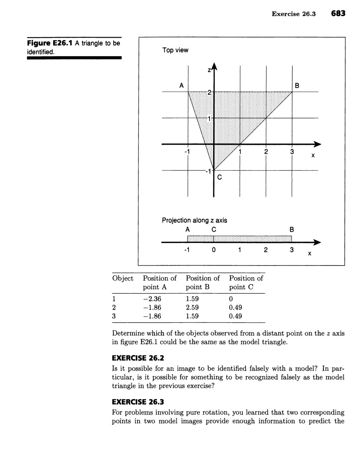
/


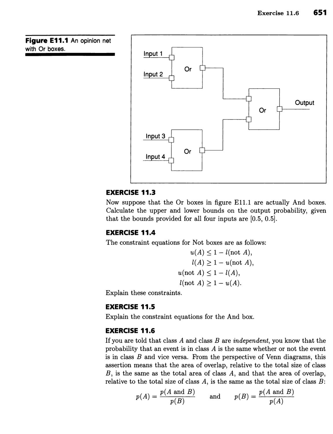


Текст
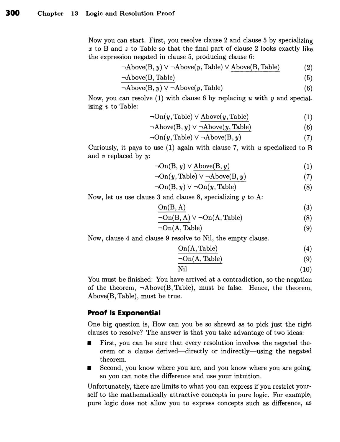
* •TIFICKL
T LLI
Third Edition
N WIN
Patrick Henry Winston
Professor of Computer Science
Director, Artificial Intelligence Laboratory
Massachusetts Institute of Technology
A
▼▼
ADDISON-WESLEY PUBLISHING COMPANY
Reading, Massachusetts ■ Menlo Park, California
New York ■ Don Mills, Ontario ■ Wokingham, England
Amsterdam ■ Bonn ■ Sydney ■ Singapore ■ Tokyo
Madrid ■ San Juan ■ Milan ■ Paris
Library of Congress Cataloging-in-Publication Data
Winston, Patrick Henry.
Artificial Intelligence / Patrick Henry Winston. — 3rd ed.
p. cm.
Includes bibliographical references (p. ) and index.
ISBN 0-201-53377-4
1. Artificial Intelligence. I. Title.
Q335.W56 1992 91-41385
006.3—dc20 CIP
Reproduced by Addison-Wesley from camera-ready copy supplied by the author.
Copyright © 1992 by Patrick H. Winston. All rights reserved. No part of this
publication may be reproduced, stored in a retrieval system, or transmitted in
any form or by any means, electronic, mechanical, photocopying, recording, or
otherwise, without prior written permission. Printed in the United States of
America.
1 2 3 4 5 6 7 8 9 10 HA 95949392
• n - s
ACKNOWLEDGMENTS
SOFTWARE
PREFACE
PART I ———
Representations and Methods
CHAPTER 1 ^m^—m^mm^mmmm
The Intelligent Computer
The Field and the Book
This Book Has Three Parts 6 ■ The Long-Term Applications Stagger the
Imagination 6 ■ The Near-Term Applications Involve New Opportunities 7
■ Artificial Intelligence Sheds New Light on Traditional Questions 7 ■
Artificial Intelligence Helps Us to Become More Intelligent 8
What Artificial Intelligence Can Do
Intelligent Systems Can Help Experts to Solve Difficult Analysis Problems 8
■ Intelligent Systems Can Help Experts to Design New Devices 9 ■
Intelligent Systems Can Learn from Examples 10 ■ Intelligent Systems Can
Provide Answers to English Questions Using both Structured Data and Free
Text 11b Artificial Intelligence Is Becoming Less Conspicuous, yet More
Essential 12
Criteria for Success 13
Summary 13
Background 14
CHAPTER 2 m—m—mm——mmm^m
Semantic Nets and Description Matching 15
Semantic Nets 16
Good Representations Are the Key to Good Problem Solving 16 b Good
Representations Support Explicit, Constraint-Exposing Description 18 ■ A
Representation Has Four Fundamental Parts 18 b Semantic Nets Convey
Meaning 19 b There Are Many Schools of Thought About the
Meaning of Semantics 20 b Theoretical Equivalence Is Different from Practical
Equivalence 22
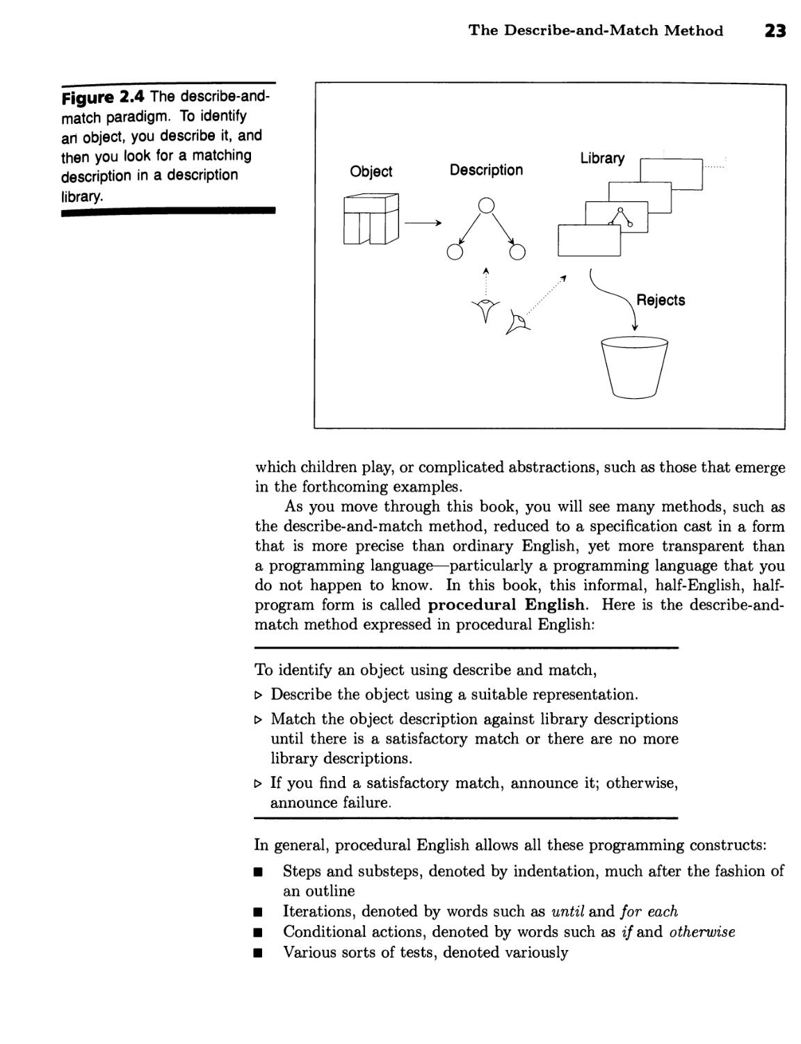
The Describe-and-Match Method 22
Feature-Based Object Identification Illustrates Describe and Match 24
The Describe-and-Match Method and Analogy
Problems 25
Geometric Analogy Rules Describe Object Relations and Object
Transformations 25 b Scoring Mechanisms Rank Answers 30 b Ambiguity
Complicates Matching 32 b Good Representation Supports Good
Performance 32
The Describe-and-Match Method and Recognition
of Abstractions 33
Story Plots Can Be Viewed as Combinations of Mental States and Events 33
b Abstraction-Unit Nets Enable Summary 36 b Abstraction Units Enable
Question Answering 41 b Abstraction Units Make Patterns Explicit 42
Problem Solving and Understanding Knowledge 42
Summary 44
Background 45
CHAPTER 3 ■HMHHH^Ml^H
Generate and Test, Means-Ends Analysis,
and Problem Reduction 47
The Generate-and-Test Method 47
Generate-and-Test Systems Often Do Identification 48 ■ Good
Generators Are Complete, Nonredundant, and Informed 49
V
The Means-Ends Analysis Method 50
The Key Idea in Means-Ends Analysis Is to Reduce Differences 50 ■ Den-
dral Analyzes Mass Spectrograms 51 ■ Difference-Procedure Tables Often
Determine the Means 53
The Problem-Reduction Method 53
Moving Blocks Illustrates Problem Reduction 54 ■ The Key Idea in Problem
Reduction Is to Explore a Goal Tree 56 ■ Goal Trees Can Make Procedure
Interaction Transparent 57 ■ Goal Trees Enable Introspective Question
Answering 59 ■ Problem Reduction Is Ubiquitous in Programming 60
■ Problem-Solving Methods Often Work Together 60 ■ Mathematics
Toolkits Use Problem Reduction to Solve Calculus Problems 61
Summary 60
Background 60
CHAPTER 4
Nets and Basic Search 63
Blind Methods 63
Net Search Is Really Tree Search 64 ■ Search Trees Explode
Exponentially 66 ■ Depth-First Search Dives into the Search Tree 66 ■ Breadth-
First Search Pushes Uniformly into the Search Tree 68 ■ The Right Search
Depends on the Tree 68 ■ Nondeterministic Search Moves Randomly into
the Search Tree 69
Heuristically Informed Methods 69
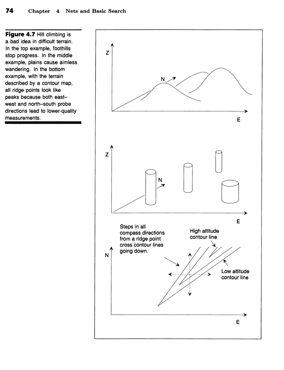
Quality Measurements Turn Depth-First Search into Hill Climbing 70 ■
Foothills, Plateaus, and Ridges Make Hills Hard to Climb 72 ■ Beam Search
Expands Several Partial Paths and Purges the Rest 73 ■ Best-First Search
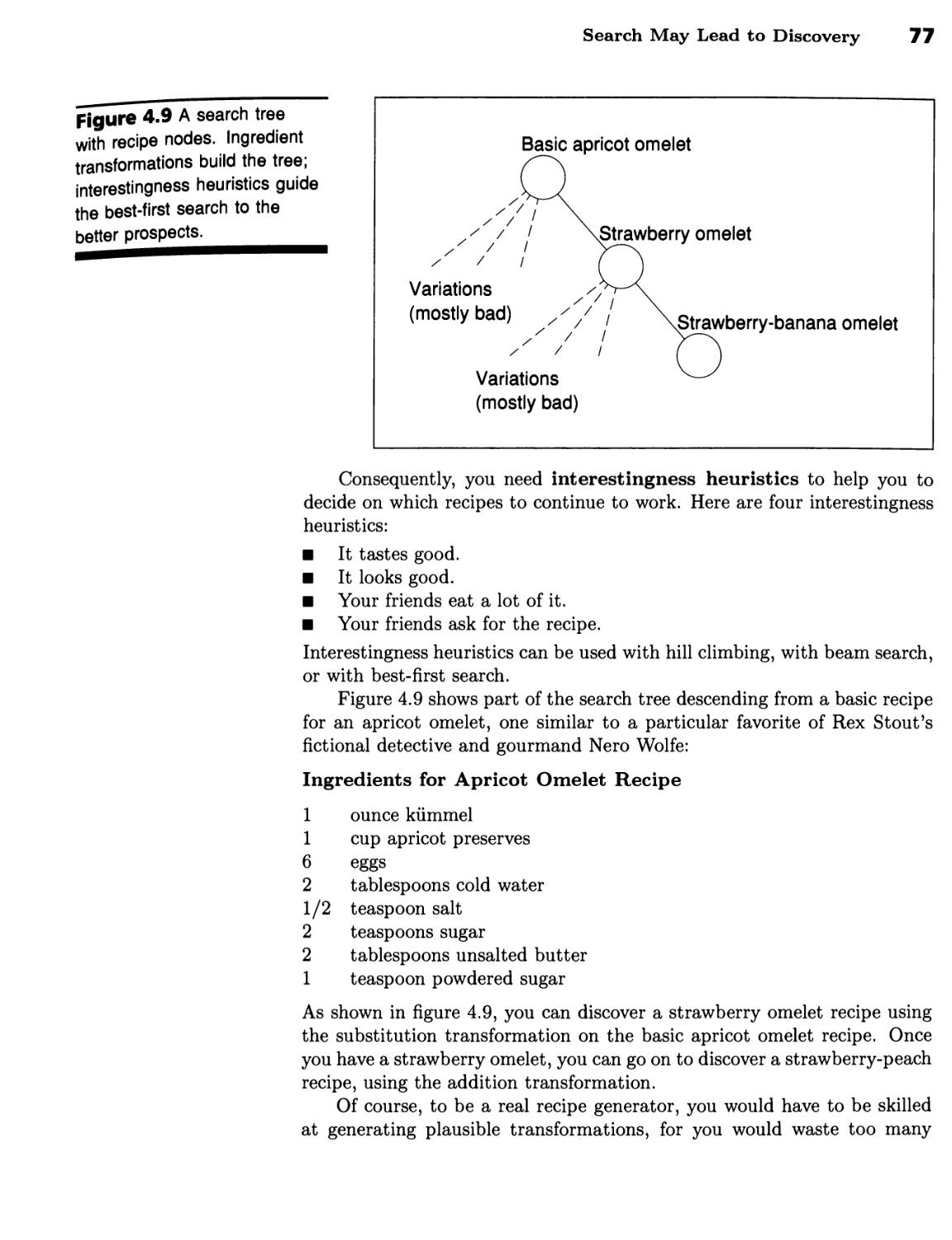
Expands the Best Partial Path 75 ■ Search May Lead to Discovery 75 ■
Search Alternatives Form a Procedure Family 78
Summary 78
Background 79
CHAPTER 5 w^^^mm—^m^^^m
Nets and Optimal Search 81
The Best Path 81
The British Museum Procedure Looks Everywhere 81 ■ Branch-and-Bound
Search Expands the Least-Cost Partial Path 82 ■ Adding Underestimates
Improves Efficiency 84
Redundant Paths
90
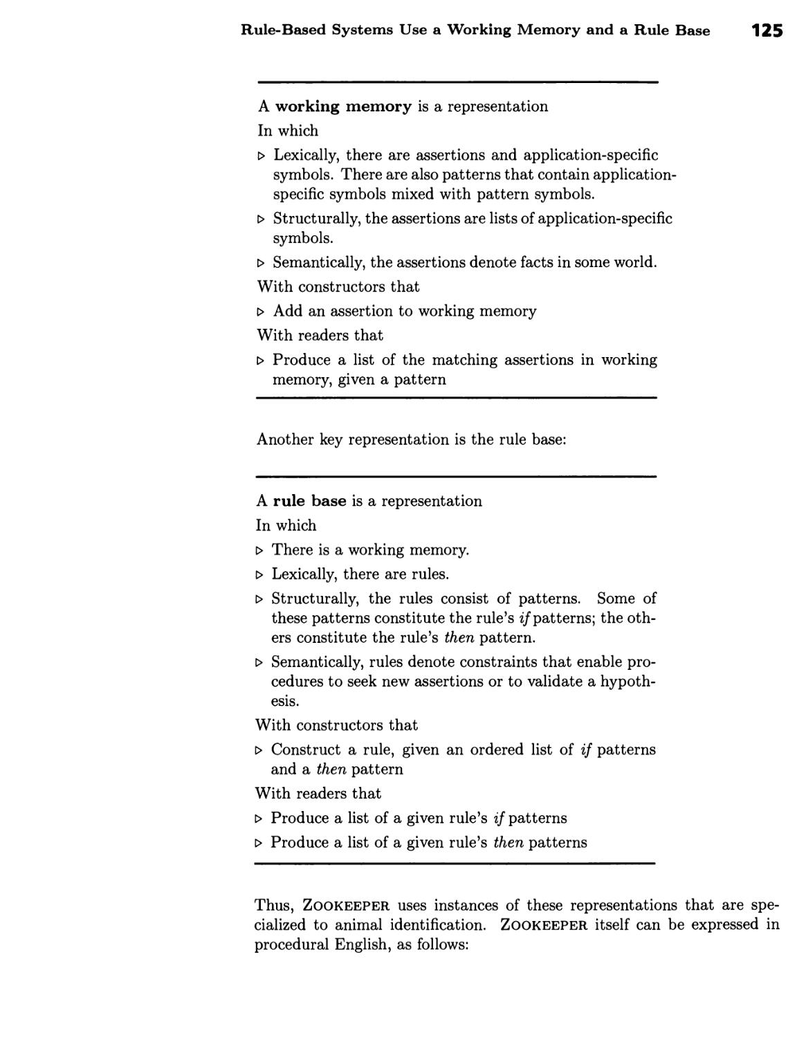
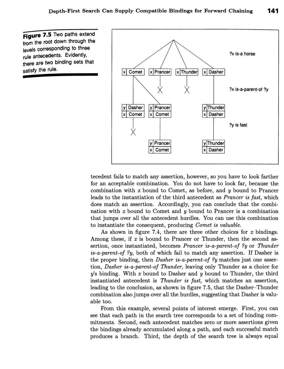
Redundant Partial Paths Should Be Discarded 90 ■ Underestimates and
Dynamic Programming Improve Branch-and-Bound Search 91 ■ Several
Search Procedures Find the Optimal Path 94 ■ Robot Path Planning
Illustrates Search 94
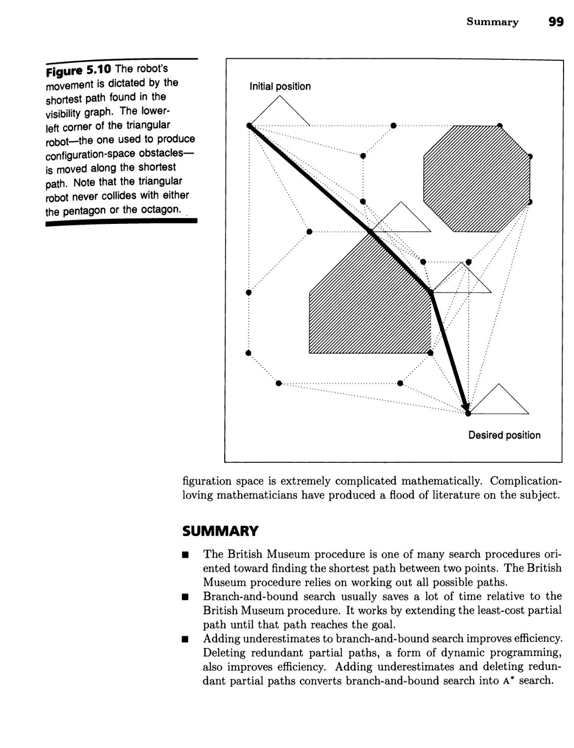
Summary 99
Background 100
CHAPTER 6
Trees and Adversarial Search 101
Algorithmic Methods 101
Nodes Represent Board Positions 101 ■ Exhaustive Search Is
Impossible 102 ■ The Minimax Procedure Is a Lookahead Procedure 103 ■ The
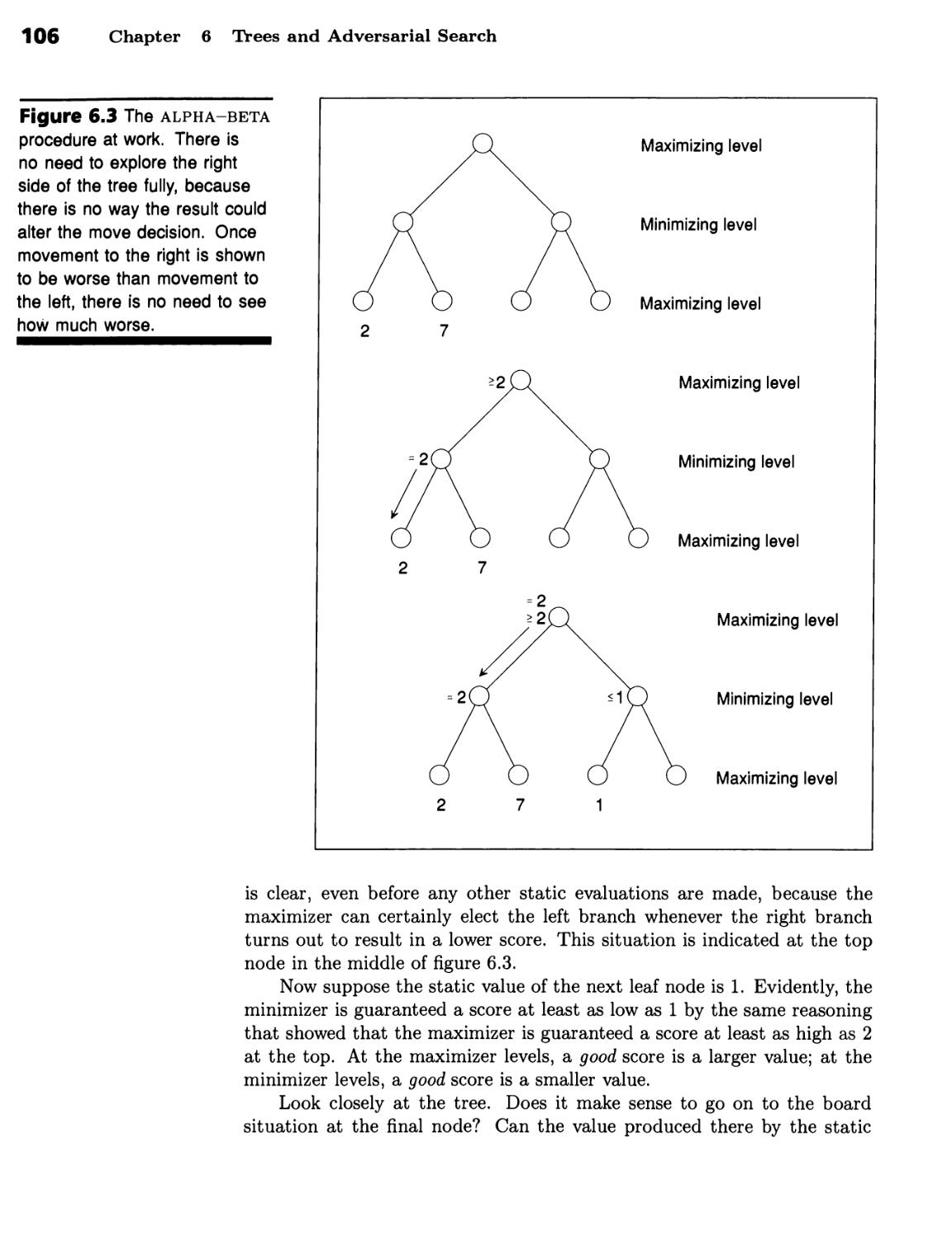
Alpha-Beta Procedure Prunes Game Trees 104 ■ Alpha-Beta May Not
Prune Many Branches from the Tree 110
Heuristic Methods 113
Progressive Deepening Keeps Computing Within Time Bounds 114 ■
Heuristic Continuation Fights the Horizon Effect 114 ■ Heuristic Pruning
Also Limits Search 115 ■ DEEP THOUGHT Plays Grandmaster Chess 117
Summary 116
Background 118
CHAPTER 7 ^^HHHHHH
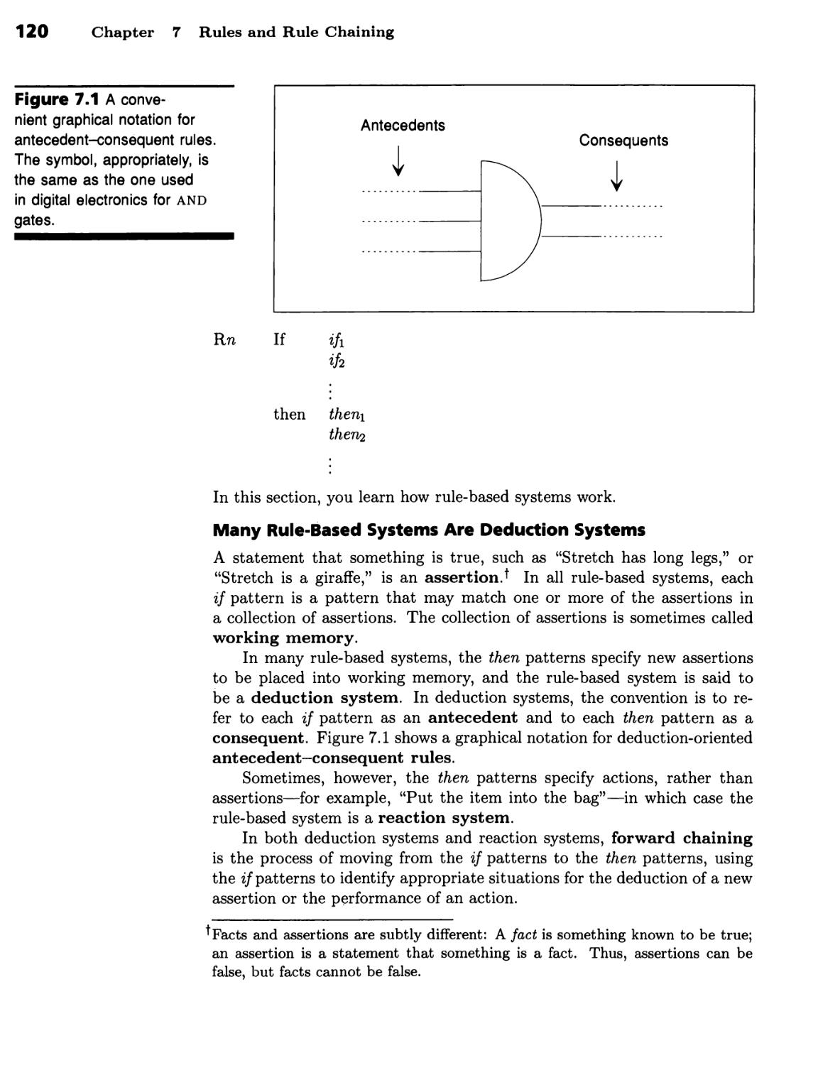
Rules and Rule Chaining 119
Rule-Based Deduction Systems 119
Many Rule-Based Systems Are Deduction Systems 120 ■ A Toy Deduction
System Identifies Animals 121b Rule-Based Systems Use a Working
Memory and a Rule Base 124 ■ Deduction Systems May Run Either Forward or
Backward 126 ■ The Problem Determines Whether Chaining Should Be
Forward or Backward 128
Rule-Based Reaction Systems 129
Mycin Diagnoses Bacterial Infections of the Blood 130 ■ A Toy Reaction
System Bags Groceries 132 ■ Reaction Systems Require Conflict
Resolution Strategies 137
Procedures for Forward and Backward Chaining 137
Depth-First Search Can Supply Compatible Bindings for Forward
Chaining 138 ■ XCON Configures Computer Systems 139 ■ Depth-First
Search Can Supply Compatible Bindings for Backward Chaining 142 ■
VII
Relational Operations Support Forward Chaining 147 ■ The Rete
Approach Deploys Relational Operations Incrementally 152
Summary 160
Background 161
CHAPTER 8 hh^i^hhi^h
Rules, Substrates, and Cognitive Modeling 163
Rule-based Systems Viewed as Substrate 163
Explanation Modules Explain Reasoning 163 ■ Reasoning Systems Can
Exhibit Variable Reasoning Styles 164 ■ Probability Modules Help You to
Determine Answer Reliability 167 ■ Two Key Heuristics Enable
Knowledge Engineers to Acquire Knowledge 167 ■ Acquisition Modules Assist
Knowledge Transfer 168 ■ Rule Interactions Can Be Troublesome 171 ■
Rule-Based Systems Can Behave Like Idiot Savants 171
Rule-Based Systems Viewed as Models for Human
Problem Solving 172
Rule-Based Systems Can Model Some Human Problem Solving 172 ■
Protocol Analysis Produces Production-System Conjectures 172 ■ SOAR
Models Human Problem Solving, Maybe 173 ■ SOAR Searches Problem
Spaces 173 ■ SOAR Uses an Automatic Preference Analyzer 175
Summary 176
Background 177
CHAPTER 9
mm
Frames and Inheritance 179
Frames, Individuals, and Inheritance 179
Frames Contain Slots and Slot Values 180 ■ Frames may Describe
Instances or Classes 180 ■ Frames Have Access Procedures 182 ■
Inheritance Enables When-Constructed Procedures to Move Default Slot Values
from Classes to Instances 182 ■ A Class Should Appear Before All Its
Superclasses 185 ■ A Class's Direct Superclasses Should Appear in Order 187
■ The Topological-Sorting Procedure Keeps Classes in Proper Order 190
Demon Procedures 197
When-Requested Procedures Override Slot Values 197 ■ When-Read and
When-Written Procedures Can Maintain Constraints 198 ■ With-Respect-
to Procedures Deal with Perspectives and Contexts 199 ■ Inheritance and
Demons Introduce Procedural Semantics 199 ■ Object-Oriented
Programming Focuses on Shared Knowledge 201
Viii Contents
Frames, Events, and Inheritance 202
Digesting News Seems to Involve Frame Retrieving and Slot Filling 202 ■
Event-Describing Frames Make Stereotyped Information Explicit 206
Summary 206
Background 206
CHAPTER 10
Frames and Commonsense 209
Thematic-role Frames 209
An Object's Thematic Role Specifies the Object's Relation to an Action 209
■ Filled Thematic Roles Help You to Answer Questions 212 ■ Various
Constraints Establish Thematic Roles 214 ■ A Variety of Constraints Help
Establish Verb Meanings 215 ■ Constraints Enable Sentence Analysis 216
■ Examples Using Take Illustrate How Constraints Interact 218
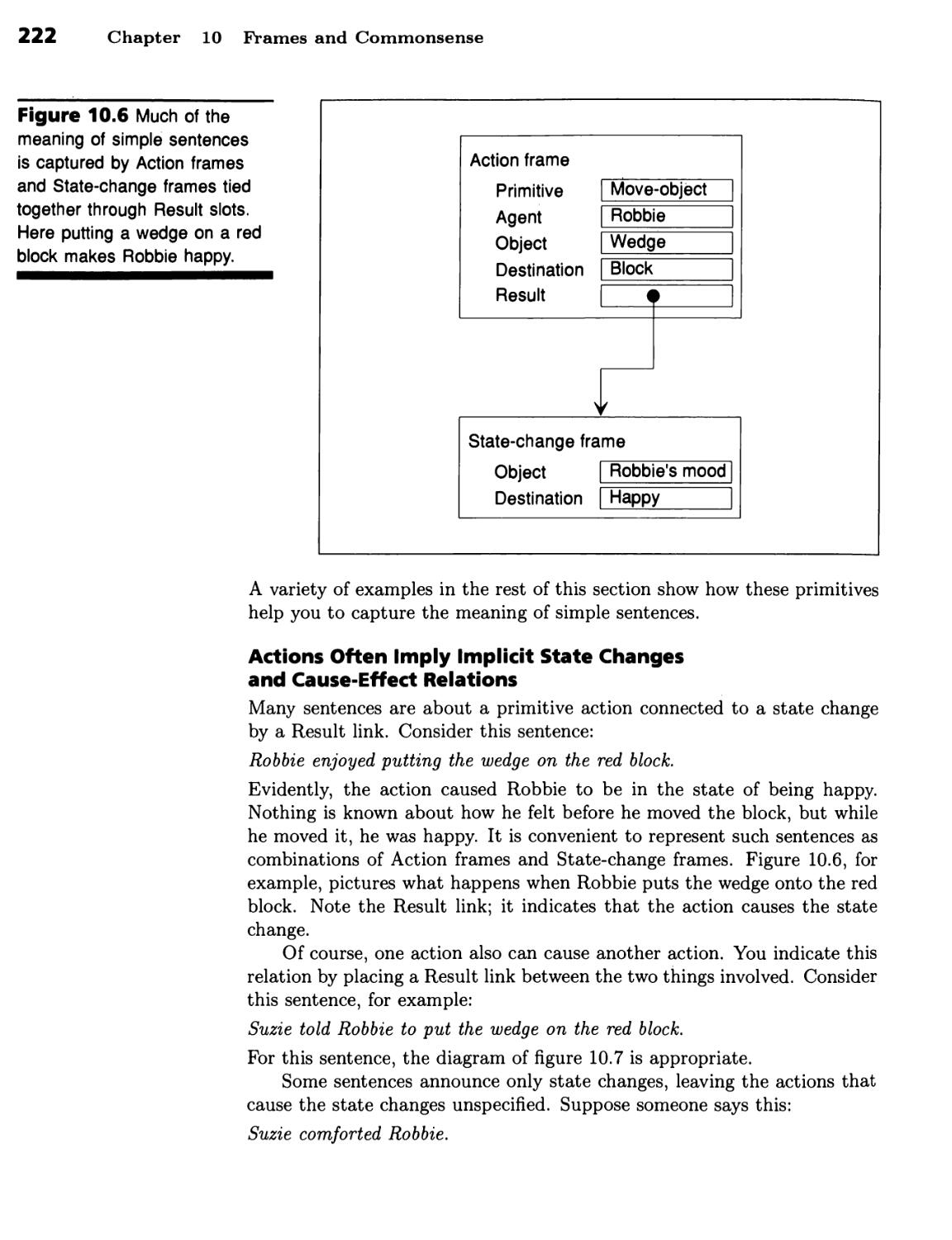
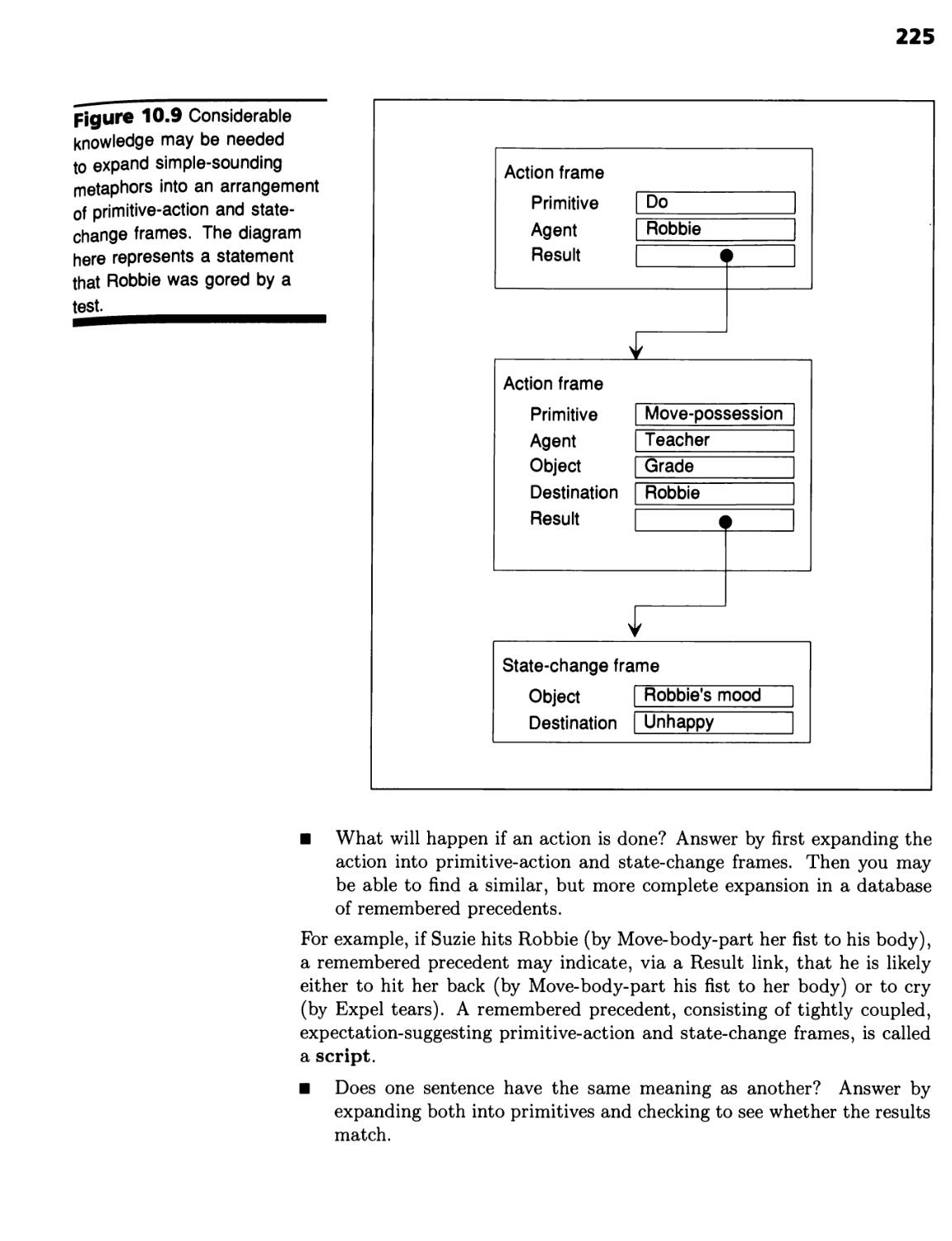
Expansion into Primitive Actions 221
Primitive Actions Describe Many Higher-Level Actions 221 ■ Actions
Often Imply Implicit State Changes and Cause-Effect Relations 222 ■ Actions
Often Imply Subactions 223 ■ Primitive-Action Frames and State-Change
Frames Facilitate Question Answering and Paraphrase Recognition 224 ■
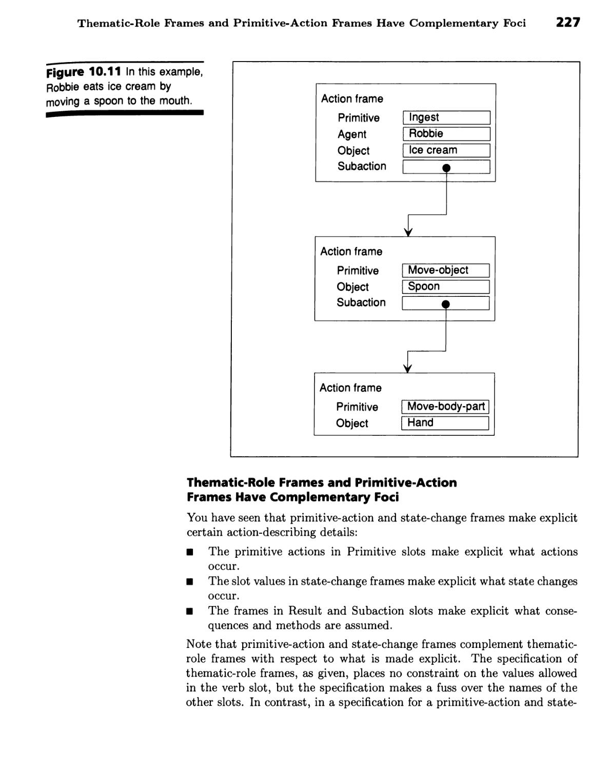
Thematic-Role Frames and Primitive-Action Frames Have Complementary
Foci 226 ■ CYC Captures Commonsense Knowledge 229
Summary 228
Background 228
CHAPTER 11 iHH^H^iH
Numeric Constraints and Propagation 231
Propagation of Numbers Through Numeric
Constraint Nets 231
Numeric Constraint Boxes Propagate Numbers through Equations 231
Propagation of Probability Bounds Through
Opinion Nets 234
Probability Bounds Express Uncertainty 234 ■ Spreadsheets Propagate
Numeric Constraints Through Numeric-Constraint Nets 235 ■ Venn
Diagrams Explain Bound Constraints 237 ■ Propagation Moves Probability
Bounds Closer Together 241
Propagation of Surface Altitudes Through Arrays 241
Local Constraints Arbitrate between Smoothness Expectations and Actual
Data 242 ■ Constraint Propagation Achieves Global Consistency through
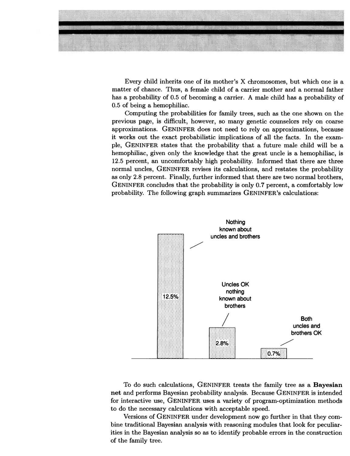
Local Computation 244 ■ GENINFER Helps Counselors to Provide Precise
Genetic Advice 246
Summary 245
Background 248
CHAPTER 12 ■■■■h^^^^^^m
Symbolic Constraints and Propagation 249
Propagation of Line Labels through Drawing
Junctions 249
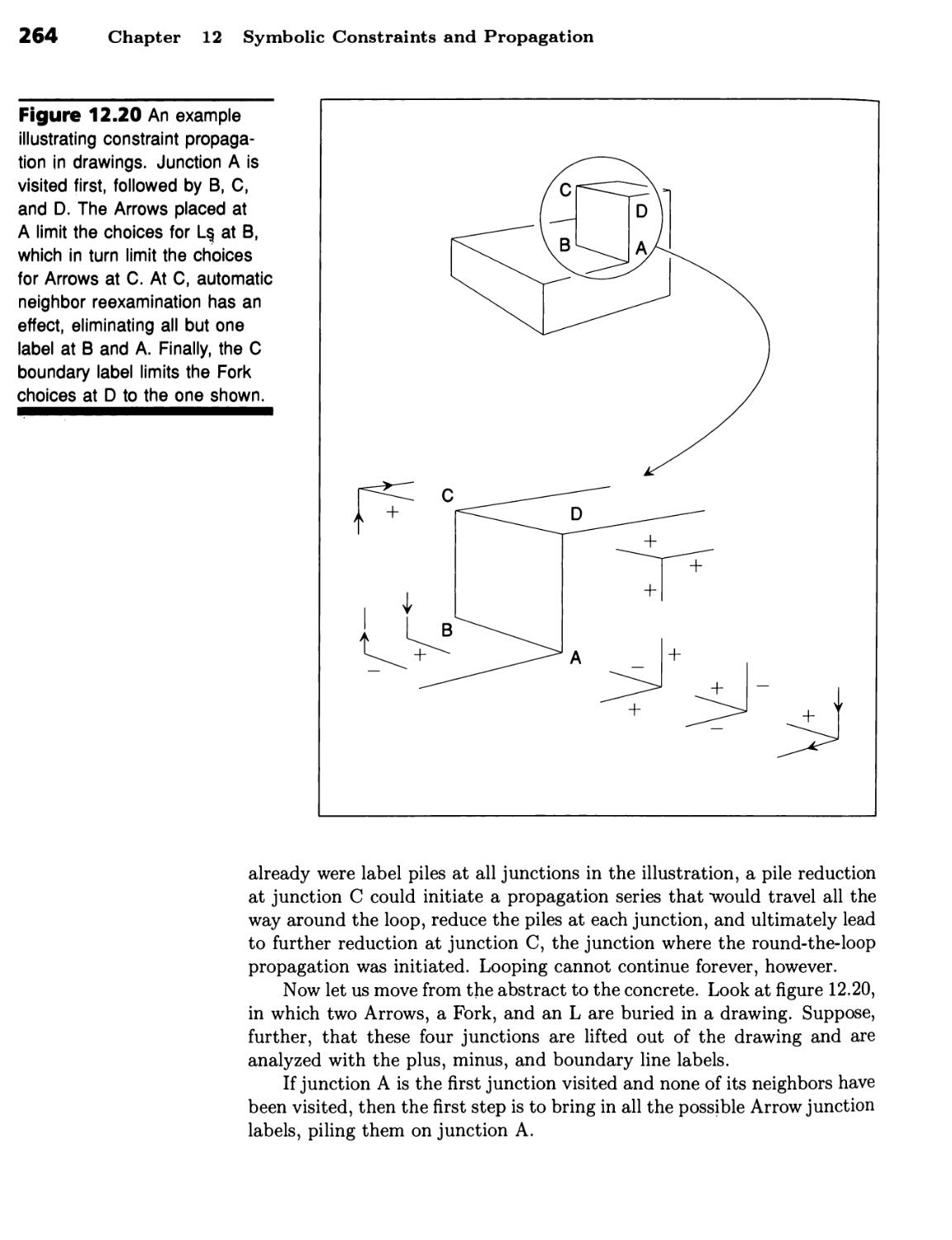
There Are Only Four Ways to Label a Line in the Three-Faced-Vertex World 250
■ There Are Only 18 Ways to Label a Three-Faced Junction 254 ■ Finding
Correct Labels Is Part of Line-Drawing Analysis 257 ■ Waltz's Procedure
Propagates Label Constraints through Junctions 262 ■ Many Line and
Junction Labels Are Needed to Handle Shadows and Cracks 266 ■
Illumination Increases Label Count and Tightens Constraint 267 ■ The Flow of
Labels Can Be Dramatic 270 ■ The Computation Required Is Proportional
to Drawing Size 272
Propagation of Time-Interval Relations 272
There Are 13 Ways to Label a Link between Interval Nodes Yielding 169
Constraints 272 ■ Time Constraints Can Propagate across Long
Distances 275 ■ A Complete Time Analysis Is Computationally Expensive 276
■ Reference Nodes Can Save Time 278
Five Points of Methodology 278
Summary 280
Background 280
CHAPTER 13 hh^hi^
Logic and Resolution Proof 283
Rules of Inference 283
Logic Has a Traditional Notation 284 ■ Quantifiers Determine When
Expressions Are True 287 ■ Logic Has a Rich Vocabulary 288 ■
Interpretations Tie Logic Symbols to Worlds 288 ■ Proofs Tie Axioms to
Consequences 290 ■ Resolution Is a Sound Rule of Inference 292
Resolution Proofs 293
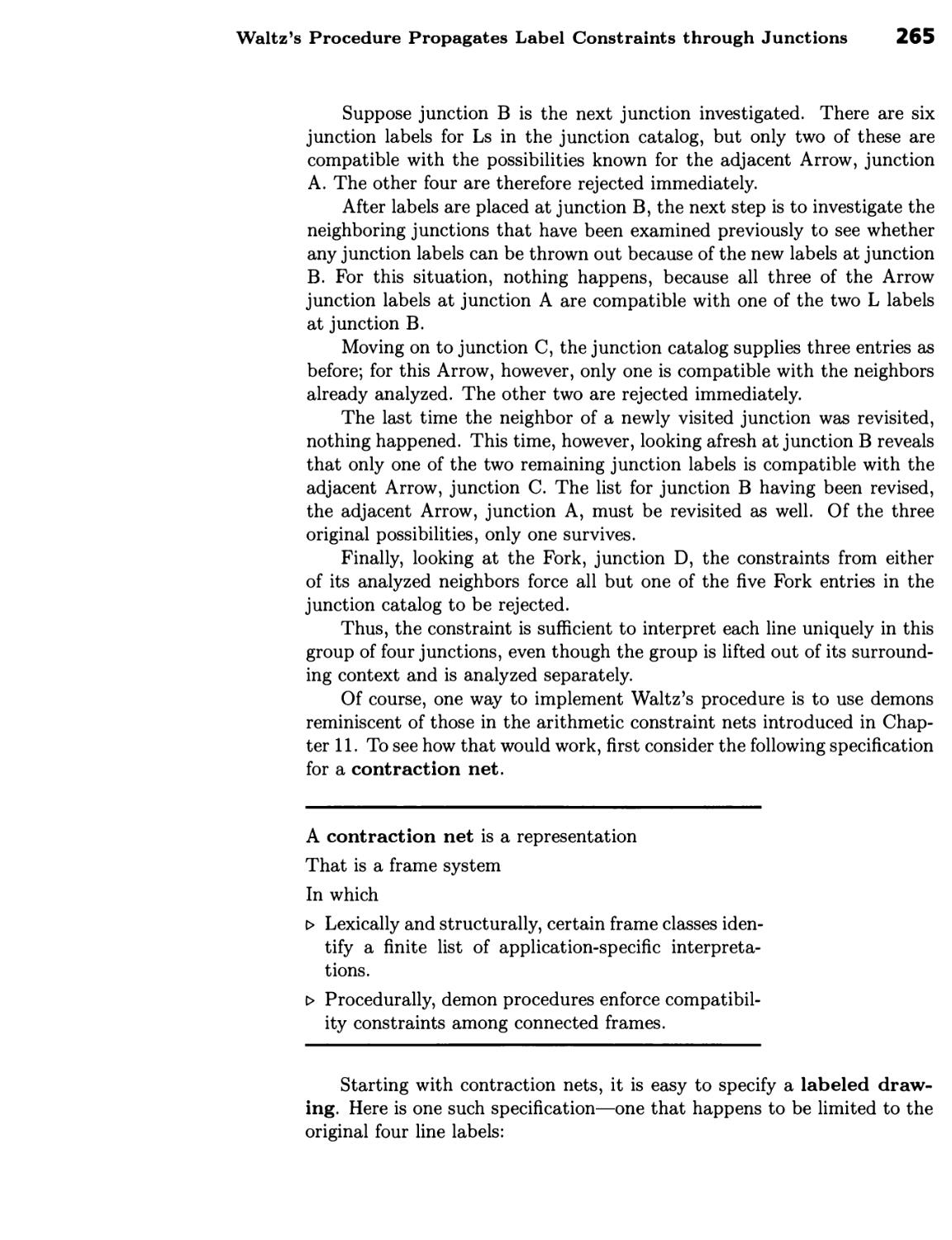
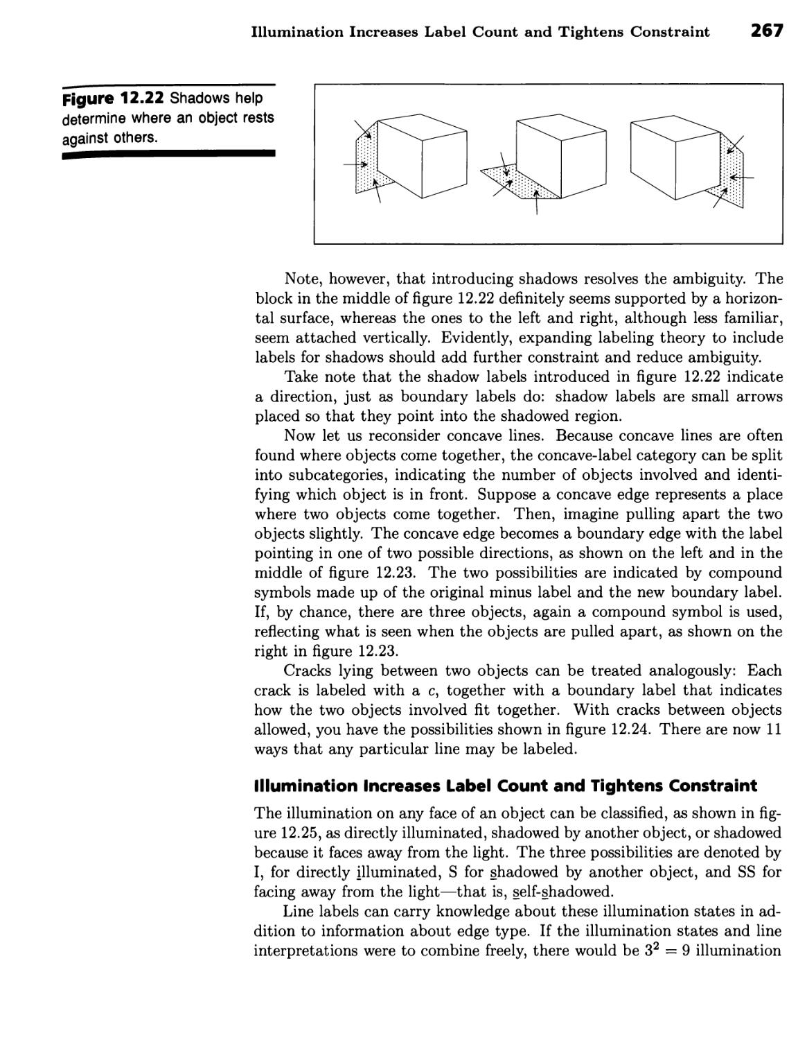
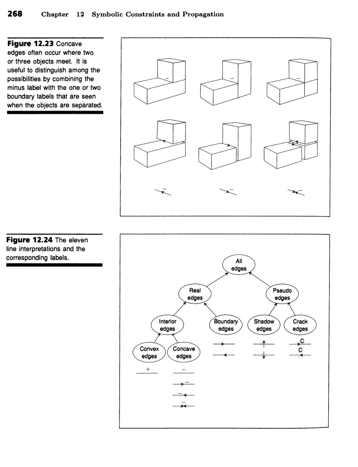
Resolution Proves Theorems by Refutation 293 ■ Using Resolution
Requires Axioms to Be in Clause Form 294 ■ Proof Is Exponential 300 ■
Resolution Requires Unification 301 ■ Traditional Logic Is Monotonic 302
■ Theorem Proving Is Suitable for Certain Problems, but Not for All
Problems 302
Summary 303
Background 304
CHAPTER 14 ■h^hhhhi
Backtracking and Truth Maintenance 305
Chronological and Dependency-Directed
Backtracking 305
Limit Boxes Identify Inconsistencies 305 ■ Chronological Backtracking
Wastes Time 306 ■ Nonchronological Backtracking Exploits
Dependencies 308
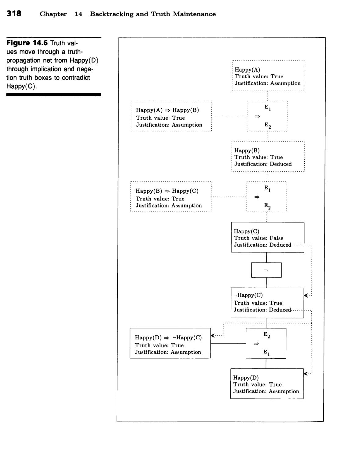
Proof by Constraint Propagation 309
Truth Can Be Propagated 309 ■ Truth Propagation Can Establish
Justifications 315 ■ Justification Links Enable Programs to Change Their
Minds 316 ■ Proof by Truth Propagation Has Limits 319
Summary 320
Background 320
CHAPTER 15 ^^^^■m^b^mm
Planning 323
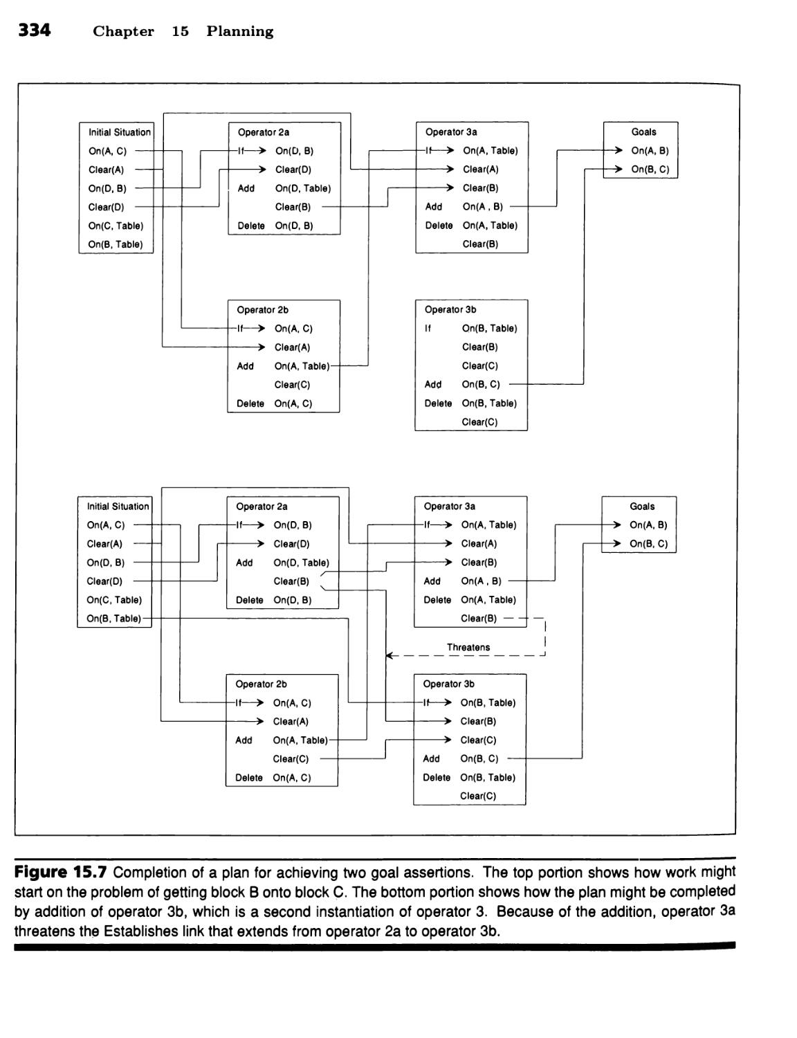
Planning Using If-Add-Delete Operators 323
Operators Specify Add Lists and Delete Lists 324 ■ You Can Plan by
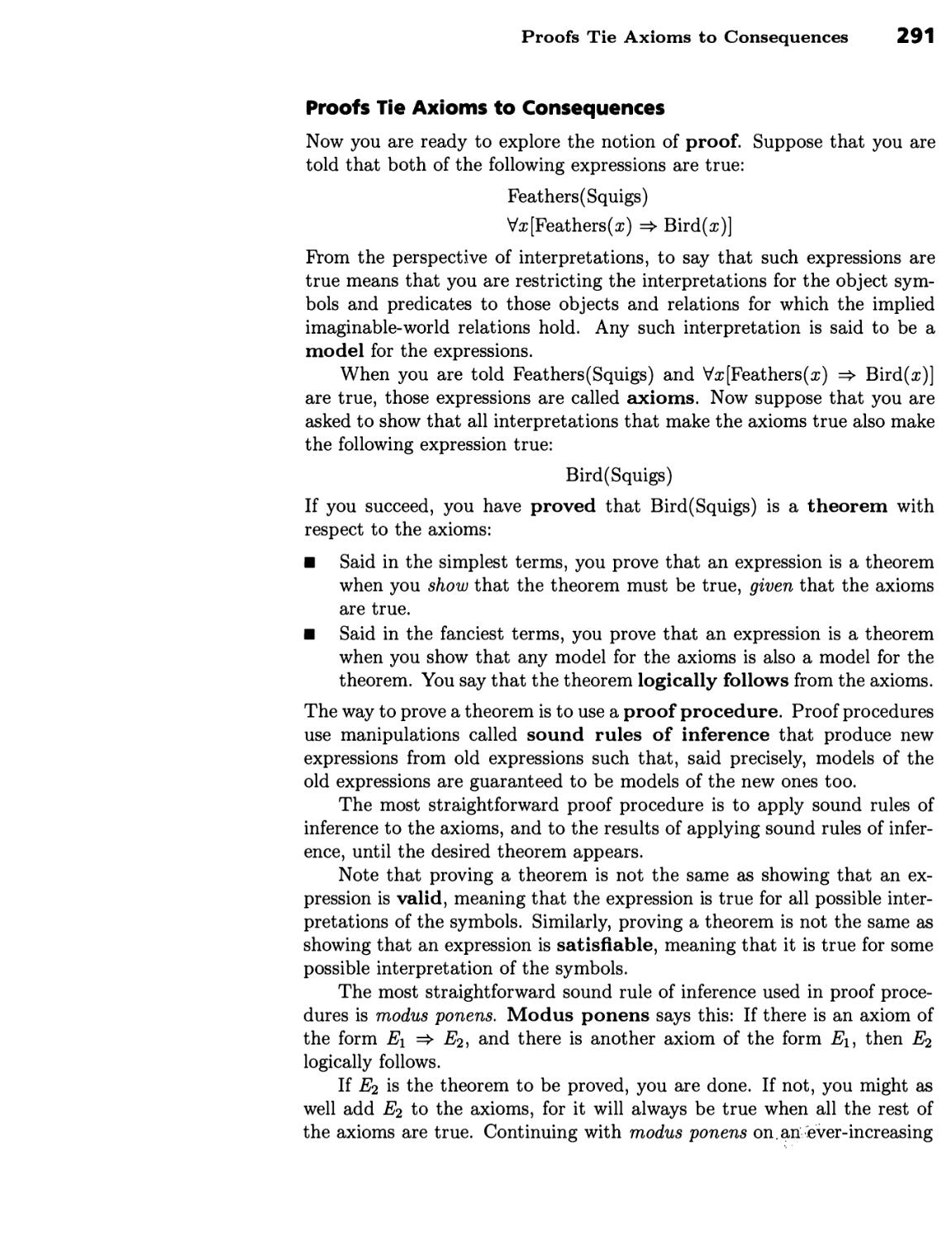
Searching for a Satisfactory Sequence of Operators 326 ■ Backward
Chaining Can Reduce Effort 327 ■ Impossible Plans Can Be Detected 331
■ Partial Instantiation Can Help Reduce Effort Too 336
Planning Using Situation Variables 338
Finding Operator Sequences Requires Situation Variables 338 ■ Frame
Axioms Address the Frame Problem 343
Summary 345
Background
346
XI
PART II _——^^—
Learning and Regularity Recognition 347
CHAPTER 16 ^^^m^h^hhhh
Learning by Analyzing Differences 349
Induction Heuristics 349
Responding to Near Misses Improves Models 351 ■ Responding to
Examples Improves Models 354 ■ Near-Miss Heuristics Specialize; Example
Heuristics Generalize 355 ■ Learning Procedures Should Avoid Guesses 357
■ Learning Usually Must Be Done in Small Steps 358
Identification 359
Must Links and Must-Not Links Dominate Matching 359 ■ Models May
Be Arranged in Lists or in Nets 359 ■ ARIEL Learns about Proteins 360
Summary 362
Background 363
CHAPTER 17 ^^^M^H^HHHH
Learning by Explaining Experience 365
Learning about Why People Act the Way they Do 365
Reification and the Vocabulary of Thematic-Role Frames Capture Sentence-
Level Meaning 366 ■ Explanation Transfer Solves Problems Using
Analogy 367 ■ Commonsense Problem Solving Can Generate Rulelike
Principles 372 ■ The Macbeth Procedure Illustrates the Explanation
Principle 373 ■ The Macbeth Procedure Can Use Causal Chains to Establish
Common Context 374
Learning about Form and Function 376
Examples and Precedents Help Each Other 377 ■ Explanation-Based
Learning Offers More than Speedup 380
Matching 380
Stupid Matchers Are Slow and Easy to Fool 380 ■ Matching Inexact
Situations Reduces to Backward Chaining 381 ■ Matching Sheds Light
on Analogical Problem Solving 383
Summary 383
Background 384
CHAPTER 18 wmmm^^^^^m^m
Learning by Correcting Mistakes 385
Isolating Suspicious Relations 385
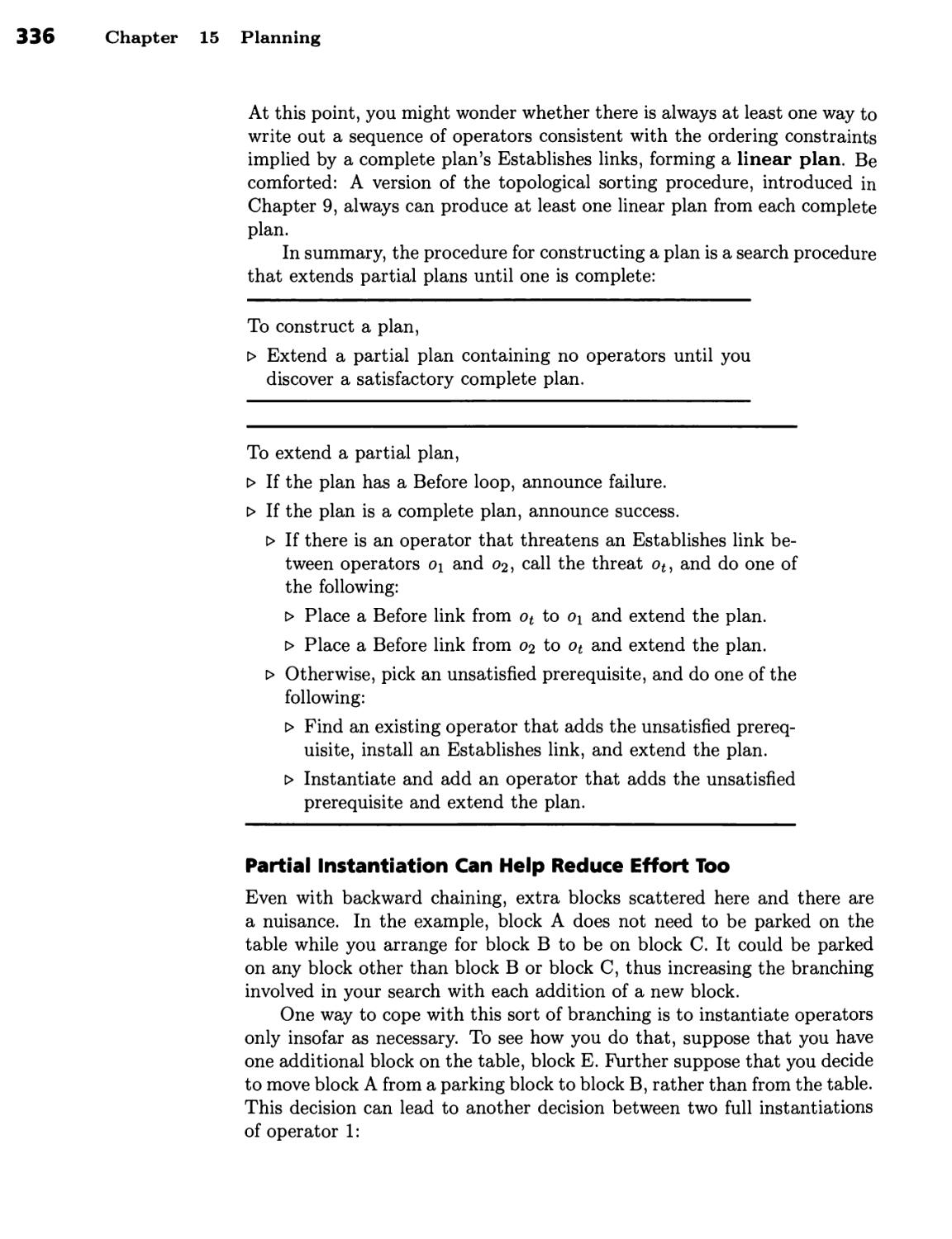
Cups and Pails Illustrate the Problem 385 ■ Near-Miss Groups Isolate
Xii Contents
Suspicious Relations 386 ■ Suspicious Relation Types Determine Overall
Repair Strategy 388
Intelligent Knowledge Repair 388
The Solution May Be to Explain the True-Success Suspicious Relations 388
■ Incorporating True-Success Suspicious Relations May Require Search 391
■ The Solution May Be to Explain the False-Success Suspicious Relations,
Creating a Censor 393 ■ Failure Can Stimulate a Search for More Detailed
Descriptions 395
Summary 396
Background 396
CHAPTER 19 ^^mamm^mam^^^
Learning by Recording Cases 397
Recording and Retrieving Raw Experience 397
The Consistency Heuristic Enables Remembered Cases to Supply
Properties 397 ■ The Consistency Heuristic Solves a Difficult Dynamics
Problem 398
Finding Nearest Neighbors 403
A Fast Serial Procedure Finds the Nearest Neighbor in Logarithmic Time 403
■ Parallel Hardware Finds Nearest Neighbors Even Faster 408
Summary 408
Background 409
CHAPTER 20 ^^mamm^mam^^^
Learning by Managing Multiple Models 411
The Version-Space Method 411
Version Space Consists of Overly General and Overly Specific Models 411
■ Generalization and Specialization Leads to Version-Space Convergence 414
Version-Space Characteristics 420
The Version-Space Procedure Handles Positive and Negative Examples
Symmetrically 420 ■ The Version-Space Procedure Enables Early
Recognition 421
XIII
Summary 422
Background 422
CHAPTER 21 hh^^^h^^h^^
Learning by Building Identification Trees 423
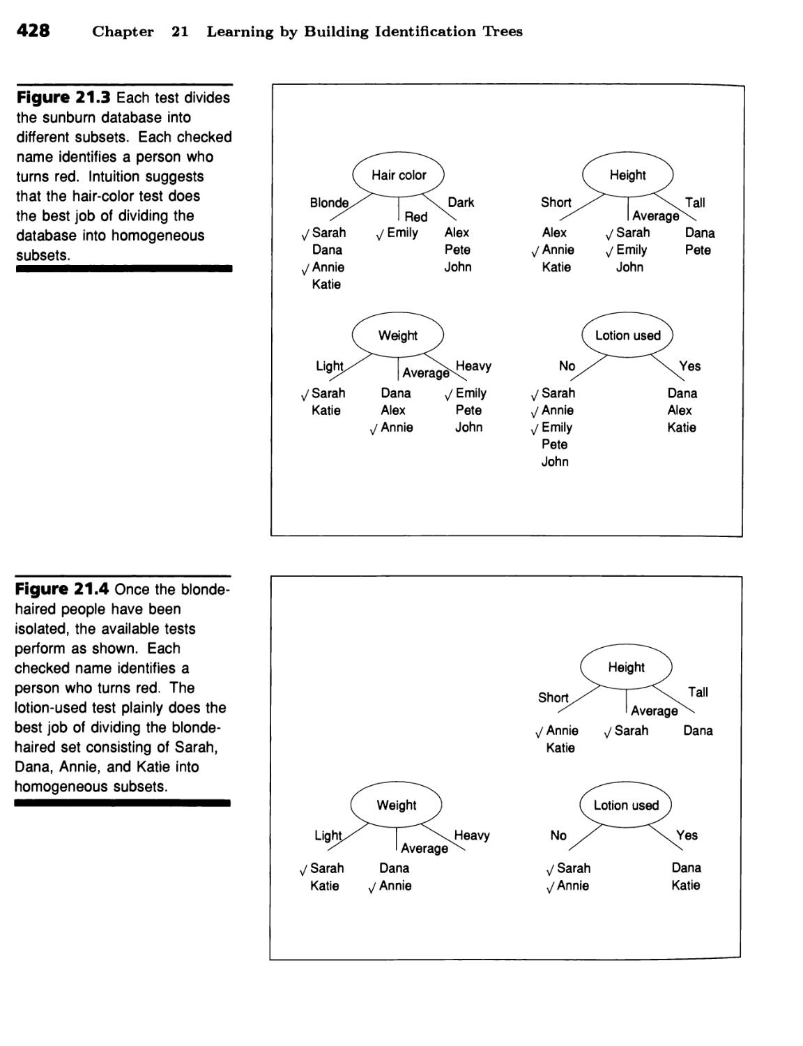
From Data to Identification Trees 423
The World Is Supposed to Be Simple 423 ■ Tests Should Minimize
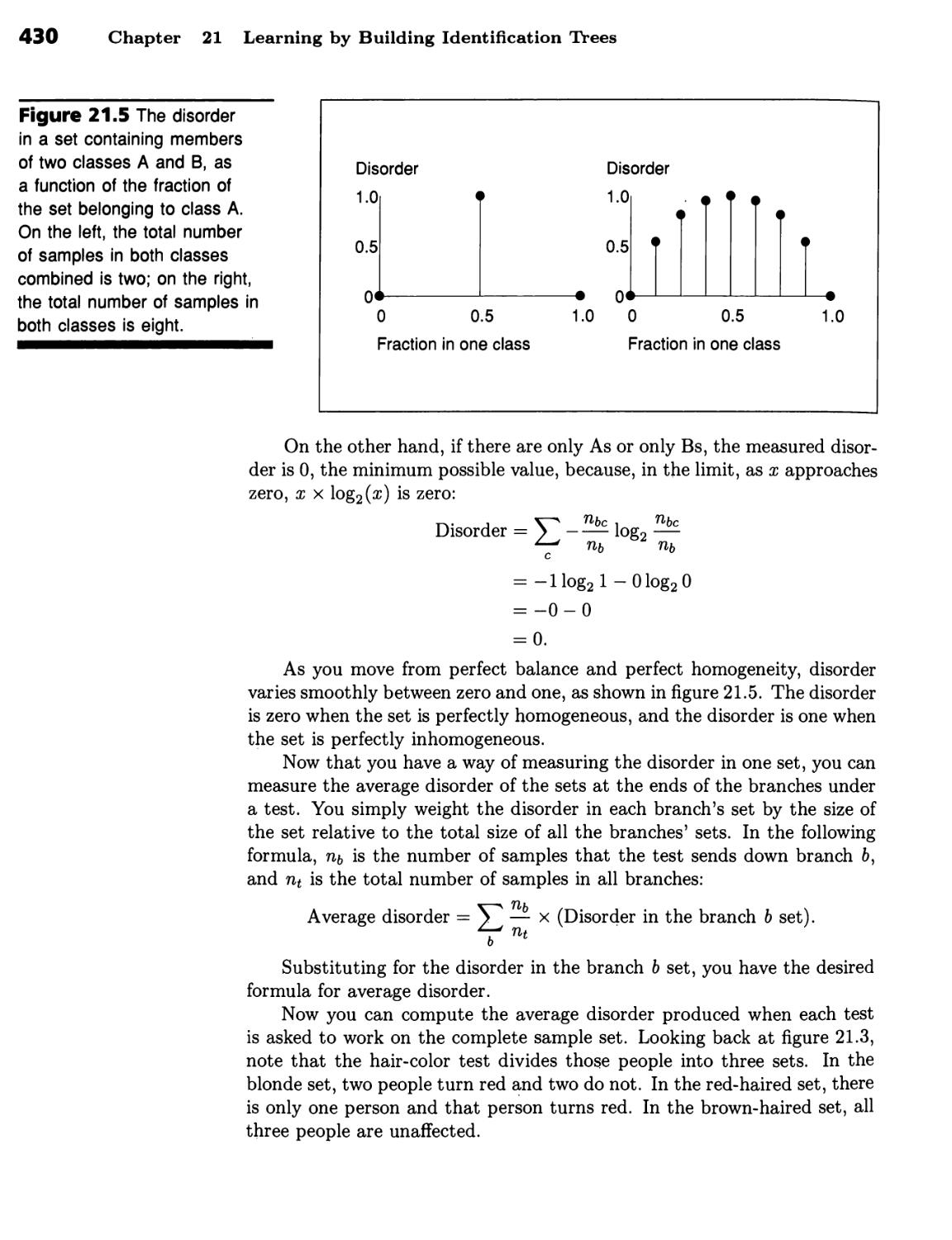
Disorder 427 ■ Information Theory Supplies a Disorder Formula 427
From Trees to Rules 431
Unnecessary Rule Antecedents Should Be Eliminated 432 ■ Optimizing a
Nuclear Fuel Plant 433 ■ Unnecessary Rules Should Be Eliminated 435 ■
Fisher's Exact Test Brings Rule Correction in Line with Statistical Theory 437
Summary 442
Background 442
CHAPTER 22 ■■■■hh^^^^^m
Learning by Training Neural Nets 443
Simulated Neural Nets 443
Real Neurons Consist of Synapses, Dendrites, Axons, and Cell Bodies 444
■ Simulated Neurons Consist of Multipliers, Adders, and Thresholds 445
■ Feed-Forward Nets Can Be Viewed as Arithmetic Constraint Nets 446
■ Feed-Forward Nets Can Recognize Regularity in Data 447
Hill Climbing and Back Propagation 448
The Back-Propagation Procedure Does Hill Climbing by Gradient Ascent 448
■ Nonzero Thresholds Can Be Eliminated 449 ■ Gradient Ascent Requires
a Smooth Threshold Function 449 ■ Back Propagation Can Be Understood
Heuristically 451 ■ Back-Propagation Follows from Gradient Descent and
the Chain Rule 453 ■ The Back-Propagation Procedure Is
Straightforward 457
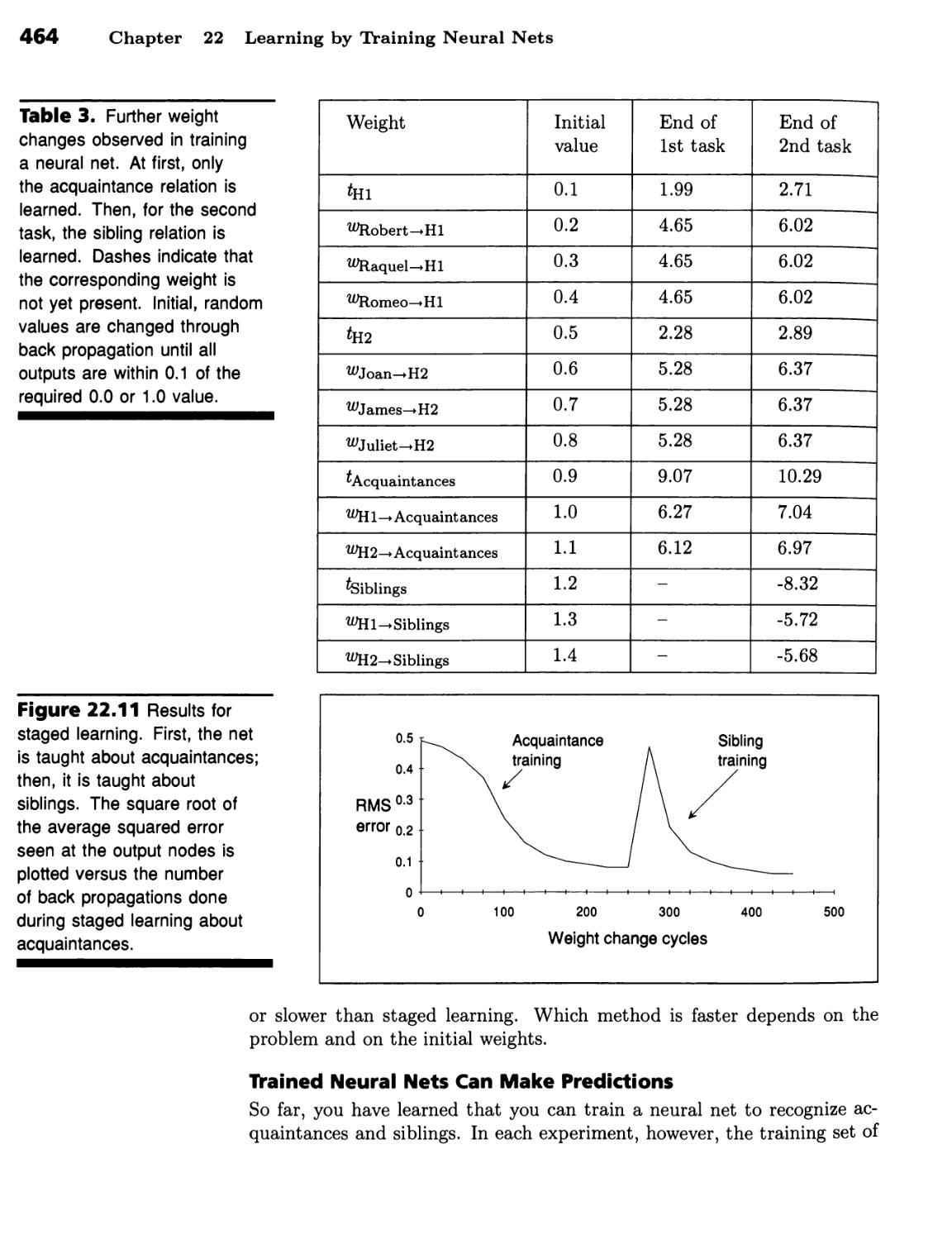
Back-Propagation Characteristics 457
Training May Require Thousands of Back Propagations 458 ■ ALVINN
Learns to Drive 459 ■ Back Propagation Can Get Stuck or Become
Unstable 461 ■ Back Propagation Can Be Done in Stages 462 ■ Back
Propagation Can Train a Net to Learn to Recognize Multiple Concepts
Simultaneously 463 ■ Trained Neural Nets Can Make Predictions 464 ■
Excess Weights Lead to Overf itting 465 ■ Neural-Net Training Is an Art 467
Xiv Contents
Summary 468
Background 469
CHAPTER 23 ^^^m^—^—^mm
Learning by Training Perceptrons 471
Perceptrons and Perceptron Learning 471
Perceptrons Have Logic Boxes and Stair-Step Thresholds 471 ■ The
Perceptron Convergence Procedure Guarantees Success Whenever Success Is
Possible 474 ■ Ordinary Algebra Is Adequate to Demonstrate
Convergence When There Are Two Weights 477 ■ Vector Algebra Helps You to
Demonstrate Convergence When There Are Many Weights 480
What Perceptrons Can and Cannot Do 482
A Straight-Through Perceptron Can Learn to Identify Digits 482 ■ The
Perceptron Convergence Procedure Is Amazing 484 ■ There Are Simple
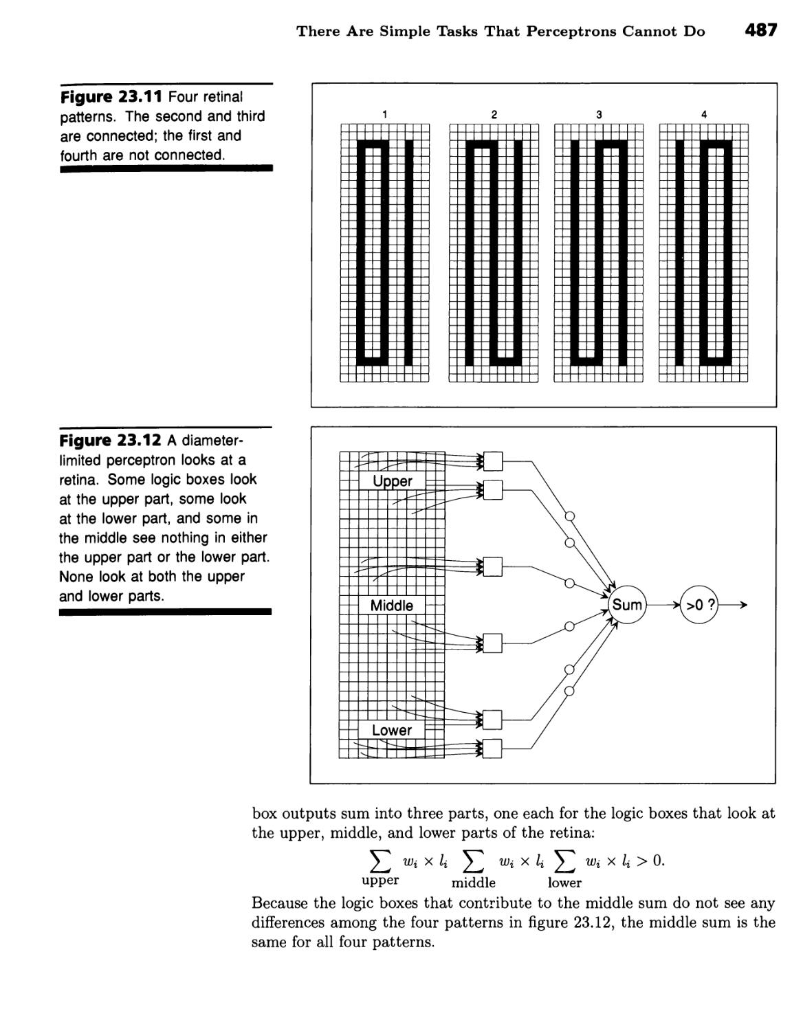
Tasks That Perceptrons Cannot Do 486
Summary 488
Background 488
CHAPTER 24 ^^^m^—^—^mm
Learning by Training Approximation Nets 491
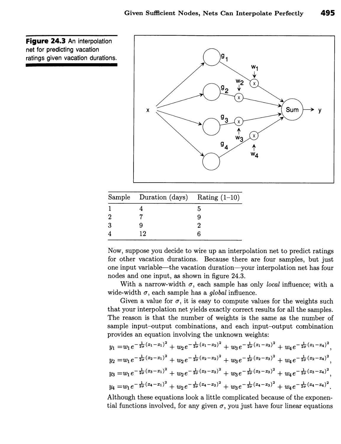
Interpolation and Approximation Nets 491
Gaussian Functions Centered on Samples Enable Good Interpolations 492
■ Given Sufficient Nodes, Nets Can Interpolate Perfectly 494 ■ Given
Relatively Few Nodes, Approximation Nets Can Yield Approximate Results
for All Sample Inputs 496 ■ Too Many Samples Leads to Weight
Training 497 ■ Overlooked Dimensions May Explain Strange Data Better than
Elaborate Approximation 499 ■ The Interpolation-Approximation Point
of View Helps You to Answer Difficult Design Questions 501
Biological Implementation 501
Numbers Can Be Represented by Position 501 ■ Neurons Can Compute
Gaussian Functions 501 ■ Gaussian Functions Can Be Computed as
Products of Gaussian Functions 502
Summary 503
Background 503
CHAPTER 25 i^hh^hh^h
Learning by Simulating Evolution 505
Survival of the Fittest 505
Chromosomes Determine Hereditary Traits 506 ■ The Fittest Survive 507
XV
Genetic Algorithms 507
Genetic Algorithms Involve Myriad Analogs 507 ■ The Standard Method
Equates Fitness with Relative Quality 510 ■ Genetic Algorithms Generally
Involve Many Choices 512 ■ It Is Easy to Climb Bump Mountain
Without Crossover 513 ■ Crossover Enables Genetic Algorithms to Search
High-Dimensional Spaces Efficiently 516 ■ Crossover Enables Genetic
Algorithms to Traverse Obstructing Moats 516 ■ The Rank Method Links
Fitness to Quality Rank 518
Survival of the Most Diverse 519
The Rank-Space Method Links Fitness to Both Quality Rank and Diversity
Rank 520 ■ The Rank-Space Method Does Well on Moat Mountain 523
■ Local Maxima Are Easier to Handle when Diversity Is Maintained 526
Summary 527
Background 528
PART
Vision and Language 529
CHAPTER 26 ^^^m^h^hhhh
Recognizing Objects 531
Linear Image Combinations 531
Conventional Wisdom Has Focused on Multilevel Description 531 ■
Images Contain Implicit Shape Information 532 ■ One Approach Is Matching
Against Templates 533 ■ For One Special Case, Two Images Are Sufficient
to Generate a Third 536 ■ Identification Is a Matter of Finding Consistent
Coefficients 537 ■ The Template Approach Handles Arbitrary Rotation and
Translation 539 ■ The Template Approach Handles Objects with Parts 542
■ The Template Approach Handles Complicated Curved Objects 545
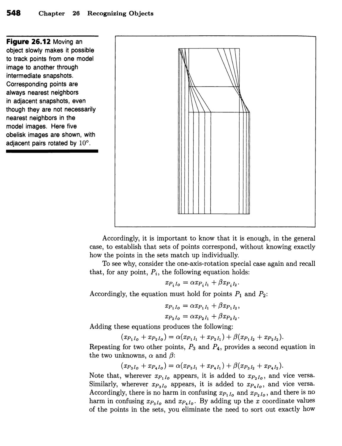
Establishing Point Correspondence 546
Tracking Enables Model Points to Be Kept in Correspondence 547 ■ Only
Sets of Points Need to Be Matched 547 ■ Heuristics Help You to Match
Unknown Points to Model Points 549
Summary 550
Background 550
CHAPTER 27 ^^^M^H^HHHH
Describing Images 553
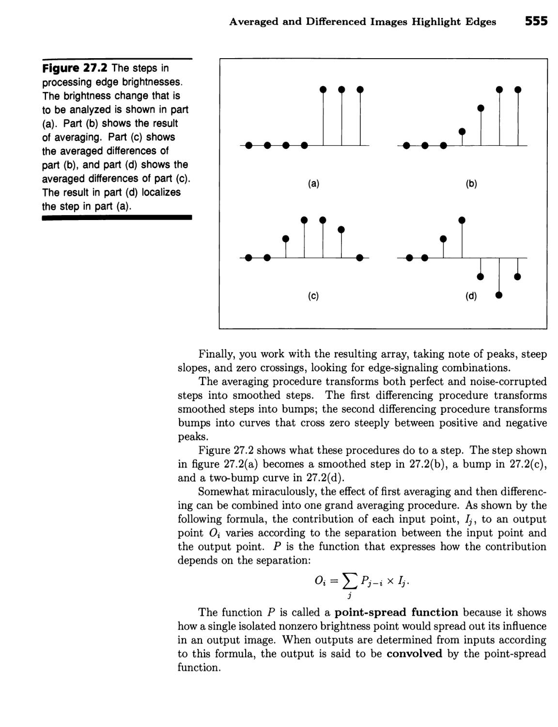
Computing Edge Distance 553
Averaged and Differenced Images Highlight Edges 553 ■ Multiple-Scale
Stereo Enables Distance Determination 557
Computing Surface Direction 562
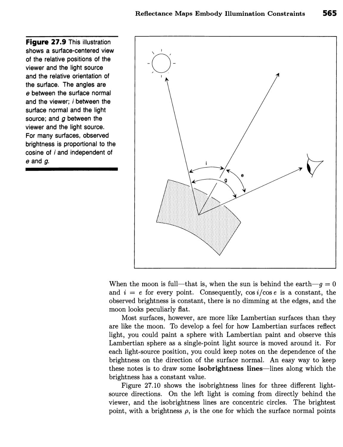
Stereo Analysis Determines Elevations from Satellite Images 563 ■
Reflectance Maps Embody Illumination Constraints 564 ■ Making Synthetic
Images Requires a Reflectance Map 567 ■ Surface Shading Determines
Surface Direction 567
Summary 572
Background 573
CHAPTER 28 i^Hi^iHH
Expressing Language Constraints 575
The Search for an Economical Theory 575
You Cannot Say That 576 ■ Phrases Crystallize on Words 576 ■
Replacement Examples Support Binary Representation 578 ■ Many Phrase
Types Have the Same Structure 579 ■ The X-Bar Hypothesis Says that All
Phrases Have the Same Structure 583
The Search for a Universal Theory 585
A Theory of Language Ought to Be a Theory of All Languages 586 ■ A
Theory of Language Ought to Account for Rapid Language Acquisition 588
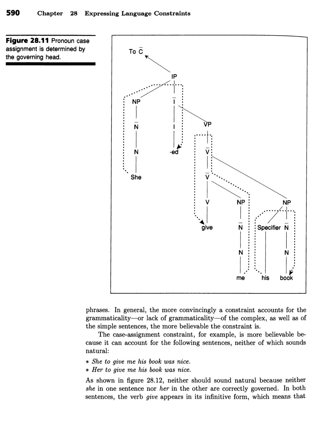
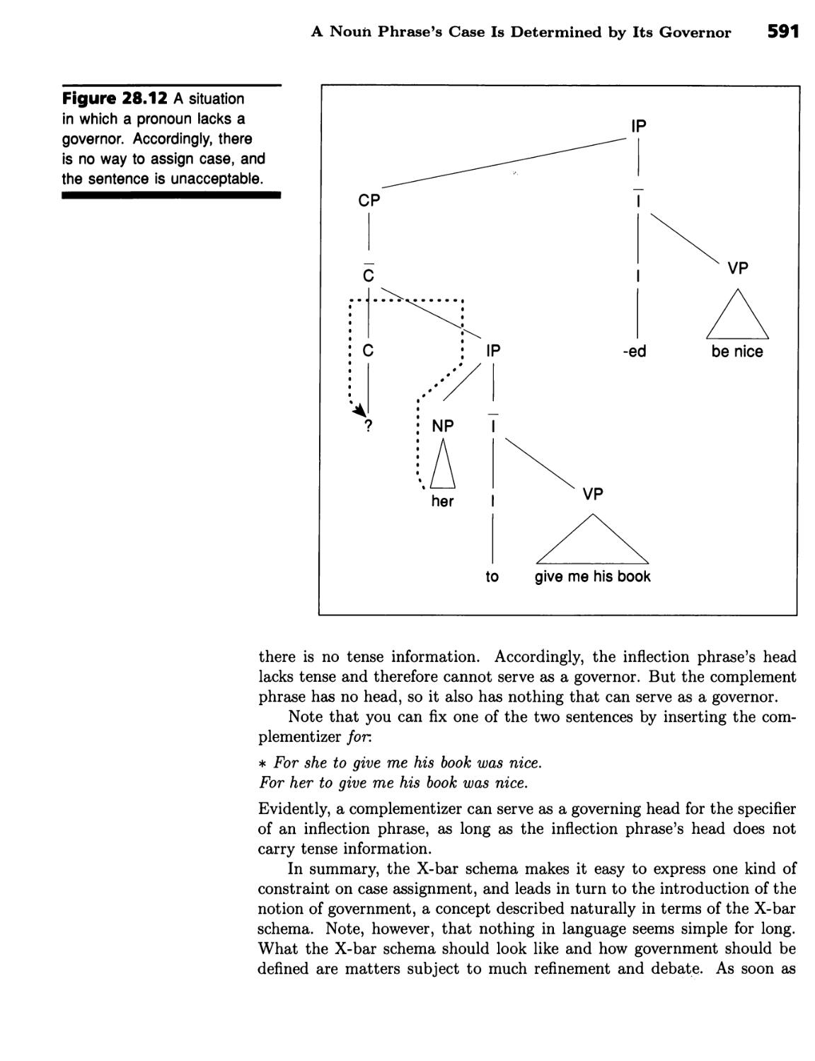
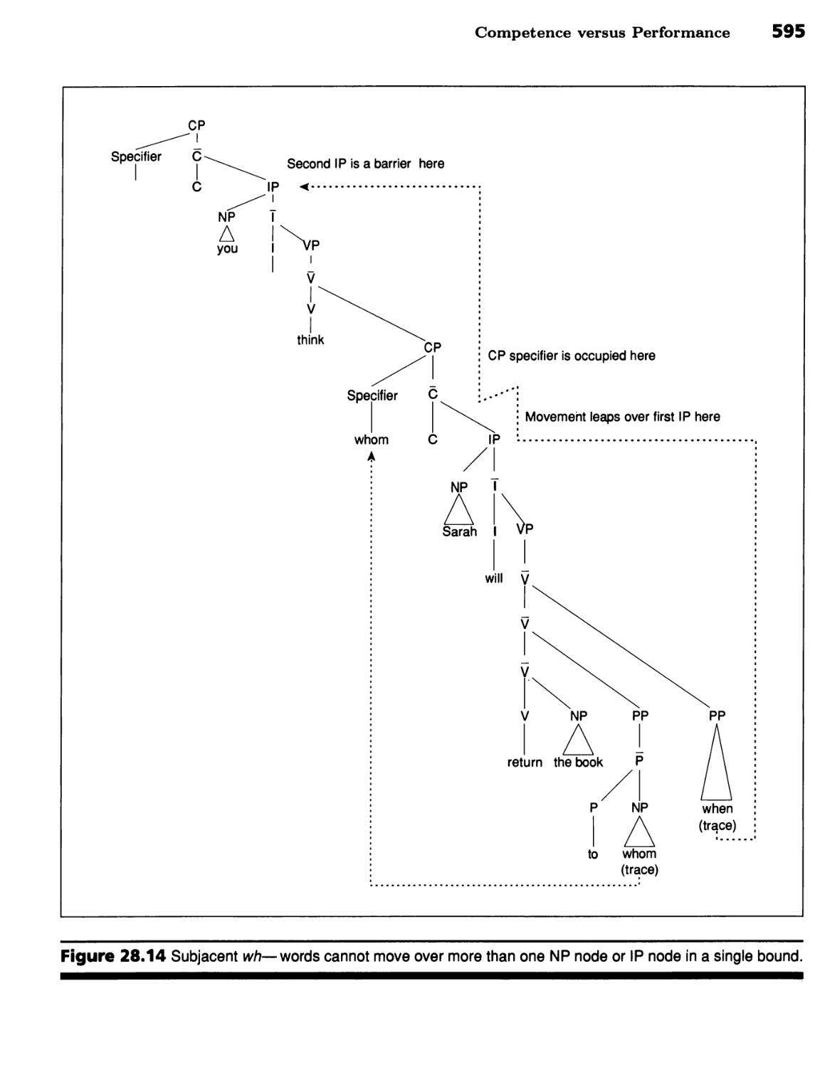
■ A Noun Phrase's Case Is Determined by Its Governor 588 ■ Subjacency
Limits Wh- Movement 592
Competence versus Performance 594
Most Linguists Focus on Competence, Not on Performance 596 ■
Analysis by Reversing Generation Can Be Silly 596 ■ Construction of a Language
Understanding Program Remains a Tough Row to Hoe 597 ■ Engineers
Must Take Shortcuts 597
Summary 598
Background 598
CHAPTER 29 ^hhhi^h
Responding to Questions and Commands 599
Syntactic Transition Nets 599
Syntactic Transition Nets Are Like Roadmaps 600 ■ A Powerful Computer
Counted the Long Screwdrivers on the Big Table 601
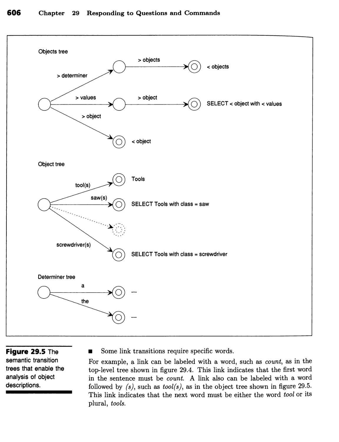
Semantic Transition Trees 603
A Relational Database Makes a Good Target 604 ■ Pattern Instantiation
Is the Key to Relational-Database Retrieval in English 604 ■ Moving from
Syntactic Nets to Semantic Trees Simplifies Grammar Construction 605 ■
xvii
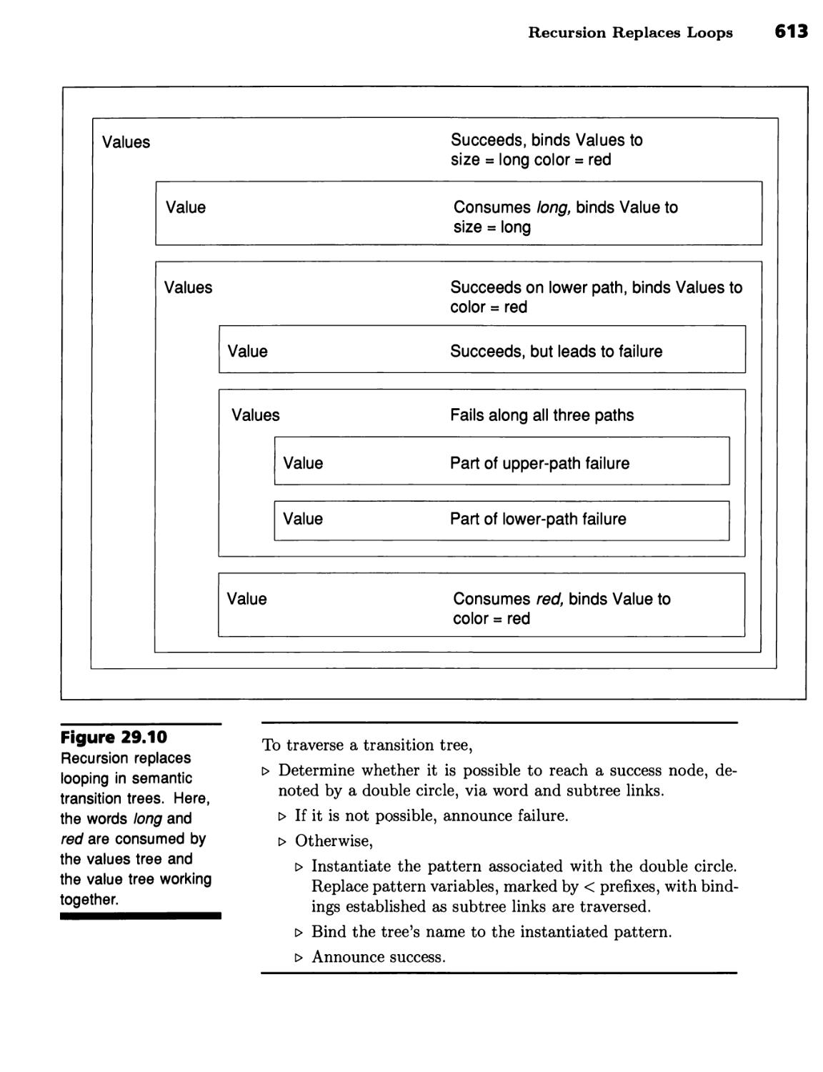
Count the Long Screwdrivers 609 ■ Recursion Replaces Loops 612 ■
Q&A Translates Questions into Database-Retrieval Commands 615
Summary 614
Background 614
APPENDIX ■■■h^^^h
Relational Databases 617
Relational Databases Consist of Tables Containing Records 617 ■
Relations Are Easy to Modify 617 ■ Records and Fields Are Easy to Extract 618
■ Relations Are Easy to Combine 619
Summary 626
EXERCISES 627
Exercises for Chapter 1 627 ■ Exercises for Chapter 2 628 ■ Exercises
for Chapter 3 630 ■ Exercises for Chapter 4 633 ■ Exercises for Chapter
5 635 ■ Exercises for Chapter 6 635 ■ Exercises for Chapter 7 639 ■
Exercises for Chapter 8 643 ■ Exercises for Chapter 9 647 ■ Exercises
for Chapter 10 649 ■ Exercises for Chapter 11 650 ■ Exercises for
Chapter 12 652 ■ Exercises for Chapter 13 656 ■ Exercises for Chapter
14 658 ■ Exercises for Chapter 15 659 ■ Exercises for Chapter 16 663 ■
Exercises for Chapter 17 667 ■ Exercises for Chapter 18 669 ■ Exercises
for Chapter 19 671 ■ Exercises for Chapter 20 674 ■ Exercises for
Chapter 21 675 ■ Exercises for Chapter 22 677 ■ Exercises for Chapter
23 678 ■ Exercises for Chapter 24 679 ■ Exercises for Chapter 25 680 ■
Exercises for Chapter 26 682 ■ Exercises for Chapter 27 684 ■ Exercises
for Chapter 28 689 ■ Exercises for Chapter 29 690
BIBLIOGRAPHY 693
INDEX 725
COLOPHON
737
The cover painting is by Karen A. Prendergast. The cover design is by
Dan Dawson. The interior design is by Marie McAdam.
A draft of this book was read by Boris Katz, who has a special gift for
rooting out problems and tenaciously insisting on improvements.
The following people also have made especially valuable suggestions:
Johnnie W. Baker (Kent State University), Robert C. Berwick (MIT), Ro-
nen Basri (MIT), Philippe Brou (Ascent Technology), David A. Chanen
(MIT), Paul A. Fishwick (University of Florida), Robert Frank
(University of Pennsylvania), W. Eric L. Grimson (MIT), Jan L. Gunther (Ascent
Technology), James R. Harrington (Army Logistics Management College),
Julie Sutherland-Piatt (MIT), Seth Hutchinson (The Beckman Institute),
Carl Manning (MIT), David A. McAUester (MIT), Michael de la Maza
(MIT), Thomas Marill (MIT), Phillip E. Perkins (Army Logistics
Management College), Lynn Peterson (University of Texas at Arlington), Tomaso
Poggio (MIT), Oberta A. Slotterbeck (Hiram College), and Xiru Zhang
(Thinking Machines, Inc.).
xix
Software in support of this book is available on diskettes from Gold
Hill Computers, Inc., Cambridge, MA 02139 (617/621-3300).
Software in support of this book is also available via the Internet. To
learn how to obtain this software, send a message to ai3@ai.mit.edu with
the word "help" on the subject line. Your message will be answered by an
automatic reply program that will tell you what to do next.
The automatic reply program also tells you how to report a bug or
offer a suggestion via the Internet. If you wish to report a bug or offer a
suggestion via ordinary mail, write to the author at the following address:
Patrick H. Winston
Room 816
Artificial Intelligence Laboratory
545 Technology Square
Cambridge, MA 02139
xxi
You Need to Know About Artificial Intelligence
This book was written for two groups of people. One group—computer
scientists and engineers—need to know about artificial intelligence to make
computers more useful. Another group—psychologists, biologists, linguists,
and philosophers—need to know about artificial intelligence to understand
the principles that make intelligence possible.
You do not need a computer-science education or advanced mathematr
ical training to understand the basic ideas. Ideas from those disciplines
are discussed, in a spirit of scientific glasnost, but those discussions are in
optional sections, plainly marked and easily detoured around.
This Edition Reflects Changes in the Field
This edition of Artificial Intelligence reflects, in part, the steady progress
made since the second edition was published. Some ideas that seemed good
back then have faded, and have been displaced by newer, better ideas.
There have been more remarkable, more revolutionary changes as well.
One of these is the change brought about by the incredible progress that
has been made in computer hardware. Many simple ideas that seemed silly
10 years ago, on the ground that they would require unthinkable
computations, now seem to be valid, because fast—often parallel—computing has
become commonplace. As described in Chapter 19, for example, one good
way to control a rapidly moving robot arm is to use a vast lookup table.
xxiii
Another remarkable change, perhaps the most conspicuous, is the focus
on learning—particularly the kind of learning that is done by neuronlike
nets. Ten years ago, only a handful of people in artificial intelligence studied
learning of any kind; now, most people seem to have incorporated a learning
component into their work. Accordingly, about one-third of the chapters
in this edition are devoted to various approaches to learning, and about
one-third of those deal with neuronlike nets.
Still another remarkable change is the emergence of breakthroughs. As
described in Chapter 26, for example, one good way to identify a three-
dimensional object is to construct two-dimensional templates for the given
object, in the given view, for each possible object class. Ten years ago, no
one suspected that the required templates could be manufactured perfectly,
simply, and on demand, no matter how the object is viewed.
Finally, there is the emphasis on scaling up. These days, it is hard to
attract attention with an idea that appears suited to toy problems only.
This difficulty creates a dilemma for a textbook writers, because textbooks
need to discuss toy problems so that the complexities of particular real
worlds do not get in the way of understanding the basic ideas. To deal
with this dilemma, I discuss many examples of important applications, but
only after I explain the basic ideas in simpler contexts.
This Edition Responds to Suggestions of Previous Users
Many readers of the first and second editions have offered wonderful
suggestions. At one meeting in Seattle, on a now-forgotten subject, Peter
Andreae and J. Michael Brady remarked, over coffee, that it was hard for
students to visualize how the ideas could be incorporated into programs.
Similarly, feedback from my own students at the Massachusetts
Institute of Technology indicated a need to separate the truly powerful ideas
and unifying themes—such as the principle of least commitment and the
importance of representation—from nugatory implementation details.
In response to such suggestions, this edition is peppered with several
kinds of summarizing material, all set off visually:
■ Semiformal procedure specifications
■ Semiformal representation specifications
■ Hierarchical specification trees
■ Powerful ideas
You Can Decide How Much You Want to Read
To encourage my students to get to the point, I tell them that I will not read
more than 100 pages of any dissertation. Looking at this book, it might
seem that I have neglected my own dictum, because this book has grown
to be many times 100 pages long. My honor is preserved, nevertheless,
because several features make this edition easier to read:
This Edition Is Supported by an Instructor's Manual XXV
■ There are few essential chapter-to-chapter dependencies. Individual
readers with bounded interests or time can get what they need from
one or two chapters.
■ The book is modular. Instructors can design their own subject around
200 or 300 hundred pages of material.
■ Each chapter is shorter, relative to the chapters in the second edition.
Many can be covered by instructors in one or two lectures.
If your want to develop a general understanding of artificial intelligence,
you should read Chapters 2 through 12 from Part I; then you should skim
Chapter 16 and Chapter 19 from Part II, and Chapter 26 from Part III
to get a feel for what is in the rest of the book. If you are interested
primarily in learning, you should read Chapter 2 from Part I to learn about
representations; then, you should read all of Part II. If you are interested
primarily in vision or in language, you can limit yourself to the appropriate
chapters in Part III.
This Edition Is Supported by Optional Software
This book discusses ideas on many levels, from the level of issues and
alternatives to a level that lies just one step short of implementation in
computer programs. For those readers who wish to take that one extra
step, to see how the ideas can be reduced to computer programs, there are
two alternatives:
■ For people who already know the Lisp programming language, a large
and growing number of programs written in support of this book are
available via the Internet; see the software note that precedes this
preface.
■ For people who do not know the Lisp programming language, the
companion book LISP, by Patrick H. Winston and Berthold K. P. Horn,
is a good introduction that treats many of the ideas explained in this
book from the programming perspective.
This Edition Is Supported by an Instructor's Manual
A companion Instructors Manual contains exercise solutions and sample
syllabuses.
P.H.W.
In part I, you learn about basic representations and methods. These
representations and methods are used by engineers to build commercial
systems and by scientists to explain various kinds of intelligence.
In Chapter 1, The Intelligent Computer, you learn about what
artificial intelligence is, why artificial intelligence is important, and how
artificial intelligence is applied. You also learn about criteria for judging
success.
In Chapter 2, Semantic Nets and Description Matching, you
learn about the importance of good representation and you learn how to
test a representation to see whether it is a good one. Along the way, you
learn about semantic nets and about the describe-and-match method. By
way of illustration, you learn about a geometric-analogy problem solver, a
plot recognizer, and a feature-based object identifier.
In Chapter 3, Generate and Test, Means-Ends Analysis, and
Problem Reduction, you learn about three powerful problem-solving
methods: generate and test, means-ends analysis, and problem reduction.
Examples illustrating these problem-solving methods at work underscore
the importance of devising a good representation, such as a state space or
a goal tree.
In Chapter 4, Nets and Basic Search, you learn about basic search
methods, such as depth-first search, that are used in all sorts of programs,
ranging from those that do robot path planning to those that provide
natural-language access to database information.
1
2
In Chapter 5, Nets and Optimal Search, you learn more about
search methods, but now the focus is on finding the best path to a goal,
rather than just any path. The methods explained include branch and
bound, discrete dynamic programming, and A*.
In Chapter 6, Trees and Adversarial Search, you learn still more
about search methods, but here the focus shifts again, this time to games.
You learn how minimax search tells you where to move and how alpha-
beta pruning makes minimax search faster. You also learn how heuristic
continuation and progressive deepening enable you to use all the time you
have effectively, even though game situations vary dramatically.
In Chapter 7, Rules and Rule Chaining, you learn that simple if-
then rules can embody a great deal of commercially useful knowledge. You
also learn about using if-then rules in programs that do forward chaining
and backward chaining. By way of illustration, you learn about toy systems
that identify zoo animals and bag groceries. You also learn about certain
key implementation details, such as variable binding via tree search and the
rete procedure.
In Chapter 8, Rules, Substrates, and Cognitive Modeling, you
learn how it is possible to build important capabilities on top of rule-based
problem-solving apparatus. In particular, you learn how it is possible for
a program to explain the steps that have led to a conclusion, to reason
in a variety of styles, to reason under time constraints, to determine a
conclusion's probability, and to check the consistency of a newly proposed
rule. You also learn about knowledge engineering and about Soar, a rule-
based model of human problem solving.
In Chapter 9, Frames and Inheritance, you learn about frames,
classes, instances, slots, and slot values. You also learn about inheritance,
a powerful problem-solving method that makes it possible to know a great
deal about instances by virtue of knowing about the classes to which the
instances belong. You also learn how knowledge can be captured in certain
procedures, often called demons, that are attached to classes.
In Chapter 10, Frames and Commonsense, you learn how frames
can capture knowledge about how actions happen. In particular, you learn
how thematic-role frames describe the action conveyed by verbs and nouns,
and you learn about how action frames and state-change frames describe
how actions happen on a deeper, syntax-independent level.
In Chapter 11, Numeric Constraints and Propagation, you learn
how good representations often bring out constraints that enable
conclusions to propagate like the waves produced by a stone dropped in a quiet
pond. In particular, you see how to use numeric constraint propagation
to propagate probability estimates through opinion nets and to propagate
altitude measurements through smoothness constraints.
In Chapter 12, Symbolic Constraints and Propagation, you learn
more about constraint propagation, but now the emphasis is on symbolic
3
constraint propagation. You see how symbolic constraint propagation solves
problems in line-drawing analysis and relative time calculation. 'You also
learn about Marr's methodological principles.
In Chapter 13, Logic and Resolution Proof, you learn about logic,
an important addition to your knowledge of problem-solving paradigms.
After digesting a mountain of notation, you explore the notion of proof, and
you learn how to use proof by refutation and resolution theorem proving.
In Chapter 14, Backtracking and Truth Maintenance, you learn
how logic serves as a foundation for other problem-solving methods. In
particular, you learn about proof by constraint propagation and about truth
maintenance. By way of preparation, you also learn what dependency-
directed backtracking is, and how it differs from chronological backtracking,
in the context of numeric constraint propagation.
In Chapter 15, Planning, you learn about two distinct approaches to
planning a sequence of actions to achieve some goal. One way, the Strips
approach, uses if-add-delete operators to work on a single collection of
assertions. Another way, the theorem-proving approach, rooted in logic,
uses situation variables and frame axioms to tie together collections of
expressions, producing a movielike sequence.
II".
C ■ i .
This book is about the field that has come to be called artificial
intelligence. In this chapter, you learn how to define artificial intelligence,
and you learn how the book is arranged. You get a feeling for why
artificial intelligence is important, both as a branch of engineering and as a
kind of science. You learn about some successful applications of artificial
intelligence. And finally, you learn about criteria you can use to determine
whether work in Artificial Intelligence is successful.
THE FIELD AND THE BOOK
There are many ways to define the field of Artificial Intelligence. Here is
one:
Artificial intelligence is ...
> The study of the computations that make it possible to
perceive, reason, and act.
From the perspective of this definition, artificial intelligence differs from
most of psychology because of the greater emphasis on computation, and
artificial intelligence differs from most of computer science because of
the emphasis on perception, reasoning, and action.
5
6 Chapter 1 The Intelligent Computer
Prom the perspective of goals, artificial intelligence can be viewed as
part engineering, part science:
■ The engineering goal of artificial intelligence is to solve real-world
problems using artificial intelligence as an armamentarium of ideas
about representing knowledge, using knowledge, and assembling
systems.
■ The scientific goal of artificial intelligence is to determine which ideas
about representing knowledge, using knowledge, and assembling
systems explain various sorts of intelligence.
This Book Has Three Parts
To make use of artificial intelligence, you need a basic understanding of
how knowledge can be represented and what methods can make use of
that knowledge. Accordingly, in Part I of this book, you learn about basic
representations and methods. You also learn, by way of vision and language
examples, that the basic representations and methods have a long reach.
Next, because many people consider learning to be the sine qua non of
intelligence, you learn, in Part II, about a rich variety of learning methods.
Some of these methods involve a great deal of reasoning; others just dig
regularity out of data, without any analysis of why the regularity is there.
Finally, in Part III, you focus directly on visual perception and
language understanding, learning not only about perception and language per
se, but also about ideas that have been a major source of inspiration for
people working in other subfields of artificial intelligence, t
The Long-Term Applications Stagger the Imagination
As the world grows more complex, we must use our material and human
resources more efficiently, and to do that, we need high-quality help from
computers. Here are a few possibilities:
■ In farming, computer-controlled robots should control pests, prune
trees, and selectively harvest mixed crops.
■ In manufacturing, computer-controlled robots should do the dangerous
and boring assembly, inspection, and maintenance jobs.
■ In medical care, computers should help practitioners with diagnosis,
monitor patients' conditions, manage treatment, and make beds.
■ In household work, computers should give advice on cooking and
shopping, clean the floors, mow the lawn, do the laundry, and perform
maintenance chores.
'Sometimes, you hear the phrase core AI used by people who regard language,
vision, and robotics to be somehow separable from the mainstream of artificial
intelligence. However, in light of the way progress on language, vision, and
robotics can and has influenced work on reasoning, any such separation seems
misadvised.
Artificial Intelligence Sheds New Light on Traditional Questions 7
■ In schools, computers should understand why their students make
mistakes, not just react to errors. Computers should act as superbooks,
displaying planetary orbits and playing musical scores, thus helping
students to understand physics and music.
The Near-Term Applications Involve New Opportunities
Many people are under the false impression that the commercial goal of
artificial intelligence must be to save money by replacing human workers.
But in the commercial world, most people are more enthusiastic about new
opportunities than about decreased cost. Moreover, the task of totally
replacing a human worker ranges from difficult to impossible because we
do not know how to endow computers with all the perception, reasoning,
and action abilities that people exhibit.
Nevertheless, because intelligent people and intelligent computers have
complementary abilities, people and computers can realize opportunities
together that neither can realize alone. Here are some examples:
■ In business, computers can help us to locate pertinent information, to
schedule work, to allocate resources, and to discover salient regularities
in databases.
■ In engineering, computers can help us to develop more effective control
strategies, to create better designs, to explain past decisions, and to
identify future risks.
Artificial Intelligence Sheds New Light on
Traditional Questions
Artificial intelligence complements the traditional perspectives of
psychology, linguistics, and philosophy. Here are several reasons why:
■ Computer metaphors aid thinking. Work with computers has led to a
rich new language for talking about how to do things and how to
describe things. Metaphorical and analogical use of the concepts involved
enables more powerful thinking about thinking.
■ Computer models force precision. Implementing a theory uncovers
conceptual mistakes and oversights that ordinarily escape even the most
meticulous researchers. Major roadblocks often appear that were not
recognized as problems at all before the cycle of thinking and
experimenting began.
■ Computer implementations quantify task requirements. Once a
program performs a task, upper-bound statements can be made about how
much information processing the task requires.
■ Computer programs exhibit unlimited patience, require no feeding, and
do not bite. Moreover, it is usually simple to deprive a computer
program of some piece of knowledge to test how important that piece
really is. It is almost always impossible to work with animal brains
with the same precision.
Chapter 1 The Intelligent Computer
Note that wanting to make computers be intelligent is not the same as
wanting to make computers simulate intelligence. Artificial intelligence
excites people who want to uncover principles that must be exploited by all
intelligent information processors, not just by those made of neural tissue
instead of electronic circuits. Consequently, there is neither an obsession
with mimicking human intelligence nor a prejudice against using methods
that seem involved in human intelligence. Instead, there is a new point of
view that brings along a new methodology and leads to new theories.
Artificial Intelligence Helps Us to Become More Intelligent
Just as psychological knowledge about human information processing can
help to make computers intelligent, theories derived primarily with
computers in mind often suggest useful guidance for human thinking. Through
artificial intelligence research, many representations and methods that
people seem to use unconsciously have been crystallized and made easier for
people to deploy deliberately.
WHAT ARTIFICIAL INTELLIGENCE CAN DO
In this section, you learn about representative systems that were enabled by
ideas drawn from artificial intelligence. Once you have finished this book,
you will be well on your way toward incorporating the ideas of artificial
intelligence into your own systems.
Intelligent Systems Can Help Experts to Solve
Difficult Analysis Problems
During the early days of research in artificial intelligence, James R. Sla-
gle showed that computers can work problems in integral calculus at the
level of college freshmen. Today, programs can perform certain kinds of
mathematical analysis at a much more sophisticated level.
The Kam program, for example, is an expert in nonlinear dynamics, a
subject of great interest to scientists who study the equations that govern
complex object interactions.
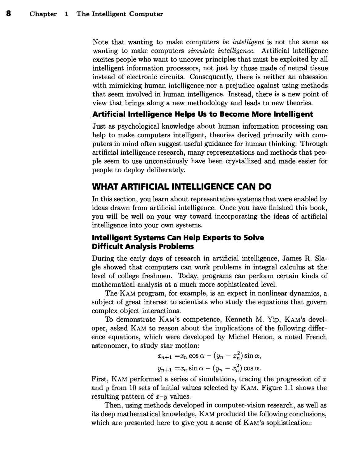
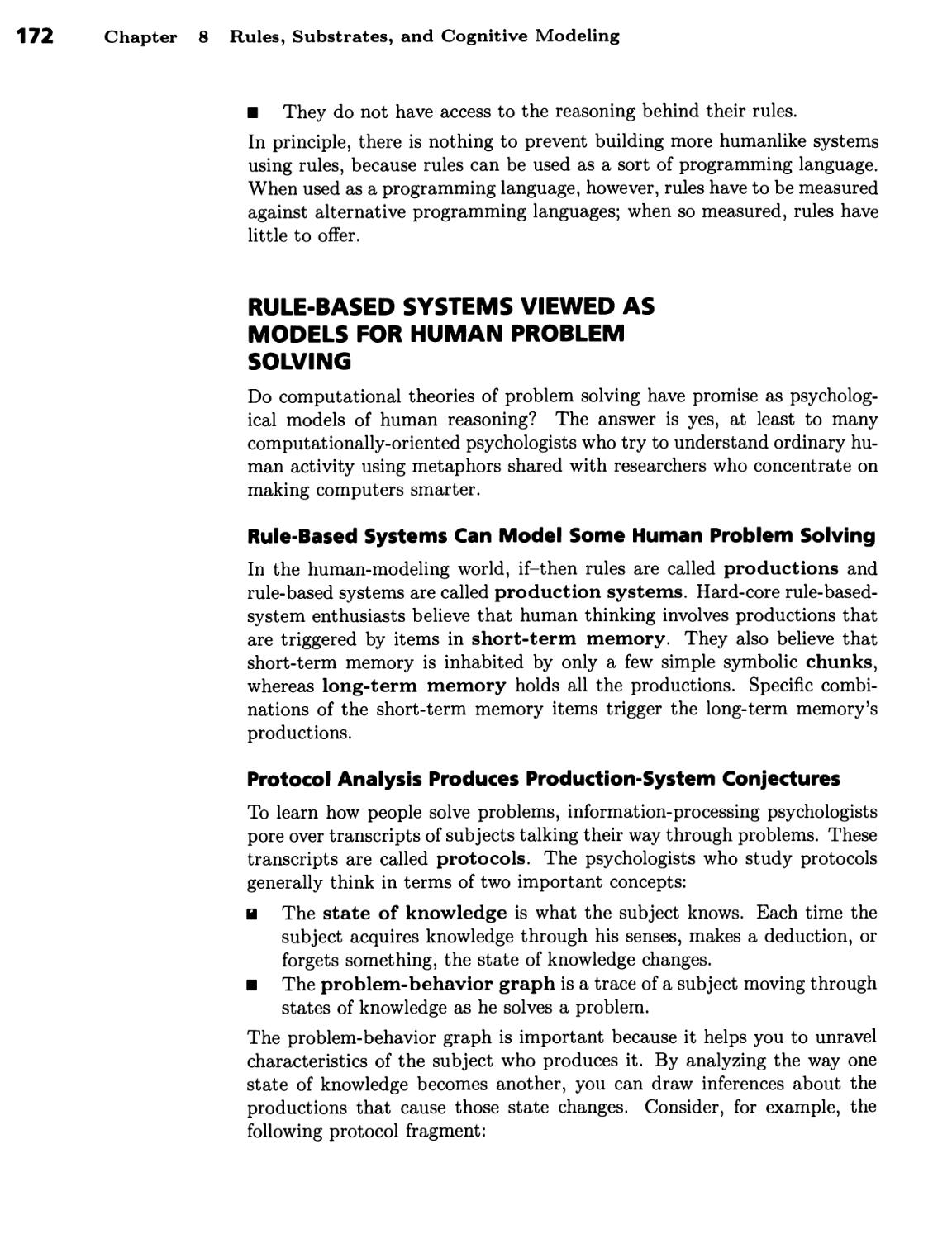
To demonstrate Kam's competence, Kenneth M. Yip, Kam's
developer, asked Kam to reason about the implications of the following
difference equations, which were developed by Michel Henon, a noted French
astronomer, to study star motion:
zn+i =xn cos a- (yn - x%) sin a,
yn+i =xn sina-(yn-xl) cos a.
First, Kam performed a series of simulations, tracing the progression of x
and y from 10 sets of initial values selected by Kam. Figure 1.1 shows the
resulting pattern of x-y values.
Then, using methods developed in computer-vision research, as well as
its deep mathematical knowledge, Kam produced the following conclusions,
which are presented here to give you a sense of Kam's sophistication:
Intelligent Systems Can Help Experts to Design New Devices
Figure 1.1 Yip's program
performs its own experiments,
which it then analyzes using
computer-vision methods and
deep mathematical knowledge.
Here you see a plot produced
by Yip's program in the course
of analyzing certain equations
studied by astronomers.
Images courtesy of Kenneth
M. Yip.
1.0
0.5
y 0.0
-0.5
-1.0
-1.0
:m (o )
^ "ms?.:
>£&■
/.'<-..'--.'J-
-0.5
0.0
x
0.5
1.0
An Analysis
There is an elliptic fixed point at (0 0 0). Surrounding the fixed
point is a regular region bounded by a Kam curve with a rotation
number between 1/5 and 1/4. Outside the regular region lies a
chain of 5 islands. The island chain is bounded by a Kam curve
with rotation number between 4/21 and 5/26. The outermost
region is occupied by chaotic orbits which eventually escape.
Kam's analysis is impressively similar to the original analysis of Henon.
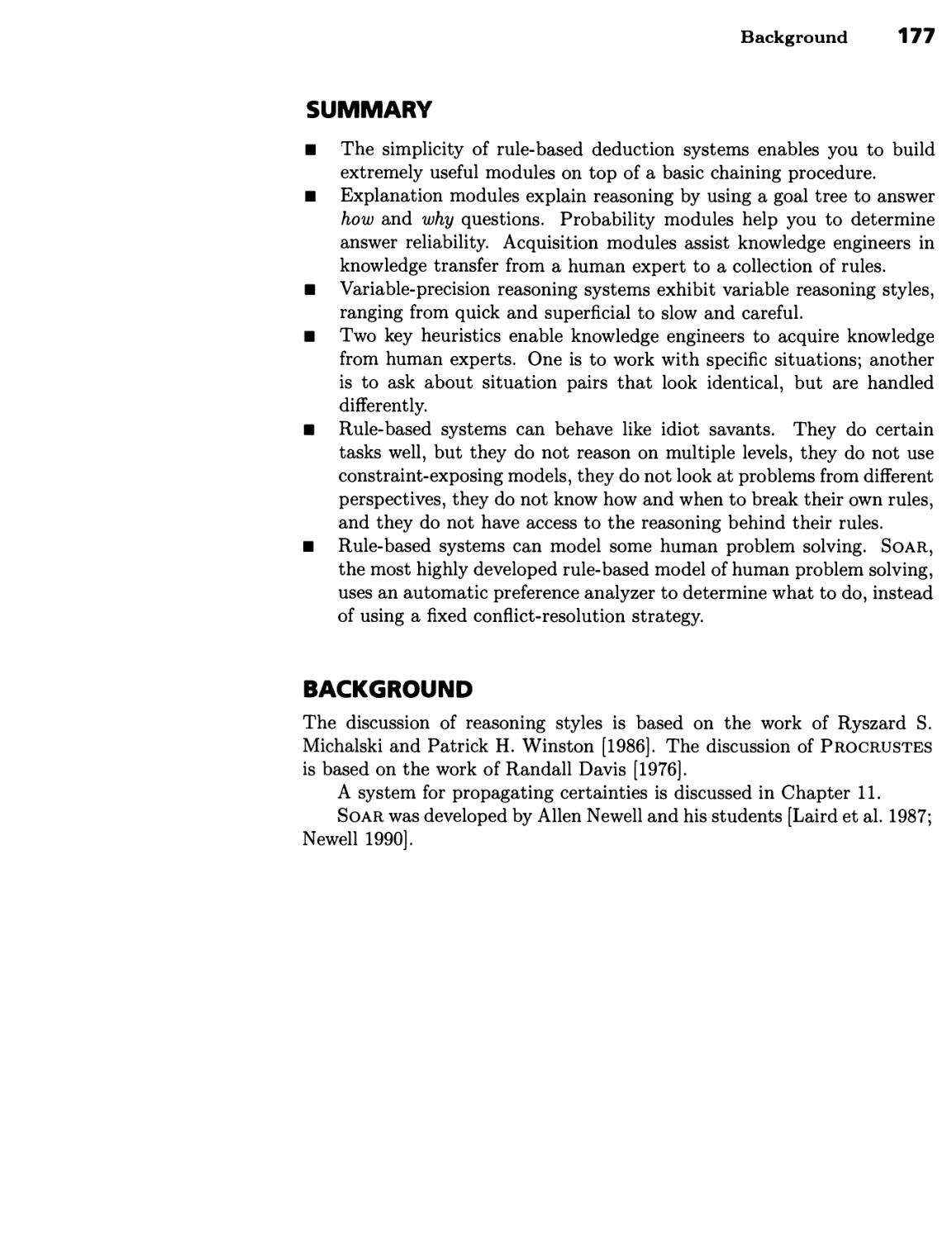
Intelligent Systems Can Help Experts to Design New Devices
The utility of intelligence programs in science and engineering is not limited
to sophisticated analysis; many recent programs have begun to work on the
synthesis side as well.
For example, a program developed by Karl Ulrich designs simple
devices and then looks for cost-cutting opportunities to reduce the number of
components. In one experiment, Ulrich's program designed a device that
measures an airplane's rate of descent by measuring the rate at which air
pressure is increasing.
The first step performed by Ulrich's program was to search for a
collection of components that does the specified task. Figure 1.2(a) shows
the result. Essentially, a rapid increase in air pressure moves the piston
to the right, compressing the air in back of the piston and driving it into
a reservoir; once the increase in air pressure stops, the air in back of the
piston and in the reservoir bleeds back through the return pipe, and the
10 Chapter 1 The Intelligent Computer
Air
entry
Return pipe
,10 20 30
mmmmmM\AAAAM
J
i
Reservoir
10 20 30
■ ■■■■■■'■■■■
Air
entry
Return pipe
/\
Reservoir
snEMnnniy^A/vvvJi
(b)
Figure 1.2 Ulrich's
program designs a
rate-of-descent device
in two steps. First,
as shown in (a), the
program discovers a
workable collection of
components. Then,
as shown in (b), the
program simplifies the
device by reducing the
number of components
required.
rate indicator returns to the zero position. Thus, in more sophisticated
language, Ulrich's program designed a device to differentiate air pressure.
The second step performed by Ulrich's program was to look for ways
for components to assume multiple functions, thus reducing the number
of components required. Figure 1.2(b) shows the result. The program
eliminated the return pipe by increasing the size of the small gap that
always separates a piston from its enclosing cylinder. Then, the program
eliminated the air reservoir by increasing the length of the cylinder, thus
enabling the cylinder to assume the reservoir function.
Intelligent Systems Can Learn from Examples
Most learning programs are either experience oriented or data oriented.
The goal of work on experience-oriented learning is to discover how
programs can learn the way people usually do—by reasoning about new
experiences in the light of commonsense knowledge.
The goal of work on data-oriented learning programs is to develop
practical programs that can mine databases for exploitable regularities. Among
these data-oriented learning programs, the most well-known is the Id3
system developed by J. Ross Quinlan. Id3 and its descendants have mined
thousands of databases, producing identification rules in areas ranging from
credit assessment to disease diagnosis.
One typical exercise of the technology, undertaken by Quinlan
himself, was directed at a database containing information on patients with
hypothyroid disease. This information, provided by the Garvan Institute
of Medical Research in Sydney, described each of several thousand cases of
thyroid disease in terms of 7 continuous variables (such as the measured
11
level of thyroid-stimulating hormone, TSH), and 16 discrete variables, (such
as whether or not the patient had already had thyroid surgery).
Prom this sea of data, Quinlan's program extracted three
straightforward rules for classification of hypothyroid disease:
If the patient's TSH level is less than 6.05 units
then the patient's class is negative
If the patient has not had thyroid surgery
the patient's TSH level is greater than 6.05 units
the patient's FTI level is less than 64.5 units
then the patient's class is primary hypothyroid
If the patient is not taking thyroxine
the patient has not had thyroid surgery
the patient's TSH level is greater than 6.05 units
the patient's FTI level is greater than 64.5 units
the patient's TT4 level is less than 150.5 units
then the patient's class is compensated hypothyroid
Evidently, of the seven continuous and 16 discrete variables available, only
five are useful in disease classification.
Intelligent Systems Can Provide Answers to
English Questions Using both Structured Data
and Free Text
As the Voyager 2 spacecraft concluded its 12-year grand tour of the outer
planets, it sent back spectacular images of Neptune's moons and rings,
much to the delight of journalists and scientists gathered to witness the
event. In cooperation with researchers from the Jet Propulsion Laboratory,
Boris Katz invited those journalists and scientists to use his Start system
to ask questions about the Neptune encounter, the Voyager spacecraft, and
the Solar system.
To answer straightforward questions, Start accessed a variety of
tables, including a distance table supplied by the Voyager navigation team
and a time-line table supplied by the Voyager sequencing group. Here are
a few representative examples:
■ When was Voyager launched?
The Voyager Spacecraft was launched in Florida on August 20 1977.
■ At what time will Voyager lose contact with Earth?
The Voyager Spacecraft will lose the contact with Earth around 2014.
■ How long is the year on Neptune?
Neptune's period of revolution is about 165 Earth years.
Start also answered questions by printing out English text drawn from
various space publications, as illustrated by the following representative
The Intelligent Computer
questions and answers. Note that the critical words in the questions—
color, talk, and weather—do not appear in the answers:
■ What color is Neptune?
When you look at a photograph of Neptune, you see the planet's
atmosphere and the tops of clouds. Neptune looks bluish because the
methane in its atmosphere reflects blue and green frequencies of light.
The methane absorbs red and yellow frequencies of sunlight.
■ How does Voyager talk to Earth?
Commands are sent from Earth to one of two receivers on the
Voyager spacecraft. Engineering data and scientific information are sent
to Earth over two channels. One channel is on all the time, but both
channels are on during encounters with the planets. The radio
transmitter on the Voyager transmits with about 25 watts of power, or with
about the same power as a refrigerator lightbulb. These faint signals
are picked up on Earth by ultrasensitive receivers known as the Deep
Space Network.
■ What's the weather on Neptune?
Neptune receives about a thousand times less sunlight than the Earth.
The temperatures there are thus quite low. Typically, the temperature
is about —360 degrees Fahrenheit (—218 degrees Celsius).
Artificial Intelligence Is Becoming Less
Conspicuous, yet More Essential
The first applications of artificial intelligence were mostly motivated by the
desire of researchers to demonstrate that artificial intelligence is of practical
value. Now, as the field is maturing, the development of applications is
motivated increasingly by the desire of business people to achieve strategic
business goals.
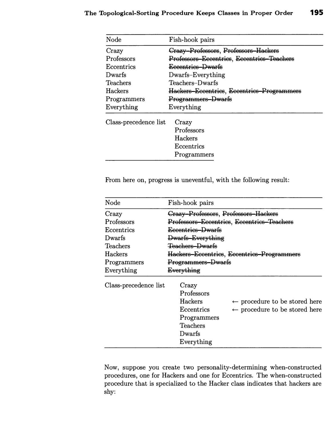
One example of a business-motivated application is the Airport
Resource Information System—Aris—developed by Ascent Technology, Inc.,
and used by Delta Airlines to help allocate airport gates to arriving flights.
The gate-allocation problem, illustrated in figure 1.3, is difficult at a
busy airport, because Aris must react immediately to arrival and departure
changes, such as those imposed by bad weather, and because there are many
constraints to consider. One obvious constraint is that you cannot park a
large aircraft at a gate designed to handle only small aircraft. Another is
that passengers want their connecting flights to be parked at gates that
are within easy walking distance. Still another, less obvious constraint is
that gate controllers want to avoid potential traffic jams as aircraft move to
and from their assigned gates. Aris handles all these constraints and many
more using artificial intelligence methods that include rule-based reasoning,
constraint propagation, and spatial planning.
Handling the constraints was not the principal challenge faced by Aris's
developers, however. Other difficult challenges were posed by the need to
Criteria for Success 13
IA2 A4 fig A8 A10 A12 A14 A16A18 A20 A22 A24 A26 A28 A30A32A34I
|fil A3 A5 A7 A9 fill A13 A15 A17 A19 A21 A23 A25 A27 A29 A31 A33 |
^4* * 4* 4 4* 4*4 4 4
provide human decision makers with a transparent view of current
operations, the need to exchange information with mainframe databases, the
need to provide rapid, automatic recovery from hardware failures, and the
need to distribute all sorts of information to personnel responsible for
baggage, catering, passenger service, crew scheduling, and aircraft
maintenance. Such challenges require considerable skill in the art of harnessing
artificial intelligence ideas with those of other established and emerging
technologies.*
CRITERIA FOR SUCCESS
Every field needs criteria for success. To determine if research work in
artificial intelligence is successful, you should ask three key questions:
■ Is the task denned clearly?
■ Is there an implemented procedure performing the denned task? If not,
much difficulty may be lying under a rug somewhere.
■ Is there a set of identifiable regularities or constraints from which the
implemented procedure gets its power? If not, the procedure may be
an ad hoc toy, capable perhaps of superficially impressive performance
on carefully selected examples, but incapable of deeply impressive
performance and incapable of helping you to solve any other problem.
To determine if an application of artificial intelligence is successful, you
need to ask additional questions, such as the following:
'Ester Dyson, noted industry analyst, has said that some of the most successful
applications of artificial intelligence are those in which the artificial intelligence
is spread like raisins in a loaf of raisin bread: the raisins do not occupy much
space, but they often provide the principle source of nutrition.
Figure 1.3 Aris helps
determine how to manage gate
resources at busy airport hubs.
The Intelligent Computer
■ Does the application solve a real problem?
■ Does the application open up a new opportunity?
Throughout this book, you see examples of research and applications-
oriented work that satisfy these criteria: all perform clearly denned tasks;
all involve implemented procedures; all involve identified regularities or
constraints; and some solve real problems or open up new opportunities.
SUMMARY
■ Artificial intelligence is the study of the computations that make it
possible to perceive, reason, and act.
■ The engineering goal of artificial intelligence is to solve real-world
problems; the scientific goal of Artificial Intelligence is to explain various
sorts of intelligence.
■ Applications of artificial intelligence should be judged according to
whether there is a well-defined task, an implemented program, and a
set of identifiable principles.
■ Artificial intelligence can help us to solve difficult, real-world problems,
creating new opportunities in business, engineering, and many other
application areas.
■ Artificial intelligence sheds new light on questions traditionally asked
by psychologists, linguists, and philosophers. A few rays of this new
light can help us to be more intelligent.
BACKGROUND
Artificial intelligence has a programming heritage. To understand the ideas
introduced in this book in depth, you need to see a few of them embodied
in program form. A coordinated book, LISP, Third Edition [1989], by
Patrick H. Winston and Berthold K. P. Horn, satisfies this need.
Id3 was developed by J. Ross Quinlan [1979, 1983].
Kam is the work of Kenneth M. Yip [1989]. The work on designing a
rate-of-descent instrument is that of Karl T. Ulrich [1988].
The work on responding to English questions using both structured
data and free text is that of Boris Katz [1990].
0:-y y<'r '?:'^\; ''' "■'
'/■■ !,;;:;i v:-"-;
'"', ■ " ■
*•*
»
'■■.'V*. ;:.'■■ >'■■-.> ■"■ ,.♦., '■* . . -
n i
c ri "
.-. / -.
' -'- >"'
-
^
s
t
c^V*. :?.
1
ii
:m
$ ,
1 n
<' 4
In this chapter, you learn about the role of representation in artificial
intelligence, and you learn about semantic nets, one of the most ubiquitous
representations used in artificial intelligence. You also learn about describe
and match, an important problem-solving method.
By way of illustration, you see how one describe-and-match program,
working on semantic-net descriptions, can solve geometric analogy
problems of the sort found on intelligence tests. You also see how another
describe-and-match program, again working on semantic-net descriptions,
can recognize instances of abstractions, such as "mixed blessing" and
"retaliation," in semantic nets that capture story plots. The piece de resistance
involves the analysis of O. Henry's intricate short story, "The Gift of the
Magi." Both the analogy program and the abstraction program show that
simple descriptions, conforming to appropriate representations, can lead to
easy problem solving.
Also, you see that the describe-and-match method is effective with
other representations, not just with semantic nets. In particular, you see
how the describe-and-match method lies underneath the feature-based
approach to object identification.
Once you have finished this chapter, you will know how to evaluate
representations and you will know what representation-oriented questions
you should always ask when you are learning how to deal with an unfamiliar
class of problems. You will have started your own personal collection of
representations and problem-solving methods by learning about semantic
15
Semantic Nets and Description Matching
nets, feature spaces, and the describe-and-match method. Finally, you will
have started your own personal collection of case studies that will serve as
useful precedents when you are confronted with new problems.
SEMANTIC NETS
In this section, you learn about what a representation is, a sense in which
most representations are equivalent, and criteria by which representations
can be judged. You also learn about semantic nets, a representation that
sees both direct and indirect service throughout artificial intelligence.
Good Representations Are the Key to Good Problem Solving
In general, a representation is a set of conventions about how to
describe a class of things. A description makes use of the conventions of a
representation to describe some particular thing.
Finding the appropriate representation is a major part of problem
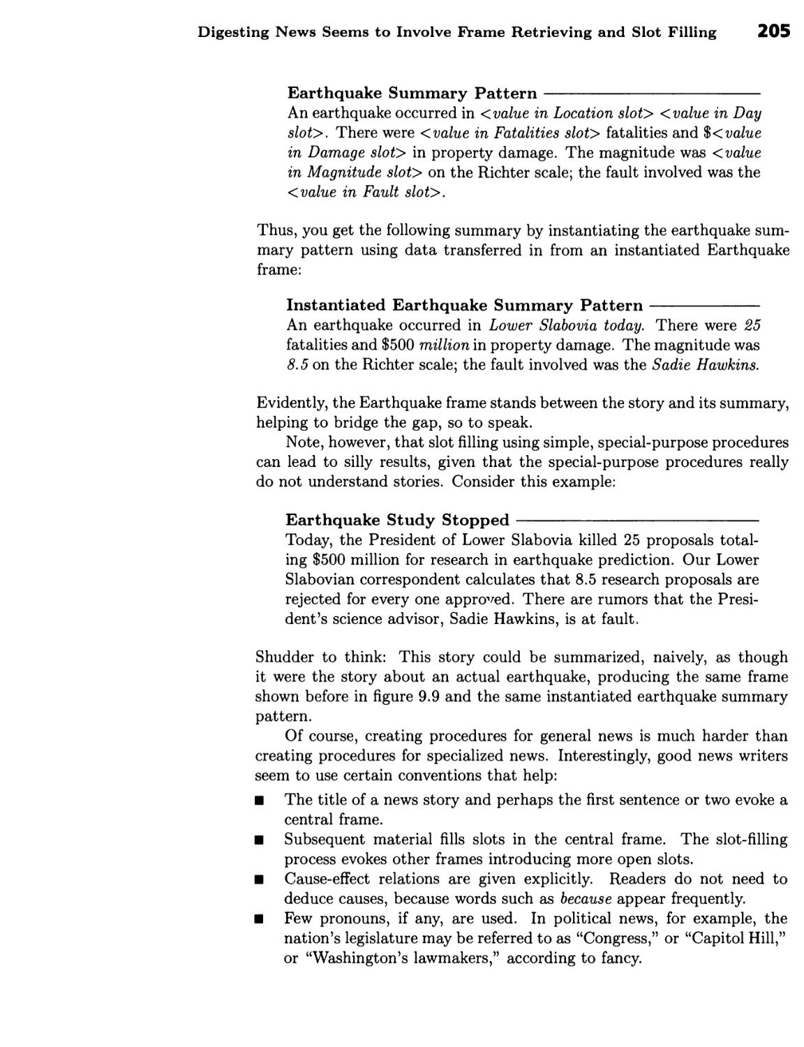
solving. Consider, for example, the following children's puzzle:
The Farmer, Fox, Goose, and Grain
A farmer wants to move himself, a silver fox, a fat goose, and some
tasty grain across a river. Unfortunately, his boat is so tiny he can
take only one of his possessions across on any trip. Worse yet, an
unattended fox will eat a goose, and an unattended goose will eat
grain, so the farmer must not leave the fox alone with the goose or
the goose alone with the grain. What is he to do?
Described in English, the problem takes a few minutes to solve because you
have to separate important constraints from irrelevant details. English is
not a good representation.
Described more appropriately, however, the problem takes no time at
all, for everyone can draw a line from the start to the finish in figure 2.1
instantly. Yet drawing that line solves the problem because each boxed
picture denotes a safe arrangement of the farmer and his possessions on the
banks of the river, and each connection between pictures denotes a legal
crossing. The drawing is a good description because the allowed situations
and legal crossings are clearly denned and there are no irrelevant details.
To make such a diagram, you first construct a node for each way the
farmer and his three possessions can populate the two banks of the river.
Because the farmer and his three possessions each can be on either of the
two river banks, there are 21+3 = 16 arrangements, 10 of which are safe in
the sense that nothing is eaten. The six unsafe arrangements place the fox,
the goose, and the grain, on one side or the other; or place the goose and
the grain on one side or the other; or place the fox and the goose on one
side or the other.
Good Representations Are the Key to Good Problem Solving 17
Figure 2.1 The
problem of the farmer,
fox, goose, and grain.
The farmer must get
his fox, goose, and
grain across the river,
from the arrangement
on the left to the
arrangement on the
right. His boat will hold
only him and one of
his three possessions.
The second and final step is to draw a link for each allowable boat
trip. For each ordered pair of arrangements, there is a connecting link if
and only if the two arrangements meet two conditions: first, the farmer
changes sides; and second, at most one of the farmer's possessions changes
sides. Because there are 10 safe arrangements, there are 10 x 9 = 90 ordered
pairs, but only 20 of these pairs satisfy the conditions required for links.
Evidently, the node-and-link description is a good description with
respect to the problem posed, for it is easy to make, and, once you have it,
the problem is simple to solve.
The important idea illustrated by the farmer, fox, goose, and grain
problem is that a good description, developed within the conventions of a
good representation, is an open door to problem solving; a bad description,
using a bad representation, is a brick wall preventing problem solving.
Semantic Nets and Description Matching
In this book, the most important ideas—such as the idea that a good
representation is important—are called powerful ideas; they are
highlighted thus:
The representation principle:
> Once a problem is described using an appropriate
representation, the problem is almost solved.
In the rest of this book, you learn about one or two powerful ideas per
chapter.
Good Representations Support Explicit,
Constraint-Exposing Description
One reason that the node-and-link representation works well with the
farmer, fox, goose, and grain problem is that it makes the important objects
and relations explicit. There is no bothering with the color of the fox or
the size of the goose or the quality of the grain; instead, there is an
explicit statement about safe arrangements and possible transitions between
arrangements.
The representation also is good because it exposes the natural
constraints inherent in the problem. Some transitions are possible; others are
impossible. The representation makes it easy to decide which is true for
any particular case: a transition is possible if there is a link; otherwise, it
is impossible.
You should always look for such desiderata when you evaluate
representations. Here is a list with which you can start, beginning with the two
ideas just introduced:
■ Good representations make the important objects and relations
explicit: You can see what is going on at a glance.
■ They expose natural constraints: You can express the way one object
or relation influences another.
■ They bring objects and relations together: You can see all you need to
see at one time, as if through a straw.
■ They suppress irrelevant detail: You can keep rarely used details out
of sight, but still get to them when necessary.
■ They are transparent: You can understand what is being said.
■ They are complete: You can say all that needs to be said.
■ They are concise: You can say what you need to say efficiently.
■ They are fast: You can store and retrieve information rapidly.
■ They are computable: You can create them with an existing procedure.
Semantic Nets Convey Meaning 19
A Representation Has Four Fundamental Parts
With the farmer, fox, goose, and grain problem as a point of reference, you
can now appreciate a more specific definition of what a representation is.
A representation consists of the following four fundamental parts:
■ A lexical part that determines which symbols are allowed in the
representation's vocabulary
■ A structural part that describes constraints on how the symbols can
be arranged
■ A procedural part that specifies access procedures that enable you
to create descriptions, to modify them, and to answer questions using
them
■ A semantic part that establishes a way of associating meaning with
the descriptions
In the representation used to solve the farmer, fox, goose, and grain
problem, the lexical part of the representation determines that nodes and links
are involved. The structural part specifies that links connect node pairs.
The semantic part establishes that nodes correspond to arrangements
of the farmer and his possessions and links correspond to river
traversal. And, as long as you are to solve the problem using a drawing, the
procedural part is left vague because the access procedures are
somewhere in your brain, which provides constructors that guide your pencil
and readers that interpret what you see.
Semantic Nets Convey Meaning
The representation involved in the farmer problem is an example of a
semantic net.
Prom the lexical perspective, semantic nets consist of nodes, denoting
objects, links, denoting relations between objects, and link labels that
denote particular relations.
Prom the structural perspective, nodes are connected to each other
by labeled links. In diagrams, nodes often appear as circles, ellipses, or
rectangles, and links appear as arrows pointing from one node, the tail
node, to another node, the head node.
Prom the semantic perspective, the meaning of nodes and links depends
on the application.
Prom the procedural perspective, access procedures are, in general, any
one of constructor procedures, reader procedures, writer
procedures, or possibly erasure procedures. Semantic nets use constructors
to make nodes and links, readers to answer questions about nodes and
links, writers to alter nodes and links, and, occasionally, erasers to delete
nodes and links.
By way of summary, the following specifies what it means to be a
semantic net in lexical, structural, semantic; and procedural terms, using
Semantic Nets and Description Matching
an informal specification format that appears throughout the rest of this
book:
A semantic net is a representation
In which
> Lexically, there are nodes, links, and application-specific
link labels.
> Structurally, each link connects a tail node to a head node.
> Semantically, the nodes and links denote application-specific
entities.
With constructors that
> Construct a node
> Construct a link, given a link label and two nodes to be
connected
With readers that
> Produce a list of all links departing from a given node
> Produce a list of all links arriving at a given node
> Produce a tail node, given a link
> Produce a head node, given a link
> Produce a link label, given a link
Such specifications are meant to be a little more precise and consistent
than ordinary English phrases, but not stuffily so. In particular, they are
not so precise as to constitute a specification of the sort you would find in
an official standard for, say, a programming language.
Nevertheless, the specifications are sufficiently precise to show that
many of the key representations in artificial intelligence form family groups.
Figure 2.2, for example, shows part of the family of representations for
which the semantic-net representation is the ultimate ancestor. Although
this semantic-net family is large and is used ubiquitously, you should note
that it is but one of many that have been borrowed, invented, or reinvented
in the service of artificial intelligence.
There Are Many Schools of Thought About the
Meaning of Semantics
Arguments about what it means to have a semantics have employed
philosophers for millennia. The following are among the alternatives advanced by
one school or another:
■ Equivalence semantics. Let there be some way of relating
descriptions in the representation to descriptions in some other representation
that already has an accepted semantics.
There Are Many Schools of Thought About the Meaning of Semantics
21
Figure 2.2 Part of the
semantic-net family of
representations. Although many
programs explained in this book
use one of the family members
shown, others use important
representations that lie outside
of the family.
Labelled drawing Interval net
K-d tree
Identification
tree
Decision Game
tree ^ tree
Goal
tree Value propagation net
Contraction net
Arithmetic
constraint
net
Frame system State space
l —J '
Semantic net
A
■ Procedural semantics. Let there be a set of programs that operate
on descriptions in the representation. Say that meaning is denned by
what the programs do.
■ Descriptive semantics. Let there be explanations of what
descriptions mean in terms we understand intuitively.
Prom the perspective of descriptive semantics, the net on the left side of
figure 2.3 is not a semantic net, because there is neither a prima facie
description in terms you understand nor an explanation of what the link
labels mean in terms you understand. The net on the right side of figure 2.3,
however, is a semantic net, because you naturally tend to ascribe meaning
to the links. Asked what the net means, most people would say immediately
that it means that an object, known as the lintel, is supported by two other
objects, known as posts.
Of course, the objects and relations involved in semantic nets need
not be so concrete. The representation used in the farmer illustration
is a semantic net because particular arrangements of the farmer and his
possessions can be viewed as abstract objects, thereby meriting node status,
and allowed river crossings can be viewed as abstract relations, thereby
meriting link status.
22 Chapter 2 Semantic Nets and Description Matching
Figure 2.3 An ordinary
net (left) and a semantic net
(right). Natural-language
labels associate intuitive
meanings with nodes and links,
thereby producing an informal
semantics.
Ultimately, both equivalence semantics and procedural semantics lead
back to descriptive semantics. In the case of equivalence semantics,
descriptions have meaning because they are equivalent to something that means
something to you. In the case of procedural semantics, descriptions have
meaning because they cause a program to exhibit a behavior that means
something to you. Thus, the alternatives all seem rooted in perceptions to
which you ascribe meaning intuitively.
Theoretical Equivalence Is Different from
Practical Equivalence
In some uninteresting theoretical sense, any computer-based representation
can do anything that any other can do, because computer-based
representations are based, ultimately, on arrangements of bits in memory.
Consequently, any representation that can be used to represent arrangements of
bits can be used as a substratum for the construction of any other
representation.
In a practical sense, however, some representations help you to focus
on the objects and relations you need to solve a class of problems. One
representation, therefore, is more powerful than another because it offers
you more convenience even though, theoretically, both can do the same
work. Convenience, however, is perhaps too weak a word. In general, the
good qualities of powerful representations make practicable what would be
impracticable with weak representations.
THE DESCRIBE-AND-MATCH METHOD
In this section, you learn about the describe-and-match method; by way of
illustration, you learn how the describe-and-match method can be used to
identify two-dimensional objects.
As illustrated in figure 2.4 the basic idea behind the describe-and-
match method is that you can identify an object by first describing it
and then searching for a matching description in a description library. The
objects involved may be simple physical entities such as the blocks with
The Describe-and-Match Method 23
Figure 2.4 The describe-and-
match paradigm. To identify
an object, you describe it, and
then you look for a matching
description in a description
library.
which children play, or complicated abstractions, such as those that emerge
in the forthcoming examples.
As you move through this book, you will see many methods, such as
the describe-and-match method, reduced to a specification cast in a form
that is more precise than ordinary English, yet more transparent than
a programming language—particularly a programming language that you
do not happen to know. In this book, this informal, half-English, half-
program form is called procedural English. Here is the describe-and-
match method expressed in procedural English:
To identify an object using describe and match,
> Describe the object using a suitable representation.
> Match the object description against library descriptions
until there is a satisfactory match or there are no more
library descriptions.
> If you find a satisfactory match, announce it; otherwise,
announce failure.
In general, procedural English allows all these programming constructs:
■ Steps and substeps, denoted by indentation, much after the fashion of
an outline
■ Iterations, denoted by words such as until and for each
■ Conditional actions, denoted by words such as z/and otherwise
■ Various sorts of tests, denoted variously
24 Chapter 2 Semantic Nets and Description Matching
Figure 2.5 A feature space.
An unknown object is identified
according to the distances
between its feature point
and those of various models.
Evidently the unknown is most
likely to be a single-hole switch
plate.
Number
of holes
4
3
2
1
O
D
8
Area
iidifii!
MM
°n
DD
.^Unknown
16
Many good programmers use a notation much like procedural English at
the design stage, when they are deciding what a procedure will do. Much of
the procedural English then survives in the form of illuminating comments.
Feature-Based Object Identification Illustrates
Describe and Match
Feature-based object identification is one of the simplest applications
of the describe-and-match method. Feature-based object identifiers consist
of a feature extractor and a feature evaluator. The feature extractor
measures simple characteristics such as an object's area. Values obtained
by the feature extractor become the coordinates of a feature point in
feature space, a multidimensional space in which there is one dimension
for each feature measured. To identify an unknown object, you compare
the distances between its feature point and the feature points of various
idealized objects. The most likely identity of the unknown object is
determined by the smallest distance. Figure 2.5 shows the points corresponding
to an unknown object and a family of idealized electrical-box covers in a
box-cover feature space.
Generally, speed and discrimination considerations determine which
features are used in particular situations. Candidate features for objects
Geometric Analogy Rules Describe Object Relations and Object Transformations 25
Figure 2.6 An easy problem
for the Analogy program.
A
(o)
C
0
B
(®)
1
□
2
El
i
3 4 5
n
|~ET|
o
such as electrical-box covers include total object area, hole area, hole count,
perimeter length, minimum distance from center of area to edge, maximum
distance from center of area to edge, average distance from center of area
to edge, length of major axis of ellipse of equal inertia moment, length of
minor axis of ellipse of equal inertia moment, total area minus hole area,
ratio of hole area to total area, and ratio of perimeter squared to area.
THE DESCRIBE-AND-MATCH METHOD
AND ANALOGY PROBLEMS
In this section, you learn that the describe-and-match method, working
in harness with a semantic-net representation, produces impressive
performance on geometric analogy problems in which the problem, as shown in
figure 2.6, is to select an answer figure, X, such that A is to B as C is to X
gives the best fit.
One way to start is to describe rules that explain how A becomes B and
how C becomes each of the answer figures. Then, you can match the rule
that explains how A becomes B to each rule that explains how C becomes
an answer. The best match between rules identifies the best answer. Thus,
the describe-and-match paradigm can be used to solve analogy problems.
The key to solving such problems lies in good rule descriptions. The
Analogy program, described in this section, does its job by matching rule
descriptions together and measuring description similarity.
Geometric Analogy Rules Describe Object
Relations and Object Transformations
Analogy uses two-part rules. One rule part describes how the objects are
arranged in the source and destination figures. One object may be above,
to the left of, or inside of another. The other rule part describes how the
objects in the source figure are transformed into objects in the destination
figure. An object may be scaled, rotated, or reflected, or may be subject
26 Chapter 2 Semantic Nets and Description Matching
Figure 2.7 A rule described
as a geometric analogy net,
which is a kind of semantic
net. Rule descriptions consist
of object-relation descriptions
and object-transformation
descriptions. Links shown
solid describe relations among
source objects and among
destination objects. Links
shown dotted describe how
objects are transformed
between the source and the
destination.
n
A
/ m \
deleted
above
above
©
unchanged
\ inside
T\ expanded
W
>: I
■■©
left-of
•0
j
to some combination of these operations. Also, an object may be added or
deleted.
A typical rule can be described using a semantic-net representation, as
illustrated in figure 2.7. This representation is not just any semantic net,
of course—it is one that is specialized to describe rules:
A geometric analogy net is a representation
That is a semantic net
In which
> The nodes denote dots, circles, triangles, squares,
rectangles, and other geometric objects.
> Some links denote relations among figures objects,
specifically inside, above, and to the left of.
> Other links describe how figure objects are transformed.
The possibilities are addition, deletion, expansion,
contraction, rotation, and reflection, and combinations of
these operations.
Geometric Analogy Rules Describe Object Relations and Object Transformations 27
Figure 2.8 Two circles, one
of which is inside a polygon.
One object is inside another if
a line drawn to infinity crosses
the boundary of the potentially
surrounding object an odd
number of times. Thus, one
circle is inside; the other is not.
You could write this specification for geometric analogy nets, of course,
without any reference to semantic nets, by importing all the descriptive
elements from the semantic-net specification. The alternative shown is
better, not only because it saves space, but also because it focuses on exactly
what you need to add to transform the general concept into a
representation tailored to a particular circumstance. As you can see, transforming
the semantic-net concept into a geometric analogy net requires only the
application-specific recitation of which link labels are allowed and what
the nodes and links denote.
Analogy uses a simple idea, illustrated in figure 2.8, to decide whether
Inside, rather than either Left-of or Above, is the appropriate relation
between objects. First, Analogy makes sure that the objects do not
touch. Then, Analogy constructs a line from any point on one figure to
infinity, as shown in figure 2.8. If the line crosses the second figure an odd
number of times, then the second figure surrounds the first. Happily, this
method involves only simple line-crossing tests, and it works even if the
figures are extremely convoluted.
As shown in figure 2.9, Analogy uses another simple procedure to
compute the spatial relationship between two objects. Analogy computes
the center of area of each of the two objects, constructs diagonal lines
through the center of area of one of them, and notes which region contains
the center of area of the other object. Because the relations used are
symmetric, it is not necessary to note both left and right relations.
Finally, Analogy uses a matching procedure to decide if an object
in one figure can be transformed into an object in another figure by a
combination of scaling, rotation, and reflection operations. The dotted
links in figure 2.7 mark objects that pass this transformation test.
Now that you have seen how rules are constructed, you can see that
the example in figure 2.10 is contrived so as to depend on only relations
i ) >
\ / i I
I
I
r\ I ,
28 Chapter 2 Semantic Nets and Description Matching
Figure 2.9 A square to the
left of a rectangle. Relations
between objects are determined
by comparing centers of area.
x left-of y
X
x above y
y
y above x
y left-of x
between objects. No object transformations can influence the solution,
because no objects are transformed in the move from the source figure to
the destination figure.
It is clear that the C-to-3 rule best matches the A-to-B rule because,
with / associated with x and m associated with ?/, the two rules match
exactly.
Note, however, that there is no a priori reason to associate / with x
rather than with y. In going from the source figure to the destination
figure, you want to be sure that squares go to squares, circles to circles,
triangles to triangles, and so on. But this need to match one object to a
geometrically similar object does not hold in comparing two rules. In the
example, answer 3 is to be selected even though the objects in A and B
are a triangle and a square, whereas in C and in all the answer figures, the
objects are a circle and a dot. In general, Analogy must try all possible
ways of associating the nodes when matching rules.
This one-for-one association of variables implies that the number of
objects that move from the source figure to the destination figure must be
the same in both of the two rules. The number of additions and deletions
must be the same as well. Any attempt to match two rules for which the
numbers are different fails immediately.
If n objects move from the source figure to the destination figure in
each of two rules being compared, there will be n! ways of associating the
variables in searching for the best way to match the rules. More generally,
Geometric Analogy Rules Describe Object Relations and Object Transformations 29
B
A
m
^-n unchanged
above
s\ unchanged
Cuv
■<D
left-of
©■
unchanged
■*®
©
above
unchanged
left-of
■>©
^-n unchanged
©
above
unchanged
•»©
above
>©
©
unchanged
©
above
unchanged
•>©
left-of
>©
Figure 2.10 A
problem whose
solution is determined
by relations only.
Comparison of the rule
descriptions verifies
that the C-to-3 rule
matches best.
if ni objects move, rv^ are added, and n^ deleted, in going to the destination
figure, then n\\ n^l n^l is the number of possible associations. All must be
tried.
In the example, there are two possible ways to associate the objects,
because n\ = 2, ^ = 0, and n^ = 0. Specifically, Analogy can associate
/ with x and m with ?/, or Analogy can associate / with y and m with x.
The previous example involves only relations between objects, because
no objects are transformed. Symmetrically, for the problem in figure 2.11,
there is only one object in each figure, so there are no relations between
30 Chapter 2 Semantic Nets and Description Matching
B
._, rotate by 45 ° /~.
o <j
—. rotate by 45 ° /~.
o <j
X
rotate by 45 °
o::::::::::»
shrink by 2
s-*. unchanged ^-^
o <j
Figure 2.11 A
problem whose
solution is determined
by transformations
only. Because each
figure has only one
object, relations
between objects
are not relevant.
Comparison of the rule
descriptions verifies
that the C-to-1 rule
provides is the best
match.
objects, and only object transformations can matter. Analogy concludes
that the C-to-1 rule best matches the A-to-B rule, because only answer 1
corresponds to a simple 45° rotation with no reflection or scale change.
Scoring Mechanisms Rank Answers
How should Analogy measure the similarity of two rules? So far, the
examples have been so simple that the best answer rule matches the A-to-
B rule exactly. But if an exact match cannot be found, then Analogy
must rank the inexact matches. One way to do this ranking is to count the
number of matching elements in the two rules involved in each match, as
shown in figure 2.12.
To tune the counting a bit, you can weight relations describing
object transformations less heavily than you weight relations describing
relations among objects. Assuming that relations among objects each add
one point to the total score, then less than one point should be added for
each object-transformation relation. Experimentally, the numbers shown
in figure 2.13 work well. A radically different set of numbers would reflect
Scoring Mechanisms Rank Answers 31
Figure 2.12 Rule similarity,
measured by degree of overlap.
You determine the answers by
finding the C-to-X rule with the
maximum number of elements
in common with the A-to-B rule.
Maximize
AtoB /
CtoX
a different judgment about how the various possibilities should be ordered.
The given set is biased toward rotations and against reflections. A different
set might indicate the opposite preference. The corresponding variations on
Analogy would occasionally disagree with one another about the answers.
Of course, it is possible to elaborate the measure of similarity in other
directions. Suppose, for example, that Sab IS ^ne se^ °f elements in the
A-to-B rule, and that Sqx is the set °f elements in the C-to-X rule. Then,
Sab n ^CX *s the set °f elements that appear in both rules, Sab ~~ ^CX
is the set of elements appearing in the A-to-B rule but not in the C-to-X
rule, and Sex _ ^AB is the set of elements appearing in only the C-to-X
rule. With these sets in hand, you can use the following formula to measure
similarity:
Similarity =a x Size(SAB n Sex)
- p x Size(SAB - SCX)
-7xSize(SCx-5,AB)
where a, /?, and 7 are weights, and Size is the function that computes the
number of elements in a set. If (3 = 0, 7 = 0, and a = 1, the formula
reduces to counting the common elements. If /? and 7 are not the same,
the formula gives asymmetric similarity judgments, allowing, for example,
32 Chapter 2 Semantic Nets and Description Matching
0.5 —\— < Unchanged
0.4 —\— < Scaled
< Rotated
0.3 —[— < Scaled and rotated
0.2 -4-
0 1 _J_ < Reflected
I < Scaled and reflected
< Rotated and reflected
< Scaled, rotated, and reflected
the A-to-B rule to be more similar to the C-to-X rule than the C-to-X rule
is to the A-to-B rule.
Be skeptical about such formulas, however. Viewed as a representation
for importance, a set of weights is not explicit and exposes little constraint.
Ambiguity Complicates Matching
So far, all the objects in the source and destination figures have distinct
shapes. Consequently, it is easy to decide how to form the rule describing
the transformation. In situations such as the one shown in figure 2.14,
however, there is ambiguity because there is no way to know which of the
two triangles has disappeared. Perhaps the larger one is gone; alternatively
the smaller one may have been deleted and the larger one may have shrunk.
In fact, you cannot judge either explanation to be superior without
considering the other figures given in the problem. Consequently, Analogy
must construct two rules, one corresponding to each way the triangles in
the source figure can be identified with triangles in the destination. In
general, for each source and destination pair, many rules are possible; and,
for each rule, there may be many ways to match it against another rule.
Good Representation Supports Good Performance
Examine figure 2.15. It shows three examples, drawn from intelligence
tests, that are well within the grasp of the Analogy procedure. In the
first example, the most reasonable theory about the rule for going from A
to B is that the inside object is deleted. The C-to-3 rule is the same, and
Figure 2.13 Weights
determine transformation-
description contributions to
similarity scores.
Story Plots Can Be Viewed as Combinations of Mental States and Events
33
Figure 2.14 An ambiguous
change. The large triangle may
have been deleted; alternatively,
the small one may have been
deleted and the large one
shrunk.
answer 3 is the best answer, with answer 4 a close second. Answer 4 would
be the clear winner if answer 3 were not present.
In the second example, answer 3 is the correct answer. Actually,
answer 3 is the only answer figure that Analogy considers seriously, because
among the answer figures, only answer 3 has the same number of objects
as B has. Remember that requiring the same number of objects is an
indirect consequence of permitting a match only between rules for which the
numbers of movements, additions, and deletions are the same.
In the third example, the A-to-B rule could be described as either a
rotation or a reflection, with answer 2 being the best answer if the
process prefers rotations, and with answer 1 being the best answer if it likes
reflections better. Analogy prefers rotations, and judges answer 2 to be
best.
THE DESCRIBE-AND-MATCH METHOD
AND RECOGNITION OF ABSTRACTIONS
In this section, you learn that the describe-and-match method, again
working in harness with a semantic-net representation, can be used to recognize
abstractions in story plots. In combination with what you have already
learned about the describe-and-match method and semantic nets, you see
that both have a broad reach.
Story Plots Can Be Viewed as Combinations of
Mental States and Events
To describe plots using a semantic net, you need a vocabulary of node
types and link labels. Happily, you soon see that you can do a lot with
a vocabulary of just three node types and three link labels. The three
node types are mental states, denoted by MS in diagrams; positive events,
denoted by +; and negative events, denoted by -. The link labels are z,
an acronym for initiates, meaning that the mental state or event at the
tail of an i link leads to the one at the head of the link; £, for terminates,
34 Chapter 2 Semantic Nets and Description Matching
Figure 2.15 Three problems
solved successfully by
Analogy.
meaning that the mental state or event at the tail turns off the one at the
head; and c, for corefers, meaning that the mental state or event at the
tail refers to the same mental state or event as the one at the head. Links
labeled with c have two heads: double-headed links are a notational
shorthand for pairs of identically labeled single-headed links pointing in
opposite directions.
With three node types and three link labels, there could be as many
as3x3x3 = 27 node-link-node combinations. Of these 27 possibilities,
15 have a natural, easily stated interpretation, and each of these is called
a base unit. In figure 2.16, for example, four base units are exhibited,
Story Plots Can Be Viewed as Combinations of Mental States and Events
35
Figure 2.16 Combinations
in which mental states and
events initiate one another.
Mental states may initiate
positive events or negative
events and vice versa. The four
possible combinations constitute
instances of success, failure,
enablement, and motivation, all
of which are base units.
Success
0
Failure
0
Enablement Motivation
+
0
( MS J
( MS j
each of which involves a mental state that initiates an event, or vice versa.
As shown, if a mental state initiates an event, you have what is casually
called a success or a failure, depending on the sign of the event. If an
event initiates a mental state, we witness enablement or motivation, again
depending on the sign.
Another group of base units is shown in figure 2.17. This time, each of
the base units involves two mental states. When one mental state initiates
another, we say that recursion has occurred. When one terminates another,
we have a change of mind. If a mental state persists over a period of time,
the individual involved is exhibiting perseverance.
The final group of base units is shown in figure 2.18. Now there are no
mental states at all; there are only events joined by termination or
coreference. The eight combinations are positive tradeoff and negative tradeoff,
positive coreference and negative coreference, loss and resolution, and mixed
blessing and hidden blessing.
In descriptions, base units often overlap, producing recognizable
aggregates. Let us call these aggregates composite units. Together, base units
and composite units constitute abstraction units. Figure 2.19 shows a
composite unit consisting of a success base unit joined, by its positive event,
to a loss base unit. When a success is followed by a loss, in normal language
we often say that "the success was fleeting," or use words to that effect.
Hence, this composite unit is called fleeting success.
Other examples of composite units are shown in figure 2.20. Each
composite unit in the figure consists of a negative event, followed by a mental
state, followed by a positive event. The composite units differ because
they involve different links, and, hence, different base units. Motivation
followed by success yields success born of adversity; motivation followed by
36 Chapter 2 Semantic Nets and Description Matching
Figure 2.17 Mental states
joined by initiate, terminate,
or corefer links. The three
possible combinations constitute
instances of recursion, change
of mind, and perseverance base
units.
Recursion
/^ """"N.
( MS )
V^
i
( MS )
Change of mind
(msJ
t
( MS J
Perseverance
V MS J
c
( MS )
a positive event that terminates the motivation-producing negative event
is a matter of fortuitous success; and finally, motivation followed by a
success involving a positive event that terminates the motivation-producing
negative event is intentional problem resolution.
When more than one person is involved, more elaborate arrangements
are possible. In figure 2.21, for example, the situation from one person's
perspective is a success born of adversity. In addition, however, the
negative event from that person's perspective corefers to a positive event from
the other person's perspective. Similarly, the positive event corefers to a
negative event. These additions, together with the success born of
adversity, constitute retaliation.
Abstraction-Unit Nets Enable Summary
To recognize abstractions in a story plot, you first describe the story plots
in terms of nodes, representing mental states and events, and links,
representing relations among those mental states and events. Then you match
the nodes and links with items in a catalog of named abstraction units.
Consider, for example, the following story about Thomas and Albert:
Thomas and Albert
Thomas and Albert respected each other's technical judgment and
decided to form a company together. Thomas learned that Albert
was notoriously absentminded, whereupon he insisted that Albert
have nothing to do with the proposed company's finances. This
angered Albert so much that he backed out of their agreement,
hoping that Thomas would be disappointed.
Abstraction-Unit Nets Enable Summary 37
Figure 2.18 Positive events
and negative events joined by
terminate or coreference links.
The possible combinations
constitute instances of
eight base units: positive
tradeoff, loss, resolution,
negative tradeoff, positive
coreference, mixed blessing,
hidden blessing, and negative
coreference.
Positive
tradeoff
+
Positive
coreference
Resolution
Negative
tradeoff
+>©<+)(-)
Negative
Mixed blessing Hidden blessing coreference
©
Figure 2.22 shows what "Thomas and Albert" looks like in semantic-net
terms. The respect abstraction is captured by the two mental states at
the top. Those mental states initiate the decision to form a company, a
positive event from both Thomas's and Albert's points of view. Thomas's
discovery about Albert is a negative event, which leads to a mental state
in which Thomas thinks about the company's finances, which leads to his
insistence that Albert keep out of them, a positive event as far as Thomas
is concerned. The insistence is a negative event from Albert's perspective,
however. For Albert, the insistence leads to a mental state that leads to
backing out of the agreement, which Albert views now as a positive event
and Thomas views as a negative one.
38 Chapter 2 Semantic Nets and Description Matching
Figure 2.19 Base units joined
to produce larger, composite
units. In this illustration, a
success unit and a loss unit,
both basic, join to produce a
fleeting success composite unit.
Fleeting success
Now think of the diagram as a mine for abstraction units. Digging a
little reveals that there are six abstraction units that are not wholly
contained in some higher-level abstraction unit. These are called top-level
units. In this particular example, the top-level units are connected to each
other by exactly one shared mental state or one shared event.
Figure 2.23 shows the resulting arrangement of top-level units, in the
form of a top-level abstraction net, with the top-level units shown in the
same relative positions that their pieces occupied in figure 2.22.
To summarize a plot using a top-level abstraction net, you describe
the central'top-level unit first. Then, you describe the surrounding top-
level units and explain how those top-level units are related to the central
top-level unit. For the "Thomas and Albert" story, you would produce the
following result:
Abstraction-Unit Nets Enable Summary 39
Figure 2.20 Three different
composite units. In this
illustration, a negative event
always is followed by a mental
state that is followed by a
positive event. In the first
case, a motivation base unit
is followed by a success base
unit producing an instance of
success born of adversity. In
the second, the success unit
disappears and a resolution unit
appears, producing a fortuitous
success. In the third, success
reappears, joining the other
two, producing an intentional
problem resolution.
Success born
of adversity
Fortuitous
success
Intentional
problem resolution
©
A Summary of Thomas and Albert
Albert retaliated against Thomas because Thomas went through
an intentional problem resolution that was bad for Albert. The
retaliation caused a loss for Thomas and a positive tradeoff for
Albert. The loss reversed Thomas's previous success, and the positive
tradeoff reversed Albert's previous success.
In addition to enabling summary, top-level abstraction nets allow you to
compare and contrast two situations, even when those two situations are
superficially quite different. Consider the following story about John and
Mary, for example:
John and Mary
John and Mary loved each other and decided to be married. Just
before the wedding, John discovered that Mary's father was
secretly smuggling stolen art through Venice. After struggling with
his conscience for days, John reported Mary's father to the police.
Mary understood John's decision, but she despised him for it
nevertheless; she broke their engagement knowing that he would suffer.
40 Chapter 2 Semantic Nets and Description Matching
Figure 2.21 Mental states,
positive events, and negative
events linked across
perspectives. In this illustration, there
are two perspectives. Each
perspective involves a positive
event that is seen as a negative
event in the other. This
particular combination of perspectives,
events, and a mental state is
called a retaliation.
Retaliation
Perspective 1
TV
Perspective 2
( MS J
+
On the surface, "John and Mary" seems to have little resemblance to
"Thomas and Albert." More abstractly, however, both involve a central
retaliation brought on by an intentional problem resolution leading
eventually to a loss and a positive tradeoff, both of which finish off a previous
success. Such similarities are easy to see, once top-level abstraction nets
are constructed: the stories' diagrams are exactly the same.
Of course, more complicated stories will have more complicated top-
level abstraction nets. Consider, for example, "The Gift of the Magi," a
story by O. Henry, with the following plot:
The Gift of the Magi
Delia and her husband, Jim, were very poor. Nevertheless, because
Christmas was approaching, each wanted to give something special
to the other. Delia cut off and sold her beautiful hair to buy an
expensive watch fob for Jim's heirloom gold watch. Meanwhile,
Jim sold his watch to buy some wonderful combs for Delia's hair.
When they found out what they had done, they were sad for a
moment, but soon realized that they loved each other so much,
nothing else mattered.
Abstraction Units Enable Question Answering 41
Figure 2.22 Two stories
viewed as aggregates of
abstraction units, both base and
composite. In this illustration,
there are two perspectives,
Thomas's and Albert's, and six
top-level abstraction units.
Thomas's
perspective
Albert's
perspective
MS K-
Respect
Form
company
Discovery' ( — )
Thought (MS
t
Ban
Respect
Form
comany
Disappointment ( — K-
Anger
Thought
>( -|- T Withdrawal
Figure 2.24 shows one plausible set of nodes and links for the story; those
nodes and links lead to the top-level abstraction net shown in figure 2.25.
Abstraction Units Enable Question Answering
Abstraction units allow you to answer certain questions by matching. Here
are examples:
■ What is the story about? Answer by naming the central abstraction
unit in the top-level abstraction net. For example, "Thomas and
Albert" is about retaliation.
■ What is the result? Answer by naming the abstraction units that are
joined to earlier abstraction units in the top-level abstraction net, but
42 Chapter 2 Semantic Nets and Description Matching
Figure 2.23 A top-level
abstraction net formed from the
top-level units of figure 2.22.
This top-level abstraction net
enables you to build a summary
description around the most
highly linked top-level unit, the
retaliation.
overlaps
not to later abstraction units. For example, the result in "Thomas and
Albert" is a loss and a positive tradeoff.
■ Does the story involve a certain abstraction? Answer by checking for
the appropriate abstraction unit. For example, "Thomas and Albert"
does contain an instance of intentional problem resolution.
■ In what way is one story like another? Answer by naming the most
highly connected abstraction unit that appears in both top-level
abstraction nets. If hard pressed, enumerate the other abstraction units
that appear in both. For example, "Thomas and Albert" is like "John
and Mary" in that both involve retaliation. Moreover, both involve
success, intentional problem resolution, loss, and positive tradeoff.
In all these examples, you could give more detailed answers by naming the
people and the events involved in the abstraction units mentioned.
Abstraction Units Make Patterns Explicit
In this section, you have seen how a base-unit semantic net facilitates
similarity analysis and summary by making mental states, events, and links
between them explicit. Thus, the first criterion of good representation—
that something important is made usefully explicit—is satisfied. Some
people argue, however, that a base-unit semantic net does not yet pass the
computability criterion for good representation because there is no fully
specified way to translate text into abstraction-unit patterns.
Problem Solving and Understanding Knowledge 43
Figure 2.24 The mental
states, positive events, and
negative events of "The Gift
of the Magi."
Jim's
perspective
Wants to give gift
Wants gift (combs, fob) ( MS
Wants money
Wants to sell (watch, hair)( MS
Gives gift
Receives gift ( — j
Regrets
Appreciates
Delia's
perspective
PROBLEM SOLVING AND
UNDERSTANDING KNOWLEDGE
When approaching a new class of problems, to be solved either by you or by
a computer, you always should start by asking yourself certain questions
about knowledge. This section discusses a few questions about
knowledge that are particularly important.
44 Chapter 2 Semantic Nets and Description Matching
Figure 2.25 The top-level
abstraction unit net for "The
Gift of the Magi." All links are
overlaps links.
■ What kind of knowledge is involved?
Perhaps the important knowledge concerns the description of concrete or
abstract objects. Alternatively, perhaps the important knowledge is about
a problem-solving method.
■ How should the knowledge be represented?
Some knowledge may, for example, fit nicely within the semantic-net
framework. Other knowledge is best embedded in a collection of procedures.
There are many possibilities.
■ How much knowledge is required?
After learning what kind of knowledge is involved in a task, this question
should be the one you ask. Are there 40 things to know, or 400, or 4,000?
One reason to ask about quantity is that you must consider the
demand for sensible resource allocation among the various chores required.
Another is that knowing the size of a problem builds courage; even if the
size is large, digesting bad news is better than anticipating even worse news
unnecessarily.
In any event, the tendency is to overestimate grossly; after seeing that
a task is reasonably complicated, it is easy to suppose that it is
unimaginably complicated. But many tasks can be performed with human-level
competence using only a little knowledge.
■ What exactly is the knowledge needed?
Ultimately, of course, you need the knowledge. To do geometric analogy
problems, you need to know what relations are possible between figure
parts, and you need to know how parts can change. To recognize
abstractions, you need a library of base and composite abstraction units. Much of
learning any subject, from electromagnetic theory to genetics, is a matter
of collecting such knowledge.
Background 45
SUMMARY
■ Once a problem has been described using an appropriate
representation, the problem is almost solved.
■ A representation consists of a lexical part, a structural part, a
procedural part, and a semantic part.
■ There are many schools of thought about the meaning of semantics.
Ultimately, meaning always seems to be rooted in human perception
and human intuition.
■ Feature-based object identification illustrates the describe-and-match
method. An unknown object is identified with an idealized object if
their feature points are nearest neighbors in feature space.
■ Geometric analogy rules describe object relations and object
transformations. You solve geometric analogy problems by determining which
rules are most similar.
■ Story plots can be viewed as combinations of mental states and events.
■ Abstraction-unit nets enable certain kinds of summary and question
answering.
■ Good representations make important objects and relations explicit,
expose natural constraints, and bring objects and relations together.
BACKGROUND
The discussion of geometric analogy problems is based on work by Thomas
Evans [1963]. The discussion of plot units is based on the work of Wendy
Lehnert; the "John and Mary" story and the analysis of "The Gift of the
Magi," in particular, are adapted from one of her highly influential papers
[1981].
Feature vectors, and object identification using feature vectors, are
described in more detail in Robot Vision, by Berthold K. P. Horn [1984].
e a ! *st
ea - na si
a > ! Pr -I! em <■■ i<c>'i<
In this chapter, you learn about three powerful problem-solving
methods: generate and test, means-ends analysis, and problem reduction. You
also learn about two new representations, both of which can be viewed
as special cases of the semantic-net representation introduced in
Chapter 2. One is the state-space representation, introduced in the discussion
of means-ends analysis, and another is the goal tree, introduced in the
discussion of problem reduction.
By way of illustration, you see how a program can find the combination
to a safe, plan a route from one city to another, and solve motion-planning
problems in a world populated by a child's blocks.
Once you have finished this chapter, you will be able to identify and
deploy three more problem-solving methods and two more representations,
thus adding considerably to your personal representation and method
collections. You will also begin to see that you yourself use similar
representations and methods daily as you solve problems.
THE GENERATE-AND-TEST METHOD
Problem solvers adhering to the generate-and-test paradigm use two
basic modules, as illustrated in figure 3.1. One module, the generator,
47
48 Chapter 3 Generate and Test, Means-Ends Analysis, and Problem Reduction
Figure 3.1 The generate-
and-test method involves a
generator and a tester.
Generator
Possible
solutions Tester
/ i\
oooooooon
o
O <-
n
Correct
solution
I
O
Incorrect
^ solutions
\
enumerates possible solutions. The second, the tester, evaluates each
proposed solution, either accepting or rejecting that solution.
The generator may generate all possible solutions before the tester
takes over; more commonly, however, generation and testing are interdig-
itated. Action may stop when one acceptable solution is found, or action
may continue until some satisfactory number of solutions is found, or action
may continue until all possible solutions are found. Here is the interdigi-
tated, stop-when-acceptable version in procedural English:
To perform generate and test,
> Until a satisfactory solution is found or no more candidate
solutions can be generated,
> Generate a candidate solution.
> Test the candidate solution.
> If an acceptable solution is found, announce it; otherwise,
announce failure.
In the rest of this section, you learn more about the generate-and-test
method, you learn which sort of problems the generate-and-test method
solves, and you learn several criteria that good generators always satisfy.
Generate-and-Test Systems Often Do Identification
The generate-and-test paradigm is used most frequently to solve
identification problems. In identification problems, the generator is said to produce
hypotheses.
Good Generators Are Complete, Nonredundant, and Informed
49
Figure 3.2 Burgling a safe
using the generate-and-test
paradigm. The generator
is the procedure that the
burglar uses to select and dial
combinations. The tester is the
procedure that the burglar uses
to work the handle. Careful
safecrackers make sure that
they try all possibilities, without
any repeats, until a twist of the
handle opens the safe.
To use the generate-and-test paradigm to identify, say, a tree, you can
reach for a tree book, then thumb through it page by page, stopping when
you find a picture that looks like the tree to be identified. Thumbing
through the book is the generation procedure; matching the pictures to
the tree is the testing procedure.
To use generate and test to burgle a three-number, two-digit safe, you
can start with the combination 00-00-00, move to 00-00-01, and continue
on through all possible combinations until the door opens. Of course, the
counting is the generation procedure, and the twist of the safe handle is
the testing procedure.
The burglar in figure 3.2 may take some time to crack the safe with
this approach, however, for there are 1003 = 1 million combinations. At
three per minute, figuring that he will have to go through half of the
combinations, on average, to succeed, the job will take about 16 weeks, if he
works 24 hours per day.
Good Generators Are Complete, Nonredundant and Informed
It is obvious that good generators have three properties:
■ Good generators are complete: They eventually produce all possible
solutions.
■ Good generators are nonredundant: They never compromise efficiency
by proposing the same solution twice.
■ Good generators are informed: They use possibility-limiting
information, restricting the solutions that they propose accordingly.
Informability is important, because otherwise there are often too many
solutions to go through. Consider the tree-identification example. If it is
Generate and Test, Means-Ends Analysis, and Problem Reduction
winter and a tree you are trying to identify is bare, you do not bother going
through a tree book's conifer section.
Similarly, if a burglar knows, somehow, that all of the numbers in a
safe combination are prime numbers in the range from 0 to 99, then he can
confine himself to 253 = 15625 numbers, getting the safe open in less than
2 days, on the average, instead of in 16 weeks.
THE MEANS-ENDS ANALYSIS METHOD
The state of a system is a description that is sufficient to determine the
future. In a state space, each node denotes a state, and each link denotes
a possible one-step transition from one state to another state:
A state space is a representation
That is a semantic net
In which
> The nodes denote states.
> The links denote transitions between states.
Thus, a state space is a member of the semantic-net family of
representations introduced in Chapter 2.
In the context of problem solving, states correspond to where you are
or might be in the process of solving a problem. Hence, the current state
corresponds to where you are, the goal state corresponds to where you
want to be, and the problem is to find a sequence of transitions that leads
from the initial state to the goal state.
In the rest of this section, you learn about means-ends analysis, a
standard method for selecting transitions. You also learn about one popular
way to implement means-ends analysis using a simple table.
The Key Idea in Means-Ends Analysis Is to Reduce Differences
The purpose of means-ends analysis is to identify a procedure that
causes a transition from the current state to the goal state, or at least to
an intermediate state that is closer to the goal state. Thus, the identified
procedure reduces the observed difference between the current state and
the goal state.
Consider the states shown in figure 3.3. Solid-line nodes identify the
current state and the goal state. Dotted-line nodes correspond to states
that are not yet known to exist. Descriptions of the current state, or of the
goal state, or of the difference between those states, may contribute to the
identification of a difference-reducing procedure.
In figure 3.4, a sequence of procedures P1,...,P5 cause transitions
from state to state, starting from the initial current state. Each of the
DENDRAL Analyzes Mass Spectrograms
DENDRAL is one of the great classic application programs. To see what it does,
suppose that an organic chemist wants to know the chemical nature of some
substance newly created in the test tube. The first step, not the one of concern here,
is to determine the number of atoms of various kinds in one molecule of the stuff.
This step determines the chemical formula, such as CsHieO. The notation indicates
that each molecule has eight atoms of carbon, 16 of hydrogen, and one of oxygen.
Once a sample's chemical formula is known, the chemist may use the sample's
mass spectrogram to work out the way the atoms are arranged in the chemical's
structure, thus identifying the isomer of the chemical.
The spectrogram machine bombards a sample with high energy electrons,
causing the molecules to break up into charged chunks of various sizes. Then, the
machine sorts the chunks by passing them through a magnetic field that deflects the
high-charge, low-weight ones more than it does the low-charge, high-weight ones.
The deflected chunks are collected, forming a spectrogram like the following:
Relative
frequency
i i r^ i ^ i 1 i
40 80 120
Mass/charge
The purpose of DENDRAL is to work, like a knowledgeable chemist, from a
chemical formula and spectrogram to a deduced structure, producing a chemical
structure like this:
CH3 - CH2 - C - CH2 - CH2 - CH2 - CH2 - CH3
O
The DENDRAL program works out structures from chemical formulas and mass
spectrograms using the generate-and-test method. The generator consists of a
structure enumerator and a synthesizer that produces a synthetic mass spectrogram by
simulating the action of a real mass spectrometer on each enumerated structure.
The structure enumerator ensures that the overall generator is complete and
nonredundant because the structure enumerator uses a provably complete and nonre-
dundant structure-enumeration procedure. The overall generator is also informed,
because the structure enumerator uses the chemical formula and knowledge about
necessary and forbidden substructures.
The tester compares the real mass spectrogram with those produced by the
generator. The possible structures are those whose synthetic spectrograms match
the real one adequately. The structure judged correct is the one whose synthetic
spectrogram most closely matches the real one.
52 Chapter 3 Generate and Test, Means-Ends Analysis, and Problem Reduction
Figure 3.3 Means-ends
analysis involves states and
procedures for reducing
differences between states. The
current state and goal state are
shown solid; other states, not
yet encountered, are shown
dotted.
Current state
Goal state
Figure 3.4 Means-ends
analysis produces a path
through state space. The
current state, the goal state,
and a description of their
difference determine which
procedure to try next. Note that
the procedures are expected,
but not guaranteed, to cause
a transition to a state that is
nearer the goal state than is the
current state.
Initial state
Goal state
Difference
procedures is selected because it is believed to be relevant to reducing the
difference between the state in which it was applied and the goal state.
Note, however, that procedure P3 takes the problem solver farther away
from the goal; there is no built-in mechanism preventing backward steps in
the most general form of means-ends analysis. Fortunately, procedure P4
and procedure P5 take the problem solver back toward the goal.
In summary, here is the means-ends procedure expressed, more
precisely, in procedural English:
The Problem-Reduction Method 53
To perform means-ends analysis,
> Until the goal is reached or no more procedures are
available,
> Describe the current state, the goal state, and the
difference between the two.
> Use the difference between the current state and goal
state, possibly with the description of the current state
or goal state, to select a promising procedure.
> Use the promising procedure and update the current
state.
> If the goal is reached, announce success; otherwise,
announce failure.
Difference-Procedure Tables Often Determine the Means
Whenever the description of the difference between the current state and
the goal state is the key to which procedure to try next, a simple difference-
procedure table may suffice to connect difference descriptions to
preferred procedures.*
Consider, for example, a travel situation in which the problem is to
find a way to get from one city to another. One traveler's preferences
might link the preferred transportation procedure to the difference between
states, described in terms of the distance between the cities involved, via
the following difference-procedure table:
Distance
More than 300 miles
Between 100 and 300 miles
Less than 100 miles
Airplane
V
Train
V
Car
V
Thus, the difference-procedure table determines generally what to do,
leaving descriptions of the current state and destination state with no purpose
other than to specify the origin and destination for the appropriate
procedure.
THE PROBLEM-REDUCTION METHOD
Sometimes, it is possible to convert difficult goals into one or more easier-
to-achieve subgoals. Each subgoal, in turn, may be divided still more finely
into one or more lower-level subgoals.
Because transition-causing procedures are often called operators, a difference-
procedure table is called a difference-operator table in some circles.
54 Chapter 3 Generate and Test, Means-Ends Analysis, and Problem Reduction
Figure 3.5 Mover is a
procedure for planning motion
sequences in the world of
bricks, pyramids, balls, and a
robot hand.
When using the problem-reduction method, you generally
recognize goals and convert them into appropriate subgoals. When so used,
problem reduction is often called, equivalently, goal reduction.
In the rest of this section, you learn more about the problem-reduction
method, you learn which problems the problem-reduction method solves,
and you learn how the problem-reduction method makes it easy to answer
certain "why?" and "how?" questions.
Moving Blocks Illustrates Problem Reduction
The Mover procedure solves problems in block manipulation and answers
questions about its own behavior. Mover works with blocks such as the
one shown in figure 3.5, obeying commands such as the following:
Put <block name> on <another block name>.
To obey, Mover plans a motion sequence for a one-handed robot that
picks up only one block at a time. Mover consists of procedures that
reduce given problems to simpler problems, thus engaging in what is called
problem reduction. Conveniently, the names of these procedures are
mnemonics for the problems that the procedures reduce. Figure 3.6 shows
how the procedures fit together.
■ PUT-ON arranges to place one block on top of another block. It works by
activating other procedures that find a specific place on the top of the
target block, grasping the traveling block, moving it, and ungrasping
it at the specific place.
■ get-space finds space on the top of a target block for a traveling block.
■ make-space helps GET-SPACE, when necessary, by moving
obstructions until there is enough room for a traveling block.
■ GRASP grasps blocks. If the robot hand is holding a block when grasp
is invoked, GRASP must arrange for the robot hand to get rid of that
Moving Blocks Illustrates Problem Reduction 55
Figure 3.6 Specialists for
moving blocks.
PUT-ON <-
-> GET-SPACE > MAKE-SPACE ,
-> GRASP > CLEAR-TOP
-> MOVE
-> UNGRASP
-> GET-RID-OP^-
block. Also, GRASP must arrange to clear off the top of the object to
be grasped.
■ clear-top does the top clearing. It works by getting rid of everything
on top of the object to be grasped.
■ get-rid-of gets rid of an obstructing object by putting it on the table.
■ UNGRASP makes the robot's hand let go of whatever it is holding.
■ MOVE moves objects, once they are held, by moving the robot hand.
Now imagine that there is a request to put block A on block B, given the
situation shown in figure 3.5. Plainly, the following sequence suffices:
■ Grasp D.
■ Move D to some location on the table.
■ Ungrasp D.
■ Grasp C.
■ Move C to some location on the table.
■ Ungrasp C.
■ Grasp A.
■ Move A to some location on B.
■ Ungrasp A.
The question is, How do the procedures in Mover find the appropriate
sequence? Here is the answer:
First, PUT-ON asks get-space to identify a place for block A on top
of block B. get-space appeals to make-space because block D is in the
way.
56 Chapter 3 Generate and Test, Means-Ends Analysis, and Problem Reduction
Figure 3.7 A goal tree.
Branches connect supergoals
to simpler subgoals.
Hard problem
Simpler problem
Simpler problem
Simpler problem
make-space asks GET-RID-OF to help by getting rid of block D. get-
rid-OF obliges by finding a place for block D on the table and by moving
block D to that place using PUT-ON.
Note that PUT-ON, at work placing block A on block B, eventually
produces a new job for PUT-ON itself, this time to put block C on the
table. When a procedure uses itself, the procedure is said to recurse.
Systems in which procedures use themselves are said to be recursive.
With block D gone, make-space can find a place for block A to go
on top of block B. Recall that make-space was asked to do this by GET-
SPACE because put-on has the duty of putting block A on B. PUT-ON can
proceed now, asking GRASP to grasp block A. But GRASP realizes that it
cannot grasp block A because block C is in the way. GRASP asks clear-
top for help, clear-top, in turn, asks get-rid-of for help, whereupon
get-rid-of arranges for block C to go on the table using PUT-ON.
With block A cleared, clear-top is finished. But if there were many
blocks on top of block A, rather than just one, clear-top would appeal
to get-rid-of many times, rather than just once.
Now GRASP can do its job, and PUT-ON can ask MOVE to move block
A to the place found previously on top of block B. Finally, PUT-ON asks
ungrasp to let block A go.
The Key Idea in Problem Reduction Is to Explore a Goal Tree
A semantic tree is a semantic net with special links, called branches,
each of which connects two nodes:
Goal Trees Can Make Procedure Interaction Transparent 57
A semantic tree is a representation
That is a semantic net
In which
> Certain links are called branches. Each branch connects
two nodes; the head node is called the parent node and
the tail node is called the child node
> One node has no parent; it is called the root node. Other
nodes have exactly one parent.
> Some nodes have no children; they are called leaf nodes.
> When two nodes are connected to each other by a chain
of two or more branches, one is said to be the ancestor;
the other is said to be the descendant.
With constructors that
> Connect a parent node to a child node with a branch link
With readers that
> Produce a list of a given node's children
> Produce a given node's parent
A goal tree, like the one shown in figure 3.7, is a semantic tree in which
nodes represent goals and branches indicate how you can achieve goals
by solving one or more subgoals. Each node's children correspond to
immediate subgoals; each node's parent corresponds to the immediate
supergoal. The top node, the one with no parent, is the root goal.
Goal Trees Can Make Procedure Interaction Transparent
A goal tree, such as the one in figure 3.8, makes complicated Mover
scenarios transparent. Clearing the top of block A is shown as an immediate
subgoal of grasping block A. Clearing the top of block A is also a subgoal
of putting block A at a place on top of block B, but it is not an immediate
subgoal.
All the goals shown in the example are satisfied only when all of their
immediate subgoals are satisfied. Goals that are satisfied only when all
of their immediate subgoals are satisfied are called And goals. The
corresponding nodes are called And nodes, and you mark them by placing arcs
on their branches.
Most goal trees also contain Or goals; these goals are satisfied when any
of their immediate subgoals are satisfied. The corresponding, unmarked
nodes are called Or nodes.
Finally, some goals are satisfied directly, without reference to any sub-
goals. These goals are called leaf goals, and the corresponding nodes are
called leaf nodes.
Generate and Test, Means-Ends Analysis, and Problem Reduction
Because goal trees always involve And nodes, or Or nodes, or both,
they are often called And-Or trees.
To determine whether a goal has been achieved, you need a testing
procedure. The key procedure, reduce, channels action into the reduce-
and and the reduce-or procedures:
To determine, using reduce, whether a goal is achieved,
> Determine whether the goal is satisfied without recourse
to subgoals:
> If it is, announce that the goal is satisfied.
> Otherwise, determine whether the goal corresponds to
an And goal:
> If it does, use the reduce-and procedure to
determine whether the goal is satisfied.
> Otherwise, use the reduce-OR procedure to
determine whether the goal is satisfied.
reduce uses two subprocedures: one deals with And goals, and the other
deals with Or goals:
To determine, using reduce-and, whether a goal has been
satisfied,
> Use reduce on each immediate subgoal until there are
no more subgoals, or until reduce finds a subgoal that is
not satisfied.
> If reduce has found a subgoal that is not satisfied,
announce that the goal is not satisfied; otherwise, announce
that the goal is satisfied.
To determine, using reduce-or, whether a goal has been
satisfied,
> Use reduce on each subgoal until reduce finds a subgoal
that is satisfied.
> If reduce has found a subgoal that is satisfied, announce
that the goal is satisfied; otherwise, announce that the
goal is not satisfied.
With reduce, reduce-and, and REDUCE-OR in hand, it is a simple matter
to test an entire And-Or tree: you just use reduce on the root node,
Goal Trees Enable Introspective Question Answering 59
PUT-ON A B
GET-SPACE A B
MAKE-SPACE A B
V
GET-RID-OF D
PUT-ON D Table
GRASP A MOVE A B UNGRASP A
CLEAR-TOP A
V
GET-RID-OF C
PUT-ON C Table
GET-SPACE D Table / /
GRASP D 7
MOVE D Table
>
UNGRASP D
GET-SPACE C Table / /
GRASP C 7
MOVE C Table
V
UNGRASP C
Figure 3.8 A goal
tree. Branches joined
by arcs are under And
nodes; other branches
are under Or nodes.
permitting the various procedures to call one another, as necessary, to
work their way down the tree.
Goal Trees Enable Introspective Question Answering
The Mover program is able to build And-Or trees because the specialists
have a tight correspondence to identifiable goals. Indeed, Mover's And-
Or trees are so illuminating, they can be used to answer questions about
how and why actions have been taken, giving Mover a certain talent for
introspection into its own behavior.
Suppose, for example, that Mover has put block A on block B,
producing the goal tree shown in figure 3.8.
Further suppose that someone asks, How did you clear the top of A?
Plainly, a reasonable answer is, By getting rid of block C. On the other
hand, suppose the question is, Why did you clear the top of A? Then a
reasonable answer is, To grasp block A.
These examples illustrate general strategies. To deal with "how?"
questions, you identify the goal involved in the And-Or tree. If the goal is
an And goal, report all of the immediate subgoals. If the goal is an Or goal,
Generate and Test, Means-Ends Analysis, and Problem Reduction
you report the immediate subgoal that was achieved. To deal with "why?"
questions, you identify the goal and report the immediate supergoal.
Problem Reduction Is Ubiquitous in Programming
Prom a programming point of view, Mover consists of a collection of
specialized procedures. Each time one specialized procedure calls another,
it effects a problem-reduction step.
More generally, whenever one procedure calls a subprocedure, there is
a problem reduction step. Thus, problem reduction is the problem-solving
method that all but the shortest programs exhibit in great quantity.
Problem-Solving Methods Often Work Together
Few real problems can be solved by a single problem-solving method.
Accordingly, you often see problem-solving methods working together.
Suppose, for example, that you want to go from your house near Boston
to a friend's house near Seattle. Earlier in this chapter, you learned that
you can use means-ends analysis to decide what sort of transportation is
most preferred for reducing the distance between where you are and where
you want to be. Because the distance between Boston and Seattle is large,
means-ends analysis doubtlessly would suggest that you take an airplane,
but taking an airplane solves only part of your problem: You still have to
figure out how get to the Boston airport from your house, and how to get
from the Seattle airport to your friend's house. Thus, the initial goal, as
shown in figure 3.9, becomes three subgoals, each of which can be handled,
perhaps, by means-ends analysis.
SUMMARY
■ Generate-and-test systems often do identification. Good generators are
complete, nonredundant, and informed.
■ The key idea in means-ends analysis is to reduce differences. Means-
ends analysis is often mediated via difference-procedure tables.
■ The key idea in problem reduction is to explore a goal tree. A goal
tree consists of And goals, all of which must be satisfied, and Or goals,
one of which must be satisfied.
■ Problem reduction is ubiquitous in programming because subprocedure
call is a form of problem reduction.
■ The Mover program uses problem reduction to plan motion sequences.
While Mover is at work, it constructs a goal tree that enables it to
answer how and why questions.
■
Mathematics Toolkits Use Problem Reduction
to Solve Calculus Problems
Because problem reduction is such an obvious, yet powerful, problem-solving
method, it is among the first to be put to use. One application of problem
reduction, the SAINT program, pioneered the use of artificial intelligence in
mathematical problem solving.
Basically, SAINT was a program that integrated symbolic expressions in one
variable. For example, when given
/
~4
-dx
(1 - z2)5/2
as the integrand, SAINT produced the dazzling result:
/
X4 , 1. 3
dx — - tan3(arcsin x) - tan(arcsin x) + arcsin x.
(1 _ ^2)5/2 3
SAINTlike programs perform variable substitutions and other algebraic
manipulations to transform difficult integrands into one or more simpler integrands, thus
exhibiting problem reduction, with the hope of eventually producing integrands
so simple that the answers are given directly in integral tables.
To do the work, SAINT reduced the integrand to a function of sines and
cosines by a substitution:
/
cos4 y
Next, SAINT reduced the integrand to a function of the tangent of y using a
trigonometric identity:
tan ydy.
/<
SAINT reduced the integrand to a rational function with another substitution:
/
rdz.
1 + Z2
Then, SAINT divided out the two polynomials, producing the following:
The first two of the integrand expressions are easy to integrate:
/ z2dz = y / -ldz = - f -ldz = -z
Finally, another reduction takes care of the third expression:
/_ dz = —dw = —
l + z2 J w 2
Thus, the original integrand is reduced to three separate integrands, all readily
handled by reference to an integral table. The results—z3/3, z, and w—produce
the desired result once the variable substitutions are reversed.
62 Chapter 3 Generate and Test, Means-Ends Analysis, and Problem Reduction
Figure 3.9 Frequently,
problem-solving methods
work together. Here, a travel
problem is split apart, using
problem reduction, into pieces
susceptible to solution using
means-ends analysis.
o
Goal:
travel to
Boston airport
Goal:
travel from your house
to friend's house
o
V
o
Goal:
travel from
Boston airport
to Seattle airport
o
Goal:
travel from
Seattle airport
to friend's house
BACKGROUND
Means-ends analysis became conspicuous through pioneering work on Gps,
the general problem solver system. Early work on Gps is described by Allen
Newell et al [1957].
The discussion of Mover is based on part of a system built by Terry
Winograd [1971]. The main thrust of Winograd's early work was to show
how a computer can be made to accept commands and questions expressed
in English.
Dendral was developed primarily by Edward A. Feigenbaum, Bruce
Buchanan, and Joshua Lederberg and their students. Dendral is
described in great detail by Robert Lindsay et al. [1969].
Saint was conceived and developed by James R. Slagle [1961]. Saint
was subsequently superseded by programs based on SiN, a program written
by Joel Moses [1967].
In this chapter, you learn how to find paths through nets, thus solving
search problems.* In particular, you learn about depth-first search and
breath-first search, both of which are methods that involve blind groping.
You also learn about hill-climbing, beam search, and best-first search, all of
which are methods that are guided by heuristic quality estimates.
Search problems pop up everywhere. In this chapter, you see examples
involving map traversal and recipe discovery. Other chapters offer many
other examples of the basic search methods in action, including an example,
in Chapter 29, of how depth-first search can be used to provide natural-
language access to a database.
Once you have finished this chapter, you will know that you must think
about several questions if you are to use search methods wisely; these are
examples:
■ Is search the best way to solve the problem?
■ Which search methods solve the problem?
■ Which search method is most efficient for this problem?
'Many problem-solving paradigms, like search, require only a weak understanding
of the domains to which they are applied. Consequently, some people call such
problem-solving paradigms weak methods. The term weak method is not used in
this book because it can be taken to mean low powered.
63
64 Chapter 4 Nets and Basic Search
Figure 4.1 A basic search
problem. A path is to be
found from the start node, S,
to the goal node, G. Search
procedures explore nets such
as these, learning about
connections and distances as
they go.
BLIND METHODS
Suppose you want to find some path from one city to another using a
highway map such as the one shown in figure 4.1. Your path is to begin at
city S, your starting point, and it is to end at city G, your goal. To find
an appropriate path through the highway map, you need to consider two
different costs:
■ First, there is the computation cost expended when finding a path.
■ And, second, there is the travel cost expended when traversing the
path.
If you need to go from S to G often, then finding a really good path is
worth a lot of search time. On the other hand, if you need to make the
trip only once, and if it is hard to find any path, then you may be content
as soon as you find some path, even though you could find a better path
with more work.
In this chapter, you learn about the problem of finding one path. In the
rest of this section, you learn about finding one path given no information
about how to order the choices at the nodes so that the most promising
are explored earliest.
Net Search Is Really Tree Search
The most obvious way to find a solution is to look at all possible paths.
Of course, you should discard paths that revisit any particular city so that
you cannot get stuck in a loop—such as S-A-D-S-A-D-S-A-D-
With looping paths eliminated, you can arrange all possible paths from
the start node in a search tree, a special kind of semantic tree in which
each node denotes a path:
Net Search Is Really Tree Search 65
Figure 4.2 A search tree
made from a net. Each node
denotes a path. Each child
node denotes a path that Is
a one-step extension of the
path denoted by its parent. You
convert nets into search trees
by tracing out all possible paths
until you cannot extend any of
them without creating a loop.
Denotes the path S-D
G) ( C) (G) 0
Denotes the path S-D-A-B-E-F-G
A search tree is a representation
That is a semantic tree
In which
> Nodes denote paths.
> Branches connect paths to one-step path extensions,
With writers that
> Connect a path to a path description
With readers that
> Produce a paths's description
Figure 4.2 shows a search tree that consists of nodes denoting the possible
paths that lead outward from the start node of the net shown in figure 4.1.
Note that, although each node in a search tree denotes a path, there
is no room in diagrams to write out each path at each node. Accordingly,
each node is labeled with only the terminal node of the path it denotes.
Each child denotes a path that is a one-city extension of the path denoted
by its parent.
Nets and Basic Search
In Chapter 3, the specification for the semantic-tree representation
indicated that the node at the top of a semantic tree, the node with no
parent, is called the root node. The nodes at the bottom, the ones with
no children, are called leaf nodes. One node is the ancestor of another, a
descendant, if there is a chain of two or more branches from the ancestor
to the descendant.
If a node has b children, it is said to have a branching factor of 6. If
the number of children is always b for every nonleaf node, then the tree is
said to have a branching factor of b.
In the example, the root node denotes the path that begins and ends at
the start node S. The child of the root node labeled A denotes the path S-
A. Each path, such as S-A, that does not reach the goal is called a partial
path. Each path that does reach the goal is called a complete path, and
the corresponding node is called a goal node.
Determining the children of a node is called expanding the node.
Nodes are said to be open until they are expanded, whereupon they become
closed.
Note that search procedures start out with no knowledge of the
ultimate size or shape of the complete search tree. All they know is where to
start and what the goal is. Each must expand open nodes, starting with
the root node, until it discovers a node that corresponds to an acceptable
path.
Search Trees Explode Exponentially
The total number of paths in a tree with branching factor b and depth d is
bd. Thus, the number of paths is said to explode exponentially as the
depth of the search tree increases.
Accordingly, you always try to deploy a search method that is likely to
develop the smallest number of paths. In the rest of this section, you learn
about several search methods from which you can choose.
Depth-First Search Dives into the Search Tree
Given that one path is as good as any other, one simple way to find a path is
to pick one of the children at every node visited, and to work forward from
that child. Other alternatives at the same level are ignored completely, as
long as there is hope of reaching the goal using the original choice. This
strategy is the essence of depth-first search.
Using a convention that the alternatives are tried in left-to-right order,
the first thing to do is to dash headlong to the bottom of the tree along
the leftmost branches, as shown in figure 4.3.
But because a headlong dash leads to leaf node C, without
encountering G, the next step is to back up to the nearest ancestor node that
has an unexplored alternative. The nearest such node is B. The remaining
alternative at B is better, bringing eventual success through E in spite of
another dead end at D. Figure 4.3 shows the nodes encountered.
Figure 4.3 An example
of depth-first search. One
alternative is selected and
pursued at each node until
the goal is reached or a node
is reached where further
downward motion is impossible.
When further downward
motion is impossible, search
is restarted at the nearest
ancestor node with unexplored
children.
Figure 4.4 An example of
breadth-first search. Downward
motion proceeds level by level,
until the goal is reached.
68 Chapter 4 Nets and Basic Search
If the path through E had not worked, then the procedure would move
still farther back up the tree, seeking another viable decision point from
which to move forward. On reaching A, the procedure would go down
again, reaching the goal through D.
Having learned about depth-first search by way of an example, you can
see that the procedure, expressed in procedural English, is as follows:
To conduct a depth-first search,
> Form a one-element queue consisting of a zero-length path that
contains only the root node.
> Until the first path in the queue terminates at the goal node or
the queue is empty,
> Remove the first path from the queue; create new paths by
extending the first path to all the neighbors of the terminal
node.
> Reject all new paths with loops.
> Add the new paths, if any, to the front of the queue.
> If the goal node is found, announce success; otherwise,
announce failure.
Breadth-First Search Pushes Uniformly into the Search Tree
As shown in figure 4.4, breadth-first search checks all paths of a given
length before moving on to any longer paths. In the example, breadth-first
search discovers a complete path to node G on the fourth level down from
the root level.
A procedure for breadth-first search resembles the one for depth-first
search, differing only in where new elements are added to the queue:
To conduct a breadth-first search,
> Form a one-element queue consisting of a zero-length path that
contains only the root node.
> Until the first path in the queue terminates at the goal node or
the queue is empty,
> Remove the first path from the queue; create new paths by
extending the first path to all the neighbors of the terminal
node.
> Reject all new paths with loops.
> Add the new paths, if any, to the back of the queue.
> If the goal node is found, announce success; otherwise,
announce failure.
Nondeterministic Search Moves Randomly into the Search Tree 69
The Right Search Depends on the Tree
Depth-first search is a good idea when you are confident that all partial
paths either reach dead ends or become complete paths after a reasonable
number of steps. In contrast, depth-first search is a bad idea if there are
long paths, even infinitely long paths, that neither reach dead ends nor
become complete paths. In those situations, you need alternative search
methods.
Breadth-first search works even in trees that are infinitely deep or
effectively infinitely deep. On the other hand, breadth-first search is wasteful
when all paths lead to the goal node at more or less the same depth.
Note that breath-first search is a bad idea if the branching factor is
large or infinite, because of exponential explosion. Breadth-first search is a
good idea when you are confident that the branching factor is small. You
may also choose breadth-first search, instead of depth-first search, if you
are worried that there may be long paths, even infinitely long paths, that
neither reach dead ends nor become complete paths.
Nondeterministic Search Moves Randomly
into the Search Tree
You may be so uninformed about a search problem that you cannot rule
out either a large branching factor or long useless paths. In such
situations, you may want to seek a middle ground between depth-first search
and breadth-first search. One way to seek such a middle ground is to choose
nondeterministic search. When doing nondeterministic search, you
expand an open node that is chosen at random. That way, you ensure that
you cannot get stuck chasing either too many branches or too many levels:
To conduct a nondeterministic search,
> Form a one-element queue consisting of a zero-length path
that contains only the root node.
> Until the first path in the queue terminates at the goal node
or the queue is empty,
> Remove the first path from the queue; create new paths by
extending the first path to all the neighbors of the terminal
node.
> Reject all new paths with loops.
> Add the new paths at random places in the queue.
> If the goal node is found, announce success; otherwise,
announce failure.
Nets and Basic Search
HEURISTICALLY INFORMED METHODS
Search efficiency may improve spectacularly if there is a way to order the
choices so that the most promising are explored earliest. In many
situations, you can make measurements to determine a reasonable ordering.
In the rest of this section, you learn about search methods that take
advantage of such measurements; they are called heuristically informed
methods.
Quality Measurements Turn Depth-First Search
into Hill Climbing
To move through a tree of paths using hill climbing, you proceed as you
would in depth-first search, except that you order your choices according to
some heuristic measure of the remaining distance to the goal. The better
the heuristic measure is, the better hill climbing will be relative to ordinary
depth-first search.
Straight-line, as-the-crow-flies distance is an example of a heuristic
measure of remaining distance. Figure 4.5 shows the straight-line distances
from each city to the goal; Figure 4.6 shows what happens when hill
climbing is used on the map-traversal problem using as-the-crow-flies distance
to order choices. Because node D is closer to the goal than is node A, the
children of D are examined first. Then, node E appears closer to the goal
than is node A. Accordingly, node E's children are examined, leading to a
move to node F, which is closer to the goal than node B. Below node F,
there is only one child: the goal node G.
From a procedural point of view, hill climbing differs from depth-first
search in only one detail; there is an added step, shown in italic type:
To conduct a hill-climbing search,
> Form a one-element queue consisting of a zero-length path
that contains only the root node.
> Until the first path in the queue terminates at the goal node
or the queue is empty,
> Remove the first path from the queue; create new paths by
extending the first path to all the neighbors of the terminal
node.
> Reject all new paths with loops.
> Sort the new paths, if any, by the estimated distances
between their terminal nodes and the goal.
> Add the new paths, if any, to the front of the queue.
> If the goal node is found, announce success; otherwise,
announce failure.
Quality Measurements Turn Depth-First Search into Hill Climbing
71
Figure 4.5 Figure 4.1
revisited. Here you see the
distances between each city
and the goal. If you which to
reach the goal, it is usually
better to be in a city that is
close, but not necessarily; city
C is closer than all but city F,
but city C is not a good place
to be.
Figure 4.6 An example of
hill climbing. Hill climbing
is depth-first search with a
heuristic measurement that
orders choices as nodes are
expanded. The numbers
beside the nodes are straight-
line distances from the path-
terminating city to the goal city.
10,4^v
CAJ
/
/
\
\
jfsV'---.,
10,4 /-S
<h-
Vx8.9
f\Dj
'""-■■ V\6.9
6.7 / Vj^O
/ \ v
' i &>
Nets and Basic Search
Generally, exploiting knowledge, as in hill climbing, reduces search time, a
point worth elevating to the status of a powerful idea:
Whenever faced with a search problem, note that,
> More knowledge generally leads to reduced search time.
Sometimes, knowledge reduces search time by guiding choices, as in the
example. Sometimes, knowledge reduces search time by enabling you to
restate a problem in terms of a smaller, more easily searched net; this
observation leads directly to another powerful idea:
When you think you need a better search method,
> Find another space to search instead.
Although search is involved in many tasks, devising a fancy, finely tuned
search procedure is rarely the best way to spend your time. You usually do
better if you improve your understanding of the problem, thereby reducing
the need for fanciness and fine tuning.
Foothills, Plateaus, and Ridges Make Hills Hard to Climb
Although it is simple, hill climbing suffers from various problems. These
problems are most conspicuous when hill climbing is used to optimize
parameters, as in the following examples:
■ On entering a room, you find that the temperature is uncomfortable.
You decide to adjust the thermostat.
■ The picture on your television set has deteriorated over time. You
decide to adjust the color, tint, and brightness controls for a better
picture.
■ You are climbing a mountain when a dense fog rolls in. You have no
map or trail to follow, but you do have a compass, an altimeter, and a
determination to get to the top.
Each of these problems conforms to an abstraction in which there are
adjustable parameters and a measured quantity that tells you about the
quality or performance associated with any particular setting of the
adjustable parameters.
In the temperature example, the adjustable parameter is the
thermostat setting, and your comfort determines how well the parameter has been
set. In the television example, the various controls are the parameters,
and your subjective sense of the picture's quality determines how well the
parameters have been set.
In the mountaineering example, your location is the adjustable
parameter, and you can use your altimeter to determine whether you are
progressing up the mountain. To get to the top using parameter-oriented
Foothills, Plateaus, and Ridges Make Hills Hard to Climb 73
hill climbing, you tentatively try a step northward, then you retreat and
try a step eastward. Next you try southward and westward as well. Then
you commit to the step that increases your altitude most. You repeat until
all tentative steps decrease your altitude.
More generally, to perform parameter-oriented hill climbing, you make
a one-step adjustment, up and down, to each parameter value, move to
the best of the resulting alternatives according to the appropriate measure
of quality or performance, and repeat until you find a combination of
parameter values that produces better quality or performance than all of the
neighboring alternatives.
But note that you may encounter severe problems with parameter-
oriented hill climbing:
■ The foothill problem occurs whenever there are secondary peaks, as
in the example at the top of figure 4.7. The secondary peaks draw the
hill-climbing procedure like magnets. An optimal point is found, but it
is a local maximum, rather than a global maximum, and the user
is left with a false sense of accomplishment or security.
■ The plateau problem comes up when there is a mostly flat area
separating the peaks. In extreme cases, the peaks may look like telephone
poles sticking up in a football field, as in the middle example of
figure 4.7. The local improvement-operation breaks down completely. For
all but a small number of positions, all standard-step probes leave the
quality measurement unchanged.
■ The ridge problem is more subtle, and, consequently, is more
frustrating. Suppose you are standing on what seems like a knife edge
contour running generally from northeast to southwest, as in the
bottom example of figure 4.7. A contour map shows that each standard
step takes you down, even though you are not at any sort of local
or global maximum. Increasing the number of directions used for the
probing steps may help.
Among these problems, the foothill problem is particularly vexing,
especially as the number of parameter dimensions increases. When you reach
a point from which all steps lead down, you could retreat to a previous
choice point and do something else, as hill climbing prescribes, but there
may be millions of paths back to the same local maximum. If there are,
you are really stuck if you stick to ordinary hill climbing.
Accordingly, you may want to do a bit of nondeterministic search when
you detect a local maximum. The reason for using this strategy is that a
random number of steps, of random size, in random directions, may shield
you from the magnetlike attraction of the local maximum long enough for
you to escape.
74 Chapter 4 Nets and Basic Search
Figure 4.7 Hill climbing is
a bad idea in difficult terrain.
In the top example, foothills
stop progress. In the middle
example, plains cause aimless
wandering. In the bottom
example, with the terrain
described by a contour map,
all ridge points look like
peaks because both east-
west and north-south probe
directions lead to lower-quality
measurements.
Q
N
Steps in all
compass directions
from a ridge point
cross contour lines
going down.
High altitude
contour line
.v
Low altitude
contour line
Search May Lead to Discovery 75
Beam Search Expands Several Partial Paths
and Purges the Rest
Beam search is like breadth-first search in that it progresses level by
level. Unlike breadth-first search, however, beam search moves downward
only through the best w nodes at each level; the other nodes are ignored.
Consequently, the number of nodes explored remains manageable, even if
there is a great deal of branching and the search is deep. Whenever beam
search is used, there are only w nodes under consideration at any depth,
rather than the exponentially explosive number of nodes with which you
must cope whenever you use breadth-first search. Figure 4.8 illustrates how
beam search would handle the map-traversal problem.
Best-First Search Expands the Best Partial Path
Recall that, when forward motion is blocked, hill climbing demands forward
motion from the most recently created open node. In best-first search,
forward motion is from the best open node so far, no matter where that
node is in the partially developed tree.
In the example map-traversal problem, hill climbing and best-first
search coincidentally explore the search tree in the same way.
The paths found by best-first search are likely to be shorter than those
found with other methods, because best-first search always moves forward
from the node that seems closest to the goal node. Note that likely to be
does not mean certainly are, however.
Search May Lead to Discovery
Finding physical paths and tuning parameters are only two applications
for search methods. More generally, the nodes in a search tree may denote
abstract entities, rather than physical places or parameter settings.
Suppose, for example, that you are wild about cooking, particularly
about creating your own omelet recipes. Deciding to be more systematic
about your discovery procedure, you make a list of ingredient
transformations for varying your existing recipes:
■ Replace an ingredient with a similar ingredient.
■ Double the amount of an ingredient.
■ Halve the amount of an ingredient.
■ Add a new ingredient.
■ Eliminate an ingredient.
Naturally, you speculate that most of the changes suggested by these
ingredient transformations will turn out to taste awful, and thus to be unworthy
of further development.
76
Chapter 4 Nets and Basic Search
Figure 4.8 An example of
beam search. Investigation
spreads through the search tree
level by level, but only the best
w nodes are expanded, where
w = 2 here. The numbers
beside the nodes are straight-
line distances to the goal node.
Search May Lead to Discovery
77
Figure 4.9 A search tree
with recipe nodes. Ingredient
transformations build the tree;
interestingness heuristics guide
the best-first search to the
better prospects.
Basic apricot omelet
Strawberry omelet
/ / /
Variations
(mostly bad) /' ' ,
Strawberry-banana omelet
/ / /
Variations
(mostly bad)
Consequently, you need interestingness heuristics to help you to
decide on which recipes to continue to work. Here are four interestingness
heuristics:
■ It tastes good.
■ It looks good.
■ Your friends eat a lot of it.
■ Your friends ask for the recipe.
Interestingness heuristics can be used with hill climbing, with beam search,
or with best-first search.
Figure 4.9 shows part of the search tree descending from a basic recipe
for an apricot omelet, one similar to a particular favorite of Rex Stout's
fictional detective and gourmand Nero Wolfe:
Ingredients for Apricot Omelet Recipe
1 ounce kummel
1 cup apricot preserves
6 eggs
2 tablespoons cold water
1/2 teaspoon salt
2 teaspoons sugar
2 tablespoons unsalted butter
1 teaspoon powdered sugar
As shown in figure 4.9, you can discover a strawberry omelet recipe using
the substitution transformation on the basic apricot omelet recipe. Once
you have a strawberry omelet, you can go on to discover a strawberry-peach
recipe, using the addition transformation.
Of course, to be a real recipe generator, you would have to be skilled
at generating plausible transformations, for you would waste too many
78 Chapter 4 Nets and Basic Search
Figure 4.10 Part of the
search family of procedures.
eggs otherwise. Essentially, you need to remember that more knowledge
generally leads to reduced search time.
Search Alternatives Form a Procedure Family
You have seen that there are many ways for doing search, each with
advantages:
■ Depth-first search is good when unproductive partial paths are never
too long.
■ Breadth-first search is good when the branching factor is never too
large.
■ Nondeterministic search is good when you are not sure whether depth-
first search or breadth-first search would be better.
■ Hill climbing is good when there is a natural measure of distance from
each place to the goal and a good path is likely to be among the partial
paths that appear to be good at each choice point.
■ Beam search is good when there is a natural measure of goal distance
and a good path is likely to be among the partial paths that appear to
be good at all levels.
■ Best-first search is good when there is a natural measure of goal
distance and a good partial path may look like a bad option before more
promising partial paths are played out.
All these methods form part of the search family of procedures, as shown
in figure 4.10.
SUMMARY
■ Depth-first search dives into the search tree, extending one partial path
at a time.
Basic search
procedures
Background 79
■ Breadth-first search pushes uniformly into the search tree, extending
many partial paths in parallel.
■ Nondeterministic search moves randomly into the search tree, picking
a partial path to extend at random.
■ Heuristic quality measurements turn depth-first search into hill
climbing. Foothills, plateaus, and ridges make hills hard to climb.
■ Heuristic quality measurements also are used in beam search and best-
first search. Beam search expands a fixed number of partial paths in
parallel and purges the rest. Best-first search expands the best partial
path.
■ Heuristically guided search may lead to discovery, as in the example of
recipe improvement.
■ Search alternatives form a procedure family.
■ More knowledge generally means less search.
■ When you think you need a better search method, try to find another
space to search instead.
BACKGROUND
Artificial intelligence is but one of many fields in which search is an
important topic. Artificial intelligence's particular contribution lies largely in the
development of heuristic methods such as those discussed in this chapter,
in Chapter 6, and in many of the chapters in Part II.
You can learn more about the contributions of other fields to search
from many books. Look for those with titles that include words such as
algorithms, linear programming, mathematical programming, optimization,
and operations research.
You can learn more about heuristic search from Principles of Artificial
Intelligence, by Nils J. Nilsson [1980].
The discussion of omelet-recipe generation is based on ideas introduced
in the work of Douglas B. Lenat [1977]. Lenat's Am program, a
breakthrough in learning research, discovered concepts in mathematics. Am
developed new concepts from old ones using various transformations, and
it identified the most interesting concepts for further development.
• i al S c I
In this chapter, you learn how to deal with search situations in which
the cost of traversing a path is of primary importance. In particular, you
learn about the British Museum procedure, branch and bound, discrete
dynamic programming, and A*. All but the British Museum procedure aspire
to do their work efficiently.
By way of illustration, you see how it is possible to find the shortest
route from one city to another using an ordinary highway map, and you
see how a robot-planning system can find the most efficient way to move
an object using configuration space.
Once you have finished this chapter, you will know what to do when
you do not care as much about how long it takes to find a path as you do
about finding the best path.
THE BEST PATH
In this section, you learn more about the map-traversal problem that
emerged in Chapter 4; here, however, you pay attention to path length.
The British Museum Procedure Looks Everywhere
One procedure for finding the shortest path through a net is to find all
possible paths and to select the best one from them. This plodding procedure,
named in jest, is known as the British Museum procedure.
81
Nets and Optimal Search
If you wish to find all possible paths, either a depth-first search or
a breadth-first search will work, with one modification: Search continues
until every solution is found. If the breadth and depth of the tree are small,
as in the map-traversal example, then there are no problems.
Unfortunately, the size of search trees is often large, making any
procedure for finding all possible paths extremely unpalatable. Suppose that,
instead of the number of levels being small, it is moderately large. Suppose
further that the branching is completely uniform and that the number of
alternative branches at each node is b. Then, in the first level, there will
be b nodes. For each of these b nodes, there will be b more nodes in the
second level, or b2. Continuing this analysis leads to the conclusion that
the number of nodes at depth d must be bd. For even modest breadth and
depth, the number of paths can be large: b = 10 and d = 10 yields 10
billion paths. Fortunately, there are strategies that enable optimal paths
to be found without all possible paths being found first.
Branch-and-Bound Search Expands the Least-Cost Partial Path
One way to find optimal paths with less work is to use branch-and-bound
search. The basic idea is simple. Suppose an optimal solution is desired
for the highway map shown Chapter 4. Also suppose that an oracle has told
you that S-D-E-F-G is the optimal solution. Being a scientist, however,
you do not trust oracles.
Nevertheless, knowing that the length of S-D-E-F-G is 13, you can
eliminate some work that you might otherwise do. For example, as shown
in figure 5.1, there is no need to consider paths that start with S-D-A-B,
because their length has to be at least 13, given that the length of S-D-A-B
is already 13.
More generally, the branch-and-bound scheme always keeps track of
all partial paths contending for further consideration. The shortest one
is extended one level, creating as many new partial paths as there are
branches. Next, these new paths are considered, along with the remaining
old ones: again, the shortest is extended. This process repeats until the
goal is reached along some path. Because the shortest path was always the
one chosen for extension, the path first reaching the goal is likely to be the
optimal path.
To turn likely into certain, you have to extend all partial paths until
they are as long as or longer than the complete path. The reason is that
the last step in reaching the goal may be long enough to make the supposed
solution longer than one or more partial paths. It might be that only a
tiny step would extend one of the partial paths to the solution point. To
be sure that this is not so, instead of terminating when a path is found,
you terminate when the shortest partial path is longer than the shortest
complete path.
Here, then, is the procedure; it differs from the basic search procedures
you learned about in Chapter 4 only in the steps shown in italic type:
Branch-and-Bound Search Expands the Least-Cost Partial Path 83
Figure 5.1 The length of the
complete path from S to G,
S-D-E-F-G is 13. Similarly,
the length of the partial path
S-D-A-B also is 13 and any
additional movement along a
branch will make it longer than
13. Accordingly, there is no
need to pursue S-D-A-B any
further because any complete
path starting with S-D-A-B has
to be longer than a complete
path already known. Only the
other paths emerging from
S and from S-D-E have to
be considered, as they may
provide a shorter path.
To conduct a branch-and-bound search,
> Form a one-element queue consisting of a zero-length path
that contains only the root node.
> Until the first path in the queue terminates at the goal
node or the queue is empty,
> Remove the first path from the queue; create new paths
by extending the first path to all the neighbors of the
terminal node.
> Reject all new paths with loops.
> Add the remaining new paths, if any, to the queue.
> Sort the entire queue by path length with least-cost paths
in front.
> If the goal node is found, announce success; otherwise,
announce failure.
Now look again at the map-traversal problem, and note how branch-and-
bound works when started with no partial paths. Figure 5.2 illustrates the
exploration sequence. In the first step, the partial-path distance of S-A
is found to be 3, and that of S-D is found to be 4; partial path S-A is
Nets and Optimal Search
therefore selected for expansion. Next, S-A-B and S-A-D are generated
from S-A with partial path distances of 7 and 8.
Now S-D, with a partial path distance of 4, is expanded, leading to
partial paths to S-D-A and S-D-E. At this point, there are four partial
paths, with the path S-D-E being the shortest.
After the seventh step, partial paths S-A-D-E and S-D-E-F are the
shortest partial paths. Expanding S-A-D-E leads to partial paths
terminating at B and F. Expanding S-D-E-F, along the right side of the tree,
leads to the complete path S-D-E-F-G, with a total distance of 13. This
path is the shortest one, but if you wish to be absolutely sure, you must
extend two partial paths: S-A-B-E, with a partial-path distance of 12,
and S-D-E-B, with a partial-path distance of 11. There is no need to
extend the partial path S-D-A-B, because its partial-path distance of 13 is
equal to that of the complete path. In this particular example, little work
is avoided relative to exhaustive search, British Museum style.
Adding Underestimates Improves Efficiency
In some cases, you can improve branch-and-bound search greatly by using
guesses about distances remaining, as well as facts about distances already
accumulated. After all, if a guess about distance remaining is good, then
that guessed distance added to the definitely known distance already
traversed should be a good estimate of total path length, e(total path length):
e(total path length) = d(already traveled) + e(distance remaining),
where d(already traveled) is the known distance already traveled, and where
e(distance remaining) is an estimate of the distance remaining.
Surely it makes sense to work hardest on developing the path with
the shortest estimated path length until the estimate is revised upward
enough to make some other path be the one with the shortest estimated
path length. After all, if the guesses were perfect, this approach would keep
you on the optimal path at all times.
In general, however, guesses are not perfect, and a bad overestimate
somewhere along the true optimal path may cause you to wander away
from that optimal path permanently.
Note, however, that underestimates cannot cause the right path to be
overlooked. An underestimate of the distance remaining yields an
underestimate of total path length, t/(total path length):
u(total path length) = d(already traveled) + u(distance remaining),
where d(already traveled) is the known distance already traveled, and where
^(distance remaining) is an underestimate of the distance remaining.
Now, if you find a total path by extending the path with the smallest
underestimate repeatedly, you need to do no further work once all partial-
path distance estimates are longer than the best complete path distance so
far encountered. You can stop because the real distance along a complete
path cannot be less than an underestimate of that distance. If all estimates
Adding Underestimates Improves Efficiency 85
Figure 5.2 Branch-and-bound
search determines that path
S-D-E-F-G is optimal. The
numbers beside the nodes are
accumulated distances. Search
stops when all partial paths to
open nodes are as long as or
longer than the complete path
S-D-E-F-G.
86 Chapter 5 Nets and Optimal Search
Figure 5.2 Continued.
Adding Underestimates Improves Efficiency 87
Figure 5.2 Continued.
15 15 13
Nets and Optimal Search
of remaining distance can be guaranteed to be underestimates, you cannot
blunder.
When you are working out a path on a highway map, straight-line
distance is guaranteed to be an underestimate. Figure 5.3 shows how straight-
line distance helps to make the search efficient. As before, A and D are
generated from S. This time, D is the node from which to search, because
D's underestimated path length is 12.9, which is shorter than that for A,
13.4.
Expanding D leads to partial path S-D-A, with an underestimated
path length of 19.4, and to partial path S-D-E, with a underestimated
path length of 12.9. S-D-E is therefore the partial path to extend. The
result is one path to B with a distance estimate of 17.7, and another path
to F with a distance estimate of 13.0.
Expanding the partial path to F is the correct move, because it is the
partial path with the minimum underestimated path length. This
expansion leads to a complete path, S-D-E-F-G, with a total distance of 13.0.
No partial path has a lower-bound distance so low, so no further search is
required.
In this particular example, a great deal of work is avoided. Here is the
modified procedure, with the modification in italic:
To conduct a branch-and-bound search with a lower-bound
estimate,
> Form a one-element queue consisting of a zero-length path
that contains only the root node.
> Until the first path in the queue terminates at the goal
node or the queue is empty,
> Remove the first path from the queue; create new paths
by extending the first path to all the neighbors of the
terminal node.
> Reject all new paths with loops.
> Add the remaining new paths, if any, to the queue.
> Sort the entire queue by the sum of the path length
and a lower-bound estimate of the cost remaining, with
least-cost paths in front.
> If the goal node is found, announce success; otherwise,
announce failure.
Of course, the closer an underestimate is to the true distance, the more
efficiently you search, because, if there is no difference at all, there is no
chance of developing any false movement. At the other extreme, an
underestimate may be so poor as to be hardly better than a guess of zero,
Adding Underestimates Improves Efficiency 89
Figure 5.3 Branch-and-
bound search augmented by
underestimates determines
that the path S-D-E-F-G is
optimal. The numbers beside
the nodes are accumulated
distances plus underestimates
of distances remaining.
Underestimates quickly push
up the lengths associated
with bad paths. In this
example, many fewer nodes
are expanded than would be
expanded with branch-and-
bound search operating without
underestimates.
90 Chapter 5 Nets and Optimal Search
Figure 5.4 An illustration
of the dynamic-programming
principle. The numbers beside
the nodes are accumulated
distances. There is no point
in expanding the instance of
node D at the end of S-A-D,
because getting to the goal via
the instance of D at the end of
S-D is obviously more efficient.
which certainly must always be the ultimate underestimate of remaining
distance. In fact, ignoring estimates of remaining distance altogether can
be viewed as the special case in which the underestimate used is uniformly
zero.
REDUNDANT PATHS
In this section, you learn still more about the map-traversal problem that
emerged in Chapter 4, but now you look at it with a view toward weeding
out redundant partial paths that destroy search efficiency. In the end, you
learn how to bring together several distinct ideas to form the A* procedure,
and you see how A* can be put to work on a robot planning problem.
Redundant Partial Paths Should Be Discarded
Now let us consider another way to improve on basic branch-and-bound
search. Look at figure 5.4. The root node, S, has been expanded, producing
partial paths S-A and S-D. For the moment, let us use no underestimates
for remaining path length.
Because S-A is shorter than S-D, S-A is extended first, leaving three
paths: S-A-B, S-A-D, and S-D. Then, S-D will be extended, because it
is the partial path with the shortest length.
But what about the path S-A-D? Will it ever make sense to extend
it? Clearly, it will not. Because there is one path to D with length 4, it
cannot make sense to work with another path to D with length 8. The
path S-A-D should be forgotten forever; it cannot produce a winner.
This example illustrates a general principle. Assume that the path from
a starting point, S, to an intermediate point, I, does not influence the choice
of paths for traveling from I to a goal point, G. Then the minimum distance
D )< Never expanded
8
Redundant Partial Paths Should Be Discarded 91
from S to G through I is the sum of the minimum distance from S to I and
the minimum distance from I to G. Consequently, the strangely named
dynamic-programming principle holds that, when you look for the
best path from S to G, you can ignore all paths from S to any intermediate
node, I, other than the minimum-length path from S to I:
The dynamic-programming principle:
> The best way through a particular, intermediate place is
the best way to it from the starting place, followed by the
best way from it to the goal. There is no need to look at
any other paths to or from the intermediate place.
The branch-and-bound procedure, with dynamic programming included, is
as follows:
To conduct a branch-and-bound search with dynamic
programming,
> Form a one-element queue consisting of a zero-length path
that contains only the root node.
> Until the first path in the queue terminates at the goal
node or the queue is empty,
> Remove the first path from the queue; create new paths
by extending the first path to all the neighbors of the
terminal node.
> Reject all new paths with loops.
> Add the remaining new paths, if any, to the queue.
> // two or more paths reach a common node, delete all
those paths except the one that reaches the common
node with the minimum cost.
> Sort the entire queue by path length with least-cost
paths in front.
> If the goal node is found, announce success; otherwise,
announce failure.
Figure 5.5 shows the effect of using the dynamic-programming principle,
together with branch-and-bound search, on the map-traversal problem. Four
paths are cut off quickly, leaving only the dead-end path to node C and
the optimal path, S-D-E-F-G.
92 Chapter 5 Nets and
Figure 5.5 Branch-and-bound
search, augmented by dynamic
programming, determines
that path S-D-E-F-G is
optimal. The numbers beside
the nodes are accumulated
path distances. Many paths,
those shown terminated with
underbars, are found to be
redundant. Thus, dynamic
programming reduces the
number of nodes expanded.
Redundant Partial Paths Should Be Discarded 93
Figure 5.5 Continued.
Nets and Optimal Search
Underestimates and Dynamic Programming
Improve Branch-and-Bound Search
The A* procedure is branch-and-bound search, with an estimate of
remaining distance, combined with the dynamic-programming principle. If
the estimate of remaining distance is a lower-bound on the actual distance,
then A* produces optimal solutions. Generally, the estimate may be
assumed to be a lower bound estimate, unless specifically stated otherwise,
implying that A*'s solutions are normally optimal. Note the similarity
between A* and branch-and-bound search with dynamic programming:
To conduct A* search,
> Form a one-element queue consisting of a zero-length path
that contains only the root node.
> Until the first path in the queue terminates at the goal
node or the queue is empty,
> Remove the first path from the queue; create new paths
by extending the first path to all the neighbors of the
terminal node.
> Reject all new paths with loops.
> If two or more paths reach a common node, delete all
those paths except the one that reaches the common
node with the minimum cost.
> Sort the entire queue by the sum of the path length
and a lower-bound estimate of the cost remaining, with
least-cost paths in front.
> If the goal node is found, announce success; otherwise,
announce failure.
Several Search Procedures Find the Optimal Path
You have seen that there are many ways to search for optimal paths, each
of which has advantages:
■ The British Museum procedure is good only when the search tree is
small.
■ Branch-and-bound search is good when the tree is big and bad paths
turn distinctly bad quickly.
■ Branch-and-bound search with a guess is good when there is a good
lower-bound estimate of the distance remaining to the goal.
■ Dynamic programming is good when many paths converge on the same
place.
■ The A* procedure is good when both branch-and-bound search with a
guess and dynamic programming are good.
Robot Path Planning Illustrates Search 95
Desired position
Robot Path Planning Illustrates Search
To see how the A* search procedure can be put to use, consider the collision-
avoidance problem faced by robots. Before a robot begins to move in a
cluttered environment, it must compute a collision-free path between where
it is and where it wants to be. This requirement holds for locomotion of the
whole robot through a cluttered environment and for robot hand motion
through a component-filled workspace.
Figure 5.6 illustrates this motion-planning problem in a simple world
inhabited by a triangular robot. The robot wants to move, without turning,
from its initial position to the new position indicated by the dashed-line
triangle. The question is, Can the robot make it through the gap between
the pentagon and the octagon?
In two dimensions, a clever trick makes the problem easy. The general
idea is to redescribe the problem in another, simpler representation, to
solve the simpler problem, and to redescribe the solution in the original
representation. Overall, taking this approach is like doing multiplication
by moving back and forth between numbers and their logarithms or like
96 Chapter 5 Nets and Optimal Search
Figure 5.7 The configuration-
space transformation. The
heavy line shows the locus of
the small triangle's lower-left
corner as the small triangle
is moved around the big one.
Numbered positions are the
starting points for each straight-
line run. Keeping the lower-left
corner away from the heavy line
keeps the small triangle away
from the pentagon.
analyzing linear systems by moving back and forth between signals and
their Fourier transforms.
For obstacle avoidance, the original representation involves a moving
object and stationary obstacles, and the new representation involves a
moving point and larger, virtual obstacles called configuration-space
obstacles.
Figure 5.7 shows how you can transform an ordinary obstacle into a
configuration-space obstacle using the object to be moved and the obstacle
to be avoided. Basically, you slide the object around the obstacle,
maintaining contact between them at all times, keeping track of one arbitrary
tracing point on the moving object as you go. As the tracing point moves
around the obstacle, it builds an eight-sided fence. Plainly, there can be
no collision between object and obstacle as long as the tracing point stays
outside the fence that bounds the configuration-space obstacle associated
with the original obstacle.
Figure 5.8 shows both of the configuration-space obstacles made from
the original triangle and the pentagon and octagon shown in figure 5.6. The
lower-left vertex of the triangular robot was used. Evidently, the robot can
get through the gap, because the configuration-space obstacles are not large
enough to close up the space.
It is not entirely clear that the shortest path is through the gap,
however. To be sure that it is, you have to search.
Robot Path Planning Illustrates Search 97
Figure 5.8 The configuration
space for the problem shown in
figure 5.6. No collision occurs
if the point is kept out of the
shaded area.
Initial position
Desired position
As yet, there is no net through which to search. The construction of
a net is easy, however, for two-dimensional configuration-space problems.
To see why it is easy, suppose that you are at any point in a configuration
space. Prom where you are, you either can see the desired position or you
cannot see it. If you can, you need to think no more, for the shortest path
is the straight line between you and the desired position.
If you cannot see the desired position from where you are, then the
only move that makes sense is a move to one of the vertexes that you can
see. Accordingly, all motion is confined to motion from vertex to vertex,
except at the beginning, when motion is from initial position to a vertex,
and at the end, when motion is from a vertex to the desired position. Thus,
the initial position, desired position, and vertexes are like the nodes in a
net. Because the links between nodes are placed only when there is an
98 Chapter 5 Nets and Optimal Search
Figure 5.9 In a two-
dimensional configuration
space, the point robot moves
along the straight lines of a
visibility graph. An a* search
through the visibility graph
produces the shortest path
from the initial position to the
desired position. The heavy
arrow shows the shortest path.
Initial position
Desired position
unobstructed line of sight between the nodes, the net is call' a visibility
graph.
Figure 5.9 illustrates the visibility graph for the robot-motion example,
along with the result of performing an A* search to establish the
shortest path for the configuration-space robot, a point, through the space of
configuration-space obstacles, all oddly shaped. Figure 5.10 shows motion
of the actual robot, along with the actual obstacles it circumnavigates, all
superimposed on the solution in configuration space.
If you allow the moving object to rotate, you can make several
configuration spaces corresponding to various degrees of rotation for the moving
object. Then, the search involves motion not only through individual
configuration spaces, but also from space to space.
Still more generally, when you need to move an arm, holding an object,
in three dimensions, rather than just two, the construction of a suitable con-
Summary
99
Figure 5.10 The robots
movement is dictated by the
shortest path found in the
visibility graph. The lower-
left corner of the triangular
robot—the one used to produce
configuration-space obstacles-
is moved along the shortest
path. Note that the triangular
robot never collides with either
the pentagon or the octagon.
Initial position
Desired position
figuration space is extremely complicated mathematically. Complication-
loving mathematicians have produced a flood of literature on the subject.
SUMMARY
■ The British Museum procedure is one of many search procedures
oriented toward finding the shortest path between two points. The British
Museum procedure relies on working out all possible paths.
■ Branch-and-bound search usually saves a lot of time relative to the
British Museum procedure. It works by extending the least-cost partial
path until that path reaches the goal.
■ Adding underestimates to branch-and-bound search improves efficiency.
Deleting redundant partial paths, a form of dynamic programming,
also improves efficiency. Adding underestimates and deleting
redundant partial paths converts branch-and-bound search into A* search.
100 Chapter 5 Nets and Optimal Search
■ The configuration-space transformation turns object-obstacle problems
in to point-obstacle problems. So transformed, robot path-planning
problems succumb to A* search.
BACKGROUND
Optimal search methods are discussed in great detail in many books on
algorithms. In particular, see the textbook, Introduction to Algorithms, by
Thomas H. Cormen, Charles E. Leiserson, and Ronald L. Rivest [1990] for
an excellent treatment.
The discussion of configuration space is based on the work of Tomas
Lozano-Perez [1980].
I
In this chapter, you learn about how programs can play board games,
such as checkers and chess, in which one choice leads to another producing
a tree of choices. In contrast with the choices in Chapter 4 and Chapter 5,
the choices here are the interdigitated choices of two adversaries.
In particular, you learn about minimax search, the basic method for
deciding what to do, and about alpha-beta pruning, an idea that greatly
reduces search by stopping work on guaranteed losers. You also learn about
progressive deepening and heuristic continuation, both of which help
programs to allocate search effort more effectively.
Once you have finished this chapter, you will know that you should
not waste time exploring alternatives that are sure to be bad, and that you
should spend a lot of time buttressing conclusions that are based on only
flimsy evidence.
ALGORITHMIC METHODS
In this section, you learn how game situations can be represented in trees,
and you learn how those trees can be searched so as to make the most
promising move.
101
102 Chapter 6 Trees and Adversarial Search
Figure 6.1 Games raise a
new issue: competition. The 0rjgjna| board SJtuatJon
nodes in a game tree represent
board configurations, and the
branches indicate how moves
can connect them. New board situations >
New board situations —>
Nodes Represent Board Positions
As shown in figure 6.1, the natural way to represent what can happen in
a game is to use a game tree, which is a special kind of semantic tree
in which the nodes denote board configurations, and the branches indicate
how one board configuration can be transformed into another by a single
move. Of course, there is special twist in that the decisions are made by
two adversaries who take turns making decisions.
The ply of a game tree, p, is the number of levels of the tree, including
the root level. If the depth of a tree is rf, then p = d +1. In the chess
literature, a move consists of one player's choice and another player's reaction.
Here, however, we will be informal, referring to each choice as a move.
Exhaustive Search Is Impossible
Using something like the British Museum procedure, introduced in
Chapter 5, to search game trees is definitely out. For chess, for example, if we
take the effective branching factor to be 16 and the effective depth to be
100, then the number of branches in an exhaustive survey of chess
possibilities would be on the order of 10120—a ridiculously large number. In
fact, if all the atoms in the universe had been computing chess moves at
picosecond speeds since the big bang (if any), the analysis would be just
getting started.
At the other end of the spectrum, if only there were some infallible
way to rank the members of a set of board situations, it would be a simple
matter to play by selecting the move that leads to the best situation that
can be reached by one move. No search would be necessary. Unfortunately,
no such situation-ranking procedure exists. When one board situation is
enormously superior to another, a simple measure, such as a piece count,
is likely to reflect that superiority, but always relying on such a measure
to rank the available moves from a given situation produces poor results.
Some other strategy is needed.
The Minimax Procedure Is a Lookahead Procedure 103
One other strategy is to use a situation analyzer only after several
rounds of move and countermove. This approach cannot be pursued too far
because the number of alternatives soon becomes unthinkable, but if search
terminates at some reasonable depth, perhaps the leaf-node situations can
be compared, yielding a basis for move selection. Of course, the underlying
presumption of this approach is that the merit of a move clarifies as the
move is pursued and that the lookahead procedure can extend far enough
that even rough board-evaluation procedures may be satisfactory.
The Minimax Procedure Is a Lookahead Procedure
Suppose we have a situation analyzer that converts all judgments about
board situations into a single, overall quality number. Further suppose
that positive numbers, by convention, indicate favor to one player, and
negative numbers indicate favor to the other. The degree of favor increases
with the absolute value of the number.
The process of computing a number that reflects board quality is called
static evaluation. The procedure that does the computation is called a
static evaluator, and the number it computes is called the static
evaluation score.
The player hoping for positive numbers is called the maximizing
player or the maximizer. The other player is called the minimizing
player or minimizer.
A game tree is a representation
That is a semantic tree
In which
> Nodes denote board configurations
> Branches denote moves
With writers that
> Establish that a node is for the maximizer or for the
minimizer
> Connect a board configuration with a board-configuration
description
With readers that
> Determine whether the node is for the maximizer or
minimizer
> Produce a board configuration's description
The maximizer looks for a move that leads to a large positive number, and
assumes that the minimizer will try to force the play toward situations with
strongly negative static evaluations.
104 Chapter 6 Trees and Adversarial Search
Thus, in the stylized, miniature game tree shown in figure 6.2, the
maximizer might hope to get to the situation yielding a static score of 8. But
the maximizer knows that the minimizer can choose a move deflecting the
play toward the situation with a score of 1. In general, the decisions of the
maximizer must take cognizance of the choices available to the minimizer
at the next level down. Similarly, the decisions of the minimizer must take
cognizance of the choices available to the maximizer at the next level down.
Eventually, however, the limit of exploration is reached and the static
evaluator provides a direct basis for selecting among alternatives. In the
example, the static evaluations at the bottom determine that the minimizer
can choose between effective scores of 2 and 1 at the level just up from the
static evaluations. Knowing these effective scores, the maximizer can make
the best choice at the next level up. Clearly, the maximizer chooses to
move toward the node from which the minimizer can do no better than to
hold the effective score to 2. Again, the scores at one level determine the
action and the effective score at the next level up.
The procedure by which the scoring information passes up the game
tree is called the minim AX procedure, because the score at each node is
either the minimum or the maximum of the scores at the nodes immediately
below:
To perform a minimax search using minimax,
> If the limit of search has been reached, compute the static
value of the current position relative to the appropriate
player. Report the result.
> Otherwise, if the level is a minimizing level, use minimax
on the children of the current position. Report the
minimum of the results.
> Otherwise, the level is a maximizing level. Use minimax
on the children of the current position. Report the
maximum of the results.
Note that the whole idea of minimaxing rests on the translation of board
quality into a single, summarizing number, the static value. Unfortunately,
a number is a poor summary.
Also note that minimaxing can be expensive, because either the
generation of paths or static evaluation can require a lot of computation. Which
costs more depends on how the move generator and static evaluator have
been implemented.
The Alpha-Beta Procedure Prunes Game Trees
At first, it might seem that the static evaluator must be used on each leaf
node at the bottom of the search tree. But, fortunately, this is not so.
The Alpha-Beta Procedure Prunes Game Trees 105
Figure 6.2 Minimaxing is
a method for determining
moves. Minimaxing employs
a static evaluator to calculate
advantage-specifying numbers
for the game situations at the
bottom of a partially developed
game tree. One player works
toward the higher numbers,
seeking the advantage, while
the opponent goes for the lower
numbers.
Maximizing level
Minimizing level
Maximizing level
Maximizing level
Minimizing level
Maximizing level
Maximizing level
Minimizing level
Maximizing level
There is a procedure that reduces both the number of tree branches that
must be generated and the number of static evaluations that must be done,
thus cutting down on the work to be done overall. It is somewhat like the
branch-and-bound idea in that some paths are demonstrated to be bad
even though not followed to the lookahead limit.
Consider the situation shown at the top of figure 6.3, in which the
static evaluator has already been used on the first two leaf-node situations.
Performing the minimax procedure on the scores of 2 and 7 determines that
the minimizing player is guaranteed a score of 2 if the maximizer takes the
left branch at the top node. This move in turn ensures that the maximizer
is guaranteed a score at least as good as 2 at the top. This guarantee
106 Chapter 6 Trees and Adversarial Search
Figure 6.3 The alpha-beta
procedure at work. There is
no need to explore the right
side of the tree fully, because
there is no way the result could
alter the move decision. Once
movement to the right is shown
to be worse than movement to
the left, there is no need to see
how much worse.
Maximizing level
Minimizing level
Maximizing level
Maximizing level
Minimizing level
Maximizing level
Maximizing level
Minimizing level
Maximizing level
is clear, even before any other static evaluations are made, because the
maximizer can certainly elect the left branch whenever the right branch
turns out to result in a lower score. This situation is indicated at the top
node in the middle of figure 6.3.
Now suppose the static value of the next leaf node is 1. Evidently, the
minimizer is guaranteed a score at least as low as 1 by the same reasoning
that showed that the maximizer is guaranteed a score at least as high as 2
at the top. At the maximizer levels, a good score is a larger value; at the
minimizer levels, a good score is a smaller value.
Look closely at the tree. Does it make sense to go on to the board
situation at the final node? Can the value produced there by the static
The Alpha-Beta Procedure Prunes Game Trees 107
evaluator possibly matter? Strangely, the answer is No. For surely if the
maximizer knows that it is guaranteed a score of 2 along the left branch,
it needs to know no more about the right branch other than that it can
get a score of no higher than 1 there. The last node evaluated could be
+100, or -100, or any number whatever, without affecting the result. The
maximizer's score is 2, as shown in the bottom of figure 6.3.
On reflection, it is clear that, if an opponent has one response
establishing that a potential move is bad, there is no need to check any other
responses to the potential move. More generally, you have an instance of
the following powerful idea:
The alpha-beta principle:
> If you have an idea that is surely bad, do not take time
to see how truly awful it is.
This idea is called the alpha-beta principle because, as you see later, it
is embodied in the alpha-beta procedure, which uses two parameters,
traditionally called alpha and beta, to keep track of expectations.
In the special context of games, the alpha-beta principle dictates that,
whenever you discover a fact about a given node, you should check what
you know about ancestor nodes. It may be that no further work is sensible
below the parent node. Also, it may be that the best that you can hope
for at the parent node can be revised or determined exactly.
With the alpha-beta principle translated into instructions for dealing
with score changes, you can work through a larger example. Unfortunately,
it is a bit difficult to see how static evaluations intermix with conclusions
about node values on paper. We must make do with boxed event numbers
placed beside each conclusion showing the order in which the conclusions
are determined. These numbers are shown in the example of figure 6.4, in
which we look at another stylized tree with a depth of 3 and a uniform
branching factor of 3:
1-2. Moving down the left branch at every decision point, the search
penetrates to the bottom where a static value of 8 is unearthed.
This 8 clearly means that the maximizer is guaranteed a score at
least as high as 8 with the three choices available. A note to this
effect is placed by step 2.
3-5. To be sure no score higher than 8 can be found, the maximizer
examines the two other moves available to it. Because 7 and 3
both indicate inferior moves, the maximizer concludes that the
highest score achievable is exactly 8 and that the correct move is
the first one examined.
6. Nailing down the maximizer's score at the lowest node enables you
to draw a conclusion about what the minimizer can hope for at
108 Chapter 6 Trees and Adversarial Search
Maximizing level
8^7 2 9 1
2 4 1
13 5 3 9 2 6 5
Ql] US E2 EH ES EH
1 2 3
[32] OS [Ml
16 6
Figure 6.4 A game
tree of depth 3 and
branching factor 3.
The boxed numbers
show the order in
which conclusions are
drawn. Note that only
16 static evaluations
are made, rather than
the 27 required without
alpha-beta pruning.
Evidently the best
play for the maximizer
is down the middle
branch.
the next level up. Because one move is now known to lead to a
situation that gives the maximizer a score of 8, you know that the
minimizer at the next level up can achieve a score of 8 or lower.
7-8. To see whether the minimizer can do better at the second level,
you must examine his two remaining moves. The first leads to a
situation from which the maximizer can score at least a 9. Here
cutoff occurs. By taking the left branch, the minimizer forces a
score of 8; but by taking the middle branch, the minimizer allows
a score that is certainly no lower than 9 and will be higher if the
other maximizer choices are higher. Hence, the middle branch is
bad for the minimizer, there is no need to go on to find out how bad
it is, and there is consequently no need for two static evaluations.
There is no change in the minimizer's worst-case expectation; it is
still 8.
9-14. The minimizer must still investigate its last option, the one to the
right. You need to see what the maximizer can do there. The next
series of steps bounces between static evaluations and conclusions
about the maximizer's situation immediately above them. The
conclusion is that the maximizer's score is 4.
15. Discovering that the right branch leads to a forced score of 4, the
minimizer would take the right branch, because 4 is less than 8,
the previous low score.
16. Now a bound can be placed at the top level. The maximizer,
surveying the situation there, sees that its left branch leads to a
score of 4, so it now knows it will score at least that high, and
The Alpha-Beta Procedure Prunes Game Trees 109
perhaps better. To see if it can do better, it must look at its
middle and right branches.
17-22. Deciding how the minimizer will react at the end of the middle
branch requires knowing what happens along the left branch
descending from there. Here, the maximizer is in action, discovering
that the best play is to a position with a score of 5.
23. Until something definite was known about what the maximizer
could do, no bounds could be placed on the minimizer's potential.
Knowing that the maximizer scores 5 along the left branch,
however, is knowing something definite. The conclusion is that the
minimizer can obtain a score at least as low as 5.
24-27. In working out what the maximizer can do below the minimizer's
middle branch, you discover partway through the analysis that
the maximizer can reach a score of 9. But 9 is a poor choice
relative to the known option of the minimizer that ensures a 5.
Cutoff occurs again. There is no point in investigating the other
maximizer option, so you avoid one static evaluation.
28-29. Looking at the minimizer's right branch quickly shows that it, too,
gives the maximizer a chance to force the play to a higher score
than the minimizer can achieve along the left branch. Cutoff saves
two static evaluations here.
30. Because there are no more branches to investigate, the minimizer's
score of 5 is no longer merely a bound; 5 is the actual value
achievable.
31. The maximizer at the top, seeing a choice leading to a higher score
through the middle branch, chooses that branch tentatively and
knows now that it can score at least as high as 5.
32-37. Now the maximizer's right-branch choice at the top must be
explored. Diving into the tree, bouncing about a bit, leads to the
conclusion that the minimizer sees a left-branch choice ensuring a
score of 3.
38. The minimizer can conclude that the left-branch score is a bound
on how low a score it can obtain.
39. Knowing the minimizer can force play to a situation with a score of
3, the maximizer at the top level concludes that there is no point
in exploring the right branch farther. After all, a score of 5 follows
a middle-branch move. Note that this saves six static evaluations,
as well as two move generations.
It is not unusual to get lost in this demonstration. Even seasoned game
specialists still find magic in the alpha-beta procedure. Each individual
conclusion seems right, but somehow the global result is strange and hard
to believe.
110 Chapter 6 Trees and Adversarial Search
Note that, in the example, you never had to look more than one level
up to decide whether or not to stop exploration. In deeper trees, with four
or more levels, so-called deep cutoffs can occur, forcing a longer look.
One way to keep track of all the bookkeeping is to use a procedure with
parameters, alpha and beta, that record all the necessary observations. The
alpha-beta procedure is started on the root node with an alpha value of
—oo and a beta value of +00; alpha-beta then calls itself recursively with
a narrowing range between the alpha and beta values:
To perform minimax search with the alpha-beta
procedure,
> If the level is the top level, let alpha be -00 and let beta
be 00.
> If the limit of search has been reached, compute the static
value of the current position relative to the appropriate
player. Report the result.
> If the level is a minimizing level,
> Until all children are examined with alpha-beta or
until alpha is equal to or greater than beta,
> Use the alpha-beta procedure, with the current
alpha and beta values, on a child; note the value
reported.
> Compare the value reported with the beta value; if
the reported value is smaller, reset beta to the new
value.
> Report beta.
> Otherwise, the level is a maximizing level:
> Until all children are examined with alpha-beta or
alpha is equal to or greater than beta,
> Use the alpha-beta procedure, with the current
alpha and beta value, on a child; note the value
reported.
> Compare the value reported with the alpha value; if
the reported value is larger, reset alpha to the new
value.
> Report alpha.
Alpha-Beta May Not Prune Many Branches from the Tree
One way deepen your understanding of the alpha-beta procedure is to
ask about its the best-case and worst-case performance.
Alpha-Beta May Not Prune Many Branches from the Tree 111
In the worst case, for some trees, the branches can be ordered such
that the alpha-beta procedure does nothing. For other trees, however,
there is no way to order the branches to avoid all alpha-beta cutoff.
For trees ordered by a cooperative oracle, the alpha-beta procedure
does a great deal. To see why, suppose a tree is ordered with each player's
best move being the leftmost alternative at every node. Then, clearly, the
best move of the player at the top is to the left. But how many static
evaluations are needed for the topmost player to be sure that this move
is optimal? To approach the question, consider the tree of depth 3 and
branching factor 3 shown in figure 6.5.
Presuming that the best moves for both players are always to the left,
then the value of the leftmost move for the maximizing player at the top
is the static value of the board situation at the bottom left. This static
value provides the maximizer with a concrete measurement against which
the quality of the alternatives can be compared. The maximizer does not
need to consider all the minimizer's replies to those alternatives, however.
To verify the correct move at a given node in an ordered tree, a player
needs to consider relatively few of the leaf nodes descendant from the
immediate alternatives to the move to be verified. All leaf nodes found below
nonoptimal moves by the player's opponent can be ignored.
Why is it necessary to deal with all the options of the moving player
while ignoring all but one of the moving-player's opponent's moves? This
point is a sticky one. To understand the explanation, you need to pay
close attention to the alpha-beta principle: if an opponent has some
response that makes a move bad no matter what the moving player does
subsequently, then the move is bad.
The key to understanding lies in the words some, and no matter what.
The some suggests that the moving player should analyze its opponent's
moves wherever the opponent has a choice, hoping that the selected move
ideal situation from
the perspective
Of the ALPHA-
BETA procedure.
The ALPHA-BETA
procedure cuts
the exponent of
exponential explosion
in half, because not all
the adversary's options
need to be considered
in verifying the left-
branch choices. In
a tree with depth 3
and branching factor
3, the ALPHA-BETA
procedure can reduce
the number of required
static evaluations from
27 to 11.
112 Chapter 6 Trees and Adversarial Search
certifies the conclusion. But to be sure that the conclusion holds no matter
what the moving player might do, the moving player must check out all its
choices.
Thus, the hope in the example in figure 6.5 is that only the leftmost
branch from node 3 to node 8 will need exploration. All the maximizer's
counter responses to that move must be checked, so static evaluations need
to be made at nodes 23, 24, and 25.
These evaluations establish that the maximizer's score at node 8, which
in turn sets a bound on what the minimizer can do at node 3, which, by
comparison with the minimizer's score at node 2, should show that no
further work below node 3 makes any sense. Similar reasoning applies to
node 4, which leads to static evaluations at node 32, node 33, and node 34.
Now, however, the question is, How can the maximizer be sure that
the score transferred up the left edge is valid? Surely, it must verify that
an intelligent minimizer at node 2 would select the leftmost branch. It
can do this verification by assuming the number coming up the left edge
from node 5 is correct and then rejecting the alternatives as efficiently as
possible. But, by the same arguments used at node 1, it is clear that not all
the minimizer's opponent's options need to be examined. Again, branching
occurs only at every second level, working out from the choice to be verified
along the left edge. Static evaluations must be done at nodes 17 and 20.
Finally, there is the question of the minimizer's assumption about the
number coming up from node 5. Answering this question requires exploring
all of the maximizer's alternatives, resulting in static evaluations at node 15
and node 16 to ensure that the static evaluation done at node 14 yields the
correct number to transfer up to node 5.
You need to make only 11 of the 27 possible static evaluations to
discover the best move when, by luck, the alternatives in the tree have been
nicely ordered. In deeper trees with more branching, the saving is more
dramatic. In fact, it can be demonstrated that the number of static
evaluations, s, needed to discover the best move in an optimally arranged tree
is given by the following formula, where b is the branching factor and d is
the depth of the tree:
J2bd/2 -1 for rfeven;
\6(rf+i)/2 + 6(d-i)/2_1 for rf odd.
A straightforward proof by induction verifies the formula. You need only
to generalize the line of argument used in the previous example, focusing
on the idea that verification of a choice requires a full investigation of only
every second level. Note that the formula is certainly correct for d = 1,
because it then simplifies to b. For d = 3 and 6 = 3, the formula yields 11,
which nicely resonates with the conclusion reached for the example.
But be warned: The formula is valid for only the special case in which
a tree is perfectly arranged. As such, the formula is an approximation to
what can actually be expected; if there were a way of arranging the tree
Heuristic Methods
113
Figure 6.6 Explosive growth.
The alpha-beta procedure
reduces the rate of explosive
growth, but does not prevent
it. The branching factor is
assumed to be 10.
Static evaluations
10,000,000 -
1,000,000 -
100,000 -
10,000 -
1,000 -
100 -
10 -
•
I
I
1
•
Without alpha-beta pruning #
\. •
• °
• °
• \
With alpha-beta pruning
i i i i i i
i i i i i i
2 3 4 5 6 7
Depth
with the best moves on the left, clearly there would be no point in using
alpha-beta pruning. Noting this fact is not the same as saying that the
exercise has been fruitless, however. It establishes the lower bound on the
number of static evaluations that would be needed in a real game. It is a
lower bound that may or may not be close to the real result, depending on
how well the moves are, in fact, arranged. The real result must lie
somewhere between the worst case, for which static values must be computed
for all bd leaf nodes, and the best case, for which static values must be
computed for approximately 2bd/2 leaf nodes. In practice, the number of
static evaluations seems nearer to the best case than the worst case, nature
proving unusually beneficent.
Still, the amount of work required becomes impossibly large with
increasing depth. The alpha-beta procedure merely wins a temporary
reprieve from the effects of the explosive, exponential growth. The procedure
does not prevent the explosive growth, as figure 6.6 shows.
HEURISTIC METHODS
In this section, you learn how to search game trees under time pressure so
you can make a reasonable move within allowed time limits. You also learn
114 Chapter 6 Trees and Adversarial Search
how to allocate computational effort so you are as confident as possible
that the best choice found is at least a good choice.
Progressive Deepening Keeps Computing Within Time Bounds
In tournaments, players are required to make a certain number of moves
within time limits enforced by a relentless clock. This rule creates a
problem, because the time required to search to any fixed depth depends on the
situation. To search to a fixed depth, independent of the evolving game,
you have to use a conservative choice for the fixed depth. Otherwise, you
will lose games by running out of time. On the other hand, a conservative
choice means that you have to be content to do less search than you could
most of the time.
The way to wriggle out of this dilemma is to analyze each situation to
depth 1, then to depth 2, then to depth 3, and so on until the amount of
time set aside for the move is used up. This way, there is always a move
choice ready to go. The choice is determined by the analysis at one level
less deep than the analysis in progress when time runs out. This method
is called progressive deepening.
At first, it might seem that a great deal of time would be wasted in extra
analysis at shallow levels. Curiously, however, little time is wasted. To see
why, let us suppose, for simplicity, that the dominant cost in analysis is
that for static evaluation. The number of nodes requiring static evaluation
at the bottom of a tree with depth d and effective branching factor b is bd.
With a bit of algebra, it is easy to show that the number of nodes in the
rest of the tree is
6o + 6i + ... + 6d-i = ^_zi.
0 — 1
Thus, the ratio of the number of nodes in the bottom level to the
number of nodes up to the bottom level is
bd(b -1) . 1
For b = 16, the number of static evaluations needed to do minimaxing
at every level up to the bottom level is but one-fifteenth of the static
evaluation needed to do minimaxing at the bottom level. Insurance against
running out of time is a good buy.
Heuristic Continuation Fights the Horizon Effect
You can get a false sense of euphoria if your analysis stops just before your
opponent captures one of your pieces; symmetrically, you can get a false
sense of depression if your analysis stops just before you capture one of
the opponent's pieces. To avoid such false senses, you have to explore the
search tree until no captures are imminent.
When a capture is imminent, often only one move makes sense, and
that move is said to be forced. Interestingly, you can usually determine
Heuristic Pruning Also Limits Search
115
Figure 6.7 An example
of the horizon effect. All
numbers shown are static
values. Looking ahead by
only one level, the leftmost
branch looks best, for it has a
static value of 6. The minimax
score, developed after looking
ahead until there are no capture
moves, is +1. The singular-
extension heuristic prevents
such blunders.
Rating
3,500 -
3,000 -
2,500 -
2,000 i
1,500 -
1,000 -
500 -
I
I
2
•
•
. • *
•
I I I I
I I I I
4 6 8 10
Depth in ply
i
i
12
?
i
i
14
whether a move is forced by analyzing the local static-value situation. In
forced-moved situations, the child node involving a capture generally has a
static value that stands out from the rest, because most static evaluators
weight piece count heavily.
The singular-extension heuristic dictates that search should
continue as long as one move's static value stands out, indicating a likely
capture. As shown by figure 6.7, for example, the maximizer's capture at
the top of the tree produces a static value that is very different from that
of other moves. Similarly, the minimizer's responding capture produces
a static value that is much different from the other moves. Eventually,
however, all available moves have static values within a narrow range,
suggesting that there is no capture opportunity at that point; hence, there is
no forced move, and no further search is dictated by the singular-extension
heuristic.
If you do not use the singular-extension heuristic, or a similar
procedure, you risk harm from the horizon effect. Early chess programs
searched all paths to the same depth, thus establishing an horizon beyond
which disasters often lurked. As a result, those early programs often seized
low-valued pieces along paths that led to the loss of high-valued pieces
farther on.
In figure 6.7, for example, if the maximizer fails to look beyond the
horizon shown, then the maximizer is seduced into a move that leads to a
node with a static value of +6. Unfortunately, that move proves to be less
advantageous than other moves with lower static values.
Heuristic Pruning Also Limits Search
Pruning procedures are used occasionally, albeit not often, in
combination with alpha-beta search to limit tree growth by reducing the effective
116 Chapter 6 Trees and Adversarial Search
Figure 6.8 Tapering search
gives more attention to the
more plausible moves. Here,
the tapering procedure reduces
the search with increases
in depth and decreases in
plausibility.
branching factor.
One way to prune a game tree is to arrange for the branching factor to
vary with depth of penetration, possibly using tapered search to direct
more effort into the more promising moves. You can perform tapered search
by ranking each node's children, perhaps using a fast static evaluator, and
then deploying the following formula:
6 (child) = 6 (parent) — r (child),
where 6(child) is the number of branches to be retained at some child node,
6(parent) is the number of branches retained by the child node's parent,
and r (child) is the rank of the child node among its siblings. If a node is
one of five children and ranks second most plausible among those five, then
it should itself have 5 — 2 = 3 children. An example of a tree formed using
this approach is shown in figure 6.8.
Another way of cutting off disasters is to stop search from going down
through apparently bad moves no matter what. If only one line of play
makes any sense at all, that line would be the only one pursued.
Needless to say, any heuristic that limits branching acts in opposition to
lines of play that temporarily forfeit pieces for eventual position advantage.
Because they trim off the moves that appear bad on the surface, procedures
that limit branching are unlikely to discover spectacular moves that seem
disastrous for a time, but then win back everything lost and more. There
will be no queen sacrifices.
SUMMARY
■ In the context of board games, nodes represent board positions, and
branches represent moves.
■ The depth, rf, of a game tree is the number of moves played. The ply, p,
is the depth plus one. The branching factor, 6, is the average number of
i
DEEP THOUGHT Plays Grandmaster Chess
To the surprise of many chess experts, an extremely good game of chess can
be played by a search-based chess program, as long as the program can search
deeply enough. The best such program at this writing, the DEEP THOUGHT
program, uses a sophisticated special-purpose computer to perform the search.
Using a special-purpose computer, and exploiting the alpha-beta procedure, DEEP
THOUGHT usually is able to search down to about 10 ply.
Using the singular extension heuristic, DEEP THOUGHT often goes much
further still, shocking some human opponents with its ability to penetrate
complicated situations.
DEEP THOUGHT'S static evaluator considers piece count, piece placement,
pawn structure, passed pawns, and the arrangement of pawns and rooks on
columns, which are called files in the chess vernacular.
Curiously, the playing strength of several generations of search-oriented chess
programs seems proportional to the number of ply that the programs can search.
In the following illustration, program strength, as measured by the U.S. Chess
Federation's rating scale, is plotted against search depth in ply:
Rating
3,500
3,000
2,500
2,000
1,500
1,000
500
2 4 6 8 10 12 14
Depth in ply
A successor to DEEP THOUGHT, projected to be 1000 times faster, is under
development. Given a real branching factor of 35 to 40 for chess, the effective
branching factor is about 6. Thus, 1000 times more speed should enable DEEP
THOUGHT'S successor to search to about 14 ply. If the relation between ply and
rating continues to hold, this next-generation machine should have a rating in
the vicinity of 3400, which is well above the 2900 rating of Gary Kasparov, the
current world champion.
118 Chapter 6 Trees and Adversarial Search
moves available at each node. You cannot play most games by working
out all possible paths to game conclusion, because the number of paths,
bdy is too large.
■ The minimax procedure is based on the analysis of numeric assessments
computed by a static evaluator at the bottom of a game tree.
■ The alpha-beta procedure prunes game trees, often cutting the
effective branching factor in half, enabling search to go twice as far. The
alpha-beta procedure embodies the idea that you should not waste
time analyzing options that you know are bad.
■ Progressive deepening finds a move with one-move lookahead, then
two-move, then three-move, and so on, until time runs out. Progressive
deepening both guarantees that there is always a move ready to play
and ensures that no time is squandered.
■ Chess-playing programs now perform so well that many people believe
they will soon overpower all human opponents. All the best chess-
playing programs use a form of heuristic continuation to play out
capture sequences.
BACKGROUND
The basic minimax approach to games was laid out by Claude E. Shannon
[1950], who anticipated most of the subsequent work to date. The
classic papers on checkers are by Arthur L. Samuel [1959, 1967]. They deal
extensively with tree-pruning heuristics, schemes for combining evidence,
and methods for adaptive parameter improvement.
The term horizon effect was coined by Hans J. Berliner [1973, 1978].
Berliner's work on chess is complemented by seminal progress on
backgammon [Berliner, 1980].
Deep Thought was developed by Teng-hsiung Hsu, Thomas Anan-
tharaman, Murray Campbell, and Andreas Nowatzyk [1990]. Hsu
conceived the singular-extension idea for searching game trees beyond normal
depth.
David A. McAllester has proposed an extremely clever approach to
growing search trees sensibly without using alpha-beta pruning [1988].
McAllester's approach introduces the notion of a conspiracy number, which
is the minimum number of static values that you must change to change
what the moving player will do. In general, small conspiracy numbers
indicate a need for further search.
K ^ :h w* ;; %i'r ' ;
|:;\V^;:^ * -7f
! *V^*
\ M^ii\ '-0^ fW^MfA ?f ;E '* v^ll: SI
.<
: u - i
•u C .'
^c>5l!;S
> i
* i';''-","" >
In this chapter, you learn about the use of easily-stated if-then rules
to solve problems. In particular, you learn about forward chaining from
assertions and backward chaining from hypotheses.
By way of illustration, you learn about two toy systems; one identifies
zoo animals, the other bags groceries. These examples are analogous to
influential, classic systems that diagnose diseases and configure computers.
You also learn about how to implement rule-based systems. You learn,
for example, how search methods can be deployed to determine which of
many possible rules are applicable during backward chaining, and you learn
how the rete procedure does efficient forward chaining.
When you have finished this chapter, you will understand the key
ideas that support many of the useful applications of artificial intelligence.
Such applications are often mislabeled expert systems, even though their
problem-solving behavior seems more like that of human novices, rather
than of human experts.
RULE-BASED DEDUCTION SYSTEMS
Rule-based problem-solving systems are built using rules like the following,
each of which contains several if patterns and one or more then patterns:
119
120 Chapter 7 Rules and Rule Chaining
Figure 7.1 A
convenient graphical notation for
antecedent-consequent rules.
The symbol, appropriately, is
the same as the one used
in digital electronics for and
gates.
Rn
If
Antecedents
i i
Consequents
ifi
then theni
theriQ,
In this section, you learn how rule-based systems work.
Many Rule-Based Systems Are Deduction Systems
A statement that something is true, such as "Stretch has long legs," or
"Stretch is a giraffe," is an assertion.* In all rule-based systems, each
if pattern is a pattern that may match one or more of the assertions in
a collection of assertions. The collection of assertions is sometimes called
working memory.
In many rule-based systems, the then patterns specify new assertions
to be placed into working memory, and the rule-based system is said to
be a deduction system. In deduction systems, the convention is to
refer to each if pattern as an antecedent and to each then pattern as a
consequent. Figure 7.1 shows a graphical notation for deduction-oriented
antecedent-consequent rules.
Sometimes, however, the then patterns specify actions, rather than
assertions—for example, "Put the item into the bag"—in which case the
rule-based system is a reaction system.
In both deduction systems and reaction systems, forward chaining
is the process of moving from the if patterns to the then patterns, using
the if patterns to identify appropriate situations for the deduction of a new
assertion or the performance of an action.
'Facts and assertions are subtly different: A fact is something known to be true;
an assertion is a statement that something is a fact. Thus, assertions can be
false, but facts cannot be false.
A Toy Deduction System Identifies Animals 121
During forward chaining, whenever an if pattern is observed to match
an assertion, the antecedent is satisfied. Whenever all the if patterns
of a rule are satisfied, the rule is triggered. Whenever a triggered rule
establishes a new assertion or performs an action, it is fired.
In deduction systems, all triggered rules generally fire. In reaction
systems, however, when more than one rule is triggered at the same time,
usually only one of the possible actions is desired, thus creating a need for
some sort of conflict-resolution procedure to decide which rule should fire.
A Toy Deduction System Identifies Animals
Suppose that Robbie, a robot, wants to spend a day at the zoo. Robbie can
perceive basic features, such as color and size, and whether an animal has
hair or gives milk, but his ability to identify objects using those features
is limited. He can distinguish animals from other objects, but he cannot
use the fact that a particular animal has a long neck to conclude that he
is looking at a giraffe.
Plainly, Robbie will enjoy the visit more if he can identify the
individual animals. Accordingly, Robbie decides to build Zookeeper, an
identification-oriented deduction system.
Robbie could build Zookeeper by creating one if-then rule for each
kind of animal in the zoo. The consequent side of each rule would be a
simple assertion of animal identity, and the antecedent side would be a
bulbous enumeration of characteristics sufficiently complete to reject all
incorrect identifications.
Robbie decides, however, to build Zookeeper by creating rules that
produce intermediate assertions. The advantage is that the antecedent-
consequent rules involved need have only a few antecedents, making them
easier for Robbie to create and use. Using this approach, Zookeeper
produces chains of conclusions leading to the identification of the animal
that Robbie is currently examining.
Now suppose that Robbie's local zoo contains only seven animals: a
cheetah, a tiger, a giraffe, a zebra, an ostrich, a penguin, and an
albatross. This assumption simplifies Zookeeper, because only a few rules
are needed to distinguish one type of animal from another. One such rule,
rule Zl, determines that a particular animal is a mammal:
Zl If ?x has hair
then ?x is a mammal
Note that antecedents and consequents are patterns that contain variables,
such as re, marked by question-mark prefixes. Whenever a rule is considered,
its variables have no values initially, but they acquire values as antecedent
patterns are matched to assertions.
Suppose that a particular animal, named Stretch, has hair. Then, if
the working memory contains the assertion Stretch has hair, the antecedent
122 Chapter 7 Rules and Rule Chaining
pattern, ?x has hair, matches that assertion, and the value of x becomes
Stretch. By convention, when variables become identified with values, they
are said to be bound to those values and the values are sometimes called
bindings. Thus, x is bound to Stretch and Stretch is re's binding.
Once a variable is bound, that variable is replaced by its binding
wherever the variable appears in the same or subsequently processed patterns.
Whenever the variables in a pattern are replaced by variable bindings, the
pattern is said to be instantiated. For example, the consequent pattern,
?x is a mammal becomes Stretch is a mammal once instantiated by the
variable binding acquired when the antecedent pattern was matched.
Now let us look at other Zookeeper rules. Three others also
determine biological class:
Z2 If ?x gives milk
then ?x is a mammal
Z3 If ?x has feathers
then ?x is a bird
Z4 If ?x flies
?x lays eggs
then ?x is a bird
The last of these rules, Z4, has two antecedents. Although it does not
really matter for the small collection of animals in Zookeeper's world,
some mammals fly and some reptiles lay eggs, but no mammal or reptile
does both.
Once Zookeeper knows that an animal is a mammal, two rules
determine whether that animal is carnivorous. The simpler rule has to do with
catching the animal in the act of having its dinner:
Z5 If ?x is a mammal
?x eats meat
then ?x is a carnivore
If Robbie is not at the zoo at feeding time, various other factors, if available,
provide conclusive evidence:
Z6 If ?x is a mammal
?x has pointed teeth
?x has claws
?x has forward-pointing eyes
then ?x is a carnivore
All hooved animals are ungulates:
A Toy Deduction System Identifies Animals 123
Z7 If ?x is a mammal
?x has hoofs
then ?x is an ungulate
If Robbie has a hard time looking at the feet, Zookeeper may still have
a chance because all animals that chew cud are also ungulates:
Z8 If ?x is a mammal
?x chews cud
then ?x is an ungulate
Now that Robbie has rules that divide mammals into carnivores and
ungulates, it is time to add rules that identify specific animal identities. For
carnivores, there are two possibilities:
Z9 If ?x is a carnivore
?x has tawny color
?x has dark spots
then ?x is a cheetah
Z10 If ?x is a carnivore
?x has tawny color
?x has black strips
then ?x is a tiger
Strictly speaking, the basic color is not useful because both of the carnivores
are tawny. However, there is no need for information in rules to be minimal.
Moreover, antecedents that are superfluous now may become essential later
as new rules are added to deal with other animals.
For the ungulates, other rules separate the total group into two
possibilities:
Zll If ?x is an ungulate
?x has long legs
?x has long neck
?x has tawny color
?x has dark spots
then ?x is a giraffe
Z12 If ?x is an ungulate
?x has white color
?x has black stripes
then ?x is a zebra
Three more rules are needed to handle the birds:
124 Chapter 7 Rules and Rule Chaining
Z13
Z14
If
then
If
then
If
then
?x is a bird
?x does not fly
?x has long legs
?x has long neck
?x is black and white
?x is an ostrich
?x is a bird
?x does not fly
?x swims
?x is black and white
?x is a penguin
?x is a bird
?x is a good flyer
?x is an albatross
Z15
Now that you have seen all the rules in Zookeeper, note that the animals
evidently share many features. Zebras and tigers have black stripes; tigers,
cheetahs, and giraffes have a tawny color; giraffes and ostriches have long
legs and a long neck; and ostriches and penguins are black and white.
To learn about how forward chaining works, suppose that Robbie is at
the zoo and is about to analyze an unknown animal, Stretch, using
Zookeeper. Further suppose that the following six assertions are in working
memory:
Stretch has hair.
Stretch chews cud.
Stretch has long legs.
Stretch has a long neck.
Stretch has tawny color.
Stretch has dark spots.
Because Stretch has hair, rule Zl fires, establishing that Stretch is a
mammal. Because Stretch is a mammal and chews cud, rule Z8 establishes that
Stretch is an ungulate.
At this point, all the antecedents for rule Zll are satisfied. Evidently,
Stretch is a giraffe.
Rule-Based Systems Use a Working Memory and a Rule Base
As you have seen in the Zookeeper system, one of the key representations
in a rule-based system is the working memory:
Rule-Based Systems Use a Working Memory and a Rule Base 125
A working memory is a representation
In which
> Lexically, there are assertions and application-specific
symbols. There are also patterns that contain application-
specific symbols mixed with pattern symbols.
> Structurally, the assertions are lists of application-specific
symbols.
> Semantically, the assertions denote facts in some world.
With constructors that
> Add an assertion to working memory
With readers that
> Produce a list of the matching assertions in working
memory, given a pattern
Another key representation is the rule base:
A rule base is a representation
In which
> There is a working memory.
> Lexically, there are rules.
> Structurally, the rules consist of patterns. Some of
these patterns constitute the rule's if patterns; the
others constitute the rule's then pattern.
> Semantically, rules denote constraints that enable
procedures to seek new assertions or to validate a
hypothesis.
With constructors that
> Construct a rule, given an ordered list of if patterns
and a then pattern
With readers that
> Produce a list of a given rule's if patterns
> Produce a list of a given rule's then patterns
Thus, Zookeeper uses instances of these representations that are
specialized to animal identification. Zookeeper itself can be expressed in
procedural English, as follows:
126 Chapter 7 Rules and Rule Chaining
Figure 7.2 Knowing
something about an unknown
animal enables identification
via forward chaining. Here, the
assertions on the left lead to
the conclusion that the unknown
animal is a giraffe.
i
i
i
Has
hair
Fired first
Is a mammal
Chews cud
Fired second
Is an ungulate
Has long legs
Has a long neck
Has a tawny color
Has dark spots
Fired third
Z11 I—H I ls a 9jraffe
To identify an animal with ZOOKEEPER (forward-chaining
version),
> Until no rule produces a new assertion or the animal is
identified,
> For each rule,
> Try to support each of the rule's antecedents by
matching it to known facts.
> If all the rule's antecedents are supported, assert the
consequent unless there is an identical assertion already.
> Repeat for all matching and instantiation alternatives.
Thus, assertions flow through a series of antecedent-consequent rules from
given assertions to conclusions, as shown in the history recorded in
figure 7.2. In such diagrams, sometimes called inference nets, the D-shaped
objects represent rules, whereas vertical bars denote given assertions and
vertical boxes denote deduced assertions.
Deduction Systems May Run Either Forward or Backward
So far, you have learned about a deduction-oriented rule-based system
that works from given assertions to new, deduced assertions. Running this
Deduction Systems May Run Either Forward or Backward 127
way, a system exhibits forward chaining. Backward chaining is also
possible: A rule-based-system can form a hypothesis and use the antecedent-
consequent rules to work backward toward hypothesis-supporting
assertions.
For example, Zookeeper might form the hypothesis that a given
animal, Swifty, is a cheetah and then reason about whether that hypothesis is
viable. Here is a scenario showing how things work out according to such
a backward-chaining approach:
■ Zookeeper forms the hypothesis that Swifty is a cheetah. To
verify the hypothesis, Zookeeper considers rule Z9, which requires that
Swifty is a carnivore, that Swifty has a tawny color, and that Swifty
has dark spots.
■ Zookeeper must check whether Swifty is a carnivore. Two rules may
do the job, namely rule Z5 and rule Z6. Assume that Zookeeper tries
rule Z5 first.
■ Zookeeper must check whether Swifty is a mammal. Again, there
are two possibilities, rule Zl and rule Z2. Assume that Zookeeper
tries rule Zl first. According to that rule, Swifty is a mammal if Swifty
has hair.
■ Zookeeper must check whether Swifty has hair. Assume Zookeeper
already knows that Swifty has hair. So Swifty must be a mammal, and
Zookeeper can go back to working on rule Z5.
■ Zookeeper must check whether Swifty eats meat. Assume
Zookeeper cannot tell at the moment. Zookeeper therefore must
abandon rule Z5 and try to use rule Z6 to establish that Swifty is a carnivore.
■ Zookeeper must check whether Swifty is a mammal. Swifty is a
mammal, because this was already established when trying to satisfy
the antecedents in rule Z5.
■ Zookeeper must check whether Swifty has pointed teeth, has claws,
and has forward-pointing eyes. Assume Zookeeper knows that Swifty
has all these features. Evidently, Swifty is a carnivore, so Zookeeper
can return to rule Z9, which started everything done so far.
■ Now Zookeeper must check whether Swifty has a tawny color and
dark spots. Assume Zookeeper knows that Swifty has both features.
Rule Z9 thus supports the original hypothesis that Swifty is a cheetah,
and Zookeeper therefore concludes that Swifty is a cheetah.
Thus, Zookeeper is able to work backward through the antecedent-
consequent rules, using desired conclusions to decide for what assertions
it should look. A backward-moving chain develops, as dictated by the
following procedure:
128 Chapter 7 Rules and Rule Chaining
Figure 7.3 Knowing
something about an unknown
animal enables identification
via backward chaining. Here,
the hypothesis that Swifty is a
cheetah leads to assertions that
support that hypothesis.
i
Has forward-pointing eyes
Has claws
Has pointed teeth
Fourth rule used
Is a carnivore
Third rule used
Eats meat
Has a tawny color
Is a mammal
Second rule used
I
__ . p Is a carnivore
Z5 • >. '.
Has dark spots
First rule used
29 I >j I Is a cheetah
To identify an animal with Zookeeper (backward-chaining
version),
> Until all hypotheses have been tried and none have been
supported or until the animal is identified,
> For each hypothesis,
> For each rule whose consequent matches the current
hypothesis,
> Try to support each of the rule's antecedents by
matching it to assertions in working memory or by
backward chaining through another rule, creating
new hypotheses. Be sure to check all matching and
instantiation alternatives.
> If all the rule's antecedents are supported, announce
success and conclude that the hypothesis is true.
In the example, backward chaining ends successfully, verifying the
hypothesis, as shown in figure 7.3. The chaining ends unsuccessfully if any required
antecedent assertions cannot be supported.
Rule-Based Reaction Systems 129
The Problem Determines Whether Chaining
Should Be Forward or Backward
Many deduction-oriented antecedent-consequent rule system can chain
either forward or backward, but which direction is better? This subsection
describes several rules of thumb that may help you to decide.
Most important, you want to think about how the rules relate facts to
conclusions. Whenever the rules are such that a typical set of facts can
lead to many conclusions, your rule system exhibits a high degree of fan
out, and a high degree of fan out argues for backward chaining. On the
other hand, whenever the rules are such that a typical hypothesis can lead
to many questions, your rule system exhibits a high degree of fan in, and
a high degree of fan in argues for forward chaining.
■ If the facts that you have or may establish can lead to a large number of
conclusions, but the number of ways to reach the particular conclusion
in which you are interested is small, then there is more fan out than
fan in, and you should use backward chaining.
■ If the number of ways to reach the particular conclusion in which you
are interested is large, but the number of conclusions that you are likely
to reach using the facts is small, then there is more fan in than fan out,
and you should use forward chaining.
Of course, in many situations, neither fan out nor fan in dominates, leading
you to other considerations:
■ If you have not yet gathered any facts, and you are interested in only
whether one of many possible conclusions is true, use backward
chaining.
Suppose, for example, that you do not care about the identity of an animal.
All you care about is whether it is a carnivore. By backward chaining
from the carnivore hypothesis, you ensure that all the facts you gather are
properly focused. You may ask about the animal's teeth, but you will never
ask about the animal's color.
■ If you already have in hand all the facts you are ever going to get, and
you want to know everything you can conclude from those facts, use
forward chaining.
Suppose, for example, that you have had a fleeting glimpse of an animal
that has subsequently disappeared. You want to know what you can deduce
about the animal. If you were to backward chain, you would waste time
pursuing hypotheses that lead back to questions you can no longer answer
because the animal has disappeared. Accordingly, you are better off if you
forward chain.
RULE-BASED REACTION SYSTEMS
In deduction systems, the z/parts of some if-then rules specify combinations
of assertions, and the then part specifies a new assertion to be deduced
P Tl
Mycin Diagnoses Bacterial Infections of the Blood
ZOOKEEPER is based on MYCIN, a well-known rule-based deduction system.
Historically, the MYCIN system played a major role in stimulating research
interest in rule-based expert systems.
MYCIN'S expertise lies in the domain of bacterial infections. Physicians
usually must begin antibiotic treatment for patients who have bacterial infections
without knowing exactly which organism is the culprit. There is no time to
wait for definitive laboratory culture evidence, which accumulates too slowly.
For the desperately sick, therapy must begin at once—not 2 days from at once.
This requirement leaves two choices: the physician can either prescribe a broad-
spectrum drug that covers all possibilities, or she can prescribe a better, disease-
specific drug.
MYCIN helps the physician to prescribe disease-specific drugs. MYCIN
informs itself about particular cases by requesting information from the physician
about a patient's symptoms, general condition, history, and laboratory-test
results that can be obtained easily and quickly. At each point, the question MYCIN
asks is determined by MYCIN's current hypothesis and the answers to all
previous questions. Thus, the questions start as though taken from a checklist, but
the questions then vary as evidence builds. Here is an excerpt from a sample
session:
> What is the patient's name?
John Doe.
> Male or female?
Male.
> Age?
He is 55.
> Have you obtained positive cultures indicating general type?
Yes.
> What type of infection is it?
Primary bacteremia.
> When did symptoms first appear?
May 5.
> Let's call the most recent positive culture CI. From what site was CI taken?
From the blood.
> When?
May 9.
> Let's call the first significant organism from this culture Ul. Do you know the
identity of Ul?
No.
> Is Ul a rod or a coccus or something else?
Rod.
> What is the gram stain of Ul?
Gram-negative.
> Have there been positive cultures from sites that are not associated with the
infections about which you are seeking advice?
No.
> Did Ul grow aerobically?
Yes.
i- V,- .•••■• . ■.....: »|flh. '.—■ ". ■■ 'I I •,!■•'.... .IIIIIII
When it is satisfied that it has a reasonably good grasp of the situation,
MYCIN announces its diagnosis:
> My recommendation will be based on the opinion that the identity of Ul may be
1. Pseudomonas-aeruginosa
2. Klebsiella-pneumoniae
3. E. coli
4. Bacteroides-fragilis
5. Enterobacter
6. Proteus-nonmirabilis.
After asking a few more questions about the patient, MYCIN announces its
recommendation:
> On a scale of 0 to 4, where higher numbers indicate greater severity, how would
you rate the patient's degree of sickness?
3.
> Does the patient have a clinically significant allergic reaction to any antimicrobial
agent?
No.
> How much does the patient weigh?
70 kilograms.
> My first recommendation is as follows: to cover for items 1, 2, 3, 5, and 6, give
gentamycin using a dose of 119 mg (1.7 mg/kg) q8h IV [or IM] for 10 days. Modify
dose in renal failure. Also, to cover for item 4, give clindamycin using a dose of 595
mg (8.5 mg/kg) q6h IV [or IM] for 14 days. If diarrhea or other gastrointestinal
symptoms develop, check for pseudomembranous colitis.
MYCIN'S pool of knowledge consists of approximately 500 antecedent-consequent
rules, which give MYCIN the ability to recognize about 100 causes of bacterial
infections. The following rule is typical:
M88 If ?x's type is primary bacteremia
the suspected entry point of ?x is the gastrointestinal tract
the site of the culture of ?x is one of the sterile sites
then there is evidence that ?x is bacteroides
MYCIN is a backward-chaining system, because physicians prefer to think about
one hypothesis at a time. By sticking with the questions that are relevant to
a particular hypothetical conclusion, the questioning is guaranteed to remain
relevant to that hypothesis. A forward-running system can jump around, working
first toward one conclusion and then toward another, seemingly at random.
Another reason why MYCIN was designed to be a backward-chaining system
is that backward chaining simplifies the creation of an English-language interface.
The interface needs to deal only with answers to specific questions, rather than
with free-form, imaginative text.
132 Chapter 7 Rules and Rule Chaining
directly from the triggering combination. In reaction systems, which are
introduced in this section, the if parts specify the conditions that have to be
satisfied and the then part specifies an action to be undertaken. Sometimes,
the action is to add a new assertion; sometimes it is to delete an existing
assertion; sometimes, it is to execute some procedure that does not involve
assertions at all.
A Toy Reaction System Bags Groceries
Suppose that Robbie has just been hired to bag groceries in a grocery store.
Because he knows little about bagging groceries, he approaches his new job
by creating Bagger, a rule-based reaction system that decides where each
item should go.
After a little study, Robbie decides that Bagger should be designed
to take four steps:
1 The check-order step: Bagger analyzes what the customer has
selected, looking over the groceries to see whether any items are missing,
with a view toward suggesting additions to the customer.
2 The bag-large-items step: Bagger bags the large items, taking care
to put the big bottles in first.
3 The bag-medium-items step: Bagger bags the medium items, taking
care to put frozen ones in freezer bags.
4 The bag-small-items step: Bagger bags the small items.
Now let us see how this knowledge can be captured in a rule-based reaction
system. First, Bagger needs a working memory. The working memory
must contain assertions that capture information about the items to be
bagged. Suppose that those items are the items listed in the following
table:
Item
Bread
Glop
Granola
Ice cream
Potato chips
Pepsi
Container type
plastic bag
jar
cardboard box
cardboard carton
plastic bag
bottle
Size
medium
small
large
medium
medium
large
Frozen?
no
no
no
yes
no
no
Next, Bagger needs to know which step is the current step, which bag
is the current bag, and which items already have been placed in bags. In
the following example, the first assertion identifies the current step as the
check-order step, the second identifies the bag as Bagl, and the remainder
indicate what items are yet to be bagged:
A Toy Reaction System Bags Groceries 133
Step is check-order
Bagl is a bag
Bread is to be bagged
Glop is to be bagged
Granola is to be bagged
Ice cream is to be bagged
Potato chips are to be bagged
Note that working memory contains an assertion that identifies the step.
Each of the rules in Bagger's rule base tests the step name. Rule Bl, for
example, is triggered only when the step is the check-order step:
Bl If step is check-order
potato chips are to be bagged
there is no Pepsi to be bagged
then ask the customer whether he would like a bottle of Pepsi
The purpose of rule Bl is to be sure the customer has something to drink
to go along with potato chips, because potato chips are dry and salty.
Note that rule Bl's final condition checks that a particular pattern does
not match any assertion in working memory.
Now let us move on to a rule that moves Bagger from the check-order
step to the bag-large-items step:
B2 If step is check-order
then step is no longer check-order
step is bag-large-items
Note that the first of rule B2's actions deletes an assertion from working
memory. Deduction systems are assumed to deal with static worlds in
which nothing that is shown to be true can ever become false. Reaction
systems, however, are allowed more freedom. Sometimes, that extra
freedom is reflected in the rule syntax through the breakup of the action part
of the rule, marked by then, into two constituent parts, marked by delete
and add. When you use this alternate syntax, rule B2 looks like this:
B2 (add-delete form)
If step is check-order
delete step is check-order
add step is bag-large-items
The remainder of Bagger's rules are expressed in this more transparent
add-delete syntax.
At first, rule B2 may seem dangerous, for it looks as though it could
prevent rule Bl from doing its legitimate and necessary work. There is
no problem, however. Whenever you are working with a reaction system,
you adopt a suitable conflict-resolution procedure to determine which rule
134 Chapter 7 Rules and Rule Chaining
to fire among many that may be triggered. Bagger uses the simplest
conflict-resolution strategy, rule ordering, which means that the rules are
arranged in a list, and the first rule triggered is the one that is allowed to
fire. By placing rule B2 after rule Bl, you ensure that rule Bl does its job
before rule B2 changes the step to bag-large-items. Thus, rule B2 changes
the step only when nothing else can be done.
Use of the rule-ordering conflict resolution helps you out in other ways
as well. Consider, for example, the first two rules for bagging large items:
B3 If step is bag-large-items
a large item is to be bagged
the large item is a bottle
the current bag contains < 6 large items
delete the large item is to be bagged
add the large item is in the current bag
B4 If step is bag-large-items
a large item is to be bagged
the current bag contains < 6 large items
delete the large item is to be bagged
add the large item is in the current bag
Big items go into bags that do not have too many items already, but the
bottles—being heavy—go in first. The placement of rule B3 before rule B4
ensures this ordering.
Note that rules B3 and B4 contain a condition that requires counting,
so Bagger must to do more than assertion matching when looking for
triggered rules. Most rule-based systems focus on assertion matching, but
provide an escape hatch to a general-purpose programming language when
you need to do more than just match an antecedent pattern to assertions
in working memory.
Evidently, Bagger is to add large items only when the current bag
contains fewer than six items.t When the current bag contains six or more
items, Bagger uses rule B5 to change bags:
B5 If step is bag-large-items
a large item is to be bagged
an empty bag is available
delete the current bag is the current bag
add the empty bag is the current bag
Finally, another step-changing rule moves Bagger to the next step:
'Perhaps a better BAGGER system would use volume to determine when bags are
full; to deal with volume, however, would require general-purpose computation
that would make the example unnecessarily complicated, albeit more realistic.
A Toy Reaction System Bags Groceries 135
B6 If step is bag-large-items
delete step is bag-large-items
add step is bag-medium-items
Let us simulate the result of using these rules on the given database. As
we start, the step is check-order. The order to be checked contains potato
chips, but no Pepsi. Accordingly, rule Bl fires, suggesting to the customer
that perhaps a bottle of Pepsi would be nice. Let us assume that the
customer goes along with the suggestion and fetches a bottle of Pepsi.
Inasmuch as there are no more check-order rules that can fire, other
than rule B2, the one that changes the step to bag-large-items, the step
becomes bag-large-items.
Now, because the Pepsi is a large item in a bottle, the conditions for
rule B3 are satisfied, so rule B3 puts the Pepsi in the current bag. Once the
Pepsi is in the current bag, the only other large item is the box of granola,
which satisfies the conditions of rule B4, so it is bagged as well, leaving the
working memory in the following condition:
Step is bag-medium-items
Bagl contains Pepsi
Bagl contains granola
Bread is to be bagged
Glop is to be bagged
Ice cream is to be bagged
Potato chips are to be bagged
Now it is time to look at rules for bagging medium items.
B7 If step is bag-medium-items
a medium item is frozen, but not in a freezer bag
delete the medium item is not in a freezer bag
add the medium item is in a freezer bag
B8 If step is bag-medium-items
a medium item is to be bagged
the current bag is empty or contains only medium items
the current bag contains no large items
the current bag contains < 12 medium items
delete the medium item is to be bagged
add the medium item is in the current bag
B9 If step is bag-medium-items
a medium item is to be bagged
an empty bag is available
delete the current bag is the current bag
add the empty bag is the current bag
136 Chapter 7 Rules and Rule Chaining
Note that the fourth condition that appears in rule B8 prevents Bagger
from putting medium items in a bag that already contains a large item. If
there is a bag that contains a large item, rule B9 starts a new bag.
Also note that rule B7 and rule B8 make use of the rule-ordering
conflict-resolution procedure. If both rule B7 and rule B8 are triggered,
rule B7 is the one that fires, ensuring that frozen things are placed in
freezer bags before bagging.
Finally, when there are no more medium items to be bagged, neither
rule B7 nor rule B8 is triggered; instead, rule BIO is triggered and fires,
changing the step to bag-small-items:
BIO If step is bag-medium-items
delete step is bag-medium-items
add step is bag-small-items
At this point, after execution of all appropriate bag-medium-item rules,
the situation is as follows:
Step is bag-small-items
Bagl contains Pepsi
Bagl contains granola
Bag2 contains bread
Bag2 contains ice cream (in freezer bag)
Bag2 contains potato chips
Glop is to be bagged
Note that, according to simple rules used by Bagger, medium items do
not go into bags with large items. Similarly, conditions in rule Bll ensure
that small items go in their own bag:
Bll If step is bag-small-items
a small item is to be bagged
the current bag contains no large items
the current bag contains no medium items
the bag contains < 18 small items
delete the small item is to be bagged
add the small item is in the current bag
Bagger needs a rule that starts a new bag:
B12 If step is bag-small-items
a small item is to be bagged
an empty bag is available
delete the current bag is the current bag
add the empty bag is the current bag
Finally, Bagger needs a rule that detects when bagging is complete:
Reaction Systems Require Conflict Resolution Strategies 137
B13 If step is bag-small-items
delete step is bag-small-items
add step is done
After all rules have been used, everything is bagged:
Step is done
Bagl contains Pepsi
Bagl contains granola
Bag2 contains bread
Bag2 contains ice cream (in freezer bag)
Bag2 contains potato chips
Bag3 contains glop
Reaction Systems Require Conflict Resolution Strategies
Forward-chaining deduction systems do not need strategies for conflict
resolution because every rule presumably produces reasonable assertions, so
there is no harm in firing all triggered rules. But in reaction systems,
when more than one rule is triggered, you generally want to perform only
one of the possible actions, thus requiring a conflict-resolution strategy
to decide which rule actually fires. So far, you have learned about rule
ordering:
■ Rule ordering. Arrange all rules in one long prioritized list. Use the
triggered rule that has the highest priority. Ignore the others.
Here are other possibilities:
■ Context limiting. Reduce the likelihood of conflict by separating the
rules into groups, only some of which are active at any time.
■ Specificity ordering. Whenever the conditions of one triggering rule are
a superset of the conditions of another triggering rule, use the superset
rule on the ground that it deals with more specific situations.
■ Data ordering. Arrange all possible assertions in one long prioritized
list. Use the triggered rule that has the condition pattern that matches
the highest priority assertion in the list.
■ Size ordering. Use the triggered rule with the toughest requirements,
where toughest means the longest list of conditions.
■ Recency ordering. Use the least recently used rule.
Of course, the proper choice of a conflict resolution strategy for a reaction
system depends on the situation, making it difficult or impossible to rely on
a fixed conflict resolution strategy or combination of strategies. An
alternative is to think about which rule to fire as another problem to be solved.
An elegant example of such problem solving is described in Chapter 8 in
the introduction of the Soar problem solving architecture.
138 Chapter 7 Rules and Rule Chaining
PROCEDURES FOR FORWARD AND
BACKWARD CHAINING
In this section, you learn more about rule-based systems. The focus is on
how to do forward and backward chaining using well-known methods for
exploring alternative variable bindings.
Depth-First Search Can Supply Compatible
Bindings for Forward Chaining
One simple way to do forward chaining is to cycle through the rules, looking
for those that lead to new assertions once the consequents are instantiated
with appropriate variable bindings:
To forward chain (coarse version),
> Until no rule produces a new assertion,
> For each rule,
> For each set of possible variable bindings determined
by matching the antecedents to working memory,
> Instantiate the consequent.
> Determine whether the instantiated consequent is
already asserted. If it is not, assert it.
For an example, let us turn from the zoo to the track, assuming the
following assertions are in working memory:
Comet
Prancer
Comet
Comet
Prancer
Dasher
Thunder
Thunder
Dasher
is-a
is-a
is-a-parent-of
is-a-parent-of
is
is-a-parent-of
is
is-a
is-a
horse
horse
Dasher
Prancer
fast
Thunder
fast
horse
horse
Next, let us agree that a horse who is the parent of something fast is
valuable. Translating this knowledge into an if-then rule produces the
following:
Parent Rule
If ?x is-a horse
?x is-a-parent-of ?y
?y is fast
then ?x is valuable
tl
i
XCON Configures Computer Systems
BAGGER is based on XCON, a well-known rule-based deduction system.
Historically, the XCON system played a major role in stimulating commercial interest
in rule-based expert systems.
XcON's domain is computer-system components. When a company buys a
big mainframe computer, it buys a central processor, memory, terminals, disk
drives, tape drives, various peripheral controllers, and other paraphernalia. All
these components must be arranged sensibly along input-output buses.
Moreover, all the electronic modules must be placed in the proper kind of cabinet in
a suitable slot of a suitable backplane.
Arranging all the components is a task called configuration. Doing
configuration can be tedious, because a computer-component family may have hundreds of
possible options that can be organized in an unthinkable number of combinations.
To do configuration, XCON uses rules such as the following:
XI If the context is doing layout and assigning a power supply
an sbi module of any type has been put in a cabinet
the position that the sbi module occupies is known
there is space available for a power supply
there is no available power supply
the voltage and frequency of the components are known
then add an appropriate power supply
X2 If the context is doing layout and assigning a power supply
an sbi module of any type has been put in a cabinet
the position the sbi module occupies is known
there is space available for a power supply
there is an available power supply
then put the power supply in the cabinet in the available space
The first rule, XI, acts rather like the one in BAGGER that asks the customer
whether he wants a bottle of Pepsi if the order contains potato chips but no
beverage. The second rule, X2, is a typical insertion rule. The context mentioned
in both rules is a combination of the top-level step and a substep. The context
is changed by rules such as the following:
X3 If the current context is x
then deactivate the x context
activate the y context
Rule X3 has the effect of deleting one item from the context designation and
adding another. It fires only if no other rule associated with the context triggers.
XCON has nearly 10,000 rules and knows the properties of several hundred
component types for VAX computers, made by Digital Equipment Corporation.
XCON routinely handles orders involving 100 to 200 components. It is
representative of many similar systems for marketing and manufacturing.
140 Chapter 7 Rules and
Rule Chaining
Figure 7.4 During forward
chaining, binding commitments
can be arranged in a tree,
suggesting that ordinary search
methods can be used to find
one or all of the possible
binding sets. Here, the parent
rule's first antecedent leads to
four possible bindings for x, and
the rule's second antecedent,
given that x is bound to Comet,
leads to two possible bindings
for y.
Dasher
Comet
X
?x is-a horse
x Comet x Prancer x Thunder x Dasher
?x is-a-parent-of ?y
y
X
Prancer
Comet
y
X
Prancer
Comet
?y is fast
Now, if there is a binding for x and a binding for y such that each antecedent
corresponds to an assertion when the variables are replaced by their
bindings, then the rule justifies the conclusion that the thing bound to x is
valuable. For example, if x is bound to Comet and y is bound to Prancer,
then each of the antecedents corresponds to an assertion—namely Comet
is-a horse, Comet is-a-parent-of Prancer, and Prancer is fast. Accordingly,
Comet must be valuable.
To conduct a search for binding pairs, you can start by matching the
first antecedent against each assertion. As shown in figure 7.4, there are
four matches and four corresponding binding choices for x in the antecedent
?x is-a horse, because Comet, Prancer, Thunder, and Dasher are all horses.
Next, proceeding in the depth-first search style, assume that z's binding
should be Comet, which is the binding produced by the first match. Then,
with x bound to Comet, the second assertion, after instantiation, is Comet
is-a-parent-of ?y. Matching this second instantiated antecedent against
each assertion produces two matches, because Comet is a parent of both
Dasher and Prancer. Thus, there are two binding choices for y given that
x is bound to Comet.
Figure 7.4 show how the x and y choices fit together. Evidently, each
of the two antecedents examined so far produces binding choices that can
be arranged in a search tree.
Traveling along the leftmost branch, with x bound to Comet and y
bound to Dasher, you proceed to the third antecedent, which becomes
Dasher is fast when instantiated with t/'s binding. This instantiated an-
Depth-First Search Can Supply Compatible Bindings for Forward Chaining 141
Figure 7.5 Two paths extend
from the root down through the
levels corresponding to three
rule antecedents. Evidently,
there are two binding sets that
satisfy the rule.
Dasher
Comet
X
x Comet x Prancer x Thunder x Dasher
X
y
X
Prancer
Comet
y
X
Prancer
Comet
?x is-a horse
Thunder
?x is-a-parent-of ?y
Dasher
Thunder
?y is fast
Dasher
tecedent fails to match any assertion, however, so you have to look farther
for an acceptable combination. You do not have to look far, because the
combination with x bound to Comet, as before, and y bound to Prancer
leads to the instantiation of the third antecedent as Prancer is fast, which
does match an assertion. Accordingly, you can conclude that the
combination with x bound to Comet and y bound to Prancer is a combination
that jumps over all the antecedent hurdles. You can use this combination
to instantiate the consequent, producing Comet is valuable.
As shown in figure 7.4, there are three other choices for x bindings.
Among these, if x is bound to Prancer or Thunder, then the second
assertion, once instantiated, becomes Prancer is-a-parent-of ?y or Thunder
is-a-parent-of ?y, both of which fail to match any assertion. If Dasher is
the proper binding, then Dasher is-a-parent-of ?y matches just one
assertion, Dasher is-a-parent-of Thunder, leaving only Thunder as a choice for
2/'s binding. With x bound to Dasher and y bound to Thunder, the third
instantiated antecedent is Thunder is fast, which matches an assertion,
leading to the conclusion, as shown in figure 7.5, that the Dasher-Thunder
combination also jumps over all the hurdles, suggesting that Dasher is
valuable too.
From this example, several points of interest emerge. First, you can
see that each path in the search tree corresponds to a set of binding
commitments. Second, each antecedent matches zero or more assertions given
the bindings already accumulated along a path, and each successful match
produces a branch. Third, the depth of the search tree is always equal
142 Chapter 7 Rules and Rule Chaining
to the number of antecedents. Fourth, you have a choice, as usual, about
how you search the tree. Exhaustive, depth-first, left-to-right search is the
usual method when the objective is to find all possible ways that a rule can
be deployed. This method is the one exhibited in the following procedure:
To forward chain (detailed version),
> Until no rule produces a new assertion,
> For each rule,
> Try to match the first antecedent with an existing
assertion. Create a new binding set with variable bindings
established by the match.
> Using the existing variable bindings, try to match the
next antecedent with an existing assertion. If any new
variables appear in this antecedent, augment the
existing variable bindings.
> Repeat the previous step for each antecedent,
accumulating variable bindings as you go, until,
> There is no match with any existing assertion using
the binding set established so far. In this case, back
up to a previous match of an antecedent to an
assertion, looking for an alternative match that produces
an alternative, workable binding set.
> There are no more antecedents to be matched. In this
case,
> Use the binding set in hand to instantiate the
consequent.
> Determine if the instantiated consequent is already
asserted. If not, assert it.
> Back up to the most recent match with unexplored
bindings, looking for an alternative match that
produces a workable binding set.
> There are no more alternatives matches to be explored
at any level.
Depth-First Search Can Supply Compatible
Bindings for Backward Chaining
You learned that forward chaining can be viewed as searching for variable-
binding sets such that, for each set, all antecedents correspond to assertions
once their variables are replaced by bindings from the set.
Backward chaining can be treated in the same general way, but there
are a few important differences and complications. In particular, you start
Depth-First Search Can Supply Compatible Bindings for Backward Chaining 143
by matching a hypothesis both against existing assertions and against rule
consequents.
Suppose, for example, that you are still working with horses using the
same rules and assertions in working memory as before. Next, suppose that
you want to show that Comet is valuable; in other words, suppose that you
want to verify the hypothesis, Comet is valuable. You fail to find a match
for Comet is valuable among the assertions, but you succeed in matching
the hypothesis with the rule consequent, ?x is valuable. The success leads
you to attempt to match the antecedents, presuming that x is bound to
Comet.
Happily, the instantiated first antecedent, Comet is-a horse, matches
an assertion, enabling a search for the instantiated second antecedent,
Comet is-a-parent-of y. This second antecedent leads to two matches, one
with the assertion Comet is-a-parent-of Dasher and one with the assertion
Comet is-a-parent-of Prancer. Accordingly, the search branches, as shown
in figure 7.6.
Along the left branch, y is bound to Dasher, leading to a futile
attempt to match the third antecedent Dasher is fast to an assertion. Along
the right branch, however, y is bound to Prancer, leading to a successful
attempt to match Prancer is fast to an assertion.
Evidently, the hypothesis, Comet is valuable, is supported by the
combination of the given rule and the given assertions because a binding set,
discovered by search, connects the hypothesis with the assertions via the
rule.
The search is more complicated, however, when the hypothesis itself
contains a variable. Suppose that the question is "Who is valuable?" rather
than "Is Comet valuable?" Then, the hypothesis itself, ?z is valuable,
contains a variable, z.
This new hypothesis, like the hypothesis Comet is valuable, matches no
assertions but does match the consequent, ?x is valuable. Now, however,
you have a match between two variables, z and x, instead of a constant,
Comet, and a variable, x.
Accordingly, now that it is time to match the first antecedent with
the assertions, you go into the match with z bound to x. The variable x
is not bound to anything, however, so the match of the first antecedent
proceeds unfettered, as though the chaining were forward. There are four
possible matches of the first antecedent to assertions, with x bound to any
one of Comet, Prancer, Thunder, or Dasher. Then, assuming z's binding
should be Comet, and working through the bindings allowed by the next
two assertions, you are led to one of the results shown in figure 7.7, with z
bound to x, x bound to Comet, and y bound to Prancer.
The fact that z, the variable in the hypothesis, matches x, a variable in
a rule, need cause you no serious pause. The only additional task you need
to perform is to instantiate all the way to constants whenever you have an
144
Chapter 7 Rules and Rule Chaining
Figure 7.6 During backward
chaining, as during forward
chaining, binding commitments
can be arranged in a tree, but
the first binding commitments
are established by the
consequent, rather than by
the first antecedent. Here, the
consequent establishes one
binding for x, and the second
antecedent establishes two
bindings for y. The binding for
x and one of the two bindings
for y establish that Comet is
valuable.
|x| Comet |
|x| Comet |
?x is valuable
?x is-a horse
?x is-a-parent-of ?y
Dasher
Comet
X
y
X
Prancer
Comet
y
X
Prancer
Comet
?y is fast
option to continue instantiating. Thus, you first replace z by x) and then
you replace x by Comet, producing an instantiated hypothesis of Comet is
valuable.
At this point, you could, if you wished, continue to look for other ways
to bind variables so as to find other valuable horses.
The search is still more complicated when more than one rule can
provide a variable binding. Suppose, for example, that you have the hypothesis
with the variable, ?z is valuable, but that you now add a new rule and two
new assertions:
Winner Rule
If ?w is-a winner
then ?w is fast
Depth-First Search Can Supply Compatible Bindings for Backward Chaining
145
Figure 7.7 During backward
chaining, hypothesis variables
can be bound not only to
assertion constants but also to
consequent variables. Here, the
hypothesis variable z is bound
to the consequent variable x.
Ultimately, two binding sets
are found, establishing that two
horses are valuable.
X
z
Comet
X
y
X
z
Dasher
Comet
X
X
?z is valuable
?x is-a horse
Prancer
Thunder
X
y
X
z
Prancer
Comet
X
y
X
z
Prancer
Comet
X
X
z
Dasher
X
y
X
z
Thunder
Dasher
X
y
X
z
Thunder
Dasher
X
?x is-a-parent-of ?y
?y is fast
Dasher Is-a Winner
Prancer Is-a Winner
Now, the search proceeds as before, as shown in figure 7.8, until it is time
to find a match for the third antecedent, ?y is fast. The first time, with
y bound to Dasher, there is no matching assertion, but there is a match
between the second rule's consequent w is fast and the instantiated first-
rule antecedent, Dasher is fast. Consequently, w becomes bound to Dasher,
and an effort is made to find a match between the second rule's instantiated
antecedent, Dasher is-a winner, against an assertion. Because there is a
match with one of the two new assertions, you can conclude that Dasher
is indeed fast, which means that the original hypothesis, ?z is valuable,
can be connected via rules to assertions using the binding set with w and
y bound to Dasher, x bound to Comet, and z bound to x. To instantiate
the hypothesis with this binding set, you first replace z with x, and then
replace x with Comet.
Note that you can gain nothing by trying to find a second match for
the instantiated antecedent, Comet is-a-parent-of y, because the ultimate
conclusion, that Comet is valuable, has already been reached. Nevertheless,
146
Chapter 7 Rules and Rule Chaining
Figure 7.8 During backward
chaining, rules chain together
whenever the antecedent of
one matches the consequent of
another. Here, an antecedent,
?y is fast, in one rule matches
a consequent, ?w is fast in
another rule.
w Dasher
Comet
Dasher
Comet
Dasher
Comet
Dasher
Dasher
Comet
?z is valuable
?x is-a horse
?x is-a-parent-of ?y
Prancer
Prancer
Comet
iThunder
iThunderj
Dasher
?w is fast
?w is-a winner
Prancer
Prancer
Comet
X
most binding-set programs are not smart enough to realize that nothing
is to be gained, so they look for other ways to bind y using Comet is-a-
parent-of y.
As shown in figure 7.8, y can be bound to Prancer, which leads to an
attempt to match the third antecedent, Prancer is fast with an assertion;
the match succeeds, reaffirming, with a different binding set, that Comet
is valuable.
Displaying even more energy, most binding programs not only note
that the instantiated antecedent, Prancer is fast, is in the database; they
also note, as shown in figure 7.8, that there is a rule that links Prancer is
fast to the assertion Prancer is-a winner, thus reaffirming, for a third time,
with a binding set that includes a binding for w, that Comet is valuable.
Depth-First Search Can Supply Compatible Bindings for Backward Chaining 147
Similarly, when searching for evidence that Dasher is valuable, the
instantiated antecedent, Thunder is fast, is not only matched to an assertion,
it is matched to the consequent, w is fast, in the second rule. This time,
however, the instantiated antecedent in the second rule, w is-a winner,
does not match any assertion, so there remains just one way of showing
that Dasher is valuable.
In summary, the backward-chaining procedure moves from the initial
hypothesis, through rules, to known facts, establishing variable bindings
in the process. When the initial hypothesis matches the consequent of a
rule, you create a binding set. Additional bindings are added to the initial
binding set as the backward-chaining procedure works on the antecedents,
and still more bindings are added when the procedure chains through an
antecedent to the consequent of another rule. The following procedure
summarizes:
To backward chain,
> Find a rule whose consequent matches the hypothesis (or
antecedent) and create a binding set (or augment the existing
binding set).
> Using the existing binding set, look for a way to deal with
the first antecedent,
> Try to match the antecedent with an existing assertion.
> Treat the antecedent as an hypotheses and try to support
it by backward chaining through other rules using the
existing binding set.
> Repeat the previous step for each antecedent, accumulating
variable bindings, until,
> There is no match with any existing assertion or rule
consequent using the binding set established so far. In this
case, back up to the most recent match with unexplored
bindings, looking for an alternative match that produces
a workable binding set.
> There are no more antecedents to be matched. In this case,
the binding set in hand supports the original hypothesis.
> If all possible binding sets are desired, report the current
binding set, and back up, as if there were no match.
> If only one possible binding set is desired, report the
current binding set and quit.
> There are no more alternative matches to be explored at
any level.
148 Chapter 7 Rules and Rule Chaining
Relational Operations Support Forward Chaining
Now it is time to look at another approach to forward chaining. First,
you learn how relational database operations can handle the bookkeeping
required for forward chaining. Then, you learn how the relational database
operations can be arranged to produce high-speed operation.
All that you need to know about relational databases in this section
is introduced as you need it. If you have not studied relational databases
elsewhere, and find the introduction in this section to be too brief, read
the appendix, which describes relational databases in more detail.
Now consider the Parent Rule and assertions previously used to
demonstrate the search-oriented approach. Here, again, is the Parent Rule.
Parent Rule
If ?x is-a horse
?x is-a-parent-of ?y
?y is fast
then ?x is valuable
Now think of the assertions as though they were part of a table. In the
language of relations, the assertions are recorded in a relation, named
Data, whose columns are labeled with field names—namely First, Second,
and Third:
First
Comet
Prancer
Comet
Comet
Prancer
Dasher
Thunder
Thunder
Dasher
Second
is-a
is-a
is-a-parent-of
is-a-parent-of
is
is-a-parent-of
is
is-a
is-a
Third
horse
horse
Dasher
Prancer
fast
Thunder
fast
horse
horse
To determine what values of x and y trigger the rule, you first determine
which of the relation's records match the first antecedent in the rule, ?x is-
a horse. In the language of relations, you need to find those records whose
Second field value is is-a and whose Third field value is horse.
Conveniently, relational database systems include an access procedure, select,
that extracts records with specified field values from one relation to
produce a new relation with fewer records. You can ask select to pick the
horses out of the Data relation, for example:
Relational Operations Support Forward Chaining
select Data with Second = is-a and Third = horse
The result is the new relation:
149
First
Comet
Prancer
Thunder
Dasher
Second
is-a
is-a
is-a
is-a
Third
horse
horse
horse
horse
All you really want to know, however, is which bindings of x produce
matches. Accordingly, you use another relational database access
procedure, project, to isolate the appropriate field:
project Result over First
At this point, the field named First is renamed X to remind you that it
consists of bindings for the x variable. The result, a single-field relation, is
as follows:
Al
X
Comet
Prancer
Thunder
Dasher
Next, you determine which of the records in the data relation match the
second antecedent in the rule, ?x is-a-parent-of ?y. You need to select
those records whose Second field value is is-a-parent-of. Then you project
the results over the First and Third fields:
project [select Data with Second = is-a-parent-of]
over First and Third
After renaming the field named First to X and the field named Third to
Y, you have the following table:
A2
X
Comet
Comet
Dasher
Y
Dasher
Prancer
Thunder
150 Chapter 7 Rules and Rule Chaining
Finally, you need to determine which of the records in the data relation
match the third antecedent in the rule, ?y is fast. Accordingly, you select
those records whose Second field value is is and whose Third field value is
fast, and you project the result over the First field:
project [select Data with Second = is and Third = fast]
over First
After renaming the field named First to Y, reflecting the fact that the field
values are possible bindings for y, you have the following table:
A3
Prancer
Thunder
You now have three new relations-Al, A2, and A3—corresponding to the
three antecedents in the rule. The next question is, What bindings of x
satisfy both the first and second antecedents? Or, What field values are
found both in Al's X field and in A2's X field?
The join operation builds a relation with records constructed by
concatenating records, one from each of two source tables, such that the records
match in prescribed fields. Thus, you can join Al and A2 over their X fields
to determine which values of x are shared. Here is the required join
operation:
join Al and A2 with X = X
The result is a relation in which field-name ambiguities are eliminated by
concatenation of ambiguous field names with the names of the relations
that contribute them:
Bl (preliminary)
X.A1
Comet
Comet
Dasher
X.A2
Comet
Comet
Dasher
Y
Dasher
Prancer
Thunder
All you really want, of course, is to find the pairs of bindings for x and
y that satisfy the first two antecedents. Accordingly, you can project the
preliminary Bl relation over, say, X.A1 and Y, with the following result,
after renaming of the fields:
Relational Operations Support Forward Chaining 151
Bl
x
Comet
Comet
Dasher
Y
Dasher
Prancer
Thunder
Bl now contains binding pairs that simultaneously satisfy the first two
antecedents in the rule. Now you can repeat the analysis to see which of
these binding pairs also satisfy the third antecedent.
To begin, you join A3 and Bl over their Y fields to determine which
values of y are shared:
JOIN A3 and Bl with Y = Y
The result is as follows:
B2 (preliminary)
Y.A3
Prancer
Thunder
X
Comet
Dasher
Y.B1
Prancer
Thunder
Now you project to determine the pairs of bindings for x and y that satisfy
not only the first two antecedents, but also the third:
B2
X
Comet
Dasher
Y
Prancer
Thunder
At this point, you know that there are two binding pairs that
simultaneously satisfy all three antecedents. Inasmuch as the then part of the rule
uses only the binding of £, you project B2 over the X field:
B2
X
Comet
Dasher
Thus, the parent rule is triggered in two ways: once with x bound to Comet,
and once with x bound to Dasher. In a deduction system, both binding sets
can be used. In a reaction system, a conflict-resolution procedure would
be required to select the next action.
The only problem with the procedure that you just learned about
is that it consumes a large amount of computation. If a rule has n
antecedents, then it takes n select and n project operations to produce
152 Chapter 7 Rules and Rule Chaining
the A relations along with n — 1 JOIN and n — 1 project operations to
produce the B relations. If there happen to be m rules, and if you check out
each rule whenever a new assertion is added to the data relation, then you
have to perform mn selects, m(2n — 1) projects, and most alarmingly,
m(n — 1) expensive joins each time a new assertion is added. Fortunately,
there is another way to search for variable bindings that does not use so
many operations.
The Rete Approach Deploys Relational
Operations Incrementally
You have just learned how to use relational operations to find binding sets,
but the method described is an expensive way to do forward chaining,
because a great deal of work has to be done to trigger a rule. Now you are
ready to learn that the relational operations can be performed
incrementally, as each new assertion is made, reducing both the total amount of work
and the time it takes to trigger a rule once all the triggering assertions are
in place.
Ordinarily, the word rete is an obscure synonym for net, found only
in large dictionaries. In the context of forward chaining, however, the
word rete procedure names a procedure that works by moving each new
assertion, viewed as a relational record, through a rete of boxes, each of
which performs a relational operation on one relation or on a few, but never
on all the relations representing accumulated assertions.
The arrangement of the rete for the valuable-horse example is shown
in figure 7.9.
As a new assertion is made, it becomes a single-record relation. That
single-record relation is then examined by a family of select operations,
each of which corresponds to a rule antecedent.
In the example, the first assertion is Comet is-a horse. Accordingly,
the following single-record relation is constructed:
First
Comet
Second
is-a
Third
horse
This relation is examined by three select operations:
select new-assertion with Second = is-a and Third = horse
select new-assertion with Second = is-a-parent-of
select new-assertion with Second = is and Third = fast
Next, whenever the record in the single-record relation makes it past a
select operation, the single-record relation endures a project operation
that picks off the field or fields that contain bindings.
The Rete Approach Deploys Relational Operations Incrementally 153
Assertions
X Y
A3
X Y
X Y
Figure 7.9 The rete for a simple rule about horses with fast offspring. Here the state of the rete is captured just
following the addition made in response to the first assertion. In this and other figures, the most recent changes
are shown shaded.
154 Chapter 7 Rules and Rule Chaining
In the example, the record makes it past the first of the three select
operations, whereupon the project and renaming operations produce the
following:
New-assertion
X
Comet
Once a record has gone past the select, project, and renaming
operations, it is added to a relation associated with a rule antecedent. Each
antecedent-specific relation is located at an alpha node created specifically
for the antecedent. Each alpha-node relation accumulates all the assertions
that make it through the corresponding, filterlike select operation. In the
example, the selected, projected, and renamed record is added to the Al
node—the one attached to the first antecedent.
The second assertion, Prancer is-a horse, follows the first through the
rete, and also ends up as a record in the relation attached to the Al node.
Then, the third assertion, Comet is-a-parent-of Dasher, following a different
route, ends up as a record in the relation attached to the A2 node.
Each addition to an alpha node's relation inspires an attempt to join
the added record, viewed as a single-record relation, with another relation.
In particular, an addition to either Al's relation or A2's relation leads to
joining of the added record, viewed as a single-record relation, with the
relation attached to the other alpha node. Importantly, the join
operation is done with a view toward determining whether the variable binding
expressed in the added record corresponds to a variable binding already
established in the other relation.
In the example, the added record—the one added to A2's relation—
produces the following single-record relation:
X
Comet
Y
Dasher
Meanwhile, Al's relation has accumulated two records:
Al
X
Comet
Prancer
Joining the two relations over the X field and projecting to eliminate one
of the redundant X fields yields a one-record, two-field relation:
The Rete Approach Deploys Relational Operations Incrementally
155
X
Comet
Y
Dasher
This new relation is then added to a relation attached to a beta node—
the B12 node—so named because it is the JOIN of the Al and A2 relations.
B12's relation contains a single record that records a pair of bindings for x
and y that satisfies the first and second antecedents.
Thus, an addition to either Al's relation or A2's relation leads to a join
operation that may add one or more records to B12's relation reflecting
variable bindings that satisfy the first two rule antecedents simultaneously.
The next assertion—the fourth—Comet is-a-parent-of Prancer,
produces the wave of activity in the rete shown by the shading in figure 7.10.
The wave starts with the addition of a second record to A2's
relation. This new record, viewed as a single-record relation, is joined to Al's
relation, producing a second record for B12's relation.
Because it is tiresome to append the phrase, viewed as a relation, each
time a record, viewed as a relation, is joined with another relation, let
us agree to speak of joining records with a relation, even though, strictly
speaking, only relations are joined.
Next, the fifth assertion, Prancer is fast, initiates a wave of additions
to the records in the rete and leads to a record in A3's relation. In general,
an addition to A3's relation leads to joining the added record with B12's
relation. This join operation is done with a view toward determining
whether the variable binding expressed in the added record corresponds to
a variable binding already established in B12's relation.
The result is added to B23's relation. In this example, the JOIN
operation is over the Y fields, and the JOIN operation produces—after doing a
project to eliminate one of the redundant Y fields—an initial record for
B23's relation:
B23
X
Comet
Y
Prancer
Projecting this new record over the X field yields a possible binding for x
in the rule's then part:
Parent-Rule Bindings B23
X
Comet
Thus, an addition to A3's relation has led to joining the added record with
B12's relation. Symmetrically, of course, any new records added to B12's
156 Chapter 7 Rules and Rule Chaining
Assertions
SELECT assertion with Second » is-a and Third » horse
SELECT assertion with Second »is-a-parent-of
SELECT assertion with Second - is and Third »fast
—
—
Comet
Prancer
X
Comet
ilOijGipifnijt:!;::
Y
Dasher
iiiL^ii&i;;;;
X
Comet
Hlili&fcliiilili
Y
Dasher
i&pfcnpwili!
X Y
Figure 7.10 Here, the state of the rete is captured just following the additions made in response to the fourth
assertion, Comet is-a-parent-of Prancer. The additions are shown shaded.
The Rete Approach Deploys Relational Operations Incrementally 157
relation are joined to A3's relation. As before, the JOIN operation is done
to determine whether the variable bindings expressed in the added records
correspond to variable bindings already expressed in the other relation
involved in the join operation.
Now consider the state of the rete after you add three more assertions—
Dasher is-a-parent-of Thunder, Thunder is fast, and Thunder is-a horse.
Al's relation indicates that there are three horses:
Al
X
Comet
Prancer
Thunder
A2's relation indicates that Comet is a parent of two children, and Dasher
is a parent of one child:
A2
X
Comet
Comet
Dasher
Y
Dasher
Prancer
Thunder
A3's relation indicates that Prancer and Thunder are fast:
A3
Prancer
Thunder
Next, the information in the alpha-node relations is joined to form the
beta-node relations:
B12
B23
X
Comet
Comet
Y
Dasher
Prancer
X
Comet
Y
Prancer
158 Chapter 7 Rules and Rule Chaining
Next, the ninth assertion, Dasher is-a horse, initiates another wave of
additions to the records in the rete—the additions indicated by the shading
in figure 7.11.
The first of these additions is the new record in Al's relation. This new
record is joined to A2's relation, producing a new record in B12's relation:
B12 (increment)
X
Dasher
Y
Thunder
But now this new B12 record is joined to A3's relation producing a new
record for B23's relation:
B23 (increment)
x
Dasher
Y
Thunder
Projection of this new record over the X field yields another possible binding
for x in the rule's consequent:
Parent-Rule Bindings (increment) B23
X
Dasher
Thus, after all nine assertions are processed, the possible bindings for x in
the rule's consequent are given by the following relation:
Parent-Rule Bindings B23
X
Comet
Dasher
As you have seen, adding a new relation produces a wavelike phenomenon
that continues through the rete as long as join operations produce new
records. Note that all the relational operations involve only small
relations containing a few assertions; they never involve the entire accumulated
database of assertions.
Although the example may seem complicated, the procedures for
building and using a rete are straightforward:
The Rete Approach Deploys Relational Operations Incrementally 159
Assertions
SELECT assertion with Second = is-a and Third = horse
SELECT assertion with Second = is-a-parent-of
SELECT assertion with Second = is and Third = fast
—
Comet
Prancer
Thunder
;!P&ifcfcl;
X
Comet
Comet
Dasher
Y
Dasher
Prancer
Thunder
Prancer
Thunder
X
Comet
Comet
iiliib&Hejijiji
Y
Dasher
Prancer
jjjJtHtfiflPr;!;!
X
Comet
i|il$?i?Heif:|:|:
Y
Prancer
iHlffiiinefeHjiji
Comet
;j$ashejt::
Figure 7.11 Here, the state of the rete is captured just following the additions made in response to the ninth
assertion, Dasher is-a horse. The most recent changes are shown shaded.
160 Chapter 7 Rules and Rule Chaining
To construct a rete,
> For each antecedent pattern that appears in the rule set,
create a select operation that examines new assertions.
> For each rule,
> For each antecedent,
> Create an alpha node and attach it to the
corresponding select operation, already created.
> For each alpha node, except the first,
> Create a beta node.
> If the beta node is the first beta node, attach it to the
first and second alpha nodes.
> Otherwise, attach the beta node to the corresponding
alpha node and to the previous beta node.
> Attach a project operation to the final beta node.
To use a rete,
> For each assertion, filter the assertion through the select
operations, passing the assertion along the rete to the
appropriate alpha nodes.
> For each alpha node receiving an assertion, use the project
operation to isolate the appropriate variable bindings. Pass
these new bindings, if any, along the rete to the
appropriate beta nodes.
> For each beta node receiving new variable bindings on
one of its inputs, use the JOIN operation to create new
variable binding sets. Pass these new variable binding
sets, if any, along the rete to the next beta node or to the
final project operation.
> For each rule, use the project operation to isolate the
variable bindings needed to instantiate the consequent.
SUMMARY
■ Rule-based systems were developed to take advantage of the fact that a
great deal of useful knowledge can be expressed in simple if-then rules.
■ Many rule-based systems are deduction systems. In these systems,
rules consist of antecedents and consequents. In one example, a toy
deduction system identifies animals.
Background 161
■ Deduction systems may chain together rules in a forward direction,
from assertions to conclusions, or backward, from hypotheses to
questions. Whether chaining should be forward or backward depends on
the problem.
■ Many rule-based systems are reaction systems. In these systems, rules
consist of conditions and actions. A toy reaction system bags groceries.
■ Reaction systems require conflict-resolution strategies to determine
which of many triggered rules should be allowed to fire.
■ Depth-first search can supply compatible bindings for both forward
chaining and backward chaining.
■ Relational operations support breadth-first search for compatible
bindings during forward chaining. The rete procedure performs relational
operations incrementally as new assertions flow through a rule-defined
rete.
BACKGROUND
The rete procedure was developed by C. L. Forgy [1982].
Mycin was developed by Edward Shortliffe and colleagues at Stanford
University [1976].
Xcon was developed to configure the Digital Equipment Corporation's
VAX computers by John McDermott and other researchers working at
Carnegie Mellon University, and by Arnold Kraft, Dennis O'Connor, and
other developers at the Digital Equipment Corporation [McDermott 1982].
In this chapter, you learn that you can build important capabilities
on top of the rule-chaining problem-solving method. In particular, simple
ideas enable rule-based systems to explain the steps that have led to a
conclusion, to reason in a variety of styles, to reason under time constraints,
to determine a conclusion's probability, and to check the consistency of a
newly proposed rule.
You learn about knowledge engineering, and about two key heuristics
that knowledge engineers use to acquire rules from human experts.
You also learn that rule-based systems have limits, when viewed from
an engineering perspective, that render them too weak to be a universal
tool for implementers who desire to capture all the characteristics of human
experts. Accordingly, you will know that you should avoid the misnomer
expert system, which commonly is used for rule-based systems that really
perform at a level more like that of a novice.
Nevertheless, some cognitive scientists believe rules and rule chaining
constitute part of a larger explanation of human information processing. By
way of illustration, you learn about the Soar problem-solving architecture.
RULE BASED SYSTEMS VIEWED AS SUBSTRATE
In this section, you learn about the benefits and limitations that follow
from using rules to represent knowledge and using rule chaining to solve
problems. You also learn how to extract knowledge in general and rules in
particular from human experts.
163
164 Chapter 8 Rules, Substrates, and Cognitive Modeling
Explanation Modules Explain Reasoning
One way to show what a set of antecedent-consequent rules can do is to
draw an inference net like those introduced in Chapter 7: one showed
how forward chaining led to the conclusion that a particular animal is a
giraffe; and another led to the verification of an hypothesis that a particular
animal is a cheetah.
Sometimes, it is useful to look at part of an inference net to answer
questions about why an assertion was used or about how an assertion was
established. Much of this ability stands on the simple, highly constrained
nature of rules. To decide how a given assertion was concluded, a rule-based
deduction system needs to reflect only on the antecedent-consequent rules
it has used, looking for those that contain the given assertion as a
consequent. The required answer is just an enumeration of those antecedent-
consequent rules, perhaps accompanied by information about their
triggering assertions.
Consider, for example the cheetah example from Chapter 7. In that
example, rule Z6 was used as shown in figure 8.1. Accordingly, if you ask
Zookeeper "How did you show that Swifty is a carnivore?" then Zoo-
keeper can determine the answer by moving to the left, saying, "By using
rule Z6 and by knowing that Swifty is a mammal, has pointed teeth, claws,
and forward-pointing eyes." If you ask "Why did you show that Swifty is a
mammal?" then Zookeeper can determine the answer by moving to the
right, saying, "Because I wanted to use rule Z6 to show that the animal
is a carnivore." Here, by way of summary, is the procedure Zookeeper
uses:
To answer a question about the reasoning done by a rule-
based deduction system,
> If the question is a how question, report the assertions
connected to the if side of the rule that established the
assertion referenced in the question.
> If the question is a why question, report the assertions
connected to the then sides of all rules that used the
assertion referenced in the question.
Other questions, such as "Did you use rule Z6?" and "When did you use
rule Z6?" are also easy to answer.
Of course, this ability to answer questions is not a surprise: you learned
in Chapter 3 that goal trees always enable you to answer simple how and
why questions, and an inference net always contains an implied goal tree.
Figure 8.2 shows the goal tree that reaches from assertions at the bottom,
through antecedent-consequent rules, to the cheetah conclusion at the top.
Reasoning Systems Can Exhibit Variable Reasoning Styles
165
Figure 8.1 Rule-based
systems retain a history of
how they have tied assertions
together, enabling a kind of
introspection. The system
answers How did you show
... ? by moving one step
backward, mentioning rules and
antecedents; it answers Why
did you show ...? questions
by moving one step forward.
i
i
i
i
How?
Why?
Is a mammal
I
I Has pointed teeth
—>
I :
Has claws |
I
Has forward-pointing eyes
-
Is a carnivore
Figure 8.2 An inference net
can be used to produce a
goal tree. Each node in this
goal tree corresponds to the
application of an antecedent-
consequent rule.
Is a cheetah
Is a carnivore Has a tawny color Has dark spots
Is a
mammal
Has hair
Has Has Has
pointed claws forward-pointing
teeth eyes
Reasoning Systems Can Exhibit Variable Reasoning Styles
Rule-based systems are often used in domains in which some assertions are
almost certainly true and others are almost certainly false.
In the horse-evaluation system, taken up in Chapter 7, the principal
rule says that a horse is valuable if it has parented something fast, which
is a way of saying that a horse qualifies as a good stud or brood mare.
Nevertheless, the conclusion breaks down if a horse happens to become
sterile, so a more reliable rule should say something about fertility:
166 Chapter 8 Rules, Substrates, and Cognitive Modeling
Fertile-Parent Rule
If ?x is-a horse
?x is-a-parent-of ?y
?y is fast
?x is fertile
then ?x is valuable
If you try to use a system containing this rule at an auction, however, you
will not buy many horses, because it is time consuming and expensive to
determine whether a horse is fertile. Accordingly, you might well elect to
assume that all horses are fertile, banishing the ?x is fertile antecedent to
a new part of the rule where providing assumptions are collected:
Modified Fertile-Parent Rule
If ?x is-a horse
?x is-a-parent-of ?y
?y is fast
then ?x is valuable
providing ?x is fertile
Now you can arrange, easily, for your system to run in two modes:
■ Show-me mode: Treat the providing assumptions as though they
were ordinary antecedents; thus, refuse to accept anything that is not
shown.
■ Ask-quest ions-later mode: Ignore all providing assumptions. This
mode is good in situations in which rapid response is more important
than careful analysis.
You can even incorporate unless assumptions into your rules to
complement the providing assumptions. Here is fanciful example:
Live-Horse Rule
If ?x is-a horse
?x is-a-parent-of ?y
?y is fast
?x is alive
then ?x is valuable
Taking the likelihood of thinking about the value of a dead horse to be
small, you can rewrite the Live-Horse Rule as follows, moving the ?x is
alive assertion to a new part of the rule where unless assumptions are
collected:
Modified Live-Horse Rule
If ?x is-a horse
?x is-a-parent-of ?y
?y is fast
then ?x is valuable
unless ?x is dead
Two Key Heuristics Enable Knowledge Engineers to Acquire Knowledge 167
In ask-questions-later mode, unless assumptions are ignored, but in show-
me mode, unless patterns are treated as ordinary antecedents, except that
they appear in negated form. Thus, ?x is dead becomes ?x is alive.
Of course, there are other ways to treat providing assumptions and
unless assumptions, in addition to show-me mode and ask-questions-later
mode. Essentially, each way specifies whether you work on providing
assumptions and unless assumptions using assertions or rules or neither or
both. Here are representative examples:
■ Decision-maker mode: Assume that providing assumptions are true.
Assume that unless assumptions are false, unless they match existing
assertions.
■ Trusting-skeptic mode: Assume that providing assumptions are
true and that unless assumptions are false, unless you can show
otherwise with a single rule. This mode is called the trusting-skeptic mode
because you assume that the likelihood of overturning providing and
unless assumptions is small and therefore trying to overturn them is
worthy of but little effort.
■ Progressive-reliability mode: Produce an answer in ask-questions-
later mode, and then, as time permits, explore more and more of the
providing and unless assumptions, producing a more and more reliable
answer. This mode is reminiscent of the progressive deepening idea,
introduced in Chapter 6, in connection with adversarial search.
Probability Modules Help You to Determine
Answer Reliability
Rule-based deduction systems used for identification usually work in
domains where conclusions are rarely certain, even when you are careful
to incorporate everything you can think of into rule antecedents. Thus,
rule-based deduction system developers often build some sort of certainty-
computing procedure on top of the basic antecedent-consequent apparatus.
Generally, certainty-computing procedures associate a probability between
0 and 1 with each assertion. Each probability reflects how certain an
assertion is, with 0 indicating that an assertion is definitely false and 1 indicating
that an assertion is definitely true.
Two Key Heuristics Enable Knowledge
Engineers to Acquire Knowledge
A domain expert is a person who has accumulated a great deal of skill
in handling problems in a particular area called the domain of
expertise. Knowledge engineering is the extraction of useful knowledge from
domain experts for use by computers. Often, albeit far from always,
knowledge engineers expect to cast the acquired knowledge in the form of rules
for rule-based systems.
168 Chapter 8 Rules, Substrates, and Cognitive Modeling
To some extent, knowledge engineering is an art, and some people
become more skilled at it than do others. Nevertheless, there are two key
heuristics that enable any knowledge engineer to do the job well.
The first of the key knowledge-engineering heuristics is the heuristic
of specific situations. According to this heuristic, it is dangerous to limit
inquiry to office interviews, asking only the general question, "How do you
do your job?" Instead, a knowledge engineer should go into the field to
watch domain experts proceed about their normal business, asking copious
questions about specific situations as those situations are witnessed.
Suppose, for example, that you are a knowledge engineer and that you
are working on new rules to be used by the Bagger system introduced in
Chapter 7. If you ignore the heuristic of specific situations, you would have
just asked a few real grocery-store baggers to describe what they do. But
no matter how cooperative your domain experts are, they are unlikely to
be able to help you much unless you provide more evocative stimulation.
You might well learn nothing about what to do with, for example, eggs.
On the other hand, if you adhere to the heuristic of specific situations,
you would get yourself into a grocery store so as to watch baggers handle
specific situations, like the one shown in figure 8.3, asking questions like,
"Do you always put the eggs on top?"
The second of the key knowledge-engineering heuristics is the heuristic
of situation comparison. The idea is to ask a domain expert for
clarification whenever the domain expert's behavior varies in situations that look
identical to the knowledge engineer. The purpose is to help the knowledge
engineer to acquire a vocabulary that is sufficiently rich to support the
necessary acquisition of knowledge.
Again, if you were the knowledge engineer charged with acquiring the
knowledge needed to support Bagger, you would need to understand the
important characteristics of groceries from the bagging perspective.
Noting, for example, that a real bagger handles the two items in figure 8.4
differently, you would ask why, whereupon the bagger would say
something about frozen food, thus signaling that frozen is a word that should
be in Bagger's vocabulary.
Note that ideas for extracting knowledge for computers also apply when
your motive is to extract knowledge for your own use. Accordingly, the two
key heuristics for knowledge engineering deserve powerful-idea status:
To learn from an expert,
> Ask about specific situations to learn the expert's general
knowledge.
> Ask about situation pairs that look identical, but that are handled
differently, so that you can learn the expert's vocabulary.
Two Key Heuristics Enable Knowledge Engineers to Acquire Knowledge
169
Figure 8.3 Knowledge
engineers generally start their
work by asking domain experts
a few general questions about
what experts do. Eventually,
most knowledge-engineering
jobs require knowledge
engineers to use the heuristic
of specific situations, watching
domain experts at work on
concrete examples.
Figure 8.4 Knowledge
engineers often ask why
similar-looking situations are
different, thus building essential
vocabulary via the heuristic of
situation comparison. Here, the
domain expert will note that the
essential difference is that one
item is frozen.
Peas
Frozen Peas
170
Chapter 8 Rules, Substrates, and Cognitive Modeling
Figure 8.5 The rules in a
rule-based deduction system
form natural groups according
to the conclusions expressed in
their consequents.
All rules
Rules about class
Z1fZ2fZ3,Z4
Rules about order
Z5, Z6, Z7, Z8
Rules about
mammals
Z1.Z2
Rules about
birds
Z3.Z4
Rules about species
ZQ.ZIO.ZI^Z^,
Z13.Z14.Z15
Rules about
ungulates
Z7, Z8
Acquisition Modules Assist Knowledge Transfer
When you represent knowledge using if-then rules, you lose flexibility and
power, but you gain the opportunity to add interesting capabilities to your
basic problem-solving apparatus. To add a question-answering superpro-
cedure, for example, you need to deal with only rules and rule histories.
Another relatively easy capability to add is a rule-transfer superproce-
dure that helps knowledge engineers to make new rules.
Suppose, for example, that you are a knowledge engineer and that you
are working on new rules to be used by the Zookeeper system introduced
in Chapter 7. Further suppose that you have determined that another rule
is needed, one that captures the idea that an animal is a carnivore if it is
seen stalking another animal.
The knowledge engineer therefore proposes the following new rule:
Z16a If ?x stalks a different kind of animal
then ?x is a carnivore
There is evidence an antecedent is missing, however. When compared with
the other rules that conclude that an animal is a carnivore, this proposed
rule lacks an antecedent requiring that the animal is a mammal. Noting
this lack, it makes sense to ask whether the omission is intended. The
answer would lead to a refined rule:
Z16b If ?x is a mammal
?x stalks a different kind of animal
then ?x is a carnivore
Suppose Robbie creates Procrustes, a knowledge-acquisition assistant,
to automate the search for omissions.
To encourage knowledge engineers to construct new rules that look like
old ones, Procrustes makes heavy use of natural rule groups. It forms
these natural rule groups by filtering all existing rules down through a tree
like the one shown in figure 8.5.
Rule-Based Systems Can Behave Like Idiot Savants 171
For each rule group, Procrustes forms a typical member by
combining all antecedents and all consequents that occur in, say, 30 percent of the
group's rules. For the group of those rules that conclude that an animal is
a carnivore, there is one such antecedent (that the animal is a mammal),
and one such consequent (that the animal is a carnivore).
Typical-carnivore
If the animal is a mammal
then it is a carnivore
All Procrustes needs to do, then, is to compare proposed rules with the
typical rules of the applicable rule groups, asking the knowledge engineer
for a decision whenever something in a typical rule is not in a proposed
rule. In the example, the carnivore rule group is applicable. Because the
only antecedent of the typical carnivore rule is missing from the proposed
rule, Z16a, Procrustes would suggest that antecedent, leading to the
more reliable rule, Z16b.
Thus, procedures such as Procrustes can do a lot by helping you to
transfer rulelike knowledge from knowledge engineers to rule-based systems.
In Chapter 17, you learn about another procedure that can do even more
by directly producing rulelike knowledge from precedents and exercises.
Rule Interactions Can Be Troublesome
It would seem that rule-based systems allow knowledge to be tossed into
systems homogeneously and incrementally without concern for relating new
knowledge to old. Evidently, rule-based systems should permit knowledge
engineers to focus their attention on the rules, letting the rule chainer
control rule interactions.
There are problems about which to worry, however. One
particular problem is that the advantage of bequeathing control becomes the
disadvantage of losing control, as King Lear failed to foresee.
Rule-Based Systems Can Behave Like Idiot Savants
Rule-based systems do some things so well, they can be said to be savants
with respect to those things:
■ Rule-based systems solve many problems.
■ Rule-based systems answer simple questions about how they reach their
conclusions.
Still, basic rule-based systems lack many of the characteristics of domain
experts, qualifying them to be idiot savants:
■ They do not reason on multiple levels.
■ They do not use constraint-exposing models.
■ They do not look at problems from different perspectives.
■ They do not know how and when to break their own rules.
172 Chapter 8 Rules, Substrates, and Cognitive Modeling
■ They do not have access to the reasoning behind their rules.
In principle, there is nothing to prevent building more humanlike systems
using rules, because rules can be used as a sort of programming language.
When used as a programming language, however, rules have to be measured
against alternative programming languages; when so measured, rules have
little to offer.
RULE-BASED SYSTEMS VIEWED AS
MODELS FOR HUMAN PROBLEM
SOLVING
Do computational theories of problem solving have promise as
psychological models of human reasoning? The answer is yes, at least to many
computationally-oriented psychologists who try to understand ordinary
human activity using metaphors shared with researchers who concentrate on
making computers smarter.
Rule-Based Systems Can Model Some Human Problem Solving
In the human-modeling world, if-then rules are called productions and
rule-based systems are called production systems. Hard-core rule-based-
system enthusiasts believe that human thinking involves productions that
are triggered by items in short-term memory. They also believe that
short-term memory is inhabited by only a few simple symbolic chunks,
whereas long-term memory holds all the productions. Specific
combinations of the short-term memory items trigger the long-term memory's
productions.
Protocol Analysis Produces Production-System Conjectures
To learn how people solve problems, information-processing psychologists
pore over transcripts of subjects talking their way through problems. These
transcripts are called protocols. The psychologists who study protocols
generally think in terms of two important concepts:
■ The state of knowledge is what the subject knows. Each time the
subject acquires knowledge through his senses, makes a deduction, or
forgets something, the state of knowledge changes.
■ The problem-behavior graph is a trace of a subject moving through
states of knowledge as he solves a problem.
The problem-behavior graph is important because it helps you to unravel
characteristics of the subject who produces it. By analyzing the way one
state of knowledge becomes another, you can draw inferences about the
productions that cause those state changes. Consider, for example, the
following protocol fragment:
SOAR Searches Problem Spaces 173
A Protocol for Robbie
Let's see, I want to identify this animal, I wonder if it's a cheetah—
I have nothing to go on yet, so I think I'll start by looking into
the possibility that it is a carnivore—I had better check to see if
it is a mammal first—yes, that is OK—hair—it doesn't seem to
be eating anything so I can't tell if it is a carnivore—but oh, yes,
it has pointed teeth, claws, and forward-pointing eyes, so it is a
carnivore all right—now where was I—it's a carnivore, and I also
see that it has a tawny color and dark spots—surely it must be a
cheetah!
It would seem that assertions accumulate in the following order: hair,
mammal, pointed teeth, claws, forward-pointing eyes, carnivore, tawny color,
dark spots, and cheetah. Prom observations such as these, the information-
processing psychologists would probably deduce that Robbie's production
system is a backward-chaining one with rules much like those used in the
Zookeeper examples.
SOAR Models Human Problem Solving, Maybe
In artificial intelligence, an architecture is an integrated collection of
representations and methods that is said to handle a specified class of problems
or to model insightfully a form of natural intelligence.
Soar* is an elaborate, production-centered architecture developed to
explain human problem solving. Like most such production-centered
systems, Soar contains a long-term memory for productions and a short-term
memory containing elements that trigger the productions.
In the rest of this section, you learn about Soar's key architectural
features, but you learn only a bit, as a full treatment would require a book,
not a section of a chapter.
SOAR Searches Problem Spaces
First, Soar developers are committed to the idea that all problems can be
formulated in terms of a search through a problem space, a net
consisting of situation-describing problem states. Soar starts from an initial
situation, the current state, in the expectation that it will arrive at an
identifiable goal state eventually. One such net is shown in figure 8.6.
Soar moves from problem state to problem state in three-step cycles:
First, Soar establishes a preference net, a net in which preference labels
and preference links describe the merits of various choices. Second, Soar
translates the preference labels and preference links into dominance
relations among the states. Third, Soar uses the dominance relations to select
"SOAR" is an acronym for state, operator, and result, which together constitute
one basic search step in SOAR. "SOAR" is an obscure acronym, however; many
SOAR researchers cannot tell you its derivation.
174 Chapter 8 Rules, Substrates, and Cognitive Modeling
Figure 8.6 A problem space.
At this point in the search, there
are no links to indicate which
problem states are considered
neighbors.
Current state
^—-x
Goal state
Figure 8.7 A preference net
uses preference labels and
preference links to describe the
absolute and relative merits of a
state and its neighbors.
Current state
/^~^ I better
I Worst
Acceptable
Acceptable
Goal state
Acceptable
SOAR Uses an Automatic Preference Analyzer 175
the next current state. Then, Soar repeats the cycle, placing new links,
determining new dominance relations, and updating the current state, until
Soar reaches the goal state.
One example of a preference net is shown in figure 8.7. State C is
the current state. The links labeled acceptable, worst, and better carry
preference information. More generally, the links that can appear in a
preference net are given in the following specification:
A preference net is a representation
That is a state space
In which
> Absolute preferences are identified by Is links that connect
states to acceptable, rejected, best, and worst nodes.
> Relative preferences are identified by better, worse, and
indifferent links that connect states to each other.
SOAR Uses an Automatic Preference Analyzer
To use preference labels and links, Soar uses an automatic preference
analyzer—one that resolves inconsistencies caused by rules with limited
vision.
To see how Soar's automatic preference analyzer works, consider the
nodes and links shown in figure 8.7. Soar's automatic preference analyzer
first collects problem states C, A, and D, as those are labeled acceptable.
Next, Soar establishes that state D dominates state A because there is a
better link from state D to state A. Then, Soar establishes that state C
is dominated by both of the other states because state A is labeled worst
and it does not dominate any other state.
At this point, all dominated states are rejected, leaving only state D.
Consequently, Soar selects state D to be the next problem state,
leaving Soar ready to start another cycle of preference marking, preference
analysis, and state selection.
While discovering new problem states and labeling known problem
states with preference information, Soar uses no conflict-resolution
strategy to decide which triggered rule should fire. Instead, Soar fires all
triggered rules and decides what to do by looking at what they all do, rather
than by using some rigidly prescribed, result-ignorant conflict-resolution
strategy that suppresses all but one of the triggered rules.
On a higher level, in addition to determining which new problem state
should replace the current state, Soar's automatic preference analyzer
looks for opportunities to reformulate the problem in terms of a better set
of problem states in which to search for the goal, thereby replacing the
current problem space. On a lower level, Soar's automatic preference
176 Chapter 8 Rules, Substrates, and Cognitive Modeling
analyzer looks for opportunities to replace the method, called the current
operator, that discovers new problem states.
Finally, whenever Soar gets stuck—finding no unambiguous way to
replace any current problem space, problem state, or operator—Soar's
automatic preference analyzer announces an impasse, and Soar's universal
subgoaling mechanism creates a subgoal to resolve the impasse. Soar
users are expected to anticipate various sorts of problem-specific impasses
so as to provide the appropriate productions for setting up subgoal-handling
problem spaces, problem-space-dependent problem states, and problem-
state-dependent operators.
In summary, the detailed behavior of Soar's automatic preference
analyzer is dictated by the following procedure:
To determine the preferred state using Soar's automatic
preference analyzer,
> Collect all the states that are labeled acceptable.
> Discard all the acceptable states that are also labeled
rejected.
> Determine dominance relations as follows:
> State A dominates state B if there is a better link from
A to B but no better link from B to A.
> State A dominates state B if there is a worse link from
B to A but no worse link from A to B.
> A state labeled best, and not dominated by another
state, dominates all other states.
> A state labeled worst, which does not dominate any
other state, is dominated by all other states.
> Discard all dominated states.
> Select the next state from among those remaining as
follows:
> If only one state remains, select it.
> Otherwise, if no states remain, select the current state,
unless it is marked rejected.
> Otherwise, if all the remaining states are connected by
indifferent links,
> If the current state is one of the remaining states,
keep it.
> Otherwise, select a state at random.
> Otherwise, announce an impasse.
Background 177
SUMMARY
■ The simplicity of rule-based deduction systems enables you to build
extremely useful modules on top of a basic chaining procedure.
■ Explanation modules explain reasoning by using a goal tree to answer
how and why questions. Probability modules help you to determine
answer reliability. Acquisition modules assist knowledge engineers in
knowledge transfer from a human expert to a collection of rules.
■ Variable-precision reasoning systems exhibit variable reasoning styles,
ranging from quick and superficial to slow and careful.
■ Two key heuristics enable knowledge engineers to acquire knowledge
from human experts. One is to work with specific situations; another
is to ask about situation pairs that look identical, but are handled
differently.
■ Rule-based systems can behave like idiot savants. They do certain
tasks well, but they do not reason on multiple levels, they do not use
constraint-exposing models, they do not look at problems from different
perspectives, they do not know how and when to break their own rules,
and they do not have access to the reasoning behind their rules.
■ Rule-based systems can model some human problem solving. Soar,
the most highly developed rule-based model of human problem solving,
uses an automatic preference analyzer to determine what to do, instead
of using a fixed conflict-resolution strategy.
BACKGROUND
The discussion of reasoning styles is based on the work of Ryszard S.
Michalski and Patrick H. Winston [1986]. The discussion of Procrustes
is based on the work of Randall Davis [1976].
A system for propagating certainties is discussed in Chapter 11.
Soar was developed by Allen Newell and his students [Laird et al. 1987;
Newell 1990].
ll£\\\ MA ^ ■ i. • -< • \ •■ ,
Fa n
- rita c -
.!••!
In this chapter, you learn about frames, slots, and slot values, and you
learn about inheritance, a powerful problem-solving method that makes it
possible to know a great deal about the slot values in instances by virtue of
knowing about the slot values in the classes to which the instances belong.
With basic frame-representation ideas in hand, you learn that frames
can capture a great deal of commonsense knowledge, informing you not only
about what assumptions to make, but also about for what information
to look and how to look for that information. You learn that much of
this knowledge is often embedded in when-constructed procedures, when-
requested procedures, when-read procedures, when-written procedures, and
with-respect-to procedures.
By way of illustration, you see how to use frames to capture the general
properties of various kinds of dwarfs, and you see how to use frames to
capture the properties of various kinds of newspaper stories.
Once you have finished this chapter, you will understand that frames
can capture a great deal of commonsense knowledge, including knowledge
about various sorts of objects ranging from individuals to events. You will
also know how the Clos inheritance procedure determines a precedence
ordering among multiple classes.
FRAMES, INDIVIDUALS, AND INHERITANCE
In this section, you learn about frames and their relation to semantic nets.
In particular, you learn how to capture general knowledge that holds for
179
Chapter 9 Frames and Inheritance
most of the individuals in a class. This capability enables you to make use
of the following general knowledge about fairy-tale dwarfs:
■ Fairy-tale competitors and gourmands are fairy-tale dwarfs.
■ Most fairy-tale dwarfs are fat.
■ Most fairy-tale dwarfs' appetites are small.
■ Most fairy-tale gourmands' appetites are huge.
■ Most fairy-tale competitors are thin.
You also learn the details of one particularly good mechanism for deciding
which general knowledge about classes to transfer to individuals.
Frames Contain Slots and Slot Values
At this point, it is convenient to introduce a few terms that make it easier
to think about semantic nets at a level slightly higher than the lowest level,
where there are just nodes and links.
As shown in figure 9.1, each node and the links that emanate from it
can be collected together and called a frame. Graphically, frames may
be shown in an alternate, rectangle-and-slot notation. Each frame's name
is the same as the name of the node on which the frame is based. The
names attached to the slots are the names of the links emanating from
that frame's node. Accordingly, you can talk about a slot, rather than
about a link that emanates from a node. Similarly, you can talk about
slot values rather than about the destinations of links emanating from
a node. Thus, the language of frames, slots, and slot values is sometimes
more concise, and hence clearer, than is the language of nodes and links,
although both describe the same concepts.
Frames may Describe Instances or Classes
Many frames describe individual things, such as Grumpy, an individual
dwarf. These frames are called instance frames or instances. Other
frames describe entire classes, such as the dwarf class. These frames are
called class frames or classes.
As soon as you know the class to which an instance belongs, you
generally assume a lot. Unless you know you are dealing with an exception,
you assume, for example, that dwarfs are fat.
A special slot, the Is-a slot, short for is-a-member-of-the-class, ties
instances to the classes that they are members of. In figure 9.2, for example,
a dwarf named Blimpy is identified as a member of the Managers class.
Another special slot, the Ako slot, short for a-kind-of, ties classes
together. The Managers class is a subclass of the Competitors class, for
example. The Managers class is also a direct subclass of the
Competitors class because there is an Ako slot in the Managers class that is filled
with the Competitors class. The Managers class is just a subclass of the
Dwarfs class, however, because you have to traverse more than one Ako
slot to get from the Managers class to the Dwarfs class. Symmetrically,
Frames may Describe Instances or Classes 181
Figure 9.1 A semantic net
can be viewed either as a
collection of nodes and links
or as a collection of frames.
At the top, a semantic net is
viewed as a collection of nodes
and links. In the middle, the
same semantic net is divided
Into chunks, each of which
consists of a node and the links
that emanate from it. Next,
at the bottom, each chunk is
shown as a frame with slots
and slot values. As the Grumpy
frame illustrates, slot values
may be shown as frame names
or as links connected to frames.
is-a
likes
.Grumpy J
Managers
Grumpy
Is-a
Likes Happy
Happy
182
Chapter 9 Frames and Inheritance
Figure 9.2 A simple class
hierarchy. Blimpy is a member
of the Managers class, which
is a direct subclass of the
Competitors class and a
subclass of the Dwarfs class.
Every class is considered to
be, ultimately, a subclass of the
Everything class.
Everything
ako
Dwarfs
ako
Competitors
ako
Managers
is-a
Blimpy
the Competitors class is said to be a direct superclass of the Managers
class, and the Dwarfs class is said to be a superclass of the Managers
class.
Note that it is convenient to draw class hierarchies with Is-a and Ako
links connecting frames that are actually connected via values in Is-a and
Ako slots. Thus, the vocabulary of nodes and links is often mixed with the
vocabulary of frames and slots.
Frames Have Access Procedures
To make and manipulate instances and classes, you need access procedures,
just as you do for any representation. In figure 9.3, the class constructor
makes a Manager frame that has one direct superclass, the Competitors
class, which appears in the Ako slot. In general, the class constructor
can make class frames that contain other slots and more than one direct
superclass.
An instance constructor makes instance frames. Its input consists of
the name of the class to which the instance belongs; its output is an instance
that belongs to those classes. The new instance is connected automatically
to the class frames via an Is-a slot in the new instance.
A slot writer installs slot values. Its input is a frame, the name of a
slot, and a value to be installed. Finally, a slot reader retrieves slot values.
Its input is a frame and the name of a slot; its output is the corresponding
slot value.
183
Figure 9.3 Instance frames
and class frames are data types
that are made and accessed
with various constructors,
writers, and readers.
Construct a class frame:
Managers
Ako | Competitors]
Construct an instance frame:
Grumpy
Is-a | Manager~|
Likes | |
Happy
Happy
Write Happy into the Likes slot
Grumpy
Is-a I Manager |
Likes | Happy |
A
Read the value in the Likes slo
Grumpy
Is-a I Manager |
Likes | Happy |
i
I
%.
:
Inheritance Enables When-Constructed
Procedures to Move Default Slot Values from
Classes to Instances
The slots in an instance are determined by that instance's superclasses. If
a superclass has a slot, then the instance inherits that slot.
Sometimes, slot values are specified after an instance is constructed.
After Blimpy is constructed, for example, you can indicate that Blimpy is
smart by inserting the value Smart in Blimpy's Intelligence slot.
Alternatively, the slot values of an instance may be specified, somehow,
by the classes of which the instance is a member. It might be, for example,
that Dwarfs are fat in the absence of contrary information; also it might be
that Competitors are thin, again in the absence of contrary information.
By writing down, in one place, the knowledge that generally holds for
individuals of that class, you benefit from the following characteristics of
shared, centrally located knowledge:
Shared knowledge, located centrally, is
> Easier to construct when you write it down
> Easier to correct when you make a mistake
> Easier to keep up to date as times change
> Easier to distribute because it can be distributed
automatically
One way to accomplish knowledge sharing is to use when-constructed
procedures associated with the classes of which the instance is a member.
Here is an example that supplies a value for the physique slot of individual
dwarfs:
184 Chapter 9 Frames and Inheritance
To fill the Physique slot when a new Dwarf is constructed,
> Write Fat in the slot.
The expectations established by when-constructed procedures are called
defaults.
In the simplest class hierarchies, no more than one when-constructed
procedure supplies a default for any particular slot. Often, however, several
when-constructed procedures, each specialized to a different class,
supply default values for the same slot. Here, for example, a second when-
constructed procedure provides a default value for the Physique slot of
individual Competitors:
To fill the Physique slot when a new Competitor is
constructed,
> Write Thin in the slot.
Whenever an individual is both a Competitor and Dwarf, both procedures
compete to supply the default value. Of course, you could specify an
inheritance procedure that allows multiple procedures to supply defaults, but
the usual practice is to allow just one procedure.
How can you decide which when-constructed procedure is the winner?
First, you learn about the special case in which no individual has more
than one Is-a link and no class has more than one Ako link. Once this
foundation is in place, you learn about more complicated hierarchies in
which individuals and class have multiple inheritance links.
One way to decide which when-constructed procedure to use, albeit a
way limited to single-link class hierarchies, is to think of classes themselves
as places where procedures can be attached. One of the sample procedures,
because it deals with new Dwarfs, is attached to the Dwarf class; the other
is attached to the Competitors class. That way, you can find both by a
search up from the new instance through Is-a links and Ako links.
Because each class in the class hierarchy in the example has only one
exiting Ako link, it is easy to form an ordered list consisting of/Blimpy
and the classes to which Blimpy belongs. This ordered list is called the
class-precedence list:
Blimpy
Managers class
Competitors class <— procedure stored here
Dwarfs class <— procedure stored here
Everything class
A procedure that is specialized to one of the classes on the class-precedence
list is said to be applicable.
A Class Should Appear Before All Its Superclasses 185
Suppose, for example, that you have just constructed Blimpy. You have
Blimpy's class-precedence list, which supplies two procedures for computing
values for the Physique slot. The procedure attached to the Competitor's
class says that Blimpy is Thin and the procedure attached to the Dwarf
class says that Blimpy is Fat. This kind of ambiguity is always resolved
in favor of the most specific applicable procedure—the one that is
encountered first on the class-precedence list. In the example, as shown by the
class-precedence list, the first of the procedure-supplying classes
encountered is the Competitors class, so the procedure attached there is the one
that determines Blimpy's physique when Blimpy is constructed. Evidently,
Blimpy is Thin.
A Class Should Appear Before All Its Superclasses
When there is more than one Is-a link above an instance or more than one
Ako link above a class, then the class hierarchy is said to branch.* Because
branching class hierarchies are more difficult to handle, yet are ubiquitous
in intelligent systems, the rest of this section is devoted to explaining the
issues involved, and to presenting an procedure that deals with those issues.
As an illustration, consider the class hierarchy shown in figure 9.4.
Suppose that there are two procedures for computing Appetite:
To fill the Appetite slot when a new Dwarf is constructed,
> Write Small in the slot.
To fill the Appetite slot when a new Gourmand is
constructed,
> Write Huge in the slot.
Because the class hierarchy branches, you must decide how to flatten the
class hierarchy into an ordered class-precedence list.
One choice is to use depth-first search. Depth-first search makes sense
because the standard convention is to assume that information from specific
classes should override information from more general classes. Left-to-right
search makes sense too, but only because you need some way to specify the
priority of each direct superclass, and the standard convention is to specify
Generally, the treatment of frames in this chapter follows the conventions of the
Common Lisp Object System, also known as CLOS. However, in contrast to
the conventions of CLOS, multiple Is-a connections are allowed—CLOS forbids
them for the sake of efficient implementation. There is no loss of generality in
CLOS, however, because an instance can be attached to a class that is wholly
dedicated to that instance and that has multiple Ako connections to the desired
superclasses.
186
Chapter 9 Frames and Inheritance
Figure 9.4 Another class
hierarchy. Because Blimpy
belongs to both the Gourmands
class and to the Diarists class,
as well as the Managers class,
the class hierarchy branches
upward. Because the Dwarfs
class has three subclasses—
Competitors, Gourmands and
Diarists—the class hierarchy
branches downward as well.
Competitors
ako
Managers
Everything
A
ako
Dwarfs
7f A ^
ako ako
\ ako
Gourmands
A
is-a is-a
Blimpy
Diarists
is-a
priority through the left-to-right superclass order provided to the class-
constructor procedure.
Note, however, that you must modify depth-first search slightly,
because you want to include all nodes exactly once on the class-precedence
list. To perform exhaustive depth-first search, you explore all paths,
depth first, until each path reaches either a leaf node or a previously-
encountered node.
To search the class hierarchy shown in figure 9.4, using exhaustive
depth-first search, you first follow the left branch at each node
encountered; the resulting path includes Blimpy, Managers, Competitors, Dwarfs,
and Everything. Then, you follow Blimpy's middle branch to Gourmands;
the resulting path terminates at Gourmands, however, because you have
already encountered the Dwarfs node. Finally, you follow Blimpy's right
branch to Diarists, where you terminate the path.
Thus, exhaustive depth-first, left-to-right search produces the following
class-precedence list for Blimpy:
A Class's Direct Superclasses Should Appear in Order 187
Blimpy
Managers class
Competitors class
Dwarfs class <— procedure stored here
Everything class
Gourmands class <— procedure stored here
Diarists class
You can see that the first Appetite-computing when-constructed procedure
encountered for Blimpy is the one attached to the Dwarfs class—the one
that would indicate that Blimpy's appetite is small. This conclusion seems
at odds with intuition, however, because the Gourmands class is a subclass
of the Dwarfs class. Surely a class should supply more specific procedures
than any of its superclasses. Rephrasing, you have a rule:
■ Each class should appear on class-precedence lists before any of its
superclasses.
To keep a class's superclasses from appearing before that class, you can
modify depth-first, left-to-right search by adding the up-to-join proviso.
The up-to-join proviso stipulates that any class that is encountered more
than once during the depth-first, left-to-right search is ignored until that
class is encountered for the last time.
Using this approach, the construction of Blimpy's class-precedence list
proceeds as before until the Competitors class is added and the Dwarfs
class is encountered. Because there are three paths from Blimpy to the
Dwarfs class, the Dwarfs class is ignored the first and second times it is
encountered. Consequently, the Gourmands class is the next one added to
the class-precedence list, followed by the Diarists class. Then, the Dwarfs
class is encountered for the third and final time, whereupon it is noted
for the first time, enabling it and the Everything class to be added to the
class-precedence list. Thus, the Gourmands class appears before the Dwarf
class, as desired:
Blimpy
Managers class
Competitors class
Gourmands class <— procedure stored here
Diarists class
Dwarfs class <— procedure stored here
Everything class
Now the first appetite-computing procedure encountered is the one that
says Blimpy's appetite is huge.
A Class's Direct Superclasses Should Appear in Order
The depth-first, left-to-right, up-to-join procedure for computing class-
precedence lists still leaves something to be desired. Consider, for example,
188 Chapter 9 Frames and Inheritance
aUn >
Eccentrics
>
ako
<
ako
Professors
is-a \
Everything
^ako
Dwarfs
ako ^^ / v
^^ ako / ako
Teachers
a
Programmers
ko^
Hackers
/ is-a
Crazy
\ako ^^\
Athletes
A
ako ako y
Weightlifters
is-a
v
/
Endomorphs
ako
Shotputters
/
/ is-a
Jacque
Figure 9.5 Another
class hierarchy, with
Is-a and Ako links
shown. The depth-
first, left-to-right,
up-to-join approach
produces appropriate
class-precedence lists
for both Crazy and
Jacque.
the situation involving two other dwarfs, Crazy and Jacque, shown in
figure 9.5.
The depth-first, left-to-right, up-to-join approach produces the
following class-precedence lists for Crazy and Jacque:
Crazy
Professors class
Eccentrics class
Teachers class
Hackers class
Programmers class
Dwarfs class
Everything class
Jacque
Weightlifters class
Athletes class
Shotputters class
Endomorphs class
Dwarfs class
Everything class
Nothing is amiss. No class appears after any of its own superclasses.
Moreover, each class's direct superclasses appear in their given left-to-right
order: The Professors class appears before the Hackers class; the Eccentrics
class appears before the Teachers class; the Weightlifters class appears
A Class's Direct Superclasses Should Appear in Order 189
Everything
Dwarfs
ako
ako
ako
Programmers
is-a
ako
Athletes
ako
\ Z^o
Endomorphs
Weightlifters
ako
Shotputters
"7
is-a
r*/^>
Jacque
Figure 9.6 Still
another class
hierarchy, with one
new Is-a link and two
new Ako links shown
by thick lines. This
time, the depth-first,
left-to-right, up-to-join
approach does not
produce appropriate
class-precedence lists
for either Crazy or
Jacque.
before the Shotputters class; and the Athletes class appears before the
Endomorphs class.
But suppose one Is-a link and two Ako links are added, as in figure 9.6.
Now the class-precedence lists for Crazy and Jacque are different:
Crazy-
Professors class
Teachers class
Hackers class
Eccentrics class
Programmers class
Dwarfs class
Everything class
Jacque
Weightlifters class
Shotputters class
Endomorphs class
Athletes class
Dwarfs class
Everything class
Again, no class appears after any of its own superclasses, but the Eccentrics
and Teachers classes—direct superclasses of the Professors class—are now
out of the left-to-right order prescribed by the Ako links exiting from the
Professors class. Similarly, the Athletes and Endomorphs classes—direct
190 Chapter 9 Frames and Inheritance
superclasses of the Weightlifters class—are now out of the left-to-right
order prescribed by the Ako links exiting from the Weightlifters class. In
both instances, the order changes are caused by the addition of Ako links
connected to other classes. These order changes are bad because left-to-
right order, by convention, is supposed to indicate priority. You need a still
better way to compute class-precedence lists that conforms to the following
rule:
■ Each direct superclass of a given class should appear on class-precedence
lists before any other direct superclass that is to its right.
The Topological-Sorting Procedure Keeps
Classes in Proper Order
The topological-sorting procedure, to be described in this section, is
definitely more complicated than the depth-first, left-to-right, up-to-join
procedure. The extra complexity is worthwhile, however, because the
topological-sorting procedure keeps direct superclasses in order on class-
precedence lists. Thus, you know the order of a class's direct superclasses
on the class's class-precedence list as soon as you know how the direct
superclasses are ordered: You do not need to know the entire structure of the
class hierarchy.
Before you learn the details of the topological sorting procedure,
however, you will find it helpful to see what happens when a path through
a class hierarchy is expressed as a list of adjacent pairs. For example,
the simple, nonbranching class hierarchy in figure 9.2 can be represented
as three pairs of adjacent classes, Managers-Competitors, Competitors-
Dwarfs, and Dwarfs-Everything.
Note that the order in which the pairs appear can be scrambled without
hindering your ability to reconstruct the original path. First, you look for
a class that occupies the left side of a pair but that does not occupy the
right side of any other pair. There will always be such a class; once you
find it, you need only to add it to the end of a list, to strike out the pair
in which it appears, and to repeat.
Next consider the classes to which Blimpy belongs, as shown in
figure 9.4. Blimpy is not just a Manager; he is also a Gourmand and a
Diarist, in that left-to-right order. Now you can express that left-to-right
order as a list of adjacent pairs, just as you previously expressed a path
up a class hierarchy as a set of left-to-right pairs. This time, you get
Managers-Gourmands and Gourmands-Diarists.
As before, you can scramble the order of the pairs without hindering
your ability to reconstruct the original left-to-right order. Again, all you
need to do is to look for a class that occupies the left side of a pair but
that does not occupy the right side of a pair. Once you find it, you add it
to the end of a list, strike out the pair in which it appears, and repeat.
The Topological-Sorting Procedure Keeps Classes in Proper Order 191
Thus, you can reconstruct either a nonbranching path up a class
hierarchy or the left-to-right order across a set of direct superclasses from
appropriately constructed lists of pairs. In one instance, you ensure that
no class is listed before any of its superclasses; in the other instance, you
ensure that the left-to-right order of direct superclasses is preserved.
Now you already understand the key idea behind the topological-sorting
procedure; all that remains is to learn about a clever way of constructing
a list of pairs such that both the upward and rightward constraints are
expressed.
The first step in forming a class-precedence list for an instance using
topological sorting is to form an exhaustive list consisting of the instance
itself and all classes that can be reached via Is-a and Ako links from that
instance. For Crazy, for example, this list contains Crazy, Professors,
Eccentrics, Dwarfs, Everything, Teachers, Hackers, and Programmers. Note
that this list constitutes raw material for building the class precedence list;
it is not the class-precedence list itself.
The next step is to form a list of pairs for the one instance and the
many classes on the raw-materials list. To make discussion easier, let us
refer to both the instance and the classes on the raw-materials list as items.
To form a list of pairs for an item on the raw-materials list, think of
passing a fish hook through the item and that item's direct superclasses, as
shown in figure 9.7. Next, walk along the fish hook from barb to eyelet while
making a list of pairs of adjacent items encountered on the hook. Following
the fish hook for Crazy produces Crazy-Professors and Professors-Hackers.
Following the fish hook for Professors produce Professors-Eccentrics and
Eccentrics-Teachers; following the fish hook for Hackers produce Hackers-
Eccentrics and Eccentrics-Programmers.
Following fish hooks for all the items on the raw materials list for Crazy
yields the following pairs:
Node Fish-hook pairs
Crazy Crazy-Professors, Professors-Hackers
Professors Professors-Eccentrics, Eccentrics-Teachers
Eccentrics Eccentrics-Dwarfs
Dwarfs Dwarfs-Everything
Teachers Teachers-Dwarfs
Hackers Hackers-Eccentrics, Eccentrics-Programmers
Programmers Programmers-Dwarfs
Everything Everything
The next step is to look for an item that occupies the left side of one or
more pairs, but does not occupy the right side of any pair. To make it easier
to refer to such an item, let us say that it is exposed. In our example,
Crazy is exposed by virtue of the pair Crazy-Professors and the absence
192 Chapter 9 Frames and Inheritance
of any pair with Crazy on the right side.
Whenever you find an exposed item, you add it to the end of the class-
precedence list and strike out all pairs in which it occurs. For the example,
this means starting the class-precedence list with Crazy and striking out
Crazy-Professors:
Node
Crazy
Professors
Eccentrics
Dwarfs
Teachers
Hackers
Programmers
Everything
Class-precedence
Fish-hook pairs
Crazy-ProfosBors, Professors-Hackers
Professors-Eccentrics, Eccentrics-Teachers
Eccentrics-Dwarfs
Dwarfs-Everything
Teachers-Dwarfs
Hackers-Eccentrics, Eccentrics-Programmers
Programmers-Dwarfs
Everything
list: Crazy
Now, with the pair Crazy-Professors struck out, the Professors class is
exposed, leading to the next addition to the class-precedence list and to
the accompanying strike-out action:
Node
Crazy
Professors
Eccentrics
Dwarfs
Teachers
Hackers
Programmers
Everything
Class-precedence
Fish-hook pairs
Crazy-Profossors, ProfoBsors-Hackors
Professors-Eccentrics, Eccentrics-Teachers
Eccentrics-Dwarfs
Dwarfs-Everything
Teachers-Dwarfs
Hackers-Eccentrics, Eccentrics-Programmers
Programmers-Dwarfs
Everything
list: Crazy, Professors
Now the Hackers class is exposed, so you add Hackers and strike Hackers-
Eccentrics:
The Topological-Sorting Procedure Keeps Classes in Proper Order 193
Everything
-Dwarfs
I Dwarfs ^ I Dwarfs ^ I Dwarfs ^ I Dwarfs ^ I Dwarfs ^
L Eccentrics ^ M_ Teachers ^ Mjfogrammers ^ \L Athletes ^ VI Endomorphs L
Eccentrics Teachers ^ Athletes Endomorphs ^
Professors
Weightlifters
Eccentrics
Programmers
Athletes
Endomorphs
Hackers
Shotputters
Professors
Hackers
Weightlifters Shotputters
Crazy
Figure 9.7 Fish hooks for Crazy and the classes reachable from Crazy. These fish hooks yield lists of class
pairs that enable the computation of a class-precedence list via the topological-sorting procedure.
194 Chapter 9 Frames and Inheritance
Node
Fish-hook pairs
Crazy Crazy-Professors, Professors-Hackers
Professors Professors-Eccentrics, Eccentrics-Teachers
Eccentrics Eccentrics-Dwarfs
Dwarfs Dwarfs-Everything
Teachers Teachers-Dwarfs
Hackers Hctckors-Eccentrics, Eccentrics-Programmers
Programmers Programmers-Dwarfs
Everything Everything
Class-precedence list: Crazy, Professors, Hackers
Now the Eccentrics class is exposed, so you add Eccentrics and strike
Eccentrics-Teachers, Eccentrics-Dwarfs, and Eccentrics-Programmers:
Node
Fish-hook pairs
Crazy Crazy-Professors, Professors-Hackers
Professors Professors-Eccentrics, Eccentrics-Teachers
Eccentrics Eccentrics-Dwarfs
Dwarfs Dwarfs-Everything
Teachers Teachers-Dwarfs
Hackers Hackors-Eccontrics, Eccentrics-Programmers
Programmers Programmers-Dwarfs
Everything Everything
Class-precedence list
Crazy
Professors
Hackers
Eccentrics
At this point, there are two exposed classes, Teachers and Programmers.
Accordingly, you need a way to break ties. One possible tie breaker—one
that tends to prevent erratic movement through the tree—is to select the
class that is a direct superclass of the rightmost class on the emerging class
precedence list.
In the example, however, neither the Teachers class nor the Hackers
class is a direct superclass of the rightmost class on the class-precedence
list, the Eccentrics class.
Generalizing a bit, you move from right to left on the emerging class-
precedence list, encountering the Hackers class. Because the Programmers
class is a direct superclass of the Hackers class, but the Teachers class is
not, the tie is broken and you can proceed:
The Topological-Sorting Procedure Keeps Classes in Proper Order 195
Node
Fish-hook pairs
Crazy Cragy-Profossors, Professors-Hackers
Professors Professors-Eccentrics, Eccontrics-Toachors
Eccentrics Eccentrics -Dwarfs
Dwarfs Dwarfs-Everything
Teachers Teachers-Dwarfs
Hackers Hackors-Eccontrics, Eccentrics-Programmers
Programmers Programmers-Dwarf6
Everything Everything
Class-precedence list
Crazy
Professors
Hackers
Eccentrics
Programmers
From here on, progress is uneventful, with the following result:
Node
Fish-hook pairs
Crazy Crazy-Professors, Professors-Hackers
Professors Professors-Eccentrics, Eccentrics-Teachers
Eccentrics Eccontrics-Dwarfs
Dwarfs Dwarfs-Evorything
Teachers Teachers-Dwarfs
Hackers Hacker6-Eccentrics, Eccentrics-Programmers
Programmers Programmers-Dwarfs
Everything Everything
Class-precedence list
Crazy
Professors
Hackers
Eccentrics
Programmers
Teachers
Dwarfs
Everything
<— procedure to be stored here
<— procedure to be stored here
Now, suppose you create two personality-determining when-constructed
procedures, one for Hackers and one for Eccentrics. The when-constructed
procedure that is specialized to the Hacker class indicates that hackers are
shy:
196 Chapter 9 Frames and Inheritance
To fill the Personality slot when a new Hacker is
constructed,
> Write Shy in the slot.
On the other hand, the when-constructed procedure that is specialized to
the Eccentrics class indicates that eccentrics are weird:
To fill the Personality slot when a new Eccentric is
constructed,
> Write Weird in the slot.
Now suppose that the Crazy instance is constructed after these when-
constructed procedures are defined. Is Crazy Shy or Weird? Evidently,
Crazy is Shy, because Hackers appears before Eccentrics on Crazy's class-
precedence list.
In summary, when new individuals are created, when-constructed
procedures supply default slot values. The class-precedence list determines
which when-constructed procedures are appropriate:
To fill the slots in a new instance,
> Compute the class-precedence list for the new instance
using the topological-sorting procedure.
> For each slot,
> Collect all when-constructed procedures for that slot.
> Move along the class-precedence list, from the most
specific end. Stop when you encounter a class that is
referred to by one of the slot-specific when-constructed
procedures. Call this when-constructed procedure
the most specific when-constructed procedure for the
slot.
> Use that most specific when-constructed procedure.
To compute the class-precedence list, you can use the topological sorting
procedure, which honors the subclass-superclass principle and the left-to-
right principle:
When-Requested Procedures Override Slot Values 197
To compute an instance's class-precedence list,
> Create fish-hook pairs
> Until all the fish-hook pairs are eliminated
> Find the exposed classes.
> Select the exposed class that is a direct superclass of
the rightmost class on the emerging class-precedence
list.
> Add the selected class to the emerging class-precedence
list.
> Strike all fish-hook pairs that contain the newly added
class.
DEMON PROCEDURES
So far, you have seen that slot values can be established by inheritance
when instances are constructed, or by the direct use of a writer for slots. In
this section, you see that reading or writing can activate when-requested
procedures, when-read procedures, or when-written procedures.
Sometimes these procedures are called demons because they lurk about
doing nothing unless they see the request, read, or write operations they
were designed to look for. In contrast to ordinary demons, these when-
requested, when-read, and when-written demons are entirely friendly.
When-Requested Procedures Override Slot Values
After an instance has been constructed, you can replace slot values installed
at creation time. If you like, you can go one step further, overriding any
existing slot values altogether, using when-requested procedures. One such
when-requested procedure indicates that athletes generally exercise as a
hobby:
When a value for the Hobby slot of an Athlete is requested,
> Return Exercise.
Thus, Exercise becomes a sort of virtual slot value. No slot actually has
Exercise in it, but it seems as though the Hobby slots of all Athletes have
Exercise in them nevertheless.
When-requested procedures do not need be as simple as the when-
requested, hobby-determining procedure for Athletes. They can, for
example, take advantage of slot values already established by when-constructed
procedures:
198 Chapter 9 Frames and Inheritance
When a value for the Hobby slot of a Dwarf is requested,
> If the dwarf's Personality slot is filled with Shy, return
Reading.
> Otherwise, return Dancing.
Now that there are two hobby-determining procedures, you need a way to
choose between them. Naturally, it makes sense to use the same precedence-
determining topological-sorting procedure that you have seen already in the
context of choosing among when-constructed procedures.
For Crazy's Hobby slot, the governing procedure is the when-requested,
hobby-determining procedure for Dwarfs that examines the dwarf's
Personality slot. Inasmuch as Crazy's Personality slot was filled with Shy when the
Crazy instance was constructed, Crazy's hobby must be reading. On the
other hand, for Jacque's Hobby slot, the governing procedure is the when-
requested procedure for Athletes that straightaway indicates the Athlete's
Hobby is Exercise.
When-Read and When-Written Procedures Can
Maintain Constraints
When-read and when-written procedures are activated when slot values
are, respectively, read and written. The following when-written procedure
is activated whenever a value is written into the Physique slot of an Athlete
after the Athlete is constructed:
When a value is written in the Physique slot of an Athlete,
> If the new value is Muscular, write Large in the Athlete's
Appetite slot.
Evidently, this when-written procedure captures a constraint relating an
Athlete's Physique to the Athlete's Appetite: If the new slot value is
Muscular, then Large is written into the Appetite slot. Thus, Muscular Athletes
have Large Appetites, in contrast to Gourmands, who have Huge Appetites,
and ordinary Dwarfs, who have Small Appetites.
As the example illustrates, when-read and when-written procedures
can be used to ensure that a change in one slot's value is reflected in an
appropriate, automatic change to another slot's value. In this role, they
perform as constraint-enforcing bookkeepers.
In contrast to when-constructed and when-requested procedures, all
applicable when-read and when-written procedures always are activated—
rather than only the one with the highest precedence as determined by
the topological sorting procedure. Given that all applicable when-read
and when-written procedures are activated, however, there is a question
With-Respect-to Procedures Deal with Perspectives and Contexts 199
of order. Sophisticated frame systems provide you with a variety of
options.
With-Respect-to Procedures Deal with
Perspectives and Contexts
Sometimes, the proper way to think about an instance is determined by
a particular perspective. A particular dwarf, Blimpy, may be considered
big for a dwarf, but small when viewed from the perspective of, say, Snow
White. At other times, the proper way to think about an instance is
conditioned by the context in which instance lies. A particular person, for
example, may be happy when hiking in the mountains, yet grumpy when
traveling on an airplane.
To deal with these dependencies, you use with-respect-to
procedures, which are when-requested procedures that are specialized to more
than one class. The following, for example, are two with-respect-to size-
determining procedures, each of which is specialized to two classes, the
first being the class to which an instance belongs, and the second being the
reference class:
When a value for the Size slot of Blimpy, from the
perspective of a typical dwarf, is requested, .
> Return Big.
When a value for the Size slot of Blimpy, from the
perspective of a typical person, is requested,
> Return Small.
Similarly, you can define with-respect-to procedures that involve context:
When a value for the Mood slot of Patrick, in the context
of Mountain Hiking, is requested,
> Return Happy.
When a value for the Mood slot of Patrick, in the context
of Airplane Travel, is requested,
> Return Grumpy.
200 Chapter 9 Frames and Inheritance
Inheritance and Demons Introduce Procedural Semantics
When no demons are used, frame systems can be viewed as semantic nets.
When demons are used, however, a great deal of procedural knowledge can
be incorporated into a particular frame system. Accordingly, the
mechanisms that enable the incorporation of procedural knowledge are prominent
in the specification for frame systems:
A frame system is a representation
That is a semantic net
In which
> The language of nodes and links is replaced by the language
of frames and slots.
> Ako slots define a hierarchy of class frames.
> Is-a slots determine to which classes an instance frame
belongs.
> Various when-constructed, when-requested, when-read, when-
written, and with-respect-to procedures supply default
values, override slot values, and maintain constraints.
> A precedence procedure selects appropriate when-constructed,
when-requested, when-read, when-written, and with-respect-
to procedures by reference to the class hierarchy.
With constructors that
> Construct a class frame, given a list of superclasses, and a
list of slots
> Construct an instance frame, given a list of direct
superclasses
> Construct a when-requested, when-read, when-written, or
with-respect-to procedure
With writers that
> Establish a slot's value, given an instance, a slot, and a value
With readers that
> Produce a slot's value, given an instance and a slot
Recall that you have an example of procedural semantics when meaning
is defined by a set of procedures that operate on descriptions in a
representation. Those procedures often lie outside the representation. In a frame
system, however, powerful procedures are brought into the representation
itself, becoming part of it.
One kind of incorporated procedural knowledge lies in the procedures
for computing class precedence and using class-precedence to determine
Object-Oriented Programming Focuses on Shared Knowledge 201
default slot values, thus contributing to the meaning of the Is-a and Ako
slots. Another kind of incorporated procedural knowledge lies in demon
procedures, many of which are permanent parts of whole classes of frame
systems.
The idea of incorporating procedural knowledge into a
representation is extremely powerful. In subsequent chapters, you see that you can
build powerful problem solvers merely by adding some class definitions and
constraint-enforcing demons to an off-the-shelf, generic frame system.
Little is left to be done from scratch, other than the description of particular
problems or situations.
Object-Oriented Programming Focuses on Shared Knowledge
You can benefit from the virtues of knowledge sharing, not only when
creating, writing, and reading slot values, but also when performing actions
in general.
Consider, for example, the problem you face when you have to decide
how to eat various foods at a fancy dinner. You can capture the advice
offered by a typical etiquette book in when-applied procedures such as the
following:
To eat when Soup is to be eaten,
> Use a big spoon.
To eat when Salad is to be eaten,
> Use a small fork.
To eat when the Entree is to be eaten,
> Use a big fork and a big knife.
Thus, a when-applied procedure is a procedure that helps you to
perform an action in a manner suited to the object acted on.
Note that when-applied procedures, like other demon procedures, are
shared among subclasses automatically. Accordingly, you do not need to
write and maintain separate procedures for every possible subclass of the
soup, salad, and entree classes. If, however, some soup, salad, or entree
subclass calls for an unusual or special tool, you can construct another
when-applied procedure easily, specialize it to the appropriate subclass,
an thereby ensure that your new, specific procedure will displace the old,
general one:
202 Chapter 9 Frames and Inheritance
To eat when the Entree is a Lobster,
> Use a tiny fork and a nutcracker.
Essentially, an object-oriented programming language enables
knowledge sharing by providing mechanisms for defining object classes, creating
individuals, and writing when-applied procedures. The virtues of
knowledge sharing have made object-oriented programming languages
increasingly popular.
FRAMES, EVENTS, AND INHERITANCE
In the previous section, you learned how you can capture general
knowledge about individuals by using frames. In this section, you learn how
frames can capture general knowledge about events of the sort described
in newspapers.
Digesting News Seems to Involve Frame
Retrieving and Slot Filling
Any news report of an earthquake probably will supply the place; the time;
the number of people killed, injured, and homeless; the amount of property
damage; the magnitude on the Richter scale; and possibly the name of the
geological fault that has slipped. To represent this kind of knowledge in
frames, you need the Earthquake, Disaster, and Event frames shown in
figure 9.8.
Now suppose you have a news story freshly arrived from a wire service.
You want to use that story to fill in the slots in an appropriate instance
frame. Curiously, for many news stories—earthquake stories in particular—
primitive when-constructed procedures can fill in the slots by looking in the
story for various sorts of numbers:
To fill the Time slot when a new Event is constructed,
> Find a number with a colon in it and write it in the slot.
To fill the Fatalities slot when a new Disaster is constructed,
> Find an integer near a word with a root such as kill or
die, and write it in the slot.
To fill the Damage slot when a new Disaster is constructed,
> Find a number next to a dollar sign, and write it in the
slot.
Digesting News Seems to Involve Frame Retrieving and Slot Filling
203
Figure 9.8 A net connecting
frames for news stories. By
Inheritance on two levels, it is
clear that earthquake stories
typically have seven slots to be
filled. All may have slot-filling
procedures attached.
To fill the Magnitude slot when a new Earthquake is
constructed,
> Find a decimal number between 1.0 and 10.0, and write
it in the slot.
Other simple procedures can fill in nonnumeric slots:
To fill the Day slot when a new Event is constructed,
> Find a word such as today, yesterday, tomorrow, or the
name of one of the days of the week, and write it in the
slot.
•^
r
—T
Disaster
Ako 1 \
^
r
Lj
Damage 1 1
Fatalities 1 1
Earthquake
Ako 1 Lj
Fault 1 1
Magnitude 1 1
Flood
Ako 1 \
!_J
River 1 1
Hrflst 1 1
—*
^
r
—T
>
Event
Ako EZ
K
Lj
Time 1 1
Day 1 1
Plnrn ' '
Celebration
Ako L_!
Lj
Host 1 1
ftliAStS 1 1
Wedding
Ako 1 \
Lj
Bride 1 1
ftrnnm I I
Birthday-party
Ako L_J
i
Celebrant 1 1
Ag« I I
204 Chapter 9 Frames and Inheritance
Figure 9.9 A frame produced
by two news stories. One news
story, correctly analyzed, is
about a genuine earthquake.
The other news story, muffed, is
about earthquake research.
Earthquake
Time
Day
Place
Damage
Fatalities
Fault
Magnitude
Today
Lower-Slabovia
500,000,000
25
Sadie-Hawkins
8.5
To fill the Place slot when a new Event is constructed,
> Find a name that appears in a dictionary of geographical
places and write that name in the slot.
To fill the Fault slot when a new Earthquake is constructed,
> Find a proper name near the word fault and write it in
the slot.
Consequently, analyzing stories such as the following can be easy, given
that the title evokes the Earthquake frame:
Earthquake Hits Lower Slabovia
Today, an extremely serious earthquake of magnitude 8.5 hit Lower
Slabovia, killing 25 people and causing $500 million in damage.
The President of Lower Slabovia said that the hard-hit area near
the Sadie Hawkins fault has been a danger zone for years.
In Chapter 7, you learned that, whenever a pattern is filled in with
appropriate variable values, it is said to be instantiated. Figure 9.9 shows the
instantiated frame constructed for the earthquake story. Once the frame is
instantiated, the frame's slot values can be used to instantiate a summary
pattern such as the following:
Digesting News Seems to Involve Frame Retrieving and Slot Filling 205
Earthquake Summary Pattern
An earthquake occurred in <value in Location slot> <value in Day
slot>. There were <value in Fatalities slot> fatalities and $<value
in Damage slot> in property damage. The magnitude was <value
in Magnitude slot> on the Richter scale; the fault involved was the
<value in Fault slot>.
Thus, you get the following summary by instantiating the earthquake
summary pattern using data transferred in from an instantiated Earthquake
frame:
Instantiated Earthquake Summary Pattern
An earthquake occurred in Lower Slabovia today. There were 25
fatalities and $500 million in property damage. The magnitude was
8.5 on the Richter scale; the fault involved was the Sadie Hawkins.
Evidently, the Earthquake frame stands between the story and its summary,
helping to bridge the gap, so to speak.
Note, however, that slot filling using simple, special-purpose procedures
can lead to silly results, given that the special-purpose procedures really
do not understand stories. Consider this example:
Earthquake Study Stopped
Today, the President of Lower Slabovia killed 25 proposals
totaling $500 million for research in earthquake prediction. Our Lower
Slabovian correspondent calculates that 8.5 research proposals are
rejected for every one approved. There are rumors that the
President's science advisor, Sadie Hawkins, is at fault.
Shudder to think: This story could be summarized, naively, as though
it were the story about an actual earthquake, producing the same frame
shown before in figure 9.9 and the same instantiated earthquake summary
pattern.
Of course, creating procedures for general news is much harder than
creating procedures for specialized news. Interestingly, good news writers
seem to use certain conventions that help:
■ The title of a news story and perhaps the first sentence or two evoke a
central frame.
■ Subsequent material fills slots in the central frame. The slot-filling
process evokes other frames introducing more open slots.
■ Cause-effect relations are given explicitly. Readers do not need to
deduce causes, because words such as because appear frequently.
■ Few pronouns, if any, are used. In political news, for example, the
nation's legislature may be referred to as "Congress," or "Capitol Hill,"
or "Washington's lawmakers," according to fancy.
206 Chapter 9 Frames and Inheritance
■ Few new frames, if any, need to be constructed. Creating new frames
requires reflection, and reflection is discouraged.
Event-Describing Frames Make Stereotyped
Information Explicit
You have seen that the information in event frames and when-constructed
procedures make certain expectations and procedures explicit:
■ The slots in event frames make explicit what you should expect to
know about them.
■ The when-constructed procedures associated with event frames make
explicit how you can try to acquire what you expect to know.
By making explicit appropriate knowledge—what you expect to know and
how to acquire what you expect to know—event frames and their associated
procedures satisfy an important criterion for good representation.
SUMMARY
■ A frame system can be viewed as a generalized semantic net. When
you speak about frames, however, your language stresses instances or
classes, rather than nodes, and stresses slots and slot values, rather
than links and link destinations.
■ Inheritance moves default slot values from classes to instances through
the activation of the appropriate when-constructed procedure.
■ To determine which when-constructed procedure dominates all other
applicable when-constructed procedures, you have to convert a class
hierarchy into a class-precedence list. Generally, the conversion should
be such that each class appears before all that class's superclasses and
each class's direct superclasses appear in order.
■ When-requested procedures override slot values. When-read and when-
written procedures maintain constraints. With-respect-to procedures
deal with perspectives and contexts.
■ Digesting news seems to involve inheritance. Your understanding of an
earthquake news story, for example, benefits from your knowledge of
the connection between earthquakes and disasters and your knowledge
of the connection between disasters and events in general.
■ Shared knowledge, located centrally, is easier to construct when you
write it down, easier to correct when you make a mistake, easier to
keep up to date as times change, and easier to distribute because it
can be distributed automatically.
Background 207
BACKGROUND
Marvin Minsky is largely responsible for defining and popularizing many of
the notions connected with frames [1975]. Other important contributions
have been made via the many frame-oriented representation languages
patterned after Minsky's ideas.
For a discussion of inheritance as embodied in a programming language,
see the monumental reference work Common Lisp, The Language, by Guy
L. Steel, Jr. [1990]
The discussion of news is based on the work of Gerald F. DeJong II
[1979].
In Chapter 9, you learned how frames can capture the properties of
individuals and events. In this chapter, you learn how frames can capture
detailed knowledge about how acts happen.
First, you learn about how thematic-role frames describe the action
conveyed by the verbs and nouns appearing in typical declarative sentences.
Next, you learn how action frames, state-change frames, subaction links
and result links describe what happens on a deeper, syntax-independent
level that is more suited to question answering, sentence paraphrasing, and
language translating.
Once you have finished this chapter, you will understand that frames
make it possible to capture and exploit some of the knowledge carried, both
explicitly and implicitly, by human language.
THEMATIC-ROLE FRAMES
Much of what happens in the world involves actions, and objects
undergoing change. It is natural, therefore, that many of the sentences in human
language amount to descriptions that specify actions, identify the object
undergoing change, and indicate which other objects are involved in the
change. In this section, you learn about one representation for that kind of
knowledge, you learn how to build descriptions using that representation,
and you learn how to use those descriptions to answer questions.
209
210 Chapter 10 Frames and Commonsense
An Object's Thematic Role Specifies the
Object's Relation to an Action
In linguistic terms, verbs often specify actions, and noun phrases identify
the objects that participate in the action. Each noun phrase's thematic
role specifies how the object participates in the action. You speak, for
example, of the agent, thematic object, and instrument thematic roles.t
The sentence, "Robbie hit a ball with a racket," for example, carries
information about how Robbie, a ball, and a racket relate to the verb hit
A procedure that understands such a sentence must discover that Robbie
is the agent because he performs the action of hitting, that the ball is the
thematic object because it is the object hit, and that the racket is the
instrument because it is the tool with which hitting is done.
Thus, sentence analysis requires, in part, the answers to these
questions:
■ What thematic roles are to be filled by a sentence?
■ How is it possible to determine the thematic roles of the noun phrases
in a sentence?
The number of thematic roles embraced by various theories varies
considerably. Some people use a half-dozen thematic roles. Others use three or four
times as many. The exact number does not matter much, as long as it is
great enough to expose natural constraints on how verbs and thematic-role
instances form sentences.
For illustration, let us confine ourselves to a world for which the
thematic roles shown in figure 10.1 are adequate.
■ Agent. The agent causes the action to occur. Volition is generally
implied, as in "Robbie hit the ball," but there are exceptions: "The
moon eclipsed the sun." The agent is often the surface subject, but in
a passive sentence, the agent also may appear in a prepositional phrase:
"The ball was hit by Robbie."
■ Coagent. The word with may introduce a noun phrase that serves as a
partner to the principal agent. The two carry out the action together:
"Robbie played tennis with Suzie."
■ Beneficiary. The beneficiary is the person for whom an action is
performed: "Robbie bought the balls for Suzie."
■ Thematic object. The thematic object is the object the sentence
is really all about—typically the object undergoing a change. Often,
the thematic object is the same as the syntactic direct object, as in
"Robbie hit the ball" On the other hand, in a passive sentence, the
thematic object appears as the syntactic subject as in " The ball was
hit by Robbie."
Some people use the term object instead of thematic object. Using thematic object
avoids confusion with the syntactic direct and indirect objects.
An Object's Thematic Role Specifies the Object's Relation to an Action 211
Time Duration
Old
surroundings
Conveyance
Trajectory
New
surroundings
Thematic-role frame
Verb |
Agent |
Coagent |
Beneficiary |
Thematic object |
Instrument |
I Source |
| Destination |
~| Old surroundings |
| New surroundings |
~| Conveyance [
~| Trajectory |
| Time | |
| Location | |
| Duration | |
Figure 10.1
Thematic roles focus
on how noun phrases
relate to actions.
Instrument. The instrument is a tool used by the agent. The
preposition with typically introduces instrument noun phrases: "Robbie hit
a ball with a racket"
Source and destination. Changes are often simple changes in
physical position. The source is the initial position, and the destination is
the final position: "Robbie went from the dining room to the kitchen."
212 Chapter 10 Frames and Commonsense
■ Old surroundings and new surroundings. The old surroundings is
the location out of which something comes, and the new surroundings
is the location in which it goes: "Robbie took the cereal out of the box
and put it into the bowl."
■ Conveyance. The conveyance is something in which or on which one
travels: "Robbie always goes by train"
■ Trajectory. Motion from source to destination takes place over a
trajectory. In contrast to the other role possibilities, several prepositions
can serve to introduce trajectory noun phrases: "Robbie and Suzie
went in through the front door; he carried her over the threshold"
■ Location. The location is where an action occurs. As in the trajectory
role, several prepositions are possible, each of which conveys meaning
in addition to serving as a signal that a location noun phrase is coming:
"Robbie and Suzie studied in the library, at a desk, by the wall, under
a picture, near the door"
■ Time. Time specifies when an action occurs. Prepositions such as
at, before, and after introduce noun phrases serving as time role fillers.
"Robbie and Susie left before noon."
■ Duration. Duration specifies how long an action takes. Prepositions
such as for indicate duration. "Robbie and Susie jogged for an hour."
Another way of summarizing all this information about thematic roles is
to use the representation specification form, noting that all the thematic
roles involved in a particular action can be viewed as slot values for a
thematic-role frame:
A thematic-role system is a representation
That is a frame system
In which
> The slots are, typically, verb, agent, coagent, beneficiary,
thematic object, instrument, source, destination, old
surroundings, new surroundings, conveyance, trajectory, time,
location, and duration.
> Each frame describes an action. The verb slot identifies
the action. Other slots identify objects that play various
roles with respect to the action.
Filled Thematic Roles Help You to Answer Questions
Because thematic-role frames make certain roles explicit, many questions
are easy to answer once values for thematic-role slots are worked out.
Consider this sentence:
Robbie made coffee for Suzie with a percolator.
Filled Thematic Roles Help You to Answer Questions
213
Figure 10.2 A filled thematic-
role frame. The slot values
provide answers to a variety
of questions about what
happened.
Thematic-role frame
Verb
Agent
Beneficiary
Thematic Object
Instrument
Make |
Robbie |
Suzie |
Coffee ~|
Percolator |
Figure 10.3 Another filled
thematic-role frame. Again, the
slot values provide answers to
a variety of questions about
what happened.
Thematic-role frame
Verb |_Go |
Agent | Robbie |
Coagent | Suzie |
Destination | Theater |
Conveyance | Car |
There are four noun phrases, each of which fits into a particular role, as
shown in figure 10.2. Four corresponding questions can be answered:
What was made?
Who made it?
With what was it made?
For whom was it made?
-►
-►
-►
-►
thematic object
agent
instrument
beneficiary
-►
-►
-►
-►
coffee
Robbie
a percolator
Suzie
Similar results follow from another sentence:
Robbie went to the theater with Suzie by car.
Again there are four noun phrases, each of which fits into a particular role,
as shown in figure 10.3.
Who went?
With whom did he go?
To where did he go?
By what means did they travel?
-►
-►
-►
-►
agent
coagent
destination
conveyance
-►
-►
-►
-►
Robbie
Suzie
the theater
car
214 Chapter 10 Frames and Commonsense
Thus, thematic roles roughly correspond to some of the simple questions
about actions.
Although such question answering is important, you must keep in mind
that it is only one of the functions of front-line semantic analysis.
Presumably, the results of thematic-role identification are the fodder for still
deeper mechanisms that understand the relations among individual
sentences, evolving contexts, and global knowledge about the world.
Various Constraints Establish Thematic Roles
Of course, slot values have to be ferreted out by a language-understanding
program before they can support question analysis. Fortunately, for simple
English sentences, many constraints help you to establish the thematic role
of any given noun phrase:
■ Each verb carries strong preferences about what thematic roles can
appear and where the noun phrases that fill those thematic roles can
be placed, relative to the verb.
■ Prepositions limit a noun phrase's role possibilities.
Here is the relation between prepositions and role possibilities:
Preposition Allowable thematic role
by agent or conveyance or location
with coagent or instrument
for beneficiary or duration
from source
to destination
Thus, the preposition by signals that you can expect an agent, a
conveyance, or a location, but not a coagent, beneficiary, instrument, source,
or destination.
■ The noun itself may limit possible role identifications.
For example, you get a different picture from "Robbie was sent to the scrap
heap by parcel post," than from "Robbie was sent to the scrap heap by
Marcel Proust," because parcel post is more likely to be a conveyance,
whereas Marcel Proust is more likely to be an agent.
■ Only one filler is allowed in any sentence for most thematic roles.
If, somehow, the thematic role of one noun phrase is determined, then the
other noun phrases in the sentence are forced to fill other thematic roles.
Note, however, that a filler may involve more than one object if the
objects are conjoined explicitly by and. In "Robbie ate with a fork with a gaz-
erkle," it is not clear whether the gazerkle is a coagent, because gazerkle is
a made-up word. It is clear, however, that the gazerkle is not an instrument
because the fork has a lock on that. On the other hand, if the sentence
were, "Robbie ate with a fork and a gazerkle," the fork and gazerkle would
A Variety of Constraints Help Establish Verb Meanings 215
fill the instrument thematic role together, and hearing such a sentence, you
would learn that a gazerkle can be an instrument.
Time, trajectory, and location are exceptions to the one-filler rule
because more than one noun phrase may be involved in their description. It is
perfectly reasonable to say, for example, "Robbie ate at noon on Monday."
A Variety of Constraints Help Establish Verb Meanings
Verbs and verb phrases in isolation exhibit meaning ambiguity just as noun
phrases exhibit thematic-role ambiguity. Conveniently, meaning-selection
constraints often seem to resolve the ambiguity.
The noun phrase in the thematic-object thematic role can help
considerably. Consider the following examples:
He shot the rabbit.
He shot the picture.
Shooting a rifle and shooting a camera are very different kinds of shooting,
even though there are similarities at a certain level of abstraction. The
words rifle and camera are not specifically mentioned; information found
in the words rabbit and picture is apparently enough to guide your
interpretation toward one meaning or the other.
Another way verb meanings are selected is through a small family of
words called particles. For example, see how particles select meanings for
throw and pick.
He threw some food.
He threw away some food.
He threw up some food.
She picked up some candy.
She picked out a nice assortment.
One other strong influence on meaning derives from the overall context.
Curiously, quite a lot can be gained from a very coarse categorization of
life's subjects into a few worlds:
■ The physical world.
Objects change position, and they acquire and lose various properties and
relations to other objects. Other worlds seem to relate to the physical world
through analogy.
■ The mental world.
The objects in the mental world are facts, ideas, and concepts. You
sometimes think about them' with actions, properties, and relations borrowed
from the physical world, just as though the abstractions were physical
things. Consider these examples:
The theory is supported by facts.
The overall concept is solid.
The idea was exposed in the class.
216 Chapter 10 Frames and Commonsense
Figure 10.4 Many constraints
help determine noun-phrase
thematic roles and verb-
phrase meanings. Among
the noun phrases, the one in
the thematic object role has
a strong influence on verb
meaning.
Preposition
Noun
Position
in the
sentence
Particle
Thematic
object
Verb
■ The ownership world.
In the ownership world, the objects are abstract certificates of control,
possession, or ownership, whose locations are in the hands of people or
organizations. Again, the events in this world often are communicated in
language that is analogous to that of the physical world:
Robbie took the ball away from Bozo.
The bank took the house back.
Note that transfer of a physical thing is not necessarily implied. Robbie is
probably holding the ball he took control of, but the bank probably never
moves a physical house.
Constraints Enable Sentence Analysis
As suggested in figure 10.4, many constraints help you to assign thematic
roles to the noun phrases in simple sentences. To see how they do so, you
need to agree to a few assumptions.
First, assume you have a dictionary of stored information about nouns
and verbs. Also, assume, for the sake of simplicity, that all noun phrases
help you to describe the action; no noun phrase helps you to describe
another noun phrase.
Of course, in addition to determining noun-phrase thematic roles, you
also need to determine the verb phrase's meaning. Several constraints
enable you to hack away at the potential meanings, ultimately determining
a unique interpretation, or, at worst, a small number of interpretations.
Noting the presence of a particle helps you considerably. You can instantly
throw out verb meanings that are inconsistent with an observed particle,
or that are inconsistent with the absence of a particle.
Constraints Enable Sentence Analysis 217
If you wish to determine the noun-phrase thematic roles, the first step
is to locate the thematic object among the noun phrases without
prepositions. If the verb phrase is passive, then the thematic object—the thing
the sentence is about—must occupy a spot in front of the verb. It is what
you learned in grammar school to call the syntactic subject.
If the verb is active, then the thematic object follows the verb. If there
is only one noun phrase after the verb, possibly accompanied by one or
more prepositional phrases, then that noun phrase is the thematic object.
In the rest of this chapter, such noun phrases are called preposition-free
noun phrases to distinguish them from noun phrases that are part of
larger prepositional phrases.
If there are two preposition-free noun phrases following the verb, then
the second is the thematic object, as long as the verb requires a thematic
object. Assume that it does, constraining sentence construction, just to
keep illustrative analysis manageable.
With the thematic object in hand, there is an opportunity to weed out
unlikely verb meanings—namely, those whose stored meanings are
incompatible with the thematic object.
At this point, it is conceivable that more than one verb meaning
remains. Accordingly, you must carry more than one interpretation forward
in parallel. Fortunately, in human communication, as the number of
interpretations seems about to explode, some powerful constraint appears to
keep the number of interpretations small. Note, incidentally, that strength
in one dimension allows flexibility in another. It is easy to imagine how a
language might have a larger number of prepositions than English has, with
an offsetting reduction in word-order constraint. Finnish is an example of
such a language.
Now you can nail down the thematic roles for other noun phrases,
starting with those without prepositions. Again, the surviving verb
meanings may state preferences about what is needed and where what is needed
can be found. Many active verbs, for example, demand an explicit agent
and prefer to find that agent in the syntactic subject position. Such verb-
carried demands are ordinarily sufficient to fix the role for the one or two
preposition-free noun phrases that may be found in addition to the thematic
object. Knowing the roles for the preposition-free noun phrases greatly
simplifies the analysis of other noun phrases, because those other noun phrases
cannot be assigned to thematic roles that are already spoken for.
Consider, for example, a sentence containing a noun phrase introduced
by the word by. This word typically introduces either the agent role or
the conveyance or the location. If you have already determined that agent
role is spoken for by the syntactic subject, then only the conveyance and
location possibilities remain. Generally, you can resolve this remaining
ambiguity either by using knowledge about the words in the noun phrase
or by deferring to the dictionary-stated needs of the verb.
218 Chapter 10 Frames and Commonsense
Finally, once the thematic roles are known for all noun phrases,
certain roles may be present that help you to resolve remaining verb-meaning
ambiguity.
Whew! It is time to capture all these steps by restating them in
procedural English:
To determine thematic roles,
> Obtain possible verb meanings from the dictionary. Throw
away those verb meanings that are inconsistent with the
verb's particle, if there are any.
> Find the thematic object among the preposition-free noun
phrases.
t> Throw away the verb meanings that the dictionary says
are inconsistent with the thematic object.
> For each remaining noun phrase, determine the thematic
role.
> Throw away the verb meanings that the dictionary says
are inconsistent with the observed thematic roles.
Although there are more complicated procedures, the one introduced here
is powerful enough to handle the forthcoming examples.
Examples Using Take Illustrate How Constraints Interact
Suppose Robbie and Suzie communicate using a simple subset of English.
To keep the illustration simple, they talk only about the things shown in
figure 10.5. The verbs may have more than one meaning, but they certainly
do not have all of the meanings possible in unrestricted English.
Robbie and Suzie move objects, get sick, engage in business activities,
and date. Consequently, the verb take has a variety of meanings:
■ Takel means transport. Either a source or a destination or both should
appear.
■ Take2 means swindle. The source and destination roles are absent
when this meaning is intended. Only people can be swindled.
■ TakeS means to swallow medicine. The available medicines include
aspirin. The beneficiary is the same as the agent.
■ Take4 means to steal. People are not stolen.
■ Take5 means to initiate and execute a social event with another person.
The particle out is always used.
■ Take6 means to remove. The particle out is always used. People cannot
be removed.
■ Takel means to assume control. The particle over signals this meaning.
■ Take8 means to remove from the body. The particle off is always used.
Examples Using Take Illustrate How Constraints Interact
219
Figure 10.5 A small world
used to Illustrate the effect of
various sentence constraints.
These various meanings of take combine with noun phrases according to
the thematic-role constraints you have been studying. Assume all
passive sentences have exactly one preposition-free noun phrase, the syntactic
subject, and that preposition-free noun phrase appears before the verb.
Also assume that thematic roles are subject to the constraints given in the
following table:
Thematic role
agent
coagent
beneficiary
thematic object
instrument
source
destination
old surroundings
new surroundings
conveyance
duration
Preposition
by
with
for
—
with
from
to
out of
into
by
for
Allowed class
person
person
person
—
inanimate
—
—
inanimate
inanimate
inanimate
a time
Now you can examine a few sentences with a view toward better
understanding the way various constraints interact.
220 Chapter 10 Frames and Commonsense
Robbie took aspirin.
The verb meanings Take5 through Take8 are eliminated, because there is no
particle. Evidently Robbie is the agent and aspirin is the thematic object
by virtue of word order and the lack of alternatives. Takel is unlikely,
because there are no noun phrases that can be either the source or the
destination of a transporting action. Take2 is out, because aspirin is not
a subclass of people and hence cannot be swindled. Thus, the sentence
means that Robbie either swallowed or stole aspirin.
Robbie took aspirin for Suzie.
Robbie is the agent and aspirin is the thematic object by the same word-
order argument used before. Again only TakeS and Take4 survive particle
and thematic object considerations. For can flag either the beneficiary
or duration, but because Suzie is not time, she must be the beneficiary.
This observation, in turn, eliminates the TakeS interpretation—swallowing
medicine—because swallowing medicine requires the agent and beneficiary
to be the same. Robbie has stolen. Of course, Robbie may have swallowed
aspirin because Suzie begged and pleaded with him to do so, but that
conclusion is incompatible with our assumptions here.
Robbie took out Suzie.
The particle limits the verb meaning to Take5 and Take6, to date or to
remove. Take6 requires an inanimate thematic object, so Robbie dated
Suzie.
Robbie took out the box.
A box is inanimate; hence it is removed, not dated.
Robbie took the ball to Suzie.
The ball is the thematic object, so Takel, to transport, and Take4, to steal,
are the alternatives. Because a destination is given, Takel is preferred.
Robbie took Suzie.
Suzie being the thematic object, Takel and Take2, to transport and to
swindle, are possible. Because there is no source or destination, Robbie
has probably swindled Suzie.
Robbie took Suzie to town.
With a destination, the swindle conclusion is unlikely. Robbie has
transported Suzie.
The bell was taken out of town by Robbie by car for a day for Suzie.
Because the sentence is passive, the bell is the thematic object. Because a
bell is both inanimate and not a medicine, the verb meaning must be Takel
or Take4- The compound preposition out of can flag old surroundings.
Knowing that a town is a place and places are possible old surroundings
resolves the ambiguity in favor of Takel. Car is an unknown word, so it
could be either the agent or a conveyance. But because Robbie is animate,
Primitive Actions Describe Many Higher-Level Actions 221
he must be an agent, thus filling the agent role, forcing the car to be a
conveyance. Finally, Suzie and day are easily resolved into beneficiary and
duration, because Suzie cannot be a time and a day cannot be a beneficiary.
EXPANSION INTO PRIMITIVE ACTIONS
In the previous section, you learned how thematic-role frames deal with
the verbs and nouns in sentences. In this section, you learn how to go
underneath the words, searching for more meaning. Here are some examples
of what your search enables you to do:
■ You can guess what happens when an action is taken. You can guess,
for example, that comforting someone probably implies that the person
emotional state improves.
■ You can guess the details of how an action is done. You can know,
for example, that eating probably involves moving a fork or a spoon,
requiring the movement of a hand.
Primitive Actions Describe Many Higher-Level Actions
How many primitives are needed to describe the actions denoted by English
verbs? The answer may be a surprisingly small number. It seems that
many ordinary verbs are used as a sort of shorthand for ideas that can be
expressed as well by combinations of basic primitives and default slot fillers.
The combination process, called telescoping, accounts for an amazing
number of superficially distinct verbs.
During the 1930s, champions of Basic English as a world language
argued persuasively that people can get by with a vocabulary of only 1000
words by depending heavily on come, get, give, go, keep, let, make, put,
take, have, say, see, and send. In Basic English, the verb eat, for example,
is translated, from the thematic-role perspective, into put, together with a
new surroundings thematic role prefilled with something such as the eater's
stomach. Indeed, the eater's stomach is so much a part of the definition of
eat that it seems strange to have it mentioned explicitly: one does not say,
"I am eating a sandwich into my stomach."
The following list of primitives is similar to the list in Basic English,
but it was originally constructed for the benefit of computer programs,
rather than for human communication. The list includes actions in the
physical world, the mental world, and the ownership world:
Move-body-part Move-object
Expel Ingest
Propel Speak
See Hear
Smell Feel
Move-possession Move-concept
Think-about Conclude
222
Chapter 10 Frames and Commonsense
Figure 10.6 Much of the
meaning of simple sentences
is captured by Action frames
and State-change frames tied
together through Result slots.
Here putting a wedge on a red
block makes Robbie happy.
Action frame
Primitive
Agent
Object
Destination
Result
Move-object |
Robbie |
Wedge |
Block
I 9 I
y
State-change fra
Object
Destination
me
Robbie's mood |
Happy I
A variety of examples in the rest of this section show how these primitives
help you to capture the meaning of simple sentences.
Actions Often Imply Implicit State Changes
and Cause-Effect Relations
Many sentences are about a primitive action connected to a state change
by a Result link. Consider this sentence:
Robbie enjoyed putting the wedge on the red block.
Evidently, the action caused Robbie to be in the state of being happy.
Nothing is known about how he felt before he moved the block, but while
he moved it, he was happy. It is convenient to represent such sentences as
combinations of Action frames and State-change frames. Figure 10.6, for
example, pictures what happens when Robbie puts the wedge onto the red
block. Note the Result link; it indicates that the action causes the state
change.
Of course, one action also can cause another action. You indicate this
relation by placing a Result link between the two things involved. Consider
this sentence, for example:
Suzie told Robbie to put the wedge on the red block.
For this sentence, the diagram of figure 10.7 is appropriate.
Some sentences announce only state changes, leaving the actions that
cause the state changes unspecified. Suppose someone says this:
Suzie comforted Robbie.
Actions Often Imply Subactions
223
Figure 10.7 One action can
cause another as when Suzie
tells Robbie to do something.
Action frame
Primitive
Agent
Result
Speak |
Suzie |
♦ i
>^
Action frame
Primitive
Agent
Object
Destination
Move-object |
Robbie |
Wedge |
Block I
There is a state change because Robbie is less sad than he was, assuming
comfort implies original sadness. But what exactly did Suzie do? She
caused Robbie to be less sad, certainly, but by what action? Did she talk
with him, take him for a walk, or just help him move the wedge? There is no
way of knowing from the sentence, so all that can be done is to represent
what is known, as shown in figure 10.8. Note the use of the maximally
nonspecific Do in the Primitive slot.
Let us look at one more example showing how actions and state changes
can interdigitate:
Robbie was gored by the test.
This language is metaphoric. The test itself presumably did no damage to
poor Robbie; it was getting a bad grade that hurt him. Moreover, no one
stuck a horn in his gut; something merely made him feel as though a horn
had been thrust into him.
The real idea conveyed, when stripped of the color, is represented in
figure 10.9. Note that Do is used because it is hard to guess precisely what
Robbie did or perhaps failed to do. Overall, the example again
demonstrates that a sentence's verb may imply a state-change rather than an
action.
Actions Often Imply Subactions
The Subaction slot is used to indicate that an action involves one or more
subactions. Through Subaction slots, actions reveal their pieces, and then
the pieces themselves reveal their pieces, ad nauseum.
224
Chapter 10 Frames and Commonsense
Figure 10.8 Some sentences
specify only state change
even though they seem to
be about actions. Saying
"Suzie comforted Robbie" gives
no clue about how Robbie's
improved state is achieved.
Action frame
Primitive
Agent
Result
[Do |
| Suzie |
| * |
y
State-change frame
Object
Destination
| Robbie's mood |
I Happy |
Putting a wedge on a red block involves a Move-object action with
three Move-body-part subactions, as indicated in figure 10.10. Moving
the hand employs one Move-body-part, whereas grasping and ungrasping
employ two others, each dealing with finger movements.
As another example, suppose that Robbie eats some ice cream.
Figure 10.11 shows how the basic action, Ingest, calls to mind a Move-object
involving a spoon. Of course, there is no way of knowing that Robbie eats
the ice cream with a spoon, given only "Robbie eats ice cream." He may
eat an ice-cream cone or drink a milk shake. Using a spoon is only a
default presumption, a general image called up if explanation is demanded
and nothing specific to the situation is known.
Primitive-Action Frames and State-Change
Frames Facilitate Question Answering and
Paraphrase Recognition
Like thematic-role frames, primitive-action frames and state-change frames
make it possible to answer certain questions directly. Here are some
examples:
■ How is an action done? Answer by expanding the action into
primitive actions and state changes. Give more detail by working through
Subaction slots.
For example, Robbie eats ice cream by ingesting it (indicated by Ingest).
He ingests it by moving a spoon (indicated by Move-object). He moves the
spoon by moving his hand (indicated by Move-body-part).
225
Figure 10.9 Considerable
knowledge may be needed
to expand simple-sounding
metaphors into an arrangement
of primitive-action and state-
change frames. The diagram
here represents a statement
that Robbie was gored by a
test.
Action frame
Primitive
Agent
Result
J)o |
Robbie |
• i
v
Action frame
Primitive
Agent
Object
Destination
Result
Move-possession |
Teacher ]
Grade ]
Robbie ]
• I
V
State-change fra
Object
Destination
me
Robbie's mood |
Unhappy |
■ What will happen if an action is done? Answer by first expanding the
action into primitive-action and state-change frames. Then you may
be able to find a similar, but more complete expansion in a database
of remembered precedents.
For example, if Suzie hits Robbie (by Move-body-part her fist to his body),
a remembered precedent may indicate, via a Result link, that he is likely
either to hit her back (by Move-body-part his fist to her body) or to cry
(by Expel tears). A remembered precedent, consisting of tightly coupled,
expectation-suggesting primitive-act ion and state-change frames, is called
a script.
■ Does one sentence have the same meaning as another? Answer by
expanding both into primitives and checking to see whether the results
match.
226 Chapter 10 Frames and Commonsense
Figure 10.10 Subaction
slots offer another way of tying
together action frames. This
simple arrangement shows that
moving a wedge is ultimately
accomplished by a sequence of
Move-body-part primitives.
Action frame
Primitive
Agent
Object
Destination
Subaction
Subaction
Subaction
Move-object |
Robbie
Wedge
Block
•
^f I
~9~\
^
r
•^
r
^
r
Action frame
Primitive
Object
Destination
Action frame
Primitive
Object
Action frame
Primitive
Object
Destination
| Move-body-part |
| Fingers |
I Open |
| Move-body-part |
| Hand |
For example, "Suzie comforted Robbie" has the same meaning as "Suzie
did something to make Robbie happy," because both expand into an action
frame with an unspecified action and a state-change frame with Robbie's
mood improving. Evidently, the sentences are paraphrases of each other.
The assumption behind the paraphrase test is that sentences have the
same meaning if and only if they expand into the same primitive-action
and state-change frames—a gigantic, heavily contested assumption. Some
people deny that primitive-action and state-change frames are good
canonical forms for describing the meanings of sentences. Other people contend
that even if primitive-action and state-change frames do qualify as a good
canonical form, there is still no reason to believe that there is a
procedure that will transform sentences with the same meaning into the same
primitive-action and state-change descriptions. Still other people do not
care, arguing that paraphrase recognition is only a small, rather
insignificant part of commonsense reasoning.
Thematic-Role Frames and Primitive-Action Frames Have Complementary Foci
227
Figure 10.11 In this example,
Robbie eats ice cream by
moving a spoon to the mouth.
Action frame
Primitive [
Agent [
Object [
Subaction [
>
Action frame
Primitive [_
Object [
Subaction [
>
Action frame
Primitive [_
Object [
Ingest |
Robbie |
Ice cream |
• I
<
Move-object |
Spoon |
• I
1
Move-body-part |
Hand ~~|
Thematic-Role Frames and Primitive-Action
Frames Have Complementary Foci
You have seen that primitive-act ion and state-change frames make explicit
certain action-describing details:
■ The primitive actions in Primitive slots make explicit what actions
occur.
■ The slot values in state-change frames make explicit what state changes
occur.
■ The frames in Result and Subaction slots make explicit what
consequences and methods are assumed.
Note that primitive-act ion and state-change frames complement thematic-
role frames with respect to what is made explicit. The specification of
thematic-role frames, as given, places no constraint on the values allowed
in the verb slot, but the specification makes a fuss over the names of the
other slots. In contrast, in a specification for a primitive-action and state-
228 Chapter 10 Frames and Commonsense
change system, the emphasis is on Subaction and Result slots and on the
vocabulary of values allowed in the Primitive slot; everything else is loose:
A primitive action system is a representation
That is a frame system
In which
> Action frames contain a Primitive slot that must be filled
by a value drawn from a small, canonical set, such as
Move-body-part, Move-object, Expel, Ingest, Propel, Speak,
See, Hear, Smell, Feel, Move-possession, Move-concept,
Think-about, Conclude, and Do.
> State-change frames contain an Object slot that is filled
with an application-specific object or quantity.
> An Action frame may be connected to one or more other
Action frames via a Subaction slot.
> Action frame and State-change frames may be connected
to each other via Result slots.
> Other slots and slot values are application specific.
SUMMARY
■ A thematic-role frame is an action-oriented representation focused on
identifying the roles played by various objects.
■ Primitive-action frames and state-change frames constitute an action-
oriented representation focused on using background knowledge to
identify primitive actions and infer subactions and state changes.
■ Various constraints establish thematic roles and verb meanings. Once a
thematic-role frame is instantiated, it can be used to answer questions
about who or what played what role in an action.
■ Instantiated primitive-action frames and state-change frames can be
used to answer questions about what probably was done or what
probably happened next.
BACKGROUND
C. J. Fillmore is closely associated with thematic-role grammar, which he
called case grammar [1968]. Many of the ideas in this chapter were more
directly influenced by the late William A. Martin. Most of his work was
never published, regrettably.
CYC Captures Commonsense Knowledge
The most ambitious knowledge-representation effort in artificial intelligence is
the CYC project, so named because one main goal of the project is to recast
much of the knowledge you would find in a desk encyclopedia so as to make that
knowledge accessible to reasoning programs.
Believing there is no way to be intelligent without knowing a lot, the
developers of CYC have created a vast network of concept-describing frames. A tiny
fraction of the frames in that vast network, along with a tiny fraction of the links
connecting the frames in that tiny fraction, is shown here:
Intangible
object type
Slot or
constraint
on a slot
Slot
Constraint
on a slot
Buying a toothbrush
Taking a taxicab
Various specialized reasoning modules work with many types of links, not
just with the inheritance links shown in the illustration. Thus, inheritance is just
one of many methods that CYC can use to reach conclusions. At the moment,
CYC has more than 4000 link types and dozens of specialized reasoning modules.
Knowledge is entered by ontological engineers, who use a sophisticated
human-machine interface to increase the speed and reliability of knowledge
entering. So far, they have entered more than 5,000 distinct, but richly interconnected
frames.
230 Chapter 10 Frames and Commonsense
The basic book on Basic English is Basic English: International Second
Language, by C. K. Ogden [1968]. It is a delightful book, which
demonstrates that a small vocabulary can convey a lot of information. The
purpose was to promote a subset of English to solve the tower-of-Babel
problem.
Yorick A. Wilks contributed importantly to establishing the value of
canonical primitives for representing what sentences say on a deeper level
[1972]. The work of Roger C. Schank is better known, however, and the
discussion of action and state-change frames is based on his work [Shank
and Colby 1973].
For arguments against canonical primitives see William A. Woods's
classic paper, "What's in a Link" [1975].
The Cyc project was conceived, championed, and developed by
Douglas B. Lenat. For a comprehensive review, see Building Large Knowledge-
Based Systems [Lenat and R. V. Guha 1990].
l e ' is r
i • .1 , a i" i
In this chapter, you learn about how propagation procedures move
numeric values through constraint boxes, thus performing what has come to
be called, somewhat idiomatically, numeric constraint propagation.
By way of illustration, you see how a procedure can propagate
probabilities through opinion nets. You also see, indirectly, how numeric constraint
propagation solves problems in image understanding by way of an example
involving elevation estimates.
When you have finished this chapter, you will understand that
numeric constraint propagation can achieve global consistency through local
computation.
PROPAGATION OF NUMBERS THROUGH
NUMERIC CONSTRAINT NETS
In this section, you learn how simple arithmetic constraints can be enforced
in nets, thus enabling fresh information to have far-reaching consequences.
Numeric Constraint Boxes Propagate Numbers
through Equations
Numeric constraints can be represented in a number of ways. One way,
of course, is by a set of equations. Alternatively, constraints can be
represented by a net consisting of variable boxes and multiplier boxes.
231
232 Chapter 11 Numeric Constraints and Propagation
For example, the net shown in figure 11.1 corresponds to the following
equations:
Bl = l.l
B5 = 3000
C5 = Bl x B5
D5 = Bl x C5
Each multiplier constrains its terminals' values such that the value at
the product terminal is the product of the values at the multiplicand
terminals. Note that it is better to talk of multiplicands and products, rather
than of inputs and outputs, because the multiplier box allows information
to flow toward any terminal. Knowing the two multiplicands of a three-
terminal multiplier, you can compute the product; knowing the product
and one multiplicand, you can compute the other multiplicand.
Similarly, adder boxes constrain their terminals' values such that the
value at the sum terminal is the sum of the numbers on addend terminals.
As with multipliers, a conclusion can be reached at any terminal.
One way to arrange for these computations is to represent numeric
constraint boxes as a frame system. That way, you can use demon procedures
to enforce constraints. Here is the specification:
A value-propagation net is a representation
That is a frame system
In which
> Variable boxes are frames that hold variable values.
> Operation boxes are frames that enforce constraints.
> Application-specific demon procedures, specialized to
particular operation-box classes, compute unknown terminal
values whenever enough information is available at the
other terminals of the same operation box.
With the specification for a value-propagation net in hand, it is easy to
specialize the idea into a specification for an arithmetic constraint net:
An arithmetic constraint net is a representation
That is a value-propagation net
In which
> Variable boxes hold numbers.
> Operation boxes enforce arithmetic constraints.
Numeric Constraint Boxes Propagate Numbers through Equations
233
Figure 11.1 A numeric
constraint net representing a
set of numeric constraints.
The following, for example, is a when-written procedure for an arithmetic
constraint net that insists that the value in the product terminal of a
multiplier is the product of the values at the multiplicand terminals:
When a value is written into the Multiplicand 1 terminal of
a multiplier,
> When there is a value at the Multiplicand2 terminal of
the multiplier,
> If there is no value at the product terminal, write the
product of the multiplicand values into the product
terminal.
> Otherwise, compare the value in the product terminal
with the product of the multiplicands,
> If they are the same, do nothing.
> Otherwise, complain.
In the example of figure 11.1, this when-written procedure produces a value
at the first multiplier's product terminal as soon as values are available at
the terminals of both ports, box Bl and box B5. Once that is done, the
same when-written procedure will place a value at the second multiplier's
product terminal inasmuch as both of its multiplicands are available. You
can determine the result by interrogating the value of the product terminal
of box D5.
In the rest of this chapter and in subsequent chapters, you see that
several other representations can be built on top of arithmetic constraint
nets. As shown in figure 11.2, these representations include opinion nets,
discussed in this chapter, as well as various kinds of neural nets, discussed
in several chapters in Part II.
234 Chapter 11 Numeric Constraints and Propagation
Figure 11-2 The arithmetic-
constraint net family of
representations.
Perceptron
Approximation net
Interpolation net
Opinion net
Arithmetic
constraint
net
J
In principle, the arithmetic-constraint-net family tree could be grafted
onto the semantic-net family tree shown in Chapter 2 because arithmetic-
constraint nets are a kind of value-propagation net, which, in turn, can
be viewed as a kind of frame system. On the other hand, the switch
from propagating symbolic descriptions to propagating mere numbers is
extremely radical. Accordingly, the arithmetic-constraint-net family is best
regarded as completely separate from the semantic-net family.
PROPAGATION OF PROBABILITY
BOUNDS THROUGH OPINION NETS
In the previous section, you learned how simple arithmetic constraints can
be enforced in nets. In this section, you learn that the same ideas enable
you to keep track of a conclusion's probability.
Probability Bounds Express Uncertainty
Suppose you like to buy stocks just before splits are announced. To decide
whether a stock is about to split, you habitually consult four advisors: two
stock brokers and two mystics. You consider the brokers, as a group, to
believe that a stock will split if either of the brokers believes that it will;
similarly, you consider the mystics, as a group, to believe that a stock will
Spreadsheets Propagate Numeric Constraints
Through Numeric-Constraint Nets
The enormously successful electronic financial spreadsheet systems can be viewed
as constraint-propagation systems. You have probably seen what a spreadsheet
system looks like in equation mode:
1
2
3
4
5
6
7
8
9
A
Ratio X
Ratio Y
Income X
Income Y
Expenses
B
1.1
1.0
1st year
3000
5000
9000
B5+B6-B7
C
2nd year
BlxB5
B2xB6
B7
C5+C6-C7
D
3rd year
BlxC5 ,
B2xC6
C7
D5+D6-D7
Each array location contains a title, a constant, or an equation. The array
locations with numbers correspond to the constants in numeric-constraint nets. The
array locations with equations describe the constraints that tie numbers together
and correspond to collections of numeric-constraint boxes. In what-if mode,
the implications of the constants are propagated throughout the spreadsheet, as
in the following example, in which a company becomes profitable after a 1-year
startup phase:
1
2
3
4
5
6
7
8
9
A
Ratio X
Ratio Y
Income X
Income Y
Expenses
B
1.1
1.0
1st year
3000
5000
9000
-1000
C
2nd year
3600
5500
9000
100
D
3rd year
4320
6050
9000
1370
For this example, the procedure for numeric constraint propagation nets could
be used.
236 Chapter 11 Numeric Constraints and Propagation
Figure 11.3 Upper and
lower bounds on probability
allow greater flexibility when
expressing certainty.
1 p
ii!
tl
ii
|! Upper bound
n Lower bound
0 1
split if either of the mystics believes that it will. Being conservative, you
believe that a stock will split only if both the brokers group and the mystics
group believe that it will.
There are many approaches to representing as numbers opinions such
as those of the brokers and the mystics. Most approaches translate opinions
into probability numbers that indicate how frequently an assertion is true.
Probability numbers range from 0 to 1, with 1 representing the idea that
an assertion is certainly true, and 0 representing the idea that an assertion
is certainly false.
The approach explained here is more sophisticated, because each
opinion is translated into a range of probability numbers, rather than into only
one value. The range is specified by a lower bound on assertion probability
and an upper bound, as shown in figure 11.3.
Upper and lower bounds enable you to deal with advisors who refuse to
be pinned down precisely. With upper and lower bounds, you can capture
statements such as, "I do not know enough to give you a probability that
the stock will split, but I do know enough to say that the probability
is definitely between one-quarter and three-quarters" Of course, the upper
and lower bounds converge to one number if an advisor is willing to express
an exact probability.
Individual opinions can be tied together in various ways. Figure 11.4
shows how the various opinions in our stock-split example fit together with
constraint boxes in between.
Of course, these constraint boxes are more complicated than those
in the arithmetic boxes, being based on probability theory, rather than
arithmetic. The following constraint equations, for example, govern the
action of or boxes. For any such or box, suppose A represents an input, B
Venn Diagrams Explain Bound Constraints 237
Figure 11.4 The opinion
of the broker group is that
the stock will split if either
group thinks this will happen.
Similarly, the opinion of the
mystic group is that the stock
will split if either group thinks
this will happen. However, your
opinion is that the stock will
split only if both the broker
group and the mystic group
think this will happen.
Broker 1
JT
Broker 2
i
Mystic 1JL
Mystic
1
Or P
Or P
Brokers' opinion
JT
And P
Overall opinion
r
Mystics' opinion
represents another input, and A or B represents the output. Then, 1(A),
1(B), and l(A or B) represent lower bounds on probability. Similarly u(A),
u(B)y and u(A or B) represent upper bounds on probability. Then, as you
soon learn, the following equations hold:
u(A) < u(A or JB),
1(A) > l(A or JB) - ti(JB),
u(B) < u(A or JB),
1(B) > l(A or JB) - u(A),
u(A or JB) < u(A) + u(B),
l(A or B) >max[/(4),/(£)].
When you combine assertions and boxes that constrain probabilities,
the result is an opinion net. When you deal with opinion nets, the words
input and output are used loosely because the constraint inequalities enable
propagation from any terminal to any terminal. You see forward
propagation, from input to output, in the upper part of figure 11.5, as upper
and lower probability bounds propagate through an Or box; in the lower
part of figure 11.5, you see backward propagation, as upper and lower
probability bounds propagate through an Or box from the output to the
two inputs.
Venn Diagrams Explain Bound Constraints
To understand probability bound constraints, you need to think about
diagrams such as the one shown in figure 11.6. In that diagram, each dot
denotes an event. Some of the events belong to class A; these are denoted
238 Chapter 11 Numeric Constraints and Propagation
Figure 11.5 The upper part
shows forward propagation
through a constraint box. New
bounds on the lower of the
two inputs, together with the
existing bounds on the other
input, constrain the output
probability to lie between 0.3
and 0.8. The lower part shows
backward propagation through a
constraint box. New bounds on
an output probability, indicating
that the probability must lie
between 0.3 and 0.8, constrain
both input probabilities to lie
between 0 and 0.4.
Existing bounds
_Cl
Changed bounds
1—I— 1
Or p
s
Newly supplied bounds
1 —
o—'
pi
'— o—'
[
Changed bounds
Newly supplied bounds
1TF
Or D
i
Changed bounds
J
by dots inside the rectangle labeled A. Other events belong to class £, and
they are denoted by dots inside rectangle B.
All events are inside a rectangle, called the universe, that contains all
events. If there are any events that belong to both class A and class B, the
corresponding rectangles overlap. The result is called a Venn diagram or
an event diagram.
Venn Diagrams Explain Bound Constraints 239
Figure 11.6 A Venn diagram.
Some of the events are in
A, others are in 8, and still
others are in both. To reduce
clutter, you normally draw Venn
diagrams without the event-
denoting dots.
The purpose of Venn diagrams is to help you visualize a key idea in
probability theory: if you increase the number of events in a class,
corresponding to an increase in the area allocated to the class in a Venn diagram,
the probability of the class must either stay the same or increase. The
probability will stay the same only if the added events have zero probability.
Now suppose you want to know how the probability of the events in
either class A or class £, written p(A or £), relates to the probabilities of
the classes themselves, p(A) and p(B). Four situations have to be
considered, because as shown in figure 11.7, class A and class B may share no
events, some events, or all events, or all events in one class may be in the
other.
The heavy black lines in figure 11.7 enclose all the events in either class
A or class B. As you see, no matter with which of the four situations you
are faced, the area enclosed by the black line is at least as large as the
larger of the areas enclosed by the rectangles for class A and for class B.
Evidently then, p(A or B) > max[p(A),p(B)]. It is also clear that the area
enclosed by the black line is not larger than the sum of the areas enclosed
by class A and class B. Thus, p(A or B) < p(A) + p(B). In summary,
there are lower and upper bounds on p(A or B):
max[p(A), p(B)} < p(A or B) < p(A) + p(B).
Now you are just a step or two away from two of the Or box-constraint
equations. You know that p(A) cannot be any less than the lower bound
given for the probability of A—namely, 1(a). Similarly, p(B) cannot be less
than 1(B). Thus, max[p(A),p(B)] cannot be any less than max[/(j4), 1(B)].
Thus, p(A or B) certainly must be greater than or equal to max[/(j4), /(B)],
which means that l(A or B) > max[l(A)J(B)}) which is one of the
constraint equations.
240 Chapter 11 Numeric Constraints and Propagation
Figure 11.7 Venn diagrams
for thinking about the probability
that an event is either in class
A or in class B.
Also, you know that p(A) cannot be any more than the upper bound,
u(A). Thus, p(A) +p{B) cannot be any more than ^(.4) + u(B).
Furthermore, p(A or B) certainly must be less than or equal to u(A) + u(B), which
means that u(A or B) < u(A) + /(#), which is another of the constraint
equations.
So far, you have considered the probability that an event is in either
class A or class B. For the other four constraint equations, you need to
focus on one of the individual classes—class A, for example.
From another look at the Venn diagram in figure 11.7, you can see
that the area enclosed by class A cannot be smaller than the area
enclosed by both class A and class B minus the area of class B. Thus,
p(A) > p(A or B) — p(B). Similarly, the area enclosed by class A
cannot be larger than the area enclosed by both class A and class B. Thus,
p(A) < p(A or B). In summary, the lower and upper bounds on p(A) are
as follows:
p(A or B) - p(B) < p(A) < p(A or B).
Now p(A or B) cannot be any smaller than l(A or £), and p(B) cannot
be any larger than u(B). Thus, p(A or B) — p(B) cannot be any smaller
than l(A or B) — u(B). Consequently, p(A) must be at least as large as
l(A or B) - u(£), which means that 1(A) > l(A or B) - u(£), which is
another of the constraint equations.
Finally, p(A or B) cannot be any larger than u(A or B). Thus, p(A)
cannot be larger than u(A or £), which means that u(A) < u(A or £),
Propagation of Surface Altitudes Through Arrays 241
which is still another of the constraint equations. The remaining two
equations are constraints on p(B) that mirror those just worked out for p(A).
Having seen how to work out equations for Or boxes, you could carry
on yourself, producing constraint equations for, say, And boxes:
u(A) < u(A and B) - l(B) + 1,
1(A) > 0,
u(B) < u(A and B) - 1(A) + 1,
1(B) > 0,
u(A and B) < mm[u(A))u(B)})
l(A and B) > 1(A) + 1(B) - 1.
Propagation Moves Probability Bounds Closer Together
Now everything is in place for the advisors example. To begin, you assume
that none of the four advisors have submitted opinions. Then, the
probability bounds associated with a stock split are between 0 and 1, written
[0,1].
Next, suppose that you learn that your first broker thinks that the
probability of a stock split is between 0.25 and 0.75, written [0.25,0.75].
With this information from your first broker, and general knowledge of
how to propagate probability bounds through Or boxes, you conclude
that the lower-bound probability expressed by the broker group must be
max[0.25,0] = 0.25. As in the rest of this example, the upper bound
remains at 1.
When you learn the opinion of the second broker, expressed as the
bounds [0.33,0.66], the lower-bound probability expressed by the broker
group becomes max[0.25,0.33] = 0.33.
The first mystic expresses his opinion as the bounds [0.15,0.15], causing
the lower-bound probability of the mystic group to be 0.15. The second
mystic expresses his opinion as the bounds [0.85,0.85], causing the lower-
bound probability to be 0.85. The change in the lower-bound probability
of the mystic group causes, at last, a change in the lower-bound probability
of the overall conclusion; that value moves from 0 to 0.18 because 0.33 +
0.85 - 1 = 0.18, as shown in figure 11.8.
PROPAGATION OF SURFACE ALTITUDES
THROUGH ARRAYS
In the previous sections, you learned how arithmetic constraints can be
enforced in nets, thus enabling fresh information to have far-reaching
consequences. In this section, you learn how arithmetic constraints on the
elements of an array can lead to far-reaching consequences as well. This
kind of constraint propagation is particularly useful when you are looking
242 Chapter 11 Numeric Constraints and Propagation
Figure 11.8 The opinion net
after all opinions are known.
at images to determine surface properties such as distance and direction.
Here, however, you learn about the ideas through an example in another,
simpler domain.
Local Constraints Arbitrate between
Smoothness Expectations and Actual Data
Suppose that you want to make a digital terrain map—that is, a map that
indicates altitude. To keep the illustration simple, let us confine ourselves
to an east-west line along which you happen to have a collection of altitude
estimates that you have obtained by sending out people with barometers
to a few accessible places.
Assume the barometer readings, 6, are sparse. Further assume that
each instrument is identified with a confidence level, c. The confidence
level ranges from 0, meaning worthless, to 1, meaning perfectly reliable.
At the top of figure 11.9, you see some actual terrain, along with
altitude estimates produced by the barometers. At the bottom of the figure,
you see the confidence levels associated with each measurement.
When you make your estimates, you should honor two principles: each
estimate should be close to the value indicated by the barometer if there
is one; and the altitude should be close to the average of the altitudes at
neighboring points, given that the terrain is fairly smooth. Prom these two
principles, it is only a small step to an equation that gives altitude, a;, at
Local Constraints Arbitrate between Smoothness Expectations and Actual Data 243
1
0.9 -jj
0.8 M
0.7 jj
0.6
0.5
0.4
0.3 -H
0.2
0.1 -H
o
1 2 3
5 6
9 10 11 12 13 14 15 16 17 18 19 20 21 22 23 24 25 26 27 28 29 30
Confidence
levels
a
1 2 3 4 5 6 7 8 9 10 11 12 13 14 15 16 17 18 19 20 21 22 23 24 25 26 27 28 29 30
Figure 11.9 The
problem is to find good
altitude estimates
for the terrain
using barometric
measurements in
which you have
varying confidence.
point i, as a weighted sum of the barometer reading there, the &;, and the
average of the neighbors' altitudes. Using the confidence factor, c^, and
1 — Ci as the weights, the equation slants the result toward the barometer
measurement in proportion to the judged reliability of the measurement.
To deal with places where there is no barometer reading, you take both b{
and C{ to be 0:
, . /-, \ ai+l + ai-l
<k = Cibi + (1 - Ci) .
Because there is one equation like this for each value of the subscript i, it
244 Chapter 11 Numeric Constraints and Propagation
is time consuming to use the standard, sequential procedures for solving
sets of linear equations. Instead, you can find an approximate solution by
numeric constraint propagation.
The first step is to find initial altitude estimates, a^, using only the b{
and C{ values (remember that both are taken to be 0 where no barometer
readings exist):
a{ = Cibi + (1 - ci) .
Next, using the initial altitude estimates, you form a second, improved set
of altitude estimates. You use the same equation as before, except that
the neighbors' altitudes are those computed as initial estimates, rather
than the barometer readings. So that you can keep the estimates straight,
superscripts specify the iteration number, with 0 representing the initial
estimates:
di = Cibi + (1 - Ci) .
In general, then, for the nth refinement, you have the following equation:
a? = cibi + {l-ci)a™+a?-1\
This kind of numeric constraint is called a relaxation formula, a term
inherited from mathematics. Procedures that use relaxation formulas are
called relaxation procedures. The general structure of a relaxation-
based propagation procedure is as follows:
To propagate numeric constraints through arrays using
relaxation,
> Call the initial array the current array.
> Until all values in the array change sufficiently slowly,
> For each element in the current array, calculate an
element for a new array using the relaxation formula.
> Make the new array the current array.
Figure 11.10 shows altitude estimates at various stages. Note that the
influence of the high, totally unreliable peak at i = 8 eventually dies out.
By the tenth iteration, things have just about settled down. After the
fortieth iteration, changes are too small to see.
Altitude values converge to their asymptotic values slowly because our
propagation procedure is too myopic. Constraint travels slowly when it
travels in tiny steps. Using a larger separation between points helps you
to reach convergence faster, but then the result lacks fine detail.
Summary 245
Barometer readings
10
9
8
7
6
5
4
3
2
1
r
n
n
nn
1 3 5 7 9 11 13 15 17 19 21 23 25 27 29
After first iteration
10
9
8
7
6
5
4
3'
2
1
nr
n
(-|
n T
n
lUlnfln 11
n
tU L
n
JJ. . . n.n.n.
1 3 5 7 9 11 13 15 17 19 21 23 25 27 29
After fifth iteration
10
9
8
7
6
5
4
3
2
1
(T
p.
n
n
n
nllllll
1 3 5
n
J 1,11,11,1 Ij linin,n^n,nn,_,nl,)
n
.UiMnonn
7 9 11 13 15 17 19 21 23 25 27 29
After tenth iteration
1°r
9
8
7
6
5
4
3
2
1
0
10
9
8
7
6
5
4
3
2
1
0J
10
9
8
7
6
5
4
3
2
1
0^
(-1
n nr
n
n
nlllllll
Illlflflflnf1nf1nn-n
flnnnnn
1 3 5 7 9 11 13 15 17 19 21 23 25 27 29
After twentieth iteration
Pi
n l~lr
n
(—11
nil
13 5 7
n n
IllllllllllflUnllnnnr, II
n
n
Minn
9 11 13 15 17 19 21 23 25 27 29
After fortieth iteration
Pi
n l~lr
nl
n
nlllllll
13 5 7
lllllllllllllllllllflnn,, 111
9 11 13 15 17 19 21 23
n
llllllnnn
25 27 29
Constraint Propagation Achieves Global
Consistency through Local Computation
The overall objective of numeric-constraint-propagation procedures is to
find values that are consistent everywhere with some stipulated constraints.
When numeric-propagation procedures use constraints that link only a few
numbers in small neighborhoods, they are said to be doing local
computation. When constraints are satisfied everywhere, the consistency is
said to be global consistency. Hence, the point of numeric constraint
propagation is to achieve global consistency through local computation.
SUMMARY
■ Numeric constraint boxes propagate numbers through equations.
■ One kind of numeric propagation operates on probability bounds
attached to various assertions connected together in an opinion net. Venn
diagrams help you to explain the constraints involved.
Figure 11.10 Raw
altitude data and
data processed by
numeric constraint
propagation. For each
iteration, you obtain
a new value for each
point by computing
a weighted average
of the point's original
raw-data value and
the point's neighbors'
values during the
previous iteration.
GENINFER Helps Counselors to Provide Precise Genetic Advice
Many people in artificial intelligence borrow heavily from other, more
established disciplines, probability theory in particular. One important example is
GENINFER, a system constructed to help genetic counselors provide advice to
prospective parents.
The purpose of GENINFER is to determine the likelihood that a future child
will have an inherited disorder. For the following family tree, GENINFER deter-
mines the probability that a future child will be a hemophiliac.
Great Great
grandmother grandfather
Hemophilia is an interesting genetic disease because it is an example of a
recessive genetic defect carried on the X chromosome.
Females have two paired X chromosomes; males have one X chromosome
paired with a Y chromosome. Because the hemophilia defect is recessive and is
carried on the X chromosome, a female with one defective X chromosome can
pass on hemophilia, but shows no sign of the disease herself. If a male has a
defective X chromosome, however, he is a hemophiliac.
Every child inherits one of its mother's X chromosomes, but which one is a
matter of chance. Thus, a female child of a carrier mother and a normal father
has a probability of 0.5 of becoming a carrier. A male child has a probability of
0.5 of being a hemophiliac.
Computing the probabilities for family trees, such as the one shown on the
previous page, is difficult, however, so many genetic counselors rely on coarse
approximations. GENINFER does not need to rely on approximations, because
it works out the exact probabilistic implications of all the facts. In the
example, GENINFER states that the probability that a future male child will be a
hemophiliac, given only the knowledge that the great uncle is a hemophiliac, is
12.5 percent, an uncomfortably high probability. Informed that there are three
normal uncles, GENINFER revises its calculations, and restates the probability
as only 2.8 percent. Finally, further informed that there are two normal brothers,
GEN INFER concludes that the probability is only 0.7 percent, a comfortably low
probability. The following graph summarizes GENINFER's calculations:
Nothing
known about
uncles and brothers
Uncles OK
nothing
known about
brothers
Both
uncles and
brothers OK
iO.7%;
To do such calculations, GENINFER treats the family tree as a Bayesian
net and performs Bayesian probability analysis. Because GENINFER is intended
for interactive use, GENINFER uses a variety of program-optimization methods
to do the necessary calculations with acceptable speed.
Versions of GENINFER under development now go further in that they
combine traditional Bayesian analysis with reasoning modules that look for
peculiarities in the Bayesian analysis so as to identify probable errors in the construction
of the family tree.
248 Chapter 11 Numeric Constraints and Propagation
■ Another kind of numeric propagation operates in altitude arrays.
Local constraints arbitrate between smoothness expectations and actual
data.
BACKGROUND
The discussion of probability bounds is based on the work of Ross Quinlan
[1983].
A system for propagating numbers through arrays is discussed in the
context of image understanding in Chapter 27.
Methods for dramatically increasing the speed of numeric constraint
propagation in the context of surface reconstruction from stereo images
have been introduced by Demetri Terzopoulos [1983].
Interestingly, simple nets of voltage sources, current sources, resistors,
and transistors can be modeled as numeric constraint nets. Thus, the
procedure for propagating numeric constraints in nets, with generalizations,
can do certain kinds of electronic-circuit analysis. The generalized
procedure seems to work through circuits the way human engineers often do,
producing a similar analysis, as described, for example, in a landmark
paper by Richard M. Stallman and Gerald J. Sussman [1977].
The discussion of Geninfer is based on the work of Peter Szolovits
[1992].
In this chapter, you learn how symbolic constraint-propagation
procedures can determine the consequences of interacting constraints.
By way of illustration, you learn about a program that interprets
drawings, and about another program that finds relations among time intervals.
Once you have finished this chapter, you will know that, when a domain
is well understood, it is often possible to describe the objects in the domain
in a way that uncovers useful, interacting constraints. You will also know
how to use Marr's methodological principles when you work on difficult
problems.
PROPAGATION OF LINE LABELS
THROUGH DRAWING JUNCTIONS
In this section, you learn about propagating symbolic labels through nets.
In particular, you learn about symbolic constraint propagation in the
context of understanding drawings of plane-faced objects, such as those in
figure 12.1. The main problem is to determine which lines are
boundary lines that separate objects. You see that boundary, convex, concave,
shadow, and crack lines come together at junctions in only a few ways, and
then you see that this restriction on junction combinations determines the
proper physical interpretation for each line in a drawing. Once correct line
interpretations are known, it is easy to use known boundary lines to divide
249
250 Chapter 12 Symbolic Constraints and Propagation
Figure 12.1 Part of drawing
analysis is to decide how each
line in a drawing should be
interpreted.
the drawing into objects. Along the way, you see that some impossible
drawings can be detected, because there is no way to interpret all the lines
consistently.
There Are Only Four Ways to Label a Line in
the Three-Faced-Vertex World
Consider a world populated by crack-free polyhedra with lighting arranged
to eliminate all shadows. The lines in drawings of this world represent
various naturally occurring edge types. A simple partitioning of these lines
is shown in figure 12.2.
All lines are divided into boundary lines and interior lines. Boundary
lines occur where one object face hides the other. The two regions in the
drawing separated by a boundary line do not abut along the boundary line.
Interior lines are those for which the two separated regions do abut one
another. The interior lines are those that are associated with concave edges
and those that are associated with convex edges.
For notational convenience, line interpretations are identified on
drawings by line labels. There are three such labels:
Line
Label
Convex +
Concave -
Boundary >
You determine the direction of the boundary line label by noting which side
of the line corresponds to a face of the object causing the boundary line.
Imagine taking a stroll along the line, keeping the boundary-line object on
the right. The direction of walking is the direction of the boundary label.
There Are Only Four Ways to Label a Line in the Three-Faced-Vert ex World
251
Figure 12.2 Drawings consist
of boundary lines and interior
lines. The interior lines may be
concave or convex.
+
Figure 12.3 An L-shaped
solid illustrates the three basic
line interpretations: convex
lines, marked with plus labels;
concave lines, marked with
minus labels; and boundary
lines, marked with boundary
labels.
>
r>^
r^^r
Combinations of line labels surrounding junctions are called junction
labels. Natural constraints severely limit the number of junction labels
that are physically realizable.
It is easy to label each of the lines in figure 12.3 such that all the
junction labels are physically realizable by using your intuition. By so
labeling a drawing, you exploit your understanding of the physical situation
to arrive at interpretations for the lines. The key idea to pursue now is that
of turning the process around, using knowledge about allowable junction
labels to derive an understanding of the physical reality.
Accordingly, you need a catalog of physically realizable junctions. To
keep straight the distinction between a drawing and the actual physical
world, note that junctions in drawings denote physical vertexes in the
world, and lines denote physical edges.
252 Chapter 12 Symbolic Constraints and Propagation
Figure 12.4 The common
junctions. Those on the right
are excluded if vertexes are all
three-faced vertexes and there
are no shadows or cracks.
Junctions can be categorized according to the number of lines coming
together and the size of the angles between the lines. Figure 12.4 assigns
mnemonic names to the common categories.
Fortunately, the following simple assumptions exclude all junctions
other than Forks, Arrows, Ls, and Ts:
■ Limited line interpretations: There are no shadows or cracks.
■ Three-faced vertexes: All vertexes are the intersection of exactly three
object faces. The vertexes at the top of the Great Pyramids of Egypt
are forbidden. The vertexes in figure 12.5 are allowed.
There Are Only Four Ways to Label a Line in the Three-Faced-Vertex World
253
Figure 12.5 Some objects
with exclusively three-faced
vertexes.
Figure 12.6 The criterion
of general viewing position
excludes both of these
configurations because any
perturbation of the viewing
position changes the junctions
indicated. On the left, you see
the front and top of a cube,
viewed without perspective.
■ General position: The choice of viewpoint is such that no junctions
change type with a small change of viewpoint. The viewpoints in
figure 12.6 are forbidden.
These assumptions are in force only temporarily; later, they will be relaxed.
The reason that these assumptions help you is that they reduce the number
of junction possibilities and hence the number of interpretations possible
for junction-surrounding lines.
Now, because there are four ways to label any given line, there must
be 42 = 16 ways to label an L. Similarly, there must be 43 = 64 ways
to label any particular Fork, Arrow, or T. Thus, the upper bound on the
number of junction labels is 208. Curiously, only 18 of these combinations
are physically realizable. It is not possible, for example, to find the June-
254 Chapter 12 Symbolic Constraints and Propagation
Figure 12.7 Some junction
labels not found in drawings
of polyhedra with three-faced
vertexes.
~^\
// Y
tion labels of figure 12.7 in drawings of real polyhedral objects, given our
assumptions.
The next job is to collect the junction labels that are possible. There
are only six for Ls, five for Forks, four for Ts, and three for Arrows. Once
you have them, analyzing drawings is like working easy jigsaw puzzles.
There Are Only 18 Ways to Label a Three-Faced Junction
At first, it might seem crazy to think that you can build a junction catalog
containing all physically realizable junction labels by looking at every
possible three-faced physical vertex from every possible direction. Fortunately,
forbidding all but general viewing positions makes the task manageable,
and assuming that drawings contain only three-faced vertexes makes the
task easy.
The three faces of any three-faced vertex define three intersecting
planes, and three intersecting planes divide space into eight octants, as
shown in figure 12.8. An object forming a vertex plainly must occupy one
or more of the eight octants so formed. Accordingly you can make a
complete junction catalog by a two-step process: consider all ways of filling up
eight octants with object material; and view each of the resulting vertexes
from the unfilled octants.
Of course, if no octants are filled, or if all are filled, then there is no
vertex, and consequently, there is nothing to consider. But suppose seven
of the eight are filled, as in the left half of figure 12.9. Evidently, the seven-
octant situation validates a Fork junction label in which each of the three
lines involved bears a minus label. Note that the only junction of interest
in the drawing is the one in the center. The surrounding drawing is only
a visual aid to understanding how the seven filled octants produce a single
drawing junction. Note further that, because seven octants are filled, there
can be only one octant from which to look at the vertex. The junction
There Are Only 18 Ways to Label a Three-Faced Junction
255
Figure 12.8 The three faces
of a three-faced vertex divide
space into eight octants. Here
the planes meet at right angles.
They need not.
Figure 12.9 Junctions seen
when seven octants are filled
or when one is. On the left,
the three concave lines are
seen, no matter where the
viewer stands within the one
available viewing octant. On
the right, the view from one
octant is such that there is a
Fork surrounded by convex
labels.
type seen is a Fork, no matter what particular position is taken within the
viewing octant. Also, the planes forming the octants do not need to be at
right angles.
Fortunately, invariance within a viewing octant and indifference to
plane angle hold in general. The junction type does not change as the
viewpoint moves within one viewing octant or as the angles between the
planes change.
So far, the junction catalog has but one entry, a Fork. One new entry is
suggested by the right half of figure 12.9, in which the junction of interest is
surrounded again by a drawing that provides a visual aid to understanding
just what is filled and what is empty. From the point of view shown,
256
Chapter 12 Symbolic Constraints and Propagation
Figure 12.10 Stick figures
help to show what a one-
octant vertex looks like from
various viewpoints. Because of
symmetry, the seven viewing
octants yield only three different
labels. These three viewpoints
yield one L and one Arrow.
the vertex appears as a Fork junction with each line labeled with a plus.
Because only one octant is rilled, however, there must be seven from which
to look, and so far you have seen only the junction label derived from the
octant diagonally opposite the stuff of the object.
Consequently, positions must be taken in the six other octants. Three
of these are the positions occupied by the stick figures in figure 12.10. Two
stick figures on stilts, shown in figure 12.11, occupy two positions above the
plane defined by the top of the cube. And one final stick figure, standing
on top of the cube, occupies the final position. All six stick-figure views
provide only two new junction labels, because three of the views produce
one kind of Arrow, and the other three produce one kind of L.
Now consider the situations with two, four, or six octants filled. All
are excluded by the initial three-faced presumption. Suppose, for example,
that two octants are to be filled. If the two were adjacent, then the edges
between them would be cracks, there would be four object faces at the
central vertex, and the vertex would not be three-faced. If the two filled
octants were not adjacent, then they would meet either along an edge or at
a common point. Either way, there would be more than three faces at the
central vertex. Similar arguments exclude the four- and six-octant cases,
leaving only the three- and five-octant cases to be considered.
There Are Only 18 Ways to Label a Three-Faced Junction
257
Figure 12.11 Stick figures
help to show what a one-
octant vertex looks like from
various viewpoints. Because of
symmetry, the seven viewing
octants yield only three different
labels.
In the three-octant case, each of the five viewing octants provides a
unique junction label, as shown in figure 12.12. Of course, one of the
viewing octants produces the view shown, which yields an Arrow. In one
of the other octants, the vertex looks like a Fork; in each of the other
three remaining octants, it looks like an L. Each of the L labels observed
is unique.
Figure 12.13 illustrates what five filled octants do. There are three
junction labels, each of which is different from those seen before.
Finally, because cracks are forbidden, Ts can be labeled in only four
ways, all of which are consequences of partial occlusion. Thus, the total
number of ways to label a junction is now 18, as collected together in
figure 12.14.
Note that there are three junction labels in the Fork column that
include boundary labels. All three could be considered rotated versions of
one another. Three distinct labels appear, to emphasize that there are
three distinct ways for a Fork to be labeled with boundary lines.
Now, all possible ways in which three-faced vertexes can be formed
have been enumerated, and you have viewed each such vertex from all
possible directions. You conclude that the 18 junction labels are all that
there can be. Any other label cannot correspond to a physically realizable
three-faced vertex.
258 Chapter 12 Symbolic Constraints and Propagation
Finding Correct Labels Is Part of Line-Drawing Analysis
Now let us examine examples showing how the junction catalog can be used.
At first, assume that each object is suspended in space. Consequently, each
object's background border has only boundary labels. Also note that there
is only one kind of Arrow junction in the junction catalog that has boundary
labels on its barbs. For any such Arrow, the shaft must be labeled with a
Finding Correct Labels Is Part of Line-Drawing Analysis 259
plus. Furthermore, there is only one kind of Fork with any plus label. For
any such Fork, all the lines are forced to be labeled with plus labels.
Now consider the cube shown in figure 12.15. Because you are to
imagine that the cube is suspended in space, the lines bordering on the
background certainly can be labeled with boundary labels. Next, each of
the Arrow's shafts is forced to be labeled with a plus because the barbs
already have boundary labels. Now, only the central Fork remains to be
investigated. Because all the Fork junction's lines already have plus labels
assigned through previous considerations, it remains only to check that a
Fork with three plus labels is in the junction catalog. It is.
Now consider the slightly harder example in figure 12.16, which is a
sort of two-tiered, double L-shaped figure. Again, it is useful to begin
by labeling the background border. Then, it is easy to move toward the
interior using the Arrows with boundary labels on their barbs, together
with the fact that a plus on any Fork line forces two more plus labels. To
260 Chapter 12 Symbolic Constraints and Propagation
Figure 12.15 Labeling begins
by placing boundary labels
pointing clockwise on the border
of the drawing. Next, it is
usually convenient to label the
shafts of the Arrow junctions
whose barbs lie on the border.
In this example, a consistent
labeling of all lines is possible,
of course.
move still further, you must return to the junction catalog to pick up the
other two Arrow junction labels. These other two Arrow junction labels
force all of the remaining junction labeling, as shown.
Starting from interior junctions is more difficult. Unlike border lines,
internal lines can get any label. In general, some ambiguity remains until
analysis reaches a border, at which time the ambiguity is usually resolved.
The border seems important to human analysis of drawings as well.
Consider the example shown in figure 12.17. By covering up the sides and
a little of the top, you can see either a series of ordinary steps or a row of saw
blades. This ambiguity may occur because the interior junctions, separated
by occlusion from the powerful border constraints, undergo reversals in
which concave, minus labels, switch with convex, plus labels.
Thus, symbolic constraint propagation offers a plausible explanation
for one kind of human information processing, as well as a good way for a
computer to analyze drawings. This idea suggests the following principle:
The principle of convergent intelligence:
> The world manifests constraints and regularities. If a
computer is to exhibit intelligence, it must exploit those
constraints and regularities, no matter of what the
computer happens to be made.
It is also interesting that the theory is useful not only in analyzing normal
drawings, but also in identifying illegal drawings—those that cannot
correspond to real objects. The drawing in figure 12.18 is illegal, a conclusion
you can reach through a labeling argument. Proceeding as before,
background lines, Arrow junctions with plus-marked barbs, and Fork junctions
with plus labels can be exploited as shown. But now one junction is
illegally labeled. The Arrow on the end of one arm insists on a minus label for
that arm, whereas the Fork on the other arm demands a plus label for that
arm. But because there is no L with one minus arm and one plus arm, the
drawing cannot be a view of a polyhedron with three-faced vertexes.
Finding Correct Labels Is Part of Line-Drawing Analysis 261
Figure 12.16 Labeling of this
two-tiered figure begins with the
background border. Next the
shafts of the border Arrows
begin a propagation of plus
labels that continues through
all Forks encountered. The rest
of the job requires use of two
other Arrow junctions found in
the junction catalog.
262
Chapter 12 Symbolic Constraints and Propagation
Figure 12.17 The
background border contributes
considerable constraint to line-
drawing analyses. If the border
of this object is covered up, the
disconnected central portion is
perceived in a variety of ways.
Figure 12.18 An impossible
object. The indicated junction is
not among the legal ones.
>
+^
, +
+_^
+\,
7 <
+
~~ Not possible ^^^
^—^^^^ Y
^^^ + ^^^^^
Waltz's Procedure Propagates Label
Constraints through Junctions
Now you are ready to learn about Waltz's procedure, a powerful
procedure for propagating symbolic constraints. To see how Waltz's
procedure works, first consider the drawing-labeling problem abstractly, in
figure 12.19, without getting into the details of the actual labels. Think of
keeping piles of label possibilities for each junction. These piles are created
when a junction is visited for the first time, and they are reexamined each
time an adjacent junction pile is altered.
In the illustration, junction A is the first junction visited, so you pile on
A all of the label possibilities allowed from the junction catalog, as shown
in the upper left of figure 12.19.
Now suppose junction B is the next junction visited. Again, you pile
on junction labels, but the total set is reduced immediately to those that
Waltz's Procedure Propagates Label Constraints through Junctions 263
Figure 12.19
Label propagation in
networks. At first, an
initial junction pile is
placed at an arbitrary
junction. Propagation
continues as long
as reduction occurs
at each junction pile
encountered.
are compatible with at least one junction in the piles of all neighboring
junctions with piles. In figure 12.19, junction A's label pile constrains
what can be in junction B's pile.
Once a pile is created and has been reduced by neighboring piles, it is
time to see whether those same neighboring piles contain junction labels
that are incompatible with every junction label at the newly installed pile.
In figure 12.19, the reduced pile at junction B constrains what can be in
the pile at junction A.
Once set in motion, constraint propagation continues as long as the
junction piles encountered continue to be reduced. In figure 12.19, for
example, after the junction pile at junction C is installed and reduced,
the outward-moving part of the process starts, travels through the pile at
junction B, and terminates at the pile at junction A.
If there were no change at junction B, the propagation initiated at
junction C would have terminated at junction B. On the other hand, if there
264 Chapter 12 Symbolic Constraints and Propagation
Figure 12.20 An example
illustrating constraint
propagation in drawings. Junction A is
visited first, followed by B, C,
and D. The Arrows placed at
A limit the choices for Lsj at B,
which in turn limit the choices
for Arrows at C. At C, automatic
neighbor reexamination has an
effect, eliminating all but one
label at B and A. Finally, the C
boundary label limits the Fork
choices at D to the one shown.
already were label piles at all junctions in the illustration, a pile reduction
at junction C could initiate a propagation series that "would travel all the
way around the loop, reduce the piles at each junction, and ultimately lead
to further reduction at junction C, the junction where the round-the-loop
propagation was initiated. Looping cannot continue forever, however.
Now let us move from the abstract to the concrete. Look at figure 12.20,
in which two Arrows, a Fork, and an L are buried in a drawing. Suppose,
further, that these four junctions are lifted out of the drawing and are
analyzed with the plus, minus, and boundary line labels.
If junction A is the first junction visited and none of its neighbors have
been visited, then the first step is to bring in all the possible Arrow junction
labels, piling them on junction A.
Waltz's Procedure Propagates Label Constraints through Junctions 265
Suppose junction B is the next junction investigated. There are six
junction labels for Ls in the junction catalog, but only two of these are
compatible with the possibilities known for the adjacent Arrow, junction
A. The other four are therefore rejected immediately.
After labels are placed at junction B, the next step is to investigate the
neighboring junctions that have been examined previously to see whether
any junction labels can be thrown out because of the new labels at junction
B. For this situation, nothing happens, because all three of the Arrow
junction labels at junction A are compatible with one of the two L labels
at junction B.
Moving on to junction C, the junction catalog supplies three entries as
before; for this Arrow, however, only one is compatible with the neighbors
already analyzed. The other two are rejected immediately.
The last time the neighbor of a newly visited junction was revisited,
nothing happened. This time, however, looking afresh at junction B reveals
that only one of the two remaining junction labels is compatible with the
adjacent Arrow, junction C. The list for junction B having been revised,
the adjacent Arrow, junction A, must be revisited as well. Of the three
original possibilities, only one survives.
Finally, looking at the Fork, junction D, the constraints from either
of its analyzed neighbors force all but one of the five Fork entries in the
junction catalog to be rejected.
Thus, the constraint is sufficient to interpret each line uniquely in this
group of four junctions, even though the group is lifted out of its
surrounding context and is analyzed separately.
Of course, one way to implement Waltz's procedure is to use demons
reminiscent of those in the arithmetic constraint nets introduced in
Chapter 11. To see how that would work, first consider the following specification
for a contraction net.
A contraction net is a representation
That is a frame system
In which
> Lexically and structurally, certain frame classes
identify a finite list of application-specific
interpretations.
> Procedurally, demon procedures enforce
compatibility constraints among connected frames.
Starting with contraction nets, it is easy to specify a labeled
drawing. Here is one such specification—one that happens to be limited to the
original four line labels:
266 Chapter 12 Symbolic Constraints and Propagation
Figure 12.21 Without
shadows, there are several
ways to interpret a cube: It
may be suspended, it may be
supported by the floor, or it may
be attached to a wall.
A labeled drawing is a representation
That is a contraction net
In which
> Lexically, there are line frames and junction frames. Lines
may be convex, concave, or boundary lines. Junctions
may be L, Fork, T, or Arrow junctions.
> Structurally, junction frames are connected by line frames.
Also, each junction frame contains a list of interpretation
combinations for its connecting lines.
> Semantically, line frames denote physical edges. Junction
frames denote physical vertexes.
> Procedurally, demon procedures enforce the constraint
that each junction label must be compatible with at least
one of the junction labels at each of the neighboring
junctions.
Many Line and Junction Labels Are Needed to
Handle Shadows and Cracks
So far, by assumption, all the examples involve objects that are hanging
suspended in space. If a cube is resting on a table, however, the bottom
lines represent concave edges; they do not represent boundaries. If a cube
is stuck against a wall, as figure 12.21 shows, other lines represent concave
edges. Without an additional clue or assumption, several interpretations
are equally plausible.
Illumination Increases Label Count and Tightens Constraint 267
Figure 12.22 Shadows help
determine where an object rests
against others.
Note, however, that introducing shadows resolves the ambiguity. The
block in the middle of figure 12.22 definitely seems supported by a
horizontal surface, whereas the ones to the left and right, although less familiar,
seem attached vertically. Evidently, expanding labeling theory to include
labels for shadows should add further constraint and reduce ambiguity.
Take note that the shadow labels introduced in figure 12.22 indicate
a direction, just as boundary labels do: shadow labels are small arrows
placed so that they point into the shadowed region.
Now let us reconsider concave lines. Because concave lines are often
found where objects come together, the concave-label category can be split
into subcategories, indicating the number of objects involved and
identifying which object is in front. Suppose a concave edge represents a place
where two objects come together. Then, imagine pulling apart the two
objects slightly. The concave edge becomes a boundary edge with the label
pointing in one of two possible directions, as shown on the left and in the
middle of figure 12.23. The two possibilities are indicated by compound
symbols made up of the original minus label and the new boundary label.
If, by chance, there are three objects, again a compound symbol is used,
reflecting what is seen when the objects are pulled apart, as shown on the
right in figure 12.23.
Cracks lying between two objects can be treated analogously: Each
crack is labeled with a c, together with a boundary label that indicates
how the two objects involved fit together. With cracks between objects
allowed, you have the possibilities shown in figure 12.24. There are now 11
ways that any particular line may be labeled.
Illumination Increases Label Count and Tightens Constraint
The illumination on any face of an object can be classified, as shown in
figure 12.25, as directly illuminated, shadowed by another object, or shadowed
because it faces away from the light. The three possibilities are denoted by
I, for directly illuminated, S for shadowed by another object, and SS for
facing away from the light—that is, self-shadowed.
Line labels can carry knowledge about these illumination states in
addition to information about edge type. If the illumination states and line
interpretations were to combine freely, there would be 32 = 9 illumination
268
Chapter 12 Symbolic Constraints and Propagation
Figure 12.23 Concave
edges often occur where two
or three objects meet. It is
useful to distinguish among the
possibilities by combining the
minus label with the one or two
boundary labels that are seen
when the objects are separated.
Figure 12.24 The eleven
line interpretations and the
corresponding labels.
Illumination Increases Label Count and Tightens Constraint
269
Figure 12.25 Illumination
information often provides
useful constraint. If there
is a single light source, it is
convenient to recognize three
surface categories: illuminated;
shadowed by intervening
objects; and self-shadowed by
virtue of facing away from the
light source.
Self-
shadowed
Illuminated
Illuminated
combinations for each of the 11 line interpretations, giving 99 total
possibilities. Only about 50 of these combinations, however, are possible. Some
combinations are forbidden because they would require an incredible
coincidence, like the projection of a shadow line exactly onto a concave edge.
Other combinations are excluded by definition; there cannot be, for
example, a combination in which both sides of a shadow line are illuminated.
Now, let us review. Initially, only basic lines were considered: boundary
lines, and interior concave and convex lines. Then, shadows were added.
Concave lines were split up to reflect the number of objects coming together
and the way those objects obscure one another. Cracks between objects
were introduced and handled analogously. Finally, line information was
combined with illumination information. Just over 50 line labels emerge
from this final expansion.
These changes make the number of physically realizable junctions large,
both for the original Fork, Arrow, L, and T types, and for other vertex
types allowed by relaxing the three-faced-vertexes and general position
constraints. What is gained in return for this increased number?
First, consider how the set of physically realizable junction labels
compares to that of the unconstrained junction labels. The following table
gives the results for the original set of line labels:
Vertex
type
L
Fork
T
Arrow
Number
of unconstrained
possible junctions
16
64
64
64
Number
of physically
realizable junctions
6
5
4
3
Ratio
(%)
37.5
7.8
6.2
4.7
270 Chapter 12 Symbolic Constraints and Propagation
The percentages shown all indicate constraint, but they do not indicate
extraordinary constraint. When the line categories are expanded, however,
all numbers grow large and the constraint becomes incredible. The number
of junction labels in the expanded set, known as Waltz's set, is large
absolutely, but the number is small compared with what it might be:
Vertex Approximate number Approximate number Ratio
type of unconstrained of physically (%)
possible junctions realizable junctions
L
Fork
T
Arrow
Psi
K
X
Multi
Peak
Kk
2.5 x 10³
1.2 x 10⁵
1.2 x 10⁵
1.2 x 10⁵
6.2 x 10⁶
6.2 x 10⁶
6.2 x 10⁶
6.2 x 10⁶
6.2 x 10⁶
3.1 x 10⁸
80
500
500
70
300
100
100
100
10
30
3.2
4.0 x 10"1
4.0 x 10"1
5.6 x 10~2
4.8 x 10~3
1.6 x 10~3
1.6 x 10~3
1.6 x 10~3
1.6 x 10~4
9.6 x 10~6
Figure 12.4 shows what all these junction types look like. For the Kk
junction, only about one junction label in 10 million is physically realizable.
To be sure, the total number of labels has increased to a size too large to use
by hand, but still the constraints are so extreme that a computer program
using the large set can converge on an unambiguous solution.
In this progression from small set, large fraction to large set, small
fraction, you can observe the following powerful idea at work:
The describe-to-explain principle:
> The act of detailed description may turn probabilistic
regularities into entirely deterministic constraints.
The Flow of Labels Can Be Dramatic
Watching a film is the best way to appreciate what can happen when
Waltz's set, instead of the dwarfish set for the three-faced vertex world, is
used to label a drawing.
Lacking a film, glancing at the drawing in figure 12.26 and at the
trace in table 1 provides some feel for how the Waltz procedure works with
Waltz's set. It would be tedious to follow the trace in detail, but some
overall points are obvious without much effort.
In each of the 80 steps, the step number is followed by a letter denoting
the junction involved. The letter is followed by the old number of junction
labels in the pile and the new number in the pile.
The Flow of Labels Can Be Dramatic 271
Figure 12.26 A drawing
analyzed successfully by
Waltz's labeling procedure.
Table 1. A trace of Waltz's
labeling procedure in action.
1
2
3
4
5
6
7
8
9
10
11
12
13
14
15
16
17
18
19
20
21
22
23
24
25
26
27
28
29
30
A
A
B
B
A
C
C
B
A
D
D
C
B
A
E
E
D
F
F
G
G
G
F
E
D
F
G
E
D
F
-
123
-
79
76
-
388
52
32
-
79
78
34
26
-
79
15
-
123
-
593
42
28
33
14
11
18
7
6
2
—►
->
->
->
->
->
->
-►
-►
-►
-►
-►
-►
-►
-►
-►
-►
-►
-►
-►
-►
-►
-►
-►
-►
-►
-►
-►
-►
_►
123
76
79
52
32
388
78
34
26
79
15
20
14
20
79
33
14
123
28
593
42
18
11
7
6
2
1
1
1
1
31
32
33
34
35
36
37
38
39
40
41
42
43
44
45
46
47
48
49
50
51
52
53
54
55
56
57
58
59
60
C
B
A
H
H
I
I
J
J
K
K
J
L
L
K
J
I
M
M
M
L
B
A
C
N
N
O
O
P
P
20
14
20
-
79
-
123
-
593
-
79
9
-
593
7
8
2
-
593
4
12
2
2
2
-
79
-
123
-
79
—►
-►
-►
-►
-►
-►
-►
-►
-►
-►
-►
-►
-►
-►
-►
-►
-►
-►
-►
-►
-►
-►
-►
-►
-►
-►.
-►
-►
-►
_►
2
2
2
79
1
123
2
593
9
79
7
8
593
12
5
6
1
593
4
1
3
1
1
1
79
1
123
2
79
5
61
62
63
64
65
66
67
68
69
70
71
72
73
74
75
76
77
78
79
80
P
O
Q
Q
Q
L
K
R
R
R
J
K
S
S
s
T
T
T
J
R
5
2
-
123
5
3
5
-
388
20
6
2
-
1391
5
-
123
4
4
4
—►
-►
-►
-►
-►
-►
-►
-►
-►
-►
-►
-►
-►
-►
-►
-►
-►
-►
-►
-►
1
1
123
5
1
1
2
388
20
4
4
1
1391
5
1
123
4
1
1
1
272 Chapter 12 Symbolic Constraints and Propagation
Note that the border junctions are visited first. This order exploits
the extra constraint available at the border. Further inspection shows that
convergence is rapid. After only two or three visits, most of the junctions
have only one unique junction label associated with them. In step 74, for
example, junction S starts with 1391 possibilities. The number is reduced
to 5 by constraints coming in from one neighbor. Then, constraints from
another neighbor reduce the number to 1, leaving but a single
interpretation.
The Computation Required lis Proportional to Drawing Size
Experiments using Waltz's set show that the work required to analyze a
drawing grows in roughly linear proportion with the number of lines in the
drawing. To see why, informally, suppose that drawings can be split into
areas of more or less fixed size in terms of the lines and junctions contained
in each area. If the areas are such that constraint does not flow across
their frontiers, then the total time required to analyze a drawing is linearly
proportional to the number of areas, and hence is linearly proportional to
the number of junctions.
Flow-impeding frontiers exist because the T junctions, common at
object boundaries, have little ability to transmit constraint: An obscuring
boundary can lie in front of any kind of edge.
PROPAGATION OF TIME-INTERVAL RELATIONS
In this section, you learn about another example of symbolic constraint
propagation; this one involves time intervals and the relations among time
intervals. The general idea is to use existing information about the
relations among time intervals to reach conclusions about other relations. For
example, if interval A is before interval B, and interval B is before interval
C, then plainly interval A has to be before C.
Time relations are easier to understand visually, especially as they
become more complicated. As shown in the upper part of figure 12.27, time
intervals can be depicted as objects resting on a time line. Alternatively,
as shown in the lower part of figure 12.27, a pair of time intervals and the
relation that lies between them can be depicted as two nodes, and a labeled
link.
There Are 13 Ways to Label a Link between
Interval Nodes Yielding 169 Constraints
Assuming that no interval is allowed to start and stop at the same time,
then the interval before relation is just one of 13 possible relations between
two intervals, seven of which are shown in figure 12.28. The other six are
members of symmetric pairs. One such symmetric pair is the before pair,
because interval A may be before interval B or interval B may be before
interval A.
273
Figure 12.27 Two time
intervals and the relation
between them. In the upper
part, two time intervals are
shown as objects resting
on a time line, with the
object representing interval A
preceding the one for interval B.
In the lower part, the two time
intervals are shown as nodes,
and the relation between them
is expressed as a link label.
Notationally, an arrow is drawn over each label to indicate the direction
in which a relation is to be read. Thus, A before B means interval A is
before interval B, whereas A before B means interval B is before interval
A. Attaching arrows to labels is necessary, rather than making the links
directional, because several labels, with arrows in opposite directions, may
be attached to one link.
Using this notation, figure 12.29 illustrates the idea that the labels on
each of a pair of links can constrain the labels on a third link. As shown,
three interval nodes are involved, one of which lies between the two links
in the link pair. The third link—the one constrained—spans the other two
interval nodes.
If two before labels point in the same direction, the constraint is severe,
allowing only a before label on the spanning relation. Curiously, however,
if the before labels both point toward the central interval, there is no
constraint whatsoever, because all the 13 ways of labeling the spanning relation
remain possible.
Of course, there are 13 x 13 = 169 pairs of relations that can connect
interval A to interval B and interval B to interval C. The key idea is that
each such pair, joined at the central interval, interval B, has something
to say about which relations can possibly connect interval A directly to
interval C. Just what each pair has to say is something you can work out
on the back of an envelope or two, producing the table shown in figure 12.30.
All the constraints captured by the tables in figure 12.30 can be
enforced, of course, by way of demon procedures in an interval net, which
is a special kind of contraction net:
274 Chapter 12 Symbolic Constraints and Propagation
Figure 12.28 Seven of
the 13 possible relations
between two time intervals. The
remaining six relations reverse
the meaning of the first six
relations shown here, allowing,
for example, interval A to be
before interval B, or interval B
to be before interval A.
A
B
A
B
A
B
RS5SSS89
wmm
BS8S3SSSS8
K88SB»8fl
BS888
tsss&m
—>
■ >
P
—>
0
0
0
before
meets
overlaps .
0,
0
0
starts
during
finishes
is equal to
Time Constraints Can Propagate across Long Distances
275
Figure 12.29 In the top half,
Interval A is before Interval B,
and interval B is before interval
C. These relations force the
conclusion that interval A is
before interval C. On the other
hand, as shown in the bottom
half, nothing can be concluded
about the relation between
interval A and interval C given
only that interval A is before
interval B and interval C is
before interval B.
0
0
before
^
before
0
>
before
0
?
^
before
<
before
0
0
An interval net is a representation
That is a contraction net
In which
> Lexically and semantically there are interval frames
denoting time intervals and link frames denoting time
relations, specifically before, before, during, during, overlaps,
overlaps, meets, meets, starts, starts, finishes, finishes, and
is equal to.
> Structurally, interval frames are connected by link frames.
> Procedurally, demon procedures enforce the constraint
that the interpretations allowed for a link frame between
two intervals must be consistent with the interpretations
allowed for the two link frames joining the two intervals
to a third interval.
Time Constraints Can Propagate across Long Distances
Given a chain of relations, it may be possible to use the table in figure 12.30
to reach a long-distance conclusion about the relation between two widely
276 Chapter 12 Symbolic Constraints and Propagation
Figure 12.30 Half of the
table constraining the labels
between X and Z when the
labels between X and Y (the
rows) and between Y and Z
(the columns) are known. So
as to fit the table on two book-
sized pages, all labels are
abbreviated by their first letter.
Empty entries correspond to
no constraint; all 13 labels are
possible.
b*
mt
"o*
"s*
d
T
IT
b*
b*
f
~b
b
~b
n\
~b
~b
~b
~b
b
mt
~o
V
b*
TttT
b
~6
~6
~s
~b
mt
~o
~s
d
~6
~6
~6
s
~6
~6
~6
d
~6
7
b*
~o
d*
~0
s
~6
~0
~6
~6
d
T
V
m
*o~
*d"
m"
*o~
*d"
*b
b
V
m"
b*
~6
7
t
*o~
*d"
m"
b
V
*o~
b*
"m
"o*
~6
s
~6
*d"
~6
7
*o~
d
T
m"
*o~
*o~
V
b*
"m
d~
T
d
7
*o~
*o~
"d
b*
b*
d~
T
"o*
*d"
7
*o~
7
V
' b*
Iff
"o*
b*
"o*
"o*
~6
7
T
separated intervals. Figure 12.31 shows how. First, the pair of relations
connecting interval A, interval B, and interval C enable a conclusion about
which relations can connect interval A to interval C.
Next, the relation that connects interval A to interval C is used in
concert with the relation that connects interval C to D to determine which
relations can connect interval A to D. Continued iteration may eventually
provide some constraint on the relation between interval A and Z.
A Complete Time Analysis Is Computationally Expensive 277
Figure 12.30 Continued.
The other half of the table
constraining the labels between
X and Z when the labels
between X and Y (the rows)
and between Y and Z (the
columns) are known. Empty
entries correspond to no
constraint; all 13 labels are
possible.
V
m"
0
s
d
T
b
b
"o*
mf
"d
T
—►
b
mf
0
*d~
T
b
mf
T
b
mf
~o
T
b*
m
d
T
*o~
"?
V
0
"d
t
0
"d
T
0
"d ,
T
rrf
0
d
T
~6
T
*o~
"o*
0
*6
0
"d
T
0
"d
T
"o*
s
d
T
*o"
~3
T
*o~
~3
T
0
s
0
"d
T
"o*
d
d
T
*o~
~6
T
*o~
~3
T
0
d
T
*o~
0
*o~
"d
"o*
~6
t
b
m"
*o~
0
0
"d
T
T
T
b
b
V
V
b
b
*o~
d~
T
V
m"
*o~
"d
m
b
V
V
m
0
"d
*o~
"d
0
b
V
*o~
0
0
"d
*o~
"d
s
b
*b
m"
*o~
s
d
"d
d
b
V
V
mf
*o~
d~
d
d
"d
| t
b
m"
*o~
"d
d
d
T
A Complete Time Analysis Is Computationally Expensive
Now suppose you want to do a complete analysis, ensuring that you have
used whatever link labels are given to determine the absolute minimum
number of labels at every link in a net of n time intervals.
Because you are free to place a link between any two nodes, if there are
n nodes, there can be as many as n — 1 links emerging from each. Avoiding
double counting by dividing by two, there must be nx^~ links.
For each link between two nodes, there are n — 2 other nodes that can
serve as a central interval. Thus, there are n — 2 link pairs that can, in
278 Chapter 12 Symbolic Constraints and Propagation
Figure 12.31 A chain of
time-interval relations labeled
before enables the placement
of other before labels, including
the placement of a before label
between the ends of the chain.
principle, force a reduction in the number of labels on a link. Each time
you cycle through all the links, you have to examine nx\^~1) x (n — 2) link
pairs.
If no labels are eliminated during a cycle, you stop. But if any labels
are eliminated, you have to continue.
In the worst case, only one label of one link is eliminated during a
cycle. Because each of the nx\™~1) links may have as many as 13 labels,
you may have to cycle through all the links, in the worst case, 13 x nx\^~ll
times. Thus, the worst-case number of pair examinations is 13 x nx\™~ ) x
nx\™~ ) x (n — 2), which is order n5. This is not good if n is large.
Reference Nodes Can Save Time
Because a complete time analysis is computationally expensive, it may
be important to single out some of the time-interval nodes to serve as
reference nodes. When you want to determine the possible labels on a link
between two given interval nodes, you start by looking for paths between
the two nodes such that all links, except for the first and last, must connect
reference node pairs. Then you collect all the nodes in all such paths and
perform a complete analysis using those nodes.
Suppose, for example, that you single out interval nodes that represent
the morning and the afternoon. Further suppose that each is connected to
three other nodes as shown in figure 12.32.
Next, suppose you want to know the possible links between interval X,
attached to the morning node, and interval Y, attached to the afternoon
node. There is only one path between them through interval nodes, and
that path happens to contain four nodes. Accordingly, you need to do
a complete analysis of only a four-node, six-link net. Without reference
nodes, you would have to do a complete analysis of an eight-node, 28-link
net.
Of course, there is a price for confining your analysis to reference nodes:
you may overlook a constraint now and then. Generally, however, with
carefully selected reference intervals, little or nothing is lost.
©before /^~~\ before ^^^\ before before /^~^\
> ¥ ¥ ►-
before before .before ^ -before
Five Points of Methodology 279
Figure 12.32 Reference
nodes can reduce dramatically
the amount of computation
required to do constraint
propagation. As shown in the
upper part, only the nodes
on reference-node paths are
considered. As shown in the
lower part, an analysis involving
the four reference-path nodes
quickly indicates that interval X
is before interval Y.
Morning
Afternoon
meets
fs
Morning
Afternoon
before I
FIVE POINTS OF METHODOLOGY
History shows that many of the methods of artificial intelligence are like
sirens, seducing you into misapplication. Consequently, to keep yourself
focused on solving problems, rather than on showing off particular methods,
you should follow Marr's methodological principles—those championed by
the late David Marr:
To follow Marr's methodological principles:
> First, identify the problem.
> Then, select or develop an appropriate representation.
> Next, expose constraints or regularities.
> Only then, create particular procedures.
> Finally, verify via experiments.
You can easily imagine that the original developers of drawing-analysis
and interval-calculation procedures could have followed such methodologi-
280 Chapter 12 Symbolic Constraints and Propagation
cal principles; in both cases, there is a clearly identified problem, a carefully
worked-out representation, and exposed constraints. Furthermore, in both
cases, there were implemented procedures that enabled convincing
experiments to be performed.
SUMMARY
■ In general terms, symbolic constraint boxes propagate information that
is used to reduce the sizes of collections of possible interpretations.
■ In line drawing analysis, for example, information propagating along
lines and through junctions leads to a steady reduction in the number
of interpretations possible for the connected junctions.
■ There are only four ways to label a line in the three-faced-vertex world:
as a convex line, a concave line, or a boundary line with two possible
orientations. The three-faced-vertex world permits only 18 ways of
arranging such line labels around a junction.
■ Waltz's procedure propagates label constraints by eliminating all
junction labels at each junction that fail to be compatible with at least one
junction labeling at each neighboring junction.
■ Many additional line and junction labels are needed to handle shadows
and cracks. Illumination also increases label count.
■ In the world of time intervals, there are 13 ways to label a link between
interval nodes, yielding 169 possible constraints on links that bridge
link pairs. These constraints can propagate time information across
long distances.
■ A complete time analysis is computationally expensive, but much of
the expense can be avoided if reference nodes are used, albeit with
some reduction in capability.
■ The world manifests many constraints and regularities. For a computer
to exhibit intelligence, it is necessary to exploit those constraints and
regularities no matter of what the computer happens to be made.
■ The act of detailed description may turn probabilistic regularities into
deterministic constraints.
■ Marr's approach specifies five steps. First, you identify the problem.
Then, you select or develop an appropriate representation. Next, you
expose constraints or regularities. After that, you create particular
procedures. Finally, you verify via experiments.
BACKGROUND
Early ad hoc methods for line-drawing analysis, such as those developed
by Adolfo Guzman [1968], stimulated much of the subsequent work on
line-drawing analysis, including David Waltz's seminal thesis on drawing
analysis, on which this chapter is largely based [Waltz 1972]. Waltz dealt
Background 281
not only with the labeling scheme explained here, but also with similar
schemes involving line and surface directions. David Huffman [1971] and
Maxwell Clowes [1971], working independently, devised labeling schemes
directly antecedent to Waltz's. Their work was limited to the simplified
domain of three-faced vertexes with no shadows. Later work by Alan K.
Mackworth shows how constraints like Waltz's can be derived automatically
[Mackworth 1973]. Subsequently, the work of Kokichi Sugihara has come
to be regarded as a tour de force [Sugihara 1978].
The idea of using constraint propagation to reason about time was
introduced in a seminal paper by James Allen [1983].
For an interesting use of symbolic constraint propagation in quite
another domain, see the work of Mark Stefik on a program that plans gene-
cloning experiments in molecular genetics [1980]. For a domain-independent
treatment of symbolic constraint propagation, see the work of Eugene C.
Freuder [1978, 1982].
The development of the Prolog programming language can be viewed
as an effort to design a programming language around the idea of constraint
expression. Prolog programmers try to express only knowledge, rather
than precise prescriptions of how knowledge is to be used. More often,
however, Prolog is viewed as a programming language based on logic.
For an excellent introduction to Prolog, see Prolog Programming for
Artificial Intelligence, by Ivan Bratko [1986].
• i n
t
In this chapter, you learn about logic, an important addition to your
knowledge of problem-solving paradigms.
Like the other paradigms, logic has both seductive advantages and
bothersome disadvantages. On the positive side, the ideas of logic, having
matured for centuries, are concise and universally understood, like Latin.
Moreover, until recently, logicians have focused on proving theorems about
what can be proved. Consequently, when a problem can be attacked by
logic successfully, you are in luck, for you know exactly what you can and
cannot do.
On the negative side, logic can be a procrustean bed, for concentrating
on logic can lead to concentrating on the mathematics of logic, deflecting
attention away from valuable problem-solving methods that resist
mathematical analysis.
First, you learn how to handle the notation used in logic; building
on that notation, you see how rules of inference, such as modus ponens,
modus tolens, and resolution, make it possible to create new expressions
from existing ones. Then, you explore the notion of proof, and you use
proof by refutation and resolution theorem proving.
In the course of learning about logic, you are exposed to a blizzard of
new concepts. Accordingly, the key points in this chapter are illustrated
with ridiculously simple examples designed to keep human intuition fully
engaged. These examples stick to the blocks world, showing how one
relation can be deduced from others.
283
284 Chapter 13 Logic and Resolution Proof
RULES OF INFERENCE
You know that something is a bird if it has feathers or if it flies and lays
eggs. This knowledge was expressed before, in Chapter 7, in the form of
if-then rules:
13 If the animal has feathers
then it is a bird
14 If the animal flies
it lays eggs
then it is a bird
In this section, you see the same sort of knowledge expressed in the language
of logic, and you learn about the rules of inference that make it possible to
use knowledge expressed in that language.
Logic Has a Traditional Notation
In logic, to express the sense of the antecedent-consequent rule concerning
feathers and birds, you need a way to capture the idea that something has
feathers and that something is a bird. You capture such ideas by using
predicates, for predicates are functions that map object arguments
into true or false values.
For example, with the normal way of interpreting the object Albatross
and the predicates Feathers and Bird, you can say, informally, that the
following are true expressions:
Feathers(Albatross)
Bird(Albatross)
Now suppose you say that the following is a true expression:
Feathers(Squigs)
Evidently, Squigs is a symbol that denotes something that has feathers,
constraining what Squigs can possibly name, for Squigs satisfies the Feathers
predicate.
You can express other constraints with other predicates, such as Flies
and Lays-eggs. In fact, you can limit the objects that Squigs can name to
those objects that satisfy both predicates together by saying that both of
the following expressions are true:
Flies(Squigs)
Lays-eggs (Squigs)
There is a more traditional way to express this idea, however. You simply
combine the first expression and the second expression and say that the
combination is true:
Flies(Squigs) and Lays-eggs(Squigs)
Logic Has a Traditional Notation 285
Of course, you can also insist that Squigs names something that satisfies
either of the two predicates. You specify this constraint as follows:
Flies(Squigs) or Lays-eggs (Squigs)
Logicians prefer a different notation, however. They like to write and as &
and or as V.1"
Now you can rewrite the expressions you wrote before, recasting them
as a logician would write them:
Flies(Squigs)&Lays-eggs(Squigs)
Flies(Squigs) V Lays-eggs (Squigs)
When expressions are joined by &, they form a conjunction, and each
part is called a conjunct. Similarly, when expressions are joined by V,
they form a disjunction, and each part is called a disjunct.
Note that & and V are called logical connectives because they map
combinations of true and false to true or false.
In addition to & and V, there are two other essential connectives: one
is not, written as -«, and the other is implies, written as =>. Consider this:
-■Feathers(Suzie)
For this expression to be true, Suzie must denote something for which
Feathers(Suzie) is not true. That is, Suzie must be something for which
the predicate Feathers is not satisfied.
Moving on, using =>, here is an expression that resembles one of the
antecedent-consequent rules:
Feathers (Suzie) => Bird(Suzie)
Saying that the value of this expression is true constrains what Suzie can
denote. One allowed possibility is that Suzie is something for which both
Feathers(Suzie) and Bird(Suzie) are true. Naturally, the definition of =>
also allows both Feathers(Suzie) and Bird(Suzie) to be false. Curiously,
another possibility, allowed by the definition of =>, is that Feathers(Suzie)
is false but Bird(Suzie) is true. If Feathers(Suzie) is true and Bird(Suzie) is
false, however, then the expression Feathers(Suzie) => Bird(Suzie) is false.
Perhaps it is time to be more precise about the =>, &, V, and -«
connectives, before it is too late. Thinking of them as functions, it is easy to
define them by listing the approved value for each possible combination of
arguments. Such a list is shown in figure 13.1, which contains diagrams
that are called truth tables.
Note that the connectives have an accepted precedence. In ordinary
arithmetic, a unary minus sign has precedence higher than that of a plus
sign, so you can write — a + 6, meaning (—a) + 6, not — (a + b). Similarly,
because -» has precedence higher than that of V, you can write -»£i V E2)
meaning (^Ei) V E2, without any possibility of confusion with ^(Ei V £2).
'Actually, most logicians write and as A, instead of as &;. In this book, &; is used
because it is easy for beginners to distinguish &; from V.
286 Chapter 13 Logic and Resolution Proof
Figure 13.1 Truth tables
show what =>, &, V, and -<
do.
The accepted precedence is -«first, followed by & and V, with =>
bringing up the rear. A good habit is to use parentheses liberally, even when
not strictly necessary, to reduce the likelihood of a mistake.
Note that the truth-table definition for => indicates that the values
of Ei => E2 are the same as the values of ^Ei V E2 for all combinations
of values for Ei and #2. Consequently, and important to note, ->Ei V E2
can be substituted for Ei => E2> and vice versa, at any time. Rules for
reversible substitution are expressed by a <*=> symbol:
Ei =>• E2 ^ ~~*Ei V E2
Truth tables also demonstrate other useful properties of logical connectives,
which are listed here, partly for the sake of completeness and partly because
Quantifiers Determine When Expressions Are True 287
you need some of them to deal with forthcoming examples. First, the &
and V connectives are commutative:
EiczE2 ^ E2c>lEi
E\ V E2 ^ E2 V E\
Next, they are distributive:
Ei&(E2 V E3) <* (EikEk) V (Ei&E3)
Ei V (E2kE3) <* (Ex V E2)k(Ei V E3)
In addition, they are associative:
Ei&(E2&E3) & (Ei&E2)kE3
Ei V (E2 V E3) <£> (Ei V E2) V E3
They obey de Morgan's laws:
^(Ei&E2) & (-nEi) V (-1E2)
-.(£1 V E2) & (-.£i)&(-i£fe)
And finally, two -« symbols annihilate each other:
-h(->#i) & Ei
Quantifiers Determine When Expressions Are True
To signal that an expression is universally true, you use a symbol meaning
for all, written as V, as well as a variable standing in for possible objects.
In the following example, the expression, when true, says that any object
having feathers is a bird:
Vz[Feathers(z) =► Bird(z)]
Like other expressions, Vz[Feathers(x) => Bird(z)] can be true or false.
If true, a V expression means that you get a true expression when you
substitute any object for x inside the square brackets. For example, if
Va;[Feathers(a;) => Bird(a;)] is true, then certainly Feathers(Squigs) =>
Bird(Squigs) is true and Feathers(Suzie) => Bird(Suzie) is true.
When an expression is surrounded by the square brackets associated
with a quantifier, the expression is said to lie within the scope of that
quantifier. The expression Feathers(a;) => Bird(z) therefore lies within the
scope of the V quantifier.
Because true expressions starting with V say something about all
possible object-for-variable substitutions within their scope, they are said to be
universally quantified. Consequently, V is called the universal
quantifier.
Some expressions, although not always true, are true at least for some
objects. Logic captures this idea using a symbol meaning there exists,
written as 3, used like this:
3z[Bird(z)]
288 Chapter 13 Logic and Resolution Proof
When true, this expression means that there is at least one possible
object, that, when substituted for £, makes the expression inside the square
brackets true. Perhaps Bird(Squigs) is true; in any case, something like
Bird(Squigs) is true.
Expressions with 3 are said to be existentially quantified. The
symbol 3 is called the existential quantifier.
Logic Has a Rich Vocabulary
One problem with logic is that there is a large vocabulary to keep straight.
For reference, let us gather together and complete the common elements of
that vocabulary now, by way of figure 13.2 and the following definitions:
■ A world's objects are terms.
■ Variables ranging over a world's objects are terms.
■ Functions are terms. The arguments to functions and the values
returned are terms.
Terms are the only things that appear as arguments to predicates.
■ Atomic formulas are individual predicates, together with arguments.
■ Literals are atomic formulas and negated atomic formulas.
■ Well-formed formulas, generally referred to, regrettably, by the
abbreviation wffs, are defined recursively: literals are wffs; wffs connected
together by, -«, &, V, and => are wffs; and wffs surrounded by
quantifiers are also wffs.
For wffs, there are some special cases:
■ A wff in which all the variables, if any, are inside the scope of
corresponding quantifiers is a sentence. These are sentences:
Vz[Feathers(z) => Bird(z)]
Feathers (Albatross) => Bird (Albatross)
Variables such as #, appearing within the scope of corresponding
quantifiers, are said to be bound. Variables that are not bound are free. The
following expression is not a sentence, because it contains a free variable,
V-
Va;[Feathers(a;) V -«Feathers(y)]
Note carefully that variables can represent objects only; variables cannot
represent predicates. Consequently, this discussion is limited to a kind
of logic called first-order predicate calculus. A more advanced topic,
second-order predicate calculus permits variables representing
predicates. A less advanced topic, propositional calculus, permits no
variables of any kind.
■ A wff consisting of a disjunction of literals is a clause.
Generally, the word expression is used interchangeably with wff, for using
a lot of wffs makes it difficult to think about logic, instead of kennels.
Logic Has a Rich Vocabulary 289
Figure 13.2 The vocabulary
of logic. Informally, the sample
well-formed formula says this:
Stating that the unspecified
object, x, satisfies the predicate
Feathers implies that x is
satisfies the predicate Bird.
Objects
Variables
Predicates
Feathers
Negation
Connectives
v &
Quantifiers
V 3
Well-formed formulas
Vx[Feathers(x) =► Bird(x)]
290 Chapter 13 Logic and Resolution Proof
Figure 13.3 An interpretation
is an accounting for how
objects and relations map to
object symbols and predicates.
Logic
Object symbols
Q ^
b <.
A ^.
A <.
Predicates
On/D A\ ^-
Un(D, A; <.
Imagi
Objects
Relations
nable world
/^
... v
^
... .V
r
^^~
r
A
~r un-reiaiioii \i
/
/ i
/
Interpretations Tie Logic Symbols to Worlds
Ultimately, the point of logic is to say something about an imaginable
world. Consequently, object symbols and predicates must be related to
more tangible things. As figure 13.3 illustrates, the two symbol categories
correspond to two world categories:
■ Objects in a world correspond to object symbols in logic. In the
example shown in figure 13.3, the object symbols A and B on the left
correspond to two things in the imaginable world shown on the right.
■ Relations in a world correspond to predicates in logic. Whenever a
relation holds with respect to some objects, the corresponding
predicate is true when applied to the corresponding object symbols. In
the example, the logic-world predicate, On, applied to object symbols
B and A, is true because the imaginable-world relation, On-relation,
holds between the two imaginable-world objects.
An interpretation is a full accounting of the correspondence between
objects and object symbols, and between relations and predicates.
Proofs Tie Axioms to Consequences 291
Proofs Tie Axioms to Consequences
Now you are ready to explore the notion of proof. Suppose that you are
told that both of the following expressions are true:
Feathers (Squigs)
Vz[Feathers(x) =► Bird(z)]
From the perspective of interpretations, to say that such expressions are
true means that you are restricting the interpretations for the object
symbols and predicates to those objects and relations for which the implied
imaginable-world relations hold. Any such interpretation is said to be a
model for the expressions.
When you are told Feathers(Squigs) and Wx[Feathers(x) => Bird(a;)]
are true, those expressions are called axioms. Now suppose that you are
asked to show that all interpretations that make the axioms true also make
the following expression true:
Bird(Squigs)
If you succeed, you have proved that Bird(Squigs) is a theorem with
respect to the axioms:
■ Said in the simplest terms, you prove that an expression is a theorem
when you show that the theorem must be true, given that the axioms
are true.
■ Said in the fanciest terms, you prove that an expression is a theorem
when you show that any model for the axioms is also a model for the
theorem. You say that the theorem logically follows from the axioms.
The way to prove a theorem is to use a proof procedure. Proof procedures
use manipulations called sound rules of inference that produce new
expressions from old expressions such that, said precisely, models of the
old expressions are guaranteed to be models of the new ones too.
The most straightforward proof procedure is to apply sound rules of
inference to the axioms, and to the results of applying sound rules of
inference, until the desired theorem appears.
Note that proving a theorem is not the same as showing that an
expression is valid, meaning that the expression is true for all possible
interpretations of the symbols. Similarly, proving a theorem is not the same as
showing that an expression is satisfiable, meaning that it is true for some
possible interpretation of the symbols.
The most straightforward sound rule of inference used in proof
procedures is modus ponens. Modus ponens says this: If there is an axiom of
the form E\ => E2, and there is another axiom of the form E\, then E2
logically follows.
If E2 is the theorem to be proved, you are done. If not, you might as
well add E<z to the axioms, for it will always be true when all the rest of
the axioms are true. Continuing with modus ponens on.an ever-increasing
292 Chapter 13 Logic and Resolution Proof
list of axioms may eventually show that the desired theorem is true, thus
proving the theorem.
For the feathers-and-bird example, the axioms are just about right for
the application of modus ponens. First, however, you must specialize the
second expression. You have Wx[Feathers(x) => Bird(z)]. Because you are
dealing with interpretations for which Feathers(a;) => Bird(z) is true for
all x, it must be true for the special case where x is Squigs. Consequently,
Feathers(Squigs) =>• Bird(Squigs) must be true.
Now, the first expression, Feathers (Squigs), and the specialization of
the second expression, Feathers (Squigs) =>• Bird(Squigs), fit modus ponens
exactly, once you substitute Feathers(Squigs) for E\ and Bird(Squigs) for
E2. You conclude that Bird(Squigs) must be true. The theorem is proved.
Resolution Is a Sound Rule of Inference
One of the most important rules of inference is resolution. Resolution
says this: If there is an axiom of the form E\ V E2) and there is another
axiom of the form ^E2 V £3, then E\ V E3 logically follows. The expression
Ei V E3 is called the resolvent of E\ V E2 and ^E2 V E3.
Let us look at the various possibilities to see whether resolution is
believable. First, suppose E2 is true; then ->E2 must be false. But if -<E2 is
false, from the second expression, then E3 must be true. But if E3 is true,
then surely E\ V E3 is true. Second, suppose that E2 is false. Then, from
the first expression, E\ must be true. But if E\ is true, then surely E\ V E3
is true. You conclude that the resolvent, E\ V £3, must be true as long as
both Ei V E2 and ^E2 V E3 are true.
It is easy to generalize resolution such that there can be any number
of disjuncts, including just one, in either of the two resolving expressions.
The only demand is that one resolving expression must have a disjunct
that is the negation of a disjunct in the other resolving expression. Once
generalized, you can use resolution to reach the same conclusion about
Squigs that you reached before with modus ponens.
The first step is to specialize the quantified expression to Squigs. The
next step is to rewrite it, eliminating =*►, producing these:
Feathers(Squigs)
-«Feathers(Squigs) V Bird(Squigs)
So written, resolution obviously applies, dropping out Feathers(Squigs) and
-«Feathers(Squigs), producing Bird(Squigs).
As a matter of fact, this example suggests a general truth: Modus
ponens can be viewed as a special case of resolution, because anything
concluded with modus ponens can be concluded with resolution as well. To
see why, let one expression be E\, and let the other be E\ => E2. According
to modus ponens, E2 must be true. But you know that E\ => E2 can be
rewritten as -^E\ V E2. So rewritten, resolution can be applied, dropping
Resolution Proves Theorems by Refutation 293
out the E\ and the -«i?i, producing E<i, which is the same result that you
obtained using modus ponens.
Similarly, resolution subsumes another rule of inference called modus
tolens. Modus tolens says this: If there is an axiom of the form E\ => E<i,
and there is another axiom of the form -'£'2, then -*E\ logically follows.
RESOLUTION PROOFS
To prove a theorem, one obvious strategy is to search forward from the
axioms using sound rules of inference, hoping to stumble across the theorem
eventually. In this section, you learn about another strategy, the one used
in resolution theorem proving, that requires you to show that the negation
of a theorem cannot be true:
■ Assume that the negation of the theorem is true.
■ Show that the axioms and the assumed negation of the theorem
together force an expression to be true that cannot be true.
■ Conclude that the assumed negation of the theorem cannot be true
because it leads to a contradiction.
■ Conclude that the theorem must be true because the assumed negation
of the theorem cannot be true.
Proving a theorem by showing its negation cannot be true is called proof
by refutation.
Resolution Proves Theorems by Refutation
Consider the Squigs example again. Recall that you know from the axioms
the following:
-■Feathers(Squigs) V Bird(Squigs)
Feathers(Squigs)
Adding the negation of the expression to be proved, you have this list:
-<Feathers(Squigs) V Bird(Squigs)
Feathers(Squigs)
-■Bird(Squigs)
Resolving the first and second axiom, as before, permits you to add a new
expression to the list:
-<Feathers(Squigs) V Bird(Squigs)
Feathers(Squigs)
-■Bird(Squigs)
Bird(Squigs)
But now there is a contradiction. All the things in the list are supposed to
be true. But it cannot be that Bird(Squigs) and -<Bird(Squigs) are both
true. Consequently, the assumption that led to this contradiction must be
294 Chapter 13 Logic and Resolution Proof
(2)
Feathers(Squigs)
(1) , (4)
-<Feathers(Squigs) V Bird(Squigs) Bird(Squigs)
(3) ¥ (5)
^Bird(Squigs) Nil
Figure 13.4 A false; that is, the negation of the theorem, -»Bird(Squigs), must be false;
tree recording the hence, the theorem, Bird(Squigs), must be true, which is what you set out
resolutions needed to show.
to prove Bird(Squigs). The traditional way to recognize that the theorem is proved is to wait
^^^mhmhmmhhh until resolution happens on a literal and that literal's contradicting
negation. The result is an empty clause—one with nothing in it—which by
convention is written as Nil. When resolution produces Nil, you are
guaranteed that resolution has produced manifestly contradictory expressions.
Consequently, production of Nil is the signal that resolution has proved the
theorem.
Usually, it is illuminating to use a treelike diagram to record how
clauses get resolved together on the way to producing an empty clause.
Figure 13.4 is the tree for the proof.
Using Resolution Requires Axioms to Be in Clause Form
Now that you have the general idea of how proof by resolution works, it is
time to understand various manipulations that make harder proofs possible.
Basically, the point of these manipulations is to transform arbitrary logic
expressions into a form that enables resolution. Specifically, you need a
way to transform the given axioms into equivalent, new axioms that are all
disjunctions of literals. Said another way, you want the new axioms to be
in clause form.
An axiom involving blocks illustrates the manipulations. Although the
• axiom is a bit artificial, so as to exercise all the transformation steps, the
axiom's message is simple. First, a brick is on something that is not a
s pyramid; second, there is nothing that a brick is on and that is on the
Using Resolution Requires Axioms to Be in Clause Form 295
brick as well; and third, there is nothing that is not a brick and also is the
same thing as the brick:
Va;[Brick(a;) => (3y[On(z, y)&-»Pyramid(y)]
&^3y[On(z, y)&On(y, x)]
&Vy[-«Brick(y) =► -.Equally)])]
As given, however, the axiom cannot be used to produce resolvents because
it is not in clause form. Accordingly, the axiom has to be transformed into
one or more equivalent axioms in clause form. You soon see that the
transformation leads to four new axioms and requires the introduction of
another function, Support:
-«Brick(a;) V On(z, Support(z))
-»Brick(u;) V -»Pyramid(Support(u;))
-•Brick(tz) V -«On(tz, y) V -iOn(y, u)
^Brick(v) V Brick(^) V -nEqual(v, z)
Next, let us consider the steps needed to transform arbitrary logical
expressions into clause form. Once explained, the steps will be summarized
in a procedure.
■ Eliminate implications.
The first thing to do is to get rid of all the implications. This step is easy:
All you need to do is to substitute -*E\ V E^ for E\ => E2. For the example,
you have to make two such substitutions, leaving you with this:
Vz[-»Brick(2;) V (3y[On(z, y)&-«Pyramid(y)]
&^3y[On(z, y)&On(y, x)]
&Vy[-.(-.Brick(y)) V -.Equai(s, y)])]
■ Move negations down to the atomic formulas.
Doing this step requires a number of identities, one for dealing with the
negation of & expressions, one for V expressions, one for -« expressions, and
one each for V and 3:
-(£i&£2) -> (-#i) V (-£2)
-.(£1 V£2)-> (-#i)&(-£2)
->(-«2?i) —* Ei
-*/x[Ei(x)] ->3x[^E1(x)}
^3x[Ei(x)] ->Vx[-.^i(x)]
For the example, you need the third identity, which eliminates the
double negations, and you need the final identity, which eliminates an 3 and
introduces another V, leaving this:
Va;[-«Brick(a;) V (3y[On(z, y)&-• Pyramid(y)\
&Vy[-.On(z, y) V -iOn(y, x)]
&Vy[Brick(y) V -nEqual(z, y)])]
296 Chapter 13 Logic and Resolution Proof
■ Eliminate existential quantifiers.
Unfortunately, the procedure for eliminating existential quantifiers is a little
obscure, so you must work hard to understand it. Let us begin by looking
closely at the part of the axiom involving 3:
3y[On(x, y)&-.Pyramid(y)]
Reflect on what this expression means. Evidently, if someone gives you
some particular object £, you will be able to identify an object for y that
makes the expression true. Said another way, there is a function that takes
argument x and returns a proper y. You do not necessarily know how
the function works, but such a function must exist. Let us call it, for the
moment, Magic(z).
Using the new function, you no longer need to say that y exists, for you
have a way of producing the proper y in any circumstance. Consequently,
you can rewrite the expression as follows:
On(z,Magic(z))&-»Pyramid(Magic(2;))
Functions that eliminate the need for existential quantifiers are called
Skolem functions. Note carefully that the Skolem function, Magic(z),
must depend on £, for otherwise it could not produce a y that depends on
a particular x. The general rule is that the universal quantifiers determine
which arguments Skolem functions need: There is one argument for each
universally quantified variable whose scope contains the Skolem function.
Here then is the evolving axiom, after eliminating the 3 and introducing
the Skolem function, which you now can call the Support function:
Va;[-«Brick(a;) V ((On(z, Support(z))&-»Pyramid(Support(2;)))
&Vy[-.On(x,y)V-.On(y,a;)]
&Vy[Brick(y) V ^Equal(z, y)])]
■ Rename variables, as necessary, so that no two variables are the same.
The quantifiers do not care what their variable names are. Accordingly,
you can rename any duplicates so that each quantifier has a unique name.
You do this renaming because you want to move all the universal quantifiers
together at the left of each expression in the next step, without confounding
them. In the example, the substitutions leave this:
Va;[-«Brick(a;) V ((On(z, Support(a;))&:-«Pyramid(Support(a;)))
&Vy[-iOn(a;, y) V ->On(y, x)]
&V*[Brick(*) V ^Equal(z, z)])]
■ Move the universal quantifiers to the left.
This step works because, by now, each quantifier uses a unique variable
name—no confusion results from leftward movement. In the example, the
result is as follows:
Using Resolution Requires Axioms to Be in Clause Form 297
VzVt/V2[-'Brick(2;) V ((On(a;,Support(a;))&:-«Pyramid(Support(a;)))
&-«On(a;, y) V -«On(t/, x)
&Brick(*) V ^Equal(z, z))]
■ Move the disjunctions down to the literals.
This step requires you to move the Vs inside the &s; to do this movement,
you need to use one of the distributive laws:
Ei V (E2SzE3) & (Ei V E2)k(Ei V E3)
For the example, let us do the work in two steps:
VxVyVz[(^Brick(x) V (On(z,Support(z))&-»Pyramid(Support(2;))))
&(^Brick(z) V ^On(z, y) V -«On(j/, x))
&(^Brick(z) V Brick(*) V -nEqual(z, z))]
VzV^V*[(^Brick(z) V On(z, Support(z)))
&(-»Brick(a;) V -«Pyramid (Support (x)))
&(^Brick(z) V -nOn(z, y) V -«On(j/, x))
&(^Brick(z) V Brick(^) V -nEqual(z, z))\
■ Eliminate the conjunctions.
Actually, you do not really eliminate them. Instead, you simply write
each part of a conjunction as though it were a separate axiom. This way
of writing a conjunction makes sense, because each part of a conjunction
must be true if the whole conjunction is true. Here is the result:
Vz[^Brick(z) V On(z,Support(z))]
Va;[-«Brick(a;) V -Pyramid(Support(x))]
VzVt/[-iBrick(2;) V -»On(a;, y) V -»On(?/, x)]
VzV2[^Brick(z) V Brick(^) V ^Equal(z, z)\
■ Rename all the variables, as necessary, so that no two variables are the
same.
There is no problem with renaming variables at this step, for you are merely
renaming the universally quantified variables in each part of a conjunction.
Because each of the conjoined parts must be true for any variable values, it
does not matter whether the variables have different names for each part.
Here is the result for the example:
Vz[^Brick(z) V On(z, Support(z))]
Vw[-<Brick(w) V -Pyramid(Support(w))]
V^Vt/[-«Brick(ii) V -»On(it, y) V -»On(?/, u)]
VvV2[^Brick(v) V Brick(*) V ^Equal(v, z)}
298 Chapter 13 Logic and Resolution Proof
■ Eliminate the universal quantifiers.
Actually, you do not really eliminate them. You just adopt a convention
whereby all variables at this point are presumed to be universally
quantified. Now, the example looks like this:
-«Brick(a;) V On(z, Support(z))
-■Brick(w) V -»Pyramid(Support(w))
-»Brick(u) V -»On(u, y) V -«On(t/, u)
^Brick(v) V Brick(^) V ^Equal(u, z)
The result is now in clause form, as required when you wish to use
resolution. Each clause consists of a disjunction of literals. Taking the whole
set of clauses together, you have an implied & on the top level, literals on
the bottom level, and Vs in between. Each clause's variables are different,
and all variables are implicitly universally quantified. To summarize, here
is the procedure for translating axioms into clause form:
To put axioms into clause form,
> Eliminate the implications.
> Move the negations down to the atomic formulas.
> Eliminate the existential quantifiers.
> Rename the variables, if necessary.
> Move the universal quantifiers to the left.
> Move the disjunctions down to the literals.
> Eliminate the conjunctions.
> Rename the variables, if necessary.
> Eliminate the universal quantifiers.
Here is the procedure for doing resolution proof:
To prove a theorem using resolution,
> Negate the theorem to be proved, and add the result to the list
of axioms.
> Put the list of axioms into clause form.
> Until there is no resolvable pair of clauses,
> Find resolvable clauses and resolve them.
> Add the results of resolution to the list of clauses.
> If Nil is produced, stop and report that the theorem is true.
> Stop and report that the theorem is false.
Using Resolution Requires Axioms to Be in Clause Form 299
Before discussing which clause pairs to resolve at any given point, let us
work out an example. The following axioms account for the observed block
relations in figure 13.5:
On(B,A)
On(A, Table)
These axioms, of course, are already in clause form. Let us use them to
show that B is above the table:
Above(B, Table)
To show this, you need the clause form of two universally quantified
expressions. The first says that being on an object implies being above that
object. The second says that one object is above another if there is an
object in between:
Va;Vt/[On(a;, y) => Above(z, y)]
VxVyVz[Above(x, t/)&Above(t/, z) => Above(z, z)]
After you go through the procedure for reduction to clause form, these
axioms look like this:
-<On(u, v) V Above(u, v)
-«Above(a;, y) V -«Above(t/, z) V Above(z, z)
Recall that the expression to be proved is Above(B, Table). No conversion
is needed after negation:
^Above(B, Table)
Next, all the clauses need identifying numbers to make it easy to refer to
them:
-<On(u, v) V Above(u, v) (1)
-«Above(a;, y) V -»Above(t/, z) V Above(z, z) (2)
On(B,A) (3)
On(A,Table) (4)
-nAbove(B, Table) (5)
300 Chapter 13 Logic and Resolution Proof
Now you can start. First, you resolve clause 2 and clause 5 by specializing
x to B and z to Table so that the final part of clause 2 looks exactly like
the expression negated in clause 5, producing clause 6:
^Above(B, y) V ^Above(t/, Table) V Above(B, Table) (2)
^Above(B, Table) (5)
-nAbove(B, y) V ^Above(t/, Table) (6)
Now, you can resolve (1) with clause 6 by replacing u with y and
specializing v to Table:
^On(y, Table) V Above(t/, Table) (1)
-nAbove(B, y) V ^Above(t/, Table) (6)
-«On(s/, Table) V ^Above(B, y) (7)
Curiously, it pays to use (1) again with clause 7, with u specialized to B
and v replaced by y:
-nQn(B, y) V Above(B, y) (1)
^On(t/, Table) V -nAbove(B, y) (7)
-nOn(B, y) V ^On(t/, Table) (8)
Now, let us use clause 3 and clause 8, specializing y to A:
On(B,A) (3)
^On(B,A) V ^On(A, Table) (8)
-nOn(A, Table) (9)
Now, clause 4 and clause 9 resolve to Nil, the empty clause.
On(A, Table) (4)
^On(A, Table) (9)
Nil (10)
You must be finished: You have arrived at a contradiction, so the negation
of the theorem, -«Above(B,Table), must be false. Hence, the theorem,
Above(B, Table), must be true.
Proof Is Exponential
One big question is, How can you be so shrewd as to pick just the right
clauses to resolve? The answer is that you take advantage of two ideas:
■ First, you can be sure that every resolution involves the negated
theorem or a clause derived—directly or indirectly—using the negated
theorem.
■ Second, you know where you are, and you know where you are going,
so you can note the difference and use your intuition.
Unfortunately, there are limits to what you can express if you restrict
yourself to the mathematically attractive concepts in pure logic. For example,
pure logic does not allow you to express concepts such as difference, as
Resolution Requires Unification 301
required by means-ends analysis, or heuristic distances, as required by
best-first search. Theorem provers can use such concepts, but then a large
fraction of the problem-solving burden rests on knowledge lying outside the
statement, in logical notation, of what is known and what is to be done.
Although some search strategies require you to separate yourself
considerably from pure logic, others do not. One such strategy, the unit-
preference strategy, gives preference to resolutions involving the clauses
with the smallest number of literals. The set-of-support strategy allows
only resolutions involving the negated theorem or new clauses derived—
directly or indirectly—using the negated theorem. The breadth-first
strategy first resolves all possible pairs of the initial clauses, then resolves
all possible pairs of the resulting set together with the initial set, level
by level. All these strategies are said to be complete because they are
guaranteed to find a proof if the theorem logically follows from the axioms.
Unfortunately, there is another side:
■ All resolution search strategies, like many searches, are subject to the
exponential-explosion problem, preventing success for proofs that
require long chains of inference.
■ All resolution search strategies are subject to a version of the halting
problem, for search is not guaranteed to terminate unless there
actually is a proof.
In fact, all complete proof procedures for the first-order predicate calculus
are subject to the halting problem. Complete proof procedures are said
to be semidecidable because they are guaranteed to tell you whether an
expression is a theorem only if the expression is indeed a theorem.
Resolution Requires Unification
To resolve two clauses, two literals must match exactly, except that one
is negated. Sometimes, literals match exactly as they stand; sometimes,
literals can be made to match by an appropriate substitution.
In the examples so far, the matching part of resolution was easy: The
same constant appeared in the same place, obviously matching, or a
constant appeared in the place occupied by a universally quantified variable,
matching because the variable could be the observed constant as well as
any other.
You need a better way to keep track of substitutions, and you need
the rules by which substitutions can be made. First, let us agree to denote
substitutions as follows:
{vi -» C;?>2 -> v3;v4 -»/(...)}
This expression mean that the variable v\ is replaced by the constant C,
the variable V2 is replaced by the variable ^3, and the variable v± is replaced
by a function, /, together with the function's arguments.* The rules for
t Other authors denote the same substitution by {C/vi, v^/v2,f{.. .)/v4}> which is
easier to write but harder to keep straight.
302 Chapter 13 Logic and Resolution Proof
such substitutions say that you can replace a variable by any term that
does not contain the same variable:
■ You may replace a variable by a constant. That is, you can have the
substitution {vi —* C}.
■ You may replace a variable by a variable. That is, you can have the
substitution {v2 —* ^3}.
■ You may replace a variable by a function expression, as long as the
function expression does not contain the variable. That is, you can
have the substitution {v4 —*/(...)}.
A substitution that makes two clauses resolvable is called a unifier, and
the process of finding such substitutions is called unification. There are
many procedures for unification. For the examples, however, inspection
will do.
Traditional Logic Is Monotonic
Suppose that an expression is a theorem with respect to a certain set of
axioms. Is the expression still a theorem after the addition of some new
axioms? Surely it must be, for you can do the proof using the old axioms
exclusively, ignoring the new ones.
Because new axioms only add to the list of provable theorems and never
cause any to be withdrawn, traditional logic is said to be monotonic.
The monotonicity property is incompatible with some natural ways of
thinking, however. Suppose that you are told all birds fly, from which you
conclude that some particular bird flies, a perfectly reasonable conclusion,
given what you know. Then, someone points out that penguins do not fly,
nor do dead birds. Adding these new facts can block your already-made
conclusion, but cannot stop a theorem prover; only amending the initial
axioms can do that.
Research on this sort of problem has led to the development of logics
that are said to be nonmonotonic.
Theorem Proving Is Suitable for Certain
Problems, but Not for All Problems
Logic is terrific for some jobs, and is not so good for others. But because
logic is unbeatable for what it was developed to do, logic is seductive.
People try to use logic for all hard problems, rather than for only those
for which it is suited. That is like using a hammer to drive screws, just
because hammers are good at dealing with nails, which are simply one kind
of fastener.
Consequently, when using logic and a theorem prover seems
unambiguously right, review these caveats:
■ Theorem provers may take too long.
Complete theorem provers require search, and the search is inherently
exponential. Methods for speeding up search, such as set-of-support resolution,
Summary 303
reduce the size of the exponent associated with the search, but do not
change the exponential character.
■ Theorem provers may not help you to solve practical problems, even if
they do their work instantaneously.
Some knowledge resists embodiment in axioms. Formulating a problem in
logic may require enormous effort, whereas solving the problem formulated
in another way may be simple.
■ Logic is weak as a representation for certain kinds of knowledge.
The notation of pure logic does not allow you to express such notions as
heuristic distances, or state differences, or the idea that one particular
approach is particularly fast, or the idea that some manipulation works
well, but only if done fewer than three times. Theorem provers can use
such knowledge, but you must represent that knowledge using concepts
other than those of pure logic.
SUMMARY
■ Logic concentrates on using knowledge in a rigorous, provably correct
way; other problem-solving paradigms concentrate on the knowledge
itself.
■ Logic has a traditional notation, requiring you to become familiar with
the symbols for implies, and, or, and not. These symbols are =>, &, V,
and -».
■ A universally quantified expression is true for all values of the quantified
variable. An existentially quantified expression is true for at least one
value.
■ An interpretation is an account of how object symbols, predicates, and
functions map to objects, relations, and functions in some imaginable
world. A model of a set of expressions is an interpretation for which
the implied imaginable-world relations hold.
■ A theorem logically follows from assumed axioms if there is a series
of steps connecting the theorem to the axioms using sound rules of
inference.
■ The most obvious rule of inference is modus ponens. Another, more
general rule of inference is resolution.
■ Resolution theorem proving uses resolution as the rule of inference and
refutation as the strategy. Resolution requires transforming axioms
and the negated theorem to clause form. Resolution also requires a
variable substitution process called unification.
■ The set-of-support strategy dictates using only resolutions in which at
least one resolvent descends from the negation of the theorem to be
proved.
304 Chapter 13 Logic and Resolution Proof
■ Logic is seductive, because it often works neatly. There are caveats
that you must obey, however, for logic is just one of many tools that
you should have in your workshop.
BACKGROUND
The development of the resolution method for theorem proving is generally
credited to J. A. Robinson [1965, 1968].
Prolog is a popular programming language based on logic. For an
excellent introduction to Prolog, see Prolog Programming for
Artificial Intelligence, by Ivan Bratko [1986]. Prolog was developed by Alain
Colmerauer and his associates [Colmerauer, H. Kanoui, R. Pasero, and P.
Roussel 1973; Colmerauer 1982].
For an excellent treatment of the role of logic in artificial intelligence,
see the papers of Patrick J. Hayes [1977].
c a •
T ' ' m . II
T - i ill
In this chapter, you see how logic serves as a foundation for other
problem-solving methods. In particular, you learn to prove statements by
constraint propagation. Although ordinary resolution theorem proving is
more powerful in some ways, proof by constraint propagation offers
distinctive benefits. For one thing, proof by constraint propagation makes it
easy to keep track of justifications enabling truth-maintenance procedures
to withdraw assumptions simply, without deriving still-true expressions all
over again.
First, however, you learn what dependency-directed backtracking is, and
how it differs from chronological backtracking. The key idea is illustrated
through a scheduling example involving exercise, entertainment, and study
time.
CHRONOLOGICAL AND
DEPENDENCY-DIRECTED
BACKTRACKING
In Chapter 11, you learned how arithmetic constraints can be enforced in
nets. In this section, you learn about dependency-directed
backtracking, which makes it possible to find the sources of inconsistencies.
305
306 Chapter 14 Backtracking and Truth Maintenance
Limit Boxes Identify Inconsistencies
Imagine that each day of the week involves a set of choices. Some choices
involve entertainment, others involve exercise, and still others involve study.
The choices are constrained by weekly objectives: There must be enough
entertainment, enough exercise, enough study, and not too much money
spent. To make things specific, let us assume these are the options:
■ Tuesday, Wednesday, and Thursday are study days. You can study 2,
4, or 6 hours, or not at all.
■ Monday and Friday are exercise days. One choice is to take a walk,
producing 5 exercise units; another is to jog 10 kilometers, producing
10 exercise units; another is to work out at a health club, producing
15 exercise units; and still another is to do nothing. The health club
costs $20 per use in fees and taxi fares.
■ Monday and Friday are also entertainment days. One choice is to go
out to eat, which costs $20 and returns 2 pleasure units. Another is to
read a library book, which costs nothing and returns 1 pleasure unit.
Another is to do nothing, which costs nothing and returns 0 pleasure
units.
Further assume that, each week, to stay stimulated and healthy, you must
have 6 hours of study, 2 units of pleasure, and 20 units of exercise. To keep
your budget in line, you must limit your expenses to $30 per week.
All these assumptions can be expressed in the slightly generalized
numeric constraint net shown in figure 14.1. The daily choices are expressed
in choice boxes. Numbers are propagated through adder boxes. The
weekly needs are expressed in limit boxes. If the value at the terminal
of a limit box is outside the allowed range, the plan is unacceptable. Now
suppose you plan the week as follows:
■ On Monday, you expect snow, making walking and jogging difficult, so
you plan to go to the health club. This takes time, so you will not have
time for entertainment.
■ You plan to study 2 hours on Tuesday.
■ You plan to study 2 more hours on Wednesday.
■ You plan to study 2 more hours on Thursday.
■ On Friday, you plan to take a walk and to read a library book.
Now, propagating these choices through the numeric constraint net to the
limit boxes, you see that you have met your study needs, for you have
studied 6 hours, yielding 6 study units. Exercise is also under control, for
you have managed to get 20 exercise units. On the other hand, you are in
trouble with entertainment. Worse yet, you cannot correct the problem by
going out to dinner because that would put you over your budget, because
you have already spent $20 on visiting your health club.
You must alter a choice to fix the plan. The question is, How can you
find a good plan quickly, preserving as much of the bad plan as possible?
Limit Boxes Identify Inconsistencies 307
Monday's exercise choices
0 Exercise Units; $0
5 Exercise Units; $0
10 Exercise Units; $0
15 Exercise Units; $20
Monday's entertainment choices
0 Pleasure Units; $0
1 Pleasure Unit; $0
2 Pleasure Units; $20
Tuesday's study choices
0 Study Units
2 Study Units
4 Study Units
6 Study Units
0 Study Units
2 Study Units
4 Study Units
6 Study Units
Thursday's study choices
0 Study Units
2 Study Units
4 Study Units
6 Study Units
Friday's exercise choices
0 Exercise Units; $0
5 Exercise Units; $0
10 Exercise Units; $0
15 Exercise Units; $20
Wednesday's study choices
+
^rn:
Exercise
> 20
Friday's entertainment choices
0 Pleasure Units; $0
1 Pleasure Unit; $0
2 Pleasure Units; $20
+
+
+
+
Money
< 30
+
+
+
Study
>6
Pleasure
-3
D D > 2
Figure 14.1 A numeric constraint net expressing activity-planning constraints.
308 Chapter 14 Backtracking and Truth Maintenance
Chronological Backtracking Wastes Time
One way to work on a faulty plan is to withdraw the most recently made
choice, and its consequences, to select an alternative at that choice point,
and to move ahead again. If all the alternatives at the last choice point have
been explored already, then go further back until an unexplored alternative
is found.
The whole process resembles what you do when you work your way
through a maze: you come to dead ends, you retreat, you go forward
again. As you learned in Chapter 4, this procedure is called depth-first
search. That part of the procedure that responds to dead ends is called
chronological backtracking, to stress that everything is undone as you
move back in time.
Chronological backtracking normally begins as soon as a dead end is
detected, as stipulated in the following procedure description:
To backtrack chronologically,
> Whenever you reach a dead end,
> Until you encounter a choice point with an unexplored
alternative,
> Withdraw the most recently made choice.
> Undo all consequences of the withdrawn choice.
> Move forward again, making a new choice.
The problem with chronological backtracking is clear: Many of the
withdrawn choices may have nothing whatever to do with why the dead end is
a dead end. In the activity-planning example, chronological backtracking
would begin on Friday, when the problem of meeting the entertainment
objective is detected. After quickly withdrawing and trying both of the
remaining entertainment choices, chronological backtracking works its way
back in time, trying other exercise alternatives for Friday, and then going
through all of Thursday's, Wednesday's, and Tuesday's study alternatives,
none of which have anything to do with the entertainment problem that
initiated the backup. Chronological backtracking must work its way through
43 = 64 study combinations before reaching back to the choice point that
matters.
Thus, chronological backtracking can be inefficient. In real problems,
the inefficiency can make a problem-solving system absurdly impractical.
Nonchronological Backtracking Exploits Dependencies
Another way to work on the faulty plan is to withdraw the choices that
matter. To identify the choices that matter, you need only to keep track of
how propagation reaches from choice boxes to the limit boxes that announce
dead ends.
Truth Can Be Propagated 309
The highlighted lines in figure 14.2 show that the entertainment limit
box complains because the choices made on Monday and Friday are
incompatible with the weekly entertainment requirement. Only those choices are
candidates for change.
The procedure for identifying relevant choices is called dependency-
directed backtracking, to emphasize that the choices to be withdrawn
are those on which the dead end depends. The procedure is also called
nonchronological backtracking, to stress that time does not determine
which choices are to be withdrawn:
To backtrack nonchronologically,
> Whenever you reach an impasse,
> Trace back through dependencies, identifying all choice
points that may have contributed to the impasse.
> Using depth-first search, find a combination of choices
at those choice points that break the impasse.
With nonchronological backtracking, only the relevant choices are
withdrawn. In the activity-planning example, none of the Tuesday, Wednesday,
and Thursday choices are withdrawn before, during, or after the
entertainment problem is fixed. Instead, Monday's entertainment choice—doing
nothing—can be changed to reading, which yields one pleasure unit at no
cost. Friday's choice can be reading again, satisfying both the pleasure and
budget constraints for the week.
Thus, nonchronological backtracking is an efficient way to find
compatible choices, as long as there is a way of tracing back over dependencies
to find the relevant choice points.
PROOF BY CONSTRAINT PROPAGATION
In the previous section, you learned about chronological backtracking and
dependency-directed backtracking in situations where numeric values have
to be kept consistent.
Now you revisit the same general ideas about backtracking in a different
context. In Chapter 13, you viewed the logical connectives, &, V, -«, and
=>, as predicates that accept arguments and return true or false. In this
section, you use expressions to build a truth-propagation net consisting
of truth boxes, which contain true and false truth values, and truth-
propagation boxes, which propagate truth values.
Truth Can Be Propagated
There are several reasons to combine logic with the idea of constraint
propagation. First, truth-propagation nets highlight the point that
theorem proving can be viewed as a way of exploiting constraints. Second,
310 Chapter 14 Backtracking and Truth Maintenance
Monday's exercise choices
0 Exercise Units; $0
5 Exercise Units; $0
10 Exercise Units; $0
15 Exercise Units; $20
Monday's entertainment choices
► 0 Pleasure Units; $0
1 Pleasure Unit; $0
2 Pleasure Units; $20
□
Tuesday's study choices
0 Study Units
2 Study Units
4 Study Units
6 Study Units
Wednesday's study choices
0 Study Units
2 Study Units
4 Study Units
6 Study Units
rn:
Exercise
: 20
+
+
+
+
Money
30
Study
Pleasure
Thursday's study choices
0 Study Units
2 Study Units
4 Study Units
6 Study Units
Friday's exercise choices
0 Exercise Units; $0
5 Exercise Units; $0
10 Exercise Units; $0
15 Exercise Units; $20
Friday's entertainment choices
0 Pleasure Units; $0
► 1 Pleasure Unit; $0
2 Pleasure Units; $20
£3^
^2
Figure 14.2 A numeric constraint net enabling nonchronological backtracking. You identify the causes of the
unmet objectives by tracing back through adder boxes in this situation.
Truth Can Be Propagated 311
truth propagation nets make it easy to keep track of what happens as
assumptions are made or withdrawn; this record-keeping feature is why
truth-propagation nets are associated with the notion of truth maintenance.
Third, truth propagation nets make it easy to see how dependency-directed,
nonchronological backtracking can help you to correct the contradictions
that occur when assumptions are incompatible.
To see how logic and constraint propagation can be combined, consider
two acquaintances, A and B. Suppose that B likes A, so if A is happy, so
is B. If you assume that A is happy, you readily conclude that B is happy
too. The question is, How can you use constraint propagation to make such
deductions about who is happy?
First, you need to create a truth box for every logical expression and
subexpression that may be true or false. In the example, Happy (A) =>
Happy(B) is an expression which may be true or false, so you need a truth
box for it. In addition, Happy (A) => Happy (B) contains two
subexpressions, the literals Happy (A) and Happy (B), which may be true or false, so
you need truth boxes for them as well.
All three truth boxes are shown in figure 14.3(a). Note that the truth
value of the truth box for the expression is true, indicating that if A is
happy, B is too. The truth value of the other two truth boxes, however,
is unknown, indicating that you do not know whether the corresponding
literals are true or false.
If you further assume that A is happy, then the truth value of Happy (A)
is true, and the truth value of Happy(B) must be true too. Thinking in
terms of propagation through constraints, you expect the truth value of
the truth box for Happy (A), together with the truth value of the truth
box for Happy(A) => Happy(B), to constrain the truth value of the truth
box for Happy(B). This constraint on Happy(B) is enforced by the truth-
propagation box shown in figure 14.3(b). Thus, truth-propagation nets
contain both truth boxes and truth-propagation boxes.
In general, each logical connective holds together a pair of
subexpressions and determines how the truth values of those subexpressions
constrain the truth value of their combination. Thus, to implement a
truth-propagation net given a set of logical expressions, you need a truth-
propagation box for each logical connective that appears in those logical
expressions.
Also, you need to know how each kind of truth-propagation box
enforces constraint. Then, a value determined for one truth box may help
you to determine values for others.
In a moment, you will see that the definition of E\ => E2 has the
following logical consequences:
^Ex V^V ^(#i => E2)
Ei V (£i => E2)
—*E2 V (Ei => E2)
312 Chapter 14 Backtracking and Truth Maintenance
Figure 14.3 In (a), literals
and logical expressions
become truth boxes in a truth
propagation net. In (b), the
truth box for an implication
expression is connected to
the literals that it contains by
way of a truth-propagation box.
Assuming that the expression is
true and that Happy(A) is true,
the truth-propagation box forces
Happy(B) to be true.
Happy (A)
Truth value:
Unknown
Happy(A) => Happy(B)
Truth value: True
(a)
Happy (B)
Truth value:
Unknown
Happy(A) => Happy(B)
Truth value: True
Happy (A)
Truth value: True
(b)
Ei
E2
Happy (B)
Truth value: True
Note that the value of at least one of the literals on each line must be
true. To highlight this point, you can rewrite the expressions as follows:
Require E\ is false or E2 is true or {E\ => E2) is false
Require E\ is true or (E\ => E2) is true
Require E2 is false or (E\ => E2) is true
Written this way, the expressions are said to be syntactically
sugared, because syntactic sugar makes the expressions easier to deal with,
Truth Can Be Propagated 313
just as sugar makes medicine easier to take. Looking at the
syntactically sugared form, you can see that at least one of the subexpressions
on each line must match the stipulated true or false value. Hence, if all
but one subexpression mismatches, the remaining subexpression is required
to match. Each line, therefore, is a constraint on the values of
expressions appearing in that line. Consequently, each line is called a constraint
expression.
Conveniently, you can implement the constraints associated with the
truth-propagation boxes using when-written procedures of the sort
introduced in Chapter 9:
A truth-propagation net is a representation
That is a value-propagation net
In which
> Truth boxes contain truth values. Each truth box
corresponds to a literal or expression.
> Truth-propagation boxes enforce logical constraints via
when-written procedures.
Using constraint expressions, you easily can construct when-written
procedures that define what each kind of constraint-propagation box must do.
Here is a when-written procedure that captures the first of the constraint
expressions for implication truth boxes:
When a value is written into any terminal of an implication
truth box,
> If Ex is true and E2 is false, write false in the implication
slot.
> Otherwise, if E\ is true and the implication is true, write
true in the E2 slot.
> Otherwise, if E2 is false and the implication is true, write
false in the E\ slot.
Now you are ready to return to the definition of E\ => E2 to see how
that definition leads to the three logical consequences that lead, in turn, to
three constraint expressions. The rest of this subsection is devoted to this
somewhat tedious task; you may choose to skip to the next subsection.
Prom the truth-table definition of =>, you know that E\ => E2 allows
only the following combinations:
314 Chapter 14 Backtracking and Truth Maintenance
£1
true
false
false
true
£2
false
false
true
true
£1 =>• £2
false
true
true
true
But there are eight possible combinations of three true or false values.
Consequently, these four remaining combinations must be forbidden:
£1
true
false
false
true
E2
false
false
true
true
E\ =>• E2
true
false
false
false
Saying the same thing another way, the following must be true, for each
line excludes one of the four forbidden combinations:
-n(£i&-£2&(£i =► £2))
&-«(-«£i&-«£3&-«(£i => E2))
&-.(-.£i&£k&-.(£i =► £2))
&^(£i&£2&^(#i =► E2))
Taking the outside negations inside, you can rewrite the expression this
way:
(-•£1 V£2 V-«(£i =► £2))
&(£i V £2 V (£1 =► £2))
&(£i V ^£2 V (£1 =► £2))
&(-«£i V -n£2 V (£1 =► £2))
Now, you can simplify by combining the second and third lines and the
third and fourth lines, producing the following equivalent expression:
(-£1 V£2 V-(£i =► £2))
&(£i V(£i =^£2))
&(^£2 V (£1 =► £2))
Aha! These are the consequences of => that you assumed before. You
could, tiresomely, repeat for &, V, and -«. Instead, be content with these
summary results:
For => truth boxes, you have each of the following constraint
expressions:
Require E\ is false or £2 is true or (£1 => £2) is false
Require E\ is true or (£1 => £2) is true
Require £2 is false or (£1 => £2) is true
Truth Propagation Can Establish Justifications 315
For & truth boxes, you have each of the following constraint expressions:
Require E\ is false or E^ is false or {Ei&Ez) is true
Require E\ is true or (Ei$zE2) is false
Require E% is true or (E1&E2) is false
For V truth boxes, you have each of the following constraint expressions:
Require E\ is true or E<z is true or (E1WE2) is false
Require E\ is false or (E\ V £2) is true
Require E<z is false or (E1WE2) is true
For -« truth boxes, you have the following constraint expressions:
Require E\ is true or ^E\ is true
Require E\ is false or ^E\ is false
Truth Propagation Can Establish Justifications
In the acquaintance example, if A is happy, so is B. Now, to expand on the
example slightly, suppose that there are two more acquaintances, C and
D. C likes B, so if B is happy, so is C. Finally, assume that A and D are
happy. Thus, you have the following assumptions:
Happy(A) =► Happy(B)
Happy(B) =► Happy(C)
Happy(A)
Happy(D)
These four expressions and literals produce the four truth boxes and two
truth-propagation boxes shown in figure 14.4. The first two assumptions,
each of which contains a =>, provide the constraint expressions that
determine how the truth-propagation boxes behave:
Require Happy(A) is false
or Happy(B) is true
or (Happy(A) => Happy(B)) is false
Require Happy (A) is true or (Happy (A) => Happy (B)) is true
Require Happy(B) is false or (Happy(A) => Happy(B)) is true
Require Happy(B) is false
or Happy(C) is true
or (Happy(B) => Happy(C)) is false
Require Happy(B) is true or (Happy(B) => Happy(C)) is true
Require Happy(C) is false or (Happy(B) => Happy(C)) is true
At this point, the truth-propagation boxes conclude that Happy(B)
and Happy(C) are both true. Moreover, as truth propagation takes place,
316 Chapter 14 Backtracking and Truth Maintenance
Figure 14.4 Constraint
expressions govern the
propagation of truth values
through truth boxes in a truth-
propagation net.
Happy(A) =► Happy(B)
Truth value: True
Happy(A)
Truth value: True
Happy(B) =► Happy(C)
Truth value: True
Ei
E2
Happy(B)
Truth value: Unknown
El
E2
Happy(C)
Truth value: Unknown
Happy(D)
Truth value: True
it is easy for the truth-propagation boxes to keep a record of how the
truth values are determined. In the record, justification links point from
each truth value to the truth-box values on which that truth value directly
depends. The justification links for the example are shown in figure 14.5.
Justification Links Enable Programs to Change Their Minds
Now assume, tentatively, that C dislikes D, so if D is happy, C is not happy:
Happy(D) =► -Happy(C)
This new expression produces two additional truth boxes and two
additional truth-propagation boxes, as shown in figure 14.6.
Justification Links Enable Programs to Change Their Minds
317
Figure 14.5 Justification links
indicate how each truth value is
established.
Happy(A) => Happy(B)
Truth value: True
Justification: Assumption
A
Happy(A)
Truth value: True
Justification: Assumption
Happy(B) =► Happy(C)
Truth value: True
Justification: Assumption
A
Ei
E2
<••
Happy(B)
Truth value: True
Justification: Deduc
El
E2
3rl
<••
Happy(C)
Truth value: True
Justification: Deduce
irl
Happy(D)
Truth value: True
Justification: Assumption
The constraint expressions for the => truth-propagation box are as
follows:
Require Happy(D) is false
or -iHappy(C) is true
or (Happy(D) => -<Happy(C)) is false
Require Happy(D) is true or (Happy(D) => -<Happy(C)) is true
Require -«Happy(C) is false or (Happy(D) => -«Happy(C)) is true
Here are the constraint expressions for the -• truth-propagation box:
Require Happy(C) is true or -<Happy(C) is true
Require Happy(C) is false or -«Happy(C) is false
318
Chapter 14 Backtracking and Truth Maintenance
Figure 14.6 Truth
values move through a truth-
propagation net from Happy(D)
through implication and
negation truth boxes to contradict
Happy(C).
Happy(A)
: Truth value: True
: Justification: Assumption
Happy(A) => Happy(B)
Truth value: True
Justification: Assumption
Happy(B)
: Truth value: True
Justification: Deduced
: Happy(B) =* Happy(C)
: Truth value: True
: Justification: Assumption
El
E2
Happy(C)
Truth value: False
Justification: Deduced
Happy(D) => -nHappy(C)
Truth value: True
Justification: Assumption
-
-nHappy(C)
Truth value: True
Justification: Deduce
<....■
»<1
E2
El
<•
Happy(D)
Truth value: True
Justification: Assumption
<-:
Proof by Truth Propagation Has Limits 319
Note, however, that the enforcement of these new constraint
expressions, by the corresponding truth-propagation boxes, leads to a
contradiction. The first constraint expression of the => set forces -»Happy(C)
to be true, because Happy(D) is true, rather than false, and because
(Happy(D) => -«Happy(C)) is assumed to be true. But if -<Happy(C) is
true, then the second constraint expression of the -• set forces Happy(C)
to be false, contradicting the previous conclusion that Happy(C) is true.
Something is wrong.
Fortunately, however, the justification links make it easy to trace back
from the truth value for Happy(C) to assumptions about A, D, and various
happiness and lack-of-happiness influences.
Consequently, when something goes wrong—if one line of reasoning
says something is true and another says that that something is false—it
is possible to track down the assumptions that lead to the contradiction.
Said another way, justification links enable you to use dependency-directed
backtracking.
In the example, tracing back from the true value for C brings you to
three assumptions:
Happy(A) =► Happy(B)
Happy(B) =► Happy(C)
Happy(A)
Tracing back from the false value for C leads to two more assumptions:
Happy(D) =► -Happy(C)
Happy(D)
Having traced back to all the contributions to the contradiction, it is time
to consider what should be done. One option is to withdraw Happy (A).
Once an assumption is withdrawn, it is easy to track down the
consequences that depend on the withdrawn assumption so that they too can
be withdrawn, if necessary. Sometimes, of course, more than one argument
supports a conclusion, and withdrawing one of them leaves the conclusion
intact.
Suppose, for example, that Happy(A) implies that another person, E, is
happy. With Happy(A) withdrawn, Happy(E) might have to be withdrawn
as well. However, suppose that Happy(D) also makes E happy, by operating
through an V constraint box, as shown in figure 14.7. With that second,
independent way to show that Happy(E) is true, Happy(E) remains true,
even when the assumption that Happy(A) is true is withdrawn.
Proof by Truth Propagation Has Limits
Truth propagation deals with propositional calculus only. Accordingly, you
cannot use truth propagation to deal with expressions containing variables,
unless the problem is such that there is a way to transform the variable-
containing expressions into a finite number of variable-free expressions.
320
Chapter 14 Backtracking and Truth Maintenance
Figure 14.7 Given a second
path establishing Happy(E),
Happy(E) remains true after a
critical assumption in the first
path is withdrawn.
Happy(A)
Truth value: Unknown
Justification: None
Happy(A) =► Happy(E)
Truth value: True
Justification: Assumption
Happy(E)
Truth value: True
Justification: Deduced
Happy(D) =► Happy(E)
Truth value: True
Justification: Assumption
Ei
V
E2
E2
El
Happy(D)
Truth value: True
Justification: Assumption
Also, it can be shown that truth propagation cannot prove all true
expressions. Accordingly, truth propagation is not a complete proof
procedure.
SUMMARY
■ Numeric choices can lead to problems identified by limit boxes. Backing
up over those choices chronologically can waste time prodigiously.
■ Nonchronological backtracking focuses on dependencies, allowing you
to zero in on those choices that actually make a difference.
■ Using the constraint-propagation approach to logic, you can propagate
truth values through nodes using constraints supplied by logical
expressions. Sometimes, propagated truth values lead to inconsistencies
that force you to withdraw an assumption.
■ Using constraint propagation, you can easily keep track of justifications
for all conclusions. These justifications make it easy for you to deal
with withdrawn assumptions nonchronologically.
Background 321
BACKGROUND
Mechanisms for nonchronological backtracking were originally developed
when constraint propagation was applied to the problem of
understanding electronic circuits. Because the transistors in a circuit may be in any
of four states, there are many combinations of choices, most of which are
incompatible. Finding the valid choice combinations using chronological
backtracking is inconceivably tedious. This problem led Richard M. Stall-
man, in collaboration with Gerald J. Sussman, to invent nonchronological
backtracking [1977].
The discussion of truth-maintenance ideas in the context of logic is
based loosely on the work of David A. McAllester [1980].
X.-> V, V*'-V- : ^ ■ ■ ' : ^
" — ''}'': *
\
- v\
»
■'*'.."■■'
in :
1
In this chapter, you learn about two distinct approaches to planning a
sequence of actions to achieve some goal. One way, the Strips approach,
uses if-add-delete operators to work on a single collection of assertions.
The other way, using logic, requires the introduction of situation variables
and frame axioms that deal with linked collections of logical statements.
Both approaches are presented in this chapter; their differences and
complementary strengths are highlighted through juxtaposition.
Fortunately, however, you can study them independently, if you wish.
By way of illustration, you see how to plan simple blocks-world
movement sequences.
First, you learn about the much more transparent Strips approach,
and how you can use notions like establishes and threatens to prevent
potentially interfering actions from destroying each other's work. Next, you
learn that logic requires you to use frame axioms whenever you want to
deal with a changing world.
PLANNING USING IF-ADD-DELETE OPERATORS
In the physical world, a plan is a prescription for a sequence of actions
that, if followed, will change the relations among objects so as to achieve
a desired goal. One way to represent a plan is by way of a sequence of
assertion additions and deletions that reflect physical movements. Thus,
323
324 Chapter 15 Planning
the deletion of on(A,C) and addition of on(A,B) means move object A
from object C to object B.
One way to create a plan is to search for a sequence of operators that
lead from the assertions that describe the initial state of the world to
assertions that describe your goal. In this section, you learn how to perform
such a search.
Operators Specify Add Lists and Delete Lists
Figure 15.1 shows an example of an initial situation and a goal situation
in which block A is on block B, and block B is on block C. A little more
precisely, part of the initial situation description consists of the following
axioms:
on(A,C)
on(C, Table)
on(D,B)
on(B, Table)
In addition, you need a way of expressing that two of the objects support
nothing. One way is to introduce the idea that a block is clear, and hence
is capable of having something placed on it only if there is nothing on it to
start with. In contrast to the blocks world discussed in Chapter 3, here no
block can directly support more than one other block. The axioms are
clear(A)
clear(D)
The goal is to arrange for the following to be part of the situation
description:
on(A,B)
on(B,C)
For this particular example, you are to assume that nothing can be moved
if it is supporting something; said another way, you cannot move x unless
z's top is clear.
To plan, you need to capture what the various actions accomplish when
they are actually deployed. One approach is to specify each action in terms
of when it can be used, what new assertions it makes true, and what
previous assertions it withdraws. These specifications can be packaged into if-
add-delete rules, introduced previously in Chapter 7. In this chapter, some
labels change in honor of the language that is used in the planning
literature: In the context of planning, if-add-delete rules are called operators
and the if conditions of each operator are called its prerequisites. Here is
the description of an operator that describes the action of moving a block:
Operators Specify Add Lists and Delete Lists 325
Figure 15.1 An initial
situation and a goal situation.
^-r-*-^/T:i .- \-.
A
C
|.:.:::- .;:••••;:: :•:..::.:: ■'..•:
A
B
c
A
D
B
•;;;;: ;. ' ''''■'■''-''''•>-\-y^y\\
Initial situation
^^-—■*■".
-H
^^—--~
\ D
^__^_^-^"
I ':. - .I..'.- ■■■'\H--.:\.: .-.'.'' '-''': '■•'•.'..'.'.• "."''.' 'VX^^^ I
Goal situation
Operator 1: Move block x from block y to block z
If:
Add list
Delete list:
ON(xyy)
clear(z)
clear(^)
ON(a;,z)
CLEAR(t/)
ON(x,y)
clear(^)
Now suppose you instantiate the move-block-from-block-to-block operator
with x bound to block A, y to block C, and z to block D:
Operator 1: Move block A from block C to block D
If:
Add list
Delete list:
on(A,C)
clear(A)
clear(D)
on(A,D)
clear(C)
on(A,C)
clear(D)
326 Chapter 15 Planning
Then, if you deploy this instantiated operator in the example's initial
situation, you will alter the situation description such that it appears as follows,
with two deleted assertions struck out and two new assertions at the end:
on(A, C)
on(C, Table)
on(D,B)
on(B, Table)
clear(A)
clear(D)
on(A,D)
clear(C)
You can, of course, move a block onto the table even though there are other
blocks on the table already. Also, the table does not become clear when a
block is moved off it. Accordingly, you need two extra operators specialized
for movements in which the table is involved:
Operator 2: Move block x from block y to Table
If: on(z, y)
clear(z)
Add list ON(z, Table)
CLEAR(t/)
Delete list: on(z, y)
Operator 3: Move block x from Table to block z
If: on(z, Table)
clear(z)
CLEAR(2)
Add list ON(a;,z)
Delete list: on(z, Table)
CLEAR^)
You Can Plan by Searching for a Satisfactory
Sequence of Operators
Once you have a problem description, planning is, in a certain silly sense,
simple. You need only to try everything, using breadth-first search, where
try everything means try every operator, instantiated in every possible way,
as long as the operators' prerequisites are satisfied. If you use this
strategy for the example, you discover a satisfactory plan after four moves, as
demonstrated by the breadth-first search tree shown in figure 15.2.
Unfortunately, this approach forces you to fight a battle against
exponential tree growth—a battle you would probably lose for any problem of
practical size. For the example, you can manage, because there is a
maximum of 12 branches under any node and because there is a solution after
Backward Chaining Can Reduce Effort
327
Figure 15.2 A simple, but
bad approach to planning. You
try every possible operator
sequence, using breadth-first
search. The heavy line marks a
plan that reaches the goal.
On DC ■•>
On D B >
OnDA ... .
On CD-..'*
OnCB. ..*
V'4 k'vV'4"4
On B Table On B A
just four moves, but if you were to scatter, say, eight irrelevant two-block
towers on the table, then there would be 100 alternatives for the first move
alone.
Plainly, you need to be smarter about how to conduct a search for a
suitable operator sequence.
Backward Chaining Can Reduce Effort
Usually, the goal is described by only a few assertions that must hold
for a problem to be solved, whereas any full description of a situation
involves many more assertions. Accordingly, you may want to chain backward
through operators, rather than forward. To backward chain, you look for
an operator that, when instantiated, has an add pattern that matches your
goal. Then, if that operator's prerequisites are not satisfied, you backward
chain through other operators until you reach assertions that describe the
initial state of the world.
For example, consider that part of the example problem that requires
block A to be on block B. For the moment, forget about getting block B
on block C.
At the top of figure 15.3, you see the initial state on the left, the
single goal assertion on the right, and an attempt to start bridging the
Chapter 15 Planning
gap between the two by moving block A from block C to block B. More
specifically, an Establishes link extends from the on(A, B) assertion in the
add list of the instantiated movement operator to the on(A, B) assertion
in the goal description.
Moving block A from block C to block B is not the only choice, of
course; it is just one of three possibilities, because block A could, in
principle, come from block D or the table. If moving it to its goal position from
block C does not work out, those other possibilities could be checked by
breadth-first search.
Given that moving block A from block C to block B is the choice to
be considered, two prerequisites have to be satisfied: both block A and
block B must be clear. One way to clear block B is to move block D to the
table. As shown in the middle of figure 15.3, this move links together two
instantiated operators; an Establishes link joins the clear(B) assertion in
the add list of operator 2's instantiation to the CLEAR(B) prerequisite in
operator l's instantiation.
Again, satisfying the clear(B) prerequisite using an instantiated
operator that moves block D to the table is just one of many choices. In
principle, any other block could be in the way.
Note that the Establishes link means that the operator that establishes
an assertion must appear in the final plan before the operator that needs
the assertion. The establisher does not need to appear right before the
establishee, however. There may be other operators in between, as long as
none of those interposed operators add or delete the established assertion.
Once block B is clear, no other operator is needed, for the remaining
prerequisites of both operators are satisfied in the initial situation, as shown
at the bottom of figure 15.3. Once again, this way of dealing with those
prerequisites is not the only one. It is the direct way, and it is a reasonable
way under the circumstances, but in principle, you could, for example,
uselessly stall by moving block D on and off block B many times to create
a longer bridge between the initial state and the movement of block A to
block B.
Alternative choices have been mentioned frequently in this discussion
to emphasize that search is involved. What you see in figure 15.3 is just
one path through a search tree.
In general, a partial path may involve choices that cannot possibly
lead to a workable plan because of devastating operator interactions. To
see why, consider the full example, with a goal involving two assertions,
on(A,B) and on(B,C), rather than only on(A,B). If you temporarily
ignored the second of the goal assertions, you could certainly make the
choices that previously led to the placement of block A on block B, leading
to the partial plan shown at the top of figure 15.4.
With the problem of moving A onto B solved, you could then attempt
to enable the movement of B onto C by moving B from the table onto C.
Backward Chaining Can Reduce Effort 329
Initial Situation
On(A. C)
Clear(A)
On(D. B)
Clear(D)
On(C, Table)
On(B. Table)
Initial Situation
On(A, C)
Clear(A)
On(D, B)
Clear(D)
On(C, Table)
On(B, Table)
Initial Situation
On(A.C)
Clear(A)
On(D.B)
Clear(D)
On(C, Table)
On(B, Table)
Operator 2
If On(D. B)
Clear(D)
Add On(D , Table)
Clear(B) —
Delete On(D, B)
Operator 2
-If—> On(D.B)
> Clear(D)
Add On(D , Table)
Clear(B) —
Delete On(D, B)
Operator 1
If On(A, C)
Clear(A)
Clear(B)
Add On(A , B)
Clear(C)
Delete On(A, C)
Clear(B)
Operator 1
If On(A, C)
Clear(A)
> Clear(B)
Add On(A , B)
Clear(C)
Delete On(A, C)
Clear(B)
Operator 1
-If-
On(A, C)
Clear(A)
Clear(B)
On(A , B)
Clear(C)
Delete On(A, C)
Clear(B)
Add
Goals
-> On(A.B)
Goals
-> On(A, B)
Goals
-> On(A.B)
Figure 15.3 Three steps toward constructing a plan for achieving a simple goal using backward chaining. All
links shown are Establishes links. Most of them tie an addition in one instantiated operator to a prerequisite in
another instantiated operator, thus creating an ordering constraint between the two operators. Other Establishes
links are connected to initial-situation assertions or goal assertions.
330 Chapter 15 Planning
Initial Situation
On(A.C)
Clear(A)
On(D.B) ZZ
Clear(D)
On(C, Table)
On(B, Table)
Initial Situation
On(A.C)
Clear(A)
On(D, B) ZZ
Clear(D)
On(C, Table)
On(B, Table)_|_.
Operator 2
-If y, On(D, B)
^ Clear(D)
Add On(D , Table)
Clear(B)
Delete On(D, B)
Operator 2
Jf y On(D, B)
^ Clear(D)
Add On(D , Table)
Clear(B) ^
Delete On(D, B)
Operator 1
Jf y, On(A.C)
y Clear(A)
^ Clear(B)
Add On(A , B)
Clear(C)
Delete On (A, C)
Clear(B)
Operator 1
_lf_
On (A, C)
Clear(A)
Clear(B)
On(A , B)
Clear(C)
Delete On(A, C)
Clear(B) _
Add
Threatens
Operator 3
Jf ^ On(B, Table)
^ Clear(B)
^ Clear(C)
On(B, C)
Add
Delete On(B, Table)
Clear(C)
Figure 15.4 Construction of a plan for achieving two goal assertions using backward chaining. All links shown
are Establishes links. The top portion deals with moving block A onto block B; the bottom portion adds an operation
intended to move block B onto block C. The plan is flawed because operator 1 interferes with an Establishes link
between operator 2 and operator 3.
Impossible Plans Can Be Detected 331
Then, to satisfy the prerequisites required to move block B from the
table onto block C, you have to be sure that both blocks are clear. At
first glance, looking only at the diagram and forgetting about real blocks,
you might think you could satisfy these prerequisites by taking advantage
of the initial situation and the additions to it made by other operators.
Using Establishes links to establish order, you might think you could move
block D onto the table, move block A onto block B, and finally move
block B onto block C. But too bad for first-glance looks: Moving block A
onto block B interferes with moving block B anywhere.
Thus, you are faced with a major problem. As you try to add an
assertion demanded by the prerequisites of one operator, you may withdraw
an assertion that you added previously to satisfy a goal or to establish a
prerequisite for another operator. Clearly, you need a method for detecting
such interference as soon as possible, so that you can terminate useless
partial plans without further work.
Impossible Plans Can Be Detected
Fortunately, it is easy to identify potential problems in the plan itself,
without appealing to your knowledge of blocks. You simply monitor each
Establishes link, checking for operators that could invalidate the link. When you
find such a link-invalidating operator, you impose an additional ordering
constraint that prevents the operator from doing any damage.
In the bottom of figure 15.4, for example, there is an Establishes link
between operator 2 and operator 3, because operator 2 adds clear(B)
and operator 3 needs clear(B). Operator 1 deletes clear(B), however,
and if operator 1 were allowed to occur after operator 2 and before
operator 3, then operator 1 would invalidate the Establishes link. Accordingly,
operator 1 is said to be a threat to the link.
To contain such threats, you need only to introduce an additional
ordering constraint: The threatening operator must appear before the estab-
lisher or after the establishee, and may not appear between them. In the
example, this constraint means that operator 1 must appear in the plan
either before operator 2 or after operator 3.
Unfortunately, neither choice works, as shown by figure 15.5, in which
implied Before links replace Establishes links, creating a kind of simple
ordering net. As shown in the top portion of the figure, operator 1
cannot appear before operator 2, because the Establishes link from operator 2
to operator 1 has already established that operator 2 appears before
operator 1. Similarly, as shown in the bottom portion of the figure, operator 3
cannot appear before operator 1, because an Establishes link from
operator 1 to operator 3 has already established that operator 1 appears before
operator 3. The only possible conclusion is that the choices made so far
cannot lead to a workable plan.
The possibility of interference is not the certainty of interference,
however. Consider figure 15.6. In the top portion, you see the initial state on
332 Chapter 15 Planning
Operator 2
If On(D, B)
Clear(D)
Add On(D , Table)
Clear(B)
Delete On(D, B)
Before
^
^
Before
Before
w-
Operator 1
If On(A, C)
Clear(A)
Clear(B)
Add On(A, B)
Clear(C)
Delete On(A, C)
Clear(B)
I
Operator 2
If On(D, B)
Clear(D)
Add On(D , Table)
Clear(B)
Delete On(D, B)
w
Before
Before
1
Operator 3
If On(B, Table)
Clear(B)
Clear(C)
Add On(B, C)
Delete On(B, Table)
Clear(C)
Operator 1
If On(A, C)
Clear(A)
Clear(B)
Add On (A , B)
Clear(C)
Delete On(A, C)
Clear(B)
Before
Before
w
A
; Before
T
Operator 3
If On(B, Table)
Clear(B)
Clear(C)
Add On(B, C)
Delete On(B, Table)
Clear(C)
Figure 15.5 You can
protect a threatened
Establishes link by
installing an additional
Before link. Here,
however, operator 1
cannot appear before
operator 2, as in the
top portion, or after
operator 3, as in the
bottom portion, without
creating a Before loop.
the left, the goal assertions on the right. This time, the choice is to move
block A from the table to block B, instead of from its initial resting place
on block C. In the bottom portion, you see how the prerequisites of the
operator that moves block A from the table can be satisfied by the assertions
in the initial state augmented by assertions placed by one instantiation of
operator 2 that moves block A from block C to the table, and by another
instantiation of operator 2 that moves block D from block B to the table.
At this point, there are no threats.
Although there are no threats, there is a question of how to get block B
onto block C. One choice is to instantiate operator 3 again, as shown in the
top portion of figure 15.7, thereby moving block B from the table, where it
lies initially. Following that choice, you need only to decide how to satisfy
the prerequisites that require block B to be on the table and both block B
and block C to have clear tops. One set of choices is shown in the bottom
portion of figure 15.7.
Note, however, that there is, once again, a threat to which you must
attend. Operator 3a, the first of the two instantiations of operator 3, deletes
the clear(B) assertion that operator 2a adds and that operator 3b needs.
Thus, operator 3a threatens the Establishes link between operator 2a and
operator 3b. Evidently, operator 3a must be placed before operator 2a
or after operator 3b. Plainly, operator 3a cannot be placed before
operator 2a, because operator 2a establishes one of operator 3a's prerequisites.
Impossible Plans Can Be Detected 333
Initial Situation
On(A, C)
Clear(A)
On(D, B)
Clear(D)
On(C. Table)
On(B, Table)
Initial Situation
On(A, C)
Clear(A)
On(D, B)
Clear(D)
On(C. Table)
On(B, Table)
Operator 2a
-If—> On(D, B)
> Clear(D)
Add On(D. Table)
Clear(B) —
Delete On(D, B)
Operator 2b
-If—> On(A, C)
> Clear(A)
Add On(A, Table)-
Clear(C)
Delete On(A, C)
Operator 3
On(A, Table)
Clear(A)
Clear(B)
On(A, B)
On(A, Table)
Clear(B)
Operator 3
-If—> On(A, Table)
> Clear(A)
> Clear(B)
Add On(A , B)
Delete On(A, Table)
Clear(B)
Figure 15.6 In the top portion, planning begins with an instantiation of operator 3; in the bottom, two
instantiations of operator 2 are added to deal with operator 3's prerequisites.
334 Chapter 15 Planning
Initial Situation
On(A, C)
Clear(A)
On(D, B)
Clear(D)
On(C, Table)
On(B, Table)
Initial Situation
On(A, C)
Clear(A)
On(D, B)
Clear(D)
On(C, Table)
On(B, Table)-
Operator 2a
-If—> On(D, B)
> Clear(D)
Add On(D, Table)
Clear(B) —
Delete On(D, B)
Operator 2b
-If—> On(A, C)
> Clear(A)
Add On(A, Table)-
Clear(C)
Delete On(A, C)
Operator 2a
-If—> On(D, B)
> Clear(D)
Add On(D, Table)
Clear(B) ^~
Delete On(D, B)
Operator 2b
-If—> On(A.C)
> Clear(A)
Add On(A, Table)-
Clear(C) —
Delete On(A, C)
Operator 3a
-If—> On(A, Table)
> Clear(A)
> Clear(B)
Add On(A,B) —
Delete On(A, Table)
Clear(B)
Operator 3b
If Qn(B, Table)
Clear(B)
Clear(C)
Add On(B, C) —
Delete On(B, Table)
Clear(C)
Goals
-> On(A. B)
-> On(B, C)
Operator 3a
-If—> On(A, Table)
> Clear(A)
> Clear(B)
Add On(A , B)
Delete On(A, Table)
Clear(B) —
Threatens
Operator 3b
-If—> On(B, Table)
> Clear(B)
> Clear(C)
Add On(B, C)
Delete On(B, Table)
Clear(C)
Figure 15.7 Completion of a plan for achieving two goal assertions. The top portion shows how work might
start on the problem of getting block B onto block C. The bottom portion shows how the plan might be completed
by addition of operator 3b, which is a second instantiation of operator 3. Because of the addition, operator 3a
threatens the Establishes link that extends from operator 2a to operator 3b.
Impossible Plans Can Be Detected
335
Figure 15.8 You can protect
the threatened Establishes
link shown in figure 15.7 by
installing an additional Before
link. Here, a new Before link
forcing operator 3b to occur
before operator 3a prevents
trouble.
Operator 2a
If On(D, B)
Clear(D)
Add On(D, Table)
Clear(B)
Delete On(D, B)
Operator 2b
If On(A, C)
Clear(A)
Add On(A, Table)
Clear(C)
Delete On(A, C)
Before
Before
^
Before
Before
w
Operator 3a
If On(A, Table)
Clear(A)
Clear(B)
Add On(A , B)
Delete On(A, Table)
Clear(B)
; Before
Operator 3b
If On(B, Table)
Clear(B)
Clear(C)
Add On(B, C)
Delete On(B, Table)
Clear(C)
Fortunately, as shown in figure 15.8, operator 3a can be after operator 3b
without creating any impossible chain of Before links.
The plan shown in the bottom of figure 15.8 is called a complete
plan because all goal assertions are asserted, all operator prerequisites are
satisfied, and the implied Before links form no loops. A partial plan is
any other plan in which the implied Before links form no loops.
Note that a complete plan does not completely specify an exact
ordering of steps. Block A can be moved to the table before block D, or vice
versa, whichever you like:
Plan 1
Plan 2
Move A to the table
Move D to the table
Move B to C
Move A to B
Move D to the table
Move A to the table
Move B to C
Move A to B
336 Chapter 15 Planning
At this point, you might wonder whether there is always at least one way to
write out a sequence of operators consistent with the ordering constraints
implied by a complete plan's Establishes links, forming a linear plan. Be
comforted: A version of the topological sorting procedure, introduced in
Chapter 9, always can produce at least one linear plan from each complete
plan.
In summary, the procedure for constructing a plan is a search procedure
that extends partial plans until one is complete:
To construct a plan,
> Extend a partial plan containing no operators until you
discover a satisfactory complete plan.
To extend a partial plan,
> If the plan has a Before loop, announce failure.
> If the plan is a complete plan, announce success.
> If there is an operator that threatens an Establishes link
between operators o\ and 02 > call the threat ot> and do one of
the following:
> Place a Before link from ot to 0\ and extend the plan.
> Place a Before link from o2 to ot and extend the plan.
> Otherwise, pick an unsatisfied prerequisite, and do one of the
following:
> Find an existing operator that adds the unsatisfied
prerequisite, install an Establishes link, and extend the plan.
> Instantiate and add an operator that adds the unsatisfied
prerequisite and extend the plan.
Partial Instantiation Can Help Reduce Effort Too
Even with backward chaining, extra blocks scattered here and there are
a nuisance. In the example, block A does not need to be parked on the
table while you arrange for block B to be on block C. It could be parked
on any block other than block B or block C, thus increasing the branching
involved in your search with each addition of a new block.
One way to cope with this sort of branching is to instantiate operators
only insofar as necessary. To see how you do that, suppose that you have
one additional block on the table, block E. Further suppose that you decide
to move block A from a parking block to block B, rather than from the table.
This decision can lead to another decision between two full instantiations
of operator 1:
Partial Instantiation Can Help Reduce Effort Too 337
Operator 1, full instantiation 1
If: on(A,D)
clear(A)
clear(B)
Add list on(A, B)
clear(D)
Delete list: on(A,D)
clear(B)
Operator 1, full instantiation 2
If: ON(A,E)
clear(A)
clear(B)
Add list on(A,B)
clear(E)
Delete list: on(A, E)
clear(B)
Alternatively, you could limit instantiation to x and z, placing just one,
partially instantiated operator, with a fresh variable to avoid variable
confusion, into the plan:
Operator 1, partial instantiation 1
If: ON(A,t/i)
clear(A)
clear(B)
Add list on(A,B)
clear(j/i)
Delete list: on(A, j/i)
clear(B)
Then, you can deal with the prerequisites of this partially instantiated
operator using another partially instantiated operator, with another fresh
variable, to get block A from block C to wherever it is supposed to go:
Operator 1, partial instantiation 2
If: ON(A, C)
clear(A)
CLEAR(^i)
Add list on(A,*i)
clear(C)
Delete list: on(A, C)
clear(^i)
Note that you do not need to decide on bindings for t/i or z\ to be sure
that the two operators work together; you need only to insist that they are
bound to the same thing.
338 Chapter 15 Planning
This idea of partial instantiation is a special case of a generally good
idea:
The principle of least commitment:
> When there is uncertainty about what commitment is
right, commit to as little as possible.
You still search, and so you are still vulnerable to the tyranny of
exponential tree growth, but you fight back with an approach that reduces the
branching factor enormously.
PLANNING USING SITUATION VARIABLES
In ordinary logic, once a statement has been shown to be true, that
statement cannot become false, because ordinary logic does not deal with the
passage of time. Accordingly, it would seem that logic would have trouble
supporting the development of a plan of action, for each action in a plan
surely must make something true that was not true, or make something
not true that was true.
One way to wiggle out of this apparent dilemma, as you learn in this
section, is to think in terms of a sequence of situations, with each action
taking one situation to the next in the sequence. Accordingly, it may be
that block A is on block B initially, so on(A,B) is true in situation s*; but
then block A can be put on the table, creating a new situation, s^+i, in
which -»on(A, B) is true. Thus, the truth of on(A, B) may change from
situation to situation, but within each situation, no time passes, nothing
changes, and on(A, B) is either true or false.
Finding Operator Sequences Requires Situation Variables
The ideas in this section are more difficult to understand than are those
in most of this book. Accordingly, the example is even simpler than usual,
so that distracting clutter is minimized. Instead of moving a block from
one support to another, the task is to put a clear block on the table, as
suggested in figure 15.9.
Clearly, on(A, B) is not true in the initial situation of the problem
world, but it could be true in other situations with different block
arrangements. Consequently, it is incomplete to say that some expression is true;
to be complete, you must specify the situation in which it is true.
You could do the necessary bookkeeping by indicating the expressions
that are known to be true in various situations, such as the following:
Initial situation Final situation
on(B, A)&on(A, Table) on(B, Table)&ON(A, Table)
Finding Operator Sequences Requires Situation Variables
339
Figure 15.9 A simple initial
situation and final situation
involving blocks. The problem
is to find a sequence of
operators that transforms the
initial situation into the final
situation.
B
A
Initial situ
_^—-—
A
^^^z.
atio
r-"""^^-^
^^ I
1
B
Goal situation
A better alternative is to add a situation argument to the predicates. To
say that block B is on block A in situation S, the initial situation, and
block A is on the table, you insert S as the value of an extra argument:
on(B, A, S)&on(A, Table, S)
Note that the initial situation, S, is a known, constant situation, not an
unknown, variable situation. Hence, an upper-case Roman character is
used.
What you want is a final situation, s/, such that block B is on the
table:
3sf [on(B, Table, sf)\
Note that s/ is an unknown, variable situation, not a known, constant
situation. Hence, you use a lower-case italic character.
Now imagine an operation, store, that changes situations by putting
an object on the table. More specifically, store takes two arguments, x
and s^ and produces a new situation, s*+i, in which on(z, Table) is true.
Thus, store's value is a situation, and store must be a function, rather
than a predicate, because a predicates's values are either true or false.
340 Chapter 15 Planning
Because store's value is a situation, store can appear as the situation
argument in an ON expression. In fact, store can be defined this way:
VsVz[-.on(z, Table, s) =► on(z, Table, store(z, s))]
To use this definition, you need a way to know when something is not on
the table. Clearly, something is not on the table if it is on something that
is not the table. This expression says the same thing:
VsVt/V2[oN(t/, z, s^-iEqual^, Table) => -"ON(t/, Table, s)]
Now you can use what you know to show that there is a way to move
block B onto the table. You simply add the definition of store and the
not-on-table expression to the list of axioms, and turn the resolution crank.
The initial axioms are
on(B, A, S)&on(A, Table, S)
VsVz[-.on(z, Table, s) => on(z, Table, store(z, s))]
VsVyV2[oN(y,2,s)&:-'Equal(2, Table) => -«ON(t/, Table, s)]
The desired expression, the theorem, is
3sf [on(B, Table, s/)]
Now, negating the desired expression, you have
^3s/[on(B, Table, s/)]
Moving the negation down to the atomic formula, you have
Vs/[-.on(B, Table, s/)]
Adding this expression to the list of axioms, larding with some expressions
about object-object equality, putting everything in clause form, and taking
care to use unique variables in each clause, you have
on(B,A,S) (1)
on(A, Table, S) (2)
on(z, Table, s3) V on(z, Table, store(z, s3)) (3)
-.ON(t/, z, s4) V Equal(2, Table) V -"ON(t/, Table, s4) (4)
-Equal(B,A) (5)
-nEqual(B, Table) (6)
-nEqual(A, Table) (7)
-nON(B, Table, sf) (8)
Note that subscripted variables, such as S3, have been used, rather than
new letters. This convention helps you to remember that these variables
all represent situations. To avoid repeating a subscript by accident, you
use subscripts that correspond to the clause number.
From here, proof is easy, as shown by figure 15.10. You can resolve
clause 3 and clause 8, using {x —> B; Sf —> store(z, S3)}, producing the
following, after renaming the variable:
on(B, Table, s9)
(9)
Finding Operator Sequences Requires Situation Variables 341
(3)
on(z, Table, s3)
Von(z, Table, store(z, s3))
(4)
-»QN(y, s, s4)
VEqual(^, Table)
V-iON(j/, Table, s4)
(7)
^Equal(A, Table)
(1)
on(B,A,5)
(8)
->on(B, Table, sf)
(9)
on(B, Table, s9)
(10)
-•on(B, w,sio)
VEqual(w, Table)
(11)
-ON(B,A,5n)
(12)
Nil
Figure 15.10 A
proof Involving an
operator, store.
Now you work with clause 9 and clause 4, using {y —* B; s4 —* s9} and
renaming the variables:
^on(B, w, sio) V Equal(w;, Table) (10)
Resolving clause 10 with clause 7, using {w —* A} and renaming, you get
the following:
-.on(B,A,*ii) (11)
Finishing by resolving clause 11 with clause 1, using {sn —* S}, you have
Nil, the empty clause:
Nil (12)
But you know only that it is possible to have a situation where block B is
on the table. You do not know how to reach that situation. Knowledge
about how to get where you want to be is implicitly locked into all the
342 Chapter 15 Planning
unifications, however. Looking back over what you have done, you see this
sequence of substitutions:
sf -> store(B, s3)
53 -* s9
511 ^S
Plugging through all the substitutions, evidently the desired situation, s/,
is the situation you get to by using the store operation on block B in the
initial situation, S.
Tracing the situation history is a tedious, error-provoking chore for
problems involving many operations. Consequently, the usual practice is to
use something called Green's trick. The basic idea is to add an extra term
to the negation of the desired result. This extra term, called the answer
term, exploits the ordinary unification apparatus to keep track of situation
information. Instead of -»on(B, Table, s/), you write -<on(B, Table, Sf) V
Answer (s/). Let us then repeat the steps in the proof:
^on(B, Table, sf) V Answer(s/) (8)
on(B, Table, 59) V Answer(STORE(B, sg)) (9)
-.on(B, wy sio) V Equal(w, Table) V Answer(sTORE(B, sio)) (10)
->on(B,A,sh) V Answer(STORE(B,sn)) (11)
Answer(STORE(B, S)) (12)
Note that, because Answer is inserted only once, without negation, into
the axioms, it can never appear negated. Consequently, the Answer term
can never be the basis of a resolution. On the other hand, it is carried
along with every clause that can be traced to the desired situation through
a series of resolutions. Moreover, Answer's argument is always a record of
the situation changes involved in the series of resolutions endured.
Of course, instead of terminating when you have Nil, you now terminate
when you have a clause containing only Answer. The resolution steps are
shown in figure 15.11. The revised resolution procedure is as follows.
Frame Axioms Address the Frame Problem 343
To prove a single-literal existentially quantified theorem
using resolution with Green's trick,
> Negate the theorem, convert it to clause form, and add
the answer term.
> Put the list of axioms into clause form. Add the clause
derived from the theorem and the answer term.
> Until a clause with only the answer term is produced or
there is no resolvable pair of clauses,
> Find resolvable clauses.
> Resolve them.
> Add the results of resolution to the list of clauses.
> If a clause with only the answer term is produced,
report that the sequence of operations in the answer term
is the required answer. If there are no resolvable clauses,
report that the required action cannot be done.
This procedure can be generalized to handle proofs for theorems with
multiple literals and universal quantification.
Frame Axioms Address the Frame Problem
Now suppose you try a problem similar to the previous one, but requiring
both block B and block A to be on the table in the final situation. That
is, the goal is
3s/[on(B, Table, s/)&on(A, Table, 5/)]
You know that the same operation, putting block B on the table, suffices.
After all, block A is already on the table. To prove that putting block B
on the table suffices, you negate and transform to clause form, as shown in
the following step:
^3sf [on(B, Table, s/)&on(A, Table, sf)]
Vsf h(oN(B, Table, s/)&on(A, Table, s/))]
Vs/[-«on(B, Table, sf) V -«on(A, Table, sf)\
-nON(B, Table, sf) V -.on(A, Table, sf)
The last expression is the one to number and to add to the axioms:
-«on(B, Table, sf) V -.on(A, Table, sf) (8)
Using {x —* B; s/ —* STORE(a;, S3)} and renaming, as in the previous proof,
you can resolve clause 3 and clause 8, producing clause 9.
on(B, Table, s9) V -.on(A, Table, store(B, s9)) (9)
Using clause 9 and clause 4, with the substitution {y —* B; S4 —* sg} and
renaming:
-.on(B, w, sio) V Equal(w, Table) V -iON(A, Table, store(B, siq)) (10)
344 Chapter 15 Planning
(3)
on(z, Table, s3)
Von(z, Table, store(z, s3))
(4)
^ON(t/,^,S4)
VEqual(^, Table)
V-.ON(t/, Table, s4)
(7)
->Equal(A, Table)
(1)
on(B,A,S)
(8)
-•on(B, Table, s/)
V Answer (s/)
(9)
on(B, Table, s9)
VAnswer(STORE(B, s9))
(10)
->on(B, w.sio)
VEqual(w, Table)
VAnswer(STORE(B, si0))
(11)
^ON(B,A,sn)
VAnswer(STORE(B, sn))
(12)
Answer(sTORE(B, S))
Figure 15.11 You
append an answer
term to the goal
expression to keep
track of the situation-
change operations
using the standard
unification apparatus.
Resolving clause 10 with clause 7, using {w —> A} and renaming, you get
-.on(B, A, sn) V -.on(A, Table, store(B, sn)) (11)
Finishing by resolving clause 11 with clause 1, using {sn —* S}, you have:
^on(A, Table, store(B, S)) (12)
At this point, you may be tempted to resolve clause 12 with clause 2,
on(A,Table, S). That would be a terrible blunder, however, for resolving
these two would require the substitution {S —* store(B,S)}. But S is a
situation, rather than a variable, so no such substitution is possible.
At first, this prohibition may seem strange, for if block A is on the table
in the initial situation, surely it remains on the table after block B is put
Summary 345
on the table too. You know block A stays put, but your knowledge is not in
the logic. The store axiom says what happens to the object being moved,
but it does not say what happens to other objects. Without knowing more,
there is no way to know which predicate's values are unchanged in going
from one situation to another. After all, some do change. This dilemma is
known as the frame problem.
Consequently, to get both block B and block A on the table, you need
to inform your resolution theorem prover about preserved relations. One
popular way to do this is to introduce frame axioms. A frame axiom is a
statement about how predicates survive operations. Here is one explaining
how ON survives store:
VsVzVt/V2[oN(z, t/, s)&->Equal(z, z) =► on(z, t/, store(2, s))]
In English, this expression says that if x is on y before a store operation,
then x remains on y afterward, as long as x was not the object put on the
table.
Now, converting the frame axiom to clause form, and changing the
variable names as required, you have this frame axiom:
->ON(p, q, s0) V Equal(p, r) V ON(p, q, STORE(r, s0)) (0)
Remember that you were stuck in the proof at the point where you had
-«on(A, Table, store(B, S)) (12)
But now you are no longer stuck, for the new frame axiom comes to the
rescue. Using the substitutions {p —* A; q —* Table; r —* B; so —* S} to
resolve clause 12 with clause 0, you have
-.on(A, Table, S) V Equal(A, B) (13)
Quickly resolving clause 13 with clause 5 and the result, clause 14, with
clause 2, you obtain Nil, completing the proof:
-.on(A, Table, S) (14)
Nil (15)
If you desire, you can use Green's trick again, producing the required
operator sequence.
At this point, you have managed to get two blocks on the table, but
it took quite a bit of doing. In general, the approach illustrated requires
a baggage of not-equal axioms and frame axioms. You need one not-equal
axiom for each pair of distinct objects, and you need one frame axiom for
most predicate-operator pairs.
SUMMARY
■ When following the Strips approach to planning, you deal with
operators that consist of prerequisites, add lists, and delete lists.
■ Planning can be viewed as a matter of searching for operator sequences
that lead to a collection of desired assertions.
346 Chapter 15 Planning
■ Like any search process, planning is expensive. Accordingly, it is
important to detect when a partial plan cannot be completed. It is also
helpful to limit instantiation to those variables for which instantiation
is necessary.
■ When following an approach to planning derived from logic, you deal
with operators expressed as logical implications.
■ Using logical deduction to search for operator sequences requires you
to keep track of situations. The usual method is to annotate predicates
with situation-denoting arguments.
■ Once situation-denoting arguments are introduced, you need a method
to keep track of those predicates whose values are unchanged as
operators are applied. Using frame axioms is one approach.
■ When there is uncertainty about what commitment is right, commit
to as little as possible.
BACKGROUND
The pioneering Strips problem solver was developed largely by Richard
E. Fikes, Nils J. Nilsson, and Peter Hart [Fikes and Nilsson 1971]. The
discussion of STRiPS-based planning in this chapter is based on an idea
conceived by David A. McAllester [McAllester and David Rosenblitt 1991],
which is closely related to an idea introduced by Austin Tate [1977].
C. Cordell Green introduced situation variables and Green's trick into
logic in his influential thesis, making it possible to derive operator sequences
[1969]. Green's thesis also introduced the idea of logic programming.
In Part II, you learn about two kinds of learning. The first kind of
learning is based on coupling new information to previously acquired knowledge.
Usually, a great deal of reasoning is involved.
In Chapter 16, Learning by Analyzing Differences, you learn how
it is possible to deploy induction heuristics, such as require-link and drop-
link, to analyze the differences that appear in a sequence of observations.
The induction heuristics make it possible to use near misses to learn about
arches. You also learn about felicity conditions, which are the implied
covenants between teachers and students that make learning possible.
In Chapter 20, Learning by Managing Multiple Models, you learn
about an elegant way to use positive and negative examples to create a
version space, which in turn helps you to zero in on what it takes to be
a member of a class. You see that there may be no need for negative
examples to be near-miss examples if it is possible to keep track of many
descriptions.
In Chapter 17, Learning by Explaining Experience, you learn how
it is possible to learn from experience by working exercises. In particular,
you learn about Macbeth, a procedure that works on precis of
Shakespeare's plays, performing one kind of explanation-based learning. You also
see how Macbeth learns to relate form and function, learning what cups
look like from a functional definition, from prior knowledge of other objects,
and from a physical description of a particular cup.
347
In Chapter 18, Learning by Correcting Mistakes, you learn how
a procedure can repair previously acquired knowledge by exploiting its own
errors. In particular, you learn how a knowledge-repair program deals
with a model that incorrectly allows pails to be identified as cups. The
program notes that pails are not cups, that cups have to be oriented, that
fixed handles enable orientation, and that cups therefore have to have fixed
handles, not hinged ones.
A second kind of learning is based on digging useful regularity out of
data, a practice sometimes referred to as database mining.
In Chapter 19, Learning by Recording Cases, you see how to learn
by recording situations as is, doing nothing to the information in those
situations until they are used. You learn about the consistency heuristic,
and you learn how it is possible to find nearest neighbors in a feature space
quickly using K-D trees.
In Chapter 21, Learning by Building Identification Trees, you
read about the most widely used learning method—a method by which
tests are assembled into an identification tree. You also learn how an
identification tree can be transformed into a perspicuous set of antecedent-
consequent rules.
In Chapter 22, Learning by Training Neural Nets, you see how
neuronlike elements, arranged in nets, can be used to recognize instances
of patterns, and you learn how neural nets can learn using the back-
propagation procedure.
In Chapter 23, Learning by Training Perceptrons, you learn about
perceptrons, which can be viewed as a special kind of neural net, and you
learn about the remarkable perceptron convergence procedure, which is
guaranteed to find a set of perceptron weights to solve a given problem if such
a set of weights exists.
In Chapter 24, Learning by Training Approximation Nets, you
learn about interpolation and approximation nets, which also can be viewed
as a special case of the general notion of neural net. Interpolation and
approximation nets are completely general, and are capable of anything a
multilayer neural net can do; yet they have only two layers of nodes.
In Chapter 25, Learning by Simulating Evolution, you learn how
search can be done using procedures that are inspired by natural evolution.
These procedures, commonly called genetic algorithms, rest on ideas that
are analogous, in some ways, to individuals, mating, chromosome crossover,
gene mutation, fitness, and natural selection. You also learn that one way
to avoid entrapment by local maxima is to populate them, rather than to
wonder how to escape from them.
L D " \
»if
In this chapter, you learn how it is possible to learn by analyzing the
differences that appear in a sequence of observations. Along the way, you
learn about induction heuristics that enable procedures to learn class
descriptions from positive and negative examples. These induction heuristics
make it possible, for example, to learn that an arch consists of one brick
that must be supported by two others that must not touch each other.t
Among the heuristics needed are the require-link and forbid-link heuristics,
which enable learning about classes from near-miss examples that miss
being class members for a small number of reasons.
You also learn about felicity conditions, which are the implied covenants
between teachers and students that make learning possible.
By way of illustration, you learn about a simple learning program that
expects a cooperative teacher to present carefully chosen examples, one
after another. The procedure learns whatever it can from each example as
the example is presented, and then forgets the example forever.
Once you have finished this chapter, you will have accumulated an
armamentarium of induction heuristics, and you will have an understanding
of the covenants that must hold between a teacher and a student. You will
be able to use these ideas not only to build learning programs, but also to
make yourself a more perceptive student and a more effective teacher.
Properly speaking, one brick supported by two others is a lintel and pair of posts;
for our purpose, however, that is just a nugatory detail.
349
350 Chapter 16 Learning by Analyzing Differences
Figure 16.1 A sequence of
positive examples and near-
miss negative examples for
learning about arches.
Arch
Near miss
Near miss
Arch
INDUCTION HEURISTICS
Induction occurs when you use particular examples to reach general
conclusions. In this section, you learn about the induction heuristics used
by a procedure, W, that learns about arches from the Arch and nonArch
sequence shown in figure 16.1. You also learn about several powerful learning
ideas that apply to human learning, as well as computer learning.
Prom the first example in figure 16.1, procedure W derives a general
idea of what an arch is. In particular procedure W learns that an arch
consists of two standing bricks that support a lying brick.
Each subsequent example drives home another point. In the second
example, procedure W sees the same objects as before, but in a different
configuration. Told that the pieces are not an arch, procedure W takes the
example to be a negative example, and concludes that the support links
must be an important aspect of the general arch concept. Note that the
Responding to Near Misses Improves Models 351
idea is conveyed by a single, well-chosen negative example, rather than by
extended, tedious training exercises.
In the third example, the two standing bricks touch. Again, procedure
W is told that the structure is not an arch. Nothing else is significantly
different from the first arch in the example sequence. Evidently, the
standing bricks must not touch if there is to be an arch. Procedure W makes
progress once again by way of a good negative example.
A teacher may or may not claim the fourth example is an arch,
according to personal taste. If it is given as an arch, then procedure W notes that
having a brick on top is not essential. At the very least, either a brick or a
wedge will do; procedure W may even guess that any simple parallelepiped
is acceptable.
Responding to Near Misses Improves Models
To do its job, procedure W needs to start with a typical member of the
class to be learned. From that example, procedure W constructs an initial
description, as shown in figure 16.2(a). During learning, the initial
description is augmented by information indicating which links are important.
The augmented description is called the evolving model.
A near miss is a negative example that, for a small number of reasons,
is not an instance of the class being taught. The description shown in
figure 16.2(b) is not a description of an arch, but, because it is only a little
different from the arch description in figure 16.2(a), it is a near miss. Its
purpose is to teach the importance of the Support links.
Because the Support links are missing, comparing the two descriptions
leads procedure W to the conclusion that arches require Support links.
Thus, procedure W synthesizes the two descriptions into a new, refined
description in which the Support links are replaced by the emphatic form,
Must-support, as in figure 16.2(c). Used in this way, the near miss is said
to supply information for the require-link heuristic. After procedure W
uses the require-link heuristic, no group of blocks is identified as an arch
unless Support links are in place.
Note that the two missing Support links associated with the near miss
in figure 16.2(b) receive identical treatment. Generally, procedure W uses
only one difference—either the only one or the one procedure W decides
is most important. Sometimes, however, two or more differences are so
similar, that they are handled as though they were just one difference.
Procedure W's reaction is to suppose that the teacher intended the two
differences to be handled in the same way. Thus, both Support links are
replaced by Must-support.
The next comparison, the one between the evolving model in
figure 16.3(a) and the near-miss in figure 16.3(b), also involves two
similar differences because two new Touch links lie between the arch's sides.
Now, however, the near miss fails to be an arch because links are present
352 Chapter 16 Learning by Analyzing Differences
Figure 16.2 The require-link
generalization rule. Compared
with the Arch description in (a),
the near-miss description in
(b) lacks Support links. The
conclusion is that Support links
are essential, so the Support
links in the Arch model are
altered, indicating that they
are required in all arches,
as shown in (c). The Left-of
link is shown to emphasize
the need for evidence that is
sufficient to establish the correct
correspondence between the
parts of the arch and the parts
of the near miss. Many links
have been omitted from the
drawing to prevent distraction
from those that matter.
(a) Arch
(b) Near miss
left-of
(c) Arch
must-support
must-support
left-of
rather than absent. Procedure W concludes that the new links should be
forbidden, and converts each Touch link to the negative emphatic link,
Must-not-t ouch, as shown in figure 16.3(c). In so doing, procedure W is
said to make use of the forbid-link heuristic.
Note that the require-link and forbid-link heuristics work because the
descriptions contain essential information and because description compar-
Responding to Near Misses Improves Models 353
Figure 16.3 The forbid-link
generalization rule. Compared
with the Arch description in part
(a), the near-miss description in
part (b) differs because it has
Touch links. The conclusion
is that the Touch links must
not be present, so Must-not-
touch links are added to the
Arch description as shown in
part (c). Many links have been
omitted from the drawing to
prevent distraction from those
that matter.
(a) Arch
must-support/ \must-support
left-of
(b) Near miss
must-support
must-support
left-of
touch
touch
7
(c) Arch
must-support
must-support
left-of
^ must-not-touch /^
must-not-touch /
354 Chapter 16 Learning by Analyzing Differences
ison provides a way of zeroing in on the proper conclusions. These points
bear elevation to principles:
You cannot learn if you cannot know.
> Good teachers help their students by being sure that their
students acquire the necessary representations.
You cannot learn if you cannot isolate what is important.
> Good teachers help their students by providing not only
positive examples, but also negative examples and near
misses.
Responding to Examples Improves Models
So far, both near-miss examples restrict the model, limiting what can be an
arch. Positive examples relax the model, expanding what can be an arch.
Consider the situation of figure 16.4. Compared to the evolving model in
figure 16.4(a), the example configuration in figure 16.4(b) has a wedge on
top instead of a brick. If this is to be an arch, procedure W must make
a change in the model that reflects a loosened constraint. At the very
least, procedure W should cut the Is-a connection between the top of the
arch and Brick, and replace that connection by a Must-be-a link to a more
general class, as shown in figure 16.4(c). Procedure W is said to use the
climb-tree heuristic.
Using the most specific common class is only one alternative, however.
In the example, replacing Brick by Block represents a conservative position
with respect to how much generalization procedure W should do, because
bricks and wedges are also polyhedra, physical objects, and things. The
new target for the top's Must-be-a link could be anything along the chain
of Ako links, depending on how aggressive procedure W is to be.
Sometimes, however, there is no classification tree to climb. For
example, if bricks and wedges were not known to be members of any common
class, the climb-tree heuristic would not be of any use. In such a case,
procedure W forms a new class, the Brick-or-wedge class, and joins the
top part of the arch to this new class with Must-be-a, thereby using the
enlarge-set heuristic.
If there are no objects other than bricks and wedges, however,
procedure W gets rid of the Is-a link completely, and is said to use the drop-link
heuristic.
Procedure W also uses the drop-link heuristic when a link in the
evolving model is not in the example. If the initiating example has color
information for some blocks and the other examples do not, procedure W
ignores color, dropping all color references from the evolving model.
Near-Miss Heuristics Specialize; Example Heuristics Generalize 355
Figure 16.4 The climb-tree
heuristic. The top of the Arch
description in part (a) is a brick,
while the corresponding object
in the example description in
part (b) is a wedge. Evidently,
the difference does not matter.
The Is-a link in the Arch
description is changed to a
Must-be-a link and redirected
from Brick to Block, as shown
in part (c), which is the most
specific common generalization
of Brick and Wedge. Many links
have been omitted from the
drawing to prevent distraction
from those that matter.
(a) Arch
must-support
L must-not-touch 7
1
must-not-touch /
(b) Arch
must-support
^ must-not-touch 7
must-not-touch /
(c) Arch
must-support
\ must-not-touch 7^
must-not-touch /
Finally, procedure W uses another heuristic if a difference involves
numbers. If one example exhibits a 10-centimeter brick, and another
exhibits a 15-centimeter brick, then procedure W supposes that bricks of any
length between 10 centimeters and 15 centimeters will do, thus using the
close-interval heuristic.
Near-Miss Heuristics Specialize; Example Heuristics Generalize
Having seen how procedure W uses induction heuristics, it is time to
summarize. Note that the near-miss heuristics, require link and forbid link,
both specialize the model, making it more restrictive. The positive-example
heuristics all generalize the model, making it more permissive.
356 Chapter 16 Learning by Analyzing Differences
■ The require-link heuristic is used when an evolving model has a link
in a place where a near miss does not. The model link is converted to
a Must form.
■ The forbW-link heuristic is used when a near miss has a link in a
place where an evolving model does not. A Must-not form is installed
in the evolving model.
■ The climb-tree heuristic is used when an object in an evolving model
corresponds to a different object in an example. Must-be-a links are
routed to the most specific common class in the classification tree above
the model object and the example object.
■ The enlarge-set heuristic is used when an object in an evolving model
corresponds to a different object in an example and the two objects are
not related to each other through a classification tree. Must-be-a links
are routed to a new class composed of the union of the objects' classes.
■ The drop-link heuristic is used when the objects that are different
in an evolving model and in an example form an exhaustive set. The
drop-link heuristic is also used when an evolving model has a link that
is not in the example. The link is dropped from the model.
■ The close-interval heuristic is used when a number or interval in
an evolving model corresponds to a number in an example. If the
model uses a number, the number is replaced by an interval spanning
the model's number and the example's number. If the model uses an
interval, the interval is enlarged to reach the example's number.
Here then are the procedures that use these heuristics:
To use specialize to make a model more restrictive,
> Match the evolving model to the example to establish
correspondences among parts.
> Determine whether there is a single, most important
difference between the evolving model and the near miss.
> If there is a single, most important difference,
> If the evolving model has a link that is not in the
near miss, use the require-link heuristic.
> If the near miss has a link that is not in the model,
use the forbid-link heuristic.
> Otherwise, ignore the example.
Learning Procedures Should Avoid Guesses 357
To use generalize to make a model more permissive,
> Match the evolving model to the example to establish
correspondences among parts.
> For each difference, determine the difference type:
> If a link points to a class in the evolving model different
from the class to which the link points in the example,
> If the classes are part of a classification tree, use the
climb-tree heuristic.
> If the classes form an exhaustive set, use the drop-
link heuristic.
> Otherwise, use the enlarge-set heuristic.
> If a link is missing in the example, use the drop-link
heuristic.
> If the difference is that different numbers, or an interval
and a number outside the interval, are involved, use the
close-interval heuristic.
> Otherwise, ignore the difference.
Note that specialize does nothing if it cannot identify a most important
difference. One way to identify the most important difference is to use a
procedure that ranks all differences by difference type and by link type.
Another way is described in Chapter 18.
Note also that both specialize and generalize involve matching.
For now, be assured that there are matching procedures that tie together
the appropriate nodes. One such matching procedure is described in
Chapter 17.
Learning Procedures Should Avoid Guesses
As described, procedure W uses examples supplied by a teacher in an order
decided on by that teacher. The learner analyzes each example as it is given;
the learner does not retain examples once they are analyzed:
To learn using procedure W,
> Let the description of the first example, which must be
an example, be the initial description.
> For all subsequent examples,
> If the example is a near miss, use procedure specialize.
> If the example is an example, use procedure generalize.
358 Chapter 16 Learning by Analyzing Differences
As given, procedure W never unlearns something it has learned once. In
principle, procedure W could unlearn, but deciding exactly what to unlearn,
such that nothing breaks, is hard. Consequently, it is better not to learn
something that may have to be unlearned:
The wait-and-see principle:
> When there is doubt about what to do, do nothing.
It may seem excessively conservative to refuse to act because no act is
absolutely safe. There is a point, however, where risk taking becomes fool-
hardiness. Honoring the wait-and-see principle, a learner is not condemned
to eternal stupidity; the learner is merely expecting to encounter difficult
situations again, later, when the learner is better prepared.
Procedure W honors the wait-and-see principle when it ignores negative
examples for which it cannot identify a single or most-important difference.
Procedure W's teacher can help procedure W to avoid the need to
ignore negative examples by ensuring that the negative examples are bona
fide near misses. Alternatively, the teacher and the student can agree on
how difference types should be ranked so that the difference that seems
most important to the student actually is important from the perspective
of the teacher. Learning-facilitating teacher-student agreements are called
felicity conditions, especially if they are implied, rather than expressed.
Even with elaborate felicity conditions, however, there will be
situations when a model is not consistent with an example, even though the
model is basically correct. Penguins, for example, are birds, even though
penguins cannot fly. In such situations, the way out is to honor another
principle:
The no-altering principle:
> When an object or situation known to be an example fails
to match a general model, create a special-case exception
model.
Thus, the wait-and-see principle says to avoid building a model that will be
wrong, and the no-altering principle says to avoid changing a model, even
if it is wrong, again because fixing a general model in one way is likely to
break it in another.
Learning Usually Must Be Done in Small Steps
Procedure W works because it exploits the knowledge it has, adding to
that knowledge in small steps using new examples.
Skillful teachers know that people learn mostly in small steps, too. If
there is too much to figure out, there is too much room for confusion and
error:
Models May Be Arranged in Lists or in Nets 359
Martin's law:
> You cannot learn anything unless you almost know it
already.
IDENTIFICATION
In the previous section, you saw what procedure W can learn about objects.
In this section, you learn how identification methods can use what has been
learned by matching unknown objects to appropriate models.
Must Links and Must-Not Links Dominate Matching
One way to determine whether an unknown matches a model adequately
is to see whether the unknown is compatible with the model's emphatic
links. Any links with names prefixed by Must must be in the unknown;
and links prefixed by Must-not must not be in the unknown.
More flexible match evaluation requires a procedure that can judge the
degree of similarity between an unknown and a model. To implement such
a procedure, you have to translate the abstract notion of similarity between
an unknown and a model, s( £/, M), into a concrete measurement. One
simple way of doing this translation, by a weighted counting of corresponding
links, was described in Chapter 2 in connection with a geometric-analogy
procedure. Note, however, that any counting scheme for combining
evidence is limited, because all information is compressed into a singularly
inexpressive number.
Models May Be Arranged in Lists or in Nets
Given a mechanism for matching an unknown with a model, the next
issue is how to arrange the models for testing. We consider two of many
possibilities: model lists and similarity nets.
Matching the unknown with the models in a model list was called the
describe-and-match method in Chapter 2. It is a reasonable approach only
if the number of models is small.
Another approach to arranging models is to use a similarity net.
Imagine a set of models organized into a net in which the links connect
model pairs that are very similar. Now suppose that an unknown object
is to be identified. What should be done when the first comparison with
a particular model in the net fails, as it ordinarily will? If the match does
not fail by much—that is, if the unknown seems like the model in many
respects—then surely other similar models should be tried next. These new
similar models are precisely the ones connected by similarity links to the
just-tried model.
ARIEL Learns about Proteins
Increasingly, an impressive demonstration on a real problem is the sine qua non
of successful research in artificial intelligence. Sometimes, the demonstration
involves a program and a human expert working in tandem to do some task that
neither could do independently.
In molecular biology, for example, the ARIEL program acts as a partner to
human biologists, helping them to improve patterns that predict protein function
Before you learn how ARIEL works, you may find it helpful to review a little
elementary protein biology.
First, proteins consist of one or a few long chains called polypeptides
Each link in a polypeptide chain is one of the 20 amino acids.
The primary structure of a protein is a specification of how the various
amino acids are arranged in the polypeptide chain.
Here, for example, is a fragment a polypeptide produced by an AIDS virus:
-a-g-k-k-k-k-s-v-t-v-1-d-v-g-d-a-y-f-s-v-p-l-d-k-d-f-r-k-y-t-a-f-t-i-p-
The secondary structure is a specification of how various short segments
in the chain fold up into small configurations, which have names such as alpha
helix, beta strand, and beta turn. The example polypeptide fragment happens
to contain several alpha helixes, beta strands, and beta turns.
The enzymatic activity of a protein is determined by its tertiary structure,
a complete description of how it folds up in space—which ultimately depends,
of course, on the primary structure of the polypeptides in the protein. As yet,
however, no one knows how to use the primary structure to predict exactly how a
protein will fold up. Nevertheless, a molecular biologist can predict that a protein
will have certain functional properties by looking for characteristic patterns in the
primary and secondary structure. One such characteristic pattern, refined with
help from ARIEL, determines that a matching protein is likely to help duplicate
DNA molecules, the ones that carry the genetic code:
DNA polymerase rule
If There is a small amino acid followed by
a beta strand followed by
a hydrophobic amino acid followed by
an aspartic acid followed by
a hydrophobic amino acid followed by
an aromatic amino acid followed by
a beta strand followed by
a beta strand
then the protein is likely to be a DNA polymerase
Note that the pattern involves primary structure, in that it specifies amino-acid
classes, as well as secondary structure, in that it specifies beta strands, which are
identified, in turn, by an analysis of primary structure. The pattern happens to
match the example primary-structure fragment from the AIDS virus.
ARIEL is able to improve such recognition patterns by artfully deploying
induction heuristics, beam search, and parallel testing. The induction heuristics
are used to perturb an existing pattern in the hope of producing a more reliable
pattern. Typically, a human biologist asks ARIEL to try a variation on the
climb-tree heuristic on a particular amino acid specified in the pattern, producing
one new pattern for each of the many possible generalizations in the amino-acid
classification tree.
None of these new patterns is perfect when tested on a database of about
50 examples and several hundred nonexamples. Instead, each pattern recognizes
some fraction of the examples and rejects some fraction of the nonexamples. In
the diagram that follows this text, you see that the seed pattern, indicated by
the black dot, recognizes about 89 percent of the examples, and rejects about 80
percent of the nonexamples.
Also shown, by open circles, are the places occupied by new patterns derived
from the seed pattern. Among these, the best are the ones that are closest to
the upper-right corner, where all examples are recognized and all nonexamples
are rejected.
Of course, it can take a lot of time to locate all the patterns on the recognize-
reject diagram, for each induction heuristic can produce tens of possible patterns,
each of which has to be tested on hundreds of examples and near-miss negative
examples. In practice, given today's technology, this kind of pattern testing is
best done on a parallel computer, such as a Connection Machine .
Once all the patterns are evaluated, a few of the best are kept for further
analysis, and the rest are rejected. Then the human biologist specifies another
induction heuristic for ARIEL to try on the surviving patterns. Thus, ARIEL
and the human biologist work their way through the space of derivative patterns
using beam search.
After moving through a few layers of the beam search, ARIEL and the human
biologist usually can do no more, halting with a family of patterns that are better
than the seed pattern originally supplied by the human biologist.
0%
100%
I
Negatives
cno/
a «* 0..0
Envelope of alternate patterns
following induction step
G
Seed pattern
•-©-<? |
!-c
}
■-q>
Positives recognized
100%
362 Chapter 16 Learning by Analyzing Differences
Figure 16.5 Identification
using a similarity net. Progress
from hypothesis to hypothesis
is guided by comparison of
difference descriptions. M80
is presumed to be the first
hypothesis tried. M12 is next if
the difference between M12 and
M80 is much like the difference
between the unknown, U, and
M80.
d(M12,M80)
.dJU, M80)^^/
(Unknown) >Tm80 J
d(M33, M80)
In an obvious improvement, the similarity links between models can
not only convey similarity, but also describe the difference, as stipulated in
the following representation specification:
A similarity net is a representation
That is a semantic net
In which
> Nodes denote models.
> Links connect similar models.
> Links are tied to difference descriptions.
Figure 16.5 illustrates a similarity net. If an unknown differs from a test
model in the same way that a neighbor of the test model differs from the
test model, then that neighbor is a particularly good model to test next.
Thus, attention moves not only to a family of likely candidates, but also
to the particular member of that family that is most likely to lead toward
success. Accordingly, the initial match is not so much a failure as it is an
enlightening knowledge probe.
Finally, note that the procedure for moving through a similarity net is
a hill-climbing procedure because movement is to the immediate neighbor
that seems most likely to yield an improved match with the unknown.
SUMMARY
■ One way to learn is to declare an initial example to be your initial
model. Then, you improve the initial model incrementally using a
series of examples.
Background 363
■ Some examples should be negative, near-miss examples. These
examples enable you to zero in on just what it is about the evolving model
that is essential, thus specializing the model.
■ Require link and forbid link are specialization heuristics.
■ Some examples should be positive examples. These enable you to
generalize the model.
■ Climb tree, enlarge set, drop link, and close interval are generalization
heuristics.
■ You cannot learn if you cannot isolate what is important. Good
teachers help you by providing not only positive examples, but also negative
examples and near misses.
■ You should avoid guessing when you learn, because a bad guess may
be hard to root out later on. One way to avoid guessing is to create a
special-case exception when an object or idea known to be an example
fails to match a general model.
■ Martin's law says that you cannot learn anything unless you almost
know it already.
BACKGROUND
The work described in this chapter is based on early work by Patrick H.
Winston that introduced many induction heuristics, along with the near-
miss idea [Winston 1970].
Subsequently, other researchers have offered improved procedures for
using specializing and generalizing induction heuristics. In particular, most
of the induction-heuristic names are adapted from the work of Ryszard S.
Michalski [1980]. Michalski's Induce system includes several additional
induction heuristics, many of which deal with chains of links and properties
of groups.
The no-altering principle is my name for one of Marvin Minsky's laws
of noncompromise discussed in The Society of Mind, Minsky's seminal
book on artificial intelligence [1985].
Martin's law is an idea that was expressed by William A. Martin in
Dubrovnik, Yugoslavia, in 1979.
The discussion of similarity nets is based on an idea by Winston [1970],
subsequently developed by David L. Bailey [1986].
Ariel is the work of Richard H. Lathrop [1990].
JO ^
■1 sJiiUiUili:! £ ~~.~
iL
1 ■
1 <
>
"
i
u
|j;'.;i
1
: ' \
U J
|j
In this chapter, you learn how it is possible to learn from experience by
working exercises. In particular, you learn about Macbeth, a procedure
that works on precis of Shakespeare's plays. Macbeth matches an exercise
description to a precedent description, then transfers explanations from the
precedent to the exercise. The transferred explanation enables Macbeth
to deal with the exercise and to construct an antecedent-consequent rule,
thus performing a sort of explanation-based learning.
By way of illustration, you see how Macbeth learns about causes,
learning, for example, that a weak character and a greedy wife can lead
a noble to want to be king. You also see how Macbeth learns to relate
form and function: given a functional definition for cups, Macbeth uses
prior knowledge of other objects, together with physical descriptions of
a particular cup, to construct a variety of possible physical descriptions,
enabling cup identification.
Once you have finished this chapter, you will see that knowing a lot
helps you to learn more.
LEARNING ABOUT WHY PEOPLE ACT
THE WAY THEY DO
Teachers constantly supply precedents, give exercises, and expect students
to do the exercises and to discover principles that apply to everyday
situations. Students must find the correspondence between the precedents and
365
366 Chapter 17 Learning by Explaining Experience
the exercises, use the precedents to deal with the exercises, generalize their
work to form principles, and store the principles so that the principles can
be retrieved when appropriate. This type of teaching and learning pervades
subjects such as management, economics, law, medicine, and engineering,
as well as aiding in the development of commonsense knowledge about life
in general.
Consider, for example, the following exercise and precis of Macbeth:
Greed
This is an exercise about a weak noble and a greedy woman. The
noble is married to the woman. Explain why the noble is likely to
want to be king.
Macbeth
This is a story about Macbeth, Lady Macbeth, Duncan, and
Macduff. Macbeth is an evil noble, and Lady Macbeth is a greedy,
ambitious woman. Duncan is a king, and Macduff is a noble. Lady
Macbeth persuades Macbeth to want to be king because she is
greedy. She is able to influence him because he is married to her
and because he is weak. Macbeth murders Duncan with a knife.
Macbeth murders Duncan because Macbeth wants to be king,
because Macbeth is evil, and because Duncan is king. Then Lady
Macbeth kills herself. Finally Macduff gets angry and kills
Macbeth because Macbeth murdered Duncan and because Macduff is
loyal to Duncan.
Told by a teacher that Macbeth is to be considered a precedent, a human
student should establish that the noble corresponds to Macbeth and the
woman corresponds to Lady Macbeth. Next, the student should note that
the characteristics of the noble and the woman are those that lead to Mac-
beth's desire to want to be king. From these correspondences, the student
should form some sort of rule suggesting that the weakness of a noble and
the greed of his wife can cause the noble to want to be king.
In the rest of this section, you learn how a program, Macbeth, can
form explanations and learn new rules as well.
Reif ication and the Vocabulary of
Thematic-Role Frames Capture Sentence-Level
Meaning
The first step in using a precedent is to prepare a suitable description, cast
in a good representation. For the Macbeth story, as given, an ordinary
semantic net can represent certain characteristics of the people, their
motivations, and their consequent actions. For example, Macbeth and Duncan
can be denoted by nodes, with a Murder link between, as shown at the top
of figure 17.1.
367
Figure 17.1 In the top part
of the figure, Macbeth murders
Duncan, as represented in the
nodes and links of an ordinary
semantic net. In the bottom
part of the figure, the reified
Murder link is treated as though
it were a node with its own
descriptive links.
murder
There is more to be said about the murder, however, because Macbeth
used a knife. Accordingly, you can think of the Murder link as though it
were a node, with descriptive links of its own, as shown at the bottom of
figure 17.1.
Treating something abstract and difficult to talk about as though it
were concrete and easy to talk about is called reification. Thus, the
elevation of a link to the status of a describable node is a kind of reification;
when a link is so elevated, it is said to be a reified link. One notation
for reified links is shown at the top of figure 17.2. To prevent illustrations
from becoming cluttered, however, it is convenient to drop the circles, along
with the redundant Agent and Object links, as shown at the bottom of
figure 17.2.
Note that many links denote actions. Accordingly, the vocabulary
used to describe links is reminiscent of the thematic-role-frame vocabulary
introduced in Chapter 10.
368 Chapter 17 Learning by Explaining Experience
Figure 17.2 Two notations
for a reified link describing
Macbeth's murder of Duncan.
instrument
murder
Macbeth
_^. Duncan
instrument
-> Knife
Explanation Transfer Solves Problems Using Analogy
How is it possible to know why an action has occurred or whether an action
is likely to occur? How is it possible to know why a relation has come to
be or whether it is likely to come to be? The answer to both questions is
that Cause links in a precedent situation are likely to identify links that
can serve as a basis for justification or prediction. Ultimately, of course,
this answer rests on the assumption that, if two situations are similar in
some respects, then they are likely to be similar in other respects as well.
To see how Macbeth makes use of precedents, consider the Macbeth
precedent, shown in semantic-net form in figure 17.3, and the accompanying
exercise, Greed, shown in figure 17.4.
Macbeth creates an explanation template consisting of the Cause
links in the precedent and all the links that the Cause links tie together.
Thus, the explanation template is a record of how links involving marriage,
greed, and weakness have led to a want-to-be-king link in Macbeth.
To use the explanation template, Macbeth must determine how the
people in the exercise correspond to the people in the precedent. In the
Explanation Transfer Solves Problems Using Analogy 369
Figure 17.3 The Macbeth
precedent with Cause links
shown in bold.
kills
4 Macbeth
Evil <-
to be
Weak
Greedy <-
Macbeth
Married
Lady-M
exercise, the noble is weak, and his wife is greedy. In Macbeth, Macbeth is
weak and his wife, Lady Macbeth, is greedy. Noting these characteristics,
Macbeth concludes that the noble corresponds to Macbeth, and that his
wife corresponds to Lady Macbeth.
Assuming that similarities among causes in two analogous situations
lead to similarities among the consequents of those causes, Macbeth
explains the want-to-be-king link in Greed by transferring the explanation
template from Macbeth to Greed, as shown in figure 17.5. Once the
explanation template taken from Macbeth is in place, a chain of overlaid Cause
links connects known relations to the want-to-be-king relation, which is the
one to be explained.
In this first example, there is only one precedent involved. When
a single precedent cannot supply the total explanation template needed,
Macbeth attempts to chain together several explanation templates. In
the following exercise, for example, it is not known that the noble is weak,
as is required for the Macbeth precedent to be completely successful:
370 Chapter 17 Learning by Explaining Experience
Figure 17.4 The Greed
exercise, with dotted links
identifying the relation to be
explained.
wants
Noble
King
■ ■ ■ > to be
Noble
Greedy +-
Woman
Noble
is
y
Weak
Noble
is
Married
Woman
Domination
This is an exercise about a noble and a domineering, greedy woman.
The noble is married to the woman. Show that the noble is likely
to want to be king.
A second precedent, the Linda and Dick story, can help Macbeth to
establish that this new noble is also weak, thus working in support of the
Macbeth precedent:
Linda and Dick
This is a story about Linda and Dick. Linda is a woman, and Dick
is a man. Dick is married to Linda. Dick is weak because he is
tired. He is tired because Linda is domineering.
Figure 17.6 shows what the Linda and Dick story looks like. Figure 17.7
shows how Linda and Dick works in support of Macbeth: Macbeth handles
the top part; Linda and Dick, handles the bottom; and the two are joined
at the link denoting the noble's weakness.
Thus, explanation templates taken from precedents serve to guide
Macbeth to the possible causes of the link to be explained. Here, in
summary, is the Macbeth procedure expressed in procedural English:
Explanation Transfer Solves Problems Using Analogy 371
Figure 17.5 The exercise,
with an explanation template,
taken from Macbeth, shown
with heavy lines.
Greedy <-
Noble
is
V
Weak
> to be
Noble
Married
Woman
To solve problems with precedents using Macbeth,
> Match the exercise to a precedent with a link
corresponding to the relation or action to be explained.
> Transfer the explanation template from the precedent to
the exercise.
> Trace through the transferred explanation template.
Determine whether the link to be explained is supported by-
existing links.
> If the desired conclusion is supported, announce
success.
> Otherwise, check whether Macbeth can justify needed,
but missing, links, using other precedents. If it can,
then announce success.
> Otherwise, announce failure.
372 Chapter 17 Learning by Explaining Experience
Figure 17.6 A precedent
showing that a person's
domineering nature can lead
to a spouse's weakness.
Dick
is
Weak
Dick
is
Married
Tired
Commonsense Problem Solving Can Generate
Rulelike Principles
Whenever explanation templates are used to explain a relation or action,
those explanation templates essentially supply an And tree that spans the
gap between the relation or action to be explained and relations or actions
that are already known. The root node of the And tree corresponds to the
relation or action to be explained; the leaf nodes correspond to relations or
actions that are already in place; the nodes in between correspond to the
links joined by Cause relations in the explanation templates.
If the exercise is a good exercise, the And tree should be a good gap
spanner in general, not just in the exercise. Accordingly, Macbeth uses
the And tree to commit a new description to memory for future use:
To learn using Macbeth,
> Find the And tree implied by the explanation templates
used to work the exercise.
> Using the climb-tree induction heuristic, generalize the
agents and objects that appear in the And tree.
> Build a new description using the links that appear in the
And tree and the generalized agents and objects.
Because the new description can involve bits of many explanation
templates, it is said to be a recollection. The word recollection is intended
to suggest that knowledge is collected in a new way—that is, knowledge is
Commonsense Problem Solving Can Generate Rulelike Principles
373
Figure 17.7 An example
Illustrating the use of two
precedents working together.
Macbeth establishes, via the
heavy lines, that the noble is
likely to want to be king, but
only if it can be established that
the noble is weak. Linda and
Dick establishes, via the heavy
dashed lines, that the noble is
likely to be weak by pushing
analysis further, ultimately
connecting the want-to-be-king
link to links that appear in the
exercise.
wants
King
A
Greedy <-
Noble
persuades
Woman
Noble
• v
| Weak
I
I
I
I
to be
Noble
is > v-'-A > influence
Married
Noble
Woman
Domineering
Tired
\- _.,
\
I
I
re-collected. In the simple example involving just Macbeth and the Greed
exercise, the recollection synthesized from the precedent and the exercise
is illustrated in figure 17.8.
Labeling the root node of the recollection with then, and labeling the
leaf nodes with if you can see that recollections can be viewed as though
they were antecedent-consequent rules of the sort used in rule-based
deduction systems:
The Want-To-Be-King Rule
If ?noble is weak
?noble is married to ?woman
?woman is greedy
Then ?noble is likely to want to be king
Because recollections are actually represented in the same semantic-net
representation as are precedents, they are treated as ordinary precedents
by Macbeth. Thus, recollections can contribute to new recollections, just
as precedents can.
374 Chapter 17 Learning by Explaining Experience
Figure 17.8 An exercise
causes part of the explanation
template of a precedent to
be extracted, leading to a
recollection. The recollection
is in the same representation
used for the precedent and
the exercise. Heavy links are
causal links.
King
wants
Noble
persuades
Greedy <-
Noble
V
Weak
to be
Noble
Woman
influence
Noble
V
Married
Woman
The MACBETH Procedure Illustrates the Explanation Principle
From the problem-solving perspective, Macbeth's job is to explain how an
action or relation can be justified or predicted on the basis of precedents.
From the learning perspective, however, Macbeth's job is to build on its
own explanations, assembling new recollections. This idea is, of course, a
good one for people to follow as well:
The explanation principle:
> If you want to understand a concept, try explaining it to
someone else.
The Macbeth Procedure Can Use Causal Chains
to Establish Common Context
The Macbeth procedure, as described, happily thinks, by virtue of the
Linda and Dick story, that a man married to a domineering woman will be
weak. But what if the man does not live with the woman? What if the
woman is only domineering with respect to her siblings? What if the man
is even more domineering?
The usual answer is that precedents such as Linda and Dick should be
used only in the right context, which raises the question of how you can
tell whether the context is right. One way—a weak way—is to look for
The Macbeth Procedure Can Use Causal Chains to Establish Common Context 375
points of general similarity between two situations. It is possible, however,
for two situations to be similar in many respects without being similar in
the right respects. Worse yet, the analogy-justifying contextual similarities
between two situations may be implicit, and may not even be visible in
their descriptions.
There is, nevertheless, a way to increase your confidence that a
precedent is applicable to an exercise even if many of the Cause links in its
explanation template are flimsy and depend on the precedent and the
exercise having the same context.
The idea is to turn the problem into an asset. If two situations have
different contexts, few matching links lead via Cause links to common
consequences. Conversely, if many matching links lead via Cause links to
common consequences, you can be increasingly confident that the
situations are similar in important ways. If they are similar in important ways,
then one is likely to be a good precedent for the other, as expressed in the
following principle:
Winston's principle of parallel evolution:
> The longer two situations have been evolving in the same
way, the more likely they are to continue to evolve in the
same way.
To see how Macbeth can use this principle, consider the following exercise:
Domination and Fatigue
This is an exercise about a noble and a greedy woman. The noble
is married to the woman. The noble is tired because the woman is
domineering. Show that the noble is likely to want to be king.
As shown in figure 17.9, Domination and Fatigue is just like Domination,
except that the noble is said to be tired, and he is tired because his wife is
domineering.
When Macbeth tries to show that this noble is likely to want to be
king, Macbeth must once again depend on the Macbeth precedent, which
leads Macbeth to look for a reason why the noble is weak. Once again,
Macbeth must use the Linda and Dick precedent. This time, however,
Domination and Fatigue and Linda and Dick both have a Cause link that
ties the woman's domineering nature to the man's fatigue. Thus, the
explanation template taken from Linda and Dick not only spans a gap in
Domination and Fatigue, but also matches a Cause link that lies just
before the gap.
Evidently, the contexts of Domination and Fatigue and Linda and Dick
are the same insofar as the contexts influence the matching Cause links. If
376 Chapter 17 Learning by Explaining Experience
Figure 17.9 This exercise
description, for Domination
and Fatigue, is like the one
for Domination, except that
there are three extra links
indicating that the noble is
fatigued because the woman
is domineering.
wants
Noble
King
A
■■■■> to be
Noble
Greedy <-
Woman
Noble
is
V
Weak
Noble
Married
Woman
is
Noble
Domineering
Tired
the context were radically different, you would expect no matching Cause
links.
Of course, one matching pair of Cause links is not substantial evidence,
but it is more evidence than none at all. Furthermore, if the number of
parallel Cause links is larger, your expectation that the situations are likely
to evolve in parallel increases in proportion.
Accordingly, Macbeth can make use of the following heuristic
corollary of Winston's principle of parallel evolution: Given a set of useful-
looking precedents, use the one with an explanation template that matches
the largest number of Cause links in the exercise.
LEARNING ABOUT FORM AND FUNCTION
Interestingly, the Macbeth procedure also learns what objects look like
from functional descriptions and descriptions of particular examples. In
Examples and Precedents Help Each Other
377
Figure 17.10 A particular
object that is likely to be a cup.
Object
has
Object > Bottom
■> Cup
Bottom -
-►Flat
~.. has
Object > Concavity
made-of
Object > Porcelain
has
Object > Decoration
Object
—> Light
has
Object > Handle
this section, you see how Macbeth can learn what cups look like once it
knows what cups are for.
Examples and Precedents Help Each Other
The first step in relating form to function is to describe the function. For
Macbeth's benefit, a cup is defined by way of the following English
sentences:
A Cup Description
This is a description of an object. The object is a cup because it
is stable and because it enables drinking.
In contrast to the functional description, the description of a particular cup,
such as the one described below and shown in figure 17.10, concentrates on
physical qualities, not functional ones:
A Particular Object
This is an exercise about a light object that is made of porcelain.
The object has a decoration, a concavity, and a handle. The
object's bottom is flat. Show that the object is a cup.
378 Chapter 17 Learning by Explaining Experience
Now it is time to demonstrate that the functional requirements are met
by the physical description. The demonstration requires precedents that
relate the cup's functional description to the description of the particular
cup. Four precedents are needed. One explains how an object can be
stable; another explains how drinking is related to carrying liquids and
being liftable; another explains how being liftable is related to being of
light weight and having a handle; and still another explains how carrying
liquids is related to having a concavity. All contain at least one relation that
is irrelevant with respect to dealing with cups; these irrelevant relations are
representative of the detritus that can accompany the useful material:
A Brick
This is a description of a brick. The brick is stable because the
brick's bottom is flat. The brick is heavy.
A Glass
This is a description of a glass. The glass enables drinking because
the glass carries liquids and because the glass is liftable. The glass
is pretty.
A Briefcase
This is a description of a briefcase. The briefcase is liftable because
it is has a handle and because it is light. The briefcase is useful
because it is a portable container for papers.
A Bowl
This is a description of a bowl. The bowl carries liquids because
it has a concavity. The bowl contains cherry soup.
With the functional description in hand, together with relevant precedents,
Macbeth is ready to go to work. First, Macbeth searches for precedents
that are relevant to showing that the object in the exercise is a cup. The
functional description is retrieved. Next, Macbeth determines the
correspondence between parts of the exercise and the parts of the functional
description—a straightforward task in this instance. Now, Macbeth
overlays the explanation template of the functional description on the exercise.
Tracing through the Cause links in the explanation template raises two
questions: Is the observed object stable? Does it enable drinking?
Questioning whether the object is stable leads Macbeth to a second
search for a precedent, and the brick precedent is retrieved. The object has
a flat bottom, like a brick, so it is likely to be stable.
Next the glass precedent is retrieved to deal with drinking. Macbeth
uses the glass precedent to translate the drinking question into a question
of carrying liquids and liftability.
Examples and Precedents Help Each Other 379
Figure 17.11 Evidence
supporting the conclusion that
a particular object is a cup is
drawn from several precedents.
Only a few of the links in the
precedents supply supporting
evidence; the rest are ignored.
is ^* enables
Object v ^> Stable; ; Object v ^ > Drinking
^L. carries ...
Object ^••■> Liquids
has
Object > Concavity;
Bowl
Glass
made-of
Object > Porcelain
has
Object > Decoration
Object ■£■■■•x> Liftable
Object
Briefcase
. r unaD)e
-—> Light |
has
Object > Handle ';
To see whether the object can carry liquids, Macbeth uses the bowl
precedent. Macbeth notes that a bowl carries liquids because it has a
concavity, just as the example object does.
Next, Macbeth considers the liftability requirement, and retrieves
the briefcase precedent. The briefcase precedent indicates that an object
is liftable if it is light and has a handle. Because the object is light and
has a handle, it must be liftable, completing the explanation of why it can
function as a cup.
At this point, Macbeth has supporting evidence for the conclusion
that the exercise object is a cup, all of which is summarized in figure 17.11.
Now it is time for Macbeth to build a recollection that deals with what
cups look like. Because this new recollection is to be used for identification,
rather than for justification or prediction, either the term identification
model or the term model is more appropriate than recollection.
Macbeth builds a cup model as it builds justification and prediction
explanations, by extracting an And tree from explanation templates. The
resulting model, shown as an antecedent-consequent rule, is as follows:
380 Chapter 17 Learning by Explaining Experience
The Cup Model
If ?object has a flat bottom
?object has a concavity
?object is light
?object has a handle
Then ?object is a cup
Prom this example, it is clear why learning form from function requires a
physical example and some precedents, in addition to a functional
description:
■ The physical example is essential: otherwise, there would be no way to
know which precedents are relevant.
■ The precedents are essential: otherwise, there would be no way to know
which aspects of the physical example are relevant.
Explanation-Based Learning Offers More than Speedup
At first glance, explanation-based learning appears to do no more than
to take note of existing Cause links, repackaging them into more directly
useful recollections, but not adding anything new. Thus, it would appear
that explanation-based learning offers speedup only, for you could always
go back to the original precedents in principle.
Looking more deeply, however, you can see that explanation-based
learning offers more than mere speedup when the learner has imprecise or
faulty knowledge of how individual precedents are allowed to form larger
explanations. The reason is that particular exercises, often supplied by a
knowledgeable teacher, provide heuristic evidence about which precedents
can be stuck together usefully to determine what objects look like. Without
that kind of heuristic evidence, a program can chain only through whatever
precedents it has, indiscriminately. Such a program could reason that cows
are cups on the grounds that they stand stably and enable drinking, thus
satisfying the functional description provided for cups.
MATCHING
Macbeth cannot do its job unless it can identify how objects in an
exercise correspond to the objects in a precedent. In the Greed example, for
instance, Macbeth has to know that the noble corresponds to Macbeth
and that the woman corresponds to Lady Macbeth. In this section, you
learn how a matching procedure can establish that sort of correspondence
with reasonable efficiency.
Stupid Matchers Are Slow and Easy to Fool
Consider Macbeth, as shown in figure 17.3, and Greed, as shown in
figure 17.4. The desired correspondence of individuals is as follows:
Matching Inexact Situations Reduces to Backward Chaining 381
Macbeth Greed Role
Macbeth The noble Victim
Lady Macbeth The woman Villain
Nothing explicitly identifies the villains and victims, however, so Macbeth
must do matching by analyzing how all the individuals fit into the two
situations.
The obvious approach, of course, is to try each possible way of pairing
off the individuals, scoring each way according to the number of relations
that are placed in congruence, and selecting the way with the highest score.
There are two problems, however, with the obvious approach. The first
problem is that the number of ways of pairing off the individuals increases
with the product of the number of individuals to be paired off. Macbeth
has four: Macbeth, Lady Macbeth, Duncan, and Macduff; Greed has two:
the noble and the woman; hence eight pairings would have to be scored,
which is not too bad. If each situation has many individuals, however, not
bad becomes scary.
A second, more serious problem, is that accidental, random
correspondences can pull the matching process away from the correspondences
that produce useful analogies. It might be, for example, that Macbeth in
Macbeth and the woman in Greed share a large number of irrelevant, but
mentioned, properties such as hair color and appetite size.
The matcher you learn about here, in contrast, is both more reliable
and faster:
■ It is driven by the purpose of the match, so it is immune to irrelevant
properties.
■ It only matches individuals that are relevant to the purpose of the
match.
Matching Inexact Situations Reduces to Backward Chaining
The matcher works by using ideas you first learned about in connection with
backward chaining through rules. Accordingly, you might find it useful to
review Chapter 7 if the forthcoming discussion seems overly telegraphic.
Two key ideas enable the reduction of situation matching to backward
chaining:
■ You treat the precedent as though it were a source of antecedent-
consequent rules.
■ You use the exercise as though it were a database of assertions.
To see how these ideas help you, first consider the use of Macbeth as a source
of antecedent-consequent rules. On examining figure 17.3, you see that
there are five links that are explained by one or more Cause links that tie
the first five links to other links. Each of the five explained links is readily
transformed into an antecedent-consequent rule, with the explained link
382 Chapter 17 Learning by Explaining Experience
constituting the consequent, the other links constituting the antecedents,
and each individual viewed as a match variable:
Rl If ?xl is loyal to 9x2
9x3 murders 9x2
Then ?xl kills 9x3
R2 If 9x3 is evil
9x3 wants to be king
9x2 is king
Then 9x3 murders 9x2
R3 If 9x4 persuades 9x3 to want to be king
Then 9x3 wants to be king
R4 If 9x4 is greedy
9x4 is able to influence 9x3
Then 9x4 persuades 9x3 to want to be king
R5 If 9x3 is weak
9x3 is married to 9x4
Then 9x4 is able to influence 9x3
The process of converting individual names into match variables is called
variablization. The following table records how the variablization has
been done:
Individual Variables
Macduff
Duncan
Macbeth
Lady Macbeth
?xl
9x2
9x3
9x4
Next, consider the use of Greed as a source of assertions. On examining
figure 17.5, you see that there are the following assertions only:
The woman is greedy
The noble is weak
The noble is married to the woman
With these assertions, and the five rules, you can now ask whether Macbeth
supports the assertion, the noble wants to be king.
Of the five rules, only rule R3's consequent matches the noble wants to
be king, creating the following variable bindings:
Variable Binding
9x3 the noble
Matching Sheds Light on Analogical Problem Solving 383
Having established the initial variable bindings, backward chaining then
attempts to find assertions corresponding to the antecedent of R3 with
the variable binding substituted for the variable—namely, ?x4 persuades
the noble to want to be king. Unfortunately, an assertion corresponding to
the antecedent of R3 is not found. Accordingly, a rule establishing who
persuades the noble to be king must be used. Rule R4 has the right kind of
consequent, because that consequent matches the antecedent of R3 exactly.
Now it is time to consider rule R4's antecedents. The first of these is
?x4 is greedy, which matches the assertion the woman is greedy, augmenting
the variable bindings:
Variable Binding
?x4 the woman
?x3 the noble
Alas, there is no assertion corresponding to the second antecedent in R4,
with variables replaced by variable bindings, the woman is able to
influence the noble. Accordingly, further chaining through another rule is
necessary. There is, fortunately, a rule that does the job—namely, R5, because
the consequent of R5 matches the antecedent of R4 exactly.
Turning to R5's antecedents, assertions are found for both, once
variable bindings are substituted for variables, for Greed supplies both the
noble is weak and the noble is married to the woman.
At this point, Macbeth has found support for the assertion that the
noble wants to be king. Also, the pairing of individuals that enables
problem solving is obvious, and is captured in the following table of variables,
variable bindings, and variable origins:
Variable Binding in Greed Origin in Macbeth
9x3 the noble Macbeth
?x4 the woman Lady Macbeth
Thus, Macbeth is paired with the noble and Lady Macbeth is paired with
the woman, as expected.
Matching Sheds Light on Analogical Problem Solving
From the way matching is done in conjunction with analogical problem
solving, you can see that each precedent is, in effect, a repository of implicit
antecedent-consequent rules, along with many useless details with respect
to any particular purpose. The job of Macbeth, then, is to find and
exploit such implicit rules of inference.
384 Chapter 17 Learning by Explaining Experience
SUMMARY
■ One way to learn is to piece together explanations from causal chains
transferred from precedents to deal with a new problem.
■ In general, to reify is to treat something abstract as though it were
concrete. To reify a link is treat it as a node so that you can describe
it. Reification and the vocabulary of thematic-role frames make it
possible to record story plots for use as precedents.
■ The Macbeth procedure uses causal chains found in story plots and
object descriptions to solve problems and to generate rulelike
principles.
■ The Macbeth procedure takes overlapping causal chains as evidence
of common context.
■ The Macbeth procedure uses a matcher that reduces matching to a
form of backward chaining. Thus, matching and problem solving are
interdigitated.
■ Explanation-based learning is particularly beneficial in that teachers
can guide students toward appropriate precedent combinations. In the
absence of such guidance, a weak student could put together the wrong
things, making silly mistakes. Thus, explanation-based learning offers
more than speedup.
BACKGROUND
The discussion of Macbeth is based on work by Patrick H. Winston [1980,
1982]. The discussion of Macbeth in the context of form and function is
based on work by Winston and his associates [Winston 1980, 1982;
Winston, Thomas O. Binford, Boris Katz, and Michael R. Lowry 1983].
The theory was shaped to a great degree by experiments that would
have been extraordinarily tedious to perform without the English
interface, developed by Boris Katz [1982], by means of which the experimental
database was prepared, revised, and revised again. As artificial intelligence
progresses beyond toy-world domains, it becomes obvious that databases
prepared and accessed using English are necessary for research, not simply
for research presentation.
-" i....... ■ * ■-, ■
e
it f
\ t ' ■
In this chapter, you learn how a procedure can repair previously
acquired knowledge by exploiting its own errors. You see that this ability is
necessary because to become an expert a program must handle an
evergrowing list of unusual cases, and so is forced to do knowledge repair.
In particular, you learn about Fixit, a procedure designed to
resonate with the healthy attitude that errors are valuable knowledge probes,
not failures. Fixit isolates suspicious relations that may cause failures,
explains why those facts cause problems, and ultimately repairs knowledge.
By way of illustration, you see how Fixit deals with a model that
incorrectly allows pails to be identified as cups. Fixit notes that the reason
pails are not cups must have something to do with the handles, that cups
have to be oriented, that fixed handles enable orientation, and that cups
therefore have to have fixed handles, rather than hinged ones.
ISOLATING SUSPICIOUS RELATIONS
In this section, you learn how to use failures to zero in on what is wrong
with an identification model. You also learn how to make superficial, ad
hoc corrections.
385
386 Chapter 18 Learning by Correcting Mistakes
Cups and Pails Illustrate the Problem
The cup-identification model that Macbeth learned in the previous
chapter can be used to identify a variety of cups, including porcelain cups and
metal cups. Unfortunately, it also allows a variety of pails, including metal
pails and wooden pails, to be identified as cups. Such failures lead to the
following questions:
■ How can a procedure use identification failures to isolate suspicious
relations that should perhaps prevent a model from being misapplied?
■ How can a procedure use precedents to explain why those now isolated
suspicious relations should prevent a model from being misapplied?
■ How can a procedure use explanations to repair a model, preventing
further misapplication?
Near-Miss Groups Isolate Suspicious Relations
If a pail differs from a cup only in the way the handle is attached, then the
pail can act as a near miss. Unfortunately, there may be many differences,
both relevant and irrelevant.
Assume, for example, that the porcelain cup in figure 18.1 is known
to be a cup, and the metal pail in figure 18.1 is known to be something
else, either because a teacher says so or because an attempt to drink from
it fails. The pail is metal, but the cup is porcelain; the metal pail is gray,
but the porcelain cup is white with balloons painted on the side; perhaps
the metal pail carries water, but the porcelain cup carries coffee.
Now assume that the tin cup in figure 18.1 is also known to be a cup,
but the wooden pail in figure 18.1 is known to be something else. Each
pail differs from the porcelain cup in many ways, and similarly, each pail
differs from the tin cup in many ways. It is important, however, that there
are fewer ways in which both the metal pail and the wooden pail differ from
both the porcelain cup and the tin cup. In fact, in the example, you are
to assume that the cups have fixed handles, whereas the pails have hinged
handles, and that nothing else characterizes the way both pails differ from
both cups.
Because the model allows all four objects to be identified as cups,
when the model is viewed as an antecedent-consequent rule, the antecedent
relations must lie in the intersection of all the relation sets describing those
four objects. Similarly, the relations, if any, that distinguish the true-
success situations from the false-success situations must lie in the union of
the two relation subsets shown shaded in figure 18.1.
Because the relations in the true-success set and the false-success set
are likely candidates for forming explanations, they are called suspicious
relations. Also, the situations used to identify the suspicious relations
constitute a near-miss group, because the situations work together as a
group to do the job performed by a single example and a single near miss
of the sort discussed in Chapter 16.
Near-Miss Groups Isolate Suspicious Relations 387
Figure 18.1 A near-miss
group. The dots represent
relations. Suspicious relations
are in the shaded area. Some
are suspicious because they
are in all the true successes,
but are not in any of the
false successes; others are
suspicious because they are
in all the false successes,
but are not in any of the true
successes.
Clearly, isolating suspicious relations is just a simple matter of using
set operations on the relations that appear in the true successes and false
successes. Here is how the repair procedure, Fixit, does the work:
To isolate suspicious relations using Fixit,
> To isolate the true-success suspicious relations,
> Intersect all true successes. Call the result f] T.
> Union all false successes. Call the result (J F.
> Remove all assertions in the union from the intersection.
These are the true-success suspicious relations, written
mathematically as f] T — (J F.
> To isolate the false-success suspicious relations,
> Intersect all false successes. Call the result f] F.
> Union all true successes. Call the result (J T.
> Remove all assertions in the union from the intersection.
These are the false-success suspicious relations, written
mathematically as f] F — \J T.
388 Chapter 18 Learning by Correcting Mistakes
In general, there will be more than one suspicious relation, but the more
true successes and false successes you have, the fewer suspicious relations
there are likely to be.
Suspicious Relation types Determine Overall Repair Strategy
In the example, the handle is fixed relation is found in both cups, but it
is not found in either pail. If a procedure could find a way to include this
relation in the model, then the model would enable more discriminating
identification. Cups would still be identified, but pails would not be.
Thus, an explanation-free repair would be to include the handle is fixed
relation in the rule view of the model as a new antecedent condition:
Repaired Cup-Identification Rule
If The object has a bottom
The bottom is flat
The object has a concavity
The object is light-weight
The object has a handle
The handle is fixed
Then The object is a cup
As described, however, the model repair is ad hoc because there is no
explanation for why the new antecedent condition should work.
INTELLIGENT KNOWLEDGE REPAIR
In this section, you learn how Fixit can explain why a particular
relation makes an identification rule go wrong, thus enabling Fixit to make
informed repairs.
The Solution May Be to Explain the
True-Success Suspicious Relations
Figure 18.2 shows the And tree form of the original, faulty model;
figure 18.3 shows the And tree form of the model once repaired by Fixit.
Comparing the And trees of the faulty and repaired models, you see
that the handle is fixed relation, which is common to the true successes,
now appears in the repaired model tree. There are also two other new
relations: object is manipulable and object is orientable.
The old model was too general, because you cannot be sure you can
drink from an object just because it carries liquids and is liftable—it has
to be orientable by virtue of having a fixed handle. The new model still
allows cups to be identified properly, but the increased specificity of the
model prevents pails from being identified as cups.
To make the repair, Fixit does a breadth-first reexamination of all the
relations in the model's And tree, looking for a relation with an explanation
The Solution May Be to Explain the True-Success Suspicious Relations 389
Figure 18.2 A model's And
tree before repair. Both cups
and pails are identified as cups.
The portion of the And tree
below the dashed line must be
replaced.
is-a
Object w ^> Cup
is "^ enables
Object A A> Stable Object —A A > Drinking
Object
Bottom >Flat
carries
Object —A—> Liquids
has
Object > Concavity
Object —A A> Liftable
Object
has
Object > Handle
that needs to be replaced. For each relation reexamined, Fixit looks for
precedents that tie the reexamined relation to at least one of the true-
success suspicious relations. If such precedents are found, Fixit replaces
the subtree beneath the reexamined relation using those precedents, thus
explaining the reexamined relation in a new way.
The new explanation should be as short as possible, because the longer
the chain of precedent-supplied Cause links, the less reliable the
conclusion. After all, the contributing precedents supply Cause links that are
only likely; they are not certain. Consequently, Fixit initially limits its
reexamination effort to the following precedents:
■ The precedents Macbeth originally used to learn the model. These are
included in the expectation that much of the model will be unchanged,
and therefore will be constructable from the original precedents. These
original precedents constitute the initial head set, so called because
they lie at the head end of the chain of Cause links that eventually
connects the model to one or more suspicious relations.
■ Those precedents in which one of the true-success suspicious relations
causes something. These precedents constitute the initial tail set, so
called to contrast with the head set.
390 Chapter 18 Learning by Correcting Mistakes
Figure 18.3 A model's And
tree after repair. The repaired
model allows only cups to be
identified as cups. The portion
of the And tree below the
dashed line has been replaced.
Object ^ " > Cup
is "^ enables
Object A A> Stable Object —A A > Drinking
Object
^L. x carries ,. fJ
Object —^r-> Liquids
has
Object > Concavity
Object A A> Liftable
Object
Manipulate
Orientable
has
Object > Handle
Handle > Fixed
When Fixit reexamines a relation, it looks for a way to explain that
relation using all but one of the precedents in the combined head and tail sets.
The exception is the precedent that was used to explain the reexamined
relation previously. That precedent is omitted so that Fixit can explore
the hypothesis that it provided an incorrect explanation, leading to the
model's defective behavior.
In the cup-and-pail example, the head set consists of the cup's
functional description, along with the brick, glass, bowl, and briefcase
precedents used by Macbeth. The tail set consist of all those precedents in
which the true-success suspicious relation, handle is fixed, causes
something. Suppose that the handle is fixed relation appears in only the door
precedent, in which it is tied by a Cause link to door is orientable. Then,
the tail set consists of the door precedent alone.
Accordingly, when Fixit reexamines the object is-a cup relation, it uses
the brick, glass, bowl, briefcase, and door precedents. It does not use the
Incorporating True-Success Suspicious Relations May Require Search 391
Figure 18.4 Reexamination
fails because the head and tail
sets are not connected to one
another. Only the relevant parts
of the precedents are shown.
is-a
Object ^ — > Cup
Functional ;
description ;
' enables
Object A A> Stable! Object ► Drinking;
Object -
r\
has I
> Bottom I
Bottom >Flat !
_,_. carries ,. ._,
Object —t-> Liquids
has
Object > Concavity!
' Head precedent set
Tail precedent set
Handle > Fixed
cup's functional description because that is the precedent Macbeth used
to explain object is-a cup when the model was learned.
At this point, Fixit's reexamination fails to lead anywhere because the
head and tail sets do not connect the reexamined relation, object is cup, to
the suspicious relation handle is fixed.
Similarly, when Fixit reexamines the object is stable relation, it uses
the cup's functional description along with the glass, bowl, briefcase, and
door precedents, omitting the brick precedent, but fails again. When it
reexamines the object enables drinking relation, it uses the cup's functional
description along with the brick, bowl, briefcase, and door precedents,
omitting the glass precedent, but fails again. Fixit also fails when it reexamines
the object carries liquids and the object is liftable relations. Evidently, more
precedents have to be used.
Incorporating True-Success Suspicious
Relations May Require Search
Once Fixit concludes that more precedents have to be considered, it
augments the precedents in either the head or the tail sets.
392 Chapter 18 Learning by Correcting Mistakes
Figure 18.5 A model tree
after repair with contributing
precedents shown. Note that
the straw precedent, having
augmented the tail set, bridges
the gap between the old model
and the suspicious relation,
handle is fixed. Now only cups
are identified as cups; pails are
not. Only the relevant parts of
the precedents are shown.
Object^ ^> Cup
is ^^ enables
Object A a > Stable: : Object a a > Drinking
Object ■
Brick
v^ujooi a A
has I
> Bottom I
Bottom >Flat i
J
. ^L. carries ,. ._,
: Object —A-> Liquids
has
Object > Concavity;
Straw
Object —AA > Manipulable \
Bowl
Object
Object
a a > Liftable
—-—► Light J
Briefcase
has
Object > Handle
Object -r—t> Orientable
Dbject —^-> Handle |
Object
Door
is
Handle > Fixed
To augment the head set, FixiT looks for precedents that extend the
Cause link chains that lead through the existing head-set precedents.
Symmetrically, to augment the tail set, FixiT looks for precedents that extend
the Cause link chains that lead through the existing tail-set precedents.
To keep the number of precedents as small as possible, FixiT
augments only the head or the tail set, whichever has fewer precedents. In
the example, FixiT augments the tail set because it currently has only one
precedent, the door precedent. FixiT adds the straw precedent because
handle is fixed causes door is orientable in the existing door precedent and
straw is orientable causes straw is manipulable in the new straw precedent.
Now FixiT starts over using the augmented tail set. As before,
reexamination fails on the object is-a cup relation, and on the first of the relations
in the next layer, object is stable. But when FixiT reexamines the object
enables drinking relation, it succeeds, connecting object enables drinking
with the handle is fixed relation via the new straw precedent and the
existing door precedent, as shown in figure 18.5. Of course, all the precedents
shown in the figure contain details that are not shown so as to avoid clutter.
393
Note that the model's And tree is restructured as necessary without
reasoning explicitly about wrong or missing nodes and branches. The
restructured And tree can be viewed as the following antecedent-consequent
rule:
Repaired Cup-Identification Rule
If The object has a bottom
The bottom is flat
The object has a concavity
The object is light-weight
The object has a handle
The handle is fixed
Then The object is a cup
Fixit stops as soon as the repaired rule no longer matches the false
successes, as the following indicates:
To deal with true-success suspicious relations using Fixit,
> Until the false successes are accounted for,
> For each relation in the model tree, starting with the
root relation and working down, breadth first,
> Form a head set consisting of all precedents that
contributed to the malfunctioning model tree.
> Form a tail set consisting of all precedents in which
one or more true-success suspicious relations cause
another relation.
> Try to find a new explanation for a relation in the
model tree using the head set, minus the precedent
that explained the relation before, plus the tail set.
> If an explanation is found, replace that portion of
the model that lies beneath the newly reexplained
relation.
> Augment the smaller of the head set and the tail set
with other precedents that extend the causal chains
found in the set's existing precedents.
The Solution May Be to Explain the
False-Success Suspicious Relations, Creating a
Censor
The repaired model tree works on all the cup-versus-pail problems, because
not one of the pail descriptions contains a handle is fixed relation. There
remains a danger, however, that a precedent-oriented identification
procedure, such as Macbeth would try hard to explain why a pail has a fixed
394 Chapter 18 Learning by Correcting Mistakes
handle, even though it already knows that the pail's description contains a
handle is hinged relation.
Fortunately, Fixit can also build recollections such as the following
one, expressed as an antecedent-consequent rule:
Hinged-Handle Censor
If Handle is hinged
Then Handle is not fixed
Once this recollection is created, Macbeth, or any other identification
procedure, can use the recollection to stop itself from trying to explain a
relation that can be shown to be false by a single Cause link. As before,
cups are identified as cups, and pails are not, but now the new recollection
blocks useless effort directed at explaining that hinged-handle pails have
fixed handles. A recollection so used is called a censor.
Fixit creates censors if it cannot account for the false successes
using the true-success suspicious relations. To create censors, Fixit does a
breadth-first reexamination of all the relations in the repaired model tree,
looking for precedents that tie the negation of each reexamined relation to a
false-success relation. The resulting explanation establishes why the false-
success suspicious relation should block identification. This explanation, in
turn, permits the creation of a new censor.
Initially, the precedent set is limited to the following, to keep the
explanation as short as possible:
■ Precedents in which the negation of the reexamined relation is caused
by something. These precedents constitute the initial head set.
■ Precedents in which one of the false-success suspicious relations causes
something. These precedents constitute the initial tail set
Here, the idea is to find an explanation for the negation of the reexamined
relation that includes at least one of the false-success suspicious relations.
If Fixit finds such a collection of precedents, it creates a new censor from
that collection of precedents.
Eventually, Fixit's breadth-first reexamination tries to explain the
handle is not fixed relation, given the false-success suspicious relation,
handle is hinged. At this point, Fixit uses the suitcase precedent, which
happens to find its way into both the head and tail sets, because handle is
hinged is connected to handle is not fixed by a cause relation:
A Suitcase
This is a description of a suitcase. The suitcase is liftable because
it is has a handle and because it is light. The handle is not fixed
because it is hinged. The suitcase is useful because it is a portable
container for clothes.
With the suitcase precedent, Fixit has what it needs to generate the
appropriate censor.
Failure Can Stimulate a Search for More Detailed Descriptions 395
As before, Fixit stops as soon as the repaired rule no longer matches
the false successes, as the following indicates:
To deal with false-success suspicious relations using Fixit,
> Until the false successes are accounted for,
> For each relation in the model tree, starting with the
root relation and working down, breadth first,
> Form a head set consisting of all precedents in which
the negation of the relation is caused by another
relation.
> Form a tail set consisting of all precedents in which
one or more false-success suspicious relations cause
another relation.
t> Try to find an explanation for the negation of the
relation in the model tree using the head set plus
the tail set.
t> If an explanation is found, create a new censor.
> Augment the smaller of the head set and the tail set
with other precedents that extend the causal chains
found in the set's existing precedents.
Failure Can Stimulate a Search for More Detailed Descriptions
If there are no suspicious relations in a near-miss group, there are still
several ways to correct the situation:
■ Although the lack of suspicious relations indicates that there is no
common explanation for failure, there may be just a few explanations,
each of which is common to a subset of the true successes or the false
successes. The problem is to partition situations into groups, inside
each of which there is a consistent explanation for failure.
■ Assume that a relation that occurs in some, but not all, the true
successes is suspicious. See whether that relation can be used to explain
the failures. If it can be, ask whether that true-success relation was
left out of the other true-success descriptions by oversight.
■ The lack of any suspicious relations may indicate that the situations
must be described at a finer grain, adding more detail, so that an
explicit explanation emerges.
Many good teachers ask their students to describe problems thoroughly
before the students start to solve the problems. As a student, Fixit
certainly benefits from thorough descriptions, for thorough descriptions are
more likely to contain relations that seem irrelevant at first, but that prove
396 Chapter 18 Learning by Correcting Mistakes
suspicious when several problems are looked at from the perspective of
near-miss groups.
SUMMARY
■ Sometimes, a learning procedure can make a mistake, leading to a need
for knowledge repair. Macbeth, for example, can learn to recognize
cups, but initially confounds cups and pails.
■ Fixit uses near-miss groups, consisting of a set of positive examples
and a set of negative examples, to isolate suspicious relations.
■ Knowledge repair may require Fixit either to explain true-success
suspicious relations, altering an original explanation, or to explain false-
success suspicious relations, creating a censor.
■ A frustrated attempt to repair knowledge suggests that the right
suspicious relations are not in the descriptions, and suggests that more
effort should go into creating more detailed descriptions.
BACKGROUND
The near-miss group idea was conceived by Patrick H. Winston; it was first
put to use by Kendra Kratkiewicz [1984] when she showed that near-miss
groups could pull informative differences out of complicated descriptions of
historic conflicts. Subsequently, Satyajit Rao showed how such informative
differences could be used to do informed knowledge repairs [Winston and
Rao 1990]. Boris Katz suggested the idea of postulating oversights when
no suspicious relation emerges from a near-miss group.
The idea of using differences to focus learning appears in the work of
Brian Falkenhainer [1988], in which he uses differences between working
devices and nonworking devices, plus domain knowledge, to deduce why
the nonworking devices fail.
The use of the term censor in artificial intelligence has been popularized
by Marvin Minsky [1985].
One defect of the approach to learning and knowledge repair described
in this chapter is that every concept has to have a name; in many
experiments, however, the concepts do not correspond well to English words,
forcing us to invent awkward, multiply hyphenated names. An approach
to dealing with this defect is explained by Rao [1991].
L. - - I
■ s ■ \—
In this chapter, you learn how it is possible to deal with problem
domains in which good models are impossible to build.
In particular, you see how to learn by recording cases as is, doing
nothing to the information in those cases until that information is used.
First, you learn that you are using the consistency heuristic whenever you
attribute a feature of a previously observed thing to a new, never-before-
seen thing. Next, you learn how it is possible to find nearest neighbors in
a feature space quickly using k-d trees.
By way of illustration, you see how to find the nearest neighbors of a
wooden block, measured by width and height, in time proportional to the
logarithm of the number of blocks. You also see how the same ideas make
it possible to move a robot's arm without developing complicated motion
equations and without obtaining difficult-to-measure arm parameters.
Once you have finished this chapter, you will know how to do nearest-
neighbor calculations, and you will understand some of the conditions under
which nearest-neighbor calculations work well.
RECORDING AND RETRIEVING RAW EXPERIENCE
In this section, you learn about the consistency heuristic, and you learn to
identify the kinds of problems you can solve by recording cases for later
use.
397
398 Chapter 19 Learning by Recording Cases
The Consistency Heuristic Enables
Remembered Cases to Supply Properties
Consider the eight blocks in figure 19.1. Each has a known color, width, and
height. Next, suppose you are confronted with a new block of size 1 by 4
centimeters and of unknown color. If you had to guess its color, given
nothing else to go on, you would have to guess that the color is the same as
that of the block that is most similar in other respects—namely in width
and height. In so guessing, you would use the consistency heuristic:
The consistency heuristic:
> Whenever you want to guess a property of something,
given nothing else to go on but a set of reference cases, find
the most similar case, as measured by known properties,
for which the property is known. Guess that the unknown
property is the same as that known property.
Plotting the widths and heights of the cases yields the feature space shown
in figure 19.2 and makes it easy to apply the consistency heuristic in the
color-guessing situation. No fancy reasoning is needed. Because the width
and height of the unknown, labeled U, are closest to the width and height
of the orange block, you have to assume that the orange block is the right
case, and to guess that block U is orange.
The Consistency Heuristic Solves a Difficult
Dynamics Problem
Consider the problem of moving a robot hand along a prescribed path in
space at a prescribed speed, as in figure 19.3. To succeed, you clearly need
to know how the joint angles should change with time, and what joint
torques will produce those joint-angle changes.
Relating the joint angles to manipulator position is a kinematics
problem. It is relatively easy to derive formulas that relate manipulator position
to joint angles. For the joint angles, 0i and 02, and segment lengths, k and
k, of the two-dimensional manipulator shown in figure 19.3, the equations
are as follows:
x = k cos#i + la cos(7r — 02 — #i),
y = Zisin#i + /2sin(7r — 02 — 0\).
For the two-joint, two-dimensional manipulator shown in figure 19.3, it is
also straightforward, albeit tedious, to derive the inverse formulas relating
joint angles to manipulator position:
fl^tan-^-tan-if, faf* )
\x J \ k + la cos02 J
The Consistency Heuristic Solves a Difficult Dynamics Problem
399
Figure 19.1 Eight blocks of
known color, width, and height.
These eight form a set of cases
by which color can be guessed
for other blocks of known width
and height.
Given formulas for joint angles, you might think it would be easy to
move a manipulator: Just chop up the desired trajectory into pieces,
determine the necessary joint motions during each piece, and tell the motors
about the results. Unfortunately, the only message that motors understand
is one that tells them the torque you want them to supply.
Relating joint motions to required motor torques is a dynamics
problem, which can be unbearably intricate mathematically, even though
everything ultimately is just a matter of Newton's second law relating force to
400 Chapter 19 Learning by Recording Cases
Figure 19.2 A feature
space relating the block of
unknown color to eight blocks
of known color. The color of the
unknown, block U, is judged to
be the same as the color of the
orange block, the one that is
closest in width and height.
Height
u
•
Red
•
Red
•
Orange
•
Violet
•
Blue
•
Yellow
•
Purple
•
Green
•
Width
the product of mass and acceleration. The following complicated-looking
equations emerge, ignoring gravity, assuming cylindrical links, for the
simple two-joint, two-dimensional manipulator shown in figure 19.3:
a /r r ii * mil? + rn^lo ,oN
+ 02(h + —£- + —^~ cos(92)
-fl; sin(92
- Oifamzkh sin02,
i2m2hh
sm8o
where each r* is a torque, each 0* is an angular velocity, each 6{ is an
angular acceleration, each rrii is a mass, each ^ is a length, and each /* is
a moment of inertia about a center of mass.
The Consistency Heuristic Solves a Difficult Dynamics Problem 401
Figure 19.3 A robot arm
throwing a ball. To arrange
the throw, you must know the
joint angles that produce the
straight-line motion shown,
and you must know how to
apply torques that produce the
desired joint angles.
The torque equations for three-dimensional manipulators are much
bulkier because six joints are required to place a manipulator at a given
position in space with a given orientation. Like the solution for two joints,
the real-world solutions demonstrate that the required torques depend, in
general, on accelerations, on velocities squared, on velocity products, and
on multipliers that depend on joint position:
■ Because there are velocities squared, the torques necessarily involve
centripetal forces.
■ Because there are products of different velocities, the torques involve
Coriolis forces.
■ Because there are multipliers that are functions of several angles, the
torques involve variable, cross-coupled moments of effective inertia.
Even with all this mathematical sophistication, it remains difficult to get
satisfactory results with real-world robot arms, and to explain how we can
manage to move our biological arms. There are just too many factors to
consider and too many measurements to be made with too much precision.
Fortunately, nearest-neighbor calculations in a feature space, together
with the notion of practice, provide an alternate approach to robot-arm
control. Imagine a giant table with columns for torques, positions,
velocities, squared velocities, velocity products, and accelerations:
402
Chapter 19 Learning by Recording Cases
Figure 19.4 The robot arm
shown In figure 19.3 tries to
follow a straight line. In the
first instance the robot arm
does poorly because its table
is sparse. In the second and
third instances, a table that
relates torques to desired path
parameters is used, and the
robot arm does much better.
No practice
One practice trajectory
Three practice trajectories
n
T"2
01
02
01
02
el
el
#1#2
el
el
Next, suppose you issue a command that causes the robot arm to be waved
about more or less randomly. Every so often, you measure the torques,
positions, and other indicated parameters, and you record the results in
the giant table.
Then, when you want to move the robot arm along a prescribed
trajectory, you break up that trajectory into little pieces; treat the giant table as a
feature space; look for entries with nearby positions, velocities, squared
velocities, velocity products, and accelerations; and interpolate among them
to find appropriate torques for the corresponding little piece of trajectory.
You might worry, legitimately, that no table could hold enough entries
to fill the feature space densely enough to do a good job, even with an
elaborate interpolation method. To combat this density problem, you
arrange for practice. The first time that you have the robot try a particular
reach or throw motion, it does miserably, because the table relating torques
to positions, velocities, and accelerations is sparse. But even though the
robot does miserably, it is still writing new entries into its table, and these
A Fast Serial Procedure Finds the Nearest Neighbor in Logarithmic Time 403
new entries are closer than old entries to the desired trajectory's positions,
velocities, and accelerations. After a few tries, motion becomes smooth
and accurate, as shown in figure 19.4, because you are interpolating among
the new table entries, and they are much closer to what you want.
FINDING NEAREST NEIGHBORS
In this section, you learn about two relatively fast ways to find nearest
neighbors; one is serial, and one is parallel.
A Fast Serial Procedure Finds the Nearest
Neighbor in Logarithmic Time
The straightforward way to determine a block's nearest neighbor is to
calculate the distance to each other block, and then to find the minimum among
those distances. For n other blocks, there are n distances to compute and
n — 1 distance comparisons to do. Thus, the straightforward approach is
fine if n is 10, but it is not so fine if n is 1 million or 1 billion.
Fortunately, there is a better way, one for which the number of
calculations is proportional to log2 n, rather than to n. This better way involves
the use of a special kind of decision tree. In general, a decision tree is
an arrangement of tests that prescribes the most appropriate test at every
step in an analysis:
A decision tree is a representation
That is a semantic tree
In which
> Each node is connected to a set of possible answers.
> Each nonleaf node is connected to a test that splits its set
of possible answers into subsets corresponding to different
test results.
> Each branch carries a particular test result's subset to
another node.
To exploit the decision-tree idea so as to deal with the block-identification
example, you divide up the cases in advance of nearest-neighbor calculation.
As illustrated in figure 19.5, all cases are divided first by height alone into
two sets, each with an equal number of blocks. In one set, all heights are
equal to or greater than 5 centimeters; in the other, equal to or less than 2
centimeters. A 3-centimeter block-free zone separates the two sets.
Next, each of the two sets is divided by width alone. The tall set is
divided into one set in which all widths are equal to or greater than 5
centimeters, and another set in which all widths are equal to or less than 2
404 Chapter 19 Learning by Recording Cases
Figure 19.5 The case sets
are divided horizontally and
vertically until only one block
remains in each set.
Height
6
4
2
0
C
Red
•
Orange
•
Red
•
)
Violet
•
2
Width
I Yellow
•
Purple
•
Blue
•
4
Green
•
6
centimeters. Similarly, the bottom set is divided into one set of blocks 2
centimeters or less, and one set of blocks 4 centimeters or greater.
Finally, each of those four sets is divided by height alone, producing
eight sets of just one block each.
The overall result is called a k-d tree, where the term k-d is used to
emphasize that distances are measured in k dimensions:
A k-d tree is a representation
That is a decision tree
In which
> The set of possible answers consists of points, one of which may
be the nearest neighbor to a given point.
> Each test specifies a coordinate, a threshold, and a neutral zone
around the threshold containing no points.
> Each test divides a set of points into two sets, according to on
which side of the threshold each point lies.
To determine the nearest neighbor of U, you first note that U's height
is more than 3.5 centimeters, which is the middling height between the
A Fast Serial Procedure Finds the Nearest Neighbor in Logarithmic Time 405
shortest tall block and the tallest short block. Prom this observation, you
conclude that U is more likely, albeit not certain, to be nearer to one of the
tall blocks than to one of the short blocks. On this ground, you temporarily
ignore the short blocks.
Because the tallest short block is 2 centimeters tall, the distance
between U and the tallest short block is at least 2 centimeters, and maybe is
more, because the difference in height alone is 2 centimeters, as is evident
in the top part of figure 19.6. If U proves to be equal to or less than 2
centimeters from a tall block, your decision temporarily to ignore the short
blocks will become a permanent decision. If U is more than 2 centimeters
from a tall block, you will have to reconsider the short blocks eventually.
Next, you consider the tall blocks, which are themselves divided into
two sets. Because U's width is less than 3.5 centimeters, U is more likely,
albeit not certain, to be nearer to one of the narrow tall blocks than to one
of the wide tall blocks. On this ground, you temporarily ignore the wide
tall blocks.
As illustrated in the middle part of figure 19.6, if U proves to be equal
to or less than 4 centimeters from a narrow tall block, your decision
temporarily to ignore the wide tall blocks will become a permanent decision,
because the width of U differs by 4 centimeters from the width of the
narrowest wide tall block.
One more step puts the unknown with the short, narrow, tall blocks, of
which there is only one, the orange block, as illustrated in the bottom part
of figure 19.6. If U proves to be equal to or less than 2 centimeters from
the orange block, there is no need to calculate the distance to the narrow
tall red block, which differs from U by 2 centimeters in height alone.
Now it is clear that the nearest block is the orange one, at a distance of
1.41 centimeters, provided that all previous decisions turn out to be
justified. In this example, those decisions are justified because 1.41 centimeters
is less than 2 centimeters, justifying the rejection of the narrow tall red
block; it is less than 4 centimeters, justifying the rejection of the yellow
and purple blocks; and it is less than 2 centimeters, justifying the rejection
of all the short blocks.
Finding the nearest block is really just a matter of following a path
through a decision tree that reflects the way the objects are divided up
into sets. As the decision tree in figure 19.7 shows, only three one-axis
comparisons are required to guess the nearest neighbor in the example, no
matter what the width and height of the unknown are. Once the distance
to the guessed nearest neighbor is calculated, only three more comparisons
are needed to validate the decisions that led to the guess if it is correct. If
you are unlucky, and the guess is wrong, you have to look harder, working
down through the sets that have been ignored previously.
In general, the decision tree with branching factor 2 and depth d will
have 2d leaves. Accordingly, if there are n objects to be identified, d will
406
Chapter 19 Learning by Recording Cases
Figure 19.6 In the top part,
unknown U cannot be closer
than 2 centimeters to any block
in the bottom set, because
the height of block U is 4
centimeters and the height of
the tallest block in the bottom
set is 2 centimeters. In the
middle part, the remaining
cases are divided into two
sets. In one set, all widths are
greater than 3.5 centimeters;
in the other, less than 3.5
centimeters. Because the width
of block U is 1 centimeter and
the width of the narrowest block
in the right set is 5 centimeters,
block U cannot be closer than 4
centimeters to any block in
the right set. Finally, in the
bottom part, only two cases
remain. Because the height of
block U is 4 centimeters and
the height of the red block is 6
centimeters, block U cannot be
closer than 2 centimeters to the
red block.
6
Height 4
2
o
(
6
Height 4
2
o
(
6
Height 4
2
o
C
u
_L
•2.00-1
i
Red
)
u
•—
)
L_
t^
o
Red
•
Orange
Violet
•
2
Red
•
Orange
•
4.00-
2
Red
•
Orange
•
2
Yellow
•
Purple
Blue
•
Green
•
4 6
Width
Yellow
•
Purple
•
4 6
Width
4 6
Width
A Fast Serial Procedure Finds the Nearest Neighbor in Logarithmic Time 407
Figure 19.7 The complete
k-d tree for Identifying a new
block's nearest neighbor.
(Height
Ho/
(Width > 3.0?)
No / \ Yes
(Height > 1.5?) (Height > 1.5?)
No / \Yes No/ \ Yes
Violet Red Green Blue
>3.5?)
\Yes
(Width > 3^5?)
No / \ Yes
(Height >5.5?) (Hieght > 5.5?)
No/ \Yes No/ \ Yes
Orange Red Purple Yellow
have to be large enough to ensure that 2d > n. Taking the logarithm
of both sides, it is clear that the number of comparisons required, which
corresponds to the depth of the tree, will be on the order of log2 n. If there
are eight objects, the saving does not amount to much. If there are 1 billion
objects, however, the number of comparisons is on the order of 30, not 1
billion, which is a substantial saving.
Here is the procedure for dividing the cases into sets, building a decision
tree along the way:
To divide the cases into sets,
> If there is only one case, stop.
> If this is the first division of cases, pick the vertical axis
for comparison; otherwise, pick the axis that is different
from the axis at the next higher level.
> Considering only the axis of comparison, find the average
position of the two middle objects. Call this average
position the threshold, and construct a decision-tree test that
compares unknowns in the axis of comparison against the
threshold. Also note the position of the two middle
objects in the axis of comparison. Call these positions the
upper and lower boundaries.
> Divide up all the objects into two subsets, according to
on which side of the average position they lie.
> Divide up the objects in each subset, forming a subtree
for each, using this procedure.
408 Chapter 19 Learning by Recording Cases
Of course, the procedure for rinding the nearest neighbor must address the
possibility that previously ignored choices will have to be examined. Its
common name is the K-D procedure:
To find the nearest neighbor using the K-D procedure,
> Determine whether there is only one element in the set
under consideration.
> If there is only one, report it.
> Otherwise, compare the unknown, in the axis of
comparison, against the current node's threshold. The
result determines the likely set.
> Find the nearest neighbor in the likely set using this
procedure.
> Determine whether the distance to the nearest neighbor
in the likely set is less than or equal to the distance to
the other set's boundary in the axis of comparison:
> If it is, then report the nearest neighbor in the likely
set.
> If it is not, check the unlikely set using this procedure;
return the nearer of the nearest neighbors in the likely
set and in the unlikely set.
Parallel Hardware Finds Nearest Neighbors Even Faster
If you happen to have a massively parallel computer, with so many
processors that each case can have its own, then none of this fancy search is
needed. Each distance measurement can proceed in parallel.
Of course, all the results have to be compared somehow to find the
case with the minimum distance from the unknown. One way to do this
comparison would be to have neighboring processors compare their results.
Then each two-processor minimum would be compared with a neighboring
two-processor minimum. Carrying on this way eventually would lead to the
global minimum after on the order of log2 n sequential steps, where n is
the number of distances to be compared. There are better ways, however,
that find the minimum distance in constant time on a parallel computer.
SUMMARY
■ The consistency heuristic is the justification for the use of remembered
cases as sources of properties for previously unseen objects.
■ Remembered cases can help you to solve many difficult problems,
including problems in dynamic arm control.
Background 409
■ The K-D procedure is a fast serial procedure that finds nearest
neighbors in logarithmic time.
■ Parallel hardware can find nearest neighbors even faster than the K-D
procedure can.
BACKGROUND
The discussion of K-D trees is based on the work of Jerome H. Friedman
and colleagues [1977].
The discussion of arm control is based on the work of Chris Atkeson
[1990]. Atkeson's more recent work does not involve K-D trees, however;
instead, he has developed fast hardware that essentially interpolates among
all cases.
^yV-'-i^lso1.!'"."."
l^:-ffi:£::=
::';^J::i--
■■■:'':i-----\-::i:.-:^;:"::
;)|;^;gp;''
."■'■ ':■;.'..":.:;."-
".'■!!"-;"^":: ::■!':■!'':■■■■'■-':"-"--
.:£:^ '
' -.iiv"
J\-^UV><>- ■ffV.".'"-.--'-\.
< 1
1
L
1 Hi 1
i )
i
•
•
> i
■>
||F:=?vi'iiVi^:;--:;::
Hill
Hill
111
In this chapter, you learn about an elegant way to use positive and
negative examples to create a version space, which in turn helps you to
zero in on what it takes to be a member of a class.
The version-space procedure can learn quickly as long as there is a
stream of noise-free positive and negative examples, there is a fixed
number of attributes, and a class-characterizing model can be expressed as a
combination of values for those attributes.
By way of illustration, you learn how to extract knowledge from a
database that describes the recent habits of a student who sometimes
exhibits a mood-depressing allergic reaction.
Once you have finished this chapter, you will see that an ability to
handle multiple alternative theories eliminates the need for the negative
examples to be near-miss negative examples.
THE VERSION-SPACE METHOD
In Chapter 16, one evolving model was modified each time a new example
became available. To prevent mistaken modifications, each new example
was required to be only a little different from the current model, thus
preventing multiple interpretations and uncertainty about how to modify
the model.
In this section, you learn about another way to deal with examples.
You prevent mistaken modifications by following each interpretation as
long as it remains viable.
411
412 Chapter 20 Learning by Managing Multiple Models
Version Space Consists of Overly General and
Overly Specific Models
A version space is a representation that enables you to keep track of all
the useful information supplied by a sequence of learning examples, without
remembering any of the examples. A version-space description consists of
two complementary trees, one containing nodes connected to overly general
models and the other containing nodes connected to overly specific models.
Each link between nodes in a version space represents either a specialization
or a generalization operation between the models connected to the nodes:
A version space is a representation
In which
> There is a specialization tree and a generalization tree.
> Each node is connected to a model.
> One node in the generalization tree is connected to a
model that matches everything.
> One node in the specialization tree is connected to a model
that matches only one thing.
> Links between nodes denote generalization and
specialization relations between their models.
With writers that
> Connect a node with a model
With readers that
> Produce a node's model
The key idea in version-space learning is that specialization of the general
models and generalization of the specific models ultimately leads to just
one, guaranteed-correct model that matches all observed positive examples
and does not match any negative examples. You are about to see how
the necessary specialization and generalization operations are done, first
abstractly, and then in the context of the allergy example.
In figure 20.1(a), you see just two nodes. One represents the most
general possible model—the one that matches every possible object. The
other represents a very specific model that matches only the description of
the first positive example seen.
In figure 20.1(b), you see that the most general model has been
specialized such that the new models derived from that most general model
all fail to match a new negative example. Each of the new models is to be
a small perturbation of the old model from which it was derived.
Also in figure 20.1(b), you see that the most specific model has been
generalized such that the new models derived from it are all general enough
Version Space Consists of Overly General and Overly Specific Models 413
o
The most general model;
matches everything
o
The most specific model;
<— matches only one thing
(a)
Positive samples
prune the general
descriptions
Negative samples
prune the specific
descriptions
(c)
Negative samples
specialize general
descriptions
Positive samples
generalize specific
descriptions
(b)
Eventually, positive
and negative samples
force the general and
specific models
to converge on a
solution
(d)
Figure 20.1 Learning in a version space. Positive examples generalize specific models and prune general
models; negative examples specialize general models and prune specific models.
414 Chapter 20 Learning by Managing Multiple Models
to match a new positive example. Again, each of the new models is to be
a small, unique perturbation.
Thus, general models become more specific to prevent match, and
specific models become more general to ensure match.
As figure 20.1(c) indicates, however, the trees emerging from the most
general model and a specific model do not expand forever. Instead, many
branches are pruned away. To see why, consider what happens when you
see a negative example. Whenever a specific model matches a negative
example, that specific model must be eliminated. The reason is that specific
models change only when positive examples are encountered, and positive
examples can only make specific models become more general. There is
nothing that makes specific models more specific. Hence, if a specific model
ever matches a negative example, any other specific model derived from it
will match that negative example too.
Symmetrically, each time a positive example is used to generalize the
specific models, you need to eliminate those general models that fail to
match the positive example. The reason is that general models can only
become more specific. Hence, if a general model ever fails to match a
positive example, any other general model derived from it will fail to match
too.
Eventually, the positive and negative examples may be such that only
one general model and one identical specific model survive. When that
happens, as shown in figure 20.1(d), no further examples are needed because
that sole survivor is sure to be the correct model, assuming that a correct
model exists.
Only two details remain. One has to do with what sort of
perturbations are allowed to the general and specific models. As emphasized in
figure 20.2(a), each time a general model is specialized, that
specialization must be a generalization of one of the specific models. Otherwise,
no combination of changes could bring the specialization to converge with
anything that emerges from the generalization of specific models.
Similarly, each time a specific model is generalized, that generalization
must be a specialization of one of the general models. Otherwise, no
combination of changes could bring the new generalization to converge with
anything that emerges from the specialization of general models.
The other detail is that, each time a general model is specialized, that
specialization must not be a specialization of another general model, as
suggested in figure 20.2(b). Otherwise, you would be retaining a needlessly
specific model in the set of general models.
Generalization and Specialization Leads to
Version-Space Convergence
Having learned about version space in abstract terms, let us consider a
concrete example. Suppose you are a doctor treating a patient who occa-
Generalization and Specialization Leads to Version-Space Convergence
415
Figure 20.2 Each
specialization of a general model must be
such that it is a generalization
of some specific model. Also,
each specialization must not be
a specialization of some more
general generalization.
Each specialization must be
a generalization of some
specific model
(a)
No specialization can be
a specialization of another
general model
(b)
sionally suffers an allergic reaction. Your intuition tells you that the allergic
condition is a direct result of a certain combination of the place where your
patient eats, the time of day, the day of the week, and the amount that your
patient spends on food. It might be, for example, that eating breakfast on
Fridays is the source of your patient's allergy, or perhaps eating something
expensive at Sam's is.
One completely specific model in this food world is a list of values
for situation-characterizing attributes such as place, meal, day, and cost.
One example of such a model is [Sam's, Dinner, Thursday, Expensive].
Such a model, with every attribute value specified, can match only one
restaurant-meal-day-cost combination. In contrast, the most general de-
416 Chapter 20 Learning by Managing Multiple Models
scriptive model does not specify any attribute value. One notation for this
general model is a list of question marks, [?, ?, ?, ?], with each question
mark signaling that any attribute value in the corresponding position is
allowed.
The model [Sam's, ?, ?, Expensive] matches any situation in which your
patient eats expensive food at Sam's on any day at any meal. Models such
as this one, with mixed attribute values and question marks, lie between
those that are completely specific and the completely general model.
Next suppose, so as to keep the example simple, that the only way
to generalize a model is to replace one of the attribute values with a
question mark. Thus, one generalization of [Sam's, ?, ?, Expensive] is
[Sam's, ?, ?, ?]. Similarly, suppose that the only way to specialize a model
is to replace a question mark with an attribute value. Thus, one
specialization of [Sam's, ?, ?, Expensive] is [Sam's, Dinner, ?, Expensive].
Note that, if your patient eats three meals per day, seven days per week,
some cheap and some expensive, at one of three places, you would have to
ask your patient to experiment with 3x7x2x3 = 126 combinations if
each combination could, in principle, produce the allergic reaction. But if
you happen to believe, somehow, that there is a particular combination of
characteristics that produces the allergy in your patient, you can do much
better.
Suppose that the examples, in the order analyzed, are as shown in the
following table:
Number
1
2
3
4
5
Restaurant
Sam's
Lobdell
Sam's
Sarah's
Sam's
Meal
breakfast
lunch
lunch
breakfast
breakfast
Day
Friday
Friday
Saturday
Sunday
Sunday
Cost
cheap
expensive
cheap
cheap
expensive
Reaction
yes
no
yes
no
no
The first example, a positive one, enables the birth of a version space—the
one shown in figure 20.3. It consists of the most general possible model,
[????], along with a completely specific model, [Sam's Breakfast
Friday Cheap], constructed by straightforward treatment of the positive
example itself as a model.
The second example, this time a negative one, forces specialization of
the most general model, as shown in figure 20.4. Note that each
specialization involves a minimal change to the most general model, [????]. You
construct each one by replacing a question mark in the most general model
by the corresponding part of the most specific model. This method ensures
that each new specialization is a generalization of the most specific model.
That, in turn, ensures that specializations of the new general models can
eventually converge with generalizations of the existing specific model.
Generalization and Specialization Leads to Version-Space Convergence
417
Figure 20.3 A version space
is born. It consists of one
positive example, together
with the most general possible
model—the one that matches
everything.
Figure 20.4 A negative
example forces specialization
of the most general possible
model. Each specialization
must be a generalization of the
single specific model.
[????]
Negative sample:
[Lobdell Lunch Friday Expensive]
[Sam's???] [? Breakfast ? ?] [??? Cheap]
[Sam's Breakfast Friday Cheap]
418 Chapter 20 Learning by Managing Multiple Models
Note that there is one exception. The specialization [? ? Friday ?] does
not appear in the version space because it matches the negative example,
[Lobdell Lunch Friday Expensive]. After all, the point of specializing the
most general description is to prevent a match with the negative example.
Without the requirement that specializations must be generalizations
of the specific model, many more specializations would be possible. Given
three restaurants, three meals, seven days, and either cheap or expensive
meals, there must be 3 + 3 + 7 + 2 = 15 different ways to specialize [????]
by replacing one question mark. Twelve of these 15 possible specializations
fail to be generalizations of the specific model.
The third example—another positive one—forces generalization of the
most specific model, as shown in figure 20.5. You construct the new model
by comparing the existing most specific model with the positive
example. In each place where the most specific model differs from the positive
example, the existing item in the most specific model is replaced by a
question mark. Thus, [Sam's Breakfast Friday Cheap] is compared with
[Sam's Lunch Saturday Cheap], producing [Sam's ? ? Cheap]. Thus, the
previous most specific model is replaced by a single new generalization that
is the same except where the new example positively forces a change.
Note also that [Sam's Lunch Saturday Cheap] cannot possibly match
either the general model [? Breakfast ? ?] or any other model that is a
specialization of [? Breakfast ? ?]. Accordingly, [? Breakfast ? ?] cannot be
on the road toward the ultimate solution, and it is pruned away.
The fourth example—this time another negative one, shown in
figure 20.6—forces specialization of any general model that matches it.
Because [Sam's ? ? ?] does not match [Sarah's Breakfast Sunday Cheap],
however, there is no need to specialize it. Because [? ? ? Cheap] does match
[Sarah's Breakfast Sunday Cheap], it requires specialization. As before, the
specialization of [? ? ? Cheap] must take the direction of a generalization of
a specific model, of which there is only one, [Sam's ? ? Cheap]. Plainly, the
only way to specialize [? ? ? Cheap] in the direction of [Sam's ? ? Cheap]
is to specialize [? ? ? Cheap] to [Sam's ? ? Cheap], which makes the new
general model identical to the only specific model.
Note, however, that this new specialization, [Sam's ? ? Cheap], is also
a specialization of another surviving general model—namely, [Sam's ? ? ?].
Accordingly, it is pruned off, because only those specializations that are
absolutely forced by the data are to be retained. That way, when the
general models and the specific models converge, you can be sure that the
positive and negative examples allow no other model.
At this point, only one general model, [Sam's ? ? ?], and one specific
model, [Sam's ? ? Cheap], remain. The next example, a negative one,
brings them together, as shown in figure 20.7, for [Sam's Breakfast
Sunday Expensive] forces a specialization of [Sam's ? ? ?], and the only way
to specialize [Sam's ? ? ?] in the direction of [Sam's ? ? Cheap] is to con-
Generalization and Specialization Leads to Version-Space Convergence
419
Figure 20.5 A positive
example forces generalization
of the single specific model.
The new, more general specific
model is general enough to
match both of the positive
examples analyzed so far. Also,
one general model is pruned.
[Sam's???] [? Breakfast ? ?] [??? Cheap]
[Sam's ? ? Cheap]
Postive sample:
[Sam's Lunch Saturday Cheap]
[Sam's Breakfast Friday Cheap]
Figure 20.6 Another negative
example forces specialization
of one of the general models.
That new, more specific
general model is quickly
pruned away, however, for it
is a specialization of another
general model.
[????]
[? ? ? Cheap]
Negative sample:
[Sarah's Breakfast Sunday Cheap]
[Sam's ? ? Cheap]
[Sam's ? ? Cheap]
[Sam's Breakfast Friday Cheap]
420 Chapter 20 Learning by Managing Multiple Models
Figure 20.7 Finally, another
negative example forces
specialization of the only
remaining general model. That
new, more specific general
model is the same as the only
specific model. Hence, the
general set and the specific
set have converged, producing
the only possible model that
handles the examples properly.
[????]
Negative sample:
[Sam's Breakfast Sunday Expensive]
[Sam's ? ? Cheap] <-
[Sam's ? ? Cheap] <-
Same!
[Sam's Breakfast Friday Cheap]
struct a new general model that is the same as the existing specific model.
Accordingly, learning concludes. Cheap food at Sam's produces the allergy.
VERSION-SPACE CHARACTERISTICS
In this section, you learn that the version-space procedure handles positive
and negative examples symmetrically. You also learn that it can do a lot
of good even before it converges on a single description.
The Version-Space Procedure Enables Early Recognition 421
The Version-Space Procedure Handles Positive
and Negative Examples Symmetrically
By way of summary, here is the version-space procedure. Note that positive
and negative examples are handled symmetrically.
To respond to positive and negative examples using a version
space,
> If the example is positive,
> Generalize all specific models to match the positive
example, but ensure the following,
> The new specific models involve minimal changes.
> Each new specific model is a specialization of some
general model.
> No new specific model is a generalization of some
other specific model.
> Prune away all general models that fail to match the
positive example
> If the example is negative,
> Specialize all general models to prevent match with the
negative example, but ensure the following,
> The new general models involve minimal changes.
> Each new general model is a generalization of some
specific model.
> No new general model is a specialization of some
other general model.
> Prune away all specific models that match the negative
example.
Evidently, the procedure allows multiple specializations as well as multiple
generalizations. There is never more than one specialization in the allergy
example, because the method used to generalize specializations never
produces more than one generalization for each positive example seen. Other
generalization methods do not have this characteristic.
The Version-Space Procedure Enables Early Recognition
Once one or more negative examples have been analyzed, you can say with
certainty that some examples cannot possibly be positive examples. Just
after the first positive and negative examples have been analyzed in the
allergy example, there are only three general models. If a combination
of attribute values does not match any of them, then it must be a nega-
422 Chapter 20 Learning by Managing Multiple Models
tive example, for none of the three general models can ever become more
general.
Thus, you can be sure that [Lobdell Dinner Wednesday Expensive]
cannot possibly be a positive example, once you have analyzed [Sam's
Breakfast Friday Cheap] and [Lobdell Lunch Friday Expensive], because
[Lobdell Dinner Wednesday Expensive] does not match [Sam's ???],[?
Breakfast ??], or [? ? ? Cheap].
SUMMARY
■ One way to learn is to maintain a set of overly general models and
a set of overly specific models in a version space. Then, you can use
positive and negative examples to move the two sets together until they
converge on one just-right model.
■ The version-space procedure enables early recognition before the overly
general set and the overly specific set converge.
■ The version-space procedure handles positive and negative examples
symmetrically. Positive examples generalize the overly specific set and
trim down the overly general set. Negative examples specialize the
overly general set and trim down the overly specific set.
BACKGROUND
The discussion in this chapter is based on the work of Tom M. Mitchell
[1982].
; 0 ^ 1
: .,&?
. ^j;jl;--iMl3^:i::;^v:*V
1 # "
!
•
•
'__
J
•
i *i •
t
1
In this chapter, you learn about a method that enables computers to
learn by assembling tests into an identification tree. You also learn how an
identification tree can be transformed into a perspicuous set of antecedent-
consequent rules.
Identification-tree building is the most widely used learning method.
Thousands of practical identification trees, for applications ranging from
medical diagnosis to process control, have been built using the ideas that
you learn about in this chapter.
By way of illustration, you see how the Sprouter and Pruner
procedures construct rules that determine whether a person is likely to be
sunburned, given a database of sample people and their physical attributes.
Once you have finished this chapter, you will know how to build
identification trees, and how to transform them into rules.
FROM DATA TO IDENTIFICATION TREES
In this section, you learn how to build identification trees by looking for
regularities in data.
423
424 Chapter 21 Learning by Building Identification Trees
The World Is Supposed to Be Simple
Imagine that you are somehow unaware of the factors that leave some
people red and in pain after a few hours on the beach, while other people
just turn tanned and happy. Being curious, you go to the beach and start
jotting down notes. You observe that people vary in hair color, height,
and weight. Some smear lotion on their bodies; others do not. Ultimately,
some turn red. You want to use the observed properties to help you
predict whether a new person—one who is not in the observed set—will turn
red.
One possibility, of course, is to look for a match between the properties
of the new person and those of someone observed previously. Unfortunately,
the chances of an exact match are usually slim. Suppose, for example, that
your observations produce the information that is listed in the following
table:
Name
Sarah
Dana
Alex
Annie
Emily
Pete
John
Katie
Hair
blonde
blonde
brown
blonde
red
brown
brown
blonde
Height
average
tall
short
short
average
tall
average
short
Weight
light
average
average
average
heavy
heavy
heavy
light
Lotion
no
yes
yes
no
no
no
no
yes
Result
sunburned
none
none
sunburned
sunburned
none
none
none
Given that there are three possible hair colors, heights, and weights,
and that a person either uses or does not use lotion, there are 3 x 3 x 3 x
2 = 54 possible combinations. If a new person's properties are selected at
random, the probability of an exact match with someone already observed
is 8/54 = 0.15, or just 15 percent.
The probability can be lower in practice, because there can be many
more properties and many more possible values for each of those
properties. Suppose, for example, that you record a dozen unrelated properties
for each observed person, that each property has five possible values, and
that each property value appears with equal frequency. Then, there would
be 512 = 2.44 x 10⁸ combinations, and even with a table of 1 million
observations, you would find an exact match only about 0.4 percent of the
time.
Thus, it can be wildly impractical to classify an unknown object by
looking for an exact match between the measured properties of that
unknown object and the measured properties of samples of known
classification.
You could, of course, treat the data as a feature space in which you
look for a close match, perhaps using the approach described in Chapter 2.
But if you do not know which properties are important, you may find a
The World Is Supposed to Be Simple 425
close match that is close because of the coincidental alignment of irrelevant
properties.
An alternative is to use the version-space method described in
Chapter 20 to isolate which properties matter and which do not. But you usually
have no a priori reason to believe that a class-characterizing model can be
expressed as a single combination of values for a subset of the attributes—
nor do you have any reason to believe your samples are noise free.
Still another alternative—the one this chapter focuses on—is to devise
a property-testing procedure such that the procedure correctly classifies
each of the samples. Once such a procedure works on a sufficient number
of samples, the procedure should work on objects whose classification is
not yet known.
One convenient way to represent property-testing procedures is to
arrange the tests involved in an identification tree. Because an
identification tree is a special kind of decision tree, the specification refers to the
decision-tree specification provided in Chapter 19:
An identification tree is a representation
That is a decision tree
In which
> Each set of possible conclusions is established implicitly
by a list of samples of known class.
For example, in the identification tree shown in figure 21.1, the first test
you use to identify burn-susceptible people—the one at the root of the
tree—is the hair-color test. If the result is blonde, then you check whether
lotion is in use; on the other hand, if the hair-color result is red or brown,
you need no subsequent test. In general, the choice of which test to use, if
any, depends on the results of previous tests.
Thus, the property-testing procedure embodied in an identification tree
is like a railroad switch yard. Each unknown object is directed down one
branch or another at each test, according to its properties, like railroad
cars at switches, according to their destination.
The identification tree shown in figure 21.1 can be used to classify the
people in the sunburn database, because each sunburned person ends up at
a leaf node alone or with other sunburned people. Curiously, however, the
identification tree shown in figure 21.2 can be used as well, even though
it contains tests that have nothing to do with sunburn susceptibility. The
identification tree in figure 21.1 seems more reasonable because you know
that hair color and exposure are reasonably congruent with sunburn
susceptibility.
The identification tree in figure 21.1 seems to us to be better than
the one in figure 21.2, but how can a program reach the same conclusion
426
Chapter 21 Learning by Building Identification Trees
Figure 21.1 An identification
tree that is consistent with the
sunburn database. This tree is
consistent with natural intuitions
about sunburn. Each checked
name identifies a person who
turns red.
N° /
yj Sarah
y/ Annie
Blonde
( Lotion used J
( Hair color J
Red
y/ Emily
Yes
Dana
Katie
Brown
Alex
Pete
John
Figure 21.2 Another
identification tree that is
consistent with the sunburn
database, albeit overly large
and inconsistent with natural
intuitions about sunburn. Each
checked name identifies a
person who turns red.
Short ^^
( Hair color J (
Blonde
~\^\ Dark
\Rech^
/^ ^^\ Alex
( Weight )
/Light \Average\
Katie y Annie
Height J
^—p^^\Tall
[Average ^"\^
>, Dana
Weight ) Pete
\ u^Ayera^\_^
J Sarah /^^ ^^\
V Hair J
Blonde y^ / \
Heavy y^ Red/Dark\
yj Emily John
Tests Should Minimize Disorder 427
without any prior knowledge of what lotion does or how hair color relates
to skin characteristics? One answer is to presume a variation on Occam's
razor:
Occam's razor, specialized to identification trees:
> The world is inherently simple. Therefore the smallest
identification tree that is consistent with the samples is
the one that is most likely to identify unknown objects
correctly.
Thus, the identification tree in figure 21.1, being smaller than the one in
figure 21.2, is the tree that is more likely to identify sunburn-susceptible
people.
Consequently, the question turns from which is the right identification
tree to how can you construct the smallest identification tree?
Tests Should Minimize Disorder
Unfortunately, it is computationally impractical to find the smallest
possible identification tree when many tests are required, so you have to be
content with a procedure that tends to build small trees, albeit trees that
are not guaranteed to be the smallest possible.
One way to start is to select a test for the root node that does the
best job of dividing the database of samples into subsets in which many
samples have the same classification. For each set containing more than
one kind of sample, you then select another test in an effort to divide that
inhomogeneous set into homogeneous subsets.
Consider, for example, the sunburn database and the four candidates
for the root test. As shown in figure 21.3, the weight test is arguably
the worst if you judge the tests according to how many people end up in
homogeneous sets. After you use the weight test, none of the sample people
are in a homogeneous set. The height test is somewhat better, because two
people are in a homogeneous set; the lotion-used test is still better, because
three people are in homogeneous sets. The hair-color test is best, however,
because four people—Emily, Alex, Pete, and John—are in homogeneous
sets. Accordingly, you use the hair-color test first.
The hair-color test leaves only one inhomogeneous set, consisting of
Sarah, Dana, Annie, and Katie. To divide this set further, you consider
what each of the remaining three tests does to the four people in the set.
The result is shown in figure 21.4.
This time, there can be no doubt. The lotion-used test divides the set
into two homogeneous subsets, whereas both the height and weight tests
leave at least one inhomogeneous subset.
428
Chapter 21 Learning by Building Identification Trees
Figure 21.3 Each test divides
the sunburn database into
different subsets. Each checked
name identifies a person who
turns red. Intuition suggests
that the hair-color test does
the best job of dividing the
database into homogeneous
subsets.
Blonde
Height
Dark
y/ Sarah y Emily Alex
Dana Pete
y/ Annie John
Katie
|Average<eavy
y/ Sarah Dana y Emily
Katie Alex Pete
y/ Annie John
Short ,
Alex
y/ Annie
Katie
No
yj Sarah
y/ Annie
y/ Emily
Pete
John
"""I ^\ Tall
I AverageX
y/ Sarah Dana
y/ Emily Pete
John
Lotion used J
/ NsYes
Dana
Alex
Katie
Figure 21.4 Once the blonde-
haired people have been
isolated, the available tests
perform as shown. Each
checked name identifies a
person who turns red. The
lotion-used test plainly does the
best job of dividing the blonde-
haired set consisting of Sarah,
Dana, Annie, and Katie into
homogeneous subsets.
Light/
y/ Sarah
Katie
Weight J
I ^\Heavy
I Average^
Dana
yj Annie
Short/"
y/ Annie
Katie
No y
yj Sarah
y/ Annie
Height J
>^~~r^<\Ta"
I Average^
yj Sarah Dana
Lotion used J
^\Yes
Dana
Katie
Information Theory Supplies a Disorder Formula 429
Information Theory Supplies a Disorder Formula
For a real database of any size, it is unlikely that any test would produce
even one completely homogeneous subset. Accordingly, for real databases,
you need a powerful way to measure the total disorder, or inhomogeneity,
in the subsets produced by each test. Fortunately, you can borrow the
formula you need from information theory:
Average disorder = Y"*(—) x (S^ log2 —-),
*-? nt *-^ nt rib
b c
where
rib is the number of samples in branch 6,
nt is the total number of samples in all branches,
ribc is the total of samples in branch b of class c.
To see why this borrowed formula works, first confine your attention
to the set of samples lying at the end of one branch 6. You want a formula
involving rib and ribc that gives you a high number when a test produces
highly inhomogeneous sets and a low number when a test produces
completely homogeneous sets. The following formula involving ribc and rib does
the job:
Disorder = > log2 —.
^^ rib nb
c
Although there is nothing sacred about this disorder formula, it
certainly has desirable features, which is why information-theory experts use
a similar formula to measure information.t
To get a feel for the desirable features of the disorder formula, suppose
that you have a set that contains members of just two classes, class A and
class B. If the number of members from class A and the number of
members from class B are perfectly balanced, the measured disorder is 1, the
maximum possible value:
T-k- j V^ Ubc i nbc
Disorder = > log2 —
rib Tib
c
1111
= -2l0g22"2l0g22
1 1
= 2 + 2
= 1.
In information theory, the disorder formula is sacred: It is the only formula that
satisfies certain general properties. The requirements imposed by heuristic tree
building are not so stringent, however.
430 Chapter 21 Learning by Building Identification Trees
Figure 21.5 The disorder
in a set containing members
of two classes A and B, as
a function of the fraction of
the set belonging to class A.
On the left, the total number
of samples in both classes
combined is two; on the right,
the total number of samples in
both classes is eight.
Disorder
1.0
0.5
•
0 0.5
Fraction in one class
Disorder
1.0
0.5
• ff
• •
•
•
1.0 0 0.5 1.0
Fraction in one class
On the other hand, if there are only As or only Bs, the measured
disorder is 0, the minimum possible value, because, in the limit, as x approaches
zero, x x log2(z) is zero:
t^- j V^ nbc i Uhc
Disorder = } log2 —
c
= -llog2l-01og20
= -0-0
= 0.
As you move from perfect balance and perfect homogeneity, disorder
varies smoothly between zero and one, as shown in figure 21.5. The disorder
is zero when the set is perfectly homogeneous, and the disorder is one when
the set is perfectly inhomogeneous.
Now that you have a way of measuring the disorder in one set, you can
measure the average disorder of the sets at the ends of the branches under
a test. You simply weight the disorder in each branch's set by the size of
the set relative to the total size of all the branches' sets. In the following
formula, n& is the number of samples that the test sends down branch 6,
and nt is the total number of samples in all branches:
Average disorder = V^ — x (Disorder in the branch b set).
Substituting for the disorder in the branch b set, you have the desired
formula for average disorder.
Now you can compute the average disorder produced when each test
is asked to work on the complete sample set. Looking back at figure 21.3,
note that the hair-color test divides those people into three sets. In the
blonde set, two people turn red and two do not. In the red-haired set, there
is only one person and that person turns red. In the brown-haired set, all
three people are unaffected.
Information Theory Supplies a Disorder Formula 431
Hence, the average disorder produced by the hair-color test when the
complete sample set is used is 0.5:
4 2 2 2 2
Average disorder = -(-- log2 - - - log2 -)
+ 1x0
3 „
+ -X0
= 0.5.
Working out the result for the other tests yields the following results:
Test Disorder
Hair 0.5
Height 0.69
Weight 0.94
Lotion 0.61
Because the hair test clearly produces the least average disorder, the hair
test is the first that should be used, which is consistent with the previous
informal analysis. Similarly, once the hair test is selected, the choice of
another test to separate out the sunburned people from among Sarah, Dana,
Annie, and Katie is decided by the following calculations:
Test Disorder
Height 0.5
Weight 1
Lotion 0
Thus, the lotion-used test is the clear winner. Using the hair test and
the lotion-used tests together ensures the proper identification of all the
samples.
In summary, to generate an identification tree, execute the following
procedure, named Sprouter:
To generate an identification tree using Sprouter,
> Until each leaf node is populated by as homogeneous a
sample set as possible:
> Select a leaf node with an inhomogeneous sample set.
> Replace that leaf node by a test node that divides the
inhomogeneous sample set into minimally
inhomogeneous subsets, according to some measure of disorder.
432 Chapter 21 Learning by Building Identification Trees
FROM TREES TO RULES
Once an identification tree is constructed, it is a simple matter to convert
it into a set of equivalent rules. You just trace each path in the
identification tree, from root node to leaf node, recording the test outcomes
as antecedents and the leaf-node classification as the consequent. For the
sunburn illustration, the four rules corresponding to the four paths in the
identification tree are as follows:
If the person's hair color is blonde
the person uses lotion
then nothing happens
If the person's hair color is blonde
the person uses no lotion
then the person turns red
If the person's hair color is red
then the person turns red
If the person's hair color is brown
then nothing happens
In the rest of this section, you learn how to simplify such rule sets so as to
increase transparency and to decrease errors.
Unnecessary Rule Antecedents Should Be Eliminated
Once a rule set is devised, you can try to simplify that set by simplifying
each rule and then eliminating useless rules. To simplify a rule, you ask
whether any of the antecedents can be eliminated without changing what
the rule does on the samples.
Two of the rules have two antecedents. For each of the two, you ask
whether both antecedents are really necessary. Consider, for example, the
two antecedents in the following rule:
If the person's hair color is blonde
the person uses lotion
then nothing happens
If you eliminate the first antecedent, the one about blonde hair, the rule
triggers for each person who uses lotion. Three of the sample people use
lotion: Dana, Alex, and Katie, none of whom turn red. Because none turn
red, it cannot be that hair color matters, so the dropped antecedent that
checks for blonde hair is unnecessary. Dropping that antecedent produces
the following, simplified rule:
If the person uses lotion
then nothing happens
^r
Optimizing a Nuclear Fuel Plant
Programs resembling SPROUTER can be used to identify key parameters in
chemical processing. Westinghouse used such a program to improve yield at a plant in
which uranium hexafloride gas is converted into uranium-dioxide fuel pellets.
Approximately six processing steps are required to do the conversion, and among these
processing steps, there are approximately 30 controllable temperatures, pressures,
and flow rates:
Flow
Hugh
Al_ow
UF,
U0
Historically, process engineers noted that yield was high on some days and low
on others; of course, they wanted to control the 30 parameters so as to guarantee high
yield every day. Unfortunately, no one knew quite what to do. Worse yet, nuclear
fuel plants are not something with which to play, so experiments were forbidden.
Fortunately, SPROUTER was able to use plant records to build an identification
tree to determine, on the basis of the parameters, when yield is high or low. In
the schematic identification tree example that follows, each test decides whether a
particular parameter value is high or low with respect to a threshold. Each of the
thresholds is determined by SPROUTER itself so as to produce the simplest tree:
(Parameter 17
Low ^>- -<C
Parameter 3)
"^^~^\High
ow
High Yield
Low ,
High
( Parameter 27
High
Once such a tree is in hand, it is easy to convert identification into control.
You just have to find the shortest path from the root of the tree to one of the
high-yield subsets. In this schematic example, you can guarantee high yield by
keeping parameter 17 low and parameter 3 high. In the Westinghouse experience,
this approach was a spectacular success: Their entire investment was recovered in
the first half-day of improved yield.
434 Chapter 21 Learning by Building Identification Trees
To make such reasoning easier, it is often helpful to construct what
statisticians call a contingency table, so called because it shows the degree to
which a result is contingent on a property. In the following contingency
table you see the number of lotion users who are blonde and not blonde,
and the number of lotion users who are sunburned and not sunburned. The
table clearly shows that knowledge about whether a person is blonde has
no bearing on determining whether the person becomes sunburned given
that the person uses lotion.
Person is blonde
Person is not blonde
No change Sunburned
2 0
1 0
Now consider the second antecedent in the same rule, the one that checks
for lotion. If you eliminate it, the rule triggers whenever the person is
blonde. Among the four blonde people, Sarah and Annie, neither of whom
use lotion, are both sunburned; on the other hand, Dana and Katie, both
of whom do use lotion, are not sunburned. Here is the contingency table:
Person uses lotion
Person uses no lotion
No change Sunburned
2 0
0 2
Plainly, the lotion antecedent has a bearing on the result for those people
who are blonde. The samples who are blonde are not sunburned if and
only if they use lotion. Accordingly, the dropped antecedent does make a
difference, and you cannot eliminate it.
Now turn to the other two-antecedent rule; it triggers on blondes who
do not use lotion:
If the person's hair color is blonde
the person does not use lotion
then the person turns red
As before, you explore what happens as antecedents are eliminated one
at a time. Eliminating the first antecedent produces a rule that looks for
people who do not use lotion. Of the five who do not, both blondes are
sunburned; among the other three, one is sunburned and two are not:
Person is blonde
Person is not blonde
No change Sunburned
0 2
2 1
Evidently the dropped antecedent is important. Without it, you cannot be
sure that a person who matches the rule is going to be burned.
Eliminating the second antecedent produces a rule that looks for people
who are blonde. Of the four who are, two turn red and two do not:
Unnecessary Rules Should Be Eliminated 435
Person uses no lotion
Person uses lotion
No change Sunburned
0 2
2 0
Again, the dropped antecedent is important. You conclude that the rule
must remain as is; any simplification makes the rule fail on some of the
sample people.
Finally, you need to look at the one-antecedent rules:
If the person's hair color is red
then the person turns red
If the person's hair color is brown
then nothing happens
If a rule has one antecedent and that antecedent is dropped, then, by
convention, the rule is always triggered. Hence, the contingency tables for
the two rules both contain all eight samples:
Person is red haired
Person is not red haired
No change Sunburned
0 1
5 2
Person is brown haired
Person is not brown haired
No change Sunburned
3 0
2 3
Repeating what you have done with two antecedent rules, you retain the
red-hair antecedent in the first of these two rules, as well as the brown-hair
antecedent in the second. Of course, these results are obvious in any case,
for a rule with no antecedents will work correctly only if all the samples
have the same result.
Unnecessary Rules Should Be Eliminated
Once you have simplified individual rules by eliminating antecedents that
do not matter, you need to simplify the entire rule set by eliminating entire
rules. For the sunburn illustration, the four candidate rules, one of which
has been simplified, are as follows:
If the person's hair color is blonde
the person uses no lotion
then the person turns red
If the person uses lotion
then nothing happens
436 Chapter 21 Learning by Building Identification Trees
If the person's hair color is red
then the person turns red
If the person's hair color is brown
then nothing happens
In this example, note that two rules have consequents that indicate that
a person will turn red, and that two rules have consequents that indicate
that nothing will happen. You can replace the two that indicate a person
will turn red with a default rule, one that is to be used only if no other
rule applies. Because there are two possible results in the example, there
are two choices:
If no other rule applies
then the person turns red
If no other rule applies
then nothing happens
In general, it makes sense to choose the default rule that eliminates as
many other rules as possible; in the example, however, because both of the
possible conclusions are indicated by two rules, you must use some other,
tie-breaking criterion. One obvious tie breaker is to choose the default rule
that covers the most common consequent in the sample set, which happens
to be that nothing happens. In the example, this produces the following
simplified rule set:
If
then
If
then
If
then
the person's hair color is blonde
the person uses no lotion
the person turns red
the person's hair color is red
the person turns red
no other rule applies
nothing happens
Another obvious tie breaker is to choose the default rule that produces the
simplest rules, perhaps as measured by the total number of antecedents.
In the example, this choice produces the following simplified rule set:
If the person uses lotion
then nothing happens
If the person's hair color is brown
then nothing happens
If no other rule applies
then the person turns red
Fisher's Exact Test Brings Rule Correction in Line with Statistical Theory 437
In summary, to convert an identification tree into a rule set, execute the
following procedure, named Pruner:
To generate rules from an identification tree using Pruner,
> Create one rule for each root-to-leaf path in the
identification tree.
> Simplify each rule by discarding antecedents that have no
effect on the conclusion reached by the rule.
> Replace those rules that share the most common
consequent by a default rule that is triggered when no other
rule is triggered. In the event of a tie, use some heuristic
tie breaker to choose a default rule.
Fisher's Exact Test Brings Rule Correction in
Line with Statistical Theory
Now let us leave the sunburn example to consider the following table, which
relates presence or absence of a certain result, R, to the presence or absence
of a certain property, P. Suppose that you denote the presence of the result
by R\ and its absence by R2. Similarly, suppose you denote the presence
of the property by P\ and its absence by P2. Then you have, in general,
the following contingency table:
Pl
P2
Ri
I
n
R2
m
0
Now the question is this: Do the values of /, m, n, and 0 indicate that
knowing about P is relevant to determining RI Consider, for example, the
following contingency table:
Pl
P2
Ri
l
0
R2
0
1
On the surface, if you use this table to decide whether to keep an antecedent
testing for P in a rule, it seems to indicate that you should keep the
antecedent, because, without the antecedent, the rule would misclassify an
example. But now consider the following contingency table:
Pl
p2
Ri
999
0
R2
0
1
Without the antecedent testing for P, you would again misclassify a
sample, but this time only one sample in 1000, rather than one in two. Is
438 Chapter 21 Learning by Building Identification Trees
a simplification worth an occasional error? Or is the table entry at the
intersection of column P^ and row R<i caused by noisy measurement?
And speaking of noise, are two examples really sufficient for you to
decide whether an antecedent should be retained? Should you reach the
same conclusion with two contingency tables, both of which have the same
numbers from a relative point of view, but one of which has 100 times more
data, as in the following pair?
Pl
p2
Ri
l
0
i?2
0
1
Pl
p2
Ri R2
1000 0
0 1000
After thinking about such questions, you might decide on a strategy that
considers both the sizes of the entries and their relative sizes. To be
conservative, if all numbers are small, you probably should get rid of an
antecedent rather than treat it as though it were solidly supported. Similarly,
if the ratio of / to m is the same or nearly the same as the ratio of n to
0, knowing about P is not helpful, and you should probably get rid of the
antecedent. On the other hand, if the numbers are large and if l/m is very
different from n/o, then knowing about P is quite enlightening, and you
should keep the antecedent.
To put this sort of reasoning on solid ground, you should consult a
statistician, who might take you through an analysis that leads, in several
steps, to Fisher's exact test. The following paragraphs sketch those
steps.
First, think about your goal. One plausible goal is to determine whether
there is a statistical dependence between the result R and the property P.
Unfortunately, if there is a statistical dependence, you probably have no
clue about which of an infinite number of forms that dependence might
take, which means you do not know exactly for what you are to test.
Fortunately, statistical independence has only one form, making
independence much easier to deal with than dependence. Accordingly, your
statistician tells you to look for statistical dependence indirectly, through
a double negative. Instead of trying to show that the result, R, depends on
the property, P, you try to show that it is unlikely that R does not depend
on P. Said in another way, your goal is to decide whether your samples
cast significant doubt on the independence hypothesis.*
Your second step is to ask about the probability of observing a
particular combination, /, m, n, 0, given that R is independent of P. To
A statistician would say that your goal is to perform a significance test on the
null hypothesis. I cannot think why.
Fisher's Exact Test Brings Rule Correction in Line with Statistical Theory 439
say something about that probability, however, you have to make more
assumptions, because with four things that can vary, the problem is still
severely under constrained, even with independence assumed.
The standard approach is to assume that there is a certain fixed
number of samples corresponding to Pi, SRl = / + ra, a certain fixed number
corresponding to P2, Sp2 = n + o, and a certain fixed number
corresponding to i?i, SRl = I + n. Of course, these assumptions fix the number
corresponding to ifo, SR2 = m + °> inasmuch as Sp^ + Sp2 must be equal
to SRl + Sr2 .
These extra assumptions are equivalent to saying that the marginal
sums of the contingency table are constants:
R\ R2 Marginal sum
Pi
P2
Marginal sum
/ m Sp1 = I + m
n 0 Sp2 = n + 0
SRl = 1 + n Sr2 = m + 0 Sp1 + Sp2 = SRl + Sr2
Once you have fixed the size of the marginal sums, you are free to choose
a value for only one of / or m or n or 0, which then, in cooperation with
the marginal sums, determines the rest.
Suppose you pick a value for /, the number of samples with result
R\ and property P\. Then, your statistician tells you that the following
probability formula, grimly full of factorials, provides the probability for
your value for / given the marginal sums:
sPl\ w Sp^
'K^p -0'- (sR -iy.(sP -(sR -i))\
p(l\SPl)Sp2)SRl)SR2) = l (gp\sP )! l '
Note that the formula does not involve SR2, because SR2 is determined by
the other marginal sums.
With the formula, you can plot, as in figure 21.6, the probabilities for
particular values of / given independence and SRl = SR2 = SRl = Sp2 = 10.
Of course, whenever the values for Spx and Sp2 are unequal, the
symmetry disappears—as shown, for example, in figure 21.7.
Your third step is to note that the combined probability of all extremely
high and low values of / is low. In the symmetric example—the one with 20
samples—the probability that / > 7 is less than 0.025. Also, the probability
that / < 3 is less than 0.025. Thus, the probability that / is outside the
three-to-seven range is less than 0.05, given that the property and the result
are independent.
If it is unlikely, however, that the observed value of / is outside the
central range, given independence, then, if the observed value actually is
outside the central range, independence must not be likely. More precisely,
if you say that the property and the result are independent whenever the
observed value of / is outside the central range, then the probability of
440 Chapter 21 Learning by Building Identification Trees
Figure 21.6 The probability
of / samples exhibiting both
a certain property and result,
given that 10 samples have the
property, 10 do not, 10 samples
exhibit the result, and 10 do
not, for a total of 20 samples.
0.4
0.3
0.2
0.1
Probability of /
—e e e—
0 1 23456789 10
Figure 21.7 The open
circles show the probability
of / samples exhibiting both
a certain property and result,
given that 10 samples have
the property, 10 do not, 10
samples exhibit the result,
and 10 do not, for a total
of 20 samples. The filled
circles show the probability
of / samples exhibiting both
a certain property and result,
given that 10 samples have the
property, 40 do not, 10 samples
exhibit the result, and 40 do
not, for a total of 50 samples.
0.4
0.3
0.2
0.1
Probability of /
0123456789 10
Fisher's Exact Test Brings Rule Correction in Line with Statistical Theory 441
blundering when the property and the result actually are independent is
less than 0.05.
Or, saying it still another way, if / lies outside the central range, you
can say that the property and the result are statistically dependent with
less than a five percent chance of wrongfully ruling out the independence
hypothesis. Your statistician says that the observed value is significant at
the 5-percent level using Fisher's exact test.
Thus, the following contingency table is seriously unlikely, given
independence. Whenever you see such a table, you should retain an antecedent
involving a property P.
R\ R2 Marginal sum
Pi
P2
Marginal sum
2
8
10
8
2
10
10
10
20
On the other hand, the following contingency table is reasonable, given
independence. Following your statistician's line of reasoning, you should
drop an antecedent involving a property P.
R\ R2 Marginal sum
Pi
P2
Marginal sum
4
6
10
6
4
10
10
10
20
Not surprisingly, when you use the test on the antecedents in the rules
derived from the sunburn example, you eliminate all the antecedents, for
there just are not enough data to say that there is significant evidence
in favor of rejecting the conservative assumption of independence. On the
other hand, were there five times as many data, with all results increased in
proportion, you would reinstate all the antecedents that seemed important
when reasoning without statistics.
Recall, for example, what happens when you drop the first antecedent
in the following rule:
If the person's hair color is blonde
the person uses lotion
then nothing happens
Given the original data, the contingency table is as follows:
No change Sunburned
Person uses lotion
Person uses no lotion
2 0
0 2
With this table, / can be only 0, 1, or 2, and the probabilities are such that
the central region covers all three values. There is no value of / such that
the independence hypothesis is unlikely.
442 Chapter 21 Learning by Building Identification Trees
On the other hand, if there are five times as many data, increased in
proportion, then the contingency table is as follows:
Person uses lotion
Person uses no lotion
No change Sunburned
10 0
0 10
With this table, / can take on any value from 0 to 10, and the probabilities
are such that the central region ranges from 3 to 7. Given / = 10, the
independence hypothesis is unlikely.
SUMMARY
■ According to Occam's razor, the world is simple. Thus, the simplest
explanation that covers the data is likely to be the right explanation.
■ One way to recognize situations is to apply the sequence of tests
dictated by an identification tree. One way to learn is to build an
identification tree, keeping it simple in harmony with Occam's razor.
■ One way to build a simple identification tree is to use a disorder
formula, borrowed from information theory, to determine which tests to
include in the tree.
■ Once an identification tree is built, you usually should convert it into
a simple set of rules so as to make the knowledge embedded in it more
comprehensible. To do the conversion, you make a rule for each path
through the tree, and then you simplify the resulting set of rules.
■ To simplify a set of rules, you first eliminate unnecessary rule
antecedents using Fisher's exact test. Then, you eliminate unnecessary
rules.
BACKGROUND
The discussion of decision trees is based on the work of Ross Quinlan on
Id3 and other decision-tree systems [1979, 1983]. Quinlan has worked out
many variations on the same idea using improved measures of tree quality.
Also, Quinlan and Ronald L. Rivest have worked out an alternative
approach based on finding a tree that enables identification using the
minimum memory [1987].
The discussion of rule extraction from decision trees is also based on
Quinlan's work [1986]. A good description of Fisher's exact test is hard to
find, but some large libraries have an instructive pamphlet by Finney et al.
[1963].
The nuclear-fuel plant application is the work of W. J. Leech and his
associates [1986].
L-~ ■ b
T i " •
ral s
In this chapter, you learn how neuronlike elements, arranged in nets,
can be used to recognize instances of patterns, and you learn how neural
nets can learn using the back-propagation procedure.
First, you review the most conspicuous properties of real neurons, and
learn how those properties are modeled in neural nets.
Next, you learn how the back-propagation procedure alters the effect of
one simulated neuron on another so as to improve overall performance.
By way of illustration, you see how a simulated neural net can be
taught to recognize which people, among six, are acquaintances and which
are siblings.
Once you have finished this chapter, you will know how simulated
neural nets work, you will understand how the back-propagation procedure
improves their performance, and you will understand why working with
them remains an art.
SIMULATED NEURAL NETS
A vast literature explains what is known about how real neurons work
from every conceivable perspective. Many books and papers explain
neurons from the cellular perspective, diving deeply into membrane potentials
and ion pumps. Others deal with neurotransmitters and the details of the
activity at and near neuron synapses. Still others concentrate on how
neurons are connected, tracing the paths taken by neurons as they process
443
444 Chapter 22 Learning by Training Neural Nets
Figure 22.1 A neuron
consists of a cell body, one
axon, and many dendrites.
Dendrites receive inputs
from axons of other neurons
via excitation or inhibition
synapses. Real neurons may
have many more dendrites.
Dendrites
^ ) V Nucleus
\ J( J Cell body
^^^^C
information and carry messages from one place to another. And still
others exploit ideas from contemporary engineering, drawing inspiration from
subjects as diverse as transmission lines and frequency modulation.
Given this vast literature, the tendency of most people who try to
understand and duplicate neural-net function has been to concentrate on
only a few prominent characteristics of neurons.
In the rest of this section, you learn what those characteristics are and
how they are mimicked in feed-forward neural nets. Although feed-forward
nets are among the most popular, there are other kinds. For example, in
Chapter 23, you learn about perceptrons, and in Chapter 24, you learn
about interpolation and approximation nets.
Real Neurons Consist of Synapses, Dendrites,
Axons, and Cell Bodies
Most neurons, like the one shown in figure 22.1, consist of a cell body plus
one axon and many dendrites. The axon is a protuberance that delivers
the neuron's output to connections with other neurons. Dendrites are
protuberances that provide plenty of surface area, facilitating connection
with the axons of other neurons. Dendrites often divide a great deal,
forming extremely bushy dendritic trees. Axons divide to some extent, but far
less than dendrites.
A neuron does nothing unless the collective influence of all its inputs
reaches a threshold level. Whenever that threshold level is reached, the
neuron produces a full-strength output in the form of a narrow pulse that
proceeds from the cell body, down the axon, and into the axon's branches.
Whenever this happens, the neuron is said to fire. Because a neuron either
fires or does nothing, it is said to be an all-or-none device.
Axons influence dendrites over narrow gaps called synapses.
Stimulation at some synapses encourages neurons to fire. Stimulation at others
discourages neurons from firing. There is mounting evidence that learning
Simulated Neurons Consist of Multipliers, Adders, and Thresholds
445
Figure 22.2 A simulated
neuron. Inputs from other
neurons are multiplied by
weights, and then are added
together. The sum is then
compared with a threshold
level. If the sum is above
the threshold, the output is 1;
otherwise, the output is 0.
"">'■'
>
■■"^ '■••
""'V'
•>'
.-■▼■■..
""-->•-""'
■>■
...-T-.
'••..•^
;.>
"'■■yy
..-•'"'4
':>
.--•'"'4
w
( X )
1 7
w \
1^^
...T©"
Sum Threshold
+ |
Uj=
^
takes place in the vicinity of synapses and has something to do with the
degree to which synapses translate the pulse traveling down one neuron's
axon into excitation or inhibition of the next neuron.
The number of neurons in the human brain is staggering. Current
estimates suggest there may be on the order of 1011 neurons per person.
If the number of neurons is staggering, the number of synapses must be
toppling. In the cerebellum—that part of the brain that is crucial to
motor coordination—a single neuron may receive inputs from as many as 105
synapses. Inasmuch as most of the neurons in the brain are in the
cerebellum, each brain has on the order of 1016 synapses.
You can get a better feel for numbers like that if you know that there
are about 1.5 x 10⁶ characters in a book such as this one. Also, the United
States Library of Congress holds on the order of 20 x 106 books. If each
book were about the size of this one, that number of books would contain
about 30 x 1012 characters. Accordingly, there are as many synapses in one
brain as there would be characters in about 300 such libraries.
Simulated Neurons Consist of Multipliers,
Adders, and Thresholds
Simulated neural nets typically consist of simulated neurons like the one
shown in figure 22.2. The simulated neuron is viewed as a node connected
to other nodes via links that correspond to axon-synapse-dendrite
connections.
Each link is associated with a weight. Like a synapse, that weight
determines the nature and strength of one node's influence on another. More
specifically, one node's influence on another is the product of the influ-
446 Chapter 22 Learning by Training Neural Nets
encing neuron's output value times the connecting link's weight. Thus, a
large positive weight corresponds to strong excitation, and a small negative
weight corresponds to weak inhibition.
Each node combines the separate influences received on its input links
into an overall influence using an activation function. One simple
activation function simply passes the sum of the input values through a
threshold function to determine the node's output. The output of each
node is either 0 or 1 depending on whether the sum of the inputs is below
or above the threshold value used by the node's threshold function.
Now you can understand what is modeled in these simplified neurons:
the weights model synaptic properties; the adder models the influence-
combining capability of the dendrites; and comparison with a threshold
models the all-or-none characteristic imposed by electrochemical
mechanisms in the cell body.
Much of the character of real neurons is not modeled, however. A
simulated neuron simply adds up a weighted sum of its inputs. Real neurons
may process information via complicated dendritic mechanisms that call to
mind electronic transmission lines and logical circuits. A simulated neuron
remains on as long as the sum of its weighted inputs is above threshold.
Real neurons may encode messages via complicated pulse arrangements
that call to mind frequency modulation and multiplexing.
Accordingly, researchers argue hotly about whether simulated neural
nets shed much light on real neural activity and whether these nets can
perform anything like as wonderfully as the real thing. Many people
consider real neural nets to be so different from contemporary simulations,
that they always take care to use the qualifiers simulated or real whenever
they use the phrase neural net. In the rest of this chapter, however, the
word simulated is dropped to avoid tedious repetition.
Feed-Forward Nets Can Be Viewed as
Arithmetic Constraint Nets
A handy way to do the computation required by a neural net is by
arithmetic constraint propagation. Accordingly, you need a representation
specification for neurons that builds on arithmetic constraint-propagation nets:
A neural net is a representation
That is a arithmetic constraint net
In which
> Operation frames denote arithmetic constraints modeling
synapses and neurons.
> Demon procedures propagate stimuli through synapses
and neurons.
Feed-Forward Nets Can Recognize Regularity in Data 447
And, of course, you need the demon procedures. One moves information
across neurons; another moves information from one neuron to another.
When a value is written into a synapse's input slot,
> Write the product of the value and the synapse's weight
into the synapse's output slot.
When a value is written into a synapse's output slot,
> Check the following neuron to see whether all its input
synapses' outputs have values.
> If they do, add the output values of the input synapses
together, compare the sum with the neuron's
threshold, and write the appropriate value into the neuron's
output slot.
> Otherwise, do nothing.
Feed-Forward Nets Can Recognize Regularity in Data
To get an idea of how neural nets can recognize regularity, consider the
neural net shown in figure 22.3. The net is equipped with weights that
enable it to recognize properties of pairs of people. Some of the pairs
involve siblings, and others involve acquaintances.
Two input connections receive a value of 1 to identify the pair of
people under consideration. All other input connections receive values of 0
because the corresponding people are not part of the pair under
consideration. Assume that the people in the top group of three are siblings, as
are people in the bottom group of three. Further assume that any pair of
people who are not siblings are acquaintances.
The nodes just to the right of the input links—the ones labeled HI,
H2, and H3—are called hidden nodes because their outputs are not
observable. The output nodes convey conclusions. The Acquaintance node,
for example, receives a value of 1 when the input arrangement corresponds
to two people who are acquaintances.
The net is not fully connected so as to simplify discussion: Certain
inputs are not connected to certain hidden nodes, and certain hidden nodes
are not connected to certain output nodes.
Any of the first three inputs produces enough stimulation to fire HI,
because all the connecting weights are 1.0 and because Hi's threshold is
0.5. Similarly, any of the second three produces enough to fire H2. Thus,
HI and H2 act as logical Or gates. At least one of HI and H2 has to fire
because two inputs are always presumed to be on.
448 Chapter 22 Learning by Training Neural Nets
Figure 22.3 A neural net
that recognizes siblings and
acquaintances. All but the
two indicated weights are 1.0.
Thresholds are indicated inside
the nodes.
Robert
Raquel
Romeo
Joan
James
Juliet
H1 Acquaintances
-X 0.5 ) X 1-5
If both HI and H2 fire, then the weighted sum presented to the
Acquaintance node is 2 because both the weights involved are 1.0 and because
the Acquaintance node's threshold is 1.5. If only one of HI and H2 fire, then
the Acquaintance node does not fire. Thus, the Acquaintance node acts as
a logical And gate: It fires only when the input pair are acquaintances.
On the other hand, if both HI and H2 fire, then the weighted sum
presented to the Siblings node is —2 because of the inhibiting —1 weights.
The value —2 is below that node's threshold of —1.5, so the node does not
fire. If only one of HI and H2 fire, then the weighted sum is —1, which is
above the Sibling node's threshold of —1.5, so it fires. Thus, the Sibling
node fires if and only if the input pair causes exactly one hidden node to
fire; this happens only when the input pair are siblings.
Note that each link and node in this example has a clear role.
Generally, however, recognition capability is distributed diffusely over many
more nodes and weights. Accordingly, the role of particular links and
hidden nodes becomes obscure.
HILL CLIMBING AND BACK PROPAGATION
There are surprisingly simple procedures that enable neural-net weights to
be learned automatically from training samples. In this section, you learn
that hill climbing is one of those simple procedures.
Gradient Ascent Requires a Smooth Threshold Function 449
The Back-Propagation Procedure Does Hill
Climbing by Gradient Ascent
In the context of neural-net learning, each hill-climbing step amounts to
small changes to the weights. The quality measurement is a measurement
of how well the net deals with sample inputs for which the appropriate
outputs are known.
The hill-climbing procedure explained in Chapter 4 requires you to try
each possible step so that you can choose a step that does the most good. If
you were to carry that hill-climbing idea over straightforwardly, you would
try changing each weight, one at a time, keeping all other weights constant.
Then, you would change only the weight that does the most good.
Fortunately, you can do much better whenever the hill you are climbing
is a sufficiently smooth function of the weights. In fact, you can move
in the direction of most rapid performance improvement by varying all
the weights simultaneously in proportion to how much good is done by
individual changes. When you use this strategy, you are said to move in
the direction of the gradient in weight space and you are said to be doing
gradient ascent.
The back-propagation procedure is a relatively efficient way to
compute how much performance improves with individual weight changes.
The procedure is called the back-propagation procedure because, as you
soon see, it computes changes to the weights in the final layer first, reuses
much of the same computation to compute changes to the weights in the
penultimate layer, and ultimately goes back to the initial layer.
In the rest of this section, you learn about back propagation from
two perspectives. The first, heuristic perspective is intended to make the
back-propagation procedure seem reasonable; the second, mathematical
perspective is intended to validate the heuristic explanation.
First, however, you need to learn about two neural-net modifications
required in preparation for back propagation and gradient ascent.
Nonzero Thresholds Can Be Eliminated
You might think that, to learn, you would need separate procedures for
adjusting weights and for adjusting thresholds. Fortunately, however, there
is a trick that enables you to treat thresholds as though they were weights.
More specifically, a nonzero-threshold neuron is computationally
equivalent to a zero-threshold neuron with an extra link connected to an input
that is always held at —1.0. As shown in figure 22.4, the nonzero threshold
value becomes the connecting weight's value. These threshold-equivalent
weights can be changed in the course of learning just like the other weights,
thus simplifying learning.
Gradient Ascent Requires a Smooth Threshold Function
Actually, the stair-step threshold function is unsuited for gradient ascent
because gradient ascent requires performance to be a smooth function of
450
Chapter 22 Learning by Training Neural Nets
Figure 22.4 Thresholds are
equivalent to links, with weight
values equal to the threshold
values, connected to inputs held
at -1.0.
—X—i)
^K 0 T J
—>
-1
\ T
*\ I
>*\ 0 T J
I >
Figure 22.5 The Squashed
S function and its slope. The
slope of the Squashed S
function approaches 0 when
the sum of the inputs is either
very negative or very positive;
the slope reaches its maximum,
0.25, when the input is 0.
Because the slope of the
Squashed S function is given
by a particularly simple formula,
the Squashed S is a popular
threshold function.
1-
0.5'
0
-5.0
0.5
0l—
-5.0
Squashed S /
7
I
I
0.0
Squashed S slope
—-^^^^ i
I
0.0
+5.0
+5.0
the weights. The all-or-none character of the stair-step produces flat plains
and abrupt cliffs in weight space. Thus, the small steps inherent in gradient
ascent do nothing almost everywhere, thus defeating the whole procedure.
Accordingly, a squashed S threshold function, shown in figure 22.5,
replaces the stair-step function. The stair-step threshold function is
somewhat more faithful to real neuron action, but the squashed S function
provides nearly the same effect with the added mathematical advantage of
smoothness that is essential for gradient ascent.
To make these modifications to the way neuron outputs are computed,
you need only to replace one when-requested procedure with another:
Back Propagation Can Be Understood Heuristically 451
When a value is written into a synapse's output slot,
> Check the following neuron to see whether all its input
synapses' outputs have values.
> If they do, add the output values of the input synapses
together, pass the sum through the squashed S
function, determine whether the result is greater than 0,
and write the appropriate value into the neuron's
output slot.
> Otherwise, do nothing.
Back Propagation Can Be Understood Heuristically
In this subsection, the back-propagation procedure is explained
heuristically, with a minimum of mathematical equipment. If you prefer a briefer,
more mathematical approach, skip ahead to the next subsection.
The overall idea behind back propagation is to make a large change
to a particular weight, w, if the change leads to a large reduction in the
errors observed at the output nodes. For each sample input combination,
you consider each output's desired value, d, its actual value, o, and the
influence of a particular weight, w, on the error, d — o. A big change to
w makes sense if that change can reduce a large output error and if the
size of that reduction is substantial. On the other hand, if a change to w
does not reduce any large output error substantially, little should be done
to that weight.
Note that most of the computation needed to compute the change to
any particular weight is also needed to compute the changes to weights that
are closer to the output nodes. Consider the net shown in figure 22.6. Once
you see how to compute a change for a typical weight, Wi^j, between a node
in layer i and a node in layer j, you see that the required computations
involve computations needed for the weights, w?->fc, between nodes in layer
j and nodes in layer k.
First note that a change in the input to node j results in a change in
the output at node j that depends on the slope of the threshold function.
Where the slope is steepest, a change in the input has the maximum effect
on the output. Accordingly, you arrange for the change in Wi^j to depend
on the slope of the threshold function at node j on the ground that change
should be liberal only where it can do a lot of good.
The slope of the squashed S function is given by a particularly simple
formula, o(l — o). Thus, the use of the squashed S function as the threshold
function leads to the following conclusion about changes to Wi^j\
■ Let the change in Wi^j be proportional to Oj(l — Oj).
Next, the change in the input to node j, given a change in the weight,
Wi^j, depends on the output of node i. Again, on the ground that change
452 Chapter 22 Learning by Training Neural Nets
Figure 22.6 A trainable
neural net. Each link has a
weight that can be changed so
as to improve the net's ability
to produce the correct outputs
for input combinations in the
training set. Threshold-replacing
links are not shown.
Column
indexed
by/7
Column
indexed
by/
Column
indexed
by;
Column
indexed
by/c
should be liberal only where it can do a lot of good, you arrange for w^j
to change substantially only if the output of node i is high:
■ Let the change in Wi^j be proportional to o*, the output at node i.
Putting these considerations together, it seems that the change to a weight,
Wi-Kj, should be proportional to o^, to Oj(l — o^), and to a factor that
captures how beneficial it is to change the output of node j. To make it
easier to write things down, let us agree that the Greek letter (3 stands for
the benefit obtained by changing the output value of a node. Thus, the
change to Wi^j should be proportional to o; x Oj(l — Oj) x fy.
Just how beneficial is it to change the output of node j? Imagine
first that node j is connected to just one node in the next layer—namely,
node k. Then, the reasoning just completed can be reapplied with a slight
modification:
■ Because change should be liberal only where it can do substantial good,
the change to Oj should be proportional to o^(l — o*.), the slope of the
threshold function at node k.
■ For the same reason, the change to Oj should be proportional to ity—fc,
the weight on the link connecting node j to node k.
Of course, node j is connected to many nodes in the next layer. The overall
benefit obtained by changing Oj must be the sum of the individual effects,
each of which includes a weight, w?_>fc, a slope 0^(1 — o^), and the factor (3k
that indicates how beneficial it is to change o^, the output of node k. Thus,
the benefit that you obtain by changing the output of node j is summarized
as follows:
fa = H wj->k<>k(l - ok)(3k.
k
At this point, recall that the change to Wi^j is proportional to f3j.
Evidently, the weight change in any layer of weights depends on a benefit
Back-Propagation Follows from Gradient Descent and the Chain Rule 453
calculation, ^, that depends, in turn, on benefit calculations, /?*, needed
to deal with weights closer to the output nodes.
To finish the analysis, you need to answer only one remaining
question concerning the benefit you obtain by changing the value of an output
node. This value depends, of course, on how wrong the output node's value
happens to be. If the difference between dZ) the desired output at node
2, and oz, the actual output at that same node, is small, then the change
in the output at node z should be relatively small. On the other hand, if
the difference is large, the change in the output at node z should be large.
Accordingly, the appropriate change to oz should be in proportion to the
difference, dz — oz. Recasting this conclusion in the framework of benefit,
you have the following:
Pz = dz - oz.
Finally, weight changes should depend on a rate parameter, r, that
should be as large as possible to encourage rapid learning, but not so large
as to cause changes to the output values that considerably overshoot the
desired values:
■ Let the change in Wi^j be proportional to a rate parameter, r,
determined experimentally.
Combining all the equations, you have the following back-propagation
formulas:
Awi^j =rOiOj(l - Oj)/3j,
(3j =2_\ wj^>kOk(l — Ok)fik for nodes in hidden layers,
k
Pz =dz — oz for nodes in the output layer.
Once you have worked out the appropriate change in the weights for one
input combination, you face an important choice. Some neural-net
enthusiasts make changes after considering each sample input. Others add up
the changes suggested by individual sample inputs and make actual changes
only after all the sample inputs are considered. In the example experiments
described later in this chapter, changes are made only after all the sample
inputs are considered, because this is the only way that is consistent with
the mathematics of gradient ascent described in the following subsection.
Back-Propagation Follows from Gradient
Descent and the Chain Rule
The previous subsection provides an heuristic argument leading to the back-
propagation formulas. This subsection provides a mathematical argument
leading to the same formulas. This mathematical argument rests on two
ideas drawn from calculus:
■ Suppose that y is a smooth function of several variables, X{. Further
suppose that you want to know how to make incremental changes to
454
Chapter 22 Learning by Training Neural Nets
the initial values of each Xi so as to increase the value of y as fast
as possible. Then, the change to each initial Xi value should be in
proportion to the partial derivative of y with respect to that particular
Xi. In other words,
dy
Ax{ oc
dxi'
When you make such a change, you are doing gradient ascent.
■ Suppose that y is a function of several intermediate variables, Xi, and
that each X{ is a function of one variable, z. Further suppose that you
want to know the derivative of y with respect to z. You obtain that
derivative by adding up the results that you obtained by multiplying
each partial derivative of y with respect to the X{ by the derivative of
X{ with respect to z:
dy ^—v dy dxi ^—v dxi dy
dz ^—* dxi dz ^r* dz dxi'
i %
When you compute such a derivative, you are using the chain rule.
Now recall that you have a set of weights that you want to improve, and
you have a sample set of inputs along with each input's desired output.
You need a way to measure how well your weights are performing, and you
need a way to improve that measured performance.
The standard way of measuring performance is to pick a particular
sample input and then sum up the squared error at each of the outputs.
Once that is done for each sample input, you sum over all sample inputs
and add a minus sign for an overall measurement of performance that peaks
at 0:
s z
where
P is the measured performance,
s is an index that ranges over all sample inputs,
z is an index that ranges over all output nodes,
daz is the desired output for sample input s at the zth node,
osz is the actual output for sample input s at the zth node.
Note that the reason that the sum of the squared errors is so popular is that
it is the choice that most often leads to pretty and tractable mathematics.
Otherwise, something else, such as adding up the absolute errors, would do
as well.
Of course, the performance measure, P, is a function of the weights.
Thus, you can deploy the idea of gradient ascent if you can calculate the
partial derivative of performance with respect to each weight. With these
partial derivatives in hand, you can climb the performance hill most rapidly
by altering all weights in proportion to the corresponding partial derivative.
Back-Propagation Follows from Gradient Descent and the Chain Rule 455
First, however, note that performance is given as a sum over all sample
inputs. Accordingly, you can compute the partial derivative of performance
with respect to a particular weight by adding up the partial derivative of
performance for each sample input considered separately. Thus, you can
reduce notational clutter by dropping the s subscript, thus focusing on the
sample inputs one at a time, with the understanding that each weight will
be adjusted by summing the adjustments derived from each sample input.
Consider, then, the partial derivative
dP
where the weight, Wi^j is a weight connecting the ith layer of nodes to the
jth layer of nodes.
Now your goal is to find an efficient way to compute the partial
derivative of P with respect to Wi^j. You reach that goal by expressing the
partial derivative mostly in terms of computations that have to be done
anyway to deal with weights closer to the output layer of nodes.
The effect of Wi^j on performance, P, is through the intermediate
variable, o^, the output of the jth node. Accordingly, you use the chain
rule to express the derivative of P with respect to Wi^j:
dP _ 8P doj _ doj dP
dwi^j doj dwi^j dwi^j doj '
Now consider doj/dwi^j. You know that you determine Oj by adding
up all the inputs to node j and passing the result through a threshold
function. Hence, Oj = /(^ Oi^_j), where / is the threshold function.
Treating the sum as an intermediate variable, Oj = Yli OiWi^j, you can
apply the chain rule again:
dpj _ df(crj) dcrj _ df(crj) _ df(oj)
dwi->j dcrj dwi^j dcrj dcrj
Substituting this result back into the equation for dP/dwi^j yields
the following key equation:
dP dfjaj) dP
dwi^j do'j doj
Note that the partial derivative, dP/doj can be expressed in terms of
the partial derivatives, dP/dok, in the next layer to the right. Because the
effect of Oj on P is through the outputs of the nodes in the next layer, the
Ofc, you can apply the chain rule to calculate dP/doj\
dP _ ^ dP dok _ y^ dok dP
doj ^ dok doj ^ doj dok'
But you know that you determine Ok by adding up all the inputs to
node k and passing the result through a threshold function. Hence, Ok =
f(^2j OjWj^k) where / is the threshold function. Treating the sum as an
456 Chapter 22 Learning by Training Neural Nets
intermediate variable, o^, and applying the chain rule again, you have the
following:
dok df(crk)dcrk df(ak) df(ak)
^~~ - ~~1 "*— = ~~1 wj^k = wj^k—\
O0j a<Jk u°j d<Jk d&k
Substituting this result back into the equation for dP/doj yields the
following, additional key equation:
dP ^ df(ak) dP
ooj *-£ dak ook
Thus, in summary, the two key equations have two important
consequences: first, the partial derivative of performance with respect to a weight
depends on the partial derivative of performance with respect to the
following output; and second, the partial derivative of performance with respect
to one output depends on the partial derivatives of performance with
respect to the outputs in the next layer. Prom these results, you conclude
that the partial derivative of P with respect to any weight in the ith layer
must be given in terms of computations already required one layer to the
right in the jth layer.
To anchor the computation, however, you still have to determine the
partial derivative of performance with respect to each output in the final
layer. This computation, however, is easy:
dP d 2
doz ooz
=2{dz - oz).
It remains to deal with the derivative of the threshold function, /, with
respect to its argument, a, which corresponds to the sum of the inputs seen
by a node. Naturally, you choose / such that it is both intuitively satisfying
and mathematically tractable:
1
/(*) =
1 + e-
df(a) = d r 1 1
da da^l + e-^V
=f(a)(l-f(a))
=o(l-o).
Unusually, the derivative is expressed in terms of each node's output, o =
f(a), rather than the sum of the inputs, a. This way of expressing the
derivative is exactly what you want, however, because your overall goal is
to produce equations that express values in terms of other values to their
right.
Finally, weight changes should depend on a rate parameter, r, that
should be as large as possible to encourage rapid learning, but not so large
The Back-Propagation Procedure Is Straightforward 457
as to cause changes to the output values that considerably overshoot the
desired values.
Now, at last, you are ready to look at the back-propagation
formulas. So that they look the same as the back-propagation formulas developed
in the previous, heuristic subsection, dP/do is written as /?, and a factor
of 2 is absorbed into the rate parameter, r.
Awi^j =roiOj(l - orfflj,
(3j =2^ %—fc°fc(l — Ok)Pk for nodes in hidden layers,
k
Pz =d>z — oz for nodes in the output layer.
Once you compute changes for each sample input combination, the
chain rule dictates that you must add up the weight changes suggested by
those individual sample input combinations. Then you can make actual
changes to the weights.
The Back-Propagation Procedure Is Straightforward
The back-propagation equations are incorporated into the following back-
propagation procedure:
To do back propagation to train a neural net,
> Pick a rate parameter, r.
> Until performance is satisfactory,
> For each sample input,
> Compute the resulting output.
> Compute (5 for nodes in the output layer using
Pz = dz - oz.
> Compute /3 for all other nodes using
Pj = H Wj^kok(l - ok)Pk-
k
> Compute weight changes for all weights using
Awi^j = rOiOj(l - Oj)Pj.
> Add up the weight changes for all sample inputs, and
change the weights.
Because weight changes are proportional to output errors, the outputs will
only approach the 1 and 0 values used as training targets; they will never
reach those values. Accordingly, performance is usually deemed satisfactory
when all outputs that are trained using 1 as the target value actually exhibit
values that are greater than 0.9 and all that are trained using 0 as the target
value actually exhibit values that are less than 0.1.
458 Chapter 22 Learning by Training Neural Nets
BACK-PROPAGATION CHARACTERISTICS
In this section, you learn that back-propagation performance depends
critically on your detailed choices and on the nature of the problem to be
solved.
Training May Require Thousands of Back Propagations
Changing weights by back propagation is efficient from a computational
point of view because the maximum number of additions and
multiplications required for the adjustment of any particular weight is on the order
of the maximum number of links emanating from a node. Impracticably
many steps may be required, however.
Consider, for example, the net shown in figure 22.7, which is similar to
part of the net shown in figure 22.3. Assume that exactly two of the inputs
presented to the net have values of 1, and that the rest have values of 0. The
purpose of the net is to determine whether the two people corresponding
to the on inputs are acquaintances. The two people are judged to be
acquaintances if the output value is greater than 0.9; they are judged to
be not acquaintances if the output value is less than 0.1; and the result is
considered ambiguous otherwise.
The problem is to adjust the weights in the net, starting from some
set of initial values, until all judgments are consistent with the knowledge
that everyone knows everyone else, but that Robert, Raquel, and Romeo
are siblings and therefore know one another too well to be considered
acquaintances, as are Joan, James, and Juliet.
Table 1 expresses the same knowledge by listing the appropriate
output in the column labeled A, for acquaintances, for all 15 possible input
combinations. The table also has a column for identifying siblings, which
is involved in subsequent training.
These sample inputs are just what you need to execute the back-
propagation procedure. Suppose, for example, that the value of the rate
parameter is 1.0. Further suppose that the back-propagation procedure is
given the initial values for thresholds and weights shown in the first column
of table 2. Note that the first initial value is 0.1, the second is 0.2, and rest
range up to 1.1 in 0.1 increments. These choices constitute a departure
from the usual practice of using random numbers for initial values. The
reason for the departure is that the use of a regular pattern of initial values
makes it easier for you to see how training changes the weights. For the
illustrations in this chapter, using random numbers for initial values
produces results that are similar to the results for the regular pattern. In fact,
just about any numbers will do, as long as they differ from one another.
When all sample inputs produce an appropriate output value, the
thresholds and weights are as shown in the second column of table 2. These
thresholds and weights are, of course, much different from the ones used
earlier during the basic explanation of how neural nets work. The way the
ALVINN Learns to Drive
The ALVINN system learns to drive a van along roads viewed through a television
camera. Once ALVINN has been trained on a particular road, it can drive at speeds in
excess of 40 miles per hour.
ALVINN, an acronym for autonomous land vehicle in a neural net, contains one
hidden layer of nodes, one output layer, and nearly 5000 trainable weights. Each of
ALVINN's 960 inputs produce an image intensity recorded on a 30 by 32 photosensitive
array. As shown in the following diagram, each of these 960 inputs is connected, via
a trainable weight, to all of the five middle-level nodes. And finally, each of the five
middle-level nodes is connected, via a trainable weight, to all of the 32 output nodes.
Input retina
If ALVINN's leftmost output node exhibits the highest output level, ALVINN directs
the van's steering mechanism to turn the van sharply left; if the rightmost output
node exhibits the highest output level, ALVINN directs the van sharply right; when
an intermediate node exhibits the highest output level, ALVINN directs the van in a
proportionately intermediate direction.
To smooth out the steering, ALVINN calculates the actual steering direction as
the average direction suggested not only by the node with the highest output level but
also by that node's immediate neighbors, all contributing in proportion to their output
level.
To learn, ALVINN monitors the choices of a human driver. As the human driver
steers the van down the training road, periodic sampling of the inputs and the human-
selected steering direction provide fodder for back propagation.
One special twist is required, however. Because the human driver does so well,
few, if any, of the periodic samples cover situations in which the van is seriously
misaligned with the road. Accordingly, monitoring a human driver is not sufficient to
ensure that ALVINN can get back on track if the van drifts off track for some reason.
Fortunately, however, ALVINN can enrich the set of human-supplied training samples
by manufacturing synthetic views from those actually witnessed. Using straightforward
geometrical formulas, ALVINN transforms a straight-ahead view of a road seen through
the windshield of a well-steered van into a view of what the road would look like if the
van were, say, 10° or so off course to the left, thus inviting a right turn that would
bring the van back on course.
460 Chapter 22 Learning by Training Neural Nets
Figure 22.7 A learning
problem involving acquaintances.
The task is to learn that
anyone in the top group of three
is an acquaintance of anyone
in the bottom group of three.
Threshold-replacing links are
not shown.
Table 1. Data for the neural-
net learning experiments. The
first six columns record the
possible input combinations.
The final two record the
corresponding outputs. The
column labeled A identifies
those pairs of people who are
acquaintances; the column
labeled S identifies siblings.
The first task involves only
the acquaintance column; the
second task involves both
the acquaintance and sibling
columns.
Robert
0
0
0
0
0
0
0
0
0
0
Raquel
1
0
0
0
0
1
1
1
1
0
0
0
0
0
0
Romeo
0
1
0
0
0
1
0
0
0
1
1
1
0
0
0
Joan
0
0
1
0
0
0
1
0
0
1
0
0
1
1
0
James
0
0
0
1
0
0
0
1
0
0
1
0
1
0
1
Juliet
0
0
0
0
1
0
0
0
1
0
0
1
0
1
1
A
0
0
0
0
0
s
1
1
0
0
0
1
0
0
0
0
0
0
1
1
1
Training May Require Thousands of Back Propagations
461
Table 2. Weight changes
observed in training a neural
net. Eventually, pairs of people
who are acquaintances are
recognized. Initial values
are changed through back
propagation until all outputs are
within 0.1 of the required 0.0 or
1.0 value.
I Weight
*H1
WRobert-Hl
WRaquel-Hl
WRomeo—HI
*H2
Wjoan-H2
WJames-H2
Wjuliet-H2
^Acquaintances
^Hl —► Acquaintances
^H2—► Acquaintances
Initial
value
0.1
0.2
0.3
0.4
0.5
0.6
0.7
0.8
0.9
1.0
1.1
End of
first task
1.99
4.65
4.65
4.65
2.28
5.28
5.28
5.28
9.07 1
6.27 1
6.12 |
Figure 22.8 Results for
a learning experiment.
The square root of the
average squared error
seen at the output nodes is
plotted versus the number
of back propagations done
during staged learning about
acquaintances.
0.5
0.4
RMS 03
error 0.2
0.1
0
c
) 100
200 300
Weight change cycles
400
500
thresholds and weights work for acquaintances is the same, however. Any
input in the first group of three pushes Hi's output near 1; and any input
in the second group pushes H2's output near 1; the Acquaintances node is
near 1 only if both HI and H2 are near 1.
This net training took more than a few steps, however. As shown in
figure 22.8, performance becomes satisfactory only after about 225 weight
changes. The weights are changed after each complete set of sample inputs
is processed with the current weights. Because there are 15 sample inputs,
the sample inputs are processed 225 x 15 = 3375 times.
462 Chapter 22 Learning by Training Neural Nets
Figure 22.9 Learning
behavior can depend considerably on
the rate parameter. Six
different rate parameters, from 0.25
to 8.0, with everything else the
same, produced these six
results.
Back Propagation Can Get Stuck or Become Unstable
Now it is time to consider what happens as the rate parameter varies.
Specifically, the experiments in the next group repeat the previous
experiment, but now the rate parameter varies from 0.25 to 8.0.
You have already seen, in figure 22.8, that the back-propagation
procedure can produce a satisfactory solution after about 225 weight changes.
For that result, the value of the rate parameter is 1.0. As shown in
figure 22.9, decreasing the rate parameter to 0.25 produces a satisfactory
solution too, but only after 900 weight changes—about four times as many
as for 1.0, as you would expect. Similarly, an intermediate value of 0.5
produces a satisfactory solution after 425 weight changes—about twice as
many as for 1.0.
Increasing the rate parameter to 2.0 again reduces the number of weight
changes required to produce a satisfactory solution, but now performance
is worse, rather than better, for a short time after getting started.
Increasing the rate parameter still further to 4.0 or 8.0 introduces
serious instability—errors increase as well as decrease. The reason for the
instability is that the steps are so large that the locally computed gradients
are not valid.
Thus, a rate parameter of 1.0 produces reasonably rapid solution, but
the steps are not so big as to introduce any apparent instability.
Accordingly, a rate parameter of 1.0 is used in the rest of the experiments in this
chapter. Note, however, that there is no right size for rate parameter in
general; the right size depends on the problem you are solving.
Back Propagation Can Be Done in Stages
For further illumination, suppose you add another output node as shown
in figure 22.10. The intent is that the output of the new node is to be 1
when the input combination indicates two siblings.
Further suppose that every pair of people who are not acquaintances
are siblings, as reflected in the column labeled S, for siblings, in table 1.
0 100 200 300 400 500 600 700 800 900
Weight change cycles
463
Figure 22.10 A learning
problem involving
acquaintances and siblings. Having
learned that anyone in the top
group of three is an
acquaintance of anyone in the bottom
group of three, the net is to
learn that each group consists
of siblings. Threshold-replacing
links are not shown.
Now you can execute the back-propagation procedure again with the
added siblings information. This time, however, you can start with the
weights produced by the first experiment; you need new weights for only
the new node's threshold and the new connecting links.
When all sample inputs produce an appropriate output value, the
weights and thresholds are as shown in the end-of-second-task column of
table 3.
As shown by the right portion of the line in figure 22.11, performance
becomes satisfactory after about 175 additional weight changes are
performed, given a value of 1.0 for the rate parameter. Again, it takes a large
number of steps to produce the result, but not so many as required to
adjust the weights to recognize acquaintances. This reduction occurs because
many of the weights acquired to recognize acquaintances are appropriate
for recognizing siblings as well.
Back Propagation Can Train a Net to Learn to
Recognize Multiple Concepts Simultaneously
At this point, it is natural to ask what happens when you try to deal with all
three output nodes from the very beginning. For this particular example,
as shown in figure 22.12, about 425 weight changes produce a satisfactory
set of weights, whereas a total of 400 weight changes were required with
staged learning. In general, simultaneous learning may be either faster
464
Chapter 22 Learning by Training Neural Nets
Table 3. Further weight
changes observed in training
a neural net. At first, only
the acquaintance relation is
learned. Then, for the second
task, the sibling relation is
learned. Dashes indicate that
the corresponding weight is
not yet present. Initial, random
values are changed through
back propagation until all
outputs are within 0.1 of the
required 0.0 or 1.0 value.
Figure 22.11 Results for
staged learning. First, the net
is taught about acquaintances;
then, it is taught about
siblings. The square root of
the average squared error
seen at the output nodes is
plotted versus the number
of back propagations done
during staged learning about
acquaintances.
Weight
*H1
WRobert-Hl
WRaquel-Hl
WRomeo-Hl
%2
Wjoan-H2
WJames-H2
Wjuliet-H2
^Acquaintances
WR1 —► Acquaint ances
^H2—► Acquaintances
Siblings
WH1- Siblings
™H2- Siblings
Initial
value
0.1
0.2
0.3
0.4
0.5
0.6
0.7
0.8
0.9
1.0
1.1
1.2
1.3
1.4
End of
1st task
1.99
4.65
4.65
4.65
2.28
5.28
5.28
5.28
9.07
6.27
6.12
-
-
-
End of
2nd task
2.71
6.02
6.02
6.02
2.89
6.37
6.37
6.37
10.29
7.04
6.97
-8.32
-5.72
-5.68
0.5 i
0.4
RMS03
error 0.2
0.1
0 ^
(
k^ Acquaintance Sibling
^X training A training
\ / \ *
\ / V
^—1 ^^_
) 100 200 300 400
Weight change cycles
500
or slower than staged learning. Which method is faster depends on the
problem and on the initial weights.
Trained Neural Nets Can Make Predictions
So far, you have learned that you can train a neural net to recognize
acquaintances and siblings. In each experiment, however, the training set of
Excess Weights Lead to Overfitting 465
Figure 22.12 The dotted line
shows the square root of the
average squared error seen
at the output nodes during
staged learning. The solid line
shows the square root of the
average squared error seen
at the output nodes during
simultaneous learning. A little
more work is required, in this
experiment, if the learning is
done in stages.
sample input-output combinations included every possible pair of people.
Thus, you have yet to see a neural net use what it has learned from sample
input-output combinations to predict the correct outputs for previously
unseen inputs.
Accordingly, suppose you divide the data shown in table 1 into a
training set and a test set. Let the training set consist of the
original data with every fifth sample input-output combination removed. The
test set consists of every fifth sample. Thus, you reserve 20 percent of the
data for testing whether the neural net can generalize from the data in the
training set.
The back-propagation procedure successfully trains the net to deal with
all the sample input-output combinations in the training set after only 225
weight changes. That is fewer changes than were required when the net
was trained on all the sample input-output combinations, because there
are three fewer input-output combinations to be accommodated.
Pleasingly, the trained net also deals successfully with the input-output
combinations in the test set, as demonstrated by the following table, in
which the d subscript denotes desired value and the o subscript denotes
observed value:
Robert
1
0
0
Raquel
0
0
0
Romeo
0
1
0
Joan
0
1
0
James
0
0
1
Juliet
1
0
1
Ad
1
1
0
Ao
0.92
0.92
0.09
sd
0
0
1
So
0.06
0.06
0.91
Excess Weights Lead to Overfitting
Intuitively, you might think that, if one neural net does well, a neural
net with more trainable weights would do even better. You must learn to
0.5
0.4
RMS 03
error 02
0.1
0
Simultaneous
traning \
\
Sequential
\ training
y
100 200 300 400
Weight change cycles
500
466 Chapter 22 Learning by Training Neural Nets
Figure 22.13 Another
neural net for dealing with the
acquaintances-siblings problem.
This one has too many weights,
and illustrates the overfitting
problem.
suppress this intuition, because neural nets become erratic and unreliable
if they have too many weights.
Consider, for example, the net shown in figure 22.13. Given that it
is enriched with a new node and nine new weights—including the one for
the new node's threshold—you might think that this net would handle the
previous training problem with no difficulty, perhaps converging faster to an
equally good solution. In any event, you would think that the additional
new weights could do no harm, because the back-propagation procedure
conceivably could drive them all toward 0.
The additional new weights do considerable harm, however. The back-
propagation procedure requires 300 weight changes to train the net to deal
with all the sample input-output combinations. Thus, more weight changes
are required by the larger net. Worse still, the performance on the test set
now exhibits errors, as demonstrated by the following table:
Robert Raquel Romeo Joan James Juliet A^ A0
Srf So
1
0
0
0
0
0
0
1
0
0
1
0
0
0
1
1
0
1
1
1
0
0.99 0
0.06 (?) 0
0.97 (?) 1
0.00
0.94 (?)
0.01 (?)
Excess Weights Lead to Overfitting
467
Figure 22.14 Overfitting is
a consequence of too much
flexibility. Here, a piece of
wood provides a nice fit to the
black dots when forced into
conformance by a few nails.
A steel rod cannot be forced
into any sort of conformance,
however; and a rope can
meander all over the terrain.
The problem is that the additional weights provide too much flexibility,
making it possible to deal with the training set too easily. To see why both
too little and too much flexibility are bad, consider the points shown in
figure 22.14. You could drive nails into a few points and use those nails to
force a thin piece of wood into a shape that would fit smoothly through all
the points. If you tried to use a heavy steel rod, however, you would find it
too stiff to bend. If you tried to use a rope, you would find it too flexible,
because you could fit the rope to all the nails yet have wild meandering in
between.
The rope is analogous to a neural net with too many trainable weights:
A neural net with too many weights can conform to the input-output
samples in the training set in many ways, some of which correspond to
wild meandering. A net that conforms to the data with wild meandering
is said to exhibit overfitting.
To avoid overfitting, you can use one good heuristic: Be sure that the
number of trainable weights influencing any particular output is smaller
than the number of training samples. For the acquaintance-sibling net
shown in figure 22.3, each output value is determined by 11 trainable
weights and there are 12 input-output samples—a dangerously small
margin, but training was successful nevertheless. For the acquaintance-sibling
net shown in figure 22.13, each output value is determined by 19 trainable
weights—an excess of more than 50 percent over the number of training
samples. Overfitting is inevitable.
468 Chapter 22 Learning by Training Neural Nets
Neural-Net Training Is an Art
You now know that you face many choices after you decide to work on a
problem by training a neural net using back propagation:
■ How can you represent information in neural net terms? How can you
use neural net inputs to express what you know? How can you use
neural net outputs to determine what you want to know?
■ How many neurons should you have in your neural net? How many
inputs? How many outputs? How many weights? How many hidden
layers?
■ What rate parameter should you use in the back-propagation formula?
■ Should you train your neural net in stages or simultaneously?
The wrong choices lead to poor performance. A small neural net may not
learn what you want it to learn. A big net will learn slowly, may get stuck
on local maxima, and may exhibit overfitting. A small rate parameter may
waste time. A large rate parameter may promote instability or provide
poor predictions.
Unfortunately, the proper choices depend on the nature of the samples.
Mathematically, you can view the samples as representative glimpses of a
hidden function, with one dimension for each input. If there are many
inputs, the function's multidimensional character makes the function hard
to think about and impossible to visualize.
Accordingly, the best guide to your choices is trial and error,
buttressed, if possible, by reference to the choices that have worked well in
similar problems. Thus, the successful deployment of neural-net
technology requires time and experience. Neural-net experts are artists; they are
not mere handbook users.
SUMMARY
■ Real neurons consist of synapses, dendrites, axons, and cell bodies.
Simulated neurons consist of multipliers, adders, and thresholds.
■ One way to learn is to train a simulated neural net to recognize
regularity in data.
■ The back-propagation procedure is a procedure for training neural nets.
Back propagation can be understood heuristically or by way of a
mathematical analysis.
■ To enable back propagation, you need to perform a simple trick that
eliminates nonzero neuron thresholds. You also need to convert
stairstep threshold functions into squashed S threshold functions.
■ You can teach a neural net, via back propagation, to recognize several
concepts. These concepts can be taught one at a time or all at once.
■ You must choose a back-propagation rate parameter carefully. A rate
parameter that is too small leads to slow training; a rate parameter
that is too large leads to instability.
Background 469
■ An excess of trainable weights, relative to the number of training
samples, can lead to overfitting and poor performance on test data.
BACKGROUND
There is a vast literature on the subject of neural nets. For an overview, see
Parallel Distributed Processing, edited by James L. McClelland and David
E. Rumelhart [1986], or Neurocomputing: Foundations of Research, edited
by James A. Anderson and Edward Rosenfeld [1989].
In the literature on neural nets, the papers by Geoffrey E. Hinton [1989,
1990] and by J. J. Hopfield [1982] have been particularly influential.
The discussion of Alvinn is based on the work of Dean A. Pomerleau
[1991]. NETtalk, a system that learns to speak, is another, often cited
application of neural nets [Terrence J. Sejnowski and Charles R. Rosenberg
1989].
wmmmmm .w
\::■;.::.;?<>»ri-;-■.■.■«..?:;-jsiWf;?v>";:.;v^*
a 'j
T i .
p •
In this chapter, you learn about perceptrons, which can be viewed as
a special kind of neural net. In a sense, a perceptron is the simplest
possible neural net, because a perceptron has just one neuronlike element.
The principal virtue of perceptrons is that they inspired a decade of deep
theoretical inquiry.
By way of illustration, you see how a simple perceptron learns to
identify digits displayed in a seven-segment digital display.
Once you have finished this chapter, you will know how perceptrons
work, you will understand how the perceptron convergence procedure
improves their performance, and you will understand that there are many
tasks that perceptrons simply cannot do.
PERCEPTRONS AND PERCEPTRON LEARNING
Perceptrons, like the simulated neurons introduced in Chapter 22, consist
of trainable, multiplicative weights, an adder, and a threshold function.
In this section, you learn about how perceptrons are different from the
simulated neurons described in Chapter 22 and how they can learn.
Perceptrons Have Logic Boxes and Stair-Step Thresholds
As illustrated in figure 23.1, perceptrons are specialized and augmented,
relative to ordinary neural nets, according to the following specification:
471
472 Chapter 23 Learning by Training Perceptions
Figure 23.1 A perceptron.
Inputs are all Os or 1s, as are
the outputs of the logic boxes.
If the sum of the weighted
outputs of the logic boxes is
greater than zero, the output
of the perceptron is 1 and the
perceptron is said to say yes,
a class has been recognized.
Otherwise, the perceptron is
said to say no, a class is not
recognized.
A perceptron is a representation
That is a neural net
In which
> There is only one neuron.
> The inputs are binary: Only 0 and 1 are allowed.
> Logic boxes may be interposed between the perceptron's
inputs and the perceptron's weights. Each logic box can
be viewed as a table that produces an output value of 0
or 1 for each combination of Os and Is that can appear at
its inputs.
> The output of the perceptron is 0 or 1 depending on
whether the weighted sum of the logic-box outputs is
greater than the threshold.
In Chapter 22, you saw how a nonzero threshold can be converted into the
combination of an extra input, an extra weight, and a zero threshold. In
this chapter, you analogously convert nonzero thresholds, limiting the need
to discuss them.
Expressing what happens in mathematical notation, suppose the
output of the ith logic box is k\ further suppose that ith weight is Wi\ and
finally, suppose that the threshold is T. Then, the output of the entire
perceptron, P is given by the following formula:
p = f 1 if Zi^i x k > T\
10 otherwise.
Perceptions Have Logic Boxes and Stair-Step Thresholds 473
Figure 23.2 Another
perceptron. Here the
inputs are arranged
in a rectangular array
with a view toward
recognizing a two-
dimensional pattern.
Note that, if any one of a perceptron's logic boxes were allowed to look at
all of the perceptron's inputs, then there would be no need for any other
logic boxes, nor would there be any need for any weights at all, nor would
there be any need for a threshold function. Instead, all the combinations
of input Os and Is would be recorded in the logic box's internal table, along
with the appropriate 0-or-l output.
Of course, the number of entries in the table would have to be 2n if
there are n inputs and all possible combinations of Os and Is are to be
handled. This exponential relation between the number of entries and the
number of inputs makes it impractical for any of a perceptron's logic boxes
to look at all the inputs, or even at a substantial fraction of all the inputs,
if there are many inputs. Accordingly, each logic box of a perceptron is
presumed to look at only a small number of inputs; for example, the logic
boxes in the perceptron in figure 23.2 look at a maximum of four inputs:
■ In an order-limited perceptron of order n, each logic box looks at
n or fewer inputs.
Alternatively, as shown in figure 23.2, a perceptron's inputs may be
arranged in a rectangular array, suggestively called a retina, when the hoped-
Learning by Training Perceptions
xi
x2
x3
for purpose of the perceptron is to recognize a two-dimensional pattern such
as an alphanumeric character. Whenever a perceptron's inputs are so
arranged, then you can limit the inputs available to each logic box in another
way:
■ In a diameter-limited perceptron of diameter d, the inputs are
assumed to be arranged in a rectangular, retinalike array, and all the
inputs to any particular logic box must lie within a circle of diameter
d.
Still another limitation is to reduce the logic boxes to a single input, which
is passed on to the corresponding multiplier:
■ In a straight-through perceptron, each logic box has just one input,
and the output is always the same as that input.
Alternatively, a straight-through perceptron can be viewed as a perceptron
without logic boxes, as illustrated in figure 23.3. The examples in this
chapter are straight-through perceptrons because learning examples are
easier to follow when there are no logic boxes.
The Perceptron Convergence Procedure
Guarantees Success Whenever Success Is
Possible
Remarkably, there is a procedure that discovers a successful set of weights
for a perceptron given that a successful set of weights exists. Moreover,
the procedure is incredibly straightforward. Basically, you start with all
weights initially set to 0. Then, you try your perceptron on all samples,
one at a time. Whenever your perceptron makes a mistake, you change the
weights so as to make the mistake less likely; otherwise, you do nothing.
475
For the moment, suppose that the perceptron says no, by producing a
0, when it should say yes, by producing a 1. You can make it more likely
to say yes the next time if you increase the weights attached to those logic
boxes that produce Is at the instant the mistake is made. One way to
ensure the eventual discovery of a completely successful set of weights is to
increase each such weight by 1.
Symmetrically, whenever the perceptron says yes when it should say
no, you decrease the weights attached to logic boxes that are producing Is,
with the decrease equal to 1.
In no case do you alter the weights attached to logic boxes that are
producing 0s. After all, those weights are multiplied by 0s, so fooling with
them cannot possibly change the current result and could make some other
correct result wrong.
Finally, to get the effect of a trainable threshold, you add an extra,
virtual input, whose value is always assumed to be 1, attached to a logic box
that just passes on the input value. With this addition, your perceptron
can be viewed as having a threshold of 0, and it says yes whenever the
weighted sum of logic-box outputs exceeds 0.
Note that you can talk about the perceptron training procedure more
concisely using the language of vectors. The logic-box outputs and the
weights, expressed in vector notation, are (Zifc...Zn) and {wiW2 ... wn).
Adding one to each of the weights attached to logic boxes that are
producing Is is the same as adding the logic box output vector to the weight
vector, as in the following description:
To train a perceptron,
> Until the perceptron yields the correct result for each
training sample, for each sample,
> If the perceptron yields the wrong answer,
> If the perceptron says no when it should say yes, add
the logic-box output vector to the weight vector.
> Otherwise, subtract the logic-box output vector from
the weight vector.
> Otherwise, do nothing.
Consider, for example, the straight-through perceptron shown in figure
23.4, and suppose you want to train it to perform a logical Or function
starting from scratch. Because the perceptron is a straight-through
perceptron, the logic-box output vector, (/ifc/3), is the same as the input vector,
(x\X2Xs). Thus, the input samples and corresponding logic-box outputs are
as follows for logical Or:
476 Chapter 23 Learning by Training Perceptrons
Figure 23.4 A straight-
through perceptron with two
ordinary inputs and a threshold-
replacing input. This one is
ready to be trained to recognize
the logical Or of its inputs. Note
that the always-1 input and
corresponding weight take the
place of a nonzero threshold.
Sample x\ = (k) 3% = (h) #3 = (k)
1 Desired
output
1
2
3
4
0
0
1
1
0
1
0
1
1
1
1
1
0
1
1
1
Cycling through these samples, the perceptron eventually learns logical Or
after four changes. The first change occurs following a mistake on the
second sample during the first pass. At that time, the weight vector is
(0 0 0), so the output is 0, when it should be 1. Accordingly, when the
input vector, (Oil), is added to the weight vector, the new weight vector
is (Oil). The next two samples encountered during the first pass both
produce a 1, as they should, so there are no further changes during the first
pass.
During the second pass, the first sample produces a 1, but should
produce a 0. Accordingly, the input vector, (0 0 1) is subtracted from the
weight vector, (0 11), producing a new weight vector, (0 1 0). With this
change, however, the third sample produces a 0 when it should produce a
1. Accordingly, the input vector, (1 0 1), is added to the weight vector,
(0 10), producing a new weight vector, (1 1 1).
Next, the first sample produces an error again during the third pass.
The result should be 0, but it is 1. Subtracting the input vector, (0 0 1),
from the weight vector, (1 1 1), leaves a new weight vector, (1 1 0), which
subsequently works for all samples.
Because there are only three weights—two for the inputs and one
for the threshold—each weight combination can be viewed as a three-
dimensional weight vector, as shown in figure 23.5. In general, the weight
477
Figure 23.5 During
perceptron training, the weight vector
starts out with all components
equal to zero. During learning,
its length grows and shrinks.
vector grows and shrinks as learning proceeds. In this example, however,
the angle between the changing weight vector and the final solution weight
always shrinks.
Ordinary Algebra Is Adequate to Demonstrate
Convergence When There Are Two Weights
To understand why the perceptron convergence procedure works, let us
consider a perceptron with just two weights, W\ and i^. There is
nothing special about two weights other than that weight combinations can be
viewed as simple two-dimensional vectors. Following mathematical
convention, boldface type is used for the names of vectors. Thus, w is the vector
with components Wi and w^-
Ordinarily, a weight vector is considered satisfactory as long as £V Wi x
k > 0 for positive samples and £V w^ x ^ < 0 for negative samples. To
ensure that the perceptron convergence procedure works, however, you
must assume that there is a special weight vector, w* that never produces
a sum lying in a small zone around 0, of width 26. Thus, the w* weight
vector provides performance only slightly better than satisfactory, because
^2i w* x li > 6 for positive samples and ^2i w* x ^ < —6 for negative
samples.
Notationally, let us agree to label weights with superscripts indicating
where they lie in the change sequence. Thus, the initial weights are Wi)0
and '£U2)0> both of which are 0. After n changes, the weights are Wi)U and
478 Chapter 23 Learning by Training Perceptions
w2,n- As changes are made, the weight vector can grow, shrink, and move
relative to the vector composed of w{ and wj •
Now you are ready to understand the key idea. Consider the angle
between w*, the vector with components wf and w£, and wn, the vector
with components Wi)U and W2,n- You soon see why this angle must lie
inside an envelope that must shrink whenever the weight vector changes.
Notably, each time the envelope shrinks, the size of the reduction increases.
Eventually, there can be no more change because the envelope becomes too
small to accommodate the next shrinkage step. But this observation means
that no further mistakes are possible either, inasmuch as each mistake
produces a weight-vector change and the envelope must shrink whenever
the weight vector changes.
All this explanation becomes clearer once you see how an expression
for the envelope emerges from the following formula for the cosine of the
angle between w* and wn:
By taking advantage of what you know about how the weights change, you
can demonstrate that this expression has to be proportional to y/n6.
The first step toward the demonstration is to note the relation between
Wi^n and Wi)U-i. For the moment, suppose that a mistake is made such
that your perceptron says no when it should say yes. It does so when
^2i Wi^n-i x li < 0, which leads to the following changes to the weights:
Wl,n =Wl,n-l + h,
W2,n =W2,n-l + fc-
With these equations giving Wi^n in terms of W;jn_i, the numerator of the
cosine expression becomes
ttfJWi.n-l + ™2 w2,n-l + ™i h + W% k-
By virtue of the original assumption that w* always produces correct
results, and produces them outside the 28 no-human's land, you know that
Will -\-W2h. > $ when the perceptron should say yes. Thus, the numerator
of the cosine expression is constrained as follows:
WlWi.n + ^2*^2,n > Kwl,n-l + ^2*^2,n-l + 6.
Having gone this far, it is easy to see that you can repeat what you have
done, this time replacing Wi,n-i with Wi,n-2> producing the following
constraint on the cosine's numerator:
W^l.n + ™2 Ufc.n > Wi Wl,n-2 + ™2W2,n-2 + 2(5.
Taking this replacement all the way back to the wif0, both of which are 0,
you have the following:
Ml Wl.n + ^2W2fn > n6.
479
Next, recall that the cosine's denominator is as follows:
Focus, for the moment, on w\ n + w2 n. Replacing WiiU by Wi,n-i + k as
before, you have this:
Wln + Wln =(wi,n-l + k) + (ttfe.n-l + fc)
= ^l2,n-l + w!,n-l + 2(^i,n_i/i + tlfc.n-.lfc) + (*l)2 + (fc)2-
Now note that Wi,n-iii + w2,n-ifc must be 0 or less because the event
that started off the change in weight was the perceptron saying no when
it should have said yes, which happens only when Wi)n-i^i + W2,n-ifc < 0.
Also note that (/i)2 + (fc)2 must be 2 or less because both k and fc must
be either 0 or 1. Thus, you have the following constraint on the sum of the
squared weights:
<n + ™ln < fl.n-1 + Wln-l + 2.
Because Wi,o2 + W2,o2 = 0, repeated substitution eventually produces the
following constraint: .
Kn + wln < 2n-
Therefore, the denominator of the cosine expression must be constrained
as follows:
Thus, you have one expression that is less than the numerator, and another
expression that is greater than or equal to the denominator. Putting both
expressions together, you see that the cosine expression is constrained as
follows:
cos 6 = -— > .
V <2 + ™2*V<n + ™2,n \J ™f + ™f V^
Writing this expression in another way, you have the following:
From this inequality, you can see that the cosine of the angle between
w* and wn must increase with each change. For a while, this increase
is fine, because as the cosine increases, the angle decreases, so wn must
be coming closer to congruence with w*. On the other hand, because a
cosine can never be greater than 1, eventually there can be no further
weight changes. At this point, no further mistakes are possible, inasmuch
as each mistake has to produce a weight change. Thus, the perceptron
convergence procedure eventually must produce a set of weights that works
on all examples, given the initial assumption that a set of weights exists.
480 Chapter 23 Learning by Training Perceptrons
Note, however, that you have assumed so far that the mistake that
caused the change was one for which the perceptron said no when it should
have said yes. What about when it says yes when it should say no?
Fortunately, the constraint is the same, because all the sign changes involved
balance out. In particular, the weight changes are negative, rather than
positive:
wun =witn-i - /i,
w2,n =w2,n-i - fc.
Thus, the numerator of the cosine expression becomes
V)fWitn-l + ^2 w2,n-l ~ w{h ~ ^/2-
When your perceptron should say no, you know w* is such that w{li +
w2*k < — <5> which is equivalent to — w{l\ — w^h > <$> which leads to the
same constraint as that observed before:
Ml Wl.n + W2 W2,n > n6.
For the denominator, the critical requirement is that
™ln + ™ln < ^ln-l + ^l.n-l + 2.
This inequality must hold, because the relation between wn and wn_! is
such that
Wln + Wln =(^l,n-l ~ h) + (^2,n-l ~ fe)
= Wln-l + Wln-l ~ 2(Wl,n-lh + tlfc.n-lfc) + (^l)2 + (k?•
Note that — 2(wijn_i/i + W2fn-ih) has to be less than or equal to 0 because
the perceptron says has said yes, requiring that ^i,n-i^i + W2fn-ih > 0.
Also, as before, (h)2 + (h)2 must be less than 2. From these observations,
you can proceed as before to demonstrate that the denominator of the
cosine expression is constrained as follows:
Thus, the numerator and the denominator of the expression for the
cosine of the angle between w* and wn are subject to the same restrictions
when the perceptron falsely says yes as they are when the perceptron falsely
says no.
Vector Algebra Helps You to Demonstrate
Convergence When There Are Many Weights
If you happen to be familiar with vectors and the meaning of vector
operations, then it is easy to generalize the treatment of two-weight perceptrons
to perceptrons with any number of weights.
To begin, let w be the vector of weights and let 1 be a vector of logic-
box outputs. Then, using the definition of the dot product of two vectors,
Yliwixk can De rewritten as w • 1. Accordingly, the key assumption made
in the analysis of the perceptron convergence theorem is that there is a
481
weight vector, w*, such that w* • 1 > 6 if 1 is produced by inputs that are
supposed to make the perceptron say yes, and w* • 1 < — 6 otherwise.
Next, the cosine of the angle between w* and wn is equal to the dot
product of the two vectors divided by their lengths:
w
COS0 =
W* 1X7
ii llllwfi||
Now suppose that the mistake that caused the change was one for
which the perceptron said no when it should have said yes. This mistake
happens when wn_i • 1 < 0, which leads to the following change to the
weight vector:
wn = wn_i +1.
Thus the numerator of the cosine expression becomes
w* -wn =w* -(wn_i +1)
=w* • wn_i +w* -1.
Because w* always produces correct results, you know that w* • 1 > <5,
given that the perceptron is supposed to say yes. Thus, the numerator of
the cosine expression is constrained as follows:
w* • wn > w* • wn_i +<5.
Repeating produces the following constraint on the cosine's numerator:
w* • wn > n6.
Now recall that the cosine's denominator is as follows:
II w* IIII w II
II w IIII wn||-
Rewriting the square of wn's length, ||wn||2, as a dot product enables the
following analysis:
||wn||2 =wn • wn
=(wn_i +1) • (wn_i +1)
= ||wn_1||2 + 2wn_1.l+||l||2.
Next, wn_i • 1 must be 0 or less because the event that started off the
change in weight was the perceptron saying no when it should have said
yes. Thus, you have the following constraint:
IIWnf^llWn.if + Hlll2.
Repeated substitution produces the following constraint:
llw II2 < nlllll2
Because all the elements of 1 are either 0 or 1, ||1||2 cannot be larger than the
number of logic boxes, #1. This fact, in turn, means that the denominator
of the cosine expression must be constrained as follows:
l|w*||||wn||<||w*||v^^i.
23 Learning by Training Perceptrons
line
to
Putting together the constraints on the numerator and the denominator,
the cosine expression evidently is constrained as follows:
y/n6
COS0 >
w*
#1
Again, you see that the lower bound on the cosine of the angle between
w* and wn must increase with each change, and that the lower bound is
proportional to y/n.
WHAT PERCEPTRONS CAN AND CANNOT DO
In this section, you see that the perceptron convergence procedure can learn
the weights required to identify the digits in digital displays.
Take care, however. The perceptron convergence procedure is so
elegant, it is easy to wax enthusiastic about perceptrons, imagining that they
must be enormously powerful, whereas in fact there are simple tasks that
perceptrons cannot do, as you learn in this section.
A Straight-Through Perceptron Can Learn to Identify Digits
As a more elaborate example showing the perceptron convergence
procedure in action, consider the problem of recognizing the digits that are often
used in digital displays—the ones that are produced by the turning on of
an appropriate combination of segments from among seven possibilities, as
shown in figure 23.6.
A Straight-Through Perceptron Can Learn to Identify Digits
483
Figure 23.7 A digit-
recognizing perceptron. Seven
of the inputs are attached
to the seven line segments;
the eighth is attached to an
always-1 input, thus replacing a
threshold.
A 2 'r7m.
;< o I >
Y/ 5 v\
Next, suppose that a hypothetical vision system is able to report which
of the seven segments in a display is actually on, thus serving to produce
inputs for the straight-through perceptron shown in figure 23.7.
As shown, the seven segment inputs, plus the always-1 input, give you a
total of eight inputs with eight corresponding weights that can be changed.
The input samples are as follows:
Digit
0
9
8
7
6
5
4
3
2
1
xo
0
0
Xi
1
1
1
0
1
1
1
0
0
0
X2
0
S3
1
1
1
1
0
0
1
1
1
1
X4
0
1
25
0
X6
1
0
1
0
1
0
0
0
1
0
To train a digit-recognizing perceptron to identify 0, you tell it that only
the first line should produce a 1. To train it to identify 1, you tell it that
only the last line should produce a 1.
Whatever the digit, the perceptron convergence procedure continues
to cycle through the samples, making the appropriate adjustment to the
weight vector whenever it makes an error, until no further changes are
required.
484 Chapter 23 Learning by Training Perceptions
Figure 23.8 The length of
the weight vector changes as
learning proceeds to produce
weight vectors for recognizing
8. Note that the length both
increases and decreases on the
way toward the final value of
the weights.
When the perceptron learns to identify 0, convergence is fast: only
two changes are needed. First, because the perceptron immediately fails to
identify 0, the first sample of the first pass, the 0 vector, (0 1 1 1 1 1 1 1) is
added to the all-0 initial weights. Next, because the perceptron falsely
identifies 9, the second sample on the first pass, (11111101) is subtracted.
The result is the weight vector (-10000010), which is satisfactory, as 0
is identified and all other digits are rejected. Curiously, this result means
that you need to look at only two segments—the ones labeled 0 and 6—to
determine whether you have a 0, an assertion that you can verify easily by
inspecting figure 23.6.
When the perceptron learns to identify 8, however, convergence is
slower than with any other digit. Sixty-five changes are required to produce
the final weight vector, (3306-1-74-7).
Because there are more than three weights in the digit-recognizing
perceptron, individual changes in the weight vector cannot be shown as
they were in figure 23.5. Nevertheless, you can follow what happens to the
length of the weight vector and the angle between the weight vector and
its final value. For example, figure 23.8 shows weight-vector changes, and
figure 23.9 shows angle changes, as the perceptron learns to identify the
digit 8.
Note that both the length of the weight vector and the angle between
the weight vector and its final value grow and shrink.
The Perceptron Convergence Procedure Is Amazing
On the surface, it is strange that the perceptron convergence procedure ever
succeeds. You would think that, each time it makes a change to improve
the handling of one particular sample, that change could ruin what is done
I I II I I I I I I I I I I I I I M I I I I I I I I I
21 31 41
Step number
The Perceptron Convergence Procedure Is Amazing
485
Figure 23.9 The angle
between the weight vector
and its final value changes as
learning proceeds to produce
weight vectors for recognizing
8. Note that the angle both
increases and decreases on
the way toward the final value
of the weights.
to other samples. This worry is reinforced when you see how the weight
vector actually changes, growing and shrinking, sometimes moving toward
congruence with the final solution, and sometimes moving away.
Nevertheless, the changes must always keep the weight vector within
an envelope defined by the constraint on the cosine of the angle between
any solution vector and the changing weight vector.
To get a feel for how the envelope can shrink, suppose that you have not
yet arranged for the digit-recognizing perceptron to identify 8, but some
oracle tells you a little about the solution that you eventually do find. More
specifically, the oracle tells you that there is a weight vector for recognizing
8 such that the length of the weight vector is 13.0. The oracle also tells
you that the weight vector produces a 1 at the outputs of the perceptron's
adder for 8, and the weight vector produces -1 or less for all other digits.
Thus, the sum-free zone around 0 for this weight vector provides a 8 of
nearly 1.
Using 13.0 as ||w*||, .99 for <5, and 8 as the number of logic boxes, the
cosine constraint expression becomes
.99^
COS0 > *-=.
13.0>/8
But this expression allows 1379 changes, with the envelope shrinking as
shown in figure 23.10, before the constraint that the cosine has to be less
than one is violated.
Accordingly, you can count yourself as lucky when you see that the
weight vector is learned after only 65 changes. Of course, you never really
know how soon you will reach a solution, because even if you know that
a satisfactory weight vector exists, you do not know what that vector is.
Thus, you cannot know, in advance, the size of 6 for that vector.
486 Chapter 23 Learning by Training Perceptions
Figure 23.10 The shrinking
envelope confining the angle
between the evolving weight
vector and a known solution
with length thirteen that
produces a 6 of .99, given
a perceptron with eight logic
boxes.
Envelope
angle
0 100 300 500 700 900
Step number
1100 1300
There Are Simple Tasks That Perceptrons Cannot Do
Although the perceptron convergence procedure guarantees success when
there is a solution, it is important to remember that there may be no
solution, even for tasks that seem simple on the surface. Among the simple
tasks that a perceptron cannot do, the most well known is the recognition
of connectivity.
To recognize connectivity, a perceptron would have to report that the
second and third of the patterns in figure 23.11 are examples of connected
patterns, whereas the first and fourth are not. The second and third
patterns are connected because you can move from any black square to any
other by a path that sticks to black squares, whereas you have to cross a
white square in the unconnected first and fourth patterns.
Now recall that a diameter-limited perceptron is one for which all the
inputs to any particular logic box must lie within a circle of diameter
d. Next, consider the diameter-limited, but otherwise general, perceptron
shown in figure 23.12.
Assume that this perceptron does recognize connectivity correctly. It
must produce a 1 at its output, signaling that the pattern is connected,
when the weighted sum of the logic box outputs is greater than 0:
y^ Wj x k > 0.
i
Now, because the perceptron is diameter limited, some of the logic boxes
look only at the upper part of the retina, others look at only the lower part,
and still others in middle part see nothing in either the upper part or the
lower part. Accordingly, suppose you break the weighted sum of the logic
There Are Simple Tasks That Perceptions Cannot Do
487
Figure 23.11 Four retinal
patterns. The second and third
are connected; the first and
fourth are not connected.
Figure 23.12 A diameter-
limited perceptron looks at a
retina. Some logic boxes look
at the upper part, some look
at the lower part, and some in
the middle see nothing in either
the upper part or the lower part.
None look at both the upper
and lower parts.
box outputs sum into three parts, one each for the logic boxes that look at
the upper, middle, and lower parts of the retina:
^ «ii x ij Y2 wix k y^ wj x ij > o.
upper middle lower
Because the logic boxes that contribute to the middle sum do not see any
differences among the four patterns in figure 23.12, the middle sum is the
same for all four patterns.
488 Chapter 23 Learning by Training Perceptrons
On the other hand, the lower sum has to increase, changing the overall
sum from negative or zero to positive, as the first pattern is transformed
into the second. This increase has to occur because neither of the other
sums change and because the unconnected first pattern becomes the
connected second pattern.
Similarly, the upper sum has to increase, changing the overall sum
from negative or zero to positive, as the first pattern is transformed into
the third. This increase has to occur because neither of the other sums
change and because the unconnected first pattern becomes the connected
third pattern.
Now, what has to happen when the first pattern is transformed into the
fourth? Plainly, the lower sum has to increase enough to drive the overall
sum positive, because the change witnessed by the lower logic boxes is the
same as that witnessed before in the transformation from the first pattern
to the second. But the upper sum also has to increase enough to drive the
overall sum positive, because the change involved is the same as the one
involved in the transformation from the first pattern to the third. Hence,
the overall sum has to become positive, indicating that the pattern is not
connected. Unfortunately, however, the pattern is connected.
This discussion started with an assumption that a perceptron can
recognize connectivity, but you see that it cannot even deal with all four of the
examples in figure 23.12, providing only that no individual logic box can
look at the changes in both the upper part of the retina and the lower part,
which is a direct consequence of the fact that the perceptron is diameter
limited. Thus, the assumption that a perceptron can recognize connectivity
must be wrong.
SUMMARY
■ A perceptron is a special kind of one-neuron neural net. In addition to
weights, a multiplier, an adder, and a stair-step threshold function, a
perceptron has logic boxes between its inputs and its multipliers.
■ The perceptron convergence procedure is a training procedure that is
guaranteed to succeed whenever successful training is possible.
■ Ordinary algebra is adequate to demonstrate the assured success of
the perceptron training procedure when there are two weights. Vector
algebra helps you to demonstrate the assured success of the perceptron
training procedure when there are many weights.
■ A straight-through perceptron can learn to identify digits easily, but
there are other simple-looking tasks that perceptrons cannot do.
BACKGROUND
The discussion of the perceptron convergence theorem is based on the work
of Seymour A. Papert [1961]. The best known work on perceptrons, and
Background 489
the source of much of our understanding of what they can and cannot
do, is the book Perceptrons, by Marvin Minsky and Seymour A. Papert
[1969]. Perceptrons, Expanded Edition contains a review by Minsky of
contemporary work on neural nets [1988].
In this chapter, you learn about interpolation and approximation nets,
which also can be viewed as a two-layer special case of the general notion of
neural net. Interpolation and approximation nets have the virtue that you
can train them either by solving linear equations or by performing gradient
ascent. They also generalize easily and naturally to do tasks that you might
think would require multilevel nets.
By way of illustration, you see how simple interpolation and
approximation nets can learn, from experience, to predict how good a vacation
will be, given the expected duration of the vacation and the average
temperature of the vacation spot during the vacation.
Once you have finished this chapter, you will know how interpolation
and approximation nets work, you will understand how to inform them with
samples, and you will understand roughly how they might be implemented
in biological systems.
INTERPOLATION AND APPROXIMATION NETS
In Chapter 22, you learned that simulated neural nets accept input values
and produce output values, or, in the vocabulary of mathematics, how
simulated neural nets compute a function.
You train a neural net so as to bring it into conformance with samples
relating particular inputs to desired outputs. Thus the function computed
by the neural net, through training, becomes more like a desired function,
491
492 Chapter 24 Learning by Training Approximation Nets
the one that produces the sample input-output combinations. Accordingly,
a trained neural net is said to implement an approximation function.
If a neural net can be trained to do even better, providing exactly correct
outputs for all the sample inputs, then the neural net is said to implement
an interpolation function.
Much is to be gained by looking at neural nets as implementations
of approximation functions and interpolation functions. In this section,
you learn, for example, that the interpolation-approximation point of view
sheds light on the question of how many neurons you need in a neural
net. Also, you learn about a mathematically inspired alternative to the
biologically inspired stair-step and squashed S threshold functions used in
many simulated neural nets.
Gaussian Functions Centered on Samples
Enable Good Interpolations
Suppose you have a black box with several inputs, x\,... ,zn, and one
output u. Further suppose that you want to predict the future values of
u, given a database of sample input-output combinations. You decide to
construct a function of the input values, y{x\)... ,£n)> with the
following properties: y's value is exactly equal to the output of the black box
whenever the inputs are drawn from one of the sample input-output
combinations; and y's value is close to the output of the black box for other
inputs.
To learn how to use the samples to construct y, you could launch
yourself into the vast literature on the mathematics of interpolation and
approximation. Returning, eventually, you would know that reasonable
assumptions lead to an interpolation function that is a weighted sum of
other functions, /;:
s
y(xi,...,Xn) = ^Wt/t(3i,...,aVi)
2=1
Although there are many possible forms for the fa, sophisticated arguments
dictate that each /2 must reach its maximum or minimum value when the
input values, a?i,..., xn, are close to the input values recorded for the ith
input-output sample. As the input values depart from the ith sample's
input values, the value of /; must change.
More precisely, suppose that you treat X\,..., xn, the current input
values, as the coordinates of a vector, x. Further suppose that you treat the
input values associated with the ith sample as the coordinates of another
vector, c2. Then, the value of /; must depend on the size of the difference
between x and c2:
/i(x) = ft(||x-ci||)
Thus, each sample input, c2, is a reference point, or center, established by
the ith input-output sample. Because the value of each /2 depends on only
Gaussian Functions Centered on Samples Enable Good Interpolations
493
Figure 24.1 Gaussian
functions of various widths
determined by three a values.
one center, the one established by the ith sample, each /2- can be said to
specialize in handling the influence of the zth sample on future predictions.
Now the question is this: Exactly what function should you choose
for Qil The Gaussian function is a popular answer for two reasons: the
Gaussian function has attractive mathematical properties; and the
Gaussian function's hill-like shape is easy to control with a parameter, a:
9i{\\x-Ci\\) = e 2* .
Occasionally, a is called the width of the Gaussian because the larger the
value of a, the more the Gaussian spreads out, as shown in figure 24.1.
Because a Gaussian function has no sharp boundary, the use of the word
width is somewhat figurative.
After incorporating hill-like Gaussian functions into the interpolation
function, you have the following:
2/(x) = ^Wie 2allx-
2=1
This interpolation function brings you back to neural nets, because the
function can be computed by a two-layer net in which the single node
in the second layer computes a weighted sum of the outputs of the first
layer nodes, and each of the first-layer nodes computes a Gaussian function
centered on a sample input. Such nets are called interpolation nets. An
example is shown in figure 24.2.
Intuitively, if the value of a is such that the Gaussian hills are extremely
narrow, then only one hill contributes substantially to the output value
produced by each sample input. Because the height of each hill is 1, each
weight, wi) must be nearly equal to the output value of the ith input-output
sample.
Usually, however, the Gaussian hills have substantial reach, so many
may contribute substantially to the output value produced by a
particular input vector. Fortunately, as you soon see, it is still easy to compute
494 Chapter 24 Learning by Training Approximation Nets
Figure 24.2 An interpolation
net. Each first-layer node
responds vigorously to one
particular sample input. The
second-layer node simply adds
up the weighted outputs of the
first layer nodes.
weights such that the proper output is produced for each of the i samples
provided.
In summary, an interpolation net is a special kind of neural net, a point
emphasized by the following specification:
An interpolation net is a representation
That is a neural net
In which
> There are only two layers of neurons.
> Each first-layer neuron computes the Gaussian of the
distance between the current input vector and a sample input
vector.
> Each second-layer neuron adds its inputs together.
> The weights between the two layers are adjusted such that
each second layer neuron's output is exactly the desired
output for each sample input.
Given Sufficient Nodes, Nets Can Interpolate Perfectly
To see how interpolation nets work, suppose that you keep track of how
much you enjoy vacations as a function of their duration. From the data
shown in the following table, it appears that, of your past four vacations,
the brief one was good, the next longer one was best, the one after that
was terrible, and the final one was better again, judged on a scale ranging
from 1 to 10:
Given Sufficient Nodes, Nets Can Interpolate Perfectly
495
Figure 24.3 An interpolation
net for predicting vacation
ratings given vacation durations.
Sample
1
2
3
4
Duration (days)
4
7
9
12
Rating (1-10)
5
9
2
6
Now, suppose you decide to wire up an interpolation net to predict ratings
for other vacation durations. Because there are four samples, but just
one input variable—the vacation duration—your interpolation net has four
nodes and one input, as shown in figure 24.3.
With a narrow-width a, each sample has only local influence; with a
wide-width a, each sample has a global influence.
Given a value for a, it is easy to compute values for the weights such
that your interpolation net yields exactly correct results for all the samples.
The reason is that the number of weights is the same as the number of
sample input-output combinations, and each input-output combination
provides an equation involving the unknown weights:
2/i =wie~^{xi~Xl)2 + w2e~^{xi'X2)2 + v^e~^{xi~Xz)2 + w4e~^{xi~X4)2,
y2 =Wle~^{x2~Xl)2 + w2e~^{x2'X2)2 + w3e~^{x2~X3)2 + w4e~^{x2~X4)2,
2/3 =wie~^{x3~Xl)2 + w2e~^{x3'X2)2 + w3e~^{x3~X3)2 + w4e~^{x3~X4)2,
y4 =wie~^{x4~Xl)2 + W2e~^{x4'X2)2 + w3e~^{x4~X3)2 + w4e~^{x4~X4)2.
Although these equations look a little complicated because of the
exponential functions involved, for any given a, you just have four linear equations
496 Chapter 24 Learning by Training Approximation Nets
in the four unknown weights, Wi, which are easy to solve. Accordingly, the
training procedure is simple:
To create an interpolation net,
> For each given sample, create a node centered on the
sample input. Then, create a equation as follows:
> Compute the distance between the sample input and
each of the node centers.
> Compute the Gaussian function of each distance.
> Multiply each Gaussian function by the corresponding
node's weight.
> Equate the sample output with the sum of the weighted
Gaussian functions of distance.
> Solve the equations for the weights.
The following table gives the values you obtain by solving the equations
for three instructive a choices:
a
1
4
16
Wi
4.90
0.87
-76.50
w2
8.84
13.93
236.49
W3
0.73
-9.20
-237.77
W4
5.99
8.37
87.55
Given a a and a corresponding set of weights, you can compute values
for the interpolation function and the corresponding net not only for the
sample inputs, but for any input. The functions illustrated in figure 24.4
are for the three a values and the corresponding weights given in the table.
Note that the four interpolation functions all intersect when the vacation
duration is 4, 7, 9, and 12 days, because each interpolation function has to
yield the recorded rating for each of the sample vacation durations.
With a = 1, each Gaussian-computing node has little reach. The
weights are positive and are nearly equal to the sample rating values, which
is what you would expect.
With a = 4, each Gaussian-computing node has more reach and
contributes to the overall rating score for adjacent sample duration values.
One of the four weights, W3, has to be negative to bring the interpolation
function down to the rating of 2 required for 9-day vacations.
Finally, with a = 16, each Gaussian-computing node has enormous
reach, relative to the separation between sample points. Large weight
values, both positive and negative, are required to produce an interpolation
function that is equal to the sample ratings at the sample duration values.
Too Many Samples Leads to Weight Training
497
Figure 24.4 Gaussian
vacation-rating Interpolation
functions for three a values.
Small a values produce bumpy
interpolation functions reflecting
little sample influence outside of
local neighborhoods. Larger a
values extend the influence of
each sample, but extremely
large a values can make
that influence too global. An
intermediate a value produces
the heavy line.
12
10
8
Rating 6
4
2
0 J
C
(7-16 >/
. = 4 ^^ /
An <r = i \ // \
) 1 2 3 4 5 6 7 8 9 10 11 12 13 14
Vacation length
Given Relatively Few Nodes, Approximation
Nets Can Yield Approximate Results for All
Sample Inputs
If you have many samples, then you have to worry about the number
of nodes becoming unreasonably high. The natural approach is to try
to approximate the unknown function with a reasonably small number of
nodes that are somehow representative, perhaps by picking a few samples
at random to serve as node centers.
If you have fewer nodes than samples, however, no choice of weights
can ensure that your net yields the correct output for all sample inputs.
You can, however, construct nets with fewer nodes than samples, call them
approximation nets rather than interpolation nets, and look for weight
values that yield reasonable approximations.
Too Many Samples Leads to Weight Training
How do you find weights that yield reasonable approximations for all the
sample inputs? One way is to use gradient ascent to look for a
maximum value for a measure of approximation-net performance. Because the
gradient-ascent approach was explained in detail in Chapter 22, the
development here only sketches what you need to do.
First, you can measure performance by summing the squared errors for
all the sample inputs. Suppose that the actual value of y for a particular
sample is yS) and the desired value is ds. Then, your goal is to maximize
P, a function whose value reaches 0 when there is no error:
S
Next, you want to find the partial derivatives of P with respect to each
weight, W{, so that weight changes can be in proportion to those partial
498 Chapter 24 Learning by Training Approximation Nets
derivatives. By invoking the chain rule, as described in Chapter 22, and
working through the algebra, you eventually arrive at the following formula
for computing weight changes, Ai^, which includes a rate constant, r,
which must be big enough to encourage quick convergence to a satisfactory
solution, but small enough to avoid overshoot or instability:
s
With this formula in hand, you can build an approximation net as follows:
To create an approximation net,
> For a few samples, create an interpolation net using the
interpolation-net procedure.
> Pick a rate constant, r.
> Until performance is satisfactory,
> For all sample inputs,
> Compute the resulting outputs.
> Compute Ami for each weight.
> Add up the weight changes for all the sample inputs,
and change the weights.
Suppose, for illustration, that you cannot contemplate more than two nodes
in your vacation-rating net, forcing you to accept prediction by an
approximation net, rather than by an interpolation net. Further suppose that you
establish initial values for your two-node net using the samples in the
original table for vacations of duration 7 and 12 days, omitting the vacations
of duration 4 and 9 days.
Next, you perform gradient ascent, adjusting the weights, using all
four samples. The results, after the weights have been adjusted 100 times
with a rate constant of 0.1, are summarized in the following table and in
figure 24.5. Not surprisingly, Wi and W2 drop a bit to reduce the error for
9-day vacations, but they do so at the expense of introducing some error
for 7-day and 12-day vacations.
Initial values
Final values
Wi W2 Ci C2
8.75 5.61 7.00 12.00
7.33 4.47 7.00 12.00
Once you understand the idea of adjusting the weights to improve
performance on sample data, you can take another step forward and adjust the
center points as well. All you need to do is to find the partial derivatives of
P with respect to the center coordinates. Then, you adjust both the center
coordinates and the weights simultaneously.
499
Figure 24.5 When there are
fewer nodes than samples,
the approximation function
cannot yield the sample outputs
for all the sample inputs.
Nevertheless, gradient ascent
may produce a set of weights
that does a reasonable job.
Figure 24.6 When there are
fewer nodes than samples, the
approximation function cannot
yield the sample outputs for all
the sample inputs. Adjustments
of both weights and centers
provides a better approximation
than adjustments to either one
alone.
12
10
8
Rating 6
4
2
o
Before training
4 5 6 7 8 9 10 11 12 13 14
Vacation length
12
10
8
Rating 6
4
2
o J
c
Centers fixed
Centers trained
^V^^V^
/ / \ ^^^L s
^f yS •
) 1 2 3 4 5 6 7 8 9 10 11 12 13 14
Vacation length
If you were to go through the mathematics, you would find that the
adjustment formula for the jth component of the ith center is as follows:
Acij = r^2<Wi(ds-ys)e &
-TZ\\xs-Ci
\Xsj
Cij).
The results, after both the weights and centers have been adjusted 100 times
with a rate constant of 0.1, are summarized in the following table and in
figure 24.6. Note that the centers have moved apart so as to accommodate
the low value of the rating for the sample duration that lies between them.
Initial values
Final values
W\
W2
c\
C2
8.75 5.61 7.00 12.00
9.13 8.06 6.00 13.72
Overlooked Dimensions May Explain Strange
Data Better than Elaborate Approximation
So far, the curious rating dip at 9-day vacations has been accommodated,
rather than explained. This observation illustrates the folly of concentrat-
500 Chapter 24 Learning by Training Approximation Nets
Figure 24.7 Predicted
vacation ratings versus vacation
durations for 73° average
temperatures. Wild variation
characterizes the approximation
function derived ignoring
temperature. Of the other two
functions, the function derived
using Celsius temperature
measurement shows more
influence from the four samples.
12
10
8
Rating 6
4
2
0
(
Temperature ignored
\^^^ /^N_ Celsius included
^^^^•^"■^w / Fahrenheit included
) 1 2 3 4 5 6 7 8 9 10 11 12 13 14
Vacation length
ing on the training scheme to the exclusion of thinking about the problem
to be solved. Suppose that your rating really depends on another factor—
average temperature, for example. Then, your raw data might look like
this:
Sample
1
2
3
4
Duration
4
7
9
12
Temperature
70
75
45
90
Rating
5
9
2
6
There are still four samples, but now there are two inputs for each.
Accordingly, you have a two-dimensional problem; solving it yields a net with two
inputs (duration and temperature) and one output (rating). Figure 24.7
shows the rating produced by the net as a function of duration for one
particular temperature—73° F. Note that the previous dip at 9 days has
vanished.
You still must be careful, however, because you are dealing with days
on one axis and degrees Fahrenheit on another. If you choose to measure
temperature in Celsius instead, you have the following table and the result
shown by the Celsius line in figure 24.7:
Sample
1
2
3
4
Duration
4
7
9
12
Temperature
21
24
7
32
Rating
5
9
2
6
Note that the Celsius approximation function is higher than the Fahrenheit
Neurons Can Compute Gaussian Functions 501
approximation function, and all that you have done is to change units.
This discrepancy is not really surprising, because the entire idea depends
on measuring distances and the numbers involved change when you change
units.
Accordingly, you have to be sure that the reach of your Gaussian
functions is reasonable in all dimensions. One way to be sure that the reach is
correct in all dimensions is to multiply the numbers in each dimension by a
reach-adjusting, dimension-dependent scale factor. Then, the scale factor
can be trained too.
The Interpolation-Approximation Point of
View Helps You to Answer Difficult Design
Questions
The interpolation-approximation point of view sheds light on the question
of how many neurons you need in a neural net. Evidently, for interpolation,
you need one neuron for each of the available samples, plus one that sums
the outputs of those sample specialists. For approximation, you can get by
with fewer neurons than samples.
Further light is shed on the question of what the neurons should
compute. Neither the sample specialists nor the summing neuron should
compute the stair-step or squashed S threshold functions described in
Chapter 22.
BIOLOGICAL IMPLEMENTATION
Whenever you work with computations performed by simulated neural nets,
it is natural to wonder whether there is a plausible biological
implementation on which nature may have stumbled during evolution. In this section,
you learn about one such implementation.
Numbers Can Be Represented by Position
Because neurons are all-or-none devices, the output of a single neuron
cannot represent a number unless the number happens to be 0 or 1. You
can use a one-dimensional array of neurons to represent a number, however;
you simply arrange for only one neuron in the array to be on, and you take
the position of that to be the number you want.
Consider the array of neurons in figure 24.8(a), for example. Among
the 16 neurons, the seventh is on, thus representing the number 7.
Neurons Can Compute Gaussian Functions
Let a Gaussian neuron be a neuron that just computes a weighted sum
of its inputs with weights that approximate a Gaussian function. Once a
number is represented by a position in a one-dimensional array of neurons,
then a Gaussian neuron can compute the approximate Gaussian of the
502
Chapter 24 Learning by Training Approximation Nets
Figure 24.8 In (a), you
see that position in a one-
dimensional array can represent
a number. The seventh neuron
is the only one on; hence, the
number is 7. In (b), you see
that neurons can compute the
approximate Gaussian of the
distance from a center. The
two neurons in the second
layer respond to the seventh
neuron; the one centered on
the seventh neuron responds
more vigorously.
-®®®®o®®®®®®®
(a)
(b)
distance of that number relative to any fixed center. The way that this
computation works is shown in figure 24.8(b), where a few weights enable
the two neurons to be stimulated in proportion to the number represented
in the first layer. Plainly, if the seventh neuron is on, a Gaussian neuron
directly above it will respond most, but the seventh neuron will have a
weighted influence even on other, offset Gaussian neurons. The degree
of influence, determined by appropriate weights, falls off with distance in
proportion to the Gaussian of that distance.
Gaussian Functions Can Be Computed as
Products of Gaussian Functions
At this point, you have a mechanism whereby neurons can compute the
Gaussian of a number relative to fixed centers in one dimension.
Conveniently, you can use this mechanism in any number of dimensions, even
though real neurons have to be wired up in our three-dimensional world.
To see why, you need to appreciate an important mathematical property
of Gaussian functions of distance. The Gaussian function is a separable
function because the Gaussian function of distance in n dimensions can
be expressed as the product of n Gaussian functions in one dimension:
e-£((*i-ci)2...(a*-cn)2) = e-£(*i-ci)2 X ... X e'^(ln_Cn)2.
From this property, it is plain that all you need to compute a Gaussian
function of distance from a particular n-dimensional center is a multiplier
neuron plus the machinery you already have to compute a Gaussian
function of distance from a particular one-dimensional center. Figure 24.9
illustrates how this would work for two dimensions.
Thus, all you need to implement an approximation net is a Gaussian
neuron and a multiplier neuron. Intriguingly, dendritic trees are well known
Summary 503
Figure 24.9 With the addition
of a multiplier neuron, two
nets that compute Gaussian
functions of one-dimensional
distances from centers can
compute Gaussian functions
of multi-dimensional distances.
D © © ©
®@®
to do Gaussian computations in, for example, the eye's retina, where there
are neurons that produce a center-weighted response to small receptive
fields. There is also some evidence that dendritic trees can perform
multiplications. It remains to be seen, however, whether neurons actually
perform Gaussian and multiplication functions in contexts well-modeled
by approximation nets. It also remains to be seen if there is a plausible
neural mechanism for training such nets.
SUMMARY
■ Neural nets can be viewed as devices that perform approximations and
interpolations.
■ An interpolation net is a neural net with one hidden layer and one
output layer. Each node in the hidden layer is specialized to a
particular sample input, and it computes a Gaussian function of the distance
between that sample and the current input. The nodes in the output
layer compute weighted sums.
■ Interpolation nets can interpolate perfectly, given that one hidden node
can be allocated per available sample.
■ An approximation net is like an interpolation net, but an
approximation net has fewer hidden nodes than there are available samples.
■ Although limited to relatively few nodes, approximation nets can yield
good approximations for all sample inputs, given appropriate weight
training. Training results depend on initial weight and center choices.
■ Overlooked dimensions may explain strange data better than does
elaborate approximation.
■ Certain real neural nets may be performing like approximation nets.
504 Chapter 24 Learning by Training Approximation Nets
BACKGROUND
This chapter is based largely on the seminal ideas of Tomaso Poggio, worked
out to a comprehensive theory by Poggio and Prederico Girosi [1990].
In this chapter, you learn how search can be done using procedures
that are inspired by natural evolution. These procedures, commonly called
genetic algorithms, rest on ideas that are analogous, in some ways, to
individuals, mating, chromosome crossover, gene mutation, fitness, and
natural selection.
You learn that natural selection often performs terribly when simple
selection mechanisms are used. To do better, you need to devise a selection
mechanism that takes note of diversity among individuals, as well as of
individual performance. Such a diversity-noting selection measure can change
the way that you think about local maxima. Instead of trying to escape
from them, you populate them with sacrificial individuals who themselves
get trapped, but who keep other evolving individuals at a distance.
By way of illustration, you see how to construct a genetic algorithm
to optimize the quantities of flour and sugar used in the production of
cookies. This optimization problem is like many others for which overall
performance has a complicated dependence on various controllable factors
that include temperatures, pressures, flow rates, and the like.
First, you review the most conspicuous mechanisms involved in
evolution. Then, you see how simple procedures may exhibit similar properties.
Once you have finished this chapter, you will know how genetic learning
procedures work, when they can be effective, and why they often break
down.
505
506 Chapter 25 Learning by Simulating Evolution
SURVIVAL OF THE FITTEST
Every living thing consists of one or more cells, but beyond that, there
are exceptions to just about every rule in biology. Nevertheless, certain
characteristics of heredity and evolution seem to be universal or nearly so.
In this section, you learn about those characteristics.
Chromosomes Determine Hereditary Traits
In higher plants and animals, each cell contains a single nucleus, which,
in turn, contains chromosomes, often many of them. Late in the
nineteenth century, chromosomes were identified as the custodians of the trait-
determining factors, traditionally called genes, that are passed on when
cells divide and when offspring are parented. Genes are strung along
chromosomes like cars on a railroad train.
The chromosomes are usually paired, with each parent contributing one
chromosome to each pair. The pairs are said to be homologous, meaning
that, for each gene in one paired chromosome, there is a gene in the other
corresponding chromosome that has the same purpose. Cells that contain
paired, homologous chromosomes are said to be diploid cells.
In preparation for mating, homologous chromosomes are brought
together, duplicated, and formed into bundles that look a bit like four ropes
twisted together. Somehow, the twisting seems to produce stresses that
lead to a great deal of cleavage and reconnection, thereby scrambling the
genes on the chromosomes involved. This scrambling is called crossover.
Once duplication and crossover occur, there are two complete sets of
scrambled chromosome pairs. The sets are herded to opposite ends of
the nucleus, whereupon the nucleus divides, initiating the division of the
entire cell. The two resulting cells then have the normal number of
chromosomes, but they are not ordinary because the chromosomes have undergone
crossover.
Next, the cells divide again; unlike in normal cell division, however,
there is no chromosome duplication. Instead, one chromosome from each
pair ends up in each of the two new cells. These new cells, either eggs or
sperm, are said to be haploid cells because, in contrast to diploid cells,
they exhibit no chromosome pairing.
Mating produces a fertilized, diploid egg, initiating the development
of a new individual. Subsequent cell division in the course of development
is much simpler. Chromosomes are copied, herded, and assigned to two
distinct cells, but there is no crossover.
Occasionally, the chromosome-copying process goes astray, producing
an altered gene that is slightly different from the corresponding gene in the
contributing parent. This never-before-seen gene is called a mutation.
If the purpose of the unmutated gene is to dictate the shape of, say,
a crucial enzyme, the mutated gene may dictate a better enzyme; more
Genetic Algorithms 507
often, the mutated gene produces either no enzyme or one with greatly
diminished activity.
Fortunately, a bad mutation in one chromosome of a diploid pair need
not be fatal, because the other, homologous chromosome is generally
normal. Inbreeding can lead to tragedy, however, because the same, defective
gene may end up on both of the two homologous chromosomes.
In lower plants and animals, chromosomes are paired only briefly,
during reproduction. Most often, reproduction involves just one parent, whose
chromosomes are copied in preparation for cell division, with the original set
of chromosomes going into one of the two new cells, and the copied set going
into the other. Occasionally, however, reproduction involves two parents,
each of which contributes a set of chromosomes to the other, whereupon
homologous chromosomes are paired, crossed, and separated in preparation
for cell division.
The Fittest Survive
In his magnum opus, The Origin of Species, published in 1859, Charles
Darwin championed the principle of evolution through natural
selection, which subsequently, after much heated argument, became generally
accepted among scientists:
■ Each individual tends to pass on its traits to its offspring.
■ Nevertheless, nature produces individuals with differing traits.
■ The fittest individuals—those with the most favorable traits—tend to
have more offspring than do those with unfavorable traits, thus driving
the population as a whole toward favorable traits.
■ Over long periods, variation can accumulate, producing entirely new
species whose traits make them especially suited to particular ecological
niches.
Of course, every horse breeder knows that traits are passed on and that
traits vary; and every horse breeder arranges for faster horses to breed more.
Darwin's contribution was to exhibit evidence that the same principles
account for the great variation seen in living things.
From a molecular point of view, natural selection is enabled by the
variation that follows from crossover and mutation. Crossover assembles
existing genes into new combinations. Mutation produces new genes,
hitherto unseen.
GENETIC ALGORITHMS
In this section, you learn how it is possible to simulate certain
characteristics of heredity and evolution.
508 Chapter 25 Learning by Simulating Evolution
1
2
3
4
5
4
3
2
1
2
3
4
5
6
5
4
3
2
3
4
5
6
7
6
5
4
3
4
5
6
7
8
7
6
5
4
5
6
7
8
9
8
7
6
5
4
5
6
7
8
7
6
5
4
3
4
5
6
7
6
5
4
3
2
3
4
5
6
5
4
3
2
1
2
3
4
5
4
3
2
1
123456789
Flour
Genetic Algorithms Involve Myriad Analogs
To understand natural selection from a computational point of view,
consider the problem faced by Kookie, a cookie maker, who is trying to
optimize the amount of sugar and flour in his cookies.
Essentially, Kookie is trying to find the optimal combination in the
two-dimensional space illustrated in figure 25.1. One axis is the number of
kilograms of flour per batch, and the other is the number of kilograms of
sugar; the quality of the resulting cookies, somehow determined, is given as
a function of the other two. In this example, the quality function resembles
a smooth bump.
In this illustration, Kookie could, of course, just try every combination,
noting that there are only 81, but as the number of options is increased,
or as the number of dimensions is increased, brute-force testing eventually
becomes impracticable.
Accordingly, assume Kookie wants to find a good combination without
trying every combination. Kookie could try one of the search procedures
described in Chapter 4. Assume, however, that Kookie is studying artificial
intelligence, and he has just learned that search can be performed using
genetic algorithms. Inspired by the miracle of evolution, Kookie decides
to try a genetic algorithm on his cookie problem.
Figure 25.1 Cookie quality
is dependent on the number
of kilograms of flour and
sugar per batch. Evidently,
the best-quality cookies are
produced when there are five
kilograms of each, for then the
judged quality of the cookies is
maximized.
9
8
7
6
Sugar 5
4
3
2
1
Bump mounta
Genetic Algorithms Involve Myriad Analogs
509
Figure 25.2 A chromosome
jn the cookie world consists
of two numbers, which act
as gene analogs. The first
determines how much flour to
use; the second determines
how much sugar to use.
Kilograms of flour
\
Kilograms of sugar
/
To begin, Kookie has to develop analogs to individuals, chromosomes,
mutation, crossover, fitness, and natural selection. Analogs for individuals,
chromosomes, mutation, and crossover are straightforward, and are easy
for Kookie to establish. Kookie first decides that each batch of cookies
is an "individual." Then he decides, as illustrated in figure 25.2, that a
"chromosome" consists of two "genes," each of which is a number from 1
to 9. The first of these genes prescribes the amount of flour to use, and
the second prescribes the amount of sugar. Kookie appears, therefore, to
be adhering to the following specification:
A chromosome is a representation
In which
> There is a list of elements called genes.
> The chromosome determines the overall fitness manifested
by some mechanism that uses the chromosome's genes as
a sort of blueprint.
With constructors that
> Create a chromosome, given a list of elements—this
constructor might be called the genesis constructor
> Create a chromosome by crossing a pair of existing
chromosomes
With writers that
> Mutate an existing chromosome by changing one of the
genes
With readers that
> Produce a specified gene, given a chromosome
Next, Kookie decides that each individual will have only one copy of one
chromosome, thus following the pattern of lower plants and animals whose
chromosomes have no homologous partners except during mating.
To mimic chromosome mutation, Kookie selects one of the
chromosome's two genes randomly, and alters it randomly by adding or subtracting
510 Chapter 25 Learning by Simulating Evolution
1, taking care to stay within the l-to-9 range. Figure 25.3 illustrates how
two chromosomes might evolve through a series of four extremely lucky
mutations, producing increasingly high-quality individuals.
Strictly speaking, individuals, which correspond to cookie batches, are
the entities that are associated with quality. Chromosomes, which
correspond to recipes for the flour and sugar contents of cookies, determine
quality indirectly by specifying the characteristics of the individuals.
Nevertheless, it is not necessary to be obsessive about the distinction, because
the characteristics of individuals are so tightly determined by the nature
of the chromosomes. Accordingly, in the rest of this chapter, chromosomes
are said to have certain quality scores, rather than to produce individuals
that have those quality scores. Similarly, chromosomes are said to
constitute populations, even though it is really the chromosome-determined
individuals that constitute populations.
To mimic the crossover involved in mating, Kookie cuts two
chromosomes in the middle and rejoins them as illustrated in figure 25.4. Then,
Kookie retains both in the hope that at least one will be a fortunate
combination. For cookies, the 5-4 chromosome is the fortunate combination, for
a 5-4 chromosome is just one mutation step away from the 5-5
combination which yields optimum, quality 9 cookies. On the other hand, the 2-1
chromosome is the unfortunate combination, for a 2-1 chromosome yields
horrible, quality 2 cookies.
Of course, with just two genes, there is just one place to cut and
rejoin; in general, however, there are many places, and many possible
procedures for determining how many places to crossover and where exactly to
crossover.
The Standard Method Equates Fitness with Relative Quality
Once Kookie has decided how to mimic mutation and crossover, he must
decide on analogs to "fitness" and "natural selection." These choices are far
less straightforward, however, for there are many alternative approaches.
In general, the fitness of a chromosome is the probability that the
chromosome survives to the next generation. Accordingly, you need a formula
that relates the fitness of the ith chromosome, /;, a probability ranging
from 0 to 1, to the quality of the corresponding cookies, <fo, a number
ranging from 1 to 9. The following formula, in which the sum is over all
candidates, is one possibility:
Henceforth, the use of this formula is referred to as the standard method
for fitness computation.
Suppose, for example, that a population consists of four chromosomes,
collectively exhibiting 1-4, 3-1, 1-2, and 1-1 chromosomes. By inspecting
The Standard Method Equates Fitness with Relative Quality 511
Figure 25.3 Two
chromosomes undergoing a series
of mutations, each of which
changes one gene by adding
or subtracting 1. Both original
chromosomes are 1-1
chromosomes, which produce quality
1 cookies. One final
chromosome is a 5-1 chromosome and
the other i$ a 2-4 chromosome,
both of which yield quality 5
cookies.
1
1
Y
2
1
V
3
1
V
4
>
5
1
1
1
1
1
V
1
2
V
1
3
V
1
4
V
2
4
figure 25.1, you can see that their qualities and corresponding fitnesses are
as shown in the following table:
Chromosomes
14
3 1
1 2
1 1
Quality
4
3
2
1
Standard
fitness
0.40
0.30
0.20
0.10
With a fitness analog established, one way that Kookie can mimic natural
selection is as follows:
512 Chapter 25 Learning
by Simulating Evolution
Figure 25.4 Two
chromosomes undergoing crossover,
each of which is cut in the
middle and reattached to the other
chromosome. One of the two
original chromosomes is a 5-
1 chromosome, and the other
is a 2-4 chromosome. One of
the two new chromosomes is a
5-4 chromosome, which yields
quality 8 cookies.
5
2
V
5
2
1
4
\ /">
X
/H
V
5
4
2
1
1
4
To mimic natural selection in general,
> Create an initial "population" of one chromosome.
> Mutate one or more genes in one or more of the current
chromosomes, producing one new offspring for each
chromosome mutated.
> Mate one or more pairs of chromosomes.
> Add the mutated and offspring chromosomes to the
current population.
> Create a new generation by keeping the best of the
current population's chromosomes, along with other
chromosomes selected randomly from the current
population. Bias the random selection according to assessed
fitness.
It Is Easy to Climb Bump Mountain Without Crossover 513
Genetic Algorithms Generally Involve Many Choices
Even after Kookie decides to deploy a genetic algorithm using the standard
method for computing fitness, many decisions remain.
■ How many chromosomes are to be in the population? If the number is
too low, all chromosomes will soon have identical traits and crossover
will do nothing; if the number is too high, computation time will be
unnecessarily excessive.
■ What is the mutation rate? If the rate is too low, new traits will appear
too slowly in the population; if the rate is too high, each generation
will be unrelated to the previous generation.
■ Is mating allowed? If so, how are mating pairs selected, and how are
crossover points determined?
■ Can any chromosome appear more than once in a population?
Generally speaking, it is helpful to know the shape of the space to be
searched, which is a variant of the principle that it is always nice to know
the answer before you work the problem.
It Is Easy to Climb Bump Mountain Without Crossover
Recall that the problem is to find an optimum mix of ingredients given the
relation between cookie quality and ingredients shown in figure 25.1.
To keep method comparison simple, suppose that Kookie decides to
specialize the general method for mimicking natural selection as follows:
■ Kookie starts with a single chromosome located at 1-1.
■ No chromosome is permitted to appear more than once in each
generation.
■ A maximum of four chromosomes survive from one generation to the
next.
■ Each survivor is a candidate for survival to the next generation, along
with any new chromosomes produced.
■ One gene is selected at random in each of the survivors, and is mutated
at random. If the mutant is different from any candidate accumulated
so far, that mutant is added to the candidates.
■ There is no crossover.
■ The chromosome with the highest score survives to the next generation.
■ The remaining survivors from one generation to the next are selected
at random from the remaining candidates, according to the standard
method for fitness computation.
Now recall that Kookie not only wants good cookies, but also wants to learn
more about how genetic algorithms work. Accordingly, he might propose
to improve his cookies 1000 times, starting from a single 1-1 chromosome
each time.
If Kookie were to go to all that trouble, he would find the best
combination of ingredients, on average, at generation 16. Among 1000
simulation experiments performed by Kookie, the luckiest produced the best
Chapter 25 Learning by Simulating Evolution
combination eight generations after starting at generation 0 with a one 1-1
chromosome, which produces quality 1 cookies:
Generation 0:
Chromosome Quality
1 1 1
A favorable mutation produced a 1-2 chromosome, which was added to the
population, producing two members:
Generation 1:
Chromosome Quality
1 2 2
1 1 1
The 1-2 chromosome mutated to 1-3, which was added to the population.
The 1-1 chromosome mutated to 1-2, which was already in the population.
Accordingly, the next generation had just one new member:
Generation 2:
Chromosome Quality
13 3
1 2 2
1 1 1
Now 1-3 mutated to 1-4; 1-2 mutated to 2-2; and 1-1 mutated to 2-1. For
the first time, the population exceeded the four-chromosome population
limit. Hence, the best plus three more chromosomes had to be selected
from the following six:
Chromosome Quality
1 4 4
22 3
1 3 3
2 1 2
1 2 2
1 1 1
The four that happened to be selected, using the standard fitness method,
were as follows:
Generation 3:
Chromosome Quality
14 4
1 3 3
1 2 2
2 1 2
Now mutation produced three new chromosomes:
It Is Easy to Climb Bump Mountain Without Crossover 515
Chromosome Quality
24 5
23 4
3 1 3
From the total of seven, four were selected for the next generation:
Generation 4:
Chromosome
24
1 4
1 3
2 1
Quality
5
4
3
2
Next, all chromosomes mutated, and the new chromosomes happened to
be selected for the next generation:
Generation 5:
Chromosome
25
1 5
23
22
Quality
6
5
4
3
Once again, all chromosomes mutated, but this time one of the existing
chromosomes—the 1-5 chromosome—survived to the next generation:
Generation 6:
Chromosome
35
1 5
32
1 4
Quality
7
5
4
4
This time, 3-5 mutates to 4-5, and 3-2 mutated to 3-1. The other two—1-5
and 1-4—happened to mutate into each other. Accordingly, four
chromosomes had to be selected from the following six:
Chromosome
45
35
1 5
32
14
31
Quality
8
7
5
4
4
3
516 Chapter 25 Learning by Simulating Evolution
These were selected:
Generation 7:
Chromosome Quality
45 8
1 5 5
1 4 4
3 1 3
Now 4-5 mutated into 5-5, the optimum, terminating the experiment with
the optimum chromosome included in the population:
Generation 8:
Chromosome Quality
5 5 9
45 8
25 6
2 1 2
Evidently, for straightforward bumplike terrain, crossover is not at all
necessary.
Crossover Enables Genetic Algorithms to
Search High-Dimensional Spaces Efficiently
Now suppose Kookie wants to see whether crossover does any good. To
decide which chromosomes to cross, Kookie proceeds as follows:
■ Kookie considers only the chromosomes that survived from the previous
generation.
■ For each such chromosome, Kookie selects a mate from among the
other survivors. Mate selection is done at random, in keeping with the
standard method for computing fitness.
■ Each mating pair is crossed in the middle, producing two crossed,
offspring chromosomes. If an offspring chromosome is different from any
candidate accumulated so far, that offspring chromosome is added to
the candidates.
Using this crossover method, Kookie finds the best combination of
ingredients on bump mountain, on average, at generation 14, two generations
sooner than without crossover.
The reason for this speedup is that crossover can unite an individual
that is doing well in the flour dimension with another individual that is
doing well in the sugar dimension. If crossover carries a good flour gene
and a good sugar gene into a new individual, the new individual has two
good genes.
For this crossover improvement to work, of course, the search space
must be such that you can search the global maximum by searching for the
maximum in each dimension independently. Essentially, crossover reduces
the dimensionality of the search space.
Crossover Enables Genetic Algorithms to Traverse Obstructing Moats 517
1
2
3
4
5
4
3
2
1
2
0
0
0
0
0
0
0
2
3
0
0
0
0
0
0
0
3
4
0
0
7
8
7
0
0
4
Ol
0
0
8
9
8
0
0
5
4
0
0
7
8
7
0
0
4
3
0
0
0
0
0
0
0
3
2
0
0
0
0
0
0
0
2
1
2
3
4
5
4
3
2
1
123456789
Flour
Crossover Enables Genetic Algorithms to
Traverse Obstructing Moats
Suspending disbelief, suppose the relation between cookie quality and
ingredients is given by the moatlike function in figure 25.5. Under these
circumstances, it is not possible for a series of random mutations to lead
a population from outside the moat to inside given just one mutation per
generation. The reason is that the necessary intermediate chromosomes—
the ones producing cookies in the moat—have 0 quality, and hence 0 fitness,
and hence 0 chance of surviving to the next generation.
On the other hand, given two well-situated parents, with 1-5 and 5-
1 chromosomes, a single mating can create a trans-moat offspring. No
zero-fitness intermediates ever need to survive. Evidently, for terrain with
moats, crossover can be more than just helpful.
Unfortunately, Kookie still does extremely poorly on moat mountain,
even after adding a crossover to each generation, because the population
as a whole tends to crawl along the flour axis or up the sugar axis, with all
four chromosomes bunching up with 5-1 chromosomes or 1-5 chromosomes.
Mutations into the moat die immediately. Mutations that take a
chromosome toward 1-1 and beyond tend to die before they get to a favorable
position for crossover.
Figure 25.5 In this example,
the function relating cookie
quality to cookie ingredients
exhibits a moat. Crossover
helps you to jump over.
9
8
7
6
Sugar 5
4
3
2
1
Moat mountai
518 Chapter 25 Learning by Simulating Evolution
When Kookie tried 1000 times to find the optimum starting with a 1-1
chromosome, he found the best combination, on average, only after 155
generations.
The Rank Method Links Fitness to Quality Rank
The standard method for determining fitness provides you with no way to
influence selection. One alternative is to use the rank method, which not
only offers a way of controlling the bias toward the best chromosome, but
also eliminates implicit biases, introduced by unfortunate choices of the
measurement scale, that might otherwise do harm.
Basically, the rank method ignores quality measurements except
insofar as those measurements serve to rank the candidates from the highest
quality to the lowest quality. Then, the fitness of the highest-quality
candidate among the ranked candidates is some fixed constant, p. If the best
candidate, the one ranked number 1, is not selected, then the next best
candidate, the one ranked number 2, is selected with fitness p. This
selection process continues until a candidate is selected or there is only one
left, in which case that last-ranked candidate is selected, as indicated in
the following procedure:
To select a candidate by the rank method,
> Sort the n individuals by quality.
> Let the probability of selecting the ith candidate, given
that the first i — 1 candidates have not been selected, be
p) except for the final candidate, which is selected if no
previous candidate has been selected.
> Select a candidate using the computed probabilities.
Suppose, for example, that p = 0.667. Next, assume you are interested in
the same chromosomes—1-4, 3-1, 1-2, and 1-1—used before to illustrate the
standard method, but this time in the context of moat mountain. Further
assume that those four chromosomes are augmented by 7-5, which produces
quality 0 cookies on moat mountain. The following table and figure 25.6
show the chromosomes' rank fitnesses, along with their standard fitnesses
for comparison.
Chromosome
1 4
1 3
1 2
52
75
Quality
4
3
2
1
0
Rank
1
2
3
4
5
Standard
fitness
0.40
0.30
0.20
0.10
0.0
Rank
fitness
0.667
0.222
0.074
0.025
0.012
Survival of the Most Diverse 519
Figure 25.6 Fitnesses for five
chromosomes, as measured
by both the standard method
and the rank method, using
quality scores as determined by
moat mountain. In contrast to
the standard method, the rank
method shows nonzero fitness
for all chromosomes, even for
the one that produces quality 0
cookies.
Probability
.5
1 4
Prot
.5
lability
1 4
31
Standard method
1 2
1 1 75
Chromosomes
Quality rank method
31 12 11 75
Chromosomes
When Kookie tried 1000 times to find the optimum, using the rank method,
starting with a 1-1 chromosome, he found the best combination, on
average, after 75 generations. Thus, the rank method provides a considerable
improvement, on the moat-mountain problem, over the standard method,
which takes, on average, 155 generations.
Unfortunately, 75 generations is still a lot through which to work. All
four chromosomes still tend to bunch up around either the 5-1 chromosome
or the 1-5 chromosomes. Now, however, it is possible to tunnel through the
0-quality moat, because the lowest fitness of any chromosome is determined
indirectly, by quality rank, rather than directly, by quality score.
Accordingly, no chromosome can have a fitness of 0, whereas with the standard
method, chromosomes in the moat have a fitness of exactly 0.
SURVIVAL OF THE MOST DIVERSE
Fitness, as measured so far, ignores diversity, which you can think of
as the degree to which chromosomes exhibit different genes. Accordingly,
520 Chapter 25 Learning by Simulating Evolution
chromosomes tend to get wiped out if they score just a bit lower than does
a chromosome that is close to the best current chromosome. Even in large
populations, the result is uniformity.
On a larger scale, however, unfit-looking individuals and species in
nature survive quite well in ecological niches that lie outside the view of
other, relatively fit-looking individuals and species:
The diversity principle:
> It can be as good to be different as it is to be fit.
In this section, you learn that being different can be incorporated into an
overall measurement of fitness, and you learn that this observation creates
a different perspective on what to do with local maxima.
The Rank-Space Method Links Fitness to Both
Quality Rank and Diversity Rank
When you are selecting chromosomes for a new generation, one way to
measure the diversity that would be contributed by a candidate
chromosome is to calculate the sum of the inverse squared distances between
that chromosome and the other, already selected chromosomes. Then, the
diversity rank of a chromosome is determined by that inverse squared
distance sum:
^ d?
Consider again the set of six candidates that include 5-1, 1-4, 3-1, 1-2,
1-1, and 7-5. The highest-scoring candidate is 5-1. Ranking the other five
by quality and inverse squared distances to 5-1 yields the following table:
Chromosome
1 4
3 1
1 2
1 1
75
Score
4
3
2
1
0
l
d*
0.040
0.250
0.059
0.062
0.050
Diversity
rank
1
5
3
4
2
Quality
rank
1
2
3
4
5
One simple way to combine rank by quality and rank by diversity into
a combined rank is to rank each chromosome according to the sum of its
quality rank and its diversity rank using one or the other of the two rankings
to break ties, as indicated in the following procedure:
The Rank-Space Method Links Fitness to Both Quality Rank and Diversity Rank 521
Figure 25.7 Rank space
enables two chromosomes to
be compared in both quality
and diversity.
5
4
Quality
rank
3
2
n_
I 7 ^ I
| / 0 |
Best corn
high qua
high diver
A I
er:
lity
sity
1
I H
I i
o I
d.
1 I
I I
I ^
I
1
2 3
Diversity rank
To select a candidate by the rank-space method,
> Sort the n individuals by quality.
> Sort the n individuals by the sum of their inverse squared
distances to already selected candidates.
> Use the rank method, but sort on the sum of the quality
rank and the diversity rank, rather than on quality rank.
Figure 25.7 illustrates this procedure. With diversity rank given by one
axis and quality rank by another, it is natural to call the diagram a rank
space, and to refer to the method as the rank-space method. Clearly,
it is best to be in the lower-left corner of rank space, where a chromosome
will be if it ranks well in terms of both quality and diversity.
Next, with a combined rank that combines the influence of quality and
diversity, selection can be done as before, setting the fitness of the first
candidate to p. Thus, the rank sum, combined rank, and fitnesses for the
five chromosomes is given by the following table. Note that there is a rank-
sum tie between 3-1 and 7-5. To break the tie, you judge the chromosome
with the better diversity rank to have a better combined rank.
522 Chapter 25 Learning by Simulating Evolution
Figure 25.8 Fitnesses for five
chromosomes, as measured
by the quality-rank method and
the rank-space method, using
the qualities provided by moat
mountain. In contrast to both
the standard method and the
rank method, the rank-space
method takes diversity into
account.
Probability
,5-i
Prob
•5_
1 4
ability
1 4
Quality rank method
''•.'".• :•...-..-.-. ••''
...................
31 12 11 75
Chromosomes
Rank space method
\:> ••••.:•:__:•:•:•.• :|
31 12 11 75
Chromosomes
Chromosome
1 4
3 1
12
1 1
75
Rank sum
2
7
6
8
7
Combined rank
1
4
2
5
3
Fitness
0.667
0.025
0.222
0.012
0.074
Figure 25.8 compares fitness measured by combined rank with fitness
measured by quality rank.
Suppose that the most probable chromosome—the 1-4 chromosome—is
selected to accompany the 5-1 chromosome into the next generation. Two
more remain to be selected. Now, however, the next one selected should be
far from both 5-1 and 1-4. Accordingly, instead of measuring the inverse
squared distance to just one reference chromosome, you sum the inverse
squared distances from both reference chromosomes, 5-1 and 1-4. At this
The Rank-Space Method Does Well on Moat Mountain 523
point, the rank sums are all the same, but using diversity rank as the tie
breaker yields the following table:
Chromosome
31
12
1 1
75
Ei?
0.327
0.309
0.173
0.077
Diversity
rank
4
3
2
1
Quality
rank
1
2
3
4
Combined
rank
4
3
2
1
Fitness
0.037
0.074
0.222
0.667
Again suppose that the most probable chromosome—this time the 7-5
chromosome—is selected to accompany the 5-1 and 1-4 chromosomes into
the next generation. Then, the ranks relevant to the final choice are
determined by the following table; again, you break the rank-sum ties by
appealing to diversity rank as the tie breaker. This time, 1-1 is the most
probable chromosome:
Chromosome
3 1
1 2
1 1
0.358
0.331
0.190
Diversity
rank
3
2
1
Quality
rank
1
2
3
Combined
rank
3
2
1
Fitness
0.111
0.222
0.667
Figure 25.9 illustrates how all this computation is progressing. Note that
the rank-space method tends to maintain diversity relative to the standard
method, which would never select 7-5, and to the plain rank method, which
would select 7-5 last, rather than third.
In summary, if you assume that the most probable chromosome is
selected at each point following the automatic selection of the highest scoring
chromosome, 5-1, then 1-4, 7-5, and 1-1 are selected for the next
generation, in that order. Had you just examined quality alone, then the order
would have been 5-1, 1-4, 3-1, and 1-2.
The Rank-Space Method Does Well on Moat Mountain
If Kookie were to try 1000 times to find the optimum, using the rank-space
method, starting with a 1-1 chromosome and p = 0.66, he would find the
best combination, on average, after about 15 generations. Thus, the rank-
space method provides a considerable improvement, on the moat problem,
over both the standard method and the rank method. The following table
summarizes the improvement:
524 Chapter 25 Learning by Simulating Evolution
Figure 25.9 The sequence of
three most probable choices
drawn from a set of five
candidates. Using the rank-
space method, selections are
made so as to retain diversity.
9 f
8L
7L
6 |
5[
41
3 r
2 iin
11
2
2 0
3 0
1 0
5 0
1°
3 0
do
iU
3
0
0
0
0
0
0
0
ik
4
0
0
7
8
7
0
0
4
5
0
0
8
9
8
0
0
hi
4
0
0
7
8
7
0
0
4
3
0
0
0
•
0
0
0
3
2
0
0
0
0
0
0
0
2
1
2
3
4
5
4
3
2
1
9 r
B[
7[
6[
5L
4 If
3r
Hi
1 I
1 2
2 0
3 0
4 0
5 0
|o
3| 0
1°
l|2
3
0
0
0
0
0
0
0
ii
4
0
0
7
8
7
0
0
4
5
0
0
8
9
8
0
0
1
4
0
0
7
8
7
0
0
4
3
0
0
0
1
0
0
0
3
2
0
0
0
0
0
0
0
2
1
2
3
4
5
4
3
2
1
1234 ~5 6789 1234 ~~5~ 6 7 8 9
9 I
eh
7G
eh
5 h
41
3 n
2h
ifl
2
> 0
) 0
0
) 0
do
) 0
3 o
2
3
0
0
0
0
0
0
0
•*!
4
0
0
7
8
7
0
0
4
5
0
0
8
9
8
0
0
I
4
0
0
7
8
7
0
0
4
3
0
0
0
|f
0
0
0
3
2
0
0
0
0
0
0
0
2
1
2
3
4
5
4
3
2
1
9 r
eh
7f
6r
5 r
4|
3L
2 pjj
1fi
2
2 0
3 0
I 0
5 0
■ •
3 0
|j 0
1 2
3
0
0
0
0
0
0
0
A
4
0
0
7
8
7
0
0
4
5
0
0
8
9
8
0
0
1
4
0
0
7
8
7
0
0
4
3
0
0
0
1
0
0
0
3
2
0
0
0
0
0
0
2
1
2
3
4
5
T
3
2
1
123456789 123456789
Mountain Standard Quality Rank
method rank space
Bump
Moat
14
155
12
75
12
15
Among 1000 simulation experiments performed by Kookie using the rank-
space method, the luckiest produced the best combination after just seven
generations, after starting at generation 0 with one 1-1 chromosome, which
produces quality 1 cookies:
Generation 0:
Chromosome Quality
1 1 1
At this point, a favorable mutation produced a 2-1 chromosome, which was
added to the population, producing two members. Crossover did not add
anything during this generation, because there was just one chromosome:
Generation 1:
Chromosome Quality
2 1 2
1 1 1
Next, mutation added a 3-1 chromosome. Crossover did not add anything
during this generation, because both chromosomes in the current
population had the same second gene, a 1.
The Rank-Space Method Does Well on Moat Mountain 525
Generation 2:
Chromosome Quality
3 1 3
2 1 2
1 1 1
Next, mutation added a 2-2 chromosome and a 4-1 chromosome. Again,
crossover added nothing. Of the existing and mutated chromosomes, the
2-1 chromosome was lost in forming the third generation:
Generation 3:
Chromosome
4 1
3 1
1 1
22
Quality
4
3
1
0
At this point, mutation produces three new chromosomes: 5-1, 1-2, and 2-
3. Crossover of the 2-2 and 4-1 chromosomes produced a 2-1 chromosome
and a 4-2 chromosome. All the rest of the mutation and crossover results
were already in the current population. Accordingly, the next generation
was selected from nine chromosomes:
Chromosome
4 1
3 1
1 1
22
5 1
1 2
23
2 1
42
Quality
4
3
1
0
5
2
0
2
0
Of these, the following \
Generation 4:
Chromosome
5 1
3 1
1 2
23
Quality
5
3
2
0
Now 5-1 mutated to 6-1, 1-2 mutated to 2-2, 3-1 mutated to 3-2, and 2-3
mutated to 2-4. Also, various crossovers yielded five new chromosomes,
2-1, 1-1, 5-2, 3-2, and 5-3. Accordingly, the next generation was selected
from 13 possibilities:
526 Chapter 25 Learning by Simulating Evolution
Chromosome
5 1
3 1
1 2
23
6 1
2 2
32
24
2 1
1 1
52
32
53
Of these,
four
Generation 5:
Chromosome
5 1
3 1
1 2
24
Quality
5
3
2
0
4
0
0
0
2
1
0
0
0
were selec
Quality
5
3
2
0
For the next generation, there was a considerable improvement as a
consequence of mating 5-1 with 2-4, which led to a 5-4 chromosome in the next
generation:
Generation 6:
Chromosome
54
14
3 1
1 2
Quality
8
4
3
2
Finally, 5-4 mutated to
Generation 7:
Chromosome
55
14
12
52
Quality
9
4
2
0
Figure 25.10 shows graphically how this evolution occurred. Note that the
rank-space method tends to keep the chromosomes apart. Because there is
some randomness in the selection of candidates, however, some bunching
still occurred.
Summary 527
1
2
3
4
5
4
3
2
I
7
0
0
0
0
0
0
0
2
3
0
0
0
0
0
0
0
3
4
0
0
7
8
7
0
0
4
5
0
0
8
9
8
0
0
5
4
0
0
7
8
7
0
0
4
3
0
0
0
0
0
0
0
3
2
0
0
0
0
0
0
0
2
1
2
3
4
5
4
3
2
1
1
2
3
4
5
4
3
II
1
2
0
0
0
0
0
1
0
2
3
0
0
0
0
0
0
0
ill
4
0
0
7
8
7
0
0
4
5
0
0
8
9
8
0
0
III
4
0
0
7
8
7
0
0
4
3
0
0
0
0
0
0
0
3
2
0
0
0
0
0
0
0
2
1
2
3
4
5
4
3
2
1
1
2
3
4
5
4
3
2
111
2
0
0
0
0
0
0
0
SI
3
0
0
0
0
0
0
0
3
4
0
0
7
8
7
0
0
4
5
0
0
8
9
8
0
0
5
4
0
0
7
8
7
0
0
4
3
0
0
0
0
0
0
0
3
2
0
0
0
0
0
0
0
2
1
2
3
4
5
4
3
2
1
1
2
3
4
5
4
3
■
1
2
0
0
0
0
i
0
0
2
3
0
0
0
0
0
0
0
■I
4
0
0
7
8
7
0
0
4
5
0
0
8
9
8
0
0
III
4
0
0
7
8
7
0
0
4
3
0
0
0
0
0
0
0
3
2
0
0
0
0
0
0
0
2
1
2
3
4
5
4
3
2
1
1
2
3
4
5
4
3
2
1
2
0
0
0
0
0
0
0
II
3
0
0
0
0
0
0
0
1
4
0
0
7
8
7
0
0
4
5
0
0
8
9
8
0
0
5
4
0
0
7
8
7
0
0
4
3
0
0
0
0
0
0
0
3
2
0
0
0
0
0
0
0
2
1
2
3
4
5
4
3
2
1
1
2
3
4
5
"#
3
*
1
2
0
0
0
0
0
0
0
2
3
0
0
0
0
0
0
0
'*■
4
0
0
7
8
7
0
0
4
5
0
0
8
9
'■t
0
0
5
4
0
0
7
8
7
0
0
4
3
0
0
0
0
0
0
0
3
2
0
0
0
0
0
0
0
2
1
2
3
4
5
4
3
2
1
1
2
3
4
5
4
3
2
jjjjjjjj
2
0
0
0
0
0
0
li
2
3
0
0
0
0
0
0
0
■
4
0
0
7
8
7
0
0
II!
5
0
0
8
9
8
0
0
5
4
0
0
7
8
7
0
0
4
3
0
0
0
0
0
0
0
3
2
0
0
0
0
0
0
0
2
1
2
3
4
5
4
3
2
1
1
2
3
4
5
IS
3
ill!
1
2
0
0
0
0
0
0
0
2
3
0
0
0
0
0
0
0
3
4
0
0
7
8
7
0
0
4
5
0
0
8
II
8
0
■I
5
4
0
0
7
8
7
0
0
4
3
0
0
0
0
0
0
0
3
2
0
0
0
0
0
0
0
2
1
2
3
4
5
4
3
2
1
Local Maxima Are Easier to Handle when
Diversity Is Maintained
Most approaches to search take the position that local maxima are traps.
Accordingly, some approaches involve trap-escaping mechanisms such as
backtracking and initially large, ever-shrinking step size. Other approaches
involve parallel search with a large number of random starting positions
in the hope that one of the parallel searches will get trapped on the local
maximum that happens to be the global maximum as well.
In contrast, if a genetic algorithm treats diversity as a component of
fitness, then some of the individuals in a population tend to hover around
already-discovered local maxima in quality or diversity, driving off other,
still peripatetic, individuals. As long as there are enough individuals to
populate all the local maxima sufficiently, there is a reasonable chance that
one individual will find its way to the global maximum.
The populate-and-conqiier principle:
> Local maxima should be populated, not avoided, when
you are seeking a global maximum.
SUMMARY
■ One way to learn may be to imitate natural evolution, using the notion
that survival is biased toward the fittest to guide a massive search.
Figure 25.10 The
results of a lucky
experiment using the
rank-space method.
The optimum point was
found in the seventh
generation.
528 Chapter 25 Learning by Simulating Evolution
■ Chromosomes determine hereditary traits. Genetic learning algorithms
modify analogs to chromosomes through analogs to mutation and
mating, thus creating new individuals that may be fitter than their parents.
■ The standard method for determining fitness equates fitness to a
measure of quality. The rank method links fitness to quality rank, thus
preventing the particular scale used to measure quality from having
deleterious effects.
■ The rank-space method links fitness to both quality rank and
diversity rank, thus promoting not only the survival of individuals that are
extremely fit from the perspective of quality, but also the survival of
individuals that are both quite fit and different from other, even more
fit individuals.
■ It can be as good to be different as it is to be fit. When diversity
is maintained, local maxima can be populated, rather than avoided
altogether. By embodying this idea, the rank-space method solves
problems that are beyond both the standard method and the rank
method.
BACKGROUND
The Origin of Species is considered to be among the most influential
scientific works of all time [Charles Darwin 1859].
Recently, new light has been shed on evolution by scientists equipped
with ideas that have emerged with the dawn of the computer age. In
particular, the idea of the importance of neutral mutations is becoming
more appreciated. See, for example, the work of Motoo Kimura [1983].
John Holland is one of the pioneers of modern work on natural
adaptation algorithms, and is a frequent contributor to the literature [1975,
1986].
An important paper by Jim Antonisse [1989] corrects a long-standing
supposition that binary representations are best for genetic algorithms.
Michael de la Maza and Bruce Tidor show how time-varying
selective pressure provides a way to maintain diversity on a variety of sample
optimization problems, including problems of protein recognition [1991].
A fascinating account of how the speed of evolution can be increased
using coevolving parasites appears in a paper by W. Daniel Hillis [1990].
To learn about molecular biology in detail, you should read the
comprehensive textbook volumes by James D. Watson et al. [1987].
fc.:?:^:i;v;t^i 1. :^-i.;i>?: v.^> vA -;;.•>,,. :••.-. -'-: >V;
II
L ■"•b i
' i \ ■■ •
S *
1
1
•:v^^^■^■:■^::^^S
• \ \ % . %„ ;1 \.
•
;
lis '
In part III, you learn about visual perception and language
understanding. You learn not only about particular representations and methods, but
also about powerful ideas that have been a major source of inspiration for
people working in other parts of artificial intelligence.
In Chapter 26, Recognizing Objects, you learn how it is possible to
identify objects by constructing custom-tailored templates from stored two-
dimensional image models. You also learn about methods for solving the
correspondence problem, which enable you to determine the corresponding
features in image pairs.
In Chapter 27, Describing Images, you learn more about computer
vision by learning about the binocular stereo problem and the shape-from-
shading problem.
In Chapter 28, Expressing Language Constraints, you learn about
the things that linguists think about when they try to explain the nature
of language. You also learn about the difference between competence and
performance, and separately, why understanding language generation may
bear little direct relation to understanding comprehension.
In Chapter 29, Responding to Questions and Commands, you
learn how it is possible to capture the knowledge required to translate
English questions or commands into relational-database commands. Along
the way, you see how word-order regularity can be captured in semantic
transition tree grammars, which are evolutionary descendants of augmented
transition net grammars.
529
L . , ; ' . r ■ ■
1/ V -: :"' '' :\ . ';'
: ;''. -.'•-"-;.''' - " * " : ' V ' -' : -■
i
)
> 0
\- / ■ : ".V v , ';'..' '■■ '■- ,
/ ■/ ■' ,-;. . - — — 7v :■:'\ :\-> "
i i •
s
II
ijll
iiii
In this chapter, you learn how it is possible to identify objects by
constructing custom-tailored templates from stored two-dimensional image
models. Amazingly, the template-construction procedure just adds
together weighted coordinate values from corresponding points in the stored
two-dimensional image models. For orthographic projections, the template
is perfect—and it is nearly perfect even in perspective projections.
Previously, many researchers thought object identification would have
to be done via the transformation of images into explicit three-dimensional
descriptions of the objects in the images. The template-construction
procedure involves no such explicit three-dimensional descriptions.
The template construction procedure does require knowledge of which
points correspond, however. Accordingly, you also learn about methods for
solving the correspondence problem.
By way of illustration, you see how the linear combination procedure
handles similar-looking stylized objects: one is an "obelisk," and another
is a "sofa."
Once you have finished this chapter, you will know how the linear
combination procedure works, you will appreciate its simple elegance, and
you will understand when it is the right approach.
LINEAR IMAGE COMBINATIONS
In this section, you learn how identification can be done by template
construction and straightforward matching.
531
532 Chapter 26 Recognizing Objects
Conventional Wisdom Has Focused on Multilevel Description
Most of the chapters in this book present ideas without providing any
explanation about how those ideas emerged. Accordingly, it is easy to
imagine that solutions to hard problems improve steadily, whereas, in
fact, the march toward solutions to hard problems always seems to
involve long periods of little progress, punctuated occasionally by a startling
advance.
To appreciate the startling advance associated with the ideas
introduced in this chapter, you really need to know that many vision experts
believed for years that object identification would require image processing
on several descriptive levels, with matching occurring only on the
highest:
■ At the lowest descriptive level, brightness values are conveyed explicitly
in the image.
■ The brightness changes in the image are described explicitly in the
primal sketch.
■ The surfaces that are implicit in the primal sketch are described
explicitly in the two-and-one-half-dimensional sketch.
■ The volumes that are implicit in the two-and-one-half-dimensional
sketch are described explicitly in the volume description.
Information in the primal sketch and the two-and-one-half-dimensional
sketch describes what is going on at each point in the original image. Hence,
the primal sketch and the two-and-one-half-dimensional sketch often are
said to be viewer centered.
Unlike the information in the primal sketch and the two-and-one-half-
dimensional sketch image, the information in a volume description often is
expressed in terms of coordinate systems attached to objects. Such
descriptions are said to be object centered. Only after constructing a volume
description, according to conventional wisdom, can you go into a library
and match a description extracted from an image with a remembered
description.
Characteristically, conventional wisdom has turned out to be
completely wrong. In the rest of this section, you learn that matching can
be done at the primal sketch level, rather than at the volume description
level.
Images Contain Implicit Shape Information
In elementary geometry, you learned that a polyhedron is an object whose
faces are all flat. When you look at a mechanical drawing of a
polyhedron, the combination of a front view, a side view, and a top view of that
polyhedron is sufficient to give you full knowledge of each vertex's three-
dimensional position.
One Approach Is Matching Against Templates 533
More generally, a few images, each showing a few corresponding
vertexes, give you an idea of where those corresponding vertexes are, relative
to one another, in three dimensions, even when the images are not the
standard front, side, and top views.
For a long time, however, it was not clear how many images and how
many vertexes are required to recover where the vertexes are, relative to
one another, in three dimensions. Then, in 1979, Shimon Ullman showed
that three images, each showing four corresponding vertexes, are almost
enough to determine the vertexes' relative positions. All that you need in
addition is some source of information about the polyhedron's size, such as
the distance between any two vertexes.
Thus, three images carry implicit knowledge of a polyhedron's shape as
long as those images all contain at least four corresponding vertexes. If you
make the knowledge of shape explicit by deriving the three-dimensional
coordinate values of all the vertexes, then you can construct any other image
by projecting those vertexes through a suitably placed eye or lens onto a
suitably placed biological retina or artificial sensor array.
Knowing that any other image can be constructed via the intermediate
step of deriving three-dimensional coordinate values naturally leads to two
important questions:
■ Given three recorded images of a polyhedron, are there simple
equations that predict the coordinate values of the points in a new, fourth
image using only the coordinate values of the corresponding points in
the three recorded images?
■ If the answer to the first question is yes, is it possible to determine
all the parameters in those simple prediction equations using only the
coordinate values of a few of the corresponding points in the recorded
images and the new image?
Happily, there are simple equations that predict the coordinate values, and
it is possible to determine all the parameters in those simple prediction
equations using only a few corresponding points. The coordinate values
of the points in a new, fourth image are given by a linear combination of
the coordinate values of the points of the three recorded images. Also, you
can determine the constants involved in the linear combination by solving
a few linear equations involving only a few of the corresponding points.
Consequently, when presented with an image of an unidentified polyhedron,
you can determine whether it can be an image of each particular polyhedron
recorded in a library.
One Approach Is Matching Against Templates
To streamline further discussion, let us agree to call each object-describing
image collection a model, short for identification model, a
representation specified loosely as follows:
534 Chapter 26 Recognizing Objects
Figure 26.1 One possible
approach to identification is to
create templates from models.
On the left, you see an object
that may be an obelisk; in the
middle, you see an obelisk
template; and on the right, the
two are overlaid. One question
is whether the models can
consist exclusively of stored
two-dimensional images.
pi
P2
\ P8
\
\ P3
P9 \
P1
Q -
P4
P7
P6
Unknown
P5
P7
P2
P8
P3
. P9
a
P4
■ ■O-
P6
•o
P5
P7
P6
O
P5
Obelisk template
Overlay
An identification model is a representation
In which
> An image consists of a list of identifiable places, called
feature points, observed in an image.
> The model consists of several images—minimally three for
polyhedra.
Furthermore, let us agree to call each unidentified object an unknown.
Using this vocabulary of models and unknowns, you want to know whether
it is practicable to match an unknown with a model by comparing the
points in an image of the unknown with a templatelike collection of points
produced from the model. In figure 26.1, for example, the nine points
seen in the image of an unknown match the nine points in an overlaid,
custom-made obelisk template.
Whenever a general question is hard, it is natural to deal with a special
case first. Accordingly, suppose that objects are allowed to rotate around
the vertical axis only; there are to be no translations and no rotations about
other axes. In figure 26.2, for example, the obelisk shown in figure 26.1 is
viewed in its original position, and then is rotated about the vertical axis
by 30°, 60°, and 90°.
In each of the images shown in figure 26.2, the obelisk is projected
orthographically along the z axis. As explained in figure 26.3, the x and y
coordinate values for points in the image are exactly the x and y coordinate
values of the obelisk's vertexes in three dimensions.
One Approach Is Matching Against Templates 535
Figure 26.2 An "obelisk" and
three orthographic projections of
the obelisk, one each for 30°,
60°, and 90° rotations.
P1 P2 P1 P2
P1 P2
P1 P2
P8
P9
P3
P4
P7>6 P5 P7 P6 P5 P7 P6 P5 P7 P5>6
Figure 26.3 Orthographic
projection. Light moves along
paths parallel to the z axis to
an image plane somewhere
on the z axis. The x and
y coordinate values of the
vertexes in an image equal
their three-dimensional x and
y coordinate values.
536 Chapter 26 Recognizing Objects
Somewhat unusually, the coordinate system shown in figure 26.3 is a
left-handed coordinate system, but most people like to have the distance
from the image plane increase with increasing z, which dictates the left-
handed arrangement.
Next, note that corresponding points in figure 26.2 are labeled with
corresponding numbers. In general, matching points in one image with
those in another to establish correspondence may be difficult; for the
moment, however, just assume that the necessary matching can be done. You
learn about several approaches in the next section.
Now, by way of preview, consider a point that appears with an x
coordinate value of x^ in one obelisk model image, and with an x coordinate
value of xj2 in another obelisk model image. Soon, you learn that the x
coordinate value of the same point in an observed image is a weighted sum
of the coordinate values seen in the model images:
xIo =axh +(3xl2.
Next you see that a and (3 can be recovered using a few corresponding
points, making it easy to predict where the remaining points should be;
providing, ultimately, an identification test.
For One Special Case, Two Images Are
Sufficient to Generate a Third
The nature of orthographic projection is such that a point corresponding to
a vertex located at (z, ?/, z) in space is located at (z, y) in the orthographic
image. After rotation about the y axis, however, the vertex is no longer
at (z, ?/, z). Although the y coordinate value is unchanged, both the x
and z coordinate values change. As demonstrated by some straightforward
trigonometry, the coordinate values, after rotation, are determined by the
sines and cosines of the rotation angle, 6. More precisely, the new x) y)
and z coordinate values, z&, ye, and zq, are related to the old z, ?/, and z
coordinate values by the following equations:
xq — zcosfl - zsinfl,
ye = y,
zq = zsinfl + zcos0.
Because the y coordinate value endures rotation and orthographic
projection without change, and because the z coordinate value does not enter
into orthographic projection, your interest is exclusively in the fate of the
x coordinate value as an object rotates.
To keep the discussion as concrete as possible, assume that the obelisk
is rotated from its original position twice, once by 6^ and once by 0/2, to
produce two model images, I\ and I<i. What you want to know is what the
obelisk looks like when rotated from its original position a third time, by
6j0, producing image I0.
Identification Is a Matter of Finding Consistent Coefficients 537
Consider a particular point with original coordinate values x, ?/, and z.
In the two model images of the rotated obelisk, the x coordinate values of
the same point are xjx and xj2. The problem is to find a way of determining
xj0 given the known values, xjY and xj2. Once you can do this for any
particular point, you can do it for all points and thus construct the desired
third image of the obelisk. So far, however, you can only relate xjx) xj2)
and xj0 to the original x and z values and the angles of rotation:
xjx = x cos 6^ — z sin 6^,
xj2 = x cos 9j2 - z sin 0j2,
xj0 = x cos 9j0 - z sin 9j0.
To understand what these equations can do for you, you need to understand
one subtle point. xjY) xj2, and xIo vary from point to point, but 0jx, 8j2)
and 9j0 do not. The angles do not change as long as you are working with
a fixed set of images. Accordingly, if you are trying to solve the equations
for xi0 for a fixed set of images, the sines and cosines of the angles are
constants.
Better still, the equations are three linear equations in the three
unknowns, xi0, x, and z. Prom elementary algebra, you know that you can
solve three linear equations in three unknowns, leaving xj0 expressed as a
weighted sum of xjY and xj2:
xIo = axh + (lxi2.
Describing this expression in mathematical language, xj0 is given by a
linear combination of xjY and xj2, and a and (3 are called the coefficients
of the linear combination.
Now, if you only knew the actual values for a and (3 relating observed
points to points in the two model images, you could predict where every
point should be from where it appears in the two model images. If the
predicted points match the actual points observed, then the observed object
matches the model object.
Of course, you could work through the algebra and determine how a
and f3 can be expressed in terms of sines and cosines of 8^, 8j2, and 8j0.
But that would not help you, because you normally do not know any of
those angles. You need another approach.
Identification Is a Matter of Finding Consistent Coefficients
You have just learned that there must be constants a and f3 such that the
coordinate values in an observed image are predicted by the equation
xIo = axh + (3xh.
Because a and f3 depend on only the three images, 7i, h, and I0, you need
only two linear equations to determine their values.
Fortunately, two sets of corresponding points provide those equations.
Suppose, for example, that you have found a point P\ in the observed image
538
Chapter 26 Recognizing Objects
Figure 26.4 Two unknown
objects compared with
templates made from obelisk
images to fit points Pi and
P2. The unknown on the left
is actually an obelisk rotated by
45°. It matches the template of
circles produced from the two
obelisk models. The unknown
on the right—the one that looks
like a jukebox—does not match
the template made for it.
and the corresponding points in the model images. Similarly, suppose you
have found point P2 and its corresponding points. Then, the x coordinate
values of both points in the observed image must satisfy the following
equations:
XPiIo = axPih + PxPih>
ZP2/0 = aXP2h + PXP2h'
Now you have two, easily solved equations in two unknowns. The solutions
are, of course,
XPXIoXP*h ~ XP2loXPlh
a =
P =
XPl h XP2 h - XP2 h XPl h
XP2IoXPlh ~ XPllQXP2h
XPl h XP2 h ~ XP2 h XPl h
Once you have used two of n sets of corresponding points to find a and /?,
you can use a and /? to predict the positions of the remaining n — 2 sets of
corresponding points of the observed object:
xP{lo = axPih + PxPih-
The predicted point positions then act like a template that the points in the
observed image must match if the object in the image is the same object
seen in the model images.
For the obelisk example, the following table gives the x coordinate
values for points Pi and P2 in the images of the obelisk after rotation by
30° and 60°. The table also gives the x coordinate values of corresponding
The Template Approach Handles Arbitrary Rotation and Translation 539
points on the two unknown objects shown in figure 26.4. The y coordinate
values are not shown, because they do not vary from image to image.
xPl
Xp2
Position in
image I\
-2.73
0.73
Position in
image h
-2.73
-0.73
Position in
image U\
-2.83
0
Position in
image U2
-3.54
0.71
Using the x coordinate values, you can calculate what a and /? must be
for each of the two unknown objects by substituting values from the table
into xpii0 = axpij1 + pxpij2. For the first unknown object, you have, for
example, the following equations after substitution:
-2.83 = a(-2.73) + /?(-2.73),
0 = a(0.73) + /?(-0.73).
Solving these equations, you have a = 0.518315 and /? = 0.518315. Solving
the corresponding equations for the second unknown yields a = 1.13465 and
(3 = 0.16205. You can use these a and /? values to predict the x coordinate
values for each of the remaining points, with the following results:
XPl
Xp2
XP3
Xp4
XPs
xp6
Xp7
xPs
Xp9
U\ predicted
-2.82
0
1.41
2.82
2.82
0
-2.82
-1.41
0
U\ actual
-2.82
0
1.41
2.82
2.82
0
-2.82
-1.41
0
Ui predicted
-3.53
0.70
2.12
3.53
3.53
-0.70
-3.53
-2.12
-0.70
t/2 actual
-3.53
0.70
2.12
4.24
3.53
-0.70
-2.82
-2.12
0
Evidently, the first unknown is an obelisk, because all predicted points
are where they should be, as shown in figure 26.4; the second unknown
is not an obelisk, because three predicted points are in the wrong place.
Although the second unknown has much in common with the obelisk, the
second unknown is wider, and its front and back are tapered, rather than
vertical, making it look a bit like a jukebox.
The Template Approach Handles Arbitrary
Rotation and Translation
In one special case, you have seen that identification can be done using only
two model images together with two points that appear in both of those
Chapter 26 Recognizing Objects
model images and in an image of an unknown object. The special case is
severely restricted, however; only rotation around one axis is permitted.
You have concentrated on the one-axis-rot at ion special case for two
reasons. First, looking at special cases is the sort of thing researchers generally
do when they are trying to develop a feel for what is going on. Second,
the one-axis-rotation special case is within the reach of straightforward
mathematics.
More generally, however, you have to expect that an unknown may
have been arbitrarily rotated, arbitrarily translated, and even arbitrarily
scaled relative to an arbitrary original position. To deal with these changes,
you first have to believe, without proof here, that an arbitrary rotation of
an object transforms the coordinate values of any point on that object
according to the following equations:
(0)x + ryx(0)y + rzx(0)z)
ye = rxy(6)x + ryy(0)y + rzy(0)z,
ze = rxz(0)x + ryz(0)y + rzz(6)z.
Note that rxx(6) is the parameter that shows how much the x coordinate of
a point, before rotation, contributes to the x coordinate of the same point
after rotation. Similarly, ryz(8) is the parameter that shows how much the
y coordinate of a point, before rotation, contributes to the z coordinate of
the same point after rotation.
If, in addition, the object is translated as well as rotated, each equation
gains another parameter:
%o — rxx (0)x + ryx(0)y + rzx(0)z + tX)
ye = rxy(6)x + ryy(0)y + rzy(0)z + ty,
zo = rxz (6)x + ryz(0)y + rzz(6)z + tz.
where the ts are all parameters that are determined by how much the object
is translated.
Now you can repeat the development for the one-axis-only special case,
only there must be three model images. These three model images yield
the following equations relating model and unknown coordinate values to
unrotated, untranslated coordinate values, z, ?/, and z:
xh = rxx (0i )z + ryx(0x)y + rzx(0x)z + k(0i),
(62)x + ryx{02)y + rzx(62)z + fe(02),
z/3 = rxx(03)x + ryx(03)y + rzx(03)z + k(03),
(0o)x + ryx(0o)y + rzx(0o)z + tx(0o).
Plainly, these equations can be viewed as four equations in four unknowns,
x, ?/, z, and xj0, which can be solved to yield xj0 in terms of xjY) z/2, and
xj3 and a collection of four constants:
xi0 = axxh + fixxi2 + 7xz/3 + 8X,
The Template Approach Handles Arbitrary Rotation and Translation 541
where ax, f3Xi 7X, and 6X are the constants required for z-coordinate-value
prediction, each of which can be expressed in terms of rs and ts. There is
no reason to go through the algebra, however, because, as in the one-axis-
only case, there is another way to obtain the values of aX) (3X) 7X, and 6X
without knowing the rotations and translations.
Following the development for the one-axis-only special case, you can
use a few corresponding points to determine the constants. This time,
however, there are four constants, so four points are required:
XPiIo = ax^PlIl + PxXp1l2 +7xZPi/3 +<5X,
xp2io = axXp2h + PxXp2i2 + lxXp2i3 + 6X)
XP3h = axxP3Ix + PxXP3I2 + lxXP3I3 + *n
XP4I0 = &xXP4h + PxXP4I2 +7x^P4/3 +<$*•
Solving these equations for ax, f3x, 7X, and 6X enables you to predict the x
coordinate values of any point in the unknown image from the
corresponding points in the three model images.
Note, however, that you have to consider the y coordinate values also.
There was no need to consider y coordinate values in the one-axis-only
special case because rotation was around the y axis, leaving all y coordinate
values constant from image to image. In the case of general rotation and
translation, the y coordinate values vary as well.
Fortunately, the development of equations for y values follows the
development of equations for the x values exactly, producing another,
different set of four constants, ay, /?y, 7y, and 6y for the following equation:
Vio = ayVh + PyVh + 1yVh + V
Thus, the identification procedure requires three model images for each
identity that an object might have:
To identify an unknown object,
> Until a satisfactory match is made or there are no more
models in the model library,
> Find four corresponding points in the observed image
and in a model's three library images.
> Use the corresponding points to determine the
coefficients, a and /J, used to predict the x and y coordinate
values of other image points.
> Determine whether a satisfactory match is made by
comparing the predicted x and y coordinate values with
those actually found in the observed image.
> If a satisfactory match occurs, announce the identity of
the unknown; otherwise, announce failure.
542
Chapter 26 Recognizing Objects
Figure 26.5 Three obelisk
images. The one on the
left has been rotated 30°
around the x axis relative to
the standard initial standing
position, pitching it forward;
the second has been rotated
around the y axis; and the third
has been rotated around the z
axis.
Figure 26.6 Three unknown
objects are compared to
templates made from obelisk
images using the points marked
by black circles. The unknown
on the left matches the obelisk
template. The unknowns
resembling a jukebox and a
sofa do not match.
Thus, you need three images, like those in figure 26.5, to have an obelisk
model that is good enough to recognize obelisks with unrestricted
rotations and translations. With such a model, and knowledge of how four
corresponding points in the model correspond to four points in each of the
object images shown in figure 26.6, you identify just one of those objects
as an obelisk.
The Template Approach Handles Objects with Parts
So far, you have learned that the x coordinate value of any point is given
by a linear combination of the coordinate values in two or three model
images. Now you learn that the x coordinate value is given by a linear
combination of the coordinate values in several model images, even if an
object has parts that move relative to one another.
The Template Approach Handles Objects with Parts
543
Figure 26.7 An object with
two parts, C\ and C2, each
of which rotates independently
about the y axis.
So as to keep the algebra as uncluttered as possible, the explanation is
focused on the special case of rotation about the y axis, and the example
is the one shown in figure 26.7.
Note that each part is, by itself, one rigid object. Accordingly, the
x coordinate value of a point in an observed image, xj0 is determined by
two model images and a particular a, ft pair specialized to one part of the
object, as indicated by elaborate a and (3 subscripts:
Z/o = a Cx lo xh + Pcx lo xh ■
The C\ in the subscripts indicates that the a and /? values are for part 1;
the I0 subscript indicate that the a and (3 values transform I\ and 72 values
into I0 values.
Similarly, xj0 is given by a different a, 0 pair if the other part is
involved:
xi0 = ac2i0 xh + Pc2 lo xh •
Amazingly, if you have enough images, you do not need to know to which
part a point belongs, for there is a set of four coefficients—a,/?,6,7—such
that the x coordinate value is determined by four model images, four
coefficients, and the following equation, no matter to which part the point
belongs:
xIo = axh + (3xh + 6xh + 7X/4.
To see why, you have to go through a bit of algebra, but in spite of the
necessary subscript clutter, there is only one mathematical insight involved:
You can solve n independent linear equations in n variables.
Chapter 26 Recognizing Objects
Strategically, you need to convince yourself that the four-coefficient
equation for x\0, the one that requires no knowledge of which part is
involved, does the same thing as the two-coefficient equation for x\0, the one
that does require knowledge of which part is involved. Said another way,
you need to be sure that there is a set of four coefficients, a, /?, <5,7, such
that the following is true if xj0 is a coordinate value of a point on part 1:
axh + pxh + 8xh + 7X/4 = ai xh + 0Cl i0 xh •
Alternatively, the following is true if xj0 is a coordinate value of a point on
part 2:
axh + (3xh + 8xh + 7X/4 = ac2i0xh + ^c2i0xh-
Focus for now on the case for which x\0 is the x coordinate of a point that
belongs to part 1. Because you assume you are dealing with just one part,
you know that two model images suffice to determine the xj0 coordinate
value of any point in any image. Accordingly, xj3 and z/4 can be determined
by xix and xi2, along with an a,/? pair suited to the part and the images
produced, as indicated by the subscripts:
z/3 =<* Ci /3 xh + 0Ci i3 xh 1
Evidently, xi0, given that the point is on part 1, must be determined by
the following after substitution for xi3 and xi4:
xIo = axh + (lxi2 +6(aCl i3 xh + 0Cl i3 xh) + l(a cx u xh + 0Cx h xh) •
Rearranging terms yields the following:
xIo = (a + 6aCli3 + 7<*Ci/4)z/i + (/? + <5/?Cl/3 + 7/?c1/4)z/2-
But you know that xj0 = airr^ +@cli0xh' So now you can equate the two
expressions for xj0, yielding the following:
<*iz/i +0c1ioxh = (a + 6aCli3 + 7<*c1/4)z/1 +(0 + 60Cii3 + 7/?c1/4)z/2-
For this equation to hold, the coefficients of xix and x\2 must be the same,
producing two equations in the four coefficients, a,/?,£,7:
ai =a + fiac1/3 +7^Ci/4)
iSd/o =P + 6pCli3 +7^/4.
Going through exactly the same reasoning, but assuming that z belongs to
part 2, produces two more equations in the four coefficients:
ac2i0 =a + 6ac2i3 +7^c2/4)
/?c2/0 =^ + */?c2/3 + 7/?c2/4-
Now you have four equations in four unknowns, thus fully constraining a,
/?, <5, and 7. The only a,/?,(5,7 combination that works, no matter what,
is the combination prescribed by those four equations.
Of course, none of this computation would do any good if you had to
use the solutions to determine a,/?,(5,7, for then you would have to know
all the particular a,/? pairs appropriate to the individual parts and images.
The Template Approach Handles Complicated Curved Objects 545
;xV::?:w:-^
:<^8^^
•^:- ^S
&tf i
Figure 26.8 Images
of two unidentified
automobiles. Images
courtesy of Ronen
Bash.
Fortunately, however, you can use the same idea that proved invaluable
before: Given that you know that an appropriate set of coefficients exists,
you can create a different set of equations, with easily obtained constants,
by looking at four distinct points:
xP\io =axPih + PxPih + fixPih + 7£Pi/4>
xp2io =axP2h + PxP*h + &xP*h + 7Zp2/4>
XP3I0 =axPzh + faPzh + SxP3h + 7Zp3/4>
xP4io =&xP4ii +Pxp4i2 +<fop4/3 + 7£p4/4-
The Template Approach Handles Complicated Curved Objects
To get a feeling for the power of the template approach, consider the two
toy-automobile images shown in figure 26.8. To initiate identification, you
have to reduce both to line drawings, as in figure 26.9.
Suppose that each automobile is known to be either an old-model
Volkswagen or an old-model SAAB. To determine which it is, you need to match
the drawings to constructed-to-order templates. Remarkably, the templates
can be made straightforwardly, even though the objects have curved
surfaces. All you need to do is to increase the number of images that constitute
a model. Instead of the two model images needed for rotation about a
vertical axis, you need three. Accordingly, you can form a Volkswagen model
by taking three pictures and rendering those pictures as drawings. You can
form a SAAB model the same way. Both are shown in figure 26.10.
546 Chapter 26 Recognizing Objects
Figure 26.9 Drawings of
two unidentified automobiles.
Drawings courtesy of Ronen
Basri.
Figure 26.10
Models consist of three At the top of figure 26.11, the unidentified automobile on the left in
drawings. Above is a figure 26.9 is shown together with a template manufactured for the drawing
Volkswagen model; from Volkswagen images. As shown, the fit is just about perfect. At
below is a SAAB the bottom of figure 26.11, the unidentified automobile on the right in
model. Drawings figure 26.9 is shown together with a template manufactured for the drawing
courtesy of Ronen from Volkswagen images. The fit is terrible, indicating that the drawing
Basri^^^^^^^^^^ is not a drawing of a Volkswagen. Had the template been made from the
SAAB model images, however, the fit would have been just about perfect.
Only Sets of Points Need to Be Matched 547
ESTABLISHING POINT CORRESPONDENCE
In this section, you learn how it is possible to determine how the points in
one image correspond to the points in another, a necessary prerequisite to
template construction.
Tracking Enables Model Points to Be Kept in Correspondence
Actually, it is relatively easy to create three images of an object, with
known point correspondences, to serve as a model. All you need to do is to
move the object slowly, taking many intermediate snapshots between each
pair of images that is to be in the model. That way, the difference between
adjacent snapshots is so small, corresponding points are always nearest
neighbors, and you can track points from one model image to another
through the intermediate snapshots, as suggested in figure 26.12.
Only Sets of Points Need to Be Matched
When you are confronted with an unknown object, there can be no such
thing as intermediate snapshots lying between the unknown's image and
one of the model images. Consequently, matching the points is much
harder.
Figure 26.11
Above is a drawing
of a Volkswagen, a
template manufactured
from Volkswagen
images, and the two
images superimposed.
Below is a drawing
of an SAAB, a
template manufactured
from Volkswagen
images, and the
two superimposed.
Drawings courtesy of
Ronen Basri.
548
Chapter 26 Recognizing Objects
Figure 26.12 Moving an
object slowly makes it possible
to track points from one model
image to another through
intermediate snapshots.
Corresponding points are
always nearest neighbors
in adjacent snapshots, even
though they are not necessarily
nearest neighbors in the
model images. Here five
obelisk images are shown, with
adjacent pairs rotated by 10°.
Accordingly, it is important to know that it is enough, in the general
case, to establish that sets of points correspond, without knowing exactly
how the points in the sets match up individually.
To see why, consider the one-axis-rotation special case again and recall
that, for any point, Pi, the following equation holds:
xp{i0 = &xPih + PxPih-
Accordingly, the equation must hold for points Pi and P<i'.
xPi Io = axPi h + PxPi h >
xP2l0 = axP2h + PxP2h'
Adding these equations produces the following:
(xPiIo + xP2Io) = a(xPih + xP2h) + P(xPih + XP2I2)-
Repeating for two other points, P3 and P4, provides a second equation in
the two unknowns, a and /?:
(xP3Io + xPaIo) = a(xP3h + xP*h) + P(xP3h + ZP4/2)-
Note that, wherever xp1j0 appears, it is added to xp2i0, and vice versa.
Similarly, wherever zp3/0 appears, it is added to £p4/0, and vice versa.
Accordingly, there is no harm in confusing xp1j0 and xp2i0, and there is no
harm in confusing xp3i0 and zp4/0. By adding up the x coordinate values
of the points in the sets, you eliminate the need to sort out exactly how
Heuristics Help You to Match Unknown Points to Model Points 549
the points in the sets correspond. It is enough to know that the points in
one set are among the points in the corresponding set.
Thus, for the one-axis-rotation special case, you do not need to find
two corresponding points in two images. You need only to find two
corresponding sets of points in two images.
The argument generalizes easily. For arbitrary rotation, translation,
and scaling, you do not need to find four corresponding points in three
images. You need only to find four corresponding sets of points in three
images.
Heuristics Help You to Match Unknown Points to Model Points
Once you know that it is enough to find corresponding sets of points, you
can use a few heuristics to help you find those corresponding sets. If an
object has a natural top and bottom, for example, the points near the top
and bottom in any image are likely to form corresponding sets.
Consider the model images and unknown shown in figure 26.13. As
before, the 30° and 60° images constitute the model to be checked against
the unknown. Earlier, you saw that you can use points P\ and P2 to find
a and ft for the first unknown, using the following equations:
-2.83 = a(-2.73)+/?(-2.73),
0 = a(0.73) + /?(-0.73).
Any other pair of points would do just as well, of course. Instead of using
Pi and P2j the points along the top, you could use any two of P5, P6> and
P7, the points along the bottom, which produce the following equations:
2.83 = a(2.73)+/?(2.73),
0 = a(-0.73)+/?(0.73),
-2.83 = a(-2.73)+/?(-2.73).
Note that sums of equations are also equations. Thus, you can add together
the equations for the top points to get a new equation. Then, you can add
together the equations for the bottom points. Thus, you have two more
equations in a and /?:
(-2.83 + 0) = a(-2.73 + 0.73) + /?(-2.73 - 0.73),
(2.83 + 0 - 2.83) = a(2.73 - 0.73 - 2.73) + 0(2.73 + 0.73 - 2.73).
Naturally, these new, composed equations have the same solution as do
the original equations involving P\ and P2—namely, a = 0.518315 and
ft = 0.518315. Thus, you can use corresponding sets of points to produce
equations in a and /?, instead of corresponding points. Within the
corresponding sets, you do not need to know exactly which point goes with
which point.
Still, even finding corresponding sets may be hard. For one thing, the
general case requires four sets of corresponding points, not just two. Also,
550 Chapter 26 Recognizing Objects
Figure 26.13 It is sufficient
to find sets of corresponding
points; it is not necessary to
know exactly how the points
within the sets correspond.
*r...... . .<4 £. ...-^
you cannot always expect objects to have a natural standing posture that
enables you to identify top and bottom sets.
SUMMARY
■ The traditional approach to object identification involves image
description, followed by surface description, followed by volume
description, followed by matching with library models.
■ Amazingly, you can construct a two-dimensional identification
template using the two-dimensional image of the object to be identified,
plus a few stored two-dimensional image descriptions. Identification
becomes a matter of template matching.
■ You construct two-dimensional templates by using a few corresponding
points to establish position-prediction coefficients.
■ For pure rotation of a polyhedron around one axis, two corresponding
points in two images are sufficient to establish position-prediction
coefficients for an unknown object in a given image. For general polyhedron
rotation and translation, you need four points in three images.
■ When fully generalized, the template approach handles objects with
parts and objects with curved surfaces.
■ To use the template approach, you need to be able to identify
corresponding features in image sets. Fortunately, you need only to find
corresponding sets of points, rather than corresponding points.
Sometimes, you can track points as they move, thus maintaining
correspondence, rather than establishing correspondence.
Background 551
BACKGROUND
Identification procedures in which a template is generated and matched to
an unknown are called alignment methods. The seminal alignment ideas
described in this chapter were developed by Shimon Ullman and Ronen
Basri [1989].
ru i •
I
,! .:.. i.: --iii
In this chapter, you learn more about computer vision through
discussions of two problems that are better understood than are most
problems. The first of these problems, the binocular stereo problem, is to find
the distance from the viewer to surfaces using two slightly different
viewpoints. The second problem, the shape-from-shading problem, is to
determine surface-direction at each point in an image by exploiting the way
surfaces in the image are shaded.
Once you have finished this chapter, you will know that image
understanding, like other problems in artificial intelligence, requires the right
representation and a thorough understanding of the constraints brought
out by that representation.
COMPUTING EDGE DISTANCE
In this section, you learn about a procedure that computes depth from
image pairs. First, however, you learn how it is possible to isolate edges in
images.
Averaged and Differenced Images Highlight Edges
At the edge between two flat faces, brightness should change sharply from
one value to another, as shown in figure 27.1(a). In practice, however, the
steplike change generally is corrupted, as in figure 27.1(b), making it hard to
determine just where the edge is. One reason is that image input devices do
553
554 Chapter 27 Describing Images
Brightness
A
Theoretical
brightness
step
Brightness
A
TTTTTTTTTT
IlIIlI
Real
brightness
step
##
(a)
(b)
Figure 27.1 The
brightness profile in
part (a) is that of an
ideal edge between
two flat faces. The one
in part (b) is that of a
real edge.
not produce simple clean images. You must cope with variations in
brightness sensitivity across the sensor, errors in image coordinate information,
electronic noise, light-source hum, and inability to accept wide variations in
brightness. Another reason is that images are complicated. Edges may be
slightly rounded, rather than sharp, and there may be mutual-illumination
effects, misleading scratches, fingerprints, and dust.
One way to handle noisy edges involves four steps. First, you make an
average-brightness array from the image to reduce the influence of noise.
The following formula illustrates the computation that you do. For
simplicity, the formula is a one-dimensional version of what you would use in
two dimensions. U is the image brightness at point z, and Ai is the local
average of brightnesses around point v.
_ Jj-i + h + Ji+1
Ai- - .
Then, you make an average-first-difference array from the average-
brightness array. To do this, you average the right-neighbor difference,
Ai+i - Ai, and the left-neighbor difference, Ai - Ai-\. This
computation is equivalent to averaging the right and left neighbors. F*, then, is
the average first difference of average brightness (and a finite difference
approximation to the first derivative):
P _ (Aj+x - Ai) + (Ai - Ai-i) _ Aj+j -Aj-i
**~ 2 2
Next, you make an average-second-difference array from the by
averaging the first differences of the average-first-difference array. Thus, Si, is
the average second difference of average brightness:
Q _ (Fj+i - Fj) + (Fj — Fj-i) _ Fj+i - Fj-i
Averaged and Differenced Images Highlight Edges 555
Figure 27.2 The steps in
processing edge brightnesses.
The brightness change that is
to be analyzed is shown in part
(a). Part (b) shows the result
of averaging. Part (c) shows
the averaged differences of
part (b), and part (d) shows the
averaged differences of part (c).
The result in part (d) localizes
the step in part (a).
i
A A A ^
W W W f^
(a)
> <
► i
i
> i
_ t_
www
i
>
i
> (
>
(b)
>
I
(c) (d) i
>
Finally, you work with the resulting array, taking note of peaks, steep
slopes, and zero crossings, looking for edge-signaling combinations.
The averaging procedure transforms both perfect and noise-corrupted
steps into smoothed steps. The first differencing procedure transforms
smoothed steps into bumps; the second differencing procedure transforms
bumps into curves that cross zero steeply between positive and negative
peaks.
Figure 27.2 shows what these procedures do to a step. The step shown
in figure 27.2(a) becomes a smoothed step in 27.2(b), a bump in 27.2(c),
and a two-bump curve in 27.2(d).
Somewhat miraculously, the effect of first averaging and then
differencing can be combined into one grand averaging procedure. As shown by the
following formula, the contribution of each input point, /j, to an output
point Oi varies according to the separation between the input point and
the output point. P is the function that expresses how the contribution
depends on the separation:
The function P is called a point-spread function because it shows
how a single isolated nonzero brightness point would spread out its influence
in an output image. When outputs are determined from inputs according
to this formula, the output is said to be convolved by the point-spread
function.
556 Chapter 27 Describing Images
Figure 27.3 The first and
second differences of an
averaging point-spread function.
Part (a) shows the averaging
function. Part (b) shows
the averaged neighboring
differences of the point-spread
function of part (a); it is also the
point-spread function equivalent
to averaging followed by the
averaging of neighboring
differences. Part (c) shows
the averaged neighboring
differences of the averaged
first differences; using the
function in part (c) as the point-
spread function is equivalent
to averaging followed by two
differencing steps.
i
AAA
> i
> i
>
a a a
V V V www
(a)
<
A A
> i
>
a a a
(b)
i
> i
>
.TT TT. 1
i
i
i
>
>
Figure 27.3(a) shows the point-spread function equivalent to three-
point, one-dimensional averaging. Figure 27.3(b) shows the point-spread
function equivalent to averaging followed by averaging neighboring
differences. Figure 27.3(c) shows the point-spread function equivalent to
averaging followed by two rounds of averaging neighboring differences.
Of course, the point-spread functions used with real images must
combine the influence of many more than seven points. Moreover, they must
be two dimensional, not one dimensional. Nevertheless, there are
reasonable computational arguments indicating that the peak-and-trough shape
of a narrow, two-dimensional point-spread function based on averaging and
differencing is essentially correct and is particularly convenient. Here is a
synopsis of those computational arguments:
■ Noise should be confronted by convolution with a point-spread function
that attenuates high frequencies.
Multiple-Scale Stereo Enables Distance Determination 557
■ A two-dimensional version of the bell-shaped Gaussian function,
described in Chapter 24, is a particularly good choice for a point-spread
function.
■ Edges should be localized by two rounds of differencing. The noise
reduction of the Gaussian convolution cancels the noise enhancement
of the differencing procedures.
■ Two-dimensional Gaussian convolution followed by two rounds of two-
dimensional differencing is equivalent to convolving with a single point-
spread function that looks rather like a Mexican hat, or sombrero. The
sombrero shape is a two-dimensional analog to the peak-and-trough
shape you have seen in one dimension.
■ The two-dimensional Mexican-hat-shaped point-spread function is
approximated closely by the difference between a narrow positive
Gaussian point-spread function and a wide negative Gaussian point-spread
function.
■ Convolution with two-dimensional Gaussian point-spread functions is
equivalent to sequential convolution with two one-dimensional
Gaussian point-spread functions, one vertical and the other horizontal. Thus,
two-dimensional Gaussian convolution can be made fast. Therefore,
sombrero convolution can be fast too.
Multiple-Scale Stereo Enables Distance Determination
Stereo vision uses information from two eyes to determine distance. Stereo
vision works because it is easy to find the distance to a visual feature once
the feature is found in two images received from two eyes with known
separation from each other.
In figure 27.4, you see an image point, two lenses, and two image planes
from above. The axes of the lenses are parallel. Both lenses are separated
from the image planes by their focal length /, and they are separated from
each other by a baseline distance b. The point P is at a distance / from the
left lens axis and r from the right. Similarly, P appears on the left image
at a distance a from the left lens axis, and in the right image at a distance
(3 from the right lens axis.
An easy way to find the formula relating object distance, d, to a and
ft is to write two equations derived from similar triangles:
d _ d+f d _ d + f
I I + a r r + /?'
These equations, with b = / + r, are easy to solve, giving the following
expression for d:
Thus, distance to a point is inversely proportional to a + /?, the sum
of the shift of the point's position in the two images. This sum is called
disparity.
558 Chapter 27 Describing Images
Figure 27.4 The geometry
of the two eyes involved in
stereo vision. The distance to
the object is determined by the
observed disparity.
Of course, the real problem in stereo vision is to find corresponding
features in the left and right images so that disparity can be measured.
There are many different stereo-vision systems that find corresponding
features with varying success. To understand them, you must answer several
questions:
■ With what visual features does the stereo-vision system work?
■ How does the system match the visual features in one image with the
correct corresponding entities in the other?
■ How does the system cope with ambiguous situations in which many
equally plausible matches are possible?
As an illustration, you are about to learn about a stereo-vision procedure
that focuses on the zero crossings in sombrero-convolved images. The
procedure is based on three assumptions: first, that it is good to work with
features that are easy to identify in both images of a stereo pair; second,
that it is good to work with features that are easy to localize with good
accuracy; and third, that steep zero crossings are easy to identify and to
localize.
To see how the procedure works, you should examine figure 27.5, which
shows the zero crossings in a narrow horizontal slice of two superimposed
sombrero-convolved images. Zero crossings from the right image are shown
Multiple-Scale Stereo Enables Distance Determination 559
Pair a
*^ 11 ^^^ :
V1
^
Pairb
^
Pairc
Figure 27.5
Matching with a simple
stereo-matching
procedure for zero
crossings. The zero
crossings in a slice are
considered matched if
they are nearest other-
image neighbors.
solid; those from the left image are shown dashed. In the slice, you identify
the closest dashed zero-crossing fragment for each solid zero-crossing
fragment, and vice versa. Thus, for each image, you find each zero crossing's
nearest neighbor in the other image. Two zero crossings are considered
matched if they are each other's nearest other-image neighbors and if they
are closer than some specified distance from each other. Other zero
crossings are ignored.
This discussion is captured in the following procedure. The width, w,
involved is the width of the sombrero function's central peak, measured
from zero crossing to zero crossing:
To determine initial correspondence,
> Find zero crossings using a width w sombrero function.
> Divide the image into horizontal slices.
> For each horizontal slice in the sombrero-convolved image,
> Find the nearest neighbors for each zero-crossing fragment
in the left image.
> Find the nearest neighbors for each zero-crossing fragment
in the right image.
> For each pair of zero-crossing fragments that are the
closest neighbors of each other, let the right fragment be
separated by initial from the left. Determine whether initial
is within a matching tolerance, m. If so, consider the zero-
crossing fragments matched with disparity initial-
In the example, all pairs match, fortuitously. In general, however, there
will be ambiguity and mismatch, for if the width, w, is small enough to
give good resolution, there will be too much detail to match well.
To see why a large width eases matching, you should take off your
glasses, if you wear them. All the fainter details blur out. Convolution
with a wide sombrero function has the same effect. Convolved versions of
an arrangement of blocks are shown in figure 27.6. The wider the function
is, the more the image is blurred.
560 Chapter 27 Describing Images
Figure 27.6 Images produced
by sombrero convolution using
sombrero functions ranging
from wide to narrow. Courtesy
of W. Eric L. Grimson.
As the sombrero function gets wider, the blurring increases, and the
number of zero crossings decreases, as shown in figure 27.7. With fewer
zero crossings, the number of accidental mismatches is reduced.
Of course, a large sombrero width also gets rid of just the detail needed
to make distance judgments precise. But you can burn this particular
candle at both ends by working with more than one sombrero function.
Figure 27.8 shows how. Assume that a wide sombrero function, with
width w) produces the zero crossings at the top. Pair a matches with a
disparity of 11; pair b matches with a disparity of 9; and pair c matches
*with a disparity of 4.
Multiple-Scale Stereo Enables Distance Determination 561
Assume that a narrower sombrero function, with width w/2, produces
the zero crossings in the middle. Because the width is different, the zero
crossings are in slightly different places. Note that the dotted line of pair
b is equally close to two solid lines, suggesting difficulty.
Now comes the key step. Before matching the width ^ zero crossings,
you shift the right-eye, solid-line zero crossings by the disparity obtained
at width w. This shifting gives you the zero crossings at the bottom. The
shifting places the right-eye, solid-line zero crossings close to the left-eye,
dotted-line zero crossings, making matching easy. The final disparities are
judged to be 10, 8, and 5.
562 Chapter 27 Describing Images
In summary, here is the procedure for establishing final correspondence;
it is a slightly altered version of the previously exhibited procedure for
finding initial correspondence:
To determine final correspondence,
> Find zero crossings using a sombrero function of reduced
width, ^, rather than w.
> For each horizontal slice,
> For each zero-crossing fragment in the left image,
> Determine the nearest zero-crossing fragment that
matched when the sombrero function width was w.
> Offset the zero-crossing fragment by a distance equal
to 5initiai, the disparity of the nearest matching zero-
crossing fragment found at the lower resolution
associated with function width w.
> Find the nearest neighbors for each zero-crossing
fragment in the left image.
> Find the nearest neighbors for each zero-crossing
fragment in the right image.
> For each pair of zero-crossing fragments that are the
closest neighbors of each other, let the right fragment
be separated by <5new from the left. Determine whether
<5new is within the reduced matching tolerance, y. If
so, consider the zero-crossing fragments matched with
disparity <5finai = <5new + initial-
Figure 27.8 shows how the procedure works. The zero-crossing fragments
from a wide filter match, producing initial disparity estimates of 11, 9,
and 4. Using these disparities, you offset the narrow-filter, solid-line
fragments, bringing them into close proximity with the dashed-line fragments.
Without the offset, one of the narrow-filter, dashed-line fragments would
be equally close to two solid-line fragments.
If necessary, you can repeat the match-offset-match cycle many times
to zero in on a precise disparity judgment. Generally, however, three or
four cycles are sufficient.
Thus, a key idea is to use results on intentionally blurred images to
guide work on less blurred images. Sometimes, the idea is called multiple-
scale image analysis.
COMPUTING SURFACE DIRECTION
In this section, you learn about a procedure that computes surface-direction
information from shading. First, however, you learn how surface direction—
\
Stereo Analysis Determines Elevations from Satellite Images
A system build by the ISTAR company, of Sophia Antpolis, Prance, determines
elevations using a multiple-scale, sombrero-convolution procedure that is similar
to the one described in this chapter. The ISTAR system uses image pairs—like
the following—produced by the French SPOT satellite.
■it •!■•*- : ■ -'>
• jrr •<*■
ft;- • ••«
-.
.:.,'.««
.-,'■ if
***
* 5,
** V
- *
*. *'
-
1 < r -
l1" { ' i*
v ■ .r *
^.v>i.:,;.
* '^^*,.'
i ',
• :■•"* * A "
K' - . 'v '%..,..
■ -tf.V.v-i
"' O ■,
/
K
%
Treating such pairs as stereo images, the ISTAR system convolves, matches,
computes disparity, determines distance, and translates distance into a digital
elevation model that contains an elevation value for every 16 square meters
of observed land. The root-mean-square accuracy of the elevation values is 2.5
meters.
The digital elevation model contains the data necessary for making ordinary
contour maps. Alternatively, ISTAR can use the data to construct artificial
terrain images. To make the following image of a mountain scene in the French
Alps, ISTAR used elevation values from the digital elevation model and intensity
values from the original satellite images.
'*.
* -v
■-y '
.'Si* V ',• "v
/
Photographs courtesy of ISTAR.
564 Chapter 27 Describing Images
Width w zeros
Pair/?
9 ^
Pair c
*4M
Width w/2 zeros
10
11
Width w/2 zeros
with left zeros displaced
to the right by disparity
of nearest width w match
Figure 27.8
Matching with a simple
stereo-matching
procedure for zero
crossings. Initial
disparity estimates are
made using a wide
function. The initial
estimates are used to
offset the estimates
made using a narrow
function. Offset
narrow-function lines
are easy to match.
relative to the viewer and the light source—constrains the brightness of the
surface.
Reflectance Maps Embody Illumination Constraints
The amount of light you see reflected from a surface obviously depends on
the material covering the surface. In addition, the amount of light you see
depends on the various angles shown in figure 27.9: the emergent angle e
between the surface normal and the viewer direction, the incident angle i
between the surface normal and the light-source direction, and the phase
angle g between the viewer direction and the light-source direction.
A Lambertian surface is a surface that looks equally bright from all
possible viewpoints. The observed brightness depends on only the direction
to the light source. The dependence is governed by the following formula,
in which E is the observed brightness; p is the surface albedo, a constant
for any particular surface material; and i is the incident angle:
E = pcosi.
In ordinary English, Lambertian surfaces are those that you would
call matte or nonspecular. Lambertian surfaces are also called perfect
diffusers.
For some surfaces—that of the earth's moon, for example—the
observed brightness varies not as cosi, but as the ratio of cosz and cose.
Reflectance Maps Embody Illumination Constraints 565
Figure 27.9 This illustration
shows a surface-centered view
of the relative positions of the
viewer and the light source
and the relative orientation of
the surface. The angles are
e between the surface normal
and the viewer; / between the
surface normal and the light
source; and g between the
viewer and the light source.
For many surfaces, observed
brightness is proportional to the
cosine of / and independent of
e and g.
When the moon is full—that is, when the sun is behind the earth—g = 0
and i = e for every point. Consequently, cos i/cos e is a constant, the
observed brightness is constant, there is no dimming at the edges, and the
moon looks peculiarly flat.
Most surfaces, however, are more like Lambertian surfaces than they
are like the moon. To develop a feel for how Lambertian surfaces reflect
light, you could paint a sphere with Lambertian paint and observe this
Lambertian sphere as a single-point light source is moved around it. For
each light-source position, you could keep notes on the dependence of the
brightness on the direction of the surface normal. An easy way to keep
these notes is to draw some isobrightness lines—lines along which the
brightness has a constant value.
Figure 27.10 shows the isobrightness lines for three different light-
source directions. On the left light is coming from directly behind the
viewer, and the isobrightness lines are concentric circles. The brightest
point, with a brightness p, is the one for which the surface normal points
566 Chapter 27 Describing Images
-T0.25.
0 degrees
Figure 27.10
Isobrightness lines on
images of Lambertian
spheres illuminated
from three different
directions.
directly at the viewer, because there cos i = 1. Brightness shades off toward
the sphere's boundary, becoming 0 at the boundary, because cos i = 0 at
the boundary.
In the middle, however, the circumstances are different because the
light-source direction is different. The viewer direction and the light-source
direction are now separated by 45°, rather than by 0°. Again, the brightest
point has a brightness p, but now it is no longer the point for which the
surface normal points toward the viewer. As always for Lambertian surfaces,
the brightest point is the one for which the surface normal points toward
the light source. Note that the line where the brightness is 0, although a
circle on the sphere, is not part of a circle in the two-dimensional image
of the sphere. The line where the brightness is 0 is sometimes called the
shadow line or the terminator, particularly when we are talking about
the earth's moon.
Finally, on the right in figure 27.10, the light is coming in from the
right, with the viewer direction and the light-source direction forming a
right angle. Now, the brightest point is on the edge of the sphere and the
shadow line is straight as seen by the viewer.
Surface Shading Determines Surface Direction 567
The spheres of figure 27.10 are not used in practice to keep track of
the relation between surface orientation and brightness. Instead, the
isobrightness lines are projected onto a flat surface, just as they are when
someone makes a map of the earth. Projected isobrightness lines are called
reflectance maps. There are many ways to make reflectance maps
because there are many ways to project lines from a sphere to a plane, as you
learn from cartographers, who are the custodians of this sort of knowledge.
One especially useful projection takes points on a unit sphere to points
on a tangent plane where the coordinate axes are labeled F and G. The
projection is done, as shown in figure 27.11, by drawing a straight line
from the point on the sphere opposite the viewer, through the point to be
projected, to the tangent FG plane. By convention, the FG plane is parallel
to the viewer's image plane. Figure 27.11(a) shows what the isobrightness
lines of figure 27.11(b) look like when projected onto the FG plane to form
FG reflectance maps.
In some circumstances, it is more convenient to use a projection called
the PQ projection. Instead of projecting onto a tangent plane from the
point on the sphere opposite the viewer, you project onto the plane from
the center of the unit sphere, as shown in figure 27.12(a). The location
of the PQ plane is the same as for the FG projection; only the projecting
point has changed. The isobrightness lines in PQ space extend to infinity,
as shown in figure 27.12(b).
Making Synthetic Images Requires a Reflectance Map
Given values for / and g for every point in an image, it is easy to determine
the proper brightness at every point using an appropriate FG reflectance
map. Consequently, it is easy to synthesize artificial images of what the
earth looks like from satellites. All that is required is / and g for every
point in the synthetic image and an FG reflectance map corresponding to
the desired position for the sun. Determining / and g is straightforward,
for / and g can be derived from elevation data.
Creating an FG reflectance map is also straightforward, for you can
start out assuming that the earth is covered with Lambertian paint.
Figure 27.13 shows two synthetic images for a portion of the Rhone river valley
lying in southwestern Switzerland. Note that one corresponds to morning
light; the other corresponds to afternoon light.
Surface Shading Determines Surface Direction
So far, you have seen how to use surface direction to predict surface
brightness. Now, let us go the other way, computing surface direction parameters
/ and g from perceived brightness.
At first, recovering surface direction by recovering / and g might seem
impossible, for the brightness of a small piece of surface determines only
a curve in FG space, rather than a single point. In fact, recovery is
possible, but only because surfaces vary smoothly for the most part; there
568 Chapter 27 Describing Images
(a)
45 degrees
CM <<) ^<-p -4
90 degrees
o
(b)
Figure 27.11 In part (a), points relating surface direction to observed brightness are projected from the surface
of a sphere to the FG plane tangent to the sphere and parallel to the image plane. In part (b), isobrightness lines
are shown on the FG plane for three viewer-light-source combinations. Interestingly, the isobrightness lines are
circles and arcs of circles because circles on the unit sphere always map into circles on the FG plane.
Surface Shading Determines Surface Direction 569
0 degrees
45 degrees
<M *o <4<-p
O
(b)
Figure 27.12 In part (a), points relating surface direction to observed brightness are projected from the surface
of a sphere to the PQ plane tangent to the sphere and parallel to the image plane. In part (b), isobrightness lines
are shown on the PQ plane for three viewer-light-source combinations. In the PQ projection, in contrast to the
FG projection, the isobrightness lines extend to infinity.
570 Chapter 27 Describing Images
Figure 27.13 Two synthetic
images for the same terrain. *?
One corresponds to morning
light; the other corresponds to * -, ' • - "V'j
afternoon light. Courtesy of ~ t ' *
Berthold K. P. Horn.
-V.*5:-
1 ;
are few discontinuities in depth or direction. Consequently, there are two
constraints to exploit, rather than just one:
■ Brightness: The surface direction, pinned down by / and #, should
not vary much from what the brightness of the surface demands.
■ Surface smoothness: The surface direction at one point should not
vary much from the surface direction at neighboring points.
Each point's calculated / and g values should be some compromise between
the values suggested by each of the two constraints. In figure 27.13,
brightness suggests that the / and g values of a particular point should lie on the
isobrightness line shown. Meanwhile, smoothness suggests that the / and
g values should lie near the average of the values at neighboring points.
Intuitively, it makes sense to pick a point somewhere between the
average point and the isobrightness line. Two questions remain, however.
First, exactly where is somewhere? Second, how do you happen to know
the correct values for the neighbors? Here are two reasonable answers:
■ Compromise at some point on a line that passes through the average
point and that is perpendicular to the isobrightness line.
■ Start by assuming that all points with unknown / and g have / = 0 and
g = 0. Find new values for each point by compromising between the
average point of the initial values and the isobrightness line. Repeat,
using updated values, until / and g values stop changing by more than
a specified threshold.
Thus, / and g can be found by relaxation, starting with some assumptions
that disappear into oblivion after a few steps. You need some values for
Surface Shading Determines Surface Direction 571
/ and g to anchor the process, however. Happily, there usually are some
such points. On the occluding boundaries of objects without sharp edges,
surface direction is perpendicular to the viewer's line of sight. All such
directions project onto a circle of radius 2 in FG space. The exact point on
the circle is such that the circle's direction in FG space and the occluding
boundary's direction in the image are the same.
To verify that all these assertions make sense, you need to use a
little worthwhile—but optional—calculus. Consider two error measures, one
capturing departures from smoothness, ei, and the other capturing
departures from predicted brightness, e,<i'>
ei = ^2 ^2(f*J " h'rf + (&J " 9id)2>
* 3
e2 = ^2^2(Eid-R(fij,gij))2
where
fid - i(/t+ij +/m+i +/t-ij +/tj-i)i
9ij = *(&+i,j + 9ij+i + 9i-ij + 9ij-i)-
The total error is then e = t\ + Ae2, where A is a constant chosen to
put into reasonable balance the two kinds of error. To find values for fcj
and gitj that minimize the total error, you differentiate with respect to fiyj
and gitj, setting the results to zero, producing the following equations:
fi,j - fid + K^id ~ R(fij>9ij)) ( -qJ- J i
9id = 9ij + KEid - R(Jij>9ij))f -q— J•
Set up this way, these equations suggest solution by way of rules
relating the values of/ and g on the (n + l)th iteration, f™^1 and 0/1*1, to the
values on the nth iteration, f-^- and gj^:
/u+1 = lnd + KEij - RVfrgfj))(J£-
9it = 9id + KEid - RV&9?j)) (Jl
where f^ = 0 and gfj = 0.
These rules are called relaxation formulas. Using these relaxation
formulas amounts to improving / and g estimates by taking a step from
the previous estimate toward the isobrightness line along a perpendicular to
that isobrightness line. The size of the step is proportional to the difference
between the observed brightness and that predicted by the current / and
g values. The size is also proportional to the error-balancing parameter, A.
572 Chapter 27 Describing Images
Figure 27.14 A vase and
the surface computed from
it using relaxation. The vase
was designed by the Finnish
architect Alvar Aalto. Courtesy
of Katsushi Ikeuchi.
w
Procedures using such relaxation formulas are often called relaxation
procedures. Sometimes, they are called cooperative procedures
because they reach for compromises influenced by all the available constraints.
To calculate surface direction using relaxation,
> Call the input array the current array. For all nonbound-
ary points, let / = 0 and g = 0. For all boundary points,
let / and g define a vector of length 2 normal to the
boundary.
> Until all values are changing sufficiently slowly,
> For each point in the current array,
> If the point is a boundary point, do nothing.
> If the point is a nonboundary point, compute a new
value for / and g using the relaxation formulas.
> Call the new array the current array.
Figure 27.14 shows a sample image and the corresponding result.
SUMMARY
■ Much vision research explores the constraints that the world imposes
on images. Work on binocular stereo and on extracting shape from
shading are representative successes.
■ A sombrero function combines smoothing and differencing. A sombrero
function is one mechanism for highlighting edges.
Background 573
■ Stereo vision depends on matching features in one image with features
in another. Multiple-scale matching of the zero crossings in sombrero-
convolved images is one method.
■ You can recover surface direction from shading by compromising
between smoothness and brightness constraints.
BACKGROUND
Hans P. Morevec first brought the idea of multiple-scales analysis to stereo
[1977]. The first proposal to use zero crossings in stereo was by Marr
and Tomaso Poggio [1979]. Their stress on the use of zero crossings was
amplified in the work of Ellen C. Hildreth on edge detection [1980].
The stereo correspondence procedure introduced in this chapter is
based on that of W. Eric L. Grimson. See Grimson's book From Images
to Surfaces [1981] for details. Grimson's book also covers his procedure for
surface reconstruction between points of known depth. Building on
Grimson's results, Demetri Terzopoulos subsequently introduced an improved
surface reconstruction procedure that handles discontinuities more
accurately, works faster, and allows multiple sources of depth and orientation
data [1983].
The ideas of zero crossings and of multiple scales are important in many
aspects of vision. One example is the work of Brady on reading printed
text [1981]. Another is the work of Andy Witkin on analyzing signals such
as those involved in oil-well data logging [1983].
Berthold K. P. Horn is responsible for understanding of the relation
between shape and shading [1970, 1984, 1989]. Horn also introduced the
needle diagram for surface representation [1982].
There are now several textbooks on vision. Robot Vision [1984], by
Horn, takes readers on several adventures in applied mathematics,
explained beautifully.
Exp e, sui 1
s i I
. r|-.. " • , 'l|,!. • 1, y . „. ' ■ •-•!-: ,-jJ .|:!h; :=!!!!,,' "'!.:!!!!:
In this chapter, you learn that the goal of most linguists is to
understand the constraints that determine how language is generated and
understood.
You also learn that linguists often express constraints using trees that
show how the words of a sentence fit together. You learn that the trees can
be built out of components that are instances of the X-bar schema, and
that the X-bar schema makes it relatively easy to express various sorts of
grammatical constraints, including constraints involving case marking and
wh— questions. In the course of this discussion, you learn what linguists
mean when they use words such as government, movement, trace, and
subjacency.
You also learn that reversing a language-generation procedure is not
necessarily the right way to build a language-understanding procedure.
Once you have finished this chapter, you will understand the
distinction between linguistic competence and linguistic performance, and you will
understand that linguists work toward an understanding of constraints on
human languages, and do not necessarily work toward a model of either
language generation or language understanding.
THE SEARCH FOR AN ECONOMICAL THEORY
Linguists, like other scientists, hope for explanations that are simple and
concise, yet comprehensive. They have little enthusiasm for explanations
575
576 Chapter 28 Expressing Language Constraints
limited to simple sentences, for such explanations are too narrow.
Similarly, an explanation consisting of multivolume, unrelated discussions of
100 distinct sentence types for each natural language would be too complex,
although conceivably it might be comprehensive.
The desire to explain language is ancient. Progress has been slow,
however; even today, after centuries of thought, a complete understanding
of language seems a long way off. Nevertheless, the rate of progress has
accelerated during the recent past, and unifying principles are emerging,
as you learn in the rest of this section.
You Cannot Say That
The following sentences are all marked with an asterisk, honoring a
standard convention, to signal that they sound strange to native English
speakers:
* She return her book.
* Her returned her book.
Challenged, a native English speaker, equipped with the vocabulary of
the English classroom, would say that each of the marked sentences are
unacceptable. Such sentences are grist for the linguistic mill. A linguist,
using the vocabulary of the seminar room, would say that each of the
marked sentences violates a well-known linguistic constraint. In the first
sentence, the subject fails to agree with the verb. In the second, the wrong
type of pronoun appears.
To formulate linguistic constraints, linguists often use sentence pairs
in which one sentence sounds natural, but the other is a near miss. The
following illustrate:
* She return her book.
She returned her book.
* Her returned her book.
She returned her book.
Naturally, unearthing the subtler constraints requires more sophisticated
near-miss pairs. Often the more sophisticated pairs involve embedded
sentences, as illustrated by the following sentences:
* Would be nice her to return her book.
It would be nice for her to return her book.
Phrases Crystallize on Words
In elementary school, you doubtlessly learned that words fall into natural
categories. Nouns, such as Sarah or book, are words that name things or
categories. Many ordinary verbs, such as return, denote actions; others,
such as love, establish relations. Eventually, you learned about most of the
following categories, albeit differently labeled.
Phrases Crystallize on Words 577
Category Examples
Determiner the, this, a
Adjective big
Adverb slowly
Noun Sarah, book
Auxiliary verb will, have
Verb return, give
Preposition to, in
Quantifier all, every
Complementizer that, which
Pronoun she, him, their
Your grammar book also noted that the words in sentences naturally seem
to form groups. Consider the following sentence, for example:
Sarah will return her book to the library in the afternoon.
Several prominent word groups denote objects. The first is the one-word
group, Sarah. The rest are her book, the library, and the afternoon. Each
group contains a noun; in three of the four groups, a determiner
accompanies the noun. All four groups are called noun phrases.
Prepositions precede two of the four noun phrases, combining with
those two noun phrases to form two prepositional phrases—namely, to
the library and in the afternoon.
Noun phrases and prepositional phrases are so named because noun
phrases crystallize on nouns and prepositional phrases crystallize on
prepositions. At the next level, there is another crystallization in which a verb
phrase, consisting of the words return her book to the library in the
afternoon, crystallizes around the verb, return. Thus, each of the three phrase
types crystallizes around a word belonging to the category for which the
phrase is named.
Graphically, trees prove handy whenever you want to describe how the
parts of a phrase fit together. In figure 28.1, for example, you see one way
to describe the verb phrase return her book to the library in the afternoon,
along with all its embedded phrases.
Many linguists argue against the sentence tree shown in figure 28.1,
however, because it fails to expose properties that are believed by those
linguists to be shared among all types of phrases. One proposed
alternative is the richer structure shown in figure 28.2 as a better alternative.
Instead of just one kind of verb phrase node, there are now three. At the
top, you have the node labeled VP, for verb phrase, the one whose
ultimate descendants are all and only the words that constitute the entire verb
phrase. This node is often called the verb's maximal projection.
At the bottom, you have the node labeled V, often called the verb
phrase's head node or head. This node's only descendant is the word
around which the verb phrase crystallizes.
578
Chapter 28 Expressing Language Constraints
Figure 28.1 One way to draw
the structure of a verb phrase.
The triangles, by standard
convention, link nodes to word
groups whose internal structure
is not shown.
Verb phrase
Verb Noun phrase Prepositional phrase Prepositional phrase
return her book to the library in the afternoon
Figure 28.2 A verb phrase
represented as a binary
sentence tree. The node
labeled VP is called the
verb's maximal projection
Intermediate nodes are V
nodes.
Verb phrase (VP)
Verb (V) Noun phrase Prepositional phrase Prepositional phrase
return her book
to the library
in the afternoon
In between is a series of nodes, each of which is labeled V (and
pronounced v-bar). Each V node connects exactly one noun phrase or
prepositional phrase to the main line between the head node, V, and the verb's
maximal projection, the VP node. Thus, the sentence tree is a binary tree
in which no node has more than two branches.
Replacement Examples Support Binary Representation
The binary-tree hypothesis states that a binary tree is the best kind
of tree for representing sentence structure at all levels. One argument
Many Phrase Types Have the Same Structure 579
Figure 28.3 Prepositional
phrases also have maximal
projection nodes, the PP nodes,
and intermediate nodes, the P
nodes.
Prepositional phrase (PP)
Prepositional phrase (PP)
Preposition (P) Noun phrase
to
Preposition (P) Noun phrase
the library
the afternoon
favoring the binary-tree hypothesis centers on sentence combinations such
as the following:
Sarah will return her book to the library in the afternoon.
Dana will do so to the store in the morning.
Emily will do so in the morning.
Katlin will do so too.
Using the binary-tree way of describing the sentence structure, you can say
that the words do so can replace the words under any V node or the VP
node. Using the more primitive sentence tree shown in figure 28.1, with
four branches under the verb phrase node, you would have to say, more
awkwardly, that do so can replace certain subsets of the verb phrase's direct
descendants, but then you would have to explain which subsets. Thus, the
binary branching hypothesis enables a simpler, more elegant explanation.
Many Phrase Types Have the Same Structure
Forgetting about particular sentences, look at figure 28.2, which shows the
structure of verb phrases in general: one VP node at the top, any number
of intermediate V connectors, and one V node at the bottom connected to
a verb.
Interestingly, most prepositional phrases exhibit the same structure: a
maximal projection node at the top, an intermediate connector tying in a
phrase from the right, and a head node at the bottom connected to a word.
Figure 28.3 shows how the prepositional phrases in Sarah will return
her book to the library in the afternoon can be drawn so as to conform to the
same pattern developed for the verb phrase. Each head node is connected
to a preposition, and each P node is connected to a noun phrase on the
right.
At first, you might think that noun phrases have a different structure:
in the sample sentence, the noun phrases have nothing to the right of
580 Chapter 28 Expressing Language Constraints
Figure 28.4 A noun
phrase, like verb phrases and
prepositional phrases, has a
maximal projection node, the
NP node, intermediate nodes,
the N nodes, and head nodes,
the N.
the noun, but three of the four have something to the left—either the
determiner the or the possessive pronoun her. For the structure of noun
phrases to look like the structure of prepositional phrases and verb phrases,
noun phrases with branches to the right should exist, and, correspondingly,
verb phrases and prepositional phrases with branches to the left should
exist.
Interestingly, such phrases do exist. Consider, for example, the
following noun phrase:
Sarah will return her book to the library in the city.
In this sentence, in the city says something about the location of the
library. Accordingly, in the city demands to be viewed as part of the noun
phrase centered on the word library. Adhering as much as possible to the
pattern established earlier in the discussions of verb phrases and
prepositional phrases, you can draw the noun phrase as shown in figure 28.4.
Drawn this way, the only difference between a noun phrase and either a
verb phrase or a prepositional phrase is the connection of a word coming
in from the left at the NP level.
Words or phrases brought in from the right are called complements.
A word or phrase brought in from the left is called a specifier.* Thus, the
tA ctually, there are two kinds of sentence constituents that come in from the right
Many Phrase Types Have the Same Structure 581
Figure 28.5 Prepositional
phrases and verb phrases can
have specifiers too.
PP
Specifier P
VP
Specifier V
P NP
precisely at
Noon
V NP
all
return their books
library in the city has both a specifier and a complement. Some other noun
phrases, such as Sarah, have neither; some have one or the other, but not
both.
Note that in some other languages, such as Japanese, words that
function like English complements appear to the left of the head and words
that function like English specifiers appear to the right.
Now it is time to reexamine verb phrases and prepositional phrases
from the noun-phrase perspective, having examined noun phrases from the
perspective established by verb phrases and prepositional phrases. The
question is whether there can be analogs to the specifiers found in noun
phrases; the answer is yes. To see why, consider the following sentence, for
example:
Sarah will return her book precisely at noon.
The word precisely used this way leads to the structure shown on the left in
figure 28.5. Thus, the word precisely provides an example of the relatively
rare, but not impossible, appearance of a prepositional-phrase specifier.
Similarly, the following sentence contains an example of a relatively
rare, but not impossible, appearance of a verb-phrase specifier:
The friends will all return their books.
To see why the word all seems to be part of the verb phrase, suppose you
ask, Who will return the books? One sensible answer, in which all and the
rest of the sentence are deleted, is as follows:
The friends will.
On the other hand, the following sentence, in which only the word all
remains, sounds strange:
in English, namely complements and adjuncts. The distinction is still a matter
of considerable debate. In the vocabulary of computation, complements are like
required arguments and adjuncts are like optional arguments.
582
Chapter 28 Expressing Language Constraints
Figure 28.6 The X-bar
schema. In English, specifiers
enter from the left at the XP
level, whereas complements
enter from the right at X levels.
Specifier
* The friends will all.
But then, the following sentences, in which the words do so replace part of
the sentence, sound acceptable:
The friends will do so.
The friends will all do so.
Treating the quantifier word, a//, as a verb-phrase specifier, as shown on
the right in figure 28.5, you can explain the acceptability or unacceptability
of these truncated sentences by the following:
■ It is grammatically acceptable to delete the words under an entire VP
node when answering a question.
■ It is grammatically acceptable to replace all the words under a VP node
or a V node by the words do so when answering a question.
■ It is not grammatically acceptable to delete the words under one branch
of a VP node, substituting no replacement, leaving the words under
another branch stranded.
Thus, verb phrases, noun phrases, and prepositional phrases all conform to
the general pattern shown in figure 28.6, although phrases do not need to
exhibit all the possible elements. To use a more technical term, the phrases
are all instances of the X-bar schema.
If you believe that all phrases are best represented as shown in
figure 28.6, with a specifier joining the main line from one side and
complements joining from the other, you are said to believe in binary X-bar
trees, which are defined in the following specification:
The X-Bar Hypothesis Says that All Phrases Have the Same Structure 583
A binary X-bar tree is a representation
That is a tree
In which
> There are three general types of nodes: X, X, and XP.
> Each node has at most two branches.
> Leaves are words.
> In English, specifiers enter XP nodes from one side;
complements enter X nodes from the other. The direction
from which specifiers and complements enter is language
specific.
> The kind of phrase that can serve as a specifier for a
particular kind of XP or complement for a particular kind
of X depends on the occupant of the head position, X.
The X-Bar Hypothesis Says that All Phrases
Have the Same Structure
You may be wondering why you have learned about verb phrases, noun
phrases, and prepositional phrases, but have not learned about phrases at
a higher level. The reason is that you need the motivation provided by the
uniformity of the other phrase types to see the binary structure in sentences,
with specifiers on one side and complements on the other. Without that
motivation, you would not be likely to conclude, for example, that the
following sentences have the same structure:
Sarah will return her book.
Sarah returned her book.
If you are a believer in X theory, however, you may see both of these
sentences as instances of an inflection phrase, usually abbreviated by
IP. As shown in figure 28.7, both sentences are represented as trees under
IP nodes. Straightforwardly, the specifiers are the noun phrase, Sarah,
which sits in what you were taught in elementary school to call the subject
position. The complements are the verb phrase, return her book to the
library.
The difference is in the head position. In the first instance, the head
position is occupied by the auxiliary verb will. In the second instance,
the head position is occupied not by a word, but rather by a word suffix,
—ed. Both serve to inflect the verb, thus supplying tense information
that indicates when the return takes place. Inflecting a verb by preceding
it with the word will signals the future; inflecting by adding an —ed ending
signals the past.
When will inflects a verb, you can read the sentence right off the X-bar
tree by reciting the words at the leaves in left-to-right order; when —ed
584 Chapter 28 Expressing Language Constraints
Figure 28.7 Simple
sentences consist of inflection
phrases. Like other phrases,
inflection phrases fit the X-bar
schema, with a noun-phrase
specifier entering the IP node,
a verb-phrase complement
entering an I node, and a head
node, I.
Inflection phrase (IP)
Inflection phrase (IP)
I VP
I VP
Sarah will return her book Sarah -ed return her book
inflects the verb, however, you cannot read it off. Do not be concerned; just
remember that the purpose of the X-bar tree is to facilitate the description
of constraints, rather than to produce a sentence.
At this point, you might expect to be finished, but there is still one
more phrase type that you should learn about. The reason is that you need
a way to handle embedded, sentencelike groups, such as the following, in
which the previous sentence appears as an embedded inflection phrase:
He said that Sarah will return her book.
Figure 28.8 shows how the embedded inflection phrase becomes part of a
complementizer phrase, usually abbreviated by CP. The head of the
complementizer phrase is the word that. The inflection phrase, Sarah will
return her book, has become a complement of the complementizer phrase.
In this example, the complementizer phrase has no specifier.
Some linguists like to have a CP node at the highest level of all
sentences, even a simple one such as Sarah will return her book. The reason
is that the empty specifier and head positions of such a CP node provide
convenient landing sites when you want to move a word from one place in
a sentence to another to turn the sentence into a question. Suppose, for
example, that you analyze the following sentence pair:
Sarah will return her book.
Will Sarah return her book?
The first sentence could be diagramed as a straight inflection phrase, but
a popular alternative is to treat it, as shown in figure 28.9, as an inflection
phrase embedded in a complementizer phrase with empty specifier and head
positions.
Then, a simple movement of the word will from the inflection phrase's
head position to a landing site in the complementizer phrase's head
position, as shown in figure 28.10, describes how the first, declarative sen-
The Search for a Universal Theory 585
Figure 28.8 A
complementizer phrase. Like other
phrases, complementizer
phrases fit the X-bar schema,
but this one has no specifier.
Complement phrase (CP)
C
c
) IP
that Sarah will return her book
tence is related to the second, question sentence, Will Sarah return her
book? Linguists call this particular kind of word movement head-to-head
movement, and refer to the emptied position as the trace position of the
moved word, or more simply as the trace.
In summary, you have seen a bit of the evidence that verb,
prepositional, noun, inflection, and complementizer phrases all can be described
by the same binary X-bar schema.
THE SEARCH FOR A UNIVERSAL THEORY
You are unlikely to be a passionate believer in the X-bar hypothesis at
this point, given that you have not been exposed to much argument in
its favor. You do know that all phrase types can be expressed uniformly
using the same X schema, with specifiers arriving from one side and
complements from the other. And uniformity in any theory lends a certain
simple elegance to the theory.
Perhaps more convincingly, you also know that the X-bar schema,
specialized to verb phrases, enables the simple expression of the replacement
constraint: you can replace the words under a VP node or V node by a
phrase such as do so only if the node has no siblings.
586 Chapter 28 Expressing Language Constraints
Figure 28.9 Sentences can
be viewed as complementizer
phrases, but most have empty
specifier and head positions.
Be assured that you could spend the rest of your life reading papers
expressing other constraints in terms of the X-bar schema. One implied
claim in all those papers is that the X-bar schema is a good representation;
as you learned in Chapter 2, a good representation makes important things
explicit and helps you to expose natural constraints.
A Theory of Language Ought to Be a Theory of All Languages
Perhaps the most powerful argument in favor of any language theory is
that it covers all human languages, no matter how far they may stand
apart from the main stream.
A Theory of Language Ought to Be a Theory of All Languages
587
Figure 28.10 An otherwise
empty complementizer's head
offers a convenient landing site
for a moving word.
Such a claim is made for the X-bar hypothesis. To be sure, specifiers
appear before the head, and complements appear after it, in languages such
as English, whereas complements come first, and specifiers come last, in
others. Otherwise, however, everything else is arguably the same: there
are X nodes, X nodes, and maximal projection XP nodes, and everything
crystallizes around the head nodes, the X.
When you learn a particular natural language, you need to learn how
specifiers and complements are arrayed around the head, but for any par-
588 Chapter 28 Expressing Language Constraints
ticular kind of phrase, there are only two choices. It is as though you need
to establish only which way a particular switch is set.
A Theory of Language Ought to Account for
Rapid Language Acquisition
Many linguists think that much of language learning is a matter of
establishing which way various switches are set. Everything else, they claim,
is carried into each person genetically, thus constituting part of what has
come to be called universal grammar.
This bias toward built-in knowledge is a consequence of the apparent
complexity of language on one hand, and the rapidity with which children
acquire it on the other. Much of human knowledge of language constraint
must be built in, so the argument goes, for otherwise there would be no
way for children to become so facile so fast.
The built-in-knowledge claim resonates with Martin's law, which you
learned about in Chapter 16. There, you read that you cannot learn
anything unless you almost know it already. Here, analogously, the claim is
that you do not actually learn much about language; rather, much of what
you need to know is already built in. Or, said another way, much of each
individual's linguistic knowledge has been learned only in the sense that
universal grammar has been developed through the long process of species
evolution.
A Noun Phrase's Case Is Determined by Its Governor
Many linguists believe that the X-bar hypothesis offers the right
perspective for determining what is in universal grammar, because it provides a
relatively easy way to express constraints.
Constraints on a word's case illustrate how the X-bar hypothesis helps.
In many languages, albeit not in English, the exact form taken on by a
determiner, adjective, or noun varies considerably according to how the
word fits into the sentence in which it appears. More precisely, the way a
word fits into the sentence establishes the word's case assignment. The
case assignment, in turn, determines the exact form of the word—a process
called case marking.
If you have studied Latin, you know that there are seven alternative
values for the case property. English is much simpler; it has only three
alternatives for case, but only a few words actually exhibit overt case marking.
Although sentences cast in older forms of English are richly endowed with
case-determined variation, today's English sentences exhibit only dim hints
of that variation, except for the use of pronouns, which vary according to
case, as shown in the following table, which relates case to person and
number:
A Noun Phrase's Case Is Determined by Its Governor 589
Person
First
Second
Third
First
Second
Third
Number
singular
singular
singular
plural
plural
plural
Nominative
I
you
he, she, it
we
you
they
Accusative
me
you
him, her, it
us
you
them
Genitive
my
your
his, her, its
our
your
their
From the perspective of grammatical acceptability, you can freely substitute
one pronoun for another, as long as both have the same case:
She gave me his book.
I gave them your book.
If you try to substitute one pronoun for another with a different case,
however, the result is unacceptable:
She gave me his book.
* Me gave his she book.
Thus, pronouns provide a way of exploring how case assignment is
constrained. Having done the necessary exploration, you might well choose to
express the case-determining constraint in terms of X-bar schemas:
To determine a pronoun's case assignment,
> Move upward from the pronoun until you arrive at either
an IP node for which the head has tense information, or
at an NP node, a PP node, or a CP node.
> Announce that the pronoun is nominative if the head
belongs to an IP node and carries tense information.
> Announce that the pronoun is accusative if the head is
a preposition, verb, or complementizer.
> Announce that the pronoun is genitive if the head is a
noun.
> Otherwise, the pronoun cannot be assigned case, and
the sentence is unacceptable.
Thus, as shown in figure 28.11 for one of the examples, the head of the
appropriate phrase determines the case of each pronoun. Casting this
observation in technical language, you say that case is determined by the
governing head, and government is a property determined by the
structure of the X-bar tree.
Of course, just about any theory can account for the case marking of
noun phrases in simple sentences. To test constraints more thoroughly,
linguists employ much more complex sentences, typically with embedded
590 Chapter 28 Expressing Language Constraints
Figure 28.11 Pronoun case
assignment is determined by
the governing head.
To C
She
me
his book
phrases. In general, the more convincingly a constraint accounts for the
grammaticality—or lack of grammaticality—of the complex, as well as of
the simple sentences, the more believable the constraint is.
The case-assignment constraint, for example, is more believable
because it can account for the following sentences, neither of which sounds
natural:
* She to give me his book was nice.
* Her to give me his book was nice.
As shown in figure 28.12, neither should sound natural because neither
she in one sentence nor her in the other are correctly governed. In both
sentences, the verb give appears in its infinitive form, which means that
A Noun Phrase's Case Is Determined by Its Governor 591
Figure 28.12 A situation
in which a pronoun lacks a
governor. Accordingly, there
is no way to assign case, and
the sentence is unacceptable.
be nice
give me his book
there is no tense information. Accordingly, the inflection phrase's head
lacks tense and therefore cannot serve as a governor. But the complement
phrase has no head, so it also has nothing that can serve as a governor.
Note that you can fix one of the two sentences by inserting the
complementizer for.
* For she to give me his book was nice.
For her to give me his book was nice.
Evidently, a complementizer can serve as a governing head for the specifier
of an inflection phrase, as long as the inflection phrase's head does not
carry tense information.
In summary, the X-bar schema makes it easy to express one kind of
constraint on case assignment, and leads in turn to the introduction of the
notion of government, a concept described naturally in terms of the X-bar
schema. Note, however, that nothing in language seems simple for long.
What the X-bar schema should look like and how government should be
defined are matters subject to much refinement and debate. As soon as
592 Chapter 28 Expressing Language Constraints
one linguist builds a wall around a theory with a collection of seemingly
unassailable examples, another linguist penetrates the wall with even more
unassailable examples.*
Subjacency Limits Wh- Movement
Linguists use the X-bar schema to express many constraints, in addition
to case-assignment constraints. For a second example, let us turn to
interrogative sentences that are formed by substituting a word such as when
or whom—a so-called wh— word—for a noun phrase or a prepositional
phrase.
Sarah will return the book to Alex in the afternoon.
Sarah will return the book to Alex when?
Sarah will return the book to whom in the afternoon?
You can not only form sentences by substituting a wh— word, as
illustrated by the previous sentences, but also move the wh— word up front as
illustrated by the following sentences:
Sarah will return the book to Alex when?
When will Sarah return the book to Alex?
Sarah will return the book to whom in the afternoon?
Whom will Sarah return the book to in the afternoon?
One hypothesis about these sentences, expressed in X-bar terms, is that
you can move a wh— word to an empty specifier position in a higher-level
complement phrase. The wh— word starts out on a level lower than that
of its landing site in the X-bar tree, but not directly under its landing site.
Thus, the wh— word is subjacent to its landing site, according to the
ordinary dictionary definition of the word subjacent. Figure 28.13 shows how
the subjacent whom moves into an empty complement phrase's specifier
position in one of the sample sentences.
Note, however, that the movement of the subjacent wh— word is
constrained; you cannot, for example, pile up wh— words:
Whom will Sarah return the book to when?
When will Sarah return the book to whom?
* When whom will Sarah return the book to?
* Whom when will Sarah return the book to?
Also, you cannot always move them to separate places:
Whom do you think Sarah will return the book to when?
When do you think Sarah will return the book to whom?
* When do you think whom Sarah will return the book to?
* Whom do you think when Sarah will return the book to?
t-ib support their theories, linguists occasionally need to use examples from
exotic languages. Among the most popular are Basque, a language spoken on the
northwest coast of Spain, and Warlpiri, an aboriginal language spoken by a few
hundred native Australians living near Alice Springs.
Subjacency Limits Wh- Movement 593
Specifier
CP
whom
ip
will NP I
A
Sarah I Vp
will V
(trace)
return the book
t° whom
(trace)
Figure 28.13 Subjacent wh— words can move into empty complement phrase's specifier positions.
594 Chapter 28 Expressing Language Constraints
To account for these and similar movement phenomena, linguists have
gathered together some of the contributing factors into the subjacency
principle. In the context of wh— word movement, the subjacency principle
says that wh— words can move to and through vacant complement-phrase
specifier positions, but they cannot move over more than one NP node or
IP node in a single bound; also, as subjacent wh— words move, they leave
behind a connected chain of one or more traces. Positions occupied by
traces are not vacant, so you cannot put a wh— word into a trace position.
Thus, the following sentence—one of the previous examples—is
unnatural, because there is no way to move the wh— words without violating
the constraint imposed by the subjacency principle:
* When do you think whom Sarah will return the book to?
To analyze this sentence in terms of subjacency, you must consider two
possibilities: either whom can move first, or when can. If whom moves first,
then when cannot move at all, as shown in figure 28.14. Here is why: The
subjacency constraint says when cannot move over the two intervening IP
nodes without setting down temporarily in a vacant complement phrase's
specifier position, but the only available complement phrase's specifier
position is occupied by the previously moved whom.
You might think that when could move first via an empty complement
phrase's specifier position, followed by movement of whom into that
previously traversed but empty complement phrase's specifier position. This
movement does not work, however, because the trace left behind by the
movement of when keeps the specifier position forever filled, as far as
movement is concerned.
Thus, in summary, the X-bar schema makes it relatively easy to express
the subjacency constraint on wh— word movement, providing a second
example of how the X-bar schema can help you to express constraint and
illustrating the sort of constraint about which linguists think. In the next
section, you learn what you should and should not do with such knowledge.
COMPETENCE VERSUS PERFORMANCE
One way to describe an X-bar structure is to write down the rules that
stipulate what sort of branches can appear. For example, an NP node can
have either an N node or both a determiner and an N node as its direct
descendants. Using standard notation, the following rewrite rules say the
same thing:
NP -+ N, _
NP —► determiner — N.
Many linguists express constraints in the form of rewrite rules, and they
talk accordingly of generative grammars, as though you could generate
actual sentences by using rewrite rules to build a complete sentence tree
Competence versus Performance 595
Specifier
Second IP is a barrier here
Figure 28.14 Subjacent wh— words cannot move over more than one NP node or IP node In a single bound.
596 Chapter 28 Expressing Language Constraints
under a CP. Superficially, it looks like you have been learning about an
explanation for language generation. Do not succumb to this seduction.
Few linguists would claim that they are working on a model of the actual
computations that produce language. The purpose of sentence trees is
to support a concise articulation of the constraints that natural-sounding
sentences obey, rather than to provide an explanation for how you produce
sentences in your head.
Most Linguists Focus on Competence, Not on Performance
If you try to articulate the constraints that language obey, you are said
to be working on a theory of language competence. By contrast, if you
are working on a program that actually generates language, or that
understands language in some sense, you are working on a model of language
performance.
Nevertheless, it is easy to fall into a mode of thinking that confounds
work on competence with work on performance. Worse yet, it is easy to
suppose that it would be easy to create a performance model of language
understanding by running the rewrite rules of a competence theory
backward. If a generative grammar is not supposed to be a performance model,
however, trying to reverse the implied computations may not be the best
approach to building language-understanding programs.
Moreover, even if generative grammars were performance models, the
best path to language understanding programs might not lie in reversing
the generation computations.
Analysis by Reversing Generation Can Be Silly
There are several explanations for why language honors grammatical
constraints. One is that the constraints make language learnable. Another
is that the constraints are manifestations of the speaker's computational
limits.
Still another explanation is that the grammatical constraints on
language generation force speakers to decorate their utterances with features
that help listeners to understand those utterances. It is important,
however, that the computations that produce the features may be much
different from the computations that use the features.
To see why they might be different, suppose that you have a seeing-eye
robot that can tell you a whole lot about what it sees. Further suppose
that it has been equipped with something like Zookeeper, the forward
chaining, rule-based expert system introduced in Chapter 7. Accordingly,
your seeing-eye robot can tell you a whole lot about any zoo animal that
happens to be standing in front of it by simply announcing what kind of
animal it perceives, presuming that you have a table in your head that
relates animal types to animal properties.
Thus, your seeing-eye robot can compress its communication with you
by taking advantage of your ability to look up animal properties in an
Engineers Must Take Shortcuts 597
existing table. It goes to a lot of computational trouble to identify the
animal, so that you will be spared the trouble of analyzing a longer message.
Note, however, that you do not have to know the rules that your seeing-
eye robot uses, and you certainly run no rules backward. You determine
what you want to know by table lookup, without reversing your robot's
message-producing procedure.
Construction of a Language Understanding
Program Remains a Tough Row to Hoe
So what is the problem? Linguists have been working for centuries, with
increasing success, to ferret out the constraints honored by native speakers.
What remaining obstacles could possibly prevent the quick development of
practical language-understanding programs? Here are a few of the most
conspicuous ones:
■ Although some of the fog that surrounds linguistic constraint is
clearing, there are few, if any, points on which linguists universally agree.
For on almost any issue, it is easy to find linguists at war against each
other, ready to fight it out indefinitely, hurling examples and
counterexamples at each other with passion.
■ There is no reason to suppose that the emerging principles will be
straightforward, simple, and easy to exploit. Evolution has been
working on language for a long time, possibly adding patch on top of hack,
just as programmers do when in a hurry to make something work.
Occam's razor may not apply.
■ A sentence do not has to be grammatical to be understood by a person.
A really satisfactory language-understanding program should exploit
grammatical decoration when exhibited, presuming that the decoration
is there to aid understanding, but the program also should survive in
the absence of grammar.
■ Sentences are full of metaphors. We speak of a tough row to hoe, or
fog surrounding something abstract, or hurling examples, or perfectly
peaceful people at war, or evolution personified, or grammar providing
a decoration, or a program surviving. Understanding such metaphors
requires understanding the world, not just understanding language per
se. Thus, the problem of understanding language is hard to separate
from the problem of understanding intelligence in general.
Engineers Must Take Shortcuts
Evidently, the search for a comprehensive theory of language understanding
will keep linguists busy for many years. This observation raises important
questions about how you can meet engineering goals now, without waiting
for many years to pass. One answer—a standard engineering answer—is
that you can narrow the focus to specific, limited tasks, hoping that you can
handle those tasks with a limited understanding of language phenomena.
598 Chapter 28 Expressing Language Constraints
One such task, the subject of Chapter 29, is that of connecting human
decision makers to the information in relational databases via a natural-
language interface.
SUMMARY
■ The X-bar hypothesis contends that all phrases conform to a tree
structure called the X-bar schema. There is growing evidence that a binary
X-bar schema is particularly good as a substrate for expressing
linguistic constraint.
■ In English, specifiers arrive from the left and complements arrive from
the right. The binary X-bar schema seems to be good for other
languages as well, but the position of specifiers and complements is
language specific.
■ A good theory of language ought to be a theory of all languages, and
it ought to account for rapid acquisition of language by children.
■ A noun phrase's case is determined by that noun phrase's governor.
To establish the governor, you climb the X-bar tree, looking for a noun
phrase or verb phrase with a head, or an inflection phrase with a tense-
exhibiting I node. Inflection phrases in which the verb appears in its
infinitive form do not exhibit tense.
■ Subjacency limits wh— movement to an empty complement phrase's
specifier position. If a moving wh— word leaps over more than one
NP node or IP node, that wh— word must be able to touch down in a
totally empty complement phrase's specifier position after each leap.
■ Most linguists focus on competence, rather than performance. That is,
they are interested in discovering constraint, not in building language-
generation or language-understanding programs.
■ There is no reason to believe that reversing a language-generation
procedure would be a good way to construct a language-understanding
program.
■ Engineers must narrow their focus and take many shortcuts to build
practical language-understanding systems today.
BACKGROUND
The chapter is largely based on the extraordinary introductory textbook,
Introduction to Government and Binding Theory, by Liliane Haegeman
[1991]. That book is an introduction to modern linguistic theory as
practiced by Noam Chomsky and other leading linguists.
Researchers have begun to make striking progress toward incorporating
the principles of modern linguistic theory into language understanding
programs. See, for example, the work of Robert C. Berwick and his students
[G. Edward Barton 1984, Sandiway Fong and Berwick 1991].
• -,
Lj • J
!•!
. - .._. -v.
• 1
•
' s
In this chapter, you learn how it is possible to capture the knowledge
required to translate English questions or commands into relational-database
commands. Thus, you see that, in certain special circumstances, you can
arrange for a computer to deal with natural language.
The key idea is to exploit the relatively regular word order and small,
domain-specific vocabularies found in the questions and commands
typically directed at relational databases. Word-order regularity is captured in
semantic transition-tree grammars, which are evolutionary descendants of
augmented transition-net grammars, usually referred to as Atn grammars.*
By way of illustration, you see how semantic transition-tree grammars
enable programs to translate English questions and commands involving
tools into database commands.
You should understand, however, that the ideas involved are just barely
strong enough to support database retrieval via natural language. The
problem of understanding unconstrained text seems unthinkably difficult,
and worse yet, the more you understand about natural language, the more
difficult the problems seem.
Once you have finished this chapter, you will be able to make simple
extensions to the sample grammar, targeting it, if you like, to another
database.
'ATN grammars have never been popular with linguists because they are partly
specified by unrestricted computer programs, which linguists legitimately argue
are a poor representation for linguistic knowledge.
599
600 Chapter 29 Responding to Questions and Commands
Figure 29.1 A simple
transition-net grammar.
Sentence
> noun phrase
a
Noun phrase
DETERMINER
^-^ > verb phrase ^^
O———Kg)
T1 T2
ADJECTIVE > prepositional phrase
T. \
a
NOUN
T3
T5
-<§p
T6
Verb phrase
a
VERB
T7
^-^ > noun phrase
T8
Prepositional phrase
s~. PREPOSITION ^^
o———o
> noun phrase
T9
T10
*@
SYNTACTIC TRANSITION NETS
In this section, you learn how syntactic transition-net grammars capture
linguistic knowledge about word order in English.
Syntactic Transition Nets Are Like Roadmaps
Generally, a grammar, viewed as a representation, is a set of conventions
for capturing linguistic knowledge of the sort you learned about in
elementary school.
A syntactic transition-net grammar consists of a sentence net and a
collection of supporting nets, like those shown in figure 29.1.
Think of those nets as though they were an atlas full of roadmaps, and
think of words as directions for driving through those roadmaps. To test
a string of words to see whether it constitutes a valid sentence, you try
to move along a series of links from the initial node in the sentence net
A Powerful Computer Counted the Long Screwdrivers on the Big Table 601
to a terminal node—one with a circle in the center—using the words as
directions. If a particular string of words enables you to reach a terminal
node, then that string is said to be accepted or recognized by the transition-
net grammar, from which you conclude that the string of words is a valid
sentence with respect to the grammar.
Consider the sentence net shown in figure 29.1, for example. To move
through it, you must first traverse the link labeled > noun phrase, which
means that you must successfully traverse the noun-phrase net.
To move through the noun-phrase net, you must have a sequence of
words starting with a determiner, a word such as a or the', followed by zero
or more adjectives, such as powerful, long, or big; followed by a noun, such
as computer, screwdrivers, or table. Each time a word enables you to cross
a link, that word is removed from the list of words to be analyzed.
The noun may be followed by a prepositional phrase, such as on the
big table. The words in prepositional phrases are traversed using the
prepositional-phrase net.
Once you have traversed the noun-phrase net, you must move through
the verb-phrase net, as indicated by the link labeled > verb phrase in the
sentence net. Providing that all the words in the sentence are accounted
for in traversing the verb-phrase net, your analysis is complete, because
you end up at a terminal node, one marked as a double circle.
A Powerful Computer Counted the Long
Screwdrivers on the Big Table
To see how such an analysis works on an actual sentence, consider the
sentence, "A powerful computer counted the long screwdrivers on the big
table." To verify that it is, in fact, a valid sentence, you must determine
whether the words specify a path through the grammar. Accordingly, you
start to move through the sentence net. Just following the entry node, you
encounter a noun-phrase link, labeled Tl in figure 29.1. This sends you off
to the noun-phrase net, which in turn requires you to attempt to traverse
the determiner link, T3, in the noun-phrase net.
Now it is time to look at the first word in the sentence. It is a, one of
the words in the determiner class. Having consumed a on the determiner
link, you are in a position to take either the adjective link, T4, or the
noun-phrase link, T5.
Assume, by convention, that you always are to try the uppermost of the
untried links first. Accordingly, you try the adjective link, T4, consuming
the word powerful.
Moving on to the next word, computer, your attempt to try the
adjective link fails, so you try the noun-phrase link instead. This time, you
succeed, inasmuch as the word computer is a noun.
This success brings you to the noun-phrase net's terminal node, where
there is the possibility of traversing the prepositional-phrase net.
602 Chapter 29 Responding to Questions and Commands
Sentence
Noun phrase
Prepositional phrase
Consumes the powerful computer
Fails
Figure 29.2 The
analysis of a sentence
beginning "The
powerful computer
counted —" In
this nested-box
diagram, graphical
inside corresponds
to a temporal during
relation among the
analyses of the
indicated nets.
Assume, by convention, that you are always to try to traverse the net
specified by a link, if a link is available, even if you are at a terminal
node. Accordingly, you try the prepositional-phrase link, T6, but you see
instantly that the next word, counted, is not a preposition. You conclude
that the prepositional-phrase net cannot be traversed, so you return to the
sentence net.
Figure 29.2 shows what has happened so far, from the point of view of
net traversals, using a nested-box diagram. By convention, a nested-box
diagram is a diagram in which graphical inside corresponds to temporal
during. Hence, the noun-phrase net must be traversed during the analysis
of the sentence net because the box describing the noun-phrase traversal is
inside the box describing the sentence-net traversal. Similarly, the failing
attempt to traverse the prepositional-phrase net occurs during the
successful analysis of the noun-phrase net.
Next, you have to see whether the remaining words in the sentence can
get you through the verb-phrase net, as required by link T2. After you
traverse the link labeled T7 with the verb counted, link T8 tells you that
you have to look for another noun phrase. This search takes you back to
the noun-phrase net again.
You quickly proceed through T3, T4, and T5, with the words the long
screwdrivers. Then, you try to traverse the prepositional-phrase link, link
T6. To get through the corresponding prepositional-phrase net, you need
a preposition, as dictated by link T9, and a noun phrase, as dictated by
link T10. The word on is a preposition, and the big table is a noun phrase,
so you get through the prepositional-phrase net, and return successfully
to the noun-phrase net. As there are no more prepositional phrases, a
subsequent attempt to go through the propositional-phrase net fails. You
are in a terminal noun-phrase node, however, so the noun-phrase net is
traversed successfully.
Semantic Transition Trees 603
Sentence
Noun phrase
Consumes the powerful computer
Prepositional phrase
Fails
Verb phrase
Consumes counted
Noun phrase
Consumes the long screwdrivers
Prepositional phrase Consumes on
Noun phrase Consumes the big table
Prepositional phrase Fails
Prepositional phrase
Fails
Figure 29.3 Analysis
of the sentence, "The
powerful computer
counted the long
screwdrivers on the
big table," using a
semantic transition-
tree grammar. The
comments show
the words that are
consumed as nets
are traversed or else
indicate failure.
Now you are in the verb-phrase net's terminal node, indicating a
successful traversal of a verb-phrase net as well. Having finished with a verb-
phrase net, you return to the sentence net, where you find you are, again,
in a terminal node. Because there are no more words, you conclude that
the sentence is valid with respect to the grammar.
Everything you did during this analysis is summarized, in nested-box
form, in figure 29.3.
Such a simple grammar is easy to derail, of course. For example,
because the grammar makes no provision for proper names, such as Hal, or
adverbs, such as quickly, it cannot deal with sentences such as "Hal quickly
counted the long screwdrivers on the big table."
SEMANTIC TRANSITION TREES
In this section, you learn how it is possible to translate sentences, such as
the following, into relational-database commands:
604 Chapter 29 Responding to Questions and Commands
Count the long screwdrivers.
What is the location of the long red screwdriver?
A Relational Database Makes a Good Target
Relational databases, described briefly in Chapter 7 and in more detail
in the appendix, consist of one or more relations, each of which is a table
consisting of labeled columns, called fields, and data-containing rows, called
records. The following example, the tools relation, consists of eight records
with entries for the class, color, size, weight, and location fields.
Class
Saw
Hammer
Wrench
Wrench
Screwdriver
Screwdriver
Screwdriver
Screwdriver
Color
black
blue
gray
gray
blue
black
red
red
Size
medium
large
small
large
long
long
long
short
Weight
heavy
heavy
light
heavy
light
light
heavy
light
Location
pegboard
workbench
pegboard
pegboard
workbench
toolchest
toolchest
toolchest
Prom the perspective of this chapter, the most important characteristic
of relational databases is that English descriptions often correspond to
simple combinations of the relational-database commands, such as select
and project. For example, you can retrieve the long screwdrivers by first
selecting the tools whose class field contains screwdriver, and then selecting
those tools whose size field contains long.
Pattern Instantiation Is the Key to
Relational-Database Retrieval in English
Now you are ready to understand the overall semantic transition-tree
approach to translating an English question or command into database
commands:
■ Use the question or command to select database-oriented patterns.
■ Use the question or command to instantiate and combine the selected
patterns.
■ Use the completed pattern to retrieve the database records specified in
the question or command.
■ Use the retrieved database items to respond to the question or
command.
For the first example, the command "Count the long screwdrivers," there
is one key pattern:
Moving from Syntactic Nets to Semantic Trees Simplifies Grammar Construction 605
Question-or-command tree
count
0> objects ^-^
>(0) COUNT < objects
how many ^-^ > objects ^-^
—O^1—O
identify
> objects
are there
->(0) COUNT < objects
>(0) SHOW < objects
> attributes ^-^ of ^-^ > objects ^-^
OX3 K§)
SHOW [PROJECT < objects over < attributes]
Figure 29.4 The top-
level transition tree
of a simple semantic
grammar.
select < object with < values
Once instantiated, the key pattern looks like this:
select [select Tools with class = screwdrivers]
with length = long
When used on the sample database, the instantiated pattern locates long
screwdrivers, as required by the original English command.
Moving from Syntactic Nets to Semantic Trees
Simplifies Grammar Construction
A few simple changes to the idea of the syntactic transition net are all that
you need to construct systems that use English sentences to drive database
retrieval. Evidently, you avoid the overwhelming complexity of natural
language, as long as you are able to restrict yourself to database-oriented
questions and commands, proscribing declaratives.
The resulting changes lead to the idea of the semantic transition-
tree grammar. An example of such a grammar is shown in figures 29.4
through 29.7.
Prom those figures, you see that semantic transition-tree grammars
differ from the syntactic transition-net grammars in several ways:
606 Chapter 29 Responding to Questions and Commands
Objects tree
> determiner
0> objects ^-^
>(0) < objects
Object tree
screwdriver(s)
Determiner tree
> object
->(0) SELECT < obiect w'th < values
O) < object
O) Tools
SELECT Tools with class = saw
nOj SELECT Tools with class = screwdriver
Figure 29.5 The
semantic transition
trees that enable the
analysis of object
descriptions.
■ Some link transitions require specific words.
For example, a link can be labeled with a word, such as count, as in the
top-level tree shown in figure 29.4. This link indicates that the first word
in the sentence must be count. A link also can be labeled with a word
followed by (s), such as tool(s), as in the object tree shown in figure 29.5.
This link indicates that the next word must be either the word tool or its
plural, tools.
Moving from Syntactic Nets to Semantic Trees Simplifies Grammar Construction 607
Values tree
> value
> values
■*©
Value tree
> value
*@
< value < values
< value
O ) < value
color = red
"X-'.:\
Figure 29.6 The
semantic transition
trees that enable
the analysis of value
descriptions.
■ Some link transitions specify phrases semantically, rather than
syntactically.
Consider, for example, the objects link and the attributes link in figure 29.4.
These links—the ones labeled with > objects and > attributes—focus on
database entries, such as those for screwdrivers and sizes, rather than on
linguistic entities, such as nouns and adjectives. Accordingly, both the
objects link and the attributes link are said to be semantically specified
transitions, reflecting the change in name from syntactic grammar to semantic
grammar.
■ There are no nodes with two inputs.
This characteristic is why we are talking about transition- tree semantic
grammars rather than transition-ne£ syntactic grammars.
Because of the change from nets to trees, there is a one-to-one
correspondence between paths and terminal nodes. Accordingly, once you
arrive at a terminal node, there is never any question about how you got
there, which makes it easy for you to decide which pattern, if any, to
use.
608 Chapter 29 Responding to Questions and Commands
Attributes tree
> attribute
Attribute tree
> attributes
->fO) < attribute < attributes
> attribute
■*©
< attribute
fO) < attribute
color
k5) weight
Figure 29.7 The
semantic transition
trees that enable the
analysis of attribute
descriptions.
By way of contrast, compare the attribute tree shown in figure 29.7
with the attribute net shown in figure 29.8. In the attribute net, all links
converge on one terminal node, so just knowing that you are at that
terminal node tells you nothing about how you got there or what you should do.
Of course, you could, in principle, keep track of how you got there via some
sort of bookkeeping mechanism off to the side, but that alternative would
complicate your procedure and diminish your grammar's transparency.
■ Whenever a tree is traversed successfully, the tree's name is considered
to be a tree variable, and is bound to a pattern located at a terminal
node. Accordingly, you can refer to the pattern as the tree variable's
binding.
Sometimes, a pattern contains one or more tree variables, each of which is
marked by a left bracket, <. Such patterns act like templates.
Count the Long Screwdrivers 609
Figure 29.8 An alternate
rendering of the attribute tree.
Because the attribute tree is
shown as a net, rather than as
a tree, this rendering cannot be
part of a semantic transition-
tree grammar.
All the paths traversing the objects tree in figure 29.5 lead to
templatelike patterns. All the paths traversing the object tree and the determiner
tree lead to variable-free patterns.
■ Tree variables, marked by left bracket symbols, <, are replaced by their
previously established bindings.
For example, the pattern attached to the terminal node of the upper path
in the values tree, shown in figure 29.6, contains two marked tree variables,
value and values. Whenever this pattern is instantiated, the marked tree
variables are replaced by the bindings that were established inside the value
tree and the values tree. Thus, the right bracket, >, is a mnemonic preface
that is meant to suggest take processing down into a subtree, whereas the
left bracket, <, is a mnemonic preface meant to suggest bring a binding up
from a subtree.
Count the Long Screwdrivers
To see how semantic transition trees work together to instantiate patterns,
consider the sentence "Count the long screwdrivers." Its analysis, as you
will see, is captured by the nested-box diagram shown in figure 29.9.
The top-level tree, the question-or-command tree, is the first used, of
course. One link leading out of the entry node is labeled with the word
count, which matches the first word in the example sentence, taking you to
the objects link, whereupon you move your attention to the objects tree.
The objects tree has three links leading out of the entry node, the first
of which moves your attention to the determiner tree. Because the next of
the remaining words in the sentence is the, the determiner tree is traversed
successfully. The next link to be traversed in the objects tree is labeled
> objects, indicating that you should turn your attention to the objects
tree again, now on a second level.
At this point, the remaining words are long screwdrivers. The word
long is not a determiner, so the effort to traverse the determiner link fails.
Thus, your attention in the objects tree is now focused on the values link.
610 Chapter 29 Responding to Questions and Commands
Question or command
Succeeds, returns database command
COUNT [SELECT [SELECT Tools with class = screwdriver]
with size = long]
Objects
Determiner
Objects
Determiner
Succeeds, binds Objects to
SELECT [SELECT Tools with class = screwdriver]
with size = long
Consumes the
Succeeds, binds Objects to
SELECT [SELECT Tools with class = screwdriver]
with size = long
Fails
Values
Succeeds on lower path, binds Values to
size = long
Value Succeeds, but leads to failure
Values
Fails along all three paths
Value Part of upper-path failure
Value Part of lower-path failure
Value Consumes long, binds Value to
size = long
Object
Consumes screwdrivers, binds Object to
[SELECT Tools with class = screwdriver]
Figure 29.9 The nested-box diagram corresponding to the analysis of "Count the long screwdrivers."
Count the Long Screwdrivers 611
Eventually, you successfully traverse the values tree, consuming the
word long as you do. To see how you do that, note that you first try
to traverse the upper path in the values tree. This attempt requires you
to traverse the value tree, which you do easily, consuming the word long.
Next, however, you must try to traverse the values tree itself on a
second level. You fail, however: On that second level, along the upper
path, you would need to traverse the value link; along the middle path
you would need the word and; and along the bottom path you would
also need to traverse the value link. Accordingly, you cannot traverse
the values tree on a second level, which means, in turn, that you
cannot traverse the original values tree along the upper path. You must
restore the previously consumed word, long, to the remaining words, and
try another path from the node where the first alternative happened to be
wrong.
You then see that the second path does not work either, because the
second path requires the word and whereas the first of the remaining words
is long.
Fortunately, however, the third path requires only the traversal of the
value tree, which you have done before and can do again with the word
long.
Now it is time to think about the consequences of successful traversals.
Recall that the successful traversal of a tree causes the tree's name to be
bound to the instantiated pattern found at the terminal node. Thus, the
successful traversal of the value tree binds value, the tree's name, to the
pattern size = long.
Similarly, successful traversal of the values tree along the lower path
binds the word values to the instantiated form of the pattern < value.
Because instantiation just replaces tree variables with their bindings, the
instantiated form of < value is size = long. Thus, the tree variables values
and value are both bound to size = long.
Now recall that all the attention to the values and value trees was
launched while you were working on the middle path of the second-level
objects tree. Having traversed the values link successfully, you next turn
your attention to the object tree, with only the word screwdrivers left to
be consumed.
Fortunately, there is a link in the object tree labeled with the word
screwdrivers. Hence, you traversed the object tree successfully, binding the
tree variable object to the instantiated pattern, select Tools with class =
screwdriver.
At this point, you can see that the meaning of the word screwdriver,
in this limited context, is captured by a database command that retrieves
all the screwdrivers from the tools relation when the database command is
executed. After you have traversed the second-level objects tree through
the middle path, the tree variable objects is bound to the instantiated
612 Chapter 29 Responding to Questions and Commands
form of the pattern, select < object with < values, which is, of course
as follows:
select [select Tools with class = screwdriver]
with size = long
Now you see that the meaning of the word long is captured by way of
the incorporation of the size = long pattern—the one found in the value
tree—into a database command.
Having traversed the second-level objects tree, you revert your
attention to the original objects tree—the one that consumed the word the along
its upper path. Because the original objects tree just binds the objects tree
variable to whatever it is bound to on the next level down, you return your
attention to the question-or-command tree with the same binding produced
by the second-level objects tree.
Now you have just finished your traversal of the upper path in the
question-or-command tree. Instantiating the upper path's pattern
produces the following, which delivers the required result when the database
command is executed:
count [select [select Tools with class = screwdriver]
with size = long]
Recursion Replaces Loops
Note that semantic transition trees have no loops of the sort used in
syntactic transition nets for adjectives and prepositional phrases. Luckily,
no loops are needed, because you can replace loops with trees that use
themselves; or said more technically, you can replace loops with
recursive tree analysis. The example grammar exhibits this replacement in the
objects-object trees, the values-value trees, and the attributes-attribute
trees.
To see how such tree pairs handle multiple words, suppose that you are
just about to try the values tree and that the remaining words are long red
screwdrivers. Clearly, you cross the value link on the upper path with the
word long, leading to another, recursive attempt to cross the values tree,
this time with the words red screwdriver. This time, after failing on the
upper two paths, you succeed on the lower path, successfully traversing the
lower level values tree as well as the upper. Figure 29.10 shows how the
values tree is traversed in detail.
Thus, you see that the values-value combination handles two word-
value sequences successfully. Longer sequences require more recursion—
nothing else.
In summary, here are the procedures for traversing semantic transition
trees and transition-tree links.
Recursion Replaces Loops 613
Values
Value
Succeeds, binds Values to
size = long color = red
Consumes long, binds Value to
size = long
Values
Succeeds on lower path, binds Values to
color = red
Value Succeeds, but leads to failure
Values Fails along all three paths
Value Part of upper-path failure
Value Part of lower-path failure
Value Consumes red, binds Value to
color = red
Figure 29.10
Recursion replaces
looping in semantic
transition trees. Here,
the words long and
red are consumed by
the values tree and
the value tree working
together.
To traverse a transition tree,
> Determine whether it is possible to reach a success node,
denoted by a double circle, via word and subtree links.
> If it is not possible, announce failure.
> Otherwise,
> Instantiate the pattern associated with the double circle.
Replace pattern variables, marked by < prefixes, with
bindings established as subtree links are traversed.
> Bind the tree's name to the instantiated pattern.
> Announce success.
614 Chapter 29 Responding to Questions and Commands
To traverse a link,
> If the link is a subtree link, marked by a right bracket, >,
and the name of a subtree, try to traverse the subtree. If
the traversal is successful, bind the subtree name to the
instantiated pattern found at the terminal node of the
subtree.
> If the link is a word link, the next word in the sentence
must be that word. The word is consumed as the link is
traversed.
SUMMARY
■ A full understanding of natural language lies beyond the present state
of scientific knowledge. Nevertheless, it is possible to achieve
engineering goals in limited contexts.
■ One way to interpret questions and commands, in the limited context
of database access, is to use the words in the questions and commands
to guide you through a collection of nets or trees. You collect
information in the course of the movement that makes it possible for you to
instantiate database retrieval patterns.
■ Moving from syntactic nets to syntactic trees eliminates loops and
simplifies pattern instantiation. Moving from syntactic trees to database-
specific semantic trees exposes constraints and simplifies tree
construction.
■ Some links in semantic transition trees are traversed by individual
words. Others require the traversal of a subtree.
■ When a subtree is traversed successfully, a pattern is instantiated, and
that instantiated pattern becomes the value bound to the subtree's
name. When the top-level tree is traversed successfully, a pattern is
instantiated, and that instantiated pattern is used to access a database.
BACKGROUND
The notion of an augmented transition net was introduced in a paper by
J. Thorne, P. Bratley, and H. Dewar [1968]. Work by Daniel G. Bobrow
and Bruce Eraser [1969] and by William A. Woods [1970] developed and
popularized the idea soon thereafter. Woods, especially, became a major
contributor.
The work of Woods on his Lunar system, and the work of Terry Wino-
grad on his Shrdlu system [1971], were the precursors to today's
commercial language interfaces, for they showed that sentence-analysis procedures
Q&A Translates Questions into Database-Retrieval Commands
The popular Q&A system is one example of a database system with a practical
natural-language interface based on the semantic-grammar approach. Q&A's
semantic grammar is much more complete than is the one you learned about in
this chapter, but it basically provides the same capabilities.
Suppose, for example, that you are an investor. You can use Q&A to keep
track of information about the companies in which you are an investor, enabling
a dialog:
> Tell me the name of the company that makes Q&A?
Q&A translates the question into a database command aimed at a database
containing company and product fields. The response to the database command
enables Q&A to print a one-record table:
Company Product
Semantec Q&A
> Which product category is Q&A?
Product Product category
Q&A Database software
> Count the number of software companies.
Q&A responds with a number. The command is easy to obey for any system
based on a semantic grammar, because it is, after all, not much different from
the command, "Count the long screwdrivers."
> Which companies in Massachusetts are software companies?
Responding, Q&A prints another table:
Company
Ascent Technology
Bachman Associates
Business
Software
Software
City
Cambridge
Burlington
State
MA
MA
> What are the product categories of Ascent Technology's products?
Responding, Q&A prints still another table:
Product Product category
Aris Resource allocation
Ferret Database mining
616 Chapter 29 Responding to Questions and Commands
can instantiate search-procedure slots. Woods's work involved questions
about moon rocks. Winograd's work involved questions about a simulated
world of blocks.
For a good exposition of semantic transition-tree grammars, see work
by Gary Hendrix and his associates [Hendrix et al. 1978]. The well-known
Lifer system is based on this work, and it led eventually to Q&A, which
provides natural-language access to databases.
I~, ■
In this appendix, you learn what a relational database is, and you
learn about relational-database operations such as add, delete, combine,
REMOVE, SELECT, PROJECT, and JOIN.
Relational databases are commonly used to store large amounts of data
in an orderly, easily manipulated form. This appendix describes the ideas
involved in relational databases. Understanding relational database ideas
makes it easier to learn about two important topics in artificial intelligence:
■ Fast forward chaining using the RETE procedure
■ Natural-language access to database information
Relational Databases Consist of Tables Containing Records
A record is a collection of named slots, each of which is called a field.
Fields are usually filled with field values. Thus, the record shown in
figure A.l has five fields and five field values. The fields are named class,
color, size, weight, and location; the field values are saw, black, medium,
heavy, and pegboard.
A record's field names and field values generally constitute a description
of one particular object—a tool in this example.
A relation is a named set of records, all of which share the same
field names. Thus, a relation is a kind of table. The relation shown in
figure A.2, the tools relation, contains records describing six tools. A
relational database is a named set of one or more relations.
■1J
f
1 1
: 1 I
1
617
618
Figure A.1 A record consists
of field values for an ordered
set of fields.
Class
field
value
i
Saw
Color
field
value
i
Black
Size
field
value
i
Medium
Weight
field
value
i
Heavy
Location
field
value
i
Pegboard
Figure A.2 A relation consists
of field names and records.
Tools
Class
Saw
Hammer
Pliers
Pliers
Wrench
T-square
Color
Black
Blue
Gray
Gray
Gray
Yellow
Size
Medium
Large
Small
Medium
Small
Medium
Weight
Heavy
Heavy
Light
Light
Light
Light
Location
Pegboard
Workbench
Pegboard
Pegboard
Pegboard
Pegboard
Field
names
Records
Relations Are Easy to Modify
To add or delete records, you use, mnemonically enough, add and delete.
The ADD and DELETE operations are illustrated in figure A.3.
ADD and DELETE handle just one relation and one record at a time.
In contrast, COMBINE and REMOVE work with two relations at a time. As
shown in figure A.4, COMBINE puts together all the records in two relations
to form one new relation; REMOVE removes records from one relation if
they happen to appear in another relation as well. Thus, combine and
REMOVE operate on relations as though relations were sets.
Records and Fields Are Easy to Extract
To answer questions using a relational database, you generally need to
extract some records from a relation using the SELECT operator. SELECT
extracts exactly those records whose field values satisfy certain criteria
specified in the SELECT operation. In figure A.5, for example, you see that
the extracted records all have screwdriver as the class field value and long
as the size field value.
Occasionally, you need to extract fields, rather than relations, using
the PROJECT operation. PROJECT extracts exactly those fields specified in
Relations Are Easy to Combine
619
Figure A.3 The tools relation.
One record is added, using
ADD, and one record is
deleted, using DELETE.
Tools
Class
Saw
Hammer
Pliers
Pliers
Wrench
T-square
Color
Black
Blue
Gray
Gray
Gray
Yellow
Size
Medium
Large
Small
Medium
Small
Medium
Weight
Heavy
Heavy
Light
Light
Light
Light
Location
Pegboard
Workbench
Pegboard
Pegboard
Pegboard
Pegboard
DELETE T-square yellow medium light pegboard from Tools
ADD wrench gray large heavy pegboard to Tools
Tools
Class
Saw
Hammer
Pliers
Pliers
Wrench
Wrench
Color
Black
Blue
Gray
Gray
Gray
Gray
Size
Medium
Large
Small
Medium
Small
Large
Weight
Heavy
Heavy
Light
Light
Light
Heavy
Location
Pegboard
Workbench
Pegboard
Pegboard
Pegboard
Pegboard
the project operation. In figure A.5, for example, the PROJECT operation
extracts the color and weight fields, and the relation is said to be projected
over color and weight.
Relations Are Easy to Combine
Suppose that you have a relation that provides both a class field and a
location field. Then, it is easy to see whether there are, for example,
any screwdrivers located on the workbench by selecting all records from
the relation that have screwdriver in the class field and workbench in the
location field.
Often, you are not so fortunate as to have a single relation with both
of the required fields. In figure A.6, for example, you see that the toolsl
relation has a class field and the tools2 relation has a location field. Thus,
620
Figure A.4 COMBINE puts
relations together. REMOVE
removes all records from one
relation that appear in another
relation. Thus, REMOVE is an
asymmetric operation.
Tools
Class
Saw
Hammer
Pliers
Pliers
Wrench
Wrench
Color
Black
Blue
Gray
Gray
Gray
Gray
Size
Medium
Large
Small
Medium
Small
Large
Weight
Heavy
Heavy
Light
Light
Light
Heavy
Location
Pegboard
Workbench
Pegboard
Pegboard
Pegboard
Pegboard
Screwdrivers
Pliers
COMBINE Screwdrivers and Tools
REMOVE Pliers from Tools
Tools
Screwdriver
Screwdriver
Screwdriver
Screwdriver
Blue
Black
Red
Red
Long
Long
Long
Short
Light
Light
Heavy
Light
Workbench
Toolchest
Toolchest
Toolchest
Pliers
Pliers
Gray
Gray
Small
Medium
Light
Light
Pegboard
Pegboard
Class
Saw
Hammer
Wrench
Wrench
Screwdriver
Screwdriver
Screwdriver
Screwdriver
Color
Black
Blue
Gray
Gray
Blue
Black
Red
Red
Size
Medium
Large
Small
Large
Long
Long
Long
Short
Weight
Heavy
Heavy
Light
Heavy
Light
Light
Heavy
Light
Location
Pegboard
Workbench
Pegboard
Pegboard
Workbench
Toolchest
Toolchest
Toolchest |
Relations Are Easy to Combine 621
Figure A.5 A SELECT
operation extracts records from
a relation, producing a new
relation with fewer records. A
PROJECT operation extracts
fields from a relation, producing
a new relation with fewer fields.
Tools
Class
Saw
Hammer
Wrench
Wrench
Screwdriver
Screwdriver
Screwdriver
Screwdriver
Color
Black
Blue
Gray
Gray
Blue
Black
Red
Red
Size
Medium
Large
Small
Large
Long
Long
Long
Short
->
I—>
Weight
Heavy
Heavy
Light
Heavy
Light
Light
Heavy
Light
SELECT Tools with class = screwdriver and size =
Class
Screwdriver
Screwdriver
Screwdriver
Color
Blue
Black
Red
Size
Long
Long
Long
I I
PROJECT [SELECT Tools with class =
over color and weight
* *
Color
Blue
Black
Red
Weight
Light
Light
Heavy
Weight
Light
Light
Heavy
= screwdriver
Location
Pegboard
Workbench
Pegboard
Pegboard
Workbench
Toolchest
Toolchest
Toolchest
ong
Location
Workbench
Toolchest
Toolchest
and size = long]
the answer to the screwdrivers-on-the-workbench question is distributed
across two relations. To get at the answer, you have to paste together the
two relations, which is the job of JOIN, the most complex of the relational-
database operations.
The JOIN operation, in the most elementary form, specifies two
relations and two fields, one in each relation. In the example shown in
figure A.6, the JOIN operation is done using the identifier field in the first
relation and the name field in the second relation, and the two relations
are said to be joined by their identifier and name fields, both of which
record serial numbers in their respective relations. JOIN operations often
use such serial-number fields.
To learn how the JOIN operation works, put your finger on the first
record in the first relation, noting the field value in the specified field. In
the example in figure A.6, the field value in the identifier field of the first
record is saw8.
Next, you look for relations in the second relation with a matching field
value in the second relation's specified field. In the example, the field value
in the name field of the first record is saw8, which matches.
For each such record, you enter a new record into the result. The new
record consists of the matching records concatenated together, as shown in
figure A.6.
Once you have finished with the first record in the first relation, you
move your finger to the second and subsequent record until you are finished,
producing, for example, the seven-field relation shown in figure A.6. Prom
that relation, you can easily select all records with screwdriver in the class
field and workbench in the location field, yielding another new relation with
just one record.
Note that the same field value can occur many times in the fields
involved in JOIN operations. Thus, a JOIN operation can produce a relation
larger than either of those that are joined. After all, a field value in a
record in one relation can match the field values in several of the records
in a second relation.
Suppose, for example, that the source relation, shown in figure A.7,
has just two fields, name and retailer. Similarly, the properties relation,
also shown in figure A.7, has just two fields, name and property, in the
expectation that several records are used for each tool.
To determine which tools purchased from Sears are expensive, you need
only to join the two relations over the name field that appears in both and
then to select the records with Sears in the retailer field and expensive in
the property field. There is, of course, just one such record in the example.
Note that, whenever the JOIN operation joins two relations that share
field names, the JOIN operation prevents ambiguity by concatenating each
shared field name with the name of the relations from which the shared
field name comes. Thus, the name field from the source relation becomes
name.source, and the name field from the properties relation becomes
name, properties.
Alternatively, of course, you could select the records in the
properties relation with expensive in the property field, join the source relation
to the result, and then select the records with Sears in the retailer field
and expensive in the property field. The JOIN operation involved in this
alternative approach is simpler in that only one record is produced for each
record in the source relation.
You can also join relations over more than one field, as shown in
figure A.8. The result is still a new relation, with corresponding records
correctly concatenated.
Relations Are Easy to Combine 623
Toolsl
Identifier
Saw8
Hammer4
Wrenchl 7
Wrench5
Screwdriver6
Screwdriver3
ScrewdriveM
Screwdrivers
Class
Saw
Hammer
Wrench
Wrench
Screwdriver
Screwdriver
Screwdriver
Screwdriver
Color
Black
Blue
Gray
Gray
Blue
Black
Red
Red
Size
Medium
Large
Small
Large
Long
Long
Long
Short
Weight
Heavy
Heavy
Light
Heavy
Light
Light
Heavy
Light
Tools2
Name
Saw8
Hammer4
Wrenchl 7
Wrench5
Screwdriver6
Screwdriver3
ScrewdriveM
Screwdrivers
Location
Pegboard
Workbench
Pegboard
Pegboard
Workbench
Toolchest
Toolchest
Toolchest
JOIN Toolsl and Tools2 with identifier = name
from Toolsl from Tools2
Identifier
Saw8
Hammer4
Wrenchl 7
WrenchS
Screwdriver6
Screwdriver3
ScrewdriveM
Screwdrivers
Class
Saw
Hammer
Wrench
Wrench
Screwdriver
Screwdriver
Screwdriver
Screwdriver
Color
Black
Blue
Gray
Gray
Blue
Black
Red
Red
Size
Medium
Large
Small
Large
Long
Long
Long
Short
Weight
Heavy
Heavy
Light
Heavy
Light
Light
Heavy
Light
Name
Saw8
Hammer4
Wrenchl 7
WrenchS
Screwdriver6
Screwdriver3
ScrewdriveM
Screwdrivers
Location
Pegboard
Workbench
Pegboard
Pegboard
Workbench
Toolchest
Toolchest
Toolchest
Figure A.6 A JOIN operation over fields that contain unique, record-identifying symbols.
624
Source Properties
Name
Saw8
Saw8
Saw8
Saw8
Hammer4
Hammer4
Hammer4
Hammer4
Property
Saw
Black
Medium
Inexpensive
Hammer
Blue
Large
Expensive
Name
Saw8
Hammer4
Retailer
Vanderhoof
Sears
JOIN Source and Properties with name = name
from Source from Properties
1
Name.source
Saw8
Saw8
Saw8
Saw8
Hammer4
Hammer4
Hammer4
Hammer4
Retailer
Vanderhoof
Vanderhoof
Vanderhoof
Vanderhoof
Sears
Sears
Sears
Sears
Name.properties
Saw8
Saw8
Saw8
Saw8
Hammer4
Hammer4
Hammer4
Hammer4
Property
Saw
Black
Medium
Inexpensive
Hammer
Blue
Large
Expensive
Figure A.7 Joining the source and properties relations over the name field produces multiple records for each
record in the source relation.
Relations Are Easy to Combine 625
Toolsl
Class
Saw
Hammer
Wrench
Wrench
Screwdriver
Screwdriver
Screwdriver
Screwdriver
Color
Black
Blue
Gray
Gray
Blue
Black
Red
Red
Size
Medium
Large
Small
Large
Long
Long
Long
Short
Weight
Heavy
Heavy
Light
Heavy
Light
Light
Heavy
Light
Tools2
Color
Black
Blue
Gray
Gray
Blue
Black
Red
Red
Size
Medium
Large
Small
Large
Long
Long
Long
Short
Location
Pegboard
Workbench
Pegboard
Pegboard
Workbench
Toolchest
Toolchest
Toolchest
JOIN Toolsl and Tools2 with color=color and size=size
from Toolsl from Tools2
1 1
Class
Saw
Hammer
Wrench
Wrench
Screwdriver
Screwdriver
Screwdriver
Screwdriver
Color.toolsl
Black
Blue
Gray
Gray
Blue
Black
Red
Red
Size.toolsl
Medium
Large
Small
Large
Long
Long
Long
Short
Weight
Heavy
Heavy
Light
Heavy
Light
Light
Heavy
Light
Color.tools2
Black
Blue
Gray
Gray
Blue
Black
Red
Red
Size.tools2
Medium
Large
Small
Large
Long
Long
Long
Short
Location
Pegboard
Workbench
Pegboard
Pegboard
Workbench
Toolchest
Toolchest
Toolchest
I
Figure A.8 A JOIN operation that requires matches in two fields.
All these ideas are summarized in the following specification of the
relational-database data structure.
A relational database is a data structure
In which
> Lexically, there are relations, records, application-specific fields, and
application-specific field values.
> Structurally, relations contain records, each of which contains a list of
values, one for each field.
With constructors that
> Define a relation, given a name and a set of field names.
> Combine given relations to make a new relation (combine)
With writers that
> Add a record to a given relation (add)
> Delete a record from a given relation (delete)
With readers that
> Produce a list of records in the relation
> Produce a relation with a subset of the records, given a pattern to be
matched (select)
> Produce a relation with a subset of the fields, given a field specification
(project)
Note that, as specified, a relational database is a data structure; it is
not a representation. It becomes a representation once you say something
about the semantics involved in a particular relational database.
SUMMARY
■ Relational databases consist of tables containing records.
■ To add or delete a record from a relation, you use add and delete.
You use REMOVE to eliminate from one relation all records that also
appear in another relation.
■ To extract a set of pattern-matching records from a relation, producing
a new relation, you use select. To extract particular fields from a
relation, producing a new relation, you use project.
■ To combine the records in two relations, you use combine. To form
a relation consisting of records selected from two source relations and
concatenated together, you use join.
prV ^ ^/^:\^::
V^v ^ ^ V*V":^' V ^^ ^ \^';: C —^ ^'o\rV^^ ^,:—^\V^}X:
Exe c'se
V/W
1 1
CHAPTER 1
The Intelligent
Computer
EXERCISE 1.1
Discuss the following statements:
Part 1 Artificial intelligence is the enterprise of simulating human
intelligence.
Part 2 Artificial intelligence is the enterprise of understanding human
intelligence.
Part 3 Artificial intelligence is an engineering discipline within computer
science.
EXERCISE 1.2
Discuss the following statements:
Part 1 Computers can do only what they are told to do by a programmer.
Part 2 Computers cannot think aesthetically.
Part 3 Intelligence cannot be understood.
EXERCISE 1.3
Discuss the following statement: A working program is prima facie evidence
of successful research in artificial intelligence.
627
628 Exercises
EXERCISE 1.4
Discuss the following statement: Artificial intelligence is dangerous because
managers are eager to use the ideas of artificial intelligence to eliminate
jobs.
EXERCISE 1.5
Discuss the following statements:
Part 1 People in the field of artificial intelligence reject established
engineering methods because they believe that methods based on heuristics
are better.
Part 2 People in the field of artificial intelligence reject the ideas of
psychologists, linguists, and philosophers because they believe that there is no
way to explain intelligence without using a computational point of view.
EXERCISE 1.6
Discuss the following statements:
Part 1 Artificial intelligence, viewed as a branch of engineering, is just
an amalgam of ideas borrowed from other engineering fields.
Part 2 Artificial intelligence, viewed as a branch of science, is just an
amalgam of ideas borrowed from psychology, linguistics, and philosophy.
EXERCISE 2.1
Three cannibals and three missionaries are standing on the west bank of
a river. A boat is available that will hold either one or two people. If the
missionaries are ever outnumbered—on either bank or in the boat—the
cannibals will eat them. Your job is to determine a sequence of trips that
will get everyone across the river to the east bank.
The exercise is simple to solve once you have the right representation.
One such representation is the state space shown in figure E2.1. Nodes in
the state space indicate the number of missionaries and cannibals on the
west bank. Solid-line arrows indicate trips from west to east; dotted-line
arrows indicate trips from east to west. In figure E2.1, a trip with two
cannibals from west to east is followed by a trip with one cannibal from
east to west.
Because west-to-east trips and east-to-west trips must alternate, any
valid sequence of trips must consist of alternating solid-line arrows and
dotted-line arrows.*
Part 1 Identify the safe points in the state space.
Part 2 Find a path via safe points from the initial state to the desired
state. Your path will take you through all the safe points.
+This representation is based on work by Saul Amarel [1968].
CHAPTER 2
Semantic Nets
and Description
Matching
Exercise 2.4 629
Figure E2.1 A search space
for the missionaries and
cannibals.
West-bank
missionaries
3
2
1
0
O
o
o
o
0
o
o
o
o
1
o
o
o
o
2
West-bank cannibals
o
o
o
o
3
EXERCISE 2.2
Consider cantaloupes, cherries, eggplants, oranges, papayas, and
watermelons.
Part 1 Using the pattern-recognition approach, prescribe a two-feature
system for differentiating among these fruits.
Part 2 Would your system degrade gracefully as the number of types to
be recognized increases? Explain your answer.
EXERCISE 2.3
Write out the rule descriptions in detail to show why the analogy procedure
wrongly selects answer 1 in the problem given in figure E2.2.
EXERCISE 2.4
The analogy procedure, as described, cannot solve the problem in
figure E2.3. When the A-to-B rule is matched with the C-to-1 rule, a; must be
associated with / and y with m. Similarly, for C-to-2, the opposite pairing
is forced, and you have x associated with m and y with /. But note that,
under the associations given, both C-to-1 and C-to-2 give exact match against
A-to-B. How could you generalize the analogy procedure so that it could
solve the problem correctly?
630 Exercises
Figure E2.2 A tricky analogy
problem.
Figure E2.3 An analogy
problem that cannot be solved
by the analogy procedure, as
described.
A
X a
□ b
O c
c
O i
m
□ n
B
X a
O c
□ b
1
O i
m
□ n
CVJ
□ n
m
O I
A
Ai
C
AO
x y
B
□ ■»
1
o
y
2
A
X
EXERCISE 2.5
As described, summaries are built starting with the most connected
abstraction unit in the story to be summarized. Specify two or three other
abstraction units with which you might start.
EXERCISE 2.6
One way of describing the similarity between two stories is to name the most
connected top-level abstraction unit appearing in both stories. Another is
to enumerate all the top-level abstraction units appearing in both stories.
Specify two or three other ways to describe similarity.
Exercise 3.5 631
CHAPTER 3
Generate
and Test,
Means-Ends
Analysis,
and Problem
Reduction
EXERCISE 3.1
You are working quietly with your terminal when you are attacked by an
army of ants. Wishing to counterattack, you run to the supermarket and
look around wildly, hoping that some useful weapon will catch your eye
as you randomly scan the beverages, foods, household cleaners, and other
products. You are using the generate-and-test paradigm, of course, but
your generator is not likely to have three desired properties. What are
those properties?
EXERCISE 3.2
This problem focuses on the use of generate and test in ordinary human
activities.
Part 1 Identify the generation and testing procedures that most people
use when they decide what to eat in a restaurant. Then, identify the
generation and testing procedures that most people use when they decide
what holiday gifts to order from a stack of catalogs.
Part 2 Are the generators that you identified complete and nonredun-
dant?
Part 3 Can the generators that you identified be informed?
EXERCISE 3.3
Suppose that you have just installed a new carpet in your bedroom. You
discover that the bedroom door will not open until you trim between 1/4
and 1/16 inch off the bottom. Construct a difference-operator table relating
a saw, a plane, and a file to the precise amount of wood you need to trim
off.
EXERCISE 3.4
Suppose you travel a great deal. At the moment, you figure out how to
make each trip using means-ends analysis. It occurs to you that you can
speed up your planning using experience. How can you do that?
EXERCISE 3.5
In many problems involving difference-procedure tables, more than one
difference may describe how the current state is related to the goal state.
In a travel problem, for example, you may need to consider time as well as
place.
Moreover, more than one procedure may be relevant to reducing any
particular difference. In a travel problem, for example, you may be able to
take either a bus or a taxi.
632
Exercises
Figure E3.1 An initial
situation faced by Mover.
Part 1 Invent a table-oriented scheme for procedure selection that does
the following:
■ Combines the evidence from all the observed differences
■ Considers the priority of the differences
■ Considers the likelihood with which the various procedures reduce the
various differences
Part 2 Fill in the following table for traveling from your house to the
airport. Assume that buses and taxis are equally reliable for trips that are
1 mile long or less, but buses are more reliable for trips that are longer
than 1 mile. Also assume that taxis are faster than buses, and that time
considerations have priority over distance considerations. When reliability
and time are not issues, you prefer taxis. Cost is not an issue.
More than 1 mile
1 mile or less
Adequate time for bus
Inadequate time for bus
Use taxi
Use bus
EXERCISE 3.6
Consider the three-block tower in figure E3.1.
Exercises for Chapter 4
633
Figure E3.2 A placement
problem.
Part 1 Create an And-Or tree reflecting what Mover does when asked
to put block A on block B.
Part 2 Use the And-Or tree that you constructed in the previous part to
answer the following questions:
■ Why did you move D?
■ Why did you move C?
■ Why did you move A?
■ How did you clear the top of A?
■ How did you get rid of C?
Part 3 How, in general, would you deal with questions involving when?
Use your procedure to deal with the following questions:
■ When did you move D?
■ When did you move C?
■ When did you move A?
EXERCISE 3.7
Consider the situation in figure E3.2.
Part 1 Create an And-Or tree reflecting what Mover does when asked
to put A on C.
Part 2 How does Mover blunder?
Part 3 How can you prevent Mover's blunder?
634 Exercises
Figure E4.1 A net to be
searched.
CHAPTER 4
Nets and Basic
Search
EXERCISE 4.1
Draw the tree of all loop-free paths that is equivalent to the net shown
in figure E4.1. When a node has more than one child, arrange them in
alphabetical order.
EXERCISE 4.2
Show how depth-first search would search the net shown in figure E4.1.
EXERCISE 4.3
Show how breadth-first search would search the net shown in figure E4.1.
EXERCISE 4.4
Show how hill climbing would search the net shown in figure E4.1. Use
straight-line distances, ranked visually, to sort candidates.
EXERCISE 4.5
Show how beam search, with a beam width of 2, would search the net
shown in figure E4.1. Use straight-line distances, ranked visually, to sort
candidates.
EXERCISE 4.6
Show how best-first search would search the net shown in figure E4.1. Use
straight-line distances, ranked visually, to sort candidates.
EXERCISE 4.7
Given a net with n nodes, what is the maximum number of levels in the
corresponding tree?
EXERCISE 4.8
A map can be viewed as a semantic net. Provide an informal specification
for the map representation.
Exercise 6.2 635
EXERCISE 4.9
Write a procedure, in procedural English, for best-first search.
EXERCISE 4.10
Write a procedure, in procedural English, for beam search.
CHAPTER 5
Nets and
Optimal Search
EXERCISE 5.1
Draw the complete search tree produced during branch-and-bound search
of the net shown in figure E5.1.
EXERCISE 5.2
Draw the complete search tree produced during a branch-and-bound search
with dynamic programming of the net shown in figure E5.1.
EXERCISE 5.3
Construct a family tree for the optimal search techniques.
EXERCISE 5.4
Draw the configuration space for the problem shown in figure E5.1. Use
the lower-left corner of the triangle as the reference point. You do need
to determine the precise shape of the configuration-space obstacle derived
from the circle—a sketch will do.
EXERCISE 5.5
The visibility-graph representation can be described as either a semantic
net or a map.
Part 1 Describe the visibility-graph representation in terms of semantic
nets.
Part 2 Describe the visibility-graph representation in terms of maps.
CHAPTER 6
Trees and
Adversarial
Search
EXERCISE 6.1
Consider the game tree in figure E6.1. Explore the tree using the alpha-
beta procedure. Indicate all parts of the tree that are cut off. Indicate the
winning path or paths. Strike out all static values that do not need to be
computed.
EXERCISE 6.2
Now consider the tree in figure E6.2, which is the mirror image of the one
in figure E6.1.
Explore the tree using the alpha-beta procedure. Indicate all parts
of the tree that are cut off. Indicate the winning path or paths. Strike out
all static values that to not need to be computed.
636 Exercises
Figure E5.1 An obstacle-
avoidance problem.
Initial position
Desired position
EXERCISE 6.3
Consider the game tree in figure E6.3. Explore the tree using the alpha-
beta procedure. Indicate all parts of the tree that are cut off. Indicate the
winning path or paths. Strike out all static values that do not need to be
computed.
EXERCISE 6.4
Now consider the tree in figure E6.4, which is the mirror image of the game
tree in figure E6.3.
Explore the tree using the alpha-beta procedure. Indicate all parts
of the tree that are cut off. Indicate the winning path or paths. Strike out
all static values that do not need to be computed.
EXERCISE 6.5
Criticize the following statements:
Exercise 6.5 637
Figure E6.1 A game tree.
Maximizer
Minimizer
Maximizer
Figure E6.2 The mirror image
of the game tree in figure E6.1.
Maximizer
Minimizer
Maximizer
The alpha-beta theorem demonstrates that no more than 26d/2 - 1
terminals need to be examined in trees of even depth on the average.
Given a plausible move generator that always orders the moves per-
638 Exercises
Figure E6.3 A four-ply game
tree.
Figure E6.4 The mirror image
of the four-play game tree in
figure E6.3.
6486402274933326
Exercise 7.2 639
fectly, the alpha-beta procedure gives optimal tree pruning, and only
a fool would not use it.
■ Unlike straight minimaxing, using the alpha-beta procedure can
prevent spectacular moves, such as queen sacrifices leading to checkmate,
in chess.
EXERCISE 6.6
Assume that you conspire with an opponent to fix a chess game. You agree
to some secret signals that allow you to tell him exactly how to move.
The objective is to beat him by as much as possible. How effective is the
alpha-beta procedure under these conditions?
CHAPTER 7
Rules and Rule
Chaining
EXERCISE 7.1
Assume that the Zookeeper procedure is asked to chain backward from
the following hypotheses in the given order:
Ostrich
Penguin
Albatross
Then, consider the following facts about an animal, Splashy:
■ Splashy has feathers.
■ Splashy lays eggs.
■ Splashy does not fly.
■ Splashy is black and white.
■ Splashy swims.
Assume that nothing else is known to be true.
Part 1 Simulate Zookeeper's behavior so as to determine what kind of
animal Splashy is. Take care to use the hypotheses in the specified order.
Indicate your answer by showing what is the sequence in which the rules
are used, what each rule is trying to do, and whether each rule succeeds.
Part 2 Rework the exercise in the previous part assuming that Splashy
has long legs and a long neck. The other properties are unchanged. Why
is the result peculiar?
EXERCISE 7.2
You are just starting a quiet evening at home when an old friend calls to
announce that he is coming over for dinner. This news being a big surprise,
you immediately undertake emergency dinner preparations.
Within a few minutes, you have managed to activate Bartender, a
rule-based expert system, so that you can select a beverage.
Bartender backward chains using rules given next. Note that, when
more than one rule has a consequent matching the current problem, those
rules are tried in the order given in the list.
Exercise 7.2 is based on an idea contributed by Karen A. Prendergast.
Bl If expensive wine is indicated
it is New Year's Eve
then choose Bond's Champagne
B2 If expensive wine is indicated
entree is steak
then choose Chateau Earl of Bartonville Red
B3 If cheap wine is indicated
entree is chicken
guest is not well liked
then choose Honest Henry's Apple Wine
B4 If cheap wine is indicated
entree is unknown
then choose Toe Lakes Rose
B5 If beer is indicated
entree is Mexican
then choose Dos Equis
B6 If beer is indicated
then choose Coors
B7 If guest is a health nut
then choose Glop
B8 If guest is a health nut
carrots are not to be served
then choose carrot juice
B9 If wine is indicated
guest should be impressed
then expensive wine is indicated
BIO
Bll
B12
B13 If guest is not well liked
entree is catered by Death-wish Caterers
then beer is indicated
If
then
If
then
If
then
wine is indicated
cheap wine is indicated
guest is sophisticated
wine is indicated
entree is Mexican
beer is indicated
Exercise 7.4 641
B14 If entree is anything
then choose water
Bartender's hypotheses are as follows:
■ Serve Bond's Champagne
■ Serve Chateau Earl of Bartonville Red
■ Serve Toe Lakes Rose
■ Serve Honest Henry's Apple Wine
■ Serve Dos Equis
■ Serve Coors
■ Serve Glop
■ Serve Carrot juice
■ Serve Water
Now here are some facts to assume true, if Bartender inquires:
■ Entree is catered by Death-Wish Caterers.
■ Entree is Mexican.
■ Guest is not well liked.
■ Guest is sophisticated.
■ It is New Year's Eve.
■ The entree is chicken.
Assume than nothing else is known to be true.
Part 1 Simulate Bartender's behavior for the given facts. Take care to
use the hypotheses in the specified order. Indicate your answer by showing
the sequence in which the rules are used and whether each succeeds.
Part 2 With some different set of facts, could Bartender ever
recommend the Chateau Earl of Bartonville Red with a Mexican steak? Explain
your answer.
Part 3 With some different set of facts, could Bartender ever
recommend carrot juice with steak? Explain your answer.
EXERCISE 7.3
Bagger uses the rule-ordering conflict-resolution strategy. Argue that it
also uses the context-limiting conflict-resolution strategy.
EXERCISE 7.4
Simulate Bagger operating on the following shopping list. To keep your
answer manageable, report only which are the successful rule firings and
what each rule adds.
Item number
1
2
3
4
5
6
7
8
Item
bread
glop
granola
corn flakes
frozen peas
paper towels
pepsi
popsicle
Container type
plastic bag
jar
cardboard box
cardboard box
cardboard carton
plastic bag
bottle
paper
Size
medium
small
large
large
medium
large
large
small
Frozen?
no
no
no
no
yes
no
no
yes
EXERCISE 7.5
Suppose Bagger considers whether an item is crushable, as well as the
item's other properties. Assuming that only medium items are crushable,
add rules to the Bagger system so that nothing gets crushed.
EXERCISE 7.6
In our version of Bagger, the steps are activated and deactivated by rules
that include antecedents that check the current step. Show how you can
eliminate those rules in favor of others that look at what needs to be done,
instead of at what the current step is.
EXERCISE 7.7
In the discussion of variable binding, an example in the text uses the
following rule:
Parent Rule
If ?x is-a horse
?x is-a-parent-of ?y
?y is fast
then ?x is valuable
Suppose that the first two antecedents are swapped:
Modified Parent Rule
If ?x is-a-parent-of ?y
?x is-a horse
?y is fast
then ?x is valuable
Show what the complete search tree looks like for the same set of assertions
used in the text, repeated here for your convenience:
Exercise 8.1 643
Comet
Prancer
Comet
Comet
Prancer
Dasher
Thunder
Thunder
Dasher
is-a
is-a
is-a-parent-of
is-a-parent-of
is
is-a-parent-of
is
is-a
is-a
horse
horse
Dasher
Prancer
fast
Thunder
fast
horse
horse
EXERCISE 7.8
In the rete example, all antecedents, consequents, and assertions had three
elements. What changes would you make to handle assertions of arbitrary
length?
EXERCISE 7.9
Design a rete for the following rule. Look for an opportunity to share an
operation.
Mule Rule
If
then
?x is-a horse
?x is-a-parent-of ?y
?z is-a-parent-of ?y
?z is-a donkey
?y is-a mule
EXERCISE 7.10
Now suppose that you want to use both the rule in the previous exercise
together with the Parent Rule given below. Explain how you would design
an efficient rete for these two rules.
Parent Rule
If ?x is-a horse
?x is-a-parent-of ?y
?y is fast
then ?x is valuable
CHAPTER 8
Rules,
Substrates,
and Cognitive
Modeling
EXERCISE 8.1
Add rules to the Zookeeper system, described in Chapter 7, so that it
can recognize porcupines, raccoons, and elephants. Make each rule just
strong enough to separate the recognized animal from the others in the
zoo, rather than from all possible animals.
EXERCISE 8.2
You have learned that rules with unless and providing assumptions are
similar to ordinary antecedent-consequent rules.
Part 1 Recast the following as ordinary antecedent-consequent rules:
Fly Rule
If ?x is-a bird
then ?x flies
unless
providing
ird Rule
If
then
unless
providing
?x is-a pen^
?x is alive
?x flies
?x is-a bird
?x is-a bat
?x is alive
Part 2 Explain how the given rules differ from the recast rules from the
perspective of a reasoning system operating in ask-questions-later mode.
EXERCISE 8.3
Suppose that you decide to develop a rule-based deduction system to help
you choose elective course subjects. Accordingly, you create rules that
award points to various subjects. The subject with the highest number of
points becomes your first choice. Here is a sample rule:
EO If subject is interesting
add subject points +10
Create five or six rules that reflect your own taste.
EXERCISE 8.4
According to the text, many rule-based systems are idiot savants.
Part 1 Supply a few reasons why the Bagger program can be viewed as
an idiot.
Part 2 Can you provide Bagger with a rule that embodies knowledge
of why potato chips should not be placed at the bottom of a bag? Explain
your answer.
EXERCISE 8.5
Part 1 Using Soar's automatic preference analyzer, determine which of
the states, if any, in figure E8.1 should be the next current state. Assume
that all states shown are marked acceptable, and that one of the states
shown is the current state.
Exercise 8.6 645
Figure E8.1 A state space.
rr^
L
is
V
Worst
indifferent
>fT^
\^
is
Y
Best
is
■^
r
Rejected
Figure E8.2 Another state
space.
better worse
better
worse
Part 2 Repeat part 1 for the states shown in figure E8.2. Again assume
that all states shown are marked acceptable, and assume that state A is the
current state.
Part 3 Repeat part 1 for the states shown in figure E8.3.
EXERCISE 8.6
Recall that each node in a search tree represents a path. You can use
the following search procedure, together with Soar's automatic preference
analyzer, to look for a path from the initial node to a goal node:
646 Exercises
Figure E8.3 Still another state
space.
indifferent
Worst
better
better ( _ \ is
C )—^-> Best
worse
Worst
To conduct a search,
> Until there is no acceptable node or the goal is reached,
> If the current node has been expanded already, mark
the current node refected. Otherwise, create new nodes
by extending the path corresponding to the current
node, and add preference links to the new nodes.
> Use Soar's automatic preference analyzer to establish
a new current node.
Of course, the kind of search performed depends on the preference links
inserted. Here is a prescription for preference links that lead to depth-first
search:
To insert preference links for depth-first search,
> Link all child nodes to their parent with better links.
> Arrange the child nodes in a random sequence. Link the
leftmost node to the adjacent node on its right by a better
link. Repeat for the other nodes in the child-node
sequence up to the rightmost node.
Part 1 Modify the link-insertion procedure such that the search
performed is hill climbing.
Exercise 9.1 647
oLf/t >
Eccentrics
>
ako
<
ako
Professors
is-a \
Everything
^ako
Dwarfs
ako ^^ / ^
^^ ako / ako
Teachers
a
Programmers
ko^
Hackers
/ is-a
Crazy
\ako ^^\
Athletes
A
ako ako ,
Weightlifters
is-a
<.
/
Endomorphs
^f A
ako
Shotputters
/
/ is-a
Jacque
Figure E9.1 A class
hierarchy.
Part 2 Modify the link-insertion procedure such that the search
performed is breadth first.
CHAPTER 9
Frames and
Inheritance
EXERCISE 9.1
Suppose, the Crazy class is connected as shown in figure E9.1. Further
suppose that you have the following when-constructed procedures, as in
the text:
To fill the Income slot when a new Hacker is constructed,
> Write High into the slot.
To fill the Income slot when a new Teacher is constructed,
> Write Low into the slot.
Part 1 Determine whether Crazy's income is high or low using the
topological sorting procedure.
648 Exercises
Figure E9.2 A class hierarchy
for city dwellers.
ako 1
Person
/
Driver
ako \
\
\ ako
City-dweller
/ ako
Angelino
Part 2 Now suppose that you add another when-constructed procedure:
To fill the Income slot when a new Eccentric is constructed,
> Write Erratic into the slot.
Will Crazy's income be high, low, or erratic?
EXERCISE 9.2
Compute the class-precedence list for John, who is both a professor and a
weight lifter.
EXERCISE 9.3
Consider the class hierarchy shown in figure E9.2.
Part 1 Add the Bostonian class to the hierarchy. Assume that Bostonians
are both city dwellers and drivers, but that properties from the city dweller
class are to be inherited before those from the driver class.
Part 2 Suppose that Gerry has just left Boston for Los Angeles on
sabbatical, making him both a Bostonian and an Angelino. Explain what
happens when you try to construct Gerry's class-precedence list.
EXERCISE 9.4
Suppose that a brick can be viewed as a structure, as a toy, or as a gift.
Write out with-respect-to procedures for each of these perspectives. Have
all your procedures return a reasonable answer when the purpose of a
particular instance of a brick is requested.
EXERCISE 9.5
Suggest five heuristics for using news stories to fill slots in wedding frames.
Exercise 10.3 649
EXERCISE 9.6
If a story writer uses pronouns freely, it may be hard to fill in frames.
Consider the following story:
A Birthday Party
Robbie and Suzie were going to Marvin's birthday party. One of
them wanted to buy a kite. "But he already has one" he said to
/ier, "if you give him one) he will ask you to take it back."
In this version, unraveling the pronoun references is difficult. Rewrite the
story in the form of news, circumnavigating the pronoun-reference
problems.
M^HHMHHM EXERCISE 10.1
CHAPTER J U Consider the following sentence:
Frames and Robbie grew plants with fertilizer.
Commonsense
Part 1 Work out the sentence's thematic-role frames.
Part 2 Work out the sentence's action and state-change frames.
EXERCISE 10.2
Consider the following sentences:
Macbeth murdered Duncan.
Macbeth stabbed Duncan.
Part 1 Work out the sentences' thematic-role frames.
Part 2 Work out the sentences' action and state-change frames.
EXERCISE 10.3
Using your answer to the previous exercise, indicate which sentence and
which representation you would need to answer the following questions
appropriately:
What happened to Duncan's condition?
Who murdered Duncan?
Who was stabbed?
Who did something with a knife?
650 Exercises
EXERCISE 10.4
Suppose that you speak a version of English in which the word give has
only the following meanings:
■ Givel means to transfer possession of one thing to one recipient.
■ Give2 means to distribute copies of something to many recipients.
■ GiveS means quit.
■ Give4 means to yield.
■ GiveS means to host.
■ Give6 means to infect.
■ Givel means to emit fumes.
■ Give8 means to return something.
Explain how you would use thematic roles and particles to recognize which
meaning is intended, and provide sample sentences exhibiting those
recognizable characteristics.
EXERCISE 10.5
Consider the sentence "Suzie comforted Robbie." Reducing the sentence
to primitive acts and state changes, and then generating English from the
reduced primitive acts and state changes, we have a paraphrase, "Suzie did
something that caused Robbie's mood to be happy."
Part 1 Determine what paraphrases would be generated for the following
sentences:
Robbie angered Suzie.
Robbie killed a fly.
Robbie opened the door.
Robbie walked to town.
Robbie gorged on ice cream.
Robbie hurled a stone into the stream.
Part 2 Would it be significantly more difficult to generate the paraphrases
in another language? Explain your answer.
EXERCISE 11.1
Show, in summary form, the opinion-net class of representations used to
propagate probability bounds through logic constraints. Use the
specialization of the value-propagation class of representations to the arithmetic
constraint-net class as a model.
EXERCISE 11.2
Consider the arrangement of Or boxes in figure El 1.1. Calculate the upper
and lower bounds on the output probability, given that the bounds provided
for all four inputs are [0.5, 0.5].
CHAPTER 11
Numeric
Constraints and
Propagation
Exercise 11.6 651
net
EXERCISE 11.3
Now suppose that the Or boxes in figure Ell.l are actually And boxes.
Calculate the upper and lower bounds on the output probability, given
that the bounds provided for all four inputs are [0.5, 0.5].
EXERCISE 11.4
The constraint equations for Not boxes are as follows:
u(A) < 1 - /(not A),
1(A) > 1 - u(not A),
u(not A)<1- 1(A),
/(not A) > 1 - u(A).
Explain these constraints.
EXERCISE 11.5
Explain the constraint equations for the And box.
EXERCISE 11.6
If you are told that class A and class B are independent, you know that the
probability that an event is in class A is the same whether or not the event
is in class B and vice versa. Prom the perspective of Venn diagrams, this
assertion means that the area of overlap, relative to the total size of class
B, is the same as the total area of class A, and that the area of overlap,
relative to the total size of class A, is the same as the total size of class B:
p(A) =
p(A and B)
P(B)
and p(B) =
p(A and B)
P{A)
652 Exercises
Figure E12.1 Two peculiar
objects.
Thus, p(A and B) = p(A) x p(B). Derive constraint equations for Or
boxes, given that the inputs are independent.
EXERCISE 11.7
Suppose that the Or boxes in figure Ell.l are actually independent Or
boxes. Calculate the upper and lower bounds on the output probability,
given that the bounds provided for all four inputs are [0.5, 0.5] as shown.
EXERCISE 11.8
The relaxation procedure for calculating heights from initial altitude
estimates used initial altitude estimates of 0 when there was no information.
Suggest an alternative that leads to faster convergence.
EXERCISE 11.9
The relaxation procedure for calculating heights from initial altitude
estimates converges slowly, because it takes a long time to propagate
information through many array points. Suggest a way to use a coarse grid to
speed convergence.
CHAPTER 12
Symbolic
Constraints and
Propagation
EXERCISE 12.1
Decide which of the two objects in figure E12.1 can be labeled using the
four-line-label set. Explain.
EXERCISE 12.2
Label the drawings in figure E12.2.
EXERCISE 12.3
Finish labeling figure El2.3, indicating all possible combinations of labels
that are consistent with the four-label set.
EXERCISE 12.4
Label the drawing fragment in figure E12.4.
Exercise 12.5
653
Figure E12.2 A few labeling
exercises.
Figure E12.3 A drawing with
more than one interpretation.
EXERCISE 12.5
Suppose that a robot lives in a world of polyhedra known to have no concave
edges.
Part 1 How should the four-line-label theory be modified by this robot
to detect impossible objects in the robot's world?
Part 2 What are the physically realizable junctions?
EXERCISE 12.6
What conclusion should be drawn when the Waltz procedure, operating
in three-faced-vertex world, eliminates all the labeling possibilities at a
junction?
EXERCISE 12.7
Why is it that the Waltz procedure cannot get stuck propagating
constraints around some junction loop forever?
EXERCISE 12.8
The number of possible labels for a line is 11 x 32 = 99, where there are
11 basic line types and 3 states of illumination on either side of each line.
Hence, for an L junction, the number of combinatorial^ possible labels is
ll2 x 34 = 9801.
Waltz argued that only about 50 labels survive for lines when line
type and illumination constraints are considered, giving about 502 = 2500
possible L junction labels.
Ignoring the interaction of line types and illumination states, argue on
the basis of region continuity that there can be no more than 1089 possible
L junction labels.
EXERCISE 12.9
Suppose that Pat, Terry, and Lynn are students. One wants to be a
scientist, another a lawyer, and another a manager. As it happens, one of
them reads Scientific American, another reads Business Week, and another
reads Mercenary World.
Now assume that X(Pat, Scientist) means "the person who is Pat is not
the person who wants to be a scientist," and, symmetrically, "the person
Exercise 12.8 is based on an idea contributed by Linda J. Rosentzarat.
Exercise 12.9 is based on an idea contributed by Kenneth D. For bus.
Exercise 12.9 655
who wants to be a scientist is not Pat." In this notation, suppose the facts
are as follows:
1 X(Pat, Scientist)
2 X(Pat, Mercenary World)
3 X(Scientist, Mercenary World)
4 X(Terry, Business Week)
5 X(Terry, Lawyer)
6 X(Lawyer, Business Week)
7 X(Manager, Scientific American)
8 X(Manager, Mercenary World)
You can represent the possible relations by entries in a table. Each row and
column corresponds to names, desired occupations, or magazines read. An
X entry in the table indicates that the person corresponding to the column
entry is not the same as the person corresponding to the row entry, and an
/ denotes that the two are the same. Numbers in the boxes indicate the
fact used to establish the entry:
Pat
Terry
Lynn
Scientist
x,i
Lawyer
X,5
Manager
Pat
Terry
Lynn
Scientific
American
Business
Week
X,4
Mercenary
World
X,2
Scientist
Lawyer
Manager
Scientific
American
X,7
Business
Week
X,6
Mercenary
World
X,3
X,8
The following rules describe how new table entries can be deduced:
1 If all but one entry in a row are Xs, then the remaining one is an I.
2 If one entry in a row is an I, then all others in the row are Xs.
3 If all but one entry in a column are Xs, then the remaining one is an I.
4 If one entry in a column is an I, then all others in the column are Xs.
5 If you know I(x, y) and X(y, z), then you can conclude X(x, z).
656 Exercises
Part 1 For rule 5, write a short English sentence that describes the
property of the world that the rule captures.
Part 2 Determine what Terry wants to be, using the rules and the three
tables.
EXERCISE 12.10
Consider labeling in interval nets. By looking at all the links in any interval
net, trying to reduce the label count at one node at least, you know that the
worst-case number of pair examinations is 13 x nx^,~1 x nx^,~1 x (n — 2),
which is order n5. Suppose that you look at all the nodes instead. Does
that reduce the worst-case number of pair examinations?
EXERCISE 12.11
Consider the partially labeled nets in figure E12.5.
■ For each net, determine which single label is allowed for the links
labeled with question marks.
■ Show how you reach your conclusions.
EXERCISE 12.12
For both of the nets in figure E12.5, suppose that intervals X and Y last
15 minutes, L and M last 30 minutes, and A and B last 1 hour. Further
suppose that X finishes at time Xf and that Y starts at time ys. Determine
bounds on \ys — Xf\.
EXERCISE 13.1
The most popular of the two-argument connectives are &, V, and =>. How
many two-argument connectives are possible?
EXERCISE 13.2
Show that modus tolens is a special case of resolution.
EXERCISE 13.3
Show the steps required to put the following axioms into clause form:
VxV2/[On(a;, y) => Above(a;, y)]
Va:V2/Vz[Above(a:, y)&Above(y) z) => Above(a;, z)]
EXERCISE 13.4
The following axiom says that, if x is above ?/, but is not directly on ?/,
then there must exist some third block, z, in between x and y:
VxV2/[Above(a;, ?/)&;->On(a;, y) => 3z[Above(a;, z)&Above(z, y)}]
Put the axiom in clause form. Note that you need to introduce a Skolem
function.
CHAPTER 1 3
Logic and
Resolution Proof
Exercise 13.5 657
Figure E12.5 Partially labeled
interval nets.
EXERCISE 13.5
Suppose that you are given the following axioms:
Vx[^Equal(a;,a; + 1)]
Equal(2,3)
Part 1 Show that all apples are oranges.
Part 2 Why were you able to reach a silly conclusion in part 1?
658 Exercises
EXERCISE 13.6
Before two clauses are resolved, they must have no variable names in
common. Consequently, it might seem superfluous to prohibit replacement of
a variable by a term containing that variable. Explain why the prohibition
is not superfluous.
EXERCISE 14.1
Consider the activity-planning task described in the text. Suppose that
you propose the following activities in the order given:
Planning step Activity planned
1 Study 6 hours on Tuesday
2 Do not study on Thursday
3 Go out to dinner on Monday
4 Take a walk'on Friday
5 Jog on Monday
6 Go out to dinner on Friday
Part 1 Show the contribution in units of each activity to fulfilling your
need for exercise, study, and pleasure, and the units charged in money.
Part 2 Indicate at which planning step a problem emerges.
Part 3 Explain whether chronological backtracking would lead to the
withdrawal of irrelevant choices.
EXERCISE 14.2
Again consider the activity-planning task described in the text. Suppose
that you propose the following activities to yourself in the order given:
Planning step Activity planned
1 Study 6 hours on Tuesday
2 Do not study on Thursday
3 Go out to dinner on Monday
4 Jog on Friday
5 Jog on Monday
6 Plan no entertainment on Friday
7 Study 2 hours on Wednesday
Part 1 Show the contribution in units of each activity to fulfilling your
needs for exercise, study, pleasure, and the units charged in money.
Part 2 Determine which, if any, limit boxes show violations.
CHAPTER 14
Backtracking
and Truth
Maintenance
Exercise 15.1 659
EXERCISE 14.3
Now suppose that you add a constraint to the activity-planning task to the
effect that the ratio of money spent to pleasure experienced must be less
than 8 to 1 each week.
Part 1 Add the necessary limit box to the numeric constraint net shown
in the text.
Part 2 Determine whether the new constraint would be violated by the
activities planned in the previous exercise.
Part 3 Using nonchronological backtracking, indicate which choices would
be reviewed, given the activities planned in the previous exercise. Assume
that all activities are planned before the new constraint is added to the
constraint net.
EXERCISE 14.4
Suppose that you make an activity plan that suits you just fine. You
plan to use it every week, making modifications only when necessary to
accommodate unusual circumstances.
Now suppose that you know there is a constraint that limits the relative
value of money spent to pleasure experienced, but you do not know how to
formulate it. Nevertheless, you can recognize bad combinations when you
see them. Describe what you would want to add to a numeric-constraint-
propagating system so that you could be sure that you have a satisfactory
plan each week, without doing any unnecessary work.
EXERCISE 14.5
Consider the following to be axioms:
P=>R
Q=>R
PVQ
Part 1 Show that R is a theorem using resolution.
Part 2 Repeat part 1, if possible, using the constraint-propagation proof
procedure.
CHAPTER 1 5
Planning
EXERCISE 15.1
Suppose that you have an initial situation in which all of the following
assertions hold:
on(A,B)
on(B,C)
on(C,D)
on(D, Table)
Suppose that your goal is to achieve all the following:
ON(D, Table)
on(C, Table)
ON(B, Table)
on(A, Table)
Now, you are to think about constructing a plan for each assertion using
the Strips approach. Further, suppose that you are to plan for each part
of the overall goal in the given order, using breadth-first search, until that
part of the goal is satisfied. As you proceed, you are to stay on the lookout
for threats.
■ You work on the goals one at a time, in the given order.
■ You work on each goal using breadth-first search.
■ You stay on the lookout for threats at all times, resolving them with
ordering constraints.
Part 1 Determine whether it is possible to construct a plan, and whether
the resulting plan can be less than optimal. Explain your answer.
Part 2 Repeat part 1, assuming that you must achieve the parts of the
overall goal in the opposite order.
EXERCISE 15.2
Consider the arrangement of blocks described by the following assertions:
on(A, Table)
on(B, Table)
on(C, Table)
ON (D, Table)
Suppose that your goal is to achieve all the following, using the Strips
approach:
on(A, Table)
on(B,A)
on(C,B)
on(D,C)
Further, suppose that you plan for each part of the overall goal in the given
order, using breadth-first search, until that part of the goal is satisfied. As
you proceed, you are to stay on the lookout for threats.
Part 1 Determine whether it is possible to construct a plan, and whether
the resulting plan can be less than optimal. Also determine whether any
threats will have to be resolved.
Part 2 Repeat part 1 assuming that your goal is to achieve the parts of
the overall goal in the opposite order.
Exercise 15.5 661
EXERCISE 15.3
The Strips planner explained in the text is a tactical planner in that it
checks for only local conflicts. It is not a global planner in that it has
no notion of how to avoid conflicts in the first place. To see why it is
not a global planner, consider the arrangement of blocks described by the
following assertions:
on(A,B)
on(B,C)
on(C, D)
on(D, Table)
Suppose that the goal is to achieve all the following, using the Strips
approach:
on(D,C)
on(C,B)
on(B, A)
ON(A, Table)
Part 1 What global heuristics would you use to solve the problem
efficiently?
Part 2 Why would the Strips planner solve this problem inefficiently?
EXERCISE 15.4
The topological sorting procedure, introduced in Chapter 9, can be adopted
to the task of finding a linear ordering of steps, given a complete plan.
Explain what you need to do to adapt the topological sorting procedure
to find such a linear ordering. Also, explain why the topological sorting
procedure is certain to find at least one such linear ordering.
EXERCISE 15.5
Here are some logical expressions for solving blocks-world problems:
VxV2/Vs[clear(:z;, s)&clear(2/, s) => on(x, y, put-on(:e, y, s))]
VxV2/V5[ON(a;, y, s) => -<clear(2/, s)]
VxV2/V5[ON(a;, y, s)&clear(:e, s) => ON(a;, Table, PUT-ON(a;, Table, s))]
VxV2/V5[oN(a;, y, s)&clear(:e, s) => clear(2/, put-on(:e, Table, s))]
These are the same expressions in clause form:
->CLEAR(a;i, Si) V -«CLEAR(2/i, 5i) V ON(£i, 2/i, PUT-ON(:Ei, 3/i, Si)) (1)
-^0N(X2, 2/2, S2) V -^CLEAR(j/2, S2) (2)
-^ON(a;3,2/3, 53) V^clear(2/3, 53) Von(z3, Table, put-on(z3, Table, 53)) (3)
->ON(a;4,2/4,54) V ->CLEAR(a;4, 54) V clear(2/4, put-on(:e4, Table, 54)) (4)
The initial state of the world is as follows:
ON(A,B,5) (5)
ON(B,C,5) (6)
clear(A, S) (7)
Assume that you also have axioms stating indirectly that certain objects are
different; more specifically suppose you have axioms such as Different(A, B),
Different(A, C), and Different(B,C). These axioms are used with the
following frame axioms:
VuV:eV?/Vs[clear(u, s)&Different(u, y) => clear(u, put-on(z, y, s))]
VuVuVo;V2/Vs[on(u, v, s)&Different(u, x) => on(u, v, put-on(:e, ?/, s))]
In clause form, the frame axioms are as follows:
-■CLEARS, 58) V -iDifFerent(ti8, y*) V clear(u8, put-on(z8, jfe, s8)) (8)
-«ON(ti9, v9) s9) V --Different(tig, xg) V On(u9, vg, PUT-ON(a^, y9) s9)) (9)
Part 1 Explain both of the frame axioms in English.
Part 2 Show that the following state can be achieved using set-of-support
resolution.
3s[clear(C, s)}
A good way to start is to use axiom 4. At each step in the proof,
indicate which clauses are being resolved. Rename variables consistently to
ensure that the variable names in the clauses that you resolve are mutually
exclusive. The proof requires fewer than 10 steps.
Part 3 Repeat using Green's trick to find the plan that achieves the
indicated state.
Exercise 16.2
663
Figure E16.1 A classification
tree for shapes.
CHAPTER 16
Learning by
Analyzing
Differences
( Sphere
Rounded
object
Egg
Object
( Polyhedron )
Cube J ( Wedge J
EXERCISE 16.1
Suppose that you want to teach a Martian about ostriches. You show it an
ostrich that is tall and that has a long neck, long legs, and black feathers.
Next, you select negative examples from a group that includes a penguin,
a tall black crane, a crow, an elephant, a giraffe, a gazelle, and a kiwi.
You want to convey the idea that ostriches cannot fly. Which animal
should you use? What heuristic should the Martian deduce in response?
EXERCISE 16.2
You want to teach a Martian about apples. You assume that the Martian's
perceptual system builds semantic nets with only the following information
in them:
■ An object's color is red, green, blue, purple, white, or black.
■ An object's weight is a number.
■ An object's shape is any one of those in the tree shown in figure E16.1.
■ An object may be inedible, fragrant, or smelly. There are no other
properties that an object may have.
You elect the following teaching sequence. For each example, note what
heuristic is applied and explain what is learned.
Example
1
2
3
4
5
6
7
Result
positive
positive
negative
positive
positive
positive
negative
Color
red
red
red
green
green
red
red
Shape
sphere
sphere
sphere
sphere
sphere
egg
cube
Weight
4
4
4
4
7
5
4
Quality
fragrant
inedible
Tooth length (mm)
*.
1
W/
0
1
2
3
..... 4
11//
Teeth
EXERCISE 16.3
Suppose you are trying to open a lock that is known to require an old-
fashioned key that has four teeth, each of which protrudes by 0, 1, 2, 3, or
4 millimeters from the shaft of the key. Figure E16.2 shows an example of
such a key.
Further suppose that you have wired up a sophisticated lock-picking
tool that somehow enables you to sort all available test keys into one of
two groups:
■ Group 1 keys are too loose; no tooth protrudes more than it should,
and at least one does not protrude far enough.
■ Group 2 keys are too tight; at least one tooth protrudes more than it
should; others may not protrude far enough.
Equipped with your lock-picking tool, you sort all available test keys as
shown in figure El6.3.
Part 1 Using the test results from only group 1—the too-loose keys—
determine an inner-envelope key such that
1 Each tooth on the correct key is the same length or longer than the
corresponding tooth on the inner-envelope shape.
2 Each tooth on the inner-envelope shape is as long as is justified by the
group 1 test results.
Part 2 Use whatever test results you need to determine an outer-envelope
key such that
1 Each tooth on the correct key is the same length or shorter than the
corresponding tooth on the outer-envelope shape.
Exercise 16.4
665
Figure E16.3 Some too-loose
keys and some too-tight keys.
Group 1
too loose
I I : : : :
i ; ; ;
I :
J..;.j...
1
i i i ; i
1 i
L.
L
i ■
Group 2
too tight
1 i
1 : : : :
1
1
1
Each tooth on the outer-envelope shape is as short as is justified by
the group 1 and group 2 test results.
EXERCISE 16.4
In the context of the previous exercise identify which of the following could
be viewed as a near miss:
■ A key with small area.
■ A key with large area.
■ A key that is entirely within the inner envelope.
■ A key that is entirely within the outer envelope.
■ A key that has at least one tooth within the inner envelope.
■ A key that has exactly one tooth outside the inner envelope.
■ A too-tight key that differs from a too-loose key in exactly one tooth.
■ A key whose sum of squared tooth differences with respect to the inner
envelope is minimal.
■ A key whose sum of absolute tooth differences with respect to the outer
envelope is minimal.
EXERCISE 16.5
You decide you have had it with computer science; you earn a degree in
medicine instead. As a junior resident in a university hospital, you are asked
by a department head to study a patient who has a mysterious allergy.
You somehow feel absolutely sure that the allergic reaction is caused
by the patient's eating a combination of certain foods over the course of
a day. For example, the allergic reaction may be caused by eating apples,
eggs, fish, and honey during the same day.
Accordingly, you ask the one and only patient with the allergy to write
down what he eats every day, and to indicate whether he has an allergic
reaction on that day. During 7 days, the patient produces the following
data:
Day Apples Beef Cake Dates Eggs Fish Grapes Honey Reaction
yes
no
yes
yes
yes
yes
no
no
no
no
no
no
yes
yes
yes
yes
yes
yes
yes
no
no
yes
yes
yes
no
yes
yes
yes
yes
yes
yes
no
yes
yes
yes
yes
yes
no
no
yes
yes
yes
yes
no
yes
no
no
no
no
yes
no
no
no
yes
no
no
yes
no
yes
no
yes
no
no
Part 1 From the positive examples, determine which foods could be
involved. Then, using the negative examples and the near-miss idea,
determine which foods you can proscribe such that the patient absolutely
will not have an allergic reaction if he avoids at least one food from the
proscribed group every day.
Part 2 Now suppose that your patient misunderstands your instructions
and writes down what he eats on only those days (1, 3, and 5) when he
has an allergic reaction. What food or combination of foods would you
proscribe such that the patient absolutely will not become allergic, yet is
minimally constrained in the face of the data.
Part 3 Explain whether more data will help you to reduce the constraints
placed on the patient, given that the patient continues to record what he
has eaten only when he has an allergic reaction and that the patient decides
whether to eat each food on each day by flipping a coin.
Exercise 17.1 667
Part 4 Now, suppose you change your mind. You feel absolutely sure
that the allergic reaction is caused by the patient's eating any one of certain
foods over the course of a day. For example, the allergic reaction may be
caused by eating apples or eggs or fish or honey.
From the data, determine which foods could be involved. Then, using
the near-miss idea, determine which foods you can proscribe such that the
patient absolutely will not have an allergic reaction if he avoids all of them
every day.
EXERCISE 16.6
Explain how movement through a similarity net is like solving a geometric
analogy problem of the sort described in Chapter 2.
CHAPTER 1 7
Learning by
Explaining
Experience
EXERCISE 17.1
Consider the following precedents:
Macbeth
This is a story about Macbeth, Lady Macbeth, Duncan, and
Macduff. Macbeth is an evil noble, and Lady Macbeth is a greedy,
ambitious woman. Duncan is a king, and Macduff is a noble. Lady
Macbeth persuades Macbeth to want to be king because she is
greedy. She is able to influence him because he is married to her
and because he is weak. Macbeth murders Duncan with a knife.
Macbeth murders Duncan because Macbeth wants to be king,
because Macbeth is evil, and because Duncan is king. Then, Lady
Macbeth kills herself. Finally, Macduff gets angry and kills
Macbeth because Macbeth murdered Duncan and because Macduff is
loyal to Duncan.
Linda and Dick
This is a story about Linda and Dick. Linda is a woman, and Dick
is a man. Dick is married to Linda. Dick is weak because he is
tired. He is tired because Linda is domineering.
Adam and Eve
This is a story about Adam and Eve and an apple. Adam is greedy
because Eve is foolish. Adam wants to eat a forbidden apple
because he is greedy. God punishes Adam and Eve because Adam
eats the forbidden apple.
Now consider the following problem:
This is a problem concerning a foolish noble and a domineering
lady. The noble is married to the lady. Show that the lady may
persuade the noble to want to be king.
Show the rule produced by solving the problem using information from the
Macbeth, Linda and Dick, and Adam and Eve precedents, as necessary.
EXERCISE 17.2
Given that precedents can, in principle, supply all that you can find in
learned recollections, why bother learning recollections?
EXERCISE 17.3
Given that recollections can be given directly, in English, why bother
learning them?
EXERCISE 17.4
Consider the Macbeth story, as described in the text, and the Revenge
exercise, based loosely on the characters in Hamlet, as told next:
Revenge
This is a exercise concerning Hamlet, the Ghost, Claudius, and
Gertrude. Claudius is married to Gertrude. The Ghost was king.
Claudius is evil and Claudius wanted to be king. Claudius
murdered the Ghost. Hamlet is loyal to the Ghost.
In both Macbeth and Revenge, someone who wants to be king murders
the current king. Thus, Macbeth corresponds to Claudius, Duncan to the
Ghost, and Macduff to Hamlet. Show how MATCH produces this pairing
of individuals given the task of establishing that Macbeth supports the
assertion that Hamlet kills Claudius. Be sure to think in terms of the five
rules implied in the Macbeth story:
Rl If 9x1 is loyal to 9x2
9x3 murders 9x2
Then 9x1 kills 9x3
R2 If 9x3 is evil
9x3 wants to be king
9x2 is king
Then 9x3 murders 9x2
R3 If 9x4 persuades 9x3 to want to be king
Then 9x3 wants to be king
Exercise 18.1
669
Figure E18.1 An arch and a
near miss.
Arch
Near miss
R4
R5
If ?x4 is greedy
?x4 is able to influence ?x3
Then ?x4 persuades 9x3 to want to be king
If ?x3 is weak
9x3 is married to ?x4
Then ?x4 is able to influence ?x3
EXERCISE 17.5
Given that Macbeth marries Lady Macbeth, Lady Macbeth clearly marries
Macbeth. Similarly, because Macbeth murders Duncan, it is clear that
Macbeth kills Duncan, which makes it clear that Duncan is dead.
How would you arrange for such obvious deductions to be made
automatically so that they do not need to be provided explicitly to the
Macbeth program in English form?
EXERCISE 17.6
Discuss whether the Macbeth procedure violates Martin's law, as
introduced in Chapter 16.
CHAPTER 18
Learning by
Correcting
Mistakes
EXERCISE 18.1
In Chapter 16, you learned how the arch concept can be learned from
positive and negative samples, assuming that the negative samples are near
misses. Sometimes, however, it is difficult to arrange for a negative sample
to be different in a way that admits only one interpretation.
In figure E18.1, for example, the near miss can be explained in more
than one way: one explanation is that the near miss is not an arch because
it loses the supported-by relations between the lintel and the posts; another
is that it is not an arch because it gains a right-of relation between the
lintel and both of the posts.
Explain how you can resolve the ambiguity by supplying a second near
miss and treating the two near misses as a near-miss group.
EXERCISE 18.2
Suppose that you have a rule indicating that you enjoy dinner parties
attended by George and Sally. However, after you collect more data, you
realize that sometimes your rule does not work—it needs repair.
Party George Sally Prank Ruth Henry Donna Enjoyed?
1
2
3
4
5
6
7
yes
yes
yes
yes
yes
yes
yes
yes
yes
yes
yes
yes
yes
yes
yes
no
yes
no
yes
no
yes
no
yes
yes
no
yes
yes
yes
yes
yes
no
no
yes
yes
yes
yes
no
no
yes
yes
yes
yes
yes
no
yes
no
yes
no
no
Using the near-miss-group idea, analyze the data to determine what changes
are likely to improve your rule.
EXERCISE 18.3
Repeat the previous problem, using the following data:
Party George Sally Prank Ruth Henry Donna Enjoyed?
1
2
3
4
5
6
7
yes
yes
yes
yes
yes
yes
yes
yes
yes
yes
yes
yes
yes
yes
no
no
yes
no
yes
no
yes
no
yes
yes
no
yes
yes
yes
yes
yes
no
no
yes
yes
yes
yes
yes
no
yes
yes
yes
yes
yes
no
yes
no
yes
no
no
EXERCISE 18.4
Minimally, only two descriptions are required to learn something as a
byproduct of analogical problem solving: an exercise and a precedent.
What other sorts of descriptions are involved when knowledge is repaired?
EXERCISE 18.5
Censors form a sort of fence around each rule. Are there circumstances
in which the area bounded by the fence gets bigger as more censors are
added? Explain your answer.
Exercise 19.3
671
Figure E19.1 Unknowns lying
at the corners of a space.
Height
6
4
2
0
C
U1
•
U3
•
)
2
Width
4
U2
•
U4
•
6
CHAPTER 19
Learning by
Recording Cases
EXERCISE 19.1
Explain how the consistency principle differs from the notion of object
recognition by feature space as introduced as an example of describe and
match in Chapter 2.
EXERCISE 19.2
Suppose that all unknowns lie at the corners of the space of precedents, as
shown, for example, in figure E19.1. Does finding the nearest neighbors of
these blocks in the precedent space shown ever require a review of ignored
precedents?
EXERCISE 19.3
Suppose that there is a precedent for every combination of integer widths
and heights up to, say, 6x6. Next, suppose that you want to find the
nearest neighbor of a block whose dimensions are ra + l/2xn + l/2 where
m and n are integers ranging from 1 to 5. Does finding the nearest neighbor
of any unknown block require any review and correction?
672 Exercises
Red
6 •
Orange
Yellow
Height 4 •
Green
Blue
2 •
Violet
0 I
0 2 4 6
Width
EXERCISE 19.4
Dividing the space of precedents alternately in x and y generally ensures
that division always takes place along the axis in which there is the greatest
remaining diversity. It does not always do so, however, as illustrated by
the space of precedents shown in figure El9.2.
Revise the precedent-division procedure so that division is more likely
along the axis in which there is the greatest remaining diversity.
EXERCISE 19.5
Determining that the nearest neighbor of the unknown in figure E19.3 is
blue requires some reconsideration. Show the path through the decision
tree.
EXERCISE 19.6
If you wish to predict properties, it sometimes makes sense to look at
several close neighbors, rather than at just one. But this approach raises
the question of what to do when the close neighbors predict differing values.
One solution is to let the neighbors vote with equal strength, with victory
Figure E19.2 A space in
which it makes no sense to
alternate division axes.
Exercise 19.7
673
Figure E19.3 An unknown
for which reconsideration is
needed.
Height
6
4
2
0
C
Red
•
)
Red
•
Orange
•
Violet
•
2
Width
U
•
Blue
•
4
Yellow
•
Purple
•
Green
•
6
going to the value with the most votes. Another solution is to let the
neighbors vote in proportion to a weight, w, that is determined by distance.
Here are two possibilities:
■ Each nearby neighbor votes according to the inverse square of its
distance, w = 1/rf2.
■ Each nearby neighbor votes according to a Gaussian function of the
square of its distance, w = e~kd .
Suppose that three nearby neighbors are used to predict the color of the
unknown U in figure E19.4. Determine whether U is orange or red for
inverse-square voting and for Gaussian voting with k = 0.2 and with k =
0.4.
EXERCISE 19.7
Explain how a parallel machine can compute the minimum of a set of
numbers in constant time. Make the following assumptions:
■ Each processor contains one number. Each number is represented by
n bits, where n is a constant.
■ A central controller can ask whether any processor has a particular bit
in its number turned on (or off) in 1 unit of time.
674
Exercises
Figure E19.4 More than one
nearest neighbor may be used
to determine properties.
Height
6
4
2
0
C
u
•
Red
•
)
Red
•
Orange
•
Violet
•
2
Width
Blue
•
4
Yellow
•
Purple
•
Green
•
6
The central controller can tell processors with a particular bit in their
numbers turned on (or off) that their numbers cannot be the minimum
and that they should drop out of contention.
The central controller can ask a particular processor for its number.
CHAPTER 20
Learning by
Managing
Multiple Models
EXERCISE 20.1
Explain why, in the allergy example, there is never more than one specific
model.
EXERCISE 20.2
Given that there is never more than one specific model, how can you
simplify the version-space procedure?
EXERCISE 20.3
Explain why a sample that matches all specific models is guaranteed to
be a positive sample. In particular, explain why you can be sure that
[Sam's Dinner Wednesday Cheap] is a positive sample once you have
analyzed [Sam's Breakfast Friday Cheap] and [Sam's Lunch Saturday Cheap].
Exercise 21.1 675
EXERCISE 20.4
Suppose that you drop the requirement that the version space start with
a positive sample. In particular, suppose that the order of the first two
samples in the allergy example are reversed. How does this reversal affect
the evolution of the version space? Do you get the same end result?
EXERCISE 20.5
Suppose that the days of the week are arranged in a class hierarchy that
distinguishes between workdays and weekend days, as shown in figure E20.1.
How would this class hierarchy affect specialization and generalization
operations in the allergy example?
EXERCISE 20.6
Show the development of a version space for the allergy example, given
that days are divided into workdays and weekend days.
EXERCISE 20.7
Suppose that the class hierarchy is expanded to include the notion of a
long-weekend day; see figure E20.2.
Further suppose that the sequence of samples is the same as before,
except for some changes in the day attribute:
Number
1
2
3
4
5
Restaurant
Sam's
Lobdell
Sam's
Sarah's
Sam's
Meal
breakfast
lunch
lunch
breakfast
breakfast
Day
Saturday
Saturday
Sunday
Monday
Sunday
Cost
cheap
expensive
cheap
cheap
expensive
Reaction?
yes
no
yes
no
no
Show how the version-space procedure would handle the samples.
CHAPTER 21
Learning
by Building
Identification
Trees
EXERCISE 21.1
Suppose that the sunburn database were to list weight in pounds rather
than classifying people as thin, average, or heavy. To handle such numbers,
you arrange for Sprouter to use tests in which numbers are compared to
thresholds. Each such test reports that the measured value is either high
or low. What thresholds should you try?
676 Exercises
Figure E20.1 A class
hierarchy for the days of the
week.
Monday
Tuesday ~~
Wednesday
Thursday -
Friday
Saturday
Sunday -
Figure E20.2 A class
hierarchy for the days of the
week, augmented with the long-
weekend class.
Monday —
Tuesday
Wednesday
Thursday
Friday
Saturday
Sunday
Exercise 22.3 677
EXERCISE 21.2
Suppose that you are to deal with the situation described in the following
table, which gives the history of eight past production runs in a factory
setting:
Run
1
2
3
4
5
6
7
8
Supervisor
Patrick
Patrick
Thomas
Patrick
Sally
Thomas
Thomas
Patrick
Operator
Joe
Samantha
Jim
Jim
Joe
Samantha
Joe
Jim
Machine
a
b
b
b
c
c
c
a
Overtime
no
yes
yes
no
no
no
no
yes
Output
high
low
low
high
high
low
low
low
Construct an identification tree using this information so as to determine
the factors that influence output.
EXERCISE 21.3
Devise a set of identification rules from the identification tree that you
produced in the previous exercise. Do not do any statistical pruning.
EXERCISE 21.4
What would you control in the production problem, introduced in a
previous exercise, in order to ensure high output: the supervisor, the operator,
the machine, or the overtime?
CHAPTER 22
Learning by
Training Neural
Nets
EXERCISE 22.1
Consider a neural net with stair-step threshold functions. Suppose that
you multiply all weights and thresholds by a constant. Will the behavior
change?
EXERCISE 22.2
Consider a neural net with stair-step threshold functions. Suppose that you
add a constant to all weights and thresholds. Will the behavior change?
EXERCISE 22.3
Consider the net with stair-step thresholds shown in figure E22.1, which
previously appeared in Chapter 22.
Now, suppose you gradually lower all the output-layer thresholds. What
happens?
678 Exercises
Figure E22.1 A solution to
the acquaintances, siblings, and
lovers problem.
EXERCISE 22.4
For all the illustrations in the text, the root-mean-square error is less than
0.1 at termination. Is it always that low? Explain your answer.
EXERCISE 22.5
Can adding weights slow down back propagation?
EXERCISE 22.6
Suggest a way of changing the learning rate as learning proceeds so as to
encourage speed yet discourage instability.
CHAPTER 23
Learning
by Training
Perceptrons
EXERCISE 23.1
You learned that the weight vector (-10000010) can be used to
recognize the digit 0 in a seven-line segment display. Explain why the
weight vector (-30000030) must work as well.
EXERCISE 23.2
Suppose that you are given two weight vectors for a digit-recognition per-
ceptron. Both vectors, w1 and w2, can be used to recognize some particular
digit. Suppose that w3 = w1 + w2. Can w3 be used to recognize the same
digit?
Exercise 24.3 679
EXERCISE 23.3
Exhibit a direct procedure that constructs weights for seven-segment digit
recognition without using a sequence of training samples. Use your
procedure to find suitable weight vectors for recognizing 0 and for recognizing 8.
EXERCISE 23.4
Given the procedure you found in the previous exercise, explain why there
cannot be any doubt about the convergence of the perceptron convergence
procedure on digit-recognition problems.
EXERCISE 23.5
If there is a satisfactory weight vector for a perceptron, is there is a
satisfactory weight vector with integer weights?
CHAPTER 24
Learning
by Training
Approximation
Nets
EXERCISE 24.1
The interpolation net described in the text is such that new inputs distant
from all Gaussian centers produce output values near 0. Distant from
means, of course, beyond the effective range of the Gaussian functions'
influence.
Suppose that you think that it is strange to have the output value
fall toward 0 as an input value moves away from influence of the Gaussian
functions. You decide to alter your treatment of a one-input net so that
the output value is given as follows:
5
i=l
+ ax
+ b.
Explain what the two additional terms would do for you if there were
no Gaussian terms. Then explain what the Gaussian terms provide in
addition.
EXERCISE 24.2
Write out a representation for approximation nets using the representation
for interpolation nets as a model.
EXERCISE 24.3
Show that the weight change for Wi is given by the following formula:
Awi = r^(ds-ys)e-^**-ciK\
680 Exercises
EXERCISE 24.4
Unfortunately, it is difficult to decide what width, <r, to use for the Gaussian
functions that appear in approximation nets. If the width is too small, the
range of the samples is too short; if the width is too large, the range of the
samples is too long.
Fortunately, you can train a along with weights and centers. Exhibit
the appropriate formula for training <r.
EXERCISE 24.5
The Gaussian functions described in the text are isotropic, meaning that
the distance measured between the observed input values and the Gaussian
centers does not depend on the direction in which you must travel to get
from one to the other.
Sometimes, however, distance should be measured anisotropically,
meaning that distance should be measured according to a formula like the
following one, in which j denotes a dimension and i denotes a center:
3
In qualitative terms, explain how many ks you would have to train and
how you would go about training them.
EXERCISE 24.6
As you permit centers to move, and then permit the width of each Gaussian
to change, you introduce many more trainable parameters. Suppose that
you notice that these introductions make performance deteriorate on a test
set of input-output samples. What is the likely cause of the diminished
performance?
EXERCISE 25.1
Determine the minimum number of generations required to reach the top of
bump mountain and moat mountain using one initial one-one chromosome,
crossover, and the rank-space selection method.
EXERCISE 25.2
Suppose that you are testing various tent designs and tent materials for
comfort in winter. The temperature outside the tent is —40°. The
temperature inside a tent of one design-material combination, warmed by your
body heat and a small stove, is 5° C. Other tents produce temperatures of
10° C and 15° C.
Part 1 Compute the fitness of each combination using the standard fitness
method with inside temperature as the measure of quality.
CHAPTER 25
Learning by
Simulating
Evolution
Exercise 25.4 681
Pole Mountain Random Foothills
0
0
0
0
0
0
0
0
0
0
0
0
0
0
0
0
0
0
0
0
0
0
0
0
0
0
0
0
0
0
0
0
0
0
0
0
0
0
0
0
9
0
0
0
0
0
0
0
0
0
0
0
0
0
0
0
0
0
0
0
0
0
0
0
0
0
0
0
0
0
0
0
0
0
0
0
0
0
0
0
0
1
5
7
8
6
7
6
7
4
6
8
6
7
1
2
0
7
5
8
7
2
6
1
7
2
6
4
3
2
5
4
7
2
5
1
4
1
7
8
5
9
1
3
7
3
2
0
8
5
2
0
8
3
5
7
2
2
1
0
1
2
8
5
0
3
0
6
5
0
0
6
6
4
0
6
7
7
2
8
4
5
Part 2 Now suppose that you have lost your Celsius thermometer,
reducing you to measuring temperature with an old Fahrenheit thermometer.
Recalculate the fitness of each combination with the 41° F, 50° F, and
59° F temperatures.
Part 3 Recall that the fitness computed by the standard method
determines the probability that a combination will be selected for the next
generation. For both the Celsius and Fahrenheit measurements, compute the
ratio of the highest probability to the lowest probability. Then, comment
on why your results argue against the use of the standard method.
EXERCISE 25.3
Consider the pole mountain and random foothills configurations shown in
figure E25.1. Random foothills was produced by placing a 9 at the central
position and random numbers at other positions.
Explain why neither configuration is handled well by the standard
genetic-algorithm method. Then, explain whether one configuration is
significantly harder to handle than the other is.
EXERCISE 25.4
Suppose that you are using the rank method to select candidates. Recall
that the probability of picking the first-ranked candidate is p. If the first
candidate is not picked, then the probability of picking the second-ranked
candidate is p, and so on, until only one candidate is left, in which case it
is selected.
Part 1 Suppose that you have five candidates. You decide to select one
using the rank-space method with p = 0.25. Compute the probabilities for
each of the five as a function of rank.
Part 2 What is peculiar about the probabilities that you computed in
part 1?
Figure E25.1 Two difficult
terrains for genetic algorithms.
682 Exercises
Part 3 Can you avoid the peculiarity you observed in part 2 by restricting
the probability to a particular range?
EXERCISE 25.5
Suppose that you are using the rank method to select candidates. You
want to select a candidate from among the ranked candidates such that all
have an equal chance of being selected. With what probability should you
pick the first-ranked candidate, from among those still under consideration,
such that all have an equal chance?
EXERCISE 25.6
Another method for determining fitness, the fixed-ratio method, focuses on
the ratio of the fitness of the chromosome producing the highest-quality
result to that of the chromosome producing the lowest-quality result.
Specifically, the ratio of these fitnesses is to be a constant, r; the fitness of all
other chromosomes are- to be strung out proportionately in between; and
the sum of all fitnesses, as usual, must be equal to 1:
P(qmzx) =rP(qm[n)
P(q) =P(Qmin) + q ~_^min X [P.(<?max) - P(ftnin)],
Determine a formula for P(q).
EXERCISE 26.1
Consider the thin triangle shown in figure E26.1 from above and from an
observation point down the — z axis.
The x-axis coordinates of the triangle's three points, both as is and
after rotation around the y axis by an unknown angle, are given by the
following table:
View Position of Position of Position of
point A point B point C
As is -1.0 0 3.0
Rotated -1.48 0.26 2.38
Now suppose that you see three objects from the same distant point down
the —z axis. They too are thin triangles, but they are not necessarily the
same as the model triangle. Nevertheless, you somehow establish, for each
object seen, how its points must correspond to those of the model if it is to
be the model triangle. Once this correspondence is established, you have
the following table:
CHAPTER 26
Recognizing
Objects
Exercise 26.3 683
Figure E26.1 A triangle to be
identified.
Top view
A
"
Zt
v 2
\ • 1 !
1 Y^
-1
C
Projection along z axis
/
^ c
!i;i;i;ii:iiii;i;ilii;iiiiiii;i;i;i;i
-1 0
B
I 2 3
E
:iiiii:i:;iiiii;i;i!i;i;i;i;i;iiii:;i
3
I 2 3
^
w
X
_^
W
X
Object Position of Position of Position of
point A point B point C
1
2
3
-2.36
-1.86
-1.86
1.59
2.59
1.59
0
0.49
0.49
Determine which of the objects observed from a distant point on the z axis
in figure E26.1 could be the same as the model triangle.
EXERCISE 26.2
Is it possible for an image to be identified falsely with a model? In
particular, is it possible for something to be recognized falsely as the model
triangle in the previous exercise?
EXERCISE 26.3
For problems involving pure rotation, you learned that two corresponding
points in two model images provide enough information to predict the
684 Exercises
positions of other corresponding points. Suppose that you have a situation
involving rotation around the y axis and translation along the x axis. How
many corresponding points in how many model images would you need to
predict the positions of other corresponding points?
EXERCISE 26.4
Suppose that you have a model of a thin triangle consisting of two images,
one being the triangle in standard position and one being rotated around
the y axis. Next, you see three points that you believe belong to the thin
triangle after further rotation around the y axis and translation along the
x axis. Can you construct a template for identification? Explain your
answer.
EXERCISE 26.5
Show that the x and z coordinate values of a point on an object, after
rotation by 9 around the y axis, are given by the following formulas:
xe = x cos 9 — z sin 9
ze = x sin 9 + z cos 9
Hint: The vector [x, z] can be viewed as the sum of [x, 0] and [0, z].
EXERCISE 26.6
Determine the values of a and (3 in the formula xj0 = ax^ + /?£/2 in terms
of rotation angles for the special case of pure rotation around the y axis.
EXERCISE 27.1
This exercise explores the stereo procedure invented by Hans P. Morevec.
Part 1 Suppose that you want to find that part of the right image that
best matches a particular small square patch, 'P, of the left image. You
propose to find it by maximizing the following measure of correlation:
v
where the Liyj are left-image intensities and the Ri+xj+Y are right-image
intensities in a patch offset by X and Y.
After some experiments, you determine that your measure is flawed:
Your procedure tends to get sucked toward those parts of the right image
with high average intensity. How would you fix this problem?
Part 2 Matching by correlation works best in areas that have high
variability. Morevec calls such areas interesting. Suggest a measure for locating
interesting areas.
CHAPTER 27
Describing
Images
Exercise 27.3
685
Figure E27.1 Some zero
crossings to be matched, (a)
Edge fragments from a wide
filter, (b) Edge fragments from
a narrow filter.
0 2 4 6 8 10
12 14 16 18 20 22 24 26
(a)
0 2 4 6 8 10
12 14 16 18 20 22 24 26
(b)
Part 3 Unfortunately, for high resolution, you would like to correlate
using small areas, but to avoid local maxima in the correlation measure,
you would like to correlate using large areas. How can you get the best of
both small and large areas?
EXERCISE 27.2
Consider the zero crossings found with wide and medium sombrero filters
shown in figure E27.1. Note that there are fewer lines in the coarse-scale
result.
Part 1 Match the coarse-scale zero crossings.
Part 2 Match the fine-scale zero crossing. Ignore the previous results
from coarse-scale matching.
Part 3 Match the fine-scale zero crossings. Exploit the results from
coarse-scale matching in part 1.
Part 4 What are the disparities?
EXERCISE 27.3
Note that, for the PQ projection, the projecting line is normal to the
surface of the sphere, because it goes through the center of the sphere.
This observation makes it easy to write an expression for a surface-normal
vector corresponding to the (p, q) point on the PQ plane. Show that the
surface normal is given by (p, q, -1).
Exercise 27.2 is based on an idea contributed by Ellen C. Hildreth.
EXERCISE 27.4
In addition to the surface-normal vector, (p, g, -1), two other vectors are
of consummate interest. One of these vectors points to the light source.
This vector will correspond to some particular values of p and q. Let us
call these values ps and qs, where the s is to suggest sun, corresponding to
the vector pointing to the sun, (pS) qs, -1). Another interesting vector is
the one pointing to the viewer; this vector is (0,0, —1).
With surface-normal, sun, and viewer vectors in hand, you can derive
useful formulas relating the emergent, incident, and phase angles to p and q.
Part 1 Show that the following formula holds:
PPs + qqa + 1
cos % ^ —
v/p2 + j2 + Vp,2 + «? + i"
Part 2 Derive formulas similar to that in part 1, but for cos e and cos g.
EXERCISE 27.5
Recall that the brightness of a Lambertian surface is pcosz. If the light
source is directly behind the viewer, ps = 0 and qs = 0. Exploiting the
general formula for cosz, we have this formula relating brightness to p
and q:
E = p cos i
1
= p x —-==.
yV + q2 + 1
This value is a constant when p2 + q2 + 1 is a constant. But, because
p2 + q2 + 1 = c is an equation for a circle on the PQ plane, we conclude
that the isobrightness lines on a PQ reflectance map are circles when the
light source is behind the viewer. Show that the shadow line, when present,
is straight.
EXERCISE 27.6
Examine a basketball in a room illuminated by a single small light source
to your rear.
Part 1 How does the intensity of light on the basketball vary?
Part 2 Why does the full moon look flat?
EXERCISE 27.7
Part 1 Should people with flat-looking faces use dark or light makeup to
make their faces look less flat?
Exercise 27.9 687
Beam
Collector
Surface
Secondary electrons
Part 2 Suppose Martians generally have spherical heads and Lambertian
skin. The really beautiful Martians have egg-shaped heads, with the long
axis of the egg horizontal and pointed in the direction the Martian is
looking. Describe where you would advise a Martian with a spherical head
to place dark makeup, given that the Martian wishes to look like it has
an egg-shaped head. You may assume that the light source is behind the
viewer at all times.
EXERCISE 27.8
A scanning electron microscope works because beam electrons crash into
surfaces, whereupon secondary electrons are emitted, collected, and
counted, as suggested in figure E27.2.
The steeper the surface, the greater the number of electrons emitted. In
fact, when the electron beam hits a surface perpendicularly, the secondary
electron emission goes to 0. For our purposes here, assume that the actual
observed brightness, E, is given by E = psinz, where i is the incident
angle. Curiously, pictures made with a scanning electron microscope do
not impress people as weird, in spite of the strange reflectance function
involved.
Suppose the electron beam is scanned across a surface with the cross
section shown in figure E27.3. Sketch the resulting image intensity.
EXERCISE 27.9
You have learned a well-kept secret that there are three oddly shaped
mountains of unknown origin somewhere on the equator. When seen from the
side, these mountains look as shown in figure E27.4(a).
Alphonse, an intrepid explorer, arranges a flight to go directly above
these mountains so that he can photograph them. Wishing to capture them
in their glory, he arranges the overflight for noon, when the sun is directly
overhead. His flight path is shown in figure E27.4(b).
688
Exercises
Figure E27.3 A surface
cross-section for the scanning
electron microscope.
Figure E27.4 Three
mountains, (a) Side view, (b)
Top view.
Hemisphere
mountain
(a)
Part 1 Using three PQ spaces, indicate the surface normals exhibited by
each of the three mountains.
Part 2 Alphonse is disappointed by the view; two of the mountains look
the same! Describe what he sees, assuming that the mountains are made
of a Lambertian material.
EXERCISE 27.10
A surface patch has unknown albedo, p. It is illuminated at different times
from three separate light sources. For surfaces with p = 1.0, the three lights
yield reflectance maps as shown in figure E27.5. The brightness observed
when the various lights are on is as follows:
J1=0.2 J2=0.1 J3=0.1
Part 1 Draw lines in PQ spaces representing loci where h/h is equal to
2, 3, and 4. Similarly, draw lines for h/h equal to 0.5, 1, and 2.
Exercise 28.4
689
Figure E27.5 Three
reflectance maps.
Q 0.4 1.2 2.4
0.0 +
■ P 1 h
Light source 1
P 1—h
0.0
H—I—I P
0.2
0.4
0.6
Light source 2
Light source 3
Part 2 What is the value of p?
CHAPTER 28
Expressing
Language
Constraints
EXERCISE 28.1
Draw the X-bar trees for the verb phrases in the following sentences, but
do not bother to show the internal structure of the prepositional phrases:
Sarah will go to the park by car.
Sarah will go to the park by the river.
EXERCISE 28.2
The text shows an X-bar tree for the following sentence:
Will Sarah return her book?
Using that X-bar tree as a guide, draw the X-bar tree for the following
sentence, taking care to account for the word when:
When will Sarah return her book?
EXERCISE 28.3
The text provides an X-bar diagram for the following sentence:
Whom will Sarah return the book to in the afternoon?
Draw an X-bar diagram for the following related sentence:
Who will return the book to Alex in the afternoon?
EXERCISE 28.4
Consider the following sentence:
Whom will Sarah return the book to in the afternoon?
In the text, the X-bar tree of the sentence shows the word whom moving
into a complement phrase's empty specifier position, where it is governed
by the word will, which has also moved from another position. Accordingly,
you might think that whom is accusative by virtue of having a complement
690 Exercises
phrase's head as its governor. But then you have no explanation for the
following sentence, in which a nominative pronoun appears:
Who will return the book to Alex in the afternoon?
How can you explain why one pronoun is accusative and the other is
nominative?
EXERCISE 28.5
Consider the following sentences:
Sarah returned to the library on the corner in the afternoon.
* Sarah returned to the library in the afternoon on the corner.
Part 1 Assuming that the phrase on the corner has not moved into
position, explain why one sentence is grammatical and the other is not. Use
the perspective provided by X-bar schema in your explanation.
Part 2 Explain why it is not plausible to suppose that on the corner
has not just moved into position from some other, reasonable place. Use
semantic considerations in your explanation.
EXERCISE 29.1
The sample semantic transition-tree grammar can handle sentences with a
single object-describing word sequence such as this:
Identify the short screwdrivers.
The grammar cannot handle sentences such as the following, in which there
are multiple object-describing word sequences:
Identify the short screwdrivers and the small wrenches.
Extend the grammar to handle multiple object-describing word sequences.
Do this by creating a new tree named List-of-object-descriptions, which
has Objects links. Do not make any changes to the Objects tree itself.
Note that you need the COMBINE database command, which combines
all the records from two relations into one new relation.
EXERCISE 29.2
The sample semantic transition-tree grammar does not allow much
flexibility with respect to phrasing. With only a minimal change to the Question-
or-command tree, generalize the grammar so that all the following
commands and questions are handled:
Identify the screwdrivers.
What are the long screwdrivers?
Show me the long blue screwdrivers.
List the light long blue screwdrivers.
CHAPTER 29
Responding to
Questions and
Commands
Exercise 29.5 691
EXERCISE 29.3
Extend the sample semantic transition-tree grammar so that it can deal
with phrases that indicate location, as in the following examples:
Count the long screwdrivers in the toolchest.
Count the long screwdrivers on the pegboard.
Count the long screwdrivers on the table.
EXERCISE 29.4
You have seen the nested-box description of how the word sequence long
red is analyzed. Draw the nested-box description showing how the word
sequence heavy long red is analyzed.
EXERCISE 29.5
Suppose that you work for a railroad, which maintains a database of all
the cars currently in a particular yard:
Type
Tank
Gondola
Hopper
Hopper
Box
Box
Box
Box
Owner
P&PU
TP&W
IC
IC
TP&W
P&PU
SF
SF
Size
medium
large
small
large
long
long
long
short
State
full
full
empty
full
empty
empty
full
empty
Track
one
two
one
one
two
three
three
three
How would you change the sample semantic transition-tree grammar so
that it can deal with this database, instead of with the one containing
descriptions of tools?
i < ' i v
This bibliography contains items directly cited in the chapters, as well
as some related items of special interest. To keep length manageable, I
generally list only the earliest publication together with the most recent or
most easily accessible publication for each concept.
Abelson, Harold, and Andrea diSessa, Turtle Geometry\ MIT Press,
Cambridge, MA, 1981.
Aikins, Janice, "A Theory and Methodology of Inductive Learning,"
Artificial Intelligence, vol. 20, no. 3, 1983.
Allen, James F. and C. Raymond Perrault, "Analyzing Intention in
Utterances," Artificial Intelligence, vol. 15, 1980.
Allen, James F., "Towards a General Theory of Action and Time,"
Artificial Intelligence, vol. 23, 1984.
Allen, James F., "Maintaining Knowledge About Temporal Intervals,"
Communications of the ACM, vol. 26, no. 11, 1983.
Allen, James, "Recognizing Intentions from Natural Language Utterances,"
in Computational Models of Discourse, edited by J. Michael Brady and
Robert C. Berwick, MIT Press, Cambridge, MA, 1983.
Altay, Giivenir, H. and G. W. Ernst, "Learning Problem Solving Strategies
Using Refinement and Macro Generation," Artificial Intelligence, vol.
44, 1990.
693
Amarel, Saul, "On Representation of Problems of Reasoning about
Actions," in Machine Intelligence 3, edited by Donald Michie, Edinburgh
University Press, Edinburgh, Scotland, 1968.
Ambler, A. P., H. G. Barrow, C. M. Brown, R. M. Burstall, and R. J.
Popplestone, "A Versatile System for Computer Controlled Assembly,"
Artificial Intelligence, vol. 6, no. 2, 1975.
Anderson, James A. and Edward Rosenfeld, Neurocomputing: Foundations
of Research, MIT Press, Cambridge, MA, 1989.
Antonisse, Jim, "A New interpretation of Schema Notation that Overturns
the Binary Encoding Constraint," Proceedings of the Third
International Conference on Genetic Algorithms, 1989.
Atkeson, Christopher G., "Memory-Based Approaches to Approximatirig
Continuous Functions," Proceedings of the Workshop on Nonlinear
Modeling and Forecasting, 1990.
Bailey, David Lee, "Similarity Networks as a Means of Indexing and
Retrieving Descriptions," BS Thesis, Department of Electrical
Engineering & Computer Science, Massachusetts Institute of Technology,
Cambridge, MA, 1986.
Bajcsy, Ruzena (editor), Representation of Three-Dimensional Objects,
Springer-Verlag, New York, 1982.
Ballard, Dana H., and Christopher Brown, Computer Vision, Prentice-Hall,
Englewood Cliffs, NJ, 1982.
Barlow, H. B., "Summation and Inhibition in the Frog's Retina," Journal
of Physiology, vol. 119, 1953.
Barr, Avron, Edward A. Feigenbaum, and Paul R. Cohen, The Handbook of
Artificial Intelligence (Three Volumes), William Kaufman, Los Altos,
CA, 1981.
Barrow, Harry G. and Jay M. Tenenbaum, "Interpreting Line Drawings as
Three-Dimensional Surfaces," Artificial Intelligence, vol. 17, 1981.
Barrow, Harry G., and Jay M. Tenenbaum, "Recovering Intrinsic Scene
Characteristics from Images," in Computer Vision Systems, edited by
A. Hanson and E. Riseman, Academic Press, New York, 1978.
Barrow, Harry G., and Jay M. Tenenbaum, "Computational Vision,"
Proceedings of the IEEE, vol. 69, no. 5, 1981.
Barrow, Harry G., "verify: A Program for Proving Correctness of Digital
Hardware Designs," Artificial Intelligence, vol. 24, 1984.
Barry, M., D. Cyrluk, D. Kapur, J. L. Mundy and V.-D. Nguyen, "A Multi-
Level Geometric Reasoning System for Vision," Artificial Intelligence,
vol. 37, 1988.
Barton, G. Edward, Jr., Robert C. Berwick, and Eric Sven Ristad,
Computational Complexity and Natural Language, MIT Press, Cambridge,
MA, 1987.
695
Barton, G. Edward, Jr., "Toward a Principle-Based Parser," Report 788,
Artificial Intelligence Laboratory, Massachusetts Institute of
Technology, Cambridge, MA, 1984.
Basri, Ronen, "The Recognition of Three-Dimensional Objects from Two-
Dimensional Images," PhD Thesis, Weizmann Institute of Science,
1990.
Baudet, Gerard M., "On the Branching Factor of the Alpha-Beta Pruning
Algorithm," Artificial Intelligence, vol. 10, no. 2, 1978.
Beckman, Lennart, Anders Haraldson, Osten Oskarsson, and Erik Sande-
wall, "A Partial Evaluator, and Its Use as a Programming Tool,"
Artificial Intelligence, vol. 7, no. 4, 1976.
Berliner, H. J., G. Goetsch, M. S. Campbell and C. Ebeling, "Measuring
the Performance Potential of Chess Programs," Artificial Intelligence,
vol. 43, 1990.
Berliner, Hans J. and Murray S. Campbell, "Using Chunking to Solve Chess
Pawn Endgames," Artificial Intelligence, vol. 23, 1984.
Berliner, Hans J., "An Examination of Brute-Force Intelligence," Seventh
International Joint Conference on Artificial Intelligence, Vancouver,
Canada, 1981.
Berliner, Hans J., "Some Necessary Conditions for a Master Chess
Program," Third International Joint Conference on Artificial Intelligence,
Stanford, CA, 1973.
Berliner, Hans J., "A Chronology of Computer Chess and Its Literature,"
Artificial Intelligence, vol. 10, no. 2, 1978.
Berliner, Hans J., "Computer Backgammon," Scientific American, vol. 242,
no. 9, 1980.
Berliner, Hans J., "Chess as Problem Solving: The Development of a Tactics
Analyzer," PhD Thesis, Carnegie-Mellon University, Pittsburgh, PA,
1975.
Berliner, Hans J., "Backgammon Computer Program Beats World
Champion (Performance Note)," Artificial Intelligence, vol. 14, 1980.
Berliner, Hans J., "The B* Tree Search Algorithm: A Best-First Proof
Procedure," Artificial Intelligence, vol. 12, 1979.
Berwick, Robert C, and Amy Weinberg, The Grammatical Basis of
Linguistic Performance, MIT Press, Cambridge, MA, 1983.
Berwick, Robert C, "Introduction: Computational Aspects of Discourse,"
in Computational Models of Discourse, edited by J. Michael Brady and
Robert C. Berwick, MIT Press, Cambridge, MA, 1983.
Berwick, Robert C, The Acquisition of Syntactic Knowledge, MIT Press,
Cambridge, MA, 1985. Based on a PhD thesis, Massachusetts Institute
of Technology, Cambridge, MA, 1982.
Bibel, Wolfgang, "A Comparative Study of Several Proof Procedures,"
Artificial Intelligence, vol. 18, 1982.
Binford, Thomas O., "Survey of Model-Based Image Analysis Systems,"
International Journal of Robotics Research, vol. 1, no. 1, 1982.
Binford, Thomas O., "Inferring Surfaces from Images," Artificial
Intelligence, vol. 17, 1981.
Binford, Thomas O., "Visual Perception by Computer," Proceedings of the
IEEE Conference on Systems Science and Cybernetics, Miami, 1971.
Bledsoe, W. W., "Non-Resolution Theorem Proving," Artificial
Intelligence, vol. 9, no. 1, 1977.
Bledsoe, Woodrow W., K. Kunen and R. E. Shostak, "Completeness
Results for Inequality Provers," Artificial Intelligence, vol. 27, 1985.
Bobrow Daniel G., Ronald M. Kaplan, Martin Kay, Donald A. Norman,
Henry Thompson, and Terry Winograd, "GUS, A Frame-Driven Dialog
System," Artificial Intelligence, vol. 8, no. 2, 1977.
Bobrow, Daniel G. and Patrick J. Hayes, "Artificial Intelligence: Where
Are We," Artificial Intelligence, vol. 25, 1985.
Bobrow, Daniel G., and Allan Collins, Representation and Understanding,
Academic Press, New York, 1975.
Bobrow, Daniel G., and Bruce Eraser, "An Augmented State Transition
Network Analysis Procedure," First International Joint Conference on
Artificial Intelligence, Washington, D. C, 1969.
Bobrow, Daniel G., and Terry Winograd, "An Overview of KRL, a
Knowledge Representation Language," Cognitive Science, vol. 1, no. 1, 1977.
Bobrow, Daniel G., "Qualitative Reasoning About Physical Systems: An
Introduction," Artificial Intelligence, vol. 24, 1984.
Boden, Margaret A., Artificial Intelligence and Natural Man, Basic Books,
New York, 1977.
Boley, Harold, "Directed Recursive Labelnode Hypergraphs: A New
Representation-Language," Artificial Intelligence, vol. 9, no. 1, 1977.
Booker, L. B., D. E. Goldberg and John H. Holland, "Classifier Systems
and Genetic Algorithms," Artificial Intelligence, vol. 40, 1989.
Brachman, Ronald J., "On the Epistemological Status of Semantic
Networks," in Associative Networks: Representation and Use of
Knowledge by Computers, edited by Nicholas V. Findler, Academic Press,
New York, 1979.
Brady, J. Michael (editor), Computer Vision, North-Holland, Amsterdam,
1981.
Brady, J. Michael, and Robert C. Berwick (editors), Computational Models
of Discourse, MIT Press, Cambridge, MA, 1983.
Brady, J. Michael, John M. Hollerbach, Timothy L. Johnson Tomas
Lozano-Perez, and Matthew T. Mason (editors), Robot Motion:
Planning and Control, MIT Press, Cambridge, MA, 1982.
Brady, J. Michael, "Representing Shape," in Robotics, edited by Lester
Gerhardt and J. Michael Brady, Springer-Verlag, New York, 1983.
697
Brady, Michael, "Artificial Intelligence and Robotics," Artificial
Intelligence, vol. 26, 1985.
Brand, D., "Analytic Resolution in Theorem Proving," Artificial
Intelligence, vol. 7, no. 4, 1976.
Bratko, Ivan, Prolog Programming for Artificial Intelligence, Addison-
Wesley, Reading, MA, 1986.
Brooks, Rodney A., and Tomas Lozano-Perez, "A Subdivision Algorithm in
Configuration Space for Findpath with Rotation," Eighth International
Joint Conference on Artificial Intelligence, Karlsruhe, Germany, 1983.
Brooks, Rodney A., "Planning Collision Free Motions for Pick and Place
Operations," International Journal of Robotics Research, vol. 2, no. 4,
1983.
Brooks, Rodney A., "Solving the Find-Path Problem by Good
Representation of Free Space," IEEE Transactions on Systems, Man, and
Cybernetics, vol. SMC-13, 1983.
Brooks, Rodney A., "Intelligence Without Representation," Artificial
Intelligence, vol. 47, 1991.
Brooks, Rodney A., "Symbolic Reasoning Among Three-Dimensional
Models and Two-Dimensional Images," Artificial Intelligence, vol. 17, 1981.
Based on a PhD thesis, Stanford University, Stanford, CA, 1981.
Brou, Philippe, "Finding the Orientation of Objects in Vector Maps," PhD
Thesis, Department of Electrical Engineering & Computer Science,
Massachusetts Institute of Technology, Cambridge, MA, 1983.
Brown, Malloy F., "Doing Arithmetic without Diagrams," Artificial
Intelligence, vol. 8, no. 2, 1977.
Buchanan, Bruce G. and Edward A. Feigenbaum, "Dendral and Meta-
Dendral: Their Applications Dimension," Artificial Intelligence, vol.
11, 1978.
Buchanan, Bruce G., and Edward H. Shortliffe, Rule-Based Expert
Programs: The Mycin Experiments of the Stanford Heuristic
Programming Project, Addison-Wesley, Reading, MA, 1984.
Buchanan, Bruce G., and Richard O. Duda, "Principles of Rule-Based
Expert Systems," Advances in Computers, vol. 22, 1983.
Bundy, Alan, Bernard Silver and Dave Plummer, "An Analytical
Comparison of Some Rule-Learning Programs," Artificial Intelligence, vol. 27,
1985.
Bundy, Alan, "Will It Reach the Top? Prediction in the Mechanics World,"
Artificial Intelligence, vol. 10, no. 2, 1978.
Campbell, A. N., V. F. Hollister, Richard O. Duda, and Peter E. Hart,
"Recognition of a Hidden Mineral Deposit by an Artificial Intelligence
Program," Science, vol. 217, no. 3, 1982.
Carbonell, Jaime G., "Learning by Analogy: Formulating and
Generalizing Plans from Past Experience," in Machine Learning: An Artificial
Intelligence Approach, edited by Ryszard S. Michalski, Jaime G.
Carbonell, and Tom M. Mitchell, Tioga Publishing Company, Palo Alto,
CA, 1983.
Card, Stuart, Thomas P. Moran, and Allen Newell, The Psychology of
Human-Computer Interaction, Lawrence Erlbaum Associates,
Hillsdale, NJ, 1983.
Chapman, David, "Planning for Conjunctive Goals," Artificial Intelligence,
vol. 32, 1987.
Charniak, Eugene, Christopher K. Riesbeck, and Drew V. McDermott,
Artificial Intelligence Programming, Lawrence Erlbaum Associates,
Hillsdale, NJ, 1980.
Charniak, Eugene, "Toward a Model of Children's Story Comprehension,"
PhD Thesis, Department of Electrical Engineering Sz Computer
Science, Massachusetts Institute of Technology, Cambridge, MA, 1972.
Charniak, Eugene, "Motivation Analysis, Abductive Unification, and
Nonmonotonic Equality," Artificial Intelligence, vol. 34, 1988.
Charniak, Eugene, "A Common Representation for Problem-Solving and
Language-Comprehension Information," Artificial Intelligence, vol. 16,
1981.
Charniak, Eugene, "On the Use of Framed Knowledge in Language
Comprehension," Artificial Intelligence, vol. 11, 1978.
Chester, Daniel, "The Translation of Formal Proofs into English," Artificial
Intelligence, vol. 7, no. 3, 1976.
Chomsky, Noam, Syntactic Structures, Mouton, The Hague, 1957.
Chomsky, Noam, Lectures on Government and Binding, For is, Dordrecht,
Holland, 1981.
Clancey, William J., "The Epistemology of a Rule-Based Expert System:
A Framework for Explanation," Artificial Intelligence, vol. 20, 1983.
Clancey, William J., "Heuristic Classification," Artificial Intelligence, vol.
27, 1985.
Clark, Keith L., and Sten-Ake Tarnlund, Logic Programming, Academic
Press, New York, 1982.
Clarke, M. R. B. (editor), Advances in Computer Chess 1, Edinburgh
University Press, Edinburgh, Scotland, 1977.
Clarke, M. R. B. (editor), Advances in Computer Chess 2, Edinburgh
University Press, Edinburgh, Scotland, 1980.
Clocksin, William F., and Christopher S. Mellish, Programming in Prolog,
Springer-Verlag, New York, 1981.
Clowes, Maxwell, "On Seeing Things," Artificial Intelligence, vol. 2, no. 1,
1971.
Cohen, Brian L., "A Powerful and Efficient Structural Pattern Recognition
System," Artificial Intelligence, vol. 9, no. 3, 1977.
699
Cohen, Brian L., "The Mechanical Discovery of Certain Problem
Symmetries," Artificial Intelligence, vol. 8, no. 1, 1977.
Colmerauer, A., H. Kanoui, R. Pasero, and P. Roussel, "Un Systeme
de Communication Homme-Machine en Prangais," Report II, Groupe
d'Intelligence Artificielle, Universite Aix-Marseille, 1973.
Colmerauer, Alain, "Prolog and Infinite Trees," in Logic Programming,
edited by Keith L. Clark and Sten-Ake Tarnlund, Academic Press,
New York, 1982.
Connell, Jonathan H. and Brady, Michael, "Generating and Generalizing
Models of Visual Objects," Artificial Intelligence, vol. 31, 1987.
Cormen, Thomas H., Charles E. Leiserson, and Ronald L. Rivest,
Introduction to Algorithms, MIT Press, Cambridge, MA; and McGraw-Hill,
New York, 1990.
Darwin, Charles, The Origin of Species, John Murray, 1859.
Davis, Ernest, "Constraint Propagation with Interval Labels," Artificial
Intelligence, vol. 32, 1987.
Davis, Larry S., and Azriel Rosenfeld, "Cooperative Processes for Low-level
Vision: A Survey," Artificial Intelligence, vol. 17, 1981.
Davis, Martin, "The Mathematics of Non-Monotonic Reasoning," Artificial
Intelligence, vol. 13, 1980.
Davis, Randall and Reid G. Smith, "Negotiation as a Metaphor for
Distributed Problem Solving," Artificial Intelligence, vol. 20, 1983.
Davis, Randall, and Douglas B. Lenat, Knowledge-Based Systems in
Artificial Intelligence, McGraw-Hill, New York, 1982.
Davis, Randall, and Jonathan King, "An Overview of Production Systems,"
in Machine Intelligence 8, edited by Edward W. Elcock and Donald
Michie, John Wiley and Sons, New York, 1977.
Davis, Randall, and Reid G. Smith, "Negotiation as a Metaphor for
Distributed Problem Solving," Artificial Intelligence, vol. 20, no. 1, 1983.
Davis, Randall, Bruce G. Buchanan, and Edward H. Shortliffe,
"Production Rules as a Representation for a Knowledge-Based Consultation
Program," Artificial Intelligence, vol. 8, no. 1, 1977.
Davis, Randall, Howard Austin, Ingrid Carlbom, Bud Prawley, Paul Pruch-
nik, Rich Sneiderman, and Al Gilreath, "The Dipmeter Advisor:
Interpretation of Geological Signals," Seventh International Joint
Conference on Artificial Intelligence, Vancouver, Canada, 1981.
Davis, Randall, "Expert Systems: Where Are We? And Where Do We
Go from Here?," Report AIM-665, Artificial Intelligence Laboratory,
Massachusetts Institute of Technology, Cambridge, MA, 1982.
Davis, Randall, "Teiresias: Applications of Meta-Level Knowledge," in
Knowledge-Based Systems in Artificial Intelligence, edited by Randall
Davis and Douglas B. Lenat, McGraw-Hill, New York, 1982. Based on
a PhD thesis, Stanford University, Stanford, CA, 1976.
00 Bibliography
Davis, Randall, "Diagnostic Reasoning Based on Structure and Behavior,"
Artificial Intelligence, vol. 24, 1984.
de Kleer, Johan and Brian C. Williams, "Diagnosing Multiple Faults,"
Artificial Intelligence, vol. 32, 1987.
de Kleer, Johan and John S. Brown, "Theories of Causal Ordering,"
Artificial Intelligence, vol. 29, 1986.
de Kleer, Johan and John S. Brown, "A Qualitative Physics Based on
Confluences," Artificial Intelligence, vol. 24, 1984.
de Kleer, Johan, "Causal and Teleological Reasoning in Circuit
Recognition," Report TR-529, Artificial Intelligence Laboratory, Massachusetts
Institute of Technology, Cambridge, MA, 1979.
de Kleer, Johan, "Qualitative and Quantitative Knowledge in Classical
Mechanics," PhD Thesis, Department of Electrical Engineering &
Computer Science, Massachusetts Institute of Technology, Cambridge, MA,
1975.
de Kleer, Johan, "An Assumption-Based TMS," Artificial Intelligence, vol.
28, 1986.
de Kleer, Johan, "How Circuits Work," Artificial Intelligence, vol. 24, 1984.
de Kleer, Johan, "Using Crude Probability Estimates to Guide Diagnosis,"
Artificial Intelligence, vol. 45, 1990.
de la Maza, Michael and Bruce Tidor, "Increased Flexibility in Genetic
Algorithms: The Use of Variable Boltzmann Selective Pressure to Control
Propagation," Proceedings of the ORSA CSTS Conference: Computer
Science and Operations Research: New Developments in Their
Interfaces, 1991.
Dean, Thomas L. and Drew V. McDermott, "Temporal Data Base
Management," Artificial Intelligence, vol. 32, 1987.
Dean, Thomas L. and Mark Boddy, "Reasoning About Partially Ordered
Events," Artificial Intelligence, vol. 36, 1988.
Dechter, R. and J. Pearl, "Network-Based Heuristics for Constraint-
Satisfaction Problems," Artificial Intelligence, vol. 34, 1988.
Dechter, Rina, Itay Meiri and Judea Pearl, "Temporal Constraint
Networks," Artificial Intelligence, vol. 49, 1991.
DeJong, Gerald F., II, "A New Approach to Natural Language Processing,"
Cognitive Science, vol. 3, no. 3, 1979.
Dennett, Daniel C, "Recent Work in Philosophy of Interest to AI,"
Artificial Intelligence, vol. 19, 1982.
Dennett, Daniel C, "Recent Work in Philosophy II," Artificial Intelligence,
vol. 22, 1984.
Dietterich, Thomas G. and Ryszard S. Michalski, "Inductive Learning of
Structural Descriptions," Artificial Intelligence, vol. 16, no. 3, 1981.
Dietterich, Thomas G. and Ryszard S. Michalski, "Discovering Patterns in
Sequences of Events," Artificial Intelligence, vol. 25, 1985.
701
Donald, B. R., "A Search Algorithm for Motion Planning with Six Degrees
of Freedom," Artificial Intelligence, vol. 31, 1987.
Donald, Bruce R., "A Geometric Approach to Error Detection and
Recovery for Robot Motion Planning with Uncertainty," Artificial
Intelligence, vol. 37, 1988.
Doyle, Jon and Michael P. Wellman, "Impediments to Universal Preference-
Based Default Theories," Artificial Intelligence, vol. 49, 1991.
Doyle, Jon and Ramesh S. Patil, "Two Theses of Knowledge
Representation: Language Restrictions, Taxonomic Classification, and the Utility
of Representation Services," Artificial Intelligence, vol. 48, 1991.
Doyle, Jon, "A Truth Maintenance System," Artificial Intelligence, vol. 12,
1979.
Duda, Richard O., and Peter E. Hart, Pattern Recognition and Scene
Analysis, John Wiley and Sons, New York, 1973.
Duda, Richard O., Peter E. Hart, and Nils J. Nilsson, "Subjective Bayesian
Methods for Rule-Based Inference Systems," Report TR-124, Artificial
Intelligence Center, SRI International, Menlo Park, CA, 1976.
Duda, Richard O., Peter E. Hart, Nils J. Nilsson, and Georgia L.
Sutherland, "Semantic Network Representations in Rule Based Inference
Systems," in Pattern Directed Inference Systems, edited by Donald A.
Waterman and Frederick Hayes-Roth, Academic Press, New York, 1978.
Dyer, Michael G., In-depth Understanding: A Computer Model of Integrated
Processing for Narrative Comprehension, MIT Press, Cambridge, MA,
1983.
Ernst, George, and Allen Newell, GPS: A Case Study in Generality and
Problem Solving, Academic Press, New York, 1969.
Etzioni, Oren, "Embedding Decision-Analytic Control in a Learning
Architecture," Artificial Intelligence, vol. 49, 1991.
Evans, Thomas G., "A Heuristic Program to Solve Geometric Analogy
Problems," in Semantic Information Processing, edited by Marvin Min-
sky, MIT Press, Cambridge, MA, 1968. Based on a PhD thesis,
Massachusetts Institute of Technology, Cambridge, MA, 1963.
Fahlman, Scott E, NETL: A System for Representing and Using Real-
World Knowledge, MIT Press, Cambridge, MA, 1979. Based on a PhD
thesis, Massachusetts Institute of Technology, Cambridge, MA, 1979.
Falkenhainer, Brian, Kenneth D. Forbus and Dedre Gentner, "The
Structure-Mapping Engine: Algorithm and Examples," Artificial
Intelligence, vol. 41, 1990.
Falkenhainer, Brian, "The Utility of Difference-Based Reasoning,"
National Conference on Artificial Intelligence, 1988.
Faltings, B., "Qualitative Kinematics in Mechanisms," Artificial
Intelligence, vol. 44, 1990.
Faugeras, O. D., E. Le Bras-Mehlman and J. D. Boissonat, "Representing
Stereo Data with the Delaunay Triangulation," Artificial Intelligence,
vol. 44, 1990.
Feigenbaum, Edward A., and Julian Feldman, Computers and Thought,
McGraw-Hill, New York, 1963.
Feigenbaum, Edward A., and Pamela McCorduck, The Fifth Generation,
Addison-Wesley, Reading, MA, 1983.
Feigenbaum, Edward A., "The Art of Artificial Intelligence: Themes and
Case Studies in Knowledge Engineering," Fifth International Joint
Conference on Artificial Intelligence, Cambridge, MA, 1977.
Fikes, Richard E., and Nils J. Nilsson, "STRIPS: A New Approach to the
Application of Theorem Proving to Problem Solving," Artificial
Intelligence, vol. 2, 1971.
Fikes, Richard E., Peter E. Hart, and Nils J. Nilsson, "Learning and
Executing Generalized Robot Plans," Artificial Intelligence, vol. 3, 1972.
Fillmore, C. J., "The Case for Case," in Universals in Linguistic Theory,
edited by E. Bach and R. Harms, Holt, Rinehart, and Winston, New
York, 1968.
Findler, Nicholas V. (editor), Associative Networks: Representation and
Use of Knowledge by Computers, Academic Press, New York, 1979.
Finkel, Raphael A., and John P. Fishburn, "Parallelism in Alpha-Beta
Search," Artificial Intelligence, vol. 19, no. 1, 1982.
Finney, D. J., R. Latscha, B. M. Bennet, and P. Hsu, Tables for Testing
Significance in a 2 x 2 Contingency Table, Cambridge University Press,
1963.
Follett, Ria, "Synthesizing Recursive Functions with Side Effects,"
Artificial Intelligence, vol. 13, no. 3, 1980.
Fong, Sandiway, and Robert C. Berwick, Parsing with Principles and
Parameters, MIT Press, Cambridge, MA, 1992.
Forbus, Kenneth D., "Qualitative Process Theory," Report AIM-664,
Artificial Intelligence Laboratory, Massachusetts Institute of Technology,
Cambridge, MA, 1982.
Forbus, Kenneth D., "Qualitative Reasoning About Physical Processes,"
Seventh International Joint Conference on Artificial Intelligence,
Vancouver, Canada, 1981.
Forbus, Kenneth D., "Qualitative Process Theory," Artificial Intelligence,
vol. 24, 1984.
Forgy, Charles L., "RETE: A Fast Algorithm for the Many Pattern/Many
Object Pattern Match Problem," Artificial Intelligence, vol. 19, no. 1,
1982.
Frankot, Robert T. and Rama Chellappa, "Estimation of Surface
Topography from SAR Imagery Using Shape from Shading Techniques,"
Artificial Intelligence, vol. 43, 1990.
703
Freeman, P., and Allen Newell, "A Model for Functional Reasoning in
Design," Second International Joint Conference on Artificial Intelligence,
London, 1971.
Freuder, Eugene C., "Synthesizing Constraint Expressions,"
Communications of the ACM, vol. 21, no. 11, 1978.
Freuder, Eugene C, "A Computer System for Visual Recognition Using
Active Knowledge," PhD Thesis, Department of Electrical Engineering &
Computer Science, Massachusetts Institute of Technology, Cambridge,
MA, 1976.
Freuder, Eugene C, "A Sufficient Condition for Backtrack-Free Search,"
Journal of the Association for Computing Machinery, vol. 29, no. 1,
1982.
Freuder, Eugene C, "On the Knowledge Required to Label a Picture
Graph," Artificial Intelligence, vol. 15, 1980.
Frey, Peter W. (editor), Chess Skill in Man and Machine (second edition),
Springer-Verlag, New York, 1983.
Friedman, Jerome H., Jon Louis Bentley, and Raphael Ari Finkel, "An
Algorithm for Finding Best Matches in Logarithmic Expected Time,"
ACM Transactions on Mathematical Software, vol. 3, no. 3, 1977.
Funt, V. Brian, "Problem-Solving with Diagrammatic Representations,"
Artificial Intelligence, vol. 13, no. 3, 1980.
Gardin, Francesco and Bernard Meltzer, "Analogical Representations of
Naive Physics," Artificial Intelligence, vol. 38, 1989.
Gaschnig, John, "Performance Measurement and Analysis of Certain
Search Algorithms," Report CMU-CS-79-124, Department of
Computer Science, Carnegie-Mellon University, Pittsburgh, PA, 1979.
Gelperin, David, "On the Optimality of A*," Artificial Intelligence, vol. 8,
no. 1, 1977.
Genesereth, Michael R., "The Use of Design Descriptions in Automated
Diagnosis," Artificial Intelligence, vol. 24, 1984.
Gentner, Dedre and Kenneth D. For bus, "A Note on Creativity and
Learning in a Case-Based Explainer," Artificial Intelligence, vol. 44, 1990.
Gentner, Dedre, and Albert L. Stevens (editors), Mental Models, Lawrence
Erlbaum Associates, Hillsdale, NJ, 1983.
Gentner, Dedre, "Structure-Mapping: A Theoretical Framework for
Analogy," Cognitive Science, vol. 7, no. 2, 1983.
Gentner, Dedre, "The Structure of Analogical Models in Science," Report
4451, Bolt, Beranek and Newman, Cambridge, MA, 1980.
Gillogly, James J., "The Technology Chess Program," Artificial
Intelligence, vol. 3, no. 3, 1972.
Goldberg, David E., Genetic Algorithms in Search Optimization and
Machine Learning, Addison-Wesley, Reading, MA, 1989.
Goldstein, Ira P., "Summary of MYCROFT: A System for Understanding
Simple Picture Programs," Artificial Intelligence, vol. 6, no. 3, 1975.
Based on a PhD thesis, Massachusetts Institute of Technology,
Cambridge, MA, 1973.
Gordon, Jean and Edward H. Shortliffe, "A Method for Managing
Evidential Reasoning in a Hierarchical Hypothesis Space," Artificial
Intelligence, vol. 26, 1985.
Green, Claude Cordell, The Application of Theorem Proving to Question-
answering Systems, Garland, New York, 1980. Based on a PhD thesis,
Stanford University, Stanford, CA, 1969.
Green, Claude Cordell, "Theorem Proving by Resolution as a Basis for
Question Answering," in Machine Intelligence 4, edited by Bernard
Melzer and Donald Michie, Edinburgh University Press, Edinburgh,
Scotland, 1969.
Greiner, Russell, "Learning by Understanding Analogies," Artificial
Intelligence, vol. 35, 1988.
Griffith, Arnold K., "A Comparison and Evaluation of Three Machine
Learning Procedures as Applied to the Game of Checkers," Artificial
Intelligence, vol. 5, no. 2, 1974.
Grimson, W. Eric L., From Images to Surfaces, MIT Press, Cambridge,
MA, 1981. Based on a PhD thesis, Massachusetts Institute of
Technology, Cambridge, MA, 1980.
Grimson, W. Eric L., Object Recognition by Computer: The Role of
Geometric Constraints, MIT Press, Cambridge, MA, 1990.
Grimson, W. Eric L., "The Combinatorics of Object Recognition in
Cluttered Environments Using Constrained Search," Artificial Intelligence,
vol. 44, 1990.
Grosz, Barbara J., Douglas E. Appelt, Paul A. Martin and Fernando
C. N. Pereira, "TEAM: An Experiment in the Design of Transportable
Natural-Language Interfaces," Artificial Intelligence, vol. 32, 1987.
Grosz, Barbara J., "Natural Language Processing," Artificial Intelligence,
vol. 19, no. 2, 1982.
Guzman, Adolfo, "Computer Recognition of Three-Dimensional Objects in
a Visual Scene," PhD Thesis, Department of Electrical Engineering &
Computer Science, Massachusetts Institute of Technology, Cambridge,
MA, 1968.
Haas, Andrew R., "A Syntactic Theory of Belief and Action," Artificial
Intelligence, vol. 28, 1986.
Haegeman, Liliane, Introduction to Government and Binding Theory, Basil
Blackwell Ltd, Oxford, 1991.
Hall, Roger P., "Computational Approaches to Analogical Reasoning: A
Comparative Analysis," Artificial Intelligence, vol. 39, 1989.
Hammond, K.J., "Explaining and Repairing Plans that Fail," Artificial
Intelligence, vol. 45, 1990.
705
Hanks, Steve and Drew McDermott, "Nonmontonic Logic and Temporal
Projection," Artificial Intelligence, vol. 33, 1987.
Haralick, Robert M., Larry S. Davis, and Azriel Rosenfeld, "Reduction
Operations for Constraint Satisfaction," Information Sciences, vol. 14,
1978.
Hart, Peter E., Richard O. Duda, and M. T. Einaudi, "Prospector:
A Computer-Based Consultation System for Mineral Exploration,"
Mathematical Geology, vol. 10, no. 5, 1978.
Hart, Peter E., "Progress on a Computer Based Consultant," Fourth
International Joint Conference on Artificial Intelligence, Tbilisi, Georgia,
USSR, 1975.
Hayes, Patrick J., "In Defense of Logic," Fifth International Joint
Conference on Artificial Intelligence, Cambridge, MA, 1977.
Hayes, Patrick J., "The Naive Physics Manifesto," in Expert Systems in the
Micro-Electronic Age, edited by Donald Michie, Edinburgh University
Press, Edinburgh, Scotland, 1979.
Hayes-Roth, Barbara, "A Blackboard Architecture for Control," Artificial
Intelligence, vol. 26, 1985.
Hayes-Roth, Frederick, Donald A. Waterman, and Douglas B. Lenat
(editors), Building Expert Systems, Addison-Wesley, Reading, MA, 1983.
Hayes-Roth, Frederick, "Using Proofs and Refutations to Learn from
Experience," in Machine Learning: An Artificial Intelligence Approach,
edited by Ryszard S. Michalski, Jaime G. Carbonell, and Tom M.
Mitchell, Tioga Publishing Company, Palo Alto, CA, 1983.
Hedrick, L. Charles, "Learning Production Systems from Examples,"
Artificial Intelligence, vol. 7, no. 1, 1976.
Hendrix, Gary G., Earl D. Sacerdoti, Daniel Sagalowicz, and Jonathan
Slocum, "Developing a Natural Language Interface to Complex Data,"
ACM Transactions on Database Systems, vol. 8, no. 3, 1978.
Henon, Michel, "Numerical Study of Quadratic Area-Preserving
Mappings," Quarterly of Applied Mathematics, vol. 17, 1969.
Hewitt, Carl E., and Peter de Jong, "Open Systems," Report AIM-691,
Artificial Intelligence Laboratory, Massachusetts Institute of
Technology, Cambridge, MA, 1982.
Hewitt, Carl E., "Planner: A Language for Proving Theorems in Robots,"
First International Joint Conference on Artificial Intelligence,
Washington, D. C, 1969.
Hewitt, Carl E., "Viewing Control Structures as Patterns of Passing
Messages," Artificial Intelligence, vol. 8, no. 3, 1977.
Hildreth, Ellen C, "The Measurement of Visual Motion," PhD Thesis,
Department of Electrical Engineering & Computer Science,
Massachusetts Institute of Technology, Cambridge, MA, 1983.
Hildreth, Ellen C, "The Detection of Intensity Changes by Computer and
Biological Vision Systems," Computer Vision, Graphics, and Image
Processing, vol. 22, 1983. Based on MS thesis, Massachusetts Institute
of Technology, Cambridge, MA, 1980.
Hildreth, Ellen C, "Computations Underlying the Measurement of Visual
Motion," Artificial Intelligence, vol. 23, 1984.
Hillis, W. Daniel, "Co-Evolving Parasites Improve Simulated Evolution as
an Optimizing Procedure," Physica, 1990.
Hillis, W. Daniel, "The Connection Machine," Report AIM-646, Artificial
Intelligence Laboratory, Massachusetts Institute of Technology,
Cambridge, MA, 1981.
Hillis, W. Daniel, "A High Resolution Imaging Touch Sensor,"
International Journal of Robotics Research, vol. 1, no. 2, 1982. Based on MS
thesis, Massachusetts Institute of Technology, Cambridge, MA, 1981.
Hinton, Geoffrey E., "Connectionist Learning Procedures," Artificial
Intelligence, vol. 40, 1989.
Hinton, Geoffrey E., "Mapping Part-Whole Hierarchies Into Connectionist
Networks," Artificial Intelligence, vol. 46, 1990.
Hobbs, Jerry R., and Stanley J. Rosenschein, "Making Computational
Sense of Montague's Intensional Logic," Artificial Intelligence, vol. 9,
no. 3, 1977.
Hofstadter, Douglas R., Godel, Escher, Bach: The Eternal Golden Braid,
Vintage Books, New York, 1980.
Holland, John H., K. J. Holyoak, R. E. Nisbett, and P. R. Thagard,
Induction: Processes of Inference, Learning, and Discovery, MIT Press,
Cambridge, MA, 1986.
Holland, John H., Adaptation in Natural and Artificial Systems, The
University of Michigan Press, Ann Arbor, MI, 1975.
Holland, Stephen W., Lothar Rossol, and Mitchell R. Ward, "Consight-I:
A Vision-Controlled Robot System for Transferring Parts from Belt
Conveyors," in Computer Vision and Sensor-based Robots, edited by
George G. Dodd and Lothar Rossol, Plenum Press, New York, 1979.
Hollerbach, John, "Dynamics," in Robot Motion: Planning and Control,
edited by J. Michael Brady, John M. Hollerbach, Timothy L. Johnson,
Tomas Lozano-Perez, and Matthew T. Mason, MIT Press, Cambridge,
MA, 1982.
Hollerbach, John, "A Recursive Lagrangian Formulation of Manipulator
Dynamics and a Comparative Study of Dynamics Formulation
Complexity," in Robot Motion: Planning and Control, edited by J. Michael
Brady, John M. Hollerbach, Timothy L. Johnson, Tomas Lozano-Perez,
and Matthew T. Mason, MIT Press, Cambridge, MA, 1982.
707
Hollerbach, John, "Hierarchical Shape Description of Objects by Selection
and Modification of Prototypes," MS Thesis, Department of Electrical
Engineering & Computer Science, Massachusetts Institute of
Technology, Cambridge, MA, 1976.
Hopfield, J. J., "Neural Networks and Physical Systems with Emergent
Collective Computational Abilities," Proceedings of the National Academy
of Sciences, vol. 79, 1982.
Horaud, Radu and Michael Brady, "On the Geometric Interpretation of
Image Contours," Artificial Intelligence, vol. 37, 1988.
Horn, Berthold K. P. and Michael J. Brooks (editors), Shape from Shading,
MIT Press, Cambridge, MA, 1989.
Horn, Berthold K. P., "The Binford-Horn Line Finder," Report AIM-285,
Artificial Intelligence Laboratory, Massachusetts Institute of
Technology, Cambridge, MA, 1971.
Horn, Berthold K. P., Robot Vision, MIT Press, Cambridge, MA, and
McGraw-Hill, New York, 1984.
Horn, Berthold K. P., "Obtaining Shape from Shading Information," in
Psychology of Computer Vision, edited by Patrick H. Winston, MIT
Press, Cambridge, MA, 1975. Based on a PhD thesis, Massachusetts
Institute of Technology, Cambridge, MA, 1970.
Horn, Berthold K.P., "Understanding Image Intensities," Artificial
Intelligence, vol. 8, no. 2, 1977.
Horn, Berthold K.P., "Sequins and Quills: Representations for Surface
Topography," in Representation of Three-Dimensional Objects, edited by
Ruzena Bajcsy, Springer-Verlag, New York, 1982.
Hsu, Teng-hsiung, Thomas Anantharaman, Murray Campbell, and Andreas
Nowatzyk, "A Grandmaster Chess Machine," Scientific American, vol.
263, no. 4, 1990.
Hubel, D. H., and T. N. Wiesel, "Receptive Fields, Binocular Interaction
and Functional Architecture in the Cat's Visual Cortex," Journal of
Physiology, vol. 160, 1962.
Huffman, David, "Impossible Objects as Nonsense Sentences," in Machine
Intelligence 6, edited by Bernard Meltzer and Donald Michie,
Edinburgh University Press, Edinburgh, Scotland, 1971.
Hummel, Robert A., and Steven W. Zucker, "On the Foundations of
Relaxation Labeling Processes," IEEE Transactions on Pattern Analysis
and Machine Intelligence, vol. PAMI-5, no. 3, 1983.
Hunt, Earl B., Artificial Intelligence, Academic Press, New York, 1975.
Huyn, Nam, Rina Dechter and Judea Pearl, "Probabilistic Analysis of the
Complexity of A*," Artificial Intelligence, vol. 15, 1980.
Ikeuchi, K., "Shape from Regular Patterns," Artificial Intelligence, vol. 22,
1984.
Ikeuchi, Katsushi, and Berthold K. P. Horn, "Numerical Shape from
Shading and Occluding Boundaries," Artificial Intelligence, vol. 17, 1981.
Inoue, Hirochika, "Force Feedback in Precise Assembly Tasks," Report
AIM-308, Artificial Intelligence Laboratory, Massachusetts Institute of
Technology, Cambridge, MA, 1974.
Kahn, Kenneth, and. Anthony G. Gorry, "Mechanizing Temporal
Knowledge," Artificial Intelligence, vol. 9, no. 1, 1977.
Kanade, Takeo, "A Theory of Origami World," Artificial Intelligence, vol.
13, no. 3, 1980.
Kanade, Takeo, "Recovery of the Three-Dimensional Shape of an Object
from a Single View," Artificial Intelligence, vol. 17, 1981.
Kant, Elaine, "On the Efficient Synthesis of Efficient Programs," Artificial
Intelligence, vol. 20, 1983.
Kaplan, Jerrold., "Cooperative Responses from a Portable Natural
Language Query System," in Computational Models of Discourse, edited
by J. Michael Brady and Robert C. Berwick, MIT Press, Cambridge,
MA, 1983.
Kaplan, Ronald M., "Augmented Transition Networks: Psychological
Models of Sentence Comprehension," Artificial Intelligence, vol. 3, no. 2,
1972.
Karp, Richard M. and Judea Pearl, "Searching for an Optimal Path in a
Tree with Random Costs," Artificial Intelligence, vol. 21, 1983.
Katz, Boris, and Patrick H. Winston, "A Two-Way Natural Language
Interface," in Integrated Interactive Computing Systems, edited by P.
Degano and Erik Sandewall, North-Holland, Amsterdam, 1982.
Katz, Boris, "Using English for Indexing and Retrieving," in Artificial
Intelligence at MIT: Expanding Frontiers (Two Volumes), edited by
Patrick H. Winston and Sarah Alexandra Shellard, MIT Press,
Cambridge, MA, 1990.
Kautz, Henry A. and Bart Selman, "Hard Problems for Simple Default
Logics," Artificial Intelligence, vol. 49, 1991.
Keene, Sonya E., Object-Oriented Programming in Common Lisp,
Addison-Wesley, Reading, MA, 1989.
Kimura, Motoo, The Neutral Theory of Molecular Evolution, Cambridge
University Press, Cambridge, England, 1983.
Kirsh, David, "Foundations of AI: The Big Issues," Artificial Intelligence,
vol. 47, 1991.
Kirsh, David, "Today the Earwig, Tomorrow Man?," Artificial Intelligence,
vol. 47, 1991.
Knuth, Donald E., and Ronald W. Moore, "An Analysis of Alpha-Beta
Pruning," Artificial Intelligence, vol. 6, no. 4, 1975.
Korf, R. E., "Real-Time Heuristic Search," Artificial Intelligence, vol. 42,
1990.
Kornfeld, William A., and Carl E. Hewitt, "The Scientific Community
Metaphor," IEEE Transactions on Systems, Man, and Cybernetics,
vol. SMC-11, no. 1, 1981.
709
Kowalski, Robert, Logic for Problem Solving, North-Holland, Amsterdam,
1979.
Kratkiewicz, Kendra, "Improving Learned Rules Using Near Miss Groups,"
BS Thesis, Department of Electrical Engineering & Computer Science,
Massachusetts Institute of Technology, Cambridge, MA, 1984.
Kuipers, Benjamin J., "Commonsense Reasoning About Causality:
Deriving Behavior from Structure," Artificial Intelligence, vol. 24, 1984.
Kuipers, Benjamin J., "Qualitative Simulation," Artificial Intelligence, vol.
29, 1986.
Kulikowski, Casimir A., and Sholom M. Weiss, "Representation of
Expert Knowledge for Consultant," in Artificial Intelligence in Medicine,
edited by Peter Szolovits, Westview Press, Boulder, CO, 1982.
Laird, John E., Alan Newell and Paul S. Rosenbloom, "SOAR: An
Architecture for General Intelligence," Artificial Intelligence, vol. 33, 1987.
Langley, Pat and Jan M. Zytkow, "Data-Driven Approaches to Empirical
Discovery," Artificial Intelligence, vol. 40, 1989.
Langley, Pat, Gary L. Bradshaw, and Herbert A. Simon, "Rediscovering
Chemistry with the BACON System," in Machine Learning: An
Artificial Intelligence Approach, edited by Ryszard S. Michalski, Jaime
G. Carbonell, and Tom M. Mitchell, Tioga Publishing Company, Palo
Alto, CA, 1983.
Lathrop, Richard Harold, "Efficient Methods for Massively Parallel
Symbolic Induction: Algorithms and Implementation," PhD Thesis,
Department of Electrical Engineering & Computer Science, Massachusetts
Institute of Technology, Cambridge, MA, 1990.
Lauriere, Jean-Louis, "A Language and a Program for Stating and Solving
Combinatorial Problems," Artificial Intelligence, vol. 10, no. 1, 1978.
Lee, Chia-Hoang and Azriel Rosenfeld, "Improved Methods of Estimating
Shape from Shading Using the Light Source Coordinate System,"
Artificial Intelligence, vol. 26, 1985.
Lee, Kai-Fu and Sanjoy Mahajan, "A Pattern Classification Approach to
Evaluation Function Learning," Artificial Intelligence, vol. 36, 1988.
Lee, Kai-Fu and Sanjoy Mahajan, "The Development of a World Class
Othello Program," Artificial Intelligence, vol. 43, 1990.
Leech, W. J., "A Rule Based Process Control Method with Feedback,"
Proceedings of the International Conference and Exhibit, Instrument
Society of America, 1986.
Lehnert, Wendy G., Michael G. Dyer, Peter N. Johnson, C. J. Yang, and,
Steve Harley, "BORIS: An Experiment in In-Depth Understanding of
Narratives," Artificial Intelligence, vol. 20, no. 1, 1983.
Lehnert, Wendy, "Plot Units and Narrative Summarization," Cognitive
Science, vol. 5, no. 4, 1981.
Lenat, Douglas B. and Edward A. Feigenbaum, "On the Thresholds of
Knowledge," Artificial Intelligence, vol. 47, 1991.
Lenat, Douglas B. and John S. Brown, "Why AM and EURISKO Appear to
Work," Artificial Intelligence, vol. 23, 1984.
Lenat, Douglas B. and R. V. Guha, Building Large Knowledge-Based
Systems, Addison-Wesley, Reading, MA, 1990.
Lenat, Douglas B., "The Ubiquity of Discovery," Artificial Intelligence, vol.
9, no. 3, 1977.
Lenat, Douglas B., "AM: Discovery in Mathematics as Heuristic Search," in
Knowledge-Based Systems in Artificial Intelligence, edited by Randall
Davis and Douglas B. Lenat, McGraw-Hill, New York, 1982. Based on
a PhD thesis, Stanford University, Stanford, CA, 1977.
Lesser, Victor R., and Lee D. Erman, "A Retrospective View of the
Hearsay-II Architecture," Fifth International Joint Conference on
Artificial Intelligence, Cambridge, MA, 1977.
Lettvin, Jerome Y., R. R. Maturana, W. S. McCulloch, and W. H. Pitts,
"What the Frog's Eye Tells the Frog's Brain," Proceedings of the
Institute of Radio Engineers, vol. 47, 1959.
Levesque, Hector J., "Foundations of a Functional Approach to Knowledge
Representation," Artificial Intelligence, vol. 23, 1984.
Levesque, Hector J., "Making Believers Out of Computers," Artificial
Intelligence, vol. 30, 1986.
Levesque, Hector J., "All I Know: A Study in Autoepistemic Logic,"
Artificial Intelligence, vol. 42, 1990.
Levi, Giorgio, and Sirovich Franco, "Generalized and/or Graphs," Artificial
Intelligence, vol. 7, no. 3, 1976.
Levy, David, Chess and Computers, Computer Science Press, Woodland
Hills, CA, 1976.
Lindsay, Peter H. and Donald A. Norman, Human Information Processing,
Academic Press, New York, 1972.
Lindsay, Robert, Bruce G. Buchanan, Edward A. Feigenbaum, and Joshua
Lederberg, Applications of Artificial Intelligence for Chemical
Inference: The Dendral Project, McGraw-Hill, New York, 1980.
Lowe, David G., "Three-Dimensional Object Recognition from Single Two-
Dimensional Images," Artificial Intelligence, vol. 31, 1987.
Lozano-Perez, Tomas, "Robot Programming," Report AIM-698, Artificial
Intelligence Laboratory, Massachusetts Institute of Technology,
Cambridge, MA, 1982.
Lozano-Perez, Tomas, "Spatial Planning: A Configuration-Space
Approach," IEEE Transactions on Computers, vol. 71, no. 7, 1983. Based
on a PhD thesis, Massachusetts Institute of Technology, Cambridge,
MA, 1980.
Mackworth, Alan K. and Eugene C. Freuder, "The Complexity of Some
Polynomial Consistency Algorithms for Constraint Satisfaction
Problems," Artificial Intelligence, vol. 25, 1985.
711
Mackworth, Alan K., "Consistency in Networks of Relations," Artificial
Intelligence, vol. 8, no. 1, 1977.
Mackworth, Alan K., "Interpreting Pictures of Polyhedral Scenes,"
Artificial Intelligence, vol. 4, no. 2, 1973.
Marcus, Mitchell P., A Theory of Syntactic Recognition for Natural
Language, MIT Press, Cambridge, MA, 1980. Based on a PhD thesis,
Massachusetts Institute of Technology, Cambridge, MA, 1977.
Marcus, Sandra and John McDermott, "SALT: A Knowledge Acquisition
Language for Propose-and-Revise Systems," Artificial Intelligence, vol.
39, 1989.
Marr, David, and Tomaso Poggio, "A Theory of Human Stereo Vision,"
Proceedings of the Royal Society of London, vol. 204, 1979.
Marr, David, "Artificial Intelligence: A Personal View," Artificial
Intelligence, vol. 9, no. 1, 1977.
Marr, David, Vision, W. H. Freeman, San Francisco, CA, 1982.
Martelli, Alberto, "On the Complexity of Admissible Search Algorithms,"
Artificial Intelligence, vol. 8, no. 1, 1977.
Martin, William A., "Descriptions and the Specialization of Concepts,"
Report TM-101, Laboratory for Computer Science, Massachusetts
Institute of Technology, Cambridge, MA, 1978.
Mason, Matthew T., "Compliance and Force Control for Computer
Controlled Manipulators," IEEE Transactions on Systems, Man, and
Cybernetics, vol. SCM-11, no. 6, 1981. Based on MS thesis, Massachusetts
Institute of Technology, Cambridge, MA, 1979.
Mason, Matthew T., "Manipulator Grasping and Pushing Operations,"
PhD Thesis, Department of Electrical Engineering & Computer
Science, Massachusetts Institute of Technology, Cambridge, MA, 1982.
Mayhew, John E. W., and John P. Frisby, "Psychophysical and
Computational Studies Towards a Theory of Human Stereopsis," Artificial
Intelligence, vol. 17, 1981.
Mazlack, Lawrence, J., "Computer Construction of Crossword Puzzles
Using Precedence Relationships," Artificial Intelligence, vol. 7, no. 1,
1976.
McAllester, David A., "Conspriacy Numbers for Min-Max Search,"
Artificial Intelligence, vol. 35, no. 3, 1988.
McAllester, David A., "An Outlook on Truth Maintenance," Report AIM-
551, Artificial Intelligence Laboratory, Massachusetts Institute of
Technology, Cambridge, MA, 1980.
McAllester, David A., "Conspiracy Numbers for Min-Max Search,"
Artificial Intelligence, vol. 35, 1988.
McAllester, David and David Rosenblitt, "Systematic Nonlinear Planning,"
National Conference on Artificial Intelligence, 1991.
McCarthy, John, and Patrick J. Hayes, "Some Philosophical Problems from
the Standpoint of Artificial Intelligence," in Machine Intelligence 4,
edited by Bernard Melzer and Donald Michie, Edinburgh University
Press, Edinburgh, Scotland, 1969.
McCarthy, John, "Circumscription: A Form of Non-Monotonic Reasoning,"
Artificial Intelligence, vol. 13, 1980.
McCarthy, John, "Epistemological Problems of Artificial Intelligence,"
Fifth International Joint Conference on Artificial Intelligence,
Cambridge, MA, 1977.
McCarthy, John, "Applications of Circumscription to Formalizing
Common-Sense Knowledge," Artificial Intelligence, vol. 28, 1986.
McClelland, James L. and David E. Rumelhart (editors), Parallel
Distributed Processing (Two Volumes), MIT Press, Cambridge, MA, 1986.
McCorduck, Pamela, Machines Who Think, W. H. Freeman, San Francisco,
CA, 1979.
McDermott, Drew and Ernest Davis, "Planning Routes Through Uncertain
Territory," Artificial Intelligence, vol. 22, 1984.
McDermott, Drew, and Jon Doyle, "Non-Monotonic Logic I," Artificial
Intelligence, vol. 13, 1980.
McDermott, Drew, "A General Framework for Reason Maintenance,"
Artificial Intelligence, vol. 50, 1991.
McDermott, John, "Rl: A Rule-Based Configurer of Computer Systems,"
Artificial Intelligence, vol. 19, no. 1, 1982.
McDonald, David D., "Natural Language Generation as a Computational
Problem," in Computational Models of Discourse, edited by J. Michael
Brady and Robert C. Berwick, MIT Press, Cambridge, MA, 1983.
Michalski, Ryszard S. and Patrick H. Winston, "Variable Precision Logic,"
Artificial Intelligence, vol. 29, 1986.
Michalski, Ryszard S., and Richard L. Chilausky, "Learning by Being Told
and Learning from Examples: An Experimental Comparison of the Two
Methods of Knowledge Acquisition in the Context of Developing an
Expert System for Soybean Disease Diagnosis," International Journal
of Policy Analysis and Information Systems, vol. 4, no. 2, 1980.
Michalski, Ryszard S., and Robert E. Stepp, "Learning from Observation:
Conceptual Clustering," in Machine Learning: An Artificial
Intelligence Approach, edited by Ryszard S. Michalski, Jaime G. Carbonell,
and Tom M. Mitchell, Tioga Publishing Company, Palo Alto, CA, 1983.
Michalski, Ryszard S., Jaime G. Carbonell, and Tom M. Mitchell (editors),
Machine Learning: An Artificial Intelligence Approach, Tioga
Publishing Company, Palo Alto, CA, 1983.
Michalski, Ryszard S., "Pattern Recognition as Rule-Guided Inductive
Inference," IEEE Transactions on Pattern Analysis and Machine
Intelligence, vol. 2, no. 4, 1980.
713
Michalski, Ryszard S., "A Theory and Methodology of Inductive Learning,"
Artificial Intelligence, vol. 20, no. 3, 1983.
Michalski, Ryszard S., "A Theory and Methodology of Inductive Learning,"
Artificial Intelligence, vol. 20, 1983.
Michie, Donald (editor), Expert Systems in the Micro-Electronic Age,
Edinburgh University Press, Edinburgh, Scotland, 1979.
Michie, Donald, On Machine Intelligence, John Wiley and Sons, New York,
1974.
Michie, Donald, "Chess with Computers," Interdisciplinary Science
Reviews, vol. 5, no. 3, 1980.
Miller, G. A., E. Galanter, and K. H. Pribram, Plans and the Structure of
Behavior, Holt, Rinehart, and Winston, New York, 1960.
Minker, Jack, Daniel H. Fishman, and James R. McSkimin, "The Q*
Algorithm: A Search Strategy for a Deductive Question-Answering System,"
Artificial Intelligence, vol. 4, no. 3&4, 1973.
Minsky, Marvin (editor), Semantic Information Processing, MIT Press,
Cambridge, MA, 1968.
Minsky, Marvin, "A Framework for Representing Knowledge," in
Psychology of Computer Vision, edited by Patrick H. Winston, MIT Press,
Cambridge, MA, 1975.
Minsky, Marvin, "Plain Talk about Neurodevelopmental Epistemology,"
Fifth International Joint Conference on Artificial Intelligence,
Cambridge, MA, 1977.
Minsky, Marvin, The Society of Mind, Simon & Schuster, New York, 1985.
Minsky, Marvin, "K-lines: A Theory of Memory," Cognitive Science, vol.
4, no. 1, 1980.
Minsky, Marvin, "Matter, Mind, and Models," in Semantic Information
Processing, edited by Marvin Minsky, MIT Press, Cambridge, MA,
1968.
Minton, Steven, Jaime G. Carbonell, Craig A. Knoblock, Daniel R. Kuokka,
Oren Etzioni and Yolanda Gil, "Explanation-Based Learning: A
Problem Solving Perspective," Artificial Intelligence, vol. 40, 1989.
Minton, Steven, "Quantitative Results Concerning the Utility of
Explanation-Based Learning," Artificial Intelligence, vol. 42, 1990.
Mitchell, T. M., R. M. Keller, and S. T. Kedar-Cabelli, "Explanation-Based
Generalization: A Unifying View," Machine Learning, vol. 1, no. 1,
1986.
Mitchell, Tom M., "Generalization as Search," Artificial Intelligence, vol.
18, no. 2, 1982. Based on a PhD thesis, Stanford University, Stanford,
CA, 1978.
Mitchell, Tom M., "Generalization as Search," Artificial Intelligence, vol.
18, 1982.
Montanari, Ugo and Francesca Rossi, "Constraint Relaxation May Be
Perfect," Artificial Intelligence, vol. 48, 1991.
Moore, James A., and Allen Newell, "How Can Merlin Understand?," in
Knowledge and Cognition, edited by L. Gregg, Lawrence Erlbaum
Associates, Hillsdale, NJ, 1974.
Moore, Robert C, "Semantical Considerations of Nonmonotonic Logic,"
Artificial Intelligence, vol. 25, 1985.
Morevec, Hans P., "Towards Automatic Visual Obstacle Avoidance," Fifth
International Joint Conference on Artificial Intelligence, Cambridge,
MA, 1977.
Moses, Joel, "Symbolic Integration," PhD Thesis, Department of Electrical
Engineering & Computer Science, Massachusetts Institute of
Technology, Cambridge, MA, 1967.
Mostow, Jack, "Design by Derivational Analogy: Issues in the Automated
Replay of Design Plans," Artificial Intelligence, vol. 40, 1989.
Nagel, Hans-Hellmut, "On the Estimation of Optical Flow: Relations
Between Different Approaches and Some New Results," Artificial
Intelligence, vol. 33, 1987.
Nau, Dana S., "An Investigation of the Causes of Pathology in Games,"
Artificial Intelligence, vol. 19, no. 3, 1982.
Nevatia, Ramakant, and Thomas O. Binford, "Description and Recognition
of Curved Objects," Artificial Intelligence, vol. 8, no. 1, 1977.
Nevatia, Ramakant, Machine Perception, Prentice-Hall, Englewood Cliffs,
NJ, 1982.
Newborn, M. M., "The Efficiency of the Alpha-Beta Search on Trees with
Branch-Dependent Terminal Node Scores," Artificial Intelligence, vol.
8, no. 2, 1977.
Newell, Allen, and Herbert A. Simon, Human Problem Solving, Prentice-
Hall, Englewood Cliffs, NJ, 1972.
Newell, Allen, John C. Shaw, and Herbert A. Simon, "Preliminary
Description of General Problem Solving Program-I (Gps-i)," Report
CIP Working Paper 7, Carnegie Institute of Technology, Pittsburgh,
PA, 1957.
Newell, Allen, Unified Theories of Cognition, Harvard University Press,
Cambridge, MA, 1990.
Nilsson, Nils J., Principles of Artificial Intelligence, Tioga Publishing
Company, Palo Alto, CA, 1980.
Nilsson, Nils J., "Logic and Artificial Intelligence," Artificial Intelligence,
vol. 47, 1991.
Nilsson, Nils J., "Probabilistic Logic," Artificial Intelligence, vol. 28, 1986.
Nishihara, H. Keith, "Intensity, Visible-surface, and Volumetric
Representations," Artificial Intelligence, vol. 17, 1981. Based on a PhD thesis,
Massachusetts Institute of Technology, Cambridge, MA, 1978.
Norman, Donald A., "Approaches to the Study of Intelligence," Artificial
Intelligence, vol. 47, 1991.
715
O'Gorman, Prank, "Edge Detection Using Walsh Functions," Artificial
Intelligence, vol. 10, no. 2, 1978.
Ogden, C. K., Basic English: International Second Language, Harcourt,
Brace, and World, New York, 1968.
Ohlander, Ronald B., Keith Price, and D. Raj Reddy, "Picture
Segmentation Using a Recursive Splitting Method," Computer Graphics and
Image Processing, vol. 8, 1979.
Ohlander, Ronald B., "Analysis of Natural Scenes," PhD Thesis, Carnegie-
Mellon University, Pittsburgh, PA, 1975.
Palay, Andrew J., "The B* Tree Search Algorithm: New Results," Artificial
Intelligence, vol. 19, no. 2, 1982.
Papazian, Pegor, "Principles, Opportunism and Seeing in Design: A
Computational Approach," MS Thesis, Department of Architecture,
Massachusetts Institute of Technology, Cambridge, MA, 1991.
Papert, Seymour A., "Some Mathematical Models of Learning,"
Proceedings of the Fourth London Symposium on Information Theory,
1961.
Papert, Seymour, and Cynthia Solomon, "Twenty Things to Do with
a Computer," Report AIM-248, Artificial Intelligence Laboratory,
Massachusetts Institute of Technology, Cambridge, MA, 1971.
Papert, Seymour, Mindstorms, Basic Books, New York, 1981.
Papert, Seymour, "Uses of Technology to Enhance Education," Report
AIM-298, Artificial Intelligence Laboratory, Massachusetts Institute of
Technology, Cambridge, MA, 1973.
Pastre, D., "Automatic Theorem Proving in Set Theory," Artificial
Intelligence, vol. 10, no. 1, 1978.
Patil, Ramesh S., Peter Szolovits, and William B. Schwartz, "Causal
Understanding of Patient Illness," Seventh International Joint Conference
on Artificial Intelligence, Vancouver, Canada, 1981.
Patil, Ramesh, "Causal Representation of Patient Illness for Electrolyte
and Acid-Base Diagnosis," PhD Thesis, Department of Electrical
Engineering & Computer Science, Massachusetts Institute of Technology,
Cambridge, MA, 1981.
Paul, Richard P., Robot Manipulators: Mathematics, Programming, and
Control, MIT Press, Cambridge, MA, 1981.
Pearl, Judea, "Knowledge versus Search: A Quantitative Analysis Using
A*," Artificial Intelligence, vol. 20, no. 1, 1983.
Pearl, Judea, "Distributed Revision of Composite Beliefs," Artificial
Intelligence, vol. 33, 1987.
Pearl, Judea, "Embracing Causality in Default Reasoning," Artificial
Intelligence, vol. 35, 1988.
Pearl, Judea, "Fusion, Propagation, and Structuring in Belief Networks,"
Artificial Intelligence, vol. 29, 1986.
Pednault, E. P. D., Steven W. Zucker, and L. V. Muresan, "On the
Independence Assumption Underlying Subjective Bayesian Updating,"
Artificial Intelligence, vol. 16, no. 2, 1981.
Pentland, Alex P., "Shading into Texture," Artificial Intelligence, vol. 29,
1986.
Pentland, Alex P., "Perceptual Organization and the Representation of
Natural Form," Artificial Intelligence, vol. 28, 1986.
Pereira, Fernando C. N., and David H. D. Warren, "Definite Clause
Grammars for Language Analysis: A Survey of the Formalism and a
Comparison with Augmented Transition Networks," Artificial Intelligence,
vol. 13, no. 3, 1980.
Pereira, Fernando C. N. and Martha E. Pollack, "Incremental
Interpretation," Artificial Intelligence, vol. 50, 1991.
Pitrat, Jacques, "A Chess Combination Program which Uses Plans,"
Artificial Intelligence, vol. 8, no. 3, 1977.
Poggio, Tomaso A., and Frederico Girose, "Networks for Approximation
and Learning," Proceedings of the IEEE, vol. 78, no. 9, 1990.
Pomerleau, Dean, A., "Efficient Training of Artificial Neural Networks for
Autonomous Navigation," Neural Computation, vol. 3, no. 1, 1991.
Pomerleau, Dean, A., "Neural Network Based Vision for Precise Control
of a Walking Robot," Machine Learning, 1992.
Pople, Harry E., Jr., "Heuristic Methods for Imposing Structure on Ill-
Structured Problems: The Structuring of Medical Diagnostics," in
Artificial Intelligence in Medicine, edited by Peter Szolovits, Westview
Press, Boulder, CO, 1982.
Pople, Harry E., Jr., "On the Mechanization of Abductive Logic," Third
International Joint Conference on Artificial Intelligence, Stanford, CA,
1973.
Popplestone, R.J., A. P. Ambler and I. M. Bellos, "An Interpreter for a
Language for Describing Assemblies," Artificial Intelligence, vol. 14,
1980.
Pylyshyn, Zenon W., "Literature from Cognitive Psychology," Artificial
Intelligence, vol. 19, no. 3, 1982.
Quinlan, J. Ross and Ronald Rivest, "Inferring Decision Trees Using the
Minimum Description Length Principle," Report TM-339, Laboratory
for Computer Science, Massachusetts Institute of Technology,
Cambridge, MA, 1987.
Quinlan, J. Ross, "Inferno: A Cautious Approach to Uncertain Inference,"
The Computer Journal, vol. 26, no. 3, 1983.
Quinlan, J. Ross, "Learning Efficient Classification Procedures and their
Application to Chess End Games," in Machine Learning: An Artificial
Intelligence Approach, edited by Ryszard S. Michalski, Jaime G. Car-
bonell, and Tom M. Mitchell, Tioga Publishing Company, Palo Alto,
CA, 1983.
717
Quinlan, J. Ross, "Discovering Rules by Induction from Large Collections
of Examples," in Expert Systems in the Micro-Electronic Age, edited
by Donald Michie, Edinburgh University Press, Edinburgh, Scotland,
1979.
Quinlan, J. Ross, "Simplifying Decision Trees," Report AIM-930, Artificial
Intelligence Laboratory, Massachusetts Institute of Technology,
Cambridge, MA, 1986.
Raibert, Marc H., and Ivan Sutherland, "Machines that Walk," Scientific
American, vol. 248, no. 1, 1983.
Rao, Satyajit, "Knowledge Repair," MS Thesis, Department of Electrical
Engineering & Computer Science, Massachusetts Institute of
Technology, Cambridge, MA, 1991.
Raphael, Bertram, The Thinking Computer, W. H. Freeman, San Francisco,
CA, 1976.
Reiter, R., "A Logic for Default Reasoning," Artificial Intelligence, vol. 13,
1980.
Reiter, Raymond and Alan K. Mackworth, "A Logical Framework for
Depiction and Image Interpretation," Artificial Intelligence, vol. 41, 1990.
Reiter, Raymond, "A Theory of Diagnosis from First Principles," Artificial
Intelligence, vol. 32, 1987.
Requicha, Aristides A., "Representations for Rigid Solids: Theory,
Methods, and Systems," ACM Computing Surveys, vol. 12, no. 4, 1980.
Rich, Charles and Richard C. Waters, The Programmer's Apprentice,
Addison-Wesley, Reading, MA, 1990.
Rich, Charles, and Howard E. Shrobe, "Initial Report on a Lisp
Programmer's Apprentice," IEEE Transactions on Software Engineering, vol.
SE-4, no. 6, 1978.
Rich, Elaine, Artificial Intelligence, McGraw-Hill, New York, 1983.
Richards, Whitman (editor), Natural Computation, MIT Press, Cambridge,
MA, 1988.
Richter, Jacob, and Shimon Ullman, "A Model for the Temporal
Organization of the X- and Y-Type Receptive Fields in the Primate Retina,"
Biological Cybernetics, vol. 43, 1982.
Rieger, Chuck, "On Organization of Knowledge for Problem Solving and
Language Comprehension," Artificial Intelligence, vol. 7, no. 2, 1976.
Roberts, R. Bruce, and Ira P. Goldstein, "The FRL primer," Report AIM-
408, Artificial Intelligence Laboratory, Massachusetts Institute of
Technology, Cambridge, MA, 1977.
Robinson, J. A., "A Machine-Oriented Logic Based on the Resolution
Principle," Journal of the Association for Computing Machinery, vol. 12,
no. 1, 1965.
Robinson, J. A., "The Generalized Resolution Principle," in Machine
Intelligence 3, edited by Donald Michie, Elsevier, New York, 1968.
Rosenbloom, Paul S., John E. Laird, Alan Newell and Robert McCarl, "A
Preliminary Analysis of the Soar Architecture as a Basis for General
Intelligence," Artificial Intelligence, vol. 47, 1991.
Rosenbloom, Paul S., "A World-Championship-Level Othello Program,"
Artificial Intelligence, vol. 19, no. 3, 1982.
Rosenfeld, Azriel (editor), Multiresolution Image Processing and Analysis,
Springer-Verlag, New York, 1983.
Rosenfeld, Azriel, and Avinash C. Kak, Digital Picture Processing,
Academic Press, New York, 1976.
Rosenfeld, Azriel, Robert A. Hummel, and Steven W. Zucker, "Scene
Labeling by Relaxation Operators," IEEE Transactions on Systems, Man,
and Society, vol. 6, 1976.
Ruth, Gregory R., "Intelligent Program Analysis," Artificial Intelligence,
vol. 7, no. 1, 1976.
Sacerdoti, Earl D., "Planning in a Hierarchy of Abstraction Spaces,"
Artificial Intelligence, vol. 5, no. 2, 1974.
Sacks, Elisa P., "Automatic Qualitative Analysis of Dynamic Systems Using
Piecewise Linear Approximations," Artificial Intelligence, vol. 41, 1990.
Sacks, Elisa P., "Automatic Analysis of One-Parameter Planar Ordinary
Differential Equations by Intelligent Numeric Simulation," Artificial
Intelligence, vol. 48, 1991.
Sacks, Elisa P., "A Dynamic Systems Perspective on Qualitative
Simulation," Artificial Intelligence, vol. 42, 1990.
Salisbury, J. Kenneth, Jr., and B. Roth, "Kinematic and Force Analysis
of Articulated Mechanical Hands," Journal of Mechanisms,
Transmissions, and Automation in Design, vol. 105, 1983.
Salisbury, J. Kenneth, Jr., and John J. Craig, "Articulated Hands: Force
Control and Kinematic Issues," International Journal of Hobotics
Research, vol. 1, no. 1, 1982.
Salisbury, J. Kenneth, Jr., "Kinematic and Force Analysis of Articulated
Hands," PhD Thesis, Stanford University, Stanford, CA, 1982.
Samuel, Arthur L., "Some Studies in Machine Learning Using the Game of
Checkers II. Recent Progress," IBM Journal of Research and
Development, vol. 11, no. 6, 1967.
Samuel, Arthur L., "Some Studies in Machine Learning Using the Game of
Checkers," IBM Journal of Research and Development, vol. 3, no. 3,
1959.
Schank, Roger C. and C. J. Rieger III, "Inference and the Computer
Understanding of Natural Language," Artificial Intelligence, vol. 5, 1974.
Schank, Roger C. and David B. Leake, "Creativity and Learning in a Case-
Based Explainer," Artificial Intelligence, vol. 40, 1989.
Schank, Roger C, and Kenneth Colby (editors), Computer Models of
Thought and Language, W. H. Freeman, San Francisco, CA, 1973.
719
Schank, Roger C, "Conceptual Dependency: A Theory of Natural
Language Understanding," Cognitive Psychology, vol. 3, no. 4, 1972.
Schank, Roger C, Dynamic Memory, Cambridge University Press,
Cambridge, England, 1982.
Schubert, L. K., "Extending the Expressive Power of Semantic Networks,"
Artificial Intelligence, vol. 7, no. 2, 1976.
Sejnowski, Terrence J. and Charles R. Rosenberg, "NETtalk: a Parallel
Network that Learns to Read Aloud," in Neurocomputing: Foundations
of Research, edited by James A. Anderson and Edward Rosenfeld, MIT
Press, Cambridge, MA, 1989. Based on a technical report that appeared
in 1986.
Selfridge, Mallory, "A Computer Model of Child Language Learning,"
Artificial Intelligence, vol. 29, 1986.
Selman, B. and H. A. Kautz, "Model-Preference Default Theories,"
Artificial Intelligence, vol. 45, 1990.
Shannon, Claude E., "Programming a Digital Computer for Playing
Chess," Philosophy Magazine, vol. 41, 1950.
Shannon, Claude E., "Automatic Chess Player," Scientific American, vol.
182, no. 48, 1950.
Shirai, Yoshiaki, "Analyzing Intensity Arrays Using Knowledge about
Scenes," in Psychology of Computer Vision, edited by Patrick H.
Winston, MIT Press, Cambridge, MA, 1975.
Shoham, Yoav and Drew McDermott, "Problems in Formal Temporal
Reasoning," Artificial Intelligence, vol. 36, 1988.
Shoham, Yoav , "Temporal Logics in AI: Semantical and Ontological
Considerations," Artificial Intelligence, vol. 33, 1987.
Shoham, Yoav, "Chronological Ignorance: Experiments in Nonmonotonic
Temporal Reasoning," Artificial Intelligence, vol. 36, 1988.
Shortliffe, Edward H., and Bruce G. Buchanan, "A Model of Inexact
Reasoning in Medicine," Mathematical Biosciences, vol. 23, 1975.
Shortliffe, Edward H., Mycin: Computer-Based Medical Consultations,
Elsevier, New York, 1976. Based on a PhD thesis, Stanford University,
Stanford, CA, 1974.
Shostak, Robert E., "Refutation Graphs," Artificial Intelligence, vol. 7, no.
1, 1976.
Sidner, Candace L., "Focusing in the Comprehension of Definite
Anaphora," in Computational Models of Discourse, edited by J.
Michael Brady and Robert C. Berwick, MIT Press, Cambridge, MA,
1983.
Simmons, Robert, "Semantic Networks: Their Computation and Use for
Understanding English Sentences," in Computer Models of Thought
and Language, edited by Roger Schank and Kenneth Colby, W. H.
Freeman, San Francisco, CA, 1973.
Simon, Herbert A., and Joseph B. Kadane, "Optimal Problem-Solving
Search: All-or-None Solutions," Artificial Intelligence, vol. 6, no. 3,
1975.
Simon, Herbert A., "The Structure of 111 Structured Problems," Artificial
Intelligence, vol. 4, 1973.
Simon, Herbert A., The Sciences of the Artificial, MIT Press, Cambridge,
MA, 1969.
Simon, Herbert A., "Search and Reasoning in Problem Solving," Artificial
Intelligence, vol. 21, 1983.
Slagle, James R., "A Heuristic Program that Solves Symbolic Integration
Problems in Freshman Calculus," in Computers and Thought, edited by
Edward A. Feigenbaum and Julian Feldman, McGraw-Hill, New York,
1963. Based on a PhD thesis, Massachusetts Institute of Technology,
Cambridge, MA, 1961.
Sloman, A., "Interactions Between Philosophy and Artificial Intelligence:
The Role of Intuition and Non-Logical Reasoning in Intelligence,"
Artificial Intelligence, vol. 2, 1971.
Stallman, Richard M. and Gerald J. Sussman, "Forward Reasoning and
Dependency-Directed Backtracking in a System for Computer-Aided
Circuit Analysis," Artificial Intelligence, vol. 9, no. 2, 1977.
Stefik, M., "Inferring DNA Structures from Segmentation Data," Artificial
Intelligence, vol. 11, 1978.
Stefik, Mark, "Planning with Constraints (MOLGEN: Part 1 and Part 2),"
Artificial Intelligence, vol. 16, no. 2, 1980.
Stepankova, Olga, and Ivan M. Havel, "A Logical Theory of Robot Problem
Solving and Language Comprehension," Artificial Intelligence, vol. 7,
no. 2, 1976.
Stepp, Robert E. and Ryszard S. Michalski, "Conceptual Clustering of
Structured Objects: A Goal-Oriented Approach," Artificial
Intelligence, vol. 28, 1986.
Stevens, Albert L., R. Bruce Roberts, Larry S. Stead, Kenneth D. Forbus
Cindy Steinberg, and Brian C. Smith, "Steamer: Advanced Computer
Aided Instruction in Propulsion Engineering," Report 4702, Bolt, Be-
ranek and Newman, Cambridge, MA, 1981.
Sugihara, Kokichi, "Mathematical Structures of Line Drawings of
Polyhedrons: Toward Man-Machine Communication by Means of Line
Drawings," IEEE Transactions on Pattern Analysis and Machine
Intelligence, vol. PAMI-4, 1982.
Sugihara, Kokichi, "Quantitative Analysis of Line Drawings of Polyhedral
Scenes," Proceedings of the Fourth International Joint Conference on
Pattern Recognition, Kyoto, Japan, 1978.
Sussman, Gerald J. and Guy L. Steele Jr, "Constraints: A Language for
Expressing Almost Hierarchical Descriptions," Artificial Intelligence,
vol. 14, 1980.
721
Sussman, Gerald J. and Richard M. Stallman, "Heuristic Techniques in
Computer Aided Circuit Analysis," IEEE Transactions on Circuits and
Systems, vol. CAS-22, no. 11, 1975.
Sussman, Gerald J., Terry Winograd, and Eugene Charniak, "Micro-
planner Reference Manual," Report AIM-203A, Artificial Intelligence
Laboratory, Massachusetts Institute of Technology, Cambridge, MA,
1971.
Sussman, Gerald J., A Computer Model of Skill Acquisition, Elsevier, New
York, 1975. Based on a PhD thesis, Massachusetts Institute of
Technology, Cambridge, MA, 1973.
Szolovits, Peter (editor), Artificial Intelligence in Medicine, Westview
Press, Boulder, CO, 1982.
Szolovits, Peter, Lowell B. Hawkinson, and William A. Martin, "An
Overview of OWL, a Language for Knowledge Representation," Report
TM-86, Laboratory for Computer Science, Massachusetts Institute of
Technology, Cambridge, MA, 1977.
Szolovits, Peter, "Compilation for Fast Calculation over Pedigrees," in
Cytogenetics and Cell Genetics, edited by J. W. MacCluer et al., Basel,
1992.
Tanimoto, Steven L., The Elements of Artificial Intelligence, Computer
Science Press, 1990.
Tate, Austin, "Generating Project Networks," Fifth International Joint
Conference on Artificial Intelligence, Cambridge, MA, 1977.
Tenenbaum, Jay M., and Harry G. Barrow, "Experiments in Interpretation-
Guided Segmentation," Artificial Intelligence, vol. 8, no. 3, 1977.
Terzopoulos, D., A. P. Witkin and M. Kass, "Constraints on Deformable
Models: Recovering Three-Dimensional Shape and Nonrigid Motion,"
Artificial Intelligence, vol. 36, 1988.
Terzopoulos, Demetri, "The Computation of Visible-Surface
Representations," PhD Thesis, Department of Electrical Engineering & Computer
Science, Massachusetts Institute of Technology, Cambridge, MA, 1983.
Tesauro, G. and T.J. Sejnowski, "A Parallel Network that Learns to Play
Backgammon," Artificial Intelligence, vol. 39, 1989.
Thome, J., P. Bratley, and H. Dewar, "The Syntactic Analysis of English
by Machine," in Machine Intelligence 3, edited by Donald Michie,
Edinburgh University Press, Edinburgh, Scotland, 1968.
Touretzky, David S., "BoltzCONS: Dynamic Symbol Structures in a Con-
nectionist Network," Artificial Intelligence, vol. 46, 1990.
Tversky, Amos, "Features of Similarity," Psychological Review, vol. 84, no.
4, 1977.
Ullman, Shimon and Ronen Basri, "Recognition by Linear Combinations
of Models," IEEE Transactions on Pattern Analysis and Machine
Intelligence, vol. 13, no. 10, 1991.
Ullman, Shimon and Ronen Basri, "Recognition by Linear Combinations of
Models," Report AIM-1152, Artificial Intelligence Laboratory,
Massachusetts Institute of Technology, Cambridge, MA, 1989.
Ullman, Shimon, The Interpretation of Visual Motion, MIT Press,
Cambridge, MA, 1979. Based on a PhD thesis, Massachusetts Institute of
Technology, Cambridge, MA, 1977.
Ulrich, Karl T., "Computation and Pre-Parametric Design," PhD Thesis,
Department of Electrical Engineering & Computer Science,
Massachusetts Institute of Technology, Cambridge, MA, 1988.
VanLehn, Kurt Alan, "Felicity Conditions for Human Skill Acquisition:
Validating an Al-based Theory," PhD Thesis, Department of Electrical
Engineering & Computer Science, Massachusetts Institute of
Technology, Cambridge, MA, 1983.
VanLehn, Kurt, "Learning One Subprocedure per Lesson," Artificial
Intelligence, vol. 31, 1987.
Vere, Steven A., "Relational Production Systems," Artificial Intelligence,
vol. 8, no. 1, 1977.
Waltz, David, "Natural Language Access to a Large Data Base: An
Engineering Approach," Fourth International Joint Conference on Artificial
Intelligence, Tbilisi, Georgia, USSR, 1975.
Waltz, David, "Understanding Line Drawings of Scenes with Shadows," in
Psychology of Computer Vision, edited by Patrick H. Winston, MIT
Press, Cambridge, MA, 1975. Based on a PhD thesis, Massachusetts
Institute of Technology, Cambridge, MA, 1972.
Waters, Richard C, "The Programmer's Apprentice: Knowledge Based
Program Editing," IEEE Transactions on Software Engineering, vol.
SE-8, no. 1, 1982.
Watson, James D., Nancy H. Hopkins, Jeffrey W. Roberts, Joan Ar-
getsinger Steitz, and Alan M. Weiner, Molecular Biology of the Gene
(fourth edition), Benjamin/Cummings Publishing Company, Menlo
Park, CA, 1987.
Webb, Jon A., and J. K. Aggarwal, "Structure from Motion of Rigid and
Jointed Objects," Artificial Intelligence, vol. 19, no. 1, 1982.
Webber, Bonnie L., "So What Can We Talk about Now," in
Computational Models of Discourse, edited by J. Michael Brady and Robert C.
Berwick, MIT Press, Cambridge, MA, 1983.
Weiss, Solomon M., Casimir A. Kulikowski and Saul Amarel, "A Model-
Based Method for Computer-Aided Medical Decision-Making,"
Artificial Intelligence, vol. 11, 1978.
Weizenbaum, Joseph, Computer Power and Human Reason, W. H.
Freeman, San Francisco, CA, 1976.
Weld, Daniel S., "Exaggeration," Artificial Intelligence, vol. 43, 1990.
Weld, Daniel S., "The Use of Aggregation in Causal Simulation," Artificial
Intelligence, vol. 30, 1986.
723
Weld, Daniel S., "Comparative Analysis," Artificial Intelligence, vol. 36,
1988.
Weyhrauch Richard W., "Prolegomena to a Theory of Mechanized Formal
Reasoning," Artificial Intelligence, vol. 13, 1980.
White, Barbara Y. and John R. Prederiksen, "Causal Model Progressions
as a Foundation for Intelligent Learning Environments," Artificial
Intelligence, vol. 42, 1990.
Wilks, Yorick A., Grammar, Meaning, and the Machine Analysis of
Language, Routledge and Kegan Paul, London, 1972.
Wilks, Yorick, and Eugene Charniak, Computational Semantics, North-
Holland, Amsterdam, 1976.
Wilks, Yorick, "A Preferential, Pattern-Seeking, Semantics for Natural
Language Inference," Artificial Intelligence, vol. 6, 1975.
Wilks, Yorick, "Making Preferences More Active," Artificial Intelligence,
vol. 11, 1978.
Williams, Brian C, "Qualitative Analysis of MOS Circuits," Artificial
Intelligence, vol. 24, 1984.
Winograd, Terry, "Extended Inference Modes in Reasoning by Computer
Systems," Artificial Intelligence, vol. 13, 1980.
Winograd, Terry, "Towards a Procedural Understanding of Semantics,"
Revue Internationale de Philosophie, vol. 3, 1976.
Winograd, Terry, Understanding Natural Language, Academic Press, New
York, 1972. Based on a PhD thesis, Massachusetts Institute of
Technology, Cambridge, MA, 1971.
Winograd, Terry, Language as a Cognitive Process, Volume I: Syntax,
Addison-Wesley, Reading, MA, 1983.
Winograd, Terry, "Frame Representations and the Declarative/Procedural
Controversy," in Representation and Understanding, edited by Daniel
G. Bobrow and Allan Collins, Academic Press, New York, 1975.
Winston, Patrick H. and Sarah Alexandra Shellard, Artificial Intelligence
at MIT: Expanding Frontiers (Two Volumes), MIT Press, Cambridge,
MA, 1990.
Winston, Patrick H. and Satyajit Rao, "Repairing Learned Knowledge
Using Experience," in Artificial Intelligence at MIT: Expanding Frontiers
(Two Volumes), edited by Patrick H. Winston and Sarah Alexandra
Shellard, MIT Press, Cambridge, MA, 1990.
Winston, Patrick Henry (editor), The Psychology of Computer Vision,
McGraw-Hill, New York, 1975.
Winston, Patrick Henry and Richard Henry Brown (editors), Artificial
Intelligence: An MIT Perspective (Two Volumes), MIT Press,
Cambridge, MA, 1979.
Winston, Patrick Henry, and Berthold K. P. Horn, Lisp, Third Edition,
Addison-Wesley, Reading, MA, 1989.
Winston, Patrick Henry, and Karen A. Prendergast (editors), The AI
Business: The Commercial Uses of Artificial Intelligence, MIT Press,
Cambridge, MA, 1984.
Winston, Patrick Henry, Thomas O. Binford, Boris Katz, and Michael R.
Lowry, "Learning Physical Descriptions from Functional Definitions,
Examples, and Precedents," Proceedings of the National Conference
on Artificial Intelligence, Washington, D. C, 1983.
Winston, Patrick Henry, "Learning by Creating and Justifying Transfer
Frames," Artificial Intelligence, vol. 10, no. 2, 1978.
Winston, Patrick Henry, "Learning and Reasoning by Analogy,"
Communications of the ACM, vol. 23, no. 12, 1980.
Winston, Patrick Henry, "Learning New Principles from Precedents and
Exercises," Artificial Intelligence, vol. 19, no. 3, 1982.
Winston, Patrick Henry, "Learning Structural Descriptions from
Examples," in Psychology of Computer Vision, edited by Patrick H. Winston,
MIT Press, Cambridge, MA, 1975. Based on a PhD thesis,
Massachusetts Institute of Technology, Cambridge, MA, 1970.
Winston, Patrick Henry, "Learning by Augmenting Rules and
Accumulating Censors," Report AIM-678, Artificial Intelligence Laboratory,
Massachusetts Institute of Technology, Cambridge, MA, 1982.
Winston, Patrick Henry, "The MIT Robot," in Machine Intelligence 7,
edited by Bernard Meltzer and Donald Michie, Edinburgh University
Press, Edinburgh, Scotland, 1972.
Witkin, Andy, "Scale-Space Filtering," Eighth International Joint
Conference on Artificial Intelligence, Karlsruhe, Germany, 1983.
Woodham, Robert J., "Analysing Images of Curved Surfaces," Artificial
Intelligence, vol. 17, 1981. Based on a PhD thesis, Massachusetts
Institute of Technology, Cambridge, MA, 1978.
Woods, William A., and Ronald M. Kaplan, "The Lunar Sciences
Natural Language Information System," Report 2265, Bolt, Beranek and
Newman, Cambridge, MA, 1971.
Woods, William A., "Transition Network Grammars for Natural Language
Analysis," Communications of the ACM, vol. 13, no. 10, 1970.
Woods, William A., "What's in a Link?," in Representation and
Understanding, edited by Daniel G. Bobrow and Allan Collins, Academic
Press, New York, 1975.
Yip, Kenneth Man-kam, "KAM: Automatic Planning and Interpretation
of Numerical Experiments Using Geometrical Methods," PhD Thesis,
Department of Electrical Engineering & Computer Science,
Massachusetts Institute of Technology, Cambridge, MA, 1989.
Zucker, Steven W., Azriel Rosenfeld, and Larry S. Davis, "General Purpose
Models: Expectations About the Unexpected," Fourth International
Joint Conference on Artificial Intelligence, Tbilisi, Georgia, USSR,
1975.
A* search, 94
abstraction units, 33-44
access procedures, 19
in frames, 182
acquaintances example, 447-448
activation function, 446
activity planning example, 306-
310
add-delete syntax, 133
adder boxes, 232, 306
adjunct, in language, 581
adversarial search, 10Iff
agent thematic role, 210
ako slot, 180
albedo, 564
all-or-none response, of neuron,
444
allergic reaction example, 414-420
alpha node, 154
alpha-beta principle, 107
Alvinn system, 458
ambiguity, in matching, 32
amino acid, 360
analogical problem solving,
geometrical, 25-33
using precedents, 368-371, 383
Analogy system, 25-33
ancestor, 57, 66
and goal, 57
animal-identification system, 121-
128
answer term, 342
antecedent, 120
antecedent-consequent rules, 120,
373, 381
applicable procedure, 184
applications of artificial
intelligence,
Alvinn, 458
Ariel, 360-361
Aris, 12-13
Cyc, 229
Deep Thought, 117
Dendral, 51
725
726 Index
Geninfer, 246-247
Id3,10-11
Kam, 8-9
mechanical design, 9-10
Mycin, 130-131
Q&A, 615
Saint, 61
spreadsheets, 235
Start, 11-12
stereo analysis, 563
uranium fuel, 433
Xcon, 139
approximation function, 492
approximation net, 497
apricot omelet example, 77-78
arch example, 350-358
architecture, for artificial
intelligence, 173
arguments, in logic, 284
Ariel system, 360-361
Aris system, 12-13
arithmetic constraint net, 232
artificial intelligence,
applications, 6-7
criteria for success, 13-14
definition, 5
goals, 6
representative successes, 8-13
ask-questions-later mode, 166
assertion, 120
associative connectives, in logic,
287
Atn grammars, 599
atomic formula, 288
attribute list, 415
augmented transition-net
grammar, 599
automatic preference analyzer, 175
automobile identification example,
545
autonomous vehicle example, 458
axiom, in logic, 291
axon, 444
back propagation, in neural net
learning, 448fT
back-propagation formulas, 453,
457
back-propagation procedure, 449
backtracking
chronological, 308
nonchronological, 308-309
backward chaining, 142-147
in matching, 381-383
in planning, 327-331
backward propagation, 237
bacterial infections, 130-131
Bagger system, 132-137
base unit, 34
Basic English, 221
Basque, 592
Bayesian net, 247
beam search, 75
beneficiary thematic role, 210
best-first search, 75
beta node, 155
binary X-bar tree, 582-583
binary-tree hypothesis, in
language, 578
blood infections, 130-131
bound variable, 122
in logic, 288
boundary line, 250
branch-and-bound search, 82
branch, in semantic tree, 56
branching factor, in game tree, 66
branching, in class hierarchy, 185
breadth-first search, 68
breadth-first strategy, in logic, 301
brightness constraint, 570
British Museum search procedure,
81, 102
bump mountain example, 508
case assignment, 588
case grammar, 228
case marking, 588
cause links, 368-371
chain rule, 454
chess programs, 117
child node, 65, 57
choice box, 306
chromosome, 506, 509
chronological backtracking, 308
chunking, 172
class constructor, 182
class frame, 180
class-precedence list, 184
clause form, in logic, 294
clause, in logic, 288
climb-tree heuristic, 354, 356
Clos, 185
close-interval heuristic, 355-356
closed node, 66
coagent thematic role, 210
cognitive modeling, 172-176
commutative connectives, in logic,
287
competence, in language, 596
complement, in language, 580-581
complementizer phrase, 584
complete path, 66
complete plan, 335
complete proof procedure, in logic,
301
composite units, 35
computer configuration system,
139
computer science and artificial
intelligence, 5
configuration-space obstacles, 96
conflict-resolution strategy, 137
conjunction, 285
consequent, 120
consistency heuristic, 398
conspiracy number, 118
constraint expression, 313
constraint propagation,
in arrays, 241-245
in logic, 309-320
numeric, 23Iff
symbolic, 249ff
constructor procedure, 19
context, in reasoning, 374
contingency table, 434
contraction net, 265
convergent intelligence principle,
260
conveyance thematic role, 212
convolution, 555
cooperative procedure, 572
core artificial intelligence, 6
cracks, in line-drawing analysis,
266-267
criteria for success, in artificial
intelligence, 13-14
crossover, 506
cup recognition example, 377-380
current operator, 176
current state, 50, 173
Cyc system, 229
de Morgan's laws, 287
decision tree, 403
decision-maker mode, 167
deduction system, 119-129
deep cutoff, 110
Deep Thought system, 117
default rule, 436
defaults, 184
demon procedure, in frames,
197-202
Dendral system, 51
dendrite, 444
dependency-directed backtracking,
305, 309
depth-first search, 66-68
descendant, 57, 66
describe-and-match method, 22ff
describe-to-explain principle, 270
description, definition, 16
descriptive semantics, 21
design, mechanical, 9-10
destination thematic role, 211
diameter-limited perceptron, 474
728 Index
difference, in means-ends analysis,
50
difference-operator table, 53
difference-procedure table, 53
digital display example, 482-484
digital elevation model, 563
diploid cell, 506
direct subclass, 180
direct superclass, 182
disjunction, 285
disorder minimization, 429-431
disparity, 557
distance determination, using
stereo, 557
distributive connectives, in logic,
287
diversity principle, 520
diversity rank, 520
DNA molecule, 360
domain expert, 167
domain of expertise, 167
double-headed links, 34
drawings interpretation, 249ff
drop-link heuristic, 354, 356
duration thematic role, 212
dynamic-programming principle,
91
earthquake example, 202-205
edge detection, 553-557
edge, 251
electronic spreadsheet systems,
235
emergent angle, 564
empty clause, in logic, 294
engineering goal of artificial
intelligence, 6
English interfaces,
using Q&A, 615
using semantic transition trees,
604ff
using Start, 11-12
enlarge-set heuristic, 354, 356
equivalence semantics, 20
erasure procedures, 19
estimates, in search, 84-90
event diagram, 238
evolution through natural
selection, 507
evolving model, 351
exhaustive depth-first search, 186
existential quantification, 288
expanding a node, 66
expert systems, 119ff, 163
explanation principle, 374
explanation template, 368
explanation transfer, 368-371
explanation-based learning, 365ff
exponential explosion,
in search, 66
in logic, 301
exposed class, 191
eye geometery, 557-558
fact, 120
fan in and fan out, 129
farmer example, 16-17
feature evaluator, 24
feature extractor, 24
feature point, 24, 534
feature-based object identification,
24
feed-forward neural nets, 444
felicity condition, 358
FG projection, 567
field, in relational database, 617
Finnish, 217
firing,
of rule, 121
of neuron, 444
first-order predicate calculus, 288
Fisher's exact test, 438
fitness computation, in genetic
algorithms, 507ff
FixiT procedure, 385ff
foothill problem, 73
forbid-link heuristic, 352, 356
forced move, in games 114
729
forward chaining, 120, 138-142,
148-152
forward propagation, 237
frame axioms, 345
frame problem, 345
frame system, 179fT
free variable, in logic, 288
function, in logic, 284, 288
game tree, 102-103
gate allocation system, 12-13
Gaussian function, 493
Gaussian neuron, 501
gazerkle example, 214
gene, 506
generate-and-test method, 47-50
generative grammar, 594
generator, in generate-and-test
method, 47-48
generalization heuristics, 355-356
genetic algorithms, 507fT
Geninfer system, 246-247
geometric analogy, 25-33
Gift of the Magi example, 40-41
global maximum, 73
goal node, 66
goal reduction, 54
goal state, 50, 173
goal tree, 57
goals of artificial intelligence, 6
governing head, in language, 589
government, in language, 589
gradient ascent, 449, 454
grammar, 600
Great Pyramids of Egypt, 252
Green's trick, 342
grocery-bagging system, 132-137
halting problem, 301
haploid cell, 506
head node,
of link, 19
in language, 577
head set, in knowledge repair, 389
head-to-head movement, 585
hidden node, in neural net, 447
hill climbing, 70
in neural net learning, 448-449
homologous chromosomes, 506
horizon effect, 115
horse evaluation example, 138ff
how questions, 54, 59
human problem solving, 172-176
hyperthyroid disease, 10-11
Id3 system, 10-11
identification model, 533-534
identification tree, 425
Identification, using generate-and-
test method, 48-49
idiot savants, 171
if-then rules, 120ff
illegal line drawing, 260, 262
illumination, in line-drawing
analysis, 267-270
immediate subgoal, 57
immediate supergoal, 57
incident angle, 564
induction procedures, 350, 355-357
inference net, 126, 164
inflection phrase, 583
information retrieval, 11-12, 604fT,
615
information theory, 429
inheritance, in frames, 183-185
initial description, 351
initial state, 50
instance constructor, 182
instance frame, 180
instantiation, 122
instrument thematic role, 210-211
interestingness heuristics, 77
interior line, 250
interpolation function, 492
interpolation net, 494
interpretation, in logic, 290
interval net, 273ff
is-a slot, 180
730 Index
isobrightness line, 565
John and Mary example, 39-40
junction label, 251
justification link, 316
K-D procedure, 408
k-d tree, 404
Kam system, 8-9
kinematics, 398
King Lear example, 171
knowledge engineering, 167
knowledge probe, 362
knowledge, questions about, 43
knowledge repair, 385ff
labeled drawing, 265-266
labels, in line drawings, 250ff
Lambertian surface, 564
laws of noncompromise, 363
leaf goals, 57
leaf nodes, 57, 66
learning,
by recording cases, 377ff
by analyzing difference, 347ff
by building identification trees,
423ff
by correcting mistakes, 385ff
by explaining experience, 365ff
by simulating evolution, 505ff
by training approximation nets,
491ff
by training neural nets, 443ff
by training perceptrons, 471ff
by version space method, 41 Iff
form from function, 376-380
lexical part of representation, 19
limit box, 306
line, 251
Linda and Dick example, 370
line label, 250
line-drawing analysis, 249ff
linear combination, in visual
recognition, 537
linear plan, 336
link, 17, 19
literal, in logic, 288
local maximum, 73
location thematic role, 212
logic, 283ff
logic programming, 304
logic vocabulary, 288-289
logical connectives, 285
long-term memory, 172
Macbeth example, 366
Macbeth procedure, 368-371
Marr's methodological principles,
279
Martin's law, 359
mass spectrogram analysis, 51
matching,
in geometric analogy, 25-33
in explanation-based learning,
380-383
mathematics toolkits, 61
matte surface, 564
maximal projection, 577
maximizing player, 103
means-ends analysis, 50-53
mental world, 215
mental states, 33-44
methodological principles, 279
minimax procedure, 104
minimizing player, 103
Minsky's laws of noncompromise,
363
moat mountain example, 517
model,
in learning, 351, 379
in logic, 291
in visual recognition, 533
modus ponens, 291
modus tolens, 293
monotonic logic, 302
move, in games, 102
Mover system, 54-60
multiple-scale image analysis, 562
731
multiplier box, 231
mutation, 506
Mycin system, 130-131
natural language interfaces,
using Q&A, 615
using semantic transition trees,
604ff
using Start, 11-12
near miss, 351
near-miss group, 386
nearest-neighbor problem, 403-408
negative events, 33-44
negative example, 350
Neptune encounter, 11-12
nested-box diagram, 602
net search, 63ff
neural nets, 443ff
new surroundings thematic role,
212
news understanding, 202-206
nil, in logic, 294
no-altering principle, 358
node, 16, 19
nonchronological backtracking,
309
nondeterministic search, 69
nonmonotonic logic, 302
nonspecular surface, 564
noun phrase, 217, 577
nuclear fuel example, 433
numeric constraint propagation,
231ff
object-centered description, 532
object-oriented programming, 202
Occam's razor, 427
old surroundings thematic role,
212
omelet example, 77-78
ontological engineering, 229
open node, 66
operator,
in means-ends analysis 53
in planning, 324
opinion net, 237
optimal search, 8Iff
or goal, 57
order-limited perceptron, 473
ordering net, 331
orthographic projection, 534
overfitting, 467
ownership world, 216
parallel evolution principle, 375
parameter-oriented hill climbing,
72
parent node, 57, 65
partial instantiation, 337
partial path, 66
partial plan, 335
particle, 215
perceptron convergence procedure,
474-477
perceptron learning, 471ff
perfect diffusers, 564
performance, in language, 596
phase angle, 564
physical world, 215
planning,
if-add-delete approach, 323ff
using logic, 338ff
plateau problem, 73
ply, in game trees, 102
point-spread function, 555
polypeptide, 360
populate-and-conquer principle,
527
populations, in genetic algorithms,
510
positive events, 33-44
powerful idea, 18
PQ projection, 567
precedence, in logic, 285 /
predicates, in logic, ^84.
preference net, 173, 175
prepositional phrase, 577
prerequisite, in planning, 324
732 Index
primal sketch, 532
primary structure, of protein 360
primitive action, 221-228
principle of least commitment, 338
problem reduction, 54
problem space, 173, 175
problem states, 173
problem-behavior graph, 172
problem-reduction method, 53-60
procedural English, 23
procedural part of representation,
19
procedural semantics, 21
procedure W, 350-358
Procrustes system, 170-171
production systems, 172
progressive deepening, 114
progressive-reliability mode, 167
proof by refutation, 293
proof, in logic, 291
propagation,
of numbers, 231-234
of line labels, 249-272
of probability bounds, 234-241
of surface altitudes, 241-245
of time-interval relations, 272-
279
propositional calculus, 288
protein, 360
protocols, 172
Proust example, 214
providing assumptions, 166
Pruner procedure, 437
psychology and artificial
intelligence, 5
quality score, in genetic algorithms,
510
quantifiers, in logic, 287-288
question answering,
in Mover system, 59-60
in rule-based systems, 164-165
using abstraction units, 41-42
using primitive-action frames,
224-226
using Q&A, 615
using semantic transition trees,
604ff
using Start, 11-12
using thematic-role frames,
212-214
Q&A system, 615
rank method of fitness
computation, 518, 521
reaction system, 120, 129-137
reader procedure, 19
reasoning styles, 165-167
receptive field, 503
recollection, 372
record, in relational database, 617
recursion, in problem reduction,
56
redundant path, in search, 90fT
reflectance map, 567
reification, 367
reified link, 367
relation, 148
relation, in relational database,
617
relational database operations,
148-152
relational databases, 604, 617fT
relaxation formula, 244, 571
relaxation procedure, 244, 572
representation principle, 18
representation,
definition, 16, 19
desiderata, 18
require-link heuristic, 351, 356
resolution proof, 293-303
resolvent, 292
Rete procedure, 152-160
retina, as perceptron input, 473
rewrite rule, in language, 594
ridge problem, 73
robot path planning, 95-99
root node, 57, 66
rule base, 125
rule interaction, 171
rule-based reaction systems, 129-
137
rule-based systems, 119ff
Saint system, 61
satisfiable expression, 291
satisfied antecedent, 121
scientific goal of artificial
intelligence, 6
scope, in logic, 287
scoring mechanisms, 30-32
script, 225
search tree, 64-65
search, 63fT
A* procedure, 94
alpha-beta procedure, 104-113
beam, 75
best-first, 75
branch-and-bound, 82-84
breadth-first, 68
depth-first, 66-68
dynamic programming, 91
heuristic methods, 113-117
hill-climbing, 70-74
in planning, 326-327
minimax procedure, 103-104
nondeterministic, 69
optimal, 8Iff
progressive deepening, 114
second-order predicate calculus,
288
secondary structure, of protein,
360
semantic grammar, 604ff
semantic nets, 15ff
semantic part of representation,
19
semantic transition trees, 604ff
semantic tree, 56-57
semidecidable proof procedure, in
logic, 301
sentence analysis, using semantic
roles constraints, 216-218
sentence, in logic, 288
separable function, 502
set-of-support strategy, in logic,
301
shadow line, 566
shadows, in line-drawing analysis,
266-267
short-term memory, 172
show-me mode, 166
similarity measure, 31-32
similarity net, 359, 362
simulated neural nets, 443ff
singular-extension heuristic, 115
situation-comparison heuristic,
168
situation variable, in planning,
338-345
Skolem function, 296
slot, 180
slot reader, 182
slot value, 180
slot writer, 182
smoothness constraint, in vision,
570
Snow White example, 199
Soar system, 173-176
society of mind theory 363
sombrero filter
sound rule of inference, 291
source thematic role, 211
specific-situations heuristic, 168
specifier, in language, 580
specialization heuristics, 355-356
spectrogram analysis, 51
spreadsheet systems, 235
Sprouter procedure, 431
standard method for fitness
computation, 510
Start system, 11-12
state of knowledge, 172
state space, 50
static evaluation, 103
734 Index
stereo vision, 557
stock brokers example, 234-241
straight-through perceptron, 474
structural part of representation,
19
subjacency principle, 594
summarization, using abstraction
units, 36-41
sunburn example, 424-428
surface smoothness, 570
suspicious relation, 386
symbolic constraint propagation,
249ff
synapse, 444
syntactic subject, 217
syntactic sugaring, 312
syntactic transition net, 600-603
tail node, of link 19
tail set, in knowledge repair, 389
take example, 218
tapered search, 116
telescoping, 221
tense, 583
term, in logic, 288
terminator line, 566
terrain map example, 242-245
tertiary structure, 360
test set, 465
tester, in generate-and-test
method, 48
thematic object thematic role, 210
thematic role constraints, 214-215
thematic-role frames, 209ff
theorem, in logic, 291
Thomas and Albert example,
36-39
threat, in planning, 331
threshold function, 446
threshold value, 446
time constraint propagation, 272-
279
time thematic role, 212
top-level units, 38
topological-sorting procedure, 190
trace, in language, 585
training set, 465
trajectory thematic role, 212
travel example, 53
tree variable, 608
triggered rule 121
trusting-skeptic mode, 167
truth propagation, 309-320
truth tables, 285
truth value, 309
truth-propagation box, 309
truth-propagation net, 309, 313
two-and-one-half-dimensional
sketch, 532
unification, in logic, 301-302
unit-preference strategy, in logic,
301
universal grammar, 588
universal quantification, 287
universal subgoaling mechanism,
176
unless assumptions, 166
up-to-join proviso, 187
uranium fuel example, 433
vacation example, 494-496
valid expression, in logic, 291
value-propagation net, 232
variable binding, 122
in backward chaining, 142-147
in forward chaining, 138-142
variable, in logic, 288
variablization, 382
variablization, in matching, 382
Venn diagram, 238
verb meaning constraints, 215-216
version-space method, 41 Iff
vertex, 251
viewer-centered description, 532
visibility graph, 98
vocabulary of logic, 288-289
735
vocabulary part of representation,
19
volume description, 532
Voyager 2, 11
wait-and-see principle, 358
Waltz's procedure, 262
Waltz's set, 270
Warlpiri, 592
weak methods, 63
well-formed formula, 288
W procedure, 350-358
Wh— movement, 592-594
when-applied procedure, 201
when-constructed procedure, 183-
185
when-read procedure, 197
when-requested procedure, 197
when-written procedure, 197
why questions, 54, 60
width of Gaussian function, 493
Winston's principle of parallel
evolution, 375
with-respect-to procedures, 199
working memory, 120, 125
writer procedure, 19
X-bar schema, 582
Xcon system, 139
zero crossings, 558
Zookeeper system, 121-128
Camera-ready copy for this book was created by the author using TJtjX,
Donald E. Knuth's computer typesetting language, with additional macros
written by Daniel C. Brotsky, Jerry Roylance, and the author. It is said
that Knuth started thinking about computer typesetting after looking at
the first edition of this book, which was one of the earliest books typeset
by a computer.
Source files were processed using PCTJtjX, a product of Personal T£jX,
Inc., of Mill Valley, California. Conversion of the TJtjX DVI files to the
PostScript printer language was done using DviPSONE, a product of Y&Y,
of Carlisle, Massachusetts. The drawings were prepared using Designer, a
product of Micrographics, Inc., of Richardson, Texas. The production of
film from PostScript files was done by Chiron, Inc., of Cambridge,
Massachusetts.
The principal type family is Computer Modern, and the body type is
10-point Computer Modern Roman. Titles are set in Prutiger Black. Type
in illustrations is set in Helvetica.
737
Artificial n e igence
*• *v ■•*
Artificial Intelligence
Third Edition
Patrick Henry Winston
This book explains how it is possible for computers to reason and perceive, thus
introducing the field called artificial intelligence. From the book, you learn why the
field is important, both as a branch of engineering and as a science.
If you are a computer scientist or an engineer, you will enjoy the book, because it
provides a cornucopia of new ideas for representing knowledge, using knowledge, and
building practical systems. If you are a psychologist, biologist, linguist, or philosopher,
you will enjoy the book because it provides an exciting computational perspective on
the mystery of intelligence.
This completely rewritten and updated edition of Artificial Intelligence reflects the
revolutionary progress made since the previous edition was published.
Part I is about representing knowledge and about reasoning methods that make
use of knowledge. The material covered includes the semantic-net family of
representations, describe and match, generate and test, means-ends analysis, problem
reduction, basic search, optimal search, adversarial search, rule chaining, the rete
algorithm, frame inheritance topological sorting, constraint propagation, logic, truth
maintenance, planning, and cognitive modeling.
Part II is about learning, the sine qua non of intelligence. Some methods involve
much reasoning; others just extract regularity from data. The material covered
includes near-miss analysis, explanation-based learning, knowledge repair, case
recording, version-space convergence, identification-tree construction, neural-net training,
perceptron convergence, approximation-net construction, and simulated evolution.
Part III is about visual perception and language understanding. You learn not only
about perception and language, but also about ideas that have been a major source of
inspiration for people working in other subfields of artificial intelligence. The material
covered includes object identification, stereo vision, shape from shading, a glimpse of
modern linguistic theory, and transition-tree methods for building practical natural-
language interfaces.
Special Features of this Edition:
■ Semiformal representation and procedure specifications bring the ideas to within
a step or two of implementation and highlight unifying themes.
■ Application examples provide a glimpse of the ideas at work in real-world systems.
■ Powerful ideas and principles are identified and emphasized.
■ Supporting software is available for readers who wish to augment their learning
through interactive experiments.
Patrick Henry Winston is Director of the Artificial Intelligence Laboratory at the
Massachusetts Institute of Technology, and a past president of the American
Association for Artificial Intelligence. He is coauthor of a related book, LISP, which introduces
the LISP programming language. Professor Winston is well known throughout the
world both for his contributions to artificial
intelligence and for his clear and insightful
writing about the field. „„,,,.,., „ „ „
9oooo>
Addison-Wesley Publishing Company
780201"533774
I
ISBN D-SD1-S3377-M
}