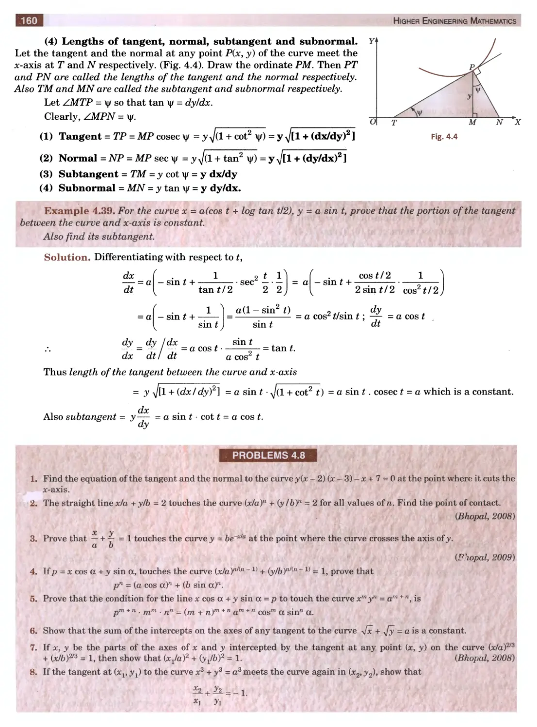
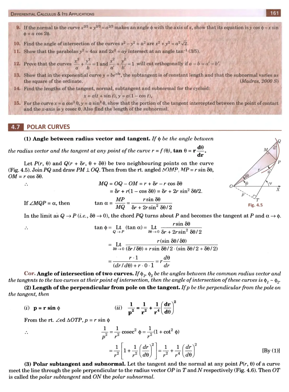
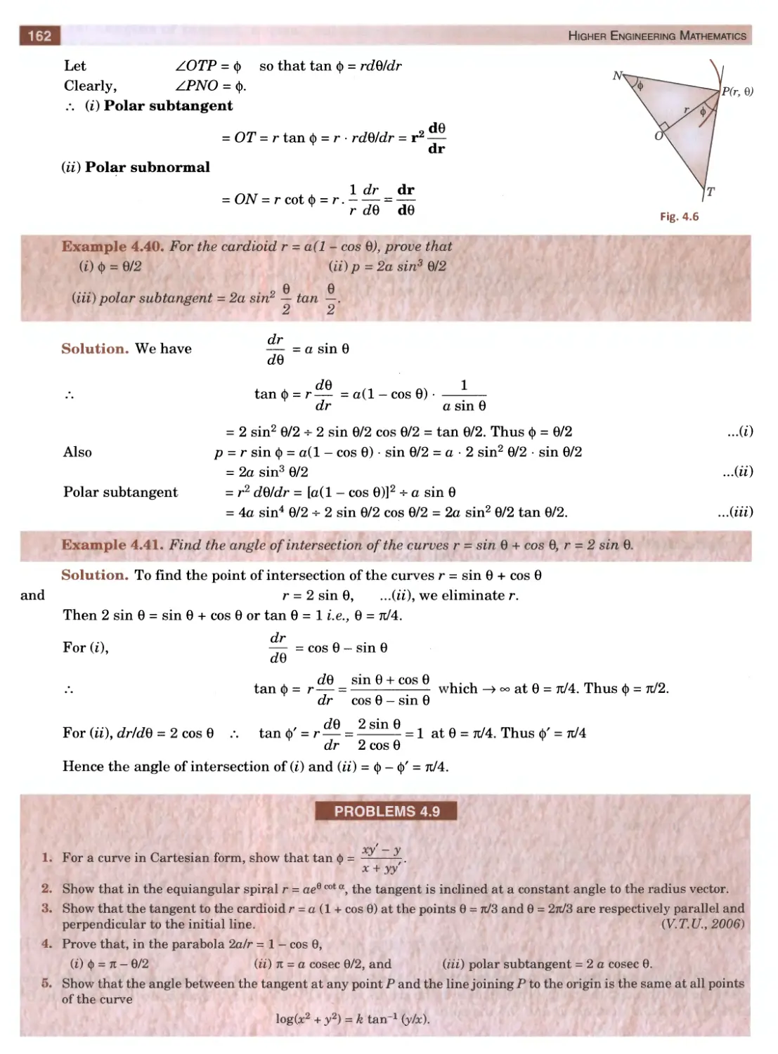
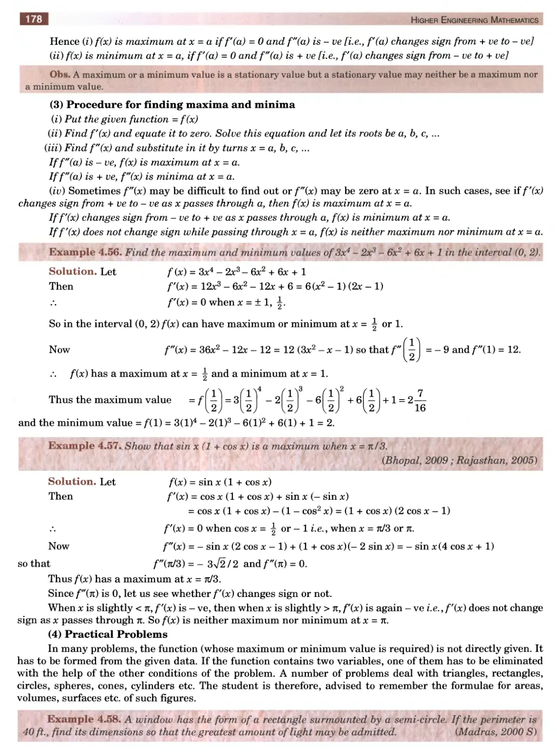
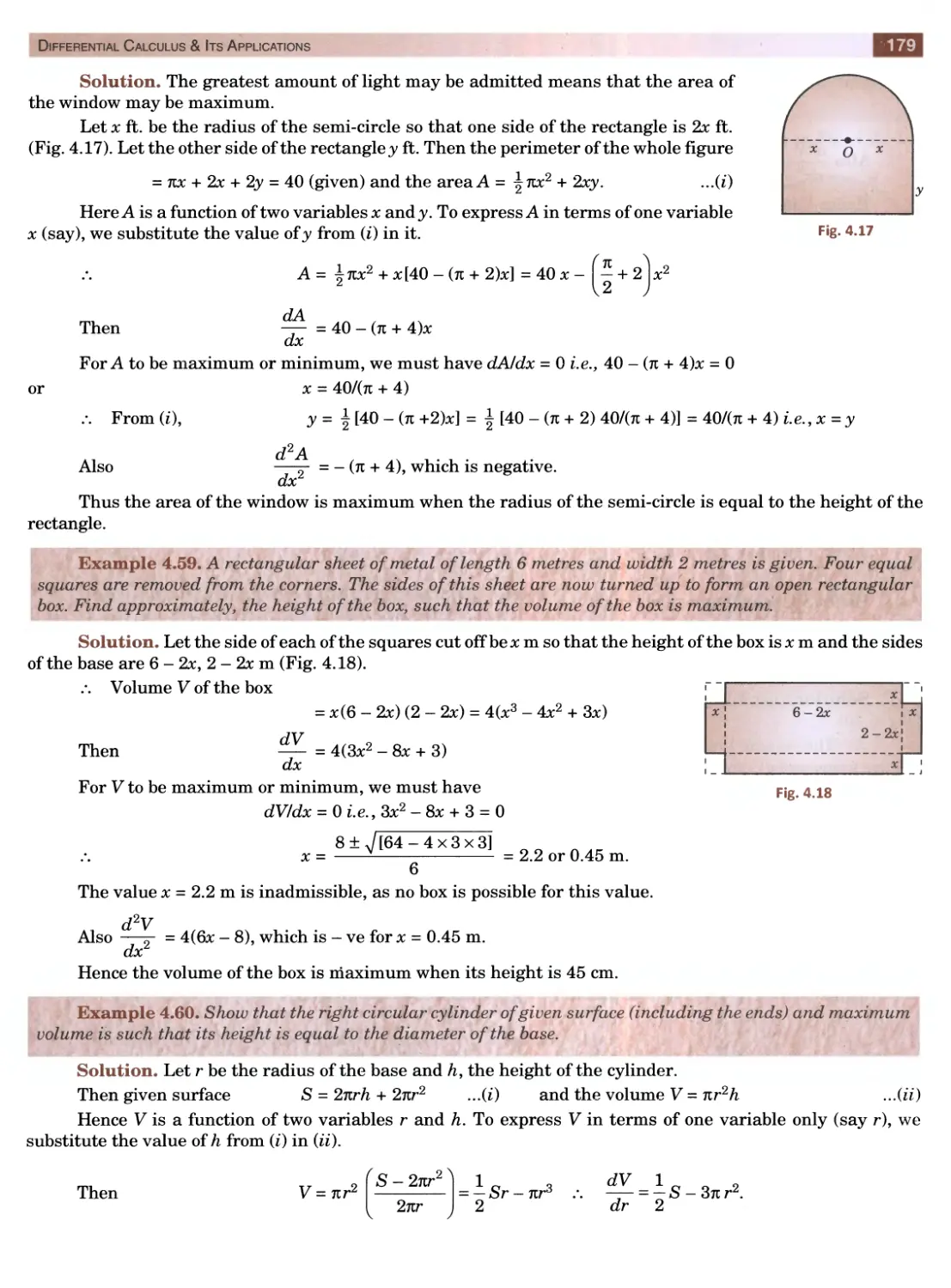
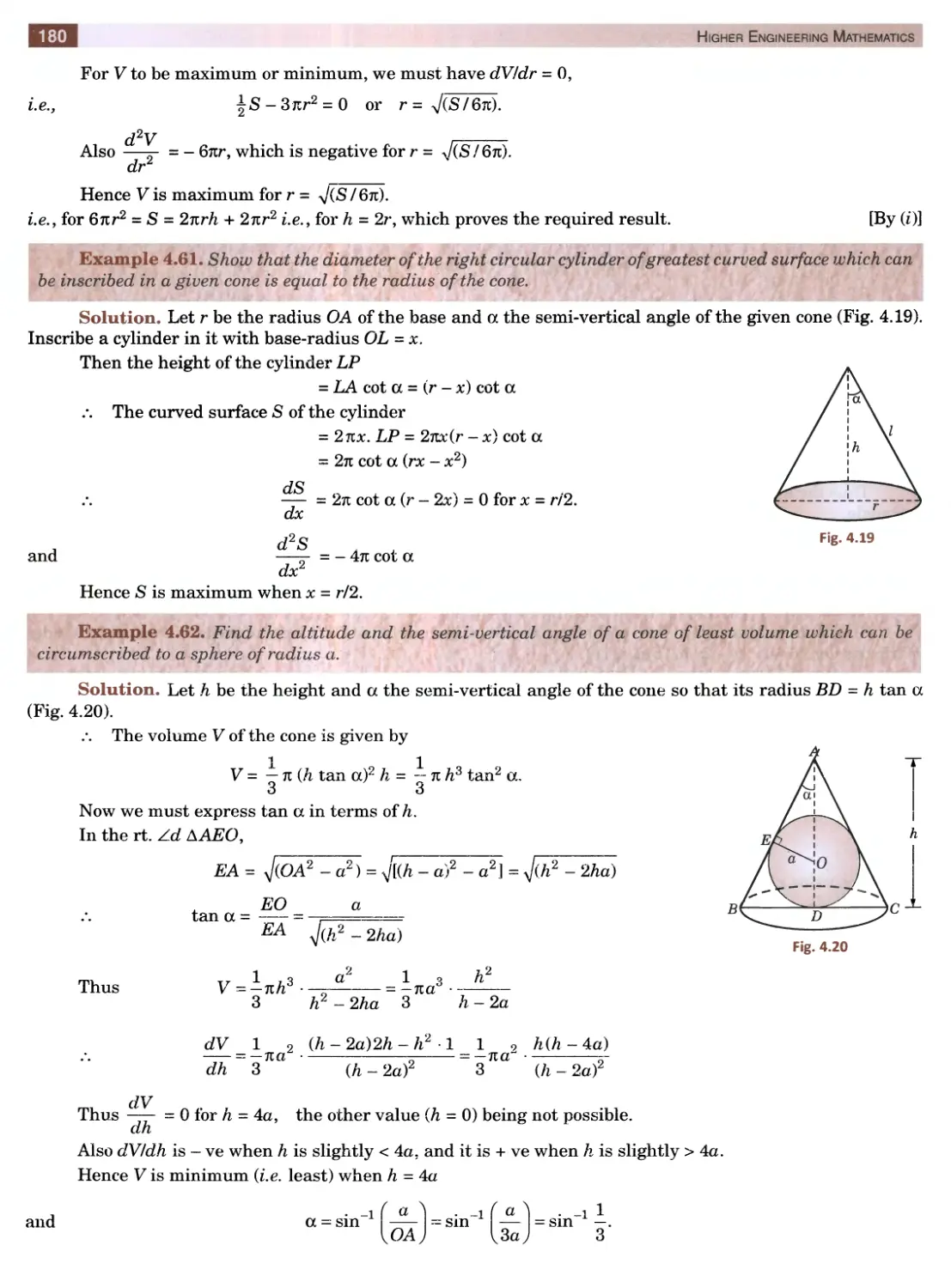
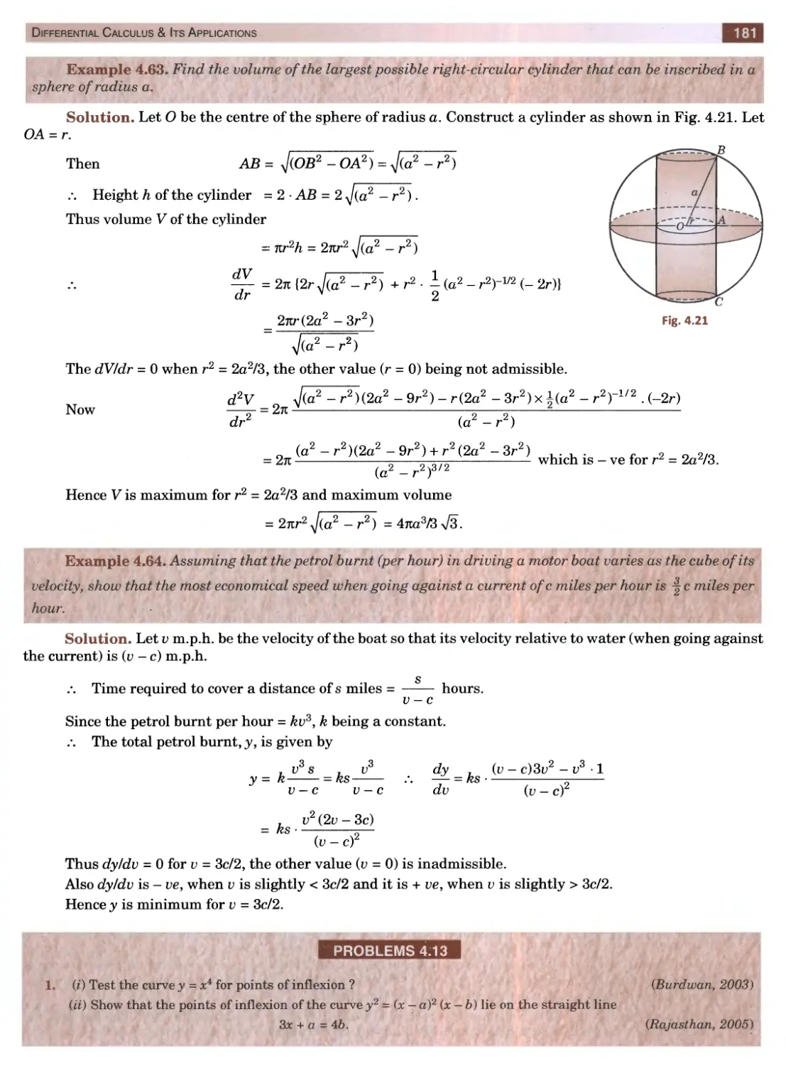
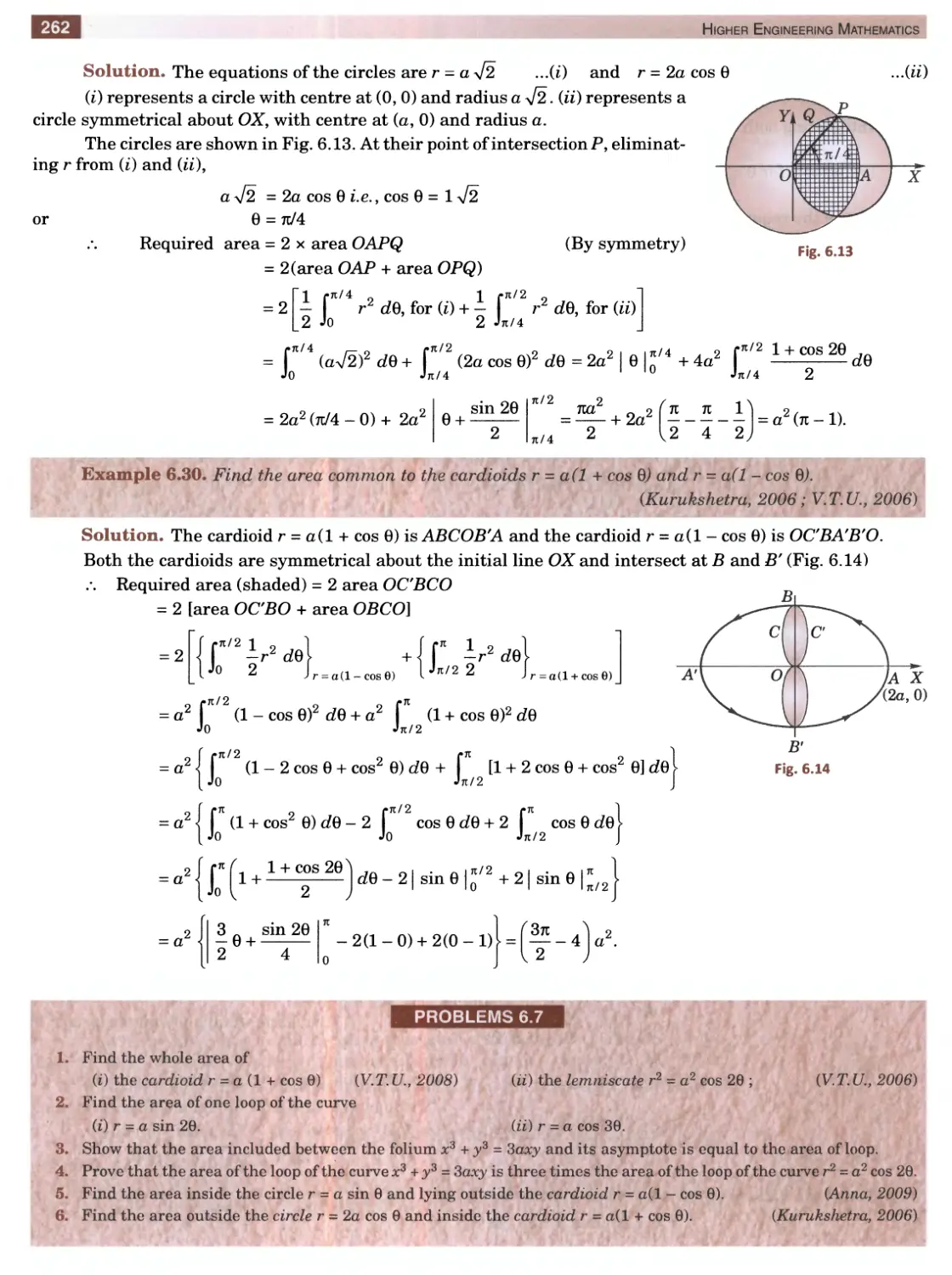
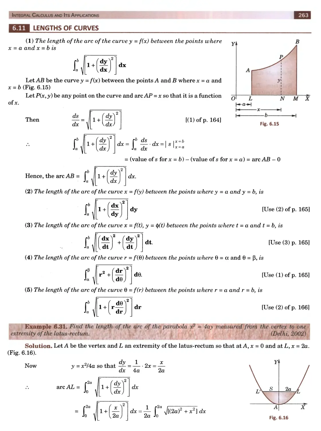
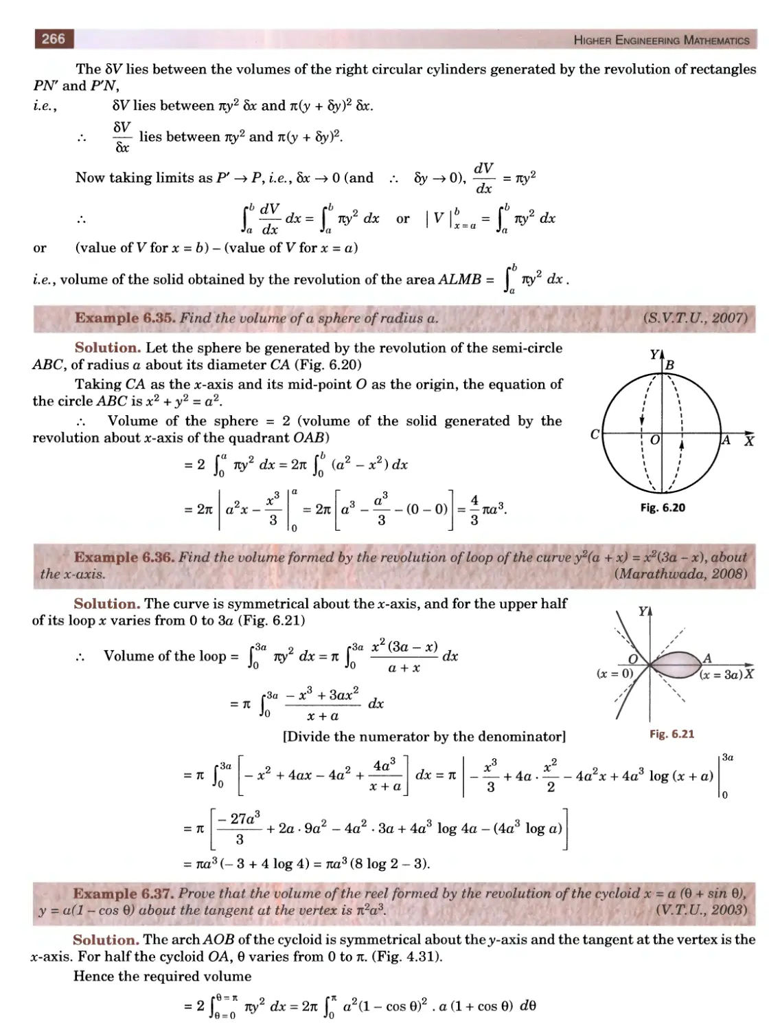
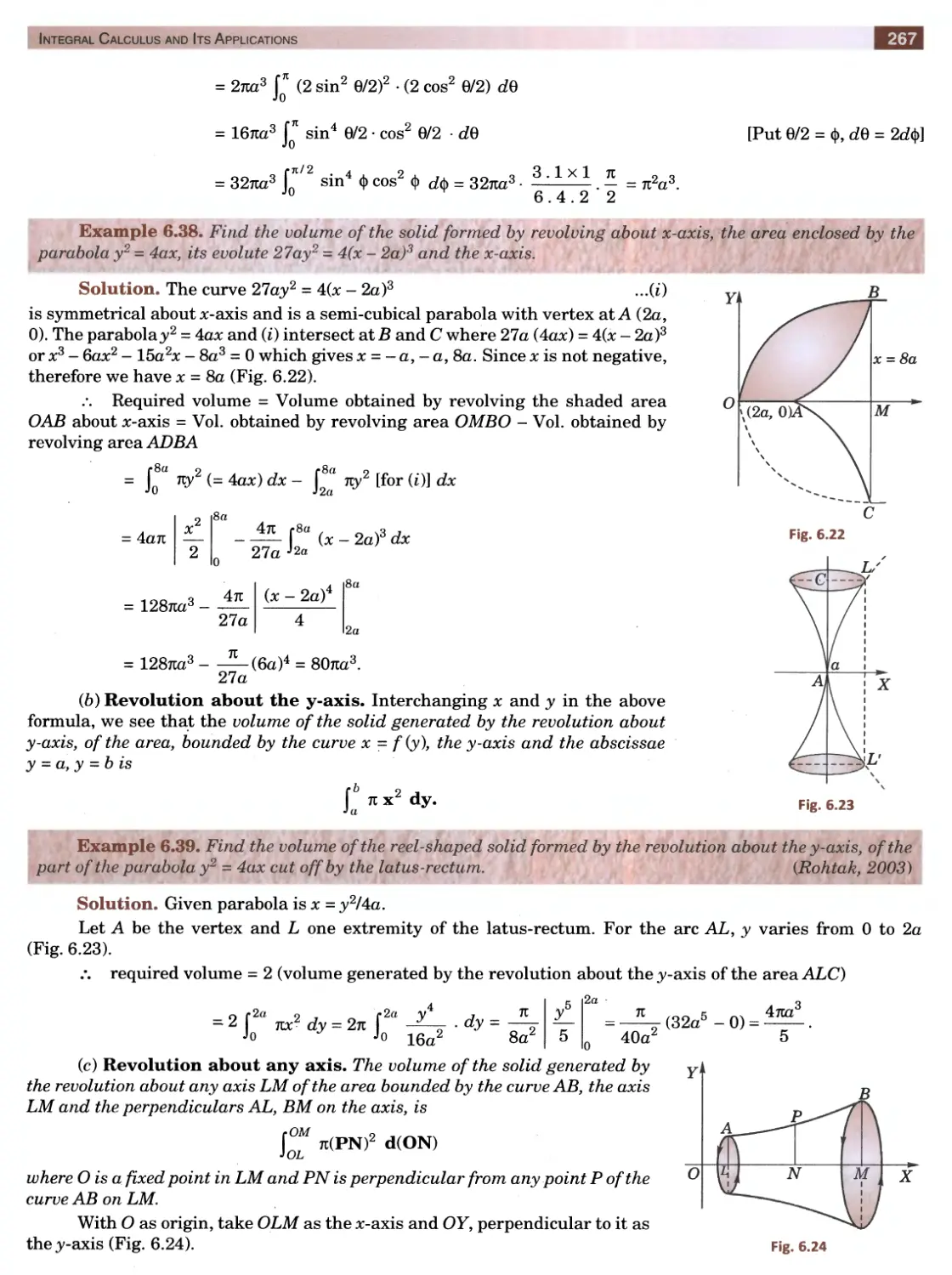
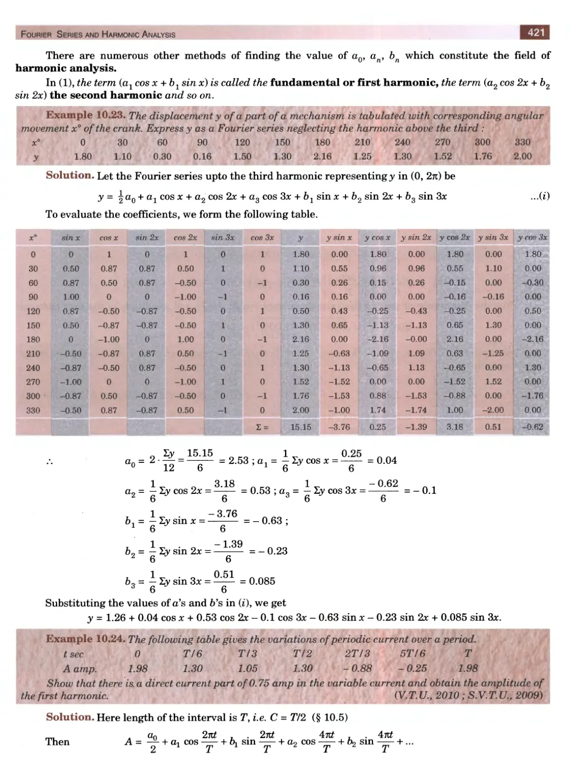
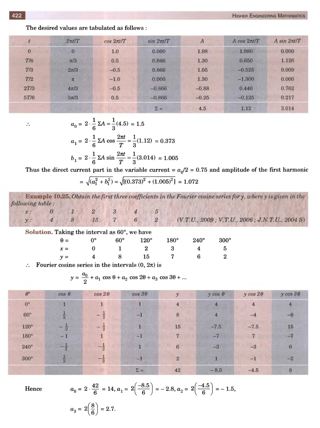
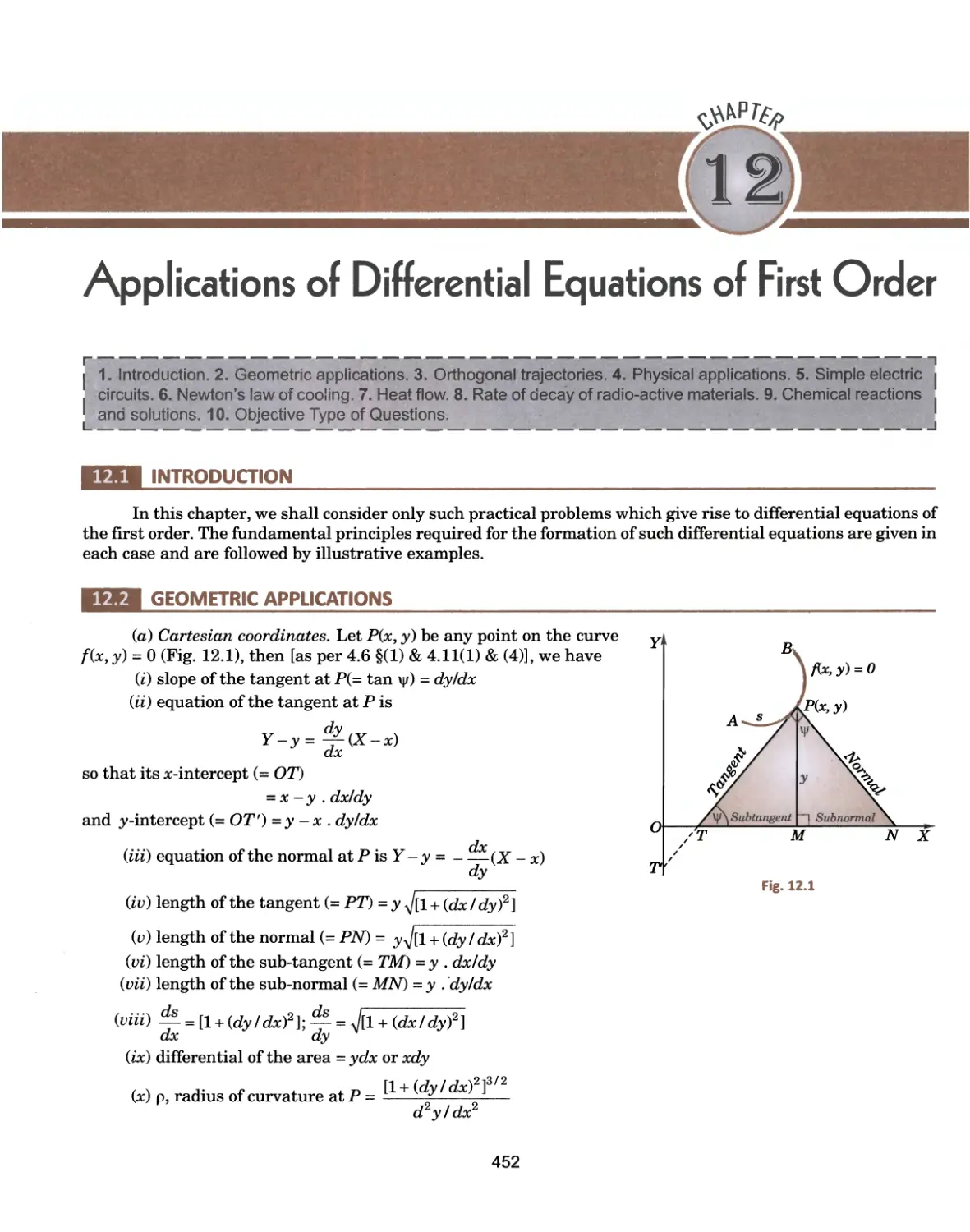
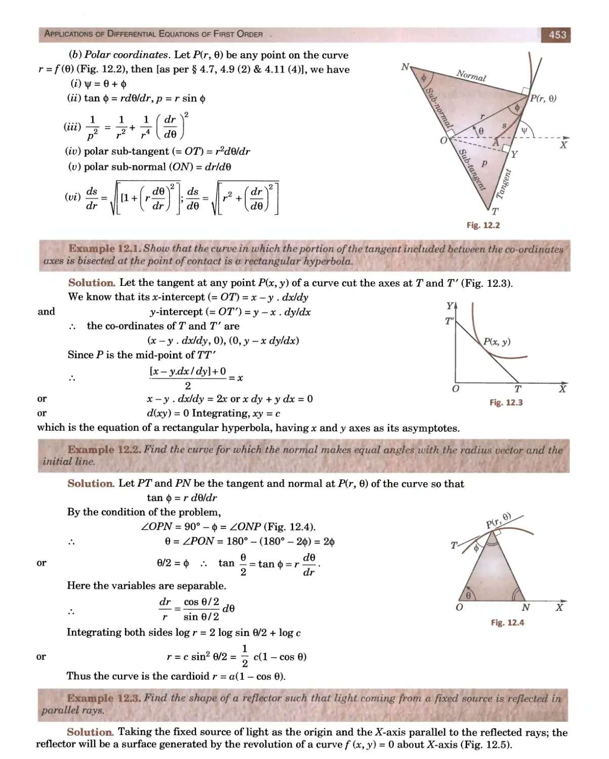
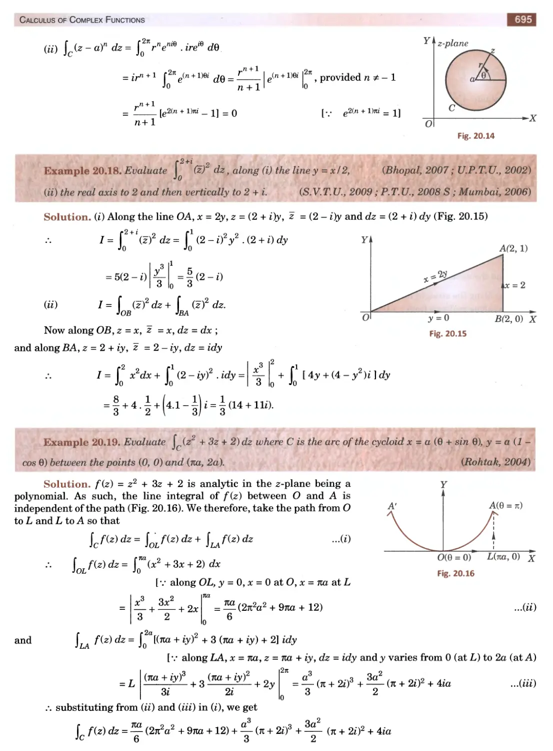
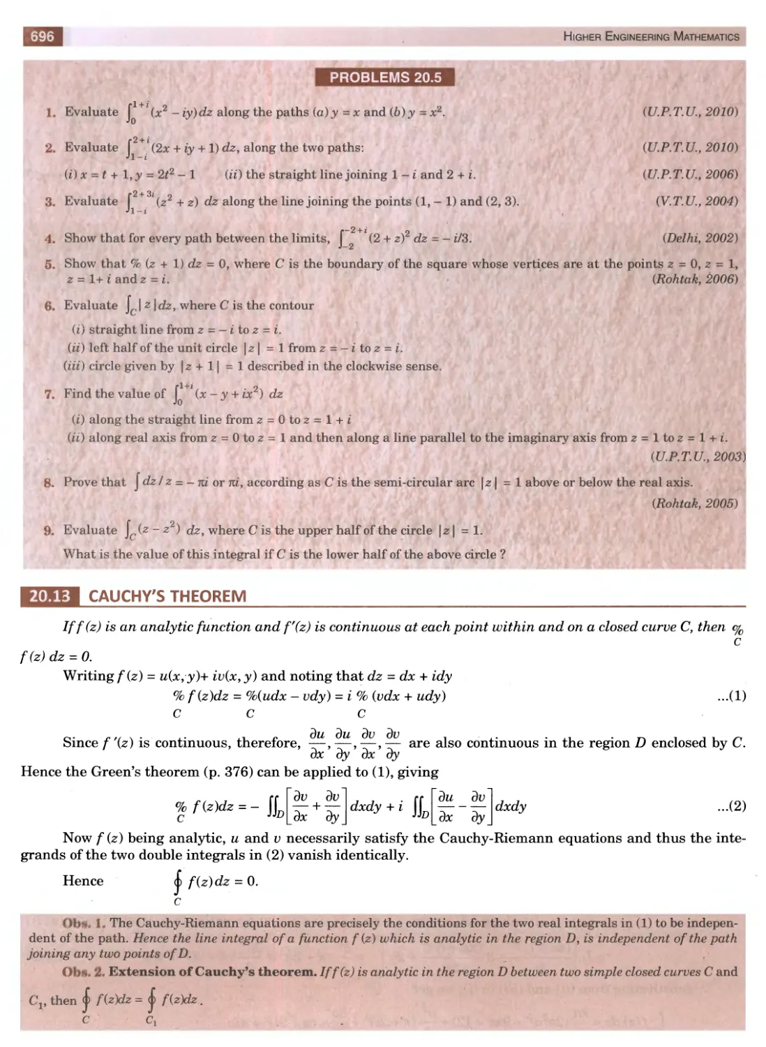
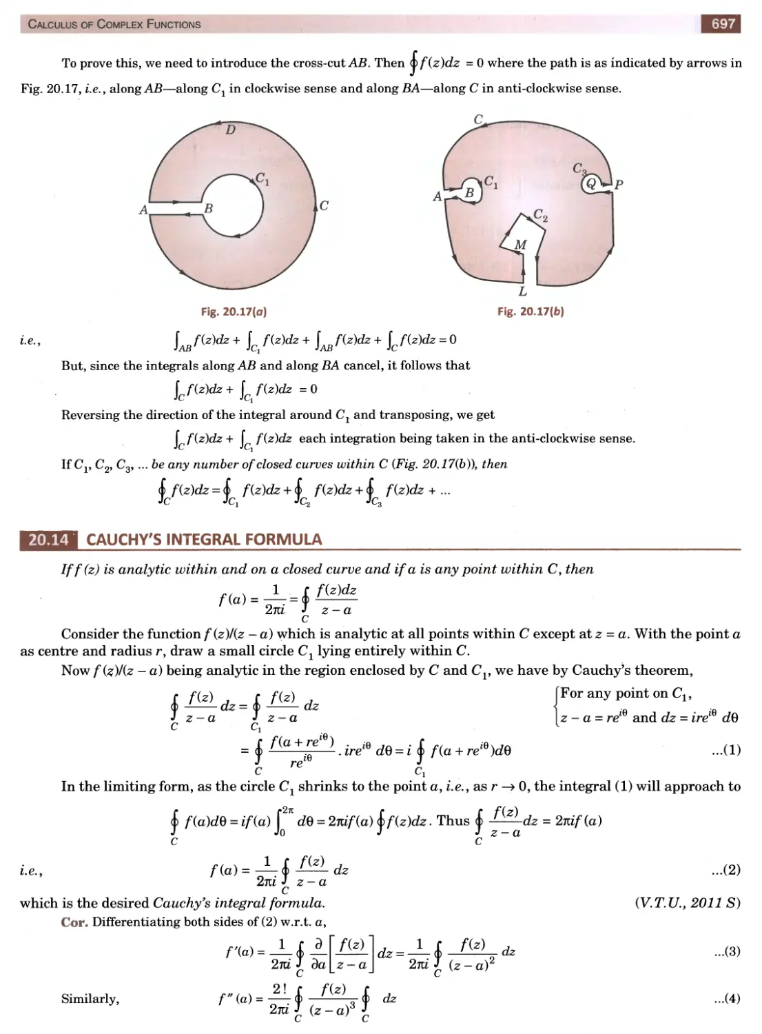
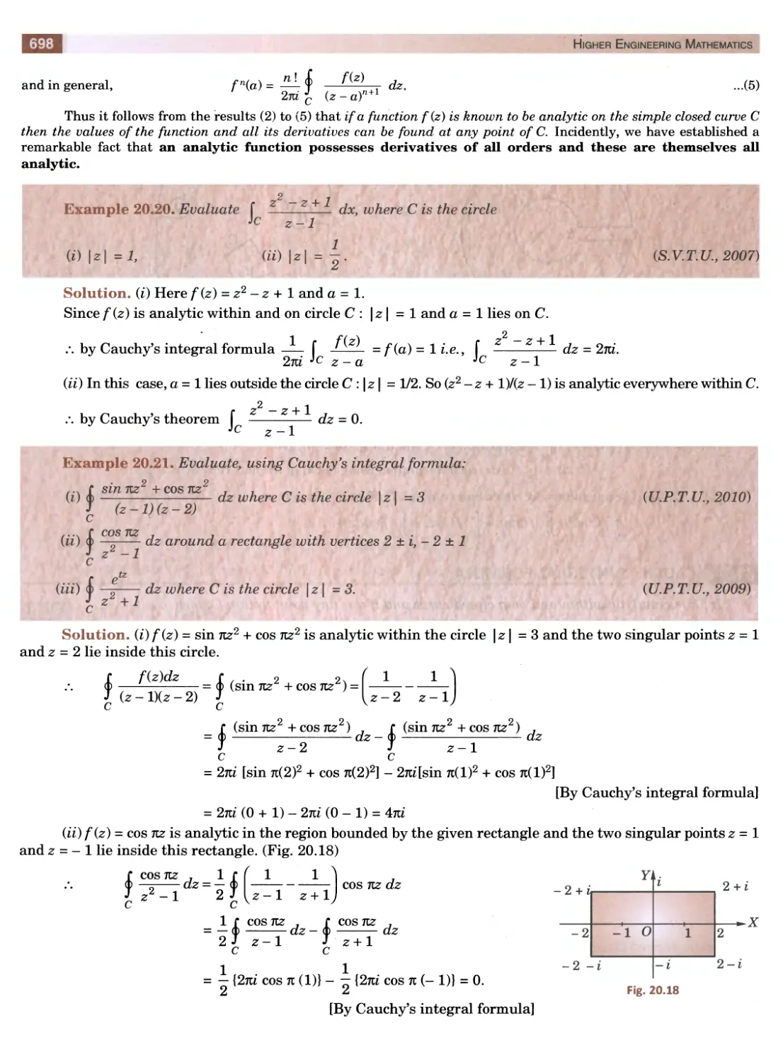
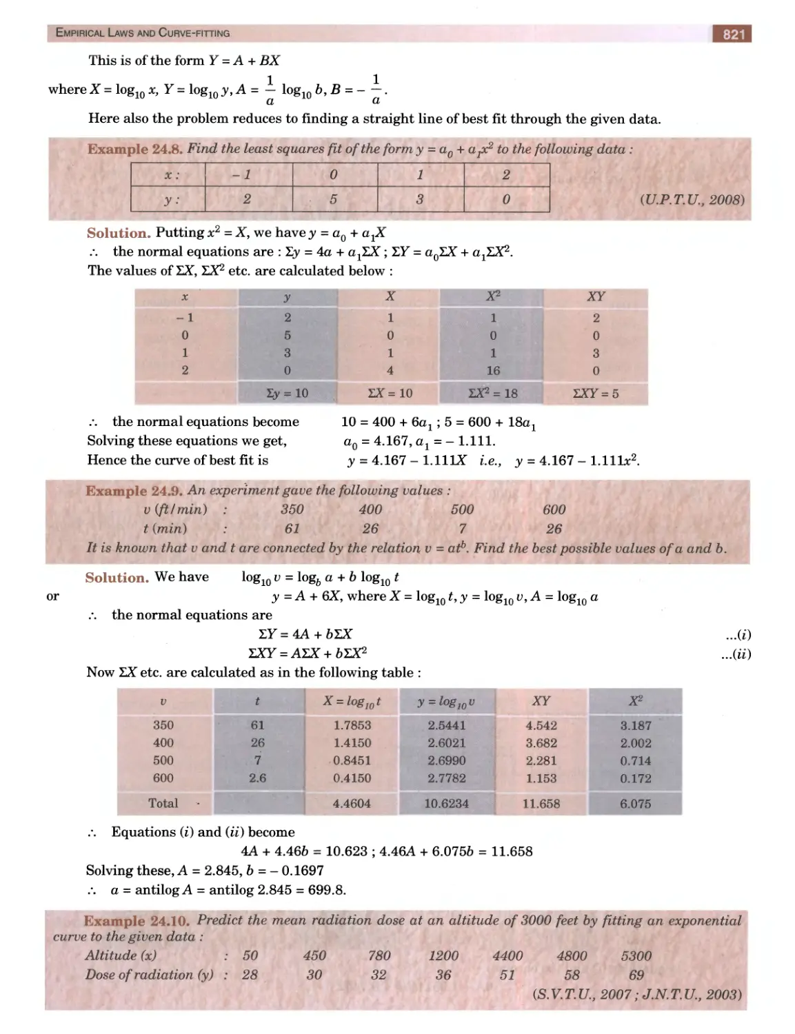
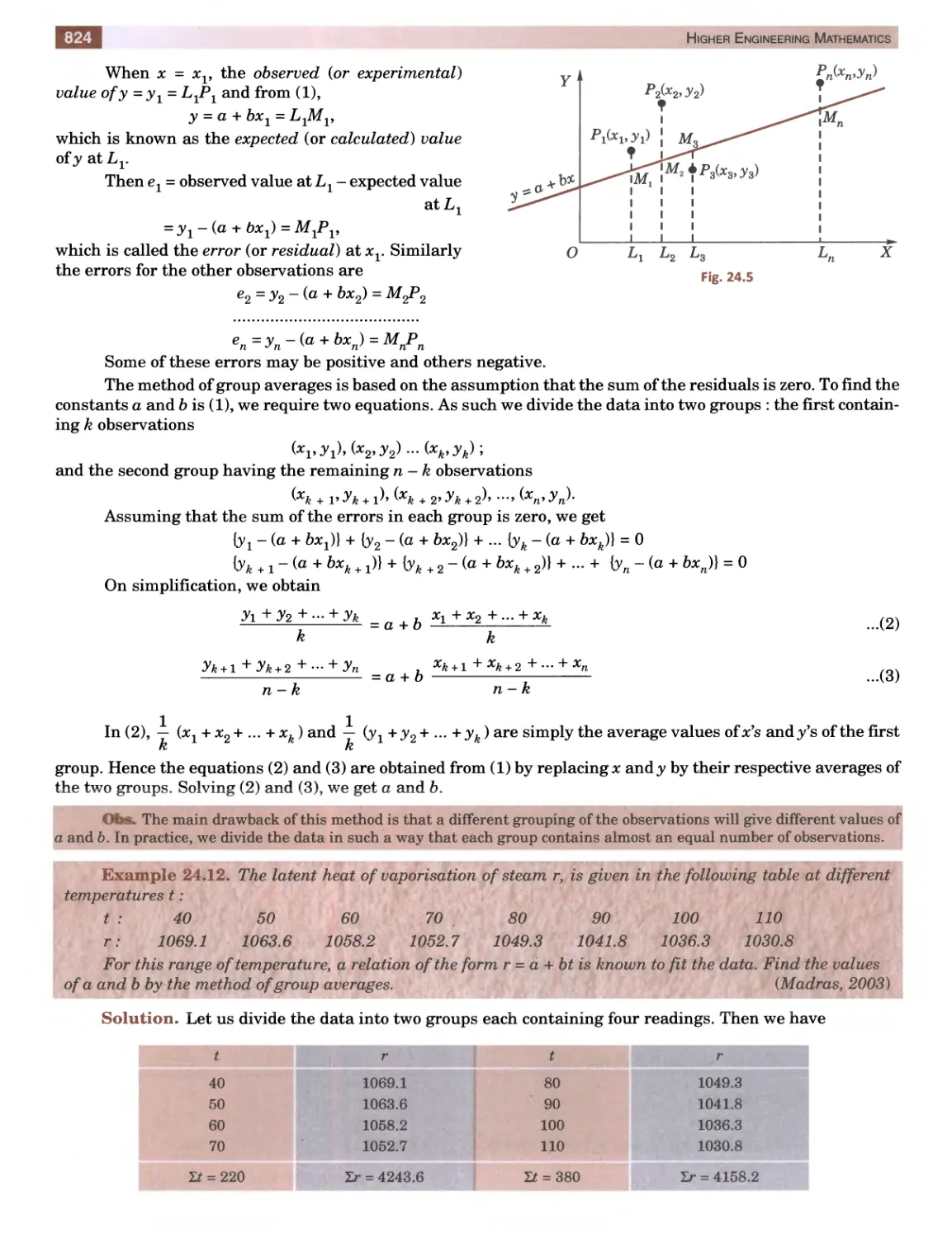
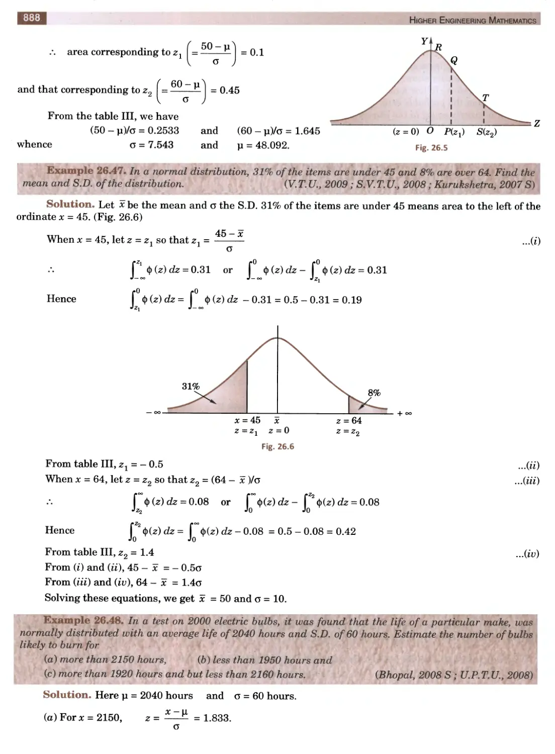
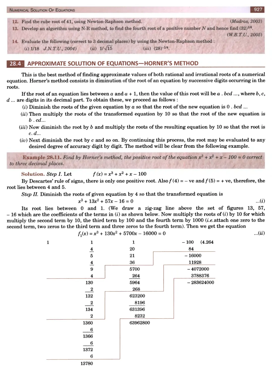
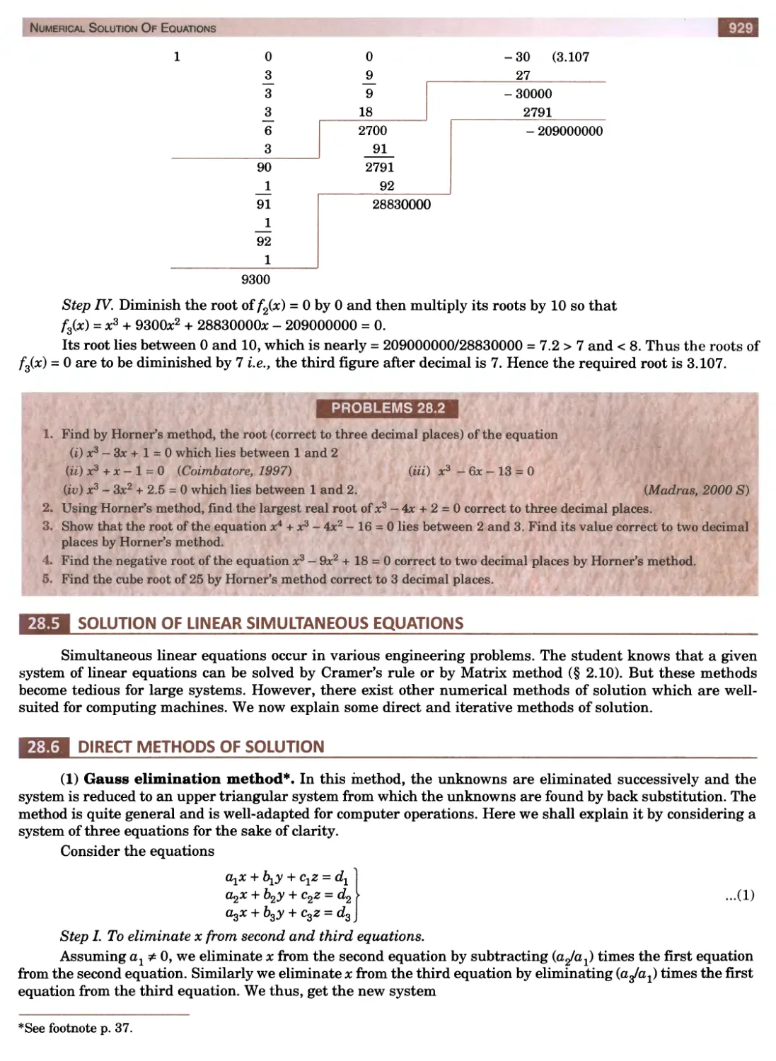
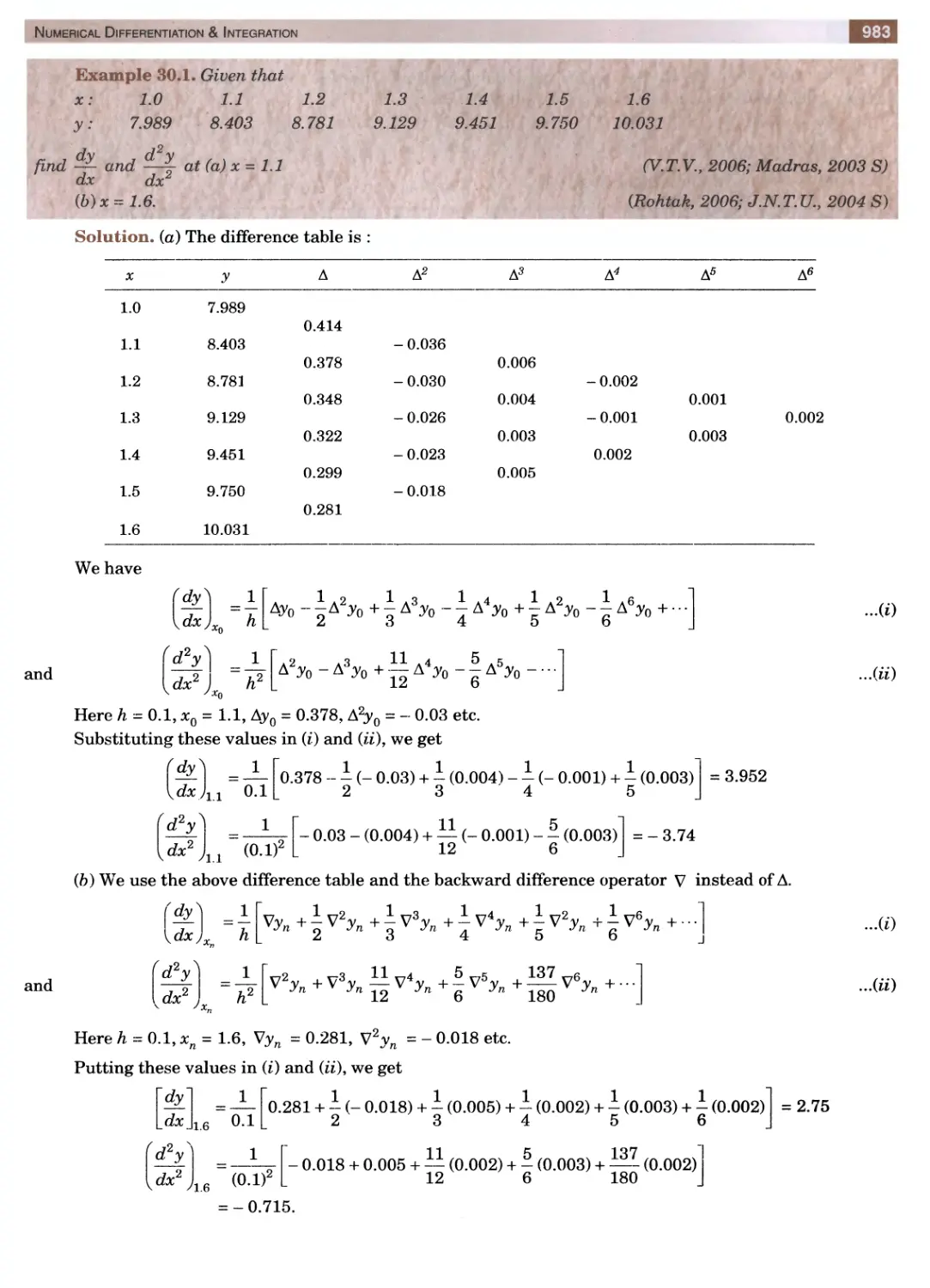
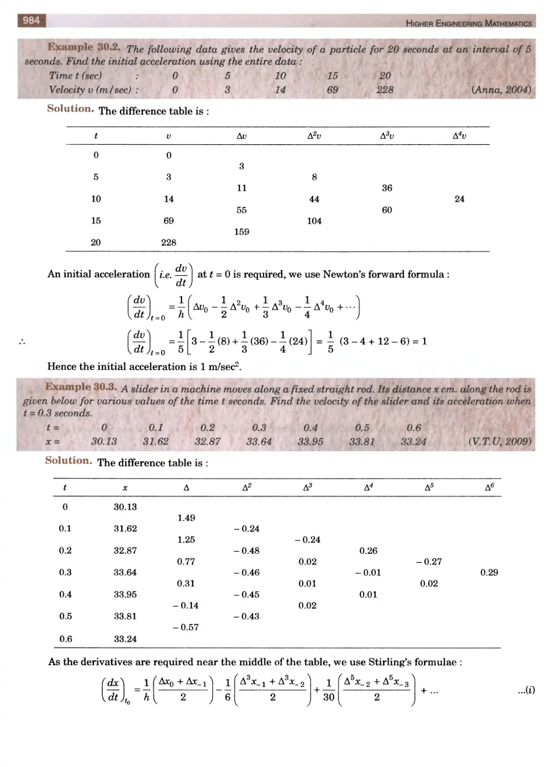
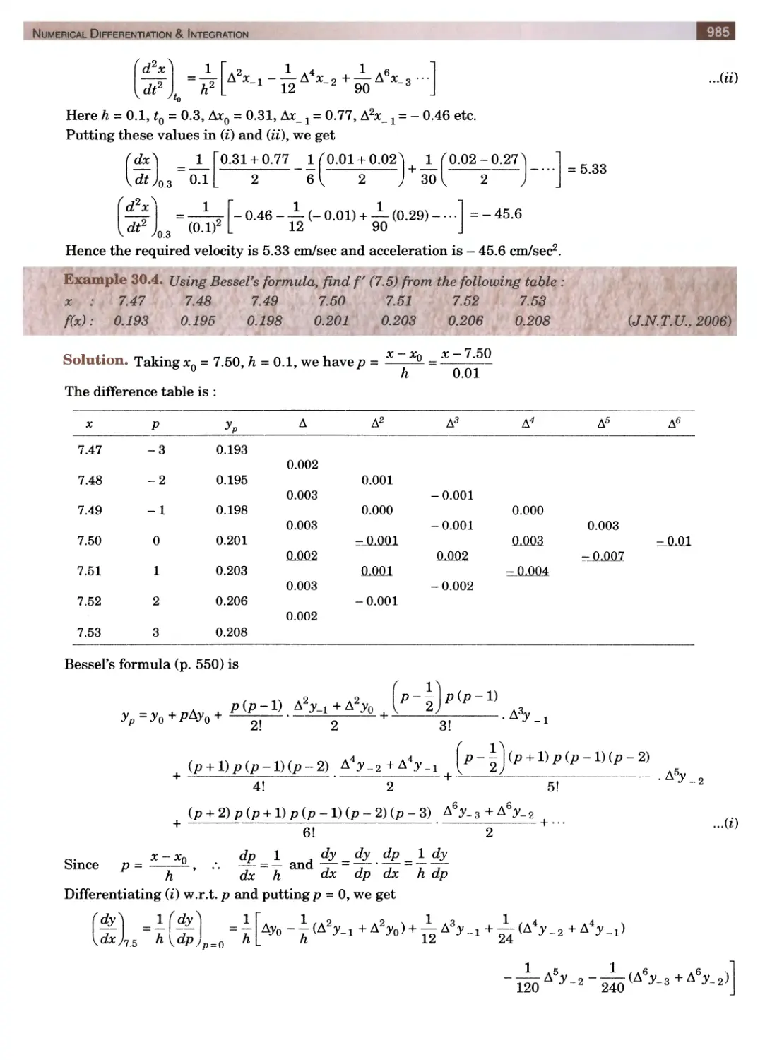
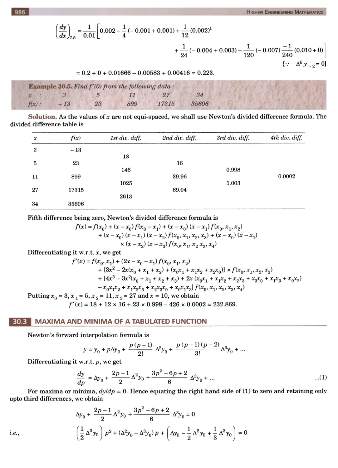
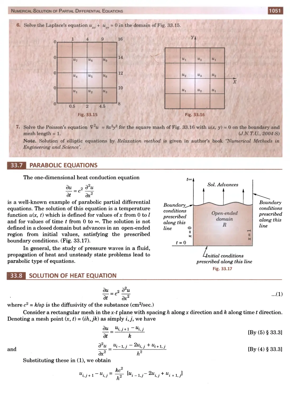
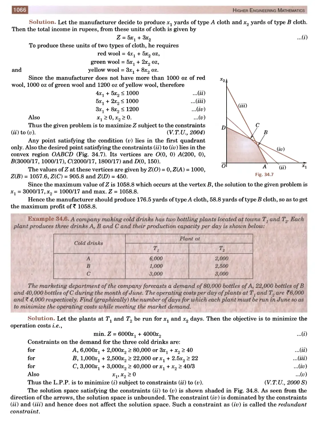
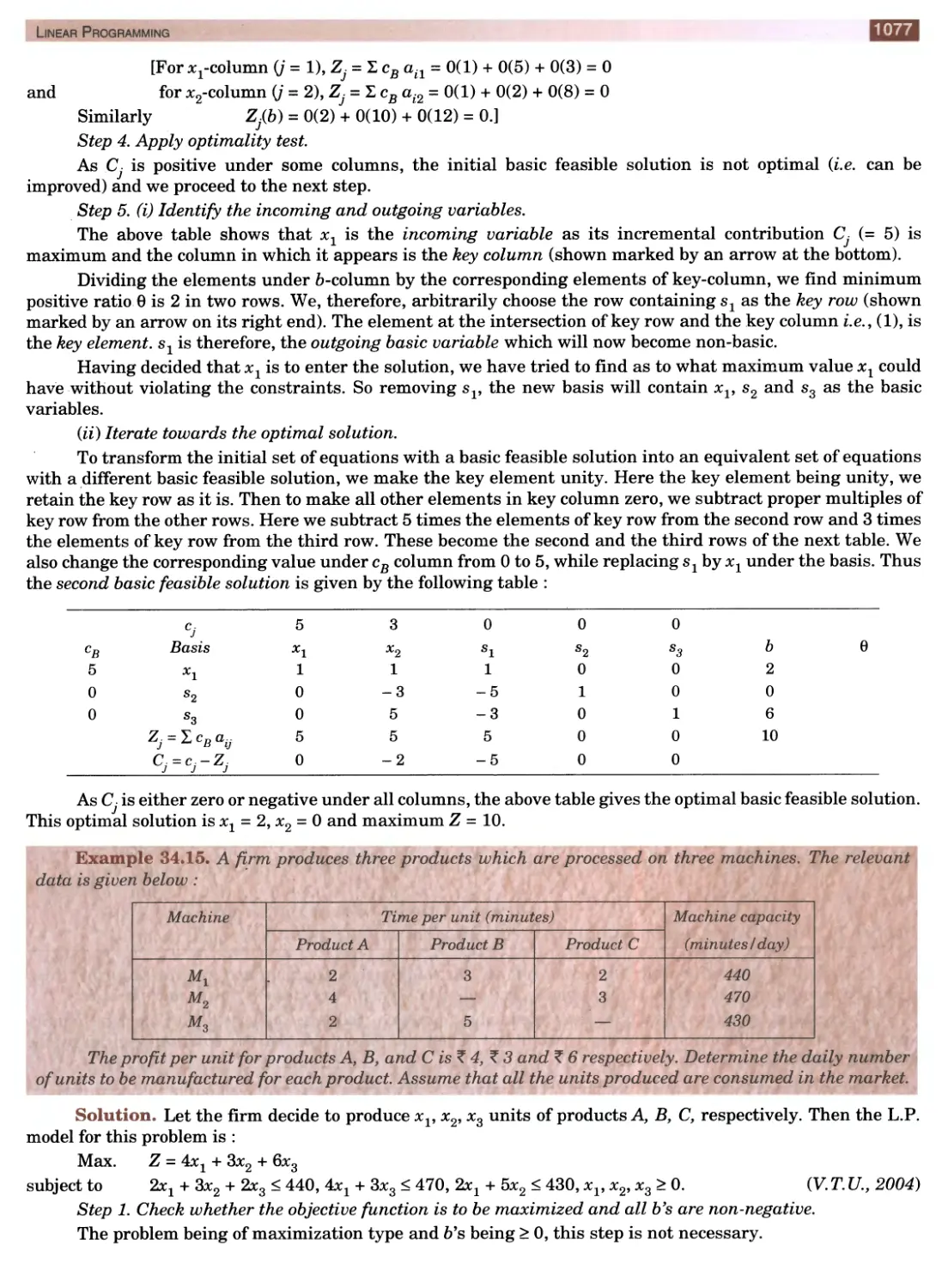
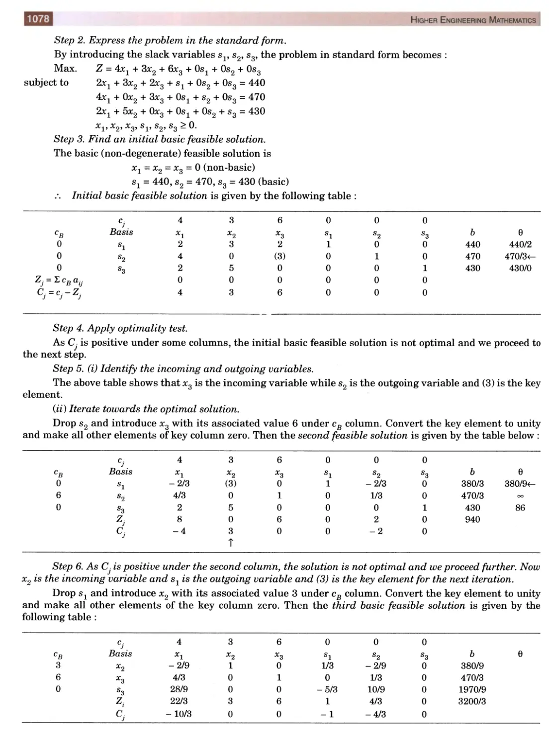
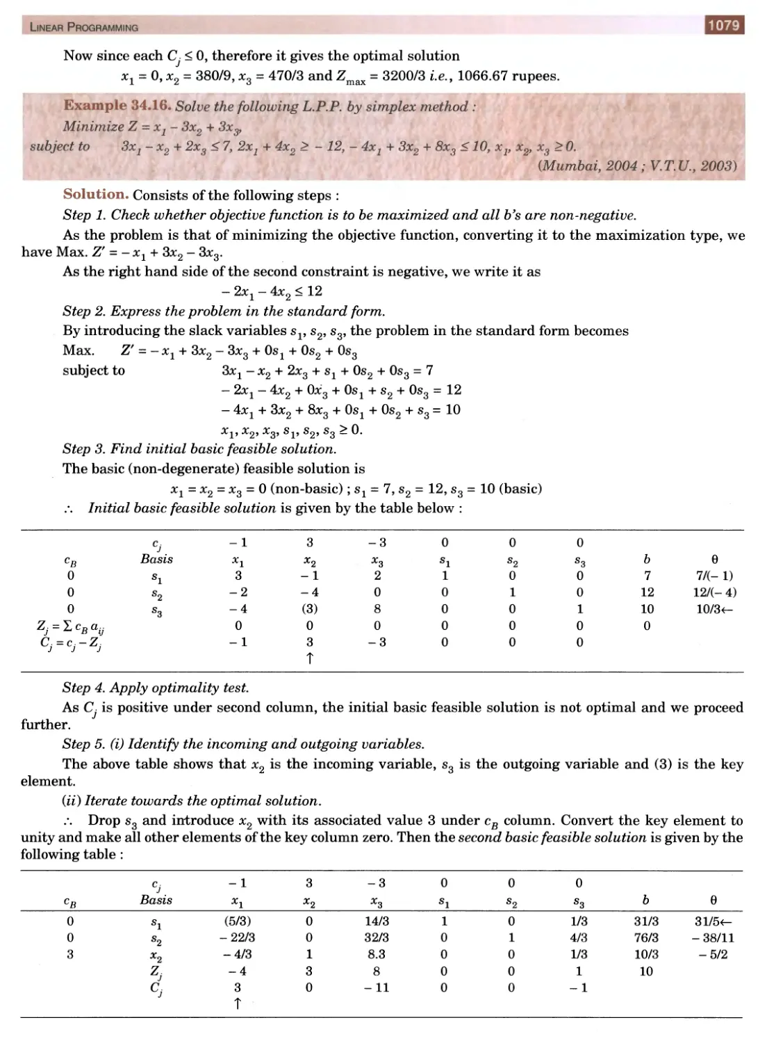
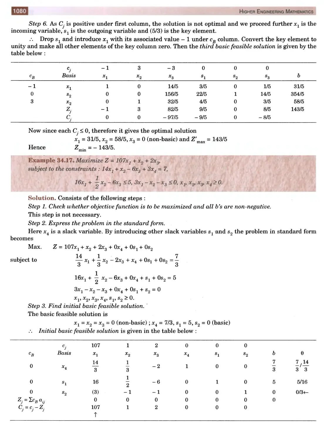
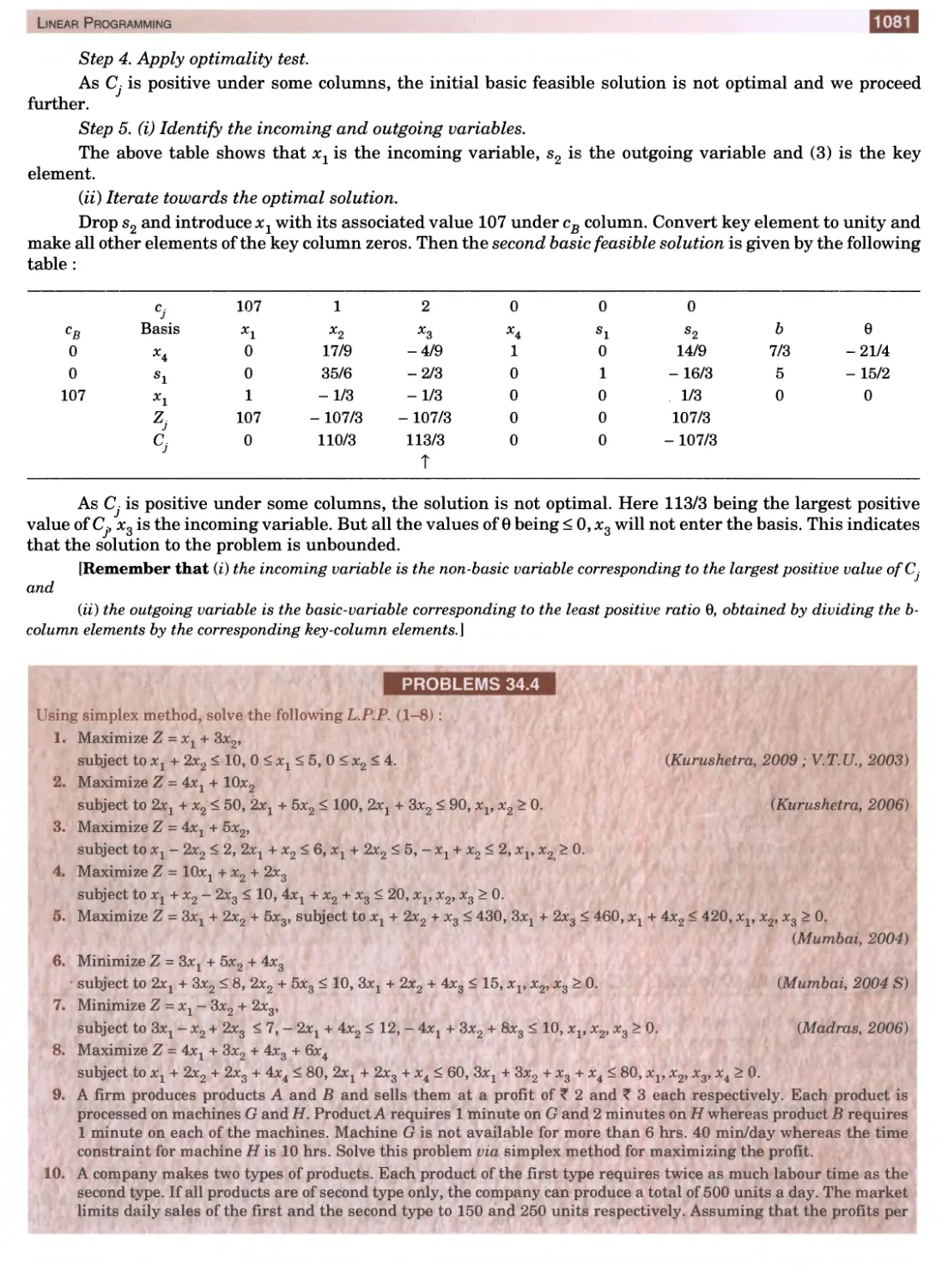
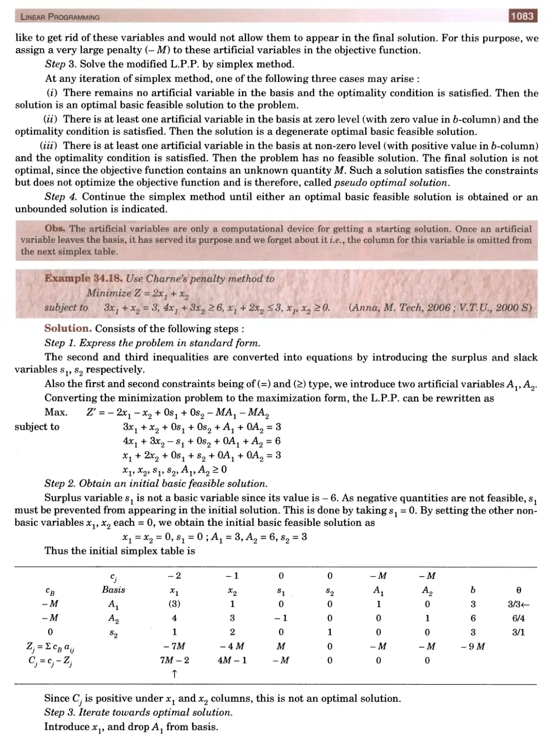
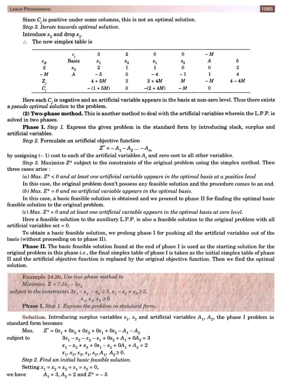
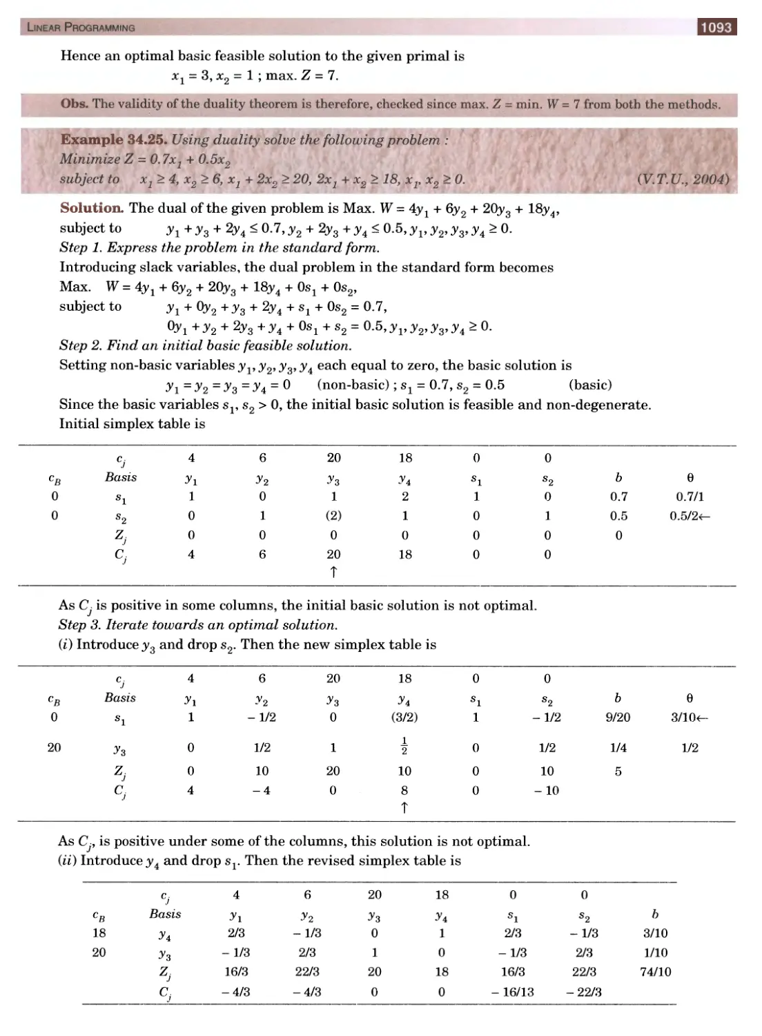
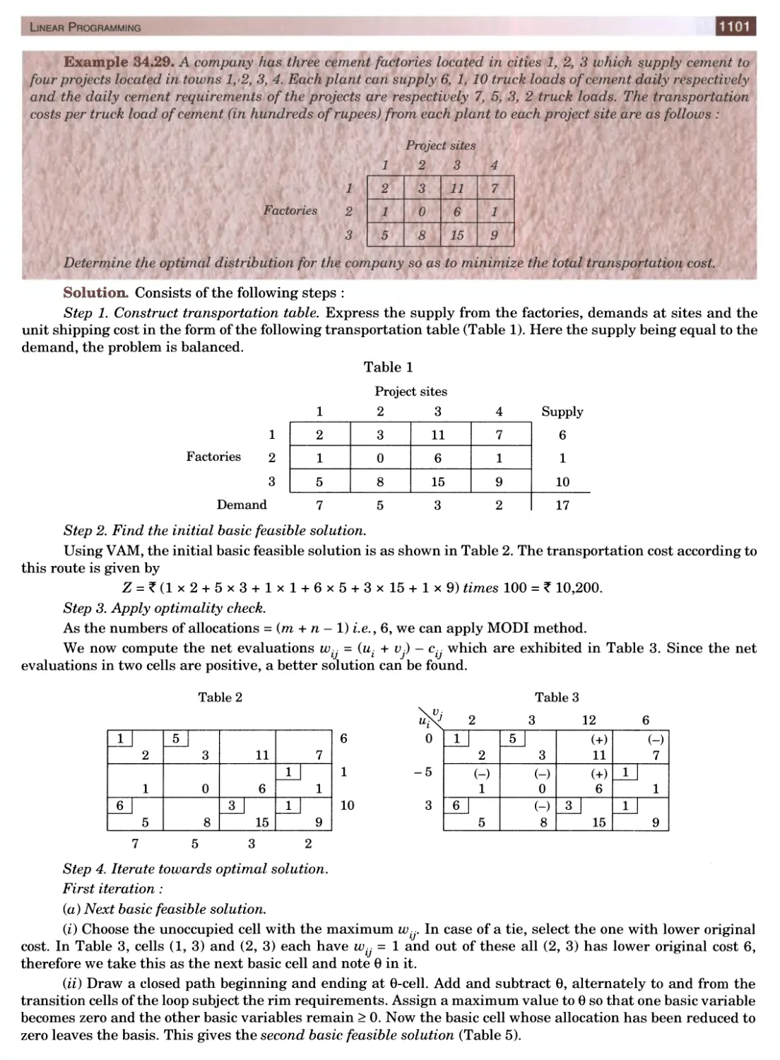
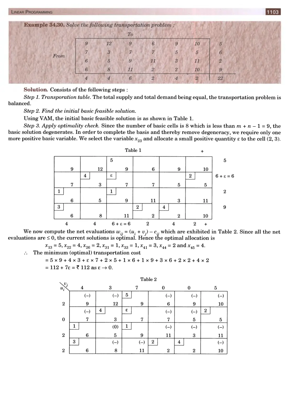
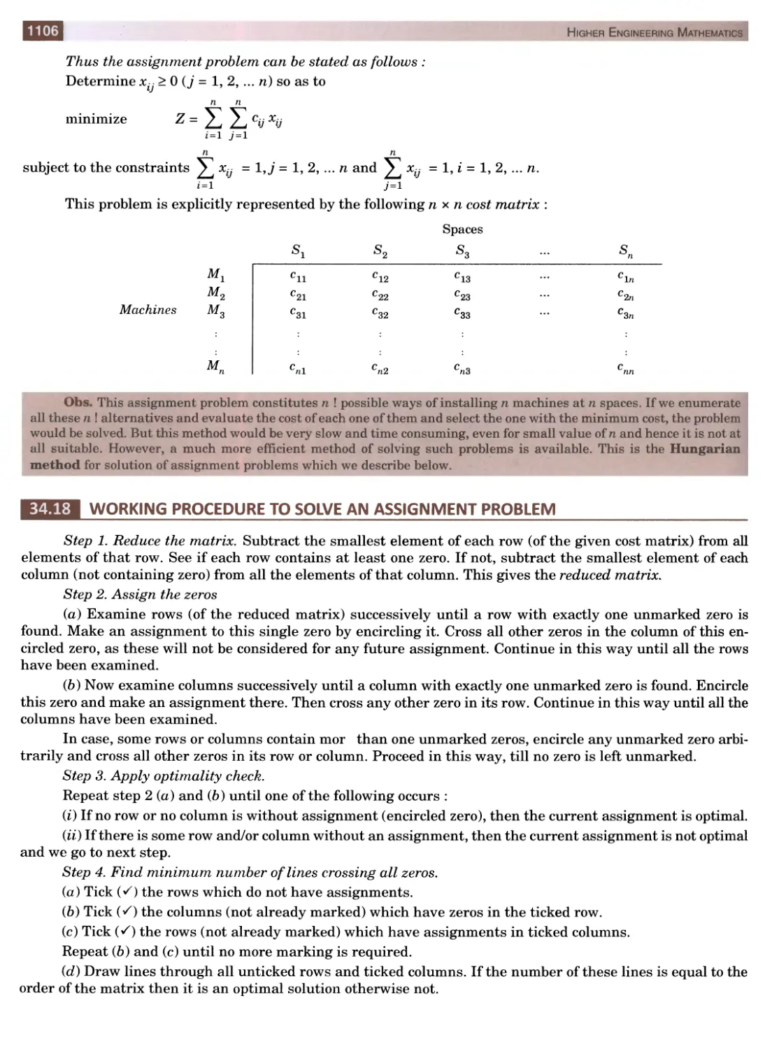
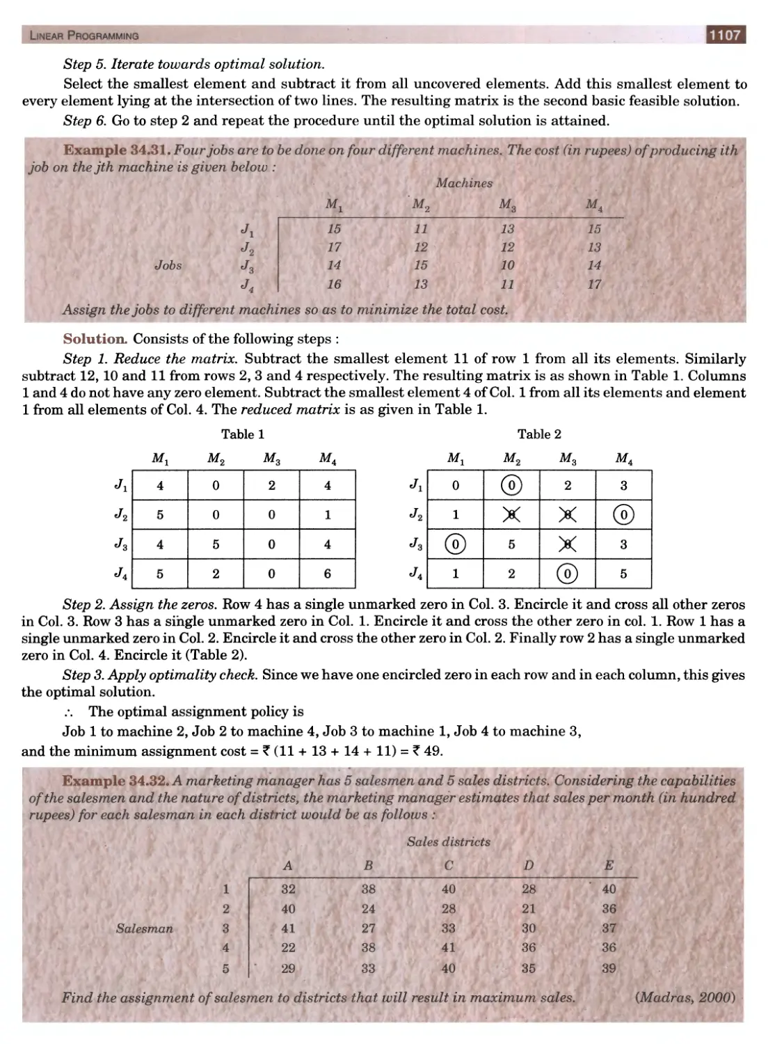
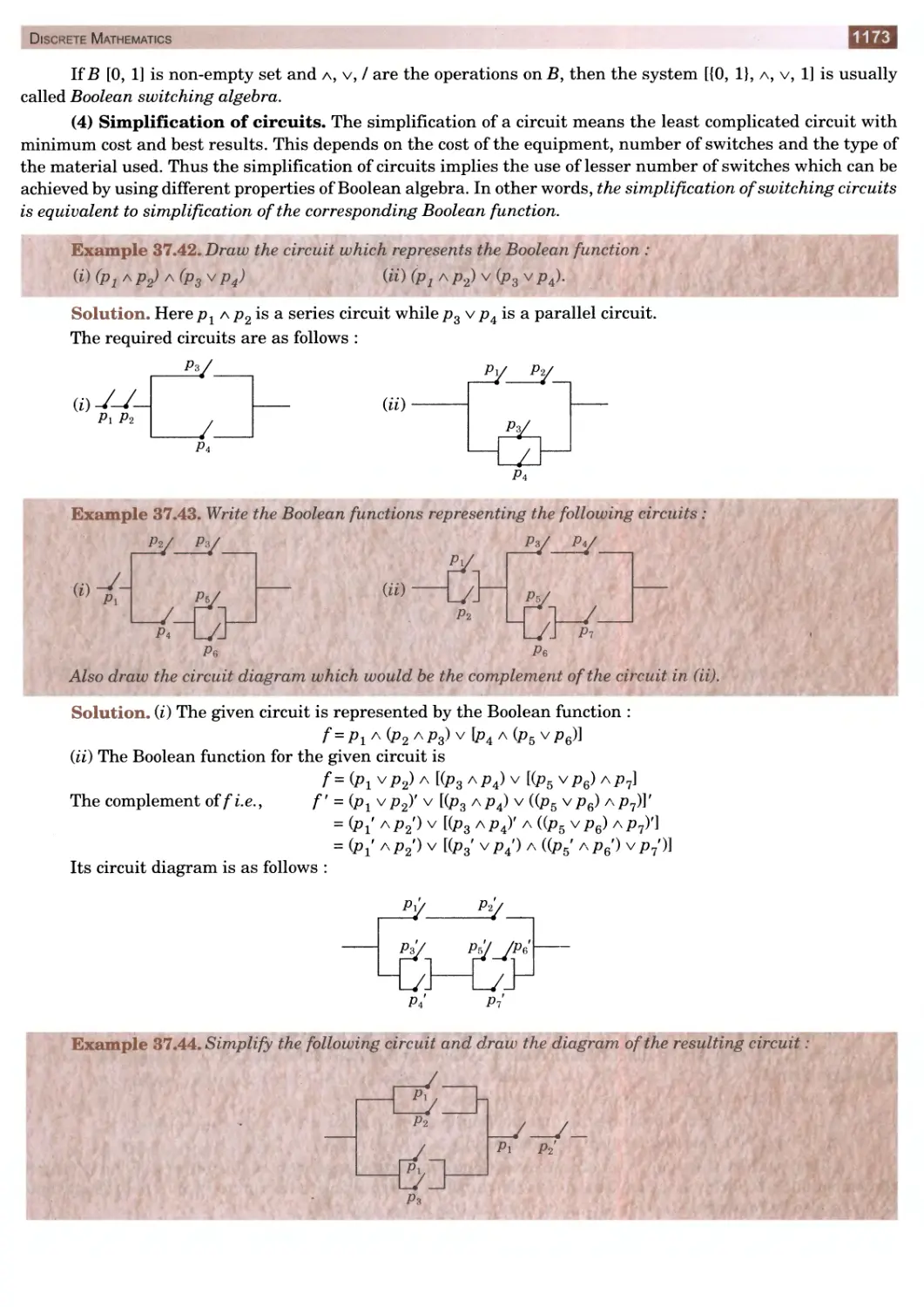
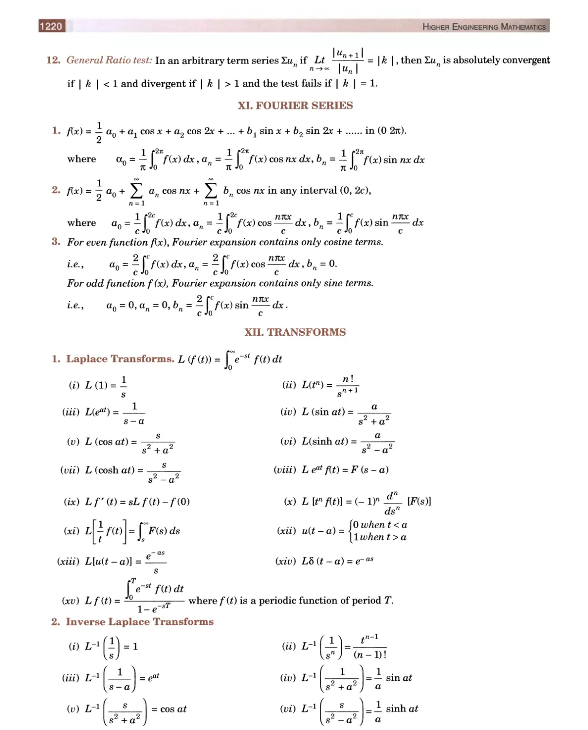
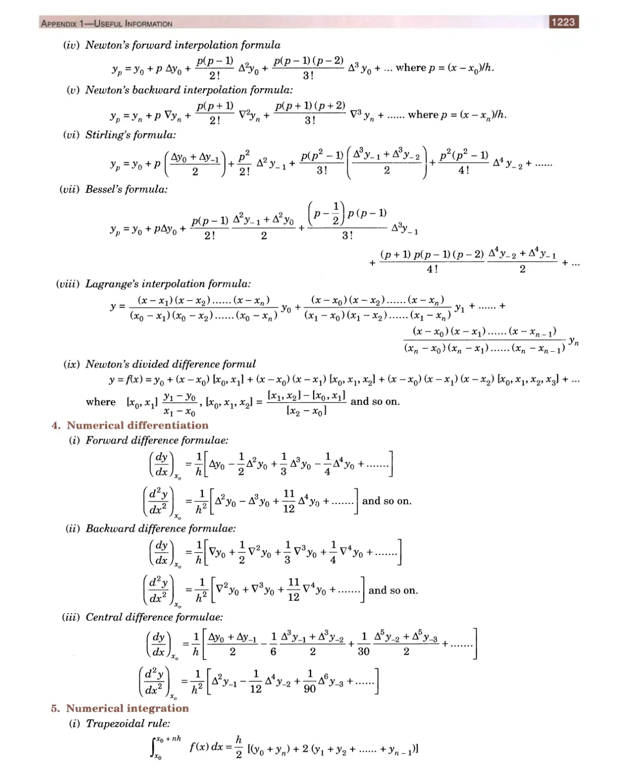
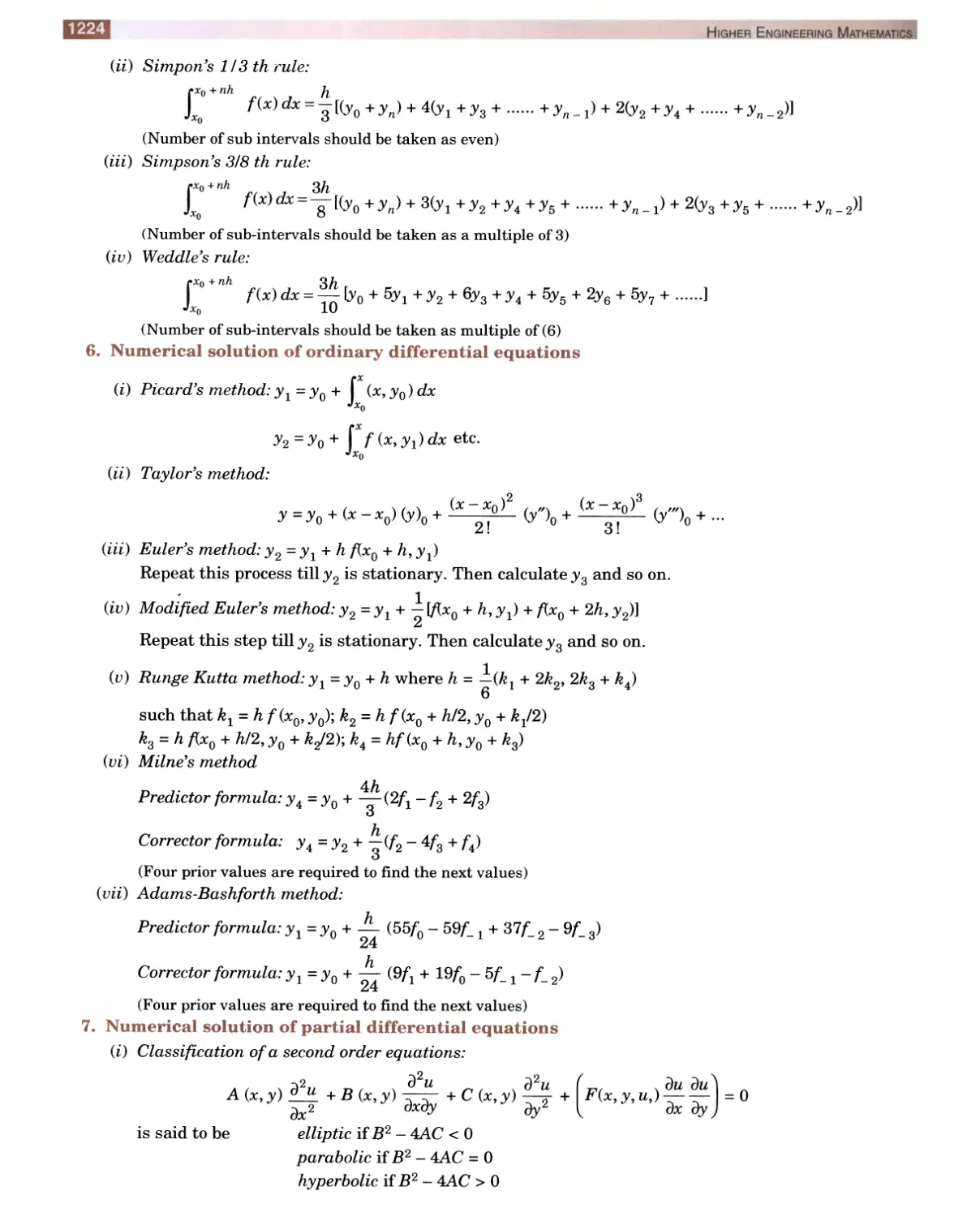
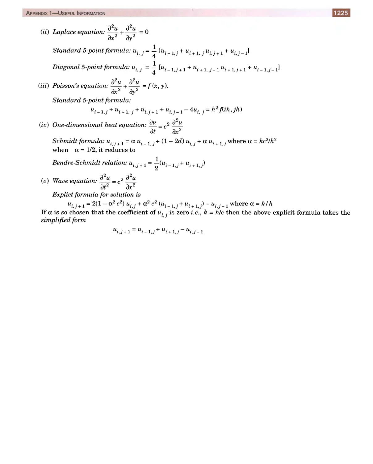
/


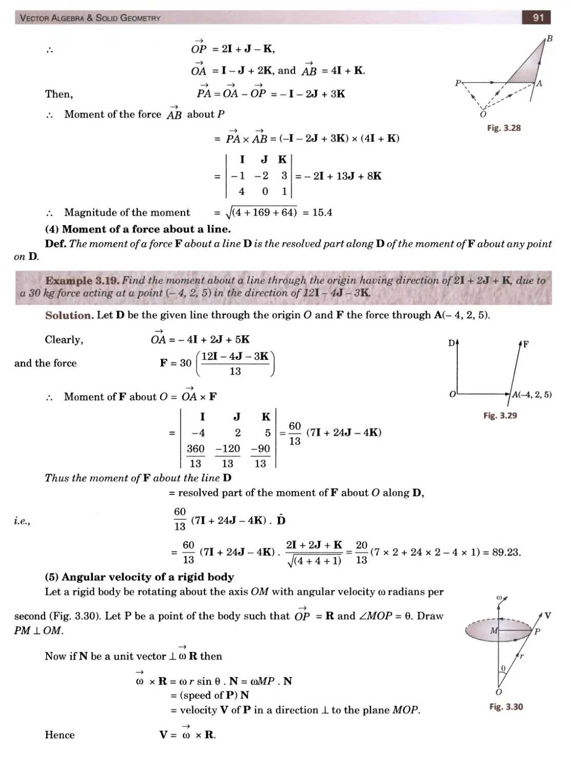


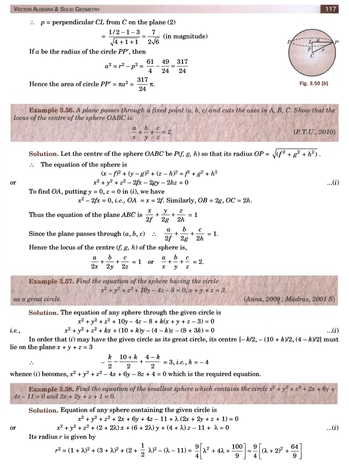

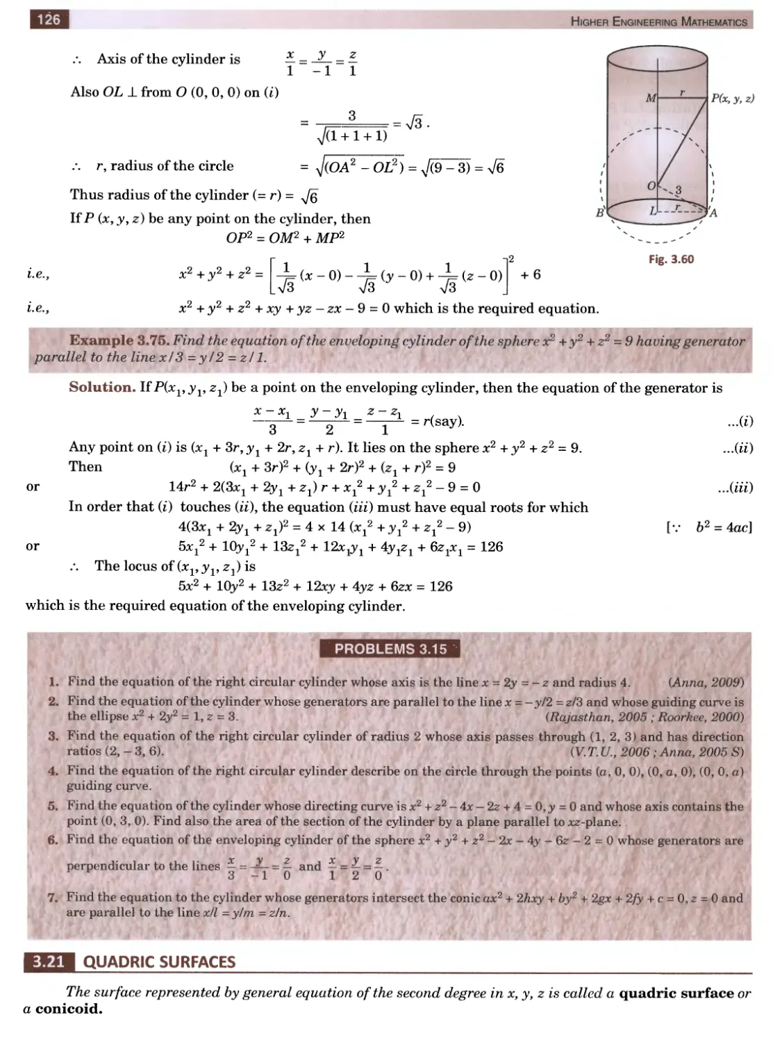


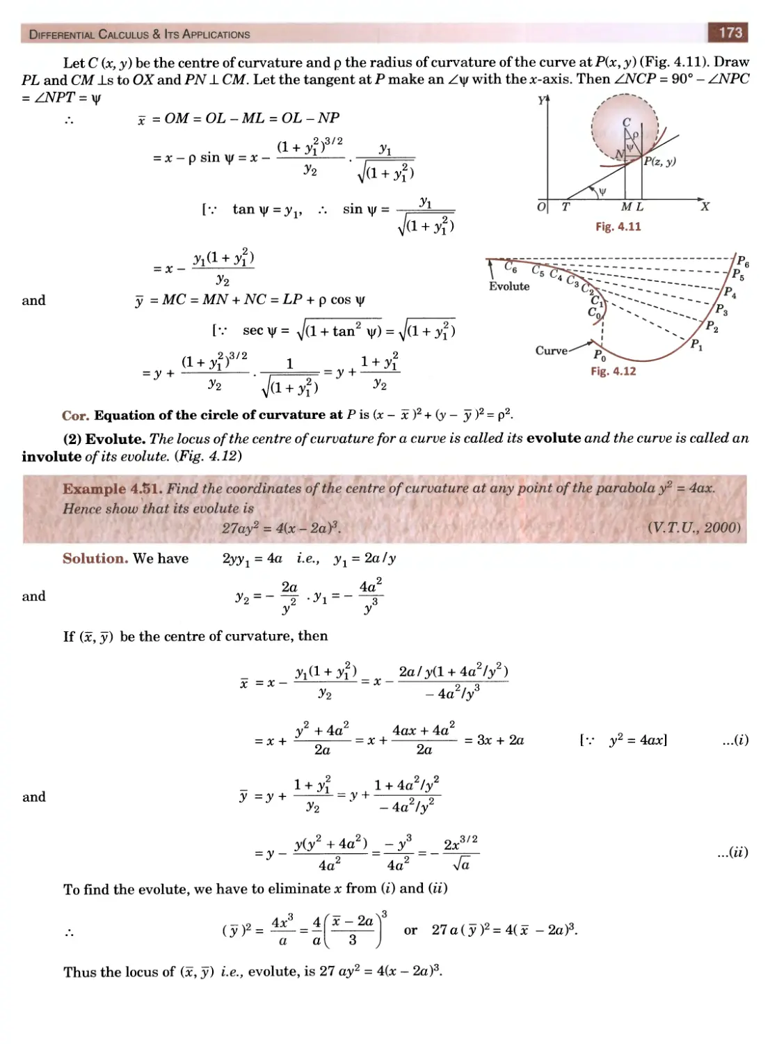
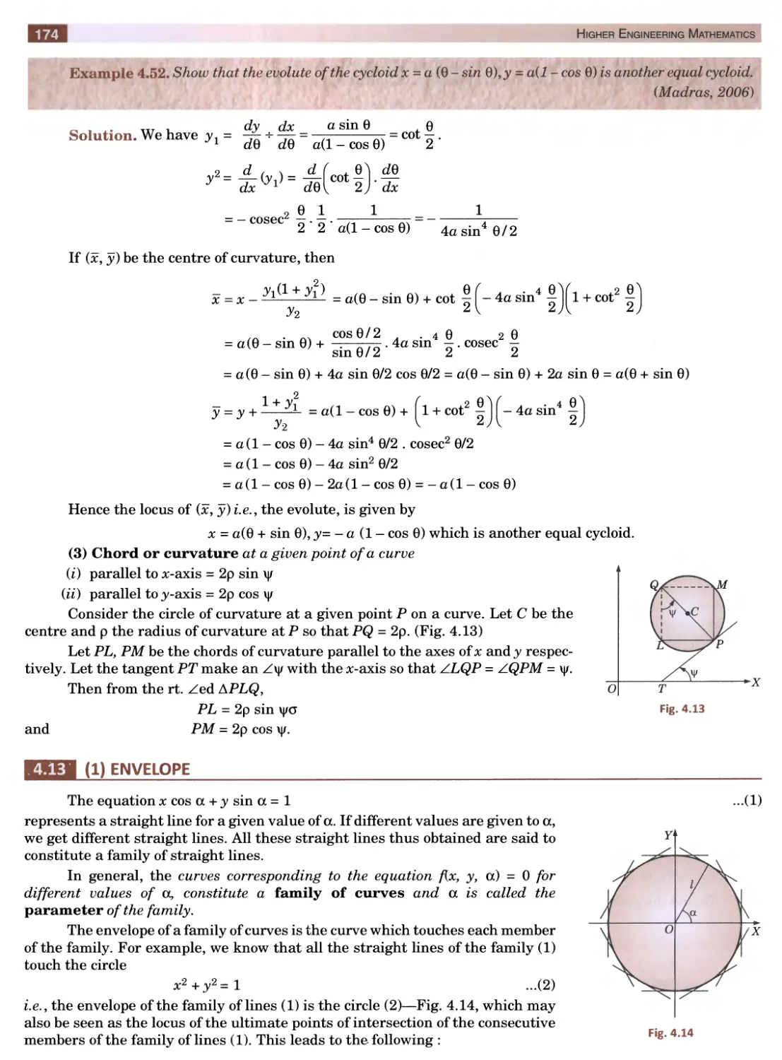
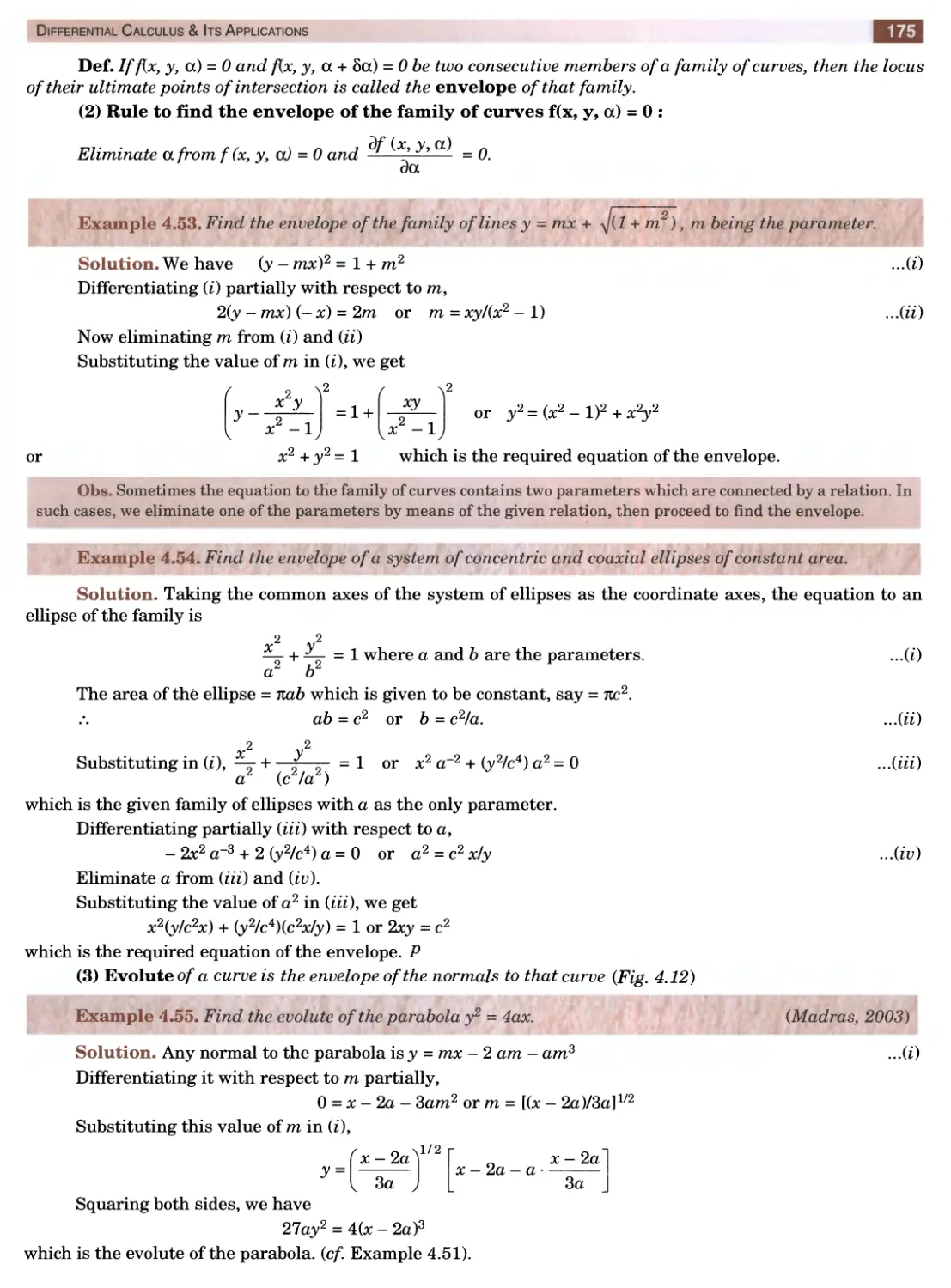

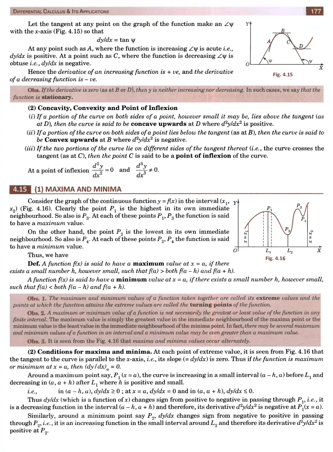


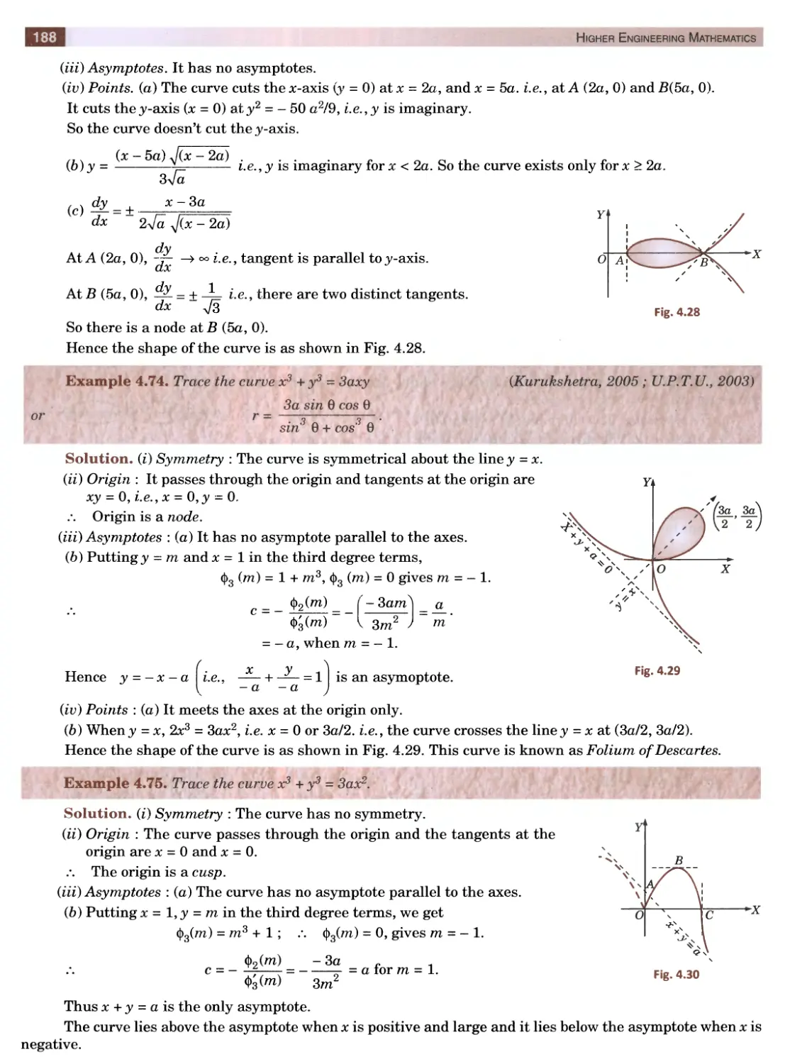
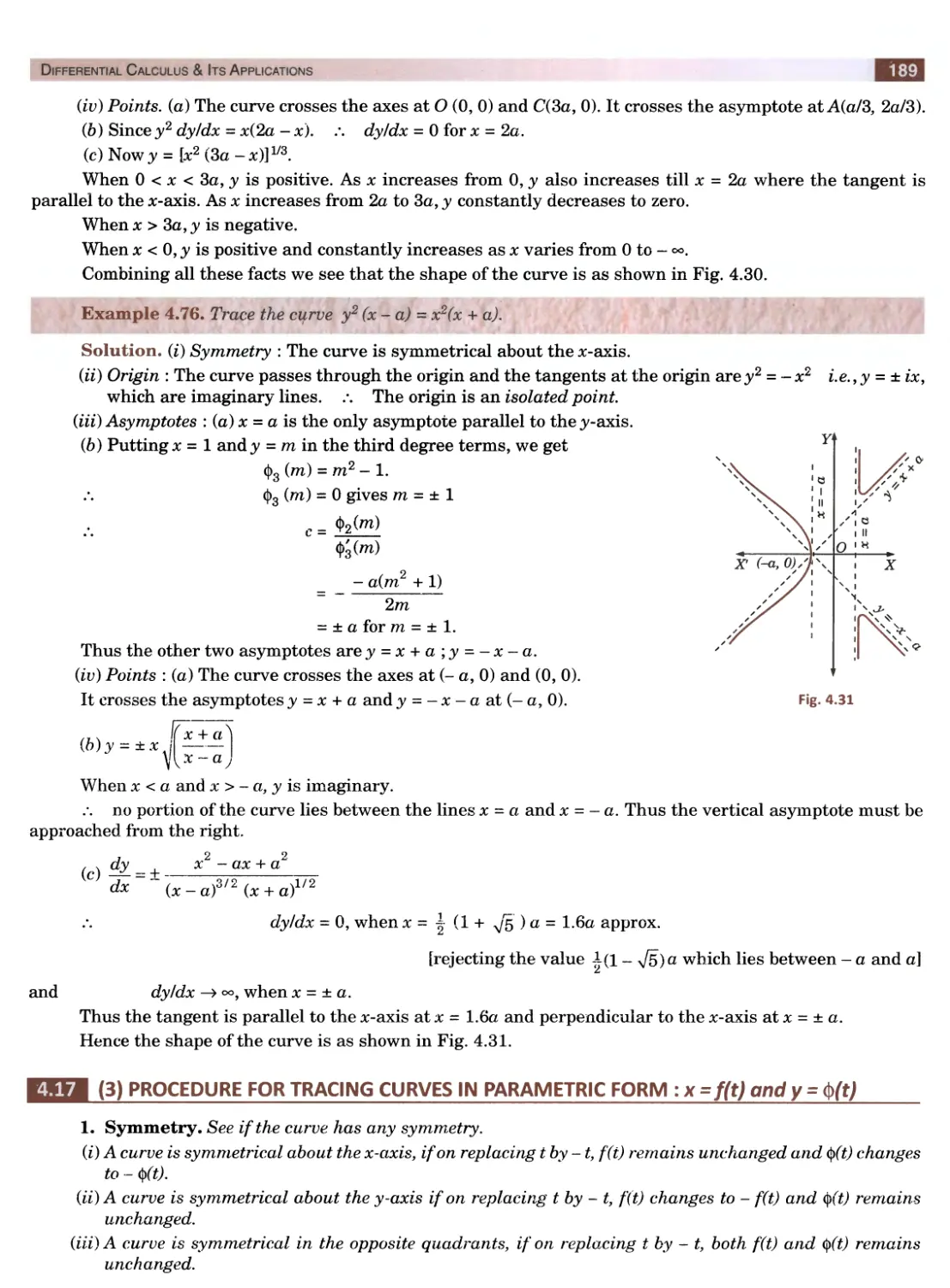

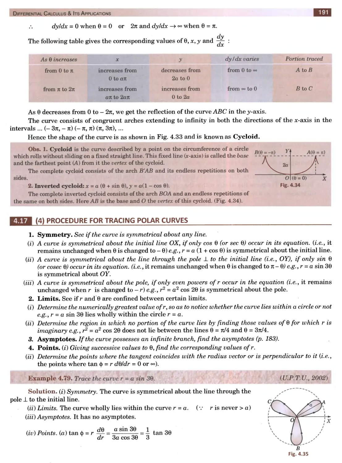
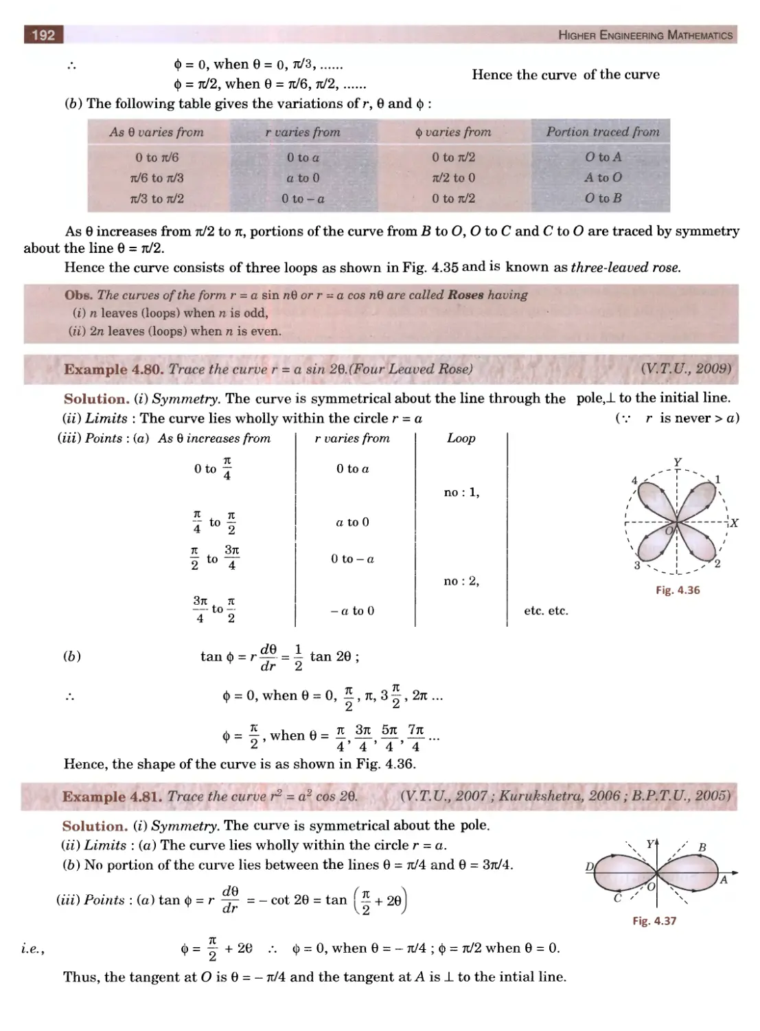


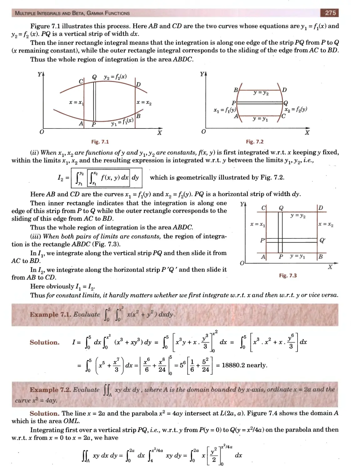


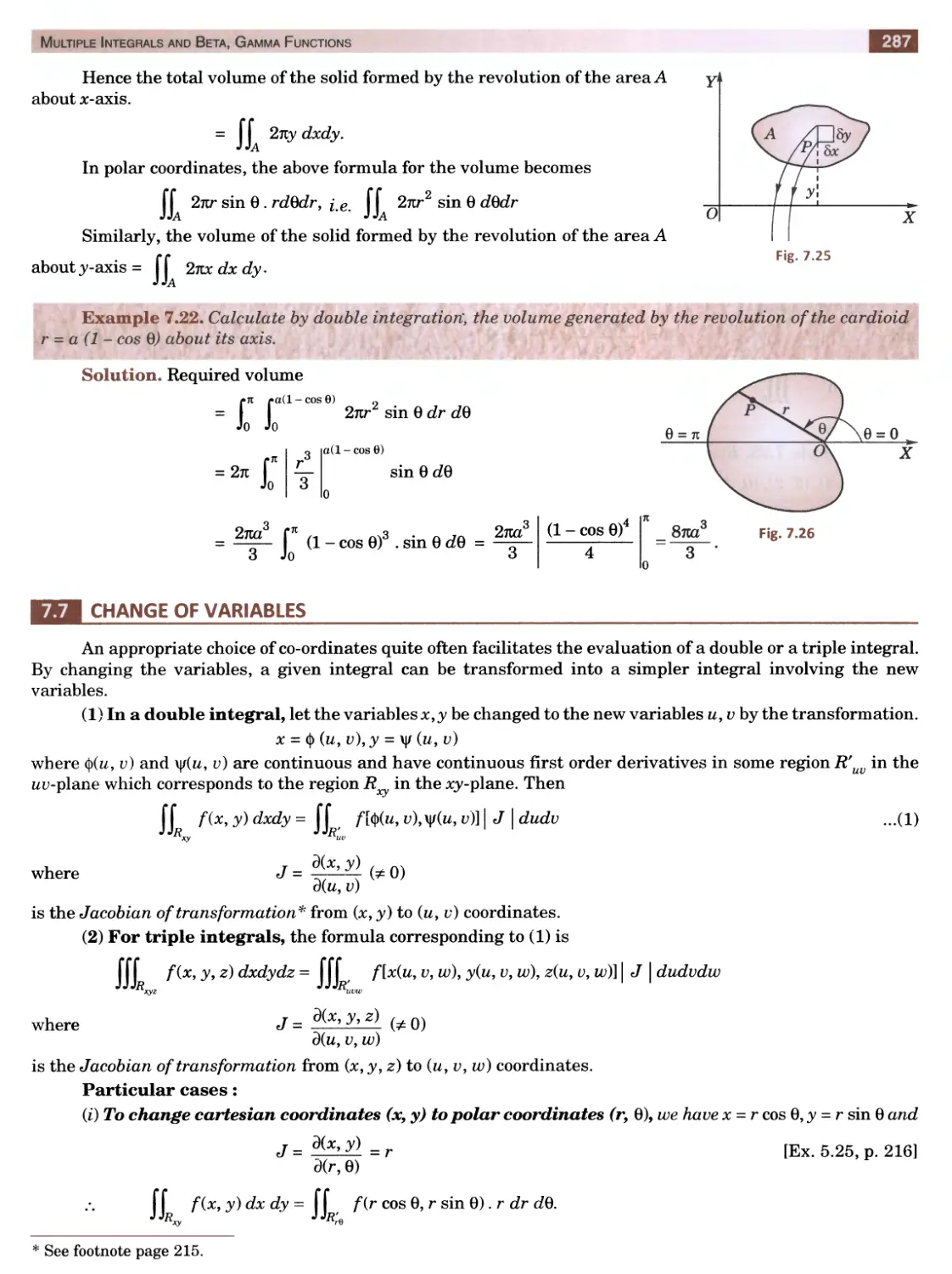


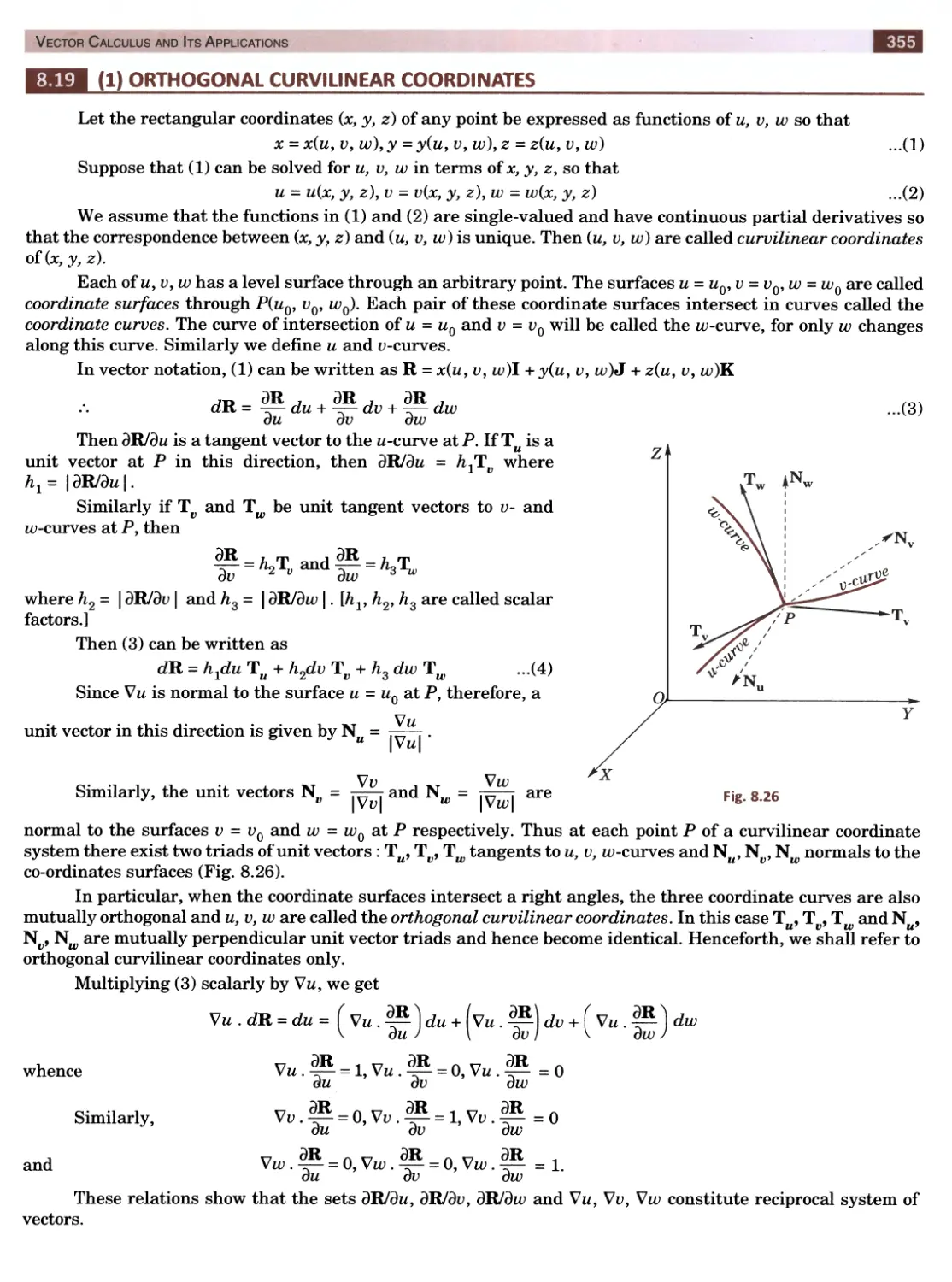
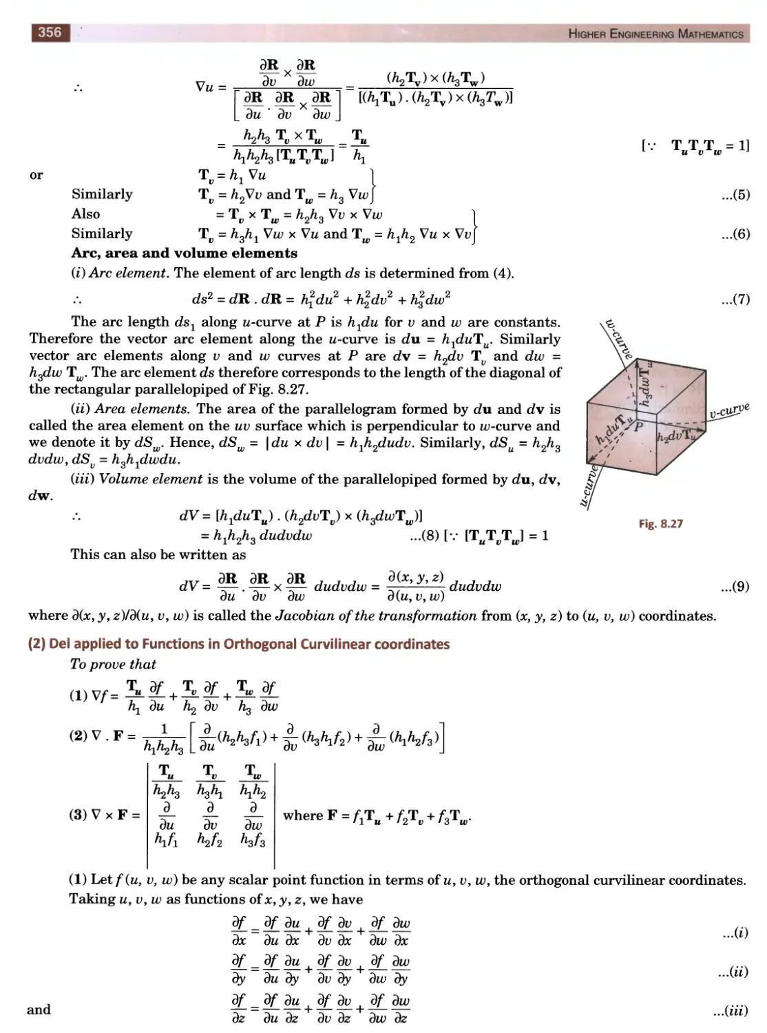

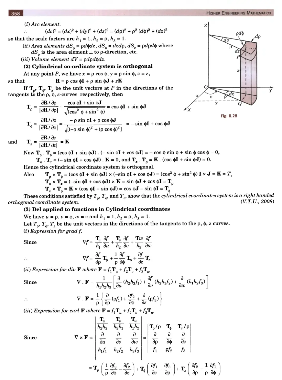
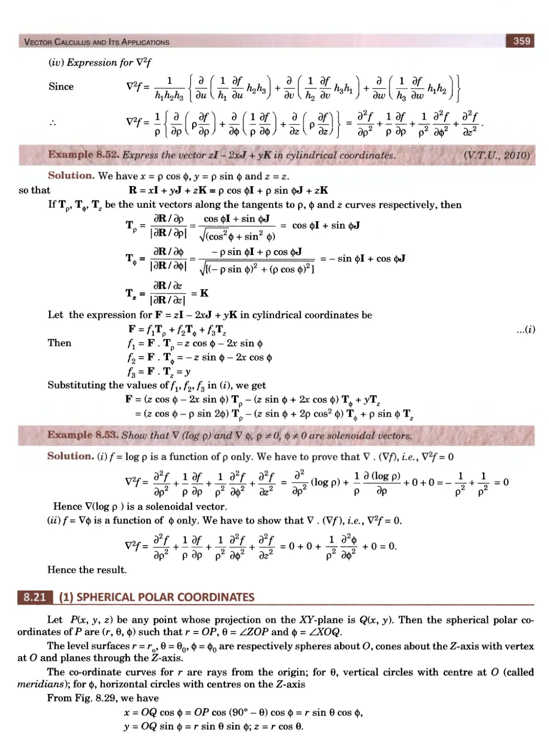


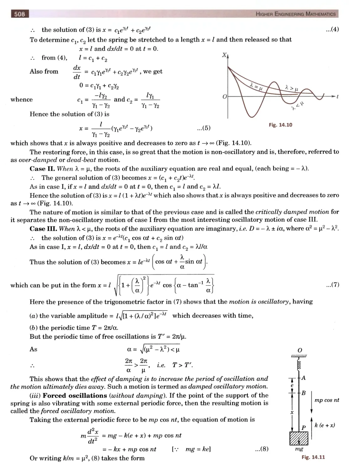


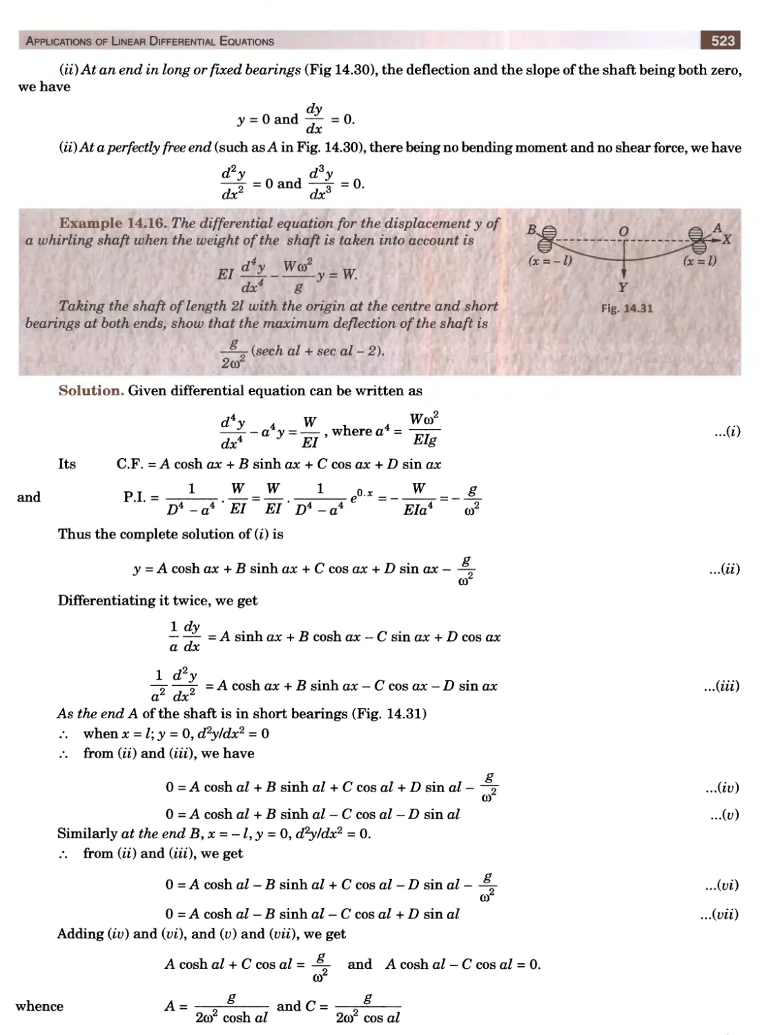


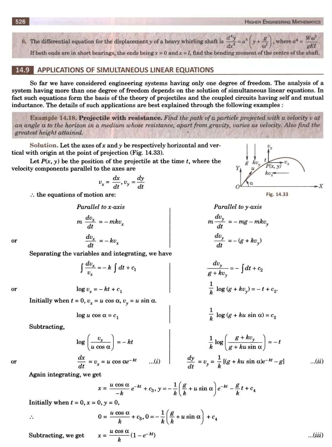
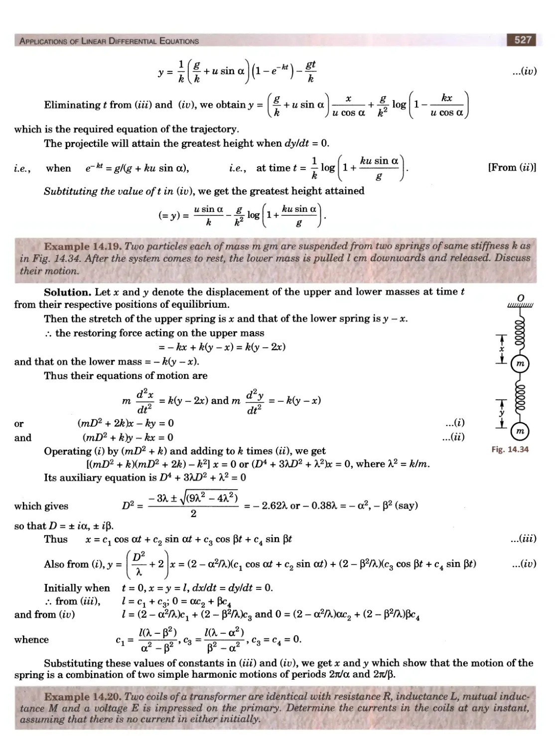
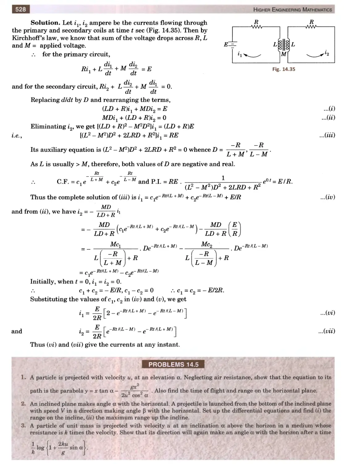


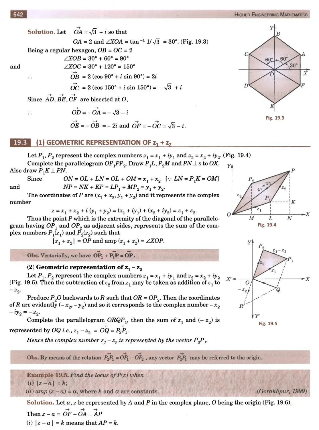


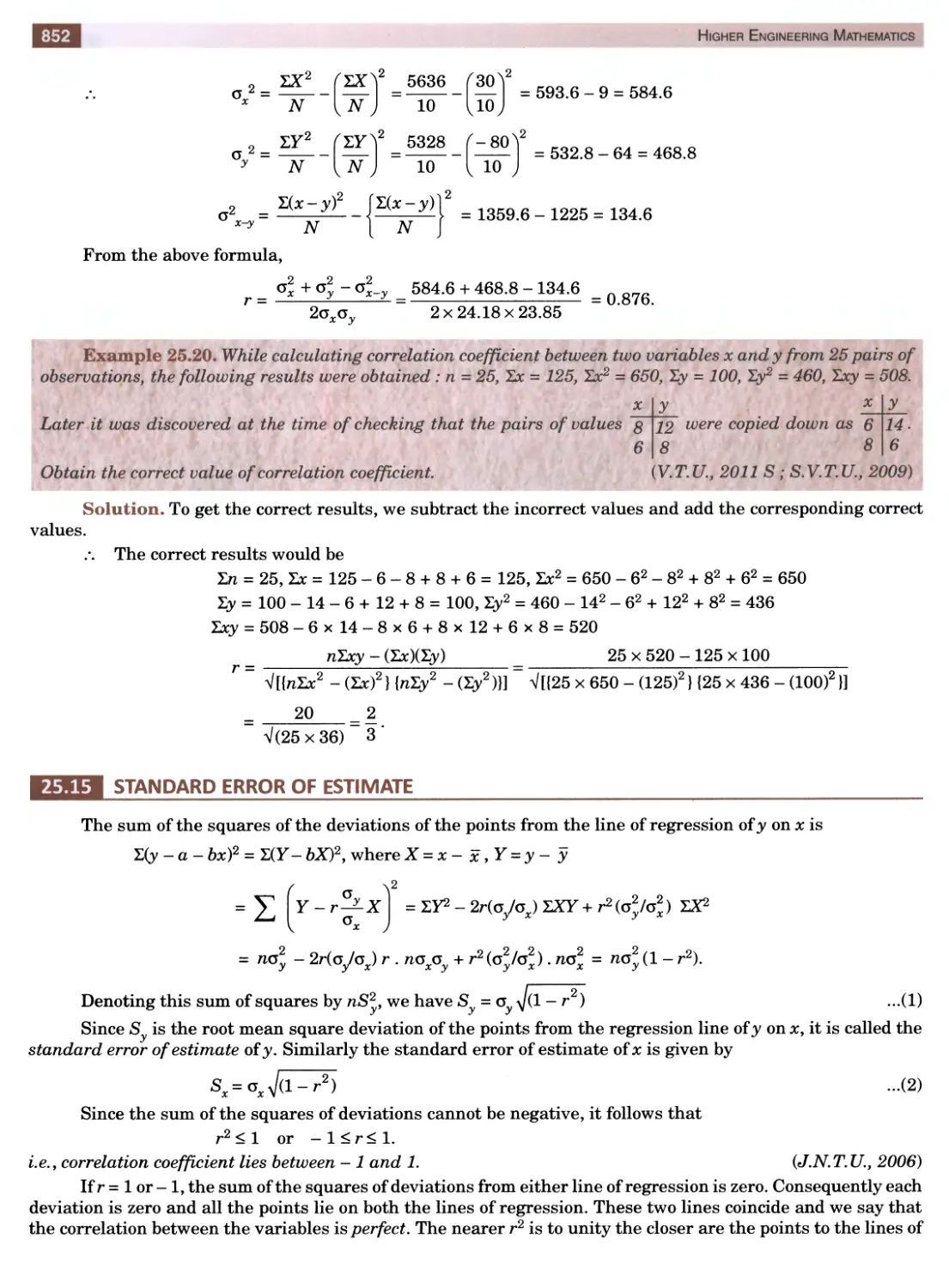
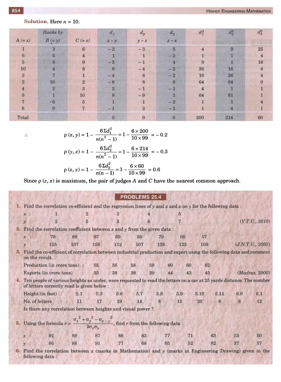


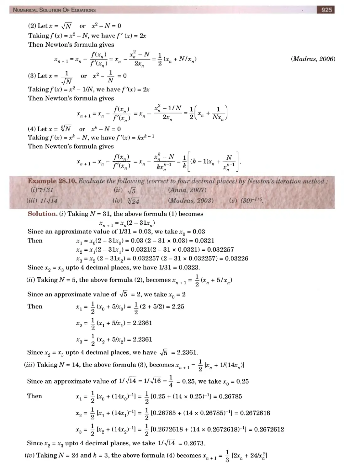


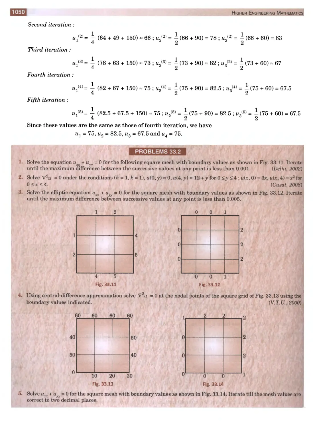
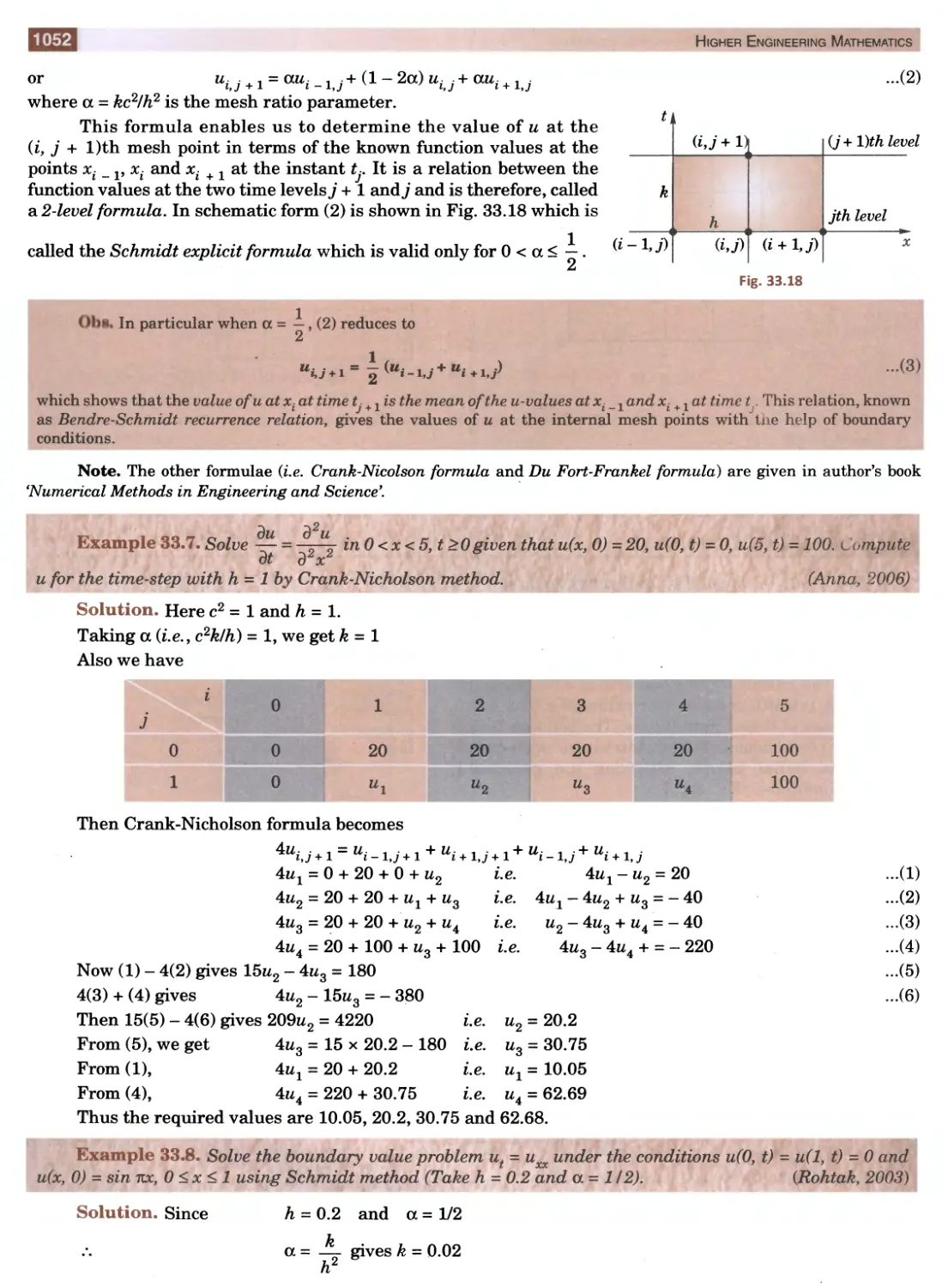


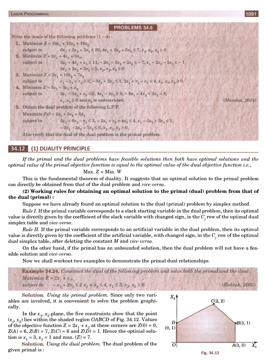

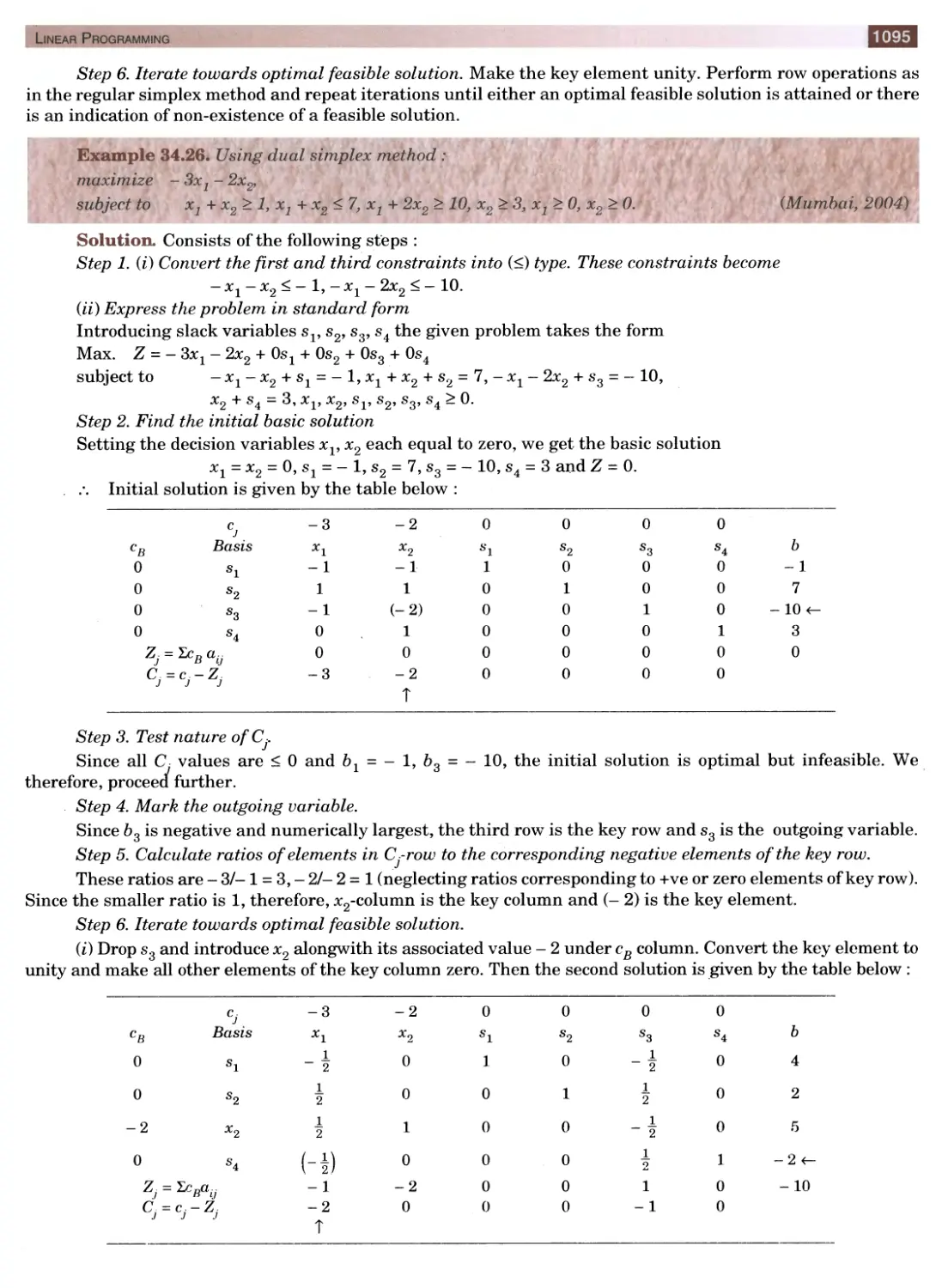
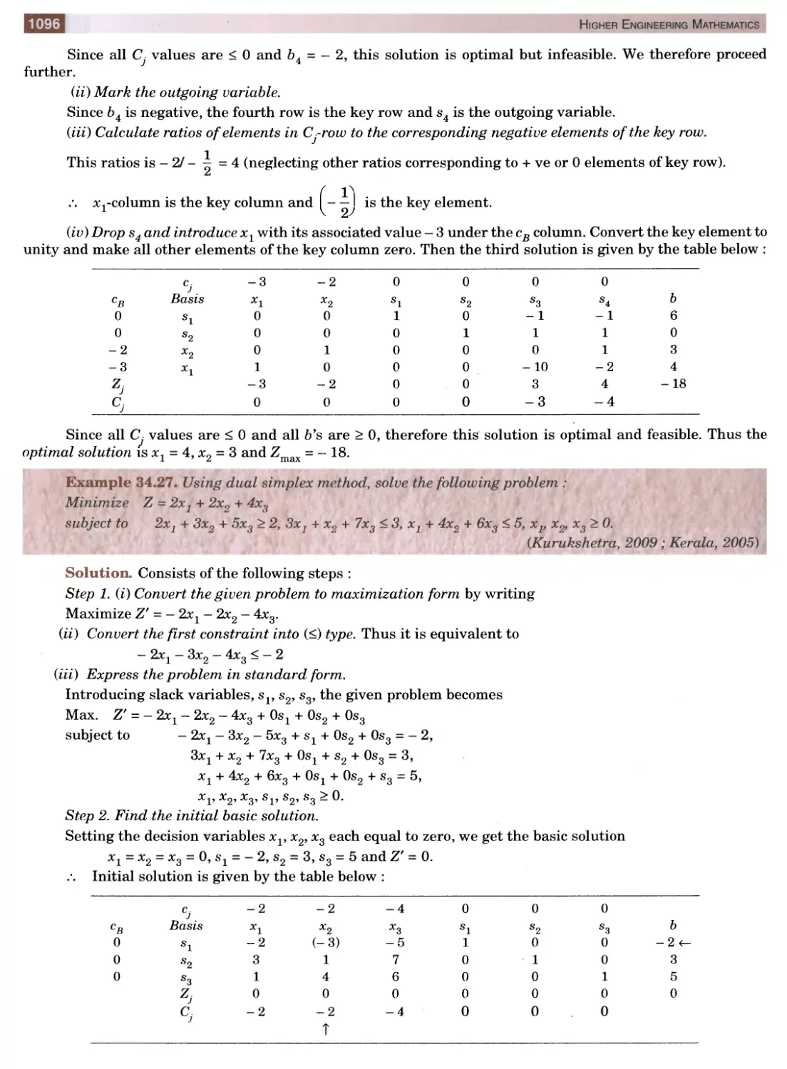
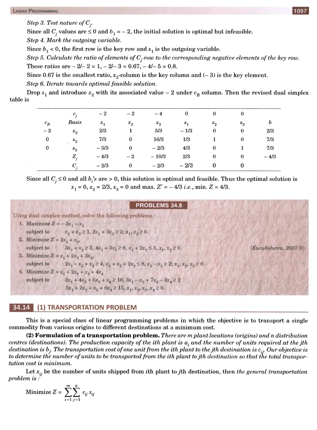
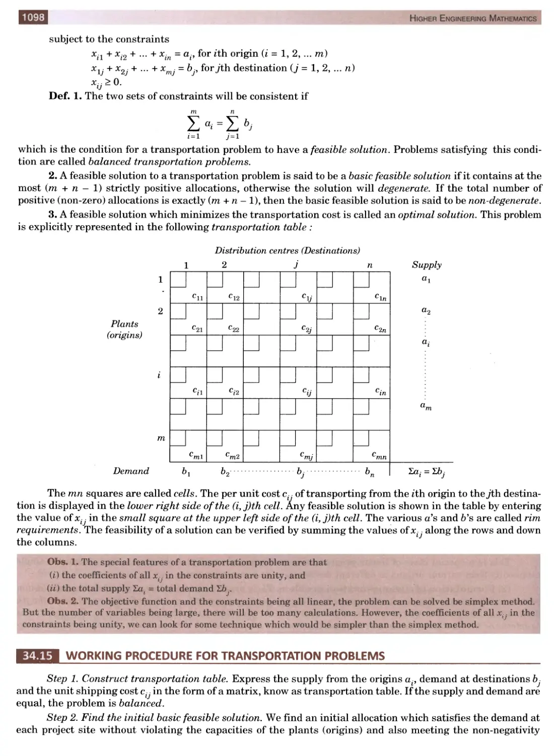


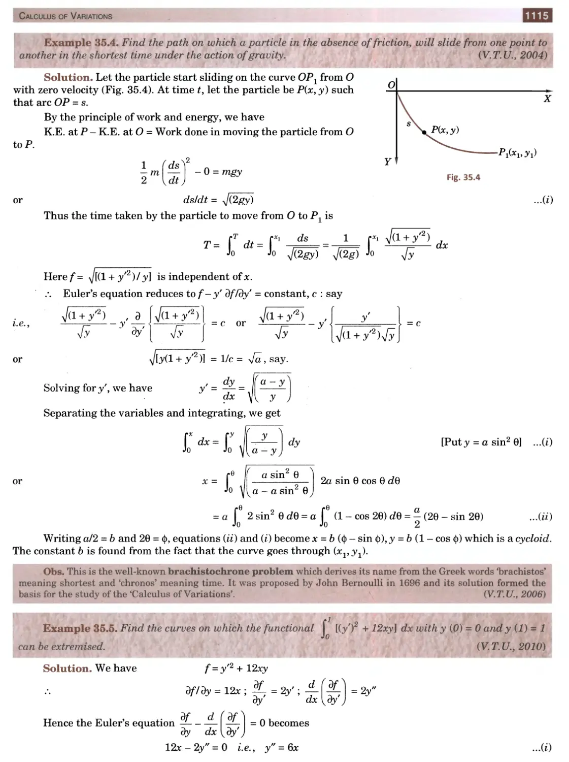
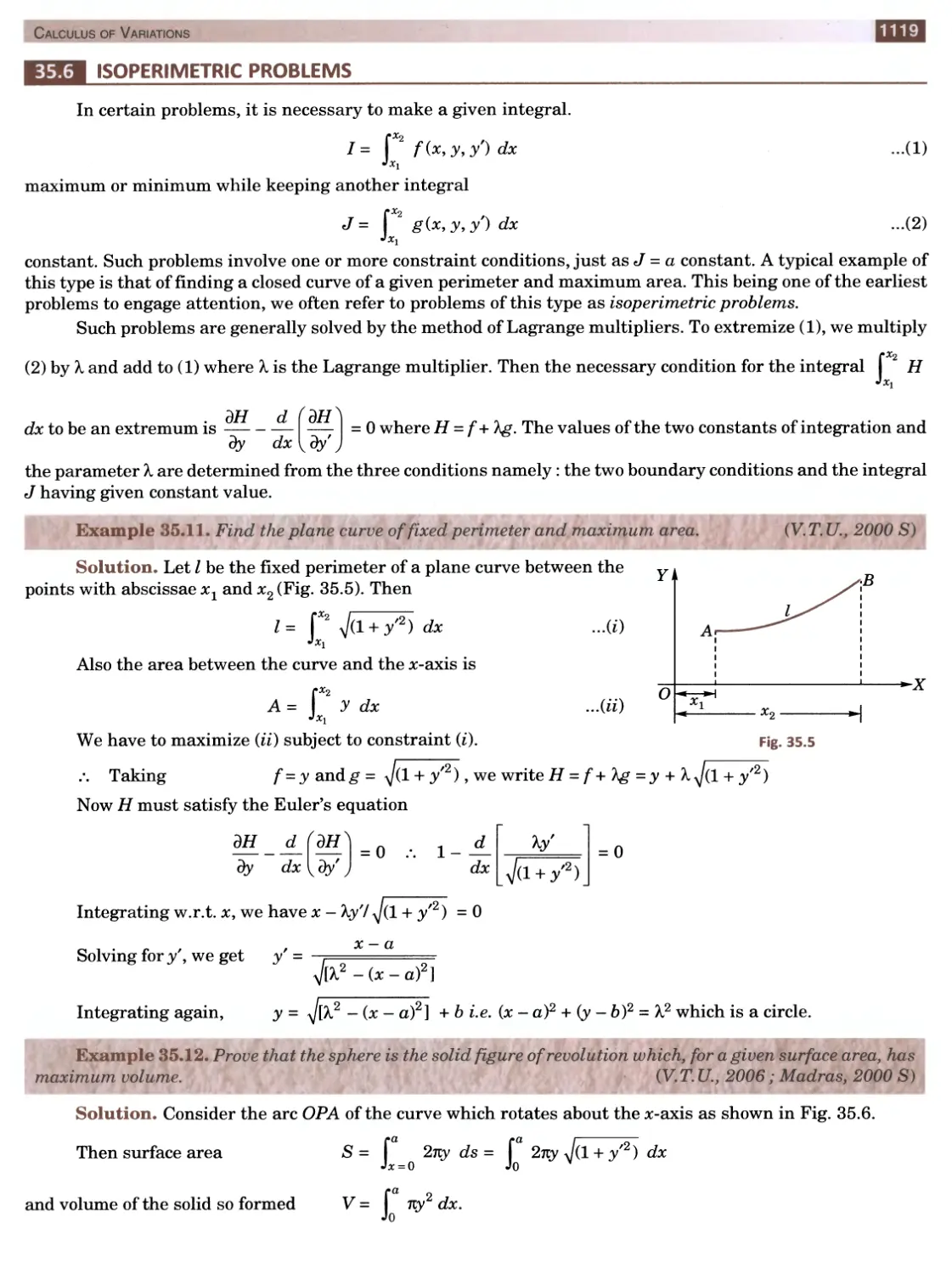
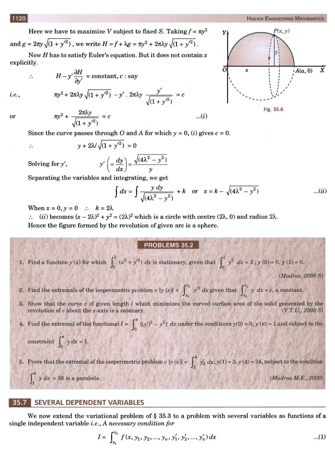


Текст
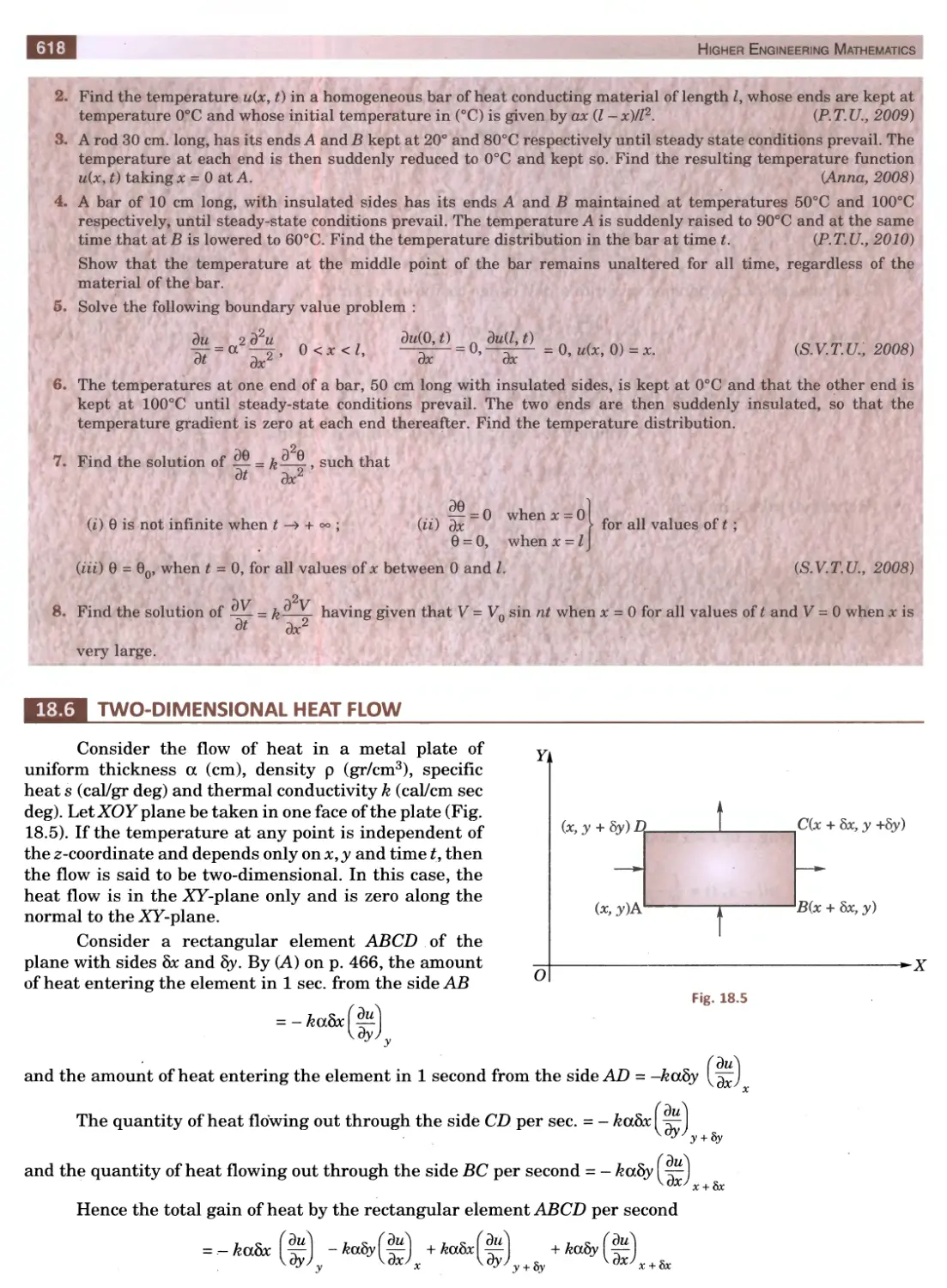
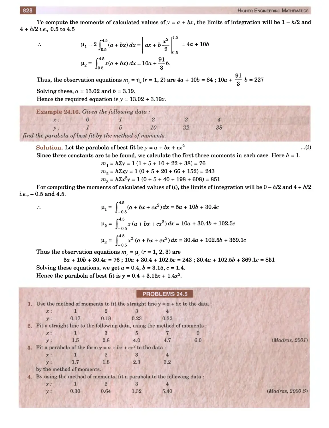
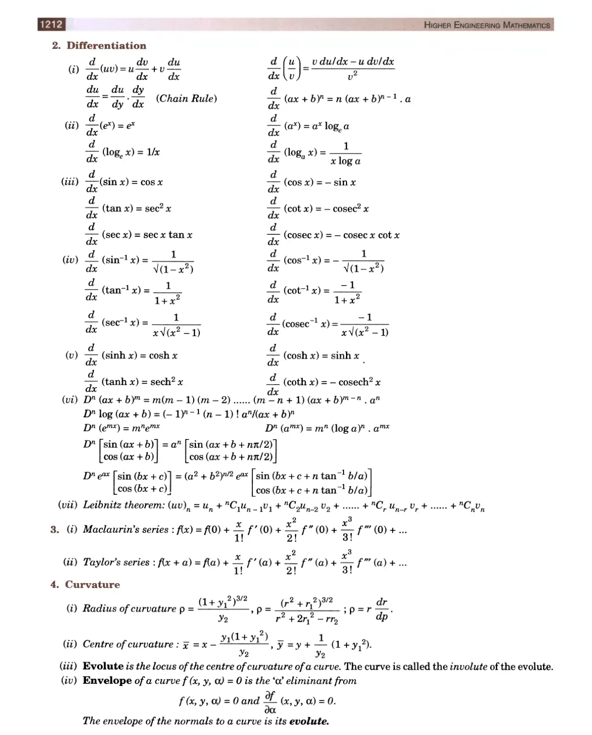
KHAN NA* PL) В LI S H E R S
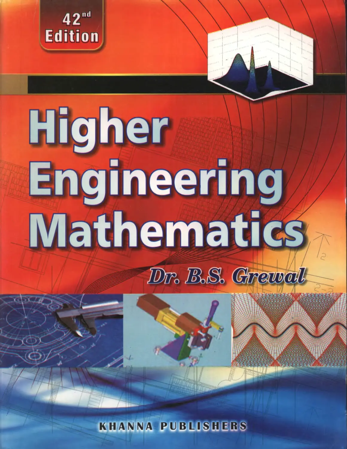
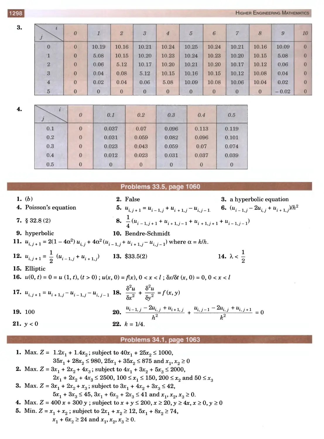
42nd Edition
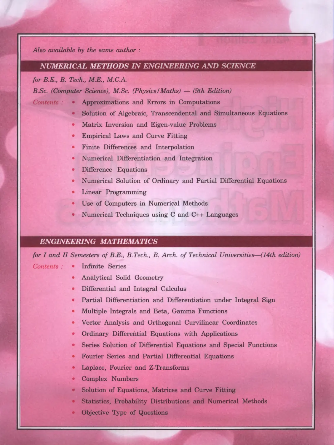
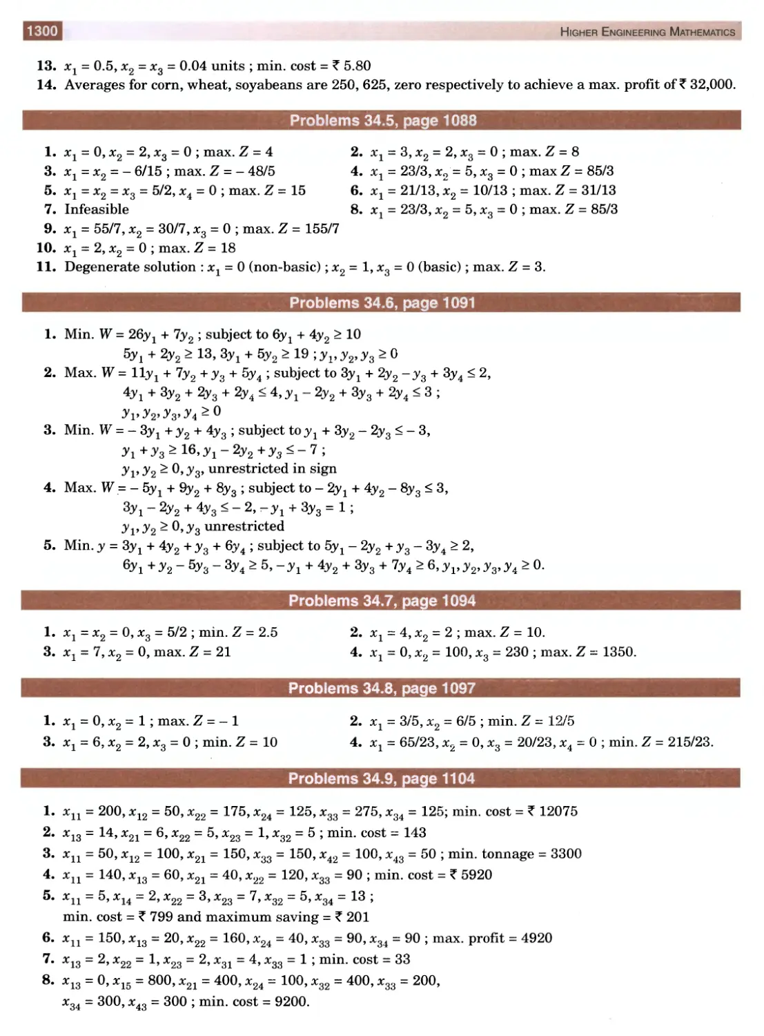
Also available by the same author :
NUMERICAL METHODS IN ENGINEERING AND SCIENCE
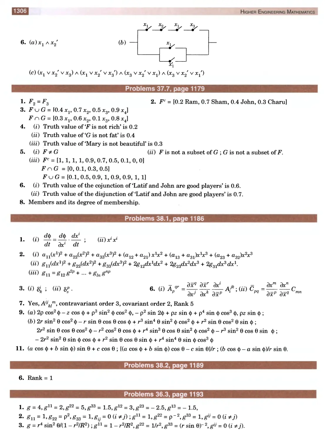
for B.E., B. Tech., M.E., M.C.A.
B.Sc. (Computer Science), M.Sc. (Physics I Maths) — (9th Edition)
Contents : • Approximations and Errors in Computations
• Solution of Algebraic, Transcendental and Simultaneous Equations
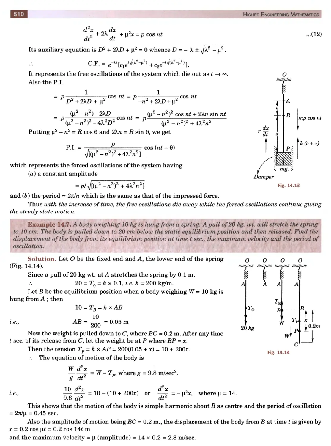
• Matrix Inversion and Eigen-value Problems
• Empirical Laws and Curve Fitting
• Finite Differences and Interpolation
• Numerical Differentiation and Integration
• Difference Equations
• Numerical Solution of Ordinary and Partial Differential Equations
• Linear Programming
• Use of Computers in Numerical Methods
• Numerical Techniques using C and C++ Languages
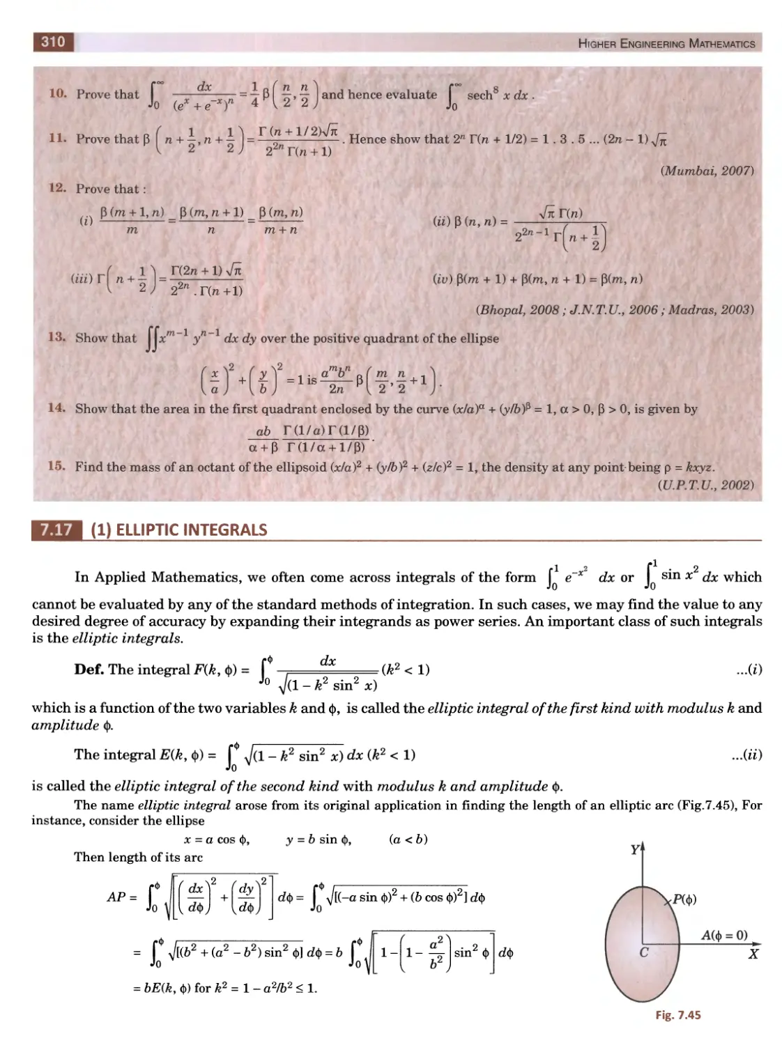
ENGINEERING MATHEMATICS
for I and II Semesters of B.E., B.Tech., B. Arch, of Technical Universities—(14th edition)
Contents : • Infinite Series
• Analytical Solid Geometry
• Differential and Integral Calculus
• Partial Differentiation and Differentiation under Integral Sign
• Multiple Integrals and Beta, Gamma Functions
• Vector Analysis and Orthogonal Curvilinear Coordinates
• Ordinary Differential Equations with Applications
• Series Solution of Differential Equations and Special Functions
• Fourier Series and Partial Differential Equations
• Laplace, Fourier and Z-Transforms
• Complex Numbers
• Solution of Equations, Matrices and Curve Fitting
• Statistics, Probability Distributions and Numerical Methods
• Objective Type of Questions
B.S. GREWAL, Ph.D.
Professor of Applied Mathematics
Principal Scientific Officer (Ex.)
Defence Research & Development Organisation,
New Delhi
Formerly of
College of Military Engineering, Poona,
Delhi College of Engineering, Delhi
J.S. GREWAL, M.I.E., I. Engr. (U.K.), Ml. Mar. Engg.
4575/15, Onkar House, Opp. Happy School
Daryaganj, New Delhi-110002
Phone 011-2324 30 42,9811541460; 011-2324 30 43
e-mail: khannapublishers@yahoo.in
Website : www.khannapublishers.in
Published by :
R.C. Khanna
&
Vineet Khanna
for KHANNA PUBLISHERS
Nai Sarak, Delhi-110006 (India).
All Rights Reserved
[This book or part thereof cannot be translated or reproduced in any form (except for review or criticism)
without the written permission of the Author and the Publishers.]
ISBN No.: 978-81-7409-195-5
Forty Second Edition: 2012, June
? 450.00
Types( tied at: Goswami Printers, Delhi.
inted at: Print India, Dilshad Garden, Delhi.
w₪₪₪₪₪₪₪₪a₪₪₪₪₪₪₪₪₪₪₪^₪tm₪₪₪₪m₪m₪₪₪₪m₪₪₪₪₪₪₪mmm₪m₪a₪₪m₪₪₪₪₪mm₪m
Preface to the 42nd Edition
The book has now been recast in an attractive new format, retaining its main features which have made it
so popular. The text has been carefully revised, the number of illustrative examples has been increased and
problems from the latest university question papers have been added. The ‘Objective Type of Questions’ have
been updated and given at the end of each chapter. It is hoped that the book in its new form will enjoy its ever
increasing popularity.
The author takes this opportunity to thank the numerous readers in India and abroad for their letters of
appreciation and fellow professors for their suggestions and patronage of the book. In particular, he is grateful to
Prof. Jeevargi Phakirappa, V.N. Engg. College, Bellary (Kar.); Prof. P. Annapurna, N.B.K.R. Inst, of Technology,
Vidyanagar (A.P.); Dr. A.P. Bumwal, R.I.T., Koderma (Jh. Kh.); Prof. M. Vasudeva Reddy, Vaishnavi Inst, of
Technology, Tarapalli (Tirupati); Dr. K.P. Ghadle, B.A.M. University, Aurangabad (Mah.); Prof. B.K. Yadav,
Chauksey Engg. College, Bilaspur (C.G.); Prof. D. Ravi Kumar, Vignan University, Guntur (A.P.); Dr. J.C.
Prajapati, Charotara University of Sc. & Technology, Changa (Guj.); Prof. Ramesh Chandra, S.R. Technology
Institute, Nalgonda (A.P.); Dr. Latika Bhandari, R.V.S. College of Engg. & Technology, Bhillai; Prof. R.
Saraswathi, Sri Padmavati Engg. College, Kavalli (A.P.) and Prof. Vikas Goyal, J.M. Inst, of Technology, Radur
(Haiyana).
Suggestions for improvement of the text and intimation of misprints will be thankfully acknowledged.
B.S. GREWAL
New Delhi
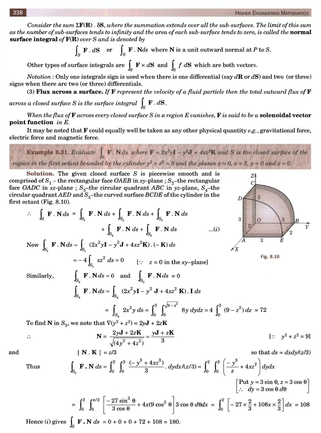
Contents
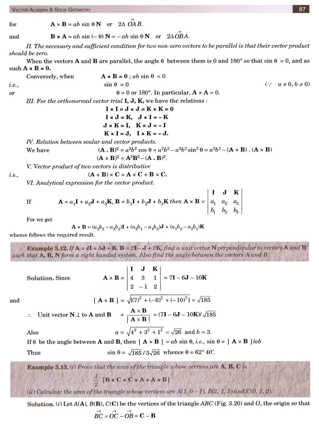
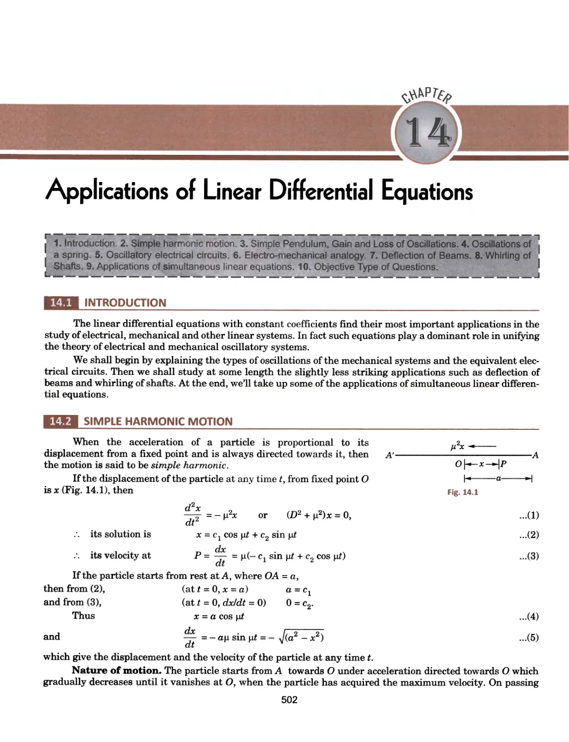
Unit 1 : ALGEBRA, VECTORS AND GEOMETRY
1.
Solution of Equations
1
2.
Linear Algebra : Determinants, Matrices
17
3.
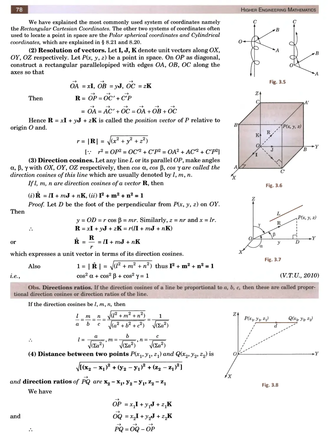
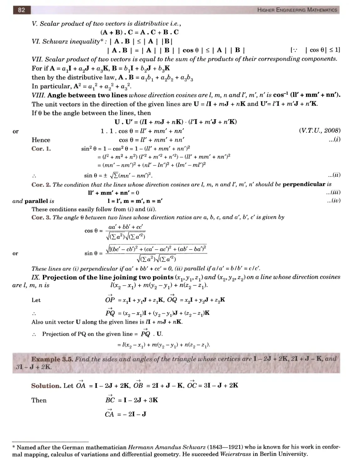
Vector Algebra and Solid Geometry
76
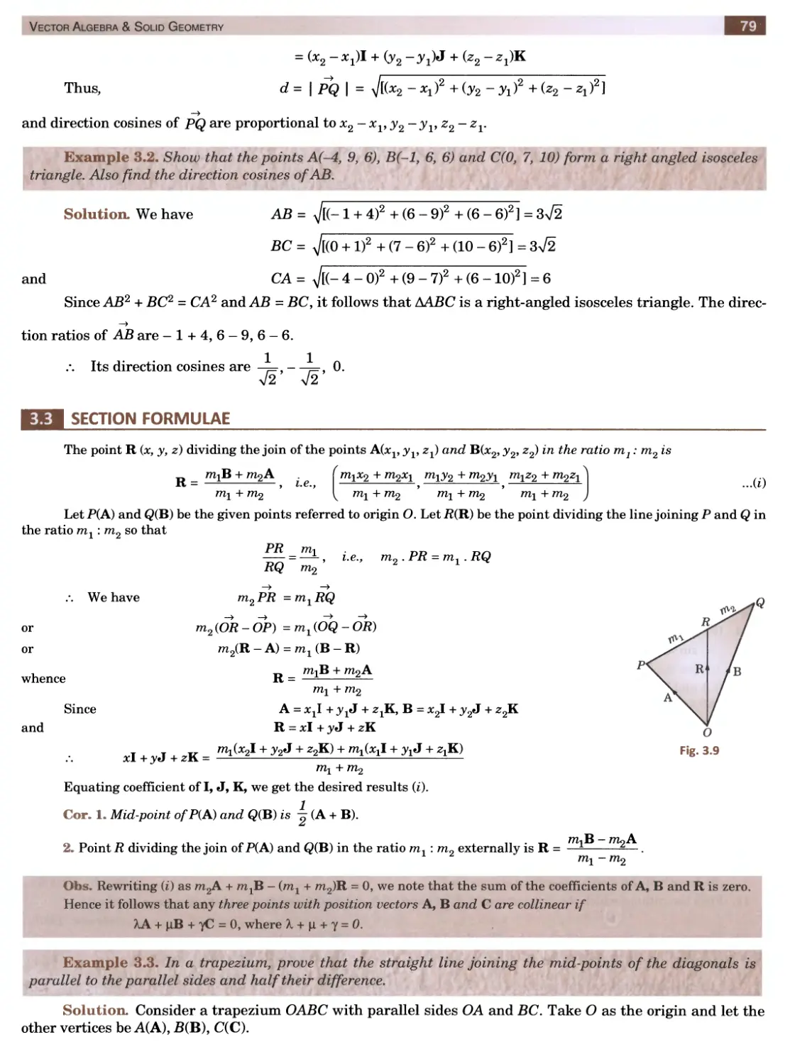
Unit II: CALCULUS
4.
Differential Calculus & Its Applications
134
5.
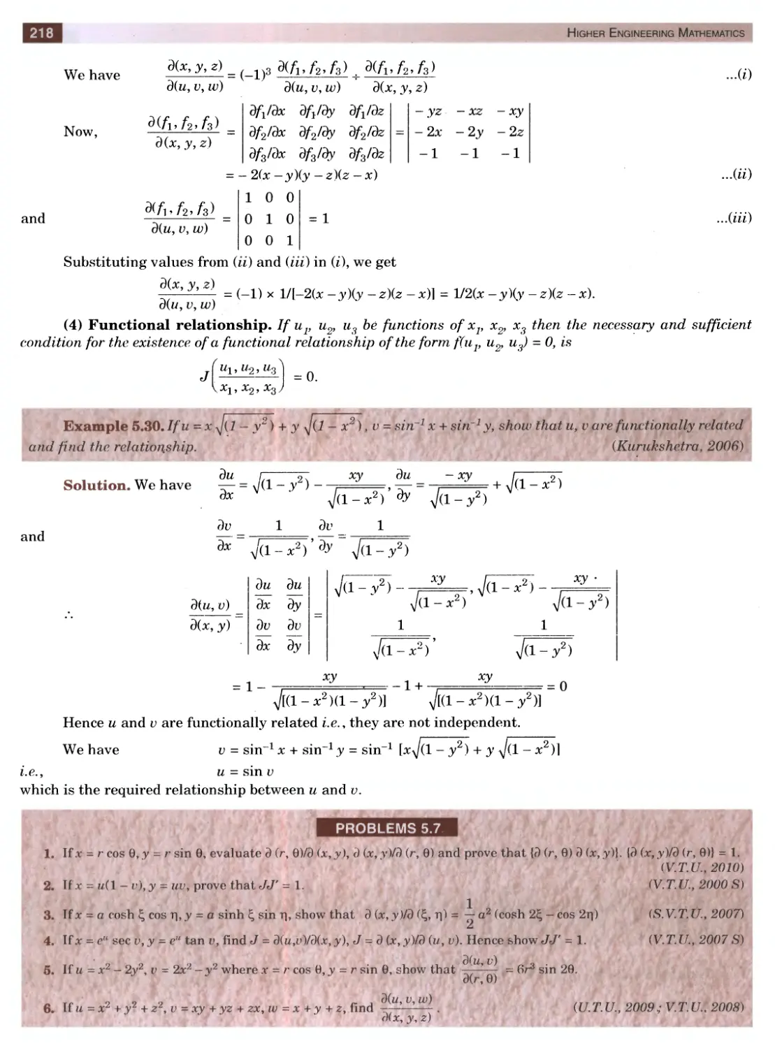
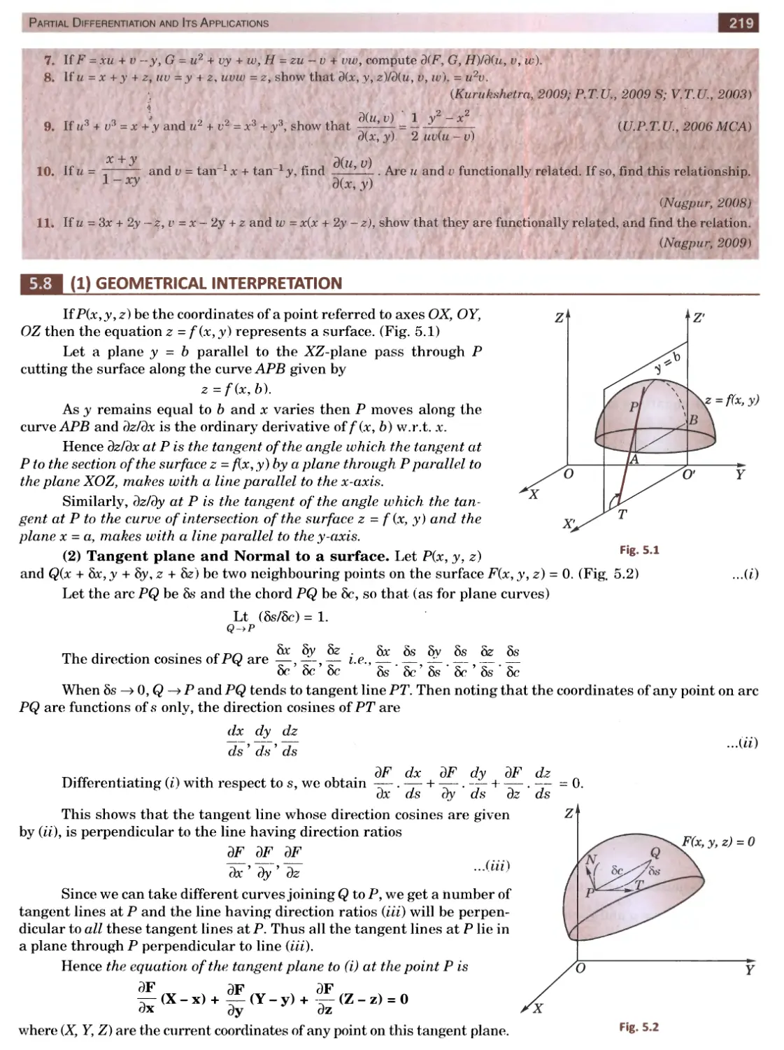
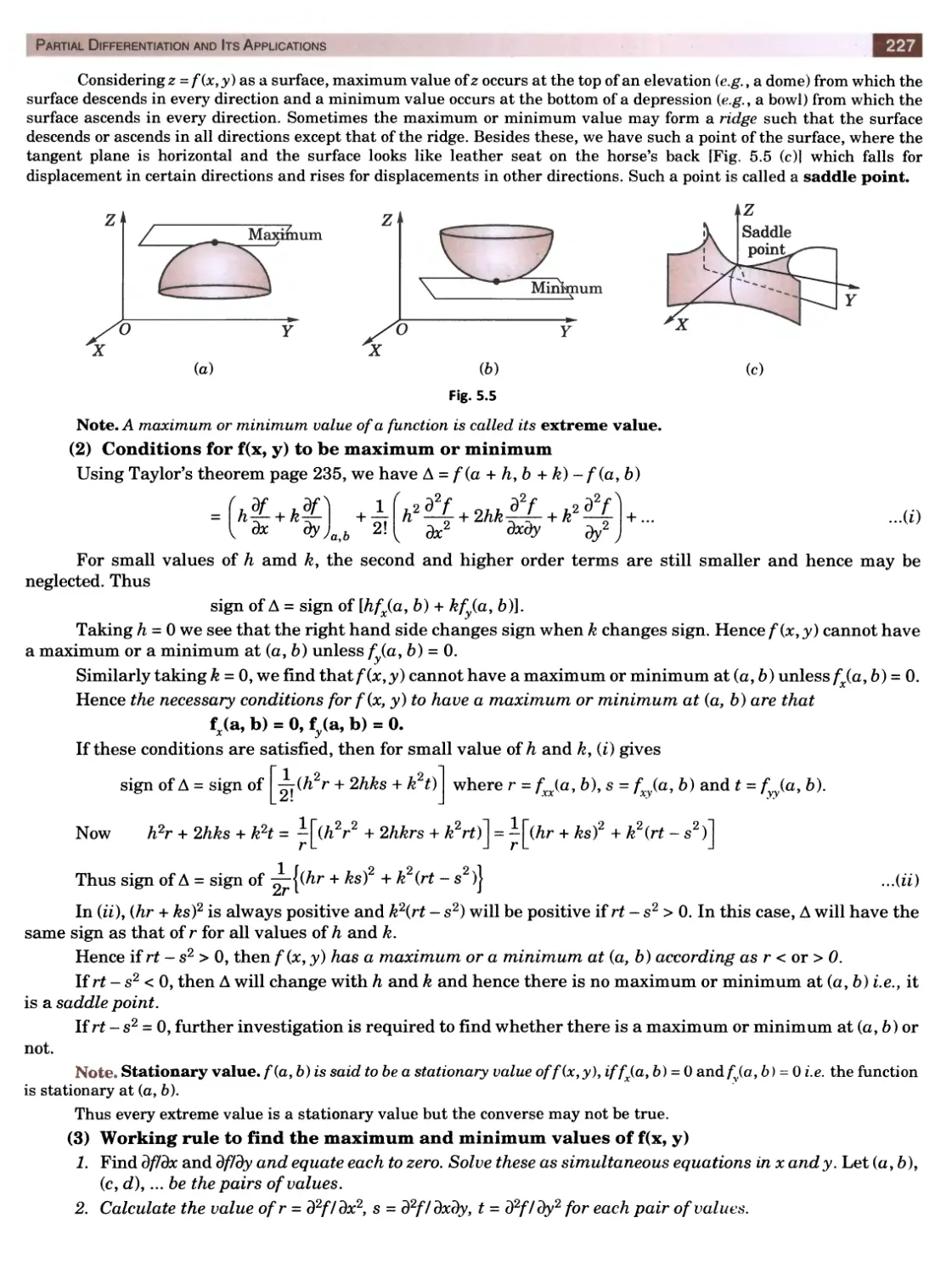
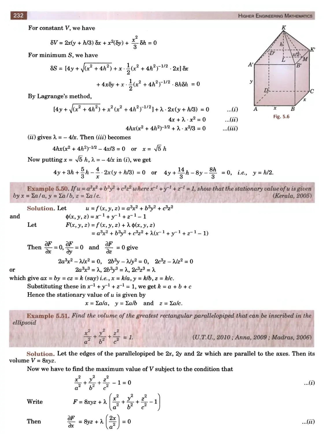
Partial Differentiation & Its Applications
197
6.
Integral Calculus & Its Applications
239
7.
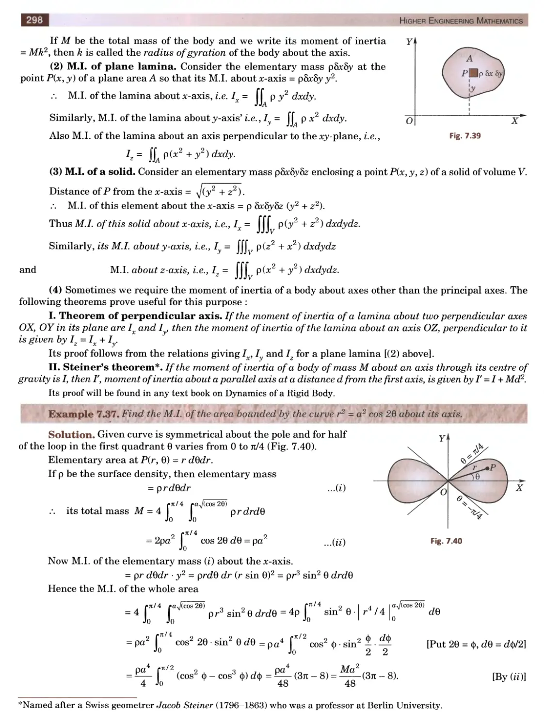
Multiple Integrals & Beta, Gamma Functions
274
&
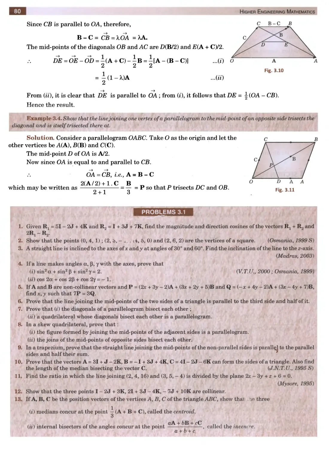
Vector Calculus & Its Applications
315
Unit III : SERIES
9.
Infinite Series
365
10.
Fourier Series & Harmonic Analysis
395
Unit IV : DIFFERENTIAL EQUATIONS
11.
Differential Equations of First Order
426
12.
Applications of Differential Equations of First Order
452
13.
Linear Differential Equations
471
14.
Applications of Linear Differential Equations
502
15.
Differential Equations of Other Types
531
16.
Series Solution of Differential Equations and Special Functions
542
17.
Partial Differential Equations
577
18.
Applications of Partial Differential Equations
600
(ix)
| Chap.
Page j
Unit V : COMPLEX ANALYSIS
19.
Complex Numbers and Functions
639
20.
Calculus of Complex Functions
672
1 Unit VI : TRANSFORMS 1
21.
Laplace Transforms
726
22.
Fourier Transforms
766
23.
Z-Transforms
793
Unit Vil : NUMERICAL TECHNIQUES 1
24.
Empirical Laws and Curve-fitting
812
25.
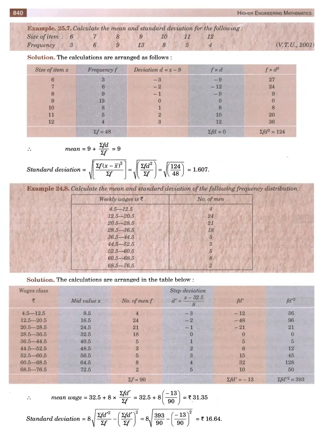
Statistical Methods
830
26.
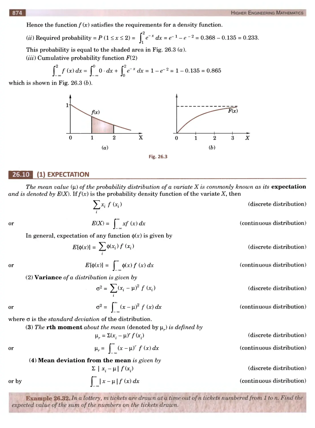
Probability and Distributions
857
27.
Sampling and Inference
897
2a
Numerical Solution of Equations
918
29.
Finite Differences and Interpolation
946
30.
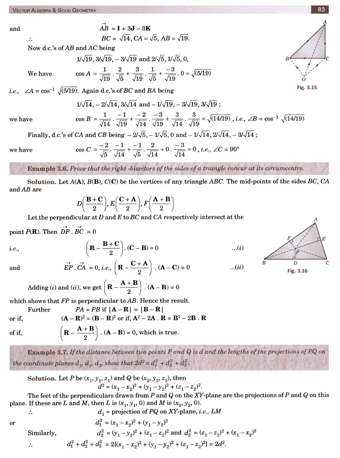
Numerical Differentiation and Integration
980
31.
Difference Equations
32.
Numerical Solution of Ordinary Differential Equations
1008
33.
Numerical Solution of Partial Differential Equations
1040
34.
Linear Programming
1061
Unit VIII : SPECIAL TOPICS 1
35.
Calculus ofVariations
1111
36.
Integral Equations
1131
37.
Discrete Mathematics
1149
38.
Tensor Analysis
1181
Appendix 1: Useful Information
1201
Appendix 2: Tables
1296
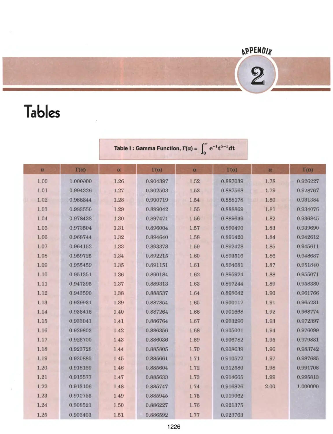
Table I: Gamma Functions
1226
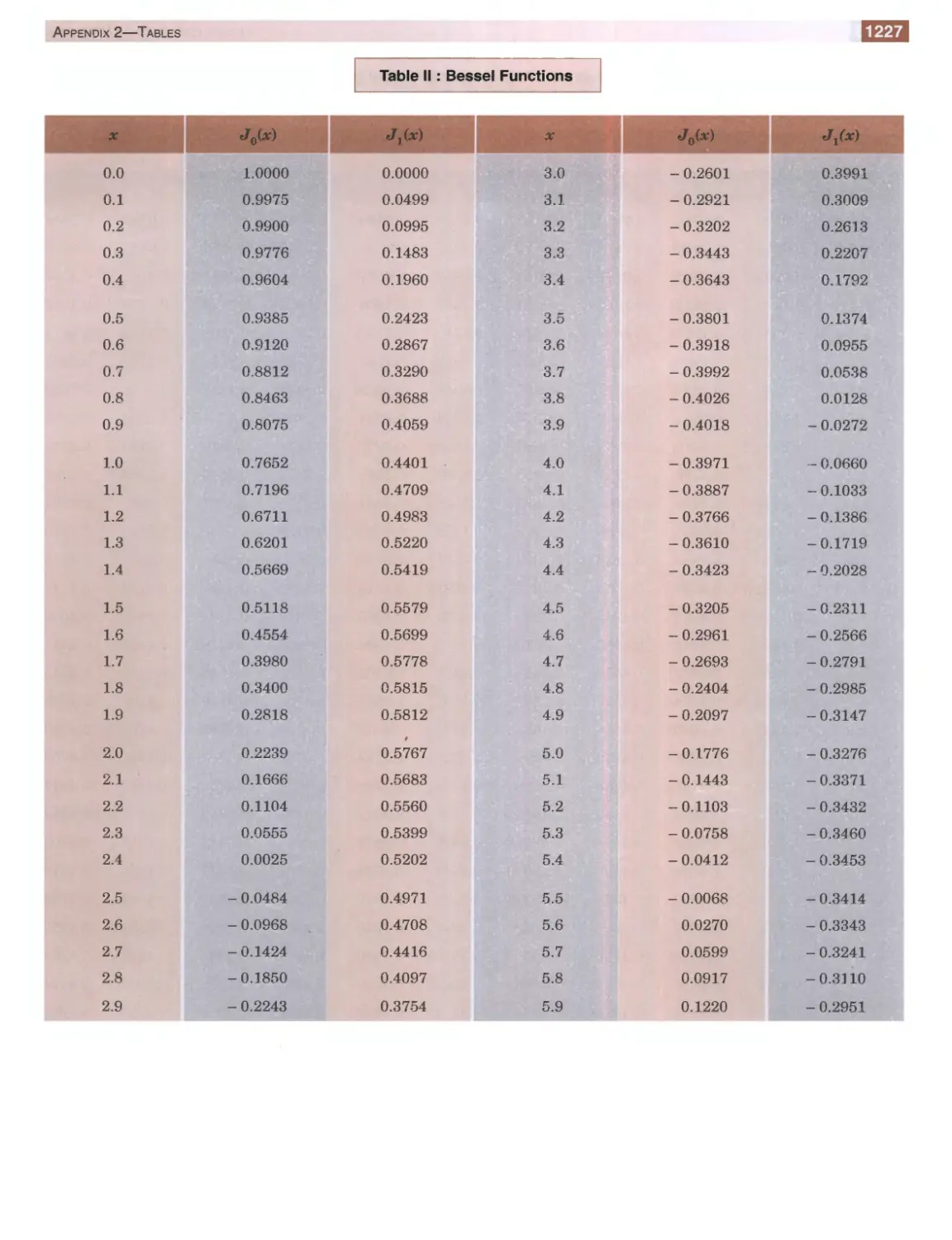
Table II: Bessel Functions
1227
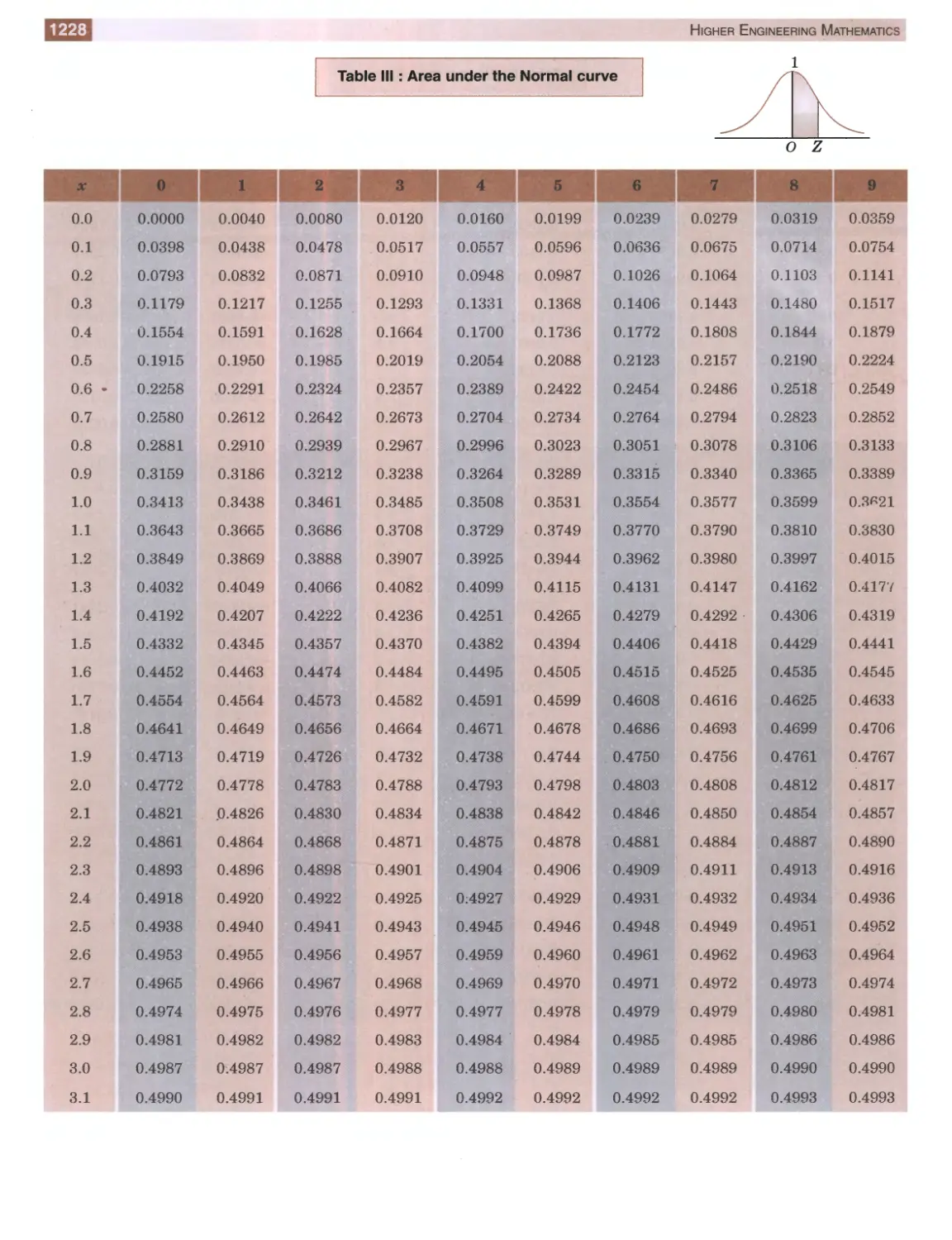
Table III: Area under the Normal curve
1228
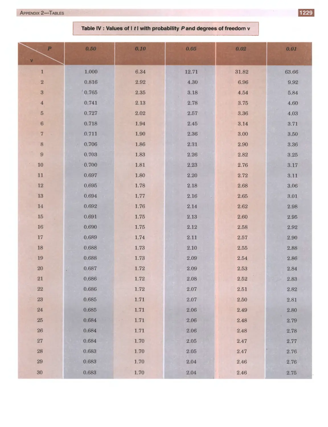
Table IV: Values of t
1229
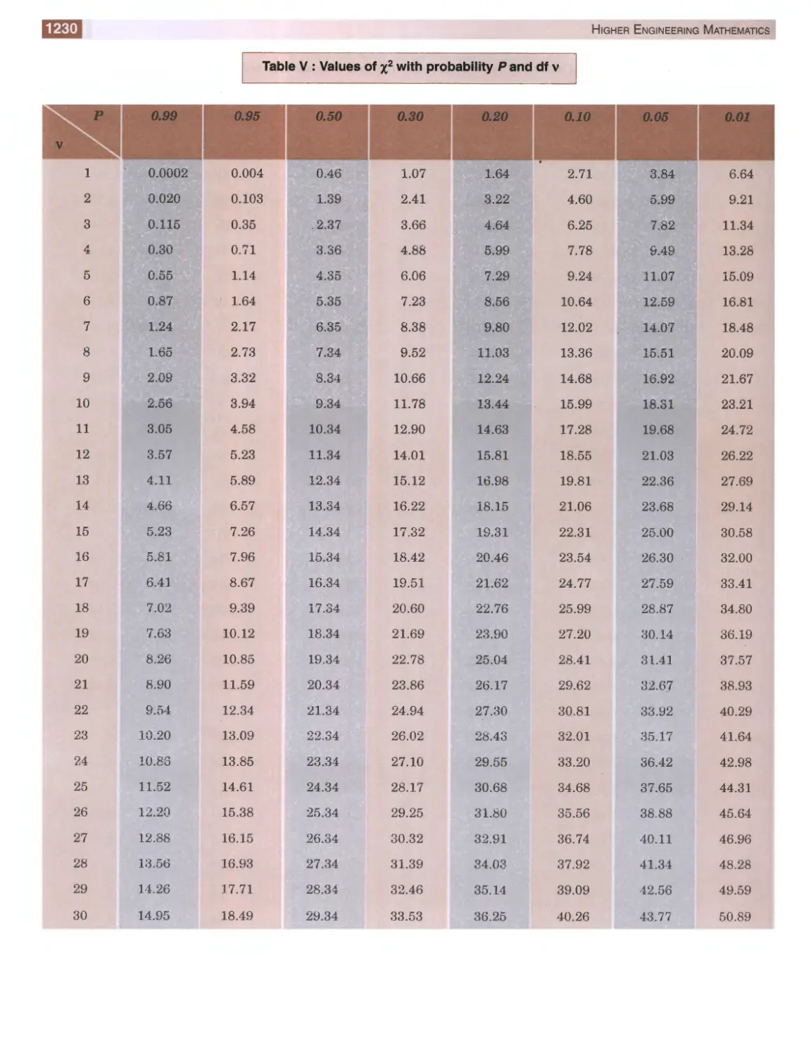
Table V: Values of X2
1230
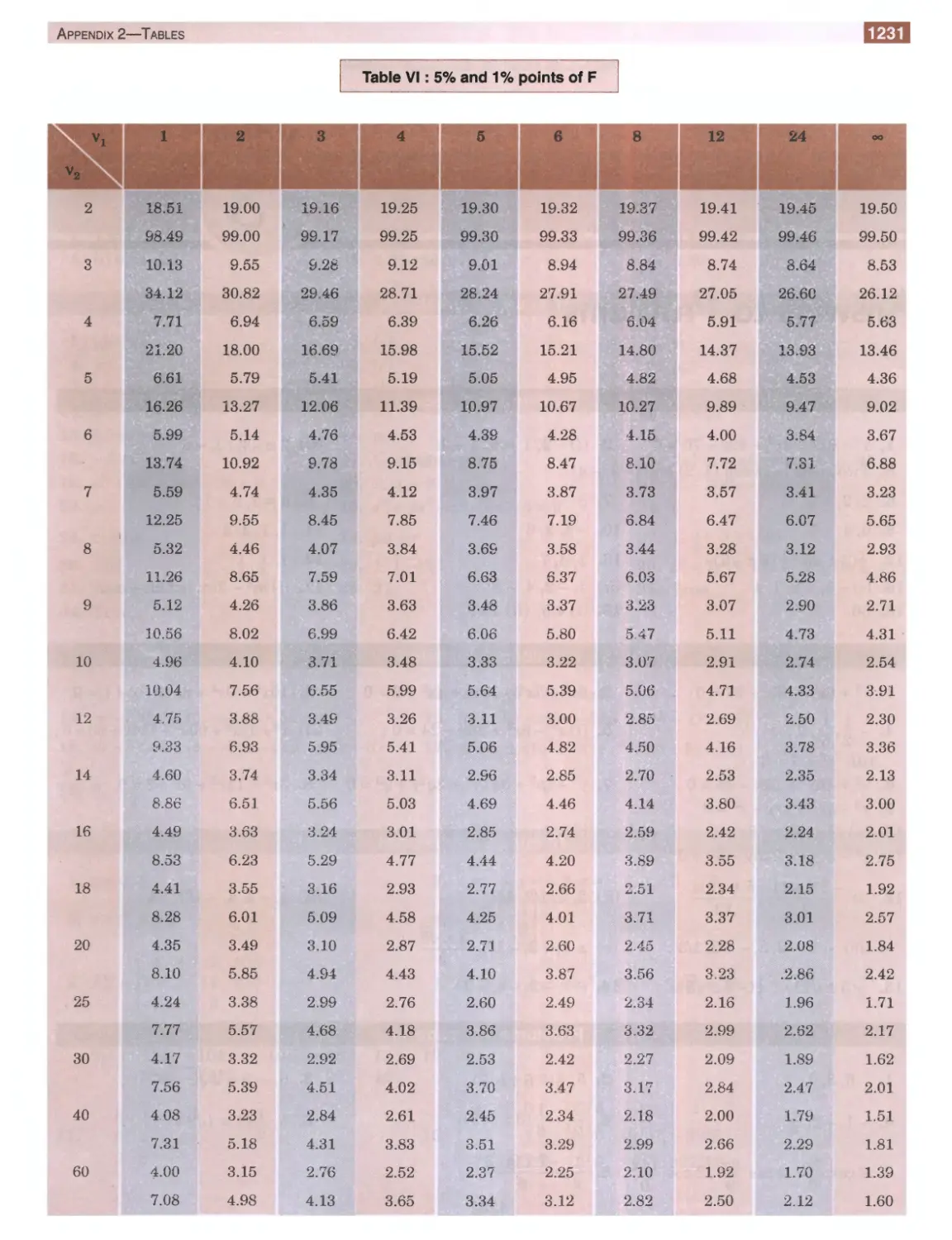
Table VI:Values of F
1231
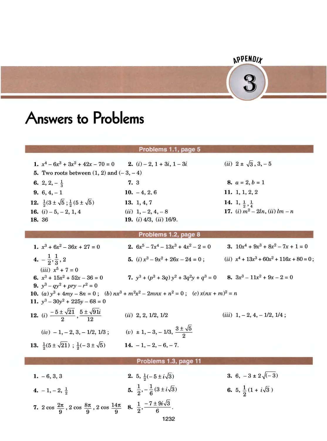
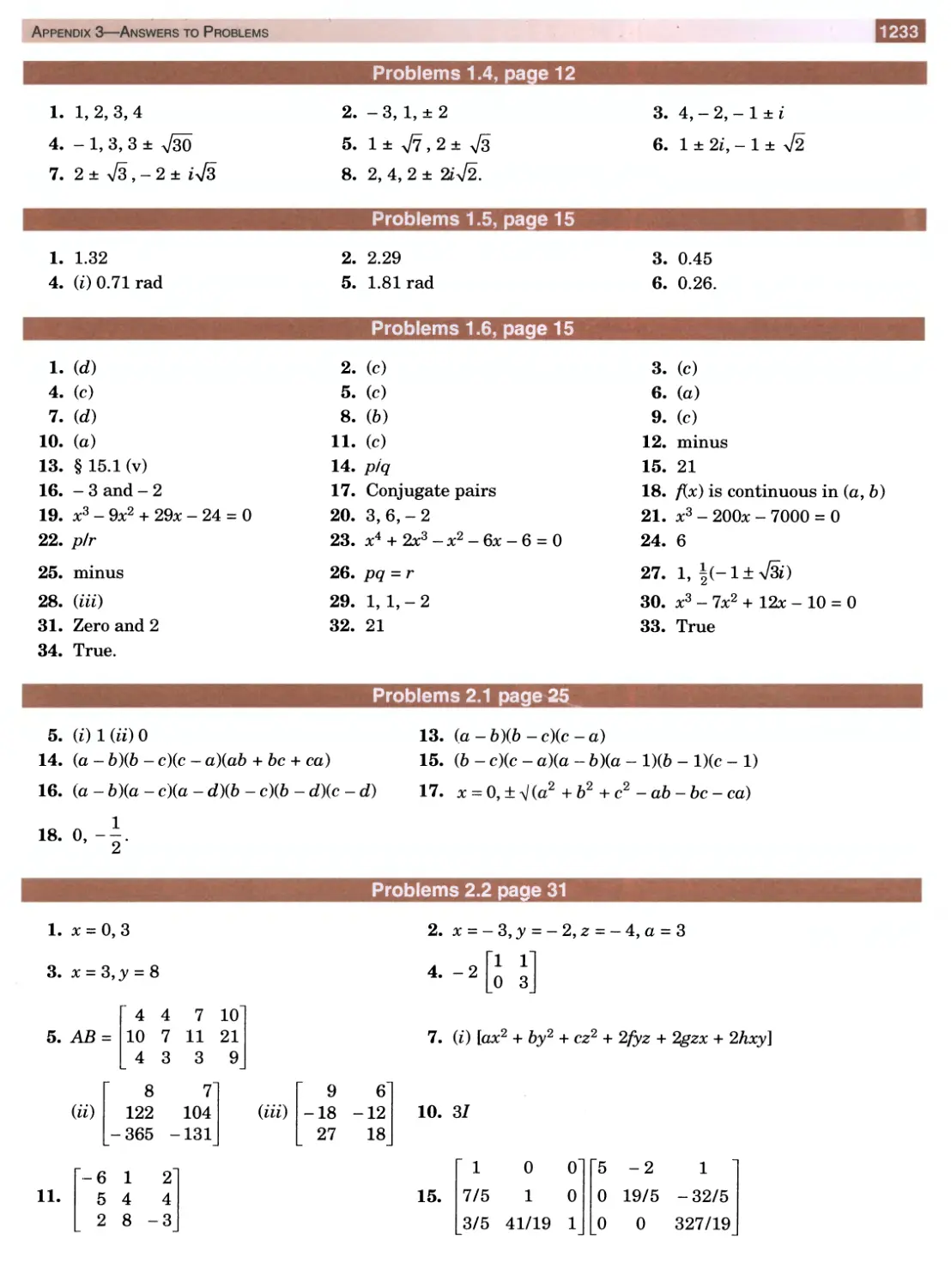
Appendix 3: Answers to Problems
1232
Index
1307
(x)
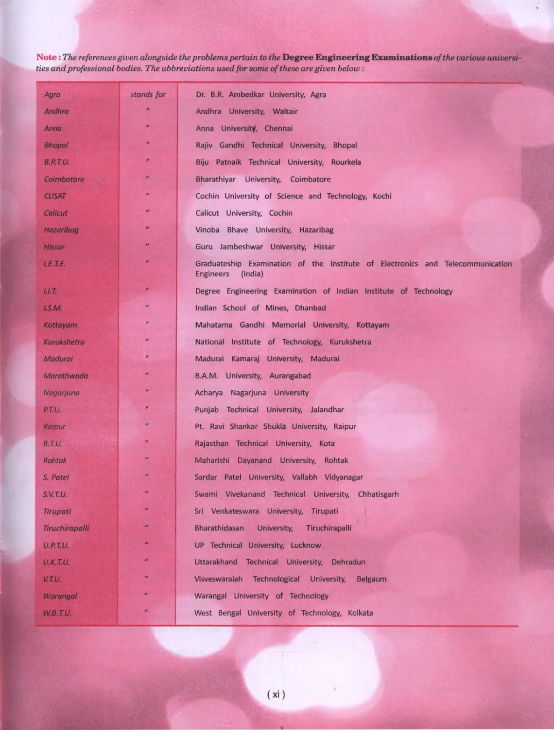
Note: The references given alongside the problems pertain to the Degree Engineering Examinations of the various
universities and professional bodies. The abbreviations used for some of these are given below :
Agra
stands for
Dr. B.R. Ambedkar University, Agra
Andhra
//
Andhra University, Waltair
Anna
"
Anna University, Chennai
Bhopal
//
Rajiv Gandhi Technical University, Bhopal
B.P.T.U.
//
Biju Patnaik Technical University, Rourkela
Coimbatore
//
Bharathiyar University, Coimbatore
CUSAT
//
Cochin University of Science and Technology, Kochi
Calicut
//
Calicut University, Cochin
Hazaribag
״
Vinoba Bhave University, Hazaribag
Hissar
״
Guru Jambeshwar University, Hissar
I.E.T.E.
Graduateship Examination of the Institute of Electronics and Telecommunication
Engineers (India)
I.I.T.
//
Degree Engineering Examination of Indian Institute of Technology
I.S.M.
Indian School of Mines, Dhanbad
Kottayam
״
Mahatama Gandhi Memorial University, Kottayam
Kurukshetra
//
National Institute of Technology, Kurukshetra
Madurai
//
Madurai Kamaraj University, Madurai
Marathwada
»
B.A.M. University, Aurangabad
Nagarjuna
Acharya Nagarjuna University
P.T.U.
!
Punjab Technical University, Jalandhar
Raipur
״
Pt. Ravi Shankar Shukla University, Raipur
R.T.U.
n
Rajasthan Technical University, Kota
Rohtak
//
Maharishi Dayanand University, Rohtak
S. Patel
׳׳
Sardar Patel University, Vallabh Vidyanagar
S.V.T.U.
״
Swami Vivekanand Technical University, Chhatisgarh
Tirupati
//
Sri Venkateswara University, Tirupati
Tiruchirapalli
//
Bharathidasan University, Tiruchirapalli
U.P.T.U.
//
UP Technical University, Lucknow
U.K.T.U.
//
Uttarakhand Technical University, Dehradun
V.T.U.
//
Visveswaraiah Technological University, Belgaum
Warangal
//
Warangal University of Technology
W.B.T.U.
//
West Bengal University of Technology, Kolkata
(xi)
Solution of Equations
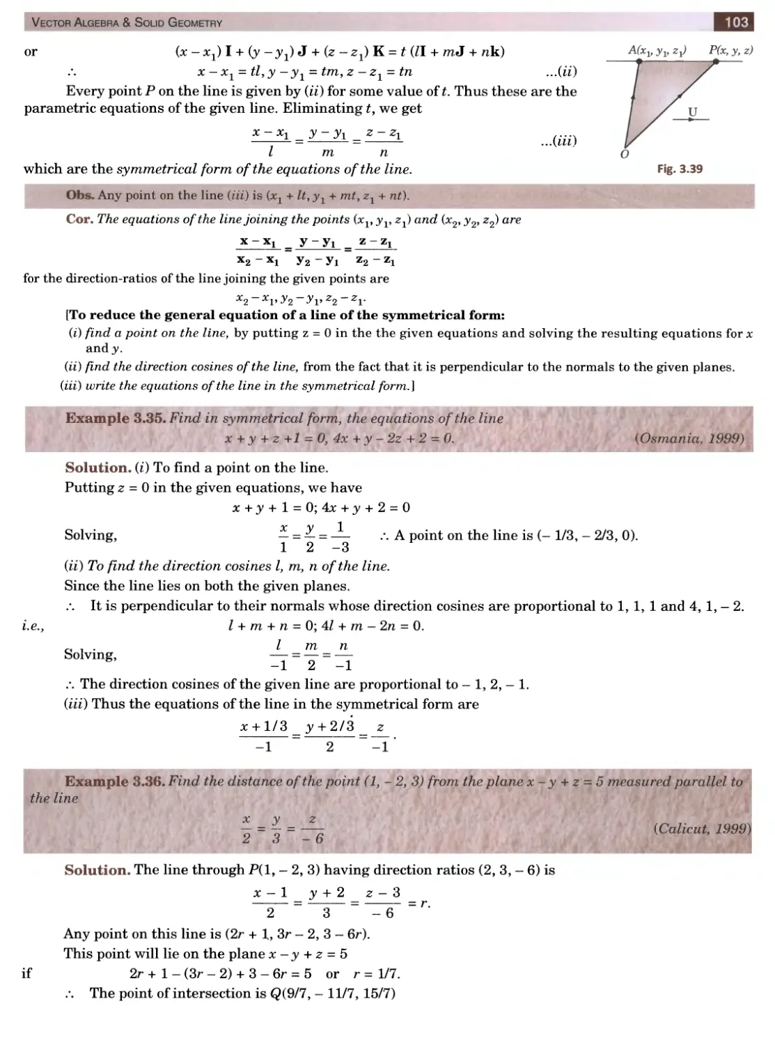
I . i 1
| 1. Introduction. 2. General properties.,3. Transformation of equations. 4. Reciprocal equations. 5. Solution of cubic !
. equations-Cardan’s method. 6. Solution of biquadratic equations—Ferrari’s method ; Descarte’s method. .
' 7. Graphical solution of equations. 8. Objective Type Questions. '
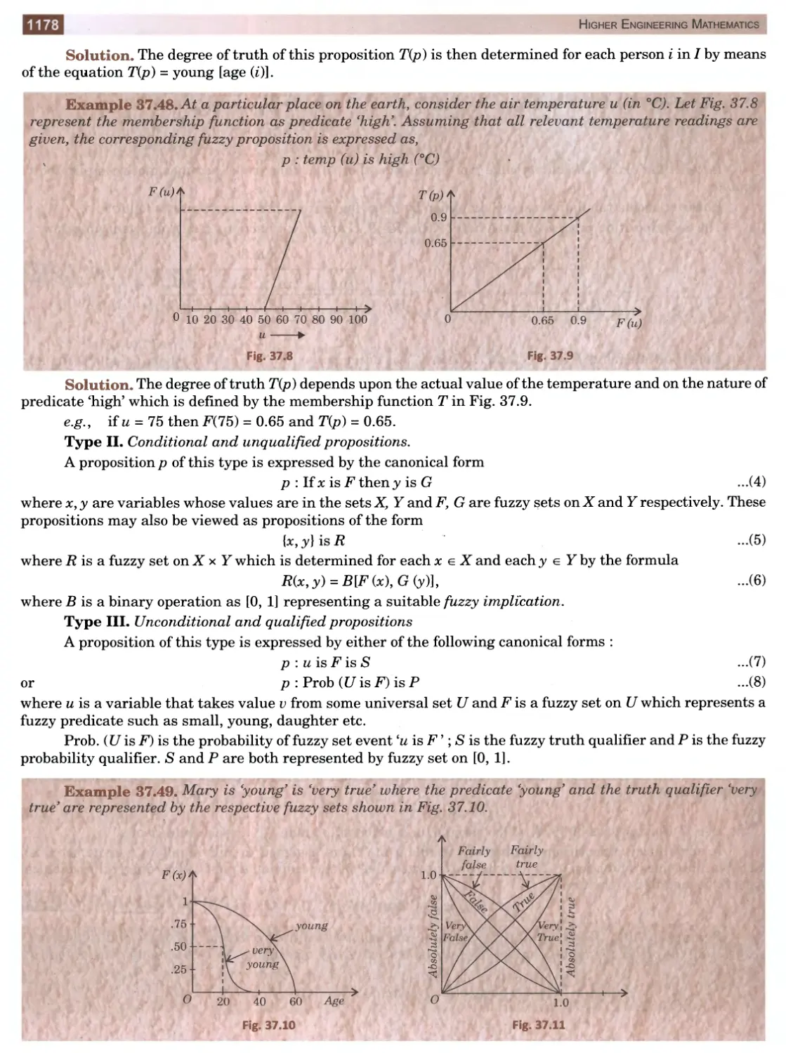
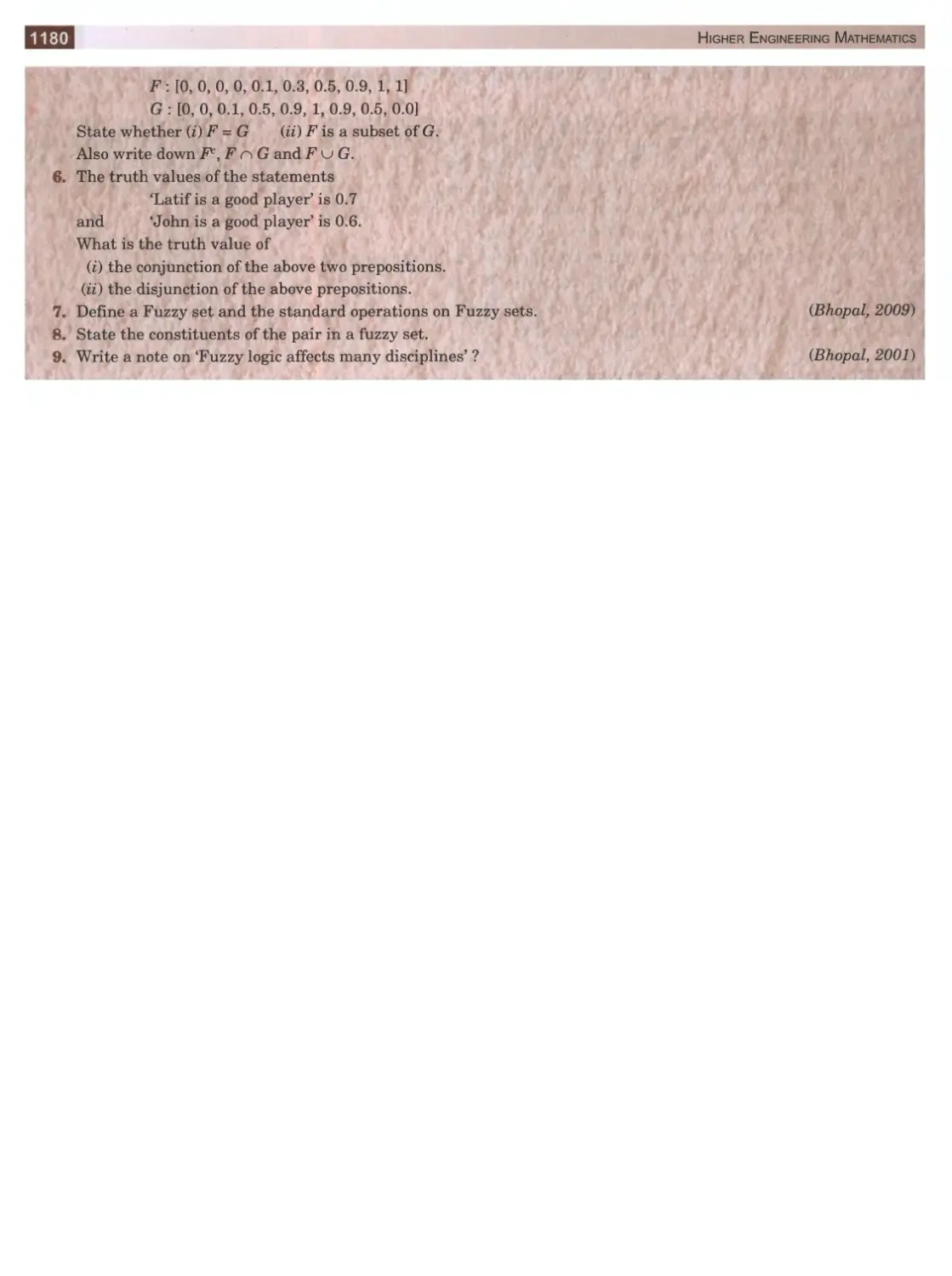
ffff INTRODUCTION
The expression fix) = a^c11 + a^"1־ + ... + an l x + an
where a’s are constants (a0 ^ 0) and n is a positive integer, is called a polynomial in x of degree n. The polynomial
fix) = 0 is called an algebraic equation of degree n. If fix) contains some other functions such as trigonometric,
logarithmic, exponential etc. ; then fix) = 0 is called a transcendental equation.
The value of x which satisfies fix) = 0, ...(1)
is called its root. Geometrically, a root of (1) is that value of x where the graph ofy = fix) crosses the *-axis. The
process of finding the roots of an equation is known as solution of that equation. This is a problem of basic
importance in applied mathematics. We often come across problems in deflection of beams, electrical circuits
and mechanical vibrations which depend upon the solution of equations. As such, a brief account of solution of
equations is given in this chapter.
MWM GENERAL PROPERTIES
I. If a is a root of the equation f(x) = 0, then the polynomial f(x) is exactly divisible by x- a and conversely.
For instance, 3 is a root of the equation x4 - 6x2 - 8x - 3 = 0, because x = 3 satisfies this equation.
.-. x - 3 divides x4 - 6x2 - Sx - 3 completely, i.e., x - 3 is its factor.
II. Every equation of the nth degree has n roots (real or imaginary).
Conversely if a1״ a2,..., an be the roots of the nth degree equation fix) = 0, then
fix) = A ix- (Xj) ix - a2)... ix - an) wher.e A is a constant.
Obs. If a polynomial of degree n vanishes for more than n value of x, it must be identically zero.
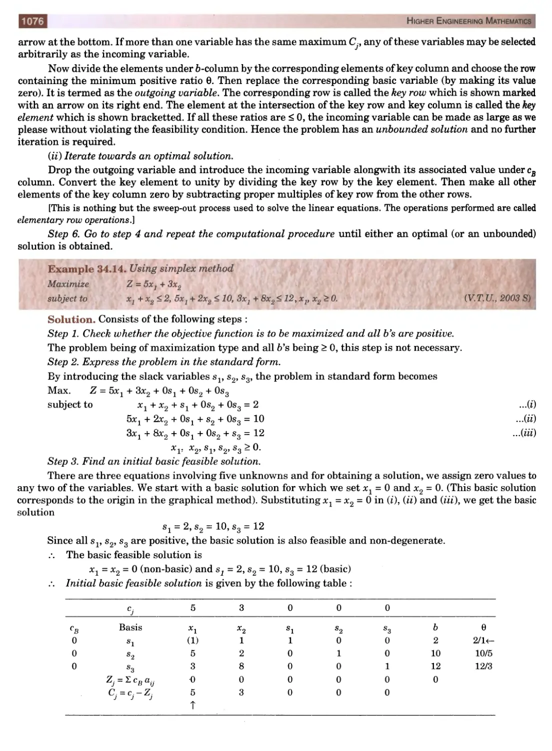
Example 1.1. Solve the equation 2x3 + x2 - 13x + 6 = 0.
Solution. By inspection, we find x = 2 satisfies the given equation.
.2 .״ is its root, i.e. x - 2 is a factor of 2x3 + x2 - 13# + 6. Dividing this polynomial by x - 2, we get the
quotient 2#2 + 5x - 3 and remainder 0.
Equating the quotient to zero, we get 2x2 + 5x - 3 = 0.
C1. tu. j . -5 + V[52-4.(2).(-3)] - 5 ± 7 01
Solving this quadratic, we get x = — = —-— = - 3, —.
Z* X Z* 4 Zi
Hence, the roots of the given equation are 2, - 3,1/2.
1
Higher Engineering Mathematics
Note. The labour of dividing the polynomial by x-2 can be saved considerably by the following simple device called
synthetic division.
2
1
-13
6
2
4
10
-6
2
5
-3
1 0
[Explanation : (I) Write down the coefficient of the powers of x in order (supplying the missing powers of x by zero
coefficients and write 2 on extreme right.
(ii) Put 2 as the first term of 3rd row and multiply it by 2, write 4 under 1 and add, giving 5.
(iii) Multiply 5 by 2, write 10 under - 13 and add, giving - 3.
(iv) Multiply - 3 by 2, write - 6 under 6 and add given zero].
Thus the quotient is 2x2 + 5x - 3 and remainder is zero.
Obs, To divide a polynomial by x + h, we write — h on the extreme right.
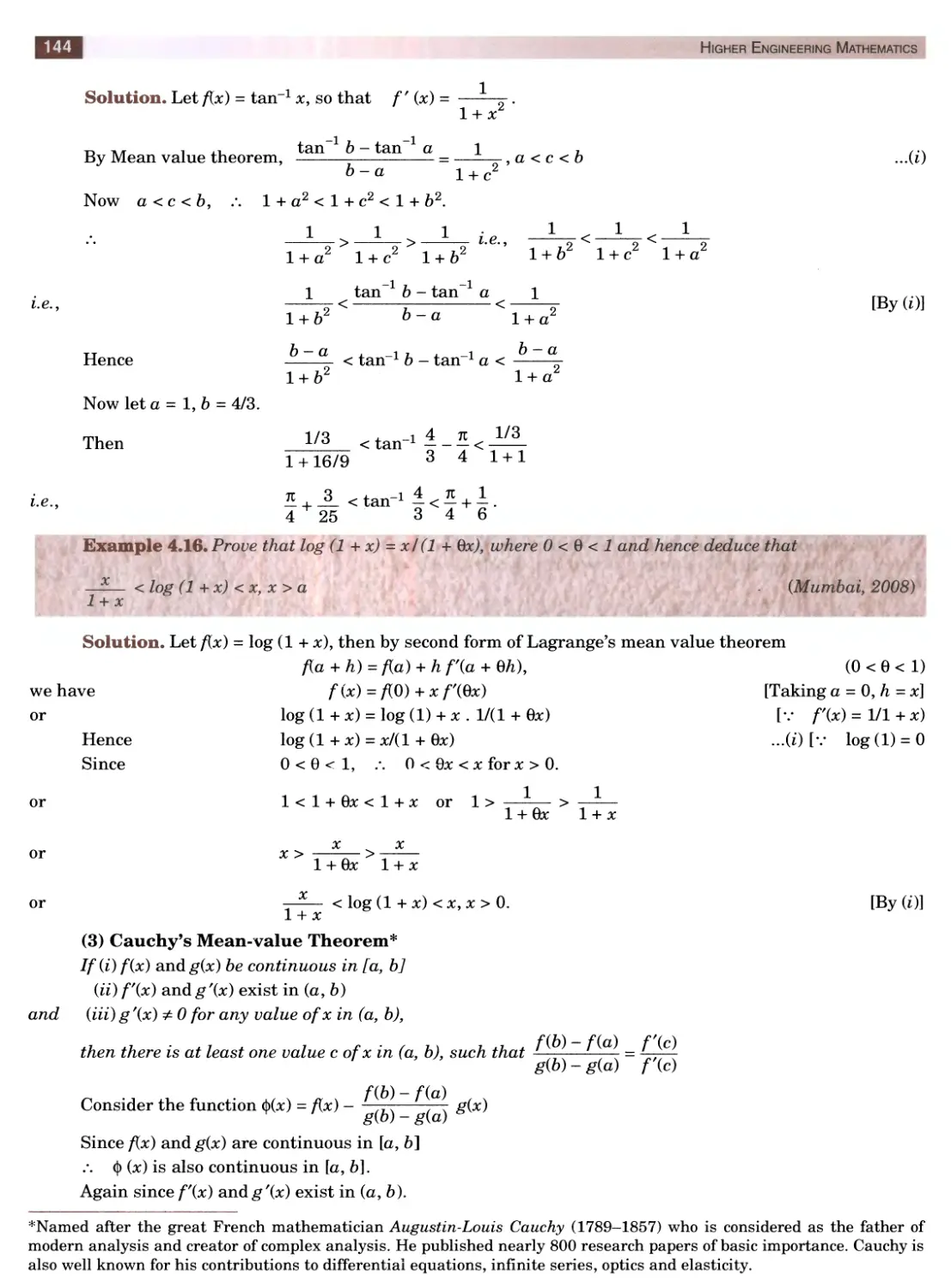
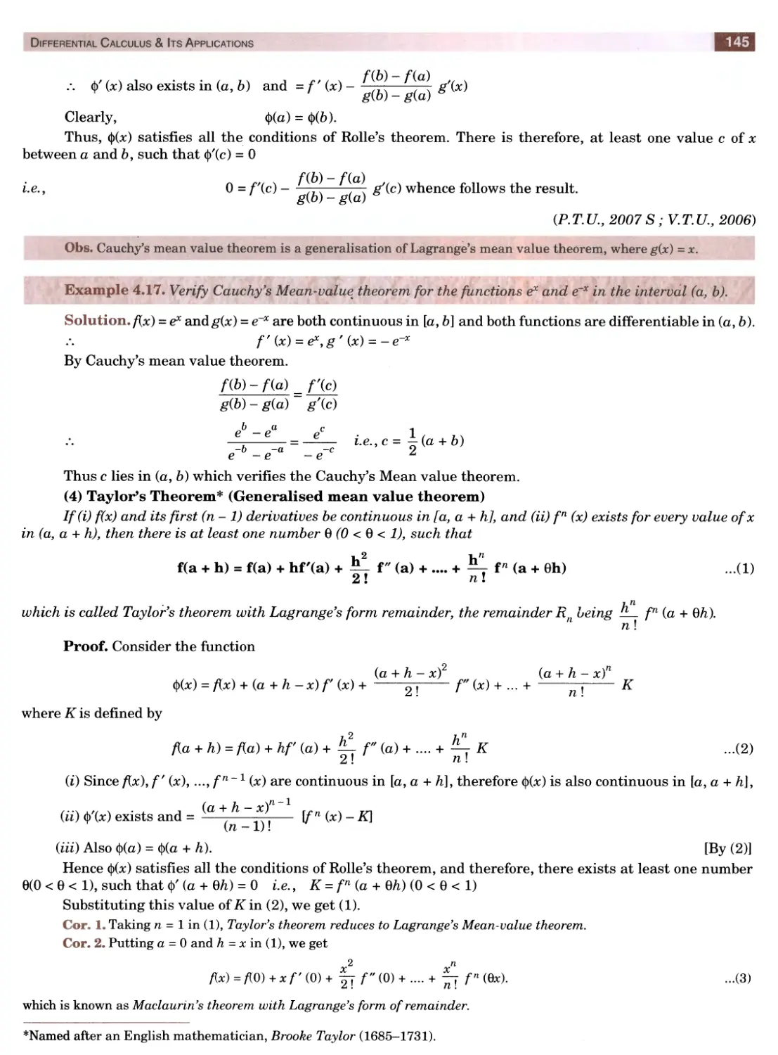
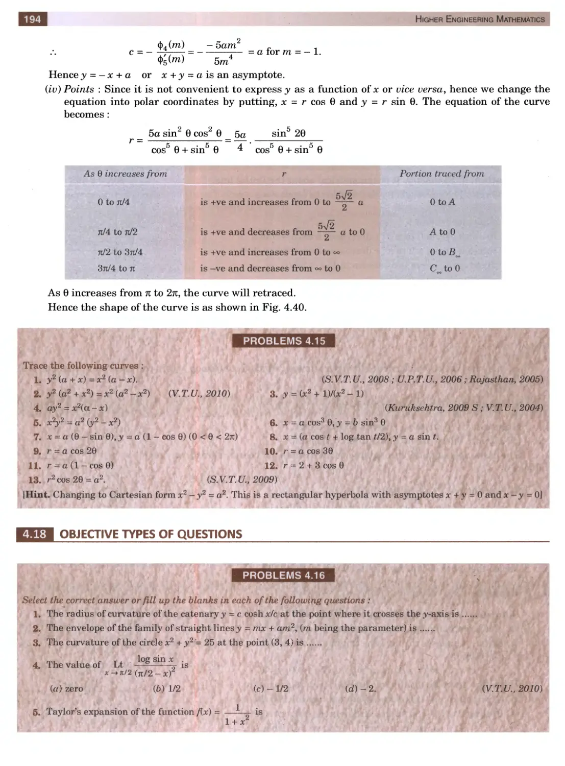
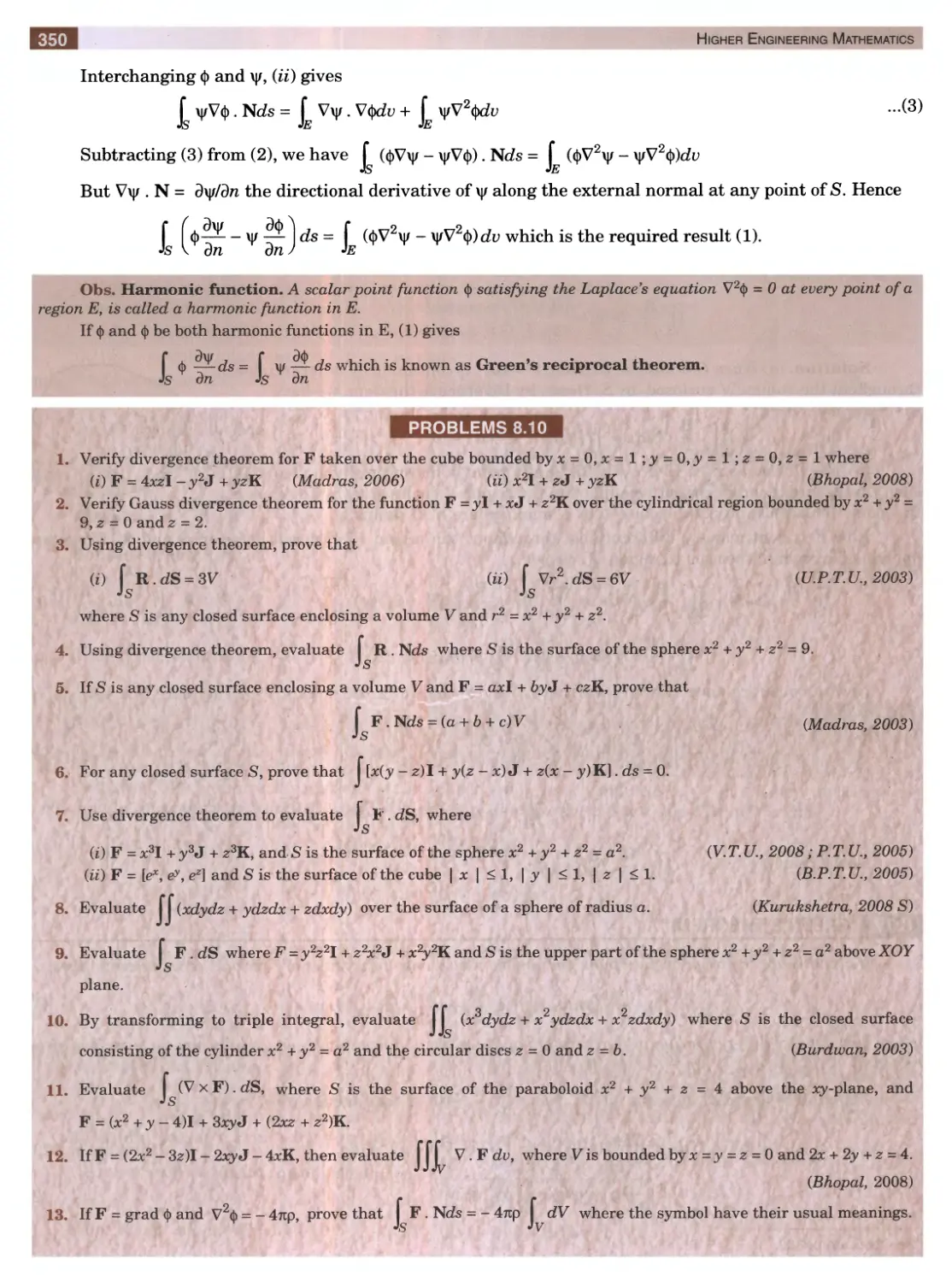
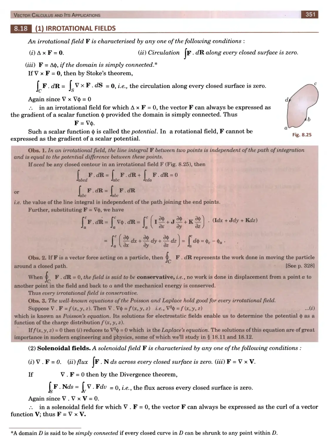
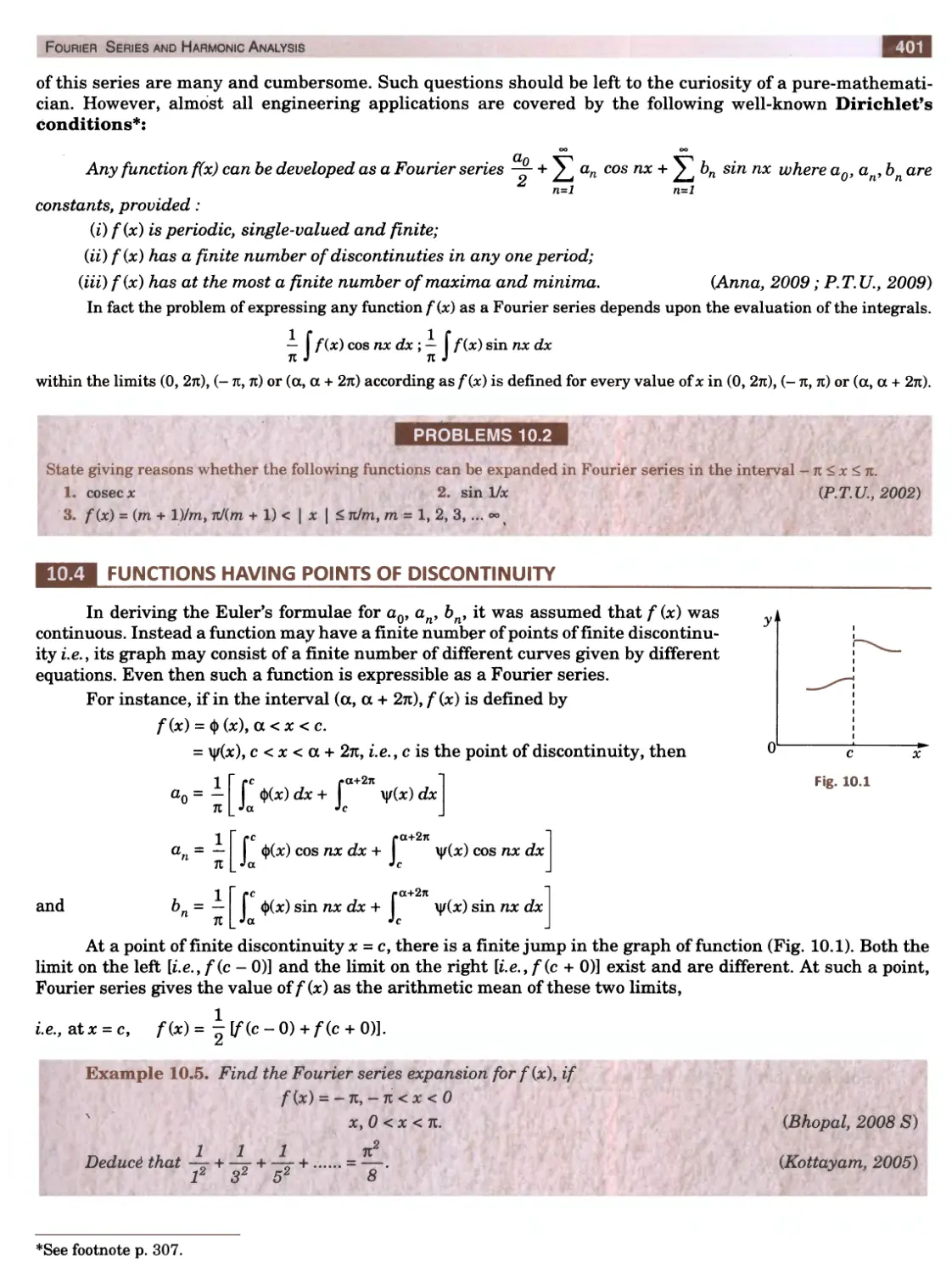
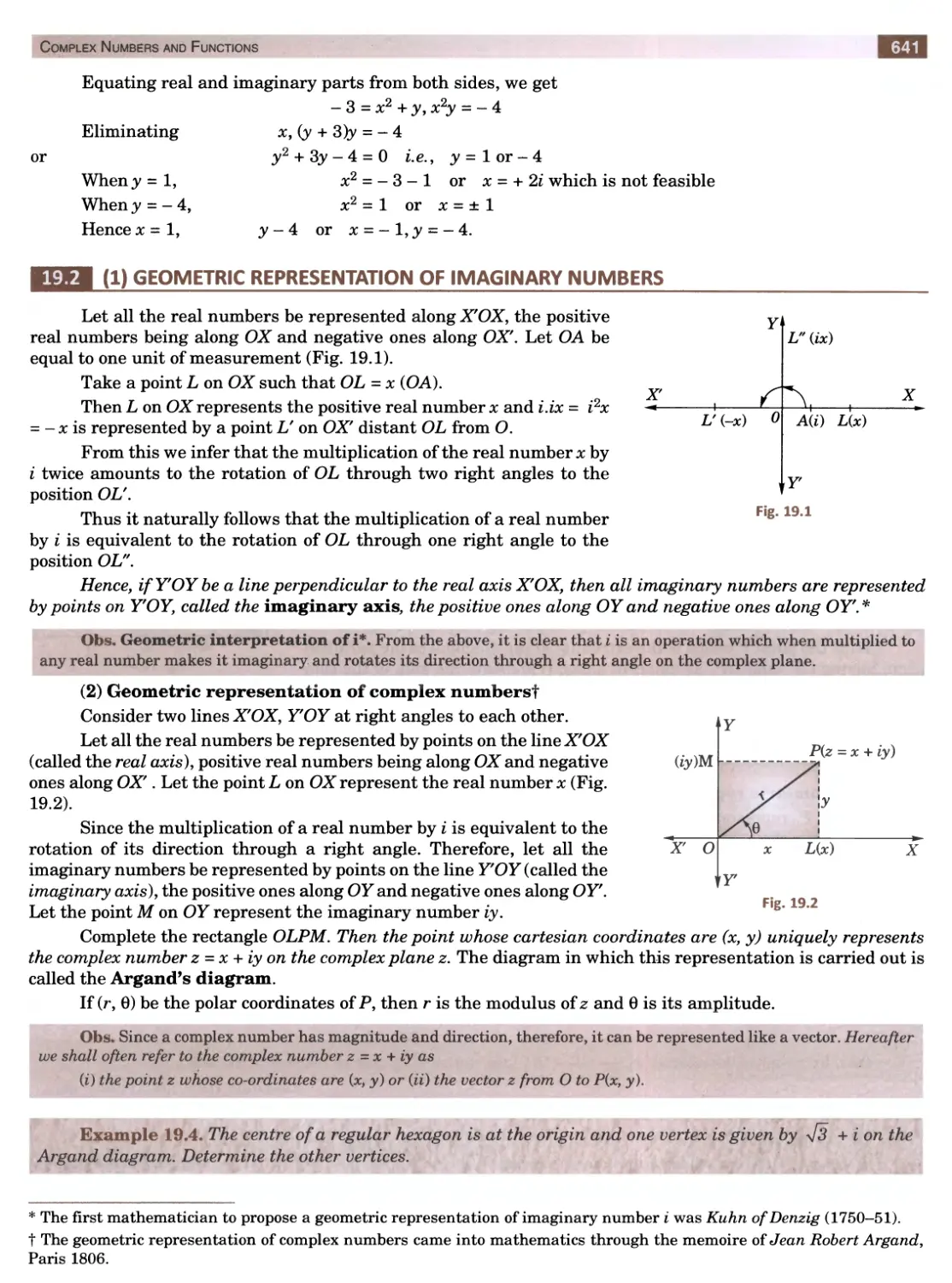
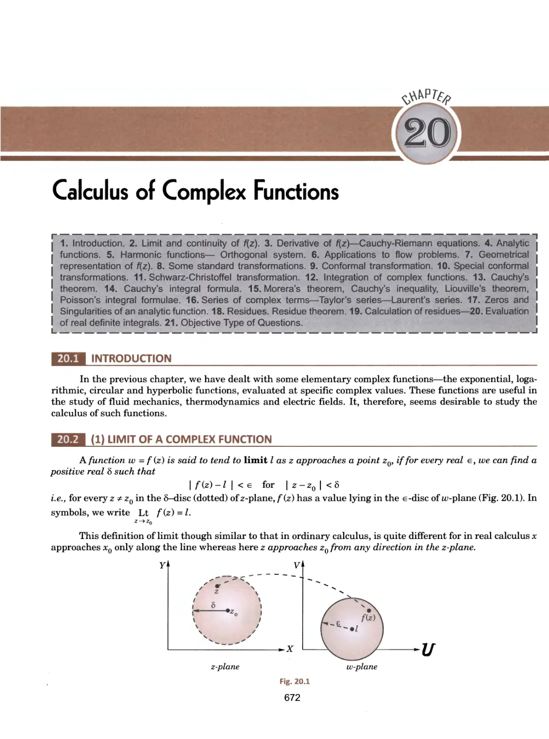
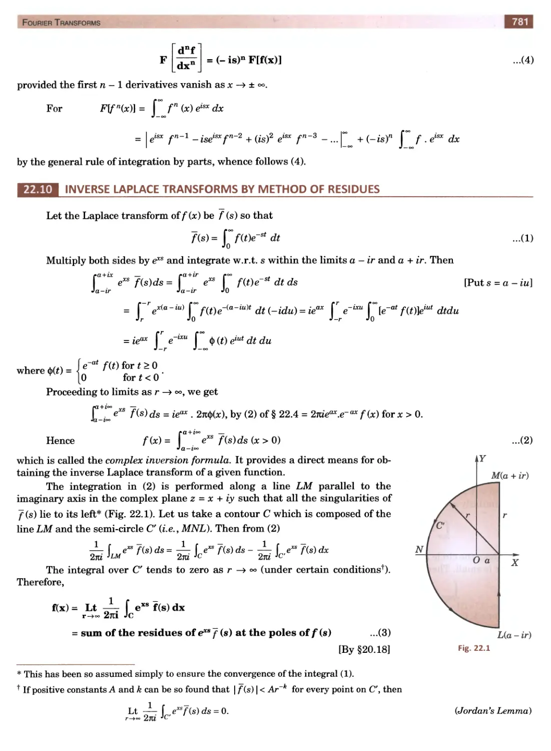
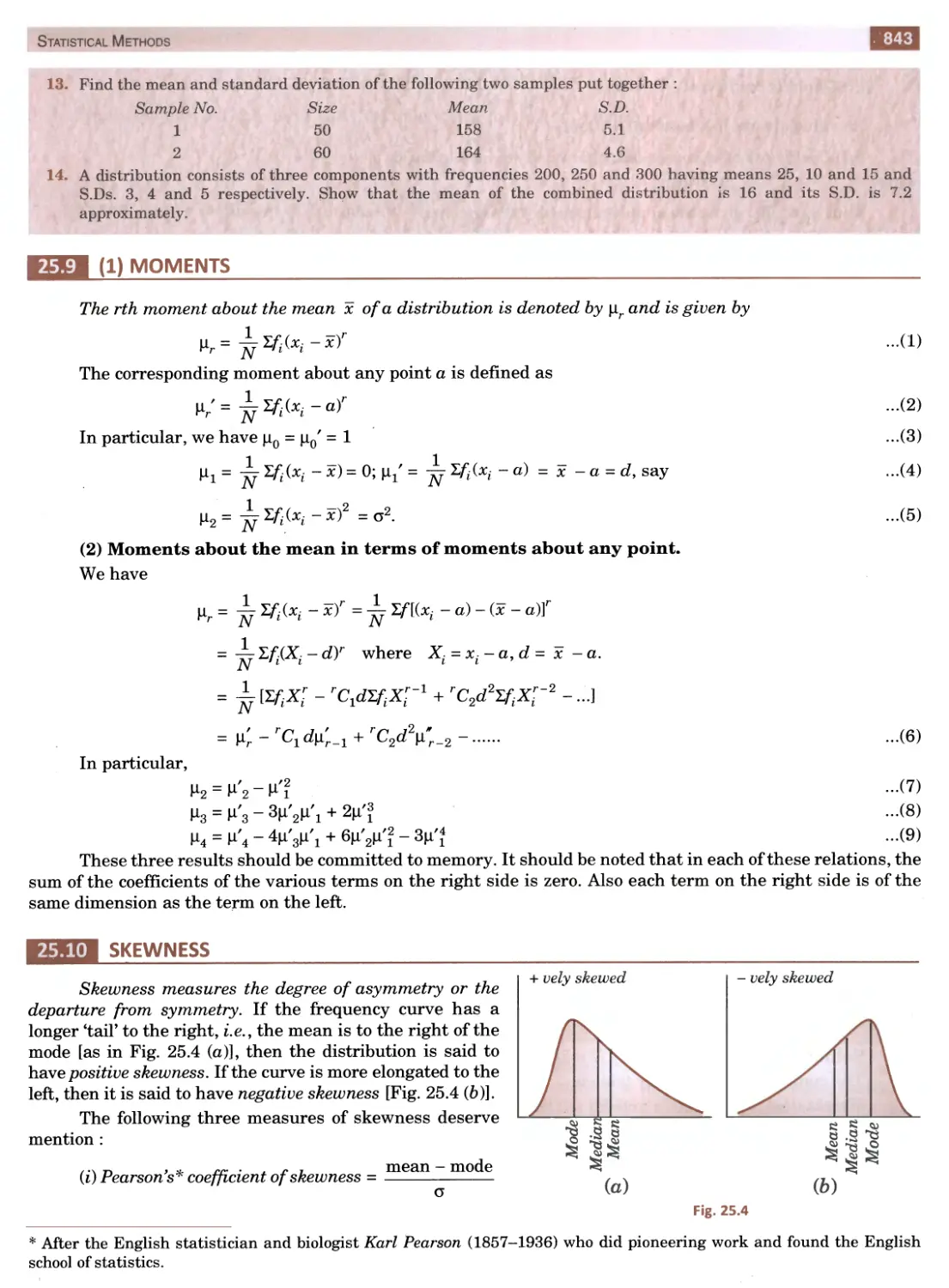
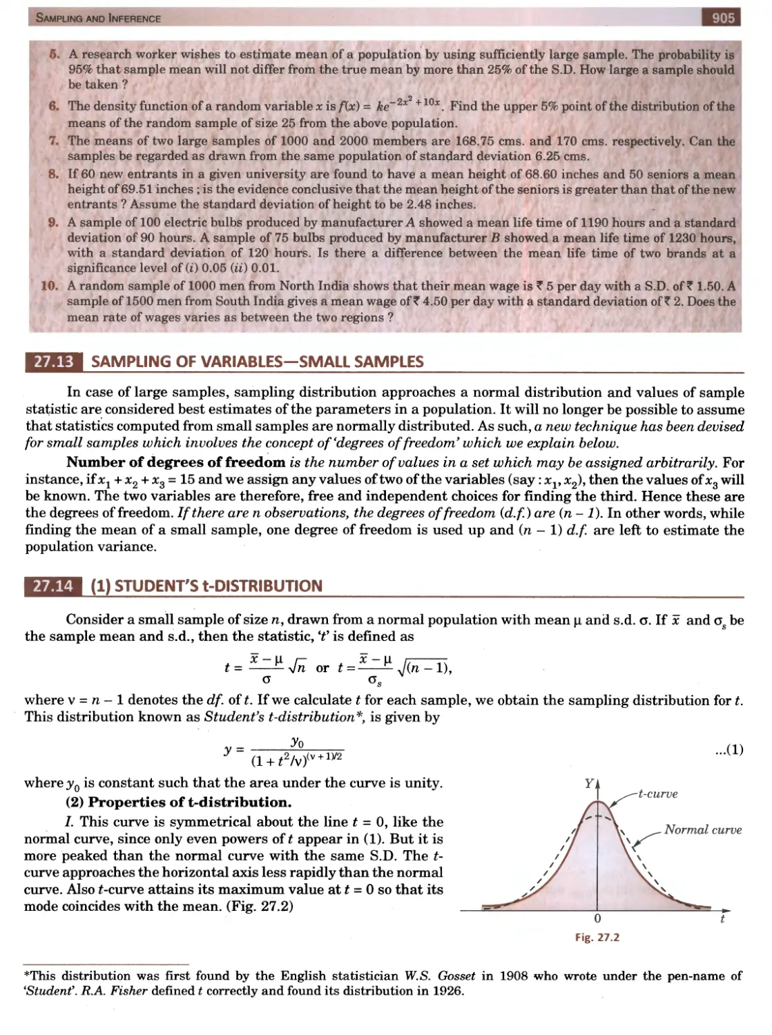
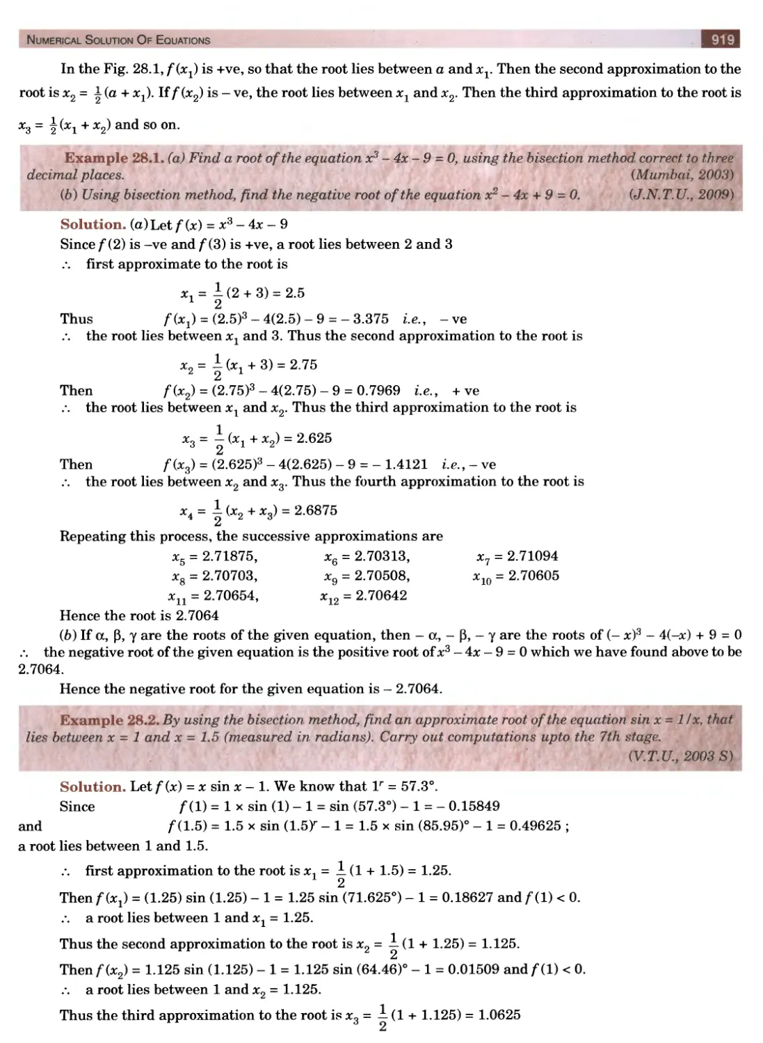
III. Intermediate value property. If fid) and fib) have different
signs, then the equation fix) = 0 has atleast one root between x = a
and x = b.
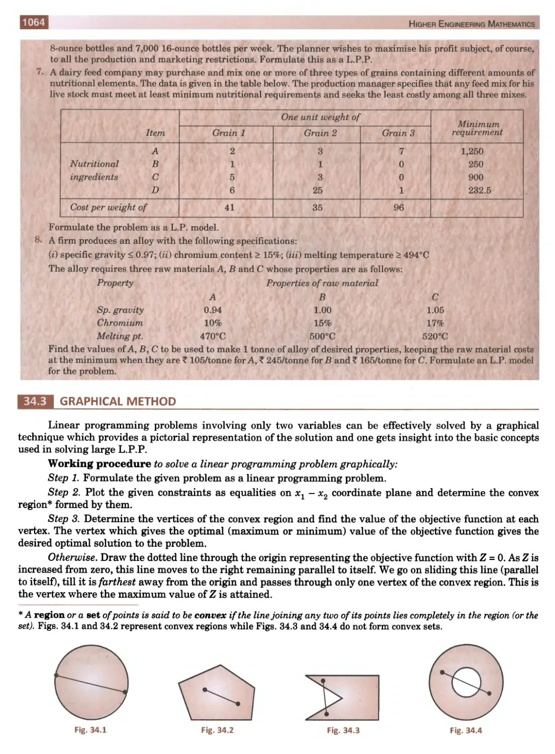
The polynomial fix) is a continuous function of x (Fig. 1.1). So while x
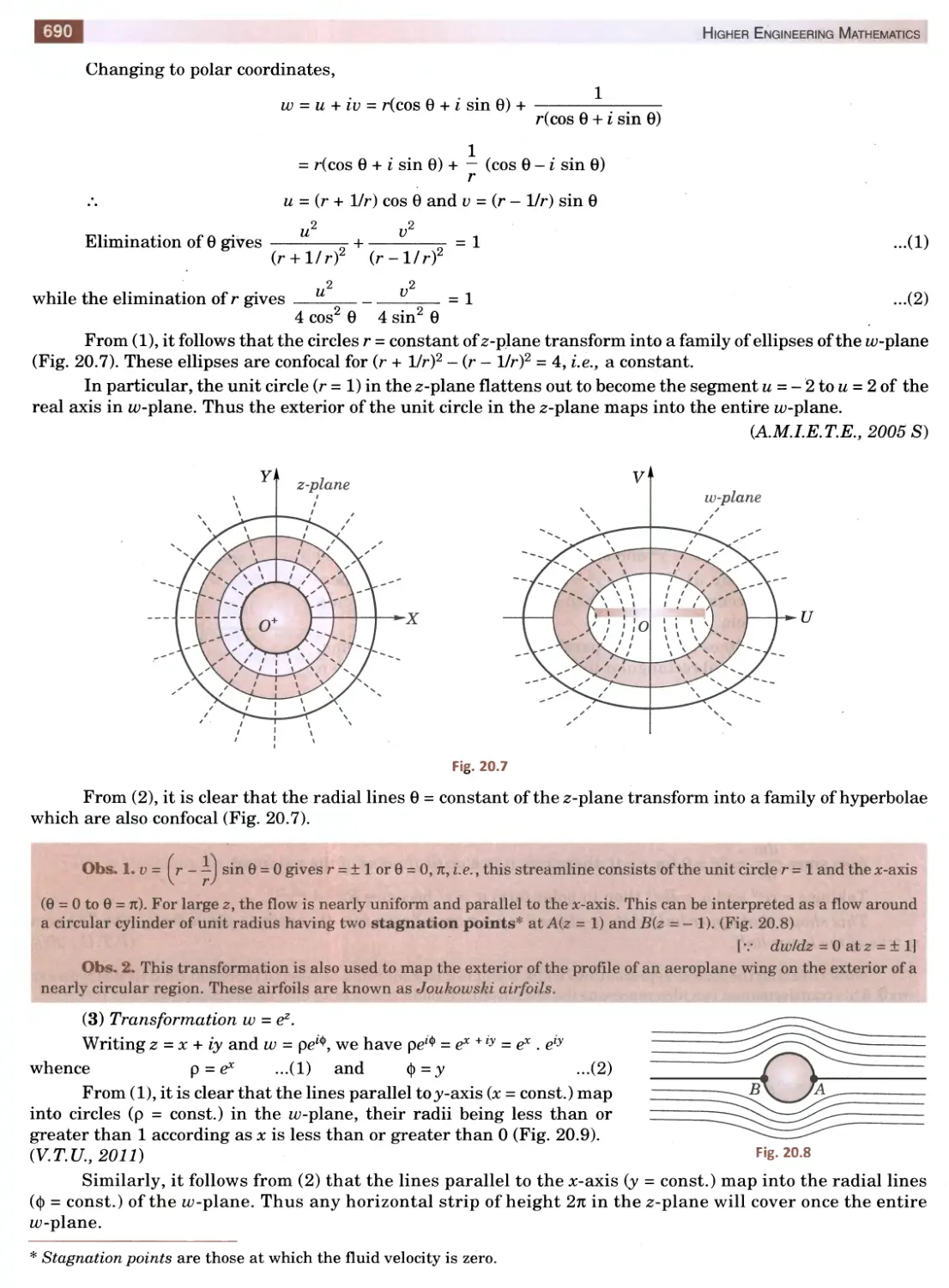
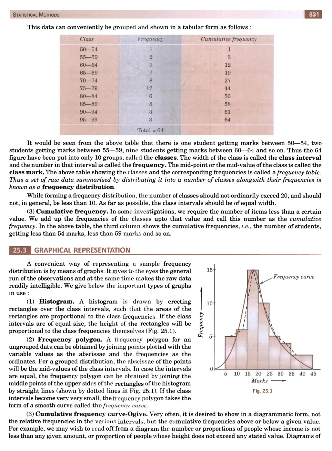
changes from a to 6, fix) must pass through all the values from fia) to fib).
But since one of these quantities fia) or fib) is positive and the other
negative, it follows that at least for one value of #(say a) lying between a and b,
fix) must be zero. Then a is the required root.
IV. In an equation with real coefficients, imaginary roots occur in
conjugate pairs, i.e., if a + ip is a root of the equation fix) = 0, then
a - ip must also be its root. (See p. 534)
Similarly if a + V& is an irrational root of an equation, then a - ^Jb must also be its root.
Obs. Every equation of the odd degree has at least one real root.
This follows from the fact that imaginary roots occur in conjugate pairs.
Example 1.2. Solve the equation 3x3 - 4x2 + x + 88 = 0, one root being 2 + V7i.
Solution. Since one root is 2 + V7i, the other root must be 2 - V7i.
.-. The factors corresponding to these roots are
ix - 2 - V7i) and (# - 2 + V7i)
or ix- 2- <li) ix- 2 + <li) = ix - 2)2 + 7 = x2 - 4x + 11,
which is a divisor of 3#3 - 4#2 + x + 88 ...H)
/. Division of ii) by x2 - 4x + 11 gives 3# + 8 as the quotient.
Thus the depressed equation is 3x + 8 = 0. Its root is - 8/3. Hence the roots of the given equation are
2 ± V7i, - 8/3.
V. Descarte’s rule of signs. *The equation f(x) = 0 cannot have more positive roots than the changes of
signs in f(x); and more negative roots than the changes of signs in fi—x).
For instance, consider the equation fix) = 2#7 - x5 + 4#3 -5 = 0 ...(1)
Sign of fix) are + — + —
vvv
Clearly, fix) has 3 changes of signs (from + to — or - to +).
Thus ii) cannot have more than 3 positive roots.
2
־, After the French mathematician and philosopher Rene Descartes (1596-1650), who invented Analytic geometry in 1637.
Solution of Equations
Also fX-x) = 2(- x)1 - (- x)5 + 4(- x)3 - 5
= - 2x7 + #5 - 4x3 - 5
This shows that fix) has 2 changes of signs. Thus (i) cannot have more than 2 negative roots.
Obs. Existence of imaginary roots. If an equation of the nth degree has at the most p positive roots and at the most q
negative roots, then it follows that the equation has at least n-(p +q) imaginary roots.
Evidently (1) above is an equation of the 7th degree and has at the most 3 positive roots and 2 negative roots. Thus
(1) has at least 2 imaginary roots.
VI. Relations between roots and coefficients, If av a2, a3,..., an be the roots of the equation
aQxn + c^x" 1־ + a<£cn~2 + ... + anlx + an = 0 ...(1)
then Za1 = - —, Ea^ = —, Ea^ag = - —
a0 «0 a0
aia2a3 aw = (“ — •
a0
Example 1.3. Solve the equation x3 - 7x2 + 36 = 0, given that one root is double of another.
Solution. Let the roots be a, P, y such that P = 2a.
Also a + p + y = 7, ap + py + ya = 0, apy = - 36
3a + y=7 ...ii)
2a2 + 3ay=0 ...(ii)
2a2y=-36 ...(Hi)
Solving (i) and (ii), we get a = 3, y = - 2.
[The values a = 0, y = 7 are inadmissible, as they do not satisfy (iii)].
Hence the required roots are 3, 6 and - 2.
Example 1.4. Solve the equation x4 - 2x3 + 4x2 + 6x - 21 = 0, given that the sum of two of its roots is zero.
(Cochin, 2005; Madras, 2003)
Solution. Let the roots be a, P, y, 8 such that a + P = 0.
Also a+p+y+8=2 y + 8 = 2
Thus the quadratic factor corresponding to a, p is of the form x2 - Ox + p, and that
corresponding to y, 8 is of the form of x2 - 2x + q.
x4 - 2x3 + 4x2 + 6x - 21 = (x2 + p) (x2 - 2x + q) ...(i)
Equating the coefficients of x2 and x from both sides of (i), we get
4=p + q, 6 = - 2p.
p = -3, q = 7.
Hence the given equation is equivalent to (x2 - 3) (x2 - 2x + 7) = 0
.״. The roots are x = ± ^3 , 1 ± i\f6 .
Example 1.5. Find the condition that the cubic x3 - Ix2 + mx - n = 0 should have its roots in
(a) arithmetical progression. (Madras, 2000 S)
(b) geometrical progression.
Solution, (a) Let the roots be a - d, a, a + d so that the sum of the roots = 3 a = Z i.e., a = 1/3.
Since a is the root of the given equation
a3-la2 + ma-n = 0 ...(/)
Substituting a = 1/3, we get (Z/3)3 - l(l/3)2 + m(l/3) - n = 0.
or 2Z3 - dim + 21n = 0, which is the required condition.
Higher Engineering Mathematics
(b) Let the roots be a/r, a, ar, so that the product of the roots = a3 = n.
Putting a = (n)1/s, in (Z), we get n - ln2/3 + m/z1/3 -/i = Oorm = Zra1/3
Cubing both sides, we get m3 = l3n, which is the required condition.
Example 1.6. Solve the equation x4 - 2x3 - 21x2 + 22x + 40 = 0 whose roots are in A.P.
Solution. Let the roots be a - 3d, a - d, a + d, a + 3d, so that the sum of the roots = 4a = 2.
a = 1/2
Also product of the roots = (a2 - 9cZ2) (a2 - d2) = 40
_ 9rf2j Q. _ ^2j = 40 or 144d4 - 40d2 - 639 = 0
d2 = 9/4 or -7/36
Thus, d = ± 3/2, the other value is not admissible.
Hence the required roots are -4,-1, 2, 5.
Example 1.7. Solve the equation 2x4 - 15x3 + 35x2 - 30x + 8 = 0, whose roots are in G.P.
Solution. Let the roots be a/r3, a/r, ar, ar3, so that product of the roots = a4 = 4.
Also the product of a/r3, ar3 and a/r, ar are each = a2 = 2.
:. The factors corresponding to a/r3, ar3 and a/r, ar are x2 + px + 2, x2 + qx + 2.
Thus, 2x4 - 15x3 + 35x2 - 30x + 8 = 2(x2 + px + 2) (x2 + qx + 2)
Equating the coefficients of x3 and x2
- 15 = 2p + 2q and 2 + 8 = 35״״pq
p = - 9/2, q = - 3.
Thus the given equation is 2 ^x2 - ^x + 2^ (x2 - 3x + 2) = 0
Hence the required roots are 1/2, 4 and 1, 2 i.e., — , 1, 2, 4.
2
Example 1.8. If a, p, y be the roots of the equation x3 + px + q = 0, find the value of
(a) Xa2p, (b) Ixx4 (c) Zot2p.
Solution. We have a + p + y = 0
ap + Py + ya = p
aPy = -q
(a) Multiplying (I) and (ii), we get
a2P + a2y + p2y + p2a + *fa + y2p + 3aPy = 0
Ea2p = - 3aPy = 3q
(b) Multiplying the given equation by x, we get x4 + px2 + qx = 0
Putting x = a, p, y successively and adding, we get Xa4 + pXa2 + qZa = 0
Za4 = - pZa2 - q(0)
Now squaring (i), we get a2 + P2 + y2 + 2(aP + Py + ya) = 0
Za2 = -2p
Hence, substituting the value of Za2 in (iv), we obtain
Za4 = -p(- 2p) = 2p2.
(c) Za3p = Za2 Zap - aPyZa = - 2pip) - (- q) (0) = - 2p2.
...(Z)
...(ii)
...(iii)
[By (iii)]
...(iv)
[By (ZZ)]
5
Solution of Equations
PROBLEMS 1.1
1.
Form the equation of the fourth degree whose roots a!e 3 + i and V7׳.
(Madras, 2000 S)
2.
Solve the equation (i) xs + 6x + 20 = 0, one root being 1 + Si.
(ii) x4 - 2x3 - 22x2 + 62x - 15 = 0, given that 2 + V3 is a root.
3.
Show that x1 - Sx4 + 2x3 -1 = 0 has at least four imaginary roots.
(Cochin, 2005)
4.
Show that the equation x4 + 15x2 + 7x - 11 = 0 has one positive, one negative and two imaginary roots.
5.
Find the number and position of real roots of x4 + 4x3 - 4x — 13 = 0.
6.
Solve the equation Sx3 - llx2 + 8x + 4 = 0, given that two of its roots are equal.
7.
If rv r2, r3 are the roots of the equation 2x3 - Sx2 + kx - 1 = 0, find constant k if sum of two roots is 1.
*
(S.V.T.U., 2009)
8.
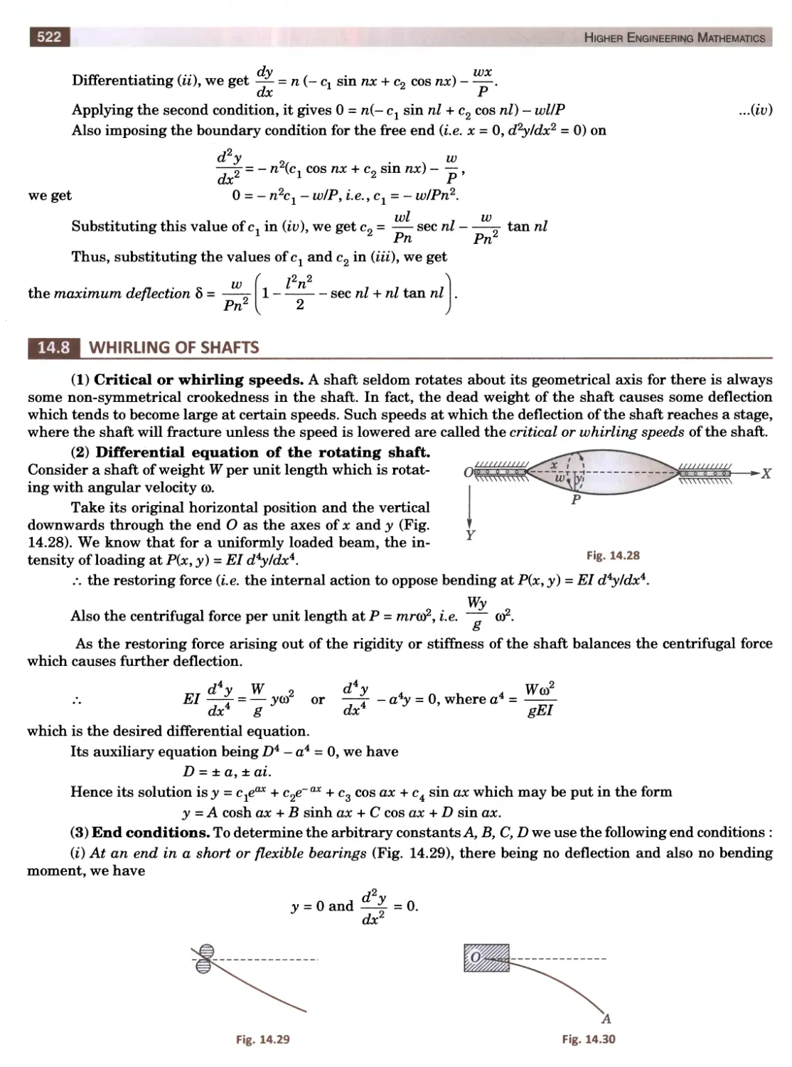
The equation x4 - 4x3 + ax2 + 4x + b = 0 has two pairs of equal roots. Find the values of a and b
Solve the following equations 9-14 :
9.
x3 - 9x2 + 14x + 24 = 0, given that two of its roots are in the ratio 3:2.
10.
x3 - 4x2 - 20x + 48 = 0 given that the roots a and P are connected by the relation a + 2p = 0.
(S.V.T.U., 2007)
11.
x4 - 6x3 + 13x2 - 12x + 4 = 0, given that it has two parts of equal roots.
(Madras, 2003)
12.
x4 - 8x3 + 21x2 - 20x + 5 = 0 given that the sum of two of the roots is equal to the sum of the other two.
13.
x3 - 12x2 + 39* - 28 = 0, roots being in arithmetical progression.
(Madras, 2001 S)
14.
8x3 - 14x2 + 7x - 1 = 0, roots being in geometrical progression.
(Osmania, 1999)
15.
O, A, B, C are the four points on a straight line such that the distances of A, B, C from O are the roots of equation
ax3 + 3 bx2 + 3cx + d = 0. If B is the middle point of AC, show that a2d - 3 abc + 263 = 0.
(S.V.T.U., 2006)
16.
Solve the equations (i) x4 + 2x3- 21x2 - 22x + 40 = 0 whose roots are in A.P.
(ii) x4 + 5x3 - 30x2 + 40x + 64 = 0 whose roots are in G.P.
17.
If a, p, y be the roots of the equation'*3 - lx2 + mx - n = 0, find the value of
(;i) La2p2, (ii) (p + y) (y + a) (a + p)
18.
Find the sum of the cubes of the roots of the equation x3 - 6x2 + 11* - 6 = 0.
19.
If a, p, y are the roots of x3 + 4x — 3 = 0, find the value of (i) a~\+ p1־ + y^1 (ii) oc~2 + P“2 + Y~2•
20.
If a, p, y be the roots of x3 + px + q = 0, show that
(i) a5 + p5 + y5 = 5ocPy (Py + Ya + aP)» (H) Za5 = 5Za3 £a4.
WEI TRANSFORMATION OF EQUATIONS
(1) To find an equation whose roots are m times the roots of the given equation, multiply the
second term by m, third term by m2 and so on (all missing terms supplied with zero coefficients).
For instance, let the given equation be
Sx4 + 6x3 + 4x2 - 8x + 11 = 0 ...(z)
To multiply its roots by ra, put y = mx (or x = y/m) in (i).
Then 3 (y/m)4 + 6(y/m)3 + 4 (y/m)2 + 8(y!m) +11 = 0
Multiplying by ra4, we get 3y4 + ra(6y3) + ra2(4y2) - m3(8y) + m4(ll) = 0
This is same as multiplying the second term by ra, third term by m2 and so on in (i).
Cor. To find an equation whose roots are with opposite signs to those of the given equation, change the signs
of the every alternative term of the given equation beginning with the second.
Changing the signs of the roots of (i) is same as multiplying its roots by - 1.
.־. The required equation will be
Sx4 + (- l)6x3 + (- l)2 4x2 - (- l)3 8x + (- l)4 11 = 0
or 3x4 - 6x3 + 4x3 + 8x + 11 = 0
which is (i) with signs of every alternate term changed beginning with the second.
(2) To find an equation whose roots are reciprocal of the root of the given equation, change x
to llx.
Higher Engineering Mathematics
6
Example 1.9. Solve 6x3 - llx2 - 3x + 2 = 0, given that its roots are in harmonic progression.
Solution. Since the roots of the given equation are in H.P., the roots of the equation having reciprocal
roots will be in A.P.
The equation with reciprocal roots is 6(l/x)3 - ll(l/x)2 - 3(1/*) + 2 = 0
or 2*3 - Sx2 - llx + 6 = 0 ...(£)
Since the roots of the given equation are in H.P., therefore, the roots of (/) are in A.P. Let the root bea-d,
a, a + d. Then
3a = 3/2 and a(a2 - d2) = - 3.
Solving these equations, we get a = 1/2, d = 5/2.
Thus the roots of (i) are - 2, 1/2, 3.
Hence the required roots of the given equation are - 1/2, 2, 1/3.
Example 1.10. If a, P, y be the 7'oots of the cubic equation x3 - px2 + qx - r = 0, form the equation whose
roots are py + 1 / oc, ya + 1 / p, ap + 1 / y.
Hence evaluate Zfap + 1 / y) (py + 1 / a). (S. V. T. U.y 2008)
Solution. If x is a root of the given equation and y a root of the required equation, then
y = Py + 1/a = = r + 1 [ v aPy = r]
a a
r + 1 r + 1
or y = => x =
* y
Thus substituting x = (r + 1 )/y in the given equation, we get
/ -«\ 3 / ,\2 ,
[ r + 1 | fr + 1) | r + 1]
-p\ — — r = o
vyy vyy v y )
or rys - q(r + 1) y2 + p(r + l)2 y — (r + l)3 = 0, which is the required equation.
Hence E (ap + 1/y) (Py + 1/a) = p(r + l)2/r.
Example 1.11. Form an equation whose roots are cubes of the roots ofx3 - 3x2 + 1= 0. ...(i)
Solution. If y be a root of the required equation, then y = x3 ...(ii)
Now we have to eliminate x from (i) and (ii)
Rewriting (/)as x3 + 1 = Sx2
Cubing both sides, x9 + Sx6 + Sx3 + 1 = 27x6
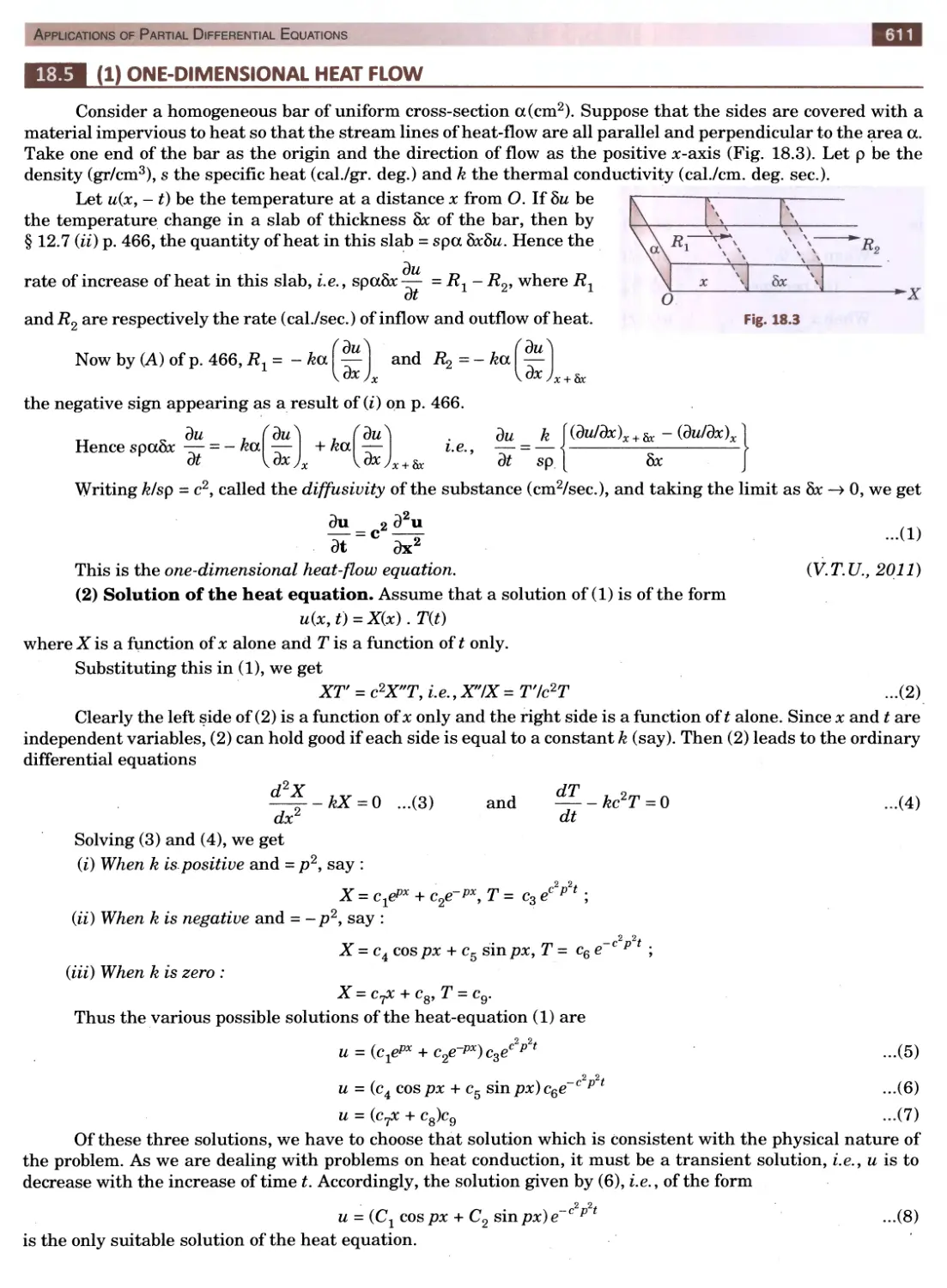
Substituting*3 = y, we get y3 - 24y2 + Sy + 1 = 0, which is the required equation.
(3) To diminish the roots of an equation f(x) = 0 by h, divide f (x) by x - h successively. Then the
successive remainders determine the coefficients of the required equation.
Let the given equation be
a^c11 + a^*11־ + ... + anlx + an = 0 ...(/)
To diminish its roots by h, put y = * - h (or * = y + h) in (/) so that
a0(y + h)n + ax(y + h)n 1־־ + ... + an = 0 ...(ii)
On simplification, it takes the form
A0yn +A1yn~1 + ... + An = 0 ...(iii)
Its coefficient A0, Av ... An can easily he found with the help of synthetic division (p. 2). For this, we put
y = x - h in (///) so that
A0 (x - h)n + Aj(* - h)n 1־ + ... + An = 0 ...(iv)
Clearly, (/) and (ia) are identical. If we divide L.H.S. of (iv) by x-h, the remainder is An and the quotient
Q =A0(x-h)n1־+A1(x-hyi~2 + ... +Anl. Similarly, if we divide Q by x-h, the remainder is Anl and the quotient
is Q1(say). Again dividing Qj by * - h, An _ 2 will be obtained as remainder and so on.
Obs. To increase the roots by /i, we take h negative.
Solution of Equations
Example 1.12. Transform the equation x3 - 6x2 + 5x + 8 = 0 into another in which the second term is
missing. Hence find the equation of its squared differences. (Cochin, 2005)
Solution. Sum of the roots of the given equation = 6.
In order that the second term in the transformed equation is missing, the sum of the roots is to be zero.
Since the equation has 3 roots, if we decrease each root by 2, the sum of the roots of the new equation will
become zero.
.־. Dividing xs - 6x2 + 5x + 8 by x - 2 successively, we have
1 -6 5 8 (2
2 -8 -6
4 -3
2 -4
-7
2
2
1 0
Thus the transformed equation is x3 - 7x + 2 = 0. ...(/)
If a, P, y be the roots of the given equation, then the roots of (£) are a - 2, p - 2, y - 2.
Let these roots be denoted by a, b, c.
Then b - c = p - y. Also a + b + c = 0, abc = - 2.
Now (b - c)2 = (b + c)2 - 2be - (a + b + c - a)2 = a2 + 4/a
a
:. The equation of squared differences of (/) is given by the transformation y = x2 + 4/x
or x3 -xy + 4 = 0 ...(H)
Subtracting (ii) from (i), we get - 7x + xy - 2 = 0 or x - 2Ky - 7)
Substituting for x in (i), the equation becomes
[2/(y-7)]3-7[2/(y-7)] + 2 = 0 or y3 - 28y2 + 245y - 682 = 0 ...(Hi)
Roots of this equation are (b - c)2, (c - a)2, (a -b)2 i.e., (p - y)2, (y - a)2, (a - p)2.
Hence (Hi) is the required equation.
WWW RECIPROCAL EQUATIONS
If an equation remains unaltered on changing x to 1/x, it is called a reciprocal equation.
Such equations are of the following standard types :
I. A reciprocal equation of an odd degree having coefficients of terms equidistant from the beginning and
end equal. It has a root = — 1.
II. A reciprocal equation of an odd degree having coefficients of terms equidistant from the beginning and
end equal but opposite in sign. It has root = 1.
III. A reciprocal equation of an even degree having coefficients of terms equidistant from the beginning and
end equal but opposite in sign. Such an equation has two roots = 1 and - 1.
The substitution x + 1/x = y reduces the degree of the equation of half its former degree.
Example 1.13. Solve 6x5 - 41x4 + 97x3 - 97x2 + 41x -6 = 0. (Coimbatore, 2001 S)
Solution. This is a reciprocal equation of odd degree with opposite signs. .״. x = 1 is a root.
Dividing L.H.S. by x - 1, the given equation reduces to
6x4 - 35x3 + 62x2 - 35x + 6 = 0
Dividing by x2, we have
6(x2 + 1/x2) - 350c + 1/x) + 62 = 0
Putting x + 1/x = y and x2 + 1/x2 = y2 - 2, we get
6(y2-2)-35y+ 62 = 0 or 6y2 - 35y + 50 = 0 or (Sy - l)(2y - 5) = 0
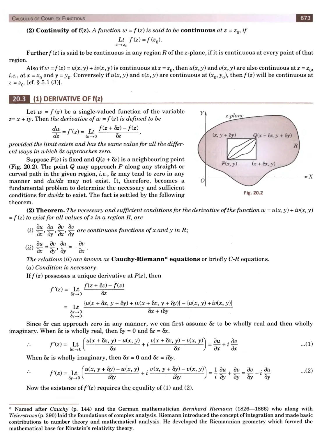
x + 1/x = y = 1/3 or 5/2
Higher Engineering Mathematics
8
i.e., 3x2 - lOx + 3 = 0 or 2x2 - 5x + 2 = 0
i.e., (Sx - l)(x - 3) = 0 or (2x - l)(x - 2) = 0
x = 1/3, 3 or 1/2, 2
Hence the required roots are 1, 1/3, 3, 1/2, 2.
Example 1.14. Solve 6x6 - 25x5 + 31x4 - 31x2 + 25x -6 = 0. (Madras, 2003)
Solution. This is a reciprocal equation of even degree with opposite signs. x = 1, - 1 are its roots.
Dividing L.H.S. by x - 1 and x + 1, the given equation reduces to
6x4 - 25x3 + 37x2 - 25x + 6 = 0
Dividing by x2, we get
6(x2 + 1/x2) - 25(x + 1/x) + 37 = 0.
Putting x + 1/x = y and x2 + 1/x2 = y2 - 2, it becomes
6(y2-2)25־y + 37 = 0 or 6y2 - 25y + 25 = 0
or (2y - 5) (3y - 5) = 0
x + 1/x = y = 5/2 or 5/3.
i.e., 2x2 - 5x + 2 = 0 or 3x2 - 5x + 3 = 0
O I/O 5±
x = 2, 1/2 or x =
6
Hence the required roots of the given equation are 1, - 1, 2, 1/2, .
PROBLEMS 1.2
1. Find the equation whose roots are 3 times the roots of x3 + 2x2 - 4x + 1 = 0.
2. Form the equation whose roots are the reciprocals of the roots of 2x5 + 4x3 - 13x2 + 7x - 6 = 0. (S.V.T. U2009)
3. Find the equation whose roots are the negative reciprocals of the roots of
x4 + 7x3 + 8x2 - 9x + 10 = 0.
4. Solve the equation 6x3 - llx2 - 3x + 2 = 0, given that its roots are in H.P.
5. Find the equation whose roots are the roots of
(i) x3 - 6x2 + llx - 6 = 0 each increased by 1. (״S.V.T. U2009)
(ii) x4 + x3 — 3x2 ־־ x + 2 = 0 each diminished by 3.
(iii) x5 - 5x4 + 10x3 - 10x2 + 5x + 6 = 0 each diminished by 1.
6. Find the equation whose roots are the squares of the roots of x3 - x2 + 8x - 6 = 0.
7. Find the equation whose roots are the cubes of the roots of x3 + px2 + q = 0.
8. If a, p, у are the roots of the equation 2x3 + 3x2 - x - 1 = 0, form the equation whose roots are (1 - a)1) ,1־ - p)1־ and
(1-y)1־.
9. If a, b, с are the roots of the equation x3 + px2 + qx + r = 0, find the equation whose roots are ab, be and ca.
(Madras, 2003)
10. If a, p, у be the roots of x3 + mx + n = 0, form the equation whose roots are
(a) a + P-у, P + Y־«. Y+“־ P. №)׳РУ«, YCi/p, ap/y (e) i + i.i + i, —+ 1
P Y Y a a P
11. Find the equation of squared differences of the roots of the cubic x3 + 6x2 + 7x + 2 = 0. .
12. Solve the equations :
(i) 6x4 + 5x3 - 38x2 + 5x + 6 = 0 (ii) 4x4 - 20x3 + 33x2 - 20x + 4 = 0. (Madras, 2003)
(iii) 8x5 - 22x4 - 55x3 + 55x2 + 22x - 8 = 0. (iv) fix5 + x4 - 43x3 - 43x2 + x + 6 = 0 (S.V.T.U., 2006)
(v) 3x6 + x5 - 27x4 + 27x2 - x — 3 = 0.
13. Show that the equation x4 — 10x3 + 23x2 - 6x - 15 = 0 can be transformed into reciprocal equation by diminishing the
roots by 2. Hence solve the equation.
14. By suitable transformation, reduce the equation x4 + 16x3 + 83x2 + 152x + 84 = 0 to an equation in which term in x3
is absent and hence solve it. (Madi'as, 2002)
Solution of Equations
EB SOLUTION OF CUBIC EQUATIONS-CARDAN'S METHOD*
Consider the equation ax3 + bx2 + cx + d = 0 ...(1)
Dividing by a, we get an equation of the form x3 + Ix2 + rax + n = 0.
To remove the x2 term, put y - x - (- Z/3) or x-y-l!3 so that the resulting equation is of the form
y3 + py + q = 0 ...(2)
To solve (2), put y = u + v
so that y3 = u3 + i?3 3 ־+־uv (u + u) = a3 + y3 + 3aiy
or y3 - 3uvy - (u3 + i>3) = 0 ...(3)
Comparing (2) and (3), we get
uv = - p/3, u3 + v3 = —q or u3 + v3 = -q and u3 v3 = - p3!21
:. u3, v3 are the roots of the equation t2 + qt- p3/27 = 0
which gives u3 = —(- q + yjq2 + 4p3/27) = Xs (say)
2
and v3 = -(- <7 - V<72 +4p3/27)
2
.״. The three values of u are A,, Axo, Axo2, where co is one of the imaginary cube roots of unity.
From uv =-p/3, we have i; = -p/3u
:. When u = X,Xco and Axo2,
JL,_£f2! and-^. Iv #.11
3X 3>. 3X
2
Hence the three roots of (2) are X —— , Axo - , Axo2 - (Being = u + v)
3A dA oA
Having known y, the corresponding values of x can be found from the relation x = y - Z/3.
Obs. 1. If one value of u is found to be a rational number, find the corresponding value of v giving one rooty = u + v.
Then find the corresponding root x = a (say). Finally, divide the left hand side of (1) by x - a, giving the remaining quadratic
equation from which the other two roots can be found readily.
Obs. 2. If u3 and v3 turn out to be conjugate complex numbers, the roots of the given cubic can be obtained in neat
forms by employing De Moivre’s theorem. (§ 19.5)
Example 1.15. Solve by Cardan's method x3 - 3x2 + 12x + 16 = 0. (U.P.T. U., 2008)
Solution. Given equation is x3 - 3x2 + 12x + 16 = 0 ...(Z)
To remove the second term from (i), diminish each root of (i) by 3/3 = 1, i.e., puty = x-l or x=y + l
[.*. Sum of roots = 3]. Then (i) becomes
(y + l)3 - 3(y + 1) + 12(y + 1) + 16 = 0 or y3 + 9y2 + 26 = 0 ...(ii)
To solve (ii), puty = u + v so thaty3 - 3uvy - (u3 + v3) = 0 ...(iii)
Comparing (ii) and (iii), we get uv = - 3 and u3 + v3 = - 26
u3, v3 are the roots of the equation t2 + 26f - 27 = 0
or (t + 27) (t - 1) = 0 whence t = - 27, t = 1.
or u3 = - 27 i.e., u = - 3 and v3 = 1 i.e.,v = l
y = u + v= -3 + l = -2 and x=y + l = — 1
Dividing L.H.S. of (i) by x + 1, we obtain x2 - 4x + 16 = 0
2
Hence the required roots of the given equation are - 1, 2 ± i 2^3.
or x =
2
*Named after an Italian mathematician Girolamo Cardan (1501—1576) who was the first to use complex number as roots of
an equation.
Higher Engineering Mathematics
10
Example 1.16. Solve the cubic equation 28x3 -9x2 + 1 = 0 by Cardan's method.
Solution. Since the term in x is missing, let us put x = 1/y in the given equation so that the transformed
equation is ys - 9y + 28 = 0 ...(i)
To solve (i), puty = u + v so thaty3 - 3uvy - (us + v3) = 0 ...(ii)
Comparing (ii) and (iii), we get uv = 3 and u3 + v3 = - 28.
u3, v3 are the roots of t2 + 28t + 27 = 0
or (t + 1) (t + 27) = 0 or Z = - 1, - 27 or u = — 1, v = — 3
.״. y = u + v = -4. Dividing L.H.S. of (i) by y + 4, we obtain y2 - 4y + 7 = 0 whence y = 2 ± i y/3.
.*. Roots of (i) are - 4, 2 ± i V3.
Hence the roots of the given cubic equation are - — or - —, (2 - iV3)/7, (2 + iV3)/7.
4 2 ± ZV3 4
Example 1.17. SoZue Z/ic equation x3 + x2 - 16x + 20 = 0.
Solution. Instead of diminishing the roots of the given equation by - 1/3, we first multiply its roots by 3,
so that the equation becomes
x3 + 3x2 - 144x + 540 = 0 ...(i)
To remove the x2 term, puty = x - (- 3/3) or x = y - 1 in (i)
so that (y - l)3 + 3(y - l)2 - 144(y - 1) + 540 = 0
or y3 - 147y + 686 = 0 ...(ii)
To solve (iii), lety = u + v, so that
y3 - 3uvy - (u3 + v3) = 0 ...(iii)
Comparing (ii) and (iii), we get
uv = 49, u3 + v3 = - 686, so that u3 v3 = (343)2.
.*. u3, v3 are the roots of the quadratic
t2 + 686Z + (343)2 = 0 or (t + 343)2 = 0
t = - 343 i.e., u3 = v3 = - 343 or u = v = — 1.
Thus y = u + v~ —14 and x = y - 1 = - 15.
Dividing L.H.S. of (i) by x + 15, we get
(x - 6)2 = 0 or x = 6, 6.
.״. The root of (i) are - 15, 6, 6.
Hence the roots of the given equation are - 5, 2, 2.
Example 1.18. Solve x3 - 3x2 + 3 = 0. (S. V. T. U., 2006)
Solution. Given equation is x3 - 3x2 + 3 = 0 ...(i)
To remove the x2 term, put y = x - 3/3 or x = y + 1,
so that (i) becomes (y + l)3 - 3(y + l)2 + 3 = 0
or y3-3y + l = 0 ...(ii)
To solve it, put y = u + v
so that y3 - 3uvy - (u3 + v3) = 0 ...(iii)
Comparing (ii) and (iii), we get uv = 1, u3 + v3 = - 1
.-. u3, v3 are the roots of the equation t2 + t + 1 = 0
u o — 1 + iyj3 , o —־־■ 1 ־ W3
Hence ua = and v^ = —
2 2
( \J—1
u = ^ —-—j put - — = r cos 0 and V3/2 = r sin 0
= [r (cos 0 + i sin 0)]1/3 so that r = 1, 0 = 2tz/3
= fcos (0 + 2nn) + i sin (0 + 2nn)]1/3,
where n is any integer or zero. Using De Moivre’s theorem (p. 647).
11
Solution of Equations
(0 + 2
u = cos + I sin
^0 + 2mC
L 3 j
Giving n the value 0, 1, 2 successively we get the three values of u to be
0 . . 0 0 + 2tt . . 0 + 2tc 0 + 0 + 47!
cos — + ism — , cos + sin , cos + i sin
3 3 3 3 3 3
2it . . 27 i87! . . 8tt 147! . .
i.e., cos -— + i sm — , cos — + i sm — , cos + i sm .
9 9 9 9 9 9
The corresponding values of v are
271 . . 27t 87c . . 871 147! . . 14ti
cos 1 sm — , cos — -1 sm — , cos 1 sm .
9 9 9 9 9 9
.׳. The three values of y — u + v are 2 cos 271/9, 2 cos 8jt/9, 2 cos 147i/9.
Hence the roots of (/) are found from 1 + y to be
1 + 2 cos 27i/9, 1 + 2 cos 87i/9, 1 + 2 cos 147t/9.
PROBLEMS 1.3
Solve the following equations by Cardan’s method :
1. x3 - 27 x + 54 = 0. (U.P.T.U., 2003) 2. x3 -18* + 35 = 0
3. x3 — 15 x = 126 (S.V. T. U., 2009) 4. 2x3 + 5x2 + x - 2 = 0 (U.P. T. 2003)
5. 9x3 + 6x2-1 = 0 (S.V.T.U., 2008)6. x3-6x2 + 5 = 0
7. x3 - 3* + 1 = 0 & 27*3 + 54*2 + 198* - 73 = 0
WE■ SOLUTION OF BIQUADRATIC EQUATIONS
(1) Ferrari^ method
This method of solving a biquadratic equation is illustrated by the following examples :
Example 1.19. Solve the equation x4 - 12x3 + 41x2 - 18x -72 = 0 by Ferrari’s method. (S.V.T.U., 2007)
Solution. Combining x4 and x3 terms into a perfect square, the given equation can be written as
(x2 -6x + X)2 + (5 - 2X)x2 + (12A - 18)x - (X2 + 72) = 0
or (x2 -6x + X)2 = {(2X - 5)x2 + (18 - 12X) x + (A2 + 72)} ...(i)
This equation can be factorised if R.H.S. is a perfect square
i.e., if (18 - 12A)2 = 4(2A- 5) (X2 + 72) Ib2 = 4ac]
i.e., if 2A3 - 41A2 + 252A - 441 = 0 which gives X = 3.
(i) reduces to (x2 - 6x + 3)2 = (x - 9)2
i.e., (x2 - 5x - 6) (x2 -Ix + 12) = 0.
Hence the roots of the given equation are - 1, 3, 4 and 6.
Example 1.20. Solve the equation x4 - 2x3 - 5x2 + 10 x - 3 = 0 by Ferrari s method.
Solution. Combining x4 and x3 terms into a perfect square, the given equation can be written as
(x2 - x + X)2 = (2X + 6) x2 - (2X + 10) x + (A2 + 3). This equation can be factorised, if R.H.S. is a perfect square i.e.,
if (2A + 10)2 = 4(2A + 6) (A2 + 3) [b2 = 4ac]
or 2A3 + 5A2 - 4A - 7 = 0, which gives A = - 1.
.״. (i) reduces to (x2 - x - l)2 = 4x2 - 8x + 4
or (x2 - x - l)2 - (2x - 2)2 = 0 or (x2 + x - 3) (x2 - 3x + 1) = 0
-l±Jl + 12 3 ± J9 - 4
~ - v - or
2
l±Vl3 3±V5
Hence the roots are
Higher Engineering Mathematics
12
(2) Descarte’s method
This method of solving a biquadratic equations consists in removing the term in x3 and then expressing the
new equation as product of two quadratics. It has been best illustrated by the following examples :
Example 1.21. Solve the equation x4 - 8x2 - 24x + 7 = 0 by Descarte’s method. (U.P.T. U.f 2001)
Solution. In the given equation, the term in x3 is already absent so we assume that
x4 - 8x2 - 24x + 7 = (x2 + px + q) (x2 -px + q) ...(i)
Equating coefficients of the like powers of x in (/), we get
- 8 = q + q’-p2, - 24 = p(q׳ - q); 7 = qq
q + q' = p2 - 8, q - q' = 24/p
(p2 — 8)2 — (24/p)2 = 4x7
p2 - 16p4 + 36p2 - 576 = 0 or t3 - 16t2 + 36Z - 576 = 0 where t = p2
Now t = 16 satisfies this cubic so that p = 4.
q + q8 = ׳, q - q' = 6 .־. q = 7, q1 = ׳
Thus (i) takes the form (x2 + 4x + 7) (x2 - 4x + 1) = 0
- 4 ± Jm- 28) 4 ± M - 4)
whence x = or x =
2 2
Hence x = - 2 ± V3i, 2 ± V3.
Example 1.22. Solve the equation x4 - 6x3 - 3x2 + 22x - 6 = 0 by Descarte’s method.
Solution. Here sum .of roots = 6 and number of roots = 4
.־. To remove the second term, we have to diminish the roots by 6/4 (= 3/2) which will be a problem.
Therefore, we first multiply the roots by 2. .*. y4 - 12y3 + 12y2 + 176y - 96 = 0 where y = 2x. Now diminishing
the roots by 3, we obtain z4 - 42z2 + 32z + 297 = 0 where z = y - 3.
Assuming that z4 - 42z2 + 32^ + 297 = (z2 + pz + q) (z2 -pz + q') ...(i)
and comparing coefficients, we get
- 42 = q + q' - p2 ; 32 = p (q' - q) ; 297 = q q'
q + q' = p2 - 42 ; q - q' = - 32/p, qq' = 297
(p2 - 42)2 - (- 32/p)2 = 4 x 297
or t3 -84 t2 + 576t - 1024 = 0 where t = p2
Now t = 4 satisfies this cubic so that p = 2.
q + q38- = ׳,q-q' = -16, .־. q = - 27, q11 - = ׳.
Thus (i) takes the form (z2 + 2z - 27) (z2 - 2z - 11) = 0
Whence 4)2±7-״TT08) or =
2 2
or *=iy=l(* + 3) = I (2 ± >/28 ) = I (4 ± >/12 )
2 2 2 2
Hence x = 1 ± V2 , 7׳ ± V3.
PROBLEMS 1.4
Solve by Ferrari’s method, the equations :
1. x4 - 10x3 + 35x2 - 50x + 24 = 0 (U.P. T. U.} 2003) 2. x4 + 2x3 - 7x2 - 8x + 12 = 0 (U.P. T. U., 2002).
3. x4 - 10x2 - 20x - 16 = 0 4. x4 — 8x3 - 12x2 + 60x + 63 = 0 (U.P.T.U., 2005),
Solve the following equations by Descartes method :
5. x4 - 6x3 + 3x2 + 22x -6 = 0 6. x4 + 12x -5 = 0
7. x4 - 8x3 - 24x + 7 = 0 (U.P.T. U.f 2001) 8. x4 - 10x3 + 44x2 - 104x + 96 = 0
Ohs. We have obtained algebraic solutions of cubic and biquadratic equations. But the need often arises to solve
higher degree or transcendental equations for which no algebraic methods are available in general. Such equations can be
best solved by graphical method (explained below) or by numerical methods (§28.2).
Solution of Equations
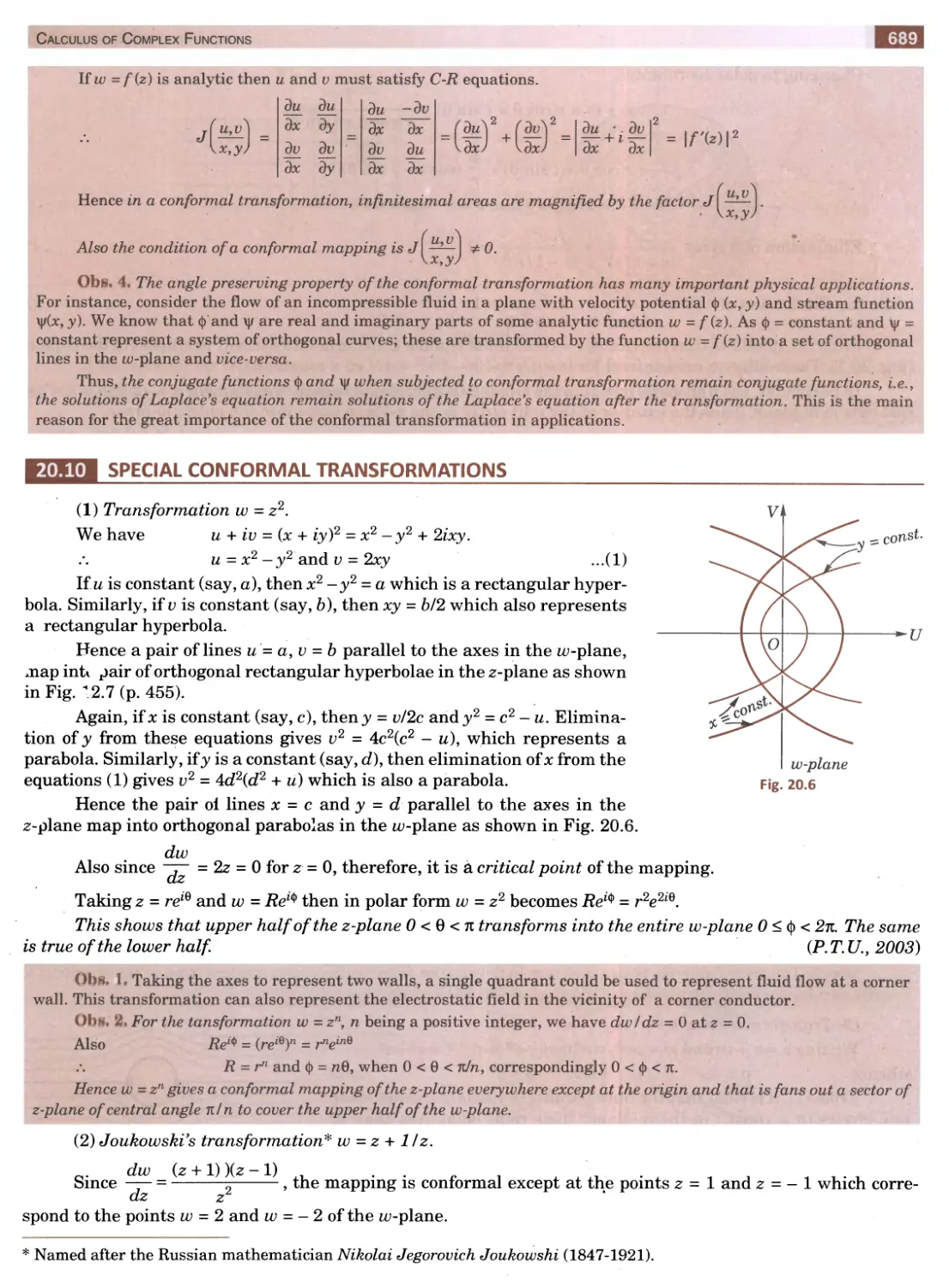
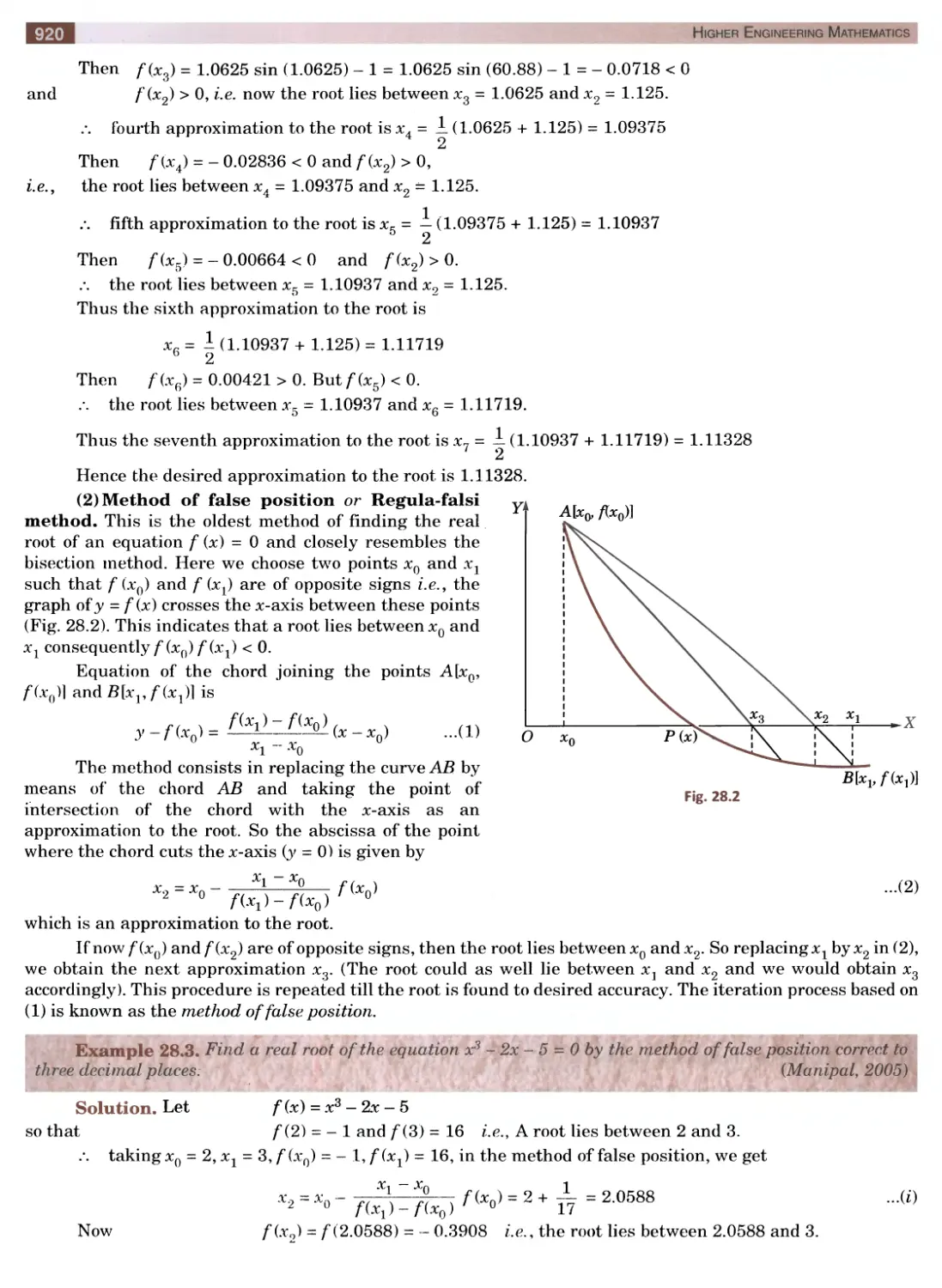
GRAPHICAL SOLUTION OF EQUATIONS
Let the equation be f(x) = 0.
(i) Find the interval (a, b) in which a root of f(x) = 0 lies.
[At least one root of fix) = 0 lies in (a, b) if f(a) and f(b) are of opposite signs—§1.2(111) p. 2].
(ii) Write the equation f(x) = 0 as §(x) = \|/0c) where \|f(x) contains only terms in x and the constants.
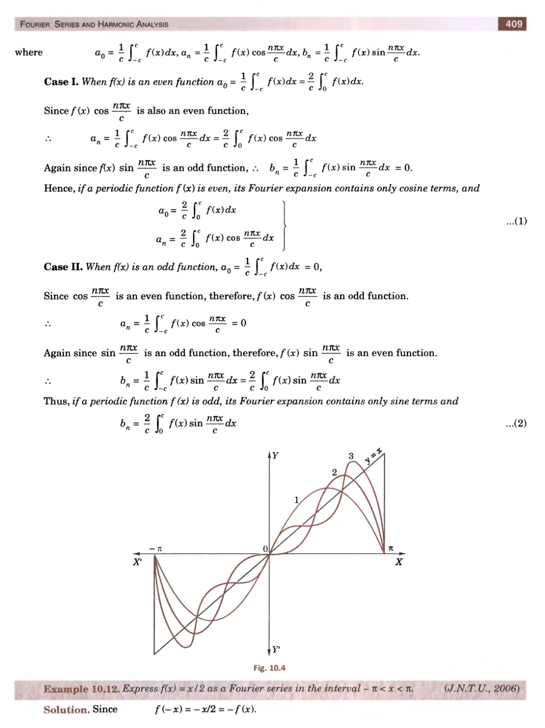
(iii) Draw the graphs ofy = §(x) and y - \\f(x) on the same scale and with respect to the same axes.
(iv) Read the abscissae of the points of intersection of the curves y = <|) (x) andy = \|f(x). These are required real
roots off(x) = 0.
Sometimes it may not be convenient to write the given equation f(x) = 0 in the form <|) (x) = \|/(jc). In such cases, we
proceed as follows :
Ci) Form a table for the value of x andy = fix) directly.
(ii) Plot these points and pass a smooth curve through them.
(iii) Read the abscissae of the points where this curve cuts the *־axis. These are the required roots of
f(x) = 0.
Obs. The roots, thus located graphically are approximate and to improve their accuracy, the curves are replotted on
the larger:scale in the immediate vicinity of each point of intersection. This gives a better approximation to the value of
desired root. The above graphical operation may be repeated until the root is obtained correct upto required number of
decimal places. But this method of repeatedly drawing graphs is very tedious. It is, therefore, advisable to improve upon
the accuracy of an approximate root by numerical method of §28.2.
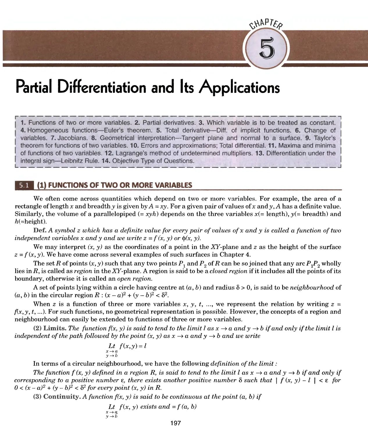
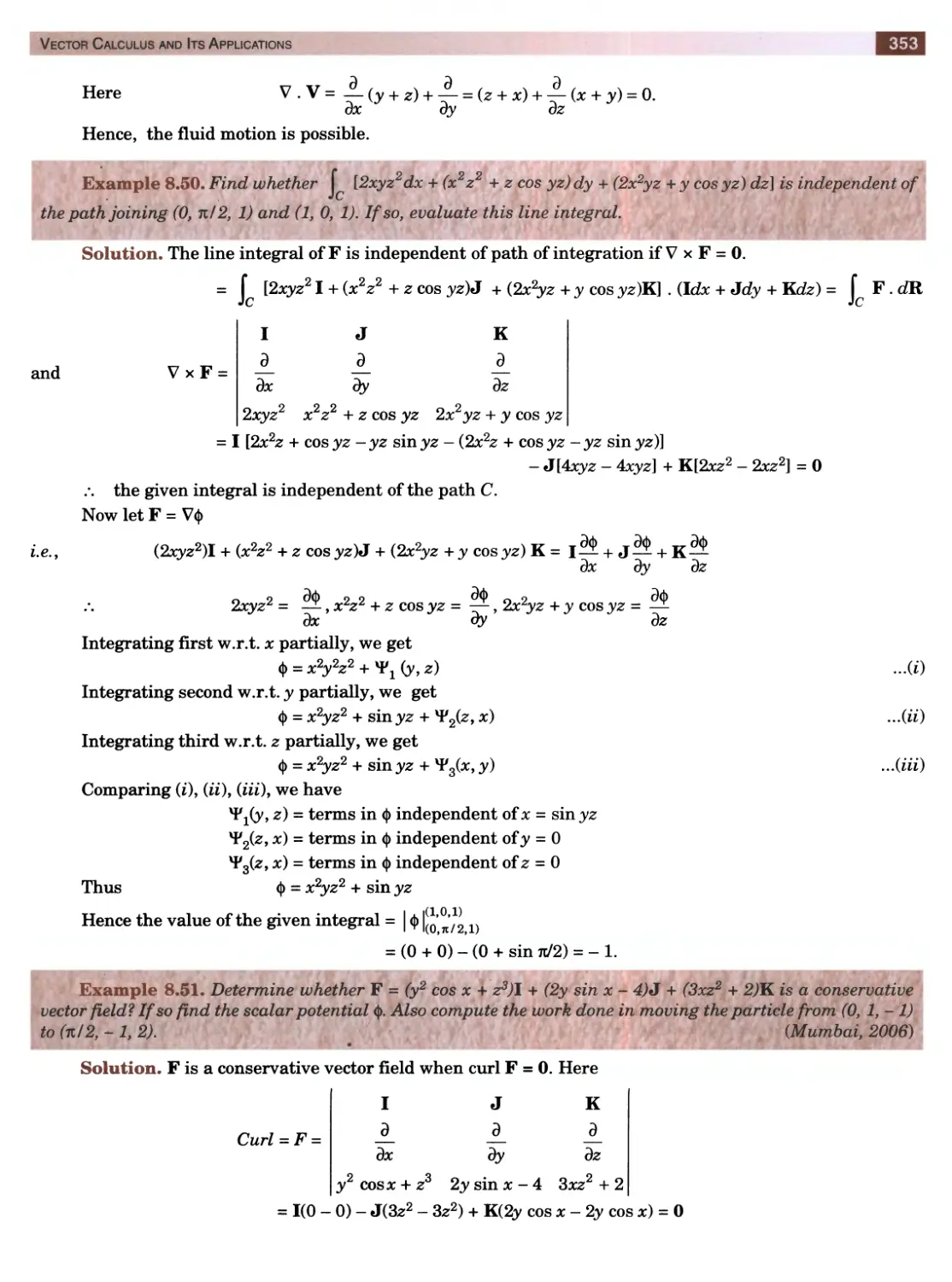
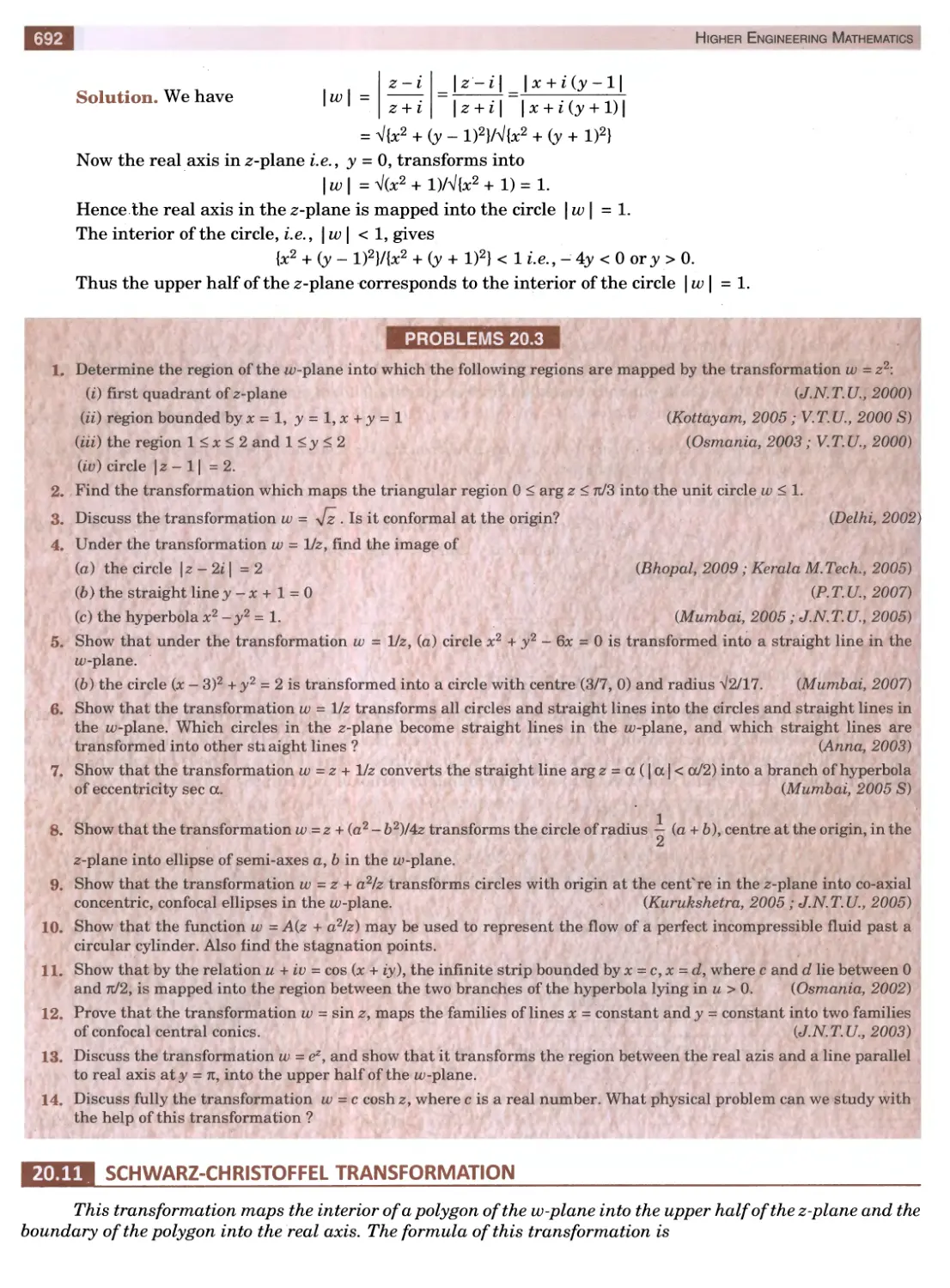
Example 1.23. Find graphically an approximate value of the root of the equation.
3-x = ex~1.
(*)״.
and
Solution. Let f(x) = ex 1 + x - 3 = 0
f( 1)= 1 + l-3 = -ve
f(2) = e + 2 - 3 = 2.718 - 1 = + ve
A root of (/), lies between x = 1 and x = 2.
Let us rewrite (i) as ex~1 = 3 — x.
The abscissa of the point of intersection of the curves
y = ex~1 ...(ii)
y = 3 — x ...(iii)
will give the required root.
To plot (ii), we form the following table of values :
and
X =
y =ex~l
1.1
1.11
1.2
1.22
1.3
1.35
1.4
1.49
1.5
1.65
1.6
1.82
1.7
2.01
1.8
2.23
1.9
2.46
2.0
2.72
Fig. 1.2
Taking the origin at (1,1) and 1 small unit along either
axis = 0.02, we plot these points and pass a smooth curve
through them as shown in Fig. 1.2.
Higher Engineering Mathematics
14
To draw the line (iii), we join the points (1, 2) and (2, 1) on the same scale and with the same axes.
From the figure, we get the required root to be x - 1.44 nearly.
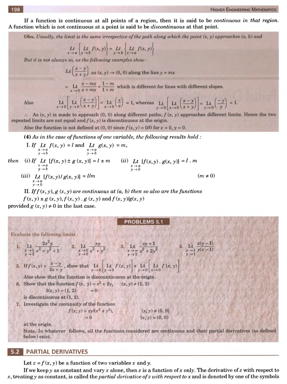
Example 1.24. Obtain graphically an approximate value of the root ofx = sin x + ill 2.
Solution. Let us write the given equation as sin x = x - id2
The abscissa of the point of intersection of the curve y - sin x
and the line y = x - n!2 will give a rough estimate of the root.
To draw a curve y = sin x, we form the following table :
x 0 Tl/4 ti/2 3ji/4 71
y 0 0.71 1 0.71 0
Taking 1 unit along either axis = n/4 = 0.8 nearly, we plot the
curve as shown in Fig. 1.3.
Also we draw the line y = x - n!2 to the same scale and with
the same axis.
From the graph, we get x = 2.3 radians approximately.
Fig. 1.3
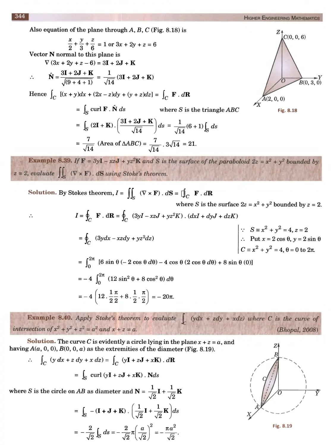
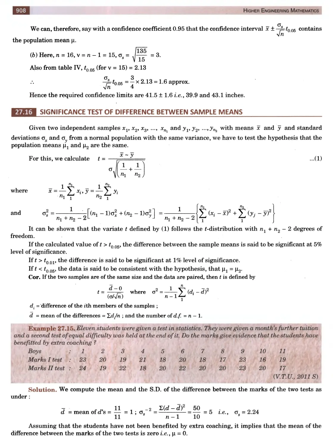
Example 1.25. Obtain graphically the lowest root of cos x cosh x - - 1.
Solution. Let f[x) = cos x cosh x + 1 = 0
f(0) = + ve,f(nJ2) = + ve and f(n) = - ve.
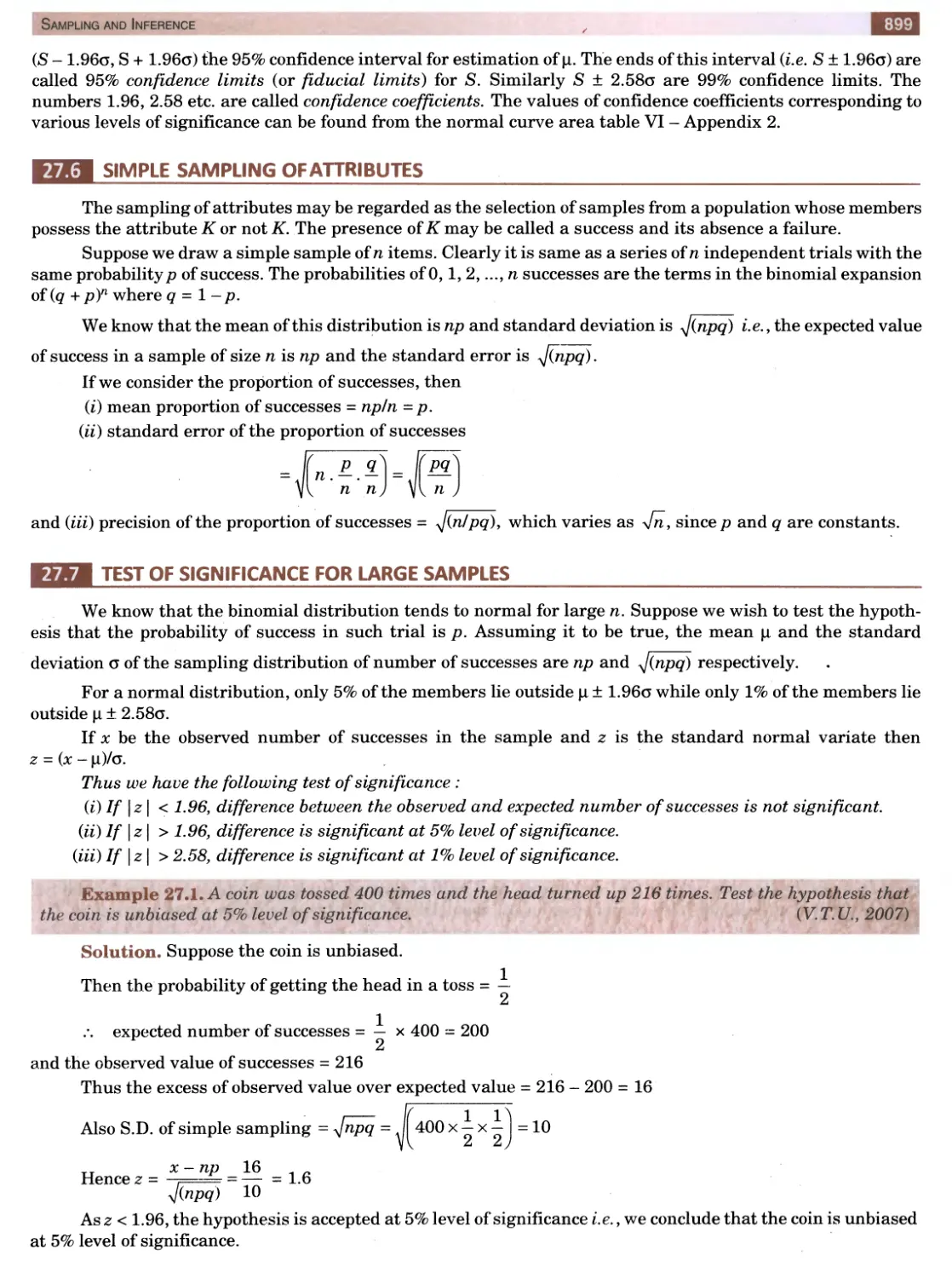
.*. The lowest root of (i) lies between x = nl2 and x = n.
Let us write (i) as cos x = - sech x.
The abscissa of the point of intersection of the curves
y = cos x ...(ii) and y = - sech x
will give the required root. To draw (ii), we form the following table of values :
X =
71/2 = 1.57
371/4 = 2.36
3.14 ־־ %
y = COS X
0
-0.71
-1
Taking the origin at (1.57, 0) and 1 unit along either axes = n/8 = 0.4 nearly, we plot the cosine curve as
shown in Fig. 1.4.
To draw (iii), we form the following table :
x = 1.57
coshx= 2.58
y = - sech x -0.39
2.36 3.14
5.56 11.12
-0.18 -0.09
...(iii)
15
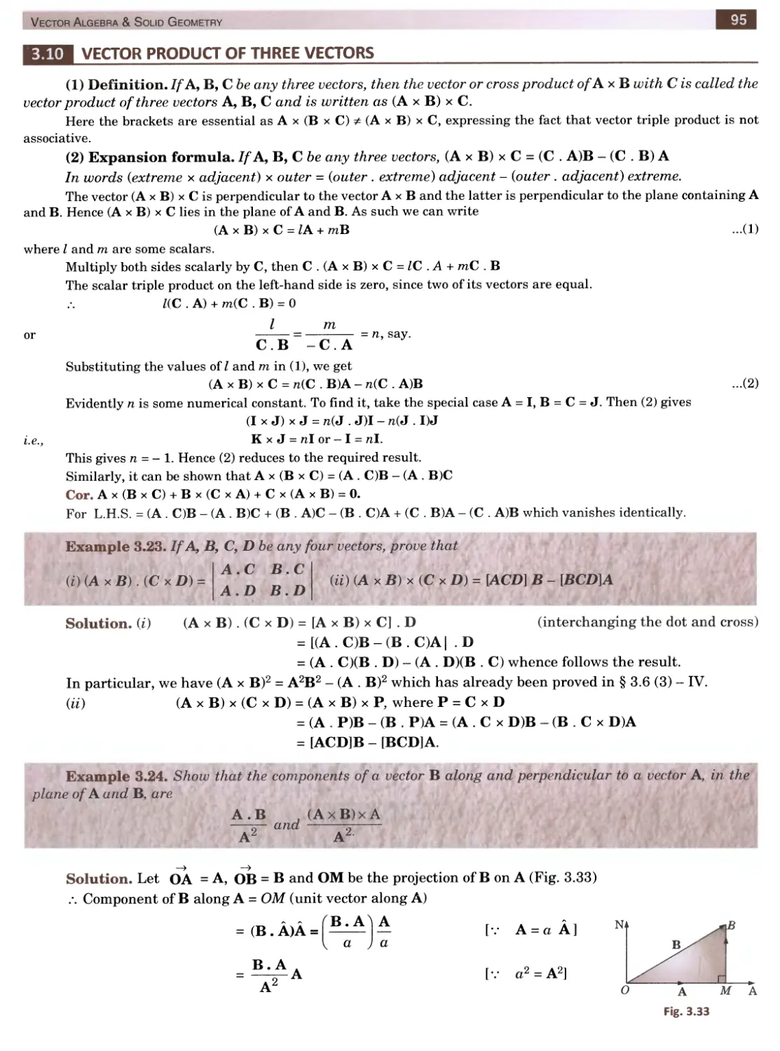
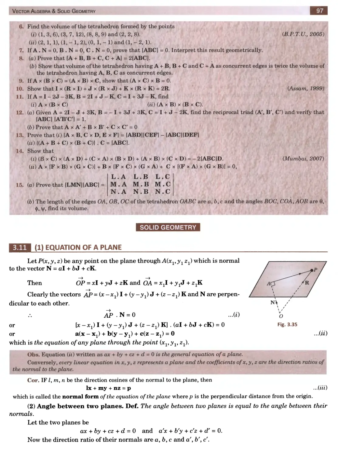
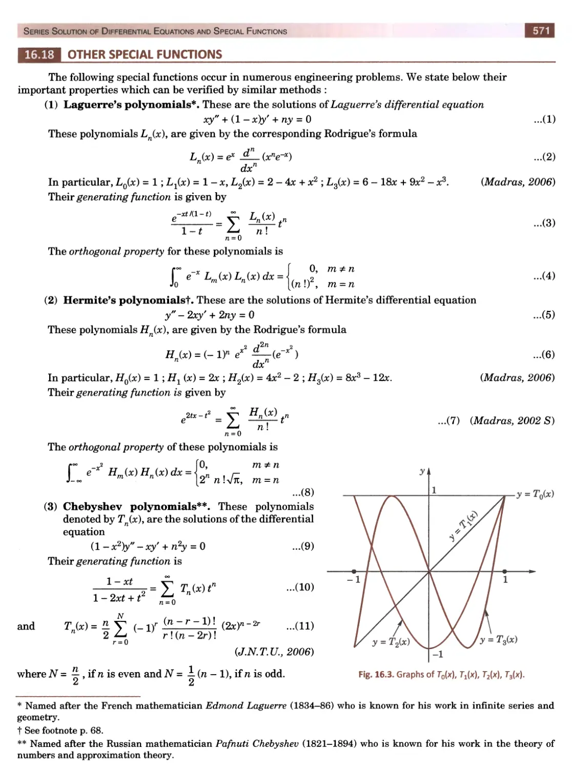
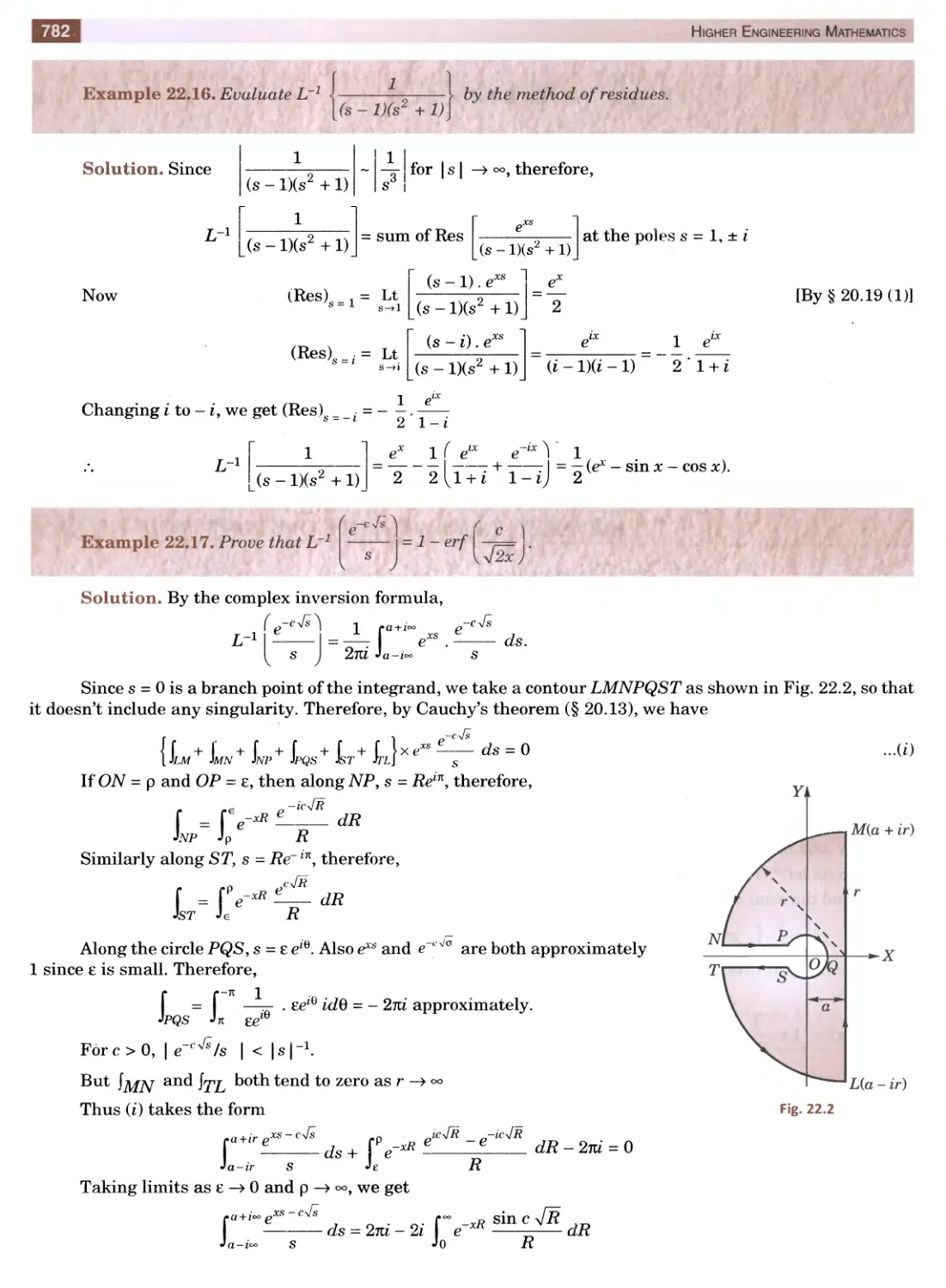
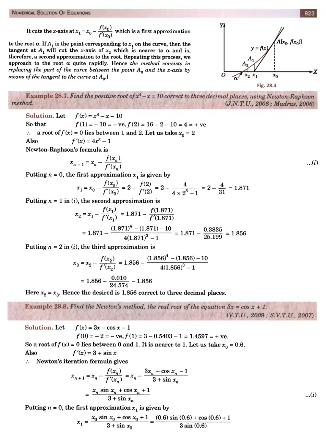
Solution of Equations
Then we plot the curve (iii) to the same scale with the same axes.
From the figure we get the lowest root to be approximately x = 1.57 + 0.29 = 1.86.
PROBLEMS 1.5
Solve the following equations graphically :
1. xs - x -1 = 0 {Madras, 2000 S)
*
CO
I
S?
I
<2\
II
o
3. x3 - 6x2 + 9x - 3 = 0.
4. tan# = 1.2as
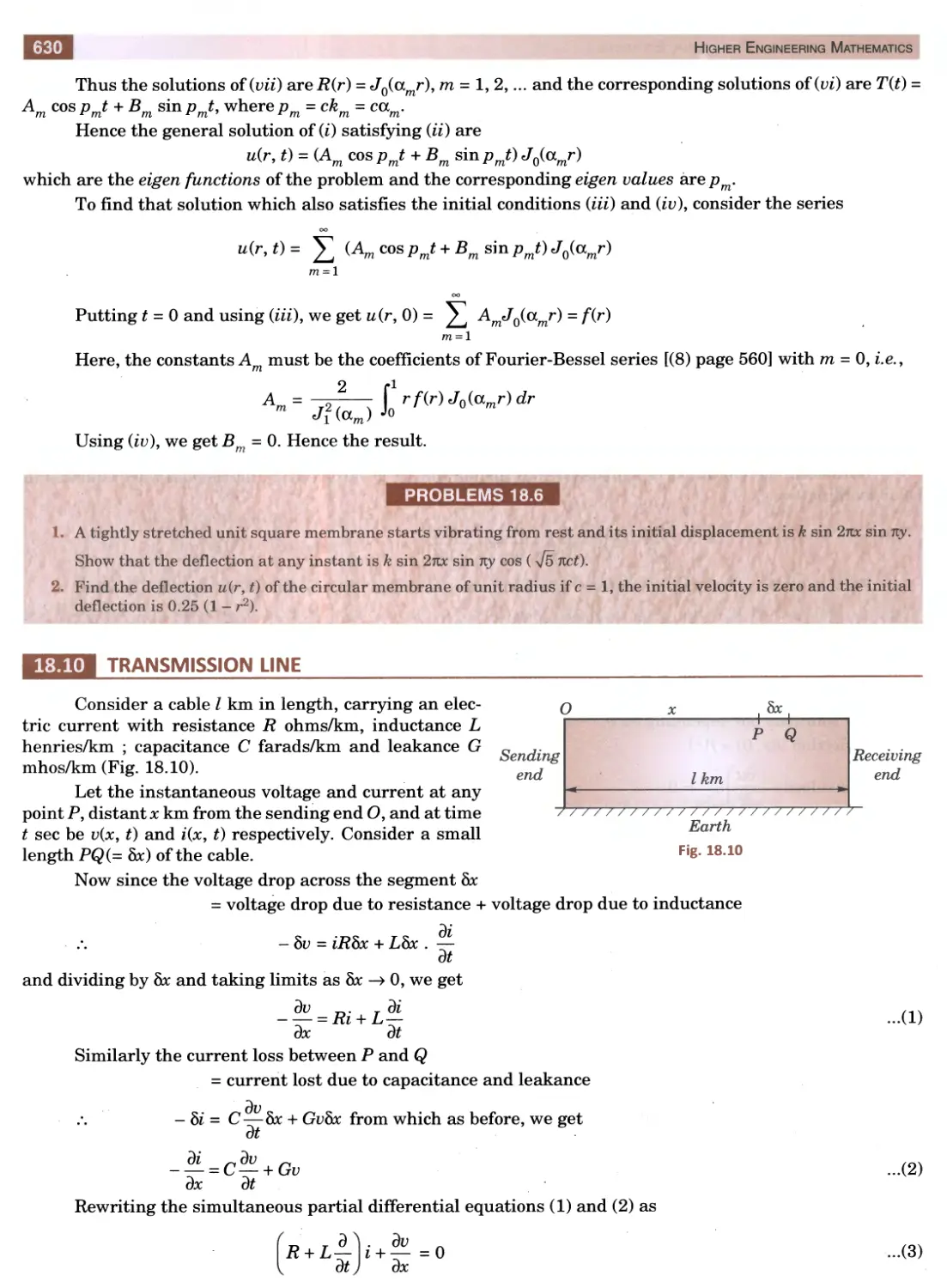
5. x = 3 cos (x - n/4)
6. e* = 5ac which is near a: = 0.2.
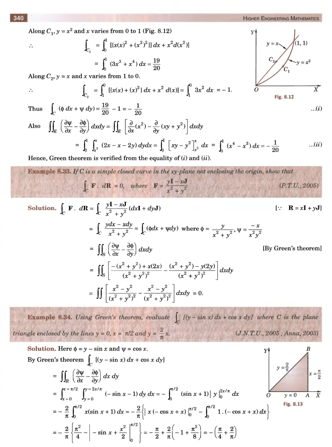
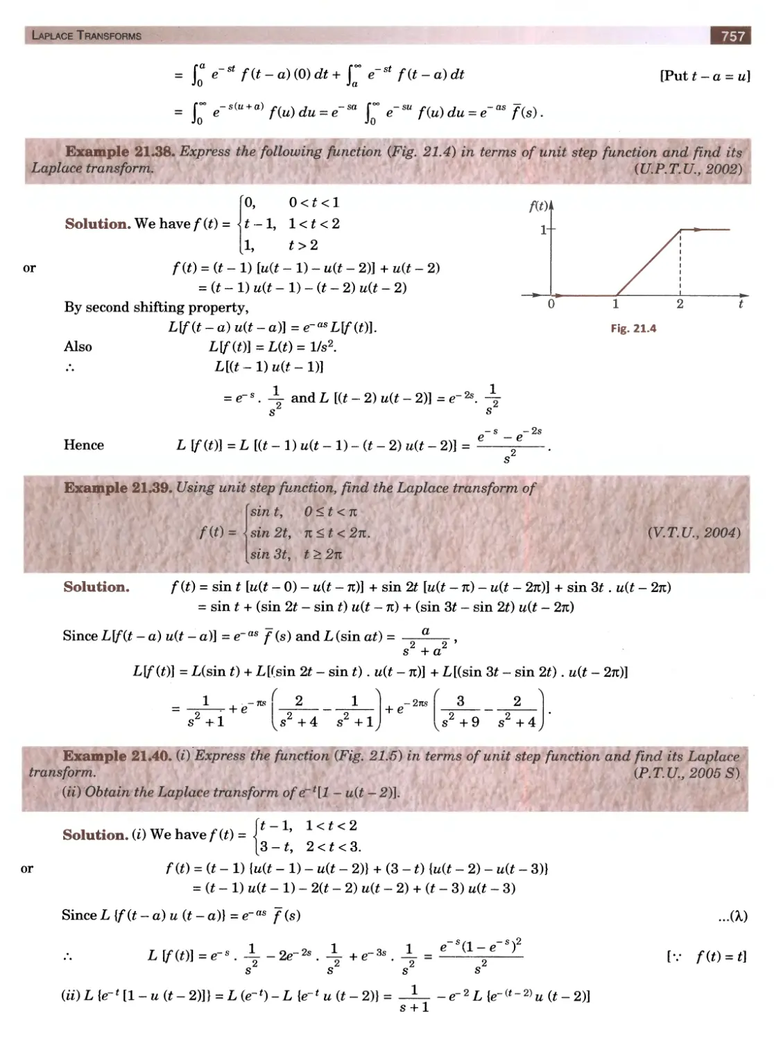
EQ OBJECTIVE TYPE OF QUESTIONS
PROBLEMS 1.6
Choose the correct answer or fill up the blanks in the following problems :
1. If for the equation x3 - 3x2 + kx + 3 = 0, one root is the negative of another, then the value of k is
(a) 3 (6) -3
(c)l
id) - 1.
2. If the roots of the equation xn - 1 = 0 are 1, av a2, , an v then
(1 - ax) (1 - a2) (1 - an x) is equal to
(a) 0 (b) 1
(c) n
( d) n + 1.
3. If a, ß, y are the roots of 2x3 - 3x2 + 6x + 1 =
0, then a2 + ß2 + ׳y2 is
(a) 15/4 (ft)-3
(c) -15/4 (d) 33/4.
4. x + 2 is a factor of
(a) x4 + 2
(6) X4 -X
2+ 12
(c) x4 - 2x3 - x + 2
(d)x4 + 2x3-x-2
5. If a + (3 + y = 5 ; a(3 + py + ya = 7 ; aPy = 3, then the equation whose roots are a, P and y is
(a) x3-7 = 0
(6) x3 - lx2 +3 = 0
(c) x3 - 5x2 + 7x - 3 = 0
(d) x3 + lx2-Z = 0.
6. If one of the roots of the equation x3 - 6x2 + lLr - 6 = 0 is 2, then the other two roots are
(a) 1 and 3
(6) 0 and 4
(c) - 1 and 5
(d) - 2 and 6.
7. The equation whose roots are the reciprocals of the roots of x3 + px
2 + r = 0 is
(a) x3 + 1/p.x2 + 1/r = 0
(6) 1/r . x3 + 1/p.x +1 = 0
(c) rx3 + px2 +1 = 0
(d) rx3 + px + 1 = 0.
8. If 1 and 2 are two roots of the equation x4 -
-as3 - 19a:2 + 49as - 30 = 0, then the remaining two roots are
(a) 3 ־־ and 5
(6) 3 and
-5
(c) - 6 and 5
(d) 6 and
-5.
9. If the roots of x3 - 3x2 + px + 1 = 0, are in arithmetic progression, then the sum of squares of the largest and the
smallest roots is
(a) 3 (6) 5
(0 6
(d) 10.
10. A root of x3 - 8x2 + px + q = 0 where p and q are real numbers is 3 + i >/3 . The real root is
(a) 2 (6) 6
(0 9
(d) 12.
11. One of the roots of the equation fix) = xn + a
,as" 1 + ... +a.x + a0 =0 where a0, a,, ...a ,are real, is given to be 2 — 3
Of the remaining, the next n - 2 roots are given to be 1, 2, 3,..., n -
■ 2. The nth root is
(a) n (b) n - 1
(c) 2 + 3i
(d) - 2 + 3
12. If a real root of fix) = 0 lies in [a, 6], then the sign of f{a).f(b) is
13. Descartes rule of signs states that
14. If a, ß, y are the roots of the equation x3 -px + q - 0, then E 1/a = ...
15. If a, ß, y are the roots of x3 = 7, then Ea3 is .
16. One real root of the equation x3 + 2x2 + 5 = 0 lies between
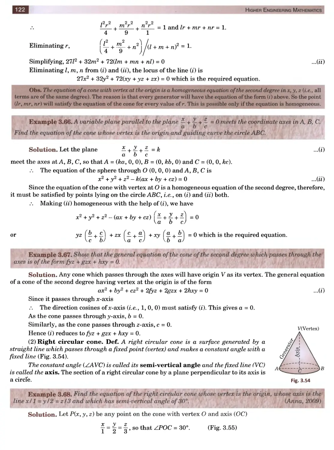
Higher Engineering Mathematics
16
17. In an equation with real coefficients, imaginary roots must occur in
18. If f (cc) and /,(P) are of opposite signs, then fix) = 0 has at least one root between cc and P provided
19. If a, P, y are the roots of the equation x3 + 2x + 3 = 0, then cc + 3, P + 3, y+3 are the roots of the equation
20. If one root is double of another in x3 - 7x20 = 36 +״, then its roots are
21. The equation whose roots are 10 times those x3 - 2x - 7 = 0, is
22. If cc, P, y are the roots of x3 + px2 + qx + r = 0, then I (1/ccP) =
23. V3 and —1 + i are the roots of the biquadratic equation
24. If oc, p, y are the roots of x3 - 3x + 2 = 0, then the value of a2 + P2 + y2 is
25. If there is a root of fix) = 0 in the interval [a, 6], then sign of fia)/fib) is
26. If cc, P, y are the roots of x3 + px2 + qx + r = 0, then the condition for oc + P = 0 is
27. The three roots of x3 = 1 are
28. One real root of the equation x3 + x - 5 = 0 lies in the interval
(i) (2, 3), Hi) (3, 4), HU) (1, 2), Hv) (- 3, - 2)
29. If two roots of x3 - 3x2 + 2-0 are equal, then its roots are
30. The cubic equation whose two roots are 5 and 1 - i is
31. The sum and product of the roots of the equation x5 = 2 are and
32. If the roots of the equation x4 + 2x3 - ax2 - 22x + 40 = 0 are - 5, - 2, 1 and 4, then a =
33. A root of x3 - 3x2 + 2.5 = 0 lies between 1.1 and 1.2. (True or False)
34. The equation x6 - x5 - lOx +7 = 0 has four imaginary roots. (True or False)
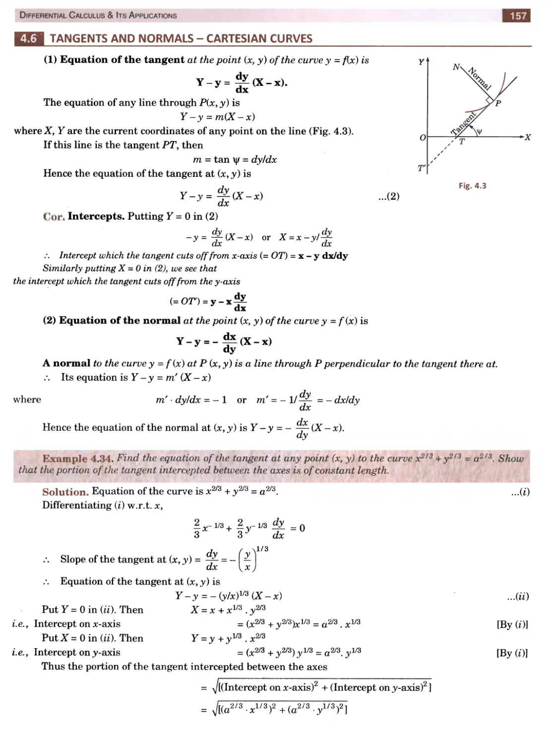
Linear Algebra : Determinants, Matrices
| 1. Introduction. 2. Determinants, Gofactors, Laplace’s expansion. 3. Properties of determinants. 4. Matrices* i
I Special matrices. 5. Matrix operations. 6. Related matrices. 7. Rank of a matrix, Elementary transformations, !
, Elementary matrices, Inverse from elementary matrices, Normal form of a matrix. 8. Partition method. 9. Solution ,
of linear system of equations. 10. Consistency of linear system of equations. 11. Linear and orthogonal
״ transformations. 12. Vectors ; Linear dependence. 13. Eigen values and eigen vectors. 14. Properties of eigen ■
I values. 15. Cayley-Hamifton theorem. 16. Reduction to diagonal form. 17. Reduction of quadratic form 16 I
I canonical form. 18. Nature of quadratic form. 19. Complex matrices. 20. Objective Types of Questions,
i — m ■ . - i L j
INTRODUCTION
Linear algebra comprises of the theory and applications of linear system of equation, linear
transformations and eigen value problems. In linear algebra, we make a systematic use of matrices and to a lesser extent
determinants and their properties.
Determinants were first introduced for solving linear systems and have important engineering
applications in systems of differential equations, electrical networks, eigen-value problems and so on. Many
complicated expressions occurring in electrical and mechanical systems can be elegently simplified by expressing them
in the form of determinants.
Cayley* discovered matrices in the year 1860. But it was not until the twentieth century was well-
advanced that engineers heard of them. These days, however, matrices have been found to be of great utility in
many branches of applied mathematics such as algebraic and differential equations, mechanics theory of
electrical circuits, nuclear physics, aerodynamics and astronomy. With the advent of computers, the usage of matrix
methods has been greatly facilitated.
WSM DETERMINANTS
is called a determinant of the second order and stands for
bo
a0
(1) Definition. The expression
-- a2bf. It contains 4 numbers av bv a2, b2 (called elements) which are arranged along two horizontal lines
(called rows) and two vertical lines (called columns).
is called a determinant of the third order. It consists of 9 elements which are
Similarly,
arranged in 3 rows and 3 columns.
*Arthur Cayley (1821-1895) was a professor at Cambridge and is known for his important contributions to algebra, matrices
and differential equations.
Higher Engineering Mathematics
18
dy...ly
22 b2 C2 ^2 * 2^ ־ ־
dn-׳ln
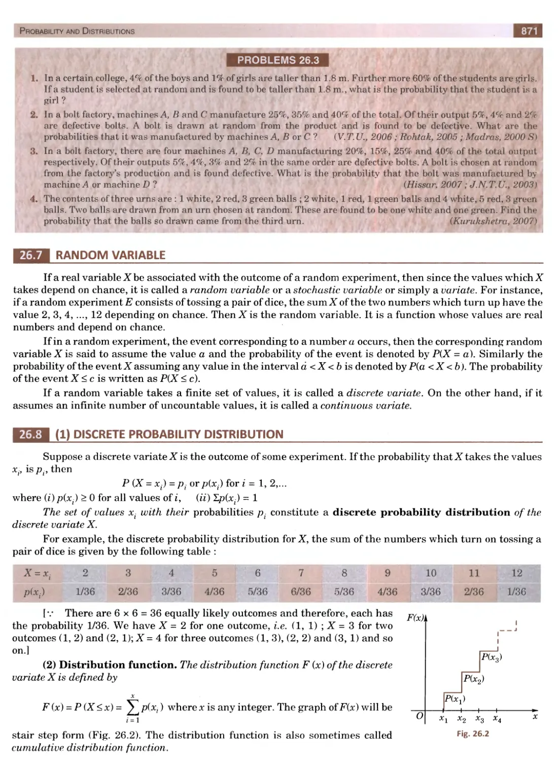
an bn Cn
In general, a determinant of the nth order is denoted by
which is a block of n2 elements arranged in the form of a square along n-rows and n-columns. The diagonal
through the left hand top corner which contains the elements av b2, c3, ... ln is called the leading or principal
diagonal.
(2) Cofactors
The cofactor of any element in a determinant is obtained by deleting the row and column which intersect
in that element with the proper sign. The sign of an element in the ith row and jth column is (— l)1 The cofactor
of an element is usually denoted by the corresponding capital letter.
a! by cx
ax
°3
and C2 = -
a!
a2 c2
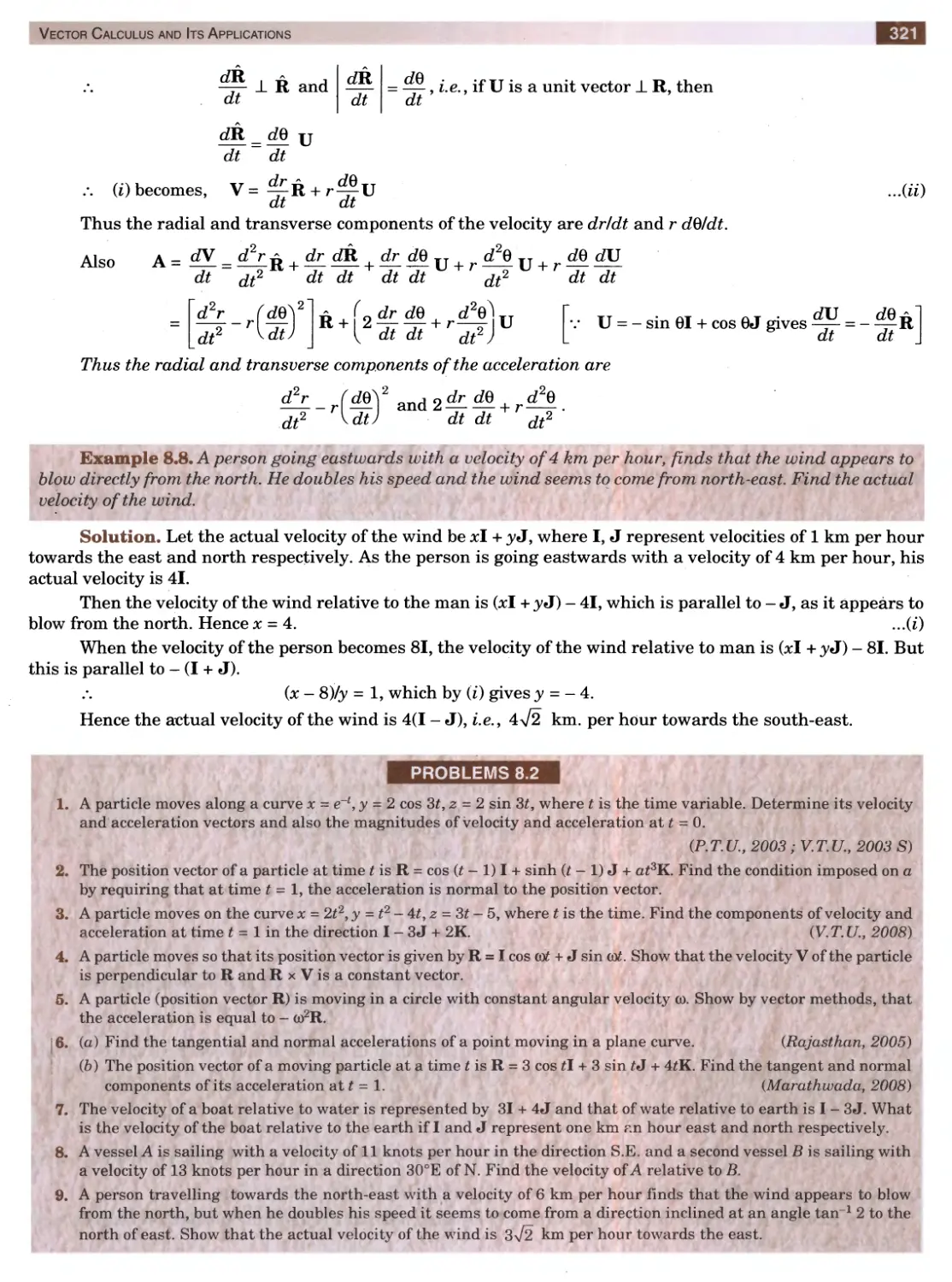
, the cofactor of 6״ i.e., B3 = (- l)3 + 2
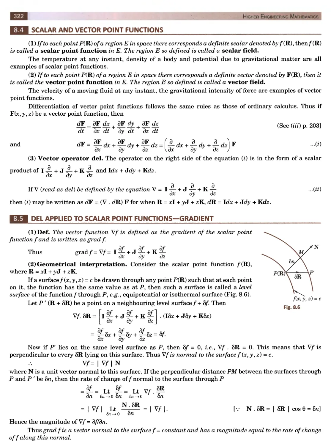
For instance, in A =
a2 b2 c2
a3 h c3
(3) Laplace’s expansion.* A determinant can be expanded in terms of any row (or column) as follows :
Multiply each element of the row (or column) in terms of which we intend expanding the determinant, by its
cofactor and then add up all these terms.
:. Expanding by Rx (i.e., 1st row),
A = ayAy ־+־ byBy + CyCy = ay
^2 c2
i
a2 c2
a2 b2
-b!
+
b3 c3
a3 c3
a3 b3
= ay(b2cs - bsc2) - by(a2cs - asc2) + Cy(a2b3 - a3b2)
Similarly, expanding by C2 (i.e., 2nd column)
a! cy
a2 c2
-b3
a! c!
a3 c3
+ b2
A — byBy + &2^2 + b3B3 — — by
a2 c2
a3 c3
= - by(a2c3 - a3c2) + b2(ayC3 - a3Cy) - b3(ayC2 - a2c1)
and expanding by R3 (i.e., 3rd row), A = a^3 + b3B3 + c3C3.
Thus A is the sum of the products of the elements of any row (or column) by the corresponding cofactors.
If, however, the sum of the products of the elements of any row (or column) by the cofactors of another row
(or column) be taken, the result is zero.
e.g., in A, a3^2 + b3&2 + c3^2 = ~a3
= - a3(byC3 - b3Cy) + b3(axc3 - a3Cy) - c3(a^b3 - a3bf) = 0
In general, a-A■ + b-B- + c-C- = A when i = j
i j i j i j
= 0 when i^j
h c!
+ 63
a! q
a! 6!
־ c3
b3 c3
<h c3
°3 b3
a h g
Example 2.1. Expand A =
h b f
8 f c
b f
-h
h f
h b
+ g
g f
f c
g c
Solution. Expanding by fi,, A = a-h +g
1 fc g c
- a(bc — f2) — h(hc — gf) + g(hf—gb) - abc + — af2 — bg2 — ch.2.
*Named after a great French mathematician Pierre Simon Marquis De Laplace (1749-1827). He made important
contributions to probability theory, special functions, potential theory and astronomy. While a professor in Paris, he taught
Napolean Bonapart for a year.
19
Linear Algebra : Determinants, Matrices
0 12 3
Example 2.2. Find the value of A =
10 3 0
2 3 0 1
■
3 0 12
3x3)]
Solution. Since there are two zeros in the second row, therefore, expanding by i?2, we get
A = —
(Expand by Cx) (Expand by i?x)
= - [1(0 x 2 - 1 x 1) - 3(2 x 2 - 1 x 3) + 0] 2) - 0]3 ־ x 2 - 3 x 1) + 3(2 x 0
- _ (_ l _ 3) - 3( 88 = 84 + 4 = (27 - 1 ־.
1
2
3
0
1
3
3
0
1
+ 0-3
2
3
1
+ 0
0
1
2
3
0
2
PROPERTIES OF DETERMINANTS
The following properties, are proved for determinants of the third order, but these hold good for
determinants of any order. These properties enable us to simplify a given determinant and evaluate it without
expanding the given determinant.
I. A determinant remains unaltered by changing its rows into columns and columns into rows.
°i W ci
A =
a2 b2 c2
[Expand by i?x]
a3 63 c3
= a1(b2c3 - 63c2) - b1(a2c3 - a3c2) + c1(a2b3
a! °2 a3
A׳ =
b2 b3
[Expand by i?x]
C1 c2 C3
Let
Then
־־ al^b2C3 b3C2^ a2 (folC3 63C1> + a3 ^blC2 b2Cl^
= a±(b2c3 - 63c2) - b1(a2c3 - a3c2) + c1(a2b3 - a3b2) = A.
Obs. 1. Any theorem concerning the rows of a determinant, therefore, applies equally to its columns and vice-versa.
2. When a row or a column is referred to in a general manner, it is called a line.
II. If two parallel lines of a determinant are interchanged, the determinant retains its numerical value but
changes in sign.
ai bi ci
[Expand by iJj]
2 b2׳
3 b3:
A =
Let
= a1(b2c3 - b3c2) - b1{a2c3 - a3c2) + c1{a2b3 - a3b2)
Interchanging C2 and C3, we have
[Expand by Rj)
i bi
'2 b2
a!
a2
c3 b3
A׳ =
= a1(c2b3 - c362) - c1(a2b3 - a3b2) + b1(a2c3 - a3c2)
= - [a1(62c3 - b3c2) - b1(a2c3 - a3c2) + c1(a263 - a3&2)] = - A.
Cor. If a line of A be passed over two parallel lines, i.e., if the resulting determinant is like
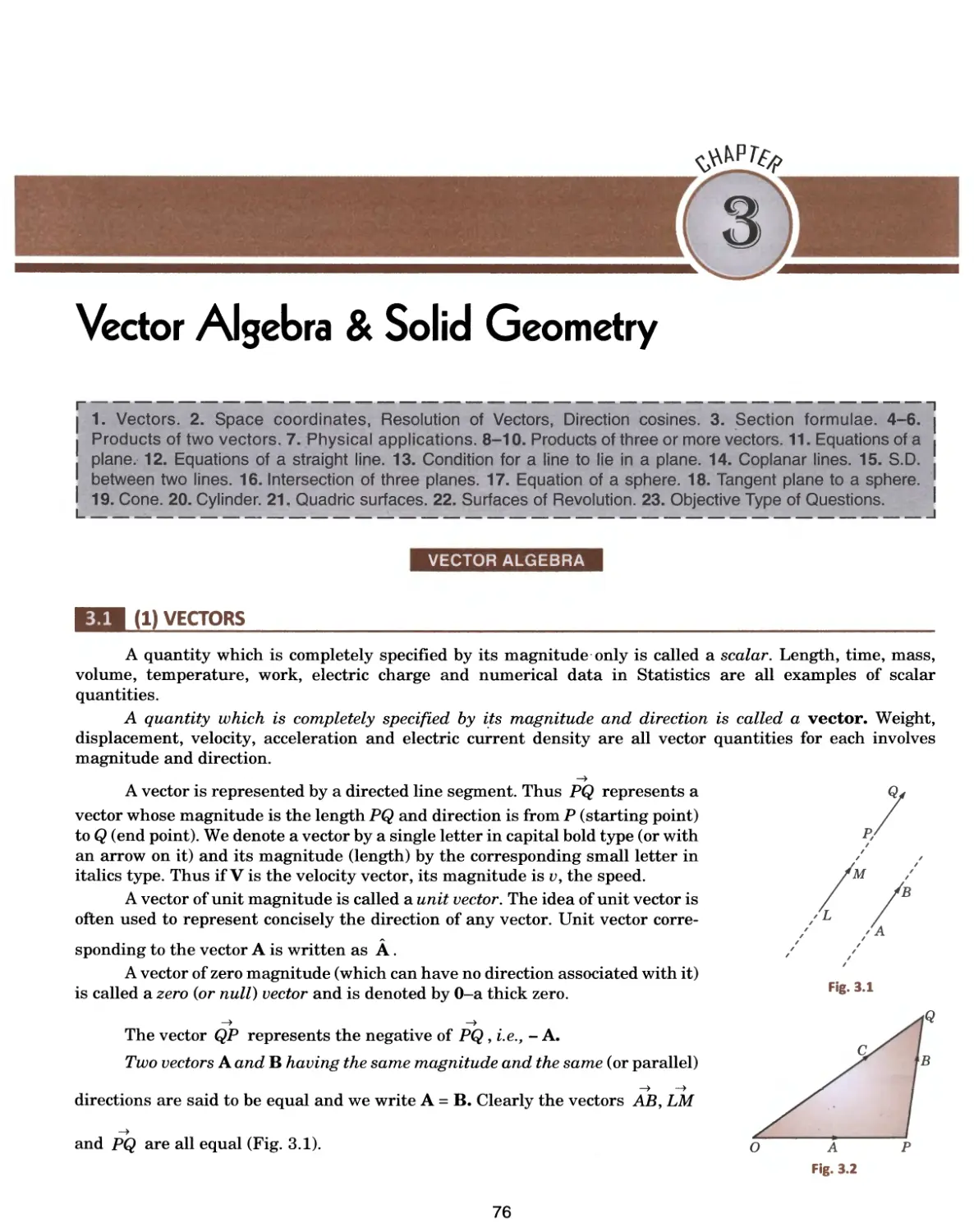
then A' = (- l)2 A.
c2 a2
b3 c3 a3
A׳ =
In general, if any line of a determinant be passed over m parallel lines, the resulting determinant
A' = (— l)m A.
III. A determinant vanishes if two parallel lines are identical.
Consider a determinant A in which two parallel lines are identical.
Higher Engineering Mathematics
20
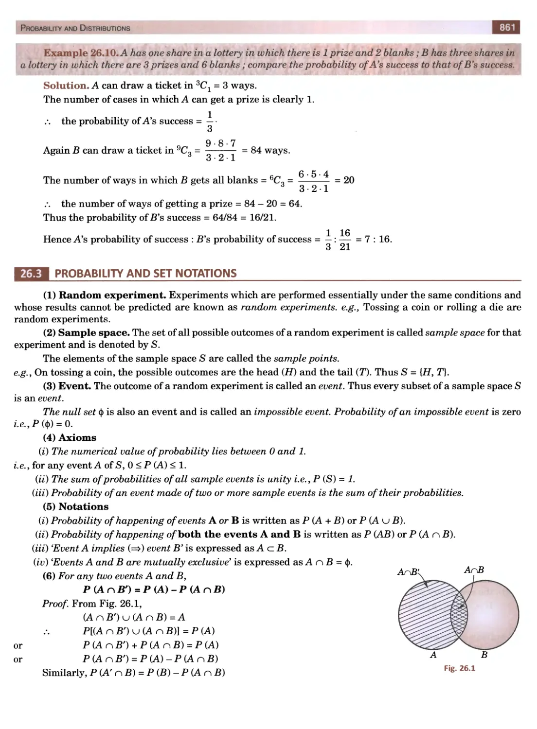
Interchange of the identical lines leaves the determinant unaltered yet by the previous property, the
interchanges of two parallel lines changes the sign of the determinant.
Hence A = A' = - A or 2A = 0, or A = 0.
IV. If each element of a line be multiplied by the same factor׳, the whole determinant is multiplied by that
factor.
i.e.,
a!
pb1
C1
ax
K
ci
a2
Pb2
c2
= P
a2
b2
c2
a3
pb3
C3
a3
^3
C3
L.H.S. = - pb1(a2c3 - a3c2) + pb2(a1c3 - a3c1) - pb3(a1c2 - a2c1)
= p{~ b1B1 + bJB2 - b3B3] = R.H.S.
For on expanding by C2,
Similarly,
Cor. If two parallel lines be such that the elements of one are equi-multiples of the elements of the other, the
determinant vanishes.
i.e.,
a!
b!
C3
°1
bx
cx
kax
kb2
kC‘2
= k
02
b2
C2
a3
h
C3
«3
b3
C3
ax
bx
pbx
ax
bx
bx
a2
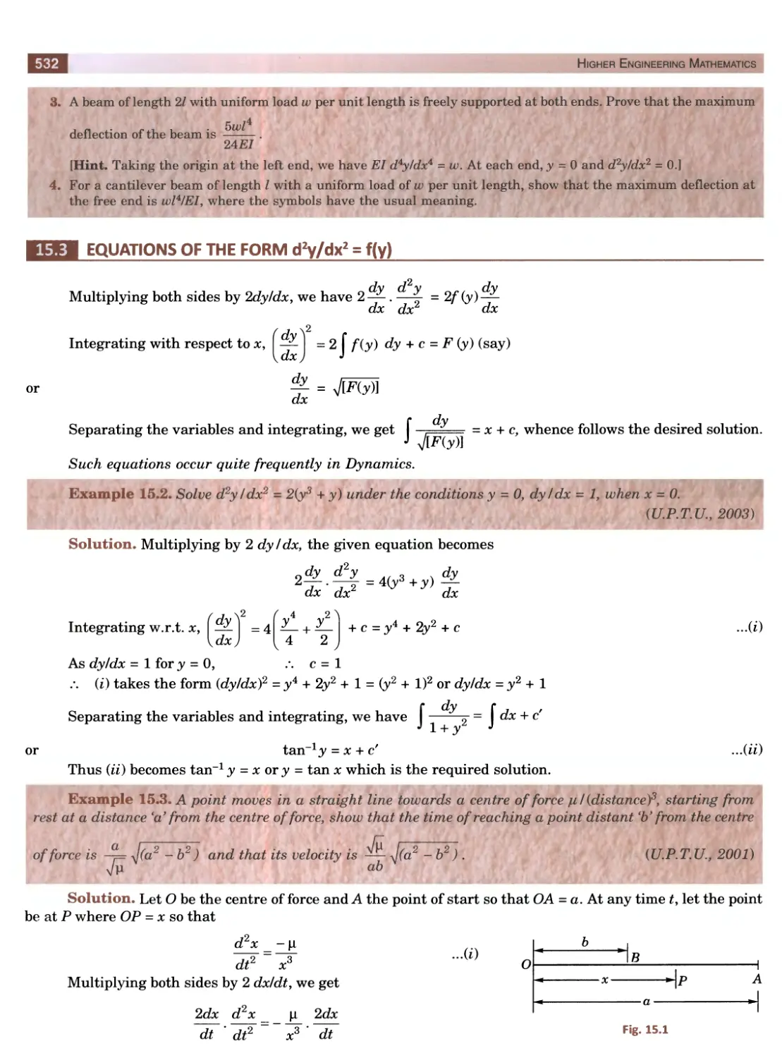
b2
pb2
= p
«2
b2
b2
O
II
o
X
II
a3
b3
pb3
a3
h
V. If each element of a line consists of m terms, the determinant can be expressed as the sum ofm determi-
nants.
ai b! c1 + dx - eY
c2 +d2
c3 + d3
Consider the determinant A =
“3׳ u3 u3 ^ “3׳ ” e3
end of whose third column elements consists of three terms.
Expanding A by C3, we have
A = (c1 + dx - ef) (a2b3 - a3b2) - (c2 + d2 - e2) (a1b3 - a3bf) + (c3 + d3 - e3) (a1b2 - Ucpf)
= [c1(a2b3 - a362) - c2(a1b3 - arjb^) + c3(a162 - a^)] + [d1(a2b3 - a362) - d2(a1b3 - a^)
+ d3(a1b2 - a2b^)] - - a3b2) - e2(a1b3 - a3&■^ + e3(a1b2 - a<fifj\
«1
bx
C1
a!
bx
dx
a!
bx
ex
a2
b2
C2
+
a2
b2
d2
-
a2
b2
e2
a3
b3
C3
a3
bs
d3
Og
b3
e3
Further, if the elements of three parallel lines consist of m, n and p terms respectively, the determinants
can be expressed as the sum ofmxnxp determinants.
= 0 in which a, b, c are different, show that abc = 1.
a
a2
a3
-1
b
b2
b3
-1
c
2
C
c3
-1
Example 2.3. If
Solution. As each term of C3 in the given determinant consists of two terms, we express it as a sum of two
determinants.
a
a2
a3 -1
a
a2
a3
a
2
a
-1
1
a
a2
a
a2
1
b
b2
63-l
b
b2
63
+
b
b2
-1
= abc
1
b
b2
-
b
b2
1
c
c2
c3 -1
c
2
C
3
c
c
c2
-1
1
c
2
C
C
c2
1
[Taking common a, b, c from Rv R2, R3 respectively of the first determinant and - 1 from C3 of the second
determinant.]
= abc
1
a
a2
1
a
a2
1
b
b2
-
1
b
b2
1
c
c2
1
c
c2
21
Linear Algebra : Determinants, Matrices
[Passing C3 over C2 and C1 in the second determinant]
1
a
a2
1
a
a2
1
b
b2
( abc- 1) = 0. Hence abc = 1, since
1
b
b2
1
c
c2
1
c
2
C
* 0 as a, ft, c are all different.
VI. If to each elements of a line be added equi-multiples of the corresponding elements of one or more
parallel lines, the determinants remains unaltered.
a1 b1 c1
a2 b2 C2
as h c3
ai + Pbi ־־ Qci
a2 + Pb2 7> ־C2
aS + Pb3 ־ Q°3
A =
A׳ =
Let
Then
a!
b!
ci
b!
C1
-Qc!
bi
ci
«2
C2
+
Pb2
b2
C2
+
- qc-2
b2
C2
a3
b3
C3
pb3
b3
C3
-qc3
b3
C3
[by IV-Cor.]
= A + 0 + 0 = A.
Obs. This property is very useful for simplifying determinants. To add equi-multiples of parallel lines, we shall
employ the following notation :
Suppose to the elements of the second row, we add p times the elements of the first row and q times the element of
the third row ; then we say :
Operate R2 + pRx + qR3.
Similarly Operate ‘C3 + mC1 - nC2
means that to the elements of the third column add m times the elements of the first column and - n times the
elements of the second column. i
21
17
7
10
24
22
6
10
Example 2.4. Evaluate
6
8
2
3
6
7
1
2
[Expand by Cx]
[v R,=2R9]
Solution. Operating i?3 - i?2 - i?4, i?2 - 3i?3, Rs - 2i?4, the given determinant becomes
-8 -12 0 -2
6-2 0 1
4 -6 0 -1
5 7 12
A =
= 0
2- 12- 8־
1 6-2
1- 6- 4-
x + 2
2x + 3
3x + 4
Example 2.5. Solve the equation
2x + 3
3x + 4
4x + 5
= 0.
3x + 5
5x + 8
lOx +17
(Operate i?2 - Rx and Rx + R3)
= 0
Solution. Operating R3 - (R± + R2), we get
x + 2 2x + 3 3x 4 ־+־
2x + 3 3x + 4 4x + 5
0 1 3x + 8
= 0
6
1
3x + 8
= 0 or (x + 1) (x + 2)
x + 2 2x + 4 6x + 12
X + l 3C + 1 x + 1
0 1 3x + 8
or
To bring one more zero in Cv operate R2 - R2.
Higher Engineering Mathematics
22
0 1 5
(x + 1) (x + 2) 1 1 1 =0
0 1 3x + 8
Now expand by Cv .*. - (x + 1) (x + 2) (Sx + 8 - 5) = 0 or - 3(x + 1) (x + 2) (x + 1) = 0
Thus, x = - 1, - 1, - 2.
= abed (1 + — + T + ~ + 1•
V a b c dJ
1 + a 111
1 1 + & 1 1
1 1 1+c 1
111 1+d
Example 2.6. Prove that
Solution. Let A be the given determinant. Taking a, 6, c, d common from Rv R2, R3, R4 respectively,
• a1+ 1־ a"1 a1־ a1־
_ b1־ b1־& 1־& 1+ 1־
A = abed ו ווו
c1־ c1־ c^+l c
d1־ d1־ d1 1־
[Operate i?x + (i?2 + Rs + R4) and take out the common factor from #ג]
= abed (1 + a1־ + b1־ + c1־ + d1־)
we get
a 1 +1
a 1
a 1
a 1
b~l
b1+ 1־
b-1
b-1
c-1
c1־
c1+ 1־
c1־
d1־
cT1
d-1
d1+ 1־
1
1 1
1
b-1
ft1+ 1־ ft1־
b'1
c-1
c1־ c1+ 1־
1־־c
d1־
d1־ d1־
d1 + 1־
[Operate C2 - Cv C3 ־־ Cv C4 - Cj]
= aftcd (1+ - + ! + - +1)
V a b c dJ
1
0
0
0
b-1
1
0
0
c-1
0
1
0
cT1
0
0
1
= afecd fl + — + + ~ +
V a b c d>
Obs If all elements on one side of the leading diagonal are zero, then the determinant is equal to the product of
leading diagonal elements and such a determinants is called a triangular determinant.
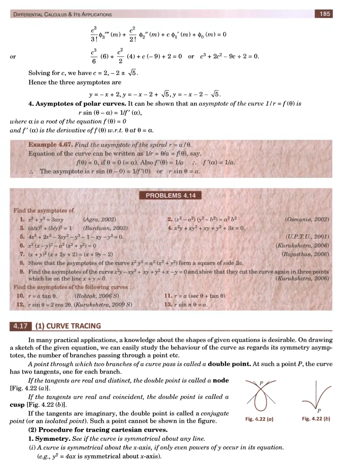
VII. Factor Theorem. If the elements of a determinant A are functions ofx and two parallel lines become
identical when x = a, then x-a is a factor of A.
Let A = fix)
Since A = 0 when x = a, fia) = 0.
i.e., (x - a) is a factor of fix).
Hence x - a is a factor of A.
Ifk parallel lines of a determinant A become identical when x = a, then (x - a)k~1 is a factor of A.
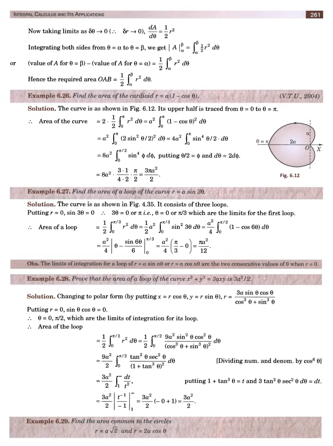
Example 2.7. Factorize A =
Solution. Putting a = 6, Rx = R2 and hence A = 0. .״. a - b is a factor of A.
Similarly, a- c and a - d are also factors of A.
Again putting b = c,R2 = R3 and hence A = 0. 6-cisa factor of A.
Similarly b - d and c-d are also factors of A.
Also A is of the sixth degree in a, b,c,d and therefore, there cannot be any other algebraic factor of A.
Suppose A = k{a -b)(a- c) (a -d)(b ־־ c) (b -d)(c- d), where k is a numerical constant.
The leading term in A = a3b2c. The corresponding term on R.H.S. = kasb2c.
k = 1.
Hence, A = (a - b) (a - c) (a - d) (b -c) (b - d) (c - d).
a3
a2
a
1
b3
b2
b
1
c3
c2
c
1
d3
d2
d
1
23
Linear Algebra : Determinants, Matrices
(b + cf a2 a2
b2 (c + b2
= 2abc (a + b + c)3.
(J.N.T.U.,1998)
c2 c2 (a + bf
Example 2.8. Prove that
Solution. Let the given determinant be A. If we put a = 0,
(b + cf 0 0
0 b2
= 0
2 ,2
c b
A =
.*. a is a factor of A. Similarly b and c are its factors.
Again if we put a + 6+ c = 0.
A =
-af a2
a2
b2 (- bf
b2
= 0
c2
(-cf
In this, three columns being identical, (a + b + c)2 is a factor of A.
As A is of the sixth degree and is symmetrical in a, 6, c the remaining factor must therefore, be of the first
degree and of the form k (a + b + c).
Thus A = kabc {a + b + c)3
To determine k, put a = b = c = 1, then
4 11
14 1 -21k or 54 = 27& i.e.,k = 2
114
Hence A = 2a6c (a + 6 + c)3.
Otherwise : Operating Cj - C3 and C2 - C3, we have
[Take (a + 6 + e) common from Cj and C2]
[Operate i?3 - i?! - R2]
Operate Cx + — Cs, C2 + — Cs
a b
0
(c + a)2 - b2
(6 + c)2 - a2
0
a
c — (a + ft) c ־־־ (a + 6) (a+ 6)'
= (a + 6 + c)2
b + c - a 0
0 c + a - 6
c-a-b c-a-b (a+ 6)
2a6
0
c + a - b
- 2 a
ft + c - a
0
-2b
[Expand by i?3]
6 + c a2/6 a2
ft2/a c + a ft2
0 0 2a6
= (a 4־ b + c)2
= (a + 6 + c)2
= 2ab(a + b + c)2 [(6 + c) (c + a) — aft] = 2a6c (a + 6 + c)3.
VIII. Multiplication of Determinants. The product of two determinants of the same order is itself a
determinant of that order.
a!
ci
h
m1
ni
Let
A1 =
Og
b2
C2
and A2 =
k
m2
ra2
03
C3
k
m3
n3
then their product is defined as
a\h + bimi + cini > aih + bi m2 + ci n2 ’ aih + bim3 + ci n3
AxA2 = a2lx + b2m1 + c2nx> a2l2 + b2m2 + c2n2, a2Z3 + &2m3 +
(23 f “t״ Z?3 m~^ -t- C3 72׳•^ , Z2 ״f■ Z?3 J722׳ + C3 , flg Z3 ״f Z?3 77T3 C3 723׳
Similarly, the product of two determinants of the nth order is a determinant of the nth order.
Higher Engineering Mathematics
24
2 *2
a + A
ab + cA
1
8
A
c
-b
Example 2.9. Evaluate
ab - cA
b2 +x2
be + aA
X
- c
A
a
ca + bA
be - aA
C 4־ K
b
- a
A
Solution. By the rule of multiplication of determinants, the resulting determinant
dn
d12
d13
A =
d21
d22
d23
dsi
d32
d33
where du = (a2 + A,2) A + (ab + cA)c + (ca - bX) (- 6) = A(a2 + b2 + c2 + A-2)
= (a2 + A2)(- c) + (ab + cA)A + (ca - bA)a = 0
0 = :.׳־,
rf2i = °״ d22 = Wa2 + b2 + c2 + A2), d23 = 0.
d31 = 0, d32 = 0, d33 = A(a2 + b2 + c2 + A2).
0
0
A(a2 + b2 + c2 + A2)
0
2 +
0
A(a2 + b2 + c2 + A2)
A(a +6 + c + A )
0
0
A =
Hence
= A3(a2 + b2 + c2 + A2)3.
A:
B!
C!
a!
b' c,
2
^2
B2
^2
=
a2
b2 C2
where A, B etc. are the co- factors of a, b, etc.
^3
B3
C3
a3
b3 c3
a!
bi
C1
A
B!
C!
a2
b2
C2
and A' =
A-2
B2
^2
a3
b3
C3
A3
B3
C3
Example 2.10. SAolc that
respectively in the determinant (a1b2c3).
Solution. Let A =
a1Al + b1B1 + c1C1,
a1A2 + bxB2 + clC2,
a1A3 + bxB3 + cxC3
A
0
0
a2A1 + b<2 B] + c2Cx,
a2-^2 + ^2^2 + C2^2»
a2^3 + ^2^3 + C2^3
=
0
A
0
= A3
a3Ax + b3Bx + c3Cv
a3A2 + b3B2 + c3C2,
a3A3 + b3B3 + c3C3,
0
0
A
AA׳ =
A׳ = A2.
Then
Hence
Obs. A' is called the reciprocal or adjugate determinant of A.
a
c
2ca - b2
2
2bc - a*
2
Example 2.11. Express
b a 2ab - c
as the square of a determinant, and hence find its value.
Solution. Given determinant
a .(-a) + b. c + c. b,
a . (־־ b) + b . a + c . c,
a.(-c) + b.b + c.a
a
6
c
- a
c
b
=
b . (- a) + c . c + a . b,
b . (- b) + c . a + a . c,
b.(-c) + c. b + a . a
=
6
c
a
X
6־
a
c
c . (- a) + a . c + b . b,
c.(- b) + a . a + b . c,
c .(- c) + a . b + b . a
c
a
b
- c
b
a
[Taking out (-1) common from Cx and interchange C2, C3׳.]
a
b
c
a
b
c
b
c
a
<N
tH
I
X
b
c
a
= A2
c
a
b
c
a
b
= - (a3 + b3 + c3 - 3abc)
a b
b c
c a
where A =
Hence the given determinant = A2 = (a3 + b3 + c3 - 3abc)2.
25
Linear Algebra : Determinants, Matrices
PROBLEMS 2.1
vanishes.
1 a o' - be
1 b
b2 - ca
2 - ab
1 c
1. Prove, without expanding, that
= 0, then prove, without expansion, that xyz = - 1 where x, y, z are unequal.
(Andhra, 1999 ;Assam, 1999)
= (x - a) (x - P) (x - y).
= - (a - b) (b -c) (c - a) (a + b + c).
X
2
X
1 + x'
2. If
y
2
y
i+y
z
2
z
1 + zK
X
I
m
' 1
Show that (i)
a
X
n
1
a
ß
X
1
a
P
y
1
a b
1
c
(a)
b + c c + a
a + b
=
2 ,2
2
a o
c
= 0, then show that abc (be + ca + ab) = a + b + c.
a
a3
a4
-1
b
CO
64
1־
=
' 3
4
c
C
C
- 1
l2 22 32 42
12 3 4
13 3 4
22 32 42 52
12 4 4
(ii)
32 42 52 62
12 3 5
42 52 62 72
4. If a, b, c are all different and
5. Evaluate (Z)
Prove the following results : (6 to 12)
= (a + b + c)3
a + b b + c
c + a
a
b c
a-b-c 2b
2c
6.
I + m m + n
n + l
-j-
Z
m n
:2
7.
2 a b - c - a
2c
p + q q + r
r + p
P
q r
2 a 2 h
c-a-b
1 + a2 - b2
2b
-2b
8.
2 ab 1
2 ,2
— a + b
2 a
is a perfect cube.
2b
- 2a2
1
2 i
-a -1
2
״ . B-C . C-A . A-B
= 4 sm —-— sin —-— sin —-—
cos A sin A
cos B sin B
cos C sin C
vanishes.
1
a
a2
o
a + bed
1
b
b2
b3 + cda
is a perfect square.
11.
1
c
c2
o
c + dab
1
d
d2
dS + a&c
9.
10.
= X3(a2 + b2 + c2 + d2 + X)
2 ׳v
a + X.
ab
ac
ad
ab
b2 +1
be
bd
ac
be
c2 + X
cd
ad
bd
cd
d2 + X
12.
Factorize each of the following determinants : (13 to 15)
13.
1
1
1
1
1
1
a
b
c
(Andhra, 1998)
14.
a2
b2
2
C
2
a
b2
2
C
a3
b3
c3
Higher Engineering Mathematics
26
i2 2 , 2
be + a
bc + a
1
a2
b2
c2
d2
c2a2+b
ca + b
1
16.
a
b
c
d
a2b2+c2
ab + c
1
1
bed
1
cda
1
dab
1
abc
(Andhra, 1999)
= 0
= 0.
= 4a W.
b
a
c - x
c
b - x
a
a- x
c
b
15.
17. If a + b + c = 0, solve
2x + 1 3jc + 1
4x + 3 6x + 3
x +1
2x
4x 46 1 ־x + 4 8x + 4
r2 2
b + C
ab
ac
0
c
b
ba
2 , 2
c + a
be
=
c
0
a
ca
cb
2 ,2
a t* b
b
a
0
18* Solve the equation
19. Show that
Bl MATRICES
(1) Definition. A system of mn numbers arranged in a rectangular formation along m rows and n
columns and bounded by the brackets []is called anmby n matrix ; which is written as m x n matrix. A matrix
is also denoted by a single capital letter.
°n
a12
-<hj
-«In
°21
a22
—a2j
-a2n
%
ai2
<״»• • •
aml
am2
amj
• • m
A =
Thus
is a matrix of order mn. It has m rows and n columns. Each of the mn numbers is called an element of the matrix.
To locate any particular element of a matrix, the elements are denoted by a letter followed by two suffixes
which respectively specify the rows and columns. Thus a״ is the element in the i־th row and 7-th column of A. In
this notation, the matrix A is denoted by [a״].
A matrix should be treated as a single entity with a number of components, rather than a collection of numbers. For
example, the coordinates of a point in solid geometry, are given by a set of three numbers which can be represented by the
matrix [x, y, z]. Unlike a determinant, a matrix cannot reduce to a single number and the question of finding the value of a
matrix never arises. The difference between a determinant and a matrix is brought out by the fact that an interchange of
rows and columns does not alter the determinant but gives an entirely different matrix.
(2) Special matrices
Row and column matrices. A matrix having a single row is called a row matrix, e.g., [l 3 5 7].
A matrix having a single column is called a column matrix, e.g.,
Row and column matrices are sometimes called row vectors and column vectors.
Square matrix. A matrix having n rows and n columns is called a square matrix of order n.
The determinant having the same elements as the square matrix A is called the determinant of the matrix
and is denoted by the symbol | A |. For example, if
A =
The diagonal of this matrix containing the elements 1, 3, 5 is called the leading or principal diagonal. The
sum of the diagonal elements of a square matrix A is called the trace of A.
A square matrix is said to be singular if its determinant is zero otherwise non-singular.
T 2 3׳
12 3
2 3 4
, then | | =
2 3 4
3 4 5
3 4 5
27
Linear Algebra : Determinants, Matrices
Diagonal matrix. A square matrix all of whose elements except those in the leading diagonal, are zero is
called a diagonal matrix.
A diagonal matrix whose all the leading diagonal elements are equal is called a scalar matrix. For
example,
3־
0
׳0
3׳
0
׳0
0
-2
0
and
0
3
0
0
0
6
0
0
3
are the diagonal and scalar matrices respectively.
Unit matrix. A diagonal matrix of order n which has unity for all its diagonal elements, is called a unit
matrix or an identity matrix of order n and is denoted by In. For example, unit matrix of order 3 is
“0 0 1״
10 0
0 0 1
Null matrix. If all the elements of a matrix are zero, it is called a null or zero matrix and is denoted by *O’; e.g.,
f0 0 0 01
is a null matrix.
0 0 0 0
Symmetric and skew-symmetric matrices. A square matrix A = [a״] is said to be symmetric when
a. = al7 for all i and j.
y Jl
If atj = - a- for all i and j so that all the leading diagonal elements are zero, then the matrix is called a skew-
symmetric matrix. Examples of symmetric and skew-symmetric matrices are
respectively.
a
h
g־
' 0
h
~g־
h
b
f
and
-h
0
f
g
f
c
_ g
-f
0
Triangular matrix. A square matrix all of whose elements below the leading diagonal are zero, is called
an upper triangular matrix. A square matrix all of whose elements above the leading diagonal are zero, is called
a lower triangular matrix. Thus
and
are upper and lower triangular matrices respectively.
Ell MATRICES OPERATIONS
(1) Equality of Matrices
Two matrices A and B are said to equal if and only if
(1) they are of the same order
and (ii) each element of A is equal to the corresponding element ofB.
(2) Addition and subtraction of matrices. If A, B be two matrices of the same order, then their sum
A + B is defined as the matrix each element of which is the sum of the corresponding elements of A and B.
ai
V
C1
<
a! + Cj
bx + dx
02
b2
+
C2
d2
=
a2 ־*" C2
b2+d2
a3
*>3j
_C3
d3
a3 + c3
b3+d3
Thus,
Similarly, A-Bis defined as a matrix whose elements are obtained by subtracting the elements ofB from
the corresponding elements of A.
Thus,
Obs. 1. Only matrices of the same order can be added or subtracted.
2. Addition of matrices is commutative,
i.e., A + B — B + A.
־a! V
־c!
1
JP
1
*£
1־hP
1
1. . ,
Sh V
־*r
1
a2 — c2 b2 — d2
Higher Engineering Mathematics
28
3. Addition and subtraction of matrices is associative,
i.e. (A + B) - C = A + (B - C) = B + (A - C).
(3) Multiplication of matrix by a scalar. The product of a matrix A by a scalar kisa matrix whose each
element is k times the corresponding elements of A.
Thus,
The distributive law holds for such products, i.e., k{A + B) = kA + kB.
Obs. All the laws of ordinary algebra hold for the addition or subtraction of matrices and their multiplication by scalars.
al bl
C1
kax
k\
kcl
1
C2_
ka2
kb2
kc2
x + y
5
Example 2.12. Find x, y, z and w given that
x y~\ \ x 5 1 T 6
3 — +
z w -1 2w z + w
3x
Sy1
x + 6
5 + x + y
3 z
Sw
-1 + z + w
2w + 5
Solution. We have
Equating the corresponding elements, we get
3x = x + 6, 3y = 5 + x + y, Sz = - 1 + z + w, Sw = 2w + 5.
2x = 6, 2y = 5 + x, 2z = w - 1, w = 5
Hence x = 3, y = 4, z = 2, w - 5.
as the sum of a lower triangular matrix with zero leading
-7
4
6
3 5
-8 11
13 -14
or
Example 2.13. Express
diagonal and an upper triangular matrix.
be the lower triangular matrix with zero leading diagonal.
be the upper triangular matrix.
0 0 0'
a 0 0
be 0
I m n
0 p q
0 0 r
Solution. Let L -
U =
and
3
5
״7-
0־
0
־0
I
m
n
-8
11
4
=
a
0
0
+
0
P
Q
13
-14
6
b
c
0
0
0
r
8 = a, 11 = p, 4 = q,
Then
Equating corresponding elements from both sides, we obtain 3 = Z, 5 = m, - 7 = n,
13 = 6, - 14 = c, 6 = r.
0
0
־0
3
5
־7-
-8
0
0
and U =
0
11
4
13
-14
0
0
0
6
Hence
(4) Multiplication of matrices. Two matrices can be multiplied only when the number of columns in the
first is equal to the number of rows in the second. Such matrices are said to be conformable.
־h
h
X
mx
m2
nx
n2
a״
For instance, the product
aih + + c!ni aih + bim2 + Cln2
a2lx + b2m1 + c2nx a2l2 + b2m2 + c2n2
ash + bsmi + csni ash + bsm2 + csn2
a4Z! + bim1 + a4/2 + bAm2 + c4n2
is defined as the matrix
29
Linear Algebra : Determinants, Matrices
an
a12 *
״ Ol*־
A!
l>12 ■
- ^
In general, if A =
a21
a22 ‘
“ a2n
and B =
^21
b22 ■
״ b2P
.0ml
am2 *
®,mrt _
bni
bn2 ■
• bnp
be two m x n and n x p conformable matrices, then their product is defined as the m x p matrix
cn
C12
J
AB =
C21
C22
C2p
Cml
Cm2
^mp _
where c״ = aa by + a i2b2j + aiSb3j + ... + ainbnj, i.e.., the element in the ith row and the jth column of the matrix AB
is obtained by weaving the ith row of A with jth column of B. The expression for c״ is known as the inner product
of the ith row with the jth column.
Post-multiplication and Pre-multiplication. In the product AB, the matrix A is said to be post-multiplied
by the matrix B. Whereas in BA, the matrix A is said to be pre-multiplied by B. In one case the product may exist
and in the other case it may not. Also the product in both cases may exist yet may or may not be equal.
Obs. 1, Multiplication of matrices is associative, i.e., (AB)C =A(BC)
provided A, B are conformable for the product AB and B, C are conformable for the product BC. (Ex. 2.16).
Obs. 2. Multiplication of matrices is distributive. i.e.,A(B + C) - AB +AC.
provided A, B are conformable for the product AB and A, C are conformable for the product AC.
Obs. 3. Power of a matrix. If A be a square matrix, then the product AA is defined as A2. Similarly, we define
higher powers of A. i.e., A . A2 - A3, A2 . A2 = A4 etc.
If A2 = A, then the matrix A is called idempotent.
, form the product ofAB. Is BA defined?
0׳
1
2
1
־2-
i
2
3
and B =
-1
0
2
3
4
2
-1
Example 2.14. If A =
Solution. Since the number of columns of A = the number of rows ofS (each being = 3).
.״. The product AB is defined and
0.1 + 1. - 1 + 2.2,
0. - 2 + 1.0 + 2.-1
:!
־2-
1.1+ 2.-1 + 3.2,
1.-2 +2.0 + 3.-1
5
-5
2.1+ 3.-1 +4.2,
2. - 2 + 3.0 + 4. - 1
7
-8
Again since the number of columns of B ^ the number of rows of A.
.-. The product BA is not possible.
, compute AB and BA and show that AB & BA.
1
3
0'
2
3
4
-1
2
1
,B =
1
2
3
0
0
2
-1
1
2
Example 2.15. If A =
Solution. Considering rows of A and columns of B, we have
AB =
Again considering the rows of B and columns of A, we have
BA =
1.2+ 3.1+ 0.-1,
1.3+ 3.2+ 0.1,
1.4+ 3.3 +0.2'
5
9
־13
-1.2+ 2.1+ 1.-1,
-1.3+ 2.1+ 1.1,
-1.4+ 2.3 + 1.2
=
-1
2
4
0.2+ 0.1+ 2.-1,
0.3+ 0.2+ 2.1,
0.4+ 0.3+ 2.2
- 2
2
4
2.1 + 3.-1 + 4.0,
2.3+ 3.2+ 4.0
׳4.2 +3.1 +2.0
1 12
11"
1.1+ 2.-1 + 3.0,
1.3+ 2.2+ 3.0
1.0 + 2.1 + 3.2
-1 7
8
-1.1 + 1.-1 + 2.0,
-1.3+ 1.2+ 2.0
-1.0+ 1.1+ 2.2
-2 -1
5
Evidently AB * BA.
Higher Engineering ■Mathematics
30
Example 2.16. If A =
'3 2 2'
13 1
5 3 4
, find the matrix B such that AB =
'3 4 2'
16 1
5 6 4
{Mumbai, 2005)
Solution. Let AB =
'3 2 2'
13 1
5 3 4
31 + 2 +
I + 3 +
51 + 3p+
I m n
p q r
U V w
2u 3m + 2q + 2v 3n + 2r + 210
u m + 3q + v n + 3r +10
4u 5m + 3q + 40 5n + 3r + 410
(given)
...(i)
...(ii)
...{Hi)
51 + 3p + = 5
5m + 3q + 416 = ׳
5n + 3r + 410 = 4
'2 4 3'
1 6 1
ב5 6 4.
Equating corresponding elements, we get
3 I + 2p + 2 3, I + 3 1,
3 m + 2q + 20 = 4, /n + 3g + = 6,
3n + 2r + 210 = 2, + 3r + = 1,
Solving the equations (i), we get l = l,p = 0,u = 0
Similarly equations (ii) give m = 0rq = 2, v = 0
and equations (iii) give n = 0, r = 0,10 = 1
l01 0 1־
2
0
Thus, B =
'1
3
2'
Example 2.17. Prove that A3 - 4A2 - 34 + 111 = 0, where A =
2
0
-1
.
1
2
3
'9
7
5"
=
1
4
1
8
9
9
1+6+2 3+0+4 2-3+6
2+0-1 6+0-2 4+0-3
1+4+3 3+0+6 2-2+9
13 2
2 0-1
12 3
13 2
2 0-1
12 3
'9
7
5'
"1
3
2
9 + 14 + 5
27 + 0 + 10
18 - 7 + 15'
'28
37
26'
1
4
1
X
2
0
-1
=
1 + 8 + 1
3 + 0 + 2
2-4 + 3
=
10
5
1
8
9
9
1
2
3
8 + 18 + 9
24 + 0 + 18
16-9 + 27
35
42
34
Solution. A2 = A x A =
A3 = A2 xA =
A3- 4A2 - 3A + 117
"28 37 26
'9
־5 7
'1
־2 3
1־
0
־0
—
10 5 1
-4
1
4 1
-3
2
0 -1
+ 11
0
1
0
35 42 34
8
9 9
1
2 3
0
0
1
11 + 28-36-3־
37
-28-
0 + 9־
26 - 20 - 6 + 0"
0־
0
־0
=
10 - 4 - 6 -
-0
5-
11 + 0 + 16 ־
1-4+3+0
=
0
0
0
= 0.
35-32-3 + 0
42
-36-
-6 + 0
34-36
-9 + 11
0
0
0
— 25n
7 -1011
Example 2.18. By mathematical induction, prove that if
11 -25] .״ r7 +
״ , then An - .
4-9 4n
A =
(i)״.
Solution. When n = 1, A" gives A1 = ^ ^
Let us assume that the result is true for any positive integer k, so that
31
Linear Algebra : Determinants, Matrices
1 + 10* - 25*
4* 1 - 10k
11 -25
4 -9
1 + 10k - 25k
4* 1 -10*
Ak =
Ak + l =Ak .A1 =
...{ii)
[by («)]
'*225 + (*10+ 1)25 - *100 - (*10 + 1)11׳ _
(*10 - 1)9 - *100 - (*10 - 1)4 + *44 ־
(1 + *)25 - (1 + *)10 + 1־ _
4(* + l) 1-10(* + 1)
This is true for n = * + 1
We have seen in (i) that the result is true for = 1.
.־. It is true for n = 1 + 1 = 2
Similarly, it is true for n = 2+1 = 3 and so on.
Hence by mathematical induction, the result is true for all positive integers n.
Example 2.19. Prove that (AB)C = A(BC), where A, B, C are matrices conformable for the products.
(,
Solution. Let A = [a״] be of order mx n, B = [6״] be of order n x p and C = [cy] be of order ofp x q.
kj
Then AB = [aik] = £ aik b,
k = i
n
P ( n ^
\
n p
£, aik Ki
• [%] =
M
M
\ cu
=
£ £aik °ij
k=!
1=1 \k=l )
1
k=! 1=1
(AB)C =
BC = [bkl] . [cy] = X bklct
1 = 1
Similarly,
°ij
n ( p
£ I £
k = i \i = l
Jki cij
k = l
,kl clj
p
i=i
A(BC) = [aik]
(AB)C = A(BC).
Hence
PROBLEMS 2.2
is singular ?
3-x 2 2
2 4-x 1
-2 -4 -1-x
1. For what values of x, the matrix
x + 3 2 y + x
7 - 0־
z-l 4a - 6
3 2a
2. Find the values of x, y, 2: and a which satisfy the matrix equation
3• Matrix A has x rows and* + 5 columns. Matrix B hasy rows and 11 - y columns. BothAjB and BA exist. Find# andy.
x [3 2]
, calculate the product AB.
, find AB or BA, whichever exists.
, verify that (AB)C = A(BC) and A(B + C) = AB + AC.
2 1-1
4-5 6
-3 7 3
3 1
1 4
and A - B =
1 -1
3 0
0 1 2־
1 2 3
1 10
and B =
12 3 4
2 0 12
3 10 5
4. If A + B =
5. IfA =
,B =
2־
״1
and C =
3-־
־1
2
3
2
0
1 2
-2 3
6. If A =
־1 3
tr Q״
1
־2
X
-6 4
X
O O
-2 1
; (Hi)
-2
x [4 5 2]x
-3
-2 5
3
5
a
h
g
X
7. Evaluate (i) [#, y, 2]
h
b
f
y
; Hi)
g
f
c
2
Higher Engineering Mathematics
32
(B.P.T.U., 2006)
8. Prove that the product of two matrices
~o
cos 0 cos 0 sin 0
^ . . 9 ^
and
2 A
COS <()
cos <{> sin <()
• 2 .
cos 0 sm 0 sm 0
cos <J) sin <))
sm <|)
cos a - sm a
sin a cos a
is a null matrix when 0 and <)) differ by an odd multiple of tz/2.
0 - tan a/2
tan a/2 0
, show that 1 + A = (I - A)
, find the value of A2 - 6A + 81, where I is a unit matrix of second order.
3 2
2 3
9. IfA =
10. If A =
, and / is the unit matrix of order 3, evaluate A2 - 3A + 91.
, verify the result (A + B)2 =A2 + BA + AB + B2.
1 -2
3 -1
1 2
2
-3
3-11
0 0 2
4-3 2
\B =
0 0 0
10 0
0 1 0
and F =
12-1
2 0 3
0 1 2
0 1 0׳
1 0 0
0 0 0
11. If A =
12. If A =
13. If E =
calculate the products EF and FE and show that E2F + FE2 = E.
cos na sm na
- sin na cos na
, when n is a positive integer,
into the form LU, where L is lower triangular and U is upper triangular
, show that An =
cos a sm a
- sin a cos a
14. If A =
5-2 1
7 1-5
3 7 4
15. Factorize the matrix A =
matnx.
RELATED MATRICES
(1) Transpose of a matrix. The matrix obtained from any given matrix A, by interchanging rows and
columns is called the transpose of A and is denoted by A'
'1
׳2
is A' =
1־
4
־7
4
5
2
5
8
7
8
Thus the transposed matrix of A =
Clearly, the transpose of an m x n matrix is an n x m matrix. Also the transpose of the transpose of a
matrix*coincides with itself, i.e., (AT = A.
For a symmetric matrix, A' = A and for a skew-symmetric matrix, A' --A.
Obs. 1. The transpose of the product of the two matrices is the product of their transposes taken in the reverse order
i.e., (AB)' = B'A'.
For, the element in the ith row and jth col. of (AB)'
= element in the jth row and ith col. of AB = inner product of jth row of A with ith col. of B
= inner product of jth col. of A' with ith row of B' = element in the ith row and jth col. of B'A'
Hence (AB)' = B'A'.
Obs. 2. Every square matrix can be uniquely expressed as a sum of a symmetric and a skew-symmetric matrix.
(J.N.T.U., 2001)
Let A be the given square matrix, then A = ~ (A + A') + ~ (A - A').
B=|(A+A׳) and C=-|(A-A')
Let
\(A + A')l = [A' + (A')'l = \ (A' + A) = B, i.e.,B= b(A + A') is a symmetric matrix.
Zt J Zt z z
B' =
33
Linear Algebra : Determinants, Matrices
= ■j־[A' - (A')'] = ~ (A' - A) = - C, i.e., C = (A - A') is a skew-symmetric matrix.
(A-A')
Again
Hence A can be expressed as the sum of a symmetric and a skew-symmetric matrix.
To prove the uniqueness, assume that P is a symmetric matrix and Q is a skew-symmetric matrix such that A = P + Q.
Then A' = (P + QY = P' + Q' = P-Q
Thus, P = | (A + AO and Q = | (A - A׳)
which shows that there is one and only one way of expressing A as the sum of a symmetric and skew-symmetric matrix.
Example 2.20. Express the matrix A as the sum of a symmetric and a skew-symmetric matrix where
A =
4 2
1 3
־3-
6-
-5 0
-7
4 1-5
2 3 0
-3 -6 -7
Solution. We have A׳ =
־3-8 8־
־2 01־
Then A + A'=
3 6-6
and A - A׳ =
-1 0 -6
-8 -6 -14
-2 6 0
1 -j
4
1.5
- 4
0
0.5
־1
a= a(A+A0+ a(a-ao =
1.5
3
-3
+
-0.5
0
-3
z z
-4
-3
-7
-1
3
0
(2) Adjoint of a square matrix. The determinant of the square matrix
A =
The matrix formed by the cofactors of the elements in A is
°i
K
ci
a!
K
ci
o2
K
C2
is A =
a2
K
C2
Og
b3
c3_
a3
b3
C3
A
Bi
[־A
^2
Al
A
B2
c2
. Then the transpose of this matrix, i.e.,
B!
B2
B3
.A
B3
c!
^2
Cs_
is called the adjoint of the matrix A and is written as Adj. A.
Thus the adjoint of A is the transposed matrix of cofactors of A.
(3) Inverse of a matrix. If A be any matrix, then a matrix B if it exists, such thatAB = BA = I, is called
the Inverse of A which is denoted by A1־ so that AA1־ = I.
1־
0
־0
= I A I
0
1
0
0
0
1
0
0
|A|
o
|A|
0
IA
o
o
A, A״ A״
Bx B2 B3
C! c2 c3
A-1 _
I A |
K
*0] or -tItt־is the inverse of A.
|A|
C3_
I A
A (Adj A) =
Adj. A _ j
Also
For
I A |
or
Obs. 1. Inverse of a matrix, is unique.
If possible, let the two inverses of the matrix A be B and C,
then AB = BA = I and
CAB = ( CA)B = I and CAB = C(AB) = =
Thus, B = C.
Higher Engineering Mathematics
34
Oils* 2. The reciprocal of the product of two matrices is the product of their reciprocals taken in the reverse order i.e.,
(AB)1־ = B1־ A1־ (Assam, 1999)
If A, B be two matrices, then the reciprocal of their product is (AB)1־.
Clearly, (AB). (B1־ A1־) = A(BB_1) A1־ [by Associative law]
= A/A1־ = AA1־ = /.
Similarly, (ZHA1־). (AB) = I
Hence B1־ A1־ is the reciprocal of AB.
Obs. 3L Multiplication by an inverse matrix plays the same role in matrix algebra that division plays in ordinary
algebra.
i.e., if [A][B] = [C][D], then [A]1־ [A]LB] = [A1־][C׳][Z>]
B=A~l[C][D), i.e.,= A'1 [C]\D\.
[A]
or
113
1 3-3
-2 -4 -4
Example 2.21. Find the inverse of
Solution. The determinant of the given matrix A is
A =
“113׳
a1 öj c1
1 3-3
a2 ^2 c2
(say)
-2 -4 -4
a3 63 c3
If Ap A2, be the cofactors of av a2... in A, then A± = - 24, A2 = - 8, A3 = - 12 ; B1 = 10, B2 = 2, B3 = 6 ;
Cx = 2, C2 = 2, C3 = 2.
Thus A = ajAj + a2A2 + a3A3 = - 8.
(Mumbai, 2008)
[Al
^2
^3
"- 24
-8
-12'
*1
*2
^3
10
2
6
c!
^2
c3_
2
2
2
1 I
I
4 4
I _I
4 4
5
4
1
4
12
6
2
-24 -8
10 2
2 2
ad/ A =
Hence the inverse of the given matrix A
A
1
-8
2 4
3 -1
3=[
= D, then
-3
5
2 1
3 2
-2 4
3 -1
= C and
3 2
5 -3
= B,
2 1
3 2
BAC = D or AC = ß1־D
A = ß1־ DC1־
2
-3
3 2
5 3
24 13
-34 -18
2-
־ 3
8 14
3 4
ß-l _ adj B
C־^
A =
1*1
2 3׳
3 5
2
-3
2 -1
-3 2
and
Note. For other methods see Examples 2.25 ; 2.28 and 2.46.
Example 2.22. Find the matrix A if
Solution. If
Now,
Similarly,
Hence,
35
Linear Algebra : Determinants, Matrices
PROBLEMS 2.3
cos a sin i
- sin a cos <
1. IfA =
l al
, verify that AA' - I - A'A, where I is the unit matrix.
5 OCJ
2. Express each of the following matrices as the sum of a symmetric and a skew-symmetric matrix :
(i)
(Mumbai, 2006)
{B.P.T.U., 2005)
{Mumbai, 2008)
{Mumbai, 2007)
{.P.T.U., 1999)
3־
-2
־6
a
a
b
2
7
-1
{ii)
c
b
b
5
4
0
c
a
c
3. If A is a non-singular matrix of order n, prove that A adj A = | A 11.
־3 2 1־
Verify that A {adj A) = {adj A) A = | A |/, where A = 13 5 .
1 5 12
'2 3 4
'4 5-2״
4. Find the inverse of the matrix (i)
4 3 1
{Mumbai, 2009)
{ii)
-2 1 1
12 4
4 10
־2 2 3״
־2 4 3'
P
1—1
11
1 3 1
, compute adj A and A1־. Also find B such that AB =
16 1
5 3 4
5 6 4
'3-3
4'
6. IfA =
2 -3
4
, {i) find A-1;
{ii) show that A3 = A~
0 -1
1
0
1
־1
-I
4
-1
1“
1
0
1
and if A = i
-2
3
-1
1
1
0
2
2
1
5
7. Find the inverse of the matrix
S
show that SAS1־ is a diagonal matrix dig (2, 3, 1).
, prove that A1־ = A'.
12 2
2 1-2
-2 2 -1
8. If A = -
-l
cos 0 - sin 0
1 - tan 0/2
1 tan 0/2
sin 0 cos 0
tan 0/2 1
-tan 0/2 1
, verify that {ABY = B'A', where A' is the transpose of A.
1׳
2
׳1-
1
0
0“
3
0
2
and B =
2
1
0
4
5
0
0
1
3
9. Show that
10. If A =
־2 1 1־
'0 2 1־
11. A =
19 3
,B =
2 3-1
.1־1A־^ = 1־(verify that (Aß ,
14 2
1 -1 3
12. If A is a square matrix, show that {i) A + A' is symmetric,* and {ii) A - A' is skew-symmetric.
13. If D = diag [dv d2, </3], dv d2, ds & 0, prove that D~x = diag [df1, d2l, c?3-1].
14. If A and B are square matrices of the same order and A is symmetrical, show that B'AB is also symmetrical.
[Hint. Show that {B'ABY = B'AB]
15. If a non-singular matrix A is symmetric, show that A1־ is also symmetric.
BK. (1) RANK OF A MATRIX
If we select any r rows and r columns from any matrix A, deleting all the other rows and columns, then the
determinant formed by these r x r elements is called the minor of A of order r. Clearly, there will be a number of
different minors of the same order, got by deleting different rows and columns from the same matrix.
Def.A matrix is said to be of rank r when
{i) it has at least one non-zero minor of order r,
and {ii) every minor of order higher than r vanishes.
Briefly, the rank of a matrix is the largest order of any non-vanishing minor of the matrix.
Higher Engineering Mathematics
36
If a matrix has a non-zero minor of order r, its rank is > r.
If all minors of a matrix of order r + 1 are zero, its rank is < r.
The rank of a matrix A shall be denoted by p(A).
(2) Elementary transformation of a matrix. The following operations, three of which refer to rows and
three to columns are known as elementary transformations :
I. The interchange of any two rows (columns).
II. The multiplication of any row (column) by a non-zero number.
III. The addition of a constant multiple of the elements of any row (column) to the corresponding elements of
any other row (column).
Notation. The elementary row transformations will be denoted by the following symbols :
{i) Rtj for the interchange of the ith and jth rows.
(ii) kR( for multiplication of the ith row by k.
(Hi) Rt + pRj for addition to the ith row, p times the jth row.
The corresponding column transformation will be denoted by writing C in place of R.
Elementary transformations do not change either the order or rank of a matrix. While the value of the minors may get
changed by the transformation I and II, their zero or non-zero character remains unaffected.
(3) Equivalent matrix. Two matrices A and B are said to be equivalent if one can be obtained from the
other by a sequence of elementary transformations. Two equivalent matrices have the same order and the same
rank. The symbol ~ is used for equivalence.
(V.T.U., 2011)
Example 2.23• Determine the rank of the following matrices
0
1
-3
-1
1
0
1
1
3
1
0
2
1
1
-2
0
(ii)
1 2
1 4
2 6
(i)
Rx and Rs - 2R± so that the given matrix
= A (say)
3
-1
-1
Solution. (i) Operate R2 -
2 1־
02-
2 0
Obviously, the 3rd order minor of A vanishes. Also its 2nd order minors formed by its 2nd and 3rd rows
.0*1־ =
are all zero. But another 2nd order minor is
p(A) = 2. Hence the rank of the given matrix is 2.
(ii) Given matrix
0״
1
-3
־1-
0־
1
-3
-1'
1
0
0
0
1
0
0
0
3
1
-3
-1
3
0
0
0
1
1
-3
-1
1
0
0
0
3- Rv R4- R±]
0 0"
= A (say)
[Operating R
0 1
10 0 0
~ 0 0 0 0
0 0 0 0
[Operating C3 + 3C2, C4 + C2]
[Operating C3 - Cv C4 - C±]
1-3-1 0־
0 0 10
0 0 0 0 ~
0 0 0 0
[Operating R3 - 3R2, R4 - R2
Obviously, the 4th order minor of A is zero. Also every 3rd order minor of A is zero. But, of ail the 2nd
pCA) = 2.
= -1*0.
0 1
1 0
order minors, only
Hence the rank of the given matrix is 2.
(4) Elementary matrices. An elementary matrix is that, which is obtained from, a unit matrix, by
subjecting it to any of the elementary transformations.
37
Linear Algebra : Determinants, Matrices
Examples of elementary matrices obtained from
'1
0
־0
‘1
0
־0
'1
0
״0
1
p
״0
0
1
0
are i?23 -
0
0
1
— C23 ; —
0
k
0
; R1 + pR2 =
0
1
0
0
0
1
0
1
0
0
0
1^
0
0
1
!3 =
(5) Theorem. Elementary row (column) transformations of a matrix A can be obtained by pre-multiplying
(post-multiplying) A by the corresponding elementary matrices.
a2 ^2
Og b3
Consider the matrix A =
'1
0
0
a!
6!
c!
a!
6!
ci
0
0
1
X
«2
b2
C2
=
a3
h
C3
0
1
0
a3
h
C3_
a2
b2
C2_
R23 x A —
Then
So a pre-multiplication by R2S has interchanged the 2nd and 3rd rows of A. Similarly, pre-multiplication
by kR2 will multiply the 2nd row of A by k and pre-multiplication by Rx + pR2 will result in the addition of p times
the 2nd row of A to its 1st row.
Thus the pre-multiplication of A by elementary matrices results in the corresponding elementary row
transformation of A. It can easily be seen that post mutiplication will perform the elementary column
transformations.
(6) Gauss-Jordan method of finding the inverse*. Those elementary row transformations which
reduce a given square matrix A to the unit matrix, when applied to unit matrix I give the inverse of A.
Let the successive row transformations which reduce A to I result from pre-multiplication by the
elementary matrices Rv R2, ... i?• so that
Rfti _ 1... R^lyA = I
Rt Rt _ x... BjjRjAA1־ = /A1־
or RiRi_1...R2R1I = A~1 [v AA1־ = /]
Hence the result.
Working rule to evaluate A1־. Write the two matrices A and I side by side. Then perform the same row
transformations on both. As soon as A is reduced to /, the other matrix represents A1־.
Example 2.24. Using the Gauss-Jordan method,find the inverse of the matrix
־113
1 3-3
( 2006)
-2 -4 -4
Solution. Writing the same matrix side by side with the unit matrix of order 3, we have
(Operate R2 - R1 and R3 + 2 R^)
(Operate ~R2 and ~RS)
A A
(Operate Rr - R2 and R3 + R2)
1
1
3
1
0
0
1
3
-3
0
1
0
-2
-4
-4
0
0
1
1׳
1
3:
1
0
־0
0
2
-6:
-1
1
0
0
-2
2:
2
0
1
1
1
3:
1
0
0
0
1
-3:
1
2
1
2
0
0
-1
1:
1
0
1
2
*Named after the great German mathematician Carl Friedrich Gauss (1777-1855) who made his first great discovery as a
student at Gottingen. His important contributions are to algebra, number theory, mechanics, complex analysis, differential
equations, differential geometry, non-Euclidean geometry, numerical analysis, astronomy and electromagnetism. He
became director of the observatory at Gottingen in 1807.
Name after another German mathematician and geodesist Wilhelm Jordan (1842-1899).
Higher Engineering Mathematics
38
Operate ft, + 3ft;, R2 - ^ft3 and [- ~j R2
- ■ 0
2 2
1 I 0
2 2
1 11
2 2 2
-3
-2
0
1
0 0
1
1
4
1
4
5
4
_1
4
0 0
0
1
0 1
0 0
[cf. Example 2.21]
1
1.
4
_1
4
3
5
4
1
4
Hence the inverse of the given matrix is
(7) Normal form of a matrix. Every non-zero matrix A of rank r, can be reduced by a sequence ofelemen
tary transformations, to the form
0
called the normal form of A.
0 0
Cor. 1. The rank of a matrix A is r if and only if it can be reduced to the normal form (i).
Cor. 2. Since each elementary transformation can be affected by pre-multiplication or post-multiplication with a
suitable elementary matrix and each elementary matrix is non-singular, therefore, we have the following result :
Corresponding to every matrix A of rank r, there exist non-singular matrices P and Q such that PAQ
equals (i).
If A be a mx nmatrix, then P and Q are square matrices of orders m and n respectively.
(U.P.T.U., 2005)
Example 2.25. Reduce the following matrix into its normal form and hence find its rank.
[2 3-1-1
1 -1 -2 -4
3 13-2
6 3 0 -7
A =
[By ft12l
[By R2 - 2 Rv R3- 3ftx, ft4 - 6ft4]
[By C2 + Cv C3 + C4 + 4Cj]
[By R4-R2- ft3]
1
-1
-2
-4
2
3
-1
-1
3
1
3
-2
6
3
0
-7
1
-1
-2
־4-
0
5
3
7
0
4
9
10
0
9
12
17
10 0 0
0 5 3 7
0 4 9 10
0 9 12 17
־0 0 0 1
7 3 5 0
10 9 4 0
0 0 0 0
Solution.
39
Linear Algebra : Determinants, Matrices
[By R2 - Äg]
1 0
0 1
0 0
6 -3
0 4 9 10
0 0 0 0
[By i?3 - 4Z?2]
1 0
0
0 0
1 -6 -3
0 0 33 22
0 0 0 0
[By C3 + 6C2, C4 + 3C2]
[By C4 - 22C3]
1־
0
0
0
0
1
0
0
0
0
33
22
0
0
0
0
1־
0
0
־0
0
1
0
0
0
0
1
22
0
0
0
0
'1
0
0
־0
0
1
0
0
0
0
1
0
0
0
0
0
Jg 0
0 0
Hence p(A) = 3.
־ 1 1־
Example 2.26. For matrix A =
12 3
0 -1 -1
f
find non-singular matrices P and Q such that PAQ is
in the normal form. Hence find the rank of A.
( 2005)
'1
1
־2
1״
0
״0
1־
0
0*
1
2
3
=
0
1
0
A
0
1
0
0
-1
-1
0
0
1
0
0
1
Solution. We write A = /A/, i.e.,
We shall affect every elementary row (column) transformation of the product by subjecting the pre-factor
(post-factor) of A to the same.
'1
0
׳0
'1
0
׳0
'1
-1
־2-
1
1
1
=
0
1
0
A
0
1
0
0
-1
-1
0
0
1
0
0
1
1״
0
׳0
1
1
׳0
1׳
-1
־2-
0
1
1
=
-1
0
0
A
0
1
0
0
-1
-1
0
0
1
0
0
1
1
0
־0
1
0
־0
'1
־1- 1-
0
1
0
-1
1
0
A
0
1 -1
0
-1
0
0
0
1
0
0 1
1־
0
־0
1
0
־0
1
־1- 1-
0
1
0
-1
1
0
A
0
1 -1
0
0
0
-1
1
1
0
0 1
Operate C2 - Cv C3 - 2Cv
Operate R2 - Rv
Operate C״ - C2,
2’
Operate R3 + R
h 0
0 0
which is of the normal form
Higher Engineering Mathematics
40
'0 10׳
"1 -1 -1'
Hence, P =
-110
«5
II
0 1-1
and p(A) = 2.
-111
0 0 1
PROBLEMS 2.4
('W.B.T.U., 2005)
(Rohtak, 2004)
(Bhopal, 2008)
(Mumbai, 2007)
13 4
3 9 12
1
3
4 1
‘ 5
6
7
8
6
7
8
9
11
12
13
14
16
17
18
19
Determine the rank of the following matrices (l-4־):
5l
2.
4.
(.P.T.U., 2005)
{Kottayam, 2005)
22
3 0
3 2
1 3
7 5
4
6
7
2
4
2
8
1.
3.
22
5.
is 3.
-1
-3
2
P
6. Determine the values of p such that the rank of A =
7. Use Gauss-Jordan method to find the inverse of the following matrices :
־1-1 2־
8־
4
־3
(i)
0 2 1
(ii)
2
1
1
{Mumbai, 2008)
5 2-3
1
2
lj
-1 2
׳2
0־
1
־2
(iii)
2 -1
2
{B.P.T.U., 2006) (iv)
1
2
3
{Kurukshetra, 2006)
2 2 -
-1
Y
3
1
1
1־
2
3
־4
L Find the non-singular matrices P and Q such that A =
2
1
4
3
is reduced to normal form. Also find its rank.
3
0
5
10
CS.V.T.U., 2000; Mumbai, 2007)
, find A1־־. Also find two non-signular matrices P and Q such that PAQ = /, where / is the unit
3-3 4
2-3 4
0-11
9. If A =
matrix and verify that A1־ = QP.
10. Find non-singular matrices P and Q such that PAQ is in the normal form for the matrices :
־1- 1- 1־
־3-2 2 1״
111
{Rohtak, 2004) {ii) A =
2-2 1 3
3 11
3 0 4 1
(i) A =
11. Reduce each of the following matrices to normal form and hence find their ranks :
(.Bhopal 2009)
{U.T.U., 2010)
8
1
3
6"
2־
1
-3
־6-
(Ö
0
3
2
2
{Kurukshetra, 2005) {ii) A =
3
-3
1
2
-8
-1
-3
4
1
1
1
2
1 2 -1 4
2 4 3 4
12 3 4
-1 -2 6 -7
(iu)
(Mumbai, 2008)
12 3 2
2 3 5 1
13 4 5
(iii)
Linear Algebra : Determinants, Matrices
SO partition method of finding the inverse
According to this method of finding the inverse, if the inverse of a matrix of order n is known, then the
inverse of the matrix An + 1 can easily be obtained by adding + l)th row and (/; + l)th column to An.
A
\ A*2
"*i
*2'
_A׳
: a
and A1־ =
X
A =
Let
1
>
>
1
1
j*!
to
J
0”
0 1
A3׳ : a
1
00
*
where A2, X2 are column vectors and A3', X3' are row vectors (being transposes of column vectors A3, X3) and a, x
are ordinary numbers. We also assume that Aj1־ is known.
Then, AA1־ = In + v i-e.,
gives AA + •^2X3' = In •••(t)
A1X2 + A2x = 0 ...(H)
A3Xx + vX3 = 0 ...(iii)
A3'X2 + ax = 1 ...(iv)
From (ii), X2 = - Ax_1 A^x and using this, (iv) gives x = (a - Ax_1 A2)_1
Hence x and then X2 are given.
Also from (i), Xx = Af1 (In -A^)
and using this, (iii) gives X3 = - A3 A!1 (a - A. 'A! 1A2) 1 = - A3'A11־ x
Then is determined and hence A1־ is computed.
Obs. This is also known as the ‘Escalator method’. For evaluation of A1־ we only need to determine two inverse
matrices Ax 1 and (a — A^A^A^T1.
11 1
4 3-1
3 5 3
Example 2.27. Using the partition method, find the inverse of
־1 :
1- :
A
: Ag
: 3
׳A.
: a
1 1
4 3
3 5
A =
Solution. Let
־1 1'
-1
־3-1־
4 3
-4 1
so that AA1־ = I.
X0
A
A1־ =
= -10
3
4
a - A3' Af1 A2 = 3 + [3 5] =
x = (a -A3'Af1 A2)—1 = - A
־3-1־
־1
f 1I 1 ־
־4
-4 1
- 1
V 10 ) 10
- 5
10
ml2 11־I
[-11 2]
£
3
4
־3-1־
1
־3-1־
־1
-4 1
10
-4 1
-1
X2 — A1 1 A<gc —
X3' = -As'A1-1x= [3 5]
x1=a1-Hi-a2xs') =
so that
Let
Also,
Then
Finally,
Higher Engineering Mathematics
42
1
44-־
־8
1.4
־0.2
10
55
-!0
-L5
0
0.2 -0.4
0 0.5
0.2 -0.1
-3
4 -
1.4
1.5
1.1
A1־ =
Hence
־0 A־
-l
1
0
1
1
B C
1־
1
0
1
cq
1
o
1
1
Example 2.28. If A and C are non-singular matrices, then show that
(Mumbai,2005)
both in the partioned
10 0 0
0 2 0 0
3 0 4 0
0 10 3
Hence find inverse of
P
R S
and its inverse be M 1 =
A
B
Solution. Let the given matrix be M =
form where A, B, C, P, Q, R, S are all matrices.
MM1־ =
1 1
to >•
o o
t 1
P
R
Q
s
= 1
AP + OR
AQ + OS'
I O'
BP + CR
BQ + CS
O I
or
Equating corresponding elements, we have
AP + OR = I, AQ + OS = 0, BP + CR = 0, BQ + CS = I.
Second relation gives AQ = 0, i.e., Q = 0 as A is non-singular.
First relation gives AP = I, i.e., P = A1־.
From third equation, BP + CR = 0, i.e., CR = - BP = - BA1־
C1־ CR = - C^BA1־ or IR = -C~1BA~1
From fourth equation, BQ + CS = I, or CS = I or S = C1־
-l
i-i
R = -C~1BA~
or
0
o-l
C־XBA־
M~1 =
Hence
O
C
A
B
0 0
0 0
4 0
0 3
1־
־0
,B =
3־
־0
, c =
4־
־0
0
2
0
1
0
3
M =
A =
(it) Let
Whence
־0 2־
,C~'=±
־0 3׳
0 1
12
0 4
1
־0 3־
[1
־0 3־
2־ Oil
12
0 4
12
0 1
1-I
A־i=I
2
C1־ (BA-1) =
1
־0 3־
־0 6־
1
־0 18־
24
0 4
0 1
24
0 4
0
0
0
1/3
0
0
1/4
0
0
1/2
0
-1/6
1
0
-3/4
0
-l _
M
Hence,
43
Linear Algebra : Determinants, Matrices
PROBLEMS 2.5
Find the inverse of each of the following matrices using the partition method :
3 2 4
2 11
13 5
3 -1 10 2
5 1 20 3
9 7 39 4
1-221
2.
4.
(Nagpur, 1997)
13 3
14 3
1 3 4.
12 3 1
13 3 2
2 4 3 3
1111
1.
3.
SOLUTION OF LINEAR SYSTEM OF EQUATIONS
...(0
[By (i)]
(1) Method of determinants—Cramer’s* rule
arx + bry + cxz - dx
Consider the equations <
a2x + b2y + c2z = d2
>
asx + b3y + c3z = d3
ax bx c1
If the determinant of coefficient be A =
a2 I
h c2
a3 I
}3 C3
[Operate + yC2 + zC3]
bi
xar
xa0
xaQ
xA =
axx + bxy + cxz
ci
d!
ci
a2x + b2y + c2z
b2
C2
=
d2
C2
a3x + b3y + c3z
h
C3
d3
b3
C3
di
ci
a!
C1
Thus
x =
d2
b2
C2
+
a2
b2
C2
provided A *0. ...(H)
d3
b3
C3
a3
b3
C3
«1
d\
C1
a!
bi
C1
Similarly,
y =
a2
d2
C2
H-
«2
b2
C2
...(iii)
a3
d3
C3
«3
b-3
C3
«1
bi
d,
a!
\
C1
z =
a2
b2
d2
־5־
a2
b2
C2
...(iv)
a3
b3
d3
«3
b3
C3
then
and
Equation (ii), (iii) and (iv) giving the values of x, y, z constitute the Cramer’s rule, which reduces the
solution of the linear equations (i) to a problem in evaluation of determinants.
(2) Matrix inversion method
Gtj foj Cj
X
־d!
a2 b2
,x =
y
and D =
d2
_°3 b3 <";j
z
d3
A =
If
[v A~1A = I\
then the equations (i) are equivalent to the matrix equation AX' = D
where A is the coefficient matrix.
Multiplying both sides of (v) by the reciprocal matrix A1־, we get
A1־ AX = A_1D or I X = A~lD
*Gabriel Cramer (1704-1752), a Swiss mathematician.
Higher Engineering Mathematics
44
(A*0)
dll
ft-
to
1
CO
a!
a2
b2
«3
h
A, A9 An
B! B2 B3
C! c2 c3
X
_ 1
i.e.,
y
A
z
X = A_1D i.e.,
or
where A1? Br etc. are the cofactors of av br etc. in the determinant A =
Hence equating the values of x, y, z to the corresponding elements in the product on the right side of (vi),
we get the desired solutions.
Obs. When A is a singular matrix, i.e., A = 0, the above methods fail.These also fail when the number of equations
and the number of unknowns are unequal. Matrices can, however, be usefully applied to deal with such equations as will
be seen in § 2.10(2).
Example 2.29• Solve the equations 3x + y + 2z = 3, 2x - 3y - z = - 3, x + 2y + z = 4 by (i) determinants
(ii) matrices.
= 3(- 3 + 2) - 2(1 - 4) + (- 1 + 6) = 8 [Expanding by CJ
2
1 [Expand by Cj]
Solution• (i) By determinants :
Here
1
3
2
3 1
-3 -3
4 2
A =
x = -
= ± [3(- 3 + 2) + 3(1 - 4) + 4(- 1 + 6)] = 1
8
3 3 2
■|
3 13
2 -3 -1
= 2 and z = —
2 -3 -3
= - 1
14 1
A
12 4
=׳<
Similarly,
Hence
x = 1, y = 2, z = - 1.
Note. The use of Cramer’s rule involves a lot of labour when the number of equations exceeds four. In such and other
cases, the numerical methods given in § 28.4 to 28.6 are perferable.
(ii) By matrices:
(say).
3 12
ar br cr
Here A =
2 -3 -1
=
a2 ^2 C2
12 1
a3 b3 C3
Then A1 =
- 1, A2 = 3, A
3 =
- 5 ; Bj = — 3,
A = a1A1 + a^A-2 + o.3A3 = 8.
Also
X
1
A
2־^
A3
dl
y
1
~ ־X
Bi
B2
B3
X
d2
z
c!
C2
C3
d3
־3
1
־20 + 3-9-
1
X
-3
1
8 ־
-9-3 + 28
=
2
4u
21 + 15-44
-1
5
7
11
3
1
5
-1
-3
7
Hence x = 1, y 2, = — 1.
Example 2.30. Solve the equations x1 - x2 + x3 + x4 = 2 ; Xj + + +
X] + x2 + x3 + x4 = 0, by finding the inverse by elementary row operations.
Solution. Given system can be written as AX = B, where
1 1 1-1־
1111
1-1-1 1
1111
JCj
־2
,x=
^2
,B =
-4
^3
4
_X4_
0
A =
45
Linear Algebra : Determinants, Matrices
0Osmania, 2003)
(.P.T.U., 2006)
(Bhopal, 2003)
('W.B.T.U., 2005)
CMumbai, 2005)
10.
(U.P.T.U., 2001)
To find A \ we write
R2 ־־ R!
R4 + R!
1:1 0 0 0
1:0 1 0 0
-1:0 010
1:0 0 0 1
1
-1
1
1
-1
1
1
1
Ro — Rn
r4-r3
1:
0:
1 0
-1 1
0
0
0'
0
i*2
0:
1 0
1
0
2:
1 0
0
1
\Rt.
1:
1
0
0
0
0:
-1/2
1/2
0
0
0:
1/2
0
1/2
0
1:
1/2
0
0
1/2
0
0
1
0
0
R9 - R,
R3-R!
1/2 1/2 +1/2 -1/2
0 1/2 1/2 0
1/2 0 1/2 0
0 0-1/2 1/2
-1/2
1/2
1/2
1/2
1/2 1/2
0 0
-1/2 0
0 -1/2
־1/2-
1/2
1/2
1/2
1/2
-1/2
0
0
1/2
0
0
-1/2
1 -1
0 2
2
2
1 -1
1
0
0
1:
1/2
1/2
0
־0
0
1
-1
0:
-1/2
1/2
0
0
Ri R4
1
0
1
0:
1/2
0
1/2
0
R2 + R3
0
0
0
1:
0
0
-1/2
1/2
000
100
010
0001
1000
0100
0010
0001
IA:
Til/2
0
-1/2
0
1/2
1/2
0
0
־1־A
2
1
-4
-1
4
2
0
-2
1/2 1/2 1/2 -1/2
1/2 0 0 1/2
0-1/2 0 1/2
0 0-1/2 1/2
X = A~1B =
xx = 1, x2 = -1, = 2, - 2.
Thus,
Hence,
i.e.
PROBLEMS 2.6
Solve the following equations with the help of determinants (1 to 4):
1. x+y + z = 4;x-y+z = 0;2x+y+z = 5.
2. x + 3y + 6z = 2 ; 3x - y + 4z = 9 ; x - 4y + 2z = 7.
3. x +y + z = 6.6 ; x -y + z = 2.2 ; x + 2y + 3z = 15.2.
4. x2 z3/y = e8 ; y2z/x = e4 ; x3y/zA = 1.
5. 2f/w/ - w/w + uv = ; 3t/u/ + 2w/w + = 19iri>u/ ; 6l>mt + Iwu -uv = Yluvw.
Solve the following system of equations by matrix method (6 to 8):
6• xx + x2 + *3 = 1, JCj + 2x2 + 3x3 = 6, + 3jc2 + 4x3 = 6.
7. ^c+y+2: = 3;a: + 2y + 32: = 4;jc + 43/ + 9z = 6.
8. 2x - 3y + 4z = - 4, x + z -- 0, - y + 4z = 2.
9. 2x - y + 3z = 8 ; x - 2y — z = - 4 ; 3x + y - 4z = 0.
10. 2xx + x2 + 2x3 + x4 = 6, 4xx + 3x2 + 3x3 - 3x4 = - 1, 6xx - 6x2 + 6x3 + 12x4 = 36, 2xx + 2x2 ~x3 + x4
46
Higher Engineering Mathematics
'3 4 5"
X
4'
12 0
,x =
y
and B =
-1
5 11
z
5
11. By finding A-1, solve the linear equation AX = B, where A =
12. In a given electrical network, the equations for the currents ivi2,i3 are
Si1 + i2 + i3 = 8 ; 2i1 - Si2 - 2i3 = - 5 ; 7ix + 2j2 - 5i3 = 0.
Calculate i1 and i3 by Cramer’s rule.
13. Using the loop current method on a circuit, the follwoing equations are obtained :
7i1 - 4i2 = 12, - 4ix + 12i2 - 6i3 = 0, - 6i2 + 14i3 = 0.
By matrix method, solve for iv i2 and i3.
14. Solve the following equations by calculating the inverse by elementary row operations :
2x± + 2*2 + 2*3 — 3*4 = 2 ; 3:*^ + 6x2 - 2x3 + x4 = 8 ; x± + x2 - Sx3 - 4x4 = - 1 ; 2*x + x2 + 5*3 + x4 = 5.
(1) CONSISTENCY OF LINEAR SYSTEM OF EQUATIONS
Consider the system of m linear equations
“11*1 + a12X2 + + alnXn = K
a2 + ^22*^2 + ••• + a2nxn = ^2
amlXl + am2X2 + - + amnXn = km
...U)
'an
a21
a12 .
a22 .
•• a2r.
and
K =
an
«21
a12 .
a22 *
•• am
- a2n
: ^3
1
aml
am2 •
•• amn_
aml
am2 •
mn
km_
containing the ti unknowns x2, ..., To determine whether the equations (i) are consistent (i.e., possess a
solution) or not, we consider the ranks of the matrices
A =
A is the co-efficient matrix and K is called the augmented matrix of the equations (i).
(2) Rouche’s theorem. The system of equations (i) is consistent if and only if the coefficient matrix A and
the augmented matrix K are of the same rank otherwise the system is inconsistent.
Proof We consider the following two possible cases :
I. Rank of A- rank ofK =r(r< the smaller of the numbers m and n). The equations (i) can, be suitable row
operations, be reduced to
bllXl + b12x2 +... + blnxn = Zj
O.Xj + b22x2 +... + b2nxn
U
0*i + 0.x2 + ... + brnxn = lr
...(ii)
and the remaining m-r equations being all of the form 0.xx + 0.x2 + + Ojc^ = 0.
The equations (ii) will have a solution, though n - r of the unknowns may be chosen arbitrarily. The
solution, will be unique only when r = n. Hence the equations (i) are consistent.
II. Rank of A (i.e., r) < rank ofK. In particular, let the rank of K be r + 1. In this case, the equations (i) will
reduce, by suitable row operations, to
^11X1 + ^12X2 + ••• + \nXn ~
0.*i + b22x2 + ... + b2nxn = /2,
O.jtj + 0.x2 + ... + brnxn = /r,
O.Xj + 0.x2 4-... + 0.xn = lr+1,
and the remaining m -(r 4-1) equations are of the form Ojtj 4- 0.x2 4- ... 4- 0.xn = 0.
Clearly, the (r 4- l)th equation cannot be satisfied by any set of values for the unknowns. Hence the
equations (i) are inconsistent.
[Procedure to test the consistency of a system of equations in n unknowns :
Find the ranks of the coefficient matrix A and the augmented matrix K, by reducing A to the triangular
form by elementary row operations. Let the rank of A be r and that of K be r .
47
Linear Algebra : Determinants, Matrices
(i) Ifr ^ r\ the equations are inconsistent, i.e., there is no solution.
(ii) If r - r' - n, the equations are consitent and there is a unique solution.
(iii) If r = r' < n, the equations are consistent and there are infinite number of solutions. Giving arbitrary
values to n - r of the unknowns, we may express the other r unknowns in terms of these.]
Example 2.31. Test for consistency and solve
5x + 3y + 7z = 4, 3x + 26y + 2z - 9, 7x + 2y + lOz = 5.
CBhopal, 2008; J.N. T. U., 2005; P. T. U., 2005)
Solution. We have
Operate 3Rv 5R2,
Operate R2 - Rv
5 3
׳7
X
4־
i
3 26
2
y
=
£
)
7 2
10
r
9
׳21
X
׳12׳
130
10
y
45
2
10
z
5
9
׳21
X
׳12׳
121 -
-11
y
=
33
2
10
z
5
I 21
׳49
X
׳28׳
» 11
-1
y
=
3
i 10
50
z
25
3
71
X
׳4
11
-1
y
=
3
0
0
z
0
15
15
7
15
0
7
7 1
Operate — Rv 5R3, —R2,
3 11
i’
Operate R3 - R1 + R2, — R
The ranks of coefficient matrix and augmented matrix for the last set of equations, are both 2. Hence the
equations are consistent. Also the given system is equivalent to
y= h+T^and *= —2—־
ii ii ii ii
ii ii
5x + 3y + 7z = 4, lly —z = 3,
where z is a parameter.
Hence
7 3
x - J-,y= — andz - 0, is a particular solution.
Obs. In the above solution, the coefficient matrix is reduced to an upper triangular matrix by row-transformations.
Example 2.32. Investigate the values of X and p so that the equations
2x + 3y + 5z = 9, 7x + 3y - 2z = 8, 2x + 3y + *kz = p,
have (i) no solution, (ii) a unique solution and (iii) an infinite number of solutions.
(Mumbai, 2007; V.T.U., 2007)
‘2
3
׳5
X
׳9‘
Solution. We have
7
3
-2
y
=
8
2
3
X
z ^
A
The system admits of unique solution if, and only if, the coefficient matrix is of rank 3. This requires that
2 3 5
7 3-2= 15(5 - X) * 0
2 3 X
Thus for a unique solution X ^ 5 and p may have any value. If X = 5, the system will have no solution for
those values of p for which the matrices
A =
׳5 3 2׳
׳9 5 3 2׳
7 3-2
and K =
7 3-28
2 3 5
2 3 5 (X
Higher Engineering Mathematics
are not of the same rank. But A is of rank 2 and K is not of rank 2 unless p = 9. Thus if X = 5 and p * 9, the system
will have no solution.
If X = 5 and p = 9, the system will have an infinite number of solutions.
Example 2.33• Test for consistency the following equations and solve them if consistent: x - 2y + 3t = 2,
2x + y + z + t = - 4; 4x - 3y + z + 7t = 8. {Mumbai, 2008)
Solution• Given equation can be written as
3 0 1-2־
111 2
4-317
X
y
z
t
X
2
y
=
0
z
0
t
X
~2
y
0
z
0
t
1
-2
0
3
0
5
1
-5
0
5
1
-5
1
-2
0
3
0
5
1
-5
0
0
0
0
Operate R2 - 2Rv R3 - 4Rv
Operate R3 - R
2’
Clearly, rank of the coefficient matrix is 2 and the rank of augmented matrix is also 2. Hence the given
equations are consistent. But the rank 2 < 4, the number of unknowns.
The number of parameters is 4 - 2 = 2
Thus the equations have doubly infinite solutions. Now putting t-kx and z = k2 in
x - 2y + St = 2 and 5y + z - 5t = 0,
5y + k2~ 5kx - 0
y = k1- kcjb
x - 2 + 2y — 3kl
= 2 + 2(k1-k2/5)-3k1
we get x - 2y + 3kr - 2 and
Hence
and
•*,־I*,
= 2■
(3) System of linear homogeneous equations. Consider the homogeneous linear equations
...(Hi)
OjjJCj + a12x2 + .
a21Xl + a22X2 + ־
״ + al nXn = °'
°2 + ״ nXn = 0
amlXl + am2X2 ״
• + amnXn = 0
tions.
Find the rank r of the coefficient matrix A by reducing it to the triangular form by elementary row
operations.
I .If r - n, the equations (iii) have only a trivial zero solution
X\ = x2 = ••• = xn = 0
If r <n, the equation (iii) have (n-r) linearly independent solutions.
The number of linearly independent solutions is (n - r) means, if arbitrary values are assigned to (n - r) of
the variables, the values of the remaining variables can be uniquely found.
Thus the equations (iii) will have an infinite number of solutions.
II. When m < n (i.e., the number of equations is less than the number of variables), the solution is always
other than xx - x2 = ... = xn = 0. The number of solutions is infinite.
III. When m = n (i.e., the number of equations = the number of variables), the necessary and sufficient
condition for solutions other than x1 = x2 = ... = xn = 0, is that the determinant of the coefficient matrix is zero. In
this case the equations are said to be consistent and such a solution is called non-trivial solution. The
determinant is called the eliminant of the equations.
49
Linear Algebra : Determinants, Matrices
Example 2.34. Solve the equations
(i) x + 2y + 3z = 0, 3x + 4y + 4z = 0, 7x + lOy + 12z = 0
(ii) 4x + 2y + z + 3w = 0, 6x + 3y + 4z + 7w = 0, 2x + y + w = 0.
[Operating R3 - 3R±]
[Operating R3 - 1R1 - 2Ä2]
Solution. ( i)Rank of the coefficient matrix
־3 12־
־3 2 1־
3 4 4
~
0 -2 -5
7 10 12
7 10 12
־3 2 1־
-
0 -2 -5
0 0 1
is 3 which = the number of variables (i.e., r - n)
:. The equations have only a trivial solution : x = y = z = 0.
(ii) Rank of the coefficient matrix
4
2
1
3
4
2
1
3
6
3
4
7
~
0
0
5/2 5/2
2
1
0
1
0
0
-1/2 -1/2
4־
2
־3 1
~
0
0
5/2 5/2
0
0
0 0
[Operating i?2 - | RVR3-
[Operating ]?״+ — R2
is 2 which < the number of variable (i.e., r <n)
:. Number of independent solutions = 4-2 = 2. Given system is equivalent to
4x + 2y + z + 3w = 0, z + w = 0.
.־. We have z = -w and y = - 2x - w
which give an infinite number of non-trivial solutions, x and w being the parameters.
Example 2.35. Find the values ofk for which the system of equations (3k- 8)x + 3y +3z = 0, 3x + (3k -■ 8)y
+ 3z = 0, 3x + 3y + (3k -8) z = 0 has a non-trivial solution. (U.P.T.U., 2006)
Solution. For the given system of equations to have a non-trivial solution, the determinant of the
coefficient matrix should be zero.
i.e.,
or
or
3k-8 3 3
3k-2 3 3
3 3k-8 3
= 0 or
3k-2 3k-8 3
= 0
[Operating C1 + (C2 + C3)]
3 3
3k-2 3 3k-8
= 0 [Operating R2 - Rv R3 - Äx]
1
3
3
1
3
3
1
3k-8
3
= 0 or (3k-2)
0
CO
35-
1
I—1
H■4
0
= 0
1
3
3k-8
0
0
3&-11
(3k-2)
(3k - 2) (3k - ll)2 = 0 whence k = 2/3, 11/3, 11/3.
Example 2.36. If the following system has non-trivial solution, prove that a + b + c = 0 or a = b = c
ax + by + cz = 0, bx + cy + az = 0, cx + ay + bz = 0. (Mumbai, 2006)
Solution. For the given system of equations to have non-trivial solution, the determinant of the
coefficient matrix is zero.
i.e.,
a
b
c
a + b + c
a + b + c
a + b + c
b
c
a
= 0 or
b
c
a
= 0
[Operating i?x + R2 + i?3]
c
a
b
c
a
b
1
1
1
1
0
0
b
c
a
= 0 or (a + b + c)
b
c - b
a - b
= 0
[Operating C2 - Cv C3 - Cx]
c
a
b
c
a- c
b- c
(a + b + c)
or
Higher Engineering Mathematics
50
or (a + b+c) l(c-b)(b-c)-(a-c)(a-b)] = 0
or (a + b + c) (- a2 - b2 - c2 + ab + be + ca) = 0
i.e., a + 6 + c = 0 or a2 + b2 + c2 — ab — be — ca = 0
or a + 6 + c = 0 or i [(a - b)2 + (6 - c)2 + (c - a)2] = 0
£-i
or a + b + c = 0;a = b,b=c,c = a.
Hence the given system has a non-trivial solution ifa + 6+ c = 0 or a = b = c.
Example 2.37. Find the values of X for which the equations
(X — l)x + (3 k + l)y + 27\Z — 0
(X-l)x + (4X- 2)y + (X + 3)z - 0
2x + (3X + l)y + 3(X - l)z = 0
are consistent, and find the ratios ofx : y : z when X has the smallest of these values. What happens when X has
the greatest of these values. (Kurukshetra, 2006; Delhi, 2002)
[Operate R2-R1]
[Operate C3 + C2]
[Expand by i?2]
Solution. The given equations will be consistent, if
= 0
X-l 3X + 1 2X
X-l 4X-2 X + 3
2 3U1 3()i-1)
= 0
X-l 3X + 1 2X
0 X-3 3-X
2 3ui 3a-1)
= 0
X-l 3X + 1 5X + 1
0 X-3 0
2 3X + 1 6X-2
if,
if,
= 0 or if, 2a - 3) [ a - 1) (3X - 1) - (5X + 1)] = 0
a-3)
if,
if,
...(i)
...(ii)
...(iii)
X-l 5X + 1
2 2(3X +1)
6A/A, - 3)2 = 0 or if, X = 0 or 3.
(a) When X = 0, the equations become - x + y = 0
- x - 2y + 3z = 0
2x + y - 3z = 0
y
. Hencex-y-z.
Solving (ii) and (iii), we get ? = ^ = ?
6-3 6-3 -1+4
(b) When X = 3, equations becomes identical.
or
or
or
or
PROBLEMS 2.7
1• Investigate for consistency of the following equations and if possible find the solutions :
4x - 2y + 6z = 8, x + y - 3z = — 1, Ibx — 3y + 9z = 21.
2. For what values of k the equations x + y + z = 1, 2x + y + 4z = k, 4^:+y + lOz = k2 have a solution and solve them
completely in each case. (Bhopal, 2008; Mumbai, 2008; V.T. U., 2006)
3. Investigate for what values of X and p the simultaneous equations
x + y + z = 6, x-+ 2y + 3z = 10, x + 2y + Xz = p,
have (i) no solution, (ii) a unique solution, (iii) an infinite number of solutions.
(Mumbai, 2007; U.P.T.U., 2006; Rohtak, 2004)
4. Test for consistency and solve,
(i) 2x - 3y + Iz = 5, 3x + y - 3z = 13, 2x + 19>* - 472 = 32. (Bhopal, 2009 ; Kurukshetra, 2005; Raipur, 2005)
(ii) x + 2y+z = 3,2x + 3y + 2z = 5,3x-5y + 5z = 2,3x + 9y-z = 4. (Bhilai, 2005 ; Madras, 2002)
(iii) 2x + 6y + 11 = 0, 6x + 20y - 6z + 3 = 0, 6y - 18z + 1 = 0. (Rajasthan, 2005)
(iv) 3x + 3y + 2z = 1, x + 2y = 4, lOy + 3z = - 2, 2x - 3y -2 = 5. (U.T.U., 2010; Nagarjuna, 2008)
51
Linear Algebra : Determinants, Matrices
5. Find the values of a and b for which the equations
x + ay + 2 = 3, x + 2y + 2z = b, x + 5y + 3z = 9
are consistent. When will these equations have a unique solution ? (Kurukshetra, 2005; Madras, 2003)
6. Show that if X * - 5, the system of equations
3x - y + 42 = 3, x + 2y - 3z - - 2, 6x + 5y + Xz - 3,
have a unique solution. If X = - 5, show that the equations are consistent. Determine the solutions in each case.
7. Show that the equations
3x + 4y + 5z = a, 4x + 5y + 6z = b, 5x + 6y + 7z = c
do not have a solution unless a + c = 2b. (Raipur, 2004; Nagpur, 2001)
8. Prove that the equations 5x + 3y + 2z = 12, 2x + 4y + 5z = 2, 39x + 43y + 45z = c are incompatible unless c -14 ; and
in that case the equations are satisfied by x = 2 + t, y = 2 - 3t, 2 = - 2 + 2t, where t is any arbitrary quantity.
9. Find the values of X for which the equations (2 - X)x + 2y + 3 = 0, 2x + (4 - X)y + 7 = 0, 2x + 5y + (6 - X) - 0 are
consistent and find the values of x and y corresponding to each of these values of X.
10. Show that there are three real values of X for which the equations (a - X) x + by + cz = 0, bx + (c - X)y + az = 0,
cx + ay + (b - X)z = 0 are simultaneously true and that the product of these values of X is
a b c
b c a
cab
11. Determine the values of k for which the following system of equations has non-trivial solutions and find them :
(k - 1) x + (4k - 2)y + (k + 3) 2 = 0, (k - 1) * + (3k + l)y + 2kz = 0,2x + (3k + l)y + 3(k - 1) z = 0.
{Mumbai, 2005)
12. Show that the system of equations 2x± - 2x2 + xs = Xxv 2x1 - 3x2 + 2x3 = Xx2, - x± + 2x2 = Xx3 can possess a non-trivial
solution only if X = 1,X = ~3. Obtain the general solution in each case.
13. Determine the values of X for which the following set of equations may possess non-trivial solution :
3xj + x2- Xx3 = 0, 4xx ~ 2x2 - 3x3 = 0, 2Xx± + 4x2 + Xx3 = 0.
For each permissible value of X, determine the general solution. {Kurukshetra, 2006)
14. Solve completely the system of equations
{i) x + y - 2z + 3w = 0 ; x - 2y + z - w = 0 ; 4x + y - 5z + 8w = 0 ; 5x - 7y + 2z - w = 0.
(ii) 3x + 4y - z - 6w = 0 ; 2x + 3y + 2z - 3w = 0 ; 2x + y - 142 - 9w = 0 ; x + 3y + 132 + 3w = 0. {J.N.T.U., 2002 S)
(1) LINEAR TRANSFORMATIONS
Let (x,y) be the co-ordinates of a point P referred to set of rectangular axes OX, OY. Then its co-ordinates
{x\ y') referred to OX', OY', obtained by rotating the former axes through an angle 0 given by
x - x cos 0 + y sin 0, 1 (j)
y' = - x sin 0 + y cos 0j
A more general transformation than {i) is
...{ii)
..Xiii)
x - axx + bxy
y' = a2x + b2y
r /~\
X
1
hS5“
1
X
/
y _
«P
t?־
1
y.
which in matrix notation is
Such transformations as (i) and {ii), are called linear transformations in two dimensions.
x = lxx + mxy + nxz
Similarly, the relations of the type y = i^x + m?y + ^ ״
z - l3x + m3y + n3z
give a linear transformation from {x, y, z) to {x', y', z') in three dimensional problems.
'y!
°i
b!
c! .
>2
־A,
a2
^2
C2 .
,x=
2׳*•
...{iv)
“n
K
Cn ■
״ K
*n.
In general, the relation Y = AX where Y =
Higher Engineering Mathematics
give linear transformation from n variables xv x2,xn to the variables yvy2> •••> yn >^he transformation of the
vector X to the vector Y.
This transformation is called linear because the linear relations A(X1 + X2) = AX'! + AX2 and A(bX) = bAX,
hold for this transformation.
If the transformation matrix A is singular, the transformation also is said to be singular otherwise non-
singular. For a non-singular transformation Y = AX', we can also write the inverse transformation X = A1־ Y.
A non-singular transformation is also called a regular transformation.
Cor. If a transformation from (xv x2, x3) to (yv y2, y3) is given by Y = AX and another transformation of (yp y2, y3) to
(zv z2, z3) is given by Z - BY, then the transformation from (xv x2, x3) to (zv z2, z3) is given by
Z = BY = B(AX) = (BA)X.
(2) Orthogonal transformation. The linear transformation (iv), i.e., Y -AX, is said to be orthogonal if,
it transforms
y\ + y22 + ...+ yn2 into X\ + X2 + - + Xn
The matrix of an orthogonal transformation is called an orthogonal matrix.
= JCj2 + x22 + ... + x2
XX - [xxx2 xn] x
We have
(Mumbai, 2006)
and similarly, Y'Y = y2 + y2 + ... + y2.
:. If Y = AX' is an orthogonal transformation, then
X X = Y'Y = (AX)' (AX) = X 'A'AX which is possible only if A'A = I.
But A1 ־A = I, therefore, A' = A1־ for an orthogonal transformation.
Hence a square matrix A is said to be orthogonal ifAA' = A'A = I.
Obs. 1. If A is orthogonal, A' and A1־ are also orthogonal.
Since A is orthogonal, A' = A1־.
(A'Y = (A1־־)' = (AT1, i.e., B' = B1־ where B = A'
Hence B (i.e., A') is orthogonal. As A' = A1־, A1־ is also orthogonal.
Obs. 2. If A is orthogonal, then \ A | = ± 1.
Since AA' = A'A = I .־. | A | | A' | = | 7 j
But I A' | = | A |, .־. | A | | A | = | 1 |
or | A |2 = 1 i.e., | A | = ± 1.
Example 2.38. Show that the transformation
yx = 2xt + x2 + x3, y2 = xx + x2 + 2x3, y3 = xi -
is regular. Write down the inverse transformation.
Solution. The given transformation may be written as
Y = AX
where X =
*1
yi
־1 1 2
x2
,Y =
y2
,A =
11 2
x3_
.>3.
10-2
= -1
1
2
-2
|A i =
Now
Thus the matrix A is non-singular and hence the transformatiuon is regular.
The inverse transformation is given by
X = A~1Y
2 -2 -1
-4 5 3
1 -1 -1
where A-1 =
53
Linear Algebra : Determinants, Matrices
Thus xx = 2yx - 2y2-yg ;x2 = -4yi+ + ;x3=yi-y2-y3
is the inverse transformation.
Example 2.39. Prove that the following matrix is orthogonal:
- 2/3
1/3
2/3
2/3
2/3
1/3
(Kurukshetra, 2005)
-
1/3
-2/3
2/3
2/3
1/3
׳2/3
2/3
2/3
־1/3
Solution. We have AA' =
2/3
2/3
1/3
X
1/3
2/3
-2/3
1/3
-2/3
2/3
2/3
1/3
2/3
= /.
- 2/9 - 2/9 + 4/9
2/9 - 4/9 + 2/9
1/9 + 4/9 + 4/9
4/9 + 2/9 + 2/9
4/9 + 4/9 + 1/9
2/9 - 4/9 + 2/9
4/9+ 1/9+ 4/9
- 4/9 + 2/9 + 2/9
- 2/9 - 2/9 + 4/9
Hence the matrix is orthogonal.
(.Mumbai,2006)
-l
is orthogonal, find a, b, c and A
1 2 a
2 lb
2 -2 c
Example 2.40. If A = —
Solution. As A is orthogonal, AA' = I
1־
2
a
1
o
־i
2
2
1־
0
־0
2
1
b
2
1
-2
=
0
1
0
2
-2
c
3
a
b
c
0
0
1
1 + 4 + a2
2 + 2 + ab
2-4 + ac
9־
0
־0
2 + 2 + ab
4 + 1 + b2
4 - 2 + be
=
0
9
0
2-4 + ac
4-2 +be
4 + 4 + c2
0
0
9
5 + a2 = 9, 5 + 62 = 9, 8 + c2 = 9, 4, 1
Thus a = 2, b = 2, c = 1.
2
1
2
Since A is orthogonal, A1־ =A'= —
O
or
(1) VECTORS
Any quantity having ^־components is called a vector of order n. Therefore, the coefficients in a linear
equation or the elements in a row or column matrix will form a vector. Thus any n numbers xv x2,..., xn written
in a particular order, constitute a vector x.
(2) Linear dependence. The vectors xp x2, xn are said to be linearly dependent, if there exist
numbers Xv X2, ..., Xr not all zero, such that
X^t + ?t2x2 + ... + ?trxr = 0. ...(/)
If no such numbers, other than zero, exist, the vector's are said to be linearly independent. If Xx & 0,
transposing ?ijXj to the other side and dividing by - Xv we write (/) in the form
xi = № + l^3x3 + - + IW
Then the vector xx is said to be a linear combination of the vectors x2, x3,..., xr.
Example 2.41. Are the vectors x1 = (l, 3, 4, 2), x2 = (3, - 5, 2, 2) and x3 = (2, - 1, 3, 2) linearly dependent ?
If so express one of these as a linear combination of the others.
Solution. The relation XjXx + A,2x2 + Xsx3 = 0.
yi, 3, 4, 2) + X2(3, - 5, 2, 2) + X3(2, - 1, 3, 2) = 0
i.e.,
^21 Hr her Engineering Mathematics
is equivalent to Xx + 3X2 + 2X3 = 0, 3Xx - 5X2 - X3 = 0,
4A,j + 2X2 + = 0, 2X^ + 2X2 + 2A,3 = 0
As these are satisfied by the values X1 = 1, X2 = 1, X3 = - 2 which are not zero, the given vectors are linearly
dependent. Also we have the relation,
Xj + x2 - 2x3 = 0
by means of which any of the given vectors can be expressed as a linear combination of the others.
Obs, Applying elementary row operations to the vectors xr x2, x3, we see that the matrices
xl
xl
A =
x2
and B =
x2
_X3.
X! +x2 - 2x3
have the same rank. The rank of B being 2, the rank of A is also 2. Moreover xr x2 are linearly independent and x3 can be
expressed as a linear combination of xA and x2 |\• x3 = + x2)] • Similar results will hold for column operations
and for any matrix. In general, we have the following results :
If a given matrix has r linearly independent vectors (t'ows or columns) and the remaining vectors are linear
combinations of these r vectors, then rank of the matrix is r. Conversely, if a matrix is of rank r, it contains r linearly independent
vectors are remaining vectors (if any) can be expressed as a linear combination of these vectors.
PROBLEMS 2.8
1. Represent each of the transformations
X1 = 3>2^2 + 1׳’ yi=Zl + 2*2 and *2 = ~y! + 4^2’ 3'2 = 32:l
by the use of matrices and find the composite transformation which express xv x2 in terms of zv z2.
2. If$ = x cos a-y sin a, r! = x sin a+y cos a, write the matrix A of transformation and prove that A1־ = A'. Hence write
the inverse transformation.
3. A transformation from the variables xv x2,, x3 to yv y2, y3 is given by Y = AX, and another transformation fromy v y2,
y3 to zv z2, z3 is given by Z - BY, where
. Obtain the transformation from xv x?, x3 to zv z2, z3.
־0 21׳
׳1 1 1׳
0 1 -2
,5 =
1 2 3
-12 1
13 5
A =
(Kurukshetra, 2005)
{Mumbai, 2005 S)
4. Find the inverse transformation of yx - xx + 2x2 + 5x3 ; y2 = 2x1 + 4x2 + llx3 ; y3 = - x2 + 2x3.
5. Verify that the following matrix is orthogonal :
(i)
1/3׳
2/3
־2/3
cos 0
0
sin 0
2/3
1/3
-2/3
{Hissar, 2005 S; P.T. U., 2003)
(ii)
0
1
0
2/3
-2/3
1/3
sin 0
0
cos 0
is orthogonal ?
0 2b c
a b - c
a -b c
is orthogonal when I = 2/7, m - 3/7, n = 6/7.
6. Find the values of a, b, c if A =
7. Prove that
I
m
n
0
0
0
0
-1
n
I
- m
0
m
n
-I
0
8. If A and B are orthogonal matrices, prove that AB is also orthogonal. {Anna, 2005)
9. Are the following vectors linearly dependent. If so, find the relation between them :
{i) (2, 1, 1), (2, 0, - 1), (4, 2, 1). {Mumbai, 2009)
(«) (1, 1, 1, 3), (1, 2, 3, 4), (2, 3, 4, 9).
{iii) x! = (1, 2, 4), x2 = (2, - 1, 3), x3 = (0, 1, 2), x4 = (- 3, 7, 2). (U.P.T.U., 2003 ; Nagpur, 2001)
(1) EIGEN VALUES
If A is any square matrix of order n, we can form the matrix A- XI, where / is the nth order unit matrix.
The determinant of this matrix equated to zero,
55
Linear Algebra : Determinants. Matrices
OjQ - X
012
«1 n
1
£
II
«21
°22 ~ ^
«2 n
= 0
Onl
an2
^'nn ~
i.e.,
is called the characteristic equation of A. On expanding the determinant, the characteristic equation takes the
form
(-1)" Xn + kfX711־ + k2Xn~2 + ... + kn = 0,
where k’s are expressible in terms of the elements a״. The roots of this equation are called the eigenvalues or
latent roots or characteristic roots of the matrix A.
(2) Eigen vectors
(i)״.
, then the linear transformation Y - AX
־1*־
~an
a12 .
•• “in"
x2
and A -
°21
“22 •
•• “2
xn_
ßnl
• 2״“
“nn _
IfX =
carries the column vector X into the column vector Y by means of the square-matrix A. In practice, it is often
required to find such vectors which transform into themselves or to a scalar multiple of themselves.
Let X be such a vector which transforms into 7X by means of the transformation (/).
Then }X = AX or AX-TJX = 0 or [A-XI]X = 0 ...(ii)
This matrix equation represents n homogeneous linear equations
(an - X)xx + al2x2 + ... + cL\nxn = 0
+ (a22 - X)x2 +... + a = 0 I
anixi + an2x2 + - + (ann - X)xn =0
which will have a non-trivial solution only if the coefficient matrix is singular, i.e., if | A - XI \ =0.
This is called the characteristic equation of the transformation and is same as the characteristic equation
of the matrix A. It has n roots and corresponding to each root, the equation (ii) [or (Hi)] will have a non-zero
solution.
X = [xv x2, , xnY, which is known as the eigen vector or latent vector.
Obs. I. Corresponding to n distinct eigen values, we get n independent eigen vectors. But when two or more eigen
values are equal, it may or may not be possible to get linearly independent eigen vectors corresponding to the repeated roots.
Obs. 2. IfX- is a solution for a eigen value then it follows from (ii) that cXt is also a solution, where c is arbitrary
constant. Thus the eigen vector corresponding to a eigen value is not unique but may be any one of the vectors cXr
(Bhopal, 2008)
5 4
1 2
Example 2A2.Find the eigen values and eigen vectors of the matrix
or X2 - IX + 6 = 0
.\ X = 6, 1.
0
= 0
Solution. The characteristic equation is [ A - XT] = 0
5 - A, 4
1 2-X
(X-6) (X-l) = 0
Thus the eigen values are 6 and 1.
If x, y be the components of an eigen vector corresponding to the eigen value X, then
5 - X 4 x
1 2-X y
[A-XBX =
= 0
1-־
׳4
[x
1
-4
k
Corresponding to X = 6, we have
i.e..
or
which gives only one independent equation - x + 4y = 0
— = Z. giving the eigen vector (4, 1).
4 1
Higher Engineering Mathematics
56
= 0
4 4
1 1
Corresponding to X = 1, we have
113
15 1
3 11
which gives only one independent equation x + y = 0.
* = _Z_ giving the eigen vector (1, - 1).
1 -1
Example 2.43. Find the eigen values and eigen vectors of the matrix
{Bhopal, 2009; Raipur, 2005)
, i.e., Xs - IX2 + 36 = 0
1-X 1 3
1 5-X 1
3 1 1-X
Solution. The characteristic equation is | A - XI | =
Since X = - 2 satifies it, we can write this equation as
(X + 2)(X2-9X + 18) = 0 or a + 2)(A,-3)(A,-6) = 0.
Thus the eigen values of A are X = - 2. 3, 6.
If x, y z be the components of an eigen vector corresponding to the eigen value X, we have
[A-XI]X =
Putting X = - 2, we have 3x + y + 3z = 0, x + ly + z - 0, 3x + y + 3z = 0.
The first and third equations being the same, we have from the first two
T-x i 3 ־
X
1 5-X 1
y
= 0
(«)״.
3 1 1-X
z
X y z
or
-20 0 20 -1 0 1
Hence the eigen vector is (- 1, 0, 1). Also every non-zero multiple of this vector is an eigen vector
corresponding to X = - 2.
Similarly, the eigen vectors corresponding to X = 3 and X = 6 are the arbitrary non-zero multiples of the
vectors (1, - 1, 1) and (1, 2, 1) which are obtained from (i).
Hence the three eigen vectors may be taken as (- 1, 0, 1), (1, - 1, 1), (1, 2, 1).
3׳
1
4
Example 2.44. Find the eigen values and eigen vectors of the matrix A =
0
2
6
(.U.P.T.U.,2005)
0
0
5
Solution. The characteristic equation is
3-X 1 4
[A — AJl = 0, i.e., 0 2 — X 6 =0
0 0 5-X
(3 - X) (2 - X) (5 - X) = 0
Thus the eigen values of A are 2, 3, 5.
If x, y, z be the components of an eigen vector corresponding to the eigen value X, we have
3-X 1 4 11V
[A-XTiX= 0 2-X 6 y =0
0 0 5-X z
Putting X = 2, we have x + y + 4z = 0, 6z = 0, 3z = 0, i.e., x + y = 0 and 2 = 0.
- = —= - = k1 (say)
1-10 1
Hence the eigen vector corresponding to X = 2 is k1 (1, - 1, 0).
Putting X = 3, we have y + 4z = 0, -y + 6z = 0, 2z = 0, i.e., y = 0, 2 = 0.
x y z ,
or
Linear Algebra : Determinants, Matrices
57
Hence the eigen vector corresponding to X = 3 is k2 (1, 0, 0).
Similarly, the eigen vector corresponding to X = 5 is k3 (3, 2, 1).
PROPERTIES OF EIGEN VALUES
I. Any square matrix A and its transpose A' have the same eigen values.
We have (A - XI)' = A' -XI' = A' -XI
\ (A-XI)' \ = \A'-XI \
| A-XI | = | A'-XI |
| A - XI | = 0 if and only if | A' - XI | =0
i.e., X is an eigen value of A if and only if it is an eigen value of A'.
II. The eigen values of a triangular matrix are just the diagonal elements of the matrix.
I ••• I B' | = | B |
Let
A =
all a12 — aln
0 a2 2 ••• &2ai
0 0
be a triangular matrix of order n.
Then | A - XI | = (an - X) (a22 - X) (ann - X).
Roots of | A - XI | =0 are X = an, a22, ..., ann.
Hence the eigen values of A are the diagonal elements of A, i.e., alv a22, ..., ann.
Cor. The eigen values of a diagonal matrix are just the diagonal elements of the matrix.
III. The eigen values of an idempotent matrix are either zero or unity.
Let A be an idempotent matrix so that A2 = A. If X be an eigen value of A, then there exists a non-zero
vector X such that
AX = XX ...(1)
.-. A(AX)=A(XX), i.e., A2X=X(AX)
AX = X(XX) [v A2=AandAX=AX
AX=X2X ...(2)
From (1) and (2), we get X2X = XX or (X2 - X) X = 0
X2 - X = 0 whence X = 0 or 1.
Hence the result.
TV. The sum of the eigen values of a matrix is the sum of the elements of the principal diagonal.
[This property will be proved for a matrix of order 3, but the method will be capable of easy extension to matrices of
any order.]
i.e.
or
Consider the square matrix
so that
an
a12
“13
A =
a21
“22
“23
_°31
“32
“33,
all -
X
“12
“13
XI | =
“21
“22 — '
X
“23
°31
“32
c<
1
CO
o3
= -
+
X2(a
u + a
22
+ “33) -
If Xv X2, X3 be the eigen values of A, then | A-XI \ = (- l)3 (X - Xx) (X - X2) (X - X3)
= -Xs + X2(X1 + X2 + X3)-...
Equating the right hand sides of (ii) and (iii) and comparing coefficients of X2, we get
X1 + X2 + = an + a22 + a33. Hence the result.
V. The product of the eigen values of a matrix A is equal to its determinant.
Putting X = 0 in (iii), we get the result.
VI. IfX is an eigen value of a matrix A, then 1IX is the eigen value of A'1.
If X be the eigen vector corresponding to X, then AX - XX
Ui)
(On expanding)
...(ii)
...(iii)
...ti)
Higher Engineering Mathematics
58
Premultiplying both sides by A1־, we get A1־ AX = A-1AX
i.e., IX = XA1־ X or X=X(A~1X), i.e., A1־X=(HX)X
This being of the same form as (i), shows that ИХ is an eigen value of the inverse matrix A1־.
VII. IfX is an eigen value of an orthogonal matrix, then 1/Xis also its eigen value.
We know that if X is an eigen value of a matrix A, then ИХ is an eigen value of A1־. [Property V\. Since A
is an orthogonal matrix, A1־ is same as its transpose A'.
л ИХ is an eigen value of A'.
But the matrices A and A' have the same eigen values, since the determinants | A-XI | and | A' -XI | are
the same.
Hence 1/X is also an eigen value of A
VIII. IfXv X2 ..., Xn are the eigen values of a matrix A, then Am has the eigen values Xf71, X2m, ..., Xnm (m
being a positive integer). (.Mumbai, 2006)
Let A• be the eigen value of A andX. the corresponding eigen vector. Then
AX. = ?i.X. ...(*)
We have A% = A(AX•) = A(Xt X.) = XIAXJ = ЩД.) = Xt%
Similarly, A3 X. = X•3 X-. In general, AmXi = XjmXi which is of the same form as (i).
Hence X™ is an eigen value ofAm.
The corresponding eigen vector is the sameX־.
CTH CAYLEY-HAMILTON THEOREM*
Every square matrix satisfies its own characteristic equation; i.e., if the characteristic equation for the nth
order square matrix A is
| A-XI | =(-l)nXn + k1Xn~1 + ... + kn = 0 ...(i)
then (- l)n An + kxAn 1־־ + ... + kn = 0.
Let the adjoint of the matrix A - XI be P. Clearly, the elements of P will be polynomials of the (n - l)th
degree in X, for the cofactors of the elements in | A - 7J | will be such polynomials.
.״. P can be split up into a number of matrices, containing terms with the same powers of X, such that
P = PfXn 1־ + P2Xn ~ 2 + ... + Pn _ г X + Pn ..XU)
where Pv P2, ...,Pn are all the square matrices of order n whose elements are functions of the elements of A.
Since the product of a matrix by its adjoint = determinant of the matrix x unit matrix.
[A - 7J\P = | A - 7J | x I
.*. by (i) and (ii), [A - XI] [Рг Xn 1־ + P2 Xn 2 ־ + ... + Pn _ г X + Pn\
= [(— \)n Xn + Xn ^ + ... + kn _ j X + I.
Equating the coefficients of various powers of X, we get
-Р1 = (-1)-/ [v №! = />!]
AP1-P2 = k1I,
AP2 ~ P3 = k 2 Л
APn - V-
Now pre-multiplying the equations by A™, A"1־ , ...,A, I respectively and adding, we get
{-l)nAn + kxAn~1 + ... + kn_ j A + knI - 0, ...(iii)
for the terms on the left cancel in pairs. This proves the theorem.
Cor. Another method of finding the inverse.
Multiplying (iii) by A-1, we get
(-1)nAn-i + kiAn-^ + ... + kn _1I + knA0 = 1־
whence A1־ = — [(- \)nAn~1 + k,An~2 + ... + k״ _ J\.
h
K״
;I־See footnote on p. 17. William Rowan Hamilton (1805-1865) an Irish mathematician who is known for his work in
dynamics.
59
Linear Algebra : Determinants, Matrices
This result gives the inverse of A in terms of n-1 powers of A and is considered as a practical method for
the computation of the inverse of the large matrices. As a by-product of the computation, the characteristic
equation and the determinant of the matrix are also obtained.
and find its inverse.
( B, 2009)
1 4
2 3
...d)
...(ii)
Example 2.45. Verify Cayley-Hamilton theorem for the matrix A =
Also express A5 - 4A4 - 7A3 + 11A2 -A - 101 as a linear polynomial in A
Solution. The characteristic equation of A is
= 0 or —
1-X 1
2 3-^.
By Cayley-Hamilton theorem, A must satisfy its characteristic equation (i), so that
A2 - 4A - 5/ = 0
1 0
0 1
-5
1 4
2 3
-4
1 4
2 3
1 4
2 3
A2 -4A-51 -
Now
= 0
9־
׳16
4׳
׳16
5״
׳0
0׳
0
_8
17
8
12
0
5
0
0
This verifies the theorem.
Multiplying (ii) by A1־, we get A - 41 -5A0 = 1־
a-i 1!a at\ 1 f1 4I Z1 °TI 1T-3 4־
5 5|i2 3J [o lj} 5[ 2 -1_
Now dividing the polynomial X5 - 4X4 - 7X3 + ll/.2 - X- 10 by the polynomial 5, we obtain
?i5 - 4X4 -7X3-X 10 ־ I = (X2 -4X-5)(X3-2X
= X + 5 [By (i)]
Hence A5 - 4A4 - 7A3 + 11A2 - A - 10/ = A + 5, which is a linear polynomial in A.
frl
A
1־ o'
j_l
־4 3-־
IL2 3.
— 4
0 1
J 5
2-1
or
and hence find its
1 3
3 -3
■4 -4
1
1
2
Example 2.46. Find the characteristic equation of the matrix A =
inverse.
= 0, i.e.,?.3-20?i + 8 = 0.
1-X 1 3
1 3-?i -3
-2 -4 -4-X
Solution. The characteristic equation is
By Cayley-Hamilton theorem, A3 - 20A + = 0, whence A1־ = — ~ A2,
2 3
' 1
0
0 '
1
'-4
-8
׳12-
3
1
׳3/2
0
1
0
1
10
22
6
=:
-5/4
-1/4
-3/4
[cf. Ex. 2.21
0
0
1
8
2
2
22
-1/4
-1/4
-1/4
Example 2.47. Find the characteristic equation of the matrix, A =
2 11
0 10 and hence compute A־/
1 1 2.
(U.T.U., 2010)
Also find the matrix represented by
A8 - 5A7 + 7A6 - 3A5 + A4 - 5A3 + 8A2 - 2A +1. (Anna, 2009; Rajasthan, 2005; U.P. T. U., 2003)
Solution. The characteristic equation of the matrix A is
2-X 1 1
0 1 -X 0
112-?.
= 0 or [?i3 - 5?.2 + 7?. - 3 = 0]
Higher Engineering Mathematics
(/).״
According to Cayley-Hamilton theorem, we have A3 - 5A2 + 7A 37 = 0
Multiplying (i) by A1־, we get
A2 - 5A + 77
-3A
-l _
0
or
A
- 5A + 77]
2 ־
1
1 '
‘ 2
1
־ 1
4+0+1״
2 + 1 + 1
׳2+0+2
5 ־
4
־ 4
But
A2 =
0
1
0
0
1
0
=
0 + 0 + 0
0 + 1 + 0
0 + 0 + 0
=
0
1
0
1
1
2
1
1
2
2 + 0 + 2
1 + 1 + 2
1 + 0 + 4
4
4
5
" 5
4
־ 4
" 2
1
1 "
" 1
0
־ 0
2
-1
-1
0
1
0
-5
0
1
0
+ 7
0
1
0
=
0
3
0
4
4
5
1
1
2
0
0
1
-1
-1
2
A2 - 5A + 77 =
2 -1 -1
0 3 0
1-1 2
A8 - 5A7 + 7A6 - 3A5 + A4 - 5A3 + 8A2 -2A +1
= A5 (A3 - 5A2 + 7A - 37) + A(A3 - 5A2 + 7A - 37) + A2 + A + 7
= A2 + A + 7 [v A3 - 5A2 + 7A - 37 = 0]
Hence from (ii), A1 = 1־
O
Now
5׳
4
״4
2׳
1
׳1
" 1
0
0 '
' 8
5
־ 5
0
1
0
+
0
1
0
+
0
1
0
=
0
3
0
4
4
5
1
1
2
0
0
1
5
5
8
PROBLEMS 2.9
(Madras, 2000)
{Bhopal, 2002 S)
14 3״
Find the sum and product of the eigen values of 0 2 6
0 0 5
Find the eigen values and eigen vectors of the matrices :
1 4
3 2
(6)
(־W.B.T.U., 2005)
4 3
2 9
(a)
Find the latent roots and the latent vectors of the matrices :
2 8-6־
(a)
-6 1
1 -4
{Bhopal, 2008; Nagarjuna, 2008; S.V.T. U., 2008; J.N.T. U., 2006)
2
I 3
־1 0 2־
(b)
0 2 0
(<J.N.T.U., 2005; Kurukshetra, 2005)
1 0 2
2 2-־
־3-
(c)
2 1
-6
{Mumbai 2006; B.P.T.U., 2000; U.P.T.U., 2000)
-i -2
0
6 -2
־2
“1-1 2׳
(d)
-2 3
-1
(Kurukshetra, 2005) (e)
1 1-2
(Madras, 2000)
2 -1
3
-1-2 1
If X be an eigen value of a non-singular matrix A, show that | A | /X is an eigen value of the matrix adj A.
{U.P.T.U., 2001)
{Mumbai, 2006)
Find the eigen values of adj A and of A2 - 2A + /, where A =
are = 1 each. Find the eigen values of A1־.
2 2 1
13 1
12 2
Two eigen values of the matrix A =
(P.T.U., 2005)
Show that if Xv A,2, \ are the latent roots of a matrix A, then A2 has the latent roots A|, ... A2.
61
Linear Algebra : Determinants, Matrices
8. For a symmetrical square matrix, show that the eigen vectors corresponding to two unequal eigen values are
orthogonal.
9. Using Cayley-Hamilton theorem, find the inverse of
(Osmania, 2000 S)
(!U.P.T.U., 2006)
1
0
3
2
1
-1
1
-1
1
1
1
־2
0
-2
0
0
0
3
1
3
״7
4
2
3 .
1
2
1
(ii)
(iv)
(Bhopal, 2002 S)
5 3
3 2
1 1 3
1 3-3
2 -4 -4
(i)
(iii)
(Bhopal, 2008; Anna, 2005; Kerala, 2005)
10. Find the characteristic equation of the matrix A =
obtain the inverse of the given matrix.
11. Verify Cayley-Hamilton theorem for the matrix A and find its inverse.
(Anna, 2009; S.V.T.U., 2008; Madras, 2006)
(P.T.U., 2006)
(Anna, 2003)
(Madras, 2006)
(Bhopal, 2008)
2-1 1
-1 2-1
1-1 2
3 2 4
4 3 2
2 4 3
(iii)
7 2-2
-6 -1 2
6 2-1
(i)
(ii)
1 2
2 -1
(Coimbatore, 2001)
12. Using Cayley-Hamilton theorem, find A8, if A =
, find A4.
2-12
-1 2-1
1-1 2
13. If A =
1
2
0
2
-1
0
0
0
-1
(Mumbai, 2006)
14. Using Cayley-Hamilton theorem, find A2־־, where A =
, evaluate A-1, A2־ and A3־.
, show that An = An 2 ־ + A2 - 1. Hence find A50.
4 6 6
1 3 2
-1 -4 -3
15. If A =
1 0 0
1 0 1
0 10
16. If A =
(1) REDUCTION TO DIAGONAL FORM
If a square matrix A of order n has n linearly independent eigen vectors, then a matrix P can be found such that P1־ AP
is a diagonal matrix.
[This result will be proved for a square matrix of order 3 but the method will be capable of easy extension to matrices
of any order.]
Let A be a square matrix of order 3. Let Xv X2, be its eigen values and
be the corresponding eigen vectors.
xx
*2
*3
y1
,x2 =
2׳<
and X3 =
%
_*2_
_Z3_
by P, we have
Xj X2 Xg
3׳i 33׳3 2׳
Denoting the square matrix [X1X2X3] =
AP = A[X1X2X3] = [AXVAX2,AX3] = ^3X3]
Higher Engineering Mathematics
62
PD, where D is the diagonal matrix.
Xxxx
x2
x3
X
0
0
Vi
2^2^׳
=
!׳3
2׳3
y3
X
0
X2
0
Kzi
X2z2
A,323_
.2i
Z2
Z3_
0
0
A,3
P”1 AP = P1־ PD = D, which proves the theorem.
Obs. 1. The matrix P which diagonalises A is called the modal matrix of A and the resulting diagonal matrix D is
known as the spectral matrix of A.
2. The diagonal matrix has the eigen values of A as its diagonal elements.
3. The matrix P, which diagonalise A, constitutes the eign vectors of A.
(2) Similarity of matrices• A square matrix A of order h is called similar to a square matix A of order n if
A - P1־AP for some non-singular n x n matrix P.
This transformation of a matrix A by a non-singular matrix P to A is called a similarity
transformation.
Obs. If the matrix A is similar to the matrix A, then A has the same eigen values as A.
//,x is an eigen vector of A, then y = P1־ x is an eigen vector of A corresponding to the same eigen value.
(3) Powers of a matrix. Diagonalisation of a matrix is quite useful for obtaining powers of a matrix.
Let A be the square matrix. Then a non-singular matrix P can be found such that
D = P~1AP
D2 = (P^AP) (P1־AP) = P~1A2P I v PP^ = 7]
Similarly, Ds = P1־ A3P and in general, Dn - P1־ AnP ...(i)
To obtain An, premultiply (i) by P and post-multiply by P1־.
Then PD^P1־ = PP1־ An PP1־ = An which gives An.
K
0
0
Thus,
An = PDnP־x where, Dn -
0
K
0
0
0
K
Working procedure :
1. Find the eigen values of the square matrix A.
2. Find the corresponding eigen vectors and write the modal matrix P.
3. Find the diagonal matrix D from D = P~1AP
4. Obtain An from An = PZPP1־.
1 2-2
Example 2.48. Reduce the matrix A =
12 1
to the diagonal form.
-1-1 0
(V.T.U., 2011; U.T.U., 2010; Bhopal, 2009 ; U.P.T.U., 2006)
Solution. The characteristic equation of A is
= 0 or Xs - X2 - 5X + 5 = 0.
-1-X 2 -2
1 2 -A, 1
- 1 - 1 -־ X
Solving, we get X± = 1, X2 = y/E , = - V5 as the eigen values of A.
When X = 1, the corresponding eigen vector is given by
-2x + 2y-2z = 0,x+y + z = 0,-x-y-z = 0
Solving the first two equations, we get ~ giving the eigen vector (1, 0, - 1)
z u z
When X = 4b, the corresponding eigen vector is given by
(-1- ) x + 2y - 2z = 0, x + (2 - J5)y + z = 0,-x-y - z = 0.
Linear Algebra : Determinants, Matrices
Solving 2nd and 3rd equations, we get
y.
1
a/5-1
or
i-S
6 - 2\f5-l + y/5
giving the eigen vector ( >/5 — 1, 1, — 1).
Similarly the eigen vector corresponding to X = - a/5 , is (>/5 + 1, - 1, 1).
Writing the three eigen vectors as the three columns, we get the transformation (modal) matrix as
1׳ a/5-1 >/5 + 1״
-1
1
P =
Hence the diagonal matrix is
X
0
־0
'1
0
־0
D =
0
X2
0
=
0
a/5
0
0
0
X.g_
0
0
-a/5_
to the diagonal form.
113
15 1
3 11
Example 2.49• Find the matrix P which transforms the matrix A =
Hence calculate A4.
Solution. The eigen values of A (found in Ex. 2.43) are - 2, 3, 6 and the eigen vectors are (-1, 0, 1),
(1, - 1,1), (1, 2,1). Writing these eigen vectors as the three columns, the required transformation matrix (modal
matrix) is
(say)
'-1
1
T
0
-1
2
1
1
1
-1
1
1
ai
&L
c!
0
-1
2
=
a2
*2
C2
1
1
1
a3
h
C3
\p\ =
A1 = -3,B1 = 2,C1 = 1,A2 = 0,B2 = -2,C2 = 2,A3 = 3,Bs = 2,C3 = 1
| P | = a1A1 + b1B1 + c1C1 = 6
\A1
A2
1
-3
0
׳3
B!
B2
B3
_ 1
r*
2
-2
2
Cl
C2
c3j
6
1
2
1
1
I *,I
2 0 0
0 3 0
0 0 6
L
J
’(- 2)4
0
0
16־
0
0
0
34
0
=
0
81
0
0
0
64
0
0
1296
-3
0
3
2
-2
2
1
2
1
16 0 0
0 81 0
0 0 1296
1 1
-1 2
1 1
-1
0
1
D = P~1AP -
D4 =
A4 = PD4P- = i
6
-1
1
־1
8-־
0
־ 8
251־
485
־235
0
-1
2
27
-27
27
=
485
1051
485
1
1
lj
216
512
216
235
485
251
To find P1־,
Also
Thus
Hence
Higher Engineering Mathematics
64
(Mumbai,2006)
[By 2RV2
[By R2 -
By 2 R,
2
[By R2 -
3/2 1/2
1/2 3/2
Example 2.50. Find and 4AifA =
Solution. The characteristic equation of A is
= 0, (3/2 1/4 = 0.
X2 -3X + 2- 0 whence 1, 2.
3/2 - X 1/2
1/2 3/2 - X
When X = 1, [A - Ai] X = 0, gives
X״
1 1
1 1
or
1/2'
Xj
־0'
i/2
x2
0
'1 1'
x2
־0־
0 0
x2
0
.־. xx + x2 = 0. If x2 - - 1, Xj = 1, i.e., the eigen vector is [1, - 1]'.
When X = 2, [A — Ai] X = 0, gives
1/2-־
1/2'
Xj
ו°ז_
1/2
-!/2
_x2_
k
Xj
'0'
X‘2 _
0
X!
0
_x2
0
-1
1
‘-I 1
0 0
-Xj + = 0, i.e., Xj = x2
Ifx2 = 1, Xj = 1, i.e., the eigen vector is [1, 1]'
Now D =
'1
0'
and P =
1 1'
0
2
-1 1
p- 1 = adj P i
\P\ 2
f(A) = eA, № = eD = P 2
[ 0 e2
If
1 -1
1 1
0 e
1 1
1 1
eA = Pf[D)P-1 =
e + e2 - e + e2
e + e
e + e
e
e2־
[1
־1-
- e
2
e
Ll
1
<
20־
־12
10־
־6
!2
20
6
!0
Replacing e by 4, we get
4a= -
2
or
or
or
REDUCTION OF QUADRATIC FORM TO CANONICAL FORM
A homogeneous expression of the second degree in any number of variables is called a quadratic form.
and X ׳ = [x y z\, then
a
h
g
X
h
b
f
,x=
y
g
f
c
z
A =
For instance, if
X 'AX = ax2 + by2 + cz2 + 2fyz + 2gzx + 2 hxy
which is a quadratic form.
Linear Algebra : Determinants, Matrices
Let Xv X2, Xs be the eigen values of the matrix A and
3׳<
.*3 =
x2
2׳3
.*2 =
!׳3
x1 =
X
0
0"
x2
x3
0
X2
0
where P =
3׳i
2׳3
3׳3
0
0
^3׳ J
_zi
22
23.
be its corresponding eigen vectors in the normalized form {i.e., each element is divided by square root of sum of
the squares of all the three elements in the eigen vector).
Then by § 2.16(1), P1־ AP =
Hence the quadratic form (i) is reduced to a canonical form (or sum of squares form or Principal
axes form).
Xxx2 + X^y2 + XgZ2
and P is the matrix of transformation which is an orthogonal matrix.
Note. Congruent (or orthogonal) transformation. The diagonal matrix D and the matrix A are called
congruent matrices and the above method of reduction is called congruent (or orthogonal) transformation.
Remember that the matrix A corresponding to the quadratic form
ax2 + by2 + cz2 + 2fyz + 2gzx + 2 hxy
a h g
h b f
g f c
i.e.,
— coeff. of yz coeff. of zx
z z
coeff. of x
coeff. of yz coeff. of y2 coeff of xy
z z
—■ coeff of zx — coeff of xy coeff. of z2
2 2
is
Example 2.51. Reduce the quadratic form 3x2 + 5y2 + 3z2 —2yz + 2zx - 2xy to the canonical form and
specify the matrix of transformation. - {Bhopal, 2009; Kurukshetra, 2006)
3-1 1
-1 5-1
1-1 3
Solution. The matrix of the given quadratic form is A =
= 0
3-X -1 1
-1 5-X -1
1 -1 3-X
Its characteristic equation is | A - XI | = 0, i.e.,
which gives X = 2, 3, 6 as its eigen values. Hence the given quadratic form reduces to the canonical form
Xxx2 + X^y2 + X^z2, i.e., 2x2 + 3y2 + 6z2.
To find the matrix of transformation
From [A - XI\ X = 0, we obtain the equations
(3-A)x-y + ^ = 0;-jc + (5-A)y-2: = 0;jic-y + (3-A)^ = 0.
Now corresponding to X = 2, we get x-y + z = 0,-x + 3y-z = 0, and x-y + z = 0,
x = y_
1 0
whence
The eigen vector is X± (1, 0, - 1) and its normalised form is (1/V2 , 0, - 1/V2 ).
Similarly, corresponding to X = 3, the eigen vector isX2(l, 1,1) and its normalised form is (1/V3 ,1/V3 ,
V&).
Finally, corresponding to X = 6, the eigen vector is X2,1-,1) ״) and its normalised form is (1 / ^6 , - 2/ ^6 ,
1/a/2 1/V3 l/%/6
0 1!S -2/S
- 1/V2 1/73 1/76
Hence the matrix of transformation is P =
Higher Engineering Mathematics
NATURE OF A QUADRATIC FORM
2.18
Let Q = X AX be a quadratic form in n variables xv x2,... xn.
Index. The number of positive terms in its canonical form is called the index of the quadratic form.
Signature (S) of the quadratic form is the difference of positive and negative terms in the canonical form.
If the rank of the matrix A is r and the signature of the quadratic form Q is s, then the quadratic form is said to be
(i) positive definite if r = n and s = n
(ii) negative definite if r = n and s = 0
(Hi) positive semidefinite if r < n and s = r
(iv) negative semidefinite if r <n and s = 0
(v) indefinite in all other cases.
In other words a real quadratic form XAX in a variable is said to be
(i) positive definite if all the eigen values of A > 0.
(ii) negative definite if all the eigen values of A < 0.
(iii) positive semidefinite if all the eigen values of A > 0 and at least one eigen value = 0.
(iv) negative semidefinite if all the eigen values of A < 0 and at least one eigen value = 0.
(v) indefinite if some of the eigen values of A are positive and others negative.
Example 2.52. Reduce the quadratic form 2x1x2 + 2x1x3 - 2x2xJ to a canonical form by an orthogonal
reduction and discuss its nature. (Madras, 2006)
Also find the modal matrix.
1 1
0 -1
-1 0
= 0
Solution, (i) The matrix of the given quadratic form is A =
-X 1 1
1 — X -1
1 -1 — X
Its characteristic equation is \A - XI\ = 0, i.e..
which gives Xs - 3X + 2 = 0
Solving, we get X = 1,1, - 2 as the eigen values. Hence the given quadratic form reduces to the canonical form
X±x2 + X^y2 + XgZ2 = 0, i.e., x2 + y2 - 2z2 - 0
(ii) Since some of the eigen values of A are positive and others are negative, the given quadratic form is
Indefinite.
(iii) To find the matrix of transformation
From [A — XI] X = 0, we get the equations
-Xx+y + z = 0,x-Xy+z = 0,x-y-Xz = 0
When X = - 2, we get 2x+y+z = 0,x + 2y-z = 0,x-y + 2z = 0.
Solving first and second equations, we get
z_
1
.X
-1
.*. The corresponding eigen vector Xx = (- 1, 1, 1) and its normalised form is (- 1/V3,1/V3,1/V3)
When X — 1, we get -x+y+z = 0,x -y -z = 0, x -y -z = 0.
These equations are same. Takey = 0 so that x-z.
:. The corresponding eigen vector X2 = (1, 0, 1) and its normalised form is (1/V2 , 0, 1/V2 )
To find the eigen vector X3 = (I, m, n) (say)
SinceX3 is orthogonal toXv :. -Z + m + /2 = 0
Since X3 is orthogonal to X2, :. I + n = 0
These equations give - = .
.״. The eigen vector X3 = (1, 2, - 1) and normalised form is (1 /76, 2/Vß,- l/Vß).
67
Linear Algebra : Determinants, Matrices
-1/ S i/S
1/S 0 2/S
l/S 1/S -1/S
Hence the modal matrix is
P =
PROBLEMS 2.10
, show that P1־ AP is a diagonal matrix.
-1/2
l
col
to
׳0
1/2
S/2
״0
-^3/2'
1/2
0
and P =
-S/2
1/2
0
0
0
0
0
0
1
1. If A =
, changes the matrix
2 h
Show that the linear transformation
1
- 1־where 0 = — tan ,
2 a-b
cos 0 sin 0
sin 0 cos 0
to the diagonal form D = HCH'.
= r ״
L־si
[a i
h ■
H
CB.P.T.U., 2005)
(Mumbai, 2006)
0Coimbatore, 2001)
(Mumbai, 2006)
and hence reduce 6*2 + 3y2 -13 ־z2 - 2y2 + 42* — 4xy to a ‘sum of
(Calicut, 2005)
to the diagonal form.
= T7 19־I
[-42 16j
3. Reduce the matrix A
, find An and A4.
, calculate A4.
4. If A
3-1 1
-1 5 -1
1-1 3
5. If A =
, then prove that 3 tan A = A tan 3.
r-1 4
L 2 1
6. If A
2 6-2
1- 3 2־
3 2-1
7. Find the eigen vectors of the matrix
squares’. Also write the nature of the matrix.
8. Reduce the quadratic form 2xy + 2yz + 2zx into canonical form.
(Anna, 2009; Kurukshetra, 2006; Mumbai, 2003)
0 0
3 -1
-1 3
9. (a) Find the eigen values, eigen vectors and the modal of matrix
(b) Reduce the quadratic form xx2 + 3x22 + 3x32 - 2x^pc3 to a canonical form. (Anna, 2009)
10. Reduce the following quadratic forms into a ‘sum of squares’ by an orthogonal transformation and give the matrix
of transformation. Also state the nature of each of these.
(i) 3x!2 + 3x22 + 3x32 + 2xxx2 + 2x±x3 - 2*2X3.
(ii) 8x2 + 7y2 + 3z2 - 12xy - 8yz + 4zx (Anna, 2002 S)
OOO
11. Find the index and signature of the quadratic form x1 + 2*2 3 ־x3. (Madras, 2006)
12. Find the nature of the quadratic form x2 + 5y2 + z2 + 2xy + 2yz + 6zx. (Bhopal, 2009)
13. Show that the form 5*^ + 26x22 + 10*32 + 4*2X3 + + 6xix21S a Positive semi-definite and find a non-zero set of
values of xv *2, *3 which make the form zero. (P.T.U., 2003)
COMPLEX MATRICES
So far, we have considered matrices whose elements were real numbers. The elements of a matrix can,
however, be complex numbers also.
(1) Conjugate of a matrix. If the elements of a matrix A = [ars] are complex numbers ars + i prs, ars and prs
being real, then the matrix
2.19
Higher Engineering Mathematics
68
A = [a,rs ] = [ccrs - iprs] is called the conjugate matrix of A.
The transpose of a conjugate of a matrix A is denoted by A* or Ae, i.e., (A)~ = A*.
(2) Hermitian matrix. A square matrix A such that A' - A is said to be a Hermitian matrix*. The
elements of the leading diagonal of a Hermitian matrix are evidently real, while every other element is the
is a Hermitian
2 3 + 4 i
3-4 i -5
complex conjugate of the element in the transposed position. For instance A =
= A
2 3-4 i
3 + 4 i -5
matrix, since A' =
(3) Skew-Hermitian matrix. A square matrix A such that A' - - A is said to be a skew-Hermitian
matrix. This implies that the leading diagonal elements of a skew-Hermitian matrix are either all zeros or all
purely imaginary.
Obs. A Hermitian matrix is a generalisation of a real symmetric matrix as every real symmetric matrix is
Hermitian. Similarly, a skew-Hermitian matrix is a generalisation of a real skew- symmetric matrix.
Properties
I. Any square matrix A can be written as the sum of a Hermitian and skew-Hermitian matrices.
{Mumbai, 2007)
B= —(A + A')and C = — (A - A')
2 2
B’= -(A + A’) = -{A’ + A)
2 2
B = -( A + A') = -(A + A'
2 2
C = - (A - A'Y A)
2 2
c = Xa-A') = Xa-A') = -C'
A A
Take
Then
and
i.e., B is a Hermitian matrix.
Again,
and
,4= -(A + A') + -(A - A’) = B + C
2 2
{Mumbai, 2007)
[v X׳=A]
.*. C" = - C, i.e., C is a skew-Hermitian matrix.
Thus,
Hence the result.
II. If A is a Hermitian matrix, then (iA) is a skew-Hermitian matrix.
We have {AY = {I AY = {- LAY = - LA
- - iA
Thus (iA) is a skew-Hermitian matrix.
Similarly if A is a skew-Hermitian matrix then (iA) is a Hermitian matrix.
III. The eigen values of a Hermitian matrix are real, (see Fig. 2.1)
Let X be the eigen value and X the corresponding eigen vector of a Hermitian matrix A, so that
AX = XX
Y/ax=Y/xx = xY/x or x =Yax/Yx
Since X'X = xiXi + x2x2 +... + xnxn = | |2 + \x212 + ... + \xn |2 is real and non-zero. Also X'AX is a Hermitian form
which is always real.
.*. X, the eigen value of a Hermitian matrix is real.
IV. The eigen values of a skew-Hermitian matrix are purely imaginary or zero.
* Named after the French mathematician Charles Hermite (1822-1901), known for his contributions to algebra and number
theory.
69
Linear Algebra : Determinants, Matrices
Let X be the eigen value and X the corresponding eigen vector of a skew-Hermitian matrix B so that BX = XX.
X'BX = X'XX = XXX or X = X'BX / XX
Since X'X is real and non-zero. Also XBX is a skew-Hermitian form which is purely imaginary or zero.
.־. X, the eigen value of a skew-Hermitian matrix is purely imaginary or zero.
4. Unitary matrix. A square matrix U such that U' = U~x is called a unitary matrix. For a unitary
matrix, U, U. U* = E7* . U = I.
This is a generalisation of the orthogonal matrix in the complex field.
Properties
I. Inverse of a unitary matrix is unitary
If U is a unitary matrix, then
U’ = u1־
or U' = U1־
[(C/׳[1־(1־ = u1־
Writing U1־ = V, we have
[V1־]' =V or V1־ = V׳
Thus V (= t/1־) is also unitary.
Cor. Inverse of an orthogonal matrix is orthogonal.
II. Transpose of a unitary matrix is unitary
If U is a unitary matrix, U' = U1־
or (U') = U~1
or [{U')Y ={U-1X ={UT1
Writing U - V, we have V' = V1־
Thus V(i.e., U') is also unitary.
Cor. Transpose of an orthogonal matrix is orthogonal.
III. Product of two unitary matrices is a unitary matrix.
If U and V are unitary matrices then
U' = U1־, V’ = v-1
Now, (JJVT1 = ( uvr1 = vX
= V'U'
= (UV)' [v U, V are unitary.]
Thus, UV is a unitary matrix.
Cor. Product of two orthogonal matrices is an orthogonal matrix.
IV. The eigen value of a unitary matrix has absolute value 1. (U.T. U., 2010)
If U is a unitary matrix then UX = XX ...(1)
Taking conjugate transpose of (1),
(UX)' = (uxy = W = X'u1־
Also (Uxy = (XX y = XX’
i.e., X'U~l=W’ ...(2)
Post-multiplying (2) by (1), we get
c x׳ u1־) (ux)=ax')=(xx)
X’ (irHl)X = QX) (X'X) [ v
Y'x = (xx') Y’x
Thus U׳=|X|2=1. [v XX *01
Hence the result.
Cor. The eigen value of an orthogonal matrix has absolute value 1.
Higher Engineering Mathematics
70
, show that AA* is a Hermitian matrix, where A* is the conju-
(J.N. T. U., 2005; U.P. T. U., 2003)
Skew-Hermitian
(skew-symmetric)
Unitary
(orthogonal)
Hermitian
J (symmetric)
Real X
Fig. 2.1. Eigen values of various matrices.
2 + i 3 — 1 + 3i
-5 i 4- 2i
Example 2.53. If A =
gate transpose of A..
2 + i - 5
3 i
-1 + 3£ 4-2i
Solution. We have A' =
2-i 5־
3 -i
-1-3 i 4 + 2i
2-i -5
3 -i
-1-3 i 4 + 2 i
2 — i 3 — 1 + 3i
-5 i 4-2i
A* =
AA* =
4 - i2 + 9 + 1 - 9t2 -10 - 5t - 3t -10 + lOi
- 10 + 5i + 3i - 10 - lOi 25 - 16 - 4
, which is a Hermitian matrix.
24 - 20 + 21
-20-2 i 46
and
is unitary and find A 1.
|« + y + «
j«♦«
Example 2.54. Prove that the matrix A =
C Mumbai, 2006)
= 1
1 0
0 1
1־
-(-1-0
ia+o
1(1-0
i<i+o
la-o'
i(l + i) 1(1־ + *)
2 2
la+o
|(l + i) i(l-i)
.2 2
■־a + n
4
-1(1-02 + t(1
4 4
i(l + l) + i(l + l)
4 4
-״-Ö
־־־־ (i- + i) +
4
- - (1 + if + - (1 + if
Solution. Conjugate of A, i.e., A =
.*. Transpose of A , i.e., Ae =
Now Ae.A =
Similarly, AAe = /.
Hence A is a unitary matrix.
׳1-0)1 1-0)1
-\a+i) l<i+i)
A~1=A* =
Also
71
Linear Algebra : Determinants, Matrices
, show that ( 1 - A) (1 + A) 1 is a unitary matrix.
( 2007)
0
1 + 2i 0
Example 2.55. Given that A =
.M)
...(ii)
, \I + A\ = l-(-l-4) = 6
1 - 1 - 2t
1 - 2i 1
- 4 - 2 - 4i
2 - 4t - 4
+ 6 =
•f 6. Also - A =
1 -1-2
1-2 i 1
1 1 + 2
-1 + 2 i 1
1 -1-2
1-2 i 1
1 -1 - 2i
1 - 2 i 1
- 4 2 + 4t
i - 2 + 4i - 4
Solution. I + A =
(.I + A)-* =
(/-A)(7 + A)ri־
Its conjugate-transpose =
I.
1
36־
־0
36״
0
36
- 4 2 + 4i
- 2 + 4i - 4
-4 - 2-4i
2 - 4i - 4
Product of (i) and (ii) = —
36
Hence the result.
PROBLEMS 2.11
1. Prove that every Hermitian matrix can be written as A + iB, where A is real and symmetric and B is real and skew-
symmetric : (P.T.U., 1999)
2. Show that every square matrix can be uniquely expressed as P + iQ, where P and Q are Hermitian matrices.
(Mumbai, 2008; Bhopal, 2002 S)
3. Show that a Hermitian matrix remains Hermitian when transformed by an orthogonal matrix.
(U.P.T.U., 2006)
is a unitary matrix, if a2 + ß2 + y2 + 52 = 1.
a + iy - ß + id
ß + id a-iy
4. Show that the matrix
3 + i is a Hermitian matrix.
4
, show that A is a Hermitian matrix and iA is a skew-Hermitian matrix.
(Sambalpur, 2002)
2 + i 2i ־
3
7-4 i
5.
Show that
7 + 4i
-2
-2-5 i
3-i
" -1
2 + i
5 - 31
6.
If A =
2-
i 7
5 i
5 + 3 i —5 i
2
(Mumbai, 2008)
3 3
2 i 2 -i
(ii)
7. Show that the following matrix is unitary
(U.P.T.U., 2002)
1 1 + i
1 -i -1
il)Ts
2 i
2+i 1-i
8. Express A =
-2 + i -i Si
as P + iQ where P is real and skew-symmetric and Q is real and symmetric.
-1-
-i Si 0
(Mumbai, 2006)
1 1״
1 "
9. IfS =
1 a2
a
, where a = e2l7c/3, prove that S'1 = —S'. (Kurukshetra, 2006; J.N.T. U., 2001)
1 a
2
a
Higher Engineering Mathematics
OBJECTIVE TYPE OF QUESTIONS
■■J
2.20
PROBLEMS 2.12
1 + 2n - A n
l + n 1-2n
id)
{d) 32
14־ 3
4-17
id)
(<d) none of the above.
Choose the correct answer or fill up the blanks in the following problems :
1. To multiply a matrix by scalar k, multiply
(a) any row by k (b) every element by k
r3 -4
(c) any column by k.
, then An is
2. If A =
1 + 3n 1-4 n
l+n 1-n
(c)
3” (-4)"
1 (־ If
(b)
l + 2n -An
n 1-2 n
(a)
is
-0.5 0 0
0 4 0
0 0 1
0,5׳
0
״0
0.5׳
0
־0
'-2
0
״0
2׳
0
׳0
0
-4
0
(6)
0
-4
0
(c)
0
0.25
0
id)
0
-0.25
0
0
0
1
0
0
1
0
0
ld
0
0
-1
3. The inverse of the matrix
(a)
2״
0
׳0
1׳
2
3^
0
2
0
and B -
0
1
3
, then the determinant AB has the value
0
0
2
0
0
2
4. If A =
(a) 4 (b) 8 (c) 16
5. The system of equations x + 2y + z = 9, 2x + y + Sz = 7 can be expressed as
X
1׳
2
״1
־9־
X
y
(b)
2
1
3
=
7
-
y
z
r
z
"1
2
־1
־9־
2
1
3
_7_
(d) none of the above.
12 1
2 13
(a)
(c)
1 3
-2 1
(O
, then X equals
(b)
, then A (adj A) equals
X =
5 4
1 1
6. If
1 -2
3 1
1
10
10
1
(c)
0 10
10 0
(6)
-3 -14
4 17
2 3־
4 1
0 10
10 0
(a)
7. If A =
(a)
8• If Sx + 2y + z = 0, x + 4y + 2: = 0, 2x + y + Az = 0, be a system of equations, then
(а) it is inconsistent
(б) it has only the trivial solution x = 0, y = 0, z = 0.
(c) it can be reduced to a single equation and so a solution does not exist.
(d) determinant of the matrix of coefficients is zero.
cos 0 sin 0
־ sin 0 cos 0
, then
1׳
־0
0
״1
and C =
,15 =
0
1
-1
0
9. If A =
(b) C = A sin 0 + B cos 0
(d) C = A cos 0 + B sin 0.
(a) C = A cos 0-13 sin 0
(c) C = A sin 0-13 cos 0
73
Linear Algebra : Determinants, Matrices
"1
0
־0
1־
0
׳0
a
1
0
and B =
2
1
0
, then
_ß
Y
1
3
4
1
10. Let A =
(a) A is row equivalent to B only when a = 2, p = 3, and y = 4
(b) A is row equivalent to B only when a * 0, p * 0, and y = 0
(c) A is not row equivalent to B
(d) A is row equivalent to B for all value of oc, (3, y.
״1 0
1- 2
, then A is
2
1“
where A =
a
b
-1
0
c
d
11. If A
1 0־
2 1“
1 2״
(b)
(c)
-1 0^
(d)
-1/2 -1/2
2 -1
2 1
0 0
(a)
(b) depends upon the matrices
(d) less than r.
Matrix has a value. This statement
(a) is always true
(c) is false
If A is a square matrix such that AA' = /, then value of A'A is
(a) A2 №)/ (c) A1־
If every minor of order r of a matrix A is zero, then rank of A is
(a) greater than r (b) equal to r (c) less than or equal to r
A square matrix A is called orthogonal if
(a) A = A2 (b) A' = A1־ (c) AA1־ = I
״1 3 2-1״
16. The rank of matrix 1 4 - 2 1 is
5 2 4 3_
The sum of the eigen values of a matrix is the of the elements of the principal diagonal.
f 2• -31
12.
13.
14.
15.
are and respectively. (Anna, 2009)
4 -2
The sum and product of the eigen values of the matrix
17.
18.
1
2
־2-
' 3
2
־ 6
-1
* A
3
0
is
1
1
k
then k is
v. 0
-2
1
2
2
5
19. Inverse of
(Anna, 2009)
1 2
4 2
20. Using Cayley-Hamilton theorem, the value of A4 - 4A3 - 5A2 - A + 21 when A =
are 3 and 15, then the third eigen value is
-6 2
7 -4
-4 3
8
6־
2
21. If two eigen values of
(b) A + B exist ?
A quadratic form is positive semi-definite when
x n and Bpx are two matrices. When will
(a) A . B exist
Am x n and Bpx are two matrices. When will
22.
23.
is
0 0
3 -1
-1 3
24. The product of the eigen values of
25.
(b) 4- X2#2׳ + ••• + ^nxn
The quadratic form corresponding to the diagonal matrix diag (kv X2, ..., Xn) is
(a) xf + jc| + + xn
(c)
An example of a 3 x 3 matrix of rank one is
[1 2"
The quadratic form corresponding to the symmetric matrix is
.,2 =
Solving the equations x + 2y + Sz = 0, 3x + 4y + 4z = 0, Ix + lOy + 122 = 0, x = , y =
26.
27.
28.
Higher Engineering Mathematics
74
are
6-2 2
2 3 -1
2-13
is
29, The eigen values of the matrix
30,
31,
A matrix A is idempotent if
1 1״
The rank of the matrix
1
2-3 4
3-2 3
“-1
2
״3
32. If A =
0
3
5
, then the eigen values of A2 are
0
0
-2
is
33. The sum of the eigen values of
(S.V.T.U., 2009)
(Anna, 2009)
3 1 1־
1 15
3 -1 -1^
(i) - 2 (ii) 3 (iii) 6
The maximum value of the rank of a 4 x 5 matrix is
The sum of two eigen values and trace of a 3 x 3 matrix are equal, then the value of | A | is
(iv) 7
If the sum of the eigen values of the matrix of the quadratic form is zero, then the nature of the quadratic form is
The eigen values of matrix
34.
35.
36.
is 16, then the third eigen value is
cos 0 - sin 0
. ^ . are
- sin 0 - cos 0
The eigen values of a triangular matrix are
2 6-2״
-2 3 -1
2 -i 3
40. If X-, i = 1, 2, n are the eigen values of a square matrix A, then the eigen values of AT are
41. By applying elementary transformations to a matrix, its rank
(a) increases (6) decreases (c) does not change
42. If X is an eigen value of A, then it is an eigen value of B, only if B =
37. The eigen values of matrix . ^ „ are
38.
39. If the product of two eigen values of the matrix
“1
2
׳3
43. If A =
0
2
5
, then eigen values of A1־ are
0
0
3
5 10 3
4- 3- 2־
7 5 3
44. The characteristic equation of
, then eigen values of A1־ are
is singular for x =
2 1
1 2
x 2
1 x -1
45. If A =
Matrix
Every Hermitian matrix can be written as A + iB, where A is real and and B is real and ,
׳1 2 2״
13 1 are and
12 2
The sum and product of the eigen values of
, then A3 =
46.
47.
48.
cos 0 sin 0
- sin 0 cos 0
The product of the eigen values of a matrix is equal to
are the roots of the equation .
1 1
2 5
49. If A =
50.
51. The eigen values of A =
75
Linear Algebra : Determinants, Matrices
52. A system of linear non-homogeneous equations is consistent, if and only if the rank of coefficient matrix is equal to
rank of
53. The matrix of the quadratic form q = 4x2 - 2y2 + z2 — 2xy + 6zx is
54. If Xv X2, X3 are the eigen values of a matrix A, then A3 has the eigen values
55. If X, is an eigen value of a non-singular matrix A, then the eigen value of A“1 is
56. The matrix corresponding to the quadratic form x2 + 2y2 - lz2 - 4xy + 8xy + 5yz is
False)
False)
False)
False)
False)
False)
False)
False)
False)
False)
(True or
(True or
(True or
(True or
(True or
(True or
(True or
(True or
(True or
(True or
(True or False)
(True or False)
is
3
1
4
0
2
6
0
0
5
57. The sum of the squares of the eigen values of
If the rank of a matrix A is 2, then the rank of A' is ,
2 2 2
The index and signature of the quadratic form xx + 2x2 — 3x3 are respectively and .
The equations x + 2y = 1, Ix + 14y = 12 are consistent.
If rank (A) = 2, rank (B) = 3, then rank (A5) = 6.
Any set of vectors which includes the zero vector is linearly independent.
If X is an eigen value of a symmetric matrix,then X is real.
Every square matrix does not satisfy its own characteristic equation.
If X is an eigen value of an orthogonal matrix, then 1/X is also its eigen value.
If the rank of a matrix A is 3, then the rank of 3AT is 1.
The vectors [1, 1, - 1, 1], [1, -1, 2, - 1], [3, 1, 0, 1] are linearly dependent.
The eigen values of a skew-symmetric matrix are real.
Inverse of a unitary matrix is a unitary matrix.
A is a non-zero column matrix and B is a non-zero row matrix, then rank of AB is one.
0
0
3
-1
-1
3
58.
59.
60.
61.
62.
63.
64.
65.
66.
67.
68.
69.
70.
71. The sum of the eigen values of A equals to the trace of A =
Vector Algebra & Solid Geometry
1. Vectors. 2. Space coordinates, Resolution of Vectors, Direction cosines. 3. Section formulae. 4-6.
Products of two vectors. 7. Physical applications. 8-10. Products of three or more vectors. 11. Equations of a
plane. 12. Equations of a straight line. 13. Condition for a line to lie in a plane. 14. Coplanar lines. 15. S.D.
between two lines. 16. Intersection of three planes. 17. Equation of a sphere. 18. Tangent plane to a sphere.
19. Cone. 20. Cylinder. 21, Quadric surfaces. 22. Surfaces of Revolution. 23. Objective Type of Questions.
VECTOR ALGEBRA
WWW (11 VECTORS
A quantity which is completely specified by its magnitude only is called a scalar. Length, time, mass,
volume, temperature, work, electric charge and numerical data in Statistics are all examples of scalar
quantities.
A quantity which is completely specified by its magnitude and direction is called a vector. Weight,
displacement, velocity, acceleration and electric current density are all vector quantities for each involves
magnitude and direction.
—>
A vector is represented by a directed line segment. Thus PQ represents a
vector whose magnitude is the length PQ and direction is from P (starting point)
to Q (end point). We denote a vector by a single letter in capital bold type (or with
an arrow on it) and its magnitude (length) by the corresponding small letter in
italics type. Thus if V is the velocity vector, its magnitude is v, the speed.
A vector of unit magnitude is called a unit vector. The idea of unit vector is
often used to represent concisely the direction of any vector. Unit vector
corresponding to the vector A is written as A.
A vector of zero magnitude (which can have no direction associated with it)
is called a zero (or null) vector and is denoted by 0-a thick zero.
—^ —>
The vector QP represents the negative of PQ , i.e., - A.
Two vectors A and B having the same magnitude and the same (or parallel)
—> —>
directions are said to be equal and we write A = B. Clearly the vectors AB, LM
Fig. 3.1
and PQ are all equal (Fig. 3.1).
Fig. 3.2
76
77
Vector Algebra & Solid Geometry
(2) Addition of vectors. Vectors are added according to the triangle law of addition, which is a matter of
<— <— <־־
common knowledge. Let A and B be represented by two vectors OP and PQ respectively then OQ = C is called
the sum or resultant of A and B. Symbolically, we write,
C = A + B
(3) Subtraction of vectors. The subtraction of a vector B from A is taken to be the addition of-B to A
and we write
A + (- B) = A-B
(4) Multiplication of vectors by scalars.
We have just seen that A + A = 2A
and -A + (-A) = -2A
where both 2A and - 2A denote vectors of magnitude twice that of A ; the former having the same direction as A
and the latter the opposite direction.
In general, the product mA of a vector A and a scalar mis a vector whose magnitude is m times that of A
and direction is the same or opposite to A according as m is positive or negative.
A = aA.
Thus
Example 3.1. If A and B are the vectors determined by two adjacent sides of a regular hexagon. What are
the vectors represented by the other sides taken in order ?
Solution. Let ABCDEF be the given hexagon, such that
AB = A and BC = B
AC = AB + BC = A + B
Also AD = 2 BC = 2B
CD = AD - AC = 2B - (A + B) = B - A
Now DE = -AB = - A
EF = -BC = -B
Now DE = -AB = - A [v AB = and || ED]
EF = -BC=-B [y BC = and || FE]
and FA = - CD = -(B-A) = A- B [*.* CD = and || AF]
3.2. (1) Space coordinates. Let X'OX and Y'OY, Z'OZ be three
mutually perpendicular lines which intersect at O. Then O is called the
origin.
X'OX is called the x-axis, Y'OY the y־axis, Z'OZ the z-axis and
taken together these are called the coordinate axes.
The plane YOZ is called the yz־plane, the plane ZOX the zx-
plane, the plane XOY the xy־plane and taken together these are called
the coordinate planes.
Let P be any point in space, Draw PL, PM, PN _Ls to the yz, zx and
ry-planes. Then LP, MP, NP are respectively called the coordinates of P
(Fig. 3.4). In practice, if OA = x, AN y, NP = z, then (x, y, z) are the
coordinates of P which are positive along OX, OY, OZ respectively and
negative along OX', OY', OZ'.
The three coordinate planes divide the space into eight compartments called octants. The octant OXYZ
in which all the coordinates are positive is called the positive or first octant.
Note. Three non-coplanar vectors A, B, C are said to form a right-handed (or a left-handed) system according as a
right threaded screw rotated through an angle less than 180° from A to B will advance along (or opposite to) C as shown in
Fig. 3.5.
An area of a closed curve described in a given manner is represented by a vector whose magnitude is the given area and
direction normal to the plane of the area. Thus the vector A representing the area is taken to be positive or negative
according as the direction of description of the boundary of the curve and the sense of A correspond to a right-handed or a left-
handed system.
Higher Engineering Mathematics
O
(V.T.U., 2010)
We have explained the most commonly used system of coordinates namely
the Rectangular Cartesian Coordinates. The other two systems of coordinates often
used to locate a point in space are the Polar spherical coordinates and Cylindrical
coordinates, which are explained in § 8.21 and 8.20.
(2) Resolution of vectors. Let I, J, K denote unit vectors along OX,
OY, OZ respectively. Let P(x, y, z) be a point in space. On OP as diagonal,
construct a rectangular parallelopiped with edges OA, OB, OC along the
axes so that
OA =xl, OB =yJ, OC =zK
R = OP = OC' + CP
-» -a -» -»
Then
= OA = AC' + OC = OA + OB + OC
Hence R = xl + y J + zK is called the position vector of P relative to
origin O and.
r = |R| = *J(x2 + y2 +z2)
[ v r2 = OP2 = OC'2 + C'P2 = OA2 + AC'2 + CP2]
(3) Direction cosines. Let any line L or its parallel OP, make angles
a, P, y with OX, OY, OZ respectively, then cos a, cos P, cos y are called the
direction cosines of this line which are usually denoted by I, m, n.
If I, m, n are direction cosines of a vector R, then
(OR = II + mJ + nK, (ii) I2 + m2 + n2 = 1
Proof Let D be the foot of the perpendicular from P(x, y, z) on OY.
y - OD = r cos P = mr. Similarly, z - nr and x = Ir.
R = xl + y J + zK = r(ll + mJ + nK)
= II + mJ + nK
R
R =
Then
or
which expresses a unit vector in terms of its direction cosines.
Also 1 = | R | = yj(l2 + m2 +n2) thus I2 + m2 + n2 = 1
cos2 a + cos2 P + cos2 y = 1
i.e.,
Obs. Directions ratios. If the direction cosines of a line be proportional to a, b, c, then these are called
proportional direction cosines or direction ratios of the line.
If the direction cosines be Z, m, n, then
I
i n _ yj(l2 + m2 + ri2) 1
a b c ^(a2 + ö2 + c2) yjila2)
Xa2)
n =
, m :
I =
(4) Distance between two points P(xv yv zf) and Q(x2, y2, z2) is
^/[(x2 - X!)2 + (y2 - y!)2 + (z2 - Z!)2]
—>
and direction ratios of PQ are Xg - xv y2 - yv z2 - zx
We have
OP = Xjl + yxJ + z±K
—>
OQ = x2I + y2J + z2K
PQ = OQ - OP
and
Vector Algebra & Solid Geometry
= ( X2- XX)I + (y2 - 3׳!)J + ( - 2X)K
Thus, d = I PQ I = ^[(x2 - + (j2׳ - J2( 1׳ + (■z2 - zx)2]
and direction cosines of PQ are proportional to x2 - xv y2 - yv z2 - zv
Example 3.2. Show that the points A(-4, 9, 6), B(-l, 6, 6) and C(0, 7, 10) form a right angled isosceles
triangle. Also find the direction cosines of AB.
AB = 7[(-1 + 4)2 + (6 - 9)2 + (6 - 6)2] = 3n/2
Solution. We have
BC = Vf(0 +1)2 + (7 - 6)2 + (10 - 6)2] = 3n/2
and CA = V!(- 4 - 0)2 + (9 - 7 + (6 -10)2 ] = 6
Since AB2 + BC2 = CA2 and AB = BC, it follows that AABC is a right-angled isosceles triangle. The
direction ratios of AB are - 1 + 4, 6 - 9, 6 - 6.
.*. Its direction cosines are 0—,=4־.
V2 v2
WWM SECTION FORMULAE
The point R (x, y, z) dividing the join of the points A(xv yv zf) and B(x2, y2, z2) in the ratio m1: m2 is
r \
+ m2xi rn\y2 + /77! z2 + m2z1
K rtli + m2 ’ ml + m2 ’ /71!+ 7772 ,
Let P(A) and Q(B) be the given points referred to origin O. Let R{R) be the point dividing the line joining P and Q in
the ratio m1: m2 so that
(£)״■
/711B + 777oA
R = — —
mi + m2
— = -^L, i.e.,
RQ׳V
—> —>
m2 PR = m1 RQ
m2 {OR - OP) = mx (OQ - OR)
/7i2(R - A) = m1 (B - R)
m{B + m2A
K =
m! + m2
A = *jl + yxJ + ZjK, B = x2I + y2J + z2K
R = xl+ y J + zK
77l!(jC2l + + z2^) + ^!fe!I + y!«I + ^!K)
We have
or
or
whence
Since
and
xl + y J + zK =
/77! + m2
Equating coefficient of I, J, K, we get the desired results (i).
Cor. 1. Mid-point ofP(A) and Q(B) is J־ (A + B).
2. Point R dividing the join of P(A) and Q(B) in the ratio m, : m9 externally is R = —^2A
/77! - m2
Ohs. Rewriting (i) as + m1 B - (/rij + m2)R = 0, we note that the sum of the coefficients of A, B and R is zero.
Hence it follows that any three points with position vectors A, B and C are collinear if
AA + pB + ׳yC = 0, where A + p + y = 0.
Example 3.3. In a trapezium, prove that the straight line joining the mid-points of the diagonals is
parallel to the parallel sides and half their difference.
Solution. Consider a trapezium OABC with parallel sides OA and BC. Take O as the origin and let the
other vertices be A(A), 15(B), C(C).
Higher Engineering Mathematics
Since CB is parallel to OA, therefore, C B ־ C B
B־C= CB = XOA = AA.
The mid-points of the diagonals OB and AC are D(B/2) and E(A + C)/2.
DE = OE - OD = -(A + C) - = -[A -(B - C)]
2 2 2
= -(1 - X)A
2
From (ii), it is clear that DE is parallel to OA ; from (i), it follows that DE = \ (OA - CB).
Hence the result.
Example 3.4. Show that the line joining one vertex of a parallelogram to the mid-point of an opposite side trisects the
diagonal and is itself trisected there at.
Solution. Consider a parallelogram OABC. Take O as the origin and let the c B
other vertices be A(A), B(B) and C(C).
The mid-point D of OA is A/2.
Now since OA is equal to and parallel to CB.
Fig. 3.11
= — = P so that P trisects DC and OB.
3
OA = CB, i.e., A = B - C
2(A/2) +1. C B
2 + 1
which may be written as
PROBLEMS 3.1
1. Given Rx = 51 - 2 J + 4K and R2 = I + 3 J + 7K, find the magnitude and direction cosines of the vectors Rx + R2 and
2RX - R2.
2. Show that the points (0, 4, 1); (2, b, — X, . ^4, 5, 0) and (2, 6, 2) are the vertices of a square. (Osmania, 1999 S)
3. A straight line is inclined to the axes of x andy at angles of 30° and 60°. Find the inclination of the line to the z-axis.
(Madras, 2003)
4. If a line makes angles a, P, y with the axes, prove that
(i) sin2 a + sin2 p + sin2y = 2. (V.T. U., 2000; Osmania, 1999)
(ii) cos 2a + cos 2p + cos 2y = — 1.
5. If A and B are non-collinear vectors and P = (2x + 3y - 2)A + (3x + 2y + 5)B and Q = (- x + 4y - 2)A + (3x - 4y + 7)B,
find x, y such that 7P = 3Q.
6. Prove that the line joining the mid-points of the two sides of a triangle is parallel to the third side and half of it.
7. Prove that (i) the diagonals of a parallelogram bisect each other ;
(ii) a quadrilateral whose diagonals bisect each other is a parallelogram.
8. In a skew quadrilateral, prove that:
(i) the figure formed by joining the mid-points of the adjacent sides is a parallelogram.
(ii) the joins of the mid-points of opposite sides bisect each other.
9. In a trapezium, prove that the straight line joining the mid-points of the non-parallel sides is parall^ to the parallel
sides and half their sum.
10. Prove that the vectors A = 31 + J - 2K, B = -1 + 3 J + 4K, C = 41 - 2 J - 6K can form the sides of a triangle. Also find
the length of the median bisecting the vector C. (J.N.T. U., 1995 S)
11. Find the ratio in which the line joining (2, 4, 16) and (3, 5, - 4) is divided by the plane 2x - 3y + z + 6 = 0.
(Mysore, 1995)
12. Show that the three points I - 2J + 3K, 21 + 3 J - 4K, - 7J + 10K are collinear.
13. If A, B, C be the position vectors of the vertices A, B,C of the triangle ABC, show that ne three
(i) medians concur at the point — (A + B + C), called the centroid.
3
(ii) internal bisectors of the angles concur at the point + —•+ —•, called the iticeru e.
a + b + c
81
Vector Algebra & Solid Geometry
Fig. 3.12
14. Show that the coordinates of the centroid of the triangle whose vertices are
(xv yv z!), (x2, y2, z2), (x3, y3, z3) are
־x1 + x2 + s3 yx + y2 + y3 z1+z2+z3־
3 ’ 3 ’ 3
15. Show that the coordinates of the centroid of the tetrahedron whose vertices
are (xr, yr, zr) : r = 1, 2, 3, 4 are
־r(״rl + x2 + x3 + x±)’ 1^7־ + J2 + ^3 + ^4)i 1^7־ + z2 + z3+ z4) •
4 4 4
[Def. A tetrahedron is a solid bounded by four triangular faces. Thus the
tetrahedron ABCD has four faces—the As ABC,ACD,ADB, BCD. (Fig. 3.12.)
It has four vertices A, B, C, D and three pairs of opposite edges AB, CD ; BC, AD ; CA, BD.
The centroid of the tetrahedron divides the join of each vertex to the centroid of the opposite triangular face in the
ratio 3:1].
16. M and N are the mid-points of the diagonals AC and BD respectively of a quadrilateral ABCD. Show that the
resultant of the vectors AB, AD, CB, CD is 4 MN. (Cochin, 1999)
EE1 products of two vectors
Unlike the product of two scalars or that of a vector by a scalar, the product of two vectors is sometimes
seen to result in a scalar quantity and sometimes in a vector. As such, we are led to define two types of such
products, called the scalar product and the vector product respectively.
The scalar and vector products of two vectors A and B are usually written as A. B and A x B respectively
and are read as A dot B and A cross B. In view of this notation, the former is sometimes called the dot product
and the latter the cross product.
In vector algebra, the division of a vector by another vector is not defined.
SCALAR OR DOT PRODUCT
M
(1) Definition. The scalar or dot product of two vectors A and B is
defined as the scalar ab cos 0, where 0 is the angle between A and B.
Thus A.B = ab cos 0.
(2) Geometrical interpretation. A.B is the product of the length of
one vector and the length of the projection of the other in the direction of the
former.
Fig. 3.13
Let OL = A, OM - B then
A.B - ab cos 0 = a(OM cos 0) = a(ON) - \ A \ Proj. of | B | in
the direction of A.
Similarly, A . B = | B | Proj. of | A | in the direction of B.
(3) Properties and other results.
I. Scalar product of two vectors is commutative.
i.e., A . B = B . A for A . B = ab cos 0 = ba cos (- 0) = B . A
II. The necessary and sufficient condition for two vectors to be perpendicular is that their scalar product
should be zero.
When the vectors A and B are perpendicular, A.B = ab cos 90° = 0.
Conversely, when A. B = 0, ab cos 0 = 0, i.e., cos 0 = 0. (v a * 0, b * 0), or 0 = 90°.)
III. A . A = a2 which is written as A2. Thus the square of a vector is a scalar which
stands for the square of its magnitude.
IV. For the mutually perpendicular unit vectors, I, J, K, we have the relations.
I.J = J.K = K.I = 0
and I2 = J2 = K2 = 1
which are of great utility.
Higher Engineering Mathematics
82
V. Scalar product of two vectors is distributive i.e.,
(A + B).C=A.C + B.C
VI. Schwarz inequality*: | A . В | < | A | | В |
| A . В | = | A | | В | | cos 0 | < | A | |B| [v | cos 0| < 1]
VII. Scalar product of two vectors is equal to the sum of the products of their corresponding components.
For if A = ajl + a2 J + a3 К, В = bfL + b2 J + 63K
then by the distributive law, A . В = a1b1 + a2b2 + a3bs
In particular, A2 = a2 + a2 + a2.
VIII. Angle between two lines whose direction cosines are I, m, n and V, m, n' is cos1) 1־Г + mm' + nn').
The unit vectors in the direction of the given lines are U = ZI + m J + nK and U'= Z'l + m' J + nfK.
If 0 be the angle between the lines, then
U . U' = (ZI + m J + nK) • (Z'l + m'J + n'K)
or 1.1. cos 0 = IV + mm' + nn' (V.T.U., 2008)
Hence cos 0 = IV + mm' + nn ...(Z)
Cor. 1. sin2 0 = 1- cos2 0=1- {IV + mm' + nn )2
= (Z2 + m2 + n2) {V2 + m'2 + n'2) - {IV + mm' + nn')2
= {mn' — nm')2 + {nV - In')2 + {lm' - ml')2
sin 0 = ± yjY*{mri - nm')2. ...{ii)
Cor. 2• The condition that the lines whose direction cosines are Z, m, n and V, m', n' should be perpendicular is
1Г + mm' + nn' = 0 ...{iii)
and parallel is 1 = Г, m = m', n = n' ...{iv)
These conditions easily follow from (i) and {ii).
Cor. 3. The angle 0 between two lines whose direction ratios are a, bf с, and ab', c' is given by
aa + bb' + cc
cos 0 =
. „ Me’- cb'f + (ca- ac? + (ab’ - baf
or sin 0 = — i——r-
V(Za2)V(Ia2׳)
These lines are (i) perpendicular if aa' + bb' + cc' = 0, (ii) parallel if a la' - bib' -dc'.
IX. Projection of the line joining two points (xvyv z±) and (x2,y2, z2) on a line whose direction cosines
are I, m, n is l{x2 — xj + m(y2 —yf) + n(z2 - zj).
—) —>
Let OP = x±I + yxJ + ZjK, OQ = x2I + y2J + z2K
—)
PQ = ( x2- XX)I + (y2 -3׳X)J + (z2 - j)K
Also unit vector U along the given lines is ZI + mJ + nK.
—1
.*. Projection of PQ on the given line = PQ . U.
= l{x2 - x±) + m(y2 - y 1) + n{z2 - Zx).
Example 3.5. Find the sides and angles of the triangle whose vertices are I - 2J + 2K, 21 + J - K, and
31-J + 2K.
Solution. Let OA = I - 2 J + 2K, OB = 21 + J - K, OC = 31 - J + 2K
Then BC = I - 2 J + 3K
CA = - 21 - J
* Named after the German mathematician Hermann Amandus Schwarz (1843—1921) who is known for his work in confor-
mal mapping, calculus of variations and differential geometry. He succeeded Weierstrass in Berlin University.
83
Vector Algebra & Solid Geometry
AB = I + 3 J - 3K
BC = Tl4, CA = Tö, AB = 7l9.
Now d.c.’s of AB and AC being
1A/19,3/VT9, - 3/V19 and 2/75,1/75,0,
12 3 1 ״ 3־ /TeTTnT
+ /T7T + /—•0-7(5/19)
and
cos A =
We have
Tl9 ' 75 7l9־V5 719
i.e., ZA = cos5/19)7 1־). Again d.c.’s of BC and BA being
1/714, - 2/Tl4,3/714 and - 1/Tl9, - 3/V19, 3/7l9 ;
we have cos B = —p= . -pi + X . -pi + —. -p= = 7(14/19), i.e., ZB = cos14/19)7 1־)
7147197147i97i4719^ v
Finally, d.c.’s of CA and CB being - 2/75, - 1/75, 0 and - 1/Tl4, 2/Tl4, - 3/v'l l ;
— 2—1 —1 2 —3
we have cos C = . -7= + -7— . -7= + 0 . —p= = 0 , i.e., ZC = 90°
V5 Vl4 V5 Vl4 Vli
Example 3.6. Prove that the right -bisectors of the sides of a triangle concur at its circumcentre.
Solution. Let A(A), B(B), C(C) be the vertices of any triangle ABC. The mid-points of the sides BC, CA
and AB are
C^WA + B
E
B + C
D
Let the perpendicular at D and E to BC and CA respectively intersect at the
point P(R). Then DP . BC = 0
Y B + C
Fig. 3.16
...(i)
...(ii)
. (C - B) = 0
(A - C) = 0
. (A - B) = 0
R-
EP .CA =0, i.e., - C ־—j .
i.e.,
and
A + B
Adding (i) and (ii), we get R -
v
which shows that FP is perpendicular to AB. Hence the result.
Further PA = PBif|A-R| = |B-R|
or if, (A - R)2 = (B - R)2 or if, A2 - 2A . R = B2 - 2B . R
A + B
. (A — B) = 0, which is true.
R-
of if,
Example 3.7. If the distance between two points P and Q is d and the lengths of the projections on
the coordinate planes dv d2, d3,show that 2d2 = df + di, + df.
Solution. Let P be (xv yvzj and Q be (x2, y2, z2), then
d2 = (Xj -x2)2 + ()׳j -y2)2 + {z1-z2}2.
The feet of the perpendiculars drawn from P and Q on the XY-plane are the projections of P and Q on this
plane. If these are L and M, then L is (xp yv 0) and M is (x2, y2, 0).
d1 = projection of PQ on A'Y-plane, i.e., LM
or d% = (Xj - x2)2 + (ya - y2)2
Similarly, d\ = (y! -y2)2 + (z1 - z2)2 and df = (z1 - z2)2 + (xx - x2)2
d\ + df + df = 2[(x1 - x2)2 +{y1-y2f + (2l - z2)2] = 2d2.
Higher Engineering Mathematics
84
Example 3.8. A line makes angles a, p, % 8 with diagonals of a cube, prove that
cos2 a + cos2 (3 + cos2 y + cos2 8 = 4/3. (V.T. [/., 2006; Osmania, 2000 S)
Solution. Take O, a corner of the cube as origin and OA, OB, OC the three edges through it, as the axes.
Let OA = OB = OC = a. Then the coordinates of the corners are as shown in Fig. 3.17.
The four diagonals are OB, AA', BB' and CC'.
Clearly, direction cosines of OP are
z
C(o, o, a)
A'(o, a, i
/
/
/
/
/
/
/
/
/
/
✓
P
(a, a,
a)
/
0(o, o, o)
B(o, a,
B'
(a, o, a)
a - 0 a - 0 a - 0 . 1 1 1
!I!
Similarly, direction cosines of AA' are
y^A(a, o, o) C'(a, a, o)
Fig. 3.17
Similarly, direction cosines of BB' are -־=, - -JLr, -JL;
1 1
and Similarly direction cosines of CC' are
Vs’Ts’ Vs־
Let Z, m, /z be the direction cosines of the given line which makes angles a, p, y, 8 with OB, AA', BB', CC'
respectively. Then
cos o -j= (Z + m + n); cos p = (- Z + m + n)
cos y = -JL (I - m + n); cos 8 = (Z + m - n)
Squaring and adding, we get
cos2 a + cos2 p + cos2 y + cos2 8 = — [(Z + m + n)2 + (- Z + m + n)2 + (Z - m + tz)2 + (Z + m - n)2]
3
- [4(Z2 + m2 + n2)] = -.
3 3
[v 1]
Example 3.9. If the edges of a rectangular parallelopiped are a, b, c, show that the angle between the four
diagonals are cos 1־
f±a2±b2±c*0
v a2 +b2 +c2 /
Solution. Let OA = a, OB = 6, OC = c be the edges of the rectangular parallelopiped. Then the coordinates
of the corners are as shown in Fig. 3.18. The four diagonals taken in pairs are (Z) (O B, AA'), (ii) (OP, BB'),
(Hi) (OP, CC), (iv) (AA, BB'), (v) (AA, CC) and (vi) (BB\ CC).
Let the angles between these pairs of diagonals be Qv 02, ... 06 respectively. Clearly d.r.’s OB are a,b,c ;
d.r.’s, of AA' are - a, b, c, d.r.’s of BB' are a,-b,c and d.r.’s of CC' are a, b, - c.
For the pair (i) i.e., (OP, AA');
״ - a2 + b2 + c2 + c2
cos 0j =
yfici2 + ö2 + c2 fa2 + b2 + c2)
a2 -b2 + c2
a2 + 62 — c2
a2 + 62 + c2
cos 0״ =
a2+fe2_c2_
2״ . 2. . 2״ = 5 C0S
a +b +
a2 +b2 + c2
- a2 - 62 + c2
a2 + 62 + c2
a2 -b2 - c2
Similarly, cos 02 =
cos 0. =
C°S ^ = 2״ , . 2״
u a* +b* +c*
Thus, noting that at least one term in the numerator is negative, we have in general
״ ± a2± b2 ± c2
a2 +b2 +c2
cos 0 =
85
Vector Algebra & Solid Geometry
Example 3.10.Prove that the lines whose direction cosines are given by the relations al + bm + cn = 0 and
mn + nl + Im = 0 are
(i) Perpendicular if a + b ~2 + c0 = 1־ (.Burdwan, 2003)
(ii)parallel if yfa + yb + \fc = 0.
Solution. Eliminating n from the given relations, we have
r al + bm
(m + I)
+ Im - 0 or al2 + (c - a - b)lm + bm2 = 0
c J
or a(l/m)2 + (c - a - b)(l/m) + b = 0 ...(1)
If lv mv nx; Z2, m2, n2, are the direction cosines of these lines then l1/mv l<Jm2 are the roots of the qua-
dratic (1).
or hk=nhrr^=nlr^ (by symmetry) = (say),
m! m2 a 1/a 1/6 17c * J J *
The lines will be perpendicular iflfl2 + m1m2 + n^n2 = k\— + — + — 1 = 0
ya b c)
or if, - + 7 + -0־.
a b c
The lines will be parallel if Zj = Z2, mx = m2, n1 = n2.
i.e., if, l1/m1 = l2/m2; i.e. if, (c-a-b)2 = 4ab
or if, c-a-b = ± 2 ^J(ab) or if, c = a + b ± 2 V(a&) = (Va ± V6)2
or if, ± \/c = yfa ± 4b or if, yfa + V6 + Vc = 0 [Taking necessary signs]
Example 3.11. Find the angle between the lines whose direction cosines are given by the equation 113 ־m
+ 5n = 0 and 51m - 2mn + 6nl = 0.
Solution. Let us eliminate Z from the given relations, by substituting Z = - 3m - 5n in the second relation
5m (- 3m - 5n) - 2mn + 6n (- 3m - 5n) = 0
i.e., 15 m2 + 45 mn + 30 n2 = 0 or m2 + 3 mn + 2 n2 = 0
or (m + n)(m + 2n) = 0, i.e., m + /z = 0 or m + 2/1 = 0
Now let us first solve the equations Z + 3m + 5/1 = 0 and m + n = 0
These give m - - n and Z = - 2/1, i.e., = —= — ...U)
* -2-11
Similarly, solving the equations Z + 3m + 5/2 = 0 and m + 2/2 = 0,
We get L = -HL = 1 ...(ii)
1-2 1
(i) and (22) give the direction ratios of the two lines.
If 0 be the angle between these two lines, then
a (- 2) x 1 + (- 1) x (- 2) + 1 x 1 1 x(l)
cos 0 = . ■ :::1 - —, i.e., 0 = cos 1 — 1.
22)/ץ + l2 + 12)22 + 12)/ץ + l2) 6 V6J
PROBLEMS 3.2
1. If A = I + 2J + 3K, B = -I + 2J + K and C = 31 + J, find t such that A + 2B is perpendicular to C.
2.(i)Sh־wth־t(A_Bj .
(ii) Interpret geometrically (C - A). (B - C) = 0.
3. If | A + B | = |A-B |, show that A and B are mutually perpendicular.
Higher Engineering Mathematics
86
h
mx
n!
h
m2
n2
h
m3
n3
4. If A = I + 2 J - 3K and B = 31 - J + 2K, show that A + B is perpendicular to A - B. Also calculate the angle between
2A + B and A + 2B.
5. Show that the three concurrent lines with direction cosines (lv mv nf), (Z2, ra2, n2), (Z3, ra3, n3) are coplanar if
:0.
6. Find the projection of the vector I - 2J + K on 41 - 4J + 7K.
7. The projection of a line on the coordinate axes are 12, 4, 3. Find the length and direction cosines of the line.
(Rajasthan, 2006)
8. Show (by vector methods) that the mid-point of the hypotenuse of a right-angled triangle is equidistant from its
vertices.
9. Prove (by vector methods) that the angle in a semi-circle is a right angle.
10. Show (by vector methods) that the diagonals of a rhombus intersect at right angles.
11. Show that the altitudes of a triangle meet in a point (called the orthocentre).
12. ABCD is a tetrahedron having the edges BC and AC at right angles to opposite edges AD and BD respectively. Show
that the third pair of opposite edges AB and CD are also at right angles.
13. Find the angle between the lines whose direction cosines are given by the equations I + m + n = 0, Z2 + m2 + n2 = 0.
(Rajasthan, 2005)
14. Show that the lines whose direction cosines are given by the equations 4Zm - Smn - nl = 0, and 3Z + m + 2n = 0 are
perpendicular. {Anna, 2005)
15. Show that the lines whose direction cosines are given by the equations I + m + n = 0, al2 + bm2 + cn2 = 0 are
(i) perpendicular, if a + b + c = 0, Hi) parallel, if a~l + Zr1 + c*1 = 0.
16. Show that the straight lines whose direction cosines are given by the equations
f p h
al + bm + cn = 0, fmn + gnl + him = 0 are (i) perpendicular if - + 70 = - + ־ {Osmania, 2003)
a b c
(ii) parallel if y[af ± yfbg ± 4ch = 0.
17. Show that the angle between any two diagonals of a cube is cos-1 1/3. (V.T.U., 2009 ;Assam, 1999)
18. (Zp mv nf), (I m2, n2) and (Z3, ra3, n3) are the direction cosines of three mutually perpendicular lines. Prove that the
line whose d.c.’s are proportional to lx + Z2 + Z3, mx + m2 + m3, nx + n2 + n3 makes equal angles with the axes.
{V.T.U. 2003)
19. AB, BC are the diagonals of adjacent faces of a rectangular box with its centre at the origin O, its edges are parallel
to the axes. If the angles BOC, COA and AOB are equal to 0, <j>, \j/ respectively, prove that
cos 0 + cos (J) + cos \\f = - 1.
EEM VECTOR, OR CROSS PRODUCT
(1) Definition. The vector, or cross product of two vectors A and B is defined as a vector such that
{i) its magnitude is ab sin 0, 0 being the angle between A and B,
{ii) its direction is perpendicular to the plane of A and B,
and {iii) it forms with A and B a right-handed system.
If N be a unit vector normal to the plane of A and B (A, B, N forming a right-handed system), then
A x B = ab sin 0 N.
(2) Geometrical interpretation. A x B represents twice the vector area of the triangle having the vectors
A and B as its adjacent sides.
If N be a unit vector normal to the plane of the triangle OAB, then
A x B = ab sin 0 N
= 2 f\ab sin e) N = 2A OAB N = 2A
12 J
(3) Properties and other results
I. Vector product of two vectors is not commutative,
A x B * B x A. In fact, AxB = -BxA.
87
Vector Algebra & Solid Geometry
for A x B = ab sin 0 N or 2A OAB.
and B x A = ab sin (- 0) N = - ab sin 0 N or 2A OB A.
II. The necessary and su fficient condition for two non-zero vectors to be parallel is that their vector product
should be zero.
When the vectors A and B are parallel, the angle 0 between them is 0 and 180° so that sin 0=0, and as
such A x B = 0.
Conversely, when A x B = 0 ; ab sin 0=0
i.e., sin 0 =0 (y a *0,6*0)
or 0 = 0 or 180°. In particular, A x A = 0.
III. For the orthonormal vector trial I, J, K, we have the relations :
1x1 = Jx J = KxK = 0
I x J = K, J x I = - K
J X K = I, K x J = - I
K x I = J, I x K = - J.
IV. Relation between scalar and vector products.
We have (A . B)2 = a2b2 cos 0 = a2b2 - a2b2 sin2 0 = a2b2 -(AxB).(AxB)
(A x B)2 = A2B2 - (A . B)2.
V. Vector product of two vectors is distributive
i.e., (A + B)xC=AxC + BxC.
VI. Analytical expression for the vector product.
If A = afL + a2J + a3K, B = + &2J + &3K then A x B =
For we get
A x B = (a263 - a3b2)I + (asb1 - a^b^J + (a1b2 - a2bl)K
whence follows the required result.
Example 3.12. If A = 4I + 3J + K,B=2I-J + 2K, find a unit vector N perpendicular to vectors A and B
such that A, B, N form a right handed system. Also find the angle between the vectors A and B.
I
j
K
«1
a2
°3
h
*2
b3
= 71 - 6 J - 10K
I J K
4 3 1
2-12
A x B =
Solution. Since
| A X B I = Jk2(10-) + 2(6־) + 2(7׳] =
A X B = (71 - 6J - 10K)/ Jl85
A x B
Unit vector N _L to A and B
and
Also a = ^42 + 32 + l2 = V26 and 6 = 3.
If 0 be the angle between A and B, then | AxB | - ab sin 0, i.e., sin 0 = | A x B | tab
Thus sin 0 = Vl85 /3V26 whence 0 = 62° 40'.
Example 3.13. (i) Prove that the area of the triangle whose vertices are A, B, C is
-IBxC + CxA + AxBI
2 1
Hi) Calculate the area of the triangle whose vertices are A(l, 0 - 1), B(2, 1, 5) and C(0, 1, 2).
Solution, (i) Let A(A), B(B), C(C) be the vertices of the triangle ABC (Fig. 3.20) and O, the origin so that
BC = OC-OB= C-B
Higher Engineering Mathematics
A
BA = OA - OB = A-B
and
.*. Vector area of A ABC
Fig. 3.20
= - [BCx BA] = - [(C - B) X (A - B)]
2 2
= - [CxA-CxB-BxA + BxB]
2
1
= — [BxC + CxA + AxB] [ v B x B = 0]
Thus area of A ABC = A |BxC + CxA + AxB|.
2
(ii) Let O be the origin so that
OA = I - K, OB = 21 + J + 5K and = J + 2K
BC = (DC - OB = - 21 - 3K
BA = OA-OB =-I-J-6K
Then
and
I
J K
-2
0 -3
-1
-1 -6
1
= 2
>/94 •
1 —> —» 1
.־. Vector area of A ABC = — (BC x BA) = —
2 ^
A ABC - — | - 31 - 9 J+ 2K | = — ^/94 .
Thus area of
Example 3.14. In a triangle ABC; D, E, F are the mid-points of the sides BC, CA, AB; prove that
A DEF = AFCE = - A ABC.
4
Solution. Take B as the origin and let the position vectors of C and A be C and A (Fig 3.21); so that the
position vectors of D, E, F are
C/2, (C + A)/2, A/2.
A( A)
Fig. 3.21
A DEF = —(DEx DF) =
2 2 V 2 2J{2 2J
1 1 1 +־
־ =[Ax (A-C)] = ־ C x A = - A ABC
o o4
A FCE - ]- ( FCxFE) = - [C - A/2) x C/2]
Z A
*־־ 1 1
= — CxA=—A ABC . Hence the result.
o 4
Example 3.15. Prove that
(i) sin (A + B) = sin A cos B + cos A sin B.
(ii) cos (A + B) = cos A cos B - sin A sin B.
Solution. Let I, J denote unit vectors along two perpendicular lines OX, OY so that
I2 = J2 = 1,1. J = 0
and 1x1 = Jx J = 0
Let ZPOX = A and ZXOQ = B,
so that ZPOQ =A + B.
If OP - p and OQ = q, then the coordinates of P are (p cos A, -p sin A) and those of Q are (q cos B, q sin B)
so that
89
Vector Algebra & Solid Geometry
OP = (p cos A)I - (p sin A)J
OQ = (<q cos B)I + (<q sin B)J
| OP x OQ | = | [(p cos A)I - (p sin A)J] x [(q cos B)I + (<q sin B)J |
= pq | cos A sin B (I x J) - sin A cos B (J x I) |
- pq (cos A sin B + sin A cos B) for | I x J | 1 =־
—^ ^
| OP x OQ | = pq sin (A + B). Equating the two expressions, we get (/).
Then
Also
{Sine formula)
{Projection formula)
{Cosine formula)
...(A)
Similarly, (ii) follows from OP . OQ = pq cos (A + B).
Example 3,16• In any triangle ABC, prove that
(/") a/sz/z A = 6/szzz B = c/sin C.
{ii) a -b cos C + c cos
(zzz) a2 -b2 + c2 - 2bc cos A.
Solution. From AABC, we have BC + CA + AB =0
or CA + AB = - BC
—)
(z) Multiplying (A,) vectorially by AB, we get
CAxAB = -BCxAB
\CAxAB\ = \BCxAB\
be sin (71 - A) = ac sin (n - B)
a/sin A = 6/sin B.
—)
Similarly, multiplying (A) vectorially by CA ,we get
a/sin A = c/sin C, whence follows the result.
{ii) Multiplying (A) scalarly by BC , we get CA . BC + AB . BC = - {BC)2
ba cos (71 - C) + ca cos (n — B) = - a2 or a = b cos C + c cos B.
(iii) Squaring (A), we get
-» -» -> -»
(CA)2 + (AB) + 2 CA. AB = (BC)2
i.e., b2 + c2 2 be cos (n-A) = a2 or a2 -b2 + c2 - cos A.
or
or
PROBLEMS 3.3
1. Given A = 21 + 2 J - K, B = 61 - 3 J + 2K, find A x B and the unit vector perpendicular to both A and B. Also
determine the sine of the angle between A and B.
0 1
2. If A and B are unit vectors and 0 is the angle between them, show that sin — = — | A - B |.
z z
3. Find a unit vector normal to the plane of A = 31 - 2 J + 4K and B = I + j - 2K.
4. For any vector A, show that |AxI|2 + |AxJ|2 + |AxK|2 = 2 |A|2.
5. By vector method, find the area of the triangle whose vertices are (3, - 1, 2), (1, - 1, - 3) and (4, - 3, 1).
0. (a) Prove that the vector area of the quadrilateral ABCD is — x pj) .
2
(6) If 31 + J - 2K and I - 3 J - 4K are the diagonals of a parallelogram. Find its area.
Higher Engineering Mathematics
90
7. Given vectors A = I - 3 J + 2K and B = 21 + J - K. Find the projection of A x B parallel to 51 - K.
8. IfA+B + C = 0, prove that AxB = BxC = CxA, and interpret it geometrically.
9. Show that the perpendicular distance of the point C from the line joining A and Bis |BxC + CxA + AxB|
+ |B-A|
10. In AC, diagonal of the parallelogram ABCD, a point P is taken. Prove that ABAP - ADAP.
11. Prove by vector methods, that
(i) sin (A - B) = sin A cos B - cos A sin B\ (ii) cos (A - B) = cos A cos B + sin A sin B. (Cochin, 1999)
12. In any triangle ABC, prove by vector methods, that
(i) b = c cos A + a cos C; (ii) c2 = a2 + b2 - 2ab cos C.
Ell PHYSICAL APPLICATIONS
(1) Work done as a scalar product. If constant force F acting on a particle
displaces it from the position A to position B, then
Work done = (resolved part of F in the direction of AB). AB
= F cos 0 . AB = F. AB
Thus, the work done by a constant force is the scalar (or dot) product of the vectors Fig. 3.24
representing the force and the displacement.
Example 3.17. Constant forces P = 21 - 5J + 6K and Q = - I + 2 J - K act on a particle. Determine the
work done when the particle is displaced from A to B the position vectors of A and B being 41 - 3J - 2 K and 61
+ J - 3K respectively.
F = P + Q = I-3J + 5K
Solution. Resultant force
and AB = OB - OA = (61 + J - 3K) - (41 - 3J - 2K) = 21 + 4J - K
.־. Work done = F. AB = (I - 3J + 5K). (21 + 4J - K)
= 1.2-3.4 + 5. (-1) = - 15 units.
(2) Normal flux. Consider the flow of a liquid through an element of area 8s with a velocity
V inclined at an angle 0 to the out ward unit normal N to the surface 8s (Fig. 3.26).
.־. Normal flux of the liquid through 8s in unit time
V cos 0 . 8s = V . NSs.
Thus, the rate of normal flux per unit area = V . N
Obs. We can also apply this result to the case of electric or magnetic flux.
(3) Moment of a force about a point. Suppose the moment of the force F acting
at the point P about the point A is required.
—>
Draw AM _L the line of action of F (Fig. 3.27). If 0 be the angle between AP and F
—^
and N be a unit vector X to their plane, then AP x F = (AP. F sin 0) N = F(AP sin 0)
N =(F.AM) N
—)
Clearly, (i) the magnitude of AP x F = F. AM which is the numerical measure
of the moment of F about A.
—^
and (ii) the direction of AP x F is the direction of the moment of F about A.
—^
Hence the moment (or torque) of F about A is AP x F.
Example 3.18 .Find the torque about the point 21 + J - K of a force represented by 41 + K acting through
the point I - J + 2K.
—>
Solution. Let O be the origin and P be the point, moment about which of the force AB through A, is
required (Fig. 3.28).
91
Vector Algebra & Solid Geometry
OP = 21 + J - K,
OA = I - J + 2K, and AB = 41 + K.
Then, PA - = -1 - 2 J + 3K
—^
.־. Moment of the force AB about P
PAxAB =
(-1 - 2J + 3K) x (41 + K)
I J
K
-1 -2
3
= - 21 + 13J + 8K
4 0
1
.*. Magnitude of the moment = ^/(4 + 169 + 64) = 15.4
(4) Moment of a force about a line.
Def. The moment of a force F about a line D is the resolved part along D of the moment of F about any point
on D.
Example 3.19. Find the moment about a line through the origin having direction of 21 + 2J + K, due to
a 30 kg force acting at a point (- 4, 2, 5) in the direction of 121 - 4 J - 3K
Solution. Let D be the given line through the origin O and F the force through A(- 4, 2, 5).
fA(5 ,2 ,4־)
D
O
OA = - 41 + 2 J + 5K
12I-4J-3K
13
F = 30
Clearly,
and the force
Moment of F about O = OA x F
Fig. 3.29
: — (71 + 24J - 4K)
13
I
J
K
-4
2
5
360
-120
-90
13
13
13
Thus the moment ofF about the line D
= resolved part of the moment of F about O along D,
60
(71 + 24 J - 4K). D
13
i.e.,
= — (7I + 24J-4K). 2I + 2J + K = — (7 x2 + 24x2 — 4x 1) = 89.23.
13 ^(4 + 4 + 1) 13
(5) Angular velocity of a rigid body
Let a rigid body be rotating about the axis OM with angular velocity co radians per
second (Fig. 3.30). Let P be a point of the body such that OP = R and ZMOP = 0. Draw
PMiOM.
Now if N be a unit vector JL co R then
co x R = co r sin 0 . N = coMP . N
= (speed of P) N
= velocity V of P in a direction JL to the plane MOP.
V = co x R.
Hence
Higher Engineering Mathematics
92
Example 3.20• A rigid body is spinning with angular velocity 27 radians per second about an axis
parallel to 21 + J - 2K passing through the point I + 3J - K. Find the velocity of the point of the body whose
position vector is 41 + 8J + K.
21 <־ + J - 2K 1
Solution. Unit vector along the direction of co = —j====== = — (21 + J - 2K)
-> 97
co = — (21 + J - 2K) = 9(21 + J - 2K)
3
^(4 + 1 + 4) 3
-* 27
Angular velocity 0) = — (21 + J — 2K) = 9(21 + J — 2K)
3
Let A be the point I + 3 J — K and the point P of the body be (41 + 8 J - K) so that
AP = (41 + 8J + K) - (I + 3J - K) = 31 + 5J + 2K
.־. Velocity vector of P = V = co x AP = 9(21 + J - 2K) x (31 + 5J + 2K)
= 9(121 - 10 J + 7K)
1 J K
2 1-2
3 5 2
= 9
and its magnitude 9 >/'(144 + 100 + 49) = 9 >/293 .
PROBLEMS 3.4
1. A particle acted on by constant forces 41 + J - 3K and 31 + J - K is displace from the point I + 2 J + 3K to the point
51 + 4 J + K. Find the total work done by the forces.
2. Forces 21 - 5J + 6K, -1 + 2J - K and 21 + 7J act on a particle P whose position vector is 41 - 3J - 2K. Determine the
work done by the forces in a displacement of the particle to the point Q (6, 1, -3).
Also find the vector moment of the resultant of three forces acting at P about the point Q.
3. Forces of magnitudes 5, 3 1 units act in the directions 61 + 2J + 3K, 31 - 2J + 6K, 21 - 3 J - 6K respectively on a
particle which is displaced from the point (2, 1, -3) to (5, -1, 1). Find the work done by the forces.
4. The point of application of the force (-2, 4, 7) is displaced from the point (3, -5, 1) to the point (5, 9, 7). But the force
is suddenly halved when the point of application moves half the distance. Find the work done.
5. A force F = 31 + 2J - 4K is applied at the point (1, - 1, 2). Find the moment of the force about the point (2, - 1, 3).
(Assam, 1999)
6. A force with components (5, - 4, 2) acts at a point P which is at a distance 3 units from the origin. If the moment of
the force about origin has components (12, 8, - 14), find the co-ordinates of P.
7. Find the moment of the force F = 21 + 2J - K acting at the point (1,-2, 1) about z־axis.
8. A force of 10 kg acts in a direction equally inclined to the co-ordinate axes through the point (3, - 2, 5). Find the
magnitude of the moment of the force about a line through the origin and whose direction ratios are (2, -3, 6).
9. A rigid body is rotating at 2.5 radians per second about an axis OR, where R is the point 21 - 2J + K restive to O.
Find the velocity of the particle of the body at the point 4l + J + K. (All lengths are in cm).
| PRODUCTS OF THREE OR MORE VECTORS
With any three vectors A, B, C, we can form the products (A . B) C, (A x B). C and (AxB)x C. The first
being the product of a scalar A . B and a vector C, represents a vector in the direction of C. The second being the
scalar product of vectors AxB and C, represents a scalar and is usually called the scalar product of three
vectors. The third being the vector product of the vectors AxB and C, represents a vector and is usually known
as the vector product of three vectors.
The reader must, however, note that the products of the form A . (B . C), A x (B . C) and A(B x C) are
meaningless.
In practical applications, we seldom come across products of more than three vectors. Such products if
they occur can, in general, be reduced by using successively the expansion formula for vector triple products. As
an illustration, we shall consider two products (A x B). (C x D) and (A x B) x (C x D) of any four vectors, the
former being a scalar and a latter a vector.
3.8
93
Vector Algebra & Solid Geometry
EEl SCALAR PRODUCT OF THREE VECTORS
(1) Definition. If A, B, C be any three vectors then the scalar or dot product of A x B with C is called the
scalar product of the three vectors A, B, C and is written as (A x B) . C or [ABC].
No ambiguity can arise by omitting the brackets in (A x B). C as A x (B . C) would be meaningless .
(2) Geometrical interpretation. The Product A x B . C represents
numerically the volume of a parallelopiped having A, B, C as coterminous
edges.
—> —> —>
Consider a parallelopiped with OA = A, OB = B, OC = C as
coterminous edges (Fig. 3.31).
Let V be its volume, a the area of each of the two faces parallel to the
vectors A and B and p the perpendicular distance between these faces.
Then | A x B | = a and | C | cos § = p or - p according as A, B, C form
a right-handed or left-handed triad.
AxB.C=|AxB|.|C| cos § = ± ap = ± V.
Thus [ABC] = Vor-V according as A, B, C form a right-handed or left-handed triad.
{Kerala, 1990; J.N.T.U., 1988)
In particular, for an orthonormal right-handed vector triad I, J, K,
[IJK] = Ix J . K = K . K = /.
(3) Properties and other results.
I. The condition for three vectors to be coplanar is that their scalar triple product should vanish.
If three vectors A, B, C anti coplanar, then the volume of the parallelopiped so formed is zero, i.e.,
[ABC] = 0.
II. If any two vectors of a scalar triple product are equal, the product vanishes, i.e., [ABC] = 0 when either
A = B or B = C, or C = A, for in this case the parallelopiped has zero volume.
III. Two important rules {for evaluating a scalar triple product). Every scalar triple product
{i) is independent of the position of the dot or cross.
and {ii) depends upon the cyclic order of the vectors.
It is easy to note that if A, B, C is a right-handed triad so are B, C, A and C, A, B.
Moreover a parallelopiped having A, B, C as coterminous edges is the same as that having B, C, A or C,
A, B as coterminous edges.
Thus, if V be the volume of this parallelopiped,
AxB.C = V,BxC.A = V,CxA.B = y
Also, since A . B = B . A, we have
C.AxB = AxB.C = V
A.BxC = BxC.A = V
B . C x A = C x A . B = V
Thus AA xB.C=A.BxC
BxC.A = B.Cxa[ = V ...(a)
CxA.B = C.AxB
Further a right-handed triad becomes left-handed when the cyclic order of the vectors is changed.
Therefore A, C, B; B, A, C; C, B, A being left-handed triads, it follows that
AxC.B = -y,BxA.C = -V,CxB.A = -y
Thus AA xC.B = A.CxB
BxA.C = B.AxC \ =-V ...((3)
CxB.A = C.BxA
Obs. In support of the above rules, our notation [ABC] indicates the cyclic order of the factors and has nothing to do
with position of the dot or the cross.
.*. The relations (a) and (p) can be compactly written as
[ABC] = [BCA] ־ [CAB] = V and [ACB] = [BAC] = [CBA] = - V.
Higher Engineering Mathematics
94
IV. Scalar triple product is distributive
[A, B + C, D - E] = [ABD] - [ABE] + [ACD] - [ACE]
V. If A = ax I + a2 J + a3K, B = b11 + b2 J + 63K, C
c11 + c2J + c3K
al a2 a3
[ABC] = b! b2 1%
C1 c2 c3
A x B = (a2b3 - a362) I + (a3b1 - G4&3) J + (a!&2 ־־ a2&!)K
[ABC] = [a263 - a3b2) I + (a3bx - a^b3) J + (a^b2 - a,pf) K] . (cjl + c2J + c3K)
= c1(a2b3 - a362) + c2(a3b1 - axb^) + c3(a1b2 - a2b1) which is the required result.
i.e.,
then
As
Obs. Linear dependence of vectors. Any three vectors A, B, C are said to be linearly dependent if one of these
can be expressed as a linear combination of other two i.e.,
A = mB + nC
where m, n are constants. This means that A lies in the plane of B, C i.e., [ABC] = 0. Thus three vectors are linearly
dependent if their scalar triple product is zero. Otherwise these vectors are linearly independent.
Example 3.21. Show that the points - 61 + 3J + 2K, 31 - 2J + 4K, 51 + 7J + 3K and - 131 + 27J - K are
coplanar.
Solution. Let OA = - 61 + 3 J + 2K, OB = 31 - 2 J + 4K, OC = 51 + 7J + 3K
OD =- 131+ 17 J - K. Then AB = OB~OA =91- 5J+ 2K
Similarly, AC = 111 + 4J + K, and AD = - 71 + 14J - 3K.
—^ ^
The given points will be coplanar if AB, AC, AD are coplanar, i.e., if their scalar triple product is zero.
Now
9-5 2
[AB,AC,AD]= 11 4 1 = 9(-12 - 14)+ 5(-33+ 7)+ 2(154 +28) = 0
-7 14 -3
Hence the points A, B, C, D are coplanar.
and
I —> —^ ^
Example 3.22• Show that the volume of the tetrahedron ABCD is — [AB, AC, AD].
6
Hence find the volume of the tetrahedron formed by the points (1, 1, 1), (2, 1, 3), (3, 2, 2) and (3, 3, 4).
D
Solution, (i) Volume of the tetrahedron ABCD
1
= — (area of AABC) x (height h of D above the plane ABC)
- — (2 area of AABC)h
6
Fig. 3.32
= ~ (volume of the parallelopiped with AB, AC, AD as coterminus edges)
= - [AB,AC, AZ)].
6
(ii)Let OA = I + J + K, OB = 21 + J + 3K, OC = 31 + 2J + 2K and OD 31 + 3J + 4K.
Then AB = OB - OA = I + 2K
Similarly, AC = 21 + J + K and AD = 21 + 2J + 3K
5
6
10 2
2 11
2 2 3
.׳. Volume of the tetrahedron ABCD = 1 [AB, AC, AD] = —
6 6
Vector Algebra & Solid Geometry
EWTil VECTOR PRODUCT OF THREE VECTORS
(1) Definition. If A, B, C be any three vectors, then the vector or cross product of A x B with C is called the
vector product of three vectors A, B, C and is written as (A x B) x C.
Here the brackets are essential as A x (B x C) ^ (A x B) x C, expressing the fact that vector triple product is not
associative.
(2) Expansion formula. If A, B, C be any three vectors, (A x B) x C = (C . A)B - (C . B) A
In words (extreme x adjacent) x outer = (outer . extreme) adjacent - (outer . adjacent) extreme.
The vector (A x B) x C is perpendicular to the vector AxB and the latter is perpendicular to the plane containing A
and B. Hence (A x B) x C lies in the plane of A and B. As such we can write
(A x B) x C = ZA + mB ...(1)
where I and m are some scalars.
Multiply both sides scalarly by C, then C . (A x B) x C = ZC . A + raC . B
The scalar triple product on the left-hand side is zero, since two of its vectors are equal.
1(C . A) + m(C . B) = 0
I
= n, say.
m
...(2)
C.B - C . A
Substituting the values of I and m in (1), we get
(A x B) x C = 7i(C . B)A - n(C . A)B
Evidently n is some numerical constant. To find it, take the special case A = I, B = C = J. Then (2) gives
(I X J) X J = n(J . J)I 71 ־(J . I)j
K x J = nl or - I = nl.
This gives n = - 1. Hence (2) reduces to the required result.
Similarly, it can be shown that A x (B x C) = (A . C)B - (A . B)C
Cor. A x (B x C) + B x (C x A) + C x (A x B) = 0.
For L.H.S. = (A . C)B - (A . B)C + (B . A)C - (B . C)A + (C . B)A - (C . A)B which vanishes identically.
or
i.e.,
(ii) (A x B) x (C x D) = [ACD] B - [BCD]A
(interchanging the dot and cross)
Example 3.23. If A, B, C, D be any four vectors, prove that
A.C B.C
A.D B.D
(i) (A x B). (C x D) =
Solution, (i)
(A x B). (C x D) = [A x B) x C] . D
= [(A . C)B - (B . C)A | .D
= (A . C)(B . D) - (A . D)(B . C) whence follows the result.
In particular, we have (A x B)2 = A2B2 - (A . B)2 which has already been proved in § 3.6 (3) - IV.
(ii) (A x B) x (C x D) = (A x B) x P, where P = C x D
= (A P)B - (B . P)A = (A . C x D)B - (B C x D)A
= [ACD]B - [BCD]A.
Example 3.24. Show that the components of a vector B along and perpendicular to a vector A, in the
plane of A and B, are
A . B , (AxB)xA
and ״
A ^ A
—) —)
Solution. Let OA = A, OB = B and OM be the projection of B on A (Fig. 3.33)
.־. Component of B along A = OM (unit vector along A)
B. A) A
A = a A]
a2 = A2]
= (B. A)A =
B.A .
Higher Engineering Mathematics
96
(A . A)B - (A . B)A (Ax B) x A
6m=a:
Also component of B _L A = MB
= OB-
...(i)
Fig. 3.34
Example 3.25• Prove the formula
(B x C). (A x D) + (C x A) . (B x D) + (A x B) . (C x D) = 0.
and hence show that sin (0 + (|>) sin (0 - (|>) = sin2 0 - sin2 <|).
Solution. We know that
(B x C). (A x D) = (B . A)(C . D) - (B . D)(C . A)
(C x A). (B x D) = (C . B)(A . D) - (C . D)(A . B)
(A x B). (C x D) = (A . C)(B . D) - (A . D)(B . C)
Adding, we get
(B x C). (A x D) + (C x A). (B x D) + (A x B). (C x D) = 0
Let the vectors A, B, C, D be acting along coplanar lines OA, OB, OC, OD
respectively (Fig. 3.34).
Take ZAOC = d and ZAOB = ZCOD = §,
so that ZAOD = 0 + (J) and ZBOC = 0 - (J)
If N be a unit vector normal to the plane of these lines, then
(B x C) . (A x D) = [be sin (0 - <J))N]- [ad sin (0 + (j))N]
= abed sin (0 + (|>) sin (0 - <[>) ...(H)
(C x A). (B x D) = [ca sin (- 0)N]. [bd sin 0N]
= - abed sin2 0 ...(Hi)
and (A x B). (C x D) = [ab sin <J)N]. [cd sin cpN]
= abed sin2 <j) ...(if)
Substituting the values from (ii), (iii), (if) in (i), we get
abed sin (0 + ()>) sin (0 - (|>) - abed sin2 0 + abed sin2 § = 0 whence follows the required result.
{Nagpur, 2009)
Example 3.26. Prove that
(i) [B x C, C x A, A x B] = [ABC]2.
(ii) Ax|Bx(CxD))=B. D(A xC)-B.C(AxD).
[(C x A). A] = 0
[BCA] = [ABC]
B . C(A x D).
Solution, (i) [B x C, C x A, A x B] = (B x C). (CxA)x(AxB)
= (B x C). {[C x A). B]A - [(C x A). A]B]
= (B x C). {[B . (C x A)]A} [v
= [B x C). A] [(B x C). A] = [BCA]2 = [ABC]2 [ v
(ii) A x [B x (C x D)} = A x {(B . D) C - (B . C)D]
= (A x C)(B . D) - (A x D)(B . C) = (B . D) (A x C)
PROBLEMS 3.5
1. Find the volume of the parallelopied whose edges are represented by the vectors A = 21 - 3J + 4K, B = I + 2J - K,
C = 31 - J + 2K.
2. Find a such that the vectors 21 - J + K, I + 2 J - 3K and 31 + a J + 5K are coplanar.
3. (i) Prove that the vectors I - 2J + 3K, - 21 + 3 J - 4K and I - 3 J + 5K are coplanar.
(ii) Do the points (4, - 2, 1), (5, 1, 6), (2, 2-5) and (3, 5, 0) lie in a plane.
4. {a) Test the linear dependency of the vectors (1, 2, 1), (2, 1, 4), (4, 5, 6) and (1, 8, - 5).
(6) Verify whether the following set of vectors are linearly independent (4, 2, 9), (3, 2, 1), (- 4, 6, 9).
(.B.P.T.U., 2005)
5. Find the volume of the tetrahedron, three of whose coterminus edges are 31 - J + 2K, 21 + J - K and I - 2 J + 2K.
97
Vector Algebra & Solid Geometry
(B.P.T.U., 2005)
6. Find the volume of the tetrahedron formed by the points
(i) (1, 3, 6), (3, 7, 12), (8, 8, 9) and (2, 2, 8).
(ii) (2, 1, 1), (1, - 1, 2), (0, 1, - 1) and (1, - 2, 1).
7. If A . N = 0, B . N = 0, C . N = 0, prove that [ABC] = 0. Interpret this result geometrically.
8. (a) Prove that [A + B, B + C, C + A] = 2[ABC].
(b) Show that volume of the tetrahedron having A + B, B + C and C + A as concurrent edges is twice the volume of
the tetrahedron having A, B, C as concurrent edges.
9. If A x (B x C) = (A x B) x C, show that (A x C) x B = 0.
10. Show that I x (R x I) + J x (R x J) + K x (R x K) = 2R. (Assam, 1999)
11. If A = I - 2 J - 3K, B = 21 + J - K, C = I + 3 J - K, find
(i) A x (B x C) (ii) (A x B) x (B x C).
12. (a) Given A = 21 - J + 3K, B = - I + 3 J + 3K, C = I + J - 2K, find the reciprocal triad (A׳, B׳, CO and verify that
[ABC] [A'B'C1 = [׳.
(b) Prove that A x A׳ + B x B׳ + C x C0 = ׳
13. Prove that (i) [A x B, C x D, E x F] = [ABD] [CEF] - [ABC] [DEF]
(ii) {(A + B + C) x (B + C)} . C = [ABC].
14. Show that
(i) (B x C) x (A x D) + (C x A) x (B x D) + (A x B) x (C x D) = - 2[ABC]D. (Mumbai, 2007)
(ii) A x [F x B) x (G x C)1 + B x [F x C) x (G x A) + C x [(F x A) x (G x B)1 = 0,
L . A L . B L . C
M. A M.B M.C
N. A N.B N.C
(b) The length of the edges OA, OB, OC of the tetrahedron OABC are a,b,c and the angles BOC, COA, AOB are 0,
(j), >!/, find its volume.
15. (a) Prove that [LMN][ABC] =
SOLID GEOMETRY
(1) EQUATION OF A PLANE
о
Fig. 3.35
...(ii)
Let P(x, y,z) be any point on the plane through A(xv yx zf) which is normal
to the vector N = al + b J + cK.
—^ >
Then OP = xl + yJ + zK and OA = x±I + yXJ + zxK
—^
Clearly the vectors AP =(x-x1)I + (y -yx) J + (z -zf) K and N are
perpendicular to each other.
AP . N = 0 ...(£)
or [x - xj I + (y -yx) J + (z - zf) K] . (al + bJ + cK) = 0
or a(x - xx) + b(y - yx) + c(z - zx) = 0
which is the equation of any plane through the point (xv yv zf).
Obs. Equation (ii) written as ax + by + cz + d - 0 is the general equation of a plane.
Conversely, every linear equation in x, y, z represents a plane and the coefficients of x, y, z are the direction ratios of
the normal to the plane.
Cor. IF Z, m, n be the direction cosines of the normal to the plane, then
lx + my + nz = p ...(iii)
which is called the normal form of the equation of the plane where p is the perpendicular distance from the origin.
(2) Angle between two planes. Def. The angle between two planes is equal to the angle between their
normals.
Let the two planes be
ax + by + cz + d = 0 and a'x + b׳y + c'z + d' = 0.
Now the direction ratio of their normals are a, b, с and a', b', с .
Higher Engineering Mathematics
98
aa' + bb' + ccf
/2
Hence the angle 0 between the planes is given by cos 0 =
^/(a2 + 62 +c2) i/a'2 + 6'2 + c'
The planes will be perpendicular (if their normal are parallel), i.e., if aa' + 66' + cc' = 0
The planes will be parallel (if their normals are parallel), i.e., if — = —
a' b' c
(k being any constant)
...(*)
Cor. Any plane parallel to the plane ax + by + cz + d = 0
is ax + by + cz + k = 0
for the direction-ratios of their normals are the same.
(3) Perpendicular distance of the point (xv yv zf) from the plane
ax + by + cz + d = 0
ax! + by! + cz! + d
j(a2 +b2 +c2)
IS
Let PL be the perpendicular distance of P(xv yv zf) from the plane (i) so
—^
that the direction cosines of LP are
[By IX p. 82]
...(iii)
J(£a2)’J(S.a2)’ Vda2) ’
If Q (f ‘ g, h) be a point on (i) then
af+bg + ch+d = 0
^ —> —> >
PL - projection of QP on LP = QP . LP
_ (x1 - f)a + (y! - g)b + (z1 - h)c
by virtue of (ii)
yj(a2 + b2 + c2)
+ fry! + cz! + d
yj(a2 -bb2 -be2)
The sign of the radical in (iii) is taken to be positive or negative according as d is positive or negative.
Obs. The perpendicular to a plane from two points are taken to be of the same sign if the points lie on the same side
and of different signs if they lie on the opposite sides of the plane.
.*. The two points (jc1״ yv zf) and (x2, y2, z2) lie on the same side or on opposite sides of the plane ax + by + cz + d = 0,
according as ax1 + by± + czY + d and ax2 + by2 + cz2 + d are of the same sign or of opposite signs.
Cor. Planes bisecting the angles between two planes.
Let ax + by + cz + d = 0 ...(i)
and a'x + b'y + c'z + d' = 0 ...(ii)
be the given planes.
Let P(x, y, z) be any point on either of the planes bisecting the angles between the planes (i) and (ii).
Then 1 distance of P from (i) = ± distance of P from (ii),
ax + by + cz + d _ + a'x + b'y + c'z + d'
2׳ + fc2׳ + c2׳)
>/(a2 + b2 +c2)
which are the required equations of the bisecting planes.
, Example 3.27• Find the equation of the plane which
(I) cuts off intercepts a, b, c from the axes.
(ii) passes through the points A(0, 1, 1), B(l, 1, 2) and C(-l, 2, -2).
Solution, (i) Intercept form of the equation of the plane. Let the required equation of the plane be
ax + py + yz + 5 = 0 ...(1)
The plane cuts the axes at A, B, C such that OA = a, OB = b, OC - c,
i.e., it passes through the points A(a, 0, 0), B(0, b, 0), C(0, 0, c).
99
Vector Algebra & Solid Geometry
on + 5 = 0, (36 + 5 = 0, yc + 5 = 0
whence a = - 5/a, (3 = - 5/6, у = - 5/c
5 5 5 x v z
Substituting these values of a, P, у in (1), x у — 2+5 = 0 or — + — + — =1.
a b с a b с
(ii) Three points form of the equation of the plane.
Any plane through (0, 1, 1) is a{x - 0) + b(y - 1) + c(z - 1) = 0 ...(2)
It will pass through (1, 1, 2) and (-1, 2, - 2), if a + с = 0 and - a + b - 3c = 0.
By cross-multiplication, -^־ = ^ ^ •
Substituting these values in (2), we get - 1 . x + 2(у - 1) + l(z - 1) = 0
or x-2y-z + 3 = 0, which is the required equation of the plane.
Example 3.28. Find the equation of the plane which passes through the point (3,-3, 1) and is
(i) parallel to the plane 2x + 3y + 5z + 6 = 0.
(ii) normal to the line joining the points (3, 2,-1) and (2, - 1, 5). (V.T.V., 2006)
(iii) Perpendicular to the planes 7x + y + 2z = 6 and 3x + 5y - 6z = 8. (Cochin, 2005; V.T. U., 2005)
Solution. (i) Any plane parallel to the given plane is
2x + 3y + 5z + k = 0 which goes through (3, - 3, 1), if k = - 2
Thus the required plane is 2x + 3y + 5z - 2 = 0
(ii) Any plane through (3, - 3, 1) is a(x - 3) + b(y + 3) + c(z - 1) = 0
The direction cosines of the line joining the points (3, 2, - 1) and (2, - 1, 5) are proportional to 1, 3, - 6.
This line is normal to the plane (1). .״. a, b, c are proportional to 1, 3, - 6.
Substituting these values in (1), the required equation is
l(x - 3) + 3(y + 3) - 6(z - 1) = 0 or x + 3y - 6z + 12 = 0.
(iii) Any plane through (3, - 3, 1) is
a(x - 3) + b(y + 3) + c(z - 1) = 0 which will be _L to the planes
7x + y + 2z = 6 and 3x + 5y - 6z = 8
if 7a + b + 2c = 0 and 3a + 5b -6c - 0.
Solving these by cross-multiplication, we get — = ־־^־־ = —.
1 — 3 — 2
Hence the required equation is l(x - 3) - 3(y + 3) - 2(z - 1) = 0 or x - 3y - 2z - 10 = 0.
Example 3.29. The plane 4x + 5y -z-7 is rotated through a right angle about its line of intersection with
the plane 2x + 3y - 3z = 5. Find the equation of this plane in its new position.
Solution. Any plane through the line of intersection of
4x + 5y -z = 7 ...(i)
and 2x + 3y-3z = 5 ...(ii)
is 4x + 5y- z- 7 + 6 (2x + 3y - 3z - 5) = 0
i.e., (4 + 2k) x + (5 + 3k)y - (1 + 36) 2 - (7 + 56) = 0 ...(iii)
Then new position of (i) when rotated through a right angle, is such that (i) and (iii) are perpendicular.
This requires that
4(4 + 26) + 5(5 + 36) + (1 + 36) = 0
i.e., 266 + 42 = 0 or 6 = - 21/13
Substituting 6 = - 21/13 in (iii), we get Hk; + 2y + 502 + 14 = 0.
or 5x + y + 25x + 7 = 0, which is the required plane.
Example 3.30. Find the distance between the parallel planes 2x-2y+z + 3 = 0 and 4x - 4y + 2z + 9 = 0.
Find also the equation of the parallel plane that lies mid-way between the given planes. (Madras, 2003)
Higher Engineering Mathematics
100
Solution. The distance between the given planes is the perpendicular distance of any point on one of the
planes from the other.
A point on the first plane is (0, 0, - 3).
.*. Required distance = _L distance of (0, 0, - 3) from 4r-4y + 2z + 9 = 0
-6+9 31
2 ־־ 6 ־ (4 + 16 + 16)/, ־
Let the equation of the parallel plane that lies mid-way between the given planes be
2x-2y+z + k = 0 ...(i)
Now distance of any point (0, 0, - 3) on the first plane from (i) should be 1/4.
-3 + £
= 1/4 i.e., k = 15/4 or 9/4.
^(4 + 4 + 1)
Thus the required plane is 2x - 2y + 2 + 15/4 = 0.
Assume that k = 15/4 and verify that the distance of a point on this plane 4x-4y + 22 + 9 = 0is also 1/4.
-9/2 + 15/4 1
A point on this plane is (0, 0, - 9/4). Its distance from the plane (i) = = — (in magnitude)
o 4
Thus k = 9/4 is not admissible.
.-. The required plane is 2x - 2y + 2 + 15/4 = 0.
Example 3.31. A variable plane is at a constant distance p from the origin and meets the axes at A, B, C.
Find the locus of the centroid of the tetrahedron OABC.
Solution. As the given plane is at a _L distance p from the origin, therefore its equation is of the form
Ix + my + nz -p ...(/) where I, m, n are the d.c's of the _L from the origin.
/•x , x y z
(1) may be rewritten as 7—777 + ———- + 7-7—7 = 1
(pH) (p/m) (p/n)
so that OA = pH, OB - p/m, OC = p/n.
A = (p/l, 0, 0), B = (0,p/m, 0), C = (0, 0,p/n).
Thus the coordinates of the centroid G of the tetrahedron OABC are
(xv yv zx) = (p/4l, p/4m, p/4n) [See p. 81]
1 1 1 16 /72 2 2\ 16
-7+ -7 + — = -7 (lz + mz + nl) = —7
*1 y! zi P P
Thus the locus of G is x ~2 + y ~2 + z ~2 = 16p “2.
Example 3.32. A variable plane at a constant distance p from the origin meets the axes in A, B, C. Planes
are drawn through A, B, C parallel to the coordinate planes, Show that the locus of their point of intersection is
given by x2־ + y~2 + z2־ = p~2.
x y z
Solution. Let the variable plane be — + — + — =1.
a b c
Its distance from origin = . ■ = = p (given)
>/a2־2+6־ +C-2)
i.e., a~2 + b2־ + c~2 = p2־ ...(/)
Since OA = a, OB = b and OC = c, therefore equations of the planes through A, B, C parallel to 3/2, zx and
xy-planes are x-a,y = b,z-c
Let the point of intersection of these three planes be (xv yv zf).
Then xx = a,yx = b, zx = c ...(ii)
Substituting (ii) in (/), we get xf2 + yj2 + z[2 -p~2
Thus the locus of (xv y1,z1) is x~ 2 + y~ 2 + 22 ־ = p~ 2.
101
Vector Algebra & Solid Geometry
Example 3.33. A variable plane passes through the fixed point (a, b, c) and meets the coordinate axes in
A, B, C. Show that the locus of the point common to the planes through A, B, C parallel to the coordinate planes
is
a b c
— + — + - = 1.
X y z
Solution. Let ABC be any plane through the fixed point H(a, 6, c) such that OA = xv OB = yv OC = zv
Then its equation is
[See Ex. 3.27 (£)]
X y Z
— + —+ — = 1
*i y! zi
a b c
— +— +— =1.
Since H lies on it.
*l y l zi
The planes through A, B, C parallel to the coordinate planes are x = xv
y = y z = zv which meet in P(xv yv zj.
Thus changing xx to x, yv to y and z, to z in the locus of the P is
a b c
- + - + - =1.
x y z
Example 3.34. Find the equations to the two planes which bisect the angles between the planes 3x - 4y +
5z = 3, 5x + 3y - 4z - 9.
Also point out which of the planes bisects the acute angle. (V.T. U., 2007)
Solution. The equations of the planes bisecting the angles between the given planes are
3x - 4y + 5z - 3 _ + 5x + 3y - 4z - 9
.:(i)
...(ii)
67
^[32 + (-4)2 + 52] Vl52 +32 +(2(4־]
or 2x + 7y - 9z - 6 = 0
and 8x-y+z-12 = 0
which are the required planes.
Let 0 be the angle between (i) and either of the given planes, say:
5x + 3y - 4z = 9.
2x5 + 7x3(-9)x (-4)
J[22 + 7 + (-9)2]>/[52 + 32 + (-4)2] 5>/(268)
cos 0 =
Then,
tan 0 = wj1jcj1 js |ess than 1.
67
i.e., 0 < 45°.
Now 0 is half the angle between the given planes, so that (i) bisects that angle between the planes which
is 20 < 90°.
Hence the plane 2x + 7y - 9z = 6, bisects the acute angle.
PROBLEMS 3.6
1. Find the equation of the plane passing through the point (1, 2, 3) and having the vector N = 21 - J + 3K normal to
it.
2. Find the equation of the plane through the points (3, - 1, 1), (1, 2, - 1) and (1, 1, 1).
3. Find a unit vector normal to the plane through the points (-1 ,1 ,1) ,(3 ,2 ,1 ־־) and (2, - 1, 3).
4. Find the distance of the point (1, 4, 5) from the plane passing through the points (2, - 1, 5), (0, - 4,1) and (2, 0 ,6 ־־).
(Rajasthan, 2006)
5. Show that the four points (0, - 1, 0), (2, 1, - 1), (1, 1, 1) and (3, 3, 0) are coplanar. Find the equation of the plane
through them. (V. T. U., 2008)
Higher Engineering Mathematics
102
6. Show that the point (- 1/2, 2, 0) is the circumcentre of the triangle formed by the points (1, 1, 0), (1, 2, 1),
.(1-,2 ,2 -)״
[Hint. Show that the point (- 1/2, 2, 0) lies in the plane of the triangle and is equidistant from its vertices.]
7. Find the equation of the plane through the point (2, 1, 0) and perpendicular to the planes 2x -y - z = 5 and x + 2y
- 32 = 5.
8. Find the equations of the plane through (0, 0, 0) parallel to the plane x + 2y = 3z + 4. (Madras, 2006)
9. Find the equation of the plane which bisects the join of the points (xv yvz1) and (x2, y2> zf) right angles.
10. Find the equation of the plane through the points (- 1, 2, 1), (- 3, 2, - 3) and parallel toy-axis (V.T.U., 2010)
11. Find the equation of the plane through the points (2, 2, 1) and (9, 3, 6) and perpendicular to the plane 2x + 6y + 6z
= 9. (V.T. U., 2004 ; Osmania, 1999)
12. A plane contains the points A(— 4, 9, - 9) and B(5, - 9,6) and is perpendicular to the line which joins B and C(4, — 6, k).
Evaluate k and find the equation of the plane.
13. Find the distance between the parallel planes
2x - 3y + 6z + 12 = 0 and 6% — 9y + 182 -6 = 0.
Also find the equation of the parallel plane that lies mid-way between the given planes.
14. Find the angle between the plane x + y + z = 8 and 2x + y - z = 3. (B.P.TU'., 2006)
15. Two planes are given by x + 2y - 3z - 2 = 0 and 2x+y+z + 3 = 0, find
(i) direction cosines of their line of intersection,
(ii) acute angle between the planes, and
(iii) equation of the plane perpendicular to both of them through the point (2, 2, 1).
16. The plane Ix + my = 0 is rotated about its line of intersection with the plane 2 = 0, through an angle a.
Prove that the equation of the plane is Ix + my + 2 ^(Z2 + m2) tan a = 0. (Anna, 2005 S)
17. Find the equations of the two planes through the points (0,4, - 3), (6, - 4, 3) other than the plane through the origin
which cut off from the axes intercepts whose sum is zero.
18. A plane meets the coordinates axes at А, В, С, such that the centroid of the triangle ABC is the point (a, b, c), show
XV z
that the equation of the plane is — + — + — = 3. (Assam, 1999)
a b с
19. A plane passes through a fixed point (a, b, c), show that the locus of the foot of the perpendicular from the origin on
the plane is a sphere. (P.T.U., 2005)
20. A variable plane is at a constant distance p from the origin and meets the axes at А, В, C. Find the locus of the
centroid of the triangle ABC. (Rajasthan, 2005)
21. A variable plane makes with the coordinate axes a tetrahedron of constant volume 64 ks. Find the locus of the
centroid of the tetrahedron. (Rajasthan, 2006; Osmania, 2003)
22. Find equations of the planes bisecting the angle between the planes
x + 2y + 2z = 9, 4x - 3y + 12z + 12 = 0
and specify the one which bisects the acute angle.
EQUATIONS OF A STRAIGHT LINE
(1) General form. Two linear equations in x, y, z
i.e., ax + by + cz + d = 0 ...(£)
and a'x + b'y + cz + d' - 0 ...(ii)
taken together represent a straight line which is the line of intersection of the planes (i)
and (ii). (Fig. 3.38).
(2) Symmetrical form. Equations of the line through the point A(xv yv zf} and
having direction cosines I, m, n are
x ־ x! = y - y1 = z - z!
1 m n
Let P(x, y, z) be any point on the given line through A(xv yv zf) and parallel to the unit vector U = ZI + mJ
+ nK.
..Xi)
Since AP is parallel to U, we can write АР = Ш, where t is a parameter.
103
Vector Algebra & Solid Geometry
z)
Fig. 3.39
xl_y-yx_z-z1
I m n
which are the symmetrical form of the equations of the line.
or (x - xx) I + (y -yx) J + (z - zf) K = t (ZI + mJ + nk)
x — x1 = tl, y - yx = tm, z — z1 = tn ...(ii)
Every point P on the line is given by (ii) for some value of t. Thus these are the
parametric equations of the given line. Eliminating t, we get
Ofos. Any point on the line (Hi) is (x1 + It, yx + mt, zx + nt).
Cor. The equations of the line joining the points (xv yv zf) and (x2, y2, z2) are
X-X! _ y־y! = Z-Z!
X2 ־ X! y2 ־ y! Z2 - Z!
for the direction-ratios of the line joining the given points are
x2-xvy2-y1,z2-zr
[To reduce the general equation of a line of the symmetrical form:
(i) find a point on the line, by putting z = 0 in the the given equations and solving the resulting equations for x
and y.
(ii) find the direction cosines of the line, from the fact that it is perpendicular to the normals to the given planes.
(iii) write the equations of the line in the symmetrical form.]
Example 3.35 .Find in symmetrical form, the equations of the line
x + y + z +1 = 0, 4x + y - 2z + 2 = 0. (Osmania, 1999)
Solution, (i) To find a point on the line.
Putting 2 = 0 in the given equations, we have
jc+y + l = 0;4x+y + 2 = 0
Solving, — = — = — .*. A point on the line is (- 1/3, - 2/3, 0).
12-3
(ii) To find the direction cosines I, m, n of the line.
Since the line lies on both the given planes.
.־. It is perpendicular to their normals whose direction cosines are proportional to 1, 1, 1 and 4, 1, - 2.
i.e., I + m + n = 0; 4Z + m - 2n = 0.
. . I m n
Solving, — = — = —
-1 2 -1
.*. The direction cosines of the given line are proportional to - 1, 2, - 1.
(iii) Thus the equations of the line in the symmetrical form are
x + 1/3 _ y + 2/3 __ 2
-1 2 -^T’
Example 3.36. Find the distance of the point (1, - 2, 3) from the plane x-y + z = 5 measured parallel to
the line
— = = —— (Calicut, 1999)
z o — o
Solution. The line through P(l, - 2, 3) having direction ratios (2, 3, - 6) is
x- 1 y + 2 2-3
2 “ 3 = ^6״ = r*
Any point on this line is (2r + X, 3r - 2, 3 - 6r).
This point will lie on the plane x - y + z = 5
if 2r + 1 — (3r - 2) + 3 - 6r = 5 or r= 1/7.
.*. The point of intersection is Q(9/7, - 11/7, 15/7)
Higher Engineering Mathematics
104
Thus the required distance = PQ - Jl — + — + ~1 = |־
H ^49 49 49S
x + 2y + 2z = 9, 4x - 3y + 122: + 12 = 0 and specify the one which bisects the acute angle.
Example 3.37. (a) Find the image (reflection) of the point (p, q, r) in the plane 2x + y + z = 6.
(Delhi, 2002)
in the same plane.
x - 1 y - 2 z - 3
(b) Find the image 0reflection) of the line
2 14
[If two points P, P' be such that the line PP' is bisected perpendicularly by a plane then either of the points
is the image (or reflection) of the other in the plane.]
Solution, (a) Let Pf (p\ q\ r') be the image of P(p, q, r). Then the mid-point of
PP' must lie on the given plane.
p + p' q + q' r + r'
——— + - - +——— = 6
2 2 2
Also the line PP' must be perpendicular to the plane. The direction ratios of
PP' being p -p\q -q\r - r\ we therefore, have
p-p' q-tf
= k (say)
2 11
whence p' = p - 2k, q' ~ q - k, r = r - k.
Substituting these in (i) and solving, we get
k = - (2p + q + r - 6).
o
(12 - p- 2q -2r), ^(6 -2p + 2q- r), ^(6 -
O do
Hence P' is
n
...(ii)
(b) Any two points on the given line are evidently 1, 2, 3) and (on
15 8)
v3’3’3,
. The line joining P' and Q' is, therefore
8
5 8^1
putting 2 = 7) Q(3,3, 7). Their images are [by using (»)] P' —— and
3 ’3 ׳3 ) *
3 . 3x - 1 _ 3y - 5 _ 3z - 8
, i.e., ~־
4 2-1
1 5
x y
3 3
11 1 _1_5 118
3 3 3 3 3 3
which is the required image of the given line PQ [Fig. 3.40(6)].
Example 3.38. Find the angle between the line
x ~ *i _ y ~ y! _ z - z!
m
I
and the plane ax + by + cz + d = 0.
Solution. If 0 be the angle between the line and the plane, then 90° - 0 is
the angle between the line and the normal to the plane (Fig. 3.41).
Now the direction ratios of the line are I, m, n and the direction ratios of
the normal to the plane are a, 6, c.
la + mb + nc
tJ(12 + m2 + n2)J(a2 +b2 + c2)
cos (90° - 0) =
Fig. 3.41
105
Vector Algebra & Solid Geometry
la + mb + nc
V(S?W(Ia2)
sin 0 =
or
al + bm + cn
V(i^V(z7)
Hence the required angle 0 = sin1־
Cor. If the line is parallel to the plane, sin 0 = 0
al + bm + cn = 0
If the line is perpendicular to the plane, it will be parallel to its normal.
Ua - m/b = n/c.
Example 3.39• Find the equations of the two straight lines through the origin, each of which intersects
the straight line ~ (x-3)=y-3 = z and is inclined at an angle of 60° to it.
z
Solution. Let AB be the given line so that any point A on it is (2r + 3, r + 3, r).
(Fig. 3.42)
.־. Direction ratios of OA are 2r + 3 - 0, r + 3 0 ־־, r - 0.
Angle between AO and AB has to be 60°,
2(2r + 3) + l(r + 3) + l.(r)
ß +12 + l2) yj[2r + 3)2 + (r + 3)2 + r2]
1 6r+ 9
2
cos 60° =
or r2 + 3r + 2 = 0 i.e., r = - 1,-2
+ 18r +18)]
Vf6(6r2
or
/. Coordinates of A and B are (1, 2, - 1) and (- 1, 1, - 2).
x y Z X _ y _ z
Hence the equations of the required lines OA and OB are — = — = — and —j־ - y - —
PROBLEMS 3.7
1. Prove that the points (3, 2, 4), (4, 5, 2) and (5, 8, 0) are collinear. Find the equations of the line through them.
2. Find the angle between the line of intersection of the planes
2x + 2y-z + 15 = 0, 4y + z + 29 = 0 and the line fJli = . 2003 S)
4-3 1
3. Find the angle between the line of intersection of the planes 3x + 2y + z = 5 and x + y - 2z = 3 and the line of
intersection of the plane 2x = y + z and 7x + lOy = 82.
4. Find the equation of the line through the point (- 2, 3, 4) and parallel to the planes 2x + 3y + 4z = 5 and 4x + 3y +
52 = 6.
^ v + 2 2 1
5. Show that the line = = is parallel to the plane 2x + 2y - 2 = 6, and find the distance between them.
3-2 2
6. Find the equation of the line through (1, 2, - 1) perpendicular to each of the lines
£ = Z = JL and £ = £ = £.
10-1 345
7. Find the equation of the lines bisecting the angle between the lines
x - 1 _ y + 2 _ 2 - 3 x - 1 _ y + 2 _ 2 - 3
׳3-" 4 12׳״ 1 ~ 2- ~ 2
8. Find the foot of the perpendicular from (1, 1, 1) to the line joining the points (1, 4, 6) and (5, 4, 4). (V.T.U., 2010)
9. Find the perpendicular distance of the point (1, 1, 1) from the line
x-2 _ y + 3 _ z
'1^־־ 2 ־ 2
Higher Engineering Mathematics
106
10. Find the distance of the point (3, - 4, 5) from the plane 2x + 5y -6z = 16, measured parallel to the line x/2 = yf 1 =
z/- 2. (V.T.U., 2002)
11. Find the reflection (image) of the point
(i) (1, 2, 3) in the plane x + y + z = 9. {V.T. U2010)
(ii) (2, - 1, 3) in the plane 3x - 2y - z - 9 = 0.
X V 2׳ 3
12. Find the angle between the line = — = and the plane 3x + y + z = 7.
2 3 6
13. Find the equation of the plane through the points (1, 0, - 1), (3, 2, 2) and parallel to the line
X- 1 = -a-y) = -(z-2). (V.T.U., 2000)
2 3
14. Find the equations of the straight line which passes through the point (2, - 1, - 1), is parallel to the plane
4x+y+2 + 2 = 0 and is perpendicular to the line 2x+y = 0- x- z + 5.
EWEl CONDITIONS FOR A LINE TO LIE IN A PLANE
To find the conditions that the line = ——— = - ...(1)
I m n
may lie in the plane ax + by + cz + d = 0 ...(2)
Any point on the line (1) is (Ir + xv mr + yv nr + zf which will lie on the plane (2), if
a(lr + xf + b(mr + yf) + c(nr + zf) + d = 0.
or if (aZ + bm + cn) r + (ax1 + fey1 + czx + d) = 0 ...(3)
The line (1) will lie in the plane (2), if every point of the line lies in the plane so that (3) is satisfied by all
values of r.
:. The coefficient of r = 0 and the constant term = 0.
i.e., al + bm + cn = 0 ...(4)
and aXj + byx + czj + d = 0 ...(5)
These are the required conditions which state that
(i) the line should be parallel to the plane, (ii) a point of line should lie in the plane.
y y 2 2
Thus the equation of any plane through the line ——^־ = - = -
I m n
is a(x ־־ Xj) + b(y - yt) + c(z - zt) = 0 where al + bm + cn = 0.
Obs. The equation of any plane through the line of intersection of the planes
ax + by + cz + d = 0 ...(i)
and a'x + b'y + c'z + d' = 0. ...(ii)
is ax + by + cz + d + k(a'x + b'y + c'z + d') = 0.
For (i) is an equation of the first degree in x,y, z representing a plane and (ii) it is satisfied by the coordinates of the
points which satisfy both the given planes, i.e., it contains all the points common to these planes.
Example 3.40• Obtain the equation of a plane passing through the line of intersection of the planes 7x -
4y + 7z + 16 -.0 and 4x + 3y - 2z + 13 = 0 and perpendicular to the plane x-y - 2z + 5 = 0. , (V.T.U., 2009)
Solution. The equation of any plane through the line of intersection of the two given planes is
7x - 4y + 7z + 16 + k(4x + 3y -2z + 13) = 0
or (7 + 46k + (- 4 + 36)y + (7 - 26)z + (16 + 136) = 0 ...(i)
The plane (i) will be perpendicular to the plane
x-y - 2z + 5 = 0 if their normals are perpendicular,
i.e., if (7 + 46). 1 + (-4 + 36).(-1) +(7-26). (-2) = 0 or if, 6 = 3/5.
Substituting this value of 6 in (i), we get
(7 + 12/5k + (- 4 + 9/5)y + (7 - 6/5k + (16 + 39/5) = 0
or 47x - lly + 29z + 119 = 0 which is the required equation.
107
Vector Algebra & Solid Geometry
Example 3.41. Find the equation in the symmetrical form of the projection of the line
— — (y + 1) — on the plane x + 2y + z = 12.
2 4
Solution. Any plane through the given line is
A(x - 1) + B(y + 1) + C(z - 3) = 1 ...(i)
where 2A - B + 4C = 0 ...(ii)
The plane (i) will be perpendicular to the given plane, if
A + 2B + C — 0 ...(Hi)
ABC
Solving (ii) and (Hi), we get = — = —.
-9 2 5
Substituting these values in (Z), we get 9x - 2y - 5z + 4 = 0 ...(iv)
which cuts the given plane x + 2y + z = 12 ...(v)
along the required line of projection.
One point on this line is got by puttings = 0 in (iv) and (v) and solving,
it is (4/5, 28/5, 0).
The direction ratios of the line are found, by solving
I + 2m + n = 0 and 9/ - 2m - 5n = 0
to be 4, - 7, 10.
Hence the required equations of the line of projection are
x-4/5 y-28/5 z
10״ 7- ” 4
Fie 3 43
[The line of greatest slope in a plane is a line which lies in the plane
and is perpendicular to the line of intersection of the plane with the horizontal plane.
In Fig. 3.43, AS is the line of intersection of the given plane a w7ith the horizontal plane n. Then PM drawn
perpendicular to AS, is the line of greatest slope on the plane a through the point P.)
Example 3.42. Assuming the line x/4=y/-3-z/7 as vertical, find the equations of the line of greatest
slope in the plane 2x + y - 5z = 12 and passing through the point (2, 3, - 1).
Solution. The equation of the horizontal plane through the origin is 4x - 3y + Iz = 0 ...(i)
[The direction ratios of the normal are those of the given vertical line.]
If Z, m, n be the direction ratios of the line of intersection of the plane (i) and
2x +y - 5z = 12 ...(ii)
then solving, 4Z - 3m + In = 0 and 21 + m - 5n = 0, we have Z/4 = m/17 = n/5 ...(Hi)
Let I', m', n' be the direction ratios of the line of greatest slope which lies in the plane (ii).
2V + m' - 5n' = 0 ...(iv)
Also the line of greatest slope is perpendicular to the line of intersection of the planes (i) and (ii).
41' + 17 m0 = ׳5/1 + ׳ ...(v)
Solving (iv) and (u), — = = —.
3-11
Hence the equations of the line of greatest slope through (2, 3, - 1) and having direction ratios 3, - 1,1 are
x — 2 y - 3 z + 1
-1
PROBLEMS 3.8
x — 1 z — 3
1. Find the equation of the plane which contains the line = y + 1 = and is perpendicular to the plane x + 2y
2 4
+ z = 12. (V.T.U., 2006)
Higher Engineering Mathematics
108
jc — y — ^ z ~ 4 jc +1 y 1 z ״I- 2
2. Find the equation of the plane through the line —-— = —־— = —— and parallel to the line = — = .
32—2 3—41
3. Find the equation of the plane passing through the line of intersection of the planes x + y + z = 1 and 2x + 3y — z + 4
= 0 and perpendicular to the plane 2y - 3z = 4.
4. Find the equation of the plane which contains the line of intersection of the planes x + y + z = 3 and 2x —y + 3z = 4
and is parallel to the line joining the points (2, 1, 1) and (3, 2, 4). (Madras, 2006)
5. Find in symmetric form the equations of the line which lies in the plane 2x -y — 3z = 4 and is perpendicular to the
line
X + \ _ y ~1 _Z + 4
3 “ 3 ” 2
at the point where the line pierces the plane.
6. A plane is drawn through the line x + y = l,z = 0to make an angle sin1/3) 1־) with the plane x + y + z = 0. Prove that
two such planes can be drawn and find their equations. Prove also that the angle between the planes is cos7/9) 1־).
7. Find the equations of the projection of the line 3x -y + 2z - l=x + 2y—z-2 = 0on the plane 3x + 2y + z = 0 in the
symmetrical form.
8. Assuming the plane 4x - 3y + 7z = 0 to be horizontal, find the equations of the line of greatest slope through the
point (2, 1, 1) in the plane 2x + y - 5z = 0. (Roorkee, 2000)
...(2)
HUB CONDITION FOR THE TWO LINES TO INTERSECT (OR TO BE COPLANAR)
y y gr g
Let the equations of the lines be —-—- = - = -
lx m1 nx
X ~ *2 = y ~ ?2 = Z ~ Z2
h m2 n2
The equation of any plane through the line (1) is a(x - x^) + b(y — yx) + c(z - zx) = 0 ...(3)
where alx + bm1 + cn1 = 0 ...(4)
The line (2) will lie in the plane (3), if it is parallel to the plane and its point (x2, y2, z2) lies on this plane.
al2 + bm2 + cn2 = 0 ...(5)
and a{x2 -xj + b(y2 -yj + c(z2-z1) = 0 ...(6)
Eliminating a, 6, c from (6), (4) and (5), we get
I x2 ־ X1 y2 ־־ yi Z2 - Z1 I
= 0 which is the required condition.
n!
n2
mi
h
= 0
־X1
y-yi
N
1
N
1!
m!
«1
h
m2
n2
Also eliminating a, b, c from (3), (4) and (5), we get
which is the equation of the plane containing the lines (1) and (2).
Example 3.43. Show that the lines ——— = ——— = -----; ——— = ——— = ——~ are coplanar; find their
4 4 -5 7 1 3
common point and the equation of the plane in which they lie. {Madurai, 2002)
...(/)
...{ii)
4 4 T5
common point and the equation of the plane in which they lie.
Solution. Any point on the first line is (5 + 4r, 7 + 4r, - 3 - 5r)
-3 + 4 r 3 + 4r -8-5 r
7 3
= 3 + 4r, we have r = - 1.
3 + 4r -8-5 r
7
- 3 + 4r
which lies on the second line if
.״. From
This value clearly satisfies the equation ^ ^
Hence the lines intersect, {i.e., are coplanar) and from (/) their point of intersection is (1, 3, 2).
= 0
x - 5 y - 7 z + 3
4 4-5
7 13
Vector Algebra & Solid Geometry
The equation of the plane in which they lie, is
i.e., 17x - 47y - 24z + 172 = 0.
and 3x - 2y + z + 5 = 0 = 2x + 3y + 4z - 4
Example 3.44. Show that the lines
x + 4 y + 6 z- 1
3 5-2
are coplanar. Find their point of intersection and the plane in which they lie.
Solution. Any point on the first line is P(3r - 4, 5r - 6, - 2r + 1), which lie in the plane
3:r-2y+z + 5 = 0
if 3(3r - 4) - 2(5r - 6) + (- 2r + 1) + 5 = 0 or r = 2,
The point P will also lie in the plane 2x + 3y + 4z-4 = 0
if 2(3r-4) + 3(5r-6) + 4(-2r + 1) —4 = 0 or r = 2.
Since the two values of r are equal, the given lines intersect, i.e., are coplanar.
Putting r = 2 in the coordinates of P, we get (2, 4, - 3) as their point of intersection.
The equation of a plane containing the second line is
3x - 2y + z + 5 + k(2x + 3y + 4z - 4) = 0
which will contain the first line if its point (- 4, - 6, 1) lies on it.
- 12 + 12 + 1 + 5 + 6(- 8 - 18 + 4 - 4) = 0
i.e., 6 = 3/13
Substituting this value of 6, (i) becomes 45x - 17y + 25z + 53 = 0, which is the required plane.
Example 3.45. Find the equations of the line drawn through the point (1, 0,-1) and intersecting the lines
x = 2y = 2z and 3x + 4y = 1, 4x + 5z = 2. (V. T. U., 2007)
Solution. The required line will comprise of
(а) the plane containing the first line and the point (1, 0, - 1).
(б) the plane containing the second line and the point (1, 0, - 1).
The equation of any plane containing the first line
X _ y _ z
ue" 2־T־T
is a(x - 0) + b(y - 0) + c(z - 0) = 0 ...(i)
where 2a + b + c = 0 ...(ii)
Also (1, 0, -1) lies on (i) .־. a - c = 0 ...(iii)
Solving (ii) and (iii), we have y = -־—■ = y .
Substituting these values in (i), we get x - 3y + z = 0 ...(iv)
Again, the equation of any plane containing the second line is
3x + 4y -1 + k(4x + 5z - 2) = 0. Also (1, 0, - 1) lies on it. ...(v)
3 + 0 - 1 + k(4- 5 - 2) = 0, k=~.
3
Substituting 6 = 2/3 in (v), we get 17x + 12y + 10z -7 = 0 ...(iv)
Hence (iv) and (vi) constitute the required line.
Higher Engineering Mathematics
110
PROBLEMS 3.9
1.
Prove that the lines
x-1 y-2 z-S ,1-2 y-3 2-4
= ± = and = =
2 3 4 3 4 5
are coplanar and find the equation of the plane containing them.
2.
X — 4 y + 3 \ + z x — 1 y*f־l Z 410 ־
Prove that the lines = —— - = and = = intersect and find the coordinates of their point
1 -4 7 2 -3 8
of intersection.
(V.T. U., 2000 S; Andhra, 1999)
3.
x — ot y — B z — y
Find the condition that the lines —-— = = and ax + by + cz + d - 0 =
I m n
a'x + b'y + c'z + d' are coplanar.
4.
Show that the lines X + ^ = - ־*־ - = Z + and x + 2y + 3z-8 = 0 = 2x + 3y + 4z
19 3
-11 intersect. Find their point of
intersection and the equation of the plane containing them.
('V.T.U., 2009)
5.
Show that the lines x-3y + 2z-4 = 0 = 2x+y + 4z + l and
3x + 2y + 5z - 1 = 0 = 2y - z, are coplanar.
(Andhra, 2000)
6.
Prove that the lines x = ay + b=cz + d and x = ocy + P = Y2 + 6 are coplanar if
(y-c) (ap- ba) - (a-a) (c8-dy) = 0
(Rajasthan, 2006)
7.
Obtain the equations of the straight line lying in the plane.
x - 2y + 42 - 51 = 0
and interesecting the line = ־־^־־ right angles.
8.
Find the equation of the straight line perpendicular to both the lines
x-1 y — 1 z + 2 _ jt + 2 y-5 2 + 3
= = and = =
1 2 3 2 -1 2
and passing through their point of intersection.
9.
A line with direction cosines proportional to 2, 7, - 5 is drawn to intersect the lines
x-8 y — 6 2 + 1 . X + 3 y-3 2-6
= = and = = .
3-11 -3 2 4
Find the coordinates of the point of intersection and the length intercepted.
SHORTEST DISTANCE BETWEEN TWO LINES
[Two straight lines which do not lie in one plane are called skew lines. Such lines possess a common perpendicular
which is the shortest distance between them.
Let the given skew lines AB and CD be E A
TT ־—t—■ P
S.D.
EC D
Fig. 3.44
X-X! = y-y! = Z-Z! and *-*2 = y~y2 = Z~Z2
lx m1 nx l2 m2 n2
so that A = (xv yv zj and C = (x2, y2, z2).
Let I, m,n be the direction cosines of the shortest distance EF.
Since EF _L to both AB and CD.
llx + mm1 + nnx - 0 and ll2 + mm2 + nn2 = 0.
I m n
mxn2 - rn2n1 nxl2 - n2lx l1m2 - l2m1
Solving,
yj(l2 + m2 +nz) 1
- m2nxf\ sm 0
where 0 is the angle between the lines AB and CD.
Length of S. D. (EF) = projection of AC on EF
= l(x2 - xf) + m(y2-yf) + n(z2 - zf) where /, m, n have the values as given by (1).
Vector Algebra & Solid Geometry
To find the equations of the line of shortest distance, we observe that it is coplanar with both AB and CD.
...(2)
...(3)
= 0
0
x - xx
y-y!
z - z1
Plane containing the lines AB and EF is,
h
m1
n\
l
m
n
1
K
to
2׳3־׳3
z-z2
Plane containing the lines CD and EF is
k
m2
n2
I
m
n
Hence (2) and (3) are the equations of the line of shortest distance.
Obs. The condition for the given lines to be coplanar is also obtained by equating the shortest distance (EF) to zero.
Example 3.46. Find the magnitude and the equations of the shortest distance between the lines
— - y - Z and 2 - y 2 + 2 ~ 1 ־
1~ ־־־ an 3 ~ -5 2 ־
(V.T.U., 2009; Cochin, 2005)
A(0,0,0) B
E
S.D.
F C(2, 1, -2) D
Fig. 3.45
2 -3 ^₪₪₪₪₪m₪₪mm
Solution. Let I, m, n be the direction cosines of the shortest distance EF.
v EF JL to both AB and CD,
.*. 21 - 3m + n = 0, 3Z - 5m + 2n = 0.
I _ m _ n _ yj(l2 + m2 + n2) _ 1
j(l + l +1) ~V3
.*. Length ofS.D. (EF) = projection of AC on EF
= i2-0)S + {10־)l3+(0־2־)S = S־
The equations of the line of shortest distance (EF) are
Solving
X y z
x-2 y -1 z + 2
2-3 1
= 0 and
3-5 2
= 0
1 11
111
...(Z)
...(ii)
4x + y - 5z = 0 and Ix + y - 8z = 31.
Example 3.47. Find the points on the lines
x - 6 y - 7 z — 4
1
z-2
-1
y + 9
x
3־~
i.e.,
2 4
which are nearest to each other. Hence find the shortest distance between the lines and its equations.
(V.T.U., 2004 ; Burdwan, 2003; Osmania, 2003)
Solution. Any point on the line (i) is E(6 + 3r, 7 - r, 4 + r) ...(iii)
and any point on the line (ii) is F(- 3r', - 9 + 2r', 2 + 4r') ...(iv)
Then the direction cosines of EF are proportional to 6 + 3r + 3r', 16 - r - 2r', 2 + r - 4r'
Since EF JL both the lines (i) and (ii), 3(6 + 3r + 3r') - (16 - r - 2r') + (2 + r - 4 r) = 0
and - 3(6 + 3r + 3r') + 2(16 - r - 2r') + 4(2 + r - 4r') = 0
or Hr + Ir + 4 = 0, Ir + 29r' - 22 = 0, whence r = - 1, r = 1.
Substituting r = - 1 in (iii) and r - 1 in (iv), we get E = (3, 8, 3) and F = (-3,-7, 6) which are the points
on (i) and (ii) nearest to each other.
.*. Length of the shortest distance (EF) = ^/[(3 + 3)2 + (8 + 7)2 + (3 - 6)2 ] = 3V§0
4״-• ^ J* 4. (77 T7\ X 8 — /3_3 ־־ Z — 3
-1
The equations of the shortest distance (EF) is
Obs, This method is spmetimes very convenient and is especially useful when the points of intersection of the line
of shortest distance with the given lines are required.
Higher Engineering Mathematics
112
Example 3.48. Two control cables in the form of straight lines AB and CD are laid such that the
coordinates of A, B, C and D are respectively (1, 2, 3), (2, 1, 1), (- 1, 1, 2) and (2, - 1, -3). Determine the amount of
clearance between the cables.
Solution. The direction ratios of AB are 1, - 1, - 2 and those of CD are 3, - 2, - 5.
The amount of clearance between AB and CD is nothing but the shortest distance PQ between the cables.
If the direction cosines of PQ be I, m, n then
I - m - 2n = 0 and 31 - 2m -5/2 = 0
I m n
J = = J [v 1 to both AB + CD].
Thus the clearance between the cables
= shortest distance between AB and CD
= projection of AC (or BD) on PQ
= 1 (-1 -1) -1 (1 - 2) +1 (2 - 3) _ 2 (inmagnitude)
Vd +1 +1) V3
Example 3.49. Find the equation of the plane through the line
x - 1 y - 4 z - 4
3 2-2
Ui)
i u i x xi x + 1 y ~ 1 z + 2
and parallel to the line = =
...(ii)
2 -4 1
Hence find the shortest distance between them
(Hazaribagh, 2009)
= 0
Solution. The equation of the plane containing the line (i) and parallel to (ii) is
x-1 y- 4 z - 4
3 2-2
2-4 1
or 6x + 7y + 16z - 98 ...(iii)
Now the shortest distance between the lines (i) and (ii)
= Length of the perpendicular drawn from the point (- 1, 1, - 2) of (ii) on the plane (iii)
-6 + 7-32-98 120
, numerically.
V(62 +72 +162) /(341)
Example 3.50. Show that the shortest distance between z-axis and the line a'x + b'y
dc' - d'c
7t(ac׳-a׳c)2 +(6c׳6-׳c)2]
+ c'z + d' is
Solution. The plane containing the given line is
(ax + by + cz + d) + k(a'x + b'y + c'z + d') = 0 ...(/)
or (a + ka') x + (6 + kb')y + (c + kc') z + (d + kd') - 0
This plane is parallel to the z-axis (d. c's, 0, 0, 1) if c + kc' = 0 or k - - c/c'. Then (/) becomes
(ac' - a'c)x + (6c׳ - b'c)y + (dc' - d'c) = 0 ...(//)
A point on the z-axis is the origin.
_L distance of the origin from the plane (ii)
dc'-d'c
which is the required S.D.
sj[(ac' - a’cf + (be - b'cf]
Example 3.51. A square ABCD of diagonal 2a is folded along the diagonal AC, so that the planes DAC
and BAC are at right angles. Find the shortest distance between DC and AB.
113
Vector Algebra & Solid Geometry
Solution. Let the diagonals AC and BD intersect at O the folded position of the square. Let OB, OC and
OD be the axes. Then equations of DC are
x-0 _y-a _z-0 ^ x _y-a _ z
0-0~a-00"־-a 0 ~ a
0-0 a — 0 0-a
x - a _ y _ z
and those of AB are
= 0 or x-y-z + a = 0
a a 0
The equation of the plane through DC and parallel to AB is
x y - a z
0 a - a
a a 0
A point on the line AB is (a, 0, 0).
Hence required S.D. = _L distance of (a, 0, 0) from the plane (i)
a + a 2 a
VTTTTT s '
PROBLEMS 3.10
1. Find the magnitude and the equations of the shortest distance between the lines.
je -1 _ y - 2 _ 2 - 3 x-2 _y-4 _z~5
2 4 ־ 3 ־ and 3 ־ 5 ־ 4 ־
(V.T.U., 2008; Rajasthan, 2005; Madras, 2003)
2. Find the magnitude and equations of the shortest distance between the lines
(Anna, 2005 S; Osmama, 2000 S)
x-3 y- 5 2-7 . x + 1 y +1 2 + 1
= ' = and = - =
1 -2
-6
1 7
Find also the points where it intersects the lines.
x-1 y-2 2-3
3. Find the shortest distance and the equation of the line of shortest distance between the line —— - —־־־־-״■ - —־
and the y־axis. (V. T. U., 2010)
4. Show that the shortest distance between the lines y - mx = 0 = 2 — c and y + mx = 0= 2 + cisc units.
5. If the shortest distance between the lines — + — = 1, x = 0 and — - — = 1, y = 0 be 2d, then show that d2־ = a~ 2 +
be a c
b-2 + c~2.
6. Show that the shortest distance between x-axis and the line ax + by + cz + d = 0 = a'x + b'y + c'z + dr is
da! - d'a
yj{(ba'-b'a)2 + (ca׳-c׳a)2] '
7. Show that the shortest distance between a diagonal of a rectangular parallelopiped whose edges are a,b,c and the
edges not meeting it, are
bc/(b2 + c2)L2׳, cai(c2 + a2)V2, ab/(a2 + b2)V2.
8. Show that the shortest distance between two opposite edges of the tetrahedron formed by the planes x + y = 0,
y + 2 = 0,2 + x = 0 andjc+y + 2 = a is 2a/V6 •
INTERSECTION OF THREE PLANES
Any three planes (no two of which are parallel) intersect in one of the following ways :
(1) The planes may meet in a point, if the line of section of two of them is not parallel to the third.
(2) The planes may have a common line of section, if the line of section of two of them lies on the third (Fig.
3.47).
(3) The planes may form a triangular prism, if the line of section of two of them is parallel to the third but
does not lie on it. (See Fig. 3.48)
3.16
Higher Engineering Mathematics
114
Example 3.52. Prove that the planes
(i) 12x - 15y + 16z -28-0, (ii) 6x + 6y - 7z - 8 = 0. and (iii) 2x + 35y - 39z + 92 = 0,
meets the third
z-3
x -1
have a common line of intersection. Prove that the point in which the line
o — z;
plane is equidistant from other two planes.
Solution. Any plane through the line of intersection of the planes and (ii) is
12x - 15y + 16z - 28 + M6x + 6y - 7z - 8) = 0
or (12 + 6A,)* + (-15 + 6A)y + (16 - Tk)z - (28 + 0 ...(iv)
Three planes will intersect in a common line if the planes (iii) and (iv) represent the
same plane.
12 + 6X -15 + 6X 16 -7k -28-8X
(״)״.
12
which satisfies all the equations (v).
39
■25
35
, we have X =
12 + 6A. -15 + 6X
From
2 35 ’ n
Hence the given planes intersect in a line.
...(vi)
- r (say)
1־ _ y
-2
Any point on the line
3-2 1
(3r + 1, — 2r, r + 3) which lies in the plane (iii)
2(3 r + 1) + 35(- 2 r)- 39(r + 3) + 12 = 0, i.e. if = - 1.
The coordinates of the point P in which (vi) meets (iii) are (- 2, 2, 2).
is
if
- 2 (in magnitude)
12(- 2) - 15(2) + 16(2) - 28 - 50
^144 + 225 + 256 7(625)
Distance of P from plane (i) =
6(- 2) + 6(2) - 7(2) - 8
Distance of P from plane (ii) = , —= = 2 (in magnitude)
^/36 + 36 + 49
Hence the point P is equidistant from the planes (i) and (ii).
Example 3.53. Prove that the three planes
(i) 2x + y + z = 3, (ii) x - y + 2z = 4, (iii) x + z = 2,
form a triangular prism and find the area of the normal section of the prism.
Solution. Let I, m, n be the direction cosines of the line of intersection of the
planes (ii) and (iii) so that I - m + 2n = 0, / + n = 0,
_ I m n
whence — = —— = —-.
To find a point P on this line, put x = 0 in (ii) and (iii), -y + 2z = 4 and z = 2. Thus
the point P is (0, 0, 2).
Now the line of intersection of (ii) and (iii) is parallel to the plane (i).
[v 2 x 1 + 1 x (- 1) + 1 x (- 1) = 0]
Also the point P does not lie on the plane (i).
Hence the given planes form a triangular prism.
Let APQR be its normal section through P.
The equation of the plane through P perpendicular to the line of intersection of the planes (i) and (iii) is,
1(jc - 0) - l(y - 0) - l(z - 2) = 0
x-y-z+ 2 = 0 ...(iv)
Solving the equations (i), (ii) and (iv), we get
or
HQ
Vector Algebra & Solid Geometry
Solving the equation (i), (iii) and (iv), we get
*■(HI)
«■ B
3 — 2
Also PL _1_ from P on the plane (i) =
7(4 + 1 +1) S'
Hence the area of A PQR = 1 QR x PL = —
2 2 3 S 6S
PROBLEMS 3.11
1. Prove that the three planes 2x - 3y - 7z = 0, 3x - 14y - 13z = 0, 8x - 31y - 33z = 0 pass through one line.
2. Prove that the planes x = cy + bz, y = az + cx, z = bx + ay intersect in a line if a2 + b2 + c2 + 2a6c = 1 and show that the
equations of this line are
* y z
^/l_a2 ~ b2 ~ yjl-c2 (Rajasthan, 2005)
3. Show that the planes jc + 2y-3 = 0, 3*-4y + 2:-4 = 0 and 4jc + 3y - 2z - 24 = 0 from a triangular prism.
4. Prove that the planes 2x + 3y + 4z = 6, 3x + 4y + 5z = 20, x + 2y + 3z = 0 form a prism : obtain the equation of one of
its edges in the symmetrical form.
B3Tk־M SPHERE
(1) Def. A sphere is the locus of a point which remains at a constant distance from a fixed point.
The fixed point is called the centre and the constant distance the radius of the sphere
(2) The equation of the sphere whose centre is (a, b, c) and radius r, is
(x - a)2 + (y - b)2 + (z - c)2 = r2.
For the distance of any point P(x, y, z) on the sphere from the centre C(a, 6, c) = the radius r.
In particular the equation of the sphere whose centre is the origin and radius a, is
x2 + y2 + z2 = a2
(3) The equation x2 + y2 + z2 + 2ux + 2vy + 2wz + d = 0 represents a sphere whose centre is (- u,
- v, - w) and radius
= Vu2 + v2 + w2 - d .
For on writing it as (x2 + 2ux) + (y2 + 2vy) + (z2 + 2wz) = - d
(x + u)2 + (y + v)2 + (z + w)2 = u2 + V2 +
(x - a)2 + (y - b)2 + (z - c)2 - r2,
or as
and comparing with
it clearly represents a sphere whose centre is
(a, 6, c) = (- u, - v, - w) and radius r = yj(u2 + v2 + w2 - d)
Thus the general equation of a sphere is such that
(i) it is the second degree in x, y, z,
(ii) the coefficient ofx2, y2, z2 are equal,
and (iii) there are no terms containing yz, zx or xy
(4) Section of a sphere by a plane is a circle and the section of a sphere by a
plane through its centre is called a great circle.
Thus the equations x2 + y2 + z2 + 2ux 2vy + 2wz + d - 0 [Sphere]
and Ax + By + Cz + D = 0 [Plane]
V).
taken together represent a circle (Fig. 3.49) having centre L and radius LA = y](r2
Higher Engineering Mathematics
116
(5) The equation of any sphere through the circle of intersection of
the sphere S = 0
and the plane U = 0
is S + kU= 0
For the equation S + kU = 0
represents a sphere and the points of intersection of the sphere S = 0 and the plane U = 0 satisfy it.
Example 3.54. Find the equation of the sphere through the points (0, 0, 0), (0, 1, - 1), (- 1, 2; 0) and
(1, 2, 3). Locate its centre and find the radius.
Solution. Let the required equation of the sphere be
x2 + y2 + z2 + 2 ux + 2vy + 2 wz + d = 0 ...(i)
It passes through (0, 0, 0), (0, 1, - 1), (- 1, 2, 0) and (1, 2, 3).
d = 0,
l + l + 2v-2w + d = 0 or v -w + 1 = 0 ...(ii)
l + 4-2u + 4v + d = 0 or -2u + 4v + 5 = 0 ...(iii)
1 + 4 + 9 +2^ + 4!; + 6w + d = 0 or u + 2v + 3 w + 7 = 0 ...(iv)
Multiplying (ii) by (iii) and adding to (iv), we get
u + 5v + 10 = 0 ...(v)
15 25
Solving (iii) and (u), we get u = - —, v = - —
14 14
/■־N 11- ״ 25־
from (u), w = v + 1 = + 1 =
14 14
Substituting these values of u, v, w, d in (i), we get
2 2 2 15 25 11 , ..
x + y + z x y — —z = 0 ...(vi)
7 7 7
which is the required equaton of the sphere.
Its centre is (15/14, 25/14, 11/14) [(- u, — v, — w)]
and the radius = [(- 15/14)2] + (- 25/14)2 + (- 11/14)2 - 0] = 7971/14 •
Example 3.55. (a) Find the equation of the sphere which has (xv yv zf) and (x2, y2, z2) as the extremities
of a diameter.
(b) Deduce the equation of the sphere described on the line joining the points (2, -1,4) and (-2,2, -2) as
diameter. Find the area of the circle in which the sphere is intersected by the plane 2x +y -z = 3.
(Anna, 2009; Hazaribagh, 2009)
Solution, (a) Let P(x, y, z) be any point on the sphere having A(xv yv zf)
and B(x2, y2, z2) as ends of diameter (Fig. 3.50. (a)). Then AP and BP are at right
angles.
Now direction ratio of AP are x-xvy-y1,z-z1 and those of BP are x - x2,
y-y2,z-z2.
Hence
(x - xt) (x - x2) + (y - yj) (y - y2) + (z - zt) (z - z2) = 0
which is the required equation.
(b) The equation of the required sphere is
(x - 2) (x + 2) + (y + 1) (y - 2) + (z - 4) (z + 2) = 0
or x2 +y2 + z2-y - 2z - 14 = 0 ...(i)
Its centre is C(0, 1/2, 1)
and radius (r) = ^/(0,1/4 + 1 + 14) = 7(61/4).
Let the given plane 2x+y-z-3 = 0 ...(ii)
cut the sphere (1) in the circle PP' having centre L.
(in magnitude)
Vector Algebra & Solid Geometry
.־. p = perpendicular CL from C on the plane (2)
1/2 - 1 - 3 7
^4 + 1 + 1 276
If a be the radius of the circle PP', then
2 2 2 61 49 317
a* = r— p= =
^ 4 24 24
317
Hence the area of circle PPf = ка2 = n.
24
Example 3.56. A plane passes through a fixed point (a, b, c) and cuts the axes in A, В, C. Show that the
locus of the centre of the sphere О ABC is
- + - + - = 2. и., 2010)
x у z
Solution. Let the centre of the sphere OABC be P(f g, h) so that its radius OP = yj(f2 + g2 + h2).
л The equation of the sphere is
(x -f)2 + (y -g)2 + (z - h)2 =f‘+g2 + h2
or x2 + y2 + z2 - 2fx - 2gy - 2hz = 0 ...(i)
To find OA, putting у = 0, г = 0 in (i), we have
x2 - 2fx - 0, i.e., OA - x = 2f. Similarly, OB = 2g, ОС = 2h.
x у z
Thus the equation of the plane ABC is 1 = ־— + — + —־
4 P 2f 2g 2 h
Since the plane passes through (a, b, с) = 1.
2 f 2 g 2 h
Hence the locus of the centre {f g, h) of the sphere is,
a b с a b с
— + — + — =1 or - + - + -= 2.
2x 2y 2z x у z
Example 3.57. Find the equation of the sphere having the circle
x2 + y2 + z2 + lOy - 4z - 8 = 0, x + у + z = 3
as a great circle. (Anna, 2009; Madras, 2001 S)
Solution. The equation of any sphere through the given circle is
x2 + y2 + z2 + lOy - 4z - 8 + k(x + y + 2-3) = 0
i.e., x2 +y2 + z2 + kx + (10 + k)y - (4 -k)z - (8 + 3£) = 0 ...(i)
In order that (i) may have the given circle as its great circle, its centre [- k/2, - (10 + k)/2, (4 - k)/2] must
lie on the plane x + у + г = 3
k 10 + k 4-k
2 1 2 2־ = * k = - 4
whence (i) becomes, x2 + y2 + z2 - Ax + 6y - 8z + 4 = 0 which is the required equation.
Example 3.58. Find the equation of the smallest sphere which contains the circle x2 + y2 + z2 + 2x + 6y +
4z - 11 -0 and 2x + 2y + z + 1 = 0.
Solution. Equation of any sphere containing the given circle is
x2 + y2 + z2 + 2x + Gy + Az — 11 + A, (2x + 2y + г + 1) = 0
or x2+y2+z2 + (2 + 2X)x + (6 + 2X)y + (4 + Wz-ll+ ?1 = 0 ...(i)
Its radius r is given by
a+2>2+—
9
9
100
A,2 + 4A +
9
r2 = (1 + A)2 + (3 + A)2 + (2 + |■ A)2 - (A - 11) = -
2 4
Higher Engineering Mathematics
118
Now r2 has the least value when X = - 2.
.״. Substituting X = - 2 in (i), we get
x2 + y2 + z2 - 2x + 2y + 2z - 13 = 0
which is the required smallest sphere.
Example 3.59• Prove that the circles x2 + y2 + z2 - 2x + 3y + 4z - 5 = 0, 5y + 6z + 1 = 0 and x2 +y2 + z2 - 3x
- 4y + 5z - 6 = 0, x + 2y - 7z = 0 lie on the same sphere and find its equation.
Solution. Equation of any sphere containing the first circle is
x2+y2+z2-2x + 3y + 4z-5 + A, (5y + 6z + 1) = 0
or x2 + y2 + z2 - 2x + (3 + 5?i)y + (4 + 6X)z - 5 + X = 0 ...(i)
Similarly equation of any sphere containing the second given circle is
x2 + y2 + z2 - 3x - 4y + 5z - 6 + X' (x + 2y - Iz) = 0
or x2 + y2 + z2 + (— 3 ־+־ X')x + (- 4 + 2X')y + (5 - IX') z - 6 = 0 ...(H)
(i) and (ii) will represent the same sphere when
- 2 = - 3 + X' ...(iii); 3 + 5X = - 4 + 2X' ...(iv)
4 + 6X = 5-7X' ...(v); -5 + ?i = -6 ...(vi)
Now (iii) gives X' = 1 and (vi) gives X = - 1.
Clearly X = - 1 and X' = 1 also satisfy (iv) and (l>). This shows that the given circles lie on the same sphere.
Substituting X = - 1 in (i) orX'=l in (ii), we get
x2 + y2 + z2 — 2x — 2y — 2z — 6 = 0
which is the desired sphere.
PROBLEMS 3.12
1. Find the equation of the sphere through the points (2, 0, 1), (1, - 5, — 1), (0, -2, 3) and (4, - 1, 2). Also find its centre
and radius.
2. Find the equation of the sphere whose diameter is the line joining the origin to the point (2, - 2, 4). Also find its
centre and radius.
3. Obtain the equation of the sphere which passes through the points (1, 0, 0), (0, 1, 0), (0, 0, 1) and
(a) has its centre on the plane x + y + z = 6.
(b) has its radius as small as possible.
4. A sphere of constant radius k passes through the origin and meets the axes in A, B, C. Prove that the centroid of the
(i) triangle ABC lies on the sphere 9(jc2 + y2 + z2) = 4k2. (Assam, 1999)
(ii) tetrahedron OABC lies on the sphere x2 + y2 + z2 = k2/4.
5. A plane passes through a fixed points (a, b, c), show that the locus of the foot of the perpendicular from the origin on
the plane is the sphere x2 + y2 ■h z2 - ax - by - cz = 0.
6. A sphere of constant radius r passes through the origin O and cuts the axes in A, B, C. Prove that the locus of the
foot of the perpendicular from O on the plane ABC is given by
(x2 + y2 + z2)2 (x~2 + y~2 + z~2) = 4r2.
7. A plane cuts the coordinate axes at A, B, C. If OA = a, OB = b, OC = c, find the equation of the
(i) circumsphere of the tetrahedron OABC, (Assam, 1999)
(ii) circum-circle of the triangle ABC. Also obtain the coordinates of its centre.
8. Find the centre and radius of the circle x2 + y2 + z2 - 2y - 4z = 11, x + 2y + 2z = 15.
(P.T.U., 2009 S; Burdwan, 2003 ; Cochin, 2001)
9. Show that the points (2, - 6, 0), (4, - 9, 6), (5, 0, 2), (7, - 3, 8) are concyclic.
10. Find the equation of the sphere for which the circle x2 + y2 + z2 - 3x + 4y - 2z - 5 = 0, 5x - 2y + 4z + 7 = 0 is a great
circle.
11. Find the equation of the sphere having its centre on the plane 4x - 5y - z = 3 and passing through the circle x2 + y2
+ z2 - 2x - 3y + 4z + 8 = 0, x - 2y + z = 8. (Delhi, 2001)
12. Prove that the plane x + 2y — z = 4 cuts the sphere jc2+y2 + z2-jc-z-2 = 0ina circle of radius unity. Find also the
equation of the sphere which has this circle as one of its great circles. (Nagpur, 2009)
13. Find the equation of the sphere passing through the circle x2 + y2 + z2 + 2x + 3y + 6 = 0, x - 2y + 4z = 9 and the centre
of the sphere .t2 + y2 + z2 - 2jc + 4y - 6z + 5 = 0. (Anna, 2009)
119
Vector Algebra & Solid Geometry
EWEl EQUATION OF THE TANGENT PLANE
3.18
The equation of the tangent plane at any point (xv yv zf) of the sphere
x2 + y2 + z2 = a2 is xxj + yy1 + zzx = a2.
If P(x,y, z) be any point on the tangent plane at P1(xvyv z^ to the given sphere, the direction ratios of PXP
are x - x1 y —y1 z - zv Also the direction ratios of radius OP1 are x1 - 0, yx - 0, z1 - 0.
Since OP1 is normal to the tangent plane at Pv OP^ _L PJP.
xx(x - xj) + y!(y - y!) + z±(z -Z1) = 0
or xx1 + yy1 + zz1 = x2 + y2 + z2 = a2 [ v P1(xv yv z±) lies on the sphere.
This is the desired equation of the tangent plane.
Similarly, the tangent plane at (xvyv zx) to the sphere
x2 + y2 + z2 + 2 ux + 2vy + 2 wz + d = 0
is xxj + yyt + zzj + u(x + Xj) + v(y + yj) + w(z + Zj) + d = 0
Thus to write the equation of the tangent plane at (xvyv z±) to a sphere, change x2 to xxvy2 to yyv z2 to zzv
2x to x + xv 2y toy + yv 2z to z + zv
Obs. The condition for a plane (or a line) to touch a sphere is that the perpendicular distance of the centre from the
plane (or the line) = the radius.
Example 3.60• Find the equations of the spheres passing through the circle x2 + y2 + z2 - 6x - 2z + 5 = 0,
y = 0 and touching the plane 3y + 4z +0 = 5 ־.
Solution• The equation of any sphere through the given circle is
x2 + y2 + z2 - 6x - 2z + 5 + ky = 0
or x2 + y2 + z2 - 6x + ky - 2z + 5 = 0 ...(i)
Its centre = (3, - k/2,1) and radius = %/[9 + (/e2/4) + 1 - 5] = J(5 + k2 /4) •
The sphere (i) will touch the plane 3y + 4z + 5 = 0, if _L distance of the centre (3, - k!2,1) from the plane =
radius.
3(- k/2) + 4 + 5 f k2) .,2 oni, AA n
i.e., ;■ :׳ ־- + 15= or if, 4kz + 21k + 44 = 0
7(9 + 16) 4
t - 27 ± Ti(27f^704i n
k= = -Tor-4
Substituting the value of k in (1), we get
x2 +y2 + z2 -6x - ~y + 2z + 5 = 0 and x2 + y2 + z2 - 6x - 4y - 2z + 5 = 0
as the two required spheres.
Example 3.61. Find the equation of the sphere which touches the plane x - 2y - 2z = 7 at the point
L(3, -1,-1) and passes through the point M (1, 1, - 3).
Solution. If C is the centre of the sphere, then CL is perpendicular to the given plane x - 2y - 2z = 7.
.*. The direction ratios of CL being 1, - 2, - 2, the equation of CL is
xz3=y+l=z+l =k{ }
1-2-2
Any point on CL is (k + 3, - 2k - 1, - 2k - 1) which will represent C for some
value of k.
Since M lies on the sphere, therefore its radius CL = CM or (CL)2 = (CM)2
i.e. (k + 3-3)2 + (-2k-I + l)2 + (- 2k - 1 + l)2
= (k + 3 - l)2 + (- 2k - 1 - l)2 + (- 2k - 1 + 3)2
or 4k = - 12 or k = - 3.
.-. The centre C is (0, 5, 5) and radius CL = yj(9 + 36 + 36) = 9.
Higher Engineering Mathematics
120
(Anna, 2002 S)
Hence the required equation of the sphere is
(x - 0)2 + (y - 5)2 + (2 - 5)2 = (9)2
or x2 + y2 + z2 - lOy - lOz - 31 = 0
[Orthogonal spheres. Two spheres are said to cut orthogonally if the tangent planes
at a point of intersection are at right angles (Fig. 3.52).
The radii of such spheres through their point of intersection P, being _L to the tangent
planes at P are also at right angles. Thus two spheres cut orthogonally, if the square of the
distance between their centre = sum of the squares of their radii].
Example 3.62. Show that the condition for spheres
x2 + y2 + z2 + 2ux + 2vy + 2wz + d = 0
and x2 + y2 + z2 + 2u'x + 2v'y + 2w'z + d' = 0
to cut orthogonally is 2uu' + 2w' + 2ww' = d + cT
Solution. The centres of the spheres are
C(- u,-v,- w), C'(- u', - v', - w') and their radii are
rf),
2,2, 2
+ V +W
2/ 2/ 2׳ jrj,\
+ V + W - d ) •
r= sjui
r' = \f(u
Now these spheres will cut orthogonally, if (CCf)2 = r2 + r'2
(u _ U')2 + (v _ v')2 + (w _ w')2
= u2 + v2 + w2 - d + u'2 + v'2 + w'2 - d'
2uuf + 2vv' + 2wwf = d + d' which is the required condition.
i.e.,
or
Example 3.63. Find the equation of the sphere which touches the plane 3x + 2y - z + 2 = 0 at the point
(1,-2, 1) and cuts the sphere R2 - 2(21 - 3J) . R + 4 = 0 orthogonally. (Roorkee, 2000)
Solution. The given plane 3x + 2y-z + 2 = 0 ...(i)
will touch the required sphere at A (1, - 2,1) if its centre lies on the normal to (i) at A (Fig. 3.53). The equations
x — 1 y + 2 z — 1
of the normal to (i) at A are —-— = —-— = ——
o Z — -L
Any point on this line is C (3r + 1, 2r - 2, nr + 1)
Also radius (AC) of the required sphere.
= VK3r)2+(2 r)2+(-r)2] =rTl4.
Since the required sphere cuts the given sphere
x2 + y2 + z2 — 4x + 6y + 4 = 0 [Centre = (2, - 3, 0) and + radius = 3
orthogonally, therefore (distance between their centres)2 = X of squares of their radii
i.e., (3r + 1 - 2)2 + (2r - 2 + 3)2 + ( — r + l)2 = 14r2 + 9 or r = - 3/2.
Thus centre C is (- 7/2, - 5, 5/2) and radius = .
2
Hence the required sphere is
(x + 7/2)2 + (y + 5)2 + {z -5/2)2 = (3714/ 2
x2 + y2 + z2 + 7x + lOy - 12 = 0.
or
(Anna, 2009)
(Madras, 2006)
PROBLEMS 3.13
1. Find the equations of the tangent planes to the sphere
(i) x2 + y2 + z2 — 4x + 2y - 6z + 11 = 0 which are parallel to the plane x = 0.
(ii) x2 + y2 + z2 = 9 which pass through the line x + y = 6, x-2z = 3.
121
Vector Algebra & Solid Geometry
2. Find the equations of the spheres which pass through the circle
x2 + y2 + z2 = 5x + 2y + 3z = 3, and touch the plane 4x + 3y = 15. (Anna, 2009)
3. Find the equation of the sphere which is tangential to the plane x - 2y - 2z = 7 at (3, - 1, - 1) and passes through
(i, i,-3).
4. (i) Prove that the equation of the sphere which lies in the first octant and touches the coordinates planes is of the
form (x2 + y2 + z2) — 2X(x + y + z) + 2X2 = 0.
(ii) Find the equation of the sphere passing through (1, 4, 9) and touching the coordinate planes.
5. Tangent plane at any point of the sphere x2 + y2 + z2 = r2 meets the coordinates axes at A, B, C. Show that the locus
of the point of intersection of the planes drawn parallel to the coordinate planes through A, B, C is the surface x~2 +
y2־־ + z2~־ = r2. (Rajasthan, 2006)
6. Find the equation of the tangent line to the circle x2 + y2 + z2 = 3, 3x - 2y + 4z + 3 = 0 at the point (1, 1, - 1).
7. Show that the sphere x2 + y2 + z2 - 2x + 6y + 14z + 3 = 0 divides the line joining the points (2, -1,-4) and (5, 5, 5)
internally and externally in the ratio 1:2.
8. Find the shortest and the longest distance from the point (1, 2, - 1) to the sphere x2 + y2 + z2 = 24.
9. Show that the spheres x2 + y2 + z2 + 6y + 14z + 8 = 0 and x2 + y2 + z2 + 6x + 8y + 4z + 20 = 0, intersect at right angles.
Find their plane of intersection.
10. Show that the spheres x2 + y2 + z2 = 25 and x2 + y2 + z2 - 24x - 40y - 18z + 225 = 0 touch externally and find their
point of contact.
KBP1 (1) cone
Def. A cone is a surface generated by a straight line which passes through a fixed point and satisfies one
more condition e.g., it may intersect a given curve (called the guiding curve).
The fixed point is called the vertex and the straight line in any position is called a generator.
The degree of the equation of a cone depends upon the nature of its guiding curve. In case the guiding curve is a conic,
the equation of the cone shall be of the second degree. Such cones are called Quadric cones. In what follows, we shall be
conncerned only with quadric cones.
Example 3.64. Find the equation of the cone whose vertex is (3, 1, 2) and base the circle
2x2 + 3y2 = 1, z = 1.
(£)״.
Solution. Any line through (3, 1, 2) is
x-3 v-1 z-2
I rn
x - 3 y - 1 -1
It meets z - I, where
I m n
whence x = 3 - lln, y = 1 - mln.
Substituting these values of x andy in 2x2 + 3y2 = 1,
2(3 - lln)2 + 3(1 - mln)2 - 1 ...(ii)
Eliminating Z, m, n from (i) and (ii), the locus of the line (i) is
2 r i \2
+31־ &־i
2 3-^4
z - 2
or 2x2 + 3y2 + 20z2 - 6yz - 12xz + 12x + 6y - 38z + 17 = 0 which is the required equation.
Example 3.65. Find the equation of the cone whose vertex is at the origin and guiding curve is
x2 y~ z2 1 1
— + — + T=l,x+y + z = l.
Solution. Any line through (0, 0, 0) is x/l = y/m = zln ...(i)
Any point on it is P(lr, mr, nr).
If (i) intersects the given curve, the coordinates of P should satisfy its equations.
Higher Engineering Mathematics
122
^Li + ULLL + ILlt = 1 and Jr + mr + nr = 1.
4 9 1
Eliminating r, ^ j{l + m + nf = 1.
Simplifying, 27Z2 + 32m2 + 12(lm + mn + nZ) = 0 ...(H)
Eliminating Z, m, n from (i) and (ii), the locus of the line (i) is
27x2 + 32y2 + 72(ry + yz + zx) = 0 which is the required equation.
Obs. The equation of a cone with vertex at the origin is a homogeneous equation of the second degree in x, y, z (i.e., all
terms are of the same degree). The reason is that every generator will have the equation of the form (i) above. So the point
(Ir, mr, nr) will satisfy the equation of the cone for every value of r. This is possible only if the equation is homogeneous.
Example 3.66. A variable plane parallel to the plane — + + — = 0 meets the coordinate axes in A, B, C.
a b c
Find the equation of the cone whose vertex is the origin and guiding curve the circle ABC.
Solution. Let the plane — + + — = k ...(i)
a b c
meet the axes at A, B, C, so that A = (ka, 0, 0), B = (0, kb, 0) and C = (0, 0, kc).
:. The equation of the sphere through O (0, 0, 0) and A, B, C is
x2 + y2 + z2 - k(ax + by + cz) = 0 ...(ii)
Since the equation of the cone with vertex at O is a homogeneous equation of the second degree, therefore,
it must be satisfied by points lying on the circle ABC, i.e., on (i) and (ii) both.
.*. Making (ii) homogeneous with the help of (i), we have
f£ + ^ + £)=0
X2 4־ y2 + z2 - (ax + 6y + cz) — + 7 + — =0
\a b c)
or yz + .?-I + zx f— + 5.^1 + xy (— + -^1 = 0 which is the required equation.
vc bJ \a cJ \b aJ
Example 3.67. Show that the general equation of the cone of the second degree which passes through the
axes is of the form fyz + gzx + hxy = 0.
Solution. Any cone which passes through the axes will have origin V as its vertex. The general equation
of a cone of the second degree having vertex at the origin is of the form
ax2 + by2 + cz2 + 2fyz + 2gzx + 2 hxy = 0 ...(i)
Since it passes through x-axis
.*. The direction cosines ofx-axis (i.e., 1, 0, 0) must satisfy (i). This gives a = 0.
As the cone passes through y־axis, 6 = 0.
Similarly, as the cone passes through z־axis, c - 0. Tr/TT
nvertex)
Hence (i) reduces to fyz + gzx + hxy = 0. A
(2) Right circular cone. Def. A right circular cone is a surface generated by a \ \
straight line which passes through a fixed point (vertex) and makes a constant angle with a iv •״! \
fixed line (Fig. 3.54). Cf/ \
The constant angle (ZAVC) is called its semi-vertical angle and the fixed line (VC)
is called the axis. The section of a right circular cone by a plane perpendicular to its axis is ^—Q.—
a circle. Fig. 3.54
Example 3.68. Find the equation of the right circular cone whose vertex is the origin, whose axis is the
line x/1 =y/2=z/3 and which has semi vertical angle of 30°. (Anna, 2009)
Solution. Let P(x, y, z) be any point on the cone with vertex O and axis (OC)
£ = | = | f go that ZPOC = 30°. (Fig. 3.55)
Vector Algebra & Solid Geometry
Now the direction ratios of OP are x, y, z and those of OC are 1, 2, 3.
x(l) + y(2) + z(3)
\j(x2 + y2 + z2). 7(1 + 4 + 9)
x + 2y + 3z
cos 30° =
73
J[14 (x2 + + z2)]
or
Squaring 3 x 14 (x2 + y2 + z2) = 4(x + 2\y + 3z)2
or 19jc2 + 13y2 + 3z2 - 8ry - 24yz - 12zx = 0
which is the required equation of the cone.
Example 3.69• Find the equation of the right circular cone genera ted when the straight line 2y + 3z = 6,
x = 0 revolves about z-axis. (Hazaribagh, 2009)
Solution. The vertex is the point of intersection of the line 2y + 3z = 6, x = 0 and the z-axis, i.e., x = 0,
y = 0 (Fig. 3.56).
Vertex is A(0, 0, 2). A generator of the cone is
x = y = z 2 ־
0 3 -2
.*. Direction ratios of the generator are 0, 3, - 2 and the axis (z-axis) are 0, 0,1.
The semi-vertical angle a is, therefore, given by
0.0 + 3.0 + (-2).1 -2
cos a = f= = —j=
Vl3 Vl3
Let P(x, y, z) be any point on the cone so that the direction ratios of AP are x, y,
z - 2. Since AP makes an angle a with AZ, we have
x.0 + y.0 + (z-2).l
yj[x2 + y2 + (z - 2)2]
cos a -
2 4
— = cosz a = —
2 13
(z - 2)
x2 + y2 + (z -2)
Thus
or 4x2 + 4 y2- 9z2 +36z-36 = 0
which is the required equation of the cone.
Example 3.70. Find the equations to the lines in which the plane 2x + y - z = 0 cuts the cone
4x2 - y2 + 3z2 = 0.
Solution. Let x/l = y/m = z!n be one of the two lines in which the given plane 2x + y - z = 0 ...(/)
cuts the given cone 4*2 -y2+ 3z2 = 0 ...(H)
v This line lies on (Z), 21 + m - n = 0 ...(iii)
and it lies on (ii), 4l2-m2 + 3n2 = 0 ...(iv)
To eliminate n from (iii) and (iv), put n = 21 + m in (iv).
412 - m2 + 3(2/ + m)2 = 0 or (41 + m) (21 + m) = 0
Either 41 + m = 0 or 21 + m = 0
and 21 + m - n = 0
I _ m _ n
- 1 “ 2 “ 0
21 + m - n = 0
From (///)
m _ n
2 ־־ 4
_/_
-1
Hence the required lines are
x = and — - = ~ — ~.
-142 -120
Example 3.71. Find the equation of the enveloping cone of the sphere x2 + y2 + z2 = a2 with vertex at the
point (xp yp zf).
Higher Engineering Mathematics
124
Solution. The equation of any generator through V (xvyv z±) having direction
ratios Z, m, n is
..Xi)
IL = r (say)
X— •Xl _y-y1_z
I m n
Any point on (i) is P(xx + Ir, yx + mr, zx + nr).
It lies on the given sphere if
(jCj + lr)2 + (y! + mr)2 + (z1 + nr)2 = a2
...(ii)
..Xiii)
(Z2 + m2 + n2) r2 + 2 (lx1 + my1 + nz±) r + x2 + y 2 + z2 - a2 - 0
or
The line (i) will touch the given sphere if (ii) has equal roots.
(lxx + myj + nzx)2 = (Z2 + m2 + n2) (x2 + y 2 + z2 - a2)
The locus of all such lines is the enveloping cone of the given sphere wh ich is obtained by eliminating Z, m,
n from (i) and (iii).
Thus [(x - x±) x± + (y ~y1)y1 + (z - zjzj2 = [(x - xj2 + (y -y^2 + (z - z^2] (x2 + y2 + z2 - a2)
which is the equation of the enveloping cone. (Fig. 3.57)
Obs. It can be reduced to the form SSj = T2
where S - x2 + y2 + z2 - a2, Sx = x2 + y2 + z±2 - a2, T = xxx + yy± + zz1 - a2.
Thus the enveloping cone of the surface S = 0 with vertex (xp y v zf) is SSj = T2
PROBLEMS 3.14
1. Find the equation of the cone with vertex (a, p, y) and base y2 - 4ax = 0,20 = ׳.
2. Find the equation of the cone whose vertex is (3, 4, 5) and base is the conic 3y2 + 4z2 = 16, z + 2x = 0.
3. Find the equation of the cone whose vertex is (1, 2, 3) and whose guiding curve is the circle x2 + y2 + z2 = 4,
x+y +z = l. (P.T.U., 2010)
4. The generators of a cone pass through the point (1,1,1) and their direction cosines Z, m, n satisfy the relation I2 + m2
= 3n2. Obtain the equation of the cone.
5. Find the equation of the right circular cone whose vertex is at the origin and semi-vertical angle is a and having
axis of 2: as its axis. (V.T. U., 2006; Rajasthan, 2005)
6. Find the equation of the cone whose vertical angle is n/2, which has its vertex at the origin and its axis along the line
x = -2y=z. (V.T.U., 2005)
Also show that the plane z = 0 cuts the cone in two straight lines inclined at an angle cos4/5 1־.
7. Find the equation of the circular cone which passes through the point (1, 1, 2) and has its vertex at the origin and
axis the line x/2 - —yl4 = z/S. (Cochin, 2005; Rajasthan, 2005; V.T.U., 2004)
8. Find the equation of the right circular cone generated by revoling the line x = 6,y -z = 6 about the axis x = 0, x = 2.
(Anna, 2009)
9. Find the equation of the right circular cone passing through the coordinate axes having vertex at the origin. Obtain
the semi-vertical angle and the equation of the axis.
10. Find the semi-vertical angle and the equation of the right circular cone having its vertex at the origin and passing
through the circle y2 + z2 = 25, x = 4. (Anna, 2009)
11. Find the equation of the right circular cone which has its vertex at (0, 0, 10) whose intersection with the XY-plane
is a circle of radius 5. (Nagpur, 2009)
12. Find the equations to the lines in which the plane Sx + y + 5z = 0 cuts the cone 6yz - 2zx + 5xy = 0.
13. Prove that the plane ax + by + cz = 0 meets the cone yz + zx + xy = 0 in perpendicular lines if a1־6 + 1־ + c0 = 3־.
14. Find the equation of the enveloping cone of the sphere x2 + y2 + z2 + 2x - 4y + 2z - 1 = 0 with vertex at (1, 1, 1).
(1) CYLINDER
Def. A cylinder is a surface generated by a straight line which is parallel to a fixed line and satisfies one
more condition e.g., it may intersect a given curve (called the guiding curve).
The straight line in any position is called the generator and the fixed line the axis of the cylinder.
Vector Algebra & Solid Geome iry
Example 3.72. Find the equation of a cylinder whose generating lines have the direction cosines I, m, n
and which pass through the circumference of the fixed circle x2 + z2 = a2 in the ZOX plane.
Solution. Let P(xv yv zx) be any point of the cylinder so that the equation of the ]
generator through Pis ^ 1—
(i)
(ii)
n| £
II
II ״
h|—
Fig. 3.58
(/)״ ■
...(ii)
X - X1 _ y - y1 _ z - z1
n
I m
Given guiding circle is x2 + z2 = a2, y = 0
The generator (i) cuts the plane y = 0, where
x - x 1 - y1 z - zx
I m n
ny1
ly!
x = x, - — and z - z, -
1 m 1 m
i.e., where
But these values of x and z satisfy x2 + z2 = a2
- a2
m
־1* +
bl
m
x, -
Hence the locus of (xv yv zf) is
(mx - ly)2 + (mz - ny)2 = a2 m2, which is the required equation of the cylinder.
(2) Right circular cylinder. Def. A right circular cylinder is a surface generated by a straight line which
is parallel to a fixed line and is at a constant distance from it.
The constant distance is called the radius of the cylinder.
Example 3.73. The radius of a normal section of a right circular cylinder is 2 units; the axis lies along
the straight line
(.P.T.U., 2005)
, find its equation.
x-1 y + 3 z- 2
2 -1 5
Solution. A point on the axis of the cylinder is A(l, - 3, 2) and its direction ratios are 2, - 1, 5.
.*. Its actual direction cosines are ——f=, ~f= •
V30 V30 V30
Let P(x, y, z) be any point on the cylinder. Draw PM _L to the axis AM. Then MP = 2. Now AM = Projection
of AP on AM (axis)
P(x, y, z)
■ ־־־־ »״׳/
\/ ־
/ \
/ \
/ \ >
f 1 /
2
/ \
I 1
1 ■ X
1 x!
r
I 1
1 1
I A ,(l,-3,2) M I I
1 1 _JL, _=L, 5 \ I
' ! ^30' V3Ö’ ^30'' /
V / V /
wu
Fig. 3.59
1 ^
+ (z-2) 0
V3Ö
V3Ö
+ (y + 3)
= (x -1)
2x - y + 5z -15
73Ö
Also AP = J(X _ i)2 + (y + 3)2 + (z 2
.־. From the rt. Zd A AMP, (AM)2 + (MP)2 = (AP)2
— (2x-y + 5 z - 15)2 + 4 = (jc - l)2 + + 3)2 + 2)2
30
26jc2 + 29y2 + 5z2 + 4xy + 10yz - 20zx + 150y + 30z + 75 = 0.
This is the required equation of the right circular cylinder. (Fig. 3.59)
or
or
Example 3.74. Find the equation of the circular cylinder having for its base the circle x2 + y2 + z2 = 9,
x - y + z = 3. (P.T. U., 2006; Cochin, 2005)
Solution. The axis of the cylinder is the line through the centre L of the given circle (or through O (0, 0, 0)
the centre of the sphere) (Fig. 3.60) and perpendicular to the plane of the circle.
i.e. x-y+z = 3 ...(0
Higher Engineering Mathematics
126
Fig. 3.60
X = y = z
1-11
.־. Axis of the cylinder is
Also OL _L from O (0, 0, 0) on (i)
= 73.
y[(\ + 1 + 1)
- 7(OA2 - OL2) = 7(9^3) = 76
.*. r, radius of the circle
Thus radius of the cylinder (= r) = Jq
If P (x, v, z) be any point on the cylinder, then
OP2 = OM2 + MP2
+ 6
.73(* 0) S(y 0)+ S(z °\
X2 +y2 + Z2 =
x2 + y2 + z2 + xy + yz - zx - 9 = 0 which is the required equation.
i.e.,
i.e.,
Example 3.75. Find the equation of the enveloping cylinder of the sphere x2 +y2 + z2 = 9 having generator
parallel to the line x/3 = y!2-zll.
Solution. If P(xvyv zx) be a point on the enveloping cylinder, then the equation of the generator is
3 2 1
Any point on (i) is (x± + 3r, y1 + 2r, zx + r). It lies on the sphere x2 + y2 + z2 = 9. ...(ii)
Then (x1 + 3 r)2 + (yx + 2r)2 + (z1 + r)2 = 9
or 14r2 + 2(3x1 + 2y1 + Zj) r + xx2 + yx2 + z2 - 9 = 0 ...(iii)
In order that (i) touches (ii), the equation (iii) must have equal roots for which
4(3x1 + 2y1 + Zj)2 = 4 x 14 (x2 + y2 + zx2 - 9) [v b2 = 4ac]
or 5XJ2 + lOyj2 + 13z12 + 12x1y1 + 4y1z1 + §z1x1 = 126
.*. The locus of (xv y v z3) is
5x2 + 10y2 + 13z2 + 12xy + 4yz + Gzx = 126
which is the required equation of the enveloping cylinder.
PROBLEMS 3.15
1. Find the equation of the right circular cylinder whose axis is the line x = 2y = -z and radius 4. (Anna, 2009)
2. Find the equation of the cylinder whose generators are parallel to the line x = -y/2 = z/3 and whose guiding curve is
the ellipse x2 + 2y2 = 1, z = 3. (Rajasthan, 2005; Roorkee, 2000)
3. Find the equation of the right circular cylinder of radius 2 whose axis passes through (1, 2, 3) and has direction
ratios (2, - 3, 6). (V. T. U., 2006; Anna, 2005 S)
4. Find the equation of the right circular cylinder describe on the circle through the points (a, 0, 0), (0, a, 0), (0, 0, a)
guiding curve.
5. Find the equation of the cylinder whose directing curve is x2 + z2 - 4x - 2z + 4 = 0, y = 0 and whose axis contains the
point (0, 3, 0). Find also the area of the section of the cylinder by a plane parallel to xz־plane.
6. Find the equation of the enveloping cylinder of the sphere x2 + y2 + z2 - 2x - 4y - 6z - 2 = 0 whose generators are
V Z X V z
perpendicular to the lines — = = _ and = — = — .
3-10 120
7. Find the equation to the cylinder whose generators intersect the conic ax2 + 2hxy + by2 + 2gx + 2fy + c = 0, z = 0 and
are parallel to the line x/l - yhm = z/n.
■1 QUADRIC SURFACES
The surface represented by general equation of the second degree in x, y, z is called a quadric surface or
a conicoid.
c
✓
✓
'A׳
Av
־A
Y
/
O: \ZM Y
/a
/! \ 1 1 1
V / ׳ \
/ 1 \
X/
׳c.
Vector Algebra & Solid Geometry
Thus the general equation of a quadric surface is of the form
ax2 + by2 + cz2 + 2fyz + 2#zx + 2hxy + 2z/x + 2vy + 2 wz + d = 0
which can be reduced to any of the following standard forms so useful in engineering problems. We now, proceed
to study their shapes.
2 2 2
(1) Ellipsoid : 1 = ־^ + ־2־^ + ־2־־־.
a b c y
(/) It is symmetrical about each of the coordinate planes for only even
powers of x, y, z occur in its equation.
(ii) It meets the x-axis at A (a, 0, 0),A' (-a, 0, 0);
they-axis at B (0, b, 0), B' (0, - b, 0);
and the z־axis at C(0, 0, c), C ' (0, 0, - c).
(iii) Its sections by the coordinate planes are ellipses. For the section
by the yz-plane (x = 0) is the ellipse.
+ -— =1, etc.
b2 c2
(iv) The surface is generated by a variable ellipse
*1 + Z =
a2 b2 c2
(as k varies from - c to c) and is limited in every direction.
Hence its shape is as shown in Fig. 3.61 which is like that of an egg.
2 2 2
(2) Hyperboloid of one sheet: — + ^— — = 1.
a2 b2 c2
(/) It is symmetrical about each of the coordinate planes for only even powers of x, y, z occur in its
equation.
(ii) It meets the x-axis at A(a, 0, 0), A' (- a, 0, 0); they-axis at B (0, b, 0), B ' (0, - b, 0); and the z־axis in
imaginary points.
2 2
(iii) Its section by the yz-plane (x = 0) is the hyperbola ^— — =1, (i.e., DE, D'E')
12 2
b c
Fig. 3.61
Its section by the zx־plane (y = 0) is the hyperbola - = 1. (i.e., FG, F'G')
a2 c2
2 2
JC y
Its section by the xy-plane (z = 0) is the ellipse — + ^1 = ־״־.
a b
(iv) The surface is generated by a variable ellipse
2 2 y^2
+ = l+— ,z = k(ask varies from - oo to ©o) and extends to infinity on both sides of the xy-plane.
a‘ b2 c
Hence its shape is as shown in Fig. 3.62 which is like that of juggler's dabru.
2 2 2
(3) Hyperboloid of two sheets : — + *L — = 1 ־.
a2 b2 c2
(i) It is symmetrical about each of the coordinate planes for only even powers of x, y, z occur in its
equation.
(ii) It meets the z־axis at C(0, 0, c), C'(0, 0, - c) and the x and y־axes in imaginary points.
2 2
z y
(iii) Its section by theyz-plane (x - 0) is the hyperbola -y ^ - 1־
c b
2 2
Its section by the zx־plane (y = 0) is the hyperbola - = 1.
c2 a2
(i.e.,ACB,A׳C׳B׳)
(i.e., DCE, D'C'E')
Higher Engineering Mathematics
2 2
X V
Its section by the xy־plane (z = 0), is the imaginary ellipse —~ = - 1.
0C V
Its section by the xy־plane (z = 0) is the ellipse — + =1.
a b
bz
2״ 2
X V k
(iv) The surface is generated by a variable ellipse ־־־o־־ = + ״o— l,z = k,
a b c
(as k varies from — to - c and c to + 00) and extends to infinity on both sides of the xy־plane.
Hence its shape is as shown in Fig. 3.63.
2
= 0.
2 72
(4) Cone : ^7■ + ^-5־
a2 b"
(;i) It is symmetrical about each of the coordinate planes.
y = ± - z
c
Fig. 3.62
(ii) It meets the axes only at the origin.
(iii) Its section by theyz-plane (x - 0) is the pair of straight lines
(i.e., DOE' and D'OE).
Its section by the zx-plane (y = 0) is the pair of straight lines
x = ± 9l z (i.e., FOG' and F'OG).
c
2 2
Its section by the zx־plane (z = 0) is the point ellipse — + = 0.
a b
2 2 12
(iv) The surface is generated by a variable ellipse + 2 “ 9 2־־־ z = ^ ^ varies)
a b c
and extends to infinity on both sides of the ry-plane. Hence its shape is as shown in Fig. 3.64.
2 2
(5) Elliptic paraboloid : — + T _ 2z
a2 b2 c
(i) It is symmetrical about yz- and zx־planes for only even powers of x and y occur in its equation
(ii) It meets the axes at the origin only and touches the xy־plane threat.
2
(iii) Its section by theyz-plane (x = 0) is the parabolay2 = z, (i.e., DOD').
c
Vector Algebra & Solid Geometry
9 2
Its section by the zx־plane (y = 0) is the parabola x2 = z (i.e., EOE').
c
2 2
X V
Its section by the :xy-plane (z = 0) is the point ellipse — + ^y = 0
a b
2 2
(iv) The surface is generated by a variable ellipse — + = — , z = k (as k varies from 0 to «>) and it
a2 b2 c
extends to infinity above the xy-plane.
Hence its shape is as shown in Fig. 3.65 and is like that of tabla.
x2 v2 2z
(6) Hyperbolic paraboloid : = —.
a b c
(i) It is symmetrical about the yz and zx-planes for only even powers of x and y occur in its equation.
(ii) It meets the axes only at the origin and touches the xy-plane threat.
2 b2
(iii) Its section by theyz-plane (x = 0) is the parabolay2 = z. (i.e., DOD')
c
2fl2
Its section by the zx־plane (y = 0) is the parabola x2 = z (i.e., EOE').
c
Its section by the ry-plane (z = 0) is the part of lines y -± — x (not shown in Fig. 3.66.)
2 2
(iv) The surface is generated by a variable hyperbola — = 6
a2 c
and it extends to infinity on both sides of ry-plane. Hence its shape is as shown in Fig. 3.66.
(7)־ Cylinder. An equation of the form f(x,y) = 0 represents a cylinder generated by a straight line which
is parallel to the z-axis and its section by the jcy-plane is the curve f(x, y) = 0 (Fig. 3.67).
In particular (i) y2 = 4ax represents a parabolic cylinder,
*2 y2 x2 v2
(ii) — + 1 = 2־־־ represents an elliptic cylinder, (iii) — - = ! represents a hyperbolic cylinder.
a b a b
Fig. 3.67
Fig. 3.66
SURFACES OF REVOLUTION
Let P(x, y) be any point on the curve y = f(x) in the xy־plane. Draw PM ± to
*-axis so that OM = x and MP = y. Thus the equation of this curve can be written
as
MP = f(OM) ...(1)
As this curve revolves about the x־axis, the point P describe a circle with
centre M and radius MP. Let Q(x, y, z) be any other position of P. Draw QN ± to
zx־plane and join MN so that OM = x, MN = z, NQ = y
and ZMNQ = 90°. .\ MP2 = MQ2 = MN2 + NQ2 = z2 + y2.
1KI»1 Higher Engineering Mathematics
Now substituting the values of MP and MO in (1), we have
^j(y2 + z2) = fix) or y2 + z2 = [f(x>]2
which is the equation of the surface generated by the revolution of the curve y = f(x) about the x-axis (Fig. 3.68)
Similarly, the surface generated by the revolution of the curve
(i) x=f(y) about y-axis is z2 + x2 = [f(y)]2, (ii) x = f(z) about z-axis is x2 + y2 = [f(z)]2
The given revolving curve is called the generating curve.
Some standard surfaces of revolution :
Let the generating curve be y = f(x) in the xy-plane and the axis of rotation be the x-axis ; then the surface
generated is y2 + z2 = If (x)]2.
(1) Right-circular cylinder. When f(x) = a, the generating curve is a straight line (y - a) parallel to the
x-axis.
The surface generated is y2 + z2 = a2
which represents a right-circular cylinder of radius a and axis as x-axis (Fig. 3.69).
(2) Right-circular cone. When f(x) = mx, the generating curve is a straight line (y = mx) passing through
the origin.
.*. The surface generated is y2 + z2 = m2x2 or y2 + z2 = x2 tan2 a
which represents a right-circular cone of semi-vertical angle a and axis as the x-axis (Fig. 3.70).
(3) Sphere. When f(x) = yj(a2 - x2), the generating curve is a circle (x2 + y2 = a2).
:. The surface generated is
y2 + z2 == a2 — x2 i.e., x2 + y2 + z2 = a2,
which is a sphere of radius a and centre (0, 0, 0).
(4) Ellipsoid of revolution. When f(x) = b^(l - x2la2) , the generating curve is an ellipse
(2 2
*- + £-
L2 b2
The surface generated is y2 + z2 = b2( 1 - x2/a2)
which is called an ellipsoid of revolution.
(x2 y2 ^
l?+fr=1J
-1
a2 b2 b2
or
If a2 > 62, the major axis of the generating ellipse is along the x-axis—the axis of revolution and the
surface generated, in this case, is called a prolate spheroid (Fig. 3.71).
If a2 < b2, the minor axis of the ellipse lies along the x-axis—the axis of revolution and the surface thus
generated is called an oblate spheroid (Fig. 3.72).
Fig. 3.72
Fig. 3.71
Fig. 3.70
(5) Hyperboloids of revolution
(i) When f(x) = byj( 1 + x2la2) , the generating curve is - y = 1 which represents a hyperbola having
b a
conjugate axis along the x-axis.
.־. The surface generated isy2 + z2 = 62(1 + x2/a2)
2 2 2
+ — —— = 1 which is called a hyperboloid of revolution of one sheet (Fig. 3.73).
b2 b2 a2
or
Vector Algebra & Solid Geometry
(ii) When f(x) = byj(x /a - 1) , the generating curve is — - = 1 which represents a hyperbola having
a b
transverse axis along the x-axis.
.*. The surface generated is y2 + z2 = b2(x2/a2 - 1)
2 2 2״
y ^
= 1, which is called a hyperboloid of revolution of two sheets (Fig. 3.74).
a2 b2 b2
or
(6) Paraboloid of revolution. When f(x) = yj(ax) , the generating curve is a parabola (y2 = ax). The
surface generated is y2 + z2 = ax. which is called a paraboloid of revolution (Fig. 3.75).
y =ax_
O
Fig. 3.75
Fig. 3.74
Fig. 3.73
PROBLEMS 3.16
1. What surface is represented by 4x2 + 9y2 + 16z2 = 144 ? Trace it roughly. Find the area of the plane curve in which
y = 2 cuts it.
2. Sketch (roughly) the surface 5(x2 + z2) -y2 = 6.
In what curve does the plane z = 2 intersect it ? Find the area of the curve of intersection ? What surfaces are
represented by the following equations ? Draw diagrams to show their shapes.
3. x2 +y2 = 16. 4. x2/2 -y2/3 = z.
5. z2 = 4(1 + x2 + y2). 6. y2 = 4z -8 (Andhra, 2000)
7. x2 +y2 = 5- 2y. 8. x2 + y2 = 9z2.
2 2
9. *0-2»=—. (P.T.U., 2009) 10. 4x2 -y2 - 16z2 = 36.
a2 62 c
10. 4*2 — = 36.
Note. For the equations of the tangent plane and the normal line to a surface refer to § 5.8 (2).
OBJECTIVE TYPE OF QUESTIONS
PROBLEMS 3.17
Select the correct answer or fill up the blanks in each of the following questions :
1. The line x = ay + b, z = cy + d and x = a'y + b',z = c' y + d' are perpendicular if
(a) aaf + ccf = 1 (b) aa' + ccf - - 1 (c) bb' + dd' = 1 (d) bbf + dd' = - 1.
X “I- 1 v -f 3 Z -I- 2
2. The coordinates of the point of intersection of the line = — = —— with the plane 3x + 4y + 5z = 5 is
1. o — A
(a) (5, 15, - 14) (b) (3, 4, 5) (c) (1, 3, - 2) (d) (3, 12, - 10).
3. The equation of a right circular cylinder, whose axis is the z־axis and radius a is
(a) x2 + y2 + z2 = a2 (b) z2 +y2 = a2 (c) x2 + y2 = a2 (d) z2 + x2 = a2.
4. The equation yffic + Jgy + yfhz = 0 represent a
(a) sphere (b) cylinder (c) cone (d) pair of planes.
Higher Engineering Mathematics
132
5. The plane ax + by + cz = 0 cuts the cone xy + yz + zx = 0 in perpendicular lines if
(a) a + b + с = 0 (b) 1/a + 1/6 + 1/c = 0
(c) a2 + 62 + с2 = 0 (d) a6c = 0.
6. The equation of the cylinder which intersects the curve x2 + y2 + z2 = 1, x + у + z = 1 and whose generators are
parallel to the axis of z, is
(a) x2 + y2 + xy - x - у = 0 (6) x2 + у2 + xy + x + у = 0
(с) x2 + у2 — xy - x - у = 0 (d) х2 + у2 — xy + х + у = 0.
7. The equation х2 + у2 + z2 + xy + yz - zx = Й represents
(а) a sphere with x2 + y2 + z2 = 9, x - у + z = 3 as a great circle
(б) a cone with x2 + у2 + z2 = 9, л; - у + z = 3 as a guiding circle
(c) a cylinder with x2 + y2 + z2 = 9, x - у + z = 3 as a guiding circle
(d) none of the above.
8. The sum of the direction cosines of a straight line is
(a) zero (6) one (c) constant (d) n one of the above.
9. The angle between the planes jc-y + 2z-9 = 0 and 2x+y+z = 7is
(a) 30° (6) 90° (c) 60° (d) 120° (V.T.U., 2010 S)
10. The equation of the right circular cone whose axis is x = у = z, vertex is the origin and the semi-vertical angle is 45°
is given as
(a) x2 + y2 + z2 = 0 (6) 2(x2 + y2 + z2) = 3(jc + у + z)2
(c) 3(x2 + y2 + z2) = 2(x + у + z)2 (d) x2 + y2 + z2 + xy + yz + zx = 0.
11. The equation of a straight line parallel to. the *־axis is given by
, v x-a y-b z-c x-a y-b z-c
= = — Ml *Z a_yJ*b
0 0 1 1~0~0'
12. The equation of the plane passing through (4, - 2, 1) and perpendicular to the line with direction ratios 7, 2, - 3 is
(a) x + 3y - 4z - 8 = 0 (6) 2x + 7y - 3z - 24 = 0
(c) 7x + 2y - 3z - 21 = 0. (d) 7# + 3y - 2z + 21 = 0. ־ (V.T.U., 2009 S)
13. The equation to the axis of the right circular cylinder whose guiding circle is x2 + у2 + z2 = 9, x -y + z = 3 is given by
(a) x = у = z (b)x = -y-z (c) x - y - - z (d) x = — у = -z.
14. In three dimensions, the equation x2 —y2 ±= a2 represents
(a) a pair of straight lines (6) a hyperbola
(c) a cylinder (d) a cone.
16. Section of a sphere by a plane is
(a) parabola (6) ellipse (c) circle.
16. A line makes angles a, P, у with the coordinate axes, then cos 2a + cos 2P + cos 2yis equal to
(a) 1 (6)2 (c) — 1 (d) — 2. (V.T.U., 2010 S)
17. Three lines are. coplanar if
(а) they are concurrent
(б) a line is perpendicular to each of them
(c) they are concurrent and a line is perpendicular to each of them.
18. The distance between the planes 2x + 2y+z-6 = 0 and 4x + 4y + 2z - 7 = 0 is
(a) 1/3 (6) 5/6 (c) 13/3.
19. The line -—- = ——- = ——- and the plane x + у - z = 0 are
12 3
(a) parallel (6) perpendicular (c) such that the line lies in the plane.
20. The radius of a great circle of a sphere is
(a) greater than the radius of the sphere (6) less than the radius of the sphere
(c) equal to the radius of the sphere.
21. Which of the following lines are generators of the cone yz + 4zx + 3xy = 0 ?
(a) x - у = z (b) x = - у = z (c)x = 2y = -z.
133
Vector Algebra & Solid Geometry
66• The semi-vertical angle of the cone generated by revolving the line x+y = 0,z = 0 about the *-axis is
(a) 90° (6) 45° (c) 30°.
it. All cones passing through the coordinate axes are given by the equation *
(a) x2 + y2 + z2 - yz — zx - xy = 0 (6) ax2 + by2 + cz2 - yz — zx - xy = 0
(c) ayz + bzx + cxy = 0.
<y 2 2 3
M, The line —-— = —-— = ——— is perpendicular to the plane ax + by + cz + d = 0, if
3 6 9
(a) a = 26, 6 = 3c (6) 2a = 6, 6 = 3c (c) 2a = 6, 36 = 2c (rf) a = 36, 26 = c.
The equation 2(jc2 + y2 + z2) - 2ry + 2yz + 2z:x; = 3a2 represents a
(a) cone (6) right-circular cylinder
(c) sphere (d) pair of planes.
26. The equation of the plane through the point (2, - 3, 1) and parallel to the plane 3x - 4y + 2z = 5 is
(a) 3x - 4y + 2z - 20 = 0 (6) 3x + 4y - 2z + 20 = 0
(c) 3x - 4y - 2z + 20 = 0 (d) 3x + 4y + 2z - 20 = 0.
27. The direction cosines of a line which is equally inclined to the coordinate axes are
28• The direction cosines of the line x = 0 = y are
28• The equation of the axis of the cylinder x2 + y2 = 25 is
80. The image of the point (3, 2, - 1) in the YOZ plane is
81. The planex-2y -2z = k touches the sphere x2 + y2 + z2 - 2x + 4y - 6z + 5 = 0 for k - (P.T.U., 2010)
86• The condition for the three concurrent lines to be coplanar is
28. The equation of the cone whose vertex is at the origin and base the circle x = a, y2 + z2 = 62 is given by
54. The plane through points (2, 2, 1), (9, 3, 6) and perpendicular to the plane 2x + 6y + 6z = 9 is
86• Volume of the sphere x2 + y2 + z2 + 2x - 4y + 8z - 2 = 0 is
86. Angle between the planes x-y + z = 1 and 2x - 3y + z = 7 is
2 2,2
6f. The equation of the cone whose vertex is the origin and ginding curve is — + ^ + — = 1, x,+ y + z = 1, is
4 91
{Anna, 2009)
x־־־l y — 2 z — 3
88. Any two points on the line —-— = — = —-— other than (1, 2, 3) are
28. The equation of the line joining the points (1, 2, 3) and (2, 1, - 3) is
48. The equation of the sphere on the line joining (1, 5, 6) and (- 2, 1, 1) as diameter is
41. The conditions for the line h - ±—£L 1 to lie on the plane ax + by + cz + d = 0 are
. I m n
46• The distance between the planes 4x + 3y+z + 4 = 0 and &x + Qy + 2z + 12 = 0 is .......
48. The centre and radius of the sphere 2x2 + 2y2 + 2z2 - 6x + 8y - 8z - 1 = 0 are
44k The radius of the circle x2 + y2 + z2 - 2x - 4y - 11 = 0, x + 2y + 2z = 15 is
i
46. The symmetric form of the line x + y + z + 1 = 0 = 4x + y - 2z + 2 is
46• The equation y2 = 4z - 8 represents a
47. The equation x2 + y2 = jZ2 - 1 represents a
48. Angle between the lines whose d.r.s. are 1, 2, 3 and - 1, 1, 2 is
48. The intercepts of the plane 2x-3y + z = 12 on the coordinate axes are
60. The radius of the sphere whose centre is (4, 4, - 2) and which passes through the origin is
fl. The points (0, 4, 1), (2, 3, - 1), (4, 5, 0) and (2, 6, 2) are the vertices of a square. (True or False)
66. The points (3, - 1, 1), (5, - 4, 2) and (11, - 13, 5) are collinear. (True or False)
68. The plane 5x + 6y + 7z = 110, 2x + 3y - 4z = 29 are perpendicular to each other. (True or False)
84• In three dimensional space, 9jc2 + 16y2 = 144 represents
86« Equation of the right circular cone with vertex at origin and passing through the curve x2 + y2 + z2 = 9, x + y + z = 1
is
§8, A unit vector perpendicular to the vectors - 21 + 3 J + K and 41 + 2 J is
Differential Calculus & Its Applications
, ,
| 1. Successive differentiation ; Standard results. 2. Leibnitz’s theorem. 3. Fundamental theorems : Rolle’s j
I theorem, Lagrange’s Mean-value theorem, Cauchy’s mean value theorem, Taylor’s theorem. 4. Expansions of i
■ functions : Maclaurin’s series, Taylor’s series. 5. Indeterminate forms. 6. Tangents & Normals—Cartesian curves, !
Angle of intersection of two curves. 7. Polar curves. 8. Pedal equation. 9. Derivative of arc. 10. Curvature. .
11. Radius of curvature. 12. Centre of curvature, Evolute, Chord of curvature. 13. Envelope. 14. Increasing and
I decreasing functions : Concavity, convexity & Point on inflexion. 15. Maxima & Minima, Practical problems. ׳
I 16. Asymptotes. 17. Curve tracing. 18. Objective Type of Questions. I
WWW m SUCCESSIVE DIFFERENTIATION
The reader is already familiar with the process of differentiating a function y = fix). For ready reference,
a list of derivatives of some standard functions is given in the beginning.
The derivative dy/dx is, in general, another function of x which can be differentiated. The derivative of
dy/dx is called the second derivative ofy and is denoted by d2y/dx2. Similarly, the derivative of d2y/dx2 is called
the third derivative of y and is denoted by dsy/dxs. In general, the nth derivative ofy is denoted by dny/dxn.
Alternative notations for the successive derivatives of y - fix) are
Dy, D2y, D3y,..., Dny ;
or yvy2,y3,...,yn■,
or f'(x), f"(x), f'"(x)..., fn(x).
The 72th derivative of y - fix) at x = a is denoted by (dny/dxn)a, (yn)a or /^(a).
Example 4.1. Ify = eax sin bx, prove that y2 - 2ay1 + (a2 + b2)y = 0. (Cochin, 2005)
Solution. We have y = eax sin bx ...(i)
y1 = eax (cos bx . b) + sin bx (eax . a) - beax cos bx + ay [By (0]
or y1 - ay = beax cos bx ...(ii)
Again differentiating both sides,
y2 - ayx - beax (- sin bx .b) + b cos bx (eax . a) = - b2y + a(y1 - ay)
or y2 - 2ayx + (a2 + b2)y - 0.
Example 4.2. If x = a (cos t + t sin t), y = a (sin t-t cos t), find d2y/dx2.
Solution. We have — = a (- sin t + t cos t + sin t) = at cos t
dt
and dy. = a (cos t + t sin t — cos t) = at sin t
dt
134
Differential Calculus & Its Applications
a*־ini ־tan(
ax at at at cos t
2
—jr = -^-(tan Z). - sec2 t. = Vat cos3 t.
dx at dx at cos t
Solution. Differentiating y2 = fix) w.r.t. x9 we get
Differentiating (i) w.r.t. x again, we obtain
Again differentiating, we get
4 dy cFy dyd2y 2 d3y =f"'(x)
- dxdx*+2dxdxz+2ydx3 t
or 3y2 +£ + y3 (LX = \-y2fOr) [Multiplying by y2]
dx dx2 dx3 2
Hence ALarfVLl f{x)f"'(x). [v y2=/lx)]
dx2J 2
2 2
Example 4.4. If ax2 + 2 hxy + by2 = 1, proue that iLjL. - -A...Z..a^ m
dx (hx + 6y)
Solution. Differentiating the given equation w.r.t. x,
2ax + 2h (x + y\ + 2by^~ =0 or — = - +
y dx ) dx dx hx + by
Differentiating both sides of (i) w.r.t. x,
d2y _ (hx + by) (a + hdy/dx) - (ax + hy) (h + bdy/dx)
dx2 (hx + by)2
[Substituting the value of dy/dx from (/)]
(hx + by)2
_ (h2 - ab) (ax2 + 2hxy + by2)
(hx + by)3
= (h2 - ab)/(hx + by)3 [ v ax2 + 2hxy + by2 = 1]
PROBLEMS 4.1
1. Ify = (ax + b)/(cx + d), show that 2yjy3 = 3y22
d2y dy 0
2. If y = sin (sin x), prove that —+ tan x — + y cos2 x = 0.
dxT dx
3. If y = e~kt cos (It + c), show that + 2k —- + ^2v = 0, where n2 = 62 + /2.
cfcr cfo
Higher Engineering Mathematics
136
4. Ify = sink [m log lx + ^(x2 + 1)}], show that (x2 + 1) + x —2^ = ־־y.
dx
dx
(Madras, 2000 S)
(Cochin, 2005)
5. If y = sin1־ x, show that (1 - x2) y5 - 7xy4 — 9y3 = 0.
6. Ifx:
7. If x = 2 cos £ - cos 2£, y = '2 sin £ - sin 2t, find the value of d2y/dx2 when t = n!2.
8. If x = a (cos t + log tan t/2), y - a sin t, find d2y/dx2.
(fiy dy
9. If x = sin t, y = sinpt, prove that (1 - x2) —־״ -xt + p2y = 0.
rl'v• CtX
dxA
2a2 xy
־ 3,
(y2 - ax)'
d2
10. If x3 + y3 = 3axy, prove that
(2) Standard Results
We /iaue (i) Dn (ax + b)m = m(m - 1) (m - 2) ... (m - n + 1) an (ax + b)"
(-I)111־ (n-l)!an
(3) Dn log (ax + b) =
(ax + b)n
(5) Dn (emx) = m11 emx
(7) Dn cos (ax + b) = a11 cos (ax + b + n7r/2)
(- l)n (n !) a1
n + 1
ax + bj (ax + b)
(2) Dn
(4) Dn (a™*) = m" (log a)n . amx
(6) Dn sin (ax + b) = a11 sin (ax + b + n7r/2)
(8) Dn [eax sin (bx + c)] = (a2 + b2)1172 eax sin (bx + c + n tan1־־ b/a)
(9) Dn [eax cos (bx + c)] = (a2 + b2)1172 eax cos (bx + c + n tan1־ b/a)
To prove (1), let y = (ax + b)rn
yx-m . a(ax + b)m 1־
y2 = mini — l)a2 (ax + b)m 2 ־
y3 = mini — 1) (m — 2) a3 (ax + b)m 3 ־
Hence yn - m(m - 1) (m - 2) ... (m-n + 1) an (ax + b)m~n
In particular, Dn (xn) = n !.
(2) follows from (1) by taking m = - 1. The proof of (3) is left as an exercise for the student.
To prove (4), let y = amx
y1 = m log a . amx, y2 = (m log a)2 amx, etc.
In general yn = (m log a)n amx.
(5) follows from (4) by taking a = e.
To prove (6), let y = sin (ax + b)
yr = a cos (ax + b) - a sin (ax + b + n/2) .
y2 = a2 cos (ax + b + n/2) = a2 sin (ax + b + 2n/2)
y3 = a3 cos (ax + b + 27t/2) = a3 sin (ax + b + 3n/2)
In general, yn = an sin (ax + b + nn/2).
The proof of (7), is left as an exercise for the reader.
To prove (8), let y = eax sin (bx + c)
yl = eax cos (bx + c) . b + aeax sin (bx + c)
= eax [a sin (bx + c) + b cos (bx + c)]
Put a = r cos a,b = r sin a so that r = yj(a2 + b2) , oc = tan1־ b/a
y1 = reax [sin (bx + c) cos a + cos (bx + c) sin a]
_ reax gjn (fa + c + a)
y2 = r2 eax sin (bx + c + 2a)
y3 = r3 eax sin (bx + c + 3a)
Similarly,
Differential Calculus & Its Applications BUI
In general, yn = rn eax sin (bx + c + na) (V.T.U., 2000)
where r = a2 + b2) and a = tan1־ b/a.
Proceeding as in (8), the student should prove (9) himself.
(3) Preliminary transformations. Quite often preliminary simplification reduces the given function to
one of the above standard forms and then the nth derivative can be written easily.
To find the nth derivative of the powers of sines or cosines or their products, we first express each of these as
a series of sines or cosines of multiple angles and then use the above formulae (6) and (7).
(iU.P.T.U., 2003)
0)״־
x + n
x - n
(x - l)n (x + If
, show that yn - (- l)n ~2 (n-2) !
x -1
X + 1
Example 4.5• If y - * log
Solution. Differentiating y w.r.t. x, we have
X - 1 X + 1
! x — 1
y = log + X
X + 1
= log (x - 1) - log (x + 1) 4- —+ ——
x- 1 X + 1
(-!)2־1׳(n-2)! (- l)n~2 (n -2)! | (- l)n 1־ (n -1)! | (-If1־ (n-1)!
\7l-l
(x + 1)
x -1 1
(x - 1)״ (x + 1)״
+ -(»-!) + - (ra - 1) j
(x - 1)" (x + 1)״ + (x - 1)" (x + 1)״ J
X + n
Now differentiating (i) ( - 1) times w.r.t. x,
yn =
x/l-l
n
(x - If (x + If
(*-If1־
= (- If2־ (n-2)!
= (־ If2־ (n-2)!
0S.V.T.U., 2009)
Example 4.6. Find the nth derivative of(i) cos x cos 2x cos 3x
(ii) e2x cos2 x sin x.
Solution. (i) y - cos x cos 2x cos 3x = i cos x (cos 5x + cos x)
= ~ (2 cos x cos 5x + 2 cos2 x) = ^ [(cos 6x + cos Ax) + (1 + cos 2x)\
= T (l + cos 2jc + cos 4x + cos 6x)
yn = T [2n cos {2x + nn/2) + 4n cos (4x + nn!2 + 6n cos (6x + nn!2)\
(ii) cos2 x sin x = cos x (sin x cos x) = cos x . ^ sin 2x
= 1 (2 sin 2x cos x) = 1 (sin 3x + sin x)
4 4
Dn{e2x cos2 x sin x) = 1 [Dn (e2x sin 3x) + Dn {e2x sin x)]
4
= 1 [(22 + 32)n/2 sin (3x + n tan22) + (3/2 1־ + l2f/2 sin (x + n tan1־ \)]
4 z
= T [(13f/2 sin (3x + n tan5) + (3/2 1־f/2 sin (x + n tan1־ T)].
(4) Use of partial fractions. To find the nth derivative of any rational algebraic fraction, we first split
it up into partial fractions. Even when the denominator cannot be resolved into real factors, the method of
partial fractions can still be used after breaking the denominator into complex linear factors. Then to put the
result back in a real form, we apply De Moivre’s theorem (p. 647).
Example 4.7. Find the nth derivative of
(x - 1) (2x + 3)
Higher Engineering Mathematics
138
-3/2
(* - 1) (2x + 3) (x - 1) (2.1 + 3) (- 3/2 - 1) (2* + 3)
Solution.
1 1 j 3 1_
5'x-l 5' 2x + 3
1 (- 1)%! 3 (- If (n !)2n
5 ’ (x-l)n + 1 + 5 ' + 3)n +1
(- l)n n! f 1 | 3. 2n
(* - 1) (2x + 3)
Dn
Hence
Example 4.8. Find the nth derivative of —A—-.
2 2
x + a
Solution. We have y = = = -J— f —
** O O / • \ / • \
x2 + a2 (x + ia)(x-ia) x + ia
1 I (-1)" n ! (- l)n n ! ]
yn = TP
2 ia[(x-ia)n+1 (x + ia)n + 1 J
[Put .t = r cos 0, a = r sin 0 so that r - ^j(x2 + a2 ), 0 = tan-1 (u!x)\
\Tl + 1
{(cos 0 - i sin 0)_ (n + 1} - (cos 0 + i sin 0)“(n + 1})
[cos (n + 1) 0 + i sin (n + 1) 0 - [cos (n + 1) 0 - i sin (n + 1) 0]}
[By De Moivre’s theorem]
„ , 1 sin 0
Put
r a
. 2z sin (n + 1) 0
sin (n + 1) 0 sinn + 1 0.
(- If
n\
2 ia
(- if
n\
2 iarn
+ i
(- IT
n!
2 iarn
+ i
(- IT
n!
2 iarn
+ i
(- IT
n!
n + 2
(Mumbai, 2007)
(U.P.T.U., 2002)
PROBLEMS 4.2
Find the nth derivative of (1 to 11):
1. log (4x2 - 1)
(V.T.U., 2010)
2.
x + 2 . x + 2
+ log
X + 1 X + 1
3. sin3 x cos2 x
(V.T.U., 2006)
4.
COS9 X
(Mumbai, 2008)
5. sinh 2x sin 4x
(V.T.U., 2010 S)
6.
ecos x cos 3x
(Mumbai, 2007)
x + 3
7. —
(V.T.U., 2009)
8.
*2
(V.T.U., 2005)
2x +7x + 6
x
x2 + a2
10.
in terms of r and 0.
(Mumbai, 2009)
2x
1 + X + x2 + x3
9.
l-xz
11. Find the nth derivative of tan
Differential Calculus & Its Applications ^|c£]
MiSM LEIBNITZ'S THEOREM for the nth Derivative of the product of two functions*
Ifu, v be two function ofx possessing derivatives of the nth order, then
(uv) = u v + nC, u i v! + nC9 u 9 v9 + ... + nCu ״ v״ + ... + nC uvn
v 'n n In — 11 2 n — 2 2 r n - r r n n
We shall prove this theorem by mathematical induction.
Step I. By actual differentiation,
(uv)l = ul v + uv1
(uv)2 = (u2 v + u1 vf) + (ulvl + uv2)
= u2v + 2Cl ulvl + 2C2 uv2 [v 2 = 2Cv 1 = 2C2]
Thus we see that the theorem is true for n = 1, 2.
Step II. Assume the theorem to be true for n-m (say) so that
= Um V + m°l Um - 1 + ™0i Um - 2 v2 + - + ™0r - lUm - r * 1 Vr - 1
+ mCrum_rvr+... + mCmuvm
Differentiating both sides,
. 1 = (“m . 1 V + Um0״ + <1״I <“m + U - 1 + "*0i <“8״ 2 - + 1 - ־״> + -
+ mCr-l Um-r + 2 Vr-1 + Um-r. 1 ״r> + mC׳r 1 Vr + 1> + -
+ (M1 Vm + UVm + 1>
= Um+ l״ + d+ "C!) Mm + (raC1 + ״C2) Mm _ jV2 +
+ rcr _! + ״׳Cr) +! + ... + ״׳Cm + x
But 1 + mC1 = mC0 + mC1 = m+ lcv mC1 + mc2 = m + 1c2...
mC r_1 + mCr = m + 1Cr,... and mCm = l = m + 1Cm +!
(UV'>m + l = Um + lV + m+1ClUmVl + m + 1C2Um-lV2+ -+m + 1CrUm+l-rVr+ ~+m + 1Cm+lUVm+l
which is of exactly the same form as the given formula with n replaced by m + 1. Hence if the theorem is true for n = m, it is
also true for n = m + 1.
Step III. In step I, the theorem has been seen to be true for n = 2, and by step II, it must be true for n = 2 + 1 i.e., 3 and
so for n = 3 + 1 i.e., 4 and so on.
Hence the theorem is true for all positive integral values of n.
Example 4.9.׳Find the nth derivative of ex (2x + 3)3.
Solution. Take u = ex and v = (2x + 3)3, so that un = ex for all integral values of n, and v± = 6 (2x + 3)2,
v2 = 24(2x + 3), v3 = 48, v4, v5 etc. are all zero.
By Leibnitz’s theorem,
= Un V + "C1 Un - 1 V1 + "C2 Un -2 V2 + "C3 - 3 3״
i.e., [e* (2x + 3)3] = e* ( 2x + 3)3 + ne*[6 (2x + 3)2]
n(n - 1) n^n - 1) (« - 2)
+ [24(23: + 3)] + !72^
= ex {(2x + 3)3 + 6n(2x + 3)2 + 12n (n - 1) (2x + 3) + 8n(n - 1) (n - 2)}.
Example 4.10. Ify = (sin 1 x)2, show that (1 - x2) yn +2 - (2n + 1) xyn + 2 - n2 yn = 0. Hence find (yjp
(U.P.T.U., 2005)
Solution. We have y = (sin 1 x)2
Differentiating, y1 = ^ sin — or (1 - x2)y2 = 4 (sin-1 x)2 = 4y ...(i)
V(l-x2)
Again differentiating, (1 -x2) 2yxy2 + (- 2x)y12 = 4y1 ...(ii)
Dividing by 2yv (1 - x2) y2 - xyx - 2 = 0
Differentiating it n times by Leibnitz’s theorem,
*Named after the German mathematician and philosopher Gottfried Wilhelm Leibnitz (1646-1716) who invented the
differential and integral calculus independent of Sir Issac Newton.
Higher Engineering Mathematics
140
(l-x2)yn + 2 + n(-2x)y1 + ״ + n(n2 (2־־)yn — + 4 + rc(l)yn] = 0
or (1 - X2) 3׳n + 2 - (2n + 1) xyn + i~n2 yn = 0
which is the required result.
Putting x = 0, (yn + 2)0 = n2(yn)0 ...(Hi)
From (i), Cy1)0 = 0. From (ii), (y2)0 = 2.
Putting n - 1, 3, 5, 7, ... in (iii), 0 = y4 = y3 = y5 = y7 = ...
i.e., if n is odd, (y^)0 = 0
Again putting n = 2, 4, 6, ... in (iii)
(y4)o = 22 (y2)o = 2 . 22
(y6)o-42(y6)0 = 2. 22 . 42
(y8)o = 62 0V>o = 2• 22 . 42. 62
In general, if n is even, (y^)0 = 2 . 22 . 42 . 62 ... (n - 2)2, (n * 2).
Example 4.11. If y = easin x, prove that (1 - x2) yn+2~ @n + V xyn + 1 ־־ (n2 + a2^yn ~ Hence find the
value ofyn when x = 0. (V.T. U., 2003)
Solution. We have y = e ...(i)
Differentiating, y, = easm x ——-—9—;־־־ = -״
1 V(l-x2) V(l-*2)
Differentiating, y1=easin x-—-—2- = ——2 ...(//)
or (1 -^2)yj2 = a2y2.
Again differentiating, (1 -x2) 2y1y2 + (- 2x)y12 = 2a2yy1.
Dividing by 2yp (1 - x2)y2 - xy1 - a2y = 0 ...(iii)
Differentiating it n times by Leibnitz’s theorem,
(1 — *2)yn + 2 + n .(— 2x)yn+ i + n(n_X) '(_2)yn-\xyn + 1 + n.l.yn]-a2yn = 0
or (1 -x2)yn +2-(2n + l)xyn + 1- (n2 + a2)yn = 0
which is the required result.
Putting x = 0, (yn + 2)0 = ( n2 + a2) (y0(״ ...(iv)
From (i), (ii), (iii): (y)0 = 1, (y^ = a, (y2)0 = a2
Putting n = 1, 2, 3, 4 ... in (iv),
(y3)0 = (l2 + a2) (y1)0 = a(l2 + a2)
(y4)0 = (22 + a2) (y2)0 = a2(22 + a2)
(y5)0 = (32 + a2) (y3)0 l2 + a2) (32 + a2)
(y6)0 = (42 + a2) (y4)0 = a2(22 + a2) (42 + a2).
Hence in general, (yn)0 = a(l2 + a2) (32 + a2)... [(n - 2)2 + a2], when n is odd.
= a2(22 + a2) (42 + a2) [(n - 2)2 + a2], when n is even.
Example 4.12. lfy1/m +y~1,m = 2x, prove that
(x2 - l)yn + 2 + (2n + l)xyn + 1 + (n2 - m2) yn = 0.
(V.T.U., 2008 S; Mumbai, 2007; S.V.T.U., 2007)
1
Solution. We have y1/m + —V- = 2x
׳3
or (y1/m)2 - 2x(yVm) +1 = 0
2x ± y/(4x2 - 4) ff2־ ^
y1/m = = x ± yj(x - 1)
Hence y = [x ± 1J(x2 - 1) ]m
Taking logarithm, logy = m log [x ± ^(x2 - 1) ]
141
Differential Calculus & Its Applications
1
1 + ?.
1-+ . m
x ± -J(x2 — 1)
yl(x2 1)
I \J(x2 i)
Differentiating both sides w.r.t. x,
1_ _ 1 ^ ^ + x I - + 171
yyi x±^-1) ' I j(x2 - 1)
Squaring, y12 Or2 - 1) = m2 y2
Again differentiating, (x2 - 1) 2yx y2 + y2 (2x) = m2 . 2y . yx
Dividing by 2yv (x2 - 1) y2 + xy1 - ra2y = 0
Differentiating it n times by Leibnitz’s theorem,
(x2-Dyn + 2 + nyn+1(2x)+
(x2- l)yn + 2 + (2 n +1 )xyn + l+ m2) = 0.
or
PROBLEMS 4.3
Find the nth derivative of (0 x2 log Sx.! (ii) 2X cos9 x. {Mumbai, 2009)
Ify = a cos (log x) + b sin (log x), show that x2 y2 + xy 1 + y = 0 and x2yn + 2 + (2/i + 1) xyn + x + (ra2 + 1) yn = 0.
(U.P.T.U., 2004 ; Madras, 2000)
If y = sin1־ x, prove that (1 - x2) yn + 2 -j(2ra + 1) ryn + ! - n2 yn = 0. Also find (yn).
If cos1־ (y/b) = log (x/n)n, prove that x2 yn + 2 + (2rc + 1) + Y + 2n2yn = 0.
Ify = tan1־ x, prove that (1 + x2)yn + x -h + n(/i - l)yra_! = 0. Findy/i(0).
If y = cos (m sin1־ x), prove that (1 - x2) yn + 2 - (2n + 1) xy;i + x + (m2 - n2)yn = 0.
If y = sin (m sin1־ x), prove that (1 - Jt2) y2 - + m2 y = 0
and (1 - x2) yn + 2 - 2(n + 1 j xyn + l + {m2 - n2) yn = 0.
Also find (yn)0.
(S.V.T.U., 2009)
{U.P.T.U., 2006)
{Mumbai, 2008 S)
{V.T.U., 2009; Cochin, 2005)
{U.P.T.U., 2005)
{U.T.U., 2010)
{V.T.U., 2003)
{Mumbai, 2008)
{V.T.U., 2001)
{V.T.U., 2006)
{U.P.T.U., 2003)
If y = em cos x , prove that (0(1- x2) y2~xyx = m2y
{ii) (1 - x2) yn + 2 - (2/i + 1) xyn + l~{n2 ;+ m2) yn = 0. Also find (yw)0.
If y = {x2 - l)n, prove that {x2 - 1) yn + 2 + 2xyn + 1- n{n + 1) yn = 0.
If sin1־ y = 2 log 0c + 1), prove that {x + l)2 yn + 2 + (2n + 1) {x + 1) yn + 1 + {x2 + 4) yn = 0.
If y = xn log x, prove that yn + 1 = n Urx.
If Vn = -— {xn log x), show that V = nV 3 + {n - 1)!
dxn
I
Hence, show that V״ = n\ \ log x• + 1 + -i +■— + ... + ־— .
{ 2 3 nj
dnf log x) (-lf/ilL ,11 1]
Show that —- = ——j—Hog x-1- — - — -... >.
dx71{ X J Xn + 1 I 2 3 n\
9.
10.
11.
12.
13.
x + n
x-n
, show that yn = (- l)n 2 ־ {n - 2)!
x -1
X + 1
14. If y = x log
15.
{Raipur, 2005; V.T.U., 2005)
{V.T.U., 2007; Bhillai, 2005)
{x-l)n {x + l)n
If x = sin t,y = cos pt, show that (1 - x2) y2 - xyx + p2y = 0. Hence prove that
a-x2)yn+2-{2n+ 1)xyn + 1- (n2-p2)yn = 0.
Ify = log (y + i/(l + x2) )2, prove that (1 + .r2) yn + 2 + (2 n + 1) xyn + j + n2yn = 0.
Hence show that (y2^>)o = (~ ~1 • . [(k - 1) !]2, where k is positive integer.
Ify - [x + yj{x2 + 1) Yr\ prove that (0 {x2 + 1) y2 + xyx - m2y = 0, {ii) yn + 2 + (^2 ־־ Jn = 0 at x = 0. {V.T. U., 2009 S)
Hence find yn (0). {Madras, 2000)
If y = sin log {x2 + 2x + 1), prove that (0 (x + l)2 y2 + {x + 1) yx + 4y = 0
{ii) {x + l)2 yn + 2 + (2n + l)(x+ 1) yn + / + (n2 + 4) yn = 0. {U.P.T. U., 2006)
16.
17.
18.
Higher Engineering Mathematics
142
19. Ify= S,1nh * , show that (1 +x2)y2 + (2n. + 3)ay +1 + (n. + l)2y = 0. (V.T.U., 2010)
yjd + x2)
20. If v = sinh lm log (x + jx2 + 1 )], prove that (x2 + 1) yn + 2 + (2 +1) xyn + x + in2 — m2) yn = 0. (V. T. U., 2010 S)
ECT fundamental theorems
(1) Rolle’s Theorem
If (i) f(x) is continuous in the closed interval [a, b], (ii) f Xx) exists for
every value of x in the open interval (a, b) and (iii) f (a) = f(b), then there is at
least one value c ofx in (a, b) such that f'(c) = 0.
Consider the portion AB of the curve y = f(x), lying between x = a and
x = b, such that
(.i) it goes continuously from A to B,
(ii) it has a tangent at every point between A and B, and
(iii) ordinate of A = ordinate ofB.
From the Fig. 4.1, it is self-evident that there is at least one point C (may be more) of the curve at which
the tangent is parallel, to the x-axis.
i.e., slope of the tangent at C (x = c) = 0
But the slope of the tangent at C is the value of the differential coefficient of f(x) w.r.t. x thereat, therefore
/׳־(c) = 0.
Hence the theorem is proved.
Example 4.13. Verify Rolle’s theorem for (i) sin x/e* in (0, 71). (J.N.T.U., 2003)
(ii) (x - a)m (x - b)n where m, n are positive integers in [a, b]. (V.T. U., 2010; Nagarjuna, 2008)
Solution, (i) Let f(x) = sin x/ex.
f(x) is derivable in (0, n).
Also fi 0) = fin) = 0.
Hence the conditions of Rolle’s theorem are satisfied.
ex cos x - ex sin x
f'(x) = 2x vanishes where ex (cos x - sin x) = 0
e
or tan x = 1 i.e., x = nJ4.
The value x = 71/4 lies in (0,7c), so that Rolle’s theorem is verified.
(ii) Let fix) = (x - a)m (x - b)n.
Since every polynomial is continuous for all values, fix) is also continuous in [a, 6].
f'(x) = m(x - a)m 1־ (x - b)n + (x - a)m . n(x - b)n 1־
= (x - a)m 1־ (x - b)n 1־ [(m + n) x - (mb + na)\
which exists, i.e.,f(x) is derivable in (a, b).
Also f(a) = 0=f(b).
Thus all the conditions of Rolle’s theorem are satisfied and there exists c in (a, b) such that/^c) = 0.
(c - a)m 1־ (c - b)n 1־ [(m + 72) c - (mb + na)] = 0 or c = (mb + na)/(m + 72).
Hence, Rolle’s theorem is verified.
(2) Lagrange’s Mean-Value Theorem*
First form. If(i) f(x) is continuous in the closed interval [a, b], and
(ii) f'(x) exists in the open interval (a, b), then there is at least one value c ofx in (a, b), such that
f(b) - f(a) = f
b - a
*Named after the great French mathematician Joseph Louis Lagrange (1736-1813) who became professor at Military
Academy, Turin when he was just 19 and director of Berlin Academy in 1766. His important contribution are to algebra,
number theory, differential equations, mechanics, approximation theory and calculus of variations.
143
Differential Calculus & Its Applications
b - a
(j) (x) is also continuous in [a, b].
Consider the function
Since f(x) is continuous in [a, b] ;
Since f' (x) exists in (a, b);
...(0
fib) - f(a)
b - a
(J)' (x) also exists in (a, b) and = f' (x) —
. , x 6 /Xa) - a /(6)
(a) = ——7 = 4> №)•
b - a
Clearly,
Thus (j)(x) satisfies all the conditions of Rolle’s theorem.
.־. There is at least one value c of x between a and b such that <J)' (c) = 0. Substituting x = c in (1), we get
...(2)
f'(c) = /Xfo) ~ f(a)
which proves the theorem.
Second form. If we write b = a + h, then since a < c <b,
c = a + Qh where 0 < 0 < 1.
Thus the mean value theorem may be stated as follows :
If(i) f(x) is continuous in the closed interval [a, a + h]and (ii) f' (x) exists in the open interval (a,a + h), then
there is at least one number 0(0 < 0 < 1) such that
f(a + h) = f(a) + hf (a + 0h)
Geometrical Interpretation. Let A, B be the points on the
curve y = fix) corresponding to x = a and x = b so that A = [a, fia)\ and B =
lb, f(b)l (Fig. 4.2)
ru fib)-f(a)
b-a
Slope of chord AB =
By (2), the slope of the chord AB = f'ic), the slope of the tangent of
the curve at C(x = c).
Hence the Lagrange’s mean value theorem asserts that if a curve
AB has a tangent at each of its points, then there exists at least one point
C on this curve, the tangent at which is parallel to the chord AB.
Cor. Iff(x) = 0 in the interval (a, b) then f(x) is constant in [a, b]. For, ifxv x2 be any two values of x in (a, b), then by (2),
f[x2) - fix^) = (x2 - xx) f'(c) = 0 (x1 < c < x2)
Thus, fixt) = fix2) i.e., fix) has the same value for every value of x in (a, b).
Example 4.14. In the Mean value theorem f(b) - f (a) = (b - a) f'(c),
determine c lying between a and b, iff(x) = x(x - 1) (x - 2), a = 0 and b = 1/2.
...ii)
(Gorakhpur, 1999)
!)(-!)=
f'(c) - 3c2 — 6c + 2
Solution. f{a) -0,
fix) = 3x2 - 6.t + 2,
f 0־= (f־°J (3c2-6c + 2)
Substituting in ( ),
12c2 - 24c + 5 = 0
or
764 = 1.764 ; 0.236.
24 ± J(24) - 12 x 5 x 4
■ = — = 1 ± 0.
24
c = 0.236, since it only lies between 0 and 1/2.
whence
Hence
1 + a
(Mumbai, 2009; V.T.U., 2006)
b a b a
Example 4.15. Prove that (if0<a<b<l), — < tan1־ b - tan1־ a < -
l + bA
n 3 . -i 4 n 1
— + —— < tan —< — + —•
4 25 3 4 6
Hence show that
Higher Engineering Mathematics
144
Solution. Let fix) = tan1־ x, so that f'(x) = —-
' •*׳> ÖU / v**׳/ o •
1 + x
By Mean value theorem, ^?5—-——— = —, a < c <b ...(i)
6 - a i + c2
Now a <c <b, .1 .״ + a2 < 1 + c2 < 1 + 62.
— — >-+-77 > ~ — *e•» T^T2 < T^T < T^T
1 + a2 1 + c2 1 + 62 1 + & 1 + C 1 + a
1 tan-1 b- tan-1 a 1 r
i.e., =< —r < ־״ [By (t)]
1 + Ö2 6-0 1 + a
Hence ——— < tan“1 b — tan“1 a < ———
i.e.,
1 + 62 1 + a2
Now let a = 1, b = 4/3.
Then 4/3 < tan-i — - £ < 4^
1 +16/9 3 4 4 + 1
£ +A < tan1־ i<£ + I.
4 25 346
Example 4.16. Prove that log (1 + x) - x! (1 + Qx), where 0 < 0 < 1 and hence deduce that
—— < log (1 +x) <x, x> a (.Mumbai, 2008)
1 + x
Solution. Let fix) = log (1 + x), then by second form of Lagrange’s mean value theorem
fia + h) = fia) + h f'(a + 06), (0 < 0 < 1)
we have f (x) = fi0) + x f'(Qx) [Taking a = 0, h = x\
or log (1 + x) = log (1) + x . 1/(1 + Ox) [ v f'(x) = 1/1 + x)
Hence log (1 + x) = x!(l + Ox) ...(i) [v log (1) = 0
Since 0 < 0 < 1, .0 .־ < dx < x for x > 0.
or l<l + 0x<l+xorl> —-— > —-—
1 + 0# 1 + x
X X
or x > -—— >
1 + 0# 1 + X
or < log (1 + x) < x, x > 0. [By (i)]
1 + X
(3) Cauchy’s Mean-value Theorem*
If(i)f(x) andgGr) be continuous in [a, b]
(ii) f'(x) andg'(x) exist in (a, b)
and (iii) g'(x) ^ 0 for any value ofx in (a, b),
־(c)
/»/7 \ n/ \ /»/
then there is at least one value c ofx in (a, b), such that L_———— = *—
gib) - g(a) f'(c)
Consider the function <\>(x) = f(x) - —^־־—7־ g(x)
g(b) - g(a) 0
Since f(x) andg(x) are continuous in [a, 6]
(|) (x) is also continuous in [a, 6].
Again since f'(x) andg'(x) exist in (a, b).
*Named after the great French mathematician Augustin-Louis Cauchy (1789-1857) who is considered as the father of
modern analysis and creator of complex analysis. He published nearly 800 research papers of basic importance. Cauchy is
also well known for his contributions to differential equations, infinite series, optics and elasticity.
Differential Calculus & Its Applications ВВЕЗ
ф׳ (x) also exists in (a, b) and = f' (x) - g'(x)
gib) - g(a)
Clearly, ф(а) = ф(6).
Thus, ф(х) satisfies all the conditions of Rolle’s theorem. There is therefore, at least one value с of x
between a and b, such that ф'(с) = 0
i.e., 0 = f'(c) - ^7 g'(c) whence follows the result.
gib) - gia)
(P. T. U., 2007 S; V. T. U., 2006)
Obs. Cauchy’s mean value theorem is a generalisation of Lagrange’s mean value theorem, where g(x) = x.
Example 4.17. Verify Cauchy's Mean-value theorem for the functions e* and e~x in the interval (a, b).
Solution, fix) = ex andg(x) = e~x are both continuous in [a, b] and both functions are differentiable in (a, b).
f/(x) = ex,g'(x) = - e־x
By Cauchy’s mean value theorem.
f(b)-f(a)_f'(c)
gib)-gia) g'ic)
e - ea e • 1 / ,
— = i.e., с = -(a + b)
-b —a —c 9
e — e - e z
Thus c lies in (a, b) which verifies the Cauchy’s Mean value theorem.
(4) Taylor’s Theorem* (Generalised mean value theorem)
If(i) f(x) and its first (n - 1) derivatives be continuous in [a, a + h], and (ii) fn (x) exists for every value ofx
in (a, a + h), then there is at least one number Q (0 < Q < 1), such that
f(a + h) = f(a) + hf'(a) + *L. f ״ (a) + .... + f״ (a + eh) ...(1)
2! n!
which is called Taylor's theorem with Lagrange's form remainder, the remainder R being H— fn (a + 0/i).
n n!
Proof. Consider the function
(a + h - xf (a + h - x)n
c|>(x) = fix) + (a + h - x) f' (x) + 2\ f" + ••• + ff־\ K
where K is defined by
f(a + h) = fija) + hf’ (a) + f" (a) + .... + ...(2)
(i) Since fix), f' (x), ..., fn ~1 (x) are continuous in [a, a + h\, therefore (j)(x) is also continuous in [a, a + h],
(ii) <j/(x) exists and = ————^ |fn(x)-K\
\n 1/ .
(iii) Also (j)(a) = (|)(a + h). [By (2)]
Hence (j)(x) satisfies all the conditions of Rolle’s theorem, and therefore, there exists at least one number
0(0 < 0 < 1), such that (j/ (a + Qh) = 0 i.e., K = fn (a + 0/i) (0 < 0 < 1)
Substituting this value of K in (2), we get (1).
Cor. !.Taking n = 1 in (1), Taylor's theorem reduces to Lagrange's Mean-value theorem.
Cor. 2. Putting a - 0 and h = x in (1), we get
2 n
fix) = m+x r (0) + fy f" (0) +.... + /׳׳־ (ex). ...(3)
which is known as Maclaurin's theorem with Lagrange's form of remainder.
*Named after an English mathematician, Brooke Taylor (1685-1731).
Higher Engineering Mathematics
146
Example 4.18. Find the Maclaurin’s theorem with Lagrange's form of remainder for f(x) = cos x.
(<J.N.T.U., 2003)
fn (,%) = -^־ (cos x) = cos + xj so that f^ = cos (nn/2)
dxn ^ ^ ׳
Solution.
Thus ДО) = 1,
f2n (0) = cos (2/MI/2) = (- 1)"
f2n + 1 (0) = cos [(2n + 1) 71/2] = 0
Substituting these values in the Maclaurin’s theorem with Lagrange’s form of remainder i.e.,
2 2 n r2n + *
/•(x) = AO) + xf0}׳) + — r(0) +(0) + — f2n +1 (te)
2! (2/i)! (2tt + l)!
(-1)" (-1) cos (0x)
2 n +1
(2n +1)!
(-1)" +
cos (0.r)
(-1 r+1x2n+1
(2/i +1)!
cos * = 1 + 0 + — (-l) + 0 + .... +
2 ! (2n)!
1 x2 x4 . x2n
COS X = 1 h + .... + (1 ־) +
2 ! 4 ! (2/i)!
We get
СJ.N.T.U., 2005)
Zog1) ־ + x) = x +
2 3(1 + ftc)3 '
x2 x3
Deduce that log (1 + x) < x - — + — for x > 0.
Solution. By Maclaurin’s theorem with remainder R3, we have
i.e.,
Example 4.19. Iff(x) = log (1 + x), x > 0, using Maclaurin’s theorem, show that for 0 <0 < 1,
Ui)
fix) - f(o) + xf0)׳) + |y ПО) + зТ гхв*)
(1 + e*r
/(0) = о
ПО) = 1
ПО) = -1
гт =
fix) = log (1 + х),
1
Неге
1 + х
-1
(1 + х)
.3 ’
(1 + х)
f'ix) =
f"ix) =
rix) =
and
...Hi)
[By (ii)]
3(1 + Bxf
< 1
Substituting in (i), we get log (1 + ־y +
Since x >0 and 0 > 0, 0* > 0
(1 + 0x)3 > 1 i.e., 1
(1 + Qxf
x2 x3
<x־T+־3־
3(1 + 0*r
2
X
X —
־2־
2
3
X
, x
H
2
3
Hence log (1 + x) < x -
or
('V.T.U., 2005)
PROBLEMS 4.4
1. Verify Rolle’s theorem for (i) fix) = (x + 2)3 (x — 3)4 in (— 2, 3).
(ii) у = ex (sin x - cos x) in (л/4, 5л/4). (Hi) Дx) = x(x + 3) e~y2x in (- 3, 0).
[x2 + ab\
(iv) fix) = log in (a, 6).
147
Differential Calculus & Its Applications
2. Using Rolle’s theorem for f(x) = x2m 1־ (a - x)2n, find the value of x between о and a where f' (лс) = 0.
3. Verify Lagrange’s Mean value theorem for the following functions and find the appropriate value of с in each case :
(i) fix) = (x - 1) (x - 2) (x - 3) in (0, 4) (V.T. U., 2009)
(ii) f(x) = sin x in [0, n] (Nagpur, 2008)
(iii) fix) = \oge x in [1, e\. (Burdwan, 2003)
(iv) fx) = e* in [0, 1]. (V. T. U., 2007)
4. By applying Mean value theorem to
7CC JI jix 1
fix) = log 2 . sin — + log jc, prove that ~ log 2 . cos — + — = 0 for some x between 1 and 2.
2 7! 2 x
5. In the Mean value theorem : fix + h) = fix) + hf(x + 06),
show that 0 = 1/2 for fix) = ax2 + bx + с in (0, 1).
h 2
6. If Д6) = Д0) + 6 f' (0) + — /*1 > 0 > 0 ,(06)״, find 0 when 6 = 1 and fix) = (1 - x)5'2.
2!
1 0
7. If x is positive, show that x > log (1 + x) > x - ~x2. (V.T. U., 2000)
8. If f(x) = sin1־ x, 0 < a < b < 1, use Mean value theorem to prove that
b - a . ! T i b - a
—?==• < sm־A b - sin1־ a < -t====
I ^ 01X1 U — ©111 IX ■s* I
Vd -o2) Vd-62)
9. Prove that -—— < log f—1 < —— for 0 <
b \a) b
1 4 1
Hence show that — < log — < — . (Mumbai, 2008)
4 3 3
10. Verify the result of Cauchy’s mean value theorem for the functions
(i) sin x and cos x in the interval [a, 6]. (J.N.T. U., 2006 S)
(ii) loggjc and 1/x in the interval [1, e\.
11. If fix) and g(x) are respectively ex and e־x, prove that ‘c’ of Cauchy’s mean value theorem is the arithmetic mean
between a and b. (Mumbai, 2008)
12. Verify Maclaurin’s theorem fix) = (1 - xf*12 with Lagrange’s form of remainder upto 3 terms where x = 1.
13. Using Taylor’s theorem, prove that
3 3 5
X X X
x - — < sin X < x - — + —— , for X > 0.
6 6 120
Д1Д EXPANSIONS OF FUNCTIONS
(1) Maclaurin’s series. Iff(x) can be expanded as an infinite series, then
2 3
f(x) = f(0) + x f0)׳) + fy f0)״) + |y f0)׳״) + ... oo ...(1)
lif(x) possess derivatives of all orders and the remainder Rn in (3) on page 145 tends to zero as n —> «>, then
the Maclaurin’s theorem becomes the Maclaurin’s series (1).
Example 4.20. Using Maclaurin’s series, expand tan x upto the term containing x5. (V.T.U., 2006)
Solution. Let f(x) = tan x f(0) = 0
f'(x) = sec2 x - 1 + tan2 x f\0) = 1
f" (x) = 2 tan x sec2 x = 2 tan x (1 + tan2 x)
= 2 tan x + 2 tan3 x f"(0) = 0
/*'"(0) = 2 sec2 x + 6 tan2 x sec2 x
= 2(1 + tan2 x) + 6 tan2 x (1 + tan2 x)
= 2 + 8 tan2 x + 6 tan4 x f"'(0) = 2
flv(0) = 16 tan x sec2 x + 24 tan3 x sec2 x
Higher Engineering Mathematics
fH o) = o
16 = (0 )״־/
= 16 tan x (1 + tan2 x) + 24 tan3 x (1 + tan2 x)
= 16 tan x + 40 tan3 x + 24 tan5 x
fv(0) = 16 sec2 x + 120 tan2x sec2x + 120 tan4x sec2x.
and so on.
Substituting the values of/*(0), f'(0), etc. in the Maclaurin’s series, we get
x3 2x5
x2 x3 x4 x5
tan x = 0+ x. 1+ ^-+—-.2 + —— .0 + —— . 16 + ... = x + — + + ...
2! 3! 4! 5! 3 15
(2) Expansion by use of known series. When the expansion of a function is required only upto first few
terms, it is often convenient to employ the following well-known series :
e5 e7
e
2. sinh 0 = 0+ —- + — H + ...
3! 5! 7!
, . . 02 04 06
4. cosh 0 = 1 + — + — + — + ...
2! 4! 6!
x3 X5
6. tan1־ x = x 1- ...
3 5
x2 x3 x4
8. log(l+x)= X-— +-- — + ...
S 2 3 4
0 0 0
1. sin 0 = 0— ^7 + 7T־y7 + "
06 04 02 ״
3. cos 0 = 1 + + ..
2! 4! 6!
5. tan 0 = 0 + — + —05 +...
3 15
x2 x3 X4
7. ex = 1 + x + — + — + — + .
2! 3! 4!
x2 x3 x4
X + + + + .
2 3 4
9. log (1 -x) = -
. ra(n-l) o 3
10. (1 + x)n = 1 + nxH x + x + ...
3!
2!
Example 4.21. Expand esmx by Maclaurin’s series or otherwise upto the term containing x4.
(Bhopal, 2009; V.T.U., 2011)
(sin x)2 (sin x)3 (sin x)4
+TT<*-->4+■
4!
\2
3!
3!
x ,
2!
Solution. We have esinx = 1 + sin x +
2!
x-- + ...
x2-^_ +
3
X - — + ... + —
= 1 +
= 1 +
+ ...
= 1 + X +
A0) = i
r (0) = i
f"(0)= i
r (0) = o
fiv (0) = 3 ־
2 8
Otherwise, let fix) = esin x
f' (x) = esin x cos x = fix). cos x
f" (^) = f' (^) cos x - fix) sin x,
f'"{x) - f"{x) cos x - 2f\x) sin x -f(x) cos x,
Ay(x) = f'"(x) cos x - 3f"(x) sin x - 3ff (x) cos x + fix) sin x,
and so on.
Substituting the values of/(0), f'i0) etc., in the Maclaurin’s series, we obtain
149
Differential Calculus & Its Applications
(Hissar, 2005 S)
Example 4.22. Expand log (1 + sin2 x) in powers ofx as far as the term in x6.
+...
120
x —
x3A Xs )
*3־T+5T״־•
v /
f 3
X
>
_L_
f*3
]
6
V
120 '
J
I
I6
120 "■
y
Solution. We have sin2x =
= x2- 2x
.6 6
4 6 6 4 o 6
9 XXX 2 x , .
= * ־T + 60 + 36 +" = * ־3־־ + T5־ t" = ׳'say'
2 3 4
log(l + sin2x) = log (1 + ^ = ?־Y + V_V + "
Now
Substituting the value of t, we get
O
l /־! • o \ 2 X , 2^ 1
log (1 + sir x) = xz- — + —— + ... - -
3 45 2
A
+ -(X6 + ...) + ...
o
6
3
_ 2 X4 , 2x6 1
-X 3 45 2
2 54 32 6
= x2 X + X + ...
6 45
Obs. As it is very cumbersome to find the successive derivatives of log( 1 + sin2x), therefore the above method is
preferable to Maclaurin’s series method.
Example 4.23. Expand easin x in ascending powers ofx.
Solution. Let y - easm x . In Ex. 4.9, we have shown that
(y)0 = 1, 0׳x)0 = a, Cy2)0 = a2, 00(3׳ = a(l + a2), (y4)0 = a2 (22 + a2)
and so on.
Substituting these values in the Maclaurin’s series
V _ Cv־* + y I ^2^0 2 „3 ^4 )p 4
y-(y)0+ ].I 2! 3! 4!
X + ...
a2 2 a(l2 + a2) 3 a2(22+a2) 4
-X +
Iu, 7
+ CMC + —-X +
2! 3! 4!
(3) Taylor’s series. If fix + h) can be expanded as an infinite series, then
2 3
fix + h) = fix) + h f'ix) + A- + ־ f ix) + ... -
A\ o !
we get
If fix) possesses derivatives of all orders and the remainder Rn in (1) on page 147, tends to zero as n —>
then the Taylor’s theorem becomes the Taylor's series (1).
Cor. Replacing x by a and h by {x - a) in (1), we get
fix) = fia) + (x-a) f\a) + {x ־“f. f׳Xa) + fo-־--?!! f"\a) + ... ~
3!
2!
Taking a = 0, we get Maclaurin’s series.
Example 4.24. Expand loge x in powers ofix - 1) and hence evaluate loge 1-1 correct to 4 decimal places.
iBhopal, 2007 ; Kurukshetra 2006)
fi 1) = 0
r (1) = 1
r(D = -l
fix) = logex
,-=(*)׳־/
X
f"ix) = -±,
Solution. Let
Higher Engineering Mathematics
2 = (1) ׳״־/
fiv (0) = - 6
etc.
r׳ (!)+->
׳ 4
X
etc.
fiv (x) = •
(x -
3!
(* - 1)
2!
Substituting these values in the Taylor’s series
fix) - f[l) + (x - 1) f'(l) +
. , ״ (*-l)2 (*-l)3 (*-l)4
we get log x = (x - 1) + + ...
Now putting x = 1.1, so thatx - 1 = 0.1, we have
log (1.1) = 1.1 - i(0.1)2 + i(0.1)3- i (0.1)4 + ...
= 0.1 - 0.005 + 0.0003 - 0.00002 + ... = 0.0953.
Example 4.25. Use Taylor’s series, to prove that
• -7/ n , _/ /7 • * sin z sin 2z . sin3z
tan 1 (x + n) = tan 1 x + (n sm z) . — (h sin zY. —-— + (h sin zr • —^—
(Bhillai, 2005)
...(H)
[By (i)]
[By (ii)]
cot z-x
cosec2 z. dz/dx =1 or dz/dx = - sin2 z
f(x + h) = tan1־ (x + h), so that fix) = tan1־ x
1 1
where z - cot1־ x.
Solution. We have
Now let
= srrr z
l + i2 1 + cot2 z
dz
fix) =
dz
dx
f" (x) = 2 sin z cos z —— = sin 2z • (- sin2 z)
dx
f'” (x) = - [2 cos 2z • sin2 z + sin 2z • 2 sin z cos z]
= - 2 sin z [sin z cos 2z + sin 2z cos z] (- sin2 z) = 2 sin3 z sin 3z
and so on.
Substituting these values in the Taylor’s series
hs
hl
fix + h)= fix) + hf (x) + —jf’ix) + —r + ...
A. o !
2! ‘
PROBLEMS 4.5
we get the required result.
(V.T.U., 2010)
(Mumbai, 2007)
Using Maclaurin’s series, expand the following functions :
ll + x r3 r5
1• log (1 + x). Hence deduce that log =x+— +— + ...
3. yjil + sin 2x)
5. tan-1x
O , x2 7x4
8. x cosecx = 1 + g־+ ggQ +
X X X ,
x 3 5 7
j y/(l + x2) 1 _ 1 ־־־
10. tan
1 - x
2. sin x
-l,
2. sinx (P.T.U., 2005)
4. sin1־ x (Mumbai, 2007)
6. log sec x (Mumbai, 2009 S; V.T. U., 2009)
Prove that:
n . x2 , 5x4 -
7. secx=l + —+ — + ...
T2־f,-4 + £-4 + ..
2)357
-l 2x _
1 + x
sin
9.
151
Differential Calculus & Its Applications
{Raipur, 2005)
(Kurukshetra, 2009)
2V
4!
2x6
3!
12. ex cos x = 1 + x -
,x3 3x5
T ¥ “
11. sin3) 1־x - 4x3) = 3
+...
4 6
X X
180 2835
x
6־
Sin X
(Mumbai, 2008) 15. log
־־■ + 120 + 3
2 3
X X ,
- x H— — + .
3 3
13. e*sill* = 1+x2 +
{S.V.T.U. 2009; J.N.T.U., 2006 S)
{V.T.U., 2006)
{Bhopal, 2008)
{Mumbai, 2007)
+ ...
12
2 3
X X
2 6
16. log(l + sin x) = x-
17. J(l + sinx) = 1 + + + .״
v 2 2 48 384
18. log (!+<>*) = log 2+ f+j-^2 + -
! 4 ' 30 !2 ־ 6
= 1 +
e*+l
e* -1
20. -
{Bhopal, 2008 S)
ex _ 1 x x°
־־־ + 48 4 2 ! + **
19.
21. sin x cosh x = x + + ...
3 x5
21. sin x cosh x = x+ — — + ...
3 30
By forming a differential equation, show that
22. (sin1־ x)2 = 2^- + 2-22 + 2-22-42• +
6!
4!
2!
+ ...
lx3 . 1 • 3 x5 1-3-5
23. log [1 + yj(l + x2) ] = x -
23 2-45 2-4-67
24. If y = sin (m sin1־ x), show that (1 - x2) y2 - xyx + m2 y = 0
Hence expand sin m0 in powers of sin 0.
25. Using Taylor’s theorem, express the polynomial 2x3 + 7x2 + x — 6 in powers of (x - 1)
26. Expand {i) ex {Cochin., 2005) {ii) tan1־ x, in powers of (x - 1) upto four terms.
27. Expand sin x in powers of (x - n/2). Hence find the value of sin 91° correct to 4 decimal places.
28. Prove that log sin x = log sin a + (x - a) cot a — \ (x - a)2 cosec2 a + ...
29. Find the Taylor’s series expansion for log cos x about the point ti/3.
30. Compute to four decimal places, the value of cos 32°, by the use of Taylor’s series. {Kurukshetra, 2006)
31. Calculate approximately {i) log10 404, given log 4 = 0.6021. (Rohtak, 2005 S)
{ii) (1.04)301־ {Mumbai, 2007)
{S.V.T.U., 2008)
{Burdwan, 2003)
(Rohtak, 2003)
INDETERMINATE FORMS
In general Lt [/*(jc)/<J)(jc)] = Lt f{x)l Lt ty{x). But when Lt f{x) and Lt c|)(x) are both zero, then the
x->a x a x->a x->a x->a
quotient reduces to the indeterminate form 0/0. This does not imply that Lt [ f{x)/ (J)(x)] is meaningless or it
x->a
does not exist. In fact, in many cases, it has a finite value. We shall now, study the methods of evaluating the
limits in such and similar other cases :
(1) Form 0/0• Iffia) = (a) = 0, then
Lt Lt f'jx)
x-+a (()Or) x-^a (|) (x)
By Taylor’s series,
ft \ + (x ־ *) ־־ a)2 /*"(«) + -
Lt Lt —
* a <K*) , ->« ^a) + {x_ ayia) + ±] (x- fXa) + ...
Higher Engineering Mathematics
KE1
f\a) + \(x — a) +
— Lt — ־
* ->a (() (a) + ^ (x - a) <|) (a) + ...
_ /״(a) _ T /־'(x)
f(a) x —>a<(>׳(x) "A)
This is known as L’Hospital’s rule.
In general, if
fia) = f'(a) = f"(a) = ... = fn 1־ (a) = 0, but fn (a) * 0,
and (|)(a) = (j/(a) = ())"(a) = ... = (j)" 1־־ (a) = 0, but (j)" (a) ^ 0,
then from (1),
Lt f(x) = fn(a) ^ Lt fn(x)
x —>a <|)(x) (J)n(a) * —>« (J>n(x)
[Rule to evaluate Lt [fix)/§(x)] in 0/0 form :
Differentiating the numerator and denominator separately as many times as would be necessary to arrive a
determinate form].
(V.T.U., 2004 ; Osmania, 2000 S)
(form g
xex - log (I + x)
Example 4.26. Evaluate (i) Lt
x-*0
xx - X
xex - log (1 + x)
Lt
x —> 0
(ii) Lt
x l x - 1 - log x
Solution, (i)
form
(xex + ex • 1) - 1 /(1 + x)
2x
= Lt
x ->0
xe -he -he +1/(1 + x) 0 + 1 + 1 + 1 ^ !
= Lt
x ^ 0
form jj
xx - X
.M)
[By (01
Let y = xx so that
logy = x logx
I dy 1 .
—f = x • — + 1 . log x
y dx x
or (x*) = xx (1+ \ogx)
Lt i i
je —> 1 X -1 - log X
_ d(xx)/dx-1
*->i 1 - 0 - 1/x
xx(l-hlog x)-l
־־ X-}! 1-1/x
form
d(xx)/dx . (1 + log x) + xx(l/x) - 0
1/x2
xx(l -h log x)2 + xx(l/ x)
= Lt
= Lt
*->1
(ii)
= 2.
1(1 + or + 1 • 1
Example 4.27. Find the values of a and b such that Lt X^a + ^ C°S —c s^n x = 1. (Mumbai., 2007)
x —>0 x
Differential Calculus & Its Applications
^ . x , x(a + 6 cos x) - c sin x (r 0 ^
Solution. Lt form -
* —»0x5 v oj
T a + b cos x-bx sin x - c cos x , .x
= Lt 2 ...(i)
*->o 5X
As the denominator is 0 for x = 0, (i) will tend to a finite limit if and only if the numerator also becomes 0
for x - 0. This requires a + 6 - c = 0 ...(H)
With this condition, (i) assumes the form 0/0.
T , - b sin x - b (sin x + x cos x) + c sin x
(i) = Lt =
20x
T . (c - 26) sin x-bx cos x (r 0 ^
= Lt 3 formn
*->o 20x3 V oj
T J (c - 26) cos x - 6(cos x - x sin x) ... ״
= Lt x ...(m)
60x
c-26-6 c-36.. v
= = = 1 (Given)
0 0
c - 36 = 0 i.e., c = 36.
6 cos x — b cos x + bx sin x
Now (iii) = Lt
60x
, Lt ^4 Lt f™£l1־ « ־.
* -> 0 60* 60 * -> 0 ^ X J 60
i.e., 6 = 60, and .*. c = 180.
Form (ii), a - 120.
(2) Form oo/oo. It can be shown that L’Hospital’s rule can also be applied to this case by differentiating the
numerator and denominator separately as many times as would be necessary.
log X
/ Example 4.28. Evaluate Lt .
* -> o cot X
Solution. Lt ^ ־ Lt -t׳V ־ - Lt ^ ( form £1
# —> o cot x x —> o — cosec x ^ ^ o x v ״ /
2 sin x cos x
— — Lt — O
x ->0 1
Obs. Use of known series and standard limits. In many cases, it would be found more convenient to use
expansions of known functions and standard limits for evaluating the indeterminate forms. For this purpose, remember
the series of § 4.4 (2) and the following limits :
• Lt = 1, Lt
x ->0 X x-^0
Example 4.29. Evaluate Lt e S^U x x x
x ->0 x2 + x log (1 - x)
Solution. Using the expansions of ex, sin x and log (1 - x), we get
Higher Engineering Mathematics
154
2
3
+...
1x3 -0-x4 + ...
■= Lt
־־־ 3 2
x ® — Ar3 — A v4
2 3
x + x2 + Ax3 _ o • x4 + ...) - x - x2]
Lt -S ־ L ? Lt i ־
2 /2.1 3,1 4 ,
~ \X +öX +0X +••*
\ A o
(1 + x)4/* - e
Example 4.30. Evaluate Lt
x -» 0
= l-£ + *L--...
2 3
/ 2 3 A
JC , X
X ——I—— ...
2 3
V j
Solution. Let (1 + x)1/l'
1 1
logy = — log (1 + x) = x
1 - \x +f *2 - ״■ - + k*2
y - e * A = e. e 2 a
or
= efi_£+ll*2+...
I 2 24
1+ -r+F-AAf-r+r2-•)+-
= e
L x , 11 2 , \
u q + xt'*-e= Lt ( - 2 24X +-)-e
x
x->0
X
x 0
e(-^x + ™x2 +...) , ,
- n- \ 2 24 /_ Ti T־e , 11 . A e
— Lt — Lt ———E —— ex +... — — — .
x->o x ״o 2 24 I 2
PROBLEMS 4.6
CJ.N.T.U., 2006 S)
x cos x - sm x
x 0 *־־ x2 sin X
(V.T.U., 2008) 2. Lt
Evaluate the following limits :
X 7 X
CL — b
1. Lt
x —> 0 X
2 sin x - sin 2jc
log sec x - 1 x2
5. Lt
x ->0
8. Lt
x 0
ex + 2 sin jc - e * - 4jc
11. Lt
x -> 0
4' Lt
X —> 7t/2 loge sin JC
7 T JC COS JC - log (1 + x)
/. L,t ״
% —> 0
COS X - log (1 + x) - 1 + X
sin2 x
10. Lt
x —> 0
0 - sin 0
9 _> 0 sin 0 (1 - cos 0)
3. Lt
• -1 2
sin X sin X - X
6. Lt
x -» 0
9. Lt - — -tog ^ +
x->0 cosh X - COS X
ex - e2 - *־x
14. Lt
x —» 0 x - Sin X
ex + sin x - 1
x ->0 log (1 + x)
17. Lt
(Nagpur, 2009)
(Mumbai, 2009)
tan x - x
13. Lt
* ־־> o x tan x
sin {(log (1 + x)}
x->0 log (1 + sin x)
16. Lt
log (x - a)
12. Lt
x ־־> ° log (ex — ea)
X sin X
e — e
15. Lt
is finite, find the value of a and the limit.
a sinh x + b sin x 5
J ־3״
x —> 0 X — Sin X
,8. Lt !1***1"8-4־“
x -» 0 x
sin 2x + a sin x .
19. If Lt
*0«־ xö
20. Find a, b if Lt
x —> 0
(Mumbai, 2008)
= 2.
ae - b cos x + ce
x sin x
21. Find a, b, c so that Lt
x -» 0
Differential Calculus & Its Applications
(3) Forms reducible to 0/0 form. Each of the following indeterminate forms can be easily reduced to the
form 0/0 (or oo/oo) by suitable transformation and then the limits can be found as usual.
I. Form 0 x oo. If Lt fix) - 0 and Lt <|)(x) = <*>, then
x ->0 x —>oo
Lt [f{x). <|)(x)] assumes the form 0 x oo.
x —> a
To evaluate this limit, we write
fix) • §{x) = fix)/[ 1/(J) (x)] to take the form 0/0.
= (J) ix)/[l/fix)\ to take the form oo/oo.
Example 4.31. Evaluate Lt itan x log x)
x->0
iV.T.U., 2009)
form-
form —
0
log X
Lt (tan x log x) - Lt
x 0 x 0
Solution.
( . 2 \
sm x
x
V y
= - Lt
x -» 0
1/x
cosec x
= Lt
x 0
2 sin x cos x _
— Lt - — U.
x —> 0 1
II. Form oo-oo. If Lt fix) - oo = Lt (|>(x), then Lt [fix) - <|)(x)] assumes the form oo -oo.
x—»a x —> a x —>a
It can be reduced to the from 0/0 by writing
fix) - ([)(^) =
fix) (j)(x)
_1 1^_
(j) (x) fix)
1 1
x^oysmx x
Example 4.32. Evaluate Lt
form
x - sin x _ 1 - cos x
— Lt ; — Lt :—
= 0.
x -> o x sm x x -> o x cos x + sm x
sin x 0
1 1
Lt
x 0
Solution.
= Lt
x -> o xi- sin x) + cos x + cos x 0 + 1 + 1
III. Forms 0°, 1°°, oo°. Ify = Lt [/,(x)]^ assumes one of these forms, then logy = Lt <|)(x) log/Tx) takes
the form 0 x oo, which can be evaluated by the method given in I above. If logy = Z, theny = el.
\1 /x
iV.T.U., 2011)
Example 4.33. Evaluate ii) Lt isin x)tan x Hi) Lt
X-»7t/2 x-»0
/׳, \l/x
(tan x \
iiii) Lt
x —> 0
form
y = Lt (sin x)tan x.
X ->7t/2
1 t i. i 1 • log sin X
logy = Lt tan x log sm x = Lt
x —> Til 2 x —> %/ 2 Cot OC
(1/sin x) cos x j! /־ \ ^
= Lt = - Lt (sm x cos x) = 0
x->Ti/2 - cosec X x —>n/2
y = e°= 1.
Solution, ii) Let
Hence
Higher Engineering Mathematics
( X ix x\1,x
[ a +b +c )
y - Lt
x —>0
(ii) Let
form f—
log ( ax4 b + ) — log 3
logy = Lt
X -40
so that
(ax + bx + cx) (ax log a + bx log b + cx log c)
= Lt
x -> 0
= (1 + 1 + l)-1 (log a + log b + log c) = log (abc) = log (abc)v3.
o
y = (abc)1'3
* ^ 4. 2 8 + )1/X
* + T+15* +-
X
1/x'
= Lt
*->0
tan x
(iii) Lt
9 xl/xT
= Lt
-> 0
1 2
where t = — + — x2 + ...
3 15
= Lt (1 +
X -4 0
v Lt (1 +
2-4 0 j
= Lt [(l + to2)1/te f = Lt el =eV3.
X -4 0 X —» 0
PROBLEMS 4.7
Evaluate the following limits
(Burdwan, 2003)
1 1
* e*-l
cot X -
2. Lt
X -40
4. Lt
x —*0
t X - 1/x^j
X J
.cot X
8. Lt (sec xi
X -4 7C/2
(V.T.U., 2008)
(V.T.U., 2007)
2 • 2
x sin x
1. Lt
X -40
3. Lt (2x tan x-nsecx)
X -4 l
Lt ( —pr - COt2 X
*-»oU2
,1/jc
7. Lt (a* + x)
X -40
10. Lt (cos x)1,x'
x ->0
12. Lt (cotx)1/,og*
x —> 0
{ • xi/#
Lt
JC-40V. * J
14.
.cot JC
9. Lt (1 + sin x)
.t-40
.tan 2x
11. Lt (tan x)
x-*n/2
13. Lt (cos x)2
x -4 n/2
16. Lt (l-x2)in°ea~x)
X -> 1
(V.T.U., 2010; Nagpur, 2009)
(V.T.U., 2001)
Ux*
tan (tec/2a)
sin x
15. Lt
17. Lt - -)
jc -4 a V a7
(Osmania, 2000 S)
JC-42 I x — 2 log (x 1)
19. Lt
lIxT
2 (cosh x - 1)
18. Lt
X -40
157
Differential Calculus & Its Applications
gin TANGENTS AND NORMALS - CARTESIAN CURVES
(1) Equation of the tangent at the point (x, y) of the curve y = f{x) is
Y-y = ^(X-x).
dx
The equation of any line through P(x9 y) is
Y-y = m(X - x)
where X, Y are the current coordinates of any point on the line (Fig. 4.3).
If this line is the tangent PT9 then
m = tan \|/ - dy/dx
Hence the equation of the tangent at (x9 y) is
Y-y=^(X-x)...(2)
Cor. Intercepts. Putting Y = 0 in (2)
-y=^(X-x) or /&
dx *־ dx
:. Intercept which the tangent cuts off from x-axis (= OT) = x - y dx/dy
Similarly putting X = 0 in (2), we see that
the intercept which the tangent cuts off from the y-axis
(= OT)= y-x^
dx
(2) Equation of the normal at the point (x, y) of the curve y =f{x) is
Y-y = -^(X-x)
dy
A normal to the curve y = f(x) at P (x9 y) is a line through P perpendicular to the tangent there at.
Its equation is Y - y = m' (X - x)
m • dy/dx = - 1 or m' = - 1/^- = - dx/dy
J dx J
dx
where
Hence the equation of the normal at (x9 y) is Y -y = — (X - x).
dy
Example 4.34. Find the equation of the tangent at any point (x, y) to the curve x2/3 +y213 - a213. Show
that the portion of the tangent intercepted between the axes is of constant length.
(£).״
Solution. Equation of the curve is x2/s + y2/s = a2/3.
Differentiating (i) w.r.t. x9
1/3 dy _ q
dx
xl/3
1
CO
+
2
3y
dy =
h
dx
I X
...(«)
[By (/)]
[By (£)]
.*. Equation of the tangent at (x9 y) is
Y-y = -(y/x)1/s(X-x)
Put Y = 0 in (u). Then X = x + x1/s . y2/s
i.e., Intercept on x־axis = (x2/3 + y2/3)x1/3 = a2/s . x1/3
Put X = 0 in (ii). Then Y = y + y1/3 . x2/s
i.e., Intercept on y־axis = (x2/3 + y2/3) y1/3 = a2/s. y1/3
Thus the portion of the tangent intercepted between the axes
= ^[(Intercept on x-axis)2 + (Intercept on y-axis)2 ]
= ^[(a23׳ •x1/3)2 +(a2/3 •y1/3)2]
Higher Engineering Mathematics
158
־ [(3׳/+3׳2*)3׳4< ־ a23׳ ,/fa?73 !By «)1
= a, which is a constant length.
Example 4.35. Show that the conditions for the line x cos a + y sin a - p to touch the curve
(x/a)m + (y/b)m - 1 is (a cos
+ (b sin a)
xm ym
Solution. Equation of the curve is + = 1
a b
= 0
dy
m -1
my
a
171 - 1
mx
dx
171
a
Differentiating (i) w.r.t. x,
/ L.
/ \
171
f-1
x ]
IgJ
Slope of the tangent at (x, y) =
171 - 1
(X-x)
...(ii) [By (i)]
...(Hi)
dy
dx
Equation of the tangent at (.v, y) is
Y-y =
ib~
,171
/ \
X
)
J׳m
-1
Y _
xm vm
— + ^ = 1
am bm am bm
If the given line touches (i) at (x, y) then (ii) must be same as X cos a + Y sin a=p
Comparing coefficients in (ii) and (Hi),
,,171-1
' sin a = —
P
cos a
b sin a
171 — 1
a cos a I y
p ,U
Km ~1
Hr־ /
\17l - 1
[By (i)]
= 1
171- 1
b sin a
171
m-1
\
a cos a
or
or
or
whence follows the required condition.
Example 4.36. Find the equation of the normal at any point 0 to the curve x - a (cos 0 + 0 sin 0J, y = a
(sin 0-0 cos Q). Verify that these normals touch a circle with its centre at the origin and whose radius is
constant.
dx
— = a(- sin 0 + sin 0 + 0 cos 0) = a0 cos 0
dQ
Solution. We have
= a(cos 0 - cos 0 + 0 sin 0) = a0 sin 0
dy
d%
dy dy I dx _ sin 0
dx dd/ dO cos 0
Slope of the normal at 0 = - C°S ^
sin 0
Hence the equation of the normal at 0
[x - a(cos 0 + 0 sin 0)]
cos 0
sin 0
y - a(sin 0-0 cos 0) =
i.e., y sin 0 - a sin2 0 + a 0 sin 0 cos 0 = - x cos 0 + a cos2 0 + a 0 sin 0 cos 0
i.e., x cos 0 + y sin 0 = a(cos2 0 + sin2 0) = a.
Now the perpendicular distance of this normal from (0, 0) = a, which is a constant. Hence it touches a
circle of radius a having its centre at (0, 0).
159
Differential Calculus & Its Applications
(3) Angle of intersection of two curves is the angle between the tangents to the curves at their point of
intersection.
To find this angle 0, proceed as follows :
(i) Find P, the point of intersection of the curves by solving their equations simultaneously.
(ii) Find the values of dy/dx at P for the two curves (say : mv m2).
(iii) Find ZQ, using the tan 0 = ——Th-.
1 + m1m2
When m1m2 = - 1, 0 = 90° i.e., the curves cut orthogonally.
Example 4.37. Find the angle of intersection of the curves x2 = 4y ...(i)
and y2 = 4x. ...(ii)
Solution. We have x4 = 16y2 = 16.4 x = 64x
or x(xs - 64) = 0 whence x = 0 and 4.
Substituting these values in (i), y = 0 and 4.
.*. The curves intersect at (0, 0) and (4, 4).
For the curve (i), dy/dx = x/2. For the curve (ii), dy/dx = 2/y
At (0, 0), slope of tangent to (i) (= mf) = 0/2 = 0 and slope of tangent to (ii) (= m2) = 2/0 = <*>.
Evidently the curves intersect at right angles.
At (4, 4), slope of tangent to (i) (= mf) = 4/2 = 2 and slope of tangent to (ii) (= m2) = 2/4 = -
.־. Angle of intersection of the curves
־tan-1 ”1‘1"־s ־tan-1 ־tan2 '־.
1 + m1m2 1 + 2 4
Example 4.38. Show that the condition that the curves ax? + by2 = 1 and a'x2 + b'y2 = 1 should intersect
orthogonally is that
a b a b'
Solution. Given curves are ax2 + by2 = 1 ...(/) and a'x2 + b'y2 = 1 ...(ii)
Let P(h, k) be a point of intersection of (i) and (ii) so that
ah2 + bk2 ~ 1 and a'h2 + b'k2 = 1
h2 k2 1
or
-6 + 6' - a' + a ab' - a'b
h2 = (b' - b)/(ab' - a'b), k2 = (a - a')/(ab' - a'b) ...(Hi)
Differentiating (i) w.r.t. x,
2ax + 2by dy/dx = 0 or dy/dx = - ax/by.
Similarly for (ii), dy/dx = - a'x/b'y
m1 = slope of tangent to (i) at P = - ah/bk ; m2 = slope of tangent to (ii) at P = - a'h/b'k
For orthogonal intersection, we should have m1m2 = — 1.
-ah -ah 9 9
i.e., x ——— = 1 i.e., aa h2 + bb k1 - 0
bk bk
Substituting the values of h2 and k2 from (iii),
aa(b'-b) bbXa-a) n b'-b a-a'
; — + — = 0 or — + — = 0
aa
ab' - a'b ab' — a'b bb'
i.e., — - —t = — - —f which leads to the required condition.
b b a a
Higher Engineering Mathematics
(4) Lengths of tangent, normal, subtangent and subnormal.
Let the tangent and the normal at any point P(x, y) of the curve meet the
x-axis at T and N respectively. (Fig. 4.4). Draw the ordinate PM. Then PT
and PN are called the lengths of the tangent and the normal respectively.
Also TM and MN are called the subtangent and subnormal respectively.
Let ZMTP = \\f so that tan \\f = dy/dx.
Clearly, ZMPN - \|/.
(1) Tangent = TP - MP cosec \\f = yyj(l + cot2 y) = y yfl 1 + (dx/dy)2]
(2) Normal = NP - MP sec \|/ = y^j(l + tan2 \|/) = y ^[1 + (dy/dx)2]
(3) Subtangent = TM = y cot \\f = y dx/dy
(4) Subnormal = MN = y tan \j/ = y dy/dx.
Example 4.39. For the curve x = a(cos t + log tan t!2), y = a sin t, prove that the portion of the tangent
between the curve and x-axis is constant.
Also find its subtangent.
Solution. Differentiating with respect to t,
cos//2 1
2 sin t/2 cos2//2
dy
- sin t +
= a
2 t 1
• sec
2 2
dx ( . ^ 1
— = a - sin t +
dt I tan £/2
= a cos2 £/sin t; —— = a cos /
dt
a( 1 - sin t)
sin t
sin t
- sin t +
= a
dy dy/dx , sin t
= / = a cos t — = tan t.
dx dt/ dt a cos t
Thus length of the tangent between the curve and x-axis
= y y][l + (dx/dy)2] = a sin t • yj(l + cot2 t) - a sin t. cosec t - a which is a constant.
dx
Also subtangent = y— = a sin t ■ cot t = a cos t.
dy
PROBLEMS 4.8
1. Find the equation of the tangent and the normal to the curve y (x - 2) (x - 3) - x + 7 = 0 at the point where it cuts the
x־axis.
2. The straight line x/a + y/b = 2 touches the curve (x/a)n + iy/b)n = 2 for all values of n. Find the point of contact.
tBhopal, 2008)
x y
3. Prove that — + — = 1 touches the curve y = be~xla at the point where the curve crosses the axis of y.
a b
{Bhopal, 2009)
4. Ifp = x cos a + y sin a, touches the curve [x/a)n/(n 1־} + (y/b)n/(n 1 = {1־, prove that
pn = (a cos a)n + {b sin a)n.
5. Prove that the condition for the line x cos a + y sin a = p to touch the curve xmyn = am + n, is
pm + n • mrn • nn = {m + n)m + n am + n cosm a sinn a.
6. Show that the sum of the intercepts on the axes of any tangent to the curve 4x + ^Jy = a is a constant.
7. If x, y be the parts of the axes of x and y intercepted by the tangent at any point (x, y) on the curve (x/a)2/3
+ (x/b)m = 1, then show that {x Ja)2 + (y^b)2 = 1. tBhopal, 2008)
8. If the tangent at (xv yf) to the curve x3 + y3 = a3 meets the curve again in (x2, y2), show that
^+•^2-4-1.
*l y!
161
Differential Calculus & Its Applications
9. If the normal to the curve xm + ym = a273 makes an angle with the axis of x, show that its equation is y cos ty-x sin
<|) = a cos 2(().
10. Find the angle of intersection of the curves x2 -y2 = a2 are x2 + y2 = a2 V2.
11. Show that the parabolas y2 = 4ax and 2x2 = ay intersect at an angle tan3/5) 1־).
2 2 2 2
X V X V
12. Prove that the curves — + — = 1 and — + Z- = 1 will cut orthogonally if a - b = a' -b\
a b a b'
13. Show that in the exponential curve y = bex/a, the subtangent is of constant length and that the subnormal varies as
the square of the ordinate. (Madras, 2000 S)
14. Find the lengths of the tangent, normal, subtangent and subnormal for the cycloid:
x = a(t + sin t), y = a(l - cos t),
For the curve x = a cos3 0, y = a sin3 0, show that the portion of the tangent intercepted between the point of contact
and the x-axis is y cosec 0. Also find the length of the subnormal.
15,
POLAR CURVES
(1) Angle between radius vector and tangent. If § be the angle between
d0
dr
the radius vector and the tangent at any point of the curve r = f (0), tan 0 = r
O
Let P(r, 0) and Q(r + 8r, 0 + 80) be two neighbouring points on the curve
(Fig. 4.5). Join PQ and draw PM ± OQ. Then from the rt. angled AOMP. HP = r sin 80,
OM = r cos 80.
MQ = OQ - OM = r + 8r -r cos 80
= 8r + r(l - cos 80) = 8r + 2r sin2 80/2.
Tr 4-1. 4- MP rsin 80
If ZMQP = a, then tan a = =
MQ 8r + 2rsin2 80/2
In the limit as Q —> P (i.e., 80 —» 0), the chord PQ turns about P and becomes the tangent at P and a —> (J>.
rsin 80
se->o 8r + 2rsin 80/2
r(sin 80/80)
tan <|> = Lt (tan a) = Lt
Q
= Lt
00-^0 (8r/80) + rsin 80/2 • (sin 80/2 -f 80/2)
dO
r •1
(dr/d0)-hr■ 0-1 dr
Cor. Angle of intersection of two curves. If$p §2 be the angles between the common radius vector and
the tangents to the two curves at their point of intersection, then the angle of intersection of these curves is (j^ ~ §2.
(2) Length of the perpendicular from pole on the tangent. Ifp be the perpendicular from the pole on
the tangent, then
m P=rsin♦ m
From the rt. Zed AOTP, p = r sin ([)
‘i
1 2 . 1 /־. j 2 . \
— cosec <[) = 1) ־״־־ + cot (|>)
r r
[By (1)]
dO
r2+r4
dO
1 +
(3) Polar subtangent and subnormal. Let the tangent and the normal at any point P(r, 0) of a curve
meet the line through the pole perpendicular to the radius vector OP in T and N respectively (Fig. 4.6). Then OT
is called the polar subtangent and ON the polar subnormal.
Higher Engineering Mathematics
Let ZOTP = <|> so that tan <|> = rdO/dr
Clearly, ZPNO = <|>.
.״. (i) Polar sub tangent
d0
= OT - r tan (j> = r • rdO/dr - r2 —
dr
(ii) Polar subnormal
. 1 dr dr
= ON = r cot <b = r. = —
r dO d0
Example 4.40. For the cardioid r = a( 1 - cos 0), prove that
(i) <|> = 0/2
(ii) p = 2a sin3 0/2
(iii) polar subtangent =
2a sinz — tan —.
2 2
Solution. We have
dr .
— = a sin 0
dO
tan (|) = r— - a( 1 - cos 0) • —-—
dr a sin 0
= 2 sin2 0/2 2 ־5־ sin 0/2 cos 0/2 = tan 0/2. Thus <|> = 0/2
Ui)
Also p
= r sin (j> = a(l - cos 0) ־ sin 0/2 = a • 2 sin2 0/2 • sin 0/2
= 2a sin3 0/2
...(ii)
Polar subtangent
= r2 dO/dr = [a(l - cos 0)]2 ־5־ a sin 0
= 4a sin4 0/2 2 sin 0/2 cos 0/2 = 2a sin2 0/2 tan 0/2.
...(iii)
Example 4.41. Find the angle of intersection of the curves r = sin 0 + cos 0,r - 2 sin 0.
Solution. To find the point of intersection of the curves r = sin 0 + cos 0
r = 2 sin 0, ...(H), we eliminate r.
Then 2 sin 0 = sin 0 + cos 0 or tan 0=1 i.e., 0 = n/4.
dr
For (/), — = cos 0 - sin 0
dO
tan (j> = r— = S^n ^ -+-C-Q-^-- which -־» oo at 0 = n/4. Thus <|> = n/2.
dr cos 0 - sin 0
For (ii), dr/dO = 2 cos 0 .־. tan <J>' = r — = ——-- = 1 at 0 = id4. Thus (j)' = jc/4
dr 2 cos 0
Hence the angle of intersection of (i) and (ii) - (|) - (j)' = n!4.
PROBLEMS 4.9
— y
For a curve in Cartesian form, show that tan <]) =
x + yy
Show that in the equiangular spiral r = aeQ cot a, the tangent is inclined at a constant angle to the radius vector.
Show that the tangent to the cardioid r = a (1 + cos 0) at the points 0 = n/3 and 0 = 27i/3 are respectively parallel and
perpendicular to the initial line. (V.TU., 2006)
Prove that, in the parabola 2air = 1 - cos 0,
(i) (J) = 7! — 0/2 (ii) 7i = a cosec 0/2, and (iii) polar subtangent = 2 a cosec 0.
Show that the angle between the tangent at any point P and the line joining P to the origin is the same at all points
of the curve
log(x2 + y2) = k tan1־ (y/x).
163
Differential Calculus & Its Applications
6. Show that in the curve r = a0, the polar subnormal is constant and in the curve r 0 = a the polar subtangent is
constant.
7. Find the angle of intersection of the curves
(i) r = 2 sin 0, and r = 2 cos 0 CBhopal, 1991)
(ii) r = a/(l + cos 0) and r = 6/(1 - cos 0). (V.T.U., 2008 S)
8. Prove that the curves r = a( 1 + cos 0) and r = 6(1 - cos 0) intersect at right angles. (V.T.U., 2011 S)
9. Show that the curves rn = an cos nQ and rn = bn sin nQ cut each other orthogonally.
10. Show that the angle of intersection of the curves r = a log 0 and r - a!log 0 is tan2] 1־c/( 1 - e2)]. (V.T. U., 2005)
PEDAL EQUATION
If r be the radius vector of any point on the curve and p, the length of the perpendicular from the pole on
the tangent at that point, them the relation between p and r is called pedal equation of the curve.
Given the cartesian or polar equation of a curve, we can derive its pedal equation. The method is
explained through the following examples.
i))״.
(...(ii
2 2
X V
Example 4.42. Find the pedal equation of the ellipse — + —1 = ־״.
a b
= 1
Xx Yy
Solution. Equation of the tangent at (x, y) is 9
a
...(iii)
...(iv)
V[(x/a2)2+(j/&2)2]
p, length of ± from (0, 0) on (ii)
r2 = x2 + y2
Also
Substituting the value of y2 from (iv) in (/),
X2
r2
-b2
a2
a2
-b2
y2
a2
-r2
62
a2
-b2
Then from (/),
Now substituting these values of x2/a2 and y2/b2 in (iii),
2 !2 ^
r - b
1
_J
( 2
a
2I־׳־
2 t2
va ~b )
b2
U2
-b2)
a
=a +b -r
i2 b2 r2 b2 -b4 + a4 - a2 r2
2 u2
a -b
'e required pedal equation.
Hei
or
or
(V.T.U., 2010)
of the curves
rn _ an cos n 0
Example 4.43.
(i)2a/r= 1
Solution.
Taking
log 2a -
Higher Engineering Mathematics
Differentiating both sides with respect to 0, we get
1 dr 1 0
= sin 0 = cot —
r d0 1 - cos 0 2
dQ
tan § = r— = - tan 0/2 = tan (71 - 0/2) i.e., <|) = n - 0/2
dr
p - r sin <|) = r sin (71 - 0/2) i.e., p = r sin 0/2
Also
[By (/)]
= r2. air
1 - COS 0^1
p2 - r2 sin2 0/2 = t2
or
Hence p2 - ar, which is the required pedal equation.
dr
(ii) From the given equation, nr111־— = - nan sin 720
dQ
Tirn ^ (71
tan <|) = r dQ/dr = r = - cot /20 = tan I —b /20
- nan sin /20 v 2
<|) = 7C/2 + 720
so that
i.e.,
p = r sin <j) = r sin f ^ + 720 1 ־ r cos 720 = r . (rn!an) = rn+1/an.
Hence p an = rn+1, which is the required pedal equation,
ECT DERIVATIVE OF ARC
(1) For J/ic curve y -f(x), we have
dy
dx
1 +
ds
dx
Let P(x,y), Q(x + 8x,y + 8y) be two neighbouring points on the curve AB
(Fig. 4.7). Let arc AP = s, arc PQ = 8s and chord PQ = 8c.
Draw PL, QM _Ls on the x-axis and PN _L QM.
.\ From the rt. Zed APNQ,
PQ2 = PN2 + NQ2
5c2 = 8x2 + 8y2
\2 f \2
i.e.,
1 {
1+ —
[8x
8c
8x
or
o \2 /0 o \2
OS 1 (OS oc )
8x
8c 8x
'8sf =
8c J
Taking limits as Q -> P (i.e., 8c -> 0),
Cds'
2
= 1•
-=!1
\dx
\dx)
...UJ
If s increases with x as in Fig. 4.7, dy/dx is positive.
, taking positive sign before the radical.
dy
dx
1 +
ds
dx
Thus
Cor• 1. If the equation of the curve is x - f(y), then
Differential Calculus & Its Applications
...(2)
dx
dy
1 +
ds
dy
Cor. 2. If the equation of the curve is in parametric form x = f(t), y = §(t), then
ds _ ds dx
dt dx dt
...(3)
dy
dt
dx
dt
...(4)
...(5)
= y(l + tan2 \j/) = sec
dy dx
dx ds
r
dx
ds *
— =
dt
ds _
dx
COS \j/ =
Cor. 3. We have
sin \|f = tan \j/ cos \|/ =
dy
sin\j/= —
ds
Also
dr
de
r2 +
ds
(2) For the curve r = f(0), we have — =
Let P(r, 0), Q(r + 8r, 0 + 80) be two neighbouring points on the curve AZ? (Fig. 4.8). Let arc AP = s, arc PQ
= 8s and chord PQ = 8c.
PM = r sin 80 and MQ - OQ - OM = r + 8r - r cos 80 = 8r + 2r sin2 80/2
PQ2 = PM2 + MQ2
8c2 = (r sin 80)2 + (8r + 2r sin2 80/2)2
Draw PM ± OQ, then
From the rt. Zed APMQ,
or
2 f 8r 2r sin2 80/2^
+ 1
,86 80
r sin 86
80
(dr .86 sin 80/2
+ — + rsin
186 2 86/2
2 f sin 86
I 86
8s 8c
8c 86
8s f ’
8c J
Taking limits as Q —> P
dr
־dO
= r2 +
r2.12+f^l + r.0.1N
l de >
= i2.
ds
dO
As s increases with the increase of 0, ds/dO is positive. Thus
...(1)
dr
dÖ
r2 +
ds
dO
Cor. 1. If the equation of the curve is 0 = f(r), then
dO
dr
dr
dO
r2 +
ds _ ds dO
dr dO dr
Higher Engineering Mathematics
166
(2).״
= yj[1+tan2 (|)1 = sec <|>
...(3)
...(4)
(־V.T.U., 2010)
(V.T.U., 2007)
(V.T.!/., 2007)
(V.T.C/., 2007)
(V.T.U., 2005)
+ r cosec2 0 = 0.
ds2
(V.T.U., 2000)
X
Fig. 4.9
LM
I dr.
1+ r
= y][l + tan2 0]
dr
ds
dr
c?s
dr'
, dr
cos (|) = —
ds
, j , . d§ dr
sin 0 = tan <|>. cos <|) = r
dr ds
d0
ds
Sin 0 = r -
Cor. 2. We have
Also
PROBLEMS 4.10
Prove that the pedal equation of:
1• the parabola y2 = 4a(x + a) is p2 = ar.
2. the hyperbola —״
a
5. r2 = a2 sin2 0
7. r™ = am (cos m0 + sin mS)
■ ^1 = ־״ is a2 62/p2 = r2 - a2 + 62.
bz
3. the astroidx = a cos3 t,y = a sin3 t is r2 = a2 - 3p2
Find the pedal equations of the following curves :
(ii) y - c cosh x/c.
4. r = a (1 + cos 0) (V.TU., 2009)
6. r”1 cos /710 = am. (V.T.U., 2004)
5. r = aemQ.
9. Calculate ds/dx for the following curves :
(i) ay2 = x3.
10. Find ds/dS for the curve x = a(cos 0 + 0 sin 0), y = a (sin 0-0 cos 0)
11• Find ds / dS for the following curves :
(i) r - a (I t- cos 0) (V.T.U., 2004) (ii) r2 = a2 cos2 20
(iii) r = ■1 sec2 0
12. For the curves 0 = cos1־ (r/k) - J(k2 - r2)lr, prove that r — = constant.
v dr
d§
dQ
13. With the usual meanings for r, s, 0 and 0 for the polar curve r = f(Q), show that
CURVATURE
Let P be any point on a given curve and Q a neighbouring point. Let arc
AP - s and arc PQ = 5s. Let the tangents at P and Q make angle \|/ and \|/ + 8\|/
with the x-axis, so that the angle between the tangents at P and Q = 8\|/ (Fig. 4.9).
In moving from P to Q through a distance 8s, the tangent has turned
through the angle 8\|/. This is called the total bending or total curvature of the arc
PQ-
The average curvature of arc PQ = ^r^־
os
The limiting value of average curvature when Q approaches P (i.e., 8s —> 0)
is defined as the curvature of the curve at P.
Thus curvature K (at P) =
ds
167
Differential Calculus & Its Applications
Obs. Since 8\j/ is measured in radians, the unit of curvature is radians per unit length e.g., radians per centimetre.
(2) Radius of curvature. The reciprocal of the curvature of a curve at any point P is called the radius of
curvature at P and is denoted by p, so the p = ds/d\|/.
(3) Centre of curvature. A point C on the normal at any point P of a curve distant p from it, is called the centre of
curvature at P.
(4) Circle of curvature. A circle with centre C (centre of curvature at P) and radius p is called the circle of
curvature at P.
EWI■ m RADIUS OF CURVATURE FOR CARTESIAN CURVE y = f (x), is given by
p_ (1 + y!2)372
y2
We know that tan y = dy/dx = yx or \\i - tan1־ (j1׳)
Differentiating both sides w.r.t. x,
dy= 1 d(y!) _ y2
dx i + y 2 ' dxi + y 2
(Rajasthan, 2005)
2-.3/2
p= * * * =
a\\f dx d\\f y2 y2
(2) Radius of curvature for parametric equations
x = fit), y = <|>(t).
Denoting differentiations with respect to t by dashes,
dy dy/dx = , ,
yi dx dt! y
dt x'y" - y'x"x 1
(xf
d y
dt{ x') dx
Substituting the values ofy1 andy2 in (1)
/ '2 , '2x3/2
(x +y )
/ // t />
xy -yx
xy” - yxT
. (xf .
3/2
/\2
1 + K7
p =
(3) Radius of curvature at the origin. Newton’s formulae*
(i) If x-axis is tangent to a curve at the origin, then
^ form
0
[From (1)]
p at (0, 0) = Lt
x —> 0
Since x-axis is a tangent at (0, 0), (dy/dx)(] or (v-[)0 = 0
^ T x 1
x
■= Lt
= Lt
->c
1
= Lt
x->o{2dy/dxJ x->o d2y/dx2 Wo
2
f 2\
X
W
Lt
X -» 0
Also
(y2)o (y2)o
(ii) Similarly, ify-axis is tangent to a curve at the origin, then
2x
p at (0, 0) = Lt
x->0
* Named after the great English mathematician and physicist Sir Issac Newton (1642-1727) whose contributions are of
utmost importance. He discovered many physical laws, invented Calculus alongwith Leibnitz (see footnote p. 139) and
created analytical methods of investigating physical problems. He became professor at Cambridge in 1699, but his
‘Mathematical Principles of Natural Philosophy’ containing development of classical mechanics had been completed in 1687.
1K;1 Higher Engineering Mathematics
(iii) In case the curve passes through the origin but neither x־axis nor y־axis is tangent at the origin, we
write the equation of the curve as
[By Maclaurin’s series]
[v AO) = 0]
y = fix) = AO) + xf\0) + 2T +
= px + qx2/ 2 + ...
where p = f\0) and q = /*"(0)
Substituting this in the equation y = fix), we find the values of p and q by equating coefficients of like
powers of x. Then p (0, 0) = (1 + p2)3/2/q.
Obs- Tangents at the origin to a curve are found by equating to zero the lowest degree terms in its equation.
Example 4.44. Find the radius of curvature at the point (i) i3a/2, 3a/2) of the Folium x3 + y3 = 3axy.
(Anna, 2009; Kurukshetra, 2009 S; V.T.U., 2008)
(ii) (a, 0) on the curve xy2 = a3 - x3. (Anna, 2009; Kerala, 2005)
Solution, (i) Differentiating with respect to x, we get
.dy
dx
3x2 + 3y2 -3a (y + x
at (3a/2, 3a/2) = - 1
dy
dx
...ii)
dx
(y2 - ax) - ay-x2
dx
Differentiating (i),
at (3a/2, 3a/2) = - 32/3
2x
(in magnitude).
3a
8V2
dx
[i+(-d2]s
dx
dx
dx
dx
[1 + (dyldx?f
32/3a
d y / dx
y2 = a3 x1־ - x2
Hence p at (3a/2, 3a/2)
(ii) We have
2\y dyldx = - a3!2 - 2־x or dyldx = - a3l(2x2y) - x/y
At (a, 0), dyldx —» oo, so we find dx/dy from xy2 = a3 - x3
x-2y+y2^=-3x2^-
dy dy
^ = -1^ or £at(a,0) = 0.
dy 3x + y2 dy
dx
dy
dx
(3x + y ) - 2y-z 2x - (- 2xy) 6x— + 2y
dy
(3x2 + 32(2׳
d x
dy2
d2x m (3a2 +0)(0-2o)-0 -2
~ at (a, 0) = r — = —
2 (3n2 + m2 3a
(3a + Or
dy
3/2
3a
2
.3/2
(1 + 0)
(a, 0)
dx
dy
1 +
(-2/3a)
( ?2 ^
a x
Aa,0)
dy2
p at (a, 0) =
Hence
or
or
or
Example 4.45. Show that the radius of curvature at any point of the cycloid x = a (0 + sin 0),
y = a(1 - cos 0) is 4a cos Q/2. (V. T. U., 2011; P. T. U’., 2006)
Solution. We have ^ = a (1 + cos 0), = a sin 0.
de de
Differential Calculus & Its Applications
dy = dy^dx= a sin 9 = 2 sin 6/2 cos 6/2 =
dx cJ0 cJ0 a(l + cos 0) 2 cos2 0/2
d*y_ =d_( dy_\dO=l gec2 6 1
dx2 dS ydx) dx 2 S6C 2 a(l + cos 0)
1 2 0 1 1 4 0
= — sec — . = — sec —.
2 2 2a cos 0/2 4a 2
= [1 + (dyldxff12 _ 4a(1 + tan2 0/2)3/2
d2y!dx2 sec4 0/2
= 4a • (sec2 0/2)3/2 • cos4 0/2 = 4a cos 0/2.
Example 4.46. Prove that the radius of curvature at any point of the astroid x213 + y2/3 = a213, is three
times the length of the perpendicular from the origin to the tangent at that point.
(J.N.T. U., 2005; Bhopal, 2002 S)
Solution. The parametric equation of the curve is
x = a cos3 t,y = a sin3 t.
x' (= dx/dt) = - 3a cos2 t sin t, y = 3a sin21 cos t.
x" = - 3a (cos3 t - 2 cos t sin2 £) = 3a cos t (2 sin2 t - cos2 £)
y" = 3a (2 sin t cos2 t - sin3 £) = 3a sin t (2 cos2 t - sin2 £)
x'2 + y'2 = 9a2 (cos4 t sin21 + sin4 t cos2 £) = 9a2 sin21 cos2 t
x' y" - y' x" = - 9a2 cos2 t sin21 (2 cos2 t - sin2 /)
- 9a2 cos2 t sin21 (2 sin2 t - cos2 t) = - 9a2 sin2 t cos2 t
= - 3a sin t cos t.
/ '2 , «2\3/2 orr 3 • 3 ^ 3 ^
(x + y ) 27a sin £ cos £
a 2 • 2 « 2 i
- 9 a sin £ cos £
/ 0
■ yx
/ 0
xy ■
p =
dytdx - y'/x' = - tan £,
Equation of the tangent at (a cos3 £, a sin3 £) is y - a sin3 £ = - tan t (x - a cos3 £)
x tan £ + 3/ - a sin £ = 0
0 + 0 - a sin £ . , , rn! o
Since
= - a sin £ cos £. Thus p = 3p.
y](tan2 £ +1)
i.e.,
p, length of _L from (0, 0) on (i) =
EExample 4.47.//‘p1 and p2 6c the radii of curvature at the ends of a focal chord of the parabola y2 - 4ax,
then show that pf2/s + p22) = 213־a)~2,3. (Rohtak, 2006 S ; Kurukshetra, 2005)
Solution. Given parabola is y2 = 4ax or x = at2, y = 2at. If dashes denote differentiation w.r.t. t, then
x' = 2at, y' = 2a ; x" = 2a, y" = 0.
(Numerically)
(/)״.
[By (£)]
= 2a( 1 + £2)372
,A 2 .2 t A 2x3/2
(4a £ + 4a )
/ '2 , '2x3/2
(* + y )
' * // /
xy -X y
(a£2, 2a£) =
p at
0 - 4a
If P(£x) and Q(£2) be the extremities of the focal chord of the parabola, then
t1t2 = - 1 i.e., t2 = - l/£x
px at P(£x) = 2a (1 + £p3/2; p2 at Q(£2) = 2a (1+ £|)3/2
Thus p2/3־ + p22) = 2/3־a)1_(|£ + 1) + 1-(£2 + 1)] = 2/3־]
1 t2
= (2a )2/3־
= (2a )2/3־
Example 4.48. Show that the radius of curvature ofP on an ellipse x2 la2 +y2 lb2 = 1 is CD3 lab where CD
is the semi-diameter conjugate to CP. (J.N.T. U., 2002)
Higher Engineering Mathematics
Solution. Two diameters of an ellipse are said to be conjugate if each bisects chords parallel to the other.
If CP and CD are two semi-conjugate diameters and P is (a cos 0, b sin 0) then D is a cos ^0 + -^j, b sin ^0 +
i.e., (- a sin 0, b cos 0).
Also C(0, 0) is the centre of the ellipse.
CD = ^/(a2 sin2 0 + b2 cos2 0)
At P, we have x = a cos 0, y = 6 sin 0.
-A co sec3 0 .
4.0 d y b 2 a d6
cot0 ; —7T = — cosec 0 . -r-
dr1 cl dx
\3/2
dxz «
( !2
dy _ dy/dQ _ b cos 0
dx dx/dQ - a sin 0
(Numerically)
1 + cot 0
I a )_
- Ay cosec3 0
a
/2 • 2 ״ j 2 2 /״v \ 3 / 2
(a sin 0 + 6 cos 0)
[1 + (<*y/(fo)2]3/2
(/2y / c/.r2
p =
a3 sin3 0
6 cosec 0
(a2 sin2 0 + 62 cos2 0)3/2 CD3
ab
ab
Example 4.49. Find p at the origin for the curves
(i) y4 + x3 + a (x2 +y2) - a2 y = 0 (ii) y - x = x2 + 2xy + y2
Solution. (i) Equating to zero the lowest degree terms, we gety = 0.
.*. x-axis is the tangent at the origin. Dividing throughout by y, we have
2״ f _2 ^
-a2 = 0
( 2
x ,
— + y
y 3׳
Q X
y* + x . — + a
y
Lt (x /2y) = p.
Let x —> 0, so that
0 + 0.2p + a(2p + 0) - a2 = 0 or p = a/2.
(ii) Equating to zero the lowest degree terms, we gety = x, as the tangent at the origin, which is neither of
the coordinates axes.
Puttingy = px + qx2/2 + ... in the given equation, we get
px + qx2/2 + ... - x = x2 + 2x (px + qx2/2 + ...) + (px + qx2/2 + ...)2
Equating coefficients of x and x2,
p - 1 = 0, q!2 = 1 + 2p + p2 i.e., p = 1 and q = 2 + 41 + 212=8.
p (0, 0) = (1 + p2)3/2/q = (1 + l)3/2/8 = 1/2V2.
(4) Radius of curvature for polar curve r = f(Q) is given by
(r2+r2)3/2
p r2 + 2r2 - rr2
With the usual notations, we have from Fig. 4.10.
\|/ = 0 + <j)
Differentiating w.r.t. s,
1_ dy _ dti d§ = dQ dty dB
p ds ds ds ds c?0 ’ ds
...(1)
d§
de
dQ
= ^ 1 + ^
ds
Differential Calculus & Its Applications
Also we know that
(2)״.
(3)״.
/ \
r_
or <|) = tan 1
d0
tan § = r
r + r,
d(j) _
d0
l + tr/r!)
ds /, 2 , 27
5e = ’ +r■’
Differentiating w.r.t. 0,
Also,
2 , 2
r +r! J
Substituting the value from (2) and (3) in (1),
r 2
r.
1 +
2 , 2
r + rx
J
(r2 + r12)3'2
p r2 + - rr2
Hence
(1).״
[By (3) and (4) of §4.9 (2)]
[By (1)]
(5) Radius of curvature for pedal curve p = fir) is given by
dr
P = rd?
With the usual notation (Fig. 4.10), we have \|/ = 0 + (j)
Differentiating w.r.t. s,
1 - _ dO dQ
p ds ds ds
Also we know that p = r sin (j)
dp . . d(j)
——— - sin <b + r cos <b —-
dr ds
d0 , dr d§
= r f r— . —-
ds ds dr
de | d(j)
ds ds
= r
dr
p=r*׳
Hence
Example 4.50. Show that the radius of curvature at any point of the cardioid r = a (1 - cos 0) varies
as *Jr. (V.T.U., 2003)
Solution. Differentiating w.r.t. 0, we get
rx-a sin 0, r2 = a cos 0
(r2 + r12)372 = [a2(l - cos 0)2 + a2 sin2 0]3/2 = a3[2 (1 - cos 0)13/2
r2 - rr2 + 2r2 = a2 (1 - cos 0)2 - a2 (1 - cos 0) cos 0 + 2a2 sin2 0 = 3a2 (1 - cos 0)
(;r2+r2f2 _ a3 2\f2 cos 9)3/2
3a (1 - cos 6)
r2 — rr2 + 2 r2
P =
Thus
4־r.
1/2
Vr.
[v p = r3/2/V(2a) from (i)]
2V2 n\i/2 2\f2af r
= —“(i-cose)“3— ־—(-
Otherwise. The pedal equation of this cardioid is 2ap2 = r3
Differentiating w.r.t. p, we get
. o 2 dr , dr 4ap 4ar312
4ap = 3rz — whence p = r— = =
dp 3r 3r. yj(2d)
dp
that
Higher Engineering Mathematics
172
PROBLEMS 4.11
('V.T.U., 2010)
(Rohtak, 2005; Madras, 2000)
(Rajasthan, 2006)
0c2+/)3/2
2c2
Find the radius of curvature at any point
(i) (a£2, 2a£) of the parabola y2 = 4ax.
(ii) (o, c) of the catenary y = c cosh x/c.
(iii) (a, 0) of the curve y = x3 (x — a).
Show that for (i) the rectangular hyperbola xy = c2, p =
(V.T.U., 2000 S)
(<J.N.T.U., 2006 S)
(V.T.U., 2009 S)
(V.T.U., 2008)
(V.T.U., 2003)
(Anna, 2009)
(Calicut, 2005)
a b
(Burdwan, 2003)
(Kurukshetra, 2005)
(P.T.U., 2010; J.N.T.U., 2006)
(P.T.U., 2005)
(Kurukshetra, 2006)
(ii) the curve y = aex/a, p = a sec2 0 cosec 0 where 0 = tan-1 (y/a).
Show that the radius of curvature at
(i) (a, 0) on the curve y2 = a2 (a— x)/x is a/2.
(ii) (a/4, a/4) on the curve yfx + yjy = -Ja is a/ 42 .
(iii) x = tc/2 of the curve y = 4 sin x - sin 2x is 5 V5 /4.
For the curve y = - , show that j ^j + ^j .
Find the radius of curvature at any point on the
(i) ellipse : x = a cos 0, y - b sin 0.
(ii) cycloid : x = a (0 - sin 0), y = a (1 - cos 0).
(iii) curve :x = a (cos t + t sin t),y = a (sin t-t cos t).
Show that the radius of curvature (i) at the point (a cos3 0, a sin3 0) on the curve
#2/3+3,2/3 = am is 3a sin e cos e
(ii) at the point t on the curve x = et cos t,y = el sin t is 42el.
X
If p be the radius of curvature at any point P on the parabola, y2 - 4ax and S be its focus, then show that p2 varies
as (SP)3. (Kurukshetra, 2006)
Prove that for the ellipse in pedal form —־״
P2
2 2 , the radius of curvature at the point (p, r) is p = a2 b2/p3.
a b
(V.T.U., 2010 S)
Show that the radius of curvature at an end of the major axis of the ellipse x2/a2 +y2/b2 = 1 is equal to the semi-latus
rectum. (Osmania, 2000 S)
Show that the radius of curvature at each point of the curve x - a (cos t + log tan t/2), y - a sin t, is inversely
proportional to the length of the normal intercepted between the point on the curve and the x-axis.
(J.N.T.U., 2003)
Find the radius of curvature at the origin for
(i) x3 + y3 — 2x2 + 6y = 0
(ii) 2x4 + 3y4 + 4x2y + xy - y2 + 2x = 0
(iii) y2 = x2 (a + x)/(a - x).
Find the radius of the curvature at the point (r, 0) on each of the curves :
(i) r = a (1 - cos 0)
(ii) P1 = an cos n 0.
For the cardioid r = a(l + cos 0), show that p2/r is constant.
Find the radius of curvature for the parabola 2a/r = 1 + cos 0.
If pp p2 be the radii of curvature at the extremities of any chord of the cardioid r = a (1 + cos 0) which passes
through the pole, show that px2 + p22 = 16 a2/9.
For any curve r = /*(0), prove that — = sin § \ 1 + I •
P V dOJ
8.
9.
10.
11.
12.
13.
14.
15.
16.
(1) CENTRE OF CURVATURE at any point P (x, y) on the curve y = f (x) is given by
1 + y!
y2
:y +
y!d + y!)
y2
x = x
Differential Calculus & Its Applications ^££1
Let C (x, y) be the centre of curvature and p the radius of curvature of the curve &tP(x,y) (Fig. 4.11). Draw
PL and CM _Ls to OX and PN _L CM. Let the tangent at P make an Z\ff with the x-axis. Then ZNCP = 90° - ZNPC
= ZNPT = \|/
Y‘
• .
P(z, y)
T ML
Fig. 4.11
O
x = OM = OL - ML = - NP
yl
/•1 . 2x3/2
(i + y!)
2׳3
= X - p Sin 1|/ =
y1
VaTy2)
[ v tan \j/ = yv .*. sin \|/ =
y!(l + y!)
2׳<
= X ■
y =MC = MN + NC p cos
[v sec \| / = ^(1 + tan2 \(i) = -J(l + y2)
i + y!
2׳<
--y +
+ y!)
yla
2x3/2
(i + y!)
^2
-y+
and
Cor. Equation of the circle of curvature at P is (x - x )2 + (y - y )2 = p2.
(2) Evolute. The locus of the centre of curvature for a curve is called its evolute and the curve is called an
involute of its evolute. (Fig. 4.12)
Example 4.51. Find the coordinates of the centre of curvature at any point of the parabola y2 = 4ax.
Hence show that its evolute is
27ay2 = 4(x - 2a)3. (V. T. U.y 2000)
Solution. We have 2yy1 = 4a i.e., y1 = 2a/y
, 2 a 4 a2
and y2= -y! = 3־
y y
If (x, y) be the centre of curvature, then
Jid + yi) 2a/y(l + 4a /y )
X =x - — x —
■ 4a2 /y3
y 2
y2 + 4a2 4ax + 4a2 0 9
= x + — = x + -3x + 2a [v yz = 4ax] ...(i)
2 a
2 a
2
_ 1 + y\ 1 + 4 a2/y2
y =y+ —— = y + ־
- 4a2/y2
and
...(ii)
3/2
2x
y(y2 +4 a ) _- y
Va
4a
4a
-y —
To find the evolute, we have to eliminate x from (i) and (ii)
or 27 a (y )2 = 4( x - 2a)3.
4x3 4(x-2a
a a
(y)2 =
Thus the locus of (x, y) i.e., evolute, is 27 ay2 = 4(x - 2a)3.
Higher Engineering Mathematics
174
Example 4.52. Show that the euolute of the cycloid x = a (0 - sin 0),y = a(l - cos 0) is another equal cycloid.
(Madras, 2006)
dy^^dx= asin 0 _ 0
c/0 c/0 a(l - cos 0) 2 ־
Solution. We have yx =
2 d , x d ( Jl (i0
y=^)=de cot2)■&
a(l-cos 0) 4a sin4 6/2
2 6 1
= - cosec
^ - + -'-1- - = a(0 - sin 0) + cot ^ (- 4a sin4 1 + cot2 ^
y2 ^/v ^y
״ COS 0/2 .4 0 2 0
= a(0 - sin 0) + .■4 . ■■■:■- ׳a sin —. cosec —
sin 0/2 2 2
= a(0 - sin 0) + 4a sin 0/2 cos 0/2 = a(0 - sin 0) + 2a sin 0 = a(0 + sin 0)
If ( x,y) be the centre of curvature, then
.y,(l + ;•2
X = X
A *40
4 a sin —
z
-| z /׳
y = y + + ^ = a(l - cos 0) + | 1 + cot2 ^
y 2
= a(l - cos 0) - 4a sin4 0/2 . cosec2 0/2
= a (1 - cos 0) - 4a sin2 0/2
= a(l - cos 0) - 2a(1 - cos 0) = - a(l - cos 0)
Hence the locus of (x, y) i.e., the evolute, is given by
x = a(0 + sin 0), y= - a (1 - cos 0) which is another equal cycloid.
(3) Chord or curvature at a given point of a curve
(i) parallel to x-axis = 2p sin \|/
(ii) parallel toy-axis = 2p cos v!f
Consider the circle of curvature at a given point P on a curve. Let C be the
centre and p the radius of curvature at P so that PQ = 2p. (Fig. 4.13)
Let PL, PM be the chords of curvature parallel to the axes of x and y
respectively. Let the tangent PT make an Z\|/ with the x-axis so that ZLQP = ZQPM = \|/.
Then from the rt. Zed APLQ,
PL = 2p sin i|K7
and PM = 2p cos \|/.
(1) ENVELOPE
.(1)
Fig. 4.14
The equation x cos a + y sin a = 1
represents a straight line for a given value of a. If different values are given to a,
we get different straight lines. All these straight lines thus obtained are said to
constitute a family of straight lines.
In general, the curves corresponding to the equation fix, y, a) = 0 for
different values of a, constitute a family of curves and a is called the
parameter of the family.
The envelope of a family of curves is the curve which touches each member
of the family. For example, we know that all the straight lines of the family (1)
touch the circle
x2+y2=l ...(2)
i.e., the envelope of the family of lines (1) is the circle (2)—Fig. 4.14, which may
also be seen as the locus of the ultimate points of intersection of the consecutive
members of the family of lines (1). This leads to the following :
175
Differential Calculus & Its Applications
Def. If fix, y, a) - 0 and fix, y, a + 8a) = 0 be two consecutive members of a family of curves, then the locus
of their ultimate points of intersection is called the envelope of that family.
(2) Rule to find the envelope of the family of curves f(x, y, a) = 0 :
Eliminate a from f(x, y, a) = 0 and —— = 0.
da
Example 4.53. Find the envelope of the family of lines y = mx + yj(l + m2), m being the parameter.
Solution. We have (y - mx)2 = 1 + m2 ...(i)
Differentiating (i) partially with respect to m,
2(y - mx) (- x) = 2m or m = xy/(x2 - 1) ...(ii)
Now eliminating m from (i) and (ii)
Substituting the value of m in (/), we get
or y2 = (x2 - l)2 + x2y2
/ 9 A2 / \2
X y
y-־y—
xy
= 1 +
x2 -1
/ vx J.j
X -1
V >
or x2 + y2 = 1 which is the required equation of the envelope.
Obs. Sometimes the equation to the family of curves contains two parameters which are connected by a relation. In
such cases, we eliminate one of the parameters by means of the given relation, then proceed to find the envelope.
Example 4.54. Find the envelope of a system of concentric and coaxial ellipses of constant area.
Solution. Taking the common axes of the system of ellipses as the coordinate axes, the equation to an
ellipse of the family is
2 2
= 1 where a and b are the parameters. ...(i)
a b
The area of the ellipse = nab which is given to be constant, say = nc2.
ab = c2 or b = c2/a. ...(ii)
2 2
Substituting in (i), ^ = 1 or x2 ar2 + (y2/c4) a2 = 0 ...(Hi)
a (c /a )
which is the given family of ellipses with a as the only parameter.
Differentiating partially (iii) with respect to a,
- 2x2 a2 + 3־ (y2/c4) a = 0 or a2 = c2x/y ...(iv)
Eliminate a from (iii) and (iv).
Substituting the value of a2 in (iii), we get
x2(y/c2x) + (y2/c4)(c2x/y) = 1 or 2xy = c2
which is the required equation of the envelope. P
(3) Evolute of a curve is the envelope of the normals to that curve (Fig. 4.12)
Example 4.55. Find the evolute of the parabola y2 = 4ax. (Madras, 2003)
Solution. Any normal to the parabola is y - mx - 2 am - am3 ...(i)
Differentiating it with respect to m partially,
0 = x - 2a - Sam2 or m = [(x - 2a)/3a]1/2
Substituting this value of m in (i),
. 1 / o _
x - 2a
3 a
x -2a- a-
r o \1/2
x - 2 a]
3 a
y =
Squaring both sides, we have
21 ay2 = 4(x - 2a)3
which is the evolute of the parabola, (cf. Example 4.51).
Higher Engineering Mathematics
PROBLEMS 4.12
1. Find the coordinates of the centre of curvature at {at2, 2at) on the parabola y2 = 4ax. (V.T. U., 2000 S)
2. If the centre of curvature of the ellipse x2/a2 + y2/b2 = 1 at one end of the minor axis lies at the other end, then show
that the eccentricity of the ellipse is Ул/2. (Anna, 2005 S; Madras, 2003)
3. Show that the equation of the evolute of the
(i) parabola x2 = 4ay is 4(y - 2a)3 = 21ax2.
(ii) ellipse x = a cos 0, у = b sin 0 (i.e., x2/a2 + y2/b2 = 1) is
(ax)2/s + (by)m = (a2 - b2)m.
(iii) rectangular hyperbola xy = c2, (i.e., x = ct,y = c/t) is
(x + у)273 - (x -y)2/3 = (4c)273.
4. Find the evolute of (i) cycloid x = a(t + sin t), у = a( 1 - cos t)
(ii) the curve x = a(cos 0 + 0 sin 0), у = a(sin 0-0 cos 0).
5. Find the evolute of the curve x = a cos3 0, у = a sin3 Q i.e., х2/3 + у273 = a273.
6. Show that the evolute of the curve x = a(cos t + log tan t/2), у = a sin t is у = a cosh x/a.
7. Find the circle of curvature at the point (i) (a/4, a/4) of the curve yfx + ^fy = \fa.
(ii) (3/2, 3/2) of the curve x3 + y3 = 3xy (Anna, 2009; Madras, 2006; Calicut, 2005)
8. Show that the circle of curvature at the origin for the curve x + у = ax2 + by2 + ex3 is
(a + b) (x2 + y2) = 2(x + y). * (Nagpur, 2009)
9. If Cx, Cy be the chords of curvature parallel to the axes at any point on the curve у = aexla, prove that
_L 1 - 1
C2X+C*2־aCx'
10. In the curve у = a cosh x/a, prove that the chord of curvature parallel to y־axis is the double the ordinate.
Find the envelope of the following family of lines :
11. у = mx + a/m, m being the parameter. (Madras, 2006)
x у
12. — cos a + — sin a = 1, a being the parameter.
a b
(Anna, 2009)
(Anna, 2003)
(Anna, 2009 S)
(Osmama, 2002)
(Anna, 2005 S)
(Anna, 2009)
-, a being the parameter.
13. y = mx - 2am - am3.
14. y = mx + yj(a2m2 + b2), m being the parameter.
15. Find the envelope of the family of parabolas y = x tan a -
2a cos oc
16. Find the envelope of the straight line x/a + y/b = 1, where the parameters a and b are connected by the relation :
(i) a + b = c. (ii) ab = c2
(iii) a2 + b2 = c2.
17. Find the envelope of the family of ellipses x2/a2 + y2/b2 = 1 for which a + b = c. (Madras, 2006)
Prove that the evolute of the
(J.N.T.U., 2006 ; Anna, 2005)
(Anna, 2009)
18. ellipse = 1 is (ax)m + (by)213 = (a2 - b2)213.
az b2
19. hyperbola —1 = - ־״ is (ax)273 - (by)213 = (a2 + 62)273.
19. hyperbola —
a b
20. parabola x2 = 4by is 27bx2 = 4(y — 2b)3.
(1) INCREASING AND DECREASING FUNCTIONS
In the function y = f(x), ify increases as x increases (as at A), it is called an increasing function of x.
On the contrary, ify decreases as x increases (as at C), it is called a decreasing function ofx.
177
Differential Calculus & Its Applications
Let the tangent at any point on the graph of the function make an Z\|/
with the x־axis (Fig. 4.15) so that
dy/dx = tan \|/
At any point such as A, where the function is increasing is acute i.e.,
dy/dx is positive. At a point such as C, where the function is decreasing Z\\f is
obtuse i.e., dy/dx is negative.
Hence the derivative of an increasing function is + ve, and the derivative
of a decreasing function is - ve.
Ob». If the derivative is zero (as at B or D), then y is neither increasing nor decreasing. In such cases, we say that the
function is stationary.
(2) Concavity, Convexity and Point of Inflexion
(i) If a portion of the curve on both sides of a point, however small it may be, lies above the tangent (as
at D), then the curve is said to be concave upwards at D where d2y/dx2 is positive.
(ii) If a portion of the curve on both sides of a point lies below the tangent (as at B), then the curve is said to
be Convex upwards at B where d2y/dx2 is negative.
(iii) If the two portions of the curve lie on different sides of the tangent thereat (i.e., the curve crosses the
tangent (as at C), then the point C is said to be a point of inflexion of the curve.
d2y d3y
At a point of inflexion —ip = 0 and —~ * 0.
F dx2 dx3
(1) MAXIMA AND MINIMA
Consider the graph of the continuous function y = /(x) in the interval (xv
x2) (Fig. 4.16). Clearly the point P1 is the highest in its own immediate
neighbourhood. So also is P3. At each of these points Pv Ps the function is said
to have a maximum value.
On the other hand, the point P9 is the lowest in its own immediate
neighbourhood. So also is P4. At each of these points P2, P4 the function is said
to have a minimum value.
Thus, we have
Def. A function f(x) is said to have a maximum value at x = a, if there
exists a small number h, however small, such that f(a) > both f(a - h) and f(a + h).
A function f(x) is said to have a minimum value atx-a, if there exists a small number h, however small,
such that f(a) < both f(a~ h) and f(a + h).
Ob». 1. The maximum and minimum values of a function taken together are called its extreme values and the
points at which the function attains the extreme values are called the turning points of the function.
Obs.2. A maximum or minimum value of a function is not necessarily the greatest or least value of the function in any
finite interval. The maximum value is simply the greatest value in the immediate neighbourhood of the maxima point or the
minimum value is the least value in the immediate neighbourhood of the minima point. In fact, there may be several maximum
and minimum values of a function in an interval and a minimum value may be even greater than a maximum value.
Obs* 3. It is seen from the Fig. 4.16 that maxima and minima values occur alternately.
(2) Conditions for maxima and minima. At each point of extreme value, it is seen from Fig. 4.16 that
the tangent to the curve is parallel to the x-axis, i.e., its slope (= dy/dx) is zero. Thus if the function is maximum
or minimum atx-a, then (dy/dx)a = 0.
Around a maximum point say, Px (x = a), the curve is increasing in a small interval (a - h, a) before L1 and
decreasing in (a, a + li) after L1 where h is positive and small.
i.e., in (a - h, a), dy/dx > 0 ; at x - a, dy/dx = 0 and in (a, a + h), dy/dx < 0.
Thus dy/dx (which is a function of x) changes sign from positive to negative in passing through Pv i.e., it
is a decreasing function in the interval (a-h,a + h) and therefore, its derivative d2y/dx2 is negative at P1(x = a).
Similarly, around a minimum point say P9, dy/dx changes sign from negative to positive in passing
through P2, i.e., it is an increasing function in the small interval around L2 and therefore its derivative d2y/dx2 is
positive at P2.
Higher Engineering Mathematics
178
Hence (i) f(x) is maximum atx-a iff'(a) = 0 and f"(a) is - ve [i.e., f'(a) changes sign from + ve to - ve]
(ii) f(x) is minimum at x = a, iff'(a) = 0 and f"(a) is + ve [i.e., f'(a) changes sign from - ve to + ve]
Obs. A maximum or a minimum value is a stationary value but a stationary value may neither be a maximum nor
a minimum value.
(3) Procedure for finding maxima and minima
(i) Put the given function - f(x)
(ii) Find f'(x) and equate it to zero. Solve this equation and let its roots be a, b, c, ...
(iii) Find f"(x) and substitute in it by turns x = a, b, c, ...
If f" (a) is - ve, f(x) is maximum atx-a.
Iff"(a) is + ve, f"(x) is minima atx-a.
(iv) Sometimes f"(x) may be difficult to find out or f"(x) may be zero at x - a. In such cases, see if f'(x)
changes sign from + ve to - ve as x passes through a, then f(x) is maximum at x = a.
lff(x) changes sign from -veto + ve as x passes through a, f(x) is minimum atx-a.
Iff'(x) does not change sign while passing through x-a, f(x) is neither maximum nor minimum atx-a.
Example 4.56. Find the maximum and minimum values of3x4 - 2x3 - 6x2 + 6x + 1 in the interval (0, 2).
Solution. Let f (x) = 3x4 - 2x3 - 6x2 + 6x + 1
Then f'(x) = 12x3 - 6x2 - 12x + 6 = 6(x2 - 1) (2* - 1)
f'(x) = 0 when x = ± 1,
So in the interval (0, 2) f(x) can have maximum or minimum at x = -־- or 1.
Now f”(x) - 36x2 - 12x - 12 = 12 (3x2 - x - 1) so that /* | 9 - = [ ־־־־ and /*"(1) = 12.
+ 1 = 2—
16
2
f(x) has a maximum at x = \ and a minimum at x - 1.
f fi\3 f ^\2
+ 6
2 U.11U, Cl 1111111114■ Ulll Cll) •A/ X •
_ A . G . O ^
l nus tne maximum value =/i—j = 3l—J — J + bl
and the minimum value = f( 1) = 3(1)4 - 2(1)3 - 6(1)2 + 6(1) +1 = 2.
Thus the maximum value =/*( —) = 3[ —) - 2| — | -6| —
Example 4.57^ Show that sin x (1 + cos x) is a maximum when x = n/3.
{Bhopal, 2009; Rajasthan, 2005)
Solution. Let f(x) = sin x (1 + cos x)
Then f'(x) = cos x (1 + cos x) + sin x (- sin x)
- COS X (1 + cos x)-(l- cos2 x) = (1 + COS x) (2 COS X - 1)
f'(x) = 0 when cos x- ^ or -!i.e., when x = 7t/3 or n.
Now f"(x) = - sin x (2 cos x - 1) + (1 + cos x)(- 2 sin x) = - sin x(4 cos x + 1)
so that /*"(7C/3) = - 3>/2 /2 and f"(n) = 0.
Thus f(x) has a maximum at x = 7t/3.
Since f"(n) is 0, let us see whether ff(x) changes sign or not.
When x is slightly < n, f'(x) is - ve, then when x is slightly > n, f'(x) is again - ve i.e., ff(x) does not change
sign as x passes through n. So f(x) is neither maximum nor minimum at x = n.
(4) Practical Problems
In many problems, the function (whose maximum or minimum value is required) is not directly given. It
has to be formed from the given data. If the function contains two variables, one of them has to be eliminated
with the help of the other conditions of the problem. A number of problems deal with triangles, rectangles,
circles, spheres, cones, cylinders etc. The student is therefore, advised to remember the formulae for areas,
volumes, surfaces etc. of such figures.
Example 4.58. A window has the form of a rectangle surmounted by a semi-circle. If the perimeter is
40 ft., find its dimensions so that the greatest amount of light may be admitted. (Madras, 2000 S)
Differential Calculus & Its Applications
Solution. The greatest amount of light may be admitted means that the area of
the window may be maximum.
Let x ft. be the radius of the semi-circle so that one side of the rectangle is 2x ft.
(Fig. 4.17). Let the other side of the rectangle y ft. Then the perimeter of the whole figure
(i)״.
= nx + 2x + 2y = 40 (given) and the area A = \tuc2 + 2xy.
Here A is a function of two variables x andy. To express A in terms of one variable
x (say), we substitute the value of y from (i) in it.
+ 2 \x
A = ^nx2 + x[40 - (tc + 2)x] = 40 x -
dA
—— = 40 - (tc + 4)x
dx
Then
For A to be maximum or minimum, we must have dA/dx = 0 i.e., 40 - (tc + 4)x = 0
x - 40/(tc + 4)
From (i), y ~ 2 [40 ־־ (n +2)*] = \ [40 - (tc + 2) 40/(tc + 4)] = 40/(tc + 4) i.e., x = y
d2A
or
= - (tc + 4), which is negative.
dx2
Also
Thus the area of the window is maximum when the radius of the semi-circle is equal to the height of the
rectangle.
Example 4.59. A rectangular sheet of metal of length 6 metres and width 2 metres is given. Four equal
squares are removed from the corners. The sides of this sheet are now turned up to form an open rectangular
box. Find approximately, the height of the box, such that the volume of the box is maximum.
Solution. Let the side of each of the squares cut off be x m so that the height of the box is x m and the sides
of the base are 6 - 2x, 2 - 2x m (Fig. 4.18).
.*. Volume V of the box
= x(6 - 2x) (2 - 2x) - 4(x3 - 4x2 + Sx)
, *
6-2*
2-2*
*
dV
= 4(3x2 - 8x + 3)
dx
Then
Fig. 4.18
= 2.2 or 0.45 m.
For V to be maximum or minimum, we must have
dV/dx = 0 i.e., Sx2 - 8x + 3 = 0
8 + ^164-4x3x3]
X =
The value x = 2.2 m is inadmissible, as no box is possible for this value.
= 4(6x - 8), which is - ve for x = 0.45 m.
d*V
dx2
Also
Hence the volume of the box is maximum when its height is 45 cm.
Example 4.60. Show that the right circular cylinder of given surface (including the ends) and maximum
volume is such that its height is equal to the diameter of the base.
Solution. Let r be the radius of the base and h, the height of the cylinder.
Then given surface S = 2nrh + 2nr2 ...(i) and the volume V = nr2h ...(H)
Hence V is a function of two variables r and h. To express V in terms of one variable only (say r), we
substitute the value of h from (/) in (ii).
- — S-Snr2.
dV
dr
-■ — Sr- nr3
2
f S - 2nr2'
2nr
V = nr2
Then
Higher Engineering Mathematics
For V to be maximum or minimum, we must have dV/dr = 0,
iS - 3 ftr2 = 0 or r = VOS/6ft).
i.e.,
d2V ,——-
Also —6 - = ־״ftr, which is negative for r = y(S/6ft).
dr
[By (01
Hence V is maximum for r - ^(S/6n).
i.e., for 6ftr2 = S = 2nrh + 2ftr2 i.e., for h = 2r, wThich proves the required result.
Example 4.61. Show that the diameter of the right circular cylinder of greatest curved surface which can
be inscribed in a given cone is equal to the radius of the cone.
Solution. Let r be the radius OA of the base and a the semi-vertical angle of the given cone (Fig. 4.19).
Inscribe a cylinder in it with base-radius OL = x.
Then the height of the cylinder LP
= LA cot a = (r - x) cot a
.־. The curved surface S of the cylinder
= 2ftx. LP = 2nx(r - x) cot a
= 2ft cot a (rx - x2)
dS
— = 2ft cot a (r - 2x) = 0 for x = r/2.
dx
- - 4ft cot a
d2S
dx2
and
Hence S is maximum when x = r/2.
Example 4.62. Find the altitude and the semi-vertical angle of a cone of least volume which can be
circumscribed to a sphere of radius a.
Solution. Let h be the height and a the semi-vertical angle of the cone so that its radius BD = h tan a
(Fig. 4.20).
.*. The volume V of the cone is given by
V = ^ n(h tan a)2 h= ~nhs tan2 a.
o o
Now we must express tan ec in terms of h.
In the rt. Zd AAEO,
EA - y[(OA2 - a2) = ^j[(h - a)2 - a2] = yj(h2 - 2ha)
EO
tan a =
h1
1 3
: -fta
a‘
h2 - 2ha 3 h -2a
2
V = -iih3 ■
Thus
dV 1 2 (h-2a)2h-h •11 9 h(h - 4a)
= —fta —nar —
dh 3 {h - 2a) 3 (h - 2a)
dV
Thus ——0 = ־ for h = 4a, the other value (h = 0) being not possible.
dh
Also dV/dh is - ve when h is slightly < 4a, and it is + ve when h is slightly > 4a.
Hence V is minimum {i.e. least) when h = 4a
181
Differential Calculus & Its Applications
Example 4.63. Find the volume of the largest possible right-circular cylinder that can be inscribed in a
sphere of radius a.
Solution. Let O be the centre of the sphere of radius a. Construct a cylinder as shown in Fig. 4.21. Let
OA = r.
Then AB = ^{OB2 -OA2 ) = j(a2 -r2)
Height h of the cylinder = 2 • AB = 2 fa2- r2).
Thus volume V of the cylinder
= nr2h = 2nr2 yj(a2 - r2)
= 2n {2rJ(a2 -r2 ) + • 1 (a2 - r2)2 -) 1/2־r)J
dr v 2
2ro2)־a2 - 3r2)
]{a2 - r2)
The dV/dr = 0 when r2 = 2a2/3, the other value (r = 0) being not admissible.
d2V J(a2 - r2)(2a2 -9r2)-r(2a2 -3r2)x±(a2 -r2)2-). 112־r)
■ = 2n z
which is - ve for r2 = 2a2/3.
(a2 - r2)
Now
(a - r )(2a - 9r ) + r (2a - 3r )
(a2 — r2)3/2
: 27C
Hence V is maximum for r2 = 2a2/3 and maximum volume
= 27cr2 yj(a2 - r2) = 47ca3/3 >/3.
Example 4.64. Assuming that the petrol burnt (per hour) in driving a motor boat varies as the cube of its
velocity, show that the most economical speed when going against a current ofc miles per hour is j c miles per
hour.
Solution. Let v m.p.h. be the velocity of the boat so that its velocity relative to water (when going against
the current) is (v - c) m.p.h.
g
.־. Time required to cover a distance of s miles = hours.
v - c
Since the petrol burnt per hour = kvs, k being a constant.
/. The total petrol burnt, y, is given by
.3
dy _ (v - c)3i>2 - vs • 1
— tZS * i
dv (v - c)
7 v3 s , IT
y= k = ks —
vz(2v-S c)
= ks •
(v - c)2
Thus dy/dv = 0 for v = Sc/2, the other value (v = 0) is inadmissible.
Also dy/dv is - ve, when v is slightly < 3c/2 and it is + ve, when v is slightly > 3c/2.
Hence y is minimum for v = Sc/2.
PROBLEMS 4:13
1. (/’) Test the curve y = x4 for points of inflexion ? (Burdwan, 2003)
(ii) Show that the points of inflexion of the curve y2 = (x- a)2 (x - b) lie on the straight line
Sx + a = 46. (Rajasthan, 2005)
Higher Engineering Mathematics
182
2. The function fix) defined by fix) = a/x + bx, fi 2) = 1, has an extremum at jc = 2. Determine a and b. Is this point (2, 1),
a point of maximum or minimum on the graph of fix) ?
3. Show that sinPQ cos90 attains a maximum when 0 = tan1־ ip/q). iRajasthan, 2006)
4. If a beam of weight w per unit length is built-in horizontally at one end A and rests on a support O at the other end,
the deflection y at a distance x from O is given by
Ely = 3 lx3 + Px),
where I is the distance between the ends. Find* fory to be maximum.
5. The horse-power developed by an aircraft travelling horizontally with velocity v feet per second is given by
TT aw2 7
H= + bv,
v
where a, b and w are constants. Find for what value of v the horse-power is maximum.
6. The velocity of waves of wave-length X on deep water is proportional to yJiX/ a + a IX), where a is a certain constant,
prove that the velocity is minimum when X = a.
7. In a submarine telegraph cable, the speed of signalling varies as x2 loge (1/x), where x is the ratio of the radius of the
core to that of the covering. Show that the greatest speed is attained when this ratio is 1/yfe.
8. The efficiency e of a screw-jack is given by e = tan 0/tan (0 + a), where a is a constant. Find 0 if this efficiency is to
be maximum. Also find the maximum efficiency.
9. Show that of all rectangles of given area, the square has the least parameter.
10. Find the rectangle of greatest perimeter that can be inscribed in a circle of radius a.
11. A gutter of rectangular section (open at the top) is to be made by bending into shape of a rectangular strip of metal.
Show that the capacity of the gutter will be greatest if its width is twice its depth.
12. Show that the triangle of maximum area that can be inscribed in a given circle is an equilateral triangle.
13. An open box is to be made from a rectangular piece of sheet metal 12 cms x 18 cms, by cutting out equal squares
from each corner and folding up the sides. Find the dimensions of the box of largest volume that can be made in this
manner.
14. An open tank is to be constructed with a square base and vertical sides to hold a given quantity of water. Find the
ratio of its depth to the width so that the cost of lining the tank with lead is least.
15. A corridor of width b runs perpendicular to a passageway of width a. Find the longest beam which can be moved in
a horizontal plane along the passageway into the corridor
16. One corner of a rectangular sheet of paper of width a is folded so as to reach the opposite edge of the sheet. Find the
minimum length of the crease.
17. Show that the height of closed cylinder of given volume and least surface is equal to its diameter.
18. Prove that a conical vessel of a given storage capacity requires the least material when its height is V2 times the
radius of the base. (Warangal, 1996)
19. Show that the semi-vertical angle of a cone of maximum volume and given slant height is tan1־ V2 .
20. The shape of a hole bored by a drill is cone surmounting a cylinder.. If the cylinder be of height h and radius r and the
semi-vertical angle of the cone be a where tan a = h/r, show that for a total fixed depth H of the hole, the volume
H 1
removed is maximum if h- — (1 + V7׳). iRaipur, 2005)
6
21. A cylinder is inscribed in a cone of height h. If the volume of the cylinder is maximum, show that its height is hf3.
22. Show that the volume of the biggest right circular cone that can be inscribed in a sphere of given radius is 8/27 times
that of the sphere.
23. A given quantity of metal is to be cast into a half-cylinder with a rectangular base and semi-circular ends. Show
that in order that the total surface area may be a minimum, the ratio of the length of the cylinder to the diameter
of its semi-circular ends is n/in + 2).
24. A person being in a boat a miles from the nearest point of the beach, wishes to reach as quickly as possible a point
b miles from that point along the shore. The ratio of his rate of walking to his rate of rowing is sec a. Prove that he
should land at a distance b - a cot a from the place to be reached.
25. The cost per hour of propelling a steamer is proportional to the cube of her speed through water. Find the relative
speed at which the steamer should be run against a current of 5 km per hour to make a given trip at the least cost.
Differential Calculus & Its Applications
ASYMPTOTES
(1) Def. An asymptote of a curve is a straight line at a finite distance from the origin, to which a tangent to
the curve tends as the point of contact recedes to infinity.
In other words, an asymptote is a straight line which cuts a curve on two points, at an infinite distance
from the origin and yet is not itself wholly at infinity.
(2) Asymptotes parallel to axes. Let the equation of the curve arranged according to powers of x be
atfcn + {ayy + bf)xn 1־ + {a^y2 + b^y + c2)xn 1)... 0 ... + 2 ־)
If a0 = 0 and y be so chosen that a^y + bx = 0, then the coefficients of two highest powers of x in (1) vanish
and therefore, two of its roots are infinite. Hence a±y + bx = 0 is an asymptote of (1) which is parallel to x-axis.
Again if a0, a1, 61 are all zero and ify be so chosen that a^y2 + b^y + c2 = 0, then three roots of (1) become
infinite. Therefore, the two lines represented by a^y2 + b^y + c2 = 0 are the asymptotes of (1) which are parallel to
x-axis, and so on.
Similarly, for asymptotes parallel toy-axis.
Thus we have the following rules :
I. To find the asymptotes parallel to x-axis, equate to zero the coefficient of the highest power of x in the
equation, provided this is not merely a constant.
II. To find the asymptotes parallel to y-axis, equate to zero the coefficient of the highest power ofy in the
equation, provided this is not merely a constant.
4.16
183
Example 4.65. Find the asymptotes of the curve
x2y2 - x2y - xy2 + X + у + 1 = 0.
Solution. The highest power of x is x2 and its coefficient is y2 -y.
.*. The asymptotes parallel to the x-axis are given by
yiy - 1) = 0 i.e., by у = 0 and у = 1.
The highest power ofy is y2 and its coefficient is x2 - x.
.*. The asymptotes parallel to the у-axis are given by
x(x - 1) = 0 i.e., by x = 0 and x = 1.
Hence the asymptotes are x = 0, x=l,y = 0 and у = 1.
(3) Inclined asymptotes. Let the equation of the curve be of the form
xn§n(y/x) + x"1־ ф״.! (y/x) + xn2$־n_2(y/x) + ... = 0 ...(1)
where фr(y/x) is an expression of degree r is y/x.
To find where this curve is cut by the line у = mx + c, ...(2)
put y/x = m + с/х in (1). The resulting equation is
xn§ n(m + с/х) + Xй1־ ф/г_1 (га + с/х) + x" 2 ־ ф n_2(m + с/х) + ... = 0
which gives the abscissae of the points of intersection.
Expanding each of the ф-functions by Taylor’s series,
xnj ф״(т) + —ф'(m) + —r- <j>n"(m) +... I + я" 1־ |ф» _!(״») + - ф׳п_!(т) + ...I
[я 2 !xz J x J
+ хп-2{фп_2(т) + ...} = 0
or x"<|)n(m) + xn~1 {сф'п(т) + фп _ ^m)}
^2־{!уФЛ^ + сф;.!(״!)2.^(,״)} +.... = о ...(з)
If the line (2) is an asymptote to the curve, it cuts the curve in two points at infinity i.e., the equation (3)
has two infinite roots for which the coefficients of two highest terms should be zero.
i.e., Ф„ ( m) = 0 ...(4) and с ф'п (m) + фп _ x ( ) = 0 ...(5)
If the roots of (4) be mv m2,... mn, then the corresponding values of с (i.e. cv c2, cn) are given by (5).
Hence the asymptotes are
у = m1x + cvy = m2x + c2, ,y = mnx + cn.
Higher Engineering Mathematics
184
Obs. If (4) gives two equal values of m, then the corresponding values of c cannot be found from (51. Then c is
determined by equating to zero the coefficient of xn 2 ־ i.e., from
o
f׳n (m) + c <}>״׳_! (m) + §n—2(m) = 0 ...(6)
In this case, there will he two parallel asymptotes.
Working rule :
1. Put x = 1, y = m in the highest degree terms, thus getting (J>n(m). Equate it to zero and solve for m. Let its roots
be mv m2,
2. Form <|) 3 (m) by putting x = 1 andy = m in the (n — l)th degree terms.
3. Find the values of c (i.e. cv c2, 1 by substituting m = mv m2, in turn in the formula
c = ~ <!>,,_! (m)/ty'n (m)
[Sometimes it take (0/0) form, then find c from (6).]
4. Substitute the values of m and c in y = mx + c in turn.
Example 4.66. Find the asymptotes of the curve
(i) y3 - 2xy2 - x2y + 2x3 + 3y2 - 7xy + 2y2 + 2y + 2x + 1 = 0,
(//) x3 + 3x2y - 4y3 - x + y + 3 = 0.
(iii) (x + y)2 (x + y + 2) = x + 9y - 2. (Rohtak, 2005)
Solution. (i) Putting x = 1 and y = m in the third degree terms,
(J>3(m) = /?13 - 2m2 -771 + 2, .*. (J)3(t7i) = 0 gives ?n3 - 2m2 - m + 2 = 0
or (m2 - 1) (tti - 2) = 0 whence m = 1, - 1, 2.
Also putting x = 1 and y = m in the 2nd degree terms, §2(m) - 3m2 - 7m + 2
_ <t>2(Tn) _ 377l2 - 7/72 + 2
$3(772) 3/722 - 4772 - 1
= - 1 when 77?. = 1, = — 2 when m = - 1, = 0 when m = 2.
Hence the asymptotes are y = x - 1, y = - x - 2 and y = 2x.
(ii) Putting x = 1 and y = m in the third degree terms,
(J)3 (772) = 1 + 3/72 47723 ־
(J>3 (772) = 0 gives 4/723 - 3m -1 = 0, or (m - 1) (2m + l)2 = 0
whence m = 1, - 1/2, - 1/2.
Similarly, §2(m) - 0
(>2(772> _ Q
())'(to)12 _ 3 ־m2
= 0 when 772 = 1, = ^ form when m ~ ~
Thus (when rn = -\) c is to be obtained from
c2
— ([)"3 (772) + c <J)'2 (772) + ([)j (772) = 0
c2
or — (- 24772) + c . 0 + (— 1 + 772) = 0
2
Putting 772 = - 1/2, 6c2 - 3/2 = 0 whence c = ± 1/2.
Hence the asymptotes are y = x, y = - \x + , y = - \x - .
(iii) Putting x - 1 and y = m in the third degree terms, ([)3 (m) - (1 + m)3.
(J>3 (772) = 0 gives (772 + l)3 = 0 whence m = - 1, - 1, - 1.
Similarly, (J)2 (772) = 2(1 + m)2, (772) = - 1 - 9/72, (J>0 (772) = 2.
For these three equal values of m = - 1, values of c are obtained from
185
Differential Calculus & Its Applications
3 2
~ <t)3׳" ( m) + <b2/׳ (m) + c ^>j_' (m) + <>0 ( ) = 0
o! A\
3 2
— (6) + — (4) + c (- 9) + 2 = 0 or c3 + 2c2 - 9c + 2 - 0.
6 2
or
Solving for c, we have c = 2, - 2 ± V5.
Hence the three asymptotes are
y = -x +2, y = -x-2 + V5, y = - x - 2- yfd.
4. Asymptotes of polar curves. It can be shown that an asymptote of the curve Hr = fid) is
r sin (0 - a) = 1 If' (a),
where a is a root of the equation fid) - 0
and ff (a) is the derivative of fid) w.r.t. 0 at 0 = a.
Example 4.67. Find the asymptote of the spiral r - aid.
Equation of the curve can be written as 1/r = d/a = /(0), say.
fid) = 0, if 0 = 0 (= a). Also f'id) = 1/a /. f'ia) = 1/a.
.*. The asymptote is r sin (0 - 0) = Vf'(0) or r sin 0 = a.
PROBLEMS 4.14
iOsmania, 2002)
{U.P.T.U., 2001)
iKurukshetra, 2006)
(Rajasthan, 2006)
2. (x2 - a2) (y2 - £2) = a2 £2
4. x2y + xy2 + xy + y2 + Sx = 0.
Find the asymptotes of
1. x3 + y3 = 3axy {Agra, 2002)
3. ia/x)2 + ib/y)2 = 1 (Burdwan, 2003)
5. 4x3 + 2x2 - 3xy2 - y3 - 1 - xy - y2 = 0.
6. x2 (x - y)2 - a2 (x2 + y2) = 0
7. (x + y)2 (x + 2y + 2) = (x + 9y - 2)
8. Show that the asymptotes of the curve x2 y2 = a2 {x2 + y2) form a square of side 2a.
9. Find the asymptotes of the curve x2y - xy2 + xy + y2 + x -y = 0 and show that they cut the curve again in three points
which lie on the line x + y = 0. iKurukshetra, 2006)
Find the asymptotes of the following curves :
10. r = a tan 9. iRohtak, 2006 S) 11. r = a (sec 0 + tan 0)
12. r sin 0 = 2 cos 20. iKurukshetra, 2009 5) 13. r sin a 0 = a.
(1) CURVE TRACING
In many practical applications, a knowledge about the shapes of given equations is desirable. On drawing
a sketch of the given equation, we can easily study the behaviour of the curve as regards its symmetry
asymptotes, the number of branches passing through a point etc.
A point through which two branches of a curve pass is called a double point. At such a point P, the curve
has two tangents, one for each branch.
If the tangents are real and distinct, the double point is called a node
[Fig. 4.22 (a)].
If the tangents are real and coincident, the double point is called a
cusp [Fig. 4.22 (6)].
If the tangents are imaginary, the double point is called a conjugate
point (or an isolated point). Such a point cannot be shown in the figure.
(2) Procedure for tracing cartesian curves.
1. Symmetry. See if the curve is symmetrical about any line.
ii) A. curve is symmetrical about the x-axis, if only even powers ofy occur in its equation.
{e.g., y2 = 4ax is symmetrical about x-axis).
P
Fig. 4.22 (6)
Fig. 4.22 (o)
Higher Engineering Mathematics
186
{ii) A curve is symmetrical about the y-axis, if only even powers ofx occur in its equation.
{e.g., x2 = 4ay is symmetrical about y־axis).
(iii) A curve is symmetrical about the liney = x, if on interchanging x andy its equation remains unchanged,
{e.g., x3 + y3 = 3axy is symmetrical about the liney = x).
2. Origin. {i) See if the curve passes through the origin.
(A curve passes through the origin if there is no constant term in its equation).
(ii) If it does, find the equation of the tangents thereat, by equating to zero the lowest degree terms.
{iii) If the origin is a double point, find whether the origin is a node, cusp or conjugate point.
3. Asymptotes, {i) See if the curve has any asymptote parallel to the axes (p. 183).
{ii) Then find the inclined asymptotes, if need be. (p. 183).
4. Points, {i) Find the points where the curve crosses the axes and the asymptotes.
{ii) Find the points where the tangent is parallel or perpendicular to the x-axis,
{i.e. the points where dy/dx = 0 or °o).
{iii) Find the region (or regions) in which no portion of the curve exists.
Example 4.68. Trace the curve y2 {2a - x) = x3.
{P.T.U., 2010, V.T.U., 2008; Rajasthan, 2006; U.P T.U., 2005)
Solution, {i) Symmetry: The curve is symmetrical about the x־axis.
[ v only even powers of y occur in the equation.
{ii) Origin : The curve passes through the origin
[v there is no constant term in its equation.
The tangents at the origin arey = 0,y = 0 [Equating to zero the lowest degree terms.]
.״. Origin is a cusp
{iii) Asymptotes : The curve has an asymptote x = 2a.
[v co־eff. ofy3is absent, co־eff. ofy2 is an asymptote.
{iv) Points : (a) curve meets the axes at (0, 0) only. (6) y2 = xs/{2a - x)
When x is -ve, y2 is -ve {i.e. y is imaginary) so that no portion of the cuve lies to the left of they-axis. Also
when x > 2a, y2 is again -ve, so that no portion of the curve lies to the right of the line Sx = 2a.
Hence, the shape of the curve is as shown in Fig. 4.23. This curve is known as Cissoid.
{V. T. U., 2010; B.P. T. U., 2005)
Example 4.69. Trace the curve y2 (a-x) = x2(a + x).
Solution, {i) Symmetry : The curve is symmetrical about the x־axis.
{ii) Origin : The curve passes through the origin and the tangents at the
origin are y2 = x2,
y = x and y = — x. .׳. Origin is a node.
{iii) Asymptotes : The curve has an asymptote x- a
(iv) Points : (a) When x = 0, y = 0 ; wheny = 0, x = 0 or
.*. The curve crosses the axes at (0, 0) and ( - a, 0).
i.e.
a.
a + x
a - x
We havey = ±x
When x > a or < - a, y is imaginary.
.״. No portion of the curve lies to the right of the line x = a or to the left of the line x = - a.
Hence the shape of the curve is as shown in Fig. 4.24. This curve is known as Strophoid.
Example 4.70. Trace the curve y = x2 !(1 - x2).
Solution. (/) Symmetry : The curve is symmetrical about y־axis.
{ii) Origin : It passes through the origin and the tangent at the origin isy = 0 {i.e., x־axis).
Differential Calculus & Its Applications
(iii) Asymptotes : The asymptotes are given by 1 - x2 = 0 or x = ± 1 and
y = - 1•
(iv) Points : (a) The curve crosses the axes at the origin only. (6) When
x —> 1 from left, y —> <x>
When x —> 1 from right y —> — oo
When x > 1, y is - ve
Hence the curve is as shown in Fig. 4.25.
(P. T. U., 2009; V. T. U., 2008 S)
Example 4.71. Trace the curve a2y2 = x2(a2 - x2).
Solution, (i) Symmetry. The curve is symmetrical about x־axis,y־axis
and origin.
(ii) Origin. The curve passes through the origin and the tangents at
the origin are a2y2 = a2x2 i.e., y = ± x.
(iii) Asymptotes. The curve has no asymptote.
(iv) Points, (a) The curve cuts x־axis (y = 0) at x = 0, ± a. and cuts y־axis
(x = 0) at y = 0 i.e., (0, 0) only.
(b) 4y = *(a2 -2*2) _> oo at (a,0)
2
a y
dx
i.e., tangent to the curve at (a, 0) is parallel toy-axis. Similarly the tangent at (- a, 0) is parallel toy-axis.
(c) We havey = — ^a2 - x2 which is real for x2 < a2 i.e., - a <x < a.
:. The curve lies between x - a and x =- a
Hence the shape of the curve is as shown is Fig. 4.26.
Example 4.72. Trace the curve y = x3 - 12x -16.
(P.T.U., 2008)
Solution, (i) Symmetry. The curve has no symmetry.
(ii) Origin. It doesn’t pass through the origin.
(iii) Asymptotes : The curve has no asymptote.
(iv) Points, (a) The curve cuts x־axis (y = 0) at (- 2, 0), (4, 0) and
cuts y־axis (x = 0) at (0, - 16).
(b) & = 3x2 - 12
dx
dy
At (- 2, 0), = 0 i.e., tangent is parallel to x-axis at (- 2, 0).
dy
At (4, 0), “j: = 36 i.e., tan 0 = 36 i.e., tangent makes an acute
angle tan36 1־ with x־axis at (4, 0).
Also = 0 at 3x2 -12 = 0 or x = ±2 i.e., tangent is also parallel to x־axis at (2, - 32).
dx
(c) y —> °° as x —> °° and y—>-°oasx—>-<>o;yis + i;e for x > 4 and y is - ve for x < 4.
Hence the shape of the curve is as shown in Fig. 4.27.
(J.N.T.U., 2008)
Example 4.73. Trace the curve 9ay2 = (x - 2a) (x - 5a)2
Solution, (i) Symmetry. The curve is symmetrical about the x־axis.
(ii) Origin. The curve does’nt pass through the origin.
Higher Engineering Mathematics
(iii) Asymptotes. It has no asymptotes.
(iv) Points, (a) The curve cuts the x-axis (y = 0) at x = 2a, and x = 5a. i.e., at A (2a, 0) and B(5a, 0).
It cuts they-axis (x = 0) aty2 = - 50 a2!9, i.e.,y is imaginary.
So the curve doesn’t cut they-axis.
(b)y = ——__ i.e., y is imaginary for x < 2a. So the curve exists only for x> 2 a.
3 va
x - 3 a
(Kurukshetra, 2005; U.P.T.U., 2003)
(c) ^ = ± r ,
dx 2va yj(x - 2a)
dy
At A (2a, 0), » oo i.e., tangent is parallel toy-axis.
At B (5a, 0), = ± i.e., there are two distinct tangents.
dx 73
So there is a node at B (5a, 0).
Hence the shape of the curve is as shown in Fig. 4.28.
Example 4.74. Trace the curve x3 + y3 = 3axy
3a sin 0 cos 0
r =
3 3
sin 0 + cos' 0
a
m
- 3am
3m2
(j>2(m)
(m)
_ t2׳
C =
= - a, when m = - 1.
or
Solution, (i) Symmetry : The curve is symmetrical about the liney = x.
(ii) Origin : It passes through the origin and tangents at the origin are
xy = 0, i.e., x = 0, y = 0.
.*. Origin is a node.
(iii) Asymptotes : (a) It has no asymptote parallel to the axes.
(6) Puttingy = m and x = 1 in the third degree terms,
(|>3 (m) = 1 + ms, <|)3 (m) - 0 gives m = — 1.
Hence y = —x - a | i.e., = lj is an asymoptote.
(iv) Points : (a) It meets the axes at the origin only.
(b) Wheny = x, 2x3 = 3ax2, i.e. x = 0 or 3a/2. i.e., the curve crosses the liney = x at (3a/2, 3a/2).
Hence the shape of the curve is as shown in Fig. 4.29. This curve is known as Folium of Descartes.
Example 4.75. Trace the curve x3 + y3 = 3ax2.
Solution. (i) Symmetry : The curve has no symmetry.
(ii) Origin : The curve passes through the origin and the tangents at the
origin are x = 0 and x = 0.
.״. The origin is a cusp.
(iii) Asymptotes : (a) The curve has no asymptote parallel to the axes.
(6) Putting x = 1, y = m in the third degree terms, we get
())3(772) = m3 + 1 ; ()>3(772) = 0, gives m = - 1.
62(ra) -3a ~ 1
c = - —j—- = = a for 772 = 1.
03 3 m2
Thus x + y = a is the only asymptote.
The curve lies above the asymptote when x is positive and large and it lies below the asymptote when x is
negative.
189
Differential Calculus & Its Applications
(iv) Points, (a) The curve crosses the axes at O (0, 0) and C(3a, 0). It crosses the asymptote at A(a/3, 2a/3).
(b) Since y2 dy/dx = x(2a - x). .״. dy/dx = 0 for x = 2a.
(c) Nowy = [x2 (3a -x)]1/s.
When 0 < x < 3a, y is positive. As x increases from 0, y also increases till x = 2a where the tangent is
parallel to the *־axis. As x increases from 2a to 3a, y constantly decreases to zero.
When x > 3a, y is negative.
When x < 0, y is positive and constantly increases as x varies from 0 to - «>.
Combining all these facts we see that the shape of the curve is as shown in Fig. 4.30.
Example 4.76. Trace the curve y2 (x - a) = x2(x + a).
Solution. (/) Symmetry : The curve is symmetrical about the x-axis.
(ii) Origin : The curve passes through the origin and the tangents at the origin arey2 = -x2 i.e.,y = ± ix,
which are imaginary lines. The origin is an isolated point.
(Hi) Asymptotes : (a) x = a is the only asymptote parallel to they-axis.
(b) Putting x = 1 andy = m in the third degree terms, we get
(m) = m2 - 1.
<|>3 (m) = 0 gives m = ± 1
c = 4*2^)
<J>3 (m)
- a(m + 1)
2m
- ± a for m = ± 1.
Thus the other two asymptotes are y=x + a\y = -x-a.
(iv) Points : (a) The curve crosses the axes at (- a, 0) and (0, 0).
It crosses the asymptotes y = x + a and y = - x - a at (- a, 0).
y{x-aj
When x < a and x > - a, y is imaginary.
.*. no portion of the curve lies between the lines x - a and x = - a. Thus the vertical asymptote must be
approached from the right.
- ax + a
(x - a)oU (x + a)172
<c>^־±
dx
dy/dx = 0, when x = | (1 + ^5 ) a = 1.6a approx.
[rejecting the value 1(1 - V5)a which lies between - a and a]
dy/dx —> when x = ± a.
Thus the tangent is parallel to the x-axis at x = 1.6a and perpendicular to the x-axis at x = ± a.
Hence the shape of the curve is as shown in Fig. 4.31.
and
(3) PROCEDURE FOR TRACING CURVES IN PARAMETRIC FORM : x =f(t) and y = <b(t)
1. Symmetry. See if the curve has any symmetry.
(i) A curve is symmetrical about the x-axis, if on replacing t by -1, f(t) remains unchanged and §(t) changes
to - <|)(t).
(ii) A curve is symmetrical about the y-axis if on replacing t by - t, f(t) changes to - f(t) and <j)(t) remains
unchanged.
(iii)A curve is symmetrical in the opposite quadrants, if on replacing t by - t, both f(t) and <j)(t) remains
unchanged.
4.17
Higher Engineering Mathematics
2. Limits. Find the greatest and least values ofx and y so as to determine the strips, parallel to the axes,
within or outside which the curve lies.
3. Points, (a) Determine the points where the curve crosses the axes.
The points of intersection of the curve with the x-axis given by the roots of §(t) = 0, while those with the
y-axis are given by the roots of fit) = 0.
(6) Giving t a series of value, plot the corresponding values ofx and y, noting whether x and y increase or
decrease for the intermediates values oft. For this purpose, we consider the sign of dx/dt and dyldt for
the different values of t.
(c) Determine the points where the tangent is parallel or perpendicular to the x-axis, (i.e., where dy/dx = 0
Or —> oo).
(d) When x and y are periodic functions oft with a common period, we need to study the curve only for one
period, because the other values of t will repeat the same curve over and over again.
Obs. Sometimes it is convenient to eliminate t between the given equations and use the resulting cartesian
equation to trace the curve.
Example 4.77. Trace the curve x = a cos3 t,y - a sin3 t or x213 + y2/3 = a2/3.
(P.T.U., 2009 S ; U.P.T.U., 2005 ; V.T.U., 2003)
Solution. (i) Symmetry. The curve is symmetrical about the *־axis.
[ v On changing t to - t, x remains unchanged buty changed to -y]
(ii)Limits. v | x \ < a and | y | < a.
:. The curve lies entirely within the square bounded by the lines x = ± a,
y = ±a.
Portion traced
AtoB
B to C
— = - 3a cos2 t sin t,
dt
(iii) Points : We have
dy _
di
dy/dx = 0 when t = 0 or n
—^ = 3a sin2 t cos t, 4^־ = ־ tan £•
dt dx
and dy/dx —» oo, when t = n/2.
The following table gives the corresponding values of t, x, y and dy/dx.
dy/dx varies
from 0 to oo
from oo to 0
+ve and increases
from 0 to a
+ve and decreases
from a to 0
+ve and decreases
from a to 0
+ ve and increases
numerically from
0 to - a
As t increases
from 0 to 7i/2
from n/2 to n
As t increases from n to 2n, we get the reflection of the curve ABC in the x-axis. The values oft>2n give
no new points.
Hence the shape of the curve is as showTn in Fig. 4.32 and is known as Astroid.
Example 4.78. Trace the curve x = a (Q + sin 0), y = a (1 + cos 6J.
Solution, (i) Symmetry. The curve is symmetrical about they-axis.
[ v On changing 6 to - 0, x changes to - x and y remains unchanged]
y
c
A( e = o) C(e = 2
\ 1 /
\ 1 /
XI
x• B׳ie = -n) o
II
CD
Fig. 4.33
(ii) Limits. The greatest value ofy is 2a and the least value is zero.
Hence the curve lies entirely between the lines y -2a and y = 0.
(iii) Points. We have
dx ^ dy . i dLy ,
7־־Y = a(l + cos 0), -777 = a sin 0 and -r~ = - tan 0/2.
a0 a0 dx
191
Differential Calculus & Its Applications
dy/dx = 0 when 6 = 0 or 2n and dy/dx —> °o when 6 = n.
dy
The following table gives the corresponding values of 6, x, y and -j— :
As 0 increases x y dy/dx varies Portion traced
from 0 to 7i increases from decreases from from 0 to AtoB
0 to an 2a to 0
from tc to 2tc increases from increases from from °o to 0 B to C
an to 2an 0 to 2a
As 6 decreases from 0 to - 2n, we get the reflection of the curve ABC in the y-axis.
The curve consists of congruent arches extending to infinity in both the directions of the x־axis in the
intervals ... (- Sn, - n) {- n, n) {n, 37r),...
Hence the shape of the curve is as showTn in Fig. 4.33 and is known as Cycloid.
Obs. 1. Cycloid is the curve described by a point on the circumference of a circle
which rolls without sliding on a fixed straight line. This fixed line Gt-axis) is called the base
and the farthest point (A) from it the vertex of the cycloid.
The complete cycloid consists of the arch BfAB and its endless repetitions on both
sides.
2. Inverted cycloid: x - a (0 + sin 0), y = a(l - cos 0).
The complete inverted cycloid consists of the arch BOA and an endless repetitions of
the same on both sides. Here AB is the base and O the vertex of this cycloid. (Fig. 4.34).
(4) PROCEDURE FOR TRACING POLAR CURVES
1. Symmetry. See if the curve is symmetrical about any line.
{i) A curve is symmetrical about the initial line OX, if only cos 0 (or sec G) occur in its equation, {i.e., it
remains unchanged when 6 is changed to - 6) e.g., r = a (1 + cos 0) is symmetrical about the initial line.
(ii) A curve is symmetrical about the line through the pole _L to the initial line (i.e., OY), if only sin 0
(or cosec G) occur in its equation, (i.e., it remains unchanged when 6 is changed to n - G) e.g. ,r-a sin 30
is symmetrical about OY.
{Hi) A curve is symmetrical about the pole, if only even powers of r occur in the equation (i.e., it remains
unchanged when r is changed to - r) e.g., r2 - a2 cos 20 is symmetrical about the pole.
2. Limits. See if r and 0 are confined between certain limits.
(i) Determine the numerically greatest value ofr, so as to notice whether the curve lies within a circle or not
e.g., r-a sin 30 lies wholly within the circle r-a.
{ii) Determine the region in which no portion of the curve lies by finding those values of 6 for which r is
imaginary e.g. ,r2 - a2 cos 20 does not lie between the lines 0 = 7t/4 and 0 = 2>nlA.
3. Asymptotes. If the curve possesses an infinite branch, find the asymptotes (p. 183).
4. Points, {i) Giving successive values to 6, find the corresponding values ofr.
{ii) Determine the points where the tangent coincides with the radius vector or is perpendicular to it {i.e.,
the points where tan <\) = r dG/dr - 0 or °o).
Example 4.79. Trace the curve r-a sin 36. {U.P.T.U., 2002)
Solution. {i) Symmetry. The curve is symmetrical about the line through the
pole _L to the initial line.
{ii) Limits. The curve wholly lies within the curve r-a. (v r is never > a)
{iii) Asymptotes. It has no asymptotes.
4.17
B(6 = —7l) Y
II
CD
a
A.
CM
o
II
S
Fig. 4.34
Higher Engineering Mathematics
192
Hence the curve of the curve
<b=0, when 0 = 0, я/3,
6 = я/2, when 0 = я/6, я/2,
(b) The following table gives the variations of r, 0 and ф :
As 0 varies from
r varies from
ф varies from
Portion traced from
0 to я/6
0 to a
0 to я/2
0 to A
я/6 to я/3
a to 0
к!2 to 0
A to 0
я/3 to я/2
0 to - a
0 to я/2
0 to В
As 0 increases from n/2 to n, portions of the curve from B to O, O to C and C to O are traced by symmetry
about the line 0 = tc/2.
Hence the curve consists of three loops as showTn in Fig. 4.35 and is known as three-leaved rose.
Obs. The curves of the form r - a sin nti or r - a cos nQ are called Roses having
(i) n leaves (loops) when n is odd,
(ii) 2n leaves (loops) when n is even.
(V.T.U., 2009)
Example 4.80. Trace the curve r = a sin 2Q.(Four Leaved Rose)
Solution. (i) Symmetry. The curve is symmetrical about the line through the pole,± to the initial line.
(v r is never > a)
(ii) Limits : The curve lies wholly within the circle r = a
Fig. 4.36
etc. etc.
(iii) Points : (a) As 6 increases from
г varies from
Loop
n . я
Oto 4
0 to a
no : 1,
я я
4 t0 2
a to 0
к Зл
2 t0 4
0 to - a
no : 2,
Зл х я
— to —
4 2
— a to 0
(6) tan ф = г 4^ =
dr
~ tan 20 ;
2
ф = 0, when 0 = 0, ^, я, 3 —2 ,־я
<>= §,when0 = E 3E *E lK'"
2 4’ 4 ’ 4 ’ 4
Hence, the shape of the curve is as shown in Fig. 4.36.
Example 4.81. Trace the curve r2 = a2 cos 20. (V. T. U., 2007; Kurukshetra, 2006; B.P. T. U., 2005)
Solution. (i) Symmetry. The curve is symmetrical about the pole.
(ii) Limits : (a) The curve lies wholly wTithin the circle r = a.
(b) No portion of the curve lies between the lines 0 = tc/4 and 0 = 3fl/4.
dd
В
Д
'О
Fig. 4.37
dB /
(Hi) Points : (a) tan ф = r - - cot 20 = tan | + 20
ф = 0, when 0 = - я/4 ; ф = я/2 when 0 = 0.
+ 20
i.e.
Thus, the tangent at O is 0 = - 7t/4 and the tangent at A is _L to the intial line.
Differential Calculus & Its Applications
(b) The variations of r and 0 are given below :
As* 0 varies from
r varies from
Portion traced
0 to 7c/4
a to 0
ABO
3tc/4 to 71
0 to a
ocb
As 0 increase from n to 2n, we get the reflection of the arc ABOCD in the initial line. Hence the shape of
the curve is as shown in Fig. 4.37. This curve is known as Lemniscate of Bernoulli.
Example 4.82• Trace the curve r = a + b cos 0 (Limacon)
Solution, (i) Symmetry. It is symmetrical about the initial line.
(ii) Limits : The curve wholly lies within the circle r - a + b
(v r is never > a + b)
(iii) Points : (a) when a > b.
As 0 increases from 0 to vJ2 ; r decreases from a + b to a
As 0 increases from n/2 ton;r decreases from atoa-b
The shape of the curve is as shown in Fig. 4.38 (i).
((3) when a <b.
As 0 increases from 0 to 7t/2 ; r decreases from a + b to a
As 0 increases from n!2 to a ; r decreases from a to 0
As 0 increases from a to 7t; r decreases from 0 to a - b
when a = cos1־ f- -^j
In this case, the curve consists of two parts, one of which forms a loop within the other and the shape is as
shown in Fig. 4.38 (ii).
(Spiral)
Example 4.83• Trace the curve r0 = a.
Solution, (i) Symmetry. There is no symmetry.
(ii) Limits : There are no limits to the values of r.
The curve does not pass through the pole for r does not become zero for any real
value of 0.
1 0
(iii) Asymptotes : — = — = /(0)
r a
/(0) = 0 for 0 = 0 ; f' (0) = 1/a, f\0) = 1/a.
.־. Asymptote is r sin (0 - 0) = Hf\0)
i.e., y = r sin 0 = a is an asymptote.
(iv) Points : As 0 increases from 0 to r to positive and decreases from ~ to 0.
Hence the space of the curve is as shown in Fig. 4.39.
Example 4.84• Trace the curve x5 + y5 ~ 5ax2y2.
Solution, (i) Symmetry. The curve is symmetrical about the liney = x.
v On interchanging x and y, it remains unchanged.]
(ii) Origin : It passes through the origin and the tangents at the origin are
given by
x2 y2 = 0, i.e. ,x = 0,je = 0;y = 0,y0־.
Hence the curve has both node and the cusp at the origin.
(iii) Asymptotes : (a) It has no asymptotes parallel to the axes.
(b) Putting x = 1, y = m in the fifth degree terms, we get
(|>5 (m) = 1 + m5. <j)5 (m) = 0 gives m = - 1.
Fig. 4.40
Higher Engineering Mathematics
<|)Am) - 5am2
c- 7-—- = — = a for m = - 1.
5m4
Hence y = -x + a or * + y = a is an asymptote.
(iv) Points : Since it is not convenient to express y as a function of x or vice versa, hence we change the
equation into polar coordinates by putting, x = r cos 0 and y - r sin 0. The equation of the curve
becomes :
5a sin2 0 cos2 0 5a sin5 20
cos5 0 + sin5 0 4 cos5 0 + sin0 0
As 0 increases from
r
Portion traced from
0 to tc/4
is +ve and increases from 0 to ^־^7־ a
0 to A
Ti/4 to Tt/2
is +ve and decreases from a to 0
A to 0
Tt/2 to 3tc/4
is +ve and increases from 0 to 00
0 to B״
371/4 to n
is -ve and decreases from 00 to 0
C. toO
As 0 increases from 71 to 271, the curve will retraced.
Hence the shape of the curve is as shown in Fig. 4.40.
Bg₪flR PROBLEMS 4.15
Trace the following curves :
1. y2 (a + x) = x2 (a - x).
(S.V.T.U., 2008; U.P.T.U., 2006; Rajasthan, 2005)
2. y2 (a2 + x2) = x2 (a2 - x2)
(V. T. U., 2010) 3. y = (x2 + l)/(x2 - 1)
4. ay2 = x2(a - x)
(Kuruksehtra, 2009 S; V.T.U., 2004)
5. x2y2 - a2 (y2 - x2)
6. x = a cos3 0, y = b sin3 0
7. x = a (0 — sin 0),y = a (1
- cos 0) (0 < 0 < 27i) 8. x = (a cos t + log tan t/2), y - a sin t.
9. r - a cos 20
10. r - a cos 30
11. r = a (1 - cos 0)
12. r - 2 + 3 cos 0
13. r2 cos 20 = a2.
CS.V.T.U., 2009)
[Hint. Changing to Cartesian form x2 - y2 = a2. This is a rectangular hyperbola with asymptotes x + y = 0 and x - y = 0]
OBJECTIVE TYPES OF QUESTIONS
PROBLEMS 4.16
Select the correct answer or fill up the blanks in each of the following questions :
1. The radius of curvature of the catenary y = c cosh x/c at the point where it crosses the y-axis is
2. The envelope of the family of straight lines y = mx + am2, (m being the parameter) is
3. The curvature of the circle x2 + y2 = 25 at the point (3, 4) is
4. The value of Lt J?§f J?? * js
*->71/2 (n/2 - x)
(a) zero (b) 1/2 (c) -1/2 (d) - 2. {V.T.U., 2010)
5. Taylor’s expansion of the function f{x) = —is
1 + x2
195
Differential Calculus & Its Applications
(a) ^ (־ l)n x2n for - 1 < x < 1 (b) ^ x2n for - 1 < x < 1
n = 0 n- 0
(c) ^ (־־ l)nx2n for any realx (d) ^ (~l)nxn for-l<x<l.
n=0 n=0
6. A triangle of maximum area inscribed in a circle of radius r
(a) is a right angled triangle with hypotenuse measuring 2r
(!b) is an equilateral triangle
(c) is an isosceles triangle of height r
0d) does not exist.
7. The extreme value of (x)Vx is
(a) e (b) (l/c)e (c) (c)^ W) 1.
8. The percentage error in computing the area of an ellipse when an error of 1 per cent is made in measuring the major
and minor axes is
(a) 0.2% (b) 2% (c) 0.02%.
9. The length of sub tangent of the rectangular hyperbola x2 -y2 = a2 at the point (a, V2a ) is
3/2 ■
(a) V2 a (b) 2a (c) JL (d) ״ .
W 2a V 7 V2 '
10. The length of subnormal to the curve y = x2 at (2, 8) is
(a) 2/3 (6) 32 (c) 96 W) 64.
11. If the normal to the curve y2 - 5x - 1 at the point (1,-2) is of the form ax — 5y + b = 0, then a and b are
(a) 4, 14 №) 4, - 14 (c) - 4, 14 W) - 4, - 14.
12. The radius of curvature of the curve y = ex at the point where it crosses the y־axis is
(a) 2 №) V2 (c) 2V2 (d) |V2 .
13. The equation of the asymptotes of x3 + y3 = 3axy, is
(a)x + y-a = 0 №)x — y + a = 0 (c)x+y + a=0 (d)x-y-a = 0.
14. If <|> be the angle between the tangent and radius vector at any point on the curve r = f (0), then sin <[) equals to
(a) (b) (c)r^.
ds ds dr
15. Envelope of the family of lines x = my + Urn is ...
16. The chord of curvature parallel to y־axis for the curve y - a log sec x/a is ....
17. sinh x = ... x + ... x3 + ... x5 + ...
18. The nth derivative of (cos x cos 2x cos 3x) =
19. If x3 + y3 - 3axy = 0, then d2yfdx2 at (3a/2, 3a/2) -־
20. When the tangent at a point on a curve is parallel to x־axis, then the curvature at that point is same as the second
derivative at that point. (True or False)
21. If x = at2, y = 2at, t being the parameter, then xy d2y/dx2 =
22. The radius of curvature for the parabola x = a, y = 2at at any point t =
23. If (a, b) are the coordinates of the centre of curvature whose curvature is k, then the equation of the circle of
curvature is
24. Evolute is defined as the of the normals for a given curve.
X
25. Envelope of the family of lines ~ +yt = 2c (where t is the parameter) is
26. The angle between the radius vector and tangent for the curve r = ae6 cot a is
27. The subnormal of the parabola y2 = 4ax is
28. The fourth derivative of (e~x x3) is
Higher Engineering Mathematics
196
equals
/ 9 Л
2d ״ J ־
29• Ify2 - P (x), a polynomial of degree 3, then —
3 d у
у -Л
dx\
(a) F" (x) + F (x) lb) P״ (x) + F" (x) (c) P(x) P״׳ (jc).
30• The envelope of the family of straight line — cos 6+7־ sin 0 = 1.
a b
31• Curvature of a straight line is
(A) 00 (B) zero (C) Both (A) and (B) (D) None of these.
32. The value of ‘c״ of the Cauchy’s Mean value theorem for fix) = andg(x) = e־־* in 12, 3] is
33• If the equation of a curve remains unchanged when x and y are interchanged, then the curve is symmetrical about
34. For the curve у2 (1 + x) = x2 (1 - x), the origin is a (node/cusp/conjugate point).
35. The number of loops of r = a sin 20 are and these of r - a cos 30 are .
36• Tangents at the origin for the curve y2 (x2 + y2) + a2 (x2 - y2) = 0 are
37. The asymptote to the curve y2 (4 - x) = x3 is
38. The points of inflexion of the curve y2 = (x - a)2 (x— b) lie on the line 3x + a =
39• The curve r = a/(l + cos 0) intersects orthogonally with the curve
(А) г = Ы( 1 - cos 0) IB) r = 6/(1 + sin 0) (С) г = 6/(1 + sin2 0) ID) r = 6/(1 + cos2 0). (У.Т. U., 2010)
40. The region where the curve r - a sin 0 does not lie is
41. If Дх) is continuous in the closed interval [a, 6], differentiable in (a, 6) and Да) = fib), then there exists at least one
value с of x in (a, 6) such that f' (c) is equal to
(A) 1 (P)-l (C).2 (P>jO. * (V.T.U., 2009)
42. If two curves intersect orthogonally in cartesian form, then the angle between the same two curves in polar form is
(А) я/4 (В) Zero (С) 1 radian (D) None of these.
43. If the angle between the radius vector and the tangent is constant, then the curve is,
(A) r = a cos 0 (B) r2 = a2 cos2 0 (С) r = аеы. IV,T. U., 2009)
Partial Differentiation and Its Applications
i 1
| 1. Functions of two or more variables. 2. Partial derivatives. 3. Which variable is to be treated as constant, i
I 4. Homogeneous functions—Eulers theorem. 5. Total derivative—Diff. of implicit functions. 6. Change of !
■ variables. 7. Jacobians. 8. Geometrical interpretation—Tangent plane and normal to a surface. 9. Taylor’s ,
theorem for functions of two variables. 10. Errors and approximations; Total differential. 11. Maxima and minima
' of functions of two variables, 12. Lagrange’s method of undetermined multipliers. 13. Differentiation under the ׳
I integral sign—Leibnitz Rule. 14. Objective Type of Questions.
(1) FUNCTIONS OF TWO OR MORE VARIABLES
We often come across quantities which depend on two or more variables. For example, the area of a
rectangle of length x and breadth y is given by A = xy. For a given pair of values ofx andy, A has a definite value.
Similarly, the volume of a parallelopiped (= xyh) depends on the three variables x(= length), y(~ breadth) and
h(~ height).
Def. A symbol z which has a definite value for every pair of values ofx and y is called a function of two
independent variables x and y and we write z = f(x, y) or (j)fx, y).
We may interpret (x, y) as the coordinates of a point in the AY־plane and z as the height of the surface
z — f (x, y). We have come across several examples of such surfaces in Chapter 4.
The set R of points (.x, y) such that any two points Px and P2 of R can be so joined that any arc P1P2 wholly
lies in R, is called as region in the AY-plane. A region is said to be a closed region if it includes all the points of its
boundary, otherwise it is called an open region.
A set of points lying within a circle having centre at (a, b) and radius 8 > 0, is said to be neighbourhood of
{a, b) in the circular region R : (x - a)2 + (y - 6)2 < 82.
When z is a function of three or more variables x, y, t, ..., we represent the relation by writing z -
fix,y, t,...). For such functions, no geometrical representation is possible. However, the concepts of a region and
neighbourhood can easily be extended to functions of three or more variables.
(2) Limits. The function f(x, y) is said to tend to the limit I as x —> a and y —> 6 if and only if the limit I is
independent of the path followed by the point (x, y) as x —> a and y —> b and we write
Lt f{x9y) = l
x —> a
y-*b
In terms of a circular neighbourhood, we have the following definition of the limit:
The function f(x, y) defined in a region R, is said to tend to the limit I as x —> a and y —» b if and only if
corresponding to a positive number e, there exists another positive number 8 such that | f (x, y) - I | <8 for
0 < (x - a)2 + (y - b)2 < S2 for every point (x, y) in R.
(3) Continuity. A function f(x, y) is said to be continuous at the point (a, b) if
Lt f(x, y) exists and =f (a, b)
197
X —> (\
y -*b
Higher Engineering Mathematics
198
If a function is continuous at all points of a region, then it is said to be continuous in that region.
A function which is not continuous at a point is said to be discontinuous at that point.
Ohs. Usually, the limit is the same irrespective of the path along which the point (x, y) approaches (a, b) and
Lt \ Lt fix, yn = Lt < Lt fix,y)>
[y-»& J [x—>a J
But it is not always so, as the following examples show :
-Lt as (x, y) —»(0, 0) along the line y = mx
x — mx 1 — m
= Lt = ־ which is different for lines with different slopes.
x-*o x + mx 1 + m
Also
Lt
Lt I
y\
= Lt (-)
x 0 <-־
_3׳->o'
Kx + y)
x^O^xJ
Lt pi =1•
y J
As ix, y) is made to approach (0, 0) along different paths, f (x, y) approaches different limits. Hence the two
repeated limits are not equal and f{x,y) is discontinuous at the origin.
Also the function is not defined at (0, 0) since f (x, y) = 0/0 for x = 0, y - 0.
(4) As in the case of functions of one variable, the following results hold :
I. If Lt fix, y) - I and Lt gix, y) = m,
X —> tt
y-*b
x —» a
y-*b
then (!) If Lt [fix,y)± gix,y)\ =1 ±m (it) Lt [f(x,y). g{x, y)] = I ■ m
x —»a x —> a
y —> b y—>b
x —> a
y->b
(m ^ 0)
(Hi) Lt [f(x,y)f g(x, y)] = Mm
x —> a
y-*b
II. If fix, y), g (x, y) are continuous at (a, b) then so also are the functions
fix, y) ± g(*, y), fix, y). g ix, 3׳) and fix, y)/gix, )
provided g (x, y ) ^ 0 in the last case.
PROBLEMS 5.1
Evaluate the following limits :
x(y -1)
^l}׳(x־l)
3׳-*!
4. Lt
xy + 1
X2 + 2
3. Lt
X —> 00
2 <־׳3
xy
Lt 2 2
*->0x +y
>׳ —> o J
2cc 2y
Lt 2 2
X + y +1
32<־׳ J
Lt f
* Lt
Lt fix,y)
y ->0
y -> 0
x —> 0
5. If f (x, y) = ——— , show that Lt Lt f (x, y) ^ Lt Lt f (x, y)
2x + y x-»0L30«-׳ j y->0|_x-^0
Also show that the function is discountinuous at the origin.
6. Show that the function f (x, y) = x2 + 2y, (x, y) * (1, 2)
3(x, y) = (1, 2) =0
is discontinuous at (1, 2).
7. Investigate the continuity of the function
fix, y) = xylix2 + y2), (x, y) * (0, 0)
= 0 (x, y) = (0, 0)
at the origin.
Note. In whatever follows, all the functions considered are continuous and their partial derivatives (as defined
below) exist.
PARTIAL DERIVATIVES
Let z - fix, y) be a function of two variables x and y.
If we keepy as constant and vary x alone, then z is a function of x only. The derivative of z with respect to
x, treatingy as constant, is called the partial derivative ofz with respect to x and is denoted by one of the symbols
199
Partial Differentiation and Its Applications
fix + 8x, y) - fix, y)
5x
. = Lt
&x &->o
Thus
Similarly, the derivative of z with respect to y, keeping x as constant, is called the partial derivative ofz
with respect to y and is denoted by one of the symbols.
— f(v ,,־> n f TW dz T+ ^ y + Sy) -
dy ’ dy ’fy ’y ’yf' dy dy-> o 5y
Similarly, if 2: is a function of three or more variables xv x2, x3, ... partial derivative of z with respect to xv is
obtained by differentiating z with respect to xv keeping all other variables constant and is written as dz/dxr
In general fx and fy are also functions of x and y and so these can be differentiated further partially with
respect to x and y.
Thus
o2f
or
dxdy yx
or
d2z
d2z
d,
Ox \ 0y) dxdy
d (
or ^
V׳, •<־'׳ r° ־№>
d2z
or
dx2
0X2
d2z
d2f
or 7
(I)
d (dz\
_a_
dx
It can easily be verified that, in all ordinary cases,
d z
= t.
tfz
dy2
= S,
2\׳
d z
dxdy dydx ’
Sometimes we use the following notation
^2„
dz dz d z
Example 5.1• Find the first and second partial derivatives ofz - x3 + y3 - 3axy.
= Sx2 + 0 - 3ay(l) = Sx2 - Say, and ^ = 0 + 3y2 - 3ax(l) = 3y2 - Sax
dy
Solution. We have z = x3 + y3 - Saxy.
dz
dx
^2
<LA = Ä. i3x2 - 3 ay) = 6x, ffy = (3*2 - 3ay) = - 3a
dydx dy
dx2 dx
Also
3ax) = - 3a.
= ^-(3y2
dxdy dx
^־1־־ = (Sy2 - Sax) = 6y, and ^ 2
dy dy
~\2 ~\2
d z d z
dydx dxdy
We observe that
Example 5.2. If u =x2tan 1 — tan1־
X y
2 2 2
show that d u _ x y
(.Mumbai, 2008 S)
dxdy x2 + y2
7 d^u _ d2u
(Madras, 2000)
and ״v ׳\
dxdy dydx
y
1 2 , 1 X- ״ 1 o
— . 2y . tan — + y> .
1 + ix/yf ׳3 } *
Solution. We have —- - x2 .
dy 1 + iy/x)2
-y^־—j = x - 2y tan1־ —
x + y y
-1 X
- 2y tan
2 , 2
x +y
*It is important to note that in the subscript notation the subscripts are written in the same order in which we
differentiate whereas in the ‘d’ notation the order is opposite.
Higher Engineering Mathematics
200
= 2v tan1־ x] = 2 - 1־y 1 i = i _ _2t£_ -
dxdy a*f yl 1 x2+y2
Similarly, du = 2x tan-1 y/x - y
dx
-*2 ׳v r 1 2 2
and r—| 2x tan“1 — - y = —-—. Hence the result.
dydx dy I x J x2 + y2
Example 5.3. If z ^ f(x + ct) + § (x - ct), prove that
~\2 p\2
-4 = c2 —f (J.N. T. U., 2006; V. T. U., 2003
dt dx
Solution. We have — =f'(x + ct). (x + ct) + (J)' (x - ct) ^-(x-ct)= f'(x + ct) + (J)' (x - ct)
dx dx dx
and ^ = f" (x + ct) + 0" (x - ct) ...(i)
dx2
1 d d
Again = f' (x + crt (x + ct) + <]>' (x - ct) (x - ct) = cf' (x - ct) - c([)' (x - ct)
and ^-5■ = c2f" (x + ct) + c2 ([>" (x - c£) = c2 I/5" (x + c£) + <[)" (x - c/)] ...(£!)
0*2
From (i) and (w), it follows that iLi: = c2 •
dt2 dx2
Obs# This is an important partial differentia] equation, known as wave equation (§ 18.4).
Example 5.4. Ifd-tn e7r /4t, what value ofn will make ־4־ r2 ^ ?
y• dr dr J dt
tNagpiir,2009; Kurukshetra, 2006'; U.P-.T.U., 2006)
Solution. We have ^.-tn.e r2/4t' f——) ~-—tn Vri/4'
dr 2
1 -2 50 r3 .n
e■ ׳T־־fr^׳
3 2
and i.fr2 36) = _ 3l_ _ r_ 1 -r2/4* r 2/f|
3rV dr) 2 2 V 4*;
—r/4t
e
2-1 0 f 2 00^ f 3 n-1 r .n
*2 T־ 7flr 5T
a I 00 ,n-1 -r2/4t .n -r2!4t r2 ( .n-1 1 2./1-2) -r2/4f
Also ~ = nt .e +t .e .—- = I nt +—r t e
dt 2*4 ‘ ' ־ V 4 J
Since -lAfr2 *T) = 90,
r2 drV dr) dt
( 3 .n-1 , 1 2 .n — 2 \ -r2/4t ( .n-1 , 1 2.n-2\ -r2/4t („ , 3\ .n-1 -r2/4t n
I - —t + — rt \e = ynt + Je \ 2־) ~
Hence n = -3/2 ־־.
Example 5.5. If v = (x2 + y2 + 22J־Z/2 proi;c that
^22
= 0. (Laplace equation)* (V. T. U., 2006; Osmania, 2003 S)
dx dy. dz
*See footnote p. 18.
Partial Differentiation and Its Applications
Solution. We have (x2 + y2 + z2) 3/2 . 2x = — x(x2 + y2 + z2)~s/2
—’^ = - 1[1 . (x2 + y2 + z2) ~312 + x(— 3/2) (x2 + y2 + z2)~5/2 . 2x]
and
= - (x2 + y2 + z2) 5/2 [x2 + y2 + 22 - 3x2] = (x2 + y2 + z2)~5/2 (2x2 - y2 - 22)
= (x2 + y2 + z2)~5/2 (- x2 + 2y2 - z2) and = (x2 + y2 + 22)- 5/2 (- x2 - y2 + 2z2)
3x
32
32a
dy2
~ + ^ + ^ = (x2+y2 +
dx2 dv dz-
Similarly,
Hence
Obs. A function v satisfying the Laplace equation is said to be a harmonic function.
Example 5.6. If u =>log (x3 + y3 + z3 - 3xyz), show that j
(P.T.U., 20j
f d ^ d )
i\._ M
{dx dy dz) (x + y + zf
10 ;Anna, 2009 ; Bhopal, 2008 ; U.P.T.U., 2006)
3z — 3xy
du
3y - 3zx
du
3x - 3y2
dx x3 + y3 + 23 — 3xy2 dy x3 + y3 + 23 — 3xy2 dz x3 + ys + _ 3^y^
1 | 3a
3x 3y 3z
Solution. We have =
3a 3a 3a _ 3(x2 + y2 + z2 - xy - yz- zx)
(V.T.U.. 2009)
x3 + y3 + 23 - 3xy2
222
3(x + y +2 - xy - yz - zx) _ 3
(x + y + 2) (x2 + y2 + 22 - xy - y2 - 2x) x + y + 2
3 3 3 n 3a 3a 3a
3x 3y 327 \ dx dy dz)
A +_L +JL) J 3 )
dx dy dz) \x + y + z)
3 3 3 = 9
(x + y + z)2 (x + y + z)2 (x + y + z)2 (x + y + z)2
A- + 2L + A.
dx dy dz
Now
(U.P.T.U., 2003)
...(0
X
+ y
1
2
a + u
b2 +u
• <
C^_
a
ro
f du
9bcJ
:dy) 1
l<k.
Example 5.7. If
= 2, prove that
(duf (du\ (du^\ 3a 3a 3a ^
. IsJ +U?J
Solution. We have x2 (a2 + a)-1 + y2 (b2 + a)-1 + z2 (c2 + a)-1 = 1
Differentiating O’) partially w.r.t. x, we get
2x(a2 + a)-1 - x2 (a2 + a)-2 ^r~ -y2 (b2 + a)-2 — - z2 (c2 + a)-2 ^ = 0
3x 3v dz
2x _ f x2 y2 y2 1 3a
a2 +u {(a2 + a)2 (62 + a)2 (c2 + a)2 J ^
dj£ = where v = —^ +
dx (a2 + a)i;
(a2 + u)2 (b2 + u)2 (c2 + a)2
or
or
Similarly differentiating (i) partially w.r.t. y, we get
Higher Engineering Mathematics
Similarly, differentiating (i) partially w.r.t. we get
2 z \ x2 y2 z2
(b2 + u) I (a2 + uf + (ib2 + uf + (c2 + uf { dz dz (c2 + u)v
du du 2 z
— or — =
(a2 + u)2 (ib2 + u)2 (c2 +u)2 f v
f d^_)2 f 5^2 _ 4
dxJ vdyj \dzJ v2
[By (i)] ...(Hi)
(Anna, 2009)
2x f 2y
of du , du , du) o
dx dy dzy [(a2 4־ u)v (b2 + u)v (c2 + u)v J
_ 4 J x2 y2 z2 ] _ 4
Also
״ (a2 + u) (62 + u) (c2 + u)
Hence the equality of (ii) and (Hi) proves the result.
d3u d3u
(i)״.
dx2dy
■2 ■
Example 5.8. //־u = xy, show that
Solution• We have — = xy loge x and .—JE. = yxy 1־. log x + xy . — = xy1־ (y log x + 1)
dy dxdy x
^ 2
d - = JL [x11־ ׳ (y log X + 1)]
dx2dy 9x
Again — -yxy~ 1 and JLii. = 1 . xy~ 1 + y (— xylog x) = 1 (1 + y logx)
dx dydx ■x ׳
_^L_ = A bo־׳i(ylogx + l)]
dxdydx dx
From (i) and (ii) follows the required result.
PROBLEMS 5.2
(V.T.U., 2003)
(V.T.U., 2010)
(Mumbai, 2009)
(Rohtak, 2006 S)
(Anna, 2009)
(ii) z = log (x2 + y2);
(iv) x + y + 2 = log 2:.
Evaluate dz/dx and dz/dy, if
(i) z = x2y — x sin xy ;
(iii) z = tan1־ {(x2 + y2)/(x + y)} ;
fdz
T
1
(M
^ii
׳ dz
[dx ־
dy) 1
v dx־
" dyj
If 2: = eax + by f (ax - by), prove that b — + a — = 2abz.
dx dy
Given u =er cos 0 cos (r sin 0), v =er cos 6 sin (r sin 0); prove that — - — — anc[ = _ A .
or r 00 dr r 00
If 2: = tan (y + ax) - (y - ax)312, show that ? z - a2 d z. .
dx2 dy2
Verify that f = f, when f is equal to (i) sin1־ (y/x); (ii) log x tan3־ (x2 + y2).
xy yx
= 0.
dy.
dy
(l-x2)|£
dx
(ii) u = log (x2 + y2) + tan^1 (y/x).
2 xy
2 2
x -y
lff(x, y) = (1 - 2xy + y2Ym, show that AL
dx
-\2 -\2
Prove that —— + = 0 if’(?) u = tan*1
dx2 dy2
If v = —e * /4“ *, prove that do _ a2 d v .
4i dt ax2
202
1.
2.
3.
4.
5.
6.
7.
8.
9•
203
Partial Differentiation and Its Applications
1 vz
10• The equation -7L = p—!£ refers to the conduction of heat along a bar without radiation, show that if u = Ae~gx sin
dt dxz
(Raipur, 2005)
(nt -gx), where A, g, n are positive constants then g = yj(n/2p) .
11. Find the value of ;z so that the equation V = r31 (3 cos2 0-1) satisfies the relation
(2 , i a (. * n
r —— -F ——- — sm0— = 0.
\ 0r) sm 0 00 k 00)
d_
dr
12. If 2 = log (ex + ey), show that rt - s2 = 0 where r = d2z/dx2, s = d2z/dxdy, t - d2z/dy2.
13. IfM= Z + £,showthat*^ + y^ + 2!i =0.
2 X ox dy OZ
14. Let r2 = x2 + y2 + z2 and V = rm, prove that Vxx + Vyy + Vgz - m(m + l)rm 2 ־.
f P)2 d2 r)2 1
15. If l׳ = log {x2 + y2 + 22), prove that (x2 + y2 + 22) I —4 —4 —I = 2.
V0X 0V 02 )
{Anna, 2005)
{Bhopal, 2008)
{Rajasthan, 2005; Osmania, 2003 S)
0* 0y 02׳
16. If v = prove that x^- +v^■ = l׳(x + y + log v).
dx dy
= - (x log ex) 1.
022
0X0y
17. If xxyyzz = c, show that at x = y = 2,
18. If u = find the value of
0X 0y 02
WHICH VARIABLE IS TO BE TREATED AS CONSTANT
(1) Consider the equation x = r cos 0, y = r sin 0 ...(1)
To find dr/dx, we need a relation between r and x. Such a relation will contain one more variable 0 ory, for
we can eliminate only one variable out of four from the relations (1). Thus the two possible relations are
r = x sec 0 ...(2) and r2 = x2 + y2 ...(3)
Now we can find 0r/0x either from (2) by treating 0 as constant or from (3) by regardingy as constant. And
there is no reason to suppose that the two values of dr/dx so found, are equal. To avoid confusion as to which
variable is regarded constant, we introduce the following :
Notation : {dr/dx)q means the partial derivative of r with respect to x keeping 0 constant in a relation
expressing r as a function of x and 0.
Thus from (2), (0r/0x)e = sec 0.
When no indication is given regarding the variable to be kept constant, then according to convention (0/0x)
always means (0/0x)v and d/dy means (d/dy)x. Similarty, d/dr means (0/0r)e and 0/00 means (0/00)r.
(2) In thermodynamics, we come across ten variables such as p (pressure), v (volume), T (temperature), W
(work), <|> (entropy) etc. Any one of these can be expressed as a function of other two variables e.g., T = f{p, v),
T = g(p, <|>)
As we shall see, these respectively give rise to the following results :
...(£)
...{ii)
״p dT , 0T ,
dT = -Tr— dp 4־ —— dv
dp dv
dT= dp+ 47 d<t>
dp 0<p
Now, dT/dp appearing in {i), has been obtained from T as function of p and v, treating v as constant, we
write it as {dT/dp)v.
Similarly, dT/dp occurring in {ii), is written as (dT/dp)
Example 5.9. Ifu= f(r) and x = r cos 0, y = r sin 0, prove that
<?1L + 7jL =f"(r)+ -f'(r).(S.V.T.U., 2006; U.P.T.U., 2005)
dx2 dy2 r
Higher Engineering Mathematics
9ar
dx2
2
Solution. We have *L = f'(r). *Land = f" (r).
dr Hr 2״^־
dx dx"
v2 -,2.
dx
2i
2
d2r d2r
dr2 öv2
+ f'(r)
dr
dr )
dxj vöy
dy‘
-,2 -!2
O U O U — f"
dx2 dy2
Similarly,
Now to find ^ ^ etc., we write r = (.x2 + y2)172
dx dy
= l (r2 + y2)-i/2 9r _ *. anr| d2r r . 1 - x . dr/3x _ r - x2/r _ y2
dx 2 ' r T 23 ” 2 “ 2 ״ ’
dx r r r
dr y , d2r x2
Similarly,
Substituting the values of dr/dx etc. in O'), we get
= f"(r)+±-f'(r).
r 2 2 ~
* , y
2 2
+ r(r)
2 2
* . ׳3
3 3
r r
r r
~\2 ׳v2
O U O U — f" fr)
dx2 dy2
Example 5.10. If x = ercos 6 cos (r sin 0) and y = ercos 6 sin (r sin 0). prove that dydy__ dx_
dr
dr’de
—(i)
...(H)
...(iii)
...(iv)
(״)...
...(vi)
de
= 0.
Hence show that + r^r- ־
dr
dr
de"
[— sin (r sin 0)] . r cos 0
,r cos G
Solution. We have x = er cos e cos (r sin 0)
dx
= er cos e (- r sin 0). cos (r sin 0) + e
30
[sin 0 cos (r sin 0) + cos 0 sin (r sin 0)]
sin (0 + r sin 0)
,r cos 0
,r COS 0
= — re
= — re
dx _ er cos 0 cog Q cog (r gjn Q) _ £r cos 0 gjn 0 (r gjn 0) gjn 0
dr
- er cos 0 cos (0 + r sin 0)
= re1'cos 0 cos (0 + r sin 0)
dy_ _ er cos 0 gjn (0 + r gjn 0)
dr
d2y
drd0
d2y
d0dr
d2x
d02
which gives - 1_ + i d ^
r2 d0 r drdO
2„
0.
drz
dx _ 1^ dy
dr r d0
d2x , r dx | r2 d2x = r d2y | dy dy [ ^ d2y _
drd0 d0 d0 drd0
drz
dr
d0z
and
Similarly, y = er cos 0 sin (r sin 0) gives
dy[
d0
and
From (i) and (iu), ^5. = _ r
d0 dr
From (ii) and (iii), — = r —
d0 dr
From (l>),
From (ui),
205
Partial Differentiation and Its Applications
PROBLEMS 5.3
(Burdwan, 2003)
(Mumbai, 2008)
1. If x = r cos 0, y = r sin 0, show that (i) — = — (ii) A - r AA f Al| + f —1 = 1.
0x 0r r 00 dx \dx/ \dyJ
1. If x - r cos 0, y = r sin 0, show that (i) — = — (ii) ~ = r , (iii) f+ f-^
0X 0r r 00 0X V0X>׳ V0y
2. If . «״ ♦ b״,y‘ - an - 6„, prove «,at (*[ ||;{" | 11 ' ]1 !־)„
S. If ־ ״ fa ♦ n,y, v = mx — ly, ־how that . (|)־ _(|) ־ ״ —
4• If x = r cos 0, y = r sin 0, prove that
,2 2
/ + 771
—=0 (x*0,y*0).
dx2 dy2
2 2 3
5• If 2 = x log (x + r) - r where r2 = x2 + y2, prove that A g + d z 1 d g _ x .
(ii)
Mtf
f-1
\ dx)
dx2 dy2 r
dx2+dy2 *+3׳'dx3 7•3
>22 ״2^ ..2,: ״
6. If u = /■(r) where r = J(x2 +y2 +z2), show that —■f + = /'" (r) + ~ f' (r).
dx2 dy2 dz2
(1) HOMOGENEOUS FUNCTIONS
An expression of the form a^pcn + axxn 1y + a^n 2 y2 + ••• + a„yri in which every term is of the nth degree,
is called a homogeneous function of degree n. This can be rewritten as
xn[aQ. + ax(y/x) + a2(ylx)2 + ... + an (y/x)n\.
Thus any function f(x, y) which can be expressed in the form xn c|)(y /x), is called a homogeneous function
of degree n in x and y.
For instance, xs cos (y/x) is a homogeneous function of degree 3, in x andy.
In general, a function f(x,y, z, t,...) is said to be a homogeneous function of degree n inx,y,£, t,..., if it can
be expressed in the form xn<t> (y/x, z/x, t/x, ...).
(2) Euler’s theorem on homogeneous functions*. If u be a homogeneous function of degree ninx and y,
then
du 0u
x d^ + y^=nu•
Since u is a homogeneous function of degree n in x andy, therefore,
u = xn f (yix)
nx
du du
and ER - xnf' \ y\± = xn1־ H - . Hence x — + v— = nxnf ^ =nUm
dy \x) x \xj dx dy VxJ
In general, if u be a homogeneous function of degree n in x,y,z,t, ..., then,
■ nu.
y
du
dx
du
du du du du
x— + y-- + z— + t —
dx ‘ dy dz dt
Example 5.11• Show that x— + y— = 2u log u where log u = (x? + y3)/(3x + 4y).
dx 0 ״v
x3+y3 9 l + (y/x)3
= X2 •
3 + 4 (y/x)’
3x + 4y
z = log u -
Solution. Since
* After an enormously creative Swiss mathematician Leonhard Euler (1707-1783). He studied under John Bernoulli and
became a professor of mathematics in St. Petersburg, Russia. Even after becoming totally blind in 1771, he contributed to
almost all branches of mathematics.
Higher Engineering Mathematics
206
-0)
z is a homogeneous function of degree 2 in x andy.
By Euler’s theorem, we get
dz dz 0
x— + j— =
dx dy
dz__\du and =
dy
dx u dx
But
Hence (i) becomes
1 du 1 dll 0// 01/
X* — t־־ + y • — — = 2 log u or x— + y— = 2 u log u.
u dx u dy
(■U.P.T.U.,2004)
Example 5.12. Ifu = sin 1 X + ^ + ,find the value of x^■ + y^- + z—.
x + y + z8 dx dy dz
—(i)
Solution. Here u is not a homogeneous function. We therefore, write
x + 2y + 3z 7 1+
_!l — 'Y‘—• •
co = sm u
x 4־ y 4־ z 1 + (y/x) + (z/x)
Thus co is a homogeneous function of degree - 7 in x, y, z. Hence by Euler’s theorem
3co 3co 3co
3co du 3co du d(x) du
— = cos u —־, — = cos u —, — = cos u —
dx dx dy dy dz dz
But
(i) becomes x cos u~ 4־ y cos u— 4־ z cos u— = - 7 sin u or x— 4־ y — + z — = - 7 tan u.
dx dy dz dx dy dz
I!! 7 r du du du
, find the value of x 1- y— 4־ z—.
dx dy dz
xy 4־ yz 4־ ZX
4־ log
X y z
\^X 4־ y 4־ Z
X־4 ׳ y° -t ,
Example 5.13• If u =
CMumbai, 2009)
...tf)
...(Hi)
xy 4- yz 4־ ZX
X2 4־ y2 4־ z2
and w = log
x3y3z3
X3 4־ y3 4־ z3
Solution. Let v
so that u - v + w
Since v = x6 —I x) (zf x)— ^ therefore v is a homogeneous function of degree 6 in x, y, z.
l + (y/x) 4־(z/x)
i t-. 7 , . dv dv dv
Hence by Euler s theorem x — + y-- + z = 6v
dx dy dz
therefore w is a homogeneous function of degree zero in x, y, z.
y y z z
— -4 —• — ־4 —
X X X X
1 +
Since w = log
Hence by Euler’s theorem x— + y — 4־ z — = 0
3x dy dz
Addint (ii) and (iii), we obtain
= 6v
(dv dw
4־ Z 4
V dz dz
r dv ^ dw^
dy dy
+ y
dv dw
1
dx dx
[By (i)l
״ du du du
3. , 3״ , 3״ ~ 37 2 + 7^xaT + y3
*3.yV
dy dz x3+y3+ z3
dx
or
207
Partial Differentiation and Its Applications
Example 5.14. If z is a homogeneous function of degree n in x and y, show that
~\2 ~\2 ~\2
x2 —f + 2xy—~ + y2 —| = n(n - 1) z. (Anna, 2009; V. T. U., 2007 U.P. T. U., 2006)
dz dz
Solution. By Euler’s theorem, x — + y — = nz ...(i)
dx dy
d2z + dz + d2z _ dz
dx2 dx ' dxdy dx
Differentiating (i) partially w.r.t. x, we get x—^ + — + y —- ^ = n
d2z d2z , dz
i-e., x— + y-— = (n-1)— ...(ii)
d2z 00 d2z dz
dx * dxdy dx
Again differentiating (i) partially w.r.t. y, we get x . . ^
dydx dy dy dy
d2z d2z dz
+ y - = (n -1)
dxdy * dy dy
Multiplying (ii) by x and (iii) by y and adding, we get
= n(n — 1) z. [By (i)]
2 d2z d2z 2 d2Z Y dz dz^l
x —^ + 2xy——+ y —״ =(n-l) x— + y—
dx2 • dxdy J dy2 { dx Jdy)
-i *+:>׳&«£) ׳/
Example 5.15. Ifu- sin 1 —=—1-p^, proue that x — + y — = — tan u.
Vx + vy 3•>2 ׳
(Rajasthan, 2006; Calicut, 2005)
* 9 d2n _ d2n 9 d2n si/i u cos 2u _ _
arcrf * x2 — + 2xy—— + y-—5= ־ ״ . (P.T.U., 2006)
dx dxdy dyw 4 cos u
X T־ V
Solution. Here u is not a homogeneous function but z = sin u = ——'1— is a homogeneous function of
VX + -Jy
degree 1/2 in x and y.
By Euler’s theorem, x — + y — = —z
J dx dy 2
dll dll 1
or x cos u — + y cos n— = — sin n
dx dy 2
mi dll du 1
Thus x——1־ y— = — tan n ...(i)
dx dy 2
Differentiating (i) w.r.t. x partially, we get
d2ll dll d2ll 1 2 dll d2l! d2H fl 2 ^ dzi
x—^ + — + y—— = — sec n— or x—-—F y = — sec u - 1 — ...(u)
dx dx ' dxdy 2 dx dx dxdy V 2 J dx
Again differentiating (i) w.r.t. y partially, we get
d2uMdu_! !> a2u a2a r! 2
+ .y~ — sec or v-^4-v—= -sec2 w-1 —
dy2 dy2 dy ardy dy2 U Ja*
Multiplying (ii) by x and (iii) by y and adding, we obtain
2 d2ll 0 d2ll 2 d2ll f 1 2
x —— + 2xy + y —— = — sec n-1
d2ll d2׳ll 2 d2ll fl 2 dll dll ^
2 dzn d2n 2 d2n fl 2 iVY I m /N1
or x — + 2xy —— + y — = -sec ii - l - tan ii [By (i)]
dxz dxdy dy V2 A 2 )
l sin u l sin u sin n (2 cos2 u - l)
4 cos3 n 2 cos n 4 cos3 n
TT 2 d2n _ d2n 2 d2n sin u cos 2u
Hence x —- + 2xy + y—— =
dx dxdy dy" 4 cos u
Higher Engineering Mathematics
208
PROBLEMS 5 4
(J.N.T.U., 1999)
(Hazaribagh, 2009; Osmania, 2003 S)
(Bhopal 2009; V.T.U., 2003)
(Kottayarn, 2005 ; V.T.U., 2003 S)
(V.T.U., 2004)
(P.T.U., 2010)
(Mumbai, 2008)
(V.T.U., 2000 S)
(S.V.T.U., 2009; U.T.U., 2009)
(S.V.T.U., 2009; U.P.T.U., 2006)
(P.T.U., 2009 S)
(Mumbai, 2009; Bhopal, 2008; S.V.T.U.. 2007)
1. Verify Euler’s theorem, when (i) f(x, y) = ax2 + 2hxy + by2
(ii) f{x, y) = x2 (x2 -y2)3/(x2 + y2)3.
(iii) f (x, y)'= 3x2 yz + Bxy2z + 4z4
2• If u = sin1־ — + tan‘1 — , prove that x— + y — =0.
y x dx ‘ 3y
״ rr • 1 X2 + y2 ,! ^ du du
3. If u = sin1־ , prove that x— + y — = tan u
x 4 y dx dy
4. If sin u = , show that x— + y — =3 tan w.
x + y dx dy
- Tf i x + y , du du 1
5• If u = cos 1 —p=—, prove that x— + y — = cot u.
6• Show that x — 4 y — = 2u log u, where u = e*2 + 3r
3x 3>־
7. Ifz = f(y/x) 4 /(x2 + y2) , show that x-^4y — = Jx2 4y2 .
dx dy '
^ x v z du du du
8. If w = 4 —-—4 , show that x—4 y — 4 z— = 0.
y + zz + xx + y dx dy dz
9. If sin u = t , show that xux 4 yu + zuz + 3 tan u = 0.
y](x8 4 y8 4 Z8)
:0.
> 32z 32z 2 d2u
'72+2^TT׳3 + ־
dx dxdy dy
10. If z = x^J 4 > prove that
<• n• x i x3 + y3 i,3u du .
11. It u = tan 1 , prove that x — 4 y — = sin 2u.
x 4 y dx dy
= 2 cos 3u sin u.
2 32W _ 32W 2 d2U ,
4 y -—־ xy^ ־*־ ־״— and x
dx2 dxdy dy2
12• Given z = x11 f,(y/x) + y~n f7(x/y), prove that x2 —2 4 ■§־xy ^ Z 4 y2 4 x—-- 4 y — = n2z.
dx dxdy dy2 dx dy
(Kurukshetra, 2009 S; Rohtak, 2003)
(U.T. U., 2009; Hissar, 2005 S)
(Bhillai, 2005; P.T.U., 2005)
d2u 2 d2u
dx2 J 3x3y y dy2
13. If u = x2 tan 1 (y/x) - y2 tan 1 (x/y), evaluate x2 —4 2xy -2-^- +
14. If u ~ tan 1 (y2/x), prove that x2 4 2xy 4 y2 = - sin2 u . sin 2u.
dxz dxdy dy
2 d2u d2u 2 d2u tan u f 13 tan2 u
1/2
3x3y ‘ ' dy2 12 1^12 12
(Mumbai, 2008; Rohtak, 2006 S)
2xy ----- 4 y ־*־ ־״— prove that x ,
X1/24y1/2>
1/3
V 1
+ y1/3J
15• If u = cosec1־
(1) TOTAL DERIVATIVE
If u = f(x, y), where x = $(£) and y = vj/(£), then we can express u as a function of £ alone by substituting the
values of x and y in f(x, y). Thus we can find the ordinary derivative du/dt which is called the total derivative of
u to distinguish it from the partial derivatives du/dx and du/dy.
Now to find du/dt without actually substituting the values ofx andy in f(x,y), we establish the following
Chain rule :
du _ 3u dx 3u dy
dt dx dt dy dt
Proof. We have u = f(x, y)
Partial Differentiation and Its Applications |Q
Giving increment bt to t, let the corresponding increments of x,y and u be bx, 8y and bu respectively.
Then u + bu = f(x + bx, y + 8y)
Subtracting, bu = f(x + bx,y + by) -fix, y)
= {/,(x + 8x,y + by)-f(x,y + 8y)} + {/*(x,y + 8y) -f(x,y)}
bu _ fix + Sx,y + Sy)- fix, y + 8y) 8x | /,(x, y + 8y) - /Xx, y) by
bt bx bt by bt
fix, y + 5y) — f(x, y)] dy
by j
dx
— + Lt
dt Sy->o
bt bx bt by
Taking limits as bt 0, 5% and by also 0 «־־־, we have
| fix + bx,y + 8y) - fix, y + by)
bx
Lt
6>׳->o [
Lt
dt $>׳ —> o
dfix, y + by)) dx df(x, y) dy
dt dy dt
8y
= Lt
»y->o [
[Supposing d/'Cv, y)/dx to be a continuous function of y]
...Hi)
...iiii)
_ Vix,_y) dx + d/X.x, 3) c|y ^jle desired formula.
dx dt dy dt
״ ™ , . / x, du du du dy
Cor. Taking t = x, ii) becomes, = 1 • —
dx dx dy dx
Obs. If u-f (x, y, z), where x, y, 2 are all functions of a variable t, then Chain rule is
du _ du dx du dy du dz
dt dx * dt dy dt dz * dt
(2) Differentiation of implicit functions. If fix, y) = c be an implicit relation between x and y which
defines as a differentiable function of x, then Hi) becomes
o=
dx dx dy dx
This gives the important formula = - — / —
dx dx/ dy
for the first differential coefficient of an implicit function.
I•־]
Example 5.16. Given u = sin (x/y), x = e( and y - if, find du/dt us a function oft. Verify your result by
direct substitution.
21
x\
f x) ... .
C0S ־
y { 3׳A y )
-■e1 +
/ \
X
cos —
~ ttt i du du dx du dy
Solution. We have — = -- + f-
dt dx dt dy dt
= cos (eV/2) * ellt2 - 2 cos ie^t2) ׳ ellt3 = {(/ - 2)//3}e* cos (eHt2)
Also u = sin ix/y) = sin (eVt2)
du
as before.
t2el - el ■ 2t 2 t
: = —״— e cos
{*}
t4 t3
vA
= cos
dt
Example 5.17• Ifx increases at the rate of 2 cm I sec at the instant when x - 3 cm. andy = 1 cm., at what
rate musty be changing in order that the function 2xy - 3x2y shall be neither increasing nor decreasing ?
—H)
= (2y - 6xy) -y- + (2x - 3x2 )-j-
Solution. Let u = 2xy - 3x2y, so that
du _ du dx du dy _ dx
dt dx dt dy dt ^ dt dt
when x = 3 andy = 1, dx/dt = 2, and u is neither increasing nor decreasing, i.e., du/dt = 0.
dy
du du dx du dy
dt dx dt dy dt
dt
0 = (2-6x3)2 + (2x3-3x9)
.\ {i) becomes
cm/sec. Thus y is decreasing at the rate of 32/21 cm/sec.
32
21
dy
dt
or
Higher Engineering Mathematics
210
(V.T.U., 2009)
...GO
[By (£)]
(U.P.T.U., 2005)
...GO
[Using (i)l
...(ii)
[Using (£)]
...(Hi)
[Using (/)]
...(iv)
Example 5.18. If u-x log xy where x3 + y3 + 3xy = 1, find du/dx.
Solution. From f (x, y) = x3 + ys + 3xy - 1, we have
dZ. - df /tf _ 3x2 + 3y _ x2 + y
3x / 0y 3y2 + 3x y2 + x
dx
du du du dy / x / / x 7 / 7
— = — + — = (1 • log xy + x • 1/x) + (x/y) • dy/dx.
dx dx dy' dx
du/dx = 1 + log xy - x(x2 + y)/y(y2 + x)
Also
Hence
= 0.
7 + 2 du t o du 2du
, show that x — + y — + z —
' dx ' dy dz
z - x 1 1
r \
y - x z - x
xz
xy
Example 5.19. Ifu-u
X z
y - X 1 1
v = = and w =
xy X y xz
f-U
+ du
1I
V x2 J
dw
X2J
du dv du dw _ du
dv dx dw dx dv
u = u(v, w)
du
dx
2 du du du
Solution. Let
so that
dv dw
dx
or
At»
dw
du _ du du ^ du dw _ du
dy dv dy dw dy dv
2 du _ du
dy dv
du _ du dv + du dw _ du + du
dz dv dz dw dz dv dw
du du
Also
or
Similarly
dz dw
Adding (ii), (Hi) and (iv), we have
2 du 2 du 9 du
X + yZ + 2^׳ 0= .
dx dy dz
Example 5.20. Formula for the second differential coefficient of an implicit function.
If fix, y) - 0, show that
or
(Kurukshetra, 2006)
...GO
...(ii)
d2y q2r - 2pqs + p2t
dx2 3
dy _ df/dx _ p
dx df/dy
Solution. We have
q(dp/dx) - p(dq/dx)
.AJ, r]
dxl^q j
32
d (dy
dx\dx
d2y
dx2
TT • +u * *• 32/־ dq dq
Using the notations : r = —- = —, s = —— = —- , t - —r- - —,
dx dx dxdy ox dy dy
dp = dp + dp dy = r + s
dx dx dy dx q
dq dq dq dy 4x qs - pt
— ^ — + — . — -s + t (-p/q) = —
dx dx dy dx q
we have
and
q2r - 2pqs + p2t
Partial Differentiation and Its Applications
Substituting the values of dp/dx and dq/dx in Hi), we get
d2y _
Q
qr — ps
-P
'qs - pt^
{ Q J
I Q J
dx
PROBLEMS 5.5
(P.T.U., 2005)
{V.T.U.2003)
{Anna, 2009)
1. If 2 = u2 + v2 and u = at2, u = 2at, find dz/dt.
2. If u - tan1־ iy/x) where x - ef - e~\ andy = el + e1־, find du/dt.
3. Find the value of — given u =y2 - Aax, x - at2, y - 2at.
dt
4. At a given instant the sides of a rectangle are 4 ft. and 3 ft. respectively and they are increasing at the rate of 1.5 ft./
sec. and 0.5 ft./sec. respectively, find the rate at which the area is increasing at thai instant.
5. If 2 = 2xy2 - 3x2y and if x increases at the rate of 2 cm. per second and it passes through the value x - 3 cm., show that
if y is passing through the value y = 1 cm., y must be decreasing at the rate of 2— cm. per second, in order that z
15
shall remain constant.
du
6. If u = x2 + y2 + z2 and x = e2t, ■y = e2t cos 3t, 2 = e2t sin 3t. Find — as a total derivative and verify the result by direct
dt
substitution.
7. If <|) (cx -az,cy - bz) = 0, show that = —— = c.
dx dy
df d(J) dz _ df d(])
dx dx dv
8. If f(x,y) = 0, <J) (y, z) = 0, show that
9. If the curves fix, y) = 0 and (j){y, z) = 0 touch, show that at the point of contact,
(k (}y c[y ^y
öy 1 i'dfX#LJ'?C\2j
UJ [ay21־
dx
dy
dxdy
2 ־ la* JUv
10. If fix, y) = 0, show that
v0(yj
CHANGE OF VARIABLES
If u=f{x,y) ...(1)
where x = §(s, t) andy = 'PCs, t) ...(2)
it is often necessary to change expressions involving u,x,y, du/dx, du/dy etc. to expressions involving u, s, t, Ou/ds,
du/dt etc.
The necessary formulae for the change of variables are easily obtained. If t is regarded as a constant,
then x, y, u will be functions of s alone. Therefore, by (i) of page 208, we have
...(3)
du _ du dx + du dy
ds dx ds dy ds
where the ordinary derivatives have been replaced by the partial derivatives because x, y are functions of two
variables s and t.
...(4)
Similarly, regarding s as constant, we obtain — = —— . — + —־. —
dt dx dt dy dt
On solving (3) and (4) as simultaneous equations in du/dx and du/dy, we get their values in terms of du/ds,
du/dt, u,s,t.
If instead of the equations (2), s and t are given in terms of x and y, say: s = E,(x, y ) and t - r!(x, y),
...(5)
(6)״.
,, . ^ r i du du ds du dt
then it is easier to use the formulae — - — . — + — . —
dx dx dx dt dx
Higher Engineering Mathematics
212
...(7)
du du ds ^ dll dt
dy ds dy dt dy
The higher derivatives of u can be found by repeated application of formulae (3) and (4) or of (6) and (7).
Example 5.21. Ifu = F(x - ■y, y - z, z - x), prove that
du du du
...(ii)
...(Hi)
dx dy dz ®
(V.T.U., 2010; U.T.U. 2009; U.P.T.U., 2003)
x-y = r,y-z = s and z-x-t, so that u - f(r, s, t).
Solution. Put
du du dr + du ds du dt
dx dr dx ds dx dt dx
= Hü.( 1)+ .(0)+ — .(-1)=
dr ds dt dr dt
du _ du dr ^du ds du dt _ du du
dy dr dy ds dy dt dy dr ds
Similarly,
du _ du dr ^du ds + du dt _ du ^ du
dz dr dz ds dz dt dz ds dt
Adding (i), (ii) and (Hi), we get the required result.
Example 5.22• Ifz = f(x, y) and x = eu cos v, y = eu sin v, prove that x — + y — = e2u
dv ~ du dy
and
(.Mumbai, 2009)
du
dv
and
■(ii)
Solution. We have ^ = + ^
du dx du dy du
= — (eu cos v) + — (eu sin v)
dx dy
dz _ dz dx dz dy
dv dx dv dy dv
- ־) ^־־ eu sin v) + — (eu cos v)
dx dy
u dz u . dz
e cos v ——1־ e sin v —
dy
dx
+ (eu sin v)
u • dz I# dz
e sin v ——1־ e cos v —
dx dy
dx dz , u .
x ^—•־ y = (e cos
dv du
= (e2u cos2 v + e2u sin2 v) = e2u
dy dy
Now squaring (i) and (ii) and adding, we get
\2
dz dz
sin v — + cos v —
dx dy
,2 u
+ e
dz . dz
cos v — + sin v —
dx dy
2 u
Kdu) \_dv)
ÖZ ÖZ
dz 5y
+ 2 sin v cos v
rdz^
+ sin2 v
(dz)2
״IsJ
= COS
-2 u
or
02 ^ . dz dz
2 sin v cos v — —
dx dy
2
(ter M ,2
dx) 008 V
+ sm"
+i
UJ 1
l«b׳J
+ sin2 v
= (cos2 V + sin2 i
213
Partial Differentiation and Its Applications
-2 u
= e
1 ,if
Hence
Example 5.23• Ifx + y = 2ee cos (|) and x - y ~ 2iee sin <|), show that
INagpur200,9 ־; U.P.T.U., 2002)
[See p. 205]
3xcty
- 4xy
32*/ 32zi
...GO
...(ii)
...(Hi)
...(iv)
dd2 3<|)2
Solution. We have x = eQ (cos (j) + i sin (j>) = ee . ez(t)
y = ee (cos (|) ~ i sin <j>) = e6 . e~i(})
Here u is a composite function of 0 and 0.
du _ du dx du dy
30 dx 30 dy 30
du du
dy
(ee . e1^) +— (ee . e li^) = x — + y
du
dx
dy
du
dx
. _jA. . du . 3l/
^ v) = ix zy—
3x ‘ 3 v
3 3 3
ae = ״to + y*
du = du dx + du 3y = du +
3v
3z/ _ 3w 3x 3z/ d^y _ 5i/
3(J) 3x 3(|) 3y 3(j) dx
3.3.3
— = zx iy —
3(j) 3x 3y
Also
du du )
x — + y — |
dx ay J
a a
X + V —
3x 3 ״y
Using the operator (i), we have
d2u d f du
Lae
ae2 ae
du
/
:V¥J
\
3y
׳3 +
3zz
3y v 3x
3ii ]
׳3 + ■7 .y
(dy
a ( a
= x — I x — j + x —
dx I 3x y 3x
32zz 3z/
>V + T
3y~ 3y
-v 9 -x 9
3~iz d u
+ xy + yx + y
dxdy 3y3x
d^i
dy
dx V dx J
d2u du
x —- H
, 3x 3x
= x
2 32z/ 3zi 3z/
+ y~ —0־ + X —- + y —
3x3y 3y 3x ‘ 33׳
_ 2 d2z/ q d2zz
+ 2xy
3x2
= X
'au!
(. a
. 3)f.
du
. 3i/^i
v a<jj
n״i־
־ IV IX
dy) \
dx
3zi
3?/
d2u
y TY1־^—^V
3y 3x 3y
d2u
3<j> 3(|) v 3(j)
2 32zi _ 32r/
= - x + 2xy ——
3x 3x3y
Similarly using (ii),
3 u
(P.T.U., 20i0)
tt = 0 izi£o polar coordinates.
dxdy
d2u d2i1
d2u d2u
30
+ -r~9=Axy
Adding (Hi) and (iv), we get
3x2 dy
Example 5.24• Transform the equation
and
or
Solution. We have x-r cos 0, y = r sin 0 and r = ^/(x2 + y2), 0 = tan1־ (y/x)
Higher Engineering Mathematics
(«)״.
Э . л Э cos 0 Э
— = sin 0 — + — .
dy Эг r d0
du sin 0 du)
Similarly,
sin 0 Э
~־r~ Э0
э Э
Э0У
cos 0
Эг
sin 0 Э
г Э0
Эг
cos 0
_Э_ГЭм
Эх V Эх
д2и
Эх2
2 sin 0 cos 0 Э2и sin2 0 d2u sin2 0 du 2 sin0 cos 0 du
— + + - ״— +
Э0
Эг
Э0
ЭгЭ0
= cos2 0 ־״?г
Эг2
0 3V. л du COS 0 du ^
C-1T־» П J I
J
Э0
cos d du 2 sin 0 cos 0 du
sin 0 — +
dr
cos2 0 d2u
cos
dG j
= sin 0 — +
l Эг
(
Уу j у
_Э
dy
Э 2u
dH
dr
dr
de2
■ + ־
du 2 sin 0 cos 0 Э и
ЭгЭ0
Эг
- sin2 0
i.e.,
and
Л11. /.ч J/ -4 j d2u d2u d2u 1 d2U 1 du
Adding (i) and (u), we get —- + —- = —- + — —- +
Эх dy dr‘־ г2 Э0 r dr
= 0.
1 d2u
г2 Э02
Hence the transformed equation is + — —־
dr2 r dr
PROBLEMS 5.6
1. If 2 = fix, y) and x = eu + e־v, 3׳ = e~u - ev. prove that — - — = x - 3׳ —. ■ (V.T.U., 2006)
du dv Эх ‘ dy
2. If и = f(r, s), r = x + at, s = у + bt and x, y, t are independent variables, show that — = a —+ b — .
dt dx dy t
3. If ф(г/х3, y/x) = 0, prove that x ^ + у ~ = З2. (Mumbai 2007)
dx dy
4. If u=f (x, y) and x = r cos 0, у = r sin 0, prove that f—1 + f —1 = f—1" + -4־ f—1" •
^dxJ v dyj v dr) г2^Э0'
(V.T.U., 2010 ; Madras 2006; Rohtak. 2005)
5. If и = fi2x- 3y, 3y - 4z, 4z- 2x), prove that - —, + - + - — = 0. iU.P.T. U., 2006; Raipur, 2005)
2 ЭхА 3 dy 4 dz
6. If и = /'(<׳' ~г,ег־х,ех-у), prove that ^ =0 (Mumbai, 2008 S)
dx dy dz
du du du
7. If и = f (r, s, td and r = x/y, s = y/z, t = z/x, prove that x — + у — + г — = 0. СAnna, 2009 ; Kurukshetra, 2006)
dx dy dz
8. If x = и + v + w, у - uw + wu +. uv, z = uvw and F is a function of x, y, z, show that
dF dF dF dF dF n dF
u — + v — + w — = x — + 2y — + dz — .
du dv dw dx dy dz
0 0w
9. Given that u(x, y, z) = f (x2 + v2 + z2) where x ־ r cos 0 cos ф, у = r cos 0 sin ф and 2 = r sin 0, find — and — .
Э0 ч Эф
10. If the three thermodynamic variables P, V, T are connected by a relation f(P, V, T) = 0, show that
fdPd fdTd fdVd
(Anna, 2003)
bf)vbv)P{dp)T--1■
11. If by the substitution и = x2 — y2,v = 2ry, f (x,y) = 0 v), show that
d2fd2f .,2 2.fa2e э2е1״
ту + ־r־־V = 4(дс + у2) —+ ־5־ ־9 •
dx2 3y2 [du2 dv2;
yZg 02 dz
12. Transform + 2xy2 — + 2 (v - y3) — + x2y2z = 0 by the substitutionx - uv, y = 1/v. Hence show that 2 is the same
dx dx * dy
function of u and v as of x and v.
Partial Differentiation and Its Applications
eel (1) JACOBIANS
If u and v are functions of two independent variables x and y, then the determinant
du/dx du/dy
is called the Jacobian* of u,v with respect to x, y
dv/dx dv/dy
d(u, V) j f U, V )
and is written as — or J I I .
d(x, y) \x,y)
Similarly the Jacobian of u, v, w w ith respect to x, y, z is
du/dx du/dy du/dz
d{u, v, w)
d(x, y, z)
dv/dx dv/dy dv/dz
dw/dx dw/dy dw/dz
Likewise, we can define Jacobians of four or more variables. An important application of Jacobians is in connection
with the change of variables in multiple integrals (§ 7.7).
(2) Properties of Jacobians. We give below two of the important properties of Jacobians. For simplicity,
the properties are stated in terms of two variables only, but these are evidently true in general.
I. If J = d(u, v)/d(x, y) and J' = d(x, y)/d{u, v) then JJ' - 1.
Let u - f(x, y) and v = g(x, y).
Suppose, on solving for x and y, we get x = (j)(zz, v) and y = \|f(u, v).
du
du
du
dv
dv
...»
du
dx
du
dy
dx
_|_
du
dy
' du
du
dx
1
du
dy
dx
dv
dy
dv ’
dv
dx
dv
dy_
dx
_|_
du
¥
du’
dv
dx
L
dv
dy
dx
dv
dy
dv’
= 1:
Then
du °
I-1־
and
du/dx
du/dy
dx/du
dx/dv
du/dx
du/dy
dx/du
dy/du
dv/dx
dv/dy
X
dy/du
dy/dv
dy/dx
dv/dy
X
dx/dv
dy/dv
jj' _ ^ _ x ^
dv/dx dv/dy dy/du dy/dv dy/dx dv/dy dx/dv dy/dv
(Interchanging rows and columns of the 2nd determinant).
= 1. [By virtue of (/)]
II. Chain rule for Jacobians. Ifu, v are functions of r, s and r, s are functions ofx, y, then
d(u, V) d(u, v) d(r, s)
1 0
0 1
J(r, s) ’ d{x,yf
du/dr
du/ds
dr/dx
ds/dx
dv/dr
dv/ds
X
dr/dy
ds/dy
[Interchanging rows and columns of the 2nd det.]
d(u, v)
d(x, y)
du/dx du/dy
dv/dx dv/dy
d(x, y)
d(u, v) J(r, s)
d(rf s) d(x, y)
du dr du ds du dr du ds
dr dx ds dx dr dy ds dy
dv dr dv ds dv dr dv ds
dr dx ds dx dr dy ds dy
* Called after the German mathematician Carl Gustav Jacob Jacobi (1804-1851), who made significant contributions to
mechanics, partial differential equations, astronomy, elliptic functions and the calculus of variations.
Higher Engineering Mathematics
216
Example 5.25. (/’) In polar coordinates, x = r cos 0, y = r sin 6, show that
(U.P.T.U., 2006; V.T.U., 2004 ;Andhra, 2000)
= r.
d(x, y)
d(r, 0)
(ii) In cylindrical coordinates (Fig. 8.28), x = p cos <|>, y = p sin tj), = z. show that
d(x, y, z)
— p־
3(p, (j), z)
(iii) In spherical polar coordidnates (Fig. 8.29), x-r sin 0 cos (J), y = r sin 0 sin §, z = r cos 0, show that
3(x, y, z)
(Anna, 2009; Hazaribagh, 2009; Rohtak, 2003)
- r׳־ sin 0.
= cos 0, — = ~ r sin 0 and ^ = sin 0, ־^־־ = - r cos 0
dr 30 3r 30
3(r, 0, <>)
dx
= r
3x
cos 0 —r sin 0
sin 0 r cos 0
dx
= - p sin <|>, -- = 0,
3([) dz
= COS '
3y 3y ^ _ dz ^ dz ^ dz
- sin d), — = p cos ([), —= 0 and — =0, — =0, — =1
3p 3(f> dz 3p 3([) dz
d(x, y)
3(r, 0)
dx
3p
dy
Solution, (i) We have
(ii) We have
P-
cos (j) - p sin 0 0
sin (b p cos (]) 0
0 0 1
dx dx
_ = sin 0 cos 0, — = r cos 0 cos d), — - -- r sin 0 sin <
dr 30 3<|)
d(x, y, z)
d(p, (|), z)
dx
(iii) We have
dy
r cos 0 sin (j), — = r sin 0 cos <|>,
3([)
3v . . ay
־0־ = sin 0 sin d), ־—
dr 30
dz dz
— = cos 0, — = - r sin 0, — = 0.
dr de a«()
= r2 sin 0.
sin 0 cos (j) r cos 0 cos <|> - r sin 0 sin $
sin 0 sin <|) r cos 0 sin <j) r sin 0 cos <|>
cos 0 —r sin 0 0
־, show that the Jacobian ofyp y2, y3 with respect to xv
'־ V3 •.־
-,V2 =־
a(x, _
d(r, 0, <j>)
Example 5.26.
(U.P.T.U.,2006)
xi
and
x2, x3 is 4.
3y! X2X3 3yx Xo 3y! x2
3xx X2 ’ 3x2 Xf 9 dx3 x1
0y2 _ X3X1 d>2 _ XL
Xo dx2 x2
jb!3=X2 ^■>’3 _ *1*2
3xx x3 ’ dx2 x3 9 dx3
Solution. We have
x3
and
x2
x3
-XoX
~X2X3
3X1
-Xt x
'1*2
*3
x3
dy! dy! 0y!
dx2
d)’2 dy2 (h2׳
f)xj dx2 dx3
dy3 dy3 (jy3
3x! dx2 dx3
9(jiy2y3)
d( x^x2x3)
217
Partial Differentiation and Its Applications
-x2xs
X3X!
XjX2
2 2 2
1־
1
1
X2XS
-Xgx!
XjX2
X! X2 X3
2 2 2
1
-1
1
x2x3
— X^Xo
x!x2x3
1
1
1־
xfx2x3
= - 1(1 - 1) - 1(- 1 - 1) + 1(1 + 1) = 0 + 2 + 2 = 4.
Example 5.27. In u = x + 3y2 - z3, v = 4x2yz, w = 2z2 - xy, evaluate d(u, v, w) / d(x, y, z) at (1, -1, 0).
(V.T.U., 2006)
du
du
du
dx
dy
dz
1
6y -3z2
Solution.
d(u, v, w)
dv
dv
dv
=
8xyz
4x2z 4x2y
d(x, y, z)
dx
dy
dz
-y
-x 4 2
dw
dw
dw
dx
dy
dz
d(u,
d(x,
v, w)
y, z)
1
-6
0
.׳. At the point (1, - 1, 0)
=
0
0
1 -4
= 4 (- 1 + 6)
1
-1
0
d(uy v)
Example 5.28. If u = x2 - y2, v = 2xy and x = r cos 6, y = r sin 0, find g(r q)״
(V. T. [/., 2009; Madras, 2000)
- 4(x2 + y2)
d(n, u) _ d(n, id d(x, y)
d(r, 0) d(x, y) d(r, 0)
d(n, i>)
d(x, y)
Solution. We have
Since n = x2 -y2, n = 2xy
...(iii)
[Using {ii) & (iii)]
du
du
dx
dy
2x
dv
dv
2y
dx
dy
dx
dx
dr
30
cos 0
dy
3y
sin 0
dr
d0
Since x = r cos 0, y = r sin 0,
d(x, y)
d(r,0)
= 4 (x2 + y2). r - 4 (r2 cos2 0 + r2 sin2 0). r - 4r3
d(n, v)
d(r, 0)
Hence,
(3) Jacobian of Implicit functions. If up u2, u3 instead of being given explicitly in terms xp x2, x3, be
connected with them equations such as
fl(uv u2, u?p xv x2, x3) = 0, f2 (uv u2, n3, xv x2, x3) = 0, (np n2, n3, xp x2, x3) = 0, then
d(nxyu2yu3) _ ^ _^3 d(/!, f2, /3) ^ d(/1 > /2> /3)
d(x!, x2, x3) d(n!, u2, u3)
d(x^, x2, X3)
Obs. This result can be easily generalised. It bears analogy to the result ~ = - ~־y/—־, where x,y are connected by
the relation f(x, y) = 0.
Example 5.29. //*?/ = x, y, z, v ־־ x2 + y2 + z2, w = x + y + 2, find d(x, y, z)!d(u, u, nd. (U.P.T. U., 2003)
Solution. Let fi = u-xyz,f2 = v-x2 -y2 -z2yf3 = w-x -y -z.
Higher Engineering Mathematics
218
0(x, y, z) _ (_1)3 d(fi, /2 > /3 ) d(/*L > /2 > /3 )
0(z/, i>, w) 0(z/, d, iu) 0(x, y, 2)
Wl9f2,f3)
dfx/dx
dfiQy
a/i/dz
- yz
- xz
-xy
df2/dx
df2/dy
df2/c)z
=
- 2x
2־ y
-2 z
df3/dx
df3/dy
dfjdz
-1
-1
-1
...Hi)
...{Hi)
- - 2(x -y)(y - z)(z - x)
10 0
= 1
0 10
0 0 1
d(x,y, z)
d{u, v, k;)
We have
Now,
and
Substituting values from (ii) and (iii) in ii), we get
d(x, y, ^ l/[-2(x -y)(y - z)(z - x)] = l/2(x -y)(y - z){z - x).
o(u, v, w)
(4) Functional relationship. If up u2, u3 be functions of xp x2, x3 then the necessary and sufficient
condition for the existence of a functional relationship of the form f(up u2, u3) - 0, is
f u!, u2, U3
=: 0.
3׳^* 29׳^• < 1׳^•
Example 5.30. Ifu - x ^(1 — y2) + y yj(l — x2), v = sin1־ x + sin 1 y, show that 11, v are functionally related
(Kurukshetra, 2006)
• y](l - X2)
-xy
du
xy
yjd- x2) ־ /)
Ol’ 1
v'ÖT- JC2)’ a->׳ V(l-.y2)
Oz/
Ox
Of
Ox
and find the relationship.
Solution. We have
and
xy
To7/)
, 7(1 - X2)
xy
7<! - /)
>/(!-/)
7(!-/)
= 0
׳3*
7d - />
—1+—
Oz/
du
d(u, v)
Ox
dy
0(x, y)
Or
dv
Ox
dy
xy
= 1
TtaTx2)a-/)] 7«1-*2x1־/)]
Hence u and v are functionally related i.e., they are not independent.
We have v = sin1־ x + sin1־ y = sin1־ [x^(l - y2) + y y](1 - x2)l
i.e., u = sm v
which is the required relationship between w and u.
PROBLEMS 5.7
1. If x = r cos 0, y = r sin 0, evaluate 0 (r, 0)/O (x,y), d (x, y)/0 (r, 0) and prove that {0 (r, 0) d (x, y)}. O (x, y)/d (r, 0)} = 1.
(V.T.U., 2010)
2. If x = z/(l - r), y = uv, prove that JJ' - 1.
(V.T.U., 2000 S)
(S.V.T.U., 2007)
(V.T.t/., 2007 S)
3. If x-a cosh £ cos rj, y = a sinh £ sin rj, show that ö (x, y )/d (£, rj) = — a2 (cosh 2^ - cos 2r!)
4. If x = sec v, y — e11 tan v, find J = d(u,v)/d(x, y), J = d(x, y)/d (u, v). Hence show JJ' = 1.
5. If u = x2 - 2y2, u = 2x2 -y2 where x = r cos 0, y = r sin 0, show that ^ =: 6r3 sin 20.
dir, 0)
(U.T.U., 2009; V.T.U., 2008)
0(z/, i>, a))
0(x, y, 2)
6. If u = x2 + y2 + z2, v = xy + yz + zx, w = x + y + z, find
219
Partial Differentiation and Its Applications
7. If F = xu + v -׳<־, G = u2 + vy + w, H = zu - v + vw, compute d{F, G, H)/d(u, v, u׳)-
8. If u = x + y + 2, uv = y + 2, woui = 2, show that 3(x, y, z)/d(u, v, w). = u2v.
(Kurukshetra, 2009; P. 71f/., 2009 .S; V. P. t/., 2003)
4 2 2
9. If i/3 4 o3 = JC +'y and K2 + u2 = jc3 + .y3, show that = I . ([/.P.T. U., 2006 MCA)
d(x, y). 2 Ml>(u - id
X+y
10. If w = ־ and u = tan1־ x + tan1־y, find ! Are z/ and v functionally related. If so, find this relationship.
J “ x׳y 5(x, y)
CNagpur, 2008)
11, If w = 3x + 2y 2 ־־, v = x - 2y + 2 and w = x(x + 2y - 2), show that they are functionally related, and find the relation.
(Nagpur, 2009)
(1) GEOMETRICAL INTERPRETATION
(£)״.
If P(x,y, 2) be the coordinates of a point referred to axes OX, OY,
OZ then the equation 2 = fix, y) represents a surface. (Fig. 5.1)
Let a plane y - b parallel to the XZ-plane pass through P
cutting the surface along the curve APB given by
2 = fix, b).
As y remains equal to b and x varies then P moves along the
curve APB and dz/dx is the ordinary derivative of fix, b) w.r.t. x.
Hence dz/dx at P is the tangent of the angle which the tangent at
P to the section of the surface z = fix, y) by a plane through P parallel to
the plane XOZ, makes with a line parallel to the x-axis.
Similarly, dz/dy at P is the tangent of the angle which the
tangent at P to the curve of intersection of the surface z = fix, y) and the
plane x = a, makes with a line parallel to they-axis.
(2) Tangent plane and Normal to a surface. Let P(x, y, 2)
and Qix + 5x, y + 8y, 2 + 82) be two neighbouring points on the surface Fix, y, z) = 0. (Fig. 5.2)
Let the arc PQ be 8s and the chord PQ be 8c, so that (as for plane curves)
Lt (8s/8c) =1.
Q->P
The direction cosines of PQ are
0.
dz
ds
Differentiating H) with respect to s, we obtain
8x 8y 82 . 8x 8s 8y 8s 82 8s
Sc’8c’8c 8s 8c’8s 8c ’ 8s 8c
When 8s —> 0, Q —> P and PQ tends to tangent line PT. Then noting that the coordinates of any point on arc
PQ are functions of s only, the direction cosines of PT are
dx dy dz
ds’־d^’fc
. dF dx dF dy 3F
Differentiating it) with respect to s, we obtain . — + —7- .־- + ——
dx ds dy ds dz
This shows that the tangent line whose direction cosines are given
by iii), is perpendicular to the line having direction ratios
dF dF dF
ax’ay’lk -(iii)
Since we can take different curves joining Q to P, we get a number of
tangent lines at P and the line having direction ratios iiii) will be
perpendicular to all these tangent lines at P. Thus all the tangent lines at P lie in
a plane through P perpendicular to line iiii).
Hence the equation of the tangent plane to (i) at the point P is
dF
|*-<Y-y) + -^(Z-z) = 0
dy dz
^־־ (X - x) +
dx
where (X, Y, Z) are the current coordinates of any point 011 this tangent plane.
Higher Engineering Mathematics
Also the equation of the normal to the surface at P (i.e., the line through P, perpendicular to the tangent
plane at P) is
X-x Y-y Z-z
dF/dx ” dF/dy " dF/dz ’
Example 5.31. Find the equations of the tangent plane and the normal to the surface z2 = 4(1 + x2 + y2) at
(2, 2, 6).
Solution. We have F(x, y, z) = 4x2 + 4y2 - z2 + 4.
dF/dx = 8x, dF/dy = 8y, dF/dz = - 2z, and at the point (2, 2, 6)
dF/dx = 16, dF/dy — 16, dF/dz = — 12
Hence the equation of the tangent plane at (2, 2, 6) is 16(X - 2) + 16(Y - 2) -12(Z - 6) = 0
i.e., 4X + 4Y - 3Z + 2 = 0 ...(i)
Also the equation of the normal at (2, 2, 6) [being perpendicular to (i)] is
X-2 Y-2 Z-6
4 “ 4 ~ '
PROBLEMS 5.8
Find the equations of the tangent plane and normal to each of the following surfaces at the given points :
1. 2x2 + y2 = 3 - 2z at (2, 1, - 3) (Assam, 1998) 2. x3 + ys + 3xyz - 3 at (1, 2, - 1) (Osmama, 2003 S)
3. xyz = a2 at (xp yv zfi. 4. 2 xz2 - 3 xy - Ax = 7 at (1, - 1, 2).
5. Show the pJane 3x + 12y - 6z - 17 - 0 touches the conicoid 3x2 - 6y2 + 9z2 + 17 = 0. Find also the point of contact.
2 7 2
~ , , . , . ״ ״ ״ _ a b
6. Show that the plane ax + by + cz + d = 0 touches the surface px2 + qy2 + 2z = 0, if — + — + 2cd = 0.
P <7
(P.T.U., 2009 S)
7. Find the equation of the normal to the surface x2 + y2 + z2 = a2.
3 TAYLOR'S THEOREM FOR FUNCTIONS OF TWO VARIABLES
Considering fix + h, y + k) as a function of a single variable x, we have by Taylor’s theorem*
df(x,y+k) h2 d2f(x, y + k)
- + ...
dx2
2!
dx
f (x + h, y + k) = f (x, y + P) + h
Now expanding fix, y + k) as a function ofy only,
f(x,y + k)-f(x,y) + k — + — ^—+ ...
dy
y) 3(׳
־.. (i) takes the form/*(x + h, y + k) = f(x,y) + k —^ + — —9— + ...
dy
+...
d(x, 3׳)
h2 02
df(x,y) k2 ()2fix, 3׳)
2! dy2
dy
+ k —■! fix, y) + k
I
dx
+.
2d2f l03 ״V + k2d‘y
dxdy dy2
h2 —V + 2
dx
Hence, f(x + h,y + k)=f(x,y)+
f, 3 , d) r 1 (' d 7 df
In symbols we write it as f(x + h, y + k) = /*(x, y) + ^h — + k — \f + — ^ h — + k —J /* + ...
Takingx = a andy = 6, (1) becomes
f (a + h, b + k) = fia, b) + [A£ (a, 6) + kfy(a, 6)] + 1• [ft24(a, 6) + 2 (a, ft) + £2 /^(a, 6)] + ...
*See footnote on page 145.
Partial Differentiation and Its Applications
Putting a + h = x and b + k - y so that h = x — a, k = y — b, we get
f(x, y) = f(a, b) + [(x - a) fx (a, b) + (y - b) fy (a, b)]
+ 1- [(x - a)2 fxx (a, b) + 2(x - a)(y - b) fxy (a, b) + (y - b)2 f^a, b)] + (2)
This is Taylor's expansion of fix, y) in powers of (x - a) and (y - b). It is used to expand f(x, y) in the
neighbourhood of (a, b).
Cor• Putting a = 0, b = 0, in (2), we get
f(x, y) = f(0, 0) + [xfx(0, 0) + yfy (0, 0)] +
This is Maclaurin’s expansion of fix, y).
f(x, y) = f(0, 0) + [xfx(0, 0) + yfy (0, 0)] + — [x2 fxx (0, 0) + 2xy fxy (0, 0) + y2 fyy (0, 0)] + ... ...(3)
Example 5.32• Expand ex log (1 + y) in powers ofx and y upto terms of third degree.
(V. T. U., 2010 ; P. T. U., 2009; J.N. T. U., 2006)
Solution. Here
f (x, y) = ex log (1 + y)
f{0, 0) = 0
fx(x,y) = ex log (1 +y)
fx(0, 0) = 0
f (x, y) = (A
y 1 + y
fy(0, 0)=1
fxx(x, y) = ex log (1 +y)
4(o,°) = o
fxy(x,y) = ex 1 + y
fxy(0,0)=l
fyy(x,y) = -ex(l+y)-2
fyy(0, 0) = — 1
fxxx(x’ ■>׳) = exlog (1 + y)
4*(o.°> = o
fxxy (*,y) = <A 1 + y
4,(o, o) = i
fXyy (x, y) - - ex {\ + y)2־
Vi
O
0
II
1
h1־
fyyy(.x,y) = 2ex (.1 +y)3־
fm(0,0) 2־
Now Maclaurin’s expansion of fix, y) gives
fix, y) = A0, 0) + xfx(0, 0) + yfy(0, 0) + {x2 fJO, 0) + 2xy fxyi 0, 0) + y2 y0, 0)}
+ {x3 4*(0• 0) + ‘3x2yfxJ°’ 0) + 3xy2fxyy(0, 0) + y3 0, 0)} + ...
e* log (1 +y) = 0 + x(0) +y(l) + ^ {x2 (0) + 2xy(l) + y2 (-1)}
+ — {x3(0) + 3x2y(l) + 3xy2(-l) +y3(2)} + ...
= y + xy - -y2 + - (x2y -xy2) + -y3 + ...
Example 5.33. Expand x2y + 3y - 2 in powers of (x - 1) and (y + 2) using Taylor’s theorem.
(P.T.U., 2010; V.T.U., 2008; U.P.T.U., 2006; Anna, 2005)
Solution. Taylor’s expansion of fix,y) in powers of (x - a) and (x - b) is given by
f(x,y)=f(a,b)+ [(x - a) fx{a, b) + (y ~ b) fy(a,6)] + ■h
+ 2 (x - a)(y - 6) fxy(a, b) + (y - bf f^a, )] + ^ [(x - a)3 fxJa, b)
+3 (x - a)2 (y - b) b) + 3(x-a)(y- b)2 fxyy (a, b)
+ (y-b)3 fy
Hence a = 1, b = -2 and fix,y) = x2y + 3y — 2
+ {y-b)3 fyyy(a,b)] + ... ...(i)
Higher Engineering Mathematics
/10 - = (2 - ,1)־, fx = 2xy, fx(1, - 2) = - 4; fy x2 + 3, /;(1, - 2) = 4; /׳23 = ״־,
fJl,-2) = -4;fn = 2x,fma,-2) = 2;fyy = 0,fyya,-2) = 0;fxxx = 0,f3ax = (l,-2) = 0■,
4,(1, - 2) 2 ־־, fxyy(l, - 2) = 0,///1, - 2) = 0
All partial derivatives of higher order vanish.
Substituting these in (/), we get
x2y + 3y - 2 = - 10 + l(x - 1) (- 4) + (y + 2) 4] + ~ [(* - l)2 (- 4) + 2(x - 1) (y + 2) (2)
+ <y + 2)2 (0)1 + i [(jc - l)3 (0) + Six - l)2 iy + 2) (2) + 3 (x - 1) (y + 2)2 (0) + (y + 2)3(0)1
= - 10 - 40k - 1) + 4 (y + 2) - 2 ix - l)2 + 2(jc - 1) (y + 2) + (jc - l)2 (y + 2).
Example 5.34. Expand f(x, y) - tan1־ (ylx) in powers of (x - 1) and (y ~ 1) upto third-degree terms. Hence
compute f( 1.1, 0.9) approximately. (V.T. U., 2010 ; J.N. T. U., 2006; U.P.T. U., 2006)
Solution. Here a = 1, h = 1 and f (1, 1) = tan7 = (1) 1־t/4.
f, (i, i)=5
4,«, i) = o
II
-y
4(1, 1) = -
fy =
X
2 , 2
x +y
2 2 ’
x + y
II
2xy
fj^ D=|;
fxy =
y2 2*־
(x2+y2)2’
(x2+y2)2’
II
-2xy
(x2 + y2)2 '
4(1’2 ’
fXXX
2y° — 6x2y
4A d = 4־
f =
fxxy
2jc3 - 6jcy2
(x2 + y2)3 ’
ixS +y2)3
f =
׳ xyy
6x2y - 2y3
(x2+y2)3 ’
4/1’ ^ ~ 2 ’
f =
yyy
6xy2 - 2x3
/2 2 \3
ix + y )
Taylor’s expansion of f(x,y) in powers of (x - 1) and (y - 1) is given by
f(x,y)=fa, i) + ~ ux -1) fxa, i) + o1- ׳)fya, di + ^ k* - d2 f״a,!) + %x - ixy - d
4/i, i) + (y -1)2y i, i)+ A k* -1)3 4,/i, i) + 3(x -1)2 o4 (1- ׳/i, i)
(-3}
+ 3(x - l)(y - 1)2 4/1, 1) + (y - l)3 4/1, 1)} + ...
tan1־־ j = ~ +- j(x - 1) fj + (y - 1) lj + ~־|(x - l)2 i + 2(x - IKy -1X0) + (y - I)2
+ —riix - l)3 I - — I + 3(x - l)2 (v -1) {- --1 + 3(x - 1) (v - l)2 — + (v - 1)° 41 ־
I {(* _ 1)2 _(y_ !)2} _ J_ ((JC _ !)3 + 3{x _ !)2 (y _ 1)
4 12
- 3(x - l)(y - I)2 - (y - I)3} + ...
f( 1.1, 0.9) = - - - (0.2) + - (0) - — {(0.1)3 - 3(0.1)3 - 3(0.1)3 - (- 0.1)3!
4 2 4 12
-1 (y)
n
I X)
= 4
+
4־
J! I
71
” 4 “
1((X
2
x ~ 1.1 and 1
- 0.7854 - 0.1000 + 0.0003 = 0.6857.
(1) ERRORS AND APPROXIMATIONS
Let f(x,y) be a continuous function ofx andy. If 8x and 8y be the increments of jc andy, then the new value
of fix, y) will be fix + 8x, y + 8y). Hence
Partial Differentiation and Its Applications ■2*1
8f -fix + 8x,y + 5y)-/*(x,y).
Expanding fix + 8x, y + 8y) by Taylor’s theorem and supposing Sx, 8y to be so small that their products,
squares and higher powers can be neglected, we get
8f = 8x + 8y, approximately,
dx dy
Similarly if /,be a function of several variables x, y, 2, t, ..., then
^j' 0^*
Sf= — 8x + -—8 ־y + — 82 + — 8£ + ... approximately.
dx dy dz dt
These formulae are very tiseful in correcting the effect of small errors in measured quantities.
(2) Total Differential
If u is a function of two variables x and y, the total differential of u is defined as
du _ du _
du = — dx + — dy ...(1)
dx dy
The differentials dx and dy are respectively the increments bx and by in x and y. If x and y are not independent
dx dy
variables but functions of another variable t even then the formula (1) holds and we write dx = —— dt and dy = — dt. Similar
dt dt
definition can be given for a function of three or more variables.
Example 5*35. The diameter and altitude of a can in the shape of a right circular cylinder are measured
as 4 cm and 6 cm respectively. The possible error in each measurement is 0.1 cm. Find approximately the
maximum possible error in the values computed for the volume and the lateral surface.
71
Solution. Let x be the diameter and y the height of the can. Then its volume V = — xly
8V = 8x + 8y = — (2xy8x + x2 8y)
dx dy ‘ 4
When x = 4 cm., y = 6 cm. and Sx = 8y = 0.1 cm.
8V= 2) 7־ x 4 x 6 x 0.1 + 42 x 0.1) = 1.67T cm3
4
Also its lateral surface S = 7ixy
8S = 7i(y 8x + x 8y)
When x = 4 cm., y = 6 cm. and 8x = 8y = 0.1 cm., we have 8S = n(6 x 0.1 + 4 x 0.1) = n cm2.
Example 5.36. The period of a simple pendulum is T-2n y[(l/g), find the maximum error in T due to the
possible error upto 1% in I and 2.5% in g. (U.P. T. U., 2004)
Solution. We have T = 2n yjillg)
1 1
or log T = log 27t + - log I - - log#
1 11 11
— 8T = °+ —y8/-——
Y"100 = \IT100 75•1 = (5•2 * 1)\ =!100 ? ־ or 075 ־
v8 ׳
Thus the maximum error in T = 1.75%
Example 5.37. A balloon is in the form of right circular cylinder of radius 1.5 rn and length 4 rn and is
surmounted by hemispherical ends. If the radius is increased by 0.01 m and length by 0.05 m, find the
percentage change in the volume of balloon. (U.P.T. U., 2005)
Higher Engineering Mathematics
Solution. Let the volume of the balloon (Fig. 5.3) be V, so that
2 2 4
V = nr2h + — nr3 + ־־ nr3 = nr2h + — nr3
O O u
4
SV = 2nrbrh + nr28h + — 7r3r2Sr
o
nr[2hbr + rbh + 4r8r]
?7 4 s
nr h + — nr
3
2{h + 2r) br + rbh 2(4 + 3) (.01) + 1.5(.05)
SV
V־
or
1.5x4 + 2(1.5) ־
ü
/ ^ 2
r/i + -r
3
0.14 + 0.075 0.215
= 2.39%
SV 21.5
V
6 + 3
Hence, the percentage change in V = 100
Example 5.38. In estimating the cost of a pile of bricks measured as 2 m x 15 x 1.2 m, the tape
stretched 1% beyond the standard length. If the count is 450 bricks to I cu. m. and bricks cost ? 530 per 1000,
find the approximate error in the cost. (V. T. U., 2001)
Solution. Let x, y and z mbe the length, breadth and height of the pile so that its volume V = xyz
SV
8x Sy Sz
— =— + — + —
V x y z
log V = logx + logy + log;
1
1ÖÖ
&
z
Sy_
y
8jc
V = 2 x 15 x 1.2 = 36 m3, and
Since
3
1ÖÖ
8V"=36
= 1.08 m°.
Number of bricks in bV = 1.08 x 450 = 486
= ? 257.58 which is a loss to the brick seller.
530
1000
Thus error in the cost = 486 x
or
Example 5.39. The height h and semi-oertical angle a of a cone are measured and from them A, the total
area of the surface of the cone including the base is calculated. Ifh and a are in error by small quantities bh
and 8a respectively, find the corresponding error in the area. Show further that if a =-* nI6, an error of + 1% in
h will be approximately compensated by an error of - 0.33 degrees in a.
Solution. If r be the base radius and I the slant height of the cone, (Fig. 5.4), then total area
A = area of base + area of curved surface
= 7ir2 + Url = TZrir + I)
= nh tan a (h tan a + h sec a)
= nh2 (tan2 a + tan a sec a)
8A 8A
8A = — bh + — 8a
bh 8a
= 27r/i(tan2 a + tan a sec a)8/i
+ nh2 (2 tan a sec2 a + sec3 a + tan a sec a tan a)Sa
which gives the error in the area A.
Putting bh = A/100 and a = 7r/6, we get
\2
8a
8 1
— + —
«14
2. -= . - +
S' 3 3S S' S' S
+ nh2
100
1 2
+ s׳s
Is
SA = 2nh
Partial Differentiation and Its Applications
= + 2>/ЗяЛ2 5a
The error in h will be compensated by the error in a, when
2
8A = 0 i.e., - + 2yfSnh2 8a = 0
100
or 8a = radians - - - — x 57.3° = - 0.33°.
100S 1-732
Example 5.40. Show that the approximate change in the angle A of a triangle ABC due to small changes
8a, 86, 8c in the sides a, b, с respectively, is given by
8A = ~SL f8a - 8b cos С - 8c cos BJ
2A
where A is the area of the triangle. Verify that 8A + 8B + 8C = 0.
Solution. We know that a2 - b2 + e2 - 26c cos A
so that 2a8a = 2686 + 2c8c - 2(c86 cos A ■68 ־־c cos A + be sin A 8A)
be sin A 8A = a8a - (6 - с cos A) 86 - (c - 6 cos A) 8c
or 2 ASA = a8a - (c cos A + a cos С - с cos A) 86 - (a cos В + 6 cos A -6 ־־ cos A) 8c
[ v 6 = с cos A + a cos С etc. ...(i)]
= a8a - a cos С 86 - a cos В 8c
or 8A = 7^ (8a - 86 cos С - 8c cos B)
By symmetry, we have
8B = A (86 - 8c cos A - 8a cos C)
2A
8C = — (8c - 8a cos В - 86 cos A)
2A
8A + 8B + 8C = 777• (a - 6 cos С - с cos В) 8a + (6 - с cos A - a cos C) 86
2A
+ (c - a cos В - 6 cos A)]
= 7~־ [(a - a) 8a + (6 - 6) 86 + (c - c) 8c] = 0 [By (i)]
Example 5.41. If the sides of a plane triangle ABC vary in such a way that its circumradius remains
, , . da - db . dc n
constant, prove that —־—r + — + 77 = 0.
cos A cos В cos С
Solution. The circumradius R of A ABC is given by
a b с
R =
2 sin A 2 sin В 2 sin С
a = 2R sin A [v R is constant
Taking differentials, da = 2R cos A dA or ■ = 2RdA
cos A
Similarly, = 2RdB, —4 =
cos B cos C
= 2R
cos A cos В cos С
Now A + В + С = 7i, gives dA + dB + dC = 0 ...(i)
Thus -^T + -^0=^-+״ [By (01
cos A cos В cos С
Higher Engineering Mathematics
226
PROBLEMS 5.9
1. Expand the following functions as far as terms of third degree :
(i) sin x cos y (V.: T. U., 2009) (ii) e* sin y at (- 1, k/4) {Anna, 2009)
(iii) xy2 + cos xy about (1, n/2). (Hissar, 2005 S; V.T.U., 2003)
2. Expand /*(x, >0 = xy in powers of (x - 1) and (y - 1). {U.T.U., 2009)
3. If fix, y) = tan1־ xy, compute f (0.9, - 1.2) approximately.
4. If the kinetic energy k = wv2/2g, find approximately the change in the kinetic energy as w changes from 49 to 49.5
and v changes from 1600 to 1590. (V.T.U., 2006)
5. Find the possible percentage error in computing the resistance r from the formula 1/r = l/r1 + l/r2, if rv r2 are both
in error by 2%.
6. The voltage V across a resistor is measured with an error h, and the resistance R is measured with an error k. Show
that the error in calculating the power W(V, R) = V^/R generated in the resistor, is VR~2 (2Rh - Vk).
(V.T.U., 2009)
7. Find the percentage error in the area of an ellipse if one per cent error is made in measuring the major and minor
axes. (V.T.U., 2011)
8. The time of oscillation of a simple pendulum is given by the equation T = 2n^j(l/g) . In an experiment carried out to
find the value of g, errors of 1.5% and 0.5% are possible in the values of I and T respectively. Show that the error in
the calculated value of g is 0.5%. - (Cochin, 2005)
9. If pv2 = k and the relative errors in p and v are respectively 0.05 and 0.025, show that the error in k is 10%.
(Mysore, 1999)
10. If the H.P. required to propel a steamer varies as the cube of the velocity and square of the length. Prove that a 3%
increase in velocity and 4%> increase in length will require an increase of about 17% in H.P.
11. The range R of a projectile which starts with a velocity v at an elevation a is given by R = (v2 sin 2a)/g. Find the
percentage error in R due to an error of 1% in v and an error of —■ % in a. (Kurukshetra, 2009)
z
12. In estimating the cost of a pile of bricks measured as 6 m x 50 m x 4 m, the tape is stretched 1% beyond the standard
length. If the count is 12 bricks in 1 m3 and bricks cost ^ 100 per 1000, find the approximate error in the cost.
(U.T.U., 2010; U.P.T.U., 2005)
13. The deflection at the centre of a rod of length I and diameter d supported at its ends, loaded at the centre with a
weight w varies at wl3d~4. What is the increase in the deflection corresponding to p% increase in w, q% decrease in
I and r% increase in d?
14. The work that must be done to propel a ship of displacement D for a distance s in time t is proportional to (s2Dm/t2).
Find approximately the increase of work necessary when the displacement is increased by 1%, the time is
diminished by 1% and the distance diminished by 2%.
15. The indicated horse power I of an engine is calculated from the formula I = PLAN/ 33,000, where A = nd2/4.
Assuming that error of r per cent may have been made in measuring P,L,N and d, find the greatest possible error
in /.
16. The torsional rigidity of a length of wire is obtained from the formula N = 8n Illt2rA. If I is decreased by 2%, r is
increased by 2%, t is increased by 1.5%, show that the value of N is diminished by 13% approximately.
(V.T.U., 2003)
17. If x2 + y2 + z2 - 2xyz = 1, show that ^ ^z. = 0.
Va-*2) yja-y2) vu-z2)
[Hint. 2(x —yz) dx + 2(y - zx) dy + 2(z — xy) dz = 0. Also (x —yz)2 = (1 -y2) (1 - z2), ...]
(1) MAXIMA AND MINIMA OF FUNCTIONS OF TWO VARIABLES
Def. A function f(x, y) is said to have a maximum or minimum at x = a,y = 6, according as
f(a + h,b + k) < or >f(a, b),
for all positive or negative small values ofh and k.
In other words, if A = f(a + h,b + lz) - f(a, b), is of the same sign for all small values ofh, k, and if this sign
is negative, then f(a, b) is a maximum. If this sign is positive, f(a, b) is a minimum.
5.11
227
Partial Differentiation and Its Applications
Considering z=f(x, y) as a surface, maximum value of 2: occurs at the top of an elevation (e.g., a dome) from which the
surface descends in every direction and a minimum value occurs at the bottom of a depression (e.g., a bowl) from which the
surface ascends in every direction. Sometimes the maximum or minimum value may form a ridge such that the surface
descends or ascends in all directions except that of the ridge. Besides these, we have such a point of the surface, where the
tangent plane is horizontal and the surface looks like leather seat on the horse’s back [Fig. 5.5 (c)l which falls for
displacement in certain directions and rises for displacements in other directions. Such a point is called a saddle point.
(c)
(a) (b)
Fig. 5.5
Note. A maximum or minimum value of a function is called its extreme value.
(2) Conditions for f(x, y) to be maximum or minimum
Using Taylor’s theorem page 235, we have A = f(a + h,b + k) -f(a,b)
...(0
+...
h^ + 2hkpL + k^
dx2
+h.
dx
For small values of h amd k, the second and higher order terms are still smaller and hence may be
neglected. Thus
sign of A = sign of [hfx(a, b) + kfy(a, 6)].
Taking A = 0 we see that the right hand side changes sign when k changes sign. Hence f(x, y) cannot have
a maximum or a minimum at (a, 6) unless fy(a, 6) = 0.
Similarly taking k = 0, we find that f(x,y) cannot have a maximum or minimum at (a, b) unless f (a, b) = 0.
Hence the necessary conditions forf(x, y) to have a maximum or minimum at (a, 6) are that
f*(a, b) 0 ־־, fy(a, b) 0 ־־.
If these conditions are satisfied, then for small value of A and A, (i) gives
sign of A = sign of
where r = fxx(a, b),s= fxy(a, b) and t = fyy(a, b).
±(h2r + 2 h + k2t)
Now A2r + 2hks + k2t = — £(A2r2 + 2hkrs + A2r£)J = —j^Ar + ks)2 + k2(rt - s2)J
Thus sign of A = sign of 7^r{^r + ^2 + k2(rt - s2 )J
In (ii), (hr + ks)2 is always positive and k2(rt - s2) will be positive if rt-s2 > 0. In this case, A will have the
same sign as that of r for all values of A and k.
Hence if rt -s2 > 0, then f(x, y) has a maximum or a minimum at (a, b) according as r < or > 0.
If rt-s2 < 0, then A will change with A and k and hence there is no maximum or minimum at (a, 6) i.e., it
is a saddle point.
If rt-s2 = 0, further investigation is required to find whether there is a maximum or minimum at (a, b) or
not.
Note. Stationary value. f(a, b) is said to be a stationary value off(x,y), iffx(a, b) = 0 and ff a, b) - 0 i.e. the function
is stationary at (a, b).
Thus every extreme value is a stationary value but the converse may not be true.
(3) Working rule to find the maximum and minimum values of f(x, y)
1. Find df/dx and df/dy and equate each to zero. Solve these as simultaneous equations in x andy. Let (a, b),
(c, d),... be the pairs of values.
2. Calculate the value ofr = d2f!dx2, s = d2f/dxdy, t = d2f/dy2 for each pair of values.
Higher Engineering Mathematics
228
3. (i) Ifrt — s2 > 0 and r < 0 at (a, b), f(a, b) is a max. value.
(ii) Ifrt - s2 > 0 and r > 0 at (a, b), f(a, b) is a min. value.
(iii) If rt — s2 < 0 at (a, b), f (a, b) is not an extreme value, i.e., (a, b) is a saddle point.
(iv) Ifrt - s2 = 0 at (a, b), case is doubtful and needs further investigation.
Similarly examine the other pairs of values one by one.
Example 5.42• Examine the following function for extreme values :
f(x, y) = x4 + y4 - 2x2 + 4xy - 2y2.
(J.N.T.U., 2003)
Solution. We have fx = 4x3 - 4x + 4y ; f = 4y3 + 4x - 4y
and r-fxx = 12x2-4,s=fxy = 4,t = fyy = 12y2-4 ...(i)
Now f-0,f=0givex3-x+y = 0, ...(i) 33׳+x— 30 = ׳ ...(«)
* 3׳
Adding these, we get 4(:r3 + y3) = 0 or y = - x.
Putting y = - x in (i), we obtain x3 - 2x = 0, i.e. x = y/2 , - V2 , 0.
/. Corresponding values ofy are - y[2 , V2 , 0.
At (y[2, - 42), rt - s2 = 20 x 20. - 42 = + ve and r is also + ve. Hence f(\l2, - V2) is a minimum value.
At (- y[29 y[2) also both rt - s2 and r are + ve.
Hence/*(- V2, V2) , is also a minimum value.
At (0, 0), rt - s2 = 0 and, therefore, further investigation is needed.
Now f (0, 0) = 0 and for points along the x־axis, where y = 0, f (x, y) = x4 - 2jc2 = jc2(jc2 - 2), which is negative for points
in the neighbourhood of the origin.
Again for points along the line y =x,f (x, y) = 2x4 which is positive.
Thus in the neighbourhood of (0, 0) there are points where f (x, y)<f (0, 0) and there are points where f (x, y)>f (0,0).
Hence f (0, 0) is not an extreme value i.e., it is a saddle point.
Example 5.43.Discuss the maxima and minima off(x, y) = x3y2(l -x-y).
(Anna, 2009; J.N.T.U., 2006; Bhopal, 2002)
Solution. We have fx = 3x2y2 - 4x3y2 - 3x2y3 ; fy - 2x3y - 2x4y - 3x3y2
r — fxx ~6*312 - 2׳x2y2- 6xy3 ;s =fxy 6x2y - 8x3y - 9x2y2 ; = 2x4 - 6
When f = 0, f = 0, we have x2y2(3 -4x- 3 = 0, 2 - = 0
X y
Solving these, the stationary points are (1/2, 1/3), (0, 0).
Now rt — s2 = x4y2[12(l — 2x — y) (1 — x — (6 — 9y)2]
>0
14
12 1 -1 - i 1 - i -1 - (6 - 4 - 3)
1
16 ' 9
-s2 -
<0
1 1
2 ’ 27
1 2
9׳ 4
1 1
2 ' 9
1
־432
1_I_I
2 3
1 1
8 9
Hence f(x, y) has a maximum at (1/2, 1/3) and maximum value =
and
At (1/2, 1/3), rt
Also
At (0, 0), rt -s2 = 0 and therefore further investigation is needed.
For points along the liney = x,f(x,y) = x5( 1 - 2x) which is positive for x = 0.1 and negative for x - -0.1 i.e.,
in the neighbourhood of (0, 0) there are points where fix, y) > f( 0, 0) and there are points where fix, y) < f(0, 0).
Hence /*(0, 0) is not an extreme value.
Example 5.44• In a plane triangle, find the maximum value of cos A cos B cos C.
(V. T. U., 2010; Nagpur, 2009; Anna, 2005 S)
Solution. We have A + B + C = n so that C = n - (A + B).
cos A cos B cos C = cos A cos B cos [n - (A + B)\
= - cos A cos B cos (A + B) = f(A, B), say.
Partial Differentiation and Its Applications
We get = cos B [sin A cos (A + B) + cos A sin (A + jB)]
dA
= cos B sin (2A + B)
df
and = cos A sin (A + 2B)
dB
~ = 0, = 0 only when A = B = 7t/3.
dA dB J
d^ f d^ f
Also r = —= 2 cos E cos (2A + B), t - —= 2 cos A cos (A + 2B)
dA2 2
2\־ /»
s - = ־־ sin ^ sin (2A + jB) + cos 23 cos (2A + B) = cos (2A + 223)
0A023
When A = B = 7i/3, r = - 1, s = - 1/2, £ = - 1 so that rt - s2 = 3/4.
These show that f(A, B) is maximum for A = B = n/S.
Then C = n - (A + B) = n/3.
Hence cos A cos B cos C is maximum when each of the angles is rc/3 i.e., triangle is equilateral and its
maximum value = 1/8.
HH LAGRANGE'S METHOD OF UNDERTERMINED MULTIPLIERS
Sometimes it is required to find the stationary values of a function of several variables which are not all
independent but are connected by some given relations. Ordinarily, we try to convert the given function to the
one, having least number of independent variables with the help of given relations. Then solve it by the above
method. When such a procedure becomes impracticable, Lagrange’s method* proves very convenient. Now we
explain this method.
Let u-f(x,y,z) ...(1)
be a function of three variables x, y, z which are connected by the relation.
<|)(x, y, z) = 0 ...(2)
For u to have stationary values, it is necessary that
du/dx = 0, du/dy = 0, du/dz = 0.
^ dx + ^ dy + ^ dz = du = 0 ...(3)
dx dy dz
Also differentiating (2), we get ^ dx + ^ dy + ^ dz = d§ = 0 ...(4)
dx dy *׳ dz
Multiply (4) by a parameter A and add to (3). Then
+ + ^ a<!>^ _״
V 0x dx j
——1־ X~z— dy +1 ——1־ X—— dz — 0
dy dy J {dz dz J
This equation will be satisfied if ^ + A^ = 0, ^ + A-^ = 0, ^ + A^ = 0.
dx dx dy dy dz dz
These three equations together with (2) will determine the values of x, y, z and A for which u is stationary.
Working rule: 1. Write F = fix, y, z) + A<|>(x, y, z)
2. Obtain the equations = 0, ^ = 0, ~ - 0.
dx dy dz
3. Solve the above equations together with (j) (x, y, z) = 0.
The values ofx, y, z so obtained will give the stationary value of fix, y, z).
Obs. Although the Lagrange’s method is often very useful in application yet the drawback is that we cannot
determine the nature of the stationary point. This can sometimes, be determined from physical considerations of the
problem.
*See footnote page 142.
Higher Engineering Mathematics
230
Example 5.45. A rectangular box open at the top is to have volume of 32 cubic ft Find the dimensions of
the box requiring least material for its construction. (Kurukshetra, 2006; P. T. U2006; U.P. T. U., 2005)
Solution. Let x, y and z ft. be the edges of the box and S be its surface.
Then S = xy + 2yz + 2zx ...(i)
and xyz = 32 ...(H)
32 (1 l)
Eliminating 2 from (i) with the help of (ii), we get S = xy + 2(y + x)— = xy + 64 — + —
xy yx y)
dS/dx=y-64/x2 = 0 and dS/dy = x - 64/y2 = 0.
Solving these, we get x = y = 4.
Now r = d2S/dx2 = 128/x3, s = d2S/dxdy = 1, t = d2S/dy2 = 128/y3.
At x = y = 4, rt - s2 = 2x2-1 = + ve and r is also + ve.
Hence S is minimum for x = y = 4. Then from (ii), z = 2.
Otherwise (by Lagrange’s method):
Write F = xy + 2yz + 2zx + X(xyz - 32)
Then ^ -y + 2z + Xyz = 0 ...(iii)
ox
hF
-zr- = x + 2z + Xzx = 0 ...(m)
^ =232 + ׳x + Aa:>0 = ׳ ...(y)
d2
Multiplying (iii) by x and (iv) by y and subtracting, we get 2zx - 2zy = 0 or x = y.
[The value z - 0 is neglected, as it will not satisfy («)]
Again multiplying (iv) by y and (v) by 2 and subtracting, we get y = 2z.
Hence the dimensions of the box are x = y = 2z = 4 ...(vi)
Now let us see what happens as z increases from a small value to a large one. When z is small, the box is
flat with a large base showing that S is large. As z increases, the base of the box decreases rapidly and S also
decreases. After a certain stage, S again starts increasing as z increases. Thus S must be a minimum at some
intermediate stage which is given by (vi). Hence S is minimum when x = y = 4 ft and z = 2 ft.
Example 5.46. Given x + y + z = a, find the maximum valve ofxmynzp. (Anna, 2009)
Solution. Let f(x, y, z) = xmynzp and (j)(x, y, z) = x + y + z - a.
Then F(x,y,z) =f(x,y,z) + Xty(x,y,z)
= xmynzp + X(x + y + z - a).
For stationary values of F, ^ = 0, ^ = 0, ^ = 0
dx dy dz
mxm~1ynzp + X = 0, nxm yn~x zp + X = 0, pxmynzp~l + X = 0
or -X = mxn~1ynzp = nxm yH1־ zp = pxmynzp~l
m n p m+n+p m+n+p ,
i.e. — = — = — = — = — [y x+y+z = a
x y z x+y+z a
The maximum value of f occurs when
x - am/(m + n + p),y = an/(m + n + p),z = ap/(m + n + p)
q,m + n + p jjim P
Hence the maximum value of fix, v, z) = — .
(m + n + p)m
Example 5.47. Find the maximum and minimum distances of the point (3, 4, 12) from the sphere
+ z2 - 4.
.ii)
Solution. Let P{x, y, z) be any point on the sphere and A(3, 4, 12) the given point so that
AP2 = (x - 3)2 + (y - 4)2 + ( 12)2 = f (x, y, z), say
Partial Differentiation and Its Applications
We have to find the maximum and minimum values of fix, y, z) subject to the condition
<t)(x, y, z) = x2 + y2 + z2 - 4 = 0 ...(H)
Let Fix, y, z) = fix, y, z) + A^x, y, z)
= (x - 3)2 + iy - 4)2 + (z - 12)2 + A(x2 4־ y2 + z2 — 4)
Then ^ = 2(x - 3) + 2 he,^ = 2(y -4) + 2Ay, ^ = 2(z -12) + 2A*
dx dy dz
dF ~ dF n A dF n .
-t—- = 0, -t— = 0 and —— = 0 give
dx dy dz
x-3 + Ax = 0,y-4 + Ay = 0, z-12 + Az = 0 ...(iii)
x - 3 _ y - 4 _ z -12
x
which give A = -
= ^ V«* - 3)2 + (y - 4)2 + (z - 12
1 - ,-2 , 2״ , 2״//
-J(X2 + J22 + 2׳)
Substituting for A. in (״/), we get
3 3 4 12
x = 7TT = T1־ rr' y ~ Z2’ .~־ ~
!±^ i±77’ !±77’ !±77
9 + 16 + 144 !69
J2, _i_ /. .2 . ~,2 —
x +y +2 ־ d±77)2 ~(i±77)2
169
(i ± 77)2
Using(1 ,(״ = ibp-r or 1 ± 77 = ± 13, 77 = 12, 14.
[We have left out the negative values of 77 » because 77 = •AP's + ve by (01
Hence maximum AP = 14 and minimum AP = 12.
Example 5.48. Show that the rectangular solid of maximum volume that can be inscribed in a sphere is
a cube. (Kurukshetra, 2006; U.P.T.U., 2004)
Solution. Let 2x , 2y, 2z be the length, breadth and height of the rectangular solid so that its volume
V - Sxyz ...(i)
Let R be the radius of the sphere so that x2 + y2 + z2 = R2 ...(ii)
Then F(x, y, z) = 8xyz + A(x2 + y2 + z2 - R2)
and dF/dx = 0, dF/dy = 0 and dF/dz = 0 give
8yz + 2xA = 0, 8zx + 2yA = 0, 8xy + 2zA = 0
or 2x2A = - 8xyz = 2y2A = 2z2A
Thus for a maximum volume x = y = z.
i.e., the rectangular solid is a cube.
Example 5.49. A tent on a square base of side x, has its sides vertical of height y and the top is a regular
pyramid of height h. Find x andy in terms ofh, if the canvas required for its construction is to be minimum for
the tent to have a given capacity.
Solution. Let Vbe the volume enclosed by the tent and S be its surface area (Fig. 5.6).
Then V = cuboid (ABCD, A'B'C'D') + pyramid (K, A'B'C'D')
= x2y + \x2h = x2iy + hi3)
o
S = 4(ABGF) + 4A KGH = 4xy + 4~(* • KM)
= 4xy + *7(*2 ±4^) [••• = 7( LM1) = ■J\h2 (x 2)2 ]
Higher Engineering Mathematics
For constant V, we have
2
SV = 2x(y + hi3) 6x + x2(8y) + Sh = 0
3
For minimum S, we have
8S = [4y + sjofVTh2) + x • \(x2 + 4h2)~V2 - &c
44 ־x8y + x • ־—(x2 48 • 1/2~(462 ־/i8/i = 0
A
By Lagrange’s method,
[4y 4־ tJ(x2 + 4h2) 4־ x2 (x2 + 4h2)~1/2] 4־ A • 2x(y 4־ h!3) = 0 ...(0
4x 4־ A • x2 = 0 ...(H)
4hx(x2 + 4ft2)־4 172־ A • x2/3 = 0 ...(Hi)
(ii) gives A = - 4/x. Then (Hi) becomes
4hx(x2 + 462)4 - 172־x/3 = 0 or x = V5 h
Now putting x = V5 h, A = - 4/x in (i), we get
4y + 3h + ^h---2x(y + h/3)=0 or = 0, i.e., y =
o X O o
Example 5.50. Ifu = a5x2 + b3y2 4־ c3z2 where x־4 1־y־i 4- z1־ = lf show that the stationary value ofu is given
by x = la I a, y = la I b, z = la I c. (Kerala, 2005)
Solution. Let u= fix, y, 2:) = a3x2 + 63y2 4■ c322
and <|)(x, y, 2) = x~1 4־ y~1 4- z~1 — 1
Let F(x,y,z) -f(x,y,z) 4־ A<|>(x,:y,z)
= a3x2 463 ־y2 + c3z2 4־ A(x1־ + y~1 + 21 - 1־)
mi dF n dF n t 0F n .
Then -r— = 0, -TT- = 0 and -— = 0 give
dx dy dz
2a3x2 - A/x2 = 0, 263y - AJy2 = 0, 2c32 ־־־ Alz2 = 0
or 2a3x3 = A, 263y3 = A, 2c323 = A
which give ax - by - cz -k (say) i.e., x = kla, y = A/6,2 = klc.
Substituting these in x4 1־- y1 = 1־2 ־4 1־, we get k = a 4־4 6 ־ c
Hence the stationary value of u is given by
x = la/a, y = la/b and 2 = laic.
Example 5.51. Find the volume of the greatest rectangular parallelopiped that can be inscribed in the
ellipsoid
(U.T. U., 2010; Anna, 2009; Madras, 2006)
־־ 2 - 2, - 2
a 0 c
Solution. Let the edges of the parallelopiped be 2x, 2y and 22 which are parallel to the axes. Then its
volume V = 8xy2.
Now we have to find the maximum value of V subject to the condition that
233
Partial Differentiation and Its Applications
(2^ ״ dF ״ J2z
(8xy + J =0 ...(iv = ־^־ (0 ...(iii =
dF Q *
~zr = 8zx + A
&
Equating the values of X from (ii) and (iii), we get x2/a2 = y2/b2
Similarly from (iii) and (iv), we obtain y2/b2 = z2!c2 :. x2/a2 = y2/b2 = z2!c2
1 x2 y2 z2 1
Substituting these in (i), we get x2/a2 = — i.e. -r = -”־^- = ־ = —
3 a2 62 c 3
These give x = a/^3 , y = b/y/3 , z = c/yfs ...(v)
When x = 0, the parallelopiped is just a rectangular sheet and as such its volume V = 0.
As x increases, V also increases continuously.
Thus V must be greatest at the stage given by (v).
tt j! j. a. i Sabc
3%/3 '
Hence the greatest volume =
PROBLEMS 5.10
1. Find the maximum and minimum values of
(i) x3 + y3 - 3axy (U.P.T.U., 2005) (ii) xy + as/x + a3/y.
(iii) x3 + 3xy2 - 15x2 - 15y2 + 72x (Mumbai, 2007) (iv) 2(x2-y2) - x4 + y4 (Osmania, 2003)
(v) sin x sin y sin (x + y).
2. If xyz - 8, find the values of x, y for which u = 5xyz/(x + 2y + 4z) is a maximum.
(S.V.T.U., 2007; Kurukshetra, 2005)
3. Find the minimum value of x2 +y2 + z2, given that
(i) xyz - a3 (P.T.U., 2009; Osmania, 2003) (ii) ax + by + cz = p. (V.T. U., 2010; U.P.T. U., 2006)
(iii) xy + yz + zx = 3a2 (Anna, 2009)
4. Find the dimensions of the rectangular box, open at the top, of maximum capacity whose surface is 432 sq. cm.
(Madras, 2000 S)
5. The sum of three numbers is constant. Prove that their product is maximum when they are equal.
6. Find the points on the surface z2 = xy + 1 nearest to the origin. (Burdwan, 2003; Andhra, 2000)
7. Show that, if the perimeter of a triangle is constant, the triangle has maximum area when it is equilateral.
8. Find the maximum and minimum distances from the origin to the curve 5x2 + 6xy + 5y2 -8 = 0.
9. The temperature T at any point (x, y, z) in space is T = 400 xyz2. Find the highest temperature on the surface of the
unit sphere x2 +y2 + z2 = 1. (V.T. U., 2009; Hissar, 2005 S)
10. Divide 24 into three parts such that the continued product of the first, square of the second and the cube of the third
may be maximum. (Bhillai, 2005)
11. Find the stationary values of u = x2 + y2 + z2 subject to ax2 + by2 + cz2 = 1 and Ix + my + nz = 0. (S.V.T.U., 2008)
Hfcl differentiation under the integral sign
If a function f(x, a) of two variables x and a (called a parameter), be integrated with respect to x between
rb
the limits a and b, then f(x, a) dx is a function of a : F(a), say. To find the derivative of F(a), when it exists,
Ja
it is not always possible to first evaluate this integral and then to find the derivative. Such problems are solved
by the following rules :
(1) Leibnitz’s rule*
df (x, oc)
Iff(x, a) and —^— be continuous functions ofx and a, then
fb rb df(Xj oc)
f(x, a)dx = —zr^—dx where, a, b are constants independent of a.
Ja Ja dOC
jd_
da
*See foot note on p. 139.
Higher Engineering Mathematics
Let f fix, a)dx = F(d),
la
rb /*6 rb
F(a + 8a) - F(a) = fix, a + 8a) dx - fix, a )dx = [fix, a + 8a) - fix, a)]dx
la la la
fb dfix,a + 06a)
= 5a — ^ dx, (0 < 0 < 1)
la da
then
y fix, a + h) - fix, a) = hf'ix, a + 0Л)
where 0 < 0 < 1, by Mean Value Theorem
F(a + 8a) - F(a) cb Эfix, a + 0 • 0)
-dx
da
-r
•׳a
5a
3a
Proceeding to limits as 5a — 0, Lt
6a ->0
dx which is the desired result.
dF_= f6 Э/Хх, a)
da la da
or
Obs. 1. Leibnitz’s rule enables us to derive from the value of a simple definite integral, the value of another definite
integral which it may otherwise be difficult, or even impossible, to evaluate.
Obs. 2. The rule for differentiation under the integral sign of an infinite integral is the same as for a definite
integral.
(V.T.U., 2010)
Ль)
in*) = nl log n
...Hi)
(Madras, 2006)
Ль)
rl X(t — 1
Example 5.52. Evaluate I — dx, a >0.
lo log X
Solution. Let F(a) = f — -dx
Jo log x
Jo da ^ log x J J0 log x
= fV
Jo
then
1 + a
a +1
dx =
Now integrating both sides w.r.t. a, F(a) = log (1 + a) + c
From (i), when a = 0, F(0) = 0
From (ii), F(0) = log (1) + c, i.e., c = 0. Hence (ii) gives, F(a) = log (1 + a).
(a > b),
dx
+ bCOS* ^2 _b2}
rn
Example 5.53. Given —
Jo a
dx
cos x
(a + b cos xT
evaluate
r 4* and r
ia + b cos xf 0
Solution. We have f — = —
Jo + cos x ^(a2 -62)
Differentiating both sides of (i) w.r.t. a,
fif—I—״U _ 3 f, 71 I
Jo da\a + b cos x) da I ^(a2 _ b2)
f — = n • {- (a2 - b2)~s/2 • 2a
Jo (a + b cos x)2
2
mi
i.e.
dx
Jo (a-f6cosx)2 (a2-ft2)372
Now differentiating both sides of (i) w.r.t. b,
- (a + b cos x)-2 ■ cos x dx = n(- (a2 - b2)~312 - (- 26)
г
Jo
235
Partial Differentiation and Its Applications
7l6
-dx =
cos x
r
Jo
Jo (a + bcosx)2 (a2
(2) Leibnitz’s rule for variable limits of integration
If fix, a), be continuous functions of x and a, then
da
I f(x, a)dxl =
J<b(a) •׳d
(Hissar, 2005 S)
.M)
v<a)0f(x, a) d\|/ 4fT d(j) mr. / v ,
, .. . —r dx + f [\j/(a), a] - —f [<|)(a), a]
da [ J<j>(a) J -׳<j)(a> da da da
provided ())(a) and \|/(a) possesses continuous first order derivatives w.r.t. a.
Its proof is beyond the scope of this book.
Example 5.54. Evaluate f /?ff. ^ + dx and hence show that
1 + X2
f' ‘«<l±*dx.Zlog.2
JO I + x2 s
№)= r 1
•׳o 1 4־ X
-dx
Solution. Let
-0
_ ra d log (1 + ax)^ c?(a) log(l + a2)
1 + a
da
Then by the above rule, F' (a) = f — i \ dx +
Jo v 1 + J
...(ii)
log(l + a2)
1 + a2
-dx +
(1 + ax)(l + x
-f
Jo
Breaking the integrand into partial fractions,
“ dx
+ x
r“ x dx_ a,ra dx 1 r“ 2x ^ a r“
׳־o (l + ax)(l + x2) 1 + a2 Jo l + ax 2(1 +a2) Jo 1 + x2 1 + a2 Jo 1
1
tan 1 x
a
,o 1 + a2
.+ ax 2(1 +a2)
j | log(l + ax)j“ + — 2~xI log(l + x2) I“ +
2(1 +a2)
1 + a
log(l + a ) log(l + a ) a tan a
2(1 +a2) 1 + a2
log(l + a2) a tan-1 a
2(1 +a2) 1 + a2
1 + a
Substituting this value in (ii), F' (a) =
Now integrating both sides w.r.t. a,
F(a) = — f log(l + a2) —— c/a + f a ^an a da [Integrating by parts]
2 J 1 + a2 J 1 + a
1 , o \ x -l f 2a , _i , fa tan-1 a ,
= — log(l + a ) • tan a - • tan a + I ״—da + c
2 Jl + a2 J 1 + a2
...(iii)
= — log(l 4• a2) • tan 1 a 4־ c
2
But from (/), when a = 0, F(0) = 0.
From (Hi), F(0) = 0 4־ c, i.e., c = 0. Hence (Hi) gives, F(a) = — log(l 4- a ) tan a.
2
Putting a = 1, we get = ^loge 2.
Higher Engineering Mathematics
236
PROBLEMS 5.11
.2)2
rx rJy 1 v Cx dx
1. Differentiating I ———— = — tan” — under the integral sign, find the value of I —״ .
Jo X2-ha2 a a *0 (xz + azY
f1 1 f1
2. By successive differentiation of I xm dx = w.r.t. m, evaluate I xm (log x)n dx.
Jo m + 1 Jo
f7t
3. Evaluate I log(l + a cos x) dx, using the method of differentiation under the sign of integration.
Jo
rn jr pJZ rf-Y
4. Given that —--— = • . • , evaluate — ״. (V.T.U., 2009)
Jo a - cos x J(a2 - 1) J0 (a - cos
€
Hint. Use I eax cos bx dx = —״ 77 (a cos bx + b sin bx)
Prove that:
5
f e x s}n ax _^an-ia Hint. Use f
Jo x L
6. f e~ax — ־״ - dx = tan”1 — . Hence show that f —11 - = —. (Rohtak, 2003)
Jo X a Jo X 2
7. f “ 1 ax tfx = - log( 1 + a) where a >0. (V. T. [/., 20JO; V. T. 2009; Rohtak. 2006 S; Anna, 2005 S)
Jo x(l + x2) 2
f“ e~x
8. I (1 - e~*lx) dx = log (1 +'a), (a > - 1).
Jo x
9. f log (a2 cos2 0 + p2 sin2 0) d0 = 7i log Ytl (S. V. T. U., 2008)
Jo 2
10 1og(l+..vsin2x)dA; = K _ !] (S.V.T.U., 2008)
Jo sin X
11. f" j^-11 cos j;) dx = nsin-1 a. U., 2007)
Jo cos X
12. f e~x cos ax dx -e~a/4 (Mumbai, 2009 S)
Jo 2
2
13. — I tan —dx = 2a tan” a log (a + 1). Verify your result by direct integration.
da 1 o a 2
f7t/2
14. I sin 6 cos1־ (cos a cos 0) = — (1 - cos oc). (Burdwan, 2003)
JnJ2-a 2
fx d2y
15. Ify = I fit) sin[£(x - t)\dt, prove thaty satisfies the differential equation —+ k2y = k f(x).
Jo dxz
EEE1 OBJECTIVE TYPE OF QUESTIONS
PROBLEMS 5.12
Select the correct answer or fill up the blanks in each of the following problems :
d2u d2u
1. If u = ex(x cos y -y sin y), then —77 + —77 = ...
dyz
2. If* = uv,y = u/v, then ^ is
3 (u, v)
(a) - 2u/v (b) —2v/u (c) 0 (d) 1. (V.T.U., 2010)
237
Partial Differentiation and Its Applications
d(w, v) d(x, y) , T T
3. If J, = — and J2 = ——־־, then J.J2 = ...
1 d(x,y) z d(u, u) 1 z
4. If u = f(y/x), then
, . du du /7. du du , . dw dw _ , ״ dw du
(a) x— -y— =0 (6) x— + y— =0 (c)x—+ y— =2u (d) x— + y— = 1.
dx dy dx dy dx dy OX dy
5. If w = x3', then d&/dx is
(a) 0 (6) yx31־׳ (c) xy log x.
6. If x = r cos 0, y - r sin 0, then
, . dx .dr dx dr dx
(a) — = 1/— (6)— = — (c) — =0.
dr dx dr dx dr
7. If w = x3׳, then dw/dy is
(a) yx3'0(№ 1־ (c) x3׳ log x.
d^u
8. If u = x3 + y3, then is equal to
dxdy
(a) - 3 (6)3 (c)0 №3x + 3y (V.T.U., 2010 S)
9. If u = x2 + 2xy + y2 + x + y, then x— + y— is equal to
dx dy
(a) 2w (6) w (c) 0 (d) none of these.
10. If u = log —, then x— + y — is equal to
y dx dy
(a) 2u (6) 3w (c) a (d) 1. (V.T.t/., 2010 S)
d (x v)
11. If x = r cos 0, y = r sin 0, then ———— is equal to
d(r, 0)
(a) 1 (6) r (c) 1/r (rf) 0. (V.T. K, 2010 S)
12. If A = f (a, 6), U = /L(a, 6), C = /L(a, 6), then /*(x, y) will have a maximum at (a, 6) if
XX xy yy
(a) fx = 0,fy= 0, AC<£2andA<0 (.b) fx = 0,fy = 0 ,AC = £2andA>0
(c) f = 0, f = 0, AC > B2 and A > 0 (rf) f = 0, /0 = ,־, AC > £2 and A < 0.
• -i
air» —
.״TP •1 NF2?־1־ dz . dz .
13. If 2: = sin 1 - , then x— + y— is
x + y dx dy
(a) 0 (6) 1/2 (c) 1 (d) 2. CBhopal, 2008)
14. If u = sin1־ (x/y) + tan1־־ (y/x), then x du/dx + y du/dy equals
(a) sin1־ (x/y) + tan1־ (y/x) (6) 2[sin1־ (x/y) + tan1־ (y/x)]
(c) Sfsin1־ (x/y) + tan1־ (y/x)] (d) zero.
15. If an error of 1% is made in measuring its length and breadth, the percentage error in the area of a rectangle is
(a) 0.2% (6) 0.02% (c) 2% (d) 1%. (V.T.U., 2010)
16. equals
d(x, y) d(u, v)
(a) - 1 (6)1 (c) zero id) none of these.
!7. —£ is a homogeneous function of degree
Vx + VJ
18. If z = log (x3 + y3 - x2y - xy2), then — + — is equal to
dx dy
19. If r = d2//dx2, s = d2f/dxdy and t - d2f/dy2, then the condition for the saddle point is
■rrr/ \ 1 1 1 y df .
20. If/Xx,y)= + ־״»then x—+ y — is
xd yd xd + y6 dx dy
(a) 0 (6)3/* (c) 9 (d)-Sf. (V.T.U., 2009 S)
21. If w = x4 + y4 + 3x2y2, then x^ + y=
dx dy
Higher Engineering Mathematics
238
d(u, u) dir, s)
22. If u and v are functions of r, s where r, s are functions of x, y, then
(V.T.t/., 2010)
du
dt
dir, s) 0(x, y)
23. The necessary conditions for a function fix, y) to have an extreme at (a, b) are ......
24. If u = ix - y)4 + (y - z)4 + (z - x)4, then — + — + — is
dx dy dz
(a) 1 (b) u (c) 4u id) 0.
25. If u is a composite function of t, defined by the relations u = fix,y);x = §it),y = \|/(£), then total derivative
(־V.T.U., 2010)
id) 1.
26. If u - cos 1 ix/y) + tan1־ iy/x), then x2uxx + 2xyuxy + y2uyy is
ic) 0
ib)2u
. I
ia) u
27. If fix,y, z) = 0, then ^ ~ =
dy dz dx
02U
28. If u = f(x + ay) + g(x - ay), then —5- equals
dy
(V.T.U., 2010)
d2U
dxdy
(d)
2 d^u
dx2
(c) a
c)2u
a?
(b) a
t \ d2U
(a) —״-
dx2
29. If sum of three numbers is constant, then their product is a maximum when the numbers are
(True or False)
0 y_
dx2
dtz
30. y = cosh (/a:) cosh X at) is a solution of
Integral Calculus and Its Applications
1. Reduction formulae. 2. Reduction formulae for J sin" x J cos" x dx and evaluation of J* sin" x dx,
J*72 cos'1 x dx. 3. Reduction formula for J sinm x cos" x dx and evaluation of J*72 sinm x cos" x dx
4. Reduction formulae for J tan" x dx J cot" x dx.5. Reduction formulae for j sec" x dx, J cosec" x dx
6. Reduction formulae for J x" eax dx, J xm (log x)n dx. 7. Reduction formulae for J x" sin mx dx,
| x" cos nx dx and J cos'" x sin nx dx. 8. Definite integrals. 9. Integral as the limit of a sum. 10. Areas of
curves. 11. Lengths of curves. 12. Volumes of revolution. 13. Surface areas of revolution. 14. Objective Type of
Questions.
BCT REDUCTION FORMULAE
The reader is already familiar with some standard methods of integrating functions of a single variable.
However, there are some integrals which cannot be evaluated by the afore-said methods. In such cases, the
method of reduction formulae proves useful. A reduction formula connects an integral with another of the same
type but of lower order. The successive application of the reduction formula enables us to evaluate the given
integral. Now we shall derive some standard reduction formulae.
(1) REDUCTION FORMULAE for
[Integrated by parts]
(a) J sin" x dx (6) J cos'1 x dx.
(a) J sin" x dx = J sin" “1 x • sin x dx
- sinn 1־ x • (- cos x) - J (n - 1) sinn 2 ־ x cos x (- cos x) dx
= - sin" 1־ x cos x + (n - 1) | sin” “ 2 x (1 - sin2 x) dx
= - sinn 1־ x cos x + {n- 1) J sin" ~ 2 x dx - (n - 1) J sinn x dx
Transposing
n J sin'1 x dx =- sinn 1־ x cos x + (n - 1) J sinn 2 x dx
c . n i sinn “1 x cos x n-1 r . ״-<>
sin x dx = + sin x dx
n n J
or
239
UJjg Higher Engineering Mathematics
/14 о • i f n 7 SH1XC0S1_״X n-1 r n_2 7
(o) Similarly, cos x dx = + cos x dx
J n n J
Thus we have the required reduction formulae.
Obs. To integrate J sinn x dx or J cos" x dx,
(a) when the index of sin x is odd put cos x = t
when the index of cos x is odd, put sin x = t
(b) when the index is an even positive integer, express the integrand as a series of cosines of multiple angles and
integrate term by term if n is small, otherwise use the method of reduction formulae.
, , , f7l/2 . ״ , f 71/2
f 71/2 f 71/2
(2) To show that | sin" x dx = | cos" x dx
Jo Jo
(n - 1) (n - 3) (n - 5)... (n J .
x —, only if n is even
n (n - 2) (n - 4)... v2 J
From (i), we have
Tt/2
П-1 rn/2 . 2
1 sin x dx
ГЛ/2 . 7 ״ sin" 1 X COS X n - 1 Г71
I = sin x dx = - +
" Jo П 0 n Jo
fTt/2
T 71-1 T
i.e. I = 1 _״
n
Case I. When n is odd
Similarly I 9 = ——-1 4, I 4 = ——-1
"2־ n-2 "4־" 4־ n-4 "6־
4 T T 2 _ 2 гтг/2 , 2 j i7t/2 2
: — Iq, Iq = —Ii = — sin x dx = — - COS X L = —.
5 3 3 Jo 3 1 10 3
„ ,, , 7 (/г — 1) (/г — 3) (/г - 5)... 2
Form these, we get /„ = ...(a)
5 я n(n-2)(n-4)...3
Case II. When n is even
We have I ,= 7״
П — 2 r) Tl — 4 /1—4 71 — b
7Z — Z iv — rt
3 1 Гя/2 . о , 1 Г*/2 ,7 1 71
i4 =— /о, /о =— = sin x dx-— dx - .
4 2 о 2 2 2
^ • г (/г — 1) (д — 3) (n — 5)... 3 • 1 n .....
r orm these, we obtain 1״ = ...(ш)
n(n-2)(n-4)2 2־4.״
Combining (ii) and (iii), we get the required result for f * sin" x rfx.
jo
Proceeding exactly as above, we get the result for Jo cos" x dx.
Example 6.1. Integrate (i) J sin4 x dx (ii) 2 cos6 x dx.
Solution, (i) We have the reduction formula
c . n , sin""1 x cos x n-1
sin x dx-
J n
Putting n = 4, 2 successively,
r . „ 7 sin XCOSX n- If . n_2 7
sin x dx = + sin x ax
J J7׳ J7׳ J
f . 4 , Sin X COS X 3 r . 2 /4
sin x dx- 1- — sin x ax ...(a)
J 4 4 J
to|a
241
0)״.
Integral Calculus and Its Applications
Sin X COS X X
1
2 2
f . 2 r sin X COS X 1 f / . 0 ,
j sin x ax = + — J (sm x) ax
J (sin x)° dx = J dx = x. .־. J sin2 x dx = -
But
Substituting this in (a), we get
r . 4 , sin x cos x 3( sin x cos x x
sin x ax = — + — + —
J A A 9 9
(n — 1) (/z — 3) (72 - 5) ... f 7C
i — it // is even
J’rt/2 ^ , in -1; !n
cos' x dx- — j
o h(h-2)(h-4)... U
cmz 6 5.3.1 n 5n
cos x dx- = —.
Jo A 9 9
Putting /2 = 6, we get
/״ft/2
iS^si r £־V.T.U., 200«) (ii)f) *“*,
״(J(a2 -x2) ]° 1 + Jo (a2+x2
Example 6.2. Evaluate
ra x' dx
Put x = a sin 0, so that dx = a cos 0 d0
Also when x = 0, 0 = 0, when x = a, 0 = 7i/2
dx
7
ra X
Solution, (i) I 7־=
Jo
(״Tc/2 a' sin' 0 ^ _ 7 fft/2 . 7 7 16 6.4.2 7 ״
= . a cos 0 d0 = a sm 0 d0 = a . = — a
Jo a cos 0 Jo 7.5.3.1 35
crc/2 a7 sin7 0
(w) Putting x = 20, we get
cn A/(i-COSx) . 9 , /71/2״ J(1 - COS 20) 9
f ^ sin2 xdx = \ a sin2 26 • 2<20
J° 1 + cos x J° 1 + cos 20
2 8n/2
3 3
(2 sin 6 cos 9)2 <20 = 4yf2 f™/2 sin3 0 <20 = 4V2 • ^ =
JO o
Tt/2 V2 sin 0
0 2 cos2 0
= 2 f
J<
Put x = a tan 0, so that dx = a sec2 0 <20
Also when x = 0, 0 = 0, when = 0 = n/2
dx
0 (a2 + x2)n
(Hi) J(
1 I•*2) 1 _ ״, 2-״2״ 2׳n - 3) (2n - 5)... 3.1
1־«2״ Jo cos ־׳2״-I ‘ (2/1-2) (2n-4) ...4. 2
ft/2 a sec 0 d0
0 a2n sec2n 0 a
j,
Example 6.3. Evaluate Ja —======== dx. Hence find the value of xn sin“1 xdx.
°yj(a2-x2)
Solution. Putting x = a sin 0, we get
ra , cn/2 (usin0)n
P -7=i= dx = P'2 (a cos 0) d0 = an P'2 sin" 0 d0
Jo Jo acos0 Jo
(n - 1) (/2 - 3).... 2 ״
; — — a , if n is odd
n(n-2).... 3
(n - 1) (/2 - 3) ... 1 n n .n .
a , it n is even
dx
1
1 /1 + 1
_ f
1 X
J
0/2 + 1 17■
0
VC
/2 (/2-2) ...2 2
Now integrating by parts, we have
n + i
/2 + 1
(sin 1 x) • —
f x" sin 1 x dx =
Jo
Higher Engineering Mathematics
[Using (i) p. 241]
when n is odd
when n is even
.71 + 1
n f1 X
-J,
2 Jo (!_*2)_
1 \n n (n-2) (11- 4)... 1 n
1
(n + 1)
1 I
In
n + 1 I
I2
1 j
\n
n + 1 [2 (n + 1) (n -1) (n - 3)... 3 J
Evaluate 6.4. Evaluate I = f (a2 - x2)n dx where n is a positive integer. Hence show that
" Jo
j 2 t
I - az I 7.
2 ״n + l n1־
Solution. Putting n = a sin 0, we get
I= f (a2 - x2 )n dx = f (a2 - a2 sin2 0)" a cos 0 = a2"+1 f cos2n + 10d0
n Jo Jo Jo
[v (2/i + 1) is always odd]
= a2n +1 •
(2n) (2n-2) (2n - 4)... 4.2
(2n + 1) (2 - 1) (2n - 3)... 5.3
Now replacing nby n - 1, we get
or I„ = -—a2/ ,.
2 ״ra +1 "-1
2n
= a .
4-i 2׳i + l
(2n-2) (2n-4) ...4.2 , /»
= a2"
"~1 (2n-l) (2n-3)...5.3
which is the second desired result.
13EM (11 REDUCTION FORMULAE for J sin1״ x cos" x
[Integrate by parts]
dx.
( _ _ ~ n +1
cos X
72 + 1
COS*
J sinm x cos" jc cZjc = j* sinm 1 x • cos" x • sin x dx
r־.CQS.n.!l.^V f (wi — 1) sin"1 ~ 2 £
72 + 1 J
= sinm 1־ x •
sinm 1 X COSn + 1 X 772 -1
*COS X 772 - 1 f . m_o .Ox „
+ sin jc (1 - sirx) cos" x dx
72 + 1 772 + 1 J
sinm-1 X COSn + 1 X 772 - 1 f . m-2 « 7 772 - 1 f . m
+ I sinm * *cos"* dx sin x cos" x
׳• 1 + 72 1 + 72 1 + 72
Transposing the last term to the left and dividing by 1 + (m - 1)/(t2 +1), i.e., (m + n)/(n + 1), we obtain the
reduction formula
+ — f sinm 2 x cosn x dx ...(1)
772 + 72 J
sinm 1 X COSn + 1 X 772 -1
772 + 72
J*sinm x cos11 x dx- —
Ohs. To integrate j* sinmx cos71 x dx,
(a) when m is odd, put cos x = t
when n is odd, put sin x = t
(b) when m and n both are even integers, express the integrand as a series of cosines of multiple angles and integrate
term by term if m and n are small, otherwise use the method of reduction formulae.
(2) To show that
fn/2 • m n j (m -1) (m - 3)... x (n -1) (n - 3)... fn 7 ^
sm x cos xdx = - — - - — ־— x —, only if both m and n are even
Jo (m + n) (m + n - 2) (m + n - 4)... \ 2 /
..l-l r*/2 . m-2
+ sin x cosn# dx
m + n Jo
71/2
sinm 1 x cosn +1 x
m + n
Integral Calculus and Its Applications
From (i), we have
rn/2
/*71/Z
/m n = I sinm x cos" x dx =
’ JO
m — 1 ״
m, n m -2,n
m + n
i.e.,
Case I. When is odd
m- 3 _ m-5 j.
m-4, n9 m - 4, n ~ ־ ~
^ m - 6, n
m + n — 4
m 2״n tti + ti - 2
Similarly,
: dx
(ti + 3)(ti + 1)
(tti - 1) (m - 3) (tti - 5)... 4.2
I = ^
71 + 5
; 73,n
/ - 2
I - 2
|*7r/2
3, M ־־ „ . Q
71 + 0
i 1׳״l 71 + 3
Jo
2
cosn+1X
Tt/2
n + 3
71 + 1
0
Finally
From these, we obtain
m’n (m + n) (m + n - 2) (m + n - 4)... (n + 3) (n + 1)
Case II. When m is even
m-5
m - 3
cos" x dx
m״׳2־ m + n-2m״’4־’ m4־•" m + n-4 m׳6־"
3 11 r^2
/4 = /2 , /2 = /0 = I cosn x dx
4’" ra + 4 ’ ’ n + 2 ’ n + 2 Jo
(m -1) (m - 3) (m - 5)... 1
We have,
״,־J
...(Hi)
x (71/2 o/zZy if n is even)
From these, we have / = —
’ (m + n) (m + n - 2) (m + n - 4)... (ti + 2)
(771 - 1) (m - 3)... 1 (n - 1) (n - 3)...
(m + n)(m + n- 2)... (ti + 2) ti(ti - 2)...
Combining (w) and (iii), we get the desired result.
Example 6.5. Integrate (i) J
j* sin4 x cos2 x dx
(Raipur, 2005)
(ii) J
r°° f°° ^
5 -^dt(ill) 2 7/2
,o (1 + t ) Jo
(V.T.U., 2010 S)
Solution. (i) Taking ti = 2, in (i) of page 241, we have the reduction formula :
sinm 2 x cos2 x dx
Jsil
sinm *”1 x cos3 x m- 1
m + 2
771 + 2
J sinm # cos2 x dx =
Putting 77! = 4, 2 successively,
...(1)
J* sin2 x cos2 x dx
J cos2 x dx
sin3 x cos3 x 3 r .
6 6
sin x cos3 x 1
+ _
| sin4 x cos2 x dx = -
I sin2 x cos2 x dx = -
J 4 4
But f cos2 x dx = — f (1 + cos 2x) dx = — \ x + — sin 2x
J 2 J 2 2
Higher Engineering Mathematics
244
f . o 2 Sin X COS X 1
sin x cos x ax = + — (2x + sm 2x)
J 4 16
16
sin x cos3 x 1 . _ J
+ —(2x + sin 2x)
2 4 16
Substituting this in (1), we get
f . 4 2 sin3 X COS3 X 1 I
sin x cos xdx- + — {-
J 6 2 1
(ii) Putting t = tan 0, so that
5 31x5 •31 7t Ö7C
x —=
12 • 10 • 8 ■ 6 • 4 • 2 2 2048
1.2 2
Tl/2 tan6 0 o Cn/2 a
sec 0 d6 = I sin 0 cos6 0 d6
Jo
1o sec14 0
r°° t c
f ----------- dt= f
Jo (1 + t2)7 JC
(iii) Putting x = tan 0, so that
sin2 0 cos3 6 d6 =
rnl 2
. cn/2 tan 0 2 ^
dx = — sec 0 d0:
Jo sec 0
r°° X
Jo n -4- v:
2׳7(0 (l + x2׳־
53.1 15
Example 6.6. Evaluate : (i) I cos 30 sin 66 d6 (V.T.U., 2003 S)
Jo
(ii) x4(l - x2)3/2 dx (iii) J x2^2ax - x2) dx. (V.T.U., 2010)
J‘7t/6 . o ^7l/6 . Q
cos4 30 sm 66 de = cos4 30 (2 sin 30 cos 30)3 dQ
o Jo
Put 30 = x
so that 3d6 = dx
Also when 0 = 0, x = 0;
when 0 = 7i/6, x = 7c/2.
I Put x = sin t so that dx = cos t dt
I When x = 0, t = 0; when x = 1, t = 7i/2
sin4 t cos4 t dt
sin3 30 cos7 30 d6
J‘7C/6
0
8 cn/2 s 7
= — I sin x cos x rfx
3 Jo
8 2x6-42 1
3 10•8•6-4-2 15
f sin4 t (cos2 t)s/2 • cos t dt
Jo
31x3-1 7t 3tc
(ii) f x4(l-x2)3/2dx
Jo
8 • 6 • 4 • 2 2 256
(iii) J x2^j(2ax - x2) dx
Put x = 2a sin 0
/. dx = 4a sin 0 cos 0 d6
= J* x5/2 yj(2a - x) dx
= f (2a sin2 0)5/2 yj(2a) cos 0 • 4a sin 0 cos 0 d6
Jo
5• 3-lxl 7i 57ta4
8 • 6 • 4 • 2 2
sin6 0 cos2 0 d6 = 32 a4
rnl2
= 25a4 f
Jo
PROBLEMS 6.1
Evaluate:
2. (/) f (ix (ii) f x5 sin 1 x dx
Jo yj(l - x2) Jo
r7C/6
(J.N.T.U., 2003)
f4/״ o 4
(a) I sin x cos x dx.
Jo
0— fK/O
1. (i) 12 cos x dx (ii) I sin 30 dd
Jo Jo
f°° dx
3. (0 9-^(n>V (V.T.U., 2008 S)
Jo (1 + x )
Integral Calculus and Its Applications
f ra 772 — 1
4. If Im n = j sin x cosnx dx (m > 0, n > 0), show that Im n = Im_2 n.
fK/2 4 o
Hence evaluate I sin x cos x dx
Jo
Evaluate :
CKl2 A q
(d) I cos 30 sin 60 d0
Jo
f2a *3d*
(Madras, 2000 S)
(V.T.U., 2004)
(Marathwada, 2008)
(V.T.U., 2007)
CK/Z • 4 fi f7172 1* q
5. (i) I sin x cos x dx (Cochin, 2005) (ii) I sin x cos x dx
Jo Jo
6• (i) f x6J(l- x2) dx
Jo
/•2a
7. (i) x
Jo
8. (0 J x5/2V(2 - x) dr
i,
(«)
'7/2 (2a - x)~"1/2 dr
yj{2ax - x2)
(ii) f xsJ(4x - x2) dx
Jo
9. If In = J xriy](a - x) dx, prove that (271 + 3) In - 2an In_1- 2xn (a - x)3/2
j 2/2 ■f 1
10. if 7i is a positive integer, show that I xnJ(2ax ~ x ) dx-
Jo (n + 2)n\ 2n
n + 2
3E■ REDUCTION FORMULAE for (a) J tan” x dx (b) f cot” x dx
(a) Let
־«'
J* tan" x dx = J tan" “ 2 x • tan2 x dx = J tan" 2 x • (sec2 x - 1) dx
-j
tan" ~ 2 x sec2 x dx - J tan" “ 2 x dx
Thus,
tan" 4 x
I = 1 0 which is the required reduction formula.
2־״ 1 — 71
(b) Let
In =
J* cot" x dx = J cot" 2 x cot2 x dx = j* cot" 2 x (cosec2 x - 1) dx
cot" “ 2 x cosec2 x dx - J cot" “ 2 x dx
Thus
cot"-1 x r
..... /
72-1
which is the required reduction formula.
Example 6.7.Evaluate (i) tan5x dx (ii) j* cot6 x dx.
Solution, (i) Putting n - 5, 3 successively in the reduction formula for J tan" x dx, we get
/5 = — tan4 x -13 ; 13 = — tan2 x - Ix
4 2
Ir=— tan4 x - — tan2 x + L
O 4 2 l
Thus
f tan5 x dx = — tan4 x - — tan2 x + f tan x dx = - tan4 x - — tan2 x - log cos x.
J 4 2 J 4 2
(d) Putting n = 6, 4, 2 successively in the reduction formula for J cot" x dx, we get
76 = - — cot5 x -14 ; I4 = - ~ cot3 x -12 ; I2 = - cot x - I0
o o
i.e.,
dx
x + — cot3 x - cot x - f
3 J
Ia = COt5
Thus
Higher Engineering Mathematics
246
i.e., f cot6 x dx = - — cot5 x + — cot3 x - cot x - x.
J 5 3
Example 6.8. Ifln = tann 0 d0, prove that n (In __ l + In + x) = 1. (V. T. U.t 2003)
rn/4
Solution. The reduction formula for I tan" 0 d0 is
Jo
1 I ״ |Jt/4 1 1
I = tan x\ -I 9 = 1 2 or I +1 2 =
" n-11 10 "2~" 71-1 2־ " n71-1 2־
Changing ti to ti + 1, we obtain
| REDUCTION FORMULAE for (a) f sec” x dx (b) f cosecn x dx
(a) Let In~ \ secn x = J S6C” 2 X ’ sec2 x ^X
Integrating by parts, we have
In = sec712־x. tan x - J {(ti - 2) sec71 3־x • sec x tan x} tan x dx
dx
= sec71 2 ־ x tan x - (ti - 2) J sec" 2 x • tan2 x
= sec71 2 ־ x tan x - (ti - 2) J sec" “ 2 x • (sec2 x - 1) dx
= sec71 2 ־ x tan x - (ti - 2) In + (ti - 2) 7n _ 2
Transposing, we have
(ti - 1 )In = sec71 2־־ x tan x + (ti - 2)7n _ 2
Thus 7״ = X ^an * + ———I ״ which is the desired reduction formula.
71-1 71-1 "2־
(6) Let In = J cosec" x dx = J cosec"-2 x • cosec2 x dx
Integrating by parts, we have
In = cosec71 2 ־ x. (- cot x) - j* [(ti - 2) cosec71 ~ 3 x • (- cosec x cot x) * (- cot x) dx
= - cot x cosec71 ~ 2 x - (ti - 2) J cosec" - 2 x (cosec2 x - 1) dx
= - cot x cosec71 2 ־ x - (ti - 2)1 n + (ti - 2)7^ _ 2
or [1 + (ti - 2)]In = - cot x cosec71 2 ־ x + (ti - 2)7n _ 2
cot x cosec" - 2 x ti — 2
Thus 7 =- - + -7_ o
2־" 71-1 1 — 71
which is the required reduction formula.
J>nl4 A <•n!2 ״
sec x dx (ii) I cosec 0 d0. (V.T.U., 2008)
0 Jn/3
sec2 x tan x 2
+ —7q
Solution. (i) Putting ti = 4 in the reduction formula for J sec" x dx, we get 74 =
9 rt/4
Cn/4 4-7 sec * tan x 2 rn/4 2 1
I sec x dx = + — I sec x dx
Jo 3 3 Jo
o
2 21 * 7t / 4 2 . .
= — + — tanx L = — (1 + 1) = 4/3.
3 10 ׳3 3
Integral Calculus and Its Applications
(ii) Putting n = 3 in the reduction formula for J cosecn x dx, we get
io = cot x cosec x + — L
6 2 2
r/2 3 I 1 I , ITC/2 ^ 1 f*/2 ,
I cosec xdx = cot x cosec x\ ,״+ — cosec xdx
in/3 2׳ Ik/3 2 Jtc/3
+ — | log (cosec x - cot x )171/2
2
Itc/3
= — + i log 3.
3 4
_2 1_
.73 73
log 1 - log
1 1
~ 3 + 2
PROBLEMS 6.2
(V.T.l/., 2005)
(Madras, 2000)
(Marathwada, 2008)
(V.T.U., 2010 S)
dx.
1. Evaluate(/) J*tan6 xdx (V.T.U., 2007) (ii) j*cot5 x
J>n/4 i
tan xdx = — (5 - 6 log 2)
o 12
J*n/4
tann x dx, prove that (n - 1) (In + In _ 2) = 1.
o
Hence evaluate /5.
J>n/2 ^
cotn 0 d& (n > 2), prove that I = / _ v Hence evaluate L.
n/4 n-1
6. Evaluate 00 j* sec6 0 dQ
/•Ti/4
secn 1
I
i-7C / 2
(ii)
f
Je/6
tn
+ 1
n
+ 1
REDUCTION FORMULAE for
(Madras, 2006)
(a) | xw edx (b) J xm (log x)w dx.
(a) Let In=
Integrating by parts, we have
dx
eax f i eax
a i a
״n <ax __
X C Tl
1״ = which is the required reduction formula.
or
a a
(6) Let Im n= J xm (log x)n dx = J (log x)n . xm dx
Integrating by parts, we have
JCm + 1 r , 1 xm + 1
1mn = (1og^)n • 7 "(* | ־ 7 dx
m,n m + lJ x m + 1
״m + 1 ״ . ״«. i x ״
= ־ (log *)“ J (log x)n1־ dx or /m>n = -(log x)n —Im,n - 1
m + 1 m + 1 J m + 1 m + 1
which is the desired reduction formula.
Higher Engineering Mathematics
248
IH REDUCTION FORMULAE for
(c) J cos"1 x sin nx dx
(a) J x" sin mx dx (6) J xn cos mx dx
(a) Let In = J x" sin mx dx
Integrating by parts, we get
dx
— cos mx
m
[Again integrate by parts]
f n-1
- I nx
\
n f n-1 1
— I x cos mx dx
m J
- cos mx
dx
n-2 sin mx
m
m
m
n (n - 1) T
2 1n-2
+ ־—־־ xn~1 sin mx -
m m
V
m
xn
cos mx
m
xn
cos mx
m
xn
cos mx
I = xn
n
m
(Madras, 2003)
n-2
or K = ~
which is the desired reduction formula.
(6) Let In = J* xn cos mx dx
Integrating twice by parts as above, we get
xn sin mx n ^ n^n ~ ^
I = + —- xn cos mx - o I
m
m
m
dx
cos nx
m cosm 1 x (- sin x).
(c) Let Imjn= j* cosm x sin nx dx
Integrating by parts,
cos nx
I „ = - cosmx .
m, n
1 m m C m — 1 i
= COSm X cos nx COS X . cos nx sin X dx
n n J
~ y sin (n - 1) x - sin nx cos x - cos nx sin x
or cos nx sin x = sin nx cos x — sin (n - 1) x
= ־־־ — cosm x cos nx - ~ f cosm ~~1 x {sin nx cos x - sin (n - l)x) dx
n n J
— HL (j _ I )
n ' m, n m - 1, n - 1'
= COSm X cos nx
n
Transposing, we get
1 m m T
— COS X cos nx + — I , ,
^ J71 **1 ״, fl -I
n
1 + ^ / =■
n J m’n
J _ COS X COS nx J
m> n m 4- m _L ־n m — 1, 71 — 1
or
m + n m + n m~ ~l
which is the desired reduction formula.
J>n/2 jyi cnl2 _ j
cos77 x cos nx dx = I cosm x cos (n — 1) x dx
o m + n Jo
rn 12 —
Hence deduce that I cosn x cos nx dx = -. (S.V.T.U2008)
Jo 2n +
*k/2
Solution• Let Im n = I cosm x cos nx dx
Jo
Integrating by parts
f m-1 / • x sm nx ,
- I m cos x (- sin x) x dx
Jo n
7C / 2
m sm nx
COS X .
n
m, n
249
Integral Calculus and Its Applications
v cos (n - 1) x = cos nx cos x + sin nx sin x
or sin nx sin x = cos (n — 1) x — cos nx cos x
= — I cos771 “ x sin /ix sin x dx
n Jo
= — f cosm "1 x [cos (n - 1) X - cos /zx cos x] dx = — (/ 1 _. -1 )
n Jo n ’ ’
fTc/2 0
(cos x) dx
Transposing and dividing by (1 + m//z), we get
I - 171 I
m'n m + n ™1־“<1־
which is the required result.
f rn/2 \ ^
Putting m-n,In I = J cos71 x cos nx dx I = — _!
Changing n to n - 1,
7 = —/
71-1 2 n-2
Hence
I =
If
־J 2] =
n
2 I
2 J
22
J -
7t 71
n
2"
2 2^ +1
Example 6.11. Find a reduction formula for J enx sin x dx. Hence evaluate J ex sin3 x dx.
Solution. Let In = J eax sin" x dx = J —~ dx
Integrating by parts,
eax f l eax
I = sin" x . [ (n sin71 ~ x cos x). dx
n a J a
eax sin71 x
= - | (sin71"1 x cos x). eax dx [Again integrating by parts]
a a J
ax • n r nx
e sin x n n-1 e f f/ ^ • n-2
= sm x cos x . I \{n - 1) sm x
a a a J
sin
nx.
ax
e
a
eax
sin71
X
n
a
a
ax
e
sin71
X
n
a
a
eax
x cos x • cos x + sin" 1־ x (- sin x)} dx
dx
— (a sin x - n cosx) + ־y J 1 ־) sin” 2 x x (1 ־ sin2 x) - sin"x] ea
ax •n-1
e sm
a2 a
eax sin71-1 x . n(n -1) n2
(a smx - n cosx) + I 9 - 7־
a a a
Transposing and dividing by (1 + n2!a2), we get
y cax sin72 1 x (a sin x - n cos x) j n (n - 1) T
n ~ 2” 2 + ~2־~t 2 n-2
a + n a + n
which is the required reduction formula.
Putting a = 1 and n = 3, we get
x 2
e sin x (sin x - 3 cos x) 3.2
3~ 12+9 +12+9 1
f
Ix - j ex sin x dx - —=■ sin (x - tan1 1־).
J v2
e* sin2 x (sin x - 3 cos x) 3 eax . ,
= —77: + -. — sin (x - 71/4).
3 10 5 72
But
Higher Engineering Mathematics
250
PROBLEMS 6.3
(Madras, 2000)
CMadras, 2003)
1. If In = J xn e* dx, show that In + n In x = xn e?. Hence find 74.
rCl _
2. If u = | xn e~x dx, prove that u - (n + a) un _. + a (n - 1) un _ 0 = ״.
Jo
3. Obtain a reduction formula for J xm (log x)n dx. Hence evaluate J x5 (log x)3 dx. (S.V.TU., 2009; Bhillai, 2005)
f 1 (_ ±\n n |
4. If n is a positive integer, show that I xm (log x)n dx = V, m > - 1.
Jo (/n + lf + 1
J-tc/2
x sin71 x dx (/i > 1), prove that /i27At =n(/i־l)/n_2 + 1. Hence evaluate 75.
o
J► 7C /2 /1 — 1 1
X cos'1 X dx (/I > 1), prove that In = In _ 2 ״*. Hence evaluate /4.
0 K n
*n/2
7. If i/n = J xn sin x dx, (ti > 1), prove that un + n (n - 1) un _ 2 = ti (ti/2)" 1 ׳־. Hence evaluate a2. (Madras, 2550 S)
8. If/„ = j x" sin ax dx, show that a2In = - ax" cos ax + nxn 1־ sin ax - n (n - 1) In_2. (Marathwada, 2008)
/•71/2 n_2 ^
9. Prove that I cos x sin nx dx = , n > 1.
Jo . n-1
/•Tl/2
10. If Im n = I cosm x cos Tix dx, prove that 7m n =
•׳o
m (m - 1) j
22 1״~ m-2,n
m - n
»n/2
/• /•k/z g
11. Find a reduction formula for J eax cosn x dx. Hence evaluate J e x cos xdx.
moo
12. Obtain a reduction formula for 7m = I e~x sinm x dx where 772 > 2 in the form
Jo
(Gorakhpur, 1999)
(1 + m2) Im = m (m — 1) Im_ 2. Hence evaluate 74.
DEFINITE INTEGRALS
Property I. f f(x) dx = f f(t) dt
Ja Ja
(i.e., the value of a definite integral depends on the limits and not on the variable of integration).
J f(x) dx = <|)(x) ; | f (x) dx = ty(b) - <|)(a).
Let
/. f6 f(t)dt = №) - <|>(a).
Ja
Then J f(t) dt = <|)(£);
Hence the result.
Property II. f f(x)dx = - f f(x)dx
Ja Jb
(i.e., the interchange of limits changes the sign of the integral).
Let J/Xx)dx = <|>(x); •*. J f(x)dx = §(b) - <|)(a)
- £ f(x) dx = - | <|> (x) I“ = - [<|)(a) - <|)(6)] = <|)(b) - <|)(a).
and
Hence the result.
...(2)
[Prop. II]
[Prop. IV]
Integral Calculus and Its Applications
rb
Let
Also
Property III. f f(x)dx= f f(x) dx + f f(x)dx
•׳a Ja Jc
J fix) dx = (*)(a.־), so that J" fix) clx
f fix) dx + f fix) dx = | (K*) I® +1 <K*) I*
Ja Jc
= [0(c) 0 ־(a)] + M>(6) - 0(c)] = 0(6) - 0(a)
Hence the result follows from (1) and (2).
Property IV. f f(x) dx = f f(a ־־ x) dx
Jo Jo
Put x = a -1, so that dx = - dt. Also when x = 0,t - a \ when x = a, t = 0.
f fix) dx = - f f(a -t)dt= f f(a -t)dt = f f(a - x) dx
Jo Ja Jo Jo
o yjisin x) + yjicos x)
dx
|sip - 4]
n/2
J[sin (in - *)] + ^[cos (±n - *)]
yjicos x)
Solution. Let
Then
dx
0 yf(cösx) + ^/(sin x)
rn/2
Jo
ijc/2 U
dx = \ x
p/2 ^(sin x) + yjicos x) p/2
=f
Jo
{Cochin, 2005)
Put x = tan 0 so that dx = sec2 0 dQ
When x = 0, 0 = 0 ; when = 1, 0 = n/4
o ■yjisinx) + yficösx)
■i log il + x)
21
Adding
Hence I = n/4.
Example 6.13. Evaluate f ——dx
Jo
= f1 **" + *>dx
J0 1 +
Solution. Let
d0
9 fTc/4
sec 0 d0 = log (1 + tan 0)
Jo
J_ / .״
dQ =
[Prop. IV]
dQ
k/4 log (1 + tan 0)
1 + tan 0
■f
Jo
1 - tan 0
1 + tan 0
dQ -I
n/4
-ej
d0 = log 2 J
1 + tan
1 + tan 0
J*n/4
o 108
J*Tt/4
log
0
Transposing, 21 = log 2 • I 0 \*/4 = ^ log 2. Hence / = ־־ log 2.
i iu 4 y
• 3
Example 6.14. Evaluate f x sin x dx.
(Madras, 2006)
Jo ! + cos2 X
rn X sin X _
Solution. Let I = -— ax
J° 1 + COS X
Higher Engineering Mathematics
[Prop. IV]
dx
sin3 x
+ cos x
(n - x) sin (n- x) _
dx
Jo 1 + cos (n - x)
J'1* (n - x) sin3 x _ r *
dx = n\ -
0 1 + COS X J° 1
Jo 1
Then
• 3
sin x
2
Transposing, 21
Put cosx -t so that - sin xdx-dt
When x = 0, t = 1; When x = iz,t = — l;
. + cos X
r~1 dt
+ r
=-*r d-^2)-
ji i
dt = -2n f -9- + re f dt
Ji 1 +12 Ji
2tt. Hence, I = rc2/2 - n.
-i -2 + (i + r)
l + r
(Bhopal, 2008)
...(1) [Prop. I]
[Prop. II]
...(2)
...(1) [Prop. Ill]
[Prop. II]
...(2)
= - 2rc I tan ^ + n \ t' L - - 2k
Property V.
f f(x) dx = 2 f f(x) dx , if f(x) is an even function,
J-(X Jo
= 0 if f(x) is an odd function.
f f(x)dx= f f(x)dx+[ f (x) dx
J-a J-a Jo
f0
In I f (#) dx, put x = -1, so that dx--dt
J-a
f f(x)dx = - f f(-t)dt= f f(-t)dt= f f(-x)dx
J—a Ja Jo Jo
Substituting in (1), we get
<*a pa pa
I f(x)dx= I f(-x)dx+ I f (jc) dx
J-a Jo Jo
(i) Iff(x) is an even function, f(-x) -f (x).
/. from (2), f f(x)dx= f f(x)dx+ f f(x)dx = 2$ f(x)dx
J-a Jo Jo Jo
(ii) If f(x) is an odd function, f(-x) = - f(x).
/. from (2), f f(x)dx = - f f(x)dx+ f f(x)dx =0.
J-a Jo Jo
p2a pa
Property VI. f (x) dx = 2 I f (x) dx, if f (2a - x) = f(x)
Jo Jo
= 0, if f(2a - x) = - f(x)
p2a pa p2a
I f(x)dx= I f(x)dx+ I f(x)dx
Jo Jo Ja
- dt
f (x) dx, put x = 2a -1, so that dx -
o
Also when x = a,t = a ; when x = 2a, t = 0.
J»2a pO pa pa
f(x)dx = - I f(2a-t)dt= I f(2a-t)dt= f(2a-x)dx
0 Ja Jo Jo
Subsituting in (1), we get
p2a pa pa
I f(x)dx= I f (x) dx + I f (2a - x) dx
Jo Jo Jo
(i) If f(2a —x) = f(x), then from (2)
J>2 a pa pa pa
f (x) dx = I f (x) dx + I f (x) dx = 2 I f (x) dx
0 Jo Jo Jo
252
p2a pa pa
I f(x)dx- I f(x)dx- I f(x)dx = 0.
Jo Jo Jo
Integral Calculus and Its Applications
(ii) Iff(2a -x) = -fix), then from (2)
r2 a
f n
x cos71 x dx and if n is odd, I sin777 x cosn xdx =0.
Jo
rTt/2
sm x cos
f71
Cor. 1. If n is even, I
0׳•
p 71
sn x dx = 2 I
Jo
/2״tc
Cor. 2. If mis odd, | sinm * cos71 x dx = 0
Jo
p27C pit
and ifm is even, I sin771 x cos71 xdx = 2 I sin771 x cos71 x dx
Jo Jo
fTt/2
= 4 I sin771 jc cos71 x c&t, if n is even = 0, if n is odd.
Jo
Example 6.15. Evaluate f 6 sin2 0 cos4 0 c?0.
Jo
(V.T.U., 2009 S)
Solution. Let
I = f 0 sin2 0 cos4 0 dQ
Jo
Then
I = f (n - 0) sin2 (k- 0) cos4 (7t - 0) 71 f sin2 0 cos4 0
Jo Jo
[Prop. IV]
or
21 = nf sin2 0 cos4 0 dQ = 2n f sin2 0 cos4 0 dQ
Jo Jo
1.3.1 7t 7r2
6 . 4 . 2 ~ 2 - 16
[Prop. VI Cor. 2]
Hence
1=
32
/•71/ 2
Example 6.16. Evaluate log sin x dx.
Jo
(Anna, 2005 S)
...(Z)
...(ii)
; dx
pTt/2
. Let I = I log sin x dx
Jo
prc/2 p7i/2
I = I log sin (n/2 - x) dx = I log cos x dx
Jo Jo
Solution
then
Adding (Z) and (ii)
pTt/2
21 = I (log sin x + log cos x) dx
Jo
pjc/2 p7t/Z
= log (sin x + cos x)dx= log
Jo Jo
dx
k/z ( sin 2x
dx
...(iii)
= I log sin 2x dx - log 2 dx = log sin 2x dx - log 2 I
Jo Jo Jo J(
= [ log sin 2x dx - log 21 x |q/2 = /' - ־“ log 2
Jo ״
pK/2
F - I log sin 2x
Jo
If71 If71
= - log sin t dt = — log sin x dx
2 Jo 2 Jo
^ pTt/2
= —. 2 I log sin x dx = I.
2 Jo
Thus from (Zw), 21 = 1- (n/2) log 2, i.e., I = - 0i/2) log 2.
Put, 2x = t, so that 2dx = dt
When x - 0, t = 0 ; when x = nI2, t = n
[ v log sin (n - x) = log sin x, Prop. IV]
where
Higher Engineering Mathematics
254
[Integrate by parts]
Lt (x log x) = 0
*->o
tMadras, 2000)
(Anna, 2002 S)
(Marathwada, 2008)
Obs. The following are its immediate deductions :
rn/2 rn/2 ^
I logsinxdx = I log cos xdx = -- log 2
Jo Jo *
f log siii x dx = - n log 2.
Jo
and
f ls-^dx.
JO X
Example 6.17. Evaluate
Solution. Put sin1־ x = 0 or x = sin 0 so that dx = cos 0 d0
Also when x = 0, 0 = 0 ; when x = 1, 0 = n!2.
r1 sin-1 x , f7172 ^ cos 0 i
d6
sin 0
f1 s™^-dx= e. “
Jo x Jo si
= [0 . log sin 0]q/2 - J 1 • log sin 0 dQ
= ־־ J0 log sin 0 dQ = -^-•5 log 2^ = ^ log 2
PROBLEMS 6.4
p7C/ Z
(ii) I sin 2x log tan x dx- 0
Jo
(ii) f log (1 + tan 0) d0 = ~ loge 2
Jo 0
r- \ r° dx _n
Jo
(..) r/2 ,rin"« dx=
Jo sinn x + cosn x 4
(ii) f -—— dx = n
Jo 1 + sm x
(ii) f/2 . ■ Xf- = -^log(V2 + l).
Jo sin x + cos x 2v2
Prove that:
rn/2
p7t/Z
1. (i) I log tan x dx = 0
Jo
2. (0 f
J(
3. (i) f
Jc
dx - 0
X7(1 - x12)
28
Sin X . n
dx- —
0 (1 + x)
TC/2
lo sm x -I- cos x
•71/2
J.Z7C 6
(ii) cos x dx
0
J‘2jt 4 6
(iu) sin x cos x dx
o
J,7t 4
(ii) x cos x sin5 x dx
0
71
x dx
2 sin2 x + cos2 x 2>/2
2״
J>Tt/2
(ii)
0
.... f71 x dx 7t
Jo 1 -1- sin2 x 2V2
״ fn/z dx K
4. (!) I ——== = -.
Jo 1 + yj cot x 4
_ ... Cn'2 *tanx , 7t2
5. (1) dx = — .
Jo sec x + cos x 4
_ f71 x tan x 1 . 0v
6. (1)
Jo sec x + tan x 2
Evaluate :
fn 4
7. (i) I sin x dx
Jo
(iii) f sin6 x cos4 x dx (V.T.U., 2001)
Jo
f71 n
8. (i) xsin xdx
0׳•
Prove that:
Cn x dx 7t2
Jo a2 cos2 x + 62 sin2 x 2a6
,0. w r fa>!)
Jo a -cos x 2ay](a -1)
255
Integral Calculus and Its Applications
11. f log (1 + cos 0) d0 = - n loge 2 (.Madras, 2003)
Jo
12. (i) P 1og(1 + x2־) d* ="log, 2 (״') P ^ =k 2
Jo l2״ Jo 1 + X2
(1) integral as the limit of a sum
We have so far considered integration as inverse of differentiation. We shall now define the definite
integral as the limit of a sum :
Def. If fix) is continuous and single valued in the interval [a, b], then the definite integral of fix) between
the limits a and b is defined by the equation
p b
I f (x) dx = Lt h [f(a) + f(a + h) + f(a + 2h) + ... + f (a + n -1 h) ],
Ja h —»0
where nh = b - a. ...(1)
(2) Evaluation of limits of series
The summation definition of a definite integral enables us to express the limits of sums of certain types of
series as definite integrals which can be easily evaluated. We rewrite (1) as follows :
b n-l
f fix) dx= Lt h V f{a + rh), where nh-b - a.
Ja r = 0
Putting a = 0 and b = 1, so that h = 1 In, we get
1*1-1 / ,
^ !n± f M=j; f (x) dx
n->°o n “n Vn/ J°
n2+r2 1 + {r/n)2‘n
^ dx [Putting r!n = x and 1 In = dx]
11 r = 0 ViA/
Thus to express a given series as definite integral:
ii) Write the general term {Tr or Tr + 1 whichever involves r)
i.e., f{r/n).l/n
Hi) Replace r/n by x and 1 In by dx,
iiii) Integrate the resulting expression, taking
the lower limit = Lt {r/n) where r is as in the first term,
Tl —» oo
and the upper limit = Lt (r/n) where r is as in the last term.
n
Example 6.18. Find the limit, when n —> o°, of the series
n n n n
n2 n2 + l2 n2 + 22 n2 +(n-1)2
Solution. Here the general term (= Tr + 1) =
1 + x2
Now for the first term r = 0 and for the last term r = n-l
and the upper limit of integration = Lt f——-]= Lt [1-—1=1.
n
Lt
rl =
JI —> 00 *
^n)
Lt
(n-l
n —> 00
I n .
fl
dx
Jo 1 + x2
Hence, the required limit
Higher Engineering Mathematics
256
[To find limit of a product by integration :
Let P = Lt (given product)
Tl —» °o
Take logs of both sides, so that
log P = Lt (a series) = k (say). Then P = ek.]
Evaluate Lt \{l + —1 — I ... + —
n->“ [\ \ nJ \
HJHH-
Example 6.19.
Solution. Let I
Taking logs of both sides,
logP = Lt -|logfl + -l + log fl + —)+... + log (l + —)1
n [ \ nJ \ n) \ n/j
Its general term = log (l + — 1. — = log (1 + x). dx [Putting r/n = x and 1 In = dx]
V n) n
Also for first term r = 1 and for the last term r -n.
.*. The lower limit of integration = Lt (1/n) = 0 and the upper limit = Lt (n/n) = 1
ft -» °°
Hence log P = C log (1 + x) dx = f1 log (1 + x) .1 dx [Integrate by parts]
JO JO
= |iog(i + *).*|J-
= log 2 - f1 ^ + -—- dx = log 2 - f1 dx + f1 -
Jo i + * & Jo Jo
=log 2 - I X I* +1 log (1 + x) |p = log 2 - 1 + log 2
= log 22 - log e = log (4/e). Hence, P = 4/e.
PROBLEMS 6.5
Find the limit, as n —> °ot of the series :
1111 140 r 1
1. _L_+ -i—+ —L- + ... + —. (Bhopal, 2009) 2.-^— + -־- + ״. + —^״- + --^״ T + .״ + —
n + 1 n + 2 n + 3 2 n Ti+l Ti+8 /1+27 n+r 2n
0 T , Vn v/rc Vn Vn
3. Lt —^ .—-rrr=r + ... + .
V3(3 + 1׳)׳ V*n + 6)3 ^/ire + 3(n - l)}3
Evaluate:
4. Lt ]T 1 ■ (Bhopal, 2008)5. Lt 1(”+1} (/z + 2) -(n n)]1/"
1=־•,“«־״ J(n2-r2) ־1׳>“ n
6. Lt Jri + JLlfi + 4¥i + 4) + (Bhopal, 2008)
״--[I «2it «2X n2, t 2״Jj
areas of cartesian curves
(1) Area bounded by the curve y = f(x), the x-axis and the ordinates x = a, x = b is f6 y dx.
Ja
Let AB be the curve y ~f(x) between the ordinates LA (x - a) and MB (x = b). (Fig. 6.1)
Let P (x, y), P' (x + 8x, y + 8y) be two neighbouring points on the curve and NP, N'P* be their respective
ordinates.
Integral Calculus and Its Applications
Let the area ALNP be A, which depends on the position of P whose
abscissa is x. Then the area PNN'P6 = ׳A.
Complete the rectangles PN' and P'N'.
Then the area PNN'P׳ lies between the areas of the rectangles PN'
and P'N.
i.e., 5A lies betweenybx and (y + 8y) 8x
— lies between y andy + by.
bx
Now taking limits as P' —» P i.e., bx —> 0 (and by 0 <־־),
dA/dx = y
Integrating both sides between the limits x = a and x = b, we have
\< = \1 ydx
or (value of A for x = b)- (value of A for x = a) = fb ydx
J a
Thus areaALMB = J6 ydx.
(2) Interchanging x andy in the above formula, we see that the area bounded
f ^
by the curve x = f(y), the y-axis and the abscissae y = a, y -b is x dy. (Fig. 6.2)
Obs. 1. The area bounded by a curve, the *־axis and two ordinates is called the area under the curve. The process
of finding the area of plane curves is often called quadrature.
Obs. 2. Sign of an area. An area whose boundary is described in the anti-clockwise direction is considered positive
and an area whose boundary is described in the clockwise direction is taken as negative.
In Fig. 6.3, the area ALMB |= £ y dx J which is described in the anti-clockwise direction and lies above the *־axis,
will give a positive result.
In Fig. 6.4, the area ALMB |= y dx j which is described in the clockwise direction and lies below the x-axis, will
give a negative result.
and the area NMB
= [ydx
Fig. 6.4
will not consist of the sum of the area ALN
Fig. 6.3
In Fig. 6.5, the area ALMB J y dx
f= j" ydxj, but their difference.
Thus to find the total area in such cases the numerical value of the area of each portion must be evaluated separately
and their results added afterwards.
Example 6.20. Find the area of the loop of the curve ay2 = x2 (a - x). (S.V.T. U., 2009; Osmania, 2000)
Solution. Let us trace the curve roughly to get the limits of integration.
(i) The curve is symmetrical about x־axis.
UjjJH Higher Engineering Mathematics
(ii) It passes through the origin. The tangents at the origin are ay2 = ax2 ory = ±x. .־. Origin is a node.
(iii) The curve has no asymptotes.
(iv) The curve meets the x-axis at (0, 0) and (a, 0). It meets the y-axis at (0, 0) only.
X I
From the equation of the curve, we havey = —j= yj(a - x)
yja
For x > a, y is imaginary. Thus no portion of the curve lies to the right of the line
x = a. Also x —> — oo, y -» oo.
Thus the curve is as shown in Fig. 6.6.
.״. Area of the loop = 2 (area of upper half of the loop)
Fig. 6.6
= 2 | y dx = 2 | X)J[~—“J ^x ~ Jo ~ ־ x) dx
= f [a(a - x)1/2 - (a - x)s/2] dx = 2Va
Va Jo
(a-*)32׳
a
2
(a - x)5'2
-3/2
Ja
0
-5/2
= _ 1^0(0 - a30) + (2׳ - a52׳) = — a2 - ±a2 = -^-a2.
3 5 yfa3 5 15
Example 6.21. Find the area included between the curve y2(2a x) = and its asymptote. (V. T. U., )
Solution. The curve is as shown in Fig. 4.23.
Area between the curve and the asymptote
Put x = 2a sin2 6
so that dx = 4a sin 6 cos 6 dQ
r,|
f '
dx
Jo y
I2»-*;
J>2 a <•2
»
• 4a sin 0 cos 0 c?0
(2a sin2 6)3
2a cos2 0 j
J* 7T / 2
0 V,
= 16a2 f sin4 0 d% = 16a2 • ^ • — = 37ca2.
Jo 4-22
Example 6.22. Find the area enclosed by the curve a2x2 =y3(2a -y).
Solution. Let us first find the limits of integration.
(i) The curve is symmetrical about y-axis.
(ii) It passes through the origin and the tangents at the origin are x2 = 0 or x = 0, x = 0.
.*. There is a cusp at the origin.
(iii) The curve has no asymptote.
(iv) The curve meets the x-axis at the origin only and meets the y-axis at (0, 2a). From
the equation of the curve, we have
x=^JW2^)}
a
For y < 0 or y > 2a, x is imaginary. Thus the curve entirely lies between y = 0 (x-axis) and
y = 2a, which is shown in Fig. 6.7.
Put y = 2a sin2 0
.*. dy = 4a sin 0 cos 0 dQ
r2a 2 c2a i
:. Area of the curve =2 x dy = — yJ[y(2a - y)] dy
Jo a Jo
= — f 2a sin2 0 J[2a sin2 0 (2a - 2a sin2 0)] x 4a sin 0 cos 0 <20
a Jo
2 3-lxl n
= 7ta2.
6-4-2 2
f sin4 0 cos2 0 <20 = 32a2
Jo
= 32a^
259
Integral Calculus and Its Applications
Example 6.23 .Find the area enclosed between one arch of the cycloid x = a(Q - sin 0), y = a(l - cos 0); and
its base. (V. T. U., 2000)
Solution. To describe its first arch, 0 varies from 0 to 271 i.e., x varies from 0 to 2a7t (Fig. 6.8).
t>2mi
:. Required area
fzmi
= y dx
Jx - 0
- COS 0) dQ.
p7l/2
= a(l - cos 0) • a(l - cos 0) dQ
Je = o
where y = a(l - cos 0), dx = a(l - cos 0) dQ.
p7t/2
Je = o
Fig. 6.8
= 2a2 f (1 - cos 0)2 dQ = 8a2 f sin4 — dQ
Jo Jo 2
fJc/2 A
= 16a2 sin (j) d(j), putting 0/2 = $ so that dQ = 2d<j).
Jo
= 16a2 • ----- • — = 37ta2.
4-2 2
Example 6.24 .Find the area of the tangent cut off from the parabola x2 = 8y by the line x - 2y + 8 = 0.
Solution. Given parabola is x2 = 8y ...(Z)
and the straight line is x - 2y + 8 = 0 ...(ii)
Substituting the value ofy from (ii) in (Z), we get
x2 = 4(x + 8) or x2 - Ax - 32 = 0
or (x - 8) (x + 4) = 0 .*. x = 8, - 4.
Thus (Z) and (ii) intersect at P and Q where x = 8 and x = - 4. (Fig. 6.9)
L X
m oT
Fig. 6.9
.*. Required area POQ (i.e., dotted area) = area bounded by straight line (ii) and x-axis from x = - 4 to
x = 8 - area bounded by parabola (Z) and x-axis from x = - 4 to x = 8.
f8 f8
= J ^ y dx, from (ii) - J ^ y dx, from (Z)
r8 x + 8 7
f8 X2
1
x2
8
1
x3
1 — dx =
— + 8x
J-4 8
2
2
-4
8
3
4 2
1־
...(»)
...(ii)
= - {(32 + 64) - (- 24)} - — (512 + 64) = 36.
2 24
Example 6.25. Find the area common to the parabola y2 = ax and the circle x2 + y2 = 4ax.
Solution. Given parabola is y2 = ax
and the circle is x2 + y2 = 4ax.
Both these curves are symmetrical about x-axis. Solving (Z) and (ii)
for x, we have
x2 + ax = 4ax or x(x - 3a) = 0
or x = 0, 3a.
Thus the two curves intersect at the points where x = 0 and x = 3a.
(Fig. 6.10).
Also (ii) meets the x-axis at A(4a, 0).
Area common to (Z) and (ii) i.e., the shaded area
= 2 [Area ORP + Area PRA] (By symmetry)
Y
Fig. 6.10
| p3a p4a
= 2 y dx, from (Z) + I y dx, from (ii)
Jo J3a
f yj(ax) dx + f J(4ax - x2) dx
Jo J3a
= 2
Higher Engineering Mathematics
260
3a
+ 2 f J[4a2 - (x - 2a)2] dx
J3a V
3/2.״
4 a
3a
— 0c - 2a) J{4a2 - (x - 2a)2} + —— sin 1 ———
2 2 2a
3/2
(3a)3 7 2 +2
= 2-\/a
4-\/a >3/2
= 4>/3 a2 + 2[{0 - — a + 2a2 {ji/2 - jt/6}]
2
= 4V3־a2- V3a2 + ^-7ia2 = f^V3 + ^71 j a2.
PROBLEMS 6.6
[Kerala, 2005; V.T. U., 2003 S)
x y
1. (0 Find the area of the ellipse —1 = + ״.
a“ 6“
(a) Find the area bounded by the parabola y2 = 4ax and its latus-rectum.
2. Find the area bounded by the curvey = x[x - 3) [x - 5) and the x-axis.
3. Find the area included between the curve ay2 = x3, the x-axis and the ordinates x = a.
4. Find the area of the loop of the curve :
[i) 3ay2 = x (x - a)2 [Rajasthan, 2005) [ii) x [x2 + y2) = a [x2 - y2) [P. T. U., 2010)
5. Find the whole area of the curve :
[i) a2x2 = y3(2a -y) [Nagpur, 2009) [ii) 8a2y2 = x2[a2 -x2) [V.T.U., 2006)
6. Find the area included between the curve and its asymptotes in each case :
[i) xy2 = a2[a - x). [V. T. U., 2003) [ii) x2y2 = a2[y2 - x2). [V. T. U., 2007)
7. Show that the area of the loop of the curve y2[a + x) = x2(3a - x) is equal to the area between the curve and its
asymptote.
8. Find the whole area of the astroid x213 + ym = am or x = a cos3 0, y = a sin3 0. [V.T. U., 2005)
9. Find the area bounded by the curve Vx + ■Jy = >]a and the coordinate axes.
10. Find the area included between the cycloid x = a(0 + sin 0), y = a (1 - cos 0) and its base. Also find the area between
the curve and the x-axis. [Gorakhpur, 1999)
11. Find the area common to the circles x2 + y2 = 4 and x2 + y2 = 4x.
12. Prove that the area common to the parabolas x2 = 4ay andy2 = 4ax is 16a2/3. [S. V.T. U., 2008; Kurukshetra, 2005)
13. Find the area included between the circle x2 + y2 = 2ax and the parabola y2 - ax.
14. Find the area bounded by the parabola y2 = 4ax and the line x + y = 3a.
15. Find the area of the segment cut off from the parabola y = 4x - x2 by the straight line y = x.
[V. T. U., 2010; S. V. T. U., 2008)
(2) Areas of polar curves. Area bounded by the curve r = f[0) and the radii vectors
״ . . i rP
r2 de.
1 rß
e = a, e = ß is - I
2 Ja
B
Let AS be the curve r = /*(0) between the radii vectors OA(0 = a) and OB (0 = p).
Let P[r, 0), P'[r + 8/% 0 + 80) be any two neighbouring points on the curve. (Fig. 6.11)
Let the area OAP = A which is a function of 0. Then the area OPP' = 8A. Mark
circular arcs PQ and PfQf with centre O and radii OP and OP'.
Evidently area OPP' lies between the sectors OPQ and OP'Q' i.e., 8A lies
between ^ r2 80 and ~ (/’ + 8/’)2 80.
lies between ^ r2 and ^ (/’ + 8/’)2.
8A
80
Fig. 6.11
Integral Calculus and Its Applications
(V.T. U.,2004)
1
Now taking limits as 80 -» 0 (.8 .׳r -0 «־), — = — r2
dO 2
Integrating both sides from 0 = a to 0 = p, we get I I {* = f
J a
or (value of A for 0 = (3) - (value of A for 0 = a) = — f ^ r2 <20
2 Ja
Hence the required area OAB = ^ j* r2 <20.
Example 6.26. Find the area of the cardioid r = a(l - cos 0).
Solution. The curve is as shown in Fig. 6.12. Its upper half is traced from 0 = 0 to 0 = n.
.׳. Area of the curve = 2 • — f r2 <20 = a2 f (1 - cos 0)2 <20
2 Jo Jo
= a2 f (2 sin2 0/2)2 <20 = 4a2 f sin4 0/2 •<20
Jo Jo
9 ck/2 A
= 8a sin <j) <2<J), putting 0/2 = <|) and <20 = 2<2<|).
•׳o
3 1 n 3na
= 8a2 •
4*2 2 2
Example 6.27. Find the area of a loop of the curve r - a sin 30.
Solution. The curve is as shown in Fig. 4.35. It consists of three loops.
Putting r = 0, sin 30 = 0 30 = 0 or n i.e., 0 = 0 or n/S which are the limits for the first loop.
o a2 ckI%
2 30 = — (1 - cos 60) do
7ia
־12־
--0
1 2 |
p7l / 3
—a
2 J
0׳
7T / 3
2
a
0
T
sin 60
0
a
4־
Obs. The limits of integration for a loop of r = a sin nQ or r = a cos ?iQ are the two consecutive values of 0 when r = 0.
Example 6.28. Prove that the area of a loop of the curve x3 + y3 = 3axy is 3a2/2.
3a sin 0 cos 0
cos3 0 + sin3 0
Solution. Changing to polar form (by putting x-r cos 8,y -r sin 0), r =
Putting r = 0, sin 0 cos 0 = 0.
0 = 0,7i/2, which are the limits of integration for its loop.
Area of the loop
d8
[Dividing num. and denom. by cos6 0]
1 cn/2 r2 jq _ 1 j*7172 9a2 sin2 0 cos2 0
(cos3 0 + sin3 0)2
<20
1 r*
rz de = — f
2 Jo
9a2 cn/2 tan2 0sec2 0
1־ r
2 Jo
(1 + tan3 0)2
r
Jo
putting 1 + tan3 0 = t and 3 tan2 0 sec2 0 <20 = dt.
3a
3a r°° dt
c°° dt
Jl 72״־
3a
-1
3a
Example 6.29• Find the area common to the circles
r = a y[2 and r = 2a cos 0
Higher Engineering Mathematics
262
Fig. 6.13
(i) represents a circle with centre at (0, 0) and radius a V2. (ii) represents a
circle symmetrical about OX, with centre at (a, 0) and radius a.
The circles are shown in Fig. 6.13. At their point of intersection P,
eliminating r from (i) and (ii),
a V2 = 2a cos 0 i.e., cos 0 = 1V2
0 = 7C/4
Required area = 2 x area OAPQ (By symmetry)
= 2(area OAP + area OPQ)
1 rK/2 9
- r dQ, for (ii)
2 Jn/4
1 cn/4 9 1 cK/2 9
- r c/0, for (i) + — r dQ, for (ii)
2 Jo 2 Jtc/4
= 2
de
nl2 1 + cos 20
,tc/4 2
= f/4 (aV2)2 de + f/2 (2a cos 0)2 dB = 2a2 I 6 |4 + 4/״a2 f
JO Jn/4 u Jj
= 2a2 (jt/4 - 0) + 2a2
ti/2 2 / 1
7ca 9 f ft ft 1
2 4 2
7TO 2״
+ 2a
Jt/4
sin 20
0 +
Example 6.30. Find the area com mon to the cardioids r -a(l + cos Q) and r = a(1 - cos 0).
(.Kurukshetra, 2006; V.T.U., 2006)
Solution. The cardioid r = a(l + cos 0) is ABCOB'A and the cardioid r = a(l - cos 0) is OC'BA'B'O.
Both the cardioids are symmetrical about the initial line OX and intersect at B and B' (Fig. 6.14)
.*. Required area (shaded) = 2 area OC'BCO
= 2 [area OC'BO + area OBCO]
B
—r
-
(
1C׳
a(l + cos 0)
J
^^//20,0)
-r2 de
k/2 2
i.
r = a( 1 - cos 0)
B'
Fig. 6.14
= a2 f (1 - cos 0)2 dQ + a2 f (1 + cos 0)2 dQ
JO Jtc/2
= a21 f (1-2 cos 0 + cos2 0) dQ + f [1 + 2 cos 0 + cos2 0] de
[Jo Jtc/2
= a2| f (1 + cos2 0) de - 2 f cos0d0 + 2 f cos0d0l
[JO Jo Jtc/2 J
I n
I tc/2
de -21 sin 0 I21 + 2/״ sin 0
3 n
1 + cos 20
1 +
־״2{I-
-2(1-0)+ 2(0-1» = I Y4־ja2.
3 - sin 20
-0 +
2 4
= a
or
PROBLEMS 6.7
1. Find the whole area of
(i) the cardioid r = a (1 + cos 0) (V.T.U., 2008) (ii) the lemniscate r2 = a2 cos 20 ; (V.T.U., 2006)
2. Find the area of one loop of the curve
(i) r = a sin 20. (ii)r = a cos 30.
3. Show that the area included between the folium x3 + y3 = 3axy and its asymptote is equal to the area of loop.
4. Prove that the area of the loop of the curve x3 + y3 = 3axy is three times the area of the loop of the curve r2 = a2 cos 20.
5. Find the area inside the circle r = a sin 0 and lying outside the cardioid r = a( 1 - cos 0). (Anna, 2009)
6. Find the area outside the circle r = 2a cos 0 and inside the cardioid r = a(l + cos 0). (Kurukshetra, 2006)
Integral Calculus and Its Applications
E3E■ LENGTHS OF CURVES
(1) The length of the arc of the curve y = f(x) between the points where yA
x = a and x = b is
dx
dy
dx
1 +
r
Ja
Let AB be the curve y = fix) between the points A and B where x = a and
x = b (Fig. 6.15)
Let P(x, y) be any point on the curve and arc AP = x so that it is a function q
of x.
Fig. 6.15
[(1) of p. 164]
!♦№
\dx-
| x = b
I x = a
dx= f —■dx = \s\x=b
Ja dx ' '* = a
= (value of s for x = 6) - (value of s for = = arc AB - 0
dx.
dy
dx
1 +
ds
dx
f.
Then
rb
Hence, the arc AB =
Ja
(2) The length of the arc of the curve x = f(y) between the points where y - a and y = b, is
rb
f—T
<dyy
1 +
f
•׳a
dy [Use (2) of p. 165]
(3) The length of the arc of the curve x = f(t), y = <|>ft) between the points where t = a and t = b, is
.. r
[Use (3) p. 165]
dt.
dxf /dyf
dt J I dt J
(4) The length of the arc of the curve r = /*(0) between the points where 0 = a and 0 = p, is
f
J a
r2 + j d6. [Use (1) of p. 165]
(5) The length of the arc of the curve 0 =f(r) between the points where r = a and r = b, is
[Use (2) of p. 166]
dr
d0
dr
1 +
i
Example 6.31. Find the length of the arc of the parabola x2 = 4ay measured from the vertex to one
extremity of the latus-rectum. {Delhi, 2002)
Solution. Let A be the vertex and L an extremity of the latus-rectum so that at A, x = 0 and at L, x = 2a.
(Fig. 6.16).
Now y = x2/4a so that — = — • 2x = —
2a
Higher Engineering Mathematics
264
+ 2a2 sinh 1 1
V(8a)2
2 a
2 a
2a
Cyj[(2a)2 + x2] (2a)2 . . ! x
+ smh —
2 2 2a
2a
= a[ V2 + sinh1 1־] = a[ V2 + log (1 + V2 )] [v sinh1־ x = log [x + ^/(1 + x2) ]
Example 6.32. Find the perimeter of the loop of the curve 3ay2 = x(x - a)2.
Solution. The curve is symmetrical about the x-axis and the loop lies
between the limits x = 0 and x-a. (Fig. 6.17).
yjx(x - a)
3 x-a
2yJ(Sa) 4x
dx (By symmetry)
-x1/2 -- x1/2־
2
J(3Ö)
dy _ 1
dx •7(30) L2
We have
dx
a yj(9x2 + 6ax + a2)
: = 2J
J<
0
= 2
V(12ax)
= , ^ f ^X*_a dx = . * f (3x1/2 + ax112־) dx
V(3a) Jo yfx V(3a) Jo
= —j^= (4a3/2) = ^=.
0 7^30) n/3
..1/2
.3/2
1/2
■ + a-
3x
3/2
7(3 a)
(P.T.C/., 2009; V.T.U., 2004)
Example 6.33. Find the length of one arch of the cycloid
x = a(t - sin t), y = a(l - cos t).
Solution. As a point moves from one end O to the other end of its first arch, the parameter t increases
from 0 to 2 n.[see Fig. 6.8]
dx ,, ^ dy .
— = a(l - cos t), — = a sin t.
dt dt
Also
dx
'd£
ydtj
/•271
.״. Length of an arch = J
dt
- J \j{[a( 1 - cos £)]2 + (a sin if} dt = a j* ^/[2 (1 - cos £)]
271
= 4a[(- cos 7c) - (- cos 0)] = 8a.
cos t/2
1/2
sin t! 2 dt = 2a
J>27C
si
0
2a
Example 6.34. Fmd £Ae entire length of the cardioid r = a (1 + cos 6/.
(P.71. [/., 2010; Bhopal, 2008; Kurukshetra, 2005)
Also show that the upper half is bisected by 6 = n!3. (Bhillai, 2005)
Solution. The cardioid is symmetrical about the initial line and for its upper half, 6 increases from 0 to n
(Fig. 6.18)
dr . ״
- - a sin 0.
de
Also
dQ
dr
de
r2 +
q
.״. Length of the curve = 2
Integral Calculus and Its Applications
= 2 £ yjila( 1 + cos 8)]2 + (- a sin 8)2} dQ = 2a J ^/[2 (1 + cos 8)] dd
f cos0/2d0 = 4a
sin 0/2
Jo
172
= 8a (sin n/2 - sin 0) = 8a.
.*. Length of upper half of the curve is 4a. Also length of the arc AP from 0 to 7c/3.
p7l/3 p7t/3
= a J y][2 (1 + cos 0)] d0 = 2a cos 8/2 dQ
= 4a I sin 0/ 2 I */3 = 2a = half the length of upper half of the cardioid.
PROBLEMS 6.8
1. Find the length of the arc of the semi-cubical parabola ay2 = x3 from the vertex to the ordinate x = 5a.
2. Find the length of the curve ii) y = log sec x from x - 0 to x = tc/3. {V. T. U., 2010 S; P. T. U., 2007)
(ii) y = log l(ex - l)/(ex + 1)1 from x = 1 to x = 2.
3. Find the length of the arc of the parabola y2 = 4ax (i) from the vertex to one end of the latus-rectum.
(ii) cut off by the line 3y = 8x. (V. T. U., 2008 S; Mumbai, 2006)
4. Find the perimeter of the loop of the following curves :
(i) ay2 = x2(a - x) (ii) 9y2 = (x - 2)(x - 5)2.
5. Find the length of the curve y2 = (2x - l)2 cut off by the line x = 4. (V.T. U., 2000 S)
6. Show that the whole length of the curve x2(a2 - x2) = 8a2y2 is 7m V2 .
7. (a) Find the length of an arch of the cycloid x = a(0 + sin 0), y = a(l - cos 0).
(b) By finding the length of the curve show that the curve x = a(0 - sin 0), y = a(l - cos 0), is divided in the ratio 1: 3
at 0 = 2ti/3. (S. V. T. U., 2009)
8. Find the whole length of the curve x = a cos3 t,y = a sin3 t i.e., x2''3 + y213 = a213-
(V.T.U., 2010; Marathwada, 2008; Rajasthan, 2006)
Also show that the line 0 = 7i/3 divides the length of this astroid in the first quadrant in the ratio 1:3.
(Mumbai, 2001)
9. Find the length of the loop of the curve x-t2,y-t-13/3. (Mumbai, 2001)
10. For the curve r = aeQ cot a, prove that s/r = constant, s being measured from the origin.
11. Find the length of the curve 0 = -i + — j from r = 1 to r = 3. (Marathwada, 2008)
12. Find the perimeter of the cardioid r = a (1 - cos 0). Also show that the upper half of the curve is bisected by the line
0 = 2tt/3.
13. Find the whole length of the lemniscate r2 = a2 cos 20.
14. Find the length of the parabola r(l + cos 0) = 2a as cut off by the latus-rectum. (J.N.T.U., 2003)
(1) VOLUMES OF REVOLUTION
(a) Revolution about x-axis. The volume of the solid generated by
the revolution about the x-axis, of the area bounded by the curve y = f(x), the
x-axis and the ordinates x = a, x = 6 is
f 7cy2 dx.
Ja
Let AB be the curve y = f(x) between the ordinates LA(x = a) and
MB(x = b).
Let P(x, y), P'(x + 8x,y + by) be two neighbouring points on the curve
and NP, N'P' be their respective ordinates (Fig. 6.19).
Let the volume of the solid generated by the revolution about x-axis
of the area ALNP be V, which is clearly a function of x. Then the volume of the solid generated by the revolution
of the area PNN'P' is 8V. Complete the rectangles PN' and P'N.
Higher Engineering Mathematics
The SV lies between the volumes of the right circular cylinders generated by the revolution of rectangles
PN' and P'N,
8V lies between ny2 8x and n(y + 5y)2 8x.
i.e.,
8V
—— lies between ny2 and n(y + 8y)2.
ox
= ny*
dV
Now taking limits as P' -> P, i.e., 8x -> 0 (and .*. 8y -> 0), - ™2
dx
f —- dx = [ ny2 dx or I V Ib = [ ny2 dx
ia dx Ja 1 U = a ia J
or (value of Vfor x = b) - (value of V for x = a)
Cb 2 7
i.e., volume of the solid obtained by the revolution of the area ALMB = I ny dx.
Ja
Example 6.35. Find the volume of a sphere of radius a.
Solution. Let the sphere be generated by the revolution of the semi-circle
ABC, of radius a about its diameter CA (Fig. 6.20)
Taking CA as the x־axis and its mid-point O as the origin, the equation of
the circle ABC is x2 + y2 - a2.
Volume of the sphere = 2 (volume of the solid generated by the
revolution about x-axis of the quadrant OAB)
(, S.V.T.U.,2007)
Y,
x t
/ /
B
*TNv
\ X
\ X
/ 1
/ 1
/ 1
/ *
1 1
\ \
\ \
1 \
1 \
1 \
I 1 _
I ! 0
\ 1
\ 1
\ 1
; Ja X
1 /
1 /
\ \
X \
X v
1 /
/ /
/ X
/^X
= 2 |
^ ny2 dx =
27! f (a2 - x2) dx
JO
3
a
3
= 271
2 %
ax
= 271
a3 - — - (0 - 0)
3
0
3
Fig. 6.20
Example 6.36. Find the volume formed by the revolution of loop of the curve y2(a + x) = x2(3a - x), about
the x-axis. (.Marathwada, 2008)
Solution. The curve is symmetrical about the x-axis, and for the upper half
of its loop x varies from 0 to 3a (Fig. 6.21)
Volume of the loop = f 3° ny2 dx = n f 3a * —— dx
F Jo Jo a + x
r3a - x3 + 3ax2 7
r3a
dx
x + a
röt
= K
Jo
[Divide the numerator by the denominator]
3a
+ 4a 4a x + 4a log (x + a)
3 2
dx - n
2 A A 2
■ x + 4ax - 4a +
x + a
r 3a
= K
Jo
+ 2a • 9a2 - 4a2 • 3a + 4a3 log 4a - (4a3 log a)
- 27 a
= 71
= 7ia3 (-3 + 4 log 4) = 7ta3 (8 log 2 - 3).
Example 6.37. Prove that the volume of the reel formed by the revolution of the cycloid x = a (0 + sin Q),
y = a(l — cos 0) about the tangent at the vertex is n2a3. (V.T.U., 2003)
Solution. The arch AOB of the cycloid is symmetrical about they-axis and the tangent at the vertex is the
x-axis. For half the cycloid OA, 0 varies from 0 to n. (Fig. 4.31).
Hence the required volume
de
=2 J * j iy2dx = 2n J* a 1 - cos 0)2 . (1 + cos 0)
267
Integral Calculus and Its Applications
[Put 0/2 = ф, de = 2о?ф]
= 2na3 J* (2 sin2 0/2)2 • (2 cos2 0/2) d6
= 16na3 fЯ sin4 0/2 • cos2 0/2 • d6
Jo
= 327ta3 L sin4 ф cos2 ф с/ф = 3271a3 • - ■ ^ X ־*־ . —
J0 а л о о
6.4.2 2
Example 6.38• Find the volume of the solid formed by revolving about x-axis, the area enclosed by the
parabola y2 = 4ax, its evolute 27ay2 = 4(x - 2a)3 and the x-axis.
Solution. The curve 21ay2 = 4(x - 2a)3 ...(i)
is symmetrical about x-axis and is a semi-cubical parabola with vertex at A (2a,
0). The parabolay2 = 4ax and (i) intersect at В and С where 27a (4ax) = 4(x - 2a)3
or x3 - 6ax2 - 15a2x - 8a3 = 0 which gives x = - a, - a, 8a. Since x is not negative,
therefore we have x = 8a (Fig. 6.22).
.*. Required volume = Volume obtained by revolving the shaded area
OAB about x-axis = Vol. obtained by revolving area OMBO - Vol. obtained by
revolving area ADBA
- fn пУ2 4ax) dx - f8a 7iy2 [for (i)] dx
JO J2 a
f8a (x - 2a)3 dx
J2 a
8 a
27a J2
- 4an
8 a
2a
(x - 2a)4
471
27 a
= 1287ia3 —(6a)4 = 807ca3.
27a
(6) Revolution about the y־axis. Interchanging x and y in the above
formula, we see that the volume of the solid generated by the revolution about
y-axis, of the area, bounded by the curve x - f (y), the y-axis and the abscissae
y = a, y = b is
= 1287ca3 -
Fig. 6.23
|Й л X2 dy.
•׳(I
Example 6.39. Find the volume of the reel-shaped solid formed by the revolution about the y-axis, of the
part of the parabola y2 = 4ax cut off by the latus-rectum. (Rohtak, 2003)
Solution. Given parabola is x = y2/4a.
Let A be the vertex and L one extremity of the latus-rectum. For the arc AL, y varies from 0 to 2a
(Fig. 6.23).
.״. required volume = 2 (volume generated by the revolution about the y-axis of the area ALC)
A K 2d • Q
n (32a5-0) = i^
40a
У
8a
- 2 f2° nx2 dy = 27! f2a ■ dy -
Jo J Jo 1«„2
Jo Jo 16a 2
(c) Revolution about any axis. The volume of the solid generated by
the revolution about any axis LM of the area bounded by the curve AB, the axis
LM and the perpendiculars AL, BM on the axis, is
ti(PN)2 d(ON)
where O is a fixed point in LM and PN is perpendicular from any point P of the
curve AB on LM.
With O as origin, take OLM as the x-axis and OY, perpendicular to it as
the y-axis (Fig. 6.24).
HQJ Higher Engineering Mathematics
Let the coordinates of P be (x, y) so that x = ON, y = NP
If OL = a, OM = b, then required volume = f6 ny2 dx = \°M n(PN)2 d(ON).
Ja JOL
Example 6.40. Find the volume of the solid obtained by revolving the cissoid y2 (2a - x) - x3 about its
asymptote. (V. T. U., 2000)
Solution. Given curve is y =
2a — x
It is symmetrical about x-axis and the asymptote is x = 2a. (See Fig. 4.23). If P (x, y) be any point on it and
PN is perpendicular on the asymptote AN then PN =2a - x and
v3/2
AN = y =
[From (i)]
dx
yj(2a - x)
4(2a - x) (3/2) 4x - x3/2 . \ (2a - x)~1/2(- 1)
dx
2a - x
3ax112 — x312
d(AN) = dy =
. dx
(2a - x)3/2
2o _ .o 3ax1/2 - x3/2
dx =
3-Jx(2a - x) + x3/2
k3/2
2 (2a - x)'
rx-2a
(2a - xf2
Put x = 2a sin2 0
then dx = 4a sin 0 cos 0 d8
:. Required volume = 2 Q k(PN)2 d(AN) = 2k (2a - x)2 .
= 2k J 4(2a - x) (3a - x) 4x dx
= 2k J 4(2a) cos 0 (3a - 2a sin2 0) x V(2a) sin 0 . 4a sin 0 cos 0 d8
rn/2 .9 9 fTt/2 A 9
3 [ sin 0 cos 0 d8 - 2 [ sin 0 cos 0 d8
Jo Jo
= 2j
lxl 71 3-lxl n
o . . Z . . —
6-4-2 2
4-2 2
= 167ta3
= 167ia3
(2) Volumes of revolution (polar curves). The volume of the solid
generated by the revolution of the area bounded by the curve r = f(8) and the radii vectors
0 = a, 0 = p (Fig. 6.25)
(a) about the initial line OX (0 = 0)= f1^ — r3 sin 0 d0
Ja 3
(b) about the line OY (0 = kJ2) = — r3 cos 0 d0.
Ja 3
Example 6.41. Find the volume of the solid generated by the revolution of the cardioid r = a (1 + cos 07
about the initial line. (V.T.U.f 2010; Kurukshetra, 2009 S)
Solution. The cardioid is symmetrical about the initial line and for its upper half 0 varies from 0 to k.
[Fig. 6.18].
d8
.*. required volume = (K — nr3 sin 0 d8 = — fK a3 (1 + cos 0)3 sin 0
Jo 3 3 Jo
na 8 3
[0 - 16] = — Ka6.
6 3
(1 + cos 0)
2jza
f71 (1 + cos 0)3 • (- sin 0) dQ = -
•׳o
2tm׳
Example 6.42. Find the volume of the solid generated by revolving the lemniscate r2 = a2 cos 20 about the
line 0 = ji/2. (V: T. U., 2006)
Solution. The curve is symmetrical about the pole. For the upper half of the R.H.S. loop, 0 varies from
0 to ji/4. (Fig. 4.34).
Integral Calculus and Its Applications
required volume = 2(volume generated by the half loop in the first quadrant)
= 2 f* 4 — jcr3 cos 0 dQ = —. (n/4 a3( cos 20)3/2 cos 0 [v (cos 20)1/2]
Jo 3 3 Jo
Put J‘2 sin 0 = sin <|>
2 cos 0 c/0 = cos <> dB׳/\ .־.
4na jjt {\-2 sjn2 0)3/2 cog Q
3
4rca fic/2 . 2 a\3/2 1 , i, 4na fJt/2 4 . 4 ״jt 3 3.1 it Tia
(1 - sin <b) .-7= cos (b d(b =—■j=- cos 0 = —1= a — - —
S Jo Y ,/9 3./2 J0 Y 3./9
3 Jo '*2/^ ׳׳■» ““־ y“y2^3 ־ Jo 3V2 4.24 2־V2־
PROBLEMS 6.9
1. Find the volume generated by the revolution of the area bounded by x-axis, the catenary y = c cosh x/c and the
ordinates x = ± c, about the axis of x.
2. Find the volume of a spherical segment of height h cut off from a sphere of radius a.
3. Find the volume generated by revolving the portion of the parabola y2 = 4ax cut off by its latus-rectum about the
axis of the parabola. (V.T. U., 2009)
4. Find the volume generated by revolving the area bounded by the curve %/x + Jy = yfa, x = 0, y = 0 about the x-axis.
5. Find the volume of the solid generated by revolving the ellipse x2/a2 + y2/b2 = 1.
(i) about the major axis. (Bhopal, 2002 S) (ii) about the minor axis. (Bhillai, 2005)
6. Obtain the volume of the frustrum of a right circular cone whose lower base has radius R, upper base is of radius r
and altitude is h.
7. Find the volume generated by the revolution of the curve 21ay2 = 4(x - 2a)3 about the x-axis.
8. Find the volume of the solid formed by the revolution, about the x-axis, of the loop of the curve :
(i) y2(a - x) = x2 (a + x) (ii) 2ay2 = x (x - a)2 (iii) y2 -x (2x - l)2.
9. Find the volume obtained by revolving one arch of the cycloid
(i) x = a(t - sin t), y = a (1 - cos t), about its base. (Kurukshetra, 2006; V.T. U., 2005)
(ii) x = a (0 + sin 0), y = a (1 + cos 0), about the x-axis.
10. Find the volume of the spindle-shaped solid generated by the revolution of the astroid x273 + y273 = a273 about the
x-axis. (P. T. U., 2010; S. V. T. U., 2008)
11. Find the volume of the solid formed by the revolution, about the y-axis, of the area enclosed by the curve xy2 = 4a2
(2a - x) and its asymptote. (V. T. U., 2006)
12. Prove that the volume of the solid formed by the revolution of the curve (a2 + x2) = a3, about its asymptote is ~ 7i2 a3.
z
13. Find the volume generated by the revolution about the initial line of
(i) r = 2a cos 0 (ii) r = a (1 - cos 0). (P.T.U., 2006)
14. Determine the volume of the solid obtained by revolving the lemicon r = a + b cos 0 (a >b) about the initial line.
(Gorakhpur, 1999)
15. Find the volume of the solid formed by revolving a loop of the lemniscate r2 = a2 cos 20 about the initial line.
(J.N.T.U., 2003; Delhi, 2002)
EHIfcB SURFACE AREAS OF REVOLUTION
(a) Revolution about #־axis. The surface area of the solid generated by the revolution about x-axis, of the
arc of the curve y = f(x) from x = a to x = 6, is
rx = b
2ity ds.
J x~a
Let AB be the curve y =f(x) between the ordinates LA (x = a) and MB (x = 6). Let P(x, y), P' (x + 8xy + 8y)
be two neighbouring points on the curve and NP, N'P' be their respective ordinates (Fig. 6.19).
Let the arc AP = s so that arc PP' = 8s. Let the surface-area generated by the revolution about x־axis of the
arc AP be S and that generated by the revolution of the arc PP' be 8S.
Since 8s is small, the surface area 8S may be regarded as lying between the curved surfaces of the right
cylinders of radii PN and P'N' and of same thickness 8s.
Higher Engineering Mathematics
Thus 8S lies between 2ny 8s and 2n(y + 8y) 8s
bS
-^־ lies between 2ny and 2n(y + 8y)
Taking limits as P' —> P, i.e., 8s —> 0 and by —> 0, dS/dx = 27cy
rx = b fJQ /•£=& _ » rx = b
I -j- (is = or <S = f
ix = n ds J x = a 1 '* = “ J
*x = b
(value of S for x = b) - (value of S for x = a) = 27cy dx
J x = a
px - b
surface area generated by the revolution of the arc AB - 0 = 2ny ds.
Jx = a
rx = b
Hence, the required surface area = 27cy ds.
*x = a
(dy)‘
\dx/
1 +
*f+№f
dt) \dt J
Obs. Practical forms of the formula S = J 2jcy ds.
(j) Cartesian form \for the curve y = f(x)]
S = J 27ty dx, where
(ii) Parametric form \for the curve x - fit), y = c|)(^)]
S = J 27ty dt, where
(iii) Polar form [for the curve r = /*(0)]
ds
dx
ds
dt
s = 12ny%where y=rsine’ in 2״+s)
or
or
Example 6.43. Find the surface of the solid formed by revolving the cardioid r = a (1 + cos 6) about the
initial line. (V. T. U., 2009; Rajasthan, 2006; J.N. T. U., 2003)
Solution. The cardioid is symmetrical about the initial line and for its upper half, 0 varies from 0 to n
(Fig. 6.18).
r2 + j ־ yj[aZQ- + cos 0)2 + a2 sin2 0]
= a yj[2(1 + cos 0)] = ay][2.2 cos2 0/2] = 2a cos 0/2
fit /7 n f 71
required surface = J 2ity — d0 = 2ji J r sin 0 • 2a cos 0/2 dQ
= 4jca f a(l + cos 0) sin 0 • cos 0/2 dQ = 4na2 f 2cos2 —. 2 sin — cos —. cos — dQ
Jo Jo 2 2 2 2
-Vl
ds
de
Also
= 16na2 J" cos4 | sin | d0 = 16jia2 (- 2) Jq cos4 | sin |. |j
■ 32rca _ 32na
cos 0/2
= - 32na2
(b) Revolution about y-axis. Interchanging x and y in the above formula, we see that the surface of the
solid generated by the revolution about y-axis, of the arc of the curve x =f(y) from y = a to y = 6 is
ry = b
2rcx ds.
J v = a
•>y = a
Example 6.44. Find the surface area of the solid generated by the revolution of the astroid x-a cos3 t,
y = a sin3 t, about the y-axis.
Integral Calculus and Its Applications
Solution. The astroid is symmetrical about the x-axis, and for its portion in the first quadrant £ varies
from 0 to 7i/2. (Fig. 4.29).
, = - 3a cos2 t sin t, — = 3a sin2 t cos t.
dt dt
dx
Also
dy
dt
(fj
ds
dt
■ yj[9a2 cos4 t sin2 t + 9a2 sin4 t cos2 t]
= 3a sin t cos t yj(cos2 t + sin2 t) = 3a sin t cos t
pTt/2 (Is r it/2 3
required surface = 2 I 27tx — • dt = 4tc I a cos t • 3a sin t cos t dt
Jo dt Jo
127ia
3 1
sin t cos t dt - 127ta2
5.3.1
/*tc/2
Jo
= 12Tta2
PROBLEMS 6.10
1. Find the area of the surface generated by revolving the arc of the catenary y = c cosh x/c from x = 0 to x = c about the
x-axis.
2. Find the area of the surface formed by the revolution ofy2 = 4ax about its axis, by the arc from the vertex to one end
of the latus-rectum.
3. Find the surface of the solid generated by the revolution of the ellipse x2/a2 + y2/b2 = 1 about the x-axis.
(.Raipur, 2005; Bhopal, 2002 S)
4. Find the volume and surface of the right circular cone formed by the revolution of a right-angled triangle about a
side which contains the right angle.
5. Obtain the surface area of a sphere of radius a.
6. Show that the surface area of the solid generated by the revolution of the curve x-a cos3 t, y - a sin3 t about the
x-axis, is 12tc2/5.
7. The arc of the curve x273 + y273 = a273 in the first quadrant revolves about x-axis. Show that the area of the surface
generated is 6na2/5.
8. Find the surface area of the solid generated by revolving the cycloid x = a (t- sin £), y = a (1 - cos t) about the base.
(Marathwada, 2008; Cochin, 2005; Kurukshetra, 2005)
9. Find the surface area of the solid got by revolving the arch of the cycloid
x = a(0 + sin 0),y = a(l + cos 0) about the base. (V.T.U., 2010 S)
10. Prove that the surface and volume of the solid generated by the revolution about the x-axis, of the loop of the curve
x — t2, y — t — t3/3, [or 9y2 = x (x - 3)2],
are respectively 37r and 37r/4.
11. Prove that the surface of the solid generated by the revolution of the tractrix x-a cos t + ^ log tan21/2, y - a sin t,
about x-axis is 4t&22.
12. Find the surface area of the solid of revolution of the curve r -2a cos 0 about the initial line. (V.T. U., 2009)
13. Find the surface of the solid generated by the revolution of the cardioid r = a (1 — cos 0 ) about the initial line.
14. Find the surface of the solid generated by the revolution of the lemniscate r2 = a2 cos 20 about the initial line.
(V.T.U., 2005)
15. The part of parabola y2 = 4ax cut off by the latus-rectum revolves about the tangent at the vertex. Find the curved
surface of the reel thus formed.
!.-»El objective type of questions
PROBLEMS 6.11
Choose the correct answer or fill up the blanks in the following problems :
J»2a
f(x) dx is equal to
0
Higher Engineering Mathematics
272
(c)-2 f/W* (cOO.
Jo
W) 1־
(d)
(d) f.
(d) 2.
(d) 2 log 3.
(c)
x) dx (b) 2 f f(x) dx
JO
I ■Y
dx is equal to
0 b) 1
(a) f f{2a-
Ja
I
7s
pTc/2
Jo ^/sin x + yjcos x
(a)0
fa
The value of definite integral I | x | dx is equal to
J-a
(c) 0
is equal to
(c) J
(b)a2
n2 +(n- l)2
+ ... +
2 2 -,2 2 «2
71 72 +1 72 + 2
(a) a
lim
15
16*
W)
(c) 1
(c) log 3
✓ x 16 2
(C) 15 51
(6)0
dx equals
(6)0
(a)7 ־
4
71/2 cos 2x
COS X 4- Sin X
f
Jo
(a) -1 (6)0
lim ( — + —1—+ 10+- + j-| equals
n + l /1 + 2 Sn J
(a) loge 2 (b) 2 loge 2
J sin5 is equal to
16
15
(WS.
15
Tt/2
(a)
f • 99
8. I sin x cos x dx is equal to
Jo
(d) None of these. (V. T. [/., 2009)
99
100
(c)
100
(b)
99
(a)
rn/2
The value of I cos x dx is
J— Tt/2
(c) zero.
32
(b)
32k
(a)
35 35
The length of the arc of the equiangular spiral r = aee cot a between the points for which the radii vectors are rx and
r2 is
(a) (r2 - rx) cosec a (6) (r2 - t^) cos a (c) (r2 - rx) sin a (d) (r2 - rx) sec a.
The area of the region in the first quadrant bounded by the y־axis and the curves y = sin x and y = cos x is
(a) 72 (6) 72 + 1 (c) 72 -1. ‘ (d) 272 -1.
f1 3/2n ,3/2 , ■
I x (1 - x) dx is
Jo
10.
11.
12. The value of
(V.T.[/., 2010)
(V.T.[/., 2009)
{d) - 371/128.
(d) 5.
(a) tc/32 (b) - nf32 (c) 3tc/128
The entire length of the cardioid r = 5 (1 + cos 0) is
(a) 40 (b) 30 (c) 20
The area of the cardioid r = a (1 - cos 0) is
2 2 2 2
X V x y
If jSj and S2 are surface areas of the solids generated by revolving the ellipses —+ y1 = ־ and —j + •y = 1 about
a b b a
the y־axis, then
(a) > S2 (6) Sj < S2 (c) S1 = S2 (d) can’t predict
The area of the loop of the curve r - a sin 30 is
If ln = J tan71 0 dd, then n (/״_! + in +!) = 18. J xS yj(2x - x2) dx-
13.
14.
15.
16.
17.
273
Integral Calculus and Its Applications
p7l/2
19. sin 20 log tan 0 dQ is equal to
Jo
(a) 1 (b) - 1 (c) 0 id) n/2.
20. The area of the loop of the folium of Descartes x3 + y3 — 3xy = 0 is
(a) 7i (b) Ti/2 (c) 1.5 (d) 3.
21. The volume of the frustrum of a right circular cone whose lower base has radius rx and upper base has radius r2 and
altitude is h =
22. The length of the arc of the curve y = log sec x from x = 0 to x = n/4 is
(a) loge 2 (b)loge 3 (c) logc (1 + v/2) loge (1 + >/3). {Bhopal, 2008)
23. If v1 = volume of the solid generated by revolving the area included between *־axis and x2 + y2 = a2 about *־axis ;
v2 = volume of the solid generated by revolving the entire area of the circle x2 + y2 = a2 about *־axis, then
(a) vx = v2 (b) v2 = 2vx (c) v% = 4vx (d) v2 = 16ur
24. If f(r, 0) = f(- r, 0), then the curve is symmetrical about the
(a) initial line (b) pole (c) origin (d) tangential line. (V.T.U., 2010)
25. The volume generated by the revolution of the curve y = a3 (a2 + x2)~1 about its asymptote is
(a)n2a3/2 (b) na3/2 (c) na2/2 (d) m/2. (V.T.U., 2010)
Multiple Integrals and Beta, Gamma Functions
j~ 1. Double integrals. 2. Change of order of integration. 3. Double integrals in Polar coordinates. 4. Areas enclosed ~j
. by plane curves. 5. Triple integrals. 6. Volume of solids. 7. Change of variables. 8. Area of a curved surface. .
9. Calculation of mass. 10. Centre of gravity. 11. Centre of pressure. 12. Moment of inertia. 13. Product of inertia ;
Principal axes. 14. Beta function. 15. Gamma function. 16. Relation between beta and gamma functions.
17. Elliptic integrals. 18. Error function or Probability integral. 19. Objective Type of Questions. J
EZP DOUBLE INTEGRALS
rb
The definite integral I fix) dx is defined as the limit of the sum
Ja
fixx) 8xx + f(x2) 5x2 + ... + f{xn) bxn,
where n —> °o and each of the lengths 8:*^, 8x2, ... tends to zero. A double integral is its counterpart in two
dimensions.
Consider a function fix, y) of the independent variables x, y defined at each point in the finite region R of
the xy־plane. Divide R into n elementary areas 8Av 8A2,..., 8An. Let ixr, yr) be any point within the rth
elementary area 8Ar. Consider the sum
n
f(xvyj aAj + f(x2,y2) SA2 + ... + f(xn,yn) &An, i.e.,]T f(xr,yr)8Ar
r = 1
The limit of this sum, if it exists, as the number of sub-divisions increases indefinitely and area of each
sub-division decreases to zero, is defined as the double integral of f(x, y) over the region R and is written as
1L f(x’y^dA■
Jj '^f(x,y)dA= Lt ^ f(xr,yr)5Ar ...(1)
JR
Thus
5A -> 0 r = 1
The utility of double integrals would be limited if it were required to take limit of sums to evaluate them.
However, there is another method of evaluating double integrals by successive single integrations.
rx2 r^2
For purpose of evaluation, (1) is expressed as the repeated integral I fix,y)dxdy.
J.y!
Its value is found as follows :
(i) When yv y2 are functions ofx and xv x2 are constants, f(x, y) is first integrated w.r.t. y keeping x fixed
between limits yv y2 and then resulting expression is integrated w.r.t. x within the limits xv x2 i.e.,
rx 2
ry2
h = J
fix, y) dy
dx
JXl
hi
where integration is carried from the inner to the outer rectangle.
274
275
Multiple Integrals and Beta, Gamma Functions
Figure 7.1 illustrates this process. Here AB and CD are the two curves whose equations arey! = fix) and
y2 = f2 (x). PQ is a vertical strip of width dx.
Then the inner rectangle integral means that the integration is along one edge of the strip PQ from P to Q
(x remaining constant), while the outer rectangle integral corresponds to the sliding of the edge from AC to BD.
Thus the whole region of integration is the area ABDC.
(ii) When xv x2 are functions ofy andyvy2 are constants, f(x, y) is first integrated w.r.t. x keepings fixed,
within the limits xv x2 and the resulting expression is integrated w.r.t. y between the limits yv y2, i.e.,
which is geometrically illustrated by Fig. 7.2.
ry-2
rx2
fix, y) dx
dy
Jy1
Jxx
D
Q'
B
Q
y=y 2
X = X-,
Here AB and CD are the curves x1 = fiy) and x2 = f2iy). PQ is a horizontal strip of width dy.
Then inner rectangle indicates that the integration is along one yn
edge of this strip from P to Q while the outer rectangle corresponds to the
sliding of this edge from AC to BD.
Thus the whole region of integration is the area ABDC.
(iii) When both pairs of limits are constants, the region of
integration is the rectangle ABDC (Fig. 7.3).
In Iv we integrate along the vertical strip PQ and then slide it from
AC to BD.
In I2, we integrate along the horizontal strip P 'Q ' and then slide it
from AB to CD.
Here obviously = I2.
P y=y i
O
Fig. 7.3
Thus for constant limits, it hardly matters whether we first integrate w.r.t x and then w.r.t y or vice versa.
r5 rx2 o o
f f x(x2 + y2 ) dxdy.
Jo Jo
Example 7.1. Evaluate
dx
Solution.
H
dx f (x3 + xy3)dy = f
*3y + x .
*2
r5
dx =
In
x3 . x2 + x .
J
0 Jo Jo
o
•׳u
0
o
= 18880.2 nearly.
II
i> 1
+
io
6 8
X X
5
= 56
I + el'
3
6 24
6 24
V /
0
Example 7.2. Evaluate JJ xy dx dy, where A is the domain bounded by x-axis, ordinate x = 2a and the
curve x2 = 4ay.
Solution. The line x = 2a and the parabola x2 = 4ay intersect at L(2a, a). Figure 7.4 shows the domain A
which is the area OML.
Integrating first over a vertical strip PQ, i.e., w.r.t. y from P(y = 0) to Q(y = x2/4a) on the parabola and then
w.r.t. x from x = 0 to x = 2a, we have
2/4*!־a
dx
Й/•2 a rx 14a r2a
xy dx dy = J dx J xy dy = J x
Higher Engineering Mathematics
276
2 a
a
3
5 7 1
dx =
32a
/•2a
f X
Jo
32a
Otherwise integrating first over a horizontal strip RS, i.e., w.r.t. x from, R(x = 2 yfay ) on the parabola to
S(x = 2a) and then w.r.t. y from y = 0 to y = a, we get
2a
dy
2^)
a
3 *
2 3
ay y
|״|* /•a /•2a /•a
xy dx dy = dx xy dx- y
JJA Jo J2 fiay) Jo
= 2a f {ay-y2)dy = 2a
Jo
Example 7.3. Evaluate J J x2 dx dy where R is the region in the first quadrant bounded by the lines
x = y, y = 0, x = 8 and the curve xy = 16.
Solution. The line AL (x = 8) intersects the hyperbola xy = 16 at A (8, 2)
while the line y = x intersects this hyperbola at B (4, 4). Figure 7.5 shows the
region R of integration which is the area OLAB. To evaluate the given integral,
we divide this area into two parts OMB and MLAB.
CC 9 rocaXM *yalQ 2 /•x at L ry at Q' ״
11 x dxdy =1 I x dxdy + I I x dxdy
JJR JxatO JvatP JxatM JyatP'
/•4 /•x 2 f® f16/x 2
= x dxdy + I I x dxdy
Jo Jo J4 Jo
= J4 ,2
Jo
X
16/x
y
+ j
“8 2
x dx
y
0 J
4
0
x3 dx + j
8
16x dx =
x4
A
4
+ 16
X2
o
8
= 448
J.
4
1±
0
Z
4
CHANGE OF ORDER OF INTEGRATION
In a double integral with variable limits, the change of order of integration changes the limit of
integration. While doing so, sometimes it is required to split up the region of integration and the given integral is
expressed as the sum of a number of double integrals with changed limits. To fix up the new limits, it is always
advisable to draw a rough sketch of the region of integration.
The change of order of integration quite often facilitates the evaluation of a double integral. The following
examples will make these ideas clear.
r°° r°° _xv
Example 7.4. By changing the order of integration of \ e sin px dxdy, show that
JO JO
r — px dx =
JO X 2
MOO MOO MOO f MOO ^
Solution. e־xy sin px dxdy = J I j e־xy sin px dx dy
277
Multiple Integrals and Beta, Gamma Functions
dy
(p cos px + y sin px)
״-xy
2 , 2
P +y
n
2
־,a
tan
dy =
0 p2 +
-I
■I
On changing the order of integration, we have
Aoo ^oo ^oo I poo I
J J sin px dxdy = J sin px j J e־xy dy > dx
...in)
dx
sm px
x
f°o
p-xy
I״
1 sin px
JO
c
dx- 1
- X
J׳
־ 2
sin px dx = ft
Thus from (£) and («), we have I
Jo
Example 7.5. Change the order of integration in the integral
pa P\](a2 ~y2 )
f(x,y) dxdy.
r _ ca rv<
J- a JO
Solution. Here the elementary strip is parallel to *־axis (such as PQ)
and extends from x = 0 to x = yj(a2 - y2) (i.e., to the circle x2 + y2 = a2) and this
strip slides fromy = - a toy = a. This shaded semi-circular area is, therefore,
the region of integration (Fig. 7.6).
On changing the order of integration, we first integrate w.r.t. y along a
vertical strip RS which extends from R (y = - yj(a2 - y2)] to S \y = yj(a2 - y2)].
To cover the given region, we then integrate w.r.t. x from x = 0 to x = a.
ra r<J(a2 2*־)
1= dx r——- f(x,y) dy
Jo J-y](a2-x2)
J»a pyjia2 - x2)
0 lfr7>nx-y)iydx■
Thus
or
Example 7.6. Evaluate f f dydx/log y by changing the order of integration.
JO Jex
Solution. Here the integration is first w.r.t. y from P on y = e* to Q on
the line y = e. Then the integration is w.r.t. x from x = 0 to x = 1, giving the
shaded region ABC (Fig. 7.7).
On changing the order of integration, we first integrate w.r.t. x from R
onx = 0 to S onx = logy and then w.r.t. y fromy = 1 toy = e.
f1 re dydx _ [e j״log y dxdy
logy
= e -1.
p4a p2\fax
Example 7.7. Change the order of integration in I = I I dydx and hence evaluate.
JO Jx2/4a
CNagpur, 2009; P. T. U., 2009 S)
log y re
X
= [ dy‘
0 J1
y
r1 re dydx _ Ce r°
Jo Jex log y Jl Jo
Thus
dy
logy
Higher Engineering Mathematics
278
Sal
rffffFAiAa, 4a)
Mlßp
>8
0
Fig. 7.8
^y2 = 4ay
(S.V.T.U., 2006 S)
Solution. Here integration is first w.r.t. y and P on the parabola
x2 = 4ay to Q on the parabola y2 = 4ax and then w.r.t. x from x = 0 to x = 4a
giving the shaded region of integration (Fig. 7.8).
On changing the order of integration, we first integrate w.r.t. x from R to
S, then w.r.t. y from y = 0 to y = 4a
J‘4 a r2y[ay f4 a 2y[ay *4a 9
dxdy = dy X = (2 Jay - y /4a) d;y
0 Jy /4a JO v2/4n Jo
16a
2 fay
X
=
y2/4a
2
16a2 1
3
32a
4 a
3/2 12a
3/2
Example 7.8. Change the order of integration and hence evaluate
*a *a
11 ־
j ra ra 3׳ dxdy
״־® fa4 ־aVj
Solution. Here integration is first w.r.t. 3׳ from P on the parabola 3^ = ax
to Q on the line y = a, then w.r.t. x from x = 0 to x = a, giving the shaded region
OAB of integration (Fig. 7.9).
On changing the order of integration, we first integrate w.r.t. x from R to
S, then w.r.t. y from y = 0 to y = a.
dx
dx
Vt(//a)2-x2]
32׳ dy
y2 la
= -f f
a Jo Jo
dx
;y2
I 4 2
y(j -ax)
r= r r
Jo Jo
[ sin1) 1־) - sin0) 1־)]
1 fa 2 ,
= - y rfy
a Jo
//a
xa
71a
6
1 fa 2 , . -1
= ־־ y ay sin
a Jo
7C fa 2 T 7C
2 ־a Jo y ~ 2a
J•» 0
Example 7.9. Change the order of integration in I -
CBhopal, 2008; V. T. U., 2008; S. V. T. U., 2007; P. T. U2005 ,.־; f/.P. P. 17., 20057
Solution. Here the integration is first w.r.t. 3׳ along a vertical
strip PQ which extends from P on the parabola y = x2 to Q on the line y
= 2 - x. Such a strip slides from x = 0 to x = 1, giving the region of
integration as the curvilinear triangle OAB (shaded) in Fig. 7.10.
On changing the order of integration, we first integrate w.r.t. x
along a horizontal strip P'Q' and that requires the splitting up of the
region OAB into two parts by the line AC (y = 1), i.e., the curvilinear
triangle OAC and the triangle ABC.
For the region OAC, the limits of integration for x are from x = 0
to x = yfy and those fory are fron^ = 0 to3' = 1. So the contribution to
I from the region OAC is
r1 7 cJy
r1 r^jy
1i = Jo dy Jo
For the region ABC, the limits of integration for x are from x = 0tox = 2-y and those for y are from y = 1
to y = 2. So the contribution to I from the region ABC is
f2 r2-y
I2 = J dy xydx.
Multiple Integrals and Beta, Gamma Functions
Hence, on reversing the order of integration,
=\ I y2dy + \I 3,(2 _ y)2 = -+—=- •
2 Jo 2 Ji 6 24 8
dx and hence evaluate it.
2-y
0
7. £*
xy d + j
•2
i dy
f2 - 3׳
Jo
= f1 dy
Jo
x2
~2'y
*'I
0
2
t dy
x2
2 •
(, J.N..T. U., 2005; Rohtak, 2003)
Fig. 7.11
ri
Example 7.10. Change the order of integration ini = I I
JO Jx
Solution. Here the integration is first w.r.t. y along PQ which
extends from P on the line y = x to Q on the circle y = yj(2 . x2) • Then
PQ slides from y = 0 to y = 1, giving the region of integration OAB as
in Fig. 7.11.
On changing the order of integration, we first integrate w.r.t. x
from P' to Q' and that requires splitting the region OAB into two
parts OAC and ABC.
For the region OAC, the limits of integration for x are from
x = 0 tox = 1 and those fory are fromy = 0 toy = 1. So the contribution
to I from the region OAC is
f1 j r ^
: dx.
pi ry
h = f dy\
1 Jo Jo
V(*2+/)
For the region ABC, the limits of integration for x are 0 to -J(2 - y2 ) and these for are from 1 to \f2 . So
the contribution to I from the region ABC is
dx
-y/(*2 + y2)
Csf2 f>/(2 -/)
'־ ,1=־H
dy
Hence 1= f1 I (x2 + /)1/2 I" dy + I (x2 + j2)12׳ H
Jo I lo Ji I lo
= f (■s/2-l) ydy+ f 7(2 1 (׳< ־(V2 - 1) + 42 J(2 -1)-■! =1-1/72.
JO j 1 2 2
DOUBLE INTEGRALS IN POLAR COORDINATES
To evaluate I “ f(r9 0) drdd , we first integrate w.r.t. r between limits
Jo! Jr!
r = and r = r2 keeping 0 fixed and the resulting expression is integrated w.r.t. 0
from 0X to 02. In this integral, rv r2 are functions of 0 and 0p 02 are constants.
Figure 7.12 illustrates the process geometrically.
Here AB and CD are the curves = /^(0) and r2 = ^2(0) bounded by the lines
0 = 0X and 0 = 02. PQ is a wedge of angular thickness 80.
fr2
Then I f(r, 0) dr indicates that the integration is along PQ from P to Q
Jr!
while the integration w.r.t. 0 corresponds to the turning of PQ from AC to BD.
Thus the whole region of integration is the area ACDB. The order of
integration may be changed with appropriate changes in the limits.
Higher Engineering Mathematics
Example 7.11. Evaluate JJ r sin 0 dr rf0 over the cardioid r = a (1 - cos 0) above the initial line.
(Kerala, 2005)
Solution. To integrate first w.r.t. r, the limits are from 0 (r = 0) to P
[r = a (1 - cos 0)] and to cover the region of integration R, 0 varies from 0 to
n (Fig. 7.13).
aril (” pr = a(l - cos 0)
r sin 0 drdQ = J sin 0 J
rf0
rdr
,'I’ sine[/o
= f (1 ־ cos Ö)2 . sin 0 cZ0
2 Jo
2
a(l - cos 0) 9
f sin 0 c?0
r
= ^r (
Jo
2
2 J
0
Fig. 7.13
a2 8 4a2
2 ‘3
(1 - cos 0r
a
2
Example 7.12. Calculate JJ r3 dr c?0 over the area included between the circles r = 2 sin 6and r = 4 sinO.
Solution. Given circles r = 2 sin 0 ...(i)
and r = 4 sin 0 ...(H)
are shown in Fig. 7.14. The shaded area between these circles is the region of
integration.
If we integrate first w.r.t. r, then its limits are from P(r = 2 sin 0) to Q(r =
4 sin 0) and to cover the whole region 0 varies from 0 to n. Thus the required
integral is
״ • ~ r a !4 sin 0
!•4 sin 0 o rn
I = f der rs dr = \ dQ
Jo J2 sin 0 Jo
2 sin 0
r
4
rn . prc/2 . o I
= 60 sin4 0 dd = 60 X 2 sin4 0 rf0 = 120 x 22.5 = ״ n.
Jo Jo 4.2 2
■ PROBLEMS 7.1
Evaluate the following integrals (1-7) :
C2 f ^ 2
i. J J xy dxdy.
2. f f (x2 + y2) dx dy.
Jo Jx
(V.T.U., 2000)
3. f1 r ex/y dxdy. (P.T.U., 2005)
Jo Jo
r1 r>jo + x ) dydx
Jo Jo 1 + X2 + y2
(Rajasthan, 2005)
5. JJ xy dxdy over the positive quadrant of the circle x2 + y2 - a2.
(Rajasthan, 2006)
6. JJ (x + yfdxdy over the area bounded by the ellipse x2/a2 + y2/b2 = 1. (Kurukshetra, 2009 S; U.P.T.U., 2004 S)
7. JJ xy(x 4־ y) dxdy over the area betweeny = x2 andy = x. (V.TU., 2010)
Evaluate the following integrals by changing the order of integration (8-15):
8. f° x^dy .
Jo Jy x + y
f3 f^y)
9. jo (x + y) dxdy.
Multiple Integrals and Beta, Gamma Functions
(P.T.U., 2010; Marathwada, 2008; U.P.T.U., 2006)
log (x2 + y2) dxdy (a > 0).
fi p/<2-*2)
'° ׳־* J(x2 +y2)
■a/j2 p/ta2-/)
pa/vz py
JO Jv
(Anna, 2009)
xy dxdy.
a pa + >/(a2 -32׳)
^7)
pa pa +
13־ Jo J״-i*
(Bhopal, 2009; S.V.T.U., 2009; V.T.U., 2007)
(.S.V.T.U., 2006; U.P.T.U., 2005; V.T.U., 2004)
dydx.
—x־“ I y
o J
ff
Jo Jo
2+r2
>/cr
10.
11.
12. f1 xytfyrfx. (V.T.U., 2010)
Jo Jjc
14. f f -— dydx.
Jo J* y
15.
16. Sketch the region of integration of the following integrals and change the order of integrations,
/•2a pyj(2cix) pae^4 p7t/2
(i) I I f(x) dxdy (Rajasthan, 2006) (ii) I f(r, 0) r drd0.
Jo Jy(2ax-x2) Jo J2 log (r/a)
17. Show that JJ^ r2 sin 0 drd0 = 2a2/3, where B is the semi-circle r -2a cos 0 above the initial line.
18. Evaluate JJ r over one loop of the lemniscate r2 = a2 cos 20. (Rohtak, 2006 S; P.T. U., 2005)
19. Evaluate JJ r3 drd0 over the area bounded between the circles r = 2 cos 0 and r = 4 cos 0.
(Anna, 2009; Madras, 2006)
AREA ENCLOSED BY PLANE CURVES
(1) Cartesian coordinates.
Yl
Consider the area enclosed by the curves y = fx(x) and y = f2(x) and the
ordinates x = xv x = x2 [Fig. 7.15 (a)].
Divide this area into vertical strips of width 8x. If P(x, y), Q(x + 8x, y + 8y)
be two neighbouring points, then the area of the small rectangle PQ = 8x8y.
area of strip KL = Lt X 8x 8y.
&y->0
Since for all rectangles in this strip 8x is the same and y varies from y = 0־
f!(x) to y-f2(x).
X = X! i
Fig. 7.15(a)
£<*>
ZCT2
dy = 8x I dy.
— A(*) J*w
Now adding up all such strips from x = x1to x = x2, we get the area AB CD
= Lt f &. f־» “’’׳['* f“*’ rfj ־ p f׳*“
= f2 \f2(y) dxdy
Jvi J/i (v)
Similarly, dividing the area A'B'C'D [Fig. 7.15(6)] into horizontal
strips of width 8y, we get the area A'B'C'D'.
= f2 f^2<y) dxdy
Jj! h\iy)
(2) Polar coordinates.
Consider an area A enclosed by a curve whose equation is in polar
coordinates.
Let P(r, 0), Q(r + 5r, 0 + 80) be two neighbouring points. Mark
circular areas of radii r and r + 8r meeting OQ in R and OP (produced) in
S (Fig. 7.16).
Higher Engineering Mathematics
Since arc PR = r80 and PS = 6r.
.־. area of the curvilinear rectangle PRQS is approximately
= PR . PS = r86 . 8r.
If the whole area is divided into such curvilinear rectangles,
the sum ZZr808r taken for all these rectangles, gives in the limit the
area A.
Hence A = Lt EZr808r = IT rdQdr
8r —> 0 J J
80 —> 0
where the limits are to be so chosen as to cover the entire area.
Example 7.13. Find the area of a plate in the form of a quadrant of the ellipse
(V.T.U., 2001; Osmania, 2000 S)
2 2
— 1- —— _ 1
a2 h2 ~L
Solution. Dividing the area into vertical strips of width
8x, y varies from K(y = 0) to L\y = b yj( 1 - %־ lb2)] and then x
varies from 0 to a (Fig. 7.17).
.־. required area
I^Vd -x2/a)
*a pbJ(l- x2 /a2) pa
'!‘'*Jo M
Fig. 7.17
= — f J(a2 - x2) dx = nab/4,
a Jo
Otherwise, dividing this area into horizontal strips of width 8y, x varies from M(x = 0) to
Mx = a yj( 1 - y2/b2) 1 and then y varies from 0 to 6.
pb paJd- y2/b2) pb [7y 2 ,,2s
.*. required area = | dy f dx = | dy [x]0^ y
Jo Jo Jo
= T f №-/) dy = 7ra6/4•
6 Jo
Obs. The change of the order of integration does not in any way affect the value of the area.
Example 7.14. Show that the area between the parabolas y2 = 4ax and x2 = 4ay is a2.
(Kerala, 2005; Rohtak, 2003)
Solution. Solving the equations y2 = 4ax and x2 = 4ay, it is seen
that the parabolas intersect at O (0, 0) and A (4a, 4a). As such for the
shaded area between these parabolas (Fig. 7.18) x varies from 0 to 4a
and y varies from P to Q i.e., from y = x2/4a to y = 2 y](ax). Hence the
required area
J‘4 a /•2 sj(ax) /•4 a I ~
dydx = (2J(ax)-x /4a) dx
0 lx /4a Jo V
_ 0 /1 3/2 2 ־־ X3 _ 32 2 16 2 16 2
3* 4a'3 3 ־ a 3 a 3 ־ a *
283
Multiple Integrals and Beta, Gamma Functions
Example 7.15. Calculate the area included between the curve r - a (sec 6 + cos 6) and its asymptote.
I
p
\r = a(sec 0 + cos 0)
\^p
a
ha X
II
\
a sec 0
O
Solution. The curve is symmetrical about the initial line and has an
asymptote r = a sec 0 (Fig. 7.19).
Draw any line OP cutting the curve at P and its asymptote at P'. Along
this line, 0 is constant and r varies from a sec 0 at P ' to a (sec 0 + cos 0) at P.
Then to get the upper half of the area, 0 varies from 0 to ti/2.
fiz/2 t>a (sec 0 + cos 0)
= 2 r drdQ
Jo Ja sec 0
required area
a (sec 0 + cos 0)
c/0
a sec 0
/•71/}
= 2 I
Jo
= a2 f (2 + cos2 0) c/0 = 57ta2/4.
Jo
Fig. 7.19
Example 7.16. Find the area lying inside the cardioid r = a(l + cos 6) and outside the circle r - a.
Solution. In Fig. 7.20, ABODA represents the cardioid r = a(l + cos 0)
and CBA' DC is the circle r = a.
Yi
s*® V/////A
A׳ I o)
C W/jA X
D
(rdr) c/0
Required area (shaded) = 2 (area ABCA)
pn/2 fr = OP pn/2 /*a(l + cos0)
= 2 \ I r c/0 dr = 2 I
JO J r = OP' JO Ja
= a2 f [(1 + cos0)2 - 1] c/0
Jo
a(l + cos 0)
c/0
r
2
/•jt/2
= 2 |
Jo
Fig. 7.20
1*71/2 0 \ 2
= a2 I (cos 0 + 2 cos 0) ofG = a2 (A £ + o] = — (n + 8).
Jo V2 ’ 2 J 4
PROBLEMS 7.2
1. Find, by double integration, the area lying between the parabola y = 4x - x2 and the line y = x.
2. Find the area lying between the parabola y = x2 and the line x + y - z = 0. (Anna, 2009)
3. By double integration, find the whole area of the curve a2x2 = y3(2a —y). (U.P.T. U., 2001)
4. Find, by double integration, the area enclosed by the curves y = Sx/(x2 + 2) and 4y = x2. (J.N. T. U., 2005)
5. Find, by double integration, the area of the lemniscate r2 = a2 cos 20. (Madras, 2000 S)
6. Find, by double integration, the area lying inside the circle r = a sin 0 and outside the cardioid r = a( 1 - cos 0).
(Anna 2009; Mumbai, 2006)
7. Find the area lying inside the cardioid r = 1 + cos 0 and outside the parabola r (1 + cos 0) = 1.
8. Find the area common to the circles r = a cos 0, r = a sin 0 by double integration. (Mumbai, 2007)
TRIPLE INTEGRALS
Consider a function f(x, y9 z) defined at every point of the 3-dimensional finite region V. Divide V into n
elementary volumes SVv SV2,..., 8Vn. Let (xr,yr, zr) be any point within the rth sub-division SVr. Consider the sum
X f(xr, yr,zr)8Vr .
r = 1
The limit of this sum, if it exists, as n -» oo and 8Vr —> 0 is called the triple integral off(x, y, z) over the
region V and is denoted by
\\\ fix, y,z)dV.
For purposes of evaluation, it can also be expressed as the repeated integral
r2 ry2 |*2 ^ y ^fadydz.
Jxx Jyx Jz1
Higher Engineering Mathematics
284
If xv x2 are constants ; yv y2 are either constants or functions of x and zv z2 are either constants or
functions of x andy, then this integral is evaluated as follows :
First f (x, y, z) is integrated w.r.t. z between the limits zx and z2 keeping x and y fixed. The resulting
expression is integrated w.r.t. y between the limits yx and y2 keeping x constant. The result just obtained is
finally integrated w.r.t. x from xx to x2.
dx
dy
№ ry2w pz2\x, y)
fix, y, z)dz
Jxi ^3׳!(^) Jzx(x,y)
ry2(x)
*yi(x)
1 =
Thus
where the integration is carried out from the innermost rectangle to the outermost rectangle.
The order of integration may be different for different types of limits.
(J.N.T.U., 2006; Cochin, 2005)
/•z rx + z
Example 7.17• Evaluate (x + y + z) dxdydz.
J-l JO Jx-z
Solution. Integrating first w.r.t. y keeping x and z constant, we have
dx dz
= 0.
(x + z) (2z) + —4xz
dx dz
xy + ^ + yz
־= r r
J-l Jo
<•1
2 2
z
/• 1 ( S
3 >
4
f
X Z 2 , X
—— + Z X + ~—z
<N
II
N
o
f k־ + *
+ V
dz = 4
Z
J-l
2 2
l-i ^ 2
2
/
4
(V.T.U., 200Sb)
ri r-Ja-x2) .Ja-x2 -y2)
Example 7,18• Evaluate J J J *yz dxdydz.
> dx
yj(l-X2 -y2)
dy
[yj( 1-X2)
y'
Jo
yj( 1-X2)
dx
]
pi
o
II
8״
/ > dx
i r1
= — | x
J
2 Jo
Solution. We have
Vu-*2) f rja-x2-y2)
r1 j f2 2 .1 ׳"1־'׳'׳
' Jo *fJo y-2a־x ~y
- tt f [0--x2)2 .2x - (1-x2)A . x]dx = \\ (x - 2x3 + x5) dx
8 Jo 8 Jo
2
X
2x4
X_l(
'1
1 + 1!
2
4
+ 6
o8־'
<2
2 0J
PROBLEMS 7.3
1° •T J° +y2+z2^ ^x ^y ^z
2.
(S.V.T.U., 2009; V.T.U. 2000)
pa px px + y
4. f f f ex + y + zdzdydx.
Jo Jo Jo
(V־. T. U.f 2010; Kurukshetra, 2009 S; J.N. T. U., 2005)
re flogjy /•ex
6. I I I log z dzdxdy.
(S. V.T.U., 2008; Rohtak, 2005)
(V.T.U., 2009)
Evaluate the following integrals :
pa pb pc
1. f f f (x2 + y2 + z2) dx dy dz. (Anna, 2009)
Jo Jo Jo
3. f f f x dzdxdy
Jo Jy2 Jo
(Nagpur, 2009)
log 2 px px + log v
f f *ex + y + z dxdydz.
(Bhopal, 2008)
rdz dr d0.
r g ^ rx f
5- ( II
Jo Jo Jc
a2 -
pn/2 j»asin6 p
7II I ״
Jo Jo Jo
285
Multiple Integrals and Beta, Gamma Functions
VOLUMES OF SOLIDS
(1) Volumes as double integrals. Consider a surface
z = f (x,y). Let the orthogonal projection on AY-plane of its
portion S' be the area S (Fig. 7.21).
Divide S into elementary rectangles of area 8x 8y by
drawing lines parallel toX and Y־axes. With each of these
rectangles as base, erect a prism having its length parallel to OZ.
volume of this prism between S and the given
surface 2 = f{x, y) is 2&c8y.
Hence the volume of the solid cylinder on S as base,
bounded by the given surface with generators parallel to
the Z־axis.
= Lt XX zSx&y
&t ->o
Sy —>0
= \\zdx dy °r JI fix, y) dx dy
where the integration is carried over the area S.
Obs. While using polar coordinates, divide S into elements of area r80 5r.
.*. replacing dxdy by r808r, we get the required volume = JJ zr d0 dr.
Example 7.19. Find the volume bounded by the cylinder x2 +y2 = 4 and the planes y + z = 4 and z = 0.
(S. V. T. U2007; Cochin, 2005; Madras, 2000 S)
Solution. From Fig. 7.22, it is self-evident that z = 4 -y is to
be integrated over the circle x2 + y2 = 4 in the XY-plane. To cover the
shaded half of this circle, x varies from 0 to y](4 - y2) and y varies
from - 2 to 2.
.*. Required volume
(/־4)7
r2 J(4 -y2) r2 -y2)
= 2 I I z dxdy = 2 j I (4 -y)dxdy
J-2 JO J-2 JO
= 2 J 2 (4 - y) [x]j(4־y } dy =2 J 2 (4 -y) yj(4 - y2) dy
= 2 J 4yj(4-y2) dy- 2 J ^ yyj(4-y2) dy
= 8 J 2 yj(4-y2) dy
\j(4 - y)
[The second term vanishes as the integrand is an odd function.]
= 1671.
-2
4 . -i y
+ — Sin 7-
2 2
= 8
(2) Volume as triple integral
Divide the given solid by planes parallel to the coordinate planes into
rectangular parallelopipeds of volume 8x 8y 82 (Fig. 7.23).
.*. the total volume = Lt EEE8x8y82
&t->0
&y->0
8z->0
־III dx dy dz
with appropriate limits of integration.
Higher Engineering Mathematics
286
Example 7.20. Calculate the volume of the solid bounded by the planes x = 0, y -0, x + y + z = a and z = 0.
(P.T.U., 2009)
Solution. Volume required = J
/•a *a-x
= 1 1 (a - x -
Jo Jo
־ Jo j(a-*) -
•a- x *a - x- y
I dz dy dx
0 Jo
2 a~
ca y
- y) dy dx = (a -
Jo 2
0
2 } ^= 2 /o (° X) dX = 2
s'
CO 1
^׳co
a 3
a
־ 6 ~
0
2 2 2
Example 7.21. Find the volume of the ellipsoid — + + £_ = 1.
a 62 c2
(Anna, 2009; P.T. U., 2006; Kottayam, 2005)
Solution. Let OABC be the positive octant of the given ellipsoid
which is bounded by the planes OAB (z = 0), OBC (x = 0), OCA (y = 0) and
the surface ABC, i.e.,
2 *,2 2
+ + =1.
a2 b2 c2
Divide this region R into rectangular parallellopipeds of volume
8x5y8z. Consider such an element at P(x, y, z). (Fig. 7.24)
.־. the required volume = 8 III dx dy dz.
In this region R,
(i) z varies from 0 to MN where
MN = c •y/(l - x2 /a2 - 362/ 2׳).
(ii).y varies from 0 to EF, where EF = bfx- x2 7a2)from the equation of the ellipse OAB, i.e.,
x2/a2 + y2/b2 = 1.
(Hi) x varies from 0 to OA = a.
Hence the volume of the whole ellipsoid
_ ra .fiVd-x*/2״) p/a-**/a*-*2/ft2) _ fa [bJa ׳2*־a2) , , ^ 2)
/*a /•0^(1 /a )
dxdydz = 8 J rfx J dy | z
fd.
2 A
1 x
־a2)
/*a (*O'Jd-x /a ) re
= 8 f
Jo Jo Jo
f(i fb-J(]. — x /a ) I ö ö ״ ö
= 8c J dxj ^/(1 - x la )
_ 8c
b
8c f°
dx JP fp2- y2 ) dy when p = - x2 la2 ).
r !I.*r 4■(
Jo 2 2 p b Jo 2
47ia6c
3a
dx = 271 6c
1-
r
Jo
= 271 be
Otherwise. See Problem 27 page 292.
(3) Volumes of solids of revolution
Consider an elementary area Sx&y at the point P(x, y) of a plane area A. (Fig. 7.25)
As this elementary area revolves about x-axis, we get a ring of volume
= rc[(y + 8y)2 ־y2I = 27cy 5x 5y,
nearly to the first powers of 5y.
Multiple Integrals and Beta, Gamma Functions
Hence the total volume of the solid
about x-axis.
= JJ 2ny dxdy.
In polar coordinates, the above formula for the volume becomes
JJ 2nr sin 0 . rdddr, i e JJ 2nr2 sin 0 dedr
Similarly, the volume of the solid formed by the revolution of the area A
about y-axis= J£ 2m dxdy•
Example 7.22• Calculate by double integration, the volume generated by the revolution of the cardioid
r = a (1 - cos Q) about its axis.
27tr sin 0 dr dd
ail - cos 0)
Solution. Required volume
prc pa(l - cos 0)
Jo Jo
sin 0 de
o
r
3
f
Jo
= 2k
Fig. 7.26
8na
(1 - cos 0)
4
2 na
f (1 - cos 0)3 . sin 0 de =
Jo
2na
CHANGE OF VARIABLES
An appropriate choice of co-ordinates quite often facilitates the evaluation of a double or a triple integral.
By changing the variables, a given integral can be transformed into a simpler integral involving the new
variables.
(1) In a double integral, let the variables x,y be changed to the new variables u, v by the transformation.
X = <\)(u, v),y = \|f(u, v)
where §(u, v) and x\/(*/, v) are continuous and have continuous first order derivatives in some region R'uv in the
uv-plane which corresponds to the region in the xy-plane. Then
xy
JJ y) dxdy = Jf f[$(u, u)] I J I dudv
...d)
where
d(u, v)
is the Jacobian of transformation* from (x, y) to (u9v) coordinates.
(2) For triple integrals, the formula corresponding to (1) is
JJJ f(x, y, z) dxdydz = JJj^ flx(u, v, w), y(u, v, w), z(u, v, w)\ \ J | dudvdw
j= 8(x>y>z) (^0)
d(u, v9 w)
where
is the Jacobian of transformation from (x, y, z) to (u9 v, w) coordinates.
Particular cases:
(i) To change cartesian coordinates (x, y) to polar coordinates (r, 0), we have x-r cos 0, y = r sin 0 and
[Ex. 5.25, p. 216]
j= d(x,y) _ r
~d(r, 0)
JJ f(x> y) dx dy ״ JJ f(r cos 0, r sin 0). r dr dQ.
* See footnote page 215.
Higher Engineering Mathematics
(ii) To change rectangular coordinates (x, y, z) to cylindrical coordinates (p, <|>, z) — Fig. 8.27, we
x = p cos <|>,y = p sin = z
and J = 3(*’y> z) = p [Ex. 5.25]
have
J_ d(x, y, z)
0(p, <(), Z)
Then fix, y, z) dxdydz = Ap cos p, p sin (J), z). pdpdtydz.
(iii)To change rectangular coordinates (x, y, z) to spherical polar coordinates (r, 0, <|>)—Fig. 8.28,
we have
x = rsin 0 cos <|>, y = r sin 0 sin <| cos 0
and J = VV-WL = r2 sin e [Ex. 5.25]
3(r, 0, *)
Then jjf f(x,y, z) dxdydz = JjJ ׳ f(r sin 0 cos <|>, sin 0, sin <J), cos 0). r2 sin 0 ]>
RXyz
Example 7.23. Evaluate (x + yf dxdy, where R is the parallelogram in the xy-plane with vertices
(1, 0), (3, 1), (2, 2), (0, 1) using the transformation u = x +y and v = x- 2y. (U.P.T.U., 2004)
Solution. The region R, i.e., parallelogram ABCD in the ay-plane becomes the region R\ i.e., rectangle A'
B'C'D' in the wu-plane as shown in Fig. 7.27, by taking
u = x + y and v=x-2y ...(i)
Fig. 7.27
X = i (2u + v\ y = -j-(u-v)
3 o
From (i), we have
1
3
dx dy
du du
dx dy
dv dv
d(x, y)
d(u, v)
•l״C®
Hence, the given integral
^1 u2 I J I dudv = f f u2 . \ . dudv = ~
]R' Jl J-2 3 3
Example 7.24. Evaluate jj^ xyj(l - x - y) dx dy where D is the region bounded by x = 0, y = 0 and
x + y = 1 using the transformation x + y = u, y = uv. (Marathwada, 2008)
= u.
dx/du
dy/du
1-v V
dx/dv
dy/dv
-u u
Multiple Integrals and Beta, Gamma Functions
Solution. We have x-u- uv, y = uv
= d(*. y) _
3(u, u)
Also when x = 0, u = 0, u = 1; when j0 = ׳, u = 0, o = 0 and when x+y = l, u = l
the limits of u are from 0 to 1 and limits of v are from 0 to 1.
jj xy yjil - x - y) dxdy = J f u(l - (1 - u)m \ J \ dudv
Thus
where u = sin2 0
du= 2 sin 0 cos 0 dQ
u = 0,0 = 0
u = 1, 0 = rt/2
= f f u3(l-u)1/2
Jo Jo
= f u3 (1 - u)1/2 du x f v{l - v) dv
Jo Jo
cn/2 q
= I sin 0 cos 0 . 2 sin 0 cos d0 x
Jo
rn/2 n ״
= 2 sin 0 cos 0 d0
Jo
2 3
V v_
2 3
n 1 6.1
K6J 3*9.7.5.3 945*
J»oo poo 2 2 s
e~ x +y dxdy by changing to polar coordinates. {Anna, 2003)
o Jo
{Madras, 2003; U.P.T.U., 2003; J.N.T.U., 2000)
Hence show that f e x dx = y/n/2.
Jo
Solution. The region of integration being the first quadrant of the :ry-plane, r varies from 0 to °° and 0
varies from 0 to n!2. Hence,
...{ii)
...{iii)
d0 = ^.
/•Tt/2
= 2 Jo
dd
C°° r°° / 2 , 2s fTUA /•«> 2
/ = f [ e dxdy =| I e r rdrdQ
Jo Jo Je=o Jr = o
1 p7l/2 f poo 2 1 1 pTC/2 I 2
״1} „11־־e <2־r)‘fr}׳ie=־H K
poo 2 C°° 2 f r°° 2 1 ^
/=J ß*cfa;xJ e3'dy = jj e * dx >
Also
Thus, from {i) and {ii), we have r e *2 = Jn/2 .
Example 7.26. Find the volume bounded by the paraboloid x2 +y2 = az, the cylinder x2 + y2 = 2ay and the
plane z = 0.
Solution. The required volume is found by integrating z = {x2 + y2)!a
over the circle x2 + y2 = 2ay.
Changing to polar coordinates in the jcy-plane, we have x = r cos 0,
y = r sin 0 so that 2 = r2/a and the polar equation of the circle is r = 2a sin 0.
To cover this circle, r varies from 0 to 2a sin 0 and 0 varies from 0 to n.
(Fig. 7.28)
Hence the required volume
/•71 /•2a sin 0 i /•7t /•2a sin 0 ^
J»7t pza sin u 1 pTC pza sin ü 0
z.rdedr = -d0
o Jo a Jo Jo
3 7ta
־ 2
= 4a3 f sin4 0
Jo
2a sin 0
r
4
rf0
= ־ f
a Jo
Higher Engineering Mathematics
290
Example 7.27• Find, by triple integration, the volume of the sphere x2 + y2 + z2 = a2.
{Bhopal, 2009; Madras, 2006; V.T.U., 2003 S)
Solution. Changing to polar spherical coordinates by putting
x-r sin 0 cos 0, y - r sin 0 sin (J), z = r cos 0
we have dx dy dz = r2 sin 0 dr dQ d§.
Also the volume of the sphere is 8 times the volume of its portion in the positive octant for which r varies
from 0 to a, 0 varies from 0 to n/2 and § varies from 0 to n/2.
.־. volume of the sphere
f7•/ 71/2״T/2 q Ca o Cn/2 Cn/2
I I r sin 0 dr dQ d§ = 8 I r dr . I . sin 0 d0. I d(|)
o Jo Jo Jo Jo Jo
C°s 0 |*/2 . | = 4n . . (- 0 + 1) = | Jia3•
in/2 Jl
lo 2 ־
= 8.
Example 7.28. Find the volume of the portion of the sphere x2 + y2 + z2 - a2 lying inside the cylinder
{Rohtak, 2003)
x2 + y2 = ay.
Solution. The required volume is easily found by changing to
cylindrical coordinates (p, 0, z). We therefore, have
x - p cos (J), y = p sin (j),z = z
and J = **’?’.I) =p.
3(p, <j), 2)
Then the equation of the sphere becomes p2 + z2 = a2 and that of
cylinder becomes p = a sin <)>.
The volume inside the cylinder bounded by the sphere is twice the
volume shown shaded in the Fig. 7.29 for which z varies from 0 to
yj{a2 - p2), p varies from 0 to a sin and varies from 0 to n.
pjc /•asin(j) ryjia2 ־ p2)
Hence the required volume = 2 II I
Jo Jo Jo
Fig. 7.29
G?(|)
pdzdpdty
a sin (j)
2^3/2
/״asin(j) I ö 7T~ T71 1 9
[ p^(a - p ) dpd<)> = 2 I - —( - p
o Jo Jo | o
2«3 n 3 * \ j i 2a3 /0 .x
= -r- (1 ־ cos <j>) d(|) = —— (3n - 4).
o Jo 9
(V.T.U., 2008)
l fyja-x2) ri
Example 7.29. Evaluate [ f ^
J0 J0 ^(x2+y2+g2)
Solution. We change to spherical polar coordinates (r, 0, $), so that
x-r sin 0 cos <f>, y = r sin 0 sin <|>, z - r cos 0
and J = r2 sin 0, x2 +y2 + z2 = r2.
The region of integration is common to the cone z2 = x2 + y2 and the cylinder
x2 + y2 = 1 bounded by the plane z = 1 in the positive octant (Fig. 7.30). Hence 0
varies from 0 to n/4, r varies from 0 to sec 0 and (J) varies from 0 to n/2.
.־. given integral becomes
sec 0
sin 0 G?0
|7t/4 (a/2 — 1) 71
rn/2 ml 4
r2
0
־©-
0
f
~2
/•71/2 /•71/4 /•sece 1 ״ -tc/2 /•
I I I — . r sin Q dr dQ d§ = I d<h I
Jo Jo Jo r Jo J(
sec 0 tan 0 rf0 = — I sec 0
sin 0 c?0 = — f
4 J c
n/4 sec 0 .
= ־f
2 Je
291
Multiple Integrals and Beta, Gamma Functions
Example 7.30. Find the volume of the solid surrounded by the surface
(x/a)213 + (y/b)2/3 + (z/c)2/3 = 1. (Hissar, 2005 S)
Solution. Changing the variables, x, y, z to X, Y, Z where, (x!a)m = X, (y/6)1/3 = Y, (z/c)1/3 = Z
i.e., x = aX3, y = 6Y3, z = cZ3 so that J = 3 (x, y, «)/3 (X, Y, Z) 27 ־־ a&c X^Z2.
.״. required volume = JJJ dx dy dz - 27 abc i X2Y2Z2 dXdYdZ
taken throughout the sphere X2 + Y2 + Z2 = 1.
Now change X, Y, Z to spherical polar coordinates r, 0, so that X - r sin 0 cos Y = r sin 0 sin <(>,
Z = r cos 0, and d (X, Y, Z)/3 (r, 0, (|)) = r2 sin 0. To describe the positive octant of the sphere (i), r varies from 0 to
1, 0 from 0 to rJ2 and <|) from 0 to nl2.
/•1 /•rt/2 /•rt/2 o*2 2
required volume = 21 abc x 8 J r sin 0 cos <j) x r2 sin2 0 sin2 <J>. r2 cos2 0 . r2 sin 0 drdddty
q /•it/2 . o /•7t/2 ״ q
= 216 afec r dr sin 0 cos 0 d0 sin (j) cos <J) d(j) = 47t abcJ35.
Jo Jo Jo
PROBLEMS 7.4
(Anna, 2009)
(Mumbai, 2006)
(S.V.T.U., 2007)
(Mumbai, 2007)
(P.T.U., 2005)
(Mumbai, 2006)
(P.T.U., 2003)
/•2 ryj(2x - x2) x fa rfy
2- Jo Jo
2 2
a + y
Evaluate the following integrals by changing to polar co-ordinates :
1
(x2 + y2)dy dx. ( U., 2010)
1 f
Jo Jo
r4a f>׳ a2 - V2
3•I |2 22 ־ dxdy
Jo Jy /4a X +y
4. JJ xy(x2 + y2)nl2 dxdy over the positive quadrant of x2 + y2 = 4, supposing n + 3 > 0.
5. f f ^ ^ the lemniscate (x2 + y2) - x2 - y2.
JJ (1 + x + y )
r sin 0 cos 0 drd0.
f r
Jo Jo
6. Transform the following to cartesian form and hence evaluate
7. JJ y2 dx dy over the area outside x2 +y2 -ax = 0 and insidex2 + y2 - 2ax = 0.
8. By using the transformation x + y = u, y = no, show that f f + 3׳) dydx = ~ (e - 1).
Jo Jo ^
9. Transform J^ ^ ^ substitution x ~ s*n $ cos y = ♦ sin ® anc* show that its value is n.
(U.P.T.U., 2001)
Evaluate the following integrals by changing to spherical coordinates :
(V.T.U., 2006; Kottayam, 2005)
(Anna, 2009)
/.1 p/u-x2) ryj(i-x2 -y2) dxdydz
10’ Jo Jo Jo
11. f f f - where V is the volume of the sphere x2 + y2
JJj X + y + z
12. Evaluate f f f —■~——^ over the volume of the tetrahedron x = 0,y = 0, z = 0,x+y+2: = l. (Mumbai, 2007)
JJJ (1 + x + y + z)
dx dy dz
, the integral being extended for all the values of the variables for which
(U.T.U., 2010)
n2d3
13. Show that JJJ
1 2 2 2 27 8
y(a -X -y -z )
the expression is real.
14. I z2 dxdydz , taken over the volume bounded by the surfaces x2 + y2 = a2, x2 + y2 =z and z = 0
Higher Engineering Mathematics
292
15. Find the volume bounded by the xy-plane, the cylinder x2 + y2 = 1 and the plane x + y + z = 3. (I.S.M., 2001)
16. Find the volume bounded by the xy־plane, the paraboloid 2z = x2 + y2 and the cylinder x2 + y2 = 4. (.Raipur, 2005)
17. Find the volume cut from the sphere x2 +y2 + z2 = a2 by the cone x2 + y2 - z2.
18. Find the volume common to the cylinders x2 + y2 = a2 and x2 + z2 = a2. {S. V.T. U., 2006)
19. Find the volume cut off from the cylinder x2 + y2 = ax by the planes z = 0 and z -x. (U.P.T. U2006)
20. Find the volume enclosed by the cylinders x2 + y2 = 2ax and z2 = 2ax. {.Marathwada, 2008)
21. Find the volume of the cylinder x2 + y2 — 2ax - 0, intercepted between the paraboloid x2 + y2 = 2az and the xy-plane.
22. Find the volume bounded by the cylinder x2 + y2 = 4 and the hyperboloid x2 + y2 — z2 = 1.
23. Find the volume of the region bounded by z = x2 + y2, z = 0, x = - a, x - a and y = - a,y = a.
24. Prove, by using a double integral that the volume generated by the revolution of the cardioid r - a( 1 + cos 0) about
its axis is 87ca3/3. (V.T.U., 2000)
25. Evaluate JJj* (x + y + z) dxdydz over the tetrahedron bounded by the planes x = 0, y = 0, z = 0 and x + y + z - 1.
[See Fig. 7.34]
26. Find the volume of the tetrahedron bounded by the coordinate planes and the plane — + Z. + — =1.
a b c
(Burdwan, 2003)
27. Work out example 7.21 by changing the variables.
AREA OF A CURVED SURFACE
Consider a point P of the surface S :z = fix, y). Let its projection on
the jcy-plane be the region A. Divide it into area elements by drawing lines
parallel to the axes ofX and Y. (Fig. 7.31).
On the element 8x5y as base, erect a cylinder having generators
parallel to OZ and meeting the surface S in an element of area 8S.
As 8x5y is the projection of 8S on the xy־plane,
8x5y = bS . cos y, where y is the angle between the xy-plane and
the tangent plane to S at P, i.e., it is the angle between the Z־axis and the
normal to S at P(= ZZ'PN).
Now since the direction cosines of the normal to the surface Fix, y, z)
= 0 proportional to
dF dF dF
dx’ dy ’ dz
the direction cosines of the normal to S[F = fix, y) - z] are
proportional to-^״-^,l and those of the z-axis are 0, 0, 1.
ox dy
3T ־1־hr +1
8x 8y
cos y
bS =
cos y =
dxdy
+ 1
S = Lt V bS= (T
o JJa
Hence
Hence
Similarly, if B and C be the projections of S on theyz-and zx־planes respectively, then
S= £ | dydz
dzdx.
S
and
293
Multiple Integrals and Beta, Gamma Functions
Example 7.31. Find the area of the portion of the cylinder x2 + z2 = 4 lying inside the cylinder x2 + y2 = 4.
Solution. Figure 7.32 shows one-eighth of the required
area. Its projection on the xy-plane is a quadrant circle x2 + y2 = 4.
For the cylinder x2 + z2 = 4, ...(i)
cfe
dx
x dz _ n
2 ’ dy
we have
4 - x
(dz)2+\
(dz)
UJ +l
Hence the required surface area = 8 (surface area of the
upper portion of (i) lying within the cylinder x2 + y2 = 4 in the
positive octant)
f 2
dxdy =16 dx =32 sq. units.
Jo
4-JC2)
f2 J(4-x2)
= 8 I
Jo Jo
Example 7.32. Fmd the area of the portion of the sphere x2 + y2 + z2 = 9 lying inside the cylinder
x2 +y2 = 3y.
Solution. Figure 7.33 shows one-fourth of the required area. Its
projection on the ry-plane is the semi-circle x2 + y2 = 3y bounded by the Y-axis.
For the sphere
x2 + y2 + z2 = 9, — = - — and —
dx z
n 2 N2
y.
z
x2 + y2 + z2 = 9, — = - — and 3-
dx z dy
when x-r cos 0, y = r sin 0.
+ 1 = (x2 + y2 + z2)/z2
9
n 2 2 n 2
9 - x - y 9 - r
3/
Using polar coordinates, the required area is found by integrating
V® 2^ ־) over the semi-circle r = 3 sin 0, for which r varies from 0 to 3 sin 0
and 0 varies from 0 to tc/2.
Hence the required surface area
I 3 sin 0
3
de
V(9-r2)
1/2
J-tc/2
0
rde dr =-6
n/2 /3״sin0
V( 9-r2)
p7t/Z p,
= 4
Jo Jc
r^/2 i7t/9
= 36 (1 - cos 0) dd = 36 | 0 - sin 0 |0 = 18 (n - 2) sq. units.
PROBLEMS 7.5
1. Show that the surface area of the sphere x2 + y2 + z2 = a2 is 47ia2.
2. Find the area of the portion of the cylinder x2 + y2 = 4y lying inside the sphere x2 + y2 + z2 = 16.
3. Find the area of the portion of the sphere x2 + y2 + z2 - a2 lying inside the cylinder x2 + y2 = ax.
4. Find the area of the surface of the cone x2 + y2 = z2 cut off by the surface of the cylinder x2 + y2 = a2 above the
xy־plane.
5. Compute the area of that part of the plane x + y + z = 2a which lies in the first octant and is bounded b}^ the cylinder
x2 +y2 = a2. * (Burdwan, 2003)
Higher Engineering Mathematics
294
CALCULATION OF MASS
(a) For a plane lamina, if the surface density at the point P(x, y) be p = fix, y) then the elementary mass
at P = p8x8y.
.״. total mass of the lamina = || p dx dy
with integrals embracing the whole area of the lamina.
In polar coordinates, taking p = <|)(r, 0) at the point P(r, 0),
total mass of the lamina = || pr dQ dr
ib) For a solid, if the density at the point P(x, y, z) be p = fix, y, z), then
total mass of the solid = ||| p dx dy dz with appropriate limits of integration.
Ui)
...Hi)
Example 7.33. Find the mass of the tetrahedron bounded by the coordinates planes and the plane
iRohtak, 2003 ; U.P.T.U., 2003)
x y z
— + jr + — - I, the variable density p = \ixyz.
Solution. Elementary mass at P = \xxyz . 8x 8y 8z.
the whole mass = ||| \\xyz dx dy dz,
the integrals embracing the whole volume OABC (Fig. 7.34). The limits for z
are from 0 to z = c(l - x/a -y/b).
The limits for y are from 0 to y = 6(1 - x/a) and limits for x are from
0 to a.
Hence the required mass
pa p6(l-jc/a) pc(l - x/a - y/b)
= J J J \xxyz dz dy dx
dydz
ic(l - x/a - y/b)
xy Z~72
pa pbd-x/a)
*y-T 1-f-f
dy dx
p6(1 - x/a)
dx
dx=^rxa-x,a)*dX = ^.
24 Jo 720
= n fa f
Jo Jo
fa .6(1 -x/a)
= 1^
Jo Jo
- Z. f° f®
2 Jo Jo
2 Jo I a) 2 v a) 3b 4ft2
= f° v
2 Jo
\ 2 / \ 2 3
f)
6(1 - x/a)
X .
\2 2
- £Y _ 2^.(1 _ £)4 + 1 _ £
a) + 4
CENTRE OF GRAVITY
(a) To find the C.G. ix, y) of a plane lamina, take the element of mass p8x8y at the point Pix, y). Then
j j xp dxdy _ jJ y p dxdy
x = , y = : with integrals embracing the whole lamina.
p dxdy || p dxdy
x =
While using polar coordinates, take the elementary mass as pr808r at the point P(r, 0) so that x = r cos 0,
y = r sin 0.
|| r cos 0 pr dOdr || r sin 0 p rdQdr
|| p rdQdr
y =
|| p rdQdr
x =
Multiple Integrals and Beta, Gamma Functions ^£23
(6) To find the C.G. (x9 y, z) of a solid, take an element of mass p8xSy8z enclosing the point P(x, y, z).
Then
JjJ xp dxdydz HI yp dxdydz ||| zp dxdydz
HI p dxdydz HI p dxdydz ||| p dxdydz
Example 7 •34• Find by double integration, the centre of gravity of the area of the cardioid
r = a (1 + cos 0).
Solution. The cardioid being symmetrical about the initial line, its
C.G. lies on OX, i.e., y = 0 (Fig. 7.35).
f7c !•a(l + cos0) 0
/•7C /•au + costu 2
|| p r cos 0 . rdQdr J ^ J0 cos 0■ r dr. dQ
rdr. (70
n /•a( l + cos0)
I I
J-n JO
|| p rdQdr
x =
f COS 0
J- n
r3
3
a(l + cos 0)
dd
o _
2a
f COS 0 (1 4־ COS 0)3 (70
j- 71
Fig. 7.35
2
a(l + cos 0)
3 *
P 71 cy
f
J- 71
r
2
0
de
I (1 4־ COS 0) (70
j- 71
f cosn 0 (70 = 2 f cos" 0 dQ or 0
J-K Jo
according as n in even or odd.
f (3 cos2 0 + cos4 0) c?0
Jo
+ cos 0) dd
(1
0
J>K/'Z 9 .
(3 COS 0 4־ COS 0) G?0 . _ _ ^ «
o (as the powers of _ 2a 2 2 4. 2 2 _ 5a
״ Cn/2 , 2x7^ cos ®are even) 3־
2. (1 4- cos2 0) dd
Jo
n 1 n
2 ־ 2 2
2a
3
2a
3
Hence the C.G. of the cardioid is at G(5a/6, 0).
Example 7.35. Using double integration, find the C.G. of a lamina in the shape of a quadrant of the
curve (xta_)2,3 + (y!b)2,s = 1, the density being p = kxy, where k is a constant.
Solution. Let G (x, y) be the C.G. of the lamina OAB
(Fig. 7.36), so that
|| kxy . xdxdy || x2y dxdy
|| kxy . dxdy || xy dxdy
where the integrals are taken over the area OAB so that y
varies from 0 toy (to be found from the equation of the curve in
terms of x) and then x varies from 0 to a.
Thus
r r x2y dydx f *2 • I y2/2 T dx [a x2y2 dx
_ _ Jo Jo _ Jo I 10 _ Jo
J'd ry ra | 2 13׳ Ca 2
xy dydx x . y /2 \ dx xy dx
0 Jo Jo I 10 Jo
For any point on the curve, we have
x = a cos3 0, y = b sin3 0 so that
dx = -3a cos2 0 sin 0 dd.
Also when x = 0, 0 = n/2 ; when x = a, 0 = 0.
x =-
Higher Engineering Mathematics
296
f a2 cos6 0. b2 sin6 0. (- 3a cos2 0 sin 0) cZ0
_ Jtc/2
f a cos3 0. b2 sin6 0. (- 3a cos2 0 sin 0) cZ0
Jtc/2
rn/2 7 q
sin 0 cos 0 d0
Jo
rn/2 - c
x =•
a
128
429
= a-
b. Hence the required C.G. is G
* V429 429 J
J‘7t/Z - c
sin 0 cos 0 dd
o
£ I’kxy.ydxdy 12g
429
J״«
kxy. cfccdy
0 Jo
Hence
Similarly,
CENTRE OF PRESSURE
Consider plane area A immersed vertically in a homogeneous
liquid. Take the line of intersection of the given plane with the free
surface of the liquid as the *-axis and any line lying in this plane and
perpendicular to it downwards as they-axis (Fig. 7.37).
If p be the pressure at the point P(x, y) of the area A, then the
pressure on an elementary area S%8y at P is pSx&y which is normal to
the plane.
.־. the resultant pressure on A = JJ pdxdy.
Fig. 7.37
If this resultant pressure acting at C (h, k) is equivalent to
pressure at various points such as p&e8y distributed over the whole area A,
then C is called the centre of pressure.
.־. taking the moment of the resultant pressure at C and the sum of the moments of the individual
pressures such as pbxSy at P(x, y) about the y-axis, we get
hJJ pdxdy ={{*• pdxdy, i.e., = j{*• dxdy / jj pdxdy
Similarly, taking moments about *-axis, we have
k- JJ y • pdxdy j JJ pdxdy with integrals embracing the whole of the area A.
While using polar coordinates, replace x by r cos 0, y by r sin 0 and dxdy by r dQdr in the above formulae.
Example 7.36. A horizontal boiler has a flat bottom and its ends are plane and semi-circular. If it is just
full of water, show that the depth of the centre of pressure of either end is 0.7 x total depth approximately.
Solution. Let the semi-circle x2 + y2 = a2 represent an end of the given
boiler (Fig. 7.38). By symmetry, its centre of pressure lies on OY.
If w be the weight of water per unit volume, then the pressure p at the
point P(x, y) = w(a -y).
.־. the height k of the C.P. above OX, is given by
W*a fijia2 -x2)
y • pdxdy J fl J0 w(^a ־־ y^y dy • dx
—
JJ pdxdy r f'[JZ7־)w(a_y)dy.dx
J- a Jo
dx
2\3/2
x'y
x2)-Ua2
o
dx
— (a2 - x2)
Üay2,2-yS,3\o dx rj!fa:
fa I o / \yj(a2 -x2) ffl [ / 2
J dx J a -x
Multiple Integrals and Beta, Gamma Functions
Now put x = a sin 0, so that dx-a cos 0 dQ.
Also when x = - a, 0 = - nf2, and when x = a, 0 = n/2.
a cos 0 dd
— cos2 0 - — cos3 0
2 3
n/2
n/2
a cos 0 g?0
a2 cos 0 - — cos2 0
2
n/2
-n/2
L
= 0.3a nearly.
״16-371״
, 37C - 4 ,
?nf 2 ״
2 (3 cos 0-2 cos 0) dd
a Jo a
(2 cos2 0 - cos3 0) dQ ^
o f>n/2
d 2 |
r
Jo
Hence, the depth of the C.P. = a - k = 0.7a approximately.
PROBLEMS 7.6
1. A lamina is bounded by the curves y = x2 — 3x andy = 2x. If the density at any point is given by Xxy, find by double
integration, the mass of the lamina.
2. Find the mass of a lamina in the form of cardioid r = a(l + cos 0) whose density at any point varies as the square of
its distance from the initial line.
3. Find the mass of a solid in the form of the positive octant of the sphere x2 +y2 + z2 = 9, if the density at any point is
2xyz.
4. Find the centroid of the area enclosed by the parabola y2 = 4ax, the axis of x and its latus-rectum.
5. The density at any point (x, y) of a lamina is c(x + y)/a where a and a are constants. The lamina is bounded by the
lines x = 0, y = 0, x = a, y = b. Find the position of its centre of gravity.
6. Find the centroid of a loop of the lemniscate r2 = a2 cos 20.
7. A plane in the form of a quadrant of the ellipse (x/a)2 + (y/b)2 = 1 is of small but varying thickness, the thickness at
any point being proportional to the product of the distances of that point from the axes ; show that the coordinates
of the centroid are (8a/15, 86/15). CNagpur, 2009)
8. In a semi-circular disc bounded by a diameter OA, the density at any point varies as the distance from O ; find the
position of the centre of gravity.
9. Find the centroid of the tetrahedron bounded by the coordinate planes and the plane x +y + z = 1, the density at any
point varying as its distance from the face 2 = 0.
10. Find x where (x, y, z) is the centroid of the region R bounded by the parabolic cylinder z = 4 - x2 and the planes
x = 0, y = 0, y = 6,2 = 0. (Assume that the density is constant).
11. If the density at any point of the solid octant of the ellipsoid (x/a)2 + (y/b)2 + (z/c)2 = 1 varies as xyz, find the
coordinates of the C.G. of the solid. (P.T.U., 2005)
12. A horizontal boiler has a flat bottom and its ends consist of a square 1 metre wide surmounted by an isosceles
triangle of height 0.5 metre. Determine the depth of the centre of pressure of either end when the boiler is just full.
13. A quadrant of a circle is just, immersed vertically in a heavy homogeneous liquid with one edge in the surface. Find
the centre of pressure.
14. Find the depth of the centre of pressure of a square lamina immersed in the liquid, with one vertex in the surface
and the diagonal vertical.
15. Find the centre of pressure of a triangular lamina immersed in a homogeneous liquid with one side in the free
surface. (P. T. U.f 2003)
16. A uniform semi-circular is lamina immersed in a fluid with its plane vertical and its boundary diameter on the free
surface. If the density at any point of the fluid varies as the depth of the point below the free surface, find the
position of the centre of pressure of the lamina.
(1) MOMENT OF INERTIA
If a particle of mass m of a body be at a distance r from a given line, then mr2 is called the moment of
inertia of the particle about the given line and the sum of similar expressions taken for all the particles of the
body, i.e., Yjnr2 is called the moment of inertia of the body about the given line (Fig. 7.39).
Higher Engineering Mathematics
If M be the total mass of the body and we write its moment of inertia
= Mk2, then k is called the radius of gyration of the body about the axis.
(2) M.I. of plane lamina. Consider the elementary mass p8x8y at the
point P(x, y) of a plane area A so that its M.I. about x-axis = p8x8y y2.
.*. M.I. of the lamina about x-axis, i.e. Ix = jj p y2 dxdy.
Similarly, M.I. of the lamina about y-axis’ i.e., Iy = p x2 dxdy.
Also M.I. of the lamina about an axis perpendicular to the xyplane, i.e.,
Iz = J]^ p(x2 + y2) dxdy.
(3) M.I. of a solid. Consider an elementary mass p8x8y8z enclosing a point P(x, y, z) of a solid of volume V.
Distance of P from the x-axis = ■sj(y2 + z2).
.*. M.I. of this element about the x־axis = p 8x8y8z (y2 + z2).
Thus M.I. of this solid about x-axis, i.e., Ix = JJj^ p(y2 + z2) dxdydz.
Similarly, its M.I. about y-axis, i.e., Iy = p(z2 + x2) dxdydz
M.I. about z-axis, i.e., Iz = p(x2 + y2 ) dxdydz.
and
(4) Sometimes we require the moment of inertia of a body about axes other than the principal axes. The
following theorems prove useful for this purpose :
I. Theorem of perpendicular axis. If the moment of inertia of a lamina about two perpendicular axes
OX, OY in its plane are Ix and Iy, then the moment of inertia of the lamina about an axis OZ, perpendicular to it
is given by IZ = IX + Iy
Its proof follows from the relations giving/^, Iy and Iz for a plane lamina [(2) above].
II. Steiner’s theorem*. If the moment of inertia of a body of mass M about an axis through its centre of
gravity is I, then F, moment of inertia about a parallel axis at a distance d from the first axis, is given byF-I + Md2.
Its proof will be found in any text book on Dynamics of a Rigid Body.
Example 7.37. Find the M.I. of the area bounded by the curve r2 = a2 cos 20 about its axis.
Solution. Given curve is symmetrical about the pole and for half
of the loop in the first quadrant 0 varies from 0 to n/4 (Fig. 7.40).
Elementary area at P(r, 0) = r dOdr.
If p be the surface density, then elementary mass
= p rdOdr ...(I)
J>n/4 raj(cos 20)
p rdrdO
0 Jo
p rdrdO
Fig. 7.40
...(ii)
rn/4 ra
Jo Jo
o CK/4 *:
2pa I cos 20 dO = pa
Jo
its total mass M = 4
dO
aj(cos 20)
Now M.I. of the elementary mass (i) about the x-axis.
= pr dOdr • y2 = prrf0 dr (r sin 0)2 = pr3 sin2 0 drdO
Hence the M.I. of the whole area
rn/4 rajicos 20) pn/4
= 4J0 Jo
rn/4 raj( cos 20) f712 . 4׳a I 4 ! A \a
- 4 J p r sin 0 drdO 4 ־־־p sm 0 ■ | r / 4 | ^
cos2 20 • sin2 0 dO - pa4 J cos2 § . sin2 ^ [put 20 = (|), dO = d§/2]
^ tc / 2 4 tj #2 ׳
f (cos2 <]) - cos3 <])) c?(J> = (3jt - 8) = —^-(371-8). [Bv(u)l
4 Jo 48 48
*Named after a Swiss geometrer Jacob Steiner (1796-1863) who was a professor at Berlin University.
299
Multiple Integrals and Beta, Gamma Functions
Example 7.38. Find the moment of inertia of a hollow sphere about a diameter, its external and internal
radii being 5 metres and 4 metres.
Solution. Let p be the density of the given hollow sphere. Then the M.I. about the diameter, i.e., *־axis is
Ix = jJJv P (y2 + z2) dxdydz
Changing to polar spherical coordinates, we get
I. = f f f p{(r sin 0 sin 0)2 + (r cos 0)2} r2 sin 0 dr dd d§
x Jo Jo J4
cos 0 sin 0 d0
= 8rtp(55 _ 45) = 1120.5 m.
15
Example 7.39. A solid body of density p is in the shape of the solid formed by revolution of the centroid
r = a(1 + cos 0J about the initial line. Show that its moment of inertia about a straight line through the pole
1
r2n ״ rrc ״
r5
5
C2n (
p
1 sin 0 rf0 • 1 sin 0 dd
Y
+ Jo d*\
I °
4
(U.P.T.U., 2001)
352
perpendicular to the initial line is -j~nPa5•
Solution. An elementary area rdddr, when revolved about OX generates a
circular ring of radius LP = r sin 0 (Fig. 7.41).
M.I. of this ring about a diameter parallel to OY
/ •
(r sin 0)
= (271 r sin 0) (rdddr) p •
Fig. 7.41
[v M.I. of a ring about a diameter = Ma2/2.]
Now using Steiner’s theorem, we have M.I. of the ring about OY = M.I. of the
ring about a diameter LP parallel to OY + Mass of the ring (OL)2 (r cos 0)2
= 2npr4 sin3 0 dddr + 2nr sin 0 (rdddr) (r cos 0)2
Hence M.I. of the solid generated by revolution about OY
pK /•r = a( l + cos0)
(r4 sin3 0 + 2r4 sin 0 cos2 0) dQdr
/•a(l + cos 0)
: 7ip
r4 dr
[Put 0 = 2([)]
7ipa
1!<׳-
= 7ip f (sin3 0 + 2 sin 0 cos2 0) dd f
Jo Jo
f sin 0 (1 + cos2 0) (1 + cos 0)5 c?0
5 Jo
f sin 2([) (1 + cos2 2(b) (1 + cos 2<())5 2d§
Jo
rit/2
2 sin <[) cos ()) (1 + (2 cos2 § - l)2} (2 cos2 (j))5 2d(\>
= ^ (cos11 0-2 cos13 0+2 cos15 0) sin 0 d0
7ipa
5 Jo
npa
352 7ipa
105
k/2
COS12 0 2 cos14 0 2 COS16 0
_12
16
14
12
256 rcpa5
Example 7.40. A hemisphere of radius R has a cylindrical hole of radius a drilled through it, the axis of
the hole being along the radius normal to the plane face of the hemisphere. Find its radius of gyration about a
diameter of this face.
Higher Engineering Mathematics
Solution. M.I. of the given solid about x־axis
= JjJ p(y2 + z2) dxdydz
The limits of integration for z are from 0 to z - y](R2 — x2 - y2)
found from the equation of the sphere x2 + y2 + z2 = R2. The limits for x
andy are to be such as to cover the shaded area A in the xy־plane between
the concentric circles of radii a and R (Fig. 7.42).
Thus the required M.I. about x-axis
WfyJiR2 -x2 -y2)
^ j (y +z )dzdxdy
dxdy.
2x3/2״ 2 2<־־■׳ 1
.2\l/2 . A/nz jz, z\
y ) + — (R -x -y )
O
dxdy = p jj y2 (R2 - x
| y z + z /3
JJa I 10 ׳־ JJA
Now changing to polar coordinates, we have x = r cos 0, y = r sin 0 and dxdy = rdddr.
Also to cover the area A, r varies from a to J? and 0 varies from 0 to 2n.
Hence the required M.I. about x־axis
J'R [2 n
a JO
'* [- r2(1 - cos 26) + -(fi2 - r2)
.2 3
2n
• r(R2 - r2)12׳ dr
rdQdr
dd ■ r(R2 - r2)y2 dr
r2sin2e-(R2-r2)1/2 + -(R2-r2)32׳
+ -(R^-rz) e
3
-pf״j
Ja J(
= Pf f
Ja JO
(R
= P J
Ja
. r(R2 - rdr
R2-r2)
rR r
P Ja HV +
[Put r2 = t and rdr = dt/2]
[Integrate by parts]
7tp
3
:^P(Ä2-a2)3/2x^(4fi2+a2)
10
f (2 R2 + r2)(R2-
Ja
= ^ fR (2 R2 + t)(R2-t)
6 Ja2
= Tip 1־
9 L
(2fi2 + a2)(R2 - a2)3'2 + | (R2 - a2)5'2
v Mass = p r f * f^ ־r ’ dz ■ - = ^ a2 f2
JO Ja Jo 3
r2n rR fV(fi2-r2)
Hence, the radius of gyration = [(4 + a2)/10]1/2.
1 (1) PRODUCT OF INERTIA
If a particle of mass in of a body be at distances x andy from two given perpendicular lines, then Yjnxy is
called the product of inertia of the body about the given lines.
Consider an elementary mass 8x8y82 enclosing the point P(x, y, z) of solid of volume V. Then the product of
inertia (P.I.) of this element about the axes of x andy = p8x8y8z xy.
:. P.I. of the solid about x andy-axes, i.e., Pxy = JJJ pxy dxdydz
Similarly, Pyz = E p yz dxdydz and Pzx - E p zx dxdydz.
In particular, for a plane lamina of surface density p and covering a region A in the xy־plane,
Pxy= jj pxy dxdy whereas Pyz = Pzx = 0. [v 2 = 0]
Multiple Integrals and Beta, Gamma Functions
(2) Principal axes. The principal axes of a lamina at a given point
are that pair of axes in its plane through the given point, about which the
product of inertia of the lamina vanishes.
Let P(x,y) be a point of the plane area A referred to rectangular axes
OX, OY. Let (x',y') be the coordinates ofP referred to another pair of
rectangular axes OX', OY' in the same plane and inclined at an angle 0 to the
first pair (Fig. 7.43).
Then x' = x cos 0 + y sin 0
y' = y cos 0 - x sin 0
If Ix, Iy be the moments of inetria of the area A about OX and OY and
P be its product of inertia about these axes, then
xy
Ix = JJA py2 dA, Iy = j|A px2 dA, Pxy = jj pxy dA.
:. the product of inertia P' about OX' and OY' is given by
xy
P'xy = pxy dA = p(x cos 0 + y sin 0)(y cos 0 - x sin 0) dA
= sin 0 cos 0 p(y2 - x2) dA + (cos2 0 - sin2 0) jJA Pd^
= 1/2 sin 20 • (Ix - Iy) + cos 20 Pxy.
Now OX', OY' will be the principal axes of the area A if P' vanishes.
i.e., If 1/2 sin 20 (Ix - Iy) + cos 20 Pxy = 0
i.e., If tan 20 = 2Pxy/(Iy - Ix).
This gives two values of 0 differing by n/2.
Example 7.41. Show that the principal axes at the node of a half-loop of the lemniscate r2 - a2 cos 26 are
inclined to the initial line at angles
1 , -2 1 *n 1 ' -i 1
— tan — and — + — tan —.
2 2 2 2 2
[See Fig. 7.40]
Solution. Let the element of mass at P(r, 0) be prdOdr.
Then
rn/4 raj(cos20) 2 .9^ ,
X = p Jo Jo S ‘rdQdr
r'‘־m־eco22־e<ie־e-f5-?
Jo 16 U 3
pjc/4 raj(cos 20)
pa
~4~
pTc/4 raj(cos 20) OCT { K 2
/ =p r cos 6 rd6dr = -— —+ —
y ^ So Jo 16 U 3
rn/4 raj(cos 20) Qa4
^=pf0 j0■ ־ “ “ ־"'
Hence the required direction of the principal axes at O are given by
rn/4 raj(cos 20) nn*
P, =p r sin 0 cos 0 • rd0(7r = —.
^ K Jo Jo 48
and
pa4 / 24
2 P
Iy-Ix (pa4/16) x (4/3) 2
tan 20 =
n 1x -i 1 jTC lt _! 1
0 = — tan — and —+ —tan —.
2 2 2 2 2
or by
PROBLEMS 7.7
1. Using double integrals, find the moment of inertia about the x-axis of the area enclosed by the lines
x = 0,y = 0, (x/a) + (y/b) = 1. (.P.T.U., 2005)
2. Find the moment of inertia of a circular plate about a tangent.
3. Find the moment of inertia of the area y - sin x from x = 0 to x = 2tc about OX.
Higher Engineering Mathematics
302
4. Find the moment of inertia of a quadrant of the ellipse 0x/a)2 + (y/b)2 = 1 of mass M about the *־axis, if the density at
a point is proportional to xy.
5. Find the moment of inertia about the initial line of the cardioid r = a(l + cos 0).
6. Find the moment of inertia of a uniform spherical ball of mass M and radius R about a diameter.
7. Find the moment of inertia of a solid right circular cylinder about (i) its axis (P.T.U., 2006)
(ii) a diameter of the base.
8. Find the M.I. of a solid right circular cone having base-radius r and height h, about (i) its axis, (ii) an axis through
the vertex and perpendicular to its axis, (iii) a diameter of its base.
9. Find the moment of inertia of a hollow sphere about a diameter, its external and internal radii being 51 metres and
49 metres.
10. Find the moment of inertia about z-axis of a homogeneous tetrahedron bounded by the planes x = 0,y = 0,2 =x +y
and 2 = 1.
11. Find the moment of inertia of an octant of the ellipsoid (x/a)2 + (y/b)2 + (z/c)2 = 1, about the *־axis.
12. Find the product of inertia of a quadrant of the ellipse (x/a)2 + (y/b)2 = 1, about the coordinate axes.
13. Show that the principal axes at the origin of the triangle enclosed by x = 0,y = 0, (x/a) + (y/b) = 1 are inclined to the
*־axis at angles a and a + n/2, where a = \ tan1־ [ab/(a2 - b2)] (U.P. T. U., 2002)
14. The lengths AB and AD of the sides of a rectangle ABCD are 2a and 26. Show that the inclination to AB of one of the
i . . 1 _i f 3a6 1
principal axes at A is — tan < ״ ־״ >.
2 [2(a - b )\
BETA FUNCTION
The beta function is defined as
(3(m, n) = f xm~1(l-x)n~1 dx \m>® ...(1)
Jo [ n > 0
Putting x = 1 —y in (1), we get P(m, n) = ־־ j* (1 - y)m 1 y111־ dy
= f yn־X (l-y)m1־ dy = p(n, m)
Jo
Thus P(m, n) = p(/i, m) ...(2)
Putting x = sin2 0 so that dx - 2 sin 0 cos 0 cZ0, (1) becomes
P(m, n) - f (sin2 0)m “1 (cos2 0)" 2 1 ־ sin 0 cos 0 dd
Jo
= 2 f sin2m “1 0 cos2n 0 1־ d6 ...(3)
Jo
which is another form of P(m, n).
This function is also Euler's integral of the first kind*.
MM (1) GAMMA FUNCTION
The gamma function is defined as
r(7i) = f e~x x111־ dx (n > 0) ...(i)
Jo
This integral is also known as Euler's integral of the second kinds. It defines a function of n for positive values of n.
*After an enormously creative Swiss mathematician Leonhard Euler (1707-1783). He studied under John Bernoulli and
became a professor of mathematics in St. Petersburg, Russia. Even after becoming totally blind in 1771, he contributed to
almost all branches of mathematics.
303
Multiple Integrals and Beta, Gamma Functions
e x dx = - e x = 1.
o I lo
In particular, HI) =
J(
(2) Reduction formula for r(n).
Since T(n + 1) = j* e~x xn dx [Integrating by parts] = | - xn e~ x |q + n j*
V(n + 1) = nV{n) ...(Hi)
which is the reduction formula for r(rc). From this formula, it is clear that if T(n) is known throughout a unit
interval say : 1 < n < 2, then the values of r(n) throughout the next unit interval 2 < n < 3 are found, from which
the values of H/i) for 3 < n < 4 are determined and so on. In this way, the
values ofF(n) for all positive values of n > 1 may be found by successive
application of (iii).
Also using (iii) in the form
w . T(n + 1)
Fig. 7.44
[Put x = y2 so that dx = 2\y dy]
...(iv)
Hn) =
We can define Tini) for values of n for which the definition (1) fails.
It gives the value of r(rc) for 0 < n < 1 in terms of the values of F(n) for
1 < n < 2. Thus we can define r(rc) for all n < 0 provided its value for 1 <
n < 2 is known. Also if- 1 < n < 0, (4) gives T(n) in terms of its values for
0 < n < 1. Then we may find, H/i) for - 2 < n < - 1 and so on.
Thus (i) and (iv) together give a complete definition ofT(n) for all
values ofn except when n is zero or a negative integer and its graph is as
shown in Fig.7.44. The values of T(n) for 1 < n < 2 are given in (Table I-
Appendix 2) from which the values of T(n) for values of n outside the
interval 1 < n < 2 (n ^ 0, - 1, - 2, - 3 ) may be found.
(3) Value of r(n) in terms of factorial.
Using T(n + 1) = nV(n) successively, we get
1X2)= 1 x 1X1)= 1 !
r(3) = 2 X r(2) = 2x1 = 2!
1X4) = 3 x TX3) = 3 x 2 ! = 3 !
In general Tin + 1) = n ! provided n is a positive integer
Taking n- 0, it defines 0 ! = T(l) = 1.
(4) Value of r(^)• We have
r(^) = f0 e־x x־l,2dx
= 2 e~y dy which is also = 2 j* e~x dx
[r(|)] =4 j* j* e־[x +y ) dxdy = 4 j* j* e~r rdrdd
־'(4
...(vi) (V.T.
= 4 • — f e r rdr = 2k
2 Jo
r(|) = yfH = 1.772
whence
RELATION BETWEEN BETA AND GAMMA FUNCTIONS
[Put t - x2 so that dt = 2x dx
r(/7i) IX/I)
P(/T2, n) =
T(m + n)
rXm)=
Jo
We have
Higher Engineering Mathematics
= 2 f~ e-^x21־1״ dx
JO
...(2)
Similarly, r(re) = 2 J e~y y2"-1
Hminn) = 4 J” e1־’ x2m 1־ dx J“ e־* y2n 1־ dy
= 4 J” J” e-(x°+y2)x2m-ly2n-l dxdy...(3) [V
the limits of integration are constant.]
Now change to polar coordinates by writing x-r cos 0, y = r sin 0 and dx dy = rdQdr. To cover the region
in (3) which is the entire first quadrant, r varies from 0 to °o and 0 from 0 to tU2. Thus (3) becomes
r(m)r(n) = 4P p/2 e־f! r2
Jo Jo
l ededr-״lcos2m-l 0sin2-(״ + r .2(m-
(4).״
g-r r2(m + n)1־ dr
fOO
2 f
Jo
0 cZ0
2n -1
0 sin
2m -1
=[2/;2׳cos
But by (2), 2 e r r2^m + n) 1 dr = T(m + n)
and by (3) of § 7.14, 2 cos2m~1 0 sin2n_1 0 cZ0 = ß(ra, n).
Thus (4) gives r(ra)r(n) = P(m, n) T(m + n) (U.T. U., 2010; Bhopal, 2003; V.T.U., 2008 S)
whence follows (1) which is extremely useful for evaluating definite integrals in terms of gamma functions.
_ ״ . rn/2
[By (3) of §7.14]
...(5)
Cor. Rule to evaluate f sinp x cosq x dx.
Jo
r/2 sinp x cos9 X =
Jo 2 I 2 2
P +
2r^
...(6)
yfn
~2
yflZ
־2־
2r(£±f^
In particular, when q = 0, and p = n, we have
rn/2 . 9 ״
sin x dx
Jo
f n I v ^
COS X dx- —7
Jo f n +
Similarly,
(J.iV.T. U., 2003; Madras, 2003 S)
(V.T.t/., 2003; Gauhati, 1999)
(V.T. [/., 2003; Osmania, 2003 ; Rohtak, 2003)
Example 7.42• S/iou; £/ia£
(a) nW = j^/og dy (n > 0),
/.00 yq ~ ^
(b) p(p,q)= f — dy
V t'y H j0 (1 + y)p + q J
(1 x? -
= dx.
3° (l + x)p + q
Solution, (a) r(/i) = Jo xn 1 e~x dx (n > 0)
305
Multiple Integrals and Beta, Gamma Functions
Put y = e x
i.e., x = log (1
so that dx =- (1 dy
Put x = ——— i.e., — - 1
1 + y X
so that dx = ^-5־ dy
\Tl- 1
dy.
ß(p, q) = f1 xp 1(l - x)q 1 dx
JO
(b)
(1 + y)
■dy
-1
0-1
1 ־9,
(1 + yY
,9-1
׳3 + 1
«1 V9- 1■“ V9
dy = f —i dy + f —i dy
J0 (1+ v)P + 9 J J1 (1+v)p + 9
(l + 3׳)pH
(1 + y)p
= f° 1
J~ (l + 3׳)p1־
= r y9~x
Jo
(1 + y)p+q
p-1
dz.
־"» 1 K = fi 1 0 1 .
+ + 1) 1 (1 + 1/2)* + 91 2 J־1129־ 9 +^(1 + v)
■dx.
Now substituting 31 = ׳/z in the second integral, we get
— 1־9״׳ f0 1 1 ( 1
(1 + 1 /*)P- V
u o, ^ f1 31־9׳ i f1 1 . fxp־l+xq
Hence, B(p, q) = I — — dy + I — dz = I
Jo(l+v)P + 9 J Jo (l + z)P + q Jo
(1
l^1־ + r«1־
(1 + y)p
Example 7.43. Express the following integrals in terms of gamma functions :
(Madras,2006)
(b) ^/2^Jitan 0)
«) Jo
dx
abx dx.
{Madras, 2000)
Put x2 = sin 0, i.e., x = sin172 0
so that dx = 1/2 sin_1/2 0 cos 0 dd
/ -I \
(a) ^0 yjd-x4)
(c) J“ ^jdx (U.P.T.U., 2006)
(e) jV [log {Hx)]3 dx
ion. (a)
J0Va-*4)
Solution
ri
V7C
1״ 4
ן3)
r
-
1
UJ
-i+2
1
2־’ 2
■*/2 1 sin2׳1־ e.cosecfe 1 r*/2 . 1 dn {
sm 1/2 e —7
_ 1 ^1׳•ן sin e.cosbae _ 1 r
2 1)/ץ - sin2 6) 2 •׳°
(6) /2-\/(tan 0) de = 72sin12׳ e cos2׳1־ e de
r 1י
ן3^
—
r
—
U;
UJ
־lr
2
f! ,
י, 1 )
- + 1
-- + 1
2
r־
2
2
1
2
V )
V )
_ UJ UJ
2r (1)
fl 1 ״
2 ~ 2
2r
[ v cx = e10S( X = ex 10s e]
[Put x log c = t so that dx = log c]
f°° %c r c°° 3cc r
(c) —dx = —: dx
w Jo c* J0 gc
= f
Jo
e10*־gcxcd*
Higher Engineering Mathematics
306
——f J"tc e~tdt = T (c + l)/(log cf +1
dt
= f”
Jo
Put (6 log a) x2 =
so that dx = dlog
JogcJ log c (log c)
(d) P a~bx־dx= re-hx'2 k,R״ dx
Jo Jo
yfn
2 yj(b log a) 2^/(6 log a)
e_t t1/2־ dt =
1 r°°
lncr /7^ JO
2^/(6 log a)
Put a: = e </5 so that log (1/a:) = t/5
- e5'*־ dt
5
dx = --e~tlh dt
(e) £ x4[log (1/a:)]3 dx = -i- J“e ׳ . t3 dt
1X4)
625 625
Example 7.44. Evaluate x1711־ sin bx dx in terms of Gamma function. (U.P.T.U., 2003)
1*00 ^ 2
Solution. We have Rm) = J0 e x dx [Put x = ay, dx - ady]
(/).״
dy - T (m)/am •
־ ay m - 1
r
Jo
e~ uy am ym~1 dy or
= r
Jo
I = J e m xm 1 sin bx dac = |o e ax xm 1 (Imaginary part of elbx) dx
= I.P. of J“ e-(a-ib)x xm-idx
= I.P. of {r(m)/(a - ib)m [By (!')]
= I.P. of {T(m)/(rm (cos 0 - i sin 0)m] where a-r cos 0, b - r sin 0
= I.P. of r(ra)/(rm (cos m0 - i sin m0)] (Using Demoivere’s theorem §19.5)
r(m). (cos m0 + i sin ra0)
rm (cos md + i sin ra0) (cos ra0 - i sin ra0)
= I.P. of
where r yj(a2 + b2), 0 = tan16־/a.
r(m) . 0
Sin /710
dx
j»׳
^ . 2 » cos 0 c/0
Putting x = sin 0, dx =
Jil-x4) Jo y/(l + x4)4^2
71/2 sin 0 cos 0
Example 7.45. Prove that J
2^/(sin 0)
sec2 0 c/0
2^/(tan 0)
c/0
. ei x dx rnrz sin Ö cos Ö
Solution. ■■■■■■ x . —
0 7a -*4) cose 2V(sin e>
1 r (3/4) r (1/2) r (3/4) r (1/2)
1X1/4)
Putting x2 = tan 0, da: =
1X5/4)
3 1
4’2
= i \*'2 ^(sin 0) d0 = * ß
re/4 sec2 0 c/0
Putting 20 = (J), c/0 = — c/(|)
2
-1= ["72sin 1/2<J> d<|)
2V2 Jo
<•1 dx _ rn/4 sec 0 d0
7(1 + a;4) 27(tan 0) sec 0
1 «•Jt/4 d0
V2 7 °'־(sin 20)
1 T (1/4) T (1/2)
1 1
Then
Multiple Integrals and Beta, Gamma Functions
ri x2 dx ri dx 1 [
(1)I ־ л
0 yjii-х4) 0 yja + x4) W2[
VV) 4V2
Example 7.46. Prove that (i) ß (m, 1 !2) = 22m 1 ß (m, m)
m + —1 = ^ Г (2m)
2 I 22m1־
(ii) Г (m) Г
('V.T.U., 2004)
(Duplication Formula)
(V.T.U., 20i0; KeraZa, M.JS., 2005; Madras, 2003 S)
Solution. (Z) We know that ß (m, n) = 2 ^72sin2"1“1 0 cos2" 0 1־ cZ0 ...(1)
1 f 1 ^ ^ f7^2 • 2/77-1
Putting n = ״, we have ß m,־ö Jo sin 6 d ...(2)
Again putting n = min (i), we get ß(ra, m) = 2 JQ (sin 6 cos 0)2m 1 dQ
= * 2 f’t/2sin2m126־de
22m-2 Jo
= 02m-l Jo"^21־״׳ Ф <*Ф> Putting 20 = ф
z
1 л гтс/2 .
r.2 Jo ־sin21־״׳^*»
r>2m -
[by (2)
п т1-л!
га,
22m 1־ ß(ra, га) = 2 ^2sin20 1־ ״׳ ß
(ii) Rewriting the above result in terms of T functions, we get
1 ")
t 2 J
Г (га) Г
„ , Г ( га) Г (га)
22m -1 v / \ /
Г (m + m)
yJnV (2m)
r\2m — 1
Г (m) Г \ m +
Example 7.47. Prove that
(a) IT x11־ ym1־ dx dy = ^ ^ ^ д/ + m w}iere ]j is tfe domain x>0,y>0 and x + у <h.
Jb r(Z + ra + l) ^ ^
(U.P.T.U, 2005)
Г(1)Г(т)Г(п)
(b) \l\yX11־ уп־г z1־1׳ dxdydz —
or
or
JJJV ' ' r(l + m + n + l)
where V is the region x > 0, у > 0, z > 0 and x + у + z < 1. This important result is known as Dirichlet’s
integral*.
Solution, (a) Putting x/h = X and y/h = Y, we see that the given integral
= JJoi (hX)1 -1 (ЛУГ 1־ Л2 dXdY where D׳ is the domain X>0,Y>0andX+Y<l.
l-X
dX
rl — 1
= hl*m jV
t/ + m yl + m
= \ X1"1 (1-ХГ dX = ß (Z, ra + 1) = . „
га■׳о m Г (Z + ra +1)
Г (Z) Г(га + 1)
l I + m
*Named after a German mathematician Peter Gustav Lejeune Dirichlet (1805—1859) who studied under Cauchy and
succeeded Gauss at Gottingen. He is known for his contributions to Fourier series and number theory.
Higher Engineering Mathematics
308
...(Z) [v T (m + 1 = F (m)]
T (I) r(m)
= h1
r (Z + m +1)
(6) Taking y + z < 1 - x(= say), the triple integral
/•1 el-x rl-x-y i _
[By(»)]
= JoJo Jo ^"1 y1־"*1־"׳ dzdyd*
־ f„1*1־׳[!„‘ fv ־”־' **■] * - JÖ*1־׳ rf^n+T) '־”*"*
(m + n +1)
r (m) r(n)
r(m)r(n) (•1 1-1,1 sm + n J
= 7T, 7־ L X1 ( l-x)m+ndx = — — ß(Z, m + n + 1)
T (m + n +1) Jo r (m + 1) K
r (m) T(n) r (Z) T (m + n +1) r(Z)T(m)r(n)
r(m + n + l) r(Z + m + n + l) r (Z + /n + n +1)
Example 7.48. Evaluate the integral JJJx>’ ~l ym ־ 1 ־ dxdydz where x, y, z are all positive with
(iU.P.T.U.
so that dx = 1־du
so that dy = ~1־
so that dz = —wVr~1 dw
r
condition, (x/a)p + (y I b)q + (z/c)r <
Solution. Put {x/af = u, i.e., x = auUp
(y/by = v, i.e., y = bvVq
C z/c)r = w, i.e., z = cw1/r
and
Then JJJ x11־ y1־1״ zn dxdydz
׳ b >
v1/q1־f
w1/r 1 dudvdw
I p)
I
, 9 J
a1 bm cn
[By Dirichlet’s integral]
JJJ uVp1־ vm/q1־ wn/r1־ du dv dw where 1.
qt6mcn r(Z/p)r(m/g)r(n/r)
pqr T {Up + ml q + n/r + 1)
pqr
l 1171 ,71
x y z
Example 7.49. The plane — + — + — - 1 meets the axes in A, B and C. Apply Dirichlet’s integral to find
the volume of the tetrahedron OABC. Also find its mass if the density at any point is kxyz. (U.P.T\ U., 2004)
Solution. Put x/a = u, ylb = v,z/c = w then the tetrahedron OABC has */>0, l0 < ,0<׳ and u + v + w< 1.
.־. volume of this tetrahedron = JJJ^dxdydz
adx- adu, dy - bdv, dz - cdw
for D'-u > 0, v > 0, w > 0 & u + v + w < 1.
= JJj^aöc du dv dw
[By Dirichlet’s integral]
= abc 1 1 66,1 1 du dv dw
r(l)r(l)r(l) abc
r(l + l + l + l)6״־~
= abc-
Mass = JJJ kxyzdx dy dz = JJJ k (au) (bv) (cw)abc du dv dw
= ka2b2c2 JJJ^2 1 v2 1 16,21 du dv dw
r (2) r (2) T (2) 1 k
- ka2b2c2 r-/o . o . o . i\ ka2b2c2 . — = 7^— a2b2c2 .
6! 720
T (2 + 2 + 2 + 1) ‘
309
Multiple Integrals and Beta, Gamma Functions
PROBLEMS 7.8
(ii) 1X4.5)
1. Compute :
(i) T(3.5) (Assam, 1998)
(Andhra, 2000)
(Delhi, 2002 ;V.T.U., 2000)
(״)
(S.V.T.U., 2009) ß(2.5, 1.5)
iM!)
(iii) T
2. Express the following integrals in terms of gamma functions :
e kx dx(k > 0)
(ii) fV1־
Jo
(i) I e x dx
(Marathwada, 2008)
(Osmania, 2003 S; V.T.U., 2001)
(J.N.T.U., 2000)
(V.T.U., 2007)
(S.V.T.U., 2008)
(V: T. U, 2000; J.iV. T. K, 2005)
r°° 3 f°° cfo
(iii) Vx cfo; (J.N.T.U., 2003) (iv) D+! , 7^(-P <q < 1)
Jo J0 xF .(x- l)v
3. Show that:
® r 4
Jo 4
r (5)
- dx =
(log 4)° »
VO
(Hi) (7(tan 0) + ^/(Sfef 01] </e = | 1׳ [,-j j jr(f) + .,ir/r(| j|
11/2 de _
10 ,/(sin 0) ~
I
r/2 /—
J ^(SUl ^) X
n ~ 1
(iu)
t. Given f ־־ cfac = : ־־— , show that T(n) r(l - n) = —־—— .
Jo 1 + x sin rin sin nn
f°° dy
Jo 1 + y4 '
L + y
Hence evaluate
5. Prove that:
B I‘ <R“P“r2006 ־)* I‘
(iii) f1 x3 (1 - VI)5 dx = 2P (8, 6). (Marathwada, 2008; J.N.T. U., 2006)
Jo
6. Show that (i) f& (x - a)1־1״ (b - x)n_1 dx = (6 - a)m+n~1 p (m, n) (P.T. U., 2010; Mumbai, 2005)
Ja
f°° xm ~1 1 f°° x10 -x18
(ii) I —— dx = ——— p (m, n) (Nagpur, 2009) (iii) I 30 d:e = 0 (Mumbai, 2005)
•0׳ (a + 6jc) a , b (1 + x)
f1 (l-x4)3/4 , _ 1 1 7)״)
(l״) io (1 + x4)2 29/2 V 4 ’ 4 J
J*1 . ^ J
xm (log x)n dx = ’-rr , where n is a positive integer and m > - 1.
0 (m + l)n
(Mumbai, 2007)
(״S.V.T.U., 2006)
(Nagpur, 2009)
(Rohtak, 2006 S)
(Marathwada, 2008)
(Anna, 2005)
: x)s dx.
Hence evaluate
Hence evaluate f x (log .
Jo
8. Show that f yq~1{ log — 1 dy = — —> where p > 0, q > 0.
Jo \ y) qp
f1
9. Express I x (1 -xn)P dx in terms of gamma functions
Jo
Hence evaluate : (i) f jc(1 - a3)10 dx. (Bhopal, 2008) (ii) f . .^x
Jo Jo J(l-x
Higher Engineering Mathematics
310
10. Prove that f \ P f1 ־־ ,־־־ and hence evaluate f sech8 x dx .
Jo (e +e ) 4 ^ z 1' Jo
11. Prove that B ( n + — ,n + — 1 = ^— --. Hence show that 2n r(rc + 1/2) = 1.3.5... (2n -1)
V 2 2j 2 T(n +1)
(Mumbai, 2007)
12. Prove that:
yfn F(n)
22n~1 rU + |
(w) ß (n, rc) =
(i) P + *> ft) _ ß (m, n + 1) _ ß (ra, ra)
m + n
(iv) P(m + 1) + p(m, n + 1) = P(m, rc)
(Bhopal, 2008; J.N.T.U., 2006; Madras, 2003)
mr(n+i)=n?m>£
I 2) 22n . T(n +1)
13. Show that over the positive quadrant of the ellipse
14. Show that the area in the first quadrant enclosed by the curve (x/a)a + (y/b)$ = 1, a > 0, p > 0, is given by
ab T (1/a) T (1/(3)
a + P r(l/a + l/p) *
15. Find the mass of an octant of the ellipsoid (x/a)2 + (y/b)2 + (z/c)2 = 1, the density at any point being p = kxyz.
(U.P.T.U., 2002)
(1) ELLIPTIC INTEGRALS
ft 2 . 2
In Applied Mathematics, we often come across integrals of the form Jq e~x dx or sin x dx which
cannot be evaluated by any of the standard methods of integration. In such cases, we may find the value to any
desired degree of accuracy by expanding their integrands as power series. An important class of such integrals
is the elliptic integrals.
^ , 1 T*1/ 7 i \ dx
Def. The integralF(k, $) = f ■ dx =(k2<l)
Jo 7(1 -£2 sin2 *)
which is a function of the two variables k and is called the elliptic integral of the first kind with modulus k and
amplitude <|).
The integral E(k, <|)) = ^(1 ־ k2 sin2 x) dx (k2 < 1) ...(H)
is called the elliptic integral of the second kind with modulus k and amplitude <|).
The name elliptic integral arose from its original application in finding the length of an elliptic arc (Fig.7.45), For
instance, consider the ellipse
x = a cos <J), y = b sin <J), (a < b)
Then length of its arc
d§= f J[(-a sin <]))2 + (b cos <|))2] d§
Jo
2 / i \2
I +f-l
1 U<i>J
dx
d(|)
־ r
Jo
AP
d§
/•d)
-
2 ^
-
lo
l-
1- —
b2j
sin2 <|)
V
V J
-
= bE(k, (!)) for k2 = 1 - a2/b2 < 1.
Multiple Integrals and Beta, Gamma Functions MiB
Also the perimeter of the ellipse
= 46 f J(l-k2 sin2 <t>) c?(J) = 4bE(k, 7t/2).
Jo
This particular integral with upper limit = n/2 is called the complete elliptic integral of the second kind
and is denoted by E(k).
CKl2 9 9
Thus Elk) = (1 ־ * sinz 4>) ( 2 < 1) ״.(iu)
•0׳
Similarly, the complete elliptic integral of first kind is
r2׳ d4>
...(iv)
Ck2 < 1)
K(k)= [
Jo
^(1 - £2 sin2 $)
To evaluate it, we expand the integral in the form
(1 - k2 sin2 (J))1 = 1/2־ + — sin2 <b + sin4 cj) + ...
2 4
This series can be shown to be uniformly convergent for all k, and may, therefore, be integrated term by term [See
§ 9.19-11]. Then we have
1.2
i *v . 2 3&4 . 4 5/^ . 6
1 + — sin <b + sin 6 + sin (b+ ...
2 8 16
J>n/2
0
K(k)
k6+...
1.3.5
2.4.6.
k4 +
1.3
2.4
k2 +
I
1 +
This series may be used to compute K for various values of k. In particular, if k = sin 10°; we have
K= -(1 + 0.00754 + 0.00012 + ...) = 1.5828
2
In this way tables of the elliptic integrals are constructed. Values of F(k, 0) and E(k, <|>) are readily available for 0 < §
< nl2, 0 < k < 1. (See Peirce's short tables).
in terms of elliptic integral.
11/6 dx
yj(sin x)
f11
Example 7.50. Express I
Jo
Solution. Put cos x = cos2 and dx = -y-COS ^
<y/(l + COS2 0)
cZ(|)
sin2 $)
= 2 j f ^(2 - sin2 <|)) cZ<|) — f
[J° Jo 7(2 -sir
"72(I + cos <|>) — 1
yf(1 + cos2 $)
d§ |
d§ = 2 f
J(
71/2 2cos2(|)
— fii/2
(j)) rf(|) -
Jo
^/(l+cos2"^)
j;2׳VHw
Then
(1+ cos
cZ(|)
= = 2V2 E[ I - 72
1/2 sin2 <|>) v v2 y
0 ^(1 + cos2 $)
f"V(1 - l/2sin2 *) d,- 72־ f/2-=
< Jo 7*1־
...(vii)
(2) Elliptic functions. By putting sin x = £ and sin $ = z, (i) becomes
dt
:(k2<l)
u = f -7=
Jo7kT
Jo7k!-z xi-^z2)]
This is known as Jacobi’s form of the elliptic integral of first kind* whereas (i) is the Legendre’s formf.
lfk = 0, (vii) gives u = sin12־. By analogy, we denote (vii) sn1־ z for a fixed non-zero value of k. This leads
to the functions sn u = z = sin and cn u = cos $
which are called the Jacobi’s elliptic functions.
* See footnote p. 215.
t A French mathematician Adrien Marie Legendre (1752-1833) who made important contributions to number theory,
special functions, calculus of variations and elliptic integrals.
Higher Engineering Mathematics
312
The elliptic functions sn u and cn u are periodic with a period depending on k and an amplitude equal to unity. These
behave somewhat like sin u and cos u. For instance
sn(0) = 0, cn(l) = 1 and sn(- u) = - sn(u), cn(- u) = cn(u).
Solution. Putting x = — (1 - sin 0), dx = - —־ cos 0 c/0,
2 2
2 2
2ax - x2 = — (1 - sin 0)(3 + sin 0) and a2 - x2 = — (1 + sin 0)(3 - sin 0)
4 4
Also when x = 0, 0 = n/2; when x - a/2, 0 = 0.
Thus the given integral
= _4_ ro - (a/2) cos 0 c/0 _ 2 r«/2 rf0 2_R(l)
_ 4 - (a/z) cos 0 aQ _ 2
a2 J"2׳ i(l - sin2 0)(2 - sin2 9)1 3a ־*° J[d- <
a2 J"/2 i(l - sin2 0)(2 - sin2 0)] 3a J° id־d/3)2 sin2 0] 3a v 3 J
miII:■ (1) ERROR FUNCTION OR PROBABILITY INTEGRAL
The error function or the probability integral is defined as
erf(x) = f e~l dt.
V7C J0
This integral arises in the solution of certain partial differential equations of applied mathematics and occupies an
important position in the probability theory.
The complementary error function erfc(x) is defined as erfc(x) = 1 - erf(x).
(2) Properties : (i) erf(- x) = - erf(x); (ii) erf(0) = 0
(iii) erf(o°) = -p=r f e2*־ dt = — = 1 [By (iii), p. 289]
V7C Jo V7C 2
This proves that the total area under the Normal or Gaussian error function curve is unity - § 26.16.
PROBLEMS 7.9
1• By means of the substitution k sin x = sin z, show that
® f» )<1-*tin־*)'■Hi׳*')•
(ii) ^/(l-&2sin2 x) c/x = ^-|--& j + &E ^־־•, <|)' j
where k > 1 and ф' = sin1־ № sin ф).
Express the following integrals in terms of elliptic integrals :
rn/2 j pk! 2 j eл/2
2. I , (Kerala, M.E., 2005) 3. I _^==== 4. I J(cosxj dx.
Jo y(l+ 3 sin2 jc) Jo yj(2-cosx) Jo
5. Expand er/*(*) in ascending powers of x. Hence evaluate erf(0). (P.T. I/., 2009 S)
6. Compute (i) erf(0.3), (ii) erf(0.5), correct to three decimal places.
7. Show that (i) erf(x) + erf(- x) = 0 (ii) erfc (x) + erfc (- x) = 2
8. Prove that
(i) ־—־ [erf (ax)]-Щ=е־а x (Osmania, 2003) (ii) -^-[erfc(ax)] = - ^Le~a x .
dx dx y/n
n Г -jc2 - 2ax 7 _ \/я a2
9. Prove that JQ e a* - e ц _ ^гДО)]
313.
Multiple Integrals and Beta, Gamma Functions
ШИ OBJECTIVE TYPE OF QUESTIONS
PROBLEMS 7.10
Fill up the blanks or choose the correct answer from the following problems :
■ 1- Jo Jo (* + y) * dy = 2׳ Jo1 Jo"** dy 3- j:^2 dx =
4‘ P(I’I) = (.V.T.U., 2010)5. ГС3.5) =
6. The surface area of the sphere x2 + y2 + z2 + 2x - 4y + 8z - 2 = 0 is
7. J2 J3 J\y2z dzdydx =
8. If и = x + у and v - x-2у, then the area-element dxdy is replaced by dudv.
9. In terms of Beta function 2 sin7 0^/cos 0 c?0 =
10. The value of p (2, 1) + (3(1, 2) is 11. f* f2 xy dy dx =
jo Ji
12. Volume bounded by x > 0, у > 0, z > 0 and x2 + y2 + z2 = 1 as a triple integral integral.
•1 *jc2 1
13. Value of JQ JQ xey dy dx is equal to
(a) e/2 (b) e - 1 (с) 1 - e (d) e/2 - 1. СBhopal, 2008)
14. JJ x2ys dxdy over the rectangle 0 < x < 1 and 0 < у < 3 is
!s. j;j;sinerdrde = i6 ■ CU
!7. f/2 rip= 18. f1 [V + /) dx dy =
Jo Jo /г2 + а2} Jo Jjc J J
19. To change cartesian coordinates (x, y, z) to spherical polar coordinate (r, 0, ф); dx dy dz is replaced by
2°. \l\X\y/x dydx =
x2 2
21. IT (.r + yfdxdy over the area bounded by the ellipse + J-s-' = 1, is
33 <r *
л Ji+x2 dxdy
־“• ft !,л/ =
23. jjry (x + y) dx dy over the area between у + x2 and у = x, is
24. Value of J1 xy dx dy is
(a) zero (6) - 1/24 (c) 1/24 (d) 24. (־V.T.U., 2010)
25. JJcfot dy over the area bounded by x = 0, у = 0, x2 + y2 = 1 and 5y = 3, is
26. JJ у dx dy where R is the region bounded by the parabolas y2 = 4x and x2 = 4y, is
27. JJ(x2 + y2) dx dy in the positive quadrant for which x + у < 1, is
28. Area between the parabolas y2 = 4x and x2 = 4y is
a Ja 2 —y2
29. Changing the order of integration in J J . f(x,y)dxdy =
30. Г(1/4) Г(3/4) = (V.T.U., 2011) 31. р(5/2Д/2) = 32. J~ £dydx =
00 r2a ryj(2ax-x2)
33. On changing to polar coordinates dx dy becomes
JO JO ^
Higher Engineering Mathematics
314
34. A square lamina is immersed in the liquid with one vertex in the surface and the diagonal of length vertical. Its
centre of pressure is at a depth
35. The centroid of the area enclosed by the parabola y2 = 4x, jc־axis and its latus-rectum is
36. The moment of inertia of a uniform spherical ball of mass 10 gm and radius 2 cm about a diameter is
37. M.I. of a solid right circular cone (base-radius r and height h) about its axis is
38. erfci— x) - erf{x) = 39. J* —־־־־ dx = 40. rf 1 =
41. Value of Jq J*x2y2z2 dx dy dz is
/ ^ abc ^ aW , ^
WT 27 “־־T־ (d>—■
42. The integral Jq J^( } (x + y) dy dx after changing the order of integration.
(a) JQ J^( ~y } (x + y) dx dy (b) Jq ^ ~y * (x + y) dx dy
(c) £ (* + y) dx dy (d) f1 (x + y) dx dy. ( 2011)
Vector Calculus and Its Applications
| 1. Differentiation of vectors. 2. Curves in space. 3. Velocity and acceleration, Tangential and normal acceleration,
i Relative velocity and acceleration. 4. Scalar and vector point functions—Vector operator del. 5. Del applied to i
I scalar point functions—Gradient. 6. Del applied to vector point functions—Divergence and Curl. 7. Physical !
■ interpretations of div F and curl F. 8. Del applied twice to point functions. 9. Del applied to products of point
functions. 10. Integration of vectors. 11. Line integral—Circulation—Work. 12. Surface integral—Flux. 13. Green’s
theorem in the plane. 14. Stake’s theorem. 15. Volume integral. 16. Divergence theorem. 17. Green’s theorem.
' 18. Irrotational and Solenoidal fields. 19. Orthogonal curvilinear coordinates, Del applied to functions in I
I orthogonal curvilinear coordinates. 20. Cylindrical coordinates. 21. Spherical polar coordinates. 22. Objective I
I Type of Questions. I
I 1
(1) DIFFERENTIATION OF VECTORS
If a vector R varies continuously as a scalar variable t changes, then R is said to be a function of t and is
written as R = F (t).
Just as in scalar calculus, we define derivative of a vector function R = F(f) as
u F(f + Sri - Fit)and write .t as rfR or rfF or F׳w
& o ot dt dt
(2) General rules of differentiation are similar to those of ordinary calculus provided the order of
factors in vector products is maintained. Thus, if <|), F, G, H are scalar and vector functions of a scalar variable t,
we have
dt dt
(iv) A(FxG) = Fx^ + ?xG
dt dt dt
(*) 4־ (F + G - H) = ^ ^
dt dt dt dt
(iii) jl(F.G) = F.-^- + ^ •G
dt dt dt
dt dt
dH
dt
FG
^ghI + Tf^-h
dt J |_ dt
(v) 4- [FGH] -
dt
^xg!xH + (fx xH + (FxG)x^
dt ) \ dt) dt
(vi) -f-[(F x G) x H] ־
dt
As an illustration, let us prove (iv), while the others can be proved similarly :
F x 8G + 8F x G + 8F x 8G
bt
Lt
St —> 0
[y 5G 0 as St 0]
Fx־r־ + ־rxG
dt dt
(F + 5F) x (G + 5G) - F x G
St
— t 4. Ti? 5G 5F p 5F
= Lt Fx—+ —xG + —x5G
§£_>() ot ot ot
4(FxG)= Lt
dt —> 0
rJT?
Obs. 1. IfF(t) has a constant magnitude, then F . = 0
dt
315
Higher Engineering Mathematics
316
For F(t). F(t) = [Fa)]2 = constant
F.^=0, i.e., ±F.
dt
dT?
Obs, 2• If¥(t) has constant (fixed) direction, then F x -7- = 0
dt
Let G(£) be a unit vector in the direction of F(£) so that
Fit) ^ fit) Git) where f(t)=\F(t)\.
dF_ = fdG + dG and Fxf = fGx
dt ‘dt dt dt
dG
=?Gx־dF =0*
[since G is constant, dG/dt = 0.]
Example 8.1. If A = 5*2I + tJ - <®K, B = sin tl - cos tJ, find (i) A (A. B); (ii) ■f (Ax B).
Solution, (i) ■^7(A. B) = A. — + . B
dt dt dt
2*5) ־I + tJ - t3K). [cos ( - sin t) J] + (10<I + J - 3*2K). (sin tl - cos fej)
= (5t2 cos t + t sin t) + (10£ sin t - cos t) = 5t2 cos t + lit sin t - cos t.
f-\ d ^ A dR dA ^
(n) ־tt (A x B) = A x —— + —7— x B
dt dt dt
= (5£2I + tJ - £3K) x (cos tl + sin tJ) + (10 tl + J - 3£2K) x (sin tl - cos tJ)
= [512 sin £K + r cos t (- K) - t3 cos tJ -13 sin t (- I)]
+ [- 10£ cos tK + sin t(- K) - St2 sin tJ + St2 cos t (-1)]
= (t3 sin t - 312 cos t) I - t2(t cos t + 3 sin t) J + [(512 - 1) sin t - lit cos t] K.
ECT CURVES IN SPACE
(1) Tangent. Let R(£) = jc(£)I + y(£)J + z(t)K be the position vector of a
point P. Then as the scalar parameter t takes different values, the point P
traces out a curve in space (Fig. 8.1). If the neighbouring point Q corresponds to
t + ht, then 8R = R(£ + 81) - R(£) or 8R/81 is directed along the chord PQ. As 81 —>
0, Lt 8R/8£ becomes the tangent (vector) to the curve at P whenever it exists and
is not zero.
Thus the vector R' = dRJdt is a tangent to the space curve R = F(£).
Let PQ be a fixed point of this curve corresponding to t - tQ. If s be the
length of the arc PqP, then
8R
81
gs I 8RI _ arc PQ
I 8RI 81 chord PQ
8s
81
As Q —>P along the curve QR i.e., 81 —> 0, then arc PQ/chord PQ —> 1 and
dR
dt
ds
dt
or | R\t) |.
If R'(£) is continuous, then arc PqP is given by
= f |R׳|dt= f )(x'f + (y'f + (z'f
*= I |R׳|df=| yl(xT+(yT+(zr dt
•^0 *^0
If we take s the parameter in place of t then the magnitude of the tangent vector, i.e., \ dRJds | = 1. Thus
denoting the unit tangent vector by T, we have
׳ji _ dR
ds
(2) Principal normal. Since T is a unit vector, we have
dT/ds. T = 0
i.e., dT/ds is perpendicular to T. Or else dT/ds = 0, in which case T is a constant vector w.r.t. the arc length s and
so has a fixed direction, i.e., the curve is a straight line.
...(1)
T =
317
Vector Calculus and Its Applications
ß Normal plane
Rectifying
plane
If we denote a unit normal vector to the curve at P by N then
dT/ds is in the direction of N which is known as the principal
normal to the space curve at P. The plane of T and N is called the
osculating plane of the curve at P (Fig. 8.2).
(3) Binormal. A third unit vector B defined by B = T x N, is
called the binormal at P. Since T and N are unit vectors, B is also a
unit vector perpendicular to both T and N and hence normal to the
osculating plane at P.
Thus at each point P of a space curve there are three mutually
perpendicular unit vectors, T, N, B which form a moving trihedral
such that
T = NxB, N = BxT, B = TxN ...(2)
This moving trihedral determines the following three
fundamental planes at each point of the curve :
(j) The osculating plane containing T and N
(ii) The normal plane containing N and B
(Hi) The rectifying plane containing B and T.
(4) Curvature. The arc rate of turning of the tangent (i.e., the magnitude of dT/ds) is called the curvature
of the curve and is denoted by k.
Since dT/ds is in the direction of the principal normal N, therefore,
dT
-y- = kN
ds
r/B
/K 1 r 11/\Wini U 1־ n ־4■ 1 *"׳•־ 1־ ■־ 'W T tlTA AT7A CC׳-U
Osculating plane
Fig. 8.2
...(3)
B = 0
ds
(5) Torsion. Since B is a unit vector, we have
= 0.
dT
ds
T +B
dB
ds
Also B . T = 0, therefore
[v B.N = 0]
dB
ds
i.e., . T = 0
JD
— .T + B.(£N) = 0,
ds
or
Hence dB/ds is perpendicular to both B and T and is, therefore, parallel to N.
The arc rate of turning of the binormal (i.e., the magnitude of dB/ds) is called torsion of the curve and is
denoted by t. We may, therefore, write
...(4)
^־-tN
ds
(The negative sign indicates that for x > 0, dB/ds has direction of - N).
Finally to find dN/ds, we differentiate N = B x T.
dN
ds
^xT + Bx?=-xNxT + BxiN
ds ds
...(5)
= tB -
dN
ds
Using the relation (2), it reduces to
The equations (3), (4) and (5) constitute the well-known Frenet formulae* for space curves.
Qbs. 1. p = 1/k and a = 1/x are respectively called the radii of curvature and torsion.
2. For a plane curve x = 0.
Example 8.2. Find the angle between the tangents to the curve R = t21 + 2tJ - tsK at the point t = ± 1.
(V.T.U., 2010)
Solution. The tangent at any point‘t’ is given by
= 2fl + 2 J - 3t2K
dt
:. the tangents Tv T2 at t = 1 and t = - 1 are respectively given by
Tj = 21 + 2J - 3K ; T2 = - 21 + 2J - 3K,
* Named after a French mathematician Jean-Frederic Frenet (1816-1900).
Higher Engineering Mathematics
318
Then the required Z0 is given by T1T2 cos 0 = T1 . T2 = 2 (- 2) + 2 . 2 + (- 3)(- 3)
i.e., Vf 7 Vl7 cos 0 = 9 .0 .־ = cos9/17) 1־).
Example 8.3. Find the curvature and torsion of the curve x-a cos t, y - a sin t, z = bt.
(This curve is drawn on a circular cylinder cutting its generators at a constant angle and is known as a
circle helix).
Solution. The vector equation of the curve is R = a cos tl + a sin t J + btK
dR/dt = - a sin tl + a cos t J + 6K
Its arc length from P0 (t = 0) to any point P(t) (Fig. 8.3) is given by
8= £ \dR/dt\dt = far+b2)t
ds r 2 717
־dt = +b 1
T = ^ /^s - ~a sin ^ + cos ^ +
~di~־dil־dt~ J(a2 + b2)
dT _ dT Ids _ j a(cos tl + sin tJ)
ds dt / dt
and N = - (cos £l + sin &J)
2 , !2
a +b
..Ai)
2 !2
a + o
dT
ds
k =
B = T x N = (b sin tl-b cos tJ + aK)/V(a2 + 62)
^5■ = / 7 = 8(cos tl + sin tJ)/(a2 + b2) = - xN = x(cos tl + sin t J)
ds dt / dt
Then
and
Thus
Also
...{ii)
T =
Hence
PROBLEMS 8.1
(Bhopal, 2007 S)
1. Show that, if R = A sin octf + B cos cot, where A, B, co are constants, then (i) —— = - co2R
dtA
.... _ dR ^
(ii) R x —^־ = - coA x B.
2. Given R = tm A + tn B, where A, B are constant vectors, show that, if R and d2R/dt2 are parallel vectors, then
m + n = 1, unless m -n.
3. If P = 5t2l + £3J - £K and Q = 21 sin t - J cos t + 5£K, find (i) — (P . Q); {ii) 7־ (Px Q).
dt dt
4. If^=WxUand^=WxV, prove that — (U x V) = W x (U x V).
dt dt ^dt
(Mumbai, 2009)
5. If A = x2yzl - 2xz3J + xz2K and B = 2zl + yJ - jc2K, find 7 ---- (A x B) at (1, 0, - 2).
oxoy
6. If R = (a cos t) I + (a sin t) J + {at tan ce) K, find the value of
{Rohtaky 2005)
dR d2R d3R
(ii)
dR
dt 2
(0
dt ’ dt2 ’ 3
Also find the unit tangent vector at any point t of the curve.
7. Find the unit tangent vector at any point on the curve x = t2 + 2, y - 4t — 5, z = 212 - 6£, where t is any variable. Also
determine the unit tangent vector at the point t = 2.
8. Find the equation of the tangent line to the curve x-a cos 0, y - a sin 0,2: = a0 tan a at 0 = k/4.
9. Find the curvature of the (i) ellipse R(£) = a cos tl + b sin tJ ; (ii) parabola R(t) = 2tl + £2J at the point t = 1.
319
Vector Calculus and Its Applications
10. Find the education of the osculating plane and binormal to the curve
(i) x = 2 cosh (t/2), y = 2 sinh (t/2), z = 2t at t = 0 ; (ii) x = el cos t,y = el sin t,z = etatt = 0.
11. A circular helix is given by the equation R(t) = (2 cos t) I + (2 sin t) J + K. Find the curvature and torsion of the curve
at any point and show that they are constant.
12. Show that for the curve R = a(3t -13) I + 3at2J + a(3t + t2) K, the curvature equals torsion.
m VELOCITY AND ACCELERATION
Let the position of a particle P at time t on a path (curve) C be R (t). At time t + 8t, let the particle be at Q
(Fig. 8.1), then 8R = R(£ + 8f) - R(£) or 8R/8* is directed along PQ. As Q ־־» P along C, the line PQ becomes the
tangent at P to C.
L! SR _ cZR _ y
st ־־> o 81 dt
is the tangent vector of C at P which is the velocity (vector) V of the motion and its magnitude is the speed
v = ds/dt, where s is the arc length of P from a fixed point PQ (s = 0) on C.
The derivative of the velocity vector V(t) is called the acceleration (vector) Aft), which is given by
A(f)=
dt dt2
(2) Tangential and normal accelerations. It is important to note that the magnitude of acceleration is
not always the rate of change of | V | because A(£) is not always tangential to the path C. Infact
V(f) = ^ = — —. where dR/ds is a unit tangent vector of C.
dt ds ’ dt
A (t)=dV=d_
dt dt
Now since dR/dt. d2TUdt2 = 0, d2RJdt2 is perpendicular to dRJdt. Hence the acceleration A(£) is comprised
of (i) the tangential component d2s/dt2 . dR/ds, called the tangential acceleration, and
(ii) the normal component (ds/dt)2 . d2RJds2, called the normal acceleration.
Obs. The acceleration is the time rate change of | V | = ds/dt, if the normal acceleration is zero, for then
ds
dR
_ d2s
— + 1
\2 c?2R
dt
ds
|<N
•K>
5*׳ 1
1
ds
v dt;
1 ds
d2s
dR
d2 s
dt2
ds
dt2
(3) Relative velocity and acceleration. Let two particles Px and P2 moving
along the curves Cx and C2 have position vectors R1 and R2 at time t, (Fig. 8.4), so that
R = PiP2 =R2-R!
Differentiating w.r.t. t, we get ^ ...(Hi)
dt dt dt
This defines the relative velocity (vector) of P2 w.r.t. P± and states that the
velocity (vector) ofP2 relative to P1 = velocity (vector) ofP9— velocity (vector) ofPv
Again differentiating (iii), we have ^ ^ = ^ ^ ...(iv)
Fig. 8.4
dr
dt"
dr
i.e., acceleration (vector) ofP2 relative to P1 = acceleration (vector) ofP2 - acceleration (vector) ofPv
Example 8.4. A particle moves along the curve x = t3 + 1, y = t2, z = 2t + 3 where t is the time. Find the
components of its velocity and acceleration att-1 in the direction I + J + 3K.
= ^ = i I(*3 +1) i + *2J + 3)K]
at at
= %t2l + 2td + 2K = 31 + 2J + 2K at t = 1
Solution. Velocity
— Qt\ + 2J + OK — 61 + 2J at t — 1.
d2 R
dt2
and acceleration
Higher Engineering Mathematics
320
Now unit vector in the direction of I + J + 3K is * + = + ^ = —£~ (I + J + 3K).
7(i2 + i2 + 32) Vii
component of velocity at t = 1 in the direction I + J + 3K
(31 + 2 J + 2K). (I + J + 3K) 3 + 2 + 6
= 701)
7ÖI) 7(Ш
and component of acceleration at t = 1 in the direction
_ _ . _ _ _ .... /7— 6 + 2
7ÖT) Toi)
I + J + 3K = (61 + 2J). (I + j + зю/7(П) =
Example 8.5. A particle moves along the curve R = + + 4t)J + (8t2 - K where t denotes
time. Find the magnitudes of acceleration along the tangent and normal at time t-2. (V.T.U., 2003 S)
Solution. Velocity ^ = (3 t2- 4)1 + (2 t +4)J + (16t- 9t2)K
dt
2
and acceleration — = 6fl + 2J + (16 - 18f)K
dt2
.־. at t = 2, velocity V = 81 + 8J - 4K and acceleration A = 121 + 2J - 20K.
Since the velocity is along the tangent to the curve, therefore, the component of A along the tangent
= A. r^-r = (121 + 2J - 20K). f1 4־ ^*8 ־*־*L
I V I 7(64 + 64 + 16)
12x8 + 2x8 + (- 20) x (- 4)
= 12 =16•
Now the component of A along the normal
= | A - Resolved part of A along the tangent |
_ _ _ 8I + 8J-4K
= i I 4I-26J-44K I =2л/73.
О
12
121 + 2J - 20K - 16
Example 8.6. The position vector of a particle at time t is R = cos (t - 1) I + sinh (t- 1) J + a^K. Find the
condition imposed on a by requiring that at time t = 1, the acceleration is normal to the position vector.
Solution. Velocity = .2® = - sin (t - 1) I + cosh (t - 1) J + 3ocf2K
dt
2
Acceleration = = - cos (t - 1) I + sinh 1) J + 6cdK = -1 + 6aK at 1.
dt2
Also R = I + aK at t = 1.
If R and acceleration at t = 1 are normal, then their scalar product is zero.
(-1 + 6aK). (I + aK) =0 or - 1 + 6a2 = 0
or a2 = 1/6 or a = 1 />/б .
Example 8.7. Find the radial and transverse acceleration of a particle moving in a plane curve.
(Kurukshetra, 2006; Rajasthan, 2006)
Solution. At any time t, let the position vector of the moving particle P(r, 0) be R (Fig. 8.5) so that
R = rR = r(cos 01 + sin 0J)
.*. its velocity V = — = — R + ...(i)
dt dt dt
As R = cos 01 + sin 0J
and ^ = (- sin 01 + cos 0J) 37
dt dt
Fig. 8.5
Vector Calculus and Its Applications
d8
= —, i.e., if U is a unit vector _L R, then
dt
dR
dt
_L R and
dR
dt
dR _ d0
(ii)״.
dt
dr n
dt
V= ^-R + r^U
dt dt
:. (i) becomes,
Thus the radial and transverse components of the velocity are drldt and r db/dt.
^ , dr dR , dr d0 TT ,
R + — — + ——— U + r
Also A = ^ d2r^> , dr dR dr d0 TT d20 TT , d0 dU
— U + r — —
2 dt dt
dt
dt dt2 dt dt dt dt
־־r®
dt
U = - sin 01 + cos 0J gives ■
dt
u
R + l 2
dO
dt
- r
d*r
dt2
Thus the radial and transverse components of the acceleration are
. d20
dt2
dr d0
and 2 — — +
dt dt
d0
dt
d*r
dt2
Example 8.8. A person going eastwards with a velocity of 4 km per hour, /mds that the wind appears to
blow directly from the north. He doubles his speed and the wind seems to come from north-east. Find the actual
velocity of the wind.
Solution. Let the actual velocity of the wind be xl + y J, where I, J represent velocities of 1 km per hour
towards the east and north respectively. As the person is going eastwards with a velocity of 4 km per hour, his
actual velocity is 41.
Then the velocity of the wind relative to the man is {xl + y J) - 41, which is parallel to - J, as it appears to
blow from the north. Hence x = 4. ...(i)
When the velocity of the person becomes 81, the velocity of the wind relative to man is (xl + y J) - 81. But
this is parallel to - (I + J).
(x - 8)/y = 1, which by (i) gives y = - 4.
Hence the actual velocity of the wind is 4(1 - J), i.e., 4>/2 km. per hour towards the south-east.
PROBLEMS 8.2
1. A particle moves along a curve x-e l, y = 2 cos 3t,z = 2 sin 31, where t is the time variable. Determine its velocity
and acceleration vectors and also the magnitudes of velocity and acceleration at t = 0.
(P.T. U., 2003; V.T. U., 2003 S)
2. The position vector of a particle at time t is R = cos (t - 1) I + sinh (t - 1) J + at3K. Find the condition imposed on a
by requiring that at time t = 1, the acceleration is normal to the position vector.
3. A particle moves on the curve x = 2t2, y = t2 - 4t, z = 3t - 5, where t is the time. Find the components of velocity and
acceleration at time t = 1 in the direction I - 3J + 2K. {V.T.U., 2008)
4. A particle moves so that its position vector is given by R = I cos co£ + J sin cot. Show that the velocity V of the particle
is perpendicular to R and R x V is a constant vector.
5. A particle (position vector R) is moving in a circle with constant angular velocity co. Show by vector methods, that
the acceleration is equal to - co2R.
j 6. {a) Find the tangential and normal accelerations of a point moving in a plane curve. (Rajasthan, 2005)
{b) The position vector of a moving particle at a time t is R = 3 cos tl + 3 sin tJ + 4£K. Find the tangent and normal
components of its acceleration at t = 1. {Marathwada, 2008)
7. The velocity of a boat relative to water is represented by 31 + 4J and that of wate relative to earth is I - 3 J. What
is the velocity of the boat relative to the earth if I and J represent one km an hour east and north respectively.
8. A vessel A is sailing with a velocity of 11 knots per hour in the direction S.E. and a second vessel B is sailing with
a velocity of 13 knots per hour in a direction 30°E of N. Find the velocity of A relative to B.
9. A person travelling towards the north-east with a velocity of 6 km per hour finds that the wind appears to blow
from the north, but when he doubles his speed it seems to come from a direction inclined at an angle tan2 1־ to the
north of east. Show that the actual velocity of the wind is 3V2 km per hour towards the east.
Higher Engineering Mathematics
scalar and vector point functions
322
8.4
(1 )If to each point P(R) of a region E in space there corresponds a definite scalar denoted by f(R), then/XR)
is called a scalar point function in E. The region E so defined is called a scalar field.
The temperature at any instant, density of a body and potential due to gravitational matter are all
examples of scalar point functions.
(2) If to each point P(R) of a region E in space there corresponds a definite vector denoted by F(R), then it
is called the vector point function in E. The region E so defined is called a vector field.
The velocity of a moving fluid at any instant, the gravitational intensity of force are examples of vector
point functions.
Differentiation of vector point functions follows the same rules as those of ordinary calculus. Thus if
F(jc,y, z) be a vector point function, then
(See (Hi) p. 203]
״.(i)
d¥ = d¥dx + d¥dy + d¥dz
dt dx dt dy dt dz dt
dx + ־^־ dy + ־^־ cfe) F
dx dy dz )
_ d¥ , ^ d¥ , , OF ,
- dx + ־=— dy + dz
dx dy dz
d¥
and
(3) Vector operator del. The operator on the right side of the equation (i) is in the form of a scalar
product of I — + J — + K — and Idx + J dy + Kdz.
dx dy dz
If V (read as del) be defined by the equation V = I^- + J^- + K^־ ...(ii)
dx dy dz
then (i) may be written as d¥ = (V . dR) F for when R = xl + yJ + zK, dR = Idx + Jdy + Kdz.
IS DEL APPLIED TO SCALAR POINT FUNCTIONS—GRADIENT
(l)Def. The vector function Vf is defined as the gradient of the scalar point
function f and is written as grad f.
grad f=Vf=l|t + j^ + K^
B ' 1 dx dy dz
Thus
(2) Geometrical interpretation. Consider the scalar point function f(R),
where R - xl + y J + zK.
If a surface f(x, y, z) = c be drawn through any point P(R) such that at each point
on it, the function has the same value as at P, then such a surface is called a level
surface of the function/,through P, e.g., equipotential or isothermal surface (Fig. 8.6).
Let P' (R + 8R) be a point on a neighbouring level surface f+ bf. Then
. (I8x + J8y + К8г)
ТУ+ТУ + КУ
S ^ ¥
V/8 .־R
= ^8x +|^8у + ^-8г = 8/־.
dx dy dz
Now if P' lies on the same level surface as P, then 8/* = 0, i.e., Vf . 8R = 0. This means that Vf is
perpendicular to every 8R lying on this surface. Thus Vf is normal to the surface f (x, y, z) = c.
Vf= I V/* I N
where N is a unit vector normal to this surface. If the perpendicular distance PM between the surfaces through
P and P' be bn, then the rate of change of /,normal to the surface through P
[y N . 8R = j 8R I cos 6 = 8/г]
- = Lt ^•= Lt V/.—
dn Sn->o 8n 6/i -> о 8n
= \Vf\ Lt = I V/־ I.
6/7 —> o on
Hence the magnitude of Vf = df/dn.
Thus grad fis a vector normal to the surface f= constant and has a magnitude equal to the rate of change
of f along this normal.
323
Vector Calculus and Its Applications
(3) Directional derivative. If 8r denotes the length PP' and N' is a unit vector in the direction PP', then
the limiting value of Sf/Sr as 8r —» 0 (i.e., df/dr) is known as the directional derivative of fat P along the direction
PP'.
Since 5r = 8ra/cos a = &n/N . N'
= N'. N = N'. V/
dn
N.N'f
on
f־= Lt
dr 8r —»0
Thus the directional derivation of fin the direction of N' is the resolved part of V/* in the direction N'.
Since Vf. N' = | Vf | cos a < \ Vf \
It follows that V/* gives the maximum rate of change off.
Example 8.9. Prove that Vrn = nrn~2 R, where R + xl + yJ + zK.
CBhopal, 2007; Anna, 2003 S; V. T. U., 2000)
Solution. We have f(x, y, z) = rn = (x2 + y2 + z2)nl2
= (x2 + y2 + z2)'1722 .1־־x = nxrn2־. Similarly, ^ = nyrn2־ and ^ = /zzr'1 2־
Thus Vr״=I^ + J^ + K^ =«r2-״(a+yJ + 2K) = /xr2־״R.
dx dy dz
Otherwise: The level surfaces for f- constant, i.e., rn = constant are concentric spheres with centre O and
hence unit normal N to the level surface through P is along the radius R
i.e., N = R.
V/־= K. .N = f^R = nr1־״ R [y /■= t״־]
dn dr
= nrn 1־ (R/r) = nrTl 2 ־R.
Example 8.10. If Vu = 2r4 R, find u. (.Mumbai, 2008)
Solution. We have Vu = 2(x2 + y2 + z2)2 R [ v r = ^/(x2 +y2 + z2) ]
= 2(x2 + y2 + z2)2 (xl + yJ + zK) ...(i)
But Vu = ^ I + ^ J + ^ K ...(«)
dx dy dz
Comparing (i) and (ii), we get
3^ = 2x(x2 + y2 + z2)2, — = 2y(x2 + y2 + z2)2 ; ^ = 2z(x2 + y2 + z2)
dx dy dz
Also c?*/(x, y, z) = ^ dx + ^ dy + ^ dz = 2(x2 + y2 + z2)2 (xdx + ydy + zdz)
dx dy dz
= 212 . dL, taking x2 + y2 + z2 = t and 2(xcZx + ydy + zdz) = dt
2
Integrating both sides, u = f t2 dt + c = i t3 + c = — (x2 + y2 + z2)3 + c
3 3 ׳■
Hence u = — r372 + c.
3
Example 8.11. If u = x + y + z, v = x2 + y2 + z2 = yz + zx + xy, prove that grad u, grad v and grad w are
coplanar. (U.T.U., 2010; U.P.T.U., 2002)
Solution. grad u = ^I^ + jJ^־ + K (x+y+z) = I + J + K
grad v = 2x1 + 2yJ + 2zK, grad w = (y + z) I + (z + x) J + (z + x) K
We know that three vectors are coplanar if their scalar triple product is zero.
Higher Engineering Mathematics
324
Here [grad u, grad v, grad w]
1 1
1
2x 2 y 2 z
y + Z Z + X x + y
[Operate R2 + R3]
Ill
1
1
1
X y z
= 2
X + y + z
y + z + X
Z + X + y
y + Z Z + X x + y
y + z
Z + X
x + y
= 0.
= 2
111
= 2{x +y+z) 111
y + Z Z + X X + y
Hence grad u, grad v and grad w are coplanar.
Example 8.12• Find a unit vector normal to the surface xy3z2 = 4 at the point (- 1, - 1, 2).
{Mumbai, 2008)
Solution. A vector normal to the given surface is V (xy3z2)
= I~(xy3z2) + J ^-(xy3z2) + K^- (xy3z2) = I(y3 z2) + J(3 + K(2
ox dy oz
= - 41 - 12J + 4K at the point (- 1, - 1, 2).
Hence the desired unit normal to the surface
- 41 - 12J + 4K
■L(I + 3J-K).
V[(-4)2 +(-12)2 +42] Vll
Example 8.13. Find the directional derivative off(x, y, z) = xy3 +yz3 at the point (2, - 1, 1) in the direction
of vector I + 2 J + 2K. {Bhopal, 2008; Kurukshetra, 2006; Rohtak, 2003)
Solution. Here Vf = I(y2) + J(2xy + z3) + K(3yz2) = I - 3J - 3K at the point (2, - 1, 1).
directional derivative of f in the direction I + 2J + 2K
= (I - 3J - 3K). 1 + 2J + 2K= = (1 1 _ 3 2 - 3 . 2)/3 = - 3f .
V(l2 + 22 + 22) 3
Example 8.14. Find the directional derivative off- x2 -y2 + 2z2 at the point P (1,2, 3) in the direction of
the line PQ where Q is the point (5, 0, 4). Also calculate the magnitude of the maximum directional derivative.
Solution. We have
Vf= flA + jA + K^-] {x2 — y + 2x1 — 2yJ + 4zK
V ox dy oz)
= 21 - 4J + 12K at P(l, 2, 3)
Also pq = oq_ op = (51 + 0J + 4K) - (I + 2J + 3K) = 41 - 2J + K = A (say)
j A 4I-2J + K 4I + 2J + K
unit vector ot A = A = — = ■ = = j=
a ^(l 6 + 4 + 1) v21
—>
Thus the directional derivative of fin the direction of PQ
V/־. A = (21 - 4J + 12K). (41 - 2J + K
=(8 + 8 + 12)/>/21 = 28/^21
The directional derivative of its maximum in the direction of the normal to the surface i.e., in the direction
Hence maximum value of this directional derivative
= IV/־ I = I 21 - 4J + 12K I = (4 + 16 + 144) = >/!64 .
of V/־.
325
Vector Calculus and Its Applications
5y2z + 2.5z2x at the point P(l, 1, 1) in the
{Bhopal, 2008; U.P.T.U., 2004)
Example 8.15. Find the directional derivative of ij) = 5x2y
Iv 3
direction of the line = — = z.
2-2
Solution. We have V<t>=I^ + J^ + K^
ox dy dz
= (10xy + 2.5z2) I + (5x2 - 10yz) J + (- 5y2 + 5zx) K
= 12.51-5J at P(l, 1, 1)
- 21 - 2 J + K
Also direction of the given line is A =
o
Hence the required directional derivative
= V<J>. A = (12.51 - 5J). (21 - 2J + K)/3 = (25 + 10)/3 = Ilf.
O
Example 8.16. Find the angle between the surfaces x2 and z = x2 +y2-3 at the point (2, 1, 2).
(V.T.U., 2010; Kottayam, 2005; U.P.T.U., 2003)
Solution. Let f1 = x2 + y2 + z2 - 9 = 0 and
Then = V/־! at (2, -1, 2) = (2x1 + + 2zK) at (2, - 1, 2) = 41 - 2J + 4K
and N2 = V/2־ at (2, - 1, 2) = (2x1 + 2yJ - K) at (2, - 1, 2) = 41 - 2J - K
Since the angle 0 between the two surfaces at a point is the angle between their normals at that point and
n1;n2 are the normals at (2, — 1, 2) to the given surfaces, therefore
cos 0 = N! •N2 _ (4/ - 2 J + 4 K.(4/ - 2
nxn2 1 + 4 + 16)7 (16 + 4 + 16)/^ ־)
= 4(4) + (-2) (-2) + 4(-1) !6
6721 6721
Hence the required angle 0 = cos1־ (—^— I .
\zjzi)
Example 8.17 .Findthe values of a and b such that the surface ax2 - byz = and 4x2y + cut
orthogonally at (1, - 1, 2). (Madras, 2004)
Solution. Let fx - ax2 - byz - (a + 2) x = 0 ...(/)
and f2 = 4x2y + z3 - 4 = 0 ...(H)
Then V/*! = (2 ax -a - 2)1 - 4zJ - byK = (a - 2) I - 26J + 6K at (1, - 1, 2).
Vf2 = 8xyl + 4x2J + 3z2K = - 81 + 4J + 12K at (1, - 1, 2).
The surfaces (i) and (ii) will cut orthogonally if . Vf2 = 0, i.e., - 8 (a - 2) - 8b + 126 = 0
or -2a+ 6+ 4 = 0 ...(iii)
Also since the point (1, - 1, 2) lies on (i) and (ii),
a + 26 - (a + 2) = 0 or 6 = 1
From (iii), -2a+ 5 = 0 or a = 5/2.
Hence a = 5/2 and 6 = 1.
PROBLEMS 8.3
1. (a) Find V<|), if <J) = log (x2 + y2 + z2). (b) Show that grad (1/r) = - R/r3.
2. Find a unit vector normal to the surface x3 + y3 + Sxyz = 3 at the point (1, 2, - 1). (P.T. U., 1999)
3. Find the directional derivative of <() = x2yz + 4xz2 at the point (1,-2, 1) in the direction of the vector 21 - J - 2K.
(V. T. U.f 2007; Rohtak 2006 S; J.N.T. U., 2006; U.P.T. U., 2006)
4. What is the directional derivative of <|) = xy2 + yz3 at the point (2, - 1,1) in the direction of the normal to the surface
x logz — y2 = - 4 at (- 1, 2, 1) ? (S.V.T.U., 2009)
Higher Engineering Mathematics
5. Find the values of constants a, b, c so that the directional derivative of p = axy2 + byz + cz2x3 at (1, 2, - 1) has a
maximum magnitude 64 in the direction parallel to the z־axis. (Rajasthan, 2006)
6. Find the directional derivative of <J) = x4 + y4 + z4 at the point A (1,-2, 1) in the direction AB where B is (2, 6, - 1).
Also find the maximum directional derivative of at (1, — 2, 1). (Mumbai, 2009)
7. If the directional derivative of <)> = ax2y + by2z + cz2x at the point (1,1,1) has maximum magnitude 15 in the direction
(■U.P.T.U., 2002)
x — 1 y 3
parallel to the line —-— = —— = z, find the values of a, b and c.
8. In what direction from (3, 1, - 2) is the directional derivative of <() = x2y2z4 maximum ? Find also the magnitude of
this maximum. (Rohtak, 2003)
9. What is the greatest rate of increase of u- xyz2 at the point (1, 0, 3) ? (Bhopal, 2008)
10. The temperature of points in space is given by T (jc, y, z) = x2 + y2 - z. A mosquito located at (1, 1, 2) desires to fly in
such a direction that it will get warm as soon as possible. In what direction should it move ?
11. Calculate the angle between the normals to the surface xy = z2 at the points (4, 1, 2) and (3, 3, - 3).
12. Find the angle between the tangent planes to the surfaces x log z-y2- 1, x2y = 2 - z at the point (1, 1, 1).
(Hissar, 2005 S; J.N. T. U., 2003)
13. Find the values of a and b so that the surface 5x2 - 2yz - 9z = 0 may cut the surface ax2 + by3 = 4 orthogonally at
(1,-1, 2). % CNagpur, 2009)
14. If/* and G are point functions, prove that the components of the latter normal and tangential to the surface 0 are
[Cf. Ex. 3.24]
(G. V/•) and
(V/2(־ (V/2(־
DEL APPLIED TO VECTOR POINT FUNCTIONS
(1) Divergence. The divergence of a continuously differentiable vector point function F is denoted by div F
and is defined by the equation
divF = V.F=I.|p + J.|p + K.|p
dx ay dz
F =fl + (|)J + \)/K
If
divF = V.F=fl^ + jA + K^|.(/־I + <»J + t|iK)=^ + !^ + ^
\ dx dy dz) dx dy dz
(2) Curl. The curl of a continuously differentiable vector point function F is defined by the equation
curl F = VxF=Ix^ + Jx^ + Kx^
dx dy dz
If F = /1 + <|) J + \|/K then curl F = V x F = (lA + j3+K3| x(^! + ^j + vk)
V dx dy dz)
then
+ j№-^)+K№-f-
\dz dx/ \dx dy
chj/ _ 3(^
di)
dy
I J K
JL 1. jL
dx dy dz
f <i> V
(V. T. U. 2008; P.T. U., 2006; U.P. T. U., 2006)
Example 8.18. //,R = jcI + yj + zK, show that
(i)V. R = 3 ( ) V x R =
dy dx
dx dy
dz dx
dx dz
4- (*)+ A(y)+ I-(*
dx dy dz
I J K
d_ d_ d_
=l(^
dx dy dz
leb׳
xyz
V x R =
(ii)
= 1(0 - 0) - J(0 - 0) + K(0 - 0) = 0.
[Remember : div R = 3 ; curl R = 0]
Vector Calculus and Its Applications
Example 8.19. Find div F and curl F, where F = grad (x3 +y3 + z3 - 3xyz).
(V.T'. U2008; Kurukshetra, 2006; Burdwan, 2003)
Solution. If u = xs + ys + z3 - 3xyz, then
F = Vu=i^£ + j^. + K— = I(3x2 - 3+ J(3y2 - 3 + K(3z2 - 3
dx dy dz
div F = — (3x2 - 3yz) + (3y2 - 3zx) + -^3) ־z2 - 3xy) = 6(x + y + z)
dx ay dz
K
d_
dz
J
_a_
dy
I
d_
dx
3{x2 - yz) 3{y2 - zx) 3(z2 - xy)
curl F =
= I(- 3x + 3x) - J(- 3y + 3y) + K(- 3z + 3z) = 0.
(1) PHYSICAL INTERPRETATION OF DIVERGENCE
Consider the motion of the fluid having velocity V = vxI + v J + vzK at a
point P(x, y, z). Consider a small parallelopiped with edges 8x, 5y, 8z parallel
to the axes in the mass of fluid, with one of its corners at P (Fig. 8.7).
/. the amount of fluid entering the face PB׳ in unit time = vybzbx and
the amount of fluid leaving the face P'B in unit time
5z8x nearly
.*. the net decrease of the amount of fluid due to flow across these two
^vy
faces = ^-8x8y8^.
Finding similarly the contributions of other two pairs of faces, we have the total decrease of amount of
's׳״3
*w +<״
= vy + tySeSx =
f<)vx dvy dvz
( dx dy dz
fluid inside the parallelopiped per unit time = + -^־ SxSybz.
Thus the rate of loss of fluid per unit volume
dvx dv dvz
= —^ = div V.
dx dy dz
Hence div V gives the rate at which fluid is originating at a point per unit volume.
Similarly, if V represents an electric flux, div V is the amount of flux which diverges per unit volume in
unit time. If V represents heat flux, div V is the rate at which heat is issuing from a point per unit volume. In
general, the divergence of a vector point function representing any physical quantity gives at each point, the rate
per unit volume at which the physical quantity is issuing from that point. This explains the justification for the
name divergence of a vector point function.
If the fluid is incompressible, there can be no gain or loss in the volume element. Hence div V = 0, which
is known in Hydrodynamics as the equation of continuity for incompressible fluids.
Def. If the flux entering any element of space is the same as that leaving it, i.e., div V = 0 everywhere then
such a point function is called a solenoidal vector function.
(2) Physical interpretation of curl. Consider the motion of a rigid body rotating about a fixed axis
through O. If Q be its angular velocity, then the velocity V of any particle P(R) of the body is given by V = f2 x R.
[See p. 91]
If
Q = (Ojl + to2J
r +
C03K
and
R = xl + y J + zK
I
J
K
then
V = Qx R =
(0!
to2
co3
J(co3x + (׳<OgZ - C03)! =
X
y
z
Higher Engineering Mathematics
328
I
J
K
d_
_9_
d_
dx
dz
(03x - COjZ,
C0!>2(0 - ׳x
curl V =
[y cop co2, co3 are constants.]
= KcOj + cOj) + J(co2 + co2) + K(co3 + co3)
= 2(co1I + co2J + co3K) = 2Q. Hence Q. = — curl V
2
Thus the angular velocity of rotation at any point is equal to half the curl of the velocity vector which
justifies the name rotation used for curl.
In general, the curl of any vector point function gives the measure of the angular velocity at any point of the vector
field.
Def. Any motion in which the curl of the velocity vector is zero is said to he irrotational, otherwise rotational.
Example 8.20. Prove that div (rnT&) = (n + 3) rn. Hence show that R/r3 is solenoidal.
(V. T. U2006; U.P. T. [/., 2006; P. T. U., 2005)
Solution. We have R = xl + yJ + zK and r = y](x2 + y2 + z2)
div (r"R) = V . (x2 + y2 + z2)n/2 (xl + yJ + zK)
= JL [x(x2 + y2 + z2)n/2\ + — [y(x2 + y2 + z2)n/2\ + [z(x2 + y2 + z2)n,2\
dx dy dz
= I |l. (x2 + y2 + z2)n/2 + X . |(x2 + + z2)2 “1 . 2xJ
— — 1
= Zrn + n'Lx2(x2+y2+ z2)2 = . r" 2־
Thus div (r"R) = (;! + 3) r"
When n - -3, div (R/r3) = 0 i.e., R/r3 is solenoidal.
Example 8.21. Show that raR is any irrotational vector for any value of a but is solenoidal a + =
where R = xl + yJ + zK and r is the magnitude ofR. (V. T. U., 2006; Kottayam, 2005)
Solution. Let A = ruR = (x2 + y2 + z2Y’J2 (xl + _>T + zK) = Tx (x2 + y2 + z2)(<y2 I
K
d_
dz
J
_d_
dy
I
_d_
dx
/ 2 . 2 . 2a(x/2 ( 2 . 2 , 2\a/2 / 2 2 2\(x/2
X{X + y + Z ) y{x + y + Z ) z(x + y + Z )
curl A =
11 ־ f (*2 + y2 + 2> <־2׳“(2־J) - f (*2 + + 0 ־ ־2 .1־2׳״(2־
Hence A is irrotational for any value of a.
But div A = V . (ra R) = (a + 3) ra
which is zero for a + 3 = 0, i.e., A is solenoidal if a + 3 = 0.
13E1 DEL APPLIED TWICE TO POINT FUNCTIONS
V/* and V x F being vector point functions, we can form their divergence and curl whereas V. F being a
scalar point function, we can have its gradients only. Thus we have the following five formulae ;
(1) div grad f=V2f= ^-L + *LL + <LL
dx2 dy2 dz2
(2) curl grad /“ = V x V/= 0
(3) div curl F = V.VxF = 0
Vector Calculus and Its Applications
(4) curl curl F = grad div F - V2F, i.e., V x (V x F) = V(V . F) - V2F
(5) grad div F = curl curl F + V2F, i.e., V(V . F) = V x (V x F) + V2F.
Proofs. (1) V2/־= V .
v/=
= v.(
*1
+ J^ + K
dy
V)
dz)
= A
№
+ 3
(df)
+5 W -
aV
d2f
1 • 1
a2/ _'
dx
v dx)
2b׳
IdyJ
dzKdz)
dx2
+ ־5 ■
2׳2b
dz2 I
3x13aJ 3yl3yJ dzKdz) dx2 dy2 dz2 V3x2 dy2 dz2J
d2 d2 d2
V2 = —— + —- + —- is called the Laplacian operator and V2/* = 0 is called the Laplace's equation.
dx2 dy2 dz
(V.T.U., 2007)
= 0
I
J
K
fi£+j
_a_
a
d_
= El
f a2/־
a2/־"!
I a*
2b׳
3zJ
dx
2b׳
dz
״dydz
dzdy)
df_
df_
df_
dx
dy
dz
fV Ixf + Jxf: + Kxf:
öxJ V ox dy dz
(T d2F T 32F ^ 32F״|
I x —— + Jx + Kx ~ ~
(3) V • V x F = II
dxdz
dxdy
dx
= II
= 0.
a2F>!
dxdz
32F
dxdy
K
= I
dxdz
dz)
dxdy
dx"
= E
3F
dF
dy
dx
(4) Vx(VxF)= af x Ix^ + Jx^ + Kx
dx
Ix4 + Jx# + Kx^
dxdz
d2F ]
dxdz I
K - (I • K)
32F״|
dxdz
a2F 1
dxdy I
J-(I J)
32f1
dxdy
dxdy
I ־ (I I)
32f |
dx2
dx
32f'
dx2
32F
dx2
MY
1 +
fl•
J +
fl •
K
v dx J
3x3y;
y dxdzj
= EIx
= E
= E
{Madras, 2006)
2
• I = V(V • F) - V2 F.
dx"
3F
dz
dF
dF
= El I • + J ־ ־£— + K
dy
dx k dx
(5) is just another way of writing (4) above.
Obs. Interpretation ofV as a vector according to rules of vector products leads to correct results so far so the repeated
application of V is concerned.
e.g., 1. V . Vf= V2/• (v V.V=V2)
2. V x V/■0 ־ (v V x V = 0)
3. V.VxF = 0 (v [VVF] = 0)
4. V x (V x F) = V(V . F) — V2F by expanding it as a vector triple product.
EE■ DEL APPLIED TO PRODUCTS OF POINT FUNCTIONS
To prove that
(1) grad (fg) = f(grad g) + g(gradf)i.e. =
(2) div ifG) = (grad f).G + f(div G) i.e. V(f G) = V/. G + f V. G
(3) curl (fG) = (grad f)x G + ficurl G) i.e. V x (/־G) = V/־ x G + /־ V x G
(4) grad (F. G) = (F . V) G + (G . V) F + F x curlG + G x curl F
i.e., V (F . G) = (F . V) G + (G . V) F + F x (V x G) + G x (V x F)
Higher Engineering Mathematics
(5) div (F x G) = G . ( curlF) - F . ( curlG) i.e., V . (F x G) = G . (V x F) - F . (V x G)
(6) curl (F x G) = F (div G) - G (div F) + (G . V) F - (F . V) G
i.e., V x (F x G) = F(V . G) - G (V . F) + (G . V) F - (F . V) G
Proofs(!) V(&)־a. 3 №)־ii(t| + ä|)
df
dx
dg
= f^tx+^fx=f^+^f
V . (/ G) = II. JL(/־G) = II. f|^G + /•^
V.
dx
(V.T.U., 2011)
dx
dG
dx
I
dx
(2)
dx
• dG + w
dx dx
(V.T.U. 2008)
■■■(i)
■f II x fdG+IIdLxg
dx dx
.dG
dG
dx
= II^.G + IlfF.
dx V
v(F.G)־£i|<F.G)־a(f •G + F.f
(3)
(4)
Now G x
...(ii)
...(iii)
I = G x II x ^ + I (G . I) ^ = G x (V x F) + (G . V)F
dx dx
dF
dx.
I G.
Interchanging F and G, I (f . |^) I = F x (V x G) + (F . V) G
Substituting in (i) from (ii) and (iii), we get
V(F . G) = (F . V)G + (G . V)F + F x (V x G) + G x (V x F)
x F
dG
dx
= II. x G - II.
dx
fxG + Fxf
dx dx
[v A.(BxC )־(AxB).Cl
3G
dx.
V . (F x G) = II. JL(F x G) = II
dx
U r..dF' '
(5)
=h/xS-g־h/x
= G . (V x F) - F . (V x G)
Vx(FxG) = IIxl(FxG)=IIxf^xG + Fx^
dx
dG
dx
F - (I. F)
dG
dx
I.
dx
+ 1
dx
(6)
G
3F
dxJ
+ FII. ^ - I(F. I) ^
dx dx dx
I.
-GH.
3F
dx
dF
= I
+ I (G . I) t1- ־ (F . I)
dF
dx
GII.
dx
dG)
dx J
(I • G)
= I (G . I)
= F fll.
dx ״ dx
= F (V . G) - G(V . F) + (G . V) F - (F . V) G
Rule to reproduce the above formulae easily :
(i) Treating each of the factors as constants separately, expresss the results of V-operation as a sum of the
or
two terms.
(ii) Transform each of the two terms, noting that V always appears before a function and keeping in mind whether the
result of operation is a scalar or a vector. To carry out the simplification, we may sometimes, employ the properties of triple
products.
(iii) Restore the change of treating the functions as constants.
331
Vector Calculus and Its Applications
Let us illustrate the application of this rule to (2), (4) and (6) above :
(2) V . (f G) = V . (fc G + f Gc) = fc V . G + Gc. Vf = fV .G + G.Vf
(4) V(F . G) = V(Fc. G) + V(F . Gc)
= [Fc x (V x G) + (Fc. V)G] + [Gc x (V x F) + (Gc . V)F]
= Fx(VxG) + (F.V)G + Gx(VxF) + (G.V)F
(6) V x (F x G) = V x (Fc x G) + V x (F x Gc) = [V . GFc - (Fc. V)G] + (GC.V)F־V. FGJ
= F(V . G) - (F . V) G + (G . V)F - G(V . F).
Example 8.22. Show that V2(rn) = n(n + l)r’12־ (S. U., 2006 J.N.U., 2006; U.P. T. U., 2005)
[By § 8.9 (2)]
[Using Ex. 8.18 (i)]
[v R . R = r2]
[By §8.8(1)] ...(()]
[v r2 = X2 + y2
Hi)...
...(iii)
(׳...(it
= nV . (r" 2 ־R) = n [(Vr2 ־ ״). R + r" 2 ־ (V . R)]
(n - 2)r"3־ —. R + rn3) 2־)
Solution. W = V . (Vr״)
= V . [ nr‘
= n
= n[(n-2)r"4־ (r2) + 3r"2־] l)r"2־
2/ n\ -\2, rt>, 2\־/ n\
Otherwise : V2(r") = + ~P■
dzz
dxz
= nrn~2x
=nrn-1 = nr" 1־ - =
dx r
n-2 . / o\ n-3 X
r +(n- 2)r — x
dx
32(rn
dx2
Now
- = n |~rn 2 + (n - 2)rn 3 ^־־^J = n
= n [rn2־+(n-2)rn4־x2]
Similarly, ^ ^ = n [rn_2 +(n- )r"-4 y2J
V n-2 . f n\ n-4 2־]
= n\r +(n- 2)r Z
dy
3V)
dz2
(U.P. T. U., 2003; P.T. U., 2003)
Adding (ii), (iii) and (iv), (i) gives
V2(r") = n [3rn~2 + (n- 2)rn~4 (x2 + y2 + z2)]
= n [3 f1 2 ־ + (n - 2)rn ~ 4 r2] = n(n + l)rn 2 ־.
In particular V2(l/r) = 0.
Example 8.23. IfuF = Vv, where u, v are scalar fields and F is a vector field, show that F. curl F = 0.
Solution. Since F = — Vo .־. curl F = V x (- Vo)
u \u J
or curl F = V—xVo + —V x (Vo) [By § 8.9 (3)]
u u
= V— x Vo [y V x Vo = 0
u
Hence F . curl F = A Vo . V- x Vi; = 0, for it is a scalar triple product in which two factors are equal.
Example 8.24. If r and R have their usual meanings and A is a constant vector, prove that
(Ax R^l 2 - n A n(A . R)
V x — = —— A + — R. (Mumbai, 2009; Kurukshetra, 2006; J.N. T. U., 2005)
\ r ' r r
Solution. V x [r־n (A x R)] = r~n [V x (A x R)] + Vr־n x (A x R)] [By § 8.9 (3)]
= r~n[(V . R) A - (A . V) R] + (- nr~(n +R/r) x (A x R)
Higher Engineering Mathematics
[y V.R = 3,(A.V)R = A]
R.
= r3) ״A - A) - nr~ <"t2)Rx(AxR)
= 2A r~n- nr-<n + 2> [(R . R) A - (A . R) R]
= 2A _ _n[ r2A_ (A R) R] _ 2־^ A+n(A'R)
n + 2
n n + 2
r r
Example 8.25. Ifr is the distance of a point (x, y, z) from the origin, prove that curl x grad־־) + grad
. grad—■j = 0, where K is the unit vector in the direction OZ. (U.P.T. U., 2001)
[v r = yj(x2 + y2 +z2) ]
~2\-l/2
Solution, grad ±=i_5_ + j-2_ + K — (x2 +y2 + z2)׳
dz
dx dy
= _ I (x2 + y2 + 22)-3/2 (2xi + 2yj + 2zK)
z
= - (x2 + y2 + z2)3/2־ (xl + J + zK)
curl (k x grad^j = Vx[-(x2+y2 + 22)-3/2 (xj _ ■yj)]
K
d_
dz
J
d_
dy
I
d_
3x
// 2 2 2x3/2 // 2 2 2x3/2 n
y /(x + 3/ + 2 ) - £ /(x + 30 ( 2 + ׳
2x3/2
dz l(x2 + + z2):
2x3/2
1 (jc2 + y2 + 22)'
= 1
\—
X
y 11
|3x
[_(x2 + 32׳ + z2)32׳ J
dy
/ 2 , 2 , 2x3/2 f
(x +y +Z ) JJ
Ui)
_ - 3x2l - 3yzJ + (x2 + y2 - 2z2 )K
(x2+y2+z2f,2
(xl + yJ + zK)
/ 2 , 2~ 2x3/2
(x +y +z )
-z
grad |^K . grad -J = V < - K .
/q 2 2 2 2 \T7•
(32 - x - y - z )K
722 ~2 ־x5/2
u + y +z )
8y ־ “ azj |(x2 + j2 + z2)3/2
3xzl 3yzJ
+
/•2 2 2 \5/2 / 2 2 2x5/2
(x +3׳ +Z ) (x +3׳ +Z )
_ 3xzl + 33׳zJ - (x2 + 32 - 2׳z2)K
/ 2 , 2 ' 2x5/2
(X +3׳ + Z )
Adding (i) and Hi), we get
curl [k x grad -1 + grad (K . grad -J = 0.
13H
c dt
Example 8.26 .Inelectromagnetic theory, V. D = p, V . H = V x = —
1 32H
c2 dt2
Hi)V2H -
(pV)
V X H = | (pV + • Prove that
(i)V2D - ־T^~T =VP +4i
c2 dt2 c ^
VxH־K־׳v+f'
VxD = -i^
at
[Using § 8.8 (4)]
1 dH
c d
V x D = -
■ + pV
1 d D
r2 dt V dt
+ ^(pV) =
a2D
dt2 dt
Vector Calculus and Its Applications
Solution. (i) We have —־
c
= II- (VxH)= Ivx^
c dt
= - V x (V x D)
= - [V(V . D) - V2 D]
= - Vp + V2D
Hence V2D - \= Vp + \A (pV)
-2 dt2 r ׳ c2 at
1 3H
c 3£
1 a2H־v2H+ia
C d£
2
c d£
L.H.S. = V2H
= V2H + ־!־(VxD)
c dt
H-f)
= V2H +
= V2H + Vx(vxH-Ipv] = V2H + V x (V x H) - IV x (pV)
(;ii)
[Using § 8.9 (4)]
[v V.H = 0]
= V2H + V (V . H) - V2H - V X (pV),
c
= V(V.H)- IVx(pV)
c
= - — V x pV = R.H.S.
c
PROBLEMS 8.4
1. Evaluate div F pid curl F at the point (1, 2, 3) given (i) F = x2yzl + xy2zJ + xyz2K. (B.P.TU., 2005)
(ii) F = 3jc2I + 5xy2J + 5xyz3K. (S. V. T. U., 2009)
(iii) F = grad [x3y + y3z + z3x - x2y2z2] (V. T. U., 2007)
I
2. If V = (xl + yJ + zK)/yj(x2 + y2 + z2), show that V.V = 2/y](x2 + y2 + z2) and V x V = 0. (Osmania, 2002)
3. If F = (x + y + 1) I + J - (x + y)K, show that F. curl F = 0. (V. T. U2000 S)
4. Find the value of a if the vector (ax2y + yz) I + (xy2 — xz2) J + (2xyz - 2x2y2) K has zero divergence. Find the curl of the
above vector which has zero divergence.
5. Show that each of following vectors are solenoidal :
(i) (- x2 + yz) I + (4y - z2x) J + (2xz - 4z) K (Delhi, 2002)
(ii) Sy4z2l + 4x3z2J + 3x2y2K (iii) V(j) x Vy.
6. If A and B are irrotational, prove that A x B is solenoidal. (Madras, 2003; V.T. U., 2001)
7. If u - x2 + y2 + z2 and V = xl + yJ + zK, show that div (uV) = 5u.
8. If R = xl + yJ + zK and r * 0, show that (i) V/(l/r2) = - 2RJr4 ; V . (RJr2) = 1/r2
(ii) div (rn R) = (n + 3)dl ; curl (rn R) = 0 (P.T. U., 2006; Kottayam, 2005)
(iii) grad (div y) = - ^ • (V. T. 2010 S)
9. If Vj and V2 be the vectors joining the fixed points (Xj, yv zL) and (x2, y2, z.:;) respectively to a variable point (x, y, z),
prove that
(i) div (V! x V2) = 0, (ii) grad (V!. V2) =V1 + V2>
(iii)curl (V! x V2) = 2(V! - V2)
Higher Engineering Mathematics
334
CMumbai, 2008)
R
fir)
10. Show that (j) V .
(ii) s/2f(r)=f"(r)+ ~f'(r)
(U.T: U., 2010; Bhopal, 2008; S.V.T. U., 2008; V.T. U., 2006)
(iii) V . (<[)V\|/ - \j/V({)) = <J)V2\j/ - \j/V2(J).
11. If A is a constant vector and R = xl + yJ + zK, prove that
(i) grad (A . R) = A {Delhi, 2002) (ii) div (A x R) = 0
(Hi) curl (A x R) = 2A (V.T.U., 2010 S) (iv) curl [(A. R)R] = A x R.
12. Prove that (i) VA2 = 2(A . V) A + 2A x (V x A), where A is a constant vector.
(ii) V x (R x U) = R(V . U) - 2U - (R . V)U.
13. Calculate (i) curl (grad f), given f(x, y, z) - x2 + y2 - z.
(ii) curl (curl A) given A = x2yl + y2z J + z2yK
14. (a) If f = (x2 + y2 + z2Y n, find div grad f and determine n if div grad f = 0.
(b) Show that div (grad rn) = n(n + l)rn 2 ־ where r2 = x2 + y2 + z2.
15. For a solenoidal vector F, show that curl curl curl curl F = V4F.
16. If u- x2yz, v = xy - 3z2, find (i) V(Vu . Vv); (ii) V . (Vu x Vv).
17. Find the directional derivative of V . (V<()) at the point (1,-2, 1) in the direction of the normal to the surface xy2z =
Sx + z2, where <|) = 2x3y2z4. (Raipur, 2005)
3(A. R) (B. R) A . B
(Burdwan, 2003)
(.Kurukshetra, 2009 S)
(B.P.T.U., 2006)
(V.T.U., 2003)
(S. V. T. U., 2009; J.N. T. U. 2003)
(Bhopal, 2008; U.P.T.U., 2003)
where A and B are constant vectors.
18. Prove that A . V (b . V i) = -
INTEGRATION OF VECTORS
If two vector functions F(£) and G(£) be such that
dG(t) _ x
= F (t),
dt
then G(f) is called an integral of F(£) with respect to the scalar variable t and we write
J F(t) dt = Git).
If C be an arbitrary constant vector, we have
Fit) = ^ [G + C] then J dt = Git) + €
This is called the indefinite integral of¥(t) and its definite integral is
f F(*) dt = [G(*) + Cf = G(6) - G(a).
la a
Example 8.27. Given R (t) = 3t2 I + tJ - t3K, evaluate f (Rx d2R/dt2 ) dt.
Jo
d(Rx<m)<mxdR+R״^B = R><־fB
dt v dt J dt dt dt dt
dtz
dt
dt
dt
dtz
= (3i2I + tJ- K)
x (6« + J - 3t2K)
I
J K
=
312
t -t3
= - 2*3I + S- St2K
61
1 -3
dt = \- 2t3I + 3t4J - 3t2K
= - 21 + 3 J - 3K
Solution.
dr
i ״
Thus
335
Vector Calculus and Its Applications
PROBLEMS 8.5
1. Given F(£) = (5t2 - St)l + 6£3J - It K, evaluate ^ F(t) dt.
2. If = 6tl - 12t2J + 4 cos tK, find P, Given that = - 1 - 3K and P = 21 + J when t = 0.
dt
dr
3. The acceleration of a particle at any time t > 0 is given by 12 cos 2tl - 8 sin 2t J + 16£K, the velocity and acceleration
are initially zero. Find the velocity and displacement at any time.
21 - J + 2K when t = 1
31 - 2 J + 4K when t = 2,
r2 / Jt>\
dt = 10.
r (־•f)
4. If R (t) =
show that
(1) LINE INTEGRAL
Consider a continuous vector function F(R) which is defined at each point of curve C in
space. Divide C into n parts at the points A = PQ, Pv ..., P• v P- ..., Pn = B (Fig. 8.8). Let their
position vectors be R0, Rp ..., R• _ v R.,Rw. Let U., be the position vector of any point on the arc
P P
r i-i i
i-1
\cP0=A
Fig. 8.8
Now consider the sum S = ^ ). 8R •, where dR- = R- - Rt 1.
i = 0
The limit of this sum as n —» °o in such a way that | 8R• | —» 0, provided it exists, is called the
tangential line integral of F(R) along C and is symbolically written as
r ut;. art or I jp . dt.
Jc k: dt
dt.
£ F(R). rfR or F. dt.
When the path of integration is a closed curve, this fact is denoted by using in place of j".
If F(R) = If (x ,y, z) + y,z) + K\!Kx, y, z)
and dR = I dx + Jdy + Kdz
then f F(R). dR = f (fdx + (bdy + \i/d2:).
Jc Jc
Two other types of line integrals are F x dR and /dR which are both vectors.
(2) Circulation. If F represents the velocity of a fluid particle then the line integral I F. dR is called the
Jc
circulation of F around the curve. When the circulation of F around every closed curve in a region E vanishes, F is said to
he irrotational in E.
(3) Work. If F represents the force acting on a particle moving along an arc AB then the work done during the small
displacement 8R = F . 8R.
.*. the total work done hy F during the displacement from A to B is given hy the line integral r F. dR.
Example 8.28. If F = 3xy\ - y2J, evaluate J F . dR, where C is the curve in the xy-plane y = 2x2 from
(0y 0) to (I 2). (V. T. U.} 2010)
Solution. Since the particle moves in the ry־plane (z = 0), we take R = xl + yJ. Then F • dR ? where
C is the parabola y - 2x2
= f (3xyl - y2 J). (dxl + dyJ) = f (3xydx-y2dy) ...(i)
Jc Jc
Higher Engineering Mathematics
Substituting y = 2x2, where x goes from 0 to 1, (0 becomes
= f1 [3x(2x2) dx - (2x2)2 d(2x2)] = f* (6x3 - 16x5) dx = - 7/6.
Jx = 0 JO
Otherwise, let x = t in y - 2x2. Then the parametric equation of C are x = t,y = 212. The points (0, 0) and
(1, 2) correspond to t = 0 and t = 1 respectively. Then (i) becomes
= f1 [3t(2t2) dt - (212 f d(2t2)] = f1 (6ts - 16t5 )dt =- 7/6.
Jt = o Jo
Example 8.29• A vector field is given by F = sin yl + x(l + cos y) J. Evaluate the line integral over a
circular path given by x2 + y2 = a2, z = 0. (.Rohtak, 2006 S; P. T. U2003)
Solution. As the particle moves in ry־plane (z = 0), let R = xl + yJ so that dR = dx I + dyJ. Also the circular
path is x = a cos t,y = a sin t, z = 0 where t varies from 0 to 2n.
^ F . dR = [sinyl + ^:(1 + cos y)J] . (dxI + dyJ)
= [sin y dx + x(l + cos y) dy] = [(sin y dx + x cosy dy) + xdy]
= | [d(x sin y) + xdy] = [d{a cos t sin (a sin £)} + a2 cos2 t dt]
2n
■■ Jta2.
sin 2
t + ־
2 »2jj 2
= | a cos t sin (a sin t) \0% + ^1) ] ־־ + cos 2t) dt = ^~
Example 8.30• Find the work done in moving a particle in the force field F = 3x21 + (2xz -y) J + zK, along
(a) the straight line from (0, 0, 0) to (2, 1, 3). (S.V.T.U., 2007; J.N.T.U., 2002)
(b) the curve defined by x2 = 4y, 3x3 = 8z from x - 0 to x - 2. (Delhi, 2002)
...(0
Solution. F . dR = [3x2I + (2xz - y)J + zK\. (dxI + dyJ + dzK)
= [3^:2d^: + (2xz - y)dy + zdz]
(a) The equations of the straight line from (0, 0, 0) to (2, 1, 3) are x/2 = yl 1 = z/3 = t (say)
.*. x = 2t,y = t,z = 3t are its parametric equations. The points (0, 0, 0) and (2,1, 3) correspond to t = 0 and
t = 1, respectively
work done = £ F . dR = [3(2£)22d£ + {(4£)(3£) - t]dt + (3£) 3d£]
= £ (36/2 + St) dt = 16•
(b) Let x = t in x2 = 4y, 3#3 = 8z. Then the parametric equations of C are x = t,y = t2/4, z = 313/8 and t varies
from 0 to 2.
I 312 I
8
V /
J. 3t w
ir
V'
v4J
r_
3 t3
8
V /
3/2 dt + 2/
= 16.
f3*2 ־T־
dt =
‘3-T- +
V7_te
I 8
64 j
J
32
128
work done = F . dR =
J Jo
= f
Jo
PROBLEMS 8.6
r 2 2 2
1. Evaluate the line integral I [(x + xy)dx + (x + y )dy] where C is the square formed by the lines y = ± 1 and x - ± 1.
(Delhi, 2002)
Vector Calculus and Its Applications
2. If F = (5xy - 6x2)I + (2y - 4x)J, evaluate I F. dR along the curve C in the Jty-plane, y = x3 from the point (1,1) to
Jc
(2,8). (J.N.T.U., 2006)
f 2 2
3. Compute the line integral I (y dx- x dy) about the triangle whose vertices are (1, 0), (0, 1) and (-0 ,1 ־).
JC
4. If A - (3x2 + 6y)l - 14yz J + 20xz2K, evaluate j* A . dR from (0, 0, 0) to (1, 1, 1) along the path x = tty = t2, z = t3.
(V.T.U., 2001)
5. Evaluate I (xy + z2) ds where C is the arc of the helix x = cos t, y = sin t,z = t which joins the points (1, 0, 0) and
Jc
(- 1, 0,71).
6. Find the total work done by the force F = 3xyl -yJ + 2zxK in moving a particle around the circle x2 + y2 = 4.
(V.T.U., 2010)
7. Find the total work done in moving a particle in a force field given by F = 3ryl - 5zJ + IOjcK along the curve
x = t2 + 1, y = 2£2, z = t3 from t = 1 to t = 2. (Bhopal, 2008)
8. Using the line integral, compute the work done by the force F = (2y + 3)1 + xzJ + (yz - x)K when it moves a particle
from the point (0, 0, 0) to the point (2, 1, 1) along the curve x = 212, y = t, z = t3. (Madras, 2000)
9. Evaluate | F . dR, where F = [2z, x, -y] and C is R = [cos t, sin t, 2t] from (1, 0, 0) to (1, 0, 4n). (B.P. T. U., 2006)
JC
10. If F = 2yl -zJ + xK, evaluate I Fx dR along the curve x = cos t,y = sin t, z = 2 cos t from t = 0 to t = n/2.
JC
1 M m SURFACES
As seen in § 5.8, a surface S may be represented by F(x, y, z) = 0.
The parametric representation of S is of the form R (u, v) = x (u, v) I + y(u, v) J + z(u, p)K and the
continuous functions u = <)>(£) and v = \|/(£) of a real parameter t represent a curve C on this surface S.
For example, the parametric representation of the circular cylinder x2 + y2 = a2, - 1 < 2: < 1, (radius a and height 2), is
R(w, v) = a cos ul + a sin uJ + i>K
where the parameters u and v vary in the rectangle 0 < u < 2n and 1 ־־ < v < 1. Also u =t,v = bt represent a circular helix (Fig.
8.3) on this circular cylinder. The equation of the circular helix is R = a cos £l + a sin t J + btK.
j.- j.- n n / \ x * 4- dR 3R du , 3R dv
Differentiating R = R (u, v), w.r.t. t, we get -7- = -r—. — + . —
dt du dt dv dt
The vectors dRJdu and dTUdv are tangential to S at P and determine the tangent plane of S at
P. N = dRJdu x dR/di> (* 0) gives a normal vector N of S at P.
Def. IfS has a unique normal at each of its points whose direction depends continuously on the points ofS,
then the surface S is called a smooth surface. If S is not smooth but can be divided into finitely many smooth
portions, then it is called a piecewise smooth surface.
For instance, the surface of a sphere is smooth while the surface of a cube is piecewise smooth.
Def. A surface S is said to be orientable or two sided if the positive normal direction at any point P ofS
can be continued in a unique and continuous way to the entire surface. If the positive direction of the normal is
reversed as we move around a curve on S passing through P, then the surface is non-orientable (i.e.,
onesided). A j !5
An example of a non-orientable surface is the Mobius strip*. If we take a long ^
rectangular strip of paper and giving a half-twist join the shorter sides so that the two
points A and the two points B in Fig. 8.9 coincide, then the surface generated is non- B' -*A
orientable. Such a surface is a model of a Mobius strip. Fig. 8.9
(2) Surface integral. Consider a continuous function F(R) and a surface S. Divide S into a finite number
of sub-surfaces. Let the surface element surrounding any point P(R) be 8S which can be regarded as a vector; its
magnitude being the area and its direction that of the outward normal to the element.
*Named after a German mathematician August Ferdinand Möbius (1790-1868) who was a student of Gauss and professor of
astronomy at Leipzig. His important contributions are in projective geometry, theory of surfaces and mechanics.
Higher Engineering Mathematics
Consider the sum £F(R). 8S, where the summation extends over all the sub-surfaces. The limit of this sum
as the number of sub-surfaces tends to infinity and the area of each sub-surface tends to zero, is called the normal
surface integral o/FCR) over S and is denoted by
JF . dS or I F . Nds where N is a unit outward normal at P to S.
S J s
Other types of surface integrals are jj^ F x dS and Jj^ f dS which are both vectors.
Notation : Only one integrals sign is used when there is one differential (say dR or dS) and two (or three)
signs when there are two (or three) differentials.
(3) Flux across a surface. If F represent the velocity of a fluid particle then the total outward flux of F
across a closed surface S is the surface integral i F.dS.
When the flux of F across every closed surface S in a region E vanishes, F is said to be a solenoidal vector
point function in E.
It may be noted that F could equally well be taken as any other physical quantity e.g., gravitational force,
electric force and magnetic force.
Example 8.31. Evaluate J F . Nds where F = 2x2yl —y2 J + 4xz2K and S is the closed surface of the
region in the first octant bounded by the cylinder y2 + z2 = 9 and the planes x = 0, x = 2, y = 0 and z = 0.
Solution. The given closed surface S is piecewise smooth and is
comprised of St - the rectangular face OAEB in xy-plane ; S2-the rectangular
face OADC in xz-plane ; S3-the circular quadrant ABC in yz־plane, S4-the
circular quadrant AED and S5-the curved surface BCDE of the cylinder in the
first octant (Fig. 8.10).
0).״
f F . N ds = [ F. N ds + J F. N ds + f F. N ds
JS \ JS2 3
+f F.Nc/s + f F.N
Js4 Js5
Now f F. N rfs = f (2x2yl -y2 J + 4xz2K.(- K)
[ v z = 0 in the ry-plane]
f F. N ds = 0 and f F.Nds=0
Js2 h
f F. N ds = f (2x2 yl - y2 J + 4 xz2 K) .Ids
JS,i ״Sa
xz ds = 0
Js,
-4
Similarly,
[v y2 + z2 = 9]
= 2x2y ds = 8y dydz = 4 j* (9 - z2) dz - 72
To find N in S5, we note that V(y2 + z2) = 2yJ + 2zK
2yJ + 2zK yJ + zK
so that ds = dxdyKz!3)
dydx
—— + 4 xz2
f2 f3
.dydx/(z/3)= J J
V(4y2 + 4z2) 3
| N. K | = 2/3
2 f3 (-y3+4xz3)
and
Thus £ F. N £ J(
Put y = 3 sin 0, z = 3 cos 0
.״. dy = 3 cos 0 d0
dx = 108
27xf+ 108*xf
3 3
־ r [-
3 cos 0 dddx
- 27 sin 0 2 Q
— h 4x(9 cos 0
3 cos 0
/7״c/2
o Jo
Hence (i) gives J F.Nds=0 + 0 + 0 + 72-i180 = 108 ־.
339
Vector Calculus and Its Applications
PROBLEMS 8.7
1. If velocity vector is F = yl + 2J + xzK m/sec., show that the flux of water through the parabolic cylinder y = x2,
0 < x < 3, 0 < 2: < 2 is 69 m3/sec.
2. Evaluate F. dS where F =xl + (z2 - zx) J - xyK and S is the triangular surface with vertices (2, 0, 0), (0, 2, 0)
Js
and (0, 0, 4).
3. Evaluate I F . N ds where F = 6zl - 4 J + yK and S is the portion of the plane 2x + 3y + 6z = 12 in the first octant.
JS
4. If F = 2yl - 3J + x2 K and S is the surface of the parabolic cylinder y2 = 8x in the first octant bounded by the planes
y = 4 and z = 6, show that f F. N ds = 132.
Js
m GREEN'S THEOREM IN THE PLANE*
If <|)(x, y), \|/(x, y), §y and Xj/^ be continuous in a region E of the xy-plane
bounded by a closed curve C, then
Jc«״•'♦*׳*')=JL ־I)*6־,
Fig. 8.11
Consider the region E bounded by a single closed curve C which is cut
by any line parallel to the axes at the most in two points.
Let E be bounded by x = a, y = £ (x), x = b and y = r!(x), where r! > so
that C is divided into curves Cx and C2 (Fig. 8.11).
...(2)
(3).״
jl %■ dxdy= a *[£ ih= *!♦c
= f [<J>(x, r!) - (j)(x, £)] dx =- f (j)(x, y) dx - f Q(x,y)dx
Ja C2 Jc״
= _ I <K•*» y) dx
Jc
Similarly, it can be shown that
ff 3V
IL -£dxdy=lc*x,y
On subtracting (2) from (3), we get (1).
This result can be extended to regions which may be divided into a finite number of sub-regions such that
the boundary of each is cut at the most in two points by any line parallel to either axis. Applying (1) to each of
these sub-regions and adding the results, the surface integrals combine into an integral over the whole region ;
the line integrals over the common boundaries cancel (for each is covered twice but in opposite directions),
whereas the remaining line integrals combine into the line integral over the external curve C.
Obs. This theorem converts a line integral around a closed curve into a double integral and is a special case of
Stoke’s theorem. (See Cor. p. 342)
Example 8.32. Verify Green's theorem for [ [(xy + y2) dx + x2dy], where C is bounded by y=x and y^x2.
Jc
(V.T.U., 2011; S.V.T.U., 2009; Rohtak, 2003)
Solution. Here = xy + y2 and \j/ = x2
(<t> dx + y dy) =
*Named after the English mathematician George Green (1793-1841) who taught at Cambridge and is known for his work on
potential theory in connection with waves, vibrations, elasticity, electricity and magnetism.
Higher Engineering Mathematics
3x dx = - 1.
Fig. 8.12
...(*)
dxdy
Along Cv y = x2 and x varies from 0 to 1 (Fig. 8.12)
[{x(x)2 + (x2)2}] dx + x2d(x2)]
= (3x3 + x4) dx =
Along C2, y = x and x varies from 1 to 0.
; -f
Thus £ (<|>d* + ydy) = -|| ־ = 1־^
dxdy
r
19
20
[{jc(x) + ( x)2) d d(x)] •
20
=Ji [l<*2)־lto+:y2)
13<j)
fe V dx
H
Also
= £ J*2 (2x - x - 2y) dydx = [xy - y2dx = £ (x4 _ *3) = _ _L
Hence, Green theorem is verified from the equality of (0 and (ii).
CP.T.U.,2005)
[v R = xI+yJ]
Example 8.33. If C is a simple closed curve in the xy-plane not enclosing the origin, show that
yl - xJ
2 2
X +y
dR = 0, where F =
^ XJ2 (dxl + dyJ)
X + y
ydx - xdy
k*'
Solution, F . dR =
= £ + 1| idy)where <|> = r^—i, i|/ =
* x + y * x+y xy
[By Green’s theorem]
dxdy
(x2 + y2) + x(2x) (x2 + y2) - y(2y)
( 2 , 2x2
(x +y )
dxdy = 0.
11־
( 2 . 2x2
(x + y )
2 2
x -y
2 2
x -y
/ 2 2x2 / 2 2x2
(x +y ) (x +y )
II
Example 8.34. Using Green's theorem, evaluate J /(y - sm x) dx + cos x dy] where C is the plane
2
triangle enclosed by the lines y - 0, x = n/2 and y = — x. (J.N.T. U., 2005; Anna, 2003)
Solution. Here = y - sin x and \|/ = cos x.
By Green’s theorem [(y - sin x) dx + cos x dy]
**(£-& 11 ־
\2x/n
Fig. 8.13
(sin x + 1) I y |0 dx
n/2
n/2
Jr V dx dy
c = 7c/2 ey = 2x!n
f- n/2 ry = 2x/n m
I (- sin x -1) dy dx - - I
= 0 Jy = 0 •b
= “ ־־ x(sin x + l)dx = -^j| x (- cos x + x) |*/2 1 * ־. (- cos x + x) dx
-(M
£+2['_1 v'j
2 it( 8 J
7C/2
- Sin X +
2l 7t_
n I 4
341
Vector Calculus and Its Applications
Example 8.35.Apply Green's theorem to evaluate [(2x2-y2)dx + (x2 + y2)dy], where C is the boundary
Jc
(U.P.T.U., 2005)
of the area enclosed by the x-axis and the upper-half of the circle x2 + y2 = a2.
Solution. By Green’s theorem
J" l(2x2 -y2)dx + (x2 + y2)dy]
= ^(x2+/)-|-(2x2-/) dxdy
= 2 (x + y) dxdy, where A is the region of Fig. 8.14
= 2 f f r (cos 0 + sin 0) ־ rd0 dr
Jo Jo
[Changing to polar coordinates (r, 0), r varies from 0 to a and 0 varies from 0 to 7i]
4a
3
= 2 f r2 dr f (cos 0 + sin 0) d0 = 2 1 + 1) • — ־):
Jo Jo 3
PROBLEMS 8.8
1. Verify Green’s theorem for I [(3jc - 8y2) dx + (4y 6 ־־xy) dy] where C is the boundary of the region bounded by
Jc
x = 0, y = 0 and x + y = 1. (Nagpur, 2008; Kerala, 2005; Anna, 2003 S)
2. Verify Green’s theorem for l(x2 - coshy)djc + (y + sin x)dy] where C is the rectangle with vertices (0, 0), (n, 0),
Jc
(7i, 1), (0,1). (Nagpur, 2009; P. T. U., 2006)
3. Verify Green’s theorem for j* (x2ydx + x2 dy) where C is the boundary described counter clockwise of triangle with
vertices (0, 0), XI, 0), (1, 1). (U.T.U., 2010)
4. Apply Green’s theorem to prove that the area enclosed by a plane curve is — f (xdy -ydx).
2 Jc
Hence find the area of an ellipse whose semi-major and semi-minor axes are of lengths a and b.
CKerala, 2005; V.T.U., 2000 S)
5. Find the area of a circle of radius a using Green’s theorem. (Madras, 2003)
6. Evaluate I [(jc2 + xy)dx + (jc2 + y2)dy], where C is the square formed by the lines jc = ± 1, y = ± 1.
Jc
(S.V.T. U., 2008; Marathwada, 2008)
7. Evaluate [(jc2 - 2xy)dx + (jc2y + 3)dy], around the boundary of the region defined by y2 = 8jc and jc = 2.
Jc
8. Evaluate by Green’s theorem F • dR where F = - jcyGcI -yJ) and C is r = a(l + cos 0). (Mumbai, 2006)
Jc
■:HE!■ STOKE'S THEOREM* (Relation between line and surface integrals)
If S be an open surface bounded by a closed curve C and F = ffL + f2J + f^K. be any continuously
differentiable vector point function, then
f F dR = f curl F • Nds
Jc Js
where N = cos al + cos pj + cos yk is a unit external normal at any point of S.
* Named after an Irish mathematician Sir George Gabriel Stokes (1819-1903) who became professor in Cambridge. His
important contributions are to infinite series, geodesy and theory of viscous fluids.
Higher Engineering Mathematics
Writing dR = dxI + dy J + dzK, it may be reduced to the form
(2)״.
cos y
,dx dy,
cos ß +
dz dx
cos a +
dy dz
jc (f!dx+fßy+4*) = £
Let us first prove that
ds
£/,d,=£(li־cosP־i־c°sT
Let ^ = g(x, y) be the equation of the surface S whose
projection on the jcy-plane is the region E. Then the projection of
C on the jcy-plane is the curve C' enclosing region E.
I fx{x, y, z)dx = Jc fx\x, y,g(x, y)}dx
= ־ ff ־T״ f\(x> y> g)dxdy, by Green’s theorem
JJE oV
...(3)
dxdy
-n
Fig. 8.15
J JE^ dy dz dy/
The direction cosines of the normal to the surface z =
g(x, y) are given by
cos a cosß cosy
a q = a ־K = — i— (See P• 219)
- dg/dx - dg/dy 1
Moreover
dxdy = projection of ds on the xy-plane
= ds cos y, i.e., ds = cos y.
right side of (2)
ff (dfi cosß dfi^ , , ff (d/i dg'!, ,
= 11 = 11 ־ {£+-£i,d*dy
= 11 If־—
JJE ^ dz cos y dy J yoy dz dy J [ cos y dy
= Left side of (2), by (3).
Thus we have proved (2). Similarly, we can prove the other corresponding relations for f2 and fs. Adding
these three results, we get (1).
Cor* Green’s theorem in a plane as a special case of Stokes theorem. Let F = <1>I + \j/J be a vector function
which is continuously differentiable in a region S of the xy-plane bounded by a closed curve C. Then
j* F.dS=j* ($I + \|/J)־(dxI + dyJ)= J (<|>dx + Vj/dy)
d\\f 3<|)
3jc dy
I
J
K
and
curl F • N =
d/dx
d/dy
0
K
¥
0
dxdy which is Green's theorem in a plane.
Hence Stoke’s theorem takes the form f (<|> dx + \j/ dy) = f (— - —
Jc Jc \ dx dy ,
Example 8.36. Verify Stoke’s theorem for F = (jc2 + y2)I - 2xy J taken around the rectangle bounded by the
lines x = ±a,y = 0,y = b. CBhopal, 2008 S; V T. U., 2007; J.N. T. U., 2003 ; U.P. T. U.t 2003)
Solution. Let ABCD be the given rectangle as shown in Fig. 8.16.
f F • dR = f F • dR + f F • dR + f F • dR + f F dR
JABCD JAB JBC JCD JDA
and F dR = [(jc2 + y2)I - 2jcyJ] ׳ (Idjc + Jdy) = (jc2 + y2)dx - 2jcydy
Along AS, jc = a (i.e., dx = 0) andy varies from 0 to b.
f F dR = -2af y dy = -2a■ — - - ab2 •
Jab Jo 2
Vector Calculus and Its Applications
2 ab
Similarly, f F • dR = f “ (x2 + = - — -
JBC Ja 3
ab
|cdF dR2 ־o \°ydy־-
f F dR ־ r •
JDA J-a 3
f F dR =- 4ab2
JABCD
curl F = - 4Ky
f curl F • N ds = f f - 4Ky • K dxdy = - 4 f f y dxdy
Js JO J-a Jo j-a
and
Thus
Also since
= - 4ab
- "4 J0 \xta y
Hence Stoke’s theorem is verified from the equality of (i) and (ii).
Example 8.37. Verify Stoke’s theorem for the vector field F = (2x - y) I - yz2 J - y2z K over the upper half
surface ofx2 + y2 + z2 - 1, bounded by its projection on the xy-plane.
tBhopal, 2008; Madras, 2006; S. V. T. U., 2006)
Solution. The projection of the upper half of given sphere on the ry-plane (z = 0) is the circle c[x2 + y2 = 1]
(Fig. 8.17).
£ F. dR = J>c [{2x -y)dx - yz2 dy -y2 zdz] = J> (2x -y)dx [z = 0 in the ry-plane]
(•271
= J (2 cos 0 - sin 0) (- sin 0 d0) [Putting x = cos 0, y = sin 0]
= \2n (- sin 20 + sin2 0) d0 = x0 + 4 \nl2 sin2 0 d0 = n. ...(i)
JO JO
I
J
K
a
a
a
dx
dy
dz
2x -
y -y2
-y2z
curl F =
Now
= (- 2\yz + 2yz) 1 + 0 J + K = K
[ curlF. Nds = L K.Nds= f K.N dxdy
1 s | N. K |
where A is the projection of S on xy-plane and ds = dxdy / N . K
f curl F. Nds = L K .N ds - f K.N—
J JS JA |N,
.Mi)
= dx dy = area of circle C - n
Hence, the Stokes theorem is verified from the equality of (i) and (ii).
Example 8.38. Uses Stoke’s theorem evaluate [(# + y)dx + (2x - z)dy + (y + z)dz\ where C is the
boundary of the triangle with vertices (2, 0, 0), (0, 3, 0) and (0, 0, 6).
(Nagpur, 2009; Kurukshetra, 2009 S; Kerala, 2005)
F = Or + y) I + (2x - z) J + (y + z) K
Solution. Here
= 21 + K
I
j
K
a
a
a
ax
dy
dz
x + y 2 x - z y + z
curl F =
Higher Engineering Mathematics
Also equation of the plane through A, B, C (Fig. 8.18) is
X y z
- + — + - = 1 or 3x + 2y + z = 6
Vector N normal to this plane is
V (3* + 2y + z - 6) = 31 + 2J + K
r (31 + 2J + K)
31 + 2 J + K
N =
7(9 + 4 +1) 714
Hence jc [(jc + y)dx + (2x - z)dy + (y + z)dz\ = | F. dR
= Js curl F . N ds where S is the triangle ABC
r ,nr ™ T3I + 2J + KN1 , 1 .
= 1(2I+K)׳[ jnJ *= ;n(6+1)i*
= -]= (Area of A ABC) = -4— 3Tl4 = 21.
Vl4 7l4 '
Example 8.39. If F = 3yl - xzJ + yz2K and S is the surface of the paraboloid 2z = x2 + y2 bounded by
z -2, evaluate Jjj^ (V x F). dS using Stoke’s theorem.
Solution. By Stokes theorem, I = JJ (V x F). dS = [j^ F . dR
where S is the surface 2z = x2 +y2 bounded by z = 2.
v S = x2 + y2 = 4, 2 = 2
Put x = 2 cos 0, y = 2 sin 0
C = x2 + y2 = 4, 0 = 0 to 271.
/ = I F . dR = <j) (3yl - xzJ + yz2K). (dxl + dyJ + dzK)
JC JC
= (b (3ydx - xzdy + yz2dz)
JC
= {2n [6 sin 9 (- 2 cos 0 d9) - 4 cos 0 (2 cos 0 + 8 sin 0 (0)]
Jo
= - 4 \2n (12 sin2 0 + 8 cos2 0)
0׳•
= -4 [ 12 i^ + 8 i = - 207t.
I 22 2 2J
Example 8.40. Apply Stoke’s theorem to evaluate (ydx + zdy + xdz) where C is the curve of
(Bhopal, 2008)
intersection ofx2 +y2 + z2 = a2 and x + z = a.
Solution. The curve C is evidently a circle lying in the plane x + z = a, and
having A(a, 0, 0), B(0, 0, a) as the extremities of the diameter (Fig. 8.19).
ic (y dx + z dy + x dz) - J (yl + zJ + xK). dR
= curl (yl + zJ + xK). Nds
where S is the circle on AB as diameter and N = ~^=I + ־t^K
V2 V2
( 1 1 ^
= f -(I + J + K). -prI + -=K
Is 172 72
2 2
na
2
72 772J 72
f ds = jp=7־C
JS
Vector Calculus and Its Applications
Example 8.41. If S be any closed surface, prove that curl F. dS = 0.
Solution. Cut open the surface S by any plane and let Sv S2 denote its upper and lower portions. Let C be
the common curve bounding both these portions.
f curl F . dS = f curl F . dS + L curl F . dS = f F . dR - f F . dR = 0,
JS 4S! JS2 Jc Jc
on applying Stoke’s theorem. The second integral is negative because it is traversed in a direction opposite to
that of the first.
PROBLEMS 8.9
1. Verify Stoke’s theorem for the vector field (i) F = (x2-y2)I + 2xyJ over the box bounded by the planes x = 0, x = a;
y = 0, y = b; z = 0, z = c ; if the face z = 0 is cut. (B.P.T. U., 2006; Delhi, 2002)
(ii) F = (z2, 5x, 0) and S': 0 < x < 1, 0 < y < 1, z = 1.
2. Verify Stoke’s theorem for a vector field defined by F = - y3I + jc3J, in the region x2 + y2 < 1, z = 0.
3. Evaluate I F . dR where F = (x2 + y2)I - 2xy J and c is the rectangle in the ay-plane bounded by y = 0, x = a, y = b,
Jc
x = 0. (Mumbai, 2007)
4. Verity Stoke’s theorem for F = (y — z + 2)1 + (yz + 4)J - xzK where S is the surface of the cube x = 0, y = 0, z = 0,
x = 2, y = 2, z = 2 above the ay-plane. (Andhra, 2000)
5. Evaluate I F. dR where F = yl + jcz3J - 2y3K, C is the circle x2 + y2 = 4, z = 1.5.
JC
6. Evaluate by Stoke’s theorem ^ (yz dz + zxdy + zx dz) where C is the curve x2 + y2 = 1, z = y2. (J.N.T.U., 2005)
7. If S' be the surface of the sphere x2 + y2 + z2 = 1, prove that f curl F . dS = 0. (J.N.T. U., 1999)
Js
8. Prove that J A x R . dR = 2A . jdS, A being any constant vector, and deduce that ^ Rx dR is twice the vector
area of the surface enclosed by C.
9. If<J> is a scalar point function, use Stoke’s theorem to prove that (i) curl (grad <|>) = 0. (ii) div curl F = 0. (Kerala, 2005)
10. Evaluate j) (sin z dx - cos x dy + sin y dz) where C is the boundary of the rectangle 0 < x < n. 0 < y < 1, z = 3.
(Rohtaky 2005)
11. Use Stoke’s theorem to evaluate (V x F) . N ds, where F = yl + (# — 2xz) J - xyK and S is the surface of the sphere
x2 + y2 + z2 = a2 above the jcy-plane. (.Kottayam, 2005)
12. Evaluate JV x V . dS over the surface of the paraboloid z = 1 - x2 - y 2, z > 0 where V = yl + z J + jcK.
in VOLUME INTEGRAL
Consider a continuous vector function F(R) and surface S enclosing the region E. Divide E into finite
number of sub-regions Ev E2, ..., En. Let 8l>• be the volume of the sub-region Et enclosing any point whose
position vector is R-.
Consider the sum V =
i-1
The limit of this sum as n ~^°°in such a way that *0 <־־־, is called the volume integral o/’F(R) over E and
is symbolically written as [ F dv.
Je
If F(R) = f(x, y, z)I + §(x, y, z)J + y, z)K so that Sv = SxSybz, then
J F dv = I JJJ fdxdydz + J JJJ tydxdydz + K JJJ \jfdxdydz.
Higher Engineering Mathematics
GAUSS DIVERGENCE THEOREM* (Relation between surface and volume integrals)
If F is a continuously differentiable vector function in the region
E bounded by the closed surface S, then
J F . Nds = J div F dv
where N is the unit external normal vector.
IfF(R) = f(x,y,z)l + §(x,y,z)J + \\f(x,y, z)K
then it is required to prove that
dxdydz
JJ (fdydz + §dzdx + \jfdxdy)
-sl
dx dy dz
Firstly consider such a surface S that a line parallel to z-axis
cuts it in two points; say Pj(x, y, zx) and P2 (x, y, z2) (z1 < z2) (Fig. 8.20).
If S projects into the area Az on the xy-plane, then
III tr dxdydz = \\Adxdy J* fj: dz
= Wix, y,z2)~ *?(x, y, z1)] dxdy = J£ ¥(x, y, z2) dxdy - Jj^ ¥(x, y, z1) dxdy ...(2)
Let Sv S2 be the lower and upper parts of the surface S corresponding to the points P1 and P2 respectively
and N be the unit external normal vector at any point of S. As the external normal at any point of S2 makes an
acute angle with the positive direction of z-axis and that at any point of Sx an obtuse angle, therefore
JJ '¥(x,y,z2)dxdy=\ \j/N.Kds
J •׳A׳• ״So
(3)...
(4).״
(5).״
(6).״
(7)•״
HJ(x, y, z1) dxdy = - V|/N . Kc/s
2) now becomes
j*JJ — dxdydz = J \j/N.Ko?s+j" \|/N.K<is= J \|/N.K<is
Using (3) and (4), (2) now becomes
El
Similarly, we have
Addition of (5), (6) and (7) gives
fff f — + — + — I dxdydz = f (fl + + \j/K) • Nds which is same as (1).
JJJE y dx dy dz J JS
Secondly, consider a general region E. Assume that it can be split up into a finite number of sub-regions
each of which is met by a line parallel to any axis in only two points. Applying (1) to each of these sub-regions and
adding the results, the volume integrals will combine to give the volume integral over the whole region E. Also
the surface integrals over the common boundaries of two sub-regions cancel because each occurs twice and
having corresponding normals in opposite directions whereas the remaining surface integrals combine to give
the surface integral over the entire surface S.
Finally consider a region E bounded by two closed surfaces Sv S2 (S1 being within S2). Noting that
outward normal at points of S1 is directed inwards (i.e., away from S2) and introducing an additional surface cutting
Sv S2 so that all parts of E are bounded by a single closed surface, the truth of the theorem follows as before.
Thus theorem also holds for regions enclosed by several surfaces.
Hence the theorem is completely established.
*See footnote p. 37.
347
Vector Calculus and Its Applications
Example 8.42. Verify Divergence theorem for F = (x2 - yz)I + (y2 - zx) J + (z2 - xy)K taken over the
(Rohtak, 2006 S ; Madras, 2000 S)
־ \־ \־V
Solution. As div F = — (x2 - yz) + — (y2 - zx) + — (z2 - xy)
dz
rectangular parallelepiped 0 < x < a, 0 <y <b, 0 <z <c.
d_
f div ¥ dv = 2 [ f f (x + y + z) dxdydz
Jr Jo Jo Jo
cc cb (a2 ^
“2 J» *J» ^Y + 3,“ + “J
_ r ,fa2, ab2 . ^
dx
= 2(x + y + z)
rb <*a
Fig. 8.21
0 I* a* ab . I
= 2 dz — 6 + + a&z
Jo ^ 2 2 J
a26 a&2 7 c“
c + ao —
/
= 2
= a&c (a + b + c)
— c h
2 2
f F.Nds= f F. Nds + f F.Nds + ...+ f F.Nds
JS 1 J^2 Js6
Also
where in the face OAC'B, S2 the face CB'PA', Ss the face OBA'C, S4 the face ACTS', S5 the face OCBA and S6
the face SAP'C' (Fig. 8.21).
2jl2
a &
f F . Nds = f F , (-K) ds = - I* f (0 - xy) dxdy =
JS! Js! Jo Jo
Now
2
a b
f F. Nds = f F. Kds = f6 f (c2 - xy) dxdy = -
JS2 Js2 Jo Jo
Similarly, f F.Nds = •^־, f F.N
is, 4 J s44
Thus
2 2 2 2
f F. Nds = and f F. Nds = ab2c -
Js5 4 J se4
I F . Nds = abc(a + b + c) ...(d)
Js
Hence the theorem is verified from the equality of (i) and (ii).
Example 8.43. Evaluate I F . ds where F = 4x1 - 2y2J + z2K and S is the surface bounding the region
Js
x? +y2 = 4, z = 0 and z = 3. (S.V.T.U., 2007 S; Mumbai, 2006; J.N.T.U., 2006)
Solution. By divergence theorem,
f F. ds = f div F dv
is Jv
dv
3 ( . 3 lo2״x , d /2״׳
— ( 4x) + — (- 2y ) + — (z2)
ox dy dz
■i
= jjj ((4 -4 y + 2z)dxdydz
i*2 fyjd-x2) f3
= I 54 - 4) ־y + 2z) dzdydx
J-2 ij(4-x2) JO
/■2 p/(4-x2)
J-2 J-^4-a:2)
/•2 r<j(4-x2)
J-2 J-\j(4-x2)
j 4z - 4yz + z | dydx
(12 - 12y + 9) dydx
Higher Engineering Mathematics
348
dx
J(4-*2)
= J22 |21y-6ys
= 84n.
x-y/(4 - x2) i 4
2
+ — sin —
2 2
= 42 j* <y/(4 - x2) dx = 84 j* ^(4 - x2) dx = 84
(■U.P.T.U., 2004 S)
Example 8.44. Evaluate (yzl + zxJ + xyK). dS where S is the surface of the sphere x2 +y2 + z2 = a2 in
Js
the first octant.
Solution. The surface of the region V: OABC is piecewise smooth (Fig. 8.23)
and is comprised of four surfaces (i) S1 - circular quadrant OBC in the yz-plane,
(ii) S2 - circular quadrant OCA in the zx־plane,
(iii) S3 - circular quadrant OAB in the xy־plane,
and (iv) S-surface ABC of the sphere in the first octant.
Also F = yzl + zxJ + xyK
By Divergence theorem,
f div Fdv= f F. dS + f F.dS+ f F.dS+ f F.dS ...(1)
Jv Js! Js2 Js3 Js
div F = (yz) + (zx) + (xy) = 0.
dx dy dz
Now
For the surface Sv x = 0
a
8־
f *a fyjiu2 -y2) ca ~y2^
£ F . dS = jo Jo (yzl). (-dydzl) = - Jo Jo yzdydz = = -
/•a ryj(a2-y2)
Thus (1) becomes 0 = — + f F . dS whence f F.dS = 3a4/8.
8 Js Js
Example 8.45. Apply divergence theorem to evaluate J(lx2 + my2 + nz2) ds taken over the sphere (x-a)2
+ (y - b)2 + (z - c)2 = p2; I, m, n being the direction cosines of the external normal to the sphere.
Solution. The parametric equations of the sphere are x = a + p sin 0 cos 0, y = b + p sin 0 sin z = c +
p cos 0 and to cover the whole sphere, r varies from 0 to p, 0 varies from 0 to 7t and § from 0 to 2n.
f (lx2+my2+ nz2)ds= f (x2I + y2J + z2K). Nds
Js Js
= f div (x2I + y2J + z2K)di; = 2 f (x + y + z)dv
Jv Jv
r2n rn rp
= 2 J0 J0 J0 + ^ + c) + p(sin 0 cos ([) + sin 0 sin + cos 0)] x p2 sin 0 drd0d([)
0*3 Q
= 2(a + b + c) — | - cos 01* . 2n =— (a + b + c) p3.
o o
Example 8.46. Evaluate (a2x2 + b2y2 + c2z2)112־ dS, where S is the surface of the ellipsoid
ax2 + by2 + cz2 = 1.
Solution. Taking <|) = ax2 + by2 + cz2 - 1 = 0, V = 2axl + 2byJ + 2czK
Unit vector normal to the ellipsoid = N = ^
1^1 ij(a2x2 + b2y2 + c2z2)
Since F . N = (a2x2 + b2y2 + c2z2)־. ,1/2־. F . (oxl + byJ + czK) = 1
349
Vector Calculus and Its Applications
[y ax2 + by2 + cz2 = 1
Obviously F = xl + y J + zK
.*. By Divergence theorem,
dv = 3 f dv = 3V
Jv
4:71
3 yj(abc)
Vol. of ellipsoid =
^-(x) + ^- (y) + (z)
ox dy dz
4n
f F.dS= f divFdv= f
JS Jv Jv
4n
3 yj(abc) yj{abc)
= 3.
Example 8.47. If the position vector of any point (x, y, z) within a closed surface S, be R measured from
an origin O, then show that
[0,if O lies outside S
I ■4n, if O lies inside S
.N ds =
XL“
vdiv 1-3■ 0־
Solution, (a) When O is outside S. Here F = R/r3 is continuously differentiable
throughout the volume V enclosed by S. Hence by Divergence theorem, we have
II 7'N<fe=Ediv©‘0='״ '
(b) When O is inside S. Hence F = R/r3 has a point of discontinuity at O and as
such Divergence theorem cannot be applied to the region V enclosed by S. To remove
this point of discontinuity, we enclose O by a small sphere S' of radius p. Fig. 8.24
Now F is continuously differentiable throughout the region V' enclosed between S and S'. Therefore
applying Divergence theorem to region V', we get
JI # Nrfs+f£. “ IEdiv(3)dVs0 [v div(f}=0
...d)
II 7N*+lt 7׳N*''lll׳div(7־)‘iV’0־
ll7׳N*=־Jl£׳N*׳
Now the outward normal N on the sphere S' is directed towards the centre O. Therefore N = - R/p on S'
(Fig. 8.24).
־ It 7 ׳N *־=׳ II 7 ׳* ("־) ׳ ' • • “ s־■r ־
= It 7*'=lt !״*,^IL *״4׳4־־p2״4־
Hence from (i), f f —. N ds = 4n-
JJs r 6
9 GREEN'S THEOREM*
If § and \|/ are scalar point functions possessing continuous derivatives of first and second ordersy then
f (<|)V2\|/- \|/V2(|))di; = f f <|> —-\[f —Ids
JE Js V dn dn )
where d/dn denotes differentiation in the direction of the external normal to the bounding surface S enclosing the
region E.
Applying Divergence theorem :IF. Nds = V. Fdv to the function (j)V\|/, we get
Js •׳<s
£ 0V\|/. Nds = V . (<|)V\{/)di; = (V([). V\|/ + <J)V2\|f)dv [By (2) page 329]
= f V(J). V\i/di> + f (j)V2\|/di; ...(2)
JE je
*See footnote p. 339.
gcW Higher Engineering Mathematics
Interchanging (() and \j/, (w) gives
J \|/V([). Nds = J V\|/. V(J)dv + vj/V2<j)di; •••(3)
Subtracting (3) from (2), we have J (<|)Vv|/ - \|/V<|>). Nds = j* (<|)V2\|/ - \|/V2(|))di;
But V\|/. N = 3\|//d/i the directional derivative of \|/ along the external normal at any point of S. Hence
J| f <]>— - \|/ — ] ds = f (c|)V2v|/ - i!fV2§)dv which is the required result (1).
S \ dn on) JE
Obs. Harmonic function. A scalar point function (J) satisfying the Laplace’s equation V2<J> = 0 at every point of a
region E, is called a harmonic function in E.
If <[) and <|) be both harmonic functions in E, (1) gives
J| (j) — ds = f \\f — ds which is known as Green’s reciprocal theorem.
Is dn JS dn
PROBLEMS 8.10
1. Verify divergence theorem for F taken over the cube bounded by x = 0, x = 1 ; y = 0, y = 1 ;z = 0, z = 1 where
(i) F = 4xzl -y2J + yzK (.Madras, 2006) (ii) x2I + zJ + yzK (Bhopal, 2008)
2. Verify Gauss divergence theorem for the function F = yl + xJ + z2K over the cylindrical region bounded by x2 + y2 =
9, z = 0 andz = 2.
3. Using divergence theorem, prove that
(i) f R.dS = 3V f Vr2. (U.P.T.U., 2003)
Js JS
where S' is any closed surface enclosing a volume V and r2 = x2 + y2 + z2.
4. Using divergence theorem, evaluate I R . Nds where S is the surface of the sphere x2 + y2 + z2 = 9.
Js
5. If S' is any closed surface enclosing a volume V and F = ax I + by J + czK, prove that
| F. Nds = (a + b + c)V (Madras, 2003)
6. For any closed surface S, prove that J [ x(y I + y(z - x)J + z(x - y)K]. ds = 0.
7. Use divergence theorem to evaluate P . dS, where
JS
(i) F = x3I + y3J + z3K, and S is the surface of the sphere x2 + y2 + z2 = a2. (V.T.U., 2008; P.T. U., 2005)
(ii) F = lex, ey, ez\ and S is the surface of the cube | x | < 1, | y | < 1, | z | < 1. (B.P.T.U., 2005)
8. Evaluate j*J (xdydz + ydzdx + zdxdy) over the surface of a sphere of radius a. (Kurukshetra, 2008 S)
9. Evaluate I F . dS where F = y2z21 + z2x2 J + x2y2K and S is the upper part of the sphere x2 + y2 + z2 = a2 above XOY
JS
plane.
Я3 9 2
(x dydz + x ydzdx + x zdxdy) where S is the closed surface
consisting of the cylinder x2 + y2 = a2 and the circular discs z = 0 and z = b. (Burdwan, 2003)
11. Evaluate I (V x F). dS, where S' is the surface of the paraboloid x2 + y2 + z = 4 above the xy ־plane, and
J s
F = (x2 + y - 4)1 + 3xy J + (2xz + z2)K.
12. If F = (2x2 - 3z)I - 2xy J - 4xK, then evaluate E V . F dv, where V is bounded byx=y=z = 0 and 2x + 2y + z = 4.
(Bhopal, 2008)
13. If F = grad <() and V2<j) = - 47rp, prove that j* F . Nds = - 47!p j* dV where the symbol have their usual meanings.
Vector Calculus and Its Applications
I:ffT:l m IRROTATIONAL FIELDS
An irrotational field F is characterised by any one of the following conditions :
(i) A x F = 0. (ii) Circulation j*F. along every closed surface is zero.
(Hi) F = A([), if the domain is simply connected *
If V x F = 0, then by Stoke’s theorem,
| F.rfR־ JSV x F. <2S = o, i.e., the circulation along every closed surface is zero.
Again since V x V([) = 0
.*. in an irrotational field for which A x F = 0, the vector F can always be expressed as
the gradient of a scalar function § provided the domain is simply connected. Thus
F = V([).
Such a scalar function <|> is called the potential. In a rotational field, F cannot be
expressed as the gradient of a scalar potential.
Obs. 1. In an irrotational field, the line integral F between two points is independent of the path of integration
and is equal to the potential difference between these points.
Ifaced be any closed contour in an irrotational field F (Fig. 8.25), then
f F.dR = f F.dR+f F.dR = 0
Jabed Jabc Jcda
f F.dR = f F.dR
Jabc Jabc
or
Jabc Jabc
i.e. the value of the line integral is independent of the path joining the end points.
Further, substituting F = V<J), we have
[CF.dR= fVdR= rfi^ + j^ + K^) . (idx+Jdy + TSdz)
Ja •׳a •׳a V dx By Bz )
~ f = fd(])=(i)c-(()a.
•׳a \ OX By Bz ) Ja
Obs. 2• If F is a vector force acting on a particle, then <J> F . c?R represents the work done in moving the particle
JC
around a closed path. [See p. 328]
When 4) F . dR = 0, the field is said to be conservative, i.e., no work is done in displacement from a point a to
JC
another point in the field and back to a and the mechanical energy is conserved.
Thus every irrotational field is conservative.
Obs. 3. The well-known equations of the Poisson and Laplace hold good for every irrotational field.
Suppose V . F =f(x,y,z). Then V . V<|) =f{x,y,z) i.e., V2<J) = f(x,y,z) ...(i)
which is known as Poissonfs equation. Its solutions for electrostatic fields enable us to determine the potential <|> as a
function of the charge distribution f(x, y, z).
If f(x, y, z) = 0 then (i) reduces to V2<J) = 0 which is the Laplace's equation. The solutions of this equation are of great
importance in modern engineering and physics, some of which we’ll study in § 18.11 and 18.12.
(2) Solenoidal fields. A solenoidal field F is characterised by any one of the following conditions :
(i) V . F = 0. (ii) flux Jf . N ds across every closed surface is zero. (Hi) F = V x V.
If V . F = 0 then by the Divergence theorem,
f F. Nds
~lv^ ^V = across every closed surface is zero.
Again since V . V x V = 0.
.״. in a solenoidal field for which V . F = 0, the vector F can always be expressed as the curl of a vector
function V; thus F = V x V.
*A domain D is said to be simply connected if every closed curve in D can be shrunk to any point within D.
Higher Engineering Mathematics
352
Example 8.48. A vector field is given by F = (x2 - y2 + x)I - (2xy + y) J.
Show that the field is irrotational and find its scalar potential.
Hence evaluate the line integral from (1, 2) to (2, 1).
= 0
I
J
K
d
d
d
dx
dy
dz
2 2
x - y + X
-(2xy + y)
0
Solution. Since V x F =
this field is irrotational and the vector F can be expressed as the gradient of a scalar potential,
i.e.,{x2-y2 + x)I-{2xy+y)J= V<|> = ^I + ^J
dx dy
...(ii)
...(iii)
...(iv)
dty/dx = x2 - y2 + x
d$/dy = - (2xy + y)
whence
x3 x2
Integrating (i) w.r.t. x, keepings constant, we get ([)= y x + — + f(y)
3 2
O y2
Similarly integrating (ii) w.r.t. y, keepings constant, we obtain ()> = - xy2 - — + g(x)
2
x3 x2 “2־
Equating (iii) and (iv), we get y2x + — + f(y) = - xy2 -
3 2
+ £(*)
y2 X3 X2
and g(x)= — + —
2 s 3 2
f(y) =
2
, X3 2 X2
(b = xy + —
3 2
:-7-
8 o i 4 1
2x1 +
3 2 2
_4
2 2
Hence
Since the field is irrotational,
Jf . dR from (1, 2) to (2, 1) = (|)1 2 - (j)2^ = f 1 _ ! x 4 + -
(U.P.T.U., 2004)
Example 8.49. A fluid motion is given byV = (y + z)I + (z + x) J + (x + y)K
(a) 7s £/us motion irrotational? If so, f 'rd the velocity potential.
(b) Is the motion possible for an incompressible fluid?
[§ 20.6]
= 1(1 ־ (1 ־ J(1 1 ־) + K(1 - 1) = 0.
I
J
K
3
d
d
dx
dy
dz
Solution. We have V x V =
y + Z Z + X x + y
this motion is irrotational and if $ is the velocity potential then V = V(|).
(y + 2)1 + (z + x)J + (x +y)K = ^1 + —J + —K
dx dy dz
3(1) dd) Öd)
—= y + z, —- = z + x, — = x + y
dx J dy dz J
Integrating these, we get
i.e.,
(j) = (y + z)x + fx(y, z) ...(/)
<|> = (z + x)y + f2(z, x) ...(ii)
and <]> = (x + y)z + fpc, y) ...(iii)
Equality of (i), (ii) and (iii), requires that
fx(y, 2?) = yz, f2(z, x) = /g(x, y) = xy.
Hence § = yz + zx + xy.
(b) The fluid motion is possible if V satisfies the equation of continuity which for an incompressible fluid
is V. V = 0. [See §8.7(1)
353
Vector Calculus and Its Applications
V . V = A (y + z) + A = (z + x) + A (x + y) = 0.
dx dy dz
Here
Hence, the fluid motion is possible.
Example 8.50. Find whether | \2xyz2dx + (x2 z2 + z cos yz) dy + (2x2yz + y cos yz) dz] is independent of
Jc
the path joining (0, n/2, 1) and (1, 0, 1). If so, evaluate this line integral.
Solution. The line integral of F is independent of path of integration if V x F = 0.
= f [2xyz21 + (x2z2 + z cos yz) J + (2x2yz + y cos yz) K] . (Idx + Jdy + Kdz) = [ F. dR
JC Jc
I
J
K
a
a
a
cfce
dy
dz
2xyz2 x2z2 + z cos yz 2x2yz + y cos yz
V x F =
...(0
...(ii)
...(iii)
= I [2x2z + cos yz - yz sin yz - (2x2z + cos yz - yz sin yz)]
- J[4xyz - 4xyz] + K[2xz2 - 2xz2] = 0
.״. the given integral is independent of the path C.
Now let F = V(j)
(2xyz2)I + (x2z2 + z cos yz)J + (2x2yz + y cos yz) K = I^ + J^ + K—
dx dy dz
2xyz2 = —, x2z2 + z cos yz = ■, 2x2yz + y cos yz = —
dx dy dz
Integrating first w.r.t. x partially, we get
= x2y2z2 + X¥1 (y, z)
Integrating second w.r.t. y partially, we get
<|) = x2yz2 + sin yz + 'F2C2'> x)
Integrating third w.r.t. z partially, we get
<|) = x2yz2 + sin yz + *FgCx, y)
Comparing (i), (ii), (iii), we have
xF1(jy, z) = terms in <|) independent of x = sin yz
*F2(z, x) = terms in <|> independent ofy = 0
43׳(z, x) = terms in <|> independent of z = 0
Thus <|> = x2yz2 + sin yz
!(1,0,1)
and
i.e.,
Hence the value of the given integral = | <j) j/2 1}
= (0 + 0) - (0 -f sin 7c/2) = - 1.
Example 8.51. Determine whether F = (y2 cos x + z3)I + (2y sin x 4 ־־)J + (3xz2 + is a conservative
vector field? If so find the scalar potential <|). Also compute the work done in moving the particle from (0, 1, - 1)
to (n/2, - 1, 2). (Mumbai, 2006)
*
Solution. F is a conservative vector field when curl F = 0. Here
Curl = F =
i
J
K
a
a
a
dx
3y
dz
y2 cosx + z3 2y sin x - 4 3x22 + 2
= 1(0 - 0) - J(3z2 - 3z2) + K(2y cos x - 2y cos x) = 0
Higher Engineering Mathematics
354
.*. F is a conservative field.
Now let F = V([)
( y2 cos x + z3) I + (2•y sin * - 4) J + (3xz2 + 2) K = 1^ + J ^ + K ^
dx By dz
o o d(b . 3(J) « o ^ 3<b
yz cos x + z - —, 2\y sm x - 4 = —, 3xzz + 2 = —
dx dy dz
Integrating first w.r.t. x partially, we get
$ = y2 sin x + xz3 + ^ (y, z) ...(/)
Integrating second w.r.t. y partially, we get
$ = y2 sin x - 4y + T2(z, x) ...(H)
Integrating third w.r.t. z partially, we obtain
$ = xz3 + 2z + *F3(x, y) ...(ui)
Comparing (i), (ii), (iii), we get
z) = terms in § independent of x = - 4y + 2z
^(z, x) = terms in independent ofy = xz3 + 2z
'FgCz, x) = terms in independent of z = y2 sin x - 4y
Thus = xz3 + y2 sin x - 4y + 2z
In a conservative field, the work done = §B - (J)A
= 4» (f’־(2’1־‘K0•1•1־)
= (4ji + 1 + 4 + 4) - (- 4 - 2) = 4n + 15.
.e.y
PROBLEMS 8.11
1. If § is a solution of the Laplace equation, prove that V<f> is both solenoidal and irrotational.
2. Show that the vector field defined by F = (x2 + xy2)I + (y2 + x2y)J is conservative and find the scalar potential. Hence
evaluate j*F. c?R from (0, 1) to (1, 2).
3. Find the work done by the variable force F = 2yl + xyJ on a particle when it is displaced from the origin to the point
R = 41 + 2J along the parabola y2 = x.
4. Show that the vector field given by A = 3x2yl + (x3 - 2yz2) J + (3z2 — 2y2z)K is irrotational but not solenoidal. Also find
<])(x, y, z) such that V<J) = A.
5. Show that the following vectors are irrotational and find the scalar potential in each case :
(i) (x2 - yz)I + (y2 - zx)J + (z2 - xy)K
(ii) 2xyl + (x2 + 2yz)J + (y2 + 1)K (V.T.U., 2007)
(iii) (6xy + z3)I + (3x2 - z)J + (3xz2 - y)K (Raipur, 2005; V. T. U., 2003 S)
(iv) (2xy2 + yz)I + (2x2y + xz + 2yz2)J + (2y2z + xy)K. (V.T.U., 2010)
6. Fluid motion is given by V = axl + ayJ - 2azK.
(i) Is it possible to find out the velocity potential ? If so, find it.
(ii) Is the motion possible for an incompressible fluid ?
7. Show that the vector field defined by F = (y sin z - sin x)I + (x sin z + 2yz)J + (xy cos z + y2)K is irrotational and find
its velocity potential. (Kottayam, 2005)
8. Show that F = (2xy + z3)I + x2J + 3xz2K is a conservative vector field and find a function <|) such that F = V<|>. Also find
the work done in moving an object in this field from (1, - 2, 1) to (3, 1, 4). (Nagpur, 2009)
9. If F = (x + y + az)I + (bx + 2y - z)J + (x + cy + 2z)K, find a,b,c such that curl F = 0, then find <|> such that F = V<|>.
(V.T.U., 2000)
10. Find the constant a so that V is a conservative vector field, where
V = (axy - z3)I + (a - 2)x2J + (1 - a)xz2K.
Calculate its scalar potential and work done in moving a particle from (1, 2, - 3) to (1, - 4, 2) in the field.
(Mumbai, 2006; Rajasthan, 2006)
355
Vector Calculus and Its Applications
liHl 11) ORTHOGONAL CURVILINEAR COORDINATES
8.19
Let the rectangular coordinates (x, y, z) of any point be expressed as functions of u, v, w so that
X = x(u, u, w), y = y(u, V, w), z = z(u, U, w) ...(1)
Suppose that (1) can be solved for u, v, w in terms of x, y, z, so that
u = u(x, y, z), v = vix, y, z), w = w(x, y, z) ...(2)
We assume that the functions in (1) and (2) are single-valued and have continuous partial derivatives so
that the correspondence between (x, y, z) and (u, v, w) is unique. Then (u, v, w) are called curvilinear coordinates
of (x, y, z).
Each of u, v, w has a level surface through an arbitrary point. The surfaces u = u0,v = v0,w = w0 are called
coordinate surfaces through P(w0, uQ, wQ). Each pair of these coordinate surfaces intersect in curves called the
coordinate curves. The curve of intersection of u = u0 and v = v0 will be called the w;-curve, for only w changes
along this curve. Similarly we define u and *;-curves.
In vector notation, (1) can be written as R = x(u, v, w)I + y(u, v, w)J + z(u, v, w)K
(3).״
in dR j 3R j dR i
aK = ~— du + ^r— dv + -r— dw
du dv dw
Then dR/dw is a tangent vector to the w-curve at P. If Tu is a
unit vector at P in this direction, then dR/dw = h1Tv where
hx = |dR/dw|.
Similarly if Tv and be unit tangent vectors to u- and
*u-curves at P, then
where h2 = | dR/du | and h3 = 1dRJdw |. [hv h2, h3 are called scalar
factors.]
Then (3) can be written as
dR = hxdu Tu + h2dv Tv + h3 dw Tw ...(4)
Since Vw is normal to the surface u = u0 at P, therefore, a
Vw
unit vector in this direction is given by Nu = .
Similarly, the unit vectors N״ = y^y and are
normal to the surfaces v = v0 and w = w0 at P respectively. Thus at each point P of a curvilinear coordinate
system there exist two triads of unit vectors : TM, T״, tangents to u, u, w;-curves and NM, N״, normals to the
co-ordinates surfaces (Fig. 8.26).
In particular, when the coordinate surfaces intersect a right angles, the three coordinate curves are also
mutually orthogonal and u, v, w are called the orthogonal curvilinear coordinates. In this case T , T , T and N ,
W 1/ Iv
are mutually perpendicular unit vector triads and hence become identical. Henceforth, we shall refer to
orthogonal curvilinear coordinates only.
Multiplying (3) scalarly by Vw, we get
dw
dR)
* dw J
dv + Vw
dR
dv
du + Vw.
dR
du
= ( Vu.
Vw . dR = du
rj 3R 1 y7 3R n y7 dR n
Vw . -r— = 1, Vw . ~zr = 0, Vw. -— = 0
dz/ du dw;
dR n ^7 dR 1 dR n
Vu . —- = 0, Vu . -z— = 1, Vu . — = 0
dw du du;
Vu;. ^ = 0, Vu;. ^ = 0, . ^ 1.
dw du dw;
whence
Similarly,
and
These relations show that the sets dR/dw, dR/du, dR/dw; and Vw, Vu, Vw; constitute reciprocal system of
vectors.
Higher Engineering Mathematics
356
№2Tv)x(^Tw)
[(h.TJAh^x(^)]
3R 3R
dv
dR dR
dv dw
T T T =1]
U V IV J
(5)״.
3R
du
_ ^2^3 T,XT, _ TB
h3h^jx3 \TuT״] Aj
= hxVu
, = h2Vv and = Vu;J
Vu =
T,
T.
or
׳h2h3 Vu x Vo = ,
(6)״.
(7).״
Similarly
Also
Similarly
= T x T
V u
T״ = h3h1 Vw x Vu and Tw - h1h2 Vu x Vvj
Arc, area and volume elements
(i)Arc element. The element of arc length ds is determined from (4).
ds2 = dR.<m= h^du + h£dv2 + 2
The arc length ds1 along w־curve at P is hxdu for v and w are constants.
Therefore the vector arc element along the w-curve is du = hxduTu. Similarly
vector arc elements along v and w curves at P are dv = h2dv and dw =
h3dw Tw. The arc element ds therefore corresponds to the length of the diagonal of
the rectangular parallelopiped of Fig. 8.27.
(ii) Area elements. The area of the parallelogram formed by du and dv is
called the area element on the uv surface which is perpendicular to w-curve and
we denote it by dSw. Hence, dSw = | du x dv | = hxh2dudv. Similarly, dSu = h2h3
dvdw, dSv = h3hxdwdu.
(iii) Volume element is the volume of the parallelopiped formed by du, dv,
dw.
dV = [hxduTu). (h2dvTv) x (h3dwTJ\
= hxh2h3 dudvdw
This can also be written as
...(8) [v [TuTvTJ = 1
(9)״.
dudvdw
d(x, y, z)
dudvdw =
mm
dv dw
dR
du
dV =
d(u, v, w)
where d(x, y, z)/d(u, v, w) is called the Jacobian of the transformation from (x, y, z) to (u, v, w) coordinates.
(2) Del applied to Functions in Orthogonal Curvilinear coordinates
To prove that
A3 dw
1 r d ״ , . d /7 ״ . d /״ ״ * J
(!) v/־= + +
’ ' h! du*2
^<Wi> + J; < W2) + W3)
where F = f1Tu+f2Tv + f3Tu
A^Ag
T״
(2) V . F =
hji2
d_
dw
^3/3
A3 A!
_a_
dv
^2/2
AgAg
_a_
V!
(3) V X F =
(1) Let f(u, v, w) be any scalar point function in terms of u, v, w, the orthogonal curvilinear coordinates.
Taking u, v, w as functions of x, y, 2, we have
df df du dfdv. df dw
...(iv)
[By (5) p. 356]
[By (6) p. 356]
[By (5) p. 330]
[By (iv) above]
Vector Calculus and Its Applications
Multiplying (i) by I, (ii) by J, (iii) by K and adding, we have
Vf= ^-Vu + ^-Vv + iLvw
du dv dw
h! du I12 dv A3 dw
which is the required result.
(2) Let F(u, v, w) be a vector point function such that
F = flTu + f2Td + fsTw = ^flh2h3 Vv X Vw
V . F = IV . {(f^hJiVv x Vi״)}
= IKf^hs)V . (Vo x Vi״) + (Vo x Vio) V(fxhji3)]
Now V . (Vv x Vw) = Vw . V x (Vv) - Vv .V x (Vw) = 0
Vw
which is the required result.
dw
yu + d(/־!ftA ) v״ +
dv dw
1 ^ dC/^Ag)
du
A1A2A3
dv
3(/!A2 A3)
du
d(AW
du
du
.*. (u) now becomes
V.F = ]T(V*;x Vu;).
= [Vw, Vo, Vio] X
Cor. Laplacian. V2f=V. (Vf)
TM y , T, y ( Tw 3/־ y 1 y
ft! 3u dv dw) )
= V.
[By (5) p. 356]
[Using (3) p. 329]
xVu
dw
dv
du
= I[VtfjAj) x Vu + fxhx V x Vu] = £
= 1
3(^A) 3 ״ ״(^A) V7 V7
Vl>xVu + —r Vw x Vu
dw
T״ xT„^ difch!) T„, x TK
h^hx
dw
h]h2
*W T„ t d(f3h3) T„
w ( 3(/!^) T„ 3(/~A) Tu ( 3(/^) T„
dv
dm!)
dv
Xfihy) T(
= z
dv A^ 3w AgA! 3w A2A3 3u A^ AgA! 3i> h2hz
difshs) 3(/2A2)־
+ two similar terms, whence follows the required result.
dw
dv
A2A3
and
(3) Let F(u, v, w) be a vector point function such that
F = flTu + ^2Tt, + Ww = + /2*2Vi; + /3*3
V X F = IV X (f^fVu)
' a^A!)
TWO SPECIAL CURVILINEAR SYSTEMS
(1) CYLINDRICAL COORDINATES
Any point P(x, y, z) whose projection on the xy-plane is Q(x, y) has the cylindrical coordinates (p, <|), z),
where p = OQ, (j) = ZXOQ and z = QP.
The level surfaces p = p0, (J) = (|)0, = z0 are respectively cylinders about the Z-axis; planes through the
Z-axis and planes perpendicular to the Z-axis.
The coordinate curves for p are rays perpendicular to the Z-axis; for (j), horizontal circles with centres on
the Z-axis; for z, lines parallel to the Z-axis.
From Fig. 8.28, we have
x = p cos (j), y = p sin (j), z = z
Higher Engineering Mathematics
358
(1) Arc element.
ids)2 = (dx)2 + (dy)2 + (dz)2 = (dp)2 + p2 (tf<|))2 + (dz)2
so that the scale factors are h1 = 1, h2 = p, A3 = 1.
(ii) Area elements dSp = pdfydz, dS^ = dzdp, dSz = pc?p*i<|) where
cZSp is the area element _L to p־airection, etc.
(iii) Volume element dV = pdpd<|)d2.
(2) Cylindrical co-ordinate system is orthogonal
At any point P, we have x = p cos <|), y = p sin <|), 2: = 2,
so that R = p cos <j)I + p sin <j)J + zK
If T , T\, T be the unit vectors at P in the directions of the
P7 (J)7 z
tangents to the p, <|>, 2-curves respectively, then
dR/dp cos <|)I + sin (()J
T = , _ .= 7 = = = cos <bl + sin <b J
p l®/3Pl V(cos20 + sin2 4)
= - sin <t>i + cos <()J
p sin <j)I + p cos <|)J
dR/d<|)
|3R/3<D| fa
sin (j))2 + (p cos <|))2]
dR/dz
= K
T* =
$
T =
and
\dR/dz\
Now Tp . = (cos (j)I + sin <(>J) • (־־ s*n + cos (M") = ־־ cos $ sin 0 + s^n 0 cos 0 = 0,
. Tz = (- sin <|>I + cos (j)J). K = 0, and Tz . Tp = K . (cos <J)I + sin 0J) = 0.
Hence the cylindrical coordinate system is orthogonal.
Also Tp x = (cos <|)I + sin (|)J) x (-sin §1 + cos (j)J) = (cos2 + sin2 ty) I x J = K = Tz
T^xT2 = (-sin (|)I + cos (J)J) x K = sin (j)J + cos <|)I = Tp
T2xTp = Kx (cos (j)I + sin (j)J) = cos <|>J - sin <|>I =
These conditions satisfied by Tp, and Tz, show that the cylindrical coordinates system is a right handed
orthogonal coordinate system. (V.T.U., 2008)
(3) Del applied to functions in Cylindrical coordinates
We have u = p,v = §, w=z and h1 = 1, h2 = p, h3 = 1.
Let Tp, T^9 Tz be the unit vectors in the directions of the tangents to the p, (j), 2: curves.
(i) Expression for grad f.
Since
~ (W!) + fv(*3*1 h + ^ (W«)
A! da h} dv A3 da׳
V/־= —T + — — T6 + — T
' 3p p p 34» ^
(ii) Expression for div F where F = ff£u + +
1
3 df2 3
V.F =
V . F =
Since
(it!) Expression for curl F where F = /’1T2’/ + ״Tti + /3T״
359
Vector Calculus and Its Applications
(iv) Expression for V2f
3p ^ 3p J 3<|) V p 3<|) J dz v dzj j 3p2 P dp p2 3(j)2 3z2
Example 8.52• Express the vector zl - 2xJ + yK in cylindrical coordinates. (V. T. U., 2010)
Solution. We have x = p cos <|>, y = p sin § and z =z.
so that R = xl + y J + zK = p cos <j)I + p sin <() J + zK
If Tp, T^, Tz be the unit vectors along the tangents to p, § and 2 curves respectively, then
__ 3R/3p cos <bl + sin <bJ _ . A _
Tp= i;m/a» i=~r=2 2 = cos 4,1 + sin
|dK/dp| y](cos <|) + sin <|))
__ 3R/3<b - p sin <bl + p cos <bJ .
Td> = nn־Ml, = r = = ־ sm (I)I + cos W
|3R/3(|)| ^[(- p sin (|>)2 + (p cos (|))2]
_ dR/dz
z \dR/dz\
Let the expression for F = zl - 2xJ + yK in cylindrical coordinates be
F=/1Tp+/2'V/3T2 .״(£)
Then fx = F . Tp = z cos § -2x sin <]>
f2 = ¥ .T^ = -z sin § - 2x cos (j)
/s = F.Tz=y
Substituting the values of fv f2, /3 in (i), we get
F = (z cos $ - 2x sin <|)) Tp - (z sin <|) + 2x cos <]>) + yT^
= (z cos (|) - p sin 2([)) Tp - (z sin § + 2p cos2 <|)) + p sin <]> Tz
Example 8.53. Show that V (log p) and V <[>, p & 0, <|) ^ 0 are solenoidal vectors.
Solution. (i)f= log p is a function of p only. We have to prove that V . (V/), i.e., V2/* = 0
vy. . |i(logp)+ Ii<!p)+„+0=__L+4 .0
3p p 3p p2 3<)2 dz2 dp P 3p p2 p2
Hence V(log p ) is a solenoidal vector.
(ii) f= V0 is a function of <j) only. We have to show that V . (Vf), i.e., V2f = 0.
2״, d2f 1 df 1 d2f a2/1 . _ ־ a2<t> n .
3p p 3p p2 3(|) dz p 3<|r
Hpnpp flip rp.Qlllf
(1) SPHERICAL POLAR COORDINATES
Let P{x, y, z) be any point whose projection on the AY-plane is Q(x, y). Then the spherical polar
coordinates of P are (r, 0, <!>) such that r = OP, 0 = ZZOP and = ZXOQ.
The level surfaces r ~ ro’ ® — (j) = (|)0 are respectively spheres about O, cones about the Z-axis with vertex
at O and planes through the Z-axis.
The co-ordinate curves for r are rays from the origin; for 0, vertical circles with centre at O (called
meridians)׳, for §, horizontal circles with centres on the Z-axis
From Fig. 8.29, we have
x = OQ cos (j) = OP cos (90° - 0) cos § = r sin 0 cos (j),
y = OQ sin <|) = r sin 0 sin z = r cos 0.
8.21
Higher Engineering Mathematics
360
Fig. 8.29
(1) Arc element
(ds)2 = (dx)2 + (dy)2 + (dz)2 = (dr)2 + r2 (d0)2 + (r sin 0)2 (d§)2
so that the scale factors are
hx = 1, h2 = r, h3 = r sin 0.
(ii)Area elements
dSr = r2 sin 0 dddty, dSQ = r sin Qdtydr, dS^ = rdrdQ
where dSr is the area element perpendicular to the /־״direction, etc.
(iii) Volume element dV = r2 sin 0 drdddij).
(2) Spherical polar coordinate system is orthogonal
At any point P, we have x = r sin 0 cos <|), y = r sin 0 sin <|), z = r cos 0,
so that R = r sin 0 cos <()I + r sin 0 sin (j)J + r cos 0K
If Tr, Te, be the unit vectors at P in the directions of the tangents x
to the r, 0, ([)־curves respectively, then
dR/dr _ sin 0 cos ([)I + sin 0 sin <|)J + cos0K
|3R/3r| ^j(gin2 0 cos2 (j) + sin2 qsin2 ^ + cos2 g)
= sin 0 cos <[)I + sin 0 sin ([)J + cos 0K
3R/30 r cos 0 cos (j)I + r cos 0 sin <J>J - r sin0K
T =
Te =
and
Now
Also
13R / 301 r cos2 0 cos2 <|) + cos2 0 sin2 <[) + sin2 0)
= cos 0 cos ([)I + cos 0 sin <()J - sin 0K
3R/3<b - rsin 0 sin <bl + r sin0 cos <bJ . ,T . T
TA = — = - 2— = - sin <bl + cos <bJ
* |3R/3<t>| rsin 0
Tr . Te = sin 0 cos 0 cos2 <|> + sin 0 cos 0 sin2 <j) - sin 0 cos 0 = 0
T0 . = - cos 0 cos <[) sin <[) + cos 0 sin <[) cos (j) = 0
. Tr = - sin 0 cos <|) sin <|) + sin 0 sin <|) cos <|) = 0
Tr x T0 = sin 0 cos <|) cos 0 sin <|)K + sin2 0 cos - sin 0 sin <[) cos 0 cos <[)K
- sin2 0 sin ([)I + cos2 0 cos <|)J - cos2 0 sin <|)I
= - sin <[)I + cos <[)J =
T0 x = cos 0 cos2 <j)K + sin2 <j) cos 0K + sin 0 sin + sin 0 cos <])I = Tr
x Tr = ־־ sin 0 sin2 <j)K + sin <() cos 0J - sin 0 cos2 <[)K + cos <[) cos 01 = T0
The above conditions satisfied by Tr, T0, and show that the spherical polar coordinate system is a right
handed orthogonal coordinate system. (V.T.U., 2008)
(3) Del applied to functions in spherical polar coordinates
We have u = r,v = Q,w = ty and hx = 1, h2 = r, h3 = r sin 0.
Let Tr, T0, be the unit vectors in the directions of the tangents to the r, 0, ([)־curves.
(i) Expression for grad f
and
1 df T
r sin 0 3<t) ^
hx du h2 dv A3 dw
Since
(ii) Expression for div F where F = fxTu + f2Tv + f3T
1
(w!) + I(w2)+(Ws>
du dv dw
(r2 sin 0 /j) + (r sin 0 (rf3)
dr d0 o<J)
1
V. F =
Since
3/3
r sin 0 3<|)
(f2 sin 0) +
r sin 0
1 3
V . F =
r sin 0 30
= ~Y r )+
r dr
361
Vector Calculus and Its Applications
(iii) Expression for curl F where F = Tu + f2Tv + f3Tw
T*
r
d_
3<J)
r sin 0/3
hih
hji2
d
3
3
3 u
dv
3 w
Kh
^2/2
^3/3
T
Te
V x F =
Since
r sin 0
d_
30
2/׳
sin 0
_3_
3 r
fi
V xF =
30
— (r sin 0f3) - -f \ + \ — (rf2) - —r־
dr
3<j)
3r
2Tr I j-(rsmy3)-j-w}־—
r sin 0 [ 30 3<|> J r sin 0
3(() J r I sin 0 3<j) 3r
— (/3 sin 0) -
1
l±
fMs
df)
3
1
h^h!
df]
3
_1_
(hyh2
ani
[ du
I K
du.;
dv
h
dv}
T
dw
I h
dw)j
r sin 0 [ 30
(iv) Expression for V2f.
Since V2/"=
df
r sin 0 3<J>
3 2f
A|>stoeA'|+A|'£iA£Al+A
dr y dr J dOy r 30 3<J)
vy= -=
r2 sin 0
sin 0 3<J)
") 1
J r2 si!
K
30
sin 0
1 a f2d£\ 1 3
r2 3r \ 3r/ r2 sin 0 30
32/~ ( 2 3/־ | cot 0 3/־
•/32 1 -/32
+ 7T ־S־ +־ =
3r2 r2 302 r2 sin2 0 3<>2 r 3r r2 30
Example 8.54• Express the vector field 2yl - z J + 3xK m spherical polar coordinate system.
Solution. We have jc = r sin 0 cos <|>, y = r sin 0 sin <|),z = r cos 0
so that R = r sin 0 cos <|>I + r sin 0 sin 4> J + r cos 0K.
If Tr, T0, be the unit vectors along the tangents to r, 0, (j), curves respectively, then
dR / dr sin 0 cos <|)I + sin 0 sin <|>J + cos 0K
T =
|3R/3r| ^[(sin 0 cos <|))2 + (sin 0 sin (j))2 + cos2 0]
= sin 0 cos + sin 0 sin <|>J + cos 0K
_ 3R/d0 _ r cos 0 cos 4>I + rcos 0 sin tyJ - rsin 0K
|3R/30| ^[(r cos 0 cos <|))2 + (r cos 0 sin <|))2 + (-r sin 0)2]
= cos 0 cos 4)1 + cos 0 sin <)>eJ - sin 0K
rp 3R/3<b -r sin 0 sin d>I + r sin 0 cos (bJ ! T . T
= 1- = T T = — Sin (pi + COS (pj.
|3R/d<|>| yjK-r sin 0 sin 4>)2 + (r sin 0 cos §)2]
Let the expression for F = 2yl -zJ + SxK in spherical polar coordinates be
F = /^Tr + f2^Q + ^3^(1)
Then fx = F . Tr = (2r sin 0 sin 4>I - r cos 0J + 3r sin 0 cos <J)K). (sin 0 cos <pl + sin 0 sin <|>J + cos 0K)
= 2r sin2 0 sin (j) cos 4> - r sin 0 cos 0 sin 4> + 3r sin 0 cos 0 cos §
Higher Engineering Mathematics
KEEl
f2 = F . T0 = (2r sin 0 sin §I-r cos 0J + 3r sin 0 cos (|)K). (cos 0 cos <|)I + cos 0 sin tyJ - sin 0K)
= 2r sin 0 cos 0 sin § cos § - r cos2 0 sin - Sr sin2 0 cos <|).
f3 = F . = (2r sin 0 sin <J)K - r cos 0J + 3r sin 0 cos <J)K). (-sin <|)I + cos (j)J)
= - 2r sin 0 sin2 <|) - r cos 0 cos §
Substituting the values of fv f2, f3 in (£), we get the desired expression.
Example 8.55. Prove that V(cos 0J x V<|> = V (1 !r). r & 0.
Solution. In spherical polar coordinates,
r sin 0 3(J) ^
V/=^Tr+i|-Te+ 1
dr r 30
...(i)
...(H)
10 1
V (cos 0) = ־ (cos 0)Te = - - sin 0 Te
r 30 r
r sin 0 9<J)
V<|) =
v(7)4<r1־,T^־^T'
V (cos 0 ) X V 4) = - A- Te x T* = - ± Tr = V
and
and
Now from (i) and (ii), we get
Example 8.56• IfF = r2 cos 0 Tr Te + —;—- T find the value of¥ x curl F.
r r sin 0 ^
Solution. In spherical coordinates,
Tr / f2 sin 0 Te / r sin 0 T^/r
d_
3<|)
r sin Qf3
d_
30
2/׳
d_
dr
fl
curl F =
= r sin 0T\
x (r sin 0TJ = - (r3 sin 0 cos 0Tft + sin 0T).
Tr rTe r sin 0 X^,
2
3 3 3
r2 sin 0
dr 30 3<|)
r2 cos 0-1 1
f ״
_ 1 1
r cos 0Tr Te + 1| x
r r sin 0 )
Here fx = r2 cos 0, f2 = - 1/r, f3 = Hr sin 0.
curl F =
PROBLEMS 8.12
(V.T.U., 2009)
1. Express the following vectors in cylindrical coordinates
(i) 2yl — zJ + SxK (ii) 2x1 — Sy2J + zxK
2. Express the following vectors in spherical polar coordinates
(i) xl + 2yJ + yzK (ii) xyl + yzJ + zxK
3. Evaluate V<j> = xyz in cylindrical coordinates.
4. Show that V(r/sin 0) x V0 = V<|).
5. Prove that V = (T/sin 0 - T^cos 0 + r4!^) is solenoidal.
6. Show that (i) V2 (log r) = 1/r2 (ii) V x [(cos 0) (V<>)] = V(l/r).
Vector Calculus and Its Applications
is irrotational.
2z
Tp + cot 2<J)T(])
7. Prove that V = pz sin 2<J)
8. If u,v,w are orthogonal curvilinear coordinates with hv h2, h3 as scale factors, prove that
[Vu, Vv, Vw] ־ hlh2h3■
dR dR dR
du 9 dv 9 dw
OBJECTIVE TYPE OF QUESTIONS
PROBLEMS 8.13
Fill up the blanks or choose the correct answer from the following problems :
1. A unit tangent vector to the surface x = t,y = t2,z = t3 at t = 1 is
2. The equation of the normal to the surface 2jc2 + y2 + 2z = 3 at (2, 1, —3) is
3. If u = u(x, y) and v = v(x, y), then the area-element dudv is related to the area-element dxdy by the relation
4. If A = 2jc2I 3 ־yzJ + xz2 K, then V. A =
5. div curl F =
<6• Area bounded by a simple closed curve C is
7. If S is a closed surface enclosing a volume V and if R = xl + y J + zK, then
J R.Nds =
8. div R = ; curl R =
9. If A is such that V x A = 0, then A is called
10. If V . F = 3, then I F. Nds where Sis a surface of a unit sphere, is
J s
11. If V . F = 0, then F is called
12. The directional derivative of <j> (x, y, z) -x2 yz + 4jcz2 at the point (1, — 2, — 1) in the direction PQ where P = (1, 2, - 1)
and Q = (-1, 2, 3) is
13. If u - x2yz, v - xy - 3z2, then V . (Vw x Vu) =
14. curl (xyl + yzJ + zxK) =
15. If F = fjl + /*2J + f3K, then V . F =
16. If F is a conservative force field then curl F is
17. If <J) = 3x2y -y3z2, grad <)> at the point (1, -2, - 1) is
18. curl (xl + y J + zK) =
19. Workdone by a particle along the square formed by the linesy = ± 1 and* = ± 1 under the force
F = (x2 + xy) I + (x2 + y2)J is
20. Curl (grad <J>) =
21. If A is a constant vector, then div (A x R) =
22. If R = xl + yJ + zK, then V log r = ;V (rn) =
23. A level surface is defined as
24. Unit normal vector to the surface z = 2xy at the point (2, 1, 4) is
25. If the directional derivative of f= ax + by + cz at (1, 1, 1) has maximum magnitude 4 in direction parallel to x-axis,
then the values of a, 6, c are
26. Maximum value of the directional derivative of <|) = x2 — 2y2 + 4z2 at the point (1, 1, - 1) is
27. If r2 = x2 +y2 + z2, then V . (RJr) =
28. Directional derivative of f= xyz at the point (1, 2 - ,1 ־־־) in the direction of the vector 21 - 2J + K is
29. If V = *2I + xye?J + sin zK, then V . (V x F) =
30. If f - tan1־ (y/x) then div (gradf) is equal to
(a) 1 (6) - 1 (c) 0 (d) 2.
31. The value of curl (grad /), where /*= 2jc2 - 3y2 + 4z2 is
(a) 4x - 6y + 8z, (b) 4x1 - 6yJ + 8zK (c) 0 (d) 3.
Higher Engineering Mathematics
364
32. The value of jgrad (x + y - z) dR from (0, 1, -1) to (1, 2, 0) is
(a) 0 №)3 (c) - 1 (d) not obtainable.
33. If F = ax I + by J + czK, then I F . dS , S being the surface of a unit sphere, is
•Is
(a) (4/3) n (a + b + c)2 (6)0 (c) 4rc/3 (a + 6 + c) (d) none of these.
34. A necessary and sufficient condition that the line integral J* F . dR for every closed C vanishes, is
(a) curl F = 0 (6) div F = 0 (c) curl F * 0 (d) div F * 0.
35. The value of Jj(yzdydz + zxdz dx + xy dxdy), where S is the surface of unit sphere x2 +y2 + z2 = 1 is
s
(a) 0 (6) 4n (c) 4ji/3 (d) 1071.
36. If u = *2 + y2 + z2 and V = xl + yJ + zK, then V (uV) =
37. For any scalar function \|/, V x V \j/ =
38. F. dR is independent of the path joining any two points if and only if it is
Jc
39. The value of the line integral I (y2dx + x2dy) where C is the boundary of the square -1 < x < 1, - 1 <y < 1 is
JC
(a) 0 (6) 2(x + y) (c) 4 (d) 4/3. (V.T.U., 2010)
40. If V is the instantaneous velocity vector of the moving fluid at a point P, then div V represents
4*1. The spherical coordinate system is
(a) Orthogonal (6) Coplanar (c) Non-coplanar (d) Not orthogonal. (V.T.U., 2010)
42. Physical interpretation of V § is that
43. The magnitude of the vector drawn perpendicular to the surface x2 + 2y2 + z2 = 7 at the point (1,-1, 2) is
(a) 2/3 (6) 3/2 (c) 3 (d) 6.
44. The value of X so that the vector (x + 3y)I + (y - 2z) J + (x + X^)K is a solenoidal vector, is
(a) - 2 (6)3 (c) 1 (d) none of these.
45. The work done by the force F = yzI + zxJ + xyK, in moving a particle from the point (1, 1, 1) to the point (3, 3, 2)
along the path c is
(a) 17 (6) 10 (c) 0 (d) cannot be found.
46. Value of I (y2dx + x2dy) where c is the boundary of the square -1<jc<1, - l<y<l, is
Jc
(a) 4 (6)0 (c)2(x+y) (d) 4/3.
47. The directional derivative of f(x, y) = (x2 - y2)/xy at (1, 1) is zero along a ray making an angle with the positive
direction of *־axis :
(a) 45° (6) 60° (c) 135° (d) none of these.
48. The vector V = ex sin yl + ex cos y J, is
(a) solenoidal (6) irrotational (c) rotational.
49. If u = 1/r where r2 = x2 + y2, then V2u = 0. (True or False)
50. F = (* + 3y) I + (z - 3y)J + (* + 2z)K is a solenoidal vector function. (True or False)
51. F = yz I + zx J + xyK is irrotational. (True or False)
Infinite Series
־־־־׳ I ־r—־ 1
1. Introduction. 2. Sequences. 3. Series : Convergence. 4. General properties. 5. Series of positive terms— i
6. Comparison tests. 7. Integral test. 8. Comparison of ratios. 9. D’Alembert’s ratio test. 10. Raabe’s test, !
Logarithmic test. 11. Cauchy’s root test. 12. Alternating series ; Leibnitz’s rule. 13. Series of positive or negative .
terms. 14. Power series. 15. Convergence of Exponential, Logarithmic and Binomial series. 16. Procedure for
testing a series for convergence. 17. Uniform convergence. 18. Weierstrass’s M-test. 19. Properties of uniformly '
convergent series. 20. Objective Type of Questions.
E3 INTRODUCTION
Infinite series occur so frequently in all types of problems that the necessity of studying their convergence
or divergence is very important. Unless a series employed in an investigation is convergent, it may lead to
absurd conclusions. Hence it is essential that the students of engineering begin by acquiring an intelligent grasp
of this subject.
I SEQUENCES
(1) An ordered set of real numbers, av a2, a3, ..., an is called a sequence and is denoted by (!an). If the
number of terms is unlimited, then the sequence is said to be an infinite sequence and an is its general term.
For instance (/) 1, 3, 5, 7,..., (2n - 1),..., (ii) 1, 1/2, 1/3, ..., 1/n,...,
(iii) 1, - 1, 1, - 1, ..., (- l)"“1, ... are infinite sequences.
(2) Limit. A sequence is said to tend to a limit Z, if for every e > 0, a value N of n can be found such that
| an -11 < 8 for n > N.
We then write Lt (an) = I or simply (a ) -> I as n -> oo.
n ->00
(3) Convergence. If a sequence (aj has a finite limit, it is called a convergent sequence. If (an) is not
convergent, it is said to be divergent.
In the above examples, (ii) is convergent, while (i) and (iii) are divergent.
(4) Bounded sequence. A sequence (an) is said to be bounded, if there exists a number k such that an<k
for every n.
(5) Monotonic sequence. The sequence (an) is said to increase steadily or to decrease steadily according
as an + 1 > an or an+1 < an, for all values of n. Both increasing and decreasing sequences are called monotonic
sequences.
A monotonic sequence always tends to a limit, finite or infinite. Thus, a sequence which is monotonic and
bounded is convergent.
(6) Convergence, Divergence and Oscillation. If Lt (an) = I is finite and unique then the sequence
n ~>oo
is said to be convergent.
365
9.2
Higher Engineering Mathematics
366
If Lt (an) is infinite (± °°), the sequence is said to be divergent.
n —> 00
If Lt (an) is not unique, then (an) is said to be oscillatory.
n —> 00
Example 9.1. Examine the following sequences for convergence :
(i)an = n-2n (jj) a^ (in) l)n.
3n + n
- Lt -—= 1/3 which is finite and unique. Hence the sequence (a״) is
*-*~3 + l/rc
^ 212 -2n
k 3ft2 + /2
Solution, (i) Lt
convergent.
(ii) Lt (2n) = 00. Hence the sequence (a ) is divergent.
(Hi) Lt [3 + (— 1)” ] =3 + 1 = 4 when n is even
n —>00
= 3-1 = 2, when n is odd
i.e., this sequence doesn’t have a unique limit. Hence it oscillates.
PROBLEMS 9.1
4. a״ = sin n
3. an = [n + (- I)1־־[1׳
\2
Examine the convergence of the following sequences :
3/i — l
8. a2 = ״/i.
/1
/i-l
7.
2. a = 1 + 2//i
n
6. a = 1 + (- !)7V/i
1. a —
n l + 2/i
5. a, = 1/2n
| SERIES
(1) Def'.If Up u2, u3, ..., un, ... be an infinite sequence of real numbers, then
U^ + H2 ^3 ••• 00
is called an infinite series. An infinite series is denoted by Hun and the sum of its first n terms is denoted by sn.
(2) Convergence, divergence and oscillation of a series.
Consider the infinite series Xz/ = u, + u0 + z/Q + ... + u״ + ...
n 1 Z O M
and let the sum of the first n terms be s״ = u, + zi״ + u~ + ... + zi
n 1 2 o /1
Clearly, sn is a function of n and as n increases indefinitely three possibilities arise :
(!i) If sn tends to a finite limit as n —> °o, the series Hun is said to be convergent.
(ii) If sn tends to ± 00 as n —> the series lLun is said to be divergent.
(iii) If sn does not tend to a unique limit as n —> °o, then the series Hun is said to be oscillatory or non-
convergent.
9.3
Example 9.2. Examine for convergence the series (i) 1 + 2 + 3 + ... + 21 +...
(ii) 5-4-1 +5-4-1 +5-4-1+... 00
Solution. (i) Here sn = 1 + 2 + 3 + ... + n = +
n 2
Lt sn = — Lt n(n + 1) —> 00, Hence this series is divergent.
n —» OO 2 n->°o
(ii) Here sn = 5- 4- l + 5- 4- l + 5- 4- l + ...n terms
= 0, 5 or 1 according as the number of terms is 3m, 3m + 1, 3m + 2.
Clearly in this case, sn does not tend to a unique limit. Hence the series is oscillatory.
367
Infinite Series
Examples 9.3. Geometric series. Show that the series 1 + r + r2 + r3 + ... «>
(/) converges if \r\ < 1, (ii) diverges ifr > 1, and (iii) oscillates if r <- 1.
Solution. Let s״=l + r + r2 + ...+ rn־Y
Case I. When | r | < 1, Lt rn = 0.
n ->
1 — rn 1 r11 1
Also s״ = = so that Lt s״ =
1 — r 1 — r 1 — r n->oo 1 - r
the series is convergent.
Case II. (i) When r > 1, Lt rn °°
n -
rn -1 rn 1
Also s״ = = so that Lt s־ ״+ °°
r — 1 r — 1 r — 1 n-^oo
.״. the series is divergent.
(ii) When r - 1, then sn = 1 + 1 + 1 + 1 = n
and Lt sn —» °° .״. The series is divergent.
n —»
Case ///. (i) When r = - 1, then the series becomes 1 — 1+1 — 1 + 1 — 1... which is an oscillatory series.
(ii) When r < - 1, let r = - p so that p > 1. Then rn = (- l)n p"
1 -rn l-(-l)V T* *
and sn = = as Lt p —»
n 1 — r 1 + p rc->~
Lt sn —> - oo or + oc according as n is even or odd. Hence the series oscillates.
: PROBLEMS 9:2
Examine the following series for convergence :
2. ,.i+11 +
2 4 8 3 3 33 34
3. 6 - 10 + 4 + 6 - 10 + 4 + 6 - 10 + 4 + 4. — + — + — +... 2006)
1*2 2.3 3.4
5. A ball is dropped from a height h metres. Each time the ball hits the ground, it rebounds a distance r times the
distance fallen where 0<r<l. IfA = 3 metres and r = 2/3, find the total distance travelled by the ball.
ElE■ GENERAL PROPERTIES OF SERIES
The truth of the following properties is self-evident and these may be regarded as axioms :
1. The convergence or divergence of an infinite series remains unaffected by the addition or removal of a
finite number of its terms; for the sum of these terms being the finite quantity does not on addition or removal
alter the nature of its sum.
2. If a series in which all the terms are positive is convergent, the series remains convergent even when some
or all of its terms are negative; for the sum is clearly the greatest when all the terms are positive.
3. The convergence or divergence of an infinite series remains unaffected by multiplying each term by a
finite number.
15131 SERIES OF POSITIVE TERMS
1. An infinite series in which all the terms after some particular terms are positive, is a positive term series,
e.g., - 7- 5- 2 + 2 + 7+13+ 20 + ... is a positive term series as all its terms after the third are positive.
2. A series of positive terms either converges or diverges to + 00; for the sum of its first n terms, omitting the
negative terms, tends to either a finite limit or +
Higher Engineering Mathematics
3. Necessary condition for convergence. If a positive term series Hun is convergent, then Lt un = 0.
n —> 00
CP.T.U., 2009)
Let sn = u1 + u2 + u3 + ... 4־ uR. Since E^n is given to be convergent.
Lt sn = a finite quantity k (say). Also Lt sn_1=k
n —> 00 n —> 00
But u=sn- s! Lt un= Lt (sn -sn_1) = 0.
n —> 00 n —> 00
Hence the result.
Obs. 1. It is important to note that the converse of this result is not true.
Consider, for instance, the series 1 4- -i 400 ... -4 ־4 ... ־4 ■=1־־ ־
V 2 V3 ■sin
Since the term go on descending,
n 11 1111 In. r
S — 1+ 1— 4־4 ... ־4 —. ־4 —. ־4 —, < —1 ־4 ... ־4 —1 ־ .— — i— I.e., yjn
V 2 V3 ■sjn yjn yjn yjn yjn sin
Lt sn = Lt yfn -4 00
n -> «> n —> 00
Thus the series is divergent even though Lt un = Lt = 0
n —> 00 71 —> 00 sj n
Hence Lt un = 0 is a necessary but not sufficient condition for convergence of Yjin-
n-> 00
Obs. The above result leads to a simple test for divergence :
If Lt un * 0, the series must be divergent.
n —>00
CT1 COMPARISON TESTS
I. If two positive term series Eun and Y*vn be such that
(i) lLvn converges, (ii) un < vn for all values ofn, then "Lun also converges.
Proof. Since Y,vn is convergent,
Lt (l>1 + v2 4־ v3 4־4 ... ־ vn) = a finite quantity k (say)
n —> 00
Also since ux < vv u2 < v2, ..., un < vn
.-. Adding, ux + u2 + ... 4־ un < v + v2 + ... 4־ vn
Lt (u1 + u2 + ... + m ) < Lt (v1 + v2 + ... + v ) = k.
Tl —> 00 n —> «»
Hence the series also converges.
Obs. If, however, the relation < un holds for values of n greater than a fixed number m, then the first m terms of
both the series can be ignored without affecting their convergence or divergence.
II. If two positive term series "Lun and Y,v be such that:
(i) E*;״ diverges, (ii) un > vn for all values ofn, then Ewn also diverges.
Its proof is similar to that of Test I.
III. Limit form
If two positive term series E^n and Hvn be such that
Lt — = finite quantity (* 0), then Hu and Eu converge or diverge together.
n —» 00 Vn
Proof. Since Lt — = Z, a finite number (* 0)
n-> ooVn
By definition of a limit, there exists a positive number £, however small, such that
—-I <£ for n>m
vn
Infinite Series
for n > m
for n> m
- e < — - Z < £
Vn
I — £ < — < Z + £
or
or
Omitting the first m terms of both the series, we have
...(2)
[By (2)]
...(3)
[By (3)]
for all n
Case I. When is convergent, then
Lt (u1 + v2 + ... + vn) = k, a finite number
n —> °o
Also from (1), — < I + e, i.e., a < (Z + £)u for all a.
Lt (a, + a9 + ... + a ) <(/ + £) Lt (v, + v0 + ... + ) = (Z + £)&
n->oo 1 z n n-^oo 1 z n
Hence is also convergent.
Case II. When is divergent, then
Lt (u1 + + ... + v ) —^ °°
n —> °° 1 z n
Also from (1) Z-£<— or u > (Z - £)1;״ for all n
Vn
Lt (u, + u2 + ... + a ) > (Z - £) Lt (u + i>2 + ... + v ) 00 «־־
n —^00 n —> °°
Hence is also divergent.
sn INTEGRAL TEST
A positive term series f(l) + f(2) + ... + f(n) + ..., where f(n)
decreases as n increases, converges or diverges according as the integral
...(1) is finite or infinite.
dx
j>
The area under the curve y = fix), between any two ordinates lies
between the set of inscribed and escribed rectangles formed by ordinates
atx = 1, 2, 3,... as in Fig. 9.1. Then
/־(!)+ fi2) + ... + fin) > J" +1 fix) dx > 2) + A3) + ... + + 1)
or
S־״ JT fix)dxZsn + 1-fil)
Taking limits as n —> <», we find from the second inequality that Lt sn + 1< j* f(x) dx + f(l).
Hence if integral (1) is finite, so is Lt sn + r Similarly, from the first inequality, we see that if the integral
(1) is infinite, so is Lt sn. But the given series either converges or diverges to + i.e., Lt sn is either finite or
infinite as n o°.
Hence the result follows.
Example 9.4. Test for Comparison. Show that the p-series
^ 1111
/ — + P + ... 00
“i np lp 2P3P
n-i
(i) converges forp > 1 (ii) diverges for p < 1. (P.T. U., 2009; V.T. U., 2006; Rohtak, 2003)
Solution. By the above test, this series will converge or diverge according as
Higher Engineering Mathematics
370
f°° dx
= Lt
rm dx
3^
1
ъ
1
M
——
—~
= Lt.
-׳I
m
Ji XP
m —>oo
i-p
V ^ J
If P * 1,
, i.e. finite for p > 1
for p < 1
p- 1
f°° dx f°°
If p = 1, I — = I log jc ־־־> <*>, this proves the result.
Ji x h
Qbs. Application of comparison tests. Of all the above tests the ‘limit form’ is the most useful. To apply this
comparison test to a given series Xwn, the auxiliary series Xvn must be so chosen that Lt (un/vn) is non-zero and finite. To
do this, we take vn equal to that term of un which is of the highest degree in 1In and the convergence or divergence of vn
is known with the help of the above series.
(P.T.U., 2009)
(V.T.U., 2010)
Example 9.5. Test for convergence the series
13 5
1.2.3 2.3.4 3.4.5
14 9
4.7.10 7.10.13 10.13.16
1
(0
(ii)
22 33
2-1 In
2n-l
(,Hi) 1 -f- —— + —— h—— + ... °°•
2 33 44
Solution. (i) We have zz = - 0
n(n + l)(n + 2) n (1 + 1//i)(l + 2/n)
Take vn = 1/n2; then
Lt Lt 21־/yi = 2־°
n —> oo Vn n -> oo (1 + 1/72•)(1 + 2/ n) (1 + 0)(1 + 0)
= 2, which is finite and non-zero
.*. both lLun and Xvn converge or diverge together.
But ^j)n = X1/ti2 is known to be convergent.
Hence Xun is also convergent.
1 2׳72
7Z
П
n \ 3 ч— 3 h— 3 +
72
(371 + 1)(ЗТ2 + 4)(3д + 7)
v = —, we find that
(ii) Here
Taking
= — *0
27
3+- 3+- 3+
n
n
■= Lt
Lt
, ignoring the first term.
Now since Xi>n is divergent, therefore Xzzn is also divergent.
nn 1
/ \n
П
,71 + 1 ,
Ur (n + 1)71 + 1 72 + 1
vn = 1/n, we have
n
(iii) Here
Taking
^n + lj
= Lt . Lt
n —> °° 721 + ׳ n—»<*
Lt
. Lt - = 1.-^0
(1 + 1 /п)п e
= Lt
n —> «
1 + 1/n
V
Now since Xi>n is divergent, therefore Xzzn is also divergent.
Higher Engineering Mathematics
111’
1
Cl 1 I 1 1
n 3! n35!
־ n2
3! n25! ra4
Taking vn = —572״’ we fmd that
Lt ^-= Lt + = 1^0
«־־>co vn [(1 + 2/rc) -1/n ]
Since is convergent, therefore is also convergent.
iii) Here
1.11
u - — sin — = —
n n Tl
Taking vn = —, we have
n
= 1*0
i—^+- 1
Lt =a-= Lt
_־" 5 3
Since is convergent, therefore YLun is also convergent.
iiii) We have Lt = 0, i.e., ־0-״y.1 > -״״ or (log n)2 < ny4
n n
1
(log nf n1/4
(v p = 5/4 >1)
rc3/2 rc5/4
„3/2
Since £l//z5/4 converges by p-series.
Hence by comparison test, ^un also converges.
that f(x) = (1°g — -
SO
n (log n)p
fin) =
iiv) Let
<0
x2 J x2 [ (log x)p +1 (log x)p
f׳(x) = — (log x) p 1 . - + (log x) p . f- -^-1 = - -i-
i.e., fix) is a decreasing function.
p + i
(log x)־
-p +1
dx
Also
= — [0 + (log 2)־*] which is finite
k
f fix) dx = f
•2׳ h x(log x)p
Ifp > 1, thenp - 1 = &(say) > 0
(log xTk
-k
dx -
Thus by integral test, the given series converges for p > 1.
Ifp < 1, then 1 -p > 0 and Hog x)l~p —> °° as x -» «>.
f fix) dx —> oo.
J 2
Thus the given series diverges for p < 1.
Ifp = 1, then f fix) dx = f ——— = I log (log
J2 J2 x log x
Thus the given series diverges for p = 1.
PROBLEMS 9.3
Test the following series for convergence :
373
Infinite Series
('V.T.U., 2009 S)
(Osmania, 2000 S)
(J.N.T.U., 2006 S)
, 2 3 4 5
6. 1 H + F ... 00
!P 3P 4P
12 3
8 + + + ...00
1.3.5 3.5.7 5.7.9
Zr־
10.
(n + l)(n + 2)
n2yfn
12.
22 32 42
5. 1 H •־ 1 F ... 00
2! 3! 4!
JL_ 1 + 2 1 + 2 + 3
7״ l2 + l2 + 22 + l2 + 22 + 32 +
3 4 5 6
9 _ 4- — + — + — + ... °o
1 8 27 64
n = 0
13. ]T [V(«2 +1) - n] (V.T. U., 2010; P.T. 2009) 14•£ $(n3 +1) - n] (P. T. U., 2007; Rohtak 2003)
n-1
CJ.N.T.U., 2003)
1 . 1
—pr sin —
Vn ft
^/(/i +1) - 1
■Z
16
i8. V ——3—
+־; (n + 2) -1
n = l
y [^(n4 + 1) - \J(n4 - 1)1
00 1
- y _J
2 = ״ V« 10g ״
1 COMPARISON OF RATIOS
15
17
If Yu and Yvn be two positive term series, then Yun converges if (i) Yvn converges, and (ii) from and after
some particular term,
^71 + 1 ^71 + 1
<
Let the two series beginning from the particular term be ux + u2 + u3 + ... and + v2 + i>3 + ...
1 + Ü2 +ifS +...
Ml Ul
< — (l>x + v2 + V3 + ...).
Jf «2 <2״
U! I׳! ’ U2 U2 ’
then Uj + u2 + m3 + ... = ux
= u!
Hence, if '£vnconverges, X«״ also converges.
Obs.A more convenient form of the above test to apply is as follows :
+ ff2
< ux
L V2 Vn
1 + —+ —
\
Vo
. — + ...
W!
“l
U2
J
I v! vx
( 2״
n
V
Un
Yu converges if(i) Yv״ converges and (ii) from and after a particular term —— >
un + i vn +1
u vn
Similarly, Yun diverges, if (i) Yvn diverges and (ii) from and after a particular term < .
un + l vn + i
D'ALEMBERT'S RATIO TEST*
In a positive term series Yu , if
= X, then the series converges for X < 1 and diverges for X > 1.
n + 1
Lt -
n —> °° u
Case I. When Lt - n + i- = X < 1,
71 ־־>°° U״
*Called after the French mathematician Jean le-Rond d'Alembert (1717-1783), who also made important contributions to
mechanics.
Higher Engineering Mathematics
374
n + 1
By definition of a limit, we can find a positive number r (< 1) such that < r for all n > m
un
Leaving out the first m terms, let the series be ux + u2 + u3 + ...
so that — < r, — < r, — < r,... and so on. Then u1 + u2 + zz3 + ... 00
U1 u2 U3
1 + Ü2+ÜA + ÜA.Ü +
ux u2 ux u3 u2 ux
:W!
[V r< 1]
< Wj(l + r r2 + r3 + ...
Y־־—, which is finite quantity. Hence Xu״ is convergent.
_
Case II. When Lt = X > 1
־״»- un
Un 2
By definition of limit, we can find m, such that > 1 for all n>m.
un
Leaving out the first m terms, let the series be
ux + zz2 + zz3 + ... so that —>1, —>1, —>1 and so on.
u\ u2 u3
ux + ZZ2 + ZZ3 + ZZ4 + ... + Un = u
ux u2 ux ,
> ux (1 + 1 + 1 + ... to n terms) = nu1
Lt (ux + u2 + ... + u )
Tl —>
> Lt (nu,), which tends to infinity. Hence Xz/_ is divergent.
n ־־» OO A n
OVkw 1♦ Ratio test fails when X = h Consider, /or instance, the series Xwn = X! /zip.
1
= Lt - = 1.
n-> oo (1 + 1/^
Here X = Lt ־ — = Lt
n -» ®° > c
> + l)P 1
Then for all values of p, X = 1; whereas Xl/rcp converges for p > 1 and diverges for p < 1.
Hence X = 1 both for convergence and divergence of Xzzn, which is absurd.
Oh%* 2. It is important to note that this test makes no reference to the magnitude of un + 1/unbut concerns only with
the limit of this ratio.
Ill 1 un + l n
For instance in the series 1 + — + 7־־ + ־.+ ... + — + ..., the ratio = < 1 for all finite values of n, but tends
2 3 4 n un n +1
to unity asn-)oo, Hence the Ratio test fails although this series is divergent.
Practical form of Ratio test. Taking reciprocals, the ratio test can be stated as follows :
In the positive term series Xzz . if Lt Ujl = k, then the series converges for k > 1 and diverges for k < 1
־־״>°° un + l
but fails for k = 1.
Example. 9.8. Test for convergence the series
1 x2 x4 x^
(i) —F= + —7= + -7- + —7= + ... 00. (P. T. U., 2005; V.T. U., 2003; I.S.M., 2001)
24l 3s[2 4s[3 5J4
(ii) l + -x + -x2 + —x3 +... + ——xn~1 + ...(x> 0). (P.T.U., 2009; V.T.U., 2004)
5 9 17 2n +1
x2n~2 x2n
Solution, (i) We have zz = = and zz„. = .
n (H + 1W£ ” + 1 (n + 2)yJ(n +1)
Infinite Series
x2”2־ (n + 2) Jin + 1)
l + l)\fn x2n
Lt -i2-= Lt — =
n -> oo Un + 1 n -» oo (ft + 1)^Jn
-2 -2
X = X .
• Vd + l/n)
1 + 2/71
1 +1/n
Lt
I־״־,
'n + lV'2־
—9 _
x = Lt
77 —> oo
n +1 1
V n J
72 —> oo
Hence Ymh converges i
series.
If x2 = 1, then, u = —r= — 1
״ (n + l)>/n 71 1 + 1/n
Taking i> = —7-0 , we get Lt — = Lt = 1, a finite quantity.
n n Vn n-*oo 1-fl/n
diverge together. But Y,vn = T] 3/2 is a convergent
n
converges if x2 < 1 and diverges if x2 > 1.
.*. Both yZun and '£vn converge or
lLun is also convergent. Hence the given series
2" -2 2n +1 +1 1 /״“ «2־T 1
1-A 2 + 1-
✓-*77 /־־. ti
1 + 1- 2--1*
2" 2"
n2 " 1+ "2 1 + ״n + 1-2x"
u011 + 2 1-0 ״
(ii) Here
Lt J^ = ±—lmZZ±.± = ±
n00 un + 1 1-fO 2>0x x
Thus by Ratio test, Ymu converges for x1 < 1־ i.e., for x < 1 diverges for x > 1. But it fails for x = 1.
1-^-
Lt u״ = Lt - = Lt ^ = 1*0
n n —*<*1+ "2 ־ n —> °° 1 +
2"
When x = 1,
2
x = 1. Hence the given series converges for x < 1 and diverges for x > 1.
(V.T.C/., 200SS)
(n + 1)!
^Lun diverges for
Example 9.9. Discuss the convergence of the series
^ n l 2! 3 * 4!
(*)St^-F (P.T.U., 2010)
t1! (”■)
)••• + t־~~ + t־־ + ־9־ + 1 (ii)
44 33 22
Solution. (0 We have un = and un + 1=
! (t7 + 1)2(" + 1)
Lt Lt —r— x
n-> oo un + 1 n (n + 1) !
2 n
. (n +1)
77 + 1
(" + 1)21 + ״= Lt
n —» «
2 n
00 «־־ (1 + n + 1) = e. Lt (n) .
n
n
1+1
77
= Lt
n —»■>
= Lt
/2 —> 00
Hence the given series is convergent.
• • V V1 tr un n! (n + l)" + 1 (n + 1)" 1
(77) Given series is Zn״ = > —. Here —— = —. = = 1 + —
BTi׳l" U n" (n + 1)! 77״ I n.
—— =Lt(l + l| = e, which is > 1. Hence the given series is convergent.
n + 1 «-»“V nj
Lt -
77 —>oa 1/
Higher Engineering Mathematics
[ v xn + 1 0 <־־ as n ־־> <*>]
(J.N.T.U., 2006)
0Rohtak, 2005)
(Madras, 2000)
r...
Example 9.10. Examine the convergence of the series :
+ ... °o
■ + ־
X X ״ ,
+ ((l
1 + X 1 + x2 1 + x3
/ • •\ i a + 1 (a + 1) (2a + 1) (a + 1) (2a + 1) (3a + 1)
(11) 1 + + + ׳ + ... co
b + 1 (b + 1) (2b + 1) (b + 1) (2b + 1) (3b + 1)
+ 1
X
n + 1 l + xn + 1
and u
x
,71 + 1
1 + X
,71 + 1
X + X
= Lt
n —»<*
,71 + 1
1 + x
xn + l l + xn
2-= Lt
Solution, (i) Here
71 + 1
Lt
= —, ifx < 1.
x
= 1 if x > 1.
T + i/*n+1
l + x/xn + 1
■ = Lt
71 + 1
Lt
Also
.*. by Ratio test, Yun converges for x < 1 and fails for x > 1.
When x = 1, Yun = i + i + — + ... + oq, which is divergent.
2 2 2
Hence the given series converges for x < 1 and diverges for x > 1.
(ii) Neglecting the first term, we have
n,
a +1
nb + l
U . = U
71 + 1 7i
־ Lt Lt b*1,n
a + 1/n a
*a + 1
Lt
71 ^71 + 1
By Ratio test, Yun converges for b/a > 1 or a < b, and diverges for a >b.
When a = 6, the series becomes 1 + 1 + 1 + ... ©°, which is divergent.
Hence the given series converges for 0 < a < b and diverges for 0 < b < a.
PROBLEMS 9.4
*3+...
2•
y
2, n (n — 1) (n - 2)
71 = 2
vt jl]
1 U n+
71 = 1 v /
+־> n3 + a
L. 2" +a
71 = 1
Z3
4.
6.
8.
10.
Test for convergence the following series :
*2 *3
1. X + + + ...OO.
2 3
x x2 x3 xn
°° ... ״— + ...+ — + — + - + 1 .3
1+ 10 5 2
2P sp 4P
5. 1 + — + — + — + ... oo (Kurukshetra, 2005)
2! 3! 4!
(Kerala, 2005)
xn (P.T.U., 2006)
7•
nn
71 = 1
yfn
n = l y](n2 + 1)
*■ I
1.2.3
3.5.7
1.2
3.5
12.
11. —+ — + 2-4•6 (V.T.U., 2010)
3.4 3.5.6 3.5.7.8
377
Infinite Series
(Madras, 2000)
(J.N.T.U., 2006)
(V.T.U., 2004)
4 4 .12 4 .12 . 20
18 + 18.27 + 18.27.36 + *’ °°
14.
+ ... oo CDelhi, 2002)
l2 . 22 .32
l2 .22
1.3.5 1.3.5.7.9
13. 1 +
1 * x2 x1־1׳
15, + + + ... + + ... oo
1P 3P 5p (2n-l)p
5n
3. 6 . 9 ... 3n
4. 7.10...(3/i-fl) 3/i + 2
>• z
n-1
16.
1 + a ^ (1 + a) (1 + 2a) ^ (1 + a) (1 + 2a) (1 + 3a) +
* +TTp+ (1 + p) (1 + 2(3) + (l + p)(l + 2p)(l + 3p) +■־־
anil FURTHER TESTS OF CONVERGENCE
When the Ratio test fails, we apply the following tests :
f \
(1) Raabe’s test*. In the positive term series ljin, if Lt n —- 1 -k,
n^°° l^ + i ,
then the series converges for k > 1 and diverges for k < 1, but the test fails for k = 1.
When k > 1, choose a number p such that k > p > 1, and compare with the series *S' — which is
np
convergent since p > 1.
Ymu will converge, if from and after some term,
un
_g^>i + £ + ggz«+...
+ ...
Pi? ~ 1)
2 n
««+1
n
2/i
(
\
r
or if, Lt
n
^71
-1
> Lt
Tl -» oo
^77 + 1
)
71 —» oo
(n + iy (, lY
> or 1 + —
np I n
piPZ i)
2 n
>p +
•~n
un +1
/
2__1
U
1 + 71׳
U
or if,
=k,
n +1
n log
i.e., if k >p, which is true. Hence Ymu is convergent.
The other case when k < 1 can be proved similarly.
(2) Logarithmic test. In the positive term series Ymu if Lt
then the series converges for k > 1, and diverges for k < 1, but the test fails for k = 1.
Its proof is similar to that of Raabe’s test.
Obs. 1# Logarithmic test is a substitute for Raabe’s test and should be applied when either n occurs as an exponent
in un/un + p or evaluation of Lt becomes easier on taking logarithm of un/un+r
n —» oo
Ohs. 2. If un/un+1 does not involve n as an exponent or a logarithm, the series £un diverges.
y g ■ / ... (dn + £xn 200g 2006 y (nt) x2n
Example 9.11. Test for convergence the series
4.7 ...(3n + l)
1 +1 In
3 + 4/rc
^ , a. • /•in un 4. 7...(3n + l) 4. 7...(3n+ 4) n + 1 rc + 1 1
Solution, (i) Here —^ = — x" + ■ q — xn = -. - =
un + 1 1.2...n 1.2...(/i + l) 3n + 4 x
w
n + 1
Lt -Ü—1
3x
'71 + 1
71 -» oo U.
*Called after the Swiss mathematician Joseph Ludwig Raabe (1801-1859).
Higher Engineering Mathematics
Thus by Ratio test, the series converges for — > 1, i.e., for x < and diverges for x > |. But it fails for
x = 1־. .*. Let us try the Raabe’s test.
[Expand by Binomial Theorem]
+...
3 n 9
3 n
1 +
1 + - 1 +
ln +1
Now
16
3 n 9 n2
= U-
V n
■ which < 1.
3
(
Un
\
_ 1
1
4
Lt n
Tl —» oo
f \
Kun +1
)
+ 3־־
9/2
1
^ un + 1 j
Thus by Raabe’s test, the series diverges.
Hence the given series converges for x < and diverges for x > •|.
/ t f[2(n + l)]! 1) (2/i + 2) 1 2(2n + l) 1
(n +1)2 X2 + 1
(2n)! '
Tl !
(n + 1)!
(ii) Here
Tl + 1
Lt Lt 2(2 + 1/n) 1 4
1 + 1 In x2 x2
Tl + 1
n 00 U.
Thus by Ratio Test, the series converges for x2 < 4 and diverges for x2 > 4. But fails for x2 - 4.
n
2/1 + 2
-1
2/2 + 1
2/2 + 2
= --<1
2
_7l ^
ln +1
fs__!
n
Lt /2
When x2 = 4,
Thus by Raabe’s test, the series diverges.
Hence the given series converges for x2 < 4 and diverges for x2 > 4.
(P. T. U., 2008; Cochin, 2005; Rohtak, 2003)
nn 11
Example 9.12. Discuss the convergence of the series
2zx2 33x3 44x4
x + + + + + ...
3! 4! 5!
nnxn (n+
2!
(n + lfx (1 + 1 ln)n X
(/2 + 1)!
“n + 1 n]
n-*°°un + l ex
Solution. Here
Lt
Thus by Ratio test, the series converges for x < He and diverges for x > He. But it fails for x = l/e. Let us try
the log-test.
Un + 1 (1 + 1 / n)n
Now
+...
2 n 3/2 2
(-, 1I
I 1 f1
1
1 ^
1 + -
= 1 - n
+ 7T
V nj
1 u
2n2
3n j
= —, which < 1. Thus by the log-test, the series diverges.
2
“n + i
/
log
Tl log -^S—
un + l
Lt
Hence the given series converges for x < 1/e and diverges for > 1/e.
Example 9.13. Discuss the convergence of the hypergeometric series
a.P a(a + l)fi(fi + l) 2a(a +l)(a + 2)$($ +1)($ +2)
1 + -x+ — x + x + ... oo. ( 2005)
1.2.3.y(y+l)(y +2)
1. y 1.2 .y(y+ 1)
379
Infinite Series
Solution. Neglecting the first term, we have
(a + n) (P + n)
Un + 1 Un + Y) (y + n)
(1 + 1/n) (1 + у/n) 1 = 1
(1 + a/n) (1 + p/д) x x
(n + 1) (y+n) JL =
(ос +/г) (P + n) x n-+~
= Lt
Lt
by Ratio test, the series converges for 1/x > 1, i.e., for x < 1, and diverges for x > 1. But it fails for x = 1.
let us try the Raabe’s test.
[tt(l + Y- a-P) + Y-aP|
[ n2 + n(a + P) + aP I
-1 у = Lt n
= 1 + Y-a-P
(n + 1) (n + y)
I (n + a)(n + P)
(1 + y - ос - P) + (y - aP)-
/
r
Lt n
un
-1
= Lt д |
n —> 00
Kun +1
1 °° <׳־־ д
n
1 + (a + p)—i- aP . —־״
= Lt
I n n J
Thus the series converges for 1 + y- oc - P > 1, i.e., for y > oc + P and diverges for y < oc + p. But it fails for
Y = a + p. Since ujun + x does not involve n as an exponent or a logarithm, the series Hun diverges for y = oc + p.
Hence the series converges for x < 1 and diverges for x > 1. When x = 1, the series converges for y > oc + P
and diverges for y ^ oc + p.
PROBLEMS 9.5
Test the following series for convergence :
1. ...У. . + Л— + JE— + J£— + ... °°(x>0) (Mumbai, 2009)
1.2 3.4 5.6 7.8
2 3 4
2* 7^ + #0 + + тЧг + - °° (V.T. U., 2008; J.N.T. U., 2003)
1. Z Z , о 0.4 4.5
1 + ~ x + x2 + ^ * *j ‘ ^ x3 + ... °o (x > 0) (Raipur, 2005)
Z Z . 4 Z . 4 . b
2 2.3 2 2.3.4 з
°° 1 5 3 + *5־־3+*1+3 .4
_ , x ,2! 2 3! з 4! 4
5. 1+ +—־״ л: +-3-JC + ... °°
2 з2 43 54
. 3 3.6 2 3.6.9 3 3.6.9.12 4
fi 1+ ■־־׳ X H X H X H X + 00
b• 7 7.10 7.10.13 7.10.13.16
7. £ + !.^. + 14.^. + !44.4r + > 0) (V.T.[/., 2007; Дофцг. 2005)
1 2 о 2.4 5 2.4.6 7
*■ 14 |т + Ш4 + Мт:1ло ■5 +
9.0)
.״ _...+44^+10.4+44
4 4 .8 4.8.12 1! 2! 3!
12. x2(log 2)9 + Xй(log 3)9 + x*(log 4)e +... °o 13. \+l + 2~+ } + 2,+ S „ +••• (.V.T.I
1 Г + 22 Г + 22 + 32
! a a(a +1) 2 a(a + l)(a + 2) 3 , , л
14. 1+tX+ ■ ■■■ ■ x + ■-Vv оч x° + ... 00 (a, 6 > 0, x > 0).
b b(b + 1) b(b + 1)(6 + 2)
Higher Engineering Mathematics
CAUCHY'S ROOT TEST*
In a positive series Hun, if Lt (un)1/n = X,
then the series converges for X < 1, and diverges for X > 1.
Case I. When Lt (un)Vn = X < 1.
n —»
By definition of a limit, we can find a positive number r (X < r < 1) such that
(Ur)Vn < r f°r n > m’ 0r Un< rTl ^°r n > m-
Since r < 1, the geometric series 2>n is convergent. Hence, by comparison test, Hun is also convergent.
Case II. When Lt (un)l,n = X > 1.
By definition of a limit, we can find a number m, such that
(Ur)Vn > 1 ^°r a^ n > m’ 0r Un> ^ f°r a^ 71 > m'
Omitting the first m terms, let the series be u1 + u2 + us + .... so that u1 > 1, u2 > 1, u3 > 1 and so on.
u1 + u2 + u3 + ... + un> n and Lt (ux + u2 + ... + un) 00 «־־
n —»
Hence the series Hun is divergent.
Obs. Cauchy's root test fails when X = 1.
Example 9.14. Test for convergence the series
(Hi) X (1 + 1 l4nT n CP• T. U., 2009; Kurukshetra, 2005)
(ii) X(log n)2־n
Solution. (i) We have u = n3/3n.
3”
Lt
f n3"1
= Lt
(n1/n)3 1
(n > = j■ (< 1)
v Lt n1/n = 1
n —»
'S
:0
71 —> o°
3 3
n —» 00
1 In
Lt log n = 0]
n —»
Lt (u ״)
Hence the given series converges by Cauchy’s root test.
(ii) Here un = (log n)~ 2n
Lt (un)1/n = Lt (log n)1 >) 0 = 2־)
n -» 00 n —» 00
Hence, by Cauchy’s root test, the given series converges.
u = (i + i/V^r3״
(iii) Here
1 In
= - , which is < 1. Hence the given series is convergent.
(1 + 1/yfnT
1
(u)Vn =
Lt (u1(״/n = Lt
(l + l/V^)7" e
Example 9.15. Discuss the nature of the following series :
+ + *2 +f^) X
(n + 1)" X״
n + 1
(ii) I
(V.T.U., 2006)
+ ... OO
V 2״
-I
1
V 3^
—Z
1
f*4 4I
U2_iJ
T
U3 ־
T
(3־34}
(iii)
*See footnote p. 144.
381
Infinite Series
xn, so that
n + 2
Solution. (i) After leaving the first term, we find that un =
(l + l/n
X = X
1 + 2/ti
Lt (u1(״/n= Lt
By Cauchy’s root test, the given series converges for x < 1 and diverges for x > 1.
/2 + 1
1 +
n +1
/2 + 1
1 +
/2 + 1
/2 + 2
When x =1, u =
ht un = - ^ 0. Since 22^ does not tend to zero, Hun is divergent.
n —»00 e
Thus the given series converges for x < 1 and diverges for x > 1.
(«) Here (u^) =
Tl
Lt /2/72 = 1
rc —»00
X = X
Lt (u1(״/n= Lt — ■~rn Lt fl + -l
n—>°« Tl Tl n~>°° v /2y
The given series converges for x < 1 and diverges for x > 1.
l/rc
11+I
n
n
When x =1, u = -
’ n rc + 1
72
= e * 0 and finite.
Lt
/ \
Un 1
= Lt I
n-*°°
°0 «־־ 71
I /2j
1
n
Taking
By comparison test both lLun and '£vn behave alike.
But 'Lvn = X ■־־ is divergent (v p = 1). .״. 'Lun also diverges. Hence the given series converges for x < 1
/2 + 1
,n +1
(n +1)
n + 1
-1
1 + 1'
72
/2 + 1
72
/2 + 1
n
and diverges for x > 1.
(iii) Here un =
(u)Vn =
[v e>l]
Lt (un)1/n = 1 • (e - I)1 > 9 -1- = 1־
n->00 n e - 1
Thus the given series converges.
(P.T.U., 2005)
(V.T.U., 2007)
PROBLEMS 9.6
(log n)n
2 3
At XXX• , ^
4. 1 + — 4—+ ... + (x > 0)
2 32 43
, x > 0
[(2/i +1) xf
Discuss the convergence of the following series :
1. yl
(P.T.C/., 2020)
3. Y —
5-
ln + 3,
7‘ *2+(f) *3 +-־°°(JC>0)
Higher Engineering Mathematics
382
ALTERNATING SERIES
(1) Def. A series in which the terms are alternately positive or negative is called an alternating series.
(2) Leibnitz’s series. An alternating series u1 - u2 + us - u4 + ...
converges if(i) each term is numerically less than its preceding term, and (ii) Lt un = 0.
If Lt un ^ 0, the given series is oscillatory.
n -
The given series is ux - u2 + u3 - u4 + ...
Suppose u1> u2> us> u4... > un + 1 ... ...(1)
and Lt un = 0 ...(2)
Tl —> 00
Consider the sum of 2n terms. It can be written as
S2n = ^U1 ־־ U2^ + (U3 ~ U4^ + •** + (U2n - 1 “ U2r) ...(3)
or as S2n = Ux - (u2-u3) - (u4-u5) ... - u2n ...(4)
By virtue of (1), the expressions within the brackets in (3) and (4) are all positive.
It follows from (3) that s2n is positive and increases with n.
Also from (4), we note that s2n always remains less than uv
Hence s2n must tend to a finite limit.
Moreover Lt s2n + 1 = Lt (s2n + u2n + 1) = Lt s2n +0 [by (2)
Tl—ft—»00 Tl—»00
Thus Lt sn tends to the same finite limit whether n is even or odd.
Tl 00 «־־
Hence the given series is convergent.
When Lt un * 0, Lt s2n * Lt s2n + 1. The given series is oscillatory.
n-*°o n —> 00 n-^00
Example 9.16. Discuss the convergence of the series
,״v , 1 1 1 /••x 5 7 9 11
(l) 1 — —pr 4־ ■= — + ... (ll) — + — — + ...
42 S 41 2 4 6 8
m jJ— - j±- + jJ— - j^— +... cp.r. u., 2010)
log 2 log 3 log 4 log 5
Solution. (i) The terms of the given series are alternately positive and negative; each term is numerically
<0
less than its preceding term
-Jn yjn - 1
Also Lt un = Lt (1/ \fn) = 0. Hence by Leibnitz’s rule, the given series is convergent.
Tl —» 00 n —» 00
(ii) The terms of the given series are alternately positive and negative and
2n + 3 2 n + 1 — 6 n r i
u — u , = = < 0 for n > 1.
n n- 1 <־* O 1 ״ \
2n 2n - 2 4n(n - 1)
i.e., un < u j for n > 1. Also Lt un = Lt ^ = 1*0
n —* ©o n —> oo 2n
Hence by Leibnitz’s rule, the given series is oscillatory.
(iii) The terms of the given series are alternately positive and negative.
Also n + 2 > n + 1, i.e., log (n + 2) > log (n + 1)
1.1.
1’et 1 7 7TT < 1 7 tt , I.e., U . < u.
log (n + 2) log (n + 1) n + 1 n
and Lt u = Lt - —— = 0
Tl ־־» oo Tl oo log (n + 1)
Hence the given series is convergent.
Infinite Series
Example 9.17. Examine the character of the series
^ (-!)711־n .. ^ (-If־'/
W 2j 2n -1 L ’0<x<1■
n — 1 n-2
Solution. (i) The terms of the given series are alternately positive and negative ; each term is numerically
less than its preceding term.
n n — 1 — 1
<0
n 1 2n - 1 2n - 3 (2n - 1 )(n - 3)
——— = 4r which is not zero.
2-1 In 2
Lt u״ = Lt
But
Hence the given series is oscillatory.
(ii) The terms of the given series are alternately positive and negative
(v 0<jc<1)
( Y 0 < X < 1)
< 0 for n > 2,
xn 1 [(n - 2)x - n]
n -1
n n~1 n(n- 1) (n- 1) (/г - 2) n (n - 1) (n - 2)
“״״>״-! for n* 2• Also ^ un = = 0
Hence the given series is convergent.
i.e.,
PROBLEMS 9.7
Discuss the convergence of the following series :
1. 1 - I +1_ I + ... oo. ( P.T.U.,2009) 2. 1 — ^ ^+ ... ~. 2010)
2 3 4 5 9 13
7Г (Delhi, 2002) 4. ^ (1 ־
3
5. — —+ -i — +... ־о (Osmania, 200 6. I-A + J* ±. + JL _ ... «.
1-2 3-4 5-6 7-8 6 11 16 21 26
7. 1 - 2x + 3x2-4x3 + ... + “, f* с ■^1. (,Cochin, 2005) 8. ^
cos nn
n I n2+ 1׳
n-1
2 3 4
9. ——r + —?L— - ———7־ + ... oo (0 < * < 1). U., 2004; Delhi, 2002)
1 + * 1 + x2 1 + *3 1 + x4
״,. fi 1 'l_fi 1 'Ufi 1 '1_Г± 1 ■
2 log 2 J I 2 log 3 J I 2 log 4) I 2 log 5
SERIES OF POSITIVE AND NEGATIVE TERMS
The series of positive terms and the alternating series are special types of these series with arbitrary
signs.
Def. (1) If the series of arbitrary terms ux + u2 + us + ... + un + ...
be such that the series \ ux | + | u2 | + | us | +... + | un | + ...
is convergent, then the series is said to be absolutely convergent.
(2) If'L\un\is divergent but YMn is convergent, then Ymu is said to be conditionally convergent.
For instance, the series 1 - 4־s4־ + ־s־ —V + 4־s־ - ••• is absolutely convergent, since the series
2 3 4 5
1+ 4־r + -4s־ h—4^ ־4—1־ + ... is known to be convergent.
2 32 4 5
9.13
Higher Engineering Mathematics
384
Again, since the alternating series 1 - ־־ + ^- — + \ - ... is convergent, and the series of absolute values
2 3 4 5
1111
1+ — + — + -T + -z: + ... is divergent, so the original series is conditionally convergent.
2 3 4 5
Obs. 1• An absolutely convergent series is necessarily convergent but not conversely.
Let Xw be an absolutely convergent series.
Clearly ux + u2 + u3 + ... + un + ...
< | ux | + | u2 | + | u3 | + ... + | un | + ... which is known to be convergent.
Hence the series 'Zun is also convergent.
Obs. 2. As the series X | un | is of positive terms, the tests already established for positive term series can be
applied to examine lLun for its absolute convergence. For instance, Ratio test can be restated as follows :
\un+1|
The series X u is absolutely convergent if Lt — j— < 1,
n oo I un I
and is divergent if Lt -------j-■ > 1. This test fails when the limit is unity.
n ־־» ~ I un I
Example 9.18. Examine the following series for convergence :
a) i + 42006 °° -+4 - 4 - ־4+־4+4 - 1- ־)
22 32 42 5 6 7 82
(ii) J- - -L(i + 2) + -±r(l + 2 + 3)-^(1 + 2 + 3 + 4)
23 33 43 5s
Solution, (i) The series of absolute terms is 1 + 4־r + — + 4־r + — + ־4־ + ... which is, evidently
2 32 4 5 62
convergent.
.*. the given series is absolutely convergent and hence it is convergent.
( 1Vi-i (1 + 2 + 3 + ...+ n)
Ur, = (1 ־) Ö
(n + l)3
(ii) Here
= (- l)n1־ U(n + ^ =(- l)1־״ 5— (Say).
2 (n + l)3 2 (n + l)2
2 , 1
71 + 71 — 1
> 0.
2 (n + l)2 + 2)2
n + 1
(2 ־1־ 1) (n ־1־ n)
Then a x1= —
n n + 1 o
i.e., an + i< an■ Also Lt a״=l Lt • = 0.
n oo Z n-)“ ^J
Thus by Leibnitz’s rule, X<\ and therefore Ymu is convergent.
Also \ un\ = —. Taking vn= — , we note that
2 n + 1 n
Lt 1^-1 = 1 Lt -4— = \ *0
n~* o° 2 n-^oo n + 1 2
Since Xu״ is divergent, therefore X | un | is also divergent.
i.e., Hun is convergent but X | un | is divergent.
Thus the given series Ymu is conditionally convergent.
Example 9.19• Test whether the following series are absolutely convergent or not ?
m t '<״•) t —־2־־־־־־־־־־־■
n = l 2n~1 2 = ״ )
Solution, (i) Given series is X«־^ -1 = ״ + ^- ^ + ... °°
OO/
Infinite Series
= 0
2/1-1
This is an alternating series of which terms go on decreasing and Lt un = Lt
n ־+ oo n -+oc
.*. by Leibnitz’s rule, ^un converges.
The series of absolute terms is 1 + + ^ + + ... 00
o 5 7
Here un - —-—. Taking vn = - ,we have
n 2n-l *nn
= — * 0 and finite,
z
2-
/1
n
— 10 ד = Lt
n->°o V״ n—1 2/1 — 1 / 71 —» oc
Lt ־־&■ = Lt
Vn
.*. by Comparison test, Xwn diverges [v Xt>״ diverges.
Hence the given series converges and the series of absolute terms diverges, therefore the given series
converges conditionally.
(ii) The terms of given series are alternately positive and negative. Also each term is numerically less than
2
the preceding term and Lt | un | = Lt [1/zi (log n) ] = 0.
= 0 and finite.
.*. by Leibnitz’s rule, the given series converges.
Also
f~ dx
1
1
*2 x (log x)2
log X
2 l°e2
i.e., the series of absolute terms converges.
Hence, the given series converges absolutely.
EWEl POWER SERIES
(1) Def. A series of the form a0 + a4x + a2 x2 + ... + anxn + ... ...(/)
where the as are independent of x, is called a power series in x. Such a series may converge for some or all
values of x.
(2) Interval of convergence
In the power series (i), un = anxn.
. x
71 + 1
an
71 + 1
Lt
an + lx
a״x
= Lt
71 —> °c
71 + 1
Lt
= I, then by Ratio test, the series (i) converges, when lx is numerically less than 1, i.e.,
71• + 1
If Lt
Tl 00 +־־
when | x | < 1/Z and diverges for other values.
Thus the power series (i) has an interval - 1/Z < x < 1/Z within which it converges and diverges for values
of x outside this interval. Such an interval is called the interval of convergence of the power series.
Example 9.20• State the values ofx for which the following series converge :
11 1
1 - x 2(1- xf3(1 - xf
,71 + 1
(ii)
x2x3 x4 X5 ר
°° י"- 5־+4־־3־+2~-l)x}
Solution, (i) Here u = (- 1)" 1 — and . = (- 1)" ——-
n n n + i 1
I * I = I * |
Lt -
71—1 + 1/71
71 + 1
—-— x and Lt
/1 + 1 71 —> oo
R + 1
by Ratio test the given series converges for | x | < 1 and diverges for | x | > 1.
Higher Engineering Mathematics
386
Let us examine the series for x = ±1.
For x = I, the series reduces tol-^- + 4־-־T + ־־ + ...
2 3 4 5
which is an alternating series and is convergent.
For x--l, the series becomes - fl + ^ + ^ + ־־־ + T + •••
v 2 3 4 5 )
which is a divergent series as can be seen by comparison with p-series when p = 1.
Hence the given series converges for - 1 < x < 1.
1
u״ =
n n(l - xf
(ii) Here
1-x
n
n + 1
Lt
1
1 — л:
- X
1 >1
• n(l - x)n
{n + m-x)n+l
Lt
Un + 1
= Lt
я-»■»
/1 —> 00
1-x
By Ratio test, converges for
i.e., for -1>1— x>lorx<0 and x > 2.
Let us examine the series for x = 0 and x = 2.
For x = 0, the given series becomes 1+ ^ + ^ + ^ + ... + ־־־ which is a divergent harmonic series.
Ill (- l)n
Forx = 2, the given series becomes -1+ + ...
2 3 4 n
It is an alternating series which is convergent by Leibnitz’s rule
[ v un<un_ i for all n and Lt un = 0.]
Hence the given series converges for x < 0 and x > 2.
2 3
XXX
Example 9.21. Test the series ~j= —-?= + —?— -... for absolute convergence and conditional convergence.
уЗ у 5 у 7
(V.T.U., 2010)
xn 1)”
Solution. We have un = (- 1)"1־ — г and . = —,•••.. -
V(2 +1) n + 1 V(2n + 3)
(-1)
= Lt
П -» «
. V(2n +1)
(-1)״ jcn + 1
>/(2 n + 3)
= Lt
П > oc
*П + 1
Lt
:\x\
2 +1 In
2 + 3 / n
= Lt
Hence the given series is absolutely convergent for | x | < 1 and is divergent for | x \ > 1 and the test fails
for | x | = 1.
ji -1
1/2־
. Since 2n + 1 < 2n + 3 or (2n + 1)2) < 1/2־n + 3)
(- 1У
n V(2n + 1)
For x = 1,
= 0.
^ ^(2/г + 1)
г/ > , v Also Lt w„ = Lt —r
n n + 1 „ V n ״ . /,
i.e.,
.*. the series is convergent by Leibnitz’s test.
1—— л—+ ... has i/ —
л/з л/5 л/7 " y](2n +1) л/n 7(2 + 1 /я)
But
Infinite Series MM
On comparing it with vn = -־+, Xun is divergent.
y/n
Hence the given series is conditionally convergent for x = I.
For x = - 1, the series becomes -
But we have seen that the series + -^r + 4־=r + ... is divergent.
y/S JE yf7
Hence, the given series is divergent when x = - 1.
j (1) CONVERGENCE OF EXPONENTIAL SERIES
X2 Xn
The series 1 + x + 777 + ... + —־ + ... is convergent for all values ofx. (J.N.T.U., 2006)
Z I n !
= Lt - = 0
n
n- 1
X
Here Lt -iil = Lt
it —>00 Un it —>«
77׳ ! (n - 1) !
Hence the series converges, whatever be the value of x.
(2) Convergence of logarithmic series
2 3 xn
The series x —— + -— ... + (- l)n — + ... 00 is convergent for - 1 <x< 1.
2 3 n
rj / 1 \H + 1 It + 1 r v
Here Lt " + 1 -- Lt 7 . ■ = - Lt —Lt {-—77—} =-x.
n->°° Un ft —>00 72 + 1 (— 1) X n —> 72 + 1 n-»°°[l + l/ 72j
Hence the series converges for | x | < 1 and diverges for | x | > 1.
When x = 1, the series being l׳4_3 + 2־־־ + *s convergenL
When x = - 1, the series being - (! + 1 + 1 + 1 + ... j, is divergent.
Hence the series converges for - 1 < x < 1.
(3) Convergence of binomial series
m7 . 2/) ... (1 — 72)72 ״ (1 - 72)72 ״ — r + 1)
The series 1 + nx+ —— xL + ... + : xr + ... 00
2! r I
converges for \ x | <1.
Here rtn-1) (n-r) ^-,and 1-«׳),׳) r +1) ^
r (r -1)! r +1 r\
Lt —-1- = Lt — r - - x — Lt ( n + - ll X = - X for r > 72 + 1.
r —»°o Ur r —>°° r r y r J
Hence, the series converges for | x | <1.
PROBLEMS 9.8
E-. \tt — I / -» \71 — 1
1. Test the following series for conditional convergence : (i)
.
2. Prove that the series -14- - s*n. - ... converges absolutely. (Rohtak, 2006 S)
r 2'6 S6
3. Test the following series for conditional convergence :
1.3.5 1.1-3 1(״) ״ . 1 1 , 1
Higher Engineering Mathematics
388
’v״"' (— l)71 xn
4. Discuss the absolute convergence of (i) ^ — (Hissar, 2005 S)
n-0
(ii) x- —-—h ——— + ... °o (Ui) , V- L== x2 - ... 00
9 16 a/(: 13 + 1) V(23 +1) V(3 + D
4
2 3 4
5. Find the nature of the series —~ + ... (V.T. U., 2009)
1-2 2-3 3-4 4-5
6. For what values of x are the following series convergent:
2 3 4
(i) X - 4=• + 4- - 4= + - ~ (P.T. t/., 2009 s; V.T.t/., 2008)
V2 V3 V4
2 3 4
XX X
(11) X- ־9־־ + —n o + ...OO
22 32 42
7. Find the radius of convergence of the series ^ xn. (Calicut, 2005)
^ /i71
8. Prove that — + —^—־ + —i— + ... is a divergent series.
a a +1 a + 2 a + 3 a + 4 a + 5
9. Test the series 1 + —4=■ for
2V2 3^3 4V4
(i) absolute convergence and (ii) conditional convergence. (V.T.U., 2007; Rohtak, 2005)
PROCEDURE FOR TESTING A SERIES FOR CONVERGENCE
First see whether the given series is
(i) a series with terms alternately positive and negative ;
(ii) a series of positive terms excluding power series ;
or (iii) a power series.
For alternating series (i), apply the Leibnitz’s rule (§ 9.12).
For series (ii), first find un and if possible evaluate Lt uR. If Lt un * 0, the series is divergent. If Lt un = 0,
compare 'Lu/i with XIlrtp and apply the comparison tests (§ 9.6).
If the comparison tests are not applicable, apply the Ratio test (§ 9.9). If Lt ujun +1 = 1, i.e., the ratio test
fails, apply Raabe’s teat (§ 9.10). If Raabe’s test fails for a similar reason, apply Logarithmic test (§ 9.10). If this
also fails, apply Cauchy’s root test (§ 9.11).
For the pouuer series (iii), apply the Ratio test as in § 9.14. If the Ratio test fails, examine the series as in
case (ii) above.
9.16
PROBLEMS 9.9
Test the convergence of the following series :
(x > 0). (Osmania, 1999)
y
“ 2n +1
1.
n = i
1 22 33
3. 1+ ־T + ^3 +^4- +-״
2 S6 4
+ ... 00.
2 3
X X + X
1 + Vl 2 + V2 3 + V3
6.
(x0 <־).
(n + l)(n + 2)
2•־
1 + V2 1 + 2V3 1 + 3V4
5.
22
02 a2 2״ a 2 a2
2.4 2 2.4.6 3
7• 1 + X ■i 2 o **״2 2 2 ^ ׳^ +
3" 32 . 52 3.5. lz
“l (2״-l f2״
10.
-x‘.
(2 n)!
389
Infinite Series
V■ (3jc + 5)1׳ V Oc + 2)"
L (n + D! 2" ־^
11.
o (׳״3 £1 !(1 + *׳«
13 y1 I)'1 14 ^ (_-1)” ~3 sin rac
n3
f-* log
n — Z
lfl. n/2 ~ 1 + n/5 - 1 + x/4 - 1 + ^ (V.T.U., 2003)16. Y — .
33 - 1 4 -1 53 -1 n = 2 (n 1oR dog log « )
HUJ UNIFORM CONVERGENCE
Let z^Oc) + w2te) + ... °° = X M״(x) -(1)
n = 1
be an infinite series of functions each of which is defined in the interval (a, ft). Let sn Oc) be the sum of its first n
terms, i.e., sn Oc) = u^x) + u2{x) + ... + un(x)
At some point x = xv if Lt sn 0^) = sOc!),
n
then the series (1) is said to converge to sum s(*!) at that point. This means at x - xx given a positive number £,
we can find a number N such that | s(#!) - sw0c3) | < £ for n > N ...(2)
Evidently N will depend on £ but generally it will also depend on xv Now if we keep the same £ but take
some other value x2 of x for which (1) is convergent, then we may have to change N for the inequality (2) to hold.
If we wish to approximate the sum s(x) of the series by its partial sums sn(x), we shall require different parti al
sums at different points of the interval and the problem will become quite complicated. If, however, we choose an N
which is independent of the values of x, the problem becomes simpler. Then the partial sum sn(x), (n > N)
approximates to s(x) for all values of x in the interval (a, ft) and £ is uniform throughout this interval. Thus we have
Definition. The series Hun 0c) is said to be uniformly convergent in the interval (a, 6), if for a given £ > 0,
a number N can be found independent of x, such that for every x in the interval (a, ft),
| sOc) - | < £ for all n > N.
Example 9.21. Examine the geometric series 1 + x + x2 + ... + xn 1־ + ~ for uniform convergence in the
interval
1 - xn
Solution. We have sn(x) = 1 + x + x2 + ... + xn _1 =
1 - xn
and sOc) = Lt
n > 00 1 — x 1 — x
\n
x I
which will be < £, if | x \n < e (1 - x).
1 n 1 1
xn
x
1- X
1- X 1
| sO^-s^Oc) | =
1 — x
Choose N such that | x |A" = £ (1 - x)
or N - log [£ (1 -x)]/log | x | ...(i)
Evidently N increases with the increase of | x | and in the interval <x< \, it assumes a maximum
value N' = log (e/2)/log \ at x = \ for a given £.
Thus | sOc) - s„0c) | < £ for all n>N' for every value of x in the interval (- tt, tt) .
Hence the geometric series converges uniformly in the interval (- \, ■|).
Obs. The geometric series though convergent in the interval (- 1. 1), is not uniformly convergent in this interval,
since we cannot find a fixed number N for every x in this interval
(v N given by (i) —»00 as | x | —» 1).
Higher Engineering Mathematics
390
WEIERSTRASS'S M-TEST*
A series X\un (x) is uniformly convergent in an interval (a, b), if there exists a convergent series YMn of
positive constants such that | un (.x) | < Mn for all values ofx in (a, 6).
Since YMn is convergent, therefore, for a given e > 0, we can find a number N, such that | s - sn \ < e for
every n > N,
where s = M, + M9 + ... + M״ + Mn . , + ... and s״ = M, + M9 + ... + Mti
1 Z n n + 1 n 1 Z n
This implies that | Mn +1 + Mn + 2 + ... | < e for every
Since | un(x) | <Mn
I un +1 Ok) | + un + 2(x) + ...| < | un + 1(x) | + | un + 2(x) | + ...
< Mn + j + Mn + 2 + ... < 8 for every n>N.
i.e., | s(x) - sn(x) | < e for every n > N, where s(x) is the sum of the series Y,un (x).
Since N does not depend on x, the series ^Lun(x) converges uniformly in (a, b).
Obs. Xwn (x) is also absolutely convergent for every x, since \ un (x) | < Mn.
Example 9.22• Show that the following series converges uniformly in any interval:
/ •x cos nx ^ 1
2 4״ , 3
n + n X
(ii) J]
(Andhra, 1999)
n
d) Z
cos nx 1
1 < — (= M) for all values of x.
n*
cos nx
n*
Solution• (i)
Since ^ Mn = ]T — converges for p > 1,
72 = 1 72 = 1 ^
72 = 1
.*. By M-test, the given series converges uniformly for all real values of x and p > 1.
(ii) For all values of x, n3 + n4x2 > n3
< — (= Mn). But lMn being p-series with p > 1, is convergent.
n
n3 + n4x2
(P.T.U., 2005 S)
.-. By M־test, the given series converges uniformly in any interval.
Example 9.23• Examine the following series for uniform convergence :
£ + (P.T.U..2009) (ii) £ ׳
n = i n(n + 2) ^
—J np +nqx2
< — (= Mn) for all real x.
n
sin (nx + x2)
| sin (nx + x2) |
n(n + 2)
722 + 272
Solution• (i)
1 .
Since ^ Mn = ^ — is convergent, therefore, by M-test, the given series is uniformly convergent for
72 = 1 72 = 1 11
all real values of x.
(ii) For all real values of x, x2 > 0, i.e., nqx2 > 0
1 . 1 / X
np + nqx2 > np or
i.e.,
n + nHx n
1 .
Since ^ Mn = ^ — is convergent for p > 1,
72 = 1 72 = 1 R
:. by M־test, the given series is uniformly convergent for all real values of x and p > 1.
* Named after the great German mathematician Karl Weierstrass (1815-1897) who made basic contributions to Calculus,
Approximation theory, Differential geometry and Calculus of variations. He was also one of the founders of Complex
analysis.
Infinite Series
SEE! PROPERTIES OF UNIFORMLY CONVERGENT SERIES
I. If the series YMnix) converges uniformly to sum s(x) in the interval {a, b) and each of the functions un(x)
is continuous in this interval, then the sum s(x) is also continuous in (a, b).
II. If the series Zwn(x) converges uniformly in the interval (a, b) and each of the functions un(x) is
continuous in this interval, then the series can be integrated term by term
i.e., f [ux(x) + u2(x) +...] dx = f u!(x) dx + f u2(x) dx + ...
Ja •׳a Ja
iii. if Ymu(x) is a convergent series having continuous derivatives of its terms, and the series YMn(x)
converges uniformly, then the series can be differentiated term by term
— [u^x) + u2(x)+ ...] = ufix) + u2(x) + ....
dx
J,] 7 yii \ °° ^
Y-r dx-^ —z .
0 l^n2) 4״J1n2(״ + l)
Solution. | xn | < 1 for 0 < x < 1
xn 1
< (= Mn) for 0 < x < 1. But YMn is a convergent series.
n n2
by M-test, the series Yixn/n2) is uniformly convergent in 0 < x < 1. Also xn!n2 is continuous in this
the series Yixnln2) can be integrated term by term in the interval 0 < x < 1.
(1 + ׳
interval.
i.e.,
Imp. Obs. There is no relation between absolute and uniform convergence. In fact, a series may converge absolutely
but not uniformly while another series may converge uniformly but not absolutely.
For instance, the series
— —־— + —o־ ••• can be seen to converge uniformly but not absolutely, while the series
x2+l X*+ 2 x2+3
+ ... can be shown to converge absolutely but not uniformly.
x2 +1 (xz + 1 r (xz + IT
PROBLEMS 9.10
2 y cos nx
jLu on
Test for uniform convergence the series :
L ־3/2״
(.P.T.U.,2003 ;Andhra, 2000)
n~ 1
sin x sin 2x sin Sx sin 4x
1 1 1 + ... oo.
I2 22 32 42
+ ... oo.
cos x cos 3x cos 5x
o + ־־ ״ + Ö
5.
+ ... converges uniformly in the interval x > 0 but not absolutely.
1 1
+
1 + x2 2-hx2 3 + x2 4 + x2
3.
sin 2x sin 3x sin 4x
4. Sin X 7=^- + r= r=- ־*־ ••• °o*
2/2 3V3 4-J4 r 3"5 ׳"
ax a2x2 a3x3 anxn
6. — + + + ... + —5 + ...
2 5 10 n +1
7. Show that the series Xr" sin //0 and Xr" cos nti converge uniformly for all real values of 0 if 0 < 1.
8. Show that
Zoc
jr- is uniformly convergent for all real values of x.
n(l + nx )
Higher Engineering Mathematics
392
\ (2n-1)4 '
10. Examine the following series for uniform convergence :
cos (x2 + n2x)
<״> Z
(I) % n4 + nV
I1־ (ysin^i x—L_+_i + (״) rry^)rfe = 2X
Jo U-׳ * J 3.3! 5.5! 7.7! J0 I/-3„ ׳ J z.
/1 = 1
11. Show that
(;i)
EM OBJECTIVE TYPE OF QUESTIONS
PROBLEMS 9.11
Choose the correct answer or fill up the blanks in each of the following problems :
1. The series — + — + — + ... converges if
lp 2P 3P
(d) p < 1.
(d) - - <x< -
2 2
(c) p > 1
(c) - 2 < x < 2
(a) p > 0 (6) p < 1
2. The series ^ (2x)n converges if
^ 1 1
(ft) < x < —
2 2
/1 = 0
(a) - 1 < x < 1
(ft) absolutely convergent
(d) none of the above.
Q ^ .2 3 4 5
3. The series ״־־־ ^— + ״ ״ + ... is
l2 2^ 32 4
(a) conditionally convergent
(c) divergent
4. Which one of the following series is not convergent ?
(b) li- li + ll-ll + ...
2 3 4 5
x + x2 + x3 + x4 + ... °o where | x | < 1 .
r \ 1 1 1
{a) —— 4- —= 47— ־=r + ... oo
«)
2V2 3n/3 4V4
1111
(c) * 41 ־
^ ; 2 3 4 5
5. The sum of the alternating harmonic series 1- i 4־ — - — + ... is
2 3 4
(a) zero (ft) infinite (c) log 2
(d) not defined as the series is not convergent.
6. Let £un be a series of positive terms. Given that Zun is convergent and also
Lt exists, then the said limit is
(ft) necessarily greater than 1
(d) necessarily less than 1.
(c) divergent.
(ft) conditionally convergent
(d) absolutely convergent.
(a) necessarily equal to 1
(c) may be equal to 1 or less than 1
is
(ft) oscillatory
iH
(a) convergent
Q 1 1 1 1
8. 1 -= + —=—=■ 4■ ... is
s/2 sj3 ^
(a) oscillatory
(c) divergent
393
Infinite Series
(V.T.U., 2010)
^712 5“־(m + 1)
72 = 1
(d) y
(b) convergent
(d) divergent.
00
(c) 2 n(n - 1)
71=0
1111111
1 + 9 9 9 9 9 9 9 + ••• 00 IS
2 32 4 5 62 7 8
(a) conditionally convergent
(c) oscillatory
dx =
(6) ^ n2(n-l)
71 = 1
r[xSj
10.
n(n +1)
71 =0
11. If Xwnis a convergent series of positive terms, then Lt un is
(d) 0.
(a) 1 (6) + 1 (c) 0
Geometric series 1 + x + x2 + ... + xn 1־ + ... °o
(a) converges in the interval (6) converges uniformly in the interval
x2 x3 x4
The series x - — + — — + ... °° converges in the interval
If Lt —— = k, then Xnn converges for k
71 -> 00 UR +l
A sequence (an) is said to be bounded, if there exists a number k such that for every n, an is
The series 2-5 + 3 + 2--5 + 3- 5 + ... is (Convergent etc.)
X x2 x3 x4
The series 1+ — + — + — + — + converges for .
1! 2! 3! 4!
If Lt n< —— - 1 > =k, then diverges for k
7l-»o° [Un + 1 J
A sequence which is monotonic and bounded is ....
12 3
The series + + + ... 00 is (Convergent etc.)
1.2 3.4 5.6
2P 3P 4P
The series — + — + — + ... °o converges for
!<7 2q Sq
The series I— + /— + I— + ... 00 is (Convergent etc.)
V 4 V6 V 8
12.
13.
14.
15.
16.
17.
18.
19.
20.
21.
22.
is ... (Convergent etc.)
(2n -1)
23. The series
The series 1 - — (x - 2) + — (x - 2)2... + (- 1 ־־ (x - 2)n + ... 00 converges in the interval
2 4 K 2)
00 _ 1
T 8 tan n
Is the series ^ —an 0 n convergent ?
^ 1 + n2
(True/False)
(Convergent/divergent/oscillatory)
71 = 1
x x2 xn
The exponential series 1 + — + — + ... + —j- + ... °o is absolutely convergent.
.111 1
The series — + + + ... + — + ...«», is
1.2 2.3 3.4 n(n +1)
Is the series Xn tan 1 In convergent ?
The series ^ ־־— converges for x
nx11
00 vn
24.
25.
26.
27.
28.
29.
Zx
—5־ converges uniformly when x lies in the interval
- n3
71 = 1
Higher Engineering Mathematics
394
31. Every absolutely convergent series is necessarily
(a) divergent (6) convergent
(c) conditionally convergent (d) none of these.
(V.T.U., 2009)
32. The convergence of the series 1- — + — + ..
. is tested by
(a) Ratio test (6) Raabe’s test
(c) Leibnitz’s
(d) Cauchy root test.
(V.T.U., 2009)
33.
34.
Y־! xn
The series > , x > 0 is
^ (n + l)n
(a) divergent (b) convergent
2 sin(£)is
(c) oscillatory
(d) none of these.
(V.T.U., 2010)
(a) convergent (6) divergent
(c) oscillatory
(d) none of these.
35.
°° 1
is convergent.
2 = ״
(True or False)
Fourier Series
1 1
| 1. Introduction. 2. Euler’s Formulae. 3. Conditions for a Fourier expansion. 4. Functions having points of j
• discontinuity. 5. Change of interval. 6. Odd and even function—Expansions of odd or even periodic functions. .
7. Half-range series. 8. Typical wave-forms. 9. Parseval’s formula. 10. Complex form of F-series. 11. Practical
Harmonic Analysis. 12. Objective Type of Questions.
INTRODUCTION
In many engineering problems, especially in the study of periodic phenomenae* in conduction of heat,
electro-dynamics and acoustics, it is necessary to express a function in a series of sines and cosines. Most of the
single-valued functions which occur in applied mathematics can be expressed in the form.
^a0t + ax cos x + a2 cos 2x + t
+ bx sin x + b2 sin 2x +
within a desired range of values of the variable. Such a series is known as the Fourier series^.
MUKI EULER'S FORMULAE
The Fourier series for the function f(x) in the interval a<x<a + 2nis given by
a 00 00
f (x) = ^ an cos nx + bn sin nx
n = 1
1 pa + 2n
a0 = — j fdx
fa + 2rc
an- — I fix) cos nx dx
TC Ja
j 1 fa + 2k
bn = — f(x) sin nx dx
n Ja
where
These values of a0, an, bn are known as Euler's formulae**.
*Periodic functions. If at equal intervals of abscissa x, the value of each ordinate fix) repeats itself, i.e. ,fix) = fix + a), for
all x, then y = fix) is called a periodic function having period a, e.g., sin x, cos x are periodic functions having a period 2n.
t To write aj2 instead of a0 is a conventional device to be able to get more symmetric formulae for the coefficients.
$ Named after the French mathematician and physicist Jacques Fourier (1768-1830) who was first to use Fourier series in
his memorable work ‘Theorie Analytique de la Chaleur’ in which he developed the theory of heat conduction. These series
had a deep influence in the further development of mathematics and mathematical physics.
**See footnote p. 205.
395
Higher Engineering Mathematics
To establish these formulae, the following definite integrals will be required :
a + 2k
(n!t 0)
(nit 0)
(n * 0)
= 0
cos nx dx =
a + 2n
= 0
cos nx
sin nx dx = -
cos mx cos nx dx
f״a + 2%
1- J
pa + 2k
J
׳a
2- 1
pa + 2rc
J
׳a
3. 1
pa + 2k
'a
j
j /*a + z7i
= — I [cos (m + n)x + cos (m - n)x] dx
2 Jot
a + 2k
(m * n)
(n ± 0)
(m * n)
(n !t 0)
(m ± n)
(n * 0)
= 0
1 I sin (m + n)x sin (m - n)x
2 m + n
m-n
a + 2n
= 71
a
x sin 2nx
2 + 4 n
cos nx dx =
a + 2 k
f
Ja
= 0
cos (m - n)x cos (m + n)x
m + n
m-n
a + 2n
sin mx cos nx dx = - —
A
ra + 2k
= 0
• 2
sin nx
2 n
sin nx cos nx dx =
!•a + 2n
a + 2rc
= 0
sin (m - n)x sin (m + n)x
m + n
sin mx sin nx dx = -
a + 2 n
f
Ja
4.
5.
6.
7.
= 71.
x sin 2rcx
sin rcx dx =
-a + 2rc
m-n
a + 2rc
2 4n
Proof. Let /,(x) be represented in the interval (a, a + 2n) by the Fourier series :
r
Ja
8.
fix) = cos Tix + sin rac —d)
n = 1 /1=1
To find the coefficients a0, a^, bn, we assume that the series (/) can be integrated term by term from x - a
to x = a + 271.
To find a0, integrate both sides of (i) from x = octox = a + 2tt. Then
dx
[By integrals (1) and (2) above]
r + 2rc ־L ra + 27C mx + 2k ^ ra + 271
f(x) dx = — a0 J dx+ J \ 2^ an cos nx dx + I I } bn sin rac
a a \n=l ) a \n=l
(
= — a0(a + 27T-a) + 0 + 0 = a07i
2
*X + 271
Hence aQ= — J f(x) dx.
To find an, multiply each side of (i) by cos nx and integrate from x = a to x = a + 271. Then
cos nx dx
cos nx
n-1 )
cos nx dx
cos nx dx +
~ \n = 1
*f fs*-
+ 2n
fx+2,t ^ ^ i f“
J f(x) cos nx dx =—a0 J
Sin 71X
v/i = 1 /
[By integrals (1), (3), (4), (5) and (6)]
= 0 + rca + 0
n
t + 271
KX + Z7t
an = — J f(x) cos nx dx •
Hence
Fourier Series and Harmonic Analysis
To find bn, multiply each side of (i) by sin nx and integrate from x = atox = a + 2k. Then
sin nx dx
cos nx
\
sin nx dx
il sin nx
\n = 1 /
[By integrals (2), (5), (6), (7) and (8)]
pa + Z7t —
dx + I l an
\n = 1
[OL + Xn —
+ 1 2, si
•׳a *-־
a + 2n
sin nx
pa + 2n 1 f
f(x) sin nx dx = — a0
•׳a 2 Jc
= 0 + 0 + ubn
/>a + 2n
^ [Cl+zn
b = — I /*(x) sin /ix dx.
71 Ja
Hence
Cor. 1. Making a = 0, the interval becomes 0 < x < 2n, and the formulae (I) reduce to
^ />2n
a0
...(II)
I dx
...(III)
(S.V.T.U., 2007)
0)״.
1 pZTt
= — I /*(*) dx
71 JO
^ p27C
an = — I /,(x) cos nx dx >
71 Jo
! *2n
bn = — I f(x) sin nx dx
n Jo
Cor. 2. Putting a = -n, the interval becomes - n < x < n and the formulae (I) take the form :
1 Cn
a0 = — I fix) dx
K J- 7t
1 rn
an = — I fix) cos nx dx >
n J-n
1 rn
bn = — I fix) sin nx dx
71 J- k
Example 10.1. Obtain the Fourier series for f(x) = e~x in the interval 0 < x < 2n.
e~X ~ ~2 + ^ C°S UX + ^ ^n S^n UX
n-1 n=1
1 f'2n sr \ ^i f2,1 -x j 11 -x i2n 1 ־e_2,t
an = — \ fix)dx = —\ e dx = — - e =
u 71 Jo K Jo 71 I k) K
1 C2n 1 f27t -X
a = — fix) cos nx dx = ־־ I e cos nx
n 71 Jo 71 J°
1
Solution. Let
Then
n2 +1
dx
1 - e־
and
K
- X / • x I 271
e (- cos nx + n sin nx) =
10
1
fl-e2־^
1
= °2’״
etc.
2
V 71 J
5
1 <2״ti
sin nx dx - — I
e~ x sin nx dx
Kin + 1)
fl-e2־*
K
1 r2n
Finally,
n
n2 -hi
| 2tc
'l-e2־jl'
lo
I 71 J
Kin + 1) 1
3 .
2 .
2
• — etc.
5
1 .
- 271
1 - e
1- e~2n 1
bi =
n 2
Substituting the values of a0, an, bn in O’), we get
10
+ — cos x + — cos 2x + — cos 3x + ... + — sin x + — sin 2x + — sin 3a: + ... >.
10
1
- 271
1 - e
Higher Engineering Mathematics
398
Example 10.2. Find a Fourier series to represent x -x? from x = -nto x = n.
(V.T.U., 2011; Madras, 2006)
Ui)
nx
n = 1
2nf
Solution. Let x - x2 = ~ + V an cos nx + V bn sin
n = 1 Tl
an = — f (x - x2) dx =—
n J-71 K
a״ = — f (x - x2) cos nx dx*
n K J-n
2 3
X X
2 “ 3
Then
sin rat ox cos nx) , sin rat
(x - Xz) — (1 - 2x) x 2־ J + (- 2) —3־—
[v COS /271 = (— l)71]
1
n
- 4(- 1 r
a1 = 4/12, a2 = - 4/22, a3 = 4/32, a4 = - 4/42 etc.
1 f" 2
ft = — I (x - x ) sin rat dx
n K J-n
Finally,
= - 2(- 1 Tin
cos nx
V n
cos nx) ox( smnx)
- (1 - 2x) x — + (- 2)
(x - X )
b1 = 2/1, b2 = - 2/2, b3 = 2/3, 64 = - 2/4 etc.
Substituting the values of a’s and b’s in (i), we get
2
sin x sin 2x sin 3x sin 4x
+ + ...
cos x cos 2x cos 3x cos 4x
4
+ 2
9 K A
x -x2 - - —4 + ־
o
Obs. Putting x = 0, we find another interesting series 0 = - ־־2^ + ־^־ 4 + ־^־^+*j
1 1_ JL 1_ =7C^
l2 22 + 32 42 + * 12
Note. In the above example, we have used the results sin nn = 0 and cos nn = (- l)n
Also sin (n + i j n = (- l)n and cos fra + ijji = 0. The reader should remember these results.
i.e.,
Example 10.3. Expand f(x) = x sin x as a Fourier series in the interval 0 < x < 2n.
(S. V. T. U., 2009; Bhopal, 2009; Rohtak, 2006)
...(0
Solution. Let
fix) =
ao
2
+ ^ an cos nx +
X bn sin nX
n = 1
/1 = 1
Then
a0 =
I1 , . ״2־
x sin x dx - —
0׳ n
I x (- cos x) - 1
* Apply the general rule of integration by parts which states that if u, v be two functions of x and dashes denote
differentiations and suffixes integrations w.r.t. x, then
J uv dx = uv1 - uv2 + u"v3 - u'" v4 + ...
In other words : Integral of the product of two functions
= 1st function x integral of 2nd -go on differentiating 1st, integrating 2nd signs alternately +ve and -ve.
399
Fourier Series and Harmonic Analysis
^ /•2 n ^ p2Tt
a - — I x sin x cos nx dx = 7— I x (2 cos nx sin x) dx
n n Jo 2n Jo
1 C2n
= -r— I x [sin (n + l)x - sin (n - l)x] dx
2n Jo
2n
I sin (n + 1) x sin (n - 1) x I
(n - ir
. (n * 1)
(n +1)
2
- cos (/! + 1) x cos (/2 - 1) X
1 + 1
/2 + 1 /2-1
COS 2 (/2 + 1) n COS 2 (/2 - 1) K
/2 + 1 /2-1
271
2n<-
1_
2k
J_
271
j ^ p27i
When /2 = 1, an = — I x sin x cos x dx - —— I x sin 2x dx
1 7C JO 271 Jo
1
2'
2n
sin 2x
(-cos 2x^ ״ ( si
It־־•1־־
4
2 r 27C 1 /2 ״TC
Finally, b = — x sin x sin /ix dx = — x [cos (n - l)x - cos (n + l)x]dx
n n Jo 2n Jo
[ sin (n - l)x sin (n +1)
27C
2tc
COS (n - l)x + COS (n + 1) X I
(n + iy
= 0 (n * 1)
(n-ir
l.<
1 1
+
[ /2-1 /2 + 1
COS 2 (n - 1)7T COS 2 (n + 1) K
(.n - if in +1)2 ( - if ( +1)2
) dx
1 f2rc 1 r2n
When n = 1, b, = — x sin x sin x dx - — x (1 - cos 2x)
k Jo 2k Jo
_ J_
27C
_ J_
271
1 r2n
2n
״ f x2 cos 2x
-1. — +
2 4
sin 2x
XX--
271
Substituting the values of a’s and &’s, in (2), we get
1 2 2
x sin x = - 1 + k sm x - — cos x + —- cos 2x + — cos 3x + ...
2 2 -1 32 -l
111
1 1 h .
1.3 3.5 5.7
Example 10.4. Expand fix) = ^/(2-cos x), 0 <x <2n in a Fourier series. Hence evaluate
iMumbai, 2006; J.N.T.U., 2006)
Solution. We have fix) = 1 - cos x) = ^2 sin x/2 .
f {x) = ■^־ + ^a״ cos nx + ^f^bn sin nx —(i)
Let
4>/2
!271
O n
- 2 cos — =
10
1 /•271 _ x J2 [27״t
a״ = — v 2 sin — cos nx dx = 2 cos nx sin x/2 dx
n k JO 2 2k JO
1 f2״ . ( l\ ( lV
= r- sm /2-1— x - sm n x
V2nJo ^ 2j ( 2j,
71=1 71=1
I r2n ^2
ao ~ ־־ V 2 sin x/2 dx
k Jo K
1 c2n
Then
271
dx
2n + li 2 2n-l
H cos x
2n-l
-cos
[cos (2n -1)71-1]
2n-l
[cos (2n + l)7t -1] +
2n + l
1
42 n 1 2n +1
V2 71
2
Higher Engineering Mathematics
[y cos (2n + 1)7C = cos (2n - 1)71 = - 1]
4V2
V2 f 2
n ^2n + l 2n-lJ n(4n2-l)
1 r2n nz . x . , V2 r2* .
fizn 1— x 2 f
^r, = ־־ v2 sin —sin nxdx = 2 sin nx sin x/2 dx
n n Jo 2 271 Jo
1 f2*
dx
cos f n - — \x - cos ( n + — \x
{2 {2
2n
2 . (2n-l\ 2 . (2n + l\
sin be sm be
271 + 1
—r
V2rt׳־o
1
= 0
{sin (2n - l)n - 0} {sin (2 + l)n - 0}
2n -1
1
-s/2 71
V2f
2/2+1
2/2-1
7C
Substituting the values of a's and 6's in (i), we get
2V2 ^ 4V2
J(1 - COS x) = > ״ COS 72X
V 77־
7C “ (4/2 71(1־
When x = 0, we have
111 1
I.e., 1 1 h oo_ —.
1.3 3.5 5.7 2
2V2 4V2 1
rc ^ (4n2 -1)
y L
0 =
PROBLEMS 10.1
1. Obtain a Fourier series to represent from x = - n to x = n. Hence derive series for 7i/sinh n.
v—^ _ Pfis n/r
(P.T.U., 2009; Bhopal, 2008; B.P.T.U., 2006)
- n < X < 7L
cos nx
2. Prove that x2 = + 4^ (-l)71
n-1
(Anna, 2009; P.T. U., 2009; Osmania, 2003)
n2 6
(S.V.T.U., 2008)
(Bhopal, 2008)
(Delhi, 2002; Madras, 2000)
1111 nz
(Hi)
Hence show that ( )
^ 1 _ 712
(w) ^ (2n-l)2-״8״
1 7l4
<*׳> L
COS /IX
2 ־
־)If
/ _ .y2 2 00
3. If /*(jc) = f - - X 1 in the range 0 to 2ji, show that f(x) = ^ ^
/2=1 ^
Vi
2az ^ /i2 + a2
/2=1
2a
4. Prove that in the range - 7t < x < n, cosh ax = sinh an
n
5. f(x) = x+ x2 for - n < x < n and f (x) = n2 for x = ±n. Expand f(x) in Fourier series.
(Kurukshetra, 2005; U.P.T.U., 2003)
2״ r 4
2 •
cos nx Sill nx
3 IV n J
show that x + x2 = — -f ^ (-If \
/2=1
(V.T.U.,2008)
n
8־
111
l2 + 32 + 52 +־
Hence
and
CONDITIONS FOR A FOURIER EXPANSION
The reader must not be misled by the belief that the Fourier expansion of f(x) in each case shall be valid.
The above discussion has merely shown that \ff(x) has an expansion, then the coefficients are given by Euler’s
formulae. The problems concerning the possibility of expressing a function by Fourier series and convergence
401
Fourier Series and Harmonic Analysis
of this series are many and cumbersome. Such questions should be left to the curiosity of a pure-mathemati-
cian. However* almost all engineering applications are covered by the following well-known Dirichlet’s
conditions*:
Any function f(x) can be developed as a Fourier series ^ an cos nx + ^T^bn sin nx where a0, an, bn are
n=i
n=l
constants, provided:
(i) f(x) is periodic, single-valued and finite;
Hi) fix) has a finite number of discontinuties in any one period;
iiii) fix) has at the most a finite number of maxima and minima. iAnna, 2009; P.T. U., 2009)
In fact the problem of expressing any function fix) as a Fourier series depends upon the evaluation of the integrals.
— f fix) cos nx dx ; — f fix) sin nx dx
n J n J
within the limits (0, 2k), (- k, k) or (a, a + 2k) according as fix) is defined for every value of x in (0, 2k), (- k, k) or (a, a + 2k).
PROBLEMS 10.2
State giving reasons whether the following functions can be expanded in Fourier series in the interval -n<x<n.
1. cosec x 2. sin 1/x iP.T.U., 2002)
3. fix) = im + l)/m, 7iKm + 1) < | x \ < n!m, m = 1, 2, 3,... «> ^
FUNCTIONS HAVING POINTS OF DISCONTINUITY
In deriving the Euler’s formulae for a0, an, bn, it was assumed that f ix) was
continuous. Instead a function may have a finite number of points of finite
discontinuity i.e., its graph may consist of a finite number of different curves given by different
equations. Even then such a function is expressible as a Fourier series.
For instance, if in the interval (a, a + 2n),fix) is defined by
fix) = <(> ix), a < x < c.
= yix), c < x < a + 2k, i.e., c is the point of discontinuity, then
\ T pc pa+2rc
ao = ־־ ¥>x) dx + \|fix) dx
K [_J<x Jc
1 I pc *a+2n
an = — j <t>(x) cos nxdx+ J \\fix) cos nx dx
1 [ |*C i״a+2n
bn = — I <|)(jc) sin nx dx + I \|/(jc) sin nx dx
K L •׳a Jc
and
At a point of finite discontinuity x = c, there is a finite jump in the graph of function (Fig. 10.1). Both the
limit on the left [i.e., fic - 0)] and the limit on the right [i.e., fic + 0)] exist and are different. At such a point,
Fourier series gives the value of fix) as the arithmetic mean of these two limits,
i.e., at x-c, fix) - -־ [fic - 0) +/*(c + 0)].
iBhopal, 2008 S)
iKottayam, 2005)
Example 10.5. Find the Fourier series expansion for fix), if
fix) - ~n,-n<x<0
x, 0 < x < n.
.2
n
T
Deduct that ~ + ־4- + ־4־־ +
l2 32 52
*See footnote p. 307.
Higher Engineering Mathematics
402
-ti)
nx
Solution. Let fix) = — + ^ an cos nx + ^ bn sin
n=1
/1=1
71
2
״.(w)
...(Hi)
f x dx — ־—
- 71 I X 1° + I X2 / 2 I
_ 1
f TT2 ^
2 71
- 7t +
Jo J 71
1 \—n \ lo _
7t
to
p0 pju
(—tc) cos nx dx + x cos nx dx
J-n Jo
X Sin 71X COS nx
+ —-—
(cos nn -1)
nn
0
sin nx
+
n
-n
1
]
- 7T
71
71
1
a0= -
71
1
a = —
n
n
= 1
71
_ 1
K
Then
- 2 2 2
öj = > ^2 — a3 99״ — — 4^ <״ etc.
7C . 1 7C . 3
57 ־C . 52
p0 prc
(-n) sin nx dx + I x sin nx dx
J-n Jo
cos nx sin nx
-x + —
71 71
K COS 71X
= —(1 - 2 COS 717l)
71
7C , . 7t
— (1 - COS 717t) COS 7171
71 71
4״6
Finally,
1 1
b1 = 3,b2 = - 1,64 = - ־, etc.
Hence substituting the values of a’s and 6’s in (i), we get
sin 2x 3 sin 3x sin 4x
cos Sx cos 5x
/*(x) = cos x+ ^+ —״ 3 + sin x-
1 1 1
1 H—- H—+ .
32 5
5-
n_
4 7C
n 2
4 7C\ 3“
which is the required result.
Putting x = 0 in (ii), we obtain /*(0) = -
Now fix) is discontinuous at x = 0. As a matter of fact
f(0 - 0) - - nand /■(0 + 0) = 0 /0)־) = i 1/(0 - 0) + /0 + 0)־)] = -
2
whence follows the result.
1 sin x 2 cos 2tix
JL JL JL
l2 + 32 + 52 +-_
k k 2
Hence (iii) takes the form - — =
2 4 71
1=1/ ״
0, -n< x <0
sin x, 0 < x <k
1 ״ ^ rr \ ;1 ^ X ^ 1/ 1 Sin X Z COS ZnX
Example 10.6. if fOr) = i ,prove that fix) = — + — > —
sin jc, 0 < x < 7t jt 2 4n2-l
V 7 /1=1
111 1
+ ... - oo = — (7״t - (Bhopal, 2008; Mumbai, 2005 S; Rohtak, 2005)
1.3 3.5 5.7 4
Hence show that
nx
Solution. Let f(x) = — + ^ an cos nx + sin
n = i
n = i
a0 = — f f(x)dx = ~ f 0 dx + f sin x dx = —
7C J־־it n\_J-K JO J 71
1 rn If0 rn
an = — f (x) cos nx dx = — 0 . dx + I sin x cos nx dx
K J-n K j-n Jo
Then
cos (n + l)x cos (ti - l)x
71-1
71 + 1
p n 1
[sin (ti + l)x - sin (n - 1) x] dx = —
Jo 271
1 fn r .
27U
403
Fourier Series and Harmonic Analysis
(n* 1)
COS (n + l)jl COS (n - l)7t + 1 1
2n
71 + 1 n-1 71 + 1 71-1
1 [l-(-l)n+1 (-1)"1־-!'
= 0, when n is odd
n-1 J
, when n is even.
2n I n + 1
_ 2
n(n2 ׳(1־
= 0
cos 2x
1 rn 1 cK 1
When n = 1, a, = — sin xcosx dx = — I sin 2xdx = —
1 7t Jo 2n Jo 27t
1 j*!t iff0 cn
Finally, bn = — f(x) sin nx cix; = — 0 .dx+ sin x sin nxdx
71 •71-׳ [_ J-n Jo
= 0 (/i * 1)
••.(*)
sin /1 — lx sin /i + 1*
n-1 n+1
sin 2jcT
r71 1
I [cos 71 - lx - cos n + 1 jc] = —
Jo 27t
J_f"
2n
x -
1 CK If71 1
When /i = l, b, = — I sin x sin x dx = — (1 - cos 2x) dx- —
1 n Jo 2n Jo 2tc
1 .
+ —sin X
2
cos 2x cos 4x cos 6x
22 -1 + 42 -1 + 62-l
Hence f = — - —
n
Putting x = — in (i), we get 1 = — - —f —— + — — + ...«>
2 3.5 5.7
1 1 1 1 / OL
Whence ... 00 — —(Jl 2).
wnence 1 g g g 5 ? 4
Example 10.7. Find the Fourier series for the function
-1
for
— n < t < — n/2
0
for
- n/2 <t< n/2
1
for
n/2 <t<n
fit) = ־7־ + ^ a7i cos nt + ^ bn sin nt
n=1
n=l
1 71•/ 71/2•> 2/1 f /•-n־
an=-H (-l)dt+ I (0)rft+ (1) eft
u 7t [J-n J-n/2 Jn/2 J
»־«׳< - *+* - 2/״>; ־ {״T +1 * E\ *־ = ;{I
[ 71•/ 2/1 f /•-n/2 /•n
a = - (-1) cos nt dt + (0) cos ntdt + (1) cos n£ dt >
K [J-n J-n/2 Jn/2 J
Solution. Let
Then
-n/2
1
sin nt
* 1
\ = — (
' sin Tin
sin Tin')
-n
n
n/2 J
[ TOT I
, 2
2 J
1 I sin nt
n I n
1 1 f r_7t/2 Cn/2 f7*
6„=—^ (-l)sin/i£d£ + (0)sin/i£d£ + (l)sin/i£d£
7C [J-n J-n/2 Jn/2
mi
cos — - cos nn
I cos nt
-n/2
cos nt
* ]
1 __2_f
11»
+
-n
n
n/2 J
f mu
and
Higher Engineering Mathematics
u 2 u 2 i2 .
bi= ->b2 = - ~’b3 =^zetc•
71 K oK
Hence substituting the values of a’s and 6’s in (i), we get f(t) = —f sin t - sin 21 + ^sin 3t + ... 1.
Ttl 3
(S. V. T. U., 2008; B.P. T. U., 2005 S)
CMadras 2000 S; V.T. U., 2000 S)
(V.T.U., 2007; Calicut, 2005)
(Mumbai, 2009)
(Hissar, 2007)
(iU.P.T.U., 2005)
PROBLEMS 10.3
1. Find the Fourier series to represent the function /*fe) given by
fix) = x for 0 < x < n, and = 2k - x for n < x < 2n.
ill it2
Deduce that -75־ + —o+~o+-00-־ = tt-
l2 32 5 8
2. An alternating current after passing through a rectifier has the
form
i = 70 sin x
for 0 < x < n
= 0 for n < x < 2k
where 70 is the maximum current and the period is 271
(Fig. 10.2). Express i as a Fourier series and evaluate
111
00...־1 1 1
1.3 3.5 5.7
3. Draw the graph of the function /‘(x) = 0,-71<jc<0
= x2, 0 < x < n.
If f (2n + x) = f{x), obtain Fourier series of fkc).
4. Find the Fourier series of the following function :
f(x)=x2, 0<x<7!:,
- n < x < 0.
־-r4
5. Find a Fourier series for the function defined by
-1, for - n < x < 0
0, for x = 0
1, for 0 < x < k
f(x) =
111 n
Hence prove that 1- — + — - 7- + ...°° = —.
o 5 7 4
CHANGE OF INTERVAL
In many engineering problems, the period of the function required to be expanded is not 2n but some other
interval, say : 2c. In order to apply the foregoing discussion to functions of period 2c, this interval must be
converted to the length 271. This involves only a proportional change in the scale.
Consider the periodic function f(x) defined in (a, a + 2c). To change the problem to period 2n
put z = Tcx/c or x = czln ...(1)
so that when x - a, z = aide - |3 (say)
when x = a + 2c, z = (a + 2c)idc - |3 + 2n.
Thus the function f(x) of period 2c in (a, a + 2c) is transformed to the function f {czln) [= F{z) say] of period
2n in (p, p + 27c). Hence f{cz!n) can be expressed as the Fourier series
...(2)
(3).״
COS nz + 2^ bn sin nz
TI-1 71 = 1
1 fP+2,t Jcz\ , 1
vH׳'״(?)*
1 f V+2K f(cz\,
a״ = — / — cos nzdz
n 71 Jß ' V 71
where
1 fp+2jt fez] . ,
0„ = — I / — sm nzdz
n KJß ' V
Fourier Series and Harmonic Analysis
Making the inverse substitutions z = 7xx/c, dz = (71/c) dx in (2) and (3) the Fourier expansion off(x) in the
interval (a, a + 2c) is given by
. nnx
n = l
...(4)
,, n \ a0 ,V nnx
cos — +2 sin ״2^ a + — = (*)־/
1 = 1/
1 /»a+ 2 c־
a - - f(x)dx
0 C Ja
1 /»a + 2c
7la /'WC0S=״a
1 /• a + 2c־
6 = - f(x) sin
n C Ja
where
dx
nnx
c
nnx
Cor. Putting a = 0 in (4), we get the results for the interval (0, 2c) and putting a = - c in (4), we get results for the
interval (- c, c).
Example 10.8. Expand f(x) = e~x as a Fourier series in the interval (- Z, I).
CKerala, 2005; V.T.U., 2004)
Solution. The required series is of the form
. nnx
/1 = 1
/1 = 1
2 sinh I
{a cos bx + b sin bx)
2 , !2
a +0
I
e™ cos cZx =
I
-x _
a0
2
1 1
S0 =
I J
1 I
'n =
I J
Then
and
[y cos nn = (- l)n
21(- l)n sinhZ
Z2 + (mi)2
-1
nnx nn . nnx
cos־r + Tsin־r
1 + (nn/l)
- 21 sinh Z 21 sinh Z 21 sinh Z
f e0*
e“* sin dx = — — (a sin bx -b cos bx)
J a + 6
1־^• n ,1 fZ -X • nnx
Finally, bn=j] e sin—
2nn(~ 1)" sinh I
I2 + {nnf
nnx nn nnx .
r־Tcos־r־sin־
etc.
-I
67 ־c sinhZ
1 + (nn/l)
u -2n sinhZ u _ An sinhZ u _
= ־־ 2 ’ 9 9־ T9 T9 9" > 2 —
1 /2 2 ’ 2 /2 , q2 2 ’ 2 2 , Q2 2
I n L + Z 7t Z + o 71
Substituting the values of a’s and 6’s in (i), we get
1 271X , 1 37CC
cos — + — cos
1 nx
cos —
l2+ n2 I I2 + 22n2I I "־
e~x = sinh Z j y — 2Z
2 . 2nx , 3 . Snx
Sin —t— + — 7—״T sin
1 . nn
sin —
l*+n2 / I2 + 22 n2I I ■־־
- 271
Example 10.9. Find the Fourier series expansion of f(x) - 2x - x2 in (0, 3) and hence deduce that
(Mumbai, 2005)
_1 i J 1_
I2 22 32 42 *•* i2
Higher Engineering Mathematics
(*)״.
Solution. The required series is of the form
2x -x2 = an cos——• + y Z>n sin~x where Z = 3/2.
71 = 1
ft 1;־
- 0
2 X3
־ ״T
Then an = 7 f (2x - x2)dx = %
u Z Jo 3
1 t ra 2\ nnx J 2 f3 /2 ״\
a = t (2x - x ) cos—-—ax = — (2*-* )cos—-—dx
n I Jo i 3 Jo 3
(2jc - x2)Sm_2nm/3 _ (g _ ״^-cos 2tikx/3 + (_ 2)- sin 2/ikx/3
(2nn/3)
(2mc/3)
9
2 2
/IK
2nnJ3
:[(2 - 6) cos 2nK - 2] = -
9
dx
2raTtx
3 42״k2
6 = y f (2jc - *2) sin^y^-dx = y [ (2#-*2)sin
n I Jo I o Jo
/2.. ..״cos 2n Ji*/3 /0 0 ^ - sin 2n/ce/3 ^ cos 2/wcx/3
\2x — X ) ~ — (2 — 2*) 5— + \— 2)
(2/171/3)
(2mt/3)
3
2nTt/3
§ | —f. cos 2rat ^y־y (cos 2/ik -1) I = —
3 I n2«2 4n 7i J »״
3 . 2/17CC
— sin ——
/iK 3
Substituting the values of a0, an, bn in (i), we get
0v v2 _ V1 9 ״״״ .
2,008■2.33־- ^־ —+ L
/1 = 1 ^ 71
Putting x = 3/2, we get
n-1
COS /IK 71 3
~~i? »"i
-z
cos nn or
/1=1
^2TT2
n 7C
3-!־-I
n=l
(V'T.U., 2011; Bhopal, 2008; Mumbai, 2007)
f(x) =
l 1 _i L + JL_ =2E_
l2 22 32 42 52 '׳12 “־־
Example 10.10. Obtain Fourier series for the function
TLX, 0 < X< 1
n(2 - x), l<x< 2
2
Deduce that 4־ + ־4- + ־4־r + .״°° = v־
l2 3 5 8
Solution. The required series is of the form
fix) s= + ]!T an cos /iTDc + ^jT sin nra
n=i
+ 7C
/1=1
pi p2
Then a0 = rcxdx + J tc(2 - x)dx = 7C
f1 r2
a״ = I 7dc cos rnvcdx + I tc(2 - x) cos nnxdx
n Jo Ji
2J*
n 71
/n x sm n?tx , x f cos nnx
n(2 - x)' (- n) -
nn
2 2
n n )
sm nnx f cos nnx
nx n\ -
nn
K-ir-l]
n2n
rcos2nn cos mt
nn j
n2n
cos nn
^ n2n n2n2
or
407
Fourier Series and Harmonic Analysis
= 0 when n is even ; - — when n is odd.
n K
b = [ nx sin mix dx + f k(2 - x) sin nnx dx
n Jo J!
( sin mu;
2 2
v n n )
70 ־)־
- COS MIX
Ml
n(2 - x)
\
Sin MIX
2 2
n n y
־ ־־־ 7C ־
COS MIX
Ml
71X -
= 0
r COS Ml^ f cos rnC
n j I n y
■ + ...00
cos me cos 37ix cos 5tu
Hence
cos 2tc cos 6tc cos IOtc
l2 + 32 + 52
.2
Putting x = 2, 0 = ^ —
£ 71
Whence 4 + T+־T + -“ = T•
l2 3 5 8
Example 10.11. Find th Fourier series for
f(t) = 0,-2 <t <- 1
= 1 +t, - 1 <t <0
-1-t, 0<t<l
= 0,
(«).״
[ •.• 2c = 2 - (- 2) so that 2]
OO OO
Solution. Let f (t) = an cos 6„ sin
M = 1
ft = 1
r2 , 1 1
’ f2
0
*2
1I
f (0)* 2־
2־ + *
+
2־־‘
1
j i
-1
OJ
[Integrate by parts]
־SK-W)-MB
an - — | J jd + « cos !^-dt + Jo (1 - t) cos^fdt
0
-1
(1 + « sin COS — -j-f
n 71
2 J n 71
I
Then
4 , 2\nnt . ).
_ s _j״1) (. c-) _ _ (_ „*)״ _ a
(1 - cos nti/2)
2 2
71
dt
nnt
bn = i { J 1 (1 + t) sin^^dt + £ (1 - t) sin
f nnt) 2 -f . nnt) 4
(1 + « - cos-7— 1 - sin
k 2 J nn V
i
2 JnV
Higher Engineering Mathematics
408
= 0
4 . nn
212־ Sm^־
n n
4 . 7171 ^
T2smy
72׳ n Z J
Substituting the values of a’s and 6’s in (£), we get
nnt
cos
PROBLEMS 10.4
(Mumbai, 2009)
(Mumbai, 2006)
1. Obtain the Fourier series for fix) = 7uc in 0 < x < 2.
2. (i) Find the Fourier series to represent x2 in the interval (0, a).
(£0 Find a Fourier series for f[t) = 1 - Z2 when - 1 < t < 1.
(V.T.U., 2006)
(Anna, 2008)
3. If f(x) ^ 2x - x2 in 0 < x < 2, show that fix) = ”2־2 ־־ cos nnx •
Ö n TT
4. Find the Fourier series for fix) =
/t1 =־
| * in 0<>x<3
|^6 — x in 3 < # < 6
5. A sinusoidal voltage E sin coZ is passed through a half-wave rectifier which clips the negative portion of the wave.
Develop the resulting periodic function
U(t) - 0 when - 772 < t < 0
5= E sin coZ when 0 < Z < 772,
and T = 27t/co, in a Fourier series. (Calicut, 2000)
7UC, 0 < * < 1
0, * = 1
n (x - 2), 1 < x. < 2
6. Find the Fourier series of the function fix) =
(Mumbai, 2008)
Hence show that ^ = + +
(!) even and odd functions
A function fix) is said to be even iff(-x) = fix),
e.g., cos x, sec x, x2 are all even functions. Graphically an even function is symmetrical about the y-axis.
A function fix) is said to be odd iff(- x) = - fix),
Even function
Fig. 10.3
e.g. sin x, tan x, xs are odd functions. Graphically, an odd function is symmetrical about the origin.
We shall be using the following property of definite integrals in the next paragraph :
f f(x)dx = 2 f f(x)dx, when fix) is an even function.
J-c JO
= 0, when fix) is an odd function.
(2) Expansions of even or odd periodic functions. We know that a periodic function fix) defined in
(- c, c) can be represented by the Fourier series
409
Fourier Series and Harmonic Analysis
.(1)
...(2)
where an = — f f{x)dx,an =— f f(x) cos^^-dx, bn = — f fix) sin^^-dx.
u C J-c c J-c c C J-c c
1 re 2 fc
Case I. When f(x) is an even function aQ = - J f(x)dx = ~ Jo f(x)dx.
MIX
Since f{x) cos is also an even function,
c
1 fc r, x nnx , 2 fc n, N nnx ,
a״ = — f\x) cos dx = — fyx) cos ax
n C J-c c c Jo c
Again since fix) sin is an odd function, b = - f /Xx) sin = 0.
c c J-c c
Hence, if a periodic function f{x) is even, its Fourier expansion contains only cosine terms, and
a0 = — f f{x)dx
u c Jo
2 fc \ nnx ,
a = — f (x) cos dx
n c Jo c
1 fc
Case II. When f(x) is an odd function, a0 = - f{x)dx = 0,
C J — c
nnx nnx
Since cos is an even function, therefore, f{x) cos is an odd function.
c c
a = — f f{x) cos = 0
n C J-c C
Again since sin is an odd function, therefore, f{x) sin is an even function,
c c
t 1 f0 O, X • nnx J 2 f0 n( \ • 717EX ,
0 = - f(x) sin dx = — /(x)sin dx
n C J-C c c Jo c
Thus, if a periodic function f(x) is odd, its Fourier expansion contains only sine terms and
1 2 C° £( \ • ra^x t
0 = — /(x) sin ax
n c Jo c
(J.N.T.U., 2006)
Fig. 10.4
Example 10.12• Express f(x) = x! 2 as a Fourier series in the interval - n< x < n.
Solution. Since f(-x) = - x/2 = -f(x).
Higher Engineering Mathematics
410
...(0
fix) is an odd function and hence fix) = bn sin nx
n=1
b = — f Ax) sin nxdx = — f “ sin nx dx
n K Jo n Jo 2
where
sin nx
cos nx
x --
= 1/1, b2 = - 1/2, 63 = 1/3, b4 = - 1/4, etc.
Hence the series is x/2 = sin x - 4 sin 2x + 4 sin 3x - 4 sin 4x + ,
2 3 4
Obs. The graphs of y = 2 sin x, y = 2 (sin x - sin 2x) and
y = 2(sin x — ■־ sin 2x + ־־ sin 3x) are shown in Fig. 10.4, by the
curves 1, 2 and 3 respectively. These illustrate the manner in
which the successive approximations to the series ii) approach
more and more closely to y - x for all values of x in - 71 < x < n, but X
not for x = ± 71.
As the series has a period 27c, it represents the
discontinuous function, called saw-toothed waveform, shown in Fig. 10.5. It
is important to note that the given function y = x is continuous
and each term of the series (i) is continuous, but the function
represented by the series ii) has finite discontinuities at x = ± n, ± 37C, ± 571 etc
{S.V.T.U., 2008)
...ii)
[See footnote p. 398]
[y cos nn = (- l)n]
Example 10.13• Find a Fourier series to represent x2 in the interval (- I, I).
Solution. Since fix) = x2 is an even function in (- Z, Z),
ft \ ao , V1 n7lx
f(x) = ־2־ + Zja״ cos T
n = 1
2T
3
2 f1 2 . 2
Then
2 nnx 1
cos —-—dx
a = J x
n J0
x/l]
sin nn
■Jl) J
COS nn Xi
nn/l J 2*I nV/Z2J + 21 nW J
2 ( sin nnx/l
= 4Z2 (- l)n/n2n2
ax = - 4Z2/tc2, a2 = 4Z2/22tc2, a3 = - 4Z2/32tc2, a4 = 4l2/42n2 etc.
Substituting these values in (i), we get
■ +..
4Z2 f cos nx/l cos 2nx/l cos 37tx/Z cos 47ix/Z
3 k:
which is the required Fourier series.
Example 10.14. lff(x) = \ cos x I, expand f(x) as a Fourier series in the interval (- n, n).
f(-x) = | cos (- x) | = | cos x | = fix), | cos x | is an even function,
x ao ^
Solution. As
fix) - -77־ + Xa cos nx
A n
2 2 r*/2 p7t
an = — I cos x I dx = — cos x dx + (- cos x) dx
u 71 Jo 71 Jo J 7t / 2
[ Y cos x is - ve when 7t/2 < x < n]
where
Fourier Series and Harmonic Analysis
I {| sin * |2/״ - I sin X y = -0) - (0 - 1)] = i
dx
a - — f I cos x I cos nx dx
n 71 Jo
2 r |*7C/2 p7C
= — cos x cos nx dx + (- cos x) cos nx dx
n [Jo J71/2
J f /•71/2 /*71
= — < \ [cos (n + l)x + cos (tz - l)x] dx - [cos (/x + Dx + cos (n - Dx]
71 JO Jn/2
and
71/2
sin (n + Dx + sin in - Dx
n- 1
71/2
sin (ft + Dx + sin (ft ־־־ l)x
n -1
n +1
sin (n + l)7i/2 sin (n - l)7i/2] f sin (n + 1)7t/2 sin (n - 1)ti/2
n -1
(V.r.E/., 2010; Mumbai, 2007)
= j,
7C
71 | 71 + 1 "l" /1-1 /1 + 1
2 (cos md2 cos md2\ - 4 cos rni/2 ,
= ־ : = — ״ in * 1)
n{ n + 1 n-1 J n(n2-D
2 r p7l/2 2 pTC 2 I
In particular a, = — cos x dx - cos x dx =0
7C [ Jo Jti/2 J
2 4 [1 1 1
Hence | cos x\ = — + — {— cos 2x - — cos 4x + ...}.
n n 13 15 J
Example 10.15. Obtain Fourier series for the function f(x) given by
f(x) = 1 + 2x1 Ti, - n< x< 0,
= l-2x/k, 0<x<n.
2
Deduce that h + h + h +... = —■■
1232 58
2x
fi-x) = 1 - — in (- n, 0) = fix) in (0,7z)
2X
f(-x)=l+ — in (0,n) = fix) in (- 71, 0)
Solution. Since
and
A'BA (Fig. 10.6) which is symmetrical about the y-axis.
fix) = — + an cos nx ...ii)
2 n= 1
2 *2V ״
71 = 1
2 P /Y w 2 P (\ 2•*2 7 ^׳ f X2 ]
an = — I fix)dx = — I 1 dx = — x =0
71 Jo 71 Jo \ n / Ti{ U JQ
a = - f fix) cos nx dx = — f fl - — ) cos nx dx
K Jo 71 Jo V n )
where
and
[i־)־in
2_2
Tin / n 71
2 cos nn
Tin
= 2
0 n
cos nx
n2 J
2x \ sin nx
K \ 71 J n
ax = 8/tc2, a3 = 8/32 7c2, a5 = 8/52tc2, ...
a2 = a4 = a6 = ... = 0.
Thus substituting the values of a’s in ii), we get
and
...Hi)
cos x cos 3x cos 5x
fix) =
7T
as the required Fourier expansion
Higher Engineering Mathematics
412
l2 32
Putting x = 0 in (tt), we get 1 = /5- = (0)־- + — + — +...
whence follows the desired result.
(Mumbai, 2009; S.V.T.U., 2008)
(V. T. U., 2008; Anna, 2003)
C U.P.2005)
PROBLEMS 10.5
1. Obtain the Fourier series expansion of fix) = x2 in (0, a). Hence show that
— = — — _L +
32 + 22 + 2! ־ 6
sin x 2 sin 2x 3 sin 3x
+ —
!2 2 o2 2 q2 2
1 —a 2 — a o — a
2 sin an
n
2. Show that for - n < x < n9 sin ax =
3. Expand the function f(x)=x sinx as a Fourier series in the interval - n<x<n.
Deduce that — — + — — + ... = — (n - 2).
1.3 3.5 5.7 7.9 4
CS.V.T.U., 2009)
CBhopal, 2007; V.T.U., 2004)
n(-l)n .
—״ sin nx.
n — 1
4. Prove that in the interval - n < x < n, x cos x = - — sin x + 2 ^
2 TLt
71 = 2
5. For a function fix) defined by fix) = | x |, - n < x < n, obtain a Fourier series.
(S. V; T. U., 2009 ; Kerala, 2005; P. T. U., 2005)
(Mumbai, 2008)
(P.T.U., 2009 S)
(Rohtak, 2005)
7• Given f(x) =
^ ^ 4. 1 1 1 1 *I
Deduce that — + — + — + — + ״.= — .
I2 32 5 7 8
6. Find the Fourier series to represent the function
(i) f(x)= | sin x |, - 7i < x < n.
0ii) f(x)= | cos (nx/l) | in the interval (-1, 1).
-x + 1 for - n < x < 0,
x + 1 for 0 < x < 71.
Is the function even or odd? Find the Fourier series for
fix) and deduce the value of
j_ j_ j_
12 +32 + 52 + ■'■
8. Find the F ourier series of the periodic function fix): fix)
= - k when - 7i < x < 0 and fix) = k when 0 < x < n, and
f (x + 27i) = f (x). Sketch the graph of f (x) and the two
partial sums. (See Fig. 10.7)
( i \n +1
Deduce that >
71
4
(-if
2n-l
Tl=l
9. A function is defined as follows :
fix) = - x when - 7i<x<0=x when 0 < x < n.
1 1 o 1
־75־־ COS X + -75־ COS 3X + —^r cos 5x + ...
Show that fix) = — - —
2 71
Deduce that
^(2*-l)2 8
HALF RANGE SERIES
Many a time is is required to obtain a Fourier expansion of a function fix) for the range (0, c) which is half
the period of the Fourier series. As it is immaterial whatever the function may be outside the range 0 < x < c, we
extend the function to cover the range - c < x < c so that the new function may be odd or even. The Fourier
expansion of such a function of half the period, therefore, consists of sine or cosine terms only. In such cases the
413
Fourier Series and Harmonic Analysis
graphs for the values of x in (0, c) are the same but outside (0, c) are different for odd or even functions. That is
why we get different forms of series for the same function as is clear from the examples 10.16 and 10.17.
Sine series• If it be required to expand f (x) as a sine series in 0 < x < c ; then we extend the function
reflecting it in the origin, so that fix) = -/״(- x).
Then the extended function is odd in (- c, c) and the expansion will give the desired Fourier sine series :
...(1)
717ZX
fix) = jr bsin
n = 1
t 2 fc n, v . nnx i
o״=— \ f(x) sin ax
c Jo c
where
Cosine series. If it be required to express f (x) as a cosine series in 0 < x < c, we extend the function
reflecting it in the y-axis, so that /*(- x) = fix).
Then the extended function is even in (- c, c) and its expansion will give the required Fourier cosine series :
...(2)
nnx
cos
n = 1
fix) = ^ +
z rc
a0 = — I f ix) dx
c Jo
an=— fV(x)־o־^d־
C Jo c
where
and
Example 10.16. Express f(x) = x as a half-range sine series in 0 < x < 2.
Solution. The graph of fix) = x in 0 < x < 2 is the line OA. Let us
extend the function fix) in the interval - 2 < x < 0 (shown by the line BO)
so that the new function is symmetrical about the origin and, therefore,
represents an odd function in (- 2, 2) iFig. 10.8)
Hence the Fourier series for fix) over the full period (- 2, 2) will
contain only sine terms given by
nnx
B
Fig. 10.8
r, , v l • nnx
fix) =2 JKsin ־2־
n- 1
i 2 f2 ׳v x . nnx 7 f2 . nnx ,
ot = — fix) sin —— dx = x sin —— dx
n 2 Jo 2 Jo 2
4(-ir
where
nn
4 . nnx
2JSinT
n K
2x nnx ,
cos —— +
nn 2
Thus bx - 4/tc, b2 = - 4/2n, b3 = 4/3tc, b4 = - 4/4n etc.
Hence the Fourier sine series for fix) over the half-range (0, 2) is
f, x 4 ( . nx 1 . 2nx , 1 . 37DC 1 . 471X , ^
re I. 2” 4 2~ 3 ”2” 2 ~ ״2״” ^ ‘
Example 10.17. Express f(x) - x as a half-range cosine series in 0 < x < 2.
{S.V.T. U2009; Bhopal, 2007; Mumbai, 2006)
Solution. The graph of f ix) = x in (0, 2) is the line OA. Let us extend the function f (x) in the interval
(- 2, 0) shown by the line OB' so that the new function is symmetrical about they-axis and, therefore, represents
an even function in (- 2, 2). (Fig. 10.9)
Hence the Fourier series for fix) over the full period (- 2, 2) will contain only cosine terms given by
nnx
cos
S an
n = 1
fix)= -f +
Fig. 10.9
IITDC ,
cos ——dx
ao=\tn*)dx= txdx = 2
2 f2 *( \ nizx 7 f2
°2 =״ Jo fWcos — jQX
where
and
2 2
Tl n
2x • TITOC , 4 AZ7tJC
717C Sin 2 ״V C0S 2
Thus a1 = - 8/tc2, a2 = 0, a3 = - 8/32ic2, a4 = 0, a5 = - 8/52tc2 etc.
Hence the desired Fourier series for fix) over the half-range (0, 2) is
COS7DC/2 cos37a:/2 C0S570C/2
+ + + ...
f(x) = 1-
n
Important Obs. It must be clearly understood that we expand a function in 0 < x < c as a series of sines or cosines,
merely looking upon it as an odd or even function of period 2c. It hardly matters whether the function is odd or even or
neither.
Example 10.18• Obtain the Fourier expansion of x sin x as a cosine series in (0, n).
(V. T. U., 2003; U.P. T. U., 2002)
n - 2
{Anna, 2001)
Hence show that - ~~ + -~
l.o 0.0 o. 7
cos nx
Solution. Let x sin x = — +^an cos nx
n = 1
Then aQ= — f x sin x dx = — I x (-cos x) -1 (-sin x) = 2
K Jo K u
2 rn 1 Cn
an = — x sin x cos nx dx = — \ x (sin n + 1 x - sin n - 1 x) dx
71 Jo 71 Jo
f - cos (n + 1)* cos (n 2 1*(1 ־ I “ s*n + s*n ~
{n- l)z
(n + 1)
n-1
71 + 1
1 f COS (Tl — 1)71 008(71 + 1)71],
7 ־C i Un *1).
71 71-1 77 + 1
2 f71 If71
When 7i = 1, a. = — x sin x cos x dx - — x sin 2x dx
n Jo n Jo
1
2
if n cos 2n
7C 2
f - cos 2x^ ^ f - sin 2x
1 0 f cos 2x cos 3x cos 4x
Hence x sin x = 1 - — cos x - 2 < ——1—— ... 00
2 [ l.o 0.0 5.7
Putting x = 7i/2, we obtain k/2 = 1 + 2 { —+ -J— -...<»)
11.3 3.5 5.7 J
71-2
Hence — — +
1.3 3.5 5.7
{Bhopal, 2008; V.T.U., 2008)
{Rohtak, 2006; U.P.T.U., 2003)
Example 10.19. Obtain a half range cosine series for
f( \ - f 0 - x - M %
t{X)־ \k{l-x),H2<x<L
f( \ - f kx’ 0 - x - M %
nx)־\k{l-x\i
Deduce the sum of the series —7700 ... + ־7— + 17- + ־
1 32 52
Solution. Let the half-range cosine series be
, ao . nnx
fix = — + 2, a״ cos —
Tl + 1
415
Fourier Series and Harmonic Analysis
| J kxdx + k(l - x) 1 dx = <
I 0 1/2 J
x2
2
U2
{l-xf
2
I '
0
1/2
<*0=7
Then
M
2
0-
2k l\?_
I '2[ 4
״ rll2
a = y | f kx cos dx + f jfe(Z - x) cos cfo
" I I Jo I h/2 I
U2
inn nr
( sinnnx/l ^ i nnx! I
x —— 1־ - cos
nn/l
2k
I
1/2
cos nnx/1
inn/if
If I . Jin
— - — sin ——
7171 I 2 2
-(-1)
2k\r
I k
(Z - x) sin rnix/l
nn/l
2k
nn n
2_2 i cos ~2 cos
z
n 71
( I2
. nn
-— . sin
2nn 2
= 2k
I
nn
cos nn - COS
2 2
n n
2kl f 0 nn i i xzi 1
=S?l2cosT-1-(-1))
nn
2 cos
2k V
7*22
1 n n
Hence the required Fourier series is
1 2nx , 1 67ÜC , 1 107ÜC
־״־־ COS —j- + — COS -j- + —- cos —— + ...
2 1 62 1 102 1
v kl Ski
fM= 7־T
Putting x = I, we get
111
h oo
U2 62 102 J
2
n - — _
4
111 71
h co =
i2 a2 fi2 8
Thus
Example 10.20. Expand f(x) = — - x, if 0 <x < ,
4 2
f —
as the Fourier series of sine terms. (' 2011; Andhra, 2000)
Solution. Let /’(x) represent an odd function in (- 1, 1) so that (x) = ^ fy! sin nitx
71 = 1
2 f1
where 6 = — f(x) sin 7i7i% dx
n 1 Jo
n = i
sin nnx dx
x sin nnx dx +
№-
2 2
n n
2
( 3 N
\ cos nnx
+ 2
— x ——
+
0
V 4,
/ nn
1 a cos nnx sin nnx
4 J nK 7!2 7C2
1 717C sin7l7C/2
4717CC 2
cos nn
Ann
+ 2
sin nn/2
2 2
n n
1 _ nn , 1
-— cos —— + -—
Ann 2 Ann
= 2
= 2
= 2
1 [i _(_!)"]_ 4sinrai/2
2 2
n n
2nn
Higher Engineering Mathematics
416
; b6 = 0 etc.
b,=
1.
7C
4 • h
2 ’ ^2
7C
h -
J_
1 4 •
־ °3
37C
aV’
•־־ h
J_
4
־ 5
Ö7C
5V ’
sin 570: + •
5 it 5V
sin 370 +
{—*—i
3tc 32n2
Sin 70 +
n2)
fix) =
Thus
Hence
PROBLEMS 10.6
1. Show that a constant c can be expanded in an infinite series — J sin x + —- — + +... i in the range 0 < x < n.
71 1 3 5 J
(.Marathwada, 2008; Kerala, 2005)
2. Obtain cosine and sine series for fix) = x in the interval 0 < x < n. Hence show that
2״
(Osmania, 2003 S)
1 1 1 _ 7T
12 + 32 + 52 + ~ 8
°° 1
V —:L. =
+((2r +1)2
3. Find the half-range cosine series for the function fix) = x2 in the range 0 < jt. (B.P.T. U., 2005; Kottayam, 2005)
4. Find the Fourier cosine series of the function f(x) = n - x in 0 < x < 7t. Hence show that
2-i (2r +1)2 ” 8 (West Bengal, 2004)
5. Find the half-range cosine series for the function f(x) = (x- l)2 in the interval 0 < x < 1.
(V.T.U., 2010; J.N.T.U., 2006)
(111 )
Hence show that 7t2 = 8 \^2+2^+2^־+"'\ (Anna, 2003)
6. Find the half-range sine series for the function f(t) = t-t2,0<t< 1.
7. Represent fix) = sin (sin (70/Z), 0 < x < I by a half-range cosine series.
8. Find the half range sine series for f(x)=x cos x in (0,71).
9. Obtain the half-range sine series for ex in 0 < x < 1.
10. Find the half range Fourier sine series of fix) = x (n - x), 0 < x < n and hence deduce that
(Mumbai, 2009)
(Anna, 2008 S)
(Mumbai, 2005)
^ (2n - l)b 960
n — 1
Hi) £
(Anna, 2009)
(i) =
n4 9C
^ 72 90
11. lif(x)=x, 0<JC<7l/2
= 71 - X, Tl/2 < X < 71,
(Mumbai, 2008; S. V.T. U., 2008; V.T. U., 2004)
(V.T.U., 2011)
1 • o 1 • r
sm x —״ sin 3x + —r sin 5x -
show that (i) fix) = —
71
— COS 2x + -^r COS 6x + -4r COS IOjc + ...
12 32 5
Cii)f(x) = ■7- —
4 71
(P.T.U., 2010)
0, 0 <x<l/2
12. Find the half-range cosine series expansion of the function f(x) =
[Z-jc, l/2<x<l
13. If f(x) = sin x for 0 < x < 7i/4
= cos x for tc/4 < x < n/2, expand f(x) in a series of sines.
14. For the function defined by the graph OAB in Fig. 10.10, find the half-range Fourier sine series.
Fig. 10.10
mm
Fourier Series and Harmonic Analysis
Bf»I:i TYPICAL WAVEFORMS
We give below six typical waveforms usually met with in communication engineering :
(1) Square waveform (Fig. 10.7) is an extension of the function of Problem 8, page 412.
(2) Saw-toothed waveform (Fig. 10.5) is an extension of the function in Ex. 10.12, page 409.
(3) Modified saw-toothed waveform (Fig. 10.11) is extension of the function
f(x) = 0> -n<x<0
= X, 0 < X < 71,
Its Fourier expansion is
cos 3x cos 5x ^ a ( . sin 2x sin 3x
cos x + —r— + —-— +... + —I sm x + +...
'4 n2 { 3252 ) tcL 2 3
(4) Triangular waveform (Fig. 10-6) is an extension of the function of Ex. 10.15, page 411.
(5) Half-wave rectifier (Fig. 10.2) is an extension of the function of Problem 2, page 412.
(6) Full-wave rectifier (Fig. 10.12) is an extension of the function fix) = a sin xy 0 < x < n. Its Fourier expansion is
, , 4a f i i 0 1 . 1 c 1
fix) = — < cos 2x cos 4x cos 6x -... >
‘ n I 2 1.3 3.5 5.7 \
(1) PARSEVAL'S FORMULA*
...(1)
To prove that J I fix)]2 dx = I j ^ (a2 + b2) |,
provided the Fourier series for f(x) converges uniformly in(-1, I).
oo /
Tl׳» A AT׳• C£»1»1ftC Vinr P (1T1 ( 1 J\ 1C P ( ^0 ^ PITCX
The Fourier series for fix) in (- Z, 1) is fix) = -9־ + V* an cos + bn sin ——
2 ״=A 1 1
Multiplying both sides of (1) by f (x) and integrating term by term from -I to I [which is justified as the
series (1) is uniformly convergent -p. 389], we get
(2)״.
Now
(3)״.
(Mumbai, 2005
f Ifix)]2 dx = ~^[ f(x) dx + V j a״ f (x) cos [ sin
j-i 2 3-1 I 3-1 I I
n = i v־
f/
J ^ fix) dx = la0,
j* ^ fix)cos ,^y־ dx = lan and J ^ fix) sin dx = lbn, by (4) of p. 405
l [ 2 « ]
(2) takes the form j" ^ [fix)]2 dx = I j + y + I
which is the desired Parseval’s formula.
/1 = 1
*Named after the French mathematician Marc Antoine Parseval (1755-1836).
Higher Engineering Mathematics
418
nnx . nnx \ . or.
cos —j— + bn sin —j— J in (0,21), then
Cor. 1. If f(x) = —+ ]T ( an
n = 1
(4).״
|o lf(x)]2 dx = / j + jr (a2 + 62)
/2 = 1
Cor* 2« If the half-range cosine series is (0, I) for f(x) is
...(5)
...(6)
f{x)~ ^- + ^ a״ cos f 1^y־ J »then
/2=1
f tA^)]2 dbc = — I — + a2 + af + af + ... °°
Jo 2^2 j
Cor• 3* If the half-range sine series in (0, I) for f (x) is f (x) = ^ bn sin ^ —y- j y then
/2=1
f IA*)12 =l- №! + &i + z| + -~)
Jo 2
/2=1
(2) Root mean square (rms) value. The root mean square value of the function f (x) over an interval
(a, b) is defined as
...(7)
f [fix]? dx
Ja
b - a
The use of root mean square value of a periodic function is frequently made in the theory of mechanical vibrations
and in electric circuit theory. The r.m.s. value is also known as the effective value of the function.
sin nx
^ an cos nx + Y, K si
Solution. Let y
/2 = 1
/2 = 1
n 4
an = 2 —, an = ~2 (- l)n, b = 0 for all n (See problem 2, p. 400)
Oft
We have
If y be the r.m.s. value ofy in (- n, 7c), then
[By (3) and (7) §10.9]
/2 = 1
= ^.+8y 1
9 t—‘ .,4
^(-1)2” + 0
n
+ -
f 2n2)
/2 = 1
3
V y
Also by definition,
(v)2 = — f” y2 f x4
Ky> 2tc J-*y 2tc J_* 5
Equating the two values of (y)2, we get
419
Fourier Series and Harmonic Analysis
PROBLEMS 10.7
7C XIX
1. By using the sine series for fix) = 1 in 0 < x < n, show that — = 1 + —r- + —״— + ״ + •••
8 3^
TÜC , 1 371X , 1 Ö7IX ,
cos ——I—״ COS —— + ־־r COS —T— + ...
Z 3 I k2 I
2. Prove that in 0 < x < Z, jc = — ־5-- ־־־
2 ^
7t
96
14 34 5
and deduce that
an v 1 nTlx
3. If — + ^ an cos —— is the half-range cosine series of f (x) of period 21 in (0, Z), then show that the mean square
'2>.2
n = 1
2 2
value of/׳(*) in (0, Z) is —
Use this result to evaluate l4 5 + 4 3 + 4־ + from the half-range cosine series of the function f ix) of period 4
defined in (0, 2) by
jnx, 0 < x < 1
\n(2 - x), l<x<2
f(x) =
COMPLEX FORM OF FOURIER SERIES
10.10
...d)
.(2)
.(3)
The Fourier series of a periodic function ) of period is
On
f(x)=f
/•/ \ a0 , V I nnx . u • nnx
fix) = -f + 2^ an cos-J- + K Sin
I
I
n = 1
1 / J6 . \ j ^ ^ /J0 -i0 \
cos 0 = — (e + e ) and sin 0 = — (el - e ),
2 2 i
Since
therefore, we can express (1) as
h
( inwc/l , -inwc/l ^
e + e
+ K
n
( innx! 1 -imvc/l')
e — e
2
2 i
I
I
v J
V J
J
n = 1
Zf inwc/l , -imtx/n
{Cne +C-ne I
n=1
(״« + iK - ״_an - C¥ = ״C0 = !0O’ C
where
> sin m^-dx
dx = -^ J ^ fix)einnx/l dx
nnx . . nnx
—: I sin —:—
Now
c ־ Jj
21 ״ \
j* fix) COS
II
^ fix) |
fcos
c־n 21 J
>)
COS
and
Combining these, we have cn = ־^־ J ^ /*(x)c m7״c// dx
where ra = 0, ± 1, ± 2, ± 3,
Then the series (2) can be compactly written as :
in nx/l
f(x), 2
n=-°°
which is the complex form of Fourier series and its coefficients are given by (3).
Obs. The complex form of a Fourier series is especially useful in problems on electrical circuits having impressed
periodic voltage.
Higher Engineering Mathematics
420
Example 10.22. Find the complex form of the Fourier series of f(x) = e x in - 1 < x < 1.
{Mumbai, 2005 S; Madras, 2000 S)
(v Z = 1)
Solution. We have fix) = ^ cn em
1+inn _ ^-(l+m7c)
2(1 + inn)
-l
-(1 + in n)x
-(1 + inn)
inn)x dx = \
c 4 f 1 e־x ■e־inia dx = )-f1 e־(l + l
n 2 J-i 2 J-i
e(cos nn + i sin nn) - e 1(cos nn-i sin me) _e~ e1 , 1- inn
2(1 + inn) 2
(- If (1 - in n) sinh 1
sinh 1 • eu
(- If (1-inn)
-x= V U~*
1 + n2Tt
where
Hence
PROBLEMS 10.8
Find the complex form of the Fourier series of the following periodic functions :
1. f to = eaxf - I <x <1. tMadras, 2003) 2. fit) = sin t, 0 < t < n
3. fix) = cos ax, - 7i < x < n {Anna, 2009; Mumbai, 2009)
\0 when 0<x<l
a when I <x< 21'
4. fix) = cosh 3x + sinh 3x in (- 3, 3). iMumbai, 2008) 5. fix) =
PRACTICAL HARMONIC ANALYSIS
10.11
...(1)
We have discussed at length, the problem of expanding y = fix) as Fourier series :
fix) = ^ ian cos nx + bn sin nx)
n = 1
...(2)
I f2*
־־ 0^
n Jo
I |2״n
n
n Jo
I f2"
n ~
n Jo
where
So far, the function has always been defined by an explicit function of an independent variable. In
practice, however, the function is often given not by a formula but by a graph or by a table of corresponding
values. In such cases, the integrals in (2) cannot be evaluated and instead, the following alternative forms of (2)
are employed.
1
Since the mean value of a function y = fix) over the range (a, 6) is I fix) dx.
b-a Ja
/. the equations (2) give,
1 r2n
a2 = ״ x — fix) dx = 2[mean value of f(x) in (0, 2ji>]
u 2jc Jo
1 c2n
a = 2 x — fix) cos nx dx = 2[mean value of f(x) cos nx in (0, 27c)] r ...(3)
n Zn Jo
1 c2n
b = 2 x — fix) sin nx dx = 2[mean value of f(x) sin nx in (0, 2n)]
n Zn Jo J
421
Fourier Series and Harmonic Analysis
There are numerous other methods of finding the value of aQ, an, bn which constitute the field of
harmonic analysis.
In (1), the term (ax cos x + b1 sin x) is called the fundamental or first harmonic, the term (a2 cos 2x + b2
sin 2x) the second harmonic and so on.
Example 10.23. The displacement y of a part of a mechanism is tabulated with corresponding angular
movement x° of the crank. Express y as a Fourier series neglecting the harmonic above the third :
x° 0 30 60 90 120 150 180 210 240 270 300 330
y 1.80 1.10 0.30 0.16 1.50 1.30 2.16 1.25 1.30 1.52 1.76 2.00
Solution. Let the Fourier series upto the third harmonic representing y in (0, 2n) be
y = + a1 cos x + a2 cos 2x + a3 cos 3x + b± sin x + b2 sin 2x + b3 sin 3x ...(i)
To evaluate the coefficients, we form the following table.
x°
sinx
COS X
sin 2x
cos 2x
sin 3x
cos 3x
У
у sin x
у COS X
у sin 2x
у cos 2x
у sin 3x
у cos 3x
0
0
1
0
1
0
1
1.80
0.00
1.80
0.00
1.80
0.00
1.80
30
0.50
0.87
0.87
0.50
1
0
1.10
0.55
0.96
0.96
0.55
1.10
0.00
60
0.87
0.50
0.87
-0.50
0
-1
0.30
0.26
0.15
0.26
-0.15
0.00
-0.30
90
1.00
0
0
-1.00
-1
0
0.16
0.16
0.00
0.00
-0.16
-0.16
0.00
120
0.87
-0.50
-0.87
-0.50
0
1
0.50
0.43
-0.25
-0.43
-0.25
0.00
0.50
150
0.50
-0.87
-0.87
-0.50
1
0
1.30
0.65
-1.13
-1.13
0.65
1.30
0.00
180
0
-1.00
0
1.00
0
-1
2.16
0.00
-2.16
-0.00
2.16
0.00
-2.16
210
-0.50
-0.87
0.87
0.50
-1
0
1.25
-0.63
-1.09
1.09
0.63
-1.25
0.00
240
-0.87
-0.50
0.87
-0.50
0
1
1.30
-1.13
-0.65
1.13
-0.65
0.00
1.30
270
-1.00
0
0
-1.00
1
0
1.52
-1.52
0.00
0.00
-1.52
1.52
0.00
300
-0.87
0.50
-0.87
-0.50
0
-1
1.76
-1.53
0.88
-1.53
-0.88
0.00
-1.76
330
-0.50
0.87
-0.87
0.50
-1
0
2.00
-1.00
1.74
-1.74
1.00
-2.00
0.00
£ =
15.15
-3.76
0.25
-1.39
3.18
0.51
-0.62
a0= 2= =2.53;«,= lz;ycosx = ^ =0.04
0 12 6 1 6 6
^ 2 ^ q 02
a״ = — Zy cos 2x = —— = 0.53 ;a״ = — Ту cos 3x = :— = - 0.1
2 e 6 3 6 6
1^, . -3.76
Ъл = — Zy sin x = = - 0.63 ;
1 6 6
1 — 1 39
6״ = -'Eysin 2x = —:— = -0.23
2 6 6
b, = -ly sin 3x = = 0.085
3 6 6
Substituting the values of a’s and b’s in (i), we get
у = 1.26 + 0.04 cos x + 0.53 cos 2x - 0.1 cos 3x - 0.63 sin x - 0.23 sin 2x + 0.085 sin Зле.
Example 10.24. The following table gives the variations of periodic current over a period,
tsec 0 Т/6 Т/3 Т/2 2T/3 5T/6 T
A amp. 1.98 1.30 1.05 1.30 - 0.88 - 0.25 1.98
Show that there is. a direct current part of 0.75 amp in the variable current and obtain the amplitude of
the first harmonic. (V. T. U., 2010; S. V. T. U., 2009)
Solution. Here length of the interval is 71, i.e. С = T/2 (§ 10.5)
__ . a0 27it , . 27zt Ant , . Ant
Then A = — + a! cos + sm + a2 cos + b2 sm + ...
2 T T T T
Higher Engineering Mathematics
The desired values are tabulated as follows :
422
t
2nt/T
cos 2nt/T
sm 2rct/T A A cos 2!üfT
A sin 2nt/T
0
0
1.0
0.000 1.98 1.980
0.000
776
7l/3
0.5
0.866 1.30 0.650
1.126
773
2ti/3
-0.5
0.866 1.05 -0.525
0.909
772
7t
-1.0
0.000 1.30 -1.300
0.000
2773
4it/3
-0.5
-0.866 -0.88 0.440
0.762
5 T/6
5ti/3
0.5
-0.866 -0.25 -0.125
0.217
1= 4.5 1.12
3.014
a0= 2■
lzA = 1(4.5)
6 3
= 1.5
a1= 2 •
1 va 2nt
— IA cos :
6 T
= 1(1.12) =0.373
3
b1= 2■
1 A . 27tf
— EA sin =
T
= 1(3.014) = 1.005
3
Thus the direct current part in the variable current = a0/2 = 0.75 and amplitude of the first harmonic
= ^/(af + ) = a/KO.373)2 + (1.005)2] = 1.072
Example 10.25. Obtain the first three coefficients in the Fourier cosine series fory, where y is given in the
following table:
x: 0
1
2 3
4 5
y: 4
8
15 7
6 2 (V.T.U., 2009; V.T.U.} 2006; J.N.T.U., 2004 S)
Solution. Taking the interval as 60°,
we have
0 =
0° 60°
120° 180° 240° 300°
X =
0 1
2 3 4 5
4 8
15 7 6 2
.״. Fourier cosine series in the intervals (0, 2n) is
J 2
+ a! cos 0 + a2
cos 20 + as cos 30 + ...
e°
COS 0
cos 20
cos 36 y y cos 6 y cos 26
y cos 36
0°
1
1
14 4 4
4
60°
1
2
1
2
-18 4-4
-8
120°
1
2
1
2
1 15 -7.5 -7.5
15
180°
-1
1
-17-7 7
-7
240°
1
2
1
2
1 6-3-3
6
300°
1
2
1
2
-12 1-1
-2
Z = 42 - 8.5 -4.5
8
Hence
a0= 2•
42
׳7׳2‘(2(I־־״
423
Fourier Series and Harmonic Analysis
Example 10.26. The turning moment T is given for a series of values of the crank angle 0° = 75°
9°: 0 30 60 90 120 150 180
T: 0 5224 8097 7850 5499 2626 0
Obtain the first four terms in a series of sines to represent T and calculate T for 0 = 75°.
Solution. Let the Fourier sine series to represent T in (0, 180) be
T = b1 sin 0 + b2 sin 20 + b3 sin 30 + b4 sin 40 + ...
To evaluate the coefficients, we form the following table :
0°
T
sin 0
sin 26
sin 36
sin 46
0
0
0
0
0
0
30
5224
0.500
0.866
1
0.866
60
8097
0.866
0.866
0
-0.866
90
7850
1.000
0
-1
0
120
5499
0.866
-0.866
0
0.866
150
2626
0.500
-0.866
1
-0.866
b1 = | ly sin 0 = i {(5224 + 2626) 0.5 + (8097 + 5499) 0.866 + 7850} = 7850
O t)
69 = %Zy sin 20 = i {(5224 + 8097) 0.866 + (5499 + 2626X-0.866)) = 1500
z 6 3
&3 = | lysin 30 = i {5224 - 7850 + 2626} =0 ־.
O t)
b4 = | ly sin 40 = i {(5224 + 5499)(0.866) + (8097 + 2626X-0.866)} = 0
O t)
Hence T = 785° sin 0 + 150° sin 20
For 0 = 75°, T = 7850 sin 75° + 1500 sin 150°
= 7850° (0.9659) + 1500 (0.5) = 8332.
PROBLEMS 10.9
1. The following values of y give the displacement in inches of a certain machine part for the rotation x of the flywheel.
Expand y in terms of a Fourier series :
x :
0
n!6
271/6
371/6
471/6
571/6
y:
0
9.2
14.4
17.8
17.3
11.7
Compute the first two harmonics of the Fourier series of fix) given
in the following table
x :
0
tc/3
2n/3
71
4tc/3
57C/3
2tc
fix) :
1.0
1.4
1.9
1.7
1.5
1.2
1.0
fix): 1.0 1.4 1.9 1.7 1.5 1.2 1.0 {Anna, 2009)
3. Obtain the constant term and the coefficients of the first sine and cosine terms in the Fourier expansion of y as
given in the following table :
*: 0 1 2 3 4 5
y: 9 18 24 28 26 20 (V.T.U., 2011; Anna, 2005 S)
4. In a machine the displacement y of a given point is given for a certain angle 0 as follows :
0° : 0 30 60 90 120 150 180 210 240 270 300 330
y: 7.9 8.0 7.2 5.6 3.6 1.7 0.5 0.2 0.9 2.5 4.7 6.8
Find the coefficient of sin 20 in the Fourier series representing the above variation.
5. Determine the first two harmonics of the Fourier series for the following values :
x° : 30 60 90 120 150 180 210 240 270 300 330 360
y: 2.34 3.01 3.68 4.15 3.69 2.20 0.83 0.51 0.88 1.09 1.19 1.64
(Madras, 2006; Cochin, 2005)
6. The turning moment T on the crankshaft of a steam engine for the crank angle 0 degrees is given as follows :
0: 0 15 30 45 60 75 90 105 120 135 150 165 180
T: 0 2.7 5.2 7.0 8.1 8.3 7.9 6.8 5.5 4.1 2.6 1.2 0
Expand T in a series of sines upto the fourth harmonics.
Higher Engineering Mathematics
424
BIiKUi OBJECTIVE TYPE OF QUESTIONS
are.
are
(True or False)
(odd or even)
CNagpur, 2009)
tP.T.U., 2010)
(Anna, 2009)
PROBLEMS 10.10
Fill up the blanks or choose the correct answer in each of the following problems :
1. The period of cos 3* is x -
2. If x = c is a point of discontinuity then the Fourier series of f(x)atx = c gives fix) =
3. A function fix) defined for 0 < x < 1 can be extended to an odd periodic function in
4. The mathematical function representing the following graph is
5. Fourier expansion of an odd function has only terms.
6. Formulae for evaluation of Fourier coefficients for a given set of points (xit y ■): i = 0, 1, 2, n
7. If fix) = x4 in (- 1, 1), then the Fourier coefficient bn =
8. The period of a constant function is
f-1, -1 < £ < 0
9. If/״(£)=i ״ , then fit) is an
II, 0 < t < 1
10. Fourier expansion of an even function fix) in (־־ n, n) has only terms.
{- x, — k < x < 0
, then fix) is an function in (— n, n).
x, 0 < x < k
12. The smallest period of the function sin f -n7D: ] is
(2nnx\ .
m brj ,£
13. In the Fourier series expansion of f (x) - | sin x | in (- n, n), the value of bn =
14. In the Fourier series for f(x) = xin(-n<x< n), the terms are absent.
15. If f (x) is an even function in (- I, I), then the value of bn =
16. If f (x) - x2 in - 2 < x < 2, fix + 4) = fix), then an is
17. If fix) is a periodic function with period 2T, then the value of the Fourier coefficient bn =
18. Dirichlet conditions for the expansion of a function as a Fourier series in the interval c! < * < c2
19. If fix) = x sin x in (- 7i, ti), then the value of bn -
20. The formulae for finding the half range cosine series for the function fix) in (0,1) are
21. The half-range sine series for 1 in (0, ti), is
22. Period of | sin 11 is
23. The value of bn in the Fourier series of fix) = | x \ in (־־־ ti, ti) =
24. If fix) is defined in (0, Z) then the period of fix) to expand it as a half range sine series is
25. The complex form of Fourier series for e~x in (1 ,1 ־־) is
26. fix) is an odd function in (- n, n), then the graph of fix) is symmetric about the *-axis.
f- 7t, - K < X < 0
27. f(x)= < then f (0) =
[ x, 0<x<n,
_ _ _, . f toc in 0 < x < 1
28. If / to = i . then it is function,
[k(2 - x) m 1 < x < 2,
29. If fix) is an odd function in (—Z, Z), then the values of a0 and an are
30. The root mean square value of fit) = 3 sin 2t + 4 cos 21 over the range 0 < t < n is
31. In the Fourier series expansion of the function
/./ ^ f-(7t + *), — K < X < 0 , , ״T
f to = i v the value of o״ is
[-(7U-*), 0 < X <71,
32. Let fix) be defined in (0, 27c) by
1 + cos*
fit) = <
,0<x<n
n-x /*(*) + 2ti = fix). The value of fin) is
cos x,n<x<2n,
425
Fourier Series and Harmonic Analysis
33. The mean value of fix) cos nx in (0, 2tc) =
34. Using sine series for fix) = 1 in 0 < x < it, show that ! + JL + _L + JL + ...oo =
3 5 7
35. Fourier series representing fix) = | x | in - n < x < ft, is
36. Fourier series of fix) = cos4 x in (0, 2n) is
37. If fix)-x2 + x in (0,1), then the even extension of fix) in (־־ Z, 0) is
38. If f ix) = x il - x) in (0,1), then the extension of fix) in (Z, 2Z) so as to get sine series is
39. A function fix) defined in (- xc, tc) can be expanded into Fourier series containing both sine and cosine terms.
(True or False)
(True or False)
s an odd function.
(True or False)
41. If fix) = x2 in (־־׳ Kt tc), then the Fourier series of fix) contains only sine terms.
Differential Equations of First Order
i—• 1
| 1. Definitions. 2. Practical approach to differential equations. 3. Formation of a differential equation. 4. Solution of |
I a differential equation—Geometrical meaning—5. Equations of the first order and first degree. 6. Variables !
. separable. 7. Homogeneous equations. 8. Equations reducible to homogeneous form. 9. Linear equations. 10. Bernoulli’s ,
equation. 11. Exact equations. 12. Equations reducible to exact equations. 13. Equations of the first order and
higher degree. 14. Clairut’s equation. 15. Objective Type of Questions.
IIBI DEFINITIONS
(1) A differential equation is an equation which involves differential coefficients or differentials.
+ n2x - 0
= c
'd?y
dx2
3/2
dy
dx
d2x
dt2
1 +
(ii)
(iv)
Thus (i) ex dx + ey dy = 0
/•••x dy
(in) y ~x— +
, du du 0
(ivi) x—+ v— =2u
dx dy
dx dyjdx
dx dv
(v) wy - a cos pt, — + wx = a sin pt
dt dt
(vii) = c2 are all examples of differential equations.
dt dx
(2) An ordinary differential equation is that in which all the differential coefficients have reference to
a single independent variable. Thus the equations (i) to (v) are all ordinary differential equations.
A partial differential equation is that in which there are two or more independent variables and partial
differential coefficients with respect to any of them. Thus the equations (vi) and (vii) are partial differential
equations.
(3) The order of a differential equation is the order of the highest derivative appearing in it.
The degree of a differential equation is the degree of the highest derivative occurring in it, after the
equation has been expressed in a form free from radicals and fractions as far as the derivatives are concerned.
Thus, from the examples above,
(i) is of the first order and first degree ; (ii) is of the second order and first degree ;
(iii) written as y — = x\ — j + x is clearly of the first order but of second degree ;
dx I dx )
is of the second order and second degree.
1 + 1
r*?l
3
= c2
( j2 \
d y
1
{dx)
(dx2 J
and (iv) written as
426
427
Differential Equations of First Order
nWM practical approach to differential equations
11.2
Differential equations arise from many problems in oscillations of mechanical and electrical systems,
bending of beams, conduction of heat, velocity of chemical reactions etc., and as such play a very important role
in all modern scientific and engineering studies.
The approach of an engineering student to the study of differential equations has got to be practical
unlike that of a student of mathematics, who is only interested in solving the differential equations without
knowing as to how the differential equations are formed and how their solutions are physically interpreted.
Thus for an applied mathematician, the study of a differential equation consists of three phases :
(i) formulation of differential equation from the given physical situation, called modelling.
Hi) solutions of this differential equation, evaluating the arbitrary constants from the given conditions, and
(iii) physical interpretation of the solution.
FORMATION OF A DIFFERENTIAL EQUATION
An ordinary differential equation is formed in an attempt to eliminate certain arbitrary constant from a
relation in the variables and constants. It will, however, be seen later that the partial differential equations may
be formed by the elimination of either arbitrary constants or arbitrary functions. In applied mathematics, every
geometrical or physical problem when translated into mathematical symbols gives rise to a differential
equation.
11.3
Example 11.1. Form the differential equation of simple harmonic motion given by x =A cos (nt + a).
Solution. To eliminate the constants A and a differentiating it twice, we have
— = - nA sin (nt + a) and = - n2A cos (nt + a) = - n2x
dt dt2
Thus ^ + n2x = 0
dt
is the desired differential equation which states that the acceleration varies as the distance from the origin.
Example 11.2. Obtain the differential equation of all circles of radius a and centre (h, k).
(Andhra, 1999)
..(ii)
Solution. Such a circle is (x - h)2 + (y - k)2 = a2
where h and k, the coordinates of the centre, and a are the constants.
Differential it twice, we have
x-h + (y-k)—= 0 and 1 + (y - k) + f—1
/7׳-v ^7a.״ I ✓7׳v״ I
dx
dx
,tfy _
dx
1 -\-(dy/dx)2
d2y/dx2
y-k =
Then
dy^
dx
x-h = -(y-k) dy /dx =
d2y/dx2
Substituting these in (i) and simplifying, we get [1 + (dy/dx)2]3 - a2 (d2y/dx2)2
and
as the required differential equation
,2 !3 / 2
=
[1 + (dy/dx) ]
Writing (ii) in the form
d2y/dx2
it states that the radius of curvature of a circle at any point is constant.
Example 11.3. Obtain the differential equation of the coaxial circles of the system x2 + y2 + 2ax + c2 = 0
where c is a constant and a is a variable. (J.N.T. U., 2003)
Higher Engineering Mathematics
...(*)
Solution. We have x2 + y2 + 2ax + c2 = 0
Differentiating w.r.t. jc, 2jc + 2ydy/dx + 2a = 0
2a = -2f* + :y^■
V ax
or
Substituting in (i), x2 + y2 -2 (x +y dy!dx)x + c2 = 0
or 2ry dyldx =y2 -x2 + c2
which is the required differential equation.
1 HEM (II SOLUTION OF A DIFFERENTIAL EQUATION
A solution (or integral) of a differential equation is a relation between the variables which satisfies the
given differential equation.
For example, x = A cos (nt + a) ...(1)
d2x
+ n2x = 0 [Example 11.1] ...(2)
dt
is a solution of
The general (or complete) solution of a differential equation is that in which the number of arbitrary
constants is equal to the order of the differential equation. Thus (1) is a general solution (2) as the number of
arbitrary constants (A, a) is the same as the order of (2).
A particular solution is that which can be obtained from the general solution by giving particular values
to the arbitrary constants.
For example, x = A cos (nt + 7c/4)
is the particular solution of the equation (2) as it can be derived from the general solution (1) by putting a = tc/4.
A differential equation may sometimes have an additional solution which cannot be obtained from the
general solution by assigning a particular value to the arbitrary constant. Such a solution is called a singular
solution and is not of much engineering interest.
Linearly independent solution. Two solutions y1 (x) and y2(x) of the differential equation
...(3)
+ a^x)^- + a2(x)y = 0
dx dx
are said to be linearly independent ifc^y1 + c^y2 = 0 such that c1 = 0 and c2- 0
If cx and c2 are not both zero, then the two solutions yx andy2 are said to be linearly dependent.
Ifyi(x) and y2(x) any two solutions of (3), then their linear combination c1y1 + c^y2 where cr and c2 are
constants, is also a solution of(3).
Example 11.4. Find the differential equation whose set of independent solutions is [ex, xex].
Solution. Let the general solution of the required differential equation be y = cxex + Ccgee* ...(i)
Differentiating (i) w.r.t. x, we get
yx = c^e* + c2 (e* + xex)
y-y! = c2ex ...(ii)
Again differentiating (ii) w.r.t. x, we obtain
y!-y2 = c2eX
Subtracting (Hi) from (ii), we get
y-y1-(y1-y2) = ° or 3/2־y1+y2 = 0
which is the desired differential equation.
(2) Geometrical meaning of a differential equation. Consider any
differential equation of the first order and first degree
% -/<*.?> -«>
If P(x,y) be any point, then (1) can be regarded as an equation giving the
value of dyldx (= m) when the values of x andy are known (Fig. 11.1). Let the
value of m at the point A0(x0, y0) derived from (1) be mQ. Take a neighbouring Fjg n 1
429
Differential Equations of First Order
point A1(xvy1) such that the slope of A(JA1 is mQ. Let the corresponding value of m at A± be mr Similarly take a
neighbouring point A2{x2,y2) such that the slope of A±A2 is m1 and so on.
If the successive points A0, Av A2, A3 ... are chosen very near one another, the broken curve A(JA1A2A3 ...
approximates to a smooth curve C[y = §{x)] which is a solution of (1) associated with the initial point A0 (x0,y0).
Clearly the slope of the tangent to C at any point and the coordinates of that point satisfy (1).
A different choice of the initial point will, in general, give a different curve with the same property. The
equation of each such curve is thus a particular solution of the differential equation (1). The equation of the
whole family of such curves is the general solution of{ 1). The slope of the tangent at any point of each member of
this family and the co-ordinates of that point satisfy (1).
Such a simple geometric interpretation of the solutions of a second (or higher) order differential equation
is not available.
iSHl PROBLEMS 11.1
Form the differential equations from the following equations :
1.
y = ax3 + bx2. 2. y = Cx cos 2x + C2 sin 2x
{Bhopal, 2008)
3.
xy = Aex + Be~x + x2. (U.P.T.U., 2005) 4. y = ex (A cos x + B sin x).
{.P.T.U., 2003)
5.
y = ae2* + be~ Sx + ce״*.
Find
the differential equations of:
6.
A family of circles passing through the origin and having centres on the jc־axis.
{J.N.T.U., 2006)
7.
All circles of radius 5, with their centres on the y־axis.
8.
All parabolas with x-axis as the axis and (a, 0) as focus.
9.
Ify.(jc) = sin 2x andy2 (x) = cos 2x are two solutions ofy" + 4y = 0, show thatyj^ Gc) andy2 (x) are linearly independent
solutions.
10.
Determine the differential equation whose set of independent solutions is [ex, xex, x2 ex]
{U.P.T.U., 2002)
11.
Obtain the differential equation of the family of parabolas y =x2 + c and sketch those members of the family which
pass through (0, 0), (1, 1), (0, 1) and (1,-1) respectively.
EQUATIONS OF THE FIRST ORDER AND FIRST DEGREE
It is not possible to solve such equations in general. We shall, however, discuss some special methods of
solution which are applied to the following types of equations :
(i) Equations where variables are separable, (ii) Homogeneous equations,
(iii) Linear equations, (iv) Exact equations.
In other cases, the particular solution may be determined numerically (Chapter 31).
VARIABLES SEPARABLE
If in an equation it is possible to collect all functions of x and dx on one side and all the functions ofy and
dy on the other side, then the variables are said to be separable. Thus the general form of such an equation is f(y)
dy - (|)(x) dx
Integrating both sides, we get \ f{y)dy = | §{x) dx + c as its solution.
0 7 7 / 7 X№ l°8 X + 1)
Example 11.5. Solve dy/dx =
{V.T.U., 2008)
sin y + y cos y
Solution. Given equation isx (2 logx + 1 )dx = (siny + y cosy) dy
Integrating both sides, 2 J (log x. x + x) dx J sin + J cos
11.6
11.5
Higher Engineering Mathematics
430
2 2
A/״ A/״
2x2 log x - — + — = - cos y 4 y sin y + cos y + c
2 2
Hence the solution is 2x2logx-y siny = c.
Example 11.6. Solve — = e3x 2 ־y + x2 e2־y.
dx
or
Solution. Given equation is — = e 2y (eSx + x2) or e2y dy = (e3x + x2) dx
dx
Integrating both sides, j* e2y dy = j* (e3x 4 x2) dx + c
2 y 3x 3
= + — + c or 3e2y = 2(e3x + x3) 4 6c.
2 3 3
or
(V.T. 17., 2005)
[Putting t - 20]
+ c.
Example 11.7. Solve — = sin (x + y) + cos (x + y).
dx
Solution. Putting x + y = t so that dy I dx - dt I dx - 1
dt
The given equation becomes ^ - 1 = sin t + cos t
dt/dx = 1 + sin t + cos t
dt
+ c
sin t 4־ cos t
2 dB
dd + c
sec2 0
+ tan 0
-h
4 sin 20 4 cos 20
2rf0
Integrating both sides, we get dx =
J 1 4 si
x = I —
J 1
■/־
J 2 cos2 0 4 2 sin 0 cos 0
= log (1 4 tan 0) 4 c
Hence the solution is x = log [l 4 tan 4 y)] + c.
Example 11.8. Solve dy/dx = (4x 4 y 4 l)2, if y (0) = 1.
Solution. Putting 4x 4 y 4 1 = t, we get — = — - 4.
dx dx
the given equation becomes — -4 = t2 or — =44 t2
dx dx
Integrating both sides, we get f —= f dx 4 c
J 4 + /2 J
= X 4 C.
— (4x 4 y 4 1)
2
4 4r
1 * 1־ t 1 . 1־
— tan — = x 4 c or — tan
2 2 2
4x 4 y 4 1 = 2 tan 2(x 4 c)
or
or
or
or
(V.T.U., 2003)
When x = 0, y = 1 .־. — tan1) 1־) = c i.e. c = 71/8.
Hence the solution is 4x 4 y 4 1 = 2 tan (2x + n/4).
= 0.
Example 11.9. Solve — + ——— -
x dx 2(x 4 y )4 1
Solution. Putting x2 4 y2 = t, we get 2x 4 2y = — or — — = — — - 1.
dx dx x dx 2x dx
431
Differential Equations of First Order
Therefore the given equation becomes — — - 1 + ——— = 0
2x dx 2t + 1
o i + 1
or 2x dx = dt
t 2 ־+־
_ t + 2
2x dx 2£ +1 2£ +1
or
[ v t = x2 + y2\
dt
2-
2x dx -
t 42 ־
v y
x2 = 2t - 3 log (£ + 2) + c
x2 + 2y2 - 3 log (x2 + y2 + 2) + c = 0
Integrating, we get
or
or
which is the required solution.
PROBLEMS 11.2
2.
(x2 -yx2) — + y2 + xy2 = 0.
dx
4.
y^ = ja + x2+y2 + x2y2h
x dx
(V.T.U., 2011)
6.
— = _ * , if y = 0 when x = 0.
dx
(J.N.T.U., 2006)
8.
(xy2 + x) dx + {yx2 + y) dy = 0.
10.
dy (2 dv^
y״־&“T +^J•
12.
(x-y)2 ^ = a2.
dx
14.
sin1־ (dy/dx) = x + y
(V.T.U., 2010)
16.
— - x tan (y - x) = 1.
Solve the following differential equations :
1- ys[a-X2)dy +xja-y2) dx = 0•
3. sec2 x tan y dx + sec2 y tan x dy = 0. (P.T. U., 2003)
7. x — + cot y = 0 if y = 7i/4 when x = y/2.
dx
9. —= e2^ 4 + ׳33 ־x2 e׳33 ־.
dx
11. (x + 1) — + 1 = 2e־^. (.Madras, 2ÜÖÖ S)
dx
13. (x+y + l)2 ^ = 1.
dx
(Kurukshetra, 2005)
15. = cos (x + y + 1) (V.T.U., 2003)
dx
17. x4— + x3y + cosec (xy) = 0.
dx
HOMOGENEOUS EQUATIONS
11.7
dy _ f y)
are of the form
..Xi)
dx <|)(:x;, y)
where f(x, y) and § (x, y) are homogeneous functions of the same degree in x and y (see page 205).
To solve a homogeneous equation (i) Puty = vx, then — = v + x — ,
dx dx
(ii) Separate the variables v and x, and integrate.
Example 11.10. Solve (x2 -y2) dx - xy dy - 0.
dy x2 — ׳y2
Solution. Given equation is — = — which is homogeneous in x andy.
dx xy
Puty - vx, then — = v + x—. .־. (i) becomes v + x — = -——
dx
dx
..2
dx
dv 1-v 1 - 2ir
x— = v =
dx v v
or
Higher Engineering Mathematics
432
dx
x
dx
dv =
l-2v2
v dv
Separating the variables,
Integrating both sides, f - — ■ = f — + c
J 1- 2v J x
[Put v -y/x]
(V.T.U., 2006)
- — f dv- f — + c or - — log(1 - 2c2) = logx + c
4 J 1 — 2v J x 4
4 log * + log (1 - 2c2) = - 4c or log x4 (1 - 2v2) = - 4c
jc4(1 - 2y2/x2) - e~3c = c'
Hence the required solution is *2Or2 - 2y2) = c'.
Example 11.11. Solve (x tany/x-y sec2 y/x) dx-x sec2 y/x dy = 0.
Solution. The given equation may be rewritten as
or
or
or
— sec --tan —I cos 2y/x
yx x x J
vy
dy
dx
which is a homogeneous equation. Putting y = cx, (i) becomes v + x — = (c sec2 c - tan v) cos2 v
dx
dv . ״
or x — = v - tan v cosz v — v
dx
Separating the variables SeC V dv = - —
tan c ^
Integrating both sides log tan v = - log * + log c
or x tan c = c or x tan y /x = c.
Example 11.12. Solve (1 + e?/y) dx + e?!y (1 ־־ x/y) dy = 0.
(P. T. C7., 2006; Rajasthan, 2005; V. T. U., 2003)
Solution. The given equation may be rewritten as
dx _ ex/y(l - x/y)
־dy1 ־ + exly
which is a homogeneous equation. Putting x = vy so that (i) becomes
dv ev(l-v) dv ev(l-v) v + ev
v + y — = or y = V
dy l + ev dy 1 + ev l + ev
Separating the variables, we get
dy l + ev d(v + ev)
— = dv -
y v + ev v + ev
Integrating both sides, - logy = log (v + ev) + c
or y (v + ev) = e~c or x + yex,y = c' (say)
which is the required solution.
...G)
PROBLEMS 11.3
(Bhopal, 2008)
{Raipur, 2005)
0S.V.T.U.> 2009)
2. (x2y - 2ry2) dx - (x3 - 3x^) dy = 0.
4.ydx-xdy- yjx2 +y dx.
6. (3xy — 2ay2) dx + (x2 - 2axy) dy = 0.
Solve the following differential equations :
1. (x2 - y 2) dx = 2xy dy
3. x2y dx - (x3 + y3) dy = 0. (V.; T. U., 2010)
c 2.2 dy dy
5. yz + xz — = xy —.
dx dx
433
Differential Equations of First Order
[Equations solvable like homogeneous equations : When a differential equation contains ylx a number of times, solve it
like a homogeneous equation by putting ylx = l>].
7. + sin ^. (V.T. U., 2000 S) 8. ye* dx = (xex/y + dy. (V. T. U., 2006)
dx x x
9. xy (log x/y) dx + [y2 - x2 log (x/y)] dy = 0. 10. x dx + sin2 (y/x) (ydx - xdy) = 0.
v y
11. x cos — (ydx 4 xdy) = y sin — (xdy — ydx).
equations reducible to homogeneous form
dy ax 4 by 4 с
The equations of the form — = —- — ; ...(1)
dx ax+ by + с
can be reduced to the homogeneous form as follows :
Case I. When ф —f
a b
Putting x = X 4 h, у = Y 4 k, (h, k being constants)
so that dx = dX, dy = dY, (1) becomes
dY aX 4 bY 4 (ah + bk + c)
dX ־ a'X 4 b'Y 4 (ah 4 b'k 4 c)
Choose h, k so that (2) may become homogeneous.
Put ah 4 bk 4 с = 0, and a'h 4 b'k 4 c' = 0
h k 1
...(2)
be - b'c ca' - c'a ab' - ba'
so that
7 be' - b'c , ca' - c'a
or h- —T-r-, k = —7—7 7 ...(3)
ab - b a ab - ba
Thus when ab' - ba' * 0, (2) becomes which is homogeneous in X, Y and can be solved by
dX a X 4o!
putting Y - vX.
Case II. When 4 = ^
a b
i.e., ab' - b'a = 0, the above method fails as h and k become infinite or indeterminate.
Now —7 = 77 = — (say)
a b m
...(4)
a' = am, b' = bm and (1) becomes
dy _ (ax 4 by) 4 с
dx m(ax 4 by) 4 c
dy dt
Put ax 4 by - t, so that a 4 b -f- = —r־
dx dx
or = ־־ {!j- - al .4) .״) becomes t f4^ ־ = ^,+ ° >
dx b\dx J b\dx ) mt + c
dt bt 4 be (am 4 b)t 4 ac 4 be
or — = a 4 — 7 = 7 ׳
ax mt + c mt + c
so that the variables are separable. In this solution, putting t = ax + by, we get the required solution of (1).
Example 11.13. Solve (Raipur, 2005)
dx y - x - 4
a ^ b
Case —7 * 77
a b
Solution. Given equation is ^־ = — + *—^
dx у - x - 4
Higher Engineering Mathematics
434
...(ii)
Putting x = X + h , y = Y + k, (h, kbeing constants) so that dx = dX, dy = dY, (i) becomes
dY Y + X + (k + h-2)
dX־Y-X + (k-h- 4)
Put k + h -2 = 0 and k-h-4 = 0so that h = - 1, k = 3.
dY Y + Z
(ii) becomes -=== - ——— which is homogeneous in Z and Y. ...(Hi)
dX i - a
.*. put Y = yZ, then = v + X
/.•־m v dv y + 1 v rfi; v +1 1 + 2y - v2
.*. (m) becomes v+X-p^ = or a—— = - v = r
dZ y - 1 dX v -1 v -1
v-1 , dZ
or ״- ay = —.
1 + 2y - v2 X
If 2 — 2v , frfZ
+ c.
Z
1 r 2 — 2y r
Integrating both sides, - — ״ dv -
2 J 1 + 2v - y J
or - 4 log (1 + 2y - y2) = logZ + c
i+f
2
/ ״V TT-2
or log
or
log(^ +2XY-Y2) = -2c or X2 + 2XY2 =
Putting X = x — h=x + l,Y = y — k=y— 3, (iv) becomes
(x + l)2 + 2(x + 1) (y - 3)- (y-3)2 = c׳
or x2 + 2xy - y2 - 4x + 8y - 14 = c'which is the required solution.
Example 11.14. Solve ( 3y + 2x + 4) dx-(4x + 6y + 5) = 0. (Madras, 2000 S)
Solution. Given equation is ^ + 3/l+ % —
dx 2(2x + 3y) + 5
Putting 2x + 3y = tso that 2 + 3^- = ^- :. (i) becomes if- 2) = i + 4
& dx dx 3\dx )
dt3 ״t + 12 It +22 21 + 5 ,
or — = 2 + = or dt = dx
dx 2t +5 2t + 5 +22
f 21 + 5 f
Integrating both sides, dt- \dx + c
J It + 22 J
r(2 9 1^ 2 9
or I . \ dt = x + c or —t log (It + 22) = x + c
H7 7 7£ + 22j 7 49
Putting t = 2x + 3y, we have 14(2x + 3y) - 9 log (14x + 21y + 22) = 49x + 49c
or 21x - 42y + 9 log (14x + 21y + 22) = c' which is the required solution.
PROBLEMS 11.4
(.Rajasthan, 2006)
(V.T. U., 2009 S; Madras, 2000)
0. (J.N.T.U., 2000)
dy _ x + y + 1
dx 2x + 2y + 3
CBhopal, 2002 S; V.T.U., 2001)
Solve the following differential equations :
1. (x - y - 2) dx + (x - 2y - 3) dy - 0.
2. (2x + y - 3) dy = (x + 2y - 3) dx.
3. (2x + 5y + 1) dx - (5x + 2y - 1) dy
dy ax + hy + g
4. — + ——— = 0.
dx hx + by + f
6. (4x - 6y - 1) dx + (3y - 2x - 2) dy = 0.
7. (x + 2y)(dx - dy) = dx + dy.
435
Differential Equations of First Order
BEI LINEAR EQUATIONS
11.9
A differential equation is said to be linear if the dependent variable and its differential coefficients occur
only in the first degree and not multiplied together.
Thus the standard form of a linear equation of the first order, commonly known as Leibnitz's
linear equation,* is
— + Py = Q where, P, Q are the functions ofx. ...(1)
dx
To solve the equation, multiply both sides by elPdx so that we get
dy f Pdx ^ f Pdx d f Pdx f Pdx
~—.eJ +y(eJ P) = QeJ i.e., — (ye} ) = QeJ
dx dx
f Pdx r f Pdx
Integrating both sides, we get yeJ = I QeJ dx + c as the required solution.
Obs. The factor e\Pdx on multiplying by which the left-hand side of (1) becomes the differential coefficient of i
single function, is called the integrating factor (I.F.) of the linear equation (1).
f Pdx
It is important to remember that I.F. = eJ
and the solution is y (I.F.) =
j*Q(I.F.) dx + c.
f Pdx
I.F. = eJ
: + c.
Example 11.15• Solve (:x + 1) -p-y e3x (x + If.
Solution. Dividing throughout by (x + 1), given equation becomes
= e3x (x + 1) which is Leibnitz’s equation. ...(i)
dx x +1
P and f Pdx = - f — = - log (x + 1) = log (x + l)1־
x + 1 J J x + 1
Here
IF = JPdx = ßlog (x + ir1
X + 1
Thus the solution of (1) is y(I.F.) = J[eSx (x + 1)] (I.F.) dx + c
or —= (e3x dx + c = -^eSx + c or y=Ue3x+c)(x+ 1).
x + 1 J 3 \d /
dy y e 2^
Solution. Given equation can be written as + -7= = —=— ...(i)
dx 4x 4x
f x'2 dx O JZ
I.F. = eJ = e2dx
re2־Vx
Thus solution of (i) is y (I.F.) = J (I.F.) dx + c
2-fx fC2 ^2־jx ,
ye = —!=- ■ e dx + c
J yx
ye= J*2׳1־ dx + c or ye24־x 2^ + c.
or
or
* See footnote p. 139.
Higher Engineering Mathematics
4 16
Example 11.17• Solve 3x(l - x2) y2 + (%x2 1 ־)y3 = {Rajasthan, 2006)
ax
dy dz
Solution. Putting y3 = z and 3y2 ^r־־ - ־^, the given equation becomes
dz . 2x2 -1 axS (• \
3־Z = 3
CIX y — y Y — Y
•A/ Ar A A
x{ 1 - X2)
dz
dx
+ (2x2 -1)
z = ax3,
or
is Leibnitz’s equation in z
f
r
2a!2 -1 >
I.F. = exp
/
3 dx
V
x-x J
Now
J 2X2 3־ dr=(f-
1
0 1 +
1 1 >
dx
1 x-x3 H
X
2 1 + x
2 1 - x j
= -log[*J(l-*2)]
I.F. = e־log[^tt־j2)' = [xtJ(1 — x2)]-1
Thus the solution of (i) is
z(I.F.) = | (I.F.)
x-x
3 1
-a [ ——. — _ : dx + c = a f x(l - x2) _3/2 dx
J L 2s J
or
[Xy/(1 -X2)] x(l-x2) Xyj(l -X2)
- - ^ f (— 2x)(l - x2)-3/2 dx + c = a (1 - x2)112־ + c
2 •׳
Hence the solution of the given equation is
y3 = ax + cx ,J( 1-x2) . I v z = y3]
Example 11.18• So/ue y (log y) dx + {x - log y) dy = 0. {U.P.T. U., 2000)
Solution. We have ^ — = - ... (i)
J׳ log 3׳3 ׳
which is a Leibnitz’s equation in x
f 1 dy
I.F. = e yXo%y = elog ״og ^ = log 3׳
Thus the solution of (i) is x (I.F.) = {~ (I.F.) dy + c
x log3׳ = log3׳ dy + c= (log32(׳ + c
i.e., x~ \ 10S3׳ + c (logy)1־.
Example 11.19. Solve (l+y2)dx= (tan.-1 y-x)dy. (Bhopal, 2008; V. T. U., 2008 ; U.P. T. U., 2005)
Solution. This equation contains y 2 and tan-1y and is, therefore, not a linear iny; but since only x occurs,
it can be written as
!A dx dx , X tan ׳13־
d+j) dy= tan y~x<* ^+I7777־T־
which is a Leibnitz’s equation in x.
I.F. = JPdy =J1 + y
1- ^12־
j ^ - 1־J _tan y
eJ - e - e
rtan 1v
Thus the solution is x (I.F.) = 5- (I.F.) dy + c
J 1 + ./
437
Differential Equations of First Order
Put tan y - t
*־3^-
1 + y2
(Integrating by parts)
...Ö )
dy + c
tan y tan1־
. e
+ y
_ ft a
" 1
tan 1 y
= J dt + c = t. e* - J 1. e dt + c
= t .et -et +c = (tan“1 y — 1) etan y + c
x = tan _1 y - 1 + ce~tan y .
Example 11.20• Solve r sin 0 d0 + (r3 - 2r^ cos 0 + cos 0) dr = 0.
Solution. Given equation can be rewritten as
dO 1
sin 0 y- + — (1 - 2r2) cos 0 = - r2
dr r
Put cos 0 = y so that - sin 0 dd/dr = dy/dr
Then (i) becomes - — + f — - 2r 1 y = - r2 or ^ + f 2r - — I y = r2
dr ' j ^ dr v r
:. I.F. = e\{2r~l,r)dr =er2-logr _ 1
or
or
+ c
which is a Leibnitz’s equation
Thus its solution is y j ^ e j = J r2 . er ^ dr
r2 / 1 f r2o . ^ 1 r2
ye ' r I e 2 r dr + c = — e +!
2 2 2
2 cr cos 0 = re + 2 cr or r (1 + 2 ce~r ) = 2 cos 0.
or
or
PROBLEMS 11.5
('V.T.U., 2011)
(V.T.Ü7., 2003)
(J.N.T.U., 2003)
(Nagpur, 2009)
(J.N.T.U., 2003)
(Marathwada, 2008)
dv
2. .r log jc + y = log jc2.
Solve the following differential equations :
1. cos2 x + y = tan jc.
d% ־
3. 2y' cos x + 4y sin x = sin 2x, given y = 0 when x = k/3.
dy
4. cosh jc ־^; + y sinh jc = 2 cosh2 jc sinh jc .
6. (I-*2) & + 2xJ(l-x2)
dx v
5. (1-x2) & -xy=l U., 2010)
dy _ x + y cos .r
ax l + sin x
dy 2
9. ^ + 2xy = 2e (P.T.U., 2005)
11. ^(l - y2) dx = (sin1־ y —x) dy.
8. dr + (2r cot 0 + sin 20) d0 = 0.
dy
dx 1 + sin *
.׳3= ^ .10
12. ,ye* dx = (y3 + dy.
13. (1 + y2) dx + (x- e_tan **) dy = 0. (V.T.U., 2006) 14. e־* sec2ydy = dx+xdy.
BERNOULLI'S EQUATION
11.10
The equation -|־־ + Py = Qy71
where P, Q are functions of x, is reducible to the Leibnitz’s linear equation and is usually called the Bernoulli’s
equation*.
*Named after the Swiss mathematician Jacob Bernoulli (1654-1705) who is known for his basic work in probability and
elasticity theory. He was professor at Basel and had amongst his students his youngest brother Johann Bernoulli (1667-
1748) and his nephew Niklaus Bernoulli (1687-1759). Johann is known for his basic contributions to Calculus while Niklaus
had profound influence on the development of Infinite series and probability. His son Daniel Bernoulli (1700-1782) is known
for his contributions to kinetic theory of gases and fluid flow.
Higher Engineering Mathematics
438
(2)״.
To solve (1), divide both sides by yn, so thaty4 71־^ + Py1 71 = Q
ax
Put y171 ־ = z so that (1 - n)y־n ^ = •
,<־׳- + £ ft.« or,
/. (2) becomes
■■■(ii)
which is Leibnitz’s linear in 2 and can be solved easily.
Example 11.21. Solve x^ +y = x3y6.
» —5
Solution. Dividing throughout by xy6, y4 6־ = x2
Put y~ 5 = z, so that - 5y_ 6 -jj״. ^ = ■־־. (i) becomes ~ \ + ~ ~ %2
dx dx
J r
— z = - 5x2 which is Leibnitz’s linear in z.
dx x
or
eiog*- = x~ 5
I P - e-\(5/x^dx _ 5 log x _
the solution of (ii) is z (I.F.) = J (- 5x2) (I.F.)dx + c or zx~ 5 = J (- 5x2) x~ 5 dx + c
[v z=y5־]
(Nagpur, 2009)
-2
y- 5x״2^ .5 - = 5 ־ + c
Dividing throughout by y5־x2.5) = 1 ,5־ + cx2) x3y5 which is the required solution.
o dy
Example 11.22• Solve xy (1 + xy2)1 = ^־.
Solution. Rewriting the given equation as
or
- yx = y 3X2
dx
dy
and dividing by x2, we have
...(i)
_o dx _1 s
X dy־yX y
Putting x 1־ = z so that - x־־ = ־־|־־ 2 ־j^00 ־ becomes
+ yz = -y3 which is Leibnitz’s linear in z.
dz
dy
Here I.F. = Jydy =ey2/2
.*. the solution is z (I.F.) = J(-y3) (I.F.) dy + c
Put \ y2 = t
so that y dy = dt
[Integrate by parts]
y /2 _
...(A)
= -jy2.e2 . ydy 4־ c
= -2jt.etdt + c
= -2 [t. et - J l.et dt] +c = -2 [tel - el\ + c = (2 -y2) e372 ׳ + c
_Iy2 _Iv2
z = (2 -y2) + ce 2 or 1/x = (2 -y2) + cc 2 .
dy . ™ \ ^
ze
or
or
Note. General equation reducible to Leibnitz's linear is f׳ (y) -j- + Pfiy) = Q
ax
where Pf Q are functions ofx. To solve it, put f(y)=z.
439
Differential Equations of First Order
Example 11.23. Solve ־|־ + x sin 2y = x3 cos2y. {V.T.U., 2011; Marathwada, 2008; J.N.T.U., 2005)
Solution. Dividing throughout by cos2 y, sec2 y 4^ + 2x s^n y ^QS y _ x3
doc cos y
...(£)
(£).״
...(«)
sec2 y ^ + 2x tany = x3 which is of the form (A) above.
.־. put tan y = z so that sec2 y 4^- = 4^0) .־. ־ becomes 4^ + 2xz = x3.
dx dx dx
f 2jc dx 2
This is Leibnitz’s linear equation in z. I.F. = eJ =ex
.*. the solution is zex = J ex x3dx + c = (x2 - 1) ex + c.
1 _ 2
Replacingz by tany, we get tany = (x2 - 1) + ce x which is the required solution.
Example 11.24.Solve ^ + f 1)logz = -(logz)2.
dx v xJ x
Solution. Dividing by z, the given equation becomes
-^ + -log z = - (log z)2
z dx x x
~ZT + -log z = - (log z)2
^ , 1 dz dt
Put log z = t so that — . .00 .״ becomes
1 dt . 1 1 1
dt t r
dx* x x °r t2 dx x t x
This being Bernoulli’s equation, put 1 It = v so that (ii) reduces to
dx x x
f 1/x dx
J = 1/X
dv v 1 dv 1 1
— H— - — or v
dx x x dx x x
or
This is Leibnitz’s linear in v. .״. I.F. = e
the solution is v — dx + c = —+ c
X ^ X X X
Replacing v by 1/log z, we get (x log z)1־ = x1־ + c or (log z)1 = 1־ + cx
which is the required solution.
{V.T.U., 2005)
{B.P.T.U., 2005)
(I.S.M., 2001)
{V.T.U., 2009)
{Sambalpur, 2002)
CV.T.U., 2006)
PROBLEMS 11.6
dr
2. r sin 6 - cos 0 = r2.
4. (x3y2 + xy) dx = dy.
6. x(x — y) dy + y2 dx = 0.
+ 1 \=ex.
dy
dx
׳. e-j
dy
10. tan y “jr־ + tan x = cos y cos2 x.
12. (y log x - 2) ydx - xdy = 0.
{P.T.U., 2005)
Solve the following equations :
1. 4^ = y tan x - y2 sec x.
dx
{Bhillai, 2005)
5.
3. 2xy' = 10x3y5 + y.
dy __ x2 + y2 + 1
dx 2xy
dy tan y
dx ” 1 + x = (1 + x) ß* sec y. {Bhopal, 2009) 8,
dy
9. sec2 y ^ + x tan y = x3.
{V.T.U., 2011)
dy__ y_
dx x- yj{xy)
11. ^L =
Higher Engineering Mathematics
EXACT DIFFERENTIAL EQUATIONS
11.11
(1) Def. A differential equation of the form M(x, y) dx + N (x, y) dy - 0 is said to be exact if its left hand
member is the exact differential of some function u (x, y) i.e., du = Mdx + Ndy - 0. Its solution, therefore, is
u (x,y) = c.
(2) Theorem• The necessary and sufficient condition for the differential equation Mdx + Ndy = 0 to be
exact is
dM _ dN
dy dx
Condition is necessary :
The equation Mdx + Ndy - 0 will be exact, if
Mdx + Ndy s du
where u is some function of x any y.
...(2)
du - ^dx + ^~dy
dx dy
But
.״. equating coefficients of dx and dy in (1) and (2), we get M = ^ and N = |־־
а мд2и , элг э
ду дудхаПС^ dx dxdy '
(Assumption)
d 2u
d2u
But
dydx dxdy
= § which i5 lhe ne€essary for exactness.
Condition is sufficient: i.e., if ־^־ = ־^־, then Mdx + Ndy = 0 is exact.
...(3)
(given)
d2u
dM _dN
dy
dx
d2u
Let J Mdx = u, where y is supposed constant while performing integration.
Then JLjJj,*)״!־ =
dydx dxdy
and
du
dx
d (du
dM d2u dN
~ or =
...(4)
[By (3) and (4)]
...(5)
dy dydx dx dxdy dx y dy J
Interating both sides w.r.t. x (taking y as constant).
du
N - + f(y), where f(y) is a function of y alone.
+ f(y) } dy
du
dy
Mdx + Ndy =^dx +
dx
dx + ^ dy j + dy = du+ f(y) J f(y)dy]
which shows that Mdx + Ndy = 0 is exact.
(3) Method of solution. By (5), the equation Mdx + Ndy = 0 becomes d[u + J f(y)dy] = 0
Integrating u + J f(y)dy = 0.
But u = f Mdx and fiy) = terms of N not containing x.
J v constant
Jy constant
The solution of Mdx + Ndy = 0 is
J M dx + J (terms of N not containing x) dy = с
(у cons.)
dM = dN
dy dx
provided
441
Differential Equations of First Order
Example 11.25. Solve (y2 exy + 4x3) dx + (2xy exy - 3y2) dy = 0. (V.T. U., 2006)
Solution. Here M = y2 exy + 4x3 and N = 2xy e*37 - 3y2
BM 0 ry2 2 *>2׳ o diV
־^־ =%ye +y2eJ •2*3׳=-^
Thus the equation is exact and its solution is
I Mdx + [ (terms of N not containing x) dy = c
hy const) ־*
Le., f (y2ey x + 4x3)dx + f (- 3y2)dy = c or exy + x4-y3 = c.
J(y const.) j
Example 11.26. Solve jy + cos yj dx + (x + Zog x - x sin 3/) dy = 0.
(Marathwada, 2008 S; V. T. U., 2006)
Solution. Here M = y (1 + 1/x) + cos y and N = x + log x - x sin y
azif - . aw
zr— = 1 + 1/X - Sin V =
dy dx
Then the equation is exact and its solution is
I Mdx + I (terms of N not containing x) dy = c
J (3׳ const) j
f |f 1 +—| y + cos y I dx = c or (x + log x)y + x cosy = c.
J(y const) [V X y J
Example 11.27. Solve (1 + 2xy cos x2 - 2xy) dx + (sin x2 - x2) dy = 0.
Solution. Here M = 1 + 2xy cos x2 - 2xy and N = sin x2 - x2
^ = 2xcos *2 - 2x = ^
dy dx
Thus the equation is exact and its solution is
I Mdx + I (terms of N not containing x) = c
Hy const) J
i.e., J const) ^ + 2xy C0S X2 “ 2xy^ dx = c or * + y [ Jcos X2 . 2xdx - J2x dx J = c
or x + y sin x2 -yx2 = c.
Example 11.28. Solve + y cos x t s^n y = q (Kurukshetra, 2005)
r dx sm x + x cos y + x
Solution. Given equation can be written as
(y cos x + sin y + y) dx + ( sin x + x cos y + x) dy = 0.
Here M—y cos x + sin y + y and N = sin x + x cos y + x.
dM 1 diV
—— = COS X + COS y + 1 = .
dy dx
Thus the equation is exact and its solution is
j Mdx + [ (terms of N not containing x) dy = c
J(y const) J
i.e., J (y cos x + sin y + y) dx + J (0) dx = c or y sin x + (sin y + y) x = c.
(3׳ const.)
Higher Engineering Mathematics
442
('U.P.T.U., 2005)
[By componendo & dividendo]
Example 11.29. Solve (2x2 + 3y2 - 7) xdx - (3x2 + 2y2 - 8) ydy = 0.
Solution. Given equation can be written as
ydy _ 2x2 + 3y2 - 7
xdx 3x2 + 2y2 - 8
ydy + xdx _ 5(x2 + y2 - 3)
ydy-xdx -x2-[- y2+l
xdx-\-ydy _ xdx-ydy
2 2
x -y
2 , 2
X +y
+ C
r 2xdx + 2ydy _ r 2xdx - 2ydy
j X2 + y2 - 3 J jc2 - y2 - 1
Integrating both sides, we get
r2xdx + 2ydy
[Writing c = log c']
log (x2 + y2 - 3) = 5 log (x2 -y2 - 1) + log c'
x2 + y2 -3 = c' (x2 —y2 - l)5
or
or
or
or
which is the required solution.
PROBLEMS 11.7
(Kurukshetra, 2005)
4. (jc4 — 2xy2 + y4) dx - (2x2y — 4xy3 + sin y) dy = 0
(V.T.U., 2008)
(Marathwada, 2008)
(Nagpur, 2009)
Solve the following equations :
1. (jc2 - ay) cZjc = (ax - y2) dy.
2. (x2 + y2 - a2) xdx + (x2 -y2 - b2) ydy = 0
3. 0c2 - 4xy - 2y2) dx + (y2 - 4xy - 2x2) dy = 0.
5. yexydx + (xexy + 2y) dy = 0
6. (5x4 + 3x2y2 - 2xy3) o?jc + (2*3y - 3x2y2 - 5y4) dy - 0
7. (3jc2 + 6xy2) dx + (6jc^y + 4y3) dy = 0
9. y sin 2x dx - (1 + y2 + cos2 x) dy = 0
10. (sec jc tan jc tan y -e*) dx + sec jc sec2 y dy = 0
11. (2jcy + y — tany) djc + jc2 - jc tan2y + sec2y) dy = 0.
EQUATIONS REDUCIBLE TO EXACT EQUATIONS
11.12
Sometimes a differential equation which is not exact, can be made so on multiplication by a suitable factor
called an integrating factor. The rules for finding integrating factors of the equation Mdx + Ndy = 0 are as
follows :
(1) I.F. found by inspection. In a number of cases, the integrating factor can be found after regrouping
the terms of the equation and recognizing each group as being a part of an exact differential. In this connection
the following integrable combinations prove quite useful:
xdy + ydx = d (xy)
log
xdy - ydx y \ xdy _ ydx = ^
-l y
d tan
) xy
x \ xdy - ydx
y
1 . y')
log L
,2 x-yl
= d
xdy - ydx
y2
xdy - ydx
2 2
X -y
(.Kurukshetra, 2005)
Example 11.30. Solve y (2xy +ex)dx = ex dy.
Solution. It is easy to note that the terms yexdx and exdy should be put together.
(yexdx - exdy) + 2xy2 dx - 0
Differential Equations of First Order mjj
Now we observe that the term 2xy2 dx should not involve y2. This suggests that 1/y2 may be I.F.
Multiplying throughout by 1/y2, it follows
yex dx-ex dy f v ^
+ 2xdx - 0
+ 2xdx = 0 or d
y2
e
Integrating, we get — + x2 = c which is the required solution.
(2) I.F. of a homogeneous equation. IfMdx + Ndy = 0 be a homogeneous equation in x and y, then
l/(Mx + Ny) is an integrating factor (Mx + Ny ^ 0).
Example 11.31. Solve (x^y - 2xy2) dx - (x3 - 3x2y) dy = 0. (Osmania, 2003 S)
Solution. This equation is homogeneous in x andy.
1 11
I.F. =
Mx + Ny (x2y -2xy2) x - (x3 - 3x2y)y x2y2
Multiplying throughout by 1 /x2y2, the equation becomes
dy = 0 which is exact.
12
y j
y y
the solution is f Mdx + f (terms of N not containing or — - 2 log 3 log j = c.
J(j const) J y
(3) I.F. for an equation of the type fj(xy)ydx + f2(xy)xdy = 0.
If the equation Mdx + Ndy = 0 be of this form, then H(Mx - Ny) is an integrating factor {Mx - Ny * 0).
Example 11.32. Solve (1 + xy) ydx + (1 - xy) xdy = 0. (S.V.T. U., 2008)
Solution. The given equation is of the form fx{xy) ydx + f2{xy) xdy = 0
Here M = (1 + xy) y, N = (1 ־־ xy) x.
!.¥.= = ~
Mx-Ny (1+ xy)yx - (1 - xy)xy 2x y
Multiplying throughout by l/2x2y2, it becomes
dy = 0, which is an exact equation.
1 1 >
dx +1
1 )
2x2y 2x
.2 ry2
23׳ J
the solution is [ Mdx + [ (terms of N not containing x)dy -c
J(y const) j
ff4(־־logJ:־Jlon = C or log-- — = c׳.
2y\ x) 2 2 y xy
(4) In the equation Mdx + Ndy = 0,
dM dN
(a) if — — be a function of x only - fix) say, then A f^x)dx is an integrating factor.
dM
dN
dy
dx
N
dN
dM
dx
dy
(6) if X w be a function ofy only = F(y) say, then AF(^y)dy is an integrating factor.
M ^
Example 11.33. Solve (xy2 - e1/x3)dx - x2ydy = 0. (S.V.T.U., 2009; Mumbai, 2007)
Solution. Here M = xy2 - ellx and N = - x2y
dM dN
_dy dx_ _ 2xy—( 2xy) _ _ 4 a functi0n of x only.
N - x2y x
or
Higher Engineering Mathematics
444
I.F. = J־tdx =e-4l°ex = x-‘
e x
dx dy -0
44 6
Multiplying throughout byi4־, we get
which is an exact equation.
the solution is f (Mdx) + [ (terms of N not containing x) dy = c.
J(y const) J
^ X X J
2 3 J 3
Otherwise it can be solved as a Bernoulli’s equation (§ 11.10)
Example 11.34. Solve (xy3 + y) dx + 2 (x2y2 = 0.
Solution. Here M = xy3 +y,N = 2 + + y4)
or
or
i■—- (4.ry2 + 2 - 3 xy2- 1) = —, which is a function of y alone.
y(xyz +1) 3׳
dN
dx cty
M
I.F. = J1,ydy =el° =y
Multiplying throughout by y, it becomes (xy4 + y2) dx + (2x2y3 + 2xy + 2y5) dy = 0, which is an exact
equation.
its solution is [ (Mdx) + [ (terms of N not containing x)dy = 0
J(y const) J
f Uy4 + y2)dx + [2 or — + —
J(v const) Z O
(U.P.T.U., 2004)
J(y const)
Example 11.35. Solve (y logy) dx + (x - logy) dy = 0
Solution. Here M -y logy and N - x - logy
or
—-— (1 - logy - 1) = - —, which is a function ofy alone.
J log y y
~Wdy - loe v 1
dN dM
dx dy
M
I.F. = e y =e~loey =
X - log y
(log y) = ^-
dy ox
Multiplying the given equation throughout by 1/y, it becomes
logy dx + — (x - logy) dy = 0
׳3
which is an exact equation
its solution is | (Mdx) + I (terms of N not containing x) dy = c
J(v const)
or X log y - - (log 32( ׳ = c.
logy Jrfx+ jf lpg3,U = c
or
(5) For the equation of the type
xayb (mydx + nxdy) + xa'yb' (m'ydx + n'xdy) = 0,
an integrating factor is xhyk
7 a + h + 1 b + k + l a -rh + 1 b + k + 1
where = , = .
m
m
445
Differential Equations of First Order
(Hissar, 2005; Kurukshetra, 2005)
Example 11.36. Solve y(xy + 2x2y3) dx + x (xy - x2y2) dy = 0.
Solution. Rewriting the equation as xy (ydx + xdy) + x2y2 (2ydx - xdy) = 0 and comparing with
xayb (mydx + nxdy) + xa'yh' (m'ydx + n'xdy) = 0,
we have a = b = 1, m = n = 1; a' = b' = 2, m! = 2, n' = - 1.
I.F. = xhyk.
a •¥ h + 1 b + k + 1 a' + h + 1 b' + k + 1
where
m n m n
1 ׳2/ ־+־ -f-1 1 + ^ + 1 2 + /z1 + & + 2 1 + ׳
1 12
h - k = 0, h + 2k + 9 = 0
Solving these, we get h = k = - 3. I.F. = l/x3y3.
Multiplying throughout by l/x3y3, it becomes
dx = 0, which is an exact equation.
xy
dx +
1 2
“2“ + _
* y *
The solution is i Mdx + (terms of N not containing x) dy = c
J( v const) J
+ 2 logx - logy = c or 2 logx - logy - 1 /xy. = c.
J(y const)
(־־)-
y V *y
i.e.
or
or
PROBLEMS 11.8
(U.P.T.U., 2005)
2. xdx + ydy = “2Ixdy-ydx)'
x2 +y2
dy _ jc + y
dx jcy2
6. (x2y2 + xy + l)ydx + (x2y2 - xy + 1) xdy = 0.
8. (4xy + 3y2 - x) dx + x (x + 2y)dy = 0 (Mumbai, 2006)
(Mumbai, 2006)
(Rajasthan, 2005)
Solve the following equations :
1. xdy - ydx + a(x2 + y2) dx = 0.
3. ydx - xdy + log xdx = 0.
5. (x3y2 + x) dy + (x2y3 -y) dx = 0.
7. (y4 + 2y) dx + (xy3 + 2y4 - 4x) dy = 0.
״ , dy
9. x4 ^ + x3y + cosec (xy) = 0.
10. (y - xy2) dx - (x + x2y) dy = 0
11. ydx - xdy + 3x2y2 £*3 dx = 0. (Kurukshetra, 2006) 12. (y2 + 2x2y) dx + (2x3 - xy)dy = 0.
13. 2ydx + x(2 log x - y) dy = 0. (P.T. U., 2005)
EQUATIONS OF THE FIRST ORDER AND HIGHER DEGREE
11.13
As dy/dx will occur in higher degrees, it is convenient to denote dy/dx by p. Such equations are of the form
f(x, y, p) = 0. Three cases arise for discussion :
Case. I. Equation solvable for p. A differential equation of the first order but of the nth degree is of the
form
pn + P1p711־ + P2Pn~2 + ••• + Pn = 0 •••(1)
where Pv P2, :.,Pn are functions of x andy.
Splitting up the left hand side of (1) into n linear factors, we have
\p -/*!(*, y)] \p -/*2(^y)] ••• \p ״*/־(*, y)] = 0.
Equating each of the factors to zero,
P = f!(*, yX P = f2(x> yP = fn(x, y)
Solving each of these equations of the first order and first degree, we get the solutions
F\(x, y, c) = 0, F2(x, y, c) = 0,..., Fn (x, y, c) = 0.
Higher Engineering Mathematics
446
These n solutions constitute the general solution of (1).
Otherwise, the general solution of (1) may be written as
Fx(x, y, c). F2(x, y, c) Fn(x, y, c) = 0.
Example 11.37. Solve = £ _ 1.
dx dy y x
.0 = 1- ״-£
;׳3 *
Solution. Given equation is p = where p - — or p2 + p
n v x dx
1 x y dy
Solution. Given equation isp = ״tU״— — —
pyx
Factorising (p + y/x)(p - x/y) = 0.
Thus we have p + y/x = 0 ...(/) and p - x/y = 0 ...(ii)
From (i), — + — = 0 or xdy + ydx = 0
dx x
i.e., d(xy) = 0. Integrating, xy = c.
dy x
From (ii), = 0 or xdx - ydx = 0
dx y
Integrating, x2 -y2 = c. Thus xy = c or x2 -y2 = c, constitute the required solution.
Otherwise, combining these into one, the required solution can be written as
(xy-c)(x2-y2-c) = 0.
Example 11.38• Solve p2 + 2py cot x = y2. (Bhopal, 2008; Kerala, 2005)
Solution. We have p2 + 2py cot x + (y cot x)2 = y2 + y2 cot2 x
or p + y cot x = ± y cosec x
i.e., p = y (- cot x + cosec x) ...(i)
or p = y (- cot x - cosec x) ...(ii)
dy dy
From (/), — = y(- cot x + cosec x) or — = (cosec x - cot x) dx
dx y
x c tan x / 2
Integrating, logy = log tan log sin x + log c = log —
2 sin x
Q
or y = — ory (1 + cos x) = c ...(iii)
2 cos x /2
dy dy
From (ii), — = - y (cot x + cosec x) or — = - (cot x + cosec x) dx
dx y
X c
Integrating, logy = - log sin x - log tan — + log c = log
^ sin x tan —
2
c
or y = or y(l - cos x) = c ...(iv)
j-» . 2 X
2 sin —
2
Thus combining (iii) and (iv), the required general solution is
31) ׳ ± cos x) = c.
PROBLEMS 11.9
Solve the following equations :
+ (x-y) -x = 0. 2. p(p + y) = x (x + y). (V.T.U., 2011) 3.y =* Ip + yj(l + p2)].
(Madras, 2003)
dx
- (x2 + y2) — + xy = 0. 5. p3 + 2xp2-y2p2 - 2xy2p = 0.
dx
dy'
dx j
' dy
, dx
1• y
4. xy
447
Differential Equations of First Order
Case II. Equations solvable for y. If the given equation, on solving for y, takes the form
y=f(x,p). ...(1)
then differentiation with respect to x gives an equation of the form
dp
x> at
dx
dy A
p = — = ф
dx
Now it may be possible to solve this new differential equation in x and p.
Let its solution be F(x, p,c) - 0. ...(2)
The elimination of p from (1) and (2) gives the required solution.
In case elimination of p is not possible, then we may solve (1) and (2) for x andy and obtain
x = Fx(p, c), y = F2(p, c)
as the required solution, where p is the parameter.
Obs. This method is especially useful for equations which do not contain x.
Example 11.39. Solve y - 2px = tan1־ (xp2).
Solution. Given equation isy = 2px + tan1־ (xp2) ...(i)
dy ( \ 2xp ?
Differentiating both sides with respect to x, 72 = ־ p + x — H
ax V 1 + xzp4
/ \
= 0
/
1+ x2
1 +
or p + 2x^- + (p + 2x— 1. P =0 or f p + 2x~
dx V dx) 1 + x2p4 I dx
This gives p + 2xdp/dx = 0.
r dx f dp
Separating the variables and integrating, we have — + 2 — = a constant
J x J p
or log x + 2 log p = log c or log xp2 = log c
whence xp2 = c or p = yj(c/x) ...(H)
Eliminatingp from (i) and (ii), we get y = 2 yj(c/x)x + tan1־ c
or y = 2yj(cx) + tan1־ c which is the general solution of (i).
Obs* The significance of the factor 1 + p/(l + x2p4) = 0 which we didn’t consider, will not be considered here as it
concerns ‘singular solution’ of (i) whereas we are interested only in finding general solution.
Caution. Sometimes one is tempted to write (ii) as
dy= M
dx vljJ
and integrating it to say that the required solution is у = 2yj(cx) + с'. Such a reasoning is incorrect.
Example 11.40. Solve у = 2px + pn. (Bhopal, 2009)
Solution. Given equation is у = 2px + pn ...(i)
Differentiating it with respect to x, we get
dy сл dp п_л dp dx л
— = p = 2p + 2x — + np — or p — + 2x = - np 1־
dx dx dx dp
dx 2x _ 9
or — + — -~npn z ...(и)
dp p
I ~ 2
This is Leibnitz’s linear equation in x and p. Here I.F. = e p = e gp = p
Higher Engineering Mathematics
.*. the solution of (ii) is
x(I.F.) = J(_npn~2). (I.F.) dp + c or xp2 = - ra Jpn dp + c = - + c
...(iii)
...(iv)
n-1
-2 HP
x = cp Z -
n +1
Substituting this value of £ in (i), we get y = — + -——
p 1 + Al
or
The equations (iii) and (iv) taken together, with parameter p, constitute the general solution (i).
Obs. In general, the equations of the formy =xf(p) + <j)(p), known as Lagrangef$ equation, are solvable fory and lead
to Leibnitz’s equation in dx/dp.
-y = 0.
3. ,־f^l
\dx J dx
6. y = p sin p + cos p.
PROBLEMS 11.10
2. y+px=x4p2. (S.V.T.U., 2007)
5. y = xp2 + p.
Solve the following equations :
1. y - x + a tan1־ p.
4. xp2 + x = 2yp.
-.(1)
Case III. Equations solvable for x. If the given equation on solving for x, takes the form
x=f(y,p)
then differentiation with respect to y gives an equation of the form
dp
9 dy
y, P
1 dx
- = — = <i>
p dy
Now it may be possible to solve the new differential equation in y and p. Let its solution be F(y, p, c) = 0.
The elimination ofp from (1) and (2) gives the required solution. In case the elimination is not feasible, (1)
and (2) may be expressed in terms of p and p may be regarded as a parameter.
(Bhopal, 2008)
Obs. This method is especially useful for equations which do not contain y.
Example 11.41. Solve y = 2px + y2p3.
y - y2ps
2 p
Solution. Given equation, on solving for x, takes the form x =
dy
dy
1-2 y.p
1
2
dx
dy
Differentiating with respect to y,
a q dp dp o a dp
2p=p-2ypi-Zy‘>p*-^ y dy+y Pdy
dp dp rjn
p + 2 yp4 + 2y2p3 'dy+y־dy =0orP(1+ 2y/>3) + y — (1 + 2 = 0.
p + j׳ ^r2 +1) (־p30 = (3׳ This gives = 0. or -y (py) = 0.
dy) dy dy
or
or
or
...(£)
py = c.
Integrating
C3 . 2
Thus eliminating from the given equation and (i), we gety = 2 — x + — y ory2 = 2cx + c
which is the required solution.
449
Differential Equations of First Order
PROBLEMS 11.11
Solve the following equations :
1. p3 - 4xyp + 8y2 = 0. tKanpur, 1996) 2. p3y + 2px = y.
3. x-yp = ap2. (Andhra, 2000) 4. p = tan f x -
V 1 + p
3. x~yp = ap2. (Andhra, 2000) 4. p = tan x . (S.V.T.U., 2008)
\ l + P y
CLAIR AUT'S EQUATION*
11.14
An equation of the form y =px + f(p) is known as Clairaut’s equation ...(1)
dp dp
Differentiating with respect to x, we have p = p + x — +f'(p) —
dx dx
dp dp
or [x + f' (p)] - 0 = 0, or x + /*' (p) = 0
dp
— =0, gives p =c ...(2)
Thus eliminatingp from (1) and (2), we get y = cx + f(c) ...(3)
as the general solution of (1).
Hence the solution of the Clairaufs equation is obtained on replacing p by c.
Obs. If we eliminate p from x + f'(p) = 0 and (1), we get an equation involving no constant. This is the singular
solution of (1) which gives the envelope of the family of straight lines (3).
To obtain the singular solution, we proceed as follows :
(i) Find the general solution by replacingp by c i.e., (3)
(ii) Differentiate this w.r.t. c giving x + f(c) = 0. ...(4)
(iii) Eliminate c from (3) and (4) which will be the singular solution.
Example 11.42• Solve p = sin (y - xp). Also find its singular solutions.
Solution. Given equation can be written as
sin_1p =y - xp ory = px + sin_1p which is the Clairaufs equation.
.*. its solution is y = cx + sin1־ c.
To find the singular solution, differentiate (i) w.r.t. c giving
0 = x + — ...(ii)
VI-c2
To eliminate c from (i) and (ii), we rewrite (ii) as
c = N(x2 - l)/x
Now substituting this value of c in (i), we get
y = N(x2 - 1) + sin1־ {N(x2 - l)/x]
which is the desired singular solution.
Obs. Equations reducible to Clairaut’s form. Many equations of the first order but of higher degree can be
easily reduced to the Clairaut’s form by making suitable substitutions.
Example 11.43• Solve (px-y)(py + x) = a2p. (V.T.U., 2011; J.N.T.U., 2006)
Solution. Put x2 = u and y2 = v so that 2xdx = du and 2ydy - dv
dy dv !du x ~ n dv
p = — = — / — = — P, where P = —
dx y / x y du
*After the name of a youthful prodigy Alexis Claude Clairaut (1713-65) who first solved this equation. A French
mathematician who is also known for his work in astronomy and geodesy.
Higher Engineering Mathematics
450
xP
= a
xP
•y + x
y
xP
•x-y
y j \
a2P
P + l
Then the given equation becomes
(uP - v)(P + 1) = a2P or uP -v =
v = uP - a2P/(P + 1), which is Clairaut’s form.
v -uc- a2c!(c + 1), i.e.,y2 = cx2 - a2c!(c + 1).
or
or
its solution is
PROBLEMS 11 12
1. Find the general and singular solution of the equations :
(i) xp2-yp+a = 0. CJ.N.: T. U., 2006) (ii) p = log (px - y).
(iii) y =px + a2p2 + b2) (W.B.T. U., 2005) (iv) sin px cos y = cos px sin y + p (P.T. U2006)
Solve the following equations :
2. y + 2 =(x + l>3^. 3. (y -px)(p - 1) =p.4. f 1
\ dx J dx
5. x2(y-px) =yp2. 6. (px + y)2 = py2.7. (px-y)(x+py) = 2p.
2* y + 2 f ^1־ =(* + l)־r3 •־. (y-px)(p - 1) =p.4. f 1 0.
V dx J dx \ dx J dx
OBJECTIVE TYPE OF QUESTIONS
11.15
PROBLEMS 11.13
Fill up the blanks or choose the correct answer in the following problems :
1. y =cx- c2, is the general solution of the differential equation
(i) (y')2 ־־ xy' + y = 0 (ii) y" = 0 (iii) y■ = c (iv) (y')2 + xy' + y = 0.
2. The differential equation having a basis for its solution as sinh 6x and cosh 6x is
(i) y" + 36y = 0 (ii) y" - 36y = 0 (iii) y" + 6y = 0 (iv) none of these.
3. The differential equation (dx/dy)2 + 5ym = x is
(i) linear of degree 3 (ii) non-linear of order 1 and degree 6
(iii) non-linear of order 1 and degree 2.
4. The differential equation ydx/dy + 1 = y, y(0) = 1, has
(i) a unique solution (ii) two solutions
(iii) infinite number of solutions (iv) no solution
5. Solution of (x2 + y2) dy = xy dx is
6• Solution of (3jt - 2y) dx = xdy is
7• Solution of dy/dx —y = 2xy2 e~x is
8. The differential equation (y2exy2 + 6jc) dx + (2xyexy2 - 4y)dy = 0 is
(i) linear, homogeneous and exact (ii) non-linear, homogeneous and exact
(iv) non-linear, non-homogeneous and exact (iv) non-linear, non-homogeneous and inexact.
xdy - ydx • >3 , 3״
9. Solution of xdx + ydy + —״ 2“ is 10. Solution of dy/dx = is
* +y ■ xy2
11. The differential equation (x + x8 + ay2) dx + (y8 —y + bxy) 0 is exact if
(i) b = 2a (ii) a = b (iii) a *2b (iv) a = 1, b = 3.
12. Solution of xy (1 + xy2) dy = dx is 13. Solution of xp2 - yp + a = 0 is
14. The differential equation p = log (px - y) has the solution
o ! x• r dy dx x y .
15. Solution of = is
dx dy y x
451
Differential Equations of First Order
{V.T.U., 2009)
(V.T.U., 2010)
{Bhopal, 2008)
(Nagarjund, 2008)
{Nagarjuna, 2008)
c (V.T.U., 2011)
> = 0 (True or False)
(True or False)
16. The order of the differential equation (1 + yf )3,2I'y2 = c is
17. The general solution of 2 2 (xdy + ydx) = 0 is
x y
dx Sx 1
18. Integrating factor of the differential equation — + — = —־״ is
dy y yz
(a) ey (b)y3 (c)jc3 (d)-y3.
dy v v
19. Solution of the equation — = — — cosec — is
dx x x
(a) cos iy/x) - log x-c (h) cos iy/x) + log x = c
(c) cos2 iy/x) + log x-c (d) cos2 iy/x) - log x = c.
20. Solution of x yj{ 1 + x2) + y-\j(l + y2) dy/dx = 0 is •
21. Solution of dy/dx + y = 0 given 3/(0) = 5 is
dy x + y + 1
22• The substitution that transforms the equation — = — to homogeneous form is
ax Ax + Ay + o
23. Integrating factor of xy׳ + y = x3y6 is
24. Solution of the exact differential equation Mdx + Ndy = 0 is
25. Solution of (2x3y2 + x4) dx + (x4y + y4) dy = 0 is
dy y
26. The general solution of the differential equation — + ~ = tan 2x is
fdy)5 2 .
־ x\ — \ x y = 0 is
27. Degree of the differential equation
x dx
(a) 2 (b) 0 (c) 3 (d) 5
28. Integrating factor of the differential equation ־jr + y cos x = [s
{a) esin2x (b)esin3x (c) csin^ (d) sin x
29. The differential equation of the family of circles with centre as origin is
_ 2
30. Solution of x e x dx + sin y dy = 0 is
31. Solution of p = sin (y - xp) is
(a) y = — + sin1־ c (b)y = cx + sin c (c) y = cx + sin1־ c (d)y = x + sin1־
JC
32. Differential equation obtained by eliminating A and B form y = A cos x + B sin x is d2y/dx2 - 3
33. (x3 - Sxy2) dx + (y3 - 2x2y) dy = 0 is an exact differential equation.
Applications of Differential Equations of First Order
j j
| 1. Introduction. 2. Geometric applications. 3. Orthogonal trajectories. 4. Physical applications. 5. Simple electric |
. circuits. 6. Newton’s law of cooling. 7. Heat flow. 8. Rate of decay of radio-active materials. 9. Chemical reactions .
' and solutions. 10. Objective Type of Questions. J
W9MW INTRODUCTION
In this chapter, we shall consider only such practical problems which give rise to differential equations of
the first order. The fundamental principles required for the formation of such differential equations are given in
each case and are followed by illustrative examples.
Wggm GEOMETRIC APPLICATIONS
(a) Cartesian coordinates. Let P(x, y) be any point on the curve
fix, y) = 0 (Fig. 12.1), then [as per 4.6 §(1) & 4.11(1) & (4)], we have
Ci) slope of the tangent at P(= tan \j/) = dy/dx
(ii) equation of the tangent at P is
Y-y=^{X-x)
dx
so that its x-intercept (= OT)
-x—y. dx/dy
and ^-intercept (= OT׳) = y — x . dy/dx
dx
(iii) equation of the normal at P is Y-y = (X - x)
dy
(iv) length of the tangent (= PT) = y ^/[1 +(dx/dy)2]
(v) length of the normal (= PN) = y->/[l + (dy/dx)2]
(vi) length of the sub-tangent (= TM) = y . dx/dy
(vii) length of the sub-normal (= MAO = y . dy/dx
(viii) = [i + (dy/dx)2]; = ^[1 + (dx/dy)2]
dx dy
(ix) differential of the area = ydx or xdy
2i3/2
(x) p, radius of curvature at P - ^ +
d y/dx
452
Applications of Differential Equations of First Order
(b) Polar coordinates. Let P(r, 0) be any point on the curve
r - f(Q) (Fig. 12.2), then [as per § 4.7, 4.9 (2) & 4.11 (4)], we have
(i) \j/ = 0 + (]>
(ii) tan <j) = rdO/dr, p = r sin (j)
\2
dr
de
4״ + 2,
(iii) = —
P r
(iv) polar sub-tangent (= OT) =
(v) polar sub-normal (ON) = dr/de
2 (dr
r + —
Ue
ds
’de
de
dr
[1+ r
dr
Example 12.1. Show that the curve in which the portion of the tangent included between the co-ordinates
axes is bisected at the point of contact is a rectangular hyperbola.
Solution, Let the tangent at any point P(x, y) of a curve cut the axes at T and T' (Fig. 12.3).
We know that its ^-intercept (= OT) = x -y . dx/dy
y-intercept (= OT') = y - x . dy/dx
.*. the co-ordinates of T and T' are
(x-y . dx/dy, 0), (0, y - x dy/dx)
Since P is the mid-point of TTr
[x - y.dx / dy] + 0 _
and
- = x
x-y . dx/dy = 2x orx dy + y dx = 0
d(xy) = 0 Integrating, xy - c
or
or
which is the equation of a rectangular hyperbola, having x and y axes as its asymptotes.
Example 12.2. Find the curve for which the normal makes equal angles with the radius vector and the
initial line.
Solution. Let PT and PN be the tangent and normal at P(r, 0) of the curve so that
tan <j) = r dB/dr
By the condition of the problem,
ZOPN = 90° - (j) = ZONP (Fig. 12.4).
0 = ZPON = 180° - (180° - 2<j)) = 2<j)
0/2 = (|) /. tan — = tan <b = r —.
2 Y dr
or
d0
Fig. 12.4
Here the variables are separable.
dr cos 0/2
r
sin 0/2
Integrating both sides log r = 2 log sin 0/2 + log c
r = c sin2 0/2 = — c(l - cos 0)
z
Thus the curve is the cardioid r = a(l - cos 0).
or
Example 12.3. Find the shape of a reflector such that light coming from a fixed source is reflected in
parallel rays.
Solution. Taking the fixed source of light as the origin and the X-axis parallel to the reflected rays; the
reflector will be a surface generated by the revolution of a curve f (x, y) = 0 about X-axis (Fig. 12.5).
Higher Engineering Mathematics
In the XY-plane, let PP' be the reflected ray, where P is the point (x, y)
on the curve f(x, y) = 0.
If TPT' be the tangent at P, then
v angle of incidence = angle of reflection,
<|) = ZOPT = ZP'PT׳ = ZOTP = \|/
p = — = tan ZXOP = tan 2<b
dx
2 p
= 0
.:(i)
y_dp
P dy_
2 tan <j)
1 - tan2 (j) 1 - p2
2x- — -yp which is solvable for x
P
1 +
dp
dy
-+p
-p-y
J dp
differentiating (i) w.r.t. y, — =
p p p1 dy
dp
y — =0 or
dy
1 1
(1
-+p
+
~2 +1
p J
I p y
i.e.,
or
i.e.,
This gives dp/p = - dy/y
Integrating, log p = log c - log y, i.e., p = c/y
Thus eliminating p from (i) and (ii), we have family of curves y2 = 2cx + c2.
Hence the reflector is a member of the family of paraboloids of revolution y2 + z2 = 2cx + c2.
PROBLEMS 12.1
1. Find the equation of the curve which passes through
(i) the point (3, - 4) and has the slope 2y/x at the point (x, y) on it.
(ii) the origin and has the slope x + 3y - 1.
2• At every point on a curve the slope is the sum of the abscissa and the product of the ordinate and the abscissa, and
the curve passes through (0, 1). Find the equation of the curve.
3. A curve is such that the length of the perpendicular from origin on the tangent at any point P of the curve is equal
to the abscissa of P. Prove that the differential equation of the curve is
0 dy
y2 - 2xy ־£~ - x2 = 0, and hence find the curve:
4. A plane curve has the property that the tangents from any point on the y־axis to the curve are of constant length a.
Find the differential equation of the family to which the curve belongs and hence obtain the curve.
5. Determine the curve whose sub-tangent is twice the abscissa of the point of contact and passes through the point
(1, 2). (Sambalpur, 1998)
6. Determine the curve in which the length of the sub-normal is proportional to the square of the ordinate.
7. The tangent at any point of a certain curve forms with the coordinate axes a triangle of constant area A. Find the
equation to the curve.
8. Find the curve which passes through the origin and is such that the area included between the curve, the
ordinate and the x-axis is twice the cube of that ordinate.
9. Find the curve whose (i) polar sub-tangent is constant.
(ii) polar sub-normal is proportional to the sine of the vectorial angle.
10• Determine the curve for which the angle between the tangent and the radius vector is twice the vectorial angle.
(Kanpur, 1996)
11. Find the curve for which the tangent at any point P on it bisects the angle between the ordinate at P and the line
joining P to the origin.
12, Find the curve for which the tangent, the radius vector r and the perpendicular from the origin on the tangent form
a triangle of area kr2.
(1) ORTHOGONAL TRAJECTORIES
Two families of curves such that every member of either family cuts each member of the other family at
right angles are called orthogonal trajectories of each other (Fig. 12.6).
455
Applications of Differential Equations of First Order
The concept of the orthogonal trajectories is of wide use in
applied mathematics especially in field problems. For instance, in an
electric field, the paths along which the current flows are the
orthogonal trajectories of the equipotential curves and vice versa. In fluid
flow, the stream lines and the equipotential lines (lines of constant
velocity potential) are orthogonal trajectories. Likewise, the lines of
heat flow for a body are perpendicular to the isothermal curves. The
problem of finding the orthogonal trajectories of a given family of
curves depends on the solution of the first order differential
equations.
(2) To find the orthogonal trajectories of the family of
curves F(x, y, c) = 0.
(i) Form its differential equation in the form f(x, y, dy / dx) = 0 by
eliminating c.
(ii) Replace, in this differential equation, dy/dx by - dx/dy, (so that the product of their slopes at each point
of intersection is - 1).
(iii) Solve the differential equation of the orthogonal trajectories i.e., f(x, y, - dx/dy) = 0.
Example 12.4• If the stream lines (paths of fluid particles) of a flow around a corner are xy = constant
(Marathwada, 2008)
find their orthogonal trajectories (called equipotential lines-§ 20.6)
Solution. Taking the axes as the walls, the stream lines of the flow
around the corner of the walls is
xy = c ...(i)
...(ii)
+ y = 0
dy
dy
Defferentiating, we get, x — + y = 0
as the differential equation of the given family (i).
dy dx
Replacing — by - — in (ii), we obtain x
dx dy
...(iii)
or xdx - ydy = 0
as the differential equation of the orthogonal trajectories.
Integrating (iii), we get x2 -y2 = c' as the required orthogonal
trajectories of (i) i.e., the equipotential lines, shown dotted in Fig. 12.7.
= 1, where X
2 a2 + X
Example 12.5. Find the orthogonal trajectories of the family ofconfocal conics —
(V.T.U., 2009 S)
2y dy = ()
2x
i2 a2 + X dx
-xy
is the parameter.
Solution. Differentiating the given equation, we get
or
...(0
a2 + X a2 (dy/dx) a2 + X a2 (dy/dx)
Substituting this in the given equation, we get
Y'2 rv
= 1 or
or
(x2 - a2) — = xy
dx
xy
a2 a2 (dy/dx)
which is the differential equation of the given family.
Changing dy/dx to - dx/dy in (i), we get (a2 - x2) dx/dy = xy as the differential equation of the orthogonal
trajectories.
Separating the variables and integrating, we obtain
r c a2 — x2 1 1
I ydy = [ dx + c or —y2 - a2 log x x2 + c
J J x 2 2
or x2 + y2 = 2a2 log x + c' [c' = 2c]
which is the equation of the required orthogonal trajectories.
Higher Engineering Mathematics
Example 12.6• Find the orthogonal trajectories of a system of confocal and coaxial parabolas.
Solution. The equation of the family of confocal parabolas having x-axis as their axis, is of the form
y2 = 4 a(x + a) ...(i)
...(ii)
dy
y־r =2a
dx
Differentiating,
Substituting the value of a from (ii) in (/), we gety2 = 2y — ( x + — y —
c!il 2 dx
f d | ^
y ~7~ + — - y = 0 as the differential equation of the family.
I dx ) dx
i.e.,
2x — - y = 0
dy
dx
v dy
Replacing by - in (Hi), we obtain y
dx dy
dy
+ 2x — - y - 0 which is the same as (Hi).
dx
y
(dx
or
Thus we see that a system of confocal and coaxial parabolas is self-orthogonal, i.e., each member of the
family (i) cuts every other member of the same family orthogonally.
(3) To find the orthogonal trajectories of the curves F(r, 0, c) = 0.
(/) Form its differential equation in the form f(r, 0, dr!de) -0 by eliminating c.
(ii) Replace in this differential equation,
dr , o de
— by - r —
rf0 dr
[v for the given curve through P(r, 0) tan <|) = rdQ/dr
and for the orthogonal trajectory through P
1 dr
tan <t>' = tan (90° + <|>) = - cot (|)
r d0
Thus for getting the differential equation of the orthogonal trajectory
d® •4. u 1 a u 1 dr
r — is to be replaced by
dr P r de
(Kurukshetra, 2005)
...(ii)
— is to be replaced by - r2 — .]
dd dr
(iii) Solve the differential equation of the orthogonal trajectories
f(r, 0, - r2 del dr) - 0.
Example 12.7• Find the orthogonal trajectory of the cardioids r = a(l - cos 0).
Solution. Differentiating
or
i.e.,
r = a(l - cos 0).
dr . ״
= a sin 0
de
with respect to 0, we get
Eliminating a from (i) and (ii), we obtain
—. — = s^n ^ = Cot — which is the differential equation of the given family.
de r 1 - cos 0 2
— + tan —</8 = 0
r 2
Replacing dr/dQ by - r2 dQ/dr, we obtain
if 2 de) e
--r — =cot- or
r I dr ) 2
as the differential equation of orthogonal trajectories. It can be rewritten as
dr _ (sin 0/2 )d0
r cos 0/2
(V.T.U., 2006)
Applications of Differential Equations of First Order
Integrating, log r - 2 log cos 0/2 + log c
r = c cos2 0/2 = — c(l + cos 0) or r = a'(l + cos 0)
A
or
which is the required orthogonal trajectory.
Example 12.8• Find the orthogonal trajectory of the family of curves r*1 = a sin nO.
= cot nO
ldr
r de
or
dr
tan /10. de = 0
r
or
Solution. We have n log r = log a + log sin ti0.
Differentiating w.r.t. 0, we have
n dr _n COS 710
r de sin 7i0
Replacing dr/de by - r2 de/dr, we obtain
1 T 2 de)
— - r = cot 77 0
r I dr)
de = c,
Sin 770
COS 770
Integrating,
log r log COS 770 = C or log (f1!COS 77 0) = 77C = log b. (say)
77
7. C.,
or 7%/l = b cos 770, which is the required orthogonal trajectory.
PROBLEMS 12.2
(J.N.T.U., 2006)
(J.N.T.U., 2005)
(J.N.T.U., 2006)
(.Kurukshetra, 2006)
(V.T.U., 2010 S)
(Nagpur, 2008)
(V.T.U.. 2009 S)
(V.T.U. 2011)
(Kerala, 2005)
(Mumbai, 2005)
2• Parabolas y = ax2.
Find the orthogonal trajectories of the family of:
1. Parabolas y2 = 4ax. (Marathwada, 2009)
3. Semi-cubical parabolas ay2 = x3.
4. Coaxial circles x2 + y2 + 2Xx + c = 2, X being the parameter.
1 = ־, X being the parameter.
7. r -2a (cos 0 + sin 0)
y
5. Confocal conics
a2 + X b2 + X
6. Cardioids r = a (1 + cos 0). (J.N.T.U., 2003)
8. Confocal and coaxial parabolas r = 2a/( 1 + cos 0).
9. Curves r2 = a2 cos 20.
10. rn cos /70 = an.
11. Show that the family of parabolas x2 - 4a (y + a) is self orthogonal.
12. Show that the family of curves f1 = a sec /70 and r*1 = b cosec ti0 are orthogonal.
13. The electric lines of force of two opposite charges of the same strength at (± 1, 0) are circles (through these points)
of the form x2 + y2 -ay = 1. Find their equipotential lines (orthogonal trajectories).
[Isogonal trajectories. Two families of curves such that every member of either family cuts each member of the
other family at a constant angle a (Say), are called isogonal trajectories of each other. The slopes m, m' of the
tangents to the corresponding curves at each point, are connected by the relation -/?—?— = tan a - const.]
1 + mm'
14. Find the isogonal trajectories of the family of circles x2 + y2 = a2 which intersect at 45°.
PHYSICAL APPLICATIONS
(1) Let a body of mass m start moving from O along the straight line OX under the action of a force F. After
any time t, let it be moving at P where OP = x, then
(7) its velocity (v) = —
dt
..... . , dv vdv d2x
(u) its acceleration (a) - — or or ——
dt dx dt
Higher Engineering Mathematics
458
P
4—
v = 0 x
O
If, however, the body be moving along a curve, then
(/) its velocity (v) = ds/dt and
(ii) its acceleration (a) = v^- or .
dt ds dt
The quantity mv is called the momentum.
d
(2) Newton’s second law states that F = — (mv).
dt
dv
If m is constant, then F = m — = ma, i.e., net force = mass x acceleration.
dt
(3) Hooke’s law* states that tension of an elastic string (or a spring) is proportional to extension of the
string (or the spring) beyond its natural length.
Thus T = Xe/1,
where e is the extension beyond the natural length I and X is the modulus of elasticity.
Sometimes for a spring, we write T = ke,
where e is the extension beyond the natural length and k is the stiffness of the spring.
(4) Systems of units
I. F.P.S. [foot (ft.) pound (lb.), second (sec.)] system. If mass m is in pounds and acceleration (a) is in
ft/sec2, then the force F(= ma) is in poundals.
II. C.G.S. [centimetre (cm.), gram (g), second (sec)] system. If mass m is in grams and acceleration a is in
cm/sec2 then the force F(= ma) is dynes.
III. M.K.S. [metre (m), kilogram (kg.), second (see)] system. If mass m is in kilograms and acceleration a
in m/sec2, then the force F(= ma) is in newtons (nt).
These are called absolute units. If g is the acceleration due to gravity and w is the weight of the body, then
wig is the mass of the body in gravitational units.
g - 32 ft/sec2 = 980 cm/sec2 = 9.8 m/sec2 approx.
Example 12.9. Motion of a boat across a stream. A boat is rowed with a velocity u directly across a
stream of width a. If the velocity of the current is directly proportional to the product of the distances from the
two banks, find the path of the boat and the distance down stream to the point where it lands.
Solution. Taking the origin at the point from where the boat starts,
let the axes be chosen as in Fig. 12.10.
At any time t after its start from O, let the boat be at P(x, y), so that
dxldt = velocity of the current = ky(a -y)
dy/dt = velocity with which the boat is being rowed = u.
dy _dy dx _ u ^
dx dt dt ky(a - y)
This gives the direction of the resultant velocity of the boat which is
also the direction of the tangent to the path of the boat.
Now (I) is of variables separable form and we can write it as
u
y(a -y)dy = — dx
y u
— = — x + c
3 k
c = 0.
ay
2
x = 0,
Integrating, we get
Since y = 0 when
Hence the equation to the path of the boat is x = —y2(3a - 2y)
6u
Putting y = a, we get the distance AB, down stream where the boat lands = kas/6u.
*Named after an English physicist Robert Hooke (1635-1703) who had discovered the law of gravitation earlier than
Newton.
459
Applications of Differential Equations of First Order
Example 12.10. Resisted motion. A moving body is opposed by a force per unit mass of value cx and
resistance per unit of mass of value bv2 where x and v are the displacement and velocity of the particle at that
instant. Find the velocity of the particle in terms of x, if it starts from rest. (.Marathwada, 2008)
Solution. By Newton’s second law, the equation of motion of the body is v — = - cx- bv2
dx
dv
v ־7־ + bv2 = - cx ...(i)
dx
This is Bernoulli’s equation. .־. Put v2 = z and 2v dv/dx = dz/dx, so that (i) becomes
dz
־j~ + 2bz = - 2cx ...(ii)
This is Leibnitz’s linear equation and I.F. = e2bx.
:. the solution of (ii) is ze2bx = - J 2cxe2bx dx + c [Integrate by parts]
or
+ C׳ = - — e2bx +C
b 2b2
e2bx fl e2bx ,
x . II. dx
2b J 2b
= - 2c
or v2 - _£_ + c'e26*-— ...(Hi)
2 b2 b
Initially v = 0 when x = 0 .0 .״ = c/2b2 + c'.
Thus, substituting c' = - c/2b2 in (iii), we get v2 = (1 - e2־bx) - — .
2 b2 b
Example 12.11. Resisted vertical motion. A particle falls under gravity in a resisting medium whose
resistance varies with velocity. Find the relation between distance and velocity if initially the particle starts
from rest. (U.P.T. U., 2003)
Solution. After falling a distance s in time t from rest, let v be velocity of the particle. The forces acting on
the particle are its weight mg downwards and resistance mXv upwards.
equating of motion is m = mg - mXv
dv , dv
or — = g — Xv or = dt
dt g~Xv
Integrating, f ——— = f dt + c or - r log (g - Xv) = t + c
J g-Xv J A
1
Since v = 0 when t = 0, c = - ~ log#
g-Xv
= t or = e־u
g
g
g-Xv
Thus ^ log
or j = y = i(l־ew) ,,m(i)
dt X
Integrating, s = ־— J(1 - e u)dt + c 0r +
Since s = 0 when t = 0, .״. c - — g/X2
Thus s - £-t + Ar (e1 ~ *1־) —(w)
X X2
Eliminating t from (i) and (ii), we get
which is the desired relation between s and v.
Higher Engineering Mathematics
460
Example 12.12• A body of mass m, falling from rest is subject to the force of gravity and an air resistance
proportional to the square of the velocity (i.e., kv2). If it falls through a distance x and possesses a velocity v at
that instant, prove that
= log , where mg = ka2.
m a -v
Solution. If the body be moving with the velocity v after having fallen through a distance x, then its
equation of motion is
mv — = mg - kv2 or mv — - k(a2 - v2). [v mg = ka2] ...(i)
dx dx
■ , ! ! . ״ ,. . f vdv c k 7
.״. separating the variables and integrating, we get f — = f — dx + !
J a - v J m
1 o o kx
or - — log (a2 - v2) = — + c ...(ii)
Initially, when x = 0, v = 0. - — log a2 = c ...(iii)
£
Subtracting (iii) from (ii), we have — [log a2 - log (a2 - v2)] - kx/m
a
( 2 ״ A
a
~2 2
2kx 1
or = log
m
Obs. When the resistance becomes equal to the weight, the acceleration becomes zero and particle continues to fall
with a constant velocity, called the limiting or terminal velocity. From (i), it follows that the acceleration will become
zero when v = a. Thus, the limiting velocity, i.e., the maximum velocity which the particle can attain is a.
Example 12.13. Velocity of escape from the earth. Find the initial velocity of a particle which is
fired in radial direction from the earth's centre and is supposed to escape from the earth. Assume that it is acted
upon by the gravitational attraction of the earth only.
Solution. According to Newton’s law of gravitation, the acceleration a of the particle is proportional to
1/r2 where r is the variable distance of the particle from the earth’s centre. Thus
dv p
dr r2
a = v
where v is the velocity when at a distance r from the earth’s centre. The acceleration is negative because v is
decreasing. When r = R, the earth’s radius then a = —g, the acceleration of gravity at the surface.
, -d2
dv gR
2
C
dr r2
dr
i.e., ~g = ~ VJR2, i.e.,p= gR2 .״. i; —
Separating the variables and integrating, we obtain J vdv = - gR2 J־y +
i.e., v2 = ——■■■■ + 2c ...(i)
r
On the earth’s surface r = R and v = vQ (say), the initial velocity. Then
Vq = 2gR + 2c, i.e., 2c = vjj - 2gR
2gR2
Inserting this value of c in (i), we get v2 - —— + v% - 2gR
r
When v vanishes, the particle stops and the velocity will change from positive to negative and the particle
will return to the earth. Thus the velocity will remain positive, if and only if Vq > 2gR and then the particle
projected fron the earth with this velocity will escape from the earth. Hence the minimum such velocity of
projection vQ = yj(2gR) is called the velocity of escape from the earth [See Problem 9, page 454].
461
Applications of Differential Equations of First Order
Example 12.14. Rotating cylinder containing liquid. A cylindrical tank of radius r is filled with
water to a depth h. When the tank is rotated with angular velocity co about its axis, centrifugal force tends to
drive the water outwards from the centre of the tank. Under steady conditions of uniform rotation, show that
the section of the free surface of the water by a plane through the axis, is the curve
Solution. Let the figure represent an axial section of the cylindrical tank. Forces acting on a particle of
mass m at P(x, y) on the curve, cut out from the free surface of water, are :
(i) the weight mg acting vertically downwards,
(ii) the centrifugal force nm2x acting horizontally outwards.
As the motion is steady, P moves just on the surface of the water and, therefore, there is no force along the
tangent to the curve. Thus the resultant R of mg and m(o2x is along the outward normal to the curve.
.״. R cos \|/ = mg and R sin \|f = m(02x
...(0
dy A mco2x (02x
— = tan \jf = =
dx mg g
whence
This is the differential equation of the surface
of the rotating liquid.
Integrating (i), we get
xdx + c
K = T J
...(ii)
+ c
g J
(02X2
2 g
y - ־
i.e.,
To find c, we note that the volume of the liquid
remains the same in both cases (Fig. 12.11).
When x = 0 in (ii), OA (= y) - c. When x- r
...(iii)
in (ii), K (= y) = + c
2 g
Now the volume of the liquid in the non־rotational case = nr2h, and the volume of the liquid in the
rotational case
[From (i/)]
[By (777)]
= %r2h' - f me2dy = nr2h' - f (y-c)dy
Joa Cl)
־ + c
<o2
coV
4 g
= nr2h' - ^r(h' - c)2 = nr2
cor
4 g
whence c-h -
■ + c
CD
v 4 g
nr2h = nr2
Thus
+ h
x2-r-
2 J
CD
2g
or y =
CD2*2
+ h
CD2*2
y =
.*. (77) becomes,
2 g 4 g
which is the desired equation of the curve.
Example 12.15. Discharge of water through a small hole. If the velocity of flow of water through a
small hole is 0.6 y]2gy where g is the gravitational acceleration andy is the height of water level above the hole,
find the time required to empty a tank having the shape of a right circular cone of base radius a and height h
filled completely with water and having a hole of area A0 in the base.
Solution. At any time t, let the height of the water level be y and radius of its surface be r (Fig. 12.12) so that
h-y h /7 x,7
— = — or r - a(h - y)/h
r a
Higher Engineering Mathematics
A
surface area of the liquid = nr2 = 7m2 (1 -y/h)2
Volume of water drained through the hole per unit time
= 0.6 J(2gy) Aq= 4.8 JyAQ
.*. rate of fall of liquid level = 4.8 A0 yjy + na2(l - y/h)2
dy 4.8 Aq yjy
dt
[v g = 32
(- ve is taken since the water level decreases)
i.e., —- = -
7ia2(l - y/h)2
Hence time to empty the tank (= t)
- 2y1/2/h + y3,2/h2)dy
1/2׳
-1/2
Ch
[ O'־
Jo
0 na2 (1 -y/h)2 _ na2
h 4.8 Aq yjy y 4.8 Aq Jo
= 0.2 Jta2 o•
..5/2
5h
mi
4.8 Ao
z + 8z
Example 12.16. Atmospheric pressure. Find the atmospheric pressure p lb. per ft. at a height z ft.
above the sea-level, both when the temperature is constant or variable.
Solution. Take a vertical column of air of unit cross-section.
Let p be the pressure at a height z above the sea-level and p + bp at height z + 8z.
Let p be the density at a height z. (Fig. 12.13)
Now since the thin column 8z of air is being pressured upwards with pressure p
and downwards with p + bp, we get by considering its equilibrium;
p = p + bp + gp8z. -
Taking the limit, we get dp/dz = - gp
which is the differential equation giving the atmospheric pressure at height z.
(i) When the temperature is constant, we have by Boyle’s law*,p = kp
.*. Substituting the value of p from (ii) in (i), we get
— = -gp/k or f — = -■־־■ \dz + c or log p = - f z + c
dz J P k J k
At the sea-level, where z = 0,p = p0 (say) then c = logp0
g
logp - logp0 = - p i.e., logp/p0 = -gz/k
Hence p is given by p - p0e~gz/k.
(ii) When the temperature varies, we have p = kpn.
Sea level
p + 8f
׳״J f1
(H)...
O
Fig. 12.13
.1/nz־1-1 /n) = gk.
־ P
n /1-1/71
(Po
n - 1
Proceeding as above, we shall find that p is given by
PROBLEMS 12.3
1• A particle of mass m moves under gravity in a medium whose resistance is k times its velocity, where k is a
constant. If the particle is projected vertically upwards with a velocity v, show that the time to reach the highest
kv
mg
1 +
point is — log.
k
2• A body of mass m falls from rest under gravity and air resistance proportional to square of velocity. Find velocity as
function of time. (Marathwada, 2008)
3. A body of mass m falls from rest under gravity in a field whose resistance is mk times the velocity of the body. Find
the terminal velocity of the body and also the time taken to acquire one half of its limiting speed.
4. A particle is projected with velocity v along a smooth horizontal plane in the medium whose resistance per unit
mass is ji times the cube of the velocity. Show that the distance it has described in time t is JL ( /! + 2|iu2/ -1).
*Named after the English physicist Robert Boyle (1627-1691) who was one of the founders of the Royal Society.
Applications of Differential Equations of First Order
When a bullet is fired into a sand tank, its retardation is proportional to the square root of its velocity. How long will
it take to come to rest if it ehters the sand bank with velocity vQ ?
A particle of mass m is attached to the lower end of a light spring (whose upper end is fixed) and is released. Express
the velocity v as a function of the stretch x feet.
A chain coiled up near the edge of a smooth table just starts to fall over the
2 = gx.
5.
6.
edge. The velocity v when a length x has fallen is given by xv — + v
dx
Show that v = 8 yJ(x/S) ft/sec.
A toboggan weighing 200 lb., descends from rest on a uniform slope of 5 in 13
which is 15 yards long. If the coefficient of friction is 1/10 and the air
resistance varies as the square of the velocity and is 3 lb. weight when the
velocity is 10 ft/sec.; prove that its velocity at the bottom is 38.6 ft/sec and
show that however long, the slope is the velocity cannot exceed 44 ft per sec.
[Hint. Fig. 12.14. Equation of motion is
W dv
— •v-^=-VR-kv2 + W sin a]
Show that a particle projected from the earth’s surface with a velocity of 7 miles/sec. will not return to the earth.
[Take earth’s radius = 3960 miles and# = 32.17 ft/sec2].
A cylindrical tank 1.5 m. high stands on its circular base of diameter 1 m. and is initially filled with water. At the
bottom of the tank there is a hole of diameter 1 cm., which is opened at some instant, so that the water starts
draining under gravity. Find the height of water in the tank at any time t sec. Find the times at which the tank is
one-half full, one quarter full, and empty.
[Hint. Take g = 980 cm/sec2 in v = 0.6 ■J(2gy) ]
The rate at which water flows from a small hole at the bottom of a tank is proportional to the square root of the
depth of the water. If half the water flows from a cylindrical tank (with vertical axis) in 5 minutes, find the time
required to empty the tank.
A conical cistern of height h and semi-vertical angle a is filled with water and is held in vertical position with vertex
downwards.t Water leaks out from the bottom at the rate of kx2 cubic cms per second, k is a constant and x is the
height of water level from the vertex. Prove that the cistern will be empty in (jzh tan2 a)/k seconds.
Upto a certain height in the atmosphere, it is found that the pressure p and the density p are connected by the
relation p = kpn (n > 1). If this relation continued to hold upto any height, show that the density would vanish at a
finite height.
8.
9.
10.
11.
12.
13.
SIMPLE ELECTRIC CIRCUITS
We shall consider circuits made up of
00 three passive elements—resistance, inductance, capacitance and
(ii) an active element—voltage source which may be a battery or a generator.
(1) Symbols
Element
Symbol
Unit*
1.
Quantity of electricity
Q
coulomb
2.
Current (= time rate
flow of electricity)
i
ampere (A)
3.
Resistance, R
^4WAVVV^-
R
ohm (Q)
4.
Inductance, L
-±־ЛЁ
L
henry (H)
5.
Capacitance, C
с
farad (F)
*These units are respectively named after the French engineer and physicist Charles Augustin de Coulomb (1736-1806);
French physicist Andre Marie Ampere (1775-1836); German physicist George Simon Ohm (1789-1854); Italian physicist
Joseph Henry (1797-1878); American physicist Michael Faraday (1791-1867) and the Italian physicist Alessandro Volta
(1745-1827).
Higher Engineering Mathematics
464
Unit
volt (V)
Symbol
1־F
Battery, E = Constant
Element
6. Electromotive force
(e.m.f) or voltage, E
Generator, 25 = Variable
7. Loop is any closed path formed by passing through two or more elements in series.
8. Nodes are the terminals of any of these elements.
(2) Basic relations
(i) i = or q- f idt
dt H J
(ii) Voltage drop across resistance R - Ri
_ ״ , . T T di
[v current is the rate of flow of electricity]
[Ohm’s Law]
(i) i = —1~ or q = J idt
dt
(iii) Voltage drop across inductance L-L
(iv) Voltage drop across capacitance C = —.
u
(3) Kirchhoff ,s laws*. The formulation of differential equations for an electrical circuit depends on the
following two Kirchhoff’s laws which are of cardinal importance :
I. The algebraic sum of the voltage drops around any closed circuit is equal to the resultant electromotive
force in the circuit.
II. The algebraic sum of the currents flowing into (or from) any node is zero.
(4) Differential equations
(i) R, L series circuit. Consider a circuit containing resistance R and
inductance L in series with a voltage source (battery) E. (Fig. 12.15).
Let i be the current flowing in the cir<xi any time t. Then by Kirchhoff’s
first law, we have sum of voltage drops across R and L~E
L
(2).״
R
-A/VW
־־I +
> E
Fig. 12.15
...d)
T di „ di R . E
Ri + L— = E or — + —i = —
dt dt L L
i.e.,
E
This is a Leibnitz’s linear equation.
f Ydt
t XT' -JT.
I.F. = e L = eRt,L and therefore, its solution is £(I.F.) = f — (I.F.)rf^ + c
•׳ T j
,Rt/L
i • e
R
L
% eRt/L dt + c=VLeRt/L whence ce_Rt/L
L L R R
If initially there is no current in the circuit, i.e., i - 0, when t = 0, we have c = - E/R.
E / -mn.\ .... .... ... i
= ji׳■
or
I
tj h
c/!
Fig. 12.16
Ijj / —Tft/T \
Thus (2) becomes i = ^1 - e J which shows that i increases with t
and attains the maximum value E/R.
(ii) R, L, C series circuit. NowT consider a circuit containing resistance R, E
inductance L and capacitance C all in series with a constant e.m.f. E (Fig. 12.16)
If i be the current in the circuit at time t, then the charge q on the
dq
dt
r • 7 •
= J i dt, i.e., i = —־.
condenser =
Applying Kirchhoff’s lavr, we have, sum of the voltage drops across R, L and C ־ E.
Ri+L# + £־£
dt C
i.e.,
*Named after the German physicist Gustav Robert Kirchhoff( 1824-1887).
Applications of Differential Equations of First Order
dt C
dt
or
This is the desired differential equation of the circuit and will be solved in § 14.5.
Example 12.17. Show that the differential equation for the current i in an electrical circuit containing an
inductance L and a resistance R in series and acted on by an electromotive force E sin cot satisfies the equation
L di/dt + Ri = E sin cot.
Find the value of the current at any time t, if initially there is no current in the circuit
(Kurukshetra, 2005)
״.(i)
Solution. By Kirchhoff’s first law, we have sum of voltage drops across R and L-E sin cot
di
Ri + L— = E sin co£.
dt
di R E
This is the required differential equation which can be written as — + —i = — sin tot
dt L L
\rdt IT
This is a Leibnitz's equation. Its I.F. = e L -eL
rE .
i.e.
co£ - tan + c
R
Rt/L
r sin
+(02]
L yjl(R/L)
sin (to t -<[>) + ce~Rt,L where tan $ = Lto/i?
the solution is i(I.F.) = f — sin cot • (I.F.)d£ + c
•׳ Tj
IgRt/L _ J eRt/L sjn co^ dt + c ^
E
X.R2 + to2L2)
i =
T ... 1, , . n . ״ ״ sin (-(])) . Esin*
Initially when t -0 ; i = 0. .0 .־ = + e, i.e., c = 2.
№ .CO2!2) ’ •
E sin (cot - ([)) E sin (|) -Rt/L
yj(R2 + to2L2) J(E2 +to2L2)
[sin (co^ — 0) + sin $ . e~Rt/L] which gives the current at any time t.
Thus (i) takes the form i =
E
V(E2 +to2L2)
I ~
or
or
or
Obs. As t increases indefinitely, the exponential term will approach zero. This implies that after sometime the
current i(t) will execute nearly harmonic oscillations only (Fig. 12.17).
PROBLEMS 12.4
1. When a switch is closed in a circuit containing a battery E, a resistance R and an inductance L, the current i builds
up at a rate given by L di/dt + Ri = E.
Find i as a function of t. How long will it be, before the current has reached one-half its final value if E = 6 volts,
R = 100 ohms and L = 0.1 henry ?
2. When a resistance R ohms is connected in series with an inductance L henries with an e.m.f. of E volts, the current
i amperes at time t is given by L di/dt + Ri = E.
If E = 10 sin t volts and i = 0 when t = 0, find i as a function of t.
Higher Engineering Mathematics
466
3. A resistance of 100 Q, an inductance of 0.5 henry are connected in series with a battery of 20 volts. Find the current
in the circuit at t - 0.5 sec, if i - 0 at t = 0. (Marathwada, 2008)
4. The equation of electromotive force in terms of current i for an electrical circuit having resistance R and condenser
of capacity C in series, is
E = Ri + f —
J C
Find the current i at any time t when E = Em sin cot. (S.V.T.U., 2008, P.T.U., 2006)
5. A resistance R in series with inductance L is shunted by an equal resistance R with capacity C. An alternating
e.m.f. E sin pt produces currents ix andi2 in two branches. If initially there is no current, determine and i2 from
the equations
di־\ dio
L—L + Rii = E sin pt and — + R—r- = pE cos pt.
dt C dt
Verify that if R2C = L, the total current i1 + i2 will be (E sin pt)/R.
NEWTON'S LAW OF COOLING*
According to this law, the temperature of a body changes at a rate which is proportional to the difference in
temperature between that of the surrounding medium and that of the body itself
If 0O is the temperature of the surroundings and 0 that of the body at any time t, then
dQ
— = - k(Q - 0O), where k is a constant.
Example 12.18. A body originally at 80°C cools down to 60°C in 20 minutes, the temperature of the air
being 40°C. What will be the temperature of the body after 40 minutes from the original ?
Solution. If 0 be the temperature of the body at any time t, then
dQ
—— = - £(0 - 40), where k is a constant.
dt
Integrating, J -—— - - k [ dt + log c , where c is a constant.
J 0 — 40 J
log (0 - 40) = - kt + log c i.e., 0 - 40 = ce־kt ...(i)
When t = 0, 0 = 80° and when t = 20, 0 = 60°. 40 - c, and 20 = ce20־k ; k - ^log 2.
¬ו — log 211
Thus (i) becomes 0 - 40 = 40c 20
When t = 40 min., 0 = 40 + 40c40 + 40 = 2 ^210־clo^(1/4) = 40 + 40 x 1 = 50°C.
4
or
HEAT FLOW
The fundamental principles involved in the problems of heat conduction are :
(i) Heat flows from a higher temperature to the lower temperature.
(ii) The quantity of heat in a body is proportional to its mass and temperature.
(Hi) The rate ofheat-flow across an area is proportional to the area and to the rate of change of temperature
with respect to its distance normal to the area.
If q (cal./sec.) be the quantity of heat that flows across a slab of area a (cm2) and thickness 8x in one
second, where the difference of temperature at the faces is 8T, then by (Hi) above
q = - kctdT/dx ...(A)
where k is a constant depending upon the material of the body and is called the thermal conductivity.
*Named after the great English mathematician and physicist Sir Issac Newton (1642-1727) whose contributions are of
utmost importance. He discovered many physical laws, invented Calculus alongwith Leibnitz (see footnote p. 139) and
created analytical methods of investigating physical problems. He became professor at Cambridge inl699, but his
‘Mathematical Principles of Natural Philosophy’ containing development of classical mechanics had been completed in 1687.
12.7
467
Applications of Differential Equations of First Order
Example 12.19. A pipe 20 cm in diameter contains steam at 150°C and is protected with a covering 5 cm
thick for which k = 0.0025. If the temperature of the outer surface of the covering is 40°C, find the temperature
half-way through the covering under steady state conditions.
Solution. Let q caL/sec. be the constant quantity of heat flowing
out radially through a surface of the pipe having radius x cm. and length
1 cm (Fig. 12.18). Then the area of the lateral surface (belt) = 2nx.
:. the equation (A) above gives
, _ dT . rry Q dx
Direction of flow
Fig. 12.18
...(iii)
...(iv)
..Xv)
40°C>
2nk x
or dT =
dx
q = - k • 27xx ■
Integrating, we have
loge x + c
T= -
...(i)
...(ii)
2nk
Since T = 150, when x = 10.
Again since T = 40, when x = 15, 40 = log„ 15 + c
q
Subtracting (ii) from (i), 110 = —- loge 1.5
2jik
<=2־rtl08«12'5 + C
2nk
log, 1.25
Let T = t, when x = 12.5
Subtracting (i) from (iv), t - 150 = log, 1.25
, whence t = 89.5°C.
loge 1.5
t -150
110
Dividing (v) by (iii),
PROBLEMS 12.5
1. If the temperature of the air is 30°C and the substance cools from 100°C to 70°C in 15 minutes, find when the
temperature will 40°C.
2. If the air is maintained at 30°C and the temperature of the body cools from 80°C to 60°C in 12 minutes, find the
temperature of the body after 24 minutes.
3. Two friends A and B order coffee and receive cups of equal temperature at the same time. A adds a small amount of
cool cream immediately but does not drink his coffee until 10 minutes later, B waits for 10 minutes and adds the
same amount of cool cream and begins to drink. Assuming the Newton’s law of cooling, decide who drinks the hotter
coffee ?
4. A pipe 20 cm. in diameter contains steam at 200°C. It is covered by a layer of insulations 6 cm thick and thermal
conductivity 0.0003. If the temperature of the outer surface is 30°C, find the heat loss per hour from two metre
length of the pipe.
5. A steam pipe 20 cm. in diameter contains steam at 150°C and is covered with asbestos 5 cm thick. The outside
temperature is kept at 60°C. By how much should the thickness of the covering be increased in order that the rate
of heat loss should be decreased by 25% ?
RATE OF DECAY OF RADIO-ACTIVE MATERIALS
This law states that disintegration at any instant is proportional to the amount of material present.
du
of material at any time t, then — = - ku, where k is a constant.
Example 12.20• Uranium disintegrates at a rate proportional to the amount then present at any instant.
IfM1 and M2 grams of uranium are present at times T; and T2 respectively, find the half-life of uranium.
Higher Engineering Mathematics
...(ii)
...(iii)
...(iv)
Solution. Let the mass of uranium at any time t be m grams.
dm
Then the equation of disintegration of uranium is = - \xm, where |n is a constant.
T , .. , rdm r ,
Integrating, we get f —— = - !! f dt + c or log m = c - \xt
J d t. J
(i) becomes, !tt = log M - log m
° > dt
Initially, when £ = 0 ,m=M (say) so that c = log M
Also when t-Tvm- M1 and when t-T2,m- M2
.״. From (ii), we get \\TX = log M - log M1
\iT2 = log M - log M2
Subtracting (iii) from (iv), we get
\og(Mi/M2)
\i(T2 - Tf) = log M1 - log M2 = log (Мг/М2) whence |Li =
Let the mass reduce to half its initial value in time T. i.e., when t-T,m- —M.
IlT = log M - log (M/2) = log 2.
T= -
r=llog2=(T2"Tl)10g2
from (ii), we get
Thus
log (M1/M2)
CHEMICAL REACTIONS AND SOLUTIONS
A type of problems which are especially important to chemical engineers are those concerning either
chemical reactions or chemical solutions. These can be best explained through the following example :
Example 12.21. A tank initially contains 50 gallons of fresh water. Brine, containing 2 pounds per
gallon of salt, flows into the tank at the rate of 2 gallons per minute and the mixture kept uniform by stirring,
runs out at the same rate. How long will it take for the quantity of salt in the tank to increase from 40 to 80
pounds ? (Andhra, 1997)
2 gal. tmin.
Solution. Let the salt content at time t be u lb. so that its rate of
change is du/dt
- 2 gal. x 2 lb. = 4 lb./min.
If C be the concentration of the brine at time t, the rate at which
the salt content decreases due to the out-flow
= 2 gal. x C lb. = 2C lb./min.
du _
= 4 - 2C
dt
...(ii)
...(iii)
Also since there is no increase in the volume of the liquid, the con- ^ lb./gal.
centration C = ul50. F»g• 12.19
/•x, du A n u
:. (i) becomes — = 4-2—
dt 50
Separating the variables and integrating, we have
Jd£ = 25 J + k or t = - 25 loge (100 - u) + k
0 = - 25 log 100 + k
Initially when t = 0, и = 0
100
Eliminating k from (ii) and (iii), we get t = 25 loge
Taking t = t1 when u = 40 and t = t2 when u - 80, we have
100 100
ty = 25 loge — and t2 = 25 loge —
.־. The required time (t2 - tf) = 25 loge 5-25 loge 5/3
= 25 log 3 = 25 x 1.0986 = 27 min. 28 sec.
469
Applications of Differential Equations of First Order
HHUÖLEMb 12.6
1. The number N of bacteria in a culture grew at a rate proportional to N. The value of N was initially 100 and
increased to 332 in one hour. What would be the value of N after 1■־־ hours ? (.Nagarjuna, 2008; J.N.T. U., 2003)
2. The rate at which bacteria multiply is proportional to the instantaneous number present. If the original number
doubles in 2 hours, in how many hours will it triple ? (Andhra, 2000)
3. Radium decomposes at a rate proportional to the amount present. If a fraction p of the original amount disappears
in 1 year, how much will remain at the end of 21 years ?
4. If 30% of radio active substance disappeared in 10 days, low long will it take for 90% of it to disappear ?
(.Madras, 2000 S)
5. Under certain conditions cane-sugar in water is converted into dextrose at a rate which is proportional to the
amount unconverted at any time. If of 75 gm. at time / = 0,8 gm. are converted during the first 30 minutes, find the
amount converted in 1^ hours.
6. In a chemical reaction in which two substances A and B initially of amounts a and b respectively are concerned, the
velocity of transformation dx/dt at any time t is known to be equal to the product (a —x) (b -x) of the amounts of the
two substances then remaining untransformed. Find t in terms of x if a = 0.7, b = 0.6 and x = 0.3 when t = 300
seconds.
7. A tank contains 1000 gallons of brine in which 500 It. of salt are dissolved. Fresh water runs into the tank at the
rate of 10 gallons /minute and the mixture kept uniform by stirring, runs out at the same rate. How long will it be
before only 50 It. of salt is left in the tank ?
[Hint. If u be the amount of salt after t minutes, then du/dt = - 10iz/1000.]
8. A tank is initially filled with 100 gallons of salt solution containing 1 lb. of salt per gallon. Fresh brine containing
2 lb. of salt per gallon runs into the tank at the rate of 5 gallons per minute and the mixture assumed to be kept
uniform by stirring, runs out at the same rate. Find the amount of salt in the tank at any time, and determine how
long it will take for this amount to reach 150 lb.
tWTOl objective type of questions
PROBLEMS 12.7
Fill up the blanks or choose the correct answer in the following problems :
1. If a coil having a resistance of 15 ohms and an inductance of 10 henries is connected to 90 volts supply then the
current after 2 secs is
2. A tennis ball dropped from a height of 6 m, rebounds infinitely often. If it rebounds 80% of the distance that it falls,
then the total distance for these bounces is
3. Radium decomposes at a rate proportional to the amount present. If 5% of the original amount disappears in 50
years then % will remain after 100 years.
4. The curve whose polar subtangent is constant is
5. The curve in which the length of the subnormal is proportional to the square of the ordinate, is
6. The curve in which the portion of the tangent between the axes is bisected at the point of contact, is
7. If the stream lines of a flow around a corner are xy = c, then the equipotential lines are
8. The orthogonal trajectories of a system of confocal and coaxial parabolas is
9. When a bullet is fired into a sand tank, its retardation is proportional to yj(velocity). If it enters the sand tank with
velocity vQ, it will come to rest after seconds.
10. The rate at which bacteria multiply is proportional to the instantaneous number present. If the original number
doubles in two hours, then it will triple after hours.
11. Ram and Sunil order coffee and receive cups simultaneously at equal temperature. Ram adds a spoon of cold cream
but doesn’t drink for 10 minutes, Sunil waits for 10 minutes and adds a spoon of cold cream and begins to drink.
Who drinks the hotter coffee ?
12. The equation y - 2x = c represents the orthogonal trajectories of the family
(i) y = ae2־* (ii) x2 + 2y2 = a (iii) xy = a (iv) x + 2y = a.
Higher Engineering Mathematics
470
13. In order to keep a body in air above the earth for 12 seconds, the body should be thrown vertically up with a velocity
of
(a) V6 g m/sec (6) Vl2 g m/sec (c) 6 g m/sec (d) 12g m/sec.
14. The orthogonal trajectory of the family x2 + y2 = c2 is
(a) * + y = c (b) xy = c (c) x2 + y2 = x + y (d) y = ex. (V.T.U., 2010)
15. If a thermometer is taken outdoors where the temperature is 0°C, from a room having temperature 21°C and the
reading drops to 10°C in 1 minute then its reading will be 5°C after minutes.
16. The equation of the curve for which the angle between the tangent and the radius vector is twice the vectorial angle
is r2 = 2a sin 20. This satisfies the differential equation
(a) = tan 20 (b) r^~ = cos 20 (c) r^־־ = tan 20 (d) = cos 20.
dQ dd dr dr
17. Two balls of m1 and ra2 grams are projected vertically upwards such that the velocity of projection of ml is double
that of m2. If the maximum height to which m1 and m2 rise be hx and h2 respectively then
(a) hx = 2h2 (b) 2hx = h2 (c) h± = 4h2 (d) 4h1 = h2.
18. Two balls are projected simultaneously with same velocity from the top of a tower, one vertically upwards and the
other vertically downwards. If they reach the ground in times tl and t2, then the height of the tower is
(a) •i gtfo №) 1 g(t\ + tl) (c) | g(tl - tl) (d) | g(^ +12)2.
19. A particle projected from the earth’s surface with a velocity of 7 miles/sec will return to the earth.
(Taking g = 32.17 and earth’s radius = 3960 miles) (True/False)
20. If a particle falls under gravity with air resistance k times its velocity, then its velocity cannot exceed g/&.
(True/F alse)
Linear Differential Equations
| 1. Definitions. 2. Complete solution. 3. Operator D. 4. Rules for finding the Complementary function. 5. Inverse |
. operator. 6. Rules for finding the particular integral. 7. Working procedure. 8. Two other methods of finding RI.— .
. Method of variation of parameters ; Method of undetermined coefficients. 9. Cauchy’s and Legendre’s linear
equations. 10. Linear dependence of solutions. 11. Simultaneous linear equations with constant coefficients. '
> 12. Objective Type of Questions. I
ffffl DEFINITIONS
Linear differential equations are those in which the dependent variable and its derivatives occur only
in the first degree and are not multiplied together. Thus the general linear differential equation of the rcth order
is of the form
dny dn־V dn2־y
1־ P-I 7־1־ ־ p9 r + ...+ p״y — X,
dxn 1 dx712 1־ dx11-2 ^
where pv p2, pn and X are functions of x only.
Linear differential equations with constant co-efficients are of the form
in in-1 _7n2
d y . d y i d y j v
—-- + k, =f + k9 £ + ... + = X
7 n 1 , n-1 Z i n-2 ir
dx dx dx
where kv k2, ..., kn are constants. Such equations are most important in the study of electro-mechanical
vibrations and other engineering problems.
Ifltl m THEOREM
Ify1 , y2 are only two solutions of the equation
ill 111 1 7 — 2
d y i d y i d y .
—— + h — + hy 7־ + ... + kv — 0 ...(1)
dxh ^ dx711־ ^ dxn2־ ^
then c1y1 + c^y2 (= u) is also its solution.
Since y = yx andy = y2 are solutions of (1).
in-2a.
-^- + k1 ^- + ^2 |+.״ + Vi = 0 •••(2)
dx11 ^ dx"2 1־ dxn~2
and ^ + + + = 0 ...(3)
dxn ^ dx"1־ dxn2־
If cv c2 be two arbitrary constants, then
d"(C1?1 4■ C2y2) i'~ (ClJ•, + + + k ( + ,
dxn ^ dx"-1 n 11
471
= c
Higher Engineering Mathematics
( dny,dn־xy, (dny0 ^
= c, I —^ + A, ^ + .״ + Ky, I + c״ | —^ + k, ^ + ... + kny2 I
1Ux״ ^ dx"-1 nJl) 2{dxn A־״ 1־״
= Cx(0) + c2(0) = 0 [By (2) and (3)]
i.e., + k, ——y + ... + k y - 0 ...(4)
dx11 ^ dx"1־
This proves the theorem.
(2) Since the general solution of a differential equation of the rath order contains n arbitrary constants, it
follows, from above, that if yv y2, y3,..., yn, are n independent solutions of (1), then c1y1 + c^y2 + ... + c^yn (= u) is
its complete solution.
(3) Ify = v be any particular solution of
ill Tft-l
d y , d y
then ^tL + k.^—^+... + knv=X ...(6)
dx1 dx11
Adding (4) and (6), we have ^ — +■■■■—■ + ^ T ^ + ••• + + v)=X
dxn dx11
This shows thaty = u + v is the complete solution of (5).
The part u is called the complementary function (C.F.) and the part v is called the particular
integral (P.I.) of (5).
the complete solution (C.S.) of (5) is y = C.F. + P.I.
Thus in order to solve the question (5), we have to first find the C.F., i.e., the complete solution of (1), and
then the P I., i.e. a particular solution of (5).
BbTEi OPERATOR D
2 3
Denoting jL *L etc. by D, D2, D3 etc., so that
dx ’ dx2 ’ dx3
-2- = Dy, —^ = D2y, d x = £)3y e^c ? ^he equation (5) above can be written in the symbolic form (Dn + kfi711־ +
dx dx2 dr3
... + kn)y=X, i.e., f (D)y = X,
where f(D) = Dn + k^D11 1־ + ... + kn, i.e., a polynomial in D.
Thus the symbol D stands for the operation of differentiation and can be treated much the same as an
algebraic quantity i.e., f(D) can be factorised by ordinary rules of algebra and the factors may be taken in any
order. For instance
d/2 d
-A + 2 -£ 3 ־y = (D2 + 2D - 3) y = (D + 3)(D - 1 or CD - 1)(D + 3)y.
BMB1 RULES FOR FINDING THE COMPLEMENTARY FUNCTION
dny dn~^y dn2y
To solve the equation —— + b + h Z + _ + kv = 0 ...(1)
^ i n j n-1 2 , n-2 n J
dx dx dx
where k’s are constants.
The equation (1) in symbolic form is
(.Dn + kxDn-1 + kJDn2־ + ... + kn)y = 0 ...(2)
Its symbolic co-efficient equated to zero i.e. ~
Dn + k1Dn1־ + k2Dn2־ + ...+kn = 0
is called the auxiliary equation (A.E.). Let mv m2, ..., mn be its roots.
Case I. If all the roots be real and different, then (2) is equivalent to
(D - mf) (D - m2)... (D - mn)y = 0 ...(3)
Linear Differential Equations
dy
Now (3) will be satisfied by the solution of (D - m)y = 0, i.e., by -־■ - mv- 0.
n dx n
This is a Leibnitz’s linear and I.F. = e־mnX
.*. its solution is y e־mnX = cn, i.e.,y = cnemnX
Similarly, since the factors in (3) can be taken in any order, it will be satisfied by the solutions of
(D - mf)y = 0, (D - m2)y = 0 etc. i.e., by y = c^e1^, y - c2em2X etc.
Thus the complete solution of(l) is y = + c2em2X + ... + cnemnX ...(4)
Case II. If two roots are equal (i.e., mx = ra2), then (4) becomes
/ . \ mAx , rrioX _ mnx
y = (c1 + c2)e 1 +c3e 3 + ... +cne n
y = Ce7UlX + c3em*x + ... + cnemnX [v cx + c2 = one arbitrary constant C]
It has only /! — I arbitrary constants and is, therefore, not the complete solution of (1). In this case, we
proceed as follows :
The part of the complete solution corresponding to the repeated root is the complete solution of (D -mf)
\ r\
(D - mjy = 0
J
Putting (D - mffy - z, it becomes (D - mf) z = 0 or _ - mxz - 0
dx
This is a Leibnitz’s linear in z and I.F. = e miX. .״. its solution is ze~ miX = ct or z = cfe1^
Thus (D -m^y = z = c1emiX or - mry = c^™^ ...(5)
Its I.F. being e~ , the solution of (5) is
ye~mix - J c^emix dx + c2 = c±x + c2 or y = (CjX + c2)emiX
Thus the complete solution of (1) is y = {cxx + c2) emiX + c3 eh% + ... + cn cmnX
If, however, the A.E. has three equal roots {i.e., mx = m2 = m3), then the complete solution is
y = (cxx2 + c^x + C3) + C4 + ... + Cn
Case III. If one pair of roots be imaginary, i.e., mx - a + /p, m2 = a - ifi, then the complete solution is
y = Cje(a + I^ + c2e^a־l^x + c3em*x + ... 4־ cnemnX
= e^ic^ + c2e~^x) + c3 em*x + ... + cn
= e^Ic^cos fix + i sin px) + c2 (cos px-i sin px)] + c3em*x ־f ... + cnemnX
[ v by Euler's Theorem, elQ = cos 0 + i sin 0]
= eax (Cx cos fix + C2 sin fix) ־f c3 em*x ־f ... ־f cn enlnX
where Cx = cx + c2 and C2 = 2(cx- c2).
Case IV. If two points of imaginary roots be equal i.e., mx = m2 = a ־f ip, m3 = m4 = a - ifi, then by case II,
the complete solution is
y _ eax[(c^x + cos + + gjn px] + + emnx
Example 13.1. Solve *LJL + 5^. ־f 6x - 0,given x(0) = 0, — (0) = 25. (V.T.U., 2010)
dt2 dt dt
Solution. Given equation in symbolic form is (D2 ־f 5D ־f 6) x = 0.
Its A.E. is D2 ־f 5D + 6 = 0, i.e., (2) + 2) (D ־f 3) = 0 whence D = - 2,-3.
C.S. is x = cxe~ 21 ־f c2e3־* and 2 - = ־■־^־ae3 - 21 ־c2e3 ־*
When t - 0,x = 0. .0 .־ = cx + c2 (2)
When t = 0, dx/dt = 15 .2 - = 15 .״cx - 3c2 ' ...(22)
Higher Engineering Mathematics
Solving (i) and (ii), cx = 15, c2 = - 15.
Hence the required solution is x = 15 (e~ 21 - e־ St).
Example 13.2. Solve + 6— + 9x = 0.
dt2 dt
Solution. Given equation in symbolic form is (D2 + 6D + 9) = 0
A.E. is D2 + 6D + 9 = 0, i.e., (D + 3)2 = 0 whence D = - 3,-3.
Hence the C.S. is x = (cx + c2t) e~ st.
Example 13.3. Solve (D3 + D2 + 4D + 4) = 0.
Solution. Here the A.E. is D3 + D2 + 4D + 4 = 0 i.e., (D2 + 4) (D + 1) = 0 .״. D = - 1, ± 2i.
Hence the C.S. is y = cxe~x + e0x (c2 cos 2x + c3 sin 2x)
i.e., y = c1e~x + c2 cos 2x + c3 sin 2x.
Example 13.4. Solve (i) (D4 -4D + 4) y -0
(Bhopal, 2008)
(ii) (D2 + l)s y = 0 where D = d/dx.
Solution, (i) The A.E. equation is D4 - 4D2 + 4 = 0 or (D2 - 2)2 = 0
D2 = 2, 2 i.e., D = ± V2 , ± V2 .
Hence the C.S. is ((c! + c^c)e^x + (c3 + c^e-^2* ) [Roots being repeated]
(ii)The A.E. equation is (D2 + l)3 = 0
D = ± i, ± i, ± i.
Hence the C.S. is y = e°* [(Cj + c^c + CgX2) cos x + (c4 + c5x + CgX2) sin x]
i.e., „ y = (c1 + c2 + c^2) cos x + (c4 + c5 x + CgX2) sin x.
Example 13.5. So/ue * + 4x = 0.
dt4 * -
Solution. Given equation in symbolic form is (D4 + 4) x = 0
.־. A.E. is D4 + 4 = 0 or (D4 + 4D2 + 4) - 4D2 = 0 or (D2 + 2)2 - (2D)2 = 0
or (D2 + 2D + 2) (D2 - 2Z> + 2) = 0
either D2 + 2D + 2 = 0 or D2 -2D + 2 = 0
, _ -2±VT4) , 2±>/fI4) . n . •
whence D = and i.e., Z> = - 1 ± i and 1 ± i.
2 2
Hence the required solution is x = e~l (cj cos t + c2 sin t) + el (c3 cos t + c4 sin Z).
PROBLEMS 13.1
(V.T.U., 2008)
3. 4y4 + ״׳y״+y0 = ׳.
5. ll-A + 3&~y = 0.
dx3 dx2 ^
7. (4 D4- 8Z>3 - 7D2 1LD + 6b0 = ׳.
Solve :
.2=^,(0)*,0 = *13 + 41־
dt
d2x A dx
dtz
2. y2 -״y׳ + lOy = 0,y (0) = 4,y1 = (0) ׳.
(V.T.U., 2000 S)
1. + y = 0.
dx°
6. ^416 + ^8 + ־y = 0. (J.N.T. U., 2005)
dx dx
8. (D2 + l)2 (D - l)y = 0.
d4x
9. If ־4^־ = m4x, show that x = cx cos mt + c2 sin mt + c3 cosh mt + c4 sinh mt.
Linear Differential Equations
EIEI INVERSE OPERATOR
1
(1) Definition. is that function of x, not containing arbitrary constants which when operated
upon by f (D) gives X.
i.e., f(D) {—?— x\ =X
\f(D)J
Thus ־^X satisfies the equation f(D)y = X and is, therefore, its particular integral.
Obviously, f(D) and 1 /f(D) are inverse operators.
(2)
- X = fxdx
D J
Let
Lx-y
• M)
Operating by D,
D—X = Dyi.e.,X=^
D dx
Integrating both sides w.r.t. x, y = j X dx, no constant being added
as (i) does not contain any constant.
Thus
—X= f Xdx.
D J
(3)
1 X = eax f Xe axdx.
D-a J
Let
־w~x=y
D-a
...(ii)
Operating by D - a, (D - a). —X = (D - a)y.
D -a
or X = ~ ay , i.e., — - ay -X which is a Leibnitz’s linear equation.
dy fa
av i o - ay - X which is a Leibnitz’s linear equation.
dx
:. I.F. being e־“*, its solution is
ye-ax _ jXe axdx, no constant being added as (ii) doesn’t contain any constant.
Thus —X = y = eaxf Xeaxdx.
D - a J
RULES FOR FINDING THE PARTICULAR INTEGRAL
dny dn~^y dn2־y
Consider the equation —— + + ... + k״y = X
dxn 1 dx111־ ^ dxn2־
which is symbolic form of (Dn + k-J)111־ + kJDn2־ + ... + kn)y = X.
PI• = —^ 5 X.
Dn + k!Z)"-1 + hj)n-2
Case I. When X = eax
Since Z)e°* = cieax
D2eax = aV*
Dneax = aneax
(Dn + fcjD1־״ + ... + &n)e“* = (an + ^a1־״ + ... + kn)eax, i.e., f(D)eax = fiaie™
Higher Engineering Mathematics
476
1 f(D)eax = —— f {a) e™or -e“
f(D)
f(D)
f(D)’ f(D)
Operating on both sides by
dividing by/,(a),
(1)״.
1 _ax 1 _ax
e =f(^)e provided, f {a) * 0
If f(a) = 0, the above rule fails and we proceed further.
Since a is a root of A.E. f(D) = 1)" + k}D" 1 + ... + kn = 0.
:. D - ais a factor of f(D).Suppose f(D) = (D - «) <p (/?), where <|) (a) * 0. Then
[By (1)]
[By §13.5 (3)]
(2).״
f'(a)
v fW) = {D-a)${D) + l.¥D)
:. f'(a) = 0 x (J)'(6 ■ (J)(a)
——eax = —
l_eax = x———ea
f(D) D-a ([)(D) D-a c|)(a)
= —. -J—e“ = J_. f e“. e־axdx
(|)(a) D-a (|)(a) J
= — eaxf dx = x—
<Ha) ■׳ <K«)
f(D)
-e“ i.e.,
(3)״.
Bax, provided * 0
f״(a)
Iff '(a) = 0, then applying (2) again, we get eax = x2
f(D)
and so on.
Example 13.6. Find the of(D2 + 5D + 6)y = e*.
1
12
[e~2x+ex-e~x]
-ex [Put D 1] =
P.I. =
Solution.
D2+5D + 6 1 + 5.1 + 6
Example 13.7. Find the P.I. of (D + 2) (D - l)2y = e~2x + 2 sinh x.
1 . _5!r 1 , , • ״
(D + 2)(Z) -1)2
[e 2x +2 sinh *]
P.I. =
Solution.
(D + -1)2
Let us evaluate each of these terms separately.
-2x
(D -1)
2x -1 „-2x
-e = —. e
9 D +
D + 2
1
(D + 2 )(D-1Y
D + 2 (-2 -1)2
(D + 2) = 1
dD
AD -1) = 2
dD*
-.x.-e~2x = —e~2x
9 1 9
1 1 v 1 2 1
. —e =- = —
1 + 2 {D-I)2 3 2 6
(D + 2)(D -1)־
1
(-1 + 2X- 1 ־ IP
(D + 2 )(- 1T
and
Hence, P.I. = -e2־* +—ex+-e־x.
9 6 4
Case II. When X = sin (ax + b) or cos (ax + b).
Since D sin (ax + b) = a cos (ax + b)
D2 sin (ax + b) = - a2 sin (ax + b)
D3 sin (ax + 6) = - a3 cos (ax + 6)
Linear Differential Equations
D4 sin (ax + b) = a4 sin (ax + b)
i.e., D2 sin (ax + b) = (- a2) sin (ax + 6)
(D2)2 sin (ax + &) = (- a2)2 sin (ax + b)
In general (D2)r sin (ax + 6) = (- a2)r sin (ax + 6)
/,(D2) sin (ax + b) = f(- a2) sin (ax + 6)
Operating on both sicjes l/f(D2),
. f(D2) sin (ax + b) = ———/*(- a2) sin (ax + b)
f(D2)' f(D2)
or sin (ax + b) = /(- a2) sin (ax + b)
f(D )
:. Dividing by f(- a2) . s*n (ax + b) = 2~ sin (ax + b) provided f(-a2) * 0 ...(4)
.״. Dividing by f(- a2) . —^r- sin (ax + b) =
f(D ) f(-az)
Iff(- a2) = 0, the above rule fails and we proceed further.
Since cos (ax + b) + i sin (ax + 6) = el ^ax + h) [Euler’s theorem]
—sin (ax + 6) = I.P. of el iax + b) [Since f(- a2) = 0 .״. by (2)]
f(D ) f(D )
- I.P. of x———el(<ax + V where D2 = - a2
f'(D )
—— sin (ax + b) = x — sin (ax + b) provided f'(- a2) * 0 ...(5)
f(D2) f'(־a2)
Iff'(- a2) = 0, ir־ • sin (ax + b) = x2 sin (ax + b), provided f"(- a2) ^ 0, and so on.
f(D2) f"(- a )
Similarly, —-— cos (ax + b) = 1 cos (ax + b), provided a2) * 0
f(D2) f(-a2)
Iff(- a2) = 0, —־־^— cos (ax + b) = x . 1—-cos (ax + b), provided f'(- a2) * 0.
f(D ) f'(-a )
Iff'(- a2) = 0, 7T cos (ax + b) = x2 — cos (ax + b), provided f"(- a2) * 0 and so on.
f(D2) f"(-a )
Example 13.8. Find the P.I. of(D3 + l)y = cos (2x - 1).
Solution. P.I. = —J1— cos (2x - 1) [Put D2 = -22 - - 4]
Ds +1
^ cos (2x - 1) [Multiply and divide by 1 + 4D]
D(- 4) +1
(1 + — cos (2a: -1) =(1 + 4D). L_^0s(2x-1) [PutD2 = - 22 = -4]
(1-4D)(1 + 4D) i_i6
1 1
= (1 + 4D) cos (2x -1) = — [cos (2x - 1) + 4D cos (2x - 1)]
1 -16(-4) 65
= — [cos (2x - 1) - 8 sin (2x - 1)].
65
d^v dv
Example 13.9. Find the P.I. of —- + 4— = sin 2x.
dx3 dx
Solution. Given equation in symbolic form is ( 3 + 4 = sin 2x
Higher Engineering Mathematics
478
[ v D2+ 4 = 0 for D2 = -Apply (5) 477]
-sin 2x
D(D + 4)
P.I. =
[D3 +4D] = 3D2+ 4
[Put D2=-22 = -4]
dD
-sin 2.T
= x-
3D + 4
1 • ״ x ■ ״
= x sin 2x = sin 2x.
3(-4) + 4 8
Case III. When X = xm.
f(D)
P.I. =
Here
Expand \f (Z))]1־ in ascending powers of D as far as the term in Dm and operate on xm term by term. Since
the (to + l)th and higher derivatives of x'n are zero, we need not consider terms beyond Dm.
(6)״.
Example 13.10. Find the P.I. of —^ + — = x2 + 2x + 4.
dx2 dx
Solution. Given equation in symbolic form is (D2 + D)y =
RL = 'iyb'+'i)^2 +2x + 4) = ^ + *»־V
= i(l - D + D2 -...X*2 + 2x + 4) = J_[x2
D
X
= f (x2 + 4 )dx = — + 4x.
׳•
Case IV. When X = e^ V, V being a function ofx.
If u is a function of x, then
D(eaxu) = eaxDu + aeaxu + eax(D + a)u
D\eaxu) = aaxD2u + 2 aeaxDu + a2eaxu = eax(D + a)2u
and in general, Dn(eaxu) = eax(D + a)nu
f CD)(eaxu) = f (D + a)u
Operating both sides by l/f(D),
e^u = ——[eaxf(D + a)u]
■ax 1 v =
f(D + a) fWY ’
V, so that e
f{D + d)
f(D)
Now put f(D + a)u = V, i.e., u =
i_(eaxV) ־ eax * V.
[Replace Dby 1]
[Put Z)2 = - l2 = - 1]
f(D) f(D + a)
Example 13.11. Find P.I. of (D2 4)y = ex cos x.
1
i.e.,
D2-2D + 4
P.I. =
Solution.
COS X
D2 + 3
cos x
(D +1) - 2(Z> +1) + 4
= e
x 1 1 ^
= e cos — cos x.
-1 + 3 2
Linear Differential Equations
Case V. When X is any other function of x.
Here P.I. = -2— X.
f(D)
If /CD) = (D — m^){D — m2)... (D — mn), resolving into partial fractions,
1 Ai AoA״
5 + ...+ — + —־—״ = ^——
f(D) D -mi D - n%2 D - mn
X
A1 A! An
+ ——^ + ... + 2-
D — niy D - m2D -
P.I. =
= Att1־— X + a2TT— x + - + AnTT:—*
1D- m1 z D - m2 11 D - mn
= Ave״hXJ Xe^dx +A2.em'xjXe־^xdx +... + An.em«x J[By §13.5 ...(3)]
Obs. This method is a general one and can, therefore, be employed to obtain a particular integral in any given case.
■fcU WORKING PROCEDURE TO SOLVE THE EQUATION
dny dn~1y udy
—+ h ,׳״״,׳it + — + kn-i ~iz + K. = X
dxn dxn 1 dx
of which the symbolic form is
(.Dn + k1Dn~1 +... + kn_xD + kn)y = X.
Step I. To find the complementary function
(i) Write the A.E.
i.e., Dn + kJD111־ + ... + kn lD + kn = 0 and solve it for D.
(ii) Write the C.F. as follows :
* Roots of A.E.
C.F.
1.
tnv m2, m3 ... (real and different roots)
Clem'x + ctfT* + c3e^ + ...
2.
mv mv m3 ... (two real and equal roots)
(cx + c2x)emiX + c3e3”׳* + ...
3.
mv m1, mv m4 ... (three real and equal roots)
(c! + c2x + c3x2)em'x + c4em*x + ...
4.
a + ip, a - ip, ra3 ... (a pair of imaginary roots)
eax(c1 cos fix + c2 sin px) + c^e171*00 + ...
5.
a ± ip, a ± ip, m5 ... (2 pairs of equal imaginary
roots)
eax[(cx + c^c) cos Px + (c3 + c4x) sin Px] + c5em6X + ...
Step II. To find the particular integral
From symbolic form P.I. = : X = ——־ or —X
Dn + kxDn1־ +... + kn_iD + knfW) 2)
(i) When X = eftx
P.I. = ־fJjD) ^’PUt D = a’ l/(a)?tO]
= x V eaxt pUt D = a, = 0, ± 0]
= x2 J^D)£aX ’ put D = a, If'(d) - 0, ± 0]
and so on.
where f'(D) = diff. coelf. of f(D) w.r.t. D
f "(D) = diff. coeff. off '(D) w.r.t. etc.
Higher Engineering Mathematics
[«- a2) *0]
[<K- a2) = 0,f(-a2)*0]
[f(- a2) 0, $"(- a2) * 0]
(ii) When X = sin (ax + b) or cos (ax +
P.I. = tt sin (ax + b) [or cos (ax + 6)], put = - a2
<|>(D2)
sin (ax + b) [or cos (ax + 6)], put D2 = -a2
<|AD1)
= x ■
sin (ax + b) [or cos (ax + &)], put D2 - - a2
= X
and so on.
where §'(D2) = diff. coeff. of §(D2) w.r.t. D,
<|)"(D2) = diff. coeff. of <j>%D2) w.r.t. D, etc.
(iii) When X = xm, m being a positive integer.
xm = [f(D)] 1 xm
/,(D)
P.I. =
To evaluate it, expand [/(D)]1־ in ascending powers of D by Binomial theorem as far as Dm and operate on
xm term by term.
(iv) When X = eaxV, where V is a function of x.
P.I.= A-eaxV = eax* V
f(D + a)
f(D)
V as in (i), (ii), and (iii).
and then evaluate
X
f(D)
f(D + a)
(v) When X is any function ofx.
P.I. =
Resolve J(D)'n^° Par^a^ fractions and operate each partial fraction on X remembering that
— — X = eax f
D-a J
Step III. To find the complete solution
Then the C.S. is y = C.F. + P.I.
Example 13.12. Solve + y = (1 - ex)2.
dx2 dx
Solution. Given equation in symbolic form is (D2 + D + l)y = (1 - ex)2
(i) To find C.F.
Its A.E. is D2 + D + 1 = 0, .1-)!=<£ .־ +
2
Ci cos —x + Co sm —x
1 2 2 2
Thus C.F. = e~x/2
(ii) To find P.I.
(e0x -2ex +e2x)
■ (1 - 2ex + e2*) = •
D2 +D+1 D2 + D + 1
P.I. =
2x
- e2x = l - _ +
l2. + l + r ' 22 + 2 + 1 3 7
02 + 0 + 1
, 2 * e2*
+ 1 - -ex + — —
3 7
s/3
Ci cos —x + Co sm —x
1 2 1 2
_ 0-x!2
(iii) Hence the C.S. is y = e
481
Linear Differential Equations
Example 13.13. Solve y" + 4y' + 4y = 3 sin x + 4 cos x,y(0) = 1 and y'(0) = 0. (<J.N.T.U., 2003)
Solution. Given equation in symbolic form is (.D2 + 4D + 4)y = 3 sin x + 4 cos x
(£) To find C.F.
Its A.E. is (D + 2)2 = 0 where D = - 2,-2 .״. C.F. = (cj + c^c)e~2x.
(ii) To find P.I.
1 1
P.I. = —״ 3) sin x + 4 cos x) = — —- (3 sin x + 4 cos x)
D2 +4D +4 -1 + 4D + 4
4£3־׳ ,o • ״ x (4Z)-3) .
= (3 sm x + 4 cos x) = (3 sm x + 4 cos x)
16£r - 9 - 16 - 9
= -J1 {3(4 cos x - 3 sin x) + 4(- 4 sin x - 3 cos x)} = sin x
25
(Hi) C.S. is y = (cj + c2) e2־* + sin x
When x = 0, y - 1, .*. 1 = c1
Also y' - c2e-2* + (c1 + c2x)(-2)e~2x + cos x.
When x = 0, y = 0, .*. 0 = c2 - 2c1 + 1, i.e., c2 = 1.
Hence the required solution is y = (1 + x) e2־* + sin x.
Example 13.14• Solve (D - 2)2 = 8(e2* + sin 2x + x2).
(D - 2)2
[ v by putting D = 2, (D - 2)2 = 0, 2CD - 2) = 0]
sin 2x +
(D - 2)
e2x +
Solution, (i) To find C.F.
Its A.E. is (D -2)2 = 0,
Thus C.F. = (cx + c^jc) e2x.
Hi) To find P.I.
1
(D - 2)
P.I. = 8
e2* _ 2״
(D-2)2 2(1)
Now
־ sin 2x
(- 2 ) - 4D + 4
sin 2x =
D -4D +4
- sin 2x =
(D - 2)
- cos 2x^ 1
= — cos 2x
2 , 8
1 f • 1 7 ״
= sm 2x dx =
A J A
D) (- 2X- 3) f D
2)+ 2! I 2
3"!
1 + (- 2)
— x2 = — f 1 — —~\x2 = ־־־
— 2 f 41 2) 4
(D-2)
= — \ x + 2x +
...J X
+ ־
t
and
Thus P.I. = 4x2e2x + cos 2x + 2x2 + 4x + 3.
(iii) Hence the C.S. is y = (c1 + c^c) e2* + 4x2e2x + cos 2x + 2x2 + 4x + 3.
Example 13.15. Find the complete solution ofy" - 2y' + 2y = x + ex cos x. (U P. T. U., 2002)
Solution. Given equation in symbolic form is (.D2 - 2D + 2)y =x+ ex cos x
(i) To find C.F.
Its A.E. is D2 - 2D + 2 = 0 .-. D = 2±^(4 — = l±i.
2
Thus C.F. = ex (cx cos x + c2 sin x)
Higher Engineering Mathematics
(ii) To find P.I.
-(cos x)
(ex cos x)
1
P.I. = ״־־ ״־־ + (*)—
D -2D + 2 D2 - 2D+ 2
(D + if 2־(D + l) + 2
(x) + e*
D1
D -
1-
[Case of failure]
COS X
D2 +1
1 — ־־ + D x + ex
2I 2J
1 / . r 1 1 / Xe% f 1 / Xe% •
= — (x + 1 - 0) + e • x cos x = — (x + 1) + cos x ax = — (x + 1) + —— sm x
9 9 D 9 9 J 9 9
2 2D
1 XC"^
(iw) Hence the C.S. is y = ex(c1 cos x + c2 sin x) + — (x + 1) + —— sin x .
d v dy 0
Example 13.16• Solve —2 + — 3 - ־״y = xe3x + sin 2x.
dx dx
(V. T. U., 2008; Kottayam, 2005; U.P. T. U., 2003)
Solution. Given equation in symbolic form is (D2 - 3D + 2)y = xe3x + sin 2x
(i) To find C.F.
Its A.E. is D2 - 3D + 2 = 0 or CD - 2)CD - 1) = 0 whence D = 1,2.
Thus C.F. = cjC* +
(ii) To find P.I.
1 ^ - 1
(sin 2x)
D2 - 3D+ 2
(edx . x) +
(sin 2x)
D2 - 3D +
1
(xe + sin 2x) =
4 - 3D + 2
+ (*)־
D2 - 3D+ 2
3x 1
PI. =
(D + 3r - 3(D + 3) + 2
= e
-l
f 3D + D2
1 +
,3*
2~
, , 3D - 2 . .
(*) ö (sin 2 ) =
,3*
+ — (3 cos 2x - sin 2x)
2) 20
3x
D2 + 3D + 2 9D2 - 4
3D
••• x + —6) ־ cos 2x - 2 sin 2x) =
J 40
3״x
+ — (3 cos 2x - sin 2x).
ZU
'x_ 3N
2 4
V ^ ^
(Hi) Hence the C.S. is;y = c^ex + CgC2* + e3x
(Madras, 2000 S)
d v
Example 13.17. Solve —— - 4y = x sink x.
dx2
Solution. Given equation in symbolic form is (D2 - 4)y = x sinh x.
(£) To find C.F.
Its A.E. is D2 - 4 = 0, whence D = ±2.
Thus C.F. = c^2* + c2e2־x
(ii) To find P.I.
e •x e • x
D2 -4
D2 -4
P.I. = —~— x sinh x = —״ x
D2 -4
D2 -4
D -2D-3
-x-e
D + 2D - 3
1
2
(D - ir 4 ־
-x-e
(D + I)2 - 4
1
2
482
483
Linear Differential Equations
(2D Z)2^l] 1
I 1־
f 2D I
( 3 + 3 J •*1 3-־ + l 3־jJ *
1-1
^3
e\x + —\-e*\x--T■
2D
2D
— sinh x - — cosh x .
3 9
ex + e x
cos x
x 2
(iii) Hence the C.S. is y = c^e2* + c^er2־* - — sinh x cosh x .
3 9
Example 13.18. Solve (D2 - l)y = xsin 3x + cos x.
Solution, (i) To find C.F.
Its A.E. is D2 — 1 = 0, whence 1. .־. C.F. = c^* + c2e~x
(ii) To find P.I.
P-I• = —1— (x sin 3x + cos x) = —— x (I.P. of h
D2 -1
D2 - 1
D2 -1
COS X
3״ix
(D + 3i)2 - 1
cos x = I.P. of
(- ir-i
= I.P. of -A—
D -1
[Replacing D by D + 3i]
[Expand by Binomial theorem]
cos x
cos x
2
\—1
Six
D2 + 6 iD-10
3 iD D2
10
1-
-10
3iV cosx
X + — I -
'J
3״ix
10
= I.P. of
cos x
3״ ix
3״ ix
10
cos x
3
XH—
5
(cos 3 x + isin 3x)
-1
10
= I.P. of
= I.P. of
= I.P. of
= I.P. of
COS X
+ i| x sin 3x + — cos 3x
3 sin 3x
5
COS X
X cos 3x -
־--LRof
1 ( ■ ״ ״ 3 ״I
— x sin 3x + — cos 3x -
10 k 5 J
(iii) Hence the C.S. is y = cyex + c2e~x - — (5x sin 3x + 3 cos 3x + 25 cos x).
ou
d y dy
Example 13.19. Solve —~-2~- + y =xe*sinx. (S.V.T.U., 2007; J.N.T.U., 2006; U.P.T.U., 2005)
dxz dx
Solution. Given equation in symbolic form is (D2 - 2D + l)y = xe* sin x
(i) To find C.F.
Its A.E. is D2 - 2D + 1 = 0, i.e., (D - l)2 = 0
D =1,1. Thus C.F. = (c± +
Higher Engineering Mathematics
(ii) To find P.I,
X sin X
[Integrate by parts]
I dx
(Nagarjuna, 2008; Rajasthan, 2005)
(D-l)2 ' ' 1 -1)2
= ex —־7־ x sin x = ex [x sin x dx
D2 D J
= e% COS ^ cos x^ ^x~\ = e% J x cos x + s*n x^ ^x
= ex [- {x sin x-jl. sin x <£rj - cos xj = ex[ — x sin x — cos x — cos x]
= - ex(x sin x + 2 cos x).
(Hi) Hence the C.S. is y = (c1 + c^c) ex - ex(x sin x + 2 cos x).
Example 13.20• Solve (D4 + 2D2 + 1) y = x2 cos x.
Solution. (i) To find C.F.
Its A.E. is (D2 + l)2 = 0 whose roots are D = ±i,±i
.-. C.F. = (c1 + c^c) cos x + (c3 + c4x) sin x
(ii) To find P.I.
x2(Re.P. of elx)
(D2 + l)2
X COS X =
[(D + i) + 1]
1 eix.x2l =Re.P. of
(D2 + l)2
(D2 +1)2
= Re.P. of I
P.I. =
120־ X
AD2
2
■x > = Re.P. of
(D + 2 iDf
iDs
2 1
u,
J
f 1 ,V ״ ״ 1(
C
00
r—
3
\\ = Re.P. of e
. — — + ix
* r
) (4
D{ 3
2 JJ
i+2f+3
_Ie-
1
C
4
' D2
_leix
1
4
' D2
= Re.P. of
= Re.P. of
1 \ ■ (r4 /r3 -1
= - — Re.P. of <; e™ | — + — 7x2 \ [ = — Re.P. of {(cos x + i sin x)(x4 + 4ix3 - 9x2)}
I ^12 3 4
[(x4 - 9x2) cos x - 4x3 sin x]
4
1
48
(Hi) Hence the C.S. is y = (cx + c^c) cos x + (cs + c4x) sin x + — [4x3 sin x - x2 (x2 - 9) cos x).
48
(J.N.T.U., 2006; U.P.T.U., 2004)
(x sin 2x)
Example 13.21• Solve (D2 — 4D + 4)y = 8x2e2x sin 2x.
Solution, (i) To find C.F.
Its A.E. is D2 - 4D + 4 = 0 i.e., (D - 2)2 = 0. .״. D = 2,2
.-. C.F. = (cx + eg) e2*
(ii) To find P.I.
P.I. = (8x2e2x sin 2x) = 8e2x 1
(D + 2 - 2)
(jD - 2)
= 8e2׳r (.x2 sin 2x) = 8e2* . 4־ f x2 sin 2x dx
D2 D 1
485
Linear Differential Equations
dx
- cos 2x
-\2x
- cos 2x
dx
sin 2x
-J1•
sin 2x
= 8e2x.±\x
= 8e2x — \ cos 2x + x
D I 2
dx
cos 2x
= 8e2x f \ - — cos 2x + — sin 2x +
J 9 9
sin 2x
8
- j(־ x)s*n^x dx 1 + | sin 2x dx j +
2 2
- x2 sin 2x
.2x
= 8e
sin 2x + J x sin 2x dx
\
sin 2x + x
(- COS 2x^1 r
cos 2x^
1 .
|i•
ax
J
I 2 J J
I 2 J
1
f-x2 !1
4 +8
V y
(l x2
2x
= 8e
8 4
x cos 2x sin 2x
.2 A
.2*
= 8c
sin 2x -
1 x
4־~ 8
.2x
= 8e
[Resolving into partial fractions]
2 4
= e2x[(S - 2x2) siii 2x - 4x cos 2x]
(Hi) Hence the C.S. is y = e2x[c1 + c^x + (3 - 2x2) sin 2x-4x cos 2x\,
d2 v
Example 13.22. Solve —— + a2y = sec ax-
dx2
Solution. Given equation in symbolic form is (D2 + a2)y = sec ax.
(i) To find C.F.
Its A.E. is D2 + a2 = 0 .־. D = ± ia.
<
Thus C.F. = cx cos ax + c2 sin ax.
(ii) To find P.I.
1 1
sec ax
(D + ia)(D - ia)
sec ax =
D2 + a2
P:I. =
1 1
sec ax - ——— sec ax
D + ia
D -ia
2 ia
sec ax =
= 1
2 ia
V —X = eax\Xe~ax dx
D-a 3
■~iax dx
sec ax. e
sec ax:
x + — log cos ax
a
D-ia D + ia
: = eiax f
D-ia '
= eiax tcosax-lsinaxdx = eiax f (1 _ • tan ax)dx = ei
J cos ax J
Now
= e
x log cos ax
a
Changing i to - i, we have
1
sec ax-e
D -\-ia
e < x + — log cos ax > - e < x log cos ax
x . 1 _
= — sm ax + — log cos ax . cos ax.
I a
iax . -iax
2 ia
Thus P.I. =
a
1 . e + e
+ -77 log cos ax .
a2 2
X g“״ - e~mx
a 2i _
(iii) Hence the C.S. is
y = c1 cos ax + c2 sin ax + (l/a)x sin ax + (1/a2) cos ax log cos ax.
Higher Engineering Mathematics
(V.T.U., 2005)
(Madras, 2000)
(.Delhi, 2002)
(.Nagpur, 2009)
(.Bhopal, 2008)
PROBLEMS 13.2
Solve :
1. —4 - 6^ + 9y = 6e3x + 7e_2x - log 2
dx2 ^
2. ^5 + —4 + 4־y = - 2 cosh x. Also findy wheny = 0, — = 1 at x = 0.
dx2 dx dx
d2x dx
—ft + 2— + 3x = sin t.
dt2 dt
6. (D2 - 4D + 3)y = sin 3x cos 2x.
+ 2— + 3׳ =e2x - cos2 x.
dx2 dx
2׳
d2X 2 t / \
3. —^ + /i x = k cos (nt + a).
dt
d2v dv
5. —4 + 3 —2 + —־y =4 cos2 x. (Bhopal, 2002 S)
dx2 dx
d3׳y d2׳y dy
7. —4 + 2 —4 + 4־ =e־^ sin 2x. (V. T. U., 2004) 8.
dx3 dx2 dx
d v
9. CD3 - 5D2 + ID - 3)y = e2* cosh x. (Nagarjuna, 2008) 10. —4 — y = ex + x2ex.
dx
d2y dv
11. (Ds - D)y = 2x + 1 + 4 cos x + 2e*. (Mumbai, 2006) 12. —2 25 + —6 ־y = e2* + sin x + x. (V.71. £/., 2006)
dx2 dx
d2y dy
—6 + — 5 + ״y = e_2x sin 2x.
dr2 dx
(V.T.t/., 2010)
(Raipur, 2005; Anna, 2002 S)
d y , 9 dy , o ״ _
—9־ ^ +־r״ + öy = e cos x.
dx2 dx
(V.T.U., 2010 S)
(V.T.U., 2005)
d4y ,
7־ - y = cos x cosh X.
dx4
*2y a.
13. (D2 + l)2 y = x4 + 2 sin x cos 3x. (Madras, 2006) 14.
Jo
15. (D4 + D2 + l)y = e~xJ2 cos —x . (Rajasthan, 2006) 16.
z
17. (D2 + 4D + 3)y = sin x + xe3*.
d2y
18. —?r + 2y = x2 e3x + ex cos 2x.
dx2
19.
20. CD3 + 2D2 + Db׳ = x2«?2* + sin2 x. (P. T. U., 2003) 21. -16 + 4־y = x sin 3x.
dx
23. (D2 - l)y = x sin x + (1 + x2)e*.
25. (D2 + a2)y = tan ax.
22. (D2 + 2D + l)y =x cos x. (Rajasthan, 2006)
24. —^ + 3— + 2y = egX. (S.V.T.U., 2009)
dx‘‘ dx
TWO other methods of FINDING P.I.
I. Method of variation of parameters. This method is quite general and applies to equations of the form
y"+py' + qy=X ...(1)
where p, q, and X are functions ofx. It gives P.I. = - y * f ^■~-dx + y2 [ ^==-dx ...(2)
j W J W
where yx andy2 are the solutions ofy" + py' + qy = 0 ...(3)
y! J2׳
y'l 32׳
Proof Let the C.F. of (1) bey = c1y1 + c^y2
Replacing cv c2 (regarded as parameters) by unknown functions u(x) and v(x), let the P.I. be
y = uyx + vy2 ...(4)
Differentiating (4) w.r.t. x, we gety' = uy\ + vy'2 + u'y1 + v'y2
is called the Wronskian* ofyvy2.
and W =
*Named after the Polish mathematician and philosopher Hoene Wronsky (1778-1853).
Linear Differential Equations
= uyf + vy2' ...(5)
on assuming that u'yl + v'y2 - 0 ...(6)
Differentiate (4) and substitute in (1). Then noting thatj^ and y2, satisfy (3), we obtain
u'yi' + v'y2'=X ...(7)
Solving (6) and (7), we get
where W = y1y2'-y2y!'
V2% ׳״ yix
U = 77^~, V =-
w
W
•y!X
r yoX r y\
Integrating u = - dx, v = ----- dx. Substituting these in (4), we get (2).
J W J W
w
w
(V.T.U., 2008; Bhopal, 2S.V.T.U., 2006 S)
Example 13.23. Using the method of variation of parameters, solve
d2y
4 + ־y = tan 2x.
dx*
Solution. Given equation in symbolic form is (.D2 + 4)y = tan 2x.
(i) To find C.F.
Its A.E. is D2 + 4 = 0, .*. D = ± 2i
Thus C.F. is y = cx cos 2x + c2 sin 2x.
(ii) To find P.I.
Here y± = cos 2x, y2 = sin 2x and X = tan 2x
= 2
y!
y2
cos 2x
sin 2x
yi
2׳3
- 2 sin 2x
2 cos 2x
W =
pj.= -y! +
^3־
w
Thus,
dx
cos 2x tan 2x
dx + sin 2x |
sin 2x tan 2x
= - COS
= - — cos 2x [ (sec 2x - cos 2x)dx + — sin 2x [ sin 2x dx
2 2 J
= -־7־ ־ cos 2x[ log (sec 2x + tan 2x) - sin 2x\ - \ sin 2x cos 2x
4 4
= - — cos 2x log (sec 2x + tan 2x)
Hence the C.S. is y - cx cos 2x + c2 sin 2x - — cos 2x log (sec 2x + tan 2x).
Example 13.24. Solve, by the method of variation of parameters, d2y/dx2 -y =2/(1 + ex).
(V. T. U., 2005; Hissar, 2005)
Solution. Given equation is D2 - 1 = 2/(1 + ex)
A.E. is D2 - 1 = 0, D - ± 1, .*. C.F. = c^e* + c2e~x
Here y± = ex,y2 = e־x and X = 2/(1 + ex)
W =
y!
/
2׳3
/
e* e~x
1
1
II
y!
2׳3
ex -e-x
dx
PL = “31׳ \^Tdx + y2 f ^rdx=~eX\^ —^—dx + e~X\^-d■—^—
j W 1 J W- 2 1 + e* -2 1 + e*
■y_2X
W
Thus
■e x log(l +
dx
e~x +1
/־
dx-e x log(l + ex) = ex
1
X
J
= e
= ex [~e~x + log (e~x + 1)] - e~x log (1 + ex) = - 1 + ex log (e~x + 1) - e~x log (ex + 1)
y = c^e? + c2e~x - 1 + ex log (e~x + 1) - e~x log (ex + 1).
Hence C.S. is
Higher Engineering Mathematics
488
Example 13.25. Solve by the method of variation of parameters y" — 6y' = e3x/x2.
(.2009; S.V.T.U., 2009)
Solution. Given equation is (D2 — 6 D + 9)y = e‘2x/x2
A.E. is D2 - 6D +9 = 0 i.e. (D - 3)2 = 0 .-.C.F. = (cx + c^c)e3x
Here .׳<־, = eZx, y2 = xe3x and X = e'2x/x2
= e6x.
y\
y2
e3x xe3x
yl
y2
3e3x e3x + 3xe3x
W =
dx
r e3x e3x
J ־F'lF
dx + xe3x
3* 3x
PI = -y! \^rdx+y* = ־e3* |
= -e3x J* — + xe3x J* x2־ dx = - e3x (log x + 1)
y = (c1 + c^c)e3x - e3x (log x + 1).
•J2׳*
e6״ x2
Thus
Hence C.S. is
Example 13.26• Solve, by the method of variation of parameters, y" - 2y' + y = ex log x.
(V.T.U., 2006; Kurukshetra, 2005; Madras, 2003)
Solution. Given equation in symbolic form is (D2 - 2D + 1 )y = ex logx
(i) To find C.F.
Its A.E. is (D - I)2 = 0, .־. jD = 1, 1
Thus C.F. isy = (c1 + c^)c)ex
(ii) To find P.I.
Here y x = ex, y2 = xe30 and X = ex log x
W =
Thus
yl
y2
ex
xex
$
II
y!
y2׳
ex
(1 + x) ex
f!fd**Klifdx
= -ex j— ־ e2xl°gXdx + xe* J6 'e£*Xdx =~eX log* dx + xex jlog dx
= -e* ^-l°g x- j-i. J + jc . e* f jc log x- j-i. J
+ x ex (x log x -x) = — x2ex (2 log x - 3)
(2 2
X , X
—logx
2 4
= -e*
Hence C.S. is y - (c1 + c^c) ex + — x2e* (2 log x - 3).
4
II. Method of undetermined coefficients
To find the P.I. of f(D) y = X, we assume a trial solution containing unknown constants which are
determined by substitution in the given equation: The trial solution to be assumed in each case, depends on the form
ofX. Thus when (i)X = 2e3*, trial solution = ae3x.
(ii) X=3 sin 2x, trial solution = a1 sin 2x + a2 cos 2x
(Hi) X = 2x3, trial solution = a±x3 + a^c2 + a^c + a4
However when X = tan x or sec x, this method fails, since the number of terms obtained by differentiating
X = tan x or sec x is infinite.
The above method holds so long as no term in the trial solution appears in the C.F. If any term of the trial
solution appears in the C.F., we multiply this trial solution by the lowest positive integral power of x which is
large enough so that none of the terms which are then present, appear in the C.F.
489
Linear Differential Equations
Example 13.27. Solve ^1■ + 2 — + 4y = 2X2 + 3e~x. (V2008 .־)
dx2 dx
Solution. Here C.F. = e~x (cx cos yfs x + c2 sin yfs x)
Assume P.I. as y = axx2 + a^c + as + a4e־x
Dy = 2axx + a2 - a4e~x and D2y = 2a1 + a4e~x
Substituting these in the given equation, we get
4a1x2 + (4 a1 + 4a2) x + (2 ax + 2a2 + 4a3) + 3 a4e־x = 2x2 + 3c־*
Equating corresponding coefficients on both sides, we get
4ax = 2, 4a1 + 4a2 = 0, 2ax + 2a2 + 4a3 = 0, 3a4 = 3
Then a, = — , a0 = - — , aQ = 0, aA= 1. Thus P.I. = — x2 - —x + e~x
1 2 2 2 3 4 2 2
C.S. is y = c־x (c* cos ^|3x + c0 sin yf3x ) + —x2 - — x + e~x.
1 2 2 2
Example 13.28. Solve (D2 + l)y = sin x.
Solution. Here C.F. = c4 cos x + c2 sin x
We would normally assume a trial solution as a1 cos x + a2 sin x.
However, since these terms appear in the C.F., we multiply by x and assume the trial P.I. as
y = x (a1 cos x + a2 sin x)
Dy = (a1 + a^c) cos x + (a2 - axx) sin x and D2y = (2a2 - axx) cos x - (2a1 + a^c) sin x
Substituting these in the given equation, we get 2ax cos x - 2a2 sin x = sin x
Equating corresponding coefficients,
2a1 = 0, - 2a2 =1 so that ax = 0, a2 = - — . Thus P.I. = - ־ x sin x
2 2
.־. C.S. is y = c1 cos x + c2 sin x - — x sin x.
2
Example 13.29• Solve by the method of undetermined coefficients,
d2 y
—— - y - e3x cos 2x - e2x sin 3x.
dx
Solution. Its A.E. is D2 - 1 = 0, D = ± 1.
Thus C.F. = CjC* + c2e־x
Assume P.I. as y = e3x (c1 cos 2x + c2 sin 2x) - e2x(c3 cos 3x + c4 sin 3x)
dy
dx
= e3x {(Зс4 + 2c2) cos 2x + (3c2 - 2c sin 2x] - e2x {(2c3 + 3c4) cos 3x + (2c4 - 3c3) sin 3x}
d2 v
and —j~Y = e3x {(5cx + 12c2) cos 2x + (5c2 - 12c1) sin 2x] - e2* {(12c4 - 5c3) cos 3x - (5c4 + 12c3) sin 3x]
Substituting these in the given equation, we get
e3x {(4cx + 12c2) cos 2x + (4c2 - 12с4) sin 2x) - e2* {(12c4 - 6c3) cos 3x - (6c4 + 12c3) sin 3x}
= e3x cos 2x — e2x sin 3x
Equating corresponding coefficients,
4c4 + 12c2 = 1, 4c2 - 12cx = 0 ; 12c4 - 6c3 = 0, 6c4 + 12c3 = - 1
whence cx = 1/40, c2 = 3/40, c3 = -1/15, c4 = - 1/30
Higher Engineering Mathematics
490
PROBLEMS 13.3
Solve by the method of variation of parameters :
CBhopal, 2007)
d2y
2. —״ + y = sec x.
dx
d2 y
4. +y=x sinx. (S.V.T.U., 2007; J.N.T.U., 2005)
dx1
(V.T.U., 2010 S; U.P.T.U., 2005)
8. - 2 — = e* sin x. U., 2003)
dxz dx
(V.T.U., 2004)
(V.T.U., 2000 S)
(V.T.U., 2010)
(V.T.U., 2006)
+ y = 2 cos x.
d2y
dx2
11.
d y dy
13. —o + — 2y = x + sin x.
dxz dx
15. (D2 - 2D) y = e* sin x.
+ a2y = cosec ax.
+ y = tan x. (P. T. U., 2005; Raipur, 2004)
d2y
dx2
d2y
dx2
1.
5. tLy~2^ + y=ex/]x. {V.T.U., 2006)
dx * dx
d2y ״ dy 1
6• ־־־j 2 + — 3 ־־y - - — .
dx dx 1 + e
7. y" - 2y2 + ׳y = e* tan re. (V.T. [/., 2020)
n d2y 1
9. —־2־ + y = ; :
dx 1 + sin x
Solve by the method of undetermined coefficients :
10. (D2-3D + 2)y=x2 + ex. {V.T.U., 2003 S)
12. ^ - 5 ^ + 6y = e3* + sin *.־ U., 2008)
dx2 dx
14. (D2 - 2D + 3) y = x3 + cos x.
«1:1 EQUATIONS REDUCIBLE TO LINEAR EQUATIONS WITH CONSTANT COEFFICIENTS
Now we shall study two such forms of linear differential equations with variable coefficients which can be
reduced to linear differential equations with constant coefficients by suitable substitutions.
I. Cauchy’s homogeneous linear equation*. An equation of the form
״n d y k ״n — l d y k ^ dy ^ . V1/ ״ \
x -—— + kxx -——rr- + ... + kn_1x— + kny-X ...(1)
dxn dxn 1 dx
where X is a function of x, is called Cauchy’s homogeneous linear equation.
Such equations can be reduced to linear differential equations with constant coefficients, by putting
x = el or t = log x. Then if D = —
dt
dy = dy M=dy lt ie> x*l=Dy.
dx dt dx dt x dx
d2y d (1 dy} 1 dy Id(cfyA dt 1 dy 1 d2y dt 1 (d2y dy\
dx2 dx Kx dt) x2 dt + xdt lefrj dx dt2 dx x2 (eft2 J
d2 y d^v
i.e., x2 —o־ = D(D - 1) y. Similarly, xs —7־ = D(D - 1) (D - 2) y and so on.
dx dx6
After making these substitutions in (1), there results a linear equation with constant coefficients, which
can be solved as before.
(V.T.U., 2010)
d2 ^
Example 13.30• Solve x2 —^ -x— + y = log x.
dx dx
Solution. This is a Cauchy’s homogeneous linear.
*See footnote p. 144.
491
Linear Differential Equations
Put x = el, i.e., t = log x, so that x -7־ = x2 = D(D - l)y where D = —
ax dx dt
C.F. = (c, + c9t)el and P.I. = t = (1 -D)~2 = (1 + + 3D2 + ...) 2.
1 z (n 1 V5
Then the given equation becomes [D(D - 1) - D + 1] y - t or (D - l)2 y = t ...(i)
which is a linear equation with constant coefficients.
Its A.E. is (D - l)2 = 0 whence D - 1,1.
C.F. = (c, + c״ty and P.I. = —r t = (1 - Z>)2 + 1) = 2־D + 3D2 + ...) + 2.
12 (D -1)2
Hence the solution of (i) is j׳ = (c1 + c2t)el + t + 2 or, putting t = log x and el = x, we get
y = (cj + c2 log x) x + log x + 2 as the required solution of (Z).
Example 13.31. Solvex2!*-1 + 3* + y = —1——. T.2003)
dx2 dx (1- xf
d2 y
Solution• Put x = e* i.e., t = log x so that x dy/dx = Dy, x2 —— = D (D - 1) y
dx2
Then the given equation becomes
[D(D-1) + 3D + l]y= 1— or + 1) y = I_
(1 - el)2 (X-elf
Its A.E. is D2 + 2D + 1 = 0 or (Z) + l)2 = 0 i.e., 1,-1.
C.F. = (cx + Cgx) e־ * = (cx + c2 log x) —
P.I. = —- ^ = —-— u, where u = —-—. i.e. — + = (1 - e0_ 2
CD + 1)2 (1-e')2 D + l D + l (1 - ) dt
which is Leibnitz’s linear equation having I.F. = e1
.־. its solution is uel = f —— dt = ——- or u = ——-
J n -J} 1 ■i -J
(1 - el )2 1 - e* 1-e*
1 1 f
f —-y dt = - f
«1 ׳ — e
■■e*
1 r a־*
l-el J J 1-e' *(1 -
dx = — [log x - log (1 -x)] = — log
x x x -1
D + l
P.I. =
X
Hence the solution is y = J cx + c2 log x + log
A A <=» ..
[ x - 1J X
Example 13.32. SoZue x2 ^ + x ^+3'־ Zog x sin (log x).
dx dx
(.Kurukshetra, 2006; Madras, 2006; Kerala, 2005)
Solution. Putting x = el i.e. t = log x, the given equation becomes
[D (D - 1) + D + 1] y = t sin t i.e. (D2 + l)y = t sin t ...(i)
Its A.E. is D2 + 1 = 0 i.e. D = ±i.
C.F. = Cj cos t + c2 sin t
and P.I. = -J— tsint = t (I.P. of eir)
D2+1 D2 + 1
= I.P. of elt ״ t = I.P. of elt. —r—^ 1
(D + i) +1
Higher Engineering Mathematics
492
iD
t + ־
1-
1 .it 1 '
= I.P. of eu t = I.P. of —
2iD(l + D/2i) 2 D
1 Jt 1
2 i D
1 + 1-... t = I.P. of — e
iD
2־+2~
= I.P. of — —
2 i D
= I.P.of^T + df = I.P.of—
2i J v 2j 2
= cos + — sin t
4 4
/ . o \
(it2 t I
= I.P. of f - t2 + ] = I.P. of (cos t + i sin t)
t t
Hence the C.S. of (i) is y = c, cos t + c9 sin t - — cos t + — sin t
z 4 4
or ;y = c, cos (log x) + c9 sin (log x) - — (log x)2 cos (log x) + — log (log x) sin (log x)
4 4
which is the required solution.
Example 13.33. Solve x2 ^ y _ 3X + y = iQg x s^n t1.
dx2 dx x
Solution. Put x = el, i.e., t = log x so that x = Dy, x2 —£ =D (D-l)y
dxA
dx
or (Z)2 - 4Z) + 1) y = e 11 (sin t + 1)
sin t +1
Then the given equation becomes
[D (D - 1) - 3D + 1} y = t
t (sin t + 1)
which is a linear equation with constant coefficients.
Its A.E. is D2 - 4D + 1 = 0 whence D = 2± y[s
C.F. = Cle(2 + S)t + c2j2 (c^ + c2e~ ^)
1 , 1
—- e~t t (sin t + 1) = e~l 5
D2 -4D + 1 -l)2 - 4 - 1) +1
P.I. =
and
£sin£
־ t +
D2 - 6D + 6 6
= e
t=-a + D)t =.- (f+1)
6 6
elt t
!2 V
6D-D
6
D2 -6D + 6
1
D2 -6D +6
t sin t - I.P. of
D - 6 + 6
-t
D + (2i -6) D + (5 - 6i)
t = I.P. of elt
(D + i) — 6 +i) + 6
= I.P. of
D
2 i-
5-6i
5 — 6i
t = I.P.
(2 i -6) D + £>2
5-6i
At
1 +
5 -6
= I.P. of
2t - 6
5 - 6i
t-
(cos t + isin t)
(5 +
61
= I.P. of
42 + 26i
61
= I.P. of — {(5 cos t -6 sin + (5 sin 6 cos £)}
61
42
61
(5 cos t -6 sin t) + (5 sin t + cos
61 I
26
3721
Linear Differential Equations
t 2
— (5 sin t + cos t) + (27 sin t + 191 cos t)
61 3721
11 2
— (£ + 1) + — (5 sin t + 6 cos t) + (27 sin t + 191 cos t)
6 61 3721
P.I. = e4־
— (t + 1) + — (5 sin t + 6 cos t)
6 61
y= e2t(Cle^ +c2e-St) + e-t
Hence
(27 sin t + 191 cos t)
3721
— (log* + 1) + X {5 sin (logx) + 6 cos (log x)}
6 61
y = x2(^^ + c2x ^) + —
X
or
{27 sin (log*) + 191 cos (log*)}
3721
(Kurukshetra, 2005; U.P. T. U., 2005)
Example 13.34• Solve x2 —+ 4x — + 2y = ex .
dx dx
Solution• Puttings = el, i.e., t = logx, the given equation becomes
ID (D - 1) + AD + 2] y = e* i.e., (D2 + 3D + 2)y = /
Its A.E. is D2 + 3D + 2 = 0 whence D = -1,-2.
.״. C.F. = cy1־ + c2e2־t = cfiT1 + c<£C2
1 j 1 ( 1
Z) + l Z) + 2
(D2 + SD + 2) (Z) + 1) (Z) + 2)
P.I. =
and
״־* =
D +1 Z) + l (Z)-l) + l
- ^ ־*־ J
Now
= e 1 — elee = e 1 j ee d(e*) = x 1 J exdx = x 1e
2t e
e e
(D - 2) + 2
J el d(el)
-21 -2t
- e .ee = e
Z) + 2 D + 2
[v e* = x]
[Integrating by parts]
-2* 1 y 2t -2t
= e —e e = e
D
= 2 J ex x dx
= x~ 2(xex - ex)
P.I. = x~ Xex -x~2 (xex - ex) = x~2ex
Hence the required solution is y = c1 x~1 + x~ 2 (c2 + ex).
II. Legendre’s linear equation*. An equation of the form
...(2)
(ax + b)n^- + kl (ax + bf-1^—^
dxn * dxn
where k’s are constants and X is a function of x, is called Legendre's linear equation.
Such equations can be reduced to linear equations with constant coefficients by the substitution
ax + b =et, i.e.,t = log (ax + b).
(dy)
dt
a2 (d2y
dy)
V dt)
dx
(ax + b)2 I dt2
dt)
^ d dy dy dt a dy . , ־ x dy _
D = — , —= — = . -£■ i.e. (ax + b) — =a Dy
dt dx dt dx ax + b dt dx
I ax + bdt) (ax + b)2 dt
Then, if
* A French mathematician Adrien Marie Legender (1752 - 1833) who made important contributions to number theory,
special functions, calculus of variations and elliptic integrals.
Higher Engineering Mathematics
r3A.
i.e., (ax + b)2 = a2 D(D - 1)y. Similarly, (ax + b)3 a3D(D - 1) (D - 2)y and so on.
dx1 dx6
After making these replacements in (2), there results a linear equation with constant coefficients.
Example 13.35• Solve (1 + x)2^—^- + (1 + x) — +y = 2 sin [log (1 +x)].
dx dx
...Ö)
(V. T. U., 2009; J.N. T. U., 2005
; Kerala, 2005)
Solution. This is a Legendre’s linear equation.
.*. put 1 + x = el, i.e., t = log (1 + x)9 so that (1 + x) — - Dy
dx
and
(1 + x)2 ^ J = D(D - 1) y, where D = —
dx2 dt
Then (i) becomes D(D -l)y + Dy+y = 2 sin t
or
(D2 + l)y = 2 sin t
This is a linear equation with constant co-efficients
Its A.E. is D2 + 1 = 0, whence D - ±i .״. C.F. = cr cos t + c2 sin t
...(ii)
and
P.I. = 2 —^— sin t - 2t. —sin t
D2 +1 2D
= t J sin t dt--t cos t [״.* on replacingD2 by
- I2, D2 + 1 = 0]
Hence the solution of (ii) is y = c1 cos t + c2 sin t-t cos t and on replacing t by log (1 + xj, we get y = cx cos
[log (1 + jc)] + c2 sin [log (1 + x)] - log (1 + x) cos [log (1 + x)] as the required solution.
Example 13.36. Solve (2x -l)2 ^ y + (2x- 1) — -2y - 8x2 -2x + 3.
dx2 dx
(V.T.U., 2006)
Solution• This is a Legendre’s linear equation.
.*. put 2x - 1 = el i.e., t = log (2x -1) so that (2x - 1) — = 2Dy
dx
!2 i
and (2x -l)2 —^ = where D = —-
z dt
Then the given equation becomes
+ 3
2
l + el
-2
I 2 ;
2
\ y
4D (D - 1) y + -2y = 8
2D2y — Dy —y = e2t+ — el + 2 ...(!)
2
This is a linear equation with constant coefficients.
Its A.E. is 2D2 -D - 1 = 0 whence D = 1, - 1/2.
or
C.F .=0^+ c2e~1,2
and P.I.= —j-i [> + 3e*+2j = 1 g2t+l_?_et+2>_l eo *
2D - D -1\2 J 2.4-2-1 2 4D-1 2.02-0-l
[ v on putting t = 1, 2D2 1 = 0
1 2t 1 / n 1 9( £ /
= — e + —. — e - 2 = — e + — e - 2
5 2 4-1 5 2
Hence the solution of (i) is
y = + c2e2/*־ + —e2t + — te* - 2 and on replacing t by log (2r - 1),
5 2
495
Linear Differential Equations
y - cx (2x - 1) + c2 (2x - 1)2) — + 1/2־x - l)2 + — (2x - 1) log (2x - 1) - 2.
5 2
which is the required solution.
PROBLEMS 13.4
2*^1 -4y
(V.T.U., 2005 S)
,2 '
dx
= x + -
dx
2. x'
d y 2 y
dx2 x
Solve:
1. *4-^5־,f
dx2dx
o 2״ d2y ״ dy
3. ^4- 3x+ Ay = (1 + x2). ( 2007) 4. x
dx2dx
5. The radial displacement a in a rotating disc at a distance r from the axis is given by rl —־״ + r — - u + kr6 = 0,
dr ar
where k is a constant. Solve the equation under the conditions u = 0 when r = 0, u = 0 when r - a.
Solve :
7. x3+ 3x2 —^ + x — + y = x + log x CBhopal, 2008)
dx1 dx
(V.T.U., 2011)
(S.V.T.£/., 2000; P.T.C/., 2002)
6. x2 —^ + 4x■^ + 2y = log x. (.Bhopal, 2009)
dx2 dx
8. x2y" + xy' + y = 2cos2 (log x).
= io|x + -
o dy o 2 d y 0
9. x3—-r + 2x —£ + 2y
dx
dx0
{U.P.T.U., 2004)
{Bhopal, 2008)
{V.T. U., 2007; Kerala, 2005; Anna, 2002 S)
{Nagpur, 2009)
{P.T.U., 2006; V.T.U., 2004)
{Mumbai, 2006)
(P. T. U..2003) 11. x2 + 5x — + Ay = x log x.
„2 d y , 0dy
dx dx
+ 3x-^־ + y =
dx , (1-x)
10.
dx1
12. x2 ^2 + ־־x^ - 12y = x3 log x.
dx dx
dy
dx
13. (2x + 3)2 ir - (2x + 3) 7■ — 12y = 6x.
r/'T
dx4
14. (x - l)3 + 2(x -1)2 —^ - 4 (x - 1) ^ + 4y = 4 log (x - 1).
dx3 dx2 dx
15. (1 + x)2־^־־־־ +(l+x>3^ +>׳ = sin [2 log (1 + x)]
dx2dx
16. (3x + 2)2 + 5 (3x + 2) % 3y = x2 + x + 1.
dx
dx
(1) LINEAR DEPENDENCE OF SOLUTIONS
Consider the initial value problem consisting of the homogeneous linear equation
y" + py' + qy = 0 ...(1)
with variable coefficients p (x) and q (x) and two initial conditions y (x0) = kQ, y' (x0) = kx ...(2)
Let its general solution be y = c1y1 + c2y2 ...(3)
which is made up of two linearly dependent solutions y x and y2.*
If p{x) and q{x) are continuous functions on some open interval I and xQ is any fixed point on I, then the
above initial value problem has a unique solution y(x) on the interval I.
13.10
* As in §2.12, yv y2 are said to be linearly dependent in an interval I, if and only if there exist numbers Xv not both zero
such that \y1 + = 0 for all x in I.
If no such numbers other than zero exist, then yv y2 are said to be linearly independent.
Higher Engineering Mathematics
(2) Theorem. Ifp{x) and q(x) are continuous on an open interval I, then the solutions yi and y2 of (1) are
= 0 for some x0 on /. If there is an x =
y! y2
linearly dependent in I if and only if the Wronskianf W(yp y2) =
y:l y2׳
x1 in I at which W (yp y2) * 0, then yp y2 are linearly independent on I.
Proof Ifyp y2 are linearly dependent solutions of (1) then there exist two constants cv c*2 not both zero, such that
(4)••• ^ = 2^2׳^ +
Differentiating w.r.t. x, Cjyf + c<$2 = 0 ...(5)
Eliminating cv c2 from (4) and (5), we get
y! y2
:0
W(yvy2) =
...(6)
= 0
which, on eliminating cv c2, give W” (yv y2) =
yi 32׳
Conversely, suppose W (yv y2) = 0 for some x = xQ on I and show that yv y2 are linearly dependent.
Consider the equation
Cl3׳l(*o) + C23°1 = (0*)2׳
Ciy\(xQ) + c2y2(x0) = 0\
3׳l(^o) 32׳^o)
/i(*o) yy*b)
Hence the system has a solution in which cv c2 are not both zero.
Now introduce the function y (ac) = c^^x) + c^y2(x)
ThenyOt) is a solution of (1) on I. By (6), this solution satisfies *the initial conditions y Oe0) = 0 andy'Gx:0) = 0. Also since
p (jc) and q(x) are continuous on I, this solution must be unique. But y = 0 is obviously another solution of (1) satisfying the
given initial conditions. Hence y = y i.e., c1y1 + c^y2 = 0 in I. Now since cv c2 are not both zero, it implies thatyx andy2 are
linearly dependent on I.
Example 13.37. Show that the two functions sin 2x, cos 2x are independent solutions of y" + 4y = 0.
Solution. Substitutingyx = sin 2x (or y2 = cos 2x) in the given equation we find thaty1,y2 are its solutions.
sin2x cos2x
2cos2x -2sin2x
for any value of x. Hence the solutions yv y2 are linearly independent.
= -2^0
W(yvy2) =
Also
-J pdx
PROBLEMS 13.5
Solve :
1. Show that e~x, xe~x are independent solutions of y" + 2y' + y = 0 in any interval.
2• Show that ex cos x, e* sin x are independent solutions of the equation xy" - 2y' = 0.
3. Ifyv y2 be two solutions ofy" + p(x) y' + q(x) y = 0, show that the Wronskian can be expressed as W(y v y2) = ce
SIMULTANEOUS LINEAR EQUATIONS WITH CONSTANT COEFFICIENTS
13.11
Quite often we come across linear differential equations in which there are two or more dependent
variables and a single independent variable. Such equations are known as simultaneous linear equations. Here
we shall deal with systems of linear equations with constant coefficients only. Such a system of equations is
solved by eliminating all but one of the dependent variables and then solving the resulting equations as before.
Each of the dependent variables is obtained in a similar manner.
Example 13.38• Solve the simultaneous equations :
dx dy
— + 5x - 2y = t, — + 2x + y = 0
dt ’ dt
C S.V.T.U.,2009; Kurukshetra, )
being given x = y = 0 when t = 0.
t See footnote on p. 486.
497
Linear Differential Equations
Solution• Taking dldt = D, the given equations become
(D + 5)x-2y = t ...(i)
2x + (D + l)y = 0 ...(ii)
Eliminate x as if D were an ordinary algebraic multiplier. Multiplying (i) by 2 and operating on (ii) by
D + 5 and then subtracting, we get
[- 4 - (D + 5) (D + 1)] y = 2t or (D2 + 6Z> + 9) y = - 2*
Its auxiliary equation is D2 + 6D + 9 = 0, i.e., (D + 3)2 = 0
whence D = - 3,-3 .*. C.F. = (c1 + c2t) e~st
and P.I.= + = ——
(D + Z)2 9 V 3/ 9V 3 9 27
2( 4
Hence y = (c, + c״£) e~3t - — + — ...(iii)
9 27
iVoio to /ind x, either eliminate y from (i) and (ii) and solve the resulting equation or substitute the value
ofy in (ii). Here, it is more convenient to adopt the latter method.
2
9
Substituting for y and Dy in (ii), we get
From (iii), Dy = c2e 31 + (cx + c2t) (- 3) e 31 - —
e 31 + — + —
9 27 .
1 c2 I + c2t
2
x = - ^ [i>y + y] =
Hence (iii) and (iv) constitute the solutions of the given equations.
Since x = y = 0 when t = 0, the equations (iii) and (iv) give
0 = c, + — and c! - — c0 + — = 0 whence c, = —— , c״ = - —.
1 27 1 2 2 27 1 27 2 9
Hence the desired solutions are
* = - — (l + 6t)e~3t + — (l + 3f),y = -— (2 + 3t)e~3t +-(2-3
27 27 27 27
dx d״v
Example 13.39. Solve the simultaneous equations — + 2y + sin t = 0, — - 2x - cos £ = 0 given that
dt dt
x = 0 and y = 1 when t-0.
Solution• Given equations are
Dx + 2ly = - sin t ...(i); -2x + Dy - cos t ...(ii)
Eliminating * by multiplying (i) by 2 and (ii) by D and then adding, we get
4y + £)2y = - 2 sin t - sin t or (£>2 + 4)y = - 3 sin t
Its A.E. is D = ± 2i .״. C.F. = cx cos 21 + c2 sin 2£
__ _ 1 . 0 1
P.I. = - 3 sin t = - 3 sin t = ~ sm t
D2 + 4 -1 + 4
y = c1 cos 21 + c2 sill 21 - sin t ...(iii)
and dy/dt = - 2 sin 2£ + 2c2 cos 2£ - cos t .,.(iv)
Substituting (iii) in (ii), we get
2x-Dy- cos t = - 2CJ sin 2f + 2c2 cos 2£ - 2 cos t
or x = - c1 sin 2£ + c2 cos 2£ + - cos t ...(v)
When t = 0, x = 0, y = 1, (iii) and (o) give 1 = cp 0 = c2 - 1
Hence x = cos 2£ - sin 21 - cos £, y = cos 21 + sin 2i - sin t.
Example 13.40. Solve the simultaneous equations
dx dy dx dy
— + — - 2y = 2 cos t - 7 sin t, — + 2x -4 cos t-3 sin t. (U.P. T. U., 2001)
dt dt dt dt
Higher Engineering Mathematics
498
Solution. Given equations are
Dx + (D - 2)y = 2 cos t - 7 sin t ...(0
CD + 2) x-£>y = 4 cos £ - 3 sin £ ...(H)
Eliminate y by operating on (i) by D and (ii) by (D - 2) and then adding, we get
D2x + (D - 2) (D + 2)x = - 2 sin t - 7 cos t + 4 (- sin t - 2 cos £) - 3 (cos t - 2 sin £)
or 2(D2 - 2) x = - 18 cos t or (D2 - 2) x = - 9 cos t
Its A.E. is D2 — 2 = 0 or D = ± ^/2 > • • C.F. = + c2e2^־*
P.I. = (- 9) —0“— C0SZ = - 008 ^ = 3 cos t.
D2 -2 - 1 - 2
Hence x = + C2C~^ 3 cos £.
Now substituting this value of x in (ii), we get
Dy = (D + 2) (c^e^21 + C2e~^ + 3 cos t) - 4 cos t + 3 sin t
= c1 fee^ + 2c1e*2t + c2 (- V2 e-2*) + 2c2 e3 - *2^־ sin t + 6 cos t - 4 cos t + 3 sin t
= (2 + V2) + (2 - V2) c2e2 + ^־ cos t
Hence y = (>/2 + 1) - (>/2 - 1) c2e_>S + 2 sin t + c3.
Example 13.41. The small oscillations of a certain system with two degrees of freedom are given by the
equations
D2x + 3x - 2y = 0
D2x + D2y - 3x + 5y = 0
where D -dldt. Ifx - 0, y = 0, Dx - 3, Dy = 2 when t = 0, find x and y when t = H2.
Solution. Given equations are (.D2 + 3) x - 2y = 0 ...(i)
(D2 - 3)x + (D2 + 5)y = 0 ...(ii)
To eliminate x, operate these equations by D2 - 3 and D2 + 3 respectively and subtract (i) from (ii). Then
l(D2 + 3)(D2 + 5) + 2(D2 - 3)] y = 0 or (D4 + 10D2 + 9)y = 0
Its auxiliary equation is D4 + 10D2 + 9 = 0 whence D = ± i, ± 3i
Thus y = c1 cos t + c2 sin t + c3 cos 31 + c4 sin 3£ ..:(iii)
To find x, we eliminate y from (i) and (ii).
.־. operating (i) by D2 + 5 and multiplying (ii) by 2 and adding, we get
(D4 + 10D2 + 9) x = 0. Thus x = k1 cos t + k2 sin t + k3 cos 3£ + k4 sin 3£ ...(iv)
To find the relations between the constants in (iii) and (io), substitute these values ofx andy either of the
given equations, say (i). This gives
2(k1 - cf) cos t + 2 (k2 - c2) sin t-2 (3k3 + c3) cos 3£ - 2 (3&4 + c4) sin 3£ = 0
which must hold for all values of t.
:. Equating to zero the coefficients of cos t, sin t, cos 3£ and sin 3£, we get
k1 = cv k2 = c2, k3 = — 03/3, = — c4/3
Thus x = cx cos t + c2 sin t - ^ (c3 cos 3£ + c4 sin 3£) ...(0)
Hence (iii) and (ii>) constitute the solutions of (i) and (ii).
Since x = y = 0, when t = 0; .*. (iii) and (u) give
0 = c1 + c3 and c1 - lc3 = 0 i.e. c4 = c3 = 0
Thus (iii) and (!;) reduce to
y = c2 sin t + c4 sin 3£
and . Ca f •••(w)
X = Co sin t —- sin 3£
Linear Differential Equations
Dx = c2 cos t -c± cos 3t and Dy = c2 cos t + 3c4 cos 3t.
Dx = 3 and Dy = 2 when t = 0
3 = c2 — c4 and 2 = c2 + 3c4, whence c2 = 11/4, c4 = - .
Since
...(uw)
111
Hence equation (vi) becomes x = 11) 7־ sin t + ~ sin 3£), y = — (11 sin t - sin 3£)
4 o 4
= 1.4015
[11 (0.4794+ f (0.9975)
3
11 sin (0.5) + - sin (1.5)
3
y = - [11 sin (0.5) - sin (1.5)] = 1.069.
4
dx dy dz
Example 13.42. Solve the simultaneous equations: — = 2y, — = 2z, — = 2x ■
dt dt dt
and
(*).״
(S.V. 2006 S; T. U., 2004)
d'^x dy
Solution. Differentiating first equation w.r.t. t, —-y - 2 — = 2 (2
dt dt
Again differentiating w.r.t. t, - — -4 — = 4(2x)
dt2 dt
(D3 - 8) * = 0
Its A.E. is D3 - 8 = 0 or (D -2) ( + 2D + 4) = 0
D = 2,-l±i\/3
/. the solution of (i) is x = c^e2* + e~1 (c2 cos y[3t + c3 sin
1 dx
From the first equation, we have y = ^
y = 1 [2c1e2< + (-l)e־* (c2 cos yfst + c3 sin ) + -v/3 c2 sin y/3t +>J3 c3 cos y/St)]
...(ii)
...(Hi)
y = cxe2t + — e *|(>/3c3 - c2) cos -J3t - (c3 + V3c2) sin V3tJ
1 dy
...(iv)
From the second equation, we have z = —
2 = ^ 2 c!e21 + ץ [ (- l)e~l {(V3c3 - c2) cos V3 - (c3 + V3c2) sin >/3 J
+ e-t|V3(c2 - V3c3) sin \[3t - V3(c3 + V3c2) cos -V3f jj
¬ב Cje2< + ץ e~l | (- 2c2 - 2 V3c3) cos >J3i - (23/ץ c2 - 2c3) sin V3t }
z = Cje2t - ץ e * {c2 - c3)sin •s/3f + (c2 + V3c3) cos V3t }
Hence the equations («), (Hi) and (iv) taken together give the required solution.
or
or
or
or
PROBLEMS 13.6
Solve the following simultaneous equations :
dy
dx
1. 37 = 5x + y> 37 = y-4x.
dt
dy
dt
dx
2. ר־^ + y = sin t, ־^־ + x = cos £; given that x = 2 and y - 0 when t = 0.
{Bhopal, 2009 ; J.N. T. U., 2006 ; Kerala, 2005)
Higher Engineering Mathematics
500
3.
dx dy
— + 2x + 3y = 0, 3x + — + 2y = 2e2t. {Delhi, 2002)
4.
dx dy
-^-7x+y = 0, -
r?
1
II
p
5.
dx dy
— + 2y = ef, ^2־־x = e~K {Bhopal, 2002 S)
6.
dx dy
Tt +2x-3y=t’ä
- 3x + 2y = e2*. {Nagpur, 2009)
7.
{D - 1) x + Dy = 2t + 1, {2D + l)x + 2Dy = t.
8.
{D+ l)x + {2D + l)y:
= e\ {D - 1) x + {D + 1) y = 1.
9.
Dx + Dy + 3x = sin t, Dx + y - x = cos t.
(iU.P.T.U., 2003)
10.
dx dy
t — + y = 0, t + x = 0 given a: (1) = l,y (- 1) = 0.
11.
dx dy
~TT + 3 + 77־x = sin t,
dt dt
dx
— + y - X = cos £.
12.
d2x d2\
--2 -3x-4y = 0, ^ + ־c+y = 0.
dr dt2
{U.P.T.U., 2005)
13.
d2x d2y
9־ + y = sin £, 9־ + X = COS £.
dt2 J dt2
{U.P.T.U., 2004)
14.
A mechanical system with two degrees of freedom satisfies the equations
2^£ + 3f ־-^!;4־
dt2 dt dt2
, dx
dt
= 0.
Obtain expression for x andy in terms of t, given x, y, dx/dt, dy/dt all vanish at £
= 0.
WWWVM OBJECTIVE TYPE OF QUESTIONS
PROBLEMS 13.7
Fill up the blanks or choose the correct answer in the following problems :
1. The complementary function of (D4 - a4)y = 0 is
2. P.I. of the differential equation (D2 + D + l)y = sin 2x is
3. P.I. of y" - Sy' + 2y = 12 is 4. The Wronskian of x and ex is
5. The C.F. of y" -2y' + y = xex sin x is
(a) Cxex + C2e־x {b) (Cxx + C2)ex (c) {C1 + C^c)e~x {d) None of these. (V. T. U., 2010)
6. The general solution of the differential equation (D4 - 6D3 + 12D2 - 8D) y = 0 is
7. The particular integral of (D2 + a2) y = sin ax is
/ \ x / x ax / tx ax
(a) - ^cos ax (o) ^cos ax (c) - — cos ax (a) — cos ax.
8. The solution of the differential equation (D2 - 2D + 5)2 y = 0, is
9. The solution of the differential equation y" + y = 0 satisfying the conditions y(0) = 1 andy(7i/2) = 2, is
10. e'x (q cos y/3x + c2 sin >/3x) + c3e 2x is the general solution of
(a) (Py/dx3 + 4y = 0 (b) d3y/dx3 - 8y = 0
(c) d3y/dx3 + 8y = 0 {d) d?y!dx3 - 2d2y/dx2 + dyldx -2 = 0.
11. The solution of the differential equation (D2 + l)2y = 0 is
12. The particular integral of d2y/dx2 + y = cos h 3x is
13. The solution of x2y" + xy' - 0 is 14. The general solution of (D2 - 2)2, y = 0 is
1
15. P.I. of (D + l)2 y = xe~x is 16. If f{D) = D2 - 2, e2* =
17. If f{D) = D2 + 5, 2* = 18. The particular integral of (D + l)2y = e~x is
19. The general solution of (4D3 + 4D2 + D)y = 0 is
501
Linear Differential Equations
(Bhopal, 2008)
(V.T.U., 2010)
(V.T.U., 2011)
(V.T.U., 2010)
(Bhopal, 2008)
(True or False)
(True or False)
20. P.I. of (.D2 + 4)y = cos 2x is
(a) — sin 2x (h) — x sin 2x (c) — x sin 2x (d) ־^x cos 2x.
2 2 4 2
21. By the method of undetermined coefficients yp of y" + 3y' + 2y = 12x2 is of the form
(a) a + bx + cx2 (b) a + bx (c) ax + bx2 + cx3 (d) None of these.
dx dy
22. In the equation ~ + y = sin t + 1, ~ + x = cos t if y = sin t + 1 + e % then x =
23. (,x2D2 + xD + 7)y = 2/x converted to a linear differential equation with constant coefficients is
d2y dy
24. P.I.of —y + -rL=x2 + 2x + 4is
dxz dx
2 3 3 3
(a)Y + 4x Y + 4 (c) ^3+4x T + 4x2'
d2y 0 dy
25. The solution of the differential equation —־־ ־״ o — + 2y = is given by
dxz dx
(a) y = C!ex + C2e2x +1 e3* (6) y = Gy־* + C2e2־* + ± e3*
(c) y = C!e~* + C2e2jc + - e3* (c?) y = C1e־x + C2e2x + — e~3x .
2 2
d
26. The particular integral of the differential equation (D3 - D)y = ex + e~x, D = is
(a) — (e* + e~x) (b) — x (ex + e~x) (c) — x2 (ex + e־x) (d) x2 (ex - e~x).
2 2 2 2
27. The complementary function of the differential equation x2y" - xy' + y = log x is
28. The homogeneous linear differential equation whose auxiliary equation has roots 1, - 1 is
29. The particular integral of (D2 - 6D + 9)y = log 2 is
30. To transform x —^ + — = — into a linear differential equation with constant coefficients, put x =
dx dx x
31. The particular integral of (D2 - 4)y = sin 3x is
(a) 1/4 (b) - 1/13 (c) 1/5 (d) None of these.
d3y d2y
32. The solution of —^ - 3 —9 + 4y = 0 is
dx dx
33. The differential equation whose auxiliary equation has the roots 0, — 1, - 1 is
d2y dy
34. Complementary function of x2 —9 -x~ — y = 2x log x is
dxz dx
(a) (C1 + C2 x)ex (b) (Cl + C2 log x)x (d) (C4 + C2 x) log x (d) (C1 + C2 log x)ex.
35. The general solution of (D2 - D - 2) x = 0 is x = c^1 + c2e2־t
36. _L_(Aa*) = -—-ieaxx2)■
f(D) f(D + a)
Applications of Linear Differential Equations
. 1. Introduction. 2. Simple harmonic motion. 3. Simple Pendulum, Gain and Loss of Oscillations. 4. Oscillations of .
a spring. 5. Oscillatory electrical circuits. 6. Electro-mechanical analogy. 7. Deflection of Beams. 8. Whirling of
• Shafts. 9. Applications of simultaneous linear equations. 10, Objective Type of Questions. •
INTRODUCTION
The linear differential equations with constant coefficients find their most important applications in the
study of electrical, mechanical and other linear systems. In fact such equations play a dominant role in unifying
the theory of electrical and mechanical oscillatory systems.
We shall begin by explaining the types of oscillations of the mechanical systems and the equivalent
electrical circuits. Then we shall study at some length the slightly less striking applications such as deflection of
beams and whirling of shafts. At the end, well take up some of the applications of simultaneous linear
differential equations.
14.1
SIMPLE HARMONIC MOTION
When the acceleration of a particle is proportional to its ^2X
displacement from a fixed point and is always directed towards it, then A׳ A
the motion is said to be simple harmonic. O ►|P
If the displacement of the particle at any time t, from fixed point O H a H
is x (Fig. 14.1), then Fig. 14.1
d2x
—w- = - p2x or (D2 + p2)x = 0, ...(1)
dt2
:. its solution is x = cx cos \xt + c2 sin \xt ...(2)
dx
:. its velocity at P - — = p(- cx sin \it + c2 cos \it) ...(3)
If the particle starts from rest at A, where OA = a,
then from (2), (at t = 0, x = a) a = cx
and from (3), (at t = 0, dx/dt = 0) 0 = c2.
Thus x- a cos \xt ...(4)
and ~ = -a^i sin \xt~- J(a2 - x2) ...(5)
dt
which give the displacement and the velocity of the particle at any time t.
Nature of motion. The particle starts from A towards O under acceleration directed towards O which
gradually decreases until it vanishes at O, when the particle has acquired the maximum velocity. On passing
502
503
Applications of Linear Differential Equations
through O, retardation begins and the particle comes to an instantaneous rest at A', where OA' = OA. It then
retraces its path and goes on oscillating between A and A'.
The amplitude or maximum displacement from the centre is a.
The periodic time, i.e., the time of complete oscillation is 2n I \i, for when t is increased by 2nl\i, the values
of x and dx/dt remain unaltered.
The frequency or the number of oscillations per second is
11 periodic time, i.e., \il2n.
Example 14.1. In the case of a stretched elastic horizontal string which has one end fixed and a particle
of mass m attached to the other, find the equation of motion of the particle given that I is the natural length of
the string and e is its elongation due to weight mg. Also find the displacement s of particle when initially s = 0,
v = 0.
Solution. Let OA(= I) be the elastic horizonta string with the end O ^ s
fixed and having a particle of mass m attached to the end A. (Fig. 14.2) q ! ««
rp P
At any time t, let the particle be at P where OP = s ; so that the / ►| A
elongation AP = s - I.
Since for the elongation e, tension = mg
.*. for the elongation s - I, tension T = ——
e
Tension being the only horizontal force, the equation of motion is
d2s m d2s T g(s-l)
m—7r - — T or —״- = = ...ii)
dt2 dt2, m e
which is the required equation of motion.
Now (/) can be written as CD2 + g!e)s - gl/e, where D = d/dt ...(ii)
Fig. 14.2
.*. the auxiliary equation is D2 + g!e = 0 or D - ±i y](g/e)
C.F. = Cj cos yj(g/e)t + c2 sin y[ig/e)t
and P.I.= —^= eot=l
D + gte e e D + gle
Thus the solution of (ii) is
S = C1 COS ■Jig/e) t + c2 sin yj(g/e) t + I ...dii)
When t = 0, s = s0, .*. s0 = cx + 0 + I i.e., c± = sQ -1
Again from (iii), -־^ ~~ci yf(gfe) Jig/e) t + c2 yj(g/e) cos yj(g/e)t
When t = 0, ds/dt = 0 ; .*. 0 = c2.
Substituting the values of cx and c2 in (iii), we have
s = (s0-1) cos y](g/e) t + I which is the required result.
Example 14.2. Two particles of masses m1 and m9 are tied to the ends of an elastic string of natural
length a and modulus X. They are placed on a smooth table so that the string is just taut and m2 is projected
with any velocity directly away from mv Show that the string will become slack after the lapse of time
Kyj[am1m2/X(m1 + m2)].
Solution. Taking O as fixed point of reference, let particle m1 be P T T Q
at O and m2 at a distance a from mx at time t - 0 Fig. 14.3. At any time t, I •—» • — ־•
let m1 be of a distance x from O and m2 be at a distance y from O. Then ^ 1Ul 1712
the equation of motion of m1 is Fig• 14.3
m^x/dt2 = T ...(i)
and equation of motion of rn2 is m2d2y/dt2 --T ...(ii)
where T - X(y - x)!a
Higher Engineering Mathematics
d u )1(171-1 +irio)u ,
—— = - — where u - y -
y-x
1712 ml
X(y - x) 'j2
From (i) and (ii) d2y!dt2 - d2x!dt2 =
m1 m2 a
dt1
or
— + —
m1 m2
d2 (y-x)
dt2
am1m2
This is S.H.M. with periodic time x = 2k
y [AXra! + m2)J
The string will acquire its original length (i.e. become slack) after time x1 of m2 moving towards m1 such that
׳I am1m2
[^(m! + m2) J
X! = — + — = — = 71
1 4 4 2
or
Example 14.3. A particle of mass m executes S.H.M. in the line joining the points A and B, on a smooth
table and is connected with these points by elastic strings whose tensions in equilibrium are each T. Ifl, V be the
extensions of the strings beyond their natural lengths, find the time of an oscillation.
B
m
־־•-
T
X 171 *2
B
C P
Fig. 14.4
[By (£)]
Solution. In the equilibrium position, let the particle be at C so
that AC = a + I and BC = a' + I', where a, a' are natural lengths of the
strings (Fig. 14.4). Then the tensions (at this time) are given by
T = U/a = 'k'l'/a' ...(£)
At any time t, let the particle be at P, so that CP = x. Then
Tx = and T2 =
a
a
d2x
^ g I x
the equation of motion is m = T2 — Tx = X : X
a
dr
KL-M)_(?L+h.)x = JT+ )
a a J I a a)v
d2x l + l' T
—2=-\xx wheren = ——. —
dt 11 m
or
mlV
2ji
Hence the periodic time = —== = 27c
(1) SIMPLE PENDULUM
Fig. 14.5
O
A heavy particle attached by a light string to a fixed point and oscillating
under gravity constitutes a simple pendulum.
Let O be the fixed point, I be the length of the string and A be the position of
the bob initially (Fig. 14.5). If P be the position of the bob at any time t, such that arc
AP = s and ZAOP = 0, then s = Z0.
d2s
.-. the equation of motion along PT is m —- = - mg sin 0
dt2
= -g sin 6
dHm
dt2
to a first approx.
0 — —— + ...
3!
dt2 I I
i.e.,
or
Here the auxiliary equation being D2 + g/l = 0, we have D = ± ^J(g/l)i
.\ its solution is 0 = c4 cos yj(gll) t + c2 sin t.
Thus the motion of the bob is simple harmonic and the time of an oscillation is 2n yj(Hg).
Applications of Linear Differential Equations
Obs. The movement of the bob from one end to the other constitutes half an oscillation and is called a beat or a swing.
Thus the time of one beats = n^Jd/g).
A seconds pendulum beats 86400 times a day for there are 86,400 seconds in 24 hours.
(2) Gain or loss of oscillations. Let a pendulum of length I make n beats in time T, so that
rp
T - time of nbeats = nn^J(Ug) or = —( )1/2
Taking logs, log n = log {Tin) + — (log# - log I).
z
dg dl
. 8 1
...(2)
dn _ 1'
n 2 ^
dn _ dg
n 2g
dn = dl
n 21
Taking differentials of both sides, we get
If onlyg changes, I remaining constant,
If only I changes, g remaining constant,
Example 14.4. Find how many seconds a clock would lose per day if the length of its pendulum were
increased in the ratio 900 : 901.
901 1
900 ~ 900
Solution. If the original length I of the string be increased to I + dl, then
I + dl _ 901 (U
־־dl 900' “ I
dn _ dl _ _ 1
1800 ־־21־
n 86400
-48.
n
dn = —
using (2) above, we have
1800 1800
Since dn is negative, the clock will lose 4 seconds per day.
i.e.,
Example 14.5. A simple pendulum of length I is oscillating through a small angle 0 in a medium in
which the resistance is proportional to the velocity. Find the differential equation of its motion. Discuss the
motion and find the period of oscillation.
O
Solution. Let the position of the bob (of mass m), at any time t be P and
O be the point of suspension such that OP = I, ZAOP = 0 and therefore, arc AP
= 8 = ie. (Fig. 14.6)
the equation of motion along the tangent PT is
m^—^- - - mg sin 0 - X— where X is a constant.
dt2 dt
d2m , x dim . Q n
+ + g sin 0 = 0
m dt
dtz
or
Fig. 14.6
0).״
Replacing sin 0 by 0 since it is small and writing TJm = 2k, we get
^ + 2*£»+i* ־o
dt2 dt I
which is the required differential equation.
Its auxiliary equation has roots D = k ± yj(k2 - w2) where w = g!l.
The oscillatory motion of the bob is only possible when k < w.
Then the roots of the auxiliary equation are - k ± i y](w2 - k2).
:. the solution of (i) is
0 — e-kt
which gives a vibratory motion of period 2iz/y](w2 - k2).
Higher Engineering Mathematics
506
Example 14.6• A pendulum of length I has one end of the string fastened to a peg on a smooth plane
inclined to the horizon at an angle cl With the string and the weight on the plane, its time of oscillation is t sec.
If the pendulum of length V oscillates in one sec. when suspended vertically, prove that a = sin2־~^} 1־ j-
(Kurukshetra, 2006)
Solution. At any time t, let the bob of mass m be at P and O
be the point of suspension so that OP = I and ZAOP = 0 (Fig. 14.7).
The component of weight along the plane being mg sin a, the
equation of motion of the bob along the tangent at P is
d2s
[v s = Z0]
= - mg sin a sin 0
2 =-g sin a sin 0
m־T2
dt
d2m
dt
+...
r
3!
0
d d
— =-g sm a
dt2
= - p0 where p = — S-*n a, to a first approximation.
dr I
־. the motion being simple harmonic, the time of oscilla-
or
or
or
tion t.
I
(*)״.
p \g sin a
We know that for a pendulum of length /׳when suspended
vertically, the time of oscillation
1= 2nyJF7g
I
V sin a ,
1 א■ /
t2 = l/r sin a or a = sin1־ (Z/Z72).
dividing (i) by (w), we have t =
or
PROBLEMS 14.1
1. A particle is executive simple harmonic motion with amplitude 20 cm and time 4 seconds. Find the time required by
the particle in passing between points which are at distances 15 cm and 5 cm from the centre of force and are on the
same side of it.
2. At the ends of three successive seconds, the distances of a point moving with S.H.M. from its mean position are xv
x2, x3. Show that the time of a complete oscillation is
27c/cos
*i + *3
, 2*2 /
3. An elastic string of natural length 2a and modulus X is stretched between two points A and B distant 4a apart on
a smooth horizontal table. A particle of mass 772 is attached to the middle of the string. Show that it can vibrate in
line AS with period 271/0), where co2 = 2)Jam.
4. A particle of mass 772 moves in a straight line under the action of force mn2(OP), which is always directed towards
fixed point O in the line. If the resistance to the motion is 2X mnv, where v is the speed and 0 < X < 1, find the
displacement x in terms of the time t given that when t = 0, x - 0 and dx/dt = u where OP = x.
5. A point moves in a straight line towards the centre of force p/(distance3) starting from rest at a distance a from
the centre of force, show that the time of reaching a point b from the centre of force is ayj(a2 -b2)/1ן/ץ and that its
CU.P.T.U., 2001)
velocity then is ~yj(a2 -b2).
ab
507
Applications of Linear Differential Equations
6. A clock loses five seconds a day, find the alteration required in the length of its pendulum in order that it may keep
correct time.
7. A clock with a seconds pendulum loses 10 seconds per day at a place where g = 32 ft/sec2. What change in the gravity
is necessary to make it accurate ?
8. A seconds pendulum which gains 10 seconds per day at one place loses 10 seconds per day at another; compare the
acceleration due to gravity at the two places. (Kurukshetra, 2005)
9. Show that the free oscillations of a galvanometer needle, as affected by the viscosity of the surrounding air which
d0
d2e
varies directly as the angular velocity of the needle, are determined by the equation —+ K — + p0 =0, where k
dt
dt
is the co-efficient of viscosity and 0 is the angular deflection of the needle at time t. Obtain 0 in terms of t and discuss
the different cases that can arise.
10. If I = —?j- = - mgl sin 0, where 7, m, g, I are constant, given that at t = 0, 0 = 0 and dQ/dt = 0)0 = m. yj(mgl) / 7, then
(Nagpur, 2009)
dt
show that t = — log 71 + ^
co0 4
KEEl OSCILLATIONS OF A SPRING
(i) Free oscillations. Suppose a mass m is suspended from the end A of a light
spring, the other end of which is fixed at O. (Fig. 14.8)
Let e (= AB) be the elongation produced by the mass m hanging in equilibrium. If
k be the restoring force per unit stretch of the spring due to elasticity, then for the
equilibrium at B,
mg - T - ke ...(1)
At any time t, after the motion ensues, let the mass be at P, where BP = x. Then
the equation of motion of m is
-A
-B
k (e + x)
mg.
Fig. 14.8
[By (1)]
...(2)
= mg - k(e + x) = - kx
d x
dt2
m-
Or writing k/m - p2, it becomes
d2X 9
־ + \rx = 0
dt
This equation represents the free vibrations of the spring which are of the simple harmonic form having
centre of oscillation at B—its equilibrium position and the period of oscillation
,[By (1)]
O
m
M׳
/ \
e
= 27t
2rc
(ii) Damped oscillations. If the mass m be subjected to do damping
force proportional to velocity (say : r dx/dt) (Fig. 14.9), then the equation of
motion becomes
[By (1)]
...(3)
d2x 7, N dx
m—- = mg - k(e + x) - r —
dt2 dt
. dx
= - kx -r —
dt
Or writing r/m = 2X and khn = (j2, it becomes
d2x dx 2 ^
—- + 2X— + ii x = 0
dt2 dt
.״. its auxiliary equation is
D2 + 2XD + p2 = 0 whence D = - X ± .
Case I. When X > |i, the roots of the auxiliary equation are real and
distinct (say yv y2).
Higher Engineering Mathematics
508
...(4)
the solution of (3) is x = qe71* + c2ey2t
To determine cv c2 let the spring be stretched to a length x-l and then released so that
x = I and dx/dt = 0 at t = 0.
I = c1 + c2
= qYje71* + c2y2el2t, we get
nYi*
dt
:. from (4),
Also from
*Yi
Yi־Y2
(5)״.
(y!cv ־Y2ßYl*)
and c2 =
pY2*
0 = CjY! + C2y2
-I!2
C1 ־
whence
Yi־Y2
Hence the solution of (3) is
I
x =
Y1-Y2
which shows that x is always positive and decreases to zero as t —> 00 (Fig. 14.10).
The restoring force, in this case, is so great that the motion is non-oscillatory and is, therefore, referred to
as over-damped or dead-beat motion.
Case II. When X = p, the roots of the auxiliary equation are real and equal, (each being = - X).
.*. The general solution of (3) becomes x = (c1 + c2t)e~'kt.
As in case I, if x = I and dx/dt = 0 at t = 0, then c1 = I and c2 = XL
Hence the solution of (3) is x = I (1 + Xt)e^ which also shows that x is always positive and decreases to zero
as t —> 00 (Fig. 14.10).
The nature of motion is similar to that of the previous case and is called the critically damped motion for
it separates the non־oscillatory motion of case I from the most interesting oscillatory motion of case III.
Case III. When X < p, the roots of the auxiliary equation are imaginary, i.e. D = - X ± ia, where a2 = p2 - X2.
.*. the solution of (3) is x = e~u(c1 cos at + e2 sin at)
As in case I, x = Z, dx/dt = 0 at t = 0, then cx-l and c2 = XU a
, ,A . k \
Thus the solution of (3) becomes x = le~u cos at + —sin at
\ OC
...(7)
-1 X
tan
a
e Xt cos I a ■
which can be put in the form x = I
Here the presence of the trigonometric factor in (7) shows that the motion is oscillatory, having
mp cos nt
k (e + x)
O
illinium
T'־A
e
-- -B
(а) the variable amplitude = /^[1 + (XIa)2]e }d which decreases with time,
(б) the periodic time T = 2n/a.
But the periodic time of free oscillations is T' = 27e/!i.
As a= yj(p,2 - X2) < p
i.e. T>T.
This shows that the effect of damping is to increase the period of oscillation and
the motion ultimately dies away. Such a motion is termed as damped oscillatory motion.
(iii) Forced oscillations (without damping). If the point of the support of the
spring is also vibrating with some external periodic force, then the resulting motion is
called the forced oscillatory motion.
Taking the external periodic force to be mp cos nt, the equation of motion is
= mg — k(e + x) + mp cos nt
d x
dt2
m-
mg
(8).״
mg = ke\
Fig. 14.11
- — kx + mp cos nt
Or writing k/m - p2, (8) takes the form
Applications of Linear Differential Equations
...(9)
-cos nt.
D + p
d x 2
—— + p X = p COS nt
dt
Its C.F. = c1 cos [it + c2 sin [it and P.I. = p
New two cases arise :
Case I. When p *n.
cos nt.
P.I. =
cos nt.
the complete solution of (9) is x = ccos |i/ + c2 sin fi/ + —
cos nt
On writing Cj cos pt + c2 sin pt as r cos (p£ + <|)), we have
P
2 2
p -n
X = r COS (p£ + <])) +
This shows that the motion is compounded of two oscillatory motions : the first (due to the C.F.)gii>es free
oscillations of period 2n/\i, and the second (due to the P.I.) gives forced oscillations of period 2n/n.
Also we observe that if the frequency of free oscillations is very high (i.e., p is large), then the amplitude of
forced oscillations is small.
Case II. When p = n.
P.I. = pt. -—cos at = — f cos [it dt = — sin p£
2D P 2 1 2p K
the complete solution of (9) is x = cx cos [it + c2 sin p£ + — sin [it
2p
sin \\t -F c! cos \\t.
\ pt I
c9 + —
I “ 2vj
Putting c2 + pt/2p = p cos \j/ and cx = p sin vp, we get
x = p sin (p£ + \p) ...(H)
This shows that the oscillations are of period 2jc/p and amplitude p = ^[(c2 + pt/ 2p)2 + cf] , which clearly
increases with time (Fig. 14.12).
Thus the amplitude of the oscillations may become abnormally large causing over-strain and
consequently breakdow n of the system. In practice, however, collapse rarely occurs, though the amplitudes may
become dangerously large since there is always some resistance present in the system.
This phenomenon of the impressed frequency becoming equal to the natural frequency of the system, is
refered to as resonance.
Thus, while designing a machine or a structure, the occurrence of reso- Xi
nance should always be avoided to check the rupture of the system at any stage.
That is why, the soldiers break step while marching over a bridge for the fear that
their steps may not be in rhym with the natural frequency of the bridge causing q
its collapse due to ‘resonance’.
(iv) Forced oscillations (with damping). If, in addition, there is a
damping force proportional to velocity (say : r dx/dt) (Fig. 14.13), then the equation (8)
becomes
Fig. 14.12
dx
dt
d2x
m—— = mg - k(e + x) + mp cos nt - r
dt
| ־.־ mg - ke
dx
dt
- - kx + mp cos nt - r
On writing r/m = 2X and k/m = p2, it takes the form
Higher Engineering Mathematics
(12).״
d2x . dx
—2־ j + x = P cos nt
dt dt
Its auxiliary equation is D2 + 2XD + p2 = 0 whence D = - X ± yjx2 - p2.
O
C.F. = + c2e־'^].
It represents the free oscillations of the system which die out as t —» °o.
Also the P.I.
1 1
-cos nt
cos nt
■n + 2XD ■+• p
cos nt = p-
P D2+2XD + n2
(p2 -n2)- 2XD (p2 - n2 )2 cos nt + 2Xn sin nt
nnc rtf — T-» “
= p-
^ (p2 -ai2)2 -4^2D2 " (p2 - 4 + 2(2״X2n2
Putting p2 - n2 = R cos 0 and 2Xn = R sin 0, we get
P
cos {nt - 0)
P.I. =
Fig. 14.13
7[()12 -n2)2 +4X.2n2]
which represents the forced oscillations of the system having
(a) a constant amplitude
= -n2)2 + 4X2n2]
and (6) the period = 2n!n which is the same as that of the impressed force.
Thus with the increase of time, the free oscillations die away while the forced oscillations continue giving
the steady state motion.
Example 14.7• A body weighing 10 kg is hung from a spring. A pull of 20 kg. wt. will stretch the spring
to 10 cm. The body is pulled down to 20 cm below the static equilibrium position and then released. Find the
displacement of the body from its equilibrium position at time t sec., the maximum velocity and the period of
oscillation.
OOOO
uimunjj mm Jim/ muuimi
.2m
Tpi i x
P״i°
*Bi
Br
W
w]
Solution. Let O be the fixed end and A, the lower end of the spring
(Fig. 14.14).
Since a pull of 20 kg wt. at A stretches the spring by 0.1 m.
20 = TQ = k x 0.1, i.e. k - 200 kg/m.
Let B be the equilibrium position when a body weighing W = 10 kg is
hung from A ; then
10 = TB = k x AB
20 kg
= 0.05 m
10
200
AB =
i.e.,
Fig. 14.14
Now the weight is pulled down to C, where BC = 0.2 m. After any time
t sec. of its release from C, let the weight be at P where BP = x.
Then the tension Tp = k x AP = 200(0.05 + x) = 10 + 200x.
/. The equation of motion of the body is
W d2x
=- =W - Tp, where g = 9.8 m/sec2.
rr ^7■/^ r
= - p2x, where p = 14.
d x
= 10-(10+ 200*) or
g dt*
10 d2x
i.e.,
9.8 dt2 dt2
This shows that the motion of the body is simple harmonic about B as centre and the period of oscillation
= 27t/p = 0.45 sec.
Also the amplitude of motion being BC = 0.2 m., the displacement of the body from B at time t is given by
x - 0.2 cos pt = 0.2 cos 14£ m
and the maximum velocity = p (amplitude) = 14 x 0.2 = 2.8 m/sec.
511
Applications of Linear Differential Equations
Example 14.8. A spring fixed at the upper end supports a weight of980gm at its lower end. The spring
stretches ■|־ cm under a load of 10 gm and the resistance (in gm wt.) to the motion of the weigth is numerically
equal to jq of the speed of the weight in cm/sec. The weight is pulled down ■J־ cm. below its equilibrium position
and then released. Find the expression for the distance of weight from its equilibrium position at time t during
its first upward motion.
Also find the time it takes the damping factor to drop to of its initial value.
O
////////////
_1 dx
10 dt
T
49 cm
1/4 cm
j_pi
Solution. Let O be the fixed end and A the other end of the spring (Fig. 14.15).
Since load of 10 gm attached to A stretches the spring by \ cm.
10 = TQ = k . — i.e., k = 20 gm/cm.
2
Let B be the equilibrium position when 980 gm. weight is attached to A, then
980
= 49 cm.
20
980 = Tn = k x AB, i.e., AB -
cm.
w
Fig. 14.15
g = 980 cm/sec2 (p. 449)
״.(i)
Now the 980 gm weight is pulled down to C, where BC = j
After any time t of its release from C, let the weight be at P, where BP = x.
Then the tension
1 dx
T = k x AP = 20 (49 + x) = 980 + 20x and the resistance to motion = .
10 dt
:. the equation of motion is
980 d2x m 1 dx r
^ -w-T [
g dt2 10 dt
= 980 - (980 + 20x)
Its auxiliary equation is 10 D2 + D + 200 = 0,
10^+*+200* =0
dt2 dt
i.e.
1 dx
10־dt
= - 0.05 ± i (4.5)
4 - 1]^ + 1 ־ x 10 x 200] -1 + i(89.4)
20
20
D
whence
...(ii)
...(Hi)
the solution of (i) is x = e05 °־*[q cos (4.5)£ + c2 sin (4.5)£]
_ £-o.05^_ o.05) [c1 cos (4.5)£ + c2 sin (4.5)£]
dx
dt
Also
+ e°5 °־t [- c1 sin (4.5)£ + c2 cos (4.5)t](4.5)
Initially when the mass is at C, t = 0, x = \ cm. and dx/dt = 0.
1
From (ii), c1 = and from (Hi) 0 = (- 0.05)c1 + c2(4.5), i.e., c2 = - 0.003.
Thus, substituting these value in (//), we get
x = g0.05־f[Q 25 COS (4.5)t + 0.003 sin (4.5)*]
which gives the displacement of the weight from the equilibrium position at any time t.
Here damping factor = re~° °5t, where r is a constant of proportionality.
Its initial value = re° = r.
Suppose after time t, the damping factor = r/10. .*. r/10 = re־omt or et/20 = 10.
t = 20 log 10 = 20 x 2.3 = 46 sec.
Thus
Example 14.9. A spring which stretches by an amount e under a force m X2e is suspended from a support
O and has a mass m at the lower end. Initially the mass is at rest in its equilibrium position at a point A below
O. A I'jrHcal oscillation is now given to the support O such that at any time (t > 0) its displacement below its
initial position is a sin nt. Show that the displacement x of the mass below A is given by
Higher Engineering Mathematics
512
d2x/dt2 + X2x = X2a sin nt
Hence show that ifn^X, the displacement is given by x = Xa (X sin nt - n sin Xt)/(X2 - n2). What happens
when n = X ?
Solution. If k be the stiffness of the spring then mX2e - ke i.e., k - mX2.
Also in equilibrium mg = ke ...(i)
Initially the mass is in equilibrium at A (Fig. 14.7). At time t, the support P is given a downward
displacement a sin nt. If the mass is displaced through a further distance x from A, then the equation of motion
of the mass is given by
d2 x
m—— = mg - k(x + e) + ka sin nt
dt2
= - kx + ka sin nt [By (/)]
or + X2x - X2a sin nt [ v k = mX2]
dt
or (D2 + X2)x - X2a sin nt ...(ii)
Its A.E. = c± cos Xt + c2 sin Xt
P.I. = ——^—TrX2a sin nt.
D2+X2
Now two cases arise :
Case I. When n^X
P.I. = X a — -sin nt
n +X
X2a
:. the complete solution of (ii) is x = cx cos Xt + c2 sin Xt + — -sin nt ...(Hi)
X -n
dx . . ״ ״ ״ X2an
— = - c,X sin Xt + c9X cos Xt + —9 r-cos nt
dt 1 2 X2-n2
Initially when t = 0, x = 0 and dx/dt = 0.
= 0 and 0 = c2X + X2an/(X2 - n2) i.e., c2 = Xan/(X2 - n2)
Thus, substituting the values of c^ and c2 in (iii), we have
# = ^T-sm Xt + -—— ---sin nt = 9-—^-(^ sin nt - n sin Xt)
X — 72 X2-n2 X2-n2
Case II. When n = X
P.I. = X2a——^—-sin nt = X2at. -־?—sin Xt = ^ — f sin Xt dt-- cos
D2 +X2 2D 2 J 2
.-. the complete solution is
Xt
x = c, cos Xt + c9 sin Xt - ——־ cos Xt ...(iv)
1 2 2
— =-c,X sin Xt + c9X cos Xt + ^ a^sin Xt - — cos Xt
dt 1 2 2 2
When t = 0, x - 0 and dx/dt = 0
0 = c1 and 0 = c2X - Xa/2 i.e., c2 = a/2.
Thus, substituting the values of c± and c2 in (iv), we get
a . Xat .
x = —sin Xt cos Xt
Applications of Linear Differential Equations
Its amplitude f—1 = —^/(1 + X2t2), which increases with time. Hence the phenomenon of resonance
occurs.
Example 14.10. A spring of negligible weight which stretches 1 inch under tension of 2 lb is fixed at one
end and is attached to a weight ofw lb at the other. It is found that resonance occurs when an axial periodic
force 2 cos 2t lb acts on the weight. Show that when the free vibrations have died out, the forced vibrations are
given by x = ct sin 2t, and find the values of w and c.
Solution. As a weight of 2 lb attached to the lower end A of the spring stretched it by ^ ft.
-A
B
T
2 cos 21
T
X
1
Fig. 14.16
(*)״.
2 = T = k . — , i.e., k = 24 lb/ft.
12
Let B be the equilibrium position of the weight w attached to A (Fig. 14.16), then
w = TB = k x AB = 24 x AB
AB = w/24 ft.
At any time t, let the weight be at P, where BP = x.
= w + 2Ax
Then the tension T at P = k x AP = 24 [ — + x
124
/. its equation of motion is
w d2x
= - T + w + 2 cos 21 - -w - 24x + w + 2 cos 21
+ 2Agx = 2g cos 21
gdt2
d x
dt2
w-
or
The phenomenon of resonance occurs when the period of free oscillations is equal to the period of forced
oscillations.
2 g
2v - — cos 21, where p2 = 24g/w, the period of free oscillations is found to be 2n/p
w
d x
־2־—־ + \i*x =
dt2
Writing (i) as
and the period of the force (2g/w) cos 21 is n.
2n/p = 7i or 24g/w = jll2 = 4. Thus the weight, w = 6g.
Taking this value of w,{i) takes the form
^-^ + 4jc = — cos 2t ...(ii)
dt2 3
We know that the free oscillations are given by the C.F. and the forced oscillations by the P.I.
Thus, when the free oscillations have died out, the forced oscillations are given by the P.I. of (ii).
1
—. —J1—cos 2t = —t. cos 21 = —t sin 21.
3 D2+4 3 2D 12
Now P.I. of (ii) =
12'
c =
Hence
PROBLEMS 14.2
1. An elastic string of natural length a is fixed at one end and a particle of mass m hangs freely from the other end.
The modulus of elasticity is mg. The particle is pulled down a further distance I below its equilibrium position
and released from rest. Show that the motion of the particle is simple harmonic and find the pariodicity.
2. A mass of 4 lb suspended from a light elastic string of natural length 3 feet extends it to a distance 2 feet. One end
of the string is fixed and a mass of 2 lb is attached to other. The mass is held so that the string is just unstretched
and is then let go. Find the amplitude, the period and the maximum velocity of the ensuing simple harmonic
motion.
Higher Engineering Mathematics
514
3. A light elastic string of natural length I has one extremity fixed at a point A and the other end attached to a stone,
the weight of which in equilibrium would extend the string to a depth lv Show that if the stone be dropped from rest
at A, it will come to instantaneous rest at a depth ^{Ji2 -/2) below the equilibrium position.
4. A 4 lb weight on a string stretches it 6 in. Assuming that a damping force in lb wt. equal to X times the
instantaneous velocity in ft/sec. acts on the weight, show that the motion is over damped, critically damped or
oscillatory according as X > = < 2. Find the period of oscillation when X = 1.5.
5. A mass of 200 gm is tied at the end of a spring which extends to 4 cm under a force 196,000 dynes. The spring is
pulled 5 cm and released. Find the displacement t seconds after release if there be a damping force of2000 dynes per
cm per second.
6. A body weighing 16 lb is suspended by a spring in a fluid whose resistance in lb wt. is twice the speed of the body in
ft/sec. A pull of 25 lb wt. would stretch the spring 3 inches. The body is drawn 3 inches below the equilibrium
position in the fluid and then released. Find the period of oscillations and the time required for the damping factor
to be reduced to one-tenth of its initial value. (Sambhalpur, 1998)
7. A mass M suspended from the end of a helical spring is subjected to a periodic force f-F sin cof in the direction of its
length. The force /*is measured positive vertically downwards and at zero time M is at rest. If the spring stiffness is
S, prove that the displacement of M at time t from the commencement of motion is given by
* 0) .
sin (ot sm pt
P
M(p2 - CO2)
X =
wherep2 = S/M and damping effects are neglected. (U.P.T.U., 2002)
8. A vertical spring having 4.5 lb/ft. has 16 lb wt. suspended from it. An external force of 24 sin 91 (t > 0) lb wt. is
applied. A damping force given numerically in lb. wt. by four times its velocity in ft/see, is assumed to act. Initially
the weight is at rest at its equilibrium position. Determine the position of the weight at any time. Also find the
amplitude, period and the frequency of the steady-state solution.
9. A body weighing 4 lb hangs at rest on a spring producing in the spring an extension of 1ft. The upper end of the
spring in now made to execute a vertical simple harmonic oscillation x = sin 41, x being measured vertically
downwards in feet. If the body is subject to a frictional resistance whose magnitude in lb wt. is one-quarter of its
velocity in feet per second, obtain the differential equation for the motion of the body and find the expression for its
displacement at time t, when t is large.
10. A body executes damped forced vibrations given by the equation
d2x dx .
—2 + ־״k— + b2x = e~kt sm nt.
dt2 dt
Solve the equation for both the cases, when n2*b2 - k2 and n2 = b2 - k2. (U.P.T.U.f 2004)
gEia oscillatory electrical circuit
(i) L-C circuit
Consider an electrical circuit containing an inductance L and capacitance C (Fig. 14.17).
Let i be the current and q the charge in the condenser plate at any time t, so
that the voltage drop across
t _ t di _ T d2q
L, — Li— — L——
dt dt2
and the voltage drop across C = q/C.
As there is no applied e.m.f. in the circuit, therefore, by Kirchhoff,s first law,
we have
r d2q q
־d^^C =0־
d2q
Or dividing by L and writing 1/LC = p, , we get —2 + p2q = 0
dt
This equation is precisely same as (2) on page 507 and, therefore, it represents free electrical oscillations of
the current having period 2n/\i = 2K\jLC.
Thus the discharging of a condenser through an inductance L is same as the motion of the mass m at the
end of a spring.
Fig. 14.17
...(1)
Applications of Linear Differential Equations ftlEl
(ii) L-C-R circuit
Now consider the discharge of a condenser C through an inductanc L and the resistance R (Fig. 14.18).
Since the voltage drop across L, C and R are respectively
iff« £ an(| r*L.
dt2 c dt
c/2 d
:. by Kirchhoff’s law, we have L—% + R-^- + -^ = 0 ...(2)
dt dt C
d2a da <?
Or writing R/L = 2X and 1/LC = p2, we have —2 + ־״X— + p q = 0
dt dt
This equation is same as (3) on page 507 and, therefore has the same solution as for the mass m on a
spring with a damper.
Thus the charging or discharging of a condenser through the resistance R and an inductance L is an
electrical analogue of the damped oscillations of mass m on a spring.
(iii) L--C circuit with e.m.f. = p cos nt.
d2q q
The equation (1) for an L-C circuit (Fig. 14.19), now becomes L—- + — = p cos nt.
dt C
Or writing 1/LC = p2, we have —% + p2q = ^cos nt ...(3)
dt L
At-
p cos nt
m—nsss'-
R L
Fig. 14.20
Hh
Fig. 14.19
-WA W-
R L
Fig. 14.18
This equation is of the same form as (9) on page 509 and, therefore, has the solution as for the motion of a
mass m on a spring with external periodic force p cos nt acting on it.
Thus the condenser placed in series with source of e.m.f. (= p cos nt) and discharging through a coil
containing inductance L is an electrical analogue of the forced oscillations of the mass m on a spring.
An electrical instance of resonance phenomena occurs while tuning a radio-station, for the natural
frequency of the tuning of L-C circuit is made equal to the frequency of the desired radio-station, giving the
maximum output of the receiver at the said receiving station.
(iv) L-C-R circuit with e.m.f. = p cos nt.
d2q
(Fig. 14.20)
(4)״.
r>dq q
—s־ + R 1- — = p cos nt.
dt2 dtC
The equation of (2) above, now becomes L
Or writing R/L = 2X and 1/LC = p2 as before, we have
+ 2X — + p2q = — cos nt
dt2 dt L
This equation is exactly same as (12) on page 510 and, therefore, its C.F. represents the free oscillations of
the circuit whereas the P.I. represents the forced oscillations.
Here also as t increases, the free oscillations die out while the forced oscillations persist giving steady
motion.
Thus the L-C-R circuit with a source of alternating e.m.f. is an electrical equivalent of the mechanical
phenomena of forced oscillations with resistance.
ELECTRO-MECHANICAL ANALOGY
We have just seen, how merely by renaming the variables, the differential equation representing the oscillation of a
weight on a spring represents an analogous electrical circuit. As electrical circuits are easy to assemble and the currents and
Higher Engineering Mathematics
516
voltages are accurately measured with ease, this affords a practical method of studying the oscillations of complicated
mechanical systems which are expensive to make and unwieldy to handle by considering an equivalent electrical circuit.
While making an electrical equivalent of a mechanical system, the following correspondences between the elements should
be kept in mind, noting that the circuit may be in series or in parallels :
Mech. System
Series circuit
Parallel circuit
Displacement
Current i
Voltage E
Force or couple
Voltage E
Current i
Mass m or M.I.
Inductance L
Capacitance C
Damping force
Resistance R
Conductance 1/R
Spring modulus
Elastance 1/C
Susceptance 1/L
Example 14.11. An uncharged condenser of capacity C is charged by applying an e.m.f. E sin t! yj(LC),
through leads of self-inductance L and negligible resistance. Prove that at any time t, the charge on one of the
EC f tt t 1
plates is •! sin —. cos > (U.P. T. U., 2003)
LSLUsLGO VCS a ot/fc׳ , . . r VU.l •X.»»/., UKJVJCJ)
2 [ J(lc) J(lc) 4(lc)\
Solution. If q be the change on the condenser, the differential equation of the circuit is
T d2q q n ■ t / *,
L—+ — = Esin i ...(i)
dt2 C VC LC)
Its A.E. is LD2 + 1/C = 0 or D = ±1 /J(LC)
C.F. = C] cos + c2 sin t/JiLC)
and P.I. = —— E sin . * Putting D2 = ——, denom. = 0
LD*+k VC LC) J
C
1 ״ . t Etr . t״ Et t Et [C t
- Et sin • —- = — sin dt = yJ(LC) cos . = J— cos -j=
1
LC
Et
F.
2
\L
2 LD J(LC)2 LJ J(LC) 2 J(LC) 2 V JLC
t t Et [C t
Thus the C.S. of(i) is q=Clcos ^ + c2 sin -^= - — cos
When t = 0, q = 0, cx = 0
t Et [C t
,־®“■״it1)״ ®‘״I)
Differentiating (ii) w.r.t. t, we get
dqc2 t E [C [ t t . t 1
— — COS r— - — J— < COS F= Sin —7 >
dt VZC 71c 2 VL [ Tic Tic TIC
Also when t = 0, dq/dt = i -0,
c2 E [C~״ EC
■J= - — .hr =0 or c0=—pr■
TZC 2VL 2 2 •
Substituting the value of c2 in (ii), q at any time t is given by
EC \ . t t t 1
q = ——- <! sin —== —j= cos L
2 [ Tic Tic Tic J'
Example 14.12. In an L—C—R circuit, the charge q on a plate of a condenser is given by
LJi+R4a.+!L=Bsiapt
dt2 dt C
The circuit is tuned to resonance so that p2 = 1 /LC.. If initially •the current i and the charge q be zero,
show that, for small values of R/L, the current in the circuit at time t is given by
t Et/2L)sin pt. ( U., 2004)
Applications of Linear Differential Equations
..Xi)
2 _ 1
P ~ LC
. 2 _ 1
P ~ LC
...(ii)
Solution. Given differential equation is ( 2 + RD + 1/C)q = E sin pt
Its auxiliary equation is LD2 + RD +1/C = 0,
R2 1
4L2 LC
R_
2 L
,2 4L
■ı. R
2 L
D =
which gives
As i?/L is small, therefore, to the first order in
±ip
R
D = - JL±i—L
2 L V(LC) 2L
C.F. = e~{Rt,2L) (cx cos pt + c2 sin pt)
- (1 - Rt!2L)(c1 cos pt + c2 sin pZ) rejecting terms in (R/L)2 etc.
sin pt
- Lp + RD + 1/C
E sin pt = E
LD + RD + 1/C
P.I. =
and
f E
J sin pt dt = - — cos pt
E
R
( Rt ^ E
Thus the complete solution of (i) is q = ^ J (cx cos pt + c2 sin pt) - —- cos pt
Rp
R E
(- c1 sin pt + c2 cos pt) p — (c1 cos pt + c2 sin pZ) + — sin pZ
ZL Lt
Rt
2 L
־1 =
dq
dt
i =
Initially, when t = 0, q = 0, i = 0 .־. from (//), 0 = cx - 2?/i?p cx = E/Rp and from (wi),
0 = Cgp - Rc*J2L c2 = Rc^/2Lp - E/2Lp2
Thus, substituting these values of c1 and c2 in (iii), we get
E
+ — sin pt
R
[v R/L is small]
cos pt + sin pt
Rp 2
R_
2 L
E . t . E
— —- sm pt + cos pt
2Lp
Rp
(+ Rt
'= 12־L
Et ■ .
21 ־ Smpi'
PROBLEMS 14.3
1. Show that the frequency of free vibrations in a closed electrical circuit with inductance L and capacity C in series
30
is W(Zcj per minute•
2. The differential equation for a circuit in which self-inductance and capacitance neutralize each other is L
d2i i
—0 = — + ־״. Find the current i as a function of t given that I is the maximum current, and i = 0 when t = 0.
dt L
3. A constant e.m.f. E at t = 0 is applied to a circuit consisting of inductance L, resistance R and capacitance C in
series. The initial values of the current and the charge being zero, find the current at any time t, if CR2 < 4L. Show
that the amplitudes of the successive vibrations are in geometrical progression.
d2 da
4. The damped LCR circuit is governed by the equation L —% + R— + — = 0 where, L, R, C are positive constants.
dr dt C
Find the conditions under which the circuit is over damped, under damped and critically damped. Find also the
critical resistance. (U.P.T.U., 2005)
5. A condenser of capacity C discharged through an inductance L and resistance R in series and the charge q at time
dZQ Q
t satisfies the equation L —־״ + R — + — =0. Given that L = 0.25 henries, R = 250 ohms, C = 2 x 10⁶־ farads, and
dt dt C
that when t = 0, charge q is 0.002 coulombs and the current dq/dt = 0, obtain the value of q in terms of t.
6. An e.m.f. E sin pt is applied at t - 0 to a circuit containing a capacitance C and inductance L. The current i
satisfies the equation L — + — f idt -E sin pt. If p2 = 1/LC and initially the current i and the charge q are zero,
dt C J
show that the current at time t is (Et/2L) sin pt, where i = dq/dt.
Higher Engineering Mathematics
518
d q D dq q
7. For an L—R—C circuit, the charge q on a plate of the condenser is given by L —y + R ~r + — = E sin co£, where
dt dt C
j
i - -~r . The circuit is tuned to resonance so that co2 = 1/LC.
dt
׳־(׳
R
cos pt + sin pt - cos G)£
2 Lp P
-Rtf2C
E
Rio
If CR2 < 4L and initially q = 0, i = 0, show that q =
R
r»2 _
where
LC’4?•
8. An alternating E.M.F. E sin pt is applied to a circuit at t = 0. Given the equation for the current i as
d2i di i
L —jjf + R — + — = pE cos pt, find the current i when (i) CR2 > 4L, (ii) CR2 < 4L.
clt dt c
*iimm deflection of beams
Consider a uniform beam as made up of fibres running lengthwise. We have to find its deflection under
given loadings.
In the bent form, the fibres of the lower half are stretched and those of upper half are compressed. In
between these two, there is a layer of unstrained fibres called the neutral surface. The fibre which was initially
along the x-axis (the central horizontal axis of the beam) now lies in the neutral surface, in the form of a curve
called the deflection curve or the elastic curve. We shall encounter differential equations while finding the
equation of this curve.
Consider a cross-section of the beam cutting the elastic curve in P and the neutral surface in the line
AAf—called the neutral axis of this section (Fig. 14.21).
It is well-known from mechanics that the bending moment M about AA!, of all forces acting on either side
of the two portions of the beam separated by this cross-section, is given by the Bernoulli-Euler law
M = EUR
where E = modulus of elasticity of the beam,
I = moment of inertia of the cross-section about AA',
and R = radius of curvature of the elastic curve at P(x, y).
If the deflection of the beam is small, the slope of the elastic curve is also small so that we may neglect
(dy/dx)2 in the formula,
. Thus for small deflections, R - 1 Kd2y/dx2).
'd2y
dx2
3/2
dy
dx
1 +
R =
d2y
dx2
Hence (1) Bending moment M = El
519
Applications of Linear Differential Equations
-^ = £/£2.
<T_y
dx4
= EI
dx
d2M
dx2 ,
(2) Shear force =
dx
(3) Intensity of loading
(4) Convention of signs. The sum of the moments about a
section NN' due to external forces on the left of the section, if
anticlockwise is taken as positive and if clockwise (as in Fig. 14.22) is Fi8*14,22
taken as negative.
The deflection y downwards and length x to the right are taken as positive. The slope dy/dx will be positive
if downwards in the direction of ^־positive.
(5) End conditions. The arbitrary constants appearing in the solution of the differential equation (1) for a
given problem are found from the following end conditions :
(i) At a freely supported end (Fig. 14.23), there being no deflection and no bending moment, we havey = 0
and d2y/dx2 = 0.
Fig. 14.23
(;ii) At a (horizontal) fixed end (Fig. 14.24), the deflection and the slope of the beam being both zero, we
y = 0 and dy/dx = 0.
(ii) At a perfectly free end (A in Fig. 14.24), there being no bending moment or shear force, we have
have
= 0
d3y _
dx3
= 0 and
d2y
dx2
(6) A member of a structure or a machine when subjected to end thrusts only is called a strut and a
vertical strut is called a column.
There are four possible ways of the end fixation of a strut:
(/) Both ends fixed, called a built-in or encastre strut.
(ii) One end fixed and the other freely supported, hinged or pin-jointed.
(iii) One end fixed and the other end free, called a cantilever.
(iv) Both ends freely supported or pin-jointed.
Example 14.13• The deflection of a strut of length I with one end (x = 0) built-in and the other supported
and subjected to end thrust P, satisfies the equation
a2R
d2y 2 «׳■“ ׳ x
— I cos ax + I — x L where al = tan al.
sm ax
a
R
Prove that the deflection curve is y= —
(U.P.T.U., 2001)
(/)״.
a2R
Solution. Given differential equation is (D2 + a2)y = —il-x)
Its auxiliary equation is D2 + a2 = 0, whence = ± at.
Higher Engineering Mathematics
520
(I - x) = ^(l -x)
■ +...
zr
R
P
...(ii)
...(iii)
R
Thus the complete solution of (i) is y = cx cos ax + c2 sin ax + — (Z - x)
dy . R
—— = — c.a sin ax + c9a cos ax — —
dx 1 ^ P
Also
Now as the end O is built in (Fig. 14.25). .*. y = dy/dx = 0 at x = 0.
I
Fig. 14.25
0 = c1 + RHP and 0 = c2a - RIP
c1- - Rl/P and c2 = R/aP
...(iv)
I cos ax + Z - x
sm ax
R
:. from (ii) and (iii), we have
whence
Thus (ii) becomes
y=p
which is the desired equation of the deflection curve.
The end A being freely supported y = 0 when x = I (We don't need the other condition d2y!dx2 = 0].
R (sin al 1 ,
0 = — I cos at whence al - tan al.
P \ a )
(iv) gives
Example 14.14. A horizontal tie-rod is freely pinned at each end. It carries a uniform load w lb per unit
length and has a horizontal pull P. Find the central deflection and the maximum bending moment, taking the
origin at one of its ends.
Solution. Let OA be the given beam of length I (Fig. 14.26).
At each end there is a vertical reaction R = wl/2.
The external forces acting to the left of the section NN' are :
(i) the horizontal pull P, (ii) the reaction R = u)U2 and (iii)
the weight of the portion ON = wx acting mid-way.
Taking moments about, N, we have
d2y ^ wl x
...(0
(x2 - Ix), where a2 = —
2 El El
2 U)
-a y =
d2y
dx2
w
Py = — (x ~ lx) or
d2y
dx2
El
or
This is the differential equation of the elastic curve. Its auxiliary equation is D2 -a2 = 0, whence D = ±a.
C.F. = c± cosh ax + c2 sinh ax
/ _ o \-l
(x2 - lx)
2
D2
a
x -lx +
a
\
w
2P
2 Ela'
(x - lx = ■
D - a2 2
P.I. =
and
(x2 -lx) = -
D
a
1 +
w
2P
...(ii)
, 2
Thus the complete solution of ( i) is y - Cj cosh ax + c2 sinh ax - 777J x - lx H—-
v a
[We don’t need the other condition d2y/dx2 = 0]
At the end O, y = 0 when x = 0,
Applications of Linear Differential Equations
..Xiii)
[We don’t need the other condition d2y/dx2 = 0]
W
1)7־ - cosh al)
Pa1
:. (ii) gives 0 = c1 - w/Pa2, or c± = w/Pa2
At the end A, y = 0 when x = Z,
...(iv)
(ii) gives 0 = c1 cosh al + c2 sinh al - w!Pa2 or c2 sinh al = 2 (1 ־־ cosh °^)
al
tanh
u;
P^2
whence
Ix +
w
2P
Substituting these values of cx and c2 in (ii), we get
w
cosh ax - tanh — sinh ax
{ 2
Pa1
y =
which gives the deflection of the beam at N.
Thus the central deflection = y (at jc = Z/2)
IL>Z
8P
sech — - ll +
wl2
8P Pa2
aZ
aZ
tanh — sinh 1 +
, al
cosh —
2
2 2
Also the bending moment is maximum at the point of maximum deflection (x = Z/2).
.״. The maximum bending moment
^2
sech — -1
2
= El—^ (at x = Z/2) = Py + -(x2- Ix) (at x = Z/2) = —
cZx 2 a
Example 14.15. A cantilever beam of length I and weighing w lb !unit is subjected to a horizontal
compressive force P applied at the free end. Taking the origin at the free end and y-axis upwards, establish the
differential equation of the beam and hence find the maximum deflection.
Solution. Let N(x, y) be any point of the beam referred to axes
through the free end as shown (Fig. 14.27).
The external forces acting to the left of the section NNf, are
(i) the compressive force P,
(ii) the weight of the portion ON = wx acting midway.
d2y x
:. Taking moments about N, we get El —2 = - Py - wx . —
dx
...(i)
7 2 2
d y _ wx
El —4 + Py = - —
or
dx2 2
which is the desired differential equation.
Dividing by El and taking P/EI = n2, we get
. *
wn
d y 2
- x
2 w
X =
2 P
D
n
w
2P
x2 =
D
dx 2 P
Its auxiliary equation is D2 + n2 = 0, whence D = ±ni.
C.F. = Cj cos nx + c2 sin nx
1
1 +
w
2P
2
wn 2
2P
D2+n2
P.I. =
...(ii)
2 2
X
2
\n
W
Thus the complete solution of (i) is y = cx cos nx + c2 sin nx +
The boundary conditions at the fixed end are
x = l,y = 8, the maximum deflection and dy/dx = 0.
Using the first condition (i.e. y - 8, when x = I), (ii) gives
w
Higher Engineering Mathematics
522
...(iv)
Differentiating (ii), we get — = n (- c! sin nx + c2 cos nx) - —.
dx P
Applying the second condition, it gives 0 = n(- cx sin nl + c2 cos nl) - wl/P
Also imposing the boundary condition for the free end (i.e. x = 0, d2y/dx2 = 0) on
d2y 2( ■ \ W
2־= - n*(c1 cos nx + c2 sin nx)
dx2 1 2 P9
0 = - - w/P, i.e.,c1 = - w/Pn2.
we get
Substituting this value of c, in (iv), we get c9 = sec nl tan nl
Pn Pn
Thus, substituting the values of cx and c2 in (iii), we get
- sec nl + nl tan nl
i2»2
I n
1-
w
~Pn2
the maximum deflection 8 =
WHIRLING OF SHAFTS
(1) Critical or whirling speeds. A shaft seldom rotates about its geometrical axis for there is always
some non-symmetrical crookedness in the shaft. In fact, the dead weight of the shaft causes some deflection
which tends to become large at certain speeds. Such speeds at which the deflection of the shaft reaches a stage,
where the shaft will fracture unless the speed is lowered are called the critical or whirling speeds of the shaft.
(2) Differential equation of the rotating shaft.
Consider a shaft of weight W per unit length which is
rotating with angular velocity co.
Take its original horizontal position and the vertical
downwards through the end O as the axes of x and y (Fig.
14.28). We know that for a uniformly loaded beam, the
intensity of loading at P(x, y) = El d4y/dx4. Flg*14,28
.*. the restoring force (i.e. the internal action to oppose bending at P(x, y) = El d4y/dx4.
Wy
Also the centrifugal force per unit length at P = ram2, i.e. ־־־ co2.
o
As the restoring force arising out of the rigidity or stiffness of the shaft balances the centrifugal force
which causes further deflection.
v W«\2
- a4y = 0, where a4 =
d4
gEI
dx
or
d4y
El
dx*g
which is the desired differential equation.
Its auxiliary equation beingD4 -a4 = 0, we have
D = ± a, ± ai.
Hence its solution is y = c^ + c2e~ax + c3 cos ax + c4 sin ax which may be put in the form
y = A cosh ax + B sinh ax + C cos ax + D sin ax.
(3) End conditions. To determine the arbitrary constants A, B, C, D we use the following end conditions :
(i) At an end in a short or flexible bearings (Fig. 14.29), there being no deflection and also no bending
moment, we have
y = 0 and = 0.
dx2
Fig. 14.30
Fig. 14.29
Applications of Linear Differential Equations
(ii)At an end in long or fixed bearings (Fig 14.30), the deflection and the slope of the shaft being both zero,
we have
dy
y = 0 and — = 0.
J dx
(ii)At a perfectly free end (such as A in Fig. 14.30), there being no bending moment and no shear force, we have
d2y dsy
= 0 and —50 = ־.
dx
dx
(x = l)
...(0
o
(x = -l)
Y
Fig. 14.31
Example 14.16. The differential equation for the displacement y of
a whirling shaft when the weight of the shaft is taken into account is
EI*y-™*y = W.
dx g
Taking the shaft of length 21 with the origin at the centre and short
bearings at both ends, show that the maximum deflection of the shaft is
0
—^r (sech al + sec al - 2).
2(0
Solution. Given differential equation can be written as
-a*y = —, where a4 =
dx* El Elg
C.F. = A cosh ax + B sinh ax + C cos ax + D sin ax
Its
g_
(D2
w
Ela4
e0x =~
W W
P.I. =
D4-a4 E
Thus the complete solution of (i) is
and
...(ii)
...(iii)
...(iv)
(״).״
...(vi)
...(vii)
g
y = A cosh ax + B sinh ax + C cos ax + D sin ax ^
CD
= A sinh ax + B cosh ax-C sin ax + D cos ax
= A cosh ax + B sinh ax -C cos ax-D sin ax
Differentiating it twice, we get
1 dy
a dx
1 d2y
a2 dx2
As the end A of the shaft is in short bearings (Fig. 14.31)
.״. when x = I; y = 0, d2y/dx2 = 0
.״. from (ii) and (iii), we have
g
0 = A cosh al + B sinh al + C cos al + D sin al - ־i
CD
0 = A cosh al + B sinh al -C cos al -D sin al
Similarly at the end B, x = -1, y = 0, d2y/dx2 = 0.
.*. from (ii) and (iii), we get
0 = A cosh al-B sinh al + C cos al -D sin al
0 = A cosh al-B sinh al-C cos al +D sin al
Adding (iv) and (vi), and (u) and (vii), we get
g_
CO2
0
A cosh al + C cos al = and A cosh al-C cos al = 0.
2cd2 cos al
CD
and C =
g
2cd2 cosh al
A =
whence
Higher Engineering Mathematics
524
Again subtracting (vi) from (iv) and (vii) from (u), we get
D sinh al + D sin al - 0 and B sinh al -D sin al = 0, whence B = 0 and D = 0.
Substituting the values of A, B, C and D in (ii), we get
cosh ax
cos ax
+ 2
cosh al cos al
8
2gt
y =
Thus the maximum deflection = value ofy at the centre (x = 0)
g
= —pr (sech al + sec al - 2).
2co
Fig. 14.32
C sin mx + D cos mx
...(ii)
...(iii)
...(iv)
.••(v)
...(vi)
1 dy
— ־־7־ = A sinh mx + B cosh mx
m dx
and
As the end O of the shaft is fixed in long bearings (Fig. 14.32).
.*. when x = 0, y = 0, dy/dx = 0,
.-. from (i) and (ii), we have
0 = A + C or C = -A
0 = B + D or D = -B
Similarly, at the end A,x = l,y = 0, dy/dx = 0.
.*. From (i) and (ii), we have
0 = A cosh ml + B sinh ml + C cos ml + D sin ml
0 = A sinh ml + B cosh ml -C sin ml + D cos ml
Substituting the values of C and D in (v) and (vi), we get
A (cosh ml - cos ml) + B (sinh ml - sin ml) = 0
A (sinh ml + sin ml) + B (cosh ml - cos ml) = 0
Eliminating A and B from these equations, we get
cosh ml - cos ml _ B _ sinh ml + sin ml
sinh ml - sin ml A cosh ml - cos ml
cosh2 ml-2 cosh ml cos ml + cos2 ml - sinh2 ml - sin2 ml
- 2 cosh ml cos ml + 2 = 0 or cos ml cosh ml - 1
which must be satisfied when the shaft whirls.
The solution of this equation gives ml = 4.73 = 3ft/2 radians approximately.
97c2
and
or
or
/2 = 772,2/2 =
w
gEI
(Oa
Thus the whirling speed of a shaft with ends in long bearings.
= co = (m approximately.
W
4P
Obs. 1. When the shaft has one long bearing and the other short bearing, the condition to be satisfied is
tan ml - tanh ml, of which the solution is ml = 3.927
525
Applications of Linear Differential Equations
. I2 = m2l2 = (3.927)2 = 15.4 nearly.
Thus the whirling speed = co = ־p־־
W J
Obs. 2. When the shaft has both short bearings, the condition to be satisfied is sin ml -0 i.e. ml = n (least non-zero
value).
W ) n2 If sEI
• I2 - m?l2 - n2. Thus the whirling speed = & = —^
Obs. 3. When the shaft has one long bearing, the condition to the satisfied is cos ml cosh ml- - 1.
Its solution gives ml = 1.865 [See Example 1.25]
. I2 = m2l2 = (1.865)2 = 3.5 nearly. Thus the whirling speed co = ^j
PROBLEMS 14.4
differential equation El -Py - — x. With conditions x = 0, y - 0 and x - I, dy/dx = 0, prove that the deflection 5
1. A horizontal tie-rod of length 21 with concentrated load W at the centre and ends freely hinged, satisfies the
d2y W
differential equation El —9־ = Py - —
dxz 2
W W
and the bending moment M at the centre (x = Z) are given by 8 = 2pn ^ ~ an^ M- — — tanh nl, where n2El
= P.
2. A light horizontal strut AB is freely pinned at A and B. It is under the action of equal and opposite compressive
d2y 1
forces P at its ends and it carries a load W at its centre. Then for 0 < x < Z/2, El —־״ + Py + ~־ Wx = 0. Also y = 0
dx *
where n2 = .
at x = 0 and dy/dx = 0 at x = Z/2.
sin nx
■ - x
W
Prove that y = —=־
J 2 P
Kn cos nil2
3. A uniform horizontal strut of length Z freely supported at both ends, carries a uniformly distributed load W per
W ( al A Wl2
—״ sec 1
Pa2 I 2 J 8 P
unit length. If the thrust at each end is, P, prove that the maximum deflection is —g sec ^ > where
Wf al }
El ־
Prove also that the maximum bending moment is of the magnitude
built in, is given by El —^ + Py = + M, where M is the moment at a fixed end. Find y in terms of jc,
4. The shape of a strut of length Z subjected to an end thrust P and lateral load w per unit length, when the ends are
1 t~it d2y wx2 wlx
built in, is given by El —^ + Py = —
dx 2 2
given that y = 0, dy/dx = 0 at x = 0 and dy/dx = 0 at x = 1/2.
5. A light horizontal strut of length Z is clamped at one end carries a vertical load W at the free end. If the horizontally
thrust at the free end is P, show that the strut satisfies the differential equation
d2y
El —־o = (8 - y) P + W(l - x), where v is the displacement of a point at a distance x from the fixed end and 8, the
dx
deflection at the free end.
W
Prove that the deflection at the free end is given by —^ (tan nl - nl), where n2EI = P.
6. A long column fixed at one end (x = 0) and hinged at the other (x = I) is under the action of axial load P. If a force F
d2y 2
is applied laterally at the hinge to prevent lateral movement, show that it satisfies the equation + n y = —■
(Z - x), where Eln2 = P. Hence determine the equation of the deflection curve.
7. A long column of length Z is fixed at one end and is completely free at the other end. If y is the lateral deflection at
a point distance x from the fixed end, when load P is axially applied, find the differential equation satisfied by x
andy. Show that the deflection curve is given by y = a {1 - cos ^/P/El) x) and find the least value of the critical
load (a is the lateral deflection of the free end).
is applied laterally at the hinge to prevent lateral movement, show that it satisfies the equation —y + n y--
Higher Engineering Mathematics
526
8. The differential equation for the displacement y of a heavy whirling shaft is —^ = a4 (y + , where a4 = .
dx v co y gEI
If both ends are in short bearings, the ends being x = 0 and x = Z, find the bending moment of the centre of the shaft.
APPLICATIONS OF SIMULTANEOUS LINEAR EQUATIONS
So far we have considered engineering systems having only one degree of freedom. The analysis of a
system having more than one degree of freedom depends on the solution of simultaneous linear equations. In
fact such equations form the basis of the theory of projectiles and the coupled circuits having self and mutual
inductance. The details of such applications are best explained through the following examples :
14.9
Example 14.18. Projectile with resistance. Find the path of a particle projected with a velocity v at
an angle a to the horizon in a medium whose resistance, apart from gravity, varies as velocity. Also find the
greatest height attained.
Mi)
Parallel to y-axis
dvy u
m —— = - mg - mkv
Solution. Let the axes ofx andy be respectively horizontal and
vertical with origin at the point of projection (Fig. 14.33).
Let P(x9 y) be the position of the projectile at the time t, where the
velocity components parallel to the axes are
dx dy
Vx~ ־dt’Vy ־־dt
the equations of motion are:
Parallel to x-axis
m = - mkv
dt x
y
dt
= - J dt c2
dv.
g + kvy
1
£ log (g + kvy) = -t + c2.
1
T log (g + ku sin a) = c2
= -t
g + kv
g + ku sin a
= v = T[(g + ku sin a)e~kt-g]
Tlog
k
dy -״ - I
dt y k
— e Kt + c3, y = - -f ^ + usin a j ekt -j-t + c4
^ =-kv
dt
Separating the variables and integrating, we have
log Vx = - kt + C1
Initially when t = 0, = u cos a,v=u sin a.
log u cos a = c1
Subtracting,
= — kt
Mi)
■kt
log
dx
= v = u cos ae
dt
Again integrating, we get
_ u cos a __kt
Initially when t = 0, x = 0, y = 0,
\
+ cA
+ u sm a
g
u cos a
0 =
or
or
or
.(iii)
_ . u cos a _
Subtracting, we get x = — (1 - e~ nt)
Applications of Linear Differential Equations
...(iv)
[From
1 (e
— I — + usin a
k\k
kx
u cos a
1-
+ 4 log
Eliminating t from (iii)and (iv), we obtain y = f — + sin a , . ״
V k ) u cos a k
which is the required equation of the trajectory.
The projectile will attain the greatest height when dyldt = 0.
ku sin a
1 +
g
i.e., at time t = — log
k
i.e., when e־kt = g!(g + ku sin a),
Subtituting the value oft in (iv), we get the greatest height attained
ku sin a
g
Example 14.19. Two particles each of mass m gm are suspended from two springs of same stiffness k as
in Fig. 14.34. After the system comes to rest, the lower mass is pulled I cm downwards and released. Discuss
their motion.
O
LU1U1LLLJJ
...(iii)
...(iv)
Solution. Let x and y denote the displacement of the upper and lower masses at time t
from their respective positions of equilibrium.
Then the stretch of the upper spring is x and that of the lower spring is y - x.
.*. the restoring force acting on the upper mass
= - kx + k(y - x) = k(y - 2x)
and that on the lower mass = - k(y - x).
Thus their equations of motion are
d2 v
= k(y - 2x) and m —— = - k(y - x)
d2x
m
.M)
...(ii)
dtz ' dt2
(mD2 + 2k)x -ky = 0
(mD2 + k)y - kx = 0
Operating (i) by (mD2 + k) and adding to k times (ii), we get
[(mD2 + k)(mD2 + 2k) - k2) x = 0 or (D4 + 3XD2 + X2)x = 0, where X2 = k!m.
Its auxiliary equation is D4 + 3XD2 + X2 = 0
or
and
= - 2.62X or - 0.38^ = - a2, - P2 (say)
D2 =
which gives
so that D = ±ia,± ip.
Thus x = c1 cos at + c2 sin at + c3 cos Pf + c4 sin Pf
x = (2 - a2/X)(c1 cos at + c2 sin at) + (2- P2/X)(cs cos p£ + c4 sin p^)
+ 2
( D2
Also from (i), y =
Initially when t = 0, x = y = I, dx/dt = dy/dt = 0.
.״. from (iii), I = cx + c3; 0 = cxc2 + Pc4
and from (iv) I = (2 - a2/X)c1 + (2 - p2/X)cs and 0 = (2 - a2/X)ac2 + (2 - P2/A,)Pc4
KX-f) „ _l(X- a2) n
2 o2 ’ C3 “ ־־ ’ 2 2״ C4 ־־
whence
1 a - P P - a ° *
Substituting these values of constants in (iii) and (iv), we get x and y which show that the motion of the
spring is a combination of two simple harmonic motions of periods 27i/oc and 27i/p.
Example 14.20. Two coils of a transformer are identical with resistance R, inductance L, mutual
inductance M and a voltage E is impressed on the primary. Determine the currents in the coils at any instant,
assuming that there is no current in either initially.
Higher Engineering Mathematics
...(0
...(H)
...(iii)
...(iv)
...(vi)
...(vii)
E—
Fig. 14.35
Solution. Let iv i2 ampere be the currents flowing through
the primary and secondary coils at time t sec (Fig. 14.35). Then by
KirchhofFs law, we know that sum of the voltage drops across R, L
and M = applied voltage.
.־. for the primary circuit,
RL+L^ + M^- =E
1 at at
dt
and for the secondary circuit, RL + L + M = 0.
2 dt dt
Replacing d/dt by D and rearranging the terms,
(LD + l?)ij + MDi2 — E
MDi1 + (LD + R)i2 = 0
Eliminating i2, we get [(LD + R)2 - M2D2]i1 = (LD + R)E
[(L2 - M2)D2 + 2LRD + R2]i1 = RE
i.e.,
-R -R
Its auxiliary equation is (L2 - M2)D2 + 2LRD + R2 = 0 whence D = ,
L + M L-M
As L is usually > M, therefore, both values of D are negative and real.
1
Rt
Rt
C.F. -c,e l + m + l-mand P.I. = RE— -—+
1 2 (L -
Thus the complete solution of (iii) is i x = C[e~Rt/>L 4 A/} + c2e~Rt(L~M) + E/R
MD .
and from (ii), we have i2 -
LD + R
MD (E
-RtKL-M)
LD + R v R
Mc2
-RtKL + M) , _ - Rt/(L - M\
o I 2 I
LD
.De
-RtKL + M)
+ R
.De
Me,
/
L-M
+ R
-R
c1 = c2 = - E/2R.
(L + M
V /
_ c^e- Rt/(L + M) _ c^e- Rt/(L - M)
Initially, when t = 0, i± = i2 = 0.
c± + c2 = - E/R, c1 — c2 = 0
Substituting the values of cp c2 in (iv) and (u), we get
E
l\- —
1 2 R
e-Rt /(L + M) _ e~ Rt KL - M)
Rtl{L + M)־
- e
:[•
2R
and
Thus (vi) and (vii) give the currents at any instant.
PROBLEMS 14.5
1. A particle is projected with velocity u, at an elevation a. Neglecting air resistance, show that the equation to its
path is the parabola y - x tan a ״ ״— . Also find the time of flight and range on the horizontal plane.
2u cos a
2. An inclined plane makes angle a with the horizontal. A projectile is launched from the bottom of the inclined plane
with speed V in a direction making angle p with the horizontal. Set up the differential equations and find (i) the
range on the incline, (ii) the maximum range up the incline.
3. A particle of unit mass is projected with velocity u at an inclination a above the horizon in a medium whose
resistance is k times the velocity. Show that its direction will again make an angle a with the horizon after a time
529
Applications of Linear Differential Equations
4. A particle moving in a plane is subjected to a force directed towards a fixed point O and proportional to the distance
of the particle from O. Show that the differential equations of motion are of the form = - k2x, —ir = - k2y. Find
dt2 dt
dx
the cartesian equation of the path of the particle if x = 1, y = 0, 0 = ־^־ and dy/dt = 2, when t = 0.
5. The currents and i2 in mesh are given by the differential equations
— coi0 = a cos pt, + coi, = a sin pt. Find the currents i, and i0 if i, = i0 = 0 at t = 0.
dt 2 dt 1 ^ 1212
6. The currents and i2 in two coupled circuits are given by
du di<)
L —— + Rix + R(ix - i2) =E;L —— + Ri2 - R(ix - i2) = 0,
UL lit
where L, R, E are constants. Find i1 and i2 in terms of t given that ix = i2 = 0 at t = 0.
7. The motion of a particle is governed by the equations
d2x dy _ d2y dx dx dy ^ , .
7־T ־־ n — = U, —־״ + n — = nza, when x = y = — = — = 0 att = 0. Find x and y m terms of t.
dt2 dt dt2 dt dt dt J
d2x rr dy ״ ,
—+ eH — = eE and
dt dt
d2y dx
m —־ ־״ eH — = 0. Find the path of the electron, if it started from rest at the origin.
dt dt
9. The voltage V and the current i at a distance x from the source satisfy the equations - dV/dt = Ri} - di/dx = GV,
where R, G are constants. If V =VQ atx = 0 and V = 0 at the receiving endx = I, show that V=VQ sinh n(l -x)/sinh nl,
i = V^iG/R). cosh n(l-x) / sinh nl, where n2 = RG.
ii x uy u y ctx ״ ax ay
7־T ־ n — = {j, —— + n — = nza, when x = y = — = — = 0 att = 0. Find x and y m terms of t.
dt2 dt dt2 dt dt dt J
d2 x ^
8. Under certain conditions, the motion of an electron is given by the equations m —+ eH — = eE and
dt dt
d2y dx
m —2־ ־ eH — = 0. Find the path of the electron, if it started from rest at the origin.
gElTil objective type of questions
3. The periodic time of the motion described by the differential equation —2 + 4x = 0 is
PROBLEMS 14.6
Fill up the blanks or choose the correct answer in the following problems:
1. A particle executing simple harmonic motion of amplitude 5 cm has a speed of 8 cm/sec when at a distance of 3 cm
from the centre of the path. The period of the motion of the particle will be
(a) 7i/2 sec (b) n sec (c) 271 sec (c) 4ti sec.
2. A ball of mass m is suspended from a fixed point O by a light string of natural length I and modulus of elasticity X.
If the ball is displaced vertically, its motion will be S.H.M. of period
(a) 2n yj(m/Xl) (b) 2n yj(ml/X) (c) 2ti yJ(l/mX) (d) 2n yj(Xm/l).
d2x
3. The periodic time of the motion described by the differential equation ^ + 4jc = 0 is
(a) nJ2 (b) n (c) 271.
4. A particle is projected with a velocity u at an angle of 60° to the horizontal. The time of flight of the projectile is
equal to
(a) y/3u/2g (b) yj3u/g (c) u/g (d) u/2g.
5. A body of 6.5 kg is suspended by two strings of lengths 5 and 12 metres attached to two points in the same
horizontal line whose distance apart is 13 meters. The tension of the strings are
(a) 2 kg & 6.5 kg (6) 2.5 kg & 6 kg (c) 2.25 kg & 6.25 kg (d) 3 kg & 5.5 kg.
6. A particle is projected at an angle of 30° to the horizontal with a velocity of 1962 cm/sec then the time of flight is
(a) 1 sec (b) 2 sec (c) 2.5 sec (d) 3 sec.
7. A point moves with S.H.M. whose period is 4 seconds. If it starts from rest at a distance of 4 meters from the centre
of its path, then the time it takes, before it has described 2 metres is
1 2 3 4
(a) — second (b) — second (c) 7־ second (d) — second.
3 3 4 5
Higher Engineering Mathematics
530
8• If the length of the pendulum of a clock be increased in the ratio 720 : 721, it would loose seconds per day.
9. The frequency of free vibrations in a closed circuit with inductance L and capacity C in series is per minute.
10. If a clock with a seconds pendulum loses 10 seconds per day at a place having g = 32 ft/sec2, g should be increased
by ft/sec2, to keep correct time.
11. The soldiers break step while marching over a bridge for the fear that their steps may not be in rhym with the
natural frequency of the bridge causing its collapse due to
12. A horizontal tie-rod is freely pinned at each end. If it carries a uniform load w lb per unit length and has a
horizontal pull P, then the differential equation of the elastic curve is
13. The conditions for an end of a whirling shaft to be in fixed bearings are and
Differential Equations of Other Types
| 1. Introduction. 2. Equations of the form (Pyldx2 = f(x). 3. Equations of the form = f(y). 4. Equations which |
. do not contain y. 5. Equations which do not contain x. 6. Equations whose one solution is known. 7. Equations .
which can be solved by changing the independent variable. 8. Total differential equation : Pdx + Qdy + Rdz = 0.
9. Simultaneous total differential equations. 10. Equations of the form dx/P = dy/Q = dz/R.
IHW INTRODUCTION
In this chapter, we propose to study some other important types of ordinary differential equations which
require special methods for their solution and have varied applications as illustrated side by side.
ТОЯ EQUATIONS OF THE FORM d2y/dx2 = f(x)
Integrating with respect to x, we have — = f f(x)dx + с = F (x). (say)
dx J
Again integrating, we get у = J F{x)dx + c' as the required solution.
dny
In general, the solution of the equations of the form —= f(x) is obtained by integrating it n times
dxn
successively.
!2
Example 15.1. Solve —L = Xex.
dx2
Solution. Integrating, we get — = xex - f ex dx + с, = (x - 1) e* + c,
dx J
Again integrating, we get
у - (x — Y)ex — J exdx + cxx + c2 = (x — 2)ex + cxx + c2.
PROBLEMS 15.1
Solve :
1 d2y 2 .
1• K■ = Xz Sin X.
dx2
2 1
= x + log X.
dx
531
Higher Engineering Mathematics
532
3. A beam of length 21 with uniform load w per unit length is freely supported at both ends. Prove that the maximum
deflection of the beam is — .
5 wl4
24 El
[Hint. Taking the origin at the left end, we have El d4y/dx4 = w. At each end, y = 0 and d2y/dx2 = 0.]
4. For a cantilever beam of length I with a uniform load of w per unit length, show that the maximum deflection at
the free end is wl4/EI, where the symbols have the usual meaning.
331 EQUATIONS OF THE FORM d2y/dx2 = f(y)
Multiplying both sides by 2dy/dx, we have 2 — . - 2f (y) —
dx dx dx
Integrating with respect to x, f— j = 2 J f(y) dy + c = F (y) (say)
Integrating with respect to x, \ — I
\dxy
or ^ i
dx
Separating the variables and integrating, we get J = x + c, whence follows the desired solution.
Such equations occur quite frequently in Dynamics.
Example 15.2. Solve d2y/dx2 = 2(y3 + y) under the conditions y - 0, dy/dx = 1, when x = 0.
(iU.P.T.U., 2003)
Solution. Multiplying by 2 dy/dx, the given equation becomes
dy d2y dy
2di-d?‘4,y
+ c = y4 + 2y2 + c ...(i)
( 4 2\
I4 2J
2
Integrating w.r.t. x, \ I - 4
\dx,
As dy/dx = 1 for y - 0, c = 1
/. (i) takes the form {dy/dx)2 =y4 + 2y2 + 1 = (y2 + l)2 or dy/dx = y2 + 1
0 x• • ui j • x 1- f dy
= \ dx + c'
Separating the variables and integrating, we have J -—= J
or tan ~1y = x + c/ ...{ii)
Thus (ii) becomes tan1־ y = x or y = tan x which is the required solution.
Example 15.3. A point moves in a straight line towards a centre of force ji/ (distance)3, starting from
rest at a distance ‘a’ from the centre of force, show that the time of reaching a point distant V from the centre
of force is ־־^L J(a2 - b2 ) and that its velocity is —- J(a2 - b2 ) . (U.P.T.U., 2001)
VP ab
Solution. Let O be the centre of force and A the point of start so that OA = a. At any time t, let the point
be at P where OP = xso that
^2^
b
, 1
IB
I
.Ip
1
A
xl
9 s •••H) _
dt x O
Multiplying both sides by 2 dx/dt, we get
2dx d2x p 2dx
dt ־ dt2 x3 ' dt F!8• 15-1
Differential Equations of Other Types
Integrating both sides, we obtain
dx ] r 2 dx - u
dt + c = + -hr + c. — ׳M ־ = —
dt) x3 dt x2
When x = a, velocity dxldt = 0. .*. c - - \\Ja2.
1 1 ^ |i(a2 - x2)
dx\2 ( i IN 2~ 2^/״,
At B (x = b), velocity towards O =
ab
cJLoc
Again (ii) can be rewritten as ־־== = ^ dt [- ve is taken since point is moving towards O]
yj(a2 -x2)
Integrating both sides, we get
i— r , r ax dx ,
^ J J /772 “2T+C or Jut = aJ(a2 -x2) + c' ...(Hi)
f^- f aXdX X׳״
J j l(a2_„2)+C
yj {a x )
c0 = ׳
or
II
SO
4
-^= ^J(a2 -x2)
>
= —j= ■/(a2 - b2).
>
PROBLEMS 15.2
Solve :
1. d2y/dx2 = 3^/y given thaty = 1, dy/dx - 2 when x = 0.
2. —^ , given that when x = 0, 0 = ־^־, y = 8.
dx2 y dx
3. If d2rI dt2 = co2r, find the value of r in terms of t, if r = a and dr/ dt = v, when t = 0.
4. The motion of a particle let fall from a point outside the earth is given by d2x/dt2 = —ga2/x2. Given that x-h and
dx/dt = 0, when t = 0, find t in terms of x.
5. A particle is acted upon by a force p (x + a4/*3) per unit mass towards the origin, where x is the distance from the
origin at time t. If it starts from rest at a distance a, show that it will arrive at the origin in time id( 4^/p).
EQUATIONS WHICH DO NOT CONTAIN y
A second order equation of this form is
f(d2y/dx2, dy/dx, x) - 0
On putting dy/dx=p and d2y/dx2 = dp/dx, it becomes
f(dp/dx, p, x) = 0.
This is an equation of the first order in x and p and can, therefore, be solved easily.
If its solution is (p =) dy/dx = <|> (x), then y = J <|> (x)dx + c is the required solution.
Obs. This method may be used to reduce any such equation of the nth order to one of the (n ־־ l)th order. If, however,
the lowest derivative in such an equation is dry /dxr
(i) put dry/dxr - p ; (ii) find p and therefrom findy, (See Ex. 15.5).
15.4
Example 15.4. Solve x I
dx y v dx J
Higher Engineering Mathematics
Solution. Putting dyldx = p and d2y /dx2 = dp/dx, the given equation becomes
xdp/dx = ^(l + p2 ).
Separating the variables and integrating, we get
f . ^ = f — + constant
J J *
log Tp + + p2)l = log* + logo = logo*.
P + ^111 p2) =c* or l+p2 = (c*-p)2
dx 21 cx
+ c' as the required solution.
x2 1 .
c logx
2 c
integrating again, we havey = —
or
or
Example 15.5. Solve = I.
dx4 dx3
Solution. Putting d3y/dx3 = p and d4y/dx4 - dp/dx, the given equation becomes — p - 1.
dx
Integrating w.r.t. x, J pdp = x + cv i.e. p2/2 = x + cx or (p =) d3y/dx3 = V2(x + q)172.
Integrating thrice successively, we get
x3/2 dy _ 2V2 (x + q)572
1/2
+ Co
CgX
5/2
+ Co, — —
dx 3
d2y =^(x + c1)3
3/2
dx
4V2 (x + C!) £2
y = 1 + c2 + CJC + C4
15 7/2 2 2 ^ 4
Hence y = (x + c,)7/2 + — c״x2 + c.,.r + c, is the desired solution.
105 1 2 sr
PROBLEMS 15.3
(f)2-
d2y
1—9
dx2
d2y
2. (1 + x2) —+1 +
dx
3/2
Solve the following equations :
d2y ^ dy
1. x—£ + 2-^- + 6x = 0.
dxz dx
>2 >
d y
0
2
-a2. 4.
1 + f—f
ldx J
dx
d3y d2y
dx3 2
3. 2x
5. A particle of mass m grammes is constrained to move in a horizontal circular path of radius a cm and is subjected to
a resistance proportional to the square of the speed at any instant. Show that the differential equation of motion is
d20 /d0^2
of the form m —- + pa — = 0. If the particle starts with an angular velocity co, find its angular displacement 0
dt2 \dt J
at time t sec.
6. When the inner of two concentric spheres of radii q and r2(q < r2) carries an electric charge, the differential
equation for the potential v at any point between two spheres at a distance r from their common centre is
dv . 2 dc _ q g0!ve for v gjven i) -i) when r = r. and v = v0 when r = r9.
dt2 r dr 12 2
535
Differential Equations of Other Types
nn EQUATIONS WHICH DO NOT CONTAIN x
15.5
A second order equation of this form is
f(d2y/dx2, dy/dx, y) - 0.
d y dp dp dy dp .
= — = — — = p —, it becomes
dx dy dx dy
dx
On putting — = p and
dx
f(p dp/dy, p, y) = 0.
This is an equation of the first order in y and p and can, therefore, be solved easily.
=0.
d y dy f dy
dx2 dx\dx
Example 15.6. Solve y
Solution. On putting dy/dx = p and d2y/dx2 = p dp/dy, the given equation becomes
yp-j- + p(p - 2y) = 0.
dy
This gives either p = 0, of which the solution is y = c ;
dp \
y dy + P) ~ 2y = 0 i,e' ’ ^dp + pdy>} = 2ydy i e' ’ d(<py ^ 2 ־ydy־
Integrating, py = 2 j ydy +cl=y2 + cv
Separating the variables and integrating, we get
r ydy r 1
I —״ = I dx + c2 or — log (y2 + Cj) = x + c2 whence y2 + cx = cse2x
J V 4־ C-i J 2•
or
Hence the required solutions are y = c and y2 + = c3 c2x.
Example 15.7. FmeZ the curve in which the radius of curvature is twice the normal and in the opposite
direction.
Solution. At any point P(x, y) of a curve, the radius of curvature q
׳cpy
dx2
3/2
dy
dx
1 +
P =
O
and the length of the normal (PN)
= yyj[l + (dy/dx)2].
Also we know that p is measured inwards and the normal is
measured outwards, i.e., both of them are positive when measured in F»g• 15•2
opposite directions. So the sign will be positive (or negative) according as p and the normal run in the opposite
(or same) directions.
-,3/2
i+№
V dx
. d y _
dx
.2
O d2y
dy'
dx j
dy
v dx
1 +
1 +
Thus for the given curve
or
On putting dy/dx = p and d2y/dx2 =p dp/dy, the given equation becomes
1 + p2 = 2y . p dp / dy.
separating variables and integrating, we have
+ constant
r 2pdp = r dy
J 1 + p2 •׳ v
2 pdp
P
log (1 + p2) = logy + log a = log ay
1 + p2 = ay or (p =) dy/dx = ^(ay - 1)
or
Higher Engineering Mathematics
.־. separating the variables and integrating, we get
J dx + b = J (ay - 1 )~1/2dy
or x + b = — (ay - 1)1/2 or a2(x + b)2 = 4 (ay - 1)
a
which is required equation of the curve and represents a system of parabolas having axes parallel to y־axis.
PROBLEMS 15.4
Solve the following equations :
nd2y f dy^ d2y (dy}2
tf'U + = ־ ’ y^V־dhc) ־ '
d2y (dy}2 d2y (dy^?
3- yti?~UX) =y l°*y■ 4. logy) ^-1) + ־2־ + log3׳) J =0.
5. Find the curve in which the radius of curvature is equal to the normal and is in the same direction.
Ihm equations whose one solution is known
Consider the equation d2y/dx2 + P dy/dx + Q = R, where P, Q and R are functions ofx only. Ify = u(x) is a
known solution of this equation, then put y = uv in it. It reduces the differential equation to one of first order in
dv/ dx which can be completely solved.
One integral belonging to the C.F. can be found by inspection as follows ;
(i) If 1 + P + Q = 0, then y = ex is a solution,
(ii) If / - P + Q = 0, then y = e~x is a solution,
(iii) If P + Qx = 0, then y = x is a solution.
Example 15.8• Solve x—^ - (2x - 1) + (x - 1)y = 0. (Bhopal, 2008 S)
dx2 dx
Solution. The given equation is —^ -(2-—1— + f 1 - —1 y = 0 ...(/)
dx2 V xjdx ^ xj
Here l+P + Q= l-(2- 1/x) + (1 - 1/x) - 0
y = ex is a part of C.F. of (i)
Now lety = exv ...(ii)
so that — = exv + ex ־7־ ...(iii) and = exv + 2ex + ex ...(iv)
dx ax dx dx dx
Substituting (iv), (iii) and (ii) in (i), we get
- (2x - l)f exv + ex —1 + (x - 1) exv = 0
dx J
exv + 2ex — + e
j
dx dx
x
or cancelling ex, it becomes £0= — + ־4־^־ or x— + p = 0, where p = —
dx2 dx dx F p dx
Integrating, we get f — = - f — + c or logp = - log x + log cx
J p J x
c! dv c!
i.e., P=— or — = — •
x dx x
Again integrating, we obtain v = cx logx + c2
Hence the complete solution of (i) is y = ex (cr log x + c2).
537
Differential Equations of Other Types
CB.P.T.U., 2005 S)
Example 15.9. Solve (1 - x2) y" - 2xy' + 2y = 0 given that y -x is a solution.
dv
Solution. Let y = xv so that y' = v + x —
dx
d2v _ dv
y - x—- + 2 —
dx dx
Substituting these in the given equation, we get
and
- 2x| v + x—] + 2xv = 0
V dx J
d v _ dv
x—- + 2—
dx dx
d v . oydv
— + (2-4x2)— =0
dxA dx
(1-x2)
(x - Xs)
(x - xs) -4 - 2) + -־־x2) p - 0 where p - —
dx dx
dp r 2 - 4x2
Integrating, we get f — + f dx = c
■׳ p x - x
, f 2 , f dx f dx
logp + -dx - = C
j X J 1- X J 1 + X
logp + 2 logx + log (1-x) - log (1 + x) = logq
dv _ q(l + x)
dx x2 (1 - x)
px2 (1 -x)/(l + x) = c1 or
dx + c״
Again integrating, v = c, f [ — + ^־ + ——
j X X 1-X
v = c1 {2 log (x/1 - x) - 1/x} + c2
Hence the required complete solution is y = x [c1 {log (x/1 - x)2 - 1/x} + c2]
Obs. Here P + Qx = 0. That is whyy = x is a solution of the given equation.
or
or
or
or
or
PROBLEMS 15.5
OJ.P.T.U., 2004)
CBhopal 2007 S)
(Bhopal, 2007)
1. If y = e*2 is a solution of y" - 4xy' + (4x2 - 2) y = 0, find a second independent solution.
2. Solve x2y" - (,x2 + 2x) yf + (x + 2)y = x3 ex.
d2 y dy
3. Solve x —=2) - ־־x -1)— + (x - 1) y = ex given that y = e* is one integral.
dxz dx
dx
d2y
4. Solve sin2 x—2 = ־־y, given that y = cot x is a solution.
dx
d2y dy
5. Solve —7) - cotx (1 - cot x) y = ex sin x.
dx dx
EQUATIONS WHICH CAN BE SOLVED BY CHANGING THE INDEPENDENT VARIABLE
(1)״.
d2 y dy
Consider the equation —-־ + P — + Qy = R
dx dx
To change the independent variable x to 2, let z = f(x)
dy _ dy dz
Higher Engineering Mathematics
538
(4).״
(2003
—
...(ii)
■■Xi
...(ii)
Substituting (2) and (3) in (1), we get + =
dz2
d2z r, dz
—״ + P —
dx dx
//
where Px =
Now equation (4) can be solved by taking Qx = a constant.
Example 15.10. Solve, by changing the independent variable, x—— —— + 4x3y = x5 (U.P.T.U.,
dx2 dx
Solution. Given equation is + 4x2y = x4
dx2 x dx
Here P = - 1/x, Q = 4x2 and R = x4.
Choose z so that Q/(dz/dx)2 = const, or (dz/dx)2 = 4x2 (say)
dz _ 2
or — = 2x or z = xz
dx
Changing the independent variable x to z by z = x2, we get
d2y , p dy
Ä + P^I/f—i 2 (■־*-) +2] ־»l/4»20־
dz
;׳7׳/ / / ('׳5׳/׳/ ׳5׳ ^7/ )
where Pj =
dx dx j/ l^dx J
0 = Q _4*2 = 1 jR = ^ _ *4 _ *2 _ *
1 (dz/dx)2 Ax2 ’ 1 (dz/dx)2 4x2 4 4
(«) takes the form ׳J + y = 2 or (D2 + 1 )•y = —
dz24 4
Its A.E. is D2 + 1 = 0, i.e.,D = ±i
C.F. = Cj cos z + c2 sin z
p.l. - -= —~ = -(1 + D2)-1z = -(1-D2 )2=7•
D2 +1 4 4 4 4
Hence the complete solution of (i) is
Z 9 . 9 X2
y = Cj cos z + c2 sin z + — or y - cx cos xz + c2 sin xz + —
d2 y . dy
+ CO/ X —
dx dx
Example 15.11. Solve —y + cot x — + 4y cosec2 x = 0.
Solution. Here P = cot x, Q = 4 cosec2 x
Choosing z so that = const• or = cosec2x (say)
dz/dx = cosec x or z = J cosec xdx- log tan x/ 2
Changing the independent variable x to z, we get
^f + P1^ + Q1y =
f d2z dz^ ^ dz^2
+ P / I — = (- cosec x cot x + cot x cosec x)/cosec2 x = 0
dz2 1 dz
fd2* d*^ //r
where Px =
dx
d z ^ dz
9 +P־7־
dx dx
539
Differential Equations of Other Types
d y
:. (ii) takes the form —4 + ־״y = 0
dz
Its solution is y - c1 cos (2z) + c2 sin (2z)
i.e., y = cx cos (2 log tan x/2) + c2 sin (2 log tan x/2)
This is the required complete solution of (i).
PROBLEMS 15.b
Solve the following equations (by changing the independent variable):
1.
+ tan x— + y cos2 x = 0. (Bhopal, 2005)
dx2 dx
0 d2y 2 dy y n
‘ d^ + ^cdx+^ ־
3.
d2y . dy .9 n
—~ - cot x — - smz xy = 0.
dx1 dx
4. x^-^r + (4x2 - 1) — + 4x3y = 2xs.
dxz dx
CU.P.T.U., 2006)
5.
d2y dy 0 0 0 ^
cos x —+ smx — - 2y cos'5 x = 2 cos0x.
dx2 dx
{Bhopal, 2006 S)
TOTAL DIFFERENTIAL EQUATIONS
(1) An ordinary differential equation of the first order and first degree involving three variables is of the
form
...(2)
= 0
~ ^ dy ״ dz
P + Q— + R —
dx dx
where P, Q, R are functions of x, y, 2 and x is the independent variable.
In terms of differentials, (1) can be written as
Pdx + Qdy + Rdz = 0
which is integrable only if
...(3)
= 0
+ R
ap
dz
dR
dx
+ Q
dR
dQ
dz
№_dQ
dy dx
(2) Rule to solve Pdx + Qdy + Rdz = 0
If the condition of integrability is satisfied, consider one of the variables say : z, as constant so that dz = 0.
Then integrate the equation Pdx + Qdy = 0. Replace the arbitrary constant appearing in its integral by <|)(z). Now
differentiate the integral just obtained with respect to x, y, z. Finally, compare this result with the given
differential equation to determine (()(z).
Example 15.12. Solve (y2 + yz)dx + (22 + zx)dy + (y2 - xy)dz - 0.
Solution. Here P = y2 + yz, Q = z2 + zx, R = y2 - xy.
dP__dQ
dy dx
+ R
^-d^) + Q
.dz dy
dR_dP
Kdx dz J
= (y2 + yz) [2z + x - (2y - x)] + (z2 + zx) l-y -y\ + (y2 - xy) [(2y + z) - z] = 0
Hence the condition of integrability is satisfied.
Considering z as constant, the given equation becomes
dx dy
= 0
z(z + x) y(y + z)
(y2 + yz)dx + (z2 + zx)dy = 0, or
Integrating and noting that z is a constant, we get
dy - constant
f dx + 1 f
(1
1 )
J Z + X Z J
[y
y + z,
log (z + x) + logy - log (y + z) = constant.
—Z--+--X- = constant = <|>(z), say
y + z
i.e.,
i.e.,
Higher Engineering Mathematics
540
or y(z + x) - (y + z) (()(z) = 0
Differentiating w.r.t. x, y, z, we obtain
y(dz + dx) + (z + x)dy - [(y + z)§'(z)dz + (dy + dz)§ (z)] = 0
or ydx + [z + x - §(z)\dy + [y - (y + z) <()'(z) - (f>(z)] dz = 0 ...(H)
Comparing (ii) with the given differential equation, we get
y2 + yz _ z2 + zx y2 - xy
y z + x - (J)(z) y - (y + z)4>' (z) - <|>(z)
The relation ~——~z = —z -־t—— reduces to (i). .״. it gives no information about <()(z).
y z + x - <|)(z)
Taking y + yz = Z ? We get
y y-(y + z)tf (z) - <|)(z)
y2 - xy = (y + z) \y - iy + z)(()' (z) - <()(z)] = y2 + yz - (y + z)2 (|)'(z) - (y + z) (|)(z)
= 3׳3)-2׳{+2׳+ z)2 (()' (z) — y(z + x) [From (i)]
= y2 - xy - (y + z)2 (|)'(z)
i.e., (y + z)2 (()' (z) = 0, i.e., <()' (z) = 0 so that <()(z) = c
Hence the required solution is y(z + x) = (y + z) c. [From (i)]
Obs. Sometimes the integral is readily obtained by simply regrouping the terms in the given equation as is
illustrated below.
Example 15.13. Solve xdx + zdy + (y + 2z) dz - 0.
Solution. Regrouping the terms, we can write the given equation as
xdx + (ydz + zdy) + 2z dz = 0
x2
of which the integral is — + yz + z2 = c.
2
PROBLEMS 15.7
2. (y2 + z2 - x2)dx - 2xydy — 2xzdz = 0.
4. (2xz —yz)dx + (2yz -zx)dy - (x2 -xy + y2)dz = 0.
6. (yz + xyz)dx + (zx + xyz) dy + (xy + xyz) dz = 0.
Solve :
1. (mz — ny)dx + (nx — lz)dy + (ly — mx)dz = 0,
3. yzdx - 2zxdy - 3xydz = 0.
5. (x + z)2dy + y2(dx + dz) = 0.
Iffil SIMULTANEOUS TOTAL DIFFERENTIAL EQUATIONS
These equations in three variables are given by
Pdx + Qdy + Rdz = 0l
P'dx + Q'dy + R'dz = Oj 1)"־)
where P, Q, R and P\ Q\ R' are any functions of x, y, z.
(a) If each of these equations is integrable and have solutions f(x, y, z) = c and Y(x, y, z) = respectively,
then these taken together constitute the solution of the simultaneous equations (1).
(b) If one or both the equations (1) is not integrable, then we write these as follows :
dx _ dy _ dz
QR' - Q'R ־ RP' - R'P ־ PQ' - P'Q
and solve these by the methods explained below.
EQUATIONS OF THE FORM dx/P = dy/Q = dz/R
(1) Method of grouping
See if it is possible to take two fractions dx/P = dz/R from which y can be cancelled or is absent, leaving
equations in x and z only.
15.10
541
Differential Equations of Other Types
If so, integrate it by giving <|)(jc, z) = c. ...(1)
Again see if one variable say : x is absent or can be removed may be with the help of (1), from the equation
dy/Q = dzlR.
Then integrate it by giving \|/(y, z) = c' ...(2)
These two independent solutions (1) and (2) taken together constitute the complete solution required.
_ dx dy dz
Example 15.14• Solve - = = — •
z y Z X y X
Solution. Taking the first two fractions and cancelling z2, we get
dx dy j _
— = — or xdx - ydy = 0
y *
which on integration gives x2 - y2 = c. ...(i)
Again taking the second and third fractions and cancelling x, we have
dy _ dz
־ ־ ־2^־ ,i.e., y2dy - z2dz = 0.
Its integral is y3 - z3 = c'. ...(H)
Thus (i) and (ii) taken together constitute the required solution of the given equations.
(2) Method of multipliers
By a proper choice of the multipliers I, m, n which are not necessarily constants, we write
dx dy dz Idx + mdy + ndz , A ln ~ ״
— = — = — = such that IP + mQ + nR = 0.
P Q R IP + mQ + nR
Then Idx + mdy + ndz = 0 can be solved giving the integral <|)0c, y,z) = c ...(1)
Again search for another set of multipliers X, p, y
so that XP + pQ + yR = 0
giving Xdx + pdy + ydz - 0,
which on integration gives the solution \|/(x, y, z) = cf ...(2)
These two solutions (1) and (2) taken together constitute the required solution.
Example 15.15. Solve f* 9 = p- = ״■ •
x(y2-z2) -y(z2+x2) +
Solution. Using the multipliers x, y, z
, r .. xdx + ydy + zdz xdx + ydy + zdz
each fraction = — = —
x2(y2_z2)_y2(z2+x2) + z2(x2+y2) 0
xdx + ydy + zdz = 0, which on integration gives the solution x2 + y2 + z2 = c ...(i)
Again using the multipliers 1/x, - 1/y, - 1/z
— dx - — dy - — dz — dx - — dy - — dz
■! r* a* x y z x y z ... dx dy dz ~
each fraction = — — = so that — =0
(y — z ) + (z + x ) — (x + y ) 0 x y z
which on integration gives logx - logy - logz = constant oryz = ex. ...(ii)
Hence the solution of the given equation is x2 + y2 + z2 = c ; yz = c'x.
PROBLEMS 15.8
Solve
1.
xdx dy _ dz
2.
I
£
I
3.
dx
dy
dz
y2z xz y2
mz — ny nx - Iz ly - m x
x2 - yz
y2 - zx
z2 - xy
4.
dx dy dz
5.
8•
I
־8>
I
8•
6.
dx
dy
dz
y-zx yz + x x2 + y2
x(y2 - z2) y(z2 - X2) z(x2 - y2)
2 2
x — y
- z2 2
2 xz
Series Solution of Differential
Equations and Special Functions
i 1
| 1. Introduction. 2. Validity of series solution. 3. Series solution when x = 0 is an ordinary point. 4. Frobenius |
i method. 5. Bessel’s equation. 6. Recurrence formulae for Jn(x). 7. Expansions for J0 and J1. 8. Value of J1/2. 9. i
I Generating function for Jn (x). 10. Equations reducible to Bessel’s equation. 11. Orthogonality of Bessel !
. functions; Fourier-Bessel expansion of f(x). 12. Ber and Bei functions. 13. Legendre’s equation. 14. Rodrigue’s .
formula, Legendre polynomials. 15. Generating function for Pn(x). 16. Recurrence formulae for Pn(x). 17.
' Orthogonality of Legendre polynomials, Fourier-Legendre expansion for f(x). 18. Other special functions. 19. '
i Strum-Liouville problem, Orthogonality of eigen functions. 20. Objective Type of Questions.
Bft*■ INTRODUCTION
Many differential equations arising from physical problems are linear but have variable coefficients and
do not permit a general solution in terms of known functions. Such equations can be solved by numerical
methods (Chapter 28), but in many cases it is easier to find a solution in the form of an infinite convergent series.
The series solution of certain differential equations give rise to special functions such as Bessel’s function,
Legendre’s polynomial, Lagurre’s polynomial, Hermite’s polynomial, Chebyshev polynomials. Strum-Lioville
problem based on the orthogonality of functions is also included which shows that Bessel’s, Legendre’s and other
equations can be considered from a common point of view. These special functions have many applications in
engineering.
TOH VALIDITY OF SERIES SOLUTION OF THE EQUATION
P0(x) ^ + P1(x)^ + P2(x)y = 0 ...(»)
dx dx
can be determined with the help of the following theorems :
Def. 1. If P0(a) ^ 0, then x = a is called and ordinary point of (i), otherwise a singular point.
2. A singular point x = aof(l)is called regular if when (i) is put in the form
d2y Qi(x) dy Q2(x) _
9~ + + 9־y ~
dx2 * ~ a dx (x _ aY
Q/x) and Q2(x) possess derivatives of all orders in the neighbourhood of a.
3. A singular point which is not regular is called an irregular singular point.
Theorem I. When x = a is an ordinary point of (i), its every solution can be expressed in the form
y = a0 + ax(x - a) + a2(x - a)2 + ... ..XU)
Theorem II. When x = a is a regular singularity of (i), at least one of the solutions can be expressed as
y = (x - a)m [a0 + ax(x - a) + a2(x - a)2 + ...] ...(in)
542
543
Series Solution of Differential Equations and Special Functions
Theorem III. The series (ii) and (iii) are convergent at every point within the circle of convergence at a.
A solution in series will be valid only if the series is convergent.
9 SERIES SOLUTION WHEN X = 0 IS AN ORDINARY POINT OF THE EQUATION
...(2)
° dx2
where P's are polynomials in x and PQ^ 0 at x = 0.
(i) Assume its solution to be of the formy = a0 + a4x + a^c2 + ... + anxn + ...
(ii) Calculate dy/dx, d2y/dx2 from (2) and substitute the values ofy, dy/dx, d2y/dx2 in (1).
(iii) Equate to zero the coefficients of the various powers of x and determine a2, a3, a4 ... in terms of a0, av
(The result obtained by equating to zero is the coefficient of xn that is called the recurrence relation).
(iv) Substituting the values of a2, a3, a4 ... in (2), we get the desired series solution having a0, a1 as its
arbitrary constants.
(V.T.U., 2010)
...(i)
d v
Example 16.1. Solve in series the equation —— + Xy = 0.
dx2
Solution. Here x = 0 is an ordinary point since coefficient of y" ^ 0 at x = 0.
Assume its solution isy = a0 + axx + a2x2 + a^3 + ... + anxn + ...
+ ...
.n - 1
= a1-\- 2a<gc + 3a^c2 + ... + nanxl
dy
dx
Then
+ ...
.n- 2
22 = ־ . la2 + 3 . 2a^c + 4 . 3a4x2 + ... + n(n - l)anx
d y
dx
[Coeff. of x° = 0]
[Coeff. of x = 0]
[Coeff. of x2 = 0]
[Coeff. of x3 = 0]
[Coeff. of xn = 0]
..(ii)
= 0 and so on.
3!
2 a!
TT
02_
5.4
3 . 2a3 + aQ = 0, i.e., a3 = -
4 . 3a4 + a1 = 0, i.e., a4 = -
5 . 4a5 + a2 = 0, i.e., a5 = -
In general, (n + 2)(n + l)an + 2 + an-1 = ^
n—1
(n + 2)(n + 1)
n + 2
a
and
Substituting in the given differential equation
1 . la2 + 3 . 2a^c + 4 . 3a4x2 + ... + n(n - l)anxn2־ + ... + x(a0 + arx + a^x2 + ... + anxn + ...) = 0
or 2 . la2 + (3 . 2a3 + a0)x + (4 . 3a4 + ax)x2 + (5 . 4a5 + a2)x3 + ... + [(n + 2)(n + l)a^ + 2 + an _ Jx" + ... = 0.
Equating to zero the co-efficients of the various powers of x,
a2 = 0,
I.e.,
which is the recurrence relation.
Putting n = 4, 5, 6, ... in (ii) successively, a6= —°^~ = ^ ^
7!
7.6
and so on.
6.5 6!
7.4oo
9!
9.8
= 0;ag =-
^־=8»
8.7 8
Substituting these values in (i), we get
1.4. 7x9 )( 2x4 2.5x7 )
...j
x3 1. 4x6
f
6!
which is the required solution.
Higher Engineering Mathematics
t Bhopal,2008; U.P.T.U., 2006)
d y dy
- x— + 4y = 0.
dx
dxz
Example 16.2. Solve in series (1 - x2)
Solution. Here x = 0 is an ordinary point since coefficient ofy" ^ 0 at x - 0.
Assume the solution of the given equation to be
y - aQ + axx + CL^x2 + a^c3 + ... + anxn +
־7־ = ax + 2 a<gc + Sa^c2 + ... + nanxn 1 + ...
dy
dx
Then
22 = ־a2 + 3.203* + 4.3a4x2 + ... + n(n - l)anxn 2 + ...
d y
dx1
Substituting in the given equation, we get
(1 -x2)[2a2 + 3.2agX + 4.3a 4x2 + ... + n(n - 1 )anxn~2 + ...]
-x[a1 + 2a^c + Sa^c2 + ... + rca^x"4 + [... + 1־[a0 + axx + a^c2 + .... + anxn + ...] = 0
Equating to zero the coefficients of the various powers of x,
2a2 + 4a0 = 0 i.e., a2 = - 2a0
1
[coeff. of x° = 0]
[coeff. of x1 = 0]
[coeff. of *2 = 0]
[coeff. of x3 = 0]
...(ii)
and
3.2a3 - a4 + 4a4 = 0 i.e., a3= - — a1
z
4.3a4 - 2a2 - 2a2 + 4a2 = 0 i.e., a4 = 0
5.4a5 - 3.2a3 - 3a3 + 4a3 = 0
a!
20a5 - 5a3 = 0 i.e., a5 = and so on.
8
In general, (n + 2 ){n + l)a^ + 2- n(n -l)a^ — nan + 4a ^ = 0
n-2
i.e.,
or
" + 2־ n + 1 n
which is the recurrence relation
Putting n = 4, 5, 6, 7... in (ii) successively,
3 3 a! 5.3 a!
°6 =
X4 3 X6 5.3 X8
־8־ ‘ 6& ־ ־8־ ‘ 6 ־ ־8־
Substituting these values in (i), we get
( x2
y - a0(l - 2x2) + axx 1
PROBLEMS 16.1
Solve the following equations in series :
3. y" + xy' + y = 0. (V: T. U.y 2008)
(P.T.U., 2006)
(U.P.T.U., 2004)
2. d-^ + x2y =0.
4rf,=«.
dx
d2y
־dx*
dxi
6. (1-x2)
+ y = 0, given y(0) = 0. (B.P. T. U., 2005 S)
d2y
dx2
4. (1 - x2)y" + 2y = 0, given y(0) = 4, y'(0) = 5.
5. (1 + x2)^-X + x^j- - y = 0. (S.V.T.U., 2008)
dx
dxA
FROBENIUS* METHOD : Series solution when x = 0 is a regular sigularity of the equation
d2y dy
P»5? + Pli+P25"°
*A German mathematician F.G. Frobenius (1849-1917) who is known for his contributions to the theory of matrices and
groups.
545
Series Solution of Differential Equations and Special Functions
(/) Assume the solution to be y = xm(aQ + ape + ape2 + apc3 + ... + anxn + ...) ...(2)
(ii) Substitute from (2) for y, dy/dx, d2y/dx2 in (1) as before.
{Hi) Equate to zero the coefficient of the lowest degree term inx. It gives a quadratic equation known as the
indicial equation.
(iv) Equating to zero the coefficients of the other powers of x, find the values of av a2, a3,... in terms of aQ.
The complete solution depends on the nature of roots of the indicial equation.
Case I. When roots of the indicial equation are distinct and do not differ by an integer, the
complete solution is
y = Ci(y)mi + c2(y)nh2
where mv m2 are the roots.
d^ y dy
Example 16.3. Solve in series the equation 9x(l - x) —— - 12 —— + 4y = 0.
,I״* nr
dx
dxz
(Madras, 2006; Roorkee, 2000)
Solution. Here x = 0 is a singular point since coefficient of y" = 0 at x = 0.
Substituting y = apxm + ape171 + 1 + ape
dy
+ ...
y.m + 2
+ ...
y-m + 1
^ = maQxm ~1 + (m + 1)apcm + (m + 2)apcn
-־־ = m(m - l)apcm~2 + (m + !)mapc”11־ + {m + 2){m + l)apcm + ...
d2y
dx
and
+ ...] = 0.
.171 + 2
ape‘
in the given equation, we obtain
9x(l -x) [m(m - 1)ape1712־ + (m + 1)mape1711־ + (m + 2){m + l)apem + ...]
- 121 mape”11־ + (m + l)apcm + (m + 2)a2Xm +1 + ...] + 4 [ape171 + ape171 +1
The lowest power of x is xm 1 ־. Its coefficient equated to zero gives
a0(9m(m - 1) - 12m] = 0, i.e., m(3m - 7) = 0 as a0 * 0.
Thu» che roots of the indicial equation are m = 0, 7/3. i.e., Roots are distinct and do not differ by an integer.
The coefficient of xm equated to zero gives a1{9(m + l)m - 12(m + 1)} + a0{4 - 9m(m - 1)} = 0
3a1(3m - 4)(m + 1) - a0(3m - 4)(3m + 1) = 0
3 ax(m + 1) = a0(3m + 1).
Similarly 3a2(m + 2) = a^Sm + 4), 3a3(m + 3) = a2(5m + 7) and so on.
3m + 1 (3m + 4)a! (3m + 4X3m + 1) (3m + 7)(3m + 4)(3m + 1)
°1 = °2 = 5tfm + ol = ״/2״,. ov°3 ״ . ,״ = , ov™ , ov״. , -n °° etC־
i.e.,
i.e.,
3 (m + 3)(m + 2)(m + 1)
3 (m + 2) 32 (m + 2)(m +1)
3 (m +1)
1 1.4 1.4.7
When m = 0,a1= -Oq,02= —— ciq, a3 = — - - a0 etc. giving the particular solution
3.6.9
3.6
„ 1 1.4 o 1.4.7 3
lH XH X H X ...
3.6.9
3.6
3
y1 = a
, 8 8.11 2 8.11.14 3
1 H X H X H X + ...
10 10 .13 10 .13 .16
When m = 7/3, the particular solution is
7/3״
y2 = a(fc
Thus the complete solution isy = c 1 j, + c^y2
1 1.4 o 1.4.7 a
Higher Engineering Mathematics
Case II. When roots of the indicial equation are equal the complete solution is
y ־ c«״,
where mv m1 are the roots.
Example 16.4. Solve in series the equation x—1- + — + xy = 0. (V.T.U., 2010; S.V.T.U., 2007)
dx2 dx
(*)״.
...(ii)
...(iii)
Solution. Substitutingy = a0xm + g^x772 1־*־ + a^772 2־1־ + ...
dy
= maQxm ~1 + (m + !)a^x171 + (m + 2)a2Xm +1 + ...
dx2
= m(m - l)a0xm_2 + (m + !)raajX772 1 + (m + 2)(m + l)a^)cm + ...
and
in the given equation, we obtain
x[m(m - l)a0xm2־ + (m + \)ma^xm~x + (m + 2)(m + !.)agX772 + ...]
+ lrna0xm~1 + (m + !.)a■^772 + (m + 2)a2Xm +1 + ...]
+ xla^772 + a^772 + 1 + a^772 + 2 + ...] = 0.
The lowest power of x is x1711־. Its coefficient equated to zero gives a0[m(m - 1) + m] = 0.
i.e., m2 = 0 as a0 * 0. m = 0,0.
The coefficients of x772, x772 + \ ... equated to zero give
ax[(m + 1 )m + m + 1] = 0, i.e., a1 = 0
a2(m + 2)2 + a0 = 0, a3(m + 3)2 + a1 = 0, a4(m + 4)2 + a2 = 0 and so on.
Clearly a3 = a5 = a7 = 0.
ao _ a2 _ a0
etc.
(/7i + 2)2’ 4 (m + 4)2 (ra + 2)2(ra + 4)2
Also
(m + 2) (m + 2) (m + 4)2 (m + 2)2 (ra + 4)2 (ra + 6r
1-
y = ÖqX77
Putting m = 0, the first solution is
x
2 4
x x
22 + 22 . 42 22 . 42 . 62
= af
y!
This gives only one solution instead of two. To get the second solution, differentiate (ii) partially w.r.t. m.
2 2
+
m + 2 m + 4
(m + 2)2 m + 2 (m + 2)2(m + 4)2
= ylog X + OqXTi
m = 0
.*. the second solution is y2 = I
(׳it)...
[(׳From (iii) & (it]
2 3
22 . 42 . 62
x4 +
l1+2j
= yilog* + o0 |^22^־
Hence the complete solution isy = c1y1 + c$2.
f, 1
6 1
1 + - +
—
X -...
2
3;
J
22 . 42 . 62
*6+...
x4 +
J_ 2 1 4 1
22 ^ + 22 . 42 * 22 . 42 . 62
y = (Cj + C2 log x)
1 + •
11 2 L_
I 22 22 . 42
+ Co
where Cx = a0Cj, C2 = aQc2.
i.e.,
547
Series Solution of Differential Equations and Special Functions
Obs. The above differential equation is called BesseVs equation of order zero, y1 is called Bessel function of the first
kind of order zero and is denoted by JQ(x). It is absolutely convergent for all values of x whether real or complex.
y2 is called the Bessel function of the second kind of order zero or the Neumann function and is denoted by Y0(x).
Thus the complete solution of the BesseVs equation of order zero is y = AJ0 (x) + BYQ (x).
Case III. When roots of indicial equation are distinct and differ by an integer, making a
coefficient of y infinite.
Let m1 and m2 be the roots such that m1 < m2. If some of the coefficients ofy series become infinite when
m = mv we modify the form of y by replacing a0 by bQ (m - ra^. Then the complete solution is
ml
dm
y — Ci^y)rri2 + (-2׳
Obs. 1. Two independent solution can also be obtained by putting m = mx (lesser of the two roots) in the modified
form of y and dy/dm.
Obs. 2. If one of the coefficients (say : a!) becomes indeterminate when m = m2, the complete solution is given by
putting m = m2 in y which contains two arbitrary constants.
(i)״.
Example 16.5. Obtain the series solution of the equation
x(l - x) —^ -(1
dx dx
Solution. Here x = 0 is a singular point, since coefficient ofy" is zero at x = 0.
.״. substituting
y = aQxm + afxm +1 + a^xm + 2 + ...
+ ...
.m + 1
dy
— = ma0xm 1־ + (m + 1)a+ (m + 2) a2 x‘
2־ = m(m - 1) aQxm ~ 2 + (m + l)ma1 xm 1־ + (m + 2) (m + 1) a^cm + ...
d2y
dx
and
in the given equation, we obtain
x(l -x)[m(m - 1) aQxm ~2 + (m + l)ma1 xm_1 + (m + 2) (m + l)a^cm + ...]
- (1 + 3x)[ma0xm1־ + (m + 1)a fxm + (m + 2)a^cm +1 + ... ] - [aQxm + a^f1 + 1 + a^cm + 2 + ...] = 0
Equating to zero the coefficients of the lowest power of x, we get a0[m(m - 1) - m] = 0, (a0 * 0),
i.e., m(m - 2) - 0, i.e. m = 0,2 i.e., the two roots are distinct and differ by an integer.
Equating to zero the coefficients of successive powers of x, we get
(m - l)al = (m + l)a0, ma2 = (m + 2)a1, (m + l)a3 = (m + 3) a2 and so on.
m + 1 (m + 1) (m + 2) (m + 1) (m + 2) (m + 3)
a0>a2 =—: r: ao>a3 = ; 77־l r: ao etc•
...(ii)
X + .
(m - l)m ° (m - l)m(m + 1)
m + 1 (m + 1) (m + 2) 2 (m + 1) (m + 2) (m + 3) 3
m- 1
Thus (i) becomes
־+ x ־
־ x + ■
1 +
y = a0x”
m- 1 (m- l)m (m - 1 )m(m + 1)
Putting m = 2 (greater of the two roots) in (ii), the first solution is
1 0 3.4 2 4.5 3
1 + 3x + x + x + ...
m (m + 1) (m + 1) (m + 2) 2 (m + 1) (m + 2) (m + 3) 3
m + x h x h x + ,
(m - 1) (m + 1)
m
m -1
y = V”
m (m + 1) x (m + 1) (m + 2) 2 (m + 1) + 2) (m + 3) o
m + + x +
(m - 1) (m + 1)
m -1
x +...
m - 2m -1 m -m- 5 2 771 -2m-ll 3
(m־lr
■ x + ■
(m -1)
־ x + -
(m־ir
1 +
m -1
+ 6^
=Vml°s*
i.e.,
2 2 J
If we put m = 0 in (ii), the coefficients become infinite.
To obviate this difficulty, put a0 = b0(m - 0) so that
Higher Engineering Mathematics
m-0
( dy'
the second solution is y9=
= 60 logx [- 1.2x2 - 2.3x3 - 3.4x4 - ...] + 60[1 —x — 5x2 - llx3 - ...]
Hence the complete solution isy = c1y1 + c^y2
i.e., y = — + 2.3x3 + 3.4x4 + ...]- 6Qc2 logx [1.2x2 + 2.3x3 + 3.4x4 + ...]
- b0c2 [- 1 + x + 5x2 + llx3 + ...]
i.e., y = (C1 + C2 logx) (1.2x2 + 2.3x3 + 3.4x4 + ...) + C2 (- 1 + x + 5x2 + llx3 + ...)
where C1 = — cxa0, C2 = - 60c2
2
(Bhopal, 2008 S; Rajasthan, 2003)
Ui)
Example 16.6. Solve in series x2^-¥- + x — + (x2 - 4) y = 0.
dx dx
Solution, x = 0 is a singular point, since coeff. ofy" is zero at x = 0.
Substituting
y = a0xm + ape171 + 1 + apcm + 2 + ...
- maQxm 1 + 772) + 1 ־) apxm + (m + 2) ape171 +1 + ...
2־ = m (m - 1) apcm 2 ־ + (m + 1) mapx171 1־ + (m + 2) (m + 1) a^771 + ...
d2y
dx
and
in the given equation, we get
x2 [m (/72 - 1) ape171 2 ־ + (m + 1) mapc171 1־ + (m + 2) (m + 1) agX772 + ...]
+ x [/72a0xm 1־ + (m + 1) axxm + (/72 + 2) agX772 +1 + ... ]
+ (x2 - 4) [a0xm + c^x772 + 1 + a^772 + 2 +...] = 0
Equating to zero the coefficients of the lowest power of x.
a0 [m (m - 1) + /72 - 4] = 0 so that m - ±2.
i.e., the two roots are distinct and differ by an integer.
Now equating to zero the coefficiens of successive powers of x, we get
/72(772 + 4) a2 = - a0, i.e., a2 = a0, a3 = 0
a0> a5 = a7 = — ־ °*
/72 (/72 + 4)
1
(/72 + 2) (/72 + 6) /72 (/72 + 4)
...(ii)
etc.
/72 (/72 + 2) (/72 + 4) (/72 + 6) (/72 + 8)
Substituting these values in (2), we get
+ ...
1-
y = sx77
/72 (/72 + 4) /72 (/72 + 2) (/72 + 4) (/72 + 6) /72 (/72 + 2) (/72 + 4)2 (/72 + 6) (/72 + 8)
Putting /72 = 2 (greater of the two roots) in (ii), the first solution is
x6
2 L X2 X4
yi = ape2 + .
2-6 2-4-6 •8 2-4• 62-8-10 ’**J
If we put /72 = - 2 in (22), the coefficients become infinite. To obviate this difficulty, let a0 = b0 (m + 2), so
that
... + ־
/72 (/72 + 4) /72 (/72 + 4) (/72 + 6) /72 (/72 + 4) (/72 + 6) (/72 + 8)
(/72 + 2) { 1 -
y = V”
549
Series Solution of Differential Equations and Special Functions
m (ra + 4) m (ra + 4) (ra + 6)
(ra + 2) < 1 ■
= bpcm log x
dm
(ra + 2) [ 1 1 1
ra (ra + 4) j ra + 2 m m + 4
1-
+ bpc”
x4 +...
m (m + 4) (m + 6) m m + 4 m + 6
m = -2
The second solution is y2 = ' —
+...
X2 X4
1 H ־—h
22 • 42
-2
+ b0x
22 • 4 23 . 4 • 6
dm
= bpc2־ logx
2-6 2•4•6•8 2-4•62•8•10
Hence the complete solution y = + c2y2
f -2 4״
y = CjX2 J1 -
i.e.,
22 •42
2־
22 • 4 23 • 4 • 6
x2 logx
+ CQ
where Cx = c^, C2 = c260.
(iU.P.T.U., 2003)
Example 16.7. SoZl׳c in series xy" + 2y' + xy = 0.
Solution. Here x = 0 is a singular point since coefficient ofy" = 0 at x = 0.
.־. Substituting y = ape171 + ajX772 + 1 + apcm + 2 + agXm + 3 + ...
+ ...
.ra + 2
— = mapcm 1־ + (ra + 1) ajXm + (ra + 2) +1 + (ra + 3) ape
dx
d2 v
—— = m (ra - 1) anxm2־־ + (ra + 1) ma,xm1־ + (ra + 2) (ra + 1) a9xm־+־ ....
dx2
and
in the given equation, we get
x [ra (ra - 1) apcm 2 ־ + (ra + 1) mapc771 1־ + (ra + 2) (ra + 1) agX772 + ...]
+ 2 [raaQxm 1־ + (ra + 1) ape171 + (ra + 2) + 1 + (ra + 3) agX772 + 2 + ...]
+ x [a0xm + apcm + 1 + apcm + 2 + agXm + 3 + ...]
Equating to zero, the coefficients of the lowest power of x,
ra (ra - 1) aQ + 2maQ = 0 so that ra = 0, - 1.
i.e., the roots are distinct of and differ by an integer.
Equating to zero, the coefficient of xm, we get
(ra + 1) max + 2 (ra + 1) ax - 0 i.e. (ra + 1) (ra + 2) ax = 0
or (ra + l)a1 = 0 [v ra + 2 ^ 0]
When ra = - 1, ax - 0/0 i.e., indeterminate.
Hence the complete solution will be given by putting m = -liny itself (containing two arbitrary constants
a0 and af).
Now equating to zero, the coefficients of successive powers of x, we get
(ra + 2) (ra + 3) a2 + a0 = 0 [Coeff. of x171 +1 = 0]
(ra + 3) (ra + 4) a3 + a1 = 0 [Coeff. of x m + 2 = 0]
(ra + 4) (ra + 5) a4 + a2 = 0 [Coeff. of x m + 3 = 0]
[Coeff. of x m + 4 = 0]
a0
(ra + 2) (ra + 3) (ra + 4) (ra + 5) ’
, a4
(ra + 5) (ra + 6) a5 + a3 = 0 etc.
a0 - a!
(ra + 3) (ra + 4)
(ra + 2) (ra + 3)
i.e.,
Higher Engineering Mathematics
550
and so on.
a!
x2 - -
(m + 3) (m + 4) (m 4 5) (m + 6)
Substituting the values in (/), we get
a0
(m + 2 )(m + 3) (m + 3) (m 4 4)
a0 + axx -
y = xm
a!
-x4 4-
a0
(m 42 ־) (m 43 ־) (m 4 4) (m 45 ־) (m 4 3) (m 44 ־) (m 4 5) (m 4 6)
Putting m = - 1, the complete solution is
1-2-3 1-2-3-4-5
x --
4 a!
y = x 1(Oo
1-2 1•2•3•4
^ \
= x1־ (a0 cos x + ax sin x).
PROBLEMS 16.2
(.P.T.U., 2007)
(S.V.T.U., 2008)
(U.P.T.U., 2005)
(U.P.T.U., 2004)
(Bhopal, 2008)
2. y״ + xy4׳(x2 + 2);y = 0.
4. 3jA + <l-x>£ -J-0.
dxz dx •
6. 2x2y" 4 xy' - (x + 1) y = 0.
Solve the following equations in power series :
1. 4x^-^ + 2 — +32005 .0 = ׳)
dx dx
״ d2y dy _
3. x—$ + -f- -y =0.
dxz dx
5. x Z-JL + (1 + X) 22. + 2y = 0. (J.N. 2006)
, dy
. dry
dx
dxz
7. 8x2^-^ + 10x— -(1+x);y = 0. (P.T.U., 2009) 8. 2x (1 ^ + (1 - ^ + 3y = 0.
dx1 dx dx2 dx
10. (2x + x3) -!*L - = 0.
dx2 dx
9. x(l-x) fL£_3^ =0.
dx dx
BESSEL'S EQUATION*
One of the most important differential equations in applied mathematics is
*j2״ ,
...d)
x2dy+xdy +
dxz dx
which is known as BesseVs equation of order n. Its particular solutions are called Bessel functions of order n.
Many physical problems involving vibrations or heat conduction in cylindrical regions give rise to this equation.
Substituting y = a^xm + a^x171 + 1 + a<gcm + 2 + ...
(1) takes the form
a0(m2 - n2) xm + ajKra 4 l)2 - n2}xm + 1 4 {a2[(m 4 2)2 - n2] 4 aQ}xm + 2 4 ... = 0.
Equating to zero the coefficient of xm, we obtain the indicial equation m2 - n2 = 0 (as a0 * 0) where m = n
or - n.
cc1 = a3 = a5 = a7= ... = 0
etc.
(m 4 4) - n
,a4 = -
ao
2 ’ 4
-x4
-X2 4 ■
(m 4 2) -n
/
1
aQ =
and
(m 4 2) - n [(m 4 2) - n ] [(m 4 4) - n ]
These give y = a^pc11
* Named after the German mathematician and astronomer Friederich Wilhelm Bessel (1784 - 1846) whose paper on Bessel
functions appeared in 1826. He studied Astronomy of his own and became director of Königsberg observatory.
Series Solution of Differential Equations and Special Functions B£||
For m = n, we get
3^ =a0*׳lII x2 H—5 *4^־ 2)••• )
[ 4(n + 1) 42 • 2! (n +1) (n + 2) 4 • 3! (rc +1) (n + 2) (n + 3) J
and for m = - n, we have
3/״ = atfc n J1 x2 + —5 x4 x6 + • • • I
[ 4(-rc + l) 42 •2!(-7i + l)(-7i + 2) 43 ■3!(־/i + l)(־n + 2)(־/i + 3) J
...(3)
Case I. When n is not integral or zero, the complete solution of (1) is y = c1y1 + c^y2.
If we take a0 = 1/2" r(rc + 1), then the solution given by (2) is called the Bessel function of the first kind of
order n and is denoted by J (x). Thus
(n > 0)
2!r(rc + 3H2; 3 ! r(rc + 4) v2
n
[IXn + l) 1! IX»+ 2) 1,2,
oo / \n + 2r
i.e. JAx) - 'V' (- l)r — —— — ...(4)
n 9 r! Tin -4- r -4- 1 ^
r = 0 V-y , . * v.״ . .
00 / \-n + 2r
r! T(n + r + 1)
°° (x\~n + ^r 1
and corresponding to (3), we have J ״(x) = >(-l)r — ...(5)
־" ! r(— n + r +1)
r = 0
which is called the Bessel function of the first kind of order - n.
Hence complete solution of the Bessel’s equation (1) may be expressed in the form.
y = AJn(x) + BJ n(x). ...(6)
Case II. When n is zero, y 1 = y2 and the complete solution of (1), which reduces to the Bessel's equation of
order zero, is obtained as in Example 16.4.
Case III. When n is integral, y2 fails to give a solution for positive values of n andyx fails to give a solution
for negative values. Thus another independent integral of the Bessel’s equation (1) is needed to form its general
solution. We now proceed to find an independent solution of (1), when n is an integer.
Lety = u(x)Jn{x) be a solution of (1). Substituting the values ofy,y' = u׳Jn + uJ'n andy" = u"Jn + 2u'Jn' +
uJn" in (1), we obtain
x2(u"J„ + 2u'J' + uJ") + odu’J + u J') + (x2 - n2)uJn = 0
IT Tl n •t' ft
or u{x2Jn" + xj; + (r2 - n2)Jn} + x2u"Jn + 2x2u'Jn' + xu'Jn = 0. ...(7)
Now since Jn is a solution of (1), therefore, x2Jn" + xJ' + (x2 - n2)Jn = 0
.*. (7) reduces tox2u"Jn + 2x2u'J'n + xu'Jn = 0.
u" e7' 1
Dividing throughout by x2u'Jn, it becomes — + 2 — + — = 0
u' Jn x
i.e., £ dog «0 + 2 J- (log JJ + A (log x):= 0 or j״og (u'j2x)] = 0.
Integrating, log (u'jfx) = log B,whence xu’j\ =B.
B r dx,
— or u= B \—+A.
L2 J *
u =
n
dx
xJn ׳־ xJx
Thus y = AJn(x) + BJn(x) j* —
x[Jn(x)]2
Hence the complete solution of the Bessel’s equation (1) is
y=AJn(x) + BYn(x) ...(8) (V.T.U., 2006)
Yn(x) = Jn(x) f ...(9)
J x[J„(x)]
Yn(x) is called the Bessel function of the second kind of order n or Neumann function*.
* Named after the German mathematician and physicist Carl Neumann (1832-1925) whose work on potential theory gave
impetus for development of integral equations by Volterra of Rome, Fredholm of Stockholm and Hilbert of Gottingen.
where
Higher Engineering Mathematics
552
Obs. Putting k = - n + r, i.e. r = k + n, and noting that T(& + 1) = k ! where k is an integer, (5) may be written as
(-l)* + ״(x/2)2Ä + n . ״״ ^
r = y /z.} = (_ iyi V
Zj (k + n)\k\ Zj
J
(k + n)\k\ ^ k\T(k + n + l)
k = 0 k = 0
Hence J (x) = (- 1 )nJn(x). ...(10) (Bhopal, 2008; S.V.T.U., 2008; V.T.U., 2006)
RECURRENCE FORMULAE FOR Jn (x)
The following recurrence formulae can easily be derived from the series expression for Jn(x):
(2) 4־ br nJn(x)] = -x~nJ1 (x).
dx n n + L
(4) J'n (x) = - [Jn _x(x) -Jn + 1 (*)].
2
0/7
(6)Jn + 1(x)=^Jn(x)-Jn_1(x).
X
(1) lLlxnJn(x)]=xnJn_1(x).
dx
(S)Jn(x)=j-(Jn_1(x) + Jn + 1(x)].
(5) J’n(x)=- Jn(x)-Jn + 1(x).
X
These formulae are very useful in the solution of boundary value problems and in establishing the various
properties of Bessel functions.
Proofs. (1) Multiplying (4) of page 551 by xn, we have
2 (n + r)
(-1 Yx
n + 2 r 00
r! T(n + 1)
2 r
■=y —
jLmU On +
־׳(I-)
r(n + r +1) ^ 2"
xnJn(x) = xnYj —
r- 0
/1-1 + 2 r
■xnJn_ !(*).
(- l)r (x/2)
Hn -1 + r +1)
=*ny-<
r!
,2(71 + 7•)-!
(-If 2 (n +
r = 0
r ! r(n + r + 1)
2 r
[xnJ (x)\ = Y —4
n / J C\Tl +
r = 0
dx
(Bhopal, 2008; V.T.U., 2005; U.P.T.U., 2005)
(2) Multiplying (4) of page 551 by x~n, we have
ir JLr
(-1)׳ x
r!r(n + r + 1)
2 r
x~nJ (x) = y
71 CyTl +
r = 0'
r -1 n + l + 2(r-l)
1x־־׳(! -)
(r - 1)! r(n + r +1)
+ 2(7• -1)
-״ V
/ J q/2 + 1
2r -1
(- l)r 2r x
r = r
A [x״־J(x)]= y 5
dx 1“ ״q 2" r! T(n + r +1)
,71 + 1 + 2k
= - x~n Jn + 1 (x), where k-r- 1.
(- If (x / 2)
h! r(/z + 1 + ^ + 1)
= -x
k = 0
(P. T. U., 2006; B.P. T. U., 2005)
...(ii)
(3) From (1), we have xnJ'(x) + nxn~1J (x) = xn J +(x)
rL 71 71— 1
or dividing by xn, J'(x) + (n/x)Jn(x) = Jn_ /x)
Similarly from (2), we get x ־" J'n(x) - nx~ n~1 Jn(x) = -r" Jn + x(x)
J׳(x)+ -Jn(x)=Jn + l(x)
or
2n
Adding (i) and (ii), we obtain —= x (x) + + x(x)
(S. V.T.[/., 2008; Anna, 2005S)
(S. V.T. U.,2007P.T. U., 2005)
(J.N.T.U., 2006;Anna, 2005)
(Madras, 2006; V.T.U., 2005)
i.e., Jn(x) — (x) + + x(x)]
2 n
(4) Subtracting (ii) from (i), we get 2J'n(x) -Jn_ 4(x) -Jn + x(x)
i.e., J'n(x) =- (Jn_ !(x) - Jn + x(x)].
2
(5) is another way of writing (ii).
(6) is another way of writing (3).
Series Solution of Differential Equations and Special Functions
ll!M 111 EXPANSIONS FOR Jn AND J!
C B.P.T.U.,2005) ...(2)
- +•
(3!r
1 [ x
3!4!l2
(2 If
\2
We have from (4) of page 551,
a!)U
—-i +—
1! 2 !1 2 J 2! 3 !
1-
Jfx) = -
1 2
and
Because of their special importance, the values
We may think that J0(x) is the simplest of the J's but actually Jy2(x) is simpler, for it can be expressed in
a finite form. Taking n = ~ in (4) of page 551, we have
(!)־־I■
2! r
UiJ 1!rli
irfi Mr(±
2 v 2 / 2 2 V 2
\ 2 2xf 2jc4 1
II! 3! 5! "־I
1/2
Jy2(x) 2 ] ־
-(!)•
_ yfx
(I
2T
Now multiplying the series by x/2 and outside by 2 we get
...(3) (V. T. U., 2009; 2003)
Similarly taking n = — in (5) of page 551, it can be shown that
...(4)
(Bhopal, 2008 S; U, 2001)
Example 16.8• Express J5(x) in terms ofJQ(x) and J^x).
Solution. We know that
X 9!i
JnM =^yn-!(*) + ^ + 1 (*)] i-e. Jn + fx) = f - Jn(x) - Jn _ ,(*)
2 4
Putting n = 1, 2, 3, 4 successively, J2(x) = — Jx(x) - JQ(x) ...(i) JJx) = — - Jfx) ...(H)
X x
6 S
J4(x) = — J3(x) -J2(x)...(iii) J5(x)= —J4(x)-J3(x) ...(iv)
Higher Engineering Mathematics
Substituting the value of J2(x) in {ii), we have
= | { | J!(X)- J0(x) j - J.ix) = ( 4 - l) <*> £ (*) -(v)
( 2005; Madras, 2003)
Now substituting the values of J3(x) from (v) and J2(x) from (i) in (Hi), we get
w = ( f-f) «w ■+ (:i - W
Finally putting the values of J4(x) from (vi) and J3(x) from (o) in (iv), we obtain
...(vi) (V.T.U., 2
384 72
4 2
X X
JÄX) =
{J.N.T.U., 2006)
sin X COS X >.
X
i.9• Prove that J5/2(x) = -J( j ~—j—
Example 16,
2n
Solution. We know that Jn + !(.x) = — Jn(x) ~Jn_ !(*)
- cos x
sin X
7CX
Putting n = 77 , we get JV2{x) = A. J1/2(x) - J 1/2(x) =
{Bhopal, 2007; V.T.U., 2006)
o o
Again putting n = — in (i), we get J5/2(x) = — Js/2{x) - J1/2{x)
2 x
3 - x . 3
— sin x cos x
— j sin x f—
7CC / A V
( 2 Y Sin X
— COS X
VTCX X
־![l
which is the required result.
Example 16.10. Prove that
(a) Jn'\x) = \ [JnJx)- 2Jn(x) + Jn + /*)/.
{J.N.T.U., 2006)
(6) it [xJn(x)Jn+i(xft = tfJn(x) ~
־/dis{V.T.U., 2006)
solution. (a) We know that J'n(x) = — {״/־_ !(:*) - +! Oc)}
2
Differentiating both sides, we get J''(x) = —{J'_x(x) - J״+i{x)}
2
...{ii)
Changing n to n - 1 in (/), we obtain J'_!(x) = —{Jn_ 2{x) - Jn{x)}
2
...{iii)
Changing n to n + 1 in (i), we have ^+!(*) = — ^
2
Substituting the values of c/^_!(x) and ^+!(^) from (iii) and {iv) in {ii), we get
J" = l[Jn_2(x)-2Jn(x) +
...{iv)
(6) ^ [xJ״(X> Jn + lW] = + ! (*) + x[Jn(x)J'n + j(*) + */■׳(*) + J (*)]
From (5) of § 16.6, we have (x) = — c/^(x) -Jn + 1 (x)
X
...{ii)
n + 1
Changing n to n + 1 in {i) of page 499, we get J'n + x (x) - Jn{x) - ^ Jn +! (x)
...{Hi)
Series Solution of Differential Equations and Special Functions
Jn + !(*)} +!w ־ (*)״/» + {(*)! + Jn^- (*)״/»} (Jn(x
Now substituting from (iii) and (ii) in (i), we get
d
[xJn(x) Jn +! (*)] = Jn(x) Jn + !(*) + *
= x{J2n(x)-Jl1(x)}.
Example 16.11• Prove that:
r %
(a) J3(x)dx = c- J2(x) Jx (x).
J X
(b) f ocJ2(x)dx = — x2 (J|(x) + jf (x)}.
״ 2
(U.P.T.U., 2004; Osmania, 2002)
...(*)
...(H)
[Integrate by parts]
[By (ii) when n = 2]
[By (ii) when n = 1]
[Integrate by parts]
[By (i) when n = 0]
dx + c
— [xJ!(x)] = xJ0(x) by § 16.6 (1)
dx
Solution, (a) We know that — [x ־" J (x)] = - x~n Jn ,, (x) [§ 16.6 (2)]
dx n n +1
Jx־n J״ +! (x)dx = -x~n Jn(x)
J Js(x)dx = | x2 • x2־Js(x)dx + c
= x2. J x2־Js(x)dx - J 2x £ J x~2Js(x)dx
= x2 [- x 2 ־ J2 (x)] - J 2x [ - x 2 ־ J2 (x)] dx + c
f 2 2
= c - J״(x) + I — J9(x) dx = c - J״(x) c/tCx)
j X X
(6) J xJ2(x)dx = J J2(x) • xdx
= J2 (x) • ־־־ x2 - j2J0(x)Jo(x). ^ x2 dx
= x2dq(x) + J x2J0(x)J1(x)dx
= -־ X2 cJq (x) + f xJx(x) • — [xJiCx)] dx
2 J dx
= \ x2Jq(x) +1 [xJ!(x)]2 = ix2 [J2(*) + J2(x)] •
z z z
or
GENERATING FUNCTION FOR Jn(x)
-*(*-I/« ^ ״
To prove that e2 = Zj ^ dn(x).
= extl2xe־x/2t
We have
xt'f
7 +
xf\ J_ (xtY J_
2 J + 2!i 2 J +3!
1 +
The coefficient of tn in this product
1 f x^
n J
v/z + 2 ^
2xY
n! 1,2;
(n + 1)!
u
J + 2! (n + 2)!
,2J
(V.T.U., 2007)
As all the integral powers of t, both positive and negative occur, we have
2% (l - r1) = J0(x) + tJ^x) + t2J2{x) + t3J3(x) + ... + ־ x(x) + t~2 + + ...
= £ tnJn{x)
i$U Higher Engineering Mathematics
This shows that Bessel functions of various orders can be derived as coefficients of different powers of t in
—x(t-l/t)
the expansion of e2 . For this reason, it is known as the generating function of Bessel functions.
Example 16.12• Show that
1 r*
1 cn
(a) Jn(x) = — I cos (nQ - x sin 0) dQ, n being an integer. (V. T. U., 2006)
n Jo
1 cn
(b) JQ{x) = — I cos {x cos <j>) d(j). {Madras, 2006)
K Jo
(c) Jl +2 Jf + 2J% + 2J§ + ... = 1. CKerala M. Tech, 2005; U.P.T.U., 2003; V.T.U., 2003 S)
Solution, (a) We know that
e^ = eJn(x) + tJAx) + t^JAx) + tsJq{x) + ... + £ ^ J_ •j(x) + t ^ *J 9(x) + t ^*J ״ (x) + ...
Since J_n(x) = (-l)nJn(x)
e2*t~1/t)=J0+J1(t-l/t) + J2(t2 + l/t2) + J3(t3-l/t3) + ... ...(i)
Now put t = cos 0 + i sin 0
so that tp = cos p& + i sin pd and l/tp =cos pd-i sin p0
giving tp + Htp = 2 cos pd and tp - l/tp = 2i sin pd.
Substituting these in (i), we get
eix sm e _ + 2[j2׳ cos 20 + J4 cos 40 + ...] + 2i [J1 sin 0 + J3 sin 30 + ... ] ...(ii)
Since elx sin 6 = cos (x sin 0) + i sin (x sin 0).
.*. equating the real and imaginary parts in (ii), we get
cos (x sin 0) = JQ + 2 [J2 cos 20 + J4 cos 40 + ...] ...{Hi)
sin {x sin 0) = 2[J1 sin 0 + J3 sin 30 + ...] ...{iv)
which are known as Jacobi series*. {V.T.U., 2006)
Now multiplying both sides of {iii) by cos /20 and both sides of {iv) by sin n& and integrating each of the
resulting expressions between 0 and n, we obtain
1 CK , . ^ ~
and
JnM,
n
even
°>
n
odd
0
n
even
JnM,
n
odd
Hence generally, if n is a positive integer,
If71 If*
JAx) = — [cos {x sin 0) cos n& + sin {x sin 0) sin n&\ dd = — I cos {nd - x sin 0) dQ.
n 71 JO n Jo
[This is Bessel’s original definition of JnM given in 1824 while investigating Planetary motion.]
(6) Changing 0 to — n - <j) in {Hi), we get
2
cos {x cos <j>) = J0 + 2J2 cos {n - 2(()) + 2J4 cos {2n - 4<j>) + ...
= JQ- 2J2 cos 2<j) + 2J4 cos 4<j) - ...
Integrating both sides w.r.t. <|> from 0 to n, we get
fK /•71
cos {x cos <j>) d§ = [JqCx) - 2J2{x) cos2<|) + 2J4(x) cos4(|) }d<|)
Jo Jo
1 1 71
= J0{x)<b-2J2{x).~ sin 2<j) + 2J4{x) • — sin 4<|) — = J {%). n whence follows the result.
Z 4 o
* See footnot p. 215.
and
Series Solution of Differential Equations and Special Functions
(c) Squaring (iii) and (iv) and integrating w.r.t. <j) from 0 to n and noting that (m, n being integers),
f cos ra0 cos /20 dQ = f sin ra0 sin /20 dd = 0, (m*ri)
Jo Jo
f cos2 /20 d& = f sin2 /20 dd = 7t/2, we obtain
Jo Jo
[J0(x)]2 n + 4 [״/־ (x)]2- + 4 [J4(x)]2 -+...= f "cos2 (x sin 6) dB
u 2 2 Jo
4 [J, (x)]2 — + 4[«/0 ״c)]2 — +...= I* sin2 (x sin 0) dB
1 2 3 2 Jo
7E [J2 + 2c/2 + 2c/| + 2c/g + •••] = f (Z0 = 7C
J 0
Jl + 2J!2 + 2J| + 2J| + ••• = !•
Adding,
Hence
PROBLEMS 16.3
1. Compute J0(2), J!(!) correct to three decimal places.
(P.T.U., 2003)
Jx(x) + (1 - ^1 J0(x)■ (ii) + J3(x) = ^
48 _ 8
X3 X,
2. Show that (i) Jd (x) =
(ii) Jy2 (x) J y2 (x) - J'_y2 (x) JV2 (x) = 2/7CX (Delhi, 2002)
3. Show that
(i) J_ 1/2(x) = J1/2(x) cot x. (S.V.T.U., 2008)
3 . 3-xz
— Sin X + ״— COS X
V
7LX
(io) J_&2(x) =
(״*)J^x)־־-i^)[sinx + ^
(V.T.U.,2000)
(P.T.U., 2009 S)
(Osmania, 2003)
(ii) — [xJx(x)] = xJ0 (x).
4. Prove that (i) — J0(x) = - Jx(x).
(iii) — [xn J(ax)] = axn J Aax). (Madras, 2000 S) (iv) J'(x) = J״(x) + J .(x)
doc 2 ^- ■*־
(״) J/׳(*) = (x) - ± J2(x).
C S.V.T.U.,2008; Äera/a M״E., 2005)
(i U.P.T.U.,2005 V.T.U., 2000 S)
5. Show by the use of recurrence formula, that
(i)J0"(x)= I U2(x)-J0(x
2
(iii) 4J0"'(x) + 3J0'(x) + J3(x) = 0.
6• Prove that
(i)v 1 M-J2n + 1 (*)1
(l) #2/־1־(X)} = ^ [J2_1 (X)_j2 + 1 (*)]
(*)! + 2(*> - — Jl/־ 2 = {(*)! + ii) 4-1 Jn(x) + Jl)
dx
(P.T.t/., 2007)
(Madras, 2003 S)
(Anna, 2005 S)
(Kerala M. Tech., 2005)
7. Prove that (i) f xj(nx) JV2 (2x) dx = 1. (P.T.U., 2005) (ii) f xj0(ax)dx = —Ji(ar).
Jo Jo a
(Hi)J x2Jx(x)dx = x2J2(x).
8. Prove that (i)[ J0(x)J1(x) dx = - i [70־(x)l2. (ii) [ -7=-״
J 2 J0 ^a2+52
9. Starting with the series of § 16.9, prove that
2nJn(x) = x{Jn _ j(x) + Jn + x(x)} and xJn'(x) = /k7n(x) - xJn + x (x).
10. Establish the Jacobi series
cos (x cos 0) = JQ - 2J2 cos 20 + 2J4 cos 40 - ...
sin (x cos 0) = 2 [Jj cos 0 - J3 cos 30 + J5 cos 50 - ...]
11. Prove that (i) sin x = 2[JX - J3 + J5 - ...]
(ii) cos x = JQ- 2J2 + 2J4 - 2J6 + ...
(iii) 1 =J0 + 2J2 + 2 J4 + 2 J6 + ...
Higher Engineering Mathematics
EQUATIONS REDUCIBLE TO BESSEL'S EQUATION
16.10
In many problems, we come across such differential equations which can easily be reduced to Bessel’s
equation and, therefore, can be solved by means of Bessel functions.
(1) To reduce the differential equation x2 + x— + (k2x2 ־־ n2)y = 0 to Bessel form.
dx2 dx
Put t = kx, so that — = k — and —- = k2 —- •
dx dt dx2 dt2
Then (1) becomes t2 —^r + t — + it2 - n2)y = 0
dt2 dt
its solution is y = c^Jd) + c2J n (t), n is non-integral,
or y = cxJn{t) + c2Yn(t), n is integral.
Hence the solution of (1) is
y = CjJ^kx) + c2J_n{kx), n is non-integral
or y = c^^kx) + c2Yn(kx), n is integral.
d2 d
(2) To reduce the differential equation x —^ + a — + k2xy = 0 to Bessel’s equation, {Madras, 2006)
dx dx
put y = xnz,
so that 4^ = %n ~T + nxTl ~1 z an<l —— = xn —— + 2nxn1־ — + n{n - l)xn 2־z
dx dx dx2 dx2 dx
d2 z dz
Then (2) takes the form xn + 1 —+ (2n + a)xn — + Ik2x2 + n2 + (a - l)7i]x" 0 = :12־.
dxz dx
Dividing throughout by xn 1־ and putting 2n + a = 1,
x2 ^z+x— + (k2x2-n2)z = 0.
dx2 dx
Its solution by (1) is 2: = cxJn{kx) + c2J_n{kx), 71 is non-integral
or 2: = c^^kx) + c2Yn{kx), 7i is integral
Hence the solution of (2) isy = xn [c^C^x) + c2J n {kx)], n is non-integral
or y = xn [c^^kx) + c2Yn(foe)], ti is integral, where n = (1 - a)/2.
(3) To reduce the differential equation x —— + c — + k2xry = 0 to Bessel form, put x = tm, i.e. t = x1/m,
dx2 dx
«,that 4־^*־i|
dx dt dx m dt
and d*y =: -f - t1-"1 rf:yl 1 t1־1 1 1 1״־^ f11"2־־ —
dx2 dt \m dt) m m2 dt2 m2 dt
״2
Then (3) takes the form —t2 m —- + -—171 + 0171 ^ 171 — + k2tmr y = 0
7712 dt2 7772 dt
or multiplying throughout by tti2/^1 ~m, t+ (1 - 777 + c77i) — + {km)2tmr + m~1 y = 0.
dt2 dt
In order to reduce it to (2), we set mr + 777 - 1 = 1, i.e. m = 2/(r + 1)
and a - 1 - 777 + C777 = (r + 2c - l)/(r + 1).
d2 v c/y o
Thus it reduces to £—^- + a — + {km)2ty = 0 which is similar to (2).
dt2 dt
Hence the solution of (3) is y = xn/m{c1Jn {kmx1/m) + c2J_n{kmxVm)}, n is a fraction
or y = xn/m {c^Jn{kmxVm) + c2Yn{kmxllm)}, n is an integer
, 1 - a 1 - c , 2
where n = = and m = - .
1 + r 1 + r
559
Series Solution of Differential Equations and Special Functions
Example 16.13• Solve the differential equations :
(i)y" + — + f S - 4־r) y = 0. (ii) 4y"+ 9xy = 0.
(iii) xy" + y' + —y = 0.
(Anna, 2005)
X \ X '
4
(jl y ay
Solution. (i) Rewriting the given equation as x2—+ x— + (8x2 - l)y = 0,
(ii) Rewriting the given equation as x —+ — x2y = 0 ...(a)
c/2 y dy
Solution. (i) Rewriting the given equation as x2—+ x— + (8x2 - l)y = 0,
dx dx
and comparing with (1) above, we see that n = 1 and k = 2\[2 .
.־. The solution of the given equation is y = c^^kx) + c2Yn (kx)
i.e., y = Cjc/j( 2^2x ) + CgYj(2\[2x ).
(ii) Rewriting the given equation as x + — ~2
dar 4
and comparing with (3) above, we find that c = 0, k = 3/2 and r = 2.
1 — c 1 2 2 , /z 1
n= = —, m- = — and— = —.
1 + r 3 1 + r 3 m 2
Hence the solution of (a) is y = xn,m {c^n(kmx1/m) + c2Y_n (kmx1/m)}
y=yfoc [clC/1/3(x3/2) + c2J_1/3 (x3/2)].
(iii) Multiplying by x, the given equation becomes
x2y" + xy׳ + —xy = 0 ...(a)
Comparing with (3) above, we get c = 1, k = 1/2 & r = 0. :. m- —-— = 2, n = -—- = 0 & — = 0
1 + r 1 + r m
Hence the solution of (a)
y = xn,m {cxJn(kmxl,m) + c2Yr (kmx1/m)} = x° jcje/o f-^2x1/2l + c2Y0 fi.2x1/2ll
i-e-> y = c!J0 (Vx ) + c2Y0( ^ )
PETO 11) ORTHOGONALITY OF BESSEL FUNCTIONS
We shall prove that
0, a ^ P
j xJn(ax)Jn(^x)dx = < 1 2 > where a, P are the roots of Jn(x) = 0.
We know that the solution of the equation
x2u"+ xu' + (a2x2 - n2)u =0 ...(1)
and x2v"+xv' + (p2x2 -n2)v = 0 ...(2)
are u = Jn(ax) and v = Jn($x) respectively.
Multiplying (1) by v/x and (2) by u/x and subtracting, we get
x(u"v - uv") + (u'v - uv') + (a2 - fi2)xuv = 0
d o o
{x(u'v - uv')} = (p2 - a2) xuv.
Now integrating both sides from 0 to 1,
or ~r־ [x(u'v - uv')} - (p2 - a2) xuv.
.(3)
(P2 - a2) J xuv dx = [x(u'v - uv')]* = (u'v - uv')x = x
Since u = Jn( ocx),
d r t (_ d r t d(ax) T,
Ij^JJ Higher Engineering Mathematics
Similarly, v = J (px) and v' = PJ' (px). Substituting these values in (3), we get
f1 ־ «J.-w.w-pj.w.-w (4)
Jo p - a
If a and P are distinct roots of Jn(x) = 0, then Jn(a) = e/״(p) = 0, and (4) reduces to
J xJn(ax)Jn($x)dx =0 ...(5)
This is known as the orthogonality relation of Bessel functions.
When p = a, the right side of (4) is of 0/0 form. Its value can be found by considering a as a root of Jn(x) = 0
and P as a variable approaching a. Then (4) gives
Lt f xJn(ax)Jn(^x)dx = Lt aJ^(a)J»(P)
P~>a J0 ״ n P-m p2-«2
or by L’Hospital’s rule, f xdf (ax) dx = Lt C^n ^}£n(ft) [J '(oc)]2
Jo " p-«x 2p 2
= ...(6) [By (5) of p. 552]
Ob». If however, the interval be from 0 to 1, it can be shown that
f xJ2(ax)dx = -lJn/ia)]2 where a is the root of J(x) = 0. ...(7) (V.T.U., 2006)
J o Z n
(2) Fourier-Bessel expansion. If f(x) is a continuous function having finite number of oscillations in the
interval (0, a), then we can write
fix) = CjJ^( axx) + c2Jn(a2x) + ... + cnJn( anx) + ... ...(8)
where av a2 ... are the positive roots of Jn(x) = 0.
To determine the coefficients cn, multiply both sides of (8) by xJn(anx) and integrate from 0 to a. Then all
integrals on the right of (1) vanish by (5), except the term in cn. This gives
f xf(x)Jn(anx)dx = cn\ xJ2(anx)dx = [By(7)]
JO JO z
ra
J xf(x)Jn(anx) dx
c =
aVLilaa„)
U V n+1\LLV.nJ
Equation (8) is known as the Fourier-Bessel expansion off(x).
Example 16.14• If ap a2,, ... an are the positive roots of J0(x) - 0, show that
1 x°° 1
- = Yj[J0(anx)/a nJ!(an)]■
n—1
Solution. If fix) = CjJ^oCjX) + c2Jn(a2x) + ... + crJn(anx) + ... ...(i)
then cr = 2 r2 2/ : f xf(x)Jn(anx)dx
a Jn+1(aar) Jo
Taking f(x) = 1, a = 1 and n = 0, we get
x^larX) 1 _ 2
arJl(ar)
2 f1 2
c. = —r xJ0(arx)dx =
J2(ar)Jo
J\ (ar) ocr o
2 . , , 1 _ Jo(anx)
From (i), 1=|] —2—J0(arx) or |=]T
“i «,J!(«,) 0 r 2 anJ!(an)•
Example 16.15• Expand f(x) = x2 in the interval 0 <x<2 in terms ofJ2(anx), where an are determined by
J2(2an) = 0.
Solution. Let the Fourier-Bessel expansion of fix) be x2 = ^ cnJ2(anx).
/2 = 1
Series Solution of Differential Equations and Special Functions
[By (7)]
Multiplying both sides by xJ2(anx) and integrating w.r.t. x from 0 to 2, we get
f2 3 f2 2 (2)2 2
Jo x J2(anx)dx = c״J0 xJ2(anx)dx =
= 2cnJ2(2an)
x J3(anx)
a״
or
anJ^2any
x2 = 4^
Hence
BER AND BEI FUNCTIONS
16.12
Consider the differential equation
= 0
ixy
djy dy
dx2dx
which occurs in certain problems of electrical engineering. This is equation (1) of §16.10 with n = 0 and = -
so that its particular solution is
y = j0(kx) = J0[(-i)1/2x\ = J0(i3/2x)
Replacing i3/2x in the series for J0(x) [§16.8], we get
•3 2 •6 4
, IX IX
y= 1 - —7T- +
22 ' (2 I)2 24 (3 !)226 (4!)2 28
•••(2)
..10
22 22 ■ 42 • 62 22 ■ 42 • 62 • 82 • 102
+ I
22• 42 22 ■ 42 • 62 • 82
which is complex for x real. The series in the above brackets are taken to define Bessel-real (or her) and Bessel-
imaginary (or bei) functions.
°° 4״m
Thus ber x - 1 + ^ (-1)‘
•••(3)
•••(4)
22 • 42 ■ 62...(4m)2
4m-2
22 • 42 • 62...(4m-2)2
m=1
bei x - - ^ (-1)”
and
m = 1
so that y - ber x + i bei x is a solution of (1).
Tables giving numerical values of ber x and bei x are also available.
(ii) ~r־(x bei' x) = x ber x.
dx
Example 16.16. Prove that (i) -^-(x ber' x) = - x bei x
dx
Am -1
4 mx
22 • 42 • 62...(4m)2
Solution. We have x ber'x = x ^ (-1)”
m=l
f 00
= - x bei x dx
Jo
4m
224)...62׳42׳m-2)24m
m = 1
(x ber' x) = - x bei x
dx
Am + 2
22 • 42 • 62...(4m)2(4m + 2)
m = 1
ex 2 00
Again JQ x ber x dx = — + ^ (-!>
or
= x bei' x or -7- (x bei' x) - x ber x.
dx
Am-2
22 • 42 • 62...(4m - 4)2(4m - 2)
= ־ I (־I)"
m = 1
Higher Engineering Mathematics
562
PROBLEMS 16.4
Obtain the solutions of the following differential equations in terms of Bessel functions :
1- *• ־*־
3. Xf + <x/ + k2xy = 0. (V.T.U., 2010) 4. X2/׳-xy' + 4x2y = 0.
5. xy" + y = 0.
6. Show that (i) xnJn(x) is a solution of the equation xy2 - 1) + ״n) y' + xy = 0. (V.T. U., 2001)
(ii) x~nJn(x) is a solution of the equation xy" + (1 + 2n)y' + xy - 0.
7. Show that under the transformation y -u! -Jx, Bessel equation becomes
( 1 - 4n2^
u" + 1 + ״— \u - 0. Hence find the solution of this equation.
^ 4x /
g. By the use of substitution y = uf Vx, show that the solution of the equation x2 —־tJ־ + x-j- +(x2-A] y =0 can be
dx1 dx \ 4/
• r sin x cos x
written m the form y = cx —j=- + c2 —t=—.
vx vx
9. Show that x(ber2 x + bei2 x) dx = p(ber p bei' p -beip ber'p).
10. If av a2,..., an are the positive roots of J0(x) = 0, prove that
a2-4
*2=2X -377
n=1
11. Expand f(x) - x3 in the interval 0 < x < 3 in terms of functions Jx(anx) where an are determined by ^(3a) = 0.
LEGENDRE'S EQUATION*
16.13
Another differential equation of importance in Applied Mathematics, particularly in boundary value
problems for spheres, is Legendre's equation,
(l-x2)^-2x^ + n(n + l)y = 0 ...(1)
dx2 dx
Here n is a real number. But in most applications only integral values of n are required.
Substituting y = ayX™׳ + axxm + 1 + a2xm + 2 + ... (aQ * 0),
(1) takes the form
aQ(m)(m - l)xm2־ + ax(m + l)mxm-1 + ... + [ar + 2 (m + r + 2)(m + r + 1)
-{(m + r)(m + r + 1) - n(n + l)}ar]xm + r + ... = 0
Equating to zero the coefficient of the lowest power of x, i.e., of xm 2 ־, we get
aQm(m - 1) = 0, m = 0, 1 [ v aQ * 0]
Equating to zero the coefficients of xm 1־ and xm + r, we get ax(m + l)m = 0 ...(2)
ar+2 (m + r + + r + ־*־) “ Km + + r + ־*־) “ + ^ar = ® 3)••״)
When m = 0, (2) is satisfied and therefore, 07 * 0. Then (3) gives, taking r = 0, 1, 2,... in turn,
71(71 + 1) (n — 1)(ti + 2)
a2 = 2I a0’ «3 = 3! a!
„ _ ־ (n - 2)(ti + 3) _ 71(71-2)(7i + l)(7H-3)
4 4T3 °2 4 ־! a°
(71 - 3)(ti + 4) (n- 1)(ti - 3)(ti + 2)(ti + 4)
a5 = - ^ 03 = ^ a,, etc.
Hence for m = 0, there are two independent solutions of (1):
y, = a„ jl - V + (n - 2)"(n4|1X" * 3K• - 1 ...(4)
*See footnote p. 493.
563
Series Solution of Differential Equations and Special Functions
(5)״.
f (n - l)(ra + 2) 3 3 -1 + 2)(n + 4) 5
y2 = al1* 5־i * + R| * ־־
5!
3!
When m = 1, (2) shows that a1 = 0. Therefore, (3) gives
a3 = a5 = a? = ... = 0
(n - l)(n + 2)
-a0
3!
and
a0, etc.
(n - 3)(n - 1 )(n + 2)(n + 4)
5!
Thus for m = 1, we get the solution (5) again. Hence y = y1 + y2 is the general solution of (1).
If n is a positive even integer, the series (4) terminates at the term in xn and y1 becomes a polynomial.
Similarly if n is an odd integer, (5) becomes a polynomial of degree n. Thus, whenever n is a positive integer, the
general solution of (1) consists of a polynomial solution and an infinite series solution.
These polynomial solutions, with aQ or a1 so chosen that the value of the polynomial is 1 for x = 1, are
called Legendre polynomials of order n and are denoted by Pn(x). The infinite series solution with (a0 or
properly chosen) is called Legendre function of the second kind and is denoted by Qn(x). (V.T. U., 2006)
(1) RODRIGUE'S FORMULA*
16.14
.(1)
.(2)
We shall prove that P״(x) = — -—(x2 -1)”
n! dxn
n-1
dv
v = (x2 - l)n. Then v 1= YZL = 2nx(x -1)‘
dx
Let
(1 -x2)v1 + 2 nxv = 0
Differentiating (2), (n + 1) times by Leibnitz’s theorem
(1 -X2)vn + 2+(n + 1)(- 2x)vn +1 + -^r(71 + l)7i(- 2)vn + 2n[xvn + 1 + (n + l)vn = 0
i.e.,
2!
dx
or
dx
which is Legendre’s equation and cvn is its solution. Also its finite series solution is Pn(x).
PJx)
...(3)
pnM = cvn =
dx
To determine the constant c, put x = 1 in (3). Then
dU f/ 1Ara/ .
X = 1
1 = c
dx11
= c[n ! (x + l)n]
+ terms containing (x - 1) and its powers]^ = x
= c . n ! 2n, i.e. c = 1/tx ! 2n.
Substituting this value of c in (3), we get (1), which is
known as the Rodrigue’s formula.
(V.T.U., 2008; Bhopal, 2007; U.P.T.U., 2004)
Obs. All roots of Pn (x) = 0 are real and lie between 1 ־־ and
+ 1. (Madras, 2003 S)
(2) Legendre polynomials. Using (1), we get
P0(x) = 1, Px(x) = X,
P (x) = — (5x3 - 3x),
3 2
P2(x)= — (3x2 - 1),
2 2
Named after the French mathematician and economist Olinde Rodrigue (1794-1851).
Higher Engineering Mathematics
2009)
-(4)
P4(x) = - (35x4 - 30x2 + 3), PrJx) = - (63x5 - 7Ox3 + 15x), etc.
8 8
(-If (2n-2r)\ xn_2r
N
v-2n - 2r
r\(n-r)V
In general, we have P״fe) ׳? £ ־., (n _ r), ^,
where AT = — /i or — (/i - 1) according as n is even or odd.
2 2
Let us derive (4) from (1).
n J1
By Binomial theorem, (x2 - l)n = ^ nCr(x2)n־r (- l)r = /7 (~ l)r
r = 0 J’ = 0
1 Ä (-l)rn! d"(x2"2־r) Ä (-l)r (2n - 2r)!
•=5>
“ 2"r!(/i-r)!(n-2r)!
dx"
U MI D 1 sr (-i■) n\
y • n- nl2n Sr!(re_r)!
n=KJ
This is same as (4), and the last term (r = iV) is such that the power of x(i.e.,n- 2r) for this term is either
Example 16.17. Express fix) = x4 + 3x3 -x2 + 5x~ 2 in terms of Legendre polynomials.
(V. T. U., 2010; S. V. T. U.y 2007)
0 or 1.
® n ( \ ^2 8
— PAx) + —X
35 4 7 35
Solution. Since PAx) = — x4 - — — • * v4 -
-x + —• X
4 8
+ 3x3 - x2 + 5x - 2
p‘ix)+r2-h
8
_8_
35
/,(x) =
v x3 = — P3(x) + — x ; x2 = — P2(x) + —
5 3 5 3 2 3
— P4 (x) + 3x3 - — x2 + 5x — —
35 4 7 35
+ 5x - —
35
- P2(x) + ־
3 2 3
— PAx) + —x
5 3 5
־-P.W + 3
[v X = Pj(x), 1 = P0(x)]
8״r. 2 „, , 34 224
= — PAx) + — PAx) PAx) + — x
35 4 5 3 21 2 5 105
8 6 2 34 224
־ -P4w+5 *w - 5J *־(*> ♦ T u» - M Ute).
Example 16.18. Show that for any function f(x), for which the nth derivative is continuous,
f1 f(x) PAxHx = —fi (1 - X2)" /•"(x) dx.
J-i 2" n! J-7
1 d"
Solution. Using Rodrigue’s formula : P„(x) = (x2 - l)n,
2 nn\dxn
[Integrate by parts]
dx
dx
d"(x2 -1)"
dx"
f1 /־(x)P„(x)dx = 7— f A*)
J-i " 2" n! J !
1 , d"1־(x2-l)"
,n-1
dx
- J
d"4־(x2 -1)"
,n-1
dx
= nx)£±^.x)״dx
2"n!J-i dx"1־
/_ i \2 j in - 2
= -—— f f”(x)— (x2- 1 )״dx
2" n! J-i dx"2־
A*)•
2" n!
[Again integrating by parts]
Series Solution of Differential Equations and Special Functions
- <־ Dn f1
= f /’" (x) (x2 — 1)" dx [Integrating by parts -2) times]
2" ra! J-i
(_ 1 \2ti -1 1 -1
= L —- | fnix) i\-x2)n dx- ——- I fn ix)il-x2)n dx
2n ra! J-i 2"ra! J-i
GENERATING FUNCTION FOR Pn(x)
16.15
_ 1 00
To show that (1 - 2xt + t2) 2 = ^ tnPn(x).
n = 0
13 13 5
Since (1-2) 2 =1 + — z + ———z2 + -—— 23 + ...
2 2! 3!
2! 4! 2 6! 3
= 1+ r—r-Z + 5-j-Z + F2'3+...
(1 !)2 2 (2 !)2 2 (3 !)2 2
[1 - 7(2x - Of 2=1 + —^-2־ ti2x -t) + —72(2x - f)2 + ...
(1 !)2 2 (2 !)2 2
(2/2 - 2r)! „ _ „ (2ri)\ „
tn~r(2x - Z)n־r + ... + -—— tn (2x - t)n + ... ...(1)
Kn-r)\f 22n~2r (nl)2 22n
The term in tn from the term containing tn ־ r (2x -t)n~r
= j2n-2ry. t״_r .n-rC(_ tYi2x)n2־r
[(ra-r)!]2 22׳2־1׳•
_ (2ra - 2r)! x (ra - r)! 1)r^ (2x)n -2r = (- l)r (2ra - 2r)! tn
[(ra-r)!]2 22"~2r r!(ra-2r)! 2nr! (ra - r)! (ra - 2r)!
Collecting all terms in tn which will occur in the term containing tn (2x - t)n and the preceding terms, we
see that terms in tn.
= Y X^.t^P^
fr‘02nr\(n-r)\(n-2r)\
where N = — n or — (n - 1) according as n is even or odd.
2 2
Hence (1) may be written as [1 - t(2x - £)]1/2־ = Pn(x) tn ...(2)
71 =0
tKerala M.E., 2005; U.P.T.U., 2005)
This shows that Pn(x) is the coefficient of tn in the expansion of (1 - 2xt + t2)~1/2. That is why, it is known
as the generating function of Legendre polynomials.
Cor. 1. P(l) = 1. (V. T. U., 2003 S; Delhi, 2002)
Taking x = 1 in (2), we have (1-21 + t2)~y2 = ^ ^(1) tn
71 = 0
i.e., Pni 1) tn = (1 - tY 1 = 1 + / + t2 +... + tn +...
71 = 0
Equating coefficients of tn, we get Pni 1) = 1.
Cor. 2. Pn (- 1) = (- 1)n. (B.P.T. U., 2005 S; V.T. U., 2003)
Taking x = - 1 in (2), we have
Y,P״i- 1) tn = (1 + ty1 = 1 - / + t2 - ... + (- l)1׳ tn + ...
n = 0
Equating coefficients of tn, we get the desired result.
Higher Engineering Mathematics
_ i)n/2 —D., when n is even (V.T. U., 2005)
2 x 4 x 6 x ...7i
0, 7£׳/iC7i 7i is odd
Cor. 3. P0)״) =
Putting x = 0 in (2), we get ^ P^W) tn = (1 + t2)~ m
n = 0
2 2.4 2-4-6- 2r
Equating coefficient of t2m, we get P2m(0) = (- l)m ^ ^ ^ ••(2m—1)
2 • 4 • 6 • • • 2m
Similarly equating coefficients of t2m + 1, we have P2m + !(0) = 0.
Cor. 4. P' (1)= -n(n + l) ( 2003)
n 2
Since Pn (x) is a solution of Legendre’s eduation, (1 - x2) P" (x) - 2xP^ (x) + n(n + 1) Pn (x) = 0
Putting x = 1, - 2P' (1) + n (n + 1) Pn (1) = 0 orP' (1) = — 7i (ti + 1) [v P (1) = 1]
TI TI 7T ^ ’ *
RECURRENCE FORMULAE FOR Pn(x)
16.16
The following recurrence formulae can be easily derived from the generating function for Pn(x)
(1) (n + 1) Pn + fic) = ( 2n + l)xPn(x) - nPn _ j{x) (2) nPn{x) = xP^ix)
(3) (2n +1 )Pn(x) = P'n + 1W-P'n_1(x) (4 (x) = xP'n_1 (x) + nPn_/*).
(5) ( 1 - x2)P'n (x) = n[Pn_ fx) - xPn (x)].
Proofs. (1) We know that (1 - 2 xt + t2)1/2־ = Pn{x)tn ...(i)
n = 0
Differentiating partially w.r.t. t, we get
-- (1 - 2xt + t2)~3/2 (~2x + 2 t) = InP(x) tn 1־
2
or (x - t) (1 - 2x£ + £2)2 - 1) = 1/2־־x£ + £2) lnPn(x) t711־
or (x - t) LPn(x) tn = (1 - 2x£ + £2) LnPn(x) t711־
Equating coefficients of t71 from both sides, we get
xPn(x) -Pn_ !(x) = (n + 1) Pn + x (x) - 2 nxPn(x) + (n-l)Pn_1 (x)
whence follows the required result. (S. V. T. U., 2007; V. T. U., 2003)
(2) Differentiating (i) partially w.r.t. x,
- -(1-2 xt+ t2)~3/2 . (- 2 t) = IP' (x)tn
2
i.e., £(1 — 2tx + £2)3/2־ = IP/ (x) t71 ...(ii)
Again differentiating (i) partially w.r.t. t, we have
(x - t) (1 - 2£x + t2)3/2־ = lnPn(x)tn 1־ ...(Hi)
Dividing (Hi) by (ii), we get -—- =
t lPn'(x)tn
i.e., LnPn(x) t71 = (x - t) IP/ (x) t71
Equating coefficients of t71 from both sides, we get (2). (J.N.T. U.y 2006; U.P.T. U., 2006)
(3) Differentiating (1) w.r.t. x, we get
(n + l)P'n + 1(x) = (2n + l)P/x) + (2n + l)xP; (x) - nP'n _ /x) ...(iv)
Substituting for xP/x) from (2) in (iv), we obtain
(n + 1) P'n + 1(x) = (2n + 1) Pn(x) + (2n + 1) InPn(x) + P'n _ 1 (x)] - nP'n _ ± (x)
or (2n + 1) Pn(x) = P'n + !(*) -P'n- !(*) (Madras, 2006)
567
Series Solution of Differential Equations and Special Functions
(4) Rewriting (iv) as
(n + 1) P'n + 1 (x) = (2ra + 1) Pn(x) + (ra + 1) xPn'(x) + n[xPn'(x) -P'n_ !(x)]
= (2ra + 1) Pn(x) + (ra + 1) xPn\x) + ) [by (2)]
= (ra + 1 )xP'n(x) + (ra2 + 2ra + l)Pn(x)
or P'n + 1(x) = xP'n(x) + (ra + 1) Pn(x)
Replacing ra by (ra - 1), we get (4).
(5) Rewriting (2) and (4) as
xPn'(x) - P'n _ j(*) = nPn(x) ...iv)
and Pn&) ~ xP'n - = nPn - ...(ira)
Multiplying iv) by x and substracting from (vi), we get
(1 - x2)P׳״(x) = n[Pn_ j(*) - xP״(x)].
Example 16.19. Prove that {2n + 1) (1 - x2) Pn'(x) = ra (ra + [Pn _ 2(x) -Pn + 2(x)].
Solution. We have the recurrence formula
(n + l)Pn + 1 (x) = (2ra + 1) xPn (x) - raP״ _ ! (x)
or (ra +1 + n)xPR (x) = (ra + 1) Pn + x(x) + nPR _ 1 (x)
or (ra + 1) [xPn(x) -Pn + !(*)] = ra lpn_1 (x) - xPn (x)]
= (l-x2)Pn׳(x) [v (1 -x2) P״'(x) = ra _ x(x) - (x)] 0).״
D , , (l-x2)P„׳(x)
or xP(x) = P ,(x) + ..Xu)
n n+i. n + 1
(1 - x2) P '(x)
Also from (i) xP„ (x) = Pn ,(x) - ...{iii)
n n- 1 n
T. ,״, w-x ״ ,X (1-X2)P„׳(X) „ ^ (l-X2)P„׳(x)
From {u) and ( m),P ,(x) = P . (x) +
n 1 ra n + i ra + 1
or ra (ra + 1) Pn _x (x) - (ra + 1) (1 - x2) P׳ (x) = ra (ra + 1) x (x) + ra (1 - x2) P' (x)
or (2ra + 1) (1 - x2) P׳ (x) = ra (ra + 1) [P1 _ ״ (x) - P״ + !(x)]
(1) ORTHOGONALITY OF LEGENDRE POLYNOMIALS
16.17
0, m^n
2
m-n
shall prove that, J pn(x) dx =
We
We know that the solutions of
(1 -x)2u"- 2xu' + m(m + 1) u = 0 ...(1)
and (1 - x2)v" 2 ־־xv' + n(n + 1) v = 0 ...(2)
are Pm(oc) and Pn(x) respectively.
Multiplying (1) by v and (2) by u and subtracting, we get
(1 - x2) (u"v - uv") - 2x(u'v - uv') + [m(m + 1) - n(n + l)]uv = 0
or — {(1 - x2) (u'v - uv')} + (m ־־ n) (m + n + 1) uv = 0.
dx
Now integrating from - 1 to 1, we get
fl I 2
(m ־־ n) (m + n + 1) I uv dx = (1 - x ) (uv' - u'v)\ = 0.
J-i I l-i
Hence J Pmt*) pn^x) dx = 0. (m*n) ...(3)
This is known as the orthogonality property of Legendre polynomials.
(S. V. T. U., 2008; Madras, 2006; V. T. U., 2006)
Higher Engineering Mathematics
When m-n, we have from Rodrigue’s formula,
in ! 2")2 | P2ix) dx = | Dnix2 - l)n • Dnix2 - Tfdx [Integrate by parts]
= I Dn(x2-1)" •Dn_1(x2 - I)"!1 - f
I I-1 i
Since Dn 1 ־(x2 - 1)" has x2 - 1 as a factor, the first term on the right vanishes for x = ± 1. Thus
(n ! 2")2 ^ P2(x) dx = - J1 D1+ ״ (x2 -l)1 .1׳ (x2 - 1)״ dx
[Integrate by parts in - 1) times]
=(־ D״ j1^2"(x2 ־i)n •(x2 ־i)׳i dx=i)n J1 i(2ra)! (*2 _ i)n dx
= 2(2«)! f (1 — x2)" dx [Put x = sin 0]
Jo
s . r12^2 ״,.״!״ 2 ■ 4 - ■ • (2 - ,\
(2n +1) (2n -!)•••2.1
= 2(2n)! cos2” +10 de = 2(2n)!
Jo
= 2(2n)! [2n(2n - 2)... 4 . 2]2/(2ra + 1)! = (2 !)2
2n +1
Hence J1^P2(x)dx = 2J(2n + 1). ...(4) (Bhopal, 2008; V.T.U., 2007; J.N.T.U., 2006)
(2) Fourier-Legendre expansion of f(x). If fix) be a function defined from x = -ltox=l,we can write
f(x)= Jcnp„(x) ...(5)
n = 0
To determine the coefficient cn, multiply both sides by Pn(x) and integrate from -1 to 1. Then (3) and (4) give
11 f {x)pn^dx = cn J_! pn w dx = or CfI=(n +1 j f(x) P„(x) dx
Equation (5) is known as Fourier-Legendre expansion of fix).
f7 2n
Example 16.20. Show that I xPn(x) Pnl(x)dx = —״ .
J4 1־n - 1
Solution. The recurrence formula (1) can be written as
(2 n + l)xPn = (n + l)Pn + 1 + nPn _ j
(2ra -1) xPn_ j = nPn + (n - 1) Pn _2 [Changing to 1]
Multiplying by Pn, we get xPPn _ 1 = -[ nP2 + 1) PnPn _ 2]
Integrating both sides w.r.t. x from x = - 1 to x =1, we get
f xPnPn_1dx = - - -f P2dx+ " 1 f — 2 dx
J-i 2n-l J-i 2/z-l J-i
+ ^ -1 (0), by Orthogonal property
2/i-l
2/2-112/1 + 1
0, when m^n
2n(n + l) 7
, when m-n
2n + 1
iS.V.T.U., 2008; U.P.T.U., 2006)
Hence f xPn (x)Pn .(x) dx = ———.
4/2 -1
Example 16.21. Show that J il - x2) P'mix) dx, =
568
or
Series Solution of Differential Equations and Special Functions
Solution. Integrating by parts,
j/l - X2) pm (*) p'n (x)dx = | (1 - x2)P,; (*) • P״(*)|* x ~ {(1 - *2) (*)}pn dx
= - | x2) (x)-2x P’m (x)}dx ...(0
Now P (x) being a solution of Legendre’s equation
(1 -x2) —\ - 2x — + m (m + l)y = 0, we have
dx dx
(1 -x2)p; (x) — 2x P'm (x) - — m (m + 1) Pm (x)
Substituting this in (i), we get
I ^(1 - X2) P'm (x) Fn(x)dx = - | ^Pn {-m(m + 1) Pm (x)} dx
= m (m + 1) j* Pm (x) Pn (x)dx ...(ii)
When m * n, J Pm (x) Pn (x) dx = 0, by orthogonality property.
f (1 - x2) F (x) F (x) dx = m(m + 1). 0 = 0 [from (ii)]
J _ j 171 TI
f* 2
When m = n, | Pnl (x) Prl (x) dx = , by orthogonality property.
¬1+ מ2 !¬י
f (1 - 2:ג ) P' (x) P'(x) dx = n(n + l). —— = .
J-1 m n 2n + 1
Example 16.22. Show that f x2 p 1Pn + 1dx= •
•־״ !-׳* n + 1
(,2006; Kerala Tech., 2005)
Solution. We have from the recurrence relation (1),
(2n + 1) x Pn = (n + 1) Pn + 1 + n Pn
XPn- 1 = 2^1 {nPn + 1 ־־} Pn21־
and xPn+1= {(2 + ״) + + l)Pn}P
x2P״ .P + 1 { + 2) PP + 1 + ״ )P 2
"-1 n + 1 (271 -1) (271 + 3) ״ n + 2
+ (n - 1) (77 + 2)Pn_2P1 - 772) + 2 + ״)P״P2_״}
Integrating both sides from - 1 to 1 and using orthogonality of Legendre polynomials, we get
f *2P״ ,R , &. ,״ f1 P2״ d* ־ .
J-1 (277 -1) (277 + 3) J-1 n (277 -1)(277 +1)(277 + 3)
Example 16.23. If fix) -0f - 1 < x <0
= x, 0 < x < 1,
show that f(x) = LP0(x) + ^P/x) + P2(x) -45P4(x) + (U.P.T.U., 2003)
4 2! 16 02
f(X)= jr cnpn(X)
n = 0
Solution. Let
Higher Engineering Mathematics
Then cn is given by cn = + A j J ^ fix) Pnix) dx
= J 0 . Pnix) dx + xPnix) dx = ^/2 + -־־j x pnix) dx
°0= I Jo = £ J0 *<**=£
c^\ixp^x)dx=\ix2dx=\
c^\ixi>2{x)dx=\ix■
c3=iixp*{x)dx=iix■
_5_
16
3x4 _ x^
4 2
.5
3x -1 , 5
—-— dx = —
2 4
5-— 3 —
dx
5x - 3x j 7
2 4
35x - 30x + 3
8
9 f1 D , s , 9 f1 35x
c4 = — xPAx) dx = — x.
2 Jo 2 Jo
= - — and so on.
32
6 4 2
y y y
35T35־T + 3T
_ _9_
16
fix) = ip0(x) + ip,(*) + |p2w - |p4w +....
Hence
PROBLEMS 16.5
(Bhopal, 2008; V.T. U., 2003 S)
1. Show that P(- x) = (- l)nP (x).
2. Prove that (i)P0 = (0)׳ (it) P2n, / (0) = ( 1)”(2w + 1)! , (S.V.T.U., 2008)
Zn + 1 2 (nl) 2 '־
3. Express the following in terms of Legendre polynomials : (i) 5x3 + x
(ii) x3 + 2x2 - x - 3, (Osmania, 2003) (iii) 4x3 + 6x2 + 7x + 2.
(ii/) x4 + 3x3 - x2 + 5x - 2
4. Prove that (i) (1 -x2) Pn' (x) = (n + 1) [xPn(x) -P1 + ״ (x)],
(ii)pn(x) = p; + 1 (X) - 2xP׳״ (x) + p; _ , (x). (iii) P>) pn + y2(x) = p2m(x)
GS.V.T.U., 2008)
(Bhopal, 2008; Madras, 2006)
(Anna, 2005 S)
rv2 /1 +1
5. Prove that (i) f1 [P״(x)]2 dx = f. (P.T.U., 2002) (ii) f P2n(x) dx = 6.
J-1 5 JO
(x)(l -2hx + A2)2׳1־ dx =
Jl '־■
6. Prove that
2n +1 ’
7. Show that f (1 - x2)[P׳(x)f dx = 2”(w +}* . (U.P.T.U., 2006; Kerala M.E., 2005)
J_ 1 n 2/z + l
8. Using Rodrigue’s formula, show that Pn(x) satisfies the differential equation
(1 + + n (n + 1) Pn (x) = 0.
d_
dx
9. Expand the following functions in terms of Legendre polynomials in the interval - 1 < x < 1 :
(i) fix) = x3 + 2x2 - x - 3 (V.T. U., 2008) (ii) fix) = x4 + x3 + 2x2 - x 3 ־.
10. If fix) = 0, - 1 <x < 0
0 < x < 1, show that fix) = 1P0 (x) + ■| P±(x) - -T P3(x) +
= 1,
571
Series Solution of Differential Equations and Special Functions
■TiBtil OTHER SPECIAL FUNCTIONS
The following special functions occur in numerous engineering problems. We state below their
important properties which can be verified by similar methods :
(1) Laguerre’s polynomials*. These are the solutions of Laguerre’s differential equation
xy" + (1 - x)y0 = + ׳
These polynomials Ln(x), are given by the corresponding Rodrigue’s formula
(2)״.
(.Madras,2006)
(3)״.
(xne־*)
dn
dxn
L(x) = e*
In particular, L0(x) = 1; Lx(x) = 1 - x, L2(x) = 2 - 4x + x2 ; Lg(x) = 6 - 18x + 9x2 - x3.
Their generating function is given by
e')i<1־().V Ln^ fn
n!
n - 0
1-t
...(4)
...(5)
...(6)
(Madras, 2006)
0, m*n
(tx!)2, m-n
The orthogonal property for these polynomials is
J e־x Lm(x) Ln(x) dx =
(2) Hermite’s polynomials!. These are the solutions of Hermite’s differential equation
y" - 2 xy' + 2ny = 0
These polynomials Hn(x), are given by the Rodrigue’s formula
2 ^Z22 1׳
H(x) = (- 1)" ex —{e־x )
dxn
In particular, H0(x) = 1; Hx (x) = 2x ; H,2(x) = 4x2 - 2 ; H3(x) = 8x3 - 12x.
Their generating function is given by
...(7) {Madras, 2
t2 _ 'ST' .n
n\
n = 0
2 tx-
e־x Hm(x)Hn(x)dx =
The orthogonal property of these polynomials is
0, m*n
2n n \yjn, m = n
...(8)
(3) Chebyshev polynomials**. These polynomials
denoted by Tn(x), are the solutions of the differential
equation
(1 ־־־ x2)y" - xy’ + n2y = 0 ...(9)
Their generating function is
\n - 2r
+ 1 71 = 0
(n-r -1) !
1 - xt
1 - 2xt
N
vn(x) = H V (_ 1 f (2x)n
2 r\(n- 2r)!
(J.N.T.U., 2006)
and
where N = ^ , if n is even and N = A (n - 1), if n is odd.
2 2
* Named after the French mathematician Edmond Laguerre (1834-86) who is known for his work in infinite series and
geometry.
t See footnote p. 68.
** Named after the Russian mathematician Pafnuti Chebyshev (1821-1894) who is known for his work in the theory of
numbers and approximation theory.
Higher Engineering Mathematics
572
In particular, T0(x) = 1, T±(x) = x, T2(x) - 2x2 - 1, T3(x) = 4x3 - 3x. Also, we have the recurrence relation
Tn + x(x) = 2x T/x) - Tn _ x(x) ...(12) (ß/iopaZ, 2002)
which defines Tn + 1 in terms of Tn and Tn r
Their orthogonal property is
0, m±n
J1 (1 - x2)2׳1־ TJx)Tn(x) dx = ■
71
־, m-n
(Anna, 2006)
...(Z)
...(ii)
71, m-n-Q
Example 16.24• Prove that e־x Lm(x) Ln(x) dx = 0, m *n.
Solution. Since Lm(x) and Ln(x) are the solutions of the Laguerre’s differential equation (1).
xL" + (1 - x)L' + rnLm = 0
m x ' m m
xL" + (1 - x)L' +nL=0
n x n n
Multiplying (i) by Ln and (ii) by Lm and subtracting, we get
*KK - W + (LnL’m - LmL'n) LmLn
A(L U -L L')+ —-(LL' -L ~ LmLn
y n m m n/ £ v n m m n' ^
This is Leibnitz’s linear equation and its
f (- - ll dx
I.F. = eKx = elozx~x = xe־x.
= 0 which proves the result.
“ = f
o Jo
(LnL'm-LmL'n)xe-x
n-m
Its solution is (Ln L'm-LmL'jXe
1~ e־xLmLndx =
or
or
2 2
Example 16.25. Prove that H (x) = l)n ex —— x ).
n dx
...(!)
...(ti)
2tx -t2 x2 -it - x)2
Solution. The generating function for Hn(x) is e
n = 0
= Hn(x)
t = 0
, 2tx-r^
(e )
r_
dtn
t = o
-it-xf
le
r_
dtn
= e
t = o
^(e2tx-x2)
dtn
Then
Also
dn 2
dxn
= (-l)n -P—(e־x )
t = o
= e
d(- x)n
Equating (i) and (ii), we get the desired result.
(Anna, 2005)
(Anna, 2005)
PROBLEMS 16.6
1. Using the generating function (3) page 571, obtain the recurrence formula
Ln +! (x) = (2n + 1 - x) Ln(x) - n2Ln _ j (x).
2. Show that (i) nLn ± (x) = nL'n _ ! (x) — L'n (x). (ii) L'n (x) =L'n_l (x) — Ln l (x).
9n f
3. Show that (i) H9 (0) = (- 1)"
Zn n!
(ii)H2n + !(0) = 0
573
Series Solution of Differential Equations and Special Functions
!m om n |
4. Prove that (i) H' (x) = 2nH 1 (x) (ii) —— [H (x)] = H (x), m<n.
n n־L dxm (n-m)\
5. Using the generating function (7) page 515, obtain the recurrence formula 2xHn(x) = 2nHn x(jc) + Hn + 1 (x).
6. Prove that (i) J e~x H2(x) H3(x) = 0, (ii) J e~x {H2(x)}2 = Syfn. (.Madras, 2003)
7. Express x3 in terms of Chebyshev polynomials T1 and T3. (U.P.TU., 2009)
8. Show that (i) T5 = 16x5 - 20x3 + 5x. (Bhopal, 2002)
(ii) (1 - x2)Tn׳ = nTn t(x) - nxTn(x). (Osmania, 2003)
2 00
9. Prove that Izl = TQ(x) + 2 ^TJx) tn. ( 2006)
1-2* t + t2 n= l
(1) STRUM*-LIOUVILLEt PROBLEM
16.19
Legendre’s equation (1 -x2)y" - 2 xy' + n (n + l)y = 0 ...(i)
can be written as, [(1 - x2)y'Y + Xy = 0 [X = n(n + 1)]
!2 dy
Bessel’s equation X2 y + X — + (X2 - n2)y = 0 can be transformed by putting X = kx (so that
dy dy dx y d y y , ,, ״
~t~ — • 7־TF = t9 — (־ = "V to the form
dx dx dX k dx k
x2y" + xy' + (k2x2 - n2) y - 0
or (xy" + y') + (Ax - n2/x) y - 0 [A = k2\
or (xy'Y + (Ax - n2/x) y - 0 ...(ii)
Both the equations (i) and (ii) are of the form
[r(x)y'Y + [Ap (x) + q(x)]y = 0 ...(1)
which is known as the Strum-Liouville equation. Similarly Laguerre’s, Hermite’s equations etc. can also be
reduced to (1). Thus all the above equations of engineering utility can be considered with a common approach by
means of Strum-Liouville’s equation.
Eqution (1) considered on some interval a < x < 6, satisfying the conditions
axy (a) + a(a) = 0, pxy (b) + (b) = 0 ...(2)
with the real constants : av a2 not both zero and Pp P2 not both zero. The conditions (2) at the end points are
called boundary condtions.
A differential equation together with the boundary conditions, is called a boundary value problem.
Equation (1) together with boundary conditions (2) is called a Strum-Liouville problem.
Obviously y = 0 is a solution of the problem for any value of the parameter A which is a trivial solution and
as such is of no practical utility. Any other solution of (1) satisfying (2) is called an eigen function of the problem
and the corresponding value of A is called an eign value of the problem.
A special case. Taking r = p = 1 and q = 0 in (1), we get
y" + Ay = 0 ...(3)
Also if ax = Px = 1 and a2 = P2 = 0, then the boundary conditions (2) become
y(a) = 0, y(b) = 0 ...(4)
Thus (3) and (4) constitute the simplest form of Strum-Liouville problem.
(2) Orthogonality. Of the various properties of eigen functions of Strum-Liouville problem the
orthogonality is of special importance.
* Named after the Swiss mathematician J.C.F. Strum (1803-1855) who later became Poisson’s successor at Sorbonne
university, Paris.
t Named after the French professor Joseph Liouville (1809-1882) who is known for his important contributions to complex
analysis, special functions, number theory and differential geometry.
|24| Higher Engineering Mathematics
Def. Two functions ym (,x) and yn (x) defined on some interval a <x <b, are said to be orthogonal on this
interval w.r.t. the weight function p(x) > 0, if
fib
p(x) ym(x)yn(x) dx = 0for
Ja
J.
The norm ofym, denoted by | | ym | |, is defined to be the non-negative square root of
Thus
J p(x) [ym(x)f dxj
11 y* 11 =
The functions which are orthogonal on a < x < b and have norm equal to 1, are called orthonormal on this
interval.
(3) Orthogonality of eigen functions.
Theorem. If(i) the functions p, q, r and r' in the Strum-Liouville equation (1) be continuous in a < x <b ;
№)ym W>yn ^ ^e *wo e^Sen functions of the Strum-Liouville problem corresponding to eigen values Xm and
Xn respectively;
then ym (x) and yn(x) (m & n) are orthogonal on that interval w.r.t the weight function p(x).
Proof. Since ym andy^ satisfy (1) above
(ry'J + amP + q)ym = 0
(ry’J + (Xnp + q)yn= 0
Multiplying the first equation by yn and the second by -ym and adding, we get
(K ~ V Pym yn = yjry'r) ~ yn(ry׳m)
= [(o־,'׳)j׳m ־ (o׳׳m)y״]> after differentiation.
Now integrating both sides w.r.t. x from a to b, we obtain
~ K* £ pymyn dx = [(O׳n )I’m ׳0) ־m )J׳n la
= r(b) \y'n( b)ym( b) ~y'm(b)yn (b)J - r(a) [y'n(a)ym (a) -/m(a)yn{a)] ...(A)
The R.H.S. will vanish if the boundary conditions are of one of the following forms :
I. y(a) = y(b) = 0 ; II. y'(a) = y\b) = 0 ; III. axy(a) + a$'(a) = 0, p1(y(6) + p$'(b) = 0 where either ax and a2 is
not zero and either Px or P2 is not zero.
fib
Thus in each case (A) reduces to Pymyn dx = 0 (m*n)
Ja
which shows that the eigen functions ym and yn are orthogonal on a < x < b w.r.t. the weight function p(x) = 0.
Obs. The third form of the boundary conditions in fact contains the first two forms as special cases.
Cor. 1. Orthogonality of Legendre polynomials has already been established directly in § 16.17. But if follows at
once from the above theorem.
We have already seen in para (1) that Legendre’s equation is Strum-Liouville equation
[(1 - x2) y'Y + Xy = 0 [X = n(n + 1)]
with r(x) = 1 - x2, p (x) = 1 and q(x) - 0.
Since y (- 1) = y(l) = 0 and for n = 0,1, 2, ..., X = 0, 1.2, 2.3, ..., the Legendre polynomials are the solutions of the
problem i.e., these are the eigen functions. Thus it follows by the above theorem, that they are orthogonal on - 1 < x < 1.
Cor. 2. Orthogonality of Bessel functions has also been established directly in § 16.11. But it can easily be seen
to follow from the above theorem.
In para (1), we transformed the Bessel’s equation
2
*2 d_J^ + xdJ!L +tX2_n2)J(־c) = 0
dx2 ^
into lxJ'n (kx)Y + (£2x - n2/x) Jn(kx) = 0 which is Strum-Liouville equation with r(x) = x, p(x) = x, q(x) = - n2/x and X = k2. Since
r(0) = 0, it follows from the above theorem that those solutions of Jn(kx) which are zero at x = 0 form an orthogonal set on
0 < x < R with weight function p(x) = x.
575
Series Solution of Differential Equations and Special Functions
Example 16.26• For the Strum-Liouville problem y" + Xy = 0, y(0) = 0, y(l) = 0, find the eigen functions
and show that they are orthogonal.
Solution. For X = - y2, the general solution of the equation isy(x) = + c2e־^
The above boundary conditions give cl = c2 = 0 and y - 0 which is not an eigen function.
For X = y2, the general solution is y(x) = A cos yx + B sin yx
The first boundary condition gives y(0) = A = 0 and the second boundary condition gives y(l) = B sin yI = 0,
y = 0, ± nil, ± 2nil,... Thus the eigen values are X = 0, n2/l2, 4n2/l2, ... and taking B = 1, the corresponding eigen
functions are
yn(x) = sin (nnx/l) n = 0, 1, 2,...
From the above theorem, it follows that the said eigen functions are orthogonal on the interval 0 < x < 1.
Obs. This problem concerns an elastic string stretched between fixed points x = 0 and x = I and allowed to vibrate.
Here y(x) is the space function of the deflection u(x, t) of the string where t is the time. (See § 18.4).
PROBLEMS 16.7
Find the eigen functions of each of the following Strum-Liouville problems and verify their orthogonality :
1. y” + Xy = 0, y(0) = 0, y( n) = 0. 2. = 0, y(0) = 0, y'(l) = 0.
3. y" + Xy =0, y' (0) = 0, y' (jt) = 0. 4. y" + 0, y(n) = (- n), y' ( ) = y' (- ji).
5. (xy'Y + tar1;)0 = ׳, y(1) = 0, y' (e) = 0.
Transform each of the following equations to the Strum-Liouville equations indicating the weight function :
6. Laguerre’s equation : xy" + (1-x) y'+ ny = 0. 7. Hermite’s equation : y" - 2xy' + 2ny = 0.
■MW»1 objective type of questions
PROBLEMS 16.8
Fill up the blanks or choose the correct answer in the following problems :
1. In terms of Legendre polynomials 2 - 3x + 4x2 is
2c d_y2 = 3. (x) dx - 4. P2n + !(0) =
ri m
5. J ^ x Pn(x)dx = (m being an integer < n)
6. The recurrence relation connecting Jn (x) to Jn_1 (x) and Jn + t(x) is
7. Orthogonality relation for Bessel functions is
8. Bessel’s equation of order zero is 9. Jy2 =
d_
dx
10. — [xnJ (x)\ = 11. Value of P2 (x) is
12. J1 P3(3c)P4ta)dx = 13. Pn(-1) = (-1)״ (True or False)
14. Rodrigue’s formula for Pn (x) is 15. f xJn(ox) Jn($x) dx = 0, if
JO
16. Expansion of 5x3 + x interms of Legendre polynomials is
17. Generating function of Pn (x) is 18. — [Jn (x)] =
dx
19. Bessel equation of order 4 is x2y" + xy' + (x2 - 4) y = 0. (True or False)
20. 4- lx2JoM] = x2J,(x). (True or False)
dx
21. Legendre’s polynomial of first degree = x. (True or False)
Higher Engineering Mathematics
576
(True or False)
(True or False)
(True or False)
(P.T.U., 2009)
22. If a is a root of Pn (jc) = 0, then Pn + 1 (oc) and Pn ± (a) are of opposite signs.
23. x = 0 is a regular singular point of 2x2y" + Sxy' + (x2 - 4) y = 0.
24. cos x = 2- 2c73 + 2J5 -
25. If JQ and Jx are Bessel functions, then J±' (jc) is given by
(a) - J0 (6) Jo0c) - 1/x Jx(x) (c) J0te) + JjU).
J.71
[JoW - Jo(x)\ dx -
0
(d) 1.
(d) none of these.
(d) xJ.Jx).
(d) none of these.
(c) 0
(c) - 1
. 00 equals
(c) xJ0(x)
(c)-l
№)-2
(a) 2
27. If Jn + j (jc) = — Jn (jc) - J0(x), then n is
(6)2
5
22(!!)2 24(2!)2 26(3!)2
(a) 0
28. The series x -
(a) JV2{x)
(b) J0(x)
If J* PnM dx = 2, then n is
(6)1
11
35
«)
35
(c)
<wi
(6) 3(4P2 + 3P1-11P0)
(d)Pn"(x).
(d) 1/10.
(d) 0.
(c)
(fc)
29.
(a) 0
30. The value of J (2x + 1)P3(jc) dx where P3 (a־) is the third degree Legendre polynomial, is
(a) 1 (fc)-l (c) 2 0.
f1 3
31. The value of the integral J x P3(x) dx, where P3 (x) is a Legendre polynomial of degree 3, is
(a) 0
32. The polynomial 2x2 + x + 3 in terms of Legendre polynomials is
(a) |(4P2-3P1+ 11P0)
(c) 1 (4P2 + 3Px + IIP„)
ü
(d) 3(4P2-3P1-11P0).
33. If Pn (jc) be the Legendre polynomial, then Pn' (— x) is equal to
(a) (- IT Pn to (6) (1 ־)" Pn'to (c) (1+ "(1 ־ Pn'to
34. Legendre polynomial P5to = W63jc5 - 70jc3 + 15jc) where X is equal to
(a) 1/2 (6) 1/5 (c) 1/8
35. J (1 + x) Pnto dxy(n> 1), is equal to
(a)
2/1 + 1 2// + 1 2n +1
36. The singular points of the differential equation x\x - l)y" + 2(x - l)y' + y - 0 are
Partial Differential Equations
I 1
| 1. Introduction. 2. Formation of partial differential equations. 3. Solutions of a partial differential equation. I
I 4. Equations solvable by direct integration. 5. Linear equations of the first order. 6. Non-linear equations of the !
, first order. 7. Charpit’s method. 8. Homogeneous linear equations with constant coefficients. 9, Rules for finding .
the complementary function. 10. Rules for finding the particular integral. 11. Working procedure to solve
■ homogeneous linear equations of any order. 12. Non-homogeneous linear equations. 13. Non-linear equations of ■
I the second order—Monge’s Method. 14. Objective Type of Questions. I
i i
■Mil INTRODUCTION
The reader has, already been introduced to the notion of partial differential equations. Here, we shall
begin by studying the ways in which partial differential equations are formed. Then we shall investigate the
solutions of special types of partial differential equations of the first and higher orders.
In what follows x andy will, usually be taken as the independent variables and z, the dependent variable
so that z = f(x, y) and we shall employ the following notation :
8z dz 82 z 82 z 82 z .
־ZZ = P’־ZT = (I> —2 = r> = s> —2 = t׳
dx 8y fa2 8x8y cjy
FORMATION OF PARTIAL DIFFERENTIAL EQUATIONS
Unlike the case of ordinary differential equations which arise from the elimination of arbitrary constants;
the partial differential equations can he formed either by the elimination of arbitrary constants or by the
elimination of arbitrary functions from a relation involving three or more variables. The method is best
illustrated by the following examples :
17.2
Example 17.1• Derive a partial differential equation (by eliminating the constants) from the equation
a b
Solution. Differentiating (i) partially with respect to x andy, we get
0 8z 2x 11 8z p
2 — = —- or — = = —
8x a2 a x 8x x
2 8z 2 у 11 8z q
and —— = -״־- or — = = —
8y b b2 у 8y у
Substituting these values of 1/a2 and 1/b2 in (i), we get
2z = xp + yq
as the desired partial differential equation of the first order.
577
Higher Engineering Mathematics
578
Example 17.2. Form the partial differential equations (by eliminating the arbitrary functions) from
(a)z = (x+y)(?(x2-y2) (P.T.U., 2009)
(b)z = fix + at) + g(x - at) (V.T.U., 2009)(c) fix2 + y2, z - xy) = 0
.:(i
...(ii)
■■■(i)
...iii)
[By (ii)]
-H)
...iii)
Solution, (a) We have z = (jc + y)<|> (x y2)
Differentiating z partially with respect to x and y,
p = ־־■= Or +y) <)' + (J)
ox
dz
q= — = (x + y)(x2-y2). (- 2y) + (x2-y2)
dy
= 2x(x +y) (x2 - y2)
= - 2y (a: + y) <()׳ (x2-y2)
p -
Q-
x
y
x + y
p-zl(x + y)
From (i),
From (ii),
Division gives
q-z/(x + y)
\p(x + y) - z\y + [q(x+y)~ z]x
(x + y) (py + qx) - z(x + y) = 0
Hence py + qz = z is required equation.
(b) We have z = f(x + at) + g(x - at)
Differentiating z partially with respect to x and t,
dz d2z
= f'(x + at) + g\x - at), —% =f"{x + at) + g"(x - at)
dx
i.e.,
i.e.,
2\־ 2\־
= a2f" (x + at) + a2g'\x - at) - a2—ö
dx2
dt
= af' (x + at) - ag'{x - at),
dx
dz
dt
d2z
f) 7
Thus the desired partial differential equation is = a2
dt2 dx2
which is an equation of the second order and (i) is its solution.
(c) Let x2 + y2 -u and z - xy - v so that f(u, v) = 0.
Differentiating partially w.r.t. x andy, we have
^+V|+^+V|=o
du dx dz J dv I dx dz )
'du
du '
1 n
| + y!
rdv +
— d)
Kdx
dz j
1 dv
vdx
dz J
df
df
dui2x)+d^(-y+p) = °
df
df
= 0 or ^(2y)+-^(-x + q) = 0
du
(du
i
du
+ *L
dv
_J_
dv >
dz ^,
dv
ydy
YzqJ
du
or
and
■y2•
xq -yp = x2
from (/) and (ii), we get
= 0
df
df
or
Eliminating ^ and
2x - y + p
2 y -x + q
Example 17.3• Find the differential equation of all planes which are at a constant distance a from the
origin. (V.T. U., 2009 S; Kurukshetra, 2006)
0)״
Solution. The equation of the plane in ‘normal form’ is
Ix + my + nz = a
where I, m, n are the d.c.s of the normal from the origin to the plane.
Partial Differential Equations
Then Z2 + m2 + n2 = 1 or n = y](l-l2 -m2)
.*. (Z) becomes Ix + my + ^(1 -I2 - m2) z = a ...(ZZ)
Differentiating partially w.r.t. x, we get
I + a/cL-Z2 - m2) . p = 0 ...(ZZZ)
Differentiating partially w.r.t. y, we get
m + yj(l-l2 -m2) . q = 0 ...(ZlO
Now we have to eliminate Z, m from (ZZ), (ZZZ) and (Zn).
From (ZZZ), Z = - ^/(1 - Z2 - m2) . p and m = - yj(l-l2 -m2) . q
Squaring and adding, Z2 + m2 = (1 - Z2 - m2) (p2 + q2)
2 , 2 1
or (Z2 + m2)(1 + p2 + q2) = p2 + q2 or 1 - Z2 - /n2 = 1 - 9= ״ ־״
1 + pz + q^ 1 +
P Q
Also Z = - 7 ■ = = and m - - , - . ■
z - a
a/(1 + p2 + q2) Vd + P2 + <?2)
Substituting the values of Z, m and 1 — Z2 — in (it), we obtain
~P* gy ,1
7(i+p2+92) 7d+p2+7 (2?׳(!+p2 +92)
or z = px + qy + a 7(1 + p2 + q2) which is the required partial differential equation.
PROBLEMS 17.1
From the partial differential equation (by eliminating the arbitrary constants from :
1. z = ax + by + a2 + b2. ■- 2. (x - a)2 + (y - 6)2 + z2 = c2. (Kottayam, 2005)
3. (x - a)2 + (y - 6 )2 = 22 cot2 a (Anna, 2009) 4. z=a log j^־] (J.ZV.T. t/., 2002
5. Find the differential equation of all spheres of fixed radius having their centres in the xy-plane. CMadras 2000 S)
6. Find the differential equation of all spheres whose centres lie on the z־axis. (Kerala, 2005)
Form the partial differential equations (by eliminating the arbitrary functions) from :
7. z= fix2-y2) (S.V.T.U2008) 8. z = f(x2 + y2) + x + y (Anna, 2009)
9. z = yfix) + xg (y). (V.T.t/., 2004) 10. z = x2f(y) + y2g(x). CAnna, 2003)
11. z =f(x) + ey g (x). 12. xyz = (J)(jc + y + z).
13. z = f±(x) f2(y). 14. z = emy$(x- y). (P. T. U.y 2002)
15. z=y2 + 2/|i + logyj. (V.T.U., 2010; J.N.T.U., 2010; Madras, 2000)
1
16. z = fxiy + 2x) + f2(y - 3x). (Kurukshetra, 2005) 17. v = ~ \f{r - at) + F(r + at)].
18. z = xfx(x + t) + f2(x + t). 19. F(xy + z2, x + y + z) = 0. (V. T. U.y 2006)
20. F(x+y + z,x2+y2 + z2) = 0. (S.V.T.U., 2007)
21. lfu=f(x2 + 2yz, y2 + 2zx), prove that (y2 - zx) ^ + (x2 - yz) ^ + (z2 - xy) ^ = 0.
5* By dz
HrJcl SOLUTIONS OF A PARTIAL DIFFERENTIAL EQUATION
It is clear from the above examples that a partial differential equation can result both from elimination of
arbitrary constants and from the elimination of arbitrary functions.
The solution f(x,y,z,a,b) = 0 ...(1)
of a first order partial differential equation which contains two arbitrary constants is called a complete integral.
Higher Engineering Mathematics
A solution obtained from the complete integral by assigning particular values to the arbitrary constants is
called a particular integral.
If we put b = § (a) in (1) and find the envelope of the family of surfaces f[x, y, z, <|)(a)] = 0, then we get a
solution containing an arbitrary function <|>, which is called the general integral.
The envelope of the family of surfaces (1), with parameters a and b, if it exists, is called a singular
integral. The singular integral differs from the particular integral in that it is not obtained from the complete
integral by giving particular values to the constants.
WOEl EQUATIONS SOLVABLE BY DIRECT INTEGRATION
We now consider such partial differential equations which can be solved by direct integration. In place of
the usual constants of integration, we must, however, use arbitrary functions of the variable held fixed.
Example 17.4. Solve —%— + 7&ry2 + sin (2x-y) = 0. (V.T.U., 2010)
dsz
dx 2dy
Solution. Integrating twice with respect to x (keeping y fixed),
d2? 1
+ 9x2y2 cos (2x -y) = f(y)
dxdy 2
^ + 3x3y2 - — sin (2x -y) = xf(y)+g(y).
dy 4
Now integrating with respect toy (keeping x fixed)
z + x3y3 - ~ cos (2x -y) = X J f(y)dy + J g(y)dy + w(x)
The result may be simplified by writing
J f(y)dy = u(y) and J g(y)dy = v(y).
Thus z = ~ cos (2x -y) - x3y3 + xu(y) + v(y) + w(x) where u, v, w are arbitrary functions.
d2z dz
Example 17.5. Solve —- + z = 0, given that when x - 0, z - ey and t1 = ־.
dx dx
Solution. If z were function of x alone, the solution would have been z = A sin x + B cos x, where A and B
are constants. Since z is a function of x andy, A and B can be arbitrary functions ofy. Hence the solution of the
given equation is z = f(y) sin x + <|)(y) cos x
־^־ = f(y) cos x - <|)(y) sin x
dx
dz
When x = 0; z = ey, .־. ey = <|) (y). When x = 0, ^ = 1, .1 .־ = f(y).
Hence the desired solution is z = sin x + ey cos x.
d2z dz
Example 17.6. Solve = sin x sin y, for which — =-2 sin y when x = 0 and z -0 when y is an odd
dxdy vy
multiple ofn!2. (V.T.U., 2010 S)
d2z
Solution. Given equation is = sin x sin y
dxdy
Integrating w.r.t. x, keeping y constant, we get
581
Partial Differential Equations
...(H)
cos (2n + 1) 7i/2 = 0]
When* = 0, — = - 2 siny, .2 - .׳ siny = - siny + f(y) or /,(y) = - siny
(i) becomes ־^־־ = - cos x sin y - sin y
dy
Now integrating w.r.t. y, keeping x constant, we get
z - cos x cos y + cos y + g Or)
Wheny is an odd multiple of tt/2, z = 0.
0 = 0 + 0+ g(x) or g(x) = 0
Hence from (ii), the complete solution is z = (1 + cos x) cos y.
= er1 cos x.
d2u _t
— o 1
dxdt
dz
3.
PROBLEMS 17.2
2־ i? =^•
d2z
5. —״ = z, gives that when y = 0, z = ex and — = e
ay a>•
dz
dy
dx
Solve the following equations :
d2z
+ a.
= cos ( 2x + 33׳).
dxdy y
d3z
6. = a2z given that when x = 0, — = a siny and — = 0.
dx2dy
!z
dx2
1.
4.
LINEAR EQUATIONS OF THE FIRST ORDER
A linear partial differential equation of the first order, commonly known as Lagrange's Linear equation*,
is of the form
Pp + Qq = R ••(1)
where P, Q and R are functions of x, y, z. This equation is called a quasi-linear equation. When P, Q and R are
independent of z it is known as linear equation.
Such an equation is obtained by eliminating an arbitrary function <|) from <])(1/, v) = 0 ...(2)
where u, v are some functions of x, y, z.
Differentiating (2) partially with respect to x and y.
...(3)
3£|
du
^1
ra״
^«1
du I
v3y
dz J
I dy
dz J
dv \ dx dz
du I dx dz
= 0
du du dv dv
— + — p — + — p
dx dz dx dz
du du du dv
— + — q — + — q
dy dz H dy dz H
3(j) 3(J>
Eliminating — and —, we get
du ov
f du dv du dv ^
v dx dy dy dxy
+ (du dv du dv ^
V dz dx dx dz J
rdu dv du dv '
which simplifies to
9y dz dz dy
This is of the same form as (1).
Now suppose u = a and v = 6, where a, b are constants, so that
du du du
— dx + — dy + — dz = du = 0
dx dy dz
dv 7 dv . dv , ,
— dx + — dy + — dz - dv - 0.
dx dy dz
*See footnote p. 142.
Higher Engineering Mathematics
582
By cross-multiplication, we have
dx _ dy _ dz
du dv du dv du dv du dv du dv du dv
dy dz dz dy dz dx dx dz dx dy dy dx
dx dy dz
or ־ ־Q4)... — - ־) [By virtue of (1) and (3)]
The solutions of these equations are u - a and v = b.
(J)(a, v) = 0 is the required solution of (1).
Thus to solve the equation Pp + Qq = R.
(i) form the subsidiary equations — = - —.
P Q R
(ii) solve these simultaneous equations by the method of§ 16.10 giving u- a and v = b as its solutions.
(iii) write the complete solution as <j)(a, v) = 0 or u = f(v).
* .2
y z
Example 17.7. Solve p + xzq =y2. (Kottayam, 2005)
Solution. Rewriting the given equation as
y2zp + x2zq = y2x,
mi i .!. . dx dy dz
The subsidiary equations are —= —9— =
inc ouuoiuiai y c^uauuiio aic 9 — 9 — ״
y Z X z y X
The first two fractions give x2dx = y2dy.
Integrating, we get x3-y3 = a ...(i)
Again the first and third fractions give xdx = zdz
Integrating, we get x2 -z2 -b ...(ii)
Hence from (/) and (ii), the complete solution is
*3 _yS = f(x2 -Z2).
Example 17.8. Solve (mz - ny) ־“־ + (nx-Iz) ־—■ = ly - mx. (V.T.U., 2010; S.V.T.U., 2009)
dx dy
0 . tt I! i i dx dy dz
Solution. Here the subsidiary equations are
mz - ny mx - Iz ly - mx
Using multipliers x, y, and z, we get each fraction = x<^x + + z^z
0
xdx + ydy + zdz = 0 which on integration gives x2 + y2 + z2 = a ...(i)
A . u. r , j ! « Idx + mdy + ndz
Again using multipliers I, m and n, we get each fraction = ^
Idx + mdy + ndx = 0 which on integration gives Ix + my + nz = b ...(ii)
Hence from (i) and (ii), the required solution is x2 + y2 + z2 = f(lx + my + nz).
Example 17.9. Solve (x2 -y2 -z2)p + 2xyq - 2xz. (V. T. U., 2010; Anna, 2009; S. V. T. U., 2008)
dx dy dz
Solution. Here the subsidiary equations are — = —— =
x — y — z 2xy 2xz
From the last two fractions, we have ^ = —
y z
which on integration gives logy = log z + log a or y/z = a ...(i)
Using multipliers x, y and z, we have
, ״ xdx + ydy + zdz 2 xdx + 2 ydy + 2 zdz dz
each fraction = 9 § 2 2 = —
x(x + y + z ) x2+y2+z2 z
Partial Differential Equations
which on integration gives log (x2 + y2 + z2) = log z + log b
X2 + v2 + z2
or •V = b ..XU)
z
Hence from (i) and (ii), the required solution is x2 + y2 + z2 = zf(ylz).
Example 17.10. Solve x2 (y - z) p + y2 (z - x) q = z2 (x - y). (P. T. U2009; Bhopal, 2008; S. V. T. U. 2007)
Solution. Here the subsidiary equations are
dx _ dy _ dz
x2 (y - z) y2(z - x) z2(x - y)
Using the multipliers 1/x, 1/y and 1/z, we have
— dx + — dy + — dz
each fraction = —
0
dx dy dz
— + — + — =0 which on integration gives
xyz
log x + logy + log z = log a or xyz = a ...(i)
Using the multipliers JL _L and — , we get
X2 ' y2 z2
\dx + \dy + \dz
each fraction = — ^
0
dx dy dz ^ _ . _
—־ + ־״I0 = ־״— + ־, which on integrating gives
xyz
״ 111
— + — + — =0 ..Xu)
xyz
Hence from (i) and (ii), the complete solution is
^111׳
I* y z)
xyz -f
Example 17.11. Solve (x2 - yzj p + (y2 - zx) q = z2 - xy. (Bhopal, 2008; V. T. U., 2006; Madras, 2000)
Ui)
Solution. Here the subsidiary equations are
dx dy dz
2 2 2
x - yz y - zx z - xy
. dx — dy dy - dz
Each of these equations - —^^ = 2־־ 2
X -y -(y-x)z y -z
i e — ~ ^ ~ z) or d(x _ z)
(x - y)(x + y + z)(y- z)(x + y + z) x-y y -z
x — y
Integrating, log (x-y) - log (y - z) + log c or = c ..Xii)
y-z
Each of the subsidiary equations (i) = x^x +
x3 + y3 + z3 - 3xyz
xdx + ydy + zdz
(x + y+ z)(x2 + y2 + z2 - yz - zx - xy)
Also each of the subsidiary equations = dx + dy + dz .,Xiv)
x2 + y2 + z2 - yz - zx - xy
Higher Engineering Mathematics
584
Equating (Hi) and (iv) and cancelling the common factor, we get
xdx + ydy + zdz , , ,
— =dx + dy +dz
X + y + z
or | (xdx + ydy + zdz) = J (x + y + z)d (x + y + z) + c'
or x2 + y2 + z2 = (x + y + z)2 + 2c' or xy + yz + zx + c' = 0 ...(v)
Combining (ii) and (v), the general solution is
x~y \
= f(xy + yz +zx).
y-z
PROBLEMS 17.3
Solve the following equations :
1. xp +yq = 3z. 2. pyfx + qyfy = yfz.
3. (z - y)p + (x - z)q = y - x. 4. p cos (x + y) + q sin {x + y) = z.
5. pyz + qzx = xy. 6. p tan x + q tan y = tan z.
7. p-q- log (x + y). 8. xp - yq - y2 - x2 (J.N. T. U., 2002 S)
9. (y + z)p - (z + x) q - x - y. 10. x(y - z)p + y(z - x)q - z(x - y). (Bhopal, 2007)
11. x(y2 - z2)p + y(z2 - x2)q - z(x2 -y2) = 0. (V.T. U., 2010; Anna, 2008)
12. y2p - xyq = x(z - 2y). (S. V. T. U., 2008) 13. (y2 + z2)p -xyq+zx = 0. (P. T. U., 2009; V.T. U., 2009)
14. (z2 - 2yz —y2)p + (xy + zx)q - xy — zx. (Kerala, 2005) 15. px(z - 2y2) = (z - qy)(z —y2 — 2xs).
rani NON-LINEAR EQUATIONS OF THE FIRST ORDER
Those equations in which p and q occur other than in the first degree are called non-linear partial
differential equations of the first order. The complete solution of such an equation contains only two arbitrary
constants (i.e., equal to the number of independent variables involved) and the particular integral is obtained by
giving particular values to the constants.]
Here we shall discuss four standard forms of these equations.
Form I. f(p, q) = 0, i.e., equations containing p and q only.
Its complete solution is z = ax + by + c ...(1)
where a and b are connected by the relation /,(a, b) - 0 ...(2)
[Since from (1), p = — - a and q = — =6, which when substituted in (2) give f(p, q) - 0].
dx dy
Expressing (2) as 6 = <|)(a) and substituting this value of b in (1), we get the required solution as z = ax +
<()(a)y + c in which a and c are arbitrary constants.
Example 17.12. Solvep-q-1. (Anna, 2009)
Solution. The complete solution is z - ax + by + c where a - b = 1
Hence z = ax + a - ly + c is the desired solution.
Example 17.13• Solve x?p2 + y2q2 = z2. (Anna, 2008; Bhopal, 2008; Kerala, 2005; Kurukshetra, 2005)
Solution. Given equation can be reduced to the above form by writing it as
f־.—T+f-.—T=i ...<•>
r
y
dz'
\z dx J
yz ‘
’ dy,
and setting — = du, — = dv, — - dw so that u - log x,v - log y,w = log z.
X y z
Then (i) becomes + = ־*־
585
Partial Differential Equations
dlV 1 ^ dw
— and Q = — .
du dv
P2 + Q2=l where P =
i.e.,
...(ii)
Its complete solution is w = au + bv + c
where a2 + b2 - 1 or b = yj(l - a2).
:. (ii) becomes w = au + yj(l - a2) v + c
log z- a log x + yj(l - a ) log y + c which is the required solution.
Form II. f(z, p, q) = 0, i.e. , equations not containing x and y.
As a trial solution, assume that z is a function of u = x + ay, where a is an arbitrary constant.
_ dz _dz du _ dz _ dz _ dz du _ dz
dx du dx du dy du dy du
Substituting the values of p and q in f(z, p, q) - 0, we get
or
_ dz _ dz du _ dz
dy du dy du
= 0 which is an ordinary differential equation of the first order.
״ ( dz dz
dz
Rewiting it as — = (J>(z, a) it can be easily integrated giving
du
F(z, a) = u + b, or x + ay + b = F(z, a) which is the desired complete solution.
Thus to solve f(z, p,q) = 0,
(i) assume u = x + ay and substitute p = dz/du, q = a dz/du in the given equation;
(ii) solve the resulting ordinary differential equation in z and u;
(iii) replace u by x + ay.
(Madras, 2000 S)
Example 17.14. Solve p(l + q) = qz.
Solution. Let u = x + ay, so thatp = dz/du and q = a dz/du.
Substituting these values of p and q in the given equation, we have
dz dz ״ r adz c i i
= az — or a — = az - 1 or = \du + b
du du J az -1 J
du
du
dz dz
— 1 + a —
duV du
log (az - 1) = u + b or log (az - 1) = x + ay + b
or
(J.NT. U., 2005; Kerala, 2005)
which is the required complete solution.
Example 17.15. Solve q2 = z2p2(l - p2).
Solution. Setting u = y + ax and z = f(u), we get
dz dz du dz _ dz du dz
p = — =— . — = a — and q = — . — = —
dx du dx du du dy du
...GO
(du
dz
du
2 2
= a z
dz
du
:. The given equation becomes
dz _ yj(a2z2 - 1)
du
a2z
or
= a2z2 - 1
(dz_
I du
a4z2
or
dz= jdu + c or (a2z2 - 1)1/2 = u + c
2
a z
Integrating,
[y u = y + ax\
(Bhopal, 2008 S)
yj(a2 z2 -1)
a2z2 = (y + ax + c)2 + 1
The second factor in (i) is dz/du = 0. Its solution is z = c'.
Example 17.16. Solve z2(p2x2 + q2) = 1.
i.e.,
Solution. Given equation can be reduced to the above form by writing it as
Higher Engineering Mathematics
586
= 1
dz
ft
dz
dx
Putting X = log x, so that x — = , (i) takes the standard form
dx dX
...(ii)
= 1
dz
dX
Let u = X + ay and put = — and — = a in (ii), so that
dX du dy du
a2 [^־j 1 ־ or ^/(1 + a2)zdz - ±du
yj( 1 + a2)z2 = ± 2u + b = ± 2(X + ay) + 6
22^(1 + a2) = ± 2 (logx + ay) + 6
dz
du
Integrating,
or
which is the complete solution required.
Form III. f(x, p) = F(y, q), i.e., equations in which z is absent and the terms containing x and p can be
separated from those containing y and q.
As a trial solution assume that f(x, p) = F(y, q) = a, say
Then solving for p, we get p = (J)(x)
and solving for q, we get q - \|/(y)
dz - — dx + — dy = pdx + qdy
dx dy
Since
dz = 4)(x)dx + \jf(y)dy
Integrating, z = J <J)(x)dx + J \jf(y)dy + b
which is the desired complete solution containing two constants a and b.
Example 17.17. Solve p2 + q2 = x + y.
(Bhopal, 2006; Madras, 2003)
Solution. Given equation is p2 - x = y - q2 = a, say
p2 - x = a gives p = J(a + x)
and y -q2 = a gives q - yj(y - a)
Substituting these values ofp and q in dz = pdx + qdy, we get
dz - yj(a + x) dx + yj(y - a) dy
2 2
.״. integrating gives, z = — (a + x)3/2 + — (y - a)3/2 + b
3 3
which is the required complete solution.
Example 17.18. Solve z2(p2 + q2) = x2 + y2.
(Bhopal, 2008)
Solution. The equation can be reduced to the above form by writing it as
0)״.
= X2 + y2
dz
dy
dz
dx
zdz = dZ, i.e., Z = — z2
and putting
Partial Differential Equations
.״. (i) becomes P2 + Q2 = x2 + y2
or P2 -x2 = y2 -Q2 = a, say.
P = yjix2 + and j(y2 - a) •
dZ = Pdx + Qdy gives
dZ = <y/(x2 + a) dx + ^/(y2 - a) dy
Integrating, we have Z = — x ^/(x2 + a) + ^ a log [x + ^/(x2 + a)]
+ ^ 3־ 2׳3)7 ׳ a log [3־ 2׳3)7 + ׳ a)] + 6
z z
• V(*2+a). nt
г2 = л: 7(x2 + a) + 3־־ 2'3)7 ׳a + a 1°S . + 26
37+׳ь־ 2׳
or
which is the required complete solution.
Example 17.19. Solve (x + y)(p + q)2 + (x -y) (p - q)2 = 1.
(Bhopal, 2006; Rajasthan, 2006; V.T. U., 2003)
Solution. This equation can be reduced to the form f(x, q) = F(y, q) by putting a = x + y, v - x - у and
taking z = z (u, v).
mi c)z dz du dz dv D ^
Then p = — = —. — + —. — = P + Q
Эх du dx dv dx
, dz dz du dz dv ~ ~ ~ dz _ dz
and q = — = —. — + —. — =P-Q, whereP = —,Q = —
dy du dy dv dy du dv
Substituting these, the given equation reduces to
u(2P)2 + v(2Q)2 =1 or 4P2w = 1 - 4Q2u = a (say)
P.±±R«־±iJbi
2 \u2 V v
dz = du + dv = Pdu + Qdv
du dv
л/а du + a dv
2 л/й 2
Integrating, we have z = ± л/а л/й ± y/l - a sTv+ 6
or z = ± yja (x + y) ± yl(l -a)(x- y) + b
which is the required complete solution.
Form IV. z = px + qy + f(p, q): an equation analogous to the Clairaufs equation (§ 11.14).
Its complete solution is z - ax + by + f(a, b) which is obtained by writing a for p and b for q in the given
equation.
Example 17.20. Solve z = px + qy + yj(l + p2 + q2 ) . (Anna, 2009)
Solution. Given equation is of the form z = px + qy + f (p, q) where /*(p, q) - ^( 1 + p2 + q2)
.״. Its complete solution is z = ax + by + -^(1 + a2 + 62).
PROBLEMS 17.4
Obtain the complete solution of the following equations :
1. pq + p + q = 0. 2. p2 + q2 = 1. (Osmania, 2000)
3. z — p2 + q2. (Anna, 2005 S; J.N.T. U., 2002 S) 4. p (1 - q2) = q(l - z) (Anna, 2006)
5. yp + xq + pq = 0. 6. p + q = sin x + sin y.
Higher Engineering Mathematics
588
7. p2-q2 =x-y. 8. y[p + yfq = x + y.
9. p2 + q2 = x2 + y2. (Osmania, 2003) 10. z = px + qy + sin (x + y).
11. y[p + yjq = 2x . (J.N.TU.f 2006) 12. z = px + qy - 2yj(pq).
13. (x - y) (px - qy) = (p - q)2. [Hint. Use x + y = u, xy = v]
CHARPIT'S METHOD*
We now explain a general method for finding the complete integral of a non-linear partial differential
equation which is due to Charpit.
Consider the equation
f(x,yz,p,q) = 0 ...(1)
Since z depends on x andy, we have
...(2)
dz = —dx + — dy= pdx + qdy
dx dy
Now if we can find another relation involving x, y, z, p, q such as ty(x, y, z, p, q) = 0 ...(3)
then we can solve (1) and (3) for p and q and substitute in (2). This will give the solution provided (2) is
integrable.
To determine we differentiate (1) and (3) with respect to x andy giving
...(4)
...(5)
...(6)
...(7)
...(8)
(9)״.
...(11)
dx dz dp dx dq dx
3$ 3([) d<\> dp 3$ dq
dx dz ^ dp dx dq dx ^
£+ £ * + £ a? =0
dy dz dp dy dq dy
dy dz dp dy dq dy
dp
Eliminating — between the equations (4) and (5), we get
dx
f df 3$ 3$ 3/*^ f df 3$ 3$ df} (3f 3$ 3$ 3/’>j dq _ q
I dx dp dx dp) I dz dp dz dp) ^ I dq dp dq dp) dx
dq
Also eliminating — between the equations (6) and (7), we obtain
dy
df 3<|) r)(J) df\ dp _ q
dp dq dp dq) dy
Q +
dtytf
dz dq
dp
dy’
I dz dq
dtydf)
dy dq
df)d$
dy dq
d2z
dq
Adding (8) and (9) and using
dx dxdy
we find that the last terms in both cancel and the other terms, on rearrangement, give
5<t>
T0 = ־
dy
dq
3<t>
dx
df_
dp
d(|> +
dz
0£\ ^ + + Q =o
dz) dp Idy dz) dq
df
dq
S*
df_
. P dp
dj)dA +
H dq) dz
(£+*
*c
l^+
(df
׳ n
dT
*J
(dx
dz j
I dp
I dy
dz )
dq i
df)
dp
_df_)
^+1
(־/d ׳
^ + f
I dp)
dx i
, dq)
dy \
i.e.,
This is Lagrange’s linear equation (§ 17.5) with x,y, z,p, q as independent variables and $ as the
dependent variable. Its solution will depend on the solution of the subsidiary equations
*Charpit’s memoir containing this method was presented to the Paris Academy of Sciences in 1784.
589
Partial Differential Equations
dx _ dy _ dz _ dp _ dq d(|)
dp dq dp dq dx dz dy dz
An integral of these equations involving p or q or both, can be taken as the required relation (3), which
alongwith (1) will give the values of p and q to make (2) integrable. Of course, we should take the simplest of the
integrals so that it may be easier to solve for p and q.
Example 17.21. Solve (p2 + q2)y = qz. (V. T. U., 2007; Hissar, 2005)
Solution. Let f(x, y, z, p, q) = (p2 + q2)y - qz = 0 ...(i)
Charpit’s subsidiary equations are
dx _ dy _ dz _ dp _ dq
- 2 py z - 2 qy -qz - pq p2
The last two of these give pdp + qdq = 0
Integrating, p2+ q2 = c2 ...(ii)
Now to solve (i) and (ii), put p2 + q2 = c2 in (/), so that q - c2y/z
Substituting this value of q in (ii), we get p = c ^j(z2 - c2y2)/ z
2
Hence dz - pdx + qdy - -^(z2 -c2y2)dx + —
I 2 2~2־ \d{z2 -C2y2)
zdz - czy dy = Cyj(z -c y )dx or —=- - c dx
7(22-cV)
Integrating, we get \j(z2 - c2y2) = ex + a or z1 = (a + cx )2 + c2y2 which is the required complete integral.
Example 17.22. Solve 2xz-px2 - 2qxy + pq = 0. (Rajasthan, 2006)
Solution. Let f(x, y, z, p, q) = 2xz -px2 - 2qxy + pq = 0 ...(i)
Charpit’s subsidiary equations are
dx _ dy _ dz _ dp _ dq
x2-q 2xy - p px2-2pq + 2qxy 2z-2qy 0
dq = 0 or q = a.
Putting q = a in (i), we get p = ^
x -a
or
, , , 2 x(z-ay) 1 _ dz-ady 2x
dz = pdx + qay = —dx + ady or = —״ ax
x -a z- ay x -a
Integrating, log (z - ay) = log (x2 - a) + log 6
or z - ay - b(x2 - a) or z = ay + 6(x2 - a)
which is the required complete solution.
Example 17.23• Solve 2z + p2 + qy + 2y2 = 0. (J.N.T. U., 2005; Kurukshetra, 2005)
Solution. Let f(x, y, z,p,q) = 2z + p2 + qy + 2y2
Charpit’s subsidiary equations are
dx _ dy _ dz _ dp dq
-2 p - y _(2p2 + 93/) 2 p 4y + 3q
From first and fourth ratios,
dp - — dx or p = - x + a
Substituting p = a - x in the given equation, we get
q- — [- 2z - 2y2 - (a - x)2]
y
Higher Engineering Mathematics
590
dz - pdx + qdy = (a - x)dx - — [2z + 2y2 + (a- x)2]dy
y
Multiplying both sides by 2y2,
2y2dz + 4yz dy = 2y2 (a - x)dx - 4y3dy - 2y(a - x)2dy
Integrating 2zy2 = - \y2(a - x)2 + y4\ + b
or y2[(x - a)2 + 2z + y2] =b, which is the desired solution.
PROBLEMS 17.5
Solve the following equations :
1. z = p2x + q2x. 2. z2 = pq xy. (Anna, 2009; V.T. U., 2004)
3. 1 + p2 = qz. 4. pxy + pq + qy = yz.
(J.N.T.U., 2006; Kurukshetra, 2006)
5. p(p2 + 1) + (b — z)q = 0. 6. q + xp = p2. (Osmania, 2003)
EEQ HOMOGENEOUS LINEAR EQUATIONS WITH CONSTANT COEFFICIENTS
An equation of the form
dnz 7 dnz 7 dnz
1־ h\ z 1־... + kn
dxn dxn dy dyn
in which k’s are constants, is called a homogeneous linear partial differential equation of the nth order with
constant coefficients. It is called homogeneous because all terms contain derivatives of the same order.
dr dr
On writing, = Dr and = D'r. (1) becomes (Dn + kJ)n־xD'r + U + ... + k D'n) z = F(x,y)
dxr dyr
or briefly f(D, D')z = F(x, y) ...(2)
As in the case of ordinary linear equations with constant coefficients the complete solution of (1) consists
of two parts, namely : the complementary function and the particular integral.
The complementary function is the complete solution of the equation f(D, D')z = 0, which must contain n
arbitrary functions. The particular integral is the particular solution of equation (2).
MkMM RULES FOR FINDING THE COMPLEMENTARY FUNCTION
02z d^z d^z
Consider the equation —p- + + ko —- = 0 ...(1)
dx2 dxdy z ay2
which in symbolic form is (D2 + k^D' + k^>f2)z = 0 ...(2)
Its symbolic operator equated to zero, i.e.,D2 + k^DD' + k^D'2 = 0 is called the auxiliary equation (A.E.)
Let its root be DID' = mv m2.
Case I. If the roots be real and distinct then (2) is equivalent to
(D - m^D'XD - m^p'te = 0 ...(3)
It will be satisfied by the solution of
(D - m<£)')z - 0, i.e., p - m2q = 0.
This is a Lagrange’s linear and the subsidiary equations are
dx dy dz ^
— = = —, whence y + m״i = a and z-b.
1 - m2 0
its solution is z = (|)(y + m^c).
Similarly (3) will also be satisfied by the solution of
(D-m1D/)z = 0, i.e., by z = f(y + mxx)
Hence the complete solution of (1) is z = f(y + mxx) + <|)(y + m2x).
Partial Differential Equations
1 ־1 :o
Case II. If the roots be equal (i.e., m1 = m2), then (2) is equivalent to
(D - miD')2z = 0
Putting (D - mrD')z = u, it becomes (D - mxD')u = 0 which gives
u = ([)(y + m-jx)
(4) takes the form (D - m^D)z = <\)(y + mpc) or p - mxq) = <|)(y + m±x)
This is again Lagrange’s linear and the subsidiary equations are
dx dy dz
1 - m1 <|>(y + m!x)
giving y + mpc = a and dz = (|)(a) dx, i.e.,z = <|)(a)x + 6
Thus the complete solution of (1) is
z -x(|)(y + mpc) = f(y + mpc). z.e., z = f(y + mxx) + x<|)(y + mpc).
...(4)
d2z d2z d2z
Example 17.24.Solve 2 9 + 5° * + 2 =0.
dx dxdy dy^
Solution. Given equation in symbolic form is (2D2 + 5DD' + 2D'2)z = 0.
Its auxiliary equation is 2m2 + 5m + 2 = 0, where m = DID'.
which gives m = - 2, - 1/2.
Here the complete solution is z = fx(y - 2x) + f2(y - |x)
which may be written as z = /^(y - 2x) + f2(2y - x).
Example 17.25. Solve 4r + 12s + 9t = 0.
(P.T.U., 2010)
Solution. Given equation in symbolic form is (4D2 + 12DD' + 9D'2)z = 0
for r = = D2z, s = ^ — = DD'z and t = ^ = Z)'2z.
dx2 dxdy dy2
.*. Its auxiliary equation is 4m2 + 12m + 9 = 0, whence m = - 3/2, - 3/2
Hence the complete solution is z = fx(y - 1.5x) + xf2 (y - 1.5x).
MESSM RULES FOR FINDING THE PARTICULAR INTEGRAL
Consider the equation (D2 + k^D' + k^>'2)z = F(x, y) i.e., f(D, D')z = F(x, y).
Case I. When F(x, y) = eax + by
Since Deax + by = aeax + by ; Ueax + by = beax + by
jyieax + by = a2eax + by . D£)'eax + by = + fry
and D'V** + by = b2eax + by
(D2 + k£>n + k^>'2)eax + by = (a2 + + &2&2) ea* + by
i.e., f(D, D')eax + by = f(a, 6) ea* +
Operating both sides by l/f(D, D'), we get
P J — ^ eax + by = j־ gax + &>׳
A A CO
Case II. When F(x, y) = sin (mx + /zy) or cos (mx + /zy)
Since D2 sin (mx + /zy) = - m2 sin (mx + ny)
DD' sin (mx + /zy) = - mn sin (mx + /zy)
and D'2 sin (mx + /zy) = -n2 sin (mx + /zy).
f(D2, DD', D'2) sin (mx + ny) = /*(- m2, - mn, - n2 ) sin (mx + ny)
Higher Engineering Mathematics
Operating both sides by 1 /f(D2, DD', D'2), we get
p.i. =
f(D2, DD', D'2) 17 f(~ m2 - mn, - n2)
Similarly about the P.I. for cos (mx + ny).
Case III. When F(x,y) - xmyn, m and n being constants.
RL = ~F!r>2 nrV Sin imx + ״y} = 2 2T Sin {mX + ny]
P.I. = xmyn = \f{D, D')]-1 xmyn.
f(D,D')
To evaluate it, we expand If (D, D')]1־ in ascending powers of D or D' by Binomial theorem and then
operate on xmyn term by term.
Case IV. When F(x, y) is any function ofx and y.
p.i. = ^—r Fix, y)
f{D, D )
To evaluate it, we resolve l/f(D, D') into partial fractions treating/*(!), D') as a function of D alone and
operate each partial fraction on F (x, y) remembering that
dx
———- F(x, y) = f F(x, c - mx)
1 - mu J
D-mU
where c is replaced by y + mx after integration.
WORKING PROCEDURE TO SOLVE THE EQUATION
17.11
dnz . dnz dnz .
1- k, : 1-... + k = Fix, y).
dxn dyn
Its symbolic form is (Dn + k1Z)Al1־ Z)'+ ... + kn D'n)z = F(x, y)
or briefly f(D, D')z = F(x, y)
Step I. To find the C.F.
(i) Write theA.E.
i.e., mn + k^m111־ + ... + kn - 0 and solve it for m.
(ii) Write the C.F. as follows
Roots of A.E. C.F.
1. mv m2, ms ... (distinct roots) fx(y + m±x) + f2(y + m^c) + fs(y + m^c) + ...
2. mv mv ms ... (two equal roots) fx(y + mxx) + xf2(y + mxx) + fs(y + m^c) + ...
3. mv mv mx ... (three equal roots) fx(y + mxx) + xf2(y + mxx) + x2fz(y + mxx) + ...
Step II. To find the P.I.
From the symbolic form, P.I. = ^ F(x, y).
(i) When F(x, y) = eax + by P.I. = —— eax + by [Put D = a and D' = b]
J f(D, D )
(ii) When F(x, y) - sin (mx + ny) or cos (mx + ny)
PI. = i
fiD ,DD', D )
P.I. = ^ — sin or cos (mx + ny) [Put D2 - - m2, DD' = - mn, U2 - - n2]
(iii) When F(x,y) = xmyn, P.I. = —-xmyn = \f(D, D')]1־ xmyn.
f (Di D )
Expand |f(D, D')]1־ in ascending powers of D or U and operate on xmyn term by term.
(iv) When F(x, y) is any function ofx and y P.I. = ——F(x, y).
f(D, D)
Partial Differential Equations
Resolve l/f(D, D') into partial fractions considering f(D, D') as a function of D alone and operate each
partial fraction on F(x, y) remembering that
- ; F(x, y) = f F (x, c - mx) dx where c is replaced by y + mx after integration.
D - mD J
(Madras, 2006)
Example 17.26. Solve (D2 + 4DD' - 5D'2)z = sin (2x + 3y).
Solution. A.E. of the given equation is m2 + 4 m -5 = 0 i.e., m = 1,-5
C.F. = fx(y + x) + f2(y - 5x)
1
sin (2x + 3y) [Put D2 - - 22, DD' = -2x3, D'2 = - 32
P.I.=
D2 + 4DZX - 5D'2
= sin (2x + 3y) = — sin (2x + 3y).
- 4 + 4(- 6) 17 (9 -)5 ־־ J
Hence the C.S. is z- f±(y + x) + f2(y - 5x) + sin (2x + 3y).
(Bhopal, 2008 S)
d2z d2z
Example 17.27. Solve —=- - ■■■ = cos x cos 2y.
dxz dxdy
Solution. Given equation in symbolic form is (D2 - DD')z = cos x cos 2y.
Its A.E. is m2 - m = 0, whence m- 0,1.
C.F. = fx(y) + f2(y + x)
PI. = COS X cos 2--2-1-nn/ [cos (x + 2y) + cos (x - 2y)]
L/ — L/L/ Z U — DD
[Put D2 = -l, -2]
[Put D2 = -1, - 2]
- cos (x + 2y)
D2 -
- cos (x - 2y)
= ^ cos (x + 2y) - i cos (x - 2y)
D2 - DD'
cos (x + 2 y)H ^ cos (x - 2y)
-1 + 2
(S.V.T.U., 2007)
X2y
Hence the C.S. is 2 = /’,(>׳) + f2(y + x cos (x + 2y) - ^ cos (x - 2y).
Example 17.28. Solve ^-f2 - ־ ^ Z = 2e2x + 3x2y.
dx3 dx2dy
Solution. Given equation in symbolic form is
CD3 - 2 D2D')z = 2e2x + 3x2y
Its A.E. is m3 — 2m2 = 0, whence m = 0,0, 2.
C.F. = ffy) + xf2(y) + f3(y + 2x)
P.I. = , 1 9 , (2c2* + 3x2y) = 2-
r»3 on2 n׳ J
D3 - 2D2D' 1 - 2D'ID)
D - 2
+ •״ \x y
/2
2D' 4
D
1 +
e2x + —=-(1 - 2D'ID)-1 x2y = I e2* + A
D6
) [v 15^x) = I dx\
V A-/־(x)= J[^ J( J /^(x) C?x) cixj c?x
= — e2x+ —x2y + — x2 .1 = —e2* + —- x2y + —x'
Da
2 - 2 . 2 (0) D
= 2-
D
DA
1 2* o * o *
= — + 3y + 2.
4 3.4.5 4.5.6
Higher Engineering Mathematics
594
e2* + x5y + x6
4 20 60
Hence the C.S. is z = fl(y) + xf2(y) + f3(y + 2x) + ^ (15c23 + ’'־x5y + x6).
Example 17.29. Solve r-4s +4t = e2x +y.
~\2 ~\2
Solution. Given equation is —§■ - 4 —— + 4—% = e2x + y.
dx dxdy dy
i.e., in symbolic form (.D2 - ADD' + 4D'2)z = e2* +y.
Its A.E. is (m - 2)2 = 0, whence m = 2,2.
C.F. = fx(y + 2x) + xf2(y + 2x)
PI = 1 c2x + y
(D- 2D')2
The usual rule fails because (D - 2D')2 = 0 for D = 2 and D' = 1.
.*. to obtain the P.I., we find from (D - 2D')u = e2x +y, the solution
u = J F(x, c - mx) dx = J e2x + (c_ 2x) dx = xec = xe2x +y [ v y = c - mx - c - 2x\
and from (D - 2D')z = u = xe2x +y, the solution
z - [ xe2x + 2x^dy = —x2ec = —x2e2x+y [ v y = c - mx = c - 2x\
J 2 2
Hence the C.S. is z = ft(y + 2x) + xf2(y + 2x) + —x2e2x+y.
2
Example 17.30. Solve - 6— = cos(2x + y). (P. T. 2010; S. V. T. 2009)
dx dxdy dy2
Solution. Given equation in symbolic form is (D2 + DD' - 6D'2)z = cos (2x + y)
Its A.E. is m2 + m - 6 = 0 whence m = - 3,2.
C.F. = fx(y - 3x) + f2(y + 2x).
Since D2 + DD' - 3D'2 = - 22 - (2)(1) - 6(- l)2 = 0
.־. It is a case of failure and we have to apply the general method.
P.I. = —״ —cos (2x + y) = - cos (2x + y)
D + DD' - 6D (D + 3D')(D-2D' J
= —-\ f cos (2x + c - 2x)dxl = n . on׳[ J cos cc^l
D + 3D'H Jc—>y+2x Bc-*y+2x
[ v y = c - mx - c - 2x
c—>y — 3x
— x cos (y + 2x) = f" f x cos (c + + 2x)dx — | f x cos (&x + c)dx
-3D' J LJ -^c^y-3x
x sin (5x + c) cos (5x + c)l
+ — [Integrating by parts]
5 25 Jc^y-3X
D + 3D'
x sin (5x + c) cos (
5 + 25
x .
= -sin (5x + y - 3x) + —cos (5x + y - 3x) = -sin (2x + y) + —cos (2x + y)
5 25 5 25
Hence the C.S. is
595
Partial Differential Equations
(Anna, 2005 S; U.P.T.U., 2003)
(Bhopal, 2008; 2008)
Example 17.31. Solve 3 z + A? _ g32 = v cos x.
dx2 dxdy
or
c->y-3x
[ v y = c - mx = c + 3x]
[Integrating by parts]
y cos x = ^ f (c + 3x) cos x dx
U Zi/ L ״ J(
r + s — 6t =y COS X.
Solution. Its symbolic form is (D2 + DD' — 6D'2)z = y cos x
and the A.E. is m2 + m— 6 = 0, whence
C.F. = fj(y - + f2(y + 2x)
1
P.I. =
c->y- 2x
(D - 2D')(D + 3D')
= — ^ ^,[(c + 3oc) sin + 3 cos *1 ,
D - 2D 1 h^y-sx
= ^ (y sin cos jc) = [ f {(c - 2x) sin x 3 cos x} dx
D — 2D L J _ <
= [(c - 2x)(~ cos x) - (- 2)(- sin x) + 3 sin x] + ^
= - y cos x + sin x
Hence the C.S. is z = fx(y - 3x) + f2(y + 2x) + sin x-y cos x.
~\2 ~\2 ~\2
Example 17.32. Solve 4—§4 - ־ — _f + —f- = 16 log (x + 2y).
dx dxdy dy
Solution. Its symbolic form is 4D2 — ADD' +1)'2 = 16 log (a: + 2
and the A.E. is 4m2 - 4m + 1 = 0, m = 1/2, 1/2.
C.F. = A[y + !*] + *f2[:y + -£*J
log (x +
D--D'
2
D~\U
16 log (x + 2y) = 4
[ v y = c - mx = c - x/2]
c->y + x/2
1
J log | x + 2^c — I d
(2D - Uf
1
P.I. =
D--D'
2
= 4
= 4 r f log (2c) dx = 4 1- [x log (jc + 2y)\
D- — D Jc^>y + x/2 £)__£)'
2 2
log 2c i x dx = 2x2 log {x + 2y)
Jc-vy + x/2
= 4
c->y+x/2
dx
x + 21 c - —
J j * log
Hence the C.S. is z = /i + ■|j + xf2 (l1° + (־ + ׳S (x + )•
(Burdwan, 2003)
PROBLEMS 17.6
d3z
-3 330
+ 4^| = e* + 2:v.
Sty3
CO
dx2dy
d3z
-4 d3z
dxdy dy
co
dx2dy
2.
Solve the following equations :
- + 4 = 0
dsx
d3z
1. —rr-4
dx2dy dxdy2
3. (D2 - 2DU + D2׳)z = {Bhopal, 2007)
Higher Engineering Mathematics
596
(S.V.T.U., 2007)
(Anna, 2008)
(U.P.T.U., 2006)
(Bhopal, 2006)
(P.T.U., 2005)
6. ^y.a2^=Esinpt.
dt dx
11. (D2 - DD')z = cos 2y (sin x + cos x).
13. (D2 + 3DD' + 2U2)z = 24xy.
15. (D2-DD'-2D'2)z = (y-l)ex.
17. (D2 + 2DD' + D'2)z = 2 cos y - x sin y.
d2z d2z
d2z
5. ^-92-־^- + ^ = sinx. (P.T. U., 2009 S)
dx dxdy dy1
= 2 sin (3x + 2y).
a3*
+ 4
d3z 4
x + xy + yz.
a2z
+ 2
7.
ax3 az2ay axay2
8. (Z>3 - 1DU2 - 6D'3)z = cos (x + 2y) + 4.
9. ^42 + ^-3־^| =e2e~y+ e*+y+ cos(x +
dx2 3bcdy dy2
32z 32z
10. —״ - — = sin x cos 2y. (U.P. T. U., 2003)
dx2 dxdy
12. (Ü2 - D'2)z = e*~y sin (x + 2_y). (Anna, 2009)
dzz
14.
ax2 3xdy dy2
16. (D3 + D2D' - DD'2 - D'3)z = e* cos 2y.
NON-HOMOGENEOUS LINEAR EQUATIONS
17.12
If in the equation f(D, D')z = F(x, y) ...(1)
the polynomial expression f(D, D') is not homogeneous, then (1) is a non-homogeneous linear partial differential
equation. As in the case of homogeneous linear partial differential equations, its complete solution = C.F. + P.I.
The methods to find P.I. are the same as those for homogeneous linear equations.
To find the C.F., we factorize f(D, D') into factors of the form D - mU - c. To find the solution of (D - mU
- c)z = 0, we write it as p - mq - cz ...(2)
The subsidiary equations are
dx _ dy _ dz
1 - m cz
Its integrals are y + mx = a and z = becx.
Taking b = 0(a), we get z = ecx 0(y + mx)
as the solution of (2). The solution corresponding to various factors added up, give the C.F. of (1).
(U.P.T.U., 2004)
Example 17.32. Solve (D2 + 2DD' + D'2 - 2D - 2D')z = sin (x + 2y).
Solution. Here f(D, D') = (D + D')(D + U - 2)
Since the solution corresponding to the factor D - mU - c is known to be
z - ecx 0(y + mx)
C.F. = 0x(y - x) + e2x f2(y - x)
1
sin (x + 2y)
-sin (x + 2y)
D2 + 2DD' + D'2 - 2D - 2D'
1
P.I. =
-sin (x + 2y)
2(D + D') - 9
-1 + 2(-2) + (-4) - 2D - 2D
1
4(D2 + 2DD' + D'2) - 81
sin (x + 2y) =
2(D + D') + 9
[2 cos (x + 2y) - 3 sin (x + 2y)]
39
Hence the complete solution is
z = 4>!Cy -x) + e^ 02(y - x) + — [2 cos (x + 2y) - 3 sin (x + 2y)].
39
597
Partial Differential Equations
PROBLEMS 17.7
(Madras, 2000 S)
2. (D-D'-l)(D-D'-2)z = e2x~y.
Solve the following equations :
, d2z d2z dz
1. 77 + T—־ ־1—־T Z — e ,
dz 2 2
+ = xz +yz.
d2z d2z
4.
dx2 dxdy dy
3. ( D + D’- 1 )(D + 2D’
dx2 dxdy dy
5. (D2 + DD' + D'- 1)2 = sin (x + 2y). (S.V.T.U., 2009) 6. (2DD' + D’2 - 3D')z = 3 cos (3x - 2y).
non-linear equations of the second order
17.13
We now give a method due to Monge*, for integrating the equation Rr + Ss + Tt = V ...(1)
in which R, S, T, V are functions of x, y, z, p and q.
Since dp = — dx + — dy = rdx + tdy, and dq = sdx + tdy,
dx dy
we have r = (dp - tdy)/dx and t = (dq - sdx)/dy.
Substituting these values of r and t in (1), and rearranging the terms, we get
(Rdpdy + Tdqdx - Vdxdy) - s(Rdy2 - Sdydx + Tdx2) = 0 ...(2)
Let us consider the equations
Rdy2 - Sdydx + Tdx2 = 0 ...(3)
Rdpdy + Tdqdx - Vdxdy = 0 ...(4)
which are known as Monge’s equations.
Since (3) can be factorised, we obtain its integral first. In case the factors are different, we may get two
distinct integrals of (3). Either of these together with (4) will give an integral of (4). If need be, we may also use
the relation dz = pdx + qdy while solving (3) and (4).
Let u(x, y, z, p,q) = a and v(x, y, z, p,q) = b be the integrals of (3) and (4) respectively. Then u = a,v = b
evidently constitute a solution of (2) and therefore, of (1) also. Taking b = <|)(a), we find a general solution of (1) to
be v = <|)(a), which should be further integrated by methods of first order equations.
Example 17.34. Solve (x -y)(xr - xs -ys + yt) = (x + y)(p - q). (S.V.T. U.y 2007)
Solution. Monge’s equations are
xdy2 + (x + y)dy dx + ydx2 = 0 ...(i)
x + y
xdpdy + ydqdx (p - q) dydx = 0 ...(ii)
x-y
(i) may be factorised as (xdy + ydx)(dx + dy) = 0 whose integrals are xy = c and x + y = c.
Taking xy = c and dividing each term of (ii) by xdy or its equivalent -ydx, we get
, dx-dy d(p-q) d(x-y)
dp-dq (p - q) = 0 or —-— — = 0
x-y p-q x-y
This gives on integration (p - q)/(x -y) = c.
Hence a first integral of the given equation isp - q = (x -y) (|)(xy) which is a Lagrange’s linear equation. Its
subsidiary equations are
dx dy ^ dz
1 -1 (x — y)ty(xy)
From the first two equations, we have x + y = a
Using this, we have
dz - - (|)(ax - x2). (a - 2x) dx which gives z = (^(ax - x2) + b
Writing b = 4>2(a) and a = x + y, we get
z = ty^xy) + (j)2(x + y).
* Named after Gaspard Monge (1746-1818), Professor at Paris.
Higher Engineering Mathematics
598
Obs• Had we started with the integral x + y = c and divided each term of (ii) by dx or -dy, we would have arrived at
the same solution.
Example 17.35. Solve y2r - 2ys + t = p + 6y. (Osmania, 2002)
Solution. Monge’s equations arey2dy2 + 2ydydx + dx2 = 0 ...(i)
and y2dpdy + dqdx - (p + 6y)dydx = 0 ...(H)
(i) gives (ydy + dx)2 = 0 i.e. y2 + 2x = c ...(Hi)
Puttingydy = - dx in (ii), we get
ydp -dq + (p + 6y)dy = 0 or (ydp + pdy) -dq + 6ydy = 0
whose integral is py -q + 3y2 = a
Combining this with (Hi), we get the integral py -q + 3y2 = §(y2 + 2x)
The subsidiary equations for this Lagrange’s linear equation are
dx _ dy _ dz
y -1 Q(y2+2x)-3y2
From the first two equations, we have y2 + 2x = c
Using this, we have dz + [<()(c) - 3y2] dy = 0
whose solution is z + y(j)(c) -y3 = b.
Hence the required solution is z = y3 -y§(y2 + 2x) + \|f(y2 + 2x).
PROBLEMS 17.8
2. r-t cos2x + p tanx = 0.
4. xy(t - r) + (x2-y2) (s-2)=py- qx.
6. (1 + q)2r - 2(1 + p + q + pq)s + (1 + p)2t = 0.
Solve :
1. (q + l)s = (p + l)t.
3. 2x2r- 5xys + 2y2t + 2(px + qy) = 0. (J.N.T.U.f 2006)
5. q2r- 2pqs + p2t = pq2.
rare1 OBJECTIVE TYPE OF QUESTIONS
PROBLEMS 17.9
Fill up the blanks or choose the correct answer in each of the following problems :
1. The equation + 2xy\—] + — = 5 is of order and degree
dx2 IdxJ dy
2. The complementary function of (.D2 — ADD' + AD'2)z = x + y is
d2z
3. The solution of —״* = sin (xy) is 4. A solution of (y — z)p + (z - x)q = x - y is
5. The particular integral of (D2 + DD')z = sin (x + y) is
6. The partial differential equation obtained from z = ax + by + ab by eliminating a and b is
7. Solution of yfp + yfq = 1 is 8. Solution of pyfx + q^fy =yfz is
9. Solution of p - q = log (x + y).
10. The order of the partial differential equation obtained by eliminating f from z =f(x2 + y2), is
11. The solution of x dz/dx = 2x + y is
12. By eliminating a and b from z = a (x + y) + b, the p.d.e. formed is
13. The solution of ID3 - 3D2U + 2DD'2]z = 0 is
14. By eliminating the arbitrary constants from 2: = a2x + ay2 + b, the partial differential equation formed is
(Anna, 2008)
2 d2u
15. A solution of w , = 0 is of the form 16. If u = x2 + t2 is a solution of c —־״— = ■״, then c =
^ dx1 dt
599
Partial Differential Equations
17. The general solution of = xy is
18. The complementary function of r - 7s + 6t = ex +y is
19. The solution of xp +yq =z is
(iii) fix, y) = 0
iii) fixy,yz)
H)fix2,y2) = 0
20. The solution of (y - z)p + (z - x)q = x - y, is
(i) f(x2 + y2 + z2) = xyz iii) fix+y + z)= xyz
iiii) fix + y + z) = x2 + y2 + z2 iiv) fix2 + y2 + z2, xyz) = 0.
21. The partial differential equation from 2: = (c + x)2 + y is
®0*־IS]^
+y
iii) z =
(I)־״®
iii) fix +y,y + log 2) = 0
(iu) None of these.
22. The solution of p + <7 = 2: is
H)fixy, y log 2:) = 0
(m)/’U-y,y-log2:) = 0
23• Particular integral of (2Z)2 - 3DD' + D'2)z = ex + 2y is
iiii) xex + 2y iiv) x2ex + 2y.
iii) z = il+y +y2)fix)
iiv) z = fxiy) + x f2iy) + x2 f3iy).
ex + 2 y
Fz
24. The solution of —0 = ״ is
dx3
(i)z = (1 + x + x2)f(y)
(iii) z = fx(x) + y f2(x) + f3(x)
25. Particular integral of (D2 - D'2)z = cos (a: + 3׳) is
(True or False)
(True or False)
(True or False)
(True or False)
(True or False)
iiv) — sin ix + y)
iiii) x sin ix + y)
iii) z = fxiy + x) + fxiy - x)
iiv) z = fix2 + y2).
iii) — cos ix + y)
A
ii) x cos ix +y)
26. The solution of d2z/dx2 = d2z/dy2 is
H)z^fYiy +x) +f2iy-x)
iiii) z= fix2-y2)
27. xux + yuy = u2 is a non-linear partial differential equation.
28. xux + = 0 is a non-linear partial differential equation.
29. u -x2 -y2 is a solution of u^ + uyy = 0.
d2u d2u
= 0.
ST dxz
30. u = e1־ sin x is a solution of
du du
31.
X ~dx + t ~dt = *S an ordinary di^erential equation.
Applications of F^rtial Differential Equations
| 1. Introduction. 2. Method of separation of variables. 3. Partial differential equations of engineering. 4. Vibrations |
. of a stretched string—Wave equation. 5. One dimensional heat flow. 6. Two dimensional heat flow. 7. Solution of .
Laplace’s equation. 8. Laplace’s equation in polar coordinates. 9. Vibrating membrane—Two dimensional wave
equation. 10. Transmission line. 11. Laplace’s equation in three dimensions. 12. Solution of three-dimensional
I Laplace’s equation. 13. Objective Type of Questions.
INTRODUCTION
In physical problems, we always seek a solution of the differential equation which satisfies some specified
conditions known as the boundary conditions. The differential equation together with these boundary
conditions, constitute a boundary value problem.
In problems involving ordinary differential equations, we may first find the general solution and then
determine the arbitrary constants from the initial values. But the same process is not applicable to problems
involving partial differential equations for the general solution of a partial differential equation contains
arbitrary functions which are difficult to adjust so as to satisfy the given boundary conditions. Most of the boundary
value problems involving linear partial differential equations can be solved by the following method.
METHOD OF SEPARATION OF VARIABLES
It involves a solution which breaks up into a product of functions each of which contains only one of the
variables. The following example explains this method :
Example 18.1. Solve (by the method of separation of variables) :
2
^־T - 2fr +10 = ־.(P.T.U., 2009 S Bhopal 2008 ; U.P. T. U., 2005)
dx2 & dy
Solution. Assume the trial solution z = X(x)Y(y) ...(i)
where X is a function of x alone and Y that of y alone.
Substituting this value of z in the given equation, we have
X"Y-2X'Y + XY' = 0 where X' = ^ etc.
dx dy
X" — 2Xr Yr
Separating the variables, we get — = - — ...(ii)
X i
Since x and y are independent variables, therefore, (ii) can only be true if each side is equal to the same
constant, a (say).
600
...(iii)
...(iv)
= a, Le.X"-2X'-aX=0
Applications of Partial Differential Equations
X" - 2X'
X
and - Y'/Y = a, i.e., Y' + aY=0
To solve the ordinary linear equation (iii), the auxiliary equation is
m2 - 2m - a = 0, whence m = 1 V (1 + a).
.״. the solution of (iii) is X = cxe[1 + ^(1 + a)]x + c2e[1 1)^ ־ + a)]x
and the solution of (iv) is Y = c3e־ay.
Substituting these values of X and Y in (i), we get
z = {c1e[1 + ^rTa]l" + c2 . c3e-“y
-ay
Z = +k2e[l~^
i.e.,
which is the required complete solution.
Obs* In practical problems, the unknown constants a, kvk2 are determined from the given boundary conditions.
Example 18.2. Using the method of separation of variables, solve ^ = 2 ^ + u where u(x, 0) = 6e3־x.
dx dt
(V.T.U., 2009; Kurukshetra, 2006; Kerala, 2005)
Solution. Assume the solution u(x, t) = X(x)T(t)
Substituting in the given equation, we have
X'T=2XT' + XT or (X' -X) T = 2XT
X'-X T' , ,
= k (say)
2X
...(ii)
...(iii)
X'-X-2kX=0 or ^=l + 2k ...(!and ^ =
logX = (1 + 2k)x + log c or X = ce(1 + 2k)x
log T = kt + log c' or T = c'ekt
u(x, t) = XT = cc' e(1 + 2k)x ekt
6c300 ־ - u(x, 0) = cc' e(1 + 2k)x
cc' = 6 and 1 + 2& = - 3 or k = - 2
Substituting these values in (iii), we get
u = 6c־e~2t i.e., u- 6c2 + *3)־t) which is the required solution.
Solving (i),
From (ii),
Thus
Now
or
(V.T.U., 2008)
(J.N.T.U., 2006)
(S.V.T.U., 2008)
(V.T.U., 2008 S)
PROBLEMS 18.1
Solve the following equations by the method of separation of variables :
1. py3 + qx2 = 0. (.V.T.U., 2011 ;S.V.T.U., 2008) 2. *2 ^ = o.
dx dy
3. — = 4—, given that u(0, y) = 8e~ 3^.
dx dy
4. 4— + — = 3u, given u - 3e~y -e5־? when x = 0.
dx dy
5. 3 — + 2— = 0, u(x, 0) = 4e־x.
dx dy
d2u du
6. Find a solution of the equation —2 + — = ־״u in the form u = f(x) g(y). Solve the equation subject to the conditions
dxz dy
(Andhra, 2000)
u = 0 and du/dx = 1 + e~ 3^, when x = 0 for all values of y.
Higher Engineering Mathematics
PARTIAL DIFFERENTIAL EQUATIONS OF ENGINEERING
18.3
A number of problems in engineering give rise to the following well-known partial differential equations :
(i) Wave equation :
d2y 2 a2y
dxz
y
dt2
2 a2*/
C dx2'
(ii) One dimensional heat flow equation : t־־—
dt
(iii) Two dimensional heat flow equation which in steady state becomes the two dimensional Laplace's
a2’
d2u d2u n
equation : —- + —- = 0.
dx dy
(iv) Transmission line equations.
(l׳) Vibrating membrane. Two dimensional wave equation.
(vi) Laplace's equation in three dimensions.
Besides these, the partial differential equations frequently occur in the theory of Elasticity and
Hydraulics.
Starting with the method of separation of variables, we find their solutions subject to specific boundary
conditions and the combination of such solution gives the desired solution. Quite often a certain condition is not
applicable. In such cases, the most general solution is written as the sum of the particular solutions already
found and the constants are determined using Fourier series so as to satisfy the remaining conditions.
VIBRATIONS OF A STRETCHED STRING—WAVE EQUATION
Consider a tightly stretched elastic string of length I and fixed ends A and B and subjected to constant
tension T (Fig. 18.1). The tension T will be considered to be large as compared to the weight of the string so that
the effects of gravity are negligible.
Let the string be released from rest and allowed to vibrate.
We shall study the subsequent motion of the string, with no
external forces acting on it, assuming that each point of the string
makes small vibrations at right angles to the equilibrium
position AB, of the string entirely in one plane.
Taking the end A as the origin, AB as the *-axis and AY
perpendicular to it as the y-axis ; so that the motion takes place
entirely in the oy-plane. Figure 18.1 shows the string in the
position APB at time t. Consider the motion of the element PQ of the string between its points P(x, y) and
Q{x + 8x, y + 8y), where the tangents make angles \|/ and \|/ + 8\|/ with the *-axis. Clearly the element is moving
upwards with the acceleration d2y/dt2. Also the vertical component of the force acting on this element.
= T sin (\|/ + 8\|/) - T sin \|/ = T[sin (\|/ + 8\|/) - sin \|/]
JM _{M
= T [tan (\|/ + 5\|/) - tan \|/], since \|/ is small = T
If m be the mass per unit length of the string, then by Newton’s second law of motion, we have
־M _
Ml
\^XJx+fa
la*J,
&x
d2y T
...(1)
m
, where c2 -
m
,2 tfy
dx2
dt2
i.e.,
M
IX + &c
d2y
mhx . —5־ = T
dt2
d2y
Taking limits as Q —> P i.e. ,dx 0, we have —5־ = c
dtz
This is the partial differential equation giving the transverse vibrations of the string. It is also called the
one dimensional wave equation.
(2) Solution of the wave equation. Assume that a solution of (1) is of the form
z = X(x)T(t) where X is a function of x and T is a function of t only.
603
Applications of Partial Differential Equations
d2y d2 y
Then = X. T" and ^ = XT . T
dt dx
Substituting these in (1), we get XT" = c2X"T i.e., — ...(2)
X c2 T
Clearly the left side of (2) is a function of x only and the right side is a function of t only. Since x and t are
independent variables, (2) can hold good if each side is equal to a constant k (say). Then (2) leads to the ordinary
differential equations :
d2X d2T
^־4־ - kX = 0 ...(3) and =-4- ~ kc2T = 0 ...(4)
dx dt
Solving (3) and (4), we get
(i) When k is positive and = p2, say X = cxepx + c2e~px ; T = c3ecpt + c4e־cpt.
(ii) When k is negative and = -p2 say X = c5 cos px + c6 sin px ;T = c7 cos cpt + c8 sin cpt.
(iii) When k is zero. X = c^c + c10 ; T = c1±t + c12.
Thus the various possible solutions of wave-equation (1) are
y = (c4epx + c2e~ px) (c3ecpt + c4e~cpt) ...(5)
y = (c5 cos px + c6 sin px)(Crj cos cpt + cg sin cpt) ...(6)
y — (CgX 7)••• ־4־)
Of these three solutions, we have to choose that solution which is consistent with the physical nature of
the problem. As we will be dealing with problems on vibrations, y must be a periodic function of x and t. Hence
their solution must involve trigonometric terms. Accordingly the solution given by (6), i.e., of the form
y = (C± cos px + C2 sin px) (C3 cos cpt + C4 sin cpt) ...(8)
is the only suitable solution of the wave equation. (Bhopal, 2008)
Example 18.3. A string is stretched and fastened to two points I apart. Motion is started by displacing
the string in the form y = a sin (nxll) from which it is released at time t = 0. Show that the displacement of any
point at a distance x from one end at time t is given by
y(x, t) = a sin (ixx/1) cos (net/1). (V.T.U., 2010; S.V.T.U., 2008; Kerala, 2005; U.P.T.U., 2004)
Solution. The vibration of the string is given by —^ = c2 —- ...(i)
׳3^2
dt2 dx2
As the end points of the string are fixed, for all time,
y(0, t) = 0 ...(ii) and y(l, t) = 0 ...(iii)
Since the initial transverse velocity of any point of the string is zero,
= 0 ...(iv)
vt Jt = o
therefore,
Also y(x, 0) = a sin (nx/l) ...(v)
Now we have to solve (i) subject to the boundary conditions (ii) and (iii) and initial conditions (iv) and (u).
Since the vibration of the string is periodic, therefore, the solution of (i) is of the form
y(x, t) = (C± cos px + C2 sin px)(C3 cos cpt + C4 sin cpt) ...(vi)
By (ii), y(0, t) = C4(C3 cos cpt + C4 sin cpt) = 0
For this to be true for all time, C4 = 0.
Hence y(x, t) = C2 sinpx(C3 cos cpt + C4 sin cpt) ...(vii)
dt
and — = C2 sin px {C3(- cp . sin cpt) + C4(cp . cos cpt)}
:. By (iv), \—] = C2 sin px . (C4 cp) = 0, whence C2C4cp = 0.
\°t)t = o
If C2 = 0, (vii) will lead to the trivial solution y(x, t) = 0,
.*. the only possibility is that C4 = 0.
Thus (vii) becomes y(x, t) = C2C3 sin px cos cpt ...(viii)
|WJ Higher Engineering Mathematics
By (iii), y(l, t) = C2CS sin pi cos cpt = 0 for all t.
Since C2 and C3 * 0, we have sin pi = 0. pi = nn, i.e., p = null, where n is an integer.
YITIX fZTtCt
Hence (i) reduces to y(x, t) = C2C3 sin —— cos —j—•
[These are the solutions of (i) satisfying the boundary conditions. These functions are called the eigen functions
corresponding to the eigen values Xn = cnn/l of the vibrating string. The set of values Xv X2, X3,... is called its spectrum.]
TVKX . 71X
Finally, imposing the last condition (v), we have y(x, 0) = C2C3 sin —j— = cl sin —
which will be satisfied by taking C2C3 = a and n = 1.
TCX TCCt
Hence the required solution is y(x, t) = a sin — cos -y- ...(ix)
״ TTT _ _ . d y (7CC^ . 7DC TCCZ (71C)
Obs* We have from (wc) ־^tt = ־ a I ־yl sm ־y־ cos y = ־־ |^y־J y-
This shows that the motion of each point yGt, t) of the string is simple harmonic with period = 2tc/(tcc/D, i.e., 2l/c.
Thus we can look upon (ix) as a sine wave y = y0 sin (tix/Z) of wave length I, wave-velocity c and amplitude
y0 = a cos (Tict/l) which varies harmonically with time t. Whatever t may be,y = 0 when x = 0, Z, 21, SI etc. and these points
called nodes, remain undisturbed during wave motion. Thus (ix) represents a stationary sine wave of ^varying amplitudes
whose frequency is c/2Z. Such waves often occur in electrical and mechanical vibratory systems.
Example 18.4. A tightly stretched string with fixed end points x = 0 and x = I is initially in a position
given by y = yQ sin3 (nx/1). If it is released from rest from this position, find the displacement y(x, t).
(Rajasthan, 2006; V.T.U., 2003; J.N.T.U., 2002)
2 d^y
Solution. The equation of the vibrating string is —tt = c —t
dtz dxz
The boundary conditions are y(0, t) = 0, y(l, t) = 0 ...(ii)
, _ . o (nx''
Also the initial conditions are y(x, 0) = y0 sin3 ^~y״J ...(Hi)
and (—1 =0 ...(iv)
Vdt Jt = o
Since the vibration of the string is periodic, therefore, the solution of (i) is of the form
y(x, t) = (cx cos px + c2 sin px) (c3 cos cpt + c4 sin cpt)
By (ii), y(0, t) = cx(c3 cos cpt + c4 sin cpt) = 0
For this to be true for all time, cx - 0.
y(x, t) = c2 sin px (c3 cos cpt + c4 sin cpt)
Also by (ii), y(l, t) = c2 sin pi (c3 cos cpt + c4 sin cpt) = 0 for all t.
This gives pi = nn or p = nn/l, n being an integer.
. nmc ( cmtt . cnnt\ , .
Thus y(x, t) = c2 sin —j— I c3 cos —— + c4 sm —— I ...(v)
dy ( . nmc\cnn( . cmtt cmtt\
— = \c2 sm - c3 sm —־— + c4 cos —־—
dt y* 1)1
( . nmc\ enn
M־o=lc!sm־rJ־T
nmc meet . . nmc meet
— cos = bn sm cos
Z I n I I
Adding all such solutions the general solution of (/) is
By (xv), — = c2 sm —— — . c4 = 0, i.e. c4 = 0.
. IlluA, ILtvUL J . ILluK
Thus (v) becomes y(x, t) = c2c3 sm —— cos —־— = bn sin—— cos
. . vi , . nmc meet ,
y(x, t) = > bn sm —— cos —— ...(vi)
n = l
605
Applications of Partial Differential Equations
nnx
sm
= Yjsi
/i=i
7DC
T
sin°
y<>
> 7 . 7DC , 2lVC 7 . 371X
= o! sm — + o2 sm — + &3 sin —— + ...
0 . nx . 37CX
3 sm — - sm -y-
or
Comparing both sides, we have
bl = 3 V4> 62 = °> 63 = ־ V4> h4 = b5= = °-
Hence from (t׳i), the desired solution is
, . 3 y0 .7vc net y0 . 37a: 3nct
y(x, f) = sm -— cos — sm cos .
J 4 I I 4 I I
Example 18.5. A tightly stretched flexible string has its ends fixed at x = 0 and x = l. At time t = 0, the
string is given a shape defined by F(x) = pr(7 - x), where p is a constant, and then released. Find the
displacement of any point x of the string at any time t > 0.
0Bhopal, 2008; Madras, 2006; J.N. T. U., 2005; P. T. U., 2005)
Mi).
...(Hi)
(׳...(it
Mv)
...(vi)
d2y o d2y
Solution. The equation of the string is —tt = c —
dt2 dx2
The boundary conditions arey(0, t) = 0,y(Z, t) = 0
Also the initial conditions are yOr, 0) = pr(Z - x)
t=o
and
The solution of (i) is of the form
y{x, t) = (cl cos px + c2 sin px) (c3 cos cpt + c4 sin cpt)
By Hi), y(0, t) = c1(c3 cos cpt + c4 sin cpt) = 0
For this to be true for all time, c4 = 0.
y(x, t) = c2 sin px (c3 cos cpt + c4 sin cpt)
Also by (ii) y(l, t) = c2 sin pl(c3 cos cpt + c4 sin cpt) = 0 for all t.
This gives pi - nn or p = mill, n being an integer.
nnx i
Thus y Or, t) = c2 sin -
nnct . nnct
c3 cos + c4 sm
I
I
I
nnct
- + c4 COS
nnct
- c3 sm
. c4 = 0
nnx nnc
I ) I
= Co sm
dt
nnx \ nnc
I
I J
nnx
= c2 sm
st = o
dy)
dt 1
nnct , . nnx nnct
— cos = b״ sm —*־- cos
I I n I I
by (iv) .״.
becomes (׳Thus (t
y(x, t) = c2c3 sin
Adding all such solutions, the general solution of (i) is
/ ^ r 7 • nnx nnct
y(x, t)= > bn sm cos
/1 = 1 1
I
mix
~T
\l(Ix - x2) - y(x, 0) = bn sin
From (Hi),
/i = i
T 2 rl 2 \ • MIX 7 1 • 1 m
b״= t I M׳(** ~ x 'sm ־־^־ Hx, by Fourier half-range sine series
n l Jo l
where
dx\
cos nnx!I
nnJl
- \\l-2x)
Jo
cos nnx/l
nnJl
= — i (lx-x2)
Higher Engineering Mathematics
dx
sin nnx/l
nnJl
- fZ(-2)
Jo
sin nnxtl
nnJl
(I - 2x)
2p
nn
dx\ =
cos nnx
I
= ^. — j f* (Z-
I nn[ Jo
{״(1-) - 1}
‘ _ 4!jZ
0 nsn3
- cos mix/I
null
2u 21 rl . nnx f 4u/
= •— sin —d* = -^2
njl /171 Jo Z n n
Hence from ( vi), the desired solution is
4|iZ2 1 - (- 1)" . nnx nnct
■ sm cos
Z Z
y(x, t) =
n = 1
Sul2 v1 1 • (2m - l)7i (2m - l)7ic£
—— > =־ sm x cos
i\3 /
I
I
(2m -1)
Example 18.6. A tightly stretched string of length I with fixed ends is initially in equilibrium position. It
is set vibrating by giving each point a velocity vQ sin3 nx! I. Find the displacement y(x, t).
CS.V.T.U., 2008; V.T.U., 2008; U.P.T.U., 2006)
...(i)
...(ii)
...(Hi)
...(iv)
d y 2 dzy
Solution. The equation of the vibrating string is —— = c ——
dt2 dx2
The boundary conditions arey(0, t) = 0,y(l, t) = 0
Also the initial conditions are y(x, 0) = 0
(^ • 3
— = sin —
UJ,=0 0 i
Since the vibration of the string is periodic, therefore, the solution of (i) is of the form
y(x, t) = (cj cos px + c2 sin px) (c3 cos cpt + c4 sin cpt)
By (ii), y(0, t) = c4(c3 cos cpt + c4 sin cpt) = 0
For this to be true for all time c4 = 0.
y(x, t) = c2 sin px (c3 cos cpt + c4 sin cpt)
y(l, t) = c2 sin pi (c3 cos cpt + c4 sin cpt) = 0 for all t.
nn
pi = nn or p = —, n being an integer.
and
Also
This gives
..Xv)
cnn . cnn
Co cos 1 + cd sm 1
3 z 4 z
nnx
~T
y(x, t) = c2 sin
for allx i.e., c2c3 = 0
[ v sin 30 = 3 sin 0-4 sin3 0]
where bn - c2c4
״ . nnx
0 = c2c3 sm —j—
. nnx . cnnt
y(x, t) = bn sm -y- sm —j—
Thus
By (iii),
Adding all such solutions, the general solution of (i) is
, . nnx . cnnt
, . nnx . cnn
y(x, t)= 2_, bn Sin — Sm —
nnx cnn cnnt
sm . cos
I I I
Zcnn, . nnx
b״ sm
I n I
nnx
~T
Zcnn,
—K sm
^ = 0
371%
z
nx
V0 sm° y
Now
By (iv),
0 . nx
3 sm sm
I
Vo_
4
cn7 . nx 2cn , . 271% 3c7l , . 371%
= —6i sm — + 69 sm + bo sm + ,
z 1 z z 2 z z 3 z
or
607
Applications of Partial Differential Equations
Equating coefficients from both sides, we get
cn l r* 2cn, v0 3cn,
־T’T6■• 0'־r6־•
6,0 = ...= 63 = 4& = 2& ,^־
4c7T 12c7T
Substituting in (y), the desired solution is
Zi;n ( . 7DC . C7lZ . 371X . 3c7tZ^
y = —— 9 sm — sin sm sm .
12c7i \ I I II
Example 18.7. A tightly stretched string with fixed end points x = 0 and x = I is initially at rest in its
equilibrium position. If it is vibrating by giving to each of its points a velocity Xx(l-x), find the displacement of
the string at any distance x from one end at any time t. (Anna, 2009; U.P. T. U., 2002)
...ti)
...(ii)
...(iii)
...(iv)
..Xv)
d2y
= c
. d2y
dt2 dx2
Solution. The equation of the vibrating string is
The boundary conditions are y(0, t) = 0, y(l, t) = 0
Also the initial conditions are y(x, 0) = 0
№
= Xx(l - x)
t = 0
dt
V I
nnx
~T
y(x, t)= ^bn sin . sin —
n = 1
Z, . mi
b״ sm —
, 1
mix nn( nnc
—. cos
I
sin
n = 1
Xx(l - x) =
nc 2 rl nnx
—nb״=— I kx(l — x) sm dx
I n I Jo Z
Z nnx
cos
3■״>3™
n n
+ (-2)
I . nnx
usinT
n n
- (I - 2x)
2,( I nnx
(Ix - X ) cos
\ nn I
2X
I
4 XI2 4 XI2
(1 -cos nn) = [l-(-l)n]
3■״>3™
n n
taking n = 2m - 1.
811
cn (2m -1)
n37t3
4113
4 4
cn n
. (2m - 1) nx . (2m - l)7icZ
sm sm
8X13
c*4 m1־! ~
y =
and
As in example 18.6, the general solution of (i) satisfying the conditions (ii) and (iii) is
y v 7 nnx . nnct
y(x, t)= 2^ bn sm
n = 1
3y =
*
By (iv),
or
Hence, from (v), the desired solution is
Example 18.8. The points of trisection of a string are pulled aside through the same distance on
opposite sides of the position of equilibrium and the string is released from rest. Derive an expression for the
displacement of the string at subsequent time and show that the mid-point of the string always remains at rest.
(Kerala, 2005)
Solution. Let B and C be the points of the trisection of the string OA(= I) (Fig. 18.2). Initially the string
is held in the form OB'C'A, where BB' = CC' = a (say).
The displacement y(x, t) of any point of the string is given by
dt2 rte2
and the boundary conditions are
y(0, t = 0
y(l, t 0
№ -o
Fig. 18.2
..XU)
...(iii)
I -u. I -(*״)
\dtJt = 0
The remaining condition is that at t = 0, the string rests in the form
of the broken line OB'C'A. The equation of OB' is y - (3a/l) x ;
i.e., y = ^(l-2x)
I
x
- 2 a
(US)
y-a =
the equation of B'C' is
3a , j,
y=—(X-l)
and the equation of C'A is
Hence the fourth boundary condition is
y(x, 0) = — x,0<x< —
I 3
21
[Where bn = C2C3]
...(vi)
...(vii)
3 a n 0 v / . . 2Z
= — (Z - 2jc), — < x < — >
I 3 3
3a / n 21
= — (x - I), — <X<1
I 3
As in example 18.6, the solution of (i) satisfying the boundary conditions (ii\ (iii) and (iv), is
, , . nwc nnct
y(x, t) = bn sm -y- cos —j—
Adding all such solutions, the most general solution of (i) is
, . nwc meet
y(x, t)= 2^ bn sm —— cos
Z
Z
nwc
־T
n = 1
Putting t- 0, we have y(x, 0) = bn sin
n = l
In order that the condition (v) may be satisfied, (l׳) and (vii) must be same. This requires the expansion of
y(x, 0) into a Fourier half-range sine series in the interval (0,1).
.*. by (1) of § 10.7,
Cl 3a , TX . nwc 1
(x — I) sm ax
I
hus I
f2^/3 3a /7 0 x . nwc ,
— (/ - 2x) sm ax +
J//3 I I
Z/3
sin (nwc/l) j
(mdl)2 I
1/3 Sax . mix 7
sm ax +
Z Z
cos (nwc/l)
(null)
6a
T
2Z/3
Z/3
2Z/3
Z2
I sin (nwc/l) j
1 (mt/Z)2 j
sin (nwc/l) |
(mdl)2 f
nn
cos —
3/271 3
2/271
+
3
2/271
sm
(2 ־)־
-<4
2/27C
sin
2Z
/227T2
2/27T Z
cos (nwc/l)
(mdl)
cos (nwc/l)
(mdl)
\ /2
(Z - 2x)
(x-l) -
cos
lz
3/27T
. 727T
2^2 S1I1T
2 2
/2 71
COS
3/27T
J
. nn
2^2 SlnT
Z2 nn Z2
COS + —
3/271 3 /2“ 71
6a
T
2Z
/2 71
. nn . 2rm
sin sin
3 3
Applications of Partial Differential Equations
6a 3
2_2״ ' 2 /
i Tl n
. 27171 . I
f 717T^
I / 1 Ml • nK
= - (- 1)" sm —
v
sin = sm
7171
3 1
3,
1 3 _
18a . nn M
— Bin —[1 + (1־H
a 71
Thus 6 = 0, when a is odd.
36a .7i7i
sin —, when n is even.
,2^2 3
n K
[Take n = 2m]
...(vii)
36a . nn . nnx nnct
—״-r- sin — sm —— cos ——
n it 3 I I
Hence (vi) gives
y(x, t)=
2mn . 2rrvn 2mnct
sm —׳— sin cos
I
n = 2,4
9 a
_2 _
7X -I 771
/72 = 1
Putting x = Z/2 in (i;ii), we find that the displacement of the mid-point of the string, i.e. y(l/2, t) = 0, because
sin mn = 0 for all integral values of m.
This shows that the mid-point of the string is always at rest.
(3) D’Alembert’s solution of the wave equation
(1)
dt2 dx2
Let us introduce the new independent variables u = x + ct, v = x - ct so thaty becomes a function of u and v.
Then £
dx du dv
d fdy , &)_ d2y| 2 |
dudv
dv {du dv) du
d2y _ d fdy
dx2 dx {du dv J
du {du dv
-v2 -\2 2\״ A
d y o d y | d y
du2 dudv dv2 ,
and
dt2
Similarly, —^
...(2)
...(3)
= 0
d2y _
dudv
Substituting in (1), we get
dy
Integrating (2) w.r.t. v, we get — = f(u)
du
where f{u) is an arbitrary function of u. Now integrating (3) w.r.t. u, we obtain
y= ^ f(u)du+ \y(v)
where \r(v) is an arbitrary function of v. Since the integral is a function of u alone, we may denote it by <])(a). Thus
y= ([)(a) + \|/(a)
i.e. y(x, t) = §(x + ct) + \|/(ac - ct) ...(4)
This is the general solution of the wave equation (1).
Now to determine <j) and \!/, suppose initially u(x, 0) = f(x) and dy(x, 0)/dt = 0.
dy
Differentiating (4) w.r.t. t, we get — = c(j)'(x + ct) - c\\f'(x - ct)
dt
At t = 0, (J)'(jc) = x/Cjc)
and y(x, 0) = (J)(jc) + \!/(x) = f{x)
(5) gives, ^(jc) = \|/0t) + k
:. (6) becomes 2\jf(x) + k = f{x)
or \!/(x) = — \f(x) - k] and <l>(x) = — Ifix) + k]
2 2
(5)״.
(6)״.
|m| Higher Engineering Mathematics
Hence the solution of (4) takes the form
yix, t) = — |f(x + ct) + k\ + — |fix - ct) - k] = fix + ct) + fix - ct) ...(7)
2 2
which is the d'Alembert's solution* of the wave equation (1) iV.T. U., 2011 S)
Obs. The above solution gives a very useful method of solving partial differential equations by change of variables.
yix, t) = — \fix + ct) + k] + — |fix - ct) - k] = fix + ct) + fix - ct)
2 2
Example 18.9. Find the deflection of a vibrating string of unit length having fixed ends with initial
velocity zero and initial deflection f(x) = kfsin x - sin 2x). (V.T. U., 2011)
Solution. By d’Alembert’s method, the solution is
yix, t) = — [fix + ct) + fix - ct)\
= — [£{sin ix + ct) - sin 2 ix + ct)} + £{sin (x - ct) - sin 2 ix - ct)}\
2
= k [sin x cos ct - sin 2x cos 2cZ]
Also yix, 0) = £(sin x - sin 2x) = fix)
and dy ix, 0)/dt = k (- c sin x sin ct + 2c sin 2x sin 2ct)t = 0 = 0
i.e., the given boundary conditions are satisfied.
PROBLEMS 18.2
1. Solve completely the equation d2y/dt2 = c2d2y/dx2, representing the vibrations of a string of length Z, fixed at both
ends, given that y(0, /) = 0 ; y(Z, t) = 0 ; yix, 0) = fix) and dyix, 0)/dt = 0, 0 < x < I. iBhopal, 2007 S; U.P.T. U.y 2005)
2. Solve the wave equation = c2 under the conditions uiO, t) = 0, uil, t) = 0 for all t; uix, 0) = fix) and (— ] =
dr dxz \dt)t = o
gix), 0 < x < I.
d2u ^2^
3. Find the solution of the wave equation —^ = c2 —corresponding to the triangular initial deflection
dt2 dx2
fix) = ~J־X when 0<jc< ^. = ^j-(l-x) when ^ < x < I,
and initial velocity zero. iBhopal, 2006; Keralaf M.E.y 2005)
4. A tightly stretched string of length I has its ends fastened at x = 0, x = Z. The mid-point of the string is then taken to
height h and then released from rest in that position. Find the lateral displacement of a point of the string at time
t from the instant of release. iAnna, 2005)
5. A tightly stretched string with fixed end points at x = 0 and x = 1, is initially in a position given by
x, 0 < x < —
2
1 - x, — < x < 1
2
fix) =
If it is released from this position with velocity a, perpendicular to the *-axis, show that the displacement uix, t) at
any point * of the string at any time t > 0, is given by
sin [(4 pi - 3) 71*] cos [(4 pi - 3) mt - id A] sin [(4 pi - 1) kx\cos [(4 pi - 1) nat - id A]
(4n -1)2
(4/i - 3)2
71 = 1
uix, t) = —2~
6. If a string of length Z is initially at rest in equilibrium position and each of its points is given a velocity v such that
v = cx for < * < Z/2
c(Z . *) for Z/2 < * < Z, determine the displacement yix, t) at anytime t. iAnna, 2008)
7. Using d’Alembert’s method, find the deflection of a vibrating string of unit length having fixed ends, with initial
velocity zero and initial deflection :
ii) fix) = a(* - *2) (Kerala, M. Tech., 2005) Hi) fix) = a sin2 nx.
*See footnote of p. 373.
Applications of Partial Differential Equations
(11 ONE-DIMENSIONAL HEAT FLOW
Consider a homogeneous bar of uniform cross-section a (cm2). Suppose that the sides are covered with a
material impervious to heat so that the stream lines of heat-flow are all parallel and perpendicular to the area a.
Take one end of the bar as the origin and the direction of flow as the positive x-axis (Fig. 18.3). Let p be the
density (gr/cm3), s the specific heat (cal./gr. deg.) and k the thermal conductivity (cal./cm. deg. sec.).
Let u(x, - t) be the temperature at a distance x from O. If 8u be
the temperature change in a slab of thickness bx of the bar, then by
§ 12.7 (ii) p. 466, the quantity of heat in this slab = spa bxbu. Hence the
du
rate of increase of heat in this slab, i.e., spa8x— = R, - R0, where R,
dt 1 z 1
and R2 are respectively the rate (cal./sec.) of inflow and outflow of heat.
and R2=- ka
(du
< dx
Now by (A) of p. 466, R1= - ka
the negative sign appearing as a result of (i) on p. 466.
du k \ Qu/dx)x + 5x - (du!dx\
bx
+^a(lr)
\°xJx + &c at sp
Hence spa&e ~ = — kal^
K dtU*
Writing k/sp = c2, called the diffusivity of the substance (cm2/sec.), and taking the limit as bx —> 0, we get
(1).״
(V.T.U., 2011)
3u _ 2 d2U
3t dx2
This is the one-dimensional heat-flow equation.
(2) Solution of the heat equation. Assume that a solution of (1) is of the form
u(x, t) = X(x). T(t)
where X is a function of x alone and T is a function of t only.
Substituting this in (1), we get
XT' = c2X"T, i.e., X"/X = T'/c2T ...(2)
Clearly the left side of (2) is a function of x only and the right side is a function of t alone. Since x and t are
independent variables, (2) can hold good if each side is equal to a constant k (say). Then (2) leads to the ordinary
differential equations
dT
...(4)
- kc2T = 0
dt
and
-kX = 0 ...(3)
dx2
Solving (3) and (4), we get
(;i) When k is positive and = p2, say :
X = c^eP00 + c2e~px, T= c3 ec2p2t ;
(ii) When k is negative and = - p2, say :
_ 2 2.
X = c4 cos px + c5 sin px, T = c6e p ;
(iii) When k is zero :
X = CrjX 4־ Cg, T = c9.
Thus the various possible solutions of the heat-equation (1) are
...(5)
2 2.
t Pt
u = (c^eP* + c2e px) c3e
u = (c4 cos px 4־ c5 sin px)c6e c p 1 ...(6)
u = (c7x 4־ c8)c9 ...(7)
Of these three solutions, we have to choose that solution which is consistent with the physical nature of
the problem. As we are dealing with problems on heat conduction, it must be a transient solution, i.e., u is to
decrease with the increase of time t. Accordingly, the solution given by (6), i.e., of the form
...(8)
u = (C1 cos px 4־ c2 sin px) e
is the only suitable solution of the heat equation.
Higher Engineering Mathematics
612
du d2u
Example 18.10• Solve the equation — = —«־ with boundary conditions u(x, 0) = 3 sin nnx, u(0, t) = 0
dt dx
and u(l, t) = 0, where 0 < x < 1, t > 0.
du d2u
Solution. The solution of the equation — = —- ...(/)
dt dx2
IS
u(x, t) = (c1 cos px + c2 sin px) e p f ...(ii)
When x = 0, u(0, t) = c1e~p 1 - 0 i.e., c1 = 0.
_ 2/
(ii) becomes u(x, t) = c2 sin pxe~p ...(iii)
- n2t
When x = 1, u( 1, t) - c2 sinp . e p = 0 or sinp = 0
i.e., p = nn.
(iii) reduces to u(x, t) - b e (wi) 1 sin nnx where 6 = c
Thus the general solution of (i) is u(x, t) = ^ bne n 711 sin nnx ...(iv)
When t = 0, 3 sin nnx - u(0, t) = ^ bne~n n * s*n n7DC
n = 1
Comparing both sides, bn = 3
Hence from (iv), the desired solution is
m = i
u(x, t) = 3 ]JT e n n 1 sin nnx.
du d2u
Example 18.11• Solve the differential equation — = a2 —— for the conduction of heat along a rod with-
dt dxz
out radiation, subject to the following conditions :
du
(i) u is not infinite for t —> (ii) — = 0 for x = 0 and x = I,
dx
(ii) u-lx-x2 for t -0, between x = 0 and x = I. (P. T. U., 2007)
Solution. Substituting u = X(x)T(t) in the given equation, we get
XT' = a2X"T i.e., X"/X = 4־ = ~ k2 (say)
a T
+ k2X = 0 and + k2a2T = 0 ...(1)
dx1 at
Their solutions are X = c1 cos kx + c2 sin kx, T = c3 e~k a 1 ...(2)
If k2 is changed to - k2, the solutions are
X = c4ekx + c5e~kx, T= c6 ek~ah ...(3)
If k2 = 0, the solutions are X = cqx + c8, T = c9 ...(4)
In (3), T —> oo for t —> oo therefore, u also —> i.e., the given condition (i) is not satisfied. So we reject the
solutions (3) while (2) and (4), satisfy this condition.
Applying the condition (ii) to (4), we get c7 = 0.
u = XT - cgc9 = a0 (say) ...(5)
From (2), ^ = (- c-. sin kx + c9 cos kx) kc~e־k a 1
dx 1 1 6
Applying the condition (ii), we get c2 = 0 and - c4 sin kl + c2 cos kl = 0
i.e., c2 = 0 and kl - nn (n an integer)
(7)״.
Applications of Partial Differential Equations
Thus the general solution being the sum of (5) and (6), is
u = a0 + 2ancos (mvc/l) e~ n 71 a m
Now using the condition (iii), we get
Ix - x2 = a0 + £ancos (mvc/l)
This being the expansion of Ix - x2 as a half-range cosine series in (0, Z), we get
z!
6
*
T
Ix2
~2
1 fZ/i 2^ 1
an= - (Ix - x ) ax = -
u Z Jo Z
2 fZ ftTDC 7 2 I nnx)
a = — (Ix - x ) cos ax-— (Ix - x ) — sin
Z Jo Z I [nn I J
I . 717CX
^sin־T
n 71
\
+ (- 2)
nnx
I
COS
2 2
n n
■ (Z - 2x)
when n is even, otherwise 0.
41
n2n2
(cos nn + 1) + 0 > = —
n2n2
7
f 2mitx ) e_ 4mV«2///2.
I I )
COS
il V JL
2 2^1 2
U =
and
Hence taking n - 2m, the required solution is
/2 /2
Example 18.12. (a) An insulated rod of length I has its ends A and B maintained at 0°C and 100°C
respectively until steady state conditions prevail. IfB is suddenly reduced to 0°C and maintained at 0°C, find
the temperature at a distance x from A at time t. (U.P. T. U., 2005)
(b) Solve the above problem if the change consists of raising the temperature of A to 20°C and reducing
that of B to 80°C. (Madras, 2000 S)
...(0
Solution, (a) Let the equation for the conduction of heat be
du _ 2 d2u
dt dx2
Prior to the temperature change at the end B, when t = 0, the heat flow was independent of time (steady
state condition). When u depends only on *, (i) reduces to d2u/dx2 = 0.
Its general solution is u = ax + b ...(ii)
Since u = 0 for * = 0 and u = 100 for x-l, therefore, (ii) gives 6 = 0 and a = 100/Z.
_ 100
...(iii)
Thus the initial condition is expressed by u(x, 0) = ~~j~x
and
Also the boundary conditions for the subsequent flow are
u(0,t) = 0 for all values of t ...(iv)
u(l, t) = 0 for all values of t ...(v)
Thus we have to find a temperature function u(x, t) satisfying the differential equation (i) subject to the
initial condition (iii) and the boundary conditions (iv) and (v).
Now the solution of (i) is of the form
...(vi)
...(vii)
2 2.
-c p i
u(x, t) = (Cx cos px + C2 sin px) e
u(0, t) = C1e c p f =0, for all values of t.
By (iv),
-c2p2t
Hence Cx-0 and (vi) reduces to uix, t) = C2 sin px . e ' p
_ 2 2.
Applying (v), (vii) gives u(l, t) = C2 sin pi . e c p =0, for all values of t.
This requires sin pi = 0 i.e., pi = nn as C2 * 0. p = mdl, where n is any integer.
, where 6 = C2.
nnx -c2n2iCt u2
Hence (vii) reduces to u(x, t) = bn sin ^
Em Higher Engineering Mathematics
[These are the solutions of (i) satisfying the boundary conditions (iv) and (v). These are the eigen functions
corresponding to the eigen values Kn = cnn/l, of the problem.]
Adding all such solutions, the most general solution of (i) satisfying the boundary conditions (iv) and (l׳) is
/ -c2n2n2t/l2 / •••x
U(X, t) = 2^ n Sm ~־i~ ' ...(Vlll)
n = 1
Z7 . ri JUC
bnsin־~T־ ...(ix)
n = 1
In order that the condition (iii) may be satisfied, (iii) and (ix) must be same. This requires the expansion
of lOOx/l as a half-range Fourier sine series in (0,1). Thus
lOOx l • nwc i , 2 cl lOOx . nwc ,
—-— = > h sin —— where bn = — —-— sin—— dx
I “ n I n I jo I I
1 200 f I2 ) 200 , 1W + 1
= —77־ COS nn = (־ lr
lz V nn ׳ nn
0 1
f cos (nwc/Z)1 f sin (nwc/l)
*1 7—7״—r-(1)1 : 77־^
(nn/l) J [ (nn/lf
n-1
200
I2
Hence (viii) gives u(x, t) - V -—— sin ■ e (cmt/1 ״
K ti n 1
(b) Here the initial condition remains the same as (iii) above, and the boundary conditions are
u(0, t) - 20 for all values of t ...Or)
u(l, t) = 80 for all values of t ...Ori)
In part (a), the boundary values (i.e., the temperature at the ends) being zero, we were able to find the
desired solution easily. Now the boundary values being non-zero, we have to modify the procedure.
We split up the temperature function u(x, t) into two parts as
u(x, t) = us Or) + ut (x, t) ...Orii)
where us Or) is a solution of (i) involving :r only and satisfying the boundary conditions 0*0 and (xi); uf (x, t) is then
a function defined by (xii). Thus ug Or) is a steady state solution of the form (ii) and ut Or, t) may be regarded as a
transient part of the solution which decreases with increase of t.
Since us (0) = 20 and us(l) = 80, therefore, using (ii) we get
us(x) = 20 460) ־/l)x ...(xiii)
Putting x = 0 in (xii), we have by Ox;),
ut(0, t) = u(0, t) - us(0) = 20 - 20 = 0 ...(xiv)
Putting x = I in (xii), we have by (xi),
ut(l, t) = u(l, t) - us(l) = 80 - 80 = 0 ...OriO
Also ut(x, 0) = u(x, 0) - us(x) = -y— - + 2oj [by (iii) and (xiii)
=^ - 20 ...(xvi)
Hence (xiv) and (xv) give the boundary conditions and (xvi) gives the initial condition relative to the
transient solution. Since the boundary values given by (xiv) and (xv) are both zero, therefore, as in part (a), we
- r2 n2/
have ut(x, t) = (C1 cos px 4־ C2 sin px) e p
By (xiv), ut(0, t) = C1e~c p 1 =0, for all values of t.
_ 2 2,
Hence C± = 0 and ut(x, t) = C2 sin px . e־cp ...(xvii)
- c2 2t
Appljdng (xv), it gives ut(l, t) = C2 sin pie c p =0 for all values of t.
This requires sin pi - 0, i.e. pi = nn as C2* 0. p = nn/l, when n is any integer.
Hence (xvii) reduces to ut(x, t) = bn sin H^e~c n K tn where bn = C2.
Applications of Partial Differential Equations Qg
Adding all such solutions, the most general solution of (xvii) satisfying the boundary conditions (xiv) and
(.xv) is
/ ^ V h ^ nnx -c2n\2t/l2 . ....
Ut(x, t)= 2L bnSin~j~e ...(xvill)
n = 1
Z°° 7 . nnx
...(xix)
n = 1
In order that the condition (xvi) may be satisfied, (xvi) and (xix) must be same. This requires the
expansion of (40/Z) x - 20 as a half-range Fourier sine series in (0, Z). Thus
40x ork , . nnx 7 , 2 cl 140x on\ . nnx , 40 ^ .
—: 20 = > h sin—7— where b = — \ — 20: sm —r— dx = (1 + cos nn)
I " n I n I J0 \ I j I nx
n = 1
i.e., bn = 0, when n is odd ; = - 80/7171, when n is even
Hence (xviii) becomes u.(x, t) - V i —— i sin^^ e~c n n t/i [Take n = 2 m\
nA ^ nn ' I
n = 2, 4...
40 V 1 2 ־mnx - 4c2m2n21112 , v
= - — > — sm — e ...(xx)
n Z
m = 1
Finally combining (xiii) and (xx), the required solution is
, ^ 40x , on 40 v 1 • 2mnx -4c2m2n2t/i2
u(x. t) = —r~ + 20 > — sm —= e
, .v 40x , ork 40 v 1 • 2m
u(x, t) = —=— + 20 > — sm —r
Z 71 A m I
m~ 1
Example 18.13. The ends A and B of a rod 20 cm long have the temperature at 30°C and 80°C until
steady-state prevails. The temperature of the ends are changed to 40°C and 60°C respectively. Find the
temperature distribution in the rod at time t.
r) d2
Solution. Let the heat equation be = c2 —^ ...(i)
dt dx2
In steady state condition, u is independent of time and depends on x only, (i) reduces to
d2u!dx2 =0. ...(ii)
Its solution is u = a + bx
Since a = 30 for x = 0 and u = 80 for x - 20, therefore a = 30, b = (80 - 30)/20 = 5/2
Thus the initial conditions are expressed by
a (x, 0) = 30 + x ...(iii)
£
The boundary conditions are u (0, t) = 40, u (20, t) = 60
Using (ii), the steady state temperature is
y m 60-40 ,
7i (x, 0) = 40 + x = 40 + x ...(iv)
20
To find the temperature u in the intermediate period,
71 (X, t) = Us (x) + Uf (X, t)
where us (x) is the steady state temperature distribution of the form (iv) and ut (x, t) is the transient
temperature distribution which decreases to zero as t increases.
Since ut (x, t) satisfies one dimensional heat equation
7i(x, t) = 40 + x + 'Yj (an cos Px + K sin px) e p 1 ...(v)
n = 1
00 2
7i(0, t) = 40 = 40 + ]T ane־p f whence an - 0.
n = 1
Higher Engineering Mathematics
616
.״. (v) reduces to u (x, t) = 40 + x + ]T bn sin pxe p 1 ...(vi)
n = 1
Also u (20, t) = 60 = 40 + 20 + bn sin 20 pe־p 1
n = 1
oo 2
or 6n sin 20 pe~p 1 = 0 i.e., sin 20p = 0 i.e.,p = nn/20
n = 1
Thus (vi) becomes u (x, t) = 40 44 * ־- jr 6n sin e־nnt/20 ...(vii)
i zu
Using (iii), 30 4־1־ ־* = w (0, 0 = 40 4־4 * ־ X s^n
sin -
2 Wj *׳/ — T * T / w ^ üiil 20
/1 = 1
3X ^ _ 1T 7 • 727DC
or -5״<2 =10-־sm —
2 ־ ^ n 20
/1 = 1
, , 2 f20 /3^ \ . n7cc , 20
where fa = — — -10 sin —— dx = (1 + 2 cos
n20 Jo I 2 /20 rat
Hence from (vii), the desired solution is
20 v1 1 + 2 COS nK■ nttX
u = 40 + x - — > sin —— e
1i n20
Tl — 1
Example 18.14• Bar with insulated ends. A bar 100 cm long, with insulated sides, has its ends kept at
0°C and 100°C until steady state conditions prevail. The two ends are then suddenly insulated and kept so.
Find the temperature distribution.
Solution. The temperature u (x, t) along the bar satisfies the equation
du 2 d2u
dt~c a*2 -(l)
By law of heat conduction, the rate of heat flow is proportional to the gradient of the temperature. Thus,
if the ends x = 0 and x = I (= 100 cm) of the bar are insulated (Fig. 18.4) so that no heat can flow through the ends,
the boundary conditions are
cMM) = du (I, t) = 0 for all t (..)
dx dx
Initially, under steady state conditions, —- = 0. Its solution is u = ax 4־ b.
dx
Since u = 0 for x = 0 and u = 100 for x •= I :. 6 = 0 and a = 1.
Thus the initial condition is u (x, 0) = x 0 < x < I. ...(iii)
_ 2 2t
Now the solution of (i) is of the form u (x, t) = (c1 cos px 4־ c2 sin px) e c p ...(iv)
Differentiating partially w.r.t. x, we get
— = (- cxp sin px 4־ c<£) cos px) e־c p 1 ...(v)
dx
Putting x = 0, (Ix) = c%Pe C P * ~ ® ^or *־
c2 = 0
Putting x = I in (v), = - qp sin ple~c p 1 for all t. [By («)]
c-jp sin pi - 0 i.e., p being * 0, either c1 = 0 or sin pi = 0.
When c1 = 0, (iv) gives u (x, t) = 0 which is a trivial solution, therefore sin pi = 0.
or pi = nn or p = nnJl, n = 0,1,2, ....
617
Applications of Partial Differential Equations
(where An = c^) ...(vi)
[by (ii/)]
Hence (iv) becomes u (.x, t) = cl cos c until
.״. the most general solution of (i) satisfying the boundary conditions (ii) is
oo 00
= ^0+ S Ai 1
mix -c2n2n2tii2
cos —— e
n = 1
u(x,t)= £ Ancoatf-e-™**
71 — 0
ZjlJlX
An cos —j— = %
71 = 1
xdx = I
2 [l
ao=TJo
where
This requires the expansion of x into a half range cosine series in (0,1).
Thus x = ^ cos mix 11
2 La n
71 = 1
mix 1 21 (
COS —— dx = (COS /171 - 1)
Z /1 71
2 fz
a״ = TJ0*
and
= 0, where n is even ; = - 4Un2n2, when n is odd.
An = ^ = Z/2, and A = a = 0 for n even ; = - 4lln2n2 for n odd.
u 2 1׳
/27TX —c 7i n t / Z
~Te
COS
41
2 2
/1 71
Hence (i/i) takes the form
z/(x, t)= L+ ^
n = 1,3,.
...(/;ZZ)
(2/1 — 1) 7DC _c
cos - e
ttz^ (2// - l)z Z
2 1 \2
B
Ax P!
-l-x-
Fig. 18.4
This is the required temperature at a point Px distant x from end A
at any time t.
Obs. The sum of the temperatures at any two points equidistant from the
centre is always 100°Ca constant.
Let Pv P2 be two points equidistant from the centre C of the bar so
that CPX = CP2 (Fig. 18.4).
If AP1 = BP2 = x (say), then AP2 - l-x.
.״. Replacing x by Z - x in (vii), we get the temperature at P2 as
(2/i - 1) 71 (Z - x)
Z
cos
n 4\ Z 4Z v1 1
—77 -22--״ =(*,*-»״
TCZY (2a-l)z
...(viii)
(2n - 1) 71X
I
(2n — 1) nx ־
cos e
it* Y (2n - 1)" I
= - cos
(2n - 1) 7tx
I
2/171 - 71 -
[ (2// - 1) 71 (Z - x)
< Y COS ־ = COS
Adding (vii) and (viii), we get u(x, t) + u(l -x,t) = Z = 100°C.
PROBLEMS 18.3
1. A homogeneous rod of conducting material of length 100 cm has its ends kept at zero temperature and the
temperature initially is
u(x, 0) = x, 0 < x < 50
= 100 —x, 50 <*<100.
Find the temperature u(x, t) at any time. (Bhopal, 2007; S. V.T. U2007 ,.־; Kurukshetra, 2006)
Higher Engineering Mathematics
618
2. Find the temperature u(x, t) in a homogeneous bar of heat conducting material of length Z, whose ends are kept at
temperature 0°C and whose initial temperature in (°C) is given by ax (Z - x)/l2. (P.T.U., 2009)
3. A rod 30 cm. long, has its ends A and B kept at 20° and 80°C respectively until steady state conditions prevail. The
temperature at each end is then suddenly reduced to 0°C and kept so. Find the resulting temperature function
u(x, t) taking x = 0 at A. (Anna, 2008)
4. A bar of 10 cm long, with insulated sides has its ends A and B maintained at temperatures 50°C and 100°C
respectively, until steady-state conditions prevail. The temperature A is suddenly raised to 90°C and at the same
time that at B is lowered to 60°C. Find the temperature distribution in the bar at time t. (P.T.U., 2010)
Show that the temperature at the middle point of the bar remains unaltered for all time, regardless of the
material of the bar.
5. Solve the following boundary value problem :
% = oc2^f, 0 <x < I,- = 0, ^ - = 0, 0) = x. (S.V.T.U., 2008)
dt dx2 dx dx
6. The temperatures at one end of a bar, 50 cm long with insulated sides, is kept at 0°C and that the other end is
kept at 100°C until steady-state conditions prevail. The two ends are then suddenly insulated, so that the
temperature gradient is zero at each end thereafter. Find the temperature distribution.
2
7. Find the solution of — = k , such that
* V
(i) 0 is not infinite when t —» + <*>; (ii) dx ־־ ^ w^en x ~ o| for a]j vaiues 0f t •
0 = 0, when x~l\
(iii) 0 = 0O, when t - 0, for all values of x between 0 and Z. (S.V.T.U., 2008)
"ITT־
8• Find the solution of - k 2_i_ having given that V =VQ sin nt when x = 0 for all values of t and V = 0 when x is
dt dx2
very large.
TWO-DIMENSIONAL HEAT FLOW
Consider the flow of heat in a metal plate of
uniform thickness a (cm), density p (gr/cm3), specific
heat s (cal/gr deg) and thermal conductivity k (cal/cm sec
deg). LetXOY plane be taken in one face of the plate (Fig.
18.5). If the temperature at any point is independent of
the ^-coordinate and depends only on x,y and time t, then
the flow is said to be two-dimensional. In this case, the
heat flow is in the XY-plane only and is zero along the
normal to the AY-plane.
Consider a rectangular element ABCD of the
plane with sides bx and &y. By (A) on p. 466, the amount
of heat entering the element in 1 sec. from the side AB
= - kabx {-^1
wy
fdu
and the amount of heat entering the element in 1 second from the side AD = -kaby
׳du)
The quantity of heat flowing out through the side CD per sec. = - kabx 3-
and the quantity of heat flowing out through the side BC per second = - kaby (3^■)
^ x + bx
Hence the total gain of heat by the rectangular element ABCD per second
, c | 5 , 7 cj ( du l , . s (du\
619
Applications of Partial Differential Equations
du
dx
x + bx
du
dx
+ kaby
du
dy
y + by
( ——
\dy.
= kabx
...(2)
du
¥
y + §y
du
dy
du
dx
x + bx
du
dx
dy
dx
= kabxby
Also the rate of gain of heat by the element
= p&r&yocs
dt
Thus equating (1) and (2),
= p&t&yocs .
dt
du]
dy)y +
du
dx
8y
■ + ־
du\
dx'x + bx
bx
kabxby
Dividing both sides by abxby and taking limits as bx —» 0, by -» 0, we get
(d2u du
Hä?
(3).״
where c2 = kips is the diffusivity.
d2U^j
dy2)
u
f—
\dx
3u 2
at־c
i.e.,
Hence the equation (3) gives the temperature distribution of the plane in the transient state.
Cor. In the steady state, u is independent of t, so that du/dt = 0 and the above equation reduces to,
3!h + ^!h=o
ax2 ay2
which is the well known Laplace’s equation in two dimensions.
Obs. When the stream lines are curves in space, i.e., the heat flow is three dimensional, we shall similarly arrive at
the equation
d u , d u , d u
dx2 + dy2 +
du 2
dt
^2^ ^2^ 02U
In a steady state, it reduces to —~ ^ ^ = 0
ax2 ay2 az2
which is the three dimensional Laplace’s equation.
SOLUTION OF LAPLACE'S EQUATION
= 0
a2u a2u
0X dy*
u = X(x)Y(y) be a solution of (1).
Let
2 2
Substituting it in (1), we get + X—= 0
...(2)
1 d2Y
dx
1 d2X
or separating the variables,
X dx2 y dy2
Since x and y are independent variables, (2) can hold good only if each side of (2) is equal to a constant k
(say). Then (2) leads to the ordinary differential equations
־f - kX = 0 and ^ 0.
dy2
d2X
dx
Higher Engineering Mathematics
620
Solving these equations, we get
(i) When k is positive and is equal to p2, say
X = cxepx + c2e־px, Y = c3 cos py + c4 sin py
(ii) When k is negative, and is equal to - p2, say
X = c5 cos px + c6 sin px, Y = c7epy + c8e־py
(iii) When k is zero; X = CgX + c10, Y = cny + c12.
Thus the various possible solutions of (1) are
u = (crepx + c2e־px) (c3 cos py + c4 sin py) ...(3)
u = (c5 cos px + c6 sin px) (c7epy + CgC4)... (^־)
u = (CgX + c10) (cny + c12) ...(5)
Of these we take that solution which is consistent with the given boundary conditions.
(V.T.U., 2011 S ; Kerala, 2005)
Temperature distribution in long plates
Example 18.15. An infinitely long plane uniform plate is bounded by two parallel edges and an end at
right angles to them. The breadth is n; this end is maintained at a temperature uQ at all points and other edges
are at zero temperature. Determine the temperature at any point of the plate in the steady-state.
(P. T. U2005; J.N. T. U., 2002 S)
Solution. In the steady state (Fig. 18.6), the temperature u(x, y) at any
point P(x, y) satisfies the equation
...(0
...(ii)
...(iii)
...(iv)
...(v)
...(vi)
= 0
-\2
O U _
-\2
d U
dxz dyz
The boundary conditions are u(0, y) = 0 for all values ofy
u(n, y) = 0 for all values ofy
u(x, oo) = 0in0<x<7C
u(x, 0) = u0 in 0 < x < n
Now the three possible solutions of (i) are
u = (c^Px + c2e~px) (c3 cos py + c4 sin py)
u = (c5 cos px + c6 sin px) (c7 epy + c8e־py)
u = (cjc +
C10^
(Cny + C12)
...(vii)
...(viii)
Of these, we have to choose that solution which is consistent with the physical nature of the problem. The
solution (vi) cannot satisfy the condition (ii) for u * 0 for x = 0, for all values ofy. The solution (viii) cannot satisfy
the condition (iv). Thus the only possible solution is (vii), i.e. of the form
u(x, y) = (C1 cos px + C2 sin px) (C3 epy + C4 e־py) ...(ix)
By (ii), u(0, y) = Cx(C3epy + C4e־py) = 0 for all y.
Hence Cj = 0 and (ix) reduces to
u(x, y) = C2 sin px (C3epy + C4e~py) ...(x)
By (iii), u(n, y) = C2 sin pn(C3epy + C4e־py) = 0, for all y.
This requires sin pn = 0, i.e. pn = nn as C2 ^ 0. .*. p = n, an integer.
Also to satisfy the condition (iv), i.e., u = 0 as y ־־> C3 = 0.
Hence (x) takes the form u(x, y) = bn sin nx . e~ny, where bn = C2C4.
the most general solution satisfying (ii), (iii) and (iv) is of the form
...(xi)
...(xii)
rny
u(x, y) = ^ bn sin nx . e
n- 1
u(x, 0) = ^ bn sin nx
Putting y = 0,
n = 1
In order that the condition (v) may be satisfied, (v) and (xii) must be same. This requires the expansion of
u as a half-range Fourier sine series in (0, n). Thus
Applications of Partial Differential Equations
u = Y K sin nx where 6 = — f un sin nx dx = [1 - (- l)n]
^ n 71 JO ° 717t
n = l
i.e., bn = 0, if n is even ; = Aujnn, if n is odd.
Hence (xi) becomes u(x, y) = e־y sin x + ^e3־y sin 3x +
k [_ 3 5
Temperature distribution in finite plates
sin 5x +...
d2u
7)2
+ 2JL = 0 subject to the conditions u(0,y) = u (I, y) =
3x2 dy2
Example 18.16. SoZl>c Z/ie Laplace equation
u(x, 0) = 0 and u(x, a) = sin nnx/l. (V.T.U., 2011; J.N.T.U., 2006; Kerala M. Tech., 2005, U.P.T.U., 2004)
Solution. The three possible solutions of
Ö
II
u = sin (n nx/l)
x — l
u = 0
= 0
d2u
2\־
d u
x = 0
u = 0
are
y = 0
u = 0
Fig. 18.7
O
dxz a/
u = (cxePx + c2e־px) (c3 cos py + c4 sinpy) ...(ii)
7i = (c5 cos px + c6 sin px) (c7epy + c8e־P3׳) ...(iii)
u = (cQx + c10) (cny + c12) ...(iv)
We have to solve (i) satisfying the following boundary conditions
ti(0, y) = 0 ...(l׳) u(l, y) = 0 ...(l׳i)
ti(x, 0) = 0 ...(vii) u(x, a) — sin mzx/l ...(viii)
Using (u) and (vi) in (ii), we get
* c1 + c2 = 0, and c^P1 + c2e~pl = 0
Solving these equations, we get c1 = c2 = 0 which lead to trivial solution. Similarly, we get a trivial solution
by using (v) and (vi) in (iv). Hence the suitable solution for the present problem is solution (iii). Using (v) in (iii),
we have cb(c1epy + c8e~py) = 0 i.e., c5 = 0
.-. (iii) becomes u = c6 sin px(CrfPy + cge־py)
Using (vi), we have c6 sin pi (c1epy + c8e~py) = 0
either c6 = 0 or sin pi = 0
If we take c6 = 0, we get a trivial solution.
Thus sin pi = 0 whence pi = nn or p = null where n- 0,1, 2,
.-. (ix) becomes u = c6 sin (nnx/l) (c^nliyl1 + c8e~nny/l)
Using (uii), we have 0 = c6sin nwdl. (c7 + c8) i.e., cg = - c?.
Thus the solution suitable for this problem is
u(x, y) = sin (enny/l - e־nny/l) where bn = c6c7
Now using the condition (viii), we have
u(x, a) = sin = 6 sin (enna/l _ e~nna/l^
...(ix)
...(x)
u(x, a) = sin I™*- - bn sin (^jca/z
I n I
1
- nnall \
-e )
nna/l
(e
b״ =
we get
. 7170C Sinh (nny/l) . nwc
;7- Sin —— = . - . — Sin ——.
-nna/l i srnh (nna/l) I
^rtny/l _ nny/l
nna/l
Hence the required solution is
u(x, y) =
Example 18.17. The function v (x, y) satisfies the Laplace's equation in rectangular coordinates (x, y) and
for points within the rectangle x = 0, x = a, y = 0, y = b, it satisfies the conditions v (0, y) = v (a, y) - v (x, b) = 0
and v (x, 0) - x(a - x), 0 <x< a. Show that v (x, y) is given by
8a2 sin (2n + 1) nx/a sinh (2n + 1) n(b - y)!a
(Madras, 2003)
sinh (2n + 1) nb/a
(2 n + If
rE
n = 0
v(x, y)
n
Higher Engineering Mathematics
...(»)
...(ü)
...(Hi)
...(iv)
(״)...
...(vi)
Solution. The only possible solution of
tfv.tfv ״
dx2
is of the form v(x, y) = (c1 cos px + c2 sin px) (c3epy + c4e~py)
The boundary conditions are
i;(0,y) = 0 ; v (a,y) = 0
v(x, b) = 0
v(x, 0) = x (a - x), 0 < x < a.
v(0, y) = c^c3epy + c4e~py) = 0 i.e., c1 = 0.
v(x, y) = c2 sin px (c3epy + c4e־py)
v(a, y) = c2 sin pa (c3epy + c^e0 = (®1־.
sin pa = 0, i.e. pa = nn or p = nn/a
nny
nny
c3e a + c4e a
, x . MIX
v(x, y) - c״ sin
^ a
Using (Hi)
.״. (ii) becomes
Again using (Hi),
(vi) becomes
i.e.,
...(vii)
v(x, y) = sin nwc (Aenny,a + Be~n™y,a) where A = c2c3, B = c2c4
or
...(via)
( nnb nnb^
Ae“ +Be «1=0
MIX
a {
v(x, b) = sin
Now using (iv),
Aennh/a + Be- nnb,a = 0 or AenKb,a - Be~ nKb/a = - ~bn (say)
i.e.,
nnn{b - y)/a g-nn(b - y)/a ]
Thus (vii) becomes v(x, y) = sin 0^-. —b (e
a 2 n i
= b sinZ^sinhn7t(6~:v)
sinh
a a
:. the most general solution of (i) is
nn (b - y)
V(x, y) = Y bn sin ^ sinh
^ 11 a a
n = 1
Using the condition (v), we have
x(a -x) = v(x, X sinh sin
71= 1
l 7 • l nnb 2C / \ • mix 7
where bn sinh = — x(a - x) sin dx
n a a jo a
n = 1
I cos nnx/a
I (nn/a)3 I
+ (- 2)
sin nnx/a
(nn/a)2
-(a- 2x)
- cos nnx/a
nn/a
(1 - cos nn)
(ax - x )
4a
3 3
n n
= 0-0 +
when n is odd, otherwise zero when n is even.
8a
3 3
n n
Hence from (viii), the required solution is
sinh nn(b - y)/a . nnx
sm
8az
n3 ti = 13 5 sinh nnb/a
v(x,y) =
sinh (2a + 1) n(b - y)/a . (2n + l)nx
sin
a
v(Xty)=§£- V
n3 (2 n + l)3 sinh (2n + l)7rf>/a
or
623
Applications of Partial Differential Equations
PROBLEMS 18.4
1. A long rectangular plate of width a cm. with insulated surface has its temperature v equal to zero on both the long
sides and one of the short sides so that v(0, y) = 0, v(a, y) = 0, v (x, = 0, v(x, 0) = kx. Show that the steady-state
temperature within the plate is
v(x, y) = — y (~ l),l+1 . e~nKy/a sin —. (J.N. T. U., 2005)
7i n a
/1 = 1
2. A rectangular plate with insulated surface is 8 cm. wide and so long compared to its width that it may be
considered infinite in length without introducing an appreciable error. If the temperature along one short edgey = 0
is given by
u(x, 0) = 100 sin (7ix/8), 0 < x < 8 ;
while the two long edges x = 0 and x = 8as well as the other short edge are kept at 0°C, show that the steady-state
temperature at any point of the plane is given by
u(x,y) = lOOe8^7־ sin (7ix/8).
3. A rectangular plate with insulated surface is 10 cm. wide and so long compared to its width that it may be
considered infinite in length without introducing an appreciable error. If the temperature of the short edge y = 0 is
given by
u- 20 x for 0 < x < 5
and u = 20(10 - x) for 5 < x < 10
and the two long edges x = 0, x = 10 as well as the other short edge are kept at 0°C, prove that the temperature u at
any point (x, y) is given by
40 (־I) (2n-l)7lX -(2/1 -l)fry/10
u = —k > ö sin 77: ■ e CAnna, 2009)
TT2 (9/7-H2 10
-\2 -\2
4. Solve = 0 for 0 < x < n, 0 < y < n, with conditions given : u (0, y) = u(n, y) = u(x, n) = 0, u(x, 0) = sin2 x.
dx dy2
5• A square plate is bounded by the lines x = 0, y = 0, x = 20 andy = 20. Its faces are insulated. The temperature along
the upper horizontal edge is given by
u(x, 20) = x(20 - x), when 0 < x < 20,
while other three edges are kept at 0°C. Find the steady state temperature in the plate. {Madras, 2003)
6. The temperature u is maintained at 0° along three edges of a square plate of length 100 cm. and the fourth edge is
maintained at 100° until steady-state conditions prevail. Find an expression for the temperature u at any point (x,
y). Hence show that the temperature at the centre of the plate
.1
cosh tc/2 3 cosh 3tc/2 5 cosh 57i/2
200
n
7. A square thin metal plate of side a is bounded by the lines x = 0,x = a,y = 0,y = a. The edges x = 0, y = a are kept at
zero temperature, the edgey = 0 is insulated and the edge x = a is kept at constant temperature TQ. Show that in the
steady state conditions, the temperature u(x, y) at the point (x, y) is given by
oo / -,Vi-1 • ^ (2n ־ l)rac _ (2n - l)7cy
*rp - (-1) sinh—״־־ cos—-■ - ■■■
u(x,y)=^»Y 2^ .
n jLj m . . (2n- 1)7C
n = i (2n - 1) sinh -
8. A rectangular plate has sides a and b. Taking the side of length a as OX and that of length b as OY and other sides
to be x = a andy = b, the sides x = 0, x = a, y = b are insulated and the edge y = 0 is kept at temperature cos — .
a
Find the temperature u(x, y) in the steady-state.
(1) LAPLACE'S EQUATION IN POLAR COORDINATES
In the study of steady-state temperature distribution in a rectangular plate, it is usually convenient to
employ Cartesian coordinates as hitherto done. Sometimes Polar coordinates (r, 0) are found to be more useful
and the Cartesian form of Laplace’s equation is replaced by its polar form :
r2 ^ + r— + ^ = o (See Ex. 5.24, p. 213-214)
dr ^ ae2
Higher Engineering Mathematics
(2) Solution of Laplace’s equation
r2^U + rdu+^U =0 ...(1)
dr2 dr ae2
Assume that a solution of (1) is of the form u = R(r). <)>(0) where R is a function of r alone and § is a function
of 0 only.
Substituting it in (1), we get r2R"§ + rR'ty + R§" = 0 or §(r2R" + rR') + R§" = 0.
Separating the variables r ^ J2)... --־■-= ־)
R (])
Clearly the left side of (2) is a function of r only and the right side is a function of 0 alone. Since r and 0 are
independent variables, (2) can hold good only if each side is equal to a constant k (say). Then (2) leads to the
ordinary differential equations
r^^- + r—-kR = 0 ...(3) and +&<[> = 0 ...(4)
dr2dr dO2
2
Putting r = ez, (3) reduces to ^ ^ - kR = 0 ...(5)
dz2
Solving (5) and (4), we get
(i) When k is positive and = p2, say :
R - cxepz + c2e~pz = crrp + c2r~p, § = c3 cos p0 + c4 sin p6
(ii) When k is negative and = - p2, say
R = c5 cos pz + c6 sin pz = c5 cos (p log r) + c6 sin (p log r), § = c7epQ + c8e~pQ
(iii) When k is zero :
i? = CgZ + c10 = c9 log r + c10, (]> = cn0 + c12
Thus the three possible solutions of (1) are
u = (CjrP + c2r~p) (c3 cos p0 + c4 sin p0) ...(6)
u = [c5 cos (p log r) + c6 sin (p log r)] (c7epe + c8e־pe) ...(7)
u = (c9 log r + c10) (cn0 + c12) ...(8)
Of these solutions, we have to take that solution which is consistent with the physical nature of the
problem. The general solution will consist of a sum of terms of type (6), (7) or (8). (S.V.T.U., 2008)
Example 18*18• The diameter of a semi-circular plate of radius a is kept at 0°C and the temperature at
the semi-circular boundary is T°C. Show that the steady state temperature in the plate is given by
, 4T ^ 1 (A2*-1 . t ״_
u(r, 0) = y — -(—) sin (2n - 1) 0. (Kerala M. Tech., 2005)
n 2 ״n-l\a)
/z = i
Solution. Take the centre of the circle as the pole and bounding
diameter as the initial line as in Fig. 18.8. Let the steady state temperature
at any point P(r, 0) be u(r, 0), so that u satisfies the equation
r*lu + rZu + lu= o
dr2 dr de2
The boundary conditions are :
u(r, 0) = 0 in0<r<a ...(ii)
u(r,n) = 0 in 0 <r<a ...(Hi)
and u(a, 0) = T ...(iv)
The three possible solutions of (i) are
u = (c±rp + c2r~p) (c3 cosp0 + c4 sinp0) ...(v)
u = [c5 cos (p log r) + c6 sin (p log r)] (c7epe + c8e~pe) ...(vi)
u = (c9 log r + c10) (cn0 + c12) ...(vii)
From (ii) and (iii), u = 0 when r = 0 i.e., u must be finite at the origin. Thus the solutions (vi) and (vii) are
to be rejected. Hence the only suitable solution is (e).
625
Applications of Partial Differential Equations
By (ii), u(r, 0) = (c-j'P + c2r~p) cs = 0
Hence c3 = 0 and (v) becomes u(r, 0) = (c^p + c2r~p) c4 sinpO ...(viii)
By (Hi), u(r, n) = + c2r־p) c4 sin pn = 0.
As c4 ^ 0, sinp7t = 0, i.e.,p = n, where a is any integer.
Hence (viii) reduces to u(r, 0) = (c^11 + c2r־n) c4 sin a0 ...(ix)
Since u- 0, when r - 0, .*. c2 = 0 and (ix) becomes
u(r, 0) = bnrn sin a0, where bn = cxc4.
:. the most general solution of (i) is of the form
u(r, 0) = bnrn sin a0 ...(x)
/z = i
Putting r = a, u(a,0) = ^ bnan sin «0.
/1 = 1
In order that (iv) may be satisfied, (iv) and (xi) must be same. This requires the expansion of T as a
halfrange Fourier sine series in (0,7t). Thus
ZO j*H OT
Bn sin a0 where B = — T sin a0 dQ = (1 - cos nn) and B -b an
n n n Jo nn n n
ZO rn O rp
Bn sin a0 where B - m ~A lr"
n n
/1 = 1
bn = = —?1) —?־ - cos rat)
n Tl
a nna
i.e., bn = 0, if n is even
4 T
, if n is odd.
Tl
nna
Hence (x) gives u(r, 0) = ^L\ sin 0 + sin 30 + sin 50 + ...]
7i 1 3 5
f;
u(a, 0) = r
Example 18.19. The bounding diameter of a semi-circular plate of radius a cm is kept at 0°C and the
temperature along the semi-circular boundary is given by
, _ f500, when 0 <Q<n/2
u a, - ^5Q( wfien n/2 <Q<n
Find the steady-state temperature function u (r, 0). . (Madras, 2003)
Solution. We know that u(r, 0) satisfies the equation
r2 + ran + a0= ,״*־ (.}
a©2 50 a©2
The boundary conditions are u(r, 0) = 0, u (r, n) = 0 ...(ii)
and u(a, 0) = 500 for 0 < 0 < n/2 ; u(a, 0) = 50(7t - 0) for n/2 < 0 < n ...(iii)
As in example 18.18, the most general solution of (P satisfying the bour dary conditions (ii) is of the form
u(r, 0) = bnrn sin nd ...(iv)
/1 = 1
Putting r - a, r(a, 0) = ^ bnan sin n0
/1 = 1
In order that the boundary condition (iii) is satisfied, we have r (a, 0) = ^ Bn sin n0
(y)״.
/1 = 1
i-tc/2 fit 1
where b an=B = — J f 500 sin //0 c/0 + f 50( tt - 0) sin /;0 dQ
n nTclJo Jjt/2
Higher Engineering Mathematics
71/2
n
25״sm2/־״.
nn
7C/2
( - cos nQ^\ x ( - sin
e—״— -d) —s—
n
e
100 f n nn sin nn/2 n nn sin
= < - — cos — + ״ + — cos — + 5
n \ 2n 2 n2 2n 2
n
V. »*׳
When n is even Bn = 0, so taking = 1, 3, 5 etc, (iv) gives
... V f 200 . nn) 1
M(r,6)= X —™T T-r sinn6
rrr. \7T n * / a
sin (2m - 1) 0.
2m 1־
m = 1,3,5,... 'Kn
200 v' (-l)m_1
^ (2m -l)2 ^a-
_ 200 y
n ^
m = 1
m = i
[Taking n = 2m - 1, n = 1, 3, 5,... ; gives m = 1, 2, 3, sin nn/2 = sin (2m - 1) Tt/2 = (- l)m 1 ־. This gives the
required temperature function.
PROBLEMS 18.5
1. A semi-circular plate of radius a has its circumference kept at temperature u (a, 0), = k§{n - 0) while the boundary
diameter is kept at zero temperature. Find the steady state temperature distribution u(r, 0) of the plate assuming
the lateral surfaces of the plate to be insulated.
2. A semi-circular plate of radius 10 cm has insulated faces and heat flows in plane curves. The bounding diameter is
kept at 0°C and on the circumference the temperature distribution maintained is w(10, 0) = (400/rc) (710 - 02), 0 < 0 <
7C. Determine the temperature distribution w(r, 0) at any point on the plate.
3. A plate in the shape of truncated quadrant of a circle, is bounded by r -a,r = b and 0 = 0, 0 = Tt/2. It has its faces
insulated and heat flows in plane curves. It is kept at temperature 0°C along three of the edges while along the edge
r - a, it is kept at temperature 0(ji/2 - 0). Determine the temperature distribution.
4. Determine the steady state temperature at the points on the sector 0 < 0 < rc/4, 0 < r < a of a circular plate, if the
temperature is maintained at 0°C along the side edges and at a constant temperature k°C along the curved edges.
5. Find the steady-state temperature in a circular plate of radius a which has one-half of its circumference at 0°C and
the other half at 60°C.
6. If the radii of the inner and outer boundaries of a circular annulus area 10 cm and 20 cm and
w(10, 0) = 15 cos 0, w(20, 0) = 30 sin 0,
find the value of u(r, 0) in the annulus. [u(r, 0) satisfies Laplace equation in the interior of the annulus?]
7. A plate in the form of a ring is bounded by the lines r = 2 and r = 4. Its surfaces are insulated and the temperature
along the boundaries are
u(2, 0) = 10 sin 0 + 6 cos 0, u{4, 0) = 17 sin 0 + 15 cos 0
Find the steady-state temperature u(r, 0) in the ring.
11) VIBRATING MEMBRANE—TWO DIMENSIONAL WAVE EQUATION
We shall now derive the equation for the vibrations of a
tightly stretched membrane, such as the membrane of a drum. We
shall assume that the membrane is uniform and the tension T in it
per unit length is the same in all directions at every point.
Consider the forces acting on an element Sx6y of the
membrane (Fig. 18.9). Forces Tbx and T&y act on the edges along the
tangent to the membrane. Let u be its small displacement
perpendicular to the xy־plane, so that the forces Thy on its opposite edges
of length hy make angles a and (i to the horizontal. So their vertical
component
= Thy sin (3 - Thy sin a
= Thy (tan |3 - tan a) approximately, since a and (3 are small
Applications of Partial Differential Equations
= Tby i f ^1־ - f ^1 1־ = Tby bx, up to a first order of approximation.
+ \oxs x J fa
Similarly, the vertical component of the force T8x acting on the edges of length 8x
= T5x
fa2
If m be the mass per unit area of the membrane, then the equation of motion of the element is
m5x5y^-j = T
d t
This is the wave equation in two dimensions.
(2) Solution of the two-dimensional wave equation - Rectangular membrane. Assume that a
solution of (1) is of the form u = X{x)Y{y)T{t)
Substituting this in (1) and dividing by XYT, we get
1 d2T 1 d2X { 1 d*Y
d2u | d2u
5x5y or ^ u = c2
a2u 32un
where c2 = T!m
(1)״.
dx2
at2
3x2 3y2
dy*
c2T dt2 X dx2 Y
This can hold good if each member is a constant. Choosing the constants suitably, we have
72 ^ ^2!
(k2 + I2) C2T = 0
d^T
dt2
and
^-4- + kzX=0, ^ = 0
dy*
dx*
Hence a solution of (1) is
u - (Cj cos kx + c2 sin kx) (c3 cos ly + c4 sin ly) x [c5 cos yj{k2 + 12 )ct + c6 sin ^(k2 +l2)ct] ...(2)
Now suppose the membrane is rectangular and is stretched between the lines x = 0, x = a, y = 0, y = b.
Then the condition u = 0 when x = 0 gives
0 = c1(cs cos ly + c4 sin ly)[c5 cos yj(k2 + l2)ct + c6 sin y[{k2 + l2)ct] i.e., cx = 0.
Then putting c1 = 0 in (2) and applying the condition u - 0 when x = a, we get sin ka - 0 or k = mnla.
(m being an integer)
Similarly, applying the conditions u = 0, wheny = 0 andy = b, we obtain
c3 = 0 and I = Tinlb (n being an integer)
Thus the solution (2) becomes
x . Tract . Tiny
u(x, y, t) = C2C4 sin — sin — (c5 cos Pmnt + c6 sin Pmnt)
where pmn = nc^[(mJaf + (nib)2] ...(3)
[These are the solutions of the wave equation (1) which are zero on the boundary of the rectangular membrane. These
functions are called eigen functions and the numbers pmn are the eigen values of the vibrating membrane.]
Choosing the constants c2 and c4 so that c2c4 = 1, we can write the general solution of the equation (1) as
...(4)
mnx . nny /A ^ .
sin sin (A ״ cos pt + Z* sin pt)
״ t mn ~ mn r 7
a b
rn = 1 /1 = 1
du
If the membrane starts from rest from the initial position u = f(x, y), i.e., — =0 when t = 0, then (3) gives
B =0.
mn
Also using the condition u - f(x, y) when t = 0, we get
/v \ v . . mnx . nny
fix,y)= > > Amnsin sin —
" “ a b
/71 = 1 /1 = 1
This is double Fourier series. Multiplying both sides by sin {mnx/a) sin {nnylb) and integrating from x = 0
to x = a and y = 0 to y = b, every term on the right except one, becomes zero. Hence we obtain
Higher Engineering Mathematics
628
...(5)
mnx . nny 7 7 ab ,
sin sin aydx = — Amn
fa fb
fix, y) si
Jo Jo
a b 4
which gives the coefficients in the solution and is called the generalised Euler’s formula.
Rectangular Membranes
Example 18.20. Find the deflection u(x, y, t) of the square membrane with a-b = 1 and c-1, if the initial
velocity is zero and the initial deflection is fix, y) = A sin tvc sin 2ny.
Solution. Taking a = b = 1 and fix, y) =A sin nx sin 27cy, in (5), we get
A4 = ״,״ I A sin 7Dc sin 27tv sin m7ur sin mty dydx
mn Jo Jo
= 4 A Jo sin 7ix sin mnx dx | sin 2Tcy sin nny dyj = 0, for m ^ 1
< Afl\ f1
f sin 71% sin nx dx -t;
Jo 2
sin 2ny sin nny dy, for m = 1
UJJo
= 4 A
A^n = 2A f sin 27TV sin nny dy = 0, for n ^ 2
mn j0
LC.,
- 2A f—1, for n = 2.
UJ
[v a - 6 - 1 = c]
A12 = A. Also from (3), pmAl = niim2 + n2)
p12 = 7iV(l2 + 22) = V57L
Hence from (4), the required solution is z/(%, y,t) = A sin 71% sin 27iy cos iyfent).
Example 18.21. Find the vibration uix, y, t) of a rectangular membrane (0 < x < a, 0 < y < b) whose
boundary is fixed given that it starts from rest and uix, y, 0) = hxyia - x)ib —y).
Solution. Proceeding as in § 18.9 (2), we have from (4),
u - ^ sin sin HfQ- {Amn cos pt + Bmn sin pt) where p - nc4[{mla)2 + inib)2
m = 1 a = 1 ^
Since the membrane starts from rest du/dt = 0 when t = 0,
mnx , nny . A ״ n /\ i_ a. r\
sm sin —— (-Amn p sin pt + pBrnn cos pt) = 0 when £ = 0
ab
I s -
m — 1 /2 = 1
This gives B = 0
״.(i)
, . mnx . nny
uix, y, t)= 2^ Zj a™ sm "77“ sm ~b~ cos p
mnx
a
171 = 1 /2 = 1
Then hxyia - x){b -y) = z/(%. y, 0) = V' Am/l sin sin
^ ^ a
m = 1 /2 = 1
. m7DC . 727T׳y , 7
sin sin dydx
a b
2 2 ra cb
where A = -. - Äxy (a - %) (6 - y).
m a 6 Jo Jo
J fa , m7Dc Iff6,, x - 7
< %(a-%)sin ax j׳(o-y)sm ay
[Jo a J [Jo b
4h { ca
ab
cos mnxia
imnJaf
(2 ־) +
mnx
sm
imnJa)
- ia - 2%) <
- cos mnxia
mrJa
iax - xJ)
4Ä
a&
- COS nny/b /f ^ N sin 7X7l/i> ] , _ COS /X7CV/&
-A— -(6-2y;^ 5־ r + (2 ־) V
nnJb J [ (nn/bf J innJbf
iby - y )
(1 - cos m7c)(l - cos nn)
Applications of Partial Differential Equations
4 2 2b3
ab m3n3
Hence from (i), we get
/ ,x X4 7־ • mWC • n7ly
u(x, y,t) = > > A sm sin cos pt
z׳-־ " a 6
m = 1 n = 1
^ i 2l2
where A = — ao (1 - cos ra7t)(l - cos /X7r) and p = 7CcV[(m/a)2 + (n/6)2l
m n n
Circular Membranes*
Example 18.22. A circular membrane of unit radius fixed along its boundary starts vibrating from rest
and has initial deflection u(r, 0) = f(r). Show that the deflection u(r, t) of the membrane at any instant is given by
u(r, t) = > Am cos (camt). J0(o.mr) where A = —״ dr,
<*m) 30
and OLm(m = 1, 2, ...) are the positive roots of the Bessel function JQ(k) = 0.
Solution. The vibrations of a plane circular membrane are governed by 2־dimensional wave equation in
polar coordinates i.e.,
d2u 2 f ^2u 1 du 1
r -\r\2 |
dtZ
dr2 r r2 ae2J
For a radially symmetric membrane (in which u does not depend on 0) the above equation reduces to
d2u 2 1 ״
For the given membrane fixed along its boundary, the boundary condition is
u(l, t) = 0 for all £ > 0 ...(H)
For solutions riot depending on 0,
initial deflection u(r, 0) = f(r) ...(iii)
and initial velocity f= 0 ...(iv)
V ot Jt = o
which are the initial conditions. We find the solutions u(r, t) = R(r)T(t) ...(v)
satisfying the boundary condition (ii).
Differentiating and substituting (u) in (i), we get
d2T/dt2 1 /־ "9'־
= — k2 (say)
d2R 1
—+
dr r dr
c2T R
d T
This leads to —+ p2T - 0 wherep = ck ...(vi)
dr
d2R 2, ?31 1 ־d a /
and —y + + k R = 0 ...(vu)
dr r dr
• • \ o d2R 1 dR
Now puttings = kr, (vu) transforms to —y- + —
ds s ds
R = aJQ(s) + bY0(s) where JQ and Y0 are Bessel’s functions of the first and second kind of order zero.
Since the deflection of the membrane is always finite, we must have 6 = 0. Then taking a = 1, we get
R(r) = J0(s) = J0(kr)
On the boundary of the circular membrane, we must have J0(k) = 0, which is satisfied for
k = ocm, m = 1, 2, ...
Now puttings = kr, (vii) transforms to —y- + — + R = 0 which is Bessel’s equation. Its general solution
o ri o
*Drums, telephones and microphones provide examples of circular membrane and as such are quite useful in engineering.
[tfcli■ Higher Engineering Mathematics
Thus the solutions of ivii) are Rir) = J0io.mr), m = and the corresponding solutions of (vi) are Tit) =
Am C0S PJ + Bm Sin Pm*’ where Pm = ckm = CCtm־
Hence the general solution of (i) satisfying (ii) are
u(r, t) = (Am cos pmt + Sinpmt) j0iamr)
which are the eigen functions of the problem and the corresponding eigen values are pm.
To find that solution which also satisfies the initial conditions (Hi) and (iv), consider the series
uir,t) = £ iAmcos pmt + Bmsin 0/־(ctmr)
m = 1
Putting t = 0 and using (Hi), we get u(r, 0) = ^ AmJ0(amr) = f{r)
m = 1
Here, the constants Am must be the coefficients of Fourier-Bessel series [(8) page 560] with 0, i.e.,
2
f r fir) J0iamr) d
Jo
Am ״»)2!/־)Jo
Using (iv), we get B = 0. Hence the result.
PROBLEMS 18.6
1. A tightly stretched unit square membrane starts vibrating from rest and its initial displacement is k sin 27xx sin ny.
Show that the deflection at any instant is k sin 27uc sin ny cos (>/5 net).
2. Find the deflection u(r, t) of the circular membrane of unit radius if c = 1, the initial velocity is zero and the initial
deflection is 0.25 (1 - r2).
TRANSMISSION LINE
18.10
Receiving
end
f/////////////////Z//////
Earth
Fig. 18.10
״.(I)
...(2)
Consider a cable I km in length, carrying an
electric current with resistance R ohms/km, inductance L
henries/km ; capacitance C farads/km and leakance G ~ ,.
mhos/km (Fig. 18.10).
Let the instantaneous voltage and current at any
point P, distant x km from the sending end O, and at time
t sec be v(x, t) and i(x, t) respectively. Consider a small
length PQ(= 8x) of the cable.
Now since the voltage drop across the segment bx
= voltage drop due to resistance + voltage drop due to inductance
- bv = iRbx + Lbx . —
dt
and dividing by bx and taking limits as bx —> 0, we get
dv r di
= Ri + L—
dx dt
Similarly the current loss between P and Q
= current lost due to capacitance and leakance
dv
.*. -8i = C—bx + Gvbx from which as before, we get
dt
di ~ dv
- — = C— + Gv
dx dt
Rewriting the simultaneous partial differential equations (1) and (2) as
Applications of Partial Differential Equations KfiU
and + + = °> —(4)
a
dt
dx dt
we shall eliminate i and v in turn.
. , a
operating (3) by — and (4) by R + L—\ and subtracting
dx
dx2 I 3f A dt J
or ^ = LC^- + (LG + RC)— + RGv ...(5)
dx dt2 dt
( & ) a
Again operating (3) by C— + G and (4) by — and subtracting
V dt J dx
(cl + G)(R + Ll)i-^=0
I dt A dt) dx2
or = LC^■ + (LG + RC) — + RGi ...(6)
3tc2 dt2 dt
which is (5) with v replaced by i. The equations (5) and (6) are called the telephone equations.
001** I* If L = G = 0, the equations (5) and (6) become
^ = ...(7) 4 = -(8>
dx2 dt dx2 dt
which are known as the telegraph equations.
dv j d2v
Rewriting (7) as — = ־״, we observe that it is similar to the heat equation [(1) p. 611].
dt RC dx
Cot** 2 If R = G = 0, the equations (5) and (6) become
...(9) 4 = iC4 •••“<»
ate2 dt2 dx2 dt2
which are called the radio equations.
״ d2v l2d2v , l9 1
Rewriting (9) as —־״ = k —״ where Ar = y—,
dt dx LC
its general solution is v(x, t) = fx(x + kt) + f2(x - kt). [See (4) p. 609]
Similarly from (10), i(x, t) = FY(x + kt) + F2(x - kt).
Thus the voltage v(x, t) for the current i(x, t) at any point along the lossless transmission line can be obtained by the
superposition of a progressive wave and a receding wave travelling with equal velocities (k). This is the case of oscillations
of v(x, t) and i(x, t) at high frequencies.
Cor* 3׳ IfL = C = 0, e.g., in the case of a submarine cable, then (5) gives
d2v
dx2
= GRv, i.e. CD2 ־ GR)v = 0
v(x) = A cosh (\lGR . x) + B sinh (\lGR . x) ...(11)
Since by (1), Ri = - = - \JGR [A sinh (\JGR .x) + B cosh (JGR . x)]
dx
i(x) = - Jg/R[A sinh (VGR . x) + B cosh (y[GR . x)] ...(12)
If v(0) = i;0 and i(0) = i0, then i>0 = A and i0 = - yl(G/R)B.
Hence writing V(GR) = y and V(JR/G) = zQ, (11) and (12) give
i>0t) = v0 cosh yx - iyZ0 sinh yx ...(13)
and i(x) = i0 cosh yx - — sinh yx. ...(14)
*0
Higher Engineering Mathematics
632
Obs. Steady-state solutions. We have so far considered the transient state solutions only. The steady-state
solutions of transmission lines are however, obtained by assuming v = Velwt and i = Ielwt, where V and I are complex functions
of x only. Substituting these in (5) and (6), we get two ordinary linear differential equations of the second order which can
be solved at once.
Example 18.23. Neglecting R and G, find the e.m.f v(x, t) in a line of length I, t seconds after the ends
7^X 5 7CC
were suddenly grounded, given that i(x, 0) = iQ and v(x, 0) = e2sin — + e5 sin —j—. {S.V.T.U., 2008)
..Xi)
.■Mi)
...{iii)
...{iv)
d2v d2v
Solution. Since R and G are negligible, we use the Radio equation —5־ = LC——
dxz dtz
Since the ends are suddenly grounded, we have the boundary conditions
v(0, t) - 0, v{l, t) = 0
Also the initial conditions are i{x, 0) = iQ
v{x, 0) = e1 sin nx/l + e5 sin 5nx/l
{x, 0) = 0
dv
dt
dv
di
^T = -c^7 ^ves
dx dt
Let v = X{x)T{t) be the solution of {i).
:. {i) gives XTT = LCXT"
V// rpn
=־A!2(say)
X" + k2X=0 and 0
Solving these equations, we get
VLC
. t + c4 sin
k
/
4lc
c3 COS
nn A 7 . nn A
— 1 + bT1 sin —. 1
i4lc i4lc
an cos
nnx
I
v = sin -
nnx nnt
- COS
nn
L ansm~j
while all other a’s are zero.
nx . bnx . nnx
?! sin — + er sin = > a„ sin
1 I 5 I ^ n I
. 5nx 5nt
+ er sin cos —
i i4lc
ax - e1 and a5 = e5
. nx nt
v = e! sin — cos —:
i i4lc
and
v = (Cj cos kx + c2 sin kx)
Using the boundary conditions {,ii), we get
c1 = 0 and k - nn/l.
Using the initial condition {iv), we get bn- 0
nnx nn
v = a„ sin —— cos —j=
i i4lc
Thus the most general solution of {i) is
is — / U/״ oiii LUis
׳ !4״ ISLC
Finally by the initial condition {iii), we have
nx . 5nx
Hence
which is the required solution.
Example 18.24. A telephone line 3000 km. long has a resistance of 4 ohms I km. and a capacitance of
5 x 10r7 farad / km. Initially both the ends are grounded so that the line is uncharged. At time t-0} a constant
e.m.f. E is applied to one end, while the other end is left grounded. Assuming the inductance and leakance to
be negligible, show that the steady state current of the grounded end at the end of 1 sec. is 5.3%.
Solution. Since L = 0, G = 0, we use the telegraph equation
633
Applications of Partial Differential Equations
-If.
...(Hi)
^ = RC—
dx2 dt
Let v = X(x)T(t)be its solution so that
TX" = RCXT'or (say)
XT
X" + k2X = 0 and T’ + (k = 0
Solving these equations, we get
X = c1 cos kx + c2 sin kx, T = cse־k t/RC
giving v = (cx cos kx + c2 sin kx)c3e־k t/RC
When Z = 0;t0 = ׳at% = 0 and v = 0 at x = I
0 = c1c3 ; 0 = (cj cos kl + c2 sin kl)c3
i.e., c1c3 = 0 and kl = nn (n an integer)
Putting these in (i) and adding a linear term, we have
V* • ~n2n2tlRCl2
v = a0x + b0 + 2^ sm —— e
n = 1
The end conditions of the problem are
v = 0 at x = 0 and v = E at x = I
Using these, (ii) gives b0 = 0 and aQ = EH
mvc e-n^t/RCi2
I
V = yx + 'Yj K sin
Then (ii) becomes
Also v = 0 when t = 0, we get - Ex/l - Y,bn sin nnxll
This requires the expansion of (- Ex/l) as a half-range sine series in (0,1).
dx
nnx
Z
sin
2 rz f- Ex
1 Jo I ~T
2f£Z ^ 2E
= — COS 7271 I =
7 7271
I V 7271
7270:
I
sm
2 2
U 71
I j
- V I nnx
cos
I J\ nn I
e-n2n2t/RCl2
21? X7271 . "־
L׳ = + > Sin
I n “ I
n = 1
Thus
= Ri
dv
dx
Also when L = 0,
COS ™e-n^t,RC?
I
B dx ~ IR IR A
/1 = 1
i? 3%
At the grounded end (x = 0), the current is
-n2n2t/RCl2
X (-!)״<
+ 2e-4*W _ j
= 0.548
/1 = 1
2IRC(2■
E 2E
IR IR
i = —
, i= - — (l -
/«I
When t = 1 sec
(3.14)
Since
2.C.,
i?CZ2 4(5x10²(3000)(7־
e-n*,RCl2 =(;-0.548 = 0 57g
When / «>, i - £/Zi?
Higher Engineering Mathematics
634
Hence from (iv), we have
i = - — {1 - 2(0.578) + 2(0.578)4 - 2(0.578)9 +...}
IR
= _ E-(1 - 1.156 + 0.223 - 0.014 + ...)
IR
= i JO.053) = 5.3% of iTO.
Example 18.25. A transmission line 1000 kilometers long is initially under steady-state conditions with
potential 1300 volts at the sending end (x = 0) and 1200 volts at the receiving end (x = 1000). The terminal end
of the line is suddenly grounded, but the potential at the source is kept at 1300 volts. Assuming the inductance
and leakance to be negligible, find the potential v(x, t). (Andhra, 2000)
Solution. The equation of the telegraph line is
d2v dv dv 1 d2v ...
—n=RC— or — = y ...U)
dx2 dt dt RC dx2
d2v
v = initial steady voltage satisfying —10/#- 1300 = 0 = ־״ = v(x, 0) ...(ii)
dxz
v' = steady voltage (after grounding the terminal end) when steady conditions are
ultimately reached = 1300 - 1.3#
v(x, t) = v' + vt(x, t) where vt(x, t) is the transient part
= 1300 - 1.3* + bne־{n n t)/(l RC) sin [By (viii), p. 614] ...(iii)
n = 1 1
where I = 1000 kilometers.
Putting t = 0, we have from (ii) and (iii)
^ ^ « v7 1־ . nnx
״(1-) 2400
n
= 1300
— 1.3# +
I
bn sin
n = 1
. mix ,
sin where
bn =
if:
I
n
I Jo
1.3x +
2400 y
(-l)n+1
e
o V1 ' • nwc ’ - 2t1.-. 717üc , 2400 (- ir+1
i.e. 1.2x - >
n = 1
Hence ״(x. t) = 1300 - 1.3* + ^ V sin ^
k “ n 1000
71 = 1
PROBLEMS 18.7
1• Find the current i and voltage e in a line of length Z, t seconds after the ends are suddenly grounded, given that
i(x, 0) = iQ, e(x, 0) = eQ sin (7zx/l).
Also R and G are negligible.
2. Show that a transmission line with negligible resistance and leakage propagates waves of current and potential
with a velocity equal to ljy](LC), where L is the self-inductance and C is the capacitance.
3. A steady voltage distribution of 20 volts at the sending end and 12 volts at the receiving end is maintained in a
telephone wire of length I. At time t - 0, the receiving end is grounded. Find the voltage and current t sec later.
Neglect leakance and inductance.
4. Obtain the solution of the radio equation
dx dt
appropriate to the case when a periodic e.m.f. V0 cost pt is applied at the end x = 0 of the line.
635
Applications of Partial Differential Equations
IECT LAPLACE'S EQUATION IN THREE DIMENSIONS
18.11
We have seen that the three dimensional heat flow equation in steady state reduces to
-_.2 d2u d2u d2u _
v“=5? + V+i?״"׳ 0־)
which is the Laplace's equation in three dimensions.
Laplace’s equation also arises in the study of gravitational potential at (x, y, z) of a particle of mass m
situated at (£, r|, Q given by
where r - V[(x - Q2 + (y - r!)2 + (z - Q2]
r
This function is called the potential of the gravitational field and satisfies the Laplace’s equation.
If a mass of density p at (£, r|, Q is distributed throughout a region R, then the gravitational potential u at
an external point (x, y, z) is given by
u(x,y,z) = G...(2)
Since V2(l/r) = 0 and p is independent of x, y and 2, we get
V2w = jj£ p V2 (1 Jr)d^dr\ = 0.
This shows that the gravitational potential defined by (2) also obeys Laplace’s equation.
Thus Laplace’s equation (1) is one of the most important equations arising in connection with numerous
problems of physics and engineering. The theory of its solutions is called the potential theory and its
solutions are called the harmonic functions.
In most of the problems leading to Laplace’s equation, it is required to solve the equation subject to
certain boundary conditions. A proper choice of coordinate system makes the solution of the problem simpler.
Now we proceed to take up the solutions of (1) in its other forms.
SOLUTIONS OF THREE DIMENSIONAL LAPLACE'S EQUATION
18.12
2 ~\2 ~\2
(1) Cartesian form of V2u = 0 is —% + —% + —^ = 0 ...(1)
dx dy dz
Let u = X(x)Y(y)Z(z) ...(2)
be a solution of (1). Substituting (2) in (1) and dividing by XYZ, we obtain
1 d2X 1 d2Y 1 d2Z
+ -.—- = 0 ...(3)
X dx2 Y dy2 Z dz2
which is of the form Fx{x) + F2(y) + F3(z) = 0.
As x, y, z are independent, this will hold good only if Fv F2, F3 are constants. Assuming these constants
to be k2,12, - (k2 + I2) respectively, (3) leads to the equations
^--k2X = 0, d-X--l2Y= 0,
dx dy dz
Their solutions are X = cxekx + c2e~ kx, Y = c3ely + c4e~ly
Z = c5 cos V(&2 + l2)z + c6 sin V(k2 + l2)z
Thus a possible solution of (1) is
u = {cxekx + c2e~kx)(c3ely + c4e־ly) {c5 cos V(£2 + l2)z + c6 sin V(&2 + l2)z}.
Since the three constants could have been taken as - k2, -12 and k2 +12, an alternative solution of (1) will be
u = (cx cos kx + c2 sin kx){c3 cos ly + c4 sin ly){c5e^(k +l )z + c6e־^(k +l )z}.
(2) Cylindrical form of V2u = 0 is + — — + = 0 ...(1)
dp P dp pz d§2 dz2
Higher Engineering Mathematics
636
|(iu) p. 359]
(2)״.
(3)״
Let u = i?(p) H(§)
be a solution of (1). Substituting it in (1), and dividing by RHZ, we get
:0
1 d2H 1 d2Z
p 2H dtf Z
d2R 1
o~
dp2 p
R
= k2Z,
cTZ
dz2
״=־‘*4
p
= - n2H and
d2H
d$z
d^R | 1 dR
dp2 p dp
_1
R
Assuming that
(2) reduces to
or
(Assam, 1999)
...(1) [(m) p. 361]
p2 + (k2p2 - n2)R = 0.
dp dp
This is Bessel’s equation [§ 16.10 (1)] and its solution is R = cYJn(kp) + c2Yn(kp).
Also the solutions of equations (3) are
H = c3 cos n§ + c4 sin 7i(J), Z = c5ekz + c6e~ kz
Thus a solution of (1) is
u = [c^J^kp) + c2Yn(kp)] [c3 cos /!()) + c4 sin n§\ [c5 ekz + c6e־kz]
which is known as a cylindrical harmonic.
(3) Spherical form of V2u = 0 is
= 0
d2H
:0
1
d2u
du 2 du 1 d u cot 0 du
dr2 r dr r2 dd2 r2 00 r2 sin2 0 0(|)2
Let u = R(r) G(0) H(§) be a solution of (1).
A
...(3)
...(4)
- = - m
H sin2 0 d§2
1 d2H
dG
H d(s>2
and
dd
y
...(2)
+ cot 0
[Vg
, de2
G
2d R dR
= n(n + 1)
dr
dR
dr
+ 2 r-
+ 2r
drz
2 d2R
' dr2
_1
R
1
R
Then
Putting
the above equation takes the form
dG
d2G
...(5)
...(6)
_ + cot 0 + [n(n 1) - m2 cosec2 0] G = 0
dO2 dQ
Now differentiating the Legendre's equation (§ 16.13)
(1 - x2)y" - 2xy׳ + n(n + 1)^ = 0,
m times with respect to x and writing u = dmy/dxm, we get
(1 - x2)u" - 2(m + l)xu׳ + (n - m)(n + m + l)u = 0
Now putting G = (1 - x2)ml2 u in (5), we get
G = 0
m
l-xz
n(n + 1) -
dx
dx
Now putting x = cos 0 in (6), it reduces to (4) and its solution is
G = (cos 0) + c2Q™ (cos 0)
The solution of (3) is H = c3 cos m(|> + c4 sin m§
To solve (2), write R = rk, so that k(k - 1) + 2k = n(n + 1) which gives k-n or - (n + 1)
Thus
Hence the general solution of (1) is
R - c5rn + c6r~n~1
u = ^ ^ {c!P™ (cos 0) + c2Q™(cos 0)}(c3 cos m§ + c4 sin m())) x (c5rn + c6r~n x)
/1=0 171 = 0
Any solution of (1) is known as a spherical harmonic.
637
Applications of Partial Differential Equations
Example 18.26. Find the potential in the interior of a sphere of unit radius when the potential on the
surface is f(d) = cos2 0.
Solution. Take the origin at the centre of the given sphere S. Since the potential is independent of § on S,
so also is the potential at any point. Therefore, the Laplace’s equation in spherical co-ordinates reduces to
d2u 2 du 1 d2u cot 0 3^
Putting u(r, 0) = R(r) G(0) in (i) and proceeding as in § 18.12 (3), we obtain the equations
—— + cot 0 + n(n + 1)G = 0 ...(ii)
dd2 dd
= n(n + 1) ...(iii)
, 1 { 2 d2R 0 dR
and — r —y + 2r
R \ dr2 dr
Putting cot 0 = v, (ii) takes the form
2 \d2G dG
(1 - v )—— - 2v + n(n + 1;G = 0
2>d2G ״ dG
dv2 dv
which is Legendre’s equation. Its solutions are
G = Pn(v) = P„(cos 0) for n = 0, 1, 2,...
The solutions of (iii) are Rn(r) = rn, Rn (r) = l/rn + 1.
Hence the equation (i) has the following two sets of solutions
urSr’ ^ = cnrn^n ^cos ^ anc^ un (r, 0) = cnPn(cos d)!rn + 1, where n = 0,1, 2,...
For points inside S, we have the general equation u(r, 0) = ^ cnrnPn (cos 0) ...(iv)
n = 0
On the boundary of S, u( 1, 0) = f(d) .*. /(0) = ^ (cos 0)
n = 0
which is Fourier-Legendre expansion of/X0). Hence by (5) p. 560, we have
f
c =
n + j J ^ /*(0) Pn(x) dx where x ~ cos 0.
= fn + |J x2Pn(x)dx [v /•(6) = cos2 0]
Pjx) dx [v PJx) = (3x2 - 1)]
[n + 2J J-iL3f>־W+3P«W
Using the orthogonality of Legendre polynomials, we get
cn = 0, except for n = 0, 2. Hence
c0 = -־- • f Pq(x) dx = c2 = — . — f P2(x) dx = —.
0 2 3 J-i 3 2 2 3 J-i 3
Substituting in (iv), we get u(r, 0) = -^ +1r2P2 (cos 0) or u(r, 0) = ^ + r2 (cos2 0 - L).
PROBLEMS 18.8
1. Show that a solution of Laplace’s equation in cylindrical co-ordinates, which remains finite at r - 0, may be
expressed in the form
Y J, (kr) {ekz (.A cos /20 + Bn sin //0) + e~kz (Cn cos nd + D״ sin nd)}.
11 71 71 Ti 71
n = 0
Higher Engineering Mathematics
638
2. The potential on the surface of a unit sphere is f(Q) = cos 20. Show that the potential at all points of space is given
by
u(r, 0) = 2r2(cos2 0 - 1/3) - — for r < 1,
3
and u(r, 0) = 2r3 ־(cos2 0 - 1/3) - r 1/3 for r > 1.
3. Show that in spherical polar coordinates (r, 0, ()>), Laplace’s equation possesses solutions of the form
(Arn + Blrn + 1)P״(}!)** im*,
where p = cos 0, A, B, m, n are constants andPn(p) satisfies Legendre’s equation
(1 — (X2) ־ ־^־־־־ + \n(n + 1) = 0•
d\i2 dg I 1-H I
ETlffl objective type of questions
PROBLEMS 18.9
up the blanks in each of the following questions :
The radio equations for the potential and current are
, The partial differential equation representing variable heat flow in three dimensions, is ..
, Temperature gradient is defined as
, The differential equation f + 2f + 4f = 0 is classified as
XX xy yy
, The partial differential equation of the transverse vibrations of a string is
, The steady state temperature of a rod of length I whose ends are kept at 30° and 40° is ....
, The equation ut = c2uxx is classified as
, The two dimensional steady state heat flow equation in polar coordinates is
The mathematical function of the initial form of the string given by the following graph is
When a vibrating string fastened to two points I apart, has an initial velocity
u0, its initial conditions are
In two dimensional heat flow, the temperature along the normal to the xy-
plane is
If a square plate has its faces and the edgey = 0 insulated, its edges x = 0 and
x -a are kept at zero temperature and the fourth edge is kept at temperature
u, then the boundary conditions for this problem are
If the ends x = 0 and x - I are insulated in one dimensional heat flow
problems, then the boundary conditions are
D’Alembert’s solution of the wave equation is
The partial differential equation of 2־dimensional heat flow in
A rod 50 cm long with insulated sides has its end A and B kept at 20° and 70°C respectively. The steady state
temperature distribution of the rod is (Anna, 2008)
The three possible solutions of Laplace equation in polar coordinates are
Solution of — = 4—, given u(0, y) = 8e~ 3y, is
Ox dy
Solution of — + 4z = —, given z(x, 0) = 4e~ 3*j is
dt
dx
,or represents
t xi x* du o d2u
In the equation — = or —־״
dt dxz
The telegraph equations for potential and current are
The general solution of one-dimensional heat flow equation when both ends of the bar are kept at zero temperature,
is of the form
= 0 are
a2!/
a2!/
Fill
1.
2.
3.
4.
5.
6.
7.
8.
9.
10.
11.
12.
13.
14.
15.
16.
17.
18.
19.
20.
21.
22.
ax2 ay2
23. The three possible solutions of Laplace equation
Complex Numbers and Functions
■ 1. Complex Numbers. 2. Argand's diagram. 3. Geometric representation of z1±z2; z^z2 and zjz2. 4. De Moivre’s ,
׳ theorem. 5. Roots of a complex number. 6. To expand sin nd, cos n0 and tan nd in powers of sin 0, cos 0 and tan ■
I 0 respectively; Addition formulae for any number of angles; To expand sinm 0, cos'7 0 and sinm 0 cos'7 0 in a series I
| of sines or cosines of multiples of 0. 7. Complex function: Definition. 8. Exponential function of a complex |
. variable. 9. Circular functions of a complex variable. 10. Hyperbolic functions. 11. Inverse hyperbolic functions. .
* 12. Real and imaginary parts of circular and hyperbolic functions. 13. Logarithmic functions of a complex variable.
I 14. Summation of series - ,C + /S’ method. 15. Approximations and Limits. 16. Objective Type of Questions.
i i
COMPLEX NUMBERS
Definition. A number of the form x + iy, where x and y are real numbers and i = ^(1־), is called a
complex number.
x is called the real part of x + iy and is written as R(x + iy) andy is called the imaginary part and is written
as I(x + iy).
A pair of complex numbers x + iy and x-iy are said to be conjugate of each other.
Properties : (1) Ifx: + iyt = x2 + iy2, then x2 - iyx = x2- iy2.
(2) Two complex numbers x2 + iy2 = and x2 + iy2 are said to be equal when
R(xx + iyfj = R(x2 + iy2), i.e.,x1 = x2
and I(x1 + iyf) = I(x2 + iy2), i.e.,y1 = y2.
(3) Sum, difference, product and quotient of any two complex numbers is itself a complex number.
If xx + iyx and x2 + iy2 be two given complex numbers, then
(i) their sum = (%x + iyf) + (x2 + iy2) = (x1 + x2) + i(yx + y2)
(ii) their difference = (xx + iyf) - (x2 + iy2) = (xx - x2) + i(yx -y2)
(i) their product = (x± + iyj + (x2 + iy2) = XjX2 -yxy2 + i(xly2 + xjyf)
and (iv)their quotient =^+^= - Zy2) = j^.y2 +i=c2y1-xly2
x2 + iy2 (x2 4־ iy2 )(x2 - iy2) x\ 4־ y\ x\ 4־ y\
(4) Every complex number x + iy can always be expressed in the form r (cos 0 + i sin 0).
Put R(x + iy), i.e., x = r cos 0 ...(/)
and I(x + iy), i.e., y = r sin 0 ...(ii)
Squaring and adding, we get x2 +y2 = r2 i.e. r = V(%2 + y2) (taking positive square root only)
Dividing (ii) by (i), we get y/x = tan 0 i.e. 0 = tan1־ (y/x).
Thus x + iy = r (cos 0 + i sin 0) where r = V(%2 + y2) and 0 = tan1־ (y/x).
Higher Engineering Mathematics
640
Definitions. The number r = + V(x2 + y2) is called the modulus of x + iy and is written as mod (x + iy) or
| x + iy |.
The angle 0 is called the amplitude or argument of x + iy and is written as amp (x + iy) or arg (x + iy).
Evidently the amplitude 0 has an infinite number of values. The value of 0 which lies between - 71 and 71 is called the
principal value of the amplitude. Unless otherwise specified, we shall take amp (.z) to mean the principal value.
Note. cos 0 + i sin 0 is briefly written as cis 0 (pronounced as 'sis 00
(«) |z| = j¥(z) + T2 (z) = I 2 I
(5) If the conjugate of z - x + iy be z, then
(i)R(z)=~(z+ z),I(z) = Yi{z־z)
(iv) zx+ Z2=Z1 + Z2
(iii) zz = \z\ ‘
(v) zxz2 = z! . Z2 (vi) (zx iz2) = zi /Z2 , where Z2 * 0 .
Example 19.1. Reduce 1 - cos a + i sin a to the modulus amplitude form.
Solution. Put 1 - cosa = r cos 0 and sin a = r sin 0
r = (1 - cos a)2 + sin2 a = 2 - 2 cos a = 4 sin2 a/2
i.e., r = 2sina/2
sin a 2 sin a/2 cos a/2
and tan 0 = = ״ = cot a/2
1-cosa 2 sin a/2
(n aO ^ n-a
I־tan f— - —1 ,e =
(2 U
7i - a . . re - a
cos + I sin
a
Thus 1 - cos a + i sin a = 2 sin —
2
(Mumbai, 2009)
2 2
Example 19.2. Find the complex number z if arg (z + 1) = n/6 and arg (z - 1) = 2n/3.
Solution. Let z = x + iy so that z + 1 = (x + 1) + iy and (z - 1) = (x - 1) + iy
= 30°
/ \
y
<X + 1S
,-1
tan
arg (z + 1) = n/6,
Since
= tan 30° = 1/ 73 , or yßy = x + 1
x + 1
i.e.,
= 120°
,-1
...(ii)
Also since arg (z - 1) = 2rc/3, tan
— - = tan 120° = - y/s , or y = - yfSx + V3 or V3y = - Sx + 3
x-1
i.e.,
Subtracting (ii) from (i), we get 4x - 2 = 0 i.e., x = 1/2
From (i), y[s y = 1/2 + 1, i.e., y = y!3/2
Hence z = — + i.
2 2
Example 19.3. Fmd the real values of x, y so that - 3 + ix2y and x2 + y + 4i may represent complex
conjugate numbers.
Solution. If z = - 3 + ix2y, then z = x2 + y + 4/
so that z = Or2 + y) - 4i
- 3 + ix2y = x2 + y - 4i
Complex Numbers and Functions
Equating real and imaginary parts from both sides, we get
- 3 = x2 + y, x2y = - 4
Eliminating x, (y + 3)y = - 4
or y2 + 3y - 4 = 0 i.e., y = 1 or - 4
Wheny - 1, x2 = — 3 — 1 or x = + 2i which is not feasible
When y - - 4, x2 = 1 or x = ± 1
Hence jc = 1, y - 4 or x = - l,y = - 4.
(1) GEOMETRIC REPRESENTATION OF IMAGINARY NUMBERS
Let all the real numbers be represented along X'OX, the positive
real numbers being along OX and negative ones along OX'. Let OA be
equal to one unit of measurement (Fig. 19.1).
Take a point L on OX such that OL = x (OA).
Then L on OX represents the positive real number x and i.ix = i2x
= - x is represented by a point L' on OX' distant OL from O.
From this we infer that the multiplication of the real number x by
i twice amounts to the rotation of OL through two right angles to the
position OL'.
Thus it naturally follows that the multiplication of a real number
by i is equivalent to the rotation of OL through one right angle to the
position OL".
Hence, ifY'OY be a line perpendicular to the real axis X'OX, then all imaginary numbers are represented
by points on Y'OY, called the imaginary axis, the positive ones along OY and negative ones along OY'.*
Obs. Geometric interpretation of i*. From the above, it is clear that i is an operation which when multiplied to
any real number makes it imaginary and rotates its direction through a right angle on the complex plane.
(2) Geometric representation of complex numberst
Consider two lines X'OX, Y'OY at right angles to each other.
Let all the real numbers be represented by points on the line X'OX
(called the real axis), positive real numbers being along OX and negative
ones along OX'. Let the point L on OX represent the real number x (Fig.
19.2).
Since the multiplication of a real number by i is equivalent to the
rotation of its direction through a right angle. Therefore, let all the
imaginary numbers be represented by points on the line Y'OY (called the
imaginary axis), the positive ones along OY and negative ones along OY'.
Let the point M on OY represent the imaginary number iy.
Complete the rectangle OLPM. Then the point whose cartesian coordinates are (x, y) uniquely represents
the complex number z = x + iy on the complex plane z. The diagram in which this representation is carried out is
called the Argand’s diagram.
If (r, 0) be the polar coordinates of P, then r is the modulus of z and 0 is its amplitude.
Obs. Since a complex number has magnitude and direction, therefore, it can be represented like a vector. Hereafter
we shall often refer to the complex number z =x + iy as
(i) the point z whose co-ordinates are (x, y) or (ii) the vector z from O to P(x, y).
Example 19.4. The centre of a regular hexagon is at the origin and one vertex is given by V3 + i on the
Argand diagram. Determine the other vertices.
* The first mathematician to propose a geometric representation of imaginary number i was Kuhn ofDenzig (1750-51).
t The geometric representation of complex numbers came into mathematics through the memoire of Jean Robert Argand,
Paris 1806.
Higher Engineering Mathematics
642
Solution. Let OA = y[3 + i so that
OA = 2 and ZXOA = tan1 1־/V3 = 30°. (Fig. 19.3)
Being a regular hexagon, OB = OC = 2
ZXOB = 30° + 60° = 90°
ZXOC = 30° + 120° = 150°
OB = 2 (cos 90° + i sin 90°) = 2i
OC = 2 (cos 150° + i sin 150°) = - \fs + i
—> —> —>
Since AD, BE, CF are bisected at O,
OD = -QA = - a/3 - i
OE = -OB =-2iand O = >/3 - i.
and
(1) GEOMETRIC REPRESENTATION OF z! + z2
Let Pv P2 represent the complex numbers z1 = x1 + iy1 and z2 = x2 + iy2. (Fig. 19.4)
Complete the parallelogram OP^PP^ Draw PXL, P^A and PN _L s to OX.
Also draw P±K _L PN.
Since ON = OL + LN = OL + OM = x± + x2 [v LN^P^^OM]
and NP = NK + KP = LP1 + MP2 = yx + y2.
The coordinates of P are (xj + x2, yx + y2) and it represents the complex
number
z = xx + x2 + i (y1 + y2) = (x1 + ijj) + (x2 + iy2) = z1+ z2.
Thus the point P which is the extremity of the diagonal of the
parallelogram having OP1 and OP2 as adjacent sides, represents the sum of the
complex numbers P^z^) and P<^z^) such that
| z1 + z21 = OP and amp (z± + z2) = ZXOP.
Obs. Vectorially, we have OP! + PXP = OP.
(2) Geometric representation of z1 - z2
Let Pv P2 represent the complex numbers z1 = x1 + iy1 and z2 = x2 + iy2
(Fig. 19.5). Then the subtraction of z2 from zx may be taken as addition of z1 to
־2*“
Produce P20 backwards to R such that OR = OP2. Then the coordinates
ofR are evidently {-x2, -y2) and so it corresponds to the complex number -x2
-iy2 = -z2.
Complete the parallelogram ORQPv then the sum of zx and (- z2) is
—> —>
represented by OQ i.e. ,z1-z2 = OQ = P2Pi.
Hence the complex number zx - z2 is represented by the vector PjPr
—> —> —> —>
Obs. By means of the relation P2P1 = OPx - OP2 , any vector P2P± may be referred to the origin.
Example 19.5. Find the locus ofP(z) when
(i) \z - a | = k;
Cii) amp (z - a) = a, where k and a are constants. (Gorakhpur, 1999)
Solution. Let a, z be represented by A and P in the complex plane, O being the origin (Fig. 19.6).
Then z - a = OP - OA = AP
(i) | z - a | = k means that AP = k.
P(z)
Complex Numbers and Functions
Thus the locus ofP(z) is a circle whose centre is A(a) and radius k.
—^
(ii) amp (z - a), i.e., amp (AP) = a, means that AP always makes a constant
angle with the X-axis.
Thus the locus ofP{z) is a straight line through A(a) making an Za with OX.
Oi
Fig. 19.6
Example 19.6. Determine the region in the z-plane represented by
(i) 1 < | z + 2i \ < 3 (ii) R(z) > 3 (Hi) n/6 < amp (z) < k/3.
Solution, (i) | z + 2i | = 1 is a circle with centre (- 2i) and radius 1 and \z + 2i \ = 3 is a circle with the
same centre and radius 3.
Hence 1 < | z + 2i | < 3 represents the region outside the circle | z + 2i | =1 and inside (including
circumference of) the circle | z + 2i | =3 [Fig. 19.7].
O
Fig. 19.8 Fig. 19.9
(ii)R(z) > 3, defines all points (z) whose real part is greater than 3. Hence it represents the region of the
complex plane to the right of the line x = 3 [Fig. 19.8].
(iii) If z = r (cos 0 + i sin 0), then amp (z) = 0.
.7 .״i/6 < amp (z) < 7t/3 defines the region bounded by and including the lines 0 = tc/6 and 0 = 7i/3. [Fig. 19.9].
Example 19.7. If zv z2 be any two complex numbers, prove that
(i) | Zj + z21 <x | z11 + | z21 [i.e., the modulus of the sum of two complex numbers is less than or at the most
equal to the sum. of their moduli].
(ii) | Zj - z21 > | Zj | - | z21 [i.e., the modulus of the difference of two complex numbers is greater than or at
the most equal to the difference of their moduli].
Solution. Let Pv P2 represent the complex numbers zv z2 (Fig. 19.10).
Complete the parallelogram OP-J?P2, so that
\z1\=OP1,\z2\=OP2 = P1P,
and | Zj + z2| = OP.
Now from A OP^P,OP < OPx + P,P, the sign of equality corresponding to the
case when O, Pv P are collinear.
Hence Izj + Zgl < \zx \ + \z2\ ...( )
Again |z!| = \(z1-z2) + z2 \ < \+ \z2\
Thus lzi 221־־ - l2i I ־ lz21
[By (»)]
...(ii)
Obs. \z1 + z2 + z3\ < \z!\ + |z2| + |z3!.
In general, \zx + z2+ ... + zn\ |z1| + |z2| + ... + |zn|.
Higher Engineering Mathematics
644
Example 19.8• If \ z2 + z21 = \z1-z2\, prove that the difference of amplitudes ofz1 and z2 is n/2.
{Mumbai, 2007)
Solution. Let z1 + z2 = r (cos 0 + i sin 0) and zx - z2 = r (cos § + i sin (())
Then 2z± = r[(cos 0 + cos §) + i (sin 0 + sin <())]
f 0 + $ 0-(|) . 0 + <j) 0־<M
= r < 2 cos —— cos + 21 sin cos }
Ui)
( \ ö + (^
i.e., amp {zfj = ——
0 + (j) . . 0 + (j)
cos + i sin
2
0-<|) /
z.-r cos
or
2z2 = r (cos 0 - cos (J)) + i (sin 0 - sin (J>)
Also
. © + <() 0 + ([)
- sin + I cos
. . (K 0 + (J)
+ I sin — + -
12 2
(k 0 + (J)
cos — + -
12 2
0-())
= 2r sin ־
. 0 — (b
— r Cl n T
2 '
. e + (|)
amp (z2 = — + -
Hence [(ii) - (i)], gives amp (z2) - amp {zf) =
or
i.e.,
Example 19.9. Show that the equation of the ellipse having foci at zp z2 and major axis 2a, is | z - z11 +
\z-z2\ =2a.
Also find its eccentricity.
O
Fig. 19.11
Solution. Let P{z) be any point on the given ellipse (Fig. 19.11)
having foci at S(z1) and S' (z2) so that SP = \z-zx \ and S'P - \z-z2\.
We know that SP + S'P = AA' {= 2a)
i.e., \z-z± \ + \z -z2\ =2a
which is the desired equation of the ellipse.
Also we know that SS' - 2ae, e being the eccentricity.
= 2ae or | z2 - zx | = 2ae
OS' - OS
or
or
I z\ ־־ z2 I = ^ae whence e = | zx - z2112a.
(3) Geometric Representation of zxz2. Let Pv P2 represent the
complex numbers
zi = xi + ^i ־ ri (cos ®i + ^ s^n ®i)
and z2=x2 + iy2 = r2 (cos 02 + i sin 02)
Measure off OA = 1 along OX (Fig. 19.12). Construct AOP<fP on OP2
directly similar to AOAPv
so that OP/OPx = OPJOA i.e., OP = OPx. OP2 = rxr2
and Z AOP = Z AOP2 + Z P2OP =. Z AOP2 + Z AOPx = 02 + 0X
.*. P represents the number
rxr2 [cos (0X + 02) + i sin (0X + 02)].
Hence the product of two complex numbers zv z2 is represented by the
point P, such that (i) | zxz21 = | z11 . | z21.
(ii) amp (zxz2) = amp (Zj) + amp (z2).
Cor. The effect of multiplication of any complex number z by cos 0 + i sin 0 is to rotate its direction through an angle
0, for the modulus of cos 0 + i sin 0 is unity.
(4) Geometric representation of Zj/z2.
Let Pv P2 represent the complex numbers
645
Complex Numbers and Functions
z!=xi + iy\ - r\ (cos 6! + i sin 0!)
and z2 = x2 + iy2 = r2 (cos 02 + / sin 02)
Measure off OA = 1, construct triangle OAP on OA directly similar to the
triangle OP2P1 (Fig. 19.13), so that
OPL=rL
OP2 r2
OP =
i.e.,
OP _ OPx
OA OP2
zxop = zp2opx = zaopx zaop2 = 91 — e2.
P represents the number
(r/rg) [cos (Gj - 02) + isin (0J - 02)].
Hence the complex number z; lz2 is represented by the point P, such that
(*) I zx/z21 ־־ | z11 /1 z21
(ii) amp (Zj/z2) = amp (Zj) - amp (z2).
Note. IfP^zf), P2fe2) and P^z^ be any three points, then
Z<\ Zt
and
- Z PXP^3.
2 y
amp
Join O, the origin, to Pv P2, and P3. Then from the figure
19.14, we have
^2^3 ־ Z3 Z2
and
/ N
z3 ~ z2
p7p3
X'
= amp
<Z1 ~z2)
Api.
P2P\ - zi z2
amp
= amp (P2P3) - amp (P2P!) = (3 - a = ZP^P^.
Example 19.10• Find the locus of the point z} when
= a where k and a are constants.
z - a
/ \
z - a
= k
(ii) amp
z-b
U6־J
ii)
Solution. Let A{a) and B(b) be any two fixed points on the complex plane and
let P(z) be any variable point (Fig. 19.15).
(i) Since | z - a | = AP and | z - b \ = BP.
-=k
z - a
z - a
AP
z-b
z-b
~ BP
Fig. 19.15
.־. The point P moves so that
i.e., P moves so that its distances from two fixed points are in a constant ratio, which
is obviously the Appollonius circle.
When k = l, BP = AP i.e., P moves so that its distance from two fixed points are
always equal and thus the locus of P is the right bisector of AB.
Hence the locus ofP{z) is a circle (unless k - 1, when the locus is the right bisector ofAB).
P(z)
Obs. For different values of k, the equation represents family of
nonintersecting coaxial circles having A and B as its limiting points.
= ZAPS = a.
(ii) From the figure 19.16, we have amp
Hence the locus ofP(z) is the arc APB of the circle which passes through
the fixed points A and B.
If, however, P' (z') be a point on the lower arc AS of this circle, then
= ZBP'A = a- n, which shows that the locus of P' is the arc
amp
Fig. 19.16
AP'S of the same circle.
Higher Engineering Mathematics
646
and
Obs. For different values of a from -n to n, the equation represents a family of intersecting coaxial circles having
AB as their common radical axis.
Example 19.11• Ifzp z2 be two complex numbers, show that
(Zj + Z^ + (z1-zz)2 = 2[\zj\2 + \z2\2].
Solution. Let zx = r1 cis 0j and z2 = r2 cis 02 so that
| zx + z2|2 = (rj cos Gj + r2 cos 02)2 + (rt sin 0X + r2 sin 02)2
= r2 + r2 + 2r1r2 cos (02 - 0j)
| zx - z2|2 = (rx cos 0X - r2 cos 02)2 + (r1 sin 0t - r2 sin 02)2
= rl + r2- 2rl r2 cos (02 - 0r)
••• lzi + Z2I2 + lzi-z2l2=2(׳i2 + 2|21|}2= (22׳+!z2|2}.
Example 19.12• If zp z2, z3 be the vertices of an isosceles triangle, right angled at z2, prove that
zj+z3 + 2z\ = 2z2 (zj, + z3).
Solution. Let A fe1), B(z2), C(z3) be the vertices of A ABC such that
AB = BC and ZABC = tt/2. (Fig. 19.17)
Then \z1-z2\ = \zs-z2 \ = r (say).
If amp (zl - z2) = 0 then amp (z3 - z2) = Tt/2 + 0
z1-z2 = r (cos 0 + / sin 0),
= r (- sin 0 + i cos 0)
(f+e)+isin(f+e)
cos
z3-z2 = r
Fig. 19.17
z3 ~ z2 = ir (cos 0 + i sin 0) = i (.z1 - z2)
(z3 ־ z2)2 - ־ (Z1 ־ Z2)2 0r Z1 + z3 + = ^3^Zl + Z2)'
Example 19.13• Ifzp z2, z3 be the vertices of an equilateral triangle, prove that
and
i.e.,
or
z\ +zl +Z23 =Z]Z2+ Z£3 + Z3Z1.
Solution. Since A ABC is equilateral, therefore, BC when rotated through
60° coincides with BA (Fig. 19.18). But to turn the direction of a complex number
through an Z 0, we multiply it by cos 0 + i sin 0.
—> —>
BC (cos tc/3 + i sin ro3׳) =
= Z1~Z2
1 + iS
(.z3-z2)
V
i\fs (z3-z2y~ 2z1 -z2-z3
- 3(z3 - z2)2 = (2z1 -z2- z3)2
4( z! + z\ + z3 - zxz2 - z<g,3 - z^z^ = 0
Squaring,
i.e..
or
or
whence follows the required condition.
PROBLEMS 19.1
1. Express the following in the modulus-amplitude form:
(V.T.U., 2011 S)
(2 +1)2 (2 ־ l)2 '
(ii)
(i) 1 + sin a + i cos a
2. If —-— + —-— = 1; x, y, u, v being real quantities, express v in terms of x andy.
x + iy u + iv
Complex Numbers and Functions
3. If x andy are real, solve the equation — — ■+ ^ = 0.
ix + 1 3 x + y
4. If a - ip = —, prove that (a2 + (32)'(a2 + b2) = 1. {Mumbai, 2008 S)
a-ib
5. Find what curve zz + (1 + 1)2 + (1 — i) z = 0 represents?
6. In an Argand diagram, show that 9 + i, 4 + 13i, - 8 + 8i and -3-4i form a square.
7. If \zx | = \z21 and amp (zx) + amp (z2) = 0, then show that z± and z2 are conjugate complex numbers.
8. A rectangle is constructed in the complex plane and its sides parallel to the axes and its centre is situated at the
origin. If one of the vertices of the rectangle is 1 + i ^/3 , find the complex numbers representing the other three
vertices of the rectangle. Find also the area of the rectangle.
9• An equilateral triangle constructed in the complex plane has its one vertex at the point 1 + i y/s. Find the complex
numbers representing the other two vertices, O the origin being its circumcentre.
10. The centre of a regular hexagon is at the origin and one vertex is given by 1 + i on the Argand diagram. Find the
remaining vertices.
11. What domain of the z-plane is represented by
(i) 2 < |z + 3 | <4 (ii) I(z) > 2
(iii) k/S < amp (z) < n!2 {iv) \z + 2\ + |z - 2 | <4.
12. If |z2 - 11 = \z |2 + 1, prove that z lies on the imaginary axis. (.Mumbai, 2007)
13. What are the loci given by (i) |z - 11 + |z + 11 =3 (ii) |z — 3 | -k |z + l| for & = 1 and 2.
14. Find the locus of z given by :
(i) |zJ = |z - 21. {ii) 13z — 11 = |z-3|.
15. Find the locus of z :
(0 when -j is real, {ii) when ——- is purely imaginary. {Osmania, 2003 S)
z + 2 z — 2
Bl’JEB DE MOIVRE'S THEOREM*
Statement ilfnbe {i) an integer, positive or negative (cos 0 + i sin 0)w = cos n0 + i sin n0;
(//) a fraction, positive or negative, one of the values of{ cos 0 + i sin 0)" is cos n0 + i sin n0.
Proof. Case I. When nis a positive integer.
By actual multiplication
cis 0X cis 02 = (cos 0X cos 02 - sin 0J sin 02) + i (sin 0X cos 02 + cos 01 sin 02)
= cos (0j + 02) + i sin (0j + 02), i.e., cis (0X + 02)
Similarly cis 0X cis 02 cis 03 = cis (0X + 02) cis 03 = cis (0X + 02 + 03)
Proceeding in this way,
cis 0X cis 02 cis 03 ... cis Qn = cis (0X + 02 + 03 + ... + 0^)
Now putting 0X = 02 = 03 = ... = 0n = 0, we obtain (cis 0)" = cis n0.
Case II. When nis a negative integer.
Let n--m., where m is a + ve integer.
(cis 0)" = (cis 0)־m = = —-— (By case I)
(cis 0)m cis ra0
cos m0 - i sin m0
(cos m0 + i sin mQ) (cos m0 - i sin ra0)
[Multiplying the num. and denom. by (cos m0 - i sin m0)]
*One of the remarkable theorems in mathematics; called after the name of its discoverer Abraham De Moivre (1667-1754),
a French Mathematician.
Higher Engineering Mathematics
648
cos mB - i sin mB . .
= cos m0 -1 sin m0
cos2 ra0 + sin2 ra0
= cos (- mB) + i sin (- m0) = cis (- mB) = cis nB [v -m- n\
Case III. When n is a fraction, positive or negative.
Let n = p/q, where q is a + ve integer and p is any integer + ve or - ve
Now (cis B/q)q = cis (q . B/q) = cis 0
.*. Taking gth root of both sides cis (B/q) is one of the q values of (cis 0)1/<7,
i.e., one of the values of (cis 0)1/Qf = cis B/p
Raise both sides to power p, then one of the values of (cis B)P/q = (cis B/qY = cis (p/q) 0 i.e., one of the values
of (cis 0)71 = cis nB. (By case I and II)
Thus the theorem is completely established for all rational values of n.
Cor. I. cis 01 . cis 02 ... cis 0n = cis (0! + 02 + ... + 0^
2. (cos 0 - i sin B)n = cos nB - i sin nB = (cos 0 + i sin 0)־ n
3. (cis mB)n = cis mnB = (cis nB)m.
^ (cos 3B + i sin 3B)4 (cos 4B - i sin 4B)5
Example 19.14. Simplify ״ j.
(cos 4B + i sin 4B) (cos 5B-\-i sin 50)
Solution. We have, (cos 30 + / sin 30)4 = cos 120 + i sin 120 = (cos 0 + i sin 0)12
(cos 40 - i sin 40)5 = cos 200 - i sin 200 = (cos 0 + / sin 0)20 ־
(cos 40 + i sin 40)3 = cos 120 + i sin 120 = (cos 0 + i sin 0)12
(cos 50 + i sin 50)4 ־ = cos 200 - i sin 200 = (cos 0 + i sin 0)20 ־
. . (cos 0 + i sin 0)12 (cos 0 + i sin 0)-20
The given expression = — — = 1.
(cos 0 + i sin 0) (cos 0 + i sin 0)
Example 19.15. Prove that
(1 + cos 0 + i sin 0)" + (1 + cos 0 - i sin B)n = 2n + 1 cosn (0/2) .(cos nB/2).
Solution. Put 1 + cos 0 = r cos a, sin 0 = r sin a.
r2 = (1 + cos 0)2 + sin2 0 = 2 + 2 cos 0 = 4 cos2 0/2 i.e., r = 2 cos 0/2
sin 0 2 sin 0/2 . cos 0/2 .
and tan a = = = tan 0/2 i.e., a = 0/2.
l + cos0 2 cos 0/2
L.H.S. = [r(cos a + i sin a)]w + [r (cos a - i sin a)]n
= rn[(cos a + i sin a)n + (cos a - i sin a)"] = r71 (cos na + i sin na + cos na-i sin no)
= rn . 2 cos na [Substituting the values of r and a]
= 2n +1 cos71 (0/2) cos (nB/2).
Example 19.16. If 2 cos 0 = x + —, prove that
x
x2n + 1 cos nB
(i) 2 cos r0 = xr + 1 /xr, (ii) 2n - i 7 7m (Madras, 2000 S)
x +x cos(n-l)B
Solution. Since x + Hx = 2 cos 0 .*. x2 - 2x cos 0+1 = 0
u 2 cos 0 ± V (4 cos2 0-4) a n
whence x = = cos 0 ± i sin 0.
2
(i) Taking the + ve sign, xr = (cos 0 + i sin 0)r = cos rB + i sin r0 (S.V.T.U., 2009)
and x~ r = (cos 0 + i sin 0)־r = cos rB - i sin r0
Adding xr + l/xr = 2 cos r0. Similarly with the - ve sign, the same result follows.
649
Complex Numbers and Functions
(Mumbai, 2009)
(Given)
...(2)
[By (1) & (2) ...(3)]
x2n + 1 (cos 0 + i sin Q)2n + 1
x2n 1 + x (cos 0 + i sin 0)2" 1 + cos 0 + i sin 0
cos 2t!0 + i sin 2t!0 + 1
(ii)
cos (2n - 1) 0 + i sin (2n - 1) 0 + cos 0 + i sin 0
(1 + cos 2t!0) + i sin 2t!0
(cos 2n -1 0 + cos 0) + i(sin 2n -1 0 + sin 0)
2 cos2 rc0 + 2i sin t!0 cos 0
2 cos 710 cos ti - 1 0 + 2i sin ti0 cos n- 10
cos 710 (2 cos 7i0 + 2i sin ti0) cos ti0
cos 7i -1 0 (2 cos 710 -F 2i sin t!0) cos ti -1 0
Example 19.17. If sin a + sin (3 + sin y = cos a + cos P + cos y = 0,
prove that (i) sin 2a + sin 2P + sin 2y-0
(ii) sin 3a + sin 3p + sin 3y = 3 sin (a + P + y)
(iii) sin 4a + sin 4$ + sin 4y = 2L sin 2 (a + P)
(iv) sin (a + P) + sin (P + y) + sin (y + a) = 0.
Solution. Let a = cis a, b = cis P and c = cis y.
Then a + b + c = (cos a + cos P + cos y) + i(sin a + sin p + sin y) = 0
(i) - + — + -= (cos a + i sin a)1־ + (cos P + i sin P)~1 + (cos y+i sin y)־]
a b c
Zcos a-i sin a 1 ^ , . . x
. = \ (cos a -1 sin a)
cos a-i sin a cos a + i sin a
= (cos a + cos P + cos y) - £(sin a + sin P + sin y) = 0
or be + ca + ab = 0
a2 + b2 + c2 = (a + b + c)2 - 2(be + ca + ab) = 0
or (cis a)2 + (cis P)2 + (cis y)2 = cis 2a + cis 2p + cis 2y = 0
Equating imaginary parts from both sides, we get
sin 2a + sin 2p + sin 2y = 0
(ii) Since a + b + c = 0, .״. a3 + ft3 + c3 = 3abc
or (cis a)3 + (cis p)3 + (cis y)3 = 3 cis a cis P cis y
or cis 3a + cis 3P + cis 3y = 3 cis (a + P + y)
Equating imaginary parts from both sides, we get
sin 3a + sin 3p + sin 3y = 3 sin (a + p + y)
(iii) From (1), a + b = - c or (a + b)2 = c2 or a2 + b2 - c2 = - 2a6
Again squaring, a4 + b4 + c4 + 2a2b2 - 2b2c2 - 2c2a2 = 4a262
i.e., a4 + b4 + c4 = 2 (a2b2 + b2c2 + c2a2)
or (cis a)4 + (cis P)4 + (cis y)4 = 2 ^ (cos a)2 (cis P)2
or cis 4a + cis 4p + cis 4y = 2 ^ cis 2a cis 2p = 2 cis 2 (a -F p)
Equating imaginary parts from both sides, we get
sin 4a + sin 4P + sin 4y = 2 ^ sin 2(a -F P)
(iv) From (2), ab + be + ca - 0
or cis a cis p + cis p cis y + cis y cis a = 0
or cis (a + P) + cis (P + y) + cis (y + a) = 0
Equating imaginary parts from both sides, we get
sin (a + P) + sin (P + y) + sin (y + a) = 0
Higher Engineering Mathematics
650
PROBLEMS 19.2
r3
= 1
(cos 50 - i sin 50) (cos 70 + i sin 70)
(cos 40 - i sin 40)9 (cos 0 + i sin 0)5
1. Prove that (i)
= cos 80 + i sin 80.
cos 0 + i sin 0)
sin 0 + i cos 0
(iii)
= sin (4a + 5ß) - i cos (4a + 5ß).
(cos a + i sin a)4
(ii)
(.Kurukshetra, 2005)
(sin P + i cos P)5
If p = cis 0 and q = cis <|), show that
(i) - — — = i tan -—- (Mumbai, 2008)
p + g 2 (p-q)(pq + l) sin0-sin<|)
If a = cis 2a, 5 = cis 2p, c = cis 2y and d = cis 28, prove that
.... (p + g) (pq - 1) _ sin 0 + sin (
KU)
(ii) — + I— = 2 cos (a + ß - y - 8).
\cd \ ab
^c־ + \ab = 2 cos + P־^
(i)
(S.V.T.U., 2009; Mumbai, 2007)
(S.V.T.U., 2006)
(S.V.T.U., 2007)
(Nagpur, 2009)
{Delhi, 2002)
(Mumbai, 2000)
(Mumbaiy 2009)
If xr = cis (n/2r), show that Lt ... xn = -l.
n —> =»
Find the general value of 0 which satisfies the equation
(cos 0 + i sin 0) (cos 20 + i sin 20)... (cos n0 + i sin nd) = 1.
f — tan-1 —
V n a
nn nQ
־2 4~
(n 0^
I cos
U 2J
1 + sin a + i cos a
Tl
I
rnn ^ . . 1
rnn ^
= COS
na +1 sin
— HCL
1 + sin a - i cos a
1
v 2 J 1
k 2 J
Prove that (i) (a + ib)m,n + (a - ib)m,n = 2(a2 + b2)m/2n cos — tan — .
U cl)
(ii) (1 + i)n + (1 - i)n = 2n/2 +1 cos rni/4.
Simplify [cos a - cos p + i (sin a - sin p)]n + [cos a - cos p - i (sin a - sin p)]72
Prove that (0(1 + sin 0 + i cos 0)n + (1 + sin 0 - i cos 0)71 = 2n + 1 cosj
(ii)
If 2 cos 0 = x + 1/x and 2 cos <|) = y + 1/y, show that one of the values of
(i) xmyn + —-— is 2 cos (ra0 + n<|)).
xmy
xm yn
(ii) —— + —— is 2 cos (ra0 - nto).
yn xm
If a, ß be the roots of x2 — 2x + 4 = 0, prove that an + ß72 = 2n +1 cos nn/S.
If a, ß are the roots of the equation z2 sin2 Q-z sin 0 + 1 = 0, then prove that
(i) an + ß72 = 2 cos nQ cosec72 0 (ii) a^ß72 = cosec2n 0.
If x2 — 2x cos 0 + 1 = 0, show that x2n - 2xn cos ra0 + 1 = 0.
If x = cos a + i sin a, y = cos ß + i sin ß, z = cos y + i sin y and x + y + z = 0, then prove that
x1־׳3 + 1־ + z0 = 1־.
If sin 0 + sin <|) + sin \|/ = 0 = cos 0 + cos <|> + cos \\f, prove that
(£) cos 20 + cos 2<|) + cos 2\\f = 0
(ii) cos 30 + cos 3([) + cos 3\|/ = 3 cos (0 + <|> + \|0
(iii) cos 40 + cos 4<|) + cos 4\j/ = 2 ]T cos 2(<J) + \|/).
If cos a + cos ß + cos y = 0 and sin a + sin ß + sin y = 0, prove that
(i) sin2 a + sip2 ß + sin2 y = cos2 a + cos2 ß + cos2 y = 3/2
' (ii) cos (a + ß) + cos (ß + y) + cos (y + a) = 0 (Mumbai, 2009; S.V.T.U., 2008)
If sin a + 2 sin ß + 3 sin y = 0, cos a + 2 cos ß + 3 cos y = 0, prove that sin 3a + 8 sin 3ß + 27 sin 3y = 18 sin (a + ß + y)
and cos 3a + 8 cos 3ß + 27 sin 3y = 18 cos (a + ß + y).
10.
11.
12.
13.
14.
15.
16.
ROOTS OF A COMPLEX NUMBER
There are q and only q distinct values of (cos 0 + i sin &)1/q, q being an integer.
Since cos 0 = cos (2nn + 0) and sin 0 = sin (2nn + 0), where n is any integer.
cis 0 = cis (2nn + 0).
651
Complex Numbers and Functions
By De Moivre’s theorem one of the values of
(cis B)Vq = [cis (2nn + G)]17? = cis (2nn + B)/q ...(1)
Giving n the values 0, 1, 2, 3,(q - 1) successively, we get the following q values of (cis G)1^;
cis0/q (forn = 0)
cis (271 + B)/q (for n = 1)
cis (47t + 0)/q (for ft = 2) ► ...(2)
cis [2(q -1)71 + B]/q (for n = q -1)
Putting n = q in (1), we get a value of (cis B)Vq = cis (271 + B/q) = cis B/q, which is the same as the value of
n = 0.
Similarly for n = q + 1, we get a value of (cis 0)1/Q׳ to be cis (271 + B)/q, which is the same as the value for
n = 1 and so on.
Thus, the values of (cis G)1^ for n = q,q + l,q + 2 etc. are the mere repetition of the q values obtained in (2).
Moreover, the q values given by (2) are clearly distinct from each other, for no two of the angles involved
therein are equal or differ by a multiple of 271.
Hence (cis B)Vq has q and only q distinct values given by (2).
Obs. (cis B)P/q where p/q is a rational fraction in its lowest terms, has also q and only q distinct values; which are
obtained by putting n = 0, 1, 2, ..., q - 1 successively in cis p (2nn + B)/q.
Note that (cis 0)6/15 has only 5 distinct values and not 15; because 6/15 in its lowest terms = 2/5
.-. In order to find the distinct values of (cis B)P,q always see that p/q is in its lowest terms.
Note. The above discussion can usefully be employed for extracting any assigned root of a given quantity. We have
only to express it in the form r (cos 0 + i sin 0) and proceed as above.
Example 19.18. Find the cube roots of unity and show that they form an equilateral triangle in the
Argand diagram.
Solution. If x be a cube root of unity, then
x = (1)1/3 = (cos 0 + £ sin 0)1/3 = (cis 0)1/3 = (cis 2ti7e)173 = cis 2nn/Z
where n = 0,1, 2.
.*. the three vlaues of x are cis 0 = 1,
1 V3
cis 2tc/3 = cos 120° + i sin 120° = - ~ + i —,
2 2
.73
I .
2
cis 4tc/3 = cos 240° + i sin 240° = -
and
These three cube roots are represented by the points A, B,C on the Argand
diagram such that OA = OB = OC and ZAOB = 120°, ZAOC = 240° (Fig. 19.19).
.״. these points lie on a circle with centre O and unit radius such that ZAOB = ZBOC = ZCOA = 120° i.e.,
AB = BC = CA.
Hence A, B, C form an equilateral triangle.
,3/4
1 №
2+T
Example. 19.19. Find all the values of
(Nagpur, 2009)
Also show that the continued product of these values is 1.
Solution. Put 1/2 = r cos 0 and V3/2 = r sin 0 so that r = 1 and 0 = 7t/3
(1/2 + V3//2)374 = [(cos tc/3 + i sin 7t/3)3]1/4 = (cis 7t)1/4
= [cis (2n + 1 )tc] 1/4 = cis (2n + 1) tc/4 where n = 0, 1, 2, 3.
Hence the required values are cis tc/4, cis 3tc/4, cis 5tc/4 and cis ln/4.
. J.1 • ,• J - • f n . 371 . 571 . 7ten! • .
their continued product = cis [ — + — + — + — I = cis 471 = 1.
^4 4 4 4 ;
Higher Engineering Mathematics
652
Example 19.20. Use De Moivre’s theorem to solve the equation. (P.T.U., 2005)
x4 -x3 + x2 -x + 1 = 0.
Solution, ‘x4 - x3 + x2 - x + 1’ is a G.P. with common ratio (- x), therefore
^ ^ 5(* ־) ־ 1
= 0, x^-1 or x5 + 1 = 0
1 ־) ־ x)
i.e., x5 = - 1 = cis n = cis (2n + l)7t
x = [cis (2n + l)7r]1/5 = cis (2n + l)n!5, where n = 0, 1, 2, 3, 4
Hence the values are cis nJ5, cis 3n/5, cis n, cis 7tz/5, cis 9tz/5
71 , • • n 371 , • • 37C 37C . . 371 71 . . K
or cos — + i sm —, cos —■ + i sin —1 - ,־, cos —— i sin —־, cos — ~i sm —
555 5 5 odd
Rejecting the value - 1 which corresponds to the factor x + 1, the required roots are :
cos 7c/5 ± i sin 7c/5, cos 37t/5 ± i sin 37t/5.
Example 19.21. Show that the roots of the equation (x - l)n = xn, n being a positive integer are i-(l + i cot
rn!n), where r has the values 1, 2, 3, ..., n- 1.
\U
x -1
Solution. Given equation is
or
or — = 1 - (l)1/n = 1 - cis , r = 0, 1, 2, ... (n - 1). [ v 1 = cis 2nr]
X n
(\ 2rn^\ • • 2rn n • 2 m o- • rn rn
— II — cos - i sin = 2 sin 2i sin — cos —
V n ) n n n n
• rn - rn
- - sin + 1 cos —
x _ l 1 n n_
2 sin — (sin — - icos —) 2sin^
n \ n n I n
= i|^l + icot^,r=l, 2,... (n-1). [v cot 0 -> <־o]
Hence the roots of the given equation are 71) ־+ i cot rn/n) where r = 1, 2, 3,... (n - 1).
Example 19.22• Find the 7th roots of unity and prove that the sum of their nth powers always vanishes
unless nbe a multiple number of 7, n being an integer, and then the sum is 7.
{Mumbai, 2008; Kurukshetra, 2005)
Solution. We have (1)1/7 = (cos 2m + i sin 2m:)1/7 = cis = ^cis ^ j
Putting r = 0, 1, 2, 3, 4, 5, 6, we find that 7th roots of unity are 1, p, p2, p3, p4, p5, p6 where p = cos 2nJl.
:. sum S of the nth powers of these roots = 1 + p" + p2n + ... + p6n ...(i)
^ p7^
= , being a G.P. with common ratio p
l-p"
When n is not a multiple of 7, p7n = (p7)n = (cis 2n)n = 1.
i.e., 1 - p7n = 0 and 1 - pn * 0, as n is not a multiple of 7.
Thus S = 0.
When nis a multiple of7=7p (say)
From (i), S = 1 + (p7)P + (p7)2^ + ... + (p7)6/? = 1 + 1 + 1 + 1 + 1 + 1 + 1 = 7.
Example 19.23• Find the equation whose roots are 2 cos n! 7, 2 cos 3n! 7, 2 cos 5n! 7.
Solution. Lety = cos 0 + i sin 0, where 0 = n/7, 3n!7,..., 13n!7.
653
Complex Numbers and Functions
Then y1 = (cos 0 + i sin 0)7 = cos 70 + i sin 70 = - 1 or y7 + 1 = 0
or (y + 1) (y6 -y5 + y4 -ys + y2 -y + 1) = 0
Leaving the factor у + 1 which corresponds to 0 = я,
We get У6-у5 + У4-у3 + У2-y + 1 = 0 ...(/)
Its roots are у = cis 0 where 0 = л/7, Зл/7, 5л/7, 9л/7, 11л/7, 13л/7.
Dividing (i) by у3, (у3 + 1/у3) - (у2 + 1/у2) + (у + 1/у) -1 = 0
or {(у + 1/у)3 - 3(у + 1/у)} - {(у + 1/у)2 - 2} - (у + 1/у) -1 = 0
or xs - я2 - 2х + 1 = 0 ...(ii)
where х = у + 1/у = 2 cos 0.
Now since cos 13л/7 = cos л/7, cos 11л/7 = cos Зл/7, cos 9л/7 = cos 5л/7
Hence the roots of (ii) are 2 cos —, 2 cos —, 2 cos —.
7 7 7
PROBLEMS 19.3
1. Find all the values of
Bd + iP (ii) (- 1 + i)m
(iii) ( - 1 + i yfS )3/2 (iv) (1 + i y/S )vs + ( 1 - i yfs )173.
2. If w is a complex cube root of unity, prove that 1 + w + w2 = 0.
3. Find all the values of (- I)176.
4. Mark by points on the Argand diagram, all the values of (1 + i yfS )V5 and verify that they form a pentagon.
5. Use De Moivre’s theorem to solve the following equations :
(i) x5 +1 = 0 (ii) x1 + x4 + x3 + 1 = 0
(iii) x9 + x5 - x4 - 1 = 0 (Madras, 2000) (iv) (x - l)5 + x5 = 0.
6. Find the roots common to the equations x4 + 1 = 0 and x6 - i = 0.
7• Solve the equation x12 —1 = 0 and find which of its roots satisfy the equation x4 + x2 + 1 = 0.
8. Show that the roots of (x + l)7 = (x - I)7 are given by ± i cot rrdl, r - 1,2, 3. (Mumbai, 2008)
9. Prove that the rath roots of unity form a geometric progression. (Mumbai, 2007)
Also show that the sum of these ra roots is zero and their product is ( - I)711־.
10. Find the equation whose roots are 2 cos 2n/l, 2 cos 4n/l, 2 cos 6tc/7.
IECT (1) TO EXPAND sin n6, cos n6 AND tan n6 IN POWERS OF sin 6, cos 6 AND tan 6
RESPECTIVELY (n BEING A POSITIVE INTEGER)
We have cos /20 + i sin /20 = (cos 0 + i sin 0)" (By De Moivre’s theorem)
= cos'1 0 + nC1 cos'10 1־ (i sin 0) + nC2 cos'10 2־ (i sin 0)2 + nC3 cos'10 3־ (i sin 0)3 + ...
(By Binomial theorem)
= (cos'1 0 - nC2 cos'1 0 2 ־ sin2 0 + ...) + i (nC1 cos'1 0 1־ sin 0 - nCs cos'1 0 3 ־ sin3 0 + ...)
Equating real and imaginary parts from both sides, we get
cos ra0 = cos'1 0 - nC2 cos'10 2־ sin2 0 + nC4 cos'10 4־ sin4 0 - ... ...(1)
sin /20 = nC1 cos'10 1־ sin 0 - nCs cos'10 3־ sin3 0 + nC5 cos'10 5־ sin5 0 - ... ...(2)
Replacing every sin2 0 by 1 - cos2 0 in (1) and every cos2 0 by 1 - sin2 0 in (2), we get the desired expansions
of cos /20 and sin /20.
Dividing (2) by (1),
, n nC! cos'1-1 0 sin 0 - nCo cosn~3 0 sin3 0 + nCr- cos'1-5 0 sin5 0 -...
fan ntt — 1 ״ °
cos'1 0 - nC2 cos'1 2 0 sin2 0 + nC4 cos'1 4 0 sin4 0 - ...
tan 720 =
and dividing numerator and denominator by cos'1 0, we get
nC1 tan 0 - nCs tan3 0 + nC5 tan5 0 - ...
1 - nC2 tan2 0 + nC4 tan4 0 -...
tan /20 =
Higher Engineering Mathematics
654
Example 19.24. Express cos 60 in terms of cos 0, {Madras, 2002)
Solution. We know that cos nO = cos" 0 - nC2 cos'10 2־ sin2 0 + nC4 cos'10 4־ sin4 0 - ...
Put n = 6, then cos 60 = cos6 0 - 6C2 cos4 0 sin2 0 + 6C4 cos2 0 sin4 0 - 6C6 sin6 0
= cos6 0-15 cos4 0(1- cos2 0) + 15 cos2 0(1- cos2 0)2 - (1 - cos2 0)3
= 32 cos6 0-48 cos4 0 + 18 cos2 0-1.
(2) Addition formulae for any number of angles
We have, cos (0! + 02 + ... + 0״) + i sin (01 + 02 + ... + 0n)
= (cos 0X + i sin ©jXcos 02 + i sin 02) ...(cos 0n + i sin 0^)
Now cos 0j + i sin 0X = cos 0! (1 + i tan 0^, cos 02 + i sin 02 = cos 02 (1 + i tan 02) and so on.
cos (0j + 02 + ... + 0n) + i sin (0X + 02 + ... + 0n)
= cos 0X cos 02 ... cos 0n ( 1 + i tan 0X)( 1 + i tan 02)...( 1 + / tan 0^)
= cos 0j cos 02 ... cos 0n [1 + i (tan 0X + tan 02 + ... + tan 0^)
+ /2(tan 0X tan.02 + tan 02 tan 03 + ...) + /3(tan 0! tan 02 tan 03 + ...) + ... + ...]
= cos 0j cos 02 ... cos 0n(l + is1 - s2 - iss + s4 + ...)
where sx = tan 0X + tan 02 + ... + tan 0n, s2 = T, tan 0! tan 02, ss = £ tan 0X tan 02 tan 03 etc.
Equating real and imaginary parts, we have
cos (0X + 02 + ... + 0^) = cos 0j cos 02 ... cos 0n (1 - s2 + s4 - ...)
sin (0X + 02 + ... + 0n) = cos 0j cos 02 ... cos 0^ (s1 -s3 + s5- ...)
S3 + S5
and by division, we get tan (04 + 02 + ••• + 0n) = -—-
Example 19.25• If tan1־ x + tan 1 y + tan 1 z = nl 2, show that xy + yz + zx = 1. (P.T.U., 2003)
Solution. Let tan1־ x = a, tan1־ y = ß, tan12־ = y so that x = tan a, y tan ß, 2 = tan y
tan a + tan ß + tan y - tan a tan ß tan y
1 - tan a tan ß - tan ß tan y - tan y tan a
We know that tan (a + ß + y) =
x + y + z - xyz
tan 71/2 = or 1 - xy - yz - zx = 0
1 - xy - yz - zx
Hence xy +yz + zx = 1.
Example 19.26. If6p 02, 05 be three values o/*0 which satisfy the equation tan 20 = X tan (0 + a) and such
that no two of them differ by a multiple ofn, show that 02 + 02 + 05 + a is a multiple of n.
Solution. Given equation can be written as ^■ = X * * ^an a where t ~ tan 0
1 _ t2 1 - t. tan a
or Xt3 + (X - 2) tan a . t2 + (2 - X) t - X tan a = 0
tan 0p tan 02, tan 03, being its roots, we have
s1 - E tan 0X = ------- tan a [By § 1.3]
X
2 — X
s2 = E tan 0j tan 02 = —־— and s3 = tan a
X
Si - So (-1 + 2/?Qtan a - tan a
*an<e1 + e2 + e3)־ ־fr^־ = , ,
= - tan a = tan (nn - a)
Thus 0X + 02 + 03 = nn - a, whence follows the result.
(3) To expand sinm 0, cosn 0 or sinm 0 cosn 0 in a series of sines or cosines of multiples of 0
If 2 = cos 0 + / sin 0 then 1 /2 = cos 0 - i sin 0.
By De Moivre’s theorem, zp = cos p0 + i sin pO and l/zp = cos p0 - / sin pO
z + I/2 = 2 cos 0, 2 - I/2 = 2i sin 0 ; zp + 1/2P = 2 cos p0, zp - l/zp = 2i sin p0
Complex Numbers and Functions T№1
These results are used to expand the powers of sin 0 or cos 0 or their products in a series of sines or cosines
of multiples of 0.
Example 19.27. Expand cos8 0 in a series qf cosines of multiples of 0.
Solution. Let z = cos 0 + i sin 0, so that z + 1/z = 2 cos 0 and zp + l/zp = 2 cos p0.
(2 cos 0)8 = (z + 1/z)8
8 + «־ ־«V . i + 8C2־־ . ^ + SC3/ . 4 + 8C4s4 . i ♦ >C,z> . i + V2 . i + »Cj2 . \ + \
2 z z z z
= (z8 + 1/z8) + 8Cj(z6 + 1/z6) + 8C2(z4 + 1/z4) + 8C3(z2 + 1/z2) + 8C4
= (2 cos 80) + 8(2 cos 60) + 28(2 cos 40) + 56(2 cos 20) + 70.
Hence cos8 0 = ־4־ [cos 80 + 8 cos 60 + 28 cos 40 + 56 cos 20 + 35].
lzo
Example 19.28. Expand sin7 6 cos3 6 in a series of sines of multiples of 0.
Solution. Let z = cos 0 + i sin 0
so that z + 1/z = 2 cos 0, z - 1/z = 2i sin 0 and zp - l/zp = 2i sin p0.
(2i sin 0)7 (2 cos 0)3 = (z - l/z)7(z + 1/z)3
= (z - 1/z)4 [(z - l/z)(z + 1/z)]3 = (z - 1/z)4 (z2 - 1/z2)3
24_4z2+6-4 + 4
V z z )
+ T z4) 14 r z*,
z6y
+ 3 z
V
= 2i sin 100 - 4(2/ sin 80) + 3(2/ sin 60) + 8(2/ sin 40) - 14(2/ sin 20)
z8-^
8
V Z
f 10 -
z10J
V
Z7 = - /,
sin7 0 cos3 0 = —\ [sin 100 - 4 sin 80 + 3 sin 60 + 8 sin 40 - 14 sin 20].
2
Since
Obs. The expansion of sinm 0 cos72 0 is a series of sines or cosines of multiples of 0 according as m is odd or even.
E PROBLEMS 19.4
1. Express sin 60/sin 0 as a polynomial in cos 0 ?
Prove that (2-5):
2. sin 70/sin 0 = 7 - 56 sin2 0+112 sin4 0-64 sin6 0.
3. = (x3 - x2 - 2x + l)2, where x = 2 cos 0.
1 + cos 0
(Madras, 2002)
r! i n«3 ,5
4. 2(1 + cos 80) = (x4 - 4x2 + 2)2 where x = 2 cos 0. 5. tan 50 - 94
1 - 10r + 514
6. If tan-1 x + tan-1 y + tan1־ z = n, show that x + y + z = xyz.
7. If a, p, y be the roots of the equation x3 + px2 + qx + p = 0, prove that
tan1־ a + tan1־ p + tan1־ y = nn radians except in one particular case.
Prove that (8-12):
where t - tan 0.
8. cos7 0 = 777 (cos 70 + 7 cos 50 + 21 cos 30 + 35 cos 0).
16
CMadras, 2003 S)
9. cos6 0 - sin6 0 = (cos 60 + 15 cos 20).
lb
10. sin8 0 = 27־ (cos 80-8 cos 60 + 28 cos 40 - 56 cos 20 + 35).
11. 32 sin4 0 cos2 0 = cos 60-2 cos 40 - cos 20 + 2.
(Mumbai, 2007)
12. sin5 0 cos2 0 = 777 (sin 70-3 sin 50 + sin 30 + 5 sin 0).
64
(Madras, 2003)
Higher Engineering Mathematics
13.
Expand cos5 0 sin7 0 in a series of sines of multiples of 0 ?
(Madras, 2002)
14.
If cos5 0 = A cos 0 + B cos 30 + C cos 50, find sin5 0 in terms of A, B, C.
15.
If sin4 0 cos3 0 = A1 cos 0 + A3 cos 30 + A5 cos 50 + A? cos 70, prove that
Aj + 9A3 + 25A5 + 49A? = 0.
COMPLEX FUNCTION
Definition. If for each value of the complex variable z (= x + iy) in a given region R, we have one or more
values ofw(=u + iv), then w is said to be a complex function of z and we write w = u (x, y) + iv(x, y) = f(z)
where u, v are real functions of x and y.
If to each value of 2, there corresponds one and only one value of w, then w is said to be a single-valued
function ofz otherwise a multi-valued function. For example, w - 1 /2 is a single-valued function and w = fz is a
multi-valued function of 2. The former is defined at all points of the 2-plane except at 2 = 0 and the latter assumes
two values for each value of 2 except at 2 = 0.
19.7
EXPONENTIAL FUNCTION OF A COMPLEX VARIABLE
(1) Definition. When x is real, we are already familiar with the exponential function
2 n
+ oo
1! 2! n\ *
Similarly, we define the exponential function of the complex variable z = x + iy, as
z z2 zn
ez or exp(z) = 1+ -7 + — + 00 ... + ־— + .״ ...(/)
1! 2 ! n !
(2) Properties :
I. Exponential form ofz = rel°
Putting x = 0 in (/), we get
iv 1 iy (iy)2 dy)3 dy)4
eiy = 1 + — + —1- —1- --z-—1- 00
1! 2! 3! 4!
r V2 v4 / V3 V5
= t12־T+4T״־j+V_3T+5T־"־J =COS3׳ + ISin:V
Thus e2 = ex . eiy = ex (cos y + / sin y)
Also x + iy = r(cos 0 + / sin 0) = relQ. Thus, 2 = relQ
II. ez is periodic function having imaginary period 2ni, [ v e2 + 2nm = e2 . e2nKl = e2].
III. e2 is not zero for any value ofz.
Since c2 = ex + iy = reie or ex . eiy = relQ
r = ex > 0, y = 0, \ eiy \ = 1,
Thus \ez\ = \ex\.\eiy\ = ex*0.
IV. e1 = ez
Since ez = ex ־iy = ex . e~iy = ex (cos y - i sin y)
= ex (cos y + i sin y) = ez
CIRCULAR FUNCTIONS OF A COMPLEX VARIABLE
(1) Definitions:
Since eiy = cos y + / sin y and e~ty = cos y - i sin y.
.’. the circular functions of real angles can be written as
657
Complex Numbers and Functions
£iy _ e-iy £iy + e-iy
sin y = — , cos y = and so on.
21 9 J 2
It is, therefore, natural to define the circular functions of the complex variable z by the equations :
elz - e"iz elz + e־lz sin z
sin z = , cos z = , tan z =
2i 2 cos z
with cosec z, sec z and cot z as their respective reciprocals.
(2) Properties:
I. Circular functions are periodic : sin 2, cos 2 are periodic functions having real period 271 while tan 2,
cot 2 have period n. [a sin (2 + 2nn) = sin 2, tan (2 + nn) = tan 2 etc.]
II. Even and odd functions : cos z, sec z are even functions while sin 2, cosec z are odd functions. [ v cos 2
— iz iz iz iz iz — iz
e +e i • y׳ \ c e e - e .
= = cos 2, and sin (- 2) = — = — = - sin 2]
2 21 21
III. Zeros of sin z are given by z - ± 2nn and zeros of cos z are given by z = ± J■ (2n + 1) n, n - 0,1, 2,...
TV. All the formulae for real circular functions are valid for complex circular functions
e.g., sin2 2 + cos2 2=1, sin (zx ± z2) = sin zx cos z2 ± cos z1 sin z2.
(3) Euler’s theorem eiz = cos 2 + i sin z.
giz g-iz giz _ g-iz
By definition cos 2 + i sin 2 = + i — = elz where 2 = x + iy.
J 2 21 J
Also we have shown that eiy = cos y + i sin y, where y is real.
Thus elQ = cos 0 + i sin 0, where 0 is real or complex. This is called the Euler's theorem*
Cor. De Moivre’s theorem for complex numbers
Whether 0 is real or complex, we have
(cos 0 + i sin 0)n = (elQ)n = emQ = cos nQ + i sin ra0
Thus De Moivre’s theorem is true for all 0 (real or complex).
Example 19.29. Prove that (i) [sin (a + 0) - eia sin 0]n = sinn a e־mG
(ii) sin (a - /20) + e~ia sin n0 = e~mQ sin a.
Solution, (i) L.H.S. = [sin a cos 0 + cos a sin 0 - (cos a + i sin a) sin 0]n
= (sin a cos 0 - i sin a sin 0)n
= sin" a (cos 0 - i sin 0)n = sinn a (e~ lB)n = sinn ae~in6
(ii) L.H.S. = sin a cos nO - cos a sin nG + (cos a-i sin a) sin nG
= sin a cos /20 — i sin a sin nG
= sin a (cos /20 - i sin nG) = sin a . e־inQ.
Example 19.30. Given — = —^־r + Cpi + ־—, where L, p, R are real, express p in the form Aeie giving the
p Lpi R
values of A and 0.
„ , . 1 R + Lp2CR(~ 1) + Lpi (R - Lp2CR) + iLR
Solution. - = r p- = ^־15־■
p Lpitt Lpia
Ri ( R — —
or p = Lp 5 x r
(R - Lp CR) + iLp (R - - iLp
t2 2 n , •J■ P/P T~1nT3\
= Lp R + iLpR (R Lp CR) = A(cog e + • gin 0)> gay
(R - Lp CR) + (Lp)
*See footnote p. 205.
Higher Engineering Mathematics
658
i))״.
(...(H
...(iii)
...(iv)
...H)
...(ii
...(iii)
...(iv)
:Xv)
...(vi)
Equating real and imaginary parts, we have
. ״ L2p2R
A cos 0 =
(R - Lp2Ci?)2 + (Lp)2
LpR ״ . .
= 0 A sm
(R - Lp2CR)2 + (Lp)2
Squaring and adding (i) and (//),
a2 = (L2p2i?)2 + (Lp Rf(R- Lp2Cii A= LpR
[(i? - Lp2CR)2 + (Lp)2 f °r ~ <[(R- Lp2CR)2 + (Lp)]2
Dividing (ii) by (/),
t ״ R - Lp2CR4 ״ , fi?(l-LCp2)]
tan 0 = or 0 = tan 1 < —}
Lp [ Lp J
Hence P = A(cos 0 + / sin 0) = AelQ
where A and 0 are given by (///) and (iv).
HYPERBOLIC FUNCTIONS
19.10
(1) Definitions: If x be real or complex,
X -x
e — e
(i ) is defined as hyperbolic sine of x and is written as sinh x.
z
X . -X
e ~i~e
(ii) is defined as hyperbolic cosine of x and is written as cosh x.
z
gX g—X gX ^ g-X
Thus sinh x = and cosh x =
2 2
Also we define,
, , sinh x ex - e־x ^ 1 ex + e־x
tanh x = — = —; coth x =
■x
cosh x ex p~x ’ tanh x ex - e
1 2 u 1 2
sech x = — = ; cosech x = — =
cosh x ex + e~x sinh x ex _ e~x
(2) Properties
I. Periodic functions : sinh z and cosh z are periodic functions having imaginary period 2ni.
[ v sinh (z + 2ni) = sinh z ; cosh (z + 27t/) = cosh z]
II. Even and odd functions : cosh z is an even function while sinh z is an odd function
III. sinh 0 = 0, cosh 0=1, tanh 0 = 0.
IV. Relations between hyperbolic and circular functions.
i׳e -;e /0 . -!0
Q, — Q 6
Since for all values of 0, sin 0 = — and cos 0 =
21 2
e~x _ g* ex -e־x .
.*. Putting 0 = ix, we have sin ix = :— = :— [ v elQ = el
2i 2i
X -X X -x
.2 e - e . e - e . . _
= 1 — = 1. = 1 sinh x
21 2
e~x + ex
and, therefore, cos ix = = cosh x
£
Thus sin ix = i sinh x
cos ix = cosh x
and tan ix = i tanh x
Cor. sinh ix = i sin x
cosh ix = cos x
tanh ix = i tan x
Complex Numeers and Functions
V. Formulae of hyperbolic functions
(a) Fundamental formulae
(I) cosh2 x - sinh2 x = 1 (2) sech2 x + tanh2 x = 1 (3) coth2 x - cosech2 x = 1.
(b) Addition formulae
(4) sinh (x ± y) = sinh x cosh y ± cosh x sinh y (5) cosh (x ± y) = cosh x cosh y ± sinh x sinh y
, , x tanh x ± tanh y
(6) tanh (x ± y) = ——-—-—־—r—
1 ± tanh x tanh y
(c) Functions of 2x.
(7) sinh 2x = 2 sinh x cosh x
(8) cosh 2x = cosh2 x + sinh2 x -2 cosh2 x - 1 = 1 + 2 sinh2 x
i ^ 2 tanh x
(9) tanh 2x = ״—
1 + tanh x
(d) Functions of 3x
(10) sinh 3x = 3 sinh x + 4 sinh3 x
(II) cosh 3x = 4 cosh3 x - 3 cosh x
3 tanh x + tanh x
1 + 3 tanh2 x
(12) tanh 3x =
x + y x — y
(14) sinh x - sinh y = 2 cosh —-— sinh —-—
z z
X + y . x — y
(16) cosh x - cosh y = 2 sinh —-— sinh —-—
x + y x — y
(<e) (13) sinh x + sinh y = 2 sinh —-— cosh —-—
z z
x + y x — y
(15) cosh x + cosh y = 2 cosh —-— cosh —-—
2 2
Proofs. (1) Since, for all values of 0, we have cos2 0 + sin2 0=1.
.״. putting 0 = ix, we get cos2 ix + sin2 ix = 1 or cosh2 x - sinh2 x = 1
+ 2-e2x- e~ + 2] = 1.
0—2x ,
[e2x +
e + e
2
/ * -*A
c — e
to
2
V y
Otherwise : cosh2 x - sinh2 x =
Similarly we can establish the formulae (2) and (3).
(4) sinh (x + y) = (1/i) sin i(x + y) = - i[sin ix cos iy + cos ix sin iy]
= - i[i sinh x . cosh y + cosh x . i sinh y] = sinh x cosh y + cosh x sinh y.
Otherwise : sinh x cosh y + cosh x sinh y
= sinh (x + y)
e'-e1־ e^+e־* e* + e1־ e׳y - ex+y -
+ • =
2*2 2 2
Similarly we can establish the formulae (5) and (6).
3 tan A - tan A
1-3 tan2 A
(12) tan 3A =
3(i tanh x) - (i tanh x)
1 - 3(i tanh x)2
or i tanh 3x =
3 tan ix - tan ix
1-3 tan2 ix
Putting A = ix, tan 3ix =
3 tanh x + tanh3 x
tanh 3x =
1 + 3 tanh2 x
Similarly, we can establish the formulae (7) to (11).
C+D C-D
(16) cos C - cos D = - 2 sin —-— sin —-—
x + y . x — y
C = ix, and D = iy, cos ix - cos iy = - 2 sin i —-— sin i ———
Putting
= 2sinh^sinh^
x-y
i sinh
x + y
cosh x - cosh y = - 2 i sinh
Similarly, we can establish the formulae (13) to (15).
or
Higher Engineering Mathematics
INVERSE HYPERBOLIC FUNCTIONS
(gjjj
19.11
(1) Definitions: If sink u = z, then u is called the hyperbolic sine inverse of 2 and is written as
u = sinh12־. Similarly we define cosh12־, tanh12־, etc.
The inverse hyperbolic functions like other inverse functions are many-valued, but we shall consider only
their principal values.
(Mumbai, 2009)
(P.T.U., 2005)
(2) To show that (i) sinh1־ z = log [2 + V (z2 + 1)]
(ii) cosh1־ z = log [2 + V(z2 - 1)], (iii) tanh1־ z = log -—-.
z 1 2
(i) Let sinh12־ = u, then 2 = sinh u = ־־ (eu - e־u)
z
2z = eu - l/eu or e2u - 2zeu -1 = 0
This being a quadratic in eu, we have
e4/^±,2=״) = z±fe2 + 1)
/. Taking the positive sign only, we have
= 2 + V (z2 + 1) or u = log [2 + V (22 + 1)]
Similarly we can establish (ii)
(iii) Let tanh2 1־ = u, then 2 = tanh u
u -u
e — e
U -W
e + e
z =
_ eu/e u — e2u
1 + 2
1-2
whence follows the result.
rl + 2^
,1-2,
2 u = log
or
i.e.,
Applying componendo and dividendo, we get
or
(Mumbai, 2008; P.T. U., 2006; Madras, 2003)
(Kurukshetra, 2006)
Example 19.31. //*// = log tan (n/4 + 0/2), prove that
(i) tanh u!2 = tan 0/2
(ii) 0 = - i log tan f■1־^־ + ־־.
u!2
_ 1 + tan 0/2
-vJ2 _ tan 0/2
Solution. We have eu = tan f — + — | or
U 2)
By componendo and dividendo, we get
1 + tan iu/2
1 - tan iu!2
w/2 _ -w/2
Tr—-—- = tan 0/2 i.e., tanh ~ = tan —
u!2 + c-w/2 2 2
\ tan = \ tanh or ^ = tanh-1 (tan ^1־ = log
2 i
...(ii)
(Kurukshetra, 2005)
0 = - log tan [ ■7 + ■77■ ] = ~i log tan [ -7 + 77
4 2
71 , IU
4 2
Example 19.32• Show that tanh1־ (cos 0/ = cosh 1 (cosec G).
Solution. Let tanh1־ (cos 0) = <|> so that cos 0 = tanh <|>
tanh2 <|> = cos2 0 or 1 - sech2 (|> = cos2 0
sech2 ()) = 1 - cos2 0 = sin2 0 or sech <|> = sin 0
cosh <|> = cosec 0 or (|> = cosh1־ (cosec 0).
or
or
or
or
or
• Complex Numbers and Functions ^•^•£1
Example 19.33• Find tanh x, if 5 sinh x - cosh x = 5. (Mumbai, 2004)
Solution. We have 5(sinh x - 1) = cosh x
or 25 (sinh x — l)2 = cosh2 x - 1 + sinh2 x
or 24 sinh2 x - 50 sinh x + 24 = 0 or 12 sinh2 x - 25 sinh x + 12 = 0
or (3 sinh x -4) (4 sinh x -3) = 0 whence sinh x = 4/3 or 3/4.
cosh x = V(1 + sinh2 x) = 5/3 or -5/4 [v cosh x = 5/4 doesn’t satisfy (/)]
Hence tanh x = ^ or - 7־.
5 5
PROBLEMS 19.5
1. Separate into real and imaginary parts
(i) exp (z2) where z = x + iy (ii) exp (5 + in/2) (iii) exp (5 + 3/)2.
2. From the definitions of sin 2: and cos z, prove that
(i) cos 2z = 2 cos2 2: - 1 (ii) ■■ Sm ^ = cot 2: (iii) sin 3z = 3 sin z — 4 sin3 z.
1 - cos 2z
3. Prove that [sin (a - 0) + e~ia sin 0]n = sin711־ a {sin (a - nd) + e־ia sin n0}
z2-l
4. If z = e10, show that -= = i tan 0.
z + 1
5. Eliminate z from p cosech z + q sech z + r = 0,p' cosech z + q' sech z + rf = 0.
6. If y = log tan x, show that sinh ny = ~ (tann x - cotn x).
7. If tan y = tan a tanh P and tan z = cot a tanh p, prove that tan (y + z) - sinh 2P cosec 2a.
8. Prove that
(i) cosh (a + P) - cosh (a - p) = 2 sinh a sinh p
(ii) sinh (a + P) cosh (a - P) = ~ (sinh 2a + sinh 2p).
9. Prove that (i) (cosh 0 ± sinh 0)w = cosh nd + sinh nQ ; (ii) (- + ^11j1 - Cosh 60 + sinh 60.
tanh 0
10. Express cosh7 0 in terms of hyperbolic cosines of multiples of 0.
11. If sin 0 = tanh x, prove that tan 0 = sinh x.
12. If tan x/2 = tanh u/2, prove that
(/) tan x = sinh u and cos x cosh u = 1; (//) u = loge tan (tc/4 + x/2).
13. If cosh x = sec 0, prove that
(/) tanh2 x/2 = tan2 0/2 (ii) x = loge tan (7i/4 + 0/2).
14. Show that tan1־ z = log £i£..
2 1 - z
15. Prove that
(/) sinh1־ x = cosh1־ V(1 + x2) = tanh5—-—— 1־- = cosech-1
V(l-x2) 2 2x^(1+ x2)
(ii) tanh1־ x = sinh5—-—— 1־-.
V( 1-x2)
16. Show that
(/) sinh1־ (tan 0) = log tan (n/4 + 0/2) (ii) sech1־ (sin 0) = log cot 0/2.
17. Solve the equation 7 cosh x + 8 sinh x = 1 for real values of x. (Mumbai, 2008)
18. Find tanh x if sinh x - cosh x = 5.
Higher Engineering Mathematics
REAL AND IMAGINARY PARTS OF CIRCULAR AND HYPERBOLIC FUNCTIONS
19.12
(1) To separate the real and imaginary parts of
(i) sin (x + iy); (ii) cos (x + iy); (iii) tan (x + iy); (iv) cot (x + iy); (v) sec (.x + iy); (vi) cosec (x + iy).
Proofs. (i) sin (x + iy) = sin x cos iy + cos x sin iy = sin x cosh y + i cos x sinh y.
Similarly, cos (x + iy) = cos x cosh y - i sin x sinh y
(iii) Let a + ip = tan (x + iy) then a - ip = tan (x - iy)
Adding, 2a = tan (x + iy) + tan (x - iy)
sin (x + iy + x - iy) _ sin 2x _ sin 2x
a ~ 2 cos (x + iy) cos (x - iy) cos 2x + cos 2iy cos 2x + cosh 2y
Subtracting, 2ip = tan (x + iy) - tan (x - iy)
sin 2iy i sinh 2y
2 cos (x + iy) cos (x - iy) cos 2x + cosh 2y
sinh 2y
cos 2x + cosh 2y
sin 2x - i sinh 2y
ip =
p =
Similarly, cot (x + iy) =
cosh 2y - cos 2x
(v) Let a + ip = sec (x + iy) then a - ip = sec (x - iy)
Adding, 2a = sec (x + iy) + sec (x - iy)
cos (x - iy) + cos (x + iy) 2 cos x cos iy _ 2 cos x cosh y
a =
2 cos (x + iy) cos (x - iy) cos 2x + cos 2iy cos 2x + cosh 2y
Subtracting, 2ip = sec (x + iy) - sec (x - iy)
cos (x - iy) - cos (x + iy) _ 2 sin x sin iy _ 2i sin x sinh y
2 cos (x + iy) cos (x - iy) cos 2x + cos 2iy cos 2x + cosh 2y
2 sin x sinh y
cos 2x + cosh 2y
sin x cosh y - i cos x sinh y
P =
Similarly, cosec (x + iy) = 2 , 0 0
J cosh 2y - cos 2x
(2) To separate the real and imaginary parts of
(i) sinh (x + iy); (ii) cosh (x + iy); (iii) tanh (x + iy).
Proofs, (i) sinh (x + iy) = (1/i) sin i (x + iy) = (1/i) sin (ix -y)
= (1/i) [sin ix cos y - cos ix sin y] = (1/i) [i sinh x cos y - cosh x sin y]
= sinh x cos y + i cosh x sin y
Similarly, cosh (x + iy) = cosh x cos y + i sinh x sin y.
(iii) If a + ip = tanh (x + iy) = (1/i) tan (ix -y)
a - ip = tanh (x - iy) = (1/i) tan (ix + y)
Adding, 2a = (1/i) [tan (ix -y) + tan (ix + y)]
sin (ix- y + ix + y) _ (1 / i) sin 2ix _ sinh 2x
i. 2 cos (ix - y) cos (ix + y) cos 2ix + cos 2y cosh 2x + cos 2y
Subtracting, 2ip = (1/i) [tan (ix -y) - tan (ix + y)]
sin [(ix + y) - (ix - y)]
i. 2 cos (ix + y) cos (ix - y)
sin 2y sin 2y
cos 2ix + cos 2y cosh 2x + cos 2y *
ip =
Example 19.34. If cosh (u + iv) = x + iy, prove that
2 2 2 2
■ ■ y . = 1 {P.T. U.,2009 S) ——7: = (Madras, 2000)
cos/z, u sinh u cos v sin v
i.e.,
i.e.,
i.e.,
then
Complex Numbers and Functions
Solution. Since x + iy = cosh (u + iv) = cos (iu - v)
= cos iu cos v + sin iu sin v = cosh u cos v + i sinh u sin v.
.*. equating real and imaginary parts, we get x = cosh u cos v ; y = sinh u sin v
x ■t y
= cos v and -r^— = sin v
cosh u sinh u
Squaring and adding, we get the first result.
% D
Again = cosh u and — = sinh u.
cos v sm v
.*. squaring and subtracting, we get the second result.
Example 19.35• If tan (0 + ip) = em, show that
0 = (n + 1/2) n/2 and (j) = log tan (n/4 + a/2). (S.V.T.U., 2007; Rohtak, 2005)
Solution. Since tan (0 + ip) = cos a + i sin a .*. tan (0 - ip) = cos a - i sin a
tan 20 = tan [(0 + ip) + (0 - ip)]
tan (0 + ip) + tan (0-ip) 2 cos a _ 2 cos a
־־> oo
e 2<\> i _ sjn a cog2 ^2 + sin2 ^2 - 2 sin a/2 cos a/2
1 - tan a/2
(cos a/2 - sin a/2)2
1-tan a/2 \4 2)' 2
Example 19.36• Separate tan1־ (x + iy) into real and imaginary parts. (S.V.T.U., 2009)
Solution. Let a + iß = tan1־ (x + iy). Then a - iß = tan1־ (x - iy)
1 , x n , . x , 1 (x + iy) + (x - iy)
2a = tan1־ (x + iy) + tan1־ (x - iy)* = tan 1 -— 7-7
J J l-(x + iyXx-iy)
1,-1 2x
a = — tan
2 2 1 — 0 ־ ^
z 1 - x - y
(x ־+־ iy) — (x — iy)
Subtracting, 2 iß = tan1־ (x + iy) - tan1־ (x - iy) = tan1־ ^ + + ^ ,
i.e.,
~ 1 - tan (0 + i§)tan (0 -ity) ! _ (cos2 a + sin2 a) 0
i.e., 20 = nn + n/2 or 0 = 1/2 )71/2
a 1 , , ״״ ... tan (0 + i<>) - tan (0 -
Also tan 2i$ = tan [(0 + n^) - (0 - n^)] = -— T ———
1 + tan (0 +1<|)) tan (0 -
, 2 ,״ isin a . . 2i> sin a
or 1 tanh 2<> = ״ 1 = —5 sin a or — 5- = —-—
1 + (cos2 a + sin2 a) e^ + e1 ׳»2־
By componendo and dividendo, we get
2$ ^ + sin a cog2 ^2 + sin2 a/2*+ 2 sin a/2 cos a/2
(cos a/2 + sin a/2)2 fl + tana/2^2
or e4(p =
or e2i* = \ + ^an = tan f-j + t1־ . Hence p = \ log tan (n/4 + a/2).
Adding,
1 + (x + iy)(* - iy)
2 v 2 v
= tan1־ i —- = i tanh1־ / [ v tan1־ iz - i tanh1־ z]
1 + X + y l + x+y
ß.ltanh2 /2 1־.
^ 1 + X + y
Example 19.37. Separate sin1־ (cos 0 + i sin 0) into real and imaginary parts, where 0 is a positive acute
angle.
* tan1־ A ± tan 1B - tan 1 ^ + —
1 + AB
Higher Engineering Mathematics
664
Solution. Let sin1־ (cos 0 + i sin 0) = x + iy
Then cos 0 + i sin 0 = sin (.x + iy) = sin x cosh y + i cos x sinh y
cos 0 = sin x coshy ...(i) and sin 0 = cos x sinhy ...(H)
Squaring and adding, we have
1 = sin2 x cosh2 y + cos2 x sinh2 y = sin2 x (1 + sinh2 y) + cos2 x sinh2 y
= sin2 x + sinh2 y (sin2 x + cos2 x)
or 1 — sin2 x = sinh2 y, i.e. cos2 x = sinh2 y.
Hence from (ii), we have sin2 0 = cos4 x, i.e., cos2 x = sin 0 because 0 being a positive acute angle, sin 0 is
positive.
As x is to be between - n/2 and n/2, therefore, we have
cos x = + V(sin 0) or x = cos1־ V(sin 0)
The relation (ii), then, gives sinhy = V(sin 0) so thaty = log [V(sin 0) + V(1 + sin 0)].
PROBLEMS 19.6
1. If sin (A + iB) =x + iy, prove that
(P.T.U., 2010)
(Kurukshetra, 2005; Madras, 2003)
(V.T.U., 2006)
= 1.
sin2 A cos2 A
(ii)
= 1
cosh2 B sinh2 B
(i)
sin (a - 0)
sin (a + 0)
2008)
2. If cos (a + ip) = r (cos 0 + i sin 0), prove that (i) e2& =
1, sin(a-0)
ta)|J= !108STfaTe)'
3. If cos (0 + i(|>) = cos a + i sin a, prove that
(i) sin2 0 = ± sin a (Madras, 2003) (ii) cos 20 + cosh 2<j) = 2.
4. If tan (A + iB) - x + iy, prove that
(i) x2 +y2 + 2x cot 2A = 1. (ii) x2 + y2 - 2y coth 2B + 1 = 0. (Hi) x sinh 2B = y sin 2A.
5. If tan (0 + i<|>) = tan a + i sec a, prove that e2(s> - ± cot cx/2 and 20 = j n + a. (Nagpur, 2009; S.V.T. U.,
(S.V.T.U., 2006)
(Mumbai, 2009)
(Mumbai, 2009)
0 w. / . x . , . v , sm2jc tani/
6. If tan (x + iy) = sin (u + w), prove that . ■ -- = .
sinh 2y tan v
7. If cosec (7i/4 + ix) = u + iv, prove that (u2 + v2) = 2 (u2 - v2).
4x
8. If x = 2 cos a cosh p, y = 2 sin a sinh p, prove that sec (a + ip) + sec (a - ip) = ״ ״ .
x + y
9. If a + ib = tanh (v + in/4), prove that a2 + b2 = 1.
10. Reduce tan1־ (cos 0 + i sin 0) to the form a + ib.
Hence show that tan1־ (eie) = + -7 - 7־ log tan f 1-■ - 7־.
2 4 2 (4 2;
11. Separate cos1־ (cos 0 + i sin 0) into real and imaginary parts, where 0 is a positive acute angle.
12. If sin1־ (u + iv) = a + ip, prove that sin2 a and cosh2 p are the roots of the equation
x2 -x(l + u2 + v2) + u2 = 0.
13. If cos1־ (x + iy) = a + ip, show that
(i) x2 sec2 a -y2 cosec2 a = 1, (ii) x2 sech2 p + y2 cosech2 p = 1.
14. Prove that (i) sin1־ (ix) = 2nn + i log (V1 + x2 + x) (ii) sin1־ (cosec 0) = n/2 + i log cot 0/2.
LOGARITHMIC FUNCTION OF A COMPLEX VARIABLE
19.13
(1) Definition. Ifz(= x + iy) and w(= u + iv) be so related that ew = z, then w is said to be a logarithm ofz to
the base e and is written as w = loge z. ...(i)
Also ew + 2inn = ew . e2inK = z [ v e2inn = 1]
logz = w + 2inn ...(ii)
665
Complex Numbers and Functions
i.e., the logarithm of a complex number has an infinite number of values and is, therefore, a multi-valued
function.
The general value of the logarithm of z is written as Log z (beginning with capital L) so as to distinguish
it from its principal value which is written as log z. This principal value is obtained by taking n - 0 in Log z.
Thus from (i) and (ii), Log (x + iy) = 2inn + log (x + iy).
Obs. 1. If y - 0, then Log x = 2inn + log x.
This shows that the logarithm of a real quantity is also multi-valued. Its principal value is real while all other values
are imaginary.
2. We know that the logarithm of a negative quantity has no real value. But we can now evaluate this,
e.g. loge (- 2) = loge 2(- 1) = loge 2 + loge (- 1) = loge 2 + in [ v - 1 = cos n + i sin n = ein]
= 0.6931 + i (3.1416).
(2) Real and imaginary parts of Log (x + iy).
Log (x + iy) = 2inn + log (x + iy)
f Put x = r cos 0, y = r sin 0 so that
= 2inn + log [r (cos 0 + i sin 0)] \
[r = V(jc + y ) and 0 = tan (y/x)
= 2inn + log (re10)
= 2inn + log r + /0 = log V(x2 + y2) + i {2nn + tan1־ (y/x)}
(3) Real and imaginary parts of( a + ip)* + iy
fPut a -r cos 0, P = r sin 0 so that
(a + / RY + iy - p(x + o׳) L°g (« + 1׳P) - + o') №nn + 1og + *s o
1 Pr ־ ־ [ r = V(a2+p2)and0 = tan1־p/a
_ e(x + iy)[2imt + \ogreie] _ + iy) [logr + i (2nn + 0)]
_ gA + iB _ gA (cog + i gjn
where A = x log r-y (2nn + 0) and B = y log r + x (2nn + 0).
the required real part = eA cos B and the imaginary part = eA sin B.
Example 19.38• Find the general value of log (- i).
J Put 0 = r cos 0, - 1 = r sin 02
Solution. Log (- i) = 2 inn + log [0 + i(- 1)] { so that r = 1 and 0 = - k/2
= 2inn + log [r (cos 0 + i sin 0)] = 2inn + log (relQ)
= 2inn + log r + iG = 2inn + log 1 + i (- n/2) = i f 2n- ^ ]tt .
Example 19.39. Prove that (i) il = e~{4n +1)11,2 and Log il = - (2n + 1^־ n.
(ii) (Jlf = e a cis a where a = n/4 y[2 . (Mumbai, 2008)
Solution, (i) By definition, we have
ii = ei Log i = ei (2inn + log i) = e-2nn + i log [exp (in/2)] [.. j = cig ^ = exp (i7l/2)]
_ g- 2m7C + 7*(t7C/2) _ g- (2m + 1/2)71
Taking logarithms, we get (ii)
(ii) (Si/1 = e71108 ^
Higher Engineering Mathematics
666
Hence (yfiT^ = e־a + m where a = n/4 V2
_ e-a em - e-a (CQg a + j gjn
Example 19.40. If (a + ib)b = mx + iy, prove that one of the values ofy/x is
2 tan1־ (b/a) + log (a2 + b2).
Solution. Taking logarithms, (a + ib)P - mx + iy gives p log (a + ib) = (x + iy) log m
(1 2 2 —1 b ^
p I — l°g (a + 6 ) + i tan — I = x log /71 + iy log m
Equating real and imaginary parts from both sides, we get
־§ log (a‘‘
Division of (ii) by (i) gives
77 log (a2 + b2) = x log m ...(i), p tan1־ — -y log m
z a
y/x = 2 tan1־ (b/a)/log (a2 + b2).
Example 19.41. If 1 = A + /B, proi/e that tan nA/2 = B/A and A2 + B2 = e7175־. (S.V.T.U., 2006 S)
Solution. 1 - A + IB i.e. iA + iB = A + iB
A + /B = g(A + iB) log i _ ^(A + iB) log (cos tc/2 + i sin rc/2)
= exp [(A + iB) log (el7t/2)] = e(A + lB) (l7t/2)
7lA • • 7tA
COS —- + I sin ——
2 2
_ e~BnJ2 ginA/2 _ g-BnJ2
Equating real and imaginary parts, we get
...(ii)
B = e־Bn/2 sin ^
2
...(i)
7lA
cos-
_ ^-ßTT/2
A = e
Division of (ii) by (i) gives B/A = tan nA/2
Squaring and adding (i) and (ii), A2 + B2 = e־Bn.
or
or
a + ib
a-ib
Hog
= 2i tan I ~ J * Hence evaluate cos
-1 (b
a + ib
a-ib
Example 19.42. Prove that log
(.P.T.U., 2006)
Solution. Putting a = r cos 0, b = r sin 0 so that 0 = tan1־ b/a, we have
= log (elQ ־*־ e~lQ)
(a + ib\ , r (cos 0 + i sin 0)
= log
r (cos 0 - i sin 0)
= log e2lQ = 2/0 = 2i tan1־ b/a.
1 - tan2 0 1 - (b/a)2 a2 - b2
1 + tan 0 1 + (b/a) a +6
= cos [Z (2/0)] = cos 20 =
a-ib
f a + ib'
{a-ib J
log
/ log
cos
Thus
Example 19.43. Separate into real and imaginary parts log sin (x + iy).
Solution.
log sin (x + iy) = log (sin x cos iy + cos x sin iy)
= log (sin x cosh y + / cos x sinh y) = log r (cos 0 + / sin 0),
r cos 0 = sin x cosh y and r sin 0 = cos x sinh y,
I o 9 2 2
r = V (sin x cosh y + cos x sinh y)
— (cosh 2y - cos 2x)
z
where
so that
V 2 2 ־
and 0 = tan1־ (cot x tanh y).
Thus log sin (x + iy) = log (relQ) = log r + /0
/1 - cos 2x 1 + cosh 2y + 1 + cos 2x cosh 2y - 1 _ ^
+ / tan 1 (cot x tanh y).
- (cosh 2y - cos 2x)
z
= I log
667
Complex Numbers and Functions
Example 19.44. Find all the roots of the equation
(i) sin z = cosh 4 (ii) sinh z-i.
If sin 0 = sin oc
then 0 = mt + (- l)n a
sin 2 = cosh 4 = cos 4i - sin (id2 - 4i)
z -nn + (- If1 (tc/2 - 4i)
Solution. (i)
e - e
i = sinh z =
e22 — 2iez -1 = 0, i.e. (ez - i)2 = 0 i.e., ez - i
z = Log i = 2inn + log i = 2inn + log elld2 = 2inn + M2 = i f 2n + i J n.
(ii)
or
or
CJ.N.T.U., 2003)
(Kurukshetra, 2005)
{Mumbai, 2007)
PROBLEMS 19.7
1. Find the general value of
(i) log (6 + 8i) {Rohtak, 2000) (ii) log (- 1).
2. Show that (i) log (1 + i tan a) = log (sec a) + ia, where a is an acute angle.
(ii) Loge ~~ = 2i [ran - tan1־ -|j .
3. If (ax + iOj) (a2 + ib2) (an + ibn) =A + iB, prove that
(i) (ax2 + 0X2) (a22 + b22) {a2 + b2) =A2 + B2
{ii) tan1־ — + tan-1 — + .
a1 a2
4. Find the modulus and argument of (i) (.1 -i)1+l. {P. T. U., 2010) (ii) ilog (1 +1)
5. If ia + ^ = a + ip, prove that a2 + P2 = e~(4n + 1)K^.
. ~ 1 tan 1 — = tan + .
A ״a
6. Prove that log fs^n (x + jyj.1 = 2i tan1־ (cot x tanh y).
[sin (x-iy) \
2 ab
־ r,2 A2
a — b
a-ib
a+ ib
ilog
7. Prove that tan
2a
8. If tan log {x + iy) = a + ib where a2 + b2 * 1, show that tan log {x2 + y2) = 22
1 - a -b
= 1, where A2 + B2 = e2u.
9. If sin1־ {x + iy) = log {A + iB)y show that 2 ^—
sin u cos u
10. Separate into real and imaginary parts log cos {x + iy).
11. Find all the roots of the equation, (i) cos z -2, (ii) tanh 2 + 2 = 0.
SUMMATION OF SERIES - 'C + iS' METHOD
19.14
This is the most general method and is applied to find the sum of a series of the form
a0 sin a + al sin (a + p) + a2 sin (a + 2p) + ...
or a0 cos a + a1 cos {a + p) + a2 cos (a + 2p) + ...
Procedure, (i) Put the given series = S (or C) according as it is a series of sines (or cosines).
Then write C (or S) = a similar series of cosines (or sines).
e.g., If S = a0 sin a + ax sin (a + p) + a2 sin (a + 2P) + ...
then C = aQ cos a + ax cos (a + p) + a2 cos (a + 2p)...
(ii) Multiply the series of sines by i and add to the series of cosines, so that
C + iS = aQ [cos oc + i sin a] + a1 [cos (a + p) + i sin (oc + p)] + ...
= a0eia + axe[ (a + & + a2ei(a + 2P} + ...
Higher Engineering Mathematics
(iii) Sum up this last series using any of the following standard series :
2 3
X X
(1) Exponential series i.e., *+*+2T+3T + '"°°
(2) Sine, cosine, sinh or cosh series
I.e., X — 00 ... —-— + 7־־־־ - Sin X, 1 — 7TT + 00 — 77־ = COS X
3! 5! 2! 4!
3 5 2 4
x + ■^־־y + 00 ... + ־1־־^־ = sinh x, 1 + ^־y + ■JT + ••• 00 = cosh x
(3) Logarithmic series
2 3 f 2 3 A
i.e., x-^ + ...00 =log(l+x), 00-* + ־^ + ־^ + ^־J =log(l-x)
(4) Gregory’s series
JC3 JC5 7 , X3 X5 . U_1 1 J 1 + X
i.e., x + ...00 = tan 1 x, x + — + — + ...<*> = tanh 1 x = — log —
oO OO Z 1 X
(5) Binomial series
n(n 2 (1 ־ n(n - l)(n - 2) 3
i.e., 1 + nx+ x + ———y- -x* + ... oo = (1 + x)n
J_.Z l.Z.u
1 n(n + 1) 2 n(n + l)(n + 2) 3
1 -nx + — X — X + ... oo = (1 + x)~n
Z! o !
n(n + 1) 2 n(n + l)(n + 2) 3 ,
1 +nx + — X + — X + ... oo = (1 - x) n
(6) Geometric series
1 rn
i.e., a + ar + ar2 + ... to n terms = a — ,a + ar + ar2 + ...oo = ,\r\< 1.
1 -r 1-r
(iv) Finally express the sum thus obtained in the form A + iB so that by equating the real and imaginary
parts, we get C = A and S = B.
Series depending on exponential series
2
X
Example 19.45. Sum the series sin a + x sin (a + p) + yyy s^n (a + 2P) + ••• °°•
x2
Solution. Let S = sin a + x sin (a + P) + sin (a + 2P) + ... 00
x2
and C = cos a + x cos (oc + P) + ^־y cos (a + 2P) + ... 00
C + iS = [cos a + i sin a] + x [cos (a + p) + i sin (a + p)]
x2
+ 2~y ^cos + ^ + 1 s*n + ^P^ + 00
iß 2 2iß 1
- , xep , x e p ,
1 H h . . 00
1! 2!
2
= eia + xe*(a + P) + . el(a + + ... °° = ei{
_ gia gXe1^ _ gia g*(cos p + i sin p) _ gX cos p + i (a + x sin p) _ gX cos p gi(a + x sin p)
_ gx cos p [cos (a + x sin p) + i sin (a + x sin P)]
Equating imaginary parts from both sides, we have S = e?cos P sin (a + x sin P).
Series depending on logarithmic series
Example 19.46. Sum the series
sin2 6- 4 sm 20 sm2 0 + 4 30 sm3 0 - 4 ^0 sin4 0 + ... ©o .
2 3 4
(P.P. 17„ 2070; V־. P. U., 2006 S)
669
Complex Numbers and Functions
Solution. Let S = sin 0 . sin 0 - i sin 20 . sin2 0 + ^ sin 30 . sin3 0 - ... <»
A o
C = cos 0 . sin 0 - i cos 20. sin2 0 + ^ cos 30. sin3 0 -... ©o
A o
and
c2־e sin2 0 e3i6 sin3 0
... 00
C + iS = elQ sin 0 -
.M)
[from (i)]
2 3
= log (1 + elQ sin 0) = log [1 + (cos 0 + i sin 0) sin 0]
= log [1 + cos 0 sin 0 + i sin2 0] [Put 1 + cos 0 sin 0 = r cos a ; sin2 0 = r sin a]
= log r (cos a + i sin a) = log rel(X = log r + ia
f . 2 ~ \
Equating imaginary parts, we have S = a = tan1־
1 + cos 0 sin 0
v y
Series depending on binomial series
Example 19.47• Find the sum to infinity of the series
1 - 4־ cos 0 + 4^7 cos 2® ~ cos 30 + ... (- 7C < 0 < 7t). (S. V.T.U., 2009)
2 2.4 2.4.0
-1/2
Solution. Let C = 1 - 4 cos 0 + 44r cos 20 - 4^4 cos 30 + ... °o
2.4.6 4•2 2
r4 s^n 30 + ... °o־4 - 20 r sin־4 + 0 and S = 0 - 4 sin
4.6•2 4•2 2
3/0 1.3.5 2/6 1.3 1/6 o i*, , ^׳/
-־ ׳iiS־2 +2 A6
-<< 1 *212!,.a2־
1/2 = f 2 cos2 — + .2 sin — cos —־(0 1/2 = (1 + cos 0 + isin־(e־1 + e) =
2 2 2 Y
0-.0 /eV1/2T e.• • 0T1/2 (n 0Y1/2
= ^2 cos — J ^cos- + isin-j = |^2 cos — J ^cos^-isin^
Equating real parts, we have C = (2 cos 0/2 )1/2־ cos 0/4.
PROBLEMS 19.8
Sum the following series :
1.
sin2 0
cos 0 + sin 0 cos 20 + — cos 30 + ... oo.
X. z
(P.T.U., 2005)
2.
sin (a + 2B) sin (a + 4(3)
2! + 4!
3.
x sin 0 - ^ *2 sin 20 + 4 sin 30 -... .
A o
CKurukshetra, 2005
4.
1 1 cPa 5a
cos 0 - — cos 20 + — cos 30 ... °o . (S.V.T. U., 2006) 5. ea cos (3 cos 3p + -— cos 5p -
AS 3 5
... °°.
6.
c3 c5
c sin a + — sin 3a + — sin 5a +... oo .
3 5
7.
1 - 4 cos 20 + 44 cos 40 - 444 cos 60 + ... oo .
A 2.4 2.4.6
(.Kurukshetra, 2006)
8.
. _ n(n +1) . n(n + l)(n + 2) . ״
n sin a + ——— sin 2a + — sin 3a +... oo.
X. Z l.Z.o
9.
sin a + sin (a + p) + sin (a + 2p) + ... sin (a + n - 1 P)
(P.T.U., 2009 S)
10.
cos a + cos (a + p) + cos (a + 2P) + ... to n terms.
(Kurukshetra, 2006)
11.
sin a cos a + sin2 a cos 2a + sin3 a cos 3a + ...oo.
12.
1 + x cos 0 + x2 cos 20 + ... + xn 1־ cos (n - 1) 0.
Higher Engineering Mathematics
APPROXIMATIONS AND LIMITS
19.15
Example 19.48. If , find an approximate value of 0 in radians.
:. 0 must be very small.
= 1 - which is nearly equal to 1.
0 600
sin 0
e3 e5
״• + !5 + !3
e
sin 0 = 0
sin 0
Solution. Since
We know that
e 6 5!
Omitting 04 and higher powers, we have
0r e2- !®•Hence 60.1 ־ radians.
1. Solve approximately sin + 0 j = 0.51.
Example 19.49
Solution. Since 0.51 is nearly equal to 1/2, which is the value of sin n/6, so 0 must be very small.
-iH
V /
sin (— + 01 = sin £ cos 0 + cos ^ sin 0 = ^
V 6/6 6 2
1 -Js
= — + -3- 0 , omitting 02 and higher powers of 0.
Zi z
Hence the given equation becomes,
1 + ^0= 0.51 or 0 = 1
z z
50^
i R
0 = j= radian = ——x 57.29 degrees nearly = 39.7'.
50V3 150 & J
or
{Madras, 2003)
PROBLEMS 19.9
1. Given , show that 0 is 1°58' nearly.
2. If -“־־־־־ = StSS , find an approximate value of 0 in radians.
0 2166
, find 0 approximately.
1681
1682
3. If cos 0
4. Solve approximately the equation cos + 0^ = 0.49.
OBJECTIVE TYPE OF QUESTIONS
PROBLEMS 19.10
Choose the correct answer or fill up the blanks in each of the following problems :
1. If x + iy = V2 + 3i, then x2 + y is
(a) 7 (6) 5 (c) 13 (d) v2 + 3
2. The real part of (sin x + i cos x)5 is
(a) - cos 5x (6) - sin 5x (c) sin 5x {d) cos 5x.
671
Complex Numbers and Functions
3. The number (i)1 is
(a) a purely imaginary number (b) an irrational number
(c) a rational number (d) an integer.
4. The relation |3-z| + |3+z| = 5 represents
(a) a circle (b) a parabola (c) an ellipse (d) a hyperbola.
5. z is a complex number with \ z \ = 1 and arg (z) = 37i/4. The value of z is
(a) (1 + i)A/2 (6) (-1 + i)A/2 (c) (1 - i)/V2 (d) (-1 - t)/V2.
6. If /Tz) = e22, then the imaginary part of f(z) is
(a) ey sin x (b) ex cos y (c) e2* cos 2y (d) e2* sin 2y.
7. Expansion of sinm 0 cos” 0 is a series of sines of multiples of 0 when m is
8. Expansion of cos 60 in terms of cos 0 is 9. If f(z) = 3z , then the value of f(z) at 2 = 2 + 4i is ,
10. If x = cos 0 + i sin 0, then xn - l/xn = ...... 11. Imaginary part of (2 + iS)/(3 - /4) is
12. Real part of cosh (x + iy) is 13 ׳. If S1^ ^ = 777^77 > then 0 = approximately.
0 2166
14. If tan x/2 = tanh yl2, then cos x cosh y = 15. Imaginary part of sin z is
16. Modulus of (Si/1 =
17. If sin a + sin ß + sin y = 0 = cos a + cos ß + cos y, then cos 3a + cos 3ß + cos 3y = 3 cos ( )
18. log (— 1) = 19. (iy is purely real or imaginary
20. If sin 0 = tanh <(>, then tan 0 =
21. Imaginary part of tan (0 + ü|>) =
22. cos 5a = ( ) cos5 a + ( ) cos3 a + ( ) cos a.
23. Cube roots of unity form triangle.
24. \f\zl + z2\ = \z1-z2 \ then amp (zj - amp (z2) is
25. If - 3 + ix2y and x2 + y + 4i represent conjugate complex number then x = and y =
= k 1), then the locus of z is
26. If
z-b
27. (- i)~l is purely real. (True or False)
28. The statements Re z > 0 and |z - 11 .< |z + 11 are equivalent. (Mumbai, 2007) (True or False)
29. Hyperbolic functions are periodic. (True or False)
30. nth roots of unity form a G.P. (True or False)
31. sin ix = -i sinhx. (Mumbai, 2008) (True or False)
32. If the sum and product of two complex numbers are real, then the two numbers must be either real or conjugate.
(Mumbai, 2008) (True or False)
33. The modulus of the sum of two complex numbers > to the sum of their moduli. (True or False)
Calculus of Complex Functions
I 1. Introduction. 2. Limit and continuity of f(z). 3. Derivative of f(z)—Cauchy-Riemann equations. 4. Analytic i
I functions. 5. Harmonic functions— Orthogonal system. 6. Applications to flow problems. 7. Geometrical !
. representation of f(z). 8. Some standard transformations. 9. Conformal transformation. 10. Special conformal .
transformations. 11. Schwarz-Christoffel transformation. 12. Integration of complex functions. 13. Cauchy’s
theorem. 14. Cauchy’s integral formula. 15. Morera’s theorem, Cauchy’s inequality, Liouville’s theorem,
■ Poisson’s integral formulae. 16. Series of complex terms—Taylor’s series—Laurent’s series. 17. Zeros and
I Singularities of an analytic function. 18. Residues. Residue theorem. 19. Calculation of residues—20. Evaluation I
of real definite integrals. 21. Objective Type of Questions. J
WnWM INTRODUCTION
In the previous chapter, we have dealt with some elementary complex functions—the exponential,
logarithmic, circular and hyperbolic functions, evaluated at specific complex values. These functions are useful in
the study of fluid mechanics, thermodynamics and electric fields. It, therefore, seems desirable to study the
calculus of such functions.
Wb.WM 11) LIMIT OF A COMPLEX FUNCTION
A function w =f{z) is said to tend to limit I as z approaches a point z0, if for every real e, we can find a
positive real 5 such that
| f(z) -1 | < e for | z - z0 | < 8
i.e., for every z * z0 in the 6-disc (dotted) of 2-plane, f (z) has a value lying in the e-disc of u;-plane (Fig. 20.1). In
symbols, we write Lt f{z) = l.
This definition of limit though similar to that in ordinary calculus, is quite different for in real calculus x
approaches x0 only along the line whereas here z approaches z0 from any direction in the z-plane.
Calculus of Complex Functions
(2) Continuity of f(z). A function w = f(z) is said to be continuous at z = zQ, if
Lt f(z)=f(zQ).
z->z0
Further f(z) is said to be continuous in any region R of the z-plane, if it is continuous at every point of that
region.
Also if w = f(z) = u(x, y) + iv(x,y) is continuous at z = zQ, then u(x,y) and v(x, y) are also continuous at z = zQ,
i.e., at x = x0 and y = yQ. Conversely if u(x, y) and v(x, y) are continuous at (x0, y0), then f(z) will be continuous at
z =Z0. [cf. § 5.1 (3)].
(1) DERIVATIVE OF f(z)
Let w = f (z) be a single-valued function of the variable
2= x + iy. Then the derivative ofw- f{z) is defined to be
dw _ _ T+ f(z + 82) - f{z)
7 T yZ) ,
dz §z—>0 oz
provided the limit exists and has the same value for all the
different ways in which 8z approaches zero.
Suppose P(z) is fixed and Q(z + 8z) is a neighbouring point
(Fig. 20.2). The point Q may approach P along any straight or
curved path in the given region, i.e., 82 may tend to zero in any
manner and dwldz may not exist. It, therefore, becomes a
fundamental problem to determine the necessary and sufficient
conditions for dwldz to exist. The fact is settled by the following
theorem.
(2) Theorem. The necessary and sufficient conditions for the derivative of the function w = u(x, y) + iv(x, y)
- f(z) to exist for all values ofz in a region R, are
... du du dv dv .. r r ! • D
\i) are continuous functions of x and y in R;
dx dy dx dy
du _ dv du _ dv
{ll) dx־ty’ dy~ dx'
The relations (,ii) are known as Cauchy-Riemann* equations or briefly C-R equations.
(a) Condition is necessary.
If f(z) possesses a unique derivative at P(z), then
f(z + 8z) - f(z)
bz
[u(x + 8x, y + 8y) + iv(x + 8x, y + 8y)} - [u{x, y) + iv(x, y)}
bx + iby
f\z)= Lt
5z^0
= Lt
8.x;->0
8j-^0
Since bz can approach zero in any manner, we can first assume 82 to be wholly real and then wholly
imaginary. When bz is wholly real, then by = 0 and bz = bx.
...(1)
...(2)
du . dv
dx dx
1 du | dv _ dv ^du
i dy dy by dy
u(x + bx, y) - u(x, y) v(x + bx, y) - v{x, y)
f'(z)= Lt
8x;-^0
bx 8y
When bz is wholly imaginary, then bx = 0 and bz = iby.
'u(x, y + 8y) — u(x, y) . v(x, y + 8y) — v(x, y)
■ 1+ ־
f'(z) = Lt
5y—>0
iby iby
Now the existence off\z) requires the equality of (1) and (2).
* Named after Cauchy (p. 144) and the German mathematician Bernhard Riemann (1826—1866) who along with
Weierstrass (p. 390) laid the foundations of complex analysis. Riemann introduced the concept of integration and made basic
contributions to number theory and mathematical analysis. He developed the Riemannian geometry which formed the
mathematical base for Einstein’s relativity theory.
...(3)
Higher Engineering Mathematics
du • dv _ dv . du
dx dx dy dy
On equating the real and imaginary parts from both sides, we get
du _ du du __ dv
dx dy7 dy dx
Thus the necessary conditions for the existence of the derivative off(z) is that the C-R equations should be
satisfied. (V. T. U., 2011 S)
(b) Condition is sufficient. Suppose f{z) is a single-valued function possessing partial derivatives
at each point of the region and the C-R equations (3) are satisfied.
dx dy dx dy
Then by Taylor’s theorem for functions of two variables (p. 220)
f{z + bz) = u(x + bx, y + 8y) + iv(x + bx, y + by)■
at each point of the region and the C-R equations (3) are satisfied.
u(x,y) + bx + ^ 8yj + ... + i
-w(£+is)Mf+i D*
[Omitting terms beyond the first powers of bx and 8y]
f(z + &)-m ־ (f■ + i I) 3*+(|J+; 6y.
Now using the C-R equation (3), replace ^ and ^ by - ^ and ^ respectively.
dy dy dx dx
or
iby
. dv_ du
1 dx + dx
8jc +
du . dv
dx 1 dx
&y =
dv [ ^ du
dx dx
bx +
du . dv_
dx + 1 dx
Then f(z + bz)-f(z) =
bz
du | ^ dv
dx dx
du | ^ dv
dx dx
+ dv • du
dx 1 dx °r dy 1 dy
(Sx + iby) =
f{z + bz) — f{z) du . dv
bz
f\z)= Lt
6z—>0
which by (1) or (2) proves the sufficiency of conditions.
ANALYTIC FUNCTIONS
A function f{z) which is single-valued and possesses a unique derivative with respect to z at all points of a
region R, is called an analytic function ofz in that region. An analytic function is also called a regular function
or an holomorphic function.
A function which is analytic everywhere in the complex plane, is known as an entire function. As
derivative of a polynomial exists at every point, a polynomial of any degree is an entire function.
A point at which an analytic function ceases to possess a derivative is called a singular point of the
function.
Thus if u and v are real single-valued functions ofx andy such that bu/bx, bu/by, bv/bx, bv/by are
continuous throughout a region R, then the Cauchy-Riemann equations
I
are both necessary and sufficient conditions for the function f (z) = u + iv to be analytic in R. The derivative of
f(z) is then, given by (1) of p. 664 or (2) of •p. 665.
The real and imaginary parts of an analytic function are called conjugate functions. The relation between
two conjugate functions is given by C-R equation (1).
du dx i du
dx=dy 3y
Example 20.1. If w = log z.find dw/dz and determine where w is non-analytic.
( T. U., 2005; J.N. T. 2005)
Calculus of Complex Functions
Solution. We have w = u + iv = log (x + iy) = \ log (x2 +y2) + i tan1־ y/x [By (2), p. 665]
so that u = ^ log (x2 + y2), v = tan1־ y/x.
du _ x _dv du _ y _ dv
dx x2 + y2 dy9 dy x2 + y2 dx '
Since the Cauchy-Riemann equations are satisfied and the partial derivatives are continuous except at
(0, 0). Hence w is analytic everywhere except at z = 0.
dw = du + idv^= x + i ~ y _ x - iy _ 1 _ 1 ^ ^ ^
dz dx dx x2 + y2 x2 + y2 (x + iy)(x - iy) x + iy z
Obs. The definition of the derivative of a function of complex variable is identical in form to that of the derivative of
a function of real variable. Hence the rules of differentiation for complex functions are the same as those of real calculus.
Thus if, a complex function is once known to be analytic, it can be differentiated just in the ordinary way.
Example 20.2• lff(z) is an analytic function with constant modulus, show that f(z) is constant
(U.P.T. U.y 2008; Mumbai, 2005 S; Madras 2003 ; Bhopalf 2002 S)
Solution. If f(z) = u + iv is an analytic function, then
| f(z) | = V(z/2 + l2׳) is constant = c (say) or u2 + v2 = c2 ...(i)
Differentiating (i) partially w.r.t. x andy, we get
2u+ 2v_ o ; 2u^ + 2v~ = 0
ox ox dy dy
du t dv n .... du , dv ~ .....
or u — + l>— =0 ...(u) u — + v—= 0 ..Xiu)
OX OX dy dy
0. du dv du dv . ~ ~
Since ^ = ffy7׳ = ~ dx equations,
(iii) becomes - u ^ + = 0 ...(iv)
dx dx
Squaring and adding (ii) and (iv), we obtain
zfduS2 2 f dv2 (dv^f 2 (du^f
“ +״ l&J+B [sj +״ IfrJ
(׳0 or ^ t * u2 + v2 = c2 * 0] ...(l =
duY + fdv
dx J I dx
or (u2 + v2)
xt r,, v du .dv
Now f (z) = ——l-1 ——
dx dx
ir(z)|a=(tr)2+(t02 =o [By(t;)i
or f\z) = 0. or f(z) = constant.
Example 20.3. Show that the function f (z) = ^\xy\ is not analytic at the origin even though C.R.
equations are satisfied thereof (A.M.I.E.T.E., 2005 S ; Osmania, 2003)
Solution. If f(z) - y]\xy\ = u (x, y) + iv (x, y), then u(x, y) = Jr\xy \ ,v(x,y) = 0
At the origin, we have
^ = Lt U^X' ~^0, = Lt ° = 0
u(x, 0) - u(0, 0)
Lt
0
-0
= 0
X
x —> 0
X
y) - u(0, 0)
Lt
0
-0
= 0
y
x —> 0
y
v(x, 0) - t0 ,0)׳)
Lt
0
-Ö
= 0
X
x->0
X
dx *->o
״ Lt
dy y^o
^ = Lt
dx x->0
Higher Engineering Mathematics
676
ÖU _ Lt u(0, y)~ d(0, 0) _ L 0-0 _ Q
y
dy y-> 0
dv
du _ dv , di£ _
dx ־ dy an dy ־ dx
i.e., C.R. equations are satisfied at the origin.
f(z) - m =
z-> 0 X + iy
z-> 0 2-0
f'(0)= Lt
However
, when 2 -> 0 along the line y = mx
0
mx
= Lt
*->o x(l
<J\rn\
״ which is not unique.
1 + im
:. AO) does not exist. Hence f{z) is not analytic at the origin.
Example 20.4. Prove that the function f{z) defined by
f(z) = - - - J2'3 ־(J ־ - (z* 0), f(0) = 0
X + y
is continuous and the Cauchy-Riemann equations are satisfied at the origin, yet f'() does not exist.
(, 2009; V.T.U., 2001)
x3(l + i) -31)3׳ - i)
2 , 2
X +y
Lt f(z)= Lt
z->0 x-^0
0<-׳3
Solution.
r, x t . x3(l + i)~ y3(l-i) x3(l + i) _ r .
Lt f(z)= Lt -—^ = Lt r = Lt [x(l + i)] — 0
z—>0 x“ + V“ *־»° X x~>°
x-->0 J
Also /(0) = 0 (given).
Thus Lt f(z) = f(0) when x —> 0 first and theny 0 and also vice-versa. Now let both x andy tend to zero
z-> 0
simultaneously along the path y = mx. Then
x3(l + i) - y3(l - i)
2~ 2
X + V
Lt f(z)= Lt
z->0 y —> mx
x-»0
_ ^ x3(l + 0 - m3x3(l - i) _ x[l + i - m3(l - i)] _ ^
1 + m
x—>0
(1 + m2)x2
x->0
Lt f (2) = A0), in whatever manner 2 —> 0. .*. /*(2) is continuous at the origin.
z-»0
Hence
3 3 3,3
x — y x + y
f (z) = -Ö f ~2 2 = 3׳) + iv(x> y)■
2 , 2
X +J
A0) = 0]
z/(0, 0) = 0, and l0 = (0 ,0)׳
3׳«) - Lt B(t'0)0’0)“־)= Lt — - 1
,dxJo,0 x~>0 x x־>° x
= - 1
y->o y
|£) = u u(0,y)-u(0,0) = u
Jo, 0 y
ijx, 0) - u(0, 0) £ _ ^
X x->0 X
fr) =Lt
\OXj00 x-y0
Now
Also
= Lt *0>y>-*0>0)= Lt — = 1.
y->o y
dv'
fy)0,0 J׳“"°
and
x3 - ys + i (X3 4־ J'3 )
Lt
Calculus of Complex Functions
tt j /r\\ du dv du dv
Hence at (0, 0), — = — and = - —
dx dy dy dx
Thus the C-R equations are satisfied at the origin.
f(z)-f( 0)_ f(z)_
z~>° (x2 + y2)(x + iy)
: Lt
z-> 0 2
/*0)׳)= Lt
z —> 0
But
1 - m:] + i(l + m3)
If z —» 0 along the path y = mx, then f '(0) =
(1 + nrC )(1 + im)
which assumes different values as m varies. So f '(z) is not unique at (0, 0) i.e., f '(0) does not exist. Thus f(z) is
not analytic at the origin even though it is continuous and satisfies the C-R equations thereat.
(!U.P.T.U., 2008; V.T.U., 2006)
(Bhopal, 2009; Kurukshetra, 2005)
Example 20.5• Show that polar form of Cauchy-Riemann equations are
du _ 1 dv dv _ 1 du
dr r 30 ’ dr r 30 ’
d2u 1 du . 1 d2u
= 0.
r dr r2 302
Deduce that
Solution. If (r, 0) be the coordinates of a point whose cartesian coordinates are (x, y), then 2 = x + iy = relQ.
u + iv = f(z) = f(rel())
where u and v are now expressed in terms of r and 0.
Differentiating it partially w.r.t. r and 0, we have
...(ii)
...(iii)
...(iv)
-\2
d v
30<3r drdd
d2v
ie
^ + - f '(reie). eie
— + i — = f'(reie) ireie f— + —
30 30 ’( ’ Ur
1 c)ju
r 30
dv
dr
..Xi)
1 dv 1 d v
r2 30 r 303r
d2 u
dr2
-\2
d v
2 r drde
-\2
3 u
1 d2y .1(1 diA 1 ( d2y ^ _ n
r 303r r\r 30V r2 I r 3r30J
1 3l>
r2 30
and
Equating real and imaginary parts, we get
du _ 1 dv
dr r 30
Differentiating (i) partially w.r.t. r, we get
Differentiating (ii) partially w.r.t. 0, we have
30
Thus using (i), (ii) and (iv)
d2u 1 du ^ 1 d2 u _ _
dr2 r dr r2 002 “
(1) HARMONIC FUNCTIONS
If f(z) = u + iv be an analytic function in some region of the 2־plane, then the Cauchy-Riemann equations
are satisfied.
...(2)
...(4)
du dv ,-.x i du dv
~=r~ — t1)... ־) and =
dx dy dy dx
Differentiating (1) with respect to x and (2) with respect toy, we obtain
i.e.,
2\־־
3 v
d2u
dy2 fydx
and
, we get
(3)״.
a2״
d2u d2v
d2v
dxdy cfydx
dx2 dxdy
Adding (3) and (4) and assuming that
Higher Engineering Mathematics
678
2\׳ 2\-
^4 + ^4 =0. ...(5)
dx2 dy2
Similarly, by differentiating (1) with respect toy and (2) with respect to x and subtracting, we obtain
d2v . d2v n
(6)... .0 = ־9— + -״—
dx dy2
Thus both the functions u and v satisfy the Laplace’s equation in two variables. For this reason, they are
known as harmonic functions and their theory is called potential theory. (.Rohtak, 2005)
(2) Orthogonal system. Consider the two families of curves
u(x,y) = c1 ...(7) and v(x, y) = c2 ...(8)
Differentiating (7), we get ^=0
dx dy dx
or
(By (1) and (2)1
Similarly (8) gives ~dx~~ ^dvfdy ~ m2
mxm2 = 1 ־׳־, i.e., (7) and (8) form an orthogonal system.
Hence every analytic function f{z) = u + iv defines two families of curves u(x, y) = c1 and v(x, y) = c2, which
form an orthogonal system. (U.P.T.U., 2009)
APPLICATIONS TO FLOW PROBLEMS
As the real and imaginary parts of an analytic function are the solutions of the. Laplace’s equation in two
variables, the conjugate functions provide solutions to a number of field and flow problems.
As an illustration, consider the irrotational motion of an incompressible fluid in two dimensions.
Assuming the flow to be in planes parallel to the xy־plane, the velocity V of a fluid particle can be expressed as
V = v 1 + v J ...(1)
X y
Since the motion is irrotational, therefore, by § 6.18 (1), there exist a scalar function (])(x,y) such that
V = V^,y)= |^I + 0 J ...(2)
[The function <\>(x, y) is called the velocity potential and the curves (j)(jc, y) = c are known as equipotential
lines.]
Thus from (1) and (2), v = and v = ^ ...(3)
x dx y dy
dvY dv
Also the fluid being incompressible div V = 0 [by § 8.7 (1)] i.e., 0 = ־^- + ־^־.
^2 . 02(K
Substituting the values of vx and v from (3), we get —0 = ־־— + ־״
dx dy
which shows that the velocity potential is harmonic. It follows that there must exist a conjugate harmonic
function \\f(x, y) such that w(z) = 0(jc, y) + i\|/(jc, y) ...(4)
is analytic.
Also the slope at any point of the curve \\f(x, y) = c' is given by
%=־ m№yc-R ‘*1׳“■»»<<״
= vjvx [By (3)]
This shows that the velocity of the fluid particle is along the tangent to the curve \|f(x, y) = c , i.e. the
particle moves along this curve. Such curves are known as stream lines and \|/(x, y) is called the stream function.
Also the equipotential lines y) = c and the stream lines \j/(x, y) = c' cut orthogonally.
679
Calculus of Complex Functions
[By C-R equations]
[By (3)]
dw _ 9([) ^ d\\f _ d(|) . dty
dz dx dx dx dy
From (4),
.״. The magnitude of the fluid velocity = V(i^ + = | dwldz |.
Thus the flow pattern is fully represented by the function w(z) which is known as the complex potential.
Similarly the complex potential w(z) can be taken to represent any other type of 2־dimensional steady
flow. In electrostatics and gravitational fields, the curves §(x, y) = c and \|/(x, y) = c' are equipotential lines and
lines of force. In heat flow problems, the curves y) = c and \|/(x, y) = c are known as isothermals and heat flow
lines respectively.
Given c|)(jc, y), we can find \\f(x, y) and vice-versa.
Example 20.6• If w = § + i\\f respresents the complex potential for an electric field and Vj/ = x2 - y2 +
(V.T.U., 2011; Mumbai, 2008 ; Bhopal, 2002 S)
—״ » determine the function (().
x + y
...Hi)
Solution. It is readily verified that \|/ satisfies the Laplace’s equation.
/. 0 and \\f must satisfy the Cauchy-Riemann equations :
d<j) _ d\j/ ^ 5(j) _ d\\t
dx dy dy ־־ dx
2 xy
/2 2x2
(x + V )
2y
x +y
— + r!(y) where r|(y׳) is an arbitrary function of y.
2 2 ,
X -y + —
3<{) = 9
dx dy
by (i),
Integrating w.r.t. x, we get (J) = - 2xy + ~—2
x +y
2 2 2 2
x — y x — y
(ii) gives - 2x + —״ ־״1Y + = 2 ־־x +
/ 2 , 2x2
(x + y )
/ 2 , 2x2 ’ 1 ״ v 7
(X 4־ y )
whence r!'(y) = 0, i.e., r!(y) = c, an arbitrary constant.
+ c
y
2 , 2
X +y
(j) = - 2x3' +
Thus
2 2
y -X
/ 2 , 2x2
(x +y )
+ i | 2x +
J
2xy
/2. 2x2
(x + y )
2 ׳y
dw _ 3<!) ^ d\!/ _ d\|/ + ^ d\j/
dz dx dx dy dx
Otherwise (Milne-Thomson’s method*):
We have
By Milne-Thomson’s method, we express dwldz in terms of z, on replacing x by z and y by 0.
2z -
= i
dw
dz
Integrating w.r.t. z, we get w = i (z2 + 1/z) + A where A is a complex constant.
: Since z = x + iy and z - x-iy, we have
y = 2J(z + z)
z + z z-z
2 ’ 2 i
i\\f
X= -{z + z),
f{z) = <J>(x,y) + h|/(x,y)
z+z z — z
2 ’ 2 i
Now considering this as a formal identity in the two independent variables z, z and putting z - z, we get
f(z) = <|)(z, 0) + h}/(z, 0) ...(2)
.2) .־) is the same as (1), if we replace x by z andy by 0.
Thus to express any function in terms of z, replace x by z and y by 0. This provides an elegant method of
finding f (z) when its real part or the imaginary part is given. It is due to Milne-Thomson.
Higher Engineering Mathematics
680
= 2־ + ^2־ 2 +C•
X +
i (z2 + —1 + A
z
Hence <|) = R
Example 20.7. Find the analytic function, whose real part is sin 2x! (cosh 2y - cos 2x).
(J.N.T.U., 2005;Anna, 2003)
Solution. Let f(z) - u + iv, where u = sin 2x/(cosh 2y - cos 2x)
f '(z) = y + = №y C־R equations]
dx dx dx dy
_ (cosh 2y - cos 2x) 2 cos 2x - sin 2x (2 sin 2x) . sin 2x(~ 2 sinh 2y)
2 ^ 2
(cosh 2y - cos 2x) (cosh 2y - cos 2x)
2 cos 2x cosh 2y - 2 . 2 sin 2x sinh 2y
= + i —
(cosh 2y - cos 2:r)2 (cosh 2y - cos 2jc)2
By Milne-Thomson’s method, we express f'(z) in terms of2 by puttingx-z andy = 0.
/>/ / \ 2 cos 22 2 ~(c\\ 2 2 o
f (2) = + i(0) = = = - cosec2 2
(1 - cos 22) 1 - cos 22 2 sin2 2
Integrating w.r.t. 2, we get f(z) = cot 2 + ic, taking the constant of integration as imaginary since u does
not contain any constant.
cos x + sin x - e~y
Example 20.8. Determine the analytic function f(z) = u + iv, ifu -v= ' ^(cos'x ~ coshy) anc^ ~ 0-
(A.M.I.E.T.E., 2005; Osmania, 2003)
cos x + sin x - e y
2 (cos x - cosh y)
du dv _ (sin x - cos x) cosh y + 1 - e~y sin x
dx dx 2 (cos x - cosh y)2
du dv _ (cos x - cosh y) e־y -1- (cos x + sin x - e~y) sinh y
dy dy 2 (cos x - cosh y)2
Solution. We have u - v =
and
dv du (sin x + cos x) sinh y + e y (cos x - cosh y - sinh y)
or - — - — = ...(11)
dx dx 2 (cos x - cosh y)
Subtracting (ii) from (/), we get
(sin x - cos x) cosh y - (sin x + cos x) sinh y + 1
0 du _ - e~y (sin x + cos x - cosh y - sinh y)
dx 2(cos x - cosh.y)2
Adding (i) and (ii), we have
(sin x - cos x) cosh y + (sin x + cos x) sinh y + 1
dv + c~y (- sin x -1- cos x - cosh y - sinh y)
dx 2 (cos x - cosh y)2
2
Thus f׳(z) = 4^־ + ^ t־ ־ CQS Z 9 [Putting x-z and y = 0]
dx dx 2(1- cos zY
- ——— = \ = 4 cosec2 4 or fte) = 4 ־ c°t 4 + c
2(1-cos 2) 4 sin2 2/2 4
Since f (tc/2) = 0, 0 = - ^ cot 7i/4 + c, whence c = ~
Z Z
681
Calculus of Complex Functions
Example 20.9. Find the conjugate harmonic ofv(r, 0) = r2 cos 26- r cos 6 + 2. Show that v is harmonic.
(Marathwada, 2008)
Solution. Let f(z) = u + v. Using C-R equations in polar coordinates (Ex. 20.5),
r ^ = 2 ־r2 sin 20 + r sin 0 ...(i)
dr d0
1 du dv ....
= ^r2= ־r cos 20 - cos 0 ...(u)
r <50 dr
:. (i) gives, ^ - 2r sin 20 + sin 0
dr
Integrating w.r.t., r
u = - r2 sin 20 + r sin 0 + (J)(0) where 0(0) is an arbitrary function.
u
d6
(2r2 cos 20 + r cos 0 + 0'(0) ...(iii - = ־־3
- 2r2 cos 26 + r cos 0 = 3^2 ־־ = ־r2 cos 26 + r cos 0 + 0'(0)
<50
From (ii) and (iii), we get
- 2r2 cos 26 + r cos 0 = 3^2 ־־ = ־r2 cos 26 + r cos 0 + 0'(0)
<50
0'(0) = 0 or 0(0) = c
Thus u = - r2 sin 20 + r sin 0 + c is the conjugate harmonic of v.
d^v 1 dv 1 d2 v
Now v will be harmonic if it satisfies the Laplace equation —w + — + — 4- — —— = 0
dr r2 002
From (i),= - 4r2 cos 20 + r cos 0. From (ii), = 2 cos 20
30 3r
d/u 1 dvd?v_ = 2 cos 20 + - (2rcos 20 - cos 0) + cos 20 + cos 0)
3r2 r 3r 302 r r
= 4 cos 20 - — cos 0 — 4 cos 20 + — cos 0 = 0
r r
Hence v is harmonic.
Example 20.10• (a) Find the orthogonal trajectories of the family of curves
x4 + y4 - 6x2y2 = constant
(b) Show that the curves rn = a sec nOand rn = /3 cosec nOcut orthogonally.
(Mumbai 2005 ; J.N.T.U., 2003)
Solution, (a) Take u(x,y) = x4 + y4 - 6x2y2. Then the family of curves v(x, y) - constant will be the required
trajectories if f(z)~u + iv is analytic.
Now ^ = Ax2 - 12xy2, = 4y3 - 12x2y
dx dy
^L = ^L-4r3_i2xv2
dydx~*X 1ZXy
Integrating, v = 4x3y - 4xy3 + <?(*)
Differentiating partially w.r.t. x
12x2y - 4y3 + = jjjC=~ = - 4y3 + 12x2y
dc(x) n , ,
—7— =0 or c = constant
dx
Thus the required orthogonal trajectories are v - constant or x3y - xy3 = constant.
(b) Writing u(r, 0) = rn cos n6 = a and v(r, 0) = rn sin n6 = p,
we have u(r, 0) + iv(r, 0) = a + ip = rn (cos n6 + i sin n6) = rn . einQ = (relQ)n = zn
Higher Engineering Mathematics
682
This is an analytic function.
Thus f(z) = u + iv, gives the curves u = a and v = (3
which cut orthogonally.
Example 20.11. Two concentric circular cylinders of radii rv r2 (rx < r2) are kept at potentials ())j and §2
respectively. Using complex function w = a log z + c, prove that the capacitance per unit length of the capacitor
formed by them is 2nX/ log {r2!rf) where X is the dielectric constant of the medium.
Solution. We have (|) + i\\f = a log (relQ) + c where z = x + iy = relQ
(j) = a log r + c, and \\t = a0
so that = a log r1 + c, §2 = a log r2 + c
Thus the potential difference = §2 - ())j = a (log r2 - log r:)
1*271 r 271 ״
f 271 r 271
Also the total charge (or flux) = d\\f = Jq a dB = 2iza.
The capacitance being the charge required to maintain a unit potential difference ; the capacitance
without dielectric
2n
2na
charge
potential difference a(log r2 - log ^) log(^/^)
A medium of dielectric constant X increases the potential difference to X times that in vacuum for the
same charge. Thus the capacitance with dielectric = 2jcA/log (r^r^.
(J.N.T'. U., 2006; Kottayam, 2005)
CMadras, 2006)
...(0
Example 20.12. Iff(z) is a regular function ofz, prove that
\f{z)\2 =4 I f׳{z) I2.
V2 I f(z) \2 = 4\ I2
Solution. Let f{z) = u(x, y) + iv(x, y) so that | f (z) | 2 = u2 + v2 = (|)(x, y), (say).
V d2
^dx2 dy2
d2 v ( dv
"dx2 U
o du , 0 dv A d2(|)
2u — + 2l׳ — and —- ־
dx
dx
dcj) _
dx
q • ! ! d2(|) Q J d2u f du I v is
Similarly, —£ = 2 \u—־״ + K־ +v—־״
dy2
&
f-1
+ 2
32<f> 02(J> ״[ f d2 ud2 u^. (d2v 02i;^]
I
■2J + ״la*2
x dx dy
= 2U\
dx2 dy2
Since u, v have to satisfy Cauchy-Riemann equations and the Laplace’s equation.
d2v d2v
dx2 dy2
d2u , d2u
dxz
\2)
dy2
and
dt;
dx
du
dx
du
dx
or
Adding, we have
2\־
Thus (i) takes the form = 4 <
dx2 dy2
I f(z) I2 =4 I f\z) I2 or V2 I fiz) 12 = 4 I f\z) |2.
dx dy
Hence
PROBLEMS 20.1
prove that If(z)- f(0)]/z —» 0 as z —» 0 along any radius vector but not as z —» 0
xsy(y - ix)/(x6 + y2), z ^ 0
,z = 0
0
along the curve y = ax3.
1. Iff(z):
683
Calculus of Complex Functions
2. Show that (a)f(z) = xy + iy is everywhere continuous but is not analytic. (Osmania, 2003 S)
(b)f(z) = z + 2z is not analytic anywhere in the complex plane. (<J.N.TU., 2003)
(Mumbai, 2007)
du
du
dx
dy
dv
dv
dx
dy
2 _
3. Iff (z) = u + iv is analytic, then show that | f׳(z) |
xy2 (x + iy) ־*־ (x2 + y4), 2 * 0
4. Find the constants a,b,c,d and e if f(z) = (ax4 + bx2y2 + cy4 + dx2 - 2y2) + i(4xsy - exy3 + 4ry) is analytic.
(Mumbai, 2008)
5. Show that zn is analytic. Hence find its derivative. (V.T.U., 2010 S)
6. Determine which of the following functions are analytic :
(i) 2xy + i(x2 —y2) (ii) (x - iy)/(x2 + y2) (iii) cosh z.
7. (a) Determine p such that the function f (z) = ^ \oge(x2 + y2) + i tan1־ (px/y) be an analytic function.
CMumbai, 2007; J.N.T.U., 2003)
(b) Show that u = 4 log (x2 + y2) is harmonic and find its harmonic conjugate function. (U.P.T.U., 2010)
8. Show that each of the following functions is not analytic at any point :
(i)z (J.N.T.U., 2003) (ii)\z\2.
9. Show that u + iv = (x — iy)/(x - iy + a) where a ^ 0, is not an analytic function of z = x + iy whereas u — iv is such a
function.
10. Show that f (z) =
[0 ,2 = 0
is not analytic at 2 = 0, although C-R equations are satisfied at the origin. (J.N.T.U., 2003)
11. Verify iff(z) = xy>^x--^- , z * 0; f (0) = 0 is analytic or not. (U.P.T.U., 2008)
X +y
x2(x T iv)
12. Examine the nature of the function f(z) = —r !?r-' 2 ® »f^) = 0. (Rohtak, 2004)
x + y
13. For the function f(z) defined by f(z)2 = (2 )2/z, 2*0; f(0) = 0, show that the C-R equations are satisfied at (0, 0), but
f(z) is not differentiable at (0, 0). (P.T.U., 2010)
14. Determine the analytic function whose real part is
(i) x3 - 3ry2 + 3jc2 - 3y2 (Bhopal, 2009) (ii) cos x coshy (Rohtak, 2004)
(iii) yl(x2 + y2) (iv) y + e* cos y (S. V. T. U., 2008; V. T. U., 2006)
(v) e~x (x sin y - y cos y) (U.P. T. U., 2008)
(vi) e2* (x cos 2y -y sin 2y) (V.T. U., 2008 S : Mumbai, 2005; Kottayam, 2005)
(vii) x sin x cosh y - y cos x sinh y (V. T. U., 2006)
(viii) ex[(x2 —y2) cos y - 2xy sin y). (V.T. U., 2010 S; Rohtak, 2005)
15. Find the regular function whose imaginary part is
(i) (x - y)Kx2 + y2) (ii) - sin x sinh y (iii) ex sin y
9 cir» v ciri y
(iv) e~x (x sin y - y cos y) (v) e~x (x cos y + y siny) (II.P.T.U., 2009) (vi) —. (Mumbai, 2006)
cos 2x + cosh 2y
16. Find the analytic function 2 = u + iv, if
(i) u ~v = (x-y) (x2 + 4xy + y2) (Mumbai, 2008; V. T. U., 2007; W.B. T. U., 2005)
.... cos x + sin x - e~y
(u) u - V = —
2 cos x - ey - e y
(ii) u - v = °°S x + S^n ■X—--7 when = 0 (Mumbai, 2007)
9 cir9 |־y
(Hi) u + v= -2- ^27“^ — . (P. T. U., 2002)
e y - e y - 2 cos 2x
17. An electrostatic field in the xy-plane is given by the potential function § = 3x2y -v3, find the stream function.
18. If the potential function is log (x2 + y2), find the flux function and the complex potential function.
19. Prove that u = x2 -y2 and v = —n9——־ are harmonic functions of (x, y) but are not harmonic conjugates.
x2 +y~
(U.P.T.U., 2004 S)
Higher Engineering Mathematics
684
20. Show that the function u = e~2xy sin (x2 - y2) is harmonic. Find the conjugate function v and express u + iv as an
analytic function of z. (Bhopal, 2007)
21. For w = exp (z2), find u and v, and prove that the curves u(x, y) = c1 and v(x, y) = c2 where c1 and c2 are constants, cut
orthogonally. (J.N. T. U., 2003)
22. Find the orthogonal trajectories of the family of curves
(i) xsy - xy3 = c (Mumbai, 2007) (ii) ex cos y - xy -c (Mumbai, 2008) (Hi) r2 cos 20 = c.
23. In a two dimensional fluid flow, the stream function \j/ is given, find the velocity potential 0 :
(i) \j/ = -y/(x2 + y2) (ii) \j/ = tan1־ (y/x).
24. Find the analytic function f (z) = u + iv, given
(i) u = a (1 + cos 0) (ii) v = (r - 1/r) sin 0, r * 0.
25. If f(z) is an analytic function of z, show that
{h1 f(z) ,j + {Jy 1 f (z) ’} = I f'{z) 12' (t/.P. U., V. T.U., 2008 S; P.T. 2005)
26. If f(z) is an analytic function of z, prove that
Rfiz)t =2 | f'(z)
' a2 d2
,dx2 dv2
(H)
(Madras, 2000 S)
( 2\- 2\־ A
~2 + ~2 lc)g I f{z) I = 0
Kdx dy J
(Kerala, 2005)
\f(z)\P =P2 \ f'(z)\2 |f(z)\P~2.
Kdx2 3y2 j
(i)
(iii)
27. Prove that \j/ = log [(jc - l)2 + (y - 2)2] is harmonic in every region which does not include the point (1, 2). Find a
function 0 such that 0 + i\j/ is an analytic function of the complex variable z =x + iy. Express 0 + i\j/ as a function of z.
GEOMETRICAL REPRESENTATION OF w = f(z)
To find the geometrical representation of a function of a complex variable, it requires a departure from the
usual practice of cartesian plotting, where we associate a curve to a real function y = fix).
In the complex domain, the function w = f(z)
i.e., u + iv-f(x + iy) ...(1)
involves four real variables x,y, u, v. Hence a four dimensional region is required to plot (1) in the cartesian
fashion. As it is not possible to have 4־dimensional graph papers, we make use of two complex planes, one for the
variable z = x ־+ iy, and the other for the variable w - u + iv. If the point z describes some curve C in the z-plane,
the point to will move along a corresponding curve C' in the it־׳plane, since to each point (x, y), there corresponds
a point (u, v) (Fig. 20.3). We then, say that a curve C in the z-plane is mapped into the corresponding curve C' in
the w-plane by the function w = f(z) which defines a mapping or transformation of the z-plane into the w-plane.
Fig. 20.3
SOME STANDARD TRANSFORMATIONS
(1) Translation, w = z + c, where c is a complex constant.
Ifz = x + iy, c = c1 + ic2 and w = u + iv, then the transformation becomes u + iv = x + iy + cx + ic2 whence
u = x + cx and v = y + c2, i.e. the point P(x, y) in the z-plane is mapped onto the point P'(x + cv y + c2) in the
685
Calculus of Complex Functions
Y, Vk
P(z)
i
i£׳-plane. Every point in the z־plane is mapped onto w-plane in the same way. Thus if the it־׳plane is superposed
on the z־plane, figure is shifted through a distance given by the vector c. Accordingly, this transformation maps
a figure in the z־plane into a figure in the it־׳plane of the same shape and size.
In particular, this transformation changes circles into circles.
(2) Magnification and rotation, w = cz, where c is a complex constant.
If c - pem, z = relQ and w = Re1*, then
Re'* = peia . reiQ = prei(Q + a)
whence R = pr and <|> = 0 + a, i.e. the point P(r, 0) in the z-plane is mapped onto the
point P' (pr, 0 + a) in the t^-plane. Hence the transformation consists of
magnification (or contraction) of the radius vector of P by p = | c | and its rotation
through an Za = amp (c). Accordingly any figure in the z־plane is transformed
into a geometrically similar figure in the it־׳plane. In particular, this
transformation maps circles into circles.
(3) Inversion and reflection, w = 1/z.
Here it is convenient to think the it־׳plane as superposed on z־plane (Fig. 20.4).
1
X, U
o
Fig. 20.4
-i0־
If z = relQ and w = Re1*, then Re1* = — e
r
whence R = 1/r and § = — 0. Thus, if P be (r, 0) and P1 be (1/r, 0), i.e. P1 is the inverse* of P w.r.t. the unit circle
with centre O, then the reflection P' of Px in the real axis represents w = 1/z.
Hence this transformation is an inversion of z w.r.t. the unit circle | z | = 1 followed by reflection of the
inverse into the real axis.
Obs. 1. Clearly the function w = 1/z maps the interior of the unit circle | z | = 1 onto the exterior of the unit circle
| w | = 1 and the exterior of | z | = 1 onto the interior of | w | = 1. In particular, the origin z = 0 corresponds to the
improper point w = called the point at infinity and the image of the improper point z = °o is the origin w = 0.
2. This transformation maps a circle onto a circle or to a straight line if the former goes through the origin.
1 u - iv
2 2
U + V
U + W
To prove this, we write z = 1/w as x + iy =
...(1)
...(2)
u2 + v2
andy =
so that
Now the general equation of any circle in the z־plane is
x2 + y2 + 2gx + 2 fy + c = 0
+ c = 0
7 + 2 f
2 2
U + V
+ 2 g
/ 2 , 2x2
(u +V)
, 2 , 2.2
(u + V )
which on substituting from (1), becomes
(3)״.
c(u2 + v2) + 2gu - 2fv + 1=0
This is the equation of a circle in the ic-plane. If c = 0, the circle (2) passes through the origin and its image, i.e., (3)
reduces to a straight line. Hence the result.
Regarding a straight line as the limiting form of a circle with infinite radius, we conclude that the transformation
w = 1/z always maps a circle into a circle.
(4) Bilinear transformation. The transformation
az + b
w = ־j ...(1)
cz + d
where a, b,c and d are complex constants and ad - be ^ 0 is known as the bilinear transformation.** The
condition ad - be ^ 0 ensures that dw/dz ^ 0 ,i.e., the transformation is conformal. If ad -be = 0 every point of the
z־plane is a critical point.
The inverse mapping of (1) is
- dw + b
...(2)
cw - a
z =
which is also a bilinear transformation.
* The inverse of a point A w.r.t. a circle with centre O and radius k is defined as the point B on the line OA such that OA.OB
= k2.
** First studied by Mobius (p. 337). Hence, sometimes called Mobius transformation
Higher Engineering Mathematics
686
Obs. 1. From (.1), we see that each point in the 2־plane except z = - die, corresponds a unique point in the ic-plane.
Similarly, (2) shows that each point in the w-plane except w= ale, maps into a unique point in the 2-plane. Including the
images of the two exceptional points as the infinite points in the two planes, it follows that there is one to one
correspondence between all points in the two planes.
Obs. 2. Invariant points of bilinear transformation. If e maps into itself in the ic־plane {i.e., w = z), then (1) gives
aZ + b 2(1 \ u n
z= - or czz + {d - a)z— b = 0
cz + d
The roots of this equation (say : zv z2) are defined as the invariant or fixed points of the bilinear transformation (I).
If however, the two roots are equal, the bilinear transformation is said to be parabolic.
Obs. 3. Dividing the numerator and denominator of the right side of (1) by one of the four constants, it is clear that
(1) has only three essential arbitrary constants. Hence three conditions are required to determine a bilinear
transformation. For instance, three distinct points zv z2, z3 can be mapped into any three specified points wv w2, w3.
Two important properties :
I. A bilinear transformation maps circles into circles.
By actual division, (1) can be written as w = — + ———
c c2 z + die
which is a combination of the transformations
7, ~, oc — aa a
w1= z + d/c, w2 = l/wv w3 = w2, w = — + w3 .
c c
be - ad
By these transformations, we successively pass from 2-plane to u^-plane, from n^-plane to u;2-plane, from
it־2׳plane to ityplane and finally from u;3־plane to n;-plane. Now each of these transformations is one or other of
the standard transformations w- z + c, w = cz, w = 1/z and under each of these a circle always maps onto a circle.
Hence the bilinear transformation maps circles into circles.
II. A bilinear transformation preserves cross-ratio* of four points.
Let the points zv z2, z3, z4 of the 2-plane map onto the points wv w2, w3, w4 of the n;-plane respectively
under the bilinear transformation (1). If these points are finite, then from (1), we have
-(*; ־zJ.
azj + b azk + b _ ad- be
Wj W}l c-Zj + d czk + d (czj + d)(c.zk + d) '
. , . , . . _ (w, -lV9)(Wn -wA) (z! ~Z9)(Zo — Za)
Using this relation for j, k = 1, 2, 3, 4, we get — =
(w1 - w4)(w3 - w2) (z1 - Z4)(z3 - z2)
Thus the cross-ratio of four points is invariant under bilinear transformation.
This property is very useful in finding a bilinear transformation. If one of the points, say : zt —> °o, the
quotient of those two differences which contain zv is replaced by 1 i.e.,
(z1 - Z2)(z3 -z4) _z3-z4
(z! - Z4)(Zo - Z9 ) Zn - Z9 ■
Example 20.13. Find the bilinear transformation which maps the points z-lri,—l onto the points w -i,
0, - i.
Hence find, (a) the image of \ z \ < 1, {Mumbai, 2006; Delhi, 2002)
(b) the invariant points of this transformation. (U.P.T.U., 2008; V.T.U., 2000)
Solution. Let the points z1 = l,z2 = i, z3 = - 1 and z4 = z map onto the points w4 = i, w2 = 0, w3 = - i and w4 = w.
Since the cross-ratio remains unchanged under a bilinear transformation.
(1 - /)(1 ־־ - z) {i- 0)(- i-w) w + i (z + 1)(1 - i)
= nr• —
(l-z)(-l-i) (i-'w){-i-0) w-i (z - 1)(1 + i)
2w (z + 1)(1 ־־ i) + (z - 1)(1 + i)
2i (z + 1)(1 - i) - (z - 1)(1 + i)
By componendo dividendo, we get
t Def. If tv t2, t3,t. i be any four numbers, then --—^ is said to be their cross-ratio and, is denoted {tv t2, t3, t4).
'2^ ־־ £3)( 4^ —
687
Calculus of Complex Functions
1 +iz
w = — ...(!)
1-iz
which is the required bilinear transformation.
.1 — w
(a) Rewriting (i) as z - i
14- W
^4—— = I z I < 1 or |i||l-it/|<|l4-n/|
14-w 11 III II I
or \l — u — iv\<\l + u + iv\ [v | i | = 1]
or (1 - u)2 + v2 < (1 4־ u)2 4־ v2 which reduces to u > 0.
Hence the interior of the circle x2 4־ y2 = 1 in the z-plane is mapped onto the entire half of the w-plane to the
right of the imaginary axis. \
(b) To find the invariant points of the transformation, we put w - z in (i).
1 4־ iz
z = — or iz2 + (i - 1) z 4- 1 = 0
1-iz
1 - i ± V[(i - l)2 - 4i\ J ״
or z = — = - ±{1 4-1 ± V(6U)
which are the required invariant points.
i — z
Example 20.14. Show that w = f+z maPs the real axis ofz-plane into the circle | w | = 1 and the half
plane y > 0 into the interior of the unit circle | w | = 1 in the w-plane. (Mumbai, 2007)
Solution. Since w = (i - z)/(i 4־ z),
| w | = 1 becomes (/ -z)/(i 4־ z) | = 1 or \i-z\ = \i + z\
i.e., | i - x - iy | = | i 4־ x 4־ iy | or | - x 4־ i(l -y) | = | x 4־ i (1 4- y) |
^l[x2 41) ־ -y)2 = >l(x2 4־4 1) ־ y)2] or (1 -y)2 = (1 4־ y)2
4y = 0 or y = 0 which is the real axis.
Hence the real axis of the z-plane is mapped to the circle | w | = 1
Now for the interior of the circle | w \ = 1
| w | < 1 i.e., | i -z | < | i 4- z | or (1 -y)2 < ( 1 4-y)2
- 4y < 0 i.e., y > 0
Hence the half plane y > 0 is mapped into the interior of the circle | w | = 1.
PROBLEMS 20.2
1. Find the invariant points of the transformation w = (z - 1 )/(z + 1). (Madras, 2003)
2. Find the transformation which maps the points — 1, i, 1 of the 2־plane onto 1, i, - 1 of the u;־plane respectively. Also
find its invariant points. (V.T. U., 2011)
3. Find the bilinear transformation which maps 1, i, - 1 to 2, i, - 2 respectively. Find the fixed and critical points of the
transformation. (S. V. T. U., 2008; Mumbai, 2007; V. T. U., 2006)
4. Determine the bilinear transformation that maps the points 1 - 2i, 2 + i, 2 + 3i respectively into 2 4- 2i, 1 + 3i, 4.
(J.N.T.U., 2003 ; Coimbatore, 1999)
5. Find the bilinear transformation which maps
(z) the points z = 1, i, - 1 into the points w = 0, 1, (V.T.U., 2008; Mumbai, 2007)
(ii) the points 2= 0, 1, i into the points w = 1 + i, - i, 2 — i (V.T.U., 2010 S)
(iii) R(z) > 0 into interior of unit circle so that z = ooyif 0 map into w = - 1, ־־ i, 1.
2 — 1
6. Under the transformation w = , show that the map of the straight line x = y is a circle and find its centre and
2 + 1
radius. (Marathwada, 2008)
Higher Engineering Mathematics
688
7. Show that the bilinear transformation iv = (2z + 3)/(z - 4) maps the circle x2 + y2 - 4x = 0 into the line 4u + 3 = 0.
(Mumbai, 2007; J.N.T.U., 2003 ; Bhopal, 2002)
8. Show that the condition for transformation w = {az + b)/(cz + d) to make the circle | w | = 1 correspond to a straight
line in the z־plane is | a | = | c |.
9. Show that the transformation w = i(l -z)/(l + z) maps the circle | z | = 1 into the real axis of the u;-plane and the
interior of the circle | z | < 1 into the upper half of the n>-plane. (Osmania, 2003 S; V.T.U., 2001)
maps the upper half of
z-z״
10. Ifz0 is the upper half of the z-plane, show that the bilinear transformation w = eli
the z־plane into the interior of the unit circle at the origin in the u;-plane.
(1) CONFORMAL TRANSFORMATION
Suppose two curves C, C1 in the z-plane intersect at the point P and the corresponding curves C' and Cf
in the z£־׳plane intersect at P' (Fig. 20.5). If the angle of intersection of the curves at P is the same as the angle of
intersection of the curves at P'in magnitude and sense, then the transformation is said to be conformal.
(2) Theorem. The transformation effected by an
analytic function w = f(z) is conformal at every point of
the z-plane where f \z) ^ 0.
Let P(z) be a point in the region R of the z-plane
and P'(w) the corresponding point in the region R' of the
w-pl&ne (Fig. 20.3). Suppose z moves on a curve C and w
moves on the corresponding curve C'. Let Q(z + 8z) be a
neighbouring point on C and Q'(w + dw) be the
corresponding point on C' so that PQ = 8z and P'Q' - dw.
Then Sz is a complex number whose modulus r is the
length PQ and amplitude 0 is the angle which PQ makes with the x-axis.
Sz = rel0
Similarly, if the modulus and amplitude of dw be r' and 0', then dw = r'el&
Hence Sw = +enti׳-ti<
UZ
Now if the tangent at P to the curve C makes an Za with the x-axis and the tangent at Pf to C' makes an
Za' with the iz-axis, then as 8z —» 0, 0 —» a and 0' —» ex'.
f'(?\ - dw _(j . r'^\ i(a'-a)
...d)
. e
f'(z)= Lt^
dz V r >
If p is the modulus and <|> the amplitude of the function f(z) which is supposed to be non-zero, then
f'(z) = pel* , ...(2)
P = Lt
from (1) and (2), we have
and
(3).״
(J) = a'-a. ...(4)
Now let Cl be another curve through P in the z-plane and Cf the corresponding curve through P' in the
i£׳-plane. If the tangent at P to Cx makes an ZP with the x־axis and tangent at P' to Cf makes an ZP' with the
a-axis, then as in (4),
V = P־׳P ..•(5)
Equating (4) and (5), a' - a = P' - P or P - a = p' - a' = y (Fig. 20.5)
Thus the angle between the curves before and after the mapping is preserved in magnitude and direction.
Hence the mapping by the analytic function w - f{z) is conformal at each point where f\z) ^ 0.
Obs. 1. A point at which f \z) - 0 is called a critical point of the transformation.
Obs. 2. The relation (4), i.e., a' = a + <J) shows that the tangent at P to the curve C is rotated through an ZcJ) = amp
if '(z)} under the given transformation.
Obs. 3. The relation (3) shows that in the transformation, elements of arc passing through P in any direction are
changed in the ratio p : 1, where p = | f'(z) |, i.e., an infinitesimal length in the z-plane is magnified by the factor \f'{z) \.
Consequently the infinitesimal areas are magnified by the factor | f'(z) |2 in a conformal transformation.
689
Calculus of Complex Functions
If w = f(z) is analytic then u and v must satisfy C-R equations.
I (־)׳־/I =
du ״. dv_
dx dx
du
du
du
-dv
dx
dy
dx
dx
dv
dv
dv
du
dx
dy
dx
dx
rfe] =
Yx.y,׳
Hence in a conformal transformation, infinitesimal areas are magnified by the factor J
Also the condition of a conformal mapping is JI * 0.
\x,yj
Qbs• 4, The angle preserving property of the conformal transformation has many important physical applications.
For instance, consider the flow of an incompressible fluid in a plane with velocity potential <j) (x, y) and stream function
\j/0t, y). We know that (]) and V}/ are real and imaginary parts of some analytic function w = f(z). As (]) = constant and \|/ =
constant represent a system of orthogonal curves; these are transformed by the function w =f(z) into a set of orthogonal
lines in the io-plane and vice-versa.
Thus, the conjugate functions (j) and \j/ when subjected to conformal transformation remain conjugate functions, i.e.,
the solutions of Laplace's equation remain solutions of the Laplace's equation after the transformation. This is the main
reason for the great importance of the conformal transformation in applications.
SPECIAL CONFORMAL TRANSFORMATIONS
20.10
(1) Transformation w = z2.
We have u + iv - (x + iy)2 = x2 -y2 + 2ixy.
u = x2-y2 and v = 2xy ...(1)
Ifu is constant (say, a), then x2 -y2 -a which is a rectangular
hyperbola. Similarly, if v is constant (say, b), then xy = b/2 which also represents
a rectangular hyperbola.
Hence a pair of lines u = a, v = b parallel to the axes in the it׳-plane,
map inti pair of orthogonal rectangular hyperbolae in the z-plane as shown
in Fig. "2.7 (p. 455).
Again, if x is constant (say, c), theny = v/2c andy2 = c2 -u.
Elimination of y from these equations gives l4 = 2׳c2(c2 - u), which represents a
parabola. Similarly, ify is a constant (say, d), then elimination of x from the
equations (1) gives v2 = 4d2(d2 + u) which is also a parabola.
Hence the pair ol lines x = c and y = d parallel to the axes in the
z-plane map into orthogonal parabolas in the w-plane as shown in Fig. 20.6.
dw
Also since 2 = ־־^־z = 0 for z = 0, therefore, it is a critical point of the mapping.
Taking z = re10 and w = Reli^ then in polar form w = z2 becomes Rel(* = r2e2lQ.
This shows that upper half of the z-plane 0 < 0 < n transforms into the entire w-plane 0 < (]) < 2n. The same
is true of the lower half (P. T. U., 2003)
Obs. I* Taking the axes to represent two walls, a single quadrant could be used to represent fluid flow at a corner
wall. This transformation can also represent the electrostatic field in the vicinity of a corner conductor.
Qbw, 2« For the tansformation w = zn, n being a positive integer, we have dw/dz = 0 at z = 0.
Also Re= (rel6)n = rnem0
R = rn and (j) = ?20, when 0 < 0 < nJn, correspondingly 0 < <j) < n.
Hence w =zn gives a conformal mapping of the z-plane everywhere except at the origin and that is fans out a sector of
z-plane of central angle n/n to cover the upper half of the w-plane.
(2) Joukowskis transformation* w - z + 1 /z.
, the mapping is conformal except at the points z = 1 and z = - 1 which corre־
dw (z + 1) )(z - 1)
Since
dz z2
spond to the points w = 2 and w = - 2 of the iL׳-plane.
: Named after the Russian mathematician Nikolai Jegorovich Joukowshi (1847-1921).
Higher Engineering Mathematics
690
r(cos 0 + i sin 0)
Changing to polar coordinates,
w = u + iv = r(cos 0 + i sin 0) +
= r(cos 0 + i sin 0) + — (cos 0 - i sin 0)
r
u = (r + Hr) cos 0 and v = (r - 1/r) sin 0
= 1
(r + l/rr (r - 1/r)
Elimination of 0 gives
= 1
while the elimination of r gives 1L -
4 cos2 0 4 sin2 0
From (1), it follows that the circles r - constant of z-plane transform into a family of ellipses of the «;־plane
(Fig. 20.7). These ellipses are confocal for (r + 1/r)2 - (r - 1/r)2 = 4, i.e., a constant.
In particular, the unit circle (r = 1) in the 2-plane flattens out to become the segment u = - 2 to u = 2 of the
real axis in «;־plane. Thus the exterior of the unit circle in the 2־plane maps into the entire «;־plane.
CA.M.I.E.T.E., 2005 S)
Fig. 20.7
From (2), it is clear that the radial lines 0 = constant of the 2־plane transform into a family of hyperbolae
which are also confocal (Fig. 20.7).
Obs. 1
Obs. 1. v = (r - -־) sin 0 = 0 gives r = ± 1 or 0 = 0, n, i.e., this streamline consists of the unit circle r = 1 and the *־axis
(0 = 0 to 0 = 7t). For large 2, the flow is nearly uniform and parallel to the jt־axis. This can be interpreted as a flow around
a circular cylinder of unit radius having two stagnation points* at A(z = 1) and B(z = - 1). (Fig. 20.8)
f v dw/dz = 0 at 2 = ± 1]
Obs. 2. This transformation is also used to map the exterior of the profile of an aeroplane wing on the exterior of a
nearly circular region. These airfoils are known as Joukowski airfoils.
(3) Transformation w = ez.
Writing 2 -x + iy and to = pel(t>, we have pel(b = ex + iy = ex . eiy
whence p = ex ...(1) and <l>=;y ...(2)
From (1), it is clear that the lines parallel toy־axis (x = const.) map
into circles (p = const.) in the «;־plane, their radii being less than or
greater than 1 according as x is less than or greater than 0 (Fig. 20.9).
(V.T.U., 2011) Fig. 20.8
Similarly, it follows from (2) that the lines parallel to the x-axis (y = const.) map into the radial lines
((|) = const.) of the «;־plane. Thus any horizontal strip of height 2n in the 2־plane will cover once the entire
«;־plane.
Stagnation points are those at which the fluid velocity is zero.
Calculus of Complex Functions
z-plane
2 ni
X
O
Fig. 20.9
The rectangular region a1 < x < a2, b1 < y < b2 in the z-plane (shown shaded) transforms into the region
eai <p<e(h,b1<§<b2 in the it>-plane bounded by circles and rays (shown shaded).
(P. T. U., 2005; Kerala, 2005)
Obs. This transformation can be used to obtain the circulation of a liquid around a cylindrical obstacle, the
electrostatic field due to a charged circular cylinder etc.
[By (2) {ii), p. 662]
(4) Transformation w = cosh z.
We have u + iv = cosh (x + iy) = cosh x cos y + i sinh x sin y
so that u = cosh x cos y and v = sinh x sin y.
Elimination of x from these equations gives
...(1)
(2)״.
= 1
= 1
cos2 y sin2 y
while elimination of y gives — + —
cosh x sinh z
(1) shows that the lines parallel to x-axis {i.e., y = const.) in the z-plane map into hyperbolae in the w-plane.
(2) shows that the lines parallel to they-axis {i.e., x = const.) in the z-plane map into ellipse in the w-plane
(Fig. 20.10). The rectangular region av < x < a2, b1 < y < b2 in the z-plane (shown shaded) transforms into the
shaded region in the ia-plane bounded by the corresponding hyperbolae and ellipses. (Kerala M. Tech., 2005)
Obs. This transformation can be used.
(i) to obtain the circulation of liquid around an elliptic cylinder;
{ii) to determine the electrostatic field due to a charged cylinder;
{iii) to determine the potential between two confocal elliptic for hyperbolic) cylinders.
Y j
I
z-plane
2ni
1 1 1
1 1 1
1 1 1
1 1 1
1 1 1
1 1 1
1 1 1
־ M !
1 1 1
1 1 1
1 1 1
1 1 1
1 i i
1 1 1
1' i i
1 1 1
1 1 1
1 1 1
o
X
Example 20.15. Show that under the transformation w = (z־־/)/(z + i), real axis in the z-plane is mapped
into the circle \ w\ - 1. Which portion of the z-plane corresponds to the interior of the circle? {J.N.T. U., 2003)
Higher Engineering Mathematics
ISEEl
_ |z-t| _ |x + t(j-l|
| z + i| | x + (y + 1) |
z - i
z + i
m -
Solution. We have
= V{x2 + (y - l)2}N{x2 + iy + l)2}
Now the real axis in 2־plane i.e., y = 0, transforms into
| w | = <{x2 + l)N{x2 + 1) = 1.
Hence the real axis in the 2־plane is mapped into the circle \ w\ =1.
The interior of the circle, i.e., \ w\ <1, gives
{x2 + (y - 1 )2}/fac2 + iy + l)2} < 1 i.e., - 4y < 0 ory > 0.
Thus the upper half of the 2-plane corresponds to the interior of the circle \ w\ =1.
PROBLEMS 20.3
1. Determine the region of the «;־plane into which the following regions are mapped by the transformation w = 22:
(i) first quadrant of 2־plane (J.N. T. U., 2000)
iii) region bounded by x = 1, y = l, x+y = l (Kottayam, 2005; V.T. U., 2000 S)
(iii) the region 1 < x < 2 and 1 < y < 2 (Osmania, 2003; V. T. U., 2000)
(iv) circle \z - 11 =2.
2. Find the transformation which maps the triangular region 0 < arg 2 < Tt/3 into the unit circle w <1.
3. Discuss the transformation w = yfz . Is it conformal at the origin? CDelhi, 2002)
4. Under the transformation w = I/2, find the image of
(a) the circle \z -2i\ =2 (Bhopal, 2009; Kerala M.Tech., 2005)
(b) the straight liney -x + 1 = 0 (P.T.U., 2007)
(c) the hyperbola x2 —y2 = 1. (Mumbai, 2005; J.N.T. U., 2005)
5. Show that under the transformation w = I/2, (a) circle x2 + y2 6 ־־x = 0 is transformed into a straight line in the
ic־plane.
(b) the circle (x - 3)2 + y2 = 2 is transformed into a circle with centre (3/7, 0) and radius V2/17. (Mumbai, 2007)
6. Show that the transformation w = 1 /2 transforms all circles and straight lines into the circles and straight lines in
the ic־plane. Which circles in the 2־plane become straight lines in the «;־plane, and which straight lines are
transformed into other stiaight lines ? (Anna, 2003)
7. Show that the transformation w = 2 + I/2 converts the straight line arg 2 = a (| a | < a/2) into a branch of hyperbola
of eccentricity sec a. (Mumbai, 2005 S)
8. Show that the transformation w = 2 + (a2 - b2)/4z transforms the circle of radius — (a+ b), centre at the origin, in the
2
2־plane into ellipse of semi-axes a, b in the «*־plane.
9. Show that the transformation w = 2 + a2/z transforms circles with origin at the cent're in the 2־plane into co-axial
concentric, confocal ellipses in the «;־plane. (Kurukshetra, 2005; J.N.T.U., 2005)
10. Show that the function w = A(z + a2/z) may be used to represent the flow of a perfect incompressible fluid past a
circular cylinder. Also find the stagnation points.
11. Show that by the relation u + iv = cos (x + iy), the infinite strip bounded by x = c, x = d, where c and d lie between 0
and 7i/2, is mapped into the region between the two branches of the hyperbola lying in u > 0. (Osmania, 2002)
12. Prove that the transformation w = sin 2, maps the families of lines x = constant and y = constant into two families
of confocal central conics. (J.N.T. U., 2003)
13. Discuss the transformation w = ez, and show that it transforms the region between the real azis and a line parallel
to real axis aty = n, into the upper half of the «;-plane.
14. Discuss fully the transformation w = c cosh 2, where c is a real number. What physical problem can we study with
the help of this transformation ?
SCHWARZ-CHRISTOFFEL TRANSFORMATION
20.11
This transformation maps the interior of a polygon of the w-plane into the upper half of the z-plane and the
boundary of the polygon into the real axis. The formula of this transformation is
693
Calculus of Complex Functions
Fig. 20.11
i־^ i־^ 1־^ dw
״(״*־*)״. »(z-x2) ״(^ = A(z-x1
dz
a!
— - 1
or w=Aj(z-x1)K ( z-x2)n...(z-xn)n dz + B ...(2)
where av a2,an are the interior angles of the polygon having vertices wv w2,..., wn which map into the points
xv x2,...,x on the real-axis of the z-plane (Fig. 20.11). Also A and B are complex constants which determines the
size and position of the polygon.
Proof. We have from (1),
GCo
1 amp (z - xf) + — - 1 amp (z - x2)
amp w=amp[(A)+^
...(3)
^ - 1 amp (z - xn)
a„
.... +
As 2 moves along the real axis from the left towards xv suppose that w moves along the side wrw1 of the polygon
towards wv As 2 crosses xx from left to right, = amp (2 - xf} changes from 71 to 0 while all other terms of (3) remain
71 = ocx — 71, i.e. increases by
—-1
-1 amp (2 - xx) decreases by
unaffected. Hence only
k — (Xj in the anti-clockwise direction. In other words, amp (dw/dz) increases by n — ar Thus the direction of w1 turns through
the angle n-ax and w now moves along the side wxw2 of the polygon.
Similarly when 2 passes through x2, = amp (2 - xj and 02 = amp (2 - x2) change from n to 0 while all other terms
remain unchanged. Hence the side w1w2 turns through the angle n - a2. Proceeding in this way, we see that as 2 moves along
x-axis, w traces the polygon w1w2w3 ... wn and conversely.
Example 20.16. Find the transformation which maps the semi-infinite strip in the w-plane (Fig. 20.12)
into the upper half of the z-plane (V.T. U., M.E. 2006; Osmania, 2003)
B' C D'
z-plane
-U
A׳
Fig. 20.12
B
Zl
C D
w-plane
V
Solution. Consider ABCD as the limiting case of a triangle with two vertices B and C and the third vertex
A or D at infinity. Let the vertices B and C map into the points B' (- l)and C' (1) of the z-plane. Since the interior
angles at B and C are n/2, we have by the Schwarz-Christoffel transformation,
Higher Engineering Mathematics
694
+ B = A cosh1־ z + B
dz
W
V(22 -1)
When z = 1, w = 0. 0 = A cosh_1(l) + B, i.e., B = 0.
When z = - 1, w = ib. :. ib - A cosh0 + (1-) 1־, i.e., cosh (ib/A) = - 1
b b
cos — = - 1 = cos n. Thus A = — .
A n
b kw
Hence w = ־־ cosh1־ z or z = cosh —.
n b
or
PROBLEMS 20.4
1. Find the transformation which maps the semi-infinite strip of width n bounded by the lines v = 0, v = n and u = 0 into
the upper half of the 2: plane.
2. Show how you will use Schwarz-Christoffel transformation to map the semi-infinite strip enclosed by the real axis
and the lines u - ± 1 of the u>־plane into the upper half of the 2-plane.
3. Find the mapping function which maps semi-infinite strip in the 2-plane - tt/2 <x< n/2, y > 0 into half 10-plane for
which v > 0, such that the points (-n/2,0), (n/2,0) in the 7t-plane are mapped into the points (-1,0), (1,0) respectively
in uj-plane.
4. Find the transformation which will map the interior of the infinite strip bounded by the lines v = 0, v = k onto the
upper half of the 2־plane.
COMPLEX INTEGRATION
20.12
We have already discussed the concept of the line integral as applied to vector fields in
§ 8.11. Now we shall consider the line integral of a complex function.
Consider a continuous function f(z) of the complex variable z = x + iy defined at all points of
a curve C having end points A and B. Divide C into n parts at the points
A = P0(z0), Pjfe!),.״ Pnizn) = B.
n
Let 82 • =zi—zi_1 and £ • be any point on the arc Pi_1Pi. The limit of the sum ^ f(Q) 82 • as
i = 1
n -4 00 in such a way that the length of the chord 82• approaches zero, is called the line integral of
f (z) taken along the path C, i.e.,
Jc№> dz.
Writing f(z) = u(x, y) + iv{xy y) and noting that dz = dx + idy,
[ f{z) dz- [ (udx - vdy) + i f (1)dx + udy)
JC JC •׳c
which shows that the evaluation of the line integral of a complex function can be reduced to the evaluation of two
line integrals of real functions.
Obs. The value of the integral is independent of the path of integration when the integrand is analytic.
Example 20.17. Prove that
dz
Fig. 20.13
{ii) I (2 - a)n dz = 0 [n, any integer 1\
- 2ni.
(i) f
J c
Jc z - a
where C is the circle \ z - a | = r. (U.P. T. U., 2003)
Solution. The parametric equation of C is 2 - a = relQ, where 0 varies from 0 to 2n as 2 describes C once in
the positive (anti-clockwise) sense. (Fig. 20.14)
r dz 1 . lfi '
(t) J = J —jr. ire do
}c z-a J° re
[••• dz = ire* d0]
r2n ,
= i d0 = 2ni
Jo
695
Calculus of Complex Functions
(ii) jc(z - a)n dz = \\nem. ire* d9
= irn + 1 f 2lt e(n +1 ,e— = 0/) ׳ 1 e(׳I + 1)e' f71, provided 1
Jo 11 lo
П + 1
= 1]
,2(n + Dni _
[v e
[e2(״ + Dm _ 1] _ 0
״П + 1
71 + 1
r2+i ״
Example 20.18• Evaluate (z) dz, along (i) the liney = x/2, CBhopal, 2007; U.P.T.U., 2002)
(ii) the real axis to 2 and then vertically to 2 + i. (S.V.T.U., 2009; P.T.U., 2008 S; Mumbai, 2006)
Solution. (i) Along the line OA, x = 2y, z = (2 + i)y, z = (2 - i)y and dz = (2 + /) d׳y (Fig. 20.15)
r2 + i 0 rl ״ ״
/= f +\zfdz= f (2 - t)2y2 . (2 + i) dy
Jo Jo
!1
= 5(2 - i)
I = f (z)2 dz + f (z)2 dz.
JOB JBA
(ii)
Now along OB, z = x, z = x, dz = dx ;
and along BA, z = 2 + iy, z =2 - iy, dz = idy
1= f xdx+ f (2 - iy)2 . idy = 4И + f [ 4y + (4 - y2)i ] dy
Jo Jo О lo Jo
Example 20.19. Evaluate jr(z2 + 3z + 2)dz where C is the arc of the cycloid x = a (0 + sin Q), y = a (1 -
(Rohtak, 2004)
cos 0) between the points (0, 0) and (na, 2a).
Solution. f(z) = z2 + 3z + 2 is analytic in the z־plane being a
polynomial. As such, the line integral of f(z) between O and A is
independent of the path (Fig. 20.16). We therefore, take the path from O
to L and L to A so that
Fig. 20.16
J cf{z)dz= jOLf(z)dz+ J^mdz
f f(z)dz= \Ш(x2 + 3x + 2) dx
JOL «0׳
...iii)
[ v along OL, у = 0, x = 0 at О at
na
= —(2л2а2 + 9m + 12)
6
x3 Зле2
1 h 2x
3 2
r 2a
j* f(z) dz = Jo [(7ia + iy)2 + 3 (na + iy) + 2] idy
[ v along LA, x = na, z = na + iy, dz = idy and y varies from 0 (at L) to 2a (at A)
and
...(iii)
n6
= — (n + 2 if + (n + 2i)2 + 4 ia
3 2
271
+ 2y
(ла + iy)3 iy)
+ 3
= L
3 i 2 i
.׳. substituting from (ii) and (iii) in (i), we get
3 3a2
f f(z) dz = — (2n2a2 + 9m +12) + — ( 2i)3 + ( + 2i)2 + 4
Jc fi я 9
Higher Engineering Mathematics
696
PROBLEMS 20.5
1. Evaluate J^ + 1(jc2 - iy)dz along the paths (a) y = x and (b) y = xz. (U.P.T.U., 2010)
2. Evaluate f2 + *(2x + iy + 1) dz, along the two paths: (U.P.T'.U., 2010)
•׳l -1
(i) x = t + 1, y - 2t2 - 1 (ii) the straight line joining 1 - i and 2 + i. (U.P.T. U.t 2006)
3. Evaluate f2+31 (z2 + z) dz along the line joining the points (1,-1) and (2, 3). (V.T.U., 2004)
•1׳ -i
4. Show that for every path between the limits, J 2 (2 + z)2 dz = - i/3. (Delhi, 2002)
4. Show that for every path between the limits, J 2 (2 + z)2 dz = - i/3. (Delhi, 2002)
5. Show that % (z + 1) dz = 0, where C is the boundary of the square whose vertices are at the points z = 0, z = 1,
z = 1+ i and z -i. (Rohtak, 2006)
6. Evaluate Jcl 2 | dz, where C is the contour
(i) straight line from 2 = - i to 2 = i.
(ii) left half of the unit circle \z \ = 1 from 2 = - i to 2 = i.
(iii) circle given by \z + 11 =1 described in the clockwise sense.
7. Find the value of (x - y + ix2) dz
(i) along the straight line from 2 = 0to2 = l + i
(ii) along real axis from 2 = 0 to 2 = 1 and then along a line parallel to the imaginary axis from 2 = lto2 = l + i.
(U.P.T.U., 2003)
8. Prove that ^dz/z = - ni or ni, according as C is the semi-circular arc \z | = 1 above or below the real axis.
(Rohtak, 2005)
9. Evaluate \c(z - z2) dz, where C is the upper half of the circle \z\ =1.
What is the value of this integral if C is the lower half of the above circle ?
CAUCHY'S THEOREM
20.13
Iff(z) is an analytic function and f׳(z) is continuous at each point within and on a closed curve C, then %
c
f(z) dz - 0.
Writing f(z) = u(x,y)+ iv(x,y) and noting that dz - dx + idy
% f(z)dz = %(udx - vdy) = i % (1)dx + udy) ...(1)
c c c
Since f '(z) is continuous, therefore, ^ ^ are ajso continuous in the region D enclosed by C.
dx dy dx dy
Hence the Green’s theorem (p. 376) can be applied to (1), giving
1 , ״ ff dv dv . rr du dv
% f(z)dz = - \\D —+ — dxdy + i HD
dxdy ...(2)
dx dy
dx dy
Now f(z) being analytic, u and v necessarily satisfy the Cauchy-Riemann equations and thus the
integrands of the two double integrals in (2) vanish identically.
Hence <£ f(z)dz = 0.
Obs. 1. The Cauchy-Riemann equations are precisely the conditions for the two real integrals in (1) to be
independent of the path. Hence the line integral of a function f(z) which is analytic in the region D, is independent of the path
joining any two points of D.
Ob»• 2. Extension of Cauchy’s theorem. Iff(z) is analytic in the region D between two simple closed curves C and
Cv then ^ f(z)dz = <£ f(z)dz.
C C!
Calculus of Complex Functions
To prove this, we need to introduce the cross-cut AB. Then <£ f(z)dz = 0 where the path is as indicated by arrows in
Fig. 20.17, i.e., along AB—along C1 in clockwise sense and along BA—along C in anti-clockwise sense.
Fig. 20.17(a)
f f(z)dz + f f(z)dz + f f(z)dz + f f(z)dz = 0
JAB C! JAB •׳C
But, since the integrals along AB and along BA cancel, it follows that
( f(z)dz+ \ f(z)dz =0
Reversing the direction of the integral around Cj and transposing, we get
f f(z)dz + | f(z)dz each integration being taken in the anti-clockwise sense.
JC JC!
If Cv C2, C3, ... be any number of closed curves within C (Fig. 20.17(b)), then
(j) f(z)dz = (f f(z)dz + (f f(z)dz + (f f(z)dz + ...
•׳C •'Ci •'Co •'Co
CAUCHY'S INTEGRAL FORMULA
20.14
Iff(z) is analytic within and on a closed curve and if a is any point within C, then
I f f(z)dz
m a־!»
2m J z-a
Consider the function f(z)/(z - a) which is analytic at all points within C except at z = a. With the point a
as centre and radius r, draw a small circle Cx lying entirely within C.
Now f(zf)!(z - a) being analytic in the region enclosed by C and Cv we have by Cauchy’s theorem,
fFor any point on Cl9
\z - a = relQ and dz = irelQ
. irelQ dd = i <£ f(a + relQ)d&
c!
_ r f(a + reie) .
(f J-— dz= b J-— dz
J z-a J z-a
C C!
i6
re
<£ f(a)dd = if (a) J = 2nif(a) <£f(z)dz. Thus <£ ----- dz = 2nif(a)
In the limiting form, as the circle C± shrinks to the point a, i.e., as r —> 0, the integral (1) will approach to
<£ f(a)dd = if (a) J c?0 = 2nif(a) <£f(z)dz. Thus <£ ----- dz = 2nif(a)
c ° c Z a
f(a) = | ----- - dz ...(2)
2ni J z-a
c
which is the desired Cauchy's integral formula. (V.T. U., 2011 S)
Cor. Differentiating both sides of (2) w.r.t. a,
f\a) = j-I AliM-1 dz = —i ^ - dz
i.e.,
...(3)
...(4)
f\a) = — |
a
־ f(z) ־
dz = —|
2ni J
c
da
z-a
2ni J
c
' 3I dz
2mJ ( I
Similarly,
Higher Engineering Mathematics
698
...(5)
dz.
№
fn(a) = |
and in general,
2ni c (z - a)n
Thus it follows from the results (2) to (5) that if a function f(z) is known to be analytic on the simple closed curve C
then the values of the function and all its derivatives can be found at any point of C. Incidently, we have established a
remarkable fact that an analytic function possesses derivatives of all orders and these are themselves all
analytic.
dx, where C is the circle
z-z + 1
z — 1
(S.V.T.U., 2007)
־2
(ii) \z | =
Example 20.20. Evaluate f
)׳•
(i) \z \ =1,
Solution. (i) Here f(z) = z2 -z + 1 and a = 1.
Since f(z) is analytic within and on circle C : \z\ =1 and a = 1 lies on C.
2
.*. by Cauchy’s integral formula —!— J f^z\ = f (a) = 1 i.e., J Z + ־*־ dz = 27U.
2m ^ z a ^ z 1
(ii) In this case, a - 1 lies outside the circle C : \ z \ = 1/2. So (z2 - z + l)/(z - 1) is analytic everywhere within C.
dz = 0.
- z + 1
by Cauchy’s theorem
(U.P.T.U., 2010)
z-i
Example 20.21. Evaluate, using Cauchy's integral formula:
dz where C is the circle \ z \ = 3
sin nz2 + cos 71z2
(z - l)(z- 2)
dz around a rectangle with vertices 2 ±i, - 2 ± 1
cos kz
1^7
(■U.P.T.U., 2009)
—^ dz where C is the circle \z\ = 3.
z2+l
c
(ii) |
c
(iii) <£
Solution. (i)f(z) = sin nz2 + cos 7tz2 is analytic within the circle | z \ - 3 and the two singular points z = 1
and z = 2 lie inside this circle.
dz
f f(z)dz _ f (sjn7l2:2 + cos KZ2) = (— —1
^(z-Diz-2) J ^2־ z-l)
(sin 71z2 + COS 7tz2)
z-l
■f
dz
(sin 71z2 + COS 7tz2)
7^2
-f
= 2ni [sin 7C(2)2 + COS 7t(2)2] - 27U[sin 7t(l)2 4■ COS 7t(l)2]
[By Cauchy’s integral formula]
= 2ni (0 + 1) - 27U (0 - 1) = 4ni
(ii)f(z) = cos 7iz is analytic in the region bounded by the given rectangle and the two singular points z-l
and z - - 1 lie inside this rectangle. (Fig. 20.18)
cos 7iz dz
-2 + i
Yi
[i
2 + i
-2
-1 0
1
2
-2 -
- i
-i
2 — i
5-
l 2־-l 2 J U1+־ 1־,
1 f COS 71z , f COS TIZ 7
= — d) dz - ip dz
2J z-l J z+1
Fig. 20.18
1 1
= — [2ni cos 7t (1)} - — {27ti cos n (- 1)} = 0.
2 2*
[By Cauchy’s integral formula]
Calculus of Complex Functions
(iii) f(z) = etz is analytic within the circle \z\ = 3.
The singular points are given by z2 + 1 = 0 i.e., z = i and z = - i which lie within this circle.
—lete(fe = — If -^-dz-i
J z +1 J 2i\z-i z + i) 2i\J z-i ׳־ z + i
[By Cauchy’s integral formula]
= — [2niet{l) - 2niet( l)}
2 i
( eu -e־u>\
= 2ni = 2ni sin t.
I 2 i J
Example 20.22. Evaluate
(.Rohtak, 2005)
(U.P.T.U., 2008)
(U.P.T.U., 2008; J.N.T.U., 2000)
(i) <p ———-r- dz, where C is the circle \z\ = 1
I (z-n/6)3
«״I
c
(iii) <£
dz, where C is the circle | z | = 3
(z + i)4
—5 - dz, where C is \z\ = 4.
(z2 + n )
Solution. (/) f(z) = sin2 z is analytic inside the circle C: \z \ =1 and the point a = n/6 (= 0.5 approx.) lies
within C.
. f(z) ^
.*. by Cauchy’s integral formula f"(a) = —1- (C ——— — dz,
2ni I (z- a)3
- (sin2 z)
dz = ni
sin2 z
(z-n/6f
I
we get
- 2 = n/6
= ni(2 cos 2z)z = n/6 = 2ni cos n/S = ni.
(ii) f (z) = e22 is analytic within the circle C: \z\ =3. Also z = - 1 lies inside C.
By Cauchy’s integral formula: /*'" (a) = f —
2ni JC (z - ay
= H[8e2*] *E«,- 2
3 1_־2 3
Z-- 1
2 ni
d3(e2z)
~6~
e*
00
2z
dz =
c (z +1 )4
J,
we get
is not analytic at z = ± ni.
(z2 + n2)2 (z + ni)2 (z - ni)2
(iii)
However both z - ±ni lie within the circle \z\ =4.
Now
A B C D
+ - + +
(z + ni)2(z - ni)2 z + ni (z + ni)2 z - ni (z - ni)2
where A = 7/27iH, C = - 7/27iH, B = D = - l/4n2
■dz)
(z - ni)2 J
where f(z) = e2.
[§ 19.9]
r{f -A&-J ^4-* jr j
h* I •׳C -57 -4 ׳T7 •׳C 7 _ ׳?׳T7 I /1 'n-2 1 Jc׳ i J
dz =
lc(z2 + n2)2 2n3i [Jcz + ni z-tu J 4n2 [Jc(z + ni)2
7 1
= —— [2ni /■(- ni) - 2ni /1(ni)] 52] ־ni ni) + 2ni f'(m)\
2n i 4n
7 i 14i fe”-e־”"! i fe” + f"'l
= -V(e־ra-e1“)- —(e־ra+ero)--^l 1 1 1
n2 I 2i J n I 2 J
27C
14/ . i i
—5־ sin 71 cos n - —
n n n
Higher Engineering Mathematics
700
Example 20.23. Verify Cauchy's theorem by integrating elz along the boundary of the triangle with the
verticles at the points 1 + i, - 1 + i and - 1 - i. (U.P.T.U., 2006)
Solution. The boundary of the given triangle consists of three lines AB, BC, CA. (Fig. 29.19).
| elzdz = | elzdz + J elzdz + J elzdz
CA
BC
1 = Y Along AB : y
z = x + i and dz = dx\.
1־1 - e1־1־e
AB
-l
ABC
| eizdz = jei(x + i)dx
AB
= \e{ix1־)dx =
Now
^ ix -1
-1
\eizdz= jei(
BC
Fig. 20.19
Y Along CA : y = r
.*. z = (1 + /, x, dz = (1 + i) dx
״.״ Along BC : x = - 1
.״. z = - 1 + ry, dz = idy
-i +1
-1
| e~l~y dy = i
l
e-i-y
-1 e־t+i -e־
-1
i f
l
f elzdz = fe*(1 + tlx (\ + i)dx
CA -1
e(i~
= (1 +
-i)_e-«-D gi-i
i(l + i)
...(Hi)
= 0
(l) |eKCfe = ; + ; + ;
ABC
I
Thus from
J i i
ABC
Also since f(x) = elz is analytic everywhere,
.־. by Cauchy’s theorem <£ f(z) = 0
Hence from (ii) and (iii), Cauchy's theorem is verified .
ABC
dz, where C is the ellipse (x I2)2 + (y/3)2 = 1, find the value of (a)
4z + z + 5
Example 20.24. IfF(l) = <£
(Bhopal, 2009; Marathwada, 2008; Mumbai, 2006)
dz
z6 + z + 1
F(3.5); (b) F(i), F" (- 1) and F"(- i).
Solution, (a) F(3.5) = | z 4
J z2 - Iz + 2
Since £ = 3.5 is the only singular point of (4z2 + z + 5)/(z - 3.5) and it lies outside the ellipse C, therefore,
(4z2 + z + 5)/(z - 3.5) is analytic everywhere within C.
Hence by Cauchy’s theorem,
f 4z2 + z + 5 ~ -x ~
dz = 0, i.e.,F(3.5) = 0.
z - 3.5
I
(6) Since/,(z) = 4z2 + z + 5 is analytic within C and £ = i, - 1 and - / all lie within C, therefore, by Cauchy’s
integral formula
dz
f(0 =—I —
2ni J z —
2ni J z-C
Calculus of Complex Functions
i.e., <£ + Z + ^ dz = 27u(4£2 + C, + 5)
J Z-L
42 + 2 + 5dz_ + ^ + 5)
c 2־־^
i.e., F(Q = 2 £ + 5)
F%) = (85 + 1) and F'%) = 16
Thus F(i) = 4 + 5) = 2n(i -1)
F2 = (1 -)׳ro[8(- 1) + 1] = - 14ra and (- =
(1) CONVERSE OF CAUCHY'S THEOREM: MORERA'S THEOREM*
20.15
Iff(z) is continuous in a region D and j) f(z)dz = 0 around every simple closed curve C in D, then f(z) is
c
analytic in D.
Since <£ f(z)dz = 0, then the line integral of f (z) from a fixed point zQ to a variable point z must be
independent of the path and hence must be a function of z only. Thus
I* f(z)dz=§(z), (say),
Let (|)(z) = U + iV and f(z) = u + iv
'׳TO. T T •T 7 / • x / 7 •IX f(x>y) , 7 IX- f(x>y) /7 , x
Then U + iV = f ’y (u + iv) (dx + idy) = f ^ (udx - vdy) + i f ’y (vdx + udy)
U = f(*,:v) (udx - vdy), V = f(* (vdx + udy)
J(Xn Vn) J(*n Vn)
Differentiating under the integral sign,
dU_ = dU_ = _ W= dV= m dU_=dV cW = _dV
dx dy dx dy dx dy ’ dy dx
Thus U and V satisfy C־R equations.
Also, since f (z) is given to be continuous, u and v and therefore, dU/dx, dU/dy, dV/dx, dV/dy, are also
continuous.
/. (()(z) is an analytic function and
dU .dV . _
(() (z) = —— + l —־ = U + IV = f(z).
oJC dx
Thus, f(z) is the derivative of an analytic function <\> (z). Hence f(z) is analytic by § 20.14 Cor.
(2) Cauchy’s inequality*. Iff(z) is analytic within and on the circle C: | z - a | = r, then
Mn!
\r(a)\<— ...(I)
where M is the maximum value of \f(z)\ on C.
From (5) of § 20.14, we get
r f(z)dz
J (z-n)n
(z-a)
n\ M
\fn(a)\=^
2n
• — I 1*1
r c
! M f , Mn! ״ Mn! „„„„
® ds = 2nr = (U.P. T. U., )
rn + 1J 9.-nrnr"
<
2n
2nrnJ 2jit"
(3) Liouville’s theorem®. Iffiz) is analytic and bounded for all z in the entire complex plane, then f{z) is
a constant.
* Named after the Italian mathematician, Giacinto Morera (1856—1909) who worked in Turin,
t See footnote p. 144
$ See footnote p. 573.
Higher Engineering Mathematics
Taking n = 1 and replacing a by 2, (I) gives
| f\z) | < M/r
As r —» 00, it gives /,'fe) = 0 i.e., f(z) is constant for all 2.
(4) Poisson’s integral formulae.Iffiz) is analytic within and on the circle C: \z\ = p andz = relQ is any
point within C, then
f(rel<*)d§
P2 ~r2
1 f2n
f (relQ) - — [
7 9.TT JO
[See footnote p. 685]
...(2)
2ir •w p2 - 2rp cos (0 - <|>) + r2
By Cauchy’s integral formula, f(z) = dw
2ni J w- 2
As the inverse of the point x w.r.t. C lies outside C and is given by p2/ z.
.־. by Cauchy’s theorem,
: dw
J_ f f(u>)
2m J - ~2
w - p /2
f(w) dw
w - z w ~ p /2
2
Subtracting (2) from (1 ),f(z) = -^7־ f
2m J
...(3)
f(w) dw
22 - p
2m c zw2 - (zz + p2) w + zp2)
Taking w = pel<t> and noting that 2 = re~lQ, (3) gives
f(rti6) = J_ f2" (r2-p2)/־(pc4)-pie*dj
2m •0׳ re~lQ m p2^2^ - (r2 + p2) peu* + rel6p2
(4)״.
1 f27t (p2 - r2) f(pe^)dty
Jo
(p2 -r2) f(pel<*)d§
- _i_ [2n
2n Jo p2 + r2 - rp[ei(e-(t)) + 27c •to p2 - 2rp cos (0 - <j>) + r2
This is called Poisson’s integral formula* for a circle. It expresses the values of a harmonic function within a circle in
terms of its values on the boundary.
Writing f(relQ) = u (r, 0) + iv (r, 0) and/Xpe^) = u (p, <|)) + iv (p, <|)) in (4) and equating real and imaginary parts from both
sides, we get the formulae:
_ f2it (p2 -r2)u (p, ([))d([)
...(5)
...(6)
fZ7
u(r, 0) = —״ ״
•top- 2rp cos (0 - (|)) + r
«,(6 ,-׳) = C (P2-^(P.^
0 p - 2rp cos (0 - (j>) + r
and
(P.T.U., 2010)
(U.P.T.U., 2007)
PROBLEMS 20.6
1. Evaluate (z - a) 1dz, where C is a simple closed curve and the point 2 = a is (i) outside C,
(ii) inside C.
f dz
2. Evaluate d) , n = 2,3, 4, ..., where C is a closed curve containing the point 2 = a.
J (2 - a)n
3. Evaluate (i) (p dz, where C is the circle 12 I = 1/2.
J z2 + 1
dz, where C is the circle \z - n | =3.
Siz
(z + 7l)3
(ii)
* Named after the French mathematician Simeon Denis Poisson (1781-1840) who was a professor in Paris and made
contributions to partial differential equations, potential theory and probability.
703
Calculus of Complex Functions
(i) (f - dz, where C is \z | =1. (P.T.U., 2005 S) (ii) <£ 2■ --—- dz, where C is \z\ = 1.
J z +2z J z(2z + 1)
4. Use Cauchy’s integral formula to calculate:
,.X r 3z 5
(U.P.T.U., 2008)
... .x f sin 712׳ + cos nz , , ^ . . . .
(ill) ф dz where С is \z\ =4.
J (z - l)(z - 2) '
(z - l)(z - 2)
where С is |z | =2.
z — 2z + 1
(Rohtak, 2003)
(U.P.T. U., 2009; Hissar, 2007; Madras, 2000)
(Bhopal, 2009)
(J.N.T.U., 2003)
dz where С is \z\ =3.
(z - i)2
~2
f
5. Evaluate (a)
(z - l)(z - 2)
(6)
6. Evaluate, using Cauchy’s integral formulae:
z 1
dz, where С is \z - 2 I = —.
z“-3z + 2 2
, where С is | z - 11 =3.
ezdz
(2 + l)5
(iii) (f l°g 2 dz wjlere js 12 - 11 = i.
J (z-l)3 2
(i)
(ii)
dz and С is the circle \z I = 2.5.
2z - z - 2
z — a
(Mumbai, 2006)
(Rohtak, 2006)
dz, where C is the circle \z \ = 2 find the values of
(ii) ()),(l - i) (iii) $1)״ - i).
dz, where C is the ellipse 4x2 + 9y2 = 1.
j (־־!)■
7. Evaluate f (2) and f (3) where f (a) = ^
C
8. If<$>(Q^j ?z2 + 7z+1
c
(i) <()(3),
9. Evaluate ^
2Г + Z + 1
z2 - 7z + 2
10. Verify Cauchy’s theorem for the integral of z3 taken over the boundary of the (i) rectangle with vertices -1, 1,1 + i,
- 1 + i; (ii) triangle with vertices (1, 2), (1, 4), (3, 2). (V.T.U., 2003)
(1) SERIES OF COMPLEX TERMS
20.16
Let (a1 + ibf) + (a2 + ib2) + ... + (an + ibn) + ... ...(1)
be an infinite series of complex terms ; a’s and 6’s being real numbers. If the series Yjan and lhn converge to the
sums A and B, then series (1) is said to converge to the sum A + iB. Also if (1) is a convergent series, then
Lt K + ibn> = °-
The series (1) is said to be absolutely convergent if the series
\ a1 + ib1 \ + \ a2 + ib2 \ + ... + | a ibn \ + ...
is convergent. Since | an \ and | bn | are both < | an + ibn \, it follows that an absolutely convergent series is
convergent.
Next let the series of functions ux(z) + u2(z) + ... + un(z) + ...(2)
converge to the sum S(z) and Sn(z) be the sum of its first n terms. Then the series (2) is said to be uniformly
convergent in a region R, if corresponding to any positive number e, there exists a positive number N, depending
on e, but not on z, such that for every z in R.
| S(z) - Sn(z) | <8 for n>N. [cf. Def. p. 389]
As in the case of real series (p. 390) Weirstrass’s M-test holds for series of complex terms. So the series
(2) is uniformly convergent in a region R if there is a convergent series of positive constants TMR such that
| un(z) | < Mn for all z in R.
Also a uniformly convergent series of continuous complex functions is itself continuous and can be
integrated term by term.
Higher Engineering Mathematics
704
Obs. If a power series Lanzn converges for z = zv then it converges absolutely for \z\ < \zx\.
Since converges, therefore, Lt axz^ = 0 and so we can find a number k such that | anz% \ <kfor all n. Then
n —> °°
Eanzn = 21 anz" | . | z/zx |n < Yktn where t = | z/zx |.
But the series YJtn converges for t < 1. Hence the series 'Larzn converges absolutely for \z\ < \zx\, i.e., if a circle with
centre at the origin and radius 121 be drawn, then the given series converges absolutely at all points inside the circle.
Such a circle 121 = R within which series Zanzn converges, is called the circle of convergence and R is called the
radius of convergence.
A power series is uniformly convergent in any region which lies entirely within its circle of convergence.
(2) Taylor’s series*. Iffiz) is analytic inside a circle C with centre at a, then for z inside C,
f(z) = f(a) + f׳(a)(z-a) + ^^ (z - a)2 + ... + ^^ (z - a)n + ... ...(/)
Proof. Let 2 be any point inside C. Draw a circle Cx with centre at a enclosing 2
(Fig. 20.20). Let t be a point on C׳r We have
׳ .־ . . f \־i
1 1 1 [_ z — a)
...(ii)
+...
2 - a
t - a
t - a
+... +
t — z t - a - (z - a) t - a
_ 1
2 - a 2 - a
1 + +
t - a \t - a
t - a
As 12 - a | < \ t-a\, i.e. | (2 - a)!(t - a) | <1, this series converges uniformly. So, multiplying both sides of
(ii) by f(t), we can integrate over C1.
...(iii)
-£M>dt +... + (־_ar.I m dt +.
J f-z J t-a J ( t-a)2J
U! '“'1 '-'1 Cj
fit)
fit)
Sineef(t) is analytic on and inside Cv therefore, applying the formulae (2) to (5) of p. 697-698 (///), we get
(/) which is known as Taylor's series.
Obs. Another remarkable fact is that complex analytic functions can always i ^ represented by power series of the
form (i).
(3) Laurent’s seriesT. If f(z) is analytic in the ring-shaped region R bounded by two concentric circles C
and Cx of radii r and rx (r > rj and with centre at a, then for all z in R
f(z) = aQ + aY(z - a) + a2(z - a)2 + ... + a_±(z - a)1־ + a_2(z - a)2־ + ...
where a = —(C—
n 2niJ(t-i
T being any curve in R, encircling Cx (as in Fig. 20.21).
Proof. Introduce cross-out AB, then f(z) is analytic in the region D
bounded by AB, C1 described clockwise, BA and C described anti-clockwise
(see Fig. 20.17). Then if 2 be any point in D, we have
t 1 dt,
2ni J (t - a)
dt
...(/)
f ±^-dt+ §l^-dt+ f d^dt+l±"
JAB t ~ Z J t - Z JBA t — Z J t -
c! c!
J t-Z J t-z
C C!
fit)
t — z
2ra
1
2ni
f(z) =
where both C and C1 are described anti-clockwise in (i) and integrals along and BA cancel (Fig. 20.21).
For the first integral in (i), expanding l/(t -z)as in § 20.16 (2), we get
2ni J t- z “ 2 ni J (t- a)
c n=l c v 7
* See footnote p. 145.
t Named after the French engineer and mathematician Pierre Alphonse Laurent (1813-1854) who published this theorem in
1843.
Calculus of Complex Functions
= 2a (z - a)n where a = -i- $ —----- ■■ dt ...(H)
n 2ni J (t — a)
n 2ia Jc(t-a)
For the second integral in (i), let t lie on Cr Then we write
\ -1
t - a i
f t - aY 1
+-++•••
1 h
’ - av
t - cO
2
_L
z - a j
r
t - a
1 + +
z - a
z - a
As|£-a|<|z-a|, i.e., | (t - a)/(z -a) | <1, this series converges uniformly. So multiplying both sides
by f(t) and integrating over Cv we get
־ id 1Sdt=% 0)""'fWdt ־ ־>״-° 2 ־ “r" ••m)
c ^ = 1 v J c n = 1
n ~ 1
where a = —— (f ^
a
2 “־ra J a-,
1־-i
2 "־niJ(t-arn+1
C!
Substituting from (ii) and (iii) in (i), we get
f(z) = ^ an(z- a)" + ^ a_n(z - a)“". ...(io)
n-0 n=1
Now f(t)!(t - a)n+1 being analytic in the region between C and T, we can take the integral giving an over T.
Similarly we can take the integral giving a n over T. Hence (iv) can be written as
dt
fit)
f(z) = V* a (z - a)n where an = —— | —-
^ n n 2niJ (t-
“ " n 27liJ (t - a)n+1
which is known as Laurent's series.
Ob»• 1• As f(z) is not given to be analytic inside T, a = -J— <C —— dt ^ L...Y1
2ni J (t- a) n !
r
However, if f(z) is analytic inside T, then a „ = 0 ; a״ = —<j) ——-dt = f-Yl
n 2niJ (t-a)1*1׳ n\
r
and Laurent’s series reduces to Taylor’s series.
Ob». 2. To obtain Taylor’s or Laurent’s series, simply expand f(z) by binomial theorem instead of finding an by
complex integration which is quite complicated.
Ob»• 3. Laurent series of a given analytic function f(z) in its annulus of convergence is unique. There may be
different Laurent series oif(z) in two annuli with the same centre.
Example 20.25. Show that the series z(l - z) + z2(l -z) + z3(l -z) + ...°oconverges for \z\ < 1. Determine
whether it converges absolutely or not.
Solution. Let the sum of the first n terms of the series be sn, so that
Sn = z - z2 + z2 - z3 + z3 - z4 + ... +zn-zn + 1 = z-zn + 1
For |z| <l,z" + 1^0asn^oo.
Lt (sn) = z, i,e.9 the given series converges for \z I <1.
72—»°°
| sn(z) | = |z (1 -z)| + | z2 (1 — z) | + ... + |z"(l -z)|
= 11 -z |{| z | + | z |2+ | z|3 + ... + | z |״}
For | z | <1, LtJS„(z)| = |l2־|^jL [G.P.]
Hence the given series converges absolutely.
Higher Engineering Mathematics
706
Example 20.26. Expand sin z in a Taylor's series about z = 0 and determine the region of convergence.
(P.T.U., 2009 S)
Solution. Given f(z) = sin z, f\z) - cos 0, f" (z) = - sin z, f"(z) = - cos z, ...
f( 0) = 0, f\ 0) = 1, /*1 = (0)״׳*/ ,0 = (0)״
By Taylor’s series about z = 0, we have
2 3
f(z) =/(0) + ^^r(0)+^^-r(0)+^i^-r0)׳)+...
3!
2!
1!
+ ...
72-1
3 5 _2/2 -|
Z Z j 7 1 Vi- ^
sinz = z-- + --... + (-1)
i.e.,
(-1)
Z2n_!
an (z - 0) where =
an+1
= Lt
(2n -1)!
n—>°°
(2n +1)!
/2 = 1
p = Lt
n—>«=
Hence
Since
Thus the radius of convergence of f(z)- 1/p =
i.e., the region of convergence of f(z) is all reals.
Example 20.27. Find Taylor’s expansion of
(i) f(z) = —5- about the point
(V.T.U., 2009 S)
(z + if
2z3 +1
(ii) f(z) - —״ about the point z = i.
(P.T.U., 2003)
z +z
Solution. (i) To expand/,(z) about z = -i, i.e., in powers of z + i, put z + i = t. Then
At
1 _ 2t + St
1 -i' (1 -if(1 -ifJ
[Expanding by Binomial theorem]
= (1 - t)1)/2 + 1] 2־ - i)]~2 = i
,n ( n + l)(z + i)n
(t-i +1)
f{z) =
1 + Y (-1)" ־
h a-ir
[By partial fractions]
Z 2 + 1
= (2i - 2) + 2(2 -/) + — +
22 + 1
2(2 +1)
= 2z - 2 +
_ 2za+l
2(2 + 1)
f(z) =
(ii)
[Expanding by Binomial theorem]
To expand Hz and 1/(2 + 1) about 2 = 1, put 2 - so that
i = ^_=ifi+4T1
z (t + i) i\ 1)
z (t + i) i
=i
i 1 i3 i4 i5
. t t2 t3 t*
I ... 00
i i2 i3 i4
...()
[Expanding by Binomial theorem]
• 1 V I 1
~ i + (2 1) + 2^ (־+—— /1־r
n= 2 1
-1
1 +
2 + 1 2 + i + l 1 + i I 1 + i
and
Calculus of Complex Functions
Substituting from (ii) and (iii) in (i), we get
Example 20.28. Expand f(z) = 2 / [(z - 2)(z - 2)] in the region:
(a) | z | < 1, (b) 1 < \ z \ <2, (c) | z | > 2, (d) 0 < \ z - 1 \ < 1.
(U.P.T.U., 2020; V.T.t/., 2010; Bhopal, 2009)
Solution, (a) By partial fractions 7 ~~7 ...(i)
(z - l)(z -2) z-2 z-1
+ (l-z) 1 ...(H)
-I.HY
For | z| <2, both | z/2 [ and | z | are less than 1. Hence (ii) gives on expansion
+ (1 ...)
\ 3 2
״.+־^ + ־^ + § + i
8 4 2
y \
/«.-I
1 3 7 o 15 s
= — + —z + —z +—z +... which is a Taylor’s series.
2 4 8 16
(6) For 2 < | z | < 2,we write (i) as
fiz)= _2(l-z/2)_2(i_2־i) -(m)
and notice that both | z/2 | and | z1־ | are less than 1. Hence (iii) gives on expansion
1)|-־<־>׳׳+f+T+T+"j־i״+z״+3"־+2־2+,־)
r« -־־-־-־' - \ -\z --...
which is a Laurent's series.
(c) For | z | > 2, we write (i) as
f / \ 1 1
f(z) = - r
z(l-2z ) z(l-z_1)
= z_1(l + 2z-1 + 4z-2 + 8z3־ + ...) - z1־(! + z—1 + z2־ + z~3 + ...)
= ... + 7Z3 + 4־z3־ + z2־ + ...
(d)For 0< | z - 2 | <2, we write (i) as
/1te) = 7 -r r־ - —^r
(z-l)-l z-1
= - (z - I)1] - 1־ - (z - I)]1־
= - (z - l)1] - 1־ + (z - 1) + (z - l)2 + (z - l)3 + ...].
7z 2 ־־־
Example 20.29. Find the Laurents' expansion off(z) = 7 —7 — in the region 1 < z + 1 < 3.
(z + l)z(z-2)
(S. V. T. U., 2009; Anna, 2003; V. T. U., 2003)
Solution. Writing z + 1 = u, we have
r, x l(u-1)-2 lu-9
f <*)= iv.. 1 o^ = 777. IV,.
u(u - l)(w -1 - 2) w(i/ - l)(w - 3)
3 1 2
= + + (splitting into partial fraction)
u u-1 u- 3
Higher Engineering Mathematics
Since 1 < u < 3 or 1 lu < 1 and u!3 < 1, expanding by Binomial theorem,
u u2 u3
2
^)־ZS + ±|1 + ± + JL + JL + ...ooi_^1 + | + ^. + ^. + .״
2 3
U U
-3 1
•■־J
1,1, 2 f-1 . M .,
... + — |- — |- — + 1 — -00...+ — I־ — -I
3 32
3l]
u u
2
2 3
u u
u
J z +1 | (z +1)2 t (z +1)3 |
2,1,1, 2
_j_ 1_ ־T ... °o — —
2 + 1 (z + 1)2 (z + 1)3 3
Hence /,(z) =
which is valid in the region 1 < z + 1 < 3.
(1) ZEROS OF AN ANALYTIC FUNCTION
Def. A zero of an analytic function f(z) is that value ofz for which f(z) = 0.
lif(z) is analytic in the neighbourhood of a point z = a, then by Taylor’s theorem
nTl / \
f(z) = aQ + ax(z - a) + a2(z - a)2 + ... + aR(z - a)n + ... where an = -——.
If a0 = ax = a2 = ... = aml = 0 but am ^ 0, then f(z) is said to have a zero of order m at z = a.
When m = 1, the zero is said to be simple. In the neighbourhood of zero (z = a) of order m,
f(z) = am(z - a)m + am + x(z - a)m + 1 + ... °o
= (z - a)m <J)(z) where (J)(z) = am + am+1(z - a) + ...
Then cf>(z) is analytic and non-zero in the neighbourhood of z = a.
(2) Singularities of an analytic function
We have already defined a singular point of a function as the point at which the function ceases to be
analytic.
(i) Isolated singularity. If z = a is a singularity of f (z) such that f (z) is analytic at each point in its
neighourhood (i.e., there exists a circle with centre a which has no other singularity), then z = a is called an
isolated singularity.
In such a case, /*(z) can be expanded in a Laurent’s series around z - a, giving
f(z) = a0 + ax(z - a) + a2(z - a)2 + ... + a_x(z - a)1־ + a_2(z - a)1)... ... + 2־)
For example, f(z) = cot (n/z) is not analytic where tan (n!z) = 0 i.e. at the points %!z = 471 or z = 1 In (n = 1, 2,
3, ...).
Thus z = 1,1/2,1/3,... are all isolated singularities as there is no other singularity in their neighbourhood.
But when n is large, z = 0 is such a singularity that there are infinite number of other singularities in its
neighbourhood. Thus z = 0 is the non-isolated singularity of f(z).
(ii) Removable singularity. If all the negative powers of (z - a) in (1) are zero, then f(z) = ^ an (z - a)n.
71 = 0
Here the singularity can be removed by defining f(z) at z = a in such a way that it becomes analytic at z = a. Such
a singularity is called a removable singularity.
Thus if Lt f(z) exists finitely, then z = a is a removable singularity.
z^>a
(iii) Poles. If all the negative powers of(z - a) in (i) after the nth are missing, then the singularity at z = a
is called a pole of order n.
A pole of first order is called a simple pole.
(iv) Essential singularity. If the number of negative powers of(z - a) in (1) is infinite, then z = ais called
an essential singularity. In this case, Lt f(z) does not exist.
z-*a
Example 20.30. Find the nature and location of singularities of the following functions:
20.17
Calculus of Complex Functions
Solution. (i) Here z - 0 is a singularity.
A, z - sin z 1 [ (״z3 z3 z\
22 Z2 I 12 3! 51 7! '"Jj 3! 51 71
Since there are no negative powers of z in the expansion, z = 0 is a removable singularity.
(ii) (z + 1) sin ־־— = (t + 2 + 1) sin \ where t - z - 2
z z t
= (f + 3)
fl
\+ 1,-•I
\-
fi- V.
1 +-3 -• ]
I*
3!£3 5! \
[
v 3!f2 5!#4
J
u
2*3 5! tj
= i + 3_j__j_ + _i =1 + _a i 1 +
* 6*2 2*3 120f4 2-2 6(z-2)2 2(z-2)3
Since there are infinite number of terms in the negative powers of (z - 2), z = 2 is a/i essential singularity.
(iii) Poles of /,(z) = —: are given by equating the denominator to zero, i.e., by cos z - sin z = 0 or
cos z - sin z
tan z = 1 or z = tz/4. Clearly z = n/4 is a simple pole off(z).
Example 20.31• What type of singularity have the following functions :■
(i) —^7״ (ii) — 2 (
l-ez (z-1)4 z2
Solution, (i) Poles of f(z) = 1/(1 - ez) are found by equating to zero 1 - e2 = 0 or ez = 1 = e2nm
z = 2nni {n = 0, ± 1, ± 2, ...)
Clearly/,(z) has a simple pole at z - 2ni.
2 z 2tt + l) 2
(ii) = = — e where t-z- 1
(z-1)4 t4 t4
L 2 t(2 tf(2 tf(2 t)4(2 tf 1 2J12 2 4 2 4# ]
l + ^T + ^r^ + —T7- + —7T- + -Z7- + -T = e l ~T 5" 5" TT7 7T T77 + •••
g2
f4 [ 1! 2! 3! 4! 5! '"] U4 t3 2 3f 3 15 ״J
Since there are finite (4) number of terms containing negative powers of (z - 1),
z = lis a pole of 4th order.
e1/z If 1 1 1 ] -2 -3 z~4
(ill) f(Z)= + —+ ..X = Z +Z + — + ...00
z z { l!z 2!z 3!z J 2
Since there are infinite number of terms in the negative powers of z, therefore f (z) has an essential
singularity at z = 0.
PROBLEMS 20.7
1. Obtain the expansion of (z - l)/z2 in a Taylor’s series in powers of (z - 1) and determine the region of convergence.
2. Find the first three times of the Taylor’s series expansion of f(z) = l/(z2 + 4) about z = ־־ i. Also find the region of
convergence. (U.P.T.U., 2006)
3. Expand in Taylor’s series (i) (z - l)/(z + 1) about the point z = 1. (Andhra, 2000)
(ii) cos z about the point z = n/2. (Marathwada, 2008) (iii) —״ about (a) z = - 1 (b) z = 1 (P.T.U., 2009)
z —z —6
4. Expand the following functions in Laurent’s series :
(i) f(z) = —^2־ for 1 < j z + 1 I < 2. (Madras, 2006)
Higher Engineering Mathematics
710
(ii) f(z) = (gl^ + g) for 1 < | 2 | < 3. (J.N.T.U., 2006)
0 Hi) f(z) = 2/K2 - 1)(2 - 3)] for | 2 - 1 | < 2. U., 2007)
Z
5. Find the Laurent’s expansion of (i) , about 2 = 1. (Rohtak, 2006)
(Z -1)2
(ii) e^Kz ־־ l)3 about the singularity z = 1.
6. Expand the following functions in Laurent series.
(i) (z - l)/z2 for \z - 11 >1 (ii) -—, about z = 0. {Rohtak, 2004)
z3
7. Find the Laurent’s series expansion of
z2-1
(i) ״־־ about2: = 0 in the region 2 < |z I < 3 (V.T.U., 2011 S; Osmania, 2003)
z2 +5z +6
z2-6z-1 . .
(«) (z'-l)(z-Sy(z + 2) m re^10n 3 < ׳\z + 21 <5
7^2 Q _ IQ
(iii) § in the region (a) |z | > 3 (6) 0 < \z - 31 < 3. {V.T.U., 2010 S)
z -9z
8. Find the Laurent’s expansion of l/[(z2 + 1) {z2 + 2)] for (a) 0 < \z\ < 1 ; {b) 1 < \z\ < ^2 i (c) \z\ >2.
Find the nature and location of the singularities of the following functions : {P.T. U., 2005)
9. —r———-. 10. sin (1/2). (U.P.T.U., 2009) 11. tan (-]. (P.T.U., 2006)
z(2-z) \zj
12. . (Osmania, 2003) 13. —-e-~: . ' 14. Cot .
(z-lf (z-l)4 (2-a)2
(1) RESIDUES
20.18
The coefficient of{z - a)~1 in the expansion off{z) around an isolated singularity is called the residue off
(z) at that point. Thus in the Laurent’s series expansion of f{z) around 2 = a i.e., f{z) = a0 + ax {z - a) + a2 {z -a)2
+ ... + a x (z - a)1־ + a_2 (z - a)2׳־ + ..., the residue of f{z) at z = a is a_r
[by (1)
Res f{a) = 1 /,(z)
27ii J
c
<£ f{z)dz = 27ii Res f{a).
i.e.,
(2) Residue Theorem
Iff{z) is analytic in a closed curve C except at a finite number of
singular points within C, then <£ f{z)dz = 2ni x {sum of the residues at the
C
singular points within C).
Let us surround each of the singular points av a2, ..., an by a small
circle such that it encloses no other singular point (Fig. 20.22). Then these
circles Cv C2, ..., Cn together with C, form a multiply connected region in
which f (z) is analytic. Fig. 20.22
applying Cauchy’s theorem, we have
j> f{z)dz = f{z)dz+ <£ f{z)dz +... + | f{z)dz
C Cl C<i Cn
= 27ti [Res f(af) + Res f(a2) + ... + Res f(an)] which is the desired result.
Calculus of Complex Functions
CALCULATION OF RESIDUES
20.19
(1) Iffiz) has a simple pole atz^a, then
Res f(a) = Lt [(z - a)f(z)].
z-*a
Laurent’s series in this case is
f{z) = c0 + cx(z - a) + c2(z - a)2 ... + c_x(z - a)1־
Multiplying throughout by z - a, we have
(z - a)f(z) = cQ(z - a) + cx(z - a)2 + ... + c_v
Taking limits as z ־■־> a, we get
Lt [(z - a)f(z)\ = c_j = Res f(a).
z—>a
(2) Another formula for Res f (a):
Let f(z) = <|)(z)/\|/(z), where \|/(z) = (z - a) F(z), F(a) * 0.
Then Lt [(z - a)(|)(z)/\j/(z)]
(z - a)[<|)(a) + (z - a)(\)'(a) + ...]
= Lt
, since \|/(a) = 0
z->a \j/(a) + (z - a)\(/'(a) + ...
<|)(a) + (z - a)<f)'(a) +...
= Lt
z->a + (z - a)\!/"(a) + ...
Res f(a) = .
V (a)
Thus
(3) Iffiz) has a pole of order = then
־■ f jn-1
tn 1 ־־)! dzn_1
I***1 Jz=a
Here f (z) = c0 + cx(z - a) + c2(z - a)2 + ... + c_1fo - a)1”־ + ... + c_n(z - a)~n.
Multiplying throughout by (z - a)n, we get
(z - a)n f(z) = c0(z - a)n + c^z - a)n +1 + c2(z - a)n + 2 + ... + c_x(z - a)n 1־ + c_2(z - a)n 2־־ + ... + c_n.
Differentiating both sides w.r.t. z, n - 1 times and putting z = a, we get
[(^ ־ a)n /Ml = (/! - 1) ! c x whence follows the result.
־—j־[(z - a)n f(z)] > = in - 1) ! c ± whence follows the result.
Obs. In many cases, the residue of a pole iz = a) can be found, by putting z = a +1 in f{z) and expanding it in powers
of t where | t | is quite small.
Example 20.32• Find the sum of the residues offiz) = - -in z at its poles inside the circle \z\ =2.
z cos z
(Rohtak, 2004)
Being — form
Solution, /,(z) has simple poles at z = 0, ± 7i/2, ± Sn/2, - ...
Only the poles z = 0 and z = ± tc/2 lies inside | z | =2.
= 0.
(z - n/2) sin z
(sin
z COS z
= Lt
Z —> 7t / 2
Res f(0) = Lt [z. f(z)\ = Lt
z —>0 z—>0
Res f (k/2) = Lt
z —> tc / 2
z-l)fiz)
(z - n/2)cos z + sin z
= Lt
Z-*Jc/2 COS Z Sin Z
1 _ 2
- n/2 n
Higher Engineering Mathematics
712
(z + n/2) cos z + sin z -1 2
-n/2 n
cos z - z sin z
Lt
z —> — 7i/2
(z + n! 2) sin z
Z COS 2
Res f(- tc/2) = Lt
z->-n/2
and
(S. V. T. U.y 2008; J.N. T. U.y 2005)
2 2
Hence sum of residues = 0 + — = 0.
K K
Example 20.33. Determine the poles of the function
f(z) = z2/(z - l)P(z + 2) and the residue at each pole.
Hence evaluate J) f(z)dz, where C is the circle \z\ =2.5.
•Ji)
Solution. Since Lt {(z + 2)f (z)} = Lt —-—^ ~
z->-2 z2־<־ (z-lf 9
which is finite and non-zero, the function has a simple pole at z = - 2 and Res f (-2) = 4/9.
Also since Lt [(z - l)2 f{z)] is finite and non-zero, f (z) has a pole of order two at z = 1.
z —> 1
5
9
d
( 2 >
z
22 + 42
2 = 1
dz
2 + 2 i
V J
2 = 1
_(2 + 2)2_
Z — l
t t
3 9
£{(z-lf f(z)}
1!
Res/-(!) =
[Otherwise writing = 1 +
(1 + tf
-a—=A1)־+t)2tt + 3>_1=A(1+
t2(3 + t) 3 r 3r
3r
f(z) =
2״ 4
= J_
3t2
Res /,(l) = coefficient of - in (/) =
t 9 _
Clearly f (z) is analytic on | z | = 2.5 and at all points inside except the poles z = - 2 and z = 1. Hence by
residue theorem
j) f(z)dz = 2ni [Res f(-2) + Res /’(!)]= 27W ^ ^
= 2ni.
at its poles and hence evaluate j) f(z)dz
(U.P.T.U., 2003)
Example 20.34. Find the residue offiz) =
where C is the circle \z\ =2.5.
Solution. The poles of f{z) are given by (z - l)4te - 2)(z - 3) = 0.
.״. z = 1 is a pole of order 4, while z = 2 and z = 3 are simple poles.
i d3
1 d3
(z -1 )4(z - 2 )(z -3)J . 6 A 2 ־)(z - 3)J
1 = 2׳
z = 1 is a pole of order 4, while z = 2 and z = 3 are simple poles.
2 = 1
1 d3
(z -1 )4(z- 2 Kz -3) f , 6 dz3 [(2 3 - 2 ־)
(z-1)4 .
2 = 1
J 2 = 1
„ (-1)33! 27 . (- l)3 3 !
8. - +
1 d3
3 \dz3
Res f( 1) =
(z - 2)
(z - 2)*
8 | 27
2 2-3
2 + 5 ■
= 1 d*
6 dz3
101
16
Calculus of Complex Functions
= -8
8
= Lt
(z - If (z - 2)(z - 3) 2^־ (Z - if - 3) (If(-1)
Res f(2) = Lt Uz-2).
27 27
Res /(3) = Lt Uz-3).
z —>3 I
[ v Pole z = 3 is outside C]
(z - l)4(z- 2X2 - 3) j (2)4 .1 16
<£ f(z)dz - 2ni[Res/1(!) + Res/(2)]
Now
27tu
־ = 8
101
16
= 2ni
(J.N. T. U.9 2003)
dz, where C is the circle
(iii) \z + 1 + i | =2.
Example 20.35. Evaluate
z-3
i
£ z2 + 2z +5
(i) \z\ = 2, (ii) \z + 1 - i\ =2,
are given by z2 + 2z + 5 = 0
^ ׳2
Solution. The poles of f (z) = —
z2 + 2z + 5
8=-2iV(4-20)=_i ±a.
i.e., by
(i) Both the poles z = - 1 + 2i and z = - 1 - 2i lie outside the circle |z | =1. Therefore, f (z) is analytic
everywhere within C.
. ~. ... f 2״ . 3־
^ 2׳ ^
Hence by Cauchy’s theorem, <}> —״ dz = 0.
J 45 + 27 ־
’ J z2 + 2z + 5
(ii) Here only one pole z = - 1 + 2i lies inside the circle C: | z + 1 - i | =2. Therefore, f (z) is analytic within
C except at this pole.
Res f (- 1 + 2i) = Lt [{z - (- 1 + 2i)} f(z)] = Lt —-——
z->-l + 2i z +2z + 5
z —> — 1 + 2i
r . z-3 - 4 + 2i
= Lt —— — ——— = i + 1/2.
z->-l + 2iZ + 1 + 2l 41
Hence by residue theorem j) f(z)dz = 27ti Res f(- 1 + 2i) = 27ti(i + 1/2) = n(i - 2).
c
(iii) Here only the pole z = - 1 - 2i lies inside the circle C: | z + 1 + i | =2. Therefore, f(z) is analytic within
C except at this pole.
Resfl-l-2־(־ Lt afe3־)
z->-l-2i z + 2z + 5
z-3 -4-21 !
= Lt —— = - - 1
z->-l-2iZ + 1-21
4 i 2
Hence by residue theorem, ^ f(z)dz = 27ri Res f (- 1 - 2i) = 27ri (^ - i) = 7t(2 + i).
c
f
Example 20.36. Evaluate <b dz, where C is the unit circle \z\ = 1. (Rohtak, 2006)
J COS 7TZ
Solution. f(z) = eVcos 7cz has simple poles at z = ± 1/2, ± 3/2, ± 5/2, ...
Out of these only the poles at z = 1/2 and z = - 1/2 lie inside the given circle | z | =1.
5form]
e׳׳2
I־־)
COS 71’Z
= Lt
z ->1/2
z-2)f(z)
Res/(1/2)= Lt
Higher Engineering Mathematics
714
^ form
(V.T.U., 2010S)
1/2. ö e־2 + e
= Lt
z-*V2 ־ K Sin 7C2 - 71
z+De*
COS 71
Res f(- 1/2) = Lt
z->-l/2
-1/2
e2+(2+i)e
= Lt
2_*_ 1/2 - 7C Sin 712:
cfe = 2ni Res f — + Res f
COS 712
I
= - 4i sinh —
z
( 1/2 -1/2 A
e — e
= -4i
A 1/2 -1/2 A
7T 7T
V /
= 27U
and
Hence
Example 20.37. Evaluate j) tan z dz where C is the circle \z\ =2.
Solution. The poles of f(z) = sin z!cos 2 are given by cos 2 = 0 i.e. z = ± 7e/2, ± 37c/2,.± 57c/2, ...
Of these poles, 2 = tc/2, and - tc/2 only are within the given circle.
[By § 20.19 (2)]
= - 1
sm 2
- sin 2
Sin 2
Res/•(Ti/2)= Lt -j = Lt
z —>7i/2 a /״ ׳ \ z—>nJ2
(cos 2)
cin 2
Similarly Res f (- 7t/2) = Lt -j = - 1.
*->-11« d (cos z)
dz
Hence by residue theorem,
| f(z)dz = 27 li{Res f (7t/2) + Res f{-tc/2)} = 2tu (- 1 - 1) = - 4ni.
dz, where C is the circle \ z| = 3.
(V.T.U., 2010; Anna, 2003 S; U.P.T.U., 2002)
sin 71 z2 + COS 71
' c (z -1) (z -
Example 20.38. Evaluate <f>
sin 7IZ2 + COS 7iz2
Solution. f(z) =
(z - l)2 (2 - 2)
is analytic within the circle | 2 | = 3 excepting the poles 2 = 1 and 2 = 2.
Since 2 = 1 is a pole of order 2.
d
f 2 ״
Sin 7C2
2 ^
+ COS 712
2 = 1
dz
I (2
-2) ,
2 = 1
^-{(z-lff(z)}
dz
Res f{ 1) = —
Z = 1
_ (2 - 2X2712 COS 7C2 - 27IZ sin 7C2 ) - (sin 7C2 + COS 7C2 )
(2 - 2
= (- 1)(- 2tc) - (- 1) = 2ti + 1
A1 r> . 1 r/ m ,, >, T, sin 7122 + COS 7E2 .
Also Res f(2)= Lt [(2 -2) f(z)]= Lt =1
z -> 2 z-»2 - 1)
Hence by residue theorem,
|> f{z) dz = 27ti [Res f( 1) + Res f(2)\ = 27ti (271 + 1 + 1) = 471(71 + l)i.
715
Calculus of Complex Functions
PROBLEMS 20.8
{J.N.T.U., 2003)
{P.T.U., 2009 S)
{J.N.T.U., 2006)
1. Expand f(z) = l/[z2 (z ־־ i)] as a Laurent’s series about i and hence find the residue thereat.
2. Find the residue of (i) zez/{z - l)3 at its pole.
{ii) z2/(z2 + a2) at z = ai.
3. Determine the poles of the following functions and the residue at each pole :
2z + 4
(z + l)(z2+l)
{J.N.T.U., 2005) {Hi)
z2 - 2z
(z + l)2(z2 + l)
(ii)
zz + l
z2 2 ־־z
{i)
4. Find the residues of the following functions at each pole.
(0(1- e^/z4 {ii) zeiz/{z2 + 1) (P. T. U., 2010)
{Mumbai, 2006)
{V.T.U., 2009)
{iii) cot z.
dz, where C is {i) | z + 1 | = 2 {ii) | z - 2 | =2.
z2 +4
s• £
for C as circle | z | = 3.
Jc {z - 2)(z + 3)
6• Evaluate the following integrals :
e2 dz
'C (z + 2)(2 + 4)(z + 7)
dz, C : | z | = 1
4z - 4z + 1
fc (z - 2)(4 + z2)
(ii) j)
{U.P.T.U., 2004)
dz, C : | z | = 2.
3z + z + 1
1C (z2 - l)(z + 3)
(iii) ^
7. Evaluate
c?z, where Cis |z + l- i | = 2
z + 4
°£
(ii)
(iU.P.T.U., 2009)
׳C z2 + 2z + 5
dz, where C is the circle | z | = 10.
(i) f — o- dz, where C is | z | = 1
•׳C 1 ^
Jc (2z-l)2
z2 — 2z
c (z +1) (z + 4)
(iii)
{Madras, 2006)
{Rohtak, 2005)
{Hissar, 2007; Anna, 2003 S; Osmania, 2003)
,C:\z-21 =
dz, C : | z - 2 | = 2.
zdz
C (z - l)(z - 2)2
3z2 +2
8. Evaluate :
{i)i —
JC(z-
I —
JC(z-
JC (z - l)(z + 9)
dz
(ii)
(iii) (£ 2 Z 2 , C : | z - i | =2.
Jc (z2 + 4)
(it) | z2eVz, : f z | = 1.
Jc (z + 4)
9. Evaluate :
r -Z
i) <t -dz, C : | z | = 1.
Jc z
(i)
T,C:\Z 1=2.
e2z dz
(iv) j>
JC (z + 1)
dz, C:| z | = 1
(iii) | C :| z -1 | = 2. 2006)
JC z2 + 4
sin6 z
t (z7־C/6)3
10. Evaluate the following integrals : (i) (£
{V.T.U., 2007)
{Marathwada, 2008)
(<J.N.T.U., 2005)
dz, C : | z - 11 =1.
z cos z
fc {z-n/2)3
ii) <£
(iii)
t dz, C : | z | = 3
,C (1-z)
(it) ^
where C is the circle | z | = 2.
dz
£s
11. Evaluate
Jc sinh 2z
12. Obtain Laurent’s expansion for the function f{z) ~ Hz2 sinh z and evaluate
f z
־, where C is the circle | z 2= | 1 ־־.
Jc z2 sinh z
Higher Engineering Mathematics
716
EVALUATION OF REAL DEFINITE INTEGRALS
20.20
Many important definite integrals can be evaluated by applying the Residue theorem to properly chosen
integrals. The contours chosen will consist of straight lines and circular arcs.
r2n
(a) Integration around the unit circle. An integral of the type JQ f (sin 0, cos 0) c/0, where the
integrand is a rational function of sin 0 and cos 0 can be evaluated by writing el6 = z.
, then integral takes the form f f{z)dz, where f(z) is a
•jc
Since sin 0 = —f 2 - — | and cos 0 = —f 2 + —
2 i\ z) 21 2
rational function of 2 and C is a unit circle | 2 | = 1.
Hence the integral is equal to 2ni times the sum of the residues at those poles off(z) which are within C.
(.Bhopal, 2009; Rohtak, 2003)
, (a2 < 1).
Example 20.39. Show that
r2n cos 20 dQ 2na2
2a cos 0 + a2 1- a2
rzn
!0 71
Solution. Putting2 = elQ, c£0 = dz/iz, cos 0 = ^1/2 + 2)־) and cos 20 = |־(e2l0+ e 2lG) = \{z2 + I/22)
.״. the given integral
(2 +1) dz
J_ f ^(22+l/22) dz _ 1 г
j С ^ л/А» X 1 / ^ f'59 ׳? JI
a(2 + l/2) + a2 iz 2i ״־c z2(z - az2 - a + a2z)
dz
(2 + 1) dz
־if
9; J С
- . . . w ™ where C is the unit circle I 2 I = 1.
2i •*c z (z — a)(l — az) Jc
Now f(z) has simple poles at 2 = a, 1/a and the second order pole at 2 = 0, of which the poles at 2 = 0 and
2 = a lie within the unit circle.
a4 +1
2ia2(l - a2)
24 + 1
22(1 - az)
Res f(a)= Lt [{z - a) f{z)] = — Lt
z -4 a 2 i z-4 a
z4 +1
z — az2 — a2z
ResД0) = Lt ^-[z2f{z)] = ±- Lt
0 dz 21 2 —> 0 dz
and
(2 - az2 - a + a22)(42 ) - (2 + 1)(1 - 2az + a ) 1 + a
2 ia
2_\2
= A Lt
21 2 —> 0
2rca
a4 +1 1 + a2
2ia2(l - a2 ) 2ia2
(2 — az2 — a + az2)
/ = 27ri [Res /,(a) + Res /Х0)] = 2ni
Hence
г2к COS 30
Example 20.40. By integrating around a unit circle, evaluate a0.
Jo 5-4 cos 0
5-4 cos 0
(S.V.T.U, 2009; U.P.T.U., 2009 ;Madras, 2003)
Solution. Putting 2 = elQ, dd = dzliz, cos 0 = — (2 + 1/2)
2
cos 30 = — (eSlQ + e3־lG) = 23) ־^־ + I/23).
2 2
and
|(*3+1/*3) dz
С 5-2(2+ 1/2)' (2
.״. the given integral / = f
J!
(2 +1) dz
dz - - — f
9; Jc
2b +1
2i 23(222 - 52 + 2) 2i Jc 23(22 - !)(2 - 2)
= —if
9/ J(
Calculus of Complex Functions
= —— f fiz) dz, where C is the unit circle | z | = 1.
2 i J ,
Now f(z) has a pole of order 3 at z = 0 and simple poles at z = — and 2 = 2. Of these only z = 0 and z = 1/2
2
lie within the unit circle.
65
24
z6 +1
u te1/2־)(g +1)= Lt
z->i/2 (2z - l)(z - 2) 2->i/2 [2z3(z - 2)J
cf1 1־
r[(z - Of/2)־)] > where n = 3
,ft - 1
J z = 0
(n - 1) ! dz
Res /(0) =
at 2 = 0
\d2( z6 +1 V
\ ~-
"(2z2
- 5z + 2) 6z5 - (z6 + l)(4z - 5)’
| dz2 U22 — 5z + 2J
\z-o־dz
2(2z2 - 5z + 2)2
0 = 2׳
8z7 - 25z6 + 1225 - 42 + 5
2(2z2 -5z + 2)2
|_d
I dz
z = 0
(2z2 - 52 + 2)2 (56z6 - 1502s + 60z4 - 4) - (8z7 - 25z6 + 12z5
- 4z + 5)2(2z2 - 5z + 2X4z - 5)
2(2z2 - 52 + 2)4
4(-4)-5(-20) 84 21
2 x 16 _ 32 _ 8
127 12
= -n\-
— \2ni [Res /1/2)־) + Res /(0)]} = - jcL
2 i [ 24 8.
1 =
Hence
(6) Integration around a small semi-circle. To evaluate J fix) dx, we consider f(z), where C is
the contour consisting of the semi-circle CR : | z | = R, together with the diameter that closes it.
Supposing that f(z) has no singular point on the real axis, we have, by the Residue theorem,
f f(z)dz+ f f(x) dx = 2ni X Res f{a).
• Cp •׳— R
f f(z)dz+ f fix) dx = 27U X Res fia).
— n
£ 00
Finally making R tend to we find the value of fix) dx, provided f fiz)dz-*0a.sR
J— 00 J Cp
(U.P.T.U.,2008)
x2 dx
- (x2 + lXx2 +4
Example 20.41. Evaluate J
...(H)
Fig. 20.23
■= J f(z)dz
z dz
Solution. Consider
iz2 + 1) iz2 + 4)
where C is the contour consisting of the semi-circle CR of radius R together
with the part of the real axis from - jR to jR as shown in Fig. 20.23.
The integrand has simple poles at z = ± i, z = ± 2i of which z = i,2i only
lie inside C.
.\ by the Residue theorem,
[ f iz) dz = 2ni [Res fii) + Res fi2i)\
•׳c
= 2ni [ Lt iz - i) f (2:) + Lt iz - 2i) f iz)]
z^i z->2i
= 2ni ]=״
16 3j 3
4 i2
2 id2 + 4) (4t2 + l)(4i)
)•/•2
= 2ni
Higher Engineering Mathematics
Also [ f(z)dz = f(x)dx + f f(z)dz ...(Hi)
•׳C J—R Cr
Now let R -» °°, so as to show that the second integral in (iii) vanishes. For any point on CR as | z \ —»<*>
—.,.1. ....
z2 (1 + z2־)(l + 4z2־)
decreases as Hz2 and tends to zero whereas the length of CR increases with z.
Consequently, Lt | f(z)dz = 0.
| z | —»<*>
x dx
(x2 + l)(x2 +4) 3
Hence from (i), (ii) and (iii), we get J
(■U.P.T.U., 2006; Delhi, 2002)
f°° COS CLX
Example 20.42. Evaluate — dx
Jo x2 +1
iaz
Solution. Consider f — dz = f f(z) dz
c z + 1 Jc
where C is the contour consisting of the semi-circle CR of radius R together with the part of the real axis from
- R to R as shown in Fig. 20.23.
The integrand has simple poles at z-i amd z = - i, of which z = i only lies inside C.
.־. by Residue theorem, j f(z) dz = 27u Res f(i) = 2Ki Lt [(z - i) f(z)]
...(ii)
y > 0]
...(iii)
= Tie
. e
2 i
= 2ni
o . Ti (z-i)eiaz 0 . e״
= 2 niLt = 2 Lt —
z + i
z-»1' Z +1
f f(z) dz = fÄ + f f(z)dz
J C J — H
| z | = R on CR and | z2 + 1 | > R2 - 1.
| £iaz | _ | eia (x + iy) | _ | £iax e~ ay | = e~ ay K ^
Also
Now
Also
R2 -1
<1.
z2+l
which -> to 0 as R —» «>.
kR
R2
dx = Tie־a
0iaz I 1
Thus f f(z)dz= f dz \< f —f■—\dz\
3cR 7 icR z2 +1 | 3cR J? _ 11 1
Hence from (/), (ii) and (iii), we get
Tie~a= J f(x)dx + 0 or |
x2 +1
ne~
Equating real parts from both sides, we obtain
cos ax _
ne~
dx =
jc2 +1
j:
Since cos ax!(x2 + 1) is an even function of x, we have
71
7 _ r °° cos ax ,
dx = Tie a or dx =
Jo ^.2,1
*2+1
cos ax
x2 + 1
i;
(c) Integration around rectangular contours
az
Solution. Consider f dz = | f(z)dz where C is the rectangle ABCD with vertices at (R, 0),
Jc ez + 1 Jc
(R, 2k), (- R, 2k) and (-R, 0), R being positive (Fig. 20.24).
Calculus of Complex Functions
r♦
C(-R, 2n)
R(R, 2te)
j
|r 7ci
f{z) has finite poles given by
ez — _ 1 = g(2 n + l)ni
z = i2n + l)ni, where n = 0, ± 1, ± 2, ± 3, ...
The only pole inside the rectangle is z = ni.
.״. by Residue theorem,
or
AiR, 0) X
...ii)
O
Fig. 20.24
Di-Rf 0)
J fiz)dz = 2ni Res fini)
+i)
= 2tii
= 2nieaKl/em = - 2nieam [v e7“ = - 1]
Jc/2)־)d2 = f(z)dz + \bc f(z)dz+jCD f(z)dZ + \da f(Z)dz
r2ii r~R f0 pR
= Jo f(R + iy)idy + fix + 2ni)dx + fi- R + iy)idy + j f(x)dx
[v z = R + iyalong AB,z = x + 2 ni along BC, = -i? + along CD and z = x along DA.]
r r, ^ • f2" ea(R+iy) s f Rea(x+2ni) j . f2n ea(~R+iy) J tR
jc fmz־<J0 J» J-» 771 "<“)
Also
or
Now for any two complex numbers zv z2
I 2! | > | 22 I, we have | zx + z2 | > | zx |z2 |
so that | eR + iy+ 1 | >eR-l.Also | ea(R + iy)| = eaR
for the integrand of first integral in Hi), we have
aR
[v a > 1]
[v a < 0]
a{R+iy)
R+iy
enxiy +1
Similarly, for the integrand of the third integral in (ii), we get
-aR
which also —» 0 as R —> <*>.
a(-R+iy)
e~R+iy +1
...iiii)
dx
1-e
Hence as R —»since the first and third integrals in iii) approach zero, we get
f f(z)dz = - e2anir -£-dx + f“ -£-dx (l - e2““) f~
Jc J ~°°ex+l*-°°ex+l ' '
ax
Thus from (i) and (iii), we obtain (1 — e2am) f c/x = — 27iiea,n
J~°°ex +1
r°° ea* TC
equating real parts, we get dx = — .
J-°°ex+1 sm an
Solution. Integrate fiz) = e z along the rectangle ABCDA having vertices A(-1), Bil), Cil + im), Di-1 +
...(i)
im) (Fig. 20.25). fiz) has no poles inside this contour. As such
Lf(z)dz + Lf(z)dz + \cDf(z)dz + = 0
On AB : z = x, on BC : z = I + iy, on CD : z = x + im and on DA : z = -1 + iy.
Therefore, ii) becomes
...iii)
0 x+im>2 dx + J° e~{~l+iyf)־e '־l+iyfidy + j)־e-*2 dx + j" e
idy ״2lmx+m2 dx + J־%2 dx - \lte-x2־e
0= -\me-e+2ily+y2 .idy
or
Higher Engineering Mathematics
(-1, m)
Yi
C(/, m)
{-1,0)
o
Ba 0) ]
Fig. 20.25
[See p. 289]
Now let I -» o°. Then the last two integrals
= ie~l ey (e~2lly - e2lly) dy = 2e1־ ey sin 2ly dy —» 0
— 72
[v As/־^oo} 0 and sin 2ly is finite]
Hence (ii) reduces to
f°° 2 .2 J>00 2״
J e dx - e J e (cos 2mx - i sin 2mx)dx = 0
Equating real parts, we get
em J e~x cos 2mx dx = J e“* dx = yfn
Jo
ne
=¥
—x
e cos 2mx dx
or
(d) Indenting the contours having poles on the real axis. So far we have considered such cases in
which there is no pole on the real axis. When the integrand has a simple pole on the real axis, we delete it from
the region by indenting the contour (i.e., by drawing a small semi-circle having the pole for the centre). The
method will be clear from the following example.
(■U.P.T.U., 2007)
dx, when m > 0.
sin mx
x
r O
Example 20.45. Evaluate Jq
Yi
Solution. Consider the integral f -—dz=\ f(z)dz where C consists of
Jc z ^c
(i) the real axis from r to R,
(ii) the upper half of the circle CR: \ z \ = R,
(iii) the real axis - R to - r,
(iv) the upper half of the circle Cr:\z\=r (Fig. 20.26).
Since f(z) has no singularity inside C (its only singular point
being a simple pole at 2 = 0 which has been deleted by drawing Cr),
we have by Cauchy’s theorem :
[R f(x)dx + f f(z)dz + P f(x)dx + f f(z)dz = 0 ...(i)
Jr JC d J — R JCr
[■: z =
imR(cos 0 + i sin 8)
e -. dQ
iQ
Re
de
n imR(cos 0 + i sin 0)
Lffz)dz = J«’
Now
for 0 < 0 < nJ2, sin 0/0 > 2/7t]
Since | ^cos ® + * s^n | = | e~ m^ s^n ® + cos ® | = £־־mR s*n ®
Jc f(z)dz < j; e-mRsine de = 2joTC/2 ^mÄsme de
= 2 r'2 e-2mReM de
Jo
= -5- (l - e־mR) which -» 0 as R -» oo,
mR V /
f f(z)dz = i f° e‘mr(cose+isi״e) i f° de i.e.,- as r -» 0.
J Cr Jn J 71
Also
Hence as r -» 0 and R -» oo, we get from (i) f f(x)dx + 0 + f° f(x)dx - in =0
JO J — OO
...(ii)
in
f f(x)dx = in i.e., f dx = i
J—oo J — oo X
Equating imaginary parts from both sides,
or
721
Calculus of Complex Functions
Oba* Equating real parts from both sides of (ii), we get
Ecos rax ,
ax = 0.
x
Example 20.46. Show that f °° — dx =0, —-— ־ <p < 1.
Jo 1 + x sin px
*p-1
Solution. Integrate f(z) - ----- along the contour consisting of the circles a and y of radii a and R and the
lines AB and FG along *-axis (Fig. 20.27). There is a simple pole at z = - 1 which is within the contour.
...(0
Thus
On AB : z = x and on FG : z = *c2m
Res/■(- 1) = Lt (1 + 2). = Lt 2P_1 (- l)p_1 =
Z —> ־ 1 1 ־־f Z Z-+-1
f(z)dz + J f{z)dz + JfG f(z)dz + f{z)dz = 2 ein(p ״־
f f(z)dz + f f(z)dz = fS j- dx + f° ^ . dx e2m
Jab ' Jbg ' Ja 1 + xJ« i + *e2“
,» ״p-i
= f r [1 - e2ni(p - 1)]
J a 1 + x
On the circle y:z = i?e,e. So
J f(z)dz = f2n ie i d0
Jr Jo ! + Reie
Rp^ R
For large R, the integrand is of the order ——i.e.
1 + R
(v p<l)
Rp 1־ which tends to zero as R -» oo.
Hence J f(z)dz ->0asi2
On the circle a : z = ae10. So
i0\p-i
f rt f° (ae* )P * •
I /\z)dz = I r^ae
J“ j2" 1 + ae
For small a, the integrand is of the order ap which tends to zero as a 0. (v p > 0)
Thus on taking limits as a-» 0 and R(!) gives
r~ xp~l
JO TVx {1 ־ e2ni(p ־l)]dx = 2ra’eMp ־X)
r xP~1 2raein<p~1) 1) 2i.ji j!
1 _ g2n־(p-l) J _ g2jpn ^ gipji _ e-ipjt sin
f” |—dx _
Jo 1 + X
or
(Osmania, 2003)
Example 20.47. Prove that f0 sin x2 dx = cosx2 dx =
Solution. Consider f e z dzwhere C consists of the real axis from O to A, part of circle AB of radius R
JC
and the line 0 = ^. (Fig. 20.28).
...(i) O
e has no singularity within C.
f e~z dz + f e־z dz + f e־z dz = 0
JOA JAB JBO
Higher Engineering Mathematics
[See p. 289]
.°° <־-
[ v integrand 0 as R -> °°]
On OA : z = x, .־. f e Z*dz = \R e *dx-^> yfn/2 asi?-^oo
J OA JO
On AB:z = Reie,
f e2*־dz = r4׳ e־R2 «*-s2e+isin2e> . Rj» . -> 0 as
JAB JO
On BO : 2 = rein/4 and z2 = r2 ein/2 = ir2
f -22 1 f® -ir2 ITC/4
*) - ־ dr -׳״־ . ־״-־ ״) = ־־ ־» )
9/, Jao Jfi Jo
when P
dx
&
1 + i
- f (cos X2 - I sin 3C2) —7=T-
Jo v2
Substituting these in (i), we get
■i x/jr + 0 - Jo (cos x2- isin 2)
Equating real and imaginary parts, we obtain
f (cos x2 + sin x2)dx = 4 V(2it) and f. (cos x2 - sin x2)dx = 0
JO o
Hence sin x2 dx - cos x2 dx - ^ J(^־) *
PROBLEMS 20.9
(Hissar, 2007; Mumbai, 2006; Kerala, 2005)
(J.N. T. U., 2006; Madras, 2006; Anna, 2003)
f 2tc cos 20
Apply the calculus of residues, to prove that
f2n dG 2k m -x
l. L o= «(0<p<l).
J° 1 - 2p sin 0 + p 1 - p
O r2n dG n
2r cos 0 + r2 1 - r2
(U.P.T.U., 2010)
(J.N.T.U., 2003)
de = ?.
5n
4 cos 0
dG
r'Zn o
Jo 5 +
(a > 1). (P.T.U., 2010) 4.
2n
2* d0
t + cos0 V (a2 - 1)
- r2TC sin 0 <20 2n r I ( 2 ,2m , x
5־ L i: ^ = ־T[a־^(a ~b )L(0<6<a).
JO a + o cos 0
(5 - 3 cos 0)2 32
(P. T. U.y 2007; Mumbai, 2006; Anna, 2003)
r2n
, (a > 0). (S.V.T.U., 2009) 7. J0
27C
2!t ad0
(a, 6 > 0) •
a2 + sin2 0 V(l + a2)
x2 dx 1
(A.M.I.E.T.E., 2003; Delhi, 2002)
dx = £ . {Madras, 2006; Kerala, 2005)
(Rohtak, 2006)
b
1 - cos x
(x2 + a2)(*2 +
x -x + 2 , 5k
—־: Ö ax — 777־
a:4 + 10* +9 12
H. f°
(1 + *2)2 4
r~ x2 jn
Jo77I^=6
(P.r.(7., 2005)
-dx = Jt/2.
- 7C sin 2
-dx =
x
sin x
00 x + 4x + 5
13.
15- i:
17־ f
(J.N.T.U., 2006)
(Kerala, 2005)
K r /7171
2SechT
dx 71
*4 + 1 V2 ’
dx
cos mx
(e-b e~a\
cos x dx
i2)(*2 + 62)
rdx = ?e"a .
(x2
x + a
1.
r2n
Jo
2.
r2n
Jo
3.
<27״C
Jo
5.
r27C
Jo
6.
r2it
Jo
8.
L
9.
L
10.
L
12.
C:
14.
r
j—00
16.
r°° i
Jo
18.
L
19.
f:-
723
Calculus of Complex Functions
HiJIH OBJECTIVE TYPE OF QUESTIONS
PROBLEMS 20.10
region onto
Select the correct answer or fill up the blanks in each of the following questions :
1. The only function that is analytic from the following is
(i) f(z) = sin 2: (ii) f(z) = z (iii) f(z) = Im (z) (iv) R (iz).
2. If f(z) = u(x, y) + iv (x, y) is analytic, then f'(z) =
,.s du dv ,-.s du .du ..... dv .dv
(i) —~i— (u).T—*3־ (m)
dx dx dx dy dy dx
3. If 2x - x2 + ay2 is to be harmonic, then a should be
(a) 1 (b) 2 (c) 3 (d) 0.
4. The analytic function which maps the angular region 0 < 0 < n/4 onto the upper half plane is
(i) z2 (ii) 42: (iii) z4 (iv) 20.
5. An angular domain in the complex plane is defined by 0 < amp (z) < n/4. The mapping which maps this regi!
the left half plane is
(i) w =z4 (ii) w = iz4 (iii) w = -z4 (iv) w = - iz4.
6. The mapping w = z2 - 2z - 3 is
(i) conformal within | 2 | = 1 (ii) not conformal at z = 1
(iii) not conformal at 2: = - 1 and z = 3 (iv) conformal everywhere.
7. If z = re10, then the image of 0 = constant under the mapping w(z) - Re= iz3 is
(i) <J) = 30 (ii) <j) = 30 + 7i/2 (iii) <[) = 30 - n/2 (iv) <[) = 03.
8. The fixed points of the mapping w = (5z + 4)/(2 + 5) are
(i) 2, 2 (ii) 2,-2 (iii) -2,-2 (iv) - 4/5, 5.
А, Kill) — A, — A } — ЧаГО, V.
9. The value of (4jc3 dx + 3y2z2 dy + 2y3 zdz) where С is any path joining A (- 1, 1, 0) to В (1, 2, 1) is
GO 0 (ii) 1 (iii) 8 (iv) - 8.
10. The value of — +^ + ~ dz where С is | 2 | = 1/2 is
(i) 2ni (ii) 0 (iii) ni (iv) ni/2.
11. The value of f ■ dz where С is the circle I 2 I = 1 is
Jc z(2z + 1)
(i) 2ni (ii) 3ni (iii) 4 (iv) - 4.
12. The residue of a function can be found if the pole is an isolated singularity :
(i) True (ii) False (iii) Partially false (iv) none of these.
13. The value of f where С : I 2 I = 4 is
Jc sm 2
(i) 2ni (ii) 0 (iii) - 2ni (iv) 4ni.
14. The value of Jc tanh 2 dz, where С : | 2 | = 3, is
(i) 0 (ii) ni (iii) 2ni (iv) 4ni.
15. The harmonic conjugate of the function u(x, у) = 2x (1 -y) is (U.P.T.U., 2009)
16. Harmonic conjugate of xz - 3xy2 is
17. The curves u(x, у) = с and v(x, y) = c' are orthogonal if
18. The value of f1+I z2 dz along the line x = у is 19. Residue of C°— at 2 = 0 is
Jo 2
20. The critical point of the transformation w2 = (z - a)(z - b) is
21. Image of \z + 11 =1 under the mapping w = 1 /2 is
22. The poles of f(z) = (23 - l)/(23 + 1) are 2 = 23. w = log 2 is analytic everywhere except at 2 =
24. Iff(z) = 2) + (1 - 2) + 1] 2 - —5— ־־ - l)2 + ], then the residue of/*(2) at 2 = 1 is
2-1
25. If 121 < 1 then Taylor’s series expansion of log (1 + 2) about 2 = 0 is
Higher Engineering Mathematics
724
2
26. The value of f ■c?2: where C is 9jc2 + 4y2 = 36, is
J c z- 4
27. The value of J z4eVz dz, where C is | z | = 1, is
(i) ni (ii) ni/12 (iii) 7U/60 (iu) - ni/60.
28. If /,fe) has a pole of order three at z = a Res [/*(a)] =
r d.z
29. The value of [ *-־״, C being I z I = 2, is
Jc (z - 3)2
30. The CR equations for f(z) = u(jc, 3׳) + iu(:*;, 3/) to be analytic are
31. If f{z) is analytic in a simply connected domain D and C is any simple closed path then f{z)dz =
32. The harmonic conjugate of e׳* cos y is
33. The value of j> cos z dz where C is the circle | z | = 1, is
C
34. The singularity of f (;z) = z/(z - 2)3 is 35. The function f{z) = z is analytic at
36. C-R equations for a function to be analytic, in polar form, are
37. If C is the circle \z - a | = r, J (z - a)n dz [ n, any integer * - 1] =
38. A simply connected region is that 39. A holomorphic function is that
40. The poles of the function f (z) = ״ are at z =
(z -1) (z + 2)
41. The cross-ratio of four points zv z2, z3, z4 is
42. The value of J \z\ dz, where C is the contour represented by the straight line from z = - i to z = i, is
Jc
43. Taylor’s series expansion of f —?-־־ } in the region \z\ < 1, is .
— 2 z — ly
44. The invariant points of the transformation w = (1 + z)/(l ־־־ z) are z =
l + ez
45. The residue at z = 0 of : is 46. The transformation w = Cz consists of
z cos z + sin z
47. The residue of f(z) at a pole is 48. The value of f —- -dz , C being |z | = 2, is
G Z JL
22 ־ Z + 1 , _ 0; 1 ״f C0S7K
are
49. IfCis |z| =1/2, f — dz = 50. Singular points of — —־
JC z — 1 — lj(2: 2 ־־)
1 • 3 • _ 1
51. Taylor series expansion of -r in |z I < 1 is 52. Lt —— r = (P.T.U., 2007)
z~2 2) -<-־z + 3)(z - l)2
(z -1)2
53. The poles of ״ are at z = 54. Cauchy’s integral theorem states that
z (z - 2)
55. The critical points of the transformation w = z + 1/z are
d z2 +1
56. f - - , where |z | = 1, is 57. The zeroes and singularities of ״ are
Jc 2z - 3 1 - z
58. Residue of tan z at z = tz/2 is 59. Singularity of ez at z = 0 is of the type
60. Res (eVz)z a 0 = 61. Taylor’s series expansion of sin z about z = n/4 is
62. Image of | z | =2 under w = z + 3 + 2i is 63. The poles of cot z are
64. If a is simple pole, then Res [<l>(z)A|Kz)]z = a =
65. Bilinear transformation always transforms circles into
66. Iff(z) and f(z) are analytic functions, then/*(z) is constant. (True or False) {Mumbai, 2006)
67. The function u(x, y) = 2xy + Sxy2 - 2y3 is a harmonic functions. (True or False) (P.T.U.y 2009 S)
68. The function e* cos y is harmonic. (True or False)
725
Calculus of Complex Functions
69. jc ״ (fc = 2if z = a is a point within C. (True or False)
70. The transformation affected by an analytic function w - f(z) is conformal at every point of the z-plane where f'(z) = 0.
(True or False)
71. The function z is not analytic at any point. (True or False)
72. Under the transformation w = 1/z, circle x2 +y2-6x = 0 transforms into a straight line in the io-plane.
(True or False)
73. If w ~f(z) is analytic, then = - i ^ . (True or False)
dz dy
74. An analytic function with constant imaginary part is constant. (True or False)
75. If u + iu is analytic, then v - iu is also analytic. (True or False)
76. f(z) = Im(z) is not analytic. (True or False)
77. The cross-ratio of four points is not invariant under bilinear transformation. (True or False)
78. z =: 0 is not a critical point of the mapping w = z2. (True or False)
79. f (z) =r Re (z2) is analytic. (True or False)
80. An analytic function with constant modulus is constant. (True or False)
81. The function | z |2 is not analytic at any point. (True or False)
82. If f{z) = z2, then the family of curves x2 -y2 = Cv and xy = C2 are orthogonal. (True or False)
Laplace Transforms
I 1. Introduction. 2. Definition ; Conditions for existence. 3. Transforms of elementary functions. 4. Properties of i
• Laplace transforms. 5. Transforms of Periodic functions. 6. Transforms of Special functions. 7. Transforms of !
derivatives. 8. Transforms of integrals. 9. Multiplication by P. 10. Division by t. 11. Evaluation of integrals by
־ Laplace transforms. 12. Inverse transforms. 13. Other methods of finding inverse transforms. 14. Convolution
* theorem. 15. Application to differential equations. 16. Simultaneous linear equations with constant co-efficients. I
^ 17. Unit step function. 18. Unit impulse function. 19. Objective Type of Questions.
INTRODUCTION
The knowledge of Laplace transforms has in recent years become an essential part of mathematical
background required of engineers and scientists. This is because the transform methods provide an easy and
effective means for the solution of many problems arising in engineering.
This subject originated from the operational methods applied by the English engineer Oliver Heaviside
(1850-1925), to problems in electrical engineering. Unfortunately, Heaviside’s treatment was unsystematic and
lacked rigour, which was placed on sound mathematical footing by Bromwich and Carson during 1916-17. It
was found that Heaviside’s operational calculus is best introduced by means of a particular type of definite
integrals called Laplace transforms.*
The method of Laplace transforms has the advantage of directly giving the solution of differential
equations with given boundary values without the necessity of first finding the general solution and then
evaluating from it the arbitrary constants. Moreover, the ready tables of Laplace transforms reduce the problem
of solving differential equations to mere algebraic manipulation.
(1) DEFINITION
Letf(t) be a function oft defined for all positive values oft. Then the Laplace transforms off(t), denoted
by L{f(t)] is defined by
L{f(t)} = J“ e~st fit) dt ...(1)
provided that the integral exists, s is a parameter which may be a real or complex number.
L{f(t)] being clearly a function of s is briefly written as f (s) i.e.,L{f(t)] = f (s),
which can also be written as fit) = L~1 {f (s)}.
Then fit) is called the inverse Laplace transform of f (s). The symbol L, which transforms fit) into
f (s), is called the Laplace transformation operator.
*Pierre de Laplace (1749-1827) (See footnote p. 18) used such transforms, much earlier in 1799, while developing the theory
of probability.
726
21.2
21.1
Laplace Transforms
(2) Conditions for the existence
f00 of
The Laplace transform of fit) i.e., I e f(t) dt exists for s > a, if
jo
(i) f (t) is continuous (iii) Lt {e~ at fit)} is finite.
t —> 00
It should however, be noted that the above conditions are sufficient and not necessary.
For example, L(lA/t) exists, though H sit is infinite at = 0.
TRANSFORMS OF ELEMENTARY FUNCTIONS
(s > 0)
Otherwise +
s1 + ״
(s > a)
(s > 0)
(s > 0)
(s > | a |)
(s > I a |)
The direct application of the definition gives the following formulae :
(1)L(1)= -
s
n!
(2) L (tn) ־־ , when n = 0, 1, 2, 3,...
(3) L (eat) = —
s - a
2 2
s +a
2 2
s + a
(4) L (sin at) =
(5) L (cos at) =
2 2
s - a
2 2
s - a
(6) L (sinh at) =
(7) L (cosh at) =
= — if s > 0.
L (tn) =f e st .tn dt= [ e p — , on puttingst = p
JO J0 p .<?
- st
Proofs. (1) L(1) = Jfl
J7•
f-]
JO
UJ
(2)
= ־T+T |0 e P •Pn dp = , if 1 and s > 0. [Page 302]
s s
In particular L (r12׳) = ^ ; L(t1/2) =
In n be a positive integer, T(n + 1) = n ! [(v) p. 302],
therefore, L (tn) = n Msn +1.
, if s > a.
s - a
-(s - a)t
-(s - a)
L (e“0 = f" e־st . eat dt = f~ e־(s־a)t dt =
JO JO
(3)
a
- st
(- s sin at - a cos at)
_2 , .,2
s + a
(4) L (sin at) = f e sin at dt =
Jo
Similarly, the reader should prove (5) himself.
(6)
f at -at\
L (sinh at) = J“ e~st sinh at dt = J“ e־st ^—J dt
for s > | a |.
2 2
s - a
s — a s + a
= I[r e-(—aX dt_ r e-(s + a)t dt
2Lj° Jo
Similarly, the reader should prove (7) himself.
Higher Engineering Mathematics
PROPERTIES OF LAPLACE TRANSFORMS
7gJ
21.4
I. Linearity property. If a, b, c be any constants and f g, h any functions oft, then
L [af(t) + bg(t) - ch(t)] = aL {f(t)} + bL {g(t)} - cL {h(t)j
For by definition,
L.H.S. ־ J“ e־st [afit) + bg(t) - chit)] dt
= a f“ e־st fit) dt + bf“ e׳*־ git) dt - c P hit dt = + )} - )}
•0׳ JO JO
This result can easily be generalised.
Because of the above property of L, it is called a linear operator.
II. First shifting property. IfL[f(t)} = f is), then
L{eatf(t)} = f(s-a).
By definition, L[eat fit)] = P e־s( eat fit) dt = P e־,s־•“ fit) dt
JO JO
= f e~H fit) dt, where = = f (r) = f(s-a).
J o
Thus, if we know the transform f (s) of f{t), we can write the transform of eat f(t) simply replacing s by
s-ato get f(s- a).
Application of this property leads us to the following useful results :
Lil) = -
s
n!
nn +1
L(tn) =
s2 + b2
s
2 , 7 2
S +0
L (sin bt) -
L (cos bt) =
s2-b2
L (sinh bt) =
2 t 2
S - b
L (cosh bt) =
(1) L (eat) ־
s - a
n!
(2) L (eattn) =
(s - a)2 + b2
s - a
(s - a)2 + b2
b
(s - a)
(3) L (eat sin bt) =
(4) L (eat cos bt) =
(s - a)2 - b2
s - a
(s - a)2 - b2
(5) L (eat sinh bt) =
(6) L (eat cosh bt) =
where in each case s > a.
12s
(iii) sin2t.
is2 + l)(s2 + 25)
s2 +12 s2 + 52
Example 21.1. Find the Laplace transforms of
(i) sin 2t sin 3t iii) cos2 2t
Solution, ii) Since sin 2 tsin 3f = i [cos t - cos 5t]
L (sin 2 tsin 3 t) = i [L (cos (cos 5t)] = —
2 2
1 s
is,
cos2 2 t = — (1 + cos At)
2
L (cos2 2 t) = 7- [L(1) + cos At] - —
2 2
Hi) Since
729
(P.T.U., 2009)
sin 6t = 3 sin 2t sin3 2
sin3 2t = |• sin 2 -•j sin 6
L (sin32t) = jL (sin 2t)~ (sin
Laplace Transforms
(iii) Since
48
4 s2 + 22 4 s2 + 62 (s2 + 4)(s2 + 36)
Example 21.2. Find the Laplace transform of
(i) e~3t (2 cos 5t - 3 sin 5t). (ii e2t cos21 (V.T.U., 2006) (iii) \fte3t.
Solution, (i) L [e~ 31 (2 cos 5t-3 sin 5t)j = 2L(e~ 3t cos 5 - sin 5
s + 3 2 5 ״s- 9
3.
(s + 3)2 + 52 ’ (s + 3)2 + 52 s2 + 6s + 34
= 2 .
or
L (cos2 t) - — L(1 + cos 2£) = — - + —
2 2 s s2 + 4
(ii) Since
1 s - 2
+
by shifting property, we get
1
L (e2t cos2 t) = —
2 [s-2 (s - 2) +4j
«״)Si־־״
by shifting property, we obtain L (e3( ) = g^3/2 •
Example 21.3. If Lfit) = f (s), show that
L [( sinhat) fit)] = ^rlf(s-a)- + a)]
L [{cosh at) fit)] = — [ f (s - a) + f (s + a)]
2
(ii) cosh 3t cos 2t.
Hence evaluate (i) sinh 2t sin 3t
= -[L{eatf(t)-L{e-atf(t)})
- (eat -e~at) fit)
Solution. We have L [(sinh at) f(t)] = L
= — [f (s - a) - f (s + a)],by shifting property.
2
L [(cosh at) fit)] =-[L [eat fit)] + {e׳at fit)}]
2
= —[f(s -a) + f (s + a)],by shifting property.
2
12s
, the first result gives
3 3
s2 + 32
2 (s - 2)2 + 32 (s + 2)2 + 32 s4 + 10s2 + 169
L (sin 3£) =
L (sinh 21 sin 3£) =
Similarly,
ii) Since
, the second result gives
s2 + 22
L (cos 21) =
2s(s - 5)
s — 3 s + 3
+
2 (s - 3)2 + 22 (s + 3)2 + 22 s4 - 10s2 + 169 '
L (cosh 3£ cos 21) =
{ii) Since
Higher Engineering Mathematics
730
Example 21.4. Show that
s2 -a2
(s2 +a2)2 *
(Bhopal, 2001) (ii) L (t cos at) =
2as
2\2
(sd + a )
(i) L (;t sin at) =
(s + ia)
(s - ia)2 [(s - ia)(s + ia)]2
(s2 - a)2 + i{2as)
Solution. Since L (t) - 1/s2. .״. L (teiat) =
L [t (cos at + i sin at)] =
(s2 + a2)2
Equating the real and imaginary parts from both sides, we get the desired results.
(Kerala, 2005)
(J.N.T.U., 2006; W.B.T.U., 2005)
Example 21.5. Find the Laplace transform off(t) defined as
(i) f(t) = t/x, when 0 <t < x
= 1, when t > x .
fi, 0<t<i
(ii) f(t) = \ t, l<t<2
[0, t> 2
- s
- st
—dt
Jo _ c
- s
t.
ion.(i) Lf(t) = V e־st .-dt+ e־st .ldt = -
J 0 T Jx x
Solution
1 - e
+
t s
Xs
1
1
a
1
o
e־*
X
- s
s2
0_
st . (0) dt־st .tdt+ P e־st .ldt+ J2 e־L[ fit)} = f1 e
)1
Hi)
l-e־s \(
—* I־—
e־st e־*
t.
- s s
e־s e2־s
— st
l
e
+
— s
0
1 2e
-2s
2 2
S S
(.Kurukshetra, 2005)
(Mumbai, 2009)
Example 21.6. Find the Laplace transform of(i) \y[t —
I Vf.
St
COS
St
iii)
Solution, (i) Since iS -1/Sf t3'2 -
L iSt - 1 / St) = Lit3'2) - 3LitV2) + V2) - Lit- 3'2)
T (3/2 + 1) or(l/2 + l)or(-1/2 + 1) T(- 3/2 + 1)
־ — O 777—: h O ־
-3/2 + 1
1 + 1/2־
1/2 + 1
S
,3/2 + 1
S
(rH (!)־1,,(r(f) ,Hi
1/2- 1/2 0 3/2 0 5/2
S S S S
3 Vic 3 yfn 3yfn [ 2y/n
1/2- 1/2 3/2״ 2 5/2״ 4
^ s * s s s
1/2־״ 1/2 3/2 5/2
Vs s s s
yfn
or
Laplace Transforms
+ ...
sm 2! g3*2 + 4! g^26! s7/2 +"'
r 1/2 1 1/2 T 1/2 1 3/2 .1/2 . T (1/2) 1 5/2 . 3/2 .1/2 . T (1/2)
e2
" 2!
4!
6!
t
+ *2
-£+
2!
4!
6!
1/2 _
.1/2
1-
t*2
.5/2
1
2!
4!
6!
’(1/2)
1
r (3/2)
. 1
s172
2!
„3/2
S
4!
COSy/t
COS yft
ft
cos VP
. V/ ,
and
and
7/2״
6!
5/2״
4!
+
3/2
-l/4s
!>־
Vs 2 s
(!>־
(S.V.T.U., 2009)
(P.T.U., 2010)
e 87
l
+ 2
0
t.e־st
~
e־st
OO
- s
-s
l
(sf
1 _
(4s) 2! (4s)2 3! (4s)3
Example 21.7. Find the Laplace transform of the function
(i)f(t) \t-l \ + \ t + 1 \,t>0
Hi) fit) = [£], where [ ] stands for the greatest integer function.
Solution, (i) Given function is equivalent to
(2, 0<£<1
'־,״I* «*i
Lf(t) = f1 e~st(2)dt + P e־st (2 = 2
JO «1׳
i +
■s A
0 - e־s 0 - e
- s
+ 2
- + i
-s s
J
= 2
(ii) Given function is equivalent to
[/] = 0 in (0, 1) + 1 in (1, 2) + 2 in (2, 3) + 3 in (3, 4) + ...
L\f(t)\ = J~ e־st[f{t)\dt = J~ e'81 [t]dt
= f1 e_st {0)dt + f2 e־ f3 f4 + ...
Jo Ji J2 J3
+ ... 00
-st
2
-sf
3
-st
4
e
- s
+ 2
1
e
- s
+ 3
2
e
- s
+
3
= 0 +
Put at-u
dt = dula
= --[(e2־! - e־s) + 2(e_3s - e2־s) + 3(e4־s -e3־s) + ...~]
s
( -s \
_ 1 t.-s . _-2s . _-3s . \ 1 ^ _ 1
= — ye +e +e +...<») = — — ־ .
s s[l-C־SJ s(cs-l)
III. Change of scale property. IfL{f(t)} - f(s), then L [fiat)] = — ]
L [flat)} = J“ e1־* fiat) dt = J” e־suJa fiu). du/a
= — f e~su/a fiu)du= — fis/a).
a Jo a
Higher Engineering Mathematics
732
T (sina*] . -i fa
L\— | = t“ 17,
׳•“ (?) *'
|(7SjHtan'
tan
a
ai
PROBLEMS 21.1
(Mumbai, 2007)
Find the Laplace transforms of
1.
e2' + 4£3 - 2 sin 3£ + 3 cos 3£. {J.N. T. U., 2003)
2.
1 + 2yjt 43 ־/yft.
3.
3 cosh 5£ - 4 sinh 51. (Nagarjuna, 2006)
4.
cos (at + b).
5.
(sin t - cos t)2.
6.
sin 2£ cos 31.
(Kottayam, 2005)
7.
sin yft.
8.
sin5 t.
(Mumbai, 2007)
9.
cos3 21.
10.
e~ at sinh bt
11.
e2t (3t5 - cos 4t). (P. T. V, 2007)
12.
e~ 3^ sin 51 sin 3£.
(V.T.U., 2006)
13.
e■־־* sin2 t. (Mumbai, 2009)
14.
e2* sin4
t
(Mumbai, 2007)
15.
cosh at sin at. (Delhi, 2002)
16.
sinh 3£ cos2 t
(Madras, 2000)
17.
t2e2t. (V.T.U., 2008 S)
18.
(1 + te~ 03
19. t V(1 + sin t) (.Mumbai, 2007)
20.
f(t)= <
4, 0 < £ < = 1
3, t > 1
(U.P.T.U., 2009)
[ sin £, 0 < t < n
21. /,ft) = j q j > n CMadras, 2000 S)
22.
/fa)־ -
[sin (x - 7t/3), x>id3
[0 , X < 7C/3
(Rajasthan, 2006)
t2,0<t <2
t ^1, 2<t <3
7, t > 3.
24. /־ft) =
cos ft - 2n/3), £ > 27c/3
0, t < 27i/3
23. fit)-
25. IfLftft)] = —± ״findL[e־V(201.
s(s + 1)
TRANSFORMS OF PERIODIC FUNCTIONS
If fit) is a periodic function with period i.e., fit + T) = fit), then
f
Jo
fT e_s< /־(f)df
-sT
1 - e
We have L{/־(f)} = P e־st f(t)dt = f e~si f f e־st fit)dt +...
JO JO JT J2T
In the second integral put £ = iz + T, in the third integral put t = u + 27״, and so on. Then
L{fit)} = \le־st fit)dt + JoT e-s(u+T) f(u + T)du + e~s(u + 2T) f(u + 2T)du +
(T-st . -sT -su w, -2 eT
e fiu)du + e i‘“1 JQ e fiu)du + ...
[v f(u) = f(u + T) = fiu + 2T)etc.]
fj e־st f{t)dt + ...
JO
= Jo e~st fit)dt + e Jo
־st fit)dt + e2־sT \T e־st f{t)dt + ...
e st f{t)dt + e sT e
£־
fit)dt
■>JT
(V.T.U., 2008; Mumbai, 2006)
+ ... °°
f(t)dt.
-2 sT
-st
= (1 + e~sT + e
= 1 fT
1 - e~sT Jo
733
Laplace Transforms
(Kurukshetra, 2005; Madras, 2003)
Example 21.9. Find the Laplace transform of the function
fit) = sin co t, 0 <t < n/co
= 0, ti/co < t < 2n/(0.
Solution. Since fit) is a periodic function with period 2n/(0.
1 f2rt/co _st
j e fit)dt
-2ns/co
1-e
U fit)}
1 r rn/(0 _o/ . , r2rc/co _ T
= s־־?— f e sin to? I e 0
l_e׳2־ts/“LJo 3*,a
to
, — 7CS/(D
(oe + co
Tt/CQ
)(sz+to2) (1 - e-’^Xs2 + co2)
2 ־ns/(o \ / 2
(1 - e
e s i-s sin cof - co cos co£)
2 2
S + GO
-271s/G)
1 - e
iU.P.T.U., 2003)
Example 21.10. Draw the graph of the periodic function
u. 0<,<K
[ n - t, n<t < 2n.
and find its Laplace transform.
Solution. Here the period of fit) = 2n and its graph is as in Fig. 21.1.
••• Lf(t)=777^־ {Jo e״st tdt+e־st (n -t)dt]
C -St \
( n~st
n
( -St ^
f -sf ^
2n '
t-־l.
+
(Jt-O
e
( 1)f 2
l־sJ
2
I «
0
“ s j
V >
I s J
n
-2ns
1 - e
1
J-rce5"־ g1 5״־ Tce2־ro e2־ns g8*־
l_g-2- « s2 +s2+ s + s2 s2
■ 2e_ns)
-2ns
= IT7^{?(e2־,ts-e״־s)+7(1
TRANSFORMS OF SPECIAL FUNCTIONS
[§ 16.7 (1), p. 553]
(1)״.
[Problem 4(0, p. 557]
(2)״.
(1) Transform of Bessel functions J0ix) and Jfix).
+
22 . 42 . 62
2 4
J0ix)= 1- *- + -£—
2 2. 4
We know that
+...
6!
22 . 42 . 62 s7
s 2 s 2 .4 s
-1/2
V(s2 + 1)
-H1♦*
Also since
V(s2 +1)
UJ^x)} = - L{J0'(x)} = - [sL{J0(*)} - 1] = 1 -
(2) Transform of Error function
ttt. , ״ , n, 2 -t2
Higher Engineering Mathematics
,5/2 7/2 A
Jo I12+ *־l3־T + -J^ = Xl _ -35 ״T2T 7737 ־ " j
2 P .2 . £4 £6
•v/ic
T(9/2)
3s5/2 ' 5.2!s7/2 7.3! s9/2
2 | H3/2) r(5/2) . 1X7/2)
yjn
„3/2
L{erf(\[x)} =
1 1 1 1.3 1 1.3.5 1
3/2 2 e572 2.4' o7/2 2. 4 . 6 ' c92׳
1_1 1 + 113 1 1.3.5 1_ +
2׳ S 2.4׳e2 2.4.6' o3
-1/2
{Mumbai, 2009) ...(3)
(§ 16.18, p. 571)
sV(s +1)
l + ±
s
1
s3/2
1
„3/2
(3) Transform of Laguerre’s polynomials Ln(x)
/ Tl —X\
\x e )
X dn
dxn
We know that L(x) = e
L[L (£)] = f“ e־*e* —{tne־i)dt = P e־(s_1)t
n JO J4J1 Jo r!tn
dU
jn-1
(a-U-Z—rie-'ndt
dtn-1
dt'
-(s-l)f (s-1)
r
Jo
(Integrating by parts)
0
>71-1
dt
e-(s-l)t d^(e-ttn)
dt"-1
= (s -1) P e־(s1־)J
Jo W/"1־
■(.-Dt dr(e-ttn)dt'
dt'11־
= {s- If P e־(s1־)* . e~l.tndt = {s- If P P . tn dt
Jo Jo
= (s — If L{tn) = (s — 1)" .
n!(s-l)
L[L (*)] = — (s > 1).
sn +1
Hence
{Mumbai, 2006)
Example 21.11. Evaluate (!) Lle־^ J0(at)} {ii) L{erf2 4t).
Solution, (i) We know that L{J0{at)) = -—^—o~
V (s +
1
V[(s + a) +a ] V(s + 2sa + 2a )
s{s +1)
By shifting property, we get
L{e~at J0{at)} =
{ii) We know that L{erf\ft) =
v(| + i) s^s + 4)‘
Uerf 2■Ji ) = Uerf4m\ = 7. ^
4 s
4
PROBLEMS 21.2
734
('V.T.U., 2007)
1. Find the Laplace transform of the saw-toothed wave of period T, given f (t) = t/T for 0 < t < T.
2. Find the Laplace transform of the full-wave rectifier
f(t) = E sin wt, 0 < t < nlw, having period n/w.
735
Laplace Transforms
3. Find the Laplace transform of the square-wave (or meander) function of period a defined as
fit) = k, when 0 < t < a
= -k, when a<t<2a. (V.T.U., 2011)
4. Find the Laplace transform of the triangular wave of period 2a given by
f(t) = t, 0 <t < a
-2 a-t, a <t < 2a. (Nagarjuna, 2008; V.T. U., 2008 S; U.P.T. U., 2002)
Find the Laplace transform of the following functions :
5. J0(ax). 6. e־atJ0(bt). 7. e2terf(4t).
TRANSFORMS OF DERIVATIVES
(1) Iff'it) be continuous and L{f(t)} =f(s), then L{f'(t)} = s f(s) - f(0).
Hf (£)} = JQ e־st f\t)dt [Integrate by parts]
= |e־st /־(*)[ - J~ (- s)e~st
Now assuming f (t) to be such that Lt e־st f (t) = 0. When this condition is satisfied, f (t) is said to be
t—*°o
exponential order s.
Thus, L [f 0)׳) = f(0) + s f~ e׳*־ fit)dt
JO
whence follows the desired result.
(2) Iff'it) and its first (n - 1) derivatives be continuous, then
L{f“(t)} = sn f (s) - s111־ f(0) - sn “2 f(0) - ... - f110) 1־־).
Using the general rule of integration by parts (Footnote p. 398).
L{fnit)) - j“ e~st fnit)dt
= |e־st fn~\t) - (- s)e~st fn~2(t) + (- s)2 e~st f n־s(t) - ...
+ (- 1)1 -) 1- ״ e~st . fit) 1“ + (-1)"(- s)n f~ e~st fit)dt
= -/0) 1־"־) - sfn~2 (0) - s2/73־׳(()) - ... - s"1־ fiO) + sn J“ e~sifit)dt
Assuming that Lt e־stfm(t) = 0 for m = 0, 1, 2,..., n - 1.
t —
This proves the required result.
RO TRANSFORMS OF INTEGRALS
IfLifit)} = fis), then L{j; f(u)duj = | f(s).
Let <|)(0 = C fiu) du, then <()'(£) = fit) euid <J>(0) = 0
JO
^ fiu) du, then <()'(£) = fit) and <J>(0) = 0
Lff it)} = s^(s) - <K0) [By § 21.7 (1)]
<|)(s) = /’(u)duj = i/’(s).
MULTIPLICATION BY tn
or
IfLifit)} = fis), then
d” -
L {tn f(t)} = (- 1)״ —— [ f (s)], where n = 1,2,3 ...
ds
Higher Engineering Mathematics
736
as
We have f e ^ fit) dt = fis).
Jo
Differentiating both sides with respect to s, 7־■ I f e~st fit) dt
ds [Jo
or By Leibnitz’s rule for differentiation under the integral sign (p. 233).
f“ ±{e-st)f(t) dt = ±!f(s)}
Jo ds 1
or f~ {- te~st f(t)} dt = 4~ [As)] or f” e־st [tf(t)} dt =
Jo ds Jo
which proves the theorem for n = 1.
Now assume the theorem to be true for n = m (say), so that
dm r-r, ״
[fis)]
TYifis)}
dm + 1
dsm
dm + 1
r e~st[tmfit)]dt = i-
Jo
= (-1)”
e־sf tm fi
[£
d
ds
Then
dsmH
or By Leibnitz’s rule, f (- te~st). tm fit) dt = (- l)m — r [fis)]
Jo dsm + 1
J,oo fjm +1 _
e־ S( [tm + 1 f(t)] dt = (- 1 +1 ^—r [fis)] .
0
or
This shows that, if the theorem, is true for n = m, it is also true for n = m + 1. But it is true for n = l. Hence
it is true for n = 1 + 1 = 2, and n- 2 + 1 = 3 and so on.
Thus the theorem is true for all positive integral values of n.
(17.P.T.[/, 2005)
iS.V.T.U2007)
iKurukshetra, 2005)
Example 21.12• Find the Laplace transforms of
ii) t cos at iRaipur, 2005) Hi) t2 sin at
iiii) t3 e3־t iKottayam, 2005) iiv) te~l sin 3t.
[cf Example 21.4]
s + a - s . 2s
,2 \2
is + a )
Solution, ii) Since L (cos at) = s/is2, + a2)
d f <
L it cos at) =
ds y
s2 + a2
2 2
s - a
2x2
isz+az)
a
sin at -
d2 1
I
f a 1
1
i= — J
[ - 2as 1
| 2a(3s2 - a2)
ds21
U2+a2J
1 ds j
[(s2 + a2)2 J
I (s2 + a2)3
^ = 6/(s + 3) .
(- If . 3 !
(s + 3)3
s + 3
L it2 sin at) = (- l)2
L (e~3t) = 1/is + 3),
L it3 e~3t) = i-l)3
ds3
L it3 e~3t) = i- l)3
(ii) Since
iiii) Since
6s
(s2 + 9)2
s2 + 32
3 d
L (sin St) = -jr , therefore L it sin St) = —
s2 + 32 ds
iiv) Since
Now using the shifting property (§ 21.4 II), we get
6(s +1) 6(s + 1)
k2 ־
[is + 1) + 9] isz +2s + 10)
L ie~l t sin St) =
Laplace Transforms
Example 21.13• Evaluate (i) L {t J0 (a£)} (ii) L (t J2 (£)} (Hi) L {t erf2y[t}.
1
V(s2 + a2)
Solution, (i) Since L {Jn (a£)} =
L {tJ0 (at)) = - j- [L J0(at)} = - -f 2*2 = 2 S 2 .,2
u ds u ds V(s2 + a ) (s2 + a2)3/2
L {1 = {(£) !/־ -
+ 1)
(ii) Since
L [tJ1 (£)} - -j IL J0(£)} = ־ ־T־ I1 2 ( , ־S J = ,2 \,3/2
ds u ds [ (V s + 1)J (s +1)
sV(s + 1)
L (tT/2 sft) = L erf^4(7) = —. 7^ :
4 Mf1
(iii) Since
sV(s + 4)
2 ] 3s + 8
Lit erf 2ft)- rfs{W(s + 4)} ds{v(s3+4s2}| s2(fi + 4)3/2
Thus
DIVISION BY t
IfL{f(t)) = f(s), then L j— f(t)j — J f (s) ds provided the integral exists.
We have f(s)= f e~st f(t) dt
Jo
Integrating both sides with respect to s from s to <*>.
J°° f(s) ds = J“ J“ e־st fit) dt ds = J" J“ fit) e־st ds dt
[Changing the order of integration]
[ v t is independent of s]
dt
1^1 . »־ d£ = L-f- /1(£)־.
= f m\[° e~st
Jo Js
= ff(t) ^־־ dt= r*
Jo -1 JO
(Madras, 2000)
(V.T.U., 2010)
Example 21.14• Find the Laplace transform of(i) (1 -el)lt
cos at - cos bt
+ t sin at.
(ii)
Solution, (i) Since L (1 - el) = L (1) - L (ef) = — —
s s-1
Higher Engineering Mathematics
U2 +«2J
ds - —
ds
s2 + a2s2 +
+ L (t sin at) =
cos at - cos bt
2s
(s2 + a2)2
- a
— log (s2 + a2) - — log (s2 + b2)
2 as
2 , 2
s + a
s2 + a2 1
2as
1/2
fs2+b^
Lt log g 2 o ' 2 l 2 ' / 2 2\2
2 s—>«» s + 6 2 s + b (s+ a )
1, fl + 0^1 1, fs2+a2>1 2as
(s2 + a2 )2
[v log 1 = 0]
(Madras, 2006)
(Mumbai, 2006)
2108 li + oj - 2108 1777J+ *108 (777J
dt
I _/ f* sin t
Example 21.15. Evaluate (i) L le —-—
(t sin t) dt dt dt
mL{i t
dt\ (P.T.U., 2005) (iii) L
* e~*t sin t
t
(ii) L j t £
s2+l
ds = — - tan-1 s = cot-
r°° 1
Jo ^
Solution. (i) We know that L (sin t) =
^ (sin t
s* +1
dt \ = — cot-1 s
t sin t
t
{£
cot-1 (s + 1).
(£^4-771
= cot-1 s
= cot-1 (s + 1)
Thus by shifting property, Lie
-1
(ii) Since
sin t
sin t
L e
dt\ = - cot-1 (s + 1)
d f cot 1 (s + 1)1
‘“r-*
* _ ^ sin t
t
■L
L It
Hence
s + (s2 + 2s + 2) cot 1(s +1)
s2(s2 + 2s + 2)
- cot 1 (s + 1)
^1
1 + (s + ir
s.
s2+l
L (sin t) =
(iii) Since
2s
d
ds (s2 + 1) (s2 + l)2
L (t sin t) = -
2s
s3 * (s2 + l)2 s2(s2 + l)2
(t sin t) dt. dt. dt \ = — L (t sin t) = —-.
{f f r
[Jo Jo Jo
Thus L
738
and
739
(V.T.U., 2007)
(.Mumbai, 2009)
Laplace Transforms
EVALUATION OF INTEGRALS BY LAPLACE TRANSFORMS
21.11
te 31 sin t dt
(iii)
dt
cos at - cos bt
(0 r
Jo
Example 21.16• Evaluate
r°° sin mt
dt
(») r
Jo
J*°° n aoö
׳ sin t dt = e~ st(t sin 0 dt where s = 3
0 Jo
= L sin t), by definition.
1 2 וs 2x3
( 1)dsU2+lJ (s2+l)2 (32+l)2 50
1־ JL
771
tan
L (sin mt) = m/(s2 + m2) - f(s)9 say.
'sin mt\ f°° v , f°° 772׳ ds
0 s2 + 7n2
(ii) Since
( sin mt ) r , r
.־. Using § 21.10, L [——J = js As) ds =
1;
1-I-״־,_!־*LÜÜ!■! *■
t 2 m
Lt tan"“1 (s/772) = 0 if m > 0 or 71 if 771 < 0.
s —»0
or by Def.,
Now
ך! ת • »ו ך! </ י sin mt _ ic
0 > 772 dt- — if 772 > 0 or - 71/2 if
s s
L (cos a£) = and L (cos bt) =
S +0
Thus taking limits as s —> 0, we get
(iii) We know that
ds
cos a£ ־־־ cos bt r°°
2ז י 2 2 , 2
s + a s + o
-r
Js
t
s + 6
s2 + a2
=|1°g
s
V
(V+62!
s2 +a2
V J
l10g
f1+fc2l
[1 + a2 J
%2 +a2 י
*5 r־
cos a£ - cos . 1 _
dt = — log
00 f _t cos ־־ cos
sin i
— ] = f = tan 1 s = — - tan1־ s = cot1־ s.
* J s2 +1 2
poo
This implies that e~st
Jo
Taking s = 1, we get | e
(iv) Since
= cot1־ (s - 1), by shifting property (§ 21.4 II).
= — cot1־ (s - 1), by § 21.8.
s
sin t
L U
f* f t
^sin t^
ו, 1
1 \e
> dt
Jo [
I t j
J .
Thus
Higher Engineering Mathematics
740
PROBLEMS 21.3
(U.P.T: U., 2005; Madras, 2003)
(.Mumbai, 2009)
(Anna, 2003)
(V.T.U, 2008)
(Anna, 2005 S)
(Mumbai, 2008)
(V.T.U., 2009 S)
(Hazaribag, 2008)
(V.T.U., 2004)
(Mumbai, 2008; P.T.U., 2006)
(V.T.U., 2008)
cos t dt
r *־'
Jo
1. FindL
2. Given L {2^(t/n))} = l/s3/2, show that L {1/V(7tf)} = 1/yfs .
cos (dt)
ft
3. Given L [sin (yft)] ... e~ y4n, prove that L
,3/2
2s
5. sin 21 - 21 cos 21.
7. t sinh at.
9. te~ 2t sin 41.
11. (e~at-e־bt)lt.
(sin t sin 5t)
t
13.
15. («?־־* sin f)/L
17. (1 - cos t)/t2.
Find the Laplace transforms of the following functions :
4. t sin2 t (Nagarjuna, 2008)
6. t2 cos at.
8. te2t sin 3t. (Madras, 2003)
10. t2 e~ 31 sin 21. (Madras, 2000 S)
12. (sin t)/t. (P.T.U., 2010)
14. (eat-cos bt)/t. (U.P.T.U., 2003)
16. (l־cos3t)/t. (V.T.U., 2006)
cos 21 - cos 3t
18. 2* + —
dT
+ t sin t.
cos 6t - cos 41
t
(iii) f te ^ sin 3t dt
Jo
dt (Mumbai, 2005)
t
e ^ sinh t sin t
sin4 t dt.
19. Evaluate (i) |
Jo
(ii) f
Jo
J>oo
te~t
o
(iv)
(, S.V.T:U., 2009; Mumbai, 2007; J.N.T. U., 2006)
-at _ -bt b
log —.
r
Jo
20. Prove that (i)
e sm t , n
at — —.
4
(V.T.U, 2009 S)
(Kurukshetra, 2006)
{J.N.T.U., 2005)
(P.T.U., 2009 S; S.V.T.U, 2009; Bhopal, 2008)
1 r°° P~t <?
dt- — log 3 (Mumbai, 2008) (iii) I
2 Jo t
e sinh t
t
(ii)
(iV) r£l55iiÄ=i log s.
Jo t 4
dt
21. Evaluate (i) L
dt.
4 el sin t
(iii) L I
Jo
dt
(ii) L f j* e 1 cos t
Q r°°
22. Show that (i) L It Jn (at)] = —^ ״ o/9 (ii) I te~^ (4^) dt - 3/125.
u (sz+azf/z Jo
INVERSE TRANSFORMS — METHOD OF PARTIAL FRACTIONS
Having found the Laplace transforms of a few functions, let us now determine the inverse transforms of
given functions of s. We have seen that L \f(t)} in each case, is a rational algebraic function. Hence to find the
inverse transforms, we first express the given function of s into partial fractions which will, then, be
recognizable as one of the following standard forms :
21.12
741
Laplace Transforms
eat t1־״
(n -1)!
(s - a)n
i_n - 1
-1
(4) L'
, n = 1, 2, 3,
(n -1)!
(6) Lr1 \—?—1 = cos at.
Vs + ay
= cosh at.
( \
s
~2 2
Is ~a y
-1
= eat cos bt.
1
(sin at - at cos at).
2a
s - a
(s - a)2 + b2
1
(s2 + a2)2 =
(8)L
= — eat sin bt. (10) L1־
b
1 ^
_ 1
s2 + a2 J
a
>
1
_ 1
2 2
s -a ,
a
1
(s - a)2 + b2
-1
(12) L
t sin at.
2a
/2 2 \2
(s + a )
(3) l1 ־
(5) Lr1
(7) L1־
(9) L1־
(11) L1־
The reader is strongly advised to commit these results to memory. The results (1) to (10) follow at once from
their corresponding results in § 21.3 and 21.4. As illustrations, we shall prove (11) and (12). Example 21.4 gives
2as
s2 - a2
7— - (7777 and L (t cos at. ,;־־׳; - (L ( tsin at
( s + a") (s + a)
, whence follows (11).
(s2 + a2 )2
t sin at - 2a Lr1
l
־ 2»-s2 ־
- r1
(s2 + a2) - 2a2
(s2 + a2 )2
— 1^
(s2 + a2 )2
- 2a2 L1־
1
rH
L
(s2 + a )
s2 + a2
t cos at = Zr1
Also
= L־X
whence follows (12).
(s2+a2)2
= — sin at — 2a2 L 1
Obs. Go through the note on the \partial fractions' given in para 10 of'useful informationy in Appendix I.
Example 21.17• Find the inverse transforms of
(V.T.U.,2008)
s + 2
(ii) ־¥
s' -3s+ 4
s2 -4s + 13
= L1־ f-1 - 3L4 + 1־L1־ f-4) = 1 - 4 . t2/2 ! = 1 - 3£ + 2
;3
(i)
s2 j
/ o . N
f s - Ss + 4 ]
l
r s + 2 ^
- Tr1
s + 2
- r1
s-2 + 4
^s2 - 4s + 13;
— XJ
(s - 2)2 + 9
— Lj
(s-2)2 +32
Solution. (i) Lr1
(ii)
= e2t cos St + | e2* sin 3f.
(s - 2)2 + 32
-i
+ 4L
s - 2
(s - 2)2 + 32
= L~l
(V.T.U., 2007; U.P.T.U., 2004)
(Kurukshetra, 2005)
Example 21.18. Fine? the inverse transforms of
... 2s2 - 6s + 5
(0 —
s' 6 ־־s + 11s - 6
4s + 5
(s - If (s + 2)
(ii)
Higher Engineering Mathematics
Solution, (i) Here the denominator = (s - 1) (s - 2) (s - 3).
2s2 - 6s + 5
ABC
+ +
So let
(s - l)(s - 2)(s -3) s -1 s - 2 s - 3
Then A = [2 . I2 - 6 . 1 + 5]/(l - 2)(1 - 3) =
B = [2 . 22 - 6 . 2 + 5]/(2 - 1)(2 - 3) = - 1
C -[2 . 32 - 6 . 3 + 5]/(3 - 1X3 - 2) = |.
J 2s2-6s+ 5 "j 1 ( 1 5 ._!f 1 1״
Is* - 6s2 + 11s - ej ° 2 XttsJ
4(- 2) + 5
= - e2t + je3t.
A B
4s + 5
(ii)Let
(s - l)2 (s + 2) s-1 (s — l)2 (- 2 - l)2(s + 2)
Multiplying both sides by (s - l)2 (s + 2), 4s + 5 = A(s - l)(s + 2) + B (s + 2) - | (s - l)2
Putting s = 1, 9 = 3 B,B = 3.
Equating the coefficients of s2 from both sides,
0=A-1, A=l
4s + 5
--L1־
1 1
+ 3L1־
1
-i!-1
1 1
_(s - l)2 (s + 2)
— — JL/
3
Is ־ lj
1
1
— — Lj
3
Is + 2J
(Rohtak, 2009; U.P.T.U., 2005)
(.2008)
(s - l)(s + 2s + 5)
As + B
5(1) + 3
5s + 3
s4 + 4a4
Solution, (i) Let , ״ ״
(s - l)(s + 2s + 5) (s - 1)(12 +2.1 + 5) s2 + 2s + 5
Multiplying both sides by (s - 1) (s2 + 2s + 5),
5s + 3 = 1. (s2 + 2s + 5) + (As + 1).
Equating the coefficients of s2 from both sides,
0 = 1+A, A = - 1.
Putting s = 0,3 = 5 - B,.־.
5s + 3
-LT1
( 1 >
+ L1־
f n \
- s + 2
(s - l)(s2 + 2s + 5)
— JL/
[s-lj
^s2 + 2s + 5 j
1 1
r 1
- (s + 1) + 3
1־r .( 1 1 L
S + 1
+ 3L1־
1
Is - ij
+ L
(s + 1)2 + 4 j
1U-1J L
(s + l)2 + 22
(s + l)2 + 22
= L~
= e‘ -e~l cos 2£ + f e~1 sin 2
(ii) Since s4 + 4a4 = (s2 + 2a2)2 - (2as)2 = (s2 + 2as + 2a2)(s2 - 2as + 2a2)
s As + B +
| |
s4 + 4a4 s2 + 2as + 2a2 s2 - 2as + 2a2
Multipljdng both sides by s4 + 4a4,
s = (As + J5)(s2 - 2as + 2a2) + (Cs + D)(s2 + 2as + 2a2)
and
= ^ e* + 3tel - 21.
Example 21.19• Find the inverse transforms of
5s + 3
(i)
(ii)
743
Laplace Transforms
...(i)
...(ii)
...(iii)
...(iu)
Uv)
Equating coefficients of s3, 0 = A + C
Equating coefficients of s2, 0 = 2 ־־־oA + B + 2aC + D
Equating coefficients of s, 1 = 2a2A - 2aB + 2a2C + 2aD
Putting s = 0, 0 = 2a2J3 + 2 a2D
From (iv), B + D = 0
(ii) becomes -A + C = 0, and by (i), we get A = C = 0.
Then (iii) reduces to Z) - B = l/2a and by (v), B = - l/4a, 7) = l/4a.
1 i-.r l 1
\s2 - 2as + 2a2 J
ls2+2as + 2a2J 4a
L8 ) 1־ I —L1־ f
vs +4a J 4a
4a
,s4 +4a
-Lzr1
1
+ — L1־
1
4a
(s + a)2 + a2
+ 4 aL
(s - a)2 + a2
sin at sinh at.
2 a2
eat - e
= - -7- • ־־־ e־at sin at + -7- . — eat sin at = —sin at
2a
4a a
4a a
H PROBLEMS 21.4
Find the inverse Laplace transforms of:
1.
2s - 5 4s - 18
+
2.
1
(S.V.T.U., 2008)
4s2 +25 9 - s2
s2 - 5s + 6
3.
s
(V.T.t/., 2010)
4.
3s
(2s - 1) (3s - 1)
s2 + 2s - 8
5.
3s+ 2 (VTTT 9f)in
6.
1
(Nagarjuna, 2008)
s2 >— s -2 ־״
s(s2 - 1)
7.
1 - 7s
(.B'P.T.U2005 S)
8.
s2 - 10s + 13
(s - 3)(s - l)(s + 2)
(s - 7)(s2 -5s + 6)’
9.
2p2 6־־p + 5
(U.P.T.U., 2004)
10.
s
(Kurukshetra, 2005)
p3 - 6p2 + lip - 6
(s2 - l)2 ■
11.
1 + 2s
12.
s
(s + 2)2(s - l)2
(s - 3)(s2 + 4)
13.
s
14.
s3
(Kurukshetra, 2005)
(s + 1)2 (s2 + l)
s* - a4
15.
1
16.
s2 +6
s3 - a3 ‘
(s2 + 1) (s2 + 4)
17.
2s-3
18.
s2 + s
s2 + 4s + 13
(s2 + 1) (s2 + 2s + 2) '
19.
s2 + 2s + 3
20.
s
(Raipur, 2005)
0 0 \J.VJLU,r/VUU,l, )
(s2 + 2s + 2) (s2 + 2s + 5)
s4 + s2 + 1
21.
a(s2 - 2a2)
s4 + 4a4
{Mumbai, 2009)
HIH OTHER METHODS OF FINDING INVERSE TRANSFORMS
We have seen that the most effective method of finding the inverse transforms is by means of partial
fractions. However, various other methods are available which depend on the following important inversion
formulae.
Higher Engineering Mathematics
I. Shifting property for inverse Laplace transforms.
If L־Mf(s)l = fit), then
L1 [f'is-a)] = eatfit) = eatL~1 (s)].
II. If L~l[f (s)} = f{t) and f(0) = 0, then
L-'ls fis)]= 4-[fit)}
at
In general, L~1 {s״ f (s)} = — [fit)) provided/0 = (0) 1־״/=,..= (0) (0)־.
dtn
The above formulae at once follow from the results of § 21.7 (Transforms of derivatives).
III. If L1־ [f(s)} = fit), then
L-m-Zm
dt
This result follows from § 21.8 (Transforms of integrals)
!M.
so on.
{!>*}*
l1 ־FM=i \ c (!׳f w *ld> and
Also
(§ 21.9)
TV. If L1־ {f is)} = fit), then
tm.L-‘{-±\rvi}
This result follows from L {t f(t)} = ——[f (s)}
ds
V. The formula of § 21.10, i.e.,
— \m
ds
= f f(s)
Js
t
is useful in finding f(t) when f(s) is given, provided the inverse transform of | f(s) ds can be conveniently
Js
calculated.
iMumbai, 2005)
Example 21.20. Find the inverse Laplace transforms of the following :
is +
is* + 4s + 8Y
iiii)
s + 3
s' -4s + 13
Hi)
is -
H)
[using shifting property]
Solution, ii) Since s2 = (s - 2)2 + 4 + 4
s2 1 4 4
T• = + — +
is - 2f s- 2 2) is - 2)
-l
I (s - 2r
+ 4 L
+ 4L1־
-l
= L
[s -2J [(s -
= e2t + 4e2t t + 2e2t t2.
s-2 5
[(s - 2)3
s + 3
745
Laplace Transforms
[Using shifting property]
= e2t cos 3t + — e2t sin St.
3
. i (s + 2)2
l(s + 2 f 4]2
= L
(s + 2?
- L~
^ T. ____(s + 2)2
(s + 4s + 8r (« + 4s + 4 + 4r
(iii) L
-i f i
}(s2 + 4)2
- -I,.-21
s' +4-4
! (s2 + 4)2 j
e 11 sin 2
■i{—gl-
j(s2 + 4)
= e~ 2t L
4 }
s2 + 4 (s2 + 4)2
= e~ 21L
= e~ 2t L~1
(if sin 21
t cos 21\\
[4l 4
2 >\
-21
4e
e 2t sin 21
j sin 21 sin 21 t cos 2t ] _ 2z f sin 2£ t cos 2£
= e
= c 2t
(P.T.U., 2003)
Example 21.21. Find the inverse transform of (i) 1/s (s2 + a2)
(ii) i/s (s + a)3.
= — sin af.
a
{s2+a2}
(s - a)s
L"1
s(s
-—,- [■ = f isinafd« = -L[-Cosaf]o = (1 - cos
+ a )J Jo a a'
i 1 r,f
[s(s + a)3 J ) [(s + a) - a](s + a)3
f 1 1 f 1 1 1
L~1 1 1 = ent L~1 *{ — \ = j eat dt- , by III above
[s-aj [(s-a)sj Jo a a
lr1 | J—5-1 - - f (*“* - O dt = \(ea 1)
(s - a)s a Jo a
Solution, (i) Since Lr1
therefore, by formula III above,
L-J-
(ii)
Now
"\
e“ _ 1 i
1 ! „at 2
J'
-—o- [ = “V f (e<lt
a) s a Jo a
r-i
2.2
j=?i!
at
e“t _ ^ - 1 = 4- 1 -
i r
- at
'a3
(s - a)
s(s + af
Hence
Example 21.22. Find the inverse Laplace transforms of:
2
(Hazaribag, 2009) (Hi) —-
(sz + a )
(s2 + a2 )2
(i) „ S 0 0 (S.V.T.U., 2009) (ii) s
(s2 + a2)2
Solution, (i) If fit) = L 1 2~”—2yf> then by formula V above,
2 ‘ s2 + a2
2 Vs2 + a2.
2s . 1
as
S (s2 + a2)2
^W; <77^-4 j;
sin at
2 a
vs2 + a2 J
m = iL-i
t 2
Higher Engineering Mathematics
Hence, f(t) = — t sin at.
2 a
sin at , . 1
so that f (s) =
{s2+a2)
m=L~i
Otherwise : Let
r-l [ d ( 1 }
Is2+a2J
t sin at.
(s2 + a2)2 2a
j i ds
. Hence Lr1
ds
2s
Then by (IV) above, t f (t) = 1 )--—[/• (s)] I = IT1
(s2 + a2 )2
t sin at _
— jL
t sin at = /*(£), say
(iz) In (i), we have proved that
L'1
=4-to
[(s2 + a2)2 J 2a
Since /*(0) = 0, we get from formula II above, that
f
= ZT1 s.-
(s2+a2)2 dt
= — — t sin a£ = — (sin at + at cos at)
dt\2a J 2 a
(s2 + a2)2
r-l
(£ sin at) = /*(£), say
= rf_r_i
dt v2a
(iii) In (i), we have shown that
1
r-l
f f* dt
Jo Jo 2a
Jo 2a
cos at'
dt
I s’(s2 + a2)2
[(s2 + a2)2 J 2a
By formula III above, we have
= L-1
(s2 + a2)2
Jo I a
cos at
a
t.
(sin at - at cos at).
2a6
1 \ — t cos at sin at
■ + —^—
2a I a
(S. V. T. U., 2009; P. T. U., 2005)
Example 21.23. Find the inverse Laplace transforms of
S + 2 /T7 rr\ tt S + 2
(s2 + 4s + 5Y
(V.T.U., 2003) (U)
4 2* 1 -*
- — e e
3 3
I s + 2 1-4L-1
f 1 ^
f 1 1
[(s + l)(s-2)J 3
Is ~ 2J
— — ii
3
,8 +
dt
1 8+2 1_
fir1
f S + 2 1
[s(s + 1) (s - 2)J
Jo
^(s + 1) (s - 2)y
s (s +1) (s - 2)
Solution, (i) Lr1
By III above, Zr1
= V (le2t --eAdt^-e21 +^^-1
Jo \S 3 / 3 3
Again by III above, L"1 -=—S-^L = zr1 J i
s (s + 1) (s - 2) Jo [s(s +
s + 2
1) (s - 2)J
= f f—e2* +— -l) dt = -(e2t-e^1-t).
Jo ^3 3 ) 3
or
= e~ 21 sin t
1 '
- L1־ \
f 1 1
,s2 + 4s + 5 j
1
[is + 2)2 + lj
= (- l)1t .e2־t sin t
= -1. e~ 21 sin t
= A t. e~ 21 sin t.
2
f,d_
' 1 "
|^cZs
Ks2 + 4s + 5y
1 2)־s+ 4)
I (s2 + 4s + 5)2
Laplace Transforms
Hi)
By II above, L~1
i.e., L
s + 2
(s2 + 4s + 5)2
r — l
or
Example 21.24• Find the inverse Laplace transforms of the following:
C S.V.T.U.,2009; V.T.U., 2008)
s2 +j .
s(s +
(S. V.T. U., 2009; Bhopal, 2008) (ii) log
s + 1
(i) log
(V.T.U., 2011; Mumbai, 2005 S)
fii
iiv) tan1־
fil
UJ
kS2 )
s - 1
(Hi) cotr1
Solution, ii) If f(t) = L~ 1 log , then by IV above,
s - 1
ds
log (s + l)l +IT1־ i ־־־־־ log — 1)
ds
= - L~
"s + T
tfit) = L-1\-■^- log
ds
= - L 1 f—-—1 + L~ 1 f—-—1 = - r = 2 sinh t
U + iJ U-iJ
, then by IV above,
S2+l
ds
= - L 1 ] — log (s2 + 1) [ + 1 — log
i f d
s2 +l)
+ L1־ j — log is +1)
= - 2 cos t 1 + r
ds
' 1 '
,s + 1>
S is + 1)
d
fit) = (2 sinh £)/£.
AO = L~1 log
s(s + 1)
log
tfit) = L~1
ds
+w!w>
' 2s '
S+b
= -L1־
fit) = — (1 + e~l -2 cos t).
fit) = Zr1 cot1־ f־־l> then by IV above,
= sin
2 >
^2+22y
'״!־}1־1*,״,If11־
AO = (sin 2t)/t.
fit) = L1־ |^tan-1 — J> then by IV above,
Thus
iii) If
Thus
iiii) If
Thus
iiv) If
Higher Engineering Mathematics
748
(I)״.
- L1״ I ^ - 1 I ^
j(s2 + 2)2 - (2s)2 J ~ {(s2 + 2 + 2s) (s2 + 2 - 2s)}
_ L-1 f 1 1 1 = L-i f 1
[s2 - 2s + 2 s2 + 2s + 2j -l)2 +1 (s +1)2 + 1
= i'1 sin t — e~1 sin t = 2 sinh £ sin f.
CONVOLUTION THEOREM
L-1 { f(s)} = fit),and L1־ [g(s)) = git),
L1־ [f(s) g(s)} = f fiu) git-u)du = F*G
Jo
21.14
If
then
[F * G is called the convolution or falting ofF and G.]
du dt
Let <)>(£)= f fiu)git-u)du
Jo
L{c|)(£)} = £ e~sf|jo fiu) git - u) du\ dt = £ £ e־st f iu) git - u)
The domain of integration for this double integral is the entire area lying
between the lines u = 0 and u = t (Fig. 21.2).
On changing the order of integration, we get
L {()>(£)}= f f e~st f iu) git - u) dt du
Jo Ju
= £ e~su f{u) | £ e~s(t ־ u) g(t - u) d£ j du
- J e'su fiu) |J e~sv giv) du j du on putting t-u -v
= JQ e־su fiu) gis) du = JQ e su fiu) du . gis)
- f fe) • £ (s) whence follows the desired result.
iV.T.U., 2010)
iV.T. U., 2011 S; Bhopal, 2008; Mumbai, 2007)
Example 21.25.Apply Convolution theorem to evaluate
s
is2 + a2 )2 *
2
׳\2
is + a* )is +bz)
(i) L1״
Hi) L~1
: — sin at
cos at and g it) = Lr1
[s2+a2j
v fiu) = cos au
git — u) = — sin ait - u)
CL
t sin ait -u) 7
cos au du
-i
Solution, (i) Since fit) = L~1
:. by Convolution theorem, we get
/־־ if" ? 1
s2 + a2 * s2 + a2
t sin at
2 a
u sin at + —- cos i2au - at)
2 a
1 1
= —- [sin at - sin (2au - at)\dt = ——
2a Jo 2a
f . ) i
l<s2+2 !2(2־a
t sin at.
Hence L 1
Laplace Transforms
749
(ii) Sineef(t) = L_1
by Convolution theorem, we get
/ \
/ \
1
s
- cos at and g(t) - L1
s
2 , 2
\ +a )
o2 A2
= cos bt,
2 2*2 7 2
S + CL s + b
t
o cos au cos b(t - u) du [v f(u) = cos au,g(t - u) = cos b(t - u)\
1 ft
2
Jt
{cos [(a - b) u + bt] + cos [(a + b) u - bt]} du
sin [(a - b)u + bt] sin [(a + b)u- bt]
a-b
a + b
1 [sin at - sin bt sin at + sin &£]] a sin at -b sin bt
a-b
a + b
2 7 2
a - o
Example 21.26. Evaluate (i) Lr1 9 9
(s2 + i)(s + 9)
(Mumbai, 2005 S)
(ii) L-1 ^ 5 .
(s2 + l)(s2 + 4)(s2 + 9)
(Madras, 2006)
Solution, ii) Since L
f \
1
vs2 +lj
- sin t, L1
ys2 + 9 J
sin St
by Convolution theorem, we get
vs2 +1 s2 + 9y
- ~ [cos (4u - 31) - cos (31 - 2u)] du - ^
h JO 6
= f sin u .
Jo
sin 3 (t - u)
du
1 I sin (4u - St) sin (3£ - 2u)
6 Jo
-2
“ 7T It (s*11 * + sin ^ (sin t - sin 3f)l = (sin t - 77 sin St)
6 14 2 J 8 3
(ii) Since Zr1
s2 + 4
= cos 2t and L
-l
(s2 + l)(s2 +9) 8
= — sin t - — sin 3£
[By (£)]
by Convolution theorem, we get
[i s = jj-1
(s2 + l)(s2 +,4)(s2 + 9)
(s2 + lXs2 + 9)’s2 + 4 I
rt 1 1
= — (sin u - — sin 3z/). cos 2 U - zz)dzz
Jo 8 3
= ^ [sin zz cos 2(£ - zz) - — sin Su cos 2(t - u)]du
~ ~ f
8 Jo
i{sin (21 -u)- sin (3zz - 2t)} - -^{sin (zi + 2t) - sin (5zz - 21)\
2 6
du
cos (21 - u) ^ cos (Su - 21)
1_
16
= — cos t —- cos 2t + — cos St.
12 10 60
48
- cos (u + 21) +
cos (5u - 21)
Higher Engineering Mathematics
750
PROBLEMS 21.5
(Madras, 2000 S)
(Mumbai, 2006)
2 2 , 7 2 *
as +o
s + 2
(s2 + 4s + 8)2
l + s']
3.
6.
m
s + 1
(s + 2)(s + 3)
f 2 ^
U--I
s2
9• log
11. log
13. log
(Mumbai, 2007; P.T.U., 2005)
(Madras, 1999)
s2 (s2 + a2) ‘
20. L1־
(Mumbai, 2009)
(V.T.U., 2007; U.P.T.Ü., 2005)
(Mumbai, 2008)
s(s + 2)3
1
s3(s2 +1) ‘
2״
2.
5.
8.
Find the inverse transforms of:
1
. (Madras, 2003 S)
(s + a)
(Anna, 2003; U.P.T.U., 2003)
(Mumbai, 2008; V. T. U., 2008)
s2(s + 5)
1
s2(s2 + a2) *
2as
(s2 + a2)2 ‘
\
s + a
1.
4.
7.
10. log
S2+021
s2 + a2
1־. -log
(!)
s2 +1
^־. (Madras, 2000 S) 15. tan1־ I —
(s -1) U>
14. log
s -1
s + 1
(s2 + a2)2 *
-l
s3(s2+l)*
22' L1[(s-2)(s + 2)2
(V.T.U., 2008 S) 24.
(s + a)(s + 6) J
s2 (s +1)2 }*
(s + 2)(s2 +9)
16. cot1־ (s). (V.T.U., 2005) 17. slog
Using Convolution theorem, evaluate :
18. Lr1 {: -j. 19. L1־
21. L1־
23. L1־
25.
+ ...
(s2 + 4s + 13)2 '
26.
... ־4
t0
(2 !r (4\Y (6 !r
(u) Lr1 - cos — 1=1 ——״ + —
(1) APPLICATION TO DIFFERENTIAL EQUATIONS
The Laplace transform method of solving differential equations yields particular solutions without the
necessity of first finding the general solution and then evaluating the arbitrary constants. This method is, in
general, shorter than our earlier methods and is specially useful for solving linear differential equations with
constant coefficients.
(2) Working procedure to solve a linear differential equation with constant coefficients by transform
method:
1. Take the Laplace transform of both sides of the differential equation using the formula of§ 21.7, and the
given initial conditions.
2. Transpose the terms with minus signs to the right.
3. Divide by the coefficient of y, getting y as a known function of s.
4. Resolve this function ofs into partial fractions and take the inverse transform of both sides. This gives y
as a function of t which is the desired solution satisfying the given conditions.
21.15
751
Laplace Transforms
('V.T.U., 2011 S)
Example 21.27• Solve by the>method of transforms, the equation
y"' + 2y" -y' -2y = 0 given y (0) = y' (0) = 0 and y" (0) = 6.
Solution. Taking the Laplace transform of both sides, we get
Is3 y - s2y(0) - sy‘X0) - y" (0)] +2 [s2y - sy(0) - /(0)] - [s y - y(0)] - 2 y = 0
Using the given conditions, it reduces to
(s3 + 2s2 - s - 2)y =6
6 6
6 6
+
- + ■
(s - 1 )(s + l)(s + 2) (s- 1)(6) (- 2)(s +1) 3(s + 2)
y =
On inversion, we get y = L3 - —-—- 1־L~1 —-— + 2Lr1
(s + 2)
(s - 1)
(Anna, 2005 S)
y = e* - 3e~1 + 2e~ 21 which is the desired result.
Example 21.28• Use transform method to solve
d2x 0 dx f 0 dx t . n
2 — + x = el with x - 2, — = - 1 at t = 0.
dt
dt
dt
Solution. Taking the Laplace transforms of both sides, we get
1
[s2jc - sjc(0) - jc'(0)] - 2{s x -*(0)}+ x =
Using the given conditions, it reduces to
s -1
2s2 - 7s + 6
(s2 - 2s + 1) 3c = —— + 2s - 5 =
s - 1 s - 1
on breaking into partial fractions.
- + ■
2s2 - 7s + 6 2
(s - l)3 s - 1 (s - l)2 (s - l)3
X =
3L~ 1 + L1־ —-
(s-1)3
(s -1
On inversion, we obtain x = 2Lr1
t p1 t2
= 2et — + —:— = 2et - 3te* + i t2eK
1! 2! 2
Example 21.29• Solve (D2 + n2) x = a sin (nt + a), x = Dx = 0 at t = 0.
Solution. Taking the Laplace transforms of both sides, we get
[s2 x - s*(0) - x' (0)] + n2 x = aL{sin nt. cos a + cos nt. sin a}
On using the given conditions,
(s2 + n2) oc = a cos a .
n . s
+ a sin a.
s2+rc2
s2+rc2
or
(s2+n2)2
+ a sm a .
(s2 +n2)2
x = an cos a .
On inversion, we obtain
[By (11) and (12) p. 741]
x-an cos a . -A— (sin nt - nt cos nt) + a sin a . — sin nt
2 n
2 n6
= a {sin nt cos a -nt cos (nt + a)}/2n2.
Example 21.30. Solve (D3- 3D2 + 3D - l)y = t2e*given that y (0) = 1, y' (0) = 0, y" (0) = - 2.
(S.V.T.U., 2009)
Higher Engineering Mathematics
Solution. Taking the Laplace transforms of both sides, we get
[s3y - s230)׳) - sy3 - [(0)׳/- (0)׳ [s2y -s>3 + [(0)/- (0)׳ [s y ->0)׳)] - y = r-
(s -1 )3
Using the given conditions, it reduces to
(s - l)2 - (s - 1) - 1
s2 - 3s + 1
is -
is -1)3
2
is -1)3 is -1)6
1 1 1
y =
s - 1 is- if is - I)3 (s - l)6
L2 + -—-— 1־Zf1 —-
T-i
is - If
is - If
is - If
-*5I
60 J
1 ]
,s-lj
On inversion, we obtain y -L1־
d2r
Example 21.31. Solve —— + 9x = cos 2t, ifx (0) = 1, x (n/2) = - 1. (Bhopal, 2008; U.P.T.U., 2006)
dt
Solution. Since x'(0) is not given, we assume x'(0) = a.
Taking the Laplace transforms of both sides of the equation, we have
s2 4- 4
L (x") 49 ־L (x) = L (cos 21) i.e., [s2 x - s x(0) - x' (0)] 49 ־ x =
s* + 9 (s* + 4)(s 4- 9)
s + a
or x = — f־
s2 4-4
(s2 49 ־) x = s + a +
4 s
— . — ־4
s2 45 9 ־ s^ 4-4 5 s2 49 ־
or
1״№
a . 1 4
On inversion, we get x = — sin St 4־ — cos 2t + — cos St
3 5 5
When t - tl/2, - 1 = - — ־־־ - or -- = - -
3 5 3 5
Hence the solution is x = — (cos 2t 44 ־ sin 3£ 44 ־ cos 30•
Obs. Laplace transform method can also be used for solving ordinary differential equations with variable coefficients
drn
of the form t.m y(n) (t) because L [tm y(n) (£)] = (- 1)™ [L y(n) it)].
dsm
(S.V.T.U., 2009)
Example 21.32. Solve ty" 42 ־y' + ty = cos t given thatyiO) = 1.
Solution. Taking Laplace transform of both sides of the equation and noting that
L [t {/(*))] = - 4־lL we set
ds
- -y־[s25׳ -sy(0)-/(0)] + 2[sy -y(0)] - ~{y)= —
ds ds 1
- fs2 ~ + 2syl + j'(0) + 0 + 2sy - 2y{0) - ^-iy)= -—
V ds J 1
or
s2 + 1 is2 + if
s dy
״־ 1 Or ־f
s2 +1 ds
{S2 4־ I)— 41 ־ = ■
ds
or
Laplace T ransforms ■Bl
On inversion and noting that L~1 {f'(s)} = - t fit), we get
-ty =- sin t- \ t sin t [See § 21.12 (11)]
1 (
or y - — I 1 + — I sin t which is the desired solution.
Example 21.33. Solve x^-~- + — + xy = 0, y (0) = 2, y' (0) = 0.
dxz dx
Solution. Taking Laplace transform of both sides of the equation, we get
L(xy") + L(y/)+L(xy) = 0
or - [s2y - syiO) -y'(O)] + [sy -y(0)] - = 0 or (s2+l)y+sj=0
ds ds as
a 4.* XI. • LI f dy f sds
VA-nororinn׳ rhn trowohlAci I 1 I —
Separating the variables, f + f ~S~ —-■ = c
J y J s* +1
y ^sHl
— 1 _ c'
log y + \ log (s2 + 1) = log c' or y =
V(sz +1)
or
Inversion gives y - c' JQ(x)
To find c', we have y (0) = c' J0(0), i.e., c/ - 2
Hence y - 2J0(jc).
Example 21.34• An alternating e.m.f E sin otf is applied to an inductance L and a capacitance C in series.
Eix)
Show by transform method, that the current in the circuit is —z 2־: y (cos cot - cos pi), where pz = 1 /LC.
(p ~ co )L
Solution. If i be a current and q the charge at time t in the circuit, then its differential equation is
L — + — = E sin co£ [v R = 0]
dt c
Taking Laplace transform of both sides, we get
L[s i(s) - i(0)J + -L(q) = E . —-—
C s2 + co2
Since i = 0 and q -0 at t = 0
r 1 , ,־ T/ \ £<*>
L s i (s) + —L(q) = —
L s + to
Also taking Laplace transform of i = dq/dt, we get
i (s) = L(dq/dt) = s L(q) - q(0)
i.e. L(q) = i (s)/s [v q[0 = (0)׳
״ (i)becomesL si (s) + — [i (s)/s]
C s2 + to2
(T 1 'I , E(£> . E(OS
or Ls + —— i (s) = or i (s) = ——— —
V CsJ co2 L(s2 +l/LC)(s2 + 032)
or i (s) = ~ — 9 — where p2 = 1/LC
L (s2 + + to2)
i■(״) =. s I
L(p — to) Is + co s2+p2
Higher Engineering Mathematics
Now taking inverse Laplace transform of both sides, we get
•u\ E00 t-i f s s 1
*W = »7 L 1״־ 7-3- ־1 37 f
- to2) [s2 + to2 is2 + J
or i{t) = (cos cot - cos pt).
Lip2 -io2)
PROBLEMS 21.6
(V.T. t/., 2008 S; Kurukshetra, 2005)
{Mumbai, 2009)
(V.T.U., 2010)
CMumbai, 2008)
(S.V.T.U., 2008)
{.Kurukshetra, 2005; Madras, 2003)
Solve the following equations by the transform method :
1. y" + 4y' + 3y = e־t,y (0) =y'(0) = 1.
2. (Z)2 - 1) jc = a cosh jc (0) = x' (0) = 0.
3. y" + y = t,y (0) = 1, y'(0) = 0.
4. y" 3 ־־y' + 2y = e3f, when y (0) = 1 andy'(O) = 0.
5. (D2 -30 + 2)y = 4e2* with y (0) = - 3, y(0) = 5.
6. y" + 25y = 10 cos 51 given that y (0) = 2, y'(0) = 0.
7. (D2 +־ co2)y = cos cot, t > 0, given that y = 0 and Dy = 0 at £ = 0.
= 0 when t = 0.
dy
dt
dt
dt*
d4y
9. —f - Aj4y = 0, where y(0) = 1, y'(0) = y"(0) = y"'(0) = 0.
dt
10. y"" {t) + 2y'' (^) + y{t) = sin t, when y(0) = y'(0) = y"(0) = y'"(0) = 0.
(P.T.U., 2010)
(P.T.U., 2005 S)
tRaipur, 2005; U.P.T.U., 2005)
+ 5 — +5y -e~l sin t, where y(0) = 0 and y'(0) = 1.
dry _^ndy
dt2 dt
11.
12. y" + 2y' + 5y = 5y = Bit - 2), y(0) = 0, y'(0) = 0.
. - 3 3 +־ — -y -t2 e2t, where y = 1, — = 0, —2 - = ־ at £ = 0.
dtA
dt
dt
dtz
dt0
13
14. (D2 + 1 )x = t cos 2t, x = Dx = 0 at t = 0.
15. £y" + 2y' + 2y = sin tt when y (0) = 1.
16. ty" + (1 — 2t) y' — 2y = 0, when y (0) = 1, y' (0) = 2.
17. y" + 2ty' -y = t, wheny (0) = 0, y' (0) = 1.
18. ty" + y' + 4ty = 0 when y (0) = 3, y'(0) = 0.
19. A voltage Ee~at is applied at t = 0 to a circuit of inductance L and resistance R. Show (by the transform method) that
E
(P.T.U.y 2002)
{U.P.T.U., 2003)
{V.T.U.y 2000)
{e~at — e~Rt/L).
the current at time t is
R-aL
20. Workout example 12.17, p. 465 by the transform method.
21. Obtain the equation for the forced oscillation of a mass m attached to the lower end of an elastic spring whose upper
end is fixed and whose stiffness is k, when the driving force is F0 sin at. Solve this equation (using the Laplace
transforms) when a2 * k/m, given that initial velocity and displacement (from equilibrium position) are zero.
Hint: The equation of motion is +־ — x = — sin at and x = — = 0 when t = 0.
dt mm dt
SIMULTANEOUS LINEAR EQUATIONS WITH CONSTANT COEFFICIENTS
21.16
The Laplace transform method can also be applied with advantage to the solution of simultaneous linear
differential equations.
dx dy
Example 21.35. Solve the simultaneous equations — + 5x - 2y = t, — + 2x +y = 0 being given x=y = 0
dt dt
when t — 0. [Ex. 13.38]
Laplace Transforms
*(0) = 0]
y(0) = 0]
•] (»...
־] (ii)...
Solution. Taking the Laplace transforms of the given equations, we get
[s x - jc(0)] + 5 x - 2 y = 1/s2 i.e., (s + 5) x - 2 y = 1/s2
sy - y(0) + 2 5c + y = 0 i.e., 25c+(s + l)y=0
Solving (i) and (ii) for x, we get
and
1/s2
-2
s + 5 - 2
s +1
1 1
1
2
0
s +1
2 s + 1
s2 (s + 3)2
" 27s + 9s2
27(s + 3)
9(s + 3)2
x =
Substituting the value of x in (w), we get
2 4 2 4
y = ־
s2(s + 3)2 27s 9s2 27(s + 3) 9(s + 3)2
On inversion, we get
1 £ 1 -3/ 2 _31 4 21 4 _qa 2 _q*
jc = — + e te , y = e te .
27 9 27 9 27 9 27 9
Example 21.36• The coordinates (x, y) of a particle moving along a plane curve at any time t, are given by
dytdt + 2x = sin 2t, dx/dt -2y = cos 2t, (t >0).lfatt = 0,x = l and y = 0, show by transforms, that the particle
moves along the curve 4x2 + 4xy + 5y2 = 4. (U.P.T. U., 2003)
...(ii)
Solution. Taking the Laplace transforms of the given equations and noting thaty (0) = 0, x (0) = 1,
2 _ o= . 2
s2 + 4
or 2 x + s y =
+ 1
s2 +4
or s x - 2 y =
s2 + 22
s2 + 22
[sy -y(0)] +
Isx - x(0)] - 2 y =
we get
and
Multiplying (i) by s and (ii) by 2 and subtracting, we get
(s2 + 4)y = - 2 or y = - 2/(s2 + 4)
= - sin 2£
s2 + 4
On inversion, y = - 2Zr1
From the given first equation,
or
and
2x = sin 21 - dy/dt = sin 2t - — (- sin 2£)
2x = sin 2£ + 2 cos 21 or 4x2 = (sin 2t + 2 cos 21)2 ...(iii)
Also 4xy = (sin 2£ + 2 cos 2t) (- 2 sin 2t) = - 2 (sin2 2£ + 2 sin 2£ cos 2£) ...(i^)
5y2= 5 sin2 21. ...(v)
Adding (iii), (iv), and (v), we obtain
4x2 + 4xy + 5y2 = sin2 2£ + 4 sin 21 cos 2£ + 4 cos2 2t -2 sin2 2t
- 4 sin 21 cos 2t + 5 sin2 2£ = 4 sin2 2£ + 4 cos2 21 = 4.
Example 21.37. The small oscillations of a certain system with two degrees of freedom are given by the
equations: D2x + 3x~2y -0, D2x + D2y - 3x + 5y = 0 where D = dldt. Ifx = 0, y = 0, x = 3, y = 2 when t = 0, find
x and y when t = H2. [Example 13.41]
Solution. Taking the Laplace transform of both the equations, we get
[s2x -sx(0)-jc'(0)] + 35c-2y=0 i.e., (s2 + 3)3c -2y =3 ...(i)
and [s2x - sx(0) - jc'(0)] + [s2y - sy(0)-y'(0)] -3 3c +5y = 0 i.e., (s2 - 3)x +(s2 + 5)y =5 ...(ii)
Solving (i) and (ii) for x and y , we get
3sz + 25
(s2 + l)(s2 + 9)
3 -2
s2 + 3 - 2
5 s2 + 5
s2 - 3 s2 + 5
X =
11 1 1 1
4V+1 4־s2+9
Higher Engineering Mathematics
756
+ 1 4 s2 + 9
2s +24 11
(s2 + l)(s2 + 9) 4
s2 +3
CO
s2 + 3 - 2
s2 - 3
5
•1
s2 - 3 s2 + 5
y =
and
On inversion, we get x = — sin t + sin 3t\y- — sin t - — sin 3£
4 12 44
which are the same as the solution in (vii) on p. 499.
Obs. The student should compare the earlier solutions of the above examples with those given now and appreciate
the superiority of the transform method over others.
PROBLEMS 21.7
(U.P.T.U., 2006; Delhi, 2002)
tKerala, 2005; U.P.T.U2004)
{P.T.U., 2009 S)
{Madras, 2003 S)
Solve the following simultaneous equations (by using Laplace transforms):
־ + x = sin t, given x (0) = 1, y (0) = 0.
dy . • 4L x ״ , ^ ^
' ־־jr־ -y -e\ + x = sin t, given x (0) = 1,y (0) = 0.
til CJLTs
dx dy
+y = sin t, -j-j: + x - cos ty given that x = 2 and y = 0 when t = 0.
d2 x
2.
3. - x = y, + y = - Xy given that at t - 0 ; x = 2, y = - 1, ^ =0 and — = 0. (P.T. f/., 2009 S)
dr dtz dt dt
4. 3^+^+2x = l, ^+4^3+־y = 0; given x - 0,y - 0 when t = 0. {Madras, 2003 S)
dt dt dt dt
5. (Z) - 2)jc -{D + l)y = 6e3*; (2D 3 ־־)jc + (D - 3)y = 6e3^ given jc = 3, y = 0 when t = 0.
6. The currents and i2 in mesh are given by the differential equations ; dix!dt - coi2 - a cos pt, di2/dt + coij = a sin pt.
Find the currents i1 and i2 by Laplace transform, if i1 = i2 = 0 at t = 0.
(1) UNIT STEP FUNCTION
21.17
At times, we come across such fractions of which the inverse transform
cannot be determined from the formulae so far derived. In order to cover such
cases, we introduce the unit step function (or Heaviside's unit function*).
Def. The unit step function u{t - a) is defined as follows :
fO for t < a
[l for t > a
where, a is always positive {Fig. 21.3). It is also denoted as H (t - a).
(2) Transform of unit function.
u(t - a) =
- St
L{u(t - a)} = f e st u{t - a) dt - \a e st .0 dt + f e st .ldt = 0 +
J0 J0 Ja
Thus L{u{t - a)} = e־as/s.
f0 for t < a
The product f{t) u(t - a) = \
If{t) foTt>a.
The function f{t - a). u{t - a) represents the graph of f{t) shifted through a distance a to the right and is
of special importance.
Second shifting property. If L{f{t)} = f (s), then
L{f(t - a). u(t - a)} = e־ as f (s)
L{f{t - a). u{t - a)} = [ e~st fit - a) u(t - a) dt
jo
*Named after the British Electrical Engineer Oliver Heaviside (1850-1925).
757
Laplace Transforms
[Put t — a - u]
= fa e St fit - a) (0) dt + f e st fit - a) dt
JO Ja
f(u) du = e"sa P e"su f(u) du = e" as .
JO
(u + a)
Example 21.38. Express the following function (Fig. 21.4) in terms of unit step function and find its
(U.P.T.U., 2002)
= f e־־
Jo
Example 21.38
Laplace transform.
Solution. We have =
Fig. 21.4
0, 0 < < 1
t- 1, 1 < £ < 2
1, >2
f(t) = (t- 1) [u(t - 1) - u(t - 2)] + u(t - 2)
= (t - 1) u(t 1) - u(t - 2)
By second shifting property,
L\f(t - a)u(t-a
Also L\f(t)] = Lit) = 1/s2.
L[(t-l)u(t
or
and L [(t - 2) u(t - 2)] ־ e־4 .28־
= e~
- s -2 s
e - e
L I f(t)\ = L [(t - 1) u(t - 1) u(t - 2)] =
Hence
Example 21.39. Using unit step function, find the Laplace transform of
sin t, 0<t< n
fit) = <
sin2t, n<t<2n.
(V.T.U., 2004)
sin 3t, t >2n
Solution. fit) = sin t [u(t - 0) - uit - n)] + sin 2 [ -n)~ u(t - 2n)] + sin 3£ . u(t - 2n)
= sin t + (sin 2£ - sin t) u(t - re) + (sin 3 - sin 2£) u(t - 2k)
a
2 , 2
s +
Since L\f(t - a) u(t - a)] = er ״s f (s) and (sin at) =
L\f (£)] = L(sin t) + L[(sin 2 t- sin t). u(t - 7t)] + L[(sin 3 - sin 2 . u(t - 2n)]
1 . -ns
-U n
to
i
4- e~2ns
CO
\
2
9 ״ ■ K
s2 +1
Ks2 + 4
s2+l;
4 fc-
^s2 +9
s2 + 4y
Example 21.40. (!) Express the function (Fig. 21.5) in terms of unit step function and find its Laplace
(P.T.U., 2005 S)
transform.
...Ck)
[v f(t) = t]
(ii) Obtain the Laplace transform of cr 1[l —
Solution, (i) We have fit) = I* * < t < ^
[3 - t,2<t<3.
fit) =(t- 1) {n(£ - 1) - u(t - 2)} + (3 - [u(t - 2) - u(t - 3)}
= (t - 1) u(t - 1) - 2(£ - 2) u(t - 2) + 3) uit - 3)
Since L {fit-a) u (t- a)} = e~asf (s)
L [fit)] = e~°.-12 ־ ־e־4 • 25־ + e3־S 1-~ = ־4 ־T
s s s s
(ii) L{e-t[l-u(t-2)]} = L (er1) -Lfe-'uit- 2)} = _L_ - e2 2־) u (t - 2)]
s + 1
or
Higher Engineering Mathematics
and using (X) above,
s +1
f (t) = e~f, f (s) =
s +1
L {e~2)u{t - 2)} = e 2s.
Le1} *־ - u (f - 2)} = (1 - e2־(s + 1}}/(s + 1).
Taking
Hence
P e־f (1
JÖ
Example 21.41. Using Laplace transform, evaluate
{Mumbai, 2007)
Solution. We have L {(1 + 2t -12 + t3) H {t - 1)}
= e~s L[1 + 2{t + 1) - (f + l)2 + {t + l)3] = e~s L(3 + 3t + 2t2 + t3)
(iU.P.T.U., 2002)
\e-s(3L+3L + ± + ±)
V s3 *4,
1 1 2! 3!
3•i + 3-4 + 2--T + -;
Vs s s s j
= e
3,346
e 21 + 1) ־־-t2 + t3) H{t - 1) dt = e־s \— + — + — +—
Vs s s s
By definition, this implies that
f°° ~-st
Jo
Taking s = 1, we obtain
J“ (1 + 2t -12 + t3) H(t - 1) dt = e~1 (3 + 3 + 4 + 6) = 16/e.
f ־־־s 3s
e - 3e
-1
Example 21.42. Evaluate (i) L
► , a > 0.
-i I se
I 2 2
\S ~ W
Hi) L
= {t - 1) u {t - 1)
= {t - 3) u (t - 3)
= it - 1) u (t - 1) - 3 {t - 3) u {t - 3)
* 2
S
ft- 1, t> 1
|o, t < l
-3s 1 ] _ — ^>3
t <3
f -s>
(
C
2
CO
1
e
o
^ s )
< s J
= L1־
= cosh
coshw;(£-a), £>a
0, t < a
= cosh u;(£ -a) u {t - a), by second shifting property.
s
-3s
L1־
L1־
Solution.
(ii) We know that L~
( -as
A (
se
_J
2 2
־
CO
1
s
)
I
Example 21.43. Find the inverse Laplace transform of:
CKurukshetra, 2005)
(V.T.U., 2000) (ii) ־0־ (c > 0).
s (s + a)
se s/2 + ne־
S + 71
(/)
= sin nt
f \
n
2 , 2
S + K
= cos nt, L 1
2 2
Solution, (i) Since L
759
Laplace Transforms
...00
L 1 [e as f (s)] = fit - a). u{t - a)
and
* 2 2
S +n
־ + ZT1
r-1 -s/2
’ 2 2
S +71
= cos 71 {t - 1/2). u {t- 1/2) + sin 71 it - 1). u it - 1)
= sin nt. u {t - 1/2) - sin nt. u {t - 1) = [u {t - 1/2) -u{t- 1)} sin nt
2 ■ s a ' s2 a2 ' s + a
- 1 I - CS
= L־
\s (s + a)
(ii) L1־
Using (X) above, we have
-{1 . u it -c)} + — {(f-c). u{t-c)} + {e~a(t~c). u{t-c)}
a
r-l
s (s + a)
= —5־{a {t - c) - 1 + e־a(t~c)] u{t - c).
Example 21.44. A particle of mass m can oscillate about the position of equilibrium under the effect of a
restoring force mk2 times the displacement. It started from rest by a constant force F which acts for time T and
then ceases. Find the amplitude of the subsequent oscillation.
Solution. The constant force F acting from t = 0 to t = T can be expressed as
F[l-u{t-T)],Q<t<T
equation of motion of the particle is
= F[l-u(t-T)]-mk2xor
dt2 dt2 m
[y x = 0, x = 0 at t = 0]
Taking Laplace transform of both sides, we get
(s2 + k2) x = (1 - e־sT)
ms
s s2 + k2
-sT
F -sT ^ 1
— • o r = -{l-e ). —
m s{s2+k2) m k2
F 1-e
x = —.
or
(1 - e-sT) — - (1 - e~sT). s
2 , Z,2
S + k
mk
Taking inverse Laplace transform, we obtain
x [(1 - cos kt) - {1 - cos k{t - T)}] u {t -T)
mk
1) ־ - cos kt) for 0 < t < T
(1 - cos kt) - {1 - cos k {t - T)} for t > T
mk
F
mk2
x =
x =
i.e.,
and
{cos k {t -T)- cos kT} for t > T
mk
x = -^־r sin 4?־ • sin k{t - 772) for t > T
mk2 2
2 F kT
Hence the amplitude of subsequent oscillation {i.e., for t > T)= sin —־
mk 2
or
Example 21.45. In an electrical circuit with e.m.f. E{t\ resistance R and inductance L, the current i
builds up at the rate given by
L di/dt + Ri = E{t). ...ii)
If the switch is connected at t = 0 and disconnected at t = a, find the current i at any instant.
Higher Engineering Mathematics
Solution. We have i = 0 at t = 0 and E(t) =
IE for 0 < t < a
|0 for t > a
.״. taking the Laplace transform of both sides, (i) becomes
/7־ , nv f°° ״-st 771/»\ i, ca_st E
(Ls + R)i = f“ e־si E(t) dt = f“ Edt — (1 - «־“)
JO Jo S
־&
£
s(Ls + .R) s(Ls + fr!)
i =
or
Ee
s (Ls + i?)
Yl £
- zr1
־£
s(Ls + i?)
-1
i-L
S7lJ|־״ 5־•'“>
[By the second shifting property]
s +
-l
-L
* W±
!I g
[sCLs + Ä)] J?
£
/j r,\i=1]5־-e R(t ״№U(<־a)
s(Ls + R)I fi
i = ^{1 -e~ntlL\ - ^{1 u(t-a)
ft ti
E
On inversion, we get
Now L~
L1־
and
i = — {1 - e~RtlL} for 0 < t < a
ft
i _ [{1 _ e-jRtlL} _ {! _ e- R(t-a)/L}] _ ~e-Rt/L (g- Ra/L _ -Q for ^ > a
ft
Thus (ZZ) becomes
Hence
and
Example 21.46. Calculate the maximum deflection of an encastre beam 1 ft. long carrying a uniformly
distributed load w lb. !ft. on its central half length.
B(x = I)
A(x = 0) 1/4 1/2 3Z/4
LiiiiiWV
777////////)//
Fig. 21.6
Solution. Taking the origin at the end A, we have
El = w(x)
dx
where w(x) = w{u(x - 1/4) - u(x - 31/4)}
Taking the Laplace transform of both sides, (Fig. 21.6), we get
EI[s4y - s5y(0) - sV(0) - sy'XO) -y0)״׳)]
( -Is/4 -3ls/4
e e
Using the conditions y(0) = y'(0) = 0 and taking y"(0) = c± and y'"(0) = c2, we have
-Is/4 - 3ls / 4
e e
El y = w
...(Z)
On inversion, we get Ely = — [fe- Z/4)4 z/(x - Z/4) - (x - 3Z/4)4 z/(x - 3Z/4)] + \cxx2 + \cCJx?
For x > 3Z/4, Ely = [(x - Z/4)2 - (x - 3Z/4)2] + ^CjX2 + ^CgX3
and £fy׳ = ~ Kx - Z/4)3 - (x - 3Z/4)3] + cxx + \ cjc2
Using the conditions y(l) = 0 and y'(l) = 0, we get 0 = J j j I + 1 c^l2 + ^ c2Z3
4^) ־ j 1 + Cl^+ 2 C2^2
0 =
and
whence cx = 11 wl2 192 ; c2 = - icZ/4.
Laplace Transforms
Thus for Z/4 < x < 3Z/4, ii) gives Ely = (x + \ I + x2 - ~jxs
24 v 4 J 384 24
Hence the maximum deflection = y(Z/2) = —
6144£/
(1) UNIT IMPULSE FUNCTION
21.18
The idea of a very large force acting for a very short time is of frequent
occurrence in mechanics. To deal with such and similar ideas, we introduce the unit
impulse function (also called Dirac delta function*).
Thus unit impulse function is considered as the limiting form of the function
(Fig. 21.7):
8e (t - a) = 1/e, a < t < a + e
= 0, otherwise
as e 0 «־־. It is clear from Fig. 21.7 that as e -0 «־, the height of the strip increases
indefinitely and the width decreases in such a way that its area is always unity.
Thus the unit impulse function 8(t - a) is defined as follows :
8(t -a) = oofor t = a ; = 0 for t * a,
f 8(Z - a) dt - 1. (a > 0)
«׳o
such that
As an illustration, a load w0 acting at the point x = a of a beam may be considered as the limiting case of
uniform loading w^e per unit length over the portion of the beam between x = a and x = a + e. Thus
w{x) - a < x < a + e,
= 0, otherwise
i.e., w(x) = w0&(x + a).
(2) Transform of unit impulse function. If f(t) be a function of t continuous at t = a, then
J0 5e(* - a) .dt = J“ + C fit). i dt
where a < ׳r! < a + e.
by Mean value theorem for integrals.
{ii)L— 8 {t-a).
= (a + e - a) /,(r!). - = /X׳r|),
e
As e -0 <־, we get f f it) hit - a) dt- f{a).
jo
In particular, when fit) = e~ st, we have L{8(t - a)} = e־ as.
Example 21.47. Evaluate ii) sin 2th it - n/4) dt
Solution, ii) We know that f fit) hit - a) dt - f{a)
Jo
Jo sin 21 hit - n/4) dt = sin (2 . n/4) = 1
{ii) We know that L {hit - a)) = e־as
r n
ds
= r L[h{t-a)]ds= P e־
Js Js
hit - a)
1
: — e~
a
a
* After the English physicist Paul Dirac (1902-84) who was awarded the Nobel prize in 1933 for his work in Quantum
mechanics.
Higher Engineering Mathematics
762
Example 21.48. Am impulsive voltage E5(t) is applied to a circuit consisting ofL, R, C in series with zero
initial conditions. If i be the current at any subsequent time t, find the limit ofiast-tO?
Solution. The equation of the circuit governing the current i is
L ^ + Ri + i dt = E&(t) where i = 0, when t = 0.
Taking Laplace transform of both sides, we get
L [si - Z(0)] + Ri + i =E [Using § 21.7 and 21.8]
u s
|^s2 + ^-s + °r + ^aS + 0/2 + = ^E/L) s
or
where R/L -2a and 1/CL = a2 + b2
w 7 __ E (s + a) - a _ E I s+a
^ t ״ 7T — ־7־ l ö n— a
L(s + af+b2 L [(s + a)2 +62 (s + a)2 + b2
On inversion, we get
i - \e~ at cos bt — ~r־e~ at sin 6z]
i = ־— |e at cos bt - e at sin 6zJ
Taking limits as t —» 0, i ־־> E/L
Although the current i = 0 initially, yet a large current will develop instantaneously due to impulsive
voltage applied at t = 0. In fact, we have determined the limit of this current which is E/L.
Example 21.49. A beam is simply supported at its end x = 0 and is clamped at the other end x - I. It
carries a load w at x-l!4. Find the resulting deflection at any point.
Solution. The differential equation for deflection is
d4y w J/Av
Taking the Laplace transform, we have s4y -s3y(0) - s2y'(0) - 0) ->0)'"׳) = J=jye~ ls/i
Using the conditions >0 = (0)׳, y"(0) = 0 and taking y'(0) = cx and y"'(0) = c2, we get
f* /> ... . Is/4
V = + +
*7 9 A 77»7 A
(i)״.
s2 s4 El ■
» *a * X3 , 10 (*-Z/4)3 ,
On inversion, it gives y - cxx + c2—j- + — — u(x - Z/4)
i.e., y = c1x + ±c2xs, 0<x<l/4
and y = c,x + ic9x3 + —^7(x - Z/4)3, l/4<x<l
1 b Z QJgJ
Using the conditions y(l) = 0 and y'{l) - 0, we get
0 = cxZ + ^c2Z3 + 9o;Z3/128L/ and 0 = cx + \cj2+ 9wl2/S2EI
whence cx - 9o;Z2/256 El, c2 = - 81a;/128Z5/.
Substituting the values of cx and c2 in (i), we get the deflection at any point.
PROBLEMS 21.8
1. Represent fit) = sin 21, 2n < t < 4n and 0 otherwise, in terms of the unit step function and hence find its Laplace
transform. (Mumbai* 2005)
2. Sketch the graph of the following functions and express them in terms of unit step function. Hence find their
Laplace transforms :
763
Laplace Transforms
(i) fit) = 2t for 0 < t < n, fit) = 1 for t > n iAssam, 1999)
Hi) fit) = t2 for 0 < t < 2, fit) = 0 for t > 2
iiii) fit) = cos iwt + <|)) for 0 <t <T, fit) = 0 for t > T.
3. Express the following functions in terms of unit step function and hence find its Laplace transform.
cos t, 0<t<n
cos t, 0 < t < n
ii)fit)= <
1, n < t < 2n iV.T. U., 2007) Hi) fit) = <
cos 21, n < t < 2k
sin t, t>2n
cos 32, t > n
iMumbai, 2008; V.T. U., 2003 S)
t2, 0<t<2
iiii) fit) = «
41, 2 < t < 4
iV.T.U., 2011)
8, t >4
Evaluate ii) L{et~1 uit - 1)} Hi) L {(£ - l)2 uit - 1)}
iiii) L il+ 2t-3t2 + 413) Hit - 2) iMumbai, 2007) iiv) L {t2 uit - 1) + 5 it - 1)}.
Evaluate
f e‘(1 + 3* +12) uit-2) dt.
Jo
iMumbai, 2006)
iP.T.U., 2002 S)
-2s
iii)
s + 8s + 25
Q — S - 3s
־2—4 + ־4-2־7 <״*>
* s s
6• Find the inverse Laplace transforms of:
— 7CS
ii)
s2 + 1
iP.T.U., 2010)
is + lf
iiii)
d2y
7. Solve using Laplace transforms —-- + 4y = fit) with conditions
dt
iMumbai, 2007)
= j11
jo׳
y(0) = 0,y1 = (0)׳ and fit)
. when 0 < t < 1
I when t > 1
8. Using Laplace transforms, solve x"it) + xit) = u it), x (0) = 1, jc'(O) = 0
/x f3, 0 < £ < 4
wThere u it) = <
[2t - 5, t> 4.
9. A beam has its ends clamped at x = 0 and x = I. A concentrated load W acts vertically downwards at the point
x = 1/3. Find the resulting deflection.
d*y W
Hint. The differential equation and the boundary conditions are —— = bix-1/3) and
El
dxA
y(0) =y/(0) = 0,y(Z) =y'(Z) = 0.
10. A cantilever beam is clamped at the end jc = 0 and is free at the end x = Z. It carries a uniform load w per unit length
from x = 0 to x = 1/2. Calculate the deflection y at any point. iKurukshetra, 2006)
[Hint. The differential equation and boundary conditions are
A = WW.(0<x<Z)where W(x) = i^0’ 0<X<1/2
dx* El [0, x>l/2
and y(0) =y'(0) = 0,y0)״) =y"'i0) = 0.]
11. An impulse I (kg־sec) is applied to a mass m attached to a spring having a spring constant k. The system is damped
with damping constant p. Derive expressions for displacement and velocity of the mass, assuming initial conditions
x (0) = x' (0) = 0.
Hint. The equation of motion is m = 150c) -kx-\i —.
L dt dt J
Higher Engineering Mathematics
OBJECTIVE TYPE OF QUESTIONS
PROBLEMS 21.9
Fill up the blanks or choose the correct answer in each of the following problems:
1. Laplace transform of it sin t) =
2. L №)) =
(a) 0 (b) e־as (c) °° (d) 1.
3• IfL {f(t)} =f(s), then L {erat fit)} is
(a) fis - a) ib) fis + a) (c) fis) id) none of these.
5. Inverse Laplace transform of is + 2)“ 2 is
4. L ie2t sin t) ~ .
6• Inverse Laplace transform of l/(s2 + 4s + 13) = 7. Laplace transform of ff it) =
T_
9. L (cosh2 2t) =
11. L(c־‘ tk) =
13. Huif- a)] =
(2s + 3)2 J
10. L (e‘) =
8. L-
e 2t cos 3
f
Jo
12.
d*F(t)
dt2
(d) negative rational.
15. If L{.F (t)} = /,(s), then
n.i[=2)־
19. L cos (21 + 3) =
(c) +ve integer
16. L (cos3 4£) =
1
is + 3)-
-l
18. L
20. L1־ il/sn) is possible only when n is
(a) zero ib) -ve integer
21. If L1־ № is)] = fit), the L~1 [e׳as $ (s)l = ....
22. L {u it + 2)} =
iV.T.U., 2011 S)
-2 8
id)
e2s
ic)
,2s
ib) e
ia) e~ 25/s2
24. IfL \f{t)).= (s), then
(V.T.U., 2010S)
s* - 3s + 4
.3
23. I1־׳
26. If fit) is a periodic function with period T, then L |f (£)] =
26. Ify satisfies y" + 3y' + 2y = e1־ withy (0) = y'(0) = 0, then L\y (rtl = ,
28. L (40 =
27. L [e3t (2 cos 5t + 3 sin 4£)] = .
L
iV.T.U2009 S)
iP.T.U., 2009)
id) e~ 28 sin 4.
(c) e~ 40 sin 2
29״ L 1 |v(s + 3)j
30. Laplace transform of sin 21 bit - 2) is
ia) e28 sin 4 ib) e~2s sin 2
8s
(4s2 +1)2
then Lr
t sin t
is + lY
31. if I1־׳
(d)None of these. (V. T. U., 2009 S)
(c) f(t — a) u (t - a)
(c) ter
(b)f(t-a) u(t)
(b) e-at
(e) -1.
32. L1־ le־“ F(=
(a) fit) u(t)
33. L-
(s + a)
(a) eat
(d) teat
765
Laplace Transforms
5!
is -
iiv
is -
is - a f + a2
iiv)
iiv) sin 2t + j- cos 2
z 4
Civ) 1 - cos t.
(V.T.U., 2011)
(P.T.U., 2009)
(V.T.U., 20i0S)
(V.T.J7., 2010)
(V.T.U., 2011)
(True or False)
(True or False)
(True or False)
־ 2
(iv)
(iv) e~as/s
18
s2 + 36
iiv)
is + 3)
iiv)
4!
(s - a)
2a(s - a)
Hs-af+a2]2
(iii)
34. Laplace transform of t* e0־* is
4! 4!
(s + af
(ii)
(s + a)4
(i)
35. Laplace transform of teat sin (at), t > 0, is
(iii)
a(s - a)
(s - a)2 + a2
(ii)
s ־־ a
(s - a)2 + a2
is
(s2 + 4)2
(i)
36. L-1
(ii) — sin 2t + — cos 2^ (iii) sin 2£ + — cos 2t
4 2 2
(i) — sin 2t + t cos 2^
4
is
37. L1־
s(s^ + 1)
(i) 1 + sin t (ii) 1 - sin t (iii) 1 + cos t
38. L [u(t - a)] where u(t - a) is a unit step function, is
(iii)
(ii)
(i)
p6 + 2n:
For a periodic function of period 2n, I f(x) dx ~
la + 2 n
18
sis2 + 36)
3
is + 3)3
(iii) es
(iii)
(ii) e~
(i) ea
(iii)
(s + 36)
2
(s + 3)2
’ Hi)
s2 + 36
(i)
(ii)
(s + 3)d
(i)
39.
40. L [ b(t ־־ a)] where b(t -a) is a unit impulse function, is
41• Laplace transform of sin2 31 is
42. [L (t2 e~ 301 =
1
ds
43.
44. Laplace transform of f(t) is defined for +ve and -ve values of t.
46. If Uf(t)] = <(> is),then L f tfit)] = 1♦ <»)]•
as
Fourier Transforms
I 1. Introduction. 2. Definition. 3. Fourier integrals — Fourier sine and cosine integral - Complex forms of Fourier i
■ integral. 4. Fourier transform — Fourier sine and cosine transforms — Finite Fourier sine and cosine transforms. «
- 5. Properties of F:transforms. 6. Convolution theorem for F־transforms. 7. Parseval’s identity for F-transforms.
8. Relation between Fourier and Laplace transforms. 9. Fourier transforms of the derivatives of a function—
10. Inverse Laplace transforms by method of residues. 11. Application of transforms to boundary value problems.
12. Objective Type of Questions. J
INTRODUCTION
In the previous chapter, the reader has already been acquainted with the use of Laplace transforms in the
solution of ordinary differential equations. In this chapter, the well-known Fourier transforms will be
introduced and their properties will be studied which will be used in the solution of partial differential
equations. The choice of a particular transform to be employed for the solution of an equation depends on the
boundary conditions of the problem and the ease with which the transform can be inverted. A Fourier
transform when applied to a partial differential equation reduces the number of its independent variables by
one.
The theory of integral transforms afford mathematical devices through which solutions of numerous
boundary value problems of engineering can be obtained e.g., conduction of heat, transverse vibrations of a
string, transverse oscillations of an elastic beam, free and forced vibrations of a membrane, transmission lines
etc. Some of these applications will be illustrated in the last section.
DEFINITION
The integral transform of a function f(x) denoted by I[f(x)], is defined by
f(s)= f2 f(x)K (s, x) dx
Jx!
where K(s, x) is called the kernel of the transform and is a known function of s and x. The function fix) is called
the inverse transform of f(s).
Three simple examples of a kernel are as follows :
(i) When K(s, x) = e~sx, it leads to the Laplace transform of fix), i.e.,
fis) = /; fix)e- sx dx. [Chap. 21]
(ii)When K(s, x) = elsx, we have the Fourier transform off(x), i.e.,
F(s)= f~ fix)eISX dx.
J — oo
22.2
22.1
766
767
Fourier Transforms
iiii) When K(s, x) = xs~ *, it gives the Mellin transform of fix) i.e.,
Mis) = f fix) 00s 1־ dx.
Jo
Other special transforms arise when the kernel is a sine or a cosine function or a Bessel’s function. These
lead to Fourier sine or cosine transforms and the Hankel transform respectively.
In order to introduce the Fourier transforms, we shall first derive the Fourier integral theorem.
fTffl f 11 FOURIER INTEGRAL THEOREM
Consider a function f Or) which satisfies the Dirichlet’s conditions (Art. 10.3) in every interval (- c, c) so
that, we have
x■/ \ ao ( nwc . mix ^ .
f<*)= y+ ZjI ancos-— + bnsm— I ...(1)
71 = 1 ^ '
where a0 = -f fit) dt, a״ = -f fit) cos — dt, and = f sin — dt.
C J-c C J-c C C
Substituting the values of a0, an and bn in (1), it takes the form
fix)= — [ fit)dt + -^f f cos——dt ...(2)
2c J-c c — J-c c
n = 1
If we assume that f | fix) \ dx converges, the first term on the right side of (2) approaches 0 as c -» ©o, since
J— oo
r nt)dt <!-r \m\dt
j-c 2c J-~
2c
2c
The second term on the right side of (2) tends to
dt
mi it - x)
Lt - У П cos
—» oo n * ^ J—oo
C-^oo С 1
71 = 1
1 ^1־ r°°
= Lt — 7 8k I fit) cos n8X it -x) dt, on writing л/с =
SX 1-^71 0^־ J-oo
71 = 1
This is of the form Lt Y FinЩ,i.e., Г FiX) dX
8X->0 ^-1 Jo
71 = 1
Thus as c ^ oo, (2) becomes fix) = — f f fit) cos X it - x) dtdX ...(3)
n Jo J-oo
which is known as the Fourier integral of fix).
Obs. We have given a heuristic demonstration of the Fourier integral theorem which simply helps in deriving the
result (3). It cannot however, be taken as a rigorous proof for that would, involve a proof of the convergence of the Fourier
integral which is beyond the scope of this book. When fix) satisfies the above-mentioned conditions, equation (3) holds
good at a point of continuity. If however, x is point of discontinuity, we replace fix) by X \f(x + 0) + fix - 0)] as in the case
of Fourier series.
(2) Fourier sine and cosine integrals. Expanding cos X it - x), (3) may be written as
/״(*)=—[ cos Xx f fit) cos Xt dt dX + — f sin Xx f fit) sin Xt dt dX ...(4)
J[ Jo J —OO JO J —oo
If fix) is an odd function, fit) cos Xt is also an odd function while fit) sin Xt is even. Then the first term on
the right side of (4) vanishes and, we get
fix)= — sin Xx Jo fit) sin Xt dt dX ...(5)
which is known as the Fourier sine integral.
Higher Engineering Mathematics
.768
Similarly, if fix) is an even function, (4) takes the form
fix)- — f cos Xx f f(t) cos Xt dt dX ,..(6)
n Jo JO
which is known as the Fourier cosine integral.
Obs. A function f(x) defined in the interval (0, «>) is expressed either as a Fourier sine integral or as a Fourier cosine
integral, merely looking upon it as an odd or even function in (- °°, <*>) on the lines of half-range Fourier series.
(3) Complex form of Fourier integrals. Equation (3) can be written as
fix) = — f f f(t) cos X(t - x)dtdX ••(7)
271 J־°°
because cos X(t - x) is an even function of X. Also since sin X(t - x) is an odd function of X, we have
0 = — f f fit) sin X(t - x)dtdX ...(8)
271 J־°° J-°°
Now multiply (8) by i and add it to (7), so that
fix) = — [” P fit) em~x)d•••(9)
271 ־’־“ J-°°
which is the complex form of the Fourier integral.
(4) Fourier integral representation of a function
Using (4), a function Fix) may be represented by a Fourier integral as
Fix) =1 r [AGO cos he + B(X) sin he]
n Jo
where A(X) = J fit) cos Xt dt; B(X) = j f(t) sin Tddt ...(10)
Iff(x) is an odd function, then [By (5)]
f(x)= — f B(X) sin dX where B(X) = 2 f fit) sinXt dt ...(11)
n Jo Jo
If fix) is an even function, then [By (6)]
fix) = — f ACWcos Xx dX where A(X) = 2 f fit) cos Xt dt ...(12)
ft Jo •,o
Example 22.1. Express fix) = 1 for 0 <x <n,
= 0 for x > n,
as a Fourier sine integral and hence evaluate
P sin ixh)dhiKottayam, 2005; J.N. T. 2004 S)
JO /
2 j*00 j*o°
ion. The Fourier sine integral for fix) = — sin (Xjc) dX fit) sin (Xt) dt
ft JO JO
Solution
9 oo oo
= - Jo sin (>j[;) dX Jo sin (Xt) dt
sin (Xx)dX
K 2 r«» 1 - cos (Xn) .
Q it X
n/2 forO<x<n
0 for X > 71
2 f°° • /1 -cos (Xt) Z r
= — sin (Ajc) dX = -
7C J0 X n 71
2
r I-cos(Xjc) . k
sin (Xx)dX = — fix)
Jo x 2
At x = 7C, which is a point of discontinuity of fix), the value of the above integral
f(n - 0) + f(n + 0) 1 7t l + 0_7l
j 24 2 ׳
Fourier Transforms
fr>JEB (1) FOURIER TRANSFORMS
Rewriting (9) of § 22.3 as
f(x)= — P e־lsx ds r f(t)elst dt,
2k
it follows that if F is) = f fit)elsidt ...(1)
J — oo
then f(x)= — P F(s)e~isx ds ...(2)
2n
The function F(s), defined by (1), is called the Fourier transform of fix). Also the function fix), as given
by (2), is called the inverse Fourier transform ofF(s). Sometimes, we call (2) as an inversion formula
corresponding to (1).
(2) Fourier sine and cosine transforms. From (5) of § 22.3, it follows that if
Fs(s) = f(x) sin sx dx ...(3)
2 r°°
then fix)=—\ FAs) sin sx ds ...(4)
n J0
The function Fs(s), as defined by (3), is known as the Fourier sine transform of fix) inO <x <<*>. Also the
function fix), as given by (4) is called the inverse Fourier sine transform ofFs(s).
Similarly, if follows from (6) of § 22.3 that if
Fcis) = J fix) cos sx dx ...(5)
2 r°°
then fix)= — Fris) cos sxds ...(6)
n Jo
The function Fcis) as defined by (5) is known as the Fourier cosine transform of fix) in 0 <x <°°. Also
the function fix), as given by (6), is called the inverse Fourier cosine transform ofFcis).
(3) Finite Fourier sine and cosine transforms. These transforms are useful for such a boundary-
value problem in which at least two of the boundaries are parallel and separated by a finite distance.
The finite Fourier sine transform of fix), in 0 < x < c, is defined as
F in) = f° fix) sin dx ...(7)
s Jo c
where n is an integer.
The function fix) is then called the inverse finite Fourier sine transform ofFs in) which is given by
fix) = - X sin —
c n~I c
The finite Fourier cosine transform of fix), in 0 <x <c, is defined as
F in) = £ fix) cos™
JO c
where n is an integer.
The function fix) is then called the inverse finite Fourier cosine transform ofFcin) which is given by
fix) =±FciO) + ~YJ Fcin) cos — ...(10)
F (n)= \C fix) cos dx ...(9)
c JO r
^ c n=l ^
Obs. The finite Fourier sine transform is useful for problems involving boundary conditions of heat distribution on
two parallel boundaries, while the finite cosine transform is useful for problems in which the velocities normal to two
parallel boundaries are among the boundary conditions.
EFU PROPERTIES OF FOURIER TRANSFORMS
(1) Linear property. IfFis) and Gis) are Fourier transforms of fix) and gix) respectively, then
F[a fix) + bgix)] = a Fis) + bGis)
where a and b are constants.
Higher Engineering Mathematics
770
F(s) = £ys* f(x)dx and j
We have
F[af(x) + bg (x)] = J elsx [afix) + bg (x)] dx -a \_<x>elsx fix) dx + b \_ooelsx g(x)dx
= ciF(s) + bG(s)
(2) Change of scale property. IfF(s) is the complex Fourier transform off(x), then
F{f(ax)}= ±F\-\,a*0
a \aJ
...a)
[By(/)]
We have F(s) = f°° eisxf(x)dx
J — oo
F{f(ax)} = J elS3Cf(ax)dx
= r eist,a P eiis/a,tf(t)dt = -F
J-oo /7 J — CO /7
Put ax = t
so that dx = dt/a
1
a la
Cor. If F (s) and F (s) are the Fourier sine and cosine transforms of f (x) respectively, then
and Ftfiax)} = - Fs\ - I.
Fs{f(ax)}= -Fs\-
a \a
...(/)
Put x- a- t
so that dx - dt
[By (/)]
...u)
(3) Shifting property. IfF{s) is the complex Fourier transform of fix), then
F{fix - a)} = elsu F(s)
We have Fis) - |°° elsx f(x')dx
F[f (x -- a)\ - | eisx fix - a)dx
_ f“ eis(t+a) f(t)dt = eisa f~ e«tf{t)dt = eisa p(s)
J — 00 J — OO
(4) Modulation theorem. IfF(s) is the complex Fourier transform of fix), then
F{fix) cos ax) = — [F is + a) + Fis - a)}
z
We have Fis) = j”/''“ fix)dx
iax ,
F{fix) cos ax] = [ elsx fix) cos ax dx = f elsx . fix).
j—00 j—00 2
dx
[Fis + a) + Fis-a)].
2
E/<s+a)* f{x)dx+f(x)dx
iAnna, 2008)
Cor. If Fis) and Fc{s) are Fourier sine and cosine transforms of fix) respectively, then
H) Fs[f{x) cos ax} = [Fsis + a) + Fg{s - a}]
Hi) Fc[f(x) sin ax} = i [Fgis + a) - Fg{s - a}]
iiii) F {fix) sin ax} = —[F is -a) - Fis + a}]
s 2
Ohs* This theorem is of great importance in radio and television where the harmonic carrier wave is modulated by
an envelope.
Example 22.2. Find the Fourier transform of
(1 for | x | < 1
0 for I x j > 1'
iV.T.U2010; S.V.T.U., 2009; U.P.T.U., 2008)
fix) =
rr 1 f00 sin x ,
Hence evaluate dx.
JO v
Fourier Transforms
Solution. The Fourier transform offix), i.e.,
is
-l
is
F{f{x)\ = f f(x)eLSX dx - f1 (1) elsx dx =
J — oo J—1
Thus F{f{x)} = F(s) = 2 Sm S , s * 0. For s = 0, we have F(s) = 2.
s
1 for | x | < 1
0 for | x | > 1
e־ls*c/s =
2 sin s _
Now by the inversion formula, we get
f(x) = _L f~ F(s)e־isxds, or -L f~
2J— 2rc J־“
Putting x = 0, we get
2k
n .*. f °° Sm-S ds = —, since the integrand is even.
Jo o 2
ds ■
sin s
j:
Example 22.3. Find the Fourier transform of :
{V.T. U., 2011 S ; Anna, 2005 S; Mumbai, 2005 S)
0 , | x | > 1
- cos — dx.
2
fix) =
fx cos x -
Hence evaluate
-l
(isf
(is)
is
Solution. F{f{x)\ = J fix) eLSX dx = F(s), say
- I"1(()) e׳sx dx + 11 (1 - x2) elsx dx + P(0) eisx dx =
J—OO J—1 J!
e" + e־ls ^
_ o
els - e~is ^
4
s2 )
-is3 j
7
= 2
Now by inversion formula, we have
fix) = — r ־“x ds
2n J-°°
_ Jl - x2, | x | < 1
0, | x j > 1
— j — (s cos s - sin s) e lsx ds =
2n J — s6
-hi
^ f°° ^ \ -is/2 7 ^
— — {s cos s - sm s)e ds- —
Ik J-- 4
371
״8״
s . . s^j
2
ö Ö I ,
cos i sin — as
2 2v׳
s cos s - sm s
Putting x = 1/2, we obtain
1
2k
r.
s cos s - sin S S 371
. cos — ds =
s3 2 8
X cos x - sin X X T 371 ^ , .
׳— . cos — dx- , since the integral is even.
x3 2 16
Example 22.4. ia) Find the Fourier transform of e ax2, a <0. Hence deduce that e x 12 is self reciprocal
or
or
or
or
{Madras, 2006; Kottayam, 2005)
in respect of Fourier transform.
ib) Find Fourier transform of{i) e 2(x ® {ii) e~*2 cos 3x.
dx
-a2(x2- isx/a2)
L
£?־aV . eisx dx =
Solution, (a) ^(e־aV)=J
_ f°° e~a2{x-is/2a2)2 g-s2/4a2
J —oo
Higher Engineering Mathematics
= J e *2 . e s2 /4q2 dt/a [Putting a(x - is/2a2) = t,dx = dt/a
-s2/4a2 -s2 / 4a2 r roo 2 "
= J e~l dt = Vti [v j e~f dt = yfn
a J־°° a L
Hence F( e~s* /4fl2
a
Taking a2 = 1/2, we have
F(e~*'2) = -^= g־s2/2 = Ä־s2/2
(1/V2)
i.e., Fourier transform of e-*2/2 is a constant times e-s /2. Also the functions e~x /2 and e־s 12 are the same.
• 2/n
Hence it follows that e~x is self-reciprocal under the Fourier transform.
(6) Since e2*2־ = e~(2x^12 = f(2x) where fix) = e־x 7 2
1
by change of scale property, F[fi2x)] = —Fis/2)
2
i.e., Fie2־x2) = F[e^>22׳] = ^e־(s 72)2/2 = ^e^'8
By shifting property FfOr - 3) = el3s F(3)
F[e-2(*-3? j = g3is ^-72 = 2/8־^e(3i2/8־־־) ...(Z)
Also by modulation theorem,
F[/(x) cos 2x] = — [F(s + a) + F(s - a)]
z
Fie~%2cos 3jc) = 1 •\/2jr[e-(s+3)272 + e־(s3,2/2־]. ...(«)
Example 22.5. Find the Fourier cosine transform of e־x. (V. T. f/., 2010; Rajasthan, 2000)
2 f00 2
Solution. We have F (e־x ) = I e~x cos sx dx = I (say)
Jo
Differentiating under the integral sign w.r.t. s,
dl r°° _r2 . ,1 f°° _JL
—- = - xe sin sx dx - — I (sin sx)(-2xe )dx
ds Jo 2 Jo
[ xe x sin sx dx - — f (sin sx)(-2xe x )dx
Jo 2 Jo
־ s cos sx . e“* dx >
1Jl •
— i sm sx.e
2 II
s -X2 J s T dl r S T !
— I e cos sx dx 1 or — = - — ds + log
2 Jo 2 I J 2
s2
or log I = - — + log c = log (ce־s2 /4 )
I = ce_s 7 4 or f cos sx dx = ce”s 74
Jo
Putting s = 0, c = f *>־*־ dx = — . i.e. I = — e
Jo 2 2
Hence Fcie~x2) = — P/4.
e 2
Example 22.6. Find £/ie Fourier sine transform of e־\xK
c°° xsinmx .
ago r vj/77 YTljC TCP
Hence show that f =- cfcc = ——, m > 0.(V. T. U., 2010; S. V. T. U., 2008; Kottayam, 2005)
Jo 1 + x22
Fourier Transforms
Solution, x being positive in the interval (0, <*>), e 1*1־ = e ־ x
.״. Fourier sine transform of fix) = e־־l*l is given by
Fs{/*(x)} = J /*(x) sin sx dx = J e * sin sx dx
1 + s2
(- sin sx - s cos sx)
sin sx ds
1 + s
Using Inversion formula for Fourier sine transforms, we get
2
0 1 + s
fix) = — f Fs{/*(x)} sin sxdx or e־x = — f
n Jo K J(
, 2 r°° s sin ms 2 p
or changing x to m, e m = — I — ds = — I
7C JO 1 + S 7T JO
f°° X!'
Jo 1
dx
x sm mx
1 + ra2
x sin mx , ne
— dx — —
Hence
. + m
iJ.N.T.U., 2006)
x, for 0 < x < 11
2 - x, for 1 <x <2
0, for x > 2
Example 22.7. Find the Fourier cosine transform of fix) =
Solution. Fourier cosine transform of fix) i.e., F \f (x)]
= J fcix) cos sx dx = J x cos sx dx + (2 - x) cos sx dx + 0. dx
x sm sx , - x - cos sx
(2 - x) (-1) ^
f - cos sx)
sm sx
cos 2s sins coss^
—־־—■+—j
1U
sm s cos s
(7־—+—
V s s'
2 cos s cos 2s 1
Example 22.8• Find the Fourier sine transform ofe'^/x. iV.T.U., 2010 S; P.T.U., 2006; Rohtak, 2005)
Solution. Let fix) = e_a*/x, then its Fourier sine transform
poo poo p~aX
Fsif(x)) = fix) sin sx dx — sin sx dx = F(s), say
Jo Jo X
Differentiating both sides w.r.t. s, we get
d V1 f°° xe־ax cos sx „ f°° T a
ds
s2 + a2
cos sx dx =
= f
Jo
dx
{Fis)}= f
Jo
f°° a i s
Integrating w.r.t. s, we obtain F{s) = I ״־־ ־״ ds = tan- — + c
Jo s + a a
But Fis) = 0, when s = 0; .*. c = 0. Hence Fis) = tan1־ is/a).
Example 22.9. Find the Fourier cosine transform of fix) = 1 HI + x2). iV.T. U., 2011 S; Anna, 2009)
Hence derive Fourier sine transform of §ix) = x/(2 + x2). iV.T.U., 2009 S)
i.e.
f00 cos sx
F If (x)] = I idx = I,say
c Jo l + x^
Solution.
Higher Engineering Mathematics
774
- dx
)
...(Hi)
...(iv)
...(v)
(.Madras, 2006)
..Xi)
...(ii)
[Where isx = -1]
T(n)/sn
(Madras, 2006)
..Xi)
...(ii)
[(1 + x ) -1] sin sx 7 r°° sin sx 7 r00 sin sx
dx +
r°° [(1 + x ) - 1J sm sx _ r°° sm
Jo x(l + x2) Jo X
x(l + XZ) J0 X Jo x(l+X2
dl n .״ °° sin sx
— = + 5- dx
ds 2 Jo x(l+ x )
or
dx = I
d2I c°° x cos sx
ds2 x(l+x2)
or —z- -1=0 or (D2 - 1)1 = 0, where D =
ds ds
Its solution is I = CjCs + c2e־s
dl/ds = cxes - c2e~s
c °° dx k
When s = 0, (i) and (iv) give cx + c2 = JQ - 2 - —
Also when s = 0, (iii) and (v) give c1-c2 = - n!2.
Solving these, cx = 0, c2 = n!2.
Thus from (i) and (it׳), we have Fc\f (x)] = I = (n/2)e~s
r x sin sx , dl
Now F [ty (x)] = j — 2־ dx = - — 9 from (ii)
J° 1 + x ds
= (n/2)e־s, from (t׳), with c1 = 0, c2 = n/2.
Example 22.10. Find the Fourier sine and cosine transform ofx*11־, n > 0.
^ 00
Solution. We know that F(xn ־x) = xn_1 sin sx dx
s Jo
and F(xn ־*) = I x"1־ cos sx dx
Jo
F (xn 1־) + / F(xn 1־) = f (cos sx + i sin sx)xn 1־ dx
c s Jo
_ f°° icr ,7-1 , f°° -t ( tY 1 ( dt
is/ \ IS
r:\2n
l-fj
I (iV Jo (i)nsn sn
( n . . n) _ w n ( nn . . nn
= I cos — + 1 sm — I T(n)/s = I cos — + 1 sm —
\ 2 2/ V 2 2
Equating real and imaginary parts, we get
F ix'1-1) = cos — and Fs ixn ־ *) = IM sin ZHL.
sn2 s s2 ״
d d
Example 22.11. (a) Show that Fg[xf(x) 1 = - — lFc(s)}; Fc[x f(x)] = ^ {Fs(s)}.
(6) Find the Fourier sine and cosine transform ofxe~ax
d d [ f00 I r°°
Solution, (a) — {F!.(s)} = — < \ f(x) cos sx dx>= I f(x) (-x sin sx)dx
ds ds [Jo J Jo
= - Jo {x f(x)} sin sxdx = - Fs[x f(x)]
— {F״(s)} = — J f f(x) sin sx dxi = f f(x) (x cos sx)dx
ds s ds [Jo J Jo
= I {x f(x)} cos sxdx = F [x f(x)]
Jo
Fourier Transforms
^ c~ax
's(e~ ax) = f e~ax sin sx dx - —- 1 - a sin sx - s cos sx |q
a + s
(b) We have
...(iii)
a2 + s2
foo _ e־G*
Fc(e ax) = I e ax cos sx dx - — | -a cos sx + s sin sx |q
0 a" + s
and
...(iv)
[by (i)
[by (iv)
[by (ii)
[by (iii)
2 as
(a2 + s2)2
d
Fc{xe~ax) = - j
A
ds
U2+S2J
(a2 + s2) - s (2s) a2-s2
2״ , 2,
(a2 + s2)2 (a2 + s2)2
A
ds
Now
7 — COS TLlL
Example 22.12. If the Fourier sine transform of fix) = ^— (0 < x< n), find fix). (Delhi, 2002)
n 71
Solution. We have fix) - inverse finite Fourier sine transform of F (n)
sm nx
2 ׳. / \ • nizx 2 f 1 — cos mz
= ־ Z Fs(n)sin-— = -£
..Xi)
it it “! I n V
71=1
־ JrZ{־
It n=l I
- cos rat}
9 r sin nx.
n J
Example 22.13. Solve the integral
[ f(6) cos ad dQ =
JO
־l-a,0<a<l
0 , a > 1
Hence evaluate J^° -- dt.
(V.T.U., 2011 S; Kurukshetra, 2005)
Solution. We have f /(8) cos a0 d9 = F (a)
Jo
1 - a, 0 < a < 1
0 , a > 1
Fla) =
By the inversion formula, we have
fid) = -
71
j*oo ^ f 1
F (a) cos a0 da = — (1 - a) cos a0 da
JO Ji Jo
[Integrating by parts]
_ 2
sin a0 .
e <״-a
_ <_!)“9 rfa
„Jo e
2
cos a0
1 2(1 - cos 0)
71
710
0
0 It02
..Xii)
F (a) = f /"(0) cos a 0 d0 = [ ——°°S cos a8 d0
Jo Jo Jt0
Now
* Refer to Chapter 26.
Higher Engineering Mathematics
776
(V.T.U., 2008)
{Put 0/2 = t, so that dO = 2
:. From (t) and (it), we have
2 f~ 1 - cos 0 fl-a,0<a<l
cos a0 a0 =
1 < 0 , a
, ״, 0 2 r 1- cos
0
2 j־“
JC Jo
d0 = 1
0Z
<20 = 7t/2
Now letting a —» 0, we get — I
ji Jo
2 sin2 0/2
0
f
Jo
or
= 7l/2.
00 sin t
i;
(Kottayam, 2005)
eax, for x < 0, a > 0
e־ax, for x > 0 a < 0
PROBLEMS 22.1
fl for | x | < 1
1. Express the function fix) = \ _ . . as a Fourier integral.
[0 for | x I > 1
Hence evaluate dk.
Jo X
2. Find the Fourier integral representation for
(i) fix) = ]12*־Tor |x|<l (Mumbai> 2008) in)fix) =
[0, for | x | > 1
3. Using the Fourier integral representation, show that
iU.P.T.U2008)
— n sin 0,0 < 0 < n
2
0 > n
cos cox , n v ^
5־ dco = — e־x ix > 0)
+ (o 2
sin na sin a0
da =
1 - a
f°° c<
(ll) Jo I
iiv) J(
(Qsinwo , Jt
r da = — e־x (x > 0)
+ or 2
f~ to!
(l) Jo 1־
״»־ sm co cos xco , n , ״ ^ .
dco = — when 0 < x < 1.
co 2
an) j־“
iW.B. T. U.f 2005; Madras, 2003; P. T. U., 2003)
iMumbai, 2009)
iS.V.T.U., 2008)
iV.T.U., 2007)
{Anna, 2009)
4. Find the Fourier transforms of
[l, | x | < a
0, | x | > a
H) fix) =
dx
sin ax
Hence evaluate
jx2, | x | < a
0 , | x | > a
iii) fix) =
J a2 - x2 for | x | < a
5. Find the Fourier transform of fix) = ^ 11
[0 for | x | > a
Hence deduce that f°° s*n — ~ *cos t dt = — •
Jo *8 4
6. Given Fie~x2) = yfne~s2 /^, find the Fourier transform of
< iV.T.U., 2008)
iii) e3־*)4־)
1, 0 < x < 2
-x2 /3
(/) e
0, x > 2
7. Find the Fourier sine and cosine transforms of fix) =
f°° r sin kx 71
8. Using the Fourier sine transform of e_a* (a > 0), show that I —x tt dx = — e~ak ik > 0).
Jo 2
iRohtak, 2006; Madras, 2003 S)
{Anna, 2009)
iv.T.u2003 s)
Hence obtain the Fourier sine transform of x/ia2 + x2).
9. Find the Fourier cosine transform of e~ax.
r°° cos Xx .
C°° cos Xx ,
Hence evaluate I —״ ־״ax.
Jo x2 + a2
10. If the Fourier sine transform of fix) is e~as/s, find fix). Hence obtain the inverse Fourier sine transform of 1/s.
iMumbai, 2009)
777
Fourier Transforms
_ 2 _ 2
11. Find the Fourier cosine transform of e x and hence evaluate Fourier sine transform of xe x .
2 2 2/q
12. Find the Fourier cosine transform of e~a x for any a > 0 and hence prove that e~x is self-reciprocal under Fourier
{Anna, 2009)
1
(Rohtak, 2006)
{U.P.T.U., 2008)
x(x2 + a2)‘
cosine transform.
13. Find the Fourier sine transform of (i)
Hi) [e'^/x], a > 0
14. Obtain Fourier sine transform of
4x,
for 0 < x < 1
4- x,
for 1 < x < 4
{V.T.U., 2006)
for x > 4
{P.T.U., 2006)
= 2x, 0
<x <4.
{V.T.U., 2011)
(Madras, 2000) {ii) f{x) =
{sin x, 0 < x < a
0 , x> a
{i)f{x)
15. Find the Fourier cosine transform of (1 - x/n)2.
— X X < c
17. Find the finite sine transform of f{x) = < 9 where 0 < c < n.
IK-X,X>C
1 f /ITC 1
18. Show that the inverse finite Fourier sine transform of Fin) = - 1 + cos /171 — 2 cos — > is
71 1 2 J
{V.T.U., 2008)
1, 0<x<n/2
-1, n/2<x<n
fix) =
l,0<t<l,
2,1 < t < 2,
{Kottayam, 2005)
0, t > 2
e~a.
{S.V.T.U., 2009; Rohtak, 2004)
19. Solve the integral equation f fix) sin tx dx =
Jo
(1) CONVOLUTION
The convolution of two functions f(x) and g(x) over the interval (— °°) is defined as
f * g = f f(u) g(x - u)du = h(x).
J — oo
(2) Convolution theorem for Fourier transforms. The Fourier transform of the convolution of fix)
and g{x) is the product of their Fourier transforms, i.e.,
F[f{x) * g{x)} = F[f{x)} . F{g{x)}
We have F{f(x) * g(x)} = j f(u) g(x -
= J | J f{u) g(x - u)du| elsx dx = ^ flu) | J glx - u). elsx j
[Changing the order of integration]
J” flu) | J” eis(.x-u)g(x _ u) d(x _״) eisu du
| elsu flu) 11 elst git) dt^ du where x-u = t
J“ e“u flu) du . F{glt)} = J” elsx fix) dx . Flglx)} = F [fix)}. F{glx))
PARSEVAL'S IDENTITY FOR FOURIER TRANSFORMS
If the Fourier transforms of fix) and g{x) are F{s) and G{s) respectively, then
li) r Fls)G ls)ds - r flx)g lx)dx (ii) y- ds - J_^| fix) |2 dx
X 7L ״—oo »—•oo “ /»
m Higher Engineering Mathematics
where bar implies the complex conjugate.
ii) j" fix)g (dx) J fix) {7 J* G(s) elsx ds j dx [Using the inversion formula for Fourier transform]
= ^ G(s) {£ fix) eisx dxj ds [Changing the order of integration]
= — f G(s)F(s)ds, by definition of F־transform.
27c J-«»
(ii) Takingg(x) = f(x), we get
— f” F(s) F (s)ds= f" fix) f(x)dx or — f“ | F(s) |2 = f” I fix) |2 dx
2k J-oo J-oo 271 J-oo
Obs. The following Parseval’s identities for Fourier cosine and sine transforms can be proved as above :
ii) — f Fc(s)Gc(s)ds= f fix) g(x)dx (ii) — f f
jl 0* 0׳• 0,• 0״
(Hi) - 17 [Fc(s)f ds = \jf(x)\2 dx (iv) - P[F5(s)]2 ds = f“[/־(x)]2 dx.
7C 0 71 0 •0׳
(S.V.T.U., 2009; ^ <"08)
Example 22.14. Using Parseval’s identities, prove that
dt n
(a + t )(b +t) + b)
2
(ii) r^_di = iE (iii) r .
׳־° (f2 + 4 Jo t(a2 + t2j 2 a2
Solution, ii) Let fix) = e־'lx and g(x) = e־bx. Then F (s) = , Gc(s) = —-
9 9 > v״/ T 9 9
a + s2 62 + s2
Now using Parseval’s identity for Fourier cosine transforms, i.e.,
9 oo oo
— f Fc(s)Gc(s)ds = f fix) g(x)dx ...(1)
K Jo •0׳
We have 2 r~ ab = \°° e~{a+b)xdx
k ■׳o (a + s )(b + s ) J°
2 abr~ ds
o 0 + 6
e־(a+6)a:
- (a + 6)
zao as
7t ■׳o (a2 + s2)(62 + s2)
Thug p dt 7i
US J° (a2 +12 X62 + 2 + b)
(ii) Let fix) = —7— so that FAf (x)] = — e~s
x2 +1 2
Now using Parseval’s identity for sine transform, i.e.,
- f°°[F {/-(x)}]2 ds = dx
71 J0
lo -4
Hence r~Y-—vdt = -
Jo (t2 + l)2 4
(iii) Let fix) = e־°* and g(x) = {*’ 0<x<a. Then Fc(s) = a , Gc(s) =
[0, x> a a2 + s2’ S
or
fl T3—]2 <<* = - rf5 H2 * = ? Ie"2‘'1־ 10^ = ] 2 ־} ” I
JoU2+lJ HJH2 J 2' lo -4 4
r~ t2JC
779
Fourier Transforms
1 - e~a
e~ax . 1 dx =
o a
ds= f
Jo
a sm as
JT J° s(a2 + s2)
sina£ ,± it ״ _c2
—5 dt = —51) ־ - e c ).
t(a + t ) 2a
n
Now using (1) above, we have _ f
it J<
f
Jo
Thus
a - | x |, for | x | < a
0 , for \x \ > a
Example 22.15. Find the Fourier transform of fix) given by fix) =
{Anna, 2008)
Hence show that f dt = — and f [ S^n * j dt-%/3.
JO t , 2 •,0 I t
sin t
[a - | x | ] cos x in an even function
[a - | x | ] sin x is an odd function
Solution. Fourier transform off{x) i.e. F[f (x)] = f fix) elsx dx= [a [a -1 x | ]elsx dx
J —oo J — a
= f [a - I x I ] (cos x + i sin sx)dx
J- a
= 2 fa ia- x) cos sx dx + 0
Jo
a 1 ״ - cos as , sin2 as/2
sin sx COS sx
{a - x)
= 2
ii) By inversion formula,
ds
4 sin2 as/2 _
fix) = — (“ Fis) e~isx = — f
27c j2 °°־tc j
r (?Bit dt.
M t )
put x = 0 and a - 2 so that
To evaluate
is an even function
[v fiO)-a = 2
sm s .
ds
■«״ sm s
sm s 7 4
—_— ds = —
s~ n •׳°
2 r°°
f(0) = ± f
rr J— c
ds = -fi 0) = ־
4 2־
fsin s^
I s >
.־■ r
Jo
iii) Using Parseval’s identity
if“ [F(s)]2ds=r \fix)\2 dx
V7T J-oo J-oo
(a - x)
-3
= J“a I la ־ | * | f dx
ds = 2 J” (a - x)2 dx = 2
2it
f 4 sin2 as/2
2
V s
+ r
271 J־c
L6 p f sm t | 2 2 3 2a r ~ [ sm f ! . 2 3
־־־ L 7T־T־ — dt = — a or dt = —a
7C Jo V2f/aja 3 7C •׳° V £ J 3
4
16 p fsin as/2
K J° t s
Putting t = as/2 and dt = ads/2
16 r°° (sin t
n
3*
dt =
2 t/a
f sin t
f
Jo
Hence
Higher Engineering Mathematics
780
PROBLEMS 22:2
{V.T.U., 2000 S)
2
given that g_ + s2) is the Fourier
{V.T.U., 2010 S)
{Rohtak, 2003)
{Anna, 2009)
(1 + s2)2’
1. Verify Convolution theorem for f{x) = g{x) = e x .
2. Use Convolution theorem to find the inverse Fourier transform of
ft
dt = —.
transform of e~ 1*1.
3. Using Parseval’s identity, show that
dx
o (4 + *2X9 +10
(Hissar, 2007)(ii) f
4 J(
(i) f“
Jo
1 if | x | < 1
0 if | x\ > 1
Jo ( t2 +1)2
4. Find the Fourier transform of f{x) =
Hence deduce that J* ^s*n j dt = ^ •
Hence deduce that J*
5. Evaluate j* —cosjrj ^
RELATION BETWEEN FOURIER AND LAPLACE TRANSFORMS
0)״.
(=je*'gG0, t >0
|0 , t < 0
If
We have
then
fit)
F{f{t)} = L{g{t)}.
F{f(t)} = J“ eist f(t)dt = J° elst .O.dt+ . e׳1־ g(t)dt
_ f e(is-x)t ^ dt= \ e-pt where
Jo Jo
Hence the Fourier transform off(t) [defined by (i)] is the Laplace transform
raCl FOURIER TRANSFORMS OF THE DERIVATIVES OF A FUNCTION
The Fourier transform of the function u(x, t) is given by
Flu(x, f)] = f~ ueisx dx
J — OO
Then the Fourier transform ofd2u/dx2, i.e.
F <?U = |־~ tfu ^dx= eisx^i_iseisx u + (-s)2 f“ ueisx
dx J-°° dx dx _oo J-oo
du
on applying the general rule of integration by parts (p. 398). If u and ^ tend to zero as x tends to ± then
faV
d2u
= r ־Tßisxdx =
du
eisx eisx u
+ (is)2 f
dx2
J—d*2
dx
J
...d)
(2)״.
(3)״.
ÖX
= - s2F[u]
Similarly in the case of Fourier sine and cosine transforms, we have
faV
= s(u)x = 0-s2F>]
dx
x = 0
laV
dx2
־ IdxJ,
and
In general, the Fourier transform of the nth derivative off{x) is given by
781
Fourier Transforms
(4)״.
= (- is)n F[f(x)]
dnf
dxn
elsx dx
(~is)n f“ f
J— OO
provided the first n - 1 derivatives vanish as —» ±
For F\fn(x)) = f fn(x) elsx dx
J — OO
= | eis* fn- 1 -i2 + eisx fn-3 _ |“
by the general rule of integration by parts, whence follows (4).
INVERSE LAPLACE TRANSFORMS BY METHOD OF RESIDUES
22.10
Let the Laplace transform of f(x) be f (s) so that
f(s)= f(t)e~stdt ...(1)
Jo
Multiply both sides by exs and integrate w.r.t. s within the limits a-ir and a + ir. Then
pa+ix — pa+ir p°°
f e*s f(s)ds = | exsf f(t)e~ dt ds [Puts = a-iu]
Ja-ir Ja-ir J 0
= rrex(a-iu)rf{t)e-(n-iu)t dt(-idu) = ieax[r e־““ f dtdu
Jr •0׳ J—r Jo
= ieax Jr e־““ J <|> it) eiut dt du
e־at fit) for t 0
0 for t < 0
Proceeding to limits as r -» °o, we get
+i°° vo ־־^
where ty(t) =
...(2)
Fig. 22.1
JT .^ exs f(s)ds = ieax . 2n§(x), by (2) of § 22.4 = 2nieax.e~ax f(x) for x > 0.
Hence f(x) = I exs f(s)ds(x> 0)
Ja-ioo
which is called the complex inversion formula. It provides a direct means for
obtaining the inverse Laplace transform of a given function.
The integration in (2) is performed along a line LM parallel to the
imaginary axis in the complex plane z = x + iy such that all the singularities of
f(s) lie to its left* (Fig. 22.1). Let us take a contour C which is composed of the
line LM and the semi-circle C' (i.e., MNL). Then from (2)
i lme- fU) ds №> * - lc,s~ fWd*
The integral over C' tends to zero asr-)«׳ (under certain conditions*).
Therefore,
fix) = Lt f exs f(s) dx
r->o° 27C1 JC
= sum of the residues of e*8 J (s) at the poles of f(s) ...(3)
[By §20.18]
(<Jordan's Lemma)
* This has been so assumed simply to ensure the convergence of the integral (1).
* If positive constants A and k can be so found that | f(s) \ < Ar־k for every point on C', then
Lt — f exsf(s)ds = 0.
2 -«-•׳m Jc׳
Higher Engineering Mathematics
782
by the method of residues.
(s - l)(s + 1)
for | s | °o, therefore,
at the poles s = 1, ± i
ss
Example 22.16. Evaluate L 1
Solution. Since
= sum of Res
[By § 20.19 (1)]
1 el:
(.i - l)(i - 1) 2 1
(s - 1). e"
(s-l)(s2+l)
(8-i).e *s
(s - l)(s2 + 1)
(s-l)(s +1)
1
(s-l)(s2 +1)
(Res) _, = Lt
־S 1 ־ S —> 1
(Res)s = i= Lt
Now
1 eu
2 1 -i
Changing i to - i, we get (Res)s = _ - = - —.
2 2 ־ (l +7 + i~i) ’2<e* ־ Si” * ־ C°SX>■
ex lie™ e
3} 2 ~ 2־ ~
c
T —1
s] 2x
= 1 - erf
L(s - l)(s2 + 1)
f
Example 22.17. Prove that Lr1 —
Solution. By the complex inversion formula,
( e־c^A 1 r«+i~ e־c^s
L1־ I I = — I exs . ־ ds.
1
2ni Ja-V
Since s = 0 is a branch point of the integrand, we take a contour LMNPQST as shown in Fig. 22.2, so that
it doesn’t include any singularity. Therefore, by Cauchy’s theorem (§ 20.13), we have
...U)
ds = 0
x e
if +| +f+f + f + L1
[JLM JMN JNP JPQS JST JTL\
If ON = p and OP = e, then along NP, s = Rein> therefore,
dR
-xR
I =f
JNP Jo
JNP Jp R
Similarly along ST, s = Re~in, therefore,
,cyfR
dR
-xR
\ =f
JST Je
JST Je R
Along the circle PQS, s = e eie. Also exs and e~Cy/G are both approximately
1 since e is small. Therefore,
— . eel° idQ = - 2ni approximately.
f = P 4
jpqs Jn eelQ
Forc>0, | e־c^s/s | < |s|-1.
B ut and \rpj^ both tend to zero as r —» °o
Thus (i) takes the form
dR - 2ni - 0
י^/i? -icyfR
P -e
Cyfs
R
ds + e
f>a+ir
Ja-ir S Je
Taking limits as e —> 0 and p —> we get
ffl + iooe*s־cVs p _ sin c 4R
I ds = 2tu - 2i I e ——— dR
Ja-ico S Jo R
R
Fourier Transforms
_L ds = 1 - - fe~l2 where R = ^
27W Ja-ioo S K Jo £
2 71 f C 1
= 1 . -- erf —-= whence follows the result.
n 2 \2yjx
PROBLEMS 22.3
Using the method of residues, evaluate the inverse Laplace transform of each of the following :
1 1״ 1
s2(s2 - a2)
(V.T.U., 2008 S)
(s - 2)(s1 + 1)
1
,2
(s2 +1):
2.
5.
(s + l)(s - 2)2 ‘
1
(s-l)V + l)'
1.
4.
APPLICATION OF TRANSFORMS TO BOUNDARY VALUE PROBLEMS
In one dimensional boundary value problems, the partial differential equation can easily be transformed
into an ordinary differential equation by applying a suitable transform. The required solution is then obtained
by solving this equation and inverting by means of the complex inversion formula or by any other method. In two
dimensional problems, it is sometimes required to apply the transforms twice and the desired solution is
obtained by double inversion.
(i) If in a problem u(x, t)x = 0 is given then we use infinite sine transform to remove du2/dx2 from the
differential equation.
In case Idu(x, t)/dx]x = 0 is given then we employ infinite cosine transform to remove d2u/dx2.
(ii ) If in a problem w(0, t) and u(l, t) are given, then we use finite sine transform to remove d2u/dx2 from the
differential equation.
In case Ou/dx)x = 0 and ©u!dx)x = z are given, then we employ finite cosine transform to remove d2u/dx2.
The method of solution is best explained through the following examples.
Heat conduction
22.11
Example 22.18. Determine the distribution of temperature in the semi-infinite medium x>0, when the
end x = 0 is maintained at zero temperature and the initial distribution of temperature is f(x).
(Osmania, 2003)
Solution. Let u(x, t) be the temperature at any point x and at any time t. We have to solve the heat-flow
equation (§ 18.5)
i))״ •
...(ii)
(...(in
[By (2) of §22.9]
[Example 20.44
[By §7.18(1)]
du o d~u , r\ . r\\
— = c —- (x > 0, t > 0)
dt dx2
subject to the initial condition u(x, 0) = fix)
and the boundary condition u(0, t) - 0
Taking Fourier sine transform of (1) and denoting Fs[z/(x, t)\ by us, we have
dus
= c2 [sz/(0, t) - S2 Us ]
dt
1 I— rc/2yj'n 2
dt = — yfn £ e dm
* We know that f e 1 cos 2mt dt = -- yfke 771
Jo 2
Integrating both sides w.r.t. m from 0 to c / 2yfx.
c! 2yfx
sin 2mt
21
2\fx)
_,2 sin (ct i 4x) . n r\ c
e dt- — erf
t 2 V
t
Higher Engineering Mathematics
[By (in)] ...(iv)]
(״).״
+ C2S2 Us =0
dus
dt
or
Also the Fourier sine transform of (ii) is us = f (s) at t = 0.
Solving (iv) and using (!;), we get us = f S(s)e־c2s2t
Hence taking its inverse Fourier sine transform, we obtain
2
־,£)= — f fAs)e c2ß2t sinxsds.
n Jo s
u(x
Example 22.19. Solve duldt- 2d2u/dx2, ifu(0, t) = 0, u(x, 0) = e־x (x > 0), u(x, t) is bounded where x>0,
t > 0. (Rohtak, 2006)
0).״
...(ii)
...(iii)
Solution. Given du/dt = 2d2u/dx2, x > 0, t > 0
with boundary conditions : w(0, t) = 0, u(x, t) is bounded
and initial condition u(x, 0) = e־x, x > 0
Since u(0, t) is given, we take Fourier sine transform of both sides of (i) so that
f°° du . _ ^ r°° d2u . ,
— sm px dx = 2 —- sin px dx
Jo dt F Jo dx2
(Integrating by parts)
f°°
du
oo
r°° du
u(x, t) sin pxdx-2
Jo
— sm px
dx
0
1 — .pcospxdx
Jo dx
= -2p f ^ cos px dx, if 0 asx-)oo where us (p, t) = [ u(x, t) sin px dx
Jo dx dx dx J0
= - 2p [ | u(x, t) cos px |o - I u(x, t)-(- p sin px) dx]
Jo
= - 2p [0 - z/(0, £) + p f z/(x, t) sin px dx]
Jo
du
d
dt
dus
dt
[Again integrating by parts]
[ v u(x, t) —» 0 as x oo by (ii)]
[By (w)]
...(iv)
= 2pu(0, t) - 2p2 us
= -2 p2us
dus
dt
Integrating J - logc = - 2p2 Jdf or log us - log c = - 2p2t
Us
us(p,t) = ce2־p2t
Taking Fourier sine transform of both sides of (iii), we get
I u(x, 0) sin px dx= f e־x sin px dx
Jo Jo
...(v)
(- sin px - p cos px)
1 + p'
ws(p, 0) =
Putting t = 0 in (iv) and using (v), we obtain p/(l + p2) = c
1 + P
Thus (iv) becomes us(p, £) =
Now taking inverse Fourier sine transform, we get
-2 pH
2 ppc2־^ .
,t)=— — sm px dp.
Jo 1 + pz
u(x
du c)2 u
Example 22.20. Solve the equation — = ——, (x > 0, t > 0) subject to the conditions
dt dx
(iii) u(x, t) is bounded. (U.P.T.U., 2003 S)
i ^ /..v (1,0 < x < 1
(i) u - 0, when x = 0, t > 0 (u) u = i
0,x< 1, when t = 0
or
or
or
or
Fourier Transforms Ti:fel
Solution. Since u(0, t) = 0, we take Fourier sine transform of both sides of the given equation, we get
r°° du . T <״~ d2u . T
— sin sx ax = —- sm sx ax
dt J0 dx2
Ju sin sx dx = -s2 u(s) + s u (0) [v u = 0, whenx = 0]
o
d_
dt
or — = - s2i/ or — + s2u =0 or (D2 + s2) u =0 i.e., D = ±is
dt dt
— 2t
.״. Its solution is u(s, t) = e ...(1)
Since u (s> t) a־ &(x, £) sin sx dx
w (s, 0) = Jo u(x, 0) sin sx dx- J* 1. sin sx dx [By («)]
,2)... ־
s
From (1) and (2), c = u (s, 0) = -———-
s
Thus (1) gives u (s, £) ~ S e~s 1
s
Now taking inverse Fourier sine transform, we get
1 - cos s _s2.
. . r °° i — cos s _
w(x, f) = e ds
jo s
which is the desired solution.
Example 22.21. Using finite Fourier transform, solve
du _ d^u
dt dx2
given u (0, t) = 0, u (4, t) = 0 and u (,x, 0) = 2x where 0 < x < 4, t > 0. (.Rajasthan, 2006)
Solution. Since 7/(0, £) = 0, we take finite Fourier sine transform of both sides of the given equation
f4 du . nn 7 f4 d2iz ...nn ,
dx2
7 r* o u . nn ,
sin — x dx = -—- sm -— x dx
A JO
4
„ cbi2 ,
or
[v u(0, t) = 0,u (4, £) = 0.]
us + [u(0, t) - (- 1)" u(4, £)]
16 4
2 2
/1 71 -
...(/)
t/(x, 0) = 2x\
■us
dt
16
71 7C
16
dus
Us
2 2
— 71 7C
log Us = “ * + C
-n2lt2t
Integrating both sides,
COS 717C
32
nn
us{x, 0) = cxe 16
— f4 Jinx
a = us (x, 0) = I t/(x, 0) sin dx
Jo 4
r* . 717CX _
= 2x sm —— dx~-
J 0 4
Putting t = 0,
or
or
Higher Engineering Mathematics
Thus (i) gives, us (x, 0) ־ - — cos nne1-)- - = 16'1^־)" e־Mn6
nn Ml
Now taking inverse Fourier sine transform, we get
u(x,0)= ^ Y ^ (-1 r+1 e-16"2*2״sinful
4 ״=! nn I 4 J
= 16 2 16 sin r
״=! nn
Example 22.22. If the initial temperature of an infinite bar is given by
e (x) = \%fo
[ 0 for | x | > a,
determine the temperature at any point x and at any instant t. (S.V.T. U., 2008; Rohtak, 2004)
Solution. To determine the temperature 00c, t) at any point at any time, we have to solve the equation
ae 2 a20
= c yj >°) •••(*)
subject to the initial condition 0 (x, 0) = -J 0 ^°r I ־*■ I< a ...(ii)
[0 for \x | > a
Taking Fourier transform of (i) and denoting F[0Oc, t)\ by 0 , we find
^ = - c2s20 [by (1) of § 22.9] ...(Hi)
dt
Also the Fourier transform of (2) is
poo pCl . pi**®' p~i**® c!n n Q
0 (s, 0) = I 0(jc, 0) elsx dx = I 0O elsx dx = 0O : = 20o ...(iv)
J-־״ J-a is s
Solving (iii) and using (iv), we get 0 = s*n as e~c2s2t
s
Hence taking its inverse Fourier transform, we get
eOc,t)= A f 26Qsinas eVA ds = ^i r “EH(cos*s-;sinxs)ds
2n J—oo S 7X J—oo s
_ 200 r
n Jo
its integrand is an odd function
20n f00 sin as 22, I The second integral vanishes as
e~c s 1 cos xs ds
_c2s2t sin (a + x)s + sin (a - x)s
e־c s r v 7 — 7 ds
Jo s
Vp f°
71 Jo
öo f°° -V2 \ • (o + x)v . (o ־ *)*>] dv 2 2 2j.
= — ev sin + sm - — where vz = c2s2t
ft J0 [ Cyt CyJt J V
— lerf + erf ——. [See footnote on p. 783]
2 cyft 2 cyft
n
Example 22.23• A bar of length a is at zero temperature. At t = 0, the end x = a is suddenly raised to
temperature uQ and the end x = 0 is insulated. Find the temperature at any point x of the bar at any time t>0,
assuming that the surface of the bar is insulated.
Solution. Here we have to solve the differential equation
du o d2u
— = c —- (0cr<a, £ > 0) ...(i)
OU 2
~di = C dx2
subject to the conditions
u(x, 0) = 0 ...(ii); ux(0, t) = 0 ...(iii) and u(a, t) = uQ (Rohtak, 2005) ...(iv)
Fourier Transforms
The Laplace transform of (i), ifL[u(x, £)] = u(x, s), is
_ , o d2u
su - u(x, 0) = c2-
dx2
(״)״.
...(vii)
d2u s _
~T2 2־U = 0
dx c
u(a, s) = —
s
at all the poles which occur at s = 0
Using (ii), we get
Similarly the Laplace transform of (iii) and (iv) are
^(0, s) = 0 ...(vi);
Solving (v),we have u = + C2e־xJ־s,c
Using we find C׳! = C2 so that
!7 = 0! (e^/c + e" ^/c) = 2C! cosh (yfsx/c)
XT •/־־XI. - cosh (yfsx/c)
Now using (i;w), we have u = — =—
s cosh (\/sa/c)
By the inversion formula (3) § 22.10, we get
est. u0 cosh (yfsx/c)
s cosh (yfsa/c)
u(x, t) = sum of the residues of
cosh (yfsa/c) = 0 i.e., at s = 0, yfsa/c = - ־־־j^L n = 0, ± 1, ±2, ...
..0,.(...).-^^ =0.1,2....
4a2
and
or at
tv> , j. \u0est cosh (yjsx/c)}
(Res)s = 0= Lt i s. — —-7=— =«o
»0<־ [ s cosh (yjsa/c) J
V ,* L \ “oeS<cosh(Vsx/c)]
(Res)s= =«o Lt (s-s„).-5 ___
s cosh (vsa/c)
Now
— form
0
est cosh ( )1
= u0 Lt \ —-—— I. Lt
s-»s״ [cosh(Vsa/c)J «־•>«„
= u0 Lt — ^
[es* cosh i'Jsx/c) ]
sinh (Vsa/c). (a/2\[s/c) s-*sn
4 Up(-1)" e_(2„_ 1)2 7t2e2f/4o2 cos (2w - Dnac
(2n - 1)ti 2a
4«o (-1)" (2n- if K2c2t/4a2 ^ (2« - 1)KS
1 v _l 2a
n = 1
Thus we get a(*, £) = u0 + V" -—e
7i 1 2a — 1
Vibrations of a string
Example 22.24.An infinite string is initially at rest and that the initial displacement is f(x), (- <*> < x < °°).
Determine the displacement y(x, t) of the string. (Rohtak, 2000)
Solution. The equation for the vibration of the string is
d2y/dt2 = c2d2y/dx2 ...(j)
and the initial conditions are
(dy/dt\ = o = 0 ; y(x, 0) = f(x) ...(ii)
Multiplying (i) by elsx and integrating w.r.t. x from - oo to <*>, we get
Higher Engineering Mathematics
788
d2YI dt2 = c2(“ s2Y) provided y and dy/dx 0 as x —»
.״. a solution of d2Y/dt2 + c2s2Y = 0 is y = A! cos csf + A2 sin cst ...(iii)
Also Fourier transforms of (ii) are
3y/3£ = 0 and Y = F(s) when t = 0
Applying these to (iii), we get
A2 = 0 and Aj = F(s)
Thus y = F(s) cos cst
Now taking inverse Fourier transforms, we get
1 r°°
y(x, t) = — F(s) cos cst.
°°-׳־ 271
r №) ± ־
~־271 J
271 J־~
I -oo + e~ icst
ds
27! J2 °°־
= — r [F(s)e־iste -ct) + F(s)e~is(x + c()] ds
4tx J—
= — [fix - ct) + fix + ct)] [ v fix) = —- f F(s) e~ls;
2 271 J‘--
Example 22.25• Ati infinitely long string having one end at x-0, is initially at rest along the x-axis. The
end x-0 is given a transverse displacement f(t), t>0. Find the displacement of any point of the string at any time.
= (x>0,t>0) ...it)
Solution. Let y(x, t) be the transverse displacement of any point x of the string at any time t. Then we
have to solve the wave equation (§ 18.4)
dt2 dx2
subject to the conditions y(x, 0) = 0, yt(x, 0) = 0, y(0, t) = fit) and the displacement y(x, t) is bounded.
The Laplace transform of (i), writing L(y(x, £)] = y(x, s) is
dt dxz
Using the first two conditions, we have
2
y ״.(ii)
d2y
dx2
S
_c
Similarly the Laplace transforms of the third and fourth conditions are
y (0, s) = f(s) at x = 0 ...(iii) and y (x, s) is bounded. ...(iv)
Solving (ii), we get
y(x, s) = C1esx/c + C2e~sx/C
To satisfy condition (iv), we must have C1 - 0
Using the condition (iii), we get C2 = f(s).
y(x, s) = f (s)e־sx,c
Using the complex inversion formula, we obtain
y=— f “ + e(t - x,c)s (s) ds = fit - xlc).
2ni Ja-ioo
Example 22.26• A tightly stretched flexible string has its ends fixed at x~0 and x = Z. At time t = 0, the
string is given a shape defined by F(x) = \\x(l - x), where p is a constant and then released. Find the
displacement of any point x of the string at any time t > 0. (V.T.U., M.E., 2006)
d2y 9d2y
Solution. We have to solve the wave equation —~ = c —(x > 0, t > 0)
dF dx
Fourier Transforms
subject to the conditions y(0, t) = 0, y(l, t) = 0
and y(x, 0) = px(l - x), yt(x, 0) = 0
Now taking Laplace transform, writing L\y(x, Z)] = y (x, s), we get
...(i)
...(ii)
2_ m dy(jc,0) 2d y
s y-sy(x, 0) = cz—f
dt dxz
y(0, s) = 0, y(Z, s) = 0
where
y = -
\2
S _
d2y
dx2
(i) reduces to
\xx(l-x) 2c2 p
tanh (s/2c)
2 c2g
Its solution is y (x, s) = c. cosh (sx/c) + c9 sinh (sx/c) +
s
Applying the conditions (ii), we get
c1 = 2c2|i/s2 and c2 = ^
1 - cosh (sl/c)
sinh (sZ/c)
\xx(l-x) 2 c2g
cosh {s(2x - Z)/ 2c}
cosh (sZ/2c)
2c2p
Thus
Now using the inversion formula (3) § 22.10, we get
yOt, t) = sum of the residues of
at all the poles + \xx(l - x) - c2pl2
cosh {s(2jc - Z)/2c}
2c2p
at all the poles
s3 cosh (sl/2c)
Proceeding exactly as in Example 22.23, we have,
e9t cosh {s(2jc - Z)/2c}
s3 cosh sl/2c
sum of the residues of 2c2p
14
(2c)
2x - V
2c ,
t2 +
- c2\i
(2 n - l)jtc£
I
cos
(2 n - 1) 7C (2jc - I)
21
cos
(-1)"
. (2 n- 1)tcc (2 -1
■ sin COS — -
(2n - if
1
(2 n - If
. (2 n- 1)tvx (2 -1)
Sill COS ;
!2Eif-Lr V
n3
n = 1
8|iZ2
~jr 2-i
71 n-1
_ 8gZ2 ^
C2\lt2 -\&(l-x) + 3
K
(2n - 1 r
n = 1
Hence y(x, t)
Transmission lines
Example 22.27. A semi-infinite transmission line of negligible inductance and leakance per unit length
has its voltage and current equal to zero. A constant voltage v0 is applied at the sending end (x = 0)att = 0. Find
the voltage and current at any point (x > 0) and at any instant.
Solution. Let v(x, t) and i(x91) be the voltage and current at any point x and at any time t. If L = 0 and
G = 0, then the transmission line equations [(1) and (2) of § 18.10] become
...(i)
...iii)
dv
d2v
di
dv
Le., RC^
The boundary conditions are v(0, t) = vQ and i(x, t) is finite for all x and t.
The initial conditions are v(x, 0) = 0, i(x, 0) = 0.
Higher Engineering Mathematics
790
...(iii)
...(iv)
..,(v)
- RCs v = 0
d2v
= RC(sv - 0) or
Laplace transforms of GO, are
d2v
dx2dx2
Laplace transforms of the conditions in (ii), are
v(0, s) = — at x = 0
s
v(x, s) remains finite as x —> °o
.״. the solution of (iii) is
vix, s) = C1esf^־sx +
To satisfy condition (v), we must have Cx = 0.
Using the condition (iv), we get C2 = Vq/s
and
Thus
v(x, s) = ^-e־'SSl
s
Using the inversion formula, we obtain
[By Ex. 22.17]
2sTt
= v0 erfc
- yJRC X . yfs
v(x, t) = Vr,L~1'
1
since i = - — —, we obtain by differentiation,
R dx
-3/2 (-RCx2/4t)
l/0X 1C _
2\fx \R
i(x, t) =
Example 22.28• A transmission line of length I has negligible inductance and leakance. A constant
voltage vQ is applied at the sending end (x = 0) and is open circuited at the far end. Assuming the initial voltage
and current to be zero, determine the voltage and current.
Solution. For a transmission line with L = G = 0, the voltage v and current i are given by the equations
...(0
...(ii)
d2v T>n^V A D• n
—- = RC— and — + Ri = 0
dx dt dx
The boundary conditions are (for t > 0)
dv
v = v0 at x = 0 and i = — = 0 at x = Z
dx
...(Hi)
...(iv)
The initial condition is v = 0 at t = 0 (x > 0)
Laplace transforms of (i) and (ii) are
a2*; ^
= RC(sv- 0)
dx2
dv
v = vJs at x = 0, — = 0 at x = I
dx
:. the solution of (iii) is
v = cx cosh V(i?Cs) x + c2 sinh >iRCs x
Applying conditions (iv), it gives
Vq/s = cv 0 = c1 sinh V(J?Cs) I + c2 cosh >l(RCs) I
and
cosh V (RCs)x - ^ sinh V (RCs)x
cosh ^(RCs)l
v =
Fourier Transforms
_ ^ cosh pqyfs where p = yj(RC) I and q = (Z - x)/l
s cosh pyjs
By the inversion formula (3) § 22.10, we get
v(x, t) = sum of the residues of (estv ) at all poles of estv . ...(iv)
These poles are at s = 0 and p yfs = ± i(2n - l)n/2 = ± ipk (say)
XT ״ , st-N T, sest u0 cosh pq4s
Now Res ( est v) n = Lt ^— = vn
s = u , ״ 1_ u
scosh pyfs
st-, _ t 4־ (s + k2)est v0 cosh pq^
and Res(e v) ,2 = Lt 5—— —form
« = ־* s^-k2 scosh pjs 10
_ v0 .est cosh pq\[s + (s + k2)(...)
— Lt
cosh pyfs + s sinh p\fs .—ps m
2
v0e־kt cosh (ipqk) + 0 _ 2v0e~ k t cos (pqk)
0 + 1/2 (ipk) sinh (ipk) - pk sin pk
Adding up all the residues, (iv) gives
v(x, t) - V0 + J 1)n e-K2״-D2״V4flC/2] cos [{2n _ 1} n(i_x)/2l]
u n4-2 ״n-l
n = 1
[ v pk = (2n - 1) Tt/2, - sin pk = (- ly1, pqk = ^ (2 - 1) n(l - x)/l,
= (2n - l)2n2/4RCl2]
1 07)
Also i=-±™. [By(/)]
R dx
PROBLEMS 22.4
0v 3^ v
1. Solve the differential equation using Laplace transform method, — = 3—~
dt dxz
wherey(rc/2, t) = 0, (dy/dx)x _ 0 = 0 andy(x9 0) = 30 cos 5x. (U.P.T.U., 2005)
d2V dV
2. Using suitable transforms, solve the differential equation —= —, 0 < x < n, t > 0.
dxz dt
where V(0, t) = 0 = V(n, t) and V(x, 0) = V0 constant.
f 2, I x I < 1
3. The initial temperature along the length of an infinite bar is given by u(x, 0) = 4 .If the temperature
2. Using suitable transforms, solve the differential equation —= —, 0 < x < n, t > 0.
[0, |*|>i
0a d2u
u(x, t) satisfies the equation — = —־״ , — find the temperature at any point of the bar at any point t.
0* dxz
(Rohtaky 2006)
4. Use the complex form of the Fourier transform to show that
J-(x-uf/4t) .
V = —L= f” ffule11׳’׳״־11־ du
2VOtf) J-~
is the solution of the boundary value problem
0V
44^ = ־-,-°°<x<°oyt>0;V = f(x) when t = 0. (U.P.T.U., 2008)
0* 0X
5. A semi-infinite solid (x > 0) is initially at temperature zero. At time t = 0, a constant temperature 0O > 0 is applied
and maintained at the face x = 0. Show that the temperature at any point x and at any time t, is given by 00c, t) =
0O erfc (x/2c ft).
Higher Engineering Mathematics
792
6. A solid is initially at constant temperature 0O, while the ends x = 0 and x = a are maintained at temperature zero.
Determine the temperature at any point of the solid at any later time t > 0.
7. An infinite string is initially at rest along the x-axis. Its one end which is at x = 0, is given a periodic transverse
displacement a0 sin (Dt, t > 0. Show that the displacement of any point of the string at any time is given by
fao sin coit - x/c), t > x/c
y{x't] = l0,
where c is the wave velocity.
8. An infinite string has an initial transverse displacement yix, 0) -fix), - °o < x < <*>, and is initially at rest. Show that
y(x, t) *= i \fix + ct) + fix ־־ cf)l.
z
9. A semi-infinite transmission line has negligible inductance and leakance per unit length. A voltage v is applied at
the sending end ix = 0) which is given by
fIV), 0<£<x
״((U)={o,
Show that the voltage at any point x > 0 at any time t > 0 is given by
— V (RC/t)
2
v(x, t) = vQ erf с
Ш1ЖУЖ OBJECTIVE TYPE OF QUESTIONS
PROBLEMS 22.5
Fill in the blanks or choose the correct answer in each of the following problems :
1. Fourier cosine transform of f it) is
2. Fourier sine transform of 1/x is
3. Convolution theorem for Fourier transforms states that
4. If Fourier transform of f ix) is F(s), then the inversion formula is
5. Fix* fix)\ =
6. If F{f ix)} = Fis), then F{f ix - a)} =
7. Fourier sine integral representation of a function fix) is given by
8. If FQ\fiax)] = k Fcis/a), then k =
9. Fourier transform of second derivative of uix, t) is
[1, 0<x<n
10. If fix) , then Fourier sine integral of fix) is
|U, x > n
11. Fourier sine transform of /*' (jc) in the interval (0,1) is
12. If FiX) is the Fourier transform of fix), then the Fourier transform of fiax) is
1 — cos JDTt
13. Inverse finite Fourier sine transform of F(p) = for p - 1, 2, 3,... and 0 < x < n is
ipn)
14. If Fourier transform of fix) = Fis), then Fourier Transform of fi 2x) is
15.
16.
Fourier cosine transform of e־* is
fix) = 1, 0 < x < oo cannot be represented by a Fourier integral.
(True or False)
17.
f" 1 f(*> I2 dx -fVc(s)|2 dx.
Jo Jo
(True or False)
18.
Fourier transform is a linear operation.
(True or False)
19.
Falxf(x)]=- 4-)•
as
(True or False)
20.
Kernel of Fourier transform is esx.
(True or False)
21.
Finite Fourier cosine transform of fix) = 1 in (0, n) is zero.
(True or False)
Z-Transforms
I” ■—> ^ •^— "|
| 1. Introduction. 2. Definition. 3. Some standard Z-transforms. 4. Linearity property. 5. Damping rule. 6. Some |
I standard results. 7. Shifting un to the right and to the left. 8. Multiplication by n. 9. Two Basic theorems. 10. Some !
useful Z-transforms. 11. Some useful inverse Z-transforms. 12. Convolution theorems. 13. Convergence .
of Z-transforms. 14. Two-sided Z-transform. 15. Evaluation of inverse Z-transforms. 16. Application to Difference
'l equations. 17. Objective Type of Questions.
INTRODUCTION
The development of communication branch is based on discrete analysis. Z־transform plays the same role
in discrete analysis as Laplace transform in continuous systems. As such, Z-transform has many properties
similar to those of the Laplace transform (§ 21.2). The main difference is that the Z-transform operates not on
functions of continuous arguments but on sequences of the discrete integer-valued arguments, i.e. n = 0, ± 1, ± 2,
The analogy of Laplace transform to Z-transform can be carried further. For every operational rule of
Laplace transforms, there is a corresponding operational rule of Z-transforms and for every application of the
Laplace transform, there is a corresponding application of Z-transform. A discrete system is expressible as a
difference equation (§ 30.2) and its solutions are found using Z-transforms.
DEFINITION
If the function un is defined for discrete values (n~0, 1, 2, ... ) and un = 0 for n <0, then its Z-transform is
defined to be
Z (un) = U(z) = ^ unz־n whenever the infinite series converges. ...(I)
n = 0
The inverse Z-transform is written as Z~x[U(z)] = un.
If we insert a particular complex number z into the power series (i), the resulting value of Z (un) will be a
complex number. Thus the Z-transform U(z) is a complex valued function of a complex variable z.
SOME STANDARD Z-TRANSFORMS
The direct application of the definition gives the following results :
(1) Z(an) = —— (2) Z(np) = - z A-Zin1*1־),P being a +ve integer,
z - a dz
Proof. (1) By definition, Z (an) = anz־n
n = 0
23.3
23.2
23.1
793
Higher Engineering Mathematics
(Kottayam, 2005)
...(ii)
[Taking p = 1 in (2)]
= 1 + (a/z) + (a/z)2 + (a/z)s + ... =
1 - (a/z) z - a
{1 + n)־1 .n.z-״n=z'£dn־Z (nP) = jr npz
(2)
n = 0
n = 0
Changing pto p - 1, we get Z(np ־ x) = ^ 1. n
n = 0
Differentiating it w.r.t. z,
-^-[Z(^1־)] = J] np 1־ . (- n) z׳)־l + ״
hi)
n = 0
Substituting (ii) in (i), we obtain Z (np) = - z~~[Z(np"1)]
az
which is the desired recurrence formula.
In particular, we have the following formulae :
"(1 ־ 2)
(4)Z(n) =
[Taking a = 1 in (1)
z-1
(3)Z(1) =
z3 + 4z2 + z
(2 ־ l)4
(6) Z(n3) =
(V.T.U., 2006)
z2 + z
(2 ־ l)3
z4 + llz3 + llz2 + z
(2-If
(5) Z(n2) =
(7) Z(n4) =
LINEARITY PROPERTY
If a, b, c be any constants and un, vn, wn be any discrete functions, then
Z (aun + bvn - cwn) = aZ(un) + bZ(vn) - cZ{wn)
Proof. By definition, Z (aun + bvn - cwn) - ^ (ciun + bvn - cwn)z~n
n = 0
= aX V״"+iX WnZ־n
71 = 0 71 = 0 71 = 0
= aZ(u״) + bZ (vj - cZ (w).
DAMPING RULE
IfZ (un) = U(z), then Z(a n un) = U(az)
Proof.By definition, Z (a~n un) = ^ a nun . z" = ^ un .(az)~n =U(az). (Madras, 2006)
71=0 71 = 0
Cor. Z (anun) = U(z/a)
Obs. The geometric factor a~n when | a [< 1, damps the function un, hence the name damping rule.
9 SOME STANDARD RESULTS
The application of the damping rule leads to the following standard results :
2 2
az + a z
(z - a)3
(2) Z(n2an) =
az
(z-aY
(1) Z(nan) =
Z-Transforms
(3) Z (cos n0) = z(z - — e) (4) Z(sin 7i0) = z sin-e
z2 - 2z cos 0 + 1 z2 - 2z cos 0 + 1
7E\ 77׳ n a\ Z^Z ־־ ° COS ^ 7C1 77׳ n • 02 0
(5) Z(an cos 7i0) = —״ 6) ־5) Z(a" sm ti0) =
z2 - 2az cos 0 + a2z2 - 2az cos 0 +
Proofs. (1) We know that Z(n) = —-—-. Applying damping rule, we have
(z 1 ־)
Z(nan) = Uia-'z) = —f -״ = az 0 . (Madras, 2000 S)
(a z-1)2 (z - a)2
22 + Z
(2) We know that Z(n2) = . Applying damping rule, we have
(z -1)3
Z(Ti2a") = Uia-h) = («1־z)2 + = + az)
(a_1z — l)3 (z - a)3
(3) and (4) We know that Z(l) = —-—. Applying damping rule, we have
z -1
Z(e~ine) = Z(e~ie)n . 1 = ze'e 2 z(z-ete)
iO -* ־־ i0 / — \
ze —1 z — e (z — e )(z — e )
_ z(z - cos 0) - iz sin 0 _ z(z - cos 0) - iz sin 0
z‘2 - z(elQ + e־lQ) + 1 z2 - 2z cos 0 + 1
Equating real and imaginary parts, we get (3) and (4). (V.T. U., 2010 S; Annay 2009)
7(7 cos 0)
(5) We know that Z (cos n0) = — . By damping rule, we have
z - 2z cos 0 + 1
Z(ancos 7i0) = a־xz (a־xz - cos 0) = z(z-acos0) (V T a 2₪6)
(a 1z)2 - 2(a 1z) cos 0 + 1 z2 - 2az cos 0 + a2
Similarly using (4) above, we get (6).
(V.T.U., 2010)
(V. T. U., 2009 S; Kottayam, 2005)
Example 23.1. Find the Z-transform of the following
(i) 3n-4 sin nn!4 + 5a (ii) (n + l)2
(iii) sin (3n + 5).
Solution, (i) Z(3n - 4 sin ^ + 5a) = 3Z(n) - 4Z^sin + 5a Z(l) [By Linearty property[
= 3 _ 4 . 2 Sin 7171/4 + ^ [Using formulae for Z(1)> Z(n)) Z(sin n0)]
(z - 1) z - 2z cos 7c/4 + 1 z ~ 1
(3 - 5a)z + 5az2 2^2z
(z - l)2 z2 - \[2z + 1
(ii) Z(n + l)2 = Z(n2 + 2n + 1) = Z(n2) + 2 Z(n) + Z(l)
_ z2 z z z z2 (2z + 1)
(z - l)3 + k-l)2+^i’ (z-lf
(iii) Z[sin (3n + 5)] = Z(sin 3n cos 5 + cos 3n sin 5)
= cos 5.Z (sin 3n) + sin 5.Z (cos 3n) (using formulae for Z (sin rc0), Z (cos nd)
= cos5zsin3 z(2 - cos 3) =z (z sin 5-sin 2)
z2 - 2z cos 3 + 1 z2 - 2z cos 3 + 1 z2 - 2z cos 3 + 1
Higher Engineering Mathematics
Example 23.2. Find the Zdransforms of the following
(i) ean Hi) nean (iii) n2ean.
Solution, (i) Let un = 1, ean = (e^Y11 = krn where k = e'־a. By damping rule Z(krn un) = U(kz),
kz
z -1
U(z) = Z(l) =
kz - 1
Z(ean) = Z(krn . 1) = U(kz) =
z - 1/k z - ea
un = n, ea/l = (ra)־׳" s; where A = e־a
(ii) Let
By damping rule, Z (ean . n) = Z(krn . n) =? U(k z) where U(z) - Z(/z) ״*
- if
e z
kz
z2 + z
(z~l?
(kz-lf k(z-l/kf - )2
(iii) Let un = n2, ean = (e1׳־(0־־ = where k = e^
By damping rule,
Z(ean . n2) = Z(k~n. n2) =s U(kz) where U(z) =! Z(n2) =
(kz)2 + kz z(z + II (z + ea)
(z-eaf
(kz - l)3 (z -
z-1
z(l) =
Example 23.3. Find the Z-transform of(i) cosh n6. (V.T.U., 2011) (ii) an cosh nB.
fene + e~nB)
Z (cosh nQ) = Z ^ g
J
Solution, (i)
= |[z{(e־e)־n . l) + z{(e6)״־ . l}]
Apply damping rule to both terms, taking un = 1.
ze
״-e
ze
ze6-1־ ze6 -1
Z(cosh /20) = —
2
z — z cosh 0
_ 1 f 2z2 -z(ee +e־e) 1
2 1 z2 - z(ee + e־e) +11
4 [z - z(e + e1 + ( ־J z - 2z cosh 9 + 1
Z(an cosh n0) = ZKa־־(1־" . cosh /10] [Apply damping rule using (i)]
(a_1z)2 - (a1־ z) cosh 0 _ z(z - a cosh 0)
(a1־ z)2 - 2(a_1 z) cosh 0 + 1 z2 - 2az cosh 0 + a2
(ii)
(U.P.T.U.,
.״(A)
[Apply damping rule, using (A)]
ez sin 2
Example 23.4. Find the Z-transfor of
(i) e* sin 2t (Madras, 2003) (ii) ck cos 0)
z sin 2
Solution, (i) We know that Z (sin 2t) =
z - 2z cos 2 + 1
Z (ef sin 2t) = Z [(e־־(1־*. sin 2
(e1־ z) sin 2
(e 1z)2 - 2(e 1 z) cos 2 + 1 z2 - 2ez cos 2 + e2
...(B)
(ii) We know that Z (cos ka) = ———CO-S a^.
z - 2z cos a +1
[Apply damping rule, using (B)]
z(z - c cos a)
Z(ck cos Aa) = Z [(c־־(1־* . cos A!a]
(c1־ z) [c1־ z - cos a]
(c 1 z)2 - 2(c 1 z) cos a +1 z2 - 2cz cos a + c2
796
797
Z-Transforms
(■U.P.T.U., 2008)
Example 23.5. Find the Z transforms of
(i) cos + IJ (V. T. U.,2011 S) (ii) cosh (^ + б) .
nn n
2 4
rjf nn n . nn . 7C^
= Z cos-— cos — - sm — sm —
v 2 4 2 4/
= cos ~ . Z (cos r~-j - sin . Z (sin [Using formulae for Z (sin no.) and Z (cos no) ]
Solution, (i) Z
z sin л/2
z(z - cos л/2)
1 _ 1 ( Z2 Z ) _ 2(z - 1)
-\/2{z2 -2zcos л/2 + l z2 - 2z cos л/2 + lj \/2Vz2 + l z2 + lj %/2(z2 +1)
|[ee Z(enn'2) + e־e Z(e“n"/2)]
^mt/2 + e ^-(тгя/2 + в)
= z
(?+°)
cosh
(«)
- я/2
= (2/nn־Z(e ,
z - e
n/2
= Z(enn/2) = Zie^r .״. ,.
z e
z - a
-e
-n/2
z-e
n/2
z-e
־1=
cosh
Since, Z(an)
Thus
(!-«)
г cosh 0 - г cosh
©•
1 -
e , -e^ r (tu/2-0) , -Чя/2-e)
+ e
г(eö+e־ö)-[e,
z -2z cosh — + 1
z2-z(en,2+e-K/2) +1
_ £
2
Example 23.6. Fine/ the Z-transform of
(ii) n+p
(t) nCp (0 <p
Solution, (i) Z(nCp) = £ (nСpzp) = 1 + ״C^z1־ + "CjZ2־ + ... + nC„z־n = (1 + z“1)״
p = 0
Z + ... oo
Z(n+pcn) = £ n+pCpz~p
P0־
= 1 + 1^־״Cjz-1 + 2 + ״C^3♦״ + 2־C^3־ + ... -
i /• -.л i (n + 2)(n + l) 2 + 3)(n + 2) + 1)
= 1 + (n + l)z-1 + — z2־ +
(ii)
3!
2!
2!
(- ra -1) (- ra - 2) (- n - 3)
+ — ( Z ) + ... oo
, -.4/ -14 (-n-l)(-n-2) , _U9
=1 + (- n - 1) (- z x) + — (- z 1r
0 n<0
1 n>0'
= (1-г1־״־(1־.
Example 23.7. Find the Z-transform of
(i) unit impulse sequence 5(n) =
1 n = 0
0 n*0
(ii) unit step sequence u(n) =
Solution, (i) Z[5(n)] = 6 (n)z”=1 + 0 + 0 + ... = 1
n = 0
0ii)Z[u(n)] = Y u(n)z־n = 1 + z-1 + z- 2 + z- 3 + ... = —= -5-.
n~0 1-21־
Higher Engineering Mathematics
(1) SHIFTING U,, TO THE RIGHT
23.7
(Madras, 2006)
(Madras, 2006)
If Z(un) = U(z), then Z (un_k) = z~k U(z) (k > 0)
Proof. By definition,
oo oo
ZK-k)= S un-kz~n =u0z-k + u1z-« + » + ...=z-k'£
n — 0 n = 0
Obs. This rule will be very useful in applications to difference equations.
(2) Shifting un to the left. If Z (un) = U(z), then
Z(un +k) = zk[U(z) -u0- u^rx - - ... -uk_1z-(k~1)]
~{n + k)
Proof. Z(un + k)= £ un + kz~n =zkYj un + kz
n = 0
k-1
n = 0
= Zk
S Unz־n - £ Unz־n
_n = 0 n = 0
Hence Z(un +k) = zk[U(z) -u0- UjZ״ 1־ u^z~2 _ jZ״ ־ **־]
In particular, we have the following standard results :
(1) Z(un +,) = z[U(z) - uj; (2) Z(un + ^ = z2[U(z) -u0- u^1]
(3) Z(un+3)= z3[U(z) - u0 -UjZ1־ - ujr2].
Example 23.8. Show that Z = r1,z•
Hence evaluate Z[l/(n + 1)1] and Z[H(n + 2)!].
1 _-2 -3
+ F + .:.
3!
i I _ V _L 1 . 2 . 2
n !J 1! 2!
n = 0
= z(e~1,z - 1)
Solution. We have Z
Shifting (1/nl) one unit to the left gives
Z
1
(n + i)!
— Z
ZU!J 1
-I
Similarly shifting (1/n!) two units to the left gives
= z2(ellz - 1 -r1).
(n + 2)!
MULTIPLICATION BY n
dU(z)
dz
If Z(u) = u(z), then Z (nu) = -z
Z(nun)= £ n.unz "=2־X un " 1 =2־־X n)•
Proof.
n = 0
n = 0
n = 0
-z-^-Uiz).
dz
=-*£ £ v
\n = 0
n = 0
Obs. We have, Z(n\) =(-ejß2 u(z)
( d\m
In general, Z (nmun) = z־^j u(z)•
799
Z-Transforms
Example 23.9. Find the Z-transform of(i) n sin nd (ii) n2en6.
z sin 0
z -2z cos 0 + 1
Solution, (i) We know thatZ (nun) = - 2 and Z(sin /20) =
Z(n sin n0) = -z-^rlZ (sin n0)] = -z—\——z.s*?-- J
dz dz v z - 2z cos 0 + 1J
z(z - 1) sin 0
sin 0-z sin 0
(z2 - 2z cos 0 + l)2 (z2 - 2z cos 0 + l)2
= -z
(ii) We know that Z(enQ) =
z - e
ze
df z ^
d \
- z
Z(n2en6) = (- 2 A^2(Ze״e) = {-z A)
dz (г-e6)2
: - z
(z - e ) (1) - z(l) I
(z -e6)2
-}(£״)־
e \(z - e6)2 (1) - z[2(z - ee)]l e z - e - 2z z(z + ee)ee
= -zeel — \ = -ze
(z - e6)3 (z-eef
(z-ee)4
TWO BASIC THEOREMS
In applications, we often need the values of un for n = 0 or as n —> oo without requiring complete knowledge
of un. We can find this as the behaviour of un for small values of n is related to the behaviour of U(z) as 2 —»and
vice-versa. The precise relationship is given by the following initial and final value theorems :
(1) Initial value theorem. IfZ(u) = U(z), then i/n = Lt U(z)
n ■ Z-*oo
Proof. We know that U(z) = Z(un) = u0 + u^z1־ + ugr2 + ...
Taking limits as 2 ־־» °o, we get Lt [U(z)] = as reQuire(i.
z —> 00
Similarly additional initial values can be found successively, giving :
M!= Lt {z[t7(z)-Mn]] \u2= Lt {z2 [t/(z)-u0-«!z1־]] and so on.
Z —> 00 J׳ Z-*°° 1 J
(2) Final value theorem. IfZ(un) = U(z), then
Lt («״)= Lt (z -1) U(z)
71 —> 00 Z —> 1
Proof, By definition, Z(un + 1- un) = ^ (“־! + ״ un)z "
n = 0
OO
zk+i>-zk>= X
n = 0
oo
zFt/(z)-u0]-t/(z)= ^ (nn + 1-un)z-n
I7(z) (z - 1) - u״z = Yj K + i־u2<״"
71 = 0
Taking limits of both sides as 2 —» 1, we get
Lt Kz - 1) U(z)] - U0 = V (tt 1 - I2n) = Lt [(Ul - W0) + (w2 - Uj) + ... + (l2n ! - Wn)]
Z —» 1 7l->oo
or
or
or
71 = 0
Higher Engineering Mathematics
(Anna, 2005
= Lt [un + 1]-u0 = uoo-«0
TI —» oo
Lt l(z-l)U(z)].
2-» 1
Hence
, evaluate u2 and ur
2z + 5z + 24
(־ 2־ l)4
Example 23.10. If U(z) =
U(z) = J_ 2 + 52 1 + 14z 2
z2‘ (1-z4(1־
Solution. Writing
By initial value theorem, u0 = Lt U(z) = 0
Z —> 00
Uj = Lt (z [C/(z) - u0]} = 0
Z —> 00
a2 = Lt {2:2 [£/(z) - u0~ u^z2 = 0 -0 -2 = {[1־
= Lt 23[[/(z) -u0- u-^z1־ - WgZ2־] = Lt z3[l7(z) - 0 - 0 - 2z2־]
Lt Jufe»+2^+8z-2l 13
2 ־־» ~ z (z - 1)
2z + 5z + 14 2
(z - l)4 ~ z2
= Lt zJ
2 —> 00
Similarly,
Now
and
PROBLEMS 23.1
1. Find the Z־transforms of the following sequences :
(Hi) (cos 0 + i sin B)n.
(ii)
(S.V.T.U., 2009)
(i) Z- (n > 0)
n\
(S.V.T.U., 2007)
(V.T.U., 2011 S)
az sinh 0
2 2 *
z - 2az cosh 0 . + a
(71 + 1)!
2. Using the linearity property, find the Z- transforms of the following functions :
(i) 2n + 5 sin nn/4 - 3a4
(iii) (n + 1) (n + 2) (Anna, 2008)
(ii) 1. (n - 1) (n + 2)
2
(w) (2n - l)2
(ii) Z(an sinh ti0) =
zea sin 0
z2e2a - 2zea cos 0 + 1
(V.T.U., 2011)
(ii) Z(e~an sin /10) =
2: sinh 0
z - 2z cosh 0 + 1
zea(zea -־ cos 0)
3. Show that (i) Z (sinh nB) =
z V° - 2zea cos e + 1
(S.V.T.U., 2007)
4. Show that (i) Z(e~an cos n0) =
Also evaluate Z(e3n sin 2n).
3 . 2
z + z
*
2
5. Using Z(n2) = t.z , show that Z (n + l)2 =
(Marathwada, 2008)
(Anna, 2009)
(Anna, 2008 S)
(z - If (z - If
6. Find the Z-transforms of (i) sin (n + 1) 0, (ii) cos ^5• + aj .
7. Find the Z-transform of cos nB and hence find Z (n cos nB).
8. Find the Z-transform of cos (nn/2) and an cos (nn/2).
9. Find the Z-transforms of the following
(i) (ii) r 2" (V.T.U., 2010 S)
10. Show that (i) Z[b(n + 1)] = 1/z (ii) (l/2)n u(n) = —^— .
2z -1
11. Show that Z(n+pCp) = (1 - 1/z) + x). Using the damping rule, deduce that
(iii) e~an n2.
(S.V.T.U., 2009)
Z(n + PCp an) = (1 + a/z)~ <P +1}.
-, find the Z-transform of un + 2.
z +1
z-1
12. HZ(u ) =
, find the value of u2 and a3.
2z + 3 z + 12
4(1 ־ 2)
13. If U
801
Z-Transforms
, | z | > 3, show that ux = 2, u2 = 21, u3 = 139.
2 z + 3z + 4
(z - 3)3
14. Given that Z(u) =
(At27io, 2005 S)
15. Show that (i) Z = z log -----. (Madras, 2003 S) (ii) Z
(zS + z) cos 0 - 2z2
(z2 - 2z cos 0 + l)2
, show that Z (n cos 720) =
(z-l)z
16. Using Z(n) =
1 SOME USEFUL Z-TRANSFORMS
Sr. No.
Sequence un(n>0)
Z-transform U(z) = Z(uj
kz!(z - 1)
kz!(z + 1)
z!(z — l)2
(z2 + z)i(z - l)3
-zd/dz [Z(nP-x)],p + ve integer.
1
z/(z - 1)
z/(z - a)
az/(z - a)2
(az2 + a2z)/(z — a)3
z sin 0
z* - 2z cos 9 + 1
z(z - cos 0)
z'2 - 2z cos 0 + 1
az sin 0
״2 ' 2
z - 2az cos 0 + a
z(z - a cos 0)
2 2
z - 2az cos 0 + a
z sinh 0
z2 - 2z cosh 0 + 1
z(z - cosh 0)
z2 - 2z cosh 0 + 1
az sinh 0
״2 2
z - 2az cosh 0 + a
z(z - a cosh 0)
־2 2
z - 2az cosh 0 + a
U(z/a)
zlU(z)-u0\
z2[U(z) -uQ- u^z1־]
Z3[U(z) -UQ- U]Z~X -
z־kU(z)
— zd/dz[U(z)\
Lt U(z)
Lt [(z-l)U(z)]
z —> 1
I n- 0
0 n * 0
[0 n< 0״
II n>0,
n“
nP
b(n) =
u(n) =
an
nan
n2an
sin 720
COS 720
an sin 720
an cos 720
sinh 7? 0
cosh 720
an sinh 720
an cosh 720
anu
n
Un+1
Un + 2
Un + 3
U״-k
nu„
n
Un
Lt (un)
n OO
1.
2.
3.
4.
5.
6.
7.
8.
9.
10.
11.
12.
13.
14.
15.
16.
17.
18.
19.
20.
21.
22.
23.
24.
Higher Engineering Mathematics
SOME USEFUL INVERSE Z-TRANSFORMS
23.11
Sr. iVo.
U(z)
Inverse Z-transform un=z 2[U(z)]
• 1.
1
z - a
1־״a
2.
1
2: + a
✓—\
1
.1
3.
1
(z - a)2
(re - l)an2־
4.
1
I (re - D (re-2) a"3־
(2 ־ a)3
2
5.
z
z - a
an
6.
z
z + a
(-a)״
7.
z2
(z - a)2
(re + l)a"
8.
zS
J- (re + 1) (re + 2) a" «(re)
(z - a)3
2!
CONVOLUTION THEOREM
IfZ1־ [U(z)\ = un and Z-HViz)] = vn, then
Z-mz).V(z)]= £ um.vn_m=un*vn
m = 0
where the symbol * denotes the convolution operation.
Proof. We have U(z) = unz n , V(z) = vnz~n
n=0 n=0
XJ{z) V(z) = (U0 + UjZ1־ + U^r2 + ... + UnZ~n + ... °°) X (vg + Uj + VjZ~2 + ... + VnZ~n + ... °°)
= Yj {U0Vn ־*־ UlVn-l + U2Vn-2 + •••+״״״O^1 + «״0״» = "־ + - + unv0>
/1 = 0
whence follows the desired result.
Obft, The convolution theorem plays an important role in the solution of difference equations and in probability
problems involving sums of two independent random variables.
i f ]
Example 23.11. Use convolution theorem to evaluate Z1־
* [(z-a)(z-b) J
Solution. We know that Z1־j—5—1 = an and Z1־j—5—I = bn
\z-aJ | z-bj
z־ {«-.)/-.)} ■־z־״ * ״“ = ■־
n n , vm
= £ am .bn-m=bn YJ (fj which is a G.P.
m = 0 m = 0
(q/6)'1+1 -1 an + 1-6n + 1
alb - 1 a - 6
23.12
Z-Transforms
CONVERGENCE OF Z-TRANSFORMS
23.13
Z-transform operation is performed on a sequence un which may exist in the range of integers - °o < n < «>,
and we write
щ2)= yunz~n
where un represents a number in the sequence for n = an integer. The region of the z-plane in which (1) converges
absolutely is known as the region of convergence (ROC) ofU(z).
We have so far discussed one-sided Z-transform only for which n> 0. Here the sequence is always
rightsided and the ROC is always outside a prescribed circle say | z | > \a | Fig. 23.2(01• For a left-handed sequence,
the ROC is always inside any prescribed contour | z | < | b |. [Fig. 23.2 (ii)].
TWO-SIDED Z-TRANSFORM OF un IS DEFINED BY
23.14
(2).״
U(z)= Yunz־n
In this case, the sequence is two-sided arid the region of convergence for (2) is the annular region | b | <
| z | < | c | [Fig. 23.2 (iii)]. The inner circle bounds the terms in negative powers ofz and the outer circle bounds
the terms in positive powers of z. The shaded annulus of convergence is necessary for the two sided sequence and
its Z-transform to exist
(iii)
\z\ < \b\
(ii)
Fig. 23.1
(i)
Example 23.12. Find the Z-transfrom and region of convergence of
(b) u(n) = nck, n>k.
(«)־(״)״ I4" forn<0
12n for n
-l
n = 0
Solution. By definition Z[u(n)] = u(n)Z n = 4nz n + 2nz n
Putting-n = m in the first series, we get
Z[u(n)] = X 4־mzm + ^ 2n z־n
Higher Engineering Mathematics
804
Now the two series in (i) being G.P. will be convergent if | zl4 | < 1
and | 2/z | < 1 i.e., if | z | < 4 and 2 < | z \ . i.e. 2 < z < 4.
Hence Z [u(n)] is convergent if z lies between the annulus as shown
shaded in Fig. 23.3. Hence ROC is 2 < z < 4.
(b) By definition, Z[u(n)] = nCkz n = nCk2nz n
- oo n = k
To find the sum of this series, we replace n by k + r
Z[u(n)\= J] k + rCk j[]
k + r n -r
Crz
[V hCr = kC
(Mumbai, 2009)
r = 0 r = 0
= Z־kl 1 + k + 1C1z~1 + k + xc2 z2־־ + ...]
= z־*(l - 1 lz)~{k + 1}
This series is convergence for | 1/z | < 1 i.e., for | z | >1.
Hence ROC is | z | > 1.
Example 23.13. Find the Z-transform and the radius of convergence of
(a) f(n) = 2n, n < 0 (b) f(n) = 5n/n\, n>0.
Solution, (a) Assuming that f(n) = 0 for n > 0 we have
-l
Z\f(n)\ = ^ f(ri)z־n = ^ 2nz~n = ^ 2~mzm where m--n
m = 1
Tl = — oo
3
= fnU HU +״-“=f11+b/2)+b/2)2 ■'1“׳׳׳
_ Z 1 2
2 1 ־ - (z/2) 2 - z
This series being a G.P. is convergent if | z/2 | < 1 | z | < 2.
Hence ROC is | z | < 2.
(6) By definition, Zln(n)] = £ ^. 1 = ^ £ = “־־ + (|) + ^(|j + ^ (g +
71 = 0 0
= e5/2
The above series is convergent for all values of z.
Hence ROC is the entire z-plane.
PROBLEMS 23.2
Find the Z-transform and its ROC in each of the following sequences :
1. u(n) = 4n, n > 0. 2. u(n) = 2n,n < 0.
3. u(n) = 4n, for n < 0 and = Sn for n > 0. 4. u(n) = n5n, n> 0.
5. u(n) = 2n!n, n > 1. 6. u(n) = 3n/a!, a > 0.
7. a(a) = can, a > 0.
EVALUATION OF INVERSE Z-TRANSFORMS
23.15
We can obtain the inverse Z-transforms using any of the following three methods :
I. Power series method. This is the simplest of all the methods of finding the inverse Z-transform. If
U(z) is expressed as the ratio of two polynomials which cannot be factorized, we simply divide the numerator by
the denominator and take the inverse Z-transform of each term in the quotient.
805
Z־Transforms
Example 23.14. Find the inverse Z-transform of log (z/z + 1) by power series method.
Solution. Putting z - 1/t, U(z) = log f—= - log (1 +y) = -y + ^-y2 - ^-ys + ...
\l/y +1) 2 3
= -z-1+ \z~2- + ...
2 3
0 for n = 0
(-1 )n!n otherwise
Thus u״ -
Example 23.15. Find the inverse Z-transform ofzl(z + l)2 by division method.
2 + z1
Solution. U(z) = = z1־ ״ > by actual division
z2 + 2z + 1 z + 2z + 1
n 3 z2 + 1־ z~2 4 z3 + 2־ z3־
= z - 2z~2 + —״ = z - 2z3 + 2־z3־ -
z + 2z + 1 z + 2z + 1
Continuing this process of division, we get an infinite series i.e.,
U(Z)= J] (-If־12/ 1־"
n = 0
Thus un = (-l)n1־n.
II. Partial fractions method. This method is similar to that of finding the inverse Lapl ace transforms
using partial fractions. The method consists of decomposing U(z)/z into partial fractions, multiplying the
resulting expansion by z and then inverting the same.
Example 23.16. Find the inverse Z-transforms of
(i) 2z* + Sz (V.T.U., 2008 S; S.V.T.U., 2007) ((״ 9?~ ?. (V.T.U., 2011)
(z + 2) (z- 4) -
״ , c\wt •+ t7/ \ 2z2+3z U(z) 22 + 3 A B
Solution, (i) We write U(z) = as = = +
(z + 2) (z - 4) z (z + 2) (z - 4) z + 2 z - 4
where A = 1/6 and B = 11/6
TT( \ 1 z 11 2
U(z) = +
6 z + 2 6 z — 4
On inversion, we have
u=U-2)" + — (4)" [Using § 23.10 (9)]
6 6
23 - 202
(2-2)3(2-4)
(ii) We write U(z) =
U(z) z2 -20 + Cz2 JD_
aS 2 (2-2)3(2-4) (22-4 3(2 ־
Readily we get Z) = 1/2. Multiplying throughout by (2 — 2)3 (2 — 4), we get
22 - 20 = (A + Bz + C22) (2 - 4) + D(2 - 2)3.
Putting 2 = 0,1, - 1 successively and solving the resulting simultaneous equations, we get A = 6, = 0,
C = 1/2.
_ . 1 12 z + z3z 12(2 - 2)2 + 422 + 82 2
2 (z- 2) 2-42 (2 - 2f 2 — 4
1J 2 +2^z2 +42] 2
Thus U(z) = —.
2 2-2 (2-2) 2-4
Higher Engineering Mathematics
[Using § 23.10 (9) & (11)]
U = - (2n + 2 . n22n) - 4n
n 2
= 2n 1־ + n22n - 4n.
On inversion, we get
Example 23.17. Find the inverse Z-transform of
2(z2 - 5z + 6.5)/[(z -2) (z - 3)2], for 2 < | z | < 3.
Solution. Splitting into partial fractions, we obtain
where A = B - C = 1
TT( v 2(z2-5z + 6.5) ABC
U(z) = — = + +
(z - 2) (z - 3)2 z-2 z- 3 (z- 3 r
jji\ 1 1 1
t/U) = + + -
z-2 z- 3 (z - 3)2
V2־
so that 2/z < 1 and z/3 < 1
- 1-- +-1--
1-2
1/
2
\
, 2z 3z4zJ
1 + — + + + ...
3 9 27
\
where 2 < | z | < 3.
1 2z 3zz 4z6
32 33 34 35
z z z
1 + — + — + — + ...
3 9 27
y
n + 2
3 3^
1N 2 4 8 1
= zl1 + z+? + 7 + -J־
1 2 22 23
0 + T2 +4־ + ־3־ +-
z z z
n + 1
n- 0
n = 0
n = 1
On inversion, we get = 2" ־x, n > 1 and = - (ti + 2)3" 2 ־, n < 0.
III. Inversion integral method. The inverse Z-transform ofU(z) is given by the formula
dz
If
n 2ni J c
= sum of residues of U(z) zn~x at the poles of U(z) which are inside the contour
C drawn according to the ROC given.
The following examples will illustrate the application of this formula :
Example 23.18. Using the inversion integral method, find the inverse Z-transform of
(V. U., 2010 S)
(z 1) (z2)
Solution. Let U(z) = . Its poles are at z = 1 and z-2.
(z-l)(z-2)
Using U(z) in the inversion integral, we have
where C is a circle large enough to enclose both the poles of U(z).
- sum of residues of U(z) zn~1 at z = 1 and z-2.
Now Res [U(z)zn-%,= LtJ(z-l). 1=-1
2 = 1 *->1[ - 1) (z - 2)J
and Res [ U(z) zn_1] _ 2 = Lt i (z - 2). i = 2n
z2«-־[ (z-l)(z-2)j
Thus the required inverse Z-transform un - 2n - 1, n = 0, 1, 2, ...
Z־Transforms
(.Madras, 2000 S)
Example 23.19. Find the inverse Z-transform of2z/[(z - 1) (z2 + 1)].
2 z
.. It has three poles at z = 1, z = ± i.
Solution. Let U(z) =
(z -1) (z + i) (z - i)
Using U(z) in the inversion integral, we have
u = f U(z). z11 1 dz, where C is a circle large enough to enclose the poles of U(z).
n 2ni J c
27U JC
= sum of residues of U(z). zn~x at z - 1, z = ± i.
= 1
2z"
(z-l)(z2 +1)
Now Res[U(z)zn x]z = 1 = Lt (z -1)
(if
2z"
(z -1) (z +i) (z - i)J 1 +
2zn} (- i)n
Res [U(z)zn~\.= Lt Uz-i)
(z - 1) (z + i) (z - i)J 1
(if (־ if
Res [£/(z) z" 1]2 = _1 = Lt \(z + i)
Z ־ 4־
Hence u1 = ״ -
1 + i 1-i
(Anna, 2009)
(Madras, 1999)
(S.V.T.U., 2009)
(Anna, 2005 S)
(Anna, 2009)
(Marathwada, 2008)
(Mumbai, 2009)
(Madras, 2003)
z -1
PROBLEMS 23.3
Using convolution theorem, evaluate the inverse Z-transforms of the following :
o / \2
(Madras, 2003)
3.
2.
(z — 1) (z - 3)
1.
(bn + 1 _ an + 1)
: (-1)
b - a
4. Show that (a) — * — = — (b) Z
n\ n\ n\
(z + a)(z + b)
Find the inverse Z-transforms of the following :
5 z
(2 - z) (3z - 1)
18z
(2z - 1) (4z + 1)
3z2 - 18z + 26
(z - 2) (z - 3) (z - 4)
z3 + 3z
(z — l)2 (z2 + 1)
6.
8.
, | z | > | a |. (Kottayam, 2005)
10.
12.
4z
z -a
z
(z -1)2
8z - z3
(4 - z)3
5.
7.
(V.T.U., 2022 S)
4z - 2z
z3 - 5z2 + 8z - 4
(l-caf)z
(z — 1) (z-e~at)
11.
13.
14. Obtain Z_1{l/[(z - 2) (z - 3)]} for (i) | z | < 2 ; (ii) 2 < | z | < 3; (iii) | z | > 3.
15. Evaluate Z1־ {(z - 5)3־} for | z | > 5.
Using inversion integral, find the inverse Z-transform of the following functions :
z + 3 (2z 1 ־־ )z
2(z - 1) (z + 0.5)
z2+z
(z -1) (z2 + 1)
19.
(S.V.T.U., 2008)
(z + 1) (z - 2)
1
z(z -1) (z + 0.5)
2z(z2 -1)
(z2 +1)2 *
16,
18.
20.
Higher Engineering Mathematics
(1) APPLICATION TO DIFFERENCE EQUATIONS
23.16
Just as the Laplace transforms method is quite effective for solving linear differential equations (§ 21.15),
the Z-transforms are quite useful for solving linear difference equations.
The performance of discrete systems is expressed by suitable difference equations. Also Z-transform plays an
important role in the analysis and representation of discrete-time systems. To determine the frequency response of
such systems, the solution of difference equations is required for which Z-transform method proves useful.
(2) Working procedure to solve a linear difference equation with constant coefficients by Z-transforms :
1. Take the Z-transform of both sides of the difference equations using the formulae of§ 26.16 and the given
conditions.
2. Transpose all terms without U(z) to the right.
3. Divide by the coefficient of U(z), getting U(z) as a function ofz.
4. Express this function in terms of the Z-transforms of known functions and take the inverse Z-transform
of both sides. This gives un as a function ofn which is the desired solution.
Example 23.20. Using the Z-transform, solve
un+2 + 4un + i + 3un = 3n with u0 = 0, u1 = 1. (U.P.T.U., 2003)
Solution. If Z(un) = U(z), then Z(un + 1) = z[U(z) - u0],
Z(u +2) = z2[U(z) -u0- ulZ~'\
Also Z(2n) = z/(z-2)
.\ taking the Z-transforms of both sides, we get
z2[U(z) -u0- uxz־x\ + 4z [U(z) - u0] + 3U(z) = z/(z - 3)
Using the given conditions, it reduces to
U(z) (z2 + 4z + 3) = z + z/(z - 3)
U(z) = 1 1 = 3 1 + J_ _JL 5_ 1
z (z + 1) (z + 3) (z - 3) (z + 1) (z + 3) 8 z + 1 24 z - 3 12 z 3
on breaking into partial fractions.
U(z)= 3_^_ +J £__A_£_
8z + l 24 2-3 12 2 + 3
On inversion, we obtain
Un= lZ_1
n 8
2
1 + — z_1
| 71 (
L+iJ
1 24 1
U-3;
I 12 I
Example 23.21. Solve yn + 2 + 6yn + 1 + 9yn = 2n with y0 = y, = 0, using Z-transforms.
(V.T.U., 2011; Anna, 2009; S.V.T.U., 2009)
Solution. If Z(yn) = Y(z), then Z(yn +1) = z[(Y(z) -y0],Z(yn + 2) = z2[Y(z) -y^y^1]
Also Z(2n) = 2/(2 - 2).
Taking Z-transforms of both sides, we get
22[Y(2) -y0 -y.2-1] + 62[Y(2) -y0] + 9 (2) = 2/(2 - 2)
Since y0 = 0, andyx = 0, we have Y(z) (22 + 62 + 9) = 2/(2 — 2)
Y(2) 1 1
, on splitting into partial fractions.
2-2 2 + 3 (2 + 3)2
(2 — 2) (2 + 3)2 25
-5
2-2 2 + 3 (2 + 3)2
On taking inverse Z-transform of both sides, we obtain
or
or . №>־ +
809
Z-Transforms
Example 23.22. Find the response of the system yn+2~ 5yn + 2 + 6yn = un, with yQ-0,y1-l and uR-l for
n = 0, 1, 2, 3, .... by Z-transform method. (V.T.U., 2010)
Solution. Taking Z-transform of both sides of the given equation, we get
z2(Y(z)-y0 -y^5 - (1־z(Y(z) - y0) + 6 =
Substituting the values y0 = 0, y x = 1, it reduces to
Cz2 - 5z + 6) Y(z) = z +z= _gl
2-1
2-1 2-1
Y(z) z
(z - 1) (z - 2) (z - 3)
or
= .A + _ g_ + . C where —
z-1 z-2 z-3 2 2
so that Y(z) = 4—2 ־ —i ——
2 2 - 1 2- 2 2 2-3
1 3
On inversion, we obtain yn = A - 2(2)" + — (3)"
Obs. The initial values given in the problem automatically appear in the generated sequence.
Example 23.23. Solve the difference equation yn + ~un+ ljun-i where uR is a unit step sequence.
Solution. Taking Z-transform of both sides of the given equation, we get
Y{z) + iz-1 Y(z)= 1+ iz1־
4 3
y(2) = fi4^/fi
There being only one simple pole at 2 = - 1/4, consider the contour | 2 | > 1/4.
((hsKVM׳(!
Res [Yiz) zn ~ 1I _ 1/4= Lt {\z + —
z~ 1/4 1/4-«-־ I 4
Hence by inversion integral method, we have
y = j+iv1־
n 121 4)
Example 23.24. Using the Z-transform, solve un+2~ 2ur + 1 + ur = 3n + 5. (S.V.T. U., 2007)
Solution. Given equation is uR +2 - 2uR + x + uR = 3ti + 5.
Taking the Z-transforms of both sides, we get
z2[U(z) -u0- u^1־l - 2z\U(z) - u0] + U(z) = 3 . - + 5 .
2
(z -1)2 ‘ 2 - 1
5z2 - 2z
or U(z) (z2 - 2z + 1) = + uJz2 - + u,z
(z 0 1
tt/ \ 5z2 — 2z z2 — 2z 2
or E/(z) = r + Uo - + Ul 2
(z - l)4 (z - l)2 (z - l)2
Higher Engineering Mathematics
...(0
On inversion, we obtain
(z-lf
[ z - 2z |
(*-1)2
-i
+ uQZ
[ 5z - 2zj
I (^-l)41
u = Z1־
n
(z - if
, Z(n) =
z- 1
N oting that Z( 1) =
z3 + 4z2 + z
(z -1)4
Z(n2) = +z , Z(n3) =
(z - If
+ B- +Zr.+C—^-r + D 2
z-1
(z -1 f
(z - If
z3 + 4z2 + z
(z-1)4
=
5 z2 - 2z
(2 ־ l)4
We write
Equating coefficients of like powers of z, we find
A= I,B = l,C = -|,Z) = 0
3-2״- - n= A״)״ -l)(ra + 3)
3
2
= —n° + n
2
|5z - 2zI
I t*-!)4
= 1 —n
(2-if
Z-1
= Z1־
I z - 2z I
I (z - if I
Also
= n.
(2 -if
7-1
Substituting these values in (7) above, we get
where c0 = u0, u0
un = — n(n — 1) (n + 3) + n0(l - n) +
= A n(n - 1) (n + 3) + C0 + Cj/l.
2
7 bir
Example 23.25. Using residue method, solveyk + ־gyk_2 = ־£־־ , k > 0.
3 2
Solution. Taking Z-transform of both sides of the given equation, we get
kn\
cos — ־,
2 k
?}*־{-*§♦ +
*2+§
Yfe) =
OT (l + i2־־
Y(z) + Az2־ F(z) = -5-^
z2 +1/9
9) (*2־A)
1+r 2)f +
Y(z) =
There are two poles of second order at z = i/3 and z = - i/3.
Residue at (z = i/3) =
.\2 k-i 4
’ 1 z z
(z2 +1/9)2
</ I j 2
dz |V 3
811
Z-Transforms
..Xi)
..XU)
kn .. kn
cos — + i sm —
Z Z
־i(2‘t4>(i),־J,4,2)(l) (cosf+isinf) =?«+2)(s)
Changing i to - i in (i), we have
Residue at (z = - i/3) = A(& + 2)(^cos~-is\n
Adding ( i) and (it), we obtain yk = A(& + 2) (L) cos •
(Kottayam, 2005)
(V.T.U., 200S S)
(■U.P.T.U., 2008)
{Madras, 2003 S)
{Anna, 2005 S)
{Anna, 2009)
{Marathwada, 2008)
{Madras, 2006)
PROBLEMS 23.4
Solve the following difference equations using Z-transforms (1 - 8):
1- + 2 ־y* + l ־־yk = 0> given that y(0)=y(l) = 1.
2. y(n + 2) + 2y{n + 1) + y{n) = 0, given that y (0) = y(l) = 0.
3- + 2 — 4yn = 0 given that y0 = 0,y1 = 2.
4. f(n) + 3f(n - 1) - 4f(n — 2) = 0, re > 2, given that/“(()) = 3, /-(I) = - 2.
5. y(n + 3) - 3y(n + 1) + 2>׳(/i) = 0, given that;y(0) = 4, >0 = (1)׳ andy(2) = 8.
6- yn + 2 5 ־^n +1 + 6•?n = 36’ given that >(0) = 3׳(D = 0•
7- >׳n + 2״׳63־ + i + 93־׳3 = ״׳•
9- >״׳ + i +\yn= (|■) (ti > 0), >0 = 0׳.
•"5 = ״׳<3 + i + ״’<4־2 + 8- >,n
10. ux + 2 + ux = 5{2X) given that uQ = 1 ,u1 = 0.
11- >״׳<4 + 2 + ״ + l + 3>־'2 = ״׳with>׳<’0 = 0׳l = L
12' “* + 2-2MA + l + “A = 2*with3׳<׳2 = 0׳l = 1• 13' >״׳<6־2 + ״׳ + l + 8>1?6 + ־'2 = ״׳•
14- >2_*^ + *׳= (!)*«*IT’ №-0)•
15. Find the response of the system given by yn + 3y{n _ 1} = un where un is a unit step sequence andy(1) = 1.
16. Find the impulse response of a system described by y(n + 1} + 2y(n) = hn ; y0 = 0.
%W1 OBJECTIVE TYPE OF QUESTIONS
PROBLEMS 23.5
Choose the correct answer or fill up the blanks in each of the following problems :
1. Z (1) = 2. If un is defined for n- 0, 1, 2, only, then Z{un) = ....
3. Z-transform of n = .... {Anna, 2009) 4. Z{nan) =
5. Z (sin 7i0) = 6. Z-transform of (1 /n\) is
7. Z {n2) = 8. Linear property of Z-transform states that...
{z + iY
10. z1
9. Z-
<z-2)
11. Initial value theorem on Z-transform states that
12. Z-transform is linear. (True or False) 13. If Z{un) = u{z), then Lt {un)= Lt {z-l)u{z).
(True or False)
(True or False)
(True or False)
(True or False)
(True or False)
(True or False)
14. Z-transform of the sequence [2k\, k > 0 is z/{z - 2).
15. Z-transform of {ak/k\}, k > 0 = edz.
16. Z-transform of {nCr}, (0 < r < n) is (1 + z)n.
17. Z-transform of unit impulse sequence 5{n) = |q ^ > q ’ z^z ~ *־
18. Z-transform of unit step sequence u{n) = ^ > q’ is 1.
Empirical Laws and Curve-fitting
I 1
| 1. Introduction. 2. Graphical method. 3. Laws reducible to the linear law. 4. Principle of Least squares. 5. Method |
. of Least squares. 6. Fitting of other curves. 7. Method of Group averages. 8. Fitting a parabola. 9. Method of .
I Moments. 10. Objective Type of Questions. '
INTRODUCTION
In many branches of applied mathematics, it is required to express a given data, obtained from
observations, in the form of a Law connecting the two variables involved. Such a Law inferred by some scheme
is known as Empirical Law. For example, it may be desired to obtain the law connecting the length and the
temperature of a metal bar. At various temperatures, the length of the bar is measured. Then, by one of the
methods explained below, a law is obtained that represents the relationship existing between temperature and
length for the observed values. This relation can then be used to predict the length at an arbitrary temperature.
(2) Scatter diagram. To find a relationship between the set of paired observations x and y (say), we plot
their corresponding values on the graph taking one of the variables along the *-axis and other along the y-axis
i.e. (xvy1), (x2, y2), (xn, yn). The resulting diagram showing a collection of dots is called a scatter diagram. A
smooth curve that approximates the above set of points is known as the approximating curve.
(3) Curve fitting. Several equations of different types can be obtained to express the given data
approximately. But the problem is to find the equation of the curve of ‘best fit’ which may be most suitable for
predicting the unknown values. The process of finding such an equation of‘best fit’ is known as curve-fitting.
If there are n pairs of observed values then it is possible to fit the given data to an equation that contains
n arbitrary constants for we can solve n simultaneous equations for n unknowns. If it were desired to obtain an
equation representing these data but having less than n arbitrary constants, then we can have recourse to any
of the four methods : Graphical method, Method of Least squares, Method of Group averages and Method of
Moments. The graphical method fails to give the values of the unknowns uniquely and accurately while the other
methods do. The method of Least squares is, probably, the best to ft a unique curve to a given data. It is widely
used in applications and can be easily implemented on a computer.
24.1
GRAPHICAL METHOD
When the curve representing the given data is a linear law y = mx + c; we proceed as follows :
(i) Plot the given points on the graph paper taking a suitable scale.
(ii) Draw the straight line of best fit such that the points are evenly distributed about the line.
(iii) Taking two suitable points (xv yx) and (x2, y2) on the line, calculate m, the slope of the line and c, its
intercept on y-axis.
When the points representing the observed values do not approximate to a straight line, a smooth curve is
drawn through them. From the shape of the graph, we try to infer the law of the curve and then reduce it to the
form y = mx + c.
812
24.2
Empirical Laws and Curve-fitting
LAWS REDUCIBLE TO THE LINEAR LAW
We give below some of the laws in common use, indicating the way these can be reduced to the linear form
by suitable substitutions :
(1) When the law is y - mxn + c.
Taking xn -X and y = Y the above law becomes Y - mX + c
(2) When the law is y = axn.
Taking logarithms of both sides, it becomes log10 y = log10 a + n log10x
Putting log10 x = X and log10 y = Y, it reduces to the form Y- nX + c, where c = log10 a.
(3) When the law is y = axn + b log x.
V xn
Writing it as —-— = a + b and taking xn/log x = X and y/log x = Y,
log x log x
the given law becomes, Y = aX + b.
(4) When the law is y = aebx
Taking logarithms, it becomes log10 y = (b log10 e) x + log10 a
Putting x - X and log10 y - Y, it takes the form Y = mX + c where m-b log10 e and c = log10 a.
(5) When the law is xy = ax + by.
y
Dividing by x, we have y = b — + a.
x
Puttingy/x = X and y = Y, it reduces to the form Y = bX + a.
24.3
813
Example 24.1. R is the resistance to maintain a train at speed V; find a law of the type R = a + bV2
connecting R and V, using the following data :
V (miles/hour):
10
20
30
40
50
R (lb!ton):
8
10
15
21
30
(2500
30)
N
(900
^i
15)
(1600
M
21)
(100,8
400) ״
10)
Y
40
30
20
10
0
(0, 0) 400 800 1200 1600 2000 2400 2800
Fig. 24.1
Solution. Given law is R - a + bV2 ...(i)
Taking V2 = x and R =y, (i) becomes
y = a + bx ...(H)
which is a linear law.
Table for the values of x and y is as follows :
X
100
400
900
1600
2500
y
8
10
15
21
30
Plot these points. Draw the straight line of best fit
through these points (Fig. 24.1)
Slope of this line (= b)
MN 21-15 6 .
= = = = 0.008o nearly.
LM 1600 - 900 700
Since L (900, 15) lies on (ii),
15 = a + 0.0085 x 900,
whence a - 15 - 7.65 = 7.35 nearly.
Example 24.2. The following values of x and y are supposed to follow the law y = ax2 + b log 1Qx. Find
graphically the most probable values of the constants a and b.
X
2.85
3.88
4.66
5.69
6.65
7.77
8.67
y
16.7
26.4
35.1
47.5
60.6
77.5
93.4
Higher Engineering Mathematics
814
y = ax2 + b log10 x
Solution. Given law is
+ 6
log10 x log10 x
Taking x2/log10 x = X and y/log10 x = Y
(i) becomes Y = aX + b
This is a linear law. Table for the values of X and Y is as follows
i.e.
X = .r2/log]0 x
17.93
25.56
32.49
42.87
53.75
67.80
80.83
Y = yiog10 x
35.59
44.83
52.50
62.90
73.65
87.04
99.56
Points
?1
P2
^3
P4
P5
^6
P7׳
Plot these points and draw the straight line of best fit through these points (Fig. 24.2).
Yi
95
85
75
65
55
45
85
0Xl5 25 35 45 55 65 75
Fig. 24.2
73.65-52.50 21.15
PS
/
r
rA
r
7
1
1
1
1
P<\
7
M
9
= 0.99
MR
Slope of this line (= a) =
P3M 53.75-32.49 21.26
Since P3 lies on (ii), therefore, 52.50 = 0.99 x 32.49 + b whence b = 20.2
Hence (i) becomes^ = (0.99) x2 + (20.2) log10x.
Example 24.3. The values ofx and y obtained in an experiment are as follows :
X
2.30
3.10
4.00
4.92
5.91
7.20
y
33.0
39.1
50.3
67.2
85.6
125.0
Th probable law is y = aebx. Test graphically the accuracy of this law and if the law holds good, find the
...(i)
...(H)
best values of the constants.
Solution. Given law is y = aebx
Taking logarithms to base 10, we have log10 y = log10 a + (b log10 e) x
Putting x = X and log10 y = Y, it becomes y = (b log10 e) X + log10 a
Table for the values of X and Y is as under :
X
II
X
2.30
3.10
4.00
4.92
5.91
7.20
Y=log10y
1.52
1.59
1.70
1.83
1.93
2.1
Points
>1
P2
^3
P4
P5
Pe
815
Empirical Laws and Curve-fitting
Scale : 1 small division along x-axis = 0.1
10 small divisions along y-axis = 0.1.
Plot these points and draw the line of best fit. As these
points are lying almost along a straight line, the given law is
nearly accurate (Fig. 24.3).
Now slope of this line (= b log10 e)
MN ״ _
= 0.12
= 0.12 x 2.303 = 0.276
NM
0.12
b =
whence
logio e
Since the point L (4, 1.71) lies on (ii), therefore, 1.71 =
0.12 x 4 -f log10 a whence a = 17 nearly.
Hence the curve of best fit is y = 17 e0216x.
PROBLEMS 24.1
1. If p is the pull required to lift the weight by means of a pulley block, find a linear law of the form p = a + bw,
connecting p and w, using the following data :
w (lb): 50 70 100 120
p (lb): 12 15 21 25
Compute p, when w = 150 lb.
2. The resistance R of a carbon filament lamp was measured at various values of the voltage V and the following
observations were made :
Voltage V... 62 70 78 84 92
Resistance R... 73 70.7 69.2 67.8 66.3
Assuming a law of the form R = ^ +6, find by graphical method the best value of a and 6.
3. Verify if the values of x and y, related as shown in the following table, obey the law y = a + b Jx . If so, find
graphically the values of a and b.
jc : 500 1,000 2,000 4,000 6,000
y : 0.20 0.33 0.38 0.45 0.51
4. The following values of T and I follow the law T = aln. Test if this is so and find the best values of a and rt.
T= 1.0 1.5 2.0 2.5
I = 25 56.2 100 1.56
5. Find the best value of a and b if y = ax + b log10 x is the curve which represents most closely the observed values
given below :
*:2 3 4 5 6
y: 3.74 5.99 7.47 8.92 9.86
6. Fit the curve y = aebx to the following data :
x: 0 2 4
y: 5.1 10 31.1 {Coimbatore, 1997)
7. The following are the results of an experiment on friction of bearings. The speed being constant, corresponding
values of the coefficient of friction and the temperature are shown in the table :
t: 120 ' 110 100 90 80 70 60
p: 0.0051 0.0059 0.0071 0.0085 0.00102 0.00124 0.00148
If p and t are given by the law p = aebt, find the values of a and b by plotting the graph for p and t.
Higher Engineering Mathematics
PRINCIPLE OF LEAST SQUARES
The graphical method has the obvious drawback of being unable to give a unique curve of fit. The principle
of least squares, however, provides an elegant procedure for fitting a unique curve to a given data.
Let the curve, y = a + bx + ex2 + ... + kxm 1־
be fitted to the set of n data points (xv yx), (x2, y2)...(xn, yn).
Now we have to determine the constants a, b, c,...k such that it
represents the curve of best fit. In case n - m, on substituting the values
(xt, yf) in (1), we get n equations from which a unique set of n constants can
be found. But when n>m, we obtain n equations which are more than the m
constants and hence cannot be solved for these constants. So we try to
determine those values of a, b, c,...k which satisfy all the equations as
nearly as possible and thus may give the best fit. In such cases, we apply
the principle of least squares.
At x = xj9 the observed (or experimental) value of the ordinate is y • =
Fig. 24.4
PjLi and the corresponding value on the fitting curve (1) is a + bxt + cx2 + ...
+ kxP1 - MjLi (= r!-, say) which is the expected (or calculated) value (Fig.
24.4). The difference of the observed and the expected values i.e. y • - r! • (= e•)
is called the error (or residual) at x = xv Clearly some of the errors ev e2, ...
en will be positive and others negative. Thus to give equal weightage to each
error, we square each of these and form their sum i.e. E = e2 + e2 + ... e2.
The curve of best fit is that for which e’s are as small as possible i.e., E, the sum of the squares of the errors
is a minimum. This is known as the principle of least squares and was suggested by Legendre* in 1806.
Obs. The principle of least squares does not help us to determine the form of the appropriate curve which can fit a
given data. It only determines the best possible values of the constants in the equation when the form of the curve is
known before hand. The selection of the curve is a matter of experience and practical considerations.
(1) METHOD OF LEAST SQUARES
For clarity, suppose it is required to fit the curve
y - a + bx + cx2 ...(1)
to a given set of observations (x1,y1), Or2,y2),..., (x5,y5). For any#-, the observed value isy• and the expected value
is r!. = a + bx. + cx2 so that the error e • = y • - r! •.
.*. the sum of the squares of these errors is
E = e2 + e2 + ... + e2
- [y! - (a + bxx + cx2)]2 + \y2 - (a + bx2 + cx22)]2 + ... + \y5 - (a + bx5 + cx2)]2 [See § 5.12 (3)]
For E to be minimum, we have
aE
da
dE
db
- ... - 2x5 \y5-(a + bx5 + cx52)] ...(3)
dE
— = 0 = - 2xx2 |y1-(a bxx + cx2)] - 2x2 Iy2 - (a + bx2 + cx22)]
- ... - 2x2 [y5 - (a + bx5 + cx2)] ...(4)
Equation (2) simplifies to
y! +y2 + ••• + y5 = 5a + b(x1 + x2 + ... + x5) + c(x2 + x2 + ... + x2)
i.e., lyt =5a + blxi + c Ix2 ...(5)
...(2)
= 0 = 2[y1 - (a + bxx + cx2)] - 2 \y2 - (a + bx2 + cx2)] - ... - 2 [y5 - (a + bx5 + cx52)]
= 0 = - 2 x1\y1 - (a + bxx + cx2)] - 2x2 \y2 - (a + bx2 + cx22)]
* See footnote on p. 311.
Empirical Laws and Curve-fitting
Equation (3) becomes
x1y1 + x2y2 + ... + x^y5 = a(x1 + x2 + ... + x5) + b(x2 + x\ + ... + x2) + c(x| + ... + x3)
i.e., lxty • = alx{ + blx2 + cZx•3 ...(6)
Similarly (4) simplifies to Zx-2y• = aZx•2 + 6Zx•3 + cEx•4 ...(7)
The equations (5), (6) and (7) are known as Normal equations and can be solved as simultaneous
equations in a, b, c. The values of these constants when substituted in (1) give the desired curve of best fit.
(2) Working procedure
(a) To fit the straight line y = a + bx
(i) Substitute the observed set of n values in this equation.
(ii) Form normal equations for each constant
i.e., ly -na + blx, Ixy = alx + &Zx2
[The normal equation for the unknown a is obtained by multiplying the equations by the coefficient of a and adding.
The normal equation for b is obtained by multiplying the equations by the coefficient of b (i.e., x) and adding.]
(iii) Solve these normal equations as simultaneous equations for a and b.
(iv) Substitute the values of a and b iny = a + bx, which is the required line of best fit.
(b) To fit the parabola : y = a + bx + cx2
(i) Form the normal equations Zy = na + blx + cZx2
Zry = alx + blx2 + clx3
and lx2y = alx2 + blx3 + cZx4
[The normal equation for c has been obtained by multiplying the equations by the coefficient of c (i.e., x2) and adding.]
(ii) Solve these as simultaneous equations for a, b, c.
(iii) Substitute the values of a, b, c iny = a + bx + cx2, which is the required parabola of best fit.
(c) In general, the curve y = a + bx + cx2 + ... + kxm 1 ־ can be fitted to a given data by writing m normal
equations.
Example 24*4. IfP is the pull required to lift a load W by means of a pulley block, find a linear law of the
form P = mW + c connecting P and W, using the following data :
P = 12
15
21
25
W=50
70
100
120
where P and W are taken in kg-wt. Compute P when W = 150 kg. wt. (U.P.T. U., 2007; V.T. U., 2002)
Solution. The corresponding normal equations are
IP = 4c + mlW
IMP = ciw + mlW2
The values of ZW etc. are calculated by means of the following table :
W
P
W2
WP
50
12
2500
600
70
15
4900
1050
100
21
10000
2100
120
25
14400
3000
Total = 340
73
31800
6750
.״. The equations (i) becomes 73 = 4c + 340m and 6750 = 340c + 31800m
i.e., 2c + 170m = 365
and 34c + 3180m = 675
Multiplying (ii) by 17 and substracting from (iii), we get
m = 0.1879 from (ii), c = 2.2785
...(ii)
...(iii)
817
Higher Engineering Mathematics
818
Hence the line of best fit is
P = 2.2759 + 0.1879 W
When W = 150 kg., P = 2.2785 + 0.1879 x 150 = 30.4635 kg.
Obs. The calculations get simplified when the central values of x is zero. It is therefore, advisable to make the
central value zero, if it be not so. This is illustrated by the next example.
Example 24.5. Fit a second degree parabola to the following data :
{P.T.U., 2006)
X
0
1
2
3
4
y
1
1.8
1.3
2.5
6.3
Solution. Let u = x - 2 and u = y so that the parabola of fit y = a + bx + cx2 becomes
v = A + Bu + Cu2
The normal equations are
Yv = 5A + BYu + CYu2 or 12.9 = 5A + 10C
Yuv = AYu + BYu2 + CYu2 or 11.3 = 10B
Yu2v = AYu2 + BYu3 + CYu4 or 33.5 = 10A + 34C
Solving these as simultaneous equations, we get
A =1.48, B = 1.13, C = 0.55.
.״. (i) becomes, v = 1.48 + 1.13u + 0.55u2
y = 1.48 + 1.13 (x - 2) + 0.55 (x - 2)2
Hence y = 1.42 - 1.07x + 0.55x2.
Example 24.6. Fit a second degree parabola to the following data :
or
x = 1.0
1.5
2.0
2.5
3.0
3.5
4.0
y = l.l
1.3
1.6
2.0
2.7
3.4
4.1
(V. T. U2009; Bhopal, 2008)
Solution. We shift the origin to (2.5, 0) and take 0.5 as the new unit. This amounts to changing the
variable x to X, by the relation X = 2x - 5.
Let the parabola of fit be y = a + bX + cX2. The values of EX’ etc., are calculated as below :
X
X
y
X2
*V
X3
x t
1.0
-3
1.1
-3.3
9
9.9
-27
81
1.5
-2
1.3
-2.6
4
5.2
-8
16
2.0
-1
1.6
-1.6
1
1.6
-1
1
2.5
0
2.0
0.0
0
0.0
0
0
3.0
1
2.7
2.7
1
2.7
1
1
3.5
2
3.4
6.8
4
13.6
8־
16
4.0
3
4.1
12.3
9
36.9
27
81
Total
0
16.2
14.3
28
69.9
0
196
The normal equations are
la + 28c = 16.2 ; 286 = 14.3 ; 28a + 196c = 69.9
Solving these as simultaneous equations, we get
a = 2.07, 6 = 0.511, c = 0.061
y = 2.07 + 0.51LX + 0.061X2
Replacing X by 2x - 5 in the above equation, we get
y = 2.07 + 0.511 (2x - 5) + 0.061 (2x - 5)2
which simplifies toy = 1.04 - 0.198x + 0.244*2. This is the required parabola of best fit.
SÜD
Empirical Laws and Curve-fitting
Example 24.7. Fit a second degree parabola to the following data :
1997
1996
1995
1994
1993
352 356 357 358 360 361 361 360 359
1992
1991
1990
1989
(U.P.T.U., 2009)
Solution. Taking u = x- 1993 and v = y -357, the equation y = a + bx + ex2 becomes
v = A + Bu + Cu2
X
u-x - 1993
y
v — y — 357
uv
U2V
u2
w4
1989
-4
352
— 5
20
16
-80
-64
256
1990
-3
360
- 1
3
9
-9
-27
81
1991
- 2
357
0
0
4
0
-8
16
1992
- 1
358
1
-1
1
1
-1
1
1993
0
360
3
0
0
0
0
0
1994
1
361
4
4
1
4
1
1
1995
2
361
4
8
4
16
8
16
1996
3
360
3
9
9
27
27
81
1997
4
359
2
8
16
32
64
256
Total
lu = 0
Zi;11 ־
Yuv = 51
Yai2 = 60
j:u2v = - 9
lu3 = 0
Ew4 = 708
17
20
or 11 = 9A + 60C
or 51 = 60B or B =
or - 9 = 60A + 708C
The normal equations are
Lv = 9A + +
Luv = ALu + +
Lu2v = ALu + + CLu4
694 17 247
On solving these equations, we get A = , B = — , C = - ——
231 20 924
247
924
■ u -
694 17
231 + 20
v=
(i) becomes
31933 - *)— + —= 357 - ׳) - HJr & 2<1933 ־
924
231 20
247 2
X X
694 32861 247,inoo,2 , 17 247 , ״x3866
(lt/üü) -I״ X
924 20
y = U933) + — + x x
231 20 924 20 924 924
y =3 — 1643.05 - 998823.36 + 357 + 0.85:*; + 1033.44a; - 0.267a;2
y = - 1000106.41 + 1034.29a; - 0.267a;2.
Hence
or
or
or
PROBLEMS 24.2 .
1. By the method of least squares, find the straight line that best fits the following data :
x: 1 2 3 4 5
y : 14 27 40 55 68
2. Fit a straight line to the following data :
Yearx : 1961 1971 1981 1991 2001
Production y :8 10 12 10 16
and find the expected production in 2006.
3. A simply supported beam carries a concentrated load P (lb) at its mid-point. Corresponding to various values of P,
the maximum deflection Y (in) is measured. The data are given below :
(U.P.T.U., 2008)
(in thousand tons)
Higher Engineering Mathematics
820
P: 100 120 140 160 180 200
Y: 0.45 0.55 0.60 0.70 0.80 0.85
Find a law of the form Y = a + bP.
4. The results of measurement of electric resistance R of a copper bar at various temperatures t°C are listed below :
t : 19 25 30 36 40 45 50
R: 76 77 79 80 82 83 85
Find a relation R = a + bt where a and b are constants to be determined by you.
5. Find the best possible curve of the form y = a + bx, using method of least squares for the data :
x : 1 3 4 6 8 9 11 14
y: 1 2 4 4 5 7 8 9 (V.T.U., 2011)
6• Fit a straight line to the following data
(a)
x :
1
2
3 4
5
6
7
8
9
y:
9
8
10
12 11
13
14
16
5
(Bhopal, 2008)
(b)
x :
6
7
7 8
8
8
9
9
10
y:
5
5
4
5 4
3
4
3
3
(J.N.T.U., 2008)
7. Find the parabola of the form y = a + bx + cx2 which fits
most closely with
the observations :
x :
-3
-2
-1
0 1
2
3
y :
4.63
2.11
0.67
0.09 0.63
2.15
4.58
(V.T.U., 2006
; J.N.T.U., 2000 S)
8. Fit a parabola y =
a + bx + cx
2 to the following data :
x :
2
4
6
8 10
y:
3.07
12.85
31.47
57.38 91.29
(V.T.U., 2003 S)
9. Fit a second degree parabola to the following data :
x :
1
2
3
4 5
6
7
8
9
10
y:
124
129
140
159 228
289
315
302
263
210
(U.P.T.U., 2009)
10. The following table gives the results of the measurements of train resistances ; V is the velocity in miles per hour.
R is the resistance in pounds per ton :
V: 20 40 60 80 100 120
R: 5.5 9.1 14.9 22.8 33.3 46.0
If R is related to Vby the relation R - a + bV + cV2, find a, b, and c. (U.P.T.U., 2002)
11• The velocity V of a liquid is known to vary with temperature according to a quadratic law V = a + bT + cT2. Find the
best values of a, b and c for the following table :
(U.P.T.U., MCA, 2010)
7
1.41
6
1.47
5
1.55
4
1.66
3
3.80
2
2.01
1
2.31
T:
V:
0i)
(Exponential curve)
(Gas equation)
FITTING OF OTHER CURVES
(1)3׳ = ax6
Taking logarithms, log10 y = log10 a + b log10 x
i.e., Y = A + bX where X = log10x, Y = log10y and A = log10 a.
.־. The normal equations for (i) are : IY = nA + bIX, IXY = AYX + bIX2
from which A and b can be determined. Then a can be calculated from A = log10 a.
(2) y = aebx
Taking logarithms, log10y = log10 a + bx log10 e
i.e., Y = A + Bx where Y = log10y, A = log10 a and B = b log10 e
Here the normal equations are : X Y = nA + BIx, IxY = AIjc + BIx2
from which A, B can be found and consequently a, b can be calculated.
(3) xyn = b (or pvy = k)
x.
10
l°g10 y = - 1«gio61 ־ ־«g
a a
Taking logarithms, log10 x + a log10y = log10 b or
Empirical Laws and Curve-fitting
1
a
This is of the form Y = A + BX
where X = log10 x, Y = log10 y, A = - log10 6, B =
Here also the problem reduces to finding a straight line of best fit through the given data.
Example 24.8. Find the least squares fit of the form y = aQ-p apt? to the following data :
(U.P.T.U., 2008)
x:
-1
0
1
2
y:
2
5
3
0
Solution. Putting x2 = X, we have y = a0 + ajX
.־. the normal equations are : ly = 4a + afIX; = aQIX + ajEX2.
The values of IX, EX2 etc. are calculated below :
X
y
X
X2
XY
-1
2
1
1
2
0
5
0
0
0
1
3
1
1
3
2
0
4
16
0
o
rH
11
a
II
o
IX2 = 18
1X7=5
10 = 400 + 6ax ; 5 = 600 + 18a1
a0 = 4.167, = - 1.111.
y = 4.167 -1.111X i.e., y = 4.167 - l.lllr2.
.״. the normal equations become
Solving these equations we get,
Hence the curve of best fit is
Example 24.9. An experiment gave the following values :
v (ft/min) ; 350 400 500 600
t (min) : 61 26 7 26
It is known that v and t are connected by the relation v = a&. Find the best possible values of a and b.
Solution. We have log10 v = log, a + b log10 t
y=A + 6X, where X = log101, y = log10 v, A = log10 a
...(ii)
:. the normal equations are
1Y = 4A -F bIX
YXY = AIX+bIX2
Now IX etc. are calculated as in the following table :
V
t
©
£
II
!*:
y = log 10v
XY
X2
350
61
1.7853
2.5441
4.542
3.187
400
26
1.4150
2.6021
3.682
2.002
500
7
0.8451
2.6990
2.281
0.714
600
2.6
0.4150
2.7782
1.153
0.172
Total
4.4604
10.6234
11.658
6.075
or
.\ Equations (i) and (ii) become
4A 44.46 ; 10.623 = 4.466 ־A + 6.0756 = 11.658
Solving these, A = 2.845, 6 = - 0.1697
.״. a = antilog A = antilog 2.845 = 699.8.
Example 24.10• Predict the mean radiation dose at an altitude of 3000 feet by fitting an exponential
curve to the given data :
Altitude (x) : 50 450 780 1200 4400 4800 5300
Dose of radiation (y) : 28 30 32 36 51 58 69
(S. V. T. U., 2007; J.N. T. U., 2003)
Higher Engineering Mathematics
822
Solution. Let y = abx be the exponential curve.
Then log10 y = log10 a + x log10 b
or Y = A + Bx where Y = log10 y,A = log10 a, B = log10 b
.׳. the normal equations are
IY = 1 A + B Ix ...(*)
IxY = AIx + BIx2
Now Ix etc. are calculated as follows :
X
y
Y=\og10y
xY
y*
50
28
1.447158
72.3579
2500
450
30
1.477121
664.7044
202500
780
32
1.505150
1174.0170
608400
1200
36
1.556303
1867.5636
1440000
4400
51
1.707570
7513.3080
19360000
4800
58
1.763428
8464.4544
23040000
5300
69
1.838849
9745.8997
28090000
I = 16980
11.295579
29502.305
72743400
.׳. equations (i) and (ii) become
11.295579 = 1A + 16980B
29502.305 = 1698QA + 72743400B
Solving these equations, we get A = 1.4521015, B = 0.0000666289
log10y = Y= 1.4521015 + 0.0000666289*
Hence y (at x = 3000) = 44.874 i.e. 44.9 approx.
Example 24.11. The pressure and volume of a gas are related by the equation = k, yand k being
constants. Fit this equation to the following set of observations
pikg/cm2) : 0.5 1.0 1.52.0 2.5 3.0
v (litres) : 1.62 1.00 0.75 0.62 0.52 0.46
Solution. We have log10 p + y log10 v = log10 k
or log10 v = 1 log10 k -1 log10 p or Y = A + BX
where X = log10 p, Y = log10 v,A = i log10 k,B = -K
;. the normal equations are
1Y=6A + BIX ...(i)
1XY = AIX + BIX2 ...(״)
Now IX etc. are calculated as follows :
P
V
X = log10p
Y = log10 v
XY
X2
.5
1.62
-0.3010
0.2095
- 0.0630
0.0906
1.0
1.00
0.0000
0.0000
- 0.0000
0.0000
1.5
0.75
0.1761
-0.1249
-0.0220
0.0310
2.0
0.62
0.3010
- 0.2076
- 0.0625
0.0906
2.5
0.52
0.3979
- 0.2840
-0.1130
0.1583
3.0
0.46
0.4771
- 0.3372
-0.1609
0.2276
Total
1.0511
- 0.7442
- 0.4214
0.5981
equations (i) and (ii) become
6A + 1.0511B = - 0.7442
823
Empirical Laws and Curve-fitting
1.0511A + 0.598LB = 0.4214 ־
Solving these, we get A = 0.0132, B = - 0.7836.
.״. y = - 1 IB = 1.1276 and k = antilog (Ay) = antilog (0.0168) = 1.039.
Hence the equation of best fit is pi;1276 = 1.039.
PROBLEMS 24.3
1. If V (km/hr) and R (kg/ton) are related by a relation of the type R = a + bV2, find by the method of least squares a and
b with the help of the following table :
V: 10 20 30 40 50
R: 8 10 15 21 30 (Indore, 2008)
2. Using the method of least squares fit the curve y = ax + bx2 to following observations :
x: 1 2 3 4 5
y: 1.8 5.1 8.9 • 14.1 19.8
3. Fit the curve y = ax + b/x to the following data :
X: 1 2 3 4 5
y: 5.4 6.3 8.2 10.3 12.6
7
17.3
6
14.9
19.5
(U.P.T.U., 2010)
4. Estimate y at x = 2.25 by fitting the indifference curve of the form xy - Ax + B to the following data :
X: 1 2 3 4
y: 3 1.5 6 7.5
5. Find the least square curve y = ax + b/x for the following data :
*: 1 2 3 4
y: - 1.5 0.99 3.88 7.66
6. Predict y at x = 3.75, by fitting a power curve y = axh to the given data :
(J.N.T.U., 2003)
(Madras, 2003)
(J.N.T.U., 2003)
(V.T.U., 2011 S ;J.N.T.U., 2006)
(U.P.T.U., 2008)
(Tiruchirapalli, 2001)
x: 1 2 3 4 5 6
y: 298 4.26 5.21 6.10 6.80 7.50
7. Fit the curve of the form y = aebx to the following data :
jc : 77 100 185 239 285
y: 2.4 3.4 7.0 11.1 19.6
8. Obtain the least squares fit of the form f(t) = ae~ zt + be21 ־ for the data :
x : 0.1 0.2 0.3 0.4
f(t) : 0.76 0.58 0.44 0.35
9. The voltage v across a capacitor at time t seconds is given by the following table :
t : 0 2 4 6 8
v : 150 63 28 12 5.6
Use the method of least squares to fit a curve of the form v = aekt to this data.
10. Using method of least squares, fit a relation of the form y = abx to the following data :
x: 2 3 4 5 6
y: 144 172.8 207.4 248.8 298.5
METHOD OF GROUP AVERAGES
..(1)
Let the straight line, y = a + bx
fit the set of n observations
(xv yf), (x2, y2),..., (xn, yn) quite closely. (Fig. 24.5)
Higher Engineering Mathematics
824
When x = xv the observed (or experimental)
value ofy = y1 = L1P1 and from (1),
y = a + bxx = L1MV
which is known as the expected (or calculated) value
ofy at Lr
Then e1 = observed value at Lx - expected value
at Lj
= yx - (a + bxx) = M1PV
which is called the error (or residual) at xr Similarly
the errors for the other observations are
e2 = >־ 2׳ + bx2> = MJ*2
en=yn-{a + bxJ = MnPn
Some of these errors may be positive and others negative.
The method of group averages is based on the assumption that the sum of the residuals is zero. To find the
constants a and b is (1), we require two equations. As such we divide the data into two groups : the first
containing k observations
;(*׳3<**) - (2׳3’2*)
and the second group having the remaining n-k observations
+ 1’■^* + l^’ ^ Xk + 2’^A + 2^’ ”•> *W״)•
Assuming that the sum of the errors in each group is zero, we get
tyx - (a + bx^)} + [y2-(a+ bx2)} + - (a + bxk)} = 0
b־ 1+ *׳ (« + K + i>l + fra + 2 ־ <“ + K + 2)} + •••+ b0 = {(״*& + ») ־ ״׳
On simplification, we obtain
yi + y2 + ... + yk =a + b x1 + *2 + ... + xk (2)
k k
yk + l+yk + 2+- + yn , Xk + l+Xk + 2+- + Xn
= a + b ...(3)
n-k n-k
In (2), — (xx + x2 + ... + xk) and — (yx + y2 + ... + yk) are simply the average values of x’s andy’s of the first
k k
group. Hence the equations (2) and (3) are obtained from (1) by replacing* andy by their respective averages of
the two groups. Solving (2) and (3), we get a and b.
Obs» The main drawback of this method is that a different grouping of the observations will give different values of
a and b. In practice, we divide the data in such a way that each group contains almost an equal number of observations.
Example 24.12. The latent heat of vaporisation of steam
r, is given in the following table at different
temperatures t:
t : 40 50 60 70 80
90
100 110
r: 1069.1 1063.6 1058.2 1052.7 1049.3
1041.8
1036.3 1030.8
For this range of temperature, a relation of the form r = a + bt is known to fit the data. Find the values
of a and b by the method of group averages.
(Madras, 2003)
Solution. Let us divide the data into two groups each containing four readings. Then we have
t
r
t
r
40
1069.1
80
1049.3
50
1063.6
90
1041.8
60
1058.2
100
1036.3
70
1052.7
110
1030.8
It = 220
I r = 4243.6
It = 380
Ir = 4158.2
Empirical Laws and Curve-fitting WOOiM
Substituting the averages of t’s and r’s of the two groups in the given relation, we get
4243.6 , 220 . ,.x
= a + 6 i.e., 1060.9 = a + 556 ...(i)
4 4
4158.2 ,380 . 1 AQO ETir QrL ,* X
= a + b i.e., 1039.55 = a + 956 ...(u)
4 4
Solving (i) and (ii), we obtain
a = 1090.26, 6 = - 0.534.
1^1:1 FITTING A PARABOLA
We have applied the method of averages to linear law involving two constants only. To fit the parabola
y = a + bx + cx2 .1)״)
which contains three constants, to a set of observations, we proceed as follows :
Let (xv yx) be a point on (1) satisfying the given data so that
yx = a + bx1 + cx2
Then y -y1 = 6 (x - xx) + c (x2 - x2)
——— = 6 + c (x + x!)
or
x- xx
Putting x + xx = X and (y -y^Kx - xx) = Y, it takes the linear form
Y=b +cX.
Now 6 and c can be found as before.
Example 24.13. The corresponding values ofx and y
are given by the following table :
x
87.5
84.0
77.8
63.7
46.7
36.9
y:
292
283
270
235
197
181
Solution. Taking x = 84, y = 283 as a particular point on y = a + bx + cx2,
we get 283 = a + b (84) + c (84)2 ...(i)
y - 283 = 6 (x - 84) + c [x2 - (84)2]
y - 283 , ,
or — = 6 + c (x + 84)
x -84
i.e., Y=b+cX ...(ii)
where X = x + 84, Y=(y- 283)/(x - 84).
Now we have the following table of values :
x y X = x + 84 Y = (y - 283) I (x- 84)
87.5 292 171.5 2.571
84.0 283 — —
77.8 270 161.8 2.097
IX = 333.3 1Y= 4.668
63.7 235 147.7 2.364
46.7 197 130.7 2.306
36.9 181 120.9 2.166
IX = 399.3 IY= 6.836
Substituting the averages ofX and Y in (ii), we get
= b + ci.e.,2.33 = b + 166.65 c
2 2
6.836 , 399.3 ooo u 1011
= 6 + c i.e., 2.28 = 6 + 131.1 c ...(iv)
Higher Engineering Mathematics
826
(iv)-(iii) gives c = 0.0014
and (Hi) gives b = 2.0967 i.e., 2.1 nearly
From (i), we get a = 96.9988 i.e., 97 nearly.
Hence the parabola of fit is
y = 97 + 2.1x + .0014*2.
Example 24.14. The train resistance R (lbs I ton) is measured for the following values of its velocity
V (km / hr) :
...(ii)
...(Hi)
V:
20
40
60
80
100
R:
5
9
14
25
36
IfR is related to V by the formula R = a + bV71, find a, 6, an d n.
Solution. To find a, we take the following three values of v which are in G.P. :
v1 = 20, v2 = 40, vs = 80
Then Rx = 5, R2 = 9, #3 = 25
(Rx - a) (i?3 — a) = (R2 — a)2
whence a = -——— = 3.67
+ JR3 — 2JF?2
Thus i? - 3.67 = bV71 or log10 (R - 3.67) = log10 b + n log10 V
i.e., Y = k + nX
where X = log10 V, Y = log10 (R - 3.67), k = log10 b.
Now we have the following table of values :
V R
X = log10 V
Y = log10 (R - 3.67)
20 5
1.3010
0.1238
40 9
1.6021
0.7267
60 14
1.7782
1.0141
IX = 4.6813
XY= 1.8646
80 25
1.9031
1.3290
100 36
2.0000
1.5096
XX =3.9031
XX = 2.8396
Substituting the averages of Xs and Ys in (i), we obtain
i.e., 0.6215 = k + 1.5604 n
1.8646 4.6813
= k + n
i.e., 1.4193 = k + 1.9516 n
2
3.9031
= k + n
2
2.8386
2 2
Solving (ii) and (iii), we get n = 2.04, k - - 2.56 approx.
6 = antilog k = antilog (- 2.56) = 0.0028.
(Tiruchirapalli, 2001)
10
108.4
PROBLEMS 24.4
1. Fit a straight line of the form y = a + bx to the following data by the method of group averages :
x: 0 5 10 15 20 25
y: 12 15 17 22 24 30
2. The weights of a calf taken at weekly intervals are given below :
Age : 1 2 3 4 5 6 7 8
Weight : 52.5 58.7 65.0 70.2 75.4 81.1 . 87.2 95.5
Find a straight line of best fit.
9
102.2
827
Empirical Laws and Curve-fitting
3. Using the method of averages, fit a parabola y = ax2 + bx + c to the following data :
x: 20 40 60 80 100 120
y: 5.5 9.1 14.9 22.8 33.3 46.0
4. While testing a centrifugal pump, the following data is obtained. It is assumed to fit the equation y = a + bx + cx2,
where x is the discharge in litre/sec and y, head in metres of water. Find the values of the constants a, b, c by the
method of group averages.
X :
2 2.5
3
3.5
4
4.5 5
5.5 6
y:
18 17.8
17.5
17
15.8
14.8 13.3
11.7 9
By the method of averages, fit a curve of the form y
= aebx to the following data :
x :
5 15
20
30
35
40
y:
10 14
25
40
50
62
CMadras, 2002)
METHOD OF MOMENTS
Let ixvyf)9 ix2,y2),... (xn9yn) be the set of n observations such that
x2 - X1 = x3 - x2 = ••• = xn - xn - 1 = h (say)
We define the moments of the observed values ofy as follows :
mv the 1st moment = KLy
ra2, the 2nd moment = hlxy
rag, the 3rd moment = hlx2y and so on.
Let the curve fitting the given data be y = fix). Then the moments of
the calculated values ofy are
pp the 1st moment = Jydr
p2, the 2nd moment = Jxy dx
jig, the 3rd moment = jx2y dx and so on.
This method is based on the assumption that the moment of the observed values ofy are respectively equal
to the moments of the calculated values ofy i.e., m1 = pp ra2 = p2, ra3 = p3 etc. These equations (known as
observation equations) are used to determine the constants in fix).
ra’s are calculated from the tabulated values of x and y while p’s are computed as follows :
In Fig. 24.6, y1 the ordinate of P1 (x = x1), can be taken as the value of y at the mid-point of the interval
(xx - hi2, xx + h/2). Similarly, yn, the ordinate of Pn (x = xn), can be taken as the value of y at the mid-point of the
interval (xn - h/2, xn + h/2). If A and B be the points such that
OA = xx- h/2 and OJ3 = xn + h/2,
+ h/2
p rxn + n/ Z
!1i = \y dx = fix) dx
J JXl-h/2
then
rx״ + h/2
rxn +fl/2
p2 = I xfix) dx
Jx.-h/2
x2fix) dx.
Xi~ h/2
xn + h/2
xx-h/2
Vs
and
Example 24.15. Fit a straight line y = a + bx to the following data by the method of moments :
x: 1 2 3 4
y: 16 19 23 26 iMadras, 2001S)
Solution. Since only two constants a and b are to be found, it is sufficient to calculate the first two
moments in each case. Here h = 1.
m1 = hXy = 1 (16 + 19 + 23 + 26) = 84
ra2 = hlxy =1(1 x 16 + 2x 19 + 3x 22 + 4x 26) = 227
Higher Engineering Mathematics
828
To compute the moments of calculated values of y = a + bx, the limits of integration will be 1 - 6/2 and
4 + h!2 i.e., 0.5 to 4.5
4 5 2 45
P! = 2 f (a + bx) dx= ax + b — = 4a + 106
Jo.5 2
0.5
/■4.5
, *2
1 (a + bx) dx =
ax + 6 —
Jo.5
2
r45 91
p9 = x(a + bx) dx = 10a + —6.
Jo.5 3
91
Thus, the observation equations mr - r|r(r = 1, 2) are 4a + 106 = 84 ; 10a + — 6 = 227
o
Solving these, a = 13.02 and 6 = 3.19.
Hence the required equation is y = 13.02 + 3.19*.
4
38
Example 24.16. Given the following data :
x: 0 1 2 3
y: 1 5 10 22
find the parabola of best fit by the method of moments.
0)״.
Solution. Let the parabola of best fit be y = a + bx + cx2
Since three constants are to be found, we calculate the first three moments in each case. Here 6 = 1.
m1 = KLy = 1 (1 + 5 + 10 + 22 + 38) = 76
m2 = KLxy = 1 (0 + 5 + 20 + 66 + 152) = 243
ms = hlx2y = 1 (0 + 5 + 40 + 198 + 608) = 851
For computing the moments of calculated values of (i), the limits of integration will be 0 - 6/2 and 4 + 6/2
i.e., - 0.5 and 4.5.
r4•5 9
]i, = I (a + bx + cx )dx = 5a + 106 + 30.4c
J- 0.5
0.5־
r4.5
= f x (a + bx + cx2)dx = 10a + 30.46 + 102.5c
J- 0.5
1*2
p = f x2 (a + bx + cx2)dx = 30.4a + 102.56 + 369.1c
J- 0.5
Thus the observation equations mr = pr (r = 1, 2, 3) are
5a + 106 + 30.4c = 76 ; 10a + 30.4 + 102.5c = 243 ; 30.4a + 102.56 + 369.1c = 851
Solving these equations, we get a = 0.4, 6 = 3.15, c = 1.4.
Hence the parabola of best fit is^ = 0.4 + 3.15x + 1.4x2.
(Madras, 2001)
CMadras,, 2000 S)
PROBLEMS 24.5
1. Use the method of moments to fit the straight line^y = a + bx to the data :
x: 1
2 3 4
y : 0.17
0.18 0.23 0.32
2. Fit a straight line to the following data, using the method of moments
x: 1
3 5 7
9
y : 1-5
2.8 4.0 4.7
6.0
3. Fit a parabola of the form y = a + bx + cx2 to the data :
x: 1
2 3 4
y: 17
1.8 2.3 3.2
by the method of moments.
4. By using the method of moments, fit a parabola to the following data :
xi 1 2 3 4
y : 0.30 0.64 1.32 5.40
829
Empirical Laws and Curve-fitting
OBJECTIVE TYPE OF QUESTIONS
PROBLEMS 24.6
Fill up the blanks or choose the correct answer in the following problems :
1. The law y = ax2 + bx converted to linear form is
2. The gas equation pvr - k can be reduced to y = a + bx where a = and 6 =
3. The principle of 'least squares' states that
4. y = axb + c in linear form is
5. To fit the straight line y = mx + c to n observations, the normal equations are
(i)Iy - nix + Icm, Ixy = c Ix2 + c In.
(ii) ly = mix + nc, Ixy = m Ix2 + c Ix.
(iii) ly = c Ix + m In, Ixy = c Ix2 + m Ix.
6. To fit y = abx by least square method, normal equations are
7. The observation equations for fitting a straight line by method of moments are
8. The method of group averages is based on the assumption that the sum of the residuals is
9. y = ax2 + b log10 x reduced to linear law takes the form
0 1 2
then the straight line of best fit is
10. Given
x:
y: 0 1.1 2.1
11. The method of moments is based on the assumption that
12. Iny = a + bx, Ix = 50, ly - 80, Ixy = 1030, Ix2 = 750 and n = 10, then a - , b - .
13. y = x/(ax + b) in linear form is
14. If y = a + bx + cx2 and
x: 0 1 2 3 4
y: 1 1.8 1.3 2.5 7.3
then the first normal equation is :
(a) 15 = 5a + 106 + 29c,
(y) 12.9 = 5a + 106 + 30c
(p) 15 = 5a + 106 + 31c
(8) 34 = 5a + 106 + 27c.
Ify = 2x + 5 is the best fit for 8 pairs of values (x, y) by the method of least squares and ly = 120, then IX =
(a) 35 (6)40 (c) 45 (d) 30.
15.
Statistical Methods
1. Introduction. 2. Collection and classification of data. 3. Graphical representation. 4. Comparison of frequency
distributions. 5. Measures of central tendency. 6. Measures of dispersion. 7. Coefficient of variation; Relations
between measures of dispersion. 8- Standard deviation of the combination of two groups. 9. Moments. 10.
Skewness. 11. Kurtosis. 12. Correlation. 13. Coefficient of correlation. 14. Lines of regression. 15. Standard error
of estimate. 16. Rank correlation. 17. Objective Type of Questions.
INTRODUCTION
Statistics deals with the methods for collection, classification and analysis of numerial data for drawing
valid conclusions and making reasonable decisions. It has meaningful applications in production engineering, in
the analysis of experimental data, etc. The importance of statistical methods in engineering is on the increase.
As such we shall now introduce the student to this interesting field.
(1) COLLECTION OF DATA
The collection of data constitutes the starting point of any statistical investigation. Data may be
collected for each and every unit of the whole lot (population), for it would ensure greater accuracy. But
complete enumeration is prohibitively expensive and time consuming. As such out of a very large number of
items, a few of them (a sample) are selected and conclusions drawn on the basis of this sample are taken to
hold for the population.
(2) Classification of data. The data collected in the course of an inquiry is not in an easily assimilable
form. As such, its proper classification is necessary for making intelligent inferences. The classification is done
by dividing the raw data into a convenient number of groups according to the values of the variable and finding
the frequency of the variable in each group.
Let us, for example, consider the raw data relating to marks obtained in Mechanics by a group of 64
students :
79
88
75
60
93
71
59
85
84
75
82
68
90
62
88
76
65
75
87
74
62
95
78
63
78
82
75
91
77
69
74
68
67
73
81
72
63
76
75
85
80
73
57
88
78
62
76
53
62
67
97
78
85
76
65
71
78
89
61
75
95
60
79
83
830
Em
Statistical Methods
This data can conveniently be grouped and shown in a tabular form as follows :
Cumulative frequency
1
3
12
19
27
44
50
58
61
64
Frequency
1
2
9
7
8
17
6
8
3
3
Total = 64
Class
50—54
55—59
60—64
65—69
70—74
75—79
80—84
85—89
90—94
95—99
It would be seen from the above table that there is one student getting marks between 50—54, two
students getting marks between 55—59, nine students getting marks between 60—64 and so on. Thus the 64
figure have been put into only 10 groups, called the classes. The width of the class is called the class interval
and the number in that interval is called the frequency. The mid-point or the mid-value of the class is called the
class mark. The above table showing the classes and the corresponding frequencies is called a frequency table.
Thus a set of raw data summarised by distributing it into a number of classes alongwith their frequencies is
known as a frequency distribution.
While forming a frequency distribution, the number of classes should not ordinarily exceed 20, and should
not, in general, be less than 10. As far as possible, the class intervals should be of equal width.
(3) Cumulative frequency. In some investigations, we require the number of items less than a certain
value. We add up the frequencies of the classes upto that value and call this number as the cumulative
frequency. In the above table, the third column shows the cumulative frequencies, i.e., the number of students,
getting less than 54 marks, less than 59 marks and so on.
GRAPHICAL REPRESENTATION
&
S
a
CF
A convenient way of representing a sample frequency
distribution is by means of graphs. It gives to the eyes the general
run of the observations and at the same time makes the raw data
readily intelligible. We give below the important types of graphs
in use :
(1) Histogram. A histogram is drawn by erecting
rectangles over the class intervals, such that the areas of the
rectangles are proportional to the class frequencies. If the class
intervals are of equal size, the height of the rectangles will be
proportional to the class frequencies themselves (Fig. 25.1).
(2) Frequency polygon. A frequency polygon for an
ungrouped data can be obtained by joining points plotted with the
variable values as the abscissae and the frequencies as the
ordinates. For a grouped distribution, the abscissae of the points
will be the mid-values of the class intervals. In case the intervals
are equal, the frequency polygon can be obtained by joining the
middle points of the upper sides of the rectangles of the histogram
by straight lines (shown by dotted lines in Fig. 25.1). If the class
intervals become very very small, the frequency polygon takes the
form of a smooth curve called the frequency curve.
(3) Cumulative frequency curve-Ogive. Very often, it is desired to show in a diagrammatic form, not
the relative frequencies in the various intervals, but the cumulative frequencies above or below a given value.
For example, we may wish to read off from a diagram the number or proportions of people whose income is not
less than any given amount, or proportion of people whose height does not exceed any stated value. Diagrams of
Marks —
Fig. 25.1
Higher Engineering Mathematics
832
this type are known as cumulative frequency curves or ogives. These are of two kinds ‘more than’ or ‘less than’
and typically they look somewhat like a long drawn S (Fig. 25.2).
&
s
a
K
cT~
Ö
s
a
o
Fig. 25.2
Example 25.1. Draw the histogram, frequency polygon, frequency curve and the ogive ‘less than9 and
‘more than' from the following distribution of marks obtained by 49 students :
Class
(Marks group)
Frequency
(No. of students)
Cumulative frequency
(Less than)
(More than)
5—10
5
5
49
10—15
6
11
44
15—20
15
26
38
20—25
10
36
23
25—30
5
41
13
30—35
4
45
8
35—40
2
47
4
40—45
2
49
2
Solution. In Fig. 25.1, the rectangles show the histogram; the dotted polygon represents the frequency
polygon and the smooth curve is the frequency curve.
The ogives ‘less than’ and ‘more than’ are shown in Fig. 25.2.
COMPARISON OF FREQUENCY DISTRIBUTIONS
The condensation of data in the form of a frequency distribution is very useful as far as it brings a long
series of observations into a compact form. But in practice, we are generally interested in comparing two or more
series. The inherent inability of the human mind to grasp in its entirety even the data in the form of a frequency
distribution compels us to seek for certain constants which could concisely give an insight into the important
characteristics of the series. The chief constants which summarise the fundamental characteristics of the
frequency distributions are (i) Measures of central tendency, (ii) Measures of dispersion and (ii) Measures of
skewness.
MEASURES OF CENTRAL TENDENCY
A frequency distribution in general, shows clustering of the data around some central value. Finding of
this central value or the average is of importance, as it gives a most representative value of the whole group.
25.5
25.4
Statistical Methods
Different methods give different averages which are known as the measures of central tendency. The commonly
used measures of central value are Mean, Median, Mode, Geometric mean and Harmonic mean.
(1) Mean. If xv x2, x3, ..., xn are a set of n values of a variate, then the arithmetic mean (or simply mean)
is given by
X-, + Xn + Xq + ... + X2 . ״-Xy
x = * § a-,Le. —L ...(1)
n n
In ^ frequency distribution, if xv x2,..., xn be the mid-values of the class-intervals having frequencies fv f2,
..., fn respectively, we have
fa + f2X2 + ... + fnxn _
f1+f2+...+fnIf,
Calculation of mean. Direct method of computing especially when applied to grouped data involves
heavy calculations and in order to avoid these, the following formulae are generally used :
lid
I. Short-cut method x = A + --1 ...(3)
11i
Ifu
II. Step-deviation method x = A + h —-z— ...(4)
i
where d = x - A and u - (x -A)/h, A being an arbitrary origin and h the equal class interval.
Proof. If xv x2, ...9xn are the mid-values of the classes with frequencies fv f2, ..., fn, we have
Zfixi = Zfi(A + di)=A'Lfi + 'Lfidi
Ifa Ifa
Vi Vi
Further ut - djh or dt - hu{. Substituting this value in (3), we get (4).
Obs. The algebraic sum of the deviations of all the variables from their mean is zero, for
Vi (*,-*) = sfo - x !/־ = i/־x, - ^. I/;. =o.
Cor. If xl9 x2 be the means of two samples of size nx and n2, then the mean x of the combined sample of size n1 + n2
is given by
= + n2x2
n! + n2
For n±xi = sum of all observations of the first sample,
and n2 x2 = sum of all observations of the second sample.
sum of the observations of the combined sample = n1 x! + n2 x2 .
Also number of the observations in the combined sample = n1 + n2.
:. mean of the combined sample = 7*1־*T +. nczxl. m
nx + n2
Example 25.2. The following is the frequency distribution of a random sample of weekly earnings of 509
employees:
Weekly earnings : 10 12 14 16 18 20 22 24 26 28 30 32 34 36 38 40
No. of employees: 3 6 10 15 24 42 75 90 79 55 36 26 19 13 9 7
Calculate the average weekly earnings.
Solution. The calculations are arranged in the following table. The arbitrary origin is generally taken as
the value corresponding to the maximum frequency.
By direct method, we have
Mean 5c = = 13>315 = 26.16
If 509
By step-deviation method, we have
- a, Ifu295 ״
x=A + h-r=25 + 2x —
= 25 + 1.16 = 26.16, which is same as found above.
Higher Engineering Mathematics
834
Weekly
earnings
Mid value
X
No. of
employees
f
fxx
Step deviations
u = (x - 25)12
f x u
10—12
11
3
33
7־
-21
12—14
13
6
78
-6
-36
14—16
15
10
150
-5
-50
16—18
17
15
255
-4
-60
18—20
19
24
456
-3
-72
20—22
21
42
882
2־־
-84
22—24
23
75
1725
-1
-75
24—26
25
90
2250
0
-398
26—28
27
79
2133
1
79
28—30
29
55
1595
2
110
CO
0
1
CO
to
31
36
1116
3
108
32—34
33
26
858
4
104
34—36
35
19
665
5
95
36—38
37
13
481
6
78
38—40
39
9
351
7
63
40—42
41
7
287
8
56
+ 693
2/= 509
Ific = 13,315
I fu = 295
(2) Median. If the values of a variable are arranged in the ascending order of magnitude, the median is the
middle item if the number is odd and is the mean of the two middle items if the number is even. Thus the median
is equal to the mid-value, i.e., the value which divides the total frequency into two equal parts.
For the grouped data,
■C)
(1N
Median = L + ——-
x h
where L = lower limit of the median class, N = total frequency,
f - frequency of the median class, h - width of the median class,
and C = cumulative frequency upto the class preceding the median class.
Quartiles. Quartiles are those values which divide the frequency into four equal parts, when the values are
arranged in the ascending order of magnitude. The lower quartile (Qx) is mid-way between the lower extreme and the
median. The upper quartile (Qs) is midway between the median the upper extreme.
For the grouped data, these are calculated by the formulae :
-C) .
x h
(~N ■
Q! = L + -S
(f N - C) ^
־4־j xh
Qs = L
and
where L = lower limit of the class in which Q1 or Q3 lies, f= frequency of this class, h = width of the class
and C = cumulative frequency upto the class preceding the class in which Q1 or Q3 lies.
The difference between the upper and lower quartiles, i.e., Qs—Q1 is called the inter-quartile range.
Obs. The ogives give a ready method of marking on the curve the values of the median and the quartiles. The two
ogives ‘less than’ and ‘more than’ cut each other at the median (Fig. 25.2).
(3) Mode. The mode is defined as that value of the variable which occurs most frequently, i.e., the value of
the maximum frequency.
For a grouped distribution, it is given by the formula
A! ,
A! + A2
Mode = L +
where L = lower limit of the class containing the mode,
835
Statistical Methods
A1 = excess of modal frequency over frequency of preceding class,
A2 = excess of modal frequency over following class,
and h = size of modal class.
For a frequency curve (Fig. 25.1), the abscissa of the highest ordinate determines the value of the mode.
There may be one or more modes in a frequency curve. Curves having a single mode are termed as unimodal,
those having two modes as bi-modal and those having more than two modes as multi-modal.
Obs. In a symmetrical distribution, the mean, median and mode coincide. For other distributions, however, they
are different and are known to be connected by the empirical relationship :
Mean - Mode = 3(Mean - Median).
Example 25.3. Calculate median and the lower and upper quartiles from the distribution of marks
obtained by 49 students of example 25.1. Find also the semi-interquartile range and the mode.
Solution. Median (or 49/2) falls in the class (15—20) and is given by
15 + (49/2>־n x 5 = !5 + 1M = 19 5 marks,
lo o
Lower quartile Qx (or 49/4) = 12.25) also falls in the class 15—20.
= 15 + (49/4>־n x 5 = !5 + = 15,4 marks
.LO o
Upper quartile (or ■| x 49 = 36.75) falls in the class 25—30.
^ _ 36.75-36 , _
Q25 = ״ + x 5 = 25.75 marks.
d 5
o • • 4. 4■'i i {r\ r\ \ 25.75 — 15.4 10.35 c lr7r
bemi-interquartue range - f(Q3 - Qp = = —-— = 5.175.
z z
Mode. It is seen that the mode value falls in the class 15—20. Employing the formula for the grouped
distribution, we have
15-6
Mode = 15 + ttz—77T—prz—-rjrz x 5 = 18.2 marks.
(15 - 6) + (15 - 10)
Obs. In Fig. 25.2, the ogives meet at a point whose abscissa is 19.5 which is the median of the distribution. The
values for the lower and upper quartiles are similarly seen to be 15.4 (for frequency 12.25) and 25.7 (for frequency 36.75).
Example 25.4. Given below are the marks obtained by a batch of 20 students in a certain class test in
Physics and Chemistry.
Roll No. of
students
Marks in
Physics
Marks in
Chemistry
Roll No. of
students
Marks in
Physics
Marks in
Chemistry
1
53
58
11
25
10
2
54
55
12
42
42
3
52
25
13
33
15
4
32
32
14
48
46
5
30
26
15
72
50
6
60
85
16
51
64
7
47
44
17
45
39
8
46
80
18
33
38
9
35
33
19
65
30
10
28
72
20
29
36
In which subject is the level of knowledge of the students higher ?
Solution. The subject for which the value of the median is higher will be the subject in which the level of
knowledge of the students is higher. To find the median in each case, we arrange the marks in ascending order
of magnitude :
Higher Engineering Mathematics
836
Sr. No.
Marks in
Marks in
Sr. No.
Marks in
Marks in
Physics
Chemistry
Physics
Chemistry
1
25
10
11
46
42
2
28
15
12
47
44
3
29
25
13
48
46
4
30
26
14
51
50
5
32
30
15
52
55
6
33
32
16
53
58
7
33
33
17
54
64
8
35
36
18
60
72
9
42
38
19
65
80
10
45
39
20
72
85
Median marks in Physics = A.M. of marks of 10th and 11th terms
_ 45 + 46
2
Median marks in Chemistry = A.M. of marks of 10th and 11th items.
39 + 42
2 405
Since the median marks in Physics is greater than the median marks in Chemistry; the level of knowledge
in Physics is higher.
Example 25.5. An incomplete frequency distribution is given as below :
Variable : 10—20 20—30 30—40 40—50 50—60 60—70 70—80
Frequency : 12 30 ? 65 ? 25 18
Given that the total frequency is 229 and median is 46, find the missing frequencies.
Solution. Let fv f2 be the missing frequencies of the classes 30—40 and 50—60 respectively.
Since the median lies in the class 40—50,
46 = 40, **/2-(12 + 30 + A>x1q
65
which gives fx = 33.5 which can be taken as 34.
f2 = 229 - (12 + 30 + 34 + 65 + 25 + 18) = 45.
(4) Geometric mean. If xv x2, ..., xn are a set of n observations, then the geometric mean is given by
G.M. = (x1 x2 ... xn)1/n
or log G.M. = ■־־■ (log xx + log x2 + ... + log xn) ...(1)
In a frequency distribution, let xv x2,..., xn be the central values with corresponding frequencies fv f2,...,
fn, we have
G.M. = . (x2/2... (xn /״ ~fn where n = I
or log G.M. = i [/־! log x1 + f2log X2 + ... + fn log xn] ...(2)
Hence (1) and (2) show that logarithm of G.M. = A.M. of logarithms of the values.
(5) Harmonic mean. If xv x2, ... xn be a set of n observations, then the harmonic mean is defined as the
reciprocal of the (arithmetic) mean of the reciprocals of the quantities. Thus
1
if 1 1 1־
— + — + ... 4-
H.M. =
In a frequency distribution, H.M. = — — where n = X/’ .
lf/i^/2^ ^fn)
837
Statistical Methods
Example 25.6. Three cities A, B, C are equidistant from each other. A motorist travels from A to B at 30
km !hr, from B to C at 40 km !hr, from C to A at 50 km I hr. Determine the average speed.
Solution. Let AB = BC = CA = s km
Time taken to travel from A to B = s/30
Time taken to travel from B to C - s/40
Time taken to travel from C to A = s / 50
־״־rage time taken ־I(JL + JL + JL)
Thus the average speed
3\30 40 50
In other words, the average speed is the harmonic mean of 30, 40, 50 km !hr.
Hence the average speed = —— — = 38.3 km/hr.
3 \30 + 40 + 50/
Obs. Of the various measures of central tendency, the mean is the most important for it can be computed easily. The
median, though more easily calculable, cannot be applied with ease to theoretical analysis. Median is of advantage when
there are exceptionally large and small values at the ends of the distribution.
The mode, though most easily calculated, has the least significance. It is particularly misleading in distributions
which are small in numbers or highly unsymmetrical.
The geometrical mean though difficult to compute, finds application in cases like populations where we are
concerned with a quantity whose changes tend to be directly proportional to the quantity itself.
The harmonic mean is useful in limited situations where time and rate or prices are involved.
PROBLEMS 25.1
1. Draw the histogram and frequency polygon for the following distribution. Also calculate the arithmetic mean :
Class interval : 0—99 100—199 200—299 300—399 400—499 500—599 600—699 700—799
Frequency : 10 54 184 264 246 40 1 1
2. The following marks were given to a batch of candidates :
Frequency
: 10
54
184
264
246
40
The following marks were
given to a batch of candidates :
66 62
45
79
32
51
56
60
51
49
25 42
54
54
58
70
43
58
50
52
38 67
50
59
48
65
71
30
46
55
82 51
63
45
53
40
35
56
70
52
67 55
57
30
63
42
74
58
44
55
Draw a cumulative frequency curve.
Hence find the proportion of candidates securing more than 50 marks. Also mark off the median, the first and third
quartiles.
3. Find the mean, median and mode for the following :
Mid Value: 15 20 55 50 45 40 35 30 25 ־
Frequency: 2 22 19 14 3 4 6 1 1 (.Kerala, 1990)
4. Calculate mean, median and mode of the following data relating to weight of 120 articles :
Weight (in gm) : 0—10 10—20 20—30 30—40 40—50 50—60
No. of articles : 14 17 22 26 23 18
5. The population of a country was 300 million in 1971. It became 520 million in 1989. Calculate the percentage
compound rate of growth per annum.
[Hint. Use Pn = P0(l + r)n, r being the growth rate.]
6. The number of divorces per 1000 marriages in the United States increased from 84 in 1970 to 108 in 1990. Find the
annual increase of the divorce rate for the period 1970 to 1990.
7. An aeroplane flies along the four sides of a square at speeds of 100, 200, 300 and 400 km/hr. respectively. What is
the average speed of the plane in its flight around the square.
в. A man having to drive 90 km. wishes to achieve an average speed of 30 km/hr. For the first half of the journey, he
averages only 20 km/hr. What must be his average speed for the second half of the journey if his overall average is
to be 30 km/hr.
Higher Engineering Mathematics
838
9. Following table gives the cumulative frequency of the age of a group of 199 teachers. Find the mean and median age
of the group.
Age in years : 20—25 25—30 30—35 35—40 40—45 45—50 50—55 55—60 60—65 65—70
Cum. frequ. : 21 40 90 130 146 166 176 186 195 199
10. Recast the following cumulative table in the form of an ordinary frequency distribution and determine the median
and the mode :
No. of
days absent
No.
of students
No. of
days absent
No.
of students
Less than 5
29
Less than 30
644
Less than 10
224
Less than 35
650
Less than 15
465
Less than 40
653
Less than 20
582
Less than 45
655
Less than 25
634
MEASURES OF DISPERSION
Although measures of central tendency do exhibit one of the
important characteristics of a distribution, yet they fail to give any idea
as to how the individual values differ from the central value, i.e.,
whether they are closely packed around the central value or widely
scattered away from it. Two distributions may have the same mean and
the same total frequency, yet they may differ in the extent to which the
individual values may be spread about the average (See Fig. 25.3). The
magnitude of such a variation is called dispersion. The important
measures of dispersion are given below :
(1) Range. This is the simplest measure of dispersion and is given by the difference between the greatest
and the least values in the distribution. If the weekly wages of a group of labourers are
Fig. 25.3
48
39
then
? 21 23 28 25 35 42
range = Max. value - Min. value = 48 - 21 = ^ 27.
(2) Quartile deviation or semi-interquartile range. One half of the interquartile range is called
quartile deviation, or semi-interquartile range. If Qx and Q3 are the first and third quartiles, the semi-
interquartile range
Q=i(Q3-Qi)•
(3) Mean deviation. The mean deviation is the mean of the absolute differences of the values from the
mean, median or mode. Thus mean deviation (M.D.)
= \Vi I*,.-A I
where A is either the mean or the median or the mode. As the positive and negative differences have equal
effects, only the absolute value of differences is taken into account.
(4) Standard deviation. The most important and the most powerful measure of dispersion is the
standard deviation (S.D.): generally denoted by a. It is computed as the square root of the mean of the squares of the
differences of the variate values from their mean.
Thus standard deviation (S.D.)
...(1)
2%(xf -x)
N
c= a/
where N is the total frequency Z/’..
If however, the deviations are measured from any other value, say A, instead of x , it is called the root-
mean-square deviation.
The square of the standard deviation is known as the variance.
Calculation of S.D. The change of origin and the change of scale considerably reduces the labour in the
calculation of standard deviation. The formulae for the computation of a are as follows :
...(2)
A
I a J
j
Statistical Methods
I. Short-cut method
a = V
II. Step-deviation method,
M21
if,• JI
a=lwH^
A
x = A +
where dt = x• - A and d't = (x• - A)/h, being the assumed mean and h the equal class interval.
Proof. We know that xi—x = (xi-A) — (x -A)
Iffc - X)2 = x/־.[^ - (* -A)]2 = I/2^־ + (x -A)2 I/2- •־(* -A) Z/&
Zfiix-x? (ZfA
A
A
G2 =
Hence
Further d\ - (x- -A)/h = djh or d• = hd't, then substituting this value in (2), we get (3).
Obs. The root mean square deviation is least when measured from the mean.
The root mean square deviation is given by
7 2 W., [1 7 ־
- A - x - A
...(4)
2״ and
S 1 ^ *5 ־/, -LA+ 2*
.־. from (2), we have s2 = o2 + (x - A)2
This shows that s2 is always > G2 and the least value of s2 = c2. This occurs when A = x ,
(1) COEFFICIENT OF VARIATION
The ratio of the standard deviation to the mean, is known as the coefficient of variation. As this is a ratio
having no dimension, it is used for comparing the variations between the two groups with different means. It is
often expressed as a percentage.
^ ^ ~ a
Coefficient of variation = ־=■ x 100
(2) Relations between measures of dispersion
(i) Quartile deviation =2/3 {standard deviation)
(ii) Mean deviation = 4/5 {standard deviation)
F33E1 STANDARD DEVIATION OF THE COMBINATION OF TWO GROUPS
Ifmvclbe the mean and S.D. of a sample of size nx and ra2, o2 be those for a sample of size n2, then the S.D.
g of the combined sample of size n1 + n2 is given by
(nx + n2)o2 = n1of + n2of + njyf + n^f
where Di = mi-m,m being the mean of combined sample.
From (4), we have ns2 = nc2 + n{ x -A)2 where n is the size of the sample.
i.e. sum of the squares of the deviations from A = no2 + n{ x -A)2.
Now let us apply this result to the first given sample taking A at m. Then, sum of the squares of the
deviations of nx items from m = npf + n1{m1 - m)2 ...(5)
Similarly for the second given sample taking A at m, sum of the squares of the deviations of n2 items from
m = n2o2 + n2{m2 - m)2 ...(6)
Adding (5) and (6), sum of the squares of the deviations of nx + n2 items from m
= np2 + n2o2 + n1{m1 - m)2 + n2{m2 - m)2
{nx + n2) G2 = npf + n202 + n^D\ + n<p\
This result can be extended to the combination of any number of samples, giving a result of the form
g2 = ^{np2) + 1(nD2).
Higher Engineering Mathematics
840
Example. 25.7. Calculate the mean and standard deviation for the following :
Size of item :6 7 8 9 10 11 12
Frequency : 3 6 9 13 8 5 4 (V.T.U., 2001)
Solution. The calculations are arranged as follows :
Size of item x
Frequency f
Deviation d-x-9
fx d
fxd2
6
3 .
-3
-9
27
7
6
-2
- 12
24
8
9
-1
— 9
9
9
13
0
0
0
10
8
1
8
8
11
5
2
10
20
12
4
3
12
36
*2
II
00
a
II
o
Zfd2 = 124
-f-
mean
= 1.607.
[Zf(x - xf
_!
Ifd2^
-1(124)
L * -
1
V J
VI 48 J
Standard deviation =
Example 24.8. Calculate the mean and standard deviation of the following frequency distribution :
Weekly wages is ^
No. of men
4.5—12.5
4
12.5—20.5
24
20.5—28.5
21
28.5—36.5
18
36.5—44.5
5
44.5—52.5
3
52.5—60.5
5
60.5—68.5
8
68.5—76.5
2
Solution. The calculations are arranged in the table below :
Step deviation
x - 32.5
8
fd'
fd'2
-3
-12
36
-2
-48
96
-1
-21
21
0
0
0
1
5
5
2
6
12
3
15
45
4
32
128
5
10
50
Ifd' = - 13
Ifd'2 = 393
Wages class
Mid value x
No. of men f
4.5—12.5
8.5
4
12.5—20.5
16.5
24
20.5—28.5
24.5
21
28.5—36.5
32.5
18
36.5—44.5
40.5
5
44.5—52.5
48.5
3
52.5—60.5
56.5
5
60.5—68.5
64.5
8
68.5—76.5
72.5
2
90=־/£
= ?31.35
13-
־90־
= 32.5 + 8
2/d׳
mean wage = 32.5 + 8 x
= ? 16.64.
-13
90
1 393
90
\2
2/d2׳ f Ifd'
2/ I V
Standard deviation = 8,
841
Statistical Methods
Example 25.9. The following are scores of two ba tsmen A and B in a series of innings :
A: 12 115 6 73 7 19 119 36 84 29
B: 47 12 16 42 4 51 37 48 13 0
Who is the better score getter and who is more consistent ? (V.T. U., 2004)
Solution. Let x denote score of A and y that of B.
Taking 51 as the origin, we prepare the following table :
d2 y
82
6 (=y-51)
d(- x - 51)
12
-39
1521
47
-4
16
115
64
4096
12
-39
1521
6
-45
2025
16
-35
1225
73
22
484
42
-9
81
7
— 44
1936
4
-47
2209
19
-32
1024
51
0
0
119
68
4624
37
-14
196
36
-15
225
48
-3
9
84
33
1089
13
-38
1444
29
-22
484
0
-51
2601
Total
- 10
17508
-240
9302
A.M. x = 51 + — = 51 - 50
n 10
= V{1750.8 - (- I)2} =41.8
Ed
n
Erf2
S.D. = V
For A,
= ^- x 100 = x 100 = 83.6%
x 50
= 27
240
10
E8
A.M. y = 51 + — = 51
J n
coefficient of variation
For B,
V {930.2-(-24)2) = 18.8
E§
n
E8
n
S.D. o2 = V
£_ X100 = x 100 = 69.6%
coefficient of variation
j 27 —1
Since the A.M. of A > A.M. of B, it follows that A is a better score getter (i.e., more efficient) than B.
Since the coefficient of variation of B < the coefficient of variation of A, it means that B is more consistent
than A. Thus even though A is a better player, he is less consistent.
Example 25.10• The numbers examined, the mean weight and S.D. in each group of examination by
three medical examiners are given below. Find the mean weight and S.D. of the entire data when grouped
together.
Med. Exam.
No. Examined
Mean Wt. (lbs.)
S.D. (lbs.)
A
50
113
6
B
60
120
7
C
90
115
8
nx = 50, xx = 113, Gj = 6
722 = 60, x2 = 120, G2 = 7
n3 = 90, x3 = 115, g3 = 8.
Solution. We have
Higher Engineering Mathematics
842
If x is the mean of the entire data,
n,x,+n9x9+n~x50 ״x113 + 60x120 + 90x115 23200
X - —L—L- ^ = 116 IK
n1+n2+ n3 50 + 60 + 90 200
If a is the S.D. of the entire data.
No2 = + nep\ + TigGg + nXD2 + n2D2 + n3D2
where N = nl + n2 + n3 = 200, D± = xx - x - - 3, D2 = x2 - x =4 and D3 = x3 - x = - 1.
200g2 = 50 x 36 + 60 x 49 + 90 x 64 + 50 x 9 + 60 x 16 + 90 x 1
= 1800 + 2940 + 5760 + 450 + 960 + 90
a2 = 1^qq0 = 60- Hence o = >/60 = 7.746 lb.
PROBLEMS 25.2
1. The crushing strength of 8 cement concrete experimental blocks, in metric tonnes per sq. cm., was 4.8, 4.2, 5.1, 3.8,
4.4, 4.7, 4.1 and 4.5. Find the mean crushing strength and the standard deviation.
2. Show that the variance of the first n positive integers is (n2 — 1). (V.T.U., 2003)
IZ
3. The mean of five items of an observation is 4 and the variance is 5.2. If three of the items are 1, 2 and 6, then find
the other two. (V. T. U., 2002)
4. For the distribution
x: 5 6 7 8 9 10 11 12 13 14 15
f: 18 15 34 47 68 90 80 62 35 27 11
find the mean, median and lower and upper quartiles, variance and the Standard deviation.
5. The following table shows the marks obtained by 100 candidates in an examination. Calculate the mean, median and
standard deviation :
Marks obtained : 1—10 11—20 21—30 31—40 41—50 51—60
No. of candidates : 3 16 26 31 16 8
(Osmania, 2003 S; V.T.U., 2003 S)
6. Compute the quartile deviation and standard deviation for the following :
x: 100—109 110—119 120—129 130—139 140—149 150—159 160—169 170—179
f: 15 44 133 150 125 82 35 16
7. Calculate (i) mean deviation about the mean, (ii) mean deviation about the median for the following distribution :
8.
Calculate the standard deviation in each case. Which set of data is more reliable ? Can the same conclusion be
reached by calculating the mean deviation ?
Qtos. The smaller the coefficient of variation, the greater is the reliability or consistency in the data.
9. The heights and weights of the 10 armymen are given below. In which characteristics are they more variable ?
Height in cm. 170 172 168 177 179 171 173 178 173 179
Weight in kg. 75 74 75 76 77 73 76 75 74 75
10. The index number of prices of two articles A and B for six consecutive weeks are given below :
A : 314 326 336 368 404 412
B : 330 331 320 318 321 330
Find which has a more variable price ?
11. The scores of two golfers A and B in 12 rounds are given below. Who is the better player and who is the more
consistent player ?
A : 74 75 78 72 78 77 79 81 79 76 72 71
B: 87 84 80 88 89 85 86 82 82 79 86 80
12. The scores obtained by two batsmen A and B in 10 matches are given below :
A : 30 44 66 62 60 34 80 46 20 38
B : 34 46 70 38 55 48 60 34 45 30
Calculating mean, S.D. and coefficient of variation for each batsman, determine who is more efficient and who is
more consistent.
Class : 3—4.9
5—6.9
7—8.9
9—10.9
11—12.9 13—14.9
15—16.9
f : 5
8
30
82
45 24
6 (Madras, 2002)
Two observers bring the following two sets of data which represent measurements of the same quantity :
I. 105.1
103.4
104.2
104.7
104.8 105.0
104.9
II. 105.3
105.1
104.8
105.2
106.7 102.9
103.1
843
Statistical Methods
13. Find the mean and standard deviation of the following two samples put together :
Sample No. Size Mean S.D.
1 50 158 5.1
2 60 164 4.6
14. A distribution consists of three components with frequencies 200, 250 and 300 having means 25, 10 and 15 and
S.Ds. 3, 4 and 5 respectively. Show that the mean of the combined distribution is 16 and its S.D. is 7.2
approximately.
(1) moments
The rth moment about the mean x of a distribution is denoted by |_i׳. and is given by
= Jf'Zfixt-xY ...Cl)
The corresponding moment about any point a is defined as
Vr׳= jf 1■fix,-a)r ...(2)
In particular, we have p0 = p0' = 1 ...(3)
JL1! = Jj E£(x; - *) = 0; Ml' = Jf 1fMi -“) = X say ...(4)
^2= Jf V;(*,: 2(^ ־ = o2• ...(5)
(2) Moments about the mean in terms of moments about any point.
We have
-xf =jjT a)]r
- -t- I>fi(Xj - d)r where X - xr~ a, d - x -a.
= -1[TfiXr - rc1dLfixr1 + rc2d2^:x[2־ - ...]
- hr C,1d^ir_1+ C2d hr-2 •••(6)
In particular,
h2 = h 2 ־ y’l •••(7)
h3 = h'3 3 ־h2׳M2 + !׳h'f •••(8)
h4 = h4 ־ 4׳h'3h׳i + 6h'2h'i 3 ־h9)••• !׳)
These three results should be committed to memory. It should be noted that in each of these relations, the
sum of the coefficients of the various terms on the right side is zero. Also each term on the right side is of the
same dimension as the term on the left.
SKEWNESS
Skewness measures the degree of asymmetry or the
departure from symmetry. If the frequency curve has a
longer ‘tail’ to the right, i.e., the mean is to the right of the
mode [as in Fig. 25.4 (a)], then the distribution is said to
have positive skewness. If the curve is more elongated to the
left, then it is said to have negative skewness [Fig. 25.4 (6)].
The following three measures of skewness deserve
mention :
r., ^ , * rrr - j. * i mean - mode
(i) Pearson s* coefficient of skewness =
g
(a) (6)
Fig. 25.4
25.10
25.9
* After the English statistician and biologist Karl Pearson (1857-1936) who did pioneering work and found the English
school of statistics.
Higher Engineering Mathematics
844
(ii) Quartile coefficient of skewness = — + ^—<^2-
Qs - Qi
Its value always lies between - 1 and + 1.
(iii) Coefficient of skewness based on third moment y3 .
where
Thus gives the simplest measure of skewness.
KURTOSIS
25.11
Kurtosis measures the degree of peakedness of a distribution and is given by P2 = p4/ji|.
/ \
(b) Platykurtic (c) Mesokurtic
Fig. 25.5
y2 = P2 ־־ ^ gives the excess of Kurtosis. The curves with P2 > 3 are called Leptokurtic and those with
P2 < 3 as Platykurtic. The normal curve for which P2 = 3, is called Mesokurtic [Fig. 25.5].
Example 25.11. The first four moments about the working mean 28.5 of a distribution are 0.294, 7.144,
42.409 and 454.98. Calculate the moments about the mean. Also evaluate Pp P2 and comment upon the
skewness and kurtosis of the distribution. (V. T. U., 2^ 73 S)
Solution. The first four moments about the arbitrary origin 28.5 are = 0.294, p'2 = 7.144, p'3 = 42.409,
p454.98 = 4׳.
^ = ^Z fiA 5•28־) = fiXi 0 294•° = 5•28 ־ ^ = 5•28־r * = 28•794
(i2 = \y'2 - = 7.144 - (0.294)2 = 7.058
(Xg = n3׳ - WjL’i + 2g7.144)3 - 42.409 = 3׳X0.294) + 2(0.294)3 = 36.151.
M4־ = H4 ־ 4׳H>'i + 6|X>3 - ?׳\i’\
= 454.98 - 4(42.409) x (0.294) + 6(7.144)(0.294)2 - 3(0.294)4 = 408.738
Now p! = = (36.151)2/(7.058)3 = 3.717
P2 = g4/(i| = 408.738/(7.058)2 = 8.205.
= Ai - 1-928, which indicates considerable skewness of the distribution.
y2 = P2 - 3 = 5.205 which shows that the distribution is leptokurtic.
Example 25.12. Calculate the median, quartiles and the quartile coefficient of skewness from the
following data:
Weight (lbs) : 70-80 80-90 90-100 100-110 110-120 120-130 130-140 140-150
No. of persons : 12 18 35 42 50 45 20 8
70-80 80-90 90-100 100-110 110-120 120-130 130-140 140-150
12 18 35 42 50 45 20 8
12 30 65 107 157 202 222 230
Solution. Here total frequency N = X/*. = 230.
The cummulative frequency table is
Weight (lbs)
f
cum. f.
Now N/2 = 230/2 = 115th item which lies in 110-120 group.
a- r N/2-C 115-107 ״ ^
median or Q2 = L + x/i = 110 + x 10 = 111.6
f 50
Also N/4 = 230/4 = 57.5 i.e. Qx is 57.5th or 58th item which lies in 90-100 group.
845
Statistical Methods
q = l + ——7.^ x /t - 90 + 57 5 30 x 10 = 97.85
f 35
Similarly, 3A74 = 172.5 i.e. Q:, is 173rd item which lies in 120—130 group.
3 ״N/4-C , 172.5-157 _ J
— xh = 120 + x 10 = 123.44
f 45
Q,= L + xh=120 + : x 10 = 123.44
^ f A Pi
Hence quartile coefficient of skewness = —1 +
Q3 ~Qi
97.85 + 123.44 - 2 x 111.6
- = - 0.07 (approx.).
123.44-97.85
1. Calculate the first four moments of the following distribution about the mean :
012345678
f: 1 8 28 56 70 56 28 8 1
Also evaluate P! and P2. (V. T. U., 2004 ; Madras, 2003)
2. The following table gives the monthly wages of 72 workers in a factory. Compute the standard deviation, quartile
deviation, coefficients of variation and skewness. (V.T.U., 2001)
Monthly wages
(in*)
No. of workers
Monthly wages
(in*)
No. of workers
12.5—17.5
2
37.5—42.5
4
17.5—22.5
22
42.5—47.5
6
22.5—27.5
19
47.5—52.5
1
27.5—32.5
14
52.5—57.5
1
32.5—37.5
3
3. Find Pearson’s coefficient of skewness for the following data :
Class : 10-19 20-29 30-39 40-49 50-59 60-69 70-79 80-89
Frequency :5 9 14 20 25 15 8 4 (V.T.U., 2000 S)
4. Compute the quartile coefficient of skewness for the following distribution :
x : 3-7 8-12 13-17 18-22 23-27 28-32 33-37 38-42
f: 2 108 580 175 80 32 18 5
(Madras, 2002; V.T.U., 2000)
Also compute the measure of skewness based on the third moment.
5. The first three moments of a distribution about the value 2 of the variable are 1, 16 and - 40. Show that the mean
= 3, the variance = 15 and jll3 = - 86. (V.T. U.f 2003 S)
6. Compute skewness and kurtosis, if the first four moments of a frequency distribution f(x) about the value x = 4 are
respectively 1, 4, 10 and 45. (Coimbatore, 1999)
7. In a certain distribution, the first four moments about a point are - 1.5, 17, - 30 and 108. Calculate the moments
about the mean, px and P2 ; and state whether the distribution is leptokurtic or platykurtic ?
CORRELATION
So far we have confined our attention to the analysis of observations on a single variable. There are,
however, many phenomenae where the changes in one variable are related to the changes in the other variable.
For instance, the yield of a crop varies with the amount of rainfall, the price of a commodity increases with the
reduction in its supply and so on. Such a simultaneous variation, i.e. when the changes in one variable are
associated or followed by changes in the other, is called correlation. Such a data connecting two variables is
called bivariate population.
If an increase (or decrease) in the values of one variable corresponds to an increase (or decrease) in the
other, the correlation is said to be positive. If the increase (or decrease) in one corresponds to the decrease (or
increase) in the other, the correlation is said to be negative. If there is no relationship indicated between the
variables, they are said to be independent or uncorrelated.
25.12
Higher Engineering Mathematics
To obtain a measure of relationship between the two variables,
we plot their corresponding values on the graph, taking one of the
variables along the x-axis and the other along they-axis. (Fig. 25.6).
Let the origin be shifted to (x, y), where x, y are the means ofx’s
and y’s that the new co-ordinates are given by
X = x-x, Y - y-y.
Now the points (X, Y) are so distributed over the four quadrants
of XY-plane that the product XY is positive in the first and third
quadrants but negative in the second and fourth quadrants. The
algebraic sum of the products can be taken as describing the trend of
the dots in all the quadrants.
.״. (i) If IXY is positive, the trend of the dots is through the first
and third quadrants, Fig• 25.6
(ii) if IXY is negative the trend of the dots is in the second and fourth quadrants, and
(iii) if IXY is zero, the points indicate no trend i.e. the points are evenly distributed over the four
quadrants.
The IXY or better still — IXY, i.e., the average of n products may be taken as a measure of correlation. If
we put X and Y in their units, i.e., taking gx as the unit for x and oy for y, then
IXY. IXY
— I—. —, i.e.,
nGxOy
is the measure of correlation.
COEFFICIENT OF CORRELATION
25:13
The numerical measure of correlation is called the coefficient of correlation and is defined by the relation
IXY
r =
nGxoy
where X = deviation from the mean x = x - x, Y - deviation from the mean y = y - y,
ax = S.D. of x-series, oy = S.D. ofy-series and n = number of values of the two variables.
Methods of calculation :
(а) Direct method. Substituting the value of ov and cr in the above formula, we get
X y
_ IXY
r~ V(ix2zy2)
Another form of the formula (1) which is quite handy for calculation is
_ nlxy - Ixly
r ־V [{nix2 - (Ix)2} x InX- (2 }]
(б) Step-deviation method. The direct method becomes very lengthy and tedious if the means of the two
series are not integers. In such cases, use is made of assumed means. If dx and dy are step-deviations from the
assumed means, then
...(2)
...(3)
nldxdy - IdxIdy
V [{riLd2x - (Idx f} x Inld2 - (Jdy f )1
r =
where d - (x - a)/h and d - (y -b)Ik.
Obs. The change of origin and units do not alter the value of the correlation coefficient since r is a pure number.
(c) Co-efficient of correlation for grouped data. When x and y series are both given as frequency
distributions, these can be represented by a two-way table known as the correlation-table. It is double-entry
table with one series along the horizontal and the other along the vertical as shown on page 848. The co-efficient
of correlation for such a bivariate frequency distribution is calculated by the formula.
847
Statistical Methods
n(Wxdy)-(£fdxmdy)
r = (4)
<[{nLfdx2 - ( Ifdxf} x {n-Lfdy2 - (Xfdy }]
where dx = deviation of the central values from the assumed mean of *-series,
dy = deviation of the central values from the assumed mean ofy-series,
f is the frequency corresponding to the pair (*, y)
and /2(= Z/‘) is the total number of frequencies.
Example 25.13. Psychological tests of intelligence and of engineering ability were applied to 10 students.
Here is a record of ungrouped data showing intelligence ratio (I.R.) and engineering ratio (E.R.). Calculate the
co-efficient of correlation.
Student
A
B
C
D
E
F
G
H
I
J
I.R.
105
104
102
101
100
99
98
96
93
92
E.R.
101
103
100
98
95
96
104
92
97
94
(Andhra, 2000)
Solution. We construct the following table :
Student Intelligence ratio Engineering ratio
y = Y
X2
Y2
XY
3
36
9
18
5
25
25
25
2
9
4
6
0
4
0
0
-3
1
9
-3
2־
0
4
0
6
1
36
-6
-6
9
36
18
-1
36
1
6
-4
49
16
28
0
170
140
92
*
*
1
HI
II
><
׳3
A
105
6
101
B
104
5
103
C
102
3
100
D
101
2
98
E
100
1
95
F
99
0
96
G
98
-1
104
H
96
-3
92
I
93
6־
97
J
92
-7
94
Total
990
0
980
From this table, mean of*, i.e., x = 990/10 = 99 and mean ofy, i.e. y = 980/10 = 98.
IX2 = 170, ZY2 = 140 and IXY = 92.
Substituting these values in the formula (1) p. 744, we have
IXY 92
r = — = = 92/154.3 = 0.59.
V(ZX2ZY2) V(170 x 140)
Example 25.14. The correlation table given below shows that the ages of husband and wife of 53 married
couples living together on the census night of 1991. Calculate the coefficient of correlation between the age of the
husband and that of the wife. (J.N.T. U., 2003)
Age of
husband
Age of wife
Total
15-25
25-35
35-45
45-55
55-65
65-75
15-25
1
1
-
-
-
-
2
25-35
2
12
1
-
-
-
15
35-45
-
4
10
1
-
-
15
45-55
-
-
3
6
1
-
10
55-65
-
-
-
2
4
2
8
65-75
-
־
-
-
1
2 .
3
Total
3
17
14
9
6
4
53
Higher Engineering Mathematics
848
Solution.
Age of husband
Age of wife x-series
Suppose
, x - 40
d*= 10
_y — 40
y 10
15-25
25-35
35-45
45-55
55-65
65-75
Total
f
Years
Mid
pt. X
20
30
40
50
60
70
Age
group
Mid
pt-y
-20
-10
0
10
20
30
fdy
fdy
fdxdy
\dx
dS\
-2
-1
0
1
2
3
15-25
20
-20
-2
4
1
2
1
2
4־
8
6
25-35
30
-10
-1
4
2
12
12
0
1
15
-15
15
16
35-45
40
0
0
0
4
0
10
0
1
15
0
0
0
45-55
50
10
1
0
3
6
6
2
1
10
10
10
8
55-65
60
20
2
4
2
16
4
12
2
8
16
32
32
65-75
70
30
3
6
1
18
2
3
9
27
24
Total f
3
17
14
9
6
4
53 = n
16
92
86
fdx
-6
-17
0
9
12
12
10
Thick figures in
small sqs. stand for
fdxdy
Check:
Ifdxdy = 86
from both sides
fdx
12
17
0
9
24
36
98
fdxdy
8
14
0
10
24
30
86
With the help of the above correlation table, we have
n{Yfdxdy) - (Ifdx)(Ifdy)
’־ -(rnxf \ x Well -(WyT\\
= 53x86-10x16 = 4398 = 4398 = 0.91 (approx.).
V [(53 x 98 - 100) x (53 x 92 - 256)] V (5094 x 4620) 4850
LINES OF REGRESSION
It frequently happens that the dots of the scatter diagram generally, tend to cluster along a well defined
direction which suggests a linear relationship between the variables x andy. Such a line of best-fit for the given
distribution of dots is called the line of regression (Fig. 25.6). In fact there are two such lines, one giving the best
possible mean values ofy for each specified value of* and the other giving the best possible mean values of* for
given values ofy. The former is known as the line of regression ofy on x and the latter as the line of regression of
x on y.
25.14
Statistical Methods
Consider first the line of regression of y on x. Let the straight line satisfying the general trend of n dots in
a scatter diagram be
y - a + bx ...(1)
We have to determine the constants a and b so that (1) gives for each value of x, the best estimate for the
average value ofy in accordance with the principle of least squares (page 816), therefore, the normal equations
for a and b are
ly = na + blx ...(2)
and Ixy = alx + blx2 ...(3)
(2) gives — ly = a + b . —Ix i.e., y = a + bx.
n n
This shows that (x, y), i.e., the means ofx andy, lie on (1).
Shifting the origin to (x, y), (3) takes the form
Kx - x)(y - y) = al(x - x) + blix - xf, but al(x - x) = 0,
1
r —
nOxGy
l(x-x)(y-y) = IXY = IXY = ^
l(x - xf IX2 ug\ gx
- Gv -
Thus the line of best fit becomes y-y = r-(x-x) ...(4)
which is the equation of the line of regression ofy on x. Its slope is called the regression coefficient ofy on x.
Interchanging x and y, we find that the line of regression of x on y is
x-x = r—(y-y) ...(5)
cy
Thus the regression coefficient ofy on x = rGy/Gx ...(6)
and the regression coefficient ofx ony = rGx/Gy ...(7)
Cor. The correlation coefficient r is the geometric mean between the two regression co-efficients.
Gy Or o
For r—xr— = r.
cx Gy
Example 25.15. The two regression equations of the variables x andy are x = 19.13 - 0.87y andy = 11.64
- 0.50x. Find (i) mean ofx’s, (ii) mean ofy’s and (iii) the correlation coefficient between x andy.
(V. T. U., 2004 ; Anna, 2003 ; Burdwan, 2003)
Solution. Since the mean ofx’s and the mean ofy’s lie on the two regression lines, we have
x = 19.13 -0.87y ...(£)
y = 11.64 - 0.503c ...(ii)
Multiplying (ii) by 0.87 and subtracting from (i), we have
[1 - (0.87X0.50)] x = 19.13 - (11.64X0.87) or 0.57 5c = 9.00 or 3c = 15.79
y = 11.64 - (0.50X15.79) = 3.74
.״. regression coefficient ofy on x is - 0.50 and that of x on y is - 0.87.
Now since the coefficient of correlation is the geometric mean between the two regression coefficients.
r = V[(- 0.50)(- 0.87)] = V(0.43) = - 0.66.
[- ve sign is taken since both the regression coefficients are - ve]
Example 25.16. In the following table are recorded data showing the test scores made by salesmen on an
intelligence test and their weekly sales :
Salesmen
1
2
3
4
5
6
7
8
9
10
Test scores
40
70
50
60
80
50
90
40
60
60
Sales (000)
2.5
6.0
4.5
5.0
4.5
2.0
5.5
3.0
4.5
3.0
Calculate the regression line of sales on test scores and estimate the most probable weekly sales volume if
a salesman makes a score of 70.
Higher Engineering Mathematics
850
\jd2x -(Ed*)2 /n]
Solution. With the help of the table below, we have
x = mean of x (test scores) = 60 + 0/10 = 60
y = mean of y (sales) = 4.5 + (- 4.5)/10 = 4.05.
Regression line of sales (y) on scores (x) is given by
y-y = r{Gy! Gx){x-x)
IXY
or (a2(״
n
(o*r
ov IXY ov
r—= x —
where
= 0.06
140
2400
0 x (-4.5)
10
oxoy
140-
2400 - 02/10
.״. the required regression line is
y - 4.05 = 0.06(x - 60) or y = 0.06x + 0.45.
For x = 70, y = 0.06 x 70 + 0.45 = 4.65.
Thus the most probable weekly sales volume for a score of 70 is 4.65.
Test
scores
X
Sales
y
Deviation of x from
assumed mean
(=60)
dx
Deviation ofy from
assumed average
(=4.5)
dy
dxxdy
*c2
d 2
y
40
2.5
-20
-2
40
400
4
70
6.0
10
1.5
15
100
2.25
50
4.5
-10
0
0
100
0
60
5.0
0
0.5
0
0
2.25
80
4.5
20
0
0
400
0
50
2.0
-10
-2.5
25
100
6.25
90
5.5
30
1
30
900
1.00
40
3.0
-20
-1.5
30
400
2.25
60
4.5
0
0
0
0
0
60
3.0
0
-1.5
0
0
2.25
o
11
3*
Idy = - 4.5
^xdy
= 140
Id*
= 2400
H2
=18.25 -
Example 25.17. IfB is the angle between the two regression lines, show that
„ l-r2
tan 0 = ^
r '2 .
r cx + cy
Explain the significance when r = 0 and r = ± 1. (U.P.T.U., 2007; V.T.U., 2007)
Solution. The equations to the line of regression of y on x and x on y are
y - y = r—(x - x) and x -x = r—(y - y)
°x °y
.-. their slopes are m1 = r<5yl<5x and ra2 = Gy/rcx
Thus tan 0 = _ oy/rax-ray/ax _l-r2 o*oy
l + m1m2 1 + o2 / ct2 r o2
When r =s 0, tan 0 —» or 0 = n/2 i.e. when the variables are independent, the two lines of regression are
perpendicular to each other.
When r = ± 1, tan 0 = 0 i.e., 0 = 0 or n. Thus the lines of regression coincide i.e., there is perfect correlation
between the two variables.
851
Statistical Methods
Example 25.18• In a partially destroyed labdratory record, only the lines of regression ofy on x and x on
y are available as 4x - 5y + 33 = 0 and 20x - 9y = 107 respectively. Calculate x, y and the coefficient of
corelation between x and y. (S.V.T.U., 2009 ; U.P.T.U., 2009 ; V.T.U., 2005)
(i)״.
Solution. Since the regression lines pass through (x, y), therefore,
45c - 5y + 33 = 0, 205c -9y = 107.
Solving these equations, we get 3c = 13, y = 17.
4 33
Rewriting the line of regression of y on x as y = — x + —, we get
5 5
b = ^ = 1
ro, 5
9 107
Rewriting the line of regression of xon y as —-, we get
. ox9
o״, = i—- = —
r = 0.6
20
= 0.36
9
Multiplying (i) and («), we get
4
r2 = — x -
5 20
Hence r = 0.6, the positive sign being taken as 6 and £> both are positive.
yx. xy
yx
(U.P.T.U., 2002)
90
135
87
113
78
92
+ Gy Gx-y
2oxoy
72
100
58
84
Example 25.19. Establish the formula r=-
Hence calculate r from the following data :
x: 21 23 30 54 57
y: 60 71 72 83 110
Hx - x)(y - y)
r =
naxoy
Solution, (a) Let z - x- yso that z-x-y.
z - z =(x-x)-(y-y)
(z - z)2 = (x - x)2 +(y- yf
Summing up for n terms, we have
Kz - z)2 = I Xx-x)2 + Uy - - 2Kx - Xy - y)
\2
2 ־(x - j:Xy - y)
2 2S(*-:x:)(y-y)
Ijx-^c) | S(y-y)
liz-zf
n
n
<527 = cl + cl - 2rayc
or
or
i.e.,
which is the required result.
(6) To fine r, we have to calculate cY, and gv_v. We make the following table :
y x y
X
X = x -54
X2
y
Y = y - 100
Y2
y-x
(x - y)2
21
33*־<
1089
60
-40
1600
39
1521
23
-31
961
71
-29
841
48
2304
30
— 24
576
72
-28
784
42
1764
54
0
0
83
- 17
289
29
841
57
3
9
110
10
100
53
2809
58
4
16
84
- 16
256
26
676
72
18
324
100
0
0
28
784
78
24
576
92
-8
64
14
196
87
33
1089
113
13
169
26
676
90
36
1296
135
35
1225
45
2025
Total
30
5936
-80
5328
350
13596
Higher Engineering Mathematics
852
= 593.6 - 9 = 584.6
= 532.8 - 64 = 468.8
'soy
(To)
f- 80
,IF
= 1359.6 - 1225 = 134.6
xQ
to
II
to
1
fix'
In,
)2 5636
J " 10
n 2 -
EY2 ,
fEY'
]2 5328
N
In,
) ~ 10
;2 _
M
ST
1
^״to
E(x-y)l2
x-y
N
1
N J
From the above formula,
o2 + o2 - o2_y 584.6 + 468.8 -134.6 = Q g76
2x24.18x23.85
2oxoy
r =
Example 25.20. While calculating correlation coefficient between two variables x and y from 25 pairs of
observations, the following results were obtained : n = 25, 2x = 125, lx2 = 650, ly = 100, ly2 = 460, Ixy = 508.
14.
6
12 u)ere copied down as 6
8 8
(V.T.U., 2011 S; S.V.T.U., 2009)
Later it was discovered at the time of checking that the pairs of values g
6
Obtain the correct value of correlation coefficient.
Solution. To get the correct results, we subtract the incorrect values and add the corresponding correct
values.
The correct results would be
In = 25, Ix = 125 - 6 - 8 + 8 + 6 = 125, Ix2 = 650 - 62 - 82 + 82 + 62 = 650
ly = 100 - 14 - 6 + 12 + 8 = 100, Ly2 = 460 - 142 - 62 + 122 + 82 = 436
Ixy = 508 - 6x 14-8x6 + 8x 12 + 6x8 = 520
nlxy - (Ix)(Iy) _ 25 x 520 - 125 x 100
V [{nEx2 - (Ex)2} {nly* - (E;y2)}] V [{25 x 650 - (125)2} {25 x 436 - (100)2}]
r -
20
V (25 x 36) 3
STANDARD ERROR OF ESTIMATE
25.15
The sum of the squares of the deviations of the points from the line of regression of y on x is
I(y - a- bx)2 = I(Y - bX)2, where X = x - x ,Y = y - y
= EY2 - 2r(ay/aJ IXY + r2 (o2/o2) EX2
Y-r^-X
־z
= ncy - 2riCy/cJ r . ncxcy + r2(oy/ax). nax = noy (1 - r2).
Denoting this sum of squares by nS2, we have Sy = cy y](l - r2) ...(1)
Since Sy is the root mean square deviation of the points from the regression line ofy on x, it is called the
standard error of estimate ofy. Similarly the standard error of estimate of x is given by
s.-oja-2)... (2•׳)
Since the sum of the squares of deviations cannot be negative, it follows that
r2<l or -l<r<l.
i.e., correlation coefficient lies between - 1 and 1. (J.N.T.U., 2006)
If r = 1 or -1, the sum of the squares of deviations from either line of regression is zero. Consequently each
deviation is zero and all the points lie on both the lines of regression. These two lines coincide and we say that
the correlation between the variables is perfect. The nearer r2 is to unity the closer are the points to the lines of
Statistical Methods
regression. Thus the departure of r2 from unity is a measure of departure from linearity of the relationship
between the variables.
853
RANK CORRELATION
A group of n individuals may be arranged in order to merit with respect to some characteristic. The same
group would give different orders for different characteristics. Considering the orders corresponding to two
characteristics A and By the correlation between these n pairs of ranks is called the rank correlation in the
characteristics A and B for that group of individuals.
Let jc•, y • be the ranks of the ith individuals in A and B respectively. Assuming that no two individuals are
bracketed equal in either case, each of the variables taking the values 1, 2, 3, ..., n, we have
_ _ 1 + 2 + 3 + ... + n n(n +1) /2 + 1
x - y - = — = —-—
n 2/i 2
If X, Y be the deviations of x, y from their means, then
EX2 = E(x - x)2 = Ex2 + n(x)2-2xEx,. = En2 + * ^ - 2^-±l .
v I L I, Q
n(n + l)(2/2 + 1) n(n + l)2 n(n + l)2 1/0
= 6 i 2 = 12
Similarly iy’ ־ i (n3 - n)
1Z
Now let di = xi-yi so that di = (xi— x) — (y. - ) = - Yt
Id? = EX,2 + EX 2 - 2EX.Y■
EX,y,= i(EX•2 + EF^2- Id2) = + (ns -n) - \ld2.
Hence the correlation coefficient between these variables is
r_ gCXi , 6ia,3
•lax? iifi ״-3״
This is called the rank correlation coefficient and is denoted by p.
or
Example 25.21. Ten participants in a contest are ranked by two judges as
follows:
x : 1 6 5 10 3 2
4
9 7
8
y : 64 9 8 1 2
3
10 5
7
Calculate the rank correlation coefficient p.
(V.T.U., 2002)
Solution. If dt = x• -y•, then c?• = - 5, 2, - 4, 2, 2, 0, 1, - 1, 2, 1
Id2 = 25 + 4 +16 + 4 + 4 + 0 + 1 + 1 + 4+1 = 60
6Ed,2 6 x 60
Hence p = 1 - = 1 - ■ n = 0.6 nearly.
n - n yy0
Example 25.22. Three judges, A, C, the following ranks. Find which pair of judges has common
approach
A :
1
6
5
10
3
2
4
9
7
8
B :
3
5
8
4
7
10
2
1
6
9
c
6
4
9
8
1
2
3
10
5
7
(J.N.T.U., 2003)
Higher Engineering Mathematics
854
Solution. Here n = 10.
Ranks by d1 d2 d3 d2 d2 c?|
A (~x) B(=y) C(=z) x-y y-z z-x
1 3 6 -2 -3 5 4 9 25
6 54 1 1 -2 114
5 8 9 -3 -1 4 9 1 16
10 4 8 6 -4 -2 36 16 4
3 7 1 -4 6 -2 16 36 4
2 10 2 -8 8 0 64 64 0
4 232 -1 -1 41 1
9 1 10 8 -9 1 64 81 1
114 1-2 51 6״ 7
8 9 7 -I 2-114 1
Total 0 0 0 200 214 60
/ x ^ Qldl 6x200
p 'y 2״)״-l)10 ־x99 2'°־־
“S_. OJI
n(n - 1) 10 x 99
/ x ^ 6 2dI ^ 6x60
p (z, x) = 1 — = 1 - QQ = 0.6
n(n - 1) 10 x 99
Since p (z, x) is maximum, the pair of judges A and C have the nearest common approach.
1
3
6
5
5
8
10
4
3
7
2
10
4
2
9
1
7
6״
8
9
Total
PROBLEMS 25.4
1. Find the correlation co-efficient and the regression lines of y and x and x on y for the following data :
x : 1 2 3 4 5
y : 2 5 3 8 7 (V.T.U., 2010)
2. Find the correlation coefficient between x and y from the given data :
x : 78 89 97 69 59 79 68 57
y : 125 137 156 112 107 138 123 108 (J.N.T.U., 2005)
3. Find the co-efficient of correlation between industrial production and export using the following data and comment
on the result.
Production (in crore tons) : 55 56 58 59 60 60 62
Exports (in crore tons) : 35 38 38 39 44 43 45 (Madras, 2000)
4. Ten people of various heights as under, were requested to read the letters on a car at 25 yards distance. The number
of letters correctly read is given below :
Height (in feet) : 5.1 5.3 5.6 5.7 5.8 5.9 5.10 5.11 6.0 6.1
No. of letters : 11 17 19 14 8 15 20 6 8 12
Is there any correlation between heights and visual power ?
- 2 , _ 2 ^ 2
Gx + Gy — Gx _ y
5. Using the formula r = —, find r from the following data :
x : 92 89 87 86 83 77 71 63 53 50
y : 86 88 91 77 68 85 52 82 37 57
6. Find the correlation between x (marks in Mathematics) and y (marks in Engineering Drawing) given in the
following data :
855
Statistical Methods
7. Find two lines of regression and coefficient of correlation for the data given below :
7i =18 ־, Zx = 12, ly = 18, lx2 = 60, 2y2 = 96, Ixy = 48. (U.P.T.U., MCA, 2009)
8. If the coefficient of correlation between two variables x and y is 0.5 and the acute angle between their lines of
regression is tan3/8) 1־), show that cx=\ ay- {V.T.U., 2004)
9. For two random variables x and y with the same mean, the two regression lines are y = ax + b and x = ay + (3. Show
{U.P.T.U., 2010)
that ־־־ = ־־——. Find also the common mean,
ß 1- a
10. Two random variables have the regression lines with equations 3x + 2y = 26 and 6x + y = 31. Find the mean values
and the correlation coefficient between x and y. {Madras, 2002)
11. The regression equations of two variables x andy are x = 0.7y + 5.2, y = 0.3x + 2.8. Find the means of the variables
and the coefficient of correlation between them. (Osmania, 2002)
12. In a partially destroyed laboratory data, only the equations giving the two lines of regression of y on x and x on y are
available and are respectively, lx — 16y + 9 = 0, 5y — 4x — 3 = 0. Calculate the co-efficient of correlation, x and y.
13. The following results were obtained from records of age (x) and blood pressure (y) of a group of 10 men :
and X(jc- jc)(y - y) = 1220.
x y
Mean 53 142
Variance 130 165
Find the appropriate regression equation and use it to estimate the blood pressure of a man whose age is 45.
14. Compute the standard error of estimate Sx for the respective heights of the following 12 couples :
Height x of husband (inches) : 68 66 68 65 69 66 68 65 71 67 68 70
Height y of wife (inches) : 65 63 67 64 68 62 70 66 68 67 69 71
15. Calculate the rank correlation coefficient from the following data showing ranks of 10 students in two subjects :
Maths :
3 8
9 2
7
10
4
6
1
5
Physics :
5 9
10 1
8
7
3
4
2
6
Find the rank correlation for the following data :
x : 56
42 72
36 63
47
55 49
38
42
68
60
y : 147
125 160
118 149
128
150 145
115
140
152
155
{S. V. T. U., 2009; J.N. T. U., 2003)
illH OBJECTIVE TYPE OF QUESTIONS
PROBLEMS 25.5
Select the correct answer or fill up the blanks in each of the following questions :
1. The median of the numbers 11, 10, 12, 13, 9 is
{a) 12.5 (b) 12 (c) 10.5 (d) 11.
2. The mode of the numbers 7, 7, 7, 9, 10, 11, 11, 11, 12 is
(a) 11 (b) 12 * (c) 7 {d) 1 and 11.
Higher Engineering Mathematics
856
3. S.D. is defined as
If(x-x)2 ^ If(x-x)
(a) V—y— (ft) y (c) —y—
4. Coefficient of variation is
(a) = x 100 (b) - (c) J— x 100.
x x V *
5. Average scores of three batsman A, B, C are respectively 40, 45 and 55 and their S.D.s are respectively 9, 11, 16.
Which batsman is more consistent ?
(a) A (6) B (c) C.
6. The equations of regression lines are y = 0.5* + a and * = 0.4y + b. The correlation coefficient is
(a) V(X2 (b) 0.45 (c) - V02.
7. If the correlation coefficient is 0, the two regression lines are
(a) parallel (6) perpendicular (c) coincident (d) inclined at 45° to each other.
8. If rx and r2 are two regression coefficients, then signs of rx and r2 depend on
9. Regression coefficient of y on * is 0.7 and that of * on y is 3.2. Is the correlation coefficient r consistent ?
10. The standard deviation of the numbers 24, 48, 64, 36, 53 is
11. If y = * + 1 and x = 3y - 7 are the two lines of regression then x = , y = and r =
12. If the two regression lines are perpendicular to each other, then their coefficient of correlation is
13. Quartile deviation is defined as
14. The minimum value of correlation coefficient is
15. Prediction error of Y is defined as
16. If X and Y are independent, then the correlation coefficient between X and Y is
17. The point of intersection of the two regression lines is
18. The smaller the coefficient of variation, the greater is the in the data.
19. The moment coefficient of skewness is given by
20. Kurtosis measures the of a distribution.
21. The equation of the line of regression of y on * is
22. Coefficient of variation =
23. The angle between two regression lines is given by
24. A frequency curve is said to be Mesokurtic when P2 is
25. Correlation coefficient is the geometrical mean between
26. When the variables are independent, the two lines of regression are
27• Arithmetic mean of the coefficients of regression is than the coefficient of correlation.
28. If two regression lines coincide then the coefficient of correlation is ........
29. The rank coefficient is given by
30. The ratio of the standard deviation to the mean is known as
31. The value of Zf(x - *) =
32. The value of coefficient of correlation lies between and
33. If the two regression coefficients are - 0.4 and - 0.9, then the correlation coefficient is
34. A distribution with the following constants is positively skew : Qx = 25.8, median = 49.0, Q3 = 64.2.
(True or False)
+ ^# (True or False)
Q3 ־ Q!
frequency distribution. (True or False)
35. Quartile coefficient of skewness is
36. Skewness indicates peakedness of the
Probability and Distributions
I 1. Introduction, Principle of counting, Permutations and Combinations. 2. Basic terminology, Definition of i
I probability. 3. Probability and Set notations. 4. Addition law of probability. 5. Independent events — Multiplication !
. law of probability. 6. Baye’s theorem. 7. Random variable. 8. Discrete probability distribution. 9. Continuous .
probability distribution. 10. Expectation, Variance, Moments. 11. Moment generating function. 12. Probability
generating function. 13. Repeated trials. 14. Binomial distribution. 15. Poisson distribution. 16. Normal
I distribution. 17. Probable error. 18. Normal approximation to Binomial distribution. 19. Some other distributions. I
\ 20. Objective Type of Questions. j
WrlMW 11) INTRODUCTION
We often hear such statements : Tt is likely to rain today’, T have a fair chance of getting admission’, and
‘There is an even chance that in tossing a coin the head may come up’. In each case, we are not certain of the
outcome, but we wish to assess the chances of our predictions coming true. The study of probability provides a
mathematical framework for such assertions and is essential in every decision making process. Before defining
probability, let us explain a few terms :
(2) Principle of counting. If an event can happen in n1 ways and thereafter for each of these events a
second event can happen in n2 ways, and for each of these first and second events a third event can happen for
ns ways and so on, then the number of ways these m event can happen is given by the product n1. n2 . n3 ... nm.
(3) Permutations. A permutation of a number of objects is their arrangement in some definite order.
Given three letters a, 6, c, we can permute them two at a time as “6c, cb ,ca, ac; ab, ba” yielding 6 permutations.
The combinations or groupings are only 3, i.e., be, ca, ab. Here the order is immetrial.
The number of permutations of n different thing taken r at a time is
n (n - 1) (n - 2)... (n - r + 1), which is denoted by nPr.
n!
Thus nPr = n (n - 1) (n - 2)... (n - r + 1) = -
{n - r)!
Permutations with repetitions. The number of permutations of n objects of which n1 are alike, n2 are alike
and n0 are alike is —
n! ! «2 ! n3!
(4) Combinations. The number of combinations of n different objects taken r at a time is denoted by nCr.
If we take any one of the combinations, its r objects can be arranged in r! ways. So the total number of
arrangements which can be obtained from all the combinations is nPr = nCr. r\.
nP n»
Thus nC
r! rl(n-r)!
Also nC r = nCr
n — r r
ocn q- ״ ״ oc/i 25/25 «״ x 24 x 23 x 22
e.g., ZbPA = 25 x 24 x 23 x 22; ZbC0, = ZbC. = .
4x3x2xl
857
Higher Engineering Mathematics
858
Example 26.1. In how many ways can one make a first, second, third and fourth choice among 12 firms
leasing construction equipment (J.N. T. U., 2003)
Solution. First choice can be made from any of the 12 firms. Thereafter the second choice can be made
from among the remaining 11 firms. Then the third choice can be made from the remaining 10 firms and the
fourth choice can be made from the 9 firms.
Thus from the principle of counting, the number of ways in which first, second, third and fourth choice can
be affected = 12 x 11 x 10 x 9 = 11880.
ing.
Example 26.2. Find the number of permutations of all the letters of the word (i) Committee (ii) Engineer-
Solution. (i) n-9,n1 (m, m) - 2, n2 (t, t) = 2, ns (e, e) = 2
n 1 9'
.*. no. of permutations = - = = 45360.
n^.n^l.n^l 2!. 2!. 2!
(ii) n = 11, n^e’s) = 3, n2 (g,g) = 2, ns (i, i) = 2, n4 (n’s) = 3
11!
.*. no. of permutations = - = 277200.
3! 2! 2! 3!
Example 26.3. From six engineers and five architects a committee is to be formed having three engineers
and two architects. How many different committees can be formed if (i) there is no restriction, (ii) two
particular engineers must be included, (iii) one particular architect must be excluded.
Solution, (i) Number of committees 6C״ x 5C9 = ^ ‘ ^ ^ x = 200.
3 2 3.2.1 2.1
(ii) Here we have to choose one engineer from the remaining four engineers.
5.4
.*. no. of committees = 4C, x 5C4 = ״ x = 40
1 2 2.1
(iii) Here we have to choose two architects from the remaining four architects.
.*. no. of committees = 6C״ x 4C9 = - - x = 120.
3 2 3.2.1 2.1
PROBLEMS 26.1
1. If a test consists of 12 true-false questions, in how many different ways can a student make the test paper with one
answer to each question. (J.N. T. U.t 2003)
2. How many 4־digit numbers can be formed from the six digits 2, 3, 5, 6, 7 and 9, without repetition ? How many of
these are less than 500 ?
3. A student has to answer 9 out of 12 questions. How many choices has he (i) if he must answer first two questions
(ii) if he must answer at least four of the first five questions.
4. How many car number plates can be made if each plate contains two different letters followed by three different
digits ? Solve the problem (a) with repetitions and (b) without repetitions.
(I) BASIC TERMINOLOGY
(i) Exhaustive events. A set of events is said to be exhaustive, if it includes all the possible events. For
example, in tossing a coin there are two exhaustive cases either head or tail and there is no third possibility.
(ii) Mutually exclusive events. If the occurrence of one of the events procludes the occurrence of all other,
then such a set of events is said to be mutually exclusive. Just as tossing a coin, either head comes up or the tail
and both can’t happen at the same time, i.e., these are two mutually exclusive cases.
(iii) Equally likely events. If one of the events cannot be expected to happen in preference to another then
such events are said to be equally likely. For instance, in tossing a coin, the coming of the head or the tail is
equally likely.
859
Probability and Distributions
Thus when a die* is thrown, the turning up of the six different faces of the die are exhaustive, mutually
exclusive and equally likely.
which m are favourable to an event A, then probability (p) of the happening of A is
P(A) = m/n.
As there are n-m cases in which A will not happen (denoted by A'), the chance of A not happening is q or
P (A') so that
(b) There are six possible ways in which the die can fall. Of these there are only 3 ways of getting 2, 4 or 6.
two extra days. These two days can be (0 Monday, Tuesday (//) Tuesday, Wednesday, (Hi) Wednesday, Thursday
(iv) Thursday, Friday (v) Friday, Saturday (vi) Saturday, Sunday (vii) Sunday, Monday.
Example 26.6. A five figure number is formed by the digits 0, 1, 2, 3, 4 without repetition. Find the
probability that the number formed is divisible by 4.
numbers ending in 04, 12, 20, 24, 32, 40.
Now numbers ending in 04 = 3! = 6, numbers ending in 12 = 3! - 2! = 4,
numbers ending in 20 = 3! = 6, numbers ending in 24 = 3! - 2! = 4,
numbers ending in 32 = 3! - 2! = 4, and numbers ending in 40 = 3! = 6.
[The numbers having 12, 24, 32 in the extreme right are (3! - 2!) since the numbers having zero on the extreme left
are to excluded.]
* Die is a small cube. Dots 1, 2, 3, 4, 5, 6 are marked on its six faces. The outcome of throwing a die is the number of dots on
its upper face.
(iv) Odds in favour of an event. If the number of ways favourable to an event A is m and the number of
ways not favourable to A is n then odds in favour of A = m/n and odds against A = n/m.
(2) Definition of probability. If there are n exhaustive, mutually exclusive and equally likely cases of
n-m
n
n
P(A') = 1 - P(A) so that P(A) + P(A') = 1,
i.e.,
i.e., if an event is certain to happen then its probability is unity, while if it is certain not to happen, its probability
is zero.
Obs. This definitions of probability fails when
(i) number of outcomes is infinite (not exhaustive) and (ii) outcomes are not equally likely.
(3) Statistical (or Empirical) definition of probability. If in n trials, an event A happens m times,
then the probability (p) of happening of A is given by
p = P(A) = Lt —
Example 26.4. Find the chance of throwing (a) four, (b) an even number with an ordinary six faced die.
Solution, (a) There are six possible ways in which the die can fall and of these there is only one way of
throwing 4. Thus the required chance = — •
Thus the required chance = 3/6 = — •
2
Example 26.5. What is the chance that a leap year selected at random will contain 53 Sundays ?
(Madras, 2003)
Solution. A leap year consists of 366 days, so that there are 52 full weeks (and hence 52 Sundays) and
Of these 7 cases, the last two are favourable and hence the required probability = — •
Solution. The five digits can be arranged in 5! ways, out of which 4! will begin with zero.
.־. total number of 5-figure numbers formed = 5! - 4! = 96.
Those numbers formed will be divisible by 4 which will have two extreme right digits divisible by 4, i.e.,
Higher Engineering Mathematics
860
total number of favourable ways =6+4+6+4+4+6= 30.
30 5
Hence the required probability = — =
96 16
Example 26.7. A bag contains 40 tickets numbered 1,2, 3,... 40, of which four are drawn at random and
arranged in ascending order (t1 <t2<ts< t4). Find the probability oft3 being 25?
Solution. Here exhaustive number of cases = 40C4
If t3 = 25, then the tickets t1 and t2 must come out of 24 tickets numbered 1 to 24. This can be done in 24C2
ways.
Then t4 must come out of the 15 tickets (numbering 25 to 40) which can be done in 15C1 ways,
favourable number of cases = 24C2 x 15C1
24C2 x 15C! ^ 414
40 C4 ~ 9139
Hence the probability of £״ being 25 =
Example 26.8 .An urn contains 5 red and 10 black balls. Eight of them are placed in another urn. What
is the chance that the latter then contains 2 red and 6 black balls ?
Solution The number of ways in which 8 balls can be drawn out of 15 is 15Cg.
The number of ways of drawing 2 red balls is 5C2 and corresponding to each of these 5C2 ways of drawing
a red ball, there are 10C6 ways of drawing 6 black balls.
.-. the total number of ways in which 2 red and 6 black balls can be drawn is 5C2 x 10C6.
5C2 x 10C6 _ 140
15 C8 ~~ 429
the required probability =
Example 26.9. A committee consists of 9 students two of which are from 1st year, three from 2nd year and
four from 3rd year. Three students are to be removed at random. What is the chance that (i) the three students
belong to different classes, (ii) two belong to the same class and third to the different class, (iii) the three belong
to the same class ? (V. T. U., 2002 S)
Solution. (/) The total number of ways of choosing 3 students out of 9 is 9C3, i.e., 84.
A student can be removed from 1st year students in 2 ways, from 2nd year in 3 ways and from 3rd year in
4 ways, so that the total number of ways of removing three students, one from each group is 2 x 3 x 4.
. , , 2x3x4 24 2
9C3 84 7
Hence the required chance =
(ii) The number of ways of removing two from 1st year students and one from others
= 2c2x?cr
The number of ways of removing two from 2nd year students and one from others
= 3c2x6cr
The number of ways of removing 2 from 3rd year students and one from others
= 4C2 x 5cr
the total number of ways in which two students of the same class and third from the others may be
removed
= 2c2 X 1C1 + 3C2 X 6cx+ 4c2 X 5cx = 7 + 18 + 30 = 55.
Hence, the required chance = —.
84
(iii) Three students can be removed from 2nd year group in 3C3, i.e. 1 way and from 3rd year group in 4C3,
i.e., 4 ways.
.*. the total number of ways in which three students belong to the same class = 1 + 4 = 5.
5
Hence the required chance =
84
861
Probability and Distributions
Example 26.10• A has one share in a lottery in which there is 1 prize and 2 blanks; B has three shares in
a lottery in which there are 3 prizes and 6 blanks; compare the probability ofA’s success to that of B’s success.
Solution. A can draw a ticket in 3C1 = 3 ways.
The number of cases in which A can get a prize is clearly 1.
.״. the probability ofA’s success = ^
9-8-7
Again B can draw a ticket in 9C3 = = 84 ways.
3*2*1
The number of ways in which B gets all blanks = 6C20 = 4 5 6 = 3׳
3*2*1
.*. the number of ways of getting a prize = 84 - 20 = 64.
Thus the probability of B’s success = 64/84 = 16/21.
1 16
Hence A’s probability of success : B’s probability of success = — : — = 7 : 16.
PROBABILITY AND SET NOTATIONS
(1) Random experiment. Experiments which are performed essentially under the same conditions and
whose results cannot be predicted are known as random experiments. e.g., Tossing a coin or rolling a die are
random experiments.
(2) Sample space. The set of all possible outcomes of a random experiment is called sample space for that
experiment and is denoted by S.
The elements of the sample space S are called the sample points,
e.g., On tossing a coin, the possible outcomes are the head (H) and the tail (T). Thus S = {.H, T}.
(3) Event. The outcome of a random experiment is called an event. Thus every subset of a sample space S
is an event.
The null set <b is also an event and is called an impossible event. Probability of an impossible event is zero
i.e., P ((f) = 0.
(4) Axioms
(/) The numerical value of probability lies between 0 and 1.
i.e., for any event A of S, 0 < P (A) < 1.
(//) The sum of probabilities of all sample events is unity i.e.,P (S) = 1.
(iii) Probability of an event made of two or more sample events is the sum of their probabilities.
(5) Notations
(i) Probability of happening of events A or B is written as P (A + B) or P (A u B).
(ii) Probability of happening of both the events A and B is written as P (AB) or P (A n B).
(iii) 'Event A implies (=>) event B’ is expressed asAcB.
(iv) ‘Events A and B are mutually exclusive’ is expressed as A n B = §.
(6) For any two events A and B,
P (A nB')=P (A) - JP (AnB)
Proof. From Fig. 26.1,
(A n B') u (A n B) = A
P[(A n B׳) u (A n B)] = P (A)
or P(AnB') + P(AnB) = P (A)
or P (A n B׳) = P (A)-P (A n B)
Similarly, P(A'nB) = P (B) - P (A n B)
26.3
Higher Engineering Mathematics
ADDITION LAW OF PROBABILITY or THEOREM OF TOTAL PROBABILITY
26.4
(1) If the probability of an event A happening as a result of a trial is P(A) and the probability of a mutually
exclusive event B happening is P(B), then the probability (?/*either of the events happening as a result of the trial
is P(A + B) or P(A u B) = P(A) + P(B).
Proof. Let n be the total number of equally likely cases and let m1 be favourable to the event A and m2 be
favourable to the event B. Then the number of cases favourable to A or B is m1 + m2. Hence the probability of A
or B happening as a result of the trial
= m1+m2 = inL+rn^ = p(A) + p(p)
n n n
(2) If A, B, are any two events (not mutually exclusive), then
P (A+ B) =P (A) + P (B) - P (AE)
or P (A u B) = P (A) + P (B)-P (AnB)
If the events A and B are any two events then, there are some outcomes which favour both A and B. If m3
be their number, then these are included in both m1 and m2. Hence the total number of outcomes favouring
either A or B or both is
mx + m2 - m3.
Thus the probability of occurrence of A or B or both
_ m1 + m2 - ms _ m1 + m2 m3
n n n n
Hence P(A + B) = P(A) + P(B) - P(AB)
or P(A u B) = P(A) + P(B) - P(A n B)
Obs. When A and B are mutually exclusive P(AB) or P(A nB) = 0 and we get
P(A + B) orP(A uB) = P(A) + P(B).
in general, for a number of mutually exclusive events Av A2, ... An, we have
P(A1 + A2 + ... + An) or P(At u A2 u ... uAn) = P(AX) + P(A2) + ... + P(An).
(3) If A, B, C are any three events, then
P(A+B + C) = P(A)+P(B)+P(C)-P (AB)-P (BC)-P (CA) + P (ABC).
or P(AuBuC)=P (A) + P (B) + P (C) - P (A nB) - P (B nC) - P (C nA) + P (A nB n C)
Proof. Using the above result for any two events, we have
P(AuBuC) = P[(AuB)uC]
= P(AuB) + P (C) - P KAuB)nCl
= [P (A) + P(B)-P(AnB)]+P (C)-P[(AnC)v(Bn C)] (Distributive Law)
= P(A) + P(B) + P(C)-P(AnB)-{P(AnC) + P(BnC)-P(AnBn C)}
[v (AnC)n(BnC)=AnBna
= P(A) + P(B) + P(C)-P(AnB)-P(B nC)-P(C nA) + P(AnBnC) [v A n C = C nA.]
Example 26.11. In a race, the odds in favour of the four horses Hp H2, H3, H4 are 1:4, 1 : 5, 1 :6,1:7
respectively. Assuming that a dead heat is not possible, find the chance that one of them wins the race.
Solution. Since it is not possible for all the horses to cover the same distance in the same time (a dead
heat), the events are mutually exclusive.
If pv p2, p3, p4 be the probabilities of winning of the horses Hv H2, H3, H4 respectively, then
P! = —-— = — [ v Odds in favour of H, are 1: 4]
1 1+4 5 1
and P2= A,p3= l,p4= I.
Hence the chance that one of them wins = px + p2+ p3+ p4
-111 1 533
׳840- 8 + 7 + 6 5 “
863
Probability and Distributions
Example 26.12. A bag contains 8 white and 6 red balls. Find the probability of drawing two balls of the
same colour.
Solution. Two balls out of 14 can be drawn in 14C2 ways which is the total number of outcomes.
Two white balls out of 8 can be drawn in 8C2 ways. Thus the probability of drawing 2 white balls
8C28 _ 2׳
14 C2 91
Similarly 2 red balls out of 6 can be drawn in 6C2 ways. Thus the probability of drawing 2 red balls
2
2 _15
6Co 15
14 C2 91
Hence the probability of drawing 2 balls of the same colour (either both white or both red)
- 2® 15 _ 43
” 91 + 91 “ 91
Example 26.13. Find the probability of drawing an ace or a spade or both from a deck of cards* ?
Solution. The probability of drawing an ace from a deck of 52 cards = 4/52.
Similarly the probability of drawing a card of spades = 13/52, and the probability of drawing an ace of
spades = 1/52.
Since the two events (i.e., a card being an ace and a card being of spades) are not mutually exclusive,
therefore, the probability of drawing an ace or a spade
-A A _ A-A
“ 52 + 52 52 “ 13
(1) INDEPENDENT EVENTS
Two events are said to be independent, if happening or failure of one does not affect the happening or
failure of the other. Otherwise the events are said to be dependent.
For two dependent events A and B, the symbol P(B/A) denotes the probability of occurrence ofB, when A
has already occurred. It is known as the conditional probability and is read as a ‘probability ofB given A\
(2) Multiplication law of probability or Theorem of compound probability. If the probability of an
event A happening as a result of trial is P(A) and after A has happened the probability of an event B happening as
a result of another trial (i.e., conditional probability of B given A) is P(B I A), then the probability o/*both the
events A and B happening as a result of two trials is P(AB) or P(A nB) = P(A) . P(BIA).
Proof. Let n be the total number of outcomes in the first trial and m be favourable to the event A so that
P(A) - m/n.
Let n1 be the total number of outcomes in the second trial of which m1 are favourable to the event B so that
P(B/A) = mjnv
Now each of the n outcomes can be associated with each of the n1 outcomes. So the total number of
outcomes in the combined trial is nnv Of these mm1 are favourable to both the events A and B. Hence
P(AB) or P(A nB) = THh, = P(A)P(B/A).
nnx
Similarly, the conditional probability of A given B is P(A/B).
P(AB)or P(A n B) = P(B). P(AJB)
Thus P(A nB) -P(A). P(B/A) = ).
(3) If the events A and B are independent, i.e., if the happening of B does not depend on whether A has
happened or not, then P(B/A) = P(B) and P(A/B) = P(A).
P(AB) or P(A nB) = P(A) . P(B).
In general, P(AjA2.. An)or P(AX nA2 n ... n An) - P(Aj). P(A2)... . P(An).
26.5
* Cards : A pack of cards consists of four suits i.e., Hearts, Diamonds, Spades and Clubs. Each suit has 13 cards : an Ace, a
King, a Queen, a Jack and nine cards numbered 2, 3, 4, ..., 10. Hearts and Diamonds are red while Spades and Clubs are
black.
Higher Engineering Mathematics
864
Cor. If pvp2 be the probabilities of happening of two independent events, then
(i) the probability that the first event happens and the second fails is px(l - p2).
0ii) the probability that both events fail to happen is (1 - pj) (1 - p2).
(iii) the probability that at least one of the events happens is
!-(l-PjHl- p2). This is commonly known as their cumulative probability.
In general, if pv p2, P3, ... pnbe the chances of happening of n independent events, then their cumulative probability
(i.e., the chance that at least one of the events will happen) is
1 - (1 -px) (1 -p2) (1 -p3) ... (1 -pn).
Example 26.14. Two cards are drawn in succession from a pack of 52 cards. Find the chance that the
first is a king and the second a queen if the first card is (i) replaced, (ii) not replaced.
4 1
Solution. (/) The probability of drawing a king = — =
52 13
If the card is replaced, the pack will again have 52 cards so that the probability of drawing a queen is 1/13.
The two events being independent, the probability of drawing both cards in succession = ^ x ^ •
(ii) The probability of drawing a king = — •
13
If the card is not replaced, the pack will have 51 cards only so that the chance of drawing a queen is 4/51.
14 4
Hence the probability of drawing both cards = — x — =
13 51 663
Example 26.15. A pair of dice is tossed twice. Find the probability of scoring 7 points (a) once, (b) at least
once (c) twice. (Kurukshetra, 2009 S; V.T.U., 2004)
Solution. In a single toss of two dice, the sum 7 can be obtained as (1, 6), (2, 5), (3, 4), (4, 3), (5, 2), (6,1)
i.e., in 6 ways, so that the probability of getting 7 = 6/36 = 1/6.
Also the probability of not getting 7 = 1- 1/6 = 5/6.
(а) The probability of getting 7 in the first toss and not getting 7 in the second toss = 1/6 x 5/6 = 5/36.
Similarly, the probability of not getting 7 in the first toss and getting 7 in the second toss = 5/6 x 1/6 = 5/36.
Since these are mutually exclusive events, addition law of probability applies.
5 5 5
.*. required probability = — + — =
36 36 18
5 5 25
(б) The probability of not getting 7 in either toss = — x — = —
6 6 36
25 11
/. the probability of getting 7 at least once = 1 - — = — •
36 36
(c) The probability of getting 7 twice = — x — = — •
6 6 36
Example 26.16• There are two groups of objects : one of which consists of 5 science and 3 engineering
subjects, and the other consists of3 science and 5 engineering subjects. An unbiased die is cast. If the number
3 or number 5 turns up, a subject is selected at random from the first group, otherwise the subject is selected at
random from the second group. Find the probability that an engineering subject is selected ultimately
2 i
Solution. Prob. of turning up 3 or 5 = — = — •
6 3
3
Prob. of selecting an engg. subject from first group = —
8
.*. Prob of selecting an engg. subject from first group on turning up 3 or 5
1 3 i
= — x — = — ...(*)
3 8 8
Probability and Distributions
1 2
Now prob, of not turning 3 or 5 = 1 = — ־
3 3
5
Prob, of selecting an engg. subject from second group = —
8
.*. prob, of selecting an engg. subject from second group on turning up 3 or 5
2 5 5 ....
= — x —=— ...(u)
3 8 12
Thus the prob. of selecting an engg. subject
= — + — = — . [From (i) and (ii)]
8 12 24
Example 26.17. A box A contains 2 white and 4 black balls. Another box B contains 5 white and 7 black
balls. A ball is transferred from the box A to the box B. Then a ball is drawn from the box B. Find the
probability that it is white. (V. T. U., 2004)
Solution. The probability of drawing a white ball from box B will depend on whether the transferred ball
is black or white.
If a black ball is transferred, its probability is 4/6. There are now 5 white and 8 black balls in the box B.
5
Then the probability of drawing white ball from box B is —
Thus the probability of drawing a white ball from urn B, if the transferred ball is black
- ^ A-10.
39 " 13 6־
Similarly the probability of drawing a white ball from urn B, if the transferred ball is white
- ^ A-A
6 ־X13~ 13
Hence required probability = — + — = — •
39 13 39
Example 26.18. (a) A biased coin is tossed till a head appears for the first time. What is the probability
that the number of required tosses is odd. (Mumbai, 2006)
(b) Two persons A and B toss an unbiased coin alternately on the understanding that the first who gets the
head wins. If A starts the game, find their respective chances of winning. (Madras, 2000 S)
Solution, (a) Let p be the probability of getting a head and q the probability of getting a tail in a single
toss, so that p + q = 1.
Then probability of getting head on an odd toss
= Probability of getting head in the 1st toss
+ Probability of getting head in the 3rd toss
+ Probability of getting head in the 5th toss + oo
= p +qqp + qqqqp + ... °°
= p(1 + q2 + q4 + ...) = p . —- ( < 1)
7> ־ 1
1 11
= P ■ T. w. . 7 = P — : = 7—'
(1 - q)(1 + q) (1 + 1
(b) Probability of getting a head = 1/2. Then A can win in 1st, 3rd, 5th, ... throws.
, , . . i rif i fi',41 ׳׳if i
.-. the chances of A s winning = — + — — + — — + I — j —i—
2 \ 2 J 2 \ 2 / 2 V 2 y 2
1/2 142
1 - (1/2)2 2 3 3
Hence the chance of P’s winning = 1 - 2/3 = 1/3.
Higher Engineering Mathematics
866
Example 26.19• Two cards are selected at random from 10 cards numbered 1 to 10. Find the probability
p that the sum is odd, if
(i) the two cards are drawn together.
(ii) the two cards are drawn one after the other without replacement.
(Hi) the two cards are drawn one after the other with replacement. (J.N.T.U., 2003)
Solution. (i) Two cards out of 10 can be selected in 10C2 = 45 ways. The sum is odd if one number is odd
and the other number is even. There being 5 odd numbers (1, 3, 5, /, 9) and 5 even numbers (2,4, 6,8,10), an odd
and an even number is chosen in 5 x 5 = 25 ways.
™ 25 5
Thus p ~ — = — •
45 9
(ii) Two cards out of 10 can be selected one after the other without replacement in 10 x 9 = 90 ways.
An odd number is selected in 5 x 5 = 25 ways and an even number in 5 x 5 = 25 ways
25 + 25 5
Thus p = = — •
90 9
(iii) Two cards can be selected one after the other with replacement in 10 x 10 = 100 ways.
An odd number in selected in 5 x 5 = 25 ways and an even number in 5 x 5 = 25 ways.
rp! 25 + 25 1
Thus p = = — ־
100 2
Example 26.20. Given P (A) = 1 /4, P (B) = 1 /3 and P (A u B) = 2 /2, evaluate P (A/B), P (.B/A), P (A n Br)
and P (A/P׳).
Solution, (ii) Since P (A u B) = P (A) + P(B)-P(AnB)
- = - + - -P(AnB)orP(AnB)= —
2 4 3 12
P (An B) 1/12 _ 1
P(B) 4 ~~ 1/3 ־־
P(AnB) _ 1/12 _ 1
P(A) ~~l/4׳3~־
P(A)-P(AnB) =
4 12 6
P (A n B') 1/6 1/6 1
P(B') ~ 1- P (B) 1/3 ~~ 4
Example 26.21. The odds that a book will be reviewed favourably by three independent critics are 5 to 2,
4 to 3 and 3 to 4. What is the probability that of the three reviews, a majority will be favourable.
(V.T.U., 2003 S)
Solution. The probability that the book shall be reviewed favourably by first critic is 5/7, by second 4/7
and by third 3/7.
A majority of the three reviews will be favourable when two or three are favourable.
.־. prob. that the first two are favourable and the third unfavourable
5 4 r 3X] 80
= -x-x 1 =
7 7V 7 J 343
Prob. that the first and third are favourable and second unfavourable
- ^x-xf 1 4V 45
_ 7 X 7 X v 7 J ~ 343
Prob. that the second and third are favourable and the first unfavourable
Thus
P (A/B) -
(ii)
P (B/A) =
(iii)
P (A r\B') =
(iv)
P (A/B') =
867
Probability and Distributions
Finally, prob. that all the three are favourable = — x — x — = ~^־
7 7 7 343
Since they are mutually exclusive events, the required prob.
80 45 24 60 _ 209
343 343 343 343 ~ 343
Example 26.22.1 can hit a target 3 times in 5 shots, B 2 times in 5 shots and C 3 times in 4 shots. They
fire a volley. What is the probability that (i) two shots hit, (ii) atleast two shots hit ?
(A.M.I.E.T.E., 2003; Madras, 2000 S)
Solution. Prob. of A hitting the target = 3/5, prob. of B hitting the target = 2/5
Prob. of C hitting the target = 3/4.
(i) In order that two shots may hit the target, the following cases must be considered :
3 2( 3 ^ 6
p. = Chance that A and B hit and C fails to hit = — x — x 1 =
1 5 3 I. 4 100
p0 = Chance that B and C hit and A fails to hit = — x — xfl-—1 =
2 5 4 1, 5 J 100
3 3( 2^ 27
Po = Chance that C and A hit and B fails to hit = — x — x I 1 =
3 4 5 i 5j 100
Since these are mutually exclusive events, the probability that any 2 shots hit
6 12 27 nylK
־ Pi + P 9 + P? = + + = 0.45.
1 2 s 100 100 100
(ii) In order that at least two shots may hit the target, we must also consider the case of all A, B, C hitting
the target [in addition to the three cases of (i)] for which
3 2 3 18
pA - chance that A, B,C all hit = — x — x — =
5 5 4 100
Since all these are mutually exclusive events, the probability of atleast two shots hit
6 12 27 18 .
= P^ Pv “*■ + Pa ~ * * 1 “ 0.63.
1 2 3 4 100 100 100 100
Example 26.23. A problem in mechanics is given to three students A, B, and C whose chances of solving
it are —} — and — respectively. What is the probability that the problem will be solved. (V.T.U., 2004)
2 3 4
Solution. The probability that A can solve the problem is 1/2.
The probability that A cannot solve the problem is 1 - — •
2
Similarly the probabilities that B and C cannot solve the problem are 1 ־־ ־־ and 1 * ־־ ־
־.. the probability that A, B and C cannot solve the problem is |l-i|fl-i][l-i|.
Hence the probability that the problem will be solved, i.e., at least one student will solve it
־1־HjHjHH׳
Example 26.24• The students in a class are selected at random, one after the other, for an examination.
Find the probability p that the boys and girls in the class alternate if
(i) the class consists of 4 boys and 3 girls.
(ii) the class consists of 3 boys and 3 girls. (J.N. T. U., 2003)
Solution, (i) As there are 7 students in the class, the first examined must be a boy.
Higher Engineering Mathematics
868
4
.־. prob. that first is a boy = —
3
Then the prob. that the second is a girl = — •
3
л prob. of the next boy = —
2
Similarly the prob. that the fourth is a girl = —,
4
2
the prob. that the fifth is a boy = — ,
the prob. that the sixth is a girl = i
and the last is a boy = ~ •
4 3 3 2 2 1 1 1
Thus p =
7 6 5 4 3 2 1 35
(ii) The first student is a boy and the first student is a girl are two mutually exclusive cases. If the first
student is a boy, then the probability pl that the students alternate is
3322111^
Pl ~ 6 5 4 3 2 1 ~ 20
If the first student is a girl, then the probability p that the students alternate is
= 3 3 2 2 1 1 _J^
P<1 ~ 6 5 43 2 1 ~ 20
Thus the required prob. p = рл + p0 - -A + A - A.
i 2 20 20 10
Example 26.25. (Huyghen’s problem) A and В throw alternately with a pair of dice. A wins if he throws
6 before В throws 7 and В wins if he throws 7 before A throws 6. If A begins, find his chance of winning.
{Madras, 2006; J.N.T.U., 2003)
Solution. The sum 6 can be obtained as follows : (1, 5), (2, 4), (3, 3), (4, 2), (5, 1), i.e., in 5 ways.
5
The probability of A’s throwing 6 with 2 dice is — *
/. the probability of A’s not throwing 6 is 31/36.
1
Similarly the probability of P’s throwing 7 is 6/36, i.e., — •
6
.־. the probability of P’s not throwing 7 is 5/6.
Now A can win if he throws 6 in the first, third, fifth, seventh etc. throws.
.*. the chance of A’s wining
5 31 5 5 31 5 31 5 5
= — + X — X 4־ X — X X — X + • - •
36 36 6 36 36 6 36 6 36
, (31 5 s) (31 5f (31 5 f
1+ X— + X— + X— +••
136 6 136 6 136
1+ —x— + —x —
) \36 6j Ue 6
_5_
36
5 1 5 36 x 6 30
36 ’ (31/36)x (5/6) _ 36 X 61 _ 61
PROBLEMS 26.2
1. (i) Given P (A) = 1/2, P (B) = 1/3 and P (AB) = 1/4, find the value P (A + B). (Burdwan, 2003)
(ii) Let A and P be two events with P(A) = 1/2, P(B) = 1/3 and P(A nB) = 1/4. Find P(A/B), P(A u B), P(A'/B').
(Kurukshetra, 2009; V.T.U., 2003 S)
869
Probability and Distributions
2. In a single throw with two dice, what is the chance of throwing
(a) two aces ? (6) 7 ? Is this probability the same as that for getting 7 in two throws of a single die ?
3. Compare the chances of throwing 4 with one dice, 8 with two dice and 12 with three dice.
4. Find the probability that a non-leap year should have 53 Saturdays ? (.Madras. 2003)
5. When a coin is tossed four times, find the probability of getting (i) exactly one head, (ii) at most three heads and
(iii) at least two heads ? (V.T.U.., 2000 S)
6. Ten coins are thrown simultaneously. Find the probability of getting at least seven heads. (P.T. V2003 ,.־)
7. If all the letters of word 'ENGINEER’ he written at random, what is the probability that all the latters E are found
together.
8. A ten digit number is formed using the digits from zero to nine, every digit being used only once. Find the
probability that the number is divisible by 4.
9. Four cards are drawn from a pack of 52 cards. What is the chance that
(i) no two cards are of equal value ? (ii) each belongs to a different suit ?
10. Suppose 5 cards are drawn at random from a pack of 52 cards. If all cards are red what is the probability that all of
them are hearts? (Mumbai, 2005)
11. Out of 50 rare books, 3 of which are especially valuable, 5 are stolen at random by a thief. What is the probability
that
fa) none of the 3 is included ? (b) 2 of the 3 are included ?
12. Five men in a company of twenty are graduates. If 3 men are picked out of 20 at random, what is the probability
that
(a) they are all graduates ? (6) at least one is graduate ?
13. From 20 tickets marked from 1 to 20, one ticket is drawn at random. Find the probability that it is marked with a
multiple of 3 or 5.
14. Five balls are drawn from a bag containing в white and 4 black balls. What is the chance that 3 white and 2 black
bails are drawn ?
15. The probability״ of n independent events are PVP2*P& Pn־ Find the probability that at least one of the events will
happen. Use this result to find the chance of getting at least one six in a throw of 4 dice.
16. Find the probability of drawing 4 white balls and 2 black balls without replacement from a bag containing 1 red, 4
black and 6 white balls.
17. A bag contains 10 white and 15 black balls. Twto balls are drawn in succession. What is the probability that one of
them is black and the other white ?
18. A purse contains 2 silver and 4 copper coins and a second purse contains 4 silver and 4 copper coins. If a coin is
selected at random from one of the two purses, what is the probability״ that it is a silver coin ? (Osmania 2002)
19. A box 1 contains 5 white balls and 6 black balls. Another box II contains 6 white balls and 4 black balls. A box is
selected at random and then a hall is drawn from it: (?) what is the probability that the ball drawn will be white ?
(ii) Given that the ball drawn is white, what is the probability that it came from box I. (Mumbai, 2006)
20. A party of n persons take their seats at random at a round table ; find the probability that two specified persons do
not sit together.
21. A speaks the truth in 75% cases, and В in 80% of the cases. In what percentage of cases, are they likely to contradict
each other in stating the same fact ? (V.T. U., 2002 S)
22. The probability that Sushil will solve a problem is 1/4 and the probability that Ram will solve it is 2/3. If Sushil and
Ram work independently, what is the probability that the problem will be solved by (a) both of them, (b) at. least one
of them ?
23. A student takes his examination in four subjects, Pt Q, R, S. He estimates his chances of passing in P as 4/5, in Q as
3/4, in R as 5/6 and in 8 as 2/3. To qualify, he must pass in P and at least two other subjects. What is the probability
that he qualifies ? IMadras, 2000 S)
24. The probability that a 50 year old man will be alive at 60 is 0.83 and the probability that a 45 year old women will
be alive at 55 is 0.87. What is the probability״ that a man who is 50 and his wife who is 45 will both be alive 10 years
hence ?
25. If on an average one birth in 80 is a case of twins, what is the probability that there will be at least one case of twins
in a maternity hospital on a day when 20 births occur ?
26. Two persons A and В fire at a target independently and have a probability 0.6 and 0.7 respectively of hitting the
target. Find the probability that the target is destroyed.
27. A and В throw alternately with a pair of dice. The one who throws 9 first wins. Show that the chances of their
winning are 9 : 8.
Higher Engineering Mathematics
870
BAYE'S THEOREM
An event A corresponds to a number of exhaustive events Bv B2,...,Bn. IfP(Bf) and Pi A / Bf are given, then
IPiB^PiA/Bi)
Proof. By the multiplication law of probability,
P{ABt) = P(A) P(BJA) = P(A/£■) ...(1)
PiB/A) = P{Bi)P{AI B׳i] ...(2)
׳ P(A)
Since the event A corresponds to Bv B2, Bn, we have by the addition law of probability,
P(A) = P(ABJ + P(AB2) + ... + P(ABn) = IPiABJ = LP(B-) P(A/B.) [By (1)]
U V fo'i ״u P(B•) P(A/ Bt)
Hence from (2), we have P(B./A) = —
IPiBJPiA/Bf)
which is known as the theorem of inverse probability.
Obs. The probabilities P(B.), i = 1, 2, ..., rc are called apriori probabilities because these exist before we get any
information from the experiment.
The probabilities P(A/iT), i - 1, 2,..., n are called posteriori probabilities, because these are found after the
experiment results are known.
Example 26.26. Three machines Mv M2 and M3 produce identical items. Of their respective output 5%,
4% and 3% of items are faulty. On a certain day, M1 has produced 25% of the total output, M2 has produced
30% and M3 the remainder. An item selected at random is found to be faulty. What are the chances that it was
produced by the machine with the highest output?
Solution. Let the event of drawing a faulty item from any of the machines be A, and the event that an
item drawn at random was produced by M be B . We have to find PiBJA) for which we proceed as follows :
M2
M3
Remarks
P(B,)
0.25
0.30
0.45
v sum = 1
P(A/B.)
0.05
0.04
0.03
P(£.) P(A/P.)
0.0125
0.012
0.0135
sum = 0.38
PiBJA)
0.0125
0.038
0.012
0.038
0.0135
0.038
by Baye’s theorem
The highest output being from M3, the required probability = 0.0135/0.038 = 0.355.
Example 26.27• There are three bags: first containing 1 white, 2 red, 3 green balls; second 2 white, 3 red,
1 green balls and third 3 white, 1 red, 2 green balls. Two balls are drawn from a bag chosen at random. These
are found to be one white and one red. Find the probability that the balls so drawn came from the second bag.
(J.N.T.U., 2003)
Solution. Let Bv B2, B3 pertain to the first, second, third bags chosen and A : the two balls are white and red.
Now P (Bj) = P(B2) = P (B3) = -
3
P {AJBfj -P (a white and a red ball are drawn from first bag)
= (1C, X 2C,)/6(?״ = —
1 1 2 15
Similarly P {.A/B2) = (2C! x 3C1)/eC2 =-,P C ) = (3C1 x 1C1)/6C2 = -
5 5
By Baye’s theorem, P (B^A) =
P(B1) P (A/B1) + P(B2) P ( + P (B3) P(A/B3)
1 2
871
Probability and Distributions
PROBLEMS 26.3
1. In a certain college, 4 *7c of the boys and 1% of girls are taller than 1.8 m. Further more 60% of the students are girls.
If a student is selected at random and is found to be taller than 1.8 m., what is the probability that the student is a
girl ?
2. In a bolt factory, machines A, B and C manufacture 25%, 35% and 40% of the total. Of their output 5%, 4% and 2%
are defective bolts. A bolt is drawn at random from the product and is found to be defective. What are the
probabilities that it was manufactured by machines A, B or C ? (V.T. U., 2006; Rohtak, 2005; Madras, 2000 S)
3. In a bolt factory, there are four machines A, B, C, D manufacturing 20%, 15%, 25% and 40% of the total output
respectively. Of their outputs 5%, 4% , 3% and 2%׳ in the same order are defective bolts. A bolt is chosen at random
from the factory’s production and is found defective. What is the probability that the bolt was manufactured by
machine A or machine D ? (Hissar, 2007; J.N.T. U., 2003)
4. The contents of three urns are : 1 white, 2 red, 3 green balls ; 2 white, 1 red, 1 green balls and 4 white, 5 red, 3 green
balls. Two balls are drawn from an urn chosen at random. These are found to be one white and one green. Find the
probability that the balls so drawn came from the third urn. fKurukshetra, 2007)
RANDOM VARIABLE
If a real variable X be associated with the outcome of a random experiment, then since the values which X
takes depend on chance, it is called a random variable or a stochastic variable or simply a variate. For instance,
if a random experiment E consists of tossing a pair of dice, the sum X of the two numbers which turn up have the
value 2, 3, 4, ..., 12 depending on chance. Then X is the random variable. It is a function whose values are real
numbers and depend on chance.
If in a random experiment, the event corresponding to a number a occurs, then the corresponding random
variable X is said to assume the value a and the probability of the event is denoted by P(X = a). Similarly the
probability of the event X assuming any value in the interval a < X < b is denoted by P(a <X<b). The probability
of the event X < c is written as P(X < c).
If a random variable takes a finite set of values, it is called a discrete variate. On the other hand, if it
assumes an infinite number of uncountable values, it is called a continuous variate.
26.7
(1) DISCRETE PROBABILITY DISTRIBUTION
Suppose a discrete variate X is the outcome of some experiment. If the probability thatX takes the values
x•, is pt, then
P (X = x•) = p{ or p(xf) for i = 1, 2,...
where (i) p(x}) > 0 for all values of i, (ii) Zp(x-) = 1
The set of values x( with their probabilities p. constitute a discrete probability distribution of the
discrete variate X.
For example, the discrete probability distribution for X, the sum of the numbers which turn on tossing a
pair of dice is given by the following table :
X = x{
2
3
4
5
6
7
8
9
10
11
12
p(*f)
1/36
2/36
3/36
4/36
5/36
6/36
5/36
4/36
3/36
2/36
1/36
[y There are 6 x 6 = 36 equally likely outcomes and therefore, each has
the probability 1/36. We have X - 2 for one outcome, i.e. (1, 1) ; X = 3 for two
outcomes (1, 2) and (2, 1); X = 4 for three outcomes (1, 3), (2, 2) and (3, 1) and so
on.]
(2) Distribution function. The distribution function F Ot) of the discrete
variate X is defined by
X
F Oe) = P(X<x)= ^ p(x}) where x is any integer. The graph of F(x) will be
i = i
stair step form (Fig. 26.2). The distribution function is also sometimes called
cumulative distribution function.
Higher Engineering Mathematics
872
Example 26.28• A die is tossed thrice. A success is ‘getting 1 or 6’ on a toss. Find the mean and variance
of the number of successes. (V.T.U., 2011 S ; Rohtak, 2004)
2 1 12
Solution. Probability of a success = — = — , Probability of failures = 1 - — = — ־
6 3 ” So
2 2 2 8
prob. of no success = Prob. of all 3 failures = — x — x — = —
3 3 3 27
12 2 4
Probability of one successes and 2 failures = 3c, x — x — x — = —
1 3 3 3 9
112 2
Probability of two successes and one failure = 3c0 x — x — x — = —
" 3 3 3 9
Probability of three successes = i x — x — = —
3 3 3 27
Now x3 2 1 0 = ׳
pt = 8/27 4/9 2/9 1/27
4 4 1,
••• mean n = = ° + - + - + - = 1.
4 8 5
9 9 27 _ 3
Also = 0 + - + ~ +
o.5 2
.־. variance cr2 = En,.r, — u2= -—1 = — •
/3 3 ׳ ׳
Example 26.29. The probability density function of a variateX is
X : 0 1 2 3 4 5 6
p(X): k 3k 5k7k 9k Ilk 13k
(i) Find P(X < 4),P(X > 5),P(3 <X<6). T.2010)
(ii) What will be the minimum value ofk so that P(X <2) > 3.
Solution. ( i)If X is a random variable, then
6
y p(Xj) = 1 i.e., k + 3k. + 5k + 7k + 9k + + = 1 or 1/49.
i = 0
P(X <4) = k + 3k + 5k + Ik = \5k = 16/49.
P(X>5) = Ilk + 13k = 24k - 24/49.
P(3 < X <6) = 9k + 11A + 13^ = 33^ = 33/49.
(ii) P(X<2) = k + 3k + 5k = 9k>0.3ork> 1/30
Thus minimum value of k - 1/30.
Example 26.30. A random variable X has the following probability function :
x : 0 1 2 3 4 5 6 7
p(x) : 0 k 2k 2k 3k k2 2k2 7k2 + k
(i) Find the value of the k (ii) Evaluate P (X < 6), P(X > 6)
(iii) P(0<X< 5). (W.B.T.U., 2005; J.N.T.U., 2003)
Solution, (i) If X is a random variable, then
7
Y,p(Xi)= 1, i.e., 0 + k + 2k + 2k + 3k + k2 + 2k2 + 7k2 + k = l
1 = 0
i.e., Ik2 + 9k — 1 = 0 i.e. (10 — k) (k + 1) = 0 i.e.,
(ii) P (X <6) = P (X = 0) + P (X = 1) + P (X = 2) + P (X = 3) + P (X = 4) + P (X = 5)
8 181
- 0 + k + 2k + 2k + 3k. + k2 = 8k + k2 = — + —— = ——
10 100 100
Probability and Distributions
9 1 19
P <X>6) = P(X= 6) + P(X= 7) = 2k2 + Ik2 + k = + — =
100 10 100
(ii) P (0 < X < 5) = P (X - 1) + P (X - 2) + P
= k + 2k + 2k + 3k = 8k = — = -•
10 5
K73E1 m CONTINUOUS PROBABILITY DISTRIBUTION
When a variate X takes every value in an interval, it gives rise to continuous distribution of X. The
distributions defined by the variates like heights or weights are continuous distributions.
A major conceptual difference, however, exists between discrete and continuous probabilities. When
thinking in discrete terms, the probability associated with an event is meaningful. With continuous events,
however, where the number of events is infinitely large, the probability that a specific event will occur is
practically zero. For this reason, continuous probability statements must be worded somewhat differently from
discrete ones. Instead of finding the probability that x equals some value, we find the probability of x falling in a
small interval.
Thus the probability distribution of a continuous variate x is defined by a function fix) such that the
probability of the variate x falling in the small interval x - — dx to x + — dx is f (x) dx. Symbolically it can be
2 2
expressed as p[x - ^ dx < x < x + ^ cfcjc'j = fix) dx. Then fix) is called the probability density function and the
continuous curve y - fix) is called the probability curve.
The range of the variable may be finite or infinite. But even when the range is finite, it is convenient to
consider it as infinite by supposing the density function to be zero outside the given range. Thus if fix) = cJ)(jc) be
the density function denoted for the variate x in the interval (a, b), then it can be written as
fix) = 0, x < a
- (j)(x), a <x <b
= 0, x > b.
-oo
The density function fix) is always positive and f (x)dx = 1 (i.e., the total area under the probability
curve and the x־axis is unity which corresponds to the requirements that the total probability of happening of an
event is unity).
(2) Distribution function
IfF(x) = P(X <x)= J* f dx.
then F ix) is defined as the cumulative distribution function or simply the distribution function of the
continuous variate X. It is the probability that the value of the variate X will be < x. The graph of Fix) in this case
is as shown in Fig. 26.3(6).
The distribution function F ix) has the following properties :
(i) F' (x) = fix) > 0, so that F (x) is a non-decreasing function.
(i) F (- oo) = 0 ; (iii) F (~) = 1
iiv) Pia < x < b) = Jf(x)dx=J f(x)dx-J fix) dx = F (b) - F (a).
Example 26.31• (i) Is the function defined as follows a density function?
fix) = e~x, x >0
= 0, x < 0,
(ii) If so, determine the probability that the variate having this density will fall in the interval (1, 2) ?
(iii) Also find the cumulative probability function F(2) ?
Solution, ii) fix) is clearly > 0 for every x in (1, 2) and
Higher Engineering Mathematics
Hence the function f(x) satisfies the requirements for a density function.
= 0.368 - 0.135 = 0.233.
e dx - e
C2
(ii) Required probability = P(l<x<2)= J
This probability is equal to the shaded area in Fig. 26.3 (a).
(Hi) Cumulative probability function F(2)
J* f (x)dx-^ 0 • dx + j* e~x dx = 1 — e0.865 = 0.135 - 1 = 2־
which is shown in Fig. 26.3 (b).
(b)
(a)
Fig. 26.3
(1) EXPECTATION
26.10
The mean value (p) of the probability distribution of a variate X is commonly known as its expectation
and is denoted by E(X). If f(x) is the probability density function of the variate X, then
(discrete distribution)
(continuous distribution)
(discrete distribution)
(continuous distribution)
(discrete distribution)
(continuous distribution)
(discrete distribution)
(continuous distribution)
(discrete distribution)
(continuous distribution)
f{xi]
i
or E(X) = f xf (x) dx
J — oo
In general, expectation of any function §(x) is given by
E[<\>(x)] =
i
or J5J[([)(x)] = J (|)(x) f (x) dx
(2) Variance of a distribution is given by
a2= Yj(xi f(xi)
dx
c2 = J (x - [if f (x)
or
where a is the standard deviation of the distribution.
(3) The rth moment about the mean (denoted by pr) is defined by
|ir = l(xt - \i)r f(xt)
dx
\ir - | (x - [if f (x)
or
(4) Mean deviation from the mean is given by
£ | xi-[i\ f(xt)
f \ x - \i \ f (x) dx
J— oo
or by
Example 26.32« In a lottery, m tickets are drawn at a time out ofn tickets numbered from 1 to n. Find the
expected value of the sum of the numbers on the tickets drawn.
Probability and Distributions
Solution. Let xv x2, ..., xn be the variables representing the numbers on the first, second, ..., nth ticket.
The probability of drawing a ticket out of n tickets being in each case 1 In, we have
E(x.) =l-- + 2-- + 3- + ... + re- = -(« + l)
n n n n 2
expected value of the sum of the numbers on the tickets drawn
= E(x1 +x2 + ... + xm) = E(xf) + E(x2) + ... + E(xm)
= mE(x•) = —m (n + 1).
2
Example 26.33. Xis a continuous random variable with probability density function given by
f(x) ~ kx (0 <x < 2)
= 2k (2 <x< 4)
= - kx + 6k (4 < x < 6)
Find k and mean value ofX. (J.N.T.[/., 2003)
Solution. Since the total probability is unity
I* f(x) dx = 1
Jo
<4•/ 2״ p6
i.e., kx dx + 2kdx + I (- kx + 6k) dx = 1
Jo J2 J4
or k | x2 / 2 | + 2k | x Ig + kx2 / 2 + 6kx j = 1
f2 f4
i.e., kx dx +
Jo J2
or k | x2 / 2 |o + 2k | x Ig + /sx2 / 2 +
or 2k + 4k + (- 10& + 12fe) = 1 i.e., k = 1/8.
r6
x /,(x) c/x
0
J6•> 4•/ 2 2״
^x rfx + 2to dx + x (— kx + §k)dx
0 J2 J4
= /?. x /3 + 2k \ x 12 + - ft x /3 + 6ft x /2
I !0 I 12 V I I4 I !4 J
= k (8/3) + k (12) - k (152/3) + 3k (20) = - (24) = 3.
8
Example 26.34. A variate X has the probability distribution
x : -3 6 9
P(X = x) : 1/6 1/2 1/3
Find E (X) and E (X2). Hence evaluate E (2X + 1Y.
Solution. E (X) = - 3 x — + 6x — + 9x— = 11/2.
6 2 3
E (X)2 =9x — + 36x-i + 81xi = 93/2
6 2 3
E(2X+ l)2 = E (4X2 +4X+1) = 4E(X2) + 4E(X) + 1
= 4 (93/2) + 4 (11/2) + 1 = 209.
Example 26.35. The frequency distribution of a measurable characteristic varying between 0 and 2 is as
under
f(x) = x3, 0<x<l
= (2-x)3, 1 <x <2.
Calculate the standard deviation and also the mean deviation about the mean.
Higher Engineering Mathematics
111
+ — = —
4 2
f1 о Г 2 « 1
Solution. Total frequency N = J x dx + J (2 - x) dx - —
jli/ (about the origin) = — f x • xs dx + f x(2 - xf dx
1 N Jo h
=2[־+־+—l = i
U 4 20 j
(2 - xf
20
(2 - xf
4
r2
- X
J x2 • xsdx x2 (2- x)° dx
X6
1
+
2 (2-x)4
- x
2 1 Г2 4 1
+ — 1 x(2-x) dx)
6
4
, 2 Ji
0
1 J
21־
1
g2' (about the origin) = —
-Л
-־[
j 15
1
5 + 30
15
C2 = g2 = V-2 - (hl2(׳ =
V15
Hence
i.e., standard deviation a =
Mean deviation about the mean
= {J* Ix _ Ix3 + J Ix _ I ^ _ ^
= 21J (1 - x)xs dx + J (x - 1) (2 - x)3 dx J►
j-i!.
20 Jj 5
MOMENT GENERATING FUNCTION
26.11
(1) The moment generating function (m.g.f.) of the discrete probability distribution of the variate.X about
the value x = a is defined as the expected value ofeUx~a) and is denoted by Mn(t). Thus
Ma(t) = Ipie“*i-a' .1)״)
which is a function of the parameter t only.
Expanding the exponential in (1), we get
.2 ,r
(2).״
t t
MAt) = Zp• + tJLp (x■ - a) + — Zp-(x- - a)2 + ... + — Zx- (x, - aY + ...
a i 11 2! Г^ it
t2 tr
- 1 + tu/ + — u'״ + ... + — u׳ + ...
2! 2 r\ r
where \i'r is the moment of order r about a. Thus MJt) generates moments and that is why it is called the
moment generating function. From (2), we find
g׳r = coefficient of tr/rl in the expansion of MJt).
Otherwise differentiating (2) r times with respect to t and then putting t = 0, we get
dr
..13)
* = 0
Ma(t)
dtT
Vr =
Thus the moment about any point x = a can be found from (2) or more conveniently from the formula (3).
Rewriting (1) as
Ma(t) = e~ at Zp• etXl or Ma(t) = e ־at Mf)(t) ..14)
Thus the m.g.f. about the point a = e~at (m.g.f. about the origin).
Obs. The m.g.f. of the sum of two independent variables is the product of their m.g.f s. ..15)
Probability and Distributions
(2) If fix) is the density function of a continuous variate X, then the moment generating function of this
continuous probability distribution about x = a is given by
l(t) = f enx־a)f(x)dx.
M
Example 26.36. Find the moment generating function of the exponential distribution
(Kurukshetra, 2009)
c
f(x) - — e~x/c, 0 <x < °°, c > 0. Hence find its mean and S.D.
c
Solution. The moment generating function about the origin is
MM) = f etx ■ - e־x/c dx = - f v1־/c)x dx
Jo c C Jo
I (t-l/c)x 1°°
!2- = (1 - ct)~1 = 1 + ct + c2t2 + c3ts + ...
= (c + 2 c2t + 3 cst2 + ...)t = o = c
c \(t-l/c)\
d
t = 0
MM)
dt
- 2c2, and (i2 = (i'2 - (\x\)2 = 2c2 - c2 = c2.
MM)
2 0
cF
dt
!12 =
* = 0
Hence the. mean is c and S.D. is also c.
PROBABILITY GENERATING FUNCTION
26.12
The probability generating function (p.g.f) Px(t) for a random variable x which takes integral values 0, 1,
2, 3, ... only, is defined by
= Po + Pif + ^ Prf1 = E (**)
n- 0
The coefficient of tn in the expansion of P (t) in powers of t gives P (t)x = n
= Znpn = [i1'
t = 1
ap
dt
= Zn(n-l)pn = \L2'-\l1'
t = 1
or
or
= YJriPntn1־
n= 0
■n -2
n= 0
ap
dt
d2p
dt2
= p2 + p1'2 - pf and so on
= n\ pn, k - 1, 2, ... n.
t = o
[ dkp
Also
or
For integral valued variates, we have
Px {e0 = E (etx) = m.g.f. for x.
Obs, The p.g.f. of the sum of two independent random variables is the product of their p.g.f.,s.
Example 26.37• Ifx be a random variable with probability generating function Px(t), find the probability
generating function of
(i) x + 2 (ii) 2x.
Solution. We have Px(t) = ^ pk tk
k = 0
Higher Engineering Mathematics
(i) Probability generating function of x + 2 = tk + 2 =t2 pk tk = t2 Px(t).
k = o k=o
CO DO
(ii) Probability generating function of 2x = ^ pk t2k = ^ - P (^2) •
& = 0 /2 = 0
PROBLEMS 26.4
1. A random variable * has the following probability function :
Values of * : - 2 -1 0 1 2 3
p(x) :0.1 k 0.2 2k 0.3 k
Find the value of k and calculate mean and variance. (S.V.T.U., 2007; V.T.U., 2004 ; Madras, 2003)
2. Find the standard deviation for the following discrete distribution :
x : 8 12 16 20 24
p(x) : 1/8 1/6 3/8 1/4 1/12
3. Obtain the distribution function of the total number of heads occurring in three tosses of an unbiased coin.
4. Show that for any discrete distribution p2 ^ 1.
5. From an urn containing 3 red and 2 white balls, a man is to draw 2 balls at random without replacement, being
promised Rs. 20 for each red ball he draws and Rs. 10 for each white one. Find his expectation.
6. Four coins are tossed. What is the expectation of the number of heads ?
7. The diameter of an electric cable is assumed to be a continuous variate with p.d.f. fix) = 6x (1 - *), 0 < x < 1. Verify
that the above is a p.d.f. Also find the mean and variance.
8. A random variable gives measurements X between 0 and 1 with a probability function
fix) = 12x3 - 21x2 + 10*, 0 < * < 1
= 0
(i) Find P< | j and P [x >| j
(ii) Find a number k such that P (X< k) = — ( 2003)
2
9. The power reflected by an aircraft that is received by a radar can be described by an exponential random variable X.
x>0
-x/Xn
[i
The probability density of X is given by fix) = j #o
[ 0, * < 0
where xQ is the average power received by the radar.
(i) What is the probability that the radar will receive power larger than the power received on the average ? (ii)
What is the probability that the radar will receive power less than the power received on the average ?
(Mumbai, 2006)
10. A function is defined as follows :
f(x) = 0, x <2
= — (2x + 3), 2<x<4
18
= 0, x> 4.
Show that it is a density function. Find the probability that a variate having this density will fall in the
interval 2 < * < 3 ?
11. A continuous distribution of a variable * in the range (- 3, 3) is defined as
f(x) = — (3 + x)2, -3 <x< - 1
16
1>*>1־ ,(2*6 - 2) — =
= — (3 -*)2, 1<*<3.
16
16
879
Probability and Distributions
Verify that the area under the curve is unity. Show that the mean is zero. iKurukshetra, 2005)
12. The frequency function of a continuous random variable is given by
fix) - y^pc (2 - x), 0 < x < 2.
Find the value ofy0, mean and variance of x. {Kerala, 2005; J.N.T.U., 2003)
13. The probability density p(x) of a continuous random variable is given by
p{x) = y0 e־ I * I, — < x < o°.
Prove thaty0 = 1/2. Find the mean and variance of the distribution.
(S.V.T.U., 2008; Kurukshetra, 2007; V.T.U., 2004)
.. ״״ -(*+D, -i<*<i
14. If fix) = j 2
[0, elsewhere
represents the density of a random variable X, find E(X) and Var (X).
15. A function is defined as under :
fix) = 1/k, xx < x < x2
= 0, elsewhere.
Find the cumulative distribution of the variate x when k satisfies the requirements for fix) to be a density function.
REPEATED TRIALS
26.13
We know that the probability of getting a head or a tail on tossing a coin is — . If the coin is tossed thrice,
2
the probability of getting one head and two tails can be combined as H—T—T, T—H—T, T—T—H. The
probability of each one of these being — x — x — , i.e., f -^ ) , their total probability shall be 3(1/2)3.
2 2 2 \*J
Similarly if a trial is repeated n times and if p is the probability of a success and q that of a failure, then
the probability of r successes and n — r failures is given by pr qn ־ r.
But these r successes and n — r failures can occur in any of the nCr ways in each of which the probability is
same.
Thus the probability of r successes is nCrpr qn~r.
Cor. The probabilities of at least r successes in n trials
= the sum of the probabilities of r, r + 1, ..., n successes
= nCrpr qn~r + nCr + 1pr + 1qn~r~1 + ... + nCn pn.
m BINOMIAL DISTRIBUTION*1
It is concerned with trials of a repetitive nature in which only the occurrence or non-occurrence, success or
failure, acceptance or rejection, yes or no of a particular event is of interest.
If we perform a series of independent trials such that for each trial p is the probability of a success and q
that of a failure, then the probability of r successes in a series of n trials is given by nCrpr qn~r, where r takes any
integral value from 0 to n. The probabilities of 0, 1, 2, ... r, ..., n successes are, therefore, given by
qn, nC1pqn- \ ״Cjjp V 2 ־> nCr prqn ־ r ,..., p״.
The probability of the number of successes so obtained is called the binomial distribution for the simple
reason that the probabilities are the successive terms in the expansion of the binomial iq + p)n.
:. the sum of the probabilities
= qn + nCj)qn 1 ־ + nCj)2qn 2 ־ + ... + pn = iq + p)n = 1.
(2) Constants of the binomial distribution. The moment generating function about the origin is
M0(t) = Eietx) = Z nCx pxqn־x etx [By (1) § 26.11]
= I nCx ipe*Y qn ~x = iq + pe'Y
* It was discovered by a Swiss mathematician Jacob Bernoulli and was published posthumously in 1713.
Higher Engineering Mathematics
Differentiating with respect to t and putting t = 0 and using (3) § 26.11, we get the mean
li\ = np.
Since MQ(t) = e~at MQ(t), the m.g.f. of the binomial distribution about its mean (m) = np, is given by
Mm(t) = e~npt (q + pef)n = (<qe~pt + peqt)n
( t2 . t3 t4 Y
= i + pq — +pq(Q2 - p2) — +pq(q3 3,/־,־)JI + •••
41
t2 tS t4
1 + \lj+ fi2 — + P3 + 1^4 '
t t t
= 1 + npq — + npq(q - p) — + npq [1 + 3 (n - 2) pq] — + ...
2! 3! 4!
Equating the coefficients of like powers of t on either side, we have
p2 = npq, p3 = npq(q -p), p4 = npq [1 + 3(n - 2)pq\.
Also 2 (g-pf=0-2pfand h=j± = 3+l-6pq
p23 npq npq p2
Thus mean = Mp, standard deviation = yj(npq) •
npq
or
skewness = (1 - 2p)/ J(npq), kurtosis = ß9
Ob s. The skewness is positive for p < i and negative for p > When p = i, the skewness is zero, i.e., the
probability curve of the binomial distribution will be symmetrical (bell-shaped).
As n the number of trials increase indefinitely, Px —> 0, and P2 —> 3.
(3) Binomial frequency distribution. If n independent trials constitute one experiment and this
experiment be repeated N times, then the frequency of r successes is N nCr pr qn ־ r. The possible number of
successes together with these expected frequencies constitute the binomial frequency distribution.
(4) Applications of Binomial distribution. This distribution is applied to problems concerning :
(i) Number of defectives in a sample from production line,
(ii) Estimation of reliability of systems,
(iii) Number of rounds fired from a gun hitting a target,
(iii) Radar detection.
Example 26.38• The probability that a pen manufactured by a company will be defective is 1/10. If 12
such pens are manufactured, find the probability that
(a) exactly two will be defective. (b) at least two will be defective.
(c) none will be defective. (V.T.U., 2004; Burdwan, 2003)
Solution. The probability of a defective pen is 1/10 = 0.1
.*. The probability of a non-defective pen is 1 - 0.1 = 0.9
(a) The probability that exactly two will be defective
= 12C2 (0.1)2 (0.9)10 = 0.2301
(b) The probability that at least two will be defective
= 1 - (prob. that either none or one is non-defective)
= 1 - [12C0(0.9)12 + 12C^O.l) (0.9)11] = 0.3412
(c) The probability that none will be defective
= 12C12(0.9)12 = 0.2833.
Example 26.39• In 256 sets of 12 tosses of a coin, in how many cases one can expect 8 heads and 4 tails.
(J.N.T.U., 2003)
Solution. P(head) = — and P (tail) = —
2 2
Probability and Distributions
By binomial distribution, probability of 8 heads and 4 tails in 12 trials is
495
12!
8! 4! 212 4096
!Vi
P (X = 8) = 12Ca -
= 30.9 = 31 (say).
495
4096
the expected number of such cases in 256 sets
= 256 xP(X=8) = 256
Example 26.40. In sampling a large number of parts manufactured by a machine, the mean number of
defectives in a sample of 20 is 2. Out of 1000 such samples, how many would be expected to contain at least 3
defective parts. (Vi T. U., 2004)
Solution. Mean number of defectives = 2 = np = 20
.-. The probability of a defective part is = 2/20 = 0.1.
and the probability of a non-defective part = 0.9
.-. The probability of at least three defectives in a sample of 20.
= 1 - (prob. that either none, or one, or two are non-defective parts)
= 1 - [20C0(0.9)2° + 20CjlO.l) (0.9)19 + 2°C2(0.1)2 (0.9)18]
= 1 - (0.9)18 x 4.51 = 0.323.
Thus the number of samples having at least three defective parts out of 1000 samples
= 1000 x 0.323 = 323.
Example 26.41. The following data are the number of seeds germinating out of 10 on damp filter paper
for 80 sets of seeds. Fit a binomial distribution to these data :
x: 0 1 2 3 4 5 7 8 9 10
f: 6 20 28 12 8 - 60 0 0 0 0
Solution. Here n = 10 and N = 2, fj = 80
!,fx, 20 + 56 + 36 + 32 + 30 174
mean = 1 1 = = =2.175
£ f 80 80
Now the mean of a binomial distribution = np
i.e., np = lOp = 2.175 .־. p = 0.2175, = 1 =0.7825
Hence the binomial distribution to be fitted is
N (q + p)n =80 (0.7825 + 0.2175)10
= 80.10C0 (0.7825)10 + SO.^C! (0.7825)9 (0.2175)1 + 10C2 (0.7825)8 (0.2175)2 +
... + 80C9 (0.7825)1 (0.2175)9 + 80C10 (0.2175)10
= 6.885 + 19.13 + 23.94 + ... + 0.0007 + 0.00002
.-. the successive terms in the expansion give the expected or theoretical frequencies which are
*:0123456789 10
f: 6.9 19.1 24.0 17.8 8.6 2.9 0.7 0.1 0 0 0
PROBLEMS 26.5
1. Determine the binomial distribution for which mean = 2 (variance) and mean + variance = 3. Also find P(X< 3).
(Kerala, 2005)
2. An ordinary six-faced die is thrown four times. What are the probabilities of obtaining 4, 3, 2, 1 and 0 faces ?
3. If the chance that one of the ten telephone lines is busy at an instant is 0.2.
(a) What is the chance that 5 of the lines are busy ?
(b) What is the most probable number of busy lines and what is the probability of this number ?
(c) What is the probability that all the lines are busy ? (V.T.U., 2002 S)
4. If the probability that a new-born child is a male is 0.6, find the probability that in a family of 5 children there are
exactly 3 boys. (Kurukshetra, 2005)
Higher Engineering Mathematics
882
5. If on an average 1 vessel in every 10 is wrecked, find the probability that out of 5 vessels expected to arrive, at least
4 will arrive safely. (P.T.U'., 2005)
6. The probability that a bomb dropped from a plane will strike the target is 1/5. If six bombs are dropped, find the
probability that (i) exactly two will strike the target, (ii) at least two will strike the target.
7. A sortie of 20 aeroplanes is sent on an operational flight. The chances that an aeroplane fails to return is 5%. Find
the probability that (i) one plane does not return (ii) at the most 5 planes do not return, and (iii) what is the most
probable number of returns ? (Hissar, 2007)
8. The probability that an entering student will graduate is 0.4. Determine the probability that out of 5 students
(a) none (b) one and (c) at least one will graduate.
9. Out of 800 families with 5 children each, how many would you expect to have (a) 3 boys, (6)5 girls, (c) either 2 or 3
boys ? Assume equal probabilities for boys and girls. (V.T.U., 2004)
10. If 10 per cent of the rivets produced by a machine are defective, find the probability that out of 5 rivets chosen at
random (i) none will be defective, (ii) one will be defective, and (iii) at least two will be defective.
11. In a bombing action there is 50% chance that any bomb will strike the target. Two direct hits are needed to destroy
the target completely. How many bombs are required to be dropped to give a 99% chance or better of completely
destroying the target. (V.T. U'., 2003 S)
12. A product is 0.5% defective and is packed in cartons of 100. What percentage contains not more than 3 defectives ?
13. If in a lot of 500 solenoids 25 are defective, find the probability of 0, 1, 2, 3 defective solenoids in a random sample
of 20 solenoids.
14. 500 articles were selected at random out of a batch containing 10,000 articles, and 30 were found to be defective.
How many defectives articles would you reasonably expect to have in the whole batch ? (J.N.T.U., 2003)
15. Fit a binomial distribution for the following data and compare the theoretical frequencies with the actual ones :
X :
0
1
2
3 4
5
f■
2
14
20
34 22
8
(Bhopal, 2006)
Fit a binomial distribution to the following frequency distribution :
x :
0
1
2
3 4
5 6
f•
13
25
52
58 32
16 4
(Kurukshetra, 2009; S.V.T.U., 2007)
(1) POISSQN DISTRIBUTION׳
26.15
It is a distribution related to the probabilities of events which are extremely rare, but which have a large
number of independent opportunities for occurrence. The number of persons born blind per year in a large city
and the number of deaths by horse kick in an army corps are some of the phenomena, in which this law is
followed.
This distribution can be derived as a limiting case of the binomial distribution by making n very large and
p very small, keeping np fixed (= m, say).
The probability of r successes in a binomial-distribution is
n(n-l)(n-2)-(n-r + ״_״ ״
P(r) = nCrprqn־r= —
r!
= np(np - p) (np -2 p)-(np-r- lp) (]_ yi-r
r!
As n —» p —> 0 (np = m), we have
Pir)=^~ Lt
r ! rt->oo (1 _ m/ n)r r !
so that the probabilities of 0, 1, 2..., r,... successes in a Poisson distribution are given by
m2e 171 nie
e ", me
2! r!
The sum of these probabilities is unity as it should be.
* It was discovered by a French mathematician S.D. Poisson in 1837.
883
Probability and Distributions
(2) Constants of the Poisson distribution. These constants can easily be derived from the
corresponding constants of the binomial distribution simply by making n ־־+ p —> 0, (q —> 1) and noting that
np -m
Mean = Lt {np) - m
p2 = Lt {npq) = m Lt (q) = m
Standard deviation = Vm
Also p3 = m, p4 = m + 3m2
Skewness (= ) = 1/m, Kurtosis {- p2) = 3 + 1/m.
Since p3 is positive, Poisson distribution is positively skewed and since p2 > 3, it is Leptokurtic.
(3) Applications of Poisson distribution. This distribution is applied to problems concerning :
{I) Arrival pattern of‘defective vehicles in a workshop’, ‘patients in a hospital’ or ‘telephone calls’.
(ii) Demand pattern for certain spare parts.
(Hi) Number of fragments from a shell hitting a target.
(iv) Spatial distribution of bomb hits.
Example 26.42• If the probability of a bad reaction from a certain injection is 0.001, determine the
chance that out of2,000 individuals more than two will get a bad reaction. (V.T’ U., 2008; Kottayam, 2005)
Solution. It follows a Poisson distribution as the probability of occurrence is very small.
Mean m = np = 2000(0.001) = 2
Probability that more than 2 will get a bad reaction
= 1 - [prob. that no one gets a bad reaction + prob. that one gets
a bad reaction + prob. that two get bad reaction]
[־.* m- 2]
״׳mV ־]
mV״׳'
= 1-
' 1
2
_|
2 1
_|
C- 1
1!
2! j
_e2
e2
e2_
= 1-
= 1-40.32= ־. [v e = 2.718]
Example 26.43. In a certain factory turning out razor blades, there is a small chance of 0.002 for any
blade to be defective. The blades are supplied in packets of 10, use Poisson distribution to calculate the
approximate number of packets containing no defective, one defective and two defective blades respectively in a
consignment of 10,000packets. (.Kurukshetra, 2009 S; Madras, 2006; V.T.U., 2004)
Solution. We know that m = np = 10 x 0.002 = 0.02
(0 02)2
g - 0.02 _ i _ o.02 + —— - ... = 0.9802 approximately
Probability of no defective blade is e~ m = e~ 0 02 = 0.9802
.*. no. of packets containing no defective blade is
10,000 x 0.9802 = 9802
Similarly the number of packets containing one defective blade = 10,000 x me171־
= 10,000 X (0.02) X 0.9802 = 196
Finally the number of packets containing two defective blades
2 -m /q Q2V^
= 10,000 x ——— = 10,000 x ——— x 0.9802 = 2 approximately.
Example 26.44. Fit a Poisson distribution to the set of observations :
x: 0 1 2 3 4
f: 122 60 15 2 1 tBhopal, 2007 S; V.T.U., 2004; U.P.T.U., 2003)
0 . nvyr Zfx: 60 + 36 + 6 + 4
resolution. Mean = n = = 0.5.
*fi 200
Higher Engineering Mathematics
884
mean of Poisson distribution i.e., m = 0.5.
Hence the theoretical frequency for r successes is
Ne~m{m)r200e־׳(5.) °5־ . n , ״ ״ .
= where r = 0, 1, 2, 3, 4
r! r!
.׳. the theoretical frequencies are
*:01234
f: 121 61 15 2 0 (v e~5 = 0.61)
PROBLEMS 26.6
1. If a random variable has a Poisson distribution such that P(l) = P(2), find
(i) mean of the distribution. (ii) P(4). (V.T.U., 2003)
2. Xis a Poisson variable and it is found that the probability thatX = 2 is two-thirds of the probability thatX = 1. Find
the probability that X = 0 and the probability that X = 3. What is the probability that X exceeds 3 ?
3. For Poisson distribution, prove that m p2 y1 y2 = 1, where symbols have their usual meanings. (S.V.T.U., 2008)
4. A certain screw making machine produces on average of 2 defective screws out of 100, and packs them in boxes of
500. Find the probability that a box contains 15 defective screws. (.Kurukshetra, 2006)
5. A manufacturer knows that the condensers he makes contain on the average 1 % defectives. He packs them in boxes
of 100. What is the probability that a box picked at random will contain 3 or more faulty condensers ?
6. A car-hire firm has two cars which it hires out day by day. The number of demands for a car on each day is
distributed as a Poisson distribution with mean 1.5. Calculate the proportion of days (i) on which there is no
demand, (ii) on which demand is refused. (e~15 = 0.2231). (Bhopal, 2008 S; J.N.T. U., 2003)
7. The incidence of occupational disease in an industry is such that the workmen have a 10% chance of suffering from
it. What is probability that in a group of 7, five or more will suffer from it ?
8. The frequency of accidents per shift in a factory is as shown in the following table :
Accidents per shift :0 1 2 3 4
Frequency : 180 92 24 3 1
Calculate the mean number of accidents per shift and the corresponding Poisson distribution and compare with
actual observations.
9. A source of liquid is known to contain bacteria with the mean number of bacteria per cubic centimetre equal to 3.
Ten 1 c.c., test-tubes are filled with the liquid. Assuming that Poisson distribution is applicable, calculate the
probability that all the test-tubes will show growth i.e., contain atleast 1 bacterium each.
10. Find the expectation of the function §(x) = xe~x in a Poisson distribution. (V.T.U., 2003)
[Hint : If m be the mean of the Poisson distribution, then expectation of
J \ ,V §(x)-mx e~m ,
§(x) = > = 772 exp. 772 (c 1 - 772 - 1)
x = 0
11. Fit a Poisson distribution to the following :
*:01234
f: 46 38 22 9 1 (Kurukshetra, 2009 ;Bhopal, 2008 ;V.T.U., 2003 S)
12. Fit a Poisson distribution to the following data given the number of yeast cells per square for 400 squares :
No. of cells per sq. :0 1.2 3 4 5 6 7 8 9 10
No. of squares : 103 143 98 42 8 4 2 0 0 0 0
(S.V.T.U., 2007)
(1) NORMAL DISTRIBUTION*
Now we consider a continuous distribution of fundamental importance, namely the normal distribution.
Any quantity whose variation depends on random causes is distributed according to the normal law. Its
importance lies in the fact that a large number of distributions approximate to the normal distribution.
* In 1924, Karl Pearson found this distribution which Abraham De Moivre had discovered as early as 1733. See footnote
p. 843 and 647.
26.16
885
Probability and Distributions
Let us define a variate z -
>/(npq)
where x is a binomial variate with mean np and S.D. yj(npq) So that 2: is a variate with mean zero and variance unity.
In the limit as n tends to infinity, the distribution of z becomes a continuous distribution extending from - °o to <*>.
It can be shown that the limiting form of the binomial distribution (1) for large values of n when neither p
nor q is very small, is the normal distribution. The normal curve is of the form
...(2)
0-(x - !a)2 / 2g2
ay/(2n)
y =
where p and a are the mean and standard deviation respectively.
(2) Properties of the normal distribution
I. The normal curve (2) is bell-shaped and is symmetrical about its mean. It is unimodal with ordinates
decreasing rapidly on both sides of the mean (Fig. 26.3). The maximum ordinate is l/c-sj(2n) , found by putting
x = p in (2).
As it is symmetrical, its mean, median and mode are the same. Its points of inflexion (found by putting
d2y/dx2 = 0 and verifying that at these points d3y/dx3 ^ 0) are given by x = p ± a, i.e., these points are equidistant
from the mean on either side.
II. Mean deviation from the mean p
[Put z = (x - p)/a]
dx
- (x - !i)2 / 2o2
= f | x - ]1 |
<3^(2k)
~ V(2n) ■I־־“
e~*2/2
ze־ r 12
2 a
yji2n) Jo
dz
- Z /2
dz + ze
- Z /2
ze
= f° -
yj(2n) L J00־
־־ o(0 - 1) = 0.7979 a - (4/5) a
^n)
-z /2
2a I
V(2nj I
III. Moments about the mean
W(2n)
_2 n +1 *oo 0
= f z2n + le~
V(27c) J־°°
= 0, since the integral is an odd function.
dz where z = (x - p)/a
Thus all odd order moments about the mean vanish.
e-(x-!if/2o2 d%
[Integrate by parts]
= g2n f
yj(2n) 1
_2n I"!
■2"-1e-^.zdz
dz
,2n - 2 - zz/2
J (2n - 1 )z
z2n-le-z*/2
yj(2n)
,(0-0) + (2n -l)a2 p2„_
J2n
־־
Repeated application of this reduction formula, gives
]x2n = (2n-l)(2n-S) ...S .lc2n
In particular, p2 = a2, p4 = 3a4.
P1=^=0and P2 = -^־Y = 3
V2
Hence
H2
Higher Engineering Mathematics
886
i.e., the coefficient of skewness is zero {i.e. the curve is symmetrical) and the Kurtosis is 3. This is the basis for
the choice of the value 3 in the definitions of platykurtic and leptokurtic (page 844).
IV. The probability ofx lying between x1 and x2 is given by the area under the normal curve from to x2,
i.e., P {xr < x < x2)
d%
dz where z - {x - p)/a, dz - dx/a and z1 = (x± - p)/a, z2 = (x2 - p)/a.
- z /2
%2/2*־ dz\ =P2(z)-P1(z)
Zle~z2/2 dz - f
) k
= 1 f
cV(2ti) •׳
1 f*2
V(2ji)
I
V(2 n)
The values of each of the above integrals can be found from the table III-Appendix 2, which gives the
values of
dz
-zz/2
= 1 n
^J{2к) Jo
P(z)
for various values of 2:. This integral is called the probability integral or the error function due to its use in the
theory of sampling and the theory of errors.
Using this table, we see that the area under the normal curve from z = 0 to z = 1, i.e. from x = p to p + a is
0.3413.
GO The area under the normal curve between the ordinates x = p - a and x = p + a is 0.6826, ~ 68%
nearly. Thus approximately 213 of the values lie within these limits.
{ii) The area under the normal curve between x = p - 2c and x = p + 2a is 0.9544 ~ 95.5%, which implies
that about 4^ % of the values lie outside these limits.
{ii) 99.73% of the values lie between x = p - 3a and x =
p + 3a i.e., only a quarter % of the whole lies outside these
limits.
{iv) 95% of the values lie between x - p - 1.96a and x =
p + 1.96 a i.e., only 5% of the values lie outside these limits.
(l>) 99% of the values lie between x = p - 2.58a and x =
p + 2.58a i.e., only 1% of the values lie outside these limits.
{vi) 99.9% of the values lie between x = p - 3.29a and
x = p + 3.29a.
In other words, a value that deviates more than a
from p occurs about once in 3 trials. A value that deviates
more than 2a or 3a from p occurs about once in 20 or 400
trials. Almost all values lie within 3a of the mean.
The shape of the standardised normal curve is
1
...(3)
where z -{x- p)/a
-zr!2
V(27i)
y =
and the respective areas are shown in Fig. 26.4. ‘z’ is called a normal variate.
(3) Normal frequency distribution. We can fit a normal curve to any distribution. If N be the total
frequency, p the mean and a the standard deviation of the given distribution then the curve
...(4)
- (x- ja)2 /2g2
N
ayfl2nj
y =
will fit the given distribution as best as the data will permit. The frequency of the variate between x1 and x2 as
given by the fitted curve, will be the area under (1) from xx to x2.
(4) Applications of normal distribution. This distribution is applied to problems concerning :
(i) Calculation of errors made by chance in experimental measurements.
{ii) Computation of hit probability of a shot.
(Hi) Statistical inference in almost every branch of science.
Probability and Distributions
PROBABLE error
26.17
Any lot of articles manufactured to certain specifications is subject to small errors. In fact, measurement
of any physical quantity shows slight error. In general, these errors of manufacture or experiment are of random
nature and therefore, follow a normal distribution. While quoting a specification of an experimental result, we
usually mention the probable error (X). It is such that the probability of an error falling within the limits p - X
and p + X is exactly equal to the chance of an error falling outside these limits, i.e. the chance of an error lying
within p - X and p + X is — •
K K 2
1 r + \-(x־H)2/2c^.._ 1
—i= f e-yx־»’lzo dx =
aJ(2n) •+
or f
aV(2n) •׳n-*. 2
' ־ *־׳’״-%“׳A
V(27c) Jo 4 L g
The table V, (Appendix 2) gives X/a = 0.6745
2
Hence the probable error X = 0.6745a ~ — o.
o
1 2 4
Obs. Quartile deviation = — (Q3 - Qx) o; Mean deviation ~ — a [p. 839]
2 3 5
.-. Q.D. : M.D. : S.D. = 10 : 12 : 15. {Madras, 2003)
Example 26.45. Xisa normal variate with mean 30 and S.D. 5, find the probabilities that (i) 26 <X <40,
(ii) X >45and (iii) \X - 30 \ >5. {J.N. T. U., 2005)
Solution. We have p = 30 and 0 = 5
X -p X -30
^ = — =
o 5
ii) When X = 26,2 = - 0.8; when X = 40, z 2
P(26 <X<40) = P (-0.8 <2 < 2)
= P(- 0.8 <z <0) + P(0 < ^ < 2) [Using Table III]
= P(0 <2 < 0.8) + 0.4772
= 0.2881 + 0.4772 = 0.7653
(ii) When X= 45,2 = 3
P CX" > 45) = P (2 > 3) = 0.5 - P (0 < 2 < 3)
= 0.5 - 0.4986 = 0.0014
(iii) P [| X-30 | <5] =P [25<X<35]
= P(-1<2<1) = 2P(0<z<1)
= 2 x 0.3413 = 0.6826
P [| Z-30 | > 5] = 1-P [| Z-30| <5]
= 1 - 0.6826 = 0.3174.
Example 26.46. A certain number of articles manufactured in one batch were classified into three
categories according to a particular characteristic, being less than 50, between 50 and 60 and greater than 60. If this
characteristic is known to be normally distributed, determine the mean and standard deviation for this batch
if 60%, 35% and 5% were found in these categories.
Solution. Let p be the mean (at z = 0) and a the standard deviation of the normal curve (Fig. 26.5).
Now 60% of the articles have the characteristic below 50, 35% between 50 and 60 and only 5% greater
than 60.
Let the area to the left of the ordinate PQ be 60% and that between the ordinates PQ and ST be 35% so
that the areas to the left of PQ (z = zf) and ST (z = z2) are 0.6 and 0.95 respectively, i.e., the area OPQR = 0.6 -
0.5 = 0.1 and the area OSTR = 0.45.
Higher Engineering Mathematics
Yk ״
= 0.1
50 - p
= 0.45
= 60J-p> =
a >
area corresponding to zx
and that corresponding to z2
(z = 0) O P(Zl) S(z2)
Fig. 26.5
and (60 - p)/o = 1.645
and p = 48.092.
From the table III, we have
(50 - p)/a = 0.2533
whence a = 7.543
Example 26.47. In a normal distribution, 31% of the items are under 45 and 8% are over 64. Find the
mean and S.D. of the distribution. (V.T.U., 2009; S.V.T.U., 2008; Kurukshetra, 2007 S)
Solution. Let x be the mean and a the S.D. 31% of the items are under 45 means area to the left of the
ordinate x = 45. (Fig. 26.6)
, 45 -x
..XI)
When x = 45, let z = zx so that zx =
J* 1 <[) (z) dz = 0.31 or j* <|)(z)dz-J (|) (z) dz = 0.31
f°<|>(z)dz = f° $(z)dz -0.31 = 0.5-0.31 = 0.19
"Zi J— oo
Hence
z = z1 z = 0
Fig. 26.6
...(ii)
...(iii)
From table III, z1 = - 0.5
When x = 64, let z = z2 so that z2 = (64 - x )/a
f (j) (z) dz = 0.08 or f ty(z) dz- { 2 ([)(z) dz = 0.08
JZ2 Jo Jo
p ([)(2) dz = P<|>(2) dz - 0.08 = 0.5 - 0.08 = 0.42
Jo Jo
Hence
...(iv)
From table III, z2 = 1.4
From (i) and (ii), 45 - x = - 0.5a
From (iii) and (iv), 64 - x = 1.4a
Solving these equations, we get x = 50 and a = 10.
Example 26.48. In a test on 2000 electric bulbs, it was found that the life of a particular make, was
normally distributed with an average life of2040 hours and S.D. of 60 hours. Estimate the number of bulbs
likely to burn for
(a) more than 2150 hours, (b) less than 1950 hours and
(c) more than 1920 hours and but less than 2160 hours. (Bhopal, 2008 S; U.P.T.U., 2008)
Solution. Here p = 2040 hours and a = 60 hours.
(a) For x = 2150, 2 = ^ = 1.833.
889
Probability and Distributions
area against z = 1.83 in the table III = 0.4664.
We, however, require the area to the right of the ordinate at z = 1.83. This area = 0.5 - 0.4664 = 0.0336.
Thus the number of bulbs expected to burn for more than 2150 hours
= 0.0336 x 2000 = 67 approximately.
(b) For X = 1950,2 = = - 1.5
o
The area required in this case is to the left of z = - 1.33
i.e., = 0.5 - 0.4082 (table value for z = 1.33)
= 0.0918.
the number of bulbs expected to burn for less than 1950 hours
= 0.0918 x 2000 = 184 approximately.
(c) When * = 1920, z = 1920 2- = --4?2־
60
When x = 2160, z = 2160 2 = 2040־.
60
The number of bulbs expected to burn for more than 1920 hours but less than 2160 hours will be
represented by the area between z = - 2 and z = 2. This is twice the area from the table for z = 2, i.e., = 2 x 0.4772
= 0.9544.
Thus the required number of bulbs = 0.9544 x 2000 = 1909 nearly.
Example 26.49. If the probability of committing an error of magnitude x is given by
h -h2x2
y = ~r e h ;
yin
compute the probable error from the following data :
m2 = 1.301; m3 = 1.295; m4 = 1.286;
m6 = 1.321; m7 = 1.283 ; m8 = 1.289;
m1Q = 1.286. ’ (.Kurukshetra, 2005)
mx = 1.305
m5 = 1.318
mn = 1.300
Solution. From the given data which is normally distributed, we have
mean = —^ = 1^984_ 129Q4
10 1 10
and g2 = — E(m, - mean)2
10
. i [(0.007)־,0.023) ♦ ־(0.02) ♦ ־(0.012) + ־(0.003) ♦ ־(0.003) . ־
+ (0.015)2 + (0.009)2 + (0.002)2 + (0.012)2 ]
= 0.0001594 whence a = 0.0126.
2
probable error = — a = 0.0084 approx.
3
Example 26.50. Fit a normal curve to the following distribution.
x:
2 4
6
8 10
f■
1 4
6
4 1
(.V.T.U., 2001)
Solution. Mean = It* 2 +16 + 36 + 32 +10 = 6
If 16
Higher Engineering Mathematics
890
Taking p = 6, a = 2 and N = 16, the equation of the normal curve is
y=4=e'(l'p)!/2<’2 ory=-^=e־(x~6f/8 ...d)
oV2n 2y/2n
Area under (i) in (xv x2) or (zv z2)
1 f22 -z2/ 2j 1 CZl - z2 /2 7 1 X-6
= -7= I e az =r e dz where z =
yj2n Jo d2n Jo 2
To evaluate these integrals, we refer to table III.
Calculations :
Mid x
(xp xt2)
(zp
Area under (i)
Expected
in (zp z^
frequency
2
(1, 3)
(- 2.5, - 1.5)
0.4938 - 0.4332
16 x 0.606 = 0.97
4
(3, 5)
(- 1.5, - 0.5)
0.4332-0.1915
16 x 0.2417 = 3.9
6
(5, 7)
(- 0.5, 0.5)
0.1915 + 0.1915
16 x0.383 = 6.1
8
(7, 9)
(0.5, 1.5)
0.4332-0.1915
16 x 0.2417 = 3.9
10
(9, 11)
(1.5, 2.5)
0.4938 - 0.4332
16 x 0.606 = 0.97
Hence the expected (theoretical) frequencies corrected to nearest integer are 1, 4, 6, 4,1 which agree with
the observed frequencies. This shows that the normal curve (i) is a proper fit to the given distribution.
PROBLEMS 26.7
1. Show that the standard deviation for a normal distribution is approximately 25% more than the mean deviation.
2. For a normally distributed variate with mean 1 and S.D. 3, find the probabilities that
(i) 3.43 < x < 6.19 Hi) - 1.43 <x < 6.19.
3. If z is normally distributed with mean 0 and variance 1, find
(i) Pr{z<- 1.64} ; (ii) zx if Pr{z > zfi = 0.84.
4. In a certain examination, the percentage of candidates passing and getting distinctions were 45 and 9 respectively.
Estimate the average marks obtained by the candidates, the minimum pass and distinction marks being 40 and 75
respectively. (Assume the distribution of marks to be normal). (Kottayam, 2005)
5. A manufacturer of air־mail envelopes knows from experience that the weight of the envelopes is normally
distributed with mean 1.95 gm and standard deviation 0.05 gm. About how many envelopes weighing (i) 2 gm or
more ; (ii) 2.05 gm or more can be expected in a given packet of 100 envelopes.
6. The mean height of 500 students is 151 cm. and the standard deviation is 15 cm. Assuming that the heights are
normally distributed, find how many students’ heights lie between 120 and 155 cm. (Burdwan, 2003)
7. The mean and standard deviation of the marks obtained by 1000 students in an examination are respectively 34.4
and 16.5. Assuming the normality of the distribution, find the approximate number of students expected to obtain
marks between 30 and 60.
8. In an examination taken by 500 candidates, the average and the standard deviation of marks obtained (normally
distributed) are 40% and 10%. Find approximately
(i) how many will pass, if 50% is fixed as a minimum ?
(ii) what should be the minimum if 350 candidates are to pass ?
(iii) how many have scored marks above 60% ?
9. The mean inside diameter of a sample of 200 washers produced by a machine is 5.02 mm and the standard deviation
is 0.05 mm. The purpose for which these washers are intended allows a maximum tolerance in the diameter of 4.96
to 5.08 mm, otherwise the washers are considered defective. Determine the percentage of defective washers
produced by the machine, assuming the diameters are normally distributed.
[Hint. 4.96 in standard units = (4.96 - 5.02)/0.05 = - 1.2
5.08 in standard units = (5.08 - 5.02)/0.05 = 1.2
Proportion of non-defective washers = 2 (area between z = 0 and z = 1.2)
= 0.7698 or 77% nearly.
.־. percentage of defective washers = 100 - 77 = 23%.]
10. Assuming that the diameters of 1000 brass plugs taken consecutively from a machine, form a normal distribution
with mean 0.7515 cm. and standard deviation 0.0020 cm., how many of the plugs are likely to be rejected if the
approved diameter is 0.752 ± 0.004 cm. ? (Bhopal, 2002)
891
Probability and Distributions
11. It is given that the age of thermostats of a particular make follow the normal law with mean 5 years and S.D. 2
years. 1000 units are sold out every month. How many of them will have to be replaced at the end of the second year.
12. The income of a group of 10,000 persons was found to be normally distributed with mean Rs. 750 p.m., and standard
deviation of Rs. 50. Show that, of this group, about 95% had income exceeding Rs. 668 and only 5% had income
exceeding Rs. 832. Also find the lowest income among the richest 100. (U.P.T.U., 2004 S)
13. Find the equation of the best fitting normal curve to the following distribution :
x: 0 1 2 3 4 5
y: 13 23 34 15 11 4
14. Obtain the equation of the normal probability curve that may be fitted to the following data :
Variable :4 6 8 10 12 14 16 18 20 22 24
Frequency: 1 7 15 22 35 43 38 20 13 5 1
15. A factory turns out an article by mass production and it is found that 10% of the product is rejected. Find the S.D. of
the number of rejects and the equation to the normal curve to represent the number of rejects.
[Hint, p = 0.1, q = 0.9, n = 100.
.*. binomial distribution of rejects gives mean = np = 10, S.D. = yjinpq) = 3
If this binomial distribution is approximated by a normal distribution, then the equation to the normal curve is
y - —e~^ ~ /2cj2 where p = 10, a = 3.]
a v(2fl)
16. Given that the probability of committing an error of magnitude x is
h _ l2 2
y = -j= e , show that the probable error is 0.4769//i.
4n
NORMAL APPROXIMATION TO BINOMIAL DISTRIBUTION
26.18
If the number of successes in a Binomial distribution range from x± to x2, then the probability of getting
these successes
= f; ncrPr *f-׳•
r = xx
As the number of trials increases, the Binomial distribution becomes approximated to the Normal
distribution. The mean np and the variance npq of the binomial distribution will be quite close to the mean and
standard deviation of the approximated normal distribution. Thus for n sufficiently large (> 30), the binomial
distribution with probability of success p, is approximated by the normal distribution with p = np, a = yjnpq .
We must however, be careful to get the correct values of z. For any success x, real class interval is Ot -
1/2, x + 1/2). Hence
111
x1 p x1 np x2 + np
z! = ־־ = j > z2 = I
a yjnpq yjnpq
fz2
so that P (x1 < x < x2) = P (z1 < z < z2) = I (j)(z) dz which can be calculated by using table III-Appendix 2.
Example 26*51. In a referendum 60% of voters voted in favour. A random sample of 200 voters was
selected. What is the probability that in the sample
(a) more than 130 voted in favour ?
(b) between 105 and 130 inclusive voted in favour ?
(c) 120 voted in favour ?
Solution. Here n = 200, p = 0.6, q = 0.4
p = np = 200 x 0.6 = 120; a = yjnpq = V48 = 6.928
130.5 -120
= P(z> 1.516) = 0.0648
V48
x >
(a) P(x> 130) = P 130.5) = P
Higher Engineering Mathematics
892
(b) P (105 < x < 130) = P (105.5 < x < 129.5)
= P (- 2.09 < z <1.37) = 0.8964
105.5 -120 129.5-120
< z <
= P
>/48 >/48
(c) P (x = 120) = P (119.5 < x < 120.5)
= P(- 0.072 < z <0.072) = 0.0575.
PROBLEMS 26.8
1. A pair of unbiased dice are rolled 180 times and their score recorded. Find
(a) P(x < 20), (6) P(20<x< 40), (c) P(20 <x < 30).
2. A marksman has a probability of 0.9 of hitting a target on a single shot. If the marksman has 40 shots, what is the
probability that he hits the target (a) at least 35 times; (b) between 34 and 36 times; (c) 37 times.
3. A certain drug is effective in 72% of cases. Given 2000 people are treated with the drug, what is the probability that
it will be effective for (a) at least 1400 patients, (b) less thap 1390 patients, (c) 1420 patients.
SOME OTHER DISTRIBUTIONS
26.19
Discrete distributions
(1) Geometric distribution. If p be the probability of success and k be the numbers of failures preceding
the first success then this distribution is
P(k) = qk p, k = 0, 1, 2, ..., <7 = 1 -p.
Obviously ^ P(k) = p ^jqk = p —-— = 1.
k = 0 k = 0
It can easily be shown that mean = q/p, and variance = q/p2.
(2) Negative binomial distribution. This distribution gives the probability that the event occurs for the
Mh time on the rth trial (r > k). If p be the probability of occurrence of an event then
P(k, r) = r1־Ck_1pk qr~ k.
It contains two parameters p and k. If k = 1, the Negative binomial distribution reduces to the geometric
distribution.
(3) Hypergeometric distribution. Suppose a bag contains m white and n black balls. If r balls are
drawn one at a time (with replacement), then the probability that k of them will be white is
P(k) = mckncr_k/m + ncr, k = 0, 1, ...r,r<m,r<n.
This distribution is known as Hypergeometric distribution.
For P{k) = 1, since £ mCk nCr_k = m + nCr
k=0 k=0
This can be proved by equating the coefficient of tr in
(1 + £)m (f + 1)“ = (1 + t)m + n
Continuous distributions
(4) Uniform (or Rectangular) distribution. A random variable X is said to be uniformly distributed
over the interval - °o < a < b < °o, if its density is given by
f(x) = —-— ,a<x<b ...(i)
b-a
The distribution given by (i) is called a uniform distribution. In this distribution, X takes the values with
the same probability.
rb 1 ° b
Its mean p = I x fix) dx =
J« b-a
a + b
a
x2
2 ) 12
f ^ 2 1
and variance o2 = p9' - (p)2 = I x • dx -
Ja b-a
\
893
Probability and Distributions
X
(5) Gamma distribution. This continuous distribution is given by fix) = (Xjc)r_ 1 e _hc for all x >, 0,
T(r)
where r and X (both > 0) are called the parameters of the gamma distribution. Its mean = r/X and variance = r/X2.
Gamma distribution tends to normal distribution as the parameter r tends to infinity.
(6) Exponential distribution. This distribution is a special case of gamma distribution when r = 1 so
that f(x) = Xe~ ** for x > 0, where X is a parameter.
It can be seen that mean = 1/X9 standard deviation = 1/X.
This distribution plays an important role in the reliability and queuing theory.
(7) Weibull distribution*. This distribution is given by
/־(*)= - xa 1־ e־*°/e, * > 0, c > 0
c
where c is a scale parameter and a a shape parameter.
Initially this distribution was used to describe experimentally observed variation in the fatigue resistance of steel
and its elastic limits. But it has also been employed to study the variation of length of service of radio service equipment.
Example 26.52. A die is cast until 6 appears. What is the probability that it must be cast more than 5 times ?
1 5
Solution. Here probability of getting 6 is p = — . Then q = — .
6 6
If X is the number of tosses required for the first success, then
P(X = x) = qx 1־ p for x = 1,2, 3, ...
required probability = P (X > 5) = 1 - P (X < 5)
, ^.fSY1־ rn . ll. S (S'? s'? (5׳V1 (B?
■(I 1-1־ K+ i MeJ ♦II
X = 1
Example 26.53• A random variable X has a uniform distribution over (- 3, 3), find k for which
P(X>k) =
3
Also evaluate P (X < 2) and P [ | X-2 | <2].
Solution. (i) Density of X = fix) =
P(X>k)= l-P(X<k)= 1- f fix) dx
J-3
b-a 3 - (- 3) 6
rk
1 rk 1 1
= 1 I dx = 1 ik + 3)= — (given)
6 J-3 6 3
r2 1 r2 5
PiX<2)= f fix)dx=-\ dx = -•
6 3 ־״ 6 3 —׳•
P [|X- 21 <2]=P[2-2<X<2 + 2]=P[0<JC<4]= f(x)dx = - =
Jo 6 Jo 2
This gives = 1.
(ii)
(Hi)
PROBLEMS 26.9
!V*
1. Show that the mode of the geometric distribution P(x) = J , x .= 1, 2, 3 ..., is unity.
2. Show that for the rectangular distribution fix) = 1, 0 < x < 1,
mean = — , variance = — and mean deviation = —.
2 12 4
* It was first used by Swedish scientist Weibull in 1951.
Higher Engineering Mathematics
894
3. Find the mean and variance of the uniform distribution given by fix) = 1 In, x=l,2, ..., n.
4. Show that for the exponential distribution
dP = y0e~ x/G, 0 < x < oof
the mean and S.D. are both equal to o.
5. Find the mean and variance of the exponential distribution fix) = — e~^x־a)/b x > a. (Mumbai, 2005)
b
6. Find the moment generating function for the triangular distribution given by
f(x) =x, 0 < x < 1
= 2-x, l<x <2.
e~ Xx11־
7. Show that for the Gamma distribution fix) = , 0 < x < <», the mean and variance are both equal to Z.
no
8. Find the moment generating function of the Gamma distribution f (x) = —e~xx~ 374, x > 0, at the origin.
-a)
(J.N.T.U., 2006; Madras, 2000 S)
[Chebyshev’s inequality*. If x is a continuous random variable with mean p and variance a2, then for any
positive real parameter t,
P (| x - 21 >t)< o2/t2 or Pi | x - p | < t) > 1 - o2/t2.
This result is known as Chebyshev’s inequality. It gives limits to the probability that the value of the variate chosen
at random will differ from mean by more than t.]
9. For the points on a symmetrical die, prove that Chebyshev’s inequality gives
P(\x-x\ >2.5) <0.478,
while the actual probability is zero.
10. For the Geometrical distribution P(x) = 2~x, x = 1, 2, 3, ..., prove that Chebyshev’s inequality gives
P(| x-2 I <2)>
while the actual probability is 15/16.
taw■■ objective type of questions
PROBLEMS 26.10
Select the correct answer or fill up the blanks in each of the following problems :
1. The probability that A happens is 1/3. The odds against happening of A are
(a) 2:1 (b) 2:3 (c) 3 : 2 (d) 5 : 2.
2. The odds in favour of an event A are 5 to 4. The probability of success of A is
(a) 4/5 (b) 5/9 (c) 4/9.
3. The probability that A passes a test is 2/3 and the probability that B passes the same test is 3/5. The probability that
only one of them passes is
(a) 2/5 (b) 4/15 (c) 2/15 (d) 7/15.
4. A buys a lottery ticket in which the chance of winning is 1/10 ; B has a ticket in which his chance of winning is 1/20.
The chance that atleast one of them wins is
(a) 1/200 (6) 29/200 (c) 30/200 (d) 170/200.
5. The probability that a non-leap year should have 53 Tuesdays is ...
6. The probability of getting 2 or 3 or 4 from a throw of single dice is ...
7. The mean of the Binomial distribution with n observations and probability of success p, is
(a) pq (b) np (c) yjnp (d) Jpq .
8. If the mean of a Poisson distribution is m, then S.D. of this distribution is
(a) m2 (b) \[m (c) m (<f) none of these.
* See footnote on page 571.
895
Probability and Distributions
9. The S.D. of the Binomial distribution is
(a) yjnpq (b) yfnp (c) npq (d) pq.
10. In a Poisson distribution if 2P (x = 1) = P(x = 2), then the variance is
(a) 0 (b) - 1 (c) 4 (d) 2.
11. If the probability of hitting a target by one shot bep = 0.8, then the probability that out of ten shots, seven will hit
the target is ...
12. For a Poisson variate x : P(x = 1) = P(x = 2), then the mean of x is ...
13. If P (A) = 0.35, P (B) = 0.73 and P (An B) = 0.14, then P (A n B') = ...
14. If A and B are independent, P (B) = 0.14 and P (A/B) = 0.24, then P (A) = ...
15. The probability distribution of the number of heads, when two coins are tossed, is ...
16. The multiplication law of probability states that...
17. The area under the standard normal curve which lies between z = 0.90 and z = - 1.85 is ...
[GivenP (0 <z < 1.85) = 0.4678, P(0<z< 0.9) = 0.3159]
18. The mean, median and mode of a normal distribution are ...
19. The mean and variance of a Poisson distribution are ...
20. If A and B are two mutually exclusive events, then P (Au B) = ...
21. For a normal distribution px = ... and p2 = ...
22. The number of ways in which five people can be lined up to get on a bus are ...
23.. A shipment of 10 television sets contains 3 defective sets. The number of ways in which one can purchase 4 of these
sets and receive 2 defective sets are ...
24. The probability of getting a total of 5 when a pair of dice is tossed is ...
25. If P (B) = 0.81 and P(AnB) = 0.18, then P (A/B) = ...
26. If two unbiased dice are thrown simultaneously, the probability that the sum of the numbers on them is at least 10,
״ is
27. IfXis a Poisson variate such that P (X = 2) = P (X = 3), then P (X = 0) = ...
28. An unbiased die is tossed twice, then the probability of obtaining the sum 6, is ...
29. The variance of Poisson distribution with parameter X = 2 is ...
30. The distribution in which mean, median, mode are equal is ...
31. For the Poisson variate, probability of getting at least one success is ...
32. Total number of events in rolling of an ideal die is ...
33. If X be normal with mean 10 and variance 4, then P (X < 11) = ...
34. IfX is a binomial variate with parameters n andp, then its m.g.f. about the origin is ...
35. In a normal distribution, mean deviation : standard deviation = ...
36. If A and B are independent and P (A) = 1/2, P (B) = 1/3 then P (A n B) = ...
37. If X is the random variable representing the outcome of the roll of an ideal die, then E (X) = ...
38. If X is a binomial variate withp = 1/5 for the experiment of 50 trials, then the standard deviation is ...
39. The area under the whole normal curve is ...
40. Given X = B (n, p), then the conditions under which X tends to a Poisson distribution, are ...
41. If A and B are mutually exclusive events then P (A u B) = ...
42. The probability of selecting x white balls from a bag containing y white and z red balls is ...
43. The mean of the binomial distribution is ...
44. If A and B are mutually exclusive events, P (A) = 0.29, P (B) = 0.43, then P (AkjB) = ... and P (An B') = ...
45. If the mean and variance of a binomial variate are 12 and 4, then the distribution is ...
46. If x is a Poisson variable such that P (x = 2) = 9 P (x = 4) + 90 P (x = 6), then the mean = ...
47. p/ the rth moment about the origin in terms of the m.g.f. is ...
48. The chance of throwing 7 in a single throw with two dice is ...
49. If A and B are any two events with P (A) = 1/2, P (B) = 1/3 and P (An B) = 1/4, then P (A/B) = ...
50. In the roll of an ideal die, the probability of getting a prime number is ...
51. If A and B are mutually exclusive events, P(Au B) = 0.6, P (B) = 0.4, then P (A) = ...
52. The probability that a leap year should have 53 Sundays is ...
i3. The probability density function of a binomial distribution is ...
54. The probable error is ... times S.D. approximately.
55. To fit a normal distribution, the parameters required are ...
Higher Engineering Mathematics
896
56.
A card is drawn from a well-shuffled pack of 52 cards, then the probability of this card being a red coloured ace is ...
57.
If P (1) = P (2), then the mean of the Poisson distribution is ...
58.
Baye’s theorem states that...
59.
If x is a Poisson variate such that P(x = 1) = 0.3 and P(x = 2) = 0.2, then P(x = 0) = ...
60.
If A and B are events such that P(A u B) = 3/4, P(A nB) = 1/4, and P(A) = 2/3, then P(A) = ...
61.
The chance of throwing 7 in a single throw with two dice is the same as that of getting 7 in two throws of a single die.
(True or False)
62.
If the mean of a Poisson distribution is 5, then its variance is 10.
(True or False)
63.
If X is normal with mean 3 and variance 1, then X - 3 is a variate with mean 0 and variance 1.
(True or False)
64.
If X is a binomial variable with parameters h = 10, p = 1/4, then its standard deviation is 2.25.
(True or False)
65.
The mean of a binomial distribution is 5 and S.D. is 3.
(True or False)
66.
The mean and variance of Poisson distribution are equal.
(True or False)
67.
The graph of the normal distribution is symmetric with respect to the liney = x.
(True or False)
68.
The standard deviation of a binomial distribution is np.
(True or False)
69.
f{x) = kx in 0 < x < 1 is a valid probability density function, if k = ...
70.
If V{x) = 2, then V(2x + 3) = ...
71.
The p.d.f. of an exponential distribution is ...
72.
If X is uniformly distributed in (- 2, 3), then its variance is ...
73.
The variance of Poisson distribution with parameter X = 2 is ...
74.
In Gamma distribution with parameter I, the variance is ...
75.
If fix) = kx3, 0 < x < 1 and 0 elsewhere, is a p.d.f., then k = ...
76.
The m.g.f. of a random variable X is (1 - 2Z)4־־, then Eix) is ...
77.
A random variable X has F-distribution with im, n) degrees of freedom, then 1/Xhas the same distribution with ...
degrees of freedom.
78.
IfX is a continuous random variable having the p.d.f. fix), then the m.g.f. about the origin is given by ...
79.
If fiX) = X + 2/k, X =1,2, 3, 4, 5 is the probability distribution of a discrete random variable, then k = ...
80.
The p.d.f. of Gamma variate is ...
81.
IfXis uniformly distributed in [a, b], then EiX) - ...
82.
The marks obtained by students were found normally distributed with mean 75 and variance 100. The percentage
of students who scored more than 75 marks is ...
83.
When four unbiased coins are tossed, the probability of getting two heads is ...
84.
Kf{x)=\kxe־X’ *>0
[ 0, elsewhere, is the p.d.f. of x, then k =...
85.
If x is a uniform distribution defined in the interval (4, 7), then its variance is ...
86.
The p.d.f. of a continuous random variable is fix) = k/x3, 5 < x < 10 ; 0 elsewhere, then the value of k is
ia) 1 ib) 50 (c) 200/3 id) 200.
87.
The relation between probability density function and cumulative density function of a random variable is ...
88.
If X has Poisson distribution with parameter X, then P iX is even) = ...
89.
Range of t- distribution is ...
90.
If the p.d.f. of x is fix) = kxil - x), 0 < x < 1, then k = ...
91.
x \kx2, 0<*<3
The function fix) = i
[ 0, otherwise, is a probability function, then k = ...
92.
If the random variable x is uniformly distributed in [0, 3], then its p.d.f. is fix) = 3, 0 < x < 3 ; 0, elsewhere.
(True or False)
93.
Exponential distribution fix) is defined by fix) = ae ־<tc, 0 < x < «>, then a = ...
94.
The p.d.f. of Beta distribution with a = 1, ß = 4 is fix) = ...
95.
For a standard normal variate z,P i-0.12 <z <0) = ...
Sampling & Inference
I I 1
| 1. Introduction. 2. Sampling distribution ; Standard error. 3. Testing of Hypothesis ; Errors. 4. Level of significance i
| ; Tests of significance. 5. Confidence limits. 6. Simple sampling of attributes. 7. Test of significance for large i
■ samples. 8. Comparison of large samples. 9. Sampling of variables. 10. Central limit theorem. 11. Confidence .
limits for unknown means. 12. Test of significance for means of two large samples. 13. Sampling of variables—
small samples. 14. Student’s f-distribution. 15. Significance test of a sample mean. 16. Significance test of
I difference between sample means. 17. Chi-square test. 18. Goodness of fit. 19. F-distribution. 20. Fisher’s '
I z-distribution. 21. Objective Type of Questions.
i 1
(1) INTRODUCTION
We know that a small section selected from the population is called a sample and the process of drawing
a sample is called sampling. It is essential that a sample must be a random selection so that each member of the
population has the same chance of being included in the sample. Thus the fundamental assumption underlying
theory of sampling is Random sampling.
A special case of random sampling in which each event has the same probability p of success and the
chance of success of different events are independent whether previous trials have been made or not, is known as
simple sampling.
The statistical constants of the population such as mean (p), standard deviation (a) etc. are called the
parameters. Similarly, constants for the sample drawn from the given population i.e., mean (3c), standard
deviation (S) etc. are called the statistic. The population parameters are in general, not known and their estimates
given by the corresponding sample statistic are used. We use the Greek letters to denote the population
parameters and Roman letters for sample statistic.
(2) Objectives of sampling. Sampling aims at gathering the maximum information about the
population with the minimum effort, cost and time. The object of sampling studies is to obtain the best possible values
of the parameters under specific conditions. Sampling determines the reliability of these estimates. The logic of
the sampling theory is the logic of induction in which we pass from a particular (sample) to general (population).
Such a generalisation from sample to population is called Statistical Inference.
SAMPLING DISTRIBUTION
Consider all possible samples of size n which can be drawn from a given population at random. For each
sample, we can compute the mean. The means of the samples will not be identical. If we group these different
means according to their frequencies, the frequency distribution so formed is known as sampling distribution of
the mean. Similarly we can have sampling distribution of the standard deviation etc.
While drawing each sample, we put back the previous sample so that the parent population remains the
same. This is called sampling with replacement and all the subsequent formulae will pertain to sampling with
replacement.
27.2
27,1
897
Higher Engineering Mathematics
898
(2) Standard error. The standard deviation of the sampling distribution is called the standard error
(S.E.). Thus the standard error of the sampling distribution of means is called standard error of means. The
standard error is used to assess the difference between the expected and observed values. The reciprocal of the
standard error is called precision.
If n > 30, a sample is called large otherwise small. The sampling distribution of large samples is assumed
to be normal.
(1) TESTING A HYPOTHESIS*
To reach decisions about populations on the basis of sample information, we make certain assumptions
about the populations involved. Such assumptions, which may or may not be true, are called statistical
hypothesis. By testing a hypothesis is meant a process for deciding whether to accept or reject the hypothesis. The
method consists in assuming the hypothesis as correct and then computing the probability of getting the
observed sample. If this probability is less than a certain preassigned value the hypothesis is rejected.
(2) Errors. If a hypothesis is rejected while it should have been accepted, we say that a Type I error has
been committed. On the other hand, if a hypothesis is accepted while it should have been rejected, we say that a
Type II error has been made. The statistical testing of hypothesis aims at limiting the Type I error to a
preassigned value (say : 5% or 1%) and to minimize the Type II error. The only way to reduce both types of errors is to
increase the sample size, if possible.
(3) Null hypothesis. The hypothesis formulated for the sake of rejecting it, under the assumption that it
is true, is called the null hypothesis and is denoted by HQ. To test whether one procedure is better than another,
we assume that there is no difference between the procedures. Similarly to test whether there is a relationship
between two variates, we take H0 that there is no relationship. By accepting a null hypothesis, we mean that on
the basis of the statistic calculated from the sample, we do not reject the hypothesis. It however, does not imply
that the hypothesis is proved to be true. Nor its rejection implies that it is disproved.
(1) LEVEL OF SIGNIFICANCE
The probability level below which we reject the hypothesis is
known as the level of significance. The region in which a sample value
falling is rejected, is known as the critical region. We generally take
two critical regions which cover 5% and 1% areas of the normal curve.
The shaded portion in the figure corresponds to 5% level of
significance. Thus the probability of the value of the variate falling in the
critical region is the level of significance.
Depending on the nature of the problem, we use a single-tail test
or double-tail test to estimate the significance of a result. In a
doubletail test, the areas of both the tails of the curve representing the
sampling distribution are taken into account whereas in the single tail test, only the area on the right of an
ordinate is taken into consideration. For instance, to test whether a coin is biased or not, double-tail test should
be used, since a biased coin gives either more number of heads than tails (which corresponds to right tail), or
more number of tails than heads (which corresponds to left tail only).
(2) Tests of significance. The procedure which enables us to decide whether to accept or reject the
hypothesis is called the test of significance. Here we test whether the differences between the sample values and
the population values (or the values given by two samples) are so large that they signify evidence against the
hypothesis or these differences are so small as to account for fluctuations of sampling.
CONFIDENCE LIMITS**
Suppose that the sampling distribution of a statistic S is normal with mean p and standard deviation a.
As in the Fig. 27.1 the sample statistic S can be expected to lie in the interval (p - 1.96a, p + 1.96a) for 95% times
i.e., we can be confident of finding p in the interval (S - 1.96a, S + 1.96a) in 95% cases. Because of this, we call
*The American statistician J. Neyman (1894—1981) and the English statistician E.S. Pearson (1895—1980)-son of Karl
Pearson (See footnote p. 843), developed a systematic theory of tests around 1930.
* V. Neyman developed the modern theory and terminology of confidence limits.
27.5
Fig. 27.1
27.4
27.3
899
/
Sampling and Inference
(S - 1.96a, S + 1.96a) the 95% confidence interval for estimation of p. The ends of this interval (i.e. S ± 1.96a) are
called 95% confidence limits (or fiducial limits) for S. Similarly S ± 2.58a are 99% confidence limits. The
numbers 1.96, 2.58 etc. are called confidence coefficients. The values of confidence coefficients corresponding to
various levels of significance can be found from the normal curve area table VI - Appendix 2.
SIMPLE SAMPLING OF ATTRIBUTES
The sampling of attributes may be regarded as the selection of samples from a population whose members
possess the attribute K or not K. The presence of K may be called a success and its absence a failure.
Suppose we draw a simple sample of n items. Clearly it is same as a series of n independent trials with the
same probability p of success. The probabilities of 0,1, 2,..., n successes are the terms in the binomial expansion
of (q + p)n where q = 1 - p.
We know that the mean of this distribution is np and standard deviation is yj(npq) i.e., the expected value
of success in a sample of size n is np and the standard error is ^/Onpq).
If we consider the proportion of successes, then
(i) mean proportion of successes = np/n = p.
(ii) standard error of the proportion of successes
\f \ j
V \
L p v 1
I PV]
n' — •־־ = J
—
1 n n) V
V n J
and (iii) precision of the proportion of successes = yj(n/pq), which varies as yfn, since p and q are constants.
TEST OF SIGNIFICANCE FOR LARGE SAMPLES
We know that the binomial distribution tends to normal for large n. Suppose we wish to test the
hypothesis that the probability of success in such trial is p. Assuming it to be true, the mean p and the standard
deviation a of the sampling distribution of number of successes are np and yj(npq) respectively.
For a normal distribution, only 5% of the members lie outside p ± 1.96a while only 1% of the members lie
outside p ± 2.58a.
If x be the observed number of successes in the sample and z is the standard normal variate then
z = (x- p)/a.
Thus we have the following test of significance :
(i) If \z \ < 1.96, difference between the observed and expected number of successes is not significant.
(ii) If \z | > 1.96, difference is significant at 5% level of significance.
(iii) If | z | > 2.58, difference is significant at 1% level of significance.
Example 27.1. A coin was tossed 400 times and the head turned up 216 times. Test the hypothesis that
the coin is unbiased at 5% level of significance. (V.T. U., 2007)
Solution. Suppose the coin is unbiased.
Then the probability of getting the head in a toss = —
2
.*. expected number of successes = ^ x 400 = 200
and the observed value of successes = 216
Thus the excess of observed value over expected value = 216 - 200 = 16
Also S.D. of simple sampling = yjnpq = ^400 x ^ x ^ j = 10
x-np 16
Hence z - , — = — = 1.6
yj(npq) 10
As z < 1.96, the hypothesis is accepted at 5% level of significance i.e., we conclude that the coin is unbiased
at 5% level of significance.
Higher Engineering Mathematics
900
Example 27.2. A die was thrown 9000 times and a throw of 5 or 6 was obtained 3240 times. On the
assumption of random throwing, do the data indicate an unbiased die ? (V.T.U., 2010)
Solution. Suppose the die is unbiased.
Then the probability of throwing 5 or 6 with one die = —
3
The expected number of successes = ^ x 0000 = 3000
and the observed value of successes = 3240
Thus the excess of observed value over expected value 3240 - 3000 = 240
Also S.D. of simple sampling = yjnpq = 9000 x ^ x ^ = 44.72
Hence־ ־ ־i5־.j nearly.
Jtflpq) 44.72
As z > 2.58, the hypothesis has to be rejected at 1% level of significance and we conclude that the die is
biased.
Example 27.3. In a locality containing 18000 families, a sample of840 families was selected at random.
Of these 840 families, 206 families were found to have a monthly income of ? 250 or less. It is desired to
estimate how many out of18,000 families have a monthly income oft 250 or less. Within what limits would you
place your estimate ?
0 , x. TT 206 103 , 317
Solution. Here p = = and q =
840 420 420
.*. standard error of the population of families having a monthly income of? 250 or less
££] p03x —x —I = .015 = 1.5%
\\n) ]/{420 420 840 J
103
Hence taking —— (or 24.5%) to be the estimate of families having a monthly income of? 250 or less in the
locality, the limits are (24.5 ± 3 x 1.5)% i.e., 20% and 29% approximately.
Wlkkim COMPARISON OF large samples
Two large samples of sizes nv n2 are taken from two populations giving proportions of attributes A’s as
pv p2 respectively.
(a) On the hypothesis that the populations are similar as regards the attribute A, we combine the two
samples to find an estimate of the common value of proportion of A’s in the populations which is given by
= !hPi + n2P2
nx + n2
If ev e2 be the standard errors in the two samples then
e> = PI and 4 = SI
n2
If e be the standard error of the difference between p1 and p2, then
z=P±l:A
,
9 2 2
ez= e1 + e2 = pq
If z > 3, the difference between px and p2 is real one.
If z < 2, the difference may be due to fluctuations of simple sampling.
But if z lies between 2 and 3, then the difference is significant at 5% level of significance.
(b) If the proportions of A’s are not the same in the two populations from which the samples are drawn,
but p1 and p2 are the true values of proportions then S.E. e of the difference px ~ p2 is given by
Sampling and Inference
e2= Pi<h , P2Q2
/2! Tl2
If z = El—El. < 3? the difference could have arisen due to fluctuations of simple sampling.
e
Example 27.4. In a city A 20% of a random sample of900 school boys had a certain slight physical defect.
In another city B, 18.5% of a random sample of1600 school boys had the same defect Is the difference between
the proportions significant ? (V.T.U., 2003 S)
Solution. We have n1 = 900, n2 = 1600
20 1 18.5
and p, = = —, p2 =
inn k mn
100 5 100
tt!p! + n2p2 = 180 + 296 = Q ig
/2׳! + n2 900 + 1600
and q = 1 - 0.19 = 0.81
= 0.19 x 0.81 j —^—1—-—1 = 0.0017
I 900 1600J
Thus e2 = pq
Vni n2
giving e = 0.04 nearly.
Also p. -p2 = — = 0.015 /. 2 = Pl ~P2 = = 0.37
1 2 100 e .04
As z < 1, the difference between the proportions is not significant.
Example 27.5. In two large populations there are 30% and 25% respectively of fair haired people. Is this
difference likely to be hidden in samples of 1200 and 900 respectively from the two populations ?
(Coimbatore, 2001)
Solution. Here p1 = 0.3, p2 = 0.25 so that p1-p2- 0.05.
= P1Q1 + P2Q2 = 0-3 x 0.7 + 0.25x0.75
nx n2 1200 900
so that e = 0.0195
־ls>־i׳]v
e 0.0195
Hence it is unlikely that the real difference will be hidden.
PROBLEMS 27.1
1. A die is tossed 960 times and it falls with 5 upwards 184 times. Is the die biased ? (V.T. U., 2006)
2. 12 dice are thrown 3086 times and a throw of 2, 3, 4 is reckoned as a success. Suppose that 19142 throws of 2, 3, 4
have been made out. Do you think that this observed value deviates from the expected value ? If so, can the
deviation from the expected value be due to fluctuations of simple sampling ?
3. Balls are drawn from a bag containing equal number of black and white balls, each ball being replaced before
drawing another. In 2250 drawings 1018 black and 1232 white balls have been drawn. Do you suspect some bias on
the part of the drawer ?
4. A sample of 1000 days is taken from meteorological records of a certain district and 120 of them are found to be
foggy• What are the probable limits to the percentage of foggy days in the district ?
5. In a group of 50 first cousines there were found to be 27 males and 23 females. Ascertain if the observed proportions
are inconsistent with the hypothesis that the sexes should be in equal proportion.
6. A random sample of 500 apples was taken from a large consignment and 65 were found to be bad. Estimate the
proportion of the bad apples in the consignment as well as the standard error of the estimate. Deduce that the
percentage of bad apples in the consignment almost certainly lies between 8.5 and 17.5.
7. 400 children are chosen in an industrial town and 150 are found to be under weight. Assuming the conditions of
simple sampling, estimate the percentage of children who are under weight in the industrial town and assign limits
within which the percentage probably lies ?
Higher Engineering Mathematics
902
8. A machine produces 16 imperfect articles in a sample of 500. After machine is overhauled, it produces 3 imperfect
articles in a batch of 100. Has the machine been improved ? (Rohtak, 2005; Madras, 2003)
9. One type of aircraft is found to develop engine trouble in 5 flights out of a total of 100 and another type in 7 flights
out of a total of 200 flights. Is there a significant difference in the two types of aircrafts so far as engine defects are
concerned ?
10. In a sample of600 men from a certain city, 450 are found smokers. In another sample of 900 men from another city,
450 are smokers. Do the data indicate that the cities are significantly different with respect to the habit of smoking
among men ? (<J.N. T. U2003 ,.־)
11. In a sample of 500 people from a state 280 take tea and rest take coffee. Can we assume that tea and coffee are
equally popular in the state at 5% level of significance ?
TOE1 (1) SAMPLING OF VARIABLES
We now consider sampling of a variable such as weight, height, etc. Each member of the population gives
a value of the variable and the population is a frequency distribution of the variable. Thus a random sample of
size n from the population is same as selecting n values of the variables from those of the distribution.
(2) Sampling distribution of the mean. If a population is distributed normally with mean p and
standard deviation c, then the means of all positive random samples of size n, are also distributed normally with
mean p and standard error c/jn. This result shows how the precision of a sample mean increases as the sample
size increases.
CENTRAL LIMIT THEOREM
27.10
This is a very important theorem regarding the distribution of the mean of a sample if the parent
population is non-normal and the sample size is large.
If the variable X has a non-normal distribution with mean p and standard deviation a, then the limiting
distribution of
x — p
z = —as n -» oo, is the standard normal distribution (i.e., with mean 0 and unit S.D.)
Oyjn
There is no restriction upon the distribution of X except that it has a finite mean and variance. This
theorem holds well for a sample of 25 or more which is regarded as large.
Thus if the population is normal, the sampling distribution of the mean is also normal with mean p and
S.E. a/yfn, while for large samples the same result holds even if the distribution of the population is non-normal.
This property is of universal use and throws light on the importance of normal distribution in statistical theory.
CONFIDENCE LIMITS FOR UNKNOWN MEAN
27.11
Let the population from which a random sample of size n is drawn, have mean p and S‘;D. c. If p is not
known, there will be a range of values of p for which observed mean x of the sample is not significant at any
assigned level of probability. The relative deviation of 3c from p is (x - p)/Va.
If x is not significant at 5% level of probability, then
| (x - p)\fn/c | < 1.96 i.e. x - 1.96o/Jn < p < x + 1.96a/yfn
Thus 95% confidence or fiducial limits for the mean of the population corresponding to given sample are
x ± 1.96c/yfn.
Similarly 99% confidence limits for p are x ± 2.58c/yfn.
Example 27.6. A sample of 900 members is found to have a mean of 3.4 cm. Can it be reasonably
regarded as a truly random sample from a large population with mean 3.25 cm and S.D. 1.61 cm.
Solution. Here x = 3.4 cm, n = 900, p = 3.25 and c = 1.61 cm
z - * ־ B _ 3.4 - 3.25 _ 28
Z ־ c/yfn 1.61/30 ־
кш
Sampling and Inference
As z > 1.96, the deviation of the sample mean from the mean of the population is significant at 5% level of
significance. Hence it cannot be regarded as a random sample.
Example 27.7. The mean of a certain normal population is equal to the standard error of the mean of the
samples of 100 from that distribution. Find the probability that the mean of the sample of 25 from the
distribution will be negative ?
Solution. If p be the mean and o the S.D. of the distribution, then
g a
Jiöö io
x - p x - g/10 5x 1
p = S.E, of the sample means =
Also for a sample of size 25, we have z =
о/л/25 6/5 о 2
Since x is negative, z < - \.
.*. the probability that a normal variate z < - \
1^2 ÄOO —У-z2
־-i [■־*?־,־ * f ,־־' dz
V27C V27C Jl/2
= 0.5 - 0.915 = 0.3085, from the tables.
Example 27.8 .An unbiased coin is thrown n times. It is desired that the relative frequency of the
appearance of heads should lie between 0.49 and 0.51. Find the smallest value of n that will ensure this result with
90% confidence.
Solution. S.E. of the proportion of heads = J— = J—. — . — = —
P P V n V2 2 n 2jn
90% of confidence = 45% or .45 of the total area under the normal curve on each side of the mean.
.*. the corresponding value of z = 1.645, from the tables.
Thus p + 1.645a = 0.49 or 0.51.
i.e., 0.5 - 1.645 . —^ = 0.49 and 0.5 + 1.645 . —-7= = 0.51
2 y/n2\[n
1.645 n ״ r 329 , ,
whence =0.01 or Vn=— — or n = 6765 approximately.
TEST OF SIGNIFICANCE FOR MEANS OF TWO LARGE SAMPLES
27.12
(a) Suppose two random samples of sizes n1 and n2 have been drawn from the same population with S;D.
g. We wish to test whether the difference between the sample means xx and x2 is significant or is merely due to
fluctuations of sampling.
If the samples are independent, then the standard error e of the difference of their means is given by
e2 = e? + el
where e1 = G/yjn! , e2 = G/Jn^ are the S.E.s of the means of the two samples.
״ J
^ t j *^1
Hence z =
1 1
e = g J — + -
e = c | — + — . rience z = — =
yin! n2 y G^jil/n! + Un2)
is normally distributed with mean zero and S.D. 1.
Test of significance (nv n2 being large):
If z > 1.96, then the difference is significant at 5% level of significance.
If z > 3, it is highly probable that either the samples have not been drawn from the same population or the
sampling is not simple.
Higher Engineering Mathematics
(b) If the samples are known to be drawn from different populations with means pv p2 and standard
deviations and a2. Then the standard error e of their means is given by
e =
Assuming that the two populations have the same mean (i.e., \i± = p2), the difference of the means of the
samples will be normally distributed with mean zero and S.D. e. Now the same procedure of test of significance
is applied.
Example 27.9. The means of simple samples of sizes 1000 and 2000 are 67.5 and 68.0 cm respectively.
Can the samples be regarded as drawn from the same population of S.D. 2.5 cm. (Madras, 2002)
Solution. We have x! = 67.5, x2 = 68.0
n1 = 1000, n2 = 2000.
On the hypothesis, that the samples are drawn from the same population of S.D. a = 2.5, we get
_ x!~x2 _ 67.5 ~ 68.0
= 5.1
2.5x0.0387 0.09675
Hence the difference between the sample means i.e., 5.1 is very much greater than 1.96 and is therefore
significant. Thus, the samples cannot be regarded as drawn from the same population.
Example 27.10. A sample of height of6400 soldiers has a mean of67.85 inches and a standard deviation
of 2.56 inches while a simple sample of heights of 1600 sailors has a mean of 68.55 inches and a standard
deviation of 2.52 inches. Do the data indicate that the sailors are on the average taller than soldiers?
Solution. Here x! = 67.85, o1 = 2.56, n1 = 6400
x2 = 68.55, o2 = 2.52, n2 = 1600.
.*. S.E. of the difference of the mean heights is
(2.56) (2.52)
6400 1600
2 2
, <?2
n1 n2
e =
= 71-001024 + .003969] = 0.005 nearly.
Also difference between the means = x2 - x! = 0.7, which > lOe. This is highly significant. Hence the data
indicates that the sailors are on the average taller than the soldiers.
PROBLEMS 27.2
1. A sample of 400 items is taken from a normal population whose mean is 4 and variance 4. If the sample mean is
4.45, can the samples be regarded as a simple sample ?
2. To know the mean weights of all 10-year old boys in Delhi, a sample of 225 is taken. The mean weight of the sample
is found to be 67 pounds with a S.D. of 12 pounds. Can you draw any inference from it about the mean weight of the
population ?
3. A normal population has a mean 0.1 and a S.D. of 2.1. Find the probability that the mean of simple sample of 900
members will be negative.
4. If the mean breaking strength of copper wire is 575 lbs. with a standard deviation of 8.3 lbs., how large a sample
must be used in order that there be one chance in 100 that the mean breaking strength of the sample is less than
572 lbs. ?
3 /—
= yjn
8.3
yfn
x - p
[Hint. |z| =
Also from table IV, z = 2.33. Hence n- 42 nearly.]
905
Sampling and Inference
5. A research worker wishes to estimate mean of a population by using sufficiently large sample. The probability is
95% that sample mean will not differ from the true mean by more than 25% of the S.D. How large a sample should
be taken ?
6. The density function of a random variable x is f(x) = ke10+ 2*2־*. Find the upper 5% point of the distribution of the
means of the random sample of size 25 from the above population.
7. The means of two large samples of 1000 and 2000 members are 168.75 cms. and 170 cms. respectively. Can the
samples be regarded as drawn from the same population of standard deviation 6.25 cms.
8. If 60 new entrants in a given university are found to have a mean height of 68.60 inches and 50 seniors a mean
height of 69.51 inches ; is the evidence conclusive that the mean height of the seniors is greater than that of the new
entrants ? Assume the standard deviation of height to be 2.48 inches.
9. A sample of 100 electric bulbs produced by manufacturer A showed a mean life time of 1190 hours and a standard
deviation of 90 hours. A sample of 75 bulbs produced by manufacturer B showed a mean life time of 1230 hours,
with a standard deviation of 120 hours. Is there a difference between the mean life time of two brands at a
significance level of GO 0.05 (ii) 0.01.
10. A random sample of 1000 men from North India shows that their mean wage is ? 5 per day with a S.D. of? 1.50. A
sample of 1500 men from South India gives a mean wage of? 4.50 per day with a standard deviation of? 2. Does the
mean rate of wages varies as between the two regions ?
SAMPLING OF VARIABLES—SMALL SAMPLES
In case of large samples, sampling distribution approaches a normal distribution and values of sample
statistic are considered best estimates of the parameters in a population. It will no longer be possible to assume
that statistics computed from small samples are normally distributed. As such, a new technique has been devised
for small samples which involves the concept of *degrees of freedom9 which we explain below.
Number of degrees of freedom is the number of values in a set which may be assigned arbitrarily. For
instance, if xl + x2 + x3 = 15 and we assign any values of two of the variables (say: xv x2), then the values of x3 will
be known. The two variables are therefore, free and independent choices for finding the third. Hence these are
the degrees of freedom. If there are n observations, the degrees of freedom (d.f.) are (n- 1). In other words, while
finding the mean of a small sample, one degree of freedom is used up and (n - 1) d.f. are left to estimate the
population variance.
(1) STUDENT'S t-DISTRIBUTION
Consider a small sample of size n, drawn from a normal population with mean p and s.d. a. If x and as be
the sample mean and s.d., then the statistic, ‘t9 is defined as
X-\i j- X-\i r ־־
t= yjn Or t = — J(n - 1),
a cs
where v = n - 1 denotes the df. of t. If we calculate t for each sample, we obtain the sampling distribution for t.
This distribution known as Student's t-distribution*, is given by
v= *>
a + t2/vf+1V2
where y0 is constant such that the area under the curve is unity.
(2) Properties of t-distribution.
I. This curve is symmetrical about the line t - 0, like the
normal curve, since only even powers of t appear in (1). But it is
more peaked than the normal curve with the same S.D. The t-
curve approaches the horizontal axis less rapidly than the normal
curve. Also f-curve attains its maximum value at t = 0 so that its
mode coincides with the mean. (Fig. 27.2)
Fig. 27.2
...(1)
27.14
27.13
*This distribution was first found by the English statistician W.S. Gosset in 1908 who wrote under the pen-name of
4Student\ R.A. Fisher defined t correctly and found its distribution in 1926.
Higher Engineering Mathematics
-if2
II. The limiting form of ^־distribution when v °o is given by y = yQ e 2 which is a normal curve. This
shows that t is normally distributed for large samples.
III. The probability P that the value of t will exceed t0 is given by
P = f y dx
ito
The values of tQ have been tabulated for various values of P for various values of v from 1 to 30 (Table IV
- Appendix 2).
IV. Moments about the mean
All the moments of odd order about the mean are zero, due to its symmetry about the line t = 0.
Even order moments about the mean are
v 3v2
" v - 2 ’ - (v - 2)(v - 4)
The ^־distribution is often used in tests of hypothesis about the mean when the population standard
deviation o is unknown.
SIGNIFICANCE TEST OF A SAMPLE MEAN
27.15
Given a random small sample xv x2, x3... xn from a normal population, we have to test the hypothesis that
mean of the population is p. For this, we first calculate t = (x - p) yfn/cs
where x = — V xi9 c 2 = V (x7■ - x)2
«Y n-1 y1 ׳
Then find the value of P for the given df from the table.
If the calculated value oft > t0 05, the difference between x and p is said to be significant at 5% level of
significance.
Ift>t0 01, the difference is said to be significant at 1% level of significance.
If t <t o 05, the data is said to be consistent with the hypothesis that p is the mean of the population.
Example 27.11. A certain stimulus administered to each of 12 patients resulted in the following
increases of blood pressure: 5, 2, 8, - 1, 3, 0, - 2, 1, 5, 0, 4, 6. Can it be concluded that the stimulus will in general
be accompanied by an increase in blood pressure. (V.T. U., 2007)
Solution. Let us assume that the stimulus administered to all the 12 patients will increase the B.P.
Taking the population to be normal with mean p = 0 and S.D. a,
6 + 4 + 0 + 5 + 1 + 2 -0 + 3 + 8-1 + 2 + 5 7־
a = = 2.583
12
Yd2 — 1
o2 = d2 = — [52 + 22 + 82 + (- l2) + 32 + 02 + (- 2)2 + l2 + 52 + 02 + 42 + 62] - (2.583)2
n 12
= 8.744. .־. a = 2.9571
Now t = -1) = 2-583 ~° J(12-l) = 2.897
os v 2.9571 v
Here d.f. y = 12 - 1 = 11.
For y = 11, t0 05 = 2.2, from table IV.
Since the 111 > t0 05, our assumption is rejected i.e., the stimulus does not increase the B.P.
Example 27.12• The nine items of a sample have the following values : 45, 47, 50, 52, 48, 47, 49, 53, 51.
Does the mean of these differ significantly from the assumed mean of 47.5 ? (V.T.U., 2010)
Sampling and Inference
Solution. We find the mean and standard deviation of the sample as follows :
X
d -x - 48
d2
45
-3
9
47
-1
1
50
2
4
52
2
4
48
0
0
47
-1
1
49
1
1
53
5
25
51
3
9
Total
10
66
x = mean = 48 + — = 48 + — - 49.1
9 9
2 66 100 494
9 81 81
2 2<T (Id
a, =
9 V 9
a2.47 = ״
x - r — 49.1-47.5 nr ^
Hence t = J(n - 1) = V8 = 1.83
as V 2047
Here d.f. v = 9 - 1 = 8
For v = 8, we get from table IV, tQ 05 = 2.31.
As calculated value of t <t0 05, the value of t is not significant at 5% level of significance which implies that
there is no significant difference between x and p. Thus the test provides no evidence against the population
mean being 47.5.
Example 27.13. A machinist is making engine parts with axle diameter ofO. 7 inch. A random sample of
10 parts shows mean diameter 0.742 inch with a standard deviation of 0.04 inch. On the basis of this sample,
would you say that the work is inferior ? (V.T.U., 2009)
Solution. Here we have p = 0.700, x = 0.742, cx = 0.040, n = 10.
Taking the hypothesis that the product is not inferior i.e., there is no significant difference between x and p.
, = = °•742 700■° ־ ^qoTT). ^ = 3.16
ox V 0.040 v 0.040
Degrees of freedom p = 10 - 1 = 9.
For p = 9, we get from table IV, t0 05 = 2.262.
As the calculated value of t>t0 05, the value of t is significant at 5% level of significance. This implies that
x differs significantly from p and the hypothesis is rejected. Hence the work is inferior. In fact, the work is
inferior even at 2% level of significance.
Example 27.14. Show that 95% confidence limits for the mean p of the population are x ±-jLt005.
yjn
Deduce that for a random sample of 16 values with mean 41.5 inches and the sum of the squares of the
deviations from the mean 135 inches2 and drawn from a normal population, 95% confidence limits for the mean of
the population are 39.9 and 43.1 inches.
Solution, (a) The probability P that t < t0 05 is 0.95. Hence the 95% confidence limits for p are given by
<tt
x - p
K).05
yfn
^0.05 - I1 ־ X +
Jn
or X -
r -1'0.05
I X - p I < 0.05^=7־־
yfn
or
Higher Engineering Mathematics
We can, therefore, say with a confidence coefficient 0.95 that the confidence interval x ± 05 contains
yjn
the population mean p.
/135
(6) Here, n = 16, v = n - 1 = 15, a = J = 3.
s V 15
Also from table IV, t0 05 (for v = 15) = 2.13
cy 3
os = — x 2.13 = 1.6 approx.
Vra ' 4
Hence the required confidence limits are 41.5 ± 1.6 i.e., 39.9 and 43.1 inches.
־ SIGNIFICANCE TEST OF DIFFERENCE BETWEEN SAMPLE MEANS
27.16
Given two independent samples xv x2, x3, ..., xUi and yv y2, with means x and y and standard
deviations cx and oy from a normal population with the same variance, we have to test the hypothesis that the
For this, we calculate t = —============= ...(1)
nl n2
where x = — Y xt = —Y yt
ni 1 2״T
* ~ y
I
1 0
— + —
It can be shown that the variate t defined by (1) follows the ^-distribution with n1 + n2- 2 degrees of
freedom.
If the calculated value of t > t0 05, the difference between the sample means is said to be significant at 5%
level of significance.
If t > t0 01, the difference is said to be significant at 1% level of significance.
If t <t0 05, the data is said to be consistent with the hypothesis, that px = p2.
Cor• If the two samples are of the same size and the data are paired, then t is defined by
-df
d - 0 2 I’ST'/.j
t = p=- where o = > (a,
(a/yfn) n - 1V
d. = difference of the ith members of the samples ;
d = mean of the differences = YjdJn ; and the number of d.f. - n - 1.
Example 27.15. Eleven students were given a test in statistics. They were given a month's further tuition
and a second test of equal difficulty was held at the end of it. Do the marks give evidence that the students have
benefitted by extra coaching ?
Boys
1
2
3
4
5
6
7
8
9
10
11
Marks I test :
23
20
19
21
18
20
18
17
23
16
19
Marks II test :
24
19
22
18
20
22
20
20
23
20
17
(V.T.U., 2011 S)
Solution. We compute the mean and the S.D. of the difference between the marks of the two tests as
under:
;7 11 ! -2 Ud-50 _ .
d = mean of as = — = 1 ; o= ״ 5= — = i.e., ao = 2.24
11 s n -1 10 s
Assuming that the students have not been benefited by extra coaching, it implies that the mean of the
difference between the marks of the two tests is zero i.e., g = 0.
Sampling and Inference
1 = 10.
1
Then
d1'־^=
1"0Vn =
2.24
1.48 nearly and dfv = 11 -
Students
X1
%
d = x2~ Xj
d- d
(d- d)2
1
23
24
1
0
0
2
20
19
-1
— 2
4
3
19
22
3
2
4
4
21
18
-3
— 4
16
5
18
20
2
1
1
6
20
22
2
1
1
7
18
20
2
1
1
8
17
20
3
2
4
9
23
23
—
-1
1
10
16
20
4
3
9
11
19
17
-2
-3
9
Xd = 11
XW- d)2 = 60
From table IV, we find that t0 05 (for v = 10) = 2.228. As the calculated value of t <t0 05, the value of t is not
significant at 5% level of significance i.e., the test provides no evidence that the students have benefited by extra
coaching.
Example 27.16. From a random sample of 10 pigs fed on diet A, the increases in weight in a certain period
were 10, 6, 16, 17, 13, 12, 8, 14, 15, 9 lbs. For another random sample of 12 pigs fed on diet B, the increases in the
same period were 7, 13, 22, 15, 12, 14, 18, 8, 21, 23, 10, 17 lbs. Test whether diets A and B differ significantly as
regards their effect on increases in weight ?
Solution. We calculate the means and standard deviations of the samples as follows :
Diet A
Diet B
Xi
xi ~ x
(xi- x)2
yt
3׳r y
6׳;- y)2
10
- 2
4
7
-8
64
6
-6
36
13
-2
4
16
4
16
22
7
49
17
5
25
15
0
0
13
1
1
12
-3
9
12
0
0
14
-1
1
8
-4
16
18
3
9
14
2
4
8
-7
49
15
3
9
21
6
36
9
-3
9
23
8
64
10
-5
25
17
2
4
120
0
120
180
0
314
X = — = 12 lbs., y = — = 15 lbs.
10 12
a2 = [I(x־ - x )2 + E(y. - y )2]/(n1 + 2)
= (120 + 314)/(10 + 12 - 2) = (434/20) = 21.1
cs = 4.65
- Assuming that the samples do not differ in weight so far as the two diets are concerned i.e., - p2 = 0.
(y - x) -0 15-12 3 /120
1.6 nearly
1 4.65V 22
4.65. | — + —
VllO 12
t =
Hence
Higher Engineering Mathematics
910
Here d.f. v = n1 + n2 - 2 = 10 + 12 - 2 = 20.
For v = 20, we find t0 05 = 2.09 [From table IV
.״. the calculated value of t <t0 05.
Hence the difference between the sample means is not significant i.e., the two diets do not differ
significantly as regards their effect on increase in weight.
PROBLEMS 27.3
1. Find the student’s t for the following variable values in a sample of eight: - 4, - 2, - 2, 0, 2, 2, 3, 3 ; taking the mean
of the universe to be zero.
2. A random sample of 10 boys had the following I.Q. :
70, 120, 110, 101, 88, 83, 95, 98, 107, 100.
Do these data support the assumption of a population mean I.Q. of 100 (at 5% level of significance) ?
(V. T. U., 2006; Coimbatore, 2001)
3. A sample of 10 measurements of the diameter of a sphere gave a mean of 12 cm and a standard deviation 0.15 cm.
Find 95% confidence limits for the actual diameter.
4. A random sample of size 25 from a normal population has the mean x = 47.5 and s.d. S = 8.4. Does this information
refute the claim that the mean of the population is p = 42.1. (J.N.T. U.f 2003)
5. A process for making certain bearings is under control if the diameter of the bearings have the mean 0.5 cm. What
can we say about this process if a sample of 10 of these bearings has a mean diameter of 0.506 cm. and s.d. of 0.004
cm ?
6. A machine is supposed to produce washers of mean thickness 0.12 cm. A sample of 10 washers was found to have a
mean thickness of 0.128 cm and standard deviation 0.008. Test whether the machine is working in proper order at
5% level of significance.
7. Find out the reliability of the sample mean of the following data : Breaking strength of 10 specimens of 1.04 crns
diameter hard-drawn copper wire :
Specimen :123456789 10
Breaking Strength (kgs) : 578 572 570 568 572 570 570 572 526 584
8. Test runs with 6 models of an expenmuiiu.l engine showed that they operated for 24, 28, 21, 23, 32 and 22 minutes
with a gallon of fuel. If the probability of a Type I error is at the most 0.01, is this evidence against a hypothesis that
on the average this kind of engine will operate for atleast 29 minutes per gallon of the same fuel. Assume normality.
(J.N.T.U., 2003)
9. Two horses A and B were tested according to the time (in seconds) to run a particular race with the following
results :
Horse A : 28 30 32 33 33 29 and 34
Horse B : 29 30 30 24 27 and 29
Test whether you can discriminate between two horses ? (Rohtak, 2005; Coimbatore, 2001)
10• A group of 10 rats fed on a diet A and another group of 8 rats fed on a different diet B, recorded the following
increase in weights :
DietA : 5 6 8 1 12 4 3 9 6 10 gm
Diet B : 2 3 6 8 10 1 2 8 gm.
Does it show that superiority of diet A over that of B? (Madras, 2003)
11. A group of boys and girls were given an intelligence test. The mean score, S.D.s and numbers in each group are as
follows :
Boys
Girls
Mean
124
121
S.D.
12
10
n
18
14
Is the mean score of boys significantly different from that of girls ?
12. The means of two random samples of sizes 9 and 7 are 196.42 and 198.82 respectively. The cum of the squares of the
deviations from the mean are 26.94 and 18.73 respectively. Can the sample be considered to have been drawn from
the same normal population ? CMumbai, 2004)
911
Sampling and Inference
Irk MbM in chi-square (x2) test
When a fair coin is tossed 80 times, we expect from theoretical considerations that heads will appear 40
times and tail 40 times. But this never happens in practice i.e., the results obtained in an experiment do not
agree exactly with the theoretical results. The magnitude of discrepancy between observation and theory is given
by the quantity %2 (pronounced as chi-square). If %2 = 0, the observed and theoretical frequencies completely
agree. As the value of %2 increases, the discrepancy between the observed and theoretical frequencies increases.
(1) Definition. IfOv 02, ..., On be a set of observed (experimental) frequencies and Ep E2, ..., En be the
corresponding set of expected (theoretical) frequencies, then %2 is defined by the relation
(Onjzlnf
E״
+ ...+ ־
E,)1
Eo
y2_ (O! ~ E1) + (P2
[EO; = EE; = n the total frequency]
E1
iOi-Ejf
E,
= z
with n- 1 degrees of freedom.
(2) Chi-square distribution*
If xv x2,..., xn be n independent normal variates with mean zero and s.d. unity, then it can be shown that
x\ + x\ + ... + x״y is a random variate having %2-distribution with ndf.
...(2)
The equation of the %2-curve is
־״ X2/2 /2״x(v-1)/2
y =y0e (x )
where v = n - 1 (Fig. 27.3).
(3) Properties of ^2-distribution
I. If v = 1, the x2־curve*(2) reduces to y = y0e־x2/2, which is the
exponential distribution.
II. If v >1, this curve is tangential to *-axis at the origin and is
positively skewed as the mean is at v and mode at v - 2.
III. The probability P that the value of %2 from a random sample
will exceed Xo is given by
J -
The values of Xo have been tabulated for various values of P and for
values of v from 1 to 30. (Table־V־Appendix 2)
For v > 30, the %2־curve approximates to the normal curve and we should refer to normal distribution
tables for significant values of x2•
TV. Since the equation of %2־curve does not involve any parameters of the population, this distribution
does not depend on the form of the population and is therefore, very useful in a large number of problems.
V. Mean = y and variance = 2y.
GOODNESS OF FIT
The value of %2 is used to test whether the deviations of the observed frequencies from the expected
frequencies are significant or not. It is also used to test how will a set of observations fit a given distribution, %2
therefore, provides a test of goodness of fit and may be used to examine the validity of some hypothesis about an
observed frequencj^ distribution. As a test of goodness of fit, it can be used to study the correspondence between
theory and fact.
This is a non-parametric distribution-free test since in this we make no assumption about the distribution
of the parent population.
27.18
*Hamlet discovered this distribution in 1875. Karl Pearson rediscovered it independently in 1900 and applied it to test
‘goodness of fit’.
Higher Engineering Mathematics
912
Procedure to test significance and goodness of fit.
(i) Set up a ‘null hypothesis’ and calculate
Ei
X2= X־
(ii) Find the df and read the corresponding values of %2 at a prescribed significance level from Table V.
(iii) From x2־table, we can also find the probability P corresponding to the calculated values of %2 for the
given d.f.
(iv) If P < 0.05, the observed value of %2 is significant at 5% level of significance.
If P < 0.01, the value is significant at 1% level.
If P > 0.05, it is a good fit and the value is not significant.
Example 27.17• In experiments on pea breeding, the following frequencies of seeds were obtained :
Round and Wrinkled and Round and Wrinkled and Total
yellow yellow green green
315 101 108 32 556
Theory predicts that the frequencies should be in proportions 9:3:3: 1. Examine the correspondence
between theory and experiment
Solution. The corresponding frequencies are
— x 556, — x 556, — x 556, — x 556 i.e., 313, 104, 104, 35.
16 16 16 16
« (315-313)2 (101-104)2 (108-104)2 (32 - 35)2
I—I or־» PCI — 1 1 1
Hence %2 = + +
313 104 104 35
4 9 16 9 n ״ a m a * o
+ + + — = 0.51 and dfv = 4-1 = 3.
313 104 104 35
For v = 3, we have 05 = 7.815 [From Table V
Since the calculated value of %2 is much less than 05, there is a very high degree of agreement between
theory and experiment.
Example 27.18. A set of five similar coins is tossed 320 times and the result is
No. of heads :0 1 2 3 4 5
Frequency : 6 27 72 112 71 32
Test the hypothesis that the data follow a binomial distribution.
(.Kottayam, 2005; P. T. II, 2005; V. T. U., 2004)
Solution. For v = 5, we have Xo.05 = H•97•
p, probability of getting a head = | ; q, probability of getting a tail = \.
Hence the theoretical frequencies of getting 0, 1, 2, 3, 4, 5 heads are the successive terms of the binomial
expansion 320 (p + q)5
= 320 (p5 + 5p4q + 10p3q2 + 10p2qs + 5pq4 + q5]
= 10 + 50 + 100 + 100 + 50+ 10
1 5 10 10 5 1
1 1 1 1 j
32 32 32 32 32 32
= 320
Thus the theoretical frequencies are 10, 50, 100, 100, 50, 10.
Hence
2(10- 32) 2(71-50) 2(100- 112) 2(72-100) 2(27-50) 2(6-10) ״
Y = 1 1 1 1 1
10 50 100 100 50 10
= — (160 + 1058 + 784 + 144 + 882 + 4840) = = 78.68
100 100
and dfv = 6-1 = 5.
913
Sampling and Inference
Since the calculated value of %2 is much greater than Xo.o5> the hypothesis that the data follow the
binomial law is rejected.
Example 27.19. Fit a Poisson distribution to the following data and test for its goodness of fit at level of
significance 0.05.
x: 0 1 2 3 4
f : 419 352 154 56 19 (V.T.U., 2008)
Yfx Q04
Solution. Mean m - = = 0.904. л e־m = e0.4049 = 904 °־.
x/; 1000
ii •ix. • 1000 x e~m (m)r л o
Hence the theoretical frequencies are ,r = 0, 1,2,3,4
r!
i.e., x: 0 1 2 3 4 Total
f: 404.9 366 165.4 49.8 11.3 997.4
(406.2) (12.6)
In order that the total observed and expected frequencies may agree, we take the first and last theoretical
frequencies as 406.2 and 12.6 instead of 404.9 and 11.3 as shown in brackets. (In case, the expected frequencies
are less than 10, we group together such classes. Here of course, none of the frequencies < 10).
Hence
2(12.6 - 19) 2(49.8 - 56) 2(165.4 - 154) 2(366 — 352) 2(406.2 - 419) ״
Vz — 1 1 i 1
1 406.2 + 366 + 165.4 + 49.8 + 12.6
= 0.403 + 0.536 + 0.786 + 0.772 + 3.251 = 5.748
Since the mean of the theoretical distribution has been estimated from the given data and the totals have
been made to agree, there are two constraints so that the number of degrees of freedom v = 5 - 2 = 3.
For v = 3, we have Xo.o5 = 7.82. [From Table V]
Since the calculated value of x2 < Xo.o5> the agreement between the fact and theory is good and hence the
Poisson distribution can be fitted to the data.
Example 27.20. Fit a normal distribution to the following data of weights of 100 students of Delhi
University and test the goodness of fit.
Weights (kg) :
60 62
63-65
66-68
69-71
72-74
Frequency
5
18
42
27
8
Solution. Here N = 100, mean m
= 67.45 anu S.D. a = 2.92. The calculations are
arranged as follows* :
Class boundary
(x)
59.5
z - (x- m)l a
-2.72
Area under
normal curve
from 0 to z
0.4967
Area for each
class (A)*
Expected
frequency
(fe-N x A)
62.5
- 1.70
0.4554
0.0413
4.13
65.5
-0.67
0.2486
0.2068
20.68
68.5
0.36
0.1406
0.3892
38.92
71.5
1.39
0.4177
0.2771
27.71
74.5
2.41
0.4920
0.0743
7.43
* A is obtained by subtracting the successive areas in the third column when the corresponding values of z have the same
sign and adding them when the z values have opposite signs (which occurs only once).
Higher Engineering Mathematics
914
2(8-7.43) 2(27.71 - 27) 2(38.92 - 42) 2(20.68 - 18) 2(5-4.13) ,
־1 ־1 + + = x
4.13 20.68 38.92 27.71 7.43
= 0.1833 + 0.3473 + 0.2437 + 0.0182 + 0.0437 = 0.8362
As regards the number of degrees of freedom (y), there are three constraints (i) discrepancy between total
observed and total estimated frequencies (ii) and (iii) mean (m) and standard deviation (a) have been estimated
from the sample data. /. r = 5-3 = 2.
For y = 2, X0.05 = 9•103 from table V.
Since x2 = 0.8362 > 0.103. Hence the fit is not good.
PROBLEMS 27.4.
1. Five dice were thrown 96 times and the number of times 4, 5 or 6 were thrown were :
No. of dice showing 4, 5 or 6 : 5 4 3 2 1 0
Frequency : 8 18 35 24 10 1
Find the probability of getting this result by chance ?
2. Genetic theory states that children having one parent of blood type M and other blood type N will always be one of
the three types M, MN, N and that the proportions of these types will on average be 1: 2 : 1. A report states that out
of 300 children having one M parent and one N parent, 30% wTere found to be of t)rpe M, 45% of type MN and
remainder of type N. Test the hypothesis by x2 test.
3. A die was thrown 60 times and the following frequency distribution was observed :
Faces :1 2 3 4 5 6
f0 : 15 6 4 7 11 17
Test whether the die is unbiased ?
4. The following table gives the number of aircraft accidents that occurred during the various days of the week. Find
whether the accidents are uniformly distributed over the week ?
Days : Sun Mon Tue Wed Thu Fri Sat Total
No. of accidents : 14 16 8 12 11 9 14 84 (Hissar, 2005)
5. Fit a binomial distribution to the data :
x : 0 1 2 3 4 5
f : 38 144 342 287 164 25
and test for goodness of fit, at the level of significance 0.05.
6. In 1000 extensive sets of trials for an event of small probability, the frequencies f0 of the number x of successes
proved to be :
0 1234 5 67
f0: 305 366 210 80 28 9 2 1
Fit a Poisson distribution to the data and test the goodness of fit.
7. The frequencies of localities according to the number of deaths due to cholera during eight years in 1000 localities
is as follows :
No. of deaths :0 1 2 3 4 5 67
No. of localities : 314 355 204 86 29 9 3 0
Fit a suitable distribution to the data and test the goodness of fit.
8. Obtain the equation of the normal curve that may be fitted to the data and test the goodness of fit.
x: 4 6 8 10 12 14 16 18 20 22 24 Total
fix): 1 7 15 22 35 43 38 20 13 5 1 200
(1) F-DISTRIBUTION*
Let-tfp x2, ... xn, and yv y2, :• y^ be the values of two independent random samples drawn from the
normal populations a2 having equal variances.
27.19
* This distribution was introduced by the English statistician Prof. R.A. Fisher (1890-1962) who had greatly influenced the
development of modern statistics.
915׳
Sampling and Inference
1 "2
Y (Vi~ y) be the sample
1 ־ l
(s^ > s|)
1 and y2 = n- 2 degrees
«2
s| =■
*)2
־^tE־
1 1 ־־
n!
Let and x2 be the sample means and s2 = -
variances.
Then we define F by the relation
4_
4
This gives /־1׳distribution (also known as variance ratio distribution) with = n1
of freedom. The larger of the variances is placed in the numerator.
(2) Properties. I. The /־1׳distribution curve lies entirely in the first quadrant and is unimodal.
II. The /־1׳distribution is independent of the population variance a2 and depends on y! and y2 only.
III. Fa(yv y2) is the value of F for Y! and y2 of such that the area to the right
of Fa is a.
Fig. 27.4
IV. It can be shown that the mode of /1׳-distribution is less than unity.
(3) Significance test. Snedecor’s /־1׳tables give 5% and 1% points of
significance for F. (Table VI - Appendix 2). 5% points of F mean that area under
the /־1׳curve to the right of the ordinate at a value of F, is 0.05. Clearly value of F
at 5% significance is lower than that at 1%. /־1׳distribution is very useful for
testing the equality of population means by comparing sample variances. As
such it forms the basis of analysis of variance.
Example 27.21. Two samples of sizes 9 and 8 give the sum of squares of deviations from their respective
means equal to 160 inches2 and 91 inches2 respectively. Can these be regarded as drawn from the same normal
population ? CV.T.U., 2002)
Solution. We have lix - x)2 = 160 and £(y - y)2 = 91
sf=M=20
1 8
and — = 13.
2 n
20
7
2
Hence F = 1.54 = — = ■|־־ nearly.
s2 13
For Yj = 8, y2 = 7> we have F0 05 = 3.73. [From Table VI]
Since the calculated value of F < F0 05, the population variances are not significantly different. Thus the
two samples can be regarded as drawn from two normal populations with the same variance. If the two
populations are to be same, their means should also be the same which can be verified by applying £־test provided the
sample means are known.
Example 27.22. Measurements on the length of a copper wire were taken in 2 experiments A and B as
under:
As measurements (mm) : 12.29, 12.25, 11.86, 12.13, 12.44, 12.78, 12.77, 11.90, 12.47.
B’s measurements (mm) : 12.39, 12.46, 12.34, 12.22, 11.98, 12.46, 12.23, 12.06.
Test whether B’s measurements are more accurate than A’s. (The readings taken in both cases being
unbiased)
Solution. Readings in both cases being unbiased, B’s measurements will be taken more accurate if its
population variance is less than that of A’s measurements.
Under the hypothesis that the two populations have the same variance (i.e. c\ = a2), we have
with Yx = nx - 1 = 8 and y2 = n2 - 1 = 7.
Higher Engineering Mathematics
We calculate the s.d.’s of the two series as follows :
916
A's measurements
B’s measurements
X
u = lOOfx - 12)
u2
y
v = 100(y - 12)
9
v-
12.29
29
841
12.39
39
1521
12.25
25
625
12.46
46
2116
11.86
-14
196
12.34
34
1156
12.13
13
169
12.22
22
484
12.44
44
1936
11.98
_2
4
12.78
78
6084
12.46
46
2116
12.77
77
5929
12.23
23
529
11.90
-10
100
12.06
6
36
12.47
47
2209
289
18089
214
7962
:-(18089-9280)= 1101.1
8
:-(7962-5724) = 319.7
7
(289)
18089 -
-i j
־ 9
Tl
(214)
n9
7962-
n2 -1
So — ־
^4 = 11^=3.44
sf 319.7
For Y! = 8 and y2 = 7, from table VI, F0 05 = 3.73 and F0 01 = 6.84.
Since the calculated value of F is less than both F0 05 and F0 01, the result is insignificant at both 5% and
1% level.
Hence there is no reason to say that B’s measurements are more accurate than those of A’s.
(1) FISHER'S z-DISTRIBUTION
27.20
Changing the variable F to z by the substitution z = — log^ F or F = e2z in the /*1־distribution, we get the
2
Fisher's z-distribution.
It is more nearly symmetrical than F-distribution. Table showing the values of 2 that will be exceeded in
simple sampling with probabilities 0.05 and 0.01 have been prepared for various values of and v2.
(2) Significance test. As 2־table give only critical values corresponding to right hand tail areas,
therefore 5% (or 1%) points of 2 imply that the area to the right of the ordinate at 2 is 0.05 (or 0.01). In other words, 5%
and 1% points of z correspond to 10% and 2% levels of significance respectively.
Example 27.23. Two gauge operations are tested for precision in making measurements. One operator
completes a set of 26 readings with a standard deviations of 1.34 and the other does 34 readings with a
standard deviations of 0.98. What is the level of significance of this difference.
0Given that for v2 = 25 and v2 = 33, zQ 05 = 0.305, zQ 01 = 0.432)
Solution. We have nx = 26, ox = 1.34 ; n2 = 34, oy = 0.98
S!2 =—^—.(T^ = — (1.34)2 2(1.34)־ and s| = —. a2 = — (0.98)2 2(0.98) ־־
/Zj — 1 25 /z2 — 1 33
F = -— = 1.8696 and 2 = - log = 1.1513 login 1.8696 = 0.3129
1,0.98 J 2 ‘ 10
= = 1.8696 and z=-
Hence
Since the calculated value of 2 is just greater than z0 05 and less than zQ 01, the difference between the
standard deviation is just significant at 5% level and insignificant at 1% level.
917
Sampling and Inference
PROBLEMS 27.5
1. Two samples of 9 and 7 individuals have variances 4.8 and 9.6 respectively. Is the variance 9.6 significantly greater
than the variance 4.6 ?
2. Test for breaking strength were carried out on two lots of 5 and 9 steel wires. The variance of one lot was 230 and
that of other was 492. Is there a significant difference in their variability ?
3. Show how you would use Fisher’s 2-test to decide whether the two sets of observations 17, 27, 18, 25, 27, 29, 27, 23,
17 and 16, 16, 20, 16, 20, 17, 15, 21, indicate samples from the same universe.
4. In two groups of ten children each, the increase in weight due to different diets during the same period, were in
pounds
3, 7, 5, 6, 5, 4, 4, 5, 3, 6
8, 5, 7, 8, 3, 2, 7, 6, 5, 7.
Is there a significant difference in their variability ?
5. The mean diameter of rivets produced by two firms A and B are practically the same but their standard deviations
are different. For 16 rivets manufactured by firm A, the S.D. is 3.8 mm while for 22 rivets manufactured by firm B
is 2.9 mm. Do you think products of firm B are of better quality than those of firm A,
6. The I.Q.’s of 25 students from one college showed a variance of 16 and those of an equal number from the other
college had a variance of 8. Discuss whether there is any significant difference in variability of intelligence.
7. Two random samples from two normal populations are given below :
Sample I : 16 26 27 23 24 22
Sample II : 33 42 35 32 28 31
Do the estimates of population variances differ significantly ?
Degrees of freedom : (5,5) (5,6) (6,5)
5% value of F : 5.05 4.39 4.95.
8. Two independent samples of sizes 7 and 6 have the following values :
Sample A: 28 30 32 33 33 29 34
Sample B: 29 30 30 24 27 29*
Examine whether the samples have been drawm from normal populations having the same variance ?
[Given that the values of F at 5% level for (6, 5) d.f. is 4.95 and for (5, 6) d.f. is 4.39].
I>*JI OBJECTIVE TYPE OF QUESTIONS
PROBLEMS 27.6
Select the correct answer or fill up the blanks in each of the following questions :
1. The ‘null hypothesis’ implies that 2. The uses of *-distribution are
3. Type I and type II errors are such that 4. A single-tailed test is used when
5. Control limit theorem states that
6. A hypothesis is true, but is rejected. Then this is an error of type
7. If the standard deviation of a %2 distribution is 10, then its degree of freedom is
8. Range of F-distribution is
9. A hypothesis is false but accepted, then there is an error of type
10. The mean and variance of a x2 distribution with 8 degrees of freedom are and respectively.
11. In a *-distribution of sample size n, the degrees of freedom are
s2
12. The test statistic F = is used when
«2
(i) s\ > sf (ii) srz < s2 (Hi) s2 - s2 (iv) none of these.
13. The *־test is applicable to samples for which n is
14. The two main uses of x2־test are
15. Range of *־distribution is
16. If two samples are taken from two populations of unequal variances, we can apply *־test to test the difference of
means. (True or False)
17. The Chi-square distribution is continuous. (True or False)
Numerical Solution of Equations
| 1. Introduction. 2. Solution of algebraic and transcendental equations—Bisection method, Method of false
I position, Newton's method. 3. Useful deductions from the Newton-Raphson Formula. 4. Approximate solution of
, equations—Horner’s method. 5- Solution of linear simultaneous equations. 6- Direct methods of solution—Gauss
elimination method, Gauss-Jordan method, Factorization method. 7. Iterative methods of solution—Jacobi’s
' method, Gauss-Seidal method, Relaxation method. 8. Solution of non-linear simultaneous equations—Newton-
I Raphson method. 9. Determination of eigen values by iteration. 10, Objective Type of Questions.
INTRODUCTION
The limitations of analytical methods have led the engineers and scientists to evolve graphical and
numerical methods. As seen in § 1.8, the graphical methods, though simple, give results to a low degree of
accuracy. Numerical methods can, however, be derived which are more accurate. With the advent of high speed
digital computers and increasing demand for numerical answers to various problems, numerical techniques
have become indispensible tool in the hands of engineers.
Numerical methods are often, of a repetitive nature. These consist in repeated execution of the same
process where at each step the result of the preceding step is used. This is known as iteration process and is
repeated till the result is obtained to a desired degree of accuracy.
In this chapter, we shall discuss some numerical methods for the solution of algebraic and transcendental
equations and simultaneous linear and non-linear equations. We shall close the chapter by describing an
iterative method for the solution of eigen-value problem. For a detailed study of these topics, the reader should refer
to author’s book ‘Numerical Methods in Engineering & Science\
28.1
SOLUTION OF ALGEBRAIC AND TRANSCENDENTAL EQUATIONS
To find the roots of an equation fix) = 0, we start with a known
approximate solution and apply any of the following methods :
(1) Bisection method. This method consists in locating the
root of the equation f Or) = 0 between a and b. If fix) is continuous
between a and 6, and f{a) and f(b) are of opposite signs then there is
a root between a and 6. For definiteness, let f{a) be negative and f{b)
be positive. Then the first approximation to the root is xx = i (a + 6).
2
Iffix^) = 0, then xx is a root of fix) = 0. Otherwise, the root lies
between a and xx or xx and b according as f(xx) is positive or negative.
Then we bisect the interval as before and continue the process until
the root is found to desired accuracy.
918
Numerical Solution Of Equations KiM
In the Fig. 28.1, fixf) is +ve, so that the root lies between a and xv Then the second approximation to the
root is x2 = ± (a + xx). If f(x2) is - ve, the root lies between xx and x2. Then the third approximation to the root is
x3 = 1■ {xx + x2) and so on.
Example 28.1. (a) Find a root of the equation x3 - 4x - 9 = 0, using the bisection method correct to three
decimal places. (Mumbai, 2003)
ib) Using bisection method, find the negative root of the equation x2 - 4x + 9 = 0. (J.N.T.U., 2009)
Solution, (a) Let fix) = xs - 4x - 9
Since /*(2) is -ve and f{3) is +ve, a root lies between 2 and 3
.-. first approximate to the root is
*. = I (2 + 3) = 2.5
1 2
Thus fixx) = (2.5)3 - 4(2.5) - 9 = - 3.375 i.e., -ve
.״. the root lies between xx and 3. Thus the second approximation to the root is
x2 = A {xx + 3) = 2.75
Then f{x2) = (2.75)3 - 4(2.75) - 9 = 0.7969 i.e., + ve
.־. the root lies between xx and x2. Thus the third approximation to the root is
x3 = ~ (jCj + x2) = 2.625
Then fixs) = (2.625)3 - 4(2.625) - 9 = - 1.4121 i.e., - ve
.*. the root lies between x2 and x3. Thus the fourth approximation to the root is
x4 = A ix2 + x3) = 2.6875
Repeating this process, the successive approximations are
*5 = 2.71875, x6 = 2.70313, x7 = 2.71094
*8 = 2.70703, x9 = 2.70508, x10 = 2.70605
xn = 2.70654, x12 = 2.70642
Hence the root is 2.7064
(6) If a, p, y are the roots of the given equation, then - a, - p, - y are the roots of (- x)3 - 4i-x) + 9 = 0
.*. the negative root of the given equation is the positive root of x3 - 4x - 9 = 0 which we have found above to be
2.7064.
Hence the negative root for the given equation is - 2.7064.
Example 28.2. By using the bisection method, find an approximate root of the equation sin x = 1 lx, that
lies between x = 1 and x = 1.5 (measured in radians). Carry out computations upto the 7th stage.
iV.T.U., 2003 S)
Solution. Let/*Or) = x sin x -1. We know that lr = 57.3°.
Since fil) = 1 x sin (1) - 1 = sin (57.3°) - 1 = - 0.15849
and /(1.5) = 1.5 x sin (1.5)r - 1 = 1.5 x sin (85.95)° - 1 = 0.49625 ;
a root lies between 1 and 1.5.
.״. first approximation to the root is xx = A (1 + 1.5) = 1.25.
Then fixx) = (1.25) sin (1.25) - 1 = 1.25 sin (71.625°) - 1 = 0.18627 and/־(l) < 0.
.-. a root lies between 1 and xx = 1.25.
Thus the second approximation to the root is x2 = A (1 + 1.25) = 1.125.
Then fix2) = 1.125 sin (1.125) - 1 = 1.125 sin (64.46)° - 1 = 0.01509 and/d) < 0.
.-. a root lies between 1 and x2 = 1.125.
Thus the third approximation to the root is x3 = A (1 + 1.125) = 1.0625
2
Higher Engineering Mathematics
920
Then f(x3) = 1.0625 sin (1.0625) - 1 = 1.0625 sin (60.88) - 1 = - 0.0718 < 0
fix2) > 0, i.e. now the root lies between xs - 1.0625 and x2 = 1.125.
.*. fourth approximation to the root is x\ = JL (1.0625 + 1.125) = 1.09375
2
Then fix A = - 0.02836 < 0 and fix A > 0,
and
1.09375 and x2 = 1.125.
i.e., the root lies between x4
:. fifth approximation to the root is x5 = — (1.09375 + 1.125) = 1.10937
Then f (x5) = - 0.00664 < 0 and f(x2) > 0.
the root lies between x5 = 1.10937 and x9 = 1.125.
Thus the sixth approximation to the root is
xr = A (1.10937 + 1.125) = 1.11719
6 2
Then f(x6) ~ 0.00421 > 0. But/*(x5) < 0.
.*. the root lies between x. = 1.10937 and xa = 1.11719.
o 6
Thus the seventh approximation to the root is x7 = i (1.10937 + 1.11719) = 1.11328
2
Hence the desired approximation to the root is 1.11328.
(2) Method of false position or Regula-falsi y
A[xq, /(x0)]
method. This is the oldest method of finding the real
root of an equation f (x) = 0 and closely resembles the
bisection method. Here we choose two points x0 and xx
such that fix 0) and f ixf) are of opposite signs i.e., the
graph ofy = f ix) crosses the X-axis between these points
(Fig. 28.2). This indicates that a root lies between x0 and
xx consequently /*(x0) fixf) < 0.
Equation of the chord joining the points A[xQ,
f(x0)] and B[xj,/*(x1)l is
fixx) - f(x0)
...(1)
- (x - xn)
Blxp f(xj]
Fig. 28.2
y-f te0) ^
Xi 0* ־
The method consists in replacing the curve AB by
means of the chord AB and taking the point of
intersection of the chord with the x־axis as an
approximation to the root. So the abscissa of the point
where the chord cuts the x-axis (3* = 0) is given by
...(2)
fix 0)
Jl c\ “ A
" u fixr)-fix0)
which is an approximation to the root.
If nowf(x0) and/’(x2) are of opposite signs, then the root lies betweenx0 andx2. So replacingx.,^ byx2 in (2),
we obtain the next approximation x3. (The root could as well lie between x5 and x2 and we would obtain x3
accordingly). This procedure is repeated till the root is found to desired accuracy. The iteration process based on
(1) is known as the method of false position.
Example 28.3. Find a real root of the equation oc3 - 2x - 5 = 0 by the method of false position correct to
iManipal, 2005)
three decimal places.
Solution. Let fix) = x3 — 2x — 5
so that fi2) = - 1 and fi3) = 16 i.e., A root lies between 2 and 3.
taking xQ = 2, x1 = 3, f(x0) = - 1, fixfl = 16, in the method of false position, we get
״.(i)
*2 =*0-^-7^-) =2.0588
fix0) = /*(2.0588) = - 0.3908 i.e., the root lies between 2.0588 and 3.
Now
921
Numerical Solution Of Equations
.־. taking x0 = 2.0588, xx = 3, f(xQ) = - 0.3908, f(xx) = 16, in (/), we get
x- = 2.0588 - (- 0.3908) = 2.0813
16.3908
Repeating this process, the successive approximations are
x4 = 2.0862, x5 = 2.0915, x6 = 2.0934, x7 = 2.0941, xg = 2.0943 etc.
Hence the root is 2.094 correct to 3 decimal places.
Example 28.4. Find the root of the equation cos x = xex using the regula-falsi method correct to four
decimal places. (Bhopal, 2009)
Solution. Let fix) = cos x - xex = 0
So that f(0) = 1, /'(1) = cos 1 - e = - 2.17798
i.e., the root lies between 0 and 1.
taking x0 = 0, xx = l,f(xQ) - 1 and fixfl = - 2.17798 in the regula-falsi method, we get
v = v Xl ~*° f(x0) = 0 + —-j—- X 1 = 0.31467 ...(i)
‘ 0 /־(*!) - f(xu) ' 0 3.17798
Now /0.51987 = (0.31467)־
i.e., the root lies between 0.31467 and 1.
.-. taking x0 - 0.31467, xx = l,f(x0) = 0.51987, f(xf) - - 2.17798 in (/‘), we get
x, = 0.31467 + —(X 0.51987 = 0.44673
3 2.69785
Now /0.20356 = (0.44673)־
i.e., the root lies between 0.44673 and 1.
/. taking x0 = 0.44673, x4 = 1, f(x0) = 0.20356, fixf) = - 2.17798 in (i), we get
x. = 0.44673 + ^•|||| 1-TX 0.20356 = 0.49402
2.38154
Repeating this process, the successive approximations are
x5 = 0.50995, *6 = 0.51520, x7 = 0.51692
xs = 0.51748, x9 = 0.51767, xl0 = 0.51775 etc.
Hence the root is 0.5177 correct to 4 decimal places.
Example 28.5• Find a real root of the equation x log10 x - 1.2 by regula-falsi method correct to four
decimal places. (V. T. U2010; J.N.T. U., 2008; Kottayam, 2005 >
Solution. Let f(x)-x log10 x - 1.2
so that f(l) = - ve,f(2) = - ve and /T3) = + ve.
a root lies between 2 and 3.
Taking xQ = 2 and x4 = 3, f(xQ) = - 0.59794 and fix^) = 0.23136, in the method of false position, we get
f(xQ) = 2.72102 ...(i)
fix!)- f(x0)
Now f(x2) = f (2.72102) = - 0.01709
i.e., the root lies between 2.72102 and 3.
.*. taking xQ = 2.72102, xx = 3,f(xQ) = -0.01709
and fixf) = 0.23136 in (i), we get
D 978Q8
x2.72102 = ״ + X 0.01709 = 2.74021
3 0.23136 + 0.01709
Repeating this process, the successive approximations are
x4 = 2.74024, X- = 2.74063 etc.
Hence the root is 2.7406 correct to 4 decimal places.
Example 28.6• Use the method of false position, to find the fourth root of 32 correct to three decimal places.
Solution. Let x = (32)1/4 so that x4 - 32 = 0
Higher Engineering Mathematics
Take fix) = x4 - 32. Then f(2) = - 16 and /(3) = 49, i.e., a root lies between 2 and 3.
taking xQ = 2, xx = 3, f(xQ) = - 16, /* (jCj) = 49 in the method of false position, we get
x2 ~ xo 7־־n—7/—T f^x= 2 + II = 2•2462 •••(i)
2 U fixj-fix65 ׳״'״(״
Now /(x2) = /"(2.2462) = - 6.5438 i.e. the root lies between 2.2462 and 3.
.-. taking x0 = 2.2462, xx = 3,f(x0) = -6.5438, = 49
3 - 2.2462
in (i), we get x3 = 2.2462 - — - -543g (- 6.5438) = 2.335
Now /(x3) = /,(2.335) = - 2.2732 i.e. the root lies between 2.335 and 3.
.־. taking x0 = 2.335 and xx = 3, f(xQ) = - 2.2732 and f (xf = 49 in (i), we obtain
x, = 2.335 - 3-~ 2•335 (- 2.2732) = 2.3645
4 49 + 2.2732
Repeating this process, the successive approximations are x5 = 2.3770, x6 = 2.3779 etc.
Since x5 = x6 upto 3 decimal places, we take (32)1/4 = 2.378.
(3) Newton-Raphson method*. Let x0 be an approximate root of the equation fix) = 0. If xx = xQ + h be
the exact root, then fixf) = 0.
.*. expanding f{x0 + h) by Taylor’s series
f(x0) + hf'(x0) + ^ f"(x0) + = 0
Since h is small, neglecting h2 and higher powers of h, we get
f ix )
f(x0) + hf'(x0) = 0 or h = - 0 . ...(1)
/ (*O'
.*. a closer approximation to the root is given by
f(x0)
Xl X° f'(x0)’
Similarly, starting with xx, a still better approximation x2 is given by
fix!)
X2 f'(^)־
T 1 f(Xn)
In general, xn + x = xn - ...(2)
which is known as the Newton-Raphson formula or Newton’s iteration formula.
. Newton’s method is useful in cases of large values off'ix) i.e. when the graph of fix) while crossing the x־axis
is nearly vertical.
Newton’s method has a second order of quadratic convergence. Suppose xn differs from the root a by
a small quantity en so that xQ = a + en and xn + ! = a + en + r
Then (2) becomes oc + £״ . . = a + £ -
n + 1 n fia + en)
a a + e ) f{a) + e״r(a) + e״r(a) + -
l e > e־ = 1+ ״ r(^) = e״ r(a) + e/(a) + ... [By Tayl°r’S exPa“i
_enr(a) + Kr(a ) + ■■■ [••/(«) = 01
/׳(a) + En/"(a) +... l• na> U|
_ £2 f"ja) _ £2 /*"(a) Tneglecting third and
~ 2[f'{a) + enf"ia)] ~ 2 * f'ia) * [higher powers of en.
2 [f'ia) + znf"ia)] 2 * f'i a) * [higher powers of en.
This shows that the subsequent error at each step, is proportional to the square of the previous error and as such
the convergence is quadratic. (P. T. U., 2005)
(tbs: §. Geometrical interpretation. Let x0 be a point near the root a of the equation f(x) = 0 (Fig. 28.3). Then the
equation of the tangent at A0 [x0, /*Oe0)l is y - f{x0) = f' ix0) ix - x0).
*See footnote p. 466. Named after the English mathematician Joseph Raphson (1648-1715) who suggested a method similar
to Newton’s method.
923
Numerical Solution Of Equations
fix )
It cuts the x-axis at xx = xQ - . 0 which is a first approximation
/ (x0)
to the root a. If Ax is the point corresponding to xx on the curve, then the
tangent at Ax will cut the x-axis of x2 which is nearer to a and is,
therefore, a second approximation to the root. Repeating this process, we
approach to the root a quite rapidly. Hence the method consists in
replacing the part of the curve between the point A0 and the x-axis by
means of the tangent to the curve at A0.]
Example 28.7. Find the positive root of x4 ־־ x = 10 correct to three decimal places, using Newton-Raphson
method. iJ.N. T. U., 2008; Madras, 2006)
Solution. Let fix) = x4 -x - 10
So that fil) = - 10 = - ve,/*(2) = 16 - 2 - 10 = 4 = + ve
a root of fix) = 0 lies between 1 and 2. Let us take x0 = 2
Also f '(x) = 4x3 - 1
Newton-Raphson’s formula is
f(xn)
״•(i)
f\xn)
x״ A 1 = x״ -
n + 1 n
Ti =1871
= 2
Putting n = 0, the first approximation is given by
* _* _ 1^ -2 A
*1־*o f'(x0) f4 ־(2)׳ x 23
Putting n = 1 in (i), the second approximation is
* -* /(3>_187i /(1.871)
2 1 /־'(x!) f\ 1.871)
(1.871)4 - (1.871) - 10 0 3835
= 1.871 — = 1.871 - = 1.856
25.199
1 ־ (1.871)4
Putting n = 2 in (i), the third approximation is
fl*2> ^ ! 956 (1856)4 10 ~ (1856) ־
1 ־ (1.856)4
' 3 f'(x2)
1856 ־ .0.1-0 0״ - 1856 =
24.574
Here x2 = x3. Hence the desired is 1.856 correct to three decimal places.
Example 28.8. Find the Newton's method, the real root of the equation 3x = cos x + 1.
iV.T.U., 2009 ; S.V.T.U., 2007)
Solution. Let fix) = 3x - cos x - 1
f(0) = - 2 = - ve, fil) = 3 - 0.5403 1.4597 = 1 ־ = + ve.
So a root of fix) = 0 lies between 0 and 1. It is nearer to 1. Let us take x0 = 0.6.
Also f'ix) = 3 + sin x
.״. Newton’s iteration formula gives
A*„)
3x„ - cos x1 - ״
n n
3 + sin x״
*־ Xn:
Tl
A*»)
X , = X ־־
71 + 1 Tl
...(i)
x״ sin x״ + cos
n n n
3 + sin xn
Putting n = 0, the first approximation xx is given by
(0.6) sin (0.6) +cos (0.6)+ 1
3 sin (0,6)
x0 sin x0 + cos x0 + 1
3 + sin xn
Higher Engineering Mathematics
924
_ 0.6 x 0.5729 -I- 0.82533 + 1 = 0 6071
3 + 0.5729
Putting n- 1 in (i), the second approximation is
_ xx sin x1 + cos x1 + 1 0.6071 sin (0.6071) + cos (0.6071)+ 1
%2 3 + sin xx 3 + sin (0.6071)
= 0.6071 x 0.57049 + 0.8213 + 1 = =
3 + 0.57049 1 2
Hence the desired root is 0.6071 correct to four decimal places.
Example 28.9. Using Newton’s iterative method, find the real root ofx log1Qx = 1.2 correct to five decimal
places. (V.T. U., 2005 ; Mumbai, 2004; Burdwan, 2003)
Solution. Let f(x)=x log10 x - 1.2
f( 1) = - 1.2 = -ve, /2 = (2)־ log10 2 - 1.2 = 0.59794 = - ve
and f(3) = 3 log10 3 - 1.2 = 1.4314 - 1.2 = 0.23136 = + ve
So a root of fix) = 0 lies between 2 and 3. Let us take xQ = 2
Also f'(x) = log10 x + x . 1. log10 e = log10 x + 0.43429
x
/. Newton’s iteration formula gives
* W 0.43429 +1.2
n + 1 ״ f'(xn) log10 xn + 0.43429
Putting n -0, the first approximation is
_ 0.43429 x x0 + 1.2 _ 0.43429 x 2 + 1.2 _ 0.86858 + 1.2 _ Q
Xl ־ logx0 + 0.43429 ־־ log10 2 + 0.43429 _ 0.30103 + 0.43429 "
Similarly putting n = 1, 2, 3, 4 in (/ ), we get
_ 0.43429x2.81 + 1.2 _01)/7׳
X2 " log10 2.81 + 0.43429 “
x = 0.43429 x 2.741 + 1.2 = 2.74064
3 log10 2.81 + 0.43429
_ 0.43429 x 2.74064 + 1.2 _ 2.74065
log10 2.74064 + 0.43429
_ 0.43429 x 2.74065 + 1.2 _ 2.74065
5 logj0 2.74065 + 0.43429
Clearly x4 = x5.
Hence the required root is 2.74065 correct to five decimal places.
fJ:El USEFUL DEDUCTIONS FROM THE NEWTON-RAPHSON FORMULA
(1 )Iterative formula to find 1 IN is xn + i=xn^~^xn)
(2) Iterative formula to find ^N is xn + x = — ixn + N/xn)
2
(3) Iterative formula to find 1 / 4n is xn + 1= — (xn + 1/Nxn)
2
(4) Iterative formula to find k[N is xn + 1= — [ik - l)xn + N/x% ”1)I
k
Proofs. (1) Let x = UN or 1/x - N = 0
Taking f (x) = 1/x - N, we have f '(x) = - x2־
Then Newton’s formula gives
7^x~) ־) + ־ " ->1) ־ ”* ־V ־ N) = *»<2 ־
925
Numerical Solution Of Equations
(Madras, 2006)
N i
- = |(:xn + N/xn)
(2) Let x = y[N or x2 - N = 0
Taking fix) = x2 - N, we have f'(x) = 2x
Then Newton’s formula gives
2x.
= x --
f(xn)
1=X״ f'(xn)
2 -i0־
or xd
(3) Let x =
JN N
Taking fix) = x2 - UN, we have f'(x) = 2x
TV»An Npwinn’s fnrmnlsi crivns
2 I*״ +
1/N i
x"
2x״
fix(״
־״*= —
f\xn)
Then Newton’s formula gives
Xn + l=X,
(k~l)xn + -j-
* -N
(4) Let x = T/V or xA’ - TV = 0
Taking f (x) = xk - N, we have f '(x) = kxk ~1
Then Newton’s formula gives
f(xn)
x״ = X״ ׳~״ ;־7״ = X״
Example 28.10. Evaluate the following (correct to four decimal places) by Newton's iteration method :
(im31 (ii) 75 (Anna, 2007)
(iii) llJT4 (iv) 3f24 (Madras, 2003) (v) (30)~115.
Solution, (i) Taking N = 31, the above formula (1) becomes
Xn + 1 = XrS^ ~ ^Xn)
Since an approximate value of 1/31 = 0.03, we take x0 = 0.03
Then = x0(2 - 31x0) = 0.03 (2 - 31 x 0.03) = 0.0321
x2 = Xj(2 - 31x7 = 0.0321(2 - 31 x 0.0321) = 0.032257
x3 = x2 (2 - 31x2) = 0.032257 (2 - 31 x 0.032257) = 0.03226
Since x2 = x3 upto 4 decimal places, we have 1/31 = 0.0323.
(ii) Taking N - 5, the above formula (2), becomes xn + 1= ^ (xn + 5/xn)
Since an approximate value of 75 = 2, we take x0 = 2
Then x, = A (xn + 5/xn) = I (2 + 5/2) = 2.25
2 0 2
x2 = A (xj + 5/Xj) = 2.2361
x3 = A (x2 + 5/x2) = 2.2361
Since x2 = x3 upto 4 decimal places, we have 75 = 2.2361.
(iii) Taking iV = 14, the above formula (3), becomes xn +1 = ^ [x^ + 1/(14x71
Since an approximate value of 1/ Vl4 = l/7l6 = ^ = 0.25, we take xQ = 0.25
Then x, = A [x + (14xn)-1] = A [0.25 + (14 x 0.25)0.26785 = [1־
i 2 0 0 2
X2 = A [Xl + (14X!)1־] = A [0.26785 + (14 x 0.26785)0.2672618 = [1־
2 2
x3 = A lx2 + (14X2)-!] = A [0.2672618 + (14 x 0.2672618)0.2672612 = [1־
z z
Since x2 = x3 upto 4 decimal places, we take l/%/l4 = 0.2673.
(iv) Taking N = 24 and k = 3, the above formula (4) becomes xn + 1= ^ [2x^ + 24/x2]
I Higher Engineering Mathematics
Since an approximate value of (24)1/3 = (27)1/3 = 3, we take x0 = 3.
Then x1 = | (2x0 + 24/x2 ) = i (6 + 24/9) = 2.88889
u O
x9 = I (2x, + 24/x,2 ) = i [(2 X 2.88889) + 24/(2.88889)2] = 2.88451
2 3 1 3
x3 = I (2x2 + 24/x2 ) = i [2 x 2.88451 + 24/(2.88451)2] = 2.8845
3 3
Since x2 = x3 upto 4 decimal places, we take (24)1/3 = 2.8845
(v) Taking N = 30 and k = - 5, the above formula (4) becomes
*״ ., = -V(- 6x30 -6)^־(‘-*/30 + ״x5)
n +1 —5 n n 5
Since an approximate value of (30) -1/5 = (32 YV5 = 1/2, we take x0 = 1/2
Then x. = ^2. (6 — 30 x0.50625 = (30/25 — 6) — = (״
1 5 0 10
(6 - 30 x?) = °•50625 [6 - 30(0.50625)5] = 0.506495
z 5 1 5
x3 = (6 — 30 *2) = 0*06495[6 _ 30(0 500495)5] _ 0.506496.
Since x2 = x3 upto 4 decimal places, we take (30)0.5065 = 1/5־.
PROBLEMS 28.1
1. Find a root of the following equations, using the bisection method correct to three decimal places :
(i) x3 - 2x - 5 = 0 (P.T.U., 2005) Hi) *3 - *2 - 1 = 0 (J.N.T.U., 2009)
(iii) x3 - x - 11 = 0 which lies between 2 and 3 (iv) 2x3 + x2 — 20x + 12 = 0.
2. Using the bisection method, find a real root of the following equations correct to three decimal places :
(i) cos x = xe* (Mumbai, 2004) iii) x log10 x = 1.2 ljdng between 2 and 3
iiii) e* - x = 2 lying between 1 and 1.4 iiv) ex = 4 sin x.
3. Find a real root of the following equations correct to three decimal places by the method of false position :
ii) x3 + x - 1 = 0 iii) x3 - 4* - 9 = 0 {V.T. U., 2007)
iiii) x3 + x — 1 = 0 near x = 1 iiv) xQ — x4 — x3 - 1 = 0. iNagarjuna, 2001)
4. Using regula-falsi method, compute the real root of the following equations correct to three decimal places :
H) xe* = 2 {S. V. T. U., 2007) iii) cos x = 3x - 1 iiii) x tan x - 1 = 0
iiv) 2x - log x = 7 iJ.N.T.U., 2006) iv) xex = sin x. (P.T.U2005)
5o Find the fourth root of 12 correct to three decimal places using the method of false position.
6. Find by Newton’s method, a root of the following equations correct to 3 decimal places :
(i)x3-3-r+ 1 = 0 iBhopal, 2009) iii) x3 - 2x - 5 = 0 iP.T.U., 2005)
iiii) x3 - bx + 3 = 0 iMumbai, 2004)
iiv) 3x3 - 9x2 + 8 = 0 lying between 1 and 2. (Madras, 2003)
7. Find a root of the following equations correct to three significant figures using Newton’s iterative method :
ii) jc4 + x3 7 ־־x2 — x + 5 = 0 lying between 2 and 3 (Madras, 2003)
iii) x5-5x2 + 3 = 0.
8. Find the negative root of the equation x3 -21x + 3500 = 0 correct to two decimal places by Newton’s method.
9. Using Newton-Raphson method, find a root of the following equations correct to the three decimal places :
(0 xex -2 = 0 {V.T. U., 2005) iii) x2 + 4 sin x = 0 (Hazaribagh, 2009)
iiii) x tan x + 1 = 0 which is near x = n {J.N.T.U.t 2006; V.T.U.t 2006)
iiv) e* = x2 + cos 25* which is near * = 4.5. {V.T. U.t 2007)
10. Find by Newton’s method, the root of the equations :
ii) cos * = xex {J.N.T. U., 2009; V.T.U.r 2003) iii) x log10 * = 12.34 {Anna, 2004)
iiii) 10* + *-4 = 0 (iv) x + log10 * = 3.375 (Rohtak, 2003)
11. Develop a recurrence formula for finding \[N , using Newton-Raphson method and hence compute to three decimal
places
(i) Vl3 (.U.P.T.U., 2008) (ii) VlO (J.N.T.U., 2008)
927
Numerical Solution Of Equations
12. Find the cube root of 41, using Newton-Raphson method. (Madras, 2003)
13. Develop an algorithm using N-R method, to find the fourth root of a positive number N and hence find (32)174.
(W.B.T.U., 2005)
14. Evaluate the following (correct to 3 decimal places) by using the Newton-Raphson method :
(i) 1/18 J.N.T.U., 2004) (ii)l/V!5 (iii) (28)1/4־.
APPROXIMATE SOLUTION OF EQUATIONS—HORNER'S METHOD
This is the best method of finding approximate values of both rational and irrational roots of a numerical
equation. Horner’s method consists in diminution of the root of an equation by successive digits occurring in the
roots.
If the root of an equation lies between a and a + 1, then the value of this root will be a . bed ..., where b, c,
d ... are digits in its decimal part. To obtain these, we proceed as follows :
(i) Diminish the roots of the given equation by a so that the root of the new equation is 0 . bed ...
(ii) Then multiply the roots of the transformed equation by 10 so that the root of the new equation is
b . cd...
(iii) Now diminish the root by b and multiply the roots of the resulting equation by 10 so that the root is
c. d...
(iv) Next diminish the root by c and so on. By continuing this process, the root may be evaluated to any
desired degree of accuracy digit by digit. The method will be clear from the following example.
28.4
Example 28.11. Find by Horner's method, the positive root of the equation x3 + x2 + x - 100 = 0 correct
to three decimal places.
Solution. Step I. Let f(x) = x3 + x2 + x - 100
By Descartes’ rule of signs, there is only one positive root. Also f(4) = - ve and /*(5) = + ve, therefore, the
root lies between 4 and 5.
Step II. Diminish the roots of given equation by 4 so that the transformed equation is
x3 + 13x2 + 57* — 16 = 0 ...d)
Its root lies between 0 and 1. (We draw a zig-zag line above the set of figures 13, 57,
- 16 which are the coefficients of the terms in (i) as shown below. Now multiply the roots of (i) by 10 for which
multiply the second term by 10, the third term by 100 and the fourth term by 1000 (i.e.attach one zero to the
second term, two zeros to the third term and three zeros to the fourth term). Then we get the equation
...(ii)
(4.264
-100
84
- 16000
11928
- 4072000
3788376
- 283624000
fx(x) = x3 + 130x2 + 5700* - 16000 = 0
1
20
21
36
5700
264
5964
268
1
±
5
4_
9
4
623200
8196
631396
8232
63962800
130
2
132
2
134
2
1360
6
1366
6
1372
6
13780
Higher Engineering Mathematics
928
Its root lies between 0 and 10.
Clearly /2)!־) = - ve, ^(3) = + ve
/. the root of (ii) lies between 2 and 3 i.e., first figure after decimal is 2.
Step III. Diminish the roots of fx(x) = 0 by 2 so that the next transformed equation is
x3 + 136x2 + 6232x - 4072 = 0 .Mil)
Its root lies between 0 and 1. (We draw the second zig-zag line above the set of figures 136, 6232, - 4072).
Multiply the roots of (Hi), by 10, i.e. attach one zero to second term, two zeros to third term and three zeros to the
fourth term. Then the new equation is
f2(x) = xs + 1360x2 + 623200x - 4072000 = 0
Its root lies between 0 and 10, which is nearly = = 6
623200
Hence second figure after decimal place is 6.
Step IV. Diminish the roots of f2(x) = 0 by 6, so that the transformed equation is
x3 + 1378x2 + 639628x - 283624 = 0.
Its root lies between 0 and 1. (We draw the third zig-zag line above the set of figures 1378, 639628,
- 283624.) As before multiply its roots by 10, z'.c.attach one zero to the second term, two zeros to the third term
and three zeros to the fourth term. Then the equation becomes
fs(x) = x3 + 13780x2 + 63962800x - 283624000 = 0
Its root lies between 0 and 10, which is nearly = 283624000 ^ ^ Thus the roots of fJx) = 0 are to be
63962800 3
diminished by 4 i.e. the third figure after decimal place is 4. But there is no need to proceed further as the root
is required correct to three decimal places only. Hence the root is 4.264.
Obs. 1. After two steps of diminishing, we apply the principle of trial divisor in which we divide the last
coefficient by last but one coefficient to get the next integer by which the roots are to be diminished. These last two
coefficients should have opposite signs.
Obs. 2. At any stage if the tried divisor suggests the next integer to be zero, then we should again multiply the roots
by 10 and write zero in decimal place of the root.
Example 28.12• Find the cube root of 30 correct to 3 decimal places, using Horner’s method.
Solution. Step I. Let x = ^30 i.e. f(x) = x3 - 30 = 0
Now f(3) = - 3 (- ve), f(4) = 34 (+ ve)
.*. the root lies between 3 and 4.
Step II. Diminish the roots of the given equation by 3 so that the transformed equation is
x3 + 9x2 + 27x -3 = 0 ...(i)
Its roots lies between 0 and 1. (We draw a zig-zag line above the set of numbers 9, 27, - 3 which are the
coefficients of the terms in (i)). Now multiply the roots of (i) by 10 for which attach one zero to the second term,
two zeros to the third term and three zeros to the fourth term. Then we get the equation
fx(x) = x3 + 90x2 + 2700x - 3000 = 0 ...(ii)
Its roots lies between 0 and 10.
Clearly fx( 1) = - ve, f2(2) = + ve
.*. the root of (ii) lies between 1 and 2 i.e., first figure after decimal place is 1.
Step III. Diminish the roots of fx(x) = 0 by 1, so that the next transformed equation is
x3 + 93x2 + 2883x - 209 = 0 ...(iii)
Its root lies between 0 and 1. (We draw a second zig-zag line above the set of figures 93, 2883, - 209).
Multiply the roots of (iii) by 10 i.e., attach one zero to second term, two zeros to third term and three zeros to the
fourth term. Then the new equation is
f2(x) = x3 + 930x2 + 288300x - 209000 = 0
Its root lies between 0 and 10, which is nearly
= 209000/288300 = 0.724 > 0 and < 1.
Hence second figure after decimal place is 0,
929
Numerical Solution Of Equations
(3.107
30־
27
30000 -
2791
- 209000000
0
_9
9
18
2700
91
2791
92
0
3^
3
3^
6
3
28830000
90
_1
91
_1
92
1
9300
Step TV. Diminish the root of f2(x) = 0 by 0 and then multiply its roots by 10 so that
f3(x) = x3 + 9300*2 + 28830000* 0 = 209000000 ־.
Its root lies between 0 and 10, which is nearly = 209000000/28830000 = 7.2 > 7 and < 8. Thus the roots of
f3(x) = 0 are to be diminished by 7 i.e., the third figure after decimal is 7. Hence the required root is 3.107.
PROBLEMS 28.2
1. Find by Horner’s method, the root (correct to three decimal places) of the equation
(i) x3 - 3x + 1 = 0 which lies between 1 and 2
(ii) x3 + x 0 = 1 ־ (Coimbatore, 1997) (iii) x3 - 6x - 13 = 0
(iv) x3 3 ־x2 + 2.5 = 0 which lies between 1 and 2. (Madras, 2000 S)
2. Using Horner’s method, find the largest real root of x3 - 4x + 2 = 0 correct to three decimal places.
3. Show that the root of the equation x4 + x3 - 4x2 - 16 = 0 lies between 2 and 3. Find its value correct to two decimal
places by Horner’s method.
4. Find the negative root of the equation x3 9 ־x2 + 18 = 0 correct to two decimal places by Horner’s method.
5. Find the cube root of 25 by Horner’s method correct to 3 decimal places.
SOLUTION OF LINEAR SIMULTANEOUS EQUATIONS
Simultaneous linear equations occur in various engineering problems. The student knows that a given
system of linear equations can be solved by Cramer’s rule or by Matrix method (§ 2.10). But these methods
become tedious for large systems. However, there exist other numerical methods of solution which are well-
suited for computing machines. We now explain some direct and iterative methods of solution.
28.5
DIRECT METHODS OF SOLUTION
(1) Gauss elimination method*. In this method, the unknowns are eliminated successively and the
system is reduced to an upper triangular system from which the unknowns are found by back substitution. The
method is quite general and is well-adapted for computer operations. Here we shall explain it by considering a
system of three equations for the sake of clarity.
Consider the equations
axx + + cxz = dx
a2x + b2y + c2z = d2> ...(1)
a3x + b3y + c3z = d3
Step I. To eliminate x from second and third equations.
Assuming ax * 0, we eliminate x from the second equation by subtracting (a<Jaf) times the first equation
from the second equation. Similarly we eliminate x from the third equation by eliminating (a^af) times the first
equation from the third equation. We thus, get the new system
*See footnote p. 37.
Higher Engineering Mathematics
axx + bxy + cxz - d1
Ky + C2Z = d2 ־
b3y + c'3z = d3
Here the first equation is called the pivotal equation and ax is called the first pivot.
Step II. To eliminate y from third equation in (2).
Assuming b2 * 0, we eliminate y from the third equation of (2), by subtracting (b^/b2) times the second
equation from the third equation. We thus, get the new system
...(3)
axx + bxy + cxz = dx
b'2y + c2z = d'2 >
it
C3Z ~ ^3.
Here the second equation is the pivotal equation and b2 is the new pivot.
Step III. To evaluate the unknowns.
The values of x, y, 2: are found from the reduced system (3) by back substitution.
a1 c1
X
־d{
a2 c2
y
=
d2
i.e., AX - D, this method consists in transform*
_a3 b3 c3
z
ds
Obs. 1• On writing the given equations as
ing the coefficient matrix A to upper triangular matrix by elementary row transformations only.
Obs. 2. Clearly the method will fail if any one of the pivots av b2 or c3 becomes zero. In such cases, we rewrite the
equations in a different order so that the pivots are non־zero.
Obs* 3* Partial and complete pivoting. In the first step, the numerically largest coefficient of x is chosen from all the
equations and brought as the first pivot by interchanging the first equation with the equation having the largest
coefficient of x. In the second step, the numerically largest coefficient ofy is chosen from the remaining equations (leaving
the first equation) and brought as the second pivot by interchanging the second equation with the equation having the
largest coefficient of y'. This process is continued till we arrive at the equation with the single variable. This modified
procedure is called partial pivoting.
If we are not taken about the elimination of x, y, z in a specified order, then we choose at each stage the numerically
largest coefficient of the entire matrix of coefficients. This requires not only an interchange of equations but also an
interchange of the position of the variables. This method of elimination is called complete pivoting. It is more complicated
and does not appreciably improve the accuracy.
■5;x + y - 6z =-12;
(.Mumbai, 2009)
•M)
...(ii)
...(iii)
Example 28.13• Apply Gauss elimination method to solve the equations x + 4y-z = -
3x - y - z - 4.
...(iv)
(״)״.
...(vi)
Solution. We have
Check sum
x + 4y-z = -5 -1
x + y - 6z = - 12 - 16
3x -y - z = 4 5
Step I. Operate (ii) - (i) and (iii) - 3(i) to eliminate x :
Check sum
- 3y - 5z = - 7 - 15
- 13y + 2z = 19 8
Check sum
73
13
Step II. Operate (v) - — (iv) to eliminate y :
71 148
3 z 3
Step III. By back-substitution, we get
From (vi):
= -1.1408
81
71
2 = Ü8 = 2.0845
71
V= Z_5fl48
3 3I71
From (iv):
931
Numerical Solution Of Equations
= 1.6479
148 117
x = - 5
From (i):
71 71
Hence x = 1.6479, y = — 1.1408, z = 2.0845
Note. A useful check is provided by noting the sum of the coefficients and terms on the right, operating on those
numbers as on the equations and checking that the derived equations have the correct sum.
Otherwise: We have
׳4-1 1׳
X
- 5
1 1-6
y
=
-12
3 -1 -1
z
4
־4-1 1׳
X
־5 -־
0 -3-5
y
=
-7
0-13 2
2
19
Operate R2 - Rl and - 3
14-1 rac I T -5
Operate R3 -R2, 0-3 -5 = -7
[0 0 71/3J[zj [148/3
Thus, we have 2 = 148/71 = 2.0845,
3y = 7 - 5z = 7 - 10.4225 = - 3.4225 i.e., 1.1408
x = —5 —4y + z = —5 + 4 (1.1408) + 2.0845 = 1.6479
Hence x = 1.6479, y = - 1.1408,2 = 2.0845.
13
Operate R3 --r- R2,
1־
4
־1-
X
0
-3
-5
y
=
O
0
0
71/3
z
and
Example 28.14. Solve lOx - 7y + 3z + 5u = 6, - 6x + 8y - z - 4u = 5, 3x + y + 4z + llu = 2, 5x - 9y - 2z + 4u
= 7 by Gauss elimination method. U., 2007)
■■Xi
...(H)
...(iii)
...(iv)
Check sum
17
2
21
5
(iv) - Yq (i)
iUi) 10 ־ ^
lOx — 7y + 32 + 5u = 6
— 6x + 8y — z — 4u = 5
3x +y + 4z + llu = 2
5x - 9y - 2z + 4m = 7
-6
10
Solution. We have
(i)
(i^-
Step I. To eliminate x, operate
...(v)
...(vi)
...(vii)
...(viii)
...(ix)
Check sum
12.2
15.9
-3.5
(v)
[-5.5
I 3.8
(vii)
3.8 y + O.82 — m = 8.6
3.1y + 3.12 + 9.5m = 0.2
— 5.5 y — 3.5z + 1.5m = 4
3.1
(v)
3.8
(vi)
Step II. To eliminate y, operate
(viii)
2.44736842 + 10.315789m = - 6.8157895
- 2.34210532 + 0.0526315m = 16.447368
- 2.3421053
r ^ (~2/c
<tt)־l ~2A.
Step III. To eliminate 2, operate
:.4473684
9.9249319& = 9.9245977
Step IV. By back-substitution, we get
u = l,z = - 7,y = 4 andx = 5.
(2) Gauss-Jordan method*. This is a modification of the Gauss elimination method. In this method,
elimination of unknowns is performed not in the equations below but in the equations above also, ultimately
reducing the system to a diagonal matrix form £.e., each equation involving only one unknown. From these
equations the unknowns x, y, z can be obtained readily.
Thus in this method, the labour of back-substitution for finding the unknowns is saved at the cost of
additional calculations.
*See footnote p. 37.
Higher Engineering Mathematics
932
2005)
Mi)
...(ii)
...(iii)
...(iv)
Mv)
...(vi)
...(vii)
...(viii)
...(ix)
(V.T.U., 2009; P.T.U.,
Example 28.15. Apply Gauss-Jordan method to solve the equations
x + y + z = 9; 2x - 3y + 4z = 13; 3x + 4y + 5z = 40.
Solution. We have x + y + z = 9
2x - 3y + 4z = 13
3* + 4y + 5z = 40
Step I. Operate (ii) - 2(i) and (iii) - 3(i) to eliminate x from (ii) and (iii).
x +y + z = 9
- 5y + 2z = - 5
y + 2z = 13
Step II. Operate (iv) + ־־־ (v) and (vi) + \ (v) to eliminate y from (iv) and (vi):
5 5
7
x + — z = 8
0
— 5y + 2z = - 5
12־*¥
o
7 5
Step III. Operate (vii) - 777 (ix) and (viii) - -7־ (ix) to eliminate z from (vii) and (viii):
1Z o
X = 1
- 5y = 15 ־־
5
9
13
40
׳9
5-
13
׳9
5-
12
9 '
5
60
׳9 ‘
15
5
־9־
3 =
5
׳1׳
3 =
5
1
-3
4
1 11
0-5 2
0 1 2_|
11 1I
0-5 2
0 0 12/5J
״1 1 1״
5-2 0
12 0 0
׳1 1 1׳
0 5 0
1 0 0
1 1 1׳
10 0
1 0 0
0 0 1׳
10 0
1 0 0
Hence the solution is = 1, = 3, = 5.
Otherwise : Rewriting the equations as
Operate R2 - 2.RvR3 - 3
Operate R3 + A R2,
5
Operate - R2, 5R3
Operate R2 + |i?3, ±R3
Operate \r2
5
Operate Rx-R2- R3
Hence, x = 1, y = 3, z = 5.
Obs. Here the process of elimination of variables amounts to reducing the given coefficient metric to a diagonal
matrix by elementary row transformations only.
933
Numerical Solution Of Equations
i))״.
...(iii)
(...(iv
(״)...
...(vi)
...(vii)
.(viii)
...()
...(*)
..Xxi
..Xxii)
(i)
4)־
(iv)
(i)
_3^
10
(iii) -
(i)
(ii)-
Step /. To eliminate x, operate
(vi)
Example 28.16. Solve the equations of example 28.14, by Gauss-Jordan method.
Solution. We have 10* - 7y + 3z + 5u = 6
- 6* + 8y - z - 4« = 5
3x + y + 4z + 11« = 2
5x - 9y - 2z + 4« = 7
-6
,10
10* - + 3z + 5« = 6
3.8y + O.80 - = 8.6
3.1y + 3.1z + 9.5« = 0.2
- 5.5y - 3.5z + 1.5« = 4
7
,3.8
lOx + 4.47368420 + 3.1578947« = 21.842105
3.8iy + 0.80 - u = 8.6
2.44736840 + 10.315789« = - 6.8157895
- 2.3421053* + 0.0526315« = 16.447368
4.473684
®־־
(viii)
(vi)
3.1
3.8
(vii) -
(vi)
(v)-
Step II. To eliminate y, operate
(xi)
- 2.3421053
2.4473684
(xii)
(xi)
(xi)
2.4473684
0.8 ^
-(
(ix)
Step III. To eliminate 0, operate
(*)-
, 2.4473684>
10* - 15.698923« = 34.301075
3.8y - 4.3720429« = 10.827957
2.44736840 + 10.315789« = - 6.8157895
9.9247309« = 9.9245975
Step IV. From the last equation u - 1 nearly.
Substitution of u = 1 in the above three equations gives * = 5, = 4,0 = - 7.
(3) Factorization method1*1. This method is based on the fact that every matrix A can be expressed as
the product of a lower triangular matrix and an upper triangular matrix, provided all the principal minors of A
are non-singular, i.e., if A = [a״], then
«11
«12
«13
*0,
«21
«22
«23
* 0, etc.
«31
«32
«33
°12
°22
0!I
°21
(1)״.
(2)״.
Also such a factorization if it exists, is unique.
Now consider the equations
«11*1 + «12*2 + «13*3 = bi
«21*1 + «22*2 + «23*3 = b2
«31*1 + «32*2 + «33*3 =
which can be written as AX = B
«11
«12
«13
*1
V
«21
«22
«23
,X=
*2
and B =
^2
«31
«32
«P
CO
1
*3.
A.
" 1
0
0
«11
«12
«13
hi
1
0
and 17 =
0
«22
«23
J31
hi
1
0
0
«33.
A =
A = LU,
L =
where
Let
where
*Another name given to this discomposition is Doolittle’s method.
Higher Engineering Mathematics
934
(3)...
(4).״
LUX = B
UX=V,
LV = B which is equivalent to the equations
V1 = &! ; ^21^1 + V2 = ^2 9 ^31V1 + ^31^2 + ^3 = ^3
Solving these for vv v2, v3, we know V. Then, (4) becomes
Then (1) becomes
Writing
(3) becomes
3’
U11X1 + U12?C2 + M13*3׳ "" V1 9 U22?C2 + U23X'3 ~ V2 9 U32?C3 V
from which x3, x2 and xx can be found by back-substitution.
To compute the matrices L and U, we write (2) as
1
0
0
«11
«12
u13
ail
012
a13
^21
1
0
0
U22
U23
=
a21
a22
a23
.^31
^32
0
0
0
U33_
_a31
a32
CO
cT
Multiplying the matrices on the left and equating corresponding elements from both sides, we obtain
(i) u1;L = alv u12 = a12, u13 = a13
x12
U11
- an>
U12 “ ai2’
U13 ־
21U11
= a21
or
^21 ־ a21^ail
31U11
~ a31
or
^31 = a3ilan
r
_ ^21_
21^12
+ u22 = a22
or
U22 ~ a22
an
ai2
21^13
+ u23 = a23
or
U23 ~ a23
_ a21
all
al3
31^12
+ ^33U22 ~ a32
or
I - 1
—־־ 32
a32 ~
u22
all
33
= a
31^13 + ^33U23 + U33
I
(iv) I
(v) LiU
which gives u33.
Thus we compute the elements ofL and U in the following set order:
(i) First row of U, (ii) First column of L,
(iii) Second row of U, (iv) Second column of L, (i>) Third row of U.
This procedure can easily be generalised.
Ohs, This method is superior to Gauss elimination method and is often used for the solution of linear systems and
for finding the inverse of a matrix. Among the direct methods, Factorization method is also preferred as the software
for computers.
(Madras, 2000 S)
Example 28.17. Apply factorization method to solve the equations :
3x + 2y + 7z = 4; 2x + 3y + z = 5; 3x + 4y + z = 7.
(i.e. A),
1 ־
0
0'
«11
«12
U13
3
2
׳7
^21
1
0
0
M22
U23
—
2
3
1
_hl
2!־)
1
0
0
U33_
3
4
1
ui3 ־
l2! = 2/3
Z3i = 1.
£^22 — 5/3,
u2S = - 11/3.
Z32 = 6/5.
Solution. Let
so that
(i) — 3, i/j2 — 2,
— 11^21׳^ (11)
^31Ull ~
(in) ^21^12 ^22 —
^21U\3 + ^23 = ^
(iv) Z31l£12 + l^2U22 =
^ ־־ U33 +
23^32׳*
(v) Z31££13 + Z
5/3 -11/3
0 -8/5
0
1
6/5
uS3 = - 8/5
1
2/3
1
A =
Thus
935
Numerical Solution Of Equations
(i.e., A)
' 1
0
O'
vi
׳4׳
Writing UX = V, the given system becomes
2/3
1
0
V2
-
5
1
6/5
1
_y3_
7
i2׳ = —
2 3
1 _ ״
or
or
Solving this system, we have = 4,
2
3v1 + v2 = 5
6
Vx+ -V2 + V3 = 7
Hence the original system becomes
׳7 2 3'
X
' 4 '
0 5/3 -11/3
y
=
7/3
0 0 - 8/5
z
1/5
3. + * + 7*4־;§y-M7 = ־;_f־=l
By back-substitution, we have z = - 1/8, y = 9/8 and x = 7/8.
Example 28.18. Solve the equations of Example 28.14 by factorization method.
i.e.,
1 ־
0
0
׳0
«1!
“12
“13
“13
' 10
-7
3
׳5
^21
1
0
0
0
“22
“23
“24
-6
8
-1
-4
^31
h‘2
1
0
0
0
“33
“34
3
1
4
11
h 1
^43
1
0
0
0
“44
5
-9
-2
4
10,
U12 =
-7,
“!3
= 3,
“14 =
5
Solution. Let
so that
(ii) C4of L: l21 = — 0.6, Z31 = 0.3, Z41 = 0.5
(iit) R2 of U: u22 = 3-8, «23 = 0.8, = - 1
(iv) C2 of L: Z32 = 0.81579, Z42 = - 1.44737
(v) Rsof U :u33 = 2.44737, u34 = 10.31579
(vi) C3of L :Z43 = - 0.95699
(; vii) R4of Z7: u44 = 9.92474
Thus
A =
1
0
0
׳0
'10
7
3
5
-0.6
1
0
0
0
3.8
0.8
-1
0.3
0.81579
1
0
0
0
2.44737
10.31579
0.5
-1.44737 -
0.95699
1
0
0
0
9.92474
V, the given system becomes
1
0
0
־0
“1
'6־
-0.6
1
0
0
“2
5
0.3
0.81579
1
0
“3
2
0.5
-1.44737 -
0.95699
1
.“4.
7
Solving this system, we get
= 6, v2 = 8.6, 6.81579, v4 = 9.92474.
Hence the original system becomes
6
8.6
- 6.81579
9.92474
X
y
z
u
5
-1
10.31579
9.92474
3
0.8
2.44737
0
-7
3.8
0
0
10
0
0
0
lOx - 7y + 3z + 5u = 6,3.8y + 0.8z - u = 8.6,
2.447372 + 10.31579u = - 6.81579, 1.
By back-substitution, we get u = 1, = - 7, = 4, = 5.
i.e.,
Higher Engineering Mathematics
936
PROBLEMS 28.3
(P.T.U., 2005)
(W.B.T.U., 2004)
(Bhopal, 2009)
(Marathwada, 2008)
(V.T.U., 2010)
(Kerala, 2003)
(Anna, 2005)
(V.T.U., 2008)
(Andhra, 2004; P.T.U., 2003)
Solve the following equations by Gauss elimination method :
1. 2x + y + z - 10 ; 3x + 2y + 3z = 18 ; x + 4y + 9z = 16.
2. 2x + 2y + z = 12 ; 3x + 2y + 2z = 8 ; 5x + lOy -8z = 10.
3. 2x—y + 3z = 9;x+y+z = 6;x—y+z = 2.
4. 2xx + 4jc2 + x3 = 3 ; 3xx + 2x2 - 2x3 = - 2 ; xx - x2 + x3 = 6.
5. 5#! + jc2 + x3 + jc4 = 4 ; jCj + 7x2 + x3 + jc4 = 12 ;
jtj + x2 + 6x3 + jc4 = - 5 ; xx + x2 + x3 + 4jc4 = - 6.
Solve the following equations by Gauss-Jordan method :
6. 2x + 5y + 7z = 52;2^:+y-z = 0;jc+y + z = 9.
7. 2x - 3y + z = - 1; x + 4y + 5z = 25 ; 3x - 4y + z = 2.
8. x + 3y + 3z = 16 ; z + 4y + 3z - 18 ; x + 3y + 4z = 19.
9. 2x + y + z = 10 ; 3jc + 2y + 3z = 18 ; x + 4y + 9z = 16.
10. 2jCj + x2 + 5x3 + x4 = 5 ; xY + x2 - 3jc3 + 4jc4 = - 1 ;
3x± + 6x2 - 2^3 + x4 - 8 ; 2xx + 2x2 + 2x3 - 3jc4 = 2.
Solve the following equations by factorization method :
11. IOjc + y + z = 12;2je + lOy + z - 13 ; 2x + 2y + IO2: = 14.
12. x + 2y + 3z = 14 ; 2x + 3y + 4z = 20 ; 3x + 4y + z = 14.
13. 2x + 3y + z = 9 ; x + 2y + 3z = 6 ; 3x + y + 2z = 8.
14. 2xx - x2 + Jt3 = - 1 ; 2x2 - jc3 + x4 = 1 ; xx + 2x3 - x4 = - 1 ; xx + x2 + 2jc4 = 5.
by Crout’s method.
1-1-1
1-2 4
1 2 2
15. Find the inverse of the matrix
ITERATIVE METHODS OF SOLUTION
The preceding methods of solving simultaneous linear equations are known as direct methods as they
yield exact solutions. On the other hand, an iterative method is that in which we start from an approximation to
the true solution and obtain better and better approximations from a computation cycle repeated as often as may
be necessary for achieving a desired accuracy.
Simple iteration methods can be devised for systems in which the coefficients of the leading diagonal are
large compared to others. We now explain three such methods :
(1) Jacobi’s iteration method*. Consider the equations
a^x + + cxz = dx
«2* + b2y + c2z = d2 I ...(1)
a3x + b3y + c3z = ds
If ax, 62, c3 are large as compared to other coefficients, then solving these for x, y, z respectively, the
system can be written in the form
x — — lxy — mxz
y = k2-l2x-m2z\ (2)
z = fe, -ZgX-mgyJ
Let us start with the initial approximations x0, y0, z0 (each = 0) for the values of x, y, z. Substituting these
on the right, we get the first approximations xx = kv yx = k2, zx = k3.
Substituting these on the right-hand sides of (2), the second approximations are given by
x2 — hx Z xy ^ m xz ^
y2 = k2 ־ Z2*l ־
z2 = k3-lg>c1-m^1
This process is repeated till the difference between two consecutive approximations is negligible.
*See footnote p. 215.
937
Numerical Solution Of Equations
Example 28.19. Solve by Jacobi's iteration method, the equations 10x+y-z = 11.19, x + lOy + z = 28.08,
- x + y + lOz = 35.61, correct to two decimal places. {Anna, 2007)
Solution. Rewriting the given equations as
x = — (11.19 -y + z), y = (28.08 — x - z),z - — (35.61 + x -y)
10 10 10
We start from an approximation, x0 = y0 = z0 = 0.
First iteration xx = — = 1.119, yx = ^ = 2.808, z1= ^ = 3.561
Second iteration
*2= 11.19),5־-y1 + z1) = 1.19
y9 = JL (28.08 -x, -2,) = 2.24
2 10 11
2, = -A- (35.61 + -y,) = 3.39
2 jo 11
Third iteration
*״= J_ (11.19 -y9 + 2,)= 1.22
2 IQ 2 2
y3=^(28.03 -*2-22) = 2.35
2, = —(35.61 + x9 -y9) = 3.45
2 IQ 2 2
Fourth iteration
23•1 = (23 + 3׳<־ 19.4 = ^ (H*
y4 = -L (28.03 - x3 - zs) = 2.34
z4 = ^ (35.61 + x3 — y3) = 3.45
Fifth iteration
x5= 3^(11-19-y4 + z4)= 1.23
y5= JL (28.08 -x4-z4) = 2.34
Hence x = 1.23, y
2g= _L (35.61 +x4-y4) = 3.45
= 2.34,2 = 3.45.
Example 28.20. Solve, by Jacobi's iteration method, the equations
20x + y - 2z = 17; 3x + 20y - z = - 18; 2x - 3y + 20z = 25. {Bhopal, 2009)
Solution. We write the given equations in the form
x^ai-y + 2Z)
y = ±(-
2 = ^ ( 2)
We start from an approximation x0 = y0 = z0 = 0.
Substituting these on the right sides of the equations (£), we get
17 n QC 18 n Q 25 ^ OK
x! = —— = 0.85 ; V! = - — = - 0.9 ; 2! = — = 1.25
1 20 1 20 1 20
Putting these values on the right of the equations (£), we obtain
1
Higher Engineering Mathematics
938
y9 = — (— 18 — 3x, + 2,) = — 0.965
'2 20 1 1
2, = -L (25 -2x, + 3y,) = 1.1515
2 20 1 1
Substituting these values in the right sides of the equations (/’), we have
*3= ± (17-y2 + 2
y3= — (- 18 - 3x2 + z2) = - 0.9954
20
2, = J- (25 - = 1.0032
3 20
Substituting these values, we get
*4= ■^(17-?3 + 223) = 1.0009
y. = -L (- 18 - 3*, + 21.0018 - = (״
20 3 3
2. = — (25 -2xo + 3•yJ = 0.9993
4 20 3 Js
Putting these values, we have
*5= - 1.0000
5 20 4 4
y5 = _L (- 18 - 3*4 + = - 1.0002
zu
*_ = j- (25 - 3y4) = 0.9996
5 go 4 4
Again substituting these values, we get
*6 = JL (17-yB + 226) = 1.0000
& go ° 3
y = 1 (- 18 - 3x5 + 2t) = - 1.0000
b 20
2fi = -L(25 - 2xc + 3yA = 1.0000
b 20 5 5
The values in the 5th and 6th iterations being practically the same, we can stop.
Hence the solution is x = 1, y = - 1, z = 1.
(2) Gauss-Seidel iteration method*. This is a modification of the Jacobi’s iteration method. As before,
we start with initial approximations x0, y0, zQ (each = 0) for x, y, 2 respectively. Substituting y =y0,z = z0 in the
first of the equations (2) on page 837, we get
xx = kx
Then putting x = xv z = z0 in the second of the equations (2) on page 837, we have
y4 = k2 ־ 1*2* ־ "Vo
Next substituting x = xv y = y ± in the third of the equations (2) on page 837, we obtain
2l=^3-Z3*l־m3>׳l
and so on, i.e., as soon as new approximation for an unknown is found, it is immediately used in the next step.
This process of iteration is continued till convergency to the desired degree of accuracy is obtained.
Obs 1* Since the most recent approximation of the unknowns are used while proceeding to the next step, the
convergence in the Gauss-Seidel method is faster than in Jacobi’s method.
Obs 2, Gauss-Sedial method converges if in each equation, the absolute value of the largest coefficient is greater
than the sum of the absolute values of the remaining coefficients.
*See footnote p. 37. After Philipp Ludwig Von Seidel (1821-1896) who also suggested a similar method.
939
Numerical Solution Of Equations
Example 28.21. Apply Gauss-Seidel iteration method to solve the equations of Ex. 28.20.
(V.T.U., 2011; Rohtak, 2005; Madras, 2003)
Solution. We write the given equation in the form
* = i (17 -y + 2z); y = i (- 18 - 3* + ; 2 = A- (25 - 2* + 3 ...(()
20 0״ 20
We start from the approximation x0 = y0 = z0 = 0. Substituting y =y0,z = zQ in the right side of the first of
equations (i), we get
= J_ (17-yn + 2z0.8500 = (״
1 20 o
Putting x = xv z = zQ in the second of the equations (i), we have
y, = -L (- 18 - 3*, + 21.0275 - = (״
20 10
Putting x = xv y = yx in the last of the equations (i), we obtain
z, = — (25 -2x.+ 3y.) = 1.0109
1 20 11
For the second iteration, we have
x9=±(17-y, + 2 zj = 1.0025
20
y9 = — (— 18 — 3*9 + z,) = — 0.9998
*2 20 2 1
z2 = — (25 - 2*2 + 3y2) = 0.9998
20
For the third iteration, we get
*3=JL(17-y2 + 222)= 1.000°
y3 = — (- 18 - 3x3 + z2) = - 1.0000
20
z3= — (25 - 3x3 + 2y3) = 1.0000
20
The values in the 2nd and 3rd iterations being practically the same, we can stop.
Hence the solution is x = 1, y = - 1, z = 1.
Example 28.22. Solve the equations :
10x2 - 2x2 - x3 - x4 = 3
- 2xt + 10x2 - x3 - x4 = 15
-x1-x2-\- 10x3 - 2x4 - 27
-x1-x2- 2x3 + 10x4 = -9
by Gauss-Seidal iteration method.
CBhopal, 2009; J.N. T. U., 2004)
Solution. Rewriting the given equations as
xx = 0.3 + 0.2jc2 + 0.1*3 + 0.1x4
..Xi)
*2 = 1.5 + 0.2*x + 0.1*3 + 0.1x4
...(H)
x3 = 2.7 + 0.1*1 + 0.1*2 + 0.2*4
...(iii)
*4 = - 0.9 + 0.1*1 + 0.1*2 + 0.2*3
First iteration
Putting *2 = 0, *3 = 0, *4 = 0 in (i), we get xx - 0.3
Putting xx = 0.3, *3 = 0, *4 = 0 in (ii), we obtain *2 = 1.56
Putting xx = 0.3, *2 = 1.56, *4 = 0 in (iii), we obtain *3 = 2.886
Putting xx - 0.3, *2 = 1.56, *3 = 2.886 in (iv), we get *4 = - 0.1368
...(iv)
Higher Engineering Mathematics
940
Second iteration
Putting x2 = 1.56, xs = 2.886, x4 = - 0.1368 in (i), we obtain
xx = 0.8869
Putting xx = 0.8869, x3 = 2.886, x4 = - 0.1368 in (ii), we obtain
x2 = 1.9523
Putting xx = 0.8869, x2 = 1.9523, x4 - - 0.1368 in (iii), we have
x3 = 2.9566
Putting Xj = 0.8869, x2 - 1.9523, x3 - 2.9566 in (iv), we get
x4 = - 0.0248.
Third iteration
Putting x2 = 1.9523, x3 = 2.9566, x4 = - 0.0248 in (i), we obtain
x± = 0.9836
Putting xx = 0.9836, x3 = 2.9566, x4 = - 0.0248 in (ii), we obtain
x2 - 1.9899
Putting x4 = 0.9836, x2 = 1.9899, x4 = - 0.0248 in (iii), we get
x3 = 2.9924
Putting xx = 0.9836, xx = 1.9899, x3 = 2.9924 in (in), we get
x4 = - 0.0042.
Fourth iteration. Proceeding as above
xx = 0.9968, x2 = 1.9982, x3 = 2.9987, x4 = - 0.0008.
Fi/i/i iteration is
xx = 0.9994, x2 = 1.9997, x3 = 2.9997, x4 = - 0.0001.
Sixth iteration is
xx = 0.9999, x2 = 1.9999, x3 = 2.9999, x4 = - 0.0001.
Hence the solution is xx = 1, x2 = 2, x3 = 3, x4 = 0.
(3) Relaxation method*. Consider the equations
axx + bxy + Cj2: = ci1; a2x + b2y + c2z = d2 ; a3x + b3y + c3z = d3
We define the residuals Rx, Ry, by the relations
Rx = dx- axx - bty - cxz \Ry = d2- a2x - b2y - c2z ;Rz = d3- a3x - b3y - c3z ...(1)
To start with we assume x = y = z = 0 and calculate the initial residuals. Then the residuals are reduced
step by step by giving increments to the variables. For this purpose, we construct the following operation table:
8R,
mz
Sx = 1
~a!
1
e
to
3»־
s*
II
M
-*׳i
-h
~b3
8°
II
~ C2
C3־־
We note from the equations (1) that if x is increased by 1 (keepingy and z constant), Rx, Ry and Rz decrease
by av a2, a3 respectively. This is shown in the above table alongwith the effects on the residuals wheny and z are
given unit increments. (The table is the transpose of the coefficient matrix).
At each step, the numerically largest residual is reduced to almost zero. To reduce a particular residual,
the value of the corresponding variable is changed ; e.g., to reduce Rx by p, x should be increased by p/ar
When all the residuals have been reduced to almost zero, the increments in x, y, z are added separately to
give the desired solution.
Obs. As a check, the computed values of x,y,z are substituted in (1) and the residuals are calculated. If these
residuals are not all negligible, then there is some mistake and the entire process should be rechecked.
Example 28.23. Solve, by Relaxation method, the equations :
9x -2y + z = 50, x + 5y - 3z = 18, - 2x + 2y + 7z = 19. (Madras, 2000 S)
*This method was originally developed by R.V. Southwell in 1935, for application to structural engineering problems.
941
Numerical Solution Of Equations
Solution. The residuals are given by
Rx = 50 - 9x + 2y - z ; Ry = 18 - x - 5y + Sz ; Rz = 19 + 2x - 2y - 7z
The operations table is
The relaxation table is
x-y-z- 0 50 ...(i)
(»)״. 5 5 =
§2 = 4 1 ...(iii)
6y = 5 11 ...(iv)
&r = l 2 -1 7<־ ...(v)
& = 0 4- 3 1־־ ..Xvi)
8y=1.6 0 1.4 0.8־־ ..Xvii)
8z = 0.23 1.17 0.69 09.־־ ..Xviii)
= 0.13 0 0.56 0.17 ...(ix)
8y = 0.112 0.224 0 0.054־־ ..Xx)
Z&c = 6.13, Z6y = 4.31,= 3.23
Thus x = 6.13, y = 4.31, z = 3.23.
[Explanation. In (i), the largest residual is 50. To reduce it, we give an increment dr = 5 and the resulting residuals
are shown in (ii). Of these Rx = 29 is the largest and we given an increment 8z = 4 to get the results in (iii). In (vi), Ry = -4
is the (numerically) largest and we give an increment 5y = - 4/5 = - 0.8 to obtain the results in (vii). Similarly the other steps
have been carried out.]
Example 28.24. Solve by Relaxation method, the equations :.
lOx - 2y - 3z = 205; 2 ־־x + lOy - 2z = 154; - 2x~y + lOz = 120.(V.T. U., 2011 S ; Rohtak, 2005)
Rx = 205 - 10jc + 2y + 3z ; Ry = 154 + 2x - lOy + 2z \ RZ- 120 + 2x + y - 10z.
Solution. The residuals are given by
Rx = 205 - 10a
The operations table is
8Rx
8RZ
8x = 1
10־־
2
2
5y = 1
2
10־-
1־*
8z = 1
3
2
-10
The relaxation table is :
x*
$
x = y = z = 0
205
154
120
&c = 20
5
194
160
6y = 19
43
4
179
& = 18
97
40
1־־
8x = 10
3־־
60
19
6y = 6
9
0
25
& = 2
15
4
5
8x = 2
5־־
8
9
8z = 1
-2
10
1־
8y = 1
0
0
0
Z8x = 32, 2y = 26,
Iz = 21.
a: = 32, y = 26, z
= 21.
Hence
Higher Engineering Mathematics
942
PROBLEMS 28.4
Solve by Jacobi’s method, the equations : 5* —y + z = 10 ; 2x + 4y = 12 ; * + у + 5z = - 1. Start with the solution
(2, 3, 0).
Solve the equations 27x + 6y - z = 85 ;x + у + 54г = 110 ; 6x + 15y + 2z = 72.
by (a) Jacobi’s method (b) Gauss-Seidel method.
Solve the following equations by Gauss-Seidel method :
2x + у + 6z = 9 ; 8x + 3y + 2z = 13 ; * + 5y + z = 7.
28* + 4y - 2 = 32 ; * + 3y + lOz = 24 ; 2x + 17y + 4z = 35.
10* + у + z = 12 ; 2* + lOy + z = 13 ; 2* + 2y + lOz = 104.
83* + lly - 4z = 95 ; 7* + 52y + 13z = 104 ; 3* + 8y + 29z = 71.
3*x - 0.1*2 - 0.2*3 = 7.85 ; O.Lx^ + 7*2 - 0.3*3 = - 19.3 ; 0.3*! - 0.2*2 + 10*3 = 71.4
1.2* + 2.1y + 4.2z = 9.9 ; 5.3* + 6.1y + 4.7z = 21.6 ; 9.2* + 8.3y + z =: 15.2.
(Anna, 2006)
(Mumbai, 2009)
(V.T.U., MCA, 2007)
(Hazaribagh, 2009)
(Mumbai, 2004)
(Bhopal, 2002)
(Bhopal, 2003)
1.
2.
3.
4.
5.
6.
7.
8.
9.
Solve by Relaxation method, the following sets of equations :
10. 3* + 9y — 2z = 11 ; 4* + 2y + 13z = 24 ; 4* — 4y + 3z = — 8.
11. 10* -2y-2z = 6;-* + lOy -2z = 7;-*-y + lOz = 8.
12. - 9* + 3y + 4z + 100 = 0 ; * - 7y + 3z + 80 = 0 ; 2* + 3y - 5z + 60 = 0.
13. 54* + у + z = 110 ; 2* + 15y + 6z = 72 ; - * + 6y + 27z = 85.
0 2-1־ O'
*
־0״
-12-10
У
0
0-1 2-1
z
0
0 0-12
и
5
SOLUTION OF NON-LINEAR SIMULTANEOUS EQUATIONS—NEWTON-RAPHSON METHOD
Consider the equations
f(x,y) = 0,g(x,y) = 0 ...(1)
If an initial approximation (*0, y0) to a solution has been found by graphical method or otherwise, then a
better approximation (x1,y1) can be obtained as follows :
Let *1 = *o + h,yx =y0 + k, so that f(xQ + h,y0 + k) = 0,g(x0 + h,y0 + k) = 0 ...(2)
Expanding each of the functions in (2) by Taylor’s series to first degree terms, we get approximately
, , df u df л
fo + ^ л— + — - 0
Э*0 Эу0
where f0 = f(x0,y0), = f Ю etc.
...(3)
9*o ^\.y0
Solving the equations (3) for h and k, we get a new approximation to the root as
x1 = x0 + h,y1=y0 + k
This process is repeated till we get the values to the desired accuracy.
Example 28.25• Solve the system of non-linear equations :
x2 +y = ll,y2 + x = 7. (Pune, 2000)
Solution. An initial approximation to the solution is obtained from a rough graph of the given equations,
as x0 = 3.5 and y0 = - 1.8.
We have f- x2 + y - 11 and g = y2 + * - 7 so that
K. = 2x,ijf- = 1 and = it 3? - 2y
dx dy dx <ty
Then Newton-Raphson’s equations (3) above will be
7 h + k= 0.55, h - 3.6& = 0.26
Solving these, we get h = 0.0855, k = - 0.0485
943
Numerical Solution Of Equations
.־. the better approximation to the root is
xi = xo + h = 3.5855, yx - y0 + k = - 1.8485
Repeating the above process, replacing (x0, y0) by (xv yf), we obtain x2 = 3.5844, y2 = - 1.8482.
PROBLEMS 28.5
1. Solve the equations x2 + y = 5 ; y2 + x = 3.
2. Solve the non-linear equations x = 2(y + 1), y2 = 3xy - 7 correct to three decimals.
3. Use Newton-Raphson method to solve the equations x = x2 + y2, y =x2—y2 correct to two decimals, starting with the
approximation (0.8, 0.4).
4. Solve the non-linear equations x2 -y2 = 4, x2 + y2 = 16 numerically with x0 = y0 = 2.828 using N.R. method. Carry out
two iterations. (V.T.U., MCA, 2007)
5. Solve the equations 2x2 + 3xy + y2 = 3 ; 4x2 + 2xy + y2 = 30. Correct to three decimal places, using Newton-Raphson
method, given that xQ = - 3, and y0 = 2.
DETERMINATION OF EIGEN VALUES BY ITERATION
...(1)
...(2)
In § 2.14, we came across equations of the type
(an - X)x! + a12x2 + a13x3 = 0
a21x± + (a22 - X)x2 + a23x3 = 0
a^x
a31x1 + n32x2 + (u33 X)x3 — 0
which in matrix form, may be written as [A - XI] X = 0 or AX = XX
where A = [a■] andXis the column matrix [x•].
ij i
Equation (1) will have a non-trivial solution if the coefficient matrix vanishes e.g.,
CL-i i X
= 0
a13
a23
׳*־ 33»
12
X11
a22
21
^31 32
This gives a cubic in X whose roots are eigen values of (2) and corresponding to each eigen value, we have
a non-zero solution X = [xv x2, x3] which is called an eigen vector. Such an equation can ordinarily be solved
easily.
In some applications, it is required to compute the numerically largest eigen value and the corresponding
eigen vector. In such cases, the following iterative method is more convenient which is also well-suited for
computing machines.
If Xv X2, X3 be the eigen vectors corresponding to the eigen values Xv X2, X3, then an arbitrary column
vector can be written as X = k1X1 + k^2 + k3X3
Then AX = k-^AX^ + k2AX2 + k3AX3 = k^X^X■^ + k,^X^C2 + k3X^X3
Similarly A2X = k17^X1 + k2X2X2 + k3X2X3
and ArX = k^X[ X1 + k2X^C2 + k3XpC3
If | Xx | > | X2 | > | X3 |, then the contribution of the term k1X[X1 to the sum on the right increases with
r and therefore, every time we multiply a column vector by A, it becomes nearer to the eigen vector Xv Then we
make the largest component of the resulting column vector unity to avoid the factor kv
Thus we start with a column vector X which is as near the solution as possible and evaluate AX which is
written as A(i) after normalisation. This gives the first approximation A(1) to the eigen value and X^^ to eigen
vector. Similarly we evaluate AX(i) = X2) which gives the second approximation. We repeat this process till
[X^-X(r~1}] becomes negligible. Then X{r) will be the largest eigen value of(l) and Xr\ the corresponding eigen
vector.
This iterative procedure for finding the dominant eigen value of a matrix is known as Rayleigh's power
method*
*After the English mathematician and physicist John William Strut known as Lord Rayleigh (1842-1919) who made
important contributions to the theory of waves, elasticity and hydrodynamics. He was professor at Cambridge and London.
945
Numerical Solution Of Equations
PROBLEMS 28.6
2 1־
1
״1 4״
3 4
(Anna, 2005)
(b)
1 3
1. Find by power method, the larger eigen-value of the matrices :
1 2I [4־ ll
(a) 3 4J (Anna, 2005) (b) ^ 3 .
2. Obtain the largest eigen-value and the corresponding eigen-vector for the equations
(2 - X)x± - x2 = 0 ; - xx + (2 ־־ X)x2 - x3 = 0 ; - x2 + (2 - X)x3 = 0
by Rayleigh Quotient method.
3. Find the dominant eigen value and the corresponding eigen vector of the following matrices using the power
method:
(V.T.U., 2011 S)
(V.T.U., 2008)
(Madras, 2006)
״22—6׳ 1—41
(a) 2 3-1 (V.T.U., 2011) (b) _ 2 3-1
-21 5j [ 2 -1 3_
4. Find the largest eigen-value and the corresponding eigen-vector of the matrices :
2 1-3׳
2 1 25״
(a)
4 4-1
(Anna, 2005) (b)
13 0
6 3 5
2 0-4
with initial approximation [1, 1, 0]T.
-1
4
10
1 3
3 2
-1 4
(c)
FTHTil OBJECTIVE TYPE OF QUESTIONS
PROBLEMS 28.7
Fill up the blanks or select the correct answer to each of the following problems :
1. Out of Regula-falsi method and Newton-Rephson method, the rate of convergence is faster for
2. If xn is the nth iterate, then the Newton-Raphson formula is
3. In the Regula-falsi method of finding the real root of an equation, the curve AB is replaced by
4. Newton’s iterative formula to find the value of VAT is
5. Newton-Raphson formula converges when
6. In solving simultaneous equations by Gauss-Jordan method, the coefficient matrix is reduced to matrix.
7. In the case of bisection method, the convergence is
(a) linear (6) quadratic (c) very slow.
8. The order of convergence in Newton-Raphson method is
(a) 2 (b) 3 (c) 0 (d) none.
9. The Newton-Raphson algorithm for finding the cube root of AT is
10. The bisection method for finding the root of an equation f(x) = 0 is
11. In Regula-falsi method, the first approximation is given by
12. The order of convergence in Newton-Raphson method is
(a) 2 (6) 3 (c) 0 (d) none.
13. The iterative formula for finding the reciprocal of N is xn + x =
14. As soon as a new value of a variable is found by iteration, it is used immediately in the following equations, this
method is called
(a) Gauss-Jordan method (b) Gauss-Seidal method
(c) Jacobi’s method (d) Relaxation method.
15. Out of Regula-falsi method and Newton-Raphson method, the rate of convergence is faster for
16. The difference between direct and iterative methods of solving simultaneous linear equations is
17. To which form the coefficient matrix is transformed when AX’ = B is solved by Gauss elimination method.
18. Jacobi’s iteration method can be used to solve a system of non-linear equations. (True or False)
19. The convergence in the Gauss-Seidal method is thrice as fast as in Jacobi’s method. (True or False)
20. By Gauss elimination method, solve x + y = 2 and 2x + 3y = 5. (Anna, 2007)
Finite Differences and Interpolation
1 ן. Finite differences. 2. Differences of a polynomial. 3. Factorial notation 4. Relations between the operators. 5. To ן
. find one or more missing terms. 6. Newton’s interpolation formulae. 7. Central difference interpolation formulae־־׳־־ !
Gauss’s interpolation formulae; Stirling’s formula; Bessel’s formula; Everett’s formula. 8. Choice of an interpolation
formula. 9. Interpolation with unequal intervals. 10. Lagrange’s formula. 11. Divided differences. 12. Newton’s
divided difference formula. 13. Inverse interpolation. 14. Objective Type of Questions. J
FINITE DIFFERENCES
Suppose we are given the following values of y = f(x) for a set of values of * :
* : *0 *! X2...Xn.
y: yo y! y2 ynm
Then the process of finding the values ofy corresponding to any value of * = *• between x0 and xn is called
interpolation. Thus interpolation is the technique of estimating the value of a function for any intermediate value
of the independent variable while the process of computing the value of the function outside the given range is
called extrapolation. The study of the interpolation is based on the concept of differences of a function which we
proceed to discuss. For a detailed study, the reader should refer to author’s book ‘Numerical Methods in
Engineering and Science’.
Suppose that the function y - f(x) is tabulated for the equally spaced values * = *0, *0 + h, x0 + 2h, ...,
x0 + nh giving y = y0, yv y2 yn. To determine the values of/*(*) or f\x) for some intermediate values of*, the
following three types of differences are found useful:
(1) Forward differences. The differences yx - y0, y2 - yv ..., yn - yn_1 when denoted by Ay0, Ayp ...,
Ay^ ! respectively are called the first forward differences where A is the forward difference operator. Thus the
first forward differences are Ayr = yr + x - yr.
Similarly, the second forward differences are defined by
A2yr = Ayr + 1—Ayr
In general, APyr = A p1־ yr+1 - A׳{1־׳׳,,
defines the pth forward differences.
These differences are systematically set out as follows in what is called a Forward Difference Table.
In a difference table, x is called the argument andy the function or the entry y0, the first entry is called the
leading term and Ay0, A2y0, A3y0 etc. are called the leading differences.
Obs. Any higher order forward difference can be expressed in terms of the entries.
We have A 2y0 = Ayx - Ay0 = (y2- yx) - (yx - 32 ־ 2׳< = (0׳J0׳3 + 1׳
A332& = 0׳y! ~ A2y0 = 02 ־ 3׳ y2 + yx) - (y2- 2y1 + y0) = 33 + 3 - 3׳y1 -yQ
A430׳ = A331׳ - A3j0׳ = (y4- 3 y3 + 3y2 - (y3 - 3y2 + 3yx -y0) =y4- + 6y2 - 4yx + yQ
The coefficients occurring on the right hand side being the binomial coefficient, we have in general,
A״y0 = yn - n°1 yn - 1 + "c2 yn- 2 ״׳13׳(1-) + - ־
29.1
946
947
Finite Differences and Interpolation
Forward Difference Table
Value of x
Value ofy
1st. diff.
2nd diff.
3rd diff
4th diff.
5th diff.
*o
yo
A>0׳
xQ + h
yi
©
<
Ay!
>
©
x0 + 2 h
y 2
A2y!
>
O
Ay2
A3y!
©
<
jc0 + 3 h
3׳<
A2y2
A4y!
$
CO
A3y2
xQ + 4 h
y 4
CO
c-h
<
Ay4
xQ + 5 h
y 5
(2) Backward differences. The differencesy±-y0,y2 ־ J!? •••>3^ ״׳{־_! when denoted by Vy1, Vy2,Vyn
respectively, are called the first backward differences where V is the backward difference operator. Similarly we
define higher order backward differences. Thus we have
Vyr = yr - yr _!, V2yr = Vjv - Vyr _ v
V33׳, = V2yr - V2yr _ j etc.
The differences are exhibited in the following :
Backward Difference Table
Value ofx
Value ofy
1st. diff
2nd diff.
3rd diff.
4th diff.
5th diff.
*0
3׳G
Vy!
x0 + h
!׳3
V2y2
Vy2
<
CO
xQ + 2 h
y 2
v2y3
V4y4
Vy3
o
CO
4k■
V5y5
xQ + 3 h
3׳3
V2y4
v4y6
•
Vy4
v3y5
x0 + 4 h
y 4
^5
Vy5
x0 + 5 h
y 5
(3) Central differences. Sometimes it is convenient to employ another system of differences known as
central differences. In this system, the central difference operator 8 is defined by the relations :
J! - J׳o = $>־ 2׳< ’1/2׳ y! = $>3/2׳’-’yn -1 = $>1/2 - ״׳
Similarly, higher order central differences are defined as
<•- ’2׳<82 = 3/2׳<$ ־ 5/2׳<$ ־1׳823 = 1/2׳<$ ־ 3/2׳<$
82y2 - 82y1 = 83y3/2 and so on.
These differences are shown in the following :
Central Difference Table
Value ofx
Value ofy 1st. diff 2nd diff. 3rd diff.
4th diff. 5th diff.
*0
xQ + h
x0+ 2 h
xQ + 3 h
x0 + 4 h
xQ + 5 h
3׳o
y! 52y!
$>3^ 3/2׳y 3/2
y2 52y2
$>83 5/2׳y5/2
y3 5 y3
$>$3 7/2׳y 7/2
y4 52y4
9/2׳<$
5׳<■
S4y2
85y 5/2
s4y3
Higher Engineering Mathematics
948
We see from this table that the central differences on the same horizontal line have the same suffix. Also
the differences of odd order are known only for half values of the suffix and those of even order for only integral
values of the suffix.
It is often required to find the mean of adjacent values in the same column of differences. We denote this
mean by (i. Thus
^8y! = i(5y!/2 + Sy3/2)’ ^823׳<-82)2 = 3/2׳i + 82>2׳) etc■
Ob^ The reader should note that it is only the notation which changes and not the differences.
3׳3- !׳o = Ay0 = %1 = Sy!y2•
Of all the interpolation formulae, those involving central differences are most useful in practice as the coefficients
in such formulae decrease much more rapidly.
Example 29.1. Evaluate (i) A tan1־ x (ii) A(ex log 2x) (Hi) A(x2/cos 2x) (iv) A2 cos 2x. (P.T. U., 2001)
Solution. (i) A tan1־ x = tan1־ (x + h) - tan1־ x
= tan1־ | x + ^ * I = tan} 1־ - 1־2
[1 + (x + h) xj [l + hx + x J
(ii) A(ex log 2x) = ex + h log 2(x + h) - c* log 2x
_ ex + h i0g 2(x + h) -ex + h log 2x + ex + h log 2x - ex log 2x
= ex + h log ־״+ - + (ex + h -ex) log 2x
eh log f1 + —1 + (eh - 1) log 2x
x
= ex
(iii)
( x2 ^ _ (x + h)2 x2 _ (x + h)2 cos 2x - x2 cos 2(x + h)
^ ^ cos 2x) cos 2(x + h) cos 2x cos 2(x + h) cos 2x
[(x: + h)2 - x2] cos 2x + x:2[cos 2x - cos 2(x + h)]
"־ cos 2(x + h) cos 2x
(2hx + h2) cos 2x + 2x2 sin (h) sin (2x + h)
~ cos 2(x + h) cos 2x
(iv) A2 cos 2x = A{cos 2 (x + h) - cos 2x]
= A cos 2 (x + h) - A cos 2x
= [cos 2(x + 2h) - cos 2 (x + h)] - [cos 2 (x + h) - cos 2x]
= - 2 sin (2x + 3h) sin h + 2 sin (2x + h) sin h
= - 2 sin h [sin (2x + 3h) - sin (2x + h)\
= - 2 sin h [2 cos (2x + 2h) sin h] = - 4 sin2 h cos (2x + 2h).
Example 29.2. Evaluate (i) A2 ( + 12 ^ (Mumbai, 2003) (ii) A2 (abx) (iii) An(ex) interval of
\x2 + 5x + 16)
differencing being unity. (Rohtak, 2003)
Solution, (i) A2 f 5x + 12 ) = A2 j + 12 1 = A2 | 2 + 3 )
x2 + 5x + 6J ־ \(x + 2)(x + 3)j x + 3]
= J4f 2 A(2f 1 1 V3
( V# + 2J ^x + 3yj [ V^ + 3 x + 2) ^x + 4 x + 3
= - 2AI, J, i — 3A {—i—1
(jc + 2)(x + 3)J |to + 3)(x + 4)
= -2 1 I -3
(x + 3)U + 4) (x + 2)U + 3)j 1 5) (:r + 3) (:r + 4)
949
Finite Differences and Interpolation
2 (5* +16)
(x + 2) (x + 3) (x + 4) (x + 3) (s + 4) (* + 5) (x + 2) (x + 3) (x + 4) (s + 5)
(ii) A(abx) = a A(bx) = a(bx + 1 -bx) = abx(b - 1)
A2(abx) = A[Aabx] = a(6 - 1) A(6*)
= a(b - 1) (bx +1 - b*) = a(b - l)2 - b*.
(Hi) Aex = ex + 1-ex = (e- l)ex
AV = A(Aex) = A[(e - 1) ex]
= (e — 1) Aex - (e - 1) (e - 1) ex = (e - l)2 ex
Similarly Asex = (e - l)3e*, A4e* = (e - l)4 ex, ... and Anex -{e -l)n ex.
WlUrM DIFFERENCES OF A POLYNOMIAL
The nth differences of a polynomial of the nth degree are constant and all higher order differences are zero.
Let the polynomial of the nth degree in x, be
fix) = axn + bx711־ + cxn2־ + ... + kix + h) + I
Afix) =fix + h)-fix)
= alix + h)n - xn] + MOe + h)n 1־ - xn 1 ־I + ... + kh
= anhxn~x + b'xn~2 + c'xn~3 + ... + k'x + lf ...(1)
where b\c\ are new constant coefficients.
Thus the first differences of a polynomial of the nth degree is a polynomial of degree
in - 1).
Similarly A2 fix) = A \f ix + h) -fix)] = Afix + h)- Afix)
= anhlix + h)n 1־ -xn~ 1I + b' [(x + h)n~2 - xn 2־] + ... + k'h
= anin - 1) h2xn2־ + b"xn3־ + c4־/״ + ...+r, [by (1)]
the second differences represent a polynomial of degree in - 2).
Continuing this process, for the nth differences we get a polynomial of degree zero i.e.
An fix) = anin - 1 )in - 2)...l . hn = an ! hn ...(2)
which is a constant. Hence the (n + l)th and higher differences of a polynomial of nth degree will be zero.
Obs* The converse of this theorem is also true i.e. if the nth differences of a function tabulated at equally spaced
intervels are constant, the function is a polynomial of degree n. This fact is important in numerical analysis as it enables
us to approximate a function by a polynomial of nth degree, if its nth order differences become nearly constant.
Example 29.3.Evaluate A10[(1 - ax) (1 - bx2) (1 - cx3) (1 - dx4)].
Solution. A10[(l - ax) (1 - bx2) (1 - cx3)il - dx4)] = A 10[abed x10 + () x9 + ( ) x8 + ... + 1]
= abed A10 ix10) [ v A10 ixn) = 0 for n < 10]
= abed (10 !). [by (2) above]
WEW1 (11 FACTORIAL NOTATION
A product of the form x(x - 1) (x - 2)... (x - r + 1) is denoted by [x]r and is called a factorial.
In particular [x] = x, [x]2 = xix - 1)
[x]s = xix - 1) ix - 2), etc.
In general [x]n = xix - 1) ix - 2)...ix - n + 1)
In case, the interval of differencing is h, then
[x]n = xix -h) ix - 2h)...ix - n-Vi)
which is called a Factorial polynomial or function.
The factorial notation is of special utility in the theory of finite differences. It helps in finding the successive
differences of a polynomial directly by simple rule of differentiation.
The result of differencing [x]r is analogous to that of differentiating xr.
Higher Engineering Mathematics
950
(2) To express a polynomial in the factorial notation
(i) arrange the coefficients of the powers of x in descending order, replacing missing powers by zeros;
(ii) using detached coefficients divide by x, x - 1, x - 2, etc. successively.
Obs. Every polynomial of degree n can be expressed as a factorial polynomial of the same degree and vice versa.
Example 29.4. Express y = 2x3 - 3x2 + 3x- 10 in a factorial notation and hence show that A3y = 12.
(.Bhopal, 2007; P.T.U., 2005)
Solution. First method : Lety = A[x]3 + B[x]2 + C[x\ + D.
Then
x3
X2
X
1
2
3־
3
—
2
-1
2
2
-1
2 = C
—
4
3
2
CO
II
to
2 =A
Hence y = 2[x]s + 3[x]2 + 2[x] - 10
Ay = 2 x 3[x]2 + 3 x 2[x] + 2
A2y = 6x 2[x] + 6
A3y = 12, which shows that the third differences ofy are constant, as they should be.
Obs. The coefficient of the highest power of x remains unchanged while transforming a polynomial to factorial
notation.
Second method (.Direct method):
Let y = 2xs - 3x2 + 3jc - 10
= 2x(x - 1) (x - 2) + Bx(x - 1) + Cx + D
Putting x = 0, - 10 = D
Putting jc = 1, 2-3 + 3- 10 = C + D
C = -8-D = -8+ 10 = 2
Putting x - 2, 16 - 12 + 6 - 10 = 2B + 2C + D
B = I (- 2C -D) = -(- 4 + 10) = 3.
2 2
Hence y - 2x (x - 1) (x - 2) + 3x(x - 1) + 2x - 10 = 2[x]s + 3[x]2 + 2[x] - 10
Ay = 2 x 3[x]2 + 3 x 2[x] + 2, A2y = 6 x 2[x] + 6, A3y = 12.
Example 29.5. Find the missing values in the following table :
x: 45 50 55 60 65
y: 3.0 — 2.0 — -2.4 (Bhopal, 2007;V.T.U., 2001)
Solution. The difference table is as follows :
X
׳3
Ay
A2y
A3)׳
45
CO
II
o
3־!׳3
50
y!
5-2yx
2־y!
9 ־ 3׳< + 1׳<3
55
y2 = 2
1
CO
+
£
3-2׳<
3.6-^-3^3
60
y3
— 2.4 -y3
1
0
1
CO
65
oi
1
II
951
Finite Differences and Interpolation
As only three entries y0, y2, y4 are given, the function у can be represented by a second degree polynomial.
A3y0 = 0 and А3уг = 0
i.e., 3yx + y3 = 9 ; уг + Зу3 = 3.6
Solving these, we get уг = 2.925, y3 = 0.225.
Otherwise : As only three entries y0 = 3,y2 = 2,y4 = - 2.4 are given, the function у can be represented by
a second degree polynomial.
A3y0 = 0 and A3yx = 0
i.e., (E - l)3 y0 = 0 and (E - l)3 уг = О
i.e., (E3 - 3E2 + 3E - 1) y0 = 0 and (E3 - 3E2 + 3E- l)y± = 0
i.e., У3 3 + ־־y1 -y0 = 0
У43־з׳з + 3з0 = 1׳3־2׳
i.e., y3 + 3yx = 9 ; 3y3 +yx = 3.6
Solving these, we getyx = 2.925, y3 = 0.225.
Example 29.6. Assuming that the following values of у belong to a polynomial of degree 4, compute the
next three values:
x: 0 1 2 3 4 5 6 7
y: l -l 1 -1 l — _ _
Solution. We construct the following difference table from the given data :
JC
У
Ау
А 2у
Д3у
А4у
0
Уо=1
-2
1
у! = -1
4
2
-8
2
У2=1
-4
16
-2
8
3
Уз = ~1
4
16
2
00
<1
4
у4 = 1
>
со
16
Ау4
А2У3>
5
У5
Л2у4
16
Л35׳
А3У4,
6
Уб
а2у5
А>6׳
7
У7
Since the values of y belong to a polynomial of degree 4, the fourth differences must be constant. But
A4y = 16.
.״. The other fourth order differences must also be 16. Thus
A4y! = 16 = A3y2 - A3y1
i.e., A 3y2 = A3yj + A4yx = 8 + 16 = 24
A2y3 = A 2y2 + A3y2 = 4 + 24 = 28
Ay4 = Ay3 + A2y3 = 2 + 28 = 30
and y5 = y4 + Ay4 = 1 + 30 = 31
Similarly starting with A4y2 = 16, we get
A3y3 = 40, A2y4 = 68, Ay5 = 98, y6 = 129.
Starting with A4y3 = 16, we obtain
A3y4 = 56, A2y5 = 124, Ay6 = 222, y7 = 351.
Higher Engineering Mathematics
952
PROBLEMS 29.1
Construct the table of differences for the data below :
* 0 1 2 3 4
fix) : 1.0 1.5 2.2 3.1 4.6
Evaluate A3f (2).
If u0 = 3,u1 = 12, u2 =18, u3 = 2000, u4 = 100, calculate Aw0.
Show that Aayi=yi + 3-3yi + 2 + 3yi + 1— yt.
Form the table of backward differences of the function
fix) = x3 - 3*2 - 5x - 7 for * = - 1, 0, 1, 2, 3, 4, 5.
Form a table of differences for the function
fix) = x3 + 5x - 7 for x = - 1, 0, 1, 2, 3, 4, 5
Continue the table to obtain f(6).
Extend the following table to two more terms on either side by constructing the difference table :
1.0
29.0
0.8
14.2
0.6
7.08
0.4
4.28
CMadras, 2001)
tP.T.U., 2001)
(ii) A log f Ox;) = log jl + ~~~~
(iii) A
0.2
3.4 ־
(Raipur, 2005)
0.0
3.0
x :
-Afix)
fix) fix + 1)
2.־־־
y: 2.6
Show that
(i) A
_f(x)
Evaluate :
6.
7.
8.
x(x + 4) (x + 6)
(ii) A tan־־
(i) A (x cos x)
( i
^x +5x + 6j
(iv) A2
Q)׳
(iü) An(ax) (Burdwan, 2003) (iv) An
(ii) A(2x/x !)
Evaluate :
(i) A(e3x log 2x)
(Mumbai, 2003)
If fix) = + h, show that its leading differences form a geometric progression.
Prove that
(i)>2׳< = 3׳ + Av! + A2>0׳ + A3y0 (ii) V2yg =y&- 2y7 + y6 ; 62>5׳ =y6- 2ys + y4.
Evaluate :
(i) A3 [(1 —x)(l — 2x) (1 - 3x)]
(ii) A10[(l - x) (1 - 2x2) (1 - 3:r3) (1 - 4jc4)], if the interval of differencing is 2.
Express x3 - 2jc2 + x-1 into factorial polynomial. Hence show that A4 fix) = 0 (P.T. U., 2001)
Express u - x4 - 12x3 + 24x2 - 30x + 9 and its successive differences in factorial notation. Hence show that A5u = 0.
Find the first and second differences of x4 - 6x3 + llx2 - 5x + 8 with h = 1. Show that the fourth difference is
constant.
Obtain the function whose first difference is 2x3 + 3x2 - 5x + 4.
Find the first term of the series whose second and subsequent terms are 8, 3, 0, - 1, 0.
If i Or) and v(x) be two functions of x, prove that
10.
11.
12.
13.
14.
15.
16.
17.
18.
v(x) Au(x) - u(x) Av(x)
v(x) v(x +1)
\u(x) 1
\v(x)l
(i) l\u(x) l>(jc)] = u(x) Av(x) + v(x + 1) Aw(jc). (ii) A
ffaEl (1) OTHER DIFFERENCE OPERATORS
We have already introduced the operators A, V and 8. Besides these, there are the operators E and g,
which we define below :
(i) Shift operator E is the operation of increasing the argument x by h so that
Ef(x) = fix + h), E2 fix) =fix + 2/i), E3 fix) =fix + 3 h) etc.
The inverse operator E1־ is defined by E1־ fix) = fix - h)
Ifyx is the function f (x), then Eyx = yx + h, E~lyx =yx_h, Enyx = yx + nh,
where n may be any real number.
Finite Differences and Interpolation
(ii) Averaging operator |1 is defined by the equation \\yx = ^(yx + h/2 + Ух _
Obs. In the difference calculus, A and E are regarded as the fundamental operators and V, 8, |ll can be expressed in
terms of these.
(2) Relations between the operators• We shall now establish the following identities :
(/) A = E - 1 (й) V = 1-E1
(ш) 6 = E1/2 - E 1/2־ (го) \i = \(E1/2 + E 1/2־)
(о) Д = EV = VE = 8E1/2 (w) E = ehD.
Proofs. (i) Ayx=yx+h-yx = Eyx-yx = (E-l) yx.
This shows that the operators A and E are connected by the symbolic relation
A = E - 1 or E = 1 + A
(И) Уух=Ух-Ух-ь=Ух-Е~1Ух = (<1-Е~1Ъх
V = 1 - E1־ or E = (1-V)-1
(«) = y. + Ы2 - yx -Ш2 = EV\ - Е~Ш yx = <&* - E ־ mbx
5 = E1/2-E1/2־.
(iv) Wx= ±(ух + ь/2 + Ух-у,2)=У(Е1/2Ух + Е-у2ух)=У(ЕУ2 + Е-у2)ух
\i= \(E1/2+ Е~Ш).
(v) EVyx = E(yx-yx_h) = Eyx-Eyx_h=yx + h-yx = Ayx л EV = A
Also VEyx = Vyx + h=yx + h-yx = Ayx л VE = Д
8£1/2y* = 8ух + ш=ух+ m + h/2-yx + h/2^h/2=yx + h-yx = Ayx
8EV2 = A
Hence A = EV = VE = 8EV2.
(vi) Ef(x) = f(x + h)
7 2
= fix) + hf\x) + — f'Xx) + ... [By Taylor’s series]
= f(x) + hDf(x) + | 2jD2f(x) ++ + .j =
E = ehD
Got. 1. E = 1 + A = ehD.
a. D = log (1 + Д) = 1(д - |д2 + i Д3 - ...j (Burdwan, 2003)
Note. A table showing the symbolic relations between the various operators is given below for ready reference. To prove
such relations between the operators, always express each operator in terms of the fundamental operator E.
(3) Relations between the various operators
In
terms of
E
Д
V
6
hD
E
Д + 1
(1 + V)1־
1+ ^62 + 8^/(1 + 82/4)
ehD
A
E-l
—
(l-V)1־-!
^82 + 6i/(l + 82/4)
ehD-l
V
1-Я1־
1- 1־(+ 1) - 1
—
- |82 + 8V(l + 82/4)
1 - е־л/)
5
Em — E־l/2
Д(1 + Д)^2
V(1 - V)-y2
—
2 sinh (hD/2)
1 (£L2׳ + E-V2)
2
(1 + Д/2) (1 + Д
(1 + V/2) (1 + V)-y2
\j(l + 82/4)
cosh (hD/2)
hD
log 2?
log (1 + Д)
log (I-)1־
2 sinh5/2) 1־)
Higher Engineering Mathematics
954
Example 29.7. Prove that
r (X
ex = — ex . —x—, the interval of differencing being h. {Bhopal, 2009)
) Aex
(
Solution. Since i — i e* = A2 . E~ V = A2ex ־ h = A2ex . e״ h = e~ hti2ex
UJ
R.H.S. = e-hA2ex . =e~hEex = e
A2 ex
Example 29.8. Prove with the usual notations, that
(i) hD = log (1 + A) = - log (1 -V) = sinhr1 (ji&J (Rohtak, 2005)
(ii) (E112 + E1) (112־ + A)112 = 2 + A {Bhopal, 2009 ; U.P. T. U., 2009)
{iii) A = 8s + 5 \j{l + S2/4) {iv) A3y2 = V3yr.
Solution, {i) We know that ehD - E - 1 + A hD = log (1 + A)
Also hD = log E = - log (E ־x) = - log (1 - V) [ v E 1 = 1־ - V]
We have proved that p = 1 {Em + E 1/2־) and 8 = Z£1/2 -E~y2
p5 = 1 (£1/2 + E ־ m) {E112 -E- m) = 1{E-E~1)= ± {ehD - e~ hD) = sinh {hD)
i.e.. hD = sinh1־ (p8).
Hence hD = log (1 + A) = - log (1 - V) = sinh1־ (p8)
{ii) {E1/2 + E- m) (1 + A)1/2 = {Em + E- m) Em = £+ l = l + A+ l = 2 + A.
(iii)+ 5^/(1+ 52/4)
= I ( Ey2 -E-1/2)2 + (E1/2-E- m) Vil + (£1/2 - 1/2 )2 /4]
= \(E + E-1~2) + (E1I2-E-V2) yl + £[4/(2 + ‘־
1-2־£ + £)| =)+ iCE^-E-^XE^ + E2׳1־)
= 1 [(E + E ~1 - 2) + (E - E 1 ־)I = I(2E - 2) = £ - 1 = A.
{iv) Asy2 = {E - l)sy2 [*•* A = E -1]
= {Es - 3E2 + SE-l)y2=y5- Sy4 + 3ys-y2 ...(1)
V3y5 = (1 - E~1)3y5 [ v A=l-E~1]
= (1 - 3£1־ + SE 2־ - E 3־) y5 = y5 - 3y4 + 3v3 -y2 ...(2)
From (1) and (2), A3y2 = V3y5.
₪ TO FIND ONE OR MORE MISSING TERMS
When one or more values of y = f{x) corresponding to the equidistant values of x are missing, we can find
these using any of the following two methods :
First method : We assume the missing term or terms as a, b etc. and form the difference table. Assuming
the last difference as zero, we solve these equations for a, b. These give the missing term/terms.
Second method: If n entries ofy are given, f{x) can be represented by a{n - l)th degree polynomial i.e.,Any
= 0. Since A = E-1, therefore {E - 1 )ny = 0. Now expanding {E - 1)" and substituting the given values, we obtain
the missing term/terms.
Example 29.9. Find the missing term in the table :
x : 2 3 4 5 6
y : 45.0 49.2 54.1 ... 67.4 {U.P.T.U., 2008)
955
Finite Differences and Interpolation
Solution. Let the missing term be a. Then the difference table is as follows :
x y Ay A 2y A sy
A4y
2 45.0 (=y0)
4.2
3 49.2 (־y^ 0.7
49.9 a - 59.7
4 54.1 (=y2) a-59.0
a-54.1 180.5-3a
5 a( = y3) 121.5 - a
67.4-a
6 67.4 (=y4)
240.2 - 4a
We know that A4y = 0 i.e., 240.2 - 4a = 0.
Hence a = 60.05.
Otherwise: As only four entries y0, yv y2, y3 are given, therefore y = fix) can
degree polynomial.
A3y = constant or A4y = 0 i.e., (E - l)4 = 0
i.e., (E4 - 4 E3 + 6E2 - 42? + 1) = 0 or y4- 4y3 + 6y2 - 4y} + y0 = 0
Let the missing entry y3 be a so that
67.4 - 4a + 6(54.1) 0 = 45 + (49.2)4 ״ or - 4a = - 240.2
Hence a = 60.05.
be represented by a third
Example 29.10. Find the missing values in the following data :
x: 45 50 55 60 65
y: 3.0 ... 2.0 ... -2.4
(Bhopal, 2007)
Solution. Let the missing value be a, b. Then the difference table is as follows :
x y Ay A 2y
A3y
45 3(=y0)
a - 3
50 a(= yx) 5 - 2a
2 - a
55 2(=y2) b+a-4
b-2
60 b(= y3) — 0.4 - 26
-2.4-6
65 - 2.4 (=y4)
3a + 6 - 9
3.6 — a — 36
As only three entries y0, y2, y4 are given, y can be represented by a second degree polynomial having third
differences as zero.
A3y0 = 0 and A3y1 = 0
i.e., 3a + b = 9, a + 36 = 3.6
Solving these, we get a = 2.925, 6 + 0.0225.
Otherwise. As only three entries y0 = 3, y2 = 2, y4 = - 2.4 are given, y can be represented by a second
degree polynomial having third differences as zero.
A3y0 = 0 and A3yx = 0
i.e., (E - l)3 yQ = 0 and (E - l)3 y 1 = 0
i.e., (.E3 - 3E3 + 3E - 1) y0 = 0 ; (E3 - 3 E2 + 3£־l).y1 = 0
or y3 - 3y2 + 3y! — y0 = 0 ; y4 - 3y3 + 3y2-y1 = 0
or y3 + 3yx = 9 ; 3y3 +y1 = 3.6
Solving three, we get yx = 2.925, y2 = 0.225.
Higher Engineering Mathematics
956
Example 29.11. Ify10 = 3, yn = 6, y12 = 11, y13 = 18, y14 27, y4. (Mumbai, 2005)
Solution. Taking y14 as uQ, we are required to find y4 i.e., u_1Q. Then the difference table is
X
u
A u
A2u
x-i
310׳ = M-4 = 3
3
X-3
y״ = M_3 = 6
5
2
0
X-2
y12 = u_2=ll
7
2
0
X-1
X0
y!3 = U-1 = 18
27 = 0» = 14׳<
9
2
y4 = u_10 = №1־)wu0 = (l-V)10 us
-10
Then
10.9 y2 10.9.8 ^3
1 - 10V +
1.2.3 2
'120 ־
= 27 - 10 x 9 + 45 x 2 - 120 x 0 = 27.
= u0- 10Vm0 + 45V2m0 - 120V3m0
Example 29.12. Ifyx is a polynomial for which fifth difference is constant and + = - 7845, y2 + y6 =
686, y3+y5 = 1088, find y4.
(Mumbai, 2004)
AS'j is constant.
Solution. Starting with y1 instead ofy(), we note that = 0
(E- l)6 y± = (E6- 6 E5 + 15 - 20 + 15 1) y± 0
y1 ~ 6 y6 + 153/5 20 ־y4 + I53/3 0 = 1׳< + 2׳<6 ־
(y7 + yx) - 6(3/5 + y2) + 15(y5 + 3/3) - 20 0
y4 = — K>׳i + 31(5׳< + 3׳()15 + (6׳3 + 2׳3)6 ־ (7׳
20
i.e.,
or
i.e.
I- 784 - 6(686) + 15(1088)] = 571.
20
Example 29.13• Prove the following identities :
A2u2 +...
3 \
1 - X
r \2
X IX]
i) UjX + u^x2 + ugfi + ... = -—— u2 + I J Au2
X2 X
u0 + xA u0 + — A2u0 + — + ...
V J
(i)
.... U, X UoX2
(״) uo+ -jt+״fy+״It־ + -=^
I־■־ Ux+h=E\]
[■: E = 1 + A]
Solution. (i) L.H.S. = xuL + x2Eu1 + x3E2u1 + ... = x(l + xE + x2E2 + ...) ux
uv taking sum of infinite G.P.
1-xE
1
= x .
2.״ a 2
xA x A
. + ־^ + + 1
\-l
1-x
xA
1-x
1-x
ux =
-aV +... = R.H.S.
(1-x)־
Aiq +
1 - x(l + A)
1 )
1-x - xAJ
t X
־+־ 111 ־
= X
= X
U1׳ l ־
1-X 1 (1 - xY
957
Finite Differences and Interpolation
(ii)
u0 = e*E Uq- *(1 + A)
f xE x2E2 x3E3 ]
3!
1 + TT + 2־־T
xA x2A2 x3A3
1 + —+—— + + •••
3!
1! 2!
= e* . e*A u0 = e*
(
- e* \ Uq + y־yA«o + yyy A “o + yyy A u0 + —J ־ RHS•
3!
2!
1!
PROBLEMS 29.2
(Madras, 2003)
{W.B.T.U., 2005)
{Mumbai, 2005)
{U.P.T.U, 2009)
(!U.P.T.U., MCA, 2008)
{J.N.T.U., MCA, 2006)
, A2iz*.
and *.
Euy.
1. Explain the difference between
2. Evaluate taking h as the interval of differencing :
x4, {h = 1)
A2>
IT
Hi)
(i) — sin a:
{iv) (A + V)2 {x2 + x), {h = 1).
( 9 A
A2 1
(iii)
©
(if) D = ^- sinh1־ ^
(iv) A - V = VA = 82.
(ii) n2 = 1 + —
4
(in) V = AE1־ = E~lA
(ii) 1 + 82/2 = 7(1+ 8V)
(in) V2 = ft2Z)2 - /!3Z)3 + — A4D4 - .
12
(ii)Afk2 = (fk+fk + 1)Afk
(iv) Em = (1 + 82/4)y2 + 8/2.
9
. , , x A~ sin {x + h)
sin {x + h) +
E sin {x + h)
3. With the usual notations, show that
(i) V= l-e~hD
{Hi) (1 + A) (1 - V) = 1.
4. Prove that
(i) 8 = A(1 + A)172־ = V(1 - V)172־
{iii) my2 + E~y2) = AE1־ + A
5. Show that {i) p8 = i (A + V)
(iii) A + V = (U.P.T.U., 2009)
V A
6. Prove that
־׳.IP/,־A׳/..,
4
(iii) A = — 82 + 8 ^
7. Prove that Vyn + x = /1 1V + ALV2 + ...j y'n.
8. The following table gives the values of y which is a polynomial of degree five. It is known that f{3) is in error.
Correct the error.
{Mumbai, 2004)
0S.V.T.U., 2007)
{U.P.T.U., 2010)
x: 0123456
y: 1 2 33 254 1025 3126 7777
9. Estimate the missing term in the following table :
x : 0 1 2 3 4
f{x) :1 3 9 — 81
10. Find the missing terms of the following data :
x : 1 1.5 2 2.5 3 3.5 4
f{x) : 6 / ? 10 20 ? 1.5 5
Higher Engineering Mathematics
958
(Mumbai, 2003)
11. Find the missing values in the following table :
x :
0
1
2 3
4
5
6
: ׳3
5
11
22 40
140
(V.T.U., 2006)
If u13 =
־ 4!^ «1
— 3, w15 = —
1, u16 = 13 find u8.
(Mumbai, 2004)
12.
13. Evaluate y4 from the following data (stating the assumptions you make) :
y0 +y8 = 1.9243, y1 +y7= 1.9590, y2 +y6 = 1.9823, y3 +y5 = 1.9956.
14. Using the method of separation of symbols, prove that
(i) u0 + ul + u2 + + un = n + 1CjUq + n + 1C3 A2u0 + + n + 1Cn + x AnuQ.
(n - X)'
<“> = *n ־ " ־xC±Ayn_! + 2_%•־״ - + (- ir -■xAn-*yn_
Using the method of finite differences, sum the following series :
(i) 2.5 + 5.8 + 8.11 + 11.14 + ... to n terms.
(ii) 1.2.3 + 2.3.4 + 3.4.5 + ... to n terms.
15.
2 a 2
X A Uq
xf (1 - xf
,2
Un xA Un
.. oo = 1
1-x (1
Hence sum the series 1.2 + 2.3x + 3.4x2 + °
16. Prove that uQ + uxx + u2x
NEWTON'S INTERPOLATION FORMULAE*
We now derive two important interpolation formulae by means of the forward and backward differences of
a function. These formulae are often employed in engineering and scientific problems.
(1) Newton’s forward interpolation formula. Let the function y = fix) take the values y0, yv y2, ...
corresponding to the values xQ, x0 + h, x0 + 2 h,... of x. Suppose it is required to evaluate fix) for x = x0 + ph, where
p is any real number.
For any real number p, we have defined E such that
Ep fix) - fix + ph)
yp = f(xo + Ph^ = EP = d + A)~p 30׳
[v E= 1 + A]
[Using Binomial theorem]
L A pip-1) 2 p(p־l)(p3 (2־ ]
i12—־׳־^־•־l—A + 3! A + -p״
+ ...
(2-p(p-l)(p ,
A Jn ^ 0 +׳3“A
2!
pip -1)
+ o+P4y0׳J:
i.e.,
p -'O p *^o 2 j o 3 j o
It is called Newton’s forward interpolation formula as (1) contains y0 and the forward differences ofy0.
Obs, This formula is used for interpolating the values of y near the beginning of a set of tabulated values and
extrapolating values ofy a little backward (i.e. to the left) ofy0.
(2) Newton’s backward interpolation formula. Let the function y - fix) take the values y0, yv y2, ...
corresponding to the values x0, x0 + h, x0 + 2 h,... of x. Suppose it is required to evaluate fix) for x = x0 + ph, where
p is any real number. Then we have
yP = /X + pV = EPf<*n> = u-vy־■pyn [v E־ 1 = 1־V]
[Using Binomial theorem]
...(2)
1 + pV + v2 + £<E±i><£±» v־ +...
3!
2!
yp=yn+ pVyn + V2yrt + p(p + + 2) vay״ + -
i.e.,
p s n ־ r ' J n 7* ־ 21 ־ft 31 ־
It is called Newton's backward interpolation formula as (2) contains^ and backward differences ofy^.
Obs. This formula is used for interpolating the values ofy near the end of a set of tabulated values and also for
extrapolating values ofy a little ahead (to the right) ofyn.
Example 29.14. The table gives the distances in nautical miles of the visible horizon for the given heights
in feet above the earth's surface :
x = height : 100 150 200 250 300 350 400
y = distance: 10.63 13.03 15.04 16.81 18.42 19.90 21.27
Find the values ofy when (i) x = 218 ft. (Madras, 2003 S) iii) 410 ft. iV.T.U., 2002)
*See foot note p.466.
959
Finite Differences and Interpolation
Solution. The difference table is as under :
x y A A2 A5 A4
100 10.63
2.40
150 13.03 - 0.39
2.01 0.15
200 15.04 - 0.24 - 0.07
1.77 0.08
0.05- 0.16־ 16.81 250
0.03 1.61
0.01- 0.13- 18.42 300
0.02 1.48
0.11 - 19.90 350
1.37
400 21.27
(0 If we take xQ = 200, then = 15.04, Ay0 = 1.77, A2yQ = - 0.16, A3y0 = 0.03 etc.
^^ 18
Since x = 218 and h - 50, p = ——20.36 = -— = ־
h 50
Using Newton’s forward interpolation formula, we get
pip- 1) <9 pip
y 218 =y0+PAy0 + x 2 Ay0 + YDD3 A^ + -
0.36(- 0.64) 0.36(- 0.64) (- 1.64)
... + (0.03)- + (0.16-)- + (1.77)0.36 + 15.04 = (218)־/
2 o
= 15.04 + 0.637 + 0.018 + 0.001 + ... = 15.696 i.e., 15.7 nautical miles
(//) Since x = 410 is near the end of the table, we use Newton’s backward interpolation formula.
.*. taking x = 400, p = %n = — = 0.2
6 y h 50
Using the line of backward differences
yn = 21.27, Vyn = 1.37, V2yn = - 0.11, V3^ = 0.02 etc.
.*. newton’s backward formula gives
y = +pVy + P(P + 1) V2y pip + Dip+ 2)
y 410 y 400 P y400 2 y 400 1 2 3 400 + •••
0.2(1.2)
= 21.27 + 0.2(1.37) + (- 0.11) + ... = 21.53 nautical miles.
Example 29.15. From the following table, estimate the number of students who obtained marks between
40 and 45:
Marks : 30—40 40—50 50—60 60—70 70—80
No. of Students :31 42 51 35 31
(V.T.U., 2011 S; S.V.T.U., 2007; Madras, 2006)
Solution. First we prepare the cumulative frequency table, as follows :
Marks less than (x) : 40 50 60 70 80
No. of Students (yx): 31 73 124 159 190
Now the difference table is
X
y
,׳(4
Aay,
A4y*
40
31
42
50
73
9
51
-25
60
124
-16
37
35
12
70
159
-4
31
80
190
Higher Engineering Mathematics
960
We shall findy45 i.e. number of students with marks less than 45.
Taking x0 = 40, x = 45, we have p = ^ ^ = 0.5 [ v li = 10]
using Newton’s forward interpolation formula, we get
pip-D a9 p(p-l)(p-2)
y45 = y40 ^P y40 + 2 A j40׳ + YT2/3 3,40 + ''־
2.5 -) (1.5-) (0.5 -)0.5 (1.5-) (0.5)0.5 ״ (0.5-)0.5 ״,) o7׳
= 31 + 0.5 x 42 + x 9 + x (- 25) + x 37
2 6 24
= 47.87, on simplification.
the number of students with marks less than 45 is 47.87 i.e., 48.
But the number of students with marks less than 40 is 31.
Hence the number of students getting marks between 40 and 45 = 48 - 31 = 17.
Example 29.16. Find the cubic polynomial which takes the following values :
x : 0 1 2 3
f(x) 1 2 1 10
Hence or otherwise evaluate f (4). (Bhopal, 2009; Rohtak, 2005; W.B.T. U., 2005)
Solution. The difference table is
X
f(x)
Af(x)
A2f(x)
A*f(x)
0
1
1
1
2
-2
-1
12
2
1
10
9
3
10
x — 0
We take x0 = 0 and p = —-— = x [ v h = 1]
.*. using Newton’s forward interpolation formula, we get
f(x) = f(0)+ — Af(0) + —A2/(0) + x(x-1) (x ~2) A3f(Q)
1 1.2 1.2.o
x(x-l) x(x-l)(x-2)
= 1 + x(l) + —-— (- 2) + (12)
2 o
= 2x3 - 7x2 + 6x + 1, which is the required polynomial.
To compute /(4), we take xn = 3, x = 4 so that p = — =1 [ v h = 1]
Using Newton’s backward interpolation formula, we get
f(4) =/3)־) + pVfi3) + ?y-y1- V2/3)־) + P(P! 2(3+2> v3f(V
= 10 + 9+10 + 12 + 41.
which is the same value as that obtained by substituting x = 4 in the cubic polynomial above.
Obs. The above example shows that if a tabulated function is a polynomial, then interpolation and extrapolation
give the same values.
Example 29.17. In the table below, the values ofy are consecutive terms of a series of which 23.6 is the
6th term. Find the first and tenth terms of the series :
x: 3 4 5 6 7 8 9
y: 4.8 8.4 14.5 23.6 36.2 52.8 73.9 {Anna, 2007)
961
Finite Differences and Interpolation
Solution. The difference table is
x y Ay A3y A4y
3 4.8
3.6
4 8.4 2.5
6.1 0.5
5 14.5 3.0 0
9.1 0.5
6 23.6 3.5 0
12.6 0.5
7 36.2 4.0 0
16.6 0.5
8 52.8 4.5
21.1
9 73.9
To find the first term, use Newton’s forward interpolation formula with x0 = 3,x=l,h = l and - 2. We
have
*D3.6 ♦ <=*£*> x 2.5 + 3 . 5 0 ״ ,
To obtain the tenth term, use Newton’s backward interpolation formula with xn = 9, x = 10, h = 1 and p = 1.
This gives
v(10) = 73.9 + -x 21.1 + ^ x 4.5 + 1—) (3) x 0.5 = 100.
1 1.2 1.2.3
PROBLEMS 29.3
1. Using Newton’s forward formula, find the value of /41.6), if
x : 1 1.4 1.8 2.2
fix) : 3.49 4.82 5.96 6.5 (J.N.T.U., 2006)
2. State Newton’s interpolation formula and use it to calculate the value of exp (1.85), given the following table :
* : 1.7 1.8 1.9 2.0 2.1 2.2 2.3
fix) : 5.474 6.050 6.686 7.389 8.166 9.025 9.974 (Kottciyam, 2005)
3. If/*(1.15)= 1.0723,/*(1.20) = 1.0954, /*(1.25) = 1.1180 and/*(1.30) = 1.1401, find/*(1.28).
4. Given sin 4«>° = 0.70r 1, sin 50° = 0.7660, sin 55° = 0.8192, sin 60° = 0.8660, find sin 52°, using Newton’s forward
formula.
6. From the following table ol half-yearly premium for policies maturing at different ages, estimate the premium for
policies maturing at age of 46 :
Age : 45 50 55 • 60 65
Premium (in rupees) : 114.84 96.16 83.32 74.48 68.48
6. The area A of a circle of diameter d is given for the following values :
d: 80 85 90 95 100
A : 5026 5674 6362 7088 7854
Calculate the area of a circle of diameter 105.
7. Estimate the value of /*(22) and /*(42) from the following available data :
(U.P.T.U., 2010)
(V.T.U., 2010)
{J.N.T.U., 2007)
70 80
0.3420 0.1737
(U.P.T.U., 2006)
60
0.5000
x : 20 25 30 35 40 45
fix) : 354 332 291 260 231 204
From the following table :
x° : 10 20 30 40 50
cos x : 0.9848 0.9397 0.8660 0.7660 0.6428
Calculate cos 25° and cos 73° using Gregory Newton formulae.
Higher Engineering Mathematics
(Nagarjuna, 2001)
OJ.P.T.U., 2008)
(Madras, 2006)
9. Find the number of men getting wages below Rs. 15 from the following data :
Wages in Rs. : 0—10 10—20 20—30 30—40
Frequency :9 30 35 42
10. Find the polynomial interpolating the data :
x : 0 1 2
fix) :05 2
11. Construct Newton’s forward interpolation polynomial for the following data :
x: 4 6 8 10
y: 1 3 8 16
Hence evaluate y for x = 5.
12. Construct the difference table for the following data :
* : 0.1 0.3 0.5 0.7 0.9 1.1 1.3
fix) : 0.003 0.067 0.148 0.248 0.370 0.518 0.697
Evaluate /(0.6)
13. Estimate from following table f (3.8) to three significant figures using Gregory Newton backward interpolation
formula:
x : 0 1 2 3 4
fix): 1 1.5 2.2 3.1 4.6 OJ.P.T.U., 2009)
14. The following table gives the population of a town during the last six censuses. Estimate the increase in the
population during the period from 1976 to 1978 :
Year : 1941 1951 1961 1971 1981 1991
Population (in thousands) : 12 15 20 27 39 52 OJ.P.T.U., 2009)
15. In the following table, the values of y are consecutive terms of a series of which 12.5 is the 5th term. Find the first
iJ.N.T.U., 2007)
iP.T.U., 2001)
iNagarjuna, 2003 S)
and tenth terms of the series.
x. 3 4 5 6 7 8 9
y: 2.7 6.4 12.5 21.6 34.3 51.2 72.9
Given ux = 40, u3 - 45, u5 = 54, find u2 and u4.
If = 10, u1 = 8, u2 - 10, u4 = 50, find u0 and u3.
Given yQ = 3,y1 = 12, y2 = 81, y3 = 200, y4 = 100, y5 = 8, without forming the difference table, find A5y0.
16.
17.
18.
WVWM CENTRAL DIFFERENCE INTERPOLATION FORMULAE
In the preceding section, we derived Newton’s forward and backward interpolation formulae which are
applicable for interpolation near the beginning and end of tabulated values. Now we shall develop central
difference formulae which are best suited for interpolation near the middle of the table.
If x takes the values xQ - 2h, xQ - h, x0, xQ + h, x0 + 2h and the corresponding values ofy = fix) arey_2,y_v
y0, yv >2׳, then we can write the difference table in the two notations as follows :
X
y
1st diff.
2nd diff.
3rd diff.
4th diff.
x0 - 2 h
y- 2
Ay2(= ^-3/2^
x Q - h
y-i
A^_2 (= S2.V-i>
4v..3(= §y_V2)
A3y_2 (= 83y__ 1/2)
x0
yo
aV! (52y0)
A4y_2 (= 54y0)
A>'0 (= Svya)
A3y_! (= S3y1/2)
xQ + h
y!
A2y0(=
Ay! (= §y3n)
x0 + 2 h
y 2
(1) Gauss’s forward interpolation formula. The Newton’s forward interpolation formula is
pip-1) pip-l)ip-2)
Finite Differences and Interpolation By!
We have A2y0 - A2y_ x = A3y_ 1
i.e., A2y0 = A2y_j + A3y_ 1 ...(2)
Similarly A3y0 = A3y_j + A4y_x ...(3)
A4y0 = A 4y_x + A5y_ 1 etc. ...(4)
Also A3y_ j - A3y_ 2 - A4y_ 2
i.e., A3y_ j = A3y_2 + A4y_2
Similarly A4y_ x = A4y 2 + A5y_ 2 etc. ...(5)
Substituting for A2y0, A3y(), A4y0 ... from (2), (3), (4)... in (1), we get
pip-1) ,
yp = yo + PAy0 + 1.2 (A y-1 + A^-i) + 123 (A:V -1 + A3׳_!)
2)(p - 3)
+ 1.2.3.4 (A^-i + A^-i} + -•
TT . P(P ־ D .9 ip + 1) pip - 1) .9
Hence yp = y0 + pAy0 + —^j— + yr
ip+ 1) pip-Dip-2)
41 A4y_ 2 + ... [Using (5)]
which is called Gauss’s forward interpolation formula.
Cor. In the central differences notation, this formula will be
pip- 1) (p + l)p(p-l) (p + 1) p (p - 1) 2)
yp = 30׳ + P&Vy2 + —2! 5'y0 + 3! byv2 + 41 “ 80לי + -
Obs. 1. It employs odd differences just below the central line and even difference on the central line as shown below:
y0 AV-i A4y_2 A6y 3 Central line
V V V V
Ay0 A y_x A y.2 A y_3
Obs. 2. This formula is used to interpolate the values ofy for p (0 <p < 1) measured forwardly from the origin.
(2) Gauss’s backward interpolation formula. The Newton’s forward interpolation formula is
p(p-l) a9
yp=y0+ PAy0 + 1 2 A y0 + A >0׳ + - -U)
We have Ay0 - Ay x - A3y x
i.e., Ay0 = Ay_1 + A2y_j ...(2)
Similarly A2y0 = A2y_x + A3y_1 ...(3)
A3y0 = A3y_j + A4y_x etc. ...(4)
Also A3y_j - A3y_2 = A4y_2
i.e., A3y j = A3y_2 + A4y_2 ...(5)
Similarly A4y_x = A4y_2 + A5y_2 etc. ...(6)
Substituting for Ay0> A2y0, A3y0,... from (2), (3), (4) in (1), we get
y p = 30׳ + P(Ay_! + A2y_j) + 21) (A2y_ 1 + A3y_ x) + (A3y_x + A4y_x)
pip-Dip-2) ip-3) d
+ 1.2. 3.4 1 + Ay_ x) + ...
(p + l)p 2 (p + 1)pip 3. (1 ־־ (p + l)p(p-l)(p-2) 4
= y0 + pAy, + Azy_x + A Vi + — A y_.
0 1.2 1 1.2.3 1 1.2.3.4 1
p (p - 1) (p - 2) 3) 5
+ A v 1 + ...
1.2.3.4 1
Higher Engineering Mathematics
964
(p + l)p (p + l)p(p-l) 3 a4 4
= 30׳ + PA31.2 + !_׳ A 3 + 1-׳ ־־'־1.2:3 (A y- 2 + A y-J
ip +1) P (p 1) — 2)
+ 12 3 4 (Aj2 _׳ + A5j_ 2) + ... [Using (5) and (6)]
ip + l)p n ip + l)pip-l) o 1) ,
Hence yp +y0+ pAy_! + 2! A >'-i + §1 A 341 + 2_׳ A 32_׳ + -
which is called Gauss's backward interpolation formula.
Cor, In the central differences notation, this formula will be
(p + l)p o0 (p + l)p(p-l) (p + 2)(p + l)p(p-l) oil
=3׳o + P*y-1/2 + —2\~ 6yo + 3! 6 1/2 + 4I S430׳ + ...
Obs. 1. This formula contains odd differences above the central line and even differences on the central line as
shov/n below :
A)״)׳ Ay_2 A5y_3
/V \/ \
y0 A y_! Ay2 Ay_3 Central line
Obs. 2. It is used to interpolate the values of y for a negative value of p lying between - 1 and 0.
Obs. 3. Gauss’s forward and backward formulae are not of much practical use. However, these serve as
intermediate steps for obtaining the important formulae of the following sections.
(3) Stirling’s formula.* Gauss’s forward interpolation formula is
pip- 1) .Q (p + l)p(p-l) ip+ 1) pip-Dip-2)
yp = 3׳o + PA3 + 0׳ 2\ y-1 + 3! A3 + 1-׳ 4! A 32 _׳ + (D
Gauss’s backward interpolation formula is
(p + l)p i0 ip + Dpip-D 1)
yp = 3׳o + pAy_! + —2!— Ay-1 + 3l A 3 + 2-׳ 4! A 3+ 2_׳ 2))
Taking the mean of (1) and (2), we obtain
(Ayf)+AyA p2 p(p2-l) f aV1+aV2] P2(P2-1) .״ _
yp =y0+P {-2 ־ J+2! y-1 “3! X I 2 J + 4! Ay-2+ (3)
which is called Stirling’s formula.
Cor. In the central differences notation, (3) takes the form
n2 .־> P(P2 + 12) ״ P2(P212־) M
>׳p=>0׳+PH§y0 + S2y0 + 3! g63y0 + ^ 64y0 + ... ...(4)
for I (Ay0 + Ay_!) = | (tyyV2 + &y_y2) = gSy0
\ (A zy_! + A3j2 _׳) = | (S33׳y2 + 83y_ V2) = (i83>0׳ etc.
Obs. This formula involves means of the odd differences just above and below the central line and even differences on
this tine as shown below :
.. Central line
2J -A4y_2-•^/ 3J •A6>3_׳•••• Central line
(4) Bessel’s formula.** Gauss’s forward interpolation formula is
p(p-l) 2 ip + Dpip-D ^ 1) 1) 2) 4
y= 30׳ + PA32 + 0׳! Ay-1 + 3l A3׳-i+ 4, — a432 _׳ (D
*Named after the Scotish mathematicians James Stirling (1692-1770).
**See footnote p. 550.
Finite Differences and Interpolation
We have
...(3)
A33׳_!
p(p2 -1)
3!
A23־ 0׳ A 2y = A33׳_!
A23׳_ i = A2j0׳ - A3y_x
Similarly A4y_2 = A4y t - A5y 2 etc.
Now (1) can be written as
P(P1)(1־a21.2, ״.
3׳p = 3׳o + PAy0 + 2! 12A^-i + 2A y~1) +
|4V־) + -
pip -l)(p- 2) 1 4
4! 1
pip2 -1)
(A2y0 — A3y_1) + g־j A3y_1
(1 ־ 1) .2 .1 P(P ־ 1 pip
2 2!
2 2!
= 30׳+PAy0+ -
+ \ —— A4y_2 + ^ —— X (A4y_j - A5y_2) + ... [Using (2), (3) etc.]
2 4! Z 41
4!
-o A3y_!
pip - 1) A2y_x + A2y0 pip-1) (p + 1 1
2!
= y0+pAy0 + —
pip2 -l)ip-2) A4y_2 + A4y_!
״■ + 2 • !4 +
3!
ip + 1) pip - 1) ip -2) A4y_2+A4y_!
+ 4! 2 ־ + ( j
pip-1) A2y_! + A2y0 ip - 1/2) 1) 3
1-^־ 1 3 9
Hence yf) =y0+ pAy0 +
i.e.,
which is known as the Bessel's formula.
Cor. In the central differences notation, (4) becomes
pip- 1) „„ ip - 1/2) pi(p +1) p (p -1) 2) m
yp = yo + P^Vl/2 + 2! I*8 3׳l/2 + 3! 8 ^1/2 + 4! I*8 y-uz + W
1 (A2}׳ j + A2y0) = y&ym, \ (A4y_2 + A4y_!) = pS4^ etc.
2 ^
for
Obs. This is a very useful formula for practical purposes. It involves odd differences below the central line and means
of even differences of and below his line as shown below :
Central line
/
" A4y_2 '
”” 43'
> A3y_! <
> A5y.2 <
/
>
o
\
_ A4y_t __
.A6y-2.
3^o״
Ay0
(5) Everett’s formula. Gauss’s forward interpolation formula is
p(p-l) 2 (p + l)p(p-l) 3 ip+ 1) pip-Dip-2) 4
3׳P = 30׳ + pAy0 + 2! A3+ 1־׳ 3! Ay־i + ZT A-y-:
2־7• !4
ip + 2) ip + 1) p ip - 1) ip -2)
+ 5! A5y_2 + (1)
We eliminate the odd difference in (1) by using the relations
Ay0 = >׳<־ !׳o> A33׳_j = A2y0 - A2y_j, A5y_2 = A4y_x - A4y_2 etc.
Then (1) becomes
, X P (P 1 ־) . O (P + 1) P (P 9, , . . (1 ־ V
yp = 3׳o + P(y! -3 + (0׳ 2!— A 33 + 1־׳! {A־ 0׳<־ A y~J
x (A4y_j - A4v_2) + ...
ip + 2) ip + 1) p ip - 1) ip - 2)
5!
A4y_2 +
(p + 1) p(p-l) 2)
4!
pip - Dip - 2)(p + 1) pip-1)
= d-p)y0 +pyi ־ 3! Ay~i+ 3! A %
Higher Engineering Mathematics
A4y_! ־ -
( p + 2) ip + 1) p 1) - 2)
A4j׳_
(p + 1) p(p- 1) ip -2) ip- 3)
5! ^ 5!
To change the terms with negative sign, putting p = 1 - q, we obtain
A230׳
P(P2~ I2)
3!
A432_׳ + i +
qiq2 -l2) iq2 -22)
5!
qiq2-!2)
A4y_1+...
pip2 -l2) ip2 -22)
5!
3׳P = «Vo + 3! A23׳_j +
This is known as Everett's formula.
Obs. This formula is extensively used and involves only even differences on and below the central line as shown below:
y0 A2y _ x A4y_ 2 A6y_ 3 Central line
>׳! A2y0 A4y_i A6y_2
CHOICE OF AN INTERPOLATION FORMULA
The coefficients in the central difference formulae are smaller and converge faster than those in Newton’s
formulae. After a few terms, the coefficients in the Stirling’s formula decrease more rapidly than those of the
Bessel’s formula and the coefficients of Bessel’s formul a decrease more rapidly than those of Newton’s formula.
As much, whenever possible, central difference formulae should be used in preference to Newton's formulae.
The right choice of an interpolation formula however, depends on the position of the interpolated value in
the given data.
The following rules will be found useful :
1. To find a tabulated value near the beginning of the table, use Newton's forward formula.
2. To find a value near the end of the table, use Newton's backward formula.
3. To find an interpolated value near the centre of the table, use either Stirling's or Bessel's or Everett's
formula.
If interpolation is required for p lying between -1/4 and 1/4, prefer Stirling’s formula.
If interpolation is desired for p lying between 1/4 and 3/4, use Bessel’s or Everett’s formula.
29.8
Example 29.18• Find f(22) from the Gauss forward formula :
x : 20
25 30
35
40 45
f(x): 354
332 291
260
231 204
{J.N.T.U., 2007)
Solution. Taking x0 = 25, h = 5, we have to find the value of f (*) for x = 22.
x־ *o 22-25
i.e., for p=—7—2■ = =-0.6
h o
The difference table is as follows :
X
P
>׳p
^y.P
A%
*5yP
20
-1
354 (=y_x)
-22
25
0
332 (=y0)
=JL9
-41
29
30
1
291 (=yx)
10
=31
-31
-8
45
35
2
260 (=y2)
2
8
-29
0
40
3
231 (=y3)
2
-27
45
4
204 (=y4)
Finite Differences and Interpolation
Gauss forward formula is
p(p-i) ip+i)pip-i) ,
yP =y0 + pAy0 + 2! A3׳-i + §1 A 3׳_i
ip+ 1) pip-Dip-2) 5
+ A 1) 1) 2) A5y_,
(-0.6) (-0.6-1) , s (-0.6 + 1) (-0.6) (-0.6 -1)
_ (_ !9) +
(-0.6 -1) (-0.6) (-0.6 - 1) (-0.6 - 2) .
(8 : + (19 -) ' ,2 + (41-) (0.6) + 332 = (22)־/
(-37)
4!
(- 0.6 + 1) (- 0.6) (- 0.6 - 1) (- 0.6 - 2) (- 0.6 + 2) , ^
+ 5! <«>
= 332 + 24.6 - 9.12 + 1.5392 - 0.5241
Hence f{22) = 347.983.
Example 29.19. Interpolate by means of Gauss's backward formula, the population of a town for the year
1974, given that:
Year : 1939 1949 1959 1969 1979 1989
Population (in thousands) :12 15 20 27 39 52
(Kottayam, 2005; Madras, 2003)
1974 -1969
Solution. Taking x0 = 1969, h = 10, the population of the town is to be found for p = — = 0.5.
The central difference table is
X
P
&
Avp
A2yp
d*yP
A4 v
Jp
A5y
1939
-3
12
3
1949
-2
15
2
5
0
1959
-1
20
2
3
7
3
10
1969
0
27
5
zzJL
12
-4
1979
1
39
1
13
1989
2
52
2
Gauss’s backward formula is
ip + Dpa2.. , ip + D pip-D . a4״
3/, =Vo +PAy-i + —2~!— ^ 3! 'V+ 2־ 4I
ip + 2)ip + D pip- Dip - 2) 5
+ ^ A + ...
1) ,׳״•BX-S),5.-) (1.5) (2.5) (5.-) (5.) (1.5) ״), «
i.e., y.s = 27 + (0.5)(7) + — (5) + (3) + — (- 7)
Z b Z4
.״ .(1.5-) (5.-) (5.) (1.5) (2.5)
(10-) +
120
= 27 + 3.5 + 1.875 - 0.1875 + 0.2743 - 0.1172 = 32.345 thousands approx.
Higher Engineering Mathematics
968
Example 29.20. Given
6°
0 5
10
15 20
25 30
tan 0 :
0 0.0875
0.1763
0.2679 0.3640
0.4663 0.5774
Using Stirling’s formula, estimate the value of tan 16°.
(Anna, 2005)
6
Solution. Taking the origin at 0° - 15°, h - 5° and p -
-15
, we have the following central difference
n
table :
P
-3
0.0000
0.08575
-2
0.0875
0.0888
0.0013
-1
0.1763
0.0028
<־
0.0916
0.0015
; o
0,2679
0.0045
0.0002
DJ3961
0,0017
- 0.0002
l
0.3640
0.0062
0.0000
0.1023
0.0017
0.0009
2
0.4663
0.0088
0.0009
3
0.5774
0.1111
0.0026
16-15
p = — = 0.2
At 0 = 16°,
Stirling’s formula is
p Ay_! + Ay0p2 2 p{p2 -1) A A >׳_! p2(p2 -1)
A\׳y_o + ...
4!
3!
+ 2\ y~l +
y״=yo+ Y
y0 2 = 0.2679 + (0.2) Q Q9611 + (0.0045) + ...
U2 I 2 J 2!
= 0.2679 + 0.01877 + 0.00009 + ... = 0.28676
Hence tan 16° = 0.28676.
Example 29.21. Employ Stirling’s formula to compute y 12 2 from the following table (yx = 1 + log10 sin x):
x° : 10 11 12 13 14
105yx : 23,967 28,060 31,788 35,209 38,368 (V.T.U., 2004)
Solution. Taking the origin at x0 = 12°, h = 1 and p = x - 12, we have the following central table :
P
yx
4yx
^yx
A*yx
-2
0.23967
0.04093
- 1
0.28060
- 0.00365
s
0.03728
0.00058
0
0.31788
- 0.00307
- 0.00013
(LÜM121
=JLQ0_Q45
1
0.35209
- 0.00062
0.03159
2
0.38368
At x = 12.2, p = 0.2. (As p lies between - 1/4 and 1/4, the use of Stirling’s formula will be quite suitable.)
2+...
Finite Differences and Interpolation
Stirling’s formula is
y -y +P^4>7o p־ t£<p2.-l> aV^aV, pV-1)
yp+ I ■ 2 2! 1 3! ' 2 4! •y-
When p = 0.2, we have
(0.03728 + 0.034212(0.2) !״
y02 = 0.31788 + 0.2 g J + 200307•0 ־ ) ־)
(0.2) [(0.2) - 1] (0.00058 - 0.00045"! (0.2)2 [(0.2)2 - 1]
6 { 2 j + 24 (00013•0 ־)
= 0.31788 + 0.00715 - 0.00006 - 0.000002 + 0.0000002 = 0.32497.
Example 29.22. Apply Bessel’s formula to obtain y2sgiven y20 2854, y24 = 3162, y28 = 3544, y32 = 3992.
(S. V. T. U., 2007; V. T. U., 2000 S)
Solution. Taking the origin at x0 = 24, h = 4,we have p = (x - 24).
.״. The central difference table is
p
y
Ay
A2y
A 3y
-1
2854
308
0
3162
74
382
=dS
1
3544
66
448
2
3992
At x = 25, p = (25 - 24)/4 = 1/4. (As p lies between 1/4 and 3/4, the use of Bessel’s formula will yield accurate
esult.)
Bessel’s formula is
pip - 1) A2y_! + A2y0ip-1/2) pip-1)
yp=y0+ PAy0 + 2\ 2 + 3! + - -(1)
When p = 0.25, we have
= 3162 + 0.25 , 382 + ^74t66^ + (-0.25) 0.25 (-0.75) (_ g)
= 3162 + 95.5 - 6 - 5625 - 0.0625 = 3250.875 approx.
yp=3162 + 0.25x382 + ---- ■ — +- — (-8)
Example 29.23. Apply Bessel’s formula to find the value off(27.5) from the table :
x : 25 26 27 28 29 30
fix): 4.000 3.846 3.704 3.571 3.448 3.333 iU.P.T.U., 2009)
Solution. Taking the origin at x0 = 27, 1, we have 27
The central difference table is
X
P
y
Ay
A2y
A3y
A*y
25
-2
4.000
-0.154
26
-1 '
3.846
0.012
-0.142
- 0.003
27
0
3.704
0.009
0.004
-0.133
- 0.001
28 -
1
3.571
0.010
-0.001
-0.123
- 0.002
29
2
3.448
0.008
-0.115
30
3
3.333
Higher Engineering Mathematics
At x = 27.5, p = 0.5 (As p lies between 1/4 and 3/4, the use of Bessel’s formula will yield accurate result)
Bessel’s formula is
A3y_!
3!
yp=y0+pAy0 + 2, ^ =2־ J
+ ...
*4
A 32_׳ + A y_ J
(p + 1) p(p-l) (p-2)
4!
(0.5) (0.5 - 1) (0.009 + 0.010
When p - 0.5, we have
= 3.704-
(0.5 +1) (0.5) (0.5 -1) (0.5 -2)(- 0.001 - 0.004
24
= 3.704 - 0.11875 - 0.00006 = 3.585
Hence /3.585 = (27.5)־.
Example 29.24. Given the table
x :310 320 330 340 350 360
logx : 2.49136 2.50515 2.51851 2.53148 2.54407 2.55630
find, the value of log 337.5 by Everett’s formula.
x — 330
Solution. Taking the origin at x0 = 330 and h = 10, we have p = ———
.־. The central difference table is
p
y
Ay
A2y
A3y
A4y A5y
-2
2.49136
0.01379
-1
2.50515
- 0.00043
0.01336
0.00004
0
2.51881
- 0.00039
- 0.00003
0.01297
0.00001
0.00004
1
2.53148
- 0.00038
0.00001
0.01259
0.00002
2
2.54407
- 0.00036
0.01223
3
2.55630
pj 330
To evaluate log 337.5 i.e. for x = 337.5, p = = 0.75
(As p > 0.5 and = 0.75, Everett’s formula will be quite suitable)
Everett’s formula is
9(<72 ־ I2) ., Q(Q2 ~ I2) (Q2 22 ־) pip2 - l2)
yp = qy0 + 3! A y_! + 5־j A4y_2 + - 1 + 3! Ay0
~ l2) (p2 - 22)
+ 5] AV_j + ...
0.25(0.0625-1) . 4 - 0.0625) (1 - 0.0625) 0.25 ,״״״״״״)
= 0.25 x 2.51851 + ״ x (- 0.00039) + ׳
6 120
0.75 (0.5625 -1)
x (- 0.00003) + 0.75 x 2.53148 + — x (- 0.00038)
+ 0^75^0.5625 — 1^(0.5625 — 4) ^ ^
1ZU
= 0.62963 + 0.00002 - 0.0000002 + 1.89861 + 0.00002 + 0.0000001 = 2.52828 nearly.
971
Finite Differences and Interpolation
PROBLEMS 29.4
(.Bhopal, 2002; Madras, 2000)
1. Using Gauss’s forward formula, evaluate /'(3.75) from the table :
x: 2.5 3.0 3.5 4.0 4.5 5.0
3/: 24.145 22.043 20.225 18.644 17.262 16.047
2. Using Gauss’s backward difference formula, findy(8) from the following table :
*: 0 5 10 15 20 25
y: 7 11 14 18 24 32 (J.N.T.U., 2007)
3. Using Gauss’s backward formula, estimate the number of persons earning wages between Rs. 60 and Rs. 70 from
the following data :
60-80
100
(Madras, 2000)
(\U.P.T.U., 2006)
100-120
50
80-100
70
40-60
120
Below 40
250
(Nagarjuna, 2003 S)
Wages (%)
No. of persons : (in thousands)
4. From the following table :
* : 1.00 1.05 1.10 1.15 1.20 1.25 1.30
e* : 2.7183 2.8577 3.0042 3.1582 3.3201 3.4903 3.6693
Find e1•17, using Gauss forward formula.
5. The pressure p of wind corresponding to velocity v is given by the following data. Estimate p wheny = 25.
1; : 10 20 30 40
p: 1.1 2 4.4 7.9
6. Using Stirling’s formula findy35, given y20 = 512, y30 = 439, y40 = 346, y50 = 243,
where yx represents the number of persons at age x years in a life table.
7. Employ Bessel’s formula to find the value of F at x = 1.95, given that
x: 1.7 1.8 1.9 2.0 2.1 2.2 2.3
F: 2.979 3.144 3.283 3.391 3.463 3.997 4.491
Which other interpolation formula can be used here ? Which is more appropriate ? Give reasons.
8. Calculate the value of /*(1.5) using Bessel’s interpolation formula, from the following table :
x : 0 1 2 3
fix) : 3 6 12 15
9. Apply Everett’s formula to obtain u25, given u2Q = 854, u2i = 3162, u28 = 3544, u32 = 3992.
10. Using Everett’s formula, evaluate /,(30), if (20) = 2854, f(28) = 3162, f (36) = 7088, fi44) = 7984
(U.P.T.U2006)
11. Given the table :
x : 310 320 330 340 350 360
log x : 2.4914 2.5052 2.5185 2.5315 2.5441 2.5563
Find the value of log 337.5 by Gauss’s, Stirling’s and Bessel’s formulae.
(U.P.T.U., 2008)
(S.V.T.U., 2007)
INTERPOLATION WITH UNEQUAL INTERVALS
The various interpolation formulae derived so far possess the disadvantages of being applicable only to
equally spaced values of the argument. It is, therefore, desirable to develop interpolation formulae for unequally
spaced values of x. Now we shall study two such formulae :
(i) Lagrange’s interpolation formula
(ii) Newton’s general interpolation formula with divided differences.
LAGRANGE'S INTERPOLATION FORMULA
29.10
Ify = f(x) takes the value j0׳, yv yn corresponding xn, then
fix)- ix-x1)ix-x2 )...ix-xn) + (x - x0) (x - x2)... (x -:
(xQ - Xj) (x0 - x2)... (Xq (Xj - X0) (x! - x2)... (Xj -
(x - x0) (x - Xj) ... (x - Xn_j)
fix)- (* ־ *lM* ״.( 2* ־ (x-Xn) + (x - x0) ... (x -
(x0 - Xj) (x0 - x2) ... (Xq-Xn)^° (Xj - X0) (x! - x2) ... (Xj - xn)
ixn-x0)ixn-x1)...ixn-xn_1) n
This is known as Lagrange’s interpolation formula for unequal intervals.
Higher Engineering Mathematics
972
Proof. Lety = fix) be a function which takes the values (xQ,y0), ixvy1),..., (xn>yn). Since there are n + 1 pairs
of values of x and y, we can represent fix) by a polynomial in x of degree n. Let this polynomial be of the form
y - fix) = a0(x -X!) (x~x2)... (x-xn) + ax(x -x0) (x-x2)... (x-xn)
+ a2(x - x0) (x - xf) (x - x3)... (x - xn) + ... + an(x - x0) (x - xf) ... (x - xn _ j) ...(2)
Putting x = x0, y = y0, in (2), we get
y0 = a0(x0 - xx) (x0 - x2)...(xQ - xn)
a0 = V^o “ X1^ (X0 - x2>—(x0 ־ Xn) 1
Similarly putting x = xv y = yx in (2), we have a1 = y1/[(x1 - xQ) (xt - x2)...(x1 - xn)]
Proceeding the same way, we find a2, a3..-an
Substituting the values of a0, alv.., an in (2), we get (1).
Obs. Lagranges interpolation formula (1) for n points is a polynomial of degree (n - 1) which is known as
Lagrangian polynomial and is very simple to implement on a computer.
This formula can also be used to split the given function into partial fractions.
For on dividing both sides of (1) by (x - *0) (x - xx)... (x - xn), we get
fix) yp 1_
(a:o ־ x0) (x0 - ^)...(xq - xn) (x0 - xx) (x0 - x2)..Xx0 - xn)' x - x0
+ ^0 1 , w , In L_
(xx - Xq) ixx - x2)..Xxi - xn) ‘ x - X! ־■־ ixn - x0) (xn - xl)..Xxn - xn_1) * X - X״ '
Example 29.25• Given the values
X :
5
7
11
13
17
fix):
150
392
1492
2366
5202
evaluate f(9), using (i) Lagrange's formula. {Anna, 2006)
Solution. (i) Here x0 = 5, xx = 7, x2 = 11, x3 = 13, x4 = 17
and y0 = 150, y1 = 392, y2 = 1452, y3 = 2366, y4 = 5202.
Putting x = 9 and substituting the above values in Lagrange’s formula, we get
(9-7) (9-11) (9-13) (9-17) v 1Kn , (9 - 5) (9 - 11) (9 - 13) (9 - 17) ooo
' (5-7) (5-11) (5-13) (5-17) X + (7-5) (7-11) (7-13) (7-17) X
+ , (9-5) (9-7) (9-13) (9-17) x 1452 + (9 - 5) (9 - 7) (9 -11) (9 - 17) x ^
(11 - 5) (11 - 7) (11 -13) (11 -17) (13 - 5) (13 - 7) (13 - 11) (13 -17)
, (9-5) (9-7) (9-11) (9-13) wCOno 50,3136.3872 2366,578 Q1n
f ־——------— ■ ■■ ■■ - -■■ ■■ — X o= — H———I 1—— = oil).
(17 - 5) (17 - 7) (17 - 11) (17 - 13) 3 15
Example 29.26. Find the polynomial f(x) by using Lagrange's formula and hence find f(3) for
(.Anna, 2005)
x :
0
1
2
5
fix):
2
3
12
147
Solution. Here x0 = 0, xv x2 = 2, x3 = 5
and >3 = ,2 = 0׳, y2 = 12, y3 = 147
Lagrange’s formula is
_ (x - Xj) (x - x2)...(x - x3) + (x-x0)(x-x2)...(x-x3)
y (x0 - Xj) (x0 - x2)...(x0 - X3) y° (x! - X0) (Xj - x2)...(x1 - X3)yi
(x - x0)(x - XjX.^X - x3) (x - x0) (x - x2)...(x - x5)
(x2 - Xq) (x2 - x1)...(x2 ~ X3) (x3 - Xq) (x3 - X2)...(x3 - X2)
(x - 1) (x - 2) (x - 5) (x - 0) (x - 2) (x - 5)
“ (0 - 1) (0 - 2) (0 - 5) (1 - 0) (1 - 2) (1 - 5)
(x- 0) (tf - 1) (x- 5) qo)+ (* 0 ־) Ot -1) (:K - 2) . v
(2 - 0) (2 - 1) (2 - 5) (5 - 0) (5 - 1) (5 - 2)
973
Finite Differences and Interpolation
Hence fix) = x3 + x2 - x + 2
/*(3) = 27+ 9-3+ 2 = 35.
Example 29.27• A curve passes through the point (0,18), (1, 10), (3,-18) and (6, 90). Find the slope of the
curve at x = 2. (J.N. T. U., 2009)
Solution. Here x0 = 0, xx = 1, x2 = 3,x3 = 6 and y0 = 18, yx - 10, y2 = - 18, y3 = 90
Since the values of x are unequally spaced, we use the Lagrange’s formula :
_ (x ־־ Xj) (x - x2) (x - x3) (x - *0) - x2) (x - x3)
y (x0 - X^iXQ - x2) (x0 - x3) y° + (xx - x0) (xJ - x2) (xx - x3) yi
(x - x0)(x - Xx) (x - X3) (x - X0) (x ־־־ JCj) (x - x2)
(/V״ v \ ( tv tv \ ( tv (tv tv \ ( tv tv \ ( tv
U2־ - XQ) (x2 ־ X, ) (Xg - X3) (x3 - XQ) (x3 - Xj) (x3 - x2)
(x - 1) (x - 3) (x - 6) (x - 0) (x - 3) (x - 6)
(0 -1) (0 - 2) (0 - 6) u ’(l-0)(l-3)(l-6)
(x - 0) (x - 1) (x - 6) (x - 0) (x - 1) (x - 3)
+ f3-0)(3-l)(3-6) K )+ (6-0) (6-1) (6-3) ( }
= (- x3 + IOjc2 - 27x + 18) + ix3 - 9x2 + 18*) + ix3 - 7x2 + 6x) + (x3 - 4x2 + 3*)
i.e., y = 2x3 - 10x2 + 18
Thus the slope of the curve at (x = 2) =
x -2
= (6x2-20x)x = 2 = -16.
3x^ + x + 1
Example 29.28. Using Lagrange's formula, express the function as a sum of partial
(x - 1) (x - 2) (x - 3)
fractions.
Solution. Let us evaluate y = 3*2 + x + 1 for x = 1, x = 2 and x = 3
These values are
X :
X0 = 1
xl~2
%2 — 3
y:
o
11
CJl
y! = 15
J2 = 31
Lagrange’s formula is
ix - Xj) (x - x2) (x - x0) (x - x2) (x - x0) (x - Xx)
y (x0 - xx) (x0 - x2) y° + (xx - x0) ix! - x2) yi + (x2 - x0)(x2 - Xj) y<l
_ (x-l)(x-2),^ t ix-1)(*-3),1C, , ix-l)ix-2)/0^
(0 -1) (0 - 2) (2-1H2-3) (3-1) (3-1)
Substituting the above values, we get
(x - 2) (x - 3) (x -1) (x - 3) (x -1) (x - 2)
= (!32)0^37(5) + (2 -1)(2 - 3)(15) + (3 -1)(3 - 2) (31)
= 2.5(x - 2) (x - 3) - 15 (x - 1) (x - 3) + 15.5 (x - 1) (x - 2)
_ 3x2 + x + 1 _ 2.5(x-2)(x-3)-15(x-l)(x-3) + 15.5(x-l)(x-2)
S (x - 1) (x - 2) (x - 3) - (x - 1) (x - 2) (x - 3)
= 2.5 15 t 15.5
x — 1 x - 2 x - 3
Example 29.29. Find the distance moved by a particle and its acceleration at the end of 4 seconds, if the
time verses velocity data is as follows :
t:
0
1
3
4
v :
21
15
12
10
Solution. Since the values of t are not equispaced, we use Lagrange’s formula :
Higher Engineering Mathematics
974
it - t!) it-t2)it-13) it - t0) it - t2)it - t3)
V = ^ i צ צ ״ + u z י־
00 - f!) it0-12) it0 -13) 0 (f! - t0)it! - -13) 1
«-<0)«-^)(^-^) (*-<b)(*-<2)(*-<5)
(^2 <b) ^2 ^1 ^ ^2 *3> ^ (^3 £q) (*3 ^2 ^^3 ^2^ ^
(f-l)(f-3)(f-4)/0ץ<1/(4-*)(3-*)£ ״ *(f-l)(f-4),1fn *(*-1)(*-3),1״N
1-) =״X-2X-4) + (1) (- 2) (- 3) * 3)־H2X-1) a2) + (4)(3X1) a0)
v = 4r (5 ־t3 + 38 t- 105 + 252)
12
i.e.,
rfs י
v~dt1
Distance moved s = (- 5 t3 + 38f2 - 10& + 252) dt
_ 1 < 5(* 38(8 105״ 5׳ V
־i2־T*l 2252 + ־(J
v y0
= ik(_ 320 + pp 549 = (1008+ 840 ־
Also acceleration = ~ = — (~15f2 + 76 - 105 + 0)
dt2
Hence acceleration at (t = 4) = — (- 15(16) + 76(4) - 105) = - 3.4.
12
PROBLEMS 29.5
1. Use Lagrange’s interpolation formula to find the value ofy when x = 10, if the following values of x andy are given :
x: 5 6 9 11
y: 12 13 14 16 (U.P.T.U., 2009; J.N.T.U., 2008)
2.8189, log10 661 = 2.8202, find by using Lagrange’s
(Hazaribagh, 2009)
2. Given log10 654 = 2.8156, log10 658 = 2.8182, log10 659
formula, the value of log10 656.
3. The following are the measurements T made on a curve recorded by oscilograph representing a change of current I
due to a change in the conditions of an electric current.
T: 1.2 2.0 2.5 3.0
1: 1.36 0.58 0.34 0.20
Using Lagrange’s formula, find / at T = 16.
4. Using Lagrange’s interpolation, calculate the profit in the year 2000 from the following data :
Year : 1997 1999 2001 2002
Profit in Lakhs of ^ : 43 65 159 248
5. Use Lagrange’s formula to find the form of fix), given
x : 0 2 3 6
fix) : 648 704 729 792
6. Ify(l) = - 3, y(3) = 9, y(4) = 30, y(6) = 132, find the Lagrange’s interpolation polynomial that takes the same values
as y at the given points. (V. T. U., 2006)
7. Given /HO) = V 18, f(l) = 0,f(3) = 0,f(5) = - 248, f(6) = 0, f(9) = 13104, find f(x). (Nagarjuna, 2003)
8. Find the missing term in the following table using interpolation
x: 1 2 4 5 6
y: 14 15 5 ... 9
(J.N.T.U., 2009)
(Anna, 2004)
(Madras, 2003 S)
as sum of partial fractions.
x + x - 3
■x + 2
JC3 - 2x2
9. Using Lagrange’s formula, express the function
jH DIVIDED DIFFERENCES
The Lagrange’s formula has the drawback that if another interpolation value were inserted, then the
interpolation coefficients are required to be recalculated. The labour of recomputing the interpolation
Finite Differences and Interpolation
coefficients is saved by using Newton’s general interpolation formula which employs what are called ‘divided
differences’. Before deriving this formula, we shall first define these differences.
If (x0, y0), (xp yx), (x2, y2), ... be given points, then the first divided difference for the arguments, x0, xx is
Vi ~yo
x! -x0
defined by the relation [x0, xj =
= ^2 y!_ Q n fl Tv V 1 - h ?2. etc.
[xx -x2]-[x0,x1]
Similarly [x^xJ = — and [x9, xJ = ^^ etc.
Xq X-i Xo ־ Xq
The second divided difference for xQ, xv x2 is defined as [x0, xv x2] =
X2 ~ X0
The third divided difference for xQ, x1, x2, x3 is defined as
r -1 [X-I , Xn , Xo ] , X-I , Xq ] J
[x0, xp X2, X3] = I ■? - -2 0 1 2 and so on.
X3 - Xq
Obs. 1• The divided differences are symmetrical in their arguments i.e. independent of the order of the arguments.
For it is easy to write [x0, xj = !_ = [xv xQ] [x0, xv x2]
x0-x! x± -x0
= y0 + y! y2
(x0 -xx)(x0 -x2) (xx -Xq)(x1 -x2) ' (x2 -x0)(x2 -Xx)
= [xp X2, xQ] or [x2, x0, x±] and so on.
Obs. 2. The nth divided differences of a polynomial of the nth degree are constant.
Let the arguments be equally spaced so that, x1-xQ=x2-x1 = ... = xn — xn _ x = h. Then
x1-x0 h
fr r .!Jval-MiLi fAv! Aypl
0’ v 2 x2 — Xq 2h{ h hJ
= - -1- - A2y״ and in general, U0, xv x2,= —— An >0׳.
2! h !
If the tabulated function is a nth degree polynomial, then Any0 will be constant. Hence the nth divided differences
will also be constant.
NEWTON'S DIVIDED DIFFERENCE FORMULA
29.12
Let y0, yj, ... , yn be the values of y = fix) corresponding to the arguments xv ..., xn. Then from the
definition of divided differences, we have
0׳3־y _
[x, X0] =
X - Xq
so that 3׳ = j׳o + (x- x0) [x, x0] ...(1)
Again [x, x0, x.] = [x,X°13]־::o,Xil
x - xx
which gives [x, xQ] = [x0, xx] + (x - xx) + (x - xx) [x, x0, xx]
Substituting this value of [x, xQ] in (1), we get
y = y0 + (x - X0) [x0, Xx] + (x - Xq) (x - Xj) [x, X0, Xx] ...(2)
A1 r [x,x0,x1]-[x0,x1,x2]
Also [x, Xq, Xp X2] - y
x x 2
which gives [x, x0, xp] = [xQ, xv x2l + (x, x2) [x, xQ, xv x2]
Substituting this value of [x, x0, Xj] in (2), we obtain
y = y0 + (x - Xq) [Xq, X^ + (x - Xq) (x - X]) [x0, Xp X2] + (x - xQ) (x - xf) (x - x2) [x, x״, xp X2]
Higher Engineering Mathematics
976
Proceeding in this manner, we get
y
= fix)- y0 + (x - x0) [x0, *j] + (x - x0) (x - xf) [x0, xv x2]
+ (x - x0) (x - xf) (x - x2) [x0, xv x2, *3] + ...
+ (x - X0) (* - X!)... (*-*״) [x, x0,xp ...,xn] ...(3)
which is called Newton's general interpolation formula with divided differences.
Example 29.30• Given the values
x : 5
7 11 13 17
f(x): 150
392 1452 2366 5202,
evaluate f (9), using Newton's divided difference formula. (V.T.U., 2010; P.T.U., 2005)
Solution. The divided difference table is
x y
5 150
1st divided differences 2nd divided differences 3rd divided differences
392 1 _ 150 ־Q]L
7-5
7 392
265-121 _Q1
11-5
1452-392 _og5 32-24 _
11-7 13-5
11 1452
00 265 ־־ 457
xj Zi
13-7
42-32 2366-1452
1 ״7־: 17 457־ 13-11
13 2366
709-457
17-11
17 5202
5202 - 2366
17-13 =709
Taking* = 9 in the Newton’s divided difference formula, we obtain
/*(9) = 150 + (9 - 5) x 121 + (9 - 5) (9 - 7) x 24 + (9 - 5) (9 11 - 9) (7 ־) x 1
= 150 + 484 + 192 - 16 = 810.
Example 29.31• Determine f (x) as a polynomial in x for the following data :
x -4
-10 2 5
f(x) : V245
33 5 9 1335 {V.T.U., 2007)
Solution. The divided differences table is
X
f(x)
1st divided
2nd divided
3rd divided
4th divided
differences
differences
differences
differences
-4
1245
404־
-1
33
94
-28
14־
0
5
10
3
2
13
2
9
88
442
5
1335
977
Finite Differences and Interpolation
Applying Newton’s divided difference formula
fix) = fix0) + ix -XQ) [x0, Xj] + (x - X0) (x - Xj) [x0, Xj, X2] + ...
= 1245 + (x + 4) (- 404) + (x + 4) (x + 1) (94)
+ (x + 4) (x + 1) (x - 0) (- 14) + (x + 4) (x + 1) x (x - 2) (3)
= 3x4 - 5x3 + 6x2 - 14x + 5.
PROBLEMS 29.6
\m Find the third divided difference with arguments 2, 4, 9, 10 of the function fix) = xs- 2x. (U.P.T'. U., 2005)
2. Use Newton’s divided difference method to compute fi5.5) from the following data :
x : 0 1 4 5 6
fix) :1 14 15 6 3 (U.P.T.U., 2010)
3״ Using Newton’s divided difference formula, evaluate /*(8) and f( 15) given :
x : 4 5 7 10 11 13
f(x): 48 100 294 900 1210 2028 (U.P.T.U., MCA, 2009, V.T.U., 2008)
4״ Obtain the Newton’s divided difference interpolation polynomial and hence find f(6):
x : 3 7 9 10
fix) : 168 120 72 63 (U.P.T.U., 2007)
5. Using Newton’s divided difference interpolation, find the polynomial of the given data :
■x : -1 0 1 3
fix) :2 1 0 -1 (Anna, 2007)
0a For the following table, find/’Oc) as a polynomial in x using Newton’s divided difference formula:
jc : 5 6 9 11
fix) : 12 13 14 16
7, Using the following table, find fix) as a polynomial in
x : -1 0 3 6 7
fix) : 3 -6 39 '822 1611 (U.P.T.U., 2009)
g, Find the missing term in the following table using Newton’s divided difference formula
X: 0 1 2 3 4
y: 1 3 9 ... 81
INVERSE INTERPOLATION
29.13
So far, given a set of values of x and y, we have been finding the values of y corresponding to a certain
value of x. On the other hand, the process of estimating the value of x for a value of y (which is not in the table)
is called the inverse interpolation.
Lagrange’s formula is merely a relation between two variables either of which may be taken as the
independent variable. Therefore, on inter-changingx andy in the Lagrange’s formula, we obtain
3■ _ (y־ y!)(y ־ hZlnl x, (y-y0)(y-y2)-^3'-yn) x
(y0 - y!) (j׳o ־ yi>-0׳o - yn) ( y1- >׳o) (31׳<)•••( 2׳3 ־ 1׳ -yj 1
(y-y0)(y-yi)-(y-y»-j)
+ "'+ (y„ -y0)(y״ -y!)-(yn -y״-i>*n
which is used for inverse interpolation.
Example 29.32. The following table gives the values ofx and y :
x: 1.2 2.1 2.8 4.1 4.9 6.2
y: 4.2 6.8 9.8 13.4 15.5 19.6
Find the value ofx corresponding toy = 12, using Lagrange’s technique. (V.T.U., 2009)
Solution. Here = 1.2, = 2.1, x2 = 2.8, x8 = 4.1, = 4.9, x5 = 6.2
and y0 = 4.2, yx = 6.8, y2 = 9.8, y3 = 13.4, y4 = 15.5, y5 = 19.6
Higher Engineering Mathematics
978
Taking y = 12, the above formula (1) gives
x 2.1
x 2.8
x 4.1
x 4.9
x 6.2
Y _ (12 - 6.8) (12 - 9.8) (12 -13.4) (12 -15.5) (12 -19.6) v x 2
(4.2 - 6.8) (4.2 - 9.8) (4.2 -13.4) (4.2 -15.5) (4.2 -19.6)
(12 - 4.2) (12 - 9.8) (12 -13.4) (12 -15.5) (12 -19.6)
+ (6.8 - 4.2) (6.8 - 9.8) (6.8 -13.4) (6.8 -15.5) (6.8 -19.6)
(12 - 4.2) (12 - 6.8) (12 -13.4) (12 -15.5) (12 -19.6)
+ (9.8 - 4.2) (9.8 - 6.8) (9.8 -13.4) (9.8 -15.5) (9.8 -19.6)
(12 - 4.2) (12 - 6.8) (12 - 9.8) (12 -15.5) (12 -19.6)
+ (13.4 - 4.2) (13.4 - 6.8) (13.4 - 9.8) (13.4 -15.5) (13.4 -19.6)
(12 - 4.2) (12 - 6.8) (12 - 9.8) (12 -13.4) (12 -19.6)
+ (15.5 - 4.2) (15.5 - 6.8) (15.5 - 9.8) (15.5 -13.4) (15.5 -19.6)
(12 - 4.2) (12 - 6.8) (12 - 9.8) (12 -13.4) (12 -15.5)
(19.6 - 4.2) (19.6 - 6.8) (19.6 - 9.8) (19.6 -13.4) (19.6 -15.5)
= 0.022 - 0.234 + 1.252 + 3.419 - 0.964 + 0.055 = 3.55.
Example 29.33• Apply Lagrange's formula inversely to obtain a root of the equation f(x) = 0, given that
f(30) = 30 ־, f (34) = - 13, f (38) = 3, and f (42) = 18. (V.T.U., 2009 S)
Solution. Here xQ = 30, x1 = 34, x2 = 38, x3 = 42
and y0 = - 30,yx = - 13,y2 = 39y3 = 18
It is required to find x corresponding toy - fix) = 0.
Taking y = 0, the Lagrange’s formula gives,
* = . (y-yo)(y-y2)^-y3)
(y0 -y!)(y0 -y2Xy0 - y3) *° (y! - y0) (y ~ y2) (y! - y3) ^
(y-y0)(y-yi)(y-y8) + (y-yoXy-yiHy-y2) x
(y2-yoXy2 ־y!)(y2 ־y3)*2 (y3 ~yoXy3 -y!)(y3 -y2) 3
18) x30+_30(_-3)(-18) x34+ 30(13)(-18) x 38 + goqg) (-3) x 42
(-17) (-33) (-48) 17 (-16) (-31) 33 (16) (-15) 48 (31) (15)
= - 0.782 + 6.532 + 33.682 - 2.202 = 37.23
Hence the desired root of fix) = 0 is 37.23.
PROBLEMS 29.7
1. Apply Lagrange’s method to find the value of x when f{x) - 15 from the given data :
iMadras, 2000)
X :
5
6
9
11
fix) :
12
13
14
16
Obtain the value of t when A =
85 from the followi
t. :
2
5
8
14
A :
94.8
87.9
81.3
68.7
wxnxim OBJECTIVE TYPE OF QUESTIONS
PROBLEMS 29.8
Select the correct answer or fill up the blanks in the following problems :
1. Newton’s backward interpolation formula is
2. Bessel’s formula is most appropriate when p lies between
ia) - 0.25 and 0.25 (6) 0.25 and 0.75 (c) 0.75 and 1.00.
979
Finite Differences and Interpolation
(Anna, 2007)
3. From the divided difference table for the* following data :
x: 5 15 22
y: 7 36 160
4. Interpolation is the technique of estimating the value of a function for any
5. Bessel’s formula for interpolation is
6. The 4th divided differences for xQ, xv x2,x3,x4 =
7. Stirling’s formula is best suited for p lying between
8. Newton’s divided differences formula is
9. Given U0, y0), (x1״ y±), (x2, y2), Lagrange’s interpolation formula is
10. If f(0) = 1, f(2) = 5, f(3) = 10 and f (x) = 14, then x 0 =־
11. Gauss forward interpolation formula involves
(a) even differences above the central line and odd differences on the central line
(b) even differences below the central line and odd differences on the central line
(c) odd differences below the central line and even differences on the central line
(d) odd differences above the central line and even differences on the central line,
12. If y(l) = 4, y(3) = 12, y(4) = 19 and y(x) = 7 find x using Lagrange’s formula,
13. Extrapolation is defined as
14. The second divided difference of f (x) = lfx, with arguments, a, 6, c, is
15. Gauss-forward interpolation formula is used to interpolate values ofy for
(a) 0 < p < 1 (b) - 1 < p < 0
(c) 0 < p < - a (d) - a < p < 0.
16. Given
x: 0 1 3 4
y: -12 0 6 12
Using Lagrange’s formula, a polynomial that can be fitted to the data is
17. The nth divided difference of a polynomial of degree n is
(a) zero (b) a constant
(c) a variable (d) none of these.
18. If h is the interval of differencing, A2*3 =
Numerical Differentiation & Integration
r 1
I 1. Numerical differentiation. 2. Formulae for derivatives. 3. Maxima and minima of a tabulated function. !
. 4. Numerical integration. 5. Newton-Cotes quadrature formula. 6. Trapezoidal rule. 7. Simpson’s 1/3rd rule. 8. .
' Simpson’s 3/8th rule. 9. Boole’s rule. 10. Weddle’s rule. 11. Objective Type of Questions. J
NUMERICAL DIFFERENTIATION
It is the process of calculating the value of the derivative of a function at some assigned value of x from the
given set of values (xt, j׳•). To compute dy/dx, we first replace the latter as many times as we desire. The choice of
the interpolation formula to be used, will depend on the assigned value of x at which dy/dx, is desired.
If the values of x are equi-spaced and dy/dx, is required near the beginning of the table, we employ
Newton’s forward formula. If it is required near the end of the table, we use Newton’s backward formula. For
values near the middle of the table, dy/dx, is calculated by means of Stirling’s or Bessel’s formula. If the values
of x are not equi-spaced, we use Newton’s divided difference formula to represent the function.
FORMULAE FOR DERIVATIVES
Consider the functiony = fix) which is tabulated for the values xt ( = x0 + ih), i = 0, 1, 2,... n.
(1) Derivatives using forward difference formula. Newton’s forward interpolation formula (p. 958) is
A p(p-l) a2 pip-l)(p-2) o
3׳ = J׳o + PAiVo + A 3׳o + gj A •>0׳ + -
Differentiating both sides w.r.t. p, we have
dy 2/>-l 3 ״p23 2 + 6/7־
־ ^AVc + — AX+ +
Since p = ——, therefore -j- = ~ •
h dx h
(I)״.
(2)״.
3!
4/73 -18/72 + 22/7 -6 a4
+ — A }״׳ + • ••
4 i 0
2p-l 2 3/72 -6/7 + 2 o .
0׳ A33 0 + ^׳3 A^o + A
2!
dy _ dy dp _1
dx dp dx h
Now
Ay° -1 AVo +1 A3,o - “ a43׳o +1 1 A6Jo + •
At x = x0,/7 = 0. Hence putting p = 0,
(&} =1
I dxJv h
980
Numerical Differentiation & Integration
...(3)
...(4)
Again differentiating (1) w.r.t. x, we get
dp
dx
dy
dp
d^y _ d
dx2 dp
2 2 6p-6 a3 -36/7 + 22 A4
— A v0 H A y0 + A y״ +
2! 3! 4!
137
11
A l׳o ־A l׳o 3׳o ־g A +^A +
A3J׳o ־| A43־+ 0׳•
h2
h3
Putting p = 0, we obtain
( ,2 'N
d y
SXq
dx"
dsy
WL
Similarly
Otherwise : We know that 1 + A = E = ehD
hD = log (1 + A) = A - — A2 + — A3 - — A4 + ...
2 3 4
A_IA2+IA3_IA4+.
D= -
or
and
d2 =
1
h2
A - - A2 + - As
2 3
1 --A4 +•••
4 j
2 1
h2
• 2 a 3 11.4
A - A + — A H—
12
and
D3 =
1
h2
1 1
>
CO
1
to | oo
>
־*«
+
1 ’ 1
^ ,0
1 ,Q 1 .Q 1.4 1.^ l.fi
• + 0 + - A y0 - - A y0׳3 A ^ ־ 0׳3 0 + g A׳^ 2 A ־ Ayo
Now applying the above identities toy0, we get
■ 2 A3 11 a4 5 5 137 ß
A3־0׳A3/0+ — A3׳o־gA3׳o+ — Ay0-•
A2
'*0
dx)x„
/ t2 'N
ay
, dx2
DyQ, i.e.,
A3
V
and
which are the same as (2), (3) and (4) respectively.
(2) Derivatives using backward difference formula. Newton’s backward interpolation formula
(p. 958) is
^ p(p + l)_2 p (p + 1) (p + 2) ^3
3׳ = ^ + pVyn + V2yn + ^^ V 7n + • • •
3!
3 p +6p + 2 3
3! "
2!
Differentiating both sides w.r.t. p, we get
2p + 1 _^2
Vyn +
^ = Vv +
dp n 2!
Since p = ———, therefore — = — •
h dx h
(5)״.
...(6)
„ 2d + 1_2 3p +6p + 2r7Q
Vy״ -^rr- V2yn + V3J„ +
3!
2!
dy _ dy dp 1
dx dp dx h
Now
At x = xn, p = 0. Hence puttingp - 0, we get
Vyn + \ v2y1+ ״ V3>־n +1 V4.vn +1V5 j„ +1V6 vn +.
dy
dx
Again differentiating (5) w.r.t. x, we have
Higher Engineering Mathematics
982
(7).״
(8)״.
(9)״.
(10)...
Putting p = 0, we obtain
V2yn + V3yn +H V4y1+ ״ V5y״ + HZ V6yn + • •
h2
(d*y)
v3yn+|v4y״ +
h3
d*y
dx3
Similarly,
Otherwise : We know that 1 - V = 25 1 - e hD
V + Iy2 +Iv3 +-V4 +•••
2 3
V4
4
V + Iy2 +Iv3 +Iy4 +•••
-hD = log (1 -V) =
1 ״
or
V2 + V3 + — V4 +
12
h2
V +1V2 +1V3 +
'3 . 8 y-4
V5־ +-V4 +•••
2
D2= -=-
h
d*=4
h3
Vy1+ ״V V + i V3yn +1 V4y1+ ״ V5y1+ ״ V6y״ + • • •
Similarly,
Applying these identities to yn, we get
Ay״ *•e־.
= IT (W + v3Ä + T5 V'y° +1 + T57 v־*״ +
180
12
״*'
rf2y
dx2
V3y„+|v4y„ +
d3y
dx6
Vax A„
and
which are the same as (6), (7) and (8).
(3) Derivatives using central difference formulae. Stirling’s formula (p. 964) is
+ /C£^!!)
4! J־‘
A3*1־ + A3y
p (p2 -12)
3!
+ ■£־־ A2 y , +
2! 1
Ay0 + Ay A
p
yp=yo+
Differentiating both sides w.r.t. p., we get
dy _
״Ay0 + Ay_0
2 PA2 3p2 -1
A3y_ i + A3y _ 2 ^
V
CO
1
to
*tJ
dp
2 ;
2! 3!
2
V J
4! A y _2 ■*״
dp _ 1
dx h
X - Xr,
Since p =
2P -P A4
12
A3y _! + A3y _ <
*2 3p 1 ־
+ PA y_! +
Ay0 + Ay_!
dy _dy dp _1
dx dp dx h
Now
At x = x0, p = 0. Hence putting p = 0, we get
Ay0 + Ay_! 1 A3y_x + A3y_2 i A5y _2 + A5y_3
2 6 2 +30 2 +
A2y_! - — A4y_2 + — A6y_3 -
1 12 2 90 3
JL_
h2
1= 1
£*׳
dx2
\ Sx0
Similarly
Obs. We can similarly use any other interpolation formula for computing the derivatives.
983
Numerical Differentiation & Integration
1.6
10.031
(V.T.V., 2006; Madras, 2003 S)
(Rohtak, 2006; J.N.T.U., 2004 S)
Example 30.1. Given that
x: 1.0 1.1 1 1.5
y: 7.989 8.403 8.781 9.129 9.451 9.750
find — and at (a) x- 1.1
dx dx
{b)x = 1.6.
Solution, (a) The difference table is :
X
y
A
A2
A5
A4
A5 A6
1.0
7.989
0.414
1.1
8.403
- 0.036
0.378
0.006
1.2
8.783
- 0.030
- 0.002
0.348
0.004
0.001
1.3
9.129
- 0.026
- 0.001
0.002
0.322
0.003
0.003
1.4
1.5
1.6
9.451
9.750
10.031
0.299
0.281
- 0.023
-0.018
0.005
0.002
..(*)
.(ii)
-Xi)
Xii)
= 3.952
1.2 1 .2 1.4 1.2 1 .fi
׳+ o׳3 7 A־ 0< 7 A +7a־ A״ + 0׳3 A״־־ Ay0
6 5 4 3 2
5 4.2 .2 H.
y0 + — A y0 - - A y0 ־A ־ 0׳< A
6 12
_1
h _
J_
h2
*0
dy_
dx
'*0
\ 2, )
dry
dx2 ״
We have
0.378 - - (- 0.03) + - (0.004) - - 0.001) + - (0.003)
2 3 4 5
= - 3.74
- 0.03 - (0.004) + — (- 0.001) - - (0.003)
12 6
,i.i 0.1
1
(0.1)2
n.\.
\dx
d2y
137
180
6
12
JL_
h2
dx
f !2 \
d y
''X.״
dx
= 2.75
0.281 + -(- 0.018) + - (0.005) + - (0.002) + - (0.003) + - (0.002)
2 3 4 5 6
0.018 + 0.005 + — (0.002) + - (0.003) + — (0.002)
12 6 180
1.6 o-i
1
(0.1)2 .
= -0.715.
dy
dx
, dx1
and
Here h ■- 0.1, x0 = 1.1, Ay0 = 0.378, A2y0 = - 0.03 etc.
Substituting these values in (i) and (ii), we get
fdy) _ 1
(b) We use the above difference table and the backward difference operator V instead of A.
(dy} _ 1
and
Here h 0.1 =־־, xn - 1.6, Vyn = 0.281, V2yn = - 0.018 etc.
Putting these values in (i) and (ii), we get
Higher Engineering Mathematics
984
Example 30.2. The following data gives the velocity of a particle for 20 seconds at an interval of 5
seconds. Find the initial acceleration using the entire data :
Timet (sec) 0 5 10 15 20
Velocity v (m! sec) : 0 3 14 69 228 (Anna, 2004)
Solution. The difference table is :
t
V
Av
A2v
A3v
A4v
0
0
3
5
3
8
11
36
10
14
44
24
55
60
15
69
104
159
20
228
An initial acceleration f i.e. ~^־ \ at £ = 0 is required, we use Newton’s forward formula :
1 I * 1*9 1*3 1*4
= --1 Av0--Av0+-Av0-
= - (3 - 4 + 12 - 6) = 1
5
3_I (8)+ i(36)-i(24)
2 3 4
dv'|
dt)tm0 h
cfoA _ 1
dt )(= o 5
Hence the initial acceleration is 1 m/sec2.
Example 30.3. a slider in a machine moves along a fixed straight rod. Its distance x cm. along the rod is
given below for various values of the time t seconds. Find the velocity of the slider and its acceleration when
t = 0.3 seconds.
t= 0 0.1 0.2 0.3 0.4 0.5 0.6
x= 30.13 31.62 32.87 33.64 33.95 33.81 33.24 (V.T.U, 2009)
Solution. The difference table is :
t
X
A
A2
A3
A4
A5 A6
0
30.13
1.49
0.1
31.62
-0.24
1.25
-0.24
0.2
32.87
-0.48
0.26
0.77
0.02
-0.27
0.3
33.64
-0.46
0.01 ״
0.29
0.31
0.01
0.02
0.4
0.5
0.6
33.95
33.81
33.24
-0.14
-0.57
-0.45
-0.43
0.02
0.01
As the derivatives are required near the middle of the table, we use Stirling’s formulae :
(Ax0 + Ax.! ^
1
^ A3x_ 1 + A3x_ 2 ^
1
_|
<A°x_2 + A5x_3 ^
I dt jto h
I 2 V
6
2 I
V J
30
2
V /
985
Numerical Differentiation & Integration
A2x , —— A4x o + —A6x o
3־ 90 2־ 12
h2
(£*\
, dt2
'U
Here h = 0.1, t0 = 0.3, Ax0 = 0.31, Ax_ x = 0.77, A2x_ x = - 0.46 etc.
Putting these values in (i) and (ii), we get
= 5.33
(J.N.T.U., 2006)
0.02 - 0.27
2
= - 45.6
0.31 + 0.77 11 0.01 + 0.02 | 1
2 61 2 + 30
- 0.46 - — 0.01) + — (0.29)
12 90
d2x'
(O.IY
0.3׳<
dt2
Hence the required velocity is 5.33 cm/sec and acceleration is - 45.6 cm/sec2.
Example 30.4• Using Bessel's formula, find ff (7.5) from the following table :
x : 7.47 7.48 7.49 7.50 7.51 7.52 7.53
fix): 0.193 0.195 0.198 0.201 0.203 0.206 0.208
x - 7.50
0.01
■o _
x - x,
Solution. Taking x0 = 7.50, h - 0.1, we have p =
The difference table is :
X
P
3׳p
A
A2
A5
A4
A5 A6
7.47
-3
0.193
0.002
7.48
-2
0.195
0.001
0.003
-0.001
7.49
-1
0.198
0.000
0.000
0.003
-0.001
0.003
7.50
0
0.201
-0.001
0.003
-0.01
(LÜÜ2
£LQQ2
-0,007
7.51
7.52
7.53
1
2
3
0.203
0.206
0.208
0.003
0.002
0.001
-0.001
- 0.002
=£Lf№
Bessel’s formula (p. 550) is
p(p-l) A2y_x+A2y0 ^ a3
y =y0+pAy0 + 1 ° + A . A3y_!
3!
2!
+ <p + 1) p (p -1) (p — 2) aV2+aV. lp-2j(ptl)P(',-1)<p-2) A.
4! 2 5! 2
(p + 2) p(p + l) p(p-l)(p-2)(p-3) A6y_3+A°>2_׳
+ ii 2 + " ״׳(t)
״. x — Xq dp 1 , dy dy dp 1 dy
Since p = , /. —- - — and — = 7־ ־7־ ־7 = —
h dx h dx dp dx h dp
Differentiating (i) w.r.t. p and putting p - 0, we get
Higher Engineering Mathematics
0.002 - - 0.001 + 0.001) + — (0.002)1
4 12
№
1 - 1
'7.5 0.01
+ — (- 0.004 + 0.003) - — 0.007) — (0.010 + 0)
24 120 240
[v A6y 0־־״]
= 0.2 + 0 + 0.01666 - 0.00583 + 0.00416 = 0.223.
Example 30.5. Fmd /,'(OJ from the following data :
x : 3
5 11 27
34
fix): - 13
23 899 17315
35606
Solution. As the values of'x are not equi-spaced, we shall use Newton’s divided difference formula. The
divided difference table is
X
fix)
1st div. diff.
2nd div. diff.
3rd div. diff.
4th div. diff.
3
-13
18
5
23
16
146
0.998
11
899
39.96
0.0002
1025
1.003
27
17315
69.04
2613
34
35606
Fifth difference being zero, Newton’s divided difference formula is
fix) = f(x0) + {x- X0) f(xQ - Xx) + (x- x0) (x - x!) f(x0, xv X2)
+ (x - 3t0) (x - xx) (x - X2) f(x0, Xv x2, xs) + (x - x0) (x - xf)
x (x - X2) {x — X3) f(x0, Xv X2 X3, X4)
Differentiating it w.r.t. x, we get
f׳(x) = f(x0, xf) + (2x -X0- xf) f(x0, xv x2)
+ [Sx2 - 2x(x0 + xx + x2) + (x(pc1 + XjX2 + XJCq)] x f(xQ9 xv x2, x3)
+ [4xs - Sx2(x0 + x1 + x2 + x3) + 2x (xQx1 + xxx2 + x2x3 + x^cQ + x^ + x^)
- x{pclx2 + XlX^)C3 + X2Xg)C0 + Xfpcfa] fix Q, Xv X2y X3, x4)
Putting x0 = 3, x x = 5, x 2 = 11, x 3 = 27 and x - 10, we obtain
f'ix) = 18 + 12 x 16 + 23 x 0.998 - 426 x 0.0002 = 232.869.
MAXIMA AND MINIMA OF A TABULATED FUNCTION
Newton’s forward interpolation formula is
pip- 1) 2 -1) - 2)
3׳ = y0 + PAy0 + ^ A 3׳o + §־j A3׳o + -
Differentiating it w.r.t. p, we get
dy 2p-lo 3p2-6p + 2 ״
= AMo + -^־ A *> + g + ... ...(1)
For maxima or minima, dyldp = 0. Hence equating the right hand side of (1) to zero and retaining only
upto third differences, we obtain
2p — 1 2 3p2 — 6p 2 ־+־ q
AVo + ~~~ Ay0 + - -6 -- A330 = 0׳
a33׳o 1 P2 + №y0 A3y0) Ay0 -1 A23׳o +1 a33׳o 1 =0
987
Numerical Differentiation & Integration
Substituting the values of Ay0, A2j0׳, A3j0׳ from the difference table, we solve this quadratic for p. Then the
corresponding values of x = x0+ph at which y is maximum or minimum.
Example 30.6• Find the maximum and minimum value ofy from the following data :
x:
-2
-1 0
1 2
3
4
y:
2
- 0.25 0
- 0.25 2
15.75
56
{Anna, 2004)
Solution.
The difference table is :
X
y Ay
A2y
A3y
A4y
A5y
-2
2
-2.25
-1
-0.25
2.5
0.25
-3
0
0
-0.5
6
-0.25
3
0
1
-0.25
2.5
6
0.25
9
0
2
2
11.5
6
13.75
15
3
15.75
26.5
40.25
4
56
Taking x0
= 0, we have y0 = 0, Ay0 = - 0.25, A2j2.5 = 0׳, A330׳ =
: 9, A436 = 0׳.
Newton’s forward difference formula for the first derivative
gives
_ 1
. 2p - 1 a2 3p2 -
Av A v i
-Sp + 2 a 4p3 -
-18p2 + 22
-6 4
A , , T
dx
־ h
3^0 2 ^
3!
4!
A J0
- 0.25 + (2.5) +1 (3x2 - 6x + 2) (9) + — (4x2 - 18x2 + 22x - 6) (6)
2 6 24
= i [- 0.25 + 2.5x - 1.25 + 4.5x2 - 9x + 3 + x3 - 4.5x2 + 5.5x - 1.5] = x3 ■
For yto be maximum or minimum, — = 0 i.e., x3 - x = 0
dx
x = 0, 1, - 1
= Sx2 - 1 = - ve for x = 0
d2y _
dx2
Now
Since
i.e.,
= + ve for x = 1
= + ve for x = - 1
x{x — 1)
y=y0+ xAy0 + ——— A \ + ...,y(0) = 0
Thus y is maximum for x = 0, and maximum value = y (0) = 0.
Also y is minimum for x = 1 and minimum value = y (0) = - 0.25.
(,S.V.T.U., 2007)
PROBLEMS 30.1
1. Find y' (0) and y” from the following table :
x:
0
1
2
3
4
5
y•
4
8
15
7
6
2
Find
the first
and second
derivatives
of fix) at x =
: 1.5 if
X
1.5
2.0
2.5
3.0
3.5
4.0
fix):
3.375
7.000
13.625
24.000
38.875
59.000
Higher Engineering Mathematics
988
3. Find the first and second derivatives of the function tabulated below, at the point x = 1.1:
2.0
1.8
1.6
1.4
1.2
1.0
x:
y:
0 0.128
0.544
1.296
2.432
4.000
{U.P.T.U., 2010; Bhopal, 2009)
Given the following table of values of x and y
x:
1.00 1.05
1.10
1.15
1.20
1.25
1.30
yJ
1.000 1.025
1.049
1.072
1.095
1.118
1.140
(V.T.U., 2008)
find — and at (a) x = 1.05 (6) x = 1.25 (c) x = 1.15.
dx dx2
5. For the following values of x and y, find the first derivative at x = 4.
6.
x :
1 2
4
8 10
y •
0 1
5
21 27
0J.N.T.U., 2009)
From the following table, find the values of dy/dx and d2y/dx2 at x = 2.03.
־. x
1.96 1.98
2.00
2.02 2.04
y:
0.7825 0.7739
0.7651
0.7563 0.7473
{Anna, 2005)
{J.N.T.U., 2009)
{U.P.T.U., 2009)
Find the value of cos 1.74 from the following table :
* : 1.7 1.74 1.78 1.82 1.86
sinx; 0.9916 0.9857 0.9781 0.9691 0.9584
The distance covered by an athlete for the 50 metre is given in the following table :
Time (sec) : 0 1 2 3 4 5 6
Distance (metre) : 0 2.5 8.5 15.5 24.5 36.5 50
Determine the speed of the athlete at t = 5 sec. correct to two decimals.
10
13
8
16.7
6
25.3
{V.T.U., 2004)
(u.p.t.u., 2006)
<3-׳3 - 3׳0 r־־ + <2-2 - y׳3) 7 - (1- ׳3 ־ l׳0
45 5
(±) =
^dxJx0
X
6
7 9
12
fix) :
1.556
1.690 1.908
2.158
{Anna, 2007)
Find the f' (6) from the following data :
x :
0
2 3 4
7
8
fix) :
4
26 58 112
466
922
{J.N.T.U., 2009; U.P.T.U., 2008)
7.
8.
9. The following data gives corresponding values of pressure and specific volume of a superheated stream.
v: 2 4
p: 105 42.7
Find the rate of change of
(i) pressure with respect to volume when v = 2,
(ii) volume with respect to pressure when p = 105.
The table below reveals the velocity v of a body during the specific time t, find its acceleration at t - 1.1 ?
t: 1.0 1.1 1.2 1.3 1.4
v: 43.1 47.7 52.1 56.4 60.8 {J.N.T.U., 2009)
The elevation above a datum line of 7 points of a road is given below :
x: 0 300 600 900 1200 1500 1800
y: 135 149 157 183 201 205 193
Find the gradient of the road at the middle point.
A rod is rotating in a plane. The following table gives the angle 0 (radians) through which the rod has turned for
various values of the time t second.
t: 0 0.2 0.4 0.6 0.8 1.0 1.2
0: 0 0.12 0.49 1.12 2.02 3.20 4.67
Calculate the angular velocity and the angular acceleration of the rod, when t = 0.6 second.
Find the value of f'{x) at x = 0.4 from the following table using Bessel’s formula
x ; 0.01 0.02 0.03 0.04 0.05 0.06
f(x): 0.1023 0.1047 0.1071 0.1096 0.1122 0.1148
If V = f(x) and yn denotes f(xQ + nh), prove that, if powers of h above h6 be neglected.
(±) L±
{clx JXy 4 h
[Hint: Differentiate Stirling’s formula w.r.t. x, and put x = 0]
Find the value of/*' (8) from the table given below :
10.
11.
12.
13.
14.
15.
16.
Numerical Differentiation & Integration
17. Find the maximum and minimum values of y from the following table :
X
0
12 3
4
5
f(x):
0
0.25 0 2.25
16
56.25
Find the value of x for which f(x) is minimum, using the table
X
9
10 11 12
13
14
fix):
1330
1340 1320 1250
1120
930
Also find the maximum value of fix) 1
NUMERICAL INTEGRATION
The process of evaluating a definite integral from a set of tabulated values of the integrand fix) is called
numerical integration. This process when applied to a function of a single variable, is known as quadrature.
The problem of numerical integration, like that of n umerical differentiation, is solved by representing/,fo)
by an interpolation formula and then integrating it between the given limits. In this way, we can derive
quadrature formula for approximate integration of a function defined by a set of numerical values only.
NEWTON-COTES QUADRATURE FORMULA
dx
= f
Ja
Let
where fix) takes the valuesy0,yvy2> — yn forx = x0, xv
x2, ... xn. (Fig. 30.1)
Let us divide the interval (a, b) into n
sub-intervals of width h so that x0 = a, xx = x0 + A, x2= xQ +
2 h, ... xn-x 0 + nh = b. Then
f %0 +Tlh mjl
I- f(x)dx = h I f(x0+rh)dr,
J{\
Fig. 30.1
r(r-l) 2 , ,
>0׳ + r Ay0 + ——— A Jo + — A3y0
3!
2!
putting x = xQ + rh, d
tn
־A J
n
r (r -1) (r - 2) (r -3) 4 r(r-l)(r-2)(r-3)(r-4) a5
+ 7־j A Vo + ״ A5y0
5!
dr
4!
r (r — 1) (r — 2) (r — 3) (r — 4) (r — 5) A6
+ — A jo +
[By Newton’s forward interpolation formula]
A330׳
6!
n(2n-3) 2 2)2 3
Integrating term by, we obtain
24
A Jo +
n
12
3׳o + g Ajo +
nh
ijcn + nh
f(x) dx =
^A5y0
5!
+ 12n
4 35n 50n
J
f«5 o .
2/i + —
6 4
A Jo
4!
- 3n
n4 3n3 lln2
״.(A)
A6 Jq
6!
4 225n 274 ^
+ 17 n + 60n
4 3
n6 15/i5
This is known as Newton-Cotes quadrature formula. From this general formula, we deduce the following
important quadrature rules by taking n = 1,2,3 ...
TRAPEZOIDAL RULE
Putting n = 1 in (A) § 30.5 and taking the curve through (jc0, j0) and (jc1; j,) as a straight line i.e. a
polynomial of first order so that differences of order higher than first become zero, we get
Higher Engineering Mathematics
990
J*° fix) dx = £y0 +i Ay0 j = ■| (y0 + y!)
Similarly f°+2h fix) dx = hfy! +1• Ay! 1 = A O'! + y2)
J‘JC0 + nh h
1־"«-.)״*'j11■׳*«-'׳
Adding these n integrals, we obtain
J'X0 +nh h
fix) dx = — [(y0 + y׳20 + <״! + y2 + ... + y״ _ !)]
This is known as the trapezium rule•
Obs. The area of each strip (trapezium) is found separately. Then the area under the curve and the ordinates at *0
and xQ + nh is approximately equal to the areas of the trapeziums.
pTtTja SIMPSON'S ONE-THIRD RULE
Putting n = 2 in (A) above and taking the curve through Gc0, y0), (xv yx) and (x2, y2) as a parabola i.e., a
polynomial of second order so that differences of order higher than second vanish, we get
/»jc0+ 2 h 1 9 h
fix) dx = 2 h(y0 + Ay0 + - A y0)- (y0 + 4ya + y2)
JxQ О О
when
J>x0+nh h
fix) dx = — + 4y3 + y4)
Xn + In О
J>x0 + nh Ji
fix) dx = —iyо + 4y _ 1 + у ), n being even.
Xn + in - 2)h 3
+nh h
fix) dx- —
x0+(n- 2)h 3
Adding all these integrals, we have (when n is even)
/•дг0 + nh h
fix) dx = — IO0׳ + Уп) + 40׳! + y3) + ... + _ !) + 202׳ + ••• + -
Jxq О
This is known as the Simpson's one-third rule or simply Simpson's rule and is most commonly used.
Obs. While applying Simpson’s 1 /3rd rule, the given interval must be divided into even number of equal
subintervals, since we find the area of two strips at a time.
Eil:l SIMPSON'S THREE-EIGHTH RULE
Putting л = 3 in (A) above and taking the curve through {x •, у •): i- 0,1, 2, 3 as a polynomial of third order
so that differences above the third order vanish, we get
£Xq + 3 h f 0 3 9 1 Q ^
£ /־(x) g& = ЗЛI y0 +- Ay0 +- A y0 +- A y0J
= ^-(Уо + 3у1 + 3у'2+Уз)
Similarly,
/•x0 + nh 3 h
fix) dx = — iy3 + 3y4 + 3y5 + yf)and so on.
Jxq + 3 h о
Adding all such expressions from xQ to x0 + nh, where n is a multiple of 3, we obtain
/•x0 + nh , . to 4
fix) dx = — [iy0 + yn) + 30•! +У2 +У4 + У5 + ... +y3׳20 + (!_״ +yc + ... +y3-״l
О
which is known as Simpson's three-eighth rule.
Obs. While applying Simpson s 3/8th rule, the number of sub-intervals should be taken as multiple of3.
Numerical Differentiation & Integration
ilfEI BOOLE'S RULE
Putting n = 4 in (A) above and neglecting all differences above the fourth, we obtain
£ ° fix) dx = Ah J^32 + 0׳Ay0 | A2y0 +1 A3y0 + ^ A4y0 j
2 h
= (7y0 + 32 yx + 12yz + 32y3 + 7y8)
Similarly
/•a:0 + 8/i 9 h
I fix) dx= — (7y4 + 32y_ + 12y6 + 32y7 + ) and so on.
J*b + 4 h 45
Adding all these integrals from xQ to x0 + nh, where n is a multiple of 4, we get
J>X0 + w/l
fix) dx = ~— (7y0 + 32y1 + 12 y2 + 32 y3 + 14y4 + 32yg + 12y6 + 32y7 + 14y8 +
*o 45
This is known as Boole's rule.
Obs. While applying Boole's rule, the number of sub-intervals should be taken as a multiple of 4.
WEDDLE'S RULE
30.10
Putting n = 6 in (A) above and neglecting all differences above the sixth, we obtain
+ 6h f 9 2 A3 123 4 11 5 1 41 0 ^
f{x)dx = \^y0 +3Ay0 + -A y0 +4A y0 + — A y0 + —A x0 + - • — A y0J
41 3
If we replace A6y0 by — A6y0, the error made will be negligible.
J*a6 + 0־h 3 h
fix) dx = — (y0 + 5y x + y2 + 6y3 + y4 + 5y5 + y6)
*o 1U
Similarly
J*x0 +12 h 3 h
fix) dx = — (y6 + 5y7 +yg + 6y9 + y10 + 5y״ + y12) and so on.
*0 + 6/i 1U
Adding all these integrals from x0 to x0 + nh, where n is a multiple of 6, we get
+ nh 3 h
fix) dx = —— (y0 + 5yx +y2 + 6y3 +y4 + 5y5 + 2y6 + 5y7 +y8 + ...)
X0 1U
This is known as Weddle's rule.
Obs. While applying Weddle's rule the number of sub-intervals should be taken as a multiple of 6. Weddle's rule is
generally more accurate than any of the others. Of the two Simpson rules, the 1/3 rule is better.
, ! v, , dx *.x ^ m
J‘6 dx
5־ by using (i) Trapezoidal rule,
0 1 + XZ
(i) Simpson's 1/3 rule, {Mumbai, 2005)
{ii) Simpson's 3/8 rule, (J.N.T.U., 2008)
{iii) Weddle's rule and compare the results with its actual value. {V.T. U., 2008)
Solution. Divide the interval (0,6) into six parts each of width h = l. The values of f{x) = ——־^־ are given
1 + x
below :
X
0
1
2
3
4
5
6
fix)
1
0.5
0.2
0:1
0.05884
0.0385
0.027
-y
0׳<
y l
2׳<•
3׳<
4׳<
5׳<
6׳<
Higher Engineering Mathematics
(i) By Trapezoidal rule,
r6 1 h
Jo T+J = 2[(yo+>׳<)2 + (6׳l+35׳<+4׳3+3׳2+3׳)]
= \[(1 + 0.027) + 2(0.5 + 0.2 + 0.1 + 0.0588 + 0.0385)] = 1.4108.
(fi) By Simpson’s 1/3 rule,
f« 1
[ ־2—־= ö l(y0 + 3׳3>4 + (6׳! + y3 + 31(4׳3 + 2^2 +(5׳
I + X O
= 3 [(1 + 0.027) + 4(0.5 + 0.1 + 0.0385) + 2(0.2 + 0.0588)] = 1.3662.
(iii) By Simpson’s 3/8 rule,
f6 1 3
l ,i/i
־*־ (5׳3 + 2=T[^ +y^ + S(yi +y2+y4
8 0 1 + x
.1.3571 = [(0.1)2 + (0.0385 + 0.0588 + 0.2 + 0.5)3 + (0.027 + 1)] ־ =
O
(iv) By Weddle’s rule,
f« 1 3
Jo T7x* = 10 ^ + 5yl +y2 + Gy3 +y45A61׳3 + 5׳
= 0.3[1 + 5(0.5) + 0.2 + 6(0.1) + 0.0588 + 5(0.0385) + 0.027] = 1.3735.
6 dx
-- = tan 1 x\ = 1.4056
+ x
-
0 1
Ob*, This shows that the value of the integral found by Weddle’s rule is the nearest to the actual value followed by
its value given by Simpson’s l/3rd.
J* °
Example 30.8• Use the Trapezoidal / ale to estimate the integral
(U.P.T.U., 2008)
Solution. Lety = , h = 0.2 and n = 10.
The values of x and y are as follows :
X :
0
0.2
0.4
0.6
0.8,
1.0
1.2
1.4
1.6
1.8
2.0
y:
1
1.0408
1.1735
1.4333
1.8964
2.1782
4.2206
7.0993
12.9358
25.5337
54.5981
J׳o
!׳<
3,2
3׳<
4׳3
5׳<
6׳<
7׳<
•Vs
^9
y!o
By Trapezoidal rule, we have
J0 «״*<** = | tCv0 + y!o> + 2(3׳i + 31(9׳3 + 8׳3 + 7׳3 + 6׳3 + 5׳3 + 4׳3 + 3׳3 + 2׳
0.2
[(1 + 54.5981) + 2(1.0408 + 1.1735 + 1.4333 + 1.8964
2
+ 2.178 + 4.2206 + 7.0993 + 12.9358 + 25.5337)]
f2 e*2 dx = 17.0621.
Jo
Hence f2 e*2 dx = 17.0621.
f0'6 - x2
Example 30.9. Use Simpson's 1 / 3rd rule to find I e ׳
2011; Bhopal, 2009)
2
Solution. Divide the interval (0, 0.6) into six parts each of width h - 0.1. The values ofy = f{x) = e־x are
given below :
993
Numerical Differentiation & Integration
X
0
0.1
0.2
0.3
0.4
0.5
0.6
x2
0
0.01
0.04
0.09
0.16
0.25
0.36
У
1
0.9900
0.9608
0.9139
0.8521
0.7788
0.6977
0׳<
!׳<
2׳<
>3
4׳3
У 5
>6
By Simpson’s !/3rd rule, we have
r0•6 _^2 , h
Je
1о e * dx=3[(^0+:Уб) + 4(У1+3׳з+32 + 5׳(у2+:У4)]
0.1
= — [(1 + 0.6977) + 4(0.99 + 0.9139 + 0.7788 + 2(0.9608 + 0.8521)]
0.1 0.1
= — [1.6977 + 10.7308 + 3.6258] = — (16.0543) = 0.5351.
3 d
C14 3
Example 30.10. Compute the value of J (sin x - log x + ex) dx using Simpson’s —th rule.
г
J0.2
(.Mumbai, 2005)
Solution. Lety = sin x - loge x + ex and h = 0.2, n = 6.
The values of y are as given below :
x :
0.2
0.4
0.6
0.8
1.0
1.2
1.4
у:
3.0295
2.7975
2.8976
3.1660
3.5597
4.UÖ98
4.4042
0׳<
!׳3
У 2
3׳3
У 4
У 5
3׳е
By Simpson’s — th rule, we have
8
r14 3 h
Jo2 ^ dX = ־8־ [<J/° +Уб) + 2(Уз) + 3(у1+у2 +35׳<+ 4׳^
r
•׳О.2
= “(0.2) [7.7336 + 2(3.1660) + 3 (13.3247)] = 4.053
о
f1-4
Hence (sin x - log. x + ex) dx = 4.053.
Jo.2
Obs. Applications of Simpson’s rule. If the various ordinates in §30.5 represent equispaced cross-sectional
areas, then Simpson’s rule gives the volume of the solid. As such, Simpson’s rule is very useful to civil engineers for
calculating the amount of earth that must be moved to fill a depression or make a dam. Similar if the ordinates denote
velocities at equal intervals of time, the Simpson's rule gives the distance travelled. The following examples illustrate
these applications.
Example 30.11. The velocity v (km/min) of a moped which starts from rests, is given at fixed intervals of
time t (min) as follows :
t:
2
4
6
8
10
12
14
16
18
20
у:
10
18
25
29
32
20
11
5
2
0
Estimate approximately the distance covered in 20 minutes.
ds
Solution. If s km be the distance covered in t (min), then — = v
dt
r20 h
= J v dt = — [X + 4.0 + 2E], by Simpson’s rule
20
_ f
S
(=0
Higher Engineering Mathema
994
O — v^ + Vrj + Uq — 10 + 25 + 32 + 11 + 2 — BO
E — l>2 + + Ug + i?g = 18 + 29 + 20 + 5 = 72
20
= - (0 + 4 x 80 + 2 x 72)
3
Hence the required distance =
t=o
= 309.33 km.
Example 30.12. The velocity v of a particle at distance s from a point on its linear path is given by
the following table:
s (m):
0
2.5
5.0
7.5
10.0
12.5
15.0
17.5
20.0
v (m/sec):
16
19
21
22
20
17
13
11
9
Estimate the time taken by the particle to traverse the distance of 20 metres, using Boole's rule.
(U.P.T.U. 2007)
)
ds
Solution. If t sec be the time taken to traverse a distance s (m) then — = v
dt
dt 1 / .
— = - = y (say),
ds v
or
11’y* 9
13’
17’
20’
22’
1
4’
s = 20 f20
then
t
yds
s=0
Here
h = 2.5 and n- 8
Also
y°=is-y'=Wy°
Zh
yds = — [7y0 + 32^ + 12 y2 + 32y3 + 14 + 32y5 + + 32 + 14
0 4o
2(2.5)
.׳. by Boole’s Rules, we have
s = 20 f20
i
Jo
s = 20
t
II
s=0
7\ —I + 32 (•—] + 12 [ ■ —] + 32 [ •—] + 14[ | + 32 (•—
116 J 119 J V 21 y I 22 J I 20 J v 17
+ 12(H)+32(n)+14(i
45
= -(12.11776) = 1.35
9
Hence the required time = 1.35 sec.
Example 30.13. A solid of revolution is formed by rotating about the x-axis, the area between the x-axi
the lines x = 0 and x = 1 and a curve through the points with the following co-ordinates
x: 0.00 0.25 0.50 0.75 1.00
y: 1.0000 0.9896 0.9589 0.9089 0.8415
Estimate the volume of the solid formed using Simpson's rule. {Raipur, 200
Solution. Here h = 0.25, y0 = 1 ,yx = 0.9896, y2 = 0.9589, etc.
/. Required volume of the solid generated
= (' ny2 dx = n ■ ^[(yg + yf) + 4(y2 + yf) + 2yf ]
•0׳ o
= 0.25 - [{1 + (0.8415)2) + 4{(0.9896)2 + (0.9089)2} + 2(0.0589)2]
3
[1.7081 + 7.2216 + 1.839] = 0.2618 (10.7687) = 2.8192.
0.25x3.1416
995
Numerical Differentiation & Integration
PROBLEMS 30.2
(J.N.T.U., 2009) (ii) Simpson’s l/3rd rule
(.Mumbai, 2004)
(J.N.T.U., 2008)
(U.P.T.U, 2010; V.T.U., 2007)
(Bhopal, 2009)
5 dx
rl ^
1. Evaluate I applying
Jo 1 + X
(i) Trapezoidal rule
(iii) Simpson’s 3/8th rule.
dx
־״ using (i) Trapezoidal rule taking h = 1/4
0 l + xz
(ii) Simpson’s 1/3rd rule taking h = 1/4.
(iii) Simpson’s 3/8th rule taking h = 1/6.
(iv) Weddle’s rule taking h = 1/6.
Hence compute an approximate value of n in each case.
3. Find an approximate value of log,, 5 by calculating to 4 decimal places, by Simpson’s 1/3 rule,
.
(Anna., 2005)
(U.P.T.U., 2009)
(U.P.T.U., 2006)
(J.N.T.U., 2007)
(U.P.T.U., 2009)
(V.T.U., 2009)
(U.P.T.U., 2007)
(Kerala, 2003)
(V.T.U., 2008)
(U.P.T.U., 2008)
(J.N.T.U., 2007)
4 i
the range into 10 equal parts.
f6
4. Evaluate I x sec x dx using eight intervals by Trapezoidal rule.
Jo
1 f6 ex
5. Evaluate using Simpson’s — rd rule (i) I dx
3 Jo 1 + x
/•2 2
(ii) I e~x dx (Take h = 0.25).
Jo
choose step length 0.25.
f1 dx
Jo X3 + X + 1
6. Evaluate using Simpson’s l/3rd rule
sinx dx using 11 ordinates.
o
Cn/2 i
I vcosO dQ taking 9 ordinates.
Jo
(ii)
8. Evaluate correct to 4 decimal places, by Simpson’s — th rule
8
Xdx
dx p7t / 2
——(U.P.T.U., M. Tech., 2010)esi
ol + xd Jo
9. Given that
x : 4.0 4.2 4.4 4.6 4.& 5.0 5.2
log« : 1.3863 1.4351 1.4816 1.5261 1.5686 1.6094 1.64^7
/•5.2
log X ( 1■y
evaluate
! l
(b) Simpson’s l/3rd rule,
r T U., 2006) (d) Weddle’s rule
/•71/2
compute I J sin x dx.
Jo
c(t) as a function of time :
5 6 7
78 70 60
H.
(a) Trapezoidal ri
(c) Simp *5 3/8 •il״
10. Use Booi
11. The
t
f(t)
Using Sim4
(Bhopal, 2007)
fhe following table :
3.5 4
2.6 ° 1
: = 4.
12. A curve i
x :
:
Estimate the area uounded by the cu*
Higher Engineering Mathematics
996
13. A river is 80 ft wide. The depth d in feet at a distance x ft. from one bank is given by the following table :
x: 0 10 20 30 40 50 60 70 80
y : 0 4 7 9 12 15 14 8 3
Find approximately the area of the cross-section. (.Rohtak, 2005)
14. A curve is drawn to pass through the points given by following table :
x; 1 1.5 2 2.5 3 3.5 4
y: 2 2.4 2.7 2.8 3 2.6 2.1
Using Weddle’s rule, estimate the area bounded by the curve, the x-axis and the lines x = 1, x = 4.(V.T.U., 2011 S)
15. A body is in the form of a solid of revolution. The diameter D in cms of its sections at distances x cm. from the one
end are given below. Estimate the volume of the solid.
x: 0 2.5 5.0 7.5 10.0 12.5 15.0
D: 5 5.5 6.0 6.75 6.25 5.5 4.0
16. The velocity v of a particle at distances s from a point on its path is given by the table :
s ft 0 10 20 30 40 50 60
v ft/sec: 47 58 64 65 61 52 38
Estimate the time taken to travel 60 ft. by using Simpson’s 1/3 rule. (U.P.T.U., 2007)
Compare the result with Simpson's 3/8 rule. (.Madras, 2003)
17. The following table gives the velocity v of a particle at time t:
t (second) :0 2 4 6 8 10 12
v (m/sec) :4 6 16 34 60 94 136
Find the distance moved by the particle in 12 seconds and also the acceleration at / = 2 sec. (S.V.T.U., 2007)
18. A rocket is launched from the ground. Its acceleration is registered during the first 80 seconds and is given in the
table below. Using Simpson’s — rd rule, find the velocity of the rocket at t = 80 seconds.
3
/ sec : 0 10 20 30 40 50 60 70 80
/’(cm/sec2) : 30 31.63 33.34 35.47 37.75 40.33 43.25 46.69 50.67
(Mumbai, 2004)
19. A reservoir discharging water through sluices at a depth h below the water surface has a surface area A for various
values of h as given below :
h (ft.) : 10 11 12 13 14
A (sq.ft.) : 950 1070 1200 1350 1530
If t denotes time in minutes, the rate of fall of the surface i© given by dh/dt = - 48 /A.
Estimate the time taken for the water level to fall from 14 to 10 ft above the sluices.
KlflTO OBJECTIVE TYPE OF QUESTIONS
PROBLEMS 30.3
Select the correct answer or fill up the blanks in the following questions .
J״i dx
by Simpson’s rule :*
o 1 + X
> IS
(a) 0.96315 (b) 0.63915 (c) 0.69315 (d) 0.69^
2. Using forward differences, the formula for f'(a) = ...
3. In application of Simpson’s 1/3 rule, the interval h for closer approximation should be ...
4. f{x) is given by
x ; 0 0.5 1
f(x): 1 0.8 0.5,
CfM
Jo
then using Trapezoidal rule, the value of I fix) dx is ...
997
Numerical Differentiation & Integration
5. If x : 0 0.5 1 1.5 2
f(x) : 0 0.25 1 2.25 4
f2
then the value of I fix) dx by Simpson’s l/3rd rule is ...
Jo
6. Simpson’s 3/8th rule states that...
7. For the data :
t : 3 6 9 12
y(t) -1 1 2 3,
r12 1
the value of I y(t) dt when computed by Simpson’s — rd rule is
J3 3
(a) 15 (b) 10 (c) 0 (d) 5.
8. While evaluating a definite integral by Trapezoidal rule, the accuracy can be increased by taking ...
rl dx
9. The value of I ״ by Simpson’s l/3rd rule (taking n = 1/4) is ...
Jo 1 + X
10. For the data:
x ' 2 4 6 8
fix) : 3 5 6 7,
/•8
J f(x) dx when found by the Trapezoidal rule is
(a) 18 ib) 25 (c) 16 (d) 32.
(dy)
11. The expression for — using backward differences is ...
\dx)x-XQ
12. The number of strips required in Weddle’s rule is ...
13. The number of strips required in Simpson’s 3/8th rule is a multiple of
(a) 1 ib) 2 (c) 3 id) 6.
14. Ify2׳1,3 = ״ = H, y2 = |, y3 = , y4 = ■| and h = ^, then using Trapezoidal rule, £ ydx = ...
1 f dx
15. Using Simpson’s — rd rule, I — = ... (taking n = 4).
3 Jo x
f4 3
16. IfyQ = l,y1 = 0.5, y2 = 0.2, y3 = 0.1, y4 = 0.06, y5 = 0.04 andy6 = 0.03, then I ydx by Simpson’s —th, rule is = ...
Jo 8
f4 1
17. If/*(0) = 1, fil) = 2.7, fi2) = 7.4, fi3) = 20.1, /*(4) = 54.6 and h = 1, then I fix) dx by Simpson’s —rd rule = ...
Jo 3
18. Simpson’s l/3rd rule and direct integration give the same result if...
J>xn
ydx by Simpson’s l/3rd rule as well as Simpson's 3/8th rule, the number of intervals should be
and respectively.
20. Whenever Trapezoidal rule is applicable, Simpson’s l/3rd rule can also be applied. (True or False)
Difference Equations
• 1. Introduction. 2. Definition. 3. Formation of difference equations. 4. Linear difference equations. 5. Rules for !
finding complementary function. 6. Rules for finding particular integral. 7. Simultaneous difference equations with
I constant coefficients. 8. Application to deflection of a loaded string. 9. Objective Type of Questions. '
INTRODUCTION
Difference calculus also forms the basis of Difference equations. These equations arise in all situations in
which sequential relation exists at various discrete values of the independent variable. The need to work with
discrete functions arises because there are physical phenomena which are inherently of a discrete nature. In
control engineering, it often happens that the input is in the form of discrete pulses of short duration. The radar
tracking devices receive such discrete pulses from the target which is being tracked. As such differences equations
arise in the study of electrical networks, in the theory of probability, in statistical problems and many other fields.
Just as the subject of Differential equations grew out Differential calculus to become one of the most
powerful instruments in the hands of a practical mathematician when dealing with continuous processes in
nature, so the subject of Difference equations is forcing its way to the fore for the treatment of discrete processes.
Thus the difference equations may be thought of as the discrete counterparts of the differential equations.
UMI DEFINITION
(1) A difference equation is a relation between the differences of an unknown function at one or more
general values of the argument
Thus Ay(״ + i)+31)... 2=(״)׳) and + u + ...(2)
are difference equations.
An alternative way of writing a difference equation is as under :
Since Ay(n + 1)= y(n + 2) -y(n + 1}, therefore (1) may be written as
3W2)-3W)+J2=(״)׳
Also since, A 2y(n_ ״ = y(n + 1)- 2 y(n) + y(n _ therefore (2) takes the form :
y^n + 2) ~ 2•JV) + - 1) = 1 -<4>
Quite often, difference equations are met under the name of recurrence relations.
(2) Order of a difference equation is the difference between the largest and the smallest arguments
occuring in the difference equation divided by the unit of increment.
Thus (3) above is the second order, for
largest argument - smallest argument _ (n 42 ־) - n
= 2,
unit of increment
and (4) is of the third order, for ^ + ^ ^—— = 3.
998
999
Difference Equations
Obs. While finding the order of a difference equation, it must always be expressed in a form free of As, for the highest
power of A does not give order of the difference equation.
(3) Solution of a difference equation is an expression fory(n) which satisfies the given difference equation.
The general solution of a difference equation is that in which the number of arbitrary constants is equal to
the order of the difference equation.
A particular solution or particular integral is that solution which is obtained from the general solution
by giving particular values to the constants.
FORMATION OF DIFFERENCE EQUATIONS
The following examples illustrate the way in which difference equations arise and are formed.
Example 31.1. Form the difference equation corresponding to the family of curves
y = ax + bx2 ...(/)
Solution. We have Ay = aA(x) + bA(x2) - a (x + 1 - x) + b[(x + l)2 - x2]
= a + b(2x + 1) ...(H)
A2y = 2b[(x + 1) -x\ = 2b ...(iii)
and
To eliminate a and b, we have from (iii), b = ^ A2y
z
and form (ii), a = Ay - b (2x + 1) = Ay - — A2y (2x + 1)
z
Substituting these values of a and b in (i), we get
x + — A2y . x2
Ay - ־־־A2y (2x + 1)
£
y =
(x2 + x) A2y - 2x Ay + 2y = 0
This is the desired difference equation which may equally well be written in terms of E as
(x2 + X)yx + 2 - (2x2 + 4x)yx + 1 + (x2 + 3x + 2)yx = 0.
Example 31.2. From yn = A2" + B(- 3)n, derive a difference equation by eliminating the constants.
Solution. We have yn = A.2" + B(- 3)n, yn + 1 = 2A.2n - SB(- 3)"
yn + 2 = 4A.2w + 9B(~ 3)n.
Eliminating A and B, we get
or
or
and
y?i
1
1
yn +1
2
-3
= 0 or yn + 2+yn + 1~6yn = 0
yn + 2
4
9
which is the desired difference equation.
PROBLEMS 31.1
1. Write the difference equation A3yx + A2yx + Ay^ + yx = 0 in the subscript notation.
2. Assuming ־־־^j־־—~ = + y!z + y+ + yr?n> > difference equations satisfied by yn.
3. Form a difference equation by eliminating arbitrary constant from un = a2n +1. (Anna, 2008)
4. Find the difference equation satisfied by
(i) y = a/x + b (Tiruchirapalli, 2001) (ii) y = ax2 - bx.
5. Derive the difference equations in each of the following cases :
(i) yn = A.3n + B.5n (ii) yn - (A + Bx) 2X. (Madras, 2001)
6. Form the difference equations generated by
(i) yn = ax + b2x (ii) yn = a2n + b(- 2)n (iii) yx = a2x + b3x + c.
Higher Engineering Mathematics
LINEAR DIFFERENCE EQUATIONS
31.4
(1)Def. A linear difference equation is that in which yn + v yn + 2, etc. occur to the first degree only and
are not multiplied together.
A linear difference equation with constant coefficient is of the form
yn+r+ aiyn+r-l + a2yn + r-2+ "■ + a^n=^ 1)•״)
where av a2, ... ar are constants.
Now we shall deal with linear difference equations with constant coefficients only. Their properties are
analogous to those of linear differential equations with constant co-efficients.
(2) Elementary properties. If ux(n), u2(n),..., ur(n) be r independent solution of the equation
yn + r + aiyn + r-l+- + <V2)- 0 = ״׳)
then its complete solution is Un = c^^n) + ... + crur{n)
where cv c2, ..., cr are arbitrary constants.
If Vn is a particular solution of (1), then the complete solution of (1) is yn = Un + VR. The part Un is called
the complementary function (C.F.) and the part Vn is called the particular integral (P.I.) of (1).
Thus the complete solution (C.S.) of(l) is yn = C.F. + P.I.
RULES FOR FINDING THE COMPLEMENTARY FUNCTION
(i.e., rules to solve a linear difference equation with constant coefficients having right hand side zero).
(1) To begin with, consider the first order linear equation yn + 1 — Xyn = 0, where X is a constant.
Rewriting it as —0 = — - ־!־־־, we have A f—1 = 0, which gives yJXn = c, a constant.
r
xn+1 xn
Thus the solution of(E - X) yn = 0 is yn = c.Xn.
(2) Now consider the second order linear equation yn + 2 + ayn + i + byn = 0 which in symbolic form is
(E2 + aE + b)yn = 0 ...(1)
Its symbolic co-efficient equated to zero i.e., E2 + aE + 6 = 0
is called the auxiliary equation. Let its roots be Xv X2.
Case I. If these roots are real and distinct, then (1) is to equivalent to
(E-X1)(E-X2)yn = 0 ...(2)
(E-X2)(E-X1)yn = 0 ...(3)
Ify„ satisfies the subsidiary equation (E - X1)yn = 0, then it will also satisfy (3).
Similarly, if yn satisfies the subsidiary equation (E - X2)yn = 0, then it will also satisfy (2).
.*. it follows that we can derive two independent solutions of (1), by solving the two subsidiary equations
(E - Xx) yn = 0 and (E - X2) yn = 0
Their solutions are respectively, yn = c^X^f1 and yn - c2(X2)n
where cx and c2 are arbitrary constants.
Thus the general solution of (1) isyn = c^X^Y1 + c2(X2)n
Case II. If the roots are real and equal (i.e., Xx = X2), then (2) becomes
(E - X1fyn = 0 ...(4)
Let yn = i.\)nzn
where zn is a new dependent variable. Then (4) takes the form
(Xj)" + 2 zn + 2 - 2X1(X1)n +1 zn +1 + Xl. (Xzn = 0
or ^ 9 - 2z„ ^ + z„ = 0 i.e., A2 z„ = 0
n + 2 71+1 n ’ n
zn = c1 + c2 n, where cv c2 are arbitrary constants.
Thus the solution of (1) becomesyn = (cx + c2n)(X^)n.
Case III. If the roots are imaginary, (i.e. Xx = a + i(3, X2 = a - i(3) then the solution of (1) is
yn = Cj(a + + c2(a - i$)n [Put a = r cos 0 and p = r sin 0]
= rn [CjCcOS /20 + i sin /20) + C2 (cos /20 - i sin /20)]
1001
Difference Equations
= rn [A1 cos n0 + A2 sin n0]
where Av A2 are arbitrary constants are r = ^/(a2 + p2), 0 = tan3)) 1־/a).
(3) In general, to solve the equation yn + r + a$n + r _ 2 + ... + ar yn = 0 where a’s are constants :
(i) Write the equation in the symbolic form (Er + a1Er~1 + ... + ar)yn = 0.
(ii) Write down the auxiliary equation i.e., Er + afEr 1־... + ar = 0 and solve it for E.
(iii) Write the solution as follows :
Solution, i.e. C.F.
c^XfY1 + c2(X2)n + c3a3)'1 + ••
(c1 + c^KXj1 + c3(X3)n +
(c1 + c2n + czn2) (yj)” +
rn ((c1 cos 0 + c2 sin n6)
where r = y/(a2 + p2)
and 0 = tan3)) 1־/a)
Boots of A.E.
1. Xv X2, X3, (real and distinct roots)
2. Xv Xv X3, (2 real and equal roots)
3. Xv XVXV (3 real and equal roots)
4. a + ip, a - ip, (a pair of imaginary roots)
Example 31.3. Solve the difference equation un+3- 2un+2 - 5un + 1+ 6un = 0.
Solution. Given equation in symbolic form is (E3 - 2E2 -5E + §)un = 0
.-. its auxiliary equation is E3 - 2E2 - 5E + 6 = 0
{E - 1){E + 2){E - 3) = 0. .־. E = 1, - 2, 3
Thus the complete solution is un = c1(l)w + c2(~ 2)n + c3(3)".
Example 31.4. Solve un+2- 2un +1 + un = 0.
Solution. Given difference equation in symbolic form is (E2 - 2E + 1) un = 0.
.״. its auxiliary equation is E2 - 2E + 1 = 0
or {E-1)2=0. .1,1=£ .־
Thus the required solution is un = (cx + c2n)(l)n, i.e., un = cx + c2n.
Example 31.5. Solve yn + 2 - 2yn cos a + yn _ t = 0.
Solution. This is a second order difference equation in yn_1; which in symbolic form is
(E2 - 2E cos a + 1) yn - 0
The auxiliary equation is E2 - 2E cos a + 1 = 0
_ 2 cos a ± J(4 cos2 a - 4)
E = — = cos a ±i sin a
4
Thus the solution is yn_1= (l)n 1־ [c1 cos (n - l)a + c2 sin (n - l)a]
or yn = c1 cos na + c2 sin na.
Example 31.6. The integers 0, 1, 1, 2, 3, 5, 8, 13, 21, .... are said to form a Fibonacci sequence. Form the
Fibonacci difference equation and solve it.
Solution. In this sequence, each number beyond the second, is the sum of its two previous number. Ify^
be the nth number then yn = yn _ x + yn _ 2 for n > 2.
or 3׳n + 2-3׳„+i0 = „׳3־(forn>0)
or (E2 - E - l)yn = 0 is the difference equation.
E2 - E - 1 = 0 which gives E = ^ (1 ± V5 ).
Its A.E. is
, for n > 0
(i + S]
2
fi-VT!
yn ־ ci
2
V J
+ c2
to
Thus the solution is
Higher Engineering Mathematics
1002
= 0
= 0
fi + VT
+ Co
(l-S)
2 i
V J
Z
2
\ /
When n = 1, y = 0
When n = 2, 0
fi + VT
2
(״1-75
ci
2 i
V J
+ c2
2
V /
Solving (i) and (ii), we get
5 — Vö 5 + Vö
Vir“dt'־ir
Hence the complete solution is
5-J5
10
yn =
PROBLEMS 31.2
Solve the following difference equations :
1. ux + 2-6ux + 1+9ux= 0. 2. yn.2 + yn + 1+2yn = 0.
3. A2un + 2Aun + un = 0. 4. (A2 - 3A + 2)yn = 0.
5* 4>׳n-3׳n + 2 = 0giventhat3׳<-0 = 0׳l = 2• 6- uk + 3-3uk + 2+4uk = 0■
7. /•(x + 3) - 3 fix + 1) - 2/־(x) = 0.
8. un + s- Sun + x = 0, given ux = 0, u2 = 8 and u3 = - 2.
9. (£3 - 5£2 + 8£ - 4)yn = 0, given that y0 = 3, yx = 2, y3 = 22.
*0■ 4.1 11 .0 = ! ־. v 16 + ״v 1 = 0.
n + 1 n. n — 1 •s m + 3 J m — 1
[Hint. 7£4 = - 16 = 16 [cos (2rc + l)7i + i sin (2rc + 1)tc] ; use De Moivre’s theorem.]
12. Show that the difference equation 7 A! 2) ־־ + r/r) / + / , = 0 has the solution.
^ m + 1 o ' m m — 1
7m = 7o sinh (n. - m) a/sinh (n - 1) a, if 7 = 70 and In = 0, a being = 2 sinh1־ ^ (r^r)172.
13. A series of values of yn satisfy the relation, yn + 2 + + x + byn.
Given thaty0 = 0,y1 = l,y2 = y3 = 2. Show thatyn = 2n/2 sin rnz/4.
14. A plant is such that each of its seeds when one year old produces 8-fold and produces 18-fold when two years old or
more. A seed is planted and as soon as a new seed is produced it is planted. Taking yn to be the number of seeds
produced at the end of the nth year, show that yn + 1 = 8yn + 18(yx + y2 + ••• + yn _ !)•
Hence show that yn + 2- 9yn +! ־ IQyn = 0 an(l hn(l yn•
RULES FOR FINDING THE PARTICULAR INTEGRAL
Consider the equation yn + r + axyn + r _!+...+ aryn = fin)
which in symbolic form is E)yn = f(n) ...(1)
where <|)(7£) = Er + a1 Er~1 + ... + ar
Then the particular integral is given by P.I. = /--■ fin).
§(E)
Case I. When f(n) = an
RL=!tW)a”pvtE = a
^ an, provided ([)(a) ^ 0
(()(a)
If <|)(a) = 0, then for the equation
(i) (E - a)v - an, P.I. = ^— an = nan 1־
n E - a
1003
[Put E = 5]
CNagpur, 2008)
71-2
a1
n(n -1)
2!
Difference Equations
(it) CE - a)2yn = an,
PI = 1 an = 1 ־X» 2 ־) _B_s
'־ (IS - a)3 3!
bn
(E- of
(til) ( E- a)3y" = an,
and so on.
Example 31.7. Solveyn+2~ 4yn + i + 3yn = 5"
Solution. Given equation in symbolic form is (E2 -4 3%yn = 5n
/. The auxiliary equation is E2 - 4E + 3 = 0
or (E - 1)(E -3) = 0. .־. IS = 1,3
C.F. = c1(1)״ + c2(3)״ = c1 + c2.3״
and P.I. = —=— 5"
3
_ \ K71 _ 5^
25-4.5 + 3 8 ’
Thus the complete solution is yn = cx + c2 . 3" + 5"/8.
Example 31.8. Solve un+2- 4un + 2 + 4!^ = 2n.
Solution. Given equation in symbolic form is (E2 - 4E + 4)un = 2n.
The auxiliary equation is E2 - 4E + 4 = 0. .״. E = 2, 2.
C.F. = (Cj + c2n)2n
P.I. = —5-. 2n = n(n ~ 1) . 2n2־ = n(tt — 1) 2"3־
(E - 2)2 2 !
Hence the complete solution is un = (c2 + c2n) 2n + n(n -l)2n~ 3.
Case II. When flji) = sin kn.
f ikn - ikn \ + r i
-a
№ (1)(E)
2i
P.I. = .־L, sin kn = ^
№
‘ * №
where a = elk and b =e־lk.
Now proceed as in case I.
f ikn , - ikn \
e + e
2
as before
(2) When f(n) = cos kn P.I. = ~=r cos kn - .־L.
<\)(E) <|)(£)
2 |_4>(E) <>(£)
Now proceed as in case I.
Example 31.9. Solve yn+2-2 cos a •yn +1 + = cos an-
Solution. Given equation in symbolic form is (E2 - 2 cos a . E + l)yn = cos an.
The auxiliary equation is E2 -2 cos a . E + 1 = 0.
= cos a ± i sin a
2cos a ± >/(4cos2 a - 4)
E =
C.F. = (ly1 [Cj cos an + c2 sin an] i.e., cx cos an + c2 sin an
1
cos an
ian . — ian
e + e
E2 - 2E cos a + 1
i
E2 - E(ja + e1 + (“־
P.I. =
Higher Engineering Mathematics
1004
(E-eia)(E-e-ia)
[Put E = e~'“]
ian ,
e + ■
(E - eia)(E - e־ia)
[Put E = em\
[n . eia{n1־}- n e־ia(n־i)]
־ m m
4 isin a
E-e־
■ eian + ■
/77! lOL\ la
(E — e ) e — e
E-e
ian
e —
/2 sin (/2 — 1) OC
2 sin oc
ia(n -1) - ia(n - 1)
e — e
2i
4i sin a
22
n sin (22 - 1) a
2 sin a
-np
2 sin a
Hence the complete solution is
yn = c1 cos an + C2 sin an +
Case III. When f(n) = np. P.I. =
-n - -
(j)(J5) ([)(1 + A)
(1) Expand [(f) (1 h- A)]1־ in ascending powers of A by the Binomial theorem as far as the term in Ap.
(2) Expand np in the factorial form (p. 950) and operate on it with each term of the expansion.
(Madras, 1999)
Example 31.10. Solve yn +2 - 4yn = n2 + n - L
Solution. Given equation is (E2 - 4)yn = n2 + n - 1.
The auxiliary equation is E2 - 4 = 0, .״. E = ±2.
C.F. = cx (2)n + c2 (- 2)n.
[22(22 - 1) + 2n - 1].
{n2 + 22 - 1) =
-1
{[21]2 + 2[2l] - 1}
(1 + Ar
-([n]2 + 2[n]-l) = - i
E2 -4
P.I. =
A + 2A - 3
) + f|a +
A2 ^
+ ...
I3 3.
) (3
3 !
J
{[n]2 + 2[n] - 1)
= _ 1{i + |a+7a*+ ...j {[n]2 + 2[n] - 1) = - I {[n]2 + 2[n] - 1 +1(2 + 2) +1 x 2}
1 [r ,2 10r ! , 171 n 7 17
= ~3\ln] ~ST = 3 9n _ 27 '
17
n2 7
Hence the complete solution is yn = c-,2" + c2(- 2)" —-— — —.
Case IV. When f(n) = an F{n), F(n), being a polynomial of finite degree in n.
F(a)
P.I. = / an F(n) = an ——
{Nagpur, 2008)
<J>(JS) (|
Now F(n) being a polynomial in n, proceed as in case III.
Example 31.11. Solve yn +2 - 2yn = n2 . 2n.
Solution. Given equation is (E2 — 2 + 1 = n2 . 2".
Its
C.F. =c1 + c2n
(1 + 2A)
■n2 = 2n
(2 E- 1 r
2n. n2 _ 2«
(E -1)
P.I. =
and
1005
Difference Equations
= 2n(l + 2A)2־ n(n - 1) + 2n(l - 4A + 12A2 - ...) ([n]2 + [n])
= 2n {[n]2 + [n] - 4(2 [n] + 1) + 12 x 2}
= 2n ({ n]2 - 7 [n] + 20) = 2" (n2 - 20)
Hence the complete solution is yn = c1 + c2n + 2" (n2 — 8n + 20).
PROBLEMS 31.3
(Madras, 2003)
(V.T.U., 2009)
(Kottayam, 2005)
(Tirchirapalli, 2001)
(.Nagpur, 2009)
(Nagpur, 2006)
(Nagpur, 2005)
Solve the following difference equations :
1• 3׳n + 2׳<5־n + i4 = ״׳<6־n>3׳o = Q.yi= 1•
2. yn + 2 + 6yn + 1 + 9yn=2n,y0=yi = 0.
3• yp + 3-33׳P + 23>׳p + i->׳p = 1•
4- 32 ־ 2 + „׳yn +1 + 43׳n = 6> given that 3׳o = 0 and y! = 2-
6• 3־ 2 + *׳ *yx ♦ l+ 4yx = 3•2* + S•4*•
8• 3׳p + 2- (2c0S2j 3׳p + i + 3׳p=sinp/2.
10. 3׳n + 3+3׳=„׳i2+l3׳o=3׳i=30 = 2׳.
13• 3'„ + 2 + +1 + 63׳„ = n + 2n.
15. 3׳n + 3 + 3yn = (2n + 3) 2n
17. (£2-5 E+ 6)yk =4k(k2-k + 5).
(.Madras,2001 S)
׳1
5. (£2 - 4E + 3b3 = ׳*.
7. un+ 2 ־ Mn = cos n^2•
9. (£2-4)^=3:2-l.
11• 35 ־־ 3 + „׳yn + 2 + 33״« + i + ®37„ = 2n + 3n.
12. (4ÜJ2 - 42£ + l)y = 2n + 2־n. (Madras, 2001)
14• Ux + 2 + ^Ux + 1 + = X^X + 3* + 7.
16. Uri.9~ 4un , 4w = rc22n.
n + Z n + 1 n.
cos + 2^ sin
18. (£2-2£+4b׳n = -2n jö
19. A beam of length /, supported at n points carries a uniform load w per unit length. The bending moments Mv M2
Mn at the supports satisfy the Clapeyron’s equation :
Mr + 2+4Mr+1+Mr = -±ivl2
If a beam weighing 30 kg is supported at its ends and at two other supports dividing the beam into three equal parts
of 1 metre length, show that the bending moment at each of the two middle supports is 1 kg metre.
HU SIMULTANEOUS DIFFERENCE EQUATIONS WITH CONSTANT COEFFICIENTS
The method used for solving simultaneous differential equations with constant coefficients also applies to
simultaneous difference equations with constants coefficients. The following example illustrates the technique.
Example 31.12. Solve the simultaneous difference equations
Ux + 1 + Vx~3ux=X> Sux +Vx + l~5vx = 4X
subject to the conditions u1 = 2,v1 = 0.
Solution. Given equation in symbolic form, are
(E - 3) ux + vx = x
3 ux +(E- 5)vx = 4*
Operating the first equation with E - 5 and subtracting the second from it, we get
l(E -5) (E -3) - 3]ux =(E-5)x - 4*
(E2 -8 E+ 12 )u =l-4x-4x
...d
...(H)
or
...{iii)
...(iv)
or er 4 19 , 4*
c,2» + c2 6»— —
Its solution is
Substituting the value of ux from (iii) in (i), we get
3r 34 ax
vx = Cl2x-3c26*- f-ft-V
Taking ux = 2, t0 = 1׳, in (iii) and (iv), we obtain
64 74
2C1 + 6C2= ^’2C118־C2=
25
25
c, = 1.33, c2 = -0.0167
when
Higher Engineering Mathematics
1006
Hence = 1.33.2* - 0.0167.6* - 0.8* - 0.76 + 4* 1־
ux = 1.33.2* - 0.05.6* - 0.6* - 1.36 - 4* 1 ־.
PROBLEMS 31.4
Solve the following simultaneous difference equations :
1• y*.i2=**־k+ l),zx + 1-yx = -2(x+ 1),
2- yn + i-yn+2zn + i = °’zn + i-zn-2yn=2n■
3• un + 1 + n = 3un+2vn,vn + 1-ri = un + 2vn,given u0 = 0,v0=3.
APPLICATION TO DEFLECTION OF A LOADED STRING
Consider a light string of length I stretched tightly between A and B. Let the forces P- be acting at its
equispaced points xt (i = 1, 2,n- 1) and perpendicular to AB resulting in small transverse displacementsyi at
these points (Fig. 31.1). Assuming the angle 0• made by the portion between xt and xi + 1 with the horizontal, to be
small, we have
sin 0. = tan 0. = 0. and cos 0■ = 1
...(2)
...(3)
(4).״
If T be the tension of the string at xi9 then T cos 0• = T
i.e., the tension may be taken as uniform.
Taking xt + 1- x{-h, we have
yi+i-yi = h tan 9f = hQt
yi-yi-1^htanei_1 = hei_1
Also resolving the forces in equilibrium at (x., y •) _L to AB, we get
T sin 0■ - T sin 0• _ 2 + P• = 0 i.e. T (0. - 0. _ x) + P. = 0
Eliminating 0■ and 0• _ x from (1), (2) and (3), we obtain
o hPt
yi + i-2yi+yi-i = - ־=r
which is a difference equation and its solution gives the displacements y ■. To obtain the arbitrary constants in
the solution, we take y0 = yn = 0 as the boundary conditions, since the ends A and B of the string are fixed.
Example 31.13. A light string stretched between two fixed nails 120 cm apart, carries 11 loads of weight
5 gm each at equal intervals and the resulting tension is 500 gm weight. Show that the sag at the mid-point is
1.8 cm.
Solution. Taking h = 10 cm, P. = 5 gm and T = 500 gm wt.,
the above equation (4) becomes y • + x - 2y. + y. _ x = - 1/10
Le■’ yi + 2-2yi + i + yi= 1
10
C.F. = c1 + c2i
Its A.E. is (E-1)2 = 0
= iz(i-n
20
1 i(i - 1) 1
10
r(iy = ־
10 (E - if
_1_
10
(E - If
P.I. =
Difference Equations
and
Thus the C.S. is yt = c1 + c2 + — (i - i2)
20
= 0, .־. Cj = 0
11
20
^12 ־־ C2 —
11 . 1 ,. .2,
y: = —1+ — (i - r)
Since
Hence
and
20 20
At the mid-point i = 6, we get y6 - 1.8 cm.
PROBLEMS 31.5
1. A light string of length (n + 1)1 is stretched between two fixed points with a force P. It is loaded with n equal masses
m at distance I. If the system starts rotating with angular velocity co, find the displacement y. of the ith mass.
BtTKl OBJECTIVE TYPE OF QUESTIONS
PROBLEMS 31.6
Select the correct answer or fill up the blanks in the following questions :
1. yn = A 2n + B Sn, is the solution of the difference equation
2. The solution of (E - l)3 un = 0 is
3. The solution of the difference equation un + 3 - 2 un + 2- 5 un + 1 + 6un = 0 is
4. The solution of yn + x - yn = 2n is
5. The difference equation yn + 1- 2\yn = n has yn - ... as its solution.
6. The difference equation corresponding to the family of curves y = ax2 + bx is
7. The particular integral of the equation (E - 2) yn = 1.
8. The solution of 4yn = yn + 2 such that y0 = 0, yx = 2, is
9. The equation A2 un + 1+ “ A2 un = 0 is of order
10. The difference equation satisfied by y = a + b/x is
11. The order of the difference equation yn+2~ 2yn + i+>;n:=^^s
12. The solution of yn + 2~ 4yn+! + 4yn = 0 is
13. The particular integral of ux + 2 - 6ux +1 + 9ux = 3 is
14. The difference equation generated by un = (a + bn) Sn is
15. Solution of 6yn + 2 + 5yn +1 - 6yn = 2n is yn = A(2/3)n + B(- S/2)n + 2”/28. (True or False)
Numerical Solution of
Ordinary Differential Equations
| 1. Introduction. 2. Picard’s method. 3. Taylor’s series method. 4. Euler’s method. 5. Modified Euler’s method. |
■ 6. Runge’s method. 7. Runge-Kutta method. 8. Predictor-corrector methods. 9. Milne’s method. 10. Adams- ,
Bashforth method. 11. Simultaneous first order differential equations. 12. Second order differential equations.
I 13. Boundary value problems. 14. Finite-difference method. 15. Objective Type of Questions. I
INTRODUCTION
The methods of solution so far presented are applicable to a limited class of differential equations.
Frequently differential equations appearing in physical problems do not belong to any of these familiar types and
one is obliged to resort to numerical methods. These methods are of even greater importance when we realise
that computing machines are now available which reduce numerical work considerably.
A number of numerical methods are available for the solution of first order differential equations of the
form :
dy
= fix, y), given J׳(x0) = y0 ...(1)
These methods yield solutions either as a power series in x from which the values of y can be found by
direct substitution, or as a set of values of x and y. The methods of Picard and Taylor series belong to the former
class of solutions whereas those of Euler, Runge-Kutta, Milne, Adams-Bashforth etc. belong to the latter class.
In these later methods, the values of y are calculated in short steps for equal intervals of x and are therefore,
termed as step-by-step methods.
Euler and Runge-Kutta methods are used for computing y over a limited range of x-values whereas Milne
and Adams-Bashforth methods may be applied for finding y over a wider range of x-values. These later methods
require starting values which are found by Picard’s or Taylor series or Runge-Kutta methods.
The initial condition in (1) is specified at the point x0. Such problems in which all the initial conditions are
given at the initial point only are called initial value problems. But there are problems involving second and
higher order differential equations in which the conditions may be given at two or more points. These are known
as boundary value problems. In this chapter, we shall first explain methods for solving initial value problems
and then give a method of solving boundary value problems.
Wm PICARD'S METHOD*
Consider the first order equation dy/dx = f(x, y) ...(1)
* Called after the French mathematician Emile Picard (1856—1941) who was professor in Paris since 1881 and is famous for
his researches in the theory of functions.
1008
Numerical Solution of Ordinary Differential Equations
It is required to find that particular solution of (1) which assumes the value y0 when x = xQ. Integrating (1)
between limits, we get
ry rx fX
dy=\ f(x,y)dx or y=y0 + f{x,y)dx ...(2)
Jy0 Jx0 Jx0
This is an integral equation equivalent to (1), for it contains the unknown y under the integral sign.
As a first approximation y2 to the solution, we put y = y0 in f(x, y) and integrate (2), giving
3^i = 3^0 ־*־ f f(x9y0) dx
Jxo
For a second approximation y2, we put y = y2 in f(x, y) and integrate (2), giving
rx
3^2 = 3^0 ־*־ f(x*y!)dx.
Jx0
rx
Similarly, a third approximation is y3= y0 + I f (x, y2) dx.
" X[\
Continuing this process, a sequence of functions of x, i.e., yv y2, ys ... is obtained each giving a better
approximation of the desired solution than the preceding one.
Ob*, Picard’s method is of considerable theoretical value, but can be applied only to a limited class of equations in
which the successive integrations can be performed easily. The method can be extended to simultaneous equations and
equations of higher order (See § 32.11 and 32.12).
Example 32.1. Using Picard's process of successive approximation, obtain a solution upto the fifth
approximation of the equation dy / dx = y + x, such thaty = 1 when x-0. Check your answer by finding the exact
particular solution.
J>x
(y + x) dx.
0
First approximation. Puty = 1, in y + x, giving
/•x
y1= 1 + (1 + x) dx = 1 + x + x2/2.
Second approximation. Puty = 1 + x + x2/2 in y + x, giving
y2 = 1 + | (1 + 2x + x2 / 2) dx = 1 + x + x2 + x3/6.
Third approximation. Put y = l+ x+x2 + x3/6 in y + x, giving
fX v3 v4
y, = 1 + I (1 + 2x + x2 + x3/6) dx = 1 + x + x2 + — + —.
Jo 3 24
Fourth approximation. Put y ■-y3 in y + x,giving
״r ( 5 4 3 ^ 4״ 3״
I - n •A✓ •A׳ •A׳
dx — 1 + x + x + 1 1 .
3 12 120
fX 2 **׳ X
y A — 1 + I 1 + 2x + x H i—
4 Jo 3 2
4 Jo 3 24
V y
Fifth approximation. Put y = y4 in y + x, giving
6 5 4 r3
A* ׳A* ׳A* ׳1 q *A
( ...<i 1 1 ־1 + dx - 1 + x + xA
720 60 12 3
׳>=l41
Jo [ 3 12 120
(6) Given equation :
— - y = x is a Leibnitz’s linear in x.
dx
Its I.F. being e־x, the solution is
ye־ x = J xe~ x dx + c = — xe~ x- je~x) dx + c = — xe~ x - e~ x + c [Integrate by parts]
y = cex-x - 1.
Since y = 1, when x = 0, .*. c = 2.
Thus the desired particular solution is y = 2ex — x—1 ...(ii)
Higher Engineering Mathematics
...(Hi)
+ ... oo
x2 x3 x4
ex = 1 + x + 1 1 + ... oo
2! 3! 4!
9 X3 X4 X5 X6
V = 1 4־ X 4־ X 4 ־ ־4 ־4 ־4
3 12 60 360
Or using the series :
we get
Comparing (i) and (iii), it is clear that (i) approximates to the exact particular solution (ii) upto the term
Obs. At x = 1, the fourth approximationy4 = 3.433 and the fifth approximation y5 = 3.434 whereas exact value is 3.44.
(P.T.U., 2002)
Example 32.2. Find the value of y for x = 0.1 by Picard's method, given that
dy _ y — x _
y(0) = 1.
dx y 4־ X
ax
y-x
Solution. We have y = 1 + J
JO y 4־ X
First approximation. Put y = 1 in the integrand, giving
dx
1 4־ x
1 +
yi = i+ r^dx i+ r
1 Jo 1 + x Jo
= 14־ [- X + 2 log (1 + x)]* = 1 - X 42 ־ log (1 4־ x)
Second approximation. Put y = 1 - x 42 ־ log (1 4־ x) in the integrand, giving
dx
2x
14-2 log (1 4־ x)
1-
f
Jo
dx = 14־
'x 1 - X 42 ־ log (1 4־ x) - X
f* 1-x
^ = 1+ Jo TT7
Jo 1 - X 42 ־ log (1 4־ x) 4־ X
which is very difficult to integrate.
Hence we use the first approximation and taking x = 0.1 in (i) we obtain
y(0.1) = 1 - (.1) 4- 2 log 1.1 = 0.9828.
ES9 TAYLOR'S SERIES METHOD*
...(1)
...(2)
Consider the first order equation dy/dx - fix, y)
Differentiating (1), we have
d2y df df dy . n r n r,
= “ + f ^ i.e., y =fx + fyf
dx dx dy dx
Differentiating this successively, wre can gety'", ylv etc. Putting x = x0 andy = 0, the values of (y')0> (y‘")0,
(y"\ can be obtained. Hence the Taylor’s series
...(3)
(y״V״.
(x - X0)
(x - x0)
y(x) = y0 4־ (x - X0) (y% 4־
2! ^ 0 3!
gives the values ofy for every value of x for which (3) converges.
On finding the value yr for x = xx from (3), y', y" can be evaluated at x = Xj by means of (1), (2) etc. Theny can
be expanded about x = xr In this way, the solution can be extended beyond the range of convergence of series (3).
Example 32.3. Find by Taylors series method the value of y at x = 0.1 and x = to fiiw places of
decimals from dy/dx = x2y - 1, y(0) = 1. (V.T. U., 2009, htak, 2005)
Solution. Here (y)0 = 1, y' = x2y - 1, (y')0 = - 1
Differentiating successively and substituting, we get
y" = 2 xy + x2y0 = ,׳
y'" = 2y + 4 xy' + x2y", (y"')0 = 2
ylv- 6/ + Qxy" + x2y'", (y־t׳)n = - 6 etc.
*See footnote p. 145.
Numerical Solution of Ordinary Differential Equations
x3 x4
Putting these values in the Taylor’s series,
x2 ~3
y(x) = y0 + xy'(O) + |y
2״
y(x) = y0 + xy'(O) + —y"{0) + —/0)״) + — y0)״) + ...,
2! o! 4!
x2 x3 x4
y(x) = 1 + x(— 1) + ■yyy (0) + yyy (2) + ^־y (— 6) + ... = 1 — — — + ...
we have
Hence y(0.1) = 0.90033 andy(0.2) = 0.80227.
Example 32.4. Employ Taylor’s method to obtain approximate value ofy = 0.2 for the differential
equation dy/dx = 2y■i: 3ex, y(0) = 0. Compare the numerical solution obtained with the exact solution.
(V. T. U., 2009; P. T. U., 2003)
Solution, (a) We have j2 - '׳y + 3ex y'0) = 2y(0) + 3e° - 3.
Differentiating successively and substituting x = 0. y = 0, we get
y" = 2y' + 3ex, y9 = 3 + (0)/2 = (0)״
y"' = 2y" + 3ex, y"'() = 2y21 = 3 + (0)״
yw = 2y"' + 3ex, /2 = (0)״y45 = 3 + (0)״׳ etc.
Putting these values in the Taylor’s series, we have
2 3 4
y(x) = y(0) + x/(0) + |y y"(0) + |yy"־־־ + (0)׳y3׳I0)״) + ...
= 0 + 3x + — x2 + —— x3 + —x4 + 3x + — —Xs + —x4 + ...
2 6 24 2 2 8
Ui)
Hence y(0.2) = 3(0.2) + 4.5(0.2)2 + 3.5(0.2)3 + 1.875(0.4)4 + ... = 0.8110
dy
(b) Now — -2y = Sex is a Leibnitz’s linear in x.
dx
Its I.F. being e~ 2x, the solution is
= J 3ex .e2xdx + c = -3ex + c or y = - 3ex + ce2x
- 2x
ye
Since y = 0 when x - 0, .־. c - 3,
Thus the exact solution is y - 3(e2x - ex)
When x = 0.2, y = 3 (c° 4 - e0■ 2) = 0.8112
Comparing (i) and (ii), it is clear that (i) approximates to the exact value upto 3 decimal places.
Example 32.5. Solve by Taylor's series method the equation — = log (xy) for y(1.1) and y(1.2), given
dx
y(l) =2. tHazaribagh, 2009)
Solution. We havey' = logx + logy ; y'(l) = log 2
Differentiating w.r.t. x and substituting x = l,y = 2, we get
y"= ~ + — / ;.y"(D = i + - log 2
x y 2
1^1 + 1 log 2J-1 (log 2)2
y׳; y׳"(l) = -1 +
y׳" = --o +-+y"+y'
xz y
Substituting these values in the Taylor’s series about 1, we have
y"'i 1) + ...
(x - l)3
(x - 1)
y'(l) +
2! 3!
y(x) = y(l) + (x - 1) /(1) +
■ 1 + 1 log 2 - - (log 2)2
2 4 4
= 2 + (x - 1) log 2 + — (x - l)2 1 h— log 2 + — (x — l)3
= 2.036
- — + — log 2 (log 2)2
2 4 4 s
(0.1)3 T 1 1
1 + ־ log 2 I +
(0.1)2
.-. y(l.l) - 2 + (0.1) log 2 +
Higher Engineering Mathematics
= 2.081.
1 + 1■ log 2 - (log 2
- 1 , ״״I (0.2)3
2 J + 6
(0.2)
y(1.2) = 2 + (0.2) log 2 +
PROBLEMS 32.1
1. Using Picard’s method, solve dy/dx = -xy with xQ = 0, y0 = 1 upto third approximation. (Mumbai, 2005)
2. Employ Picard’s method to obtain, correct to four places of decimal, solution of the differential equation dy/dx = x2
+ y2 for x = 0.4, given that y = 0 when x = 0. (J.N.T. U., 2009)
3. Obtain Picard’s second approximate solution of the initial value problem : yf - x2/(y2 + 1), y(0) = 0.
(Marathwada, 2008)
4. Find an approximate value of y when x = 0.1, if dy/dx = x - y2 and y = 1 at x = 0, using
(a) Picard’s method (b) Taylor’s series. (V.T.U., 2010; Madras, 2006)
5. Solve y' = x + y given y(l) = 0. Findy(l.l) andy(1.2) by Taylor’s method. Compare the result with its exact value.
(J.N.T. U., 2008; Anna, 2005)
6. Evaluate y(0.1) correct to six places of decimals by Taylor’s series method if y(x) satisfies
y' = xy + l,y(0) = 1.
7. Solve y = Sx + y2, y(0) = 1 using Taylor’s series method and computer y(0.1). (Mumbai, 2007)
8. Using Taylor series method, findy(O.l) correct to 3־decimal places given that
dy/dx = ex -y2,y(0) - 1.
EULER'S METHOD*
True value of y
*Approx.
value of y
dy
Consider the equation — = f(x, y)
dx
Xq + nh
given that y(xQ) = yQ. Its curve of solution through
P(x0, y0) is shown dotted in Fig. 32.1. Now we have to
find the ordinate of any other point Q on this curve.
Let us divide LM into n sub-intervals each of
width h at Lv L2, ... so that h is quite small. In the
interval LLV we approximate the curve by the
tangent at P. If the ordinate through Lx meets this
tangent in P1(x0 + h, yx), then
y1 = L1P1 = LP + R1P1
— av . DD a _ a. . h dy)
Fig. 32.1
= 3׳o + PRitan 6 = 3׳o+ I
= y0+h fix0,j0׳)
Let P1Q1 be the curve of solution of (1) through P1 and let its tangent at P1 meet the ordinate through L2
in P2(xo + 2h, y2). Then
y2 = y! + +
Repeating this process n times, we finally reach an approximation MPn of MQ given by
yn=yn-i + hf(x0+ n-l h,yn_1)
This is Euler's method of finding an approximate solution of (1).
Ob> In Euler’s method, we approximate the curve of solution by the tangent in each interval, i.e. o; d sequt ce of
short lines. Unless h is small, the error is bound to be quite significant. This sequence of lines may also devi״u-
on.־■־!durably from the curve of solution. Hence there is a modification of this method which is given in the next section.
Example 32.6. Using Euler's method, find an approximate value of y corresponding to x = 1, given that
dy/dx = x + y and y = 1 when x = 0. (Mumbai, 2005; Rohtak, 2003)
:1:See footnote p. 302.
1013
Numerical Solution of Ordinary Differential Equations
Solution. We take n = 10 and h- 0.1 which is sufficiently small. The various calculations are arranged as
follows :
X
y
x + y - dy/dx
Old y + 0.1 (dy/dx) = new y
0.0
1.00
1.00
1.00 + 0.1(1.00) = 1.10
0.1
1.10
1.20
1.10 + 0.1(1.20) = 1.22
0.2
1.22
1.42
1.22 + 0.1(1.42) = 1.36
0.3
1.36
1.66
1.36 + 0.1(1.66) = 1.53
0.4
1.53
1.93
1.53 + 0.1(1.93)= 1.72
0.5
1.72
2.22
1.72 + 0.1(2.22) = 1.94
0.6
1.94
2.54
1.94 + 0.1(2.54) = 2.19
0.7
2.19
2.89
2.19 + 0.1(2.89) = 2.48
0.8
2.48
3.89
2.48 + 0.1(3.89) = 2.81
0.9
2.81
3.71
2.81+ 0.1(3.71) = 3.18
1.0
3.18
Thus the required approximate value ofy = 3.18.
Obs. In example 32.1, the true value ofy from its exact solution atx = 1 is 3.44 whereas by Euler’s methody = 3.18
and by Picard’s methody = 3.434. In the above solution, had we chosen n = 20, the accuracy would have been considerably
increased but at the expense of double the labour of computation. Euler’s method is no doubt very simple but cannot be
considered as one of the best.
gyy y —
Example 32.7. Given — = with initial conditiony = 1 at x = 0; findy forx = 0.1 by Eulers method.
dx y + x
(P.T.U., 2001)
Solution. We divide the interval (0, 0.1) into five steps i.e. we take n = 5 and h = 0.02. The various
calculations are arranged as follows :
X
y
(y - x)/(y + x) = dy/dx
Old y + 0.02 (dy/dx) = new y
0.00
1.0000
1.0000
1.0000 + 0.02 (1.0000) = 1.0200
0.02
1.0200
0.9615
1.0200 + 0.02 (.9615) = 1.0392
0.04
1.0392
0.926
1.0392 + 0.02 (.926) = 1.0577
0.06
1.0577
0.893
1.0577 + 0.02 (.893) = 1.0756
0.08
1.0756
0.862
1.0756 + 0.02 (.862) = 1.0928
0.10
1.0928
Hence the required approximate value ofy = 1.0928.
KEUI MODIFIED EULER'S METHOD
In the Euler’s method, the curve of solution in the interval LL1 is approximated by the tangent at P
(Fig. 32.1) such that at Pv we have
3'i=3'o + /l/‘(*0’;>׳o) -(1)
Then the slope of the curve of solution through P1 [i.e. (dy / dx)Pi = f(x0 + h, y-f)] is computed and the
tangent at Px to PlQ1 is drawn meeting the ordinate through L2 in P2(xQ + 2h, y2).
Now we find a better approximation y1(1) ofy(x0 + h) by taking the slope of the curve as the mean of the
slopes of the tangents at P and Pv i.e.
y™ = >׳o+ \V+ A*0 + -(2)
As the slope of the tangent at P1 is not known, we takey! as found in (1) by Euler’s method and insert it on
R.H.S. of (2) to obtain the first modified value y!(1). The equation (1) is therefore, called the predictor while (2)
serves as the corrector ofyv
Higher Engineering Mathematics
Again the corrector is applied and we find a still better value y^2) corresponding to Lx as
3׳i(2)-= y0 + \\fix0,y0) + o + >
We repeat this step, till two consecutive values of y agree. This is then taker! as the starting point for the
next interval L1L2.
Once y± is obtained to desired degree of accuracy, y corresponding to L2 is found from the predictor
y2 =y1 + hf(xQ + h9yf)
and a better approximation y2(1) is obtained from the corrector
y2(l) = ;y! + 1־ \f(xQ + h, yj + o + 2h> y^■
We repeat this step until y2 becomes stationary. Then we proceed to calculate y3 as above and so on.
This is the modified Eulers method which is a predictor-corrector method.
Example 32.8. Using modified Euler’s method, find an approximate value ofy when x = 0.3, given that
dy/dx~x+y and y = 1 when x = 0. (Rohtak, 2005; Bhopal, 2002 S ; Delhi, 2002)
Solution. Taking h- 0.1, the various calculations are arranged as follows :
X
* +y =y'
Mean slope
Old y + 0.1 (mean slope) - new
0.0
0 + 1
—
1.00 + 0.1(1.00)
= 1.10
0.1
.1 + 1.1
(2.״ 1)1
1.00 + 0.1(1.1)
= 1.11
0.1
.1 + 1.11
i(l + 1.21)
2
1.00 + 0.1 (1.105)
= 1.1105
0.1
.1 + 1.1105
■i(l + 1.2105)
2
1.00 + 0.1(1.1052)
= 1.1105
0.1
1.2105
—
1.1105 + 0.1 (1.2105)
= 1.2316
0.2
.2 + 1.2316
-(1.2105 + 1.4316)
2
1.1105 + 0.1(1.3211)
= 1.2426
0.2
.2 + 1.2426
- (1.2105+ 1.4426)
2
1.1105 + 0.1 (1.3266)
= 1.2432
0.2
.2 + 1.2432
-(1.2105+ 1.4432)
2
1.1105 + 0.1(1.3268)
= 1.2432
0.2
1.4432
—
1.2432 + 0.1(1.4432)
= 1.3875
0.3
.3 + 1.3875
- (1.4432 + 1.6875)
2
1.2432 + 0.1 (1.5654)
= 1.3997
0.3
.3 + 1.3997
-(1.4432 + 1.6997)
2
1.2432 + 0.1(1.5715)
= 1.4003
0.3
.3 + 1.4003
1 (1.4432 + 1.7003)
2
1.2432 + 0.1 (1.5718)
= 1.4004
0.3
.3 + 1.4004
-(1.4432 + 1.7004)
2
1.2432 + 0.1 (1.5718)
= 1.4004
Hence y(0.3) = 1.4004 approximately.
Obs. In example 32.6, the approximate value ofy for x = 0.3 would be 1.53 whereas by modified Euler’s method the
corresponding value is 1.4004 which is nearer its true value 1.3997, obtained from its exact solution y = 2ex - x - 1 by
putting* = 0.3.
1014
iJ.N.T.U., 2009)
Example 32.9. Using modified Euler’s method,
y׳ = y +ex, y(0) = 0.
1015
Numerical Solution of Ordinary Differential Equations
Solution. We have y' = y + ex = fix, y); x = 0, y = 0 and h = 0.2
The various calculations are arranged as under :
To calculate y(0.2) :
X
y +ex = y'
Mean slope
Old y + h (mean slope) = new y
0.0
1
—
0 + 0.2 (1) = 0.2
0.2
0.2 + e0■2 = 1.4214
-(1 + 1.4214) = 1.2107
2
0 + 0.2 (1.2107) = 0.2421
0.2
0.2421 + e01.4635 = 2־
-(1 + 1.4635) = 1.2317
2
0 + 0.2 (1.2317) = 0.2463
0.2
0.2463 + e0•2 = 1.4677
i(l + 1.4677) = 1.2338
0 + 0.2 (1.2338) = 0.2468
0.2
0.2468 + e01.4682 = 2־
-(1+ 1.4682) = 1.2341
2
0 + 0.2 (1.2341) = 0.2468
Since the last two values of y are
To calculate y(0.4).
equal, we take y(0.2) = 0.2468.
X
y +ex = y'
Mean slope
Old y + h (Mean slope) = new y
0.2
0.2468 + e02 = 1.4682
—
0.2468 + 0.2 (1.4682) = 0.5404
0.4
0.5404 + e0A= 2.0322
-(1.4682 + 2.0322) = 1.7502
2
0.2468 + 0.2 (1.7502) = 0.5968
0.4
0.5968 + e0A = 2.0887
-(1.4682 + 2.0887) = 1.7784
2
0.2468 + 0.2 (1.7784) = 0.6025
0.4
0.6025 + e0A = 2.0943
-(1.4682 + 2.0943) = 1.78125
2
0.2468 + 0.2 (1.78125) = 0.6030
0.4
0.6030 + e0A = 2.0949
-(1.4682 + 2.0949) = 1.7815
2
0.2468 + 0.2 (1.7815) = 0.6031
0.4
0.6031 + e°4 =2.0949
-(1.4682 + 2.0949) = 1.7816
2
0.2468 + 0.2 (1.7815) = 0.6031
Since the last two value ofy are equal, we takey(0.4) = 0.6031.
Hencey(0.2) = 0.2468 andy(0.4) = 0.6031 approximately.
Example 32.10• Solve the following by Eulers modified method :
~ = log (x + y), y(0) = 2.
dx
at x = 1.2 and 1.4 with h - 0.2. (Bhopal, 2009; U.P.T. U., 2007)
Solution. The various calculations are arranged as follows :
X
log(x +y) = y'
Mean slope
Old y + 0.2 (mean slope) = new y
0.0
log (0 + 2)
—
2 + 0.2 (0.301) = 2.0602
0.2
log (0.2 + 2.0602)
1 (0.301 + 0.3541)
2
2 + 0.2 (0.3276) = 2.0655
0.2
log (0.2 + 2.0655)
1 (0.301 + 0.3552)
2
2 + 0.2 (0.3281) = 2.0656
0.2
0.3552
—
2.0656 + 0.2 (0.3552) = 2.1366
0.4
log (0.4 + 2.1366)
- (0.3552+ 0.4042)
2
2.0656 + 0.2 (0.3797) = 2.1415
0.4
log (0.4 + 2.1415)
-(0.3552 + 0.4051)
2
2.0656 + 0.2 (0.3801) = 2.1416
Higher Engineering Mathematics
1016
X
log(x+y)=y׳
Mean slope
Old y + 0.2 (mean slope) = new y
0.4
0.4051
—
2.1416 + 0.2 (0.4051) = 2.2226
0.6
log (0.6 + 2.2226)
- (0.4051 + 0.4506)
2
2.1416 + 0.2 (0.4279) = 2.2272
0.6
log (0.6 + 2.2272)
- (0.4051 + 0.4514)
2
2.1416 + 0.2 (0.4282) = 2.2272
0.6
0.4514
—
2.2272 + 0.2 (0.4514) = 2.3175
0.8
log (0.8 + 2.3175)
-(0.4514 + 0.4938)
2.2272 + 0.2 (0.4726) = 2.3217
0.8
log (0.8 + 2.3217)
1 (0.4514 + 0.4943)
2
2.2272 + 0.2 (0.4727) = 2.3217
0.8
0.4943
—
2.3217 + 0.2 (0.4943) = 2.4206
1.0
log (1 + 2.4206)
\ (0.4943 + 0.5341)
2.3217 + 0.2 (0.5142) = 2.4245
1.0
log (1 + 2.4245)
- (0.4943 + 0.5346)
2
2.3217 + 0.2 (0.5144) = 2.4245
1.0
0.5346
—
2.4245 + 0.2 (0.5346) = 2.5314
1.2
log (1.2 + 2.5314)
(0.5346 + 0.5719)
z
2.4245 + 0.2 (0.5532) = 2.5351
1.2
log (1.2 + 2.5351)
| (0.5346 + 0.5723)
2.4245 + 0.2 (0.5534) = 2.5351
1.2
0.5723
—
2.5351 + 0.2 (0.5723) = 2.6496
1.4
log (1.4 + 2.6496)
- (0.5723 + 0.6074)
z
2.5351 + 0.2 (0.5898) = 2.6531
1.4
log (1.4 + 2.6531)
- (0.5723 + 0.6078)
2
2.5351 + 0.2 (0.5900) = 2.6531
Hencey(1.2) = 2.5351 andy(1.4) = 2.6531 approximately.
Example 32.11. Using Euler's modified method, obtain a solution of the equation dy/dx = x + | yfy | ,with
initial conditions y = 1 at x = 0, for the range 0 <x <0.6 in steps of 0.2. (V.T.U., 2007)
Solution. The various calculations are arranged as follows :
X
X+ \ y[yI =y'
Mean slope
Old y + .2( mean slope) = new y
0.0
0 + 1=1
—
1 + 0.2 (1) = 1.2
0.2
0.2 + | 7(1.2) | = 1.2954
|(1 + 1.2954) = 1.1477
1 + 0.2 (1.1477) = 1.2295
0.2
0.2 + 17(1.2295) | = 1.3088
-(1 + 1.3088) = 1.1544
2
1 + 0.2 (1.1544) = 1.2309
0.2
0.2 + 17(1.2309) | = 1.3094
- (1 + 1.3094) = 1.1547
2
1 + 0.2 (1.1547) = 1.2309
0.2
1.3094
—
1.2309 + 0.2 (1.3094) = 1.4927
0.4
0.4 + 17(1.4927) | = 1.6218
- (1.3094 + 1.6218) = 1.4654
2
1.2309 + 0.2 (1.4654) = 1.5240
0.4
0.2 + 17(1.524) | = 1:6345
-(1.3094 + 1.6345) = 1.4718
2
1.2309 + 0.2 (1.4718) = 1.5253
0.4
0.4 + | 7(1.5253) | = 1.6350
- (1.3094 + 1.6350) = 1.4721
2
1.2309 + 0.2 (1.4721) = 1.5253
1017
Numerical Solution of Ordinary Differential Equations
Old y + .2 {mean slope) = new y
1.5253 + 0.2 (1.635) = 1.8523
1.5253 + 0.2 (1.798) = 1.8849
1.5253 + 0.2 (1.804) = 1.8861
1.5253 + 0.2 (1.8042) = 1.8861
Mean slope
(1.635 + 1.961) = 1.798
(1.635 + 1.9734) = 1.8042
x + \Jy\-y'
1.6350
X
0.4
0.6
0.6 +
0.6
0.6 +
0.6
0.6 +
Hencey(0.6) = 1.8861 approximately.
PROBLEMS 32.2
1. Apply Euler’s method to solve y' = x + y, y(0) = 0, choosing the step length = 0.2. (Carry out 6 steps).
(Kottayam, 2005)
2. Using simple Euler’s method solve for y at x = 0.1 from dy/dx = x + y + xy, y(0) = 1, taking step size h = 0.025.
3. Using Euler’s method, find the approximate value ofy when dy/dx = x2 + y2 and y(0) = 1 in five steps {i.e. h = 0.2).
(Mumbai, 2006)
4. Solve y - 1 - y, y(0) = 0 by modified Euler’s method and obtain y at x = 0.1, 0.2, 0.3. {Anna, 2005)
5. Given y' = x + sin y, y(0) = 1. Compute y(0.2) and y(0.4) with h = 0.2 using Euler’s modified method.
(«J.N.T.U., 2007)
6. Given that dy/dx = x2 + y and y(0) = 1. Find an approximate value of y(0.1) taking h = 0.05 by modified Euler’s
method. {V.T.U., 2010)
dy y
7. Given — = with boundary conditions y = 1 when x = 0, find approximately y for x - 0.1, by Euler’s modified
dx y + x
method (5 steps). {V.T.U., 2007)
8. Given that dy/dx = 2+ y/{xy) andy = 1 when x = 1. Find approximate value of y at x = 2 in steps of 0.2, using Euler’s
modified method. {Anna, 2004)
RUNGE'S METHOD*
...d)
Consider the differential equation,
dy
= fhc, y), y(x0) = y0
dx
Clearly the slope of the curve through P(xQ, y0) is
f(xQ,y0) (Fig. 32.2).
Integrate both sides of (1) from (.r0, y0) to (v() + h,
y0 + k), we have
...(2)
rJo + k rx o + h
I dy=\ f{x, y) dx
Jyo Jxo
ryo+k
To evaluate the integral on the right, we take N as
the mid-point of LM and find the values of f{x, y) {i.e.
dy/dx) at the points xQ, x0 + h!2, x0 + h. For this purpose, we
first determine the values of y at these points.
Let the ordinate through N cut the curve PQ in S
and the tangent PT in Sv The value ofys is given by the point
ys = NS = LP + HS1 =y0 + PH tan 0
* Called after the German mathematician Carl Runge (1856-1927) who was professor at Gottingen.
Higher Engineering Mathematics
1018
h h
= 3׳o + g (dy/dx)p =y0+ ~ f(x0, ...(3)
Also yT = M71 = LP + = y0 + PR tan 0 = y0+ /i/(x0, y0).
Now the value of y^ at xQ + h is given by the point T where the line through P drawn with slope at
T(xQ + h, yT) meets MQ.
v Slope at T = tan 0׳ = fix0 + h, yT) = f[xQ + li, y0 + A/(x0, y0)]
yQ = MR + #T׳ = y0 + PT tan 0׳ = yQ + hf[xQ + h,y0 + hf(xQ, y0)] ...(4)
Thus the value of fix, y) at P = f(xQ, y0),
the value of f(x, y) at S = f(x0 + h/2, ys)
and the value of f(x, y) at Q = f(x0 + h, yq)
where ys and y^ are given by (3) and (4).
Hence from (2), we obtain
J'XQ + h h
f(x, y) dx = — [fp + 4fs + /^] [By Simpsons’ rule (p. 1106)]
= ^ tf(x0’ yo> + 4f(x0 + h/2’ ys) + /,^o + h> yQ)1
which gives a sufficiently accurate value of k and also of y = y0 + k.
The repeated application of (5) gives the values ofy for equispaced points.
Working rule to solve (1) by Runge’s method :
Calculate successively
k1 = hf(x0,yQ)
k2 = hf(x0 +\h,yQ +^i)
k' = hf(x0+ h,y0+ kx)
and k3 - hf{xQ + h, y0 + k')
Finally compute, k- —(k1+ 4k2 + k3).
6
{Note that k is the weighted mean ofkp k2and k3)
Example 32.12. Apply Runge’s method to find an approximate value ofy when x = 0.2, given that dy f dx
= x + y and y - 1 when x = 0.
we
have xQ - 1,
h = 0.2, f(xQ, y0) = 1
= hf(x0,y0) = 0.2 (1)
= 0.200
k2
= hf(xo +\h,y0 +
Ifc!) =0.2/1.1 ,0.1)־)
= 0.240
k׳
- hf(x0 + h,y0 + kj
(1.2 ,0.2)־/0.2 =
= 0.280
ka
= hf(x0 + h, k’)
(1.28 ,0.1)־/0.2 =
= 0.296
k
= + 4&2 + k3)
and k3 = hf(xQ + h,y0 + k') = 0.2 /"(0.1, 1.28) = 0.296
k = \{kx + 4k2 + k3)
= 4 (0.200 + 0.960 + 0.296) = 0.2426
Hence the required approximate value ofy is 1.2426.
■ffypI RUNGE-KUTTA METHOD*
The Taylor’s series method of solving differential equations numerically is restricted by the labour
involved in finding the higher order derivatives. However there is a class of methods known as Runge-Kutta
methods which do not require the calculations of higher order derivatives. These methods agree with Taylor’s
series solution upto the terms in hr, where r differs from method to method and is called the order of that method.
Euler’s method, Modified Euler’s method and Runge’s method are the Runge-Kutta methods of the first, second
and third order respectively.
* See footnote p. 1017. Named after Wilhelm Kutta (1867—1944).
Numerical Solution of Ordinary Differential Equations gQQ
The fourth-order Runge-Kutta method is most commonly used and is often referred to as ‘Runge-Kutta
method9 only.
Working rule for finding the increment k of y corresponding to an increment h of x by Runge-Kutta
method from
— = fbc, y), y(xQ) = y0 is as follows :
dx
Calculate successively
kx = hf(xp y0)
k2 = hf[x0 +\h, y0 +^i)
ks = hf(xQ +\h, у + \k2)
and k4 = hf(x0 + h, y0 + k3)
Finally compute k = \(k4 + 2k2 + 2k3 + k4)
which gives the required approximate value у 4 = y0 + k.
(Note that k is the weighted mean ofkv k2, k3 and kf)
Obs. One of the advantages of these methods is that the operation is identical whether the differential equation is
linear or non-linear.
Example 32.13« Apply Runge-Kutta fourth order method, to find an approximate value of у when x = 0.2,
given that dy/dx = x+y and у = 1 when x = 0. (V. T. U., 2009; P. T. U., 2007; S. V. T. U., 2007)
Solution. Here xQ = 0, y0 = 1, h = 0.2, f(x0, y0) = 1
k4 = hf(x0,y0) = 0.2 x 1 = 0.2000
k.2 = hf(x0+^h,y0+^k1) =0.2x/X0.1, 1.1) = 0.2400
k3 = hf(x0 +\h,y0 +|^) =0.2 x /0.2440= (1.12 ,0.1)־
and k4 = hf(x0 + h, y0 + k3) = 0.2 x f(0.2, 1.244) = 0.2888
k = ~^(k4 + 2k2 + 2^g + k4)
= ^(0.2000 + 0.4800 + 0.4880 + 0.2888) = | x (1.4568) = 0.2468.
Hence the required approximate value of у is 1.2428.
7 2 2
dy _y -x
Example 32.14. Using Runge-Kutta method of fourth order, solve ! 2 2 ־־ with y(0) = 1 at x = 0.2,
ax у + x
0.4. ( T. 2010; J.N. T. U., 2009 V. T. 2008)
y2 -x2
Solution. We have fix, y) =
У2 +x2
To find y(0.2) :
Here jc0 = 0, y0 = 1, h = 0.2
kl = hf(x0, y0) = 0.2 Д0, 1) = 0.2000
k2 = hf^x0 +|л,у0 = 0-2 Д0.1, 1.1) =0.19672
k3 = hf[x0+^h,y0+^k2^ =0.2/(0.1,1.09836) =0.1967
k4 = hf(x0 + h, y0 + k3) = 0.2 Д0.2, 1.1967) = 0.1891
k = - ik4 + 2k2 + 2k3 + k4)= - [0.2 + 2(0.19672) + 2(0.1967) + 0.1891]
6 6
= 0.19599
Hence y(0.2) = y0 + k = 1.196.
Higher Engineering Mathematics
To find y{0.4):
Here x± = 0.2, y± = 1.196, h - 0.2
k1 = h f(xv y±) = 0.1891
k2 = hf^Xl +1^] =0.2/0.1795= (1.2906 ,0.3)־
k3 = hf(x! + -h, y4 + -*J = 0.2 /0.1793 = (1.2858 ,0.3)־
{22 J
k4 = hf(x4 + h,y4 + k3) = 0.2 /0.1688 = (1.3753 ,0.4)־
k = ^ (k1 + 2k2 + 2k3 + k4)
= ^ [0.1891 + 2(0.1795) + 2(0.1793) + 0.1688] = 0.1792
6
Hence y(0.4) =y± + k = 1.196 + 0.1792 = 1.3752.
Example 32.15. Apply Runge-Kutta method to find an approximate value ofy forx = 0.2 in steps of 0.1,
if dy/dx = x + y2, given that y = 1, where x = 0. {V.T.U., 2009; Osmania, 2007; Madras, 2000)
Solution. Here we take h - 0.1 and carry out the calculations in two steps.
Step L xQ = 0,y0 = 1, h = 0.1
K = hf(x0,y0) = 0.1 f{0, 1) = 0.1000
k2 = hf{x0+\h,y0+\kl) =0.1/0.1152= (1.1 ,0.05)־
h = hf{xo+\h,y0+\k2) =0.1/0.1168= (1.1152 ,0.05)־
k4 = hf(x0+ h,y0+ k3) = 0.1 f(0.1, 1.1168) =0.1347
k = \(k4+ 2k2 + 2k3 + k4)
= £ (0.1000 + 0.2304 + 0.2336 + 0.1347) = 0.1165
giving y(0.1) =y0 + k = 1.1165.
Step II. Xj = x0 + h = 0.1,3׳j = 1.1165, h = 0.1
k1 = hf(xvy1)= 0.1 /0.1347= (1.1165 ,0.1)־
k2 = hf{x1+\h,y1+\k1) = 0.1 /0.1551= (1.1838 ,0.15)־
£3= hf(Xl +\h,yi +\k2) =0.1 /0.1576= (1.194 ,0.15)־
k4 = hf(x4 +h,y2+ k3) =0.1 /0.1823 = (1.1576 ,0.2)־
k= \(k4 + 2k2 + 2k3 + k4) =0.1571
Hence y(0.2) =y± + k = 1.2736.
dy 2jcv ־1־ ex
Example 32.16. Using Runge-Kutta method of fourth order, solve for y atx = 1.2, 1.4 from —^ ״
dx x + xex
given xQ = 1, y0 = 0. {Mumbai, 2008)
Solution. We have fix, y) = &/V + e*
x + xe
To find y(1.2) :
Here xQ = 1, y0 = 0, h = 0.2
1021
Numerical Solution of Ordinary Differential Equations
,J h k>\ f2(1 + 0.1K0 + 0.07) + e11]
ka- hf\x0 + — , yg + — =0.2 }־ : ״- r־r0.1399= •] ־
3 { 2 2 J [ (1 + 0.1)2+(1 + 0.1) e11 J
f 2(1.2X0.1399) + e12
k4 = hf(xo + k> yo + = °•2 | (i 2)2 + (1 2) e12 J = °'1348
1 1
and k=~(kl + 2k2 + 2&3 + k4) = - [0.1462 + 0.2804 + 0.2798 + 0.1348}
= 0.1402.
Hence y(1.2) = y0 + k = 0 + 0.1402 = 0.1402.
To find y(1.4):
Here x4 - 1.2, y! = 0.1402, h = 0.2
k4 = hf(xv yj) = 0.2 fi 1.2, 0) = 0.1348
k2 = hf(x4 + h!2, y4 + Jfej/2) = 0.2 1.3, 0.2076) = 0.1303
&3 = + hi2, + )fej/2) = 0.2 /0.1301 = (0.2053 ,1-3)־
k4 = A/־(x1 +h,y4+ k3) = 0.2 /0.1260 = (0.2703 ,1.3)־
k = - (A. + 2k0 + 2A, + *,)0.1303 = [0.1260 + 0.2602 + 0.2606 + 0.1348] -־
6 1 2 3 4 6
Hence y(1.4) = yt + k = 0.1402 + 0.1303 = 0.2705.
PROBLEMS 32.3
1. Use Runge’s method to approximate y when x = 1.1, given thaty = 1.2 when x = 1 and dy/dbc = 3x + y2.
2. Using Runge-Kutta method of order 4, findy(0.2) given that dy/dx = Sx + —y, y(0) = 1, taking h - 0.1.
(V.T.U., 2004)
3. Using Runge-Kutta method of order 4, compute y(.2) and (.4) from 10 — = x2 + y2, y (0) = 1, taking h = 0.1.
dx
(Rohtak, 2003; Bhopal, 2002)
4. Use Runge-Kutta method to find y when x = 1.2 in steps of 0.1, given that:
dy/dx = x2 + y2 andy(l) = 1.5. {Mumbai, 2007)
5. Findy(O.l) andy(0.2) using Runge-Kutta 4th order formula, given thaty' = x2 —y andy(0) = 1. (J.N.T.U., 2006)
6. Using 4th order Runge-Kutta method, solve the following equation, taking each step oih = 0.1, given y(0) = 3, dy/dx
= (4x/y - xy). Calculate y for x = 0.1 and 0.2. {Anna, 2007)
dy
7. Use fourth order Runge-Kutta method to findy at x = 0.1, given that — = 3ex + 2y, y(0) = 0 and h = 0.1.
dx
{V.T.CJ., 2006)
8. Find by Runge-Kutta method an approximate value ofy for x = 0.8, given that y = 0.41 when x = 0.4 and dy/dx
= J(x + y). 1 (S. V. T. U., 2007 S)
dy y — x
9. Using Runge-Kutta method of order 4, find y(0.2) for the equation ־־— = , y(0) = 1. Take h - 0.2.
dx y + x
CV.T.U., 2011 S)
10. Given that dy/dx = {y2- 2x)/(y2 + x) andy = 1 at x = 0 ; findy for x = 0.1, 0.2, 0.3, 0.4 and 0.5. {Delhi, 2002)
:ffil PREDICTOR-CORRECTOR METHODS
If x• j and x• be two consecutive mesh points, we have x- = xi_1 + h. In the Euler’s method (§ 32.4), we have
y, =:>1 _«׳+ hf(x0+ i - lh,yi_1) ;i = 1,2,3,... ...(1)
Higher Engineering Mathematics
1022
The modified Euler’s method (§ 32.5), gives
Vi = yi -i+ f Wxi_ v yi -!) + y,•)] •••(2)
The value ofy• is first estimated by using (1), then this value is inserted on the right side of (2), giving a
better approximation of y.. This value of y • is again substituted in (2) to find a still better approximation of y-.
This step is repeated till two consecutive values ofy, agree. 77ws technique of refining an initially crude estimate
ofyi by means of a more accurate formula is known as predictor-corrector method. The equation (1) is
therefore called the predictor while (2) serves as a corrector of y-.
In the methods so far explained, to solve a differential equation over an interval (x-, x• + 4) only the value of
y at the beginning of the interval was required. In the predictor-corrector methods, four prior values are required
for finding the value ofy at x• + r A predictor formula is used to predict the value ofy at x- + x and then a corrector
formula is applied to improve this value.
We now describe two such methods, namely : Milne’s method and Adams-Bashforth method.
MILNE'S METHOD
Given dy/dx = fix, y) and y =y0,x=xQ;to find an approximate value ofy for x = x0 + nhby Milne's method,
we proceed as fu..
The value y0 = y(x0) being given, we compute
y! = y(xQ + h), y2 = y(x0 + 2h), y3 = y(xQ + 3/0,
by Picard’s or Taylor’s series method.
Next we calculate,
/q — /Xxq, yo), fy — fix © + h, y ^), f2 — f(x o + 2 h, y2)> /3 = /Xxq + 3 h, y3)
Then to findy4 = y(x0 + 4h), we substitute Newton’s forward interpolation formula
rt \ r A r n^n ~ 1)
2 n(n-l)(n-2) a3.
A /0+ A3/Ö +
fix, y)=f0 + nAf0 +
) dx
+ 4 h
in the relation y4 = y0 + fix, y)
[Put x = x0 + nh,dx = hdn]
fQ+nAf0 + r^-^Azf0+..)dx
dn
nin-l) ״״
״ a f0 +...
jc0 + 4 h
*0
34׳ = y0+ f
= y0+h J [ /0 + nAfo +
( 20 8 ^
= y0 + h ^4/o + 8A/q + — A2/0 + -A3/0 + .״J
Neglecting fourth and higher order differences and expressing Af0, A2f0 and A3f0 in terms of the function
values, we get
(2f± -f2 + 2f3) which is called a predictor.
(D) 4h
yf =yo+
Having found y4, we obtain a first approximation to f4 = f(x0 + 4h, y4).
Then a better value ofy4 is found by Simpson’s rule (p. 1106) as
y4c) = y2 + ~(f2 + 4fs + /*4) which is called a corrector.
3
Then an improved value of f4 is computed and again the corrector is applied to find a still better value of
y4. We repeat this step until y4 remains unchanged.
Once y4 and f4 are obtained to desired degree of accuracy, y5 = y(x0 + 5h) is found from the predictor as
4 h
yT =32/4 + 3/־ ,/2)— +!׳)
and /*5 = /Xx0 + 5/i, y5) is calculated. Then a better approximation to the value ofy5 is obtained from the corrector
as
Numerical Solution of Ordinary Differential Equations
h
yf =y3+^(f3 + *fi + f5')■
We repeat this step till y5 becomes stationary and we, then proceed to calculate y6 as before.
This is Milne's predictor-corrector method. To ensure greater accuracy, we must first improve the
accuracy of the starting values and then sub-divide the intervals.
Example 32.17 .Apply Milne's method, to find a solution of the differential equation y' = x - y2 in the
range 0 <x < 1 for the boundary conditionsy = 0 at x = 0. {V.T.U., 2009, Anna, 2005, Rohtak, 2005)
Solution. Using Picard’s method, we have
fix, y) dx, where fix, y) = x- y2.
o
To get the first approximation, we put y = 0 in fix, y),
cx x‘2
giving y = 0 + x dx- —
Jo 2
To find the second approximation, we put y = x2/2 in fix, y),
f 4 A
<• r / ^
X2 X5
dx
2 20
y 2
...(i)
x2 X^ X^ x^
dx־l[4400~160 + 20 ־
2 5 ^
X X
20 ־2־
I'l-T,
Similarly, the third approximation is
w:
giving
X —
Now let us determine the starting values of the Milne’s method from (i), by choosing h = 0.2.
Xq = 0.0, y0 = 0.0000, f0 = 0.0000
y! = 0.020, fx = 0.1996
y 2 = 0.0795, f2 = 0.3937
y3 = 0.1762, /0.5689 = 3־
^(2/3־/2 + 2/-!־)
yf = 0.3049, f4 = 0.7070
xx = 0.2,
x2 - 0.4,
x3 = 0.6,
VT =1'o^-(2/3־/2 + 2/-1־)
yT = >2 + | (/2 + 4/3 + /4). yields
Using the predictor
x = 0.8,
and the corrector,
...Hi)
yf = 0.3046, f4 = 0.7072
Again using the corrector, yf - 0.3046, which is same as in {ii)
Now using the predictor, yf -yx + — (2f2 - f3 + 2/^),
3
0.7926 = 4 ,0.4554 = ^׳3
jT = y3 + | (/3 + 4/4 + fs>> gives
0.7925 = 5־/
yi/' = 0.4555,
jc = 1.0,
and the corrector,
Again using the corrector,
yf = 0.4555, a value which is the same as before.
y(l) = 0.4555.
Hence,
Example 32.18. Given y' = x(x2 + y2) e~x, y(0) = 1, /mci y at x = 0.1, 0.2 and 0.3 by Taylors series method
and compute y{0.4) by Milne's method. {Anna, 2007)
Higher Engineering Mathematics
1024
Solution. Given y(0) = 1 and h = 0.1
We have y'(x) = x (x2 + y2) e~x; y'(0) = 0
y"(x) = Kx3 + xy2) (- e־x) + 3x2 + y2 + x(2y) y'] e~x
= e־x [- x3 - xy2 + 3x2 + y2 + 2xyy'] ; y"(0) = 1
y'״(x) = - e~ x [- x3 - xy2 + 3x2 + y2 + 2xyy' + 3x2 + y2 + 2xyy' - 6x - 2yy' - 2xy'2 - 2xyy'] y'"(0) = - 2
Substitute these values in the Taylor’s series,
X X2 X3
y(x) = y(0) + — y'(0) + ^yy'(O) + ־^־j0)"/־) + -
/0.1) = 1 + (0.1X0) + 4 (0.1)2 (1) + 1 (0.1)3 (- 2) + ...
2 6
= 1 + 0.005 - 0.0003 = 1.0047 i.e., 1.005
Now taking x = 0.1,/0.1) = 1.005, h = 0.1
1.247 - = (0.1)״/,0.849 = (0.1)'/,0.092 = (0.1)/
Substituting these values in the Taylor’s series about = 0.1,
0.1 (0.1)2 (0.1)3
/0.2) = /0.1) + —/(0.1) + --^y-/'(0.1) + ^y-/0.1)״) + ...
(0.1)2 (0.1)3
= 1.005 + (0.1X0.092) + —/—(0.849) + -(- 1.247) + ...
2 3
= 1.018
Now taking x = 0.2, /0.2) = 1.018, h = 0.1
0.819 = (0.2)״/,0.77 = (0.2)׳/,0.176 = (0.2)/
Substituting these values in the Taylor’s series
0.1 (0.1)2 (0.1)3
/0.3) =/0.2) + yy/־ + (0.2)'/ + (0.2 )׳-^y-/"(0.2) + ...
= 1.018 + 0.0176 + 0.0039 + 0.0001 = 1.04
Thus the starting values of the Milne’s method with 0.1 are
*o = 0.0 3׳o= 1 /o=y<) = ®
*j = 0.1 yt = 1.005 = 0.092
*2 = 0.2 y2 = 1.018 f2 = 0.176
jc3 = 0.3 y3 = 1.04 f3 = 0.26
4 h
Using the predictor, yp) = y0 + — (2/ -f2 + 2 f3)
= 1 + [2(0.092) - (0.176) + 2(0.26)] = 1.09
O
* = 0.4 y(P] = 1.09 f4 = /(0.4) = 0.362
— (f2 + 4/ + f4)
Using the corrector, yf} = y2 + 4/3 + /4)
y^ = 0.018 + — (0.176 + 4(0.26) + 0.362) = 1.071
3
Hence y(0.4)= 1.071.
Example 32.19. Using Runge-Kutta method of order 4, find y for x-0.1, 0.2, 0.3 given that dy/dx = xy +
y2 y(0) = 1. Continue the solution at x = 0.4 using Milne’s method.
(V. T. U., 2008; S. V. T. U.f 2007; Madras, 2006)
Solution. We have fix, y) - xy + y2.
To find yiO.l):
Here x0 = 0,y0 = 1, h = 0.1.
1025
Numerical Solution of Ordinary Differential Equations
: 0.1000
: 0.1155
: 0.1172
0.13598
k4 = h f(x0,y0) = (0.1)/,(O.l)
k2 =hf[xo ] = (0.1)/(0.05, 1.05)
k3 = hf\xQ +^h,y0 +|*2 j =(0.1)/1.0577 ,0.05)־)
k4 = hf(x0 + h,y0+ k3) = (0.1) /(0.1, 1.1172)
k = — (k4 + 2k2 + 2k3 + )
6
= - (0.1 + 0.231 + 0.2348 + 0.13598) = 0.11687
6
Thusy(O.l) =3׳j =y0 + k = 1.1169.
To find y(0.2):
Here x4 = 0.1, yj = 1.1169, h = 0.1.
kx = hf(xvy1)) = (0.1)/(0.1, 1.1169) = 0.1359
1 1 ^
k2 = hfxx +Th,y1+Tk1 = (0.1)/(0.15, 1.1848) = 0.1581
V 2 2 J
1 1 ^
k3 = hf x1+-h,y1+-k2 =(0.1)/(0.15, 1.1959) =0.1609
2 2
k4 = hf(x1 + h,y4 + k3) = (0.1) /(0.2, 1.2778) = 0.1888
k = ^ (Aj + 2k2 + 2k3 + k4) = 0.1605
Thusy(0.2) =y2 =y! + k =1.2773.
To find y(0.3):
Here x2 = 0.2, y2 = 1.2773, h = 0.1.
k4 = hf(x2, y2) = (0.1) /(0.2, 1.2773) = 0.1887
/1 l \
k2 = hf x2 +^h,y2 +Tk1 = (0.1)/(0.25, 1.3716) = 0.2224
2 2 J
f 1 1 )
k3 — hf x2 + —h,y2H— ^2 =(0.1)/(0.25, 1.3885) =0.2275
v 2 2 )
k4 = hf(:c2 + h,y2+ k3) = (0.1) /(0.3, 1.5048) = 0.2716
k = i (A1 + 2A2 + 2A3 + k4) = 0.2267
6
Thus y(0.3) = y3= y2 + k = 1.504.
Now the starting values of the Milne’s method are :
y0 = 1.0000
y4 = 1.1169
y2 = 1.2773
/0 = 1.0000
f4 = 1.3591
f2 = 1.8869
f3 = 2.7132
y3= 1.5049
= 0.0
= 0.1
x2 = 0.2
a:3 = 0.3
Using the predictor,
4h
yT =y0+—(2f1-f2 + 2f3)
f4 = 4.0988
T = 1.8344
n
x4 = 0.4
and the corrector,
/4 = 4.1159
34/ + 4/3 + 2״/) 3 + 2< = 4׳) yields
y<c) = 1.2773 + — [1.8869 + 4 (2.7132) + 4.098]
3
= 1.8386
Higher Engineering Mathematics
1026
Again using the corrector,
0.1
y{c) = 1.2773 + — [1.8869 + 4 (2.7132) + 4.1159]
3
...(0
4.1182 = .־/
= 1.8391
Again using the corrector
0.1
y[c) = 1.2773 + — [1.8869 + 4 (2.7132) + 4.1182]
3
= 1.8392 which is same as (i).
PROBLEMS 32.4
Hence y (0.4) = 1.8392.
1. Given — = x3 + y, y(0) = 2. The value ofy(0.2) = 2.073, y(0.4) = 2.452, andy(0.6) = 3.023 are got by R.K. Method of
dx
4th order. Findy(0.8) by Milne’s predictor-corrector method taking h = 0.2. {Anna, 2004)
2. Given 2 dy/dx = (1 + x2)y2 andy(0) = l,y(0.1) = 1.06, y(0.2) = 1.12,y(0.3) = 1.21, evaluate y(0.4) by Milne’s predictor-
corrector method. ("V.T.U., 2011 S ; Madras, 2003)
3. From the data given below, findy at x = 1.4, using Milne’s predictor-corrector formula :
dy=x2 + Z
dx 2
x: 1 1.1 1.2 1.3
y: 2 2.2156 2.4549 2.7514 (V.T.U., 2007)
4. Using Milne’s method, find y(4.5) given 5xy' + y2 - 2 = 0 given y(4) = 1, y(4.1) = 1.0049, y(4.2) = 1.0097, y(4.3)
= 1.0143, y(4.4) = 1.0187. (Anna, 2007)
5. If — = 2e* -y, y(0) = 2, y(0.1) = 2.010, y(0.2) = 2.04 andy(0.3) = 2.09 ; findy(0.4) using Milne’s predictor-corrector
dx
(V.T.U., 2010)
method.
6. Using Runge-Kutta method, calculate y(0.1), y(0.2), andy(0.3) given that -p —־^־־־o = = 0• Taking these
dx 1 + x2
values as starting values, findy(0.4) by Milne’s method.
" ADAMS-BASHFORTH METHOD
32.10
dy
Given — = f(x, y) and y0 = y(x0), we compute
dx
i = y(xo ~h),y _ 2 = y(x0 - 2h), y_ 3 = y(xQ - 3h)
by Taylor’s series of Euler’s method or Runge-Kutta method.
Next we calculate f _ ± = f(xQ -h,y _ x), f _ 2 = f(xQ - 2h, y _ 2), f_ 3 = f(xQ - 3h,y _ 3).
Then to findy1? we substitute Newton’s backward interpolation formula
fix,y) = f0 + n V/1 + --- + 0־) V2/o + + 1) (n + V3/o + ■ ־ ־
2 6
...(1)
[Put x = xQ + nh, dx = hdn]
dx
iXQ+h
f(x,y)
y!=y0 +
in
dx
dn
+ ^vY» + -
n(n + 1)2״,
£[/ö+«v/ö
3׳x=y0 +
= yo + h \U+nVf0+^+
=3׳o^f/ö+|v/ö+Av2/0+|w0 + ...
1
2
Numerical Solution of Ordinary Differential Equations
Neglecting fourth and higher order differences and expressing V/0, V2/0 and V3/q in terms of function
values, we get
...(2)
=y°+T4(55/059־/--i + 37/-2-9/3_־)
This is called Adams-Bashforth predictor formula.
Having found yv we find fx - fix^ + hv yx).
Then to find a better value of yv we derive a corrector formula by substituting Newton’s backward
formula at f1 i.e.,
r, x n . rjn , n(n + l) 2^• , + 1) (n + 2) 3
f(x,y)=f1 + nV/i + V /i + V7i + ••• in (1).
dx [Put x = x1 + nh,dx = hdn]
/=/> + £“(/■!+״v/-1+^^vV1 +
dn
n(n + 1) 2,
= 3׳o +
+ ^vv1 +
1 V3/!
24
1.
2
Neglecting fourth and higher order differences and expressing v/*!, V2/*! and V3/^ in terms of function
values, we obtain
...(3)
^ =y°+9) ^־/,l + 19/0 ~5f-l+f-2>
24
which is called a Adams-Moulton corrector formula.
Then an improved value of f1 is calculated and again the corrector (3) is applied to find a still better value
ofyr This step is repeated tilly1 remains unchanged and then proceed to calculate y2 as above.
Obs. To apply both Milne and Adams-Bashforth methods, we require four starting values ofy which are calculated
by means of Picard’s method or Taylor’s series method or Euler’s method or Runge-Kutta method. In practice, the Adams
formulae (2) and (3) above together with fourth order Runge-Kutta formulae have been found to be most useful.
Example 32.20. Given — =x2 (1 +y) andy(l) = 1, y(l.l) = 1.233, y(1.2) = 1.548, y(1.3) = 1.979, evaluate
dx
(V. T. U., 2010; J.N. T. U., 2009; Anna, 2004)
y(1.4) by Adams-Bashforth method.
Solution. Here fix, y) = x2 (1 + y).
Starting values of the Adams-Bashforth method with h = 0.1, are
x = 1.0, y_3 = 1.000, f_3 = (1.0)2 (1 + 1.000) = 2.000
- = 1.1, y_2 = 1.233, f_2 = 2.702
, = 1.2, y_x = 1.548, f_x = 3.669
- 1.3, y0 = 1.979,/*0 = 5.035
Using tb
h- (55f0 - 59/־_ i + 37/9 - 2 _־f_ 3)
73, /j = 7.004
U;
v i + /L2)
19 x 5.035 - 5 x 3.669 + 2.702) = 2.575
o.
Hence
Higher Engineering Mathematics
1028
dy
Example 32.21. If — = 2exy, y(0) = 0, find y (4) using Adams predictor-corrector formula by calculating
dx
y(1), y(2) and y(3) using Euler's modified formula. {J.N. T. U., 2006)
Solution. We have f(x, y) = 2exy.
To find 0.1:
X
2exy =y'
Mean slope
Old y + h(Mean slope) = new y
0.0
4
—
2+ 0.1 (4) = 2.4
0.1
2e°1 (2.4) = 5.305
| (4+ 5.305) = 4.6524
2 + 0.1 (4.6524) = 2.465
0.1
2e01 (2.465) = 5.449
|(4 +5.449) = 4.7244
2 + 0.1 (4.7244) = 2.472
0.1
2e01 (2.4724) = 5.465
4.7324 = (5.465 + 4)^־
A
2 + 0.1 (4.7324) = 2.473
0.1
2e01 (2.473) = 5.467
4.7333 = (5.467 + 4) ־7
A
2 + 0.1 (4.7333) = 2.473
0.1
5.467
—
2 + 0.1 (5.467) = 3.0199
0.2
2e0*2 (3.0199) = 7.377
1
6.422 = (7.377 + 5.467)־
2.473 + 0.1 (6.422) = 3.1155
0.2
7.611
6.539 = (7.611 + 5.467)^־
2.473 + 0.1 (6.539) = 3.127
0.2
7.639
■^(5.467+ 7.639) = 6.553
A
2.473 + 0.1 (6.553) = 3.129
0.2
7.643
^(5.467 + 7.643) = 6.555
A
2.473 + 0.1 (6.455) = 3.129
0.2
7.643
~
3.129+ 0.1 (7.643) = 3.893
0.3
2e010.51 = (3.893) 3־
9.076 = (10.51 + 7.643) ־־
A
3.129+ 0.1 (9.076) = 4.036
0.3
10.897
l
9.266 = (10.897 + 7.643)־
3.129 + 0.1 (9.2696) = 4.056
0.3
10.949
1
9.296 = (10.949 + 7.643)־
A
3.129 + 0.1 (9.296) = 4.058
0.3
10.956
| (7.643 + 10.956) = 9.299
3.129 + 0.1 (9.299) = 4.0586
To find y(0.4) by Adam's method, the starting values with h = 0.1 are
x = 0.0 y_3 = 2.4 f_3 = 4
x = 0.1 y_2 = 2.473 f_2 = 5.467
x = 0.2 y_x = 3.129 f x = 7.643
x = 0.3 y0 = 4.059 f_0 = 10.956
Using the predictor formula
y!P) =yo+ 7^ Wo 50 ־/-I + 37/-2 - 9/L3)
= 4.059 + — (55 X 10.957 - 59 x 7.643 + 37 x 5.467 -9x4)
24
= 5.383
Now * = 0.4 y4 = 5.383 /2 = !־e° 4 (5.383) = 16.061
Numerical Solution of Ordinary Differential Equations
Using the corrector formula,
^ (9/1 + ID/, - 5/ j +
24
0.1
= 4.0586 + — (9 x 6.061 + 19 x 10.956 - 5 x 7.643 + 5.467) = 5.392
24
Hence y(0.4) = 5.392.
Example 32.22. Solve the initial value problem dy/dx = x-y2, y(0) = 1 to findy(0.4) by Adam's method.
Starting solutions required are to be obtained using Runge-Kutta method of order 4 using step value h = 0.1.
(.P.T.U., 2003)
Solution. We have f (x, y) = x - y2.
To findy (0.1):
Herex0= 0,y0 = 1, h = 0.1
= hf (x0, y0) = (0.1) /*(0, 1)
= -0.1000
= - 0.08525
= (0.1)/*(0.05, 0.95)
*0 + yo +1K
k2 = hf
h = hf[xQ+^h,yQ + =(0.1)/0.0867-= (0.9574 ,0.05)־
k4 = hf(x0 +h,y0 + k3) = (0.1)/0.07341 - = (0.1,0.9137)־
h — — (^j + 2k2 + 2k3 + ^) = — 0.0883
6
Thus j0.1)׳)=y1=30.9117= 1-0.0883 = ^ + 0׳
To findy(().2):
Herea:1 = 0.1,3׳j = 0.9117, h = 0.1.
k1 = hf(xvy1)= (0.1)/0.0731-= (0.9117 ,0.1)־
1 1 ״I
k2 = hfx1+-h,y1+-k1 =(0.1)/0.0616-= (0.15,0.8751)־
2 2 ^
1 i A
&3 = hf xl+ — h,yl+ — k2\ = (0.1) /0.0626-= (0.15,0.8809)־
V 2 2)
k4 = A/fe! + h,y4 + k3) = (0.1) /0.0521 - = (0.2,0.8491)־
k = ~ (k4 + 2k2 + 2/; 3 + k j) — 0.0623
Thus 30,2)׳) = y2 = + k = 0,8494,
To findy(0.3) :
Here j<;2 = 0.2, y2 = 0.8494, y =0.1
kx = hf(x2,y2) = (0.1)/0.8494 ,0.2)־)
= - 0.0521
k2 = hf\x2+\h,y2+-kA = (0.1) /0.0428 - = (0.8233 ,0.25)־
= - 0.0436
= - 0.0349
= - 0.0438
= - 1.0000
= - 1.7312
= -0.5215
= - 0.3498
k3 = hf(x2+-h,y2+-k2] =(0.1)/0.828 ,0.25)־)
2 2
k4 = hf(x2 + h,y2 + k3) = (0.1)/0.8058 ,0.3)־)
k = — (&x + 2y2 + 2&3 +
6
Thus 30.3) ׳) = y3 = y2 + k = 0.8061
Now the starting values of Adam’s method with 0.1 are :
x = 0.0 y_3= 1.0000 = 0.0 - (1.0)2
* = 0.1 y_2= 0.9117 = 0.1 - (0.9117)2
x = 0.2 y_4 = 0.8494 f_x = 0.2 - (0.8494)2
x = 0.3 y0 = 0.8061 f0 = 0.3 - (0.8061)2
Higher Engineering Mathematics
Using the predictor,
y[p) = y0 + A (55f0 - 59/1, + 37/L2 - 9/13)
jc = 0.4 y\p) = 0.8061 + — [55 (- 0.3498) - 59 (- 0.5215) + 37 (- 0.7312) - 9 (- 1)]
J1 24
= 0.7789 /j = - 0.2067
Using the corrector,
y?=y0+±(9f1+19f0-5f_1 + L2)
y[c) = 0.8061 + yy [9 (- 0.2067) + 19 (- 0.3498) - 5 (- 0.5215) - 0.7312] = 0.7785
Hence y (0.4) = 0.7785.
PROBLEMS 32.5
1• Using Adams-Bashforth method, obtain the solution of dy/dx = x - y2 at x = 0.8, given the values
x: 0 0.2 0.4 0.6
y: 0 0.0200 0.0795 0.1762 {Bhopal, 20C
2. Using Adams-Bashforth formulae, determine y(0, 4) given the differential equation dy/dx = — xy and the data
z
x: 0 0.1 0.2 0.3
y : 1 1
3.
y : 1 1.0025 1.0101 1.0228
3. Given y' =x2-y,y(0) = 1 and the starting values y(0.1) = 0.90516, y(0.2) = 0.82127, y(0.3) = 0.74918, evaluate y (0,4)
• using Adams-Bashforth method. (S. V. T. U., 2007)
4. Using Adams-Bashforth method, findy(4.4) given 5xy' +y2 = 2,y(4) = l,y(4, 1) = 1.0049, y(4, 2) = 1.0097 andy(4.3)
= 1.0143.
5• Given the differential equation dy/dx = x2y + x2 and the data :
x: 1 1.1 1.2 1.3
y: 1 1.233 1.548488 1.978921 {Indore, 2003 S)
6. Using Adams-Bashforth method, evaluate y (1.4), ify satisfies dy/dx +y/x = 1/x2 andy(l) = l,y (1.1) = 0.996, y (1.2)
= 0.986. v (1.3) = 0.972. {Madras. 2003)
= 0.986, y (1.3) = 0.972. {Madras, 2003)
SIMULTANEOUS FIRST ORDER DIFFERENTIAL EQUATIONS
32.11
The simultaneous differential equations of the type
f; =f(x,y,z) ...(1)
and ^ = <t> (x, y, z) ...(2)
dx
with initial conditions y(xQ) = y0 and z{x0) = zQ can be solved by the methods discussed in the preceding sections,
especially by Picard’s or Runge-Kutta methods.
(/) Picard’s method gives
y\ =3׳o + \f yo. *o) dx, z1=z0 + J, (x, y0, dx
Z = /) + ff (x, y!, Zi) dx,z2=z0+ j<]> (x, y!, z!) dx
Vz=yo + (x, y2, z2) dx, z3 = z0 + J<]> (x, y2, z2) dx
and so on.
{ii) Taylor’s series method is used as follows :
If h be the step-size, y± = y (x0 + h) and zx = z (xQ + h). Then Taylor’s algorithm for (1) and (2) gives
Numerical Solution of Ordinary Differential Equations
h2 h3
y!=y0 + hy0' + Y\ y°"+ 37 3׳o'"+ -
z1-z0+ hz0' + — z0" + — + z0’" +... ...(4)
h2 h3
‘° " 27 3! T"°
Differentiating (1) and (2) successively, we gety", z", etc. So the values y0',y0",y0"'... and zQ\ z0", z0"'... are
known. Substituting these in (3) and (4), we obtain yv z4 for the next step.
Similarly, we have the algorithms
y2 = + hyj + |y y!״ + Y 3׳r + - -(5)
Z2 = Z1+ hzj' + — z!" + — + ... ...(6)
Since y4 and zx are known, we can calculate y y1",... and zf, 2:1".... Substituting these in (5) and (6), we
get y2 and z2.
Proceeding further, we can calculate the other values of y and z step by step.
(iii) Runge-Kutta method is applied as follows :
Starting at (x0,y0, z0) and taking the step-sizes for x,y, z to be h, k, I respectively, the Runge-Kutta method
gives,
k1 = hf (Xq, yp Zq) l4 = hi|) fa# yq, Zq)
k2 = hf (x0 +1 h, y0 +1 hy, z0 + | Z!j Z2 = 1 y0 +1 1 Z! j
h = hf [*0 +1 K y0 + | *2, z0 +1Z2 j Z3 = Z״j) j^0 +1 Zi, y0 +1 | Z2 j
k4 = hf(XQ + /l,y0 + fcg, + /3) /4 = /1([) (XQ + h,yQ + kS, Zq + Zg)
Hence yx = yQ + — (&2 + גk2 + 2k3 + k4) and z1 = z0 + — (Zx + 212 + 2Z3 + Z4)
6 6
To compute y2 and z2, we simply replace x0, y0,20 by x1? y 1י in the above formulae.
Example 32.23• Using Picard's method find approximate values ofy and z corresponding to x = 0.1,
given thaty(O) = 2, z(0) = 1 and dy/dx = x + z, dzldx = x-y2.
Solution. Here x0 = 0, y0 = 2, z0 = 1,
dy dz
-j^ =f(x,y, z) = x + z ; and = §(xf y, z) = x-y2
fX rx
y = y0 + \ f( x,y z)dx and + | dx.
*Xq JXq
Cx Cx 19
First approximations }׳! =y0 + I <j> (ג:, y0, z) 2 + I (x + l)cZx = 2 + je + —x
Jxq Jo 2
fX #•X \
z1=Zq+ I ty(x,y0,z0)dx = l+ I (x 4 ־־)dx = 1 - 4x + — x
1 xq Jo 2
Second approximations y2 = y0 + f f (x, y19 z1) dx = 2 + f 4 - 1 + :ג ןx + — x
J*n Jo v 2
x2
2
cZx
3 2 *3
= 2 + x~— x+ —
2 6
y!, «1) <**
*0
= 1+ [ Lc-f2+jc+— x2']dx = 1 - 4x + —x2 - x3 - -— —
J*o V 2 J 2 4 20
Higher Engineering Mathematics
1032
Cx
Third approximations y3=yQ + f (x, y2,z2) dx
JXn
x0
= 2 + x - — x2 - — x3 - — x4 - — x5 — x6
2 2 4 20 120
z3=z0+ f <p(x,y2,z2)dx
Jxo
i j 3 2 & 3 ^ 4 31 giß 1 7
= l-4x X + — X + X X + X X
2 3 12 60 12 252
and so on.
When x = 0.1,
1 7 1 , 1 ,
*o + 2 h' >׳o + g ki’ 2o + 2 1
y4 = 2.105,y2 = 2.08517, y3 = 2.08447
z1 = 0.605, z2 = 0.58397, z3 = 0.58672.
Hence y(0.1) = 2.0845, z(0.1) = 0.5867
correct to four decimal places.
Example 32.24• Solve the differential equations
— = 1 + xz, — = - xy for x = 0.3,
dx dx
using fourth order Runge-Kutta method. Initial values are x = 0, y = 0, z = 1.
Solution. Here fix, y, z) - 1 + xz, (|) (x, y, z) = - xy
x0 = 0, y0 = 0, Zq = 1. Let us take h = 0.3.
kx = h f(x0, y0, z0) = 0.3 fi0, 0, 1) = 0.3 (1 + 0) = 0.3
11 = hty (x0, y0, Zq) = 0.3 (- 0 x 0) = 0
h = h f(*o +1 h> yo +1 2o +1 j
= (0.3)/(0.15, 0.15, 1) = 0.3 (1 + 0.15) = 0.345
12 = h (,j)
= 0.3 [- (0.15) (0.15)] = - 0.00675.
/3־ = A/^0+|,y0+Y.2o+|-]
= (0.3)/(0.15, 0.1725, 0.996625)
= 0.3 [1 + 0.996625 x 0.15] = 0.34485
*3 = h4> (*o + |»>׳o +^’zo+1־]
= 0.3 [- (0.15) (0.1725)] = - 0.007762
k4 = hf(xQ + h,y0 + k3, + l3)
= (0.3)/•(0.3, 0.34485, 0.99224) = 0.3893
14 — h § (^o Zi־,yo ^3? + Z3)
= 0.3 [- (0.3) (0.34485)] = - 0.03104
Hence y(x0 + h) =y0+ — (kl + 2k2 + + k4)
i.e., y(0.3) = 0 + 1 [0.3 + 2 (0.345) + 2 (0.34485) + 0.3893] = 0.34483
6
and z (x0 + h) = z0 + i (Zj + 2Z2 + 2Z3 + Z4)
6
i.e., z(0.3) = l+ i [0 + 2 + (- 0.00675) + 2 (- 0.0077625) + (- 0.03104)] = 0.98999
6
Numerical Solution of Ordinary Differential Equations
SECOND ORDER DIFFERENTIAL EQUATIONS
32.12
Consider the second order differential equation ^r = f(x,y,^
dx
dx
By writing dy/dx = z, it can be reduced to two first order simultaneous differential equations
=fhc,y,z)
dx
= z,
dy
dx
These equations can be solved as explained above.
Example 32.25. Using Runge-Kutta method, solve y"- xy'2 - y2 for x = 0.2 correct to 4 decimal places.
Initial conditions are x = 0, y = 1, y' = 0. {Delhi, 2002)
Solution. Let dy/dx -z- f{x, y, z). Then dz/dx = xz2 -y2 - (j)(x, y, z)
We have x0 = 0, yQ = 1, zQ = 0, h = 0.2.
Using kv k2 ... for f{x, y, z) and lv l2, ... for (|)(x, y, z), Runge-Kutta formulae become
l\ ~ hty{xQ9
= 0.2(- 1) = - 0.2
Z2 = h$(x0 + ±h,y0+ \kv Zq + \lf)
= 0.2(-0.999) = -0.1998
I3 = hty(xQ + 2 Zi,y0 + 2־ k2, Zq + 212־)
= 0.2(-0.9791) = -0.1958
Z4 = h§{xQ + h, y0 + k3, Zq + Z3)
= 0.2(0.9527) = -0.1905
Z = ^ (l1 + 2Z2 + 2Z3 + 2Z4)
= -0.1970
k^hfix^y^ZQ)
= 0.2 (0) = 0
k2 — hf{xQ + 2 h, yG + 2 ky Zq + 2־ Zj)
= 0.2(- 0.1) = -0.02
k3 = hf{XQ+ 2h,yQ+ 2־ k2, Zq + 2־ Z2)
= 0.2 (- 0.0999) = - 0.02
k4 = hfix0 + h,yQ + Zq + Z3)
= 0.2 (- 0.1958) = -0.0392
k = ^(k1 + 2k2 + 2k3 + k4)
= - 0.0199
Hence at x = 0.2,
y=yo + k = l- 0.0199 = 0.9801
y'=z=z0 + l = 0- 0.1970 = - 0.1970.
and
Example 32.26. Given y" + xy' + y = 0, y(0) = 1, y'(0) = 0, obtain y for x = 0(0.1) 0.3 by any method.
Further, continue the solution by Milne’s method to calculate y(0.4). {Anna, 2004; Madras, 2003 S)
...(/)
...(//)
...{iii)
Solution. Putting y' = z, the given equation reduces to the simultaneous equations
z' + xz + y = 0, y’ = z
We employ Taylor’s series method to findy.
Differentiating the given equation n times, we get
yn + 2 + Xyn + l + nyn+yn = °
At X = 0,(yn + 2)0 = - (n + l)(y0(״
y(0) = 1, gives y2(0) = - 1,y4(0) = 32,35- = (0)6׳x 3,...
y^O) = 0 yields y3(0) = (0) = ... = 0.
Expanding y{x) by Taylor’s series, we have
2 3
y(x) = y(0) + xyx (0) + y2(0) + |y y3(0) + ...
x2 3 4 5x3״
v(V) — 1 — h X Y +
J׳W -L 2, g J * + ...
1 3 1 .
z(x) = y\x) = - X + — xx° = ...=-xy
and
and
From (ii), we have
+ - (0.1)4-... = 0.995
(0.1)2
y(0.1)= 1
Higher Engineering Mathematics
1034
(0.2)2 (0.2)4
y(0.2) = 1 - г + —— - ... = 0.9802
+ ... = 0.956
2 8
(0.3)2 (0.3)4 (0.3)6
y(0.3) - 1 -
2 8 48
From (Hi), we have
z(0.1) = - 0.0995, z(0.2) = - 0.196, z (0.3) = - 0.2863.
Also from (i), z'(x) = - (xz + y) .־. z'(O.l) = 0.985, 2) = - 0.941, z'(0.3) = - 0.87.
Applying Milne’s predictor formula, first to z and then to y, we obtain
z(0.4) = z(0) + - (0.1){2z'(0.1) - z'(0.2) + 2z'(0.3)}
3
0.4Л
— {- 1.79 + 0.941 - 1.74} = - 0.3692
3 J
= 0 +
[v y' = z]
y(0.4) = y(0) + -(0.1) {2y0.3) /2 + (0.2)/- (0.1) ׳)}
= 0 + {- 0.199 + 0.196 - 0.5736} = 0.9231
Also z0.4)*} - = (0.4)׳ )z(0.4) + y (0.4)} = {0.4(- 0.3692) + 0.9231} = - 0.7754.
Now applying Milne’s corrector formula, we get
and
z(0.4) = z (0.2) + - {z4 + (0.2) ׳z0.3) ׳) + z0.4) ׳)}
3
{- 0.941 - 3.48 - 0.7754} = - 0.3692
0.1
= -0.196 +
y(0.4) =y (0.2) + - {/(0.2) + 4/ (0.3) +/(0.4)}
О
= 0.9802 + {- 0.196 - 1.1452 - 0.3692} = 0.9232
y(0.4) = 0.9232 and z(0.4) = - 0.3692.
and
Hence
PROBLEMS 32.6
1. Apply Picard's method to find the third approximation to the values of у and z, given that dy/dx = 2, dz/dx
= x3 (y + z), given у = 1, z = — when x = 0.
2. Solve the following differential equations using Taylor series method of the 4th order, for x = 0.1 and 0.2,
dy _ dz
— = xz + 1, = - xy ; y(0) = 0 and 2(0) = 1.
dx dy
3. Findy(O.l), <г(0.1), y(0.2) and 2(0.2) from the system of equations y' = x + 2,2' = x - y2 given y(0) = 0,2(0) = 1 using
Runge-Kutta of 4th order. (J.N. T. U., 2009)
4. Using Picard’s method, obtain the second approximation to the solution of
— J = x3+ x3y so that y(0) = 1, /(0) = ^ .
dxz dx 2
с?2 у dy dy
5. Use Picard’s method to approximate у when x = 0.1, given that —£ + 2x— + у = 0 and у = 0.5, — =0.1, when
dxz dx dx
x = 0.
6. Using Runge-Kutta method of order four, solve у" = у + xy\y(0) = 1, y'(0) = 0 to findy(0.2) andy'(0.2).
7. Consider the second order value problem y" ~ 2y' + 2y e2t sin t with y(0) = - 0.4 andy'(O) = - 0.6. Using the fourth
order Runge-Kutta method, find y(0.2). (Anna, 2003)
1035
Numerical Solution of Ordinary Differential Equations
8. The angular displacement 0 of a simple pendulum is given by the equation
d2 0 g
—Y + T sin 0 = 0
dr I
where I = 98 cm andg = 980 cm/sec2. If 0 = 0 and d6/dt = 4.472 at t = 0, use Runge-Kutta method to find 0 and dQ/dt
when t = 0.2 sec.
BOUNDARY VALUE PROBLEMS
32.13
Such a problem requires the solution of a differential equation in a region R subject to the various
conditions on the boundary of R. Practical applications give rise to many such problems. We shall discuss two-point
linear boundary value problems of the following types :
y dy
(i) —^ + X(x) — + p(x)y = ׳yCr) with the conditions y(xn) = a, y(x ) = b.
dx2 dx
(i) —+ X(x) — + \i(x)y = y(x) with the conditions y(xn) = a, y(x) = b.
^7^.2 u n
d y
Hi) —7 + }dx)y = p(x) with the conditions y(x0) = y'(x0) = a and y(x ) = y'(x ) = b.
dx
While there exist many numerical methods for solving such boundary value problems, the method of
finite-differences is most commonly used. We shall explain this method in the next section.
FINITE-DIFFERENCE METHOD
In this method, the derivatives appearing in the differential equation and the boundary conditions are
replaced by their finite-difference approximations and the resulting linear system of equations are solved by any
standard procedure. These roots are the values of the required solution at the pivotal points.
The finite-difference approximations to the various derivatives are derived as under :
lfy(x) and its derivatives are single-valued continuous functions of x then by Taylor’s expansion, we have
y(x + h) -y(x) + hy' (x) + y"(x) + ~:y"' (x) + ... ...(1)
2 ! o !
h2 h3
and y(x -h) = y(x) - hy'(x) + — y"(x) - 72)— — + (*) "/־)
1 h
Equation (1) gives y\x) = — [y(* + h)-y(x)\ - —y"(x) - ...
h 2
i.e., y'ix) = \ |y(a: + h)-y(x)] + 0(h)
h
which is the forward difference approximation of y\x) with an error of the order h.
Similarly (2) gives y'(x) = — [y(*) -y(x - h)] + O(h)
h
which is the backward difference approximation ofy'(x) with an error of the order h.
Subtracting (2) from (1), we obtain
y'ix) = ~ \y(x + h) -y(x - h)\ + 0(h2)
2 h
which is the central-difference approximation ofy'{x) with an error of the order h2. Clearly this central difference
approximation to y'(x) is better than the forward or backward difference approximations and hence should be
preferred.
Adding (1) and (2), we get
/2^ = (*)׳ W* + h) - 2y(x) + y(x - h)] + 0{h2)
which is the central difference approximation ofy'Xx). Similarly we can derive central difference approximations
to higher derivatives.
32.14
iglftfcl Higher Engineering Mathematics
Hence the working expressions for the central difference approximations to the first four derivatives ofyt
are as under:
y\ =
y"i = ^2^ + i־׳<+)׳23־-i)
y,"i = ^3 0׳i + 2 - 2y(• +! + 2yt _ 1 -y. _2) ...(5)
y? = ^־(yi+2-4yi+i + ^/-4yi+i+yj_2)
Obs. The accuracy of this method depends on the size of the sub-interval h and also on the order of approximation.
As we reduce h, the accuracy improves but the number of equations to be solved also increases.
Example 32• 27. Solve the equation y" = x +y with the boundary conditions y(0) =y(l 0' (Calicut, 1999)
Solution. We divide the interval (0, 1) into four sub-intervals so that h - 1/4 and the pivot points are
x0 = 0, xx = 1/4, x2 - 1/2, x3 = 3/4 and x4 = 1.
The differential equation is approximated as
-^2 b׳i + i2־yi+yi_1]=xi+yi
or 16y; + x - 33y; + l&V; _1 = xi,i = 1,2, 3.
Using y0 =y4 = 0, we get the system of equations
16y2-33y1=i
4
16y3 - 33y2 + 16y! = |
-33y3 + 16y2= |
Their solution gives
y1 = - 0.03488, y2 = - 0.05632, y3 = - 0.05003.
sinh x
Obs. The exact solution being y(x) = x, the error at each nodal point is given in the table:
sinh 1
x Computed value y(x) Exact value y(x) Error
0.25 - 0.03488 - 0.03505 0.00017
0.5 - 0.05632 - 0.05659 0.00027
0.75 - 0.05003 - 0.05028 0.00025
Example 32.28• Determine values ofy at the pivotal points of the interval (0, 1), ify satisfies the
boundary value problem ylv + 81y = 81x2, y(0) =y(l) = y"(0) = y"(l) = 0. (Take n = 3).
Solution. Here h - 1/3 and the pivotal points are x0 = 0, xx = 1/3, x2 = 2/3, x3 = 1. The corresponding y-
values are y0(= 0),yvy2,y3 (= 0).
Replacing ylv by its central difference approximation, the differential equation becomes
_1
h4
or 3׳i + 2׳<4־i + i + 73׳i-4yi_1 + yi_2= 1,2
At i = 1, y3 - 4y2 + ly4 -4y0 + y _x = 1/9
At i = 2, y4- 4y3 + 7y2 - 4y4+y0 = 4/9
Using y0 = y3 = 0, we get - 4y2 +7y2+y _4 = 1/9 ...(i)
y4 + 7 y4- 4y4 = 4/9 ...(«)
TT 0׳i + 2 4 ־ + 1+ »׳43 ־y ■ _ j + yt _ 81y( = 81xf
Numerical Solution of Ordinary Differential Equations
Regarding the conditions y"0 = y"3 = 0, we know that
< = 2^־ (/ + i2־/+Z-i)
At i = 0, /9 = ׳(y4 -2y0+y_1)
or y_! = ~yi [••• yo=V' = 0]
At i = 3, y3" = 9(y4 - 2y3 + y2)
y^ = ~y2 L•• /=/3 = 0] ..
Using (Hi), the equation (i) becomes
- 4y2 + 63׳ j = 1/9 ...(d)
Using (iv), the equation ( ii)reduces to
6y2 4 ־Z = 4/9 —
Solving (v) and (vi), we obtain
y4 = 11/90 and y2 = 7/45.
Hence/1/3) = 0.1222 andy(2/3) = 0.1556.
Example 32.29. The deflection of a beam is governed by the equation
+ 81y = §(x)
where (j)(x) T'״ nven by the table
1/3 2/3 1,
§;%) : 81 162 243,
and boundary condition y(0) =y'(0) =y"(l) =y"'(l) = 0. Evaluate the deflection at the pivotal points of the beam
using three sub-intervals.
Solution. Here h = 1/3 and the pivotal points are x0 = 0, x1 = 1/3, x2 = 2/3, x3 = 1. The corresponding
y-values arey0(= 0),y1,y2,y3.
The given differential equation is approximated to
^It24 ־Z + i + 6y[-4y1„׳+y(_2) + 81y£ = /x.)
At i = l, y3-4y2 + 7y1-4y0+y_1 = 1
At i = 2, y4 - 4y3 + ly2 -4y1+y0 = 2 ...(ii)
At i = 3, y5 — 4y4 + 7y3 - 4y2 + y4 = 3 ...(iii)
We have y0 = 0 ...(iv)
Since y'i= +
.•. for i = 0, 0 = y'0 = 0׳i -y _!) i.e. y _1=y1 ...(v)
Since y,' = ~ (yi + !- 2y( + yf _,)
.-. for i = 3, 0 = y3 =־A־(y4 - 2y3 +y2), i.e.y4 = 2y3 -y2 ...(vi)
h
Also yf= (),j + 2 - 2y(• + 12yi_1—yi_2)
••• for j = 3, 0= y3־־^- = ״ (y5-2y4 + 2y2-y!)
y5 = 2y4-2y+yi ...(oii)
Using (iv) and (v), the equation (i) reduces to
y3 - 4y2 + 8y4 = 1 ...(viii)
Using (iv) and (vi), the equation (ii) becomes
-y3 + 3y2-2y1 = 1 ...(ix)
Higher Engineering Mathematics
1038
Using (vi) and ivii), the equation (Hi) reduces to
3y3 - 4 y2 + 2y1 = 3 ...(x)
Solving (uiii), (ix) and (x), we get
yx = 8/13, y2 = 22/13, y3 = 37/13.
Hence ;y(l/3) = 0.6154, y (2/3) = 1.6923, y(l) = 2.8462.
PROBLEMS 32.7
d2y
1. Solve the boundary value problem for x = 0.5 :
d2y
—o + y + 1 = 0, y(0) = y(l) = 0. (Take n = 4)
dx
2. Find an approximate solution of the boundary value problem :
y" + 8 (sin2 n y)y = 0, 0 < x < 1, y(0) = y(l) = 1. (Take n = 4)
3. Solve the boundary value problem
xy" + y = 0, y(l) = 1, y(2) = 2. (Take n- 4)
4. Solve the equation
y" - 4y' + 4y = e300, with the conditions y(0) = 0, y(l) = - 2, taking n - 4.
5. Solve the boundary value problem y" - 64y + 10 = 0 with y(0) = y(l) - 0 by the finite difference method. Compute the
value ofy(0.5) and compare with the true value.
6. Solve the boundary value problem
y" + xy' +y = 3x2 + 2, y(0) = 0, y(l) = 1.
7. The boundary value problem governing the deflection of a beam of length 3 metres is given by
^ + 2y = ix2 +1 x + 4, y(0) = /(0) = >0 = (3)/ = (3)׳.
dx y 3
The beam is built-in at the left end (x = 0) and simply supported at the right end (x = 3). Determine y at the pivotal
points x = 1 and x = 2.
8. Solve the boundary value problem,
d4y
־TT +81y = 729x2, y(0) = y'(0) = y"(l) = y"'(l) = 0. (Use n = 3)
dx
9. Solve the equation yw - y'" + y =x2 subject to the boundary conditions
3,(0) = y'(0) = 0 andy(l) = 2, y'(l) = 0. (Take n = 5)
IcHm OBJECTIVE TYPE OF QUESTIONS
PROBLEMS 32.8
Select the correct answer or fill up the blanks in the following questions :
1. Which of the following is a step by step method :
(a) Taylor’s (6) Adams-Bashforth (c) Picard’s (d) None.
2. The finite difference scheme for the equation 2y" + y = 5 is
3. If y" = x + y, y(0) = 1 and y(1)0t) = 1 + x + x2/2, then by Picard’s method, the value of yi2)(x) is
4. The iterative formula of Euler’s method for solving y' = fix, y) with yOt0) = y0, is
5. Taylor’s series for solution of first order ordinary differential equations is
6. Using Runge-Kutta method of order four, the value ofy(O.l) for y' = x - 2y,y(0) = 1 taking h = 0.1 is
(a) 0.813 (6) 0.825 (c) 0.0825 (d) none.
7. Given y0, yv y2, y3, Milne’s corrector formula to find y4 for dy/dx = fix, y), is
8. The second order Runge-Kutta formula is
9. Adams-Bashforth predictor formula to solve y' = fix, y) given y0 = yOt0) is
10. The multi-step methods available for solving ordinary differential equations are
11. To predict Adam’s method atleast values ofy, prior to the desired value, are required.
12. Taylor’s series solution of y' = - xy, y(0) = 1 upto x4 is
1039
Numerical Solution of Ordinary Differential Equations
(True or False)
(True or False)
(True or False)
dy
13. Using modified Euler’s method, the value ofy(O.l) for — = x -y, >1= (0)׳ is
ax
(a) 0.809 (b) 0.909 (c) 0.0809 (d) none.
14. Milne’s Predictor formula is
15. Adam’s corrector formula is
16. Using Euler’s method, dy/dx = (y — 2x)/y, >1 = (0)׳ ; gives y(0.1) =
17. —\ + y2 — + y = 0 is equivalent to a set of two first order differential equations and ...
cfcr dx
18. The formula for the 4th order Runge-Kutta method is
19. Taylor’s series method will be useful to give some of Milne’s method.
20. The name of two self-starting methods to solve y' = fix, y) given y(x0) = yQ are
21. In the derivation of fourth order Runge-Kutta formula, it is called fourth order because
22. If y' = x, y(0) = 1 then by Picard’s method, the value of y(l) is
(a) 0.915 (6) 0.905 (c) 0.981 (d) none.
23. The finite difference scheme of the differential equation y" + 2y = 0 is
24. Ify' = -y, y(0) = 1, the Euler’s method, the value ofy(l) is
(a) 0.99 (6) 0.999 (c) 0.981 (d) none.
25. In Euler’s method if h is small the method is too slow, if h is large, it gives inaccurate value.
26. Runge-Kutta method is a self-starting method.
27. Predictor-corrector methods are self-starting methods.
Numerical Solution of
Rirtial Differential Equations
I 1
I 1. Introduction. 2. Classification of second order equations. 3. Finite difference approximation to derivatives. 4. Elliptic !
equations. 5. Solution of Laplace’s equation. 6. Solution of Poisson’s equations. 7. Parabolic equations. 8. Solution
I of heat equation. 9. Hyperbolic equations. 10. Solution of wave equation. 11. Objective Type of Questions. I
i I
Wfff1 INTRODUCTION
There are many boundary value problems which involve partial differential equations. Only a few of these
equations can be solved by analytical methods. In most cases, we depend on the numerical solution of such
partial differential equations. Of the various numerical methods available for solving these equations, the
method of finite differences is most commonly used.
In this method, the derivatives appearing in the equation and the boundary conditions are replaced by
their finite-difference approximations. Then the given equation is changed to a difference equation which is
solved by iterative procedures. This process is slow but gives good results of boundary value problems. An added
advantage of this method is that the computation can be done by electronic computer. Here we shall apply this
method to the solution of important applied partial differential equations. For a detailed study, the reader
should refer to author’s book ‘Numerical Methods in Engineering and Science\
CLASSIFICATION OF SECOND ORDER EQUATIONS
The general linear partial differential equation of the second order in two independent variables is of the
form.
= 0
du du
x, y, u,—,—
dx dy
d u
d u
d2u
+ B(x, y) —— + C(x, y) —2
dx dxdy dy
A(x, y)
Such a partial differential equation is said to be
(i) elliptic, ifB2 - 4AC < 0,
(ii) parabolic, ifB2 - 4AC = 0,
and (Hi) hyperbolic, ifB2 - 4AC > 0.
Example 33.1. Classify the following equations :
d2u
^ , =0,-°o<X<oo9-l<y<l
dy
(Madras, 2003)
*d2u du ndu _ .... ״ d2u £\
+ 4^- —+ 2— =0 ——y
dxdy dy dx dy dx
... d2u . d2u
2\~ 2\״ 2\~
(m) (1 + x)—5- +(5 + 2x) 1 ) —5- = 0.
dxdt
dxz
1040
1041
Numerical Solution of Partial Differential Equations
Solution, (i) Comparing this equation with (1) above, we find that
B2- 4 AC = (4)2 -4xlx4=0
So the equation is parabolic.
(ii) Here A = x2, B = 0, C = 1
B2 - 4AC = 0 -4x2 (1 -y2) = 4x2 - 1)
For all x between — oo and oo, x2 is positive
For all y between - 1 and 1, y2 < 1 .\ B2 - 4AC < 0
Hence the equation is elliptic.
(iii) Here A = 1 + *2, JB = 5 + 2x2, C4 = ־ + x2
B2 - 4AC = (5 + 2x2)2 -4(1+ x2) (4 + x2) = 9 i.e. > 0
So the equation is hyperbolic.
PROBLEMS 33.1
(Madras, 2000 S)
CP.T.U., 2009 S)
{Anna, 2008)
1. What is the classification of the equation f + 2 f + f = 0.
XX xy yy
2. Determine whether the following equation is elliptic or hyperbolic ?
(x + 1)u^-2(x + 2)uxy + (x + 3) uyy = 0.
3. Classify the equations (i) y2 u — 2xy uw + x2 u + 2u - 3u = 0
® XX Xy yy A
du
sty
,... 2 3 M 2 3 W 3w
3* 3v 3*
32m
0 du du ״
25־^+F0־“־'
V
32u
+ I־är +
axay
dxz
3 d2u
dx2
(iii)
x4. In which parts of the (x, y) plane is the following equation elliptic ?
d2u/dx2 + d2u!dxdy + (x2 + 4y2) d2uldy2 = 2 sin (ry).
FINITE-DIFFERENCE APPROXIMATIONS TO DERIVATIVES
Consider a rectangular region R in the *־y plane. Divide this region into a rectangular network of sides
Ax-h and Ay = k as shown in Fig. 33.1. The points of intersection of the dividing lines are called mesh points,
nodal points or grid points.
Yi
R
(x, y
ST
1
(hj +1)
(x,y)
(x + h, 3׳)
(t -1, j)
a, j)
(x, y-k)
(i + l,j)
(U-1)
II
<
0
A x = h A
Fig. 33.1
Then we have the finite difference approximations for the partial derivatives in *-direction (§ 32.12):
du u(x + h,y)- u(x, y) ^x
Higher Engineering Mathematics
ujx, y) - u{x - h, y) + = u{x + A, -u(x - y). +
h 2
d2u u(x -h,y)~ y) + u(x + h, y)
a? ' i? + om
Writing u(x, y) = uiih, jk) as simply u{ , the above approximations become
U il LL\Jv 11, y) y) T ll\A, T 11, y) _
and —5־ = T5 + 0(/r)
(1) (u +0(Ä“
h
/ wi-l ־ / ui
(2)... (O(Ä + —^־־ =
h
(3) (_ Ui + lJ + 0(tl2
and ^^ + Om ...(4)
h
Similarly we have the approximations for the derivatives w.r.t. y :
U; ; . i ־ Uj :
= _h£L i—l±L + Q(k) (5)
y k
U: : - U: i 1
= + Oik) ...(6)
k
_ ui,j+i~ui,j-i_ + 0(yfe2) (7)
2k
u: : i - 2u■ ,■ +U,- i +1 ״
and « = ^ 8)... (2&)0 + 11״)
Replacing the derivatives in any partial differential equation by their corresponding difference
approximations (1) to (8), we obtain the finite-difference analogues of the given equations.
ELLIPTIC EQUATIONS
Boundary conditions
prescribed
at each
point of C
ishaded)
Fig. 33.2
Yk
The Laplace’s equation
d2U
d?
d2u _
dx2 dy2
V2u =
0
and the Poisson’s equation
d^ + ^=fixy)
dx2 dy2 r ,y)
are examples of elliptic partial differential equations. Laplace’s equation
arises in steady-state flow and potential problems. Poisson’s equation
arises in fluid mechanics, electricity and magnetism and torsion
problems.
The solution of these equations is a function u ix, y) which is satisfied at every point of a region R subject
to certain boundary conditions specified on the closed curve C (Fig. 33.2).
In general, problems concerning steady viscous flow, equilibrium stresses in elastic structures etc., lead to
elliptic type of equations.
SOLUTION OF LAPLACE'S EQUATION*
d2u d2u n
H = 0
ax2 ay2
* See p. 619
1043
Numerical Solution of Partial Differential Equations
^2,5 ^3,5 ^4,5 ^5,5
5,4
'5,3
5, 2
«2,4
«3,4
«4,4
«2,3
«3,3
«4,3
«2,2
«3,2
«4,2
6!,
^1,1 ^2,1 &3,1 ^4,1 ^5, 1 X
Fig. 33.3
Consider a rectangular region R for which u (x, y) is known
at the boundary. Divide this region into a network of square mesh
of side h, as shown in Fig. 33.3 (assuming that an exact
sub-division of R is possible). Replacing the derivatives in (1) by their
difference approximations, we have
h
+ u Kj-i-2uij + uij+i] = 0
(2)״.
\j = ^ K - ij + ui + i,j + \j +1+ \j - J
or
This shows that the value of u{ j at any interior mesh point
is the average of its values at four neighbouring points to the left,
right, above and below. (2) is called the standard 5־point
formula which is exhibited in Fig. 33.4.
...(3)
“U'+l
«i-1,7 + 1
ui + l,j + 1
\
N
\
\
N
N
\
N
N
/
/
/
/
/
/
/
/
“i-lj
«; + !,I
'J
/
/
/
/
/
/
/
/
/
\
N
N
\
N
N
N
Hj-I
1,7^1
Ui + lJ- 1
Fig. 33.5
Fig. 33.4
Sometimes a formula similar to (2) is used which is given by
1 + Ui + 1J + 1 + Ui - 1J -
This shows that the value of ui j is the average of its values at the four neighbouring diagonal mesh points.
(3) is called the diagonal 5-point formula which is represented in Fig. 33.5. Although (3) is less accurate than
(2), yet it serves as a reasonably good approximation for obtaining the starting values at the mesh points.
Now to find the initial values of u at the interior mesh points, we first use diagonal five point formula (3)
and compute u3 3, u2 4, u4 4, u4 2 and u2 2, in this order. Thus we get,
U3, 3 = ^ ^1, 5 + ^5, 1 + ^5, 5 + ^1, l) ’ U2, 4 = 5 ,1^ £־ + U3, 3 + ^3, 5 + ^1, 3^
U4, 4 = 5 ,5^ + 3 ,5^ + 5 ,3« £־ + U3, 3^ ’ U4, 2 = ־־£ ^U3, 3 + ^5, 1 + ^3, 1 + ^5, 3^
1 ,3^ + 3 ,1^ 7־ + U3, 3 + ^1,
2, 2
The values at the remaining interior points i.e. u2 3, us 4, u4 3 and us 2 are computed by the standard five-
point formula (2). Thus, we obtain
u2 3 = — (bx 3 + u3 3 + u2 4 + U2 2), ^3 4= — iu2 4 + W4 4+i3 5 + U3 g)
4 4
U3, 1^
U4, 3 ־־ — (U3, 3 + ^5, 3 + U4, 4 + U4, 2^ U3, 2 “ “ ^U2, 2 + U4, 2 + W3, 3
*3, 3 5, 3 4, 4 4, 27’ 3, 2
%3
4 ״ ’ ’ ״ ’ 4
Having found all the nine values of u{ j once, their accuracy is improved by repeated application of (2) in
the form
Higher Engineering Mathematics
1044
This formula utilises the latest iterative value available and scans the mesh points symmetrically from
left to right along successive rows. This process is repeated till the difference of values in one round and the next
becomes negligible.
This is known as Liebmann’s iteration process.
Example 33.2. Solve the elliptic equation u+ uyy = 0 for the square mash of Fig. 33.6 with boundary
values as shown. (Rohtak, 2005; V. T. U., 2005)
Solution. Let uv u2, ..., u9 be the values of u at the interior mesh-points. Since the boundary values of u
are symmetrical about AB.
• • Urj — i/jj Wg ־־־ U9, l/g — U3.
Also the values of u being symmetrical about CD, u3 = uv
U6 = W4, U9 = Urj.
Thus it is sufficient to find the values uv u2, u4 and u5.
Now we find their initial value in the following order :
1000
2000
1000
500 1000 500
С
и!
u2
u3
A
u4
U5
u6 в
Urj
u8
u9
D
0
500 1000 500
Fig. 33.6
1000
2000
1000
u, = - (2000 + 2000 + 1000 + 1000) = 1500 (Std. formula)
иг = - (0 + 1500 + 1000 + 2000) = 1125 (Diag. formula)
4
к, = i (1125 + 1125 + 1000 + 1500) - 1188 (Std. formula)
2 4
u4= - (2000 + 1500 + 1125 + 1125) 1438 ־־ (Std. formula)
4
We carry out the iteration process using the formulae :
Uin + X) = 4 I1000 + U2n) + 500 + U4in)1
u2(n +1} = ^ lu^n +1} + иг(п) + 1000 + u5(n)]
u£n +1) _ — [2000 + u^n) + u^n +1} + u^n)]
+ !)-__ [u in + 1) + u {n) + u (n + 1) + и (л)]
Сn
First iteration : (put n = 0)
u™ = - (1000 + 1188 + 500 + 1438) - 1032
4
В «) = - (1032 + 1032 + 1000 + 1500) = 1141
* 4
u,(1) = 1(2000 + 1500 + 1032 + 1032) = 1391
4
Ц (W = 1(1391 + 1391 + 1141 + 1141) = 1266
5 4
Second iteration : (put n = 1)
uf2) = -(1000 + 1141 + 500 + 1391) = 1008
4
и <2) = - (1008 + 1008 + 1000 + 1266) = 1069
г 4
и (2)_ 1(2000 + 1266 + 1008 + 1008) = 1321
u52) = 4 (1321 + 1321 + 1069 + 1069) = 1195
Numerical Solution of Partial Differential Equations
Third iteration :
u,(3) = 1(1000 + 1069 + 500 + 1321) = 973
4
U e> = 1(973 + 973 + 1000 + 1195) = 1035
2 4
u(3) _ 1(2000 + 1195 + 973 + 973) = 1288
4
и<3> = 1 (1288 + 1288 + 1035 + 1035) = 1162
5 4
Fourth iteration :
u.® = 1 (1000 + 1135 + 500 + 1288) = 956
4
U«> = 1 (956 + 956 + 1000 + 1162) = 1019
2 4
m4(4) = 1 (2000 + 1162 + 956 + 956) = 1269
u <4> = 1(1269 + 1269 + 1019 + 1019) = 1144
5 4
Fifth iteration :
в ® = 1 (1000 + 1019 + 500 + 1269) = 947
и® = 1 (947 + 947 + 1000 + 1144) 1010 ־־
2 4
и® = 1 (2000 + 1144 + 947 + 947) 1260 ־־
4
u.(5) = 1 (1260 + 1260 + 1010 + 1010) = 1135
5 4
Similarly, в!® = 942, и2(6) = 1005, ы4(6) = 1255, u5(6) = 1130
в® = 940, u2(7) = 1003, u4(7) = 1253, u5(7) = 1128
u™ = 939, m2(8) = 1002, u4(8) = 1252, m5(8) = 1127
mx(9) = 939, u2(6) = 1001, m4(9) = 1251, u5(9) = 1126
Thus there is negligible difference between the values obtained in the eighth and ninth iterations.
Hence ux = 939, u2 = 1001, n4 = 1251 and u5 = 1126.
Example 33.3. Given the values of u(x,y) on the boundary of the square in the Fig. 33.7, evaluate the
function u(x,y) satisfying the Laplace equation V2m = 0 at the pivotal points of this figure.
(Bhopal, 2009; Madras, 2003)
Solution. To get the initial values of uv u2, u3, u4, we assume u4 = 0. Then
n. = - (1000 + 0 + 1000 + 2000) = 1000
1 4
(Diag. formula)
и, = -(1000 + 500 + 1000 + 0) = 625
(Std. formula)
2 4
h, = ! (2000 + 0 + 1000 + 500) = 875
3 4
(Std. formula)
m4 = 1(875 + 0 + 625 + 0) = 375
(Std. formula)
We carry out the successive iterations, using the formulae
u(n +1) = I [2000 + M2(n) + 1000 + u3(n)]
иЫ +1) = I [иы +1) + 5oo + 1000 + u4(n)]
1045
Higher Engineering Mathematics
1046
= - [2000 + U4(n) + и i +1} + 500]
(n + 1) _
1000 1000 1000
500
U\
u2
R
oo
U4
500 0
Fig. 33.7
1000
2000
2000
1000
u{n + 1) _ [u^(n + 1) + 0 + U^n + 1) + 0]
First iteration : (put n = 0)
u™ = -(2000 + 625 + 1000 + 875) = 1125
4
״ (i) = 1(1125 + 500 + 1000 + 375) = 750
* 4
k,(1) = 1(2000 + 375 + 1125 + 500) = 1000
3 4
u4(i) = 1 (1000 + 0 + 750 + 0) 438 ־־
Second iteration : (put 1)
u™ = -(2000 + 750 + 1000 + 1000) 1188 =־
и <2> = 1 (1188 + 500 + 1000 + 438) 782 ־
z 4
u™ = - (2000 + 438 + 1188 + 500) - 1032
и .<2) = - (1032 + 0 + 782 + 0) - 454
18.6
21.9
21
17
9
4 4
Third iteration : (put n = 2)
гг/3) = - (2000 + 782 + 1000 + 1032) - 1204
1 4
u9{3) = - (1204 + 500 + 1000 + 454) * 789
z 4
(3) _ A
11.1 17 19.7
w<3) = - (2000 + 454 + 1204 + 500) 1040 ־־־
6 4
U4<3) = 1 (1040 + 0 + 789 + 0) « 458
Similarly, u/4) 1207 ־־, u2<4> 791 ־־, u3<4> 1041 ־, u4<4) = 458
u/5) = 1208, u2(5) = 791.5, u3(5) = 1041.5, u4(5) = 458.25
Thus there is no significant difference between the fourth and fifth iteration values.
Hence ux - 1208, u2 = 792, u3 = 1042 and u4 = 458.
Example 33.4. Solve the Laplace equation u^ + u = 0 given that (Fig. 33.8).
Solution. We first find the initial values in the following order :
UA
u2
CO
a
u.
Mfi
Urj
u8
u9
8.7 12.1 12.5
Fig. 33.8
u5 =
1(0+ 17+ 21+ 12.1) = 12.5
4
(Std. formula)
ul =
1(0+ 12.5+ 0 + 17) = 7.4
4
(Diag. formula)
U3 =
1(12.5 + 18.6 + 17 + 21) = 17.28
4
(Diag. formula)
U7 =
1(12.5 + 0 + 0 + 12.1) = 6.15
4
(Diag. formula)
U9 =
1 (12.5 + 9 + 21 + 12.1) = 13.65
4
(Diag. formula)
U2 =
1(17 + 12.5 + 7.4 + 17.3) = 13.55
4
(Std. formula)
U4 =
1 (7.4 + 6.2 + 0 + 12.5) = 6.52
4
(Std. formula)
and
1047
Numerical Solution of Partial Differential Equations
uR = — (17.3 + 13.7 + 12.5 + 21) = 16.12 (Std. formula)
6 4
uR = -(12.5 + 12.1 + 6.2 + 13.7) = 11.12 (Std. formula)
8 4
Now we carry out the iteration process using the Standard formula :
u(n + 1) = 1 |0)־ + nl + UU) + u(n)}j
4” +1) = \+17+4+״n)+4n))]
+ = I [(4n + 1) + 19.7 + 421.9 + (״)]
u[n + 1) = ^ [(4” + 1) + 19.7 + 4n) + 4n))]
4"+1) = \ [{u4+ 4+ (1+"4+״n) + 4n))]
4"+4+״+״4)]\ = ״n+1} + 4n) + 2d]
4n + 1) = i[0 + (4״4 + 8.7+(1+״))]
44 + (1+״4)]^ = (1+״n+1) + 12-1+4n))]
4n + 1) = - [(4n +1} + 4n) +12.8 + 17)]
4
First iteration (put n - 0, in the above results)
4״ = T (° + 11 1 + 4o) + 40)) = T (0 + 11.1 + 6.52 + 13.55) = 7.79
4 \ /4
13.64 = (17.28 + 12.5 + 17 + 7.79) 7■= ״4
4
4״ =T (13.64 + 19.7 + 16.12 + 21.9) = 12.84
4
4״ = T (0 + 7.79 + 6.15 + 12.5) = 6.61
4
4״=T (6.61 + 13.64 + 11.12 + 16.12) = 11.88
4
16.09 = (21 + 13.65 + 17.84 + 11.88) ־־ = ״4
4
4״ =T (0 + 6.61 + 8.7 + 11.12) = 6.61
4
11.06 = (13.65 + 12.1 + 11.88 + 6.61) ־־■= ״4
4
4״ = T (11.06 + 16.09 + 12.8 + 17) = 12.238
4
Second iteration (put n = 1)
42) = T (0 + 11.1 + 6.61 + 13.64) = 7.84
4
16.64 = (17.84 + 11.88 + 17 + 7.84) 7־= <42
4
42> = T (13.64 + 19.7 + 16.09 + 21.9) = 17.83
4
uf = - (0 + 7.84 + 6.61 + 11.88) = 6.58
4
Higher Engineering Mathematics
1048
42)
_ l
5
~4
, (2)
_ 1
u6
~ 4
(2)״
_ 1
u!
4־
42)
_ 1
M/g
~ 4
(2)״
_ 1
uy
" 4
t n =
: 2)
43)
_ 1
~ 4
43)
_ 1
~ 4
(4)״
_ 1
“3
" 4
43)
_ 1
~ 4
43)
_ 1
“5
4־
(3)״
_ 1
u6
4־
..(3)
_ 1
«7
~ 4
..(3)
_ 1
«8
“ 4
. (3)
_ 1
4
_ 4
Similarly, u[4) = 7.82, u(24) = 13.65, u{34) = 17.88, u[4) = 6.58, u(54) = 11.94, u(e4) = 16.28,
44) = 6.63,44) = 11.25,44) = 14.33
u[5) = 7.83,45) = 13.66,45) = 17.89,45) = 6.50,45) = 11-95,45) = 16.29,
45) - 6.64,45) -11.25,45) -14.34
■cfclM SOLUTION OF POISSON'S EQUATION*
32u 32u
—2־2— + ־ =f(x,y) .1)״)
dx dy
This is an elliptic equation which can be solved numerically at the interior mesh points of a square
network when the boundary values are known. The standard 5-point formula for (1) takes the form
ui -1 j + ui + l,j +ui,j+i+ ui, j-i -4 = h2f(ih’ Jh) -(2)
By applying (2) at each mesh-point, we arrive at linear equations in the pivotal values i, j. These
equations can be solved by Gauss-Seidal iteration method (p. 938).
Example 33.5. Solve the Poisson equation uxx + uyy = - 81xy, 0 < x < 1, 0 <y < 1 given that u(0, y) = 0,
u(x, 0) = 0, u(l, y) = 100, u(x, 1) = 100 and h = 113. {Anna, 2005)
Solution. Here h = 1/3 u. . _. u. • (Fig. 33.9)
j ־*■ j
* See p. 882.
1049
Numerical Solution of Partial Differential Equations
The standard 5-point formula for the given equation is
ui-ij + ui + 1 J+Ui,j + i +uUj- j= h2 f(ihjh) = h2 [- 81 (ih .jh)] = h4 (-81) ij = -ij ...(i)
For u1 (i = 1,7 = 2), (i) gives 0 + u2 + u3 + 100 - 4u1 = - 2
100
100
o
o
tH
II
3
100
100 u = 100
U\
u2
u3
U4
yn
0
o
It
a
0 X
0
u = 0
Fig. 33.9
0
...(a)
...(m)
...(iu)
(״)״.
...(ui)
...(vii)
...(viii)
- 4u1 + u2 + u3 = - 102
For u2 (i = 2,7 = 2), (i) gives + 100 + z/4 + 100 - 4z/2 = - 4
^u2 + w4 204 ־ ־
For (i = 1,7 = 1), (i) gives 0 + u4 + 0 + ux - 4u3 = - 1
u1 - 4u3 + u4 = - 1
i.e.,
i.e.,
i.e.,
For u4 (i = 2,7 = 1), gives u3 + 100 + u2 - 4u4 = - 2
u2 + u3- 4u4 = - 102
Subtracting (u) from (ii), - 4u1 + 4u4 = 0 i.e. u1 = u4
Then (Hi) becomes 2u1 - 4u2 = - 204
and (iv) becomes 2u1 - 4u3 = - 1
Now (4) x (ii) + (vi) gives - 14ux + 4u3 - - 612
(vii) + (viii) gives - 12ux =- 613
Thus
ux = 613/12 = 51.0833 = u4.
u9= — (u, + 102) = 76.5477
2 2 i
= 25.7916.
ZZi + —
1 2
“3=2
From (vi),
From (vii),
Example 33.6. Solve the partial differential equation V2u = - 106c2 +y2 + 10) over the square with sides
x = 0=y, x = 3= y with u = 0 on the boundary and mesh length = 1.
(Anna, 2007; P.T.U., 2007; Delhi, 2002)
Solution. Here h -1 (Fig. 33.10).
.*. The standard 5־point formula for the given equation is y!
ui -1 j+ui+ i, j+uij+i+ui, j-i -4 ui>j
= - 10(i2 + / + 10) ...(i) 0
For u^i = 1J = 2), (i) gives
0 + u9 + 0 + Un — 4 u, = - 10(1 + 4 + 10)
2 3 1 Q
i.e., u1=—(u2 + u3+ 150) ...(ii)
4
For u2(i = 2,7 = 2), (i) gives u2 = — (ux + u4 + 180) ...(iii) 0
4
For u3(i = 1,7 = 1), we have u3 = — (ux + u4 + 120) ...(iv)
4
! 0
For u4(i = 2,7 = 1), we have u4 = _ (i/2 + u3 + 150) ...(u)
4
Equations (ii) and (u) show that u4 = Thus the above equations reduce to
ux = (w2 + z/3 + 150)
ul
u2
u3
U4
0 X
...(ui)
...(vii)
...(viii)
0 0
Fig. 33.10
u2 = 2 (^1 + 90^
W3 = \ (U1 +
Now let us solve these equations by Gauss-Seidal iteration method.
First iteration : Starting from the approximations u2 = 0, u3 = 0, we obtain
u,(1) = 37.5. Then u964 ־ (90 + 37.5) - = (״ ; m49 ־־ (60 + 37.5) - = (1)״
l 2 2 2
Higher Engineering Mathematics
Second iteration:
63 = (60 + 66) = (2)66 ; m2(2) = -(66 + 90) = 78 ; u3 ־־ (150 + 49 + 64) 1 = (2>1״
Third iteration:
67 ־־ (60 + 73) = (2)82 ; w3 ־־ (90 + 73) 1 = ™73 ; u ־־ (150 + 63 + 78) 1 = (UjO
Fourth iteration:
- (82 + 67 + 150) =75 ־ ; u2(4) = -(75 + 90) = 82.5 ; u<4) = - (75 + 60) = 67.5
B«> =
Fifth iteration:
(82.5 + 67.5 + 150) 75 ־־ ; u9(5) = -(75 + 90) = 82.5 ; w,(5) =-(75 + 60) = 67.5
2 2 2
u^ =
Since these values are the same as those of fourth iteration, we have
ux - 75, u2 - 82.5, us = 67.5 and u4 = 75.
PROBLEMS 33.2
Solve the equation uxx + uyy = 0 for the following square mesh with boundary values as shown in Fig. 33.11. Iterate
until the maximum difference between the successive values at any point is less than 0.001. (Delhi, 2002)
Solve V2m = 0 under the conditions (h = l,k = 1), u(0,y) = 0, u(4,y) = 12 +y for 0 <y <4 ; u(x, 0) = 3x, u(x, 4) = jc2for
0 <x <4. (Cusat, 2008)
Solve the elliptic equation uxx + u = 0 for the square mesh with boundary values as shown in Fig. 33.12. Iterate
until the maximum difference between successive values at any point is less than 0.005.
1 2 0 0 1
4 5 0 0 1
Fig. 33.11 Fig. 33.12
Using central-difference approximation solve V2u = 0 at the nodal points of the square grid of Fig. 33.13 using the
boundary values indicated. (V. T. U., 2000)
60 60 60 60 i 2 2 o
50
40
40
50
0 0
Fig. 33.14
10 20 30
Fig. 33.13
Solve uxx + uyy = 0 for the square mesh with boundary values as shown in Fig. 33.14. Iterate till the mesh values are
correct to two decimal places.
1051
Numerical Solution of Partial Differential Equations
6. Solve the Laplace’s equation uxx + uyv = 0 in the domain of Fig. 33.15.
Yi
“l
U2 .
ux
u2
u3
u2
U!
u2
ux
X
9 16
Fig. 33.16
14
12
10
U7
00
u9
U4
U5
u6
ux
to
u3
0.5 2 4.5
Fig. 33.15
7. Solve the Poisson’s equation V2w = 8x2y2 for the square mash of Fig. 33.16 with u(x, y) = 0 on the boundary and
mesh length = 1. (J.N.T.U., 2004 S)
Note. Solution of elliptic equations by Relaxation method is given in author’s book "Numerical Methods in
Engineering and Science’.
PARABOLIC EQUATIONS
Boundary
conditions
prescribed
along this
line
Sol. Advances
Open-ended
domain
R
T־■
l-Lnitic
Boundary
conditions
prescribed
along this
line
t = 0
4Initial conditions
prescribed along this line
Fig. 33.17
The one-dimensional heat conduction equation
du _ 2 d2u
dt dx2
is a well-known example of parabolic partial differential
equations. The solution of this equation is a temperature
function u(x, t) which is defined for values of x from 0 to I
and for values of time t from 0 to The solution is not
defined in a closed domain but advances in an open-ended
region from initial values, satisfying the prescribed
boundary conditions. (Fig. 33.17).
In general, the study of pressure waves in a fluid,
propagation of heat and unsteady state problems lead to
parabolic type of equations.
BEEEl SOLUTION OF HEAT EQUATION
du _ 2 d2u
dt dx2
dt
where c2 = k/sp is the diffusivity of the substance (cm2/sec.)
Consider a rectangular mesh in the x-t plane with spacing h along x direction and k along time t direction.
Denoting a mesh point (x, t) = (ih,jk) as simply i,j, we have
du _ uij + i ~ui,j
dt ־
[By (5) § 33.3]
[By (4) §33.3]
k
d2u _ui-ij - 2utj + ui + 1j
dx2
Substituting these in (1), we obtain
hl
and
kf
h2
uU+l-ui,j =
Higher Engineering Mathematics
1052
(2)״.
or uu + 1 = aui_l j+(l- 2a) uUj + +
where a = kc2/h2 is the mesh ratio parameter.
This formula enables us to determine the value of u at the
(i, j + l)th mesh point in terms of the known function values at the
points xt _ v xt and x • + x at the instant tj. It is a relation between the
function values at the two time levels j + 1 and j and is therefore, called
a 2-level formula. In schematic form (2) is shown in Fig. 33.18 which is
called the Schmidt explicit formula which is valid only for 0 < a < —.
2
Obi, In particular when a = —, (2) reduces to
2
Uu + 1= -(3)
which shows that the value ofu at xt at time tj + 1is the mean of the u-values atxi_1 and xi + 1at time tjt This relation, known
as Bendre-Schmidt recurrence relation, gives the values of u at the internal mesh points with the help of boundary
conditions.
Note. The other formulae (i.e. Crank-Nicolson formula and Du Fort-Frankel formula) are given in author’s book
*Numerical Methods in Engineering and Science\
du d^u
Example 33.7. Solve = -9-9 in0<x<5,t >0given that u(x, 0) = 20, u(0, t) = 0, u(5, t) = 100. Compute
dt dzxz
u for the time-step with h = 1 by Crank-Nicholson method. (Anna, 2006)
Solution. Here c2 = 1 and h = 1.
Taking a (i.e., c2k/h) = 1, we get k = 1
Also we have
i
j
0
1
2
3
4
5
0
0
20
20
20
20
100
1
0
ui
u2
u3
u4
100
Then Crank-Nicholson formula becomes
4 = 0 + 20 + 0
i.e. 4ux - u2 = 20
...(1)
4 u2= 20 + 20 + Uj +
i.e. 4Uj - 4m2 + u3 = - 40
(2)״.
4 u3 = 20 + 20 +
i.e. u2 — 4u3 + u4 = - 40
(3)״.
4 u4= 20 + 100 + «, + 100
i.e. 4u3 - 4m4 + = - 220
(4).״
Now (1) - 4(2) gives 15a2 - 4 = 180
...(5)
4(3) + (4) gives
4u2 - 15u3 = - 380
...(6)
Then 15(5) - 4(6) gives 209u2 = 4220
i.e.
u2 = 20.2
From (5), we get
4u3 = 15 x 20.2 - 180
i.e.
Mg = 30.75
From (1),
4 Uj = 20 + 20.2
i.e.
Uj = 10.05
From (4),
4 u4= 220 + 30.75
i.e.
u4 = 62.69
Thus the required values are 10.05, 20.2, 30.75 and 62.68.
Example 33.8. Solve the boundary value problem ut = u under the conditions u(0, t) = u(l, t) = 0 and
u(x, 0) = sin me, 0 <x < 1 using Schmidt method (Take h = 0.2 and a = 1 !2). (Rohtak, 2003)
h = 0.2 and a = 1/2
Solution. Since
Numerical Solution of Partial Differential Equations
Since a = 1/2, we use Bendre-Schmidt relation
1
(i• * -+u i )
v i־ij i + hr
U ■ ■ :
hj +1
We have
w(0, 0) = 0, u{0.2, 0) = sin tc/5 = 0.5875
u(0A, 0) = sin 2ti/5 = 0.95111, u{0.6, 0) = sin 3n/5 = 0.9511
m(0.8, 0) = sin 47C/5 = 0.5875, u{ 1, 0) = sin n = 0
The value of u at the mesh points can be obtained by using the recurrence relation (i) as shown in table
below :
*->0
0.2
0.4
0.6
0.8
1.0
t
i
I
j
0
1
2
3
4
5
0
0
0
0.5878
0.9511
0.9511
0.5878
0
0.02
1
0
0.4756
0.7695
0.7695
0.4756
0
0.04
2
0
0.3848
0.6225
0.6225
0.3848
0
0.06
3
0
0.3113
0.5036
0.5036
0.3113
0
0.08
4
0
0.2518
0.4074
0.4074
0.2518
0
0.1
5
0
0.2037
0.3296
0.3296
0.2037
0
du d2u
Example 33.9. Find the values ofu(x, t) satisfying the parabolic equation — = 4 —and the boundary
dt dx
conditions u(0, t) = 0 = u{8, t) and u(x, 0) = 4x- — x? at the points x = i: i = 0, 1, 2, ..., 8 and t = — j :j = 0, 1,
2 8
2, ..., 5.
Solution. Here c2 = 4, h = 1 and k = 1/8. Then a = c2k/h2 = 1/2.
.״. we have Bendre-Schmidt’s recurrence relation
uij+i = ^ui-u+ui+i,?
Now since u(0, t) = 0 = u(8, t)
.-. uQ • = 0 and u8, j = 0 for all values of j, i.e., the entries in the first and last column are zero.
Since u(x, 0) = 4x - — x2
2
ut 0 = 4£ — — i2 = 0, 3.5, 6, 7.5, 8, 7.5, 6, 3.5
’ 2
for i = 0, 1, 2, 3, 4, 5, 6, 7 at t = 0
These are the entries of the first row.
i
j
0
1
2
3
4
5
6
7
8
0
0
3.5
6
7.5
8
7.5
6
3.5
0
1
0
3
5.5
7
7.5
7
5.5
3
0
2
0
2.75
5
6.5
7
6.5
5
2.75
0
3
0
2.5
4.625
6
6.5
6
4.625
2.5
0
4
0
2.3125
4.25
5.5625
6
^ 5.5625
4.25
2.3125
0
5
0
2.125
3.9375
5.125
5.5625
5.125
3.9375
2.125
0
Higher Engineering Mathematics
Putting./ = 0 in (i), we have
Ui, 1 2 ־ ^Ui 0 .1 ־ + Ui + 1, 0^
1,1״= f Ko + M2,o)= 1(0 + 6) = 3
Taking i = 1, 2,7 successively, we get
1
U-t -j —
1, i 2
1^2 i ~ ~ o ^3 — ״ —״״I 7.5) — 5.5
2 2
1 1
W3,l= 2 (w2,0+ W4,0)= 7 = (8 + 6)־
2 7.5, Wg ^ — 7, I/g 2 — 5.5, Kiy 2 — 8.
These are the entries in the second row.
Putting,/ = 1 in (i), the entries of the third row are given by
Ui, 2 = g - 1, 1 + + 1, l)
Similarly putting^ = 2, 3, 4 successively in (i), the entries of the fourth, fifth and sixth rows are obtained.
Hence the values of u■ ■ are as given in the above table.
j
Example 33.10. Solve the equation
du _ d2u
dt dx2
subject to the conditions u(x, 0) = sin nx, 0 <x < 1; u(0, t) = u(l, t) - 0. Carry out computations for two levels,
('V.T.U., 2005)
(1, 2)
(2, 2)
(1, 1)
(2,1)
V3/2 V3/2 0 *
Fig. 33.19
taking h - 1/3, k = 1/36.
Solution. Here c2 = 1, h = 1/3, k = 1/36 so that
a = kc2/h2 ~ 1/4.
Also u10 = sinn/3 =yj3/2, u2 0 = sin 2n/3 = ^3/2
and all other boundary values are zero as shown in Fig. 33.19.
Schmidt's formula [(2) of § 33.8]
uij +1 = aui-u+ O 2 ־«) uij + «״,• +
“U+1= ^[ui-W+2״U + ״i + iJ
For i = 1, 2 ;j = 0 :
becomes
u! i = — lu0 0 + 2ux o + w2,ol = 2 + 0)־־ x ^3/2 + >/3/2 ) = 0.65
u2f i = — [“!, o + 2^2, o + u3, = 2 + 3/2/< ) ־־ x y/3/2 + 0) = 0.65
For i = 1, 2J = 1 :
2 = _ (uQ ± + 2u1 x + u2 x) = 0.49
״ 4
z/2 2 = 2. x + 2u2 4+^3 j) = 0.49.
4 ’
PROBLEMS 33.3
1. Find the solution of the parabolic equation u^ = 2ut when u(0, t) = u(4, 0 = 0 and u(x, 0) = x(4 -x), taking h = 1. Find
the values upto t = 5. (Madras, 2001)
02^ ^
2. Solve the equation —־״ = — with the conditions w(0,0 = 0, w(jc, 0) = jc(1 -x) and z/(l, 0 = 0. Assume h = 0.1. Tabulate
dxz dt
(Anna, 2004)
u for t = k, 2k and 3k choosing an appropriate value of k.
Numerical Solution of Partial Differential Equations
3. Given = 0 ; f(0, t) = fi 5, £) = 0, fix, 0) = x2 (25 - jc2) ; find the values of/,for x = ih(i = 0,1, ..., 5) and
dx2 dt
t = jkij = 0, 1, ..., 6) with h = 1 and k = —, using the explicit method.
4. Solve the heat equation du/dt- d2u/dx2 subject to the conditions iz(0, t) ־- ui 1, £) = 0 and
u(x, 0) = 2x for 0 < x < ^
1
= 2(1 - x) for — < x < 1.
Take h = 1/4 and k according to Bendre-Schmidt equation.
BE■ HYPERBOLIC EQUATIONS
The wave equation : —- = c2 —— is the simplest example of hyperbolic partial differential equations. Its
d2u _ 2 d2zz .
dt2 dx2
solution is the displacement function u(x, t) defined for values of x from .0 to I and for t from 0 to °o, satisfying
the initial and boundary conditions. The solution as for parabolic equations, advances in an open-ended
region (Fig. 33.17). In the case of hyperbolic equations however, we have two initial conditions and two
boundary conditions.
Such equations arise from convective type of problems in vibrations, wave mechanics and gas dynamics.
SOLUTION OF WAVE EQUATION
33.10
(2)״.
(3)...
d2u
a?
ru 2
dt2 ~c
du
subject to the initial conditions : u = fix), — =.g(x), 0<:r<lat£ = 0
dt
and the boundary conditions : u(0, t) = c|)(£), u(l, t) = \\f(t).
Fig. 33.20
Consider a rectangular mesh in the x-t plane spacing h along x direction and k along time t direction.
Denoting a mesh point (x, t) = (ih, jk) as simply i, j, we have
d2u Ui _ i j — 2j + U( + j d2u _ Uij _ i — 2zz^ j + y + !
a^ = “^ h2 an ־*&־ k2
Higher Engineering Mathematics
Replacing the derivatives in (1) by their above approximations, we obtain
c2k2
Uu -1 ~ 2 uij + Uu+1 = -g- (u; -1 ־ + uu +1>
or ui,j +1 = 1 — o?c2) ut j + a2c2 {ui_1 j + ui+ ij — j_ x) ...(4)
where a = k/h.
Now replacing the derivative in (2) by its central difference approximation, we get
Ul,J + 1־Ul'J1־ = ^ = S(*) [See (7) p. 1042]
2k dt
or w • j +1 = w• . _ i + 2& g(x) at t = 0 i.e. w• ! = w. _! + 2£#0x;) for j - 0 ...(5)
Also initial condition u = f{x) at t = 0 becomes u{ 0 = /,(jc) ...(6)
Combining (5) and (6), we have ut 1 = f{x) + 2kg(x) ...(7)
Also (3) gives w0 . = and u1 .; = \|/(f)
Hence (4) gives the values of ui ■ x at the (/ + l)th level when the nodal values at (j - l)th and7th levels
are known from (6) and (7) as shown in Fig. 32.20. Thus (4) gives an implicit scheme for the solution of the wave
equation.
A special case : The coefficient of u • ■ in (4) will vanish if a - 1/c or k = h!c. Then (4) reduces to the simple
form
This result provides an explicit scheme for the solution of the wave equation.
Oh#• 1* For a - He, the solution of (4) is stable and coincides with the solution of (1).
For a < 1/c, the solution is stable but inaccurate.
For a > 1/c, the solution is unstable. ,
Ob», 2« The formula (4) converges for a < 1 i.e. for k <h.
Example 33.11. Evaluate the pivotal values of the equation utt = lGu^, taking h = l upto t = 1.25. The
boundary conditions are u(0, t) = u(5, t) = 0, u/x, 0) = 0 and u(x, 0) = x2 (5 - x). {Madras, 2006)
Solution. Here c2 = 16.
.*. The difference equation for the given equation is
ui,j +1 = 2d 16 ־־a2) u{ j + 16a2 (ui lj + ui + 1 j) -ut j_x where a = k/h ...(i)
Taking h = 1 and choosing k so that the coefficient of u■ • vanishes, we have 16a2 = 1, i.e., k = hi4, = 1/4.
h J
.־. (£)reduces to ui,j+i = ui-ij +ui + 1J-ui j_1 ...(»)
which gives a convergent solution (since klh < 1). Its solution coincides with the solution of the given differential
equation.
Now since ^(0, t) = u{5, t) = 0.
u0 j = 0 and u5 j = 0 for all values of j
i.e. the entries in the first and last columns are zero.
Since U(X 0) = x2{5 - x)
u. Q = ;2(5 _;) = 4, 12,18, 16 for i = 1, 2, 3, 4 at t = 0.
These are the entries of the first row.
Finally the initial condition ut (x, 0) = 0, becomes
ty, j +1 ״” *H, j -1
— = 0, when J = 0, giving Uu 1 = ui ...{iii)
Putting j = 0 in (ii), w- i = w._io+w. + i}0־w._i
= Mi-l,0 + U־ + l,0־M־,l using (iii)
OT Ui, 1= 2 ^Ui-l, 0 + Ui +1,0^
Taking i = 1, 2, 3, 4 successively, we obtain
1057
Numerical Solution of Partial Differential Equations
M2,l־ “ (Ul, 0 + U3, 0^ 7 ־^ ^ + ^ ^
U3, 1 ~ — (U2, 0 + U4, 0^ == 77 + =
2 ^
w4 1 = — (U3' o + W5, 0^ = T7 ^1® + 0) = 9
2 2
These are the entries of the second row.
Putting j = 1 in (ii), we get
“i,2=“i-l״l + “i + l״ l־“i0״
Taking i = 1, 2, 3, 4 scccessively, we obtain
“l, 2 =
“o,
1
+
U2,
־ 1
־ Ml,0 =
0 + 11-
-4 =
: 7
M2, 2 =
“l,
1
+
“3,
־ 1
~U2,0 =
6 + 14-
-12
= 8
U3, 2 =
U2,
1
+
U4,
1 "
~U3,0 =
11 + 9-
-18
= 2
M4,2 =
M3,
1
+
U5,
־ 1
־U4,0 =
14 + 0-
-16
= —
These are the entries of the third row.
Similarly putting./ = 2, 3, 4 successively in (ii), the entries of the fourth, fifth and sixth rows are obtained.
Hence the values of u■ ■ are as shown in the table below :
j
j
i
0
1
2
3
4
5
0
0
4
12
IS
16
0
1
0
6
11
14
9
p.
0
2
0
7
8
2
-2
0
3
0
2
-2
-8
-7
0
4
0
-9
-14
-11
-6
0
5
0
-16
-18
-12
-4
0
Example 33.12. The transverse displacement u of a point at a distance x from one end and at any time t
of a vibrating string satisfies the equation d2u/dt2 = 4d2u/dx2, with boundary conditions u = 0 at x = 0, t>0 and
u = 0 at x = 4, t > 0 and initial conditions u = x (4 -x) and du/dt = 0 at t = 0, 0 < x < 4. Solve this equation
numerically for one half period of vibration, taking h = 1 and k - 112.
Solution. Here, h/k = 2 = c.
:. the difference equation for the given equation is
uij+i=ui-u+ui+ij-\j-i -(*׳)
which gives a convergent solution (since k < h).
Now since u (0, t) = u (4, t) = 0,
u0 j = 0 and u4 j = 0 for all values of j.
i.e., the entries in the first and last columns are zero.
Since u(x 0) = x (4 - x),
ut 0 = i (4 — i) = 3, 4, 3 for i = 1, 2, 3 at t = 0.
These are the entries of the first row.
Also ut (x, 0) = 0 becomes
־1:~ ^2־~־ = ° when•7 = °’ ui, i = ui,-i •••(“)
Putting j = 0in (t), i = ut _i o + ui +1, o ־ ui, -l
= ui-1, o + ui +1, o־ ui, vusing G»)
Higher Engineering Mathematics
1058
Taking i = 1, 2, 3 successively, we obtain
ui, l 2 ־־ o + wi, ^ ’ W2, l ־־ ^ (ui, o + u3, (P ” ®
W3, 1 = 77 ^2, 0 + U4, 0^ = 2
These are the entries of the 2nd row.
Putting j = 1 in (/), 2=M(-u + Mi + u־Mi,o
Taking / = 1,2, 3, successively, we get
U1 2~U0 1 + U2 i־^io = 0 + 3- 3 = 0
U2, 2 ” Ml, 1 + U3, 1 ~ W2, o = 2 + 2 — 4 = 0
U3, 2 = W2, 1 + W4, 1 ~ U3y o = 3 + 0 — 3 = 0
These are the entries of the 3rd row and so on.
Now the equation of the vibrating string of length I is utt = e2 uxx.
2/ 2x4
.*. Its period of vibration = — = = 4 sec. [ v I = 4 and c = 2]
c 2
This shows that we have to compute u(x t) upto t = 2.
i.e., similarly we obtain the values of //t 2 (4th row) and u{ 3 (5th row).
Hence the values of u■ • are as shown in the table below :
i>j
j
i
0
1
2
3
4
0
0
3
4
3
0
1
0
2
3
2
0
2
0
0
0
0
0
3
0
-2
-3
-2
0
4
0
-3
_4
-3
0
d 2u d2u
Example 33.13. Find the solution of the initial boundary value problem; —— = —0<x<l; subject to
dt* dx“
the initial conditions u(x, 0) = sin 7xx,0<x<l and the boundary conditions u(0, t) = 0, u(l, t) = 0, t > 0; by using
in the (a) the explicit scheme.
(b) the implicit scheme. {Anna, 2007)
Solution, (a) Explicit scheme
Take h = 0.2, k = - = 0.2 [v c = 1]
c
:. We use the formula, u■ = u- . ■ + u•. , ■ - u■ ■ , ...(i)
I, J + X I ** 1J i + 1, J I, J — L
Since i/(0, t) = 0, i/(l, t) = 0, i/0 j = 0, r/j ^ = 0 for all values of j
i.e., the entries in the first and last columns are zero.
Since u(x, 0) = sin me, u. 0 = sin me
ui, o = 0> u2, o = s*n (0.2k) - 0.5878, //3 0 = sin (0.4k) = 0.9511, u4 0 = sin (0.6k) = 0.5878.
These are the entries of the first row.
Since ut(x, 0) = 0 we have — (r/• . +! - u{ . _! = 0, when j = 0
z ’ ’
i.e., u• i = ui -1 ...(ii)
Putting j = 0 in (i), “i,i = “i-i,o + “i + i,o־ ui. -1
Using (ii) w. 1 = I («. _ o + + lt + x> 0)
Taking / = 1, 2, 3, 4 successively, we obtain the entries of the second row.
Putting j = 1 in (i), U. 2 =“i-i,i + “i + !,! - ״j, 0
Now taking / = 1, 2, 3, 4 successively, we get the entries of the third row.
Numerical Solution of Partial Differential Equations
Similarly taking./ = 2 J = 3 J =
respectively.
4 successively, we obtain the entries of the fourth, fifth and sixth rows
0
J
1
2
3
4
5
0 0
0.5878
0.9511
0.9511
0.5878
0
1 0
0.4756
0.7695
0.9511
0.7695
0
2 0
0.1817
0.4756
0.5878
0.3633
0
3 0
0
0.0001
-0.1122
0.1816־
0
4 0
-0.1816
0.5878
- 0.7694
0.4755
0
5 0
- 0.5878
0.9511
0.9511־
0.5878 ־
0
(b) Implicit scheme
We have the formula :
ui,j +1 = 2 (1 - a2
Here c2 = 1. Take h = 0.25 and k
c2) ut j + a2 c2 (ut
- 0.5 so that a -
-i ,j+ui+h?
k/h = 2.
-uiJ-v
where a = k!h
Ui)
..(ii)
...(Hi)
(i) reduces to
uij+1 = ־ Quij+4 <״i -w+ +ij - i
U • 0 = Sin 7IX
Since
= 0.7071, m = 0.5, w3 0 = 0.7071
u
i,0 +
2{ui_1
,0
+
2 ui
+
1,
0>
%
" ־ 1
1
CO
£
o
+
2
K,
0
+
5:
ND
O
II
0.1213
%
־ = 1
- 3 u2 o
+
2
(u!
0
+
£
00
o
II
0.1716
3,
” ־ 1
1
CO
£
to
O
+
2
(u2
0
+
£
o
II
0.1213
(0 ,2) ״^״•^ ־־־ (1,0)׳“
There are the entries of the first row.
Since ut (x, 0) = 0, we have — (y• • +! -yt • _!) = 0, where./ = 0
z
Put j = 0 and using (iii), (ii) reduces to
ui, +i = -3w־,o + 2(Mi-i,o + 2wi + i,o)
Now taking i = 1, u± x = - 3 u± 0 + 2 (wQ 0 + w2 0) = 0.1213
i = 2, u2 ± = - 3 u2 0 + 2 (u1 0 + us 0) = 0.1716
i = 3, us ■x = - 3 zz3 0 + 2 (w2 o + u4 0) = 0.1213
These are the entries of the second row.
Putting./ = 1, (ii) reduces to
M;,2 = -6u;,i + 4(wi-i,2 + M־ + i,i>
Now taking i = 1, ux 2 = - 6 u± x + 4 (w0 x + w2 1) = 0.414
i = 2, m2 2 = - 6 u2 x + 4 (u1 x + w3 j) = 0.0592
i = 3, us 2 = - 6 us x + 4 (z/2 ! + w4 !) = 0.414
These are the entries of the third row.
Putting,/ = 2, (ii) reduces to
Ui, 3 = ־ Gui,2 + 4 -1,2 + 1,2* ־ Wi, 1
Now taking i=l, u13 = — 6m12 + 4 (w0 2 + u2 2) ~ui,i = 0.1097
, + 4 (wx 2 + u3 2) - u2 x = 0.1476
o), + 4K)2+M4,2)־M4)2 = ^1^
These are the entries of the third row.
Hence the value of u • - are as tabulated below :
i — 2, m2 3 - 6 u2 2
i = 3, Wq 3 = — 6 z/3 2
i
j
0
1
2
3
4
0
0
0.7071
0.5
0.7071
0
1
0
0.1213־
0.1716־
0.1213־
0
2
0
0.0414
0.0592
0.0414
0
Higher Engineering Mathematics
1060
PROBLEMS 33.4
1. Solve the boundary value problem utt = uxx with the conditions m(0, i) = u( 1, t) = 0, u(x, 0) = — jc(1 - x) and ut(x, 0) = 0,
A
taking h = k = 0.1 for 0 < t < 0.4. Compare your solution with the exact solution at x = 0.5 and t = 0.3.
('V.T.U., 2000)
2. The transverse diaplacement u of a point at a distance x from one end and at any time t of a vibrating string satisfies
the equation d2u/dt2 = 25 d2u/dx2, with the boundary conditions u (0, t) = u (5, t) = 0 and the initial conditions
u (x, 0) = 1 ^ X for 0 < x < 1 _ q g0!ve jjtig equation numerically for one half period of vibration,
[5 (5 - x) for 1 < x < 5
taking h = 1, k = 0.2.
3. Solve ytt = yxx upto t = 0.5 with a spacing of 0.1 subject to y(0, t) = 0, y(l, t) = 0, yt (x, 0) = 0, and y (x, 0)
= 10 + x (1 - x). (Anna, 2004)
4. The function u satisfies the equation
d2u/dt2 = d2u/dx2
and the conditions : u(x, 0) = ־־ sin tvc, ut(x, 0) = 0 for 0 < x < 1,
8 1
u(0, t) - u( 1, t) = 0 for t > 0.
Use the explicit scheme to calculate u for x = 0(0.1) 1 and t = 0(0.1) 0.5.
Kg»!! OBJECTIVE TYPE OF QUESTIONS
PROBLEMS 33.5
Fill up the blanks or select the correct answer from each of the following questions :
1.
Which of the following equations is parabolic :
4 + 24y + fyy =0 (c) f0 = ^/4+ ״ (d) none
2.
u\i = — (u■, -1 ■ u. i • + U■ i.i—u■■ J is Leibmann’s five point formula.
W ^ 1 -*•»J 4 1-fj h J + hj
(True or False)
3.
+ 3m^ + = 0 is classified as 4. V2u = /(jc, y) is known as
5.
The simplest formula to solve utt = oc2 u^ is 6. The finite difference form of d2u / dx2 is
7.
Schmidt’s finite difference scheme to solve ut = c2 ux is
8.
The 5־point diagonal formula gives u =
9.
The partial differential equation Ot + 1) zz - 2 (x + 2) u + (x + 3) u = 0 is classified as .
XX xy yy
10.
u. ■i = — (u.. ! , + u- i ,) is called recurrence relation.
J 2 ־*־ ^ + ■*■>,/ i Lj
11.
Interms of difference quotients 4uxx = utt is
12.
Bendre-Schmidt recurrence relation for one dimensional heat equation is
13.
The diagonal 5־point formula to solve the Laplace equation u + u =0is
14.
In the parabolic equation ut = a2 uxx if X = ka2/h2, where k = At, and h = Ax, then explicit method is
stable if X =
15.
_ d2u . d2u 0 d2u ^ ,
2 0+4+d o=0is classified as
df2 dxdy dx2
(.P.T.U., 2007)
16.
The boundary conditions of one-dimensional wave equation are ,
17.
The explicit formula for one-dimensional wave equation with 1 - Wx2 = 0 and X = k/h is
18.
The general form of Poisson’s equation in partial derivations is
19.
If u satisfies Laplace equation and u = 100 on the boundary of a square, the value of u at an interior grid point is .,
20.
The Laplace equation uxx + u = 0 in difference quotients is .
21.
The equation yuxx + uyy = 0 is hyperbolic in the region
22.
1
To solve — = ^ by Bendre-Schmidt method with h = 1, the value of k is ,
dt 2 dxz
Linear Programming
I 1
I 1. Introduction. 2. Formulation of the problem. 3. Graphical method. 4. Some exceptional cases. 5. General linear I
I programming problem. 6. Canonical and standard forms of L.P.P. 7. Simplex method. 8. Working procedure of the I
I simplex method. 9. Artificial variable techniques—M-method, Two phase method. 10. Exceptional cases— I
| Degeneracy. 11. Duality concept. 12. Duality principle. 13. Dual simplex method. 14. Transportation problem. |
| 15. Working procedure for transportation problems. 16. Degeneracy in transportation problems. 17. Assignment |
| problem. 18. Working procedure to solve assignment problems. 19. Objective Type of Questions. |
I I
ffcjy INTRODUCTION
Linear programming deals with the optimization (maximization or minimization) of linear functions
subject to linear constraints. This technique has found its applications to important areas of product mix,
blending problems and diet problems. Oil refineries, chemical industries, steel industries and food processing
industry are also using linear programming with considerable success.
In this chapter, our purpose is to present the principles of linear programming and the techniques of its
application in a manner that will suit the engineering students. Beginning with the graphical method which
provides a great deal of insight into the basic concepts, the simplex method of solving linear programming
problems is developed. Then the reader is introduced to the Duality concept. Finally a special class of linear
programming problems namely : Transportation and Assignment problems, is taken up. For a detailed study,
the student should refer to author’s book ‘Numerical Methods in Engineering and Science’.
Klfl formulation of the problem
To begin with, a problem is to be presented in a linear programming form which requires defining the
variables involved, establishing relationships between them and formulating the objective function and the
constraints. We illustrate this through a few examples.
Example 34.1. A manufacturer produces two types of models Mx and M2. Each Mj model requires 4
hours of grinding and 2 hours of polishing; whereas each M2 model requires 2 hours of grinding and 5 hours
of polishing. The manufacturer has 2 grinders and 3 polishers. Each grinder works for 40 hours a week and
each polisher works for 60 hours a week. Profit on an M2 model is% 3 and on an M2 model is ? 4. Whatever is
produced in a week is sold in the market. How should the manufacturer allocate his production capacity to the
two types of models so that he may make the maximum profit in a week.
Solution. Let xr be the number of Mx models and x2, the number of M2 models produced per week. Then
the weekly profit (in ?) is
Z = 3xr + 4x2 ...(i)
1061
Higher Engineering Mathematics
1062
To produce these number of models, the total number of grinding hours needed per week
= 4*x + 2*2
and the total number of polishing hours required per week
= 2xx + 5x2
Since the number of grinding hours available is •not more than 80 and the number of polishing hours is not
more than 180, therefore,
4x1-h 2x2< 80 ...(H)
2xx + 5*2 < 180 ...(iii)
Also since the negative number of models are not produced, obviously we must have
xx > 0 and x2 > 0 ...(iv)
Hence this allocation problem is, to find xv x2 which
maximize Z = 3*x + 4x2
subject to 4xx + 2x2 < 80, 2xx + 5*2 < 180, xv x2 > 0.
Obs. The variables that enter into the problem are called decision variables.
The expression (i) showing the relationship between the manufacturer's goal and the decision variables, is called the
objective function.
The inequalities (ii\ (iii) and (iv) are called the constraints.
The objective function and the constraints being all linear, it is a linear programming problem (L.P.P). This is an
example of a real situation from industry.
Example 34.2 .A firm making castings uses electric furnace to melt iron with the following specifications:
Minimum Maximum
Carbon 3.20% 3.40%
Silicon 2.25% 2.35%
Specifications and costs of various raw materials used for this purpose are given below :
Material Carbon % Silicon % Cost (?)
Steel scrap 0.4 0.15 850/ tonne
Cast iron scrap 3.80 2.40 900!tonne
Remelt from foundry 3.50 2.30 500!tonne
If the total charge of iron metal required is 4 tonnes, find the weight in kg of each raw material that must
be used in the optimal mix at minimum cost. (J.N.T.U., 1999 S)
Solution. Let xv *2, x3 be the amounts (in kg) of these raw materials. The objective is to minimize the cost i.e.,
_ 850 900 500 ...
minimize Z = x1 + *2 + *״ •••U)
1000 1 1000 2 1000 3
For iron melt to have a minimum of 3.2% carbon,
0.4xx + 3.8x2 + 3.5*з 32 ־ x 4’000 ־•־(“)
For iron melt to have a maximum of 3.4% carbon,
0.4*x + 3.8*2 + 3.5*з 4*3 ־ x 4>000 ...(iii)
For iron melt to have a minimum of 2.25% silicon,
0.15*1 + 2.41*2 + 2.35*з 25•2 ־ x 4,000 ...(iv)
For iron melt to have a maximum of 2.35% silicon,
0.15*1 + 2.41*2 + 2.35*з 2-35 ־ x 4,000 ...(f)
Also, since the materials added up must be equal to the full charge weight of 4 tonnes.
*a + *2 + *3 = 4,000 ...(vi)
Finally since the amounts of raw material cannot be negative ...(vii)
xx > 0, *2 > 0, *3 > 0 ...(vii)
Thus the linear programming problem is to find xv *2, *3 which
minimize Z = 0.85*х + 0.9*2 + 0.5*3
subject to 0Лхх + 3.8*2 + 3.5*3 > 12,800
0.4*: + 3.8*2 + 3.5*з 13,600 ־
1063
Linear Programming
9,000 ־ 3*2.35 + 2*2.41 + !*0.15
0.15*! + 2.41*2 + 2.35*3 - 9,400
*x + *2 + *3 = 4,000
xv *2, *3 > 0.
PROBLEMS 34.1
1• A firm manufactures two items. It purchases castings which are then machined, bored and polished. Castings for
items A and B cost ? 3 and ? 4 each and are sold at ? 6 and ? 7 each respectively. Running costs of these machines
are ? 20, ? 14 and ? 17.50 per hour respectively. Formulate the problem so that the product mix maximizes the
profit? Capacities of the machines are
Part A Part B
Machining capacity 25 per hr. 40 per hr.
Boring capacity 28 per hr. 35 per hr.
Polishing capacity 35 per hr. 25 per hr.
2. A firm manufactures 3 products A, B and C. The profits are ? 3, ? 2 and ? 4 respectively. The firm has two machines
and M2 and below is the required processing time in minutes for each machine on each product.
Product
ABC
Mx 4 3 5
M2 2 2 4
Machine
Machines Mx and M2 have 2000 and 2500 machine-minutes respectively. The firm must manufacture 100 A’s, 200
B’s and 50 C’s but not more than 150 A’s. Set up an L.P.P. to maximize profit. CKurukshetra, 2009 S)
Three products are processed through three different operations. The time (in minutes) required per unit of each
product, the daily capacity of the operations (in minutes per day) and the profit per unit sold for each product
(in rupees) are as follows:
Operation
Time per unit
Operation capacity
Product I
Product II
Product III
1
3
4
3
42
2
5
0
3
45
3
3
6
2
41
Profit (?)
3
2
1
The zero time indicates that the product does not require the given operation. The problem is to determine the
optimum daily production for three products that maximize the profit. Formulate this production planning problem
as a linear programming problem assuming that all units produced are sold.
4. An aeroplane can carry a maximum of 200 passengers. A profit of? 400 is made on each first class ticket and a profit
of? 300 is made on each economy class ticket. The airline reserves at least 20 seats for first class. However, at least
4 times as many passengers prefer to travel by economy class than by the first class. How many tickets of each class
must be sold in order to maximize profit for the airline? Formulate the problem as an L.P. model.
(Rohtak, 2006)
5. A firm manufactures headache pills in two sizes A and£. Size A contains 2 grains of asprin, 5 grains of bicarbonate
and 1 grain of codeine. Size B contains 1 grain of asprin, 8 grains of bicarbonate and 6 grains of codeine. It is found
by users that it requires at least 12 grains of aspirin, 74 grains of bicarbonate and 24 grains of codeine for providing
immediate effect. It is required to determine the least number of pills a patient should take to get immediate relief.
Formulate the problem as a standard L.P.P.
6. Consider the following problem faced by a production planner in a soft-drink plant. He has two bottling machines A
and B. A is designed for 8־ounce bottles and B for 16-ounce bottles. However, each be can used on both types with
some loss of efficiency. The following data is available:
Machine 8-ounce bottles 16-ounce bottles
A 100/minute 40/minute
B 60/minute 75/minute
The machines can be run 8 hour per day, 5 days per week. Profit on a 8-ounce bottle is 15 paise and on a 16-ounce
bottle is 25 paise. Weekly production of the drink cannot exceed 300,000 ounces and the market can absorb 25,000
Higher Engineering Mathematics
1064
8־ounce bottles and 7,000 16-ounce bottles per week. The planner wishes to maximise his profit subject, of course,
to all the production and marketing restrictions. Formulate this as a L.P.P.
7. A dairy feed company may purchase and mix one or more of three types of grains containing different amounts of
nutritional elements. The data is given in the table below. The production manager specifies that any feed mix for his
live stock must meet at least minimum nutritional requirements and seeks the least costly among all three mixes.
Item
One unit weight of
Minimum
requirement
Grain 1
Grain 2
Grain 3
A
2
3
7
1,250
Nutritional
B
1
1
0
250
ingredients
C
5
3
0
900
D
6
25
1
232.5
Cost per weight of
41
35
96
Formulate the problem as a L.P. model.
8. A firm produces an alloy with the following specifications:
(0 specific gravity < 0.97; (ii) chromium content > 15%; (iii) melting temperature > 494°C
The alloy requires three raw materials A, B and C whose properties are as follows:
Property Properties of raw material
ABC
Sp. gravity 0.94 1.00 1.05
Chromium 10% 15% 17%
Melting pt. 470°C 500°C 520°C
Find the values of A, B, C to be used to make 1 tonne of alloy of desired properties, keeping the raw material costs
at the minimum when they are ^ 105/tonne for A, ^ 245/tonne for B and ^ 165/tonne for C. Formulate an L.P. model
for the problem.
GRAPHICAL METHOD
Linear programming problems involving only two variables can be effectively solved by a graphical
technique which provides a pictorial representation of the solution and one gets insight into the basic concepts
used in solving large L.P.P.
Working procedure to solve a linear programming problem graphically:
Step 1. Formulate the given problem as a linear programming problem.
Step 2. Plot the given constraints as equalities on xx - x2 coordinate plane and determine the convex
region* formed by them.
Step 3. Determine the vertices of the convex region and find the value of the objective function at each
vertex. The vertex which gives the optimal (maximum or minimum) value of the objective function gives the
desired optimal solution to the problem.
Otherwise. Draw the dotted line through the origin representing the objective function with Z = 0. As Z is
increased from zero, this line moves to the right remaining parallel to itself. We go on sliding this line (parallel
to itself), till it is farthest away from the origin and passes through only one vertex of the convex region. This is
the vertex where the maximum value of Z is attained.
* A region or a set of points is said to be convex if the line joining any two of its points lies completely in the region (or the
set). Figs. 34.1 and 34.2 represent convex regions while Figs. 34.3 and 34.4 do not form convex sets.
34.3
1065
Linear Programming
When it is required to minimize Z, value of Z is increased till the dotted line passes through the nearest
vertex of the convex region.
Example 34.3. Solve the L.P.P.ofEx. 34.1 graphically. (V.T.U., 2003)
Solution. The problem is:
Maximize Z = 3xx + 4*2 ...(i)
subject to 4xx + 2*2 < 80 ...(H)
2xx + 5*2 £ 180 ...(iii)
xv *2>0 ...(iv)
Consider xx - *2 coordinate system as shown in
Fig. 34.5. The non-negativity restrictions (iv) imply that
the values of xv *2 lie in the first quadrant only.
We plot the lines 4xx + 2*2 = 80 and 2xx + 5*2 = 180.
Then any point on or below 4*x + 2*2 = 80 satisfies
(ii) and any point on or below 2xx + 5*2 = 180 satisfies
(iii). This shows that the desired point (xv *2) must be
somewhere in the shaded convex region OABC. This
region is called the solution space or region of feasible solutions for the given problem. Its vertices are 0(0, 0),
A(20, 0) B(2.5, 35) and C(0, 36).
The values of the objective function (i) at these points are
Z(O) = 0, Z(A) = 60, Z(B) = 147.5, Z(C) = 144.
Thus the maximum value of Z is 147.5 and it occurs at B. Hence the optimal solution to the problem is
xx = 2.5, *2 = 35 and Zmax = 147.5.
Otherwise. Our aim is to find the point (or points) in the solution space which maximizes the profit
function Z. To do this, we observe that on making Z = 0, (i) becomes 3xx + 4*2 = 0 which is represented by the
dotted line LM through O. As the value of Z is increased, the line LM starts moving parallel to itself towards the
right. Larger the value of Z, more will be the company’s profit. In this way, we go on sliding LM till it is farthest
away from the origin and passes through one of the corners of the convex region. This is the point where the
maximum value of Z is attained. Just possible, such a line may be one of the edges of the solution space. In that
case every point on that edge gives the same maximum value of Z.
Here Zmax is attained at B(2.5, 35). Hence the optical solution is xx = 2.5, *2 35 and Zmax = 147.5.
Example 34.4. Find the maximum value ofZ = 2x + 3y subject to the constraints: x +y <30, y>3,0<y>12,
x-y>0, and 0<x<20. (Rohtak, 2006)
Solution. Any point (*, y) satisfying the
conditions * > 0, y > 0 lies in the first quadrant only. Also
since * + y < 30, y > 3, y < 12, * >y and * < 20, the desired
point (*, y) lies within the convex region ABCDE (shown
shaded in Fig. 34.6). Its vertices are A(3, 3), B(20, 3),
C(20,10), 25(18,12), and E( 12,12).
The values of Z at these five vertices are Z(A) = 15,
Z(B) = 49, Z(C) = 70, Z(D) = 72, and Z(E) = 60.
Since the maximum value of Z is 72 which occurs
at the vertex 25, the solution to the L.P.P. is * = 18, y = 12
and maximum Z = 72.
Fig. 34.6
Example 34.5. A company manufactures two types of cloth, using three different colours of wool. One
yard length of type a cloth requires 4 oz of red wool, 5 oz of green wool and 3 oz of yellow wool. One yard length
of type B cloth requires 5 oz of red wool, 2 oz of green wool and 8 oz of yellow wool. The wool available for
manufacturer is 1000 oz of red wool, 1000 oz of green wool and 1200 oz of yellow wool. The manufacturer can
make a profit of% 5 on one yard of type A cloth and ? 3 on one yard of type B cloth. Find the best combination
of the quantities of type A and type B cloth which gives him maximum profit by solving the L.P.P. graphically.
Higher Engineering Mathematics
1066
Solution. Let the manufacturer decide to produce *! yards of type A cloth and x2 yards of type B cloth.
Then the total income in rupees, from these units of cloth is given by
Z = 5*x + 3*2 ...(i)
To produce these units of two types of cloth, he requires
red wool = 4x1 + 5*2 oz,
green wool = 5*! + 2*2 oz,
and yellow wool = 3*! + 8*2 oz.
Since the manufacturer does not have more than 1000 oz of red
wool, 1000 oz of green wool and 1200 oz of yellow wool, therefore
...(ii)
...{Hi)
...{iv)
Uv)
4*! + 5*2 < 1000
5*! + 2*2 < 1000
3*! + 8*2 < 1200
Also *! > 0, *2 > 0.
Thus the given problem is to maximize Z subject to the constraints
(ii) to (v). (V.T.U., 2004)
Any point satisfying the condition (v) lies in the first quadrant
only. Also the desired point satisfying the constraints (//) to (iv) lies in the
convex region OABCD (Fig. 34.7). Its vertices are 0(0, 0) A(200, 0),
5(3000/17, 1000/17), C(2000/17, 1800/17) and 0(0, 150).
The values of Z at these vertices are given by Z(O) = 0, Z(A) = 1000,
Z(B) = 1057.6, Z(C) = 905.8 and Z(D) = 450.
Since the maximum value of Z is 1058.8 which occurs at the vertex B, the solution to the given problem is
*! = 3000/17, *2 = 1000/17 and max. Z = 1058.8.
Hence the manufacturer should produce 176.5 yards of type A cloth, 58.8 yards of type B cloth, so as to get
the maximum profit of? 1058.8.
Example 34.6. A company making cold drinks has two bottling plants located at towns T2 and T£. Each
plant produces three drinks A, B and C and their production capacity per day is shown below:
Cold drinks
Plant at
T,
T2
A
6,000
2,000
B
1,000
2,500
C
3,000
3,000
The marketing department of the company forecasts a demand of80,000 bottles of A, 22,000 bottles ofB
and 40,000 bottles ofC during the month of June. The operating costs per day of plants at T2 and T2 are ?6,000
and ? 4,000 respectively. Find (graphically) the number of days for which each plant must be run in June so as
to minimize the operating costs while meeting the market demand.
Solution. Let the plants at Tx and T2 be run for *! and *2 days. Then the objective is to minimize the
operation costs i.e.,
min. Z = 6000*! + 4000*2
Constraints on the demand for the three cold drinks are:
for A, 6,000*! + 2,000*2 80,000 ־ or 3*! + *2 > 40 ...(ii)
for B, 1,000*! + 2,500*2 - 22,000 or*! + 2.5*2 > 22 ...(iii)
for C, 3,000*! + 3,000*2 > 40,000 or*! + *2 > 40/3 ...(iv)
Also *!, *2 > 0 ...(l׳)
Thus the L.P.P. is to minimize (i) subject to constraints (ii) to (v). (V.T. U., 2000 S)
The solution space satisfying the constraints (ii) to (v) is shown shaded in Fig. 34.8. As seen from the
direction of the arrows, the solution space is unbounded. The constraint (iv) is dominated by the constraints
(ii) and (iii) and hence does not affect the solution space. Such a constraint as (iv) is called the redundant
constraint.
1067
Linear Programming
V
Fig. 34.8
The vertices of the convex region ABC are A(22, 0), B( 12, 4)
and C(0, 40).
Values of the objective function (i) at these vertices are
Z(A) = 132,000, Z(B) = 88,000, Z(C) = 160,000.
Thus the minimum value of Z is ? 88,000 and it occurs at B.
Hence the solution to the problem is x1 = 12 days, x2 = 4 days, Zmin
= ? 88,000.
Otherwise• Making Z = 0, (/) becomes 3xx + 2x2 = 0 which is
represented by the dotted line LM through O. As Z is increased,
the line LM moves parallel to itself, to the right. Since we are
interested in finding the minimum value of Z, value of Z is
increased till LM passes through the vertex nearest to the origin of
the shaded region, i.e. B( 12, 4).
Thus the operating cost will be minimum for xx = 12 days, x2
= 4 days and
Zmin = 6000 x 12 4000 ־*־ x 4 = ^ 88,000.
Obs. The dotted line parallel to the line LM is called the iso-cost
line since it represents all possible combinations of xv x2 which produce
the same total cost.
SOME EXCEPTIONAL CASES
The constraints generally, give region of feasible solution which may be bounded or unbounded. In
problems involving two variables and having a finite solution, we observed that the optimal solution existed at
a vertex of the feasible region. In fact, this is true for all L.P. problems for which solutions exist. Thus it may be
stated that if there exists an optimal solution of an L.P.P., it will be at one of the vertices of the solution space.
In each of the above exmples, the optimal solution was unique. But it is not always so. In fact, L.P.P. may
have
(i) a unique optimal solution, or (ii) an infinite number of optimal solutions, or (iii) an unbounded solution,
or (iv) no solution.
We now give below a few examples to illustrate the exceptional cases (ii) to (iv).
Example 34.7 •A firm uses milling machines, grinding machines and lathes to produce two motor parts.
The machining times required for each part, the machining times available on different machines and the
profit on each motor part are given below:
Type of machine
Machining time reqd. for the motor part
(mts)
Max. time available
per week (minutes)
I
II
Milling machines
10
4
2,000
Grinding machines
3
2
900
Lathes
6
12
3,000
Profit/unit (?)
100
40
Determine the number of parts I and II to be manufactured per week to maximize the profit.
Solution. Let xv x2 be the number of parts I and II manufactured per week. Then objective being to
maximize the profit, we have maximize Z = 100x1 + 40x2 ...(/)
Constraints being on the time available on each machine, we obtain
for milling machines, 10x1 + 4*2 < 2,000 ...(ii)
for grinding machines, 3xx + 2x2 < 900 ...(iii)
Higher Engineering Mathematics
1068
for lathes, 6xx + 12x2 < 3,000 ...(iv)
Also xv *2 > 0 ...(v)
Thus the problem is to determine xv x2 which maximize
(/) subject to the constraints (ii) to (v).
The solution space satisfying (ii), (iii), (iv) and meeting
the non-negativity restrictions (v) is shown shaded in Fig. 34.9.
Note that (iii) is a redundant constraint as it does not
affect the solution space. The vertices of the convex region
OABC are
0(0, 0), A(200, 0), B(125, 187.5), C(0, 250).
Values of the objective function (i) at these vertices are
Z(0) = 0, Z(A) = 20,000, Z(B) = 20,000 and Z(C) = 10,000.
Thus the maximum value of Z occurs at two vertices A
and B.
:. Any point on the line joining A and B will also give
the same maximum value of Z i.e., there are infinite number of
feasible solutions which yield the same maximum value of Z.
Thus there is no unique optimal solution to the problem and any point on the line AB can be taken to give
the profit of? 20,000.
Ob*» An L.P.P. having more than one optimal solution, is said to have alternative or multiple optimal solutions. It
implies that the resources can be combined in more than one way to maximize the profit.
(*)״.
...(ii)
...(iii)
(Kurukshetra, 2005; V.T.U., 2003 S) ... (iv)
Example 34.8• Using graphical method, solve the following L.P.P. :
Maximize Z = 2xx + 3x2
subject to
x1-x2<2
xx+x2>4
xv x2 > 0.
Solution. Consider xx - x2 coordinate system. Any point (xv x2) satisfying the restrictions (iv) lies in the
first quadrant only. The solution space satisfying the constraints (ii) and (iii) is the convex region shown shaded
in Fig. 34.10.
Fig. 34.11
Here the solution space is unbounded. The vertices of the feasible region (in the finite plane) are A(3,1)
and B(0, 4).
Values of the objective function (i) at these vertices are Z(A) = 9 and Z(B) = 12.
But there are points in this convex region for which Z will have much higher values. For instance, the
point (5, 5) lies in the shaded region and the value of Z thereat is 25. In fact, the maximum value of Z occurs at
infinity. Thus the problem has an unbounded solution.
1069
Linear Programming
Example 34.9*Solve graphically the following L.P.P.:
Maximize Z = 4xt + 3x2 ...(0
subject to x1-x2<-1, ...(ii)
-x 1+x2<0 .״(Hi)
and xp x2>0 ...(iv)
Solution.Consider xx - x2 coordinate system. Any point (xv x2) satisfying (iv) lies in the first quadrant
only. The two solution spaces, one satisfying (ii) and the other satisfying (iii) are shown shaded in Fig. 34.11.
There being no point (xv x2) common to both the shaded regions, the problem cannot be solved. Hence the
solution does not exist since the constraints are inconsistent.
;(iHw*The above problem had no solution because the constraints were incompatible. There may be cases in which
the constraints are compatible but the problem may still have no feasible solution.
PROBLEMS 34.2
Using graphical method, solve the following L.P. problems:
1. Max. Z = 3jCj + 5x2
subject to x1 + 2x2 < 200, xx + x2 < 150, xx < 60, xv x2>0 (.Rajasthan, 2003)
2. Max. Z = 5x± + lx2
subject to x1+x2< 4, 5x1 + 8x2 < 24,10jc1 + 7x2 < 35, and xv x2 > 0.
3. Min. Z = 20xx + 30jc2
subject to xx + 2x2 < 40, 3x± + x2 > 30, 4x1 + Sx2 > 60, xv x2 > 0.
(.Kurukshetra, 2009 S; Mumbai, 2004; V.T.U., 2004)
4. Max. z = 3x + 5x2 subject to x1 + 2x2 < 2000, x1 + x2< 1500, x2 < 600 and x1 > 0, x2 > 0. (.Rohtak, 2004)
5. A firm manufactures two products A and B on which the profits earned per unit are ^ 3 and ^ 4 respectively. Each
product is processed on two machines M± and M2. Product A requires one minute of processing time on Mx and 2
minutes on M2 while B requires one minute on Mx and one minute on M2. Machine M± is available for not more than
7 hours and 30 minutes while M2 is available for 10 hours during any working day. Find the number of units of
products A and B to be manufactured to get maximum profit.
6. Two spare parts X and Y are to be produced in a batch. Each one has to go through two processes A and B. The time
required in hours per unit and total time available are given below:
X Y Total hours available
Process A 3 4 24
Process B 9 4 36
Profits per unit of X and Y are ? 5 and ? 6 respectively. Find how many number of spare parts of X and Y are to be
produced in this batch to maximize the profit. (Each batch is complete in all respects and one cannot produce
fractional units and stop the batch).
7. A manufacturer has two products I and II both of which are made in steps by machines A and B. The process times
per hundred for the two products on the two machines are:
Product M/c. A M/c. B
I 4 hrs. 5 hrs.
II 5 hrs. 2 hrs.
Set-up times are negligible. For the coming period machine A has 100 hrs, and B has 80 hrs. The contribution for
product I is ? 10 per 100 units and for product II is ? 5 per 100 units. The manufacturer is in a market which can
absorb both products as much as he can produce for the immediate period ahead. Determine graphically, how much
of products I and II, he should produce to maximize his contribution.
3• A production manager wants to determine the quantity to be produced per month of products A and B
manufactured by his firm. The data on resources required and availability of resources are given below:
Resources
Requirements
Available per month
Product A
Product B
Raw material (kg.)
60
120
12,000
Machine hrs/piece
8
5
600
Assembly man hrs.
3
4
500
Sale price/piece
^30
? 40
Higher Engineering Mathematics
1070
Formulate the problem as a standard L.P.P. Find product mix that would give maximum profit by graphical
technique.
9. A pineapple firm produces two products: canned pineapple and canned juice. The specific amounts of material,
labour and equipment required to produce each product and the availability of each of these resources are shown in
the table given below:
Canned Juice
Pineapple
Available Resources
Labour (man hrs)
3
2.0
12.0
Equipment (m/c hrs)
1
2.3
6.9
Material (unit)
1
1.4
4.9
Assuming one unit each of canned juice and canned pineapple has profit margins of ? 2 and ? 1 respectively.
Formulate this as L.P. problem and solve it graphically.
Solve the following L.P. problems graphically:
10. Maximize Z - 6x + 4y subject to 2x + y > 1, 3x + 4y > 1.5 and x, y > 0. (Bombay, 2004)
11. Minimize Z = 8x1 + 12x2 subject to 60xx + 30x2 > 240, 30:*^ + 60x2 > 300, 30xx + 180x2 > 540.
and xv x2 > 0.
12. G.J. Breweries Ltd. have two bottling plants one located at *G’ and other at ‘JL Each plant produces three drinks:
whiskey, beer and brandy. The number of bottles produced per day are as follows:
Drink
Plant at G
Plant at J
Whiskey
1500
1500
Beer
3000
1000
Brandy
2000
5000
A market survey indicates that during the month of July, there will be a demand of 20,000 bottles of whiskey,
40,000 bottles of beer and 44,000 bottles of brandy. The operating cost per day for plants at G and J are ? 600 and
? 400. For how many days each plant be run in July so as to minimize the production cost, while still meeting the
market demand. Solve graphically.
GENERAL LINEAR PROGRAMMING PROBLEM
Any L.P.P. problem involving more than two variables may be expressed as follows:
Find the values of the variables xv x2, ..., xn which maximize (or minimize) the objective function
Z - c1x1 + c^c2 + ... + cnxn ...(i)
subject to the constraints
ailXl + ai2^2 + ••־ + ainXn ~ ^1
«21*1 + «22*2 + - + a2nXn * b2
...(ii)
a nx, + a rXn + ... + a x <b
m 11 m2T2 mnn m
and meet the non-negativity restrictions
xvx2, ...,xn > 0. ...(iii)
Def. l.A set of values xv x2, ..., xn which satisfies the constraints of the L.P.P. is called its solution.
Def• 2• Any solution to a L.P.P. which satisfies the non-negativity restrictions of the problem is called its
feasible solution.
Def• 3. Any feasible solution which maximizes (or minimizes) the objective function of the L.P.P. is called
its optimal solution.
Some of the constraints in (ii) may be equalities, some others may be inequalities of (<) type and
remaining ones inequalities of (>) type. The inequality constraints are changed to equalities by adding (or
subtracting) non-negative variables to (from) the left hand side of such constraints.
Def• 4• If the constraints of a general L.P.P. be
n
y, aijxj ^ h (i = 1, 2, ... k) then the non-negative variables s• which satisfy
Linear Programming
n
^ dijXj + si=bi (i- 1,2, ... k), are called slack variables.
j= i
Def. 5. If the constraints of a general L.P.P. be
n
^ >bi,(i = k,k + l,...) then the non-negative variables s• which satisfy
j= i
71
ay*t - = bt, (i = k, k + 1,...), are called surplus variables.
7=1
CANONICAL AND STANDARD FORMS OF L.P.P.
After the formulation of L.P.P., the next step is to obtain its solution. But before any method is used to
find its solution, the problem must be presented in a suitable form. As such, we explain its following two forms:
(1) Canonical form. The general L.P.P. can always be expressed in the following form:
Maximize Z = c1x1 + c^c2 + — + cnxn
subject to the constraints aixxx + ai2pc2 + ... + ainxn < b •; i = 1, 2,... m
XVX2, ... xn > 0,
by making some elementary transformations. This form of the L.P.P. is called its canonical form and has the
following characteristics:
(1) Objective function is of maximization type,
(ii) All constraints are of (<) type,
(iii) All variables *• are non-negative.
The canonical form is a format for a L.P.P. which finds its use in the Duality theory.
(2) Standard form. The general L.P.P. can also be put in the following form:
Maximize Z = cxxx + c2pc2 + ... cnxn
subject to the constraints anxx + ai2pc2 + ... + ainxn = bpi = 1, 2,... m
XVX2,... xn > 0,
This form of the L.P.P. is called its standard form and has the following characteristics:
(i) Objective function is of maximization type;
(ii) All constraints are expressed as equations;
(iii) Right hand side of each constraint is non-negative;
(iv) All variables are non-negative.
Obs. Any L.P.P. can be expressed in the standard form.
As minimize Z = cxxx + c^c2 + ••• + cnxn
is equivalent to maximize Z'(= - Z) = - cxxx - c^c2 ... - cnxn,
the objective function can always be expressed in the maximization form.
The inequality constraints can always be converted to equalities by adding (or substracting) the slack (or surplus)
variables to the left hand sides of such constraints.
So far, the decision variables xv x2, ..., xn have been assumed to be all non-negative. In actual practice, these
variables could also be zero or negative. If a variable is negative, it can always be expressed as the difference of two
nonnegative variables e.g. a variable *• can be written as
xi = xi ־־ xi where x[ > 0, x" > 0.
Example 34.10. Converi the following L.P.P. to the standard form:
Maximize Z - 3x2 + 5x2 + 7x3,
subject to 6x2 - 4x2 < 5, 3x 7 + 2x2 + 5x3 >11, 4x2 + 3x3 < 2, xp x2 > 0.
Solution. As *3 is unrestricted, let xs = xs' - xs" where *3', *3" > 0. Now the given constraints can be
expressed as
6xx - 4*2 < 5,
3*j + 2*2 + 5*3 - 5*3 > 11
Higher Engineering Mathematics
1072
4xx + 3^3' - 3x3" < 2
xv x2, x3, x3" > 0.
Introducing the slack/surplus variables, the problem in standard form becomes:
Maximize Z = 3xx + 5x2 + 7x3' - 7x3
subject to 6Xj - 4x2 + sx - 5,
3x1 + 2x2 + 5x3' - 5x3" - s2 = 11,
4x1 + 3x3' - 3x3" + s3 = 2,
xv x2, x3, x3", sv s2, s3 > 0.
Example 34.11. Express the following problem in the standard form:
Minimize Z = 3xt + 4x2
subject to 2xt -x2- 3x3 = - 4, 3x1 + 5x2 +x4 = 10, x2 - 4x2 = 12, xp x3, x4 > 0.
Solution. Here x3, x4 are the slack/surplus variables and xv x2 are the decision variables. As x2 is
unrestricted, let x2 = x2 - x2 where x2, x2 > 0.
.*. The problem in standard form is
Maximize Z' (=- Z) = - 3x1 - 4x2 + 4x2"
subject to -2x1 + x2 - x2 + 3x3 = 4
3x1 + 5x2 — 5x2" + x4 = 10
Xj - 4x2' - 4x2" = 12
xv x2, x2", x3, x4 > 0.
SIMPLEX METHOD
(1) While solving an L.P.P. graphically, the region of feasible solutions was found to be convex, bounded
by vertices and edges joining them. The optimal solution occurred at some vertex. If the optimal solution was not
unique, the optimal points were on an edge. These observations also hold true for the general L.P.P. Essentially
the problem is that of finding the particular vertex of the convex region which corresponds to the optimal
solution. The most commonly used method for locating the optimal vertex is the simplex method. This method
consists in moving step by step from one vertex to the adjacent one. Of all the adjacent vertices, the one giving
better value of the objective function over that of the preceding vertex, is chosen. This method of jumping from
one vertex to the other is then repeated. Since the number of vertices is finite, the simplex method leads to an
optimal vertex in a finite number of steps.
(2) In simplex method, an infinite number of solutions is reduced to a finite number of promising solutions
by using the following facts:
(i) When there are m constraints and (m + n) variables (m being < n), the starting solution is found by
setting n variables equal to zero and then solving the remaining m equations, provided the solution exists and is
unique. The n zero variables are known as non-basic variables while the remaining m variables are called
basic variables and they form a basic solution.
(ii) In an L.P.P., the variables must always be non-negative. Some of the basic solutions may contain
negative variables. Such solutions are called basic infeasible solutions and should not be considered. To achieve
this, we start with a basic solution which is non-negative. The next basic solution must always be non-negative.
This is ensured by feasibility condition. Such a solution is known as basic feasible solution.
If all the variables in the basic feasible solution are positive, then it is called non-degenerate solution
and if some of the variables are zero, it is called degenerate solution.
(iii) A new basic feasible solution may be obtained from the previous one by equating one of the basic
variables to zero and replacing it by a new non-basic variable. The eliminated variable is called the outgoing
variable while the new variable is known as the incoming variable.
The incoming variable must improve the value of the objective function which is ensured by the optimality
condition. This process is repeated till no further improvement is possible. The resulting solution is called the
optimal basic feasible solution or simply optimal solution.
34.7
Linear Programming
(3) The simplex method is, therefore, based on the following two conditions:
1• Feasibility condition. It ensures that if the starting solution is basic feasible, the subsequent will also
be basic feasible.
II• Optimality condition. It ensures that only improved solutions will be obtained.
(4) Now, we shall elaborate the above terms in relation to the general linear programming problem in
standard form, i.e.,
Maximize Z = c1x1 + c2x2 +... + cnxn ...(1)
n
subject to ^ a^Xj + st = bt , i = 1,2,... m ...(2)
7=1
and Xj > 0, s• > 0,j = 1, 2, ... n ...(3)
(i) Solution. xv x2,... xn is a solution of the general L.P.P. if it satisfies the constraints (2).
(ii) Feasible solution, xv x2, ... xn is a feasible solution of the general L.P.P. if it satisfies both the
constraints (2) and the non-negativity restrictions (3). The set S of all feasible solutions is called the
feasible region. A linear programme is said to be infeasible when the set S is empty.
(iii) Basic solution is the solution of the m basic variables when each of the n non-basic variables is equated
to zero.
(iv) Basic feasible solution is that basic solution which also satisfies the non-negativity restrictions (3).
(v) Optimal solution is that basic feasible solution which also optimizes the objective function (1) while
satisfying the conditions (2) and (3).
(vi) Non-degenerate basic feasible solution is that basic feasible solution which contains exactly m non-zero
basic variables. If any of the basic variables becomes zero, it is called a degenerate basic feasible solution.
1073
Example 34.12. Find all the basic solutions of the following system of equations identifying in each case
the basic and non-basic variables: 2xx + x2 + 4x3 — 11, 3xx + x2 + 5x3 = 14. (Mumbai, 2004; V.T.U., 2003 S)
Investigate whether the basic solutions are degenerate basic solutions or not. Hence find the basic-feasible
solution of the system.
Solution. Since there are m + n = 3 variables and there are m = 2 constraints in this problem, a basic
solution can be obtained by setting any one variable equal to zero and then solving the resulting equations. Also
the total number of basic solutions = m + n Cm = 3C2 = 3.
The characteristics of the various basic solutions are as given below:
No. of
basic
sol.
Basic
variables
Nonbasic
variables
Values of basic
variables
Is the sol. feasible ?
(Are all Xj > 0 ?)
Is the sol.
degenerate ?
1.
*V X2
x3
2x1 + x2 = 11
3jcx + x2 = 14
xx = 3, x2 = 5
Yes
No
2.
x2, x3
*i
x2 + 4x3 - 11
x2 + 5x3 = 14
x2 = 3, x3 = - 1
No
Yes
3.
xv x3
*2
2xx + 4x3 = 11
3jcx + 5x3 = 14
xx = 1/2, x3 = 5/2
Yes
No
The basic feasible solutions are:
(i) x1 = 3, x2 = 5, x3 = 0; (ii) xT = 1/2, x2 = 0,x3 = 5/2
which are also non-degenerate basic solutions.
Example 34.13• Find an optimal solution to the following L.P.P. by computing all basic solutions and
then finding one that maximizes the objective function:
2x1 + 3x2 - x3 + 4x4 = 8, x1- 2x2 + 6x3 - 7x4 = - 3, xp x2, x3, x4 > 0,
Max. Z = 2x1 + 3x2 + 4x3 + 7x4.
Higher Engineering Mathematics
1074
Solution. Since there are four variables and two constraints, a basic solution can be obtained by setting
any two variables equal to zero and then solving the resulting equations. Also the total number of basic solutions
= 4C2 = 6.
The characteristics of the various basic solutions are as given below:
No.
of
basic
sol.
Basic
variables
Non-basic
variables
Values of basic
variables
Is the sol.
feasible ?
(Are all
XjZOH
Value of
Z
Is the sol.
optimal ?
1.
xv x2
II
©
2x1 + 3x2 = 8
x1 - 2x2 = - 3
x4 = 1, x2 = 2
Yes
8
No
2.
X\> X3
x2,xt = 0
2x1 - x3 = 8
x1 + 6x3 = - 3
xx = - 14/13,
x3 = - 67/13
No
3.
XVX4
*
to
CO
II
O
2x1 + 4x4 = 8
X1 ~ ^X4 ־ “ ^
xx = 22/9,
x4 = 7/9
Yes
10.3
No
4.
x2> X3
x!,x4 = 0
3x2 -x3-8
— 2x2 “}■ 6X3 — — 3
x2 = 45/16,
*3 = 7/16
Yes
10.2
No
5.
%2>
CO
II
O
3x2 + 4x4 = 8
- 2x2 -7x4 = - 3
x2 = 132/39,
x4 = — 7/13
No
6.
X3’X4
O
II
<N
rH
5^
-x3 + 4x4 = 8
6x3 — 7x4 = - 3
jc3 = 44/17,
x4 = 45/17
Yes
28.9
Yes
Hence the optimal basic feasible solution is
xx = 0, x2 = 0, x3 = 44/17, x4 = 45/17 and the maximum value of Z = 28.9.
PROBLEMS 34.3
1. Reduce the following problem to the standard form:
Determine xx > 0, x2 > 0, x3 > 0 so as to
Maximize Z = 3x1 + 5x2 + 8x3
subject to the constraints 2x± - 5x2 < 6, 3xx + 2x2 + x3 > 5, 3x1 + 4x3 < 3.
2. Express the following L.P.P. in the standard form
Maximize Z = 3xx + 2x2 + 5x3
subject to - 5xx + 2x2 < 5, 2xx + 3x2 + 4x3 > 7, 2x1 + 5x3 < 3, xv x2, x3 > 0. {Kurukshetra, 2009)
3. Convert the following L.P.P. to standard form:
Maximize Z = 3xx - 2x2 + 4x3
subject to x1 + 2x2 + x3<8, 2xx — x2 + x3 > 2, 4xx - 2x2 - 3x3 = - 6, xv x2 > 0. (Kurukshetra, 2007 S)
4. Obtain all the basic solutions to the following system of linear equations:
xx + 2x2 + x3 = 4, 2x1 + x2 + 5^:3 = 5.
5. Show that the following system of linear equations has two degenerate feasible basic solutions and the
nondegenerate basic solution is not feasible:
2x± + x2 - x3 = 2, 3jcx + 2x2 + x3 = 3. (Kurukshetra, 2007 S)
1075
Linear Programming
6. Find all the basic solutions to the following problem:
Maximize Z = x1 + 3x2 + 3jc3,
subject to xx + 2x2 + 3x3 = 4, 2xx + 3x2 + 5jc3 =7 and x1 >0,x2> 0, x3 > 0.
Which of the basic solutions are (a) non-degenerate basic feasible, (6) optimal basic feasible ?
(Kurushetra, 2009 S; Mumbai, 2003)
WORKING PROCEDURE OF THE SIMPLEX METHOD
Assuming the existence of an initial basic feasible solution, an optimal solution to any L.P.P. by simplex
method is found as follows:
Step 1. (i) Check whether the objective function is to be maximized or minimized.
If Z = + CJC2 + CjjXg + ... + Cnxn
is to be minimized, then convert it into a problem of maximization, by writing
Minimize Z = Maximize (- Z)
(ii) Check whether all b's are positive.
If any of the b ■s is negative, multiply both sides of that constraint by -1 so as to make its right hand side
positive.
Step 2. Express the problem in the standard form.
Convert all inequalities of constraints into equations by introducings slack/surplus variables in the
constraints giving equations of the form
anx1 + a12x2 + a13x3 + ... + s1 + 0s2 + 0s3 +... = b1.
Step 3. Find an initial basic feasible solution.
If there are m equations involving n unknowns, then assign zero values to any (n - m) of the variables for
finding a solution. Starting with a basic solution for which Xj :7=1, 2, ..., (n - m) are each zero, find all s•. If all
s- are > 0, the basic solution is feasible and non-degenerate. If one or more of the st values are zero, then the
solution is degenerate.
The above information is conveniently expressed in the following simplex table:
cj
C1
C2
c3..
. 0
0
0...
CB
Basis
*2
״3*
.s!
S2
s3 ... b
0
si
ail
°12
°13 •
.. 1
0
0 ... b1
0
S2
a21
°22
־ °23
.. 0
1
0 ... b2
0
S3
a31
°32
°33 •
.. 0
0
1 ... 63
Body matrix
Unit matrix
[The variables sv s2, s3 etc. are called basic variables and variables xv x2, x3 etc. are called non-basic
variables. Basis refers to the basic variables sv s2, s3 ... c■ row denotes the coefficients of the variables in the
objective function, while cB-column denotes the coefficients of the basic variables only in the objective function.
6-column denotes the values of the basic variables while remaining variables will always be zero. The
coefficients of x’s (decision variables) in the constraint equations constitute the body matrix while coefficients of
slack variables constitute the unit matrix].
Step 4. Apply optimality test.
Compute Cj = Cj - Zj ; where Zj = X cBa״
[C -row is called net evaluation row and indicates the per unit increase in the objective function if the
variable heading the column is brought into the solution.]
If all C■ are negative, then the initial basic feasible solution is optimal.
If even one Cj is positive, then the current feasible solution is not optimal (i.e., can be improved) and
proceed to the next step.
Step 5. (i) Identify the incoming and outgoing variables.
If there are more than one positive Cj, then the incoming variable is the one that heads the column
containing maximum Cj. The column containing it is known as the key column which is shown marked with an
Higher Engineering Mathematics
1076
arrow at the bottom. If more than one variable has the same maximum Cj, any of these variables may be selected
arbitrarily as the incoming variable.
Now divide the elements under 6־column by the corresponding elements of key column and choose the row
containing the minimum positive ratio 0. Then replace the corresponding basic variable (by making its value
zero). It is termed as the outgoing variable. The corresponding row is called the key row which is shown marked
with an arrow on its right end. The element at the intersection of the key row and key column is called the key
element which is shown bracketted. If all these ratios are < 0, the incoming variable can be made as large as we
please without violating the feasibility condition. Hence the problem has an unbounded solution and no further
iteration is required.
(ii) Iterate towards an optimal solution.
Drop the outgoing variable and introduce the incoming variable alongwith its associated value under cB
column. Convert the key element to unity by dividing the key row by the key element. Then make all other
elements of the key column zero by subtracting proper multiples of key row from the other rows.
[This is nothing but the sweep-out process used to solve the linear equations. The operations performed are called
elementary row operations.]
Step 6. Go to step 4 and repeat the computational procedure until either an optimal (or an unbounded)
solution is obtained.
Example 34.14. Using simplex method
Maximize Z = 5xx + 3x2
subject to x1+x2< 2, 5xx + 2x2 <10, 3xt + 8x2 < 12, xp x2 > 0.
(V.T.U., 2003 S)
Solution. Consists of the following steps :
Step 1. Check whether the objective function is to be maximized and all b’s are positive.
The problem being of maximization type and all 6’s being > 0, this step is not necessary.
Step 2. Express the problem in the standard form.
By introducing the slack variables sv s2, s3, the problem in standard form becomes
Max. Z = 5x1 + Sx2 + 0s1 + 0s2 + 0s3
subject to xx + x2 + s± + 0s2 + 0s3 = 2 ...(i)
5xj + 2x2 + Osj + s2 + 0s3 = 10 ...(ii)
־1־ Sx2 + 0s1 + 0s2 + s3 = 12 ...(Hi)
Xi« •^3* *1^ ’2׳ ~
Step 3. Find an initial basic feasible solution.
There are three equations involving five unknowns and for obtaining a solution, we assign zero values to
any two of the variables. We start with a basic solution for which we set xx = 0 and x2 = 0. (This basic solution
corresponds to the origin in the graphical method). Substituting jc1 = x2 = 0 in (i), (ii) and (iii), we get the basic
solution
s1 - 2, s2 - 10, s3 = 12
Since all sv s2, ss are positive, the basic solution is also feasible and non-degenerate.
.״. The basic feasible solution is
xi = x2 = 0 (non-basic) and s2 = 2, s2 = 10, s3 = 12 (basic)
.*. Initial basic feasible solution is given by the following table :
c,
5
3
0
0
0
CB
Basis
xx
*2
si
S2
S3
b
e
0
*i
(1)
1
1
0
0
2
2/l<—
0
S2
5
2
0
1
0
10
10/5
0
*3
3
8
0
0
1
12
12/3
Zj = %cB atj
0־
0
0
0
0
0
Cj=cj־Zj
5
3
0
0
0
t
1077
Linear Programming
[For *!־column (j = 1), Zj = £ cB aa = 0(1) + 0(5) + 0(3) = 0
and for *2־column (j = 2), Zj = ^cB ai2 = 0(1)+ 0(2) + 0(8) = 0
Similarly Zj(b) = 0(2) + 0(10) + 0(12) = 0.]
Step 4. Apply optimality test
As Cj is positive under some columns, the initial basic feasible solution is not optimal (i.e. can be
improved) and we proceed to the next step.
Step 5. (i) Identify the incoming and outgoing variables.
The above table shows that xl is the incoming variable as its incremental contribution C. (= 5) is
maximum and the column in which it appears is the key column (shown marked by an arrow at the bottom).
Dividing the elements under 6-column by the corresponding elements of key-column, we find minimum
positive ratio 0 is 2 in two rows. We, therefore, arbitrarily choose the row containing s1 as the key row (shown
marked by an arrow on its right end). The element at the intersection of key row and the key column i.e., (1), is
the key element. s1 is therefore, the outgoing basic variable which will now become non-basic.
Having decided that xr is to enter the solution, we have tried to find as to what maximum value xx could
have without violating the constraints. So removing sv the new basis will contain xv s2 and s3 as the basic
variables.
(ii) Iterate towards the optimal solution.
To transform the initial set of equations with a basic feasible solution into an equivalent set of equations
with a different basic feasible solution, we make the key element unity. Here the key element being unity, we
retain the key row as it is. Then to make all other elements in key column zero, we subtract proper multiples of
key row from the other rows. Here we subtract 5 times the elements of key row from the second row and 3 times
the elements of key row from the third row. These become the second and the third rows of the next table. We
also change the corresponding value under cB column from 0 to 5, while replacing sx by xx under the basis. Thus
the second basic feasible solution is given by the following table :
cj
5
3
0
0
0
CB
Basis
*1
*2
si
S2
S3
b
5
1
1
1
0
0
2
0
S2
0
-3
-5
1
0
0
0
S3
0
5
-3
0
1
6
Zj = Icb a..
5
5
5
0
0
10
11
1
JN)
0
-2
-5
0
0
As C is either zero or negative under all columns, the above table gives the optimal basic feasible solution.
This optimal solution is xx = 2, x2 = 0 and maximum Z = 10.
Example 34*15. A firm produces three products which are processed on three machines. The relevant
data is given below :
Machine
Time per unit (minutes)
Machine capacity
(minutes I day)
Product A
Product B
Product C
M!
2
3
2
440
M2
4
—
3
470
M3
2
5
—
430
The profit per unit for products A, B, and C is ? 4,^ 3 and ? 6 respectively. Determine the daily number
of units to be manufactured for each product. Assume that all the units produced are consumed in the market.
Solution. Let the firm decide to produce xv x2, x3 units of products A, B, C, respectively. Then the L.P.
model for this problem is :
Max. Z = 4xx + 3x2 + 6x3
subject to 2x1 + 3x2 + 2x3 < 440, 4x1 + 3x3 < 470, 2x1 + 5x2 < 430, xv x2, x3 > 0. (V.T. U., 2004)
Step 1. Check whether the objective function is to be maximized and all b’s are non-negative.
The problem being of maximization type and 6’s being > 0, this step is not necessary.
Higher Engineering Mathematics
1078
Step 2. Express the problem in the standard form.
By introducing the slack variables sv s2, s3, the problem in standard form becomes :
Max. Z = 4x1 + 3x2 + 6x3 + 0s1 + 0s2 + 0s3
subject to 2x1 + 3x2 + 2x3 + + 0s2 + 0s3 = 440
4xx + 0x2 + 3jt3 + Osj + s2 + 0s3 = 470
2x1 + 5x2 + 0jc3 + 0sx + 0s2 + s 3 = 430
Xp ^2) X3, Sp ^3 ~
Step 3. Find an initial basic feasible solution.
The basic (non-degenerate) feasible solution is
x1 = x2 = x3 = 0 (non-basic)
s1 = 440, s2 = 470, s3 = 430 (basic)
.*. Initial basic feasible solution is given by the following table :
cj
4
3 6
0
0
0
CB
Basis
*1
X2 X3
si
S2
S3
b 0
0
si
2
3 2
1
0
0
440 440/2
0
S2
4
0 (3)
0
1
0
470 470/3<—
0
S3
2
5 0
0
0
1
430 430/0
Zj = Icß atj
0
0 0
0
0
0
Cj=crZj
4
3 6
0
0
0
Step 4. Apply optimality test.
As C is positive under some columns, the initial basic feasible solution is not optimal and we proceed to
the next step.
Step 5. (i) Identify the incoming and outgoing variables.
The above table shows that x3
is the incoming variable while i
?9 is the outgoing variable and (3) is the key
element.
Hi) Iterate towards the optimal solution.
Drop s(
> and introduce
Xo with its associated value 6 under cn
, column. Convert the key element to unity
and make all other elements of key column zero. Then the second feasible solution
is given by the table below :
cj
4
3 6
0
0
0
CB
Basis
xi
x2 X3
S1
S2
S3
b 0
0
si
-2/3
(3) 0
1
-2/3
0
380/3 380/9<-
6
S2
4/3
0 1
0
1/3
0
470/3
0
S3
2
5 0
0
0
1
430 86
ZJ
8
0 6
0
2
0
940
CJ
-4
3 0
T
0
-2
0
Step 6. As C is positive under the second column, the solution is not optimal and we
proceed further. Now
x2 is the incoming variable and s± is
the outgoing variable and (3) is
the key element for the next iteration.
Drop s1 and introduce x2 with its associated value 3 under cB column. Convert the key element to unity
and make all other elements of the key column zero. Then the third basic feasible solution is given by the
following table :
cj
4
3
6
0
0
0
cB Basis
xi
*2
X3
S1
S2
S3
b e
3 x2
-2/9
1
0
1/3
-2/9
0
380/9
6 x3
4/3
0
1
0
1/3
0
470/3
0 s3
28/9
0
0
-5/3
10/9
0
1970/9
%
22/3
3
6
1
4/3
0
3200/3
- 10/3
0
0
- 1
-4/3
0
1079
Linear Programming
Now since each Cj < 0, therefore it gives the optimal solution
xx = 0, x2 - 380/9, xs = 470/3 and Zmax = 3200/3 i.e., 1066.67 rupees.
Example 34.16. Solve the following L.P.P. by simplex method :
Minimize Z - xx - 3x2 + 3x3,
subject to 3x7 - x0 + 2xQ < 7, 2x7 + 4x0 > - 12, - 4x, + 3x0 + 8x~ < 10, x1f x0, xQ > 0.
{Mumbai, 2004 ; V.T.U., 2003)
Solution. Consists of the following steps :
Step 1. Check whether objective function is to be maximized and all b’s are non-negative.
As the problem is that of minimizing the objective function, converting it to the maximization type, we
have Max. Z' = - xx + 3x2 - 3x3.
As the right hand side of the second constraint is negative, we write it as
- 2x1 - 4x2 < 12
Step 2. Express the problem in the standard form.
By introducing the slack variables sv s2, s3, the problem in the standard form becomes
Max. Z' = - x1 + 3x2 - 3x3 + 0s! + 0s2 + 0s3
subject to 3xx -x2 + 2x3 + s1 + 0s2 + 0s3 = 7
- 2xx - 4x2 + 0jc3 + Osj + s2 + 0s3 = 12
- 4x1 + 3x2 + 8x3 + Osj + 0s2 + s3 = 10
Xj, ^2$ X3, S j, $2$ S3 ^ 0.
Step 3. Find initial basic feasible solution.
The basic (non-degenerate) feasible solution is
xi = x2 = x3 = 0 (non-basic); sx = 7, s2 = 12, s3 = 10 (basic)
Initial basic feasible solution is given by the table below :
cj
- 1
3
-3
0
0
0
cB Basis
*l
*2
*3
si
S2
S3
b e
0
3
- 1
2
1
0
0
7 7/(- 1)
0 s2
-2
-4
0
0
1
0
12 12/(- 4)
0 s3
-4
(3)
8
0
0
1
10 10/3<-
Z■ = Icß a • •
0
0
0
0
0
0
0
II
0?
1
- 1
3
T
-3
0
0
0
Step 4. Apply optimality test.
As C is positive under second column, the initial basic feasible solution is
not optimal and we proceed
further.
Step 5. (i) Identify the incoming and outgoing variables.
The above table shows that x9
is the incoming variable, s3 is the outgoing variable and (3) is the key
element.
(ii) Iterate towards the optimal solution.
:. Drop So and introduce x9 with its associated value 3 under c״
column. Convert the key element to
unity and make all other elements of the key column zero. Then the second basic feasible solution is given by the
following table :
cjm
- 1
3
-3
0
0
0
cB Basis
JCj
*2
*3
S1
S2
S3
b 0
0 Sj
(5/3)
0
14/3
1
0
1/3
31/3 31/5<—
0 s2
-22/3
0
32/3
0
1
4/3
76/3 - 38/11
3 x2
-4/3
1
8.3
0
0
1/3
10/3 - 5/2
Z,
-4
3
8
0
0
1
10
3
T
0
- 11
0
0
- 1
Higher Engineering Mathematics
Step 6. As Cj is positive under first column, the solution is not optimal and we proceed further *! is the
incoming variable, s! is the outgoing variable and (5/3) is the key element.
.׳. Drop s1 and introduce *! with its associated value - 1 under cB column. Convert the key element to
unity and make all other elements of the key column zero. Then the third basic feasible solution is given by the
table below :
cj
-1
3
-3
0
0
0
CB
Basis
*1
X2
*3
si
S2
S3
b
-1
xi
1
0
14/5
3/5
0
1/5
31/5
0
S2
0
0
156/5
22/5
1
14/5
354/5
3
X2
0
1
32/5
4/5
0
3/5
58/5
ZJ
-1
3
82/5
9/5
0
8/5
143/5
CJ
0
0
-97/5
9/5־
0
-8/5
Now since each Cj< 0, therefore it gives the optimal solution
*! = 31/5, *2 = 58/5, *3 = 0 (non-basic) and Z'max = 143/5
Hence Zm,n = - 143/5.
1080
Example 34.17. Maximize Z = 107x1 + *2 + 2x3,
subject to the constraints : 14x1 + *2 - 6x3 + 3x4 = 7,
16%1 + 6 ־־ %2 ־־x3 - 3x! - x2 - x3 < 0, xp x2, x3, x4 > 0.
Solution. Consists of the following steps :
Step 1. Check whether objective function is to be maximized and all b’s are non-negative.
This step is not necessary.
Step 2. Express the problem in the standard form.
Here *4 is a slack variable. By introducing other slack variables sx and s2 the problem in standard form
becomes
Max. Z = 107*! + *2 + 2*g + 0*4 + 0s! + 0s2
14 1 7
subject to — *! + — *2 - 2*3 + *4 + 0s! + 0s2 = —
16*! + x2 ~ 6x3 + 0x4 + s! + 0^2 = ^
3*! - *2 - *3 + 0*4 + 0s! + s2 = 0
*!, ^2) *3, *4, Sp S2 ^ 0.
Step 3. Find initial basic feasible solution.
The basic feasible solution is
*! = *2 = 0C3 = 0 (non-basic); *4 = 7/3, sx = 5, s2 = 0 (basic)
.*. Initial basic feasible solution is given in the table below :
1081
Linear Programming
Step 4. Apply optimality test.
As Cj is positive under some columns, the initial basic feasible solution is not optimal and we proceed
further.
Step 5. (i) Identify the incoming and outgoing variables.
The above table shows that xx is the incoming variable, s2 is the outgoing variable and (3) is the key
element.
(ii) Iterate towards the optimal solution.
Drop s2 and introduce x1 with its associated value 107 under cB column. Convert key element to unity and
make all other elements of the key column zeros. Then the second basic feasible solution is given by the following
table :
cj
107
1
2
0
0
0
CB
Basis
*i
x2
x3
*4
S1
s2
b
0
0
*4
0
17/9
-4/9
1
0
14/9
7/3
-21/4
0
S1
0
35/6
-2/3
0
1
- 16/3
5
- 15/2
107
*1
1
- 1/3
- 1/3
0
0
1/3
0
0
ZJ
107
- 107/3
- 107/3
0
0
107/3
0
110/3
113/3
T
0
0
- 107/3
As Cj is positive under some columns, the solution is not optimal. Here 113/3 being the largest positive
value of Cj, x3 is the incoming variable. But all the values of 0 being < 0, x3 will not enter the basis. This indicates
that the solution to the problem is unbounded.
[Remember that (i) the incoming variable is the non-basic variable corresponding to the largest positive value of Cj
and
(ii) the outgoing variable is the basic-variable corresponding to the least positive ratio 0, obtained by dividing the b-
column elements by the corresponding key-column elements.]
PROBLEMS 34.4
Using simplex method, solve the following L.P.P. (1-8):
1. Maximize Z =xx + 3x2,
subject to xx + 2x2 < 10, 0 < xx < 5, 0 < x2 < 4. (Kurushetra, 2009; V.T. U., 2003)
2. Maximize Z = 4xx + 10x2
subject to 2x1 + x2< 50, 2x± + 5x2 < 100, 2xx + 3x2 < 90, xv x2 > 0. (Kurushetra, 2006)
3. Maximize Z = 4x1 + 5x2,
subject to xx - 2x2 < 2, 2xx + x2 < 6, xx + 2x2 <5,-x1 + x2<2, xv x2 > 0.
4. Maximize Z = 10:^ + x2 + 2x3
subject to xx+ x2- 2x3 < 10, 4xx +x2 + x3< 20, xv x2, x3 > 0.
5. Maximize Z = 3xx + 2x2 + 5x3, subject to xx + 2x2 + x3 < 430, 3x± + 2jc3 < 460, xx + 4x2 < 420, xv x2, x3 > 0.
(Mumbai, 2004)
6. Minimize Z = 3x± + 5x2 + 4x3
' subject to 2xx + 3x2 < 8, 2x2 + 5x3 < 10, 3x1 + 2x2 + 4x3 < 15, xv x2, x3 > 0. (Mumbai, 2004 S)
7. Minimize Z = x1 - 3x2 + 2jc3,
subject to 3x± -x2 + 2x3 < 7, - 2x1 + 4x2 < 12, - 4xx + 3x2 + 8x3 < 10, xv x2, x3 > 0. (Madras, 2006)
8. Maximize Z = 4xx + 3x2 + 4x3 + 6x4
subject to xx + 2x2 + 2x3 + 4x4 < 80, 2xx + 2x3 +x4< 60, 3xx + 3x2 +x3 + x4< 80, xv x2, x3, x4 > 0.
9. A firm produces products A and B and sells them at a profit of ? 2 and ? 3 each respectively. Each product is
processed on m achines G and H. Product A requires 1 minute on G and 2 m inutes on H whereas product B requires
1 minute on each of the machines. Machine G is not available for more than 6 hrs. 40 min/day whereas the time
constraint for machine H is 10 hrs. Solve this problem via simplex method for maximizing the profit.
10. A company makes two types of products. Each product of the first type requires twice as much labour time as the
second type. If all products are of second type only, the company can produce a total of 500 units a day. The market
limits daily sales of the first and the second type to 150 and 250 units respectively. Assuming that the profits per
Higher Engineering Mathematics
1082
unit are ? 8 for type I and ? 5 for type II, determine the number of units of each type to be produced to maximize
profit ?
11■ The owner of a dairy is trying to determine the correct blend of two types of feed. Both contain various percentages
of four essential ingredients. With the following data determine the least cost blend ?
Ingredient
% per kg of feed
Min requirement in kg.
Feed 1
Feed 2
1
40
20
4
2
10
30
2
3
20
40
3
4
30
10
6
Cost (?/kg.)
5
3
12. A manufacturing firm has discontinued production of a certain unprofitable product line. This created considerable
excess production capacity. Management is considering to devote their excess capacity to one or more of three
product 1, 2, and 3. The available capacity on machines and the number of machine-hours required for each unit of
the respective product, is given below :
Machine Type
Available Time
(hrs/week)
Productivity (hrs/unit)
Product 1
Product 2
Product 3
Milling m achine
250
8
2
3
Lathe
150
4*
3
j
Grinder
50
2
-
1
The unit profit would be ? 20, ? 6 and ? 8 respectively for products 1, 2 and 3. Find how much of each product t^e
firm should produce in order to maximize profit.
13. The following table gives the various vitamin contents of three types of food and daily requirements of vitanixiis
alongwith cost per unit. Find the combination of food for minimum cost.
Vitamin (mg)
Food F
Food G
Food H
Minimum daily
requirement (mg)
A
1
1
10
1
C
100
10
10
50
D
10
100
10
10
Cost/unit (?)
10
15
5
14. A farmer has 1,000 acres of land on which he can grow corn, wheat or soyabeans. Each acre of corn costs ? 100 for
preparation, requires 7 man-days of work and yields a profit of ? 30. An acre of wheat costs ? 120 to prepare,
requires 10 man-days of work and yields a profit of? 40. An acre of soyabeans costs ?70 to prepare, requires 8 man-
days of work and yields a profit of ? 20. If the farmer has ? 100,000 for preparation and can count on 8,000 man-days
of work, how m any acres should be allocated to each crop to maximize profits ?
ARTIFICIAL VARIABLE TECHNIQUES
So far we have seen that the introduction of slack/surplus variables provided the initial basic feasible
solution. But there are many problems wherein at least one of the constraints is of (>) or (=) type and slack
variables fail to give such a solution. There are two similar methods for solving such problems which we explain
below :
(1) M־method or Method[ of Penalties. This method is due to A. Charries and consists of the following
steps :
Step 1. Express the problem in standard form.
Step 2. Add non-negative variables to the left hand side of all those constraints which are of (>) or (=) type.
Such new variables are called artificial variables and the purpose of introducing these is just to obtain an initial
basic feasible solution. But their addition causes violation of the corresponding constraints. As such, we would
1083
Linear Programming
like to get rid of these variables and would not allow them to appear in the final solution. For this purpose, we
assign a very large penalty (- M) to these artificial variables in the objective function.
Step 3. Solve the modified L.P.P. by simplex method.
At any iteration of simplex method, one of the following three cases may arise :
(i) There remains no artificial variable in the basis and the optimality condition is satisfied. Then the
solution is an optimal basic feasible solution to the problem.
(ii) There is at least one artificial variable in the basis at zero level (with zero value in 6-column) and the
optimality condition is satisfied. Then the solution is a degenerate optimal basic feasible solution.
(iii) There is at least one artificial variable in the basis at non-zero level (with positive value in 6-column)
and the optimality condition is satisfied. Then the problem has no feasible solution. The final solution is not
optimal, since the objective function contains an unknown quantity M. Such a solution satisfies the constraints
but does not optimize the objective function and is therefore, called pseudo optimal solution.
Step 4. Continue the simplex method until either an optimal basic feasible solution is obtained or an
unbounded solution is indicated.
Obs. The artificial variables are only a computational device for getting a starting solution. Once an artificial
variable leaves the basis, it has served its purpose and we forget about it i.e., the column for this variable is omitted from
the next simplex table.
Example 34.18• Use Charne’s penalty method to
Minimize Z = 2xt + x2
subject to 3xx + x2 = 3, 4x1 + 3x2 > 6, x1 + 2x2 < 3, xv x2 > 0. {Anna, M. Tech, 2006; V. T. U., 2000 S)
Solution. Consists of the following steps :
Step 1. Express the problem in standard form.
The second and third inequalities are converted into equations by introducing the surplus and slack
variables sv s2 respectively.
Also the first and second constraints being of (=) and (>) type, we introduce two artificial variables Ap A2.
Converting the minimization problem to the maximization form, the L.P.P. can be rewritten as
Max. Z' = - 2x1 -x2 + Osj + 0s2 - MA1 - MA2
subject to 3xx + x2 + Osj + 0s2 + Ax + 0A2 = 3
4x1 + 3x2 - sx + 0s2 + OAj + A2 = 6
xj + 2x2 + OSj + s2 + OAj + 0A2 = 3
^ “ 2־^ ’2^ ’1^ ’2׳*■ ’1׳**
Step 2. Obtain an initial basic feasible solution.
Surplus variable s1 is not a basic variable since its value is - 6. As negative quantities are not feasible, sx
must be prevented from appearing in the initial solution. This is done by taking sx = 0. By setting the other non-
basic variables xv x2 each = 0, we obtain the initial basic feasible solution as
x! = x2 = 0, s1 = 0 ; A! = 3, A2 = 6, s2 = 3
Thus the initial simplex table is
cj
-2
-1
0
0
-M
-M
°B
Basis
*l
*2
si
s2
A2
b
0
-M
(3)
1
0
0
1
0
3
3/3<-
-M
^2
4
3
-1
0
0
1
6
6/4
0
S2
1
2
0
1
0
0
3
3/1
Zj = ZcB a
-1M
-4 M
M
0
-M
-M
-9 M
׳NT
1
o'5
II
׳a"
7M-2
T
4M-1
-M
0
0
0
Since Cj is positive under xx and x2 columns, this is not an optimal solution.
Step 3. Iterate towards optimal solution.
Introduce xv and drop Ax from basis.
Higher Engineering Mathematics
1084
.*. The new simplex table is
cj
-2
-1
0
0
-M
cB Basis
*i
X2
si
S2
b
0
- 2 x1
1
1/3
0
0
0
1
3
-M a2
0
(5/3)
-1
0
1
2
6/5<—
0 S2
0
5/3
0
1
0
2
6/5
-2
2 5M
3 3
M
0
-M
-2-2 M
0
1 5 M
3 + 3־ ־־
t
-M
0
0
Since C is positive under x2 column, this is not an optimal solution.
Introduce x2
and drop A2.
Then the revised simplex table is
cj
-2
-1
0
0
CB
-2
Basis
xi
*i
1
*2
0
S1
1/5
S2
0
b
3/5
- 1
x2
0
1
-3/5
0
6/5
0
S2
0
0
1
1
0
ZJ
-2
-1
1/5
0
-12/5
CJ
0
0
-1/5
0
Since none of C■ is positive, this an optimal solution. Thus, an optimal basic feasible solution to the
problem is
xx = 3/5, x2 = 6/5, Max. Z' - - 12/5.
Hence the optimal value of the objective function is
Min. Z = - Max. Z12/5 = (12/5 -) - = ׳
Example 34.19• Maximize Z = Зхг + 2x2
subject to the constraints : 2хг + x2 <2, 3xt + 4x2 > 12, xp x2 > 0.
Solution. Consists of the following steps :
Step 1. Express the problem in standard form.
The inequalities are converted into equations by introducing the slack and surplus variables sv s2
respectively. Also the second constraint being of (>) type, we introduce the artificial variable A. Thus the L.P.P.
can be rewritten as
Max. Z = 3x1 + 2x2 + 0s3 + 0s2 - MA
subject to 2x1 + x2 + sx + 0s2 + OA = 2,
3xx + 4:r2 + Osj - s2 + A = 12,
xvx2, SPA>0
Step 2. Find an initial basic feasible solution.
Surplus variable s2 is not a basic variable since its value is - 12. Since a negative quantity is not feasible,
s2 must be prevented from appearing in the initial solution. This is done by letting s2 = 0. By taking the other
non-basic variables xx and x2 each = 0, we obtain the initial basic feasible solution as
xi = x2 = s2 = 0> s\ = 2, A = 12
.*. The initial simplex table is
0
-M
Zj = ^CB «у
C. = c.-Z.
cj
3
2
0
0
-M
Basis
xi
*2
si
S2
A
b
0
si
2
(1)
1
0
0
2
2 <—
A
3
4
0
-1
1
12
3
-3 M
-4M
0
M
-M
- 12M
3 + 3 M
2 +4M
0
-M
0
1085
Linear Programming
Since Cj is positive under some columns, this is not an optimal solution.
Step 3. Iterate towards optimal solution.
Introduce x2 and drop sv
/. The new simplex table is
Cj 3 2 0 0 -Af
cB Basis xx x2 s± s2 A b
2 *2 211002
-Af A - 5 0-4-11 4
Z. 4 + 5Af 2 2 + 4M Af -M 4-4M
Cj -(1 + 5 Af) 0 -(2 + 4A0 -Af 0
Here each Cj is negative and an artificial variable appears in the basis at non-zero level. Thus there exists
a pseudo optimal solution to the problem.
(2) Two-phase method. This is another method to deal with the artificial variables wherein the L.P.P. is
solved in two phases.
Phase I. Step 1. Express the given problem in the standard form by introducing slack, surplus and
artificial variables.
Step 2. Formulate an artificial objective function
- -A!-A2 ... -Am
by assigning (- 1) cost to each of the artificial variables A. and zero cost to all other variables.
Step 3. Maximize Z* subject to the constraints of the original problem using the simplex method. Then
three cases arise :
(а) Max. Z* <0 and at least one artificial variable appears in the optimal basis at a positive level
In this case, the original problem dosn’t possess any feasible solution and the procedure comes to an end.
(б) Max. Z* = 0 and no artificial variable appears in the optimal basis.
In this case, a basic feasible solution is obtained and we proceed to phase II for finding the optimal basic
feasible solution to the original problem.
(c) Max. Z* = 0 and at least one artificial variable appears in the optimal basis at zero level.
Here a feasible solution to the auxiliary L.P.P. is also a feasible solution to the original problem with all
artificial variables set = 0.
To obtain a basic feasible solution, we prolong phase I for pushing all the artificial variables out of the
basis (without proceeding on to phase II).
Phase II. The basic feasible solution found at the end of phase I is used as the starting solution for the
original problem in this phase i.e., the final simplex table of phase I is taken as the initial simplex table of phase
II and the artificial objective function is replaced by the original objective function. Then we find the optimal
solution.
Example 34.20. Use two-phase method to
Minimize Z = 7.5x1 - 3x2
subject to the constraints 3x2 -x2 - x3 > 3, x1 - x2 + x3 > 2,
xp x2, x3 > 0.
Phase I. Step 1. Express the problem in standard form.
Solution. Introducing surplus variables sv s2 and artificial variables Av A2, the phase I problem in
standard form becomes
Max. Z* = Oxj + 0x2 + 0x3 + Osj + 0s2 -A1~A2
subject to 3xx — x2 — x3 — + 0s2 + A1 + QA2 = 3
x1-x2 + x3 + Osj - s2 + QAj + A2 = 2
xv x2, x3, sv s2, Av A2 > 0.
Step 2. Find an initial basic feasible solution.
Setting xx = x2 = x3 = = s2 = 0,
we have Ax = 3, A2 = 2 and Z* = - 5
Higher Engineering Mathematics
1086
Initial simplex table is
cj
0
0
0 0
0
-1
-1
cB Basis
*1
*2
*3 S1
S2
^2
b
0
-1
(3)
-1
1- 1־
0
1
0
3
1<-
— 1 A2
1
-1
1 0
-1
0
1
2
2
Zj* = lcBatj
-4
2
0 1
1
1־
1־
-5
Cj = cj ־־ Zj*
4
-2
1־ 0
1־
0
0
T
As C is positive under xx column, this solution is not optimal.
Step 3. Iterate towards an optimal solution.
Making key element (3) unity and replacing Ax by xv we have the new simplex table :
0
0
0 0
0
-1
-1
cB Basis
*i
x2
*3 S1
S2
A!
^2
b
0
1
1 1
1
0 xx
l
“ 3
3־ 3“
0
3
0
1
3־
1 A
n
2
1
3
1 2
u
“ 3
Is) 3
—* 1
“ 3
1
l
4 <_
ry *
n
2
4 1
1
1
1
j
u
3
3“ 3״
1
3
— 1
— 1
A
2
4 1
1
A
CJ
u
“ 3
3 3
T
— 1
“ 3
u
Since C is positive under
x3 and Sj
columns, this solution is not optimal.
Making key element (4/3) unity and replacing A2 by x3, we obtain the revised simplex table :
cj
0
0
0 0
0
-1
- 1
CB Basis
x!
*2
X3 S1
S2
^2
b
0 x1
1
1/2־
0 -1/4
- 1/4
1/4
1/4
5/4
0 x2
0
- 1/2
1 1/4
-3/4
- 1/4
3/4
3/4
z*
0
0
0 0
0
0
0
0
0
0
0 0
0
-1
-1
Since all Cj < 0, this table gives the optimal solution. Also Z*max = 0 and no artificial variable appears in
the basis. Thus an optimal basic feasible solution to the auxiliary problem and therefore to the original problem,
has been attained.
Phase II. Considering the actual costs associated with the original variables, the objective function is
Max. Z' = - 15/2x1 + 3x2 + 0x3 + Osj + 0s2 - 0AX - 0A2
subject to 3xx - x2 - x3 - sx + 0s2 + Ax + 0A2 = 3,
x2 - x2 + x3 + Osj - s2 + OAj + A2 = 2,
X>2j ^35 Sj, §2j ■Ajj A2 — 0
The optimal initial feasible solution thus obtained, will be an optimal basic feasible solution to the
original L.P.P.
Using final table of phase I, the initial simplex table of phase II is as follows :
cj
— 15/2
3
0
0
0
CB
Basis
x!
x2
x3
S1
S2
b
- 15/2
x!
1
- 1/2
0
- 1/4
- 1/4
5/4
0
X3
0
- 1/2
1
1/4
-3/4
3/4
ZJ
-15/2
15/4
0
15/8
15/8
-75/8
0
-3/4
0
-15/8
- 15/8
Since all C. < 0, this solution is optimal.
Hence an optimal basic feasible solution to the given problem is
x1 - 5/4, x2 = 0, x3 = 3/4 and min. Z = 75/8.
Linear Programming
EXCEPTIONAL CASES
34.10
(1) Tie for the incoming variable. When more than one variable has the same largest positive value in
C row (in maximization problem), a tie for the choice of incoming variable occurs. As there is no method to break
tfns tie, we choose any one of the prospective incoming variables arbitrarily. Such an arbitrary choice does not in
any way affect the optimal solution.
(2) Tie for the outgoing variable. When more than one variable has the same least positive ratio under
then 0־column, a tie for the choice of outgoing variable occurs. If the equal values of said ratio are > 1, choose any
one of the prospective leaving variables arbitrarily. Such an arbitrary choice doesn’t affect the optimal solution.
If the equal values of ratios are zeiro, the simplex method fails and we make use of the following
degeneracy technique.
(3) Degeneracy. We know that a basic feasible solution is said to be degenerate if any of the basic
variables vanishes. This phenomenon of getting a degenerate basic feasible solution is called degeneracy which
may arise
(i) at the initial state, when atleast one basic variable is zero in the initial basic feasible solution
or (ii) at any subsequent stage, when the least positive ratios under 0-column are equal for two or more
rows.
In this case, an arbitrary choice of one of these basic variables may result in one or more basic variables
becoming zero in the next iteration. At times, the same sequence of simplex iterations is repeated endlessly
without improving the solution. These are termed as cycling type of problems. Cycling occurs very rarely. In fact,
cycling has seldom occurred in practical problems.
To avoid cycling, we apply the following perturbation procedure :
(i) Divide each element in the tied rows by the positive coefficients of the key column in that row.
(ii) Compare the resulting ratios (from left to right) first of unit matrix and then of the body matrix, column by
column.
(iii) The outgoing variable lies in that row which first contains the smallest algebraic ratio.
Example 34.21. Maximize Z - 5x1 + 3x2
subject to xt + x2 <2, 5x1 + 2x2 < 10, 3Xj + 8x2 < 12; xp x2 > 0.
Solution. Consists of the following steps :
Step 1. Express the problem in the standard form.
Introducing the slack variables sv s2, s3, the problem in the standard form is
Max. Z = 5x1 + 3x2 + Osj + 0s2 + 0s3
xx + x2 + Sj + 0s2 + 0s3 = 2
5xx + 2x2 + Osj + s2 + 0s3 = 10
3x± + 8x2 + Osj + 0s2 + s3 = 12
Xp X2, Sp ^3 ~
Step 2. Find the initial basic feasible solution.
The initial basic feasible solution is
= x2 = 0 (non-basic)
Sj = 2, s2 = 10, s3 = 12 (basic) and Z = 0.
.־. Initial simplex table is
cj
5
3
0
0
0
CB
Basis
*l
*2
si
S2
S3
b
0
0
si
1
1
1
0
0
2
2/1
0
S2
(5)
2
0
1
0
10
10/5<—
0
S3
3
8
0
0
1
12
12/3
Zj = IcB a״
0
0
0
0
0
0
CJ = *J-ZJ
5
T
3
0
0
0
Higher Engineering Mathematics
1088
As Cj is positive under x2 columns, this solution is not optimal.
Step 3. Iterate towards optimal solution.
xx is the incoming variable. But the first two rows have the same ratio under 0-column. Therefore we
apply perturbation method.
First column of the unit matrix has 1 and 0 in the tied rows. Dividing these by the corresponding elements
of the key columns, we get 1/1 and 0/5, s2-row gives the smaller ratio and therefore s2 is the first outgoing
variable and (5) is the key element.
Thus the new simplex table is
cj
5 3
0
0
0
CB
Basis
*1 X2
S1
S2
S3
b e
0
si
0 (3/5)
1
-1/5
0
0 0
5
xi
1 2/5
0
1/5
0
2 5<—
0
S3
0 34/5
0
3/5־
1
6 15/17
Zi
5 2
0
1
0
10
Ci
0 1
0
1־
0
T
Cj is positive under x2
column, this solution is not optimal.
iking key element (3/5) unity and replacing s
1 by
x2, we obtain the revised simplex table :
cj
5
3
0
0 0
CB
Basis
*i
X2
si
S2 Sc
*
3
X2
0
1
5/3
-1/3 0
0
5
X1
1
0
-2/3
1/3 0
2
0
S3
0
0
-34/3
5/3 1
6
z,
5
3
5/3
2/3 0
10
c,
0
0
-5/3
-2/3 0
As Cj < 0 under all columns, this table gives the optimal solution. Hence an optimal basic feasible solution
is x, = 2, x9 -- 0 and Zt״qv = 10.
1 Z 111 cLX
PROBLEMS 34.5
(.Mumbai, 2004)
{Madras, 2003)
(.Rajasthan, 2005)
(.Kottayam, 2005)
Solve the following L.P. problems using M־method :
1. Maximize Z - 3^ + 2x2 + 3x3
subject to : 2xx + .r2 + x3 < 2, 3:^ + 4x2 + 2x3 > 8, xv x2, x3 > 0.
2. Maximize Z = 2xx + x2 + 3x3
subject to :x1+x2 + 2x3 < 5, 2xx + 3x2 + 4x3 = 12, xv x2, x3 > 0.
3. Maximize Z = 8x2,
subject to : xx - x2> 0, 2x1 + 3x2 < - 6, xv x2 unrestricted.
4. Maximize Z = 5x1 - 2x2 + 3jc3
subject to : 2x1 + 2x2 -x3>2, 3x± - 4x2 < 3, x2 + 3x3 < 5, xv x2, x3 > 0.
5. Maximize Z = xx + 2x2 + 3x3 - x4
subject to : xx + 2x2 + 3x3 = 15, 2x± + x2 + 5x3 = 20,
xx + 2a;2 + x3 + x4 = 10, xv x2, x3, x4 > 0.
Use two phase method to solve the following L.P. problems :
6. Minimize Z = x1 + x2
subject to : 2xx + x2 > 4, xY + 7x2 > 7,
xv x2 > 0.
7. Maximize Z = 5x1 + 3x2
subject to : 2xx + x2< l,x1 + 4x2 > 6,
xv x2 > 0.
IM&M
Linear Programming
8.
Maximize Z = 5x1 — 4x2 + 3x3,
9.
Maximize Z = 5xx — 4x2 + 3x3,
subject to : 2xx + 2x2 - x3 > 2,
subject to : 2xx +x2- 6x3 = 20,
Sx1 - 4x2 < 3, x2 + x3 < 5,
6xx + 5x2 + 10x3 <76,
xv x2, x3 > 0. (Mumbai, 2009)
8xx - Sx2 + 6x3 < 50,
xv x2, x3 > 0.
Solve the following degenerate L.P. problems :
10.
Maximize Z = 9x± + Sx2
11.
Maximize Z = 2xx + 3x2 + 10jc3
subject to : 4xx + x2 < 8, 2x± + x2 < 4,
subject to : + 2x3 = 0, x2 + x3 = 1,
xv x2 > 0.
xv x2, x3 > 0.
(1) DUALITY CONCEPT
One of the most interesting concepts in linear programming is the duality theory. Every linear
programming problem has associated with it, another linear programming problem involving the same data and
closely related optimal solutions. Such two problems are said to be duals of each other. While one of these is
called the primal, the other the dual.
The importance of the duality concept is due to two main reasons. Firstly, if the primal contains a large
number of constraints and a smaller number of variables, the labour of computation can be considerably reduced
by converting it into the dual problem and then solving it. Secondly, the interpretation of the dual variables from
the cost or economic point of view proves extremely useful in making future decisions in the activities being
programmed.
(2) Formulation of dual problem. Consider the following L.P.P. :
Maximize Z - clx1 + c^c2 + ... + cnxn,
subject to the constraints a11x1 + a12x2 + ... + alnxn < bv
a21Xl + «22*2 + - + a2nXn * b2>
amlXl + am2*2 + - + amnXn * bm
xvx2, ...,xn > 0.
To construct the dual problem, we adopt the following guidelines :
(i) The maximization problem in the primal becomes the minimization problem in the dual and vice
versa.
(.ii) (<) type of constraints in the primal become (>) type of constraints in the dual and vice versa.
(iii) The coefficients cv c2,..., cn in the objective function of the primal become bv 62,..., bm in the objective
function of the dual.
(iv) The constants bv 62,..., bm in the constraints of the primal become cv c2,..., cn in the constraints of the
dual.
(v) If the primal has n variables and m constraints, the dual will have m variables and n constraints i.e.
the transpose of the body matrix of the primal problem gives the body matrix of the dual.
(vi) The variables in both the primal and dual are non-negative.
Then the dual problem will be
Minimize W = b1y1 + b$2 + ... + bnym
subject to the constraints auyx + a21y2 + ... + CLmlym ^ cv
ai&l + a2232׳ + - + amtfm * C2>
a!ny! + a2^2 + -+ amJm > C״>
Example 34.22. Write the dual of the following L.P.P. :
Minimize
Z = 3x1- 2x2 + 4x3,
subject to
3x2 + 5x2 + 4x3 > 7, 6xt + x2 + 3x3 > 4, 7x2 - 2x2 - x3 < 10,
x± - 2x2 + 5x3 > 3, 4xx + 7x2 - 2x3 > 2, xv x2, x3 > 0.
34.11
Higher Engineering Mathematics
1090
Solution. Since the problem is of minimization, all constraints should be of > type. We multiply the third
constraint throughout by - 1 so that -- 7x1 + 2x2 + x3 > - 10.
Let yv y2, y3, y4 and y5 be the dual variables associated with the above five constraints. Then the dual
problem is given by
Maximize W = 7y1 + 4y2 - 10y3 + 3y4 + 2y5
subject to 3yx + 6y2 - 7y3 + y4 + 4y5 < 3, 5yx + y2 + 2y3 - 2y4 + 7y5 < - 2,
4y! + + ^3 + ^ 4> yv y*29 y&y49 ^5 ־ °*
(3) Formulation of dual problem when the primal has equality constraints. Consider the problem
Maximize Z = c1x1 + c2x2
subject to a11x1 + u12x2 = bv a21x1 + «22*2 2^ ־» xv x2 -
The equality constraint can be written as
a11X1 + U12^2 - ^1 anc^ anXl + al2*1^ - 2׳
or a11X1 + U12*2 - ^1 an^ ־־ a\\x\ ־־ ai2X2 - ~
Then the above problem can be restated as
Maximize Z = c1xl + c^c2
subject to allxl + a12*2 < bv - a11x1 - a12*2 < - bv
a21x1 + a22x2 < b2, xv x2>0.
Now we form the dual using y4, y4, y2 as the dual variables. Then the dual problem is
Minimize W = b^y4 -y/O + ^2^2*
subject to «!!(y!' ־y 1") + «21^2 - cv ai2^i ~y!^ + a2^2 - c2>>’1 yi2^<״ - °-
The term (y4 -y-,") appears in both the objective function and all the constraints of the dual. This will
always happen whenever there is an equality constraint in the primal. Then the new variable y4 — y4 (= yx)
becomes unrestricted in sign being the difference of two non-negative variables and the above dual problem
takes the form.
Minimize W = b4yx + b^2,
subject to anyi + a2i^2 - cv ai^\ + a22^2 - C2’ unrestricted in sign, y2 > 0.
In general, if the primal problem is
Maximize Z = c1x1 + c^c2 + ... + cnxn,
subject to a11x1 + a19x2 + ... + cilnxn = b1
a21Xl + a22x2 + ••• + a2nxn = ^2
°ml*l + °m2*2 + - + amnXn = bm
■*2^ <!׳’ ’**’ Xn ~
then the dual problem is
Minimize W = 61v1 + b^y2 + ... + bn^ym
subject to ajjy! + a21y2 + ... + amlym > cv
aiaVl + a22>2׳ + - + am2>׳m * C2>
aiJl + «2^2 + - + °W׳m * Cn
y4,y2, •־־>ym all unrestricted in sign.
Thus the dual variables corresponding to equality constraints are unrestricted in sign. Conversely when
the primal variables are unrestricted in sign, corresponding dual constraints are equalities.
Example 34.23. Construct the dual of the L.P.P. :
Maximize Z = 4x1 + 9x2 + 2x3,
subject to 2x1 + 3x2 + 2x3 < 1, 3xt - 2x2 + 4x3 = 5, xp x2, x3 > 0.
Solution. Lety4 andy2 by the dual variables associated with the first and second constraints. Then the
dual problem is
Minimize W = 7y1 + 5y2,
subject to 2y1 + 3y2 < 4, 3yx - 2y2 < 9, 2y1 + 4y2 <2,y1> 0, y2 is unrestricted in sign.
1091
Linear Programming
PROBLEMS 34.6
tMumbai, 2004)
Write the duals of the following problems (1 - 4):
1. Maximize Z = 10x1 + 13x2 + 19x3
subject to 6x1 + 5x2 + 3x3 < 26, 4x1 + 2x2 + 5x3 < 7, xv x2, x3 > 0.
2. Minimize Z = 2x1 + 4x2 + 3x3,
subject to 3xl + 4x2 + x3 > 11, - 2x1 - 3x2 + 2x3 < - 7, x1 - 2x2 - 3x3 < - 1
3xL + 2x2 + 2x3 > 5, xv x2, x3 > 0.
3. Maximize Z = 3xx + 16x2 + 7x3
subject to x1 - x2 + x3 > 3, - 3x± + 2jc3 < 1, 2x1 + x2 - x3 = 4, xv x?t x3 > 0.
4. Minimize Z = 3x1 - 3x2 + x3 }
subject to 2x1 - 3x2 + x3 <,s5, 4x± - 2jc2 > 9, - 8x1 + 4x2 + 3.r3 = 8,
xv x2>0 and x3 i^ unrestricted.
5. Obtain the dual problem of the following L.P.P.
Maximize fix) = 2xY + 5x2 + 6x3
subject to 5x1 + 6x2 ־־ x3 < 3, — 2x1 + x2 + 4x3 <4,x1 — 5x2 + 3x3 < 1,
- 3xl - 3x2 + 7.r3 < 6, xv x2, x3 > 0.
Also verify that the dual of the dual problem is the primal problem.
(1) DUALITY PRINCIPLE
34.12
If the primal and the dual problems have feasible solutions then both have optimal solutions and the
optimal value of the primal objective function is equal to the optimal value of the dual objective function i.e.,
Max. Z = Min. W
This is the fundamental theorem of duality. It suggests that an optimal solution to the primal problem
can directly be obtained from that of the dual problem and vice-versa.
(2) Working rules for obtaining an optimal solution to the primal (dual) problem from that of
the dual (primal) :
Suppose we have already found an optimal solution to the dual (primal) problem by simplex method.
Rule I. If the primal variable corresponds to a slack starting variable in the dual problem, then its optimal
value is directly given by the coefficient of the slack variable with changed sign, in the Cj row of the optimal dual
simplex table and vice-versa.
Rule II. If the primal variable corresponds to an artificial variable in the dual problem, then its optimal
value is directly given by the coefficient of the artificial variable, with changed sign, in the Cj row of the optimal
dual simplex table, after deleting the constant M and vice-versa.
On the other hand, if the primal has an unbounded solution, then the dual problem will not have a
feasible solution and vice-versa.
Now we shall workout two examples to demonstrate the primal dual relationships.
Example 34.24. Construct the dual of the following problem and solve both the primal and the dual:
Maximize Z - 2xT + x2,
subject to —x2+ 2x2 <2 x3 + x2< 4, x2 < 3, xv x2 > 0.
Solution. Using the primal problem. Since only two
variables are involved, it is convenient to solve the problem
graphically.
In the xv jc9-plane, the five constraints show that the point
(xv x2) lies within the shaded region OABCD of Fig. 34.12. Values
of the objective function Z = 2xx + x2 at these corners are Z(0) = 0,
Z(A) = 6, Z{B) = 7, Z(C) = 6 and Z{D) = 1. Hence the optimal
solution is = 3, x2 = 1 and max. (Z) = 7.
Solution. Using the dual problem. The dual problem of the
given primal is :
{Rohtak, 2005)
Higher Engineering Mathematics
1092
Minimize W = 2yx + 4y2 + 3y3
subject to -y x + y2 + y3 > 2, 2yx +y2> 1, yp y2 > 0.
Step 1. Express the problem in the standard form.
Introducing the slack and the artificial variables, the dual problem in the standard form is
Max. W' = - 2y± - 4y2 - 3y3 + Os! + 0s2 - MA1 - MA2
subject to —y1 + y2 + y3 -sx + 0s2 + Ax + 0A2 = 2,
2y! + y2 + 0y3 + 0sx - s2 + 0A: + A2 = 1
Step 2. Find an initial basic feasible solution.
Setting the non-basic variables yv y2, y3, sv s2, each equal to zero, we get the initial basic feasible solution
as
y1=y2=y3 = s1 = s2 = 0 (non-basic); Ax -2, A2 = 1. (basic)
.־. Initial simplex table is
<7
-2
-4
-3
0
0
-M
-M
CB
Basis
1׳<
y 2
3׳3
S1
S2
A!
^2
b
0
-M
- 1
1
1
-1
0
1
0
2
2/1
-M
^2
2
(1)
0
0
-1
0
1
1
1/1<-
zj
-M
-2 M
-M
M
M
-M
-M
-3 M
c
M-2
2M-4
M-3
-M
-M
0
0
T
As C is positive under some columns, the initial solution is not optimal.
Step 3. Iterate towards an
optimal solution.
(i) Introduce y2 and drop A2. Then the new simplex table is
ci
-2
-4
-3
0
0
-M
-M
CB
Basis
y!
y 2
3׳3
S1
S2
^2
b
e
-M
-3
0
(1)
-1
1
1
-1
1
i/i<-
-4
2׳<
2
1
0
0
-1
0
1
1
1/0
ZJ
3M-8
-4
-M
M
4-M
-M
M-4
-M-4
CJ
6-SM
0
M-3
-M
M-4
0
4-2 M
T
As Cj is positive under some columns, this solution is not optimal.
(,ii) Now introduce y3 and drop Av Then the revised simplex table is
cj
-2
-4
-3
0
0
-M
-M
CB
Basis
y!
2׳3
3׳3
S1
S2
A
^2
b
-3
3׳3
-3
0
1
-1
1
1
-1
1
-4
y 2
2
1
0
0
-1
0
1
1
ZJ
1
-4
-3
3
1
-3
-1
-7
CJ
-3
0
0
-3
-1
CO
1
*
1-M
As all Cj < 0, the optimal solution is attained.
Thus an optimal solution to the dual problem is
30 = !׳, y2 - 1, y3 = 1, Min. W = - Max. (W') = 7.
To derive the optimal basic feasible solution to the primal problem, we note that the primal variables xv
x2 correspond to the artificial starting dual variables Ap A2 respectively. In the final simplex table of the dual
problem, Cj corresponding to Av and A2 are 3 and 1 respectively after ignoring M. Thus by rule II, we get opt.
x1 = 3 and opt. x2 = 1.
1093
Linear Programming
Hence an optimal basic feasible solution to the given primal is
x1 = 3, x2 = 1 ; max. Z - 1.
Obs. The validity of the duality theorem is therefore, checked since max. Z = min. W = 7 from both the methods.
Example 34.25. Using duality solve the following problem :
Minimize Z = 0.7x1 + 0.5%2
subject to xx >4,x2> 6, xr + 2x* > 20, 2x1 + x2 > 18, xv x2 > 0.
(V.T.U., 2004)
Solution. The dual of the given problem is Max. W = 4y1 + 6y2 + 20y3 + 18y4,
subject to y1 + y3 + 2y4< 0.7, y2 + +y4< 0.5, yv y2, y3, y4 > 0.
Step 1. Express the problem in the standard form.
Introducing slack variables, the dual problem in the standard form becomes
Max. W = 4y1 + 6y2 + 20y3 + 18y4 + 0s1 + 0s2,
subject to y1 + 0y2 +y3 + 2y4 + s1 + 0s2 = 0.7,
Qy! + y2 + 2>4׳< + 3׳ + °S1 + S2 = 0‘5’ >4׳< ’3׳< ’2׳< ’1׳ ^ °*
Step 2. Find an initial basic feasible solution.
Setting non-basic variables yv y2, y3, y4 each equal to zero, the basic solution is
y1=y2-y3-y4 = ^ (non-basic); = 0.7, s2 = 0.5 (basic)
Since the basic variables sv s2 > 0, the initial basic solution is feasible and non-degenerate.
Initial simplex table is
Cj 4 6 20 18 0 0
cB Basis y1 y2 y3 y4 s2
b
0
0s110 12 10
0.7
0.7/1
0 s2 0 1 (2) 1 0 1
0.5
0.5/2«—
Zj 0 0 0 0 0 0
0
Cj 4 6 20 18 0 0
T
As Cj is positive in some columns, the initial basic solution is not optimal.
Step 3. Iterate towards an optimal solution.
(i) Introduce ys and drop s2. Then the new simplex table is
c,
4
6
20
18
0
0
CB
Basis
!׳3
y 2
3׳3
4׳3
si
S2
b
0
0
si
1
- 1/2
0
(3/2)
1
-1/2
9/20
3/10<-
20
y3׳
0
1/2
1
1
2
0
1/2
1/4
1/2
Z
j
0
10
20
10
0
10
5
Cj
4
-4
0
8
0
-10
T
As Cj9 is positive under some of the columns, this solution is not optimal.
(ii) Introduce y4 and drop sv Then the revised simplex table is
<7
4
6
20
18
0
0
CB
Basis
!׳<
3׳3
y 4
si
S2
b
18
4׳3
2/3
- 1/3
0
1
2/3
-1/3
3/10
20
3׳3
- 1/3
2/3
1
0
-1/3
2/3
1/10
16/3
22/3
20
18
16/3
22/3
74/10
CJ
-4/3
-4/3
0
0
- 16/13
- 22/3
||££J Higher Engineering Mathematics
As all Cj < 0, this table gives the optimal solution.
Thus the optimal basic feasible solution is yx = 0,y2 = 0, y3 = 20, y4 = 18, max. W - 7.4
Step 4. Derive optimal solution to the primal.
We note that the primal variables xv x2 correspond to the slack starting dual variables sv s2 respectively.
In the final simplex table of the dual problem, Cj values corresponding to sr and s2 are - 16/3 and - 22/3
respectively.
Thus, by rule I, we conclude that opt. xx = 16/3 and opt. x2 = 22/3.
Hence an optimal basic feasible solution to the given primal is
xx - 16/3, x2 - 22/3; min. Z = 7.4.
Ob«. To check the validity of the duality theorem, the student is advised to solve the given L.P.P. directly by
simplex method and see that min. Z = max. W = 7.4.
PROBLEMS 34.7
Using duality solve the following problems (1 - 4):
1• Minimize Z = 2xx + 9x2 + x3,
subject to xx + 4x2 + 2x3 > 5, 3x1 + x0 + 2x3 > 4 and xv x2 > 0. {J.N.T.U., 2001)
2. Maximize Z = 2x1 + x2,
subject to xx + 2x2 < 10, x± + x2 < 6, x. - x2 < 2, xt - 2x2 < 1, xv x2 > 0. {Andhra M. Tech., 2006)
3. Maximize Z = 3xx + 2x2,
subject to x1 + x2 > 1, x1 + x2 < 7, xx + 2x2 < 10, x2 < 3, xv x2 > 0.
4. Maximize Z = 3x1 + 2x2 + 5x3
subject to x1 + 2x2 + x3 < 430, 3xx + 2x3 < 460, x1 + 4x2 < 420, xv x2, x3 > 0.
_ (1) DUAL SIMPLEX METHOD
34.13
In § 34.9, we have seen that a set of basic variables giving a feasible solution can be found by introducing
artificial variables and using M-method or Two phase method. Using the primal-dual relationships for a
problem, we have another method (known as Dual simplex method) for finding an initial feasible solution. Whereas
the regular simplex method starts with a basic feasible (but non-optimal) solution and works towards
optimality, the dual simplex method starts with a basic unfeasible (but optimal) solution and works towards
feasibility. The dual simplex method is quite similar to the regular simplex method, the only difference lies in
the criterion used for selecting the incoming and outgoing variables. In the dual simplex method, we first
determine the outgoing variable and then the incoming variable while in the case of regular simplex method reverse
is done.
(2) Working procedure for dual simplex method :
Step 1. {i) Convert the problem to maximization form, if it is not so.
iii) Convert (>) type constraints, if any to (<) type by multiplying such constraints by -1.
{iii) Express the problem in standard form by introducing slack variables.
Step 2. Find the initial basic solution and express this information in the form of dual simplex table.
Step 3. Test the nature ofCj = Cj — Zj :
{a) If all C- < 0 and all b- > 0, then optimal basic feasible solution has been attained.
j i
{b) If all Cj < 0 and at least one bt < 0, then go to step 4.
(c) If any Cj > 0, the method fails.
Step 4. Mark the outgoing variable. Select the row that contains the most negative bi: This will be the key
row and the corresponding basic variable is the outgoing variable.
Step 5. Test the nature of key row elements :
{a) If all these elements are > 0, the problem does not have a feasible solution.
(6) If at least one element < 0, find the ratios of the corresponding elements of C•־row to these elements.
Choose the smallest of these ratios. The corresponding column is the key column and the associated variable is
the incoming variable.
1095
Linear Programming
Step 6. Iterate towards optimal feasible solution. Make the key element unity. Perform row operations as
in the regular simplex method and repeat iterations until either an optimal feasible solution is attained or there
is an indication of non-existence of a feasible solution.
Example 34.26. Using dual simplex method :
maximize - 3x1 - 2x2,
subject to xT + x2 > 1, xr + x2 < 7, xt + 2x2 > 10, x2 > 3, xx > 0, x2 > 0. {Mumbai, 2004)
Solution. Consists of the following steps :
Step 1. (i) Convert the first and third constraints into (<) type. These constraints become
-x1-x2<- l,-x1- 2x2 < - 10.
(ii) Express the problem in standard form
Introducing slack variables sv s2, s3, s4 the given problem takes the form
Max. Z = - 3xx - 2x2 + Osj + 0s2 + 0s3 + 0s4
subject to - xx - x2 + s1 = - 1, x1 + x2 + s2 = 7, - x1 - 2x2 + s3 = - 10,
X2 ״t* 6>4 — 3, X■^, *^'2> ^1’ ^2’ ^3’ ^4 ~
Step 2. Find the initial basic solution
Setting the decision variables xv x2 each equal to zero, we get the basic solution
x1 = x2 = 0, s1 = - 1, s2 = 7, s3 = - 10, s4 = 3 and Z - 0.
:. Initial solution is given by the table below :
cj
-3
-2
0
0
0
0
CB
Basis
*1
x2
*i
S2
S3
S4
b
0
si
-1
- 1
l
0
0
0
-1
0
S2
1
1
0
1
0
0
7
0
S3
-1
(2 ־)
0
0
1
0
- 10 <-
0
S4
0
1
0
0
0
1
3
= aij
0
0
0
0
0
0
0
CJ
= c -Z
J J
-3
-2
T
0
0
0
0
Step 3. Test nature of Cj.
Since all C values are < 0 and 64 = - 1, b3 = - 10, the initial solution is optimal but infeasible. We
therefore, proceed further.
Step 4. Mark the outgoing variable.
Since b3 is negative and numerically largest, the third rowT is the key row and s3 is the outgoing variable.
Step 5. Calculate ratios of elements in Cj-row to the corresponding negative elements of the key row.
These ratios are - 3/- 1 = 3,- 21- 2=1 (neglecting ratios corresponding to +ve or zero elements of key row).
Since the smaller ratio is 1, therefore, x2־column is the key column and (- 2) is the key element.
Step 6. Iterate towards optimal feasible solution.
(i) Drop s3 and introduce x2 alongwith its associated value - 2 under cB column. Convert the key element to
unity and make all other elements of the key column zero. Then the second solution is given by the table below :
CJ
-3
-2
0
0
0
0
CB
Basis
*1
x2
si
S2
S3
S4
b
0
si
1
2
0
1
0
1
2
0
4
0
S2
1
2
0
0
1
1
2
0
2
-2
x2
1
2
1
0
0
1
2
0
5
0
S4
(-1)
0
0
0
1
2
1
— 2 <-
= ^Baij
-1
-2
0
0
1
0
— 10
c
= C, - z,.
-2
0
0
0
-1
0
T
ttE»№i Higher Engineering Mathematics
Since all C. values are < 0 and 64 = - 2, this solution is optimal but infeasible. We therefore proceed
further.
(ii) Mark the outgoing variable.
Since b4 is negative, the fourth row is the key row and s4 is the outgoing variable.
(iii) Calculate ratios of elements in Cj-row to the corresponding negative elements of the key row.
This ratios is - 2/ - ^ =4 (neglecting other ratios corresponding to + ve or 0 elements of key row).
.*. x1־column is the key column and —J is the key element.
(iv) Drop s4 and introduce x1 with its associated value — 3 under the cB column. Convert the key element to
unity and make all other elements of the key column zero. Then the third solution is given by the table below :
cj
-3
-2
0
0
0
0
CB
Basis
x1
*2
si
S2
S3
b
0
si
0
0
1
0
-1
-1
6
0
S2
0
0
0
1
1
1
0
-2
x2
0
1
0
0
0
1
3
-3
X1
1
0
0
0
-10
-2
4
Z,
-3
-2
0
0
3
4
-18
c
0
0
0
0
-3
-4
J
Since all C- values are < 0 and all b*s are > 0, therefore this solution is optimal and feasible. Thus the
optimal solution is x1 = 4, x2 = 3 and Zmax = -18 ־.
Example 34.27. Using dual simplex method, solve the following problem :
Minimize Z = 2x± + 2x2 + 4x3
subject to 2x2 + 3x2 + 5x3 > 2, 3x1 + x2 + 7x3 <3, x1-\- 4x2 + 6x3 < 5, xp x2, x3 > 0.
(Kurukshetra, 2009; Kerala, 2005)
Solution. Consists of the following steps :
Step 1. (i) Convert the given problem to maximization form by writing
Maximize Z' = - 2x1 - 2x2 — 4x3.
(ii) Convert the first constraint into (<) type. Thus it is equivalent to
- 2x1 - 3x2 - 4x3 < - 2
(iii) Express the problem in standard form.
Introducing slack variables, sv s2, s3, the given problem becomes
Max. Z' — — 2x1 - 2x2 - 4x3 + 0sx + 0s2 + 0s3
subject to - 2xx - 3x2 - 5x3 + s1 + 0s2 + 0s3 = - 2,
3xj + x2 + 7x3 + 0 s4 + s2 + 0s3 = 3,
xx + 4x2 + 6x3 + 0s4 + 0s2 + s3 = 5,
xv x2, x3, sv s2, s3 > 0.
Step 2. Find the initial basic solution.
Setting the decision variables xv x2, x3 each equal to zero, we get the basic solution
x1= x2 = x3 = 0, s1 = - 2, S2 = 3, S3 = 5 and Z' = 0.
.־. Initial solution is given by the table below :
cj
-2
-2
-4
0
0
0
CB
Basis
*l
*2
*3
si
S2
S3
b
0
si
-2
(-3)
-5
1
0
0
-2 <—
0
S2
3
1
7
0
1
0
3
0
S3
1
4
6
0
0
1
5
ZJ
0
0
0
0
0
0
0
c
J
-2
-2
T
-4
0
0
0
1097
Linear Programming
Step 3. Test nature ofCj.
Since all Cj values are < 0 and b1 = - 2, the initial solution is optimal but infeasible.
Step 4. Mark the outgoing variable.
Since b1 < 0, the first row is the key row and sx is the outgoing variable.
Step 5. Calculate the ratio of elements of Cj-row to the corresponding negative elements of the key row.
These ratios are - 2/- 2 = 1,- 21- 3 = 0.67, - 4/- 5 = 0.8.
Since 0.67 is the smallest ratio, x2־column is the key column and (— 3) is the key element.
Step 6. Iterate towards optimal feasible solution.
Drop sx and introduce x2 with its associated value - 2 under cB column. Then the revised dual simplex
table is
CJ
-2
-2
-4
0
0
0
CB
Basis
x!
x2
x3
si
S2
S3
b
-2
x2
2/3
1
5/3
-1/3
0
0
2/3
0
S2
7/3
0
16/3
1/3
1
0
7/3
0
S3
-5/3
0
-2/3
4/3
0
1
7/3
-4/3
-2
- 10/3
2/3
0
0
- 4/3
-2/3
0
-2/3
-2/3
0
0
Since all C- < 0 and all b’s are > 0, this solution is optimal and feasible. Thus the optimal solution is
xx = 0, x2 = 2/3, xs = 0 and max. Z' = - 4/3 i.e., min. Z = 4/3.
PROBLEMS 34.8 \
Using dual simplex method, solve the following problems :
1. Maximize Z = - 3xx - x2
subject to x1 + x2 > 1, 2x1 + 3x2 > 2; xv x2 > 0.
2. Minimize Z = 2xx + x2,
subject to 3xx + x2 > 3, 4xx + 3x2 > 6, xx + 2x2 < 3, xv x2 > 0.
3. Minimize Z = xx + 2x2 + 3x3,
subject to 2xx - x2 + x3 > 4, Xj + x2 + 2x3 < 8, x2 - x3 > 2; xv x2, x3 > 0.
4. Minimize Z = xx + 2x2 + x3 + 4x4
subject to 2xx + 4x2 + 5x3 + x4 > 10, 3xx -x2 + 7x3 - 2x4 > 2
5x4 + 2x2 + x3 + 6x4 > 15, xv x2, x3, x4 > 0.
(Kurukshetra, 2007 S)
i:giIE■ (1) TRANSPORTATION PROBLEM
This is a special class of linear programming problems in which the objective is to transport a single
commodity from various origins to different destinations at a minimum cost.
(2) Formulation of a transportation problem. There are m plant locations (origins) and n distribution
centres (destinations). The production capacity of the ith plant is at and the number of units required at the jth
destination is bj. The transportation cost of one unit from the ith plant to the jth destination is c•. Our objective is
to determine the number of units to be transported from the ith plant to jth destination so that the total
transportation cost is minimum.
Let x״ be the number of units shipped from ith plant to jth destination, then the general transportation
problem is:
m n
Minimize Z = ^^ cy xtJ
i=lj=l
Higher Engineering Mathematics
1098
subject to the constraints
Xil + Xi2 + ••• + xin ~ ai’ ^0r ^ 0risin = 2, ... m)
xij + x2j + ••• + xmj = f°r7׳th destination (j = 1, 2, ... rt)
xtj>o.
Def. 1. The two sets of constraints will be consistent if
m n
i=1 7=1
which is the condition for a transportation problem to have a feasible solution. Problems satisfying this
condition are called balanced transportation problems.
2. A feasible solution to a transportation problem is said to be a basic feasible solution if it contains at the
most (m + n - 1) strictly positive allocations, otherwise the solution will degenerate. If the total number of
positive (non-zero) allocations is exactly (m + n - 1), then the basic feasible solution is said to be non-degenerate.
3. A feasible solution which minimizes the transportation cost is called an optimal solution. This problem
is explicitly represented in the following transportation table :
Supply
a!
La,• = L6,
1 j
Distribution centres (Destinations)
2 j n
V
C11
c12
cy
cm
C21
C22
C*J
c2n
Cll
Ci2
CU
cin
cml
Cm2
°mj
c
mn
Plants
(origins)
Demand
The mn squares are called cells. The per unit cost c. of transporting from the ith origin to the jth
destination is displayed in the lower right side of the (i, j)th cell. Any feasible solution is shown in the table by entering
the value of xtj in the small square at the upper left side of the (i, j)th cell. The various a’s and 6’s are called rim
requirements. The feasibility of a solution can be verified by summing the values of along the rows and down
the columns.
Obs. 1. The special features of a transportation problem are that
(i) the coefficients of all in the constraints are unity, and
(ii) the total supply La- = total demand Ubj.
Obs. 2. The objective function and the constraints being all linear, the problem can be solved be simplex method.
But the number of variables being large, there will be too many calculations. However, the coefficients of all xi. in the
constraints being unity, we can look for some technique which would be simpler than the simplex method.
WORKING PROCEDURE FOR TRANSPORTATION PROBLEMS
Step 1. Construct transportation table. Express the supply from the origins a•, demand at destinations bj
and the unit shipping cost ctj in the form of a matrix, know as transportation table. If the supply and demand are
equal, the problem is balanced.
Step 2. Find the initial basic feasible solution. We find an initial allocation which satisfies the demand at
each project site without violating the capacities of the plants (origins) and also meeting the non-negativity
34.15
1099
Linear Programming
restrictions. There are several methods for initial allocations e.g., North-West corner rule, Row minima method,
Least cost method, Vogel’s approximation method. The VogeVs approximation method (VAM) takes into account
not only the least cost c״ but also the costs that just exceed the least cost c״ and therefore yields a better initial
solution than obtained from other methods. As such we shall confine ourselves to VAM only which consists of the
following steps :
(i) Display the difference between the least and the next to least costs in each row, by enclosing them in
brackets to the right of the row. Similarly display the differences for each column within brackets
below that column.
(ii) Identify the row or column with the largest difference among all the rows and columns and allocate as
much as possible under the rim requirements, to the lowest cost cell in that row or column. In case of
a tie allocate to the cell associated with the lower cost.
If the greatest difference corresponds to ith row and c״ is the lowest cost in the ith row, allocate as
much as possible i.e., min (a , b ) in the (i,j)th cell and cross off the ith row or the jth column.
1 j
(iii) Recalculate the row and column differences for the reduced table and go to the previous step.
(iv) Repeat the procedure till all the rim requirements are satisfied. Note the solution in the upper left
corner small squares of the basic cells.
Step 3. Apply optimality check
In the above solution, the number of allocations must be Vn + n - V, otherwise the basic solution
degenerates.
Now to test for optimality, we apply the modified distribution (MODI) method and examine each
unoccupied cell to determine whether making an allocation in it reduces the total transportation cost and then repeat
this procedure until lowest possible transportation cost is obtained. This method consists of the following
steps :
(i) Note the numbers u{ along the left and v■ along the top of the cost matrix such that their sums equal to
the original costs of occupied cells i.e., solve the equations [ui + Vj = c״] starting initially with some
ui = 0■
(ii) Compute the net evaluations w■■ = u + v -c• for all the empty cells and enter them in upper right hand
I J \J
corners of the corresponding cells.
(iii) Examine the sign of each wtj. If all wLj < 0, then the current basic feasible solution is optimal. If even
one wtj > 0, this solution is not optimal and we proceed further.
Step 4. Iterate towards optimal solution
(I) Choose the unoccupied cell with the largest w■■ and mark 0 in it.
(ii) Draw a closed path consisting of horizontal and vertical lines beginning and ending at 0־cell and
having its other corners at the allocated cells.
(iii) Add and subtract 0 alternately to and from the transition cells of the loop subject to rim
requirements. Assign a maximum value to 0 so that one basic variable becomes zero and the other
basic variables remain non-negative. Now the basic cell whose allocation has been reduced to zero
leaves the basis.
Step 5. Return to step 3 and repeat the process until an optimal basic feasible solution is obtained.
Example 34.28• Solve the following transportation problem :
Destination
A B C D
I
21
16
25
13
11
Source II
17
18
14
23
13 Availability
III
33
27
18
41
19
Requirement
6
10
12
15
43
Solution. Consists of the following steps :
Step 1. Transportation table. Here the total availability and the total requirement being the same i.e. 43,
the problem is balanced.
Higher Engineering Mathematics
1100
Step 2. Find the initial basic feasible solution. Following VAM, the differences between the smallest and
next to the smallest costs in each row and each column are computed and displayed within brackets against the
respective rows and columns (Table 1). The largest of these differences is (10) which is associated with the fourth
column.
Table 2
Table 1
17
18
14
Jj
23
13(3)
32
27
18
41
19(9)
6
10
12
4 +
(15)
(9)
(4)
(18)
11(3)
13(3)
19(9)
21
16
25
JjJ
13
17
18
14
23
32
27
18
41
6
10
12
15
(4)
(2)
(4)
(10)
Since c14 (= 13) is the minimum cost, we allocate x,4 = min (11, 15) = 11. This exhausts the availability of
Table 5
Table 4
U111VC 14
first row and therefore we cross it.
Table 3
_3j
18
14
3(4)
27
12j
18
19
27
18
19(9)
7
12 +
9(3)
19(9)
12
(4)
10
(9)
_6j
17
18
14
32
27
18
6
10
12
(15)
(9)
(4)
The row and column differences are now computed for reduced table 2 and displayed within brackets. The
largest of these is (18) which is against the fourth column. Since c14 (= 23) is the minimum cost, we allocate
= min (13, 4) = 4.
14
This exhausts the availability of fourth column which we cross off. Proceeding in this way, the subsequent
reduced transportation tables and differences for the remaining rows and columns are shown in Tables 3, 4
and 5.
Finally the initial basic feasible solution is as shown in Table 6.
Table 7
Table 6
j 17
18
9
23
(-)
(-)
(-)
llJ
21
16
25
13
J6j
_3j
(-)
Jj
17
18
14
23
(-)
Jj
12]
(-)
32
27
18
41
i
— 10
21
16
25
11
13
_6J
17
_3j
18
14
Jj
23
32
_zJ
27
12|
18
41
Step 3. Apply optimality check
As the number of allocations = m + n - 1 (i.e., 6), we can apply MODI method.
(i) We have u2 + = 17, u2 + v2 = 18, u3 + v2 = 27
us + v3 = 18, ux + v4 = 13, u2 + v4 = 23
Let u2 = 0, then = 17, v2 - 18, u3 = 9, v3 = 9, v4 = 23, ux = - 10.
(ii) Net evaluations w■■ = (u■ + v■) - c■■ for all empty cells are
lJ 1 J yj
wn = - 14, w12 = - 8, w13 = - 26, w23 = - 5, w31 = - 6, w34 = - 9.
(iii) Since all the net evaluations are negative, the current solution is optimal. Hence the optimal
allocation is given by
x14 = 11, x21 = 6, x22 = 3, x24 = 4, x32 = 7 and x33 = 12.
The optimal (minimum) transportation cost
= 11 x 13 + 6 x 17 + 3 x 18 + 4 x 23 + 7 x 27 + 12 x 18 = ? 796.
1101
Linear Programming
Example 34.29• A company has three cement factories located in cities 1, 2, 3 which supply cement to
four projects located in towns 1,>2, 3, 4. Each plant can supply 6, 1, 10 truck loads of cement daily respectively
and the daily cement requirements of the projects are respectively 7, 5, 3, 2 truck loads. The transportation
costs per truck load of cement (in hundreds of rupees) from each plant to each project site are as follows :
Project sites
12 3 4
1
2
3
11
7
Factories 2
1
0
6
1
3
5
8
15
9
Determine the optimal distribution for the company so as to minimize the total transportation cost.
Solution. Consists of the following steps :
Step 1. Construct transportation table. Express the supply from the factories, demands at sites and the
unit shipping cost in the form of the following transportation table (Table 1). Here the supply being equal to the
demand, the problem is balanced.
Table 1
Project sites
1
2
3
4
Supply
1
2
3
11
7
6
Factories 2
1
0
6
1
1
3
5
8
15
9
10
Demand
7
5
3
2
17
Step 2. Find the initial basic feasible solution.
Using VAM, the initial basic feasible solution is as shown in Table 2. The transportation cost according to
this route is given by
Z = ?(lx2 + 5x3 + lxl + 6x5 + 3xl5 + lx9) times 100 = ? 10,200.
Step 3. Apply optimality check.
As the numbers of allocations = (m + n - 1) i.e., 6, we can apply MODI method.
We now compute the net evaluations w■■ = (u■ + v■) - c• which are exhibited in Table 3. Since the net
J • J J
evaluations in two cells are positive, a better solution can be found.
Table 3
Table 2
2
3
12
6
1
5
(+)
(-)
2
3
11
7
(-)
(-)
(+)
1
1
0
6
1
6
(-)
3 1
1
5
8
15
9
6
0
1
-5
10
3
11
15
Step 4. Iterate towards optimal solution.
First iteration :
(a) Next basic feasible solution.
(i) Choose the unoccupied cell with the maximum a;״. In case of a tie, select the one with lower original
cost. In Table 3, cells (1, 3) and (2, 3) each have wt- - 1 and out of these all (2, 3) has lower original cost 6,
therefore we take this as the next basic cell and note 0 in it.
(ii) Draw a closed path beginning and ending at 0-cell. Add and subtract 0, alternately to and from the
transition cells of the loop subject the rim requirements. Assign a maximum value to 0 so that one basic variable
becomes zero and the other basic variables remain > 0. Now the basic cell whose allocation has been reduced to
zero leaves the basis. This gives the second basic feasible solution (Table 5).
Higher Engineering Mathematics
Table 5
Table 4
1102
1-1
1 + 1
9
11
15
0 = 1
3-1
8
-e
l
+ e
9
11
-e
15
8
Total transportation cost of this revised solution.
= ?(1x2 + 5x3+1x6 + 6x5 + 2x15 + 2x9) times 100 = ? 10,100.
(6) Optimality check. As the number of allocations in table 5 = m + n - 1 (i.e., 6), we can apply MODI
method. We compute the net evaluations which are shown in Table 6. Since the cell (1, 3) has a positive value,
the second basic feasible solution is not optimal.
Table 7
Table 6
9
0 = 1
11
2-1
15
8
1-1
6 + 1
2
3
12
6
1
5
(+)
(-)
2
3
11
7
(-)
(-)
1
(-)
1
0
6
1
6
(-)
2
2
5
8
15
9
Second iteration :
(a) Next basic feasible solution. In the second basic feasible solution introduce the cell (1, 3) taking 0=1
and drop the cell (1,1) giving Table 7. Thus we obtain the third basic feasible solution (Table 8).
Table 9
Table 8
1
3
11
5
(-)
5
1
(-)
2
3
11
7
(־)
(־)
1
(-)
1
0
6
1
7 !
(-)
1
5
8
15
9
ui\
2
5
3
1
11
7
1
0
1
6
1
7
5
8
1
15
2
9
(b) Optimality Check. As the number of allocations in Table 8 = m + n - 1 (i.e., 6), we can apply MODI
method.
We compute the net evaluations which are shown in Table 9. Since all the net evaluations are < 0, this
basic feasible solution is optimal.
Thus the optimal transportation policy is as shown in Table 9 and the optimal transportation cost
= ?[5x3 + 1x11 + 1x6 + 7x5+1x15 + 2x9] times 100 = ? 10,000.
DEGENERACY IN TRANSPORTATION PROBLEMS
When the number of basic cells in a non-transportation table, is less than Vn + n - V the basic solution
degenerates. To remove the degeneracy, we assign a small positive value £ to as many zero-valued variables as
may be necessary to complete ‘m + n -Y basic variables. The cells containing £ are then treated like other basic
cells and the problem is solved in the usual way. The z’s are kept till the optimum solution is attained. Then we
let each £ —> 0.
1103
Linear Programming
Example 34.30. Solve the following transportation problem :
To
9
12
9
6
9
10
5
7
3
7
7
5
5
6
6
5
9
11
3
11
2
6
8
11
2
2
10
9
4
4
6
2
4
2
22
From
Solution. Consists of the following steps :
Step 1. Transporation table. The total supply and total demand being equal, the transportation problem is
balanced.
Step 2. Find the initial basic feasible solution.
Using VAM, the initial basic feasible solution is as shown in Table 1.
Step 3. Apply optimality check. Since the number of basic cells is 8 which is less than m + n - 1 = 9, the
basic solution degenerates. In order to complete the basis and thereby remove degeneracy, we require only one
more positive basic variable. We select the variable x23 and allocate a small positive quantity £ to the cell (2, 3).
Table 1
9
12
5
9
6
9
10
5
7
4
3
8
7
7
5
2
5
6 + 8 = 6
1
6
5
1
9
11
3
11
2
3
6
8
11
2
2
4
2
10
9
6 + 8 = 6
We now compute the net evaluations w{. = (ut + Vj) - c•• which are exhibited in Table 2. Since all the net
evaluations are < 0, the current solutions is optimal. Hence the optimal allocation is
— 5, x22 — 4, x2q — 2, x3-^ = 1, ■£33 2 — £44■ ,3 = <1 ־־ and x43 — 4.
The minimum (optimal) transportation cost
=5x9+4x3+ex7+2x5+lx6+lx9+3x6+2x2+4x2
= 112 + 7e = ?112 as £ -» 0.
Table 2
(-)
10
(־)
11
(־)
10
(-)
9
(־)
5
(-)
3
(-)
6
(־)
7
(-)
11
(-)
11
(-)
12
(0)
5
(-)
8
(־)
9
(-)
7
0
2
2
Higher Engineering Mathematics
!»!EM
PROBLEMS 34.9
1. Obtain an initial basic feasible solution to the following transportation problem :
To +
D E F G
11
13
17
14
250
16
18
14
10
300
21
24
13
10
400
200
225
275
250
A
B
C
From
2. Solve the following transportation problem :
3. Consider four bases of operations B. and three targets Tj. The tons of bombs per aircraft from any base that can be
delivered to any target are given in the following table :
V,
r> \
1
2
3
1
8
6
5
2
6
6
6
3
10
8
4
4
8
6
4
The daily sortie capability of each of the four bases is 150 sorties per day. The daily requirement in sorties over each
target is 200. Find the allocation of sorties from each base to each target which maximizes the total tonnage over all
the three targets.
4. A company has factories fvf2,f.s which supply warehouses at Wv W2 and W3. Weekly factory capacities, weekly
warehouse requirements and unit shipping costs (in rupees) are as follows :
Factories
Warehouses
Supply
w!
^2
^3
16
20
12
200
?2
14
8
18
160
F3
26
24
16
90
Demand
180
120
150
450
Determine the optimal distribution for this company to minimize shipping costs.
5. A company is spending ? 1,000 on transportation of its units from plants to four distribution centres. The supply
and demand of units, with unit cost of transportation are given below :
Plants
Distribution centres
Availabilities
*>!
d2
D3
p!
19
30
50
12
7
P-2
70
30
40
60
10
Pz
40
10
60
20
18
Requirements
5
8
7
15
What can be the maximum saving by optimal scheduling.
1105
Linear Programming
6. A departmental store wishes to stock the following quantities of a popular product in three types of containers :
Container type : 3 2 1 ״
Quantity : 170 200 180
Tenders are submitted by four dealers who undertake to supply not more than the quantities shown below :
Dealer ;1 2 3 4
Quantity : 150 160 110 130
The store estimates that profit per unit will vary with the dealer as shown below :
Dealers ־־»
Container type
I
1
2
3
4
1
8
9
6
3
2
6
11
5
10
3
3
8
7
9
Find the maximum profit of the store.
Obtain an optimum basic feasible solution to the following transportation problem :
To
Available
2
3
5
10
4
3
6
3
1
4
7
2
3
From
Demand
8. A company has three plants at locations A, B and C which supply to warehouses located as D, E, F, G and H.
Monthly plant capacities are 800, 500 and 900 units respectively. Monthly warehouse requirements are 400, 400,
500, 400 and 800 units respectively. Unit transportation costs in rupees are given below :
To
H
G
E
D
6
6
6
6
7
6
8
7
4
5
4
8
A
B
C
From
Determine an optimum distribution for the company in order to minimize the total transportation cosh
(1) ASSIGNMENT PROBLEM
An assignment problem is a special type of transportation problem in which the objective is to assign a
number of origins to an equal number of destinations at a minimum cost (or maximum profit).
(2) Formulation of an assignment problem. There are n new machines M• (i = 1, 2,... n) which are to
be installed in a machine shop. There are n vacant spaces Sj (j = 1, 2, ... n) available. The cost of installing the
machine at space Sj is c״ rupees. Let us formulate the problem of assigning machines to spaces so as to
minimize the overall cost.
Let x{j be the assignment of machine M- to space S- i.e., let be a variable such that
{1, if ith machine is installed at jth space
0, otherwise
Since one machine can only be installed at each space, we have
Xil + Xi2 + ••• + Xin = 1’ f°r machine M• (/ = 1, 2, ... n)
Xlj + X2j + - + Xnj - for sPace Sj (j = 2, - ra)
n n
Also the total installation cost is ^ ^ c•• x- .
i=1 j=1
34.17
Higher Engineering Mathematics
1106
Thus the assignment problem can be stated as follows :
Determine x■■ > 0 (/ = 1, 2, ... n) so as to
n n
minimize Z = ^ ^ctj xtJ
i=1 7=1
n n
subject to the constraints ^ xt- - l,j = 1, 2, ... n and xt- = 1, i - 1, 2, ... ra.
7=1
This problem is explicitly represented by the following n x n cost matrix :
Spaces
S!
S 2
s3
Sn
M!
C11
C12
C13
C1 n
M2
C21
C22
C23
C2n
Machines
M3
C31
C32
a
CO
CO
C3 n
Mn
Cnl
Cn2
Cn3
^nn
Obs. This assignment problem constitutes n ! possible ways of installing n machines at n spaces. If we enumerate
all these n ! alternatives and evaluate the cost of each one of them and select the one with the minimum cost, the problem
would be solved. But this method would be very slow and time consuming, even for small value of n and hence it is not at
all suitable. However, a much more efficient method of solving such problems is available. This is the Hungarian
method for solution of assignment problems which we describe below.
WORKING PROCEDURE TO SOLVE AN ASSIGNMENT PROBLEM
Step 1. Reduce the matrix. Subtract the smallest element of each row (of the given cost matrix) from all
elements of that row. See if each row contains at least one zero. If not, subtract the smallest element of each
column (not containing zero) from all the elements of that column. This gives the reduced matrix.
Step 2. Assign the zeros
(a) Examine rows (of the reduced matrix) successively until a row with exactly one unmarked zero is
found. Make an assignment to this single zero by encircling it. Cross all other zeros in the column of this
encircled zero, as these will not be considered for any future assignment. Continue in this way until all the rows
have been examined.
(b) Now examine columns successively until a column with exactly one unmarked zero is found. Encircle
this zero and make an assignment there. Then cross any other zero in its row. Continue in this way until all the
columns have been examined.
In case, some rows or columns contain mor than one unmarked zeros, encircle any unmarked zero
arbitrarily and cross all other zeros in its row or column. Proceed in this way, till no zero is left unmarked.
Step 3. Apply optimality check.
Repeat step 2 (a) and (6) until one of the following occurs :
(i) If no row or no column is without assignment (encircled zero), then the current assignment is optimal.
(ii) If there is some row and/or column without an assignment, then the current assignment is not optimal
and we go to next step.
Step 4. Find minimum number of lines crossing all zeros.
(а) Tick ('O the rows which do not have assignments.
(б) Tick (S) the columns (not already marked) which have zeros in the ticked row.
(c) Tick (✓) the rows (not already marked) which have assignments in ticked columns.
Repeat (b) and (c) until no more marking is required.
(d) Draw lines through all unticked rows and ticked columns. If the number of these lines is equal to the
order of the matrix then it is an optimal solution otherwise not.
34.18
1107
Linear Programming
Step 5. Iterate towards optimal solution.
Select the smallest element and subtract it from all uncovered elements. Add this smallest element to
every element lying at the intersection of two lines. The resulting matrix is the second basic feasible solution.
Step 6. Go to step 2 and repeat the procedure until the optimal solution is attained.
Example 34.31. Four jobs are to be done on four different machines. The cost (in rupees) of producing ith
job on the jth machine is given below :
Machines
M!
X M3
15
11 13
15
17
12 12
13
Jobs J3
14
15 10
14
16
13 11
17
Assign the jobs to different machines so as to minimize the total cost
Solution. Consists of the following steps :
Step 1. Reduce the matrix. Subtract the smallest element 11 of row 1 from all its elements. Similarly
subtract 12, 10 and 11 from rows 2, 3 and 4 respectively. The resulting matrix is as shown in Table 1. Columns
1 and 4 do not have any zero element. Subtract the smallest element 4 of Col. 1 from all its elements and element
1 from all elements of Col. 4. The reduced matrix is as given in Table 1.
Table 1 Table 2
M! M2 Af3 M4 Mx M2 M3 M4
J!
4
0
2
4
0
®
2
3
5
0
0
1
^2
1
X
X
®
J*
4
5
0
4
®
5
X
3
5
2
0
6
^4
1
2
®
5
Step 2. Assign the zeros. Row 4 has a single unmarked zero in Col. 3. Encircle it and cross all other zeros
in Col. 3. Row 3 has a single unmarked zero in Col. 1. Encircle it and cross the other zero in col. 1. Row 1 has a
single unmarked zero in Col. 2. Encircle it and cross the other zero in Col. 2. Finally row 2 has a single unmarked
zero in Col. 4. Encircle it (Table 2).
Step 3. Apply optimality check. Since we have one encircled zero in each row and in each column, this gives
the optimal solution.
.״. The optimal assignment policy is
Job 1 to machine 2, Job 2 to machine 4, Job 3 to machine 1, Job 4 to machine 3,
and the minimum assignment cost = ?(11 + 13 + 14 + 11) = ? 49.
Example 34.32• A marketing manager has 5 salesmen and 5 sales districts. Considering the capabilities
of the salesmen and the nature of districts, the marketing manager estimates that sales per month (in hundred
rupees) for each salesman in each district would be as follows :
Sales districts
A
B
C
D
E
1
32
38
40
28
40
2
40
24
28
21
36
3
41
27
33
30
37
4
22
38
41
36
36
5
29
33
40
35
39
Salesman
(Madras, 2000)
Find the assignment of salesmen to districts that will result in maximum sales.
Higher Engineering Mathematics
1108
Solution. Consists of the following steps :
Step 1. Reduce the matrix. Convert the given maximization problem into a minimization problem, by
making all the profits negative, since max. Z = min. ( - Z). Then subtract the smallest element of each row from
the elements of that row. Now subtract the smallest element of each col. (not containing zero) from the elements
of that column. This gives the reduced matrix (Table 1).
Table 1 Table 2
- 8 —
1
1
-K--
— 7 —
-<״>--
-12—
i
— 0 —
- 0 —
— 7 —
»
— 0 -
1
®
1
14
12
14
4
1
0
1
10
8
10
1
0
1
(o)
12
8
6
4
0
1
8
4
2
1
1
0
f
I
- 19- -
1
— 1 —
—OK—
- 5 -
־ 1 ־ 1
1
— 23״
— 1 —
— 0 —
— 0 —
11 1
1
— 5 -
1
-11—
— 5 —1
~<§>-
־־־&־—
״ 1 —
- 15 —
— 5 —
— 0 —
— 0 —
... ! __
1
Step 2. Assign the zeros. Rows 2 and 3 have each a single unmarked zero in Col. 1. Encircle these. Columns
2 and 5 have each a single unmarked zero in row 1. Encircle these and cross the zero in row 1. Columns 3 and 4
have each unmarked zeros. Encircle the zeros in each of the rows 4 and 5 as shown in Table 1 and cross other
zeros.
Step 3. Apply optimality check. As col. 4 is without assignment, this solution is not optimal. Therefore we
go to next step.
Step 4. Find minimum number of lines crossing all zeros. Draw the least number of horizontal and vertical
(dotted) lines which cover all the zeros. Since there are four dotted lines which are less than the order of the cost
matrix (= 5), we got to step 5.
Step 5. Iterate towards optimal solution. Select the smallest element in the Table 1, not covered by the
dotted lines. Such an element is 4 which lies at two different positions. Selecting the elements that lies at
position (3, 5) arbitrarily, subtract it from all the uncovered elements of the cost matrix (Table 1) and add the
same to the elements lying at the intersection of two dotted lines. Now draw more minimum number of dotted
lines so as to cover the new zero. Here we draw such a line in Col. 5 (Table 2).
Table 3
A
B
c
D
E
1
®
X
2
®
X
3
X
®
4
®
X
5
X
®
Now, since the number of dotted lines is equal to the order for the cost matrix, the optimal solution is
attained.
Finally, to determine this optimal assignment, we consider only the zero elements (Table 3):
(/) Examine successively the rows with exactly one zero. There is no such row.
{ii) Examine successively the columns with exactly one zero. Col. 2 has one zero, encircle it and cross all
zeros of row 1.
(iii) Encircle arbitrarily the zero in position (2,1) and cross all zeros in row 2 and Col. 1. Then encircle the
unmarked zero in row 3. Now encircle arbitrarily the zero in position (4, 3) and cross all zeros in row 4 and Col.
3. Finally encircle the remaining unmarked zero in row 5.
Now each row and each column has one encircled zero, therefore the optimal assignment policy is :
Salesman 1 to district B, 2 to A, 3 to E, 4 to C and 5 to D.
Hence the maximum sales = ? (38 + 40 + 37 + 41 + 35) x 100 = ? 19,100.
Linear Programming
PROBLEMS 34.10
1. A firm plans to begin production of three new products on its three plants. The unit cost of producing i at plant j is
as given below. Find the assignment that minimizes the total unit cost.
Plant
1
10
8
12
2
18
6
14
3
6
4
2
Product
2. Solve the following assignment problem :
A
10
12
19
11
B
5
10
7
8
C
12
14
13
11
D
8
15
11
9
3. A machine tool company decides to make four sub-assemblies through four contractors. Each contractor is to
receive only one sub-assembly. The cost of each sub-assembly is determined by the bids submitted by each
contractor and is shown in table below (in hundreds of rupees). Assign different assemblies to contractors so as to
minimize the total cost.
Contractor
A
B
C
D
I
15
13
14
17
II
11
12
15
13
III
18
12
10
11
IV
15
17
14
16
Sub-assembly
4. Four professors are each capable of teaching any one of the four different courses. Class preparations time in
hours for different topics varies from professor to professor and is given in the table below. Each professor is
assigned only one course. Find the assignment policy schedule so as to minimize the total course preparation
time for all courses.
Prof.
L.P.
Queuing Theory
Dynamic
Programming
Regression analysis
A
2
10
9
7
B
15
4
14
8
C
13
14
16
11
D
3
15
13
8
5. Consider the problem of assigning four working labour units to four jobs. The assignment costs in thousands of
rupees are given by the following matrix.
Labour unit
Job
I
I
II
III
IV
!״*
42
35
28
21
30
25
20
15
30
25
20
15
24
20
16
12
Find the optimal assignment.
6. A company has six jobs to be processed by six mechanics. The following table gives the return in rupees when the ith
job is assigned to the jth mechanic. How should the jobs be assigned to the mechanics so as to maximize the over all
return ?
Higher Engineering Mathematics
Mechanic
Job
I
/
II
III
IV
V
VI
1
9
22
58
11
19
27
2
43
78
72
50
63
48
3
41
28
91
37
45
33
4
74
42
27
49
39
32
5
36
11
57
22
25
18
6
13
56
53
31
17
28
EEWEl OBJECTIVE TYPE OF QUESTIONS
PROBLEMS 34.11
up the blanks in the following questions :
. Infeasibility in a linear programming problem means
, The significance of the (Z. - Cf) row in the simplex solution procedure is that
, The duality principle states that
. The difference between the transportation problem and the assignment problem is
> The special features of a transportation problem are
, The canonical form of an L.P.P. is such that
, The dual problem of the L.P.P. :
Max. Z = 4xx + 9x2 + 2jc3,
subject to 2xx + 3:r2 + 2x3 < 7, 3x± - 2x2 + 4x3 = 5, xv x2, x3 > 0, is
The optimality and feasibility conditions related with Dual simplex method are
Feasible and basic solutions related with a transportation problem are
A transportation problem is
Supply
2
3
11
4
15
5
6
8
7
20
10
5
12
8
Fill
1
2
3
4
5
6
7,
8.
9.
10.
Demand 10 5 12 8
Its linear programming problem is
The basic feasible solutions of 2xx + x2 + 4x3 =11, 3xx + x2 + 5x3 = 14 are
A slack variable is defined as
The advantage of dual simplex method is
If the total availability is equal to the total requirements, the transportation problem is called
An artificial variable is that
Two conditions on which the simplex method is based are
A feasible solution which minimizes the transportation cost is called an solution.
The dual problem of: Maximize 5xx + 6x2 subject to xx + 2x2 = 5, - xx + 5x2 > 3, xx unrestricted and x2 > 0, is ,
For a balanced transportation problem with 3 rows and 3 columns, the number of basic variables will be
Using graphical method, Max. Z = 5xx + 3x2 subject to 5xx + 2x2 < 10, 3xx + 5x2 < 15, xv x2 > 0, is
In a L.P. problem, unbounded solution is that
Degeneracy in a transportation problem is resolved by
A basic solution is said to be non-degenerate in L.P.P. when
The dual of the problem Max. Z = 2xx + x2 subject to - xx + 2x2 < 2, xx + x2 < 4, xx < 3, xv x2 > 0 is
The two methods used to find the initial solution of a transportation problem are
Constraints involving ‘equal to sign’ do not require use of or variables.
11.
12.
13.
14.
15.
16.
17.
18.
19.
20.
21.
22.
23.
24.
25.
26.
Calculus of filiations
I 1
| 1. Introduction. 2. Functionals. 3. Euler’s equation. 4. Solutions of Euler’s equation. 5. Geodesics. |
, 6. Isoperimetric problems. 7. Several dependent variables. 8. Functionals involving higher order derivatives. ,
1 9. Approximate solution of boundary value problems—Rayleigh-Ritz method. 10. Weighted residual method—
I Galerkin’s method. 11. Hamilton’s principle. 12. Lagrange’s equations.
INTRODUCTION
The calculus of variations is a powerful technique for the solution of problems in dynamics of rigid bodies,
optimization of orbits and vibration problems. The subject primarily concerns with finding maximum or
minimum value of a definite integral involving a certain function. It is something beyond finding stationary values of
a given function. Only an elementary exposition of the subject is given here with the sole aim of introducing the
student to a topic whose importance is fast growing in science and engineering.
Before proceeding further, the student should revise § 5.12 concerning maxima and minima of functions
of several variables.
FUNCTIONALS
Consider the problem of finding a curve through two points (xv y x) and
(x2,y2) whose length is a minimum (Fig. 35.1). It is same as determining the
curve y - y(x) for which y(xx) = yv y(x2) = y2 such that f 2 yj(l + y/2) dx is a
minimum.
In general terms, we wish to find the curvey = y(x) whereyixf) = yx and
y(x2) = y2 such that for a given function fix, y, y'),
f*2 fix, y, y) dx is a stationery value or an extremum. ...(1)
J*i
An integral such as (1), which assumes a definite value for functions of
the type y = y(x) is called a functional.
In differential calculus, we deal with the problems of maxima and minima of functions. The calculus of
variations is however, concerned with maximizing or minimizing functionals.
EULER'S EQUATION
A necessary condition for
I - J*2 fix, y, y') dx to be an extremum is that
1111
Higher Engineering Mathematics
= 0
'ar'
U/
...(2)
r)f d
dy dx
This is called Euler’s equation.
Proof. Let y =y(x) be the curve joining points A(xv yf, >2׳) which makes I an extremum. Let
(3)״.
(4)״.
[By (2)]
(5)״•
(6)...
[By (7)1
(//).״
y = y(*) + et!(x)
be a neighbouring curve joining these points so that at A, riOtj) = 0 and at B, r!(x2) = 0.
The value of I along (1) is I = I*2 f[x, + n־i(.r ), y'(x) + er!'(:*:)] dx
Jxi
This being a function of e, is a maximum or minimum for e = 0, when
dl _ , .
— = 0 at e = 0
dz
Differentiating I under the integral sign by Leibnitz’s rule (p. 139), we have
dx
dl
dz Jxi l^dx de dy dz
■I,
dx dy dy'
But e being independent of x, — = 0. Also from (1), — = r|(x) and — = r\'(x).
de de de
dx
7 r!(x) + t!'(*)
dy dy
P
Jx!
Substituting these values in (4), we get 4־ = f
rtc J:
de
Integrating the second term on the right by parts, we have
'df_
vd/,
_ f x2
i dx
x2
df
dy‘
dl rx2 df . . ,
— = ^-r!(x)dx +
dz Jx! dy
dy
df 1
Idy'J
d^_d_
dy dx
= 0
=
JXl
Since this has to be zero by (3),
dy dx{dy'J
which is the desired Euler's equation.
Obs. 1. Other forms of Euler’s equation.
/xo- df df df dy df dy'
(a) Since / is a function of x,y,y , we have — = — + -—— + —7 ——
dx dx dy dx dy dx
df df , df ״
= — + — y + — y
3* dy y dy' y
+ Vy’’
dy'
~)
dy')
,d_
dx
= y
I dy',
d_
dx
and
±\
[Ml
dx 1
w.
df df f
= — + — y -y —
dx dyj 1
Subtracting (6) from (5), we get — - —
dx dx
= 0
df]
f-y'df]-K = y>\df
dy'.
dy‘
d_
dx
or
i־o
dx
±(f.yV}_
dx {' ^ dy’)
Hence
which is another form of (/).
Anroir» oinnn ^ i
(6) Again since — is also a function of x, y, y\ say : \!f(x, y, y').
1113
Calculus of Variations
эV , э2/״ ־ d2f
—Ь + у + /
dy'2
дхду' дуду'
_3_
'df>
l+^-l
'df)
1 v1—+׳
'df)
dx
w)
1 d 1
,dy')
'y df\
,dy')
(V.T.U., 2001) ...(III)
Substituting this in (I), we get ~ - - y y" |־C = 0
dy dxdy dydy dy
which is an extended form of (7).
Obs. 2. The above problem can easily be extended to the integral
= P fix, yx, y2 ... yn, y2\ -
Jxl
involving n functions yv y2, ... yn of x. Then the necessary condition for this integral to be stationary is
..XIV)
= 0, i = 1,2..., n
fit
W.
df^_d_
cb׳i dx
These are Euler's equations for the n functions.
1 SOLUTIONS OF EULER'S EQUATION
Every solution of the Euler's equation which satisfies the boundary conditions, is called an extremal or a
stationary function of the problem. The extremal can easily be obtained in the following cases :
(1) When f is independent of x
= 0
f-yi'
ь.
d
dx
We have df/dx = 0 and Euler’s equation (77) above becomes
df
Integrating, we getf-y' — = constant. This directly gives a solution of Euler’s equation.
dy'
(2) When fis independent ofy
d ( df
We have df/dy = 0 and Euler’s equation (7) reduces to — —
dx
Integrating — = constant which gives a solution directly.
dy
(3) When fis independent ofy’.
= 0
df
We have df/dy' = 0 and the equation (7) becomes — = 0 which gives the desired solution.
dy
(4) When fis independent ofx and y
We have = 0, = 0 and = o, = 0.
dx dy dxdy' dydy'
d2f
Then the equation (777) above becomes y" = 0.
d2f
If —— * 0, it reduces to y" = 0 which gives a solution of the form y = ax + b.
dy'
(V.T.U., 2003)
Example 35.1• Find the extremals of the functional f*1 (y'2 fx3) dx.
x0
Solution. We have f -y'2/xs which is independent ofy i.e., df/dy = 0.
= ־־г (ХУ3 ~ ״y0
d
'df^
-±\
(2/>
I nx3y"-y'.3x
dx
[dy’j
dx]
U3;
I2־
= 0
Ж
dy'
d
dx
Also
Euler’s equation reduces to
Higher Engineering Mathematics
1114
r y״ r dx
Integrating both sides, — dy = 3 — + log c
J y J V
logy' = 3 log X + log c or y' = cxs
y = cx4/4 + c' or y - C±X4 + C2
i.e.,
Hence
This is the required extremal.
Example 35.2. Prove that the shortest distance between two points in a plane is a straight line.
(V.T.U., 2003 S; Bhopal, 2003)
Solution. Let A(xv yx) and B(x2, y2) be the given points and s the arc length of a curve connecting them
(Fig. 35.2). Then
B(pc2,y2)
s = f 2 ds = f2 7(1 + /2) cfo
Jjc! Jx! v
Now s will be minimum if it satisfies Euler’s equation
= 0
df d (df )
dy
Here f - tJ(1 + y'2) which is independent of y , - 0
= 0.
dx
~Ja + y'2)\ =o or
d I d
[^(1 + /2)J Fig. 35.2
.*. On integration, we have y'/ 7(1 + y'2) = constant y' = constant, m say.
Integrating, we gety = mx + c, which is a straight line, the constants m and c are determined from the fact
that the straight line passes through A and B.
Example 35.3. Find the curve passing through the points (xp y2) and (x2, y2) which when rotated about
the x-axisgives a minimum surface area. (V.T. U., 2009)
Solution. In Fig. 35.3, the surface area = f 2 27ty ds
«׳ x!
= 2jc f*2 y7(l + y'2)dx. This has to be minimum.
Jx! v
Since f = yj(l -by'2) is independent of x, therefore, Euler’s
equation reduces to
f-y= constant, c : say [By § 35.4 (1)]
3y׳
V(i + /2)-/|7{jVa + /2) j = c
x + a
32/ + 1)7 ׳) - y || (1 + y2 • 172־(2׳yj = c
, I 5־ 2׳3)7 , ־ c2^
W(!+/ )=c or y = —־—
Separating the variables and integrating, we have
dy _ r dx
c
i.e.,
or
= f — + C׳ or cosh-1 (־־־
J r \ n
x + a
y - c cosh
j
i.e.,
which is a catenary. The constants a and c are determined from the points (xv yx) and (x2, y2).
Obs. This problem is also important in connection with soap films wrhich are known to have shapes with minimum
surface areas.
1115
Calculus of Variations
Example 35.4. Find the path on which a particle in the absence of friction, will slide from one point to
(V.T.U., 2004)
Fig. 35.4
another in the shortest time under the action of gravity.
Solution• Let the particle start sliding on the curve OPx from O
with zero velocity (Fig. 35.4). At time t, let the particle be P{x, y) such
that arc OP = s.
By the principle of work and energy, we have
K.E. at P - K.E. at O = Work done in moving the particle from O
to P.
1 (ds}2 n
- m — - 0 = mgy
dt
Xi)
ds = 7(2
Thus the time taken by the particle to move from O to Px is
or
dx
r_ P^_p ds -i p 7(!+/2)
'־ Jo ־Jo TC2^TV(2J) Jo fy
7(2aO 7(2g)
= c
Vd + y2׳)^,
Here/"= 7f(l + y2׳)/y] is independent of x.
Euler’s equation reduces to /,-y' 3/Y3y' = constant, c : say
7(! + /2) , a [7(! + y2)
7y dy' | 7y J
7(!+/2)
- c or
7y
7ly(l + y2׳)l = 1/c = 7a, say.
dy _ If a - y"
i.e.,
or
dx
y =
Solving for y', we have
[Puty = a sin2 0] ...(£)
dy
Separating the variables and integrating, we get
r dx = f3
Jo Jo
y
<a~y
2a sin 0 cos 0 d0
a sin 0
sin2 0
...(d)
a sin
o - a si
o f® a
2 sin 0 d0 = a I (1 - cos 20) d0 = — (20 - sin 20)
o Jo 2
or
Writing a/2 = b and 20 = <]>, equations (d) and (i) become x = b {(j) - sin (j>), y = 6 (1 - cos <]>) which is a cycloid.
The constant b is found from the fact that the curve goes through (xv yx).
Obs. This is the well-known brachistochrone problem which derives its name from the Greek words ‘brachistos’
meaning shortest and ‘chronos’ meaning time. It was proposed by John Bernoulli in 1696 and its solution formed the
basis for the study of the ‘Calculus of Variations’. {V.T.U., 2006)
Example 35.5• Find the curves on which the functional f [(y')2 + 12xy] dx with y (0) = 0 and y (1) = 1
Jo
can be extremised. (V. T. U., 2010)
Solution. We have f-y'2+ 12 xy
3 f/dy = 12*; ^ - 2/ ; A = 2y״
'df'
U׳J
3 f/dy = 12* ; ^= 2y׳; -f
dy dx
= 0 becomes
K
dy׳
df__d_
dy dx
Hence the Euler’s equation
•M)
12x - 2y" = 0 i.e., y" = 6x
Higher Engineering Mathematics
1116
Integrating (i), y' = Sx2 + C ...(H) and y=x3 + Cx + C' ...(iii)
Using the boundary conditions, when x = 0, y = 0 (iii) gives C' = 0.
When x = 1, y = 1, (iii) again gives C = 0.
Hence (iii) reduces toy = x3 which is the only curve on which extremum can be attained.
[K/2
Example 35.6. On which curve the functional (y' - y + 2xy)dy with y(0) = 0 and y(nl2) = 0, be
Jo
extremized? (V. T. U.f 2006)
Solution. Let /*= y'2 -y2 + 2xy so that = 0 - 2y + 2x
dy
and — (-^1 = — (2j2 = (׳׳y"
1 / i v J
dx\dy ) dx
:. Euler’s equation — - — - 0 becomes
dy dx
- 2y + 2x - 2y" = 0 or y" + y = x or (.D2 + 1) y = x
Its A.E. D2 + 1 = 0 gives D = ±i.
C.F. = c1 cos x + c2 sin x
and P.I.= —^—x = (l + D2)-1x = (l-D2)x = x
D2 + 1
Thus y = Cj cos x + c2 sin x + x ...(i)
Using boundary conditions : when x = 0, y = 0, (/) gives cx = 0 ;
when x - 7c/2, y = 0, (i) gives 0 = c2 + n/2, i.e., c2 = - n/2.
K
Hence (i) reduces to y = x - — sin x, which is the only curve on which the given functional can be
2
extremized.
Example 35.7. Solve the variational problem
5 j* [x2 (y)2 + 2y(x + y)] dx = 0, given y(l) = y(2) = 0. (V.T.U., 2006)
Solution. Let f= x2 (y')2 + 2xy + 2y2 so that — = 2x + 4y, = 2x2y'
dy dy
, ,. df d (df'
.־. Euler s equation ‘
d
' df
dx
d
df
dx
lay׳
= 0 becomes
ft'.
dy dx
2x + 4y —— (2x2y) = 0 or 2x + 4y - (2x2y" + 4xy') = 0
dx
or x2y" + 2xy' -2y-x. This is Cauchy’s homogeneous linear (§ 13.9)
Putting x = e\ it reduces to (D2 + D - 2) y = eK
1 cl
Its solution is y = c1et + c2e~2t + — te* or y = c1 x + -|־ + — x log x ...(i)
3 x 3
Sincey(l) = 0, we have c1 + c2 = 0
1 2
and y(2) = 0 gives 0 = 2 c, + —c2 + — log 2
A 4 3
— 8
Solving these equations, we get cx = - c2 = log 2.
21
Putting the values of c1 and c2 in (i), we get
y = — {8 log 2 (x~ 2 - x ) + 7x log x)
21
which is the required solution.
1117
Calculus of Variations
Em geodesics
A geodesic on a surface is q curve along which the distance between any two points of the surface is a
minimum. To find the geodesics on a surface is a variational problem involving the conditional extremum. This
problem was first studied by Jacob Bernoulli in 1698 and its general method of solution was given by Euler.
Example 35.8. Show that the geodesics on a plane are straight lines. (V.T. U.} 2009)
Solution. Let y = y (x) be a curve joining the points A (xv y±) and B (.x2, y2) in the ry-plane. Then the length
of a curve joining A and B is given by
s=f — dx = \ 2 J[1 + {dy I dx)2] dx i.e., s = f 2 J( 1 + y'2) dx
JA dx J*! Jx!
The geodesic on the jey-plane is the curve y = y(x) for which s is minimum.
We have fix, y, y') = yji 1 + y2) which depends ony' only. Hence the Euler’s equation.
—f = 0 yields
& J
<¥_d_
dy dx
i.e.
±\ ,2/ [ = 0 Le.t ,0־־^-^״
dx [2^(1 +y'2)} 2^(1 + /2)
y" (1 + y'2) -y'2y" = 0 i.e., ^-=0
dxz
Integrating twice, we gety = c^x + c2
which is a straight line.
Hence the geodesics on a plane are straight lines.
Example 35.9. Find the geodesics on a right circular cylinder of radius a.
Solution. In cylindrical coordinates (p, (J), z) we have
x = r cos <|>,y = r sin <!),z = z. (p. 357
.*. The element of arc on a right circular cylinder of radius a, is given by
ds2 = idx)2 + idy)2 + idz)2 = (dp)2 + (pd<{))2 + dz2 = a2 d<J)2 + dz2 [.־. p - a and dp = 0]
or ds = ^{a2 + idz/d§)2} . d([> or s = j^2 yj(a2 + z2) d(J)
Hi
Now the geodesic for the given cylinder is the curve for which s is minimum. Here f= yjia2 + z2), which is
a function of (j) and z’ while z is absent.
.*. Euler’s equation for the functional H) reduces to
— = constant or ■■ ■ z — = c, say.
dz O 7 \
...ii)
7(a + Z2)
This simplifies to iz')2 = constant or dz/d§ = cv say.
Integrating, z = cx (j) + c2
This is the desired geodesics on a circular cylinder which is a circular helix. (Example 8.3, p. 318)
Example 35.10. Show that the geodesics on a sphere of radius a are its great circles.
Solution. In spherical coordinates (r, 0, <)>), we have
x = r sin 0 cos <|>, y = r sin 0 sin <|>, z = r cos 0. ip. 359) ...ii)
:. The arc element on a sphere of radius a, is given by
ds2 = dr2 + (r d0)2 + ir sin 0 d(j))2 = a2 d02 + (a sin 0)2 d(|)2 [v r = a, dr = 0
ds = a 7[1 + sin2 0 (d<J)/d0)2] d0, or s = a f 2 7tl + sh!2 9 • (^ )2]
J e!
or
Higher Engineering Mathematics
1118
Now the geodesic on the sphere r = a is the curve for which s is minimum. Here f= a y]{l + sin2 0. <|)'2)
which is a function of 0 and c|>' while (j) is absent.
Euler’s equation reduces to df/ 3(()/ = constant.
df _ a sin2 0 . (j)'
= constant.
df 7(1 +sin2 e.<|>2׳)
or
or
sin 0 . (j) _ c (say) or sjn2 0 (sin2 0 _ c2) ^2׳ _ c2
yj{ 1 + sin2 0 . (j)'2)
d§ _ c _ c cosec2 0
d® sin 0 y]{sin2 0 - c2) yj( 1 - c2 cosec2 0)
T . .. r c cosec2 0. d0 , . _ i c cot 0 ,
Integrating (j) = -.. + c = - sin < —: > + c
J VKl-c2)-(ccot0)2] lV(l־c2)]
or cot 0 = A cos <|> + 2? sin f or a cos 0 = Aa sin 0 cos (j) + Ba sin 0 sin <|)
or 2 = Ax + By [By (i) when r = a]
This is a plane through the centre (0, 0, 0) of the sphere which cuts the sphere along a great circle. Hence
the required geodesics are the arcs of the great circles.
PROBLEMS 35.1
{V.T.U., 2004)
{V.T.U., 2004)
{V.T.U., 2008)
{V.T.U., 2008 S)
{Madurai, M.E., 2000 S)
1. Solve the Euler’s equation for the following functionals :
{i) f 1 {x + y) yr dx (ii) f 1 (1 + x2y) y' dx.
Jx0 Jx0
2. Showr that the general solution of the Euler’s equation for the integral
Cb 1
dx is {x - h)2 +y2 = k2.
1 +
5i
f
Ja
Find the extremals of the following functionals :
3. f 2 (y2 + y'2 + 2ye*) dx.
Jx 1
pn/2 ״
f 2 (y2 + y'2 + 2yex) dx.
Jx 1
rn/2
(y +y 2־y sin x) dx, y(0) = y {n/2) = 0.
Jo
J»7t
(y2׳ - y2 + 4y cos x) dx; y(0) = 0, y {n) = 0.
0
4.
f2 *3
7. dx;y(l) = 0,y(2) = 3.
Jl y
dx.
xi 1 + y
dx ;y (1) = 0,y(2) = 1.
>k/2
x0 y
2 7(!+y2>
i,
8.
9. Solve the variational problem 5 I [y - {y) ] dx under the conditionsy(0) = 0,y(7t/2) = 2. {V.T.U.,
Jo
10. A heavy cable hangs freely under gravity between twro fixed points. Show that the shape of the cable is a catenary.
11. A particle is moving with a force perpendicular to and proportional to its distance from the line of zero velocity.
Show that the path of quickest descent (brachistochrone) is a circle.
12. Find the geodesics on a right circular cone of semi-vertical angle a.
Calculus of Variations
ETTJ ISOPERIMETRIC PROBLEMS
(2)״.
In certain problems, it is necessary to make a given integral.
1= {2f(x,y,y')dx
Jx!
maximum or minimum while keeping another integral
g(x, y, y) dx
xx
constant. Such problems involve one or more constraint conditions, just as J - a constant. A typical example of
this type is that of finding a closed curve of a given perimeter and maximum area. This being one of the earliest
problems to engage attention, we often refer to problems of this type as isoperimetric problems.
Such problems are generally solved by the method of Lagrange multipliers. To extremize (1), we multiply
Cx2
(2) by X and add to (1) where X is the Lagrange multiplier. Then the necessary condition for the integral H
JXl
dH'
= 0 where H = f+Xg. The values of the two constants of integration and
dx to be an extremum is - —
dy dx{dy' j
the parameter X are determined from the three conditions namely: the two boundary conditions and the integral
J having given constant value.
Example 35.11. Find the plane curve of fixed perimeter and maximum area.
Solution. Let I be the fixed perimeter of a plane curve between the y
points with abscissae x1 and x2 (Fig. 35.5). Then
...(0
I = f 2 y](l + y'2) dx
Jx 1
Also the area between the curve and the *־axis is
y dx
We have to maximize (ii) subject to constraint (i). Fig. 35.5
.*. Taking /■ = yandg= yJ(X + ^), we write H = f+ Xg-y + Xyjo^y2)
Now H must satisfy the Euler’s equation
= 0
dH
d
dH]
־. 0 =
. i-d
dy
dx
U׳J
dx
Va + y2)_
Integrating w.r.t. x, we have x - Xy'/^j(l + y'2) = 0
Solving for y', we get y' =
x - a
c9 J •> ^ J — I —
yj[X -{x- a) ]
Integrating again, y = X2 - (x — a)2] + b i.e. (x - a)2 + (y - b)2 = X2 which is a circle.
Example 35.12. Prove that the sphere is the solid figure of revolution which, for a given surface area, has
maximum volume. (V.T. U., 2006; Madras, 2000 S)
Solution. Consider the arc OPA of the curve which rotates about the x-axis as shown in Fig. 35.6.
Then surface area S = f 2ny ds = f 2ny J(1 + y'2) dx
Jx = o Jo
pa
and volume of the solid so formed V = I ny dx.
Jo
...(ii)
Fig. 35.6
Here we have to maximize V subject to fixed S. Taking f= ny2
andg27 = ־ly 7(1 + y2), we write H - f ■big ^ ny2 + 2nly 7(1 + y'2) •
Now H has to satisfy Euler’s equation. But it does not contain x
explicitly.
H-y'™ = constant, c : say
3v׳
= c
7(!+y2)
27cAy 7(1 + y'2) 27 • /־*Ay
7cy2 +
(/)״.
9 27cAy
7ty + - = C
7(1 + y'2)
Since the curve passes through O and A for which y = 0, (/) gives c = 0.
1 + 27J 7(1 + y2) =0
-y׳ (= ffr)=7(4^2 -y2)
I rfxj y
Solving for y',
Separating the variables and integrating, we get
\ dx= [ -—JLM==== -b k or x = k - J(AX2 - y2)
1 ]M2-y2)
When x = 0, y = 0 .*. k = 2X
.*. (w) becomes - 2X)2 +y2 = (2X)2 which is a circle with centre (2X, 0) and radius 2X.
Hence the figure formed by the revolution of given arc is a sphere.
i.e.,
or
PROBLEMS 35.2
1. Find a function y Cue) for which f (x2 + y'2) dx is stationary, given that f y2 dx = 2 ; y (0) = 0, y (1) = 0.
Jo Jo
(Madras, 2000 S)
rxi /2 r*i
2. Find the extremals of the isoperimetric pioblem v Iy Ox;)] = I y dx given that I y dx -c, a constant.
Jxo Jx0
3. Show that the curve c of given length I which minimizes the curved surface area of the solid generated by the
revolution of c about the *־axis is a catenary. (V.T. U., 2000 S)
!•7C
4. Find the extremal of the functional I = I [(y')2 - y2] dx under the conditions y(0) = 0, y (xc) = 1 and subject to the
Jo
fTE
constraint I y dx = 1.
Jo
5. Prove that the extremal of the isoperimetric problem v Iy (*)] = J y2 dx, y(l) = 3, y (4) = 24, subject to the condition
J y dx = 36 is a parabola.
CMadras M.E., 2000)
KM SEVERAL DEPENDENT VARIABLES
We now extend the variational problem of § 35.3 to a problem with several variables as functions of a
single independent variable i.e., A necessary condition for
..(1)
1= f 2 f(x,y1,y2,...,yn,y'1,yf2,...,yfn)dx
Jx!
(2).״
df
df d
3y i dx
Calculus of Variations
to be an extremum is that
— = 0, i n
iJ
Letyvy2 yn satisfy the boundary conditions= y״, y.(x2) = yi2
Consider arbitrary functions t^Oc), t|2(x),T]־׳(x) which are all zero on the boundary i.e.,
1I;(*!) = 0 =
Replacing yvy2,... byy1 + e1i!1,y2 + e2־n2,... in (1), we get
(3).״
dx
/(e) = f 2 f (x,yx + £!%, y2 + e2r!2,..., y[ + e^, y2 + e2r!2,...)
This is a function of the parameters £j, e2,... and reduces to (1) for ex = e2 = ... = 0.
To find the stationary value of (1), we find the stationary value of 1(e) for £! = s2 = ... = 0,1(e) will have a
stationary value when
dl(e) _ n 31(e) _ n
de!’ de2
Writing f=f(x,yvy2, ...,yf,y2,...)
F = fix, y1 + eit\v y2 + e2r\2 y/ + e^׳, y2£2 + ׳t!2׳, ...).
F dx.
X!
xv x2 being constants independent of ev differentiating under the integral sign, we get
dl(z) f*2 dF 7 f*2 ( dF dF
dx
*2 f dF 3F ,
*i [dy!111 + dy!711
= P If- dx = f
= 0, when £j = e2 = ... = 0 gives
= 0
dm
0E!
% f
J*i (dy! 3y! j
Integrating by parts the second term, we get
r!1 (x) dx = 0
f*2 d/■
df n
*2
r*2 d
/ \
df I
J*i qy!
dy[ 1
*1
J*! dx
w)
[v Tijfej) = 0 = rj^Xg)]
r!1(x) dx = 0
df_
ay!'
cx2 I df
1dy1 dx
= 0
*L
ay!'
df_ d_
dy1 dx
= 0 when = e2 = ... = 0, will give
dm
d£o
= 0 and so on.
_df_
&
df d
dy2 dx
and
i.e.,
Since this equation must hold good for all values of rj^x), we get
Similarly
All these conditions give a system of Euler’s equation (2). A solution of these equations leads to the desired
curves.
dt such that x (0) = 0, x (n/2)
(dy\2
dt
rn/2 (dx)
Example 35.13• Show that the functional j 2xy +1 — \ +
= - 1, y (0) = 0, y (n/2) - 1 is stationary for x = - sin t,y - sin t.
Higher Engineering Mathematics
1122
...G)
Hi))...
...(iv)
[By (iv)]
...(vi)
...(vii)
...(viii)
(...(ix
(x)״.
= 0
dt ^äx'
= 0
Solution. Euler’s equations are ~-
dx
־*L
dy'.
d_
dt
A
dy
— = 2x, — = 2y'
ay d
V=2y,l=2X',
dx ox
= y
d x
dt2
d2y
J = X
- 0 or
(2x') = 0 i.e., 2y - 2—-
dt dt2
Here f - 2xy + + y'2.
d
= 0 or
d2y _
A(2y') = 0 i.e., 2x - 2
dt
(i) becomes 2y
(ii) becomes 2x
2 2
Now to solve these simultaneous differential equations, we differentiate (iii) twice,
d2y _
d4x
de de
+ Ca
kJ2
Since
Also
(D4- 1) x = 0 which is a linear equation with constant coefficients.
Its solution is x = c1 ex + c,
From (iii), y = x" = c1 ex + c2 e־:
x = 0 when t = 0
y = 0 when t = 0
x = - 1 when t ~ jc/2
3/ = 1 when t - n/2
Adding (fii) and (viii), c1 + c2 = 0
Adding (ix) and (x), c1 eK/2 + c2e~ 71/2 = 0
Solving these equations, we get c1 = c2 = 0.
From (viii), c3 = c1 + c2 = 0. From (ix), c4 = - 1.
Hence from (u), x = - sin x and from (vi), y = sin x.
1 + c3 cos x + c4 sm x
־ C3 COS x - c4 sin X
0 = c1 + c2 + c3
0 = c! + C2 - C3
-1 -c1elt/2
or
FUNCTIONALS INVOLVING HIGHER ORDER DERIVATIVES
(1)״.
(2)...
(3)״.
A necessary condition for
dx
I = [ 2 f(x,y,y',y")
Jx 1
.0־ *-
dy" j
df^
d2 (
_|
Wj
dx2 \
d_
dx
A
dy
to be extremum is
Let y(x) be the function which makes (1) stationary and satisfies the boundary conditions
:y(*!) = yv y(x2> = y*> = y! and '(x2) = y2.
Consider the differentiable function r|(x) such that
r!(x1) = 0 = r!(x2) and r|,(x1) = 0 = rj׳(x2)
Replacing y by y + er! in (1), we get
J>x2
f(x,y + et|, y + er!', y” + zrf)dx
xx
This is a function of the parameter e and reduces to (1) for e = 0.
To find the stationary value of (1), we find the stationary value of 1(c) for e = 0. But 1(c) will have a
stationary value when dl(c)/dc = 0.
Writing f= f(x, y, y, y") and F = f(x, y + er!, y' + er!׳, y" + er!״).
J'*2
F dx
Calculus of Variations
tp x2 being constants independent of e, differentiating under the integral sign, we get
*2 fdF dF , dF ;
—׳n + —;׳n + —׳״n
* [ty ' dy dy .
dl(e) fx2 dF
de
dx = 0
= r —dx= f
Jx1 de •b
= 0 when e=0 gives f 2 f—r\ +
J*i 1 5v dv' dy"
dm
de
Integrating by parts once the second term and twice the third term, we get
*2
X1
* I־*!
df w d (<r
dy
—־— T|
dy" dx
. r! dx +
№ df . df X2 №. d (df
-r\dx+-L-׳x\ - —
Jx, dy dy Jx! dx lv3y
№. d
df
p <y\
dy
2 / ־u• \
. r| dx = 0
[By (2)]
K.
dy’
*2
dx
i:
r!(x) dx - 0
df) d2
dy'j+ dx2 [dy",
af_d_
dy dx
f'X2
Xx
or
Since this equation must hold good for all values of r|(x), we get
?L-jL(K) rf2 df)- 0
dy dx[dy׳)+ dx2\dy")
J""
In general, a necessary condition for the functional I =
df^
d2
+ _
df)
= 0
Wj
dx
W;
= 0
JM
U(n,J
dn
dxn
If
K.
d
'df'
U—
(9O
dy
dx
) dx2
which is called the Euler-Poisson equation and its solutions are called extremals.
rn/4 222״
Example 35.14. Show that the curve which extremizes the functional I = (y" - y + x ) dx under
jo
the conditions y (0) = 0, y' (0) = l,y (n/4) = y' (n/4) = 1/^2 isy = sin x. (.Madras M.E., 2000 S)
Solution. The Euler-Poisson equation is
df) d2 dfA
= o
dx2 I dy"
dL_d_
dy dx
f= (y")2-y2+x\^-=-2y,^=0,^=
dy dy dy
Here
d2
:. (i) becomes - 2y + —2) ־״y") = 0 or yw - y = 0 or (D4 - 1) y = 0
dx
Its solution is y(x) = c1 ex + c2 e~x + c3 cos x + c4 sin x
y'(x) = c^e? - c2e~ x-cs sin x + c4 cos x
Applying the given boundary conditions to (ii) and (iii), we get
0 = y(0) = c1 + c2 + c3, 1 = y0) ׳) = Cj - c2 + c4
-L = y(,1/4) = cxeM + c2e-11/4 + ,c3 + ,c4
_L = y׳(Tt/4) = c^4 - c2e־ ^ - A■ c3 + A c4
Solving the equation (/!;), we get cx = c2 = c3 = 0, c4 = 1. Hence the required curve isy = sin
...(ii)
...(Hi)
...(iv)
x.
Higher Engineering Mathematics
1124
PROBLEMS 35.3
1. Show that the functional | * + +^~dt) | suc^ = ^’y ^ = ־*־ ’x ^ = ׳־*־^,y ^ = * *s stationary
for x = 1 + t2/2, y = t.
cx i
2.
Find the extremals of the functional v (y,z) = f (2yz - 2y2 + y'2 - z2) dx (V.T. U., M.E., 2006)
Jxq
3. Find a function y(x) such that f y2 dx = 1 which makes f y*2 dx a minimum ify(O) = 0 = y(n), y"(0) = 0 = y"(n).
Jo Jo
J»k/2
(y2״ - y2 + x2) dx that satisfies the conditions y(0) = 1, y'(0) = 0,
o
y(7i/2) = 0, y'(n!2) = -1. (Madras, M.E. 2000 S)
5. Find the extremals of the functional J ^Ay +1־ |iy'2) dx which satisfies the boundary conditions y(- a) = 0, y'(- a)
= 0, y(a) = 0, y'(a) = 0.
6. Find the extremals of the following functionals :
(i) i>(y(x)] = f 1 (16y2 - y”2 + x2) dx {Nagpur, 1997) {ii) i;[y(x)] = f (2xy + y"2) dx,
JxQ Jx0
KM:! APPROXIMATE SOLUTION OF BOUNDARY VALUE PROBLEMS - Rayleigh-Ritz Method
In § 35.3, we have seen that the solution of Euler’s differential equation alongwith boundary conditions
amounts to extremising a certain definite integral. This fact provides a technique of solving a boundary value
problem approximately by assuming a trial solution satisfying the given boundary conditions and then
extremising the integral whose integrand is found from the given differential equation.
To solve a boundary value problem of Rayleigh-Ritz method, we try to write the given differential
equation as the Euler’s equation of some variational problem. Then we reduce this variational problem to a
minimizing problem assuming an approximate solution in the form
y (*) = y0 (*) + £c• (x) ...(1)
where the trial functions (x) satisfy the boundary conditions and (x) = 0 on the boundary C of its region R.
f& r
Let the integral to be extremised be I = f(y, y', x) dx ...(2)
Ja
such that y (a) = A and y (6) = B.
Substituting (1) in (2) by replacingy in y in 7, giving 7 as a function of the unknowns c•. Then c’s become
parameters which are so determined as to extremise 7. This requires
J^=0, i =
Solving these equations, we get the values of ct, which when substituted in (1) give the desired solution.
Example 35.15• Solve the boundary value problem y" - y + x = 0 (0 < x < 1), y (0) = y (1) = 0 by Rayleigh-
Ritz method.
Solution. Given differential equation isy"-y + x = 0 ...(/)
Its solution is equivalent to extremising the integral 7 = f F(x, y, y') dx
Jo
where F (x, y, y') = 2xy -y2 -y'2, ...(ii)
J f
since the Euler’s equation — —-r - 0 gives (i).
dy dx{dy J
Calculus of Variations mjj
Assume that the trial function is y (x) = c0 + cxx + c^c2 ...(Hi)
To satisfy y(0) = 0, y(l) = 0, we require c0 = 0, c2 = - cr
.־. (iii) becomes y (x) = cxx(l - x) ...(iv)
Substituting y and y' in /, we have
dx
I = J1 [2 xy-y2- (y)2] dx = J1 [2c! (x2 - x3) - c2(x - x2)2 - c2(l - x)2]
_ 1 11 2
6Cl 30Cl
111 5
Its stationary values are given by dl/dc1 = 0. « ־ tfci = ^ ci = •
t) J.O AA
— 5
Thus the approximate solution is y (x) = 1)*^־ —x) ...(v)
A A
WEIGHTED RESIDUAL METHOD—Galerkin's Method
35.10
The starting point of this method is to guess a solution to the differential equation which satisfies the
boundary conditions. This trial solution will contain certain parameters which can be adjusted to minimize the
errors so that the trial solution is as close to the exact solution as possible.
Consider the boundary value problem
y" = f(y> y’> x) withy (a) = A andy (6) = B ...(1)
We write the differential equation as R = y* -f(y, ־y , x) ...(2)
where R is the residual of the equation (R = 0 for the exact solution y (x) only which will satisfy the boundary
conditions).
Consider the trial solution as y (x) = cx (j)1(x) + c2 <J)2(x) + ...
where y (a) = A and y (b) = B. The trial solution is differentiated twice and is substituted in (2).
To find cv c2,..., we weight the residual by trial functions (|)1(x), <J)2(x),... and set the integrals to zero. Thus
we have | R$1(x)dx = 0, | R§2(x)dx =0,...
Jc Jc
These lead to simultaneous equations in the unknowns.
Having found cv c2,..., the approximate solution y (x) is obtained.
Example 35.16. Use Galerkin's method to solve the boundary value problem of Example 35.14.
Compare your approximate solution with the exact solution.
Solution. The residual is R = y* - y + x ...(i)
To find the trial solution which satisfies the boundary conditions, we derive a Lagrangian polynomial
(§ 28.8) which passes through the points :
x : 0 1/2 1
y : 0 c 0
The resulting polynomial is y (x) = 4cx (1 - x), so that <|)(x) = x (1 - x).
Substituting y (x), y”(x) in (i), we get R = 4cx2 + (1 - 4c)x - 8c
5/88.
Thus J R (j)(x) dx = 0 gives J [4cx2 + (1 4 ־־c)x - 8c] x (1 - x) dx = 0 whence c =
_ 5
Hence the approximate solution is y (x) = — x (1 -x) which is same as found in Example 34.14.
AA
Exact solution. Rewriting the given equation as (.D2 - l)y = - x,
we find its solution as y = c^x + c2e־x + x
Since y(0) = 0 and y(l) = 0, therefore c2 = -c1= l/(e - e1־).
Higher Engineering Mathematics
1126
e — c
Hence the exact solution is y = x :
-l
e - e
The approximate and the exact solutions for some values of x are given below for comparison :
X
Approx. Sol.
Exact Sol.
0.25
0.043
0.035
0.50
0.057
0.057
0.75
0.043
0.05
Obs. To obtain a trial solution containing two unknown parameters, we derive a Lagrangian polynomial which
passes through the points :
x : 0 1/3 2/3 1
y : 0 c± c2 0
More the undetermined parameters, the more accurate is the solution, but it involves more labour to find their
values.
Example 35.17.Fmrf the approximate deflection of a simply supported beam under a uniformly
distributed load w Fig. 35.7, using Galerkin’s method.
Solution. The differential equation governing the deflection y(x) of the
4 w per unit length
beam is El—- w = 0, 0 < x < I (i) [§ 14.8]
dx
rnwim
x = 0 x = l
Fig. 35.7
The boundary conditions to be satisfied are
y (x = 0) = y (x = Z) = 0 (deflection is zero at ends) ...(ii)
rf2y d2y
—(x = 0) = —7T (x = I) =0 (bending moment zero at ends)
dx dx
...(Hi)
We assume the trial solution y (x) = cx sin (nx/l) + c2 sin (3nx/l), which satisfies the boundary conditions (ii)
and (iii).
Substituting the trial solution in (/), we obtain the residual
R = EIc1 (n/l)4 sin (nx/l) + EIc2 (3n/l)4 sin (37ix/l) - w
cl cl
Thus R . sin (nx/l) = 0 and R. sin (3nx/l) = 0
Jo Jo
Computing these integrals, we get
EICl (n/l)4 1/2-w . 2l/n = 0, EIc2 (3n/l)4 l/2-w . 2l/3n = 0
Solving these, we obtain c1= ----- and c2 = —— •
n5EI 243tc5F/
Hence the deflection of the beam is given by
-, v Awl4 j . (nx \ 1 • (37CX^1
y 7£7rmU J 243Sml־rJ)'
PROBLEMS 35.4
1. Solve the boundary value problem :
y" + y + x = 0 (0 < x < 1), y (0) = y(l) = 0 by
(i) Rayleigh-Ritz method, (ii) Galerkin’s method. Compare your solution with the exact solution.
2. Using Galerkin’s method, solve the boundary value problem y" = 3x + 4y ; y(0) = 0, y (1) = 1.
3. Apply Galerkin’s method to the boundary value problem y" + y + x = 0 (0 < x < 1) ; y (0) = y (1) = 0, to find the
coefficients of the approximate solution y (x) = CjX (1 - x) + cgc2 (1 - x).
1127
Calculus of Variations
[Hint. Substituting y (x), yr (x) in the given equation replacing y, y" by y , y", we get the residual R = - 2c1 + c2
(2 - 6x) + x(l - x) (cx + Cgx) + x
/•l /•1
Thus I R . x (1 - x) dx = 0 and I R . x2 (1 - x) dx = 0.
Jo Jo
Computing these integrals, we get
3_ ^_3_ 3 , 13 _ 1
10Cl 20 °2 12 ’ 20Cl 305 °220'
Solving these, we obtain c1 = 71/369, c2 = 7/41.]
4. Using Ritz method, find an approximate solution of the problem y" -y + 4xe* = 0, y'(0) -y(0) = 1, y\ 1) + y(l) = - e.
5. Solve the boundary value problem : y" + (1 + x2) y + 1 = 0, y(- 1) = y (1) = 0, by taking the approximate solution y (x)
= cx (1 - x2) + c^c2 (1 - x2) and using (i) Ritz method, (ii) Galerkin’s method.
6. Given the boundary value problem : y" + n2y = x, y (0) = 1, y (1) = - 0.9.
Use Galerkin’s method to estimate y(0.5), taking the trial solution :
y = 1 - 1.9 x + CjX (1 - x) + CgX2 (1 - x).
7. Using Galerkin’s method, obtain an approximate solution of the boundary value problem :
lH9+y=*’y(o)=o’y(i)=1’
in the form y (x) = x + x (1 - x) (cx + c^).
8. Of all the parabolas which pass through (0, 0) and (1, 1), determine the one, which when rotated about the x־axis,
generates a solid of revolution with least possible volume between x = 0 and x = 1.
[Hint. Take the parabola as y = x + cx (1 - x).]
9. Using Rayleigh-Ritz method, find the potential at any point due to a charged sphere of radius a.
[Hint. Potential at a distance r from the centre of the sphere is <{) = <J>0 Cr/a)k, where (j>0 is the value of $ for r = a and
k < 0 so that <[> 0 «־־ as r ©o
Electrostatic field due to charged sphere being conservative, electrostatic intensity E = V<J).
Also potential energy for unit volume = -־- E2
oK
.-. Total potential energy of the field in the entire region R exterior to the given sphere is
Electrostatic field will be in stable equilibrium if Vis minimum, i.e., dV/dp = 0 and d2Vfdp2 > 0.
This gives k = — 1. Hence § = <j)0 a/r.]
HAMILTON'S PRINCIPLE*
35.11
A
An important concept of mathematical physics is Hamilton's principle which
states that the time integral of the difference between the kinetic and potential
energies of a dynamical system is stationary
Consider a particle of mass m moving from a fixed origin O under the effect
of a force F (Fig. 35.8). At any time t, let its position vector be R. Then by Newton’s
second law,
(1)״.
= F
md2 R
dt2
* Named after the Irish mathematician William Rowan Hamilton (1805-1865) who is known for his contributions to
dynamics.
Higher Engineering Mathematics
Let the natural path OB A of the particle be changed to another path OCA, end points remaining the same.
Let this variation in path, often called virtual displacement, be 8R. Then the work done during this
displacement is
[By (1)]
8W=F.8R = _ gR
Also the kinetic energy of the particle is
dR
dt
H־,
-m dR *fdR} dR c?
sr = ־״׳* H3־rJ = m3־r8>)3׳R)
2 /
87’ + 8W = m^.48)־R) + m^^.8R = m48.^]־R
dt dt w/2 dt I dt
Thus . . . .
dt dt dt
Integrating both sides w.r.t. t from t0 to tv we get
= 0
8R
dR
dt
J (8 T + SW)
...(2) [ v 8R = 0 at t0 and
If the force field is conservative, there exists a potential V such that W = — V. Then (2) takes the form
J(8T-8V)cfr =0 or 8 J (T - V) df = 0 ...(3)
is stationary. This proves the Hamilton’s principle for a particle. Its derivation can be extended to a system of
particles by summation and to a rigid body by integration. Hence the principle is true for any dynamical system.
Obs. It can be easily shown that the integral (3) is a minimum along the natural path as compared to that along
any other path joining O to A.
Def. The energy difference T -V = L is called the kinetic potential or the Lagrangian function.
LAGRANGE'S EQUATION
35.12
In a dynamical system, the position of a body can be specified by the quantities qv q2, ... qn which are
called the generalised coordinates.
The potential energy V, being a function of position only depends on these generalised coordinates q.. The
kinetic energy T, however, depends upon qt and the velocities dqjdt (i.e., qf) i = 1, 2,... n. Therefore, Lagrangian
function L = T - V is also a function of qx and q{, i = 1, 2,... n.
Ch
Thus by Hamilton’s principle, the system moves so that | L dt is stationary.
JU
= 0, i = 1, 2,... n.
dL
dqt
dL__d_
dq, dt
Euler’s equation must hold good, i.e.,
These are called Lagrange's equations which determine the motion of the system.
Example 35.18• A mass, suspended at the end of a light spring having spring constant k, is set into
vertical motion. Use Lagrange's equation, to find the equation of motion of the mass.
Solution. At any time t, let the displacement of m from the equilibrium position
O be x (Fig. 35.9). Then the kinetic energy of P is
T=±m{A- f
Also the work done during its fall from O to P is
W = f (mg - kx)dx = mgx - \kx2.
Jo
If V is the potential energy of the mass at P, then
V=-W= \kx2-mgx
mg
Fig. 35.9
Calculus of Variations
.״. Lagrangian L-T-V - -mi:2 + mgx - \kx2.
Thus the Lagrange’s equation
Ml-jL(Ml) =o
dx dtidx)
d2x
(mg - kx) - — (mi) = 0 or m —— = mg - kx
dt
dr
becomes
which is the required equation of motion.
O
Example 35.19. Apply Lagrange's equations, to show that the equations
of motion of the double pendulum of Fig. 35.10 are given by
(m1 + m2) lj Q2 + m2 l2 02 + (mi + m2) = 0
and I; 02 + Z2 02 + &% = ®
for small angles 02. (Punjab, M.E., 1997)
Solution. At any time t, let the masses mv m2 be at P1(xv yf) and P2(x2, y2) (Fig. 35.10) so that
xx = Z! sin 0j, y! = Z! cos 0! 1
x2 - Z! sin 0! + l2 sin 02, y2 = Z! cos 0! + Z2 cos 02 J
Then total kinetic energy is
T - ^m^x2 + y2) + \m2(x2 + y22)
= I־(mt + m2) Z202 + \ m2l202 + m2Z1Z20102 cos (0X - 02)
= I־(mt + m2) Z! 0! + ^m2Z202 + m2Z1Z20102 cos (0X - 02) [Using (i)]
Also total potential energy is
V = m1gl1 (1 - cos 0X) + m2g(lx + Z2 - Zx cos 0X - Z2 cos 02)
.״. Lagrangian L-T-V - \(m1 + m2) Z202 + ^m2Z| 02
+ wigZjZgGjOg cos (0X - 02) - (mj + m2)^Z1(l - cos 0!) - m2gl2 (1 - cos 02) ...(ii)
Thus the Lagrange’s equation corresponding to 0p is
= 0, becomes
dL
00!
dL d
30! dt
- m2lxl2 0!02 sin (0j - 02) - (m! + m2) glx sin 0! - [(m1 + m2) Z! 0! + rn2lxl2 02 cos (0X + 02)] = 0
(m! + m2) Z!0X + m2 Z202 cos (0X - 02) + tfi2Z2022 s*n “ ®2^ + ^mi + m2^ s*n ®i = ® ...(wi)
Similarly from (ii), Lagrange’s equation corresponding to 02, i.e.,
or
= 0
f 0L |
i»2j
aL ri
002 dt
d
becomes
m2ZiZ2 0X02 sin (0! - 02) - m2 gl2 sin 02 - ^ [ra2 Z2 02 + rn2l1l2 0X cos (0X - 02)] = 0
or Z2 02 + Z! 0X cos (0! - 02) - Z! 0^ sin (0X - 02) + g sin 02 = 0 ...(iv)
Now 0X and 02 being small, retaining first order terms only, (iii) and (iv) reduce to
(m! + m2) Z!0J + m2l202 + (m± + m2)gdx = 0 and lx0X + Z202 + gQ2 = 0.
Higher Engineering Mathematics
1130
PROBLEMS 35.5
1. In a single pendulum, a mass m is suspended by a light rod of length I and the system vibrates in a plane. Using
Lagrange’s equation, show that 0 + (g/l) sin 0 = 0.
Show that if 0 is small, the period of oscillation is 27c ץ/(/ / g).
2. Two masses m1 and m2 are connected by an inextensible string which passes over a fixed pulley. Using Lagrange’s
equations, show that the acceleration of either mass is numerically
= (m1 - m2) g/(m1 + ra2).
3. A perfectly flexible rope of uniform density per unit length is suspended with its end points fixed. Show that it
assumes the shape of a catenary.
4. A bead of mass m from rest slides without friction under gravity along a wire inclined at an angle a to the vertical
and rotating with constant angular velocity co. Show that in times t, the bead has slided through a distance
g cos a , / ^ .ץ
״|—— cosh (wt sin a - 1).
co sin a
Integral Equations
| 1. Introduction. 2. Definition. 3- Conversion of a linear differential equation to an integral equation and vice versa. |
. 4. Conversion of boundary value problems to integral equations using Green’s function. 5. Solution of an integral .
equation. 6. Integral equations of the convolution type. 7, Abel’s integral equation. 8. Integra-differential equations.
I 9. Integral equations with separable kernels. 10. Solution of Fredholm equations with separable kernels. 11. Solu- ■
I tion of Fredholm and Volterra equations by the method of successive approximations. J
INTRODUCTION
Integral equations play an effective role in the study of boundary value problems. Such equations also
occur in many fields of mechanics and mathematical physics. Integral equations may be obtained directly from
physical problems e.g., radiation transfer problem and neutron diffusion problem etc. They also arise as
representation formulae for the solutions of differential equations. A differential equation can be replaced by an
integral equation with the help of initial and boundary conditions.
Integral equations were first encountered in the theory of Fourier integrals. In 1826, another integral
equation was obtained by Abel. Actual development of the theory of integral equations began with the works of
the Italian mathematician V. Volterra (1896) and the Swedish mathematician I. Fredholm (1900).
36.1
IDEFINITION
An integral equation is an equation in which an unknown function appears under the integral sign. We
shall take up integral equations in which only linear functions of the unknown function are involved. The
general type of linear integral equation is of the form
cb
y(x) = F(x) + X I K(x, t) y(t) dt
Ja
where F(x) and K(x, t) are known functions while y(x) is to be determined. The function K(x, t) is called the Kernel
of the integral equation.
If a and b are constants, the equation is known as Fredholm integral equation.
If a is a constant while b is a variable, it is called a Volterra integral equation.
CONVERSION OF A LINEAR DIFFERENTIAL EQUATION TO AN INTEGRAL EQUATION AND
VICE VERSA
To make this transformation, the use of the following formula is necessary :
Higher Engineering Mathematics
1132
-(1)
1n = \\x-t)n~l
Ja
Proof. Let
where nis a positive integer and a is a constant.
Differentiating both sides w.r.t. x, using Leibnitz’s rule (p. 139)
dl״ r* a
(2)״.
filj-i)1־״/(()(«( + [(x-t)n־lf l-[(*-*)״_,[(*) ■/1־״.()
dx J a OX
= f (n -1) (* - t)n ~ 2 f(t)dt -(n - l)Inl(,x)
Ja
...(3)
[v 72(o) = 0]
[Using (3)] ...(4)
[v 73(a) = 0]
[Using (4)]
d
—f = (n-l)— [/״_!, (*)] = (n - 1) (n - 2) 2, using (1)
dx dx
Again differentiating (2) w.r.t. x
d2I
Proceeding in this way, we get
— A = (n - 1) (n -2)... 1. /, (at) = (n - 1)!
״n -1 1 1
dxn
Now taking n = 1 in (1), we get
1l- f fG) dt = f f(x1)dx1
Ja Ja
Putting x = a in (1), we obtain
ln (a) = 0 for all n
Taking 7i = 2 in (2), we get = /,(x)
dx
[X
2= /!(*2) dx2
Ja
rx rx2
= I I f(x\) dxi dx2
Ja Ja
dlo
Putting 7i = 3 in (2), we have = 212(x)
dt
/3 = 2 f Z2(^c) dx
Ja
*x3 px2
= 2 f(x1)dx1dx2dx3
Ja Ja Ja
Proceeding in this way, we get
In = (n-1)1 f f •• f
Ja Ja Ja
fX fXn fX2 1 1
I I • | f(x1)dxldx2...dxn=- — J (x-tf f(t)
Ja Ja Ja (71 — 1)! Ja
If x2, x3,... xn be the same as x, we get the formula (II) above.
Example 36.1. Convert the differential equation y"(x) - 3y'(x) + 2y(x) = 5 sin x, y(0) = 1, y'(0) = - 2 into an
integral equation.
Solution. Integrating both sides of the given differential equation, we get
\y'(x) -/(0)] - 3\y(x) -y (0)] + 2 Fy(t) dt = 5(1 - cos x)
JO
Since y'(0) = - 2 andy(0) = 1, it becomes
Integral Equations ||m
rx
i.e., y'(x) - 3y(*) + 2 y(t)dt = - 5 cos*
Jo
Integrating again as before, we have
\y(x) -y(0)] - 3 J y(t) dt + 2 J J y(t) dt = - 5 sin *
or y(x) - 1 - 3 f y(t) dt + 2 f (x-t) y(t) dt = - 5 sin * [Using (I) above]
Jo Jo
or y(*) + f [2(x - t) - 3] y(t) dt - 1-5 sin x
Jo
which is the desired integral equation.
Example 36.2• Show that the integral equation
y(x) = f (x + t) y(t) dt + 1 ...(i)
Jo
is equivalent to the differential equation
y"(x) - 2x y'(x) - 3y(x) = 0, y (0) = 1, y'(0) = 0. (Kerala, M. Tech., 2005)
Solution. Differentiating (i) by Leibnitz’s rule (p. 139), we have
A = f Ax + t)y (t) dt + (x + x) y(x) A (x) - (x + 0) y(0) A (0)
dx Jo dx dx dx
= f y(t) dt + 2xy(x) = f y(x) dx + 2xy (x) ...(ii)
Jo Jo
Differentiating again w.r.t. *, we get
d2y
7Y = y(x) + 2 fry1 + (*)׳ . y(*)] = 2*y3 + (*) ׳y(x)
dx
or — -3y(x) = 0 ...(iii)
dx dx
Putting x = 0 in (i), we obtain
y(0)= f (x + t) y(t)dt+ 1 i.e., y(0) = 1
Jo
and putting* = 0 in (ii), we gety' (0) = 0.
Hence (i) is equivalent to (iii) with initial conditions y(0) = l,y' (0) = 0.
Example 36.3. Show that the integral equation
y(x) = f t(t - x) y(t) dt + x2, ...(i)
Jo 2
is equivalent to the differential equation
d2y
J #־ 7 xZ.״ ־-7x* (r\\ f\
+ xy = 1 and the conditions y(0) = y'(0) = 0.
dx
Solution. Differentiating (i) w.r.t. * by Leibnitz’s rule (p. 139), we have
dy rx d
dx~ Jo dx ^ dt + ^ (t-x)y(t)]issX . 1 + *- [t (t-x)y(t)\t = Q . 0
= f t(-l) y(t) dt + x = x - f ty (t) dt ...(ii)
Jo Jo
Differentiating (ii) w.r.t. *, we get
r/2v f rx d )
^ i J I u r* «.r+w \+ «,am n . r^, (4■ m i I _ i (~\
—— = 1-1 f — [t y(t)]dt-[t y(t)]t=0 •0 + [£y (Z)], = JC •ll = l-xy(x)
dx [ Jo dx J
Higher Engineering Mathematics
1134
d y
or —־״ + ay = 1 which is the differential equation corresponding to (i).
dx
Also y(0) = 0 and y'(0) = 0.
Example 36.4. Find the integral equation corresponding to the boundary value problem
y"(x) + Xy (x) = 0, y(0) =y(l) = 0.
Solution. Integrating both sides of the given differential equation w.r.t. x over (0, x), we get
y'(x) -/(0) + X f y(x) dx - 0
Jo
y(x) dx, taking y'(0) = c ...(i)
o
Again integrating (i) w.r.t. x in (0, x), we obtain
y(x) -y(0) = cx - X y(x) dx
y(x) = cx - X (x - t) y (t) dt ...(ii)
[Using (I) of § 36.3 and noting thaty(O) = 0]
Putting x = 1 in (ii), we get
y(l) = c - X f (1 - t) y (t) dt [ v y(l) = 0]
Jo
c = X fa -t)y(t)dt
Jo
Substituting the value of c from (iii) in (ii), we get
y(x) = Xx f (1 - t) y(t) dt -X f (x-t) y(t) dt
Jo Jo
= Xx\ f (l-t)y(t)dt+ f (1 -1) y(t) dt\ - X f (x-t)y(t)dt
= Xx<y £ (1 - t) y(t) dt + J (1 - t) y(t) cfcj - X £ (x - t) y(t)
= X f t(l - x) y(t) dt + X f (1 - t) y (t) dt
JO Jx
= X J J K(x, t) y(t) dt + J K(x, t) y(t) dt\
t (1- x) when t < x
x(l-t) when t > x
where K(x, t) =
Hence y(x) = X f K(x, t) y(t) dt
Jo
which is a Fredholm integral equation with a symmetric kernel K(x, t).
PROBLEMS 36.1
Transform each of the following boundary value problems into corresponding integral equations :
1. y" + xy' + y = 0, given that y(0) = 1, y'(0) = 0. (Madras, M.E., 2000)
dy
2. y" - sin xy' + ey = x, given that y = 1, — = - 1 when x = 0.
dx
3. y" + xy = 1, given thaty(O) =y'(0) = 0. (Madras, 2000 S)
4. y" + (1 -x)y' + e~xy = x3 - 5x, given thaty = - 3, — =4 when x = 0.
dx
5. —+ _y = cos x given that y = 0, y' = 1, y" = 2 at x = 0. ( M. Tech, 2005)
dx3
1135
Integral Equations
d^y d2y 1
6. —o + —o־ ־ xy = sin x given that y = 1, y' = - 1, y" = — at x = 0.
dx6 dx2 2
d4y A d3y _ d2y , d/y . , Al
—j• -4—6 + ־־־—y -4— + y = 4 cos 2x given that
7.
dx4 dx3 dx2 8
y = - 1, y' = 4, y" = 0, y'" = 2 when x = 0.
Convert each of the following integral equations into differential equations alongwith initial conditions :
rx
9. y(x) = I (x-t) yit) dt + 3 sin x.
Jo
8. y(x)= f ix + t)yit)dt-1.
Jo
10. y(x) + 3 f (x -1)2 yit) dt = x2 - 3x + 4. 11. y(x) + f (x-t)2 + 4 (x -1) - 3} y(t) dt = e־x.
Jo Jo
rz
12. Ify" (x) = /*(x); y (0) = y(Z) = 0, show that y(x) = if (x, Z) fit) dt,
Jo
j(x-l) when t < x
x
— it— l) when >
where K(x, t) = •
CONVERSION OF BOUNDARY VALUE PROBLEMS TO INTEGRAL EQUATIONS USING
GREEN'S FUNCTION
Consider the linear homogeneous differential equation
L(y) + <J)(^c) = 0 ...(1)
y = py" + p'y' + qy ...(2)
d ( d "\
dxV dx)q
where Liy) =
together with the homogeneous boundary conditions of the form
*t|!i3)... 0־)
Now let us find a function G (x, t) which for a given number t, is given by Gx(x) when x < t and by G2(x)
when x > t and which has the following properties :
I. G1 and G2 satisfy the equation L(G) = 0 in their defined intervals i.e., L(Gf\ = 0 when x <t ;L (G2) = 0
when x > t.
II. Gj and G2 satisfy the boundary conditions at the end points x = a and x = b respectively.
III. G (x, t) is continuous at x-t i.e., Gx(t) = G2(t).
IV. The derivative of G is continuous at every point within the range of x except at x = t i.e., G2(t) - Gf(t)
= - 1 /pit)
Def. Gix, t) as defined above is called the Green’s function.
IfG(x, t) exists, then the solution of the given problem can be transformed to the integral equation
yix)= f G ix, t) (J) it) dt ...(4)
Ja
Let y = yxix) and y = y2ix) be the non-trivial solutions of the equations Liy) = 0 which satisfy the
homogeneous conditions at x = a and x = b respectively.
The above conditions I and II are satisfied if we write
G_ |G!y! ix), whenx<t
[C2y2 (#), whenx>t
Imposing the condition III on (5), we get
C2y2it)-Ciy1it) = 0 ...(6)
Imposing the condition IV on (5), we have
C2y2 it) - Cxyf it) = - Up it) ...(7)
Higher Engineering Mathematics
1136
0■* 0)'!׳3 2W׳3־ 0)'2׳3 (y!(f =
Equations (6) and (7) give a unique solution, if
3׳i(0 y2(t)
y!(t)y2'(t)
By Abel’s formula*, we find that
30)2׳3 - (*)׳ 2׳3 »!׳ y!(t) = c/p(t) ...(8)
Now [(7) x y2(t) - (6) x yx (£)] gives on using (8),
Ci = 2׳3 ^ ־ (*) and ^3׳!W
Thus (5) reduces to G (x, t) =
77 3׳i(*)32׳(*)> *<*
j •(9)״
׳3־^i(032׳ (*)» *>*
Conversely it can be shown that the integral equation.
y(x) = f G{x,t)§{t)dt
Ja
where G(x, t) is as defined by (9), satisfies the differential equation L(y) + <j)(:x;) = 0 together with the prescribed
boundary conditions.
Example 36.5. Transform the differential equation y" +y = x, y (0) = 1, y' (1) = Oto a Fredholm integral
equation, finding the corresponding Green's function. (.Madras M.E., 2000 S)
Solution. Given equation is L{y) + <j>Ge) = 0 ...(£)
with the conditions y(0) = 0, y'(l) = 0, where L (y) = y" and <j)(:x;) = y - x
The associated equation L(y) = 0 is y"(y) = 0 ...(ii)
Its solution is y = Cxx + C2 ...(iii)
Now y±(x) is a particular solution of (ii) satisfying the condition y(0) = 0.
Taking C2 = 0 and Cx = 1, we get yx(x) = x ...(iv)
y2(x) is another solution of (ii) satisfying the condition y'(l) = 0.
.־. From (iii), y׳(l) = Cx - 0. Then y(x) = C2
Taking C2 = 1, a particular solution isy2(x) = 1.
C
The constant C is found fromyAx) y2(x) — y9(x)y/(x) =
p(x)
Since L(y)= py" + p'y' + qy = y" (given), p = 1.
Thus C =y1(x)y2/(x) -y2(x)yf (x) = x . 0 - 1.1 = - 1.
.־. Green’s function is given by
'-y!(*)y2 (t)_ <t
c’ Ix,
G(x, t) = \ = ■I ...(״)
-3׳l(Oy2(*) [t, x>t
> x > t
Hence the equation (i) is equivalent to the integral equation
J׳(x) = f G(x, <1 f G (x, t) dt
J o Jo
= J G(x, t) df-jj x J t .t dt
* The conditions that yx(x) and v2(x) satisfy the equation
L(y) = 0 are (p yx ')׳ +qy!= 0 ...(i), (P3׳(׳2׳ ■•■(«)
[(i) x y2- (ii)x yxl gives y2(py1'Y -y\(py'2Y = 0
or Ip(3׳i3׳23׳3-'2׳i')]' = 0 or y1y2'-y2y1' = C/p
1137
Integral Equations
I
t2
X
t3
1I
*
+
i
2
0
3
1
I
*J
= f G(x, t) y(t) dt - — (xs + 2)
Jo 6
where G(x, t) is given by (v).
Example 36.6. Find the Green's function for the boundary value problem
d2y / dx2 + \i2x- 0, y(0) - 0 = y(l).
Solution. We observe that the solution yx = sin \\x satisfies the boundary condition y(0) = 0 and the
solution y2 = sin \i(x - 1) satisfies the second condition y(l) = 0. Also both these solutions are linearly
independent.
The constant C is found fromy^' - y2y f = C/p Or).
Since L(y) = py" + p'y' + qy = y” (given), .*. p = 1
C = yxy^ ~ I1 s^n I1 x cos M1 - ^)׳) - P sin 1 ־) cos = I1 sin №
Hence the Green’s function is given by
sin jiix sin jli(t - 1)
x < t
x>t
p sin p
sin pt sin p(:r -1)
p sin p
x<t
x>t
C
3׳!(«) y2(x)
G(x,t) =
PROBLEMS 36.2
1. Transform the problem d2y/dx2 + xy = 1; y(0) = 0 =y(l) to an integral equation, finding the corresponding Green’s
function.
2. Transform the problem y" + y = x ; y (0) = 1, y0 = (1) ׳ to an integral equation using Green’s function.
3. Construct an integral equation corresponding to the boundary value problem
2־ + eu u = x ; u (0) = 0, u (1) = 1.
d2u
dx
4. Find the Green’s function for the boundary value problem d2y/dx2 -y = 0 with y(0) = y(l) = 0.
cj2u du
5. Transform the boundary value problem x2 —־״ + x — + (he2 - 1) u = 0 ; u (0) = u (1) = 0, to an integral equation.
dxz dx
[Hint. uAx) =x,u0(x)= — -x and C = - 2]
1 z x
SOLUTION OF AN INTEGRAL EQUATION
cb
The solution of the integral equation y(x) = F(x) + X I K(x,t) y(t) dt is a function y(x) which when
Ja
substituted in the equation reduces it to an identity w.r.t. x.
Example 36.7. Show that y(x) = 2 -x is a solution of the integral equation
—(0
f ex 1 y (t) dt = ex + x- 1.
Jo
y(t) = 2 -t
Solution. Since
Higher Engineering Mathematics
= 2exl -e־t T -ex jl t.(-e׳־) I* ־ fl. (-e־‘) cfel
I lo I lo Jo
lo
= 2ex (- e~x + l) + ex (xe~x) -A-e1־
- - 2 + 2e* + x + ex (e1 - *־) = e* + x - 1.
Thus (/) is identically satisfied by y(x) = 2 - x. Hence y(x) = 2 - x is a solution of (/).
Example 36.8• Show that the function y(x) = (1 + x2)~3/2 is a solution of the Volterra integral equation :
y(x) = ■;■■■■־ 2 ״ f ——׳3 ־2־^ df. ...(;)
i + a: •׳o i + x
Solution. Substituting y(x) = (1 + x2)3/2 ־ in the R.H.S. of (t), we have
(l + t2)32׳ dt
1 r* t 1
1 + x2 Jo 1 + x2 (1 +
1 1
+
JO
1 + x2 1 + x2 (l + t2)1/2
-1 1 1 1-1-f)
1 + x2 + 1 + x2 ' (1 + X2)11 2׳ + x2 1) ־ + x2)32׳ _;V
Thus yOk) = (1 + x2)~ 3/2 is a solution of the integral equation (i).
Example 36.9• Show that the function y{x) = xex is a solution of the integral equation
J'x
cos (x - t) y(t) dt. ״.(i)
o
Solution• Substitutingy(x) = xex in the R.H.S. of (£), we have
sin x + 2 f cos (x - t). tet dt
Jo
J t. ef cos t dt + sin x J te* sin t dt^ (Integrating by parts)
f 1 I t \x 1 px ]
= sin x + 2 cos x {— \ t. e (cos t + sin £) e (cos t + sin t) dt \
[2 I lo 2 Jo J
f 1 I t I* If*, ]
+ 2 sin x \ — \t. e (sin t - cos t)\ e (sin t - cos t) dt >
[21 lo 2 Jo J
= sin x + xex (cos2 x + cos x sin x + sin2 x - sin x cos x)
*X fX
- cos x e (cos t + sin t) dt - sin x t (sin t - cos t) dt
Jo Jo
If. I* . I t \x
= sin x + xex - cos x e sin t + sin x e cos t
I lo I lo
= sin x + xex - ex cos x sin x + et sin x cos x - sin x = xex
Thus y{x) = xex is a solution of the integral equation (i).
INTEGRAL EQUATIONS OF THE CONVOLUTION TYPE
y(x) - F(x) + f K(x - t) y{t) dt
Jo
is an integral equation of convolution type and can be written as
y(x) = F(x) + K(x) * y{x) [See p. 748]
It is a special integral equation of importance in applications.
Integral Equations {£££]
Taking Laplace transform of both sides, assuming that L F (x) = f(s) and L[K Or)] = k(s) both exist, and
using convolution theorem
y (s) = f(s) + k(s). y(s) or y (s) = ^
1 - k(s)
Now taking the inverse transform of both sides, we get the required solution.
Example 36.10. Solve the integral equation
Cx
y(x)=3x2+ I y(t) sin(x-t) dt.
Jo
Solution. Given integral equation can be written as
y(x) = Sx2 + y(x) * sin (x -1) ...(i)
Taking Laplace transform of both sides and using the convolution theorem (p. 748), we get
6 s _ 6 (s2 + 1) c f 1 l')
y =1 - + y2־ or 3 = ׳ - 6 = — + —
s3 s2+l s5 Is3 S5J
= 3x2 + x4/4
On inversion, we get y = 6
which is the required solution of (i).
Obs. The above solution can also be verified by direct substitution in the given integral equation.
Example 36.11. Solve y(x) = x + 2 f cos (x - t) y(t) dt.
Jo
Solution. The given equation can be written as
y(x) = x + 2 cos (x) * y(x)
Taking Laplace transform of both sides and using convolution theorem, we get
fi- 28 1
s2+l)
| g
3׳(s) = -5- + 2 — y(s) or 3׳
sz s2 +1
s2+l 2 1 2 2
°r y s2(S-l)2 s + s2 s -1 + (s -1)2
On inversion, we obtain y = 2 + x - 2ex + 2xex
Hence y = x + 2 + 2(x - 1) ex is the desired solution.
Cx
Example 36.12. Solve the integral equation y(t) y (x - t) dt = 4 sin 9x.
Jo
Solution. The given integral equation can be written as
y(x) * y(x) = 4 sin 9x ...(i)
Taking Laplace transform of both sides and using the convolution theorem, we get
f-,u2 36 _ 6
{y (s)r = ״־־ or y=±
s2 + 81 ^/s2 + 81
On inversion and noting that L1־ — = Jn (ax), we get
36 ± = ׳ L־! 1־^====| =±GJ0 (9x)
Thus y = 6J0 (9x) and y = - 6 J0 (9x) are both solutions of (i).
Higher Engineering Mathematics
ABEL'S INTEGRAL EQUATION
36.7
f*
The integral equation —— dx = G(x)
such that G(x) is given and a is a constant (0 < a < 1), is known as Abel's integral equation. This is an important
integral equation of the convolution type. An application of this equation is in finding the shape of a smooth wire
lying in a vertical plane such that a bead placed anywhere on the wire slides to the lowest point in the same time.
This is the well known tautochrone problem and the shape of the wire is a cycloid.
fX y(t)
Example 36.13. Solve the Abel's integral equation -j=—: dt = 1 + 2x- x2.
Solution. The given equation can be written as
y(x) * x~1/2 = 1 + 2x - x2
Taking the Laplace transform of both sides and using convolution theorem, we get
y . L(x~1/2) = L(1 + 2x - x2)
־2 —n־2 • —7n ־+־
U1/2 S3/2 s5/2J
_r(l/ 2) 12 2 1
or v — = —i or y =
J S1/2 s s2 s3 ni/2)
1 1 xn
On inversion, and noting that L1־ ——r = — — , we have
sn Iui + l)
1 ^1/2־ o ^1/2 o^3/2
3׳= T^TT^7TT- + 2.-77T-2
r(l) I־(i) ' r(f) r(|)
1 ( -1/2 , a 1/2 8 3/2 I
= ^x־A׳z+4xA/z--^,zJ
Hence y = —(3 + 12* - 8jc3) is the desired solution.
Snyjx
i:M:i INTEGRO-DIFFERENTIAL EQUATIONS
An integral equation in which various derivatives of the unknown function y(x) are also present, is called
an integro-differential equation. An example of such an equation is
y׳(x) = y(x) - cos x +
The solution of integro-differential equation subject to given initial conditions can also be found by
Laplace transforms as illustrated below :
■17־ 1 A , O.. . O C* ... _ 1
ay cx
Example 36.14. Solve — + 3y + 2I given y(0) =
dx Jo
/*X
Solution. Given equation can be written as y'(x) + Sy(x) + 2 I y dx =x
Jo
Taking Laplace transform of both sides, we get
L\y'(x)\ + 3 L\y(x)\ + 2L | j* y(x) drj = L(x)
or is y(s)-y (0)} + 3 y (s) + 2 - y (s) = \ [Using § 21.6]
s s2
sy + 3y + 2-y = l + ^- [v 31 = (0)׳]
Integral Equations
l + s2 1 + s2 1 2
or v = —״ = — — = +
s(s + 3s + 2) s(s + 1) (s + 2) 2s s + 1 2(s + 2)
s + 2
+ — L1־
ls + 1J
On inversion, we obtain v = — L 1 [ — j - 2L 1
2 IsJ
1 5
Hence y = 2e־x + — e~ 2^ is the required solution.
2 2
Example 36.15. Solve — = 3 f cos 2 (x -t) y(t) dt + 2 given y(0) = 1.
dx Jo
Solution. Given equation can be written as
y'(x) = 3 cos 2x * y(x) + 2
Taking Laplace transform of both sides, we get
L[iy\x)] = 3 L(cos 2x). y(s) + —
s
-M 3sy (s) 2 - (s + 2) (s4 +4) r 11
s3׳(s)-)0)׳) = —f + - or = ״ [v j(0) = l]
s2 + 4 s s2 (s +1)
= 1 + A_3^i 6^—
S s2 s2 + 1 s2 + 1
On inversion, we obtain y = 4 + &jc - 3 cos * - 6 sin *
which is the required solution.
Obs. The given integro-differential equation can be converted into the following integral equation by integrating it
from 0 to x and using y(0) = 1.
= 2x + 1 + 3 f (x - t) cos 20c -1) y{t) dt.
Jo
y(x)
PROBLEMS 36.3
f* x-t
1. Show thaty(x) = 1 -x is a solution of the integral equation I e y(t) dt = x.
Jo
2. Show that y(x) = 1 is a solution of the Fredholm integral equation
y{x) + f x(etx - 1) y (t)dt = ex- x.
Jo
1 f* v(t)
3. Show thaty(x) = —-= is a solution of the integral equation I ^ = 1•
nyx Jo yj(x-t)
4. Show thatyOe) = ex (2x - 2/3) is a solution of the Fredholm integral equation
y(x) + { ex~l y(t) dt = 2xex.
Jo
Solve each of the following integral equations :
1 Cx q Cx
5. y(x) = x + — I (x-t) y(t) dt. 6. y(x) = x2 + I y(t) sin (x -1) dt.
6 Jo Jo
7. f y(t) y(x -t) dt = 2y(x) + x-2. 8. f y(t) y(x -t) dt = 9 sin 4x.
Jo Jo
1 cx
9. Find a solution of the integral equation y(x) = — sin 2x + I y(t) y(x -t) dt.
2 Jo
Solve the following integral equations :
10. — + 4y + 5 f y(t) dt = e־x9y (0) = 0. 11. + 2y + f yW dt = sin x, y (0) = 1. (Mumbai, 2006)
dx Jo dx Jo
Higher Engineering Mathematics
1142
13. y' (x) = f y(t) cos (x -1) dt, y (0) = 1.
Jo
y(t)
15• f —^־tTo־ dt = x(x + 1).
Jo (x-t)l/s
12. yf(x) = x + f y(x -1) cos t dt, y(0) = 1.
Jo
14. f **L dt = yfx-
Jo yj(x ~ t)
INTEGRAL EQUATIONS WITH SEPARABLE KERNELS
A kernel K(x, t) of Fredholm integral equation is said to be separable (or degenerate) if it can be expressed
as the sum of a finite number of terms, each of which is the product of a function of x alone and a function of t
alone i.e., if it is of the form K(x, t) = fn Or) gn(t) •
n-1
Also since cos (x + t) = cos x cos t - sin x sin t, cos (x + t) is a separable kernel.
36.10
(2)״•
SOLUTION OF FREDHOLM EQUATIONS WITH SEPARABLE KERNELS
Consider the integral equation
y(x) = 1׳ f6№ t) . y(t) dt + F(x)
Ja
where K(x, t) = (x). g^t) + f2(x) . g2(t) + ... + (x). gmit)
Substituting (2) in (1), we get
b 171
yC*) = a.j £/«(*)•&,(*)
y(t) dt + F(x)
n = 1
r
yix) = X f
Ja
(3)״.
= x]£ fnix) | £ gn(t) ) df 1 + Fix)
n = 1 ^ J
Cb
Evidently I gn(t)y(t) dt = Cn (say), is a constant and will be different for different values of n. Then (3
Ja
takes the form
41)״.
m
yix) = xYuCn fn (*) + №
n-1
This is a solution of (1) in which m constants Cv C2, ..., Cm are to be determined.
Now multiplying both sides of (4) by gk (x) and integrating from a to 6, we obtain
Cb Cb Cb
y(x) gk(x)dx = X > Cn fn(x) gk(x) dx + F(x)gk(x)dx
Ja Ja Ja
n = 1
Cb cb
Writing I gk(x) fn (*) dx = akn and £*,(*) F(x) dx = the above equation becomes
Ja Ja
m
Ck = Cnakn + Pa
n-1
= UC1 akl + C2ak2 + ... + + Pfe
Taking k = 1, 2,..., m, we get the following m equations which determine Cv C2,... Cm :
(1 — A,an) Ci — X<x12 C2 —... — X almCm = !3!
— Xa21 C1 + (1 — Xa22) C2 —... — X a2m Cm = P2
־ ^mlC! ־ Kn2 C2 ~ ... + (1 ־ Xamm ) Cm = pm
Equations (5) will give a unique solution if the determinant A of the coefficients of Cv C2,... Cm is not zer<
1143
Integral Equations
Now the following cases arise :
I. When F(x) = 0, (1) is said to be a homogeneous integral equation and all P’s are zero.
(/) If A * 0, the only solution of (4) is the trivial solution C1 = C2- ... = Cm = 0. Theny(x) = 0 is the trivial
solution of (1).
(ii) If A = 0, at least one of the C's can be assigned any value and the remaining C's can be found
accordingly. Then (4) gives infinitely many solutions. The values of A, for wThich A = 0 are known as the eigen values. Any
non-trivial solution of the homogeneous integral equation for a certain value of A is called the corresponding
eigen function. The solutions corresponding to eigen values of A can be expressed as arbitrary multiples of eigen
functions.
r6
II. When F(x) * 0. Let us assume that gm (x) F(x) dx = 0 so that pm = 0
Ja
(i) If A ^0, the only solution of (i) is the trivial solution C1-C2- ... = Cm = 0.
Theny = F(x) is the desired solution of (1).
(ii) If A = 0, atleast one of the C's can be given any value and the remaining C’s can be found.
Then (4) gives infinitely many solutions.
III. When atleast one of the p’s * 0
(i) IfA^O, then equations (5) give a unique solution of the constants C.
Hence there is a unique solution of (1).
(ii) If A = 0, then equations (5) will be inconsistent.
/. Either there is no solution or infinitely many solutions of (i) exist.
Example 36.16. Find the eigen values and eigen functions of the following homogeneous integral
equations with degenerate kernels:
(i)y(x) = A f (2xt - 4x2) y(t) dt (ii) y(x) = 4״־־— f ex + t y(t) dt.
jo ß — 2 jo
~(i)
.(ii)
Solution, (i) Given equation may be written as
y(x) = X12x J* ty(t) dt - 4x2 J y(t) dfj
or y(x) = (2'kx) C1 - (4Ajc2) C2
where C, = f ty(t) dt, C2 = f y(t) dt
1 Jo Jo
Substituting y(x) in Cv C2 we get
C, = £ Cj - (4 )
c2 = f1 {(2 a - (4
Jo
or C1 |l - 21 jVdi| + C2 |4A, £f3 dij = 0
C1 |- 2A, dil + C2 |l + 4A £f2 df| = 0
= 0 or (A + 3)2 = 0
C^I - + AC2 = 0 ; - AC\ + C2 (1 + 4A/3) = 0
The determinant of eigen values will be
1-2A/3 A
— A 1 + 4 A / 3
.-. The eigen values are Ax = - 3, A2 = - 3
For Ax = A2 = - 3, the equations (ii) reduce to
3C1 - 3C2 = 0 ; 3C1 -3C2 = 0 i.e., Cx = C2
.־. From (i) y(x) - - 6Cx(x - 2x2) = x - 2x2 if Cl = - 1/6
or
Higher Engineering Mathematics
1144
...W
,.(iii)
Hence the eigen function corresponding to X1 = X2 = - 3, is
y(x) = x - 2x2
(ii) Given integral equation may be written as
ex r1 c- * ex
y(x) = — fee■ y(t) dt = — C,
e2 - 1 Jo e -1
dt
= \ e* y(t)
Jo
where C
Substituting the value of y(t) from (i) in C, we get
( jt. '
e* dt
= JVf 4^־ rf
J0 !^2-lj C2-1J0
f
e2 -1 Jc
= 0 i.e. C = 0
1 T1
* e dt
C
or
Hence from (i), y(x) = 0
which shows that the given integral equation has only trivial solution.
Thus it does not contain any eigen values or eigen functions.
Example 36.17. Solve the integral equation
J»7T
sin (x - t) y(t) dt.
o
Solution. Writing the given equation in the following form :
y(x) = cos x + X jsinx J cos t y(t) dt - cos x J sin t y (t) dt
or y(x) = cos x + (X sin x) Cx - (X cos x) C2
/•71 /•71
where Cx = J cos t • y(t) dt, C2 = J sin t • y(t) dt
Substituting y(x) in C± and C2, we get
f K
C, = cos t {cos t + (X sin t) Cx - (X cos t) C2} dt
Jo
f71
C2 = I sin t {cos t + (X sin t) C1 - (A, cos t) C2} dt
Jo
C! |l - A, J* cos t sin t dt| + C2 cos2 t dt j = cos2 t dt
C! X J sin2 t dt| + C2 jl + A, J sin t cos t dt j = sin t cos t dt
By evaluating each of the integrals in (ii), we get
C1 + — C2 Xn = — n; - — C1 Xn + C2 = 0
2 2 2
The determinant of the equations (iii) is given by
or
1 ־ + - A V * 0
4
1 A Art
-A An 1
Thus the equations (m) have a unique solution
Integral Equations
Substituting these values of Cx and C2 in (i), we obtain the required solution
(27t sin x - Xn2 cos x)
4 + A27t2
(2 cos x + nX sin x).
y(x) = cos x +
y(x) =
4 + A27t2
or
PROBLEMS 36.4
Determine the eigen values and eigen functions for the following homogeneous integral equations with degenerate
kernels :
2. y(x) = X j* (5x ts + 4x2 t + 3xt) y(t) dt.
/•27t
4. y(x) - X I sin x sin t y(t) dt = 0. (Madras M.E., 2000 S)
Jo
/•27t
6. y(x) = X I sin (x + t) • y(t) dt. (Madras M.E., 2000)
Jo
/•l
8. y(x) =x + X \ (1 + x + t) y(t) dt.
Jo
/•Tt/2
10. y(x) = (2x-n) +4 sin x • y(t) dt.
Jo
CK 2
!. y(x)=x + X (x cos t + t sin x + cos x sin t) y(t) dt.
J— 7t
(A ^ 3).
SXx
2(3 - X)
12
cfc in the form y(x) = 1 +
1. y(x) = X f (3x - 2) t .y (t) dt.
Jo
/•7t/4
3. y(x) = A I sin X' y(t) dt.
Jo
f71
5. y(x) = A I sin x cos t .y (t) dt.
Jo
Solve the following integral equations :
7. y(x) = x + X f (x-t) y(t) dt.
Jo
J«7t
(1 + sin x sin t) y(t) dt.
0
J»7t / 2
sin x cos t • y(t) dt.
o
f Xt y(t)
Jo
13. Obtain the solution ofy(x) = 1 + A
What happens when A = 3 ?
14. For the integral equation
y(x) = F(x) + A f (1 - 3xt) y(t) dt,
Jo
find the eigen values of A and the corresponding eigen functions.
15. Obtain the most general solution of the equation
J»2n
sin (x + t) y(t) dt
0
where (i) F(x) = x (ii) F(x) = 1, under the assumption that A * ± 1 In.
SOLUTION OF FREDHOLM INTEGRAL EQUATION BY THE METHOD OF SUCCESSIVE
APPROXIMATIONS
36.11
f&
Consider the Fredholm equation y(x) = F(x) + A K(x, t) y(t) dt
Ja
where F(x) is continuous in a < x < b and K(x, t) is finite and continuous in the rectangle a <x <b and a <t <b.
Replacing y under the integral sign by an initial approximation y(0), we get the first approximation
y» (x) = F(x) + A t) yo) (t) dt ...(2)
J a
Replacing y under the integral sign in (1) by y(1), we get the next approximation
y2) (x) = F(x) + A [bKix, t) y״ it) dt ...(3)
Ja
Higher Engineering Mathematics
(4)״.
(5)•״
Proceeding in this manner, we get the general formula for successive approximations as
y(n) (x) = Fix) + X \b Kix, t) y(n־l) it) dt
Ja
We now, obtain the condition for the convergency of the sequence y(n) (#).
Replacing x by t and t by a dummy variable tv (2) becomes
y» a) = fh) + x f bku,*!) y0) a!) dt!
Ja
Then (3) takes the form
y(2)(x) = Fix) + X *) |^) + *£*(*, h)ym dt
= Fix) + X f bKix,t) Fit) dt + X2 f t)f6 it.) dt, dt
Ja Ja Ja
Cb
Writing K* (()(jc) = I Kix, t) <|)(£) dt, the equations (1), (2) and (5) become
Ja
y(x) = Fix) + XK* y(x)
31)׳> (x) = F(x) + XK* yo> (x)
y<2)(x) = Fix) + XK* Fix) + X2K*2y°> (x)
Similarly y(:i) (x) = Fix) + UK* Fix) + X2K*2 Fix) + 3 y(0) x
In general y(n) (x) = Fix) + XK*Fix) + X2K*2Fix) + X3 Fix) + ... + XnK*n y(m (x)
Asn^M, we get
y(x)= Lt y״(x) = ^(x)+ Lt {XK* Fix) + X2 K*2 Fix) + ... 00} ...(6)
n o n —> °°
Now F(x) and Kix, t) being continuous for all values of x and t in ia, 6), Fix) < M and | K ix, t) | < m where
M, m are their respective maximum values in (a, 6).
\b Kix, t) Fix) dt
Ja
< rnM ib — a)
dt
|X*F(x)| =
< mM
K r Fix) <mr M . ib —
| XrK*rFix)| < |?tr| .mrMib-a)r
<M[\X\ a)}r
Similarly
Then
In (6),
(7)״.
2V K*' Fix) <M^T[\X\moff
1 1
Now the series on R.H.S. being a geometric series, converges for | X \ m ib - a) < 1.
Thus by comparison test, ^^XrK*r Fix) also converges for | X | mib - a) < 1
l
1
i.e., for
mib- a)
Hence the given integral equation (1) will have a continuous solution when the condition (7) is satisfied.
Obs. 1. To evaluate the successive terms in the series (6) conveniently, we choose y(0) ix) = Fix).
Obs. 2• Volterra integral equations can also be solved by following exactly similar procedure as above (See
Example 36.19).
Example 36.18• Solve, by using the method of successive approximations, the integral equation
y(x) = 1 + XJ xtyit) dt.
Integral Equations KB
Solution. Taking the initial approximation y(0) 0x0 = 1 and substituting it in the R.H.S. of (i), we get
Xx
= 1 +
dt
Xt*
y( 1} Or) = 1 + X f xt • 1 dt = 1 + Xx
Jo
Substitutingy(1) Ox;) in the R.H.S. of (/), we have
y(2) (x) = 1 + XJ0W1 + 1 + Xx jj t
, Xx X2x
= 1 + — +
2 6
t2 X ts
— +
= 1 + Xx
2 2 3
Substitutingy(2) Or) in the R.H.S. of (/), we get
\
dt = 1 + Xx
t2
b
f1
h
x2^
t3
y
2
2
V
6;
3
y3) Or) = 1 + X J* xt j 1 + +
Xt A/t
6
X2x Xsx
, Xx
/
X X2 1
f + -
= 1 + —
1 +
— H — + • • •
6
18
2
3 32
V
y
L *׳
(V
2 fx?
i+—+
—
+ — + •••
3
V
V3;
)
= 1 + -
Hence the solution of (/) is
Xx
y(x)=l+ —
As the number of terms tends to infinity, the exact solution is
3 >
I H oo
)
1 + —+
3
[Summing up the G.P. which converges for A/3 < 1]
Xx
2־
Xx
only if A, < 3.
2 1-AV3
3Ax
y{x) = 1 +
= 1 +
y(x) = 1 +
2(3 - X)
Example 36.19• Using the method of successive approximations, solve the Volterra integral equation
y(x) = 1 + x + £ (x - t) y(t) dt.
Solution. Taking the initial approximation y(0) Or) = 1 + x and substituting it in the R.H.S. of (i), we get
y Ox;) = 1 + x + f (x - t) (1 + t) dt
Jo
x2 xs
— 1 + x + 1
2 6
x x
1
2 3
= 1+ X+ X X +
t2
1 + t + — + —\dt
2 6
Substituting y(11 (x) in the R.H.S. of (i), we obtain
y2> Ox;) = 1 + x + (x -1)
3.״
/
X X X X
1 1 1
3 8 30 y
[XXX
= 1 + X + x x + — + — + —
^ 2 6 24
Y2 ^ ׳V***
^ •A/ •A/ •A/ •A/
= 1 + X + 1 1 1
2 6 24 120
Proceeding in this manner, we get
or
Higher Engineering Mathematics
As n —> the exact solution of (i) is
2 3
i x x x
= 1+ — + — + — + ... oo = ex.
1! 2! 3!
r X x2 xs xn'
1 + — +— +— + ••• + —
1! 2! 3!
y(x) = Lt
PROBLEMS 36.5
Apply the method of successive approximations, to solve the following Fredholm integral equations : (1 to 3)
pi p2jt
1. y(x) = l-A I xt y(t) dt. 2. y(x) = sinx + A cos (x + t) y(t) dt.
Jo Jo
3. y(x) = 1 + A f (1 - 3xt) y(t) dt.
Jo
Using the iterative method, solve the following Volterra integral equations : (4 to 6)
4. y(x) = 1 + f y(t) dt. (.Madras M.E., 2000 S) 5. y(x) = 1 + x - f y(t) dt.
Jo Jo
6. y(x) = x + f (t - x) y(t) dt.
Jo
7. y(x) = 2(1 + x2) - f xy(t)dt.
Jo
8. Choosing the initial approximation y(0) (x) = 0, for the solution of the integral equation
y(x) - f t(t - x) y(t) dt + —, show that y(2)(x) = —— — •
Jo 2 2 40
9. Starting with the initial approximation y(0)(*) = 1, for the solution of the integral equation
y(x) = 1 + f (x + t) y(t) dt,
Jo
(Madras M.E., 2000)
U . nv , 3x2 7x4 77x6
show that y(3\x) = 1 + -y + -g- +
Discrete Mathematics
I I. Set Theory : 1. Sets. 2. Set operations. 3. Laws of set theory. 4. Principle of inclusion, Duality. i
I II. Algebra of Logic : 5. Introduction; Propositions & statements; Compound statements. 6. Logical operations. |
| 7. Statements generated by a set; Tautology; Contradiction. 8. Equivalence. 9. Duality law; Tautology implications. |
j 10. Arguments. 11. Predicates. 12. Quantifiers. 13. Normal forms. 14. Inference theory. |
I III. Boolean Algebra : 15. Introduction; Boolean function. 16. Duality. 17. Boolean identities. 18. Minimal Boolean I
| function. 19. Disjunctive normal form. 20. Conjunctive normal form. 21. Switching circuits; Simplification of circuits. |
I IV. Fuzzy Sets : 22. Fuzzy logic, Fuzzy set. 23. Fuzzy set operations. 24. Truth values. 25. Algebraic operations; I
I Properties of fuzzy sets. 26. Generation of rules for fuzzy problems. 27. Classification of fuzzy propositions. I
I 28. Applications of fuzzy sets. I
I I
I. SET THEORY
SETS
(1) The concept and the language of sets play a very important role in expressing mathematical ideas
concisely and precisely. It was Cantor* who first introduced and developed the notion of sets in mathematical
investigations. It is, therefore, essential for a student of engineering to grasp the basic ideas of Set Theory.
Def. A collection of objects defined by some property, is called a set. The objects belonging to a set are called
its elements or members.
Examples of a set are (i) the set of positive integers less than 25, (ii) set of pages in a book, and (iii) set of women
students in a college.
A set is denoted by a single capital letter e.g. A, B, ..., S, X, Y and the elements of a set are generally
denoted by small letters a, b, c, ..., x, y, z.
When e is an element of a set S, we write e e S and read as (e belongs to S’. When e is not an element of S,
we write e £ S.
If S be a set of odd integers, 3, 7, 11 e S but 4, 6 £ S.
(2) Representation of a set
(i) Tabular form of a set. In this, the elements are enclosed in curly brackets after separating them by
commas, e.g., the set of positive even integers less than 9 is written as S = {2, 4, 6, 8} and the set of
prime numbers between 4 and 14 is T = {5, 7, 11, 13}.
(ii) Symbolic form of a set. In this, the set is written as [xlP(x)} where x is a typical element of the set and
P(x) is the property satisfied by this element. In symbolic form, the above two sets are
S = [x/x = a positive even number < 9}
T = [x!x = a prime number between 4 and 14}.
37.1
*The great German mathematician George Cantor (1845-1918), the creator of Set theory.
Higher Engineering Mathematics
1150
(3) Empty set or null set. A set which has no elements is called an empty set or the null set and is
denoted by the symbol <J).
(4) Finite and infinite sets. A set is said to be finite if it has a finite number of elements. Otherwise a set
is said to be infinite.
The number of distinct elements in a finite set A is called its cardinality and is denoted by | A |.
For instance, the set of days in a year is finite, the set of points in a line is an infinite set.
(5) Subset. If every element of a set A is also an element of set B, then A is called a subset ofB and this
relationship is denoted byAcBorBDA; which is read as (A is contained in B\
Another definition : If A and B are two sets such that
x g A => x g B,
then A is called a subset ofB.
The notation => stands for the word ‘implies\
For instance, the set V of vowels is a subset of the set A of the English alphabet and we write V a A.
(6) Power set. For a set A, collection of all subsets of A is called the power set of A and is denoted by P(A).
If A = [1, 2, 3] thenP(A) consists of 23 i.e. 8 elements <)>, [1], [2], [3], [1, 2], [2, 3], [3, 1] and [1, 2, 3].
In general, if A has n elements, then P(A) has 2n elements.
(7) Equality of sets. Two sets A and B are said to be equal if the elements of both are the same i.e., if each
element of A is also an element of B and vice versa, and we write A = B.
In other words, if A and B are two sets such that
A a B and B dA oA = B.
Here <=> stands for ‘implies and is implied by9 or *,if and only if9.
For instance, 12, 3, 5} = {3, 2, 5, 3} = {2, 5, 3, 2}, since the change in the order of elements or the repetition of an element
is immaterial and all these contain the same elements 2, 3, 5.
(8) Proper and improper subsets. When the set B contains all the elements of A and some others, A is
said to be a proper subset ofB and is denoted byAcB.
i.e., if A czB and A^B then AdB.
If A c: B and every element ofB is also an element of A i.e., B ci A, then A is said to be an improper subset
ofB i.e., A = B.
For instance, the set of positive odd integers and the set of positive even integers are both proper subsets of the set
of natural numbers.
(9) Universal set is that which has all the sets under investigation as its subsets. It is generally denoted
by ‘U\
For instance the set of all letters of English alphabet is a universal set of the sets of the form {a, i, e, u\, {b, x, u, m} etc.
Example 37.1. If A, B, C are sets such that AdB and B cC, then show that AdC.
Solution. Let x be any element of A.
Since AdB i.e., all the elements of A belong to B,
so x g A => x g B ...(i)
Again asBcC i.e., all elements ofB belong to C,
so x g B => x g C ...(ii)
.*. It follows from (i) and (ii) that x g A => x g C
i.e., AdC.
Example 37.2• Which of the following sets are equal ?
52 = {1, 2, 2, 3j, S2 = fx : x2-2x + 1 = 0}
53 = {3, 2, 1} and S4 = {x : x3 - 6x2 + llx -6 = 0}.
Solution. Here S1 = {1, 2, 2, 3} = {1, 2, 3}
S2 = {x:(x- l)2 = 0} = {1}, Ss = {1, 2, 3}
54 = [x : (x -l)(x- 2) (x-3) = 0} = {1, 2, 3}
From these we find that Sv Ss, S4 are equal.
Discrete Mathematics HQ|
gfrCT SET OPERATIONS
(1) Union of two sets A and B is the set of all elements which belong to A or to B or to both. It is denoted by
AuB read as A union B’ and is represented by the shaded portion in Fig. 37.1.
Symbolically A uB = {x!x e A or x e B}.
Fig. 37.2
(2) Intersection of two sets A and B is the set of elements which are common to both A and B. It is denoted
by A n B read as A intersection B9 and is represented by the shaded portion in Fig. 37.2.
Symbolically A nB = [x/x e A and x t B]
Such diagrams as Figs. 37.1 and 37.2 which exhibit the various relations between the sets are known as
Venn diagrams.
(3) Disjoint sets. If the sets A and B have no common elements, they are called disjoint sets. Their
intersection is an empty set.
For instance, if A be a set of boys in a college and B the set of girls in the same college, then A and B are disjoint sets
i.e. A n B = <|>.
(4) Complement of a set. IfB c:A, the set of elements of A which are not in B is called the complement
of B in A and is denoted by Bc in A. It is also known as the difference A - B of sets A and B. Thus
Bc in A = {x/x e A and x <£ B]
which is shown shaded in Fig. 37.3 (i).
If U be a universal set, then the set (U - A’ is called the complement of A and is denoted by Ac, which is
shown shaded in Fig. 37.3 (ii).
For instance, if U = {1, 2, 3, 4, 5, ... } and A = (1, 3, 5, 7, ...), then Ac = {2, 4, 6, 8 ...}.
(5) Cartesian product of two sets A and B denoted by Ax B is defined to be set of all ordered pairs (a, b),
where a e A and b e B i.e.,
A x B = {(a, b) : a e A and b e B)
For instance if A = {1, 2}, B = {1, 2, 3}, then A x B = {(1, 1), (1, 2), (1, 3), (2, 1), (2, 2), (2, 3)}, B x A = {(1, 1), (1, 2), (2, 1),
(2, 2), (3, 1), (3, 2)} .־. AxB*BxA.
Example 37.3. If A = {2, 5, 6, 7}, B = {0, 2, 5, 7, 8}, C = fl, 2, 3, 5, 6], show that
Au(BuCJ = (Au B) n (A v C).
..ii)
...(ii)
BnC = {2,5)
Au(BnC) = {2, 5, 6, 7}
AuB = {0, 2, 5, 6, 7, 8),
AuC = {l, 2, 3, 5, 6, 7}
(AuB)n(AuC) = [2, 5, 6, 7]
Solution. Here
Again
Higher Engineering Mathematics
Hence from (i) and (ii), we get
Au(BnC) = (AuB)n(Au C).
1152
Example 37.4. With the help of Venn diagram, show that
A n (B *u C) = (A n B) *a (A n C).
Fig. 37.4
Solution. First we draw vertical lines in the whole areas of B and C so as to represent B u C.
[Fig. 37.4(f)].
Now draw horizontal lines in the whole area A. Thus the double hatched area in [Fig. 37.4 (ii)] represents
area common to A and B u C i.e., A n (B u C).
Again we draw horizontal lines in the area common to A and B so as to represent A n B [Fig. 37.4 (iii)].
Now draw vertical lines in the area common to A and C, so as to represent A n C. Then the whole hatched
area in [Fig. 37.4 (iu)] represents (AnB)u(An C).
Hence we observe that the double hatched area in Fig. 37.4 (ii) is equal to the total hatched area in
Fig. 37.4 (iv).
Example 37.5. Prove that (i) A - (B n C) = (A- B) u (A - C).
(ii) A x(BnC) = (AxB)n(Ax C).
(Tiruputi, 2001)
Solution, (i) Let x be an arbitrary element of the set A - (B n C), then
x g A-(B nC) => x gA and x £ (B nC) [ v x^(A-B)^>xgA and x £ B]
=> x g A and (x £ B or x £ C)
=> (x g A and x £ B) or (x e A and x £ C)
=> x g (A —B) or x g (A — C)
=> x g (A —B)kj (A — C).
A-(B nOc(A-B)u(A־C) ...(i)
Again if x be an arbitrary element of the set (A - B) u (A - C), then
x g (A - B) u (A - C) => x g (A—B) or x g (A —C)
=> (x g A and x g B) or (x g A and x £ C)
=> x g A and (x 0 B or x 0 C)
=> x g A and xeBnC
=> x g A — (B nC)
(A-B) u (A - C) c A - (B n C) ...(ii)
From (i) and (ii), we get A - (B n C) = (A - B) u (A - C).
(ii) (x, y) g A x (B nC)
=> x g A and y g (B nC)
=> (x g A and y g B) and (x e A and y e C)
=> (x, y) g (A x B) and (x, y) e (A x C)
=> Ge, y) e (A x B) n (A x C)
Hence A x (2? n C) = (A x B) n (A x C).
Discrete Mathematics
EEEfl LAWS OF SET THEORY
1. Commutative Law
AuB=BuA;AnB = BnA.
2. Associative Law
Au(BuC) = (AuB)uC
A n (B n C) = (A n B) n C
3. Distributive Law
An(BuC) = (AnB)u(AnC)
Au(BnC) = (AuB)n(AuC)
4. Complement Law
A u Ac = U; A n Ac = §.
5. Identity Law
Au(J)=A = (J)uA
AnU = A = UnA.
6. Absorption Law
Au(AnB)=A;An(AnB)=A
7. De Morgan's Law
(A u B)c = Ac n JBC; (A n JB)C = Ac u Bc
8. Involution Law
(Ac)c = A.
1 PRINCIPLE OF INCLUSION
(1) //*A and B be sets with cardinalities | A | and | B |, then
| AuB | = | A | + | B\ - | AuB |
Proof. The number of common elements in A and B is | A n B |. Each of these elements is counted twice
in | A | + | B |, once in | A | and once in | B \. This should be adjusted by subtracting the term | A n B | from
|A| + |B|.
Hence |AuB| = |A| + |fl| - |AnB|.
Obs. Using the distributive law, we can extend the above result for three sets A, B, C so that
| A u B u C| = |A| + |J5| + |C|־־|AnJ5|־־|J5nC|־־ \ CnA\ + \AnBnC\
(V.T.U., 2002)
For | AkjBkjC | = | (AuB)u C |
= | AuB | + | C | - | (AvB)nC |
= |A| + |B|־|AnB| + |C|־|(AnC)u(BnC)|
= |A| + |J5| + |C|-־|AnR|-[|AnC| + |J5nC| - \AnBnC\]
whence follows the result.
(2) Duality. IfS be any identity involving sets and operations (e.g. complement, intersection n and union
u etc.) and a new set S* is obtained by replacing n by u, u by n, (j) by U and U by ^in S, then the statement S*
is true and is called the dual of the statement S.
For instance, the dual of A n (B u A) = A is A u (B n A) = A.
Example 37.6. In a survey conducted on 250persons, it was found that 180 drink tea and 70 drink coffee
and 50 take both tea and coffee. How many drink atleast one bevarage and how many drink neither ?
Solution. Let A be the set of tea drinkers and B the set of coffee drinkers. Then
| A u B | = | A | + | B | - | A n B | = 180 + 70 - 50 = 200
Hence 200 persons drink at least one beverage and 250 - 200 = 50 persons drink neither tea nor coffee.
Higher Engineering Mathematics
Example 37.7. How many integers between 1 and 468 are divisible by 3 but not by 5.
= 156
468
Solution. Number of integers between 1 and 468 which are divisible by 3
= 31
468
3x5
Number of integers between 1 and 468 which are divisible by 3 and 5 =
Hence the number of integers between 1 and 468 divisible by 3 but not by 5 = 156 - 31 = 125.
Example 37.8. How many integers are between 1 and 200 which are divisible by any one of the integers
2, 3 and 5 ?
Solution. Let Av A2, A3 denote the set of integers between 1 and 200 which are divisible by 2, 3, 5
respectively.
= 40
200
= 66, [AJ =
200
= 100, [A״] =
= 20
200
= 6
200
2x3x5
2x5
= 13, [A! n A2 nA3] =
= 33, [A1 r! A3] =
200
200־
2
200
3x5
2x3
[A2 n A3] =
[A!] =
[A1 n A2] =
[A! uA2 uA3l — | Aj | + | A2 | + | A3 | | A^ n A2 |
- | A2 n A3 | - | A3 n A! | + [A! nA2 nA3]
= 100 + 66 + 40 - 33 - 13 - 20 + 6 = 146.
Hence
1.
Show that the following sets are equal:
2.
A = {2, 1}, B = {1, 2, 1, 2, 1, 2), C = {x:x2- 3x + 2 = 0}.
Which of the following statements are true ? Give reason to support your answer.
(i) {a} a {a, b, c} (ii) a d {a, b, c}
(iii) a d {a, 6, c}
(iv) {a, 6} c= {a, bf c} (v) (a, b] e {a, b, c]
(oi) <j) c [a, by c}.
3.
Prove that
(i)B-A is a subset ofAc. (ii)B-Ac = BnA
(Andhra, 2004)
4.
(iii) [AdB,BdC, C a A] => A = C.
If A = {a, by Cy dy ej, B = [a, c, e, g} and C = {b; e, /*, g]t prove that
(0 WuJS)nC = (AnC)u(J5nC)
(ii) (AnB)v(AnC)=An(Bv C).
5.
If A = A u B then prove that B = A nB.
6.
Prove that A u B'= B <z> A cz B.
7.
With the help of the Venn-diagram, prove that
(i) (A u BY =AcnBc and (A n BY = Ac u Bc.
(Andhra, 2004)
(ii) Au(BnC) = (AuJ5)n (A u C).
(V.T.U., 2001 S)
8.
If B a A, prove that
9.
©BuCcAuC (ii)BnCcAn C.
(i) If A u B = A n By show that A = B.
10.
(ii) If Au2?=A uC and A n B = A n C, show that B - C.
(i) Prove that (i) A-B=A-AnB.
(V.T.U., 2001; Madras, 2000)
11.
(ii) A - (B kj C) = (A - B) n (A - C).
Show that for any two sets A and B
12.
(i) A- B =A n Bc (ii) A d B <=> Bc < Ac
(iii) AkjB = (A n B) u (B n A) u (A n B).
If A, By C be sets such that A dB, B nC = (|>, show that A n C = <|>.
13.
Show that A u (B u CY = (A u £c) n (A u C°).
1155
Discrete Mathematics
14. Prove that A x (B u C) = (A x B) u (A x C). CAndhra, 2001)
15. If S is any set and P(s) is its power set and A and B belong to P(s), prove that B n (A ־־ B) = <|>.
16. If A and B are finite sets then prove that Au5 and A r\B are finite sets and
n(A uB) = n(A) + n(B) - n(A n B). (Andhra, 2004)
17. In survey conducted on 200 people, it was found that 140 are smokers while 80 are alcoholic and 40 are both
smokers and alcoholics. Find how many are neither smokers not alcoholics.
18. How many integers between 1 and 789 are divisible by 5 but not by 7.
19. How many integers are between 1 and 250 while are divisible by any of the integers 3, 5, and 7.
20. Out of a class of 153 students, 54 have taken History, 63 have taken Geography, 62 have taken Economics, and 43
have taken Geography and History, 45 have taken History and Economics, 46 have taken Geography and
Economics and 37 have taken all the three subjects. How many of the students have not taken any of these three
subjects ? Use a Venn diagram.
II. ALGEBRA OF LOGIC
INTRODUCTION
(1) Logic is concerned with all types of reasoning such as valid statements, mathematical proofs, valid
conclusions etc. Logical reasoning is used to prove theorems, to verify the correctness of computer programs and
to draw conclusions from experiments. Later on, we shall observe that the algebra of sets and logic is analogous
to the algebra of switching circuits which is similar to ‘Boolean Algebra״.
(2) Propositions and Statements• A proposition is a declarative sentence which is either true (1) or
false (0). Some authors use T and F respectively for 1 and 0. The truth or falsity of a proposition is defined as its
truth value.
All the declarative sentences to which it is possible to assign one and only one of the two possible truth
values are called statements.
37.5
Example 37.9. Which of the following are statements: {a) Agra is in India (b)3 + 4 = 5 (c) Where do you
live ? (d) Do you speak Hindi ?
Solution, (a) and (b) are statements that happen (a) is true and (6) is false.
(c) and (d) are questions so they are not statements.
(3) Compound statements. The statement which is composed of sub-statements and logical connectives
is called a compound statement.
e.g., It is raining and it is cold’ is a compound statement as it is comprised of two sub-statements Tt is raining* and ‘it
is cold*.
(4) Truth table. The truth value of a compound statement is completely determined by the truth value of
its substatements. A convenient way to represent a compound statement is by means of the truth table wherein
the values of a compound statement are specified for all possible choices of the values of the sub statements.
We shall use the numbers 0 and 1 to denote the false and true statements. Also we use lettersp,q,r,... to
represent a proposition or logical variable.
LOGICAL OPERATORS
(1) Conjunction. Ifp and q are two statements then their conjunctionp and q written asp a q, is defined
by the truth table 1.
Table 1 Table 2
p
q pvq
1
1 1
1
0 1
0
1 1
0
0 0
P
q pAq
1
1 1
1
0 0
0
1 0
0
o
o
Higher Engineering Mathematics
1156
For example׳, the conjunction of p : it is raining and q : I am cold is p a q : It is raining and I am cold.
(2) Disconjunction. If p and q are two statements, then their disconjunction p or q written as p v q is
defined by the truth table 2.
For example, the disjunction of p and q for p : it is raining today ; q : 3 is an odd integer is
p v q : it is raining today or 3 is an odd integer.
(3) Negation. Ifp is a given statement and its negative ‘not p\ written as ~ p (or Np or"] p) is defined by the
following truth table:
p
0
1
1
0
For example, the negation of the following statement
(a) p : 2 + 3 > 1 is ~ p : 2 + 3 < 1
(b) q : it is hot is - q : it is cold.
Example 37.10. Ifp be ‘it is hot9 and q be ‘it is raining9, describe each of the following statements by a
sentence:
(a)qv~p (b)~pA~q (c) ~ (~ p v q).
Solution, (a) It is raining or it is not hot. (b) It is not hot and it is not raining.
(c) It is hot but not raining.
(4) Conditional operator. The conditional statement ‘ifp then q9 written as p —» g is defined by the truth
table 4 :
Table 4
Table 5
p
Q
P~>Q
P
Q
p<^q
1
1
1
1
1
1
1
0
0
1
0
0
0
1
1
0
1
0
0
0
1
0
0
1
Obs. The contrapositive of conditional statement p ־־> q is the statement ~ p -־» ~ q.
(5) Biconditional operator. If p and q be two statements, then the statement ‘p if and only if q’ denoted
by p <־» q and abbreviated as ‘p if q9 is called a biconditional statement. The truth table for biconditional
statement is table 5.
Example 37.11. Construct the truth tables for
(a)p a ~ q (b)(p v q) v ~ p
(c) (p > q) a (q > p) (d) (p q) v ~ (p <-> ~ q).
Solution, (a) The truth table is
P
Q
~ Q
p A~q
1
1
0
0
1
0
1
1
0
1
0
0
0
0
1
0
)le is
P
<7
pwq
~p
(p v q)
v ~p
1
1
1
0
1
1
0
1
0
1
0
1
1
1
1
0
0
0
1
1
Discrete Mathematics
(c) The truth table is
p
Q
p->q
q~>p
(p ->q) a (q p)
1
1
1
l
1
1
0
0
l
0
0
1
1
0
0
0
0
1
l
1
truth table in this case is
P Q
p ~־> q
p ~ q
(p ־־־> ~ q) p ־* q v ~ (p ־־> ~ q)
1 1
l
0
0
l l
1 0
0
l
l
0 0
0 1
l
0
l
0 1
0 0
l
l
0
l l
STATEMENTS GENERATED BY A SET
(1) If S be a set of statements, then any valid combination of statements in S with conjunction,
disconjunction or negation is a statement generated by S.
A statement generated by a set S need not include each element of S in its expression.
For example, if p, q, r are statements in S then
(a) (p Aq) Ar (b) ~ q at (c) (p a q) v (~ qa r)
are statements generated by S. Their truth tables are :
p
Q
r
p Aq
(p a q) a r
(a)
~q
~ q a r
(b)
(c)
l
1
1
1
1
0
0
1
l
1
0
1
0
0
0
1
l
0
1
0
0
1
1
1
0
1
1
0
0
0
0
0
1
0
0
0
0
1
0
0
0
1
0
0
0
0
0
0
0
0
1
0
0
1
1
1
0
0
0
0
0
1
0
0
(2) Tautology is an expression involving logical variables which is true for all cases in its truth table. It is
also called a logical truth.
(3) Contradiction is an expression involving logical variables which is false for all cases in its truth
table. Obviously, the negation of a contradiction is a tautology.
In other words, a statement formula which is a tautology is identically true, while a formula which is a
contradiction is identically false.
Obs. The conjunction of two tautologies is also a tautology.
Example 37.12. Show that (a) p v ~ p is a tautology (b) p —» q <-> (~ p v q).
Solution, (a) The truth table is
p pv~p
1 0 1
Oil
37.7
1157
Hence p v ~ p is a tautology.
Higher Engineering Mathematics
1158
(6) The truth table is
p
Q
p ־-><?
~p
~pvq
(p -־׳> q) <-> (~ p v q)
1
1
l
0
1
1
1
0
0
0
0
1
0
1
l
1
1
1
0
0
l
1
1
1
Hence (p־־>g)o(~pvg) is true.
Blii EQUIVALENCE
(1) Ifp and q be statements generated by the set of statements S, then p and q are equivalent if p g is a
tautology which is denoted by p <^>q.
If p ־־־> q is a tautology, then we say that p implies q and write it as p => g.
Obs. All tautologies are equivalent to each other and all contradictions are equivalent to each other.
(2) Equivalent formulae. Some basic equivalent formulae are given below which can be proved by using
truth tables :
1 .pvpop
P ApOp
Idempotent laws
2.pvg<=>gAp
p a q <=> q a p
Commutative laws
3 .(pvg)vropv(gvr)
(p a g) a r <=> p a (g a r)
Associative laws
4. p v (g a r) <=> (p v q) a (p v r)
p a (g v r) <=> (p a q) v (p a r)
Distributive laws
5.p v ~ p <=> 1
p A ~ p <=> 0
Negation law
6. p v 0 <=>p
P A 1 <=>p
Identity laws
7.pvlol
p A 0 <=> 0
Null laws
8• P v (p a q) <=> p
p a (p v g) p
Absorption laws
9. ~ (p v g) <=> ~ p a ~ q
~(pvg)<=>~pv~g
De Morgan’s laws
10. p =>p v g
g=>p vg
Disjunctive addition
11. p a g => <7
?a q=>q
12. (p v q) a ~ p => q
(p v g) a - g => p
13. (p —> g) a (g —> r) => (p —> r)
Chain rule
14. p->go~pvg
Conditional equivalence
15. p <־־> q o (p —> g) a (g —> p)
Biconditional equivalence
Example 37.13• SAou; that
(a) p -> (q r) <=> p-+(~qvr)
<=> (p a q) > r
(b) [~ p a (~ q a r)] v (q a r) v (p a r)
<=> r
Solution, (a) By conditional equivalence q ־־־> r <=> ~gvr
Replacing q r by - g v r, we get p^(-gvr) which is equivalent to ~ p v (~
q v r) by the same rule.
Thus ~pv(~gvr) » (~ p v ~ g) v r
[By (3)]
» ~ (p a g) v r
[By (9)]
<=> (p a g) ־־> r
[By (14)]
(6) [~ p a (~ g a r)] v (g a r) v (p a r)
<=> [~ p a (~ g a r)] v (g v p) a r
[By (4)]
<=> [~ p a ~ q a r] v (g v p) a r
[By (3)]
^ [~ (p v g) a r] v (g v p) a r
[By (9)]
<=> [~ (p v g) v (p v g)] a r
[By (4)]
<=> 1a r
[By (5)]
<=> r
[By (6)]
1159
Discrete Mathematics
isVJil DUALITY LAW
(1) Two formulae A and A* are said to be duals of each other if either one can be obtained from the other by
replacing a by v and v by a.
If the formula A contains special variables 1 or 0, then its dual A* is obtained by replacing 1 by 0 and 0
by 1.
e.g., {i) Dual of (p v q) a r is {p a q) v r
(ii) Dual of (p a q) v 0 is (p v q) a 1.
(2) Tautology implications. A statement A is said to tautologically imply a statement B if and only if
A ־־* Bis a tautology which is read as “A implies B”.
The implications listed below have important applications which can be proved by truth tables :
1.j) A^f=>p P=>PVg
2. <? =>p (7
3. ~ (p -> q) => p ~ (p -> q) => ~ q
4. p a (p ־־» q) => q ~ p a (p v q) => q
5. (p -» q) a (q -» r) => p -» r
ARGUMENTS
(1) An argument is an assertion that a given set of propositions pv p2, ..., pn (called premises) yields
another proposition q (called conclusion). The argument is symbolically written as “p1, p2,..., pn [- q”.
An argumentpvp2, —>Pn •־ Q istrue provided q is true whenever all the premisespvp2, are true. An
argument which is true is said to be ‘valid argument\ Otherwise it is called a fallacy.
Example 37.14. Show that
(a) the argument p <־> q, q p is valid.
(b) the argument p -» q, q p is a fallacy.
Solution, (a) Let us first prepare the truth table as follows :
p
Q
p<^q
1
1
l
1
0
0
0
1
0
0
0
l
Since p <־> q is true in cases (rows) 1 and 4, and q is true in cases 1 and 3, therefore p <r>q and q both are
true in case 1 only when p is also true. This shows that the given argument is valid.
(b) Let us first prepare the truth table below :
p
Q
p->q
l
1
1
l
0
0
0
1
1
0
0
1
This table shows that p -» q and q both are true in case 3 only while
given argument is a fallacy.
(2) Theorem. The argument pv p2, ..., pn q is valid
(P\ a p2 a Pg A ..., a pj -» q is a tautology.
The proportions pvp2, are simultaneously true if and only if the proposition p1ap2a ..., a pn is true
i.e., if the proposition (px a p2 a ..., a pn) -» q is a tautology.
the conclusion p is false. Hence the
if and only if the proposition
37.10
Higher Engineering Mathematics
1160
Obs. The validity of an argument depends upon the particular form of the argument, not on the truth values of the
statement appearing in the argument.
Example 37.15. Test the validity of the following argument:
51 : If 5 is less than 3, then 6 is not a prime number
52 : 5 is not less than 6
S3: 5 is a prime number.
Solution. Let ‘5 is less than 3’ be p and ‘5 is a prime number’ be q . Then the given argument is of the form
p-+~q,~pv-q.
Since in the last line of the truth table, the premises p —» ~ q and ~ q are true but the conclusion q is false,
therefore the argument is fallacy.
p q ~ q p-*~q ~P
110 0 0
10 1 10
0 10 11
0 0 1 11
PROBLEMS 37.2
1• If p = Sam is a teacher, q = John is an honest boy, then translate the following into logical sentences :
(a)-(pAq), (b)pv~q, (c)~p <=><?, (d)p^>~q.
2. Change the following sentence into symbols :
(а) ‘If I do not have car or I do not wear good dress then I am not a millionaire’.
(б) Everyone who is healthy can do all kinds of work. (Anna, 2004 S)
3. Prepare truth tables for the following statements (a) (p => q) a ~ q, (b) (p <=> q) a (r v q).
4. Write down the truth table of
(a) p v q (Madras, 1997) (b) p a (p a q) (Madras, 2005 S)
5. Verify that the following are tautologies :
(a) p —^ \q —^ (p a q)] (Anna, 2005)
(b) (p a q => r) <=> (p => r) v (q r) (c) (p => q a r) => (~ r => ~ p).
6. Show that Qv(Pa~Q)v(~P a ~ Q) is a tautology. (Anna, 2004 S; Madras, 2003 S)
7. Over the universe of positive integers
p(n): n is prime and n < 32.
q(n): is a power of 3.
r(n): n is a divisor of 27.
(i) What are the truth sets of these propositions ?
(ii) Which of the three propositions implies one of the others ?
8. Given the propositions over the natural numbers
p : n < 4, q : 2n > 11 and r : n is a divisor of 18, what are the truth sets of
(i) q, (ii) p a q ,
(iii) r, (iv) q -» r. (Madras, 1999)
9. Show that (a) ~ Q, P -» Q => ~ P. (Madras, 2003)
(b) (P -> R) a (Q -> R) <^> (P v Q) -> R. (Madras, 2001)
10. Construct the truth table for (i) (~ p -» q) a (q p). (Bharthian, MSc. 2001)
(ii) JP v (Q a R)] (PvQ)a(Pv Rl (Andhra, 2004)
11. Prove that the following statement is a contradiction :
S = \(p v q) a (p v ~ q) a (~ p v q) a (~p v ~ q׳)].
12. If p, q, r are three statements then prove that
(a) p v (q a r) = (p v q) a (p v r) (b) (p => q) v r = (p v r) => (q v r)
(c) - (p v q) = ~ p a ~ q.
13. Define conjunction, conditional, biconditional and negation, with examples.
1161
Discrete Mathematics
14.
Show that (i) p a q logically implies p <־־» q.
(ii) p *-» ~ q does not logically imply p ־־> q.
(U.P.T.U., 2001)
15.
Write the duals of (p v q) a r and (p a q) v t.
16.
Show that s v r is tautologically implied by (p v q) a (q -» r) a (q —» s).
(Andhra, 2004 ; Bharathian, 2001)
17.
Let P(n) be ‘8n-3n is a multiple of 5\ Prove that P(n) is a tautology on n.
18.
Prove that P -»1Q, P -» Q, R I— 1P is a valid argument.
(Madras, 2003)
19.
Prove that p ־־־> (q v r) <=> (p a ] q) -> r.
(Anna, 2005)
20.
Show that Rv S follows logically from the premises C v D, CvD-+-H, H->Aa~B, Aa~B-+RvS.
PREDICATES
Statements involving variables such as 6x > T and (x = y + T are neither true nor false so long as the values
of the variable x, y are not specified. We now, discuss the ways that propositions can be evolved from such
statements. The statement (x > T has two parts : First part—The variable x’ is the subject of the statement ;
Second part-is greater than 7’ is the predicate which refers to the property that the subject of statement can
have. If P(x) denotes the statement (x > T then P is the predicate and x is the variable. The statement P(x) is also
known as the value of the propositional function P at x. The predicates are denoted by capital letters and the
objects by the variables (denoted by small letters in brackets).
Thus predicates are simple statements which turn out to be propositions involving variables whose values
are not well specified.
In other words, predicate is a variable statement which becomes specific when particular values are
assigned to the variables.
There are statements which involves more than one variable consider the statement ‘x = y + T which is denoted by
Q(x, y) where Q is the predicate and x, y are the variables. When values are assigned to the variables x, y, the statement
Q(x:, y) has the truth value.
Similarly R(x, y, z) denotes the statement of the type ‘x +y = z\ When values are assigned to x, y, z, this statement has
a truth value.
For example, consider the statements (i) Ram is fair; (ii) Sham is fair.
Here in (i) and (ii) ‘is fair’ is the predicate while Ram and Sham are the objects. If we denote the predicate
by F and the objects by r and s, then the above statements can be symbolically expressed as (i) Fir); (ii) F(s).
Now consider the statement Ram is fair and the house is pink.
Writing ‘the house is pink’ as P(h), the given statement can be expressed as F(r) a P(h).
fFfWVM QUANTIFIERS
(1) In a propositional function, when all the variables are assigned values, the resulting statement has a
truth value. However, there is another method to create a proposition from a propositional function which is
called quantification. It is of two types : Universal quantification and Existential quantification.
(2) Universal quantification. Many statements assert that a property is true for all values of a variable
in a certain domain. This domain is termed as the universe of discourse and such a statement is expressed using
universal quantification.
Thus the universal quantification ofP(x) is the proposition P(x) is true for all values of x in the universe of
discourse\
The universal quantification of P(x) is denoted by V xP(x). The symbol V is called the universal quantifier.
Obs. When it is possible to list all the elements in the universe of discourse say : xv x2, ..., xn, then the universal
quantification V x P(x) is same as the conjunction P(xx) a P(x2) a ..., P(xn) for this conjunction is true if and only if P(*!),
P(x2), ..., P(xn) are all true.
Example 37.16. What is the truth value of the quantification V x P(x) where
(a) P(x) is the statement ‘x < 5’ and universe of discourse is the set of real numbers.
(b) P(x) is the statement ‘x2 <18’ and the universe of discourse consists of positive integers not exceeding 5 ?
Solution, (a) For instance, P(6) is false ; therefore P(x) is not true for all real numbers x.
Thus V xP(x) is false.
37.11
Higher Engineering Mathematics
1162
(6) The statement V xP(x) is same as the conjunction P(l) a P(2) a P(3) a P(4) a P(5)
Here the universe of discourse is 1, 2, 3, 4, 5 and P(5) is the statement ‘52 < 18’ which is false. Hence
V xP(x) is also false.
(3) Existential quantification. Many statements assert that there is an element with a certain
property. To express such statements we use existential quantification. In such cases, we form a proposition which is
true if and only if P(x) is true for at least one value of x in the universe of discourse.
Thus the existential quantification of P(x) is the proposition ‘these exists an element x in the universe of
discourse such that P(x) is true’.
The notation 3xP(x) is used for the existential quantification wherein 3 is called the existential quantifier.
Obs. When it is possible to list all the elements in the universe say : xv x2,..., xn, then the existential quantification
3x P(x) is same as the disjunction P(xf) v P0c2) v ..., P( xn).
Example 37.17. What is the truth value of the quantification 3xP(x) where
(a) P(x) is the statement (x > 5’ and universe of discourse is the set of real numbers.
(6) P(x) is the statement ‘x2 > 18’ and the universe of discourse consists of positive integers not exceeding 5 ?
Solution, (a) Since ‘x > 59 is true, say : for x = 6, 8 etc.
.*. 3xP(x) is true.
(b) The statement 3xP(x) is same as the disjunction P(l) v P(2) v P(3) v P(4) v P(5)
The universe of discourse is 1, 2, 3, 4, 5 and P(5) is the statement 52 > 18, which is true.
Hence 3xP(x) is also true.
Example 37.18. Find the truth value of each of the following statements :
(a) 3x, x2 = 1 (b) \/x, | x | = x (c) 3x, x + 4 = x.
Solution, (a) If x0 = 1, then x02 = 1, therefore the given statement is true.
(ft) If x0 = - 3, then | x0 | * x0, therefore the given statement is false.
(c) As there is no solution to x + 4 = x, the given statement is false.
Example 37.19. Given P = {2, 3, 4, 5, 6}, state the truth values of each of the following statements :
(a) (V x e P) (x + 3 < 10) (b) (V x e P) (x + 2 <7)
(c) (3x e P) (x + 3 = 10) (d) (3x e P) (x +2 < 7).
Solution, (a) True, for each number in P satisfies x + 3 < 10.
(b) False, for if x0 = 6, then xQ + 2 is not < 7.
(c) False, for no number in P is a solution to x + 3 = 10.
(d) True, for if x0 = 2 then x0 + 2 < 7 is a solution.
Example 37.20. Negate each of the following statements :
(a) Vjc, x2 = x, (b) V x, x + 4 > x (c) \/x, | x \ = x.
Solution, (a) ~ V x, x2 = x = V x ~ (x2 = x) = V x, x2, * x.
(b) ~ V x, x + 4>x = 3x~(x + 4>x) = ^>x,x + 4<x.
(c) - V x, 1 x 1 = x = 3 x - (1 x | = x) = 3 x, \ x \ *x.
Example 37.21. Symbolise using quantifiers :
(i) Every even number is divisible by 2.
(ii) There is no prime number between 23 and 29.
(V.T.U., MCA, 2001 S)
Solution, (i) E(x): x is even number ; D{x): x is divisible by 2.
(V x) [E{x) -> D(x)]
(ii) If p denotes the set of prime numbers, then (2n) (23 < n < 29).
1163
Discrete Mathematics
Example 37.22. Symbolise the expression \All the world loves a lover/ (Madras, 2001)
Solution. Let p(x): x is a person ;
L(x) : x is a lover,
and Q (x, y) : x loves y
Then the required expression is
(V x) [p(x) (y) (p(y) A L(y)] ־־» Q(x, y).
Summary. (i) V Q(x) means that the predicate Q(x) is true for all values in the universe of x.
(ii) 3Q(jc) means that the predicate Q(x) is satisfied if there is at least one value in the universe of x.
NORMAL FORMS
(1) For the given variables pv p2, ..., pn, we may form a statement S (pv p2, ..., pn). The truth table for S
will contain 2n rows for all possible truth values of the n variables. The expression S may have the truth value 1
in all cases or may have the truth value 0 in all cases or have the truth value 1 for at least one combination of
truth values assigned to the n variables. (Here S is said to be satisfiable). The problem of finding in a finite
number of steps whether a given expression is a tautology or a contradiction or at least satisfiable is known as a
decision problem. As the formation of a truth table is quite cumbersome, we go for an alternate approach called
normal form.
In this approach, we use the word ‘sum’ in place of disjunction and ‘product’ in place of conjunction.
A sum of the variables and their negations is called an elementary sum. Similarly a product of the
variables and their negation is called an elementary product.
(2) Disjunctive normal form of a given formula is the formula which is equivalent to the given formula
and which contains the sum of the elementary products. The disjunctive normal form of a given form is not
unique. In fact, several disjunctive normal forms can be obtained for a given formula by applying the
distributive laws in different ways.
A given formula is however, identically false if every elementary product appearing in its disjunctive
normal form is identically false.
Example 37.23• Obtain the disjunctive normal forms of
(i) p a (p > q) (ii) ~ (p v q) *־> (p a q).
Solution, (i) p a (p —> q) o p a (~ p v q) <=> (p a ~ p) v (p a q).
which is the desired disjunctive normal form.
(ii) ~ (p v q) <־־» (p a q) <=> ~ (p v q) a (p a q) v (p v q) a ~ (p a q) [ v E <־> F <=> (EaF)v(-Ea-F)
<=> (~ p a - q a p a q) v [(p v q) a (~ p v - q)]
<=> (~ p a ~ q a p a q) v [(p v q) a - p] v [(p v q) a ~ q]
<=> (~pA~<7ApAg)v(pA~ p) v (q a ~ p) V (p A ~ q) V (q A ~ q)
which is the desired disjunctive normal form.
(3) Conjunctive normal form of a given formula is that formula which is equivalent to the given
formula and contains the product of elementary sums.
Example 37.24. Find a conjunctive normal form of ~ (p v q) *-> (p a q).
Solution. - (p v q) <־> (p a q) <=> [~ (p v q) -» (p a q)] a \p a q -» - (p v q)]
<* Kp v q) v (p a 9)1 [~(p a q) v ~ (p v q)] [By conditional equivalence]
<=> (p v q v p) a (p v q v q) a [(- p v ~ q) v (~ p a - q)]
<=> pvqvpA(pvqvq)A(~pv~qv~p)A(~pv~qv~q)
which is the required conjunctive normal form.
(4) Principal disjunctive normal form. Consider a formula for the propositions p and q using
conjunction as p a q, p a ~ q, ~ p Aq, - p a - q . These terms are called minterms or Boolean conjunction of p and q.
An equivalent formula for a given formula, consisting of disjunctions of minterms only is called the
principal disjunctive normal form (pdnf) or sum of products canonical form.
37.13
Higher Engineering Mathematics
1164
Procedure to obtain the principle disjunctive normal form : (i) Replace the conditions and biconditions by
their equivalent formulae containing a, v, ~ only.
(ii) Using DeMorgans laws, apply negations to the variables.
(Hi) Apply the distribution laws.
(iv) Introduce the missing factors to obtain minterms in the disjunctions.
(v) Delete identical minterms appearing in the disjunctions.
Example 37.25• Obtain the pdnffor
(i) p v q (ii) ~(p a q) (Hi) ~ p v q i.e.,p -־־> q.
Solution, (i) p v q <=> \p a (q v ~ <?)] v [q a (p v ~ p)]
<=> (p A q)V (p A ~ q)V (qa p)v (qa - p)
<=> (p a q)v (p a ~ q)v (qa ~ p)
(ii) ~ (p a q) <=> (~ p v ~ q)o [~ p a (~ qv q)] v [~ qa (p v ~ p)]
<=> (~p a ~ q)v (~p a q)v (~ q Ap) v (~ qa ~p)
<=> (~ p a ~ q)v (~p a q) v (~ qa p)
(iii) ~ p v q<=> ~ pa (q v ~ q) v [q a (p v ~ p)]
<» (~p a q) v (~p a ~ q)v (q Ap) v (q a ~p)
<=> (~p a q) v (~p a ~ q) v (q Ap).
(5) Principal conjunctive normal form. Consider a formula for the propositions p and q using
disconjunction asp v q, ~p v q,p v ~ q, ~p v ~ q. These terms are called max terms.
An equivalent formula for a given formula, consisting of conjunctions of the max terms only is called the
principal conjunctive normal form ipcnf) or product of sum canonical form.
Procedure for obtaining pcnffor a given formula is similar to the one for as all assertions made for
pdnf can be made for pcnf using duality principle.
Example 37.26. Obtain the principal disjunctive and conjunctive normal forms of
p l(p q) a ~ q v ~ p) j. (Bhai athiar, 2001)
Solution, (i) p -> Kp -> q) a ~ (~ q v ~ p)]
<=> ~ p a [(- p v q) a (q Ap)]
[Using DeMorgan’s law and equivalence p q <=> ~ v q.]
<=> ~ p v [~ p a (q a p)] v [q a (q a p)]
<» ~ p v (q a p)
<=> [~ p a (q v ~ q)] v (q a p)
<=> (~p a q) v (~p a ~ q) v (q Ap)
This is the desired pdnf.
(ii) p -> [(p q)a ~ (~ q v ~ p)]
<=> ~ p v [(- p v q) a (q a p)]
O [~ p v (~ p v q)] a [~ p v (q a p)]
<=> (~p v q) a (~p vq) a (~p vp)
<=> ~ p v q
This is the desired pcnf.
Example 37.27. Obtain the principal conjunctive normal form for (Q —» P) a (~ P a QJ. (Andhra, 2004)
Solution. (Q ־־> P) a (~ P a Q) <=> (~QvP)a(~PaQ)
<=> (~ Q v P) a [~ P v (Q a ~ Q) a Q v (P a ~ P)]
<z> (~ Q V P) A (~ P V Q) A (~ P V - Q) A (Q V P) A (Q V - P)
» (~ Q V P) A (~ P V Q) A (~ P V ~ Q) A (Q V P).
Discrete Mathematics
INFERENCE THEORY
37.14
Inferring the conclusions from certain premises is known as the inference theory. When conclusion is
reached from a set of premises by using the accepted rules of reasoning, then this process is called a deduction or
a formal proof A proof of a theorem is a valid argument.
The criteria for finding ‘whether an argument is valid’ are called rules which are expressed in terms of
premises and conclusions or in terms of statement formulae.
The proofs are of two types : Direct or Indirect.
(i) If in a proof the truth of the premises directly shows the truth of the conclusions, then it is called a
direct proof.
(ii)An indirect proof proceeds by assuming that p is true and also C is false, and then deduce a
contradiction usingp and ~ C, along with other premises.
The only difference between assumptions in a direct proof or an indirect proof is the negated conclusion.
Rules for deriving direct and indirect proofs :
(i) the proof should have finite steps only ;
(ii) each step must be either a premise or a proposition which is implied from previous steps using valid
equivalence or implication ;
(Hi) the last step for a direct proof must be conclusion while for an indirect proof it must be a contradiction.
Example 37.28• State whether the conclusion C follows logically from the premises R and S
(a) R : p ־־> q, S : p, C: ~ q
(b) R :p, S :p<r>q, C : ~ (p a q)
(c) R: p ->q, S :p, C: q
Solution. Let us first form the following truth table :
p
Q
~P
~ q
p->q
~ (p a q)
p^q
1
1
0
0
l
0
l
1
0
0
l
0
1
0
0
1
1
0
l
0
0
0
0
1
i
l
1
l
(a) Here only the first row of premises R and S contains 1 but not the conclusion C.
Hence C is not valid.
(b) Only the first row of both R and S contains 1 but not the conclusion C.
Hence C is not valid.
(c) Here both R and S contain ‘1’ only in the first row and the conclusion C also has *1’ in that row. Hence
our conclusion is valid.
Example 37.29. Find the direct and indirect proofs of p (q -־־» r), ~ r v p, q => r s.
Solution. Direct proof
(i) ~ rv p (premise) (ii) r (another premise)
(iii) p [By (i) and (ii)] (iv) p ־־» (q -־־» r) (premise)
(v) q -> r [By (iii) and (iv)] (vi) q (premise)
(vii) r [By (v) and (ui)], which is a conclusion.
Indirect proof
(i) ~ (s ־־» r) (negative of conclusion)
(ii) s a - r (By conditional equivalence)
(iii) ~ r v p (premise)
(iv) ~ r and (v) s [By conjunctive simplification]
(vi) p [By disconjunction of (iii) and (it׳)]
(vii) p ־־> (q -» r) (premise)
Higher Engineering Mathematics
1166
(viii) q —>r [By (vi) and (vii)]
(iix) q (premise)
(x) r [By (viii) and (ix)]
(xi) r a ~ r [By (x) and (it׳)]
This is a contradiction.
PROBLEMS 37.3
1. If A = [1, 2, 3, 4, 5} be the universal set, determine the truth values of each of the following statements :
(a) (V x e A) (x + 2 < 10) (b) 3 x e A (x + 2 = 10)
2. Negate each of the following statements :
(a) V x, x3 = x ; (b) V x, x + 5 > x
(c) Some students are 26 or older. (d) All students live in the hostels.
3. What is the truth value of V x P(x) where P(x) is a statement ‘x2 < 10’ and the universe of discourse consists of
positive integers not exceeding 4.
4. Use universal quantifier to state ‘the sum of any two rational numbers is rational’.
5. Over the universe of real numbers, use quantifier to say that the equation a + x = b has a solution for all values of
a and b.
6. Translate the following statements involving quantifiers, into formulae :
(a) All rationals are reals. (6) No rationals are reals.
(c) Some rationals are reals. (d) Some rationals are not reals.
7. Show that Q v (P a -׳ Q) v (~ P a ~ Q) is a tautology.
8. Convert ~ A A(~B->C) => 0 into CNF. (V.T.U., MCA, 2001)
9. Without constructing truth tables, obtain the product of sums canonical form of the formula (TP -־» R) a (Q P).
Hence find the sum of products canonicals form. (Anna, 2004 S)
10. Find the direct proof of p —» r, q -» s, p v q => s v r.
11. Prove that P -> Q, Q -» R, P v R => R by using indirect method. (Anna, 2004 S)
12. Using quantifier say Vz is not a real number ?
13. State whether the conclusion C follows logically from the premises R and S
(a) R : p -» q, S : ~ q, C :q (b) R : p ־־> q, S \q, C : ~ p.
III. BOOLEAN ALGEBRA
INTRODUCTION
(1) The concept of Boolean algebra was first introduced by George Boole* in 1854 through his paper ‘An
investigation of the laws of thought’. It is basically two values i.e., (0, 1) set. Earlier it had applications to
statements and sets which are either true or false. In 1938 Claude Shannon showed that basic rules given by
Boole could be used to design circuits. These days however, Boolean algebra has wide applications to switching
circuits, electrical networks and electronic computers.
Basically there are three operations in the Boolean algebra (i) AND, (ii) OR, and (iii) NOT, which are
symbolically represented by a, v and / respectively. Some authors, use the symbols (+), (.) and (/) for the same
operations.
Here ׳ denotes the complement of an element and is defined by 01 = ׳ and 10 = ׳.
The operator a (i.e., 'AND') has the following values 1a1 = 1, 1a0 = 0, 0a1 = 0, 0a0 = 0; while the operator
v (i.e., OR) has the values 1 v 1 = 1, 1 v0 = 1, 0 v 1 = 1, 0 v 0 = 0.
Def. Any non-empty set B with the binary operations ‘a’ and V and the uninary operation ‘T is called the
Boolean algebra [B, a, v, f] if the following axioms hold where a, b, c are elements in B :
1. Commutative law : a Ab = b a a\av b = b v a
2. Associative law : a a (b a c) = (a a b) a c
a v (b v c) = (a v b) v c
37.15
*A British mathematician George Boole (1813-1864) who created Boolean algebra.
1167
Discrete Mathematics
3. Distributive law : a v (fe a c) = (a v 6) a (a v c)
a a fe v c = (a a fe) v (a a c)
4. Complement law : a a a0 = ׳, a v a1 = ׳
The operations a, v and / are called sum, product, and complement respectively. We shall follow the usual
practice that / has precedence over v, and v has precedence over a, unless guided by brackets, e.g., a a b v c
means a a (fe v c) not (a a fe) v c while aw b' implies aw b' not (a v fe)׳.
(2) Boolean function. The variable x is called a Boolean variable if it assumes values only from B {0, 1}.
Def. A function from the set {(xv x2, ..., xj : xt e B, 1 < i < n) is called a Boolean function of degree n.
Boolean functions can be represented by expressions comprised of variables and Boolean operations.
e.g., 0, 1, xv x2, ..., xn are Boolean expressions in the variables x{ (1 < i < n). If p and q are Boolean
expressions then p a q, p w q and p׳ are also Boolean expressions and each represents a Boolean function.
By substituting 0 and 1 for the variables in the expression, the values of this function can be found.
(3) Iffandg be Boolean functions of degree n, then
(ii) Complement off is the function f' where
f' (xv X2, ..., Xn) = If(x1, X2, ..., Xn)Y
(ii) fand g are equal if f(xv x2, ..., xn) = g(xv x2, ..., xn)
(iii) Boolean sum fwgis
(fwg) (xv x2, ..., xn)=f(x1, x2, ..., xn)wg(xv x2, ..., xn)
(iv) Boolean product f Ag is
(f A g) (xv X2, ..., Xn)=f(xv X2, ..., Xn) A g(xv X2, ..., Xn).
(4) Power in a Boolean function : x2 = x w x = x
Xs = X2 V X = X V X = X, ..., Xn = X
Similarly, 2x = x, 3x = x etc.
Example 37.30. Find the values of the Boolean function f=(x Ay’) w z’.
Solution, /*being third degree Boolean function has 23 i.e. 8 values which are shown in the following table :
X
y
z
y'
Z'
^A/
(x A yf)wz'
I
1
1
0
0
0
0
1
1
0
0
1
0
1
0
1
1
0
0
0
0
1
0
1
1
0
1
1
0
0
1
1
0
0
0
1
0
0
1
1
1
1
0
1
0
0
1
0
1
0
0
0
1
1
0
1
»:VJHai DUALITY
(1) The dual of any Boolean function is obtained by interchanging Boolean sums and Boolean products
along with the interchange of zeros and ones.
For example the dual of x w (y a 0) is x a (y w 1).
The dual of any theorem of a Boolean algebra is also its theorem. This implies that the dual of any
theorem in Boolean algebra is always true.
(2) Principle of duality. The dual of any theorem (or property) in Boolean algebra is also a theorem (or
property).
Higher Engineering Mathematics
1168
BOOLEAN IDENTITIES
There are many identities in Boolean algebra which are quite useful in simplifying electrical circuits.
Some of the important ones are given below :
1. Identity law : jcv0=x;jca1=jc
2. Dominance laws : iv1 = 1;xa0 = 0
3. Complement law : x v x' = 1 ; x a x' = 0
4. Idempotent law : xvx=x;xax=x
5. Double complement law : Oe׳)' = x
6. Commutative law : xvy=yvx\XAy=y ax
7. Associative law : x v (y v z) - (x v y) v z
X A (y A z) = (X A y) A Z
8. Distributive law : x v (y a z) = (x v y) a (x v z)
X A (y V z) = (x A y) V (x A z)
9. De-Morgan's law : x a y = x' v y' ; (x v y)' = x' a y' (.Bhopal, 2008)
10. Absorption law : x a (xvy)=x
Example 37.31. Bbea Boolean algebra. Show that for all a e B, there exists a unique complement a'.
(Andhra, 2004)
Solution. Let 6 and c be two complements of a.
Then b = b a 1
[v 0 is an additive identity]
= b a (a v c)
[ v c is complement of a]
= (b a a) v (b a c) = (a a b) v (b a c)
= 0 v (b a c)
[v a a b = a a a' = 0]
= b AC
(£).״
Similarly c = CAl=CA(av6)
[ v a v 6 = a v a1 = ׳]
= (c a a) v (c a b)
= (a A c) v (b A c)
[V CAC=flAfl0 = ׳]
= 0 v (b A c)
-b AC
...(ii)
From (i) and (ii), we find that b = c.
Thus the complement of a is unique.
Example 37.32. In a Boolean algebra, show that
(i) x + (x . y) = x (ii) x . (x + y) = x.
(Bhopal, 2008)
Solution, (i) x + (x . y) = x a (x v y) = (x v 0) a (x v y)
[y xv0=x]
= XV (0 A y)
[By distributive law]
o
<
>
*
11
[By commutative law]
= x v 0
[y y a 0 = 0
= X.
(ii) x . (x + y) = x v (x a y)
= (x A 1) V (x A y)
[y X A 1 = X
= x a(1 v y)
[By distributive law]
= X A (y V 1)
[By commutative law]
= X A 1
[y y v 1 = 1
= X.
Example 37.33• Simplify the following :
(i) + y) . jc׳ . y' (ii) xvyAyvzAyvz’ (Hi) x v y a [(x a y') v y]’.
37.17
1169
Discrete Mathematics
Solution, (i) (x a y) v x' v y' = (x a y) v (x' v y')
= (x A y) V (x A y)'
[By De Morgan’s law]
= 1.
[y p v p' — 1]
(ii) xwyAywzAywz' — (y\/ x) a (y v 2) a (y v z')
[By commutative law]
= \y V (x A z)] A (y V z')
[By distributive law]
= y V [x A Z A z']
= y V [ X A (2 A 2')]
[By associative law]
= y V (x A 0)
[V 2A20=׳]
= y V 0
[y X A 0 = 0]
•׳3 =
(iii) x vy A [(x Ay') Vy]' = X Vy A \y V (x Ay')]'
[By commutative law]
= XVyA[(yVX)A(y vy׳)]'
[By distributive law]
= (x V y) A [(x v y) A 1]'
[v yvy׳=l]
= (x V y) A (x V y)' = 0.
Example 37.34• Show that
(i) X V y A y V Z A Z V X = (x A y) V (y A z) V (z A x)
>
<
>
II
<
V
£
>
<
vS
; 10
(Bhopal, 2008)
Solution. (i) R.H.S. = (x a y) v (y a z) v (2 a x)
= (x A j) V (z A j) V (2 A X)
= (X Ay) V (Z Ay V X)
= (X V Z) A (y V Z) A [X V (y V X)] A \y V (y A x)]
= (x V z) A (y V z) A [(x V y ) A (y V x)]
= (x V 2) A (3/ V z) A [Ot V y) A (x V y)]
= (X V Z) A (y V Z) A (X V y)
= (x V y) A (y V z) A (z V x)
= L.H.S.
(ii) L.H.S. = (x a y) v (x' a 2:)
= [x V (x' A 2)] A [y V (x' A 2)]
= [(x V x') V (x V 2)] A [(y V x') A (y V z)\
= [1 V (x V 2)] A [(y V x') A (y V 2)]
= {x V 2) A (y V x') A (y V 2) V 1
= (X V 2) A (y V X') A [(y V 2) V (X A x')\
= (x V 2) A (y V x') A [(y V 2) V x] V (y V z) V *']
= (x V 2) A [y V 2 V x] A (x' V y) V [*' A (y V 2)]
= (x V z) V (1 Ay) A (x' V}/)v(1a2)
= [(X V 2) A 1] A [(x' V y) V 1]
= (x v 2) a (x' v y) = R.H.S.
Example 37.35• Show that
(i)x vy AX'vy' = (!%׳ A y) V (X Ay9
(ii) [x A (xf V y7/ V [x a(xv y)] = 3/.
Solution, (i) (x V 3/) A (x' V 3/') = [(x V y) A x'] v [(x v y) a y']
= [(x A x') V (y A x')] V {(x A y') V (y A y')}
= {0 V (x' Ay)} V {(x A y') V 0}
= (x' Ay) V (x Ay').
(ii) [x A (x' V y)] V [x' A (x V y)]
= [(x A x') V (x A y)] V [(x' ax) V (x' A y)]
= [0 V (x A y)] V [0 V (x' A y)]
= (x vx') Ay =y A 1 =y.
[By distributive law]
[v XAX'=0
[v x ax' = 0
[By commutative law]
[By distributive law]
[v xvx = xetc.]
tv p/\p=p
(By commutative law)
[By distributive law]
Higher Engineering Mathematics
1170
Example 37.36• If a v x - b v x and a v x6 = ׳ v x', then prove that a = b.
Solution. Since a v x - b v x and a v x' = b v x'
{a v x) a (a v x6) = (׳ v x) a (6 v x')
i.e.,
a v 0c a x') = 6 v Or A x')
[By distributive law]
or
a v 0 = b v 0
[y x ax' = 0]
or
a - b.
Example 37.37. 7rz Boolean algebra [B, +, /7, sAoh; that
(x. y' + y . z) . (x . z + y . z’) = x . z {.Bhopal, 2008; M.P.T. U., 2001)
Solution. {Or v y) a (y v z)} v {Or v z) a (y v z')}
= {Or v y) A y} V {(x V y) A 2:} V {Or A z) A y} V {(x V z) A z'}
= {(x A y) V (y A y)} V {Or A z) V (y׳ A z)} V {(x Ay) V (z A y)}
V {(x A Z׳) V (z A z')}
= {Or A y) V 0} V {Or A z) V (yr A z)} V {(x A y) V (z A y)} V {(x
= {Or A y) V Or A y)} V {Or A Z) V (x A z')} V {(z A y) V (z A y')}
= (x A y) V (x A 1) V (z A 1) = Or A y) V X V Z
- Or V X V Z) A (y V X V Z) = Or V Z) A (y V X V z)
= Or V Z) A (1 V y) = Or V z) A 1
= X V Z.
O
>
*N
<
PROBLEMS 37.4
1.
Find the truth table for the Boolean function fix, y, z) = Or a y) v (y a z').
2.
Write the dual of the Boolean expression x + x'.y=x+y.
{Andhra, 2004)
3.
Simplify the following :
{i) Or a y a zY (ii) Or v y v z) a Cr׳ a yf A z').
4.
In a Boolean algebra [B, a, v, / ], prove that
(i) (x a y) v Or a y') = x. {Anna, 2005) {ii) xf a Or v y) = x׳ a y.
5.
If a a x = 6 a x and a ax' = b ax', then show that a = b.
6.
In a Boolean algebra [£, a, v, f\, show that
(i) x a (x a y) = x a y {ii) x v (x v y) = x v y.
7.
In Boolean algebra, prove that
(i) x a (x׳ v y) = x a y {ii) x' a y = x' a (x v y).
8.
Show that (x a y') v {x' a y) v Or' a y') = x' v y'.
9.
If B be a Boolean algebra and x,y,z e B, prove that
(x V y) A (x V yf) A (xf V y) = X A y
10.
Prove that (x v y) a [z v (x׳ a y')] = (x v y) a z.
11.
In a Boolean algebra B, prove that (a + b)' = a׳ . b' V a, 6 e B.
{Bhopal, 2009)
12.
In any Boolean algebra, show that a-b if and only if a . b' + a'. b - 0.
{Madras, 2001)
13.
In Boolean algebra, show that
{I) {a + b). {a' + c) = a . c + a'. b + b . c.
{ii) (a + b') . {b + c'). (c + a') = {a' + b). {b' + c) . (c׳ + a).
{Andhra, 2004)
14.
Give the truth table for the Boolean function
f: B3 —> B determined by the polynomial
P(xp X2, X3) = (xx V Xg) A (xx A (x2 V Xfg).
{V.T.U., 2001)
MINIMAL BOOLEAN FUNCTION
Def. A minimal Boolean function in n variables is the product ofxp x2, xn. It is also called minterm.
If x, y are two variables and x\ y' are their complementary variables respectively, then x vy, x' vy, x' a y,
x a y', x' v y׳ are each a minimal Boolean function.
37.18
1171
Discrete Mathematics
Similarly there are 23 i.e. 8 minimal Boolean functions in the three variables x, y, z i.e. ,xvyvz, x' v y v
Z, X V yf V Z, X V y V z', X V y' V Z, X׳ V y V Z׳, X׳ V y' V z, x' V y' V z'.
In general, there are 2n minimal Boolean functions (or minterms) in n variables.
Similarly the join of the variables xv x2, .... xn is called a maxterm and there will be 2n maxterms.
■:VAfc■ DISJUNCTIVE NORMAL FORM
(1) Def. A Boolean function which can be expressed as sum of minimal Boolean functions is called a
Disjunctive normal form or minterm normal form or Canonical form.
(2) If the number of distinct terms in a disjunctive normal form of Boolean function in n variables are 2n,
then it is called a complete disjunctive normal form.
(3) Complement function of a disjunctive normal form function f is the sum of all those terms of a
complete disjunctive normal form which are not present in the disjunctive normal form off. The complement of f
is denoted by/*׳.
For example, if f = (x v y) a to v y')
then its complete disjunctive normal form in variables x and y is
(x V y) A (Xr V y) A (x A yr) A (x' V y(׳
־.. The complement function of this disjunctive normal form is /*׳to, y) = (xr a y) a (x' v y׳).
Example 37.38• Find the value of the complete disjunctive normal form in three variables x, y, z.
Solution. The complete disjunctive normal form in three variables x, y, z is
fix, y, z) = (x V y V z) A (x V y V zf) A (x V y׳ V z) A to' V y V z)
A (xv y' V Z׳) A (x' V y V z') A (x' V y' V z) A (x' v / V z')
= to vy)vfe A z')] A to A y) V (z A z')] A to' A y) V (z A z')\ A [(x' V y') V (z A z')\
= to vy) V 0] A to Ay') V 0] A to' Ay) V 0] A to' Vy׳) V 0]
= [X V (y Ay׳)] A [x' V (y Ay')]
= (x v 0) a to' V 0) = X A X0 = ׳.
CONJUNCTIVE NORMAL FORM
Def. If a Boolean function f(xp x2,..., xj is expressed in the form of factors and each factor is the sum of all
the n-variables, then such a function is called a conjective normal form or maxterm normal form or dual
canonical form.
(2) If a conjective normal of a function of n variables contains all the 2n distinct factors, then such a
function is called a complete conjective normal form.
(3) Complement function of a conjective normal form function fis a Boolean function which is the
product of all those terms of complete conjective normal form which are not present in conjective normal form off.
The complement of conjective normal form f is denoted by/*׳.
For example, if f(x, y) = (x a y) v (x a y׳)
then its complete conjunctive normal form in x and y is
(x A y) V (x A yf) V (xr A y) V (x' A y׳)
.*. The complement function of this conjunctive normal form is
f to, y) = (x' A y) V (xr A yf)
Example 37.39. Given Boolean expression f where f(xp x2, x3) - (xj a x2) v to/ a x3) v (x2 a x3), simplify
this expression stating the laws used and obtain the minterm normal form. (Bharathiar, 1997)
Solution. Given f(xv x2, xs) = to3' a x2) v to/ a xs) v (x2 a xs)
= to3' a x2) v (x2 a x3) v to/ a x3) [By commutative law]
= to2 A X3) V to2 A *3) V (xf A Xs)
= [x2 a to3' v xs)] v to!' a xs) [By distributive law]
37.20
Higher Engineering Mathematics
1172
= (X2 A 1) V (xf A Xs) [v p V p' = 1]
= x2 v xf a x3 [By identity law]
Minterm normal form of f(xv x2, x3)
= [(*g׳ A X2) A (X± V xf)] V [(xf A Xs) A (^2 V Jt2׳)] V [(x2 A *g) A 0*^ V JCj׳)]
= (Xg׳ AX2 A xf) V (jtg׳ A X2 A X1׳) V 6^׳ A X3 A Xg) V 6^׳ A £g A X2) V (jC2 A Xg A xf) V (jC2 A X3 A JC^)
= (X3' A X2 A tfj) V (X3 A X2 A xf) V (Xf A X3 A X2) V 6^׳ A^A X2') V (jC2 A X3 A Xx).
Example 37.40. Express the following functions into conjunctive normal forms :
(i) x' Ay Hi) (x Ay) V 6c' Ay9.
Solution, (l) X׳ A y = X* A y A (z V Z*) = (x' A y A z) V (x' A y A Z׳).
(ii) {x Ay) V (x' A y’) = [x A y A (z V 2:')] V [x' A y' A (z V 2׳)]
= (x A y A z) V 6c A y A z) V (dC׳ A y׳ A z) V (jC׳ A y׳ A 2׳).
Example 37.41. The function f- (x Ay a z) V (x Ay' a z) v 6c Ay a v 6^ Ay׳ a z) is in conjunctive normal
form. Write its complement ?
Solution. The complete conjunctive normal form in three variables x, y, z is {x a y a z) v (x' a y a z) v
6: A y׳ A 2) V Oc V y V 2') V (JC A V' A 2') V (x' A y A Z׳) V Oc' A y' A z) V (jC׳ A y' A 2').
The complement of the given function F is
Ff = Oc' A y A 2) V (x A y' A 2') V (#' A y A z') V (x' A y' A z').
PROBLEMS 37.5
1. Find the value of a complete disjunctive normal form in
(/) two variables x, y. (ii) three variables x, y, 2.
2. Express the following functions into disjunctive normal form :
(i) x v y (ii) x a (x' v y).
3. Express the Boolean function F = A v (Br a C) in a sum of minterms.
4. Convert the function x a y' to disjunctive normal form in three variables x, y, 2.
5. Express the function f = (x v yf) a (jc v 2) a (x v y) into conjunctive normal form in which maximum number of
variables are used.
6. Write the complement of the conjunctive normal form function (x a y a z’) v (x a y׳ a z') v (x a y a z').
SWITCHING CIRCUITS
(1) A switching network is an arrangement of wires and switches (or gates) which connect two terminals. A
switch can be either closed or open. A closed switch permits and an open switch stops flow of current
(2) If p denotes a switch, then p' denotes that switch which is open when p is closed and p' is closed when
p is open.
If x denotes the state of the switch p, then x' represents the state of the switch pf. x is called the Boolean
variable which is a binary variable.
If x ~ 1 denotes the switch is closed or current flows, then x - 0 denotes that the switch is open or current
stops.
(3) Two switches pr and p2 are either connected in series (represented by a) or connected in parallel
(represented by v).
These are shown as follows :
(■) (it)
(pl & p2 in series : p1 a p2)
(px & p2 in parallel: p1 v p2)
w
-I7J-
P2
37.21
1173
Discrete Mathematics
If B [0, 1] is non-empty set and a, v, / are the operations on B, then the system [{0, 1}, a, v, 1] is usually
called Boolean switching algebra.
(4) Simplification of circuits. The simplification of a circuit means the least complicated circuit with
minimum cost and best results. This depends on the cost of the equipment, number of switches and the type of
the material used. Thus the simplification of circuits implies the use of lesser number of switches which can be
achieved by using different properties of Boolean algebra. In other words, the simplification of switching circuits
is equivalent to simplification of the corresponding Boolean function.
Example 37.42• Draw the circuit which represents the Boolean function :
(i) (p1 a p^) a (p3 v p4) (ii) (p1 a p2) v (p3 v p4).
Solution. Here p1 a p2 is a series circuit while ps v pA is a parallel circuit.
The required circuits are as follows :
py /y
Ps/
JL
(ii)
Pa
Example 37.43. Write the Boolean functions representing the following circuits:
Pz/ Ps/ Ps/ Pa/
J-
p7
r*i
-J.
Pe
fV
-V-
P2
(ii)
L/J
p6
־/־<»
Pa
Also draw the circuit diagram which would be the complement of the circuit in (ii).
Solution, (i) The given circuit is represented by the Boolean function :
f=P1A(p2Ap3)v \p4A(p5Vp6)]
(ii) The Boolean function for the given circuit is
f= (P! VP'j) A [(Pg AP4) V [(Pg VPg) AP?]
The complement of fi.e., f' = (p1 v p2)׳ v [(p3 a p4) v ((p5 v p6) a p7)V
= (Pi Ap2׳) v [(p3 ap4)׳ a ((p5 vp6) Ap7)׳]
= (Pi' AP2׳) V [(Pg׳ VP4׳) A ((Pg׳ A VP7')1
Its circuit diagram is as follows :
Py P/
— PM Jp* —
Ky] LV-J
Pi
Higher Engineering Mathematics
1174
(By distributive law)
[By absorption law]
Solution. The given circuit is represented by the Boolean function f
= vp2) v (p1 vp3)] A (px A p2׳) = (Pj vp2 vp3) A (Pj A p2׳)
= (P! A Pi A P2׳) V (p2 A px A p2׳) V (p3 A px A p2׳)
= (P! A P2׳) V (p3 APj Ap2׳) =p! A |p2׳ V (p3 A P2')]
= P! ap2׳
Its circuit diagram is 7־/ —pr^m ~
Pi P 2
PROBLEMS 37.6
Draw the circuit diagram represented by the Boolean functions :
(i) (p! a(px vp2)] V [p2A(Pi׳ VP2^ (u)p! A [(p2 vp4')v (p3׳ a(p! vp4vp3׳))] ap2.
Write the Boolean functions representing the following circuits :
CM.P.T.U., 2001)
CMadras, 1998)
(ii)
y.
Pi
Pi
y.
(i)
P2
P2
,Ps
(6) Draw the switching circuit of f.
(a) Simplify /*algebraically.
(c) Also find the minterm normal form of f.
1.
2.
3. Simplify the Boolean functions, p v (p׳ a <7) v (p a q)
4. Simplify the following circuit and draw the diagram of the resulting circuit:
P2 P 3
Draw the simplified network of fix, y, z) = (x v y v z) a (x v y׳ v z) a (x' vy'v z).
Consider the function /(xx, x2, x3) = [(Xj a x2) a (Xj a x3)] v (xx v x2׳)
5.
6.
IV. FUZZY SETS
FUZZY LOGIC
We have so far dealt with the fundamentals of classical logic. Besides this, we have crisp logic which deals
with propositions that are required to be either true or false. There is however another type of logic which
includes not only the crisp values but all the values between true (1) and false (0). But there is some degree of
vagueness about the exact value between [0, 1]. The logic to infer a definite outcome from such vague inputs is
called fuzzy logic.
(2) Fuzzy set. To provide a mathematical modelling to fuzzy logic, L.A. Zudeh introduced the concept of
‘Fuzzy sets’ in 1965 on the basis of a membership function. The theory of‘fuzzy sets’ is now fully developed.
Def. A fuzzy set F of a non-zero set X(x) is defined as F = {x, \xF(x)} : x e X.
Here pF : X —» [0, 1] is a function called the membership function of F and pF(x) is the degree of
membership of x e X in F.
In particular p(x) = 1 implies full membership
p(x) =; 0 implies non-membership
and 0 < p(x) < 1 means intermediate membership.
A fuzzy set F is, therefore, a set of pairs consisting of a particular element of the universe X and its degree
of membership i.e., each x is assigned a value in the range (0,1) indicating the extent to which x has the attribute
F. It can also be represented as F - {[x1, pF(x1)], [x2, pF(x2)], ..., [xn, pF(xn)]}.
37.22
1175
Discrete Mathematics
For example, if x is the number of cars in a lane, ‘small’ may be taken as a particular value of the fuzzy
variable x and to each x is assigned a number in the range (0, 1) then p(x) e (0, 1) is the membership function.
small
Example 37.45.In a car-race, all the cars complete the race in four time-groups: shortest time, moderate
time, long time and longest time.,If we note the time taken by each car in a group, it will give rise to a distribution
of times. Now let us find the outcome of the race based on engine power, car speed and road conditions. Each of
these variables may further be divided into :
(i) low, medium and high for the variable engine power,
(ii) slow, moderate and fast for the variable car speed,
(iii) rough, bumpy and smooth for the variable road conditions.
Now we try to predict on some basis, in which of the four groups the car will finish, if it has low engine
power, moderate speed and rough road.
Then the distribution for the engine power would correspond to the membership function for low, medium
and high. Similarly the distribution for the speed wTould depend on the membership function for slow, moderate
and fast, while the distribution for road conditions would depend on membership function for rough, bumpy and
smooth.
FUZZY SET OPERATIONS
(1) A fuzzy set is said to be normalised when the largest element of the set (called supremum) is unity.
For instance, the set of members {5, 10 , 15, 20, 25} is normalised to {0.2, 0.4, 0.6, 0.8, 1} by dividing each member by
25, the supremum in the set.
The normalization of a fuzzy set F is expressed as Sup F(x) = 1.
x eX
(2) Complement. The complement of a fuzzy set F is the set Fc with degree of membership of an element in
F° equal to one minus degree of membership of this element in F. (Fig. 37.5)
For example, if F = [0.4 Ram, 0.6 Sham, 0.8 Jyoti, 0.9 Ritu]
be a set of intelligent students, then Fc = [0.6 Ram, 0.4 Sham, 0.2 Jyoti, 0.1 Ritu]
is a set of non-intelligent students.
FnG
Fig. 37.5 Fig. 37.6
(3) Intersection. The intersection of two fuzzy sets F and G is the set FnG, where the degree of
membership of an element in F nG is the minimum of the degrees of membership of this element in F and G. (Fig. 37.6)
(4) Union. The union of two fuzzy sets F and G is the set F u G, where the degree of membership of an
element in F u G, is the maximum of this element in F and G. (Fig. 37.7)
For example, if
F = [0.5 Rani, 0.2 Suman, 0.4 Anita, 0.8 Sunita]
be a set of fat girls, and
G = [0.1 Rani, 0.6 Suman, 0.9 Anita, 0.5 Sunita]
be a set of tall girls, then
F nG = [0.1 Rani, 0.2 Suman, 0.4 Anita, 0.5 Sunita]
and F u G = [0.5 Rani, 0.6 Suman, 0.9 Anita, 0.8 Sunita]
(5) Equality. Two fuzzy sets F and G are said to be equal if and only if F{x) - G(x) for all x in X.
(6) Subset. The fuzzy set F is said to be a subset of the fuzzy set G (i.e., FnG) if and only if F(x) < G(x)
for all x eX.
(7) Double negation. If F is a fuzzy set, then (.Fb)c = 1.
(8) De Morgan’s laws. If F and G are two fuzzy sets then
(F u G)c = F° nGc ; (F n G)c = FcuGc.
37.23
Higher Engineering Mathematics
Example 37.46. Let the membership functions for the fuzzy sets F and G be as in the following table :
1176
X
1
2
3
4
5
6
7
8
9
10
F
0
0
0.1
0.5
0.8
1
0.3
0.5
0
0
G
0
0
ri
0
0.1
0.3
0.5
0.8
1
1
F°
1
1
0.9
0.5
0.2
0
0.7
0.5
1
1
Then the corresponding
FnG=[0, 0.1, 0.3, 0.5]
FuG= tO.l, 0.5, 0.8, 1, 0.5, 0.8, 1, 1]
Clearly F is not a subset of G and G is not a subset of F.
TRUTH VALUE
37.24
(1) Truth value of the negation of a proposition in fuzzy logic is one minus the truth value of the
proposition.
For example, if the truth value of the statement ‘Ram is happy’ is 0.8, then the truth value of‘Ram is not happy’ is 0.2.
(2) Truth value of the conjunction of two propositions in the fuzzy logic is the minimum of the truth values
of the two propositions.
(3) Truth value of the disconjunction of two propositions in the fuzzy logic is the maximum of the
truth values of two propositions.
For example, if the truth value of‘Ram is fat’ is 0.6, and the truth value of‘John is fat’ is 0.9, then the truth value of
the statement
(a) ‘Ram and John are fat’ is 0.6.
(b) ‘Ram or John is fat9 is 0.9.
(c) ‘neither Ram nor John is fat9 is negation of minimum of negation of‘Ram is fat’ (i.e., 0.4) and negation of‘John is,
fat’ (i.e., 0.1) = 0.1.
(d) ‘Ram is not fat or John is not fat9 is maximum of 0.4 and 0.1 i.e., 0.4.
ALGEBRAIC OPERATIONS ON FUZZY SETS
37.25
(1) Algebraic sum of two fuzzy sets F and G is defined by the membership function
hF + G (x) = p/x) + \iG(x) - \iF(x) pG(x)
and is written as F + G.
Algebraic product of two fuzzy sets F and G is defined by the membership function.
Vf.g/x) = Pg ^
and is written as F.G.
(2) Properties of fuzzy set operations which are common to crisp set operations, are as under
1. Idempotent :FuF = f, F nF = F
2. Identity :Fu<$* = F,FnU = F
3. Commutative : F u G = G u F, F n G = G nF
4. Distributive : F n (G nH) = (F n G) u(Fntf), Fu (G nH) = (Pu G) n (Fufl)
5. Associative :(Fu G)uR = Fu(Gu H), (F n G) n H = F n (G n H)
6. Absorption : F u (F n G) = F, Fn(FuG)=F.
GENERATION OF RULES FOR FUZZY PROBLEMS
37.26
We should know before hand all possible input-output relations while dealing with problems concerning
fuzzy engines or fuzzy controls. These input-output rules are then expressed with ‘if... then’ statements.
For instance, if Fs and G’s are inputs of fuzzy problems and R’s are the actions taken for each rule, then
the set of‘if... then’ rules with two input variables Fx and Gx and the actions taken are shown in table 1.
Table 1
Discrete Mathematics
i.e.,\
if F1 and or Gv then R1V else
if F2 and or Gv then R2V else
if F1 and or G2, then R12, else
if F2 and or G2, then R22.
In case, the fuzzy statements have more variables, then ‘if... then’ rules becomes more complicated to
tabulate.
However such a tabulation can be simplified by following a decomposition process as follows :
The decomposition process of three fuzzy variables F, G and H with actions R’s taken is shown below :
Rn
to
f2
&
to
22^־
G1
G2
Table 3
Table 2
221
R
222׳
R,
22
/?,
211
R,
212
R,
21
R,
121
R
122
R
12
R
in
R
112
R
H,
H0
u
R
Rn
to
?2
^21
1=0
to
to
G1
G2
Here the statements F2 and Gx and H1 then R21l is decomposed into ‘if F2 and G1 then R21’ and ‘if jf?21 and
Hv then /?211•
Similarly R21 and H2 then /?212-
This decomposition process can easily be extended to any number of input variables.
FUZZY PROPOSITIONS
37.27
(1) A fuzzy number is a fuzzy set R -0,1] <־ ]. We can easily extend classical two-valued logic to three-valued
logic. Fuzzy logic, however is an extension of multi-valued logic. It provides foundations for approximate
reasoning with imprecise fuzzy propositions using fuzzy set theory.
The classical propositions are statements which are either true or false. In fuzzy logic, the truth or falsity
of fuzzy propositions is assigned different degrees i.e., the truth and falsity are expressed by numbers in [0, 1].
A variable whose values are ‘words’ or ‘sentences’ is called a linguistic variable. For example ‘height’ is a
linguistic variable and its values are tall, very tall, quite tall, not tall, short, not very short, not quite tall etc.
(2) Classification of fuzzy propositions. The classification propositions are statements which are
either true or false. In fuzzy logic, the truth or falsity of fuzzy propositions is assigned different degrees i.e., the
truth and falsity are expressed by numbers in [0, 1].
The fuzzy propositions of simple nature can be classified into the following four types. In each case, we
introduce the relevant canonical form and then discuss its interpretation.
Type I. Unconditional and unqualified propositions.
The standard canonical form of this type of proposition is expressed as p : u if F ...(1)
Here u is the variable that takes value u from some universal set U and F is a fuzzy set on U which
represents a fuzzy predicate such as young, tall, low, high etc. Given a particular value u (say v), this value
belongs to F with membership grade F(v). This membership grade is then interpreted as the degree of truth Tip)
of proposition p
i.e., T(p) = F(v) ...(2)
Here T is a fuzzy set on [0, 1] which assigns the membership grade F(v) to each value v of u.
In some fuzzy propositions, values of variable u in (1) are assigned to individuals in a given set I i.e.,
variable u becomes a function u\I-*u where u(i) is the value of v for individual i in U. Accordingly the canonical
form (2) is modified to the form
p : u (i) is F where i e I ...(3)
Example 37.47. Consider a set I of persons, each person is characterized by his *age’ and a fuzzy set
expressing the predicate *young’ is given. Denoting our variable by *age’ and fuzzy set by *young’, the canonical
form is
p : age (i) is young.
Higher Engineering Mathematics
1178
Solution. The degree of truth of this proposition Tip) is then determined for each person / in / by means
of the equation T(p) = young [age (£)].
Example 37.48. At a particular place on the earth, consider the air temperature u (in °C). Let Fig. 37.8
represent the membership function as predicate ‘high’. Assuming that all relevant temperature readings are
given, the corresponding fuzzy proposition is expressed as,
p : temp (u) is high (°C)
F(u) +
0.65 0.9 F(u)
Fig. 37.9
0 10 20 30 40 50 60 70 80 90 100
u ►
Fig. 37.8
Solution. The degree of truth T(p) depends upon the actual value of the temperature and on the nature of
predicate ‘high’ which is defined by the membership function T in Fig. 37.9.
e.g., if u = 75 then F(75) = 0.65 and Tip) = 0.65.
Type II. Conditional and unqualified propositions.
A proposition p of this type is expressed by the canonical form
p : If x is F theny is G ...(4)
where x, y are variables whose values are in the sets X, Y and F, G are fuzzy sets on X and Y respectively. These
propositions may also be viewed as propositions of the form
{x,y} isR ...(5)
where R is a fuzzy set onlxF which is determined for each x e X and eachy e Yby the formula
R(x,y) = B[F(x),G(y)], ...(6)
where B is a binary operation as [0, 1] representing a suitable fuzzy implication.
Type III. Unconditional and qualified propositions
A proposition of this type is expressed by either of the following canonical forms :
p : u is F is S ...(7)
or p : Prob (U is F) is P ...(8)
where u is a variable that takes value v from some universal set U and F is a fuzzy set on U which represents a
fuzzy predicate such as small, young, daughter etc.
Prob. ( U is F) is the probability of fuzzy set event ‘u is F ’; S is the fuzzy truth qualifier and P is the fuzzy
probability qualifier. S and P are both represented by fuzzy set on [0, 1].
Example 37.49. Mary is ‘young’ is ‘very true’ where the predicate ‘young’ and the truth qualifier ‘very
true’ are represented by the respective fuzzy sets shown in Fig. 37.10.
1179
Discrete Mathematics
Solution. The degree of truth T(p) of any truth-qualified proposition p is given for each и e U by Tip) =
S{Ffo)}.
Assuming that Mary’s age is 20, she belongs to the set representing the predicate Very young’ with
membership grade 0.50, our proposition belongs to the set of propositions which are Very true’ with membership
grade 0.50 as shown in Fig. 37.11. This implies that the degree of truth of our truth qualified proposition is 0.50.
If the proposition be modified by changing the predicate to ‘young’ or the truth qualifier to ‘fairly true’, we
would obtain the corresponding degree of truth of such propositions by the same method.
Type IV. Conditional and qualified propositions
This type of propositions can either be expressed in the canonical form
p : If x is F, then у is G in S
or p : Prob {x is Fly is G] in P,
where Prob {x is Fly is G} is conditional probability.
APPLICATIONS OF FUZZY SETS
The concept of fuzzy sets has already influenced all engineering disciplines to various degrees.
Electrical engineering is the first such discipline where the utility of fuzzy logic and fuzzy sets has been
recognized by developing controllers. Electronic circuits for fuzzy image processing have also been developed.
Some ideas regarding the application of fuzzy sets in civil engineering emerged around 1970. In the
construction of bridges, dams, buildings etc. a designer has to take into account the safety factor for which the fuzzy
theory has an effective role to play. Fuzzy set theory has also proved quite useful for assessing the life of existing
constructions.
In mechanical engineering design problems, the utility of Fuzzy set theory was realised during mid
1980’s. The membership function is expressed in terms of thermal expansion or corrosion or cost of different
materials etc.
When the utility of fuzzy controllers was increasingly felt around mid 1980’s, the need for computer
hardware to implement the various operations involving fuzzy logic, had been recognized. In digital mode, fuzzy
sets have been expressed as vectors of (0, 1) members.
Fuzzy control and fuzzy decision making are two well-developed areas of fuzzy set theory. These are
directly relevant to industrial engineering problems. The utility of fuzzy sets has also been recognized for
estimating the service life of given equipment under various conditions.
Modern Reliability theory has also been developed on the assumption of fuzzy sets. At any given time, an
engineering product may be in functioning state to some degree or in failed state to another degree. The
behaviour of an engineering product with respect to its functioning state and failed state has been characterized
as based on fuzzy set theory.
The use of fuzzy set theory in Robotics includes approximate reasoning, fuzzy controllers, fuzzy pattern
recognition and fuzzy data bases.
PROBLEMS 37.7
1. Given fuzzy sets Fx = [0.6 Sonu, 0.9 Renu, 0.7 Paul, 0.3 Sham]
F2 = [0.3 Sham, 0.8 Paul, 0.9 Renu, 0.5 Sonu]
and F3 = [0.8 Paul, 0.3 Sham, 0.5 Sonu, 0.9 Renu]
Which of the above two sets are equal ?
2. Write the complement set of the fuzzy set F, if F = [0.8 Ram, 0.3 Sham, 0.6 John, 0.7 Charu].
3. If F = [0.3x1? 0.7x2, 0.5x3, 0.8x4] and G = [0.4xp 0.6x2, 0.1x3, 0.9x4]
been two fuzzy sets, then write down FuG and F n G.
4. State the truth values of the negation of the following propositions :
ii) Truth value of F is rich’ is 0.8
Hi) Truth value of lG is fat* is 0.6
(iii) Truth value of‘Mary is beautiful’ is 0.7.
5. Let the membership functions of fuzzy sets F and G be as follows :
X : [1, 2, 3, 4, 5, 6, 7, 8, 9, 10]
37.28
Higher Engineering Mathematics
1180
F: [0, 0, 0, 0, 0.1, 0.3, 0.5, 0.9, 1, 1]
G : [0, 0, 0.1, 0.5, 0.9, 1, 0.9, 0.5, 0.0]
State whether (i) F = G Hi) F is a subset of G.
Also write down F°, F nG and F u G.
6. The truth values of the statements
‘Latif is a good player’ is 0.7
and ‘John is a good player’ is 0.6.
What is the truth value of
(i) the conjunction of the above two prepositions.
(ii) the disjunction of the above prepositions.
7. Define a Fuzzy set and the standard operations on Fuzzy sets. (.Bhopal, 2009)
8. State the constituents of the pair in a fuzzy set.
9. Write a note on ‘Fuzzy logic affects many disciplines’ ? (.Bhopal, 2001)
Tensor Analysis
. 1. Introduction. 2. Summation Convention. 3. Transformation of coordinates, Tensor of order zero. 4. Kronecker ,
Delta. 5. Contravariant vectors, Covariant vectors. 6. Tensors of higher order. 7. Symmetric and skew-symmetric
I tensors. 8. Addition of tensors. 9. Outer product of two tensors. 10. Contraction of tensors. 11. Inner product of I
| two tensors. 12. Quotient Law. 13. Riemannian space, Metric tensor. 14. Conjugate tensor. 15. Associated |
i tensors. 16. Length of a vector, Angle between two vectors. 17. Christoffel symbols. 18. Transformation of i
■ Christoffel symbols. 19. Covariant differentiation of covariant vector; Covariant differentiation of a contravariant .
' vector. 20. Gradient, Divergence, Curl. J
ETHClI INTRODUCTION
Some physical quantities are specified by their magnitude only while others by their magnitude and
direction. But certain quantities are associated with two or more directions. Such a quantity is called a tensor.
The stress at a point of an elastic solid is an example of a tensor which depends on two directions—one normal
to the area and other that of the force on it.
The properties of tensors are independent of the frames of reference used to describe them. That is why
Einstein found tensors as a convenient tool for formulation of his Relativity theory. Since then, the subject of
tensor analysis shot into prominence and is of great use in the study of Riemannian geometry, mechanics,
elasticity, electro-magnet theory and numerous other fields of science and engineering. The emergence of tensor
calculus as a symmetric subject is due to Ricci and his student Levi-Cita.
WFWM SUMMATION CONVENTION
Consider a sum of the type
n
a1x1 + a^c2 + ... + anxn i.e., atxt ...(1)
i = i
In tensor analysis, the subscripts of the symbols xp x2, ... xn are replaced by superscripts and we write
these as x1, x2, ..., xn. The superscripts do not stand for the various powers of x but act as labels to distinguish
different symbols. The power of a symbol (say : xl) will be indicated as (x1)2, (x1)3 etc. Hence (1) is written as
]T atxl . ...(2)
I - 1
A still simpler notation is to drop the E sign and write (2) as ape1 ...(3)
In this the repeated index i successively takes up the values 1, 2, ..., n and the expression (3) represents
the sum of all such terms. The repeated index i over which the summation is to be done, is called a dummy index
since it doesn’t appear in the final result. This notation, known as summation convention, is due to Einstein. We
shall adopt this convention throughout this chapter and take the sum whenever a letter appears in a term once
as a subscript and once as superscript.
1181
Higher Engineering Mathematics
1182
Example 38.1. Write the terms contained in S = a^x7 taking n - 3.
Solution. Since the index i occurs both as a subscript and as a superscript, we first sum on i from 1 to 3.
S = ayXlxJ + a 2jx2xJ + a3jX3xJ
Now each term in S has to be summed up w.r.t. repeated index j from 1 to 3.
S = anx1x1 + a1^clx2 + a^xLt3 + a21x2x1 + a2^c2x2 + a23x2x3
+ a3lx3xx + a32x3x2 + a33x3x3
= a^x1)2 + a22(x2)2 + a83(x3)2 + (a12 + a21)x1x2 + (a13 + a31)x1x3 + (a23 + a32)x2x3.
Example 38.2. Iff is a function of n variables x\ write the differential off
Solution. Since f- fix1, x2, ..., xn)
From Calculus, we have
df= dx1 + —-dx2 + ... + ^—dxn = ^-rdx1.
dx dx dx11 dx1
(1) TRANSFORMATION OF COORDINATES
In a 3־dimensional space, the coordinates of a point are (x1, x2, x3) referred to a particular frame of
reference. Similarly in an /!־dimensional space, the coordinates of a point are n independent variables (x1, x2, ..., xn)
with respect to a certain frame of reference. Let (x1, x2,..., xn) be the coordinates of the same point referred to
another frame of reference. Suppose, x1, x2,.
..., xn
that
X1 = (j)1 (x1, X2, .
Xn)
x2 = <|>2 (x1, x2, ..
Xn)
Xn = (j)71 (x1, X2, .
Xn)
or more briefly
xl = §l (x1, X2, ..
.,X")
We can solve the equations (1) and express xl as functions of xl so that
xl - \j/1 (x1, x2,..., xn) ...(2)
The equations (1) and (2) are said to define a transformation of the coordinates from one frame of reference
to another.
(2) Scalars or invariants. A function (()(x1, x2, x3) is called a scalar or an invariant if its original value
does not change upon transformation of coordinates from x\ x2, x3 to x1, x2, x3.
i.e., (()(x1, x2, x3) = vj/Cx1, x2, x3)
A scalar or invariant is also called a tensor of order (or rank) zero.
EE■ KRONECKER DELTA*
= i, is called Kronecker delta.
= 5^=1
= 0
The quantity 5/ defined by the relations
5/ = 0, when
5/ =1, when
1 = ״״S =
and
51=52=53=
°1 2 3
82=83=82-
־ °3 2 °1
Evidently
while
*Called after the German mathematician Leopold Kronecker (1823-91) who made important contributions to number
theory, algebra and group theory.
T ensor Analysis
We note that by summing up w.r.t. the repeated index j,
+ a32^22 + a33^23 + a34^24 + “
2^2) = 0 ־4 0 ־4 2^2) + 0 =
In general, = a^1 + ai2d2 + ... + aik5/ + ... + am5/
=: 0 42> = 0 ־4 ... ־4 1 . ^2> ־4 ... ־4 0 ־j^•
Example 38.3• Show that a^A^ = A5^, where A is a determinant of order three and A}! are cofactors of cfj.
(Delhi, 2002)
Solution. By expansion of determinants, we have
auAn + a12A12 + a13A13 = A
anA21 + a12A22 + a13A23 = 0
auA31 + a12A32 + a13A33 = 0
which can be compactly written as
dyAlj = A, ayA2j = 0, a^A3•7 = 0
Using Kronecker delta notation, these can be combined into a single equation
a-yAkl = A51^
Similarly a2jAki = A52^, a3jAkj = Ab3k
All these nine equations are included in a^A^ = A5•^.
Example 38.4. If xl and xl are independent coordinates of a point, show that
dxj dxk »j
r = 0/ .
dxj dxk
dxn dxl
Solution. The partial derivatives of (j) in the two coordinate systems are different and are connected by
the following formula of Differential Calculus :
d§ _ d(|) dx1 + 5(|) dx2 + d(|) dx3 _ d<|) dxk
dxl dx1 dx1 dx2 dx1 dx3 dx1 dxk dx1
dx^ dx^ dx^
In particular, when (j) = xJ, we have —- = ——r —- ...(i)
dx1 dx dx1
Since xl is independent of xl, dxddx1 = 0, when j *i )
= 1, when j = i j ...(ii)
Hence the result follows from (i) and (ii).
fll CONTRAVARIANT VECTORS
Let A1, A2, ..., An (i.e., A1) be a set of n functions of the coordinate system x1, x2, ..., xn (i.e., xl). If these
transform in another system of coordinates x1, x2, xn(i.e., xl) according to the law
— dx'1^
dxJ
then A1 are called components of a contra variant vector or contra variant tensor of order one.
An example of a contravariant vector. Let us transform the coordinates of a point xl to 5c1 in a
n-dimensional space.
Since x is a function of xl (i.e.,xv x2, ..., xn), therefore,
dx1 , 1 dx1 , 9 dx1 , n
dx =—-dx +—-dx + ... 4־ dx
dx1 dx2 dxn
dx*
= —rdxJ, using the summation convention.
dxJ
Higher Engineering Mathematics
1184
Comparing this with (1), it follows that the set of differentials dx1, dx2, dxn is an example of a
contravariant vector. That is why the coordinates of a point are numbered by superscripts and not by subscripts.
(2) Covariant vectors. Let A- be a set of n functions of the coordinate system xl. If these transform in
another system of coordinates xl according to the law
— dx^
A ־-A, ...,2»
then A. are called the components of a со variant vector or со variant tensor of order one.
An example of a covariant vector. Let ф be a function which has a fixed value at each point of space
independent of the coordinate system employed. Therefore, ф is a function of the coordinates xl in the first
system and a function of the coordinates xl in the second system. By the chain rule
Эф _ Эф дх1 Эф дх2 Эф дх11 _ Эф дх1 Эф дх2 Эф дхп
dx1 дх1 дх1 дх2 дх1 дхп дх1 дх1 дх1 дх2 дх1 дхп дх1
Comparing this equation with (2), it follows that the set of derivatives,
Эф/Эх1, Эф/Эх2. ..., Эф/Эх"
form a covariant vector.
Example 38.5• A covariant tensor has components xy, 2y - z2, xz in rectangular coordinates. Find its
covariant components in spherical coordinates.
UD
Solution. Here x1 = x, x2 = y, x3 = z
and x1 = r, x2 = 0, x3 = <|>
Let Ax = xy, A2 = 2y -z2, A3 = xz ...(ii)
— Эx7
According to the law of transformation, we have A• = ——A (i = 1, 2, 3)
dx1
and we wish to evaluate Al9 A2, A3 where Av A2, A3 are known.
We know that x = r sin 0 cos fy9y = r sin 0 sin <j>, z = r = cos 0 ...(Hi)
Now Ax = —C-TA1 + ^—A2 + -^-A3 = — xy + — (2y - z2) 4- — xz [From (i) and (ii)]
dx1 dx1 dx1 dr dr dr
= sin 0 cos (j) . r sin 0 cos <|> . r sin 0 sin § 4־ sin 0 sin § (2r sin 0 sin <|> - r2 cos2 0)
4־ cos 0 . r sin 0 cos <|> . r cos 0 [From (iii)]
— dx1 dx2 Эx3
Similarly A2 = —rA! 4־ —-A2 4־ —-A״ = r cos 0 cos <|>. r sin 0 cos (j). r sin 0 sin (j)
dx dx dx
4־ r cos 0 sin <|) (2r sin 0 sin § - r2 cos2 0) 4־ (- r sin 0) r sin 0 cos $ . r cos 0
t dx1 A dx2 . Эx3 .
= - r sin 0 sin (|) . r sin 0 cos 0 . r sin 0 sin (j)
4־ r sin 0 cos <|> (2r sin 0 sin § -r2 cos2 0) 40 ־
TENSORS OF HIGHER ORDER
Let i and j be each given values 1 to n, then the symbol A1^ will give rise to n2 functions.
(1) IfAlJ be a set ofn2 functions of the coordinates x1, x2, ..., xn which transforms to AlJ in another system
of coordinates x1, x2,..., xn, according to the law
7״ dx1 dx1 Aui
A = 7־ —rA ...(1)
dx dx
then the functions AlJ are said to be components of a contravariant tensor of the second order.
1185
Tensor Analysis
(2) If A״ be a set of n2 functions of x1, x2, ..., xn which transform to Ay in another system of
coordinates, x1, x2,..., xn according to the law
— dx^ dx^
Aij= — —Akl, ...(2)
•7 03c1 dxJ kl
then the functions Ay are said to be the components of a covariant tensor of the second order.
(3) If A1 j be a set of n2 functions of x1, x2, ..., xn which transform to A* in another system of
coordinates, x1, x2,..., xn, according to the law
J dxdxJ
then Alj are said to be the components of a mixed tensor of the second order. It transforms like a
contravariant vector with respect to the index i and like a covariant vector with regard to the index j. That is why
i is placed as a superscript and j as subscript.
We can similarly define tensors of the orders higher than two.
Obs. Each of the above laws of transformation (1) to (3), give rise to n2 equations as i and j are each given the value
1 to n.
Example 38.6. Show that the Kronecker delta is a mixed tensor of order two.
Solution. If 5/ transforms to 8/ in the coordinate system x1, x2,..., xn by the law for mixed tensors of
order two, then
-7• dx1 dx7 dx7 dxm dxJ / ״
8/ = — '^r = —=f = hJ [v 5,m = 0forZ*m]
dx dx dx dx dx
Hence 5j is a mixed tensor of order two, having the same components in every coordinate system.
Example 38.7. Show that the velocity of a fluid at any point is a contravariant tensor of rank one.
Solution. Let dxx/dt, dx2/dt, dx3/dt be the components of fluid velocity of the point (x1, x2, x3), i.e., dxl/dt be
the components of velocity in the coordinate system x1. Suppose the corresponding components of velocity in the
coordinate system x7 are dxJ !dt. Then x1, x2, x3 being the functions of x1, x2, x3 which in turn are functions of
t, we can write
dx7 _ dx7 dx1 dx7 dx2 dx7 dx3
dt ־ dx1 dt dx2 dt dx3 dt
dxJ dxJ dx1 ...
or —— = —j—— ...U)
dt dx dt
Now according to the law of tensor transformation, (!) shows that the velocity of a fluid is a contravariant
tensor of rank one.
Example 38.8. Prove that there is no distribution between contravariant and covariant vectors if the
transformation law is of the form xl = almxm + bl, where a’s and b’s are constants such that nlralm = 5^.
(.Bhopal, 2003)
Solution. Given transformation xl = a* xm + bl ...(!)
Higher Engineering Mathematics
1186
From (ii) and (iii), it is clear that any vector with components a,b,c will on transformation give the same
components whether transformed as a contravariant vector or as a covariant vector. Thus in this case, there is
no distinction between the two.
SYMMETRIC AND SKEW-SYMMETRIC TENSORS
(1) A tensor is said to be symmetric with respect to two contravariant (or two covariant) indices if its
components remain unchanged on an interchange of the two indices.
Thus the tensor AV is symmetric if A^ = A7’1, for every i and j.
(2) A tensor is said to be skew-symmetric with respect to two contravariant (or covariant) indices, if its
components change sign on interchange of the two indices.
Thus the tensor A^7 is skew-symmetric if A71 = -AlJ for every i and j.
In general, the tensor Af* is said to be symmetric or skew symmetric in i and j according as
AM=AM <״ -ACf
38.7
Example 38.9. Show that (i) a symmetric tensor of the second order has only n(n + 1) different
components.
(ii) A skew-symmetric tensor of the second order has only j> n(n - 1) different non-zero components.
Solution, (i) Let A*j be a symmetric tensor of order two so that A*j = A7’1.
If each of the indices i and j take the values 1 to n, then Aij will have n2 components. Out of these n2
components, n components An, A22, :.Ann are independent.
Thus the remaining components are (n2 - n) which can be taken in pairs (v A12 = A21, A31 = A13 etc.)
Hence the total number of independent components
= 72 + — (n2 - 72) - — 72(72 + 1)
2 2
(ii) Let Alj be a skew-symmetric tensor of order two so that Aij = - A71. As above, A*7 will have n2
components. Out of these, n components A11, A22, ... Ann are all zero, [v A11 = - A11].
Omitting these, there are (t22 - n) components. Since A12 = - A21, A13 = - A31 etc., therefore ignoring the
sign, (n2 - n) components can be taken in pairs.
Hence the total number of independent non-zero components
= 1 (n2- n) = 1 n(n - 1) .
z z
PROBLEMS 38.1
1. Write the following using the summation convention :
(.) d± = d$_ dJ_ + 8^ dx? + + d^_ + (x2)2 + (x3)2 + + {xn)2
dt dx dt dx dt dxn dt
2. Write out in full the following :
(i) %x'xJ( i,j-1,2,3) (ii) g^dx'dxKiJ = 1,2,3)
№)glmgmp.
3. (a) Shows that 8* is an invariant. (Bhopal, 2003)
(b) Evaluate (i) 6lj &k (ii) 3pq 3qr 8rs.
4. Show that (i) - 8 p (ii) —— = 8 P.
dxq q dxq dxr r
5. If the x ,s are n independent functions of x’s and i,j, k, I each take values from 1 to n, show that
1187
Tensor Analysis
6. Write down the law of transformation for the tensors
(t) A/* («) Cmn,
7. A quantity A(i, j, k, Z, m) which is a function of the coordinates transforms to another coordinate system
xp according to the law :
j, , . dxr dxs dxk dxl dxv ,, 7 .
A <r,(, AC. J, k, I, m)
Is this quantity a tensor ? If so express it suitably and state its nature and rank ?
8. If the components of two tensors are equal in one coordinate system, show that they are equal in all coordinate
systems.
9. A covariant tensor has components 2x ־־ z, x2y, yz in cartesian coordinate system. Find its components in
(a) cylindrical coordinates (Punjab, M.E., 1989) (b) spherical coordinates.
10. If g(i) denotes the components of a covariant tensor of rank two, show that the product gtj dxl dx1 is an invariant
scalar. (Delhi, 2002)
11. A contravariant tensor has components a, 6, c in rectangular coordinates ; find the components in spherical
coordinates.
12. Prove that A^BlC* is an invariant, if Bl and C7־ are contravariant vectors and A״ is a covariant tensor.
(Madras, M.E., 2000)
13. Show that dAJdxq is not a tensor even though Ap is a covariant tensor of rank one. (Bhopal, 2003)
14. If a tensor AP^rst is a skew-symmetric with respect to the indices p and q in one coordinate system, show that it
remains skew-symmetric with respect to p and q in any coordinate system.
FflP 1 ADDITION of tensors
The sum (or difference) of two tensors of the same order and type is another tensor of the same order and
type.
Let A(j and B״ be two tensors of the same order and same type. Their components in the coordinates
system x1, x2,..., xn are Aand S״, such that
-1 ^2
,...,x art; /! anu n , sui
kJ
7־ dxk 8xl . =: dxk dxl
A =— ־\i and B,. =— -Bh,
J dxl dxJ kl״ dxl dxJ
t . 5 dxk 8xl . ._ . ״ dxk 8xl ״
Aj±Bij=~r—T(Akl±Bkl) i.e.,
Thus C• transforms in exactly the same manner as A.. and B. and is, therefore, a tensor of the same order
*J *J
JJ 8Jl 8xJ J 8xl 8xJ
Thus C■ transforms in exacth
J
and same type.
EE1E1 OUTER PRODUCT OF TWO TENSORS
If Ali is a contravariant tensor of order two and Bkl is a covariant tensor of order two then their product is
a mixed tensor ClJkl of order four such that
dxl dxj dxr dxs ^pq ^ __ dxl dxj dxr dxs ^pq
dxp dxq dxk dxl rs dxp dxq dxk dxl rs
dxr dxs
yy8xk 8J
3x Dx ^ pq
k dxp dxq
Cll=AijBh
But this is the law of transformation of a mixed tensor of order four. Therefore, ClJkl is a mixed tensor of
order four. Such products are called outer products of two tensors.
CONTRACTION OF A TENSOR
38.10
Consider a mixed tensor Afk of order four. By the law of transformation, we have
jijk = dx^_ dx^_ dx*_Apqr
1 dxp dxq dxr dx1 s
Higher Engineering Mathematics
1188
In this, put the covariant index I - a contravariant index i, so that
jijk _ dx1 dxj dxk dxs APqr _ dxj dxk dxs APqr
dxq dxr dxp
dxp dxq dxr dxl
r)yj dx^ dx^ dx^
gs pqr _ pqr
־ aT" p s ־IhPltf p
This shows that Afk is a contravariant tensor of order two.
The process of getting a tensor of lower order (reduced by 2) by putting a covariant index equal to a
contravariant index and performing the summation indicated is known as contraction.
The tensors Afk and AJk obtained from contraction of the same tensor Afk are generally different from
each other unless the tensor Afk is symmetric with respect to i and j (i.e.,Ajk = Afk).
INNER PRODUCT OF TWO TENSORS
38.11
Given the tensors A% and Bpr, if we first form their outer product Alf Bpr and contract this by putting
p = k, then the result is A^kBkr which is also a tensor, called the inner product of the given tensors.
Hence the inner product of two tensors is obtained by first taking their outer product and then by
contracting it. We can get several inner products for the same two tensors by contracting in different ways.
Example 38.10. Show that any inner product of the tensors A? and Bqs is a tensor of rank three.
Solution. The transformation laws for Ap and Bqs are
7״ dxp dxk
...(ii)
= dxq_ dx^_ dxm Bß"
dxJ dx1 dx1
and
KBl
A? =——^-—Alk ...(i)
dx1 dxr
Inner product of and B^s is
dx^_ = 5k
dxJ J
dxk dxq
dxq dxJ
dxq dxs dxm
dxJ dx1 dx1
5* Ai BJ1
' dxp
~ k ^
OX
/
K dx
dxq j
V
dxp dxs dx”
ApBqs =
dx1 dx1 dx1 3 m
dxp dxs dxrn i 7
7 m
Hence the inner product of Ap and B?s is a tensor of rank 3.
Similarly putting p = t in the product of (i) and (ii) and noting that
dxp dxm dxm
— ■
- o i,
dx1 dxp dx1
sor of rank 3.
f
Similarly, A? J3^rcan also be shown to be a tensor of rank 3.
A?Bqs is found to be a tensor of rank 3.
r p
B&iiH QUOTIENT LAW
To ascertain that a set of given functions forms the components of a tensor, we have to verify if the
functions obey the tensor transformation laws. But this is a very tedious job. A simple test is provided by the
quotient law which states that if the inner product of a set of functions with an arbitrary tensor is a tensor, then
these set of functions are the components of a tensor.
The proof of this law is given below for a particular case.
1189
Tensor Analysis
Example 38.11. Show that the expression A(i,j, k) is a tensor if its inner product with an arbitrary tensor
Bgis a tensor.
Solution. Let A(i,j, k) B[l= C\ ...(i)
where C\ is a tensor. In the coordinate system xl, let (i) transform to
A(p,q,r)B?s =c; ...m
where B?s and Csp are the components of the tensors BjJ1 and C׳/. Expressing Brqs in terms of BjJ1 and Cps in
-7, .dxq8xs dx _ a 8xs 8x‘i .....
A(p, q, r)— T —- B/ = — -C/ ...(m)
ZSTzl ZST!r R a״/ C) — P 1
terms of C■, (ii) takes the form
. dxq dxs dxk n ji dxs dx1
A(p, q, r)—: r BkjL = —7
dx1 dx dxr dx dxp
dxs dx1
Multiplying (i) by —j—3— and subtracting from (iii), we get
dx dxp
f T/ \ d*S dx* a c • dxs dx1 1 /7
Now being an arbitrary tensor, the quantity within the brackets must be identically zero, i.e.,
T/ . dxq dxs dxk A/. . j,dxs dxJ
Mp, q, r) —- -j- —r = A(i,j,k) —r- ——
But this is the law of tensor transformation. Hence A(i,j, k) is a tensor of order three, with i,j as covariant
indices and k as contravariant index.
PROBLEMS 38.2
1. Prove that if a tensor equation is true for one coordinate system, it is true for all coordinate systems.
2. Show that every tensor can be expressed as the sum of two tensors, one of which is symmetric and the other skew-
symmetric.
3. If Apqr and Bpqr are tensors, prove that their sum and differences are also tensors.
4. Show that A ״ is a tensor if its inner product with an arbitrary mixed tensor B>k is a tensor.
5. Prove that (a) the contraction of the tensor Apq is an invariant.
(6) the contraction of the outer product of the tensors Ap and Bq is also an invariant.
6. Let Apqrst be a tensor ; choose p = t and q = s and show that Apqrqp is also a tensor. What is its rank ?
(1) RIEMANNIAN SPACE
The distance ds between two adjacent points whose rectangular Cartesian coordinates are (x, y, z) and
(x + dx, y + dy, z + dz) is given by ds2 = dx2 + dy2 + dz2.
Riemann extended the concept of distance to a space of n dimensions and defined the distance ds between
two adjacent points xl and xl + dx1 (i = 1, 2, ..., n) by the relation
ds2 = a11(dx1)2 + a22(dx2)2 + ... + ann(dxn)2 + a^dx^dx2 + ... + almdxldxm + ...
= a(jdxldxJ\ using summation convention. ...(1)
The coefficients a״ are the functions of the coordinates xl. The quadratic form (1) is called a Riemannian
metric and any space in which the distance is given by a such a metric is called a Riemannian space*
If in a particular coordinate system X1, the quadratic form (1) reduces to the form
ds2 = 0dX1)2 + (dX2)2 + ... №)2,
then it is called a Euclidean metric and the corresponding space is called the Euclidean space.
38.13
* See footnote on p. 673
Higher Engineering Mathematics
1190
Obs. The geometry based on the Riemannian metric is called the Riemannian geometry and that based on the
Euclidean metric is called the Euclidean geometry.
(2) Metric tensor. As in the physical space, the distance ds in the ^־dimensional space is assumed to be
independent of the coordinate system, i.e. a scalar invariant or a tensor of order zero. In the relation (1), dxl and
dxi being displacements are components of a contravariant vector or a tensor of order one. Therefore, their outer
product dxldxi is a contravariant tensor of order two. By the quotient law, the functions a״ must be components
of a covariant tensor of order two.
Let us write a״ = gtj + htj wheregl} = \(a־>. + ajt) and htj = \(atj - a-).
Interchanging i and7, we have gjt = \(a^ + aj =gtj and hfi = \(ajt - a״) = - A״
־.. gtj is symmetric and ht■ is skew-symmetric. Thus (1) take the form
ds2 = atjdxldxJ = {gvj + ft..) dxldxJ
Now hijdxldxj is zero, since h״ is skew-symmetric. Hence ds2 =gijdxldx> wheregtj is a covariant symmetric
tensor of order two. It is called the metric tensor or the first fundamental tensor.
CONJUGATE TENSOR
38.14
Let g be the determinant \gtj | and G•■ denote the cofactors of
gtj in g. Define the function of g^ by the relation g^ = G{jJg ...(1)
Since the functions gtj and G•■ are symmetric in the subscripts, the functions gv will be symmetric in the
superscripts. Now
G״ a . Gj■
g glJ-g —- = — = 1 and ggJ=g —-
&ij g g &ij g
= 1, if I = i, = 0, if I * i
Thus gtj glj = 8/ ...(2)
If ui be an arbitrary contravariant tensor, then its inner product with the tensor gtj will be an arbitrary
covariant tensor due to contraction, i.e.,
§ijuj = vi •••(3)
gljvl = gl>gljuJ = u>,
which is a contravariant tensor of order one. Therefore by quotient law,^ are the components of a contravariant
tensor of order two. Hence g* is a symmetric contravariant tensor which is called the conjugate tensor or the
second fundamental tensor.
Obs. In view of (2), the relation between g״ and gij is reciprocal. As such the first and second fundamental tensors
are also called reciprocal tensors.
Example 38.12. Find the components of the first and second fundamental tensors in spherical
coordinates.
Solution. Let (x1, x2, x3) be the rectangular cartesian coordinates and x1, x2, x3 be the spherical
coordinates of a point so that
x1 = x, x2 = y, x3 = z, and x1 = r, x2 = 0, x3 = <|> ...(£)
and
We know that x = r sin 0 cos <)), y = r sin 0 sin z = r cos 0 ...(ii)
Let gpq and g- be the metric tensors in cartesian and spherical coordinates respectively.
Then ds2 = (dx1)2 + (dx2)2 + (dx3)2 = gpqdxpdxq
*11 = 1 = *22 = *33> and *12 = 0 = *13 = *23 etc־ -(«*>
On transformation
_ _ dxp dxq ^ _ dx1 dx1 ^ dx2 dx2 ^ dx3 dx3 ^
g,J ~ ־d¥ ~d^8pq ־ d¥ ־d¥gn + ־d¥ ־d¥822 + ־d¥ W833 lv
Tensor Analysis
Putting i-j- 1 in (iv), we have
' dx1^
2
cbc2^
2
CO
2
§u =
511 +
£22 +
(dx1)
£33
[By (i) and (iii)]
= (sin 0 cos (|>)2 + (sin 0 sin §)2 4■ (cos 0)2 = sin2 0 4- cos2 0=1 [By (ii)]
Putting i = j = 2 in (it;), we have
"ax1 f
' dx2
f
' dx3 '
2
־ £22
,^\su+
U*2.
§22 +
pX2 J
£33
[By (i) and (iii)]
&Y
aej
= (r COS 0 COS (j))2 4■ (r COS 0 sin (j))2 4■ (- r sin 0)2 = r2 COS2 0 4■ r2 sin2 0 = r2
>
533 = r2 sin2 e
"ax1 ^
2
' dx2 ?
f dx3 ^
2
£33 ~
5n +
J +
Kdx3 J
£33
Similarly
an<i §12 — 0 - 5l3 - §21 32§ ־ #31 ־־ 23§ ־־
Hence the first fundamental tensor, written in matrix form, is
flO 0 1
0
0 r4
= r4 sin2 0
0 0 r2 sin2 0
10 0
0
0 0 r sin 0
§ =
and the cofactors in are given by
G״ = r4 sin2 0, G22 = r2 sin2 0, G33 = r2 ; G12 = 0 = G13 = G21 = G23 = G31 = G32
The components of the second fundamental tensor are given by = GJg. Hence the second fundamental
10 0
0 1/r2 0
0 0 1/r2 sin2 0
tensor in matrix form, is
Example 38.13. Find the components of the metric tensor and the conjugate tensor in cylindrical
coordinates.
Solution. Let Or1, x2, x3) be the cartesian coordinates and (x1, x2, x3) be the cylindrical coordinates of a
point so that
x1 = x, x2 = y, xs = z and 5c1 = p,x2 = <\>,x3 = z
.M)
...(ii)
...(iii)
...(iv)
We know that x = p cos (j), y = p sin <f>,z=z
Let gpq and g״ be the metric tensors in cartesian and cylindrical coordinates respectively.
ds2 = (dx1)2 + (dx2)2 + (<dx3)2 = gpqdxp
£\1 “1“ §22 33^ ־־ an(^ £!2 23^“ 13^־ ® ־־ e*׳C•
dxp dxq dx1 dx1 dx2 dx2 dx3 dx3
r 7 £22 + tzt —7 £33
Then
On transformation,
0■ ■ — -0 = -0 n1 -\ ;
13 dx1 dx^ PQ dx1 dx7 dx1 dxJ dx1 dxJ
Higher Engineering Mathematics
dp) UpJ
§33 =
( a 3 ^2
dx
U*1;
fix2 f
,^P22 +
fix1 f
.ÜF & +
Putting i =j = 1 in (iv), we have
In =
[By (i) and («)]
= cos2 (|) + sin2 ()) + 0 = 1
Putting i =j = 2 in (iv), we have
f a A2 f a. \2 a ~\2
dy_\ +
8z_
dx
^<t>/
833
fix
[By (i) and (ii)]
vfix
- ^>2
^22 +
fix^
,fix2,
811 +
f dx1
, dx2
§22 ~
= (- p sin (|>)2 + (p cos (j))2 + 0 = p
533 —0 + 0+1 — 1
f fix1 f
( dx2 ^
2
' fix3 \
£33 -
+״r^,
W)
822 +
[fix3J
Similarly
and §12 - 0 - g13 - g21 - g23 532 ־ 531 ־
Hence the metric tensor, written in matrix form, is
'1
0
׳0
1׳
0
׳0
0
P2
0
8 =
0
p2
0
0
0
1
0
0
1
= P2
Also cofactors in g are given by
Gn = p2, G22 = 1, G33 = p2 ; G12 = 0 = G13 = G21 = G23 = G31 = G32
The components of the conjugate tensor are given by gv = G./g.
kJ
Hence the conjugate tensor in matrix form is
׳0 0 1׳
0 1/p2 0
0 0 1
ASSOCIATED TENSORS
38.15
From (3) of § 38.14, we have u>. g{■ = v( ...(1)
i.e., the inner product of the tensor uj with the fundamental tensor is another tensor which is called the
associated tensor of uK
Similarly, we have vv glj = ui ...(2)
Hence U? is the associated tensor of vj.
Thus the indices of any tensor can be lowered or raised by forming its inner product with either of the
fundamental tensors g- or gv as in (1) or (2) above.
(1) LENGTH OF A VECTOR
38.16
...(l)
...(2)
(3).״
[By (1)]
^ * §i ' §k ~ §iß
[By (2)]
[By (3)]
...(4)
or
Length of vector
The vector A is given by
A = Algt or A = Atgl
Also we have the associated vectors A. = g-AJ
A1 = gvAj
A=(A.׳A )1,2 = (Aigi.Ajg//2
= (gtJAAJ)m
= (AA1)112
Also length of vector A = (A . A)1/2 = (Atgl. Ajgi)112 = (gijAiAj)1/2 = (A A*)1/2
Hence the magnitude or length of the vector A = y](gijAlA^) = ^(g^AiAj) = ^(A^A1)
which is an invariant.
T ensor Analysis ££££]
Obs. The length of a vector A1, 0, 0 (in 3־dimensions) is yj(g11A1A1)9 i.e. yjgnA1. Similarly the length of the vector
0, A2, 0 is \Jg22A2 and the length of the vector 0, 0, A3 is y[g33As. Hence the physical components of a vector A1 are
yJgnA* , \lg22A2 , y]g33As.
(2) Angle between two vectors. Let A and B be the given vectors such that
A = Aigi and B = Rigj ...(5)
A . B = | A | | B | cos 0
A. B AB'ga
or cos 0 = = , - r -= [Using (4) and (5)]
I 11 I )
In terms of associated vectors, we have
A%
COS 0 = j, . .
PROBLEMS 38.3
3v
Jl
2. Find g and g'i corresponding to the metric ds2 = 2—2 + r2W02 + sin2 0 d§2).
1. If ds2 = 5(dx*)2 + 3(dx2)2 + 4(x3)2 - 6dxxdx2 + 4dx2dx3, find the values of gtj and gv.
dr2
l~*/tf 7; ־ T־׳
3. The contravariant components of a vector A in plane cartesian coordinates x = x1, y = x2 are (33, 56). Using the
tensor law of transformation, obtain the new components in polar coordinates r = 3c1 and 0 = x2.
4. Prove that the angles 012, 023 and 031 between the coordinate curves in a 3־dimensional coordinate system are given
by cos 012 = —=§M=^ cos 02o =—=MM==9 cos 031 = —=MM=.
y 777777 >/(&&)
5. Prove that for an orthogonal coordinate system
(!) g12 = §23 =§31 = 0 £1 = ״^ll- 22 = 11 S22' 33 = 1,g33■
CHRISTOFFEL SYMBOLS
38.17
Christoff el symbol of the first kind is denoted by [ij, k] and is defined by
...(1)
^£jk + dgjk _ ^£jj
dx1 dxJ dxk
ty, k\ = A'
\}j)
= gkl[ij,l] ...(2)
where g■■ are the components of the metric tensor.
1j
Christoff el symbol of the second kind is denoted by and is defined by
Iv
Some authors write Christoffel symbol of the second kind as {ij, k] or T Y.
Obs. 1. No summation is indicated in the Christoffel symbol of the first kind, but summation is to be made over I in
the Christoffel symbol of the second kind.
Obs. 2. It is evident from (1) and (2) that the Christoffel symbols of both kinds are symmetric in the indices i and j.
[k1 [k)
[ij, k] = \ji, k] and
Example 38.14. If(ds)2 = (dr)2 + r2 (dQ)2 + r2 sin2 0 (dfy)2, find the values of
(a) [22,1] and [13, 3] (6) J * \ and 3
Higher Engineering Mathematics
Solution. It is a 3־dimensional space in spherical coordinates such that
x1 = r, x2 = 0 and xs = §
Clearly gn = 1, §22 = r2> §33 = r<l sin2 0 and§ij = 0 for * *J- •••(0
Also= 1, g22 = Hr2, g33 = Hr2 sin2 0 (See Ex. 38.12) ...(H)
(a) Christoffel symbols of the first kind are given by
iii))...
...iiv)
...(vi)
[(״[By (i
By («)]]
[(״)[By
i, j, k = 1,2,3
8§jk , cglk Bgl]
dx' dx2dxk
Uj, k]
Taking i - 2,j = 2, and k = 1 in (iii), we get
= — r
1
8§21 ! 8§21 0§22
1
0)5 (0)5׳) d(r2)
2
_ dx2 dx2 1
" 2
00 50 dr
Putting i = l,j = 3 and k = 3 in (iii), we obtain
= rsin2 0
5(r2sin2 0) 5(0) 5(0)
5(|) 5<|)
dr
S§33 + %13 _ 8§13
dx1 dx3 dx3
[13, 3] = -
(6) Christoffel symbols of the second kind are defined by
I'/1'־
״j =§kl [y> l] =§kl Uj, 1] +§k2 Uj, 2] +gk3 lij, 3]
= gn[22, 1] + g12[22, 2] + g13[22, 3] = [22, 1] + 0[22, 2] + 0[22, 3]
= — r
= g31l 13, 1] + g32[13, 2] + g33[13, 3]
= 0[13, 1] + 0[13, 2] + -v -1 2 [13, 3]
rz sin2 0
1 ״9 • 1
= 9 . 9 . r sin2 0 = - .
r2 sm2 0 r
i.
f3
113
Example 38.15. Prove that
J
mk
-§“
dx
= [ik, j] + [jk, i]
8§v
dxk
(a)
...(ii)
[Refer to § 38.14 (2)
[v dli = 1 or 0]
[From (a)]
Solution, (a) By definition of Christoffel symbol of the first kind, we have
r-, n 1
8§kj [ 8§y dglk
dx1 dxk dxJ
8§ki + 8Sji _ 8§jk
dx2 dxk dx1
[jk, i] = ±
2
Since gij is a symmetric tensor, gtj = gji, gjk = gkj, gki = gik
Adding (/) and (ii), we get the required result.
(6) We know that glJgli = 5lz,
Differentiating w.r.t. xk, we get
gvdl]t + gl.^L =0
8 8xk gljdxk
Multiplying by glm and transposing, we have
§lm§ij~k=-§lm§lJJT or 8?fr=-slmslJ{+ l]J
OX 0׳«A/ 0׳«A/
1194
and
Tensor Analysis
Ik
lm
:-g
8g'm
dxk
or
Interchanging m and j, we obtain the desired result.
_ TRANSFORMATION OF CHRISTOFFEL SYMBOLS
38.18
The fundamental tensors g״־, gv and also [ij, k] are functions of the coordinates xl. Let these transform to
gij, gij and [ij, k] in another coordinate system xl.
(1) Law of transformation of Christoff el symbol of first kind.
Let [ij, k] which is a function of xl, transform to [ij, k] in another coordinate system xl. Then
— \
...(2)
...(3)
dJjk , ?g*
dx1 dxj
dxk
dxP dxq dgpq dxr
dx1 dx^ dxr dxk
PQ
§
Since gt • is a covariant tensor of order two, we have
_ dxp dxq
§ij~־d¥W§PQ
Differentiating both sides w.r.t. xk, we get
d§ij _ r d2xp dxq dxp d2xq
dxk . dxkdxl dx•* dx1 dxkdx^
dxk
[Note that gpq is in terms of original coordinates x and to differentiate it w.r.t. xk, first we differentiate it w.r.t. xr and
then differentiate xr w.r.t. xk .]
Interchanging i, k and also p, r in the last term of (3), we have
...(4)
...(5)
...(6)
qr
dxp dxq dxp <^gc
dxk dx7 dx1 dxp
*PQ
d2xp dxq + dxp d2xq
dxldxk dxj dxk dxldxj
dgjk
dx1
Similarly interchanging./, k and also q, r in the last term of (3), we get
pr
dxp dxr dxp dgt
dx1 dx dxJ dxq
*PQ
d2xp dxq dxp d2xq
dx1 dxkdxJ j ^
dx^dx1 dxk
dgik
dx7
Substituting the values from (3), (4) and (5) in (1), we obtain
dxp dxq dxr r ,
+——״TZrlP<7> H
r—7, d2xp dxq
U/, k] = — -
[lJ’ki = ^^gpq+^¥^^[pq’rl
This is the desired law of transformation of Christoffel symbol of the first kind.
(2) Law of transformation of Christoffel symbol of the second kind.
Let gkl [ij, I] transform to gkl [ij, I].
Since gkl is a contravariant tensor of order two.
dxk dx1
...(7)
...(8)
...(9)
st
g'
gkl = ־
dxp dxq dxr r ,
+ r r—T[pq, r]
dxldxJ dx1 ^Pq dx1 dx7 dx1
dxs dx1
d2xp dxq
From (6), we have [ij, I] =
Multiplying the respective sides of (7) and (8), we get
dx1 r dxp dxq st ,
2 ״P
d2x
—t
dx
dx^S dxldxJ gStgpq + dx1 *״ dx1 8xJ gSt ^ r]
dxt dx1 dxJ
bq gstg = gVg = 5 1
sö 0 pq o o pq p
Since
Higher Engineering Mathematics
1196
5 srgst\pg,r] =gH\pq,H = ( 1 \
IwJ
\11 _ d2xp gt dx1 + dxp dxq ax1 \ t
{(/J dxldxj P dx* dx1 dxj dx* jp#
and
JZ I _ d2xt dx1 + dxp dxq dx1 J t
| ij\ dxldxJ dx* dx1 dx7 dx* [PQ)
This is the law of transformation of Christoffel symbol of the second kind.
Obs. 1. From (10), we obtain the following important relation :
aV dx* 17] dxp dxq f t}
or
dxldxj dx1 |i/J dx1 dx7 \pq\
Ohs. 2* It is evident from (6) and (10) that the Christoffel 3־index symbols are not tensors. These symbols transform
like tensors only for linear transformation of coordinates.
(summation over k only)
Gik does not contain gik implicitly]
(summation over i and k) (i)
...(ii)
[By Ex. 38.15 (a)]
...{Hi)
ik
Example 38.16. Prove that i .. 1 = —r(log Jg).
[7 J dx1
Solution. Let G k be the co-factor of gik in g so that g = gik G־
ik
= G,
dg _
dgik
= = G dgik
dgj dgik dx7־ lk dx-*
gik - Qk
g
Also
We know that
Substituting the value of Gik from (ii) in (i), we get
% = gjk<%j± or 1 3? _
dxJ dx'i g dxJ dx7
-dog g) = glk(\jk, i] + [ij, k\)
dxJ
= gik\jk, i] + gik\ji, k] = |;| + |j.| = 2
Hence
or
(1) COVARIANT DIFFERENTIATION OF A COVARIANT VECTOR
38.19
Let A. and A; be the components of a covariant vector (i.e., a tensor of first order) in the coordinate system
xl and xl respectively. Let us investigate the tensor character of the partial derivatives of A• w.r.t. the variables
— dxp
xJ. From the law of transformation. A = —r An
...(1)
dA: d2xp . dxp dA dxq
—4 = :—r A_ + —r — r
dxJ dxJdxl dx1 dxq dxJ
Differentiating w.r.t. x\ we have —־z^ = :—-An + p
(Note that Ap is not directly a function of xJ).
dAr
Due to presence of the first term on the R.H.S. of (1), it is evident that —— is not a tensor.
dxq
T ensor Analysis
-A and substituting for the second derivative from (11) of § 35.18, we get
^2 s
8 X
dxldxJ
On replacing this term by
8Ai _ dxs ^ J ^ 1 dxp dxQ ^ f s 1 + ^xP ^
dx7 dx1 s|i j\ dx1 dx7 5[P#/ 8xl dxj dxq
— -as
8xq Ipq
or
dAi -t | I 1 _ 8xp 8xq
dxl [i j] dx1 dx^
dAi - \ T]
This shows that the expression ־־ ־—־ A |. . r
is a covariant tensor of the second order. This is called the covariant derivative of Ai w.r.t x7 and is denoted by
Ar
(2) Covariant differentiation of a contravariant vector. Let A1 and A1 be the components of a
dxs ~i
contravariant vector in the coordinate systems xl and xl. From the law of transformation As = —^A1.
dx1
d2xs -rj dxs 8Al
—:—r A1 + —r r
8AS
Differentiating w.r.t. , we have
dxJ dxJdxl dx1 dxJ
Substituting for the second derivative from (11) of § 35.18, we get
8AS 8xq dxs [ I
dxp dxq | s 1 -• 8xs 8A1
dxq dxJ 8xl [i j) dx1 dxj [p q) dx1 dx7
Interchanging the dummy indices i, I in the first term on the R.H.S. and putting
dxp —
—r A1 = Ap in the second term, we obtain
s j | acs
p q) ex' cxJ
dxq dAs _ dxs | i I ^7 dxq
8xJ 8xq8xl [Z j\ 8xJ
Transposing the second term on the R.H.S. to the L.H.S., we get
I j
8A1 Al 1
—r +A1 1
8xJ
8xs_
8xl
M1 + Ap| S
8xq Ip q
dxq
dxJ
s
p q
+ Ap
8xq
J i 1 _ dt
8xq
[Z j\8־xs
8x^
^ + Al
8Al
8xJ
or
is a mixed tensor of the second order. This is called the covariant deriva-
8Al
This shows that :־ + A
dx7 j
tive of A1 w.r.t. xi and is denoted by A1• j.
Obs. The following laws hold good for covariant differentiation :
(i) Covariant derivative of the sum (or difference) of two tensors = sum (or difference) of their covariant derivatives.
(ii) Covariant derivative of the product of two tensors = covariant derivative of first tensor x second tensor + covariant
derivative of second tensor x first tensor.
Example 38.17. Prove that the covariant derivative of gv is zero.
Solution. Let A. denote a covariant vector which moves parallel to itself so that
8A,Ml ״
Higher Engineering Mathematics
Let (|> = gi* AAj so that § is a scalar invariant. Differentiating it w.r.t. xk, we have
= a7AA' + i k]A,A' + *" {j *}AA
Interchanging i and I in the second term and j and I in the last term on the right, we get
[By (£)]
AAj
I k
^-+gli\
dxk 8 \lk
5(|)
dxk
Since d$/dxk is a covariant vector, the expression
IF + W/*} + *“{/*
is a tensor of the third order by quotient law. Thus it is the covariant derivative gv k.
[By Ex. 38.15 (6)]
il I J
m k\+8 I Ik\+g 1/ k
-gr
I k
= ~gJ
-״v.
[Changing the dummy index m to I]
(1) GRADIENT
38.20
If (|) be a scalar function of the coordinates, then the gradient of <|> is denoted by grad <|> = which is a
dx1
covariant vector.
(2) Divergence. The divergence of the contravariant vector A1 is defined by
which is sometimes written as A1 ..
I
Ai SAl A
div A1 = —- + A
dx1 i\
The divergence of the covariant vector A. is defined by div A. = glk Aik.
(3) Curl. Let A. be a covariant vector, then
are covariant tensors.
J 1
dA■ [ k 1 dA:
Aj=lT7-Ak\; ,. and AjA=-j--Ak
dx1
dxJ IT J
8A 8A
A, j Aj, i
19 J J9 dxJ dx1
is a covariant tensor of second order, which is called curl of A..
Thus curl A. = A. • - A. -.
1 1}j j>1
Obs L Curl At is a skew-symmetric tensor.
Since Ajt.-Aij = -{AiJ-Aji).
Ob». 2. Curl is a tensor and not a vector. In a 3־dimensional space, however, curl has only three independent
nonzero components and it can, therefore, be taken as a vector.
Example 38.18. Prove that
, s ,• . 1 8, r:Ak. „, n2l 1 fid)
T ensor Analysis
Solution, (a) Using s .> = —T-log^g=—j=—7- [By Ex. 38.16]
\ki Sx Je 8xk
״ Ai SA'i .* f i 1 SA1 Ak 8Jg 8Ak Ak
div A1 =—^ + 1 = —^ + -;=—=—r־ + -=—
8xl \k i\ 8xl Jg 8x dx
1 8-(^Ak) ...U)
5?logÄ =
1
djg
dxk
^ + Akl f
L
dA1
8x1 [k
*J
dx1
I
yfg dxk
(ii) We have V2(|> = div grad <\> ...(ii)
and grad <|) = which is a covariant vector.
dxr
The contravariant vector associated with d$/dxr is
Ak =gkrdJf>/dxr.
Then from «) and (ii), V־ *־ div |*-] - j~ g* J*■].
PROBLEMS 38.4
1. Determine Christoffel symbols of the first and second kind for an orthogonal curvilinear coordinate system.
2. Determine the Christoffel symbols of the first kind in (a) rectangular, (b) cylindrical and (c) spherical coordinates.
3. Evaluate the Christoffel symbols of the second kind in (a) rectangular, (b) cylindrical and (c) spherical coordinates.
;
4. Prove that (a) \pq, r] = [qp, r], (b) \pq, r] =g
־1 ־
־2־
and
22
!2
'1“
and
־3־
33
23
tMadras M.E., 2000)
<Madras M.E., 2000 S)
5. If (ds)2 = r2(dQ)2 + r2 sin2 0 (d§)2, find the values of
(a) [22, 1] and [12, 2] (b)
6. If (ds)2 = (dr)2 + r2(dQ)2 + r2 sin2 0 (d§)2, find the values of
(a) [33, 1] and [23, 3] (b)
7. Show that the tensors g״, gv and 61. are constants with respect to covariant differentiation.
8. Write the covariant derivative w.r.t. xk of the tensors u'i and A*״.
9. Show that the covariant derivative of g״ is zero.
10. Find the covariant derivative A^k Blmn with respect to ofi.
11. Evaluate div A1 ip (a) cylindrical, (b) spherical coordinates.
12. Obtain the Laplace’s equation in (a) cylindrical, (b) spherical coordinates.
13. If Atj k is the curl of a covariant vector, prove that
Aij,k+Ajk,i+Akij-°■
14. Using tensor notation, show that
(a) div curl Ar = 0
(b) curl grad <|) = 0.
Useful Information
I. BASIC DATA
1. Basic Constants
e =2.7183
1/e =0.3679
loge2 =0.6931
loge3
= 1.0986
n =3.1416
1/jt =0.3183
loge 10 = 2.3026
l°g!o e
= 0.4343
V2 =1.4142
y/3 =1.732
1 rad. = 57° 17״45 ׳
1°
= 0.0174 rad.
2. Conversion Factors
1 ft. = 30.48 cm = 0.3048 m 1 m = 100 cm = 3.2804 ft.
1 ft2 = 0.0929 m2 1 acre = 4840 yd2 = 4046.77 m2
1 ft3 = 0.0283 m3 1 m3 = 35.32 ft3
1 m/sec = 3.2804 ft/sec. 1 mile/h = 1.609 km/h.
3. Systems of Units
Quantity
F.P.S, system
C.G.S. system
M.K.S. system
Length
foot (ft)
centrimetre (cm)
metre (m)
Mass
pound (lb)
gram (gm)
kilogram (kg)
Time
second (sec)
second (sec)
second (sec)
Force
lb. wt.
dyne
newton (nt)
Note. The M.K.S. system
is also known as the International system of units (SI system).
Greek Letters Used
a alpha
-\ 0 tbeta
к kappa
X
tau
P beta
0 phi
ц mu
г
chi
y gamma
¥ psi
v nu
CO
omega
5 delta
i xi
я pi
Г
cap. gamma
e epsilon
r! eta
p rho
A
cap. delta
i iota
£ zeta
G sigma
I
cap. sigma
X lambda
5. Some Notations
€
belongs to
u
union
£
does not belong to
n
intersection
implies
Э/
such that
<=>
implies & implied by
1201
Higher Engineering Mathematics
1202
Factorial n i.e., n ! = n(n -1) (n — 2) 3.2.1.
Double factorials : (2n)!! = 2n (2n - 2) (2n - 4) 6.4.2.
(2n - 1) !! = (2n - 1) (2n - 3) (2n - 5) 5.3.1.
Stirling's approximation. When n is large n ! ~ V2nn . nn e~11.
II. ALGEBRA
1. Quadratic equation : ax2 + foe + c = 0 has roots
-6 + Vfe2 -4ac) -fe-V(b2-4ac)
a = , B = -
2a 2 a
a + p = -—,ap = —.
a a
Roots are equal if b2 - 4ac = 0
Roots are real and distinct if b2 - 4ac > 0
Roots are imaginary if b2 - 4ac < 0
2. Cubic equation : x3 + lx2 + mx + n = 0
Cardan's method:
(i) Remove x2 term by putting y = x-(- US)
(ii) Equate coeffs. in the new equation andy3 - 3uvy - (u3 + v3) - 0 [ v y = u + v
(iii) Find u3 and v3. Then find u and v.
(iv) Get y = u + v and x = y - l/S.
3. Biquadratic equation : x4 + kx3 + lx2 + mx + n = 0
I. Ferrari's method :
(i) Combine x4 and x3 terms into a perfect square by adding a term in X.
(ii) Make R.H.S. a perfect square to find X.
(iii) Solve resulting quadratic equations.
II. Descarte's method:
(i) Remove x3 term by putting y = x - (- k/4)
(ii) Equate transformed expression to (y2 + py + q) (y2 -py + q')
(iii) Equate coeffs. of like powers from both sides.
(iv) Find p, q and q׳ and solve resulting quadratics.
4. Cross-multiplication : axx + bxy + cxz = 0
a^c + b^y + c<^2 = 0
y
Then
b!c2 — b2c1 c1a2 — c2a1 a±b2 — a2b1
5. Method of least squares :
(i) Straight line of best fit y = a + bx.
Normal equations : ly = na + blx, Ixy = alx + blx2.
To find a, b, solve these equations.
(ii) Parabola of best fit y = a + bx + cx2
Normal equations : ly - na + blx + clx2,
Ixy = alx + blx2 + clx3, lx2y = alx2 + blx3 + clx4
To find a, b, c, solve these equations.
6. Progressions :
(!) Numbers a, a + d, a + 2d, ... are said to be in Arithmetic progression (A.P.)
Its nth term Tn = a + n - 1 d and sum Sn~ — (2a + n 1 ־ d)
2
(ii) Numbers a, ar, ar2, , are said to be in Geometric progression (G.P.)
Its nth term T = arn ~1 and sum Sn - S = - - - (r < 1)
Tl Tl -f ’ o° -f
Appendix 1—Useful Information [f£t£]
(iii) Numbers 1/a, l/(a + d), l/(a + 2d), are said to be in Harmonic progression (HP.) (i.e., a sequence
is said to be in H.P. if its reciprocals are in A.P.)
Its nth term Tn = l/(a + n - 1 d)
(iv) If a and b be two numbers then their
Arithmetic mean = — (a + b), Geometric mean - Jab, Harmonic mean = 2ab/(a + b)
2
(v) Natural numbers are 1, 2, 3, , n.
_ nin 4■ 1) 2 _ n(n +1) (2 +1) _ [n(ra +1)]2
U~ 2 ’ n ~ 6 ’ H 2 }־ ]
7. Permutations and Combinations
nP = ; nC = — = —; nCn=l = "C.
׳■ (n-r)! ־׳ r\(n-r)\ r! ’ ־״r 0 ’־׳
8. Binomial theorem
(/) When nis a positive integer
(1 + x)n = 1 + nC1 x + nC2 x2 + nCs x3 + + nCn xn.
(ii) When nis a negative integer or a fraction
„ n(n-l) 9 ra (n - 1) (n - 2)
(1 + x)n = 1 + nx + Xz + . Q X6 + oo.
1.2 1.2.3
n I
(iii) Binomial coefficients : nC =
r r\(n-r)\
9. Logarithms
(i) Naturals logarithm logx has base e and is inverse of ex.
Common logarithm log10 x-M log x where M = log10 e = 0.4343
(//) loga 1 = 0; loga 0 = - oo (a > 1); loga a = 1.
(iii) log (mn) = log m + log n ; log (m/n) = log m - log n ; log (mn) = n log m.
10. Partial Fractions
A fraction of the form ao *m+**i*m1־ + + <*m
b^x11 + b]Xn * + + bn
in which m and n are positive integers, is called a rational algebraic fraction. When the numerator is of a
lower degree than the denominator, it is called a proper fraction.
To resolve a given fraction into partial fractions, we first factorise the denominator into real factors. These
will be either linear or quadratic, and some factors repeated. Then the proper fraction is resolved into a
sum of partial fractions such that
(i) to a non-repeated linear factor x - a in the denominator corresponds a partial fraction of the form
A/(x - a);
(ii) to a repeated linear factor (x - a)r in the denominator corresponds the sum of r partial fractions of the
n A! A9 Ao Ar
lorm—i_ + s— + ^+ r~—;
■ + _ ^2״+ rr ־T3+••• + *
x - a (x-a) (x - a) (x - a)r
(iii) to a non-repeated quadratic factor (x2 + ax + b) in the denominator, corresponds a partial fraction of
^ Ax + B
the form ;
x + ax + b
(iv) to a repeated quadratic factor (x2 + ax + b)r in the denominator, corresponds the sum of r partial
r x• r Aijc + B! A9x + B9 Arx + Br
tractions of the form —^^+ + ——£ r-—.
x + ax + b (x + ax + 6) (x + ax + b)r
Then we have to determine the unknown constants A, A 1,B1 etc.
To obtain the partial fraction corresponding to the non-repeated linear factor x-a in the denominator, put
x-a everywhere in the given fraction except in the fac tor x-a itself.
Higher Engineering Mathematics
1204
In all other cases, equate the given fraction to a sum of suitable partial fractions in accordance with (i) to
(iv) above, having found the partial fractions corresponding to the non-repeated linear factors by the
above rule. Then multiply both sides by the denominator of the given fraction and equate the coefficients
of like powers of x or substitute convenient numerical values of x on both sides. Finally solve the simplest
of the resulting equations to find the unknown constants.
11. Matrices
(i) A system ofmn numbers arranged in a rectangular array ofm rows and n columns is called a matrix
of order m x n.
In particular if m - n, it is called a square matrix of order n.
(ii) Two matrices of the same order can be added or subtracted by adding or subtracting the corresponding
elements.
(Hi) Product of a matrix A by a scalar k is a matrix whose each element is k times the corresponding
elements of A.
(iv) Two matrices can be multiplied only when the number of columns in the first is equal to the number
of rows in the second. If A is of order m x n and B is of order n x p, then the product AB is a matrix of
order mxp, obtained by multiplying and adding the row elements of A with the corresponding column
elements of B.
(v) Transpose of a matrix A is the matrix obtained by interchanging its rows and columns and is denoted
by A׳.
A square matrix A is said to be symmetric if A = A' and skew symmetric if A = - A'.
(vi) If A and B are two square matrices such that AB = I (i.e., a unit matrix), then B is called the inverse of
A and is denoted by A1־. Then AA1־ = A1־ A- I.
(vii) Rank of a matrix is the largest order of any non-vanishing minor of the matrix.
(viii) Consistency of a system of equations in n unknowns.
If the rank of the coefficient matrix A be r and that of the augmented matrix K be r', then
(а) the equations are inconsistent (i.e. there is no solution) when r ^ r',
(б) the equations are consistent when r = r'.
(c) the equations are consistent and there are infinite number of solutions when r = r' < n.
(ix) Eigen values: If A is any square matrix of order n, then the determinant of the matrix A - XIn equated
to zero is called the Characterist equation of A and its roots are called the eigen values of A.
(jc) Cayley Hamilton theorem: Every square matrix satisfies its own characteristic equation.
12. Determinants
(i) A determinant is defined for a square matrix A and is denoted by | A |. Unlike a matrix it has a
single value e.g.,
09
+ cn
a2
as
!*־
b2
bs
= a.
c!
c2
c3
bi
b2
bs
a!
a2
a3
= ax (b2c3 - b3c2) - bx (a2c3 - a3c2) + cx (a2b3 - a3b2)
In this way, determinant can be expanded in terms of any row or column.
Properties:
I. A determinant remains unaltered if its rows and columns are interchanged.
II. A determinant vanishes if two of its rows (or columns) are identical or proportional.
III. If each elements of a row (or column) consists of m terms, the determinant can be expressed as the
sum of m determinants.
IV. If to each elements of a row (or column) be added equi-multiples of the corresponding elements of
two or more rows (or columns), the determinant remains unaltered.
V. If the elements of a determinant A are functions of x and two parallel lines become identical when
x-a, then x - a is a factor of A.
(ii)
Appendix 1—Useful Information
III. GEOMETRY
1. Coordinates of a point: Cartesian (x, y) and polar (r, 0).
x = r cos 0, y = r sin 0
or r - V(x2 + y2), 0 = tan1־ (y/x). (Fig. 0.1).
Distance between two points (xv y!) and (x2, y2) = V[(x2 - xx )2 + 02(!׳3־ 2׳]
Point of division of the line joining (xv yf) and (x2, y2) in the ratio m1 : m2 is
(mxx2 + m2x1 m1y2 + m2yx \
^ m1 + m2 m1 + m2 )
In a triangle having vertices (xv y1), (,x2, y2) and (x3, y3)
xi y l 1
*2 y2 1
% y<s 1
(i) Area = —
2
O
(ii) Centroid (point of intersection of medians) is
(x1+x2+x3 y1 + y2+y3]
V 3 3 )
(iii) Incentre (point of intersection of the internal bisectors of the angles) is
rax1 + bx2 + cx3 ay1 + by2 + cys ]
^ a + 6 + c a+6+c J
where a, b,c are the lengths of the sides of the triangle.
(iv) Circumcentre is the point of intersection of the right bisectors of the sides of the triangle.
(v) Orthocentre is the point of intersection of the perpendiculars drawn from the vertices to the opposite
sides of the triangle.
2. Straight Line
(1 \ C 7nr\n /־l/* f A /1 7l M /1 lAirtirt rf 4־Vl n Ilf D ^ ׳V A » \ ^ ׳V A» — y 2 y 1
x9 - X!
y-y! _
(i) Slope of the line joining the points (xv yf) and (x2, y2) =
x2 — X2
Cl ״V 1• u ״• a . coeff.of
Slope oi the line ax + by + c = 0 is i.e., ——-—
b coeff. of y
(ii) Equation of a line
(a) having slope m and cutting an intercept c on y-axis is y = mx + c.
(b) cutting intercepts a and b from the axes is — + Z = 1.
a b
(c) passing through (xv yj and having slope m is y -yx = m(x - xf)
(d) passing through (xv yf) and making an Z0 with the x-axis is X-Xl
cos 0 sin 0
(e) through the point of intersection of the lines axx + bxy + cx = 0 and a^c + b^y + c2 = 0 is axx + byy +
c1 + k(a^c + b^y + c2) = 0
(iii) Angle between two lines having slopes m1 and m2 is tan1־
1 +m1m2
Two lines are parallel if
Two lines are perpendicular if
Any line parallel to the line ax + by + c = 0 is ax + by + k = 0
Any line perpendicular to ax + by + c = 0 is bx - ay + k = 0
ax 4־ b\ ■f c
(iv) Length of the perpendicular from (x,,y,) to the line ax + by + c = 0, is —1 LI .
V(a +
771l ~ m2
m1m2 = - 1
3. Circle
(i) Equation of the circle having centre (h, k) and radius r is (x - h)2 + (y - k)2 = r2
(ii) Equation x2 +y2 + 2gx + 2\fy + c = 0 represents a circle having centre (-g,-f) and radius = V(g2 + f2 - c).
Higher Engineering Mathematics
1206
(iii) Equation of the tangent at the point (xv y x) to the circle x2 + y2 = a2 is
o
II
Ö
־4
xx1+yy1 = a2.
(iv) Condition for the line y = mx + c to touch the circle x2 + y2 = a2 is
c = a V (1 + m2).
(v) Length of the tangent from the point (jcx, yf) to the circle x2 +y2 + 2gx
+ 2fy + c = 0 is >/(.x 2 + y2 + 2)gx1 + 2fy1 4־ c).
4. Parabola
(i) Standard equation of the parabola y2 = 4ax.
Its parametric equations are x = at2, y = 2at.
Latus-rectum LL' = 4a, Focus is S (a, 0)
Directrix ZM is x + a = 0.
Focal distance of any point P (jc1? yf) on the parabola
y2 = 4a* is SP = xx + a
Equation of the tangent at (xv yf) to the parabola y2 = 4ax is
yyx = 2 a(x + xf)
Condition for the line y = mx + c to touch the parabola
y2 = 4ax is c = aim.
Equation of the normal to the parabola y2 = 4 ax in terms of its slope m is
y = mx - 2am - am3.
(ii) Other standard forms of parabola
x2 = - 4ay
x2 = - 4ay
LL' = 4a
S (0, - a)
ZM : y = a
SP=a-y
x2 = 4ay
#2 = 4ay
LZ/ = 4a
S (0, a)
ZM : y = - a
SP = a+y
y2 = -4ax
y2 = - 4ax
Latus rectum : LU = 4a
Focus : S (-a, 0)
Directrix ZM: x- a
Focal distance : SP = a—x
5. Ellipse
V2 v2
(i) Standard equation of the ellipse — + — = 1 (a > 6 > 0).
a2 62
It parametric equations are x = a cos 0, y = 6 sin 0.
Eccentricity e = V(1 - 62/a2),
Latus-rectum LSU = 2b2/a.
Foci S (- ae, 0) and S' (ae, 0)
Directrices ZM (x = - a /e) and Z'M' (x = a/e).
Sam of the focal distances of any point on the ellipse is
equal to the major axis i.e.,
SP + S'P = 2a.
Equation of the tangent at the point (xv yx) to the ellipse
= lisH!+m = i.
Appendix 1—Useful Information
M
X
M
Z
Dt S
A
-A L
B’ I 0
IB
A’
Z1
Fig. AP-1.4 (a)
x
Condition for the line y = mx + c to touch the ellipse —^ = 1
is c = V (a2 m2 + b2)
= V (a2 m2 + b2)
2 2
JC y
(ii) Another standard form of ellipse —1 = + ־״ (a > 6 > 0)
a 6
Vertices: A (Oo, a); A' (0, - a)
Foci: S (0, ae); S ' (0, - ae)
Directrices : ZM: y -ale, Z'M' \y = - ale
Latus rectum : LSL' = 2b2/a
6. Hyperbola
(i) Standard equations of the hyperbola is
2 2
y_ =
2! 2״
a o
Its parametric equations are
x = a sec 0, y = b tan 0.
Eccentricity e = V(1 + b2/a2),
Latus-rectum LSL' = 2b2ta.
Directrices
ZM (x = ale) and Z'M' (jc = - ale).
(ii) Equation of the tangent at the point (xv yx) to the hyperbola
xx! yy! = 1
2 2
־ ־2־T21 =־lS 2־
az bz az
(iii) Condition for the line y = mx + c to touch the hyperbola
—pr - y = 1 is c - V(a2 m2 - b2)
y =1 are — + — = 0 and — - — = 0.
(iv) Asymptotes of the hyperbola —— - — = 1 are — + — = 0 and — = 0.
a b2 a b a b
(v) Equation of the rectangular hyperbola with asymptotes as axes is xy = c2.
Its parametric equations are x = ct,y = dt.
7. Nature of a conic
The equation ax2 + 2hxy + by2 + 2gx + 2fy + c = 0 represents
a h g
(i) a pair of lines, if h b f (= A) = 0
g f c
(ii) a circle, if a = b, h = 0, A ^ 0
(iii) a parabola, if ab - h2 = 0, A * 0.
(iv) an ellipse, ifab - h2 > 0, A * 0.
(v) a hyperbola, ifab - h2 < 0, A * 0,
and a rectangular hyperbola if in addition, a + b = 0.
IV. SOLID GEOMETRY
1. (i) If I, m, n be the direction cosines of a line then I2 + m2 + n2 = 1.
a b
r ;n =
ylla2 Via2
r\m -
la"
I
If a, b, c be the direction ratios of a line then I =
(ii) If 0 be the angle between the lines having d.c.’s I, m, n and T, m', n', then
cos 0 = IV + mm' + nn'
Lines are perpendicular if, IV + mm' + nn' = 0
Lines are parallel ifl = l',m = m , n - n
Higher Engineering Mathematics
1208
(iii) Projection of the line joining the points (xv yv zf) and (x2, y2, z2) on a line having d.c.’s I, m, n =
I (xx - x2) + m(y1 - y2) + n(zx- z2).
2. Plane
(i) Different forms of equation of a plane
— General form : ax + by + cz = d
where a, b, c are the d.r.s of a normal to the plane.
— Normal form : Ix + my + nz - p
— Intercept form : — + — + — = 1.
a b c
— Any plane passing through the point (xv yv zx) is a (x - xf) + b (y —yf) + c(z -zf) = 0
(ii) Angle 0 between the planes ax + by + cz = d and a'x + b'y + c'z = d' is given by
n aa' + fcfe' + cc'
cos 0 =
V(a2 +b2 + c2) V(a'2 + b'2 +c'2)
Planes are perpendicular ifaa' + bb' + cc = 0
Planes are parallel if a!a' = bib' = c/c'
(m) Any plane parallel to the plane ax + by + cz = d is ax + by + cz = k.
3. Straight line
(i) Equation of the line through the point (xv yv zf) having d.r.s a, b, c is
x-xx _y~y! _ z~z1
(Symmetrical form)
(Two point form)
a b c
(ii) Equation of the line through the points (xv yv zf) and (x2, y2, z2) is
Z - 2:!
y-y 1
x - X-i
x2 ~X1 y2 ־ y 1 *2 ־ Z1
(iii) Angle 0 between the plane ax + by + cz = d and the line
x ~ *i _ y ~ y! _ z - z!
aa' + bb' + cc'
a' b'
sin 0 =
is
V(a2 +62 +c2) V(a'2 +b'2 +c'2)
Line is parallel to the plane if aa' + bb' + cc' = 0
Line is perpendicular to the plane if a la'= bib' = c/c'
(iv) Coplanar lines
Two lines = = and = =
n2
m2
= 0
U
n!
mA
L
are coplanar if
x2 ~X1 y 2 1׳< ־ z2 ~ Z1
lx m1 nx
h m2 n2
and equation of the plane containing these lines is
= 0
x ~ *i y-y! z ~ z!
lx mx nx
l2 m2 n2
(v) Shortest distance between two skew lines
x~xi y-y! z~zi j x~x2 y~y2 z~z2
—־— = = and — = =
mx nx l2 m2 n2
is l(x2 - xx) + m(y2 - yx) + n(z2 -zf)
where Z, m, n are given by llx + mmx + nnx = 0 and ll2 + mm2 + nn2 = 0
Appendix 1—Useful Information
Equation of the line of S. D. is given by
x-x! y - y! z-zx
x - x2
y ~32^-2 2׳
I! m1 nx
= 0 and
h
m2
= 0
I m n
I
m n
4. Sphere
(i) Equation of the sphere having centre (a, 6, c) and radius r is
(x - a)2 + (y - b)2 + (2 - c)2 = r2
(ZZ) Equation x2 + y2 + z2 + 2wjc + 2vy + 2wz + d = 0 represents a sphere having centre (- u, - v, - w) and
radius = V(w2 + v2 + w2 - d)
(iii) Equation of the sphere having the points (xv yv zf) and (x2, y2, z2) as the ends of a diameter is (x - xf)
(x-x2) + (y-yf) (y-y2) + (z -zf) (z-z2) = 0
(iv) Equation of a circle (i.e., section of a sphere S = 0 by the plane U = 0) is given by S = 0 and U = 0 taken
together.
(0) Equation of any sphere through the circle of intersection of the sphere S = 0 and the pl^ne U = 0 is
S + kU= 0.
(i>Z) Tangent plane at any point Ocp yv zf) of the sphere
x2 + y2 + z2 + 2ux + 2uy + 2wz + d = 0 is
xx 1 + yy1 + zzx + + JCj) + v(y + y!) + w (z + zf) + d = 0
(vii) Two spheres x2 + y2 + z2 + 2ux + 2vy + 2wz + d = 0 and
x2 + y2 + z2 + 2w'x + 2v'y + 2w'z + d' = 0 cwZ orthogonally if2uu' + 2di/ + 2wu/ = d + d'.
5. Cone
(Z) Equation of a cone with vertex at the origin is a homogeneous equation of the second degree in x, y, 2.
(ii) Enveloping cone of the sphere S = 0 with vertex (xv yv zf) is SS1 = T2״ where S = x2 + y2 + z2 - a2,
S! = x±2 + yx2 + 2X2 -a2,T = + yyj + 22j - a2
6. Quadric surfaces
(1) Ellipoid:
(ii) Hyperboloid of one sheet:
Hyperboloid of two sheets:
(iii) Cone:
(iv) Elliptic paraboloid:
Hyperbolic paraboloid:
7. Volumes and surface areas
x2
a2
+Z
&2
z2
= 1
x2
a2
b2
z2
c2
= 1
x2
+ y2
z2
b2
c2
x2
a2
b2
z2
c2
= 0
*2
2׳< +
_ 2z
a2
b2
c
fl
y
_2z
a2
b2
c
Solid
Volume
Curved surface area
Total surface area
Cube (side a)
a3
4 a2
6a2
Cuboid (length Z,
breadth b, height h)
Ibh
2(1 + b)h
2 (lb +bh + hi)
Sphere (radius r)
. fnr>
—
4 nr2
Cylinder
(base radius r, height h)
nr2h
2nrh
2izr (r + h)
Cone
(base radius r, height h)
-|tcr2h
nrl
nr(r + I)
where slant height I is given by I
= V(r2 + h2).
Higher Engineering Mathematics
V. TRIGONOMETRY
1210
360
0
1
0
1.
30 0 ־־0°
45
60
90
180
270
sin 0 0 1/2
1/V2
V3/2
1
0
-1
cos0 1 V3/2
1/V2
1/2
0
- 1
0
tan 0 0 l/>/3
1
S
00
0
— 00
Signs and variations of t-ratios
Quadrant
sin 0
cos 0
tan 0
I
+
(0 to 1)
+
(1 to 0)
+
(Ö to 00)
II
+
(1 to 0)
(0 to - 1)
(- 00 to 0)
III
(0 to - 1)
(- 1 to 0)
+
(0 to 00)
IV
(- 1 to 0)
+
(0 to 1)
(— 00 to 0)
Any t-ratio of (n . 90° ± 0) = ± same ratio ofQ, when n is even.
= ± co-ratio ofQ, when n is odd.
The sign + or- is to be decided from the quadrant in which n . 90° ± 0
lies.
e.g., sin 570° = sin (6
X
CD
O
0
+
CO
0
0
II
- sin 30° = -
1
" 2’
tan 315° = tan (3
II
0
LO
+
0
0
01
X
- cot 45° = -
- 1
4. sin (A ± B) = sin A cos B ± cos A sin B
cos (A ± B) = cos A cos B + sin A sin B
sin 2A-2 sin A cos A = 2 tan A/(l + tan2 A)
cos 2A = cos2 A - sin2 A = 1 - 2 sin2 A = 2 cos2 A - 1 = ——^an ^
1 + tan A
m tan A ± tan B , 0 , 2 tan A
tan (A ± B) = ; tan 2A = —
1 + tan A tan B 1 - tan A
5. sin A cos B = — [sin (A + B) + sin (A - B)]
z
cos A sin B = — [sin (A + B) — sin (A — B)]
2
cos A cos B = — [cos (A + B) + cos (A - B)]
2
sin A sin B = — [cos (A - B) - cos (A + B)]
2
. C+B C-D
6. sin C + sin D = 2 sin —-— cos ———
2 2
sin C — sin D - 2 cos ——— sin
2 2
״ ״ C+D C-D
cos C + cos D = 2 cos —-— cos —-—
z z
. . C-D
cos C — cos D = — 2Sin —-— sin ———
1211
Appendix 1—Useful Information
7. sin 3A = 3 sin A - 4 sin3 A, cos 3A = 4 cos3 A - 3 cos A; tan 3A = ^ ^an ^—-^־n-
1-3 tan2 A
8. a sin x + b cos x = r sin (jc + 0)
a cos x + b sin x = r cos (x - 0)
where a = r cos 0, 6 = r sin 0 so that r = V(a2 + 62), 0 = tan-1 (6/a)
9. In any AABC :
(i) a/sin A = 6/sin B = c/sin C (Sine formula)
62 + c2 — a2
(ii) cos A = (Cosine formula)
26c
(iii) a = 6 cos C + c cos B (.Projection formula)
(iv) Area of A ABC = — 6c sin A = ^s(s - a)(s- b) (s - c) where s = — (a + b + c).
2 2
10. Series
x x2 x3
(i) Exponential series : ex = 1 + — h + — + ©o
1! 2! 3!
(ii) Sin, cos, sin6, cosh series
x3 x5 *2 *4
sin x = x 1- •—- - cos = 1 - — + — - .
3! 5! 2! 4!
X3 x5 X2 x4
sinh x = x + — + — + cosh x = l + — + — +
3! 5! 2! 4!
(iii) Log series
/ 9 Q \
[ X X I
X H 1 h oo
I 2 3 J
*2 *3
log (1 + x) = X + log (1 - x) =
2 3
(iv) Gregory series
tan1־ x = x - — + — °o tanh1־ x - — log= x + — + — +
3 5 2 1- x 3 5
11. (i) Complex number :2 = jc + iy = r (cos 0 + i sin 0) = r e*e [see Fig. AP-1.1]
(ii) Euler’s theorem : cos 0 + i sin 0 = elQ
(iii) Demoivre’s theorem : (cos 0 + i sin 0)” = cos n0 + i sin n0
ex - e־x , ex + e־x
12. (i) Hyperbolic functions : (i) sinh x = ; cosh x = ;
2 2
, , sinh jc ,, cosh x , 1 ,1
tanh % = ; coth x = — ; sech x = ; cosech x =
1+ x
1- x
cosh x sinh x cosh jc sinh x
(ii) Relations between hyperbolic and circular functions :
sin ix = i sinh x; cos ix = cosh x ; tan ix = i tanh x.
(iii) Inverse hyperbolic functions:
sinh1־ x = log [x + Jx2 + l]; cosh1־ * = log fr + V(x2 - 1)]; tanh1־ £ = — log
v 2
VI. DIFFERENTIAL CALCULUS
1. Standard limits:
ein r
(i) Lt = nan ־ \ n any rational number (ii) Lt = 1
x->a X — a X-+0 X
(iii) Lt (1 + x)l/x = e (iv) Lt x1/x = 1
X 0 <-׳ X -> 00
ax — 1
(1 V) Lt = log a
jC
Higher Engineering Mathematics
du/dx - u dv/dx
d (u\_v
dx\v)
(ax + b)n - n (ax + b)n 1־. a
dx
d
— (ax) = ax loge a
1
x log a
dx
2. Differentiation
d . . dv du
(i) —(uv) = u— + v —
dx dx dx
(Chain Rule)
du _ du dy
dx dy dx
d
(ii) —(ex) = ex
dx
— (cos x) = - sin x
dx
(cot x) = - cosec2 x
dx
— (cosec x) = - cosec x cot x
dx
— (cot1־ ;t) = ~ 1
dx
(cosec'1 x) = ——
dx V(x2 - 1)
(iii) —(sin x) = cos x
dx
— (tan x) = sec2 x
dx
d
— (sec x) = sec x tan x
dx
(iv) — (sin1־ x) = —
dx V(1 —
־7־ (tan1־ x) = —_—
— (sec1־ x) =
x^l(x2 -1)
(sinh x) = cosh x
dx
A
dx
A
dx
(v)
— (cosh x) = sinh x
dx
7
_ (coth x) = - cosech2 x
dx
(vi) Dn (ax + b)m = m(m - 1) (m - 2) (m - n + 1) (ax + b)m~n . an
Dn log (ax + b) = (- 1)" 1־ (n - 1)! an/(ax + b)n
Dn (emx) = mnemx Dn (amx) = mn (log a)n . amx
— (tanh x) = sech2 x
dx
nn/2)
nn/2)
sin (bx + c + m tan-1 6/a)
cos (bx + c + n tan“"1 6/a)
sin (ax
cos (ax
+ 6)1 = an I"sin (ax + 6 +
+ 6)J [cos (ax + 6 +
sin (bx + c)l = (a2 + 62)"/2 e™
cos (bx + c) I
Dn
Dn e™
(vii) Leibnitz theorem: (uv)n = un + nC1un lv1 + nC2un_2 v2 + + nCr un r vr + + nCnvn
2 *3
3. (t) Maclcturin’s series :fix) = /(0) + — f'(0) + — (0) + —- (0) + ...
1! 2! 3!
2 r3
(ii) Taylor’s series : fix + a) = /(a) + — f'(a) + — f" (a) + — fm (a) + ...
1! 2! 3!
4. Curvature
dr
;p = r3T•
2x3/2
(l+y!2)32׳ (r2+r2)
(i) Radius of curvature p = 1 , p = —1
2׳<
>2׳ r2 + 2 r2- rr2 dp
(ii) Centre of curvature : x =x — “1—, y = y + — (1 +y,2).
>2׳ y2
(iii) Evolute is the locus of the centre of curvature of a curve. The curve is called the involute of the evolute.
(iv) Envelope of a curve f(x, y, a) = 0 is the ‘a’ eliminant from
f(x, y, a) = 0 and — (x,y, a) = 0.
da
The envelope of the normals to a curve is its evolute.
1213
Appendix 1—Useful Information
5• Asymptotes
(i) Asymptotes parallel to x-axis are obtained by equating to zero the coefficient of the highest power ofx in
the equation, provided this is not merely a constant.
Asymptotes parallel to y-axis are obtained by equating to zero the coefficient of highest power ofy in the
equation, provided this is not merely a constant.
(ii) Oblique asymptotes are obtained as follows:
Put x = 1, y = m in the highest degrees terms getting tyn(m)
Put <))n (m) = 0 and find the values of m.
Find c from c = - ^
If two values of m are equal, then find c from
c2
— (m) + ctfn_ i (m) + _ 2 (m) = 0
z
The asymptotes is y = mx + c.
(iii) Asymptotes of polar curve Hr = /(0) is r sin (0 - a) = 1 If' (a) where a is a root of f(6) = 0.
6. Curve tracing
(i) A curve is symmetrical about x-axis, if only even powers ofy occur in its equation.
(ii) A curve is symmetrical about y-axis, if only even powers oix occur in its equation.
(iii) A curve is symmetrical about the line y = x, if on interchanging x and y, its equation remains
unchanged.
(iv) A curve passes through the origin, if there is no constant term in its equation.
(v) Tangents to curve at the origin are found by equating to zero the lowest degree terms.
7. Partial Differentiation
(i) Euler's theorem. If a is a homogeneous function in x and y of degree n, then
du du o d2u _ d2u o d2u ,
x— + y— = nu; xz —- + 2 xy + yz —T = n(n - 1 )u
dx dy dx dxdy dy
(ii) Chain rule . A = A A+ A [fu= f(x?y)jX = § (t),y = y(t).
dt dx dt dy dt
(iii) ~~~ — ~ ־־ /> if y) = c
dx dx / dy
r u,v\ d(u, v)
du/dx
du/dy
Kx,y) d(x,y)
dv/dx
dv/dy
(iv) Jacobian J
If cI = d(u, v)/d(x, y) and J' = 3(x, y)/d(u, v), then JJ' = 1
d(u,v) d(u,v) d(r,s)
h j־+^V+ —+*—11-
dx dy) 2!^ dy)
d(x, y) d(r, s) d(x, y)
(v) Taylor’s series : f(a + h, b + k) = f (a, b) +
-w.
(vi) Maxima Minima (a) — = 0, — = 0
dx dy
d2f d2f d2f d2f &
(b) TT TT > TT ; —o~ < 0 for maximum " J > 0 for minimum.
dx dy dxdy dx2 dx2
(vii) Leibnitz’s Rule — j f bfix,a) dal = f da
da [Ja J Ja 3a
where fix,a) and dfjx,a) are continuous functions ofx and a and a, b are constants,
da
Higher Engineering Mathematics
VII. INTEGRAL CALCULUS
1. Integration
— dx = log^ x
X
ax dx = ax/loge a
cosx dx = sin x
cot x dx = log sin x
cosec xdx = log (cosec x - cot x)
cosec2x dx - - cot x
dx . _! x
= sm —
V(a2 - x2) a
dx . . _! x
27 = sinh ־
v (a 4־ x ) a
dx . _! x
= cosh —
V(x2 - a2)
f xn + 1
(i) [ xndx = - (n*- 1)
J n +1
J ex dx = e*
(ii) J sin x dx = - cos x
J tan xdx = - log cos x
J sec xdx = log (sec x + tan x)
J sec2 xdx - tan x
J a+x a a
f dx 1 , a + x
— 2־ = — log
J a - x 2 a a-x
f dx 1 , x - a
2־ = — log
J x - a 2 a x + a
f /. o 2\ lx^(a 2 . _!
i{a-xz)dx = - + — sin —
•2 2 ׳a
J V(a2 + x2)dx =
J 2
f eax
(v) eax sin bx dx = — - (a sin 6x - b cos fcx)
J nz + hz
(iii)
(iv)
xV(a2 + x2) a2 . , x
+ — sinh x —
2 a
xV(x2 - a2) a2 i 1 x
cosh —
2 a
ea* cos 6x dx = —- — (a cos bx + b sin 6x)
a +6
i
x I —, only if n is even
x I —, only if both m and n are even
(vi) J sinh xdx = cosh x J cosh xdx = sinh x
J tanh xdx - log cosh x J coth xdx = log sinh x
J sech2 xdx = tanhx J cosech2 xdx =- cothx
/ r/2 • n J (K/2 n J (n-l)(n-3)(n-5)
(vu) sm x dx = cos x dx
Jo Jo n(n- 2) (rc - 4)....
(m -1) (m - 3) x (/! -1) (n - 3)
(m + n) (m + n - 2) (m + n - 4).
if fix) is an even function
if fix) is an odd function.
\if(2a-x) = f(x)
iff (2a -x) = - fix).
sinm x cos'1 xdx-
0
(viii) f f(x) dx - f f(a - x) dx
Jo Jo
J f(x)dx = 2j f(x)dx9
= 0,
J2״a /■a
fix) dx- 2 /,(x) dx,
0 Jo
= 0,
1215
Sh
1 +
Appendix 1—Useful Information
2. Lengths of curves
cb
(i) Lenth of curve y = f(x) between x - a, x = b is
Ja
(1)1-
1+
dt
dy
dt
dx
dt
(ii) Length of curve x-f(y) between y = a, y = b is ^ ^
(Hi) Length of curve x = f(t), y - $ ft) between t = tv t = t2is f
Jt
rP
(it;) Length of curve r = f(0) between 0 = a, 0 = p is
•׳a
3. Areas of curves
f b
(i) Area bounded by y = f(x), x-axis and x = a, x = b is y dx
Ja
tb
(ii) Area bounded by x - f(y),y-axis andy = a,y = b is xdy
Ja
1 fP o
(iii) Area bounded by r = /*(0) and lines 0 = a, 0 = p is — r dO
2 •׳a
4. Volumes of revolution
(i) Volume of revolution about x-axis of area bounded by y = f(x), x-axis and x = a, x = b is
J ny2 dx
(ii) Volume of revolution about y-axis of area bounded by x- f(y), y-axis and y = a, y = b is
rb
f nx2 dy
Ja
(iii) Volume of revolution bounded by r - f(0) and 0 = a, 0 = (3
J״P ATI a fP ATI
—r sin 0<i0 (b) about OY - —r cos0c?0
a 3 •׳a 3
5. Surface areas of revolution
(i) Surface area of revolution about x-axis of curve y = f(x) from x - a to x = b is
J'X = b
2ny ds
x = a
dy
dt
dx
dt
ds
dx
ds
where
J*b ds
2ny— dx
a dx
where
r
Parametric form : S = 2ny — dt
J dt
dr
dO
r2 +
where ־־־־־ = J
dO y
= [ 2ny — dO
J J dO
Polar form :
(ii) Surface area of revolution about y-axis is J 2wc ds.
6. Multiple integrals
(i) Area = J J dx dy; Volume = f 2 f 2 2׳ dx dy or f 2 P2 f 2 dx dy dz
Jx! Jyi •׳*! h! h! h! h,
JJ xp dx dy JJ y p dx dy
JJ p dx dy JJ p dx dy
(ii) C.G. of a plane lamina: x =
Higher Engineering Mathematics
[[[ xpdxdydz _ I[( ypdxdydz [ff zpdxdydz
C.G. of a solid ’ I=rcf
III p dxdydz III p dxdydz N p dxdydz
JJ px dx dy JJ py dx dy
A
(Hi) Centre of pressure x =
JJ pdxdy JJ pdxdy
A A
(iv) M.I. about x-axis i.e.,Ix = JJJ p (y2 + z2)dx dy dz
M.I. abouty-axis i.e., Iy = JJJ p (z2 + x2) dx dy dz
M.I. about z-axis i.e., Iz = JJJ^P (*2 + y2)dx dy dz
MOO
7. Gamma function T(n) = e~x xn~l dx =(n- 1)!, T(n + 1) = n IXai) = n !, T( 1/2) = Vrc
Jo
Beta function (i(m, n) = f xm~l (1 - x)n “1dx
Jo
(m > 0, n > 0)
r(m) T(ai)
r(m + n)
VIII. VECTORS
1. (i) IfR = xI+yJ + zK then r = | R | = V(x2 + y2 + z2)
—>
(ii) PQ = Position vector of Q - position vector of P.
2. If A = afL + a2 J + a3 K, B = 611 + &2 J + 63 K, then
(i) Scalar product: A . B = ab cos 0 = ax bx + a2 fo2 + as b3
(ii) Vector product: A x B = ab sin 0 N = Area of the parallelogram having A and B as sides
I J K
= a1 a2 a3
^1 ^2 ^3
(iii) B_LAifA.B = 0 and A is parallel to B if A x B = 0
= Volume of parallelopiped
al a2 a3
>3
3. (i) Scalar triple product [A B C] =
c! c2 c3
(ii) If [A B C] = 0, then A, B, C are coplanar.
(iii) Vector triple product A x (B x C) = (A . C) B - (A . B) C
(A x B) x C = (C . A) B - (C . B) A
4. (i) gradf= Vf= -^1 + ^ J + ^K
dx dy dz
divF = VF = + ^ +
dx dy dz
I J K
A A A
dx dy dz
fl /2 /3
(ii) If div F = 0, then F is called a solenoidal vector.
(iii) If curl F a* 0 then F is called an irrotational vector
5. Velocity = dR/dt; Acceleration = d2RJdt2 ; Tangent vector = dRJdt; Normal vector = V §
where F = fx I + f2 J + f3 K
curl F = V x F =
6. Green’s theorem
Appendix 1—Useful Information
Stoke’s theorem: | F. dR = f curl F. N ds
Jc Js
Gauss divergence theorem: | F. N ds= | div F dv
JS Jv
7. Coordinate systems
Spherical polar
coordinates (r, 0, <)>)
x-r sin 0 cos <|)
y = r sin 0 sin $
z - r cos 0
d(x, y,z) 2 • ״
— = rz sm 0
d(r, 0, <j))
(ds)2 = (dr)2 + r2(d0)2
+ (r sin 0)2 (cf<J>)2
dV = r2 sin 0 dr d0 d<J)
Cylindrical
coordinates (p, <|>, z)
x= p cos <|)
y = p sin <[)
Z = Z
Polar coordinates
(r, 0)
x-r COS 0
Coordinate
transformations y = r sin 0
= P
0(x, y, z)
0(p, 0, z)
(ds)2 = (dp)2 + p2 (d<|>)2
+ (dz)2
dV = p dp d<|) dz
d(x, y) =r
(6 ,-׳)3
(ds)2 = (dr)2 + r2(d6)2
dxdy =r dO dr
Jacobian
(Arc-length)2
Volume-element
IX. DIFFERENTIAL EQUATIONS
1• Equations of first order
(i) Variables separable : f(y) dy/dx = ([) (x), ! f(y) dy = J <|)(x) dx + c.
(ii) Homogeneous equation dy/dx = f(x> y)/<|)(x, y) where f(x, y) and (|) (x, y) are of the same degree.
Put y = vx so that dy/dx = v +x dv/dx.
dy _ ax + by -1- c
dx a'x + b'y + c'
(iii) Equations reducible to homogenous form :
When a/a' * b/b\ put x =X + h,y -Y + k
When a/a' = b/b\ put ax + by - t.
(iv) Leibnitz's linear equation : — + Py - Q where P, Q are functions of x.
dx
f P dx C
I.F. = e, then solution is y (I.F.) =1 Q(I.F.)dx + c.
(v) Bernoulli's equation : dy/dx + Py = Qyn, reducible to Leibnitz’s equation by writing it as
y-n + pyi-n _ Q an(j puttingy1_n = z.
dx
(vi) Exact equation : M (x, y) dx + N(x, y) dy = 0
Solution is M dx + (terms of N not containing x) dy = c, provided dM/dy = dN/dx.
J(y cons.) J
(vii) Clairaut's equation : y = px + f(p) where p = dy/dx.
Solution is obtained on replacing p by c.
2• Linear equations with constant coefficients
^ + + +kn i
dxn dxn
Symbolic form : (Dn + kxDn + .... + knlD + kn) y = X.
Higher Engineering Mathematics
1218
I. To find, C.F.
Roots ofA.E.
C.F.
(i) mv m2, m3,
(ii) mv mv m3,
(iii) a + iß, a - iß, ra3,
(iv) a + iß, a + iß, m5,
Clem'x +c2em*x +c3em*x+....
(c! + c&) em'-x +csem*x +....
eaj:(c1 cos ßx + c2 sin ßx) + c.3em*x + ....
e™ [(c1 + c^c) cos ßx + (c3 + c4 x) sin ßx] + c5 e™1׳* + ....
II. To find P.I.
( i) X = e“*, P.I. = ~f^D)eUX' D = a, \f(a)i*0
= x —-— e“*, put D = a,(a) = 0, f׳ (a) * 0
/׳־CD) v >/
= x2 — eax,put D = a,If ׳(a) = 0, f" (a) * 0
f׳\D)
(ii) X = sin (ax + 6) or cos (ax + b)
P.I. = —sin (ax + 6) [or cos (ax + 6)], put D2 = - a2, [(j)(- a)2 * 0]
4>(D2)
= x —-— sin (ax + 6) [or (cos ax + 6)], put D2 = - a2, [<p(- a2) = 0, <|)'(- a2) ^ 0]
f(D2)
= x2 1— sin (ax + b) [or cos (ax + fc)], put D2 = - a2, [(j)' (- a2) = 0, (j)" (- a2) £ 0
f׳(D2)
(iii) X = xm, P.I. = —xm = 1/CD)]1־־ xm . Expand [ f(!))}1־ in ascending powers of D as for as Dm and
operate on xm term by term.
iiv) X = eax V, P.I. = — — eax V = eax V.
f (D)fW + a)
III. Complete Solution : C.S. is y = C.F. + P.I.
3. Homogeneous linear equation : x3 + kxx2 —— + k2x — + k3y = X
dx3 dx2 dx
reduces to linear equation with constant coefficients by putting
x = et,x^-= Dy, x2 !!?1 = D (D - x& = 1)
dx dx2 dx3
4• Lagrange’s linear partial differential equation
Pp + Qq = R, P, Q, R being functions of x, y, z.
To solve it (i) form the subsidiary equations — =
P Q R
(ii) solve these equations giving u = a,v = b.
(iii) Complete solution is <|> (u, v) = 0 or u = f(v).
5. Homogeneous linear partial differential equations with constant coefficients
dnz . dnz . ,
h ki z h ... ־f kn ~ P (x, y)
dxn 1 dx'1-1 dy n dyn
Symbolic form : (Dn + kxDn 1־־D' + ... + knD'n)z = F(x, y)
Appendix 1—Useful Information
To find C.F.
Roots ofA.E.
C.F.
(i) mv m2, m3,
f± (y + m^i) + f2(y + m^sc) +f3(y + m^c) +
(ii) rnv mv m3,
fi Cv + mxx) + xf2 iy ■t־ rnyx) + f3 iy + m^c) +
(iii) mv mv mv
f± (y + mxx) + xf2 (y 4־ m^x) t x2f3 (y + m3x) 4־
To find P I.
(i)F {x, y) = eax + by, P.I. = - eax + by, put D = a,= 6.
f(D,D')
(ii) F (x, y) = sin (mx + ny) or cos (mx + ny)
P.I. = —״ ־7; sin or cos (mx + ny), put D2 = - m2, DD' = - mn, D2 - -n2
f(D,DD',D)
(iii) F(x, y) = xm yn , P.I. = If (D, D')]1־ xm yn. Expand \f (D, D')]1־ and operate on xmyn.]
(iv) F(x, y) is any function of x and y, P.I. = ——-, F (x. y).
f(L), D )
Resolve 1 lf(D, D') into partial fractions considering f(D, D') as a function of D alone and operate each
partial fraction on F(x, y) remembering that F(x, y) = f F(x, c - mx) dx.
D - mU J
Complete solution: C.S. is y - C.F. + P.I.
X. INFINITE SERIES
1. Basic test: If Lt un * 0 then the series lun diverges.
n —» °°
2. G.P. Series: 1 + r + r2 + r3 + °o converge if | r | < 1; diverges if r > 1 and oscillates if r < - 1.
3. p-series: — + — 4- — + converge for p > 1; diverges for p < 1.
1* 2P Sp
4. Comparison test: If two positive term series Lun and Zvn be such that Lt —n- ־ finite quantity 0), then
n 00<־ vn
Yun and Lvn converge or diverge together.
5. Ratio test: In the positive term series la . if Lt ------ = k, then the series converges for k > 1, diverges for
n->~un + i
k < 1 and fails for k-\.
- k, then the series converges for k > 1,
-1
^“u + l
6. Raabes’ test: In the positive term series l<un, if Lt n
Tl —> oo
diverges for k < 1 and fails for k = 1.
= k, then the series converges for
7. Logarithmic test: In the positive term series Lun, if Lt
Tl —>
k > 1, diverges for k < 1 and fails for k = 1.
8. If ujun + j does not involve n as an exponent or a logarithm, then the series Lun diverges.
9. Cauchy's root test: In a positive term series Yun if K) = X, then the series converges for X < 1,
diverges for X > 1 and fails for X = 1.
10. Integral test: A positive term series Yf(n) converges or diverges according as J fix) dx is finite or infinite
where f(n) is continuous in 1 < x < ©o and decreases as n increases.
11. Leibnitz's test for alternating series An alternating series u1 - u2 + u3 - u4 + converges if each term
is numerically less than the previous term and Lt un = 0.
Tl —> 00
if Lt & 0, then the given series is oscillatory.
Higher Engineering Mathematics
1220
I Un+11
12. General Ratio test: In an arbitrary term series Lu if Lt — — = | k \, then Yun is absolutely convergent
\Un I
if | k | < 1 and divergent if | k \ > 1 and the test fails if | k \ - 1.
XI. FOURIER SERIES
1. f(x) - ^ aQ + ax cos x + a2 cos 2x + ... + bx sin x + b2 sin 2x + in (0 2n).
1 (27״C 1 |27״C ^ -27C
where a0 = — fix) dx,an- — fix) cos nxdx,bn = — f(x) sin nx dx
n Jo n Jo Ji Jo
^ CO oo
2. fix) = — aQ + ^ an cos nx + ^ bn cos nx in any interval (0, 2c),
dx
71=1 ?1= 1
1 , 1 f2c x nnx , , 1 fc x . nnx
c
1 fZc 1 rZc nnx 1 fc
where a0 = — fix) dx, a - — fix) cos dx, b = — f(x) sin
C •0׳ C JO C C JO
3. For even function fix), Fourier expansion contains only cosine terms.
2 fc \ , 2 fc x nnx 7 ,
i.e., an = — f fix) dx, a = — f fix) cos dx,b = 0.
C J0 C JO c
For odd function f(x), Fourier expansion contains only sine terms.
i.e., a0 = 0, a - 0, b = — f fix) sin dx.
u n n C JO c
XII. TRANSFORMS
i.e., a0 = 0, a - 0, b - — f fix) sin T^L dx.
u n n C JO c
1. Laplace Transforms. L (fit)) - f e st f(t)dt
Jo
(i) !׳(!) = - (U) L(tn)= nl
s sn + 1
(iii) L(eat) = —— (iv) L (sin at) = a
s-a a2
s a
(v) L (cos at) = —״ Tr (vi) L(sinh at) =
s + a s-a
(vii) L (cosh at) - —-—- (viii) L eat fit) = F (s - a)
s -a2
(ix) L f'(t) = sLf(t) -f(0) (x) L [tn m = (- 1)" ~ [Fis)]
dsn
0 when t <a
1 when t> a
־־־ /*(£)J = J ds (xü) u(t ־ a) = |
(xi) L
-as
(xiii) L[u(t-a)] = (xiv) LS(t-a) = e as
s
J e־st fit) dt
(xv) L f(t) = — ~— where fit) is a periodic function of period T.
1-e 81
2. Inverse Laplace Transforms
1221
Appendix 1—Useful Information
- _ t sin at
2 a
\
= cosh at.
(viii) L 1
/ \
s
K(s2 + a2)2 }
= t cos at.
2 2
s - a
2 2
s - a
(vii) L1־
(ix) L1־
_(s2 + a2)2
3. Fourier Transforms : F(s) = f f(t) elst. dt
J— oo
Fourier sine transform : Fs (s) = f f(f) s{n dt
Jo
Fourier cosine transform : Fc (s) = f /*(£) cos dt
Jo
= -s2F(u).
dzu
dx2
4. Z-Transforms : Z(tt״) = ^ n
n = 0
(z-ir
(ii) Z (n) =
z-1
(i) Z (1) =
(iv) Z (an) =
z- a
z sin 0
z - 2z cos 0+1
(vi) Z (sin /10) =
z2 + z
(2-l)3
az
(iii) Z(n2) =
z sinh 0
(i>iii) Z (sinh n0) =
U - a)2
z(z - cos 0)
(v) Z (nan) =
z - 2z cos 0 + 1
z (z - cosh 0)
z2 - 2z cosh 0 + 1
z2 - 2z cosh 0 + 1
XIII. STATISTICS AND PROBABILITY
o .Q D re -
(vii) Z (cos /10) =
(ix) Z (cosh /10) =
£fi
E f (Xj - x)r
£fi
2. S.D. g =
*fi
1. AM. x =
3. Moments about the mean : |!0 = 1, |!1 = 0, |i2 = a2, |ir =
4. Coeff. of skewness = (mean - mode )/a which lies between - 1 and 1.
5. Kurtosis : P2 = (i4/(i22•
n £ dxdy - E dxZdy
V [{a Ed2 ־ (Idx f} [nld2 - (Ed J2}]
6. Coeff. of correlation r =
7. Line of regression of y on x : y - y = r —— (x - x)
r o _
Line of regression of x ony : x - x = — (y - y)
« ^ i. !-•!•x No. of ways favourable to A
8. Probability p(A) = - , p + q - 1.
Total no. of equally likely ways
(i) p(A or B) = p(A) + p(B), (ii) p(A and B) = p(A) . p(B)
9. Binomial distribution : p(r) = nCr pr qn־r
Mean = np, Variance (a2) = npq
Higher Engineering Mathematics
1222
10. Poisson distribution :p(r) = ־— e~׳
r\
. x — ii
*o2 f Standard variate =
öy[2n
Mean = m, Variance (a2) = m.
11. Normal distribution :f(x) =
(i) Probable error X = 0.6745 a.
(ii) 68% of values lie between x = |i — c and x = |i + o.
95% of values lie between x = p - 1.96 a and x = p + 1.96 a
99% of values lie between x = p - 2.58 a and x = \i + 2.58 o
XIV. NUMERICAL TECHNIQUES
1. Solution of equations
A*״)•
Xj — Xq
fix!)- f(x0)
fix״)
(i) Bisection method: xn = — _!+ xn
(ii) Method of False position : x2 = x0
f'(xn)
(iii) Newton-Raphson method • x1 = x
(iv) Iterative formula to find 1 IN is xn + 1= xn (2 - Nxn)
(v) Iterative formula to find y[N is xn , = — (xn + Nix)
2
2. Solution of Linear Simultaneous equations
(/) Matrix inversion method. For the equations
ape + bp + c1z = dv ape + bpy + c2z = d2, ape + bp! + c3z = ds
aj
6!
C!
x
־d!
a2
02
C2
,x=
y
and D =
d2
a3
b3
C3
z
ds.
A =
A!
a2
■^3
־d!
B!
B2
B3
X
d2
C!
C2
C3
d3
X
1
y
z
־\A\
if
then
where Av Bv etc., are the co-factors of av bv etc., in the determinant \A \.
(ii) Gauss-elimination method. In this method the coefficient matrix is transformed to upper triangular
matrix.
(iii) Gauss-Jordan method. In this method the coefficient matrix is transformed to diagonal matrix.
(iv) Gauss-Jordan method of finding the inverse of a matrix A. The matrices A and I are written side by
side and the same row transformations are performed on both till A is reduced to I. Then the other
matrix represents A1־.
3. Finite differences and Interpolation
(i) Forward differences: Ay r - yr^x-yr
Backward differences: Vyr = yr-yr_l
Central differences: byn _1/2=yn-yn_1
(ii) Relations between operations :
A = E - 1; V = 1 -E8 ;1־ = E1/2-E~1/2
[i = 1 (E1/2 + E2'1־); A = EV - VE - 8£'1/2; E = ehD
2
(iii) Factorial notation \ x \r = x(x - 1) (x - 2)... (x - r + 1).
Factorial polynomial [x]n = x(x - h) (x - 2h) ... (x - h - 1 h)
A4y_ 2 +
RpP£Nd*4^US«№*NFORMA7K)
(iv) Newton's forward interpolation formula
pip-1) 2 p(p-l)(p-2) 3
^ = 3׳o + P Av0 + ——— A 2y0 + A־’ where p = (x - x0)/h.
(v) Newton's backward interpolation formula:
_ p(p +1) _ p(p + l)(p + 2)
3׳p = 3״׳ + P V3£1־־ + ״׳ V^y3 + ״i v3+ where c*־
) Stirling’s formula:
2 p(p2 - 1) f A3y_! + A3y_2 ^ p2(p2 - 1)
4!
J
A-V ,
3!
p--^1p(p־d
yp=y0+P
(vii) Bessel’s formula:
2)
3!
+
pip - 1) A2j׳_! + A2y0
ip + 1) pip - 1) ip -2) A4y_ 2 + A4y_!
+ 4! 2 + "
(x-x0)(x-x2) (ac-a;„)
Jo +7 T7 * 7
yp=y0 + PAyo + —^7
(i>m) Lagrange’s interpolation formula:
_ ix- X!) (x - X2)
3'„
(jc0 - X!) (x0 - x2) (x0 - xn) ixr - x0) (x1 - x2) (x! - xn)
(x - £0) (x - X!) (x- xn_1)
y =
(xn -xQ)ixn -*!) (xn -Xn_1)
(ix) Newton's divided difference formul
y = fix) ■=y0 + ix- x0) [x0, xx] + ix - x0) ix - xx) [x0, xv x2\ + ix- xQ) ix - xj ix - x2) [.x0, xv x2, x3] + ...
so on.
where [x0, x J ———, [.x0, xv x2] = -1 and
0 1 - - 0 1 2 lx2-x0]
Ay° ־־^A2y°+fA3:yo ״ ta4:Vo+־
x1-x0
4. Numerical differentiation
(/) Forward difference formulae:
(&) = 1"
Idx)v h
and so on.
fdV|
1
a2
.3 11 .4
־
\ dx2 j
־ h2
Xo
a y0
” 0 +12 0+'”
_
Hi) Backward difference formulae:
Yy0 + 4■ ^2y0 + 3 V3y0 + 3 V4y0 + ■
and so on.
V2y0+V3y0+3|v4y0+.
dy
dx
fd2y
L dx2
iiii) Central difference formulae:
f—)
_ 1
Ay0 + Ay_j 1 A3y_x + A3y_2 ^ 1 A5y_2 + A5y_3 ^
\dx)Xo
262 30 2
A2y i —— A4y o + —־ A6j Q +.
1 12 90 3
J‘OC0 + nn h
fix) dx = -[(yo+yn) + 2iy1+y2 + +yn_1)]
fd2y
L dx2
5. Numerical integration
(i) Trapezoidal rule:
rx0 + nh
3 Higher Engineering MArHaflfljH
(ii) Simpon’s 1/3 th rule:
J״x0 +nh Ji
fix) dx = -[(y0 + yn,) + 4 (y1 + y3 + + !) + 2 _2)]
(Number of sub intervals should be taken as even)
(iii) Simpsons 3/8 th rule:
f*o + nh 3 h
I0 Tix)dx- — [(yo+yn) + ziyl+y2+yi+yb + +yni) + 2(y3+y5 + + _ 2)]
(Number of sub-intervals should be taken as a multiple of 3)
(iv) Weddle's rule:
J*x0 + nh 3 h
fix) dx = —-\y0 + 5yx +y2 + 6y3 +y4 + 5 + 2y6 + + ]
X0 10
(Number of sub-intervals should be taken as multiple of (6)
6. Numerical solution of ordinary differential equations
(i) Picard's method: yx = y0 + f (x, y0)dx
Jx0
3׳<=2׳o+ \X fix, y I )dxetc.
Jx o
(ii) Taylor's method:
y=y0 + ix- X0) iy)0 + iy'% + {-^t- + ...
(iii) Euler's method: y2 = y1 + h f(xQ + h, y x)
Repeat this process till y2 is stationary. Then calculate y3 and so on.
(iv) Modified Euler's method: y2 = y x + — |/(x0 + h, y4) + /(x0 + 2h, y2)]
Repeat this step till y2 is stationary. Then calculate y3 and so on.
(v) Runge Kutta method: yx=y0 + h where h = — (kl + 2k2, 2k3 + k4)
6
such that kx = hf(xQ, y0); k2 = h f (x0 + h/2, y0 + k4/2)
k3 = h f(x0 + h!2, y0 + k<J2); k4 = hf(x0 + h,y0 + k3)
(vi) Milne's method
4 h
Predictor formula: y4 = y0 + —(2fx -f2 + 2/g)
h
Corrector formula: y4=y2 + —(f2 - 4f3 + /4)
o
(Four prior values are required to find the next values)
(vii) Adams-Bashforth method:
Predictor formula: y 4 = y0 + — (55f0 - 59f_ x + 37f_ 2 - 9f_ 3)
24
Corrector formula: y x = y0 + — (9/^ + 19f0 - 5f x - f_ 2)
24
(Four prior values are required to find the next values)
7. Numerical solution of partial differential equations
(i) Classification of a second order equations:
.. , 32« 02M r3. .״« da'!
A (a:, y) £Ji + Bix, y) ־ + C (x, y) —+ Fix, 0
dx2 W 3y v 3x 3y J
is said to be elliptic if B2 - 4AC < 0
parabolic if B2 — 4AC = 0
hyperbolic if B2 - 4AC > 0
Appendix 1—Useful Information U£££]
(ii) Laplace equation: = 0
dx dy
Standard 5-point formula: u. • = — [u■ _, • + u■ , ! • zz. • , + u■ ■A
j ^ *• •*■)j t +1, y + j. i),/ j-
Diagonal 5-point formula: ut ■ - ^ [ut _1 ■ + ! + u{ + x j_iUi + 1j + 1-\-ui_1j_1]
d2u d2u
(iii) Poissons equation: —- + —- = f(x, y).
dx dy
Standard 5-point formula:
ui -1 j +Ui + I,j + ui,j +1 + uij-1 ־ Aui, j = h2
P) P)2
(iv) One-dimensional heat equation: _ - r2 u
dt dx2
Schmidt formula: u■ ■,= a u■, • + (1 - 2d) u■ • + a u-, ■ where a = kc2/h2
when a = 1/2, it reduces to
Bendre-Schmidt relation: u■ = — (u■ , u■« ■)
I,j + 2 ■*־ *J *J
(v) Wave equation: = c2
dt2 dx2
Explict formula for solution is
ui i x. 1 = 2(1 - a2 c2) u■ . + a2 c2 (u■ , • + u■ , •) - u- . , where a = k!h
ly J + 1 ^yj I lyj I ' LyJ l9J — 1
If a is so chosen that the coefficient of u( ■ is zero i.e., k = h!c then the above explicit formula takes the
simplified form
Hj + i = ui-U^ui + 1J-uiJ_1
Tables
Table I: Gamma Function, T(a) = f e *t“ 1dt
Jo
a
Ha)
a
Ha)
a
Ha)
« w
Ha)
1.00
1.000000
1.26
0.904397
1.52
0.887039
1.78
0.926227
1.01
0.994326
1.27
0.902503
1.53
0.887568
1.79
0.928767
1.02
0.988844
1.28
0.900719
1.54
0.888178
1.80
0.931384
1.03
0.98355G
1.29
0.899042
1.55
0.888869
1.81
0.934076
1.04
0.978438
1.30
0.897471
1.56
0.889639
1.82
0.936845
1.05
0.973504
1.31
0.896004
1.57
0.890490
1.83
0.939690
1.06
0.968744
1.32
0.894640
1.58
0,891420
1.84
0.942612
1.07
0.964152
1.33
0.893378
1.59
0.892428
1.85
0.945611
1.08
0.959725
1.34
0.892215
1.60
0.893516
1.86
0.948687
1.09
0.955459
1.35
0.891151
1.61
0.894681
1.87
0.951840
1.10
0.951351
1.36
0.890184
1.62
0.895924
1.88
0.955071
1.11
0.947395
1.37
0.889313
1.63
0.897244
1.89
0.958380
1.12
0.943590
1.38
0.888537
1.64
0.898642
1.90
0.961766
1.13
0.939931
1.39
0.887854
1.65
0.900117
1.91
0.965231
1.14
0.936416
1.40
0.887264
1.66
0.901668
1.92
0.968774
1.15
0.933041
1.41
0.886764
1.67
0.903296
1.93
0.972397
1.16
0.929803
1.42
0.886356
1.68
0.905001
1.94
0.976099
1.17
0.926700
1.43
0.886036
1.69
0.906782
1.95
0.979881
1.18
0.923728
1.44
0.885805
1.70
0.908639
1.96
0.983742
1.19
0.920885
1.45
0.885661
1.71
0.910572
1.97
0.987685
1.20
0.918169
1.46
0.885604
1.72
0.912580
1.98
0.991708
1.21
0.915577
1.47
0.885633
1.73
0.914665
1.99
0.995813
1.22
0.913106
1.48
0.885747
1.74
0.916826
2.00
1.000000
1.23
0.910755
1.49
0.885945
1.75
0.919062
1.24
0.908521
1.50
0.886227
1.76
0.921375
1.25
0.906403
1.51
0.886592
1.77
0.923763
1226
1227
Appendix 2—Tables
Table II: Bessel Functions
X
J0(x)
J,(x)
X
J0(x)
Jt(x)
0.0
1.0000
0.0000
3.0
- 0.2601
0.3991
0.1
0.9975
0.0499
3.1
- 0.2921
0.3009
0.2
0.9900
0.0995
3.2
- 0.3202
0.2613
0.3
0.9776
0.1483
3.3
- 0.3443
0.2207
0.4
0.9604
0.1960
3.4
- 0.3643
0.1792
0.5
0.9385
0.2423
3.5
-0.3801
0.1374
0.6
0.9120
0.2867
3.6
-0.3918
0.0955
0.7
0.8812
0.3290
3.7
- 0.3992
0.0538
0.8
0.8463
0.3688
3.8
- 0.4026
0.0128
0.9
0.8075
0.4059
3.9
- 0.4018
- 0.0272
1.0
0.7652
0.4401
4.0
-0.3971
0.0660 ־
1.1
0.7196
0.4709
4.1
- 0.3887
-0.1033
1.2
0.6711
0.4983
4.2
- 0.3766
-0.1386
1.3
0.6201
0.5220
4.3
- 0.3610
-0.1719
1.4
0.5669
0.5419
4.4
- 0.3423
- 0.2028
1.5
0.5118
0.5579
4.5
- 0.3205
-0.2311
1.6
0.4554
0.5699
4.6
- 0.2961
- 0.2566
1.7
0.3980
0.5778
4.7
- 0.2693
-0.2791
1.8
0.3400
0.5815
4.8
- 0.2404
-0.2985
1.9
0.2818
0.5812
4.9
-0.2097
-0.3147
2.0
0.2239
9
0.5767
5.0
-0.1776
- 0.3276
2.1
0.1666
0.5683
5.1
-0.1443
-0.3371
2.2
0.1104
0.5560
5.2
-0.1103
- 0.3432
2.3
0.0555
0.5399
5.3
- 0.0758
- 0.3460
2,4
0.0025
0.5202
5.4
- 0.0412
- 0.3453
2.5
- 0.0484
0.4971
5.5
- 0.0068
-0.3414
2.6
- 0.0968
0.4708
5.6
0.0270
- 0.3343
2.7
-0.1424
0.4416
5.7
0.0599
- 0.3241
2.8
-0.1850
0.4097
5.8
0.0917
-0.3] 10
2.9
- 0.2243
0.3754
5.9
0.1220
- 0.2951
Higher Engineering Mathematics
O Z
X
0
2
3
m
1■■
6
7
8
9
0.0
0.0000
0.0040
0.0080
0.0120
0.0160
0.0199
0.0239
0.0279
0.0319
0.0359
0.1
0.0398
0.0438
0.0478
0.0517
0.0557
0.0596
0.0636
0.0675
0.0714
0.0754
0.2
0.0793
0.0832
0.0871
0.0910
0.0948
0.0987
0.1026
0.1064
0.1103
0.1141
0.3
0.1179
0.1217
0.1255
0.1293
0.1331
0.1368
0.1406
0.1443
0.1480
0.1517
0.4
0.1554
0.1591
0.1628
0.1664
0.1700
0.1736
0.1772
0.1808
0.1844
0.1879
0.5
0.1915
0.1950
0.1985
0.2019
0.2054
0.2088
0.2123
0.2157
0.2190
0.2224
o
05
«
0.2258
0.2291
0.2324
0.2357
0.2389
0.2422
0.2454
0.2486
0.2518
0.2549
0.7
0.2580
0.2612
0.2642
0.2673
0.2704
0.2734
0.2764
0.2794
0.2823
0.2852
0.8
0.2881
0.2910
0.2939
0.2967
0.2996
0.3023
0.3051
0.3078
0.3106
0.3133
0.9
0.3159
0.3186
0.3212
0.3238
0.3264
0.3289
0.3315
0.3340
0.3365
0.3389
1.0
0.3413
0.3438
0.3461
0.3485
0.3508
0.3531
0.3554
0.3577
0.3599
0.3^21
1.1
0.3643
0.3665
0.3686
0.3708
0.3729
0.3749
0.3770
0.3790
0.3810
0.3830
1.2
0.3849
0.3869
0.3888
0.3907
0.3925
0.3944
0.3962
0.3980
0.3997
0.4015
1.3
0.4032
0.4049
0.4066
0.4082
0.4099
0.4115
0.4131
0.4147
0.4162
0.4177
1.4
0.4192
0.4207
0.4222
0.4236
0.4251
0.4265
0.4279
0.4292
0.4306
0.4319
1.5
0.4332
0.4345
0.4357
0.4370
0.4382
0.4394
0.4406
0.4418
0.4429
0.4441
1.6
0.4452
0.4463
0.4474
0.4484
0.4495
0.4505
0.4515
0.4525
0.4535
0.4545
1.7
0.4554
0.4564
0.4573
0.4582
0.4591
0.4599
0.4608
0.4616
0.4625
0.4633
1.8
0.4641
0.4649
0.4656
0.4664
0.4671
0.4678
0.4686
0.4693
0.4699
0.4706
1.9
0.4713
0.4719
0.4726
0.4732
0.4738
0.4744
0.4750
0.4756
0.4761
0.4767
2.0
0.4772
0.4778
0.4783
0.4788
0.4793
0.4798
0.4803
0.4808
0.4812
0.4817
2.1
0.4821
.0.4826
0.4830
0.4834
0.4838
0.4842
0.4846
0.4850
0.4854
0.4857
2.2
0.4861
0.4864
0.4868
0.4871
0.4875
0.4878
0.4881
0.4884
0.4887
0.4890
2.3
0.4893
0.4896
0.4898
0.4901
0.4904
0.4906
0.4909
0.4911
0.4913
0.4916
2.4
0.4918
0.4920
0.4922
0.4925
0:4927
0.4929
0.4931
0.4932
0.4934
0.4936
2.5
0.4938
0.4940
0.4941
0.4943
0.4945
0.4946
0.4948
0.4949
0.4951
0.4952
2.6
0.4953
0.4955
0.4956
0.4957
0.4959
0.4960
0.4961
0.4962
0.4963
0.4964
2.7
0.4965
0.4966
0.4967
0.4968
0.4969
0.4970
0.4971
0.4972
0.4973
0.4974
2.8
0.4974
0.4975
0.4976
0.4977
0.4977
0.4978
0.4979
0.4979
0.4980
0.4981
2.9
0.4981
0.4982
0.4982
0.4983
0.4984
0.4984
0.4985
0.4985
0.4986
0.4986
3.0
0.4987
0.4987
0.4987
0.4988
0.4988
0.4989
0.4989
0.4989
0.4990
0.4990
3.1
0.4990
0.4991
0.4991
0.4991
0.4992
0.4992
0.4992
0.4992
0.4993
0.4993
1228
1229
Appendix 2—Tables
Table IV : Values of I 11 with probability Pand degrees of freedom v
0.50
0.10
0.05
0.02
0.01
1
1.000
6.34
12.71
31.82
63.66
2
0.816
2.92
4.30
6.96
9.92
3
0.765
2.35
3.18
4.54
5.84
4
0.741
2.13
2.78
3.75
4.60
5
0.727
2.02
2.57
3.36
4.03
6
0.718
1.94
2.45
3.14
3.71
7
0.711
1.90
2.36
3.00
3.50
8
0.706
1.86
2.31
2.90
3.36
9
0.703
1.83
2.26
2.82
3.25
10
0.700
1.81
2.23
2.76
3.17
11
0.697
1.80
2.20
2.72
3.11
12
0.695
1.78
2.18
2.68
3.06
13
0.694
1.77
2.16
2.65
3.01
14
0.692
1.76
2.14
2.62
2.98
15
0.691
1.75
2.13
2.60
2.95
16
0.690
1.75
2.12
2.58
2.92
17
0.689
1.74
2.11
2.57
2.90
18
0.688
1.73
2.10
2.55
2.88
19
0.688
1.73
2.09
2.54
2.86
20
0.687
1.72
2.09
2.53
2.84
21
0.686
1.72
2.08
2.52
2.83
22
0.686
1.72
2.07
2.51
2.82
23
0.685
1.71
2.07
2.50
2.81
24
0.685
1.71
2.06
2.49
2.80
25
0.684
1.71
2.06
2.48
2.79
26
0.684
1.71
2.06
2.48
2.78
27
0.684
1.70
2.05
2.47
2.77
28
0.683
1.70
2.05
2.47
2.76
29
0.683
1.70
2.04
2.46
2.76
30
0.683
1.70
2.04
2.46
2.75
Higher Engineering Mathematics
1230
Table V : Values of x2 with probability P and df v
0.99
0.95
0.50
0.30
0.20
0.10
0.05
0.01
1
0.0002
0.004
0.46
1.07
1.64
2.71
3.84
6.64
2
0.020
0.103
1.39
2.41
3.22
4.60
5.99
9.21
3
0.115
0.35
. 2.37
3.66
4.64
6.25
7.82
11.34
4
0.30
0.71
3.36
4.88
5.99
7.78
9.49
13.28
5
0.55
1.14
4.35
6.06
7.29
9.24
11.07
15.09
6
0.87
1.64
5.35
7.23
8.56
10.64
12.59
16.81
7
1.24
2.17
6.35
8.38
9.80
12.02
14.07
18.48
8
1.65
2.73
7.34
9.52
11.03
13.36
15.51
20.09
9
2.09
3.32
8.34
10.66
12.24
14.68
16.92
21.67
10
2.56
3.94
9.34
11.78
13.44
15.99
18.31
23.21
11
3.05
4.58
10.34
12.90
14.63
17.28
19.68
24.72
12
3.57
5.23
11.34
14.01
15.81
18.55
21.03
26.22
13
4.11
5.89
12.34
15.12
16.98
19.81
22.36
27.69
14
4.66
6.57
13.34
16.22
18.15
21.06
23.68
29.14
15
5.23
7.26
14.34
17.32
19.31
22.31
25.00
30.58
16
5.81
7.96
15.34
18.42
20.46
23.54
26.30
32.00
17
6.41
8.67
16.34
19.51
21.62
24.77
27.59
33.41
18
7.02
9.39
17.34
20.60
22.76
25.99
28.87
34.80
19
7.63
10.12
18.34
21.69
23.90
27.20
30.14
36.19
20
8.26
10.85
19.34
22.78
25.04
28.41
31.41
37.57
21
8.90
11.59
20.34
23.86
26.17
29.62
32.67
38.93
22
9.54
12.34
21.34
24.94
27.30
30.81
33.92
40.29
23
10.20
13.09
22.34
26.02
28.43
32.01
35.17
41.64
24
10.88
13.85
23.34
27.10
29.55
33.20
36.42
42.98
25
11.52
14.61
24.34
28.17
30.68
34.68
37.65
44.31
26
12.20
15.38
25.34
29.25
31.80
35.56
38.88
45.64
27
12.88
16.15
26.34
30.32
32.91
36.74
40.11
46.96
28
13.56
16.93
27.34
31.39
34.03
37.92
41.34
48.28
29
14.26
17.71
28.34
32.46
35.14
39.09
42.56
49.59
30
14.95
18.49
29.34
33.53
36.25
40.26
43.77
50.89
1231
Appendix 2—Tables
Table VI: 5% and 1% points of F
1
2
3
4
5
6
8
12
24
oo
2
18.51
19.00
19.16
19.25
19.30
19.32
19.37
19.41
19.45
19.50
98.49
99.00
99.17
99.25
99.30
99.33
99.36
99.42
99.46
99.50
3
10.13
9.55
9.28
9.12
9.01
8.94
8.84
8.74
8.64
8.53
34.12
30.82
29.46
28.71
28.24
27.91
27.49
27.05
26.60
26.12
4
7.71
6.94
6.59
6.39
6.26
6.16
6.04
5.91
5.77
5.63
21.20
18.00
16.69
15.98
15.52
15.21
14.80
14.37
13.93
13.46
5
6.61
5.79
5.41
5.19
5.05
4.95
4.82
4.68
4.53
4.36
16.26
13.27
12.06
11.39
10.97
10.67
10.27
9.89
9.47
9.02
6
5.99
5.14
4.76
4.53
4.39
4.28
4.15
4.00
3.84
3.67
13.74
10.92
9.78
9.15
8.75
8.47
8.10
7.72
7.31
6.88
7
5.59
4.74
4.35
4.12
3.97
3.87
3.73
3.57
3.41
3.23
12.25
9.55
8.45
7.85
7.46
7.19
6.84
6.47
6.07
5.65
I
8
5.32
4.46
4.07
3.84
3.69
3.58
3.44
3.28
3.12
2.93
11.26
8.65
7.59
7.01
6.63
6.37
6.03
5.67
5.28
4.86
9
5.12
4.26
3.86
3.63
3.48
3.37
3.23
3.07
2.90
2.71
10.56
8.02
6.99
6.42
6.06
5.80
5,47
5.11
4.73
4.31
10
4.96
4.10
3.71
3.48
3.33
3.22
3.07
2.91
2.74
2.54
10.04
7.56
6.55
5.99
5.64
5.39
5.06
4.71
4.33
3.91
12
4.75
3.88
3.49
3.26
3.11
3.00
2.85
2.69
2.50
2.30
9.33
6.93
5.95
5.41
5.06
4.82
4.50
4.16
3.78
3.36
14
4.60
3.74
3.34
3.11
2.96
2.85
2.70
2.53
2.35
2.13
8.86
6.51
5.56
5.03
4.69
4.46
4.14
3.80
3.43
3.00
16
4.49
3.63
3.24
3.01
2.85
2.74
2.59
2.42
2.24
2.01
8.53
6.23
5.29
4.77
4.44
4.20
3.89
3.55
3.18
2.75
18
4.41
3.55
3.16
2.93
2.77
2.66
2.51
2.34
2.15
1.92
8.28
6.01
5.09
4.58
4.25
4.01
3.71
3.37
3.01
2.57
20
4.35
3.49
3.10
2.87
2.71
2.60
2.45
2.28
2.08
1.84
8.10
5.85
4.94
4.43
4.10
3.87
3.56
3.23
.2.86
2.42
25
4.24
3.38
2.99
2.76
2.60
2.49
2.34
2.16
1.96
1.71
7.77
5.57
4.68
4.18
3.86
3.63
3.32
2.99
2.62
2.17
30
4.17
3.32
2.92
2.69
2.53
2.42
2.27
2.09
1.89
1.62
7.56
5.39
4.51
4.02
3.70
3.47
3.17
2.84
2.47
2.01
40
4.08
3.23
2.84
2.61
2.45
2.34
2.18
2.00
1.79
1.51
7.31
5.18
4.31
3.83
3,51
3.29
2.99
2.66
2.29
1.81
60
4.00
3.15
2.76
2.52
2.37
2.25
2.10
1.92
1.70
1.39
7.08
4.98
4.13
3.65
3.34
3.12
2.82
2.50
2.12
1.60
Answers to Problems
Problems 1.1, page 5
(ii) 2 ± >/§,3,-5
8. a = 2, b = 1
11. 1, 1,2,2
14. 1, 1 1
2 ’ 4
17. (i) m2 - 2l ( Im. -n
1. x4 - 6x3 + 3x2 + 42x - 70 = 0 2. (i) - 2, 1 + 3i, 1 - 3
5. Two roots between (1, 2) and (- 3, - 4)
6. 2, 2, - 1 7. 3
9. 6, 4, - 1 10. - 4, 2, 6
12. §(3±>/5;§(5±>/5) 13. 1,4,7
16. (i) - 5, - 2, 1, 4 1, - 2, 4, - 8
18. 36 19. (i) 4/3, (ii) 16/9.
Problems 1.2, page 8
7. j3׳ + (p3 + 3 q)y2 + 3q2y + q3 = 0 8. 3x3 — llx2 + 9x — 2 = 0
1. x3 + 6x2 - 36x + 27 = 0
2. 6x5 - 7x4 - 13x3 + 4x2 - 2 = 0 3. 10x4 + 9x3 + 8x2 - 7x + 1 = 0
5. (i) x3 - 9x2 + 26x - 24 = 0 ; (ii) x4 + 13x3 + 60x2 + 116x + 80 = 0;
(Hi) x5 + 7 = 0
6. x3 + 15x2 + 52x - 36 = 0
9. y3 - qy2 + pry - r2 = 0
10. (a) y3 + Amy - 8n -0; (b) nx3 + m2x2 - 2 mnx + n2 = 0; (c) x(nx + m)2 = n
11. y3 - 30j225 + 2׳y - 68 = 0
-5 ±>/21 5±V91 i
(iii) 1, - 2, 4, - 1/2, 1/4 ;
(ii) 2, 2, 1/2, 1/2
3±>/5
14. -1,-2,-6,-7.
12
12. (i)
(iv) - 1, - 2, 3, - 1/2, 1/3 ; (!>) ± 1, - 3, - 1/3,
13. 1(5 ± -v/21) ; ±(-3±S)
3. 6, -3 ± 2
6. 5, I (1 + i>/3 )
2
Problems 1.3, page 11
2. 5, ±(-5±isf3)
5. |,-|(3±iV3)
0 1 - 7 ± 9ix/3
־ 6 '2 '8
1232
1. -6,3,3
4. - 1, - 2, 1
7. 2 cos — 2 cos — , 2 cos ^5.
9 9 9
1233
Appendix 3—Answers to Problems
Problems 1.4, page 12
1. 1, 2,3,4
2. -3, 1, ±2
3. 4, - 2, - 1 ± i
4• — 1, 3, 3 ± Vso
5. 1 ± y/7 , 2 ± S
6. 1 ± 2/, - 1 ± >/2
7. 2 ± ^, — 2 ± i>/3
8. 2, 4, 2 ± 2/V2.
Problems 1.5, page 15
1. 1.32
2. 2.29
3. 0.45
4. (i) 0.71 rad
5. 1.81 rad
6. 0.26.
Problems 1.6, page 15
1. (d)
2. (c)
3. (c)
4. (c)
5. (c)
6. (a)
7. (d)
8. (6)
9. (c)
10. (a)
11. (c)
12. minus
13. § 15.1 (v)
14. piq
15. 21
16. - 3 and - 2
17. Conjugate pairs
18. fix) is continuous in (a, b)
19. x3 - 9x2 + 29x - 24 = 0
20. 3,6,-2
21. x3 - 200x - 7000 = 0
22. p/r
23. x4 + 2x3 — x2 — 6x — 6 = 0
24. 6
25. minus
26. pq = r
27. 1, |(-l±^i)
28. (Hi)
29. 1, 1,-2
30. x3 — 7x2 + 12x — 10 = 0
31. Zero and 2
32. 21
33. True
34. True.
Problems 2.1 page 25
13. (a - b)(b - c)(c - a)
15. (b - c)(c - a)(a - b)(a - 1 )(b - l)(c - 1)
17. x = 0, ± V (a2 + b2 + c2 - ab - be - ca)
5. (i) 1 (ii) 0
14. (a - 6X6 - c)(c - a)(a6 + be + ca)
16. (a - 6)(a - c)(a - d)(b - c)(6 - d)(c - d)
1
2*
18. 0,
Problems 2.2 page 31
2. x = -3, y = - 2,z = - 4, a = 3
׳1 1׳
3 0
4.-2
1. x = 0, 3
3. x = 3 =
7. (?) [ax2 + by2 + cz2 + 2 + 2gzx + 2
10. 31
5-2 1
0 19/5 -32/5
0 0 327/19
10 0
7/5 1 0
3/5 41/19 1
15.
‘ 4
4
7
־10
AB■
10
7
11
21
4
3
3
9
־
8
7"
9
־6
Hi)
122
104
(iii)
-18
-12
־
365
131
27
18
- €
1
־2
£
4
4
2
)
8 -
3
11.
Higher Engineering Mathematics
1234
Problems 2.3, page 35
3 ־
0
־5.5
0
-2
5
a |(a + c)
|(6 + 0
0
?r(a - c)
1(6-0
2. (i)
0
7
1.5
+
2
0
-2.5
(ii)
l(a + c) 6
^(a + 6)
+
^(c - a)
0
1(6-a)
5.5
1.5
0
-0.5
2.5
0
±(6 + 0 ±(a + 6)
c
±(c-6)
f(a-6)
0
2
־ 9/5 4/5
1/33
־ 2/11 4/33 -
4. (i)
3
-4/5 -14/5
(ii)
-4/33
14/33 13/33
-1
1/5 6/5
2/11
13/33 -1/33
1־
0
־0
1
-1
־0
5. B =
0
2
0
6. (i)
-2
3
-4
0
0
1
-2
3
-3
Problems 2.4, page 40
5. 3
4. 2
3. 3
2. 2
1. 3
8
-1
־3-
1
1
־7- 10
-5
1
2
(ii> 21
1
-11 14
10
-1
-4
-3
12 0
6. No value of p is possible.
7.
-1/9
2/9
־2/9
1/2
-1/2
־1/2
(Hi)
2/9
-1/9
2/9
(iv)
-1/2
3
-1
2/9
2/9
-1/9
5/2
-3/2
1/2
, Rank (A) = 3
1
2/3
-7/24
־5/6
0
-1/3
0
1/3
0
0
-5/24
1/2
0
0
-1/12
0
,Q =
1 oo
2 10
1-2 1
־0 1-1־
10 0
־1- 1 l־
-2 3 -4
10. (i)P =
_il o
2 2
,Q =
0 10
-2 3 -3
1 i _i
0 0 1
.2 2_
8. P =
9.
1
1
4
1
3
3
3
0
1
5
7
6
6
6
0
0
1
0
0
0
0
1
,Q =
1 0 0
-2 10
-1 -1 1
(ii) P =
11. (i) 3 (ii) 3 (iii)2 (it3 (׳.
Problems 2.5, Page 43
7
-3
־3-
1
־2-2 2־
1.
-1
1
0
2.
1
ft
-9 11 5
-1
0
1
8
5 -7 -lj
1
-2
1
־0
-
7-3 0
-5
q
1
-2
2
-3
A
8 1 -2 -
11
o.
0
1
-1
1
4.
—
5 0 1
6
-2
3
-2
3
19 5 -6 -
28
Problems 2.6, page 45
2. x = 2, y = -1, z = 1/2
4. x = j = 2: = e2
1. x = l,y = 2,z = 1
3. x = 1.2, j = 2.2,2 = 3.2
1235
Appendix 3—Answers to Problems
5.
u
= l,v = V2,w = 1/3
6.
Xj = l,x2 =
— 5, Xg
7.
X
II
JsD
II
H
N
II
o
8.
x = 1/7, y =
10/7, z
9.
X
II
II
N
II
to
10.
x1 = 2, x2 =
h1־
*
00
II
11.
X
= 1,J1=1,2 — = ׳
12.
— 1.5, :
= 2.5
13.
h
= 369/175, i2 = 24/25, is = 72/175
14.
x1 = 2, x2 =
1/5, Xg
Problems 2.7, page 50
1. Consistent; x = 1, y = 3k - 2, z = k for all k
2. k = 1, x = - 3z, y = 2z + 1 ; k = 2, x = 1 - 3z, y = 2z
3. (/) X = 3, |i * 10 ; (ii) X * 3 ; (iii) X = 3, |i = 10
4. (i) Equations are inconsistent; (ii) consistent ; x = - 1, y = 1, z = 2 ;
(///) Equations are inconsistent; (iv) Consistent: x = 2, y = 1, z = - 4
5. If a = - 1, b = 6, equations will be consistent and have infinite number of solutions
If a = - 1, b * 6, equations will be inconsistent;
If a * - 1, b has any value, equations will be consistent and have a unique solution
6. X*-5,x = 4/7,y = -9/7,z = 0;X = -5,x = |(4-5 k),y= i(13A! - 9), 2 = for all
9. X = — 1, 1, 12 ; x = — 1/11, y = —15/11; x = — 5, y = 1; x = — ,y = 1
2
11. k = 3 is the only real value for which x-y-z
12. X = 1, x1 = 2t - s, x2 = t, x3 = s ; X = — 3, x1 = — t, x2 = — 2t, x3 = t
13. X = 1, - 9. For X=l, sol. is x = k, y = - k, z = 2k
For X = 9 ־־, sol. is x = 3k, y = 9k, z = - 2k
14. (i) Have infinite number of non-trivial solutions ;x = X- b\\J3, y = X - 4!u/3, z = X, w = |i for all values of X
and |i. (ii) x = 11£2 + 6kv y = - 8£2 1^3 ־־? z = k2, w = k1 where kv k2 are arbitrary constants.
Problems 2.8, page 54
cos a sin a
- sin a cos a
,A-1 =A' =
sin a
cos a
cos a
sin a
2. A =
14-1
-1 9 -1
3 14 -1
־!x־
' 9
־6
V
_*2_
11
-2
Z2 _
1.
3 . Z = (BA)X, where BA =
6. a = ± b = ± -i-, c = ± -!-
V 2 V6 V3
4. x! = 19j1 - 9y2 + 2y3 ; x2 = - 4yx + 2y2-y3;x3=~ 2yx + y2
9. (!) No. («) No. ( iii)Yes, 9xj - 12x2 + 5x3 - 5x4 = 0.
Problems 2.9, page 60
1. 10 ; 30 2. (a) 10, 3 ; (1, 2), (3, - 1); (6) - 1, 6 ; (1, 1), (2, - 5)
3. (a) 0, 3, 5 ; (1, 2, 2), (2, 1, - 2), (2, - 2, 1) (6) 1, 2, 3 ; (1, 0, - 1), (0, 1, 0), (1, 0, 1)
(c) 5, - 3, - 3 ; (1, 2, - 1), (2, - 1, 0), (3, 0, 1)
(d) 8,2,2; (2, - 1, 1), (1, 0, - 2), (1, 2, 0) (e) 2, 3, - 1; (3,1, 1), (- 4, 1, - 3), (0, 5, 5)
5. (i) 8, 12, 6 (ii)49, 121, 25 6. 1, 1, 1/5
9. (i)
10. X3 - 4X2 - 20/1-35 = 0, ^
ÜÖ
9 Q
1
׳3 3 0׳
\
׳6 4 12׳
׳2/3 - 1/2 1׳
Z O
Q C
; (ii) -
3 2-7
; (iii) j
-5 -1 -3
; (iv)
0-1/2 0
o o
9
3 -1 -1
ft
-1 -1 -1
0 0 1/3
-4 11 -5
-1-6 25
6 1-10
Higher Engineering Mathematics
1236
׳1- 1 3
1
-3-2 2
1־
־10-8 1
13 1
<»> «
6 5-2
-8 1 10
-113
3
-6 -2 5
27
10 -8 1
124 -123 162
-95 96 -123
95 - 95 124
13. ?i3 - 6A2 + 8A. - 3 = 0,
1/5־
0
־0
1
6
־6
1
-18
־18-
0
1/5
0
15. A1־ = I
-1
6
2
2 = -L־A,
-5
10
-6
0
0
1/5
4
1
-10
-6
16
5
6
22
11. (0
12. 625/
14.
1
78
־78
1 ־
0
־0
A3־ = _L
64
-21
90
26
16.
25
1
0
21
-154
-90
25
0
1
Problems 2.10, page 67
4. A" =
2" + 3.6"
-3.2" +3.6"
> A4 =
976־
־960
- 2" + 6"
3.2" + 6"
320
336
-5 0
0 2
3.
7. (1, 1, - 1), (1, 1, - 1), (2, - 1, 1); 4
1 0 0
Oil
0 1-1
־235 405- 251
405- 891 405- .5
235 -405 251
8. x2+y2-2z2
10. (a) 1,2,4; (1, 0, 0), (0, 1, 1), (0, 1, - 1);
, positive definite ;
- i/7s o 2/76
1/73 1/72 1/76
1/73 -1/72 1/76
(b)x2 + 2x22 + 4x32
10. (i) x2 + 4x22 + 4.x;!2,
, positive semidefinite
12. Indefinite.
Problems 2.11, Page 71
1/3 2/3 2/3
2/3 1/3 - 2/3
2/3 - 2/3 1/3
(ii) 3y + 15z2,
11. 2,1
0
2
־1
2
1
־1-
8.
-2
0
0
+ i
1
-1
3
-1
0
0
-1
3
0
Problems 2.12, page 72
6. (a)
12. (c)
18. 0,8
5. (c)
11. (d)
17. sum
4. (c)
10. (a)
16. 2
3. (c)
9. id)
15. (c)
21. 0
2. (a)
8. (6)
14. ( d)
3 2
4 5
20,
1. ( )
7. (a)
13. (6)
19. 2
25. (6)
22. All the eigen values are > 0 and at least one eigen value is zero.
23. (a) n = d, (b) m = n. ti = a 24. 8
Oi|Ol
1237
Appendix 3—Answers to Problems
29. 2,2,8
33. (iv)
37. 1-1
40. i = 1, 2, ..., n
44. k3 - Ik2 + m - 12 = 0
27. x2 + 4xy - 4y228. x = y = z - 0
32. 1,4,9
36. Indefinite
39. 2
43. 1,1/2,173
26.
47. Symmetric ; skew-symmetric 48. 7 ; 5
50. its determinant 51. k2 -6 A. + 3 = 0 52. Augmented matrix
1 3 2־
2 6 4
6 9 3
30. A2 = A 31. 2
34. 4 35. zero
38. The elements of its leading diagonal
41. (c) 42. AorAT
45. 1,1/3 46.x = 3-1
cos 30 sin 30
- sin 30 cos 30
49.
1
-0.5
״0.5-
54. T^3, k3, k33
55. 1 Ik
56.
-0.5
-0.5
1
-0.5
-0.5
1
53.
59. Index = 2, Signature = 1
62. False 63. True
66. False 67. True
70. True 71. True.
58. 2
61. False
65. True
69. True
4 -1
-1 -2
3 0
57. 38
60. False
64. False
68. False
Problems 3.1, page 80
1. (i) %/l59 ; 6/%/l59, l/%/l59, ll/%/l59 ; %/m ; 9/%/l31, - 7/%®,
3. 90° 5. x = l,y = - 1 11. 2 : 1.
Problems 3.2, page 88
2. ( ii) A, B, C form a A, rt. at C 4. cos-1 (.62)
13. 60°
7. 13 ; 12/13, 4/13, 3/13
f__2j
1V 3V2IJ
1. 5
6. 2.11
14. cos-1 -
3. (2J + K)/
7. -2/%/26.
Problems 3.3, page 89
2 T 18 B- 5%) 1-״•״/fTj
^7־״׳i37K־Sm l2־TJ
6. (6)10%/3
1. I-10J-18K, —^1-
5%/l7
5. |%/(94)
3. 3.33
6. (1,2,2)
9. f(-3I + 2J+ 10K), f%/ll3
Problems 3.4, page 92
2. 17 ; - 241 + 13J + 4K
5. 21 - 7J - 2K ; ^/(57)
8. 8.25
1. 40
4. 70.5
7. 6
Problems 3.5, page 96
3. (ii) Yes 4. Not linearly dependent
11. (i) - 71 - 11J + 5K ; - 301 - 15J + 15K
2.-4
6. (i) 15 ; (ii) 1 i
1 cos \|/ cos (J)
cos \|/ 1 cos 0
cos <)> cos 0 1
1. 7
5. 5/6
15. (b) iabc
Higher Engineering Mathematics
1238
Problems 3.6, page 101
2. R . (21 + 2J + K) = 5 3. •|(2I + 2 + K)
U
5. 4* — 3y + 2z = 3 7. x—
9. X(*! - x2){x - j(x1 + x2)} =0 10. y = 2
12. k = 10.2 ; 5x - 15y - 212 = 34 13. 1/6 . -3y + 62 + 5 = 0
15. (i) -J=,-^=,-^=L (ii)83.7° (iii) 7 = 0
20. x~2 + y~2 + z~2 = 9p~2
1. 2x -y + 3z = 9
4. 3
8. 2 ; 2x + 2y - 3z = 6
11. 3x + 4y - 5z = 9
14. cos2/3/<) 1־)
17. 6x + - 2z - 18 ; 2x - Sy - 6z = 6
21. xyz = 6ks
22. (i) 25x + 17y + 62z - 78 = 0 ; (ii) x + 35y - 10z - 156 = 0 ; (iii) bisects the acute angle.
Problems 3.7, page 105
3. 90°
״ x-1_ y-2 _z +1
6' 1 ~ 1
8. (3,4,5)
10. 8.57
׳40°15 .12
14. 2-x=y + l = (z+ l)/3.
2. 43°3'
5. 3
x-3 y-2 2-4
2- ־ 3 ~ 1
1.
4. x + 2 = 1 ~3 = _
2 2
x-l_y+2_z-3x-l_y+l_ 2-3
21.5 - _ 13 ־ 11 ’ 3.5 _ 19-
7* 1
9. 4.1
11. (3, 4, 5); (ii) (26/7, - 15/7, 17/7)
13. 29* - 27y - 22z = 85
3. 11* + 12y - 82 = 5
6. x + y + 2z = l,x+y + (2/5)2 = 1
Problems 3.8, page 107
2. 2x + 3y + 6z = 38
x - 4 _ y - 6 _ z + 2/3
9 ־ 13- “ 7 ’5
g x - 2 _ y -1 _ z -1
3 -1 1
1. 7* - 2y -32 = 0
4. 3y - z = 2
7 * + 4/15 _ y - 2/5 _ 2
15״ 9 11-
Problems 3.9, page 110
2. (5,-7, 6)
4. (0, 1, 2); 4x + y - 2z + 3 = 0
x-2_y-3_z-l
7 " 4 ' -5
8.
1. x — 2y + z = 0
3^ aa + 6ß + cy + d _ a a + 6'ß + c y + d'
al+bm+cn al + b'm + c'n
7. - I(*-5)=y-3= J(2-13)
o z
9. (2, 8, - 3); (0, 1, 2); 8.83.
Problems 3.10, page 113
1. 1/V6 ;ll* + 2y-72 + 0 = 0;7*+y-52 + 7 = 0
2. 10.77; I(*-3)= l(y-5)= I(2 - 7); (3, 5, 7); (- 1, - 1, - 1)
Z u 4
3. ; 3x - 10y + 6z - 1 = 0 = x + 2z.
V 5
1239
Appendix 3—Answers to Problems
Problems 3.11, page 115
4. First and second planes cut alongx - 36 = - O' + 22) = 2.
Problems 3.12, page 118
1. x2 + y2 + z2 - 4x + 632 - ׳z + 5 = 0 ; (2, - 3, - 1); 3
2. x2 +y2 + z2 - 2x + 2y - 4z = 0 ; (1, - 1, 2); 76
3. (a) x2 + y2 + z2 - 4x - 4y - 4z + 3 = 0 z2) - 2(x + y + z)-l = 0
7. (i) x2 + y2 + z2 - ax - by - cz = 0,
a(62־+c2־) b(c~2 + a-2) c(a2־2+6־)
-2
21a
21a'
2 la'
(ii) x2 + y2 + z2 -ax - by - cz = 0 and — + 71 = — + ־;
^ J a b c ’
8. (1, 3, 4); 77 10. x2 1) = 0
11. 13(*2 +y2+ z2) - 35x - 21y + 43z + 176 = 0
12. 3(x2+y2 + z2)-lx-8y + z+ 10 = 0 13.
Problems 3.13, page 120
1. (i) x + 3 = 0, x - 7 = 0 (ii) x + 2y + 2z = 9, 2x +y -2z = 9
2. x2 + y2 + z2 + 2x + 4y + 6z - 11 = 0 and 5(x2 + y2 + z2) - 4x - Sy - 12z - 13 = 0
3. (i) x2 +y2 + z2 - lOy 10 ־־־z -31 = 0 4. (ii)x2 +y2 + z2- 14(jc + y + z) + 98 = 0
6. 8. sti.Je,
— 2 7 5
9. 3x + y + 2 + 6 = 0 10. (12/5,4,9/5).
Problems 3.14, page 124
1. (ßz - yy)2 = 4a(az - yx) (z -y)
2. 52&c2 + 363 y2 + 76z2 - 528xy - 264 yz + 353zx + 704x + 1352z - 4436 = 0
3. 5x2 + 3y2 + z2 - 2xy- 6 yz - 4 zx + 6x + 8y + 10z - 26 = 0
5. x2 + y2 = z2 tan2 a
7. 4x2 + 40y2 + 19z2 - 48ry - 72'yz + 36 = 0
9. yz ± zx ± xy = 0, cos-1 (l/y/3); x = y/ ± 1 = z!± 1
11. 4jc2 + 4y2 - z2 + 20z - 100 = 0
14. - 2x2 + y2 - 2z2 + 4xy - 8 xz + + 8x - lOy + 8z - 3 = 0.
4. x2 +y2- 3z2 -2x-2y + 6z-l = 0
6. x2 + 7y2 + z2 + 8x38 + ׳yz - 16zx = 0
8. x2-y2 + z2 + 4y-4z = 0
10. COS25 ; (41)4/7 1־x2 - 16y2 - 16z2 = 0
12. x=y/2 = z/-l;x/-2=y =z
Problems 3.15, page 126
1. 5x2 + 8y2 + 5z2 + 4yz + 8xz — 4xy - 144 = 0
2. 3x2 + 6y2 + 3z2 + 8yz - 2zx + 6x - 24y - 18z + 24 = 0
3. 45x2 + 40y2 + 13^2 + 12^336 + ׳j24 ־ ^׳*x - 42x - 112j0 = 392 - ^126 - ׳
4. x2 + 3'2 + z2-yz - zx - xy = a2
5. 9x2 + 5j9 + 2׳z2 + 12x3׳ + ßyz - 36x - 3O3׳ - I82: + 36 = 0 ; n units
6. x2 + 32 - 2׳x - 430 = 11 - ׳
7. a(nx - lz)2 + 2h(nx - Iz) (ny — mz) + b(ny - mz)2 + 2gn(nx - Iz) + 2fn(tiy - mz) + cn2 = 0.
Problems 3.16, page 131
1. Ellipsoid, 33.51
2. Hyperboloid of revolution of one sheet; Hyperbola 5x2 -y2 = 6. No area
Higher Engineering Mathematics
1240
3. Right circular cylinder with axis along z-axis
4. Hyperbolic paraboloid 5. Hyperboloid of two sheets
6. Parabolic cylinder 7. Right circular cylinder
8. Cone with vertex at the origin 9. Hyperbolic paraboloid
10. Hyperboloid of two sheets.
Problems 3.17, page 131
6. (a)
12. (c)
18. (6)
24. (c)
5. (
11. (d)
17. (c)
23. (c)
0, 0,1
29. x = 0, 0
־h
n\
n!
k
m2
n2
= 0
h
m3
n3
32.
35. 523.6
40. x2 + y2 + z2 + x - 6y - + 9 = 0
42. 2/>/26
x +1/3 _ y + 2/3 _ z
1 -2 "I
45.
50. 6
53. True
4. (ft)
10. (c)
16. (c)
22.
3. (c)
9. (c)
15. (c)
21. (b)
27. lA/3,lA/3,lA/3
31. 8 or-10
34. 12x + 31y - 20z = 66
2 2
37. ^ + + z
38. _(x-l)=y-2 = |(z-3)
j + d = 0
44. V44/3
47. Hyperboloid of two sheets
49. 6, - 4, 12
52. True
1.
(b)
2.
(a)
7.
(c)
8.
(d)
13.
(b)
14.
(c)
19.
(c)
20.
(c)
25.
(6)
26.
(a)
30.
(-3,
,2,-1)
33.
y2 +
z2 = (bx/a)2
36.
COS־
1(6/V42 )
38.
(3,5
;, 7), (5, 8, 11)
41.
oil +
bm + cn 0,
axx
55. 4(x2 + y2 + z1) + 9(x_y + + zx) = 0
43. (3/2, - 2, 2), 3^5/2
46. Parabolic cylinder
I®
׳״‘ Igsd
51. True
54. Elliptic cylinder
56. (I-2J-8K)/>/69
8. sin t/a cos4 t.
Problems 4.1, page 135
7.
6. 8t3/(l -12)3
Problems 4.2, page 138
1. (- l)"1־ (n - 1)! 2n[(2x + I)״(1 -) .2 [״־(1 - *2) + 1׳־ J ——- - + 1)! i
[(x + l)n+1 (x + 2)" (x+l)nJ
3. i (2 sin (x + nn/2) + 3” sin (3x + nn/2) - 5" sin (5x + md2)}
4. ^§6 19" cos (96 + nn/2'> + 9•7" cos (70 + md2) + 36.51׳ cos (50 + nn/2) + 84.31׳ cos (30 + nn/2) + 126 cos 0]
5. ^— [e2* sin (2x + n tan12 ־)-e~2x sin (4x - n tan12־)]
6. ^ e5x S (41)n/2 cos [Ax + n tan29) + [(0.8) 1־)'l/2 cos [2x + n tan0.4) 1־)]
Appendix 3—Answers to Problems
7 (~ 1)" n! | 4 1 | g (_ 1)n n I |_9(2f^ 4 1
3 [(x-l)n+1 (x + 2)n+1J [(2x + 3)" (x + 2)"j
(-lfn!
f 4 (i-1 1
i+1 1 |
3
[(x+l)n+1 4 (x+t־)n+1
4 (x-i)"+1J
(-1)" n!cos(n + l)e h = ! ( )
(x + a )
11. 2(-l)" 1־ (az - 1)! sin /!a sin" a where a = cot1־ x.
Problems 4.3, page 141
1. (/) -—— ^—— [in - 1) in - 2) + /i(3 - /i) x2} ;
xn
iii) 77^77 ((log 2)" 2* (cos 90 + 9 cos 70 + 3 cos 50 + 84 cos 30 + 126 cos 0)} + nC, (log 2)"2 1־X {cos 90 + n/2)
z5o
+ 9 cos (70 + nn/2) + 36 cos (50 + n/2) + 84 cos (30 + n/2) + 126 cos 0 + n/2] + + 2X {cos (90 + nn/2)
+ 9 cos (70 + nnJ2) + 36 cos (50 + nn/2) + 84 cos (30 + nn/2) + 126 cos (0 + nn/2)}]
5* y^m (°> = °>y-lm + 1 = (־ D™ ׳2) ־n> !
7. (yn)o = 0, if n is even
= m(l2 - m2) (32 - m2) [(2n - l)2 - m2], if n is odd
8. (y2n)0 = em«2 m2(22 + m2) (42 + m2) [(2n - 2)2 + m2\
(y2n + !)0 = - emld2 mil2 + m2) (32 + m2) [(2 n - l)2 + m2\
17. [m2 -in- 2)2} [m2 -in- 4)2} (m2 - 22) m2, n even
{m2 _ {n _ 2)2} {m2 _ (n _ 4)2} (m2 _ !2) m> n odd
Problems 4.4, page 146
2. x = (2m - 1) a/(2m + 2ra - 1)
3. (/) c = 3.154, 0.846 ; iii) c = 7c/2 ; iiii) c-e- 1. (iu) c = 0.5413
6. 0.36 12. 0 = 0.25.
Problems 4.5, page 150
„ x3 xs x7 .
2•*6 + !3־T־tT +
1.3.5 x7
x
1 ״ xd 1.3 X5
4. x + —. — h . — +
23 2.4 5 2.4.6 7
6 X2 + 4. X
*• T 12 45
1 X2 X3 x4
+ t־־3־+־2־־*-1
2 3 4
o i . XXX
31 ־+Jt־2-־+T+S +
3 5 7
e XXX
5. x —— + — — +
3 5 7
9A m sin 6 m(m -1 ) . 3 m(m -1 )im2 -S2) ciTl5 ö
1־ 3! Sm G + 5!
26. (i) eil + - + (* .1)2 +(* .1)3 + ,
3!
; .9998
y 1! 2!
(x-ji/2)2 (x-7t/2)4
4!
2!
27. 1 -
25. 4 + 21 (x - 1) + 13 (x - l)2 + 2(x - l)3
(ii) ־r + 77 (x — 1) - -[■(x -1)2 + - l)3
4 2 4 12
Higher Engineering Mathematics
1242
29. log (0.5) - y/3(x -
- tc/3) - 2(jc - tc/3)2 - (* - tc/3)3 +
o
30. 0.8482
31. (i) 2.6121. (ii) 1.12.
1 Problems 4.6, page 154
1. log e(a/2.
7. 1/2 8.
13. 1/3 14.
19. a = 2; 1 20.
-1/3 3. 1/3 4. a log a
1/12 9. 3/2 10. 0
2 15. 1 16. 1
a = 5, b = - 5 21. a = 1, b = 2, c = 1.
5. 1
11. 1/30
17. 2
6. 1/18
12. 1
18. lle/24
1 Problems 4.7, page 156
1. -1/3 2.
1/2 3. - 2 4. - 1/3
5. 2/3
6. 1/e
7. ae 8.
13. 0 14.
19. - i 20.
2
1 9. e 10. 1
1 15. e~m 16. e
11. 1/e
17. e2,K
12. 0
18. e112׳
I Problems 4.8, page 160 I
1. x - 20y = 7 ; 20* + y = 140 2. (a, 6)
14. T = 2a sin t/2;N = 2a tan t/2. sin t/2 ; S.71. = a sin t; S.iV. = 2a sin2
15. a sin3 0 tan 0.
10. n/4
t/2. tan t/2
Problems 4.9, page 162 I
7. (i) n/2 ;
(ii) 7t/2.
Problems 4.10, page 166 I
4. r3 = 2ap2
8. (l + m2)p2 = r2
11. (£) 2a sin 0/2 ;
5. r3 = a2p 6. pam = rm + 1
9. (i) V(1 + 9x/4a) ; (ü) cosh x/c
(ii) a ,/(sec 20) ; (iii) r ^/(8r - 3).
7. rm + 1=>j2amp
10. ad
Problems 4.11, page 172 I
1. (i) 2a (1 + 12)3/2 ;
5. (i) (a2 sin2 0 + b2
(ii) y2/c
cos2 0)3/2/a6 ; (ii) 4a sin 0/2 ;
(iii) (1 +
(iii) at
11. (/) 3/2;
(ii) 1;
(iii) y/2a
12. (/) — sin ®. ;
3 2
(ii) an/(n + 1) r" 1־
14. 2 J(r3
Problems 4.12, page 176 j
1. a(2 + 3t)t2, - 4>/2 ats/2 4. (i) x = a(t - sin £), y - 2a = a(l + cos £), (w) * = a cos 0, y = a sin 0
5• (x + ;y)273 + (x - 302/3 = 2a2/3
91 4^9
7. (/) Ox; - 3a/4)2 + (y + 3a/4)2 = a2/2 (ii) jc2 + y2 - y Ox: + 3/) + ^3 = 0
11. y2 = 4ax 12. (*/a)2 + (y/6)2 = 1 13. 21 ay2 = 4(* - 2a)3.
1243
Appendix 3—Answers to Problems
17. x23׳ + y2/3 = c23׳
5. v = (aw2/3b)m
10. Sq. with side 42a
15. (a2/3 + bmfn
3. x = ±a, y - ±b
15. y = — -
14. (x/a)2 + Cy/fe)2 = 1 ^
2# 2a2
16. (i) \lx + yfy = \[c ; (ii) 4xy = c2 ; (wi) x2/s + y2/s = c2/s
Problems 4.13, page 181
2. a = 1, b = 1/4, Point of minima 4. x = 0.42/
8. 0 = E _ P:; (1 - sin a)/(l + sin a)
4 2
14. Depth is half the width
25. 2.5 km/hr.
Problems 4.14, page 185
13. 8 + 2y/7,2 + 2y/7, 5-47
16. 34Sa/4
1. * + y + a = 0 2. x = ± a, y = ±b
4. y = 0;x+l = 0;x+y = 0 5. y=x,y + 2x = 0,y + 2x+l = 0
6. x + a = 0 ;x-a = 0 ;x-y + yj2a = 0 ;x —y - >/2a = 0
7. * + 2y + 2 = 0, *+y = ± 2V2 10. r cos 0 = a ; r cos 0 = - a 11. r cos 0 = 0 ; r cos 0 = 2a
12. r sin 0 = 2 13. r sin (0 - mn/n) = a/a cos mn.
Problems 4.15, page 194
x
/׳Pi
X
6.
V׳
✓
a^\ *
*
Q©
,׳u v*׳.
2.
1.
A(0 = ji)
Higher Engineering Mathematics
1244
Problems 4.16, page 194
6. (6)
12. (c)
3. 1/5 4. (c) 5. (a)
9. (6) 10. (c) 11. (6)
15. x2 = 4y 16. of constant length
2. x2 + 4ay = 0
8. (6)
14. (6)
c
(0
(c)
2n cos ^2x + n + 4" cos ^4x + n+ 6״ cos + n
21. -a 22. 2a(l + #2)3/2
25. xy = c2
28. e*(x3 - 12x2 - 36x - 24)
31. (B)
34. node
18. I
4
20. True
24. envelope
27. 2a
30. (x/a)2 + (y / h)2 = 1
33. x = y
x3 x5
* + 3! + 5T+-
-32/3a
(x - a)2 + (y - 6)2 = k~2
a
(iii)
c = 2.5
1.
7.
13.
17.
19.
23.
26.
29.
32.
35. Four loops of r = a sin 20 and three loops of = cos 30.
36. y = ± x
39. (A)
42. (D)
37. x = 4
40. r> a
43. (C).
38. 46
41. (D)
Problems 5.1, page 198
1. 2/3
2. Does not exist 3. Zero
4. Does not exist
7. Discontinuous.
Problems 5.2, page 202
1. (!) xy(2 - cos xy) - sin xy ; x2(l - cos xy);
(ii)2x/(x2 + y2), 2y/(x2 + y2);
(iü) (x2 + 2xy - y2)/{(x2 + y2)2 + (x + y)2}; (y2 + 2xy - x2)/{(x2 + y2)2 + (x + y)2};
(io) z
3. zero
18. exyz(x2y2z2 + 3xyz + 1).
Problems 5.4, page 208
Problems 5.5, page 211
2. -2!(e2t+ e~2t)
6. 8e4'.
Problems 5.6, page 214
dx 1-2
11. n = 2,-3
13. 2u.
10. 0 ; u = tan v
Problems 5.7, page 218
7. x(yv + 1 - w) +
2. 4a2#(#2 + 2)
4. 6.5 sq. ft./sec
9. 0 ; 0.
6. zero
11. u2 -v2 =
1245
Appendix 3—Answers to Problems
Problems 5.8, page 220
Y-2 Z + l
2. 3Y+2Z-X-3 = 0,1-
1. 4X + Y + Z = 6;- =F-l = Z + 3
X-l Y+ 1 Z - 2
7 -3 8
4. 7X-3Y+8Z = 26;
5. (-1,2, 2/3)
Problems 5.9, page 226
l. (i) *- |(x3 + 3xy2)
O
1 + {(* + 1) + 0׳ - n/4)} + ^{(x +1)2 - +1) (y - n/4) + (y - n/4)2}
272
(«)
+1 {(* + l)3 + 3(x + 1 )2(y - n/4) - 3(* + 1) (y - n/4)2 - (y - n/4)3} + ,
6
(iii) 1 + x + (x2-y2) + ^ (y3 - 3xy2) +
15. 5
2. 1 + (x - 1) + (* - 1) (y - 1) + — (x - l)2 (y - 1) + ...
7. 2%
־11- .14
5. 2%
13. (p - 3q -4
4. - 4500 units
12. Rs. 43.20
3. -0.8232
11. ^ cot a + 2
Problems 5.10, page 233
1. (i) (a, a) gives maximum if a < 0 and minimum if a > 0
(ii) Min. at (a, a) (iii) Max. at (4, 0), Min. at (6, 0)
(iv) Max. at (± 1, 0); Min. at (0, ± 1) (v) Max. at (tc/3, tc/3) ; Min. at (2n/3, 2n/3)
2• 4, 2, 1 3• (i) 3a2 ; (ii) p2/(a2 + b2 + c2); (ii/) 3a2 4• 12 x 12 x 6 cm
6. (0, 0, ± 1) 8. 4, 1 9. 50
!2 2 2
11. Two stationary values of u are given by + —^—— + —-— = 0.
az/ -1 ftw -1 cw -1
10. 4, 8, 12
Problems 5.11, page 236
2. (~ 1}" n !
(m + l)n + 1
4. - n/(a2 - l)372.
2a2 (x2 + a2)
-1 X
tan
2a
3. 7C log
Problems 5.12, page 236-
6. (6)
12. (rf)
18. 2/(x+y)
5. (6)
11. (6)
17. zero
4. (6)
10. (d)
16. (6)
3. 1
9.
15. (c)
2. (a)
8. (c)
14. ( )
1. zero
7. (c)
13. (a)
Higher Engineering Mathematics
1246
22. d/(u, v)/d(x,
du dx 3m dy^
dx dt
29. equal
21. 4
(c) 25.
28. (c)
19. rt-s2<0 20. (d)
23. fx(a, b) = 0, fy(a, b) = 0 24.
26. (c) 27. - 1
30. False.
4. 355t/10240
7. (i) 35toi4/8 ; (ii) 5na3/2
Problems 6.1, page 244
2. (i) 128/315 ; (u) 11ji/192
1. (i) 128/315 ; (ii) 8/45
3. (i) 3)(2ra ־ S) 31 E (ii)ifÄ + i
(2n- 2) (2n - 4) 4.2 2 8 18 6-
6. (i) 5ji/256 ; (ii) 1/15
5. (i)3Tt/512 (ii) 1/144
8• (Z) 5n/8 ; (ii) 28n.
Problems 6.2, page 247
1. (i) 1 tan5 x - i tan3 x + tan * - x (ii) - ^ cot4 x + ^ cot * + log sin *
5 3 4 2
/9\(׳i-2)/2 n __ o
5• Z = (2) + —+ /2 ״
" tt-1 71-1 " 2
4. — - —
4 3
3. I log 2 - x
2 4
6. (i) i sec4 x. tan x + (sec2 x + 2) tan x (ii) Uh/Ü + Ü w (o + Jq)
5 15 4 8 s
4 8
1 3 3
(Hi) - — cot x cosec x - — cot * cosec * + — log (cosec x - cot x)
4 8 8
,5 .3
8. — +1- tan-11.
5 3
7-
Problems 6.3, page 250
1. ex (1 - x + x2 - xs + x4)
p TO + 1 r rl
3. f xm (log xf dx = (log x)n f x" (log x)n 1־־ dx ; f x5 (log x)3 dx — — 1/216
J m + 1 m + lJ Jo
5. 149/225 6. 3rc2/64 - 1/4
7. ^n4-15ti2+120
+ -21 2 ■־־n-2 ’f/2 e2* COS3 = ^(3^-11)
a + n Jo 65
eax cos11 1 x(a cos x + n sin x) n(n - 1)
2 2
a + n
11. L =
12. 24/85.
Problems 6.4, page 254
7. (i) 3ti/8 ;
(ii) 5ji/8 ;
(iii) 371/256 ; (it157 (׳t/640 8.
(i) 1671/35 ;
(ii) 871/315.
Problems 6.5, page 256
1. log 2
2. i log 2
3. 1/3 4. ti/2
5. I log 2
4
6. 2e(,t-4)/2.
Problems 6.6, page 260
3. 2a2/5
2. 2li
1. (i) mib ; (ZZ) 8a2/3
rH|CO
1247
Appendix 3—Answers to Problems
6• (i) na2 ; (ii) 4a2
10• 3na2 ; na2
14. 64a2/3
4. (i) 8a2/15>/3 ; (ii) (2 - tc/2)a2 5. (0 7ca2 ; (ii) a2
o
8. 37ta2
11. 11^-2^
ü
15. 11.
8
9. a2/6
13. (3ji - 8) a/6
5. (l-Jt/4)a2 6. Jta2/2.
Problems 6.7, page 262
2. (0 Jta2/8 ; (ii) 7ta2/12
1. (i) 3Tta2/2 ; (ii) a2
Problems 6.8, page 265
2. (i) log (2 + V 3), (ii) log (e + 1/e)
4. (i)4a/\f3; (ii) 4>/3
8. 6a
12. 8a
14. 2a [72 +log (>/2 + 1)].
1. 12 —a
27
3. (i) a [72 + log (1 + 72)] ; (ii) (15/16 + log 2) a
5. 37.85 7. (i)8a
9. 473 11. 2+ |log3
3. 2rca3
6. ^(r2 + rR+R2)
Problems 6.9, page 269
2. nh2(a - A/3)
5. (i) ^ jiaft2 ; (ii) rca26
8. (i) 2ita3 (log 2 - 2/3); (ii) na3/24 ; (iii) jt/48
10. 32 rca3/105 11. 4n2a3
14. — 7ca(a2 + 62)
3
1. jic3(1 + sinh 1 cosh 1)
4. 7ta3/12
7. 48 7K13
9. (i) 57t2a3 ; (ii) 5n2a3
13. (i) — 7ia3; (ii) —
3 3
Problems 6.10, page 271
sin1־ [J(a2 - b2)/a]
a
* +
a
- (2 + sinh 2) 2. (272 - 1) 3. 2;ta6 •
Tea
cone
1 / 2 2
4. — nr2h ;nry](r + h ), where r is the base-radius and h the height of the
12. 47ta2
a 64 2
9. -T7־ rar
■ rar
64
8.
3 3
14. 4ma2(l - 1/72 ) 15. na2 [372 - log (72 + 1)].
5. 4na2
13. — 7ta2
6. (c)
12. (c)
18. 7ti/8
Problems 6.11, page 271
5. (
11. (c)
17. 1
4. (c)
10. (d)
16. Tta2/12
3. (
9. (6)
15. (iii)
2. (c)
8. (d)
3m*
14.
1. (6)
7. (c)
13. (a)
Higher Engineering Mathematics
1248
19. (Hi) 20. (iii) 21. nh(r2 + Ty2 + r22) 22. (c) 23. (a)
24. (6) or (c) 25. (a).
I Problems 7.1, page 280
1.
13
2.
3/35
3. l(e-l)
4.
•jTrlogd + V2)
5.
a4/8
6.
4ab(a2 + b2)
4
7. 3/56
8.
Tta/4
9.
241/60
10.
i- 1/V2
11• 4 (log e *)
12.
1/24
13.
2 4
— a4
3
14.
na2/b
15. 1
16.
f 2a f 2a pa ra + J(a
(i) f [ fix, y) dx dy - [ f !—
JO Jyj2a JO Ja-y](a
2-/)
— /־(*, y) tfe dy,
-3׳
(ii)
fTt/2 paeQ/2
1 1 f(r, 0) rdr dQ
JO Ja
18.
4a2/3
19.
457i/2.
Problems 7.2, page 283
l.
4.5
2.
7/6
3. lui
2
4.
I l°ge3-§
5.
a2
6.
a2( 1 -7i/4)
7. 4/3
8.
a2/4.
Problems 7.3, page 284 1
l.
^(a2 + 62 + c2)
2 ®
2* 3
a&c (a2 + 62 + c2)
3. 4/35
4.
7.
le4o _ lg2o + ga .
5na3/64.
3
8
5. 1
3
1 0 19
log2-־9־
6. •1 (13 - 8e + e2)
Problems 7.4, page 291
l.
Tl/8
2.
7i/2
3. s 1
^-^)a2
v2 3>׳a
4.
2^+3
/2 + 4
5.
7t 1
4 2
6.
0
rj 157ia4
64
9.
n
10.
n2/8
11.
47ia
12. I
2
(,0«2־I)
14.
Tta8/12
15.
3n
16.
4Tt
17. 7ta3(2 - /2 )/3
18.
16a3/3
19.
na3/8
20.
128a3/15
21. 3tki3
22.
4^3 n
23.
8a4/3
25.
1
4
26. \abc.
D
1 Problems 7.5, page 293 ]
5. 3na2
4
3. 2(rc - 2)a2 4. 2ita2
2. 64
1249
Appendix 3—Answers to Problems
Problems 7.6, page 297
,0
3. 30.375
ß f nay/2
*• I 8
2. 21npa4/32
a(4a + 3b b(3a +
1. 182-f-X
24
(1/5, 1/5, 2/5).
12. 27 metres
26
6(o + 6) ' 6(a + 6)
16c
35
4 /3a So'j 5
V20 16/
8. x = 3a/5, y = 9a/40 where a - OA 9
= 3/4
10
11. 166,.
V 35 ״ 35 ״
14• Divides the diagonal in the ratio 7 : 5
15• where a is the base, h the depth
16• C.P. lies on the radius ± to the bounding diameter at a depth 32a/(15Tt) from the centre.
4. lM(a2 + 62)
o
Problems 7.7, page 301
3. 2M/9
7. I Mr2 ; i + 4/i2)
2. 5Afa2/4
6. | MB2
5
1. ab3/ 12
5. (21/32) Jipa4
9. 104803770p
M
3M
; (it) (r2 + 4h2); (iii) Or2 + 2h2)
3 Mr*
10
8. (i)
2.2 ״
pa o
12.
7tpa&c(a2 + ft2)
30
11.
io.
30
Problems 7.8, page 309
1. (!) 3.323, (ü) 11.629; (iii)ny/2; (iv)0.1964; 0.1227
2. (i) yfn /2 ; (ii) H5/4); (iii) Vrc /3 ; (in) 2P + 1 1־ ß
F(p +1) r rU)
... 1 ,... vn A«;
" AH)
• (i) 396 <i״
9.
3/8
15 feaVc2
48
4. nJ4
10. 16/35
Problems 7.9, page 312
4. 2 V V
;erf{o) = 0 6.(i) 0.3248; (it) 0.5204.
2. 3. A Hi!?׳-(־(#!•
3 5 7
3 10 42
Problems 7.10, page 313
2. Area of the triangle having vertices (0, 0), (0,1), (1, 0)
4. 3.1416 5. 15 Vtc/8 6, 927t
8. -1/3 9. 1/2 (3(4,3/4) 10. 1
5. erf[x) - —
n
1. 4
3. •J
6. 26
Higher Engineering Mathematics
1250
11.
3/4
12.
na3
6
13.
(d)
14.
27/4
15.
Jia2/12
16.
-1/3
17.
00
18.
44/105
19.
r2 sin 8 dr dQ
1 c/(j) 20.
e2 — 1
21.
17C a& (a2 + 62).
4
22.
In log (1 +
4
72)
23.
3/256
24.
(c)
25.
6 1.3
25 + 2Sm5
26.
48/5
27.
1/6
28.
16/3
29.
pa pJ(a2-x2)
1 f /2־־ ־2 A*.
Jo J -yj(a2-x2)
, y) dy dx
72 71
/•rc/2 /•2a cos
e
30.
31.
3tc/256
32.
1/2
33.
1 la
r c/8 c/r
34.
7h
12
35.
f—
120’16/
36.
16
37.
3Af/^/10
38.
1
39.
log 2
40.
41.
(O
42. (6).
Problems
8.1, page 318
3.
(i) /3 sin / +
712 cos t +
20/ sin / -
■ 10/ ; (ii)
(20/3 + / sin / - cos
/)I
— (2 cos
!1 + 2 sin t
‘ + 75 t2J
- /(/ sin / + 2/2 cos + 10 cos /)K
5.
- 4(1 + 2 J)
1
6. (i) ( u2 sec
a), (ii) a3 tan a;!
(cos /
J - sin / I) cos a + sin
7.
{/I + 2J + (21
- 3)K)/ 7(5/2 - 12/ +
13) ; f (21 + :
3J + K)
8.
(a: - a/72 ) =
y — cl! 72
/ an
= l2־T
tan a] /72 tan a
9. (i) ab/(a2 sin2 t + b2 cos2 £)3/2 ; (ii) 1/4>/2
2J-K
10. (i) R = (p + q) I + qj + 2#K ;
(ii) R = pi + (p + 2q) J + (p + q)J + (p + qOK ; (2K - I - J)/ ^6 .
Problems 8.2 page 321
1. f(at / = 0) = V§7 , a(at / = 0) = 7325 2. a = ± 1/76
3. 8714/7 ; - 7l4/7 6. (a) c/2s/d/2 ; i2׳/p ; (6) 0 ; 3
7. 7(17) m.p.h. in the direction tan-1 (0.25) North of East
8. 21.29 knots/hr. in the direction 74°47׳ South of East.
Problems 8.3, page 325
2. (-I + 3J + 2K)/Vl4
5. a = 6, 6 = 24, c = - 8
8. 96(1+ 3J-3K); 96 7(19)
11. COS1/722) 1־)
1. (a) 2(xl + yJ + zK)/(x2 + y2 + z2). § + c
3
4. 15/717
n 20 1 , 55 55
7. a = ±^,6=±T,c = ±T
10. !(2I + 2J-K)
13. a.- — 6, 6 = — 10.
3. 12 i
3
6. - 260/(69); 7d056)
9. 9
12. COS1/73 -) 1 ־Ö)
1251
Appendix 3—Answers to Problems
zero
n.
Problems 8.4, page 333
1. (i) 12 ; 51 - 16J + 9K ; (ii) 278 ; 5(27 I-54 J + 8 K); (iii)- 32 ; 0
4. a = - 2 ; 4x (z - xy) I + (y - 2\yz + 4xy2) J + (2x2 + y2 - z2 - z) K
13• (i) 0 ; (ii) 2(x + z) J + 2y K 14• (a) 2n(2n - l)/x2 + y2 + z2)n + 1; n = 1/2
16• (0 2(y3 + 3X2)/ - 6xy2)2:I + 2(3jc3/2 + x3 - 6jc2 y) zJ + 2(ry2 + x3 - 3x2 y) yK ; (ii) Zero
17. 1724/ >/21.
Problems 8.5, page 335
2. (/3 - / + 2) I + (1 - t4)J + (4 - 4 cos / - 3/) K
1. 75 j I + 360 J - 42 K
3. V = 6 sin 2/1 + 4(cos 2t - 1)J + 8/2K ; R = 3(1 - cos 2/)I + 2 sin 2/J + K.
O
Problems 8.6, page 336
n3 sf2
5.
4. 5
10.
3. -2/3
9. 9n
2. 35
8•8־I
l. o
7. 303
Problems 8.7, page 339
3. 8.
2•3I
Problems 8.8, page 341
7. 357ia4/16.
6. 128/5
5. Zero
4. na2
3. 7ca6
Problems 8.9, page 345
12.
11. 0
10. 2
6. Zero
2a62
Problems 8.10, page 350
8. 4tki3
12. 8/3.
7. (t) ^7ta5 (ü)12(e-e_1)
5
11. -4ix
10. ~rna4b
4
4. 1087t
7ta
12
9.
Problems 8.11, page 354
4. *3y- 3/2*2 +^3
(ii) x2y + y2z + z ;
(ii/) x2y2 + ^2z2 + :ryz = 0
(ii) Yes
8. x2y + *2:3 ; 202
10. a = 4 ; 2jc2 3/ - :ra3 ; 47.
־141 .3
5. (i) i (x3 + y3 + z3 - 3ryz);
(iii) xz3 -3/2: + Sjt2^.
6. (i) Yes, |(*2+y2-2z2);
7. X3/ sin z + cos x + y2 z + c
9. a = 4, 6 = 2, c = - 1
Higher Engineering Mathematics
1252
Problems 8.12, page 362
1. (i) (p sin 2<|) - z sin 0) Tp - (2p sin2 0 + z cos 0) + 3p cos 0 Tz
(ii) (2p cos2 (() - 3p2 sin3 <|)) Tp - (p sin 20 + 3p2 sin2 0 cos 0) + p z cos 0 Tz
2. (i) r sin 0 [ {sin 0(1 + sin2 0) + r cos2 0 sin 0} Tr
+ {cos 0(1 + sin2 0) - r sin 0 cos 0 sin 0} T0 + sin 0 cos 0 ]
(ii) r2 sin 0 {(sin2 0 cos2 0 sin 0 + sin 0 cos 0 sin2 0 + cos2 0 cos 0) Tr
+ (sin 0 cos 0 cos2 0 sin 0 + cos2 0 sin2 0 - sin 0 cos 0 cos 0) Te
+ (cos 0 sin 0 cos 0 - sin 0 sin2 0 cos 0) T^}
3. pz sin 20 Tp + pz cos 20 ~ p2 sin 20 Tz.
Problems 8.13, page 363
1. 1/ \/l4 , 2/>/!4 , 3/14
2. I(*
4
- 2) =
3 + 2=1-׳< =
3. dudv = v 4 - dxdy
\h2
4. 4x - 3z + 2xz
5. zero
6. ~ f (xdy - ydx)
A JC
<1
CO
<
8. 3 ; 0
9. Irrotational
10. 4n
11.
solenoidal
12.
-28/S
13. zero.
14. -(yI + zJ + *K).
15.
*A + dA + ?k.
16.
zero
17. - (121 + 5J + 8K)
dx dy dz
18. zero
19.
zero
20.
zero
21. zero
22. R/r2;nr2־״R
23.
§8.5(2)
24.
i_ (21 + 4J - K).
V21
25. 2,-2, 2
26. 6^
27.
2/r
28.
7/3
29. zero
30. (c)
31.
(0
32.
(b)
33. (c)
34. (a)
35.
(a)
36.
5 u
37. zero
38. irrotational field
39.
(a)
40.
the rate at which fluid is originating at P per unit volume.
41. (a)
42.
it gives the maximum rate of change of <|).
43. (iv)
44. (a)
45.
(a)
46. (6)
47. (a)
48. (6)
49.
zero ?
50.
True
51. True.
I Problems 9.1, page 366
1. Convergent
2. Convergent 3. Convergent
4. Divergent
5. Convergent
6. Convergent 7. Convergent
8. Divergent.
Problems 9.2, page 367
1. Convergent
2. Convergent 3. Oscillatory
4. Convergent
5. 15 m.
Problems 9.3, page 372
1. Convergent 2. Convergent 3. Divergent 4. Divergent
5. Convergent 6. Conv. for p > 2 ; Div. for p < 2. 7. Divergent
8. Convergent 9. Convergent 10. Convergent 11. Convergent
1253
Appendix 3—Answers to Problems
15. Convergent
14. Convergent
18. Convergent.
Problems 9.4, page 376
13. Divergent
17. Divergent
12. Divergent
16. Convergent
7. Convergent
10. Convergent
13. Divergent
2. Conv. for x < 1 ; Div. for x > 1
4. Conv. for > 1 ; Div. for x < 1
6. Convergent
9. Conv. for x < 1; Div. for x > 1
12. Convergent
15. Conv. for x < 1, Div. for x > 1; Conv. for p > 1 and Div. for p < 1
17. Conv. if ß > a > 0 ; Div. if a > ß > 0.
Problems 9.5, page 379
1. Conv. for x < 1; Div. for x > 1
3. Conv. for x < 1 ; Div. for x > 1
5. Convergent for all values of p
8. Convergent
11. Convergent
14. Convergent
16. Divergent
2. Conv. for x < 1; Div. for x > 1
4. Conv. for x < 2 ; Div. for x > 2
6. Conv. for x < 1; Div. for x > 1
8. Conv. for x2 <1; Div. for x2 > 1
10. Convergent
12. Conv. for x < 1; Div. for x > 1
1. Conv. for x < 1; Div. for x > 1
3. Conv. for x < 1; Div. for x > 1
5. Conv. for x < e ; Div. for x > e
7. Conv. for x < 1 ; Div. for x > 1
9. Conv. for x2 < 4 ; Div. for x2 > 4
11. Conv. for x < 1/e ; Div. for x > 1/e
13. Diverges
14. Conv. for x < 1; Div. for x > 1. When x = 1, Conv. for b - a > 1, Div. for b - a < 1.
3. Convergent
Problems 9.6, page 381
2. Convergent
5. Conv. for x < 1 ; Div. for x > 1
1. Convergent
4. Convergent
6. Conv. for x < ~ ; Div. for x > ~ 7. Convergent.
4. Convergent
8. Convergent
Problems 9.7, page 383
3. Convergent
7. Convergent
2. Convergent
6. Oscillatory
10. Oscillatory.
Problems 9.8, page 387
1. Oscillatory
5. Convergent
9. Convergent
1. (/) and (ii) conditionally convergent
3. (i) Conditionally convgt. for 0 < p < 1 ; (ii) Conditionally convgt
4. Absolutely convergent for (i) 0 < x < 1; (ii) - 1 < x < 1 ; (iii) | x | < 1.
5. Convergent for x < 1 and not convergent for x > 1
6. (i) - 1 < x < 1 ; (ii) - 1 < x < 1 ;
7. - e < x < e 8. (i) Absolutely convergent (ii) convergent
9. Absolutely convergent.
3. Divergent
6. Conv. for x < 1; Div. for x > 1
10. Conv. for x < 2 ; Div. for x > 2
Problems 9.9, page 388
1. Conv. for x < 1; Div. for x > 1 2. Convergent
4. Convergent 5. Divergent
7. Conv. for x < 1; Div. for x > 1 8. Conv. for x < 1 ; Div. for x > 1
9. Conv. for x < 1/4 ; Div. for x > 1/4
Higher Engineering Mathematics
1254
13. Convergent
11. Convergent for all x 12. Conv. for x < 1; Div. for x > 1
14. Absolutely convergent 15. Convergent
16. Convergent for p > 1; divergent for p < 1.
Problems 9.10, page 391
2. to
6. Uniformly convergent for 0 < x < 1/a
1. Uniformly convergent for 0 < x < 1.
5. Uniformly convergent for all real values of*
10. (i) and (ii) Both converge uniformly for all real values of x.
Problems 9.11, page 392
6. (d)
16. Oscillatory
21. q — p > 1
27. Convergent
33. (d)
4. (6) 5. (c)
10. (d) 11. (c)
14. k > 1 15. an<k
19. Convergent. 20. Divergent.
25. yes 26. True
31. ( b) 32. (c)
3. (a)
9. (b)
13. - 1 < x < 1
18. k < 1
1. (c) 2. (d)
7. (a) 8. ( )
12. (a) (- 1, 1) ( ) (- 1/2, 1/2)
17. All values of x
23. Convergent. 24. 0 < 4
29. x > 1 30. 0 < x < 1
35. True.
22. Divergent
28. Divergent
34. (ft)
Problems 10.1, page 400
-
sin x 2 sin 2x 3 sin 3x
T + a2 2 + a2 32 +
...j
j 2 sinh arc J f l a cos jc a cos 2x
* |L20 _i2 + a
2 + 22+a2
22 +1 32 + 1 42 + 1
= 2
sinh rc
Problems 10.2, page 401
3. Yes.
2. No
1. No
Problems 10.3, page 404
^ o ■^o 1 t 2/0 cos 2aix 1
+ 2. -1 + iLsinx -> —- ,—
J rc 2 n fa 4n2 — l 2
/2 = 1
!1 4 I cos 3x cos 5x
1- — rc COS x + ״— +
ljf2 n2). f 2 Jt2>) . 9 I
s 17־ Tjs,n*l?־ Tjsm2* M
cos 2x cos Sx
/
COS X -
3• ~— 2
V
4. 2 ( rc - —) sin x - rc sin 2x + ^ (n ——1 sin Sx - — sin 4x
V rc/ 3 V 971/ 2
- 4 f . sin 3x sin 5x
5. — sin x + —-— + —-— + .
rc V 3 5
Problems 10.4, page 408
2 y S^n nnx
n n
/2 = 1
1255
Appendix 3—Answers to Problems
cos 4x - ...
4tix
sin
a [ 1 . 27ix 1
a 2
7C [1
i 77 cos 47c־+־ ־—־ I — l^sin
2nx
cos
2 a
COS 27C£ COS 37Ct
2. (0 —
3 n2 [12
2 3
cos (2n - l)7cc]
(ii) fit) = + -A. [ cos nt -
3 7T V
71
3 12
cos 2co£ + —cos 4cot + —cos 6o)t + ...
l.o o.o 5.7
2 7t2 “1 (2n -1)2
- E ,E . . 2E
5. —I- ־^r sin (0/
Jt 2 71
6. /"(x) = ^ (-1)" +1 sin muc; put x = 1/2.
Tl- 1
Problems 10.5, page 412
oil 2 o 2 „ 2
3. 1 - — cos x - —— cos 2x + 7—7־ cos 3x -
2 1.3 ^.4 0.5
727CX
2 - 4a2
0 ׳(1 _)־2 2 ,/ ׳l C0S
3 t n2n2
cos 3x cos 5x
5. — n cos x +
2 rrmx
m + 1
z
cos
6. (i) _ -cos 2x + cos 4x + +cos 2nx+ 'j (--)2 + y 4(- l)m + 1
Jt Jt( 3 15 4n2 -1 n ti (4m - 1)ti
It,. 4( ,1 0,1
7# — + 1 cos x + —2־ cos Sx + —־״ cos 5x + ... ; —
3 5"
sin 3x sin 5x
a 4k ( .
8. — sin X +
Problems 10.6, page 416
; 2 [sin x - sin 2x + sin Sx - ]
cos x H—. cos Sx + . cos 5x +
3 5
2. E-i
2 71
cos x - cos 2x + ^r cos Sx —\ cos 4x + ...
2 3 4
3. |-4
cos mix
5 - + —Y —
1 .
sin 2nx
4. Y -
^ n
n = 2
7. -Ml-(-l)“]
nn
a 8 f sin nt sin Snt sin 5nt
b. 1 1 1-
A l3 33 53
9. Y. --2-rao o (1 ־ e cos /27׳c) sin nnx
1l+״v
nnx
I
COS
{״(1-
72717" ,
: cos —— 1 - (
2
12. |+f -^{2
4 ,“1 I1 2(»׳
Q 1 . , ^ (- If . 2n .
8. - — sin x + > sin nx
A 1
2 1
71-1
n = 2
Sin 71X
sin 2x sin 6x sin lOx
—— —— + —r-—r- + •
1.3 5.7 9.11
10. Y -i-[l-(-l)"]
n = 1 ™
-,08 n
lo. — cos —
n 4
. na . nx 1 . 27ca . 27ix 1 . Sna . 37cx
Sin — Sin —T + —7T Sin —7— sin —r— + —^ sm —Sin —T— +
I I 22
2l2h
a(Z - a)n
14.
Higher Engineering Mathematics
Problems 10.7, page 419
Problems 10.8, page 420
3. n4/
oinnxtl
(sinh al cos nnl - i cosh al sin nnl) (a + inn)
(a2 +ra2Jt2)
2it . ~2it 4it . - Ait Joit . Sit
e + e
577
2 2L_e־”+e־־ e“'+e
>nnix/3
(-1)" (9 + mti)
81 + (ran)
where u = irac/Z.
4. sin h 9 ^
1.3 3.5
“ (-1)״ einx
CL2 ~ n
3. — sin an
7C
(eu -e־u) + he3u _e3־u) + Ue5u - e~5u) +.
d O
- a a
5. 7:
2 n
Problems 10.9, page 423
1. 11.733 - 7.733 cos 2x - 2.833 cos 4x + - 1.566 sin 2x - 0,116 sin 4x +
2. 1.45 + (- 0.37 cos x + 0.17 sin x) - (0.1 cos 2x + 0,06 sin
3. a0 = 41.66, a! = - 8.33,6X =0.0731 - .4 1.15 - ־
5. y =2.102 + 0.558 cos x + 1.531 sin x + 0.354 cos 2x + 0.145 sin 2x
6. 7.8 sin 0 + 1.5 sin 20 - 9.2 sin 30 + 11.6 sin 40 -
Problems 10.10, page 424
3. (-1,1) such that
5. Sine
9. odd
13. Zero
fix) sin dx
a + 2 T
8. not defined
12. x = kin
t>2
16.
r
I x
Jo
20. a0 = | £ fix) dx,an=j £ fix) cos ^ dx
23. Zero
22. n
26.
False
6
CO
3.5355
34.
ji2
8
cos 2x +
4
cos 4x
40.
False
29. Zero
33.
2 n
39. True
1.
2n/3
2. jft-
4. fix) = A when 0 < and fix)
6.
§ 10.11 (3)
7. Zero
10.
Cosine
11. even
14.
Cosine
15. Zero
18.
§10.3
19. Zero
21.
4 f . sin 3jc
— < sin x + —-—
n\ 3
sin 5x
+ 5 +
24.
21
2S. £(_
27.
- 7C/2
71 — — 00
28. odd
31.
zero
32. -1/2
35.
^--(cOS3C + ~
2 n [ 32
1
COS 3* + -R- cc
5
37.
X2 -X
38. xil + x)
41.
False.
1257
Appendix 3—Answers to Problems
Problems 11.1, page 429
3. *f4+2׳Ä.a:y־o
dx
dxA
dy
6. 2xy־^ + x2 -y2 = 0
10. y"'-3y" + 3y' -y =0.
2. ^ + 4y = 0
dx2
5. ^y-7f+6y = 0
dx3 dx
8. y^L = 2a.
dx
1. x2^-%-4x&
dx
dx*
4. ^y-2^y +2y = 0
dx
dxz
7. Or2 - 25) f^-1 + *2 = 0
I dx I
3. tan x tan y =
6. 2e~y = e1 + 2*־
9. 3e2x - 2e3y + 8x3 = c
12. a log f * ~ ^ 2= ־־y + c.
x - y + a
Problems 11.2, page 431
2. log - - - -i = c
y x y
5. tany = c(l -e*)
8. (*2 + 1) (y2 + 1) = c
11. (x+ l)(2-e>׳) = c
1. V(l-Jc2) + V(l״/) =c
4. (l+x^-SVd + y2) = c
7. x = 2 cos y
10. (1 - ay) (a + x) = cy
13. y = tan1־ (x + y + 1) + c
14. tan Ox; + y) = sec (jc + y) + x + c
15. x = cosec (jc + y + 1) - cot (x + y + 1) + c 16. log sin (y - x) = i x2 + cz
17. cos ry + —= c.
2:xr
= c
3. (x/y)3 = 3 log cy
6. x(c + y) = ay2
9. l״gy-^(־l״g| + l
Problems 11.3, page 432
2. cy3 = x2e~ x,y
5. y2 = 2x|y + x log (cx)]
8. ex/y = y + c
+ c 11. xy cos (y/x) = c.
1. *Ox;2 - 3y2) = c
4. 3׳ + y[(xF+~y2) = c
7. y = 2x tan-1 (ex)
1 • (2/
— sin —
2 k 3c>
10. log* = -
Problems 11.4, page 434
1. (X2 + 2Y2)2 = c (* *j whereX = jc + 1, F = y-1
3. (x + y)7 = c(x -y 3(2/3 ־־־
5. 3(2y — jc) + log (3x + 3y + 4) = c
7. lo g Ox; + y + ^) + f(y - *) = c.
2. (y - x)3 = c(y + * - 2)
4. ax2 + 2Axy + by2 + + 2/y + c = 0
6. x -y + ~ log (8x - 12y - 5) = c
4
3. y sec2 x = sec x - 2
6. y = c(l ־־ x)2 + (1 - x2)
9. yex = 2x + c
Problems 11.5, page 437
2. y = log x + c/log x
5. y yj( 1 - x2) = sin1־ x + c
8. 2r sin2 0 + sin4 0 = c
1. y = ce־tan x + tan # - 1
o
4. y cosh x = c + — cosh'
7. y(l + sin x) = c - x2/2
Higher Engineering Mathematics
1258
xy2־ = c - e~y
x2 + (4x5 + c)y4 = 0
y/x = logy + c
tan y = x3 - 3x2 + 6x - 6 + ce~x
V1־ = — log X + \ + cx2.
2 4
+ y2 = c
x2 -y2 = cy3
x2 y + xy - x tan y + tan y = c.
y + cx + log x + 1 = 0
xy + log (x/y) - (1/xy) = c
2 cos (xy) + x2־ = c
4 (xy)1/3- 1־ (x/y )3/2 = c
1) = 0
2cy = c2x2 + 1
11. x = sin1־y-l + ce sin y 12.
14. xc3׳ = c + tany.
Problems 11.6, page 439
2. 1/r = sin 0 + c cos 0 3.
5. y2 = x2 + cx - 1 6.
8. ex+y= le2x + c 9.
2
11. V* = y/y(log Jy + c) 12.
10. x = y3 + cy
13. xetan y = tan1־ y + c
1. y 1 sec x = tan x + c
-xz/2
4. 1/y = x2 - 2 + ce
7. sin y = (1 + x) (ex + c)
10. cos y = cos x (sin x + c)
Problems 11.7, page 442
2. x4 + 2x2y2 -y4 - 2a2x2 - 2b2y2 = c
5
4. — - x2 y2 + xy4 + cos y = c 5.
5
7. xs + 3x2y2 + y4 = c 8.
10. ex = sec x tan y + c 11.
3.
6.
9.
12.
Problems 11.8, page 445
2. x2 + y2 — 2a2 tan1־ (y/x) = c
5. log (y/x) + \x2y2 = c
8. 4x4y + 4x3 y2 -x4 - c
3
11. (x/y) + e* = c
Problems 11.9, page 446
2. (2y - X2 + c) (y + X + CC־*
4. (y - cx) (y2 — x2 - c) = 0
1. x3 +y3 - 3axy = c
3. x3 - 6x2y - 6xy2 + y3 = c
6. X5 + x3y2 - x2y3 - y5 = c
9. 3y cos 2x + 6y + 2y3 = c
1. ax + tan 1 y/x = c
4. 3 log x - (y/x)3 = c
7. (y + 2/y2)x + y2 = c
10. log (x/y) = c + xy
13. 4y log x = y2 + c.
1. (x - y + c) (x2 + y2 + c) = 0
3. x2 + y2 = cx
5. (y - c) (y + x2 - c) (xy + cy + 1) = 0.
Problems 11.10, page 448
, with the given relation
- tan 1 p
P- 1
Vd + p2)
log
1. X + C = —
2. xy = c2x + c 3. y = 2yj(xc) + c2
5. x = (logp -p + c) (p - l)2, with the given relation
6. x = sin p + c, with the given relation.
Problems 11.11, page 449
1. y = c(x - c)2 2. y2 = 2cx + C3
3. (y + ap) V (p2 - 1) + a cosh1־ p = c, with the given relation
4. y + (1 + p2)1־ = c, with the given relation.
1259
Appendix 3—Answers to Problems
Problems 11.12, page 450
1. (i) Gen. sol. : y = cx + ale2 ; Singular sol. : 2ax2 = (2ac + x)s
(ii) Gen. sol. : c = log (cx -y); Singular sol. : y = x(log x - 1)
/2 2 2 • I 2
(iii) Gen. sol.y = cx + \(a c + 6 ) ; Singular sol.y + y] 1 - x =0
I I 2-I
(ic) Gen. sol. y - cx - sin1־ c ; Singular sol. y = Jx2 - 1 - sin1־ V?
x
2. y = cx + (c - 2c2) 3. (y - cx) (c - 1) = c
4. (y - cx) (c + 1) + ac2 = 0 5. y2 = cx2 + c2 [Hint: Put x2 = u,y2 = v]
6. xy - cy - c2 [Hint: Put u = y,v = xy] 7. y2 = cx2 - —— .
1 + c
Problems 11.13, page 450
x /2
+ C
1.
Ci)
2.
(ii)
3.
(iii)
4.
6.
yx2 = £3 + c
7.
ex + x^y
+ cy = 0.
8.
(iii)
9.
10.
log X + c = y3/3x3
11.
(!)
12.
y2 + 1/x + ce y /2
= 2
13.
y - cx + ale2
14.
c = log
(cx -3׳)
15.
xy = c or
x2-y
I2 — c
16.
2
17.
xy = c
18.
(6)
19.
20.
(1 + x2)3'2 + (1 +y2)312 =
c
21.
y = 5e~x
22.
23.
X5־
24.
§ 11.11
(3)
25.
5x4y2 + 2(x5
+ y5)
= c
26.
sin (v/.r) = cx
27.
(a)
28.
(c)
29.
30.
e~x + 2 cos y = c
31.
(c)
32.
False
33.
Problems
12.1, page
454
1.
(i) + 4x2 = 0 ; (ti)
i 3(x
+ 3y) =
2(1 - e3x)
<
3.
x2 + y2 = cx
4. y = V (a2 -
X2) + a log
־־“)
/ 2 !
\Ja - x
X
5.
y2 - 4x
6. j = ae1
?X
V
r
8.
x = 3j2׳
9. (i) r(0
- a)
= c ; (ii)
r - a
+ 6 COS
,0 cot a
12. r = ae
11. c2x2 = 2cy + 1
10. r2 = a2 sin 20
3. 3y2 + 2x2 = c2
6. r = c(l - cos 0)
9. r2 = c2 sin 20
14. y = cx.
Problems 12.2, page 457
2. x2 + 2y2 = c2
5. This system is self-orthogonal
8. r = 26/(1 - cos 0)
13. x2 + y2 + cx + 1 = 0
1. 2x2 +y2 = c
4. x2 + y2 + 2!xy - c = 0
7. r = 6(cos 0 - sin 0)
10. rn n sin 0 = 6
Problems 12.3, page 462
iog,2
k °e
6. v2 = 2gx ——
m
1. V =
5. 2^un/k
10. y = (Vl50 - 0.001328£)2 ;t1 = 45 min. 1 sec., t2 = 1 hr. 16 min. 51 sec., ts = 1 hr. 38 min. 13 sec
11. 17 min. 4 sec.
Higher Engineering Mathematics
1260
I Problems 12.4, page 465
1. 0.0006931 sec
2. ״ a (R sin t- Lcos t + Le~Rt/L)
L + R
3. i= !(l-tr100)
5
4 i ke־t/RC +
sin (cot + 0) where 0 = cot1־ (i?Cco).
Jd + i?2cV)
Problems 12.5, page 467
1• 52.5 mts
2. 48°C
3. B drinks hotter coffee
4. 490,000 cal
5. 2.16 cm.
Problems 12.6, page 469
1. 604.9
2. 2 log 3/log 2
3. (1 - Up)21 times the original amount 4. 64.5 days
5. 21.5 gm
6. t =300 - 5 log 2 + 5 log °•7'
0.5-
- X
־ X
7. 3 hr. 50 min. 16 sec
8. 100 (2 - e~t/2°); 13.9 min.
Problems 12.7, page 469
1. 6(1 -e54 .2 (3־ m
3. 90.25%
4. r(0 -
- a) = c
5. y = aecx 6. rectangular hyperbola
7. x2-
y2 = c
8. The system is self-orthogonal
9. 2jv0/k
10. 2 log 3/log 2
11. Sunil 12. (d)
13. (c)
14. (d)
15. 2.21 16. (c)
19. False 20. True.
17. (c)
18. (a)
Problems 13.1, page 474
1. — e2t sin 3t
3
2. y = ex (4 cos 3x - sin 3x)
3. y = c1 + (c2 + Cgx) e~x/2
A Y r/2 f , • V&jP
4. y - cxerx + e*/2 \c2 cos g + c3 sin 2
5. y = (cx + c^c + Cgjc2) e*
6. y = (cx + CqX) cos 2x + (c3 + c
4 x) sin 2x
7. y = cxe~x + c2e2x + e*/2 (c3 cos x/y[2 + c4 sin x/J2 )
8. y = (cx + c^c) cos x + (c3 + c4x) sin x + c5e*.
Problems 13.2, page 486
7׳
1. y = (cx + c^) e3* + 3jc2 e3* + — e
Zu
2*~\ l°g 2
2. y = -r2* (cos + 3 sin a:) - -
5 10
4. x = e־* (Cj cos \/2f + c2 sin >/2/ )
e~x
— 3. X = cx cos nt + c2
+ ־7־ (sin £ - cos £)
4
kx
sin nt + —
2 n
sin (n£ + a)
5. y = c1e~x + c2e~ ^ + 1 + i (3 sin 2x - cos 2x)
1261
1
Appendix 3—Answers to Problems
: c.e* + c0e3x + —(10 cos 5x - 11 sin 5x) + (sin x + 2 cos x)
1 2 884 20
x^ 3 2
: C1 + (c2 + CgX) 7Te~X + -En C0S ^ ־־ ÖK S*n ^
25
50
: (cx + c^) e~x + ^ + i (2 sin 2x + cos 2x)
A o
׳3 .6
׳3 .7
׳3 .8
1 P
9. y = (cx + c^c)ex + c3 e3x + — (xe3x - x2ex) 10• y = cxe* + c2e2) — + %״x3 - 3jc2 + 9jc)
11. y = cx + c2e* + c3e~x + jcc* - (jc2 + x) - 2 sin x
12• y
11 6
= e3*((:. cos 4x + c9 sin 4x) + — e2* + —— (23 sin x + 6 cos x) + + ———
25 625
565
17
(Cj + Cpic) cos x + (c3 + c4 x) sin x + x4 — 2 + 72 + —i— sin * — 4 sin 2a:
£7
- 2x
■ c, e~ 2x1 + c9e~ Sx —— (cos 2x + 2 sin 2x)
1 z 10
13• y
14• y
15• y = e~xl2 {(cx + x/4) cos (x^JS/2) + (c2 + jc/4>/3) sin (*^/3/2} + e*/2{c3 cos yj3x/2 + c4 sin ^Sx/2^
16• y.
17• y
■ e x(c, cos \[2x + c9 sin >j2x ) + -f- (4 sin x + 5 cos x).
1 z 41
3* e"* / • o , e3x f 5)
' c1e + c2e 030 — (sin x + 2 cos x) + \^x - —J
3x / 0,- ״ m \ ex
+ — (4 sin 2x - cos 2x)
fx~ . fx~ e x ( 2 12 .50
: c, cos v2x + c9 sin v2x + —— x - — x +
■ t OAAA 11 ^ 11 121J ' 17
: cxe* + c2e~x + c3 cos x + c4 sin x - (1/5) cos x cosh x
: cx + (c2 + c3 x) e~x + ^g־ 2^״ y + ^ s*n ^ + ^ cos ^
: cx cos 4jc + c2 sin 4x + y f x sin 3jc - ~ cos 3x J
18• y־
19• y:
20. y:
: (Cj + Cyx) e x + ^ cos jc + i (jc - 1) sin x
21. y
22• y ■
23• y - cxe* + c2e־ x - —־ (jc sin jc + cos x) + 0ce*/12) (2jc2 - 3jc + 9)
24. y :
: c,e x + cne 2^ + c0e 3x + e 230. e
25• y = cx cos ax + c2 sin ax cos ax log (sec ax + tan ax).
Problems 13.3, page 490
1. y = (cx - x/a) cos ax + [c2 + (1/a2) log sin ax] sin ax
2. y = cx cos x + c2 sin jc + cos jc log (cos x) + x sin x
3• y = cx cos x + c2 sin x - cos x log (sec x + tan jc)
2
a . x . X
4. y = cx cos jc + c2 sin jc + — sm x —
^ 4
6• y = (e* + e2*) log (1 + e*) + (cx - 1 - x) e* + (c2 - x) e230
7• y = e? (cx cos x + c2 sin x) - ex cos jc log (sec x + tan x)
8. y = cx + c2e2x sin x
4. y = cx cos jc + c2 sin jc + ^ sin x - cos x 5• y = (cx + c^c) ex + xex log x
8. y = cx + c2e2x - — e30 sin x 9• y = cx cos x + c2 sin x + sin x log (1 + sin x)-x cos x
10. y = cx e* + c2 e2* + ■־־ (jc2 + 3jc + 3.5 - 2xex) 11. y = cx cos jc + c2 sinx-x sin jc
jjjjjjj Higher Engineering Mathematics
12• y - + c2eSx + xe3x + ^ (sin x + cos x) 13• y = cXex + c2e-2* - —2) ־x + 1) - (cos x + 3 sin x)
14. y = ex (c, cos ^2x + c9 sin ^2x ) + 9) ־4־jc3 + 18x2 + 6x - 8) + 4 (cos x - sin x)
i a 27 4
15. y - c1 + CgC2* - — e* sin x.
z
Problems 13.4, page 495
log*
Y
2. 3׳ = cx x4 + c2 x1־ + —
5. u = — (a2 - r2)
8
1.3׳ = CXX2 + CgX3 - X2 log X
5. u :
3. y = (cx + c2 logjc) jc2 + 2 + ־־x + \x2 (log*)2
4. y = cxx2 + c^c1 + — (x2 - 1/x) log jc
3
6. CjJC1־ + c^2־ + log *־£־־־
Z ft
7. 3׳ = CjX1־ + n/x {c2 COS [(%/3/2)log x] + c3 sin [(>/3/2 ) logx]} + ־־־ JC + log X
8. y = Cjjc2־ + x[c2 cos (yfs log x) + c3 sin (^3 log *)] + 8 cos (log x) - sin (log x)
9. y = cxx~l + {c2 cos (log jc) + c3 sin (log x)} x + 5x + 10 log x/x
10. y- — (cx + c2 logx) + — log —11. 3׳ = x2־ (cx + c2
X X J. X
1 1 ° J ^ ^ ° 2 ״ °
8. y = cxx2־ + x[c2 cos (yfs log x) + c3 sin (^3 log x)] + 8 cos (log x) - sin (log x)
. y = cxx~l + {c2 cos (log x) + c3 sin (log x)} x + 5x + 10 log x/x
logx)+ f(logx-|)
3״
12. y = CjX3 + CgX 4 + — logx (7 logx - 2)
13. 3׳ = cx(2x + 3)“ + c2(2x + 3)b -(2x + 3) + j where a,b =
14. 3׳ = cx(x - 1) + c2(x - l)2 + c3 (x - 1)2 ־ + log (x + 1) + 1
15. y = c1 cos log (1 + x) + c2 sin log (1 + x) - |■ sin [2 log (1 + x)]
16. 3/ = cx(3x + 2)1/3 + c2(3x + 2)3)-^]:^ + 1־x + 2)2 + (3x + 2) - 7
z / !_ JL5 4
Problems 13.6, page 499
1. x = (Cj + c^x) e3x ; y = [(1 - 2x) (c2 - 2Cj)] e3*
2. x = e* + e1־, y = e~t - el + sin £ 3. x = + c2e5־t + je2t ;y = c2e~5t - c^e1 + je2t
4. x = e6t (cx cos t + c2 sin t), y = e6t [(cx - c2) cos t + (cx + c2) sin t]
5. x = jre* + -cx sin 2£ + c2 cos 2£,y = + j.e־t + cx cos 21 + c2 sin 21
a t _ 5# 3 2f 2 , 13 / — 5/ 4 9( 3t 12
6. x = c/ + c2e 5<+ -e -^- — ^ = 0^-0# —
8. + c2e~2x + 2e~x, z = 3 + 2c2e~2x + 3e־x
9. x = c1e~t + c2e3t - - (cos t-2 sin t); y = 20^2 - 1־c2e3* + i (sin t + 2 cos £)
o
1 2 1
11. x = CjC-* + c2e3^ - — (cos t-2 sin t), y = 2cxerl - 2 c2e3t + — cos t + — sin t
o o o
12. x = (Cj + c2t) er1 + (c3 + c4t) el,y = - i [cx + c2 (1 + ^)] e~l + ^ [c4 (1 - - c3]e*
1263
Appendix 3—Answers to Problems
13• x = cxel + c2e~1 + c3 cos t + c4 sin t - ^ cos t + ־^־ sin t
y = - c- c2e1־ + c3 cos t + c4 sin t + — (2 + £) (sin t - cos t)
% t ~ 77 sin — *•
3 9 2
“׳5׳(‘I
14• x = —[^1 - cos
Problems 13.7, page 500
y = cxeax + c2e^x + c3 cos ax + c4 sm ax
4. e*0>c - 1)
7. (a)
9. y = cos jc + 2 sin jc
- —(3 sin 2x + 4 cos 2jc)
Zo
3. 1/6
(6) 6. = Cj + (c2 + c3 x + c4 x2) e2*
j׳ = e* (Cj + c2x) cos 2x + (c3 + c4x) sin 2x
1.
2.
5.
8.
10.
(ii)
11.
y = (fix + C2 x) COS X + (c3
+ c4 x) sin x
12.
— cosh 3x
10
13.
y = a log x + 6
14;
y = (q + c2x) e^x + (c3 + c4x)e
-sl2x
15. JljcV־*
6
16.
lp2x
2
17.
sin 2x
18• — x2 e~x
2
19.
y = (c1 + c2 x)e־x/2 + c3
20.
(c)
21. (a)
22.
x e־f
23.
d2y +7y = 2et.
dt
24. (c)
25.
(a)
26.
(b)
27.
y = (c4 + c2 log x) X
28.
x2y2 + xy4 -y = 0
29. ^log 2
30.
e{
31.
id)
32.
~ 2(1+ 2(1 -
y = c4e x + c2e c3
J2)x
33. d3y + :
dx3
34.
d2y dy
dr2 dx
35.
False
36. False.
Problems 14.1, page 506
8. 4321/4319
-Xnt
4. x = —f . . sin [nt V (1 - ?l2) ]
1. 38 sec
Jiyjli — X
6. It must be shortened by 1/8640 of its length
7. It must be increased by 0.0074 ft./sec2
-k-k.
9. k2 > 4|i, 0 = cxe 2 + c2e 2 where X= ^l(k - 4jli)
-kt/2
t + Co
>/4|i - &2
ß2 = 4ja, 0 = (ct + ) e
A’2 < 4|a, 0 = Cj erktrl cos
10. x = —(sin cos
2n
Higher Engineering Mathematics
1264
Problems 14.2, page 513
2. 1 ft. ; 7C/2V2 sec; 4>/2 ft./sec 4. n/yfi
5. x = e5־־* |cos V2207 + (5/V220) sin V220 fj . 6. 0.45 sec. ; 1.15 sec
8. x = ־ -*־£־־־־ “IT s*n f®* + t) ־^T’ ~ sec*’ cYc^es^sec
׳״ o V 4/ o 9
9. 0.8 (2 sin 4t - cos 4£)
10. (i) x = cos |^V(62 - ^2) + fij + {e~kt/(b2 + k2 - n2)} sin nt
(ii) x = Ae~kt cos jt^(b2 - k2) + - (te־־kt!2n) cos nt
Problems 14.3, page 517
4L -
3. i = 2fife־™ sin ( where k =
2. i = / sin (T/VLC)
4. 7?2 > 4L/C for over damping ; i?2 = 4 L/C for critical damping ; R2 < 4L/C for under damping ; critical
resistance = 2 •JlTc
5. q= e-500t(o 002 cos 1323* + 0.0008 sin 1323«)
£
8. (i) i = Ae״־* cosh (P« + y); (ii) i = Ae־at cos (P« + y) + — cos <(» sin (pt + <}>)
K
and <|) = tan1)} 1־ -
JJ
CL I
r2L'
K2Lj
R
where a = , ß = ±<
2 L
Problems 14.4, page 525
wl nl W , o , .
cot — + —— (x - Ix)
2 2 P
7. k2EI/412
nl
nx-—\ —
2 J 2 nP
wl nl r
cosec —cos
2 Pn
4. y
6. y - — [n sin nx - I cos nx + I - x\
i °>l ,
sech sec al
2
W
2a2
8.
Problems 14.5, page 528
g(l + sin P)
. ... 2u2 sin (a-P) cos a .....
2. (!) ; (m)
g cos p
a . a
sin pt, «2 = cos pf.
p + co
p + co
5. =
2u sin a u sin 2a
1.
'2
.-e~Rt/L
1 >
1 ~3RtlL
fl
1 -Rt/L 1-3
2
’ 12 ~ R
u
2 6 J
8 8
4. 4x2 + k = 4
7. x = a(nt — sin nt), y = a(l — cos nt)
E E
8. x = —--(I - cos oo«),y = -rr— (co« - sin co«), where co = eH/m.
Hco #co
1265
Appendix 3—Answers to Problems
-Py = ^(x2-lx
4. ( b)
8. 60 sec
d2y
dx
12. El
Problems 14.6, page 529
3. (c)
7. (6)
11. resonance
2. (6)
6. (6)
10. 0.0074 sec
1. (6)
5. (6)
9. 30/W
13. y = 0 and — = 0
dx
Problems 15.1, page 531
XX. 11 o o
2• y =— + —log x x +C.JC +c9x + Ca
24 6 35
1. y = - x2 sin x - 4x cos x + Cjjc + c2
Problems 15.2, page 533
2. V(34 +(׳83- ׳ cosh (|33 = (1-׳jc
0(0
V (o2 - to2)
orf + sinh 1 -
hx-x2 ^
sinh
-1 I*
1. 2(y1/4-l) = x
^l(v2-o2) .
3. r =
co
cos
3/2
A
>/(2g)a
4. t =
Problems 15.3 page 534
2. y = Cjjc + (c2 + 1) log (jc - cx) + c2
4. x2 +y2 = a2
(vz-vjrfö
v!r! ~ v2r2 -
6• 1; =
r!-r2
1. y = c1 -x2 -c2/x
3• 15 c\y = 4(cxjc + a2)572 + c^c + c3
1 +
5. 0 = —log
\m
Problems 15.4, page 536
1. y = 2x - 2 log (1 - cxe2x) + c2 2. y2 = x2 + cxx + c2
3. logy = Cjg* + c2e~x 4. (logy - 1 )(cjjc + c2) = 1
5. Oc - a)2 + y2 = c2, circles whose centres are on the jc-axis.
Problems 15.5, page 537
2. y = (x2 - x + c1x)ex + c<gc
4. cy = l + {k -x) cot x
1. y = e* (Cjje + c2)
3. y = ex (c1 log x + jc + c2)
c! -—cos jc - —c2e 2*(cos x + 2 sin x)
2 5
5. y =
Problems 15.6, Page 539
2• y = Cj cos (1/jc) + c2 sin (1/x)
4. y = c1 cos (2 tan1־ jc) + c2 sin (2 tan1־ x)
1. y = c1 cos (sin x) + c2 sin (sin x)
3. y = CjC* + c2e־* - t where t = cos jc
a/2 sin x + sin2 JC.
V2sin a: + £
5. y = c
Higher Engineering Mathematics
Problems 15.7, page 540
nx-lz = c(m2 - 71y)
2. x2 + y2 + z2 = cx
3. xy2 = cz3
*2 + y2 - xz = cz
5. y(x + z) = c(x + y + z)
6. X + y + z + log (xyz) = c.
Problems 15.8, page 541
Xs - y3 = Cp X2 - Z2 = C2
2. Ix + my + nz = cv x2 + y2 + z2 = c2
Ä x -V 2-JC
3. =c., = c9
y-z y-z
x2 - y - 2xy = cv x2 -y2 - z2 = C2
5. xyz = cv x2 +y2 + z2 = c2
6. y - CXZ, X2 + y2 + z2 = C2Z.
Problems 16.1, page 544
x3 x5 ן
* 3! + 5! ־'־
/
/
1
\
X4 X8
x12
\
¬ן4-3 8 • 7 • 4 • 3
12•11•8-7-4
•3 '
y
ד
x5 x9
Y 4-
x13
1
ן
'1
5-4 9 • 8 • 5 ■ 4
13 •12
-9-8•
5-4
y
x2 X4 x6
^ I
\
1
+ a!
f x3
Y 4-
X
.5
x7
-j-
ץ
2 2-4 2-4•
\
T
6
y
3
\
3
•5
3-5-7
y
y = a
y = a0
+ a!x
8״
x2 x4 x6 5x8
1 H H (־...
2 8 16 128
/
5. y= Oq
53 x° x
y = 4 + 5x — 4x2—-x — ——.
3 3 7
y = a0(l - x2 + jx4 ~\xQ + ) + a±x.
( 4
2 X
ץ
x3 3x5
ץ
1 — X H ..
4
V
y
+ a!
X + ..
2 10
V
/
Problems 16.2, page 550
2. 3׳ = a0
1 2 1 3
1 + X + -X + -x +
- 2c2
)"9־־־—4 x
l + |-)x2 +—^—(1 + 4 + 4)x3 + ...
to
00
1
(2 !)2 1
2/ (3 0
y = cx cos Vx + c2 sin Vx
y = (Cj + c2 logx)
(... + 9 . 6 . c1(l +X+ x2/4 + x3/4 . 7 + ...) + c^x2'3( 1 + I* + x2/3 . 6 + x3/3 = ׳3
y! 10g X + Oq
o 13 9
3x x~ + ...
4
y= a0fl-2x + |^x2-^x3+...j + a1
ץ
I
+ a!
y 2
X X
1 + -+™+ •••
ö 70
y=OQX
X X
1 H H 1־ .
14 616
,1/4
+ C2X
X X
1 + —+— + .
2 40
y = c!x
+ c2 Vx(x + x /2. 3 + x/2.4.3.7 + x/2.4.6.3.7.11 +...)
3 ״ ׳x2 3x3 3x4 ו
1 - 3x + + + +...
y
1-3 3*5 5-7
y = Oq V x(l - x) + a!
\
1266
1.
4.
■
1.
4.
■
1.
2.
3.
4.
6.
■
1.
3.
4.
5.
6.
7.
8.
1267
Appendix 3—Answers to Problems
9. y = a0(l - +...) + a1x4(l-2x + 3x2 -4xs + ...)
x +.
r 3 o 1.3 4 , 1.3.5 6
8.16 * + 8.16.24'
1 + -xz -
.3/2
+ C2X
l + 3x2+-x4.
10. y c!
Problems 16.3, page 557
1. 0.224,0.44.
Problems 16.4, page 562
Z. y — C1J2/5(x) + C2'J_2/r(.X)
1. y — C-^J 1/2(»*׳) +
3. y = xn[c1Jn(kx) + c$n(kx)] where n = — (1 - a)
(3a״J! (3an) - 2 J2 (2a״))
5. y = CxyfxJföyfx) + c2\fxY1(2\[x)
2 1
^ a״ J2(3an)
4. y = + 0^(2*)]
7. y= cl4xJn(x) +c2yfx
Problems 16.5, page 570
2 4 2 7
(ii)-P3 +-P2 - -P, --P0;
5 3 3 2 5 1 3 0
224 34 2 ״ 6 ״ 8
0 105 ~ 1 ־5־ + 2 21 3 5 + 4 35
3. (i)2P3 + 4P1;
8 47
(iii) -P3 4 ־P2 + —Px + 4
9. (i) /־(x) = - Jp0(x) - |p!(x) + |p2(x) + f P3(x);
Ö O Ö o
on A 40 9 Ö
(«) f(x)=-—P0(x)--P1(x)-—P2(x) + -P3(x) + —
15 5 21 5 o5
Problems 16.6, page 572
1. x3 = -(3T! + T3).
Problems 16.7, page 575
2. yn(x) = sin [(2n + l)7o/2Z], n = 0,1, 2,
4• 1, sin x, cos x, sin 2x, cos 2jc, ...
1. yn(x) = sin nx, n = 1, 2,...
3. yn(x) = cos nx, n - 0, 1, 2, ...
, n - 0, 1, 2, ...
(2n + l)-log | x |
5. yn(x) = sin
7. [e * /]' + 2ne x y = 0, p(x) = c * .
6. [xe־xy'Y + ne x y = 0, p(x) -ex
Problems 16.8, page 575
(2 n + 1)
2. 7(2/70) cos jc
6• ^C2 =(״^(^i(*) + ^!W)
9. V(2/rcc) sin jc
5. zero
d y dy
8. *—־״ + —+ ay = 0
dxz dx
1. -(10-9P1 + 8P2)
4• zero
7• f xJn(co£:)Jn(ßjc)cZjc = 0
Jo
Higher Engineering Mathematics
1268
10.
xnJn_1(x)
11. — (3x2 -1)
Z
12. zero
1 dn 9
13.
True
14. P(x) = (x 1)"
n\2" dx11 a
15. a*ß
16.
2P. + 4P,
17. (1-2 xt+ t2YV2 = X tnpn№
n=0
18.
-JJx)
19. False
20. True 21. True
22. True
23. True
24.
False
25. (6)
26. (c) 27. (iv)
28. (iii)
29. (iii)
30.
(iv)
31. (iii)
32. (iii) 33. (iii)
34. (iii)
35. (iv)
36. 0, 1.
Problems 17.1, page 579
1. z = px + qy + p2 + q2
2.
z2(p2 + q2 + 1) = c2
3• p2 + q2 = tan2 a
4• p + q = px + qy
5.
z2(p2 + q2 + 1) = 9
6. py - qx = 0
7. py + qx = 0
8.
qx —py = x + y
9. xys = px + py - z
10. xyr = 2 (px + q
y
11.
d2z dz
dy2 dy
12. xiy - z)p + y(z - x)q = z(x -y)
322 dz ״ ,
= 13. z
Dx3y dx dy
14.
p + q = mz
15. px2 + qy = 2\y2
d2z d2z
16. —+ —6—s0= ־
dx2 dxdy dy
17.
d2v a2 d
fr2^l
d2z d2z d2z
18- dx2 dxdt + dt2־°
d?=7:d?'
< dr)
19. p(x - 2z) + q(2z =
20.
(y-z)p + (z
-x)q = x-y.
Problems 17.2, page 581
x2
1. z = — logx + axy + <t»(x) + \|
2. 2
= ^3*־y +xf(y) + <|>(y)
3. u = - e_t sin x + <j>(x) + \|/(i)
4. 2
= f(x) + x<|)(y) + \|Ky) -
- sin (2x + 3y)
5. z = e*cosh y + e~x sinh x
6. 2
= sin x + ey cos x.
Problems 17.3, page 584
3. X2 + y2 + Z2 = + 3׳ +
1. x = z3f(x/y) 2. /,(Vx - yjz)
4. [cos (x + y) + sin (x + y)\cy־־x = <j)
z^2 tan
f x + y
+ ־li
5. x2
I 2
8I
8. X2 +y2 + 2z= [log (xy)]
11. §(x2 + y2 + z2, xyz) = 0
14. x2 +y2 + z2 = f(y2- 2yz -z2)
7. x log (x +y)-z =f(x +y)
10. x + y + z =f{xyz)
13. tyiylz, x2 + y2 + z2) = 0
= 0
sm x sm y
Sin y Sin 2:
9. x2 +y2 -z2 = f{x + y + z)
12. x2 +y2 =fiy2-yz)
1269
Appendix 3—Answers to Problems
Problems 17.4, page 587
3. 4z(l + a2) = (x + ay + b)2
6. z - a(x-y) - (cosx + cosj) + b
1. z-ax- ayl(l + a) + b 2. z = ax + V(1 - a2)y + c
4. (1 - a + az) = (x + ay + b)2 5. 2z = ay2 - [a/(a + l)]x2 + b
7. f 2 = (x + a)312 + (y + a)312 + 6 8. 32 = (x + a)3 + (y - a)3 + b
q __ a2 . !X x!V(x2+a2) yV(y2 - a2) a2 xy
z - — sinh — + -4 + -— cosh 1 — +
2 a 2 2 2 a
12. z = ax + fry - 2 V (aft)
11. 2 = — (zx + a)3 + a2j + b
Problems 17.5, page 590
10. 2 - ax + by + sin (a + b)
13. 2 = axy + a2(x + y) + b.
1. 2 = {V (ax) + V(6 + y)}2 /(1 + a) 2. 2 = ax6y1/fc
3. ■־־ ± {|Vz2 -4a2 - 2a2 log [z + \lz2 -4a2 j| = 2ax + 2y +
ex+2y
27
5. 2V(z - a - b) = yjax + ~j=y
\la
Problems 17.6, page 595
2. z = /^(y - x) + f2(y + 2x) + xf3(y + 2x) +
4. log (z - ax) = y - a log (a + y) + 6
6. z = axe־y - \a2e~2y + b.
1. z = /*x(y) + /^(y + 2x) + x/gCy + 2x)
4. 2 = /^(y + x) + z/2(y + x) + /j(y + 2x) - e2* +:y
3. z = fx(x + y) + x/2(x + y) + — x ex+y
E
6• y = - at) + f2(x + at) ״- sin pt
P
5. z = /j(y + x) + x/2(y + x) — sin x 6. y = /-!(x - af) + f2(x + at) ״- sin pt
P
7. z = fxty) + f2(y + 2x) + xf3(y + 2x) + 3x cos (3x + 2y)
1 2 o
8. fx(y x) + f2(y -2x) + f3(y + 3x) + — sin (x + 2y) + —x .
9. z = fx(y + x) + f2(y + 2x) + —e2x~y-xex+y- — cos (x + 2y)
10. z = fj(y) + f2(y + x) + | (sin x cos 2y + 2 cos x sin 2y)
11. z = /■-,(y) + f2(y + x) + — [sin (x + 2y) + cos (x + 2y)] - — [sin (x - 2y) + cos (x - 2y)]
3
12. z = /*x(y + x) + f2(y - x) + — e* ־y [sin (x + 2y) - 2 cos (x + 2y)]
13. z = fjiy -x) + f2(y - 2x) + 4x3y - 3x4 14. z = fx(y - x) + xf2(y - x) + — (x4 - 2x3y + 2x2y2)
16. z = /■j(y -x) + xf2(y -x) +f3(y + x) + 7^(cos 2y + 2 sin 2y)
15. z = fj(y - x) + f2(y + 2x) + ye*
17. z = f-yiy - x) + xf2(y - x) + x sin y.
Higher Engineering Mathematics
1270
j Problems 17.7, page 597 I
l.
xe x
z = e x<t>1(y) + e*<|>2(y - x) -
2. 2 = eJ:<|)1(y + x) + e2^(}׳ + x) + ^e2*31
2.
z = ־־ *) + eSx^>2(7 2 ־־*) + x + 2y + 6 4. 2 = /-!(y) + e xf2(y + x) +
-|x3 -x2 +xy2 +6x
5.
2 = e*«^()׳) + e~xfy2(x + y) + ^cos (x + 2y) 6. z = fx(x) + e3yf2(2y-x) +
3
— [4 cos (3x - 2y) + 3 sin (3x - 2y)]
5U
1 Problems 17.8, paae 598
l.
z - <|>1(x) + <|>2(x +
2. 2 = + sin x) + (|)2(y
- sin x)
3.
z = «^(:*y2) + 4>2(x2y)
4. 2 = «(*!(y/x) + <t>2(x2 + y2) + xy
5.
y = <)^(2) + e?§2(z)
6. y = ^(x + y + 2) + x(|)2(x + y + 2).
Problems 17.9, page 598
1. order two & degree two
2. 2 = /j(y + 2x) + + 2x)
3. z--x2 sin xy + yf(x) + (J)(jc)
4.
X2 + y2 + 22 = fix + y + 2)
5. - ^sin (x + y)
z
6. xp +yq = z
7.
2 = ax + (1 — •s/a )2y + c
8. 4x - yjy = f{Q!x - 4z)
9. x log (x + y) = z + f(x+y)
10.
First
11. 2 = 2jc +y logx +f(xy)
12. dz/dx = dz/dy
13.
2 = /i(y) + f2(y + *) + f3(y + 2x)
14. Ay2p = q2
15• m = J fiy)dy + (J)(*)
16.
c = 1
17. u = -x3y + xf(y) + $(y)
18. fxiy + x) + /*2(y + 6x)
19.
(io) 20. (iü)
21. (iii) 22. (£w)
23. (ii) 24. (ii;)
25.
(io) 26. (i)
27. False 28. False
29. True 30. True
31.
False.
Problems 18.1, page 601
l.
4a.r3 -3av4
z = ce .e J
2. u = cek(1/y1־/x)
3. u = Sc3־*12־*
4.
u =
5. H = 3e2 + ׳<3־*5־<r3*2־*
6. w = -izrsinh V2x + e"3:y sin jc.
y/2
Problems 18.2, page 610 !!
mvc _
sin ——ax
Z. 71TÜC nnct 2 fb
bn sin —— cos —- , when ^ = f ^•(x) si
71=1 I •0׳
o / ^ f A17CC£ . . nnct\ . A17ÜC !
2. £) = 2^ \an cos —-— + bn sin —-— sin —־— where
I
I
I
71=1
1271
Appendix 3—Answers to Problems
v 4Z c f . nx . nat 1 . Snx . Snat
6. y(x, Z) = —sm — sm — — sm —— sm ——
an I Z Z 33 Z Z
7. (Z) Z) = a(* - x2 - c2Z2); (ZZ) Z) = —(1 - COS 27ÜC COS 27CCZ).
2
Problems 18.3, page 617
1. ״(x,f)=^Y —g-l(2n+l)c/100]2 sin (2 + 1)7IX
2״ Z-2\1 . ׳
^niix^ _ (amt)2Z
900
30
100
n ^ 40 v, [1 - 4(-l)n ] .
3. u(x, t)= — > sm
n “
n=1
n
n2 ^ (2n +1)
8a sin nKX Jnnc/lf
3TT3 Z
n 71'
«• z
/i = odd
80 V1 1״i״ nJIX ״-cW(/25
oOvn 1 . mce _2 2״^. § nr
4. z/Ot, Z) = - 3x + 90 ; —sm —— c
71 ״ n 5
C / ^ 4Z ^ 1 (2n,-l)7D: -(2m-1)2c27C2^ / 25
5. ״(*, t) = - - - j2. /O, 1 \2 C0S i • e
2 7i2 j (2n -1)5
6. «(*, t) = 50 - ^ Y ^cos (2ra1־)TO . ^2"2(2״-D^/2500
’ 2״ Z-l /0״ i\2 Kn
50
71 Y (2n -1)
21. j 5tc
cos —x -.
21
An/21?kt TCK 1 A3n/2l?kt 1
3ji 1 _
cos —x + —e
2Z 5
cos — - —e
2Z 3
״46
7. 6 =
8. V = V0e ^"72*^sin [raZ - V(n/2&) x].
Problems 18.4, page 623
. (2ai-1)7üc . , (/2 — 1) 71V
qoaa ~ sm — sinh ———
5. u(l,y)= 2252y 20_
7C i (2n -1) sinh (2n - l)n
8 y1 s^n 1X00 sinh n(K ־־ y)
1. u = / ״
71 n = 13 5 “ 4) sinh nx
8. zax, y) = z/0 cosh — cosh —\b-y) sech —.
u a a a
Problems 18.5, page 626
3200-A ( r ^)2n 1 sin (2n-l)6
4 n
) sin 4n0
l
2k( r
sin (2n-l)0
(2n -1)3
2" r4n -b4n sin 2n6
\2n-l .
8& f r
1. u(r, 6) = —Y —
it , U
a4n-b4n
J. u(r, n) = - Y -
It 11"
yi = l, 3,5...
sin (2n-l)0
M 200 1
5. u(r, 6) = 50 y -——
n rr1 2n-l
. 7. u(r, 6) = 4 cos 0 (r - 1/r) + 4 sin 0 (r + 1/r).
200
2 r
+ sin 0
200 r
r 2
6. u(r, 0) = COS 0
Problems 18.6, page 630
Higher Engineering Mathematics
1272
Problems 18.7, page 634
7XX . Kt
COS — Sin J=
I
L)
; i - i0 e0
nt
lyJ(LC)
KX
1. e - en sin — cos
I
,71+1
(1־)
sin —— exp (-n2n2t / RCl2)
n ״ n I
71 = 1
20(1-x) 24
I
3. v =
20 24ri , nice . o o ,״״,,o,
i= — + — > (-1) ——exp(-n n t/RCl )
IR IR4־־' Z
/1 = 1
4. 19 = v0 cos {pt -pxj(LC) )•
Problems 18.9, page 638
d2u d2u d2u
a2;
az2
, d2v a2;
a^’a?
a2״
i• tj = lc^^2=lc^
dx2
3. If i/(x, t) is the temperature, then temperature gradient at a point is du/dx for all t.
4. elliptic 5. d2y/dt2 = c2d2y/dx2
10
6. u = —x + 30
8. r2—7T + r— + —- = 0
7. parabolic partial differential equation
_ 2h I I I
9. y = —x, 0 x<-;y = —(2 h -y\-<x<l
I 2 2 h 2
11. zero
= 0
’ Or2 Or ae2
10. y(0, t) = 0,y(Z, f) = 0,
12. u(0, y) = 0, L׳(a, y) = 0, 0 < y < a; ux(x, 0) = 0 for all f and w (x, a) = w for 0 < x < a
14. y(xr t)=f(x + ct) +f(x- ct)
3h(0,Z) ndu(l,t) ^
13. —r = 0, — = 0 for all t
dx
dx
where c2 is the diffusivity
,2 'N
dzu dzu
dx2 dy2
- _ du 2
15* äTc
16. u(x) = x2 + 20 17. § 18.8-(6), (7), (8)
18. u = 8e12־x3 ־y 19. z = 4e3x + t
20. a2 (= A/sp) is called the diffusivity of the substance (cm2/sec)
mix -c2 n2 it
22. u(x, t)= Yjbn sin e
71 = 1
25. False.
21. = rc ^= RC ^
dx df dx
23.§ 18.7 - (3), (4), (5)
Problems 19.1, page 646
1• (i) V2 ^cos + sin ■5־ j cos ^ - ■־־ j. (ii) - Si/25
3. x = ± 1.5, y = ± 2
8. - 1 + iV3, -1 - iji, 1 - iV3; 4>/3
10. - 1 - Z, V 2(+ sin 15° ± i cos 15°), V 2(+ cos 15° ± i sin 15°)
x2 + y2 - 2x + 1
2.
5. A circle: centre (-1, 1) radius V2
9. - 2 + 0. Z, 1 - iy/3
1273
Appendix 3—Answers to Problems
11. (i) Annular region between the circles of radii 2 and 4 with centre (- 3, 0) including boundary of inner
circle; (ii) Region of complex plane above the liney = 2; (iii) Infinite region bounded by the lines 0 = ixJ3 and
0 = n/2; (iv) Real axis and region above it between x = ±2
13. (i) Ellipse with foci atz = ±1 and major for axis = 3
(ii) (a) Right bisector of the line joining z = 3 and z = - 1;
(b) Circle through the points z - 3 and z = - 1;
14. (i) Right bisector of the points 0 and 2; (ii) Circle through the points ^ and 3
15. (i) A straight line; (ii) Circle with centre (1, 1/2) and radius ^5/2 .
Problems 19.2, page 650
5. 4mn/n(n + 1)
m ״• 4.1״״a~ß frc + a + ß^
7. 2n + 1 sm" cos n .
2 2 J
Problems 19.3, page 653
1. (i) (2)1/8 [0.98 ± i(0.195)]6; (2)1/2 [- 0.195 ± i (0.98)]
7t, where n = 0, 1, 2, 3, 4; (Hi) ± 2^2
An + 3
10
1 ± i —1±i
V2’ J2
n
3
n
6
1.
(i)
(ii)
(iv)
3.
± i,
5.
(i)
(ii)
(iii)
(iv)
6.
(-1
7.
±1,
9.
x3 +
Problems 19.4, page 655
1. 32 cos5 0-24 cos3 0 + 6 cos 0
13. - (2)11־ (sin 120 - 2 sin 100 - 4 sin 80 + 10 sin 60 + 5 sin 40 - 20 sin 20)
14. sin5 0 = A sin 0 - B sin 30 + C sin 50.
Problems 19.5, page 661
2 _ 2
1. (i) ex y cos 2xy, e
* y sin 2xy (ii) ie5. (iii) e16 cos 30, e16 sin 30
5. [(pq׳ -p׳q)(qr׳ - q'r)]2 = [(pq' -p'q)2 + (qr' - q'r)2](pr' -p'r)2
10. ttt (cosh 70 + 7 cosh 50 + 21 cosh 30 + 35 cosh 0)
64
18. - 13/12.
17. -log3
Higher Engineering Mathematics
1274
Problems 19.6, page 664
7C , i , i + sm e
10. ± — + — log :—- according as cos 0 is + ve or - ve
4 4 1 - sm 0
11. sin7) 1־sin ö) + i log [V (1 + sin 0) - ^sin 0j.
Problems 19.7, page 667
1. (!) loge 10 + i [tan2 ± (4/3) 1־nn\; (ii) loge 1 + i (n + 2nn)
4. (i) V2e2)־n־i)n, (2 n- + log 72 ; e8׳2"־, (ji/4) loge 2
9. ^[i(cos 2x + cosh 23־ [(׳ i tan1־ (tan * tanh y)
10. (i)2nn ± ilog (2 + 73 ); (ii) - | log 3 + (n + |)in •
Problems 19.8, page 669
1. esin e cos e cos (0 + sin2 0)
2. sin a cos (cos ß) cosh (sin ß) - cos a sin (cos ß) sinh (sin ß)
, except when x = 1 and a = (2n + l)7t 4. log (2 cos 0/2)
2c sin a
x sm a
3. tan
1 — c
6. \ tan1־
8. sin ———^/(2 sin oJ2)n
2
cos {a + ^ (n -l)ß} sin n ^
10. ^ s-
sin|ß
1 - x cos 0 - xn cos nQ + xn+1 cos n- 10
1 + x cos a
5. -^tan1־ (cos ß cosech a)
7. (2 cos 0) 1/2־ cos 0/2
. /iß ß
sm —7- cosec ^
2 2
n- 1
a +
9. sin
1 - 2x cos 0 + x
12.
sin a (cos a - sin a)
1 - sin 2a + sin2 a
11.
Problems 19.9, page 670
2. 0.053 radians
׳1°59 .3
4. 39.7.
Problems 19.10, page 670
l. (ft)
2. (c)
3. (ft)
4. (c)
5. (ft)
6. (d)
7. odd
8. 32 cos6 0-48 cos4 0+18 cos2 0
9. 6(1-2i)
10. 2i sin /10
11. ^(-6 + 17i)
12. cosh x cos y
13. ^ radians
14. 1
15. -cosacsinhy
16. e~n/4^ 17. a + |3 + Y
18. 2i nn
19. real
20. sinh (|>
21. sinh 2<(>/(cosh 20 + cosh 2(f))
22. 16 cos5 a - 20 cos3
a + 5 cos a
23. an equilateral
24. n/2
25. x = ± l,y = - 4.
26. a circle
27. True
28. True
29. True
30. True
31. False
32. True
33. False.
1275
Appendix 3—Answers to Problems
Problems 20.1, page 682
4. a = 1, 6 = - 6, c = 1, d = 2, e = 4
6. (Z) and {ii) Not analytic, (iii) Analytic
7. p = - 1
11 & 12. f(z) is not analytic at origin although C-R equations are satisfied there
14. (Z) z3 + 3z2 + 1 + ic ; (ii) cos z ; (iii) log 2 ; (iv) Hz ; (v) ez + i(c - z); (vi) ze2z + ic ; (vii) z sin 2 ; (viii) x2ez + ic
15. (i) (1 + i)/z + c ; (ii) cos z + c ; (iii) ez; (iv) ze~z + c ; (v) 1 + ize~z; (vi) (2 cos x coshy)/(cos 2x + cosh 2y)
ez + c
cot z (1 + 3Z
4־ c —-
4־ C
(1 ? f»(
16. (i) f(z) — c — iz3; (ii) f(z) = [ ־ cot 2 J ^ J
17. \|/ = 3ry2 - x3 + c
18. 2 tan1־ (y/x); 2 log 2 + c 20. v = C - e~2xy cos Or2 - y2); /(2) = C -ieu
22. (Z) x4 - 6x2y2 + y4 = c (ZZ) x2 —y2 + 2e* sin y = c (ZZZ) r2sin 20 = c'
23. (Z)*/(*2 +y2); (ZZ) £ log (x2 +y2)
24. (Z) a (1 + cos 0 + Z sin 0 log r); (ZZ) (r + 1/r) cos 0 + (r - 1/r) sin 0 + c
27. - 2 tan1־ [(y - 2)/(x - 1)], 2Z log (z - 1 - 2Z).
Problems 20.2, page 687
1. 2 = ± Z 2. W = - 1/z
3. w = (2Z - 6z)/(iz - 3); fixed points 2 = Z, 2Z; no critical points
(20 + 18Z) - (32 + 12Z)z
(29 + 17Z) - (11 - 3Z)2
4. w =
(ZZZ) u; = (1 - z)/( 1 + z).
(4Z - 2) 4- (5 - 3Z)2
2Z 4־4 1) ־ Z)2
5. (i)w = i( 1 - 2)/(! + z); (ZZ) u; =
Problems 20.3, page 692
1. (Z) I(w) > 0 ; (ZZ) Region bounded by the parabolas v2 = 4(1 ± u); and z/2 = 1 - 2v ; (ZZZ) Region bounded by
parabolas y2 = —־ ± u, v2 = 4(1 ± w); (iv) Region boundary p = 2 >/p cos 3 + ־־.
2. zz;=26
3. Lines parallel to x and y axes map into two families of rectangular hyperbolas in the w־plane which cut
each other at right angles. Lines parallel to u and v axes map into two families of parabolas in the z plane
which cut each other orthogonally. It is conformal at z = 0
4. (a) Line 4v + 1 = 0
5. (6) Every circle through the origin (z = 0) transforms into a st. line not passing through the origin (w = 0).
If a line passes through 2 = 0, its image is a line through w = 0. (6) Circle with centre (1/2,1/2) and radius
(1/V2 ) (c) Lemniscate p2 = cos 2<|)
10. 2 = ± a 11. See § 20.10 (3) 14. See § 20.10(4).
4. W = log 2.
3. ±(64Z-103)
9. (Z) f; (ZZ) - f.
Problems 20.4, page 694
3. w = sin 2
Problems 20.5, page 696
2. (Z) 4 425/3) ־)Z; (ZZ) 4 + 8Z
7. (a) 3 (Z-!),(&) g(5Z3־)
1. 2 = cosh w
1. (a) (5 - Z)/6 (ft) (5 + Z)/6
6. (Z) Z; (ZZ) 2Z; (ZZZ) 0
Higher Engineering Mathematics
1276
Problems 20.6, page 702
2. 0 3. (a) zero ; (b) zero
5. (a) - 10 ni (b) 2nie 6. (i) 47a ; (ii) 2nie1־; (iii) - 7ti
8. (i) 0 ; (ii) 27i(6 + 13i); (iii) 127ci 9. zero.
1. (i) 0 ; (ii) 2ni
4. (i) 57ti; (ii) Tci/2 (iii) 4jri
7. (i) 87ti ; (ii) 0
Problems 20.7, page 709
1. ^ (-!r+1 n(z - 1)" ; Convgt. in \z - 11 <1
n-1
1 u 7
2. /(z) = — + — (z + i) — — (2 + l)2 + Region of convergence is | z + i | <1
3 9 27
3. (t) i(z - 1) - \(z - if + \ (z -l)3 - + (z - 7t/2)3/3! - (z - rt/2)5/5! + ...
z 2 2
00 00 / ^ \ n
(iii) (a) f(z) = - ^ ^ (-1)” (2: + l)n - ^ | Z * I in f/ie region \ z + 11 <1. Also, (z + 1) < 4
ti=0 ti=0^ '
in the region | z - 11 <2. Also | z - 11 < 3
ji-1
(z -1)'
,71 +1
(®־sb3־S
2(z -1) ^ 2
71 = 1
10 Z(;
z- +
71=0 ^
f1 + j
2
1-- +
Z
3
9
z — 1
71 = 0 V
4. (i) ” + —-
2 + 1 (z +1)2 (z +1)3
12
00 h 1+i+?+-
(z - I)2־ + (z -1)־ 2) + (1 ־ 2) + 1־ l)2 + ...
4!
2! 3!
5. (i) e
(ii) e2(z - 1)2 + 3 ־e2(z - 1)2 + 2 ־e2(z - 1)1־ + + %- (z - 1) + ...
O O
2n-5
2(n -1)!
6. (i) ^(־l)n V(z^l) n for \z - 11 >1. (ii) - ^
71 = 2
71 = 1
2 3
z . z z
3 32
z + 2 (z + 2) (z + 2)
7 z - 3 5(z - 3)2 7(z - 3)2
, ־1 ——— 1 ־—— —— —־— +
5 5s
5
8
/
1
3
\
1 +
V
!_2+4_4+.
2 Z2 Z3
7. (i) 1 +
2 + 2 ' (z + 2)2 ' (z + 2)3 + + 5
864
432
2(z - 3) 12 24
(b)
j i_
y 23 4 16 64
81 45 9 7 x ,
T + ■—~־־2—7 (a) (*“)
^ Z Z Z
q / \ z 5z 21 5 . /l\ i
8’ ta) 4 - ־ 2 64 ״16״ 3,«
,2 z
9. z = 0, z = 2 are the isolated singularities 10. z = 0 is an isolated essential singularity
11. z = 0, is a non-isolated essential singularity
12. z = 1 is a pole of order 2 13. z = 1 is a pole of order 4
14. z = a is a double pole and z = 0, ± 1, ± 2, are simple poles.
Problems 20.8, page 715
1. - - - 2i + St + 4i t2 + ... where t-z-i\ - 1
t
Appendix 3—Answers to Problems
2i -1
2(i-l)
—2 + i
1 + i
, Res /(- i) =
3. (i) Res/(0) = -l/2,Res/l2) = 2|;
2 + 1 ~ ״ ״ ״ ״i
2(1 -t)
7 , Res /1- i) =
2 + i
-1 + i
(Hi) Res /(- 1) = 1, Res f(i) =
7. (i) ni; (ii) k/2 (3 + 2i), (iii) zero.
/ • x 8tc . _2
(m) yir
1 .
2 i
7t£
(ii) 0 ; (iii) in/4
(ii) ni ; (iii) 7x716
(ii) 8ni/Se2; (iii)
(ii) 2ni sec 1(1 + tan 1); (iii) - 2ni
6
12 1 1 I 72 312°
* y5 62 360 15120
. _4
me
21 to
16
2.
(i)
3.
(i)
(ii)
(iii)
4.
(i)
5.
(i)
6.
(i)
8.
(i)
9.
(i)
10.
(i)
11.
2 ni
6. (ii)
12. (i)
Problems 20.10, page 723
3. (a) 4. (iii) 5. (ii)
9. (iii) 10. (ii) 11. (ii)
15. i/Gt, j) = x2 - y2 + 2y + c
17. w + iv is an analytic function 18. 2i/3
21. 2h + 1 = 0
24. -1
27. (iii)
״a du _dv du _ du
dx־dy'dy~ dx
33. zero
Qfi du _1 du du _ 1 du
dr־ r de9 dr־ r de
20. z = — (a + ft)
23. z = 0
26. zero
29. zero
32. ex sin y
35. no point in the z-plane
(i) 2. (iii)
(ii) 8. (ii)
(ii) 14. (iii)
3jc2j -y3׳ + c
2 = 1, |(1±V3)
22 23 24
z-f7T + f7r-±r + —
2 3 4
1.
7.
13.
16.
19.
22.
25.
2 = a.
—52)} ־ - a)3/'(2)}
zero
28
31
34. 2 = 2
zero
A simply connected region is one in which any closed curve, lying entirely within it, can be shrunk to a
point without going out of the region
which is analytic or regular 40. 2 = 1, 2
(z1-z2)(z3-z4)/(z1-z4)(z3-z2) 42. i
44. ± i
46. Magnification and rotation
1,3 7 2 15 3
— + —Z + — Z +—
2 4 8 16
1
37.
38.
39.
41.
43.
8 16
45. 1
47. The coefficient of (2 - a)1־ in the expansion of/(2) around an isolated singularity (2 = a) is called the residue
of f{z) at that point.
2ni
50. 2 = 1, 2
53. 2 = 0, 2
56. zero
58. -1
49. zero
52. i/2
1 f 2 3
1 L Z z z
7T-U + 7: + -r + -^- + •••
212 4 8
§20.14 55. ±
Zeroes are at 2 = ± 1, singularity is at 2 = 0
48.
51.
54.
57.
Higher Engineering Mathematics
1278
60. zero
(z-n/4)3
59. essential singularity
3!
61. sin z - —\= < 1 + (z - ——
72 2!
62. a circle with centre (3, 2) and radius 2 in w-plane. 63. me, n an integer
64. <t>(a)A|/' (a) 65. circles 66. True 67. False 68. True 69. True
70. False 71. True 72. True 73. True 74. True 75. True
76. True 77. False 78. False 79. False 80. True 81. True
82. True.
Problems 21.1, page 732
3s-20
s2 -25
2(s - 5)
(s2 + l)(s2 + 25)
s(s + 28)
(s2 + 4)(s2 + 36)
30(s + 3)
(s2 + 6s + 13)(s2 + 6s + 73)
3.
6.
9.
12.
s - 2s + 4
2.
3/2 | 1/2
s(s + 4)
5 \ 1
4 [s2 +1 s2 + 9 s2 + 25J
60 s -2
s - 2 s2 - 4s + 20
8.
11.
1 24 3(s - 2)
s 2 ־־ s4 s4 + 9
s cos b - a sin b
s2 + a2
1.
4.
l(l/4s)
^ln-e
2s3/2
b
(s + af-
10.
s - 4
4(s - 2)
8 s - 2 s2 _ 4s + 8 s2 - 8s + 32 I
14.
(s + 2
17.
13
s2 - 9 s4 - 10s2 + 169
16. ^
(s + l)(s2 +2s+5)
a(s2 + 2a2)
s4 + 4a4
13.
15.
(4s + 4s -1)
(4s2 +1)2
19. 4
n (s + 1)2 (s + 2)3 (s + 3)4
18. - +
s2 +1
22.
1 . — 71S
1 + e
s2 +1
21.
c\ -2s -3s
24. Z- -(2 + 3s + 3s2) + ^-y-(5s - 1)
s s s
4 e
20.
s s
23. e- 2rts3/׳_S
' H
4
s2 +1
(s - l)(s - 2s + 5)
25.
Problems 21.2, page 734
3. (a/s) tanh (as/2)
6. (s2 - 2as + a2 + ft2)172־
2. [Ew/(s2 + w2)] coth (ns/2w)
1
V(s2 + a2)
5.
1. (l/s2T)-e~sT/s(l-esT)
4. (1/s2) tanh \ as
Problems 21.3, page 740
(s-2W(s + l)
16
(s2 + 4)2
5.
2(3s + 4)
s2(s2 + 4)2
4.
s + 1
s(s + 2s + 2)
1.
1279
6 (s - 2)
(s2 - 4s + 13)2
8.
11. log {(s + b)/(s + a)}
( o2 U2
S +0
14. -log
(.8-df
17. cot1־ s - ■|s log (1 + s2־)
8 (s +1)
2as
( 2 2x2
(s -a )
2 (s3 + 6s2 + 9s + 2)
(s2 + 4s + 5)3
7.
10.
13. i log ((s2 + 36)/(s2 + 16)}
f 2
Is +91
16. -log
s (s +2s + 17)
19. (i) log 2/3 ; (ii) rt/8 ; (iii) 12/169 ; (in)
s^ +9
s2 + 4
Appendix 3—Answers to Problems
n 2s3 - 6a2s
6.
/ 2 , 2 \3
(s + a )
8(s + 2)
9.
+ ölog
2s
s + 4s + 20
12. cot1־ (s)
15. cot1־ (s + 1)
i
18.
s - log 2 (s2 + i)2 2
..... cot 1 (s -1)
; (in)
21. (i) - cot 1 (s); (ii) — . -----—
s s sz + 2s + 2
Problems 21.4, page 743
2. e3* - c2*
1. i [ cos ^ - sin ^] - 4 cosh 3f + 6 sinh St
Z I A Z /
5. — (8c2* — e *)
o
8. 2e3'-fc2<-fc7<
4. c2* + 2c־ u
7. c* + e~2t — 2c3*
3. 3c*/2 + 2c*/3
6. cosh t
11. |-£(c*-c2־*)
10. \ t sinh t
0 It 2t . 5 St
9. — e - e + — e
2 2
14. ± [cos at + cosh at\
12. ^ (3c3* - 3 cos 2t + 2 sin 2f) 13. ^ (sin t - te~ *)
16. ^ (5 sin £ - sin 2t)
15. (^a2) [eat - e~atl2 {cos (V3a£/2) + V3 sin (V3a£/2)}]
18. — (1 + c־*) sin t + (1 -c־*) cos t
5 5
17. | c6) 21 ־ cos 3£ - 7 sin 31)
21. cos at sinh at.
20. (2/V3) sinh (^ £) sin (^ V3£)
19. | c־* (sin t + sin 2t)
Problems 21.5, page 750
Q 1 (bt
3. —״ cos —
a2 v a ,
״־> 4׳+2- Hr
I. ^ (e + 5f - 1)
6. \ te 21 sin 21
A
5. — t2 + cos £ + 1
2
4. 4־r f £ ־ ־־ sin at
9.
8. — (a2£2 - 4a£ + 2) c־a*
A
7. t sin at
12. y (cos at - cos &£)
11. c־*-c2־*-c3־*
sin 2£
£
15.
14. — (e* - cos t)
13. — (1 - cosh at)
-bt -at
e - e
a-b
18.
2 (sinh t-t cosh t)
17.
sin t
16.
Higher Engineering Mathematics
21. t (e~f + 1) + 2 (e־t - 1)
20. —3־ (at - sin at)
a
(sin at — at cos at)
2 a
1 t2
23. j-g (3 sin 3£ + 2 cos 21 - 2e~ 2t) 24. — + cos t - 1
(e2t — e~2t — 4 te~ 2t)
(sin St - St cos St).
16
-21
e
54
Problems 21.6, page 754
3. y - t- 3 sin t + cos t
6. y = 2 cos 51 + t sin 51
2. x = — sinh t
1 -t 3-31 1 .
^ 2־ ׳4־ ׳4
y = 2t + 3 + (est - el) - 2e2t 5. y = 4e2t (1 + t) - 7et
8• y - tt e ~ -h: e St ־ ttt (2 sin t + cos t)
J 8 40 10
10. y = [(3 - £2) sin t - St cos £] 11. (sin t + sin 2t)
y = —— sin cof
^ 2co
y (cos kt + cosh &£)
;y = —— + — e 1 cos 2t + — sin 21 13. y = e2t (x2 - 6x + 12) - el (15x2 + Ix + 11)
5 5 10
!5.3, ifiE^-cos*
21 <
18. 33 = ׳J0 (2i)
4 5 1
x = — sin 2t - — sin t - — t cos 2£
0 9 3
y = e2t
17. y = t
(n sin at -a sin nt) F^mnin2 - a2), where 2 = k!m.
Problems 21.7, page 756
x = \ (el + cos t + 2 sin t-t cos t)9y = ^ (t sin t - el + cos t - sin t)
3. x = 2 + t2!2, y - — \ —12!2
x = el + e \y = e 1 -el + sin t
x = (5 - 2e 1 - Se et/11)9 y = A (r * - r 6*/n) 5. x = c6 (1 + 2t) + 2c3^ y = sinh t + cosh t -e־St - te*
10 5
(cos cot - cos pt).
a
p - co
(sin co£ + sin pt); i2 =
p + co
Problems 21.8, page 762
(e- 2ns _ g- 4 ns■)
s2 +4
f 1 - 271 2)
s2)
(i) (1 - 21) u(t - n) + 2tu(t), — +
s
r-w2rm ^ OM 2(1 - e~2s) 4e~2s(1 + s)
(w) r [tt(f) - u(t - 2)],
s s
(iii) {u(t) - u(t - T)} cos (co£ + <|)); [(s cos <|) - co sin <|>) - e~sT x {s cos (<|) + coT) - co sin (§ + coT)}]/(s2 + co2)
1280
19.
22.
25.
1.
4.
7.
9.
12.
14.
16.
21.
1.
2.
4.
6.
■
1.
2.
1281
Appendix 3—Answers to Problems
+ ^f+ + —} 5 (iv)e־s (2 + 2s + s2 + s3)/s3
4. ii) e~s/(s - 1); (ii) 2e־s/s3 ; (iii) e~25
5. 20e2־
(ii) i e2־» 4־) sin 3 (i - 2). u(f- 2);
ü
6. (i) - sin 7c);
(iy) 3 - 4 (i - 1) - 1) + 4 (f - 3) u
7. y = •i sin 2i + ^ (1 - cos 2t) -j^l - cos - 1) 1)J
8. x = 3 - 2 cos t + 2 [t -4 - sin (f - 4)} u- 4).
, 0 < * < Z/3
2 Wir (3i - 5*)
<x<1
c-l)3•!
81EI
2Wx* (3Z - 5«) W
6£7
8m
9. 33)׳c) =
ix-l/2)4uix-l/2)
w
2AEI
12£7 24257
16257
11. x = —e“^/2m sin ni; ^ = — e ^/2m f cos ni - ■ - sin nil, where n2 = — ^-5-.
mn at m 2 ) m 4m*
Problems 21.9, page 764
3. (6)
6. ^ e~a sin 3i
s -16
I + -
9 —
9* 2
12- 5
15. s2fis)-sfi0)-f
e~3t 4
24
18.
12
21. fit - a) u
24. f7(f) dt
Jo
27. 2״(S3־) +
s2 - 6s + 34 s2 — 6s + 25
30. id)
34. (ii)
38. ii)
2. id)
5. ie2־־*
8. ^ (2-3i)e2/>3־
O
A +1
(S + 1)
11.
14. T (3/2)/s3/2
17. cot-1 (s/a)
20. (c)
23. l-3i + 2i2
26.
(s + 1r (s + 2)
3-״t
29.
33. (c)
37. (iy)
2s
(S2+1)2
1.
s2 + 16 s2 +144
s - 4s + 5
7. sf is)-
10.
13.
16.
s - log 2
o-at/s
3 s
s cos 3 - 2 sin 3
s2 +4
Te־st f
il-e־st)
r
Jo
19.
22.
25.
28. l/(s-10g4)
32. (c)
36. (ii)
1 . i
— sin —
2 2
(iii)
31.
35.
Higher Engineering Mathematics
1282
41. (Hi) 42. {d)
45. False.
Problems 22.1, page 776
40. (££)
44. False
*b
39. I f(x)dx
Ja
43. True
- 2 r°° sin A, cos Ax n , , , I 1־ a I II
1. — I aA; — for \ x < 1, — for \ x = 1, 0 for | x > 1
n JO X 2 4
2 r°° sin A, cos Ar 7C
L. - f
n Jo
..x 2 f°° a .
cos car aco
... 4 r°° sin co - cocos co . .... 2 r
2. (i) — I - cos car aco (u) —
n Jo CO 7C Jo
2 sin as
4. (£) , n ; (££) 2 {(a2 s2 - 2) sin as + 2as cos as}/s3
a + co
,... yfn
a2 + s2 ’2a
(U) Ul e^is-s /4)
2
9.
6. (t) V (3n) e3־s/4
8. V(n/2)e־as
7C
5. —(sin sa - sa cos sa)
1 - cos 2s sin 2s
7.
13. (i)—(1 - e ~as) (ii) tan 1(s/a)
2a2
־ s2 / 4a2
■ s2 / 4a2 . L
2a3 \/2
a V2
10. 1
11.
(tt) (2 cos s - cos 4s - l)/s2 - (2 sin s)/s
(- l)p - 1
14 (j) 1 fsin [a (1 - s)] _ sin [a (1 + s)]|
1 2 I 1 - s 1 + s |
16. Fs(p) = -32 (- l)P/pn ; Fc (p) = 32
p n
19. fix) = (2 + 2 cos x -4 cos 20. 2/n(l + x2).
15. 2/(ns2)
17. (ji/s) cos s/c
Problems 22.2, page 780
2.
l
f at
5. 2f1־fSl
4
J-oo
s2 >
Problems 22.3, page 783
1.
1
9
fcr'+e2* (3A-1)]
2. — (e~ 21 - 2 sin t - cos £)
5
3. (sinh at - at)!a2
4.
1
[e* (x - 1) + cos x]
5. — (sin t -1 cos t).
2
2
sin nx0
Problems 22.4, page 791
V.
2. V — (l-cosnjc)e־" tsi
z—' nrc
Al = 1
_ 2״, [ sin (1 + x) s + sin (1 - x) s | .
e st < } ds
1. y = 30 e~ 75< cos 5x
2
2^
2sj(kt)
Z f°°
3. u(x, t) = — I
n Jo
6. 0(x, t) = 0O erf\
1283
Appendix 3—Answers to Problems
Problems 22.5, page 792
1• F (s) = f f (t) cos st dt 2. s2/2
c Jo
3. The Fourier transform of the convolution of fix) and g(x) is the product of their Fourier transforms.
4. fix) = — f F is)e־“ ds 5. P tnfit) eist dt 6. e™ F(s)
2n J-~ ־׳־“
7. — f sin Xjc f fit) sin Xt dt dX 8. —
tc Jo Jo a
10. — f sin (Xjc) dX f sin iXt) dt 11. - — f fix) ■ cos dx
nJo Jo I Jo I
9. -s2 [F(u)]
12. Ijp|T|
a (,a,
14. -2)
2
18. True
sin px
1 - cos pn
!s. nr)- 4 £
ft _ 1
p=1
17. False
21. True.
16. True
20. False
16. l/(s2 + 1)
19. True
Problems 23.1, page 800
1. ii) e?2 ; Hi) zie־z 1); iiii) •־״
z-e
״ /•x 2 z. . z . ,••N z33־z2 ,...,2(2 + 1), 32 , 2 2
2• W T 7^1+־ + 7— ׳ 7 5 (*“) < + ~ ־ +
iz -1)3 iz-lf 2-1
(2-l)3
iz-lf z2 - y/2z + 1 2-1
_ ... z2sin 0 .... 2(2 — cos 8) . 2sin7t/8
6. (1) -5 (») cos a -5 sin a
22 - 22 cos rc/8 +1
z2 2״
1,——2־ •* ar I > 1.;
z2 + a2
22 +1'
22 22 cos jc/8 +1
ziz2 cos 0-22 + cos 0)
(22 - 22 COS 0 + l)2
z2 - 2z cos 0 +1
»121 > 1;
2(2 - cos 0)
22 - 22 COS 0 + 1
7.
־a)e־z + e) ,...
2 e
iz-e־af
13. w2 = 2, w3 = 11.
2 ze
9• (i) 77 ; («) :
z-e
z2i1 + 322)
(1 — 2) (1 + 22)
12.
Problems 23.2 page 804
; 3 < I 2 I < 4.
32
(4 - z) (z - 3)
6. ezlz, ROC is z-plane
; Iz I<2
2.
2 - z ' '
5• - log (1 - 3Iz); I z I > 3
; | z | >4
z - 4
; I z | > 5
5z
1.
4.
(4 - 5)2 ’
7. (1 -e“/z)1־־; | z | > | e° |.
Problems 23.3, page 807
3. — n in - 1)
7. n
2. (n + 1) a"
6. (1/3)" - 2n
1. 1 + "3)־-l)
5. 4a"
-l
9. in2 + In + 4) (4)"
4 I (2)"-1 (-4)"
Higher Engineering Mathematics
1284
11. 2 + (2)" + 3- 1) 2״, (n > 1)
; (it) (- 2" ־ x) 2־", n > 0
-at
13. un = (2)" 1־ "(4) + 1־ "(3) + 1־ (re > 0)
12. (- 1)"+1 - 2 n + cos rat/2 13. 1 -
14. (i)
/
[ 1
2
22
23
\
fl 2 22
23
\
—
+
—1 H
H 7- + •
3
32
33
34
)
2 2 2
2
/
16. 2(- i)n 1־ "(2 -) - 1־
(iii) (3n ־ "2 - 1־ x) 2־ ", n > 1, 0, ra < 0
1 / 1 \ / r»\r־n _ 3 ^ r, J /->
1 1/׳ lY11־
18. ---
3 3
20. 2n sin (rm/2), n = 0,1, 2,...
2
1 2
_|
' 1
3 3
, 2
1
u = 1 + —
n
2
Problems 23.4, page 811
2. y(n) = (n - 1)(- - 2) - 2"
4. /,(re) = 2 + (— 4)"
6. 36
8. yn = cx + c2 . 3" + 5"/8
10. 5.2"
12. = 1 - 2k + 2k
14. y =-(k + 2)\cos—
2 5 2
16. 3־ "(2 -) = ״׳ \ (ra > 1).
3. y1־ "(2 -) + 1־ "2 = ״
5. >2]^ =״׳(-l)n+(2)n]
7. = {c1 + C(gi) 3" + — - 1) Sn~2
2
9. yn = 2
11- y״ = I (־ If ־ I (- 3)” + (2)"
3 5 15
8
2" + 2n - —
3
!3. yn = c14n + I c2 - —
|l(n)
15. y„ =
Problems 23.5, page 811
4. 02/(2 - a)2
1־"2 .9
13. False
17. False
3. 2/(2 - l)2
7. (z2 + z)/(z - l)3
n — 0
6. e1/z
1. 2/(2 - 1)
- 2 sin 0
5.
22 - 2z COS 0 + 1
8. Z(aun + bvn + cm;״) = aZ (un) + bZ(vn) + cZ(wn)
10. (-l)7111 ^1־. u0 = Lf {Z(un)} 12. False
Z —> 00
14. True 15. True 16. False
18. False.
3. a = 0.2, b = 0.0044
6. 0 = 4.1,6 = 0.43
Problems 24.1, page 815
1. o = 2.28, 6 = 6.1879, p = 30.46 2. o = 1120, 6 = 55.1
4. o = 0.5012, n = 0.5 5. o = 0.115, 6 = 11.8
7. o = 0.0498, 6 = - 0.02.
EU
Appendix 3—Answers to Problems
Problems 24.2, page 819
1. y = 13.6a;
4. R =70.052 + 0.292f
6. (a)y =4.193 + 1.117*
7. y =1.243 - 0.004a + 0.22a2
10. R = 3.48 - 0.002V + 0.0029V2
2. 15.2 thousand tons
5. a = 0.545, 6 = 0.636
(6) y = 8-0.5 a
8. y = 0.34 - 0.78a + 0.99a2
11. V = 2.593 - 0.3267’ + 0.023 T2.
3. Y = 0.004P + 0.048
9. y = 18.866 + 66.158a - 4.333
Problems 24.3, page 823
1. 6.32, b = 0.0095
2. a = 1.52, 6 = 0.49
3. a = 3, 6 = 2
4. y = 7.187 -5.16 - ;4.894
X
5. a = 0.988, 6 = 3.275
6. y = 2.978 a0 5143 ;5.8769
7. a = 0.1839,6 = 0.0221
10. a = 99.86, 6 = 1.2.
8. fit) = 0.678 e~3t + 0.312 e~2t
9. a = 146.3, k = - 0.412
Problems 24.4, page 826
1. o= 11.1,6 = 0.71
4. o = 15.8, 6 = 2.1, c =-0.5
2. y = 46.05 + 6.1 a
5. a = 1.459, 6 = 0.062.
3. a = 0.0028, 6 = 0.01, c = 4.18
Problems 24.5, page 828
1. y = 0.12 + 0.47a
4. y = 0.485 + 0.397a + 0.124a2.
2. y = 1.184 + .523a
3. y = 1.53 + 0.063a + 0.074a2
Problems 24.6, page 829
1. Y = aX + b where a, = y/x
2. Y = A + BX, where X = log10p, Y = log10 v,A = - log 6,5 = - 1/r
r
3. §24.4
4. y = aX + c, where X = xb
5. Hi)
6. 'Ey = nA + BIx, I ay = Alx + Blx2 where y = log10y, A = log10 a, B = log10 6
7. §24.12 8. Zero
9. y = aX + b where X= a2/log 10z,Y = y/log10a 10. a = 0.0167, b = 1.05.
11. The moments of the observed values of y are respectively equal to the moments of the calculated values ofy
12. a = 1.7, b = 1.26 13. y = a + bx where x = 1/x,
14. (r) 15. ( b)
7. 192 km/hr
Problems 25.1, page 837
1. 336.79
2. 64% get more than 50 marks ; median 54.7, = 46, Q3 = 61.5
3. Mean = 27.9 ; Median = 25.66 ; Mode = 21.85
4. Mean = 32.58 ; Median = 32.6 ; Mode = 35.1
5. 3.1% 6. 1.3%
8. 60 km/hr 9. 38.6 ; 36.2
10. Median = 12.2 days ; Mode = 11.4 days
Problems 25.2, page 842
4. 10.04, 10.13, 11.69, 5.54, 2.35
3. 4,7
1. 4.45,0.39
Higher Engineering Mathematics
1286
7. 1.845 ; 1.8175
10. A
13. 161.3,5.68.
5. 32, 32.6,12.4 6. Q.D. = 10.9, S.D. = 15.26
8. 0.55,1.24 ; first, yes 9. Height
11. B is a better player and more consistent
12. A is more efficient, B is more consistent
2. 8.85 ; 5.25 ; 0.32 ; 1.09
6. 0 ; 2.9
Problems 25.3, page 845
1• — M־־ 3׳ M11 ־־ ״״ 2׳ > ß! 2.75 = 2? ־־־
3• -0.2064 4. 0.22; 1.157
7. ßx = 0.493 ; ß2 = 0.655 ; platykurtic.
Problems 25.4, page 854
1. r = 0.81; x = 0.5y + 0.5, y = 1.3# + 1.1 2. r = 0.96
3. r = 0.92 4. r =-0.055 5. 0.7291
6. r = 0.4517 7. r = 0.632 ;y = 0.467 + 0.8#,# = 0.167 + 0.5y
9. m = (ß - b)/(a - a) 10. # = 4, y = 7, r = - 0.5 11. # = 9.06, = 5.52, r = 0.46
12. r = 0.7395 ; # = - 0.1034 ; y = 0.5172 13. 134.5
14. 1.28 inch 15. 0.8545 16. 0.932.
Problems 25.5, page 855
1. (d) 2. (d)
3. (a)
4. (a)
5.
(b) 6. (a)
7. (b)
8. Coefficient of correlation
9.
No
10.
13.83
11.
# = 2, y = 3, r = y/s
12.
Zero
13.
14.
-1
15.
§25.9
16.
Z XY
n Ox <5y
17.
(x,y)
18.
Reliability or consistency
19.
VpT
20.
degree of peakedness
21.
ov
v V — r (Y —
22.
100 o/x
23.
tan-*[12''־ CT*a*
j y f vx — X)
{ r a2x+G2y
24.
3
25.
Two regression coefficients
26.
perpendicular
27. greater
28.
± 1
29.
6 Z df
n3 - n
30.
Coefficient of standard deviation
31.
zero
32.
-1 and 1
33.
-0.6
34.
False
35.
True
36.
False
4. (a) 676000 (b) 468000
Problems 26.1, page 858
3. 120 ;115
2. 360 ; 120
1. 4096
3. 36 : 30 : 25
6. 15/1024
Problems 26.2, page 868
1. (i)7/12 ; (ii) P(AJB) = 3/4, P{A ufl) = 7/12, P(A' = 3/8
2. (a) 1/36 ; (6) 1/6, Yes
4. 1/7 5. (i) 1/4, 7/8, (iii) 11/16
1287
Appendix 3—Answers to Problems
8. 20/81 9. ii)2816/4165; (ii)2197/2025,
11. (a) 6.739 ; (b) 0.024 12. (a) 1/114 ; (6) 685/1140
14. 10/21 15. 1 - (1 -Pl) (1 -p2)... (1 ; 0.518
17. 1/2 18. 5/12 19. 83/110 (ii) 25/83
21. 7/20 22. (a) 1/6; ( b3/4 23. 61/90
25. 0.2223 26. 0.88
7. 3/28
10. 0.11
13. 2/801
16. 15/17
20. 1 — 2/(tt - 1)
24. 0.72
4. 15/59.
Problems 26.3, page 871
2. 25/69, 28/69, 16/69 3. 0.3175, 0.254
1. 3/11
8. ii) 9/16, 7/16 ; (it) k = 0.45
13. 0.2
Problems 26.4, page 878
2. 2V5
5. ?32
7. f{x) is a p.d.f. = —, a2 = —
2 20
10. 4/9
1. k = 1; p = .8, a2 = 2.232
3. Fix) = 0,-°°<x
= 1/8, 0 < £ < 1
= 1/2, 1<*<2
= 7/8,2<*<3
= 1, 3 < x < 00
6. 2
9. ii) 0.37, (ii) 0.63
12. .y0 = 3/4 ; Mean = 1; Variance = 1/5.
15. Fix) = 0,x<x1;(x — x1)/{x2 — jc1), ; 1,
14. 1/3, 2/9
Problems 26.5, page 881
2. 4Cr(l/6)4-r (5/6)4 ,3 ,2 ,1 ,0 ;־׳
1 15
1. n = 4, p = q = —; —
2 16
3. ia) 0.02579 ; (6) 0.04571; (c) 1.024 x 100.3456 .4 7־
5. 45927/50000 6. (i) 0.246 ; (ii) 0.345
5
7. (i) 20C^l/20) (19/20)19 ; (ii) £ 20 C׳r (l/20)r (19/20)2°־r (iii) 19
r = 0
8. (a)0.08 ; ib) 0.26 ; (c) 0.92 9. (a) 250 ; (6) 25 ; (c) 500
10. ii) 0.59049 ; (ii) 0.32805 ; (iii) 0.08146 11. 11
12. 99.83 13. 0.3585, 0.3773, 0.1887 ; 0.0596
14. 600 15. 100 (.432 + .568)5
16. 200 (0.554 + 0.446)6.
Problems 26.6, page 884
2. P(0) = 0.2636, P(3) = 0.1041, P(> 3) = 0.1506
1. ii) 2; (ii) - e2־
3
4. (10)15e0.08 .5 0.035 = !10/15־
6. (i) 0.2231 (ii) 0.1913 7. 0.0008
8. m = 0.51 = a2 ; Poisson frequencies of 0, 1, 2, 3, 4 accidents are 180.1, 91.9, 23.4, 4, 0.6
9. 0.6 11. Theoretical frequencies are 44, 43, 21, 7, 1
12. Theoretical frequencies are 109, 142, 92, 40, 13, 3, 1, 0, 0, 0, 0.
Higher Engineering Mathematics
1288
I Problems 26.7, page 890
2.
(i) 0.1644 ; 0.7686
3.
(i) 0.095 ; (ii)- 0.995
4.
36.4
5.
(i) 16, (ii)2
6.
294
7.
543
8.
(i)79 ; (ii)35% ; (iii) 11
10.
52
11.
67
12.
?866
13.
100 ~?r
14.
p = 13.64. a = 3.98.
4(3.471)
Problems 26.8, page 892
1.
(a) 0.0287, (b) 0.9672, (c) 0.5111
2. (a) 0.7854, (b) 0.1815, (c) 0.1815
3.
(a) 0.97815, (6) 0.00595, (c) 0.01209.
Problems 26.9, page 893
3.
5. Mean = a + b,variance = ft2
6.
[(l-eW
8. (I-/)34׳.
Problems 26.10, page 894
1.
(a) 2. (b)
3.
(d)
4. (b)
5.
1/7 6.
1/2
7.
13.
(b) 8. (6)
0.21 14. 0.24
9.
(a)
10. (c)
11.
0.1288 12.
2
15.
X: 0 1 2
p(x): 1/4 2/4 1/4
16.
§25.5
17.
0.7837
18.
zero
19.
equal
20.
P(A) + P(B)
21.
ß! = 0,p2 = 3
22.
120
23.
0.2646
24.
1/9
25.
0.2222
26.
1/6
27.
e3־
28.
5/36
29.
2
30.
symmetrical
31.
l-e~m
32.
six
CO
CO
•
0.6915
34.
(q + pel)n
35.
4:5
36.
1/6
37.
3.5
38.
V2
39.
unity
40.
noo, p0 such that np is fixed
41.
P(A) + P(B)
42.
yCJy*zCx
43.
np
44.
P(A uB) = 0.72, P(A n B') =
0.1653
45.
(1 2 V8
brsj
46.
1 47.
t = 0
48. 1/6
49.
3/4 50.
1/2
51. 0.2
52. 2/7
53.
(q + p)n 54.
2/3
55. Mean and S.D.
56. 1/13
57.
2 58.
§26.6
59. e3׳4־
60. 1/3
61.
True 62.
False
63. True
64. False
65.
False 66.
True
67. False
68. False
69.
k = 2 70.
8
71. fix) = Xe־** for x >0, X. is a parameter
72.
25/12 73.
2
74. 1
75. 4
78. j~Jt(x־a)f(x)dx
77. n, m degrees of freedom
76. 8
1289
Appendix 3—Answers to Problems
79.
-5/7
80.
e~xx
l
j 0 < jc < °°
81.
\ib+a)
T{1)
82.
50%
83.
3/8
84.
1
85.
3/4
86.
(iii)
87.
Fix) =
f f{x)dx 88.
J—oo
X2re־x
(2r)!
89.
— oo < t < oo
90.
94.
6
4(1 -x)3
91.
95.
1/9
0.264
92.
False
93.
2
Problems 27.1, page 901
1.
Die is biased
2. No
3. Yes
6. p = 65/500, S.E. = 0.015
8. No
11. No.
4. 8.91% and 15.07% 5. Consistent
7. 37.5% ; 30.3 and 44.7 respectively
9. Difference is not significant
10. Z ~ 6.56 so that the difference is significant
Problems 27.2, page 904
2. Mean weight lies between 64.6 and 69.4 lbs.
5. 62 6. 2.696 7. No
9. (i) Yes, (ii) No 10. Yes.
1. No
3. 0.0774
8. No
3. 11.887 and 12.113 cm
6. No
8. Accept null hypothesis
11. No
Problems 27.3, page 910
1. 0.25 2. 0.62, Yes
4. Refute the claim 5. Process is not under control
7. Sample mean = 575.2 kg., S.E. = 2.75 kg
9. Yes with 75% confidence. 10. No
12. No
Problems 27.4, page 914
1. 0.41 2. Hypothesis is correct
3. Significant at 5% level 4. Yes
5. fe: 33.82 161.78 315.98 308.48 150.54 29.4
X2 = 7.97. Binomial distribution gives a good fit at 5% level
f0: 305 365
210
80
18
12
fe: 301.2 361.4
216.8
86.7
26
7.9 ; x2 = 3.097
Poisson distribution gives
a good fit at 5% level
f0: 314 355
204
85
29
12
fe: 301 362.2
217.3
86.9
26.1
6.5
Poisson distribution can be fitted to the data
8. x2 = 1.2. The fit is quite good at 5% level.
Problems 27.5, page 917
1. First variance cannot be regarded as significantly greater than the second
2. Not significant as F = 2.1 and F0 05 = 4.15 4. Not significant as F = 2.4 and F0 01 = 3.2
5. Product of firm B cannot be said to be of better quality than those of firm A.
Higher Engineering Mathematics
1290
6. Not significant at 1% level and just significant at 5% level as F = 2, FQ 01 = 2.62 and F0 05 = 1.98
7. F = 1.49, Not-significant 8. F = 1.025 ; Yes
Problems 27.6, page 917
1. §27.3(3) 2. §27.15 3. §27.3(2)
4. We are testing the hypothesis that one process is better than another
5. §27.11 6. 1 7. 50 8. (0,־o)
9. II 10. 8; 16 11. = 1 12. False
13. Less than 30 14. §27.17 15. -oo<t<°° 16. (ii)
17. True
Problems 28.1, page 926
1. (i) 2.687, (ii) 1.46, (iii) 2.375, (ii>) 2.875 2. (i) 0.519, (ii) 2.875, (iii) 1.146, (iv) 0.367
3. (i) - 0.686, (ii) 2.7065, (iii) 0.686, (iv) 1.4036
4. (i) 0.853, (ii)0.607, (iii) 2.798, (iv) 3.789, (w) - 0.134
5. 1.861 6. (i) 1.532, 2.095, («£) 1.834, (iv) 1.226
7. (!') 1.855 (ii) 2.198 (m) 1.662 8. - 16.56
9. (i) 0.853, (ii) - 1.9338, (iii) 2.7985, (it4.545 (׳
10. (i) 0.518, (ii)0.052, (iii) 0.695, (iv)2.911 11. + x = i (xn + IV/*״); (i) 3.605 (ü) 3.162
13. 2.3784
12. 3.4482
14. (i) 0.055 (ii)0.258 (iii) 0.4347
Problems 28.2, page 929
1. (i) 1.532, (ii)0.684, (iii) 3.18, (id) 1.168 2. 1.674
3. 2.231 4. -1.328
5. 2.924
Problems 28.3, page 936
3. x =1, y = 2, z = 3
6. x = l,y = 3,2 = 5
9. x = 7,y = -9,z = 5
12. * = 1, y = 2,2 = 3
1. * = 7,;y = - 9, z = 5 2. x = - 51/4, y = 115/8, z = 35/4
4. x1 = 2, x2 = — 1, x3 = 3 5. = 1, x2 = 2, x3 = - 1, x4 = - 2
7. x = 8.7, y = 5.7, z = — 1.3 8. x = 1, y = 2,2 = 3
10. x1 = 2,x2= 1/5, x3 = 0, x4 = 4/5 11. x-y-z-l
1.2 -0.4 0.2
-0.2 -0.1 0.3
-0.4 0.3 0.1
13. x - 35/18, y - 29/18,2 = 5/18 14. x± = - 1, x2 = 0, xs = 1, x4 = 2 15.
Problems 28.4, page 942
1. * = 2.556, y = 1.722, z = - 1.055
2. (a) x = 2.426, y = 3.573, z = 1.926 (b) x = 2.426, y = 3.573, z = 1.926
3. *=l,y = l,z־l 4. x = 0.998, y= 1.723, z = 2.024
6. x = 1.052, y = 1.369, z = 1.962 8. x = - 13.223, y = 16.766, z = - 2.306
9. x = 1, y = 2, z = 3, u = 4 10. x = 1.36, y = 2.103, z = 2.845
11. x=y =z = 1 12. x = 52.5,y = 44.5,z = 59.7
13. x = 1.93, y = 3.57, z = 2.43
1291
Appendix 3—Answers to Problems
Problems 28.5, page 943
1. x = 2, y = 1
2. a: = - 1.853, y = — 1.927
3. x = 0.7974, y = 0.4006
5. x = -3.131,y = 2.362
4. a: = 3.162,^ = 6.45
Problems 28.6, page 945
׳[0.67 ,1 - ,0.74] ;3.41 .2
1
0.618
; (6)4.418,
0.46
1
1. (a) 5.38,
3. (a) 6, [1,1, - 1]׳[0.5 ,0.5 - ,1] ,8 (6) ׳
4. (a) 7 ; [2.099/7, 0.467/7, 1] (6) 25.182, [1, 0.045, 0.068]1.000 ,0.422 ,0.025] 11.66 ( ) ׳].
Problems 28.7, page 945
1. Newton-Raphson method
2. a: = a: , - --־־
1-״ ״ n*n-l)
3. Chord AB
4. a: , = — (x״ + ״ )
n +1 2
5. initial approximation a:0 is
chosen sufficiently close to the root
6. diagonal
7. (c)
8. (a)
9• x״ . i = 2) ־־־* + N/x2)
/i + i 3
1=1 + ״* *10
11• *2-*o- f(Xl)-f(Xo) W
12. (o)
13. jc ^ (2 - AfaJ
/1 + 1 /1 ' n'
14. (6)
15. Newton-Raphson method
16. §28.6
17. Upper triangular matrix
18. False
19. True
20. a: = 1, y = 1.
Problems 29.1, page 952
6. 4.68, 2.68, 55.8, 99.88
1. 0.4 2. -7459 5. 239
8. (i) 1-2 sin (,x + 1/2) sin 1/2 ; (ii) tan1/2) 1־n2);
(iii) 192 [x (x + 4) (x + 8) (x + 12) (x + 16)] (iv) - 2/[(x + 2) (x + 3) (x + 4)]
9. (i) e3* [e3 log (1 + 1/x) + (e3- 1) log 2x] (ii) 2X (1 - x)/(l + x)
(iii) (a - I)71 ax ; (iv) (- l)71 n\l[x(x + 1) (x + 2)... (x + n)].
12. (i) - 36 ; (ii) 24 x 210 x 10 ! 14. u = M4 - 6 W3 + 13[x]2 + * + 9
16. — [x]4 + 3M3 + 4M + c
19. 15.
Problems 29.2, page 957
15. 4a!3 - 12a:2 + 8a: + 1; 12x{x - 1)
17. y(4) = 74, y(6) = 261
A2ux ux + 2h -2ux + h + ux
ux=ux + h-2ux+ux_h ; as--
fA2>l
,x + h.
U
Eur
E
1.
10. /(1.5) = 0.222, 5) = 22.022
13. y4 = 1 approx
16. 2/(1-a:)3.
2. (i) 2(cos 6 — 1) sin x ; (ii) 6x ; (iii) 2(cos 6 — 1) [sin (ac + 6) + 1] ; (iv) 8
8. Error = 10 9. 31
11. y(4) = 74, y(6) = 261 12. - 99
15. (i) »<3»6 + ־n + 1); <ii) rin + Wn* 2) <b .3)
4
Higher Engineering Mathematics
1292
I Problems 29.3, page 961
1. 5.54
2. 6.36 3. 1.1312
4.
0.788
5. ? 110.52
6. 8666 7. 352 ;219
8.
0.9623, 0.2903
9. 24 approx
10. fix) = 9x- 4x2 11. 1.625
12.
0.1955
13. 4.219
17. 10,22
14. 2530 15. y! = 0.1,y10 = 100
18. 755.
16.
u2 = 42, u4 = 49
Problems 29.4, page 971
1. 19.4
2. 12.826 3. 54000
4.
3.2219
5. 3.0375
9. 3250.875
6. 395 7. 3.347
11. 2.5283 by all formulae.
8.
9
| Problems 29.5, page 974
1. 14.63
2. 2.8168 3. 0.89
4.
100
5. 648 + 30x —
6. x3 — 3x2 + 5x — 6 1.x5 — 9x4 + 18x3 — x2
+ 19x - 18
8. 3
1 0.5 0.5 ״
9. +
x — 1 x + 1 x - 2
Problems 29.6, page 977
l. l
2. 3.09 3. 448,3150
4.
133.19
1 7 ^^7 1
5. fix) = — x3 - 25x + 24 x2 + -25 6. f[x) = — x3
24 6 60 20
7.
fix) = x4 — 3x3 + 5x2 — 6
8. 31.
Problems 29.7, page 978
1. 11.5
2. 6.5928 3. 37.23
Problems 29.8, page 978
1. $7.3 2. (6)
X
fix)
I.D.D.
II.D.D.
5
7
2.9
15
36
0.87
22
160
17.7
4. Intermediate value of the variables. 5• $ 7.8
6. 1*1■ «2■ *3■ *< I ־I*)■ *!■*2, *si 7. zlandl 8. $7.14
*4 ־ *o 4 4
g ^ _ (x-XtHx-Xa) + (*-*o) (*-*!) + (x-XpHx-x!)
(x0 - x1) (x0 - x2) (x, - x0) (x, - x2) (x2 - x״) (x2 - x:)
10. — 11. (c) 12. 1.857
5
13. Extrapolation is the process of estimating the value of a function outside the given range of values.
14. l/(aftc) 15. (a) 16. xs - lx2 - 18x - 12
17. (6) 18. Gh2tx + h).
1293
Appendix 3—Answers to Problems
Problems 30.1, page 987
3. 0.63,6.6
5. 2.8326
8. 13.13 m/sec
11. 0.085
15. 0.0186
18. Max/(10.04)= 1340.03
1. - 27.9, 117.67 2. 4.75, 9
4. (a) 0.493, - 1.165 (6) 0.4473, - 0.1583 ; (c) 0.4662, - 0.2043
6. -0.06;0.5 7.0.175
9. (t) - 52.4, (it) - 0.0191 10. 44.92
12. 3.82 rad/sec, 6.75 rad/sec2 13. 0.2561
16• 135 17. v (1) = 0.25, v (0) = 0
Problems 30.2, page 995
1. (!) 0.695 (ii) 0.693 (iii) 0.693 2. (i) 0.7854 (ii) 0.7854, (iii) 0.78535, (iv) 0.7854
3. 1.61 4. -6.436 5. 70.16 0.635
6. 0.6305 7. (i) 2.0009; (ii) 1.1873 8. (i) 1.1249 0.911
9. (a) 1.8276551, .0001924 ; (b) 1.8278472, .0000003 ; (c) 1.8278470, 0000005 ; (c0 1.8278474, .00000001
10. 1.3028 11. 403.67 12. 7.78
13. 710 sq.ft 14. 3.032 15. 408.8 cub. cm.
16. 1.063 sec ; 1.064 sec 17. 552 m ; 3 m/sec2. 18. 30.87 m/sec.
19. 29 min nearly.
Problems 30.3, page 996
Af(a)-~A2 f(a) + i A3 f(a)-■■■
2 3
5. 2-
3
10. (d)
12. a multiple of 6
15. 0.69
2. -
h
4. 0.775
1. (c)
3. h should be small
yn
ii• y׳«. t =
6. 30.8 7. (b)
8. larger number of sub-intervals 9. 0.7854
1
*׳> h
13. (c) 14. 0.783
16. 1.36125 17. 1.36
18. if the entire curve is itself a parabola
19. even and multiples of 3 20. False
+ ־ V2,״ + - V\ +
2 3
Problems 31.1, page 999
1• y* + 3-2y* + 2 + 2y* + i = 0 2. Ayn = (-1)"+ 1/(n + 1) 3.
4. (i) (x + 2)yx + 2 - 2(2x + 1) yx + ! + xyx = 0 ; (ii) (x2 + x)yx + 2- (2x2 + + 3x + 2)yx = 0
5. (ii) J׳n + 2-8>״׳ + i + l5yn = °;(»)y„+2-6yn + i + 4yn = 0
6. (t) (x-l)yx + 2-(3x-2)yx + 1 + 2xyx =0;(ii)yx + 2-4yx = 0;
(Hi) yx + 3 - 6yx + 2 + llyx+ x — 6yx = 0.
Problems 31.2, page 1002
3. un = c± cos md2 + c2 sin nnl2
6. uk = c1 (- 1)Ä + (c2 + c3A) 2k.
9. yn = 6 + (n-3)2"
14. = Cl (- 1)" + c2 (10)"
^ 2nn . 2nn
2. y״ = c! cos + c״ sm
j Tl 1 o Z o
1. up = (c! + C2p) 3p _1___ 3 3
4. yn = c1.2n + c2.3". 5. (2)" 1־ "(2 —) + 1־
7. fix) = (c1 + CgX) (- 1)^ + c3 . 2* 8. un = 2n + (- 2)".
10. un = 2"/2 [c1 cos nn/A + c2 sin tz7t/4]
■!1 om f m7i . mn 3mn . 3rmi\
1J־• ^ < cx cos־^־ + c2 + sm + c3 cos ^ + c4 sm - >
Higher Engineering Mathematics
1294
H
16
)״ + c3(3)n
Problems 31.3, page 1005
2. y = f— !1 (- 3)" +
n 115 25 J
25
+ 2
2 . nit . nn
—f= sin 2 cos —
V3 3 3
x-1
. P PCOS
2 sin —
2
1. yn = c!(- 1)" + C2 (6)" - 2n/12
3* yp = ci + c2P+ c3P2 + £ P(P 1 ־) (P 2 = ״׳< ׳4 (2 ־"
6• = (cx + c^c) 2X + - 1) 2X 4 . 5 + 3 ־;
5. j = c, + c9 . 3* +1. a:. 3* 1־
12 2
8. y = c1 cos — + c2 sm — +
cos [ — - 1 ] - cos —
1 12 2
2 1 - cos 1
7. nn = c! + c2 (-1)" +
\n 1־
9. y=c, + 2x + o, {-2Y-— (9*2 + 12* + 11)
xi a 27
10. 3׳ = c. (- 1)" + c9 cos — +c, + sin — + — n(n - 3)
n 1 2 g 3 3 2
1 3m z'1'
11. y = (c! + c2n) (3)" + C3(- 1)" + —(2)" - — 12. V = (c. + c2n) 2~n + — + n(n - 1) —
nl d 3 4 ״ i ■ 2 9 i 2
13. y = Cj(- 2)" + c2(- 3)" + 14. u + (c1 + cp) (- 3)* + t5)-־x - 2) + ^ ** 2
" 12 144 25 4
_n_ 7_
12 144
15. = Cj(- 2)n + 2" (c2 cos mc/3 + c3 sin n7t/3) + — (2)n + 2" 2) 4 ־n + 3)
16. Un = L + c2/i + — n(71 -1)2 (71 - 2)1 2n. 17. = c! . 2* + c2 . 3* + ^-(*2 - 13* + 61)
[ 48 J ^
18• yn = 2n !(c! + n) cos + c2 + sin j.
Problems 31.4, page 1006
1. yx = a + b (- 1Y + x, zx = a + 6 (- +1 - (* + 1)
2. yx = (a + 6*) (- 1)* - 1 . 2* + 2,z;c = %- -(- 1)* [a + 6(* - ^)]
y 9 2
3• u = 2.4" -2— ai(ai - 1), vn = 4" + 2 + — + ai(ai + 1)
n 2 n
4• a = - 2a + &(- 2)* - c + — (3 - *), vr = a + c + 6 (- 2Y + — x(x - 1).
* 2x x 2
Problems 31.5, page 1007
3. un = ci + c2(~ 2
7. jn = c{2 + 1
Problems 31.6, page 1007
2• un = c1 + c2n + c3 Al2
1• 35־2+„׳i״׳ + i + 6y0 = ״
4. yn = c + 2n. 5. yn = c(2)n - (ti + 1)
6. (x2 + x)yx + 2-(2x2 + *x)yx+ i0 = ^2 + *3 + 2*>־
8• y9 1־ "(2 -) + 2 + "(2) = ״. Third
11• Second
14״׳63־2 + ״׳3 ׳ + i + »y0 = ״
13. -x(x-l)(3Y-2
Appendix 3—Answers to Problems
10. (* + 2)>n + 2 - 2 (n +l)yn + 1 + nyn = 0
12. yn = (C1 + C2n)2״
15• True.
3. 3׳= -X3 -—x9 + ...
Problems 32.1, page 1012
2. 0.0214
x2 x4 x6
1. y=l +
2 8 48
3 81
4. (a) 0.9138, (6) 0.1938
5. >(1.1) = 0.1103,>(1.2) = 0.2428. Exact>(1.1) = 0.1103 and >(1.2) = 0.2428
6. 1.1053425 7. 1.1272 8. 1.005.
3. 4.5559
5. >(0.2) = 1.2046, >(0.4) = 1.4644
8. 5.051.
Problems 32.2, page 1017
1. 1.1831808 2. 1.1448
4. >(0.1) = 0.095, >(0.2) = 0.181, >(0.3) = 0.259
6. 2.2352 7. 1.0928
Problems 32.3, page 1021
1.
1.7278
2. 1.1749
3.
1.0207, 1.0438
4.
2.5005
5. >(0.1) = 0.9052, >(0.2) = 0.8213
6. >(0.1) = 2.9919, >(0.2) = 2.9627
7. 0.3487
8.
0.8489
9.
1.1678
10. 1.0911, 1.1677, 1.2352, 1.2902,
1.338.
Problems 32.4, page 1026
l.
3.795
2. 1.2797
3.
>(1.4) = 3.0794
4.
>(4.5) = 1.023
5. >(0.4) = 2.162
6.
>(0.4) = 0.441.
Problems 32.5, page 1030
l.
0.2416
2. 1.0408
3.
0.6897
4.
>(4.4) = 1.019
5. 2.5751
6.
>(1.4) = 0.949.
Problems 32.6, page 1034
* ^ 5 16 ־ lg 1 3 4 1 5 3 8 7 g 1-12
1. y, = 1 + — + X + X H X . Zo = 1 X H X H X H X + X
3 2 40 40 192 3 2 8 10 34 340 256
2. y(0.1) = 0.105,2(0.1) = 0.999 ; y(0.2) = 0.22,Z(0.2) = 0.997
3. y(0.1) = 2.0845,2(0.1) = 0.5867
״ 3 1 ,
°x 1 + — x H = ״4. y
40 2 2
6. y(0.2) = 0.9802, y(0.2) = - 0.196
8. 0(0.2) = 0.8367, m!dt)0 2 = 3.6545.
Problems 32.7, page 1038
5. y(0.1) = 0.5075
7. -0.5159
1. 0.14031 2. >(.25) =>(.75) = 2.4, >(.5) = 3.2
3. >(1.25) = 1.3513, >(1.5) = 1.635, >(1.75) = 1.8505
4. >(.25) = - 0.3473, >(.5) = - 0.9508, >(.75) = - 1.7257
5. n = 2, >(0.5) = 0.1389, true value = 0.1505 ; n = 4, >(0.5) = 0.147
Higher Engineering Mathematics
1296
6. y(0.25) = 0.062, ;y(0.5) = 0.25, j(0.75) = 0.562
7. y(l) = 1.0171, y(2) = 1.094 8. y(l/3) = 1.1539, y(2/3) = 3.9231; y(l) = 7.4615.
Problems 32.8, page 1038
2. yi + l-2yi+yi_l + h2yt = 5 3. 1 + x3/6
5. §31.3 6. (6)
8. Modified Euler’s method
13. (6)
1. ( b)
4. §31.4
7• y4=y2 + | (fz + Va+fJ
y!=y0+7^ (55/03 9־2 37 + 1-/59־)
10. Milne’s method and Adam-Bashforth method
11. four
10 , x2 x4
12. v = 1 + — + —
2 8
14• y4 = y0+^■ (2/i -f2 + 2/3) 15. y 1 = 39) £ + 0׳/i + 19/ - 5/1* + f_ 2)
d 24
18. §31.7
17. = + ;y(l+yz) = 0
ax ax
16. 1.1818
19. starting values
20. Picards and Runge-Kutta methods
21. It agrees with Taylor’s series solution upto the term in h4
22. (d) 23. y • + x + 2(h2 - 1) y. + y ■ _ 1= 0 24. (a)
25. True 26. False 27. False.
Problems 33.1, page 1041
2. Hyperbolic
4. Outside the ellipse (x/0.5)2 + (y/0.25)2 = 1.
1. Parabolic
3. (i) Parabolic (ii) Elliptic (iii) Elliptic
Problems 33.2, page 1050
1. u1 - 1.999, u2 = 2.999, u3 = 3.999
2. 2.37, 5.6, 9.87, 2.89, 6.14, 9.89, 3.02, 6.17, 9.51
3. u1 = 10.188, u2 = 0.5, u3 ==1.188, u4 = 0.25, u5 = 0.625, u6 = 1.25
4. ux = 26.66, u2 = 33.33, u3 = 43.33, u4 = 46.66
5. ux - 0.99, u2 - 1.49, u3 = 0.49
6• u1 = 1.57, u2 - 3.71, u3 = 6.57, = 2.06, u5 = 4.69, w6 = 8.06, u7 = 2,u8 = 4.92, u9 = 9
7• u1 = - 3, u2 = — 2, u3 = - 2.
Problems 33.3, page 1054
0
1
2
‘
3
4
0
0
3
4
3
0
1
0
2
3
2
0
2
0
1.5
2
1.5
0
3
0
1
1.5
1
0
4
0
0.75
1
0.75
0
5
0
0.5
0.75
0.5
0
HH
1.
1297
Appendix 3—Answers to Problems
i
j
0
1
2
3
4
5
6
7
8
9
10
0
0
0.09
0.16
0.21
0.24
0.25
0.24
0.21
0.16
0.09
0
1
0
0.08
0.15
0.20
0.23
0.24
0.23
0.20
0.15
0.08
0
2
0
0.075
0.14
0.19
0.22
0.23
0.22
0.19
0.14
0.075
0
3
0
0.07
0.133
0.18
0.21
0.22
0.21
0.18
0.133
0.07
0
\ i
j
0
1
2
3
4
5
0
0
24
84
144
144
0
1
0
42
84
114
72
0
2
0
42
78
78
57
0
3
0
39
60
67.5
39
0
4
0
30
53.25
49.5
33.75
0
5
0
26.6
39.75
43.5
24.75
0
6
0
19.88
35.06
32.25
21.75
0
i
J
0
1
2
3
4
0
0
0.5
1
0.5
0
1
0
0.5
0.5
0.5
0
2
0
0.25
0.5
0.25
0
3
0
0.25
0.25
0.25
0
Problems 33.4, page 1060
t = 0.3; x -
0.1
0.2
0.3
0.4
0.5
Numerical
0.02
0.04
0.06
0.075
0.08
sol. u =
Exact sol. u =
0.02
0.04
0.06
0.075
0.08
i
J
0
1
2
3
4
5
0
0
20
15
10
5
0
1
0
7.5
15
10
5
0
2
0
-5
2.5
10
5
0
3
0
-5
-10
-2.5
5
0
4
0
-5
- 10
-15
-7.5
0
5
0
-5
-10
-15
-20
0
Higher Engineering Mathematics
1298
0
1
2
3
4
5
6
7
8
9
10
0
0
10.19
10.16
10.21
10.24
10.25
10.24
10.21
10.16
10.09
0
1
0
5.08
10.15
10.20
10.23
10.24
10.23
10.20
10.15
5.08
0
2
0
0.06
5.12
10.17
10.20
10.21
10.20
10.17
10.12
0.06
0
3
0
0.04
0.08
5.12
10.15
10.16
10.15
10.12
10.08
0.04
0
4
0
0.02
0.04
0.06
5.08
10.09
10.08
10.06
10.04
0.02
0
5
0
0
0
0
0
0
0
0
0
- 0.02
0
n. i
j
0
0.1
0.2
0.3
0.4
0.5
0.1
0
0.037
0.07
0.096
0.113
0.119
0.2
0
0.031
0.059
0.082
0.096
0.101
0.3
0
0.023
0.043
0.059
0.07
0.074
0.4
0
0.012
0.023
0.031
0.037
0.039
0.5
0
0
0
0
0
0
Problems 33.5, page 1060
1. (6)
2. False 3. a hyperbolic equation
4• Poisson’s equation
5- uij +1 =ui-i j + ui +1 j~ uij -1. 6- (“i -1j ~ 2uij+ ui +
7. §32.8(2)
8. 1 (w,• _ ltj + 1 + ui + 1J_1 +ui+ hj + 1 + ut_ hj _ j)
9• hyperbolic
10. Bendre-Schmidt
11. u- . - = 2(1 - 4a2) u■ • + 4a2 (u.
ly J ־1־A I, J I
- i j + ui + i j ~ ui j -1) where a = klh.
12* UU+ 1= \ < U
13. $33.5(2) 14.
2
15. Elliptic
16. u(0, t) = 0 = u(1, t), (t >0); u{x,0) = f{x), 0 < x < I; 5x/8t 0) = 0,0 <
_ _ o2m 82u
17. uiJ + 1 = ui + 1J-ui_1J-ui j_1
18-
19. 100
o0 ui- 1J- 2uiJ + ui + l,j ui,j-l - + 1 _ 0
h
21. y < 0
22. k = 1/4.
Problems 34.1, page 1063
1• Max. Z = 1.2jc1 + 1.4:x;2; subject to 40*! + 25*2 < 1000,
35*1 + 28*2 < 980, 25*x + 35*2 < 875 and xv *2 > 0
2• Max. Z = Sx1 + 2*2 + 4*3; subject to 4x± + 3*2 + 5*3 < 2000,
2x± + 2*2 + 4*3 < 2500, 100 < xx < 150, 200 < *2 and 50 < *3
3. Max. Z = 3*x + 2*2 + *3; subject to 3*x + 4*2 + 3*3 < 42,
5*x + 3*3 < 45, 3*: + 6*2 + 2*3 < 41 and xv *2, x3 > 0.
4• Max. Z = 400 * + 300y ; subject to * + y < 200, * > 20,y > 4x, x >0,y >0
5. Min. Z = x±+ x2 ; subject to 2x1 + *2 > 12, 5*x + 8*2 > 74,
*! + 6*2 > 24 and *p *2, *3 > 0.
1299
Appendix 3—Answers to Problems
6. Max. Z = 0.15*! + 0.25*2 ; subject to
2x1 + 5x2 < 480,000, 5*! + 4*2 < 720,000,
8xx + 16*2 < 300,000, 0 < xx < 25,000 and 0 < *2 < 7,000
7. Min. Z = 41*! + 35*2 + 96*3 ; subject to
2*! + 3x2 + lx3 > 1250, *! + x2 > 250, 5*! + 3x2 > 900,
6*! + 25x2 + x3 > 232.5 and xv x2, x3 > 0
8. Min. Z = 100*! + 250*2 + 160*3 ; subject to
0.94*! + x2 + 1.04*3 < 0.98, 10*! + 15*2 + 17x3 > 14,
470*! + 500*2 + 520*3 > 495, *! + x2 + x3 = 1 and xv x2, x3 > 0.
Problems 34.2, page 1069
1. *! = 100, *2 = 50 ; max. Z = 550 2. *! = 8/15, x2 = 12/5, max. Z = 24.8
3. *! - 15, *2 = 0 ; max. Z = 300 4. *! = 1000, x2 = 500 ; max. Z = 5500
5. 450 units of product B only ; max. profit = ? 1800
6. X= 2, Y= 4.5 ; max. profit = ? 37
7. A = 1.18 units, B = 0.53 units ; max. profit = ? 14.50 approx.
8. 2000/11 units of product A and 1000/11 units of B ; max. profit = ? 10,000
9. *! = 4, *2 = 0 ; max. z = 8 10. Unbounded solution
11. *! = 2, *2 = 4 ; min. Z = 64
12. Production cost will be min. if G and J run for 12 and 4 days respectively.
Problems 34.3, page 1074
1. Max. Z = 3*! + 5*2 + 8*3 ; subject to 2*! - 5*2 + sx - 6,
3*! + 2*2 + *3 - s2 = 5, 3*1 + 4*3 + s3 = 3 ;
*!, *2? ^35׳ Sp S2> ^3 — 0
2. Min. Z = 3*! + 2*2 + 5*3, subject to - 5*! + 2*2 + sx = 5,
2*! + 3*2 + 4*3 -s2 = 7, 2*1 + 5*3 + s3 > 3
*!, *2> ^3׳) Sp ^2* ^3 ~
3. Max. Z = 3*! - 2*2 + 4*4 - 4*5 ; subject to
*! + 2*2 + *4 - *5 + sx = 8, 2x1 - *2 + *4 - *5 - s2 = 2,
- 4xx + 2*2 + 3*4 - 3*5 = 6 ; *p *2, *4, *5, s2>0
4. (i) *! = 2, *3 = 1 (Basic); *3 = 0 (Non-basic). (ii) *! = 5,
*3 = - 1 (Basic) ;*2 = 0 (Non-basic); (iii) *2 = 5/3, *3 = 2/3 (Basic) ; *! = 0 (Non-basic). All the three basic
solutions are non-degenerate
6. Basic solutions are (i) *! = 2, *2 = 1 (Basic) and *3 = 0 ;
(ii) *! = *3 = 1 (Basic) and *2 = 0 ; (iii) *2 = - 1, *3 = 2 (Basic) and *! = 0
(a) First two solutions are non-degenerate basic feasible solutions
(b) First solution is optimal and Zmax = 5.
Problems 34.4. page 1081
1. x1 = 2, *2 = 4, max. Z = 14 2. *! = 0, *2 = 20 ; max. Z = 200
3. *! = 7/3, *2 = 4/3 ; max. Z = 16 4. *! = 5, *2 = *3 = 0 ; max Z = 50
5. *! = 0, *2 = 100, *3 = 230 ; max. Z = 1350 6. *! = 89/41, *2 = 50/41, *3 = 62/41 ; max. Z = ? 765/41
7. *x = 4, *2 = 5, *3 = 0 ; min Z = - 11
8. *! = 280/13, *2 = 0, *3 = 20/13, *4 = 180/13 ; max. Z = 2280/13
9. *! = 0, *2 = 400 units ; max. profit = ? 1200
10. *! = 125, *2 = 250 units ; max profit = ? 2250
11. *! = 400 gms, *2 = 0; min. cost = ? 2 12. *! = 0, *2 = *3 = 50 ; max. profit = ^ 700
Higher Engineering Mathematics
1300
13• x± = 0.5, x2=x3 = 0.04 units ; min. cost = ? 5.80
14• Averages for corn, wheat, soyabeans are 250, 625, zero respectively to achieve a max. profit of? 32,000.
Problems 34.5, page 1088
2• x± = 3, x2 = 2, x3 = 0 ; max. Z = 8
4• x1 = 23/3, x2 = 5, x3 = 0 ; max Z = 85/3
6. xx = 21/13, x2 = 10/13 ; max. Z = 31/13
8. xx - 23/3, x2 = 5, x3 = 0 ; max. Z = 85/3
1• x± = 0, x2 = 2, x3 = 0 ; max. Z = 4
3• x± = x2 = - 6/15 ; max. Z = - 48/5
5• xx= x2 = x3 = 5/2, x4 = 0 ; max. Z = 15
7• Infeasible
9• xx = 55/7, x2 = 30/7, x3 = 0 ; max. Z = 155/7
10• x± = 2, x2 = 0 ; max. Z = 18
11• Degenerate solution : ^ = 0 (non-basic); x2 = 1, x3 = 0 (basic); max. Z = 3.
Problems 34.6, page 1091
1. Min. W = 263׳x + 7y2 ; subject to 6y, + 4y2 > 10
5 yl + 2y2 > 13, 3yt + 5 y2> 19 ; yv y2, 0
2. Max. W = llyx + 7 y2 + y3 + 5 y4subject to 3yx + 2y2 + 3y4 < 2,
4y! + 332 + 2׳j3 + 2j4 < 4, yx - 2y2 + 3y3 + 2y4<3;
yvy2,y3,y4>0
3. Min. W - -3yx + y2 + 4 y3; subject to y4 + -2y3<- 3,
y1+y3>13,y1-2y2+y3<-l;
yv y2 > 0, y3, unrestricted in sign
4. Max. W = - 5jx + 9>8 + 2׳ya ; subject to - 2yt + 4y2 - 8y3 < 3,
3 y!- 2 y2 + 4y3 < -2,-y4 + 3y3 = l;
yv y2 S 0, >3׳ unrestricted
5. Min. y = 3^ + Ay2 + y3 + 6y4 ; subject to 5 - - 3y4 > 2,
6y! + y2 -5 y3- 3y4 > 5, -yt + 4y2 + 3y3 + ly4 > 6, yvy2, y3, y4 > 0.
Problems 34.7, page 1094
1• x1= x2 = 0, x3 = 5/2 ; min. Z = 2.5
2• xx - 4, x2 - 2 ; max. Z = 10.
3• x1 = 7, x2 = 0, max. Z = 21
4• x1 - 0, x2 = 100, x3 = 230 ; max. Z - 1350.
Problems 34.8, page 1097
1• x1 = 0, x2 = 1 ; max. Z = - 1
2• x1 = 3/5, x2 = 6/5 ; min. Z - 12/5
3• x1 = 6, x2 = 2, x3 = 0 ; min. Z = 10
4• xx = 65/23, x2 = 0, x3 = 20/23, x4 = 0 ; min. Z = 215/23.
Problems 34.9, page 1104
1• xn = 200, x12 = 50, x22 = 175, x24 =
125, X33 = 275, x34 = 125; min. cost = ? 12075
2. x13 -
3• —
4. xix =
- ״* .5
14, x21 = 6, x22 = 5, x23 = 1, x32 = 5 ; min. cost - 143
50, x12 = 100, x21 = 150, x33 = 150, x42 = 100, x43 = 50 ; min. tonnage = 3300
140, x13 = 60, x21 = 40, x22 = 120, x33 = 90 ; min. cost = ? 5920
5, x2, ^3 22׳j x23 — 7, ^13 34^ — 22׳ ,
min. cost = ? 799 and maximum saving = ? 201
150, x13 - 20, x22 = 160, x24 = 40, x33 = 90, x34 - 90 ; max. profit = 4920
2, x22 = 1, x23 = 2, x31 = 4, x33 = 1 ; min. cost = 33
0, x15 = 800, x21 = 400, x24 - 100, x32 = 400, x33 = 200,
300, x43 = 300 ; min. cost = 9200.
6. xu =
7. x13 =
8• x13 =
1301
Appendix 3—Answers to Problems
Problems 34.10, page 1109
1• xn = x22 = x3S = 1 ; min. cost = ? 18
2• A —> 2, J5 —> 3, C —^ 4, Z) —> 1 ) min. Z — 38
3• I —» 5, // —»A, /// —> D, /V —> C ; min. cost = ? 49
4. A -> Dyn. Prog., J3 -> Queuing Th., C -> Reg. Analysis, Z) -> L.P. ; min. time = 28 hrs
5. (i)A -> /, B -> //, C ->///, D -> TV; (ii) A -> /, B -> ///, C TV
6• 1 —»/V, 2 3 ,// <־־ -> V7, 4 —» /, 5 —»III, 6 —» V; max. profit = ? 270
Problems 34.11, page 1110
1• § 34.5 Def. 2 2• it provides an optimality test 3• §34.11
4. §34.16(1) 5. §34.13 6. §34.6(1)
7• Min. W = lyx + 5y2, subject to 2y1 + 3y2 < 4,
3yx - 2y2 < 9, 2y1 + 4y2 <2,yx> 0, y2 is unrestricted in sign
8. §34.12(2) 9. §34.14
10• Minimize Z = (2xn + 3x12 + llx13 + 4xu) + (5x21 + 6x22 + 8x23 + 7x24),
subject to xn + x12 + xls + x14 = ax (= 15), x21 + x22 + x23 + x24 = a2 (= 20),
xn + x2i = (= 10), x12 + x22 = b2 (= 5); x13 + x23 = b3 (= 12); x14 + x24 = 64 (= 8) and x{- > 0.
[v La■ = lb■ = 35]
1 j
11. (i) *j = 3, x2 = 5, x3 = 0 ; (it) xx = 0.5, x2 = 0, x3 = 2.5 12. § 34.5 (Def. 4)
13. §34.15 14. balanced 15. §34.9
16. §34.7(3) 17. optimal
18. Minimize y = 5y4 - 3y3, subject to y4 + y3 = 5, 2 \y4- 5y׳:j > 6, y3 > 0 and y4 unrestricted
19. 5 20. Max. Z = 5/19 21. § 34.7
22. § 34.16 23. § 34.7 [2 (it)]
24. Min. W= 2yt + 4 y2+ 3y3, subject to - y4 +y2 + y3 >2, 2 +y2> 1 ,yvy2 ^ 0
25. North west corner rule and Vogeli approximation method 26. Slash or surplus variables.
Problems 35.1, page 1118
xe
3• y = c1ex + c2 e~x +
2
6. y = sinh (cxx + c2)
9• y = 2 sin x
1• (i)y= ~x2 + c1x + c2; (ii)y = c1x x+c2
4
4• y = - x cos x/2 5• y = (c + x) sin x
7. y =x2 - 1 8. (x + c)2 +y2 = k2
12• The spirals of the family r = a sec ((|) sin a + b).
Problems 35.2, page 1120
1• y = ± 2 sin mnx, where m is an integer
2• y = he2 + ax + b, where X, a, b are determined from the isoperimetric and boundary conditions.
1 1
4• y{x) = — (1 - cos x) + — (2 - n) sin x.
& ־r
Problems 35.3, page 1124
2• y - (cx + c<gc) cos x + (c3 + c4x) sin x,
z = (c1 + Ce^c) cos x + (c3 + c4x) sin x - 2c2 sin x + 2c4 cos x
(x2 - a2)2
24p
5. y = -
4• y = cos x
3• y = an sin nx, n = 1, 2, 3 ...
Higher Engineering Mathematics
1302
6. (i) y = cxe2x + c2e2־x + c3 cos 2x + c4 sin 2x ;
(ii) y = c1 + Cg* + Cg*2 + c4x3 + c5x4 + CqX5 + x7/7 !.
Problems 35.4, page 1126
4. y =0.58 + 0.27*
7. c1 = 3.27, c2 = - 2.69
2. y = 7 (5r-l)
4
1. (i) and (ii) y = —x(l-x)
18
5. (i) and (ii) ct = 0.93, c2 = - 0.05 6. 0.05
8. y = — (5x2 — 3x).
Problems 36.1, page 1134
1. y(x) = 6* - 5 + f (5 - 6x + 6t) y(t) dt.
Jo
2. y(x) = x - sin * + e* (x - 1) + [*[sin x - ex (x - £)] y(t) dt
Jo
3. y(x) = f t(t - x) y(t) dt + — x2
Jo 2
4. y(*) + f [l + ^c-2i + (x-i)e־<]y(i)di = — - —
Jo 20 6
5. y(x) = cos x - — x2 - — x3 - — f y(t)
2 3 2 Jo J
6. y(jc) = sin x -jc(a: - t)2 -1| dt
20 2 85 32 19 ״ a
cos 2x 1 x x H x
12 3
7. yix)- ^{4-Q{x-t) + 2{x-tf-^{x-tf}y{t)dt = ^
8. y"(x) -2xy'(x) - 3y(x) = 0 ;y(0) = l,y0 = (0)׳
9. y"(x)-y(x) + 3 sin x = 0 ; y(0) = 3, y'(0) = 0
10. y"\x) + 6y(x) = 0 ;y(0) = 4,y3 - = (0)׳,y2 = (0)״
11. y"\x) - 3 y'Xx) + 4y'(x) + 2y(x) + e-x = 0; y(0) = 1, /(0) = 2, y3 = (0)״.
Problems 36.2, page 1137
f1 1
1. y{x) = GO, t) ty(t) dt + —x(x - 1), where GO, t) = x(l-1), O < t) and = t(l - x), x > t
Jo 2
f1 1
2. y{x) = GO, t) y(t) dt + — O3 - Sx + 6), where GO, t) = x,x <t and = t,x>t
Jo 6
f1 1
3. u(x) = GO, t) el u(t) dt + — O3 + *), where GO, t) = x(l- 21), x < t and = t( 1 - 2*), x > t
Jo 6
a rT{yf.- sinh x sinh (t -1) sinh tsinh (* -1)
**• L) — _ , X s. I allU — , X > t
sinh 1
sinh 1
, * > t
,x<t and = — t
2
\t-t)
r1 1
5. u(x) = X I GO, t) t. u(t) dt, where GO, t) = — x
Jo 2
Problems 36.3, page 1141
6. y(x) =x2+ —x4 7. y(x) = 1
12
9. y(x) = Jx (2x) O > 0)
5. yO) = — (sin * + sinh *)
2
8. y(x) = ± 6J0 (4*)
1303
Appendix 3—Answers to Problems
11. y{x) = (1 -x)e־x + 1/2 sin x
14. y(x) = 1/2
10. y(x) = —e~ 21 (cos x + 3 sin x) - — e~x
2 2
13. y(x) = 1 + x2/2
12. y(x) = 1 + x2 + x4/24.
15. y(x) =
^x1/3 (3jc + 2).
471
Problems 36.4, page 1145
1. Has no eigen values and eigen functions
2. Eigen value A = 1/4 ; eigen function is y{x) = x2 + 3x12
3. Eigen values X = 8/(71 - 2); eigen function is y(x) = sin2 (x)
4. Eigen value X = I/71, y = sin x 5. Has no eigen values or eigen functions
6. Eigen values are X = ± l/7t; eigen functions are y{x) - cos x + sin x, y(x) = cos x - sin x
X[(6-X)x-4] « / x X
8. y(x) = x +
6) + 10] ״ + A׳) x]
12 (1 - 2A) - X
2Xn + — 712 [ 1 - — A7C I + 7C(1 - 2A7C) sin X I
12 + X2
1
2
_1
2
(1 - A7c) \ 1 - — Atc I + 4A2
7. y(x) = x +
9. y(x) = x +
sin x,X*2
2-X
11. y(x) =
2 • 2
71 Sin X
7C-1
10. y(x) = 2x - K +
- (Xnx - 4Xn sin x + cos x)
2Xn
cos x
2n
X2n2 -1
12. y(x) = x+ ,־־-״״-
1 + 2X n
13. There is no solution to the integral equation when X = 3
14. Xx = 2, X2 = - 2 ; = 1 -x, j2(x) = 1 - 3x
^ [ 2A7C2
15. (i) When F(x) = x, solution is j(x) = x + X 1 ~y9־ sin x +
[X n -1
(ii) When F(x) = 1, solution is y(x) = 1.
I A27c2 -1
Problems 36.5, page 1148
2. y(*) = Sinx only if I I < -
1 + An n
3Ax
2(3 + A)
1. y(x) = 1 -
4. y - ex
7. j(x) = 2.
Problems 37.1, page 1154
3. y(jc) = 4 + — (2 3x) a * 2)
4 - X
6. j = sin x
5. v(x) = 1
2. (i) True, since {a} is a subset of the set {a, fc, c}; (w) and (m) False, since the element a cannot be a subset
of the set {a, fc, c}; (iu) True, since the set {a, 6} is a subset of the set {a, b, c}; (v) False, since the set {a, 6}
is not an element of the set [a, b, c} ; (vi) True, since the null set is a subset of every set.
17. 20 18. 105 19. 136
20. Number of students not taking any of these courses is 71.
Higher Engineering Mathematics
1304
Problems 37.2, page 1160
1. (a) It is not true that Sam is a teacher and John is an honest boy ; (b) Sam is a teacher and John is not an
honest boy ; (c) Sam is not a teacher iff John is an honest boy ; (d) If Sam is a teacher then John is not an
honest boy.
2. (a) (p v q) => r where p = / have no car, q = / do not wear good dress, r = I am not, a millionaire.
p
Q
~q
p=*q
p=*qA~q
1
1
0
1
0
1
0
1
0
0
0
1
0
1
0
0
0
1
1
1
P
q
r
p&q
r v q
(p <^> q) A (r v q)
1
l
1
1
1
1
1
l
0
1
1
0
1
0
1
0
1
0
1
0
0
0
0
0
0
1
1
0
1
0
0
1
0
0
1
0
0
0
1
1
1
1
0
0
0
1
0
0
(■b)
7. (£) Tp = [2, 3, 5, 7, 11, 13, 17, 19, 23, 29, 31]
7; =[1,3, 9, 27,...], Tr = [1, 3, 9, 7]
(ii)Tr <Tq
p
q
HP
p ־־» (q ->p)
0
0
1
1
0
l
1
1
1
0
0
0
1
1
1
1
15. (i) Dual of (p a q) v r is (p a q) v r (ii) Dual of (p a q) v t is (p v q) a t
Problems 37.3, page 1166
1. (a) (V x e A) Or + 2 < 10) (6) (1 x e A) Or + 2 = 10)
2. (a) V x, Or3 * x) (6) —> x, Or + 5 < x)
(c) None of the students are 26 or older {d) Some students do not live in the hostels.
3. V x P(x) is false 4. V (xv x2) Q(xx + x2)Q
5. V (a, 6) R(a + x = b)
6. (a) V x[Q (x) —> R(x)] (b) ~ V x[Q(x) - i?(x)], (c) 3 x[Q(x) a i?(x)], (c?) 3x [Q Or) a ~ R(x)\
8. (~ A v - A) a (B v ~A) a (~ A v C) a (B v C)
10. 1. p v g (Premise), 2. ~ p —> g (conditional equivalence)
3. g —> s (Premise) 4. ~ p —> s (2, 3 chain rule)
5. p r (Premise) 6. ~ s —> p (4, conditional equivalence)
7. ~ s —> r(5, 6 chain rule) 8. s v r (7, conditional equivalence)
12. (6 x)R{x= yfz ) 13. (a) Conclusion is not valid (6) Conclusion is not valid
1305
Appendix 3—Answers to Problems
Problems 37.4, page 1170
*
y
z
X A y
z'
y AZ
(x Ay) V (y Az’)
0
0
0
0
1
0
0
0
0
1
0
0
0
0
0
1
0
0
1
1
1
1
0
0
0
1
0
0
i
1
0
1
1
1
1
l
0
1
0
0
0
0
0
1
1
0
0
0
0
1
1
1
1
0
0
1
2. xv z'Ay = XAy 3. (i) x' v y' v z' (ii) 0
*1
*2
*3
*! VJCg
׳3*
*2V*3'
xx A (x2 V x3')
p
0
0
1
1
0
0
0
0
0
1
0
0
1
1
0
0
0
1
0
0
1
1
0
0
1
0
0
1
1
1
1
1
1
1
0
1
1
1
1
1
0
1
1
1
0
1
0
0
1
0
1
1
0
0
0
0
1
1
1
1
0
1
1
1
Problems 37.5, page 1172
1. (i) 0 (ii) 0 2. (i) (x v y v z) a (x v y v z') (ii) x vy a (x v/) a (*' v y)
4. (* v y V z) A (x V y V z') A (x V y' v z) a (x v y' V z) a(x V y' V z') a(x' V y' V z) A (x v/v z')
5. (x Ay A z)v (x Ay A z')v (x Ay' A z) V (x Ay' A z)
6. F = (* A y A z) V (* A y' A z) V (*' A y A z) V (*' A y A z) V (*' A y' A z)
Problems 37.6, page 1174
Pis X
Py_
rC3
P^s
p\
—✓-
P’3 Pi
Pi.
— (ii)
Ps
(Ü) [(Pj V p2) V (Pj V p3)] A (px A p20
4. p/ a p2 vp3 ;
“P2
Pi
~P2
1. (i)
Pi
2. (i) px v [p2׳ a (pj v p2׳)l
3. JK Ay
Higher Engineering Mathematics
1306
xx x2 xx x3
(b)
6. (a) Xj A X2'
(c) (xx V X2' V X3) A (xx V X2 V X3') A (x3 V X2 V Xj) A (xg V X2 V Xj')
Problems 37.7, page 1179
1. F =F
3* 2 ״1
2. Fc = [0.2 Ram, 0.7 Sham, 0.4 John, 0.3 Charu]
3. FuG = [0.4 xv 0.7 x2, 0.5 xs, 0.9 x4]
FnG = [0.3 Xp 0.6 x2, 0.1 x3, 0.8 x4]
4. (i) Truth value of ‘F is not rich’ is 0.2
(ii) Truth value of ‘G is not fat’ is 0.4
(Hi) Truth value of‘Mary is not beautiful’ is 0.3
(i) F * G (ii) F is not a subset of G ; G is not a subset of F.
(m£) Fc = [1, 1, 1, 1, 0.9, 0.7, 0.5, 0.1, 0, 0]
FnG = [0,0.1,0.3,0.5]
F u G = [0.1, 0.5, 0.9, 1, 0.9, 0.9, 1, 1]
(i) Truth value of the cojunction of ‘Latif and John are good players’ is 0.6.
(ii) Truth value of the disjunction of‘Latif and John are good players’ is 0.7.
8. Members and its degree of membership.
5.
6
Problems 38.1, page 1186
(ii) X1 X1
(i) _JL = _L.
d(|)
dxl ■«. - dxm dxn
—— A{ ; (ii)
dty dxl
dt dxl dt
(i) an(xx)2 + a22(x2)2 + a33(x3)2 + (a12 + a21) x*x2 + (a13 + a31)x1x3 + (a23 + a32)x2x3
(ii) gn(dx1)2 + g22(dx2)2 + g33(dx3)2 + 2g12dxxdx2 + 2g23dx2dx3 + 2g31dx3 dxl.
(iii) gn = g12g2P + ... + glngnP
dxq dxr
1.
2.
6. (0 Apqr
(ii) 5p .
3. (i) 51
dxj dxk dxp 1 9 PQ dxp dxq mn
7. Yes, A^zm, contravariant order 3, covariant order 2, Rank 5
9. (a) 2p cos2<])-z cos § + p3 sin2 cos2 (J), - p2 sin 2(|) + pz sin cj) ־+־ p4 sin <J> cos3 <|>, pz sin <]);
(b) 2r sin2 0 cos2 § - r sin 0 cos 0 cos § + r3 sin4 0 sin2 $ cos2 § + r2 sin 0 cos2 0 sin (|>;
2r2 sin 0 cos 0 cos2 <|) - r2 cos2 0 cos § + r4 sin3 0 cos 0 sin2 § cos2 <\) - r3 sin2 0 cos 0 sin § ;
- 2r2 sin2 0 sin $ cos § + r2 sin 0 cos 0 sin <|> + r4 sin4 0 sin $ cos3 §
11. (a cos $ + 6 sin (|>) sin 0 + c cos 0 ; {(a cos <|) + b sin <|>) cos 0 - c sin 0)/r ; (b cos <|) - a sin <|))/r sin 0.
Problems 38.2, page 1189
6. Rank = 1
Problems 36.3, page 1193
1. g = 4, g11 = 2, g22 = 5, g33 = 1.5, g12 = 3, g23 = - g13 = -
2‘ Sn = 1,-?22 = P2>^33 = Sij = 0 (t" ;su 2,g33 = 1, = o (i *j)
3. g = r4 sin2 0/( 1 — r2/R2); gn = 1 — r2/R2, g22 = 1/r2, g33 (r sin 0)2 ־, glJ = 0 *j).
1307
Appendix 3—Answers to Problems
1 3A+
r sin 0 3<|)
cot 0 dv
Problems 38.4, page 1199
(a) [Ü, i] = — dgij/dxl,[ii, dg-ldx*1,
2 2 “
1.
[ik, k] = [ki, k] = — dg.Jdx', [ij, k] = 0, when i,j, k are all different
*1-1« üteü - 1
28
11
2־ dxl
u
Cb)
_ ää ^no summation over i or k)
2
ki
< ^ = 0, when i, j, k are all different
IwJ
2. (a) All are zero
(b) [21, 2] = p = [12, 2] ; [22, 1] = p, all others are zero
(c) [21, 2] = r = [12, 2] ; [31, 3] = r sin2 0 = [13, 3] ; [32, 3]
= r2 sin 0 cos <|) = [23, 3] ; [22, 1] = - r ; [33, 1] = - r sin2 0 ;
[33, 2] = - r2 sin 0 cos <|); all others are zero
3. (a) All are zero
= —, all others are zero
P
I2
[21
3I
13[
r sin 0,
33
= -p>
r,
= - sin 0 cos 0,
= cot 0, all others are zero
;
323
33
(b)
(c)
Ahsj +
(b) - sin 0 cos 0 ; cot 0
(6) - r sin2 0 ; cot 0
(6) Ah = v -fS
*k dxk 1ik
5. (a) r2 sin 0 cos 0 ; r2 sin 0 cos 0
6. (a) - r sin2 0 ; r2 sin 0 cos 0
uSJ +
8. (a) u»,k
dx
10. A>, Bjm+Aj ״
k,qn k n, q
(sin 0 Ae) +
1 3 VA,) + -i
2 dr ׳ r sin 0 dr
(b)
A<pap) + A<a,, + A<pa,)
11. (a) -
P
3 d 1 3 d 1 3 v 2 dv .
*"—5—TV1 H—5 ־5— -5— + ־5— ((b
drr 90 r2 sin2 0 d§ r dr
io i \d2v 1 d2v d2v 1 dv ״
12־ (fl) T? + TTT + Ti + ־V=0
dp p 9<|) dz2 p 9p
\SDfj׳
Central limit theorem, 902
Centre of
curvature, 72
gravity, 294
pressure, 296
Change of, interval in F-series, 404
variables, 211, 287
Charpit’s method, 588
Chebyshev polynomials, 571
inequality, 894
Chemical reactions and solutions, 468
Chi-square distribution, 911
Christoffel symbols, 1193
Circle of convergence, 704
Circulation, 335
Clairaut’s equation, 449
Co-efficient of, correlation, 845
variation, 839
Comparison tests, 368
Complementary function, 472, 590,
1000
Complex inversion formula, 781
Complex numbers, 639
Complex potential, 679
Complex variable, 656
derivative of a function of, 673
Exponential and circular functions
of, 656
Hyperbolic functions of, 658
Logarithmic functions of, 664
Concavity, Convexity, 177
Conditional convergence of series, 383
Conditions for a Fourier expansion, 400
Conditions for parallelism,
of lines, 82
of planes, 98
of a line and a plane, 105
Bernoulli’s equation, 437
Bernoulli-Euler law, 518
Bessel’s interpolation formula, 964
Bessel functions, 550
Generating function of, 555
Orthogonality of, 559
Bessel’s equation, 550
Beta function, 302
Bilinear transformation, 685
Binomial distribution, 879
Binormal, 317
Bisection method, 918
Boolean algebra, 1166
identities, 1168
Boole’s rule, 991
Boundary value problems, 783, 1035,
1124
Calculus of variations, 1111
Canonical form, 64, 1071
Cantilever beam, 519
Capacitance, 463
Cardan’s method, 9
Catenary, 1114
Cauchy-Reimann equations, 673
Cauchy’s homogeneous linear
equation, 490
inequality, 701
integral formula, 697
Mean value theorem, 144
root test, 380
theorem, 696
Cayley-Hamilton theorem, 58
Central differences, 947
Abel’s integral equation, 1140
Absolute convergence, 383, 703
Acceleration vector, 319
Addition of complex numbers, 639
of matrices, 27
of vectors, 77
Adjoint matrix, 33
Adams-Bashforth method, 1026
Algebra of Logic, 1155
Alternating series, 382
Amplitude, of complex quantity, 640
of 503
Analytic function, 674
Angle between, two lines, 82, 1193
two planes, 97
Angular velocity of a rigid body, 91
Area as a double integral, 281
of curves, 256
of a curved surface, 292
Argand’s diagram, 641
Argument of a complex number, 640
Arguments, 1159
Assignment problem, 1105
Associated tensor, 1192
Asymptotes, 183
Atmospheric pressure, 462
Augmented matrix, 46
Auxiliary equation, 472
в
Baye’s theorem, 870
Bending moment, 518
Ber and Bei functions, 561
1308
1309
Index
method for numerical solution of
differential equations, 1012
theorem, 205, 657
Even functions, 408
Events, equally likely, 858
exhaustive, 858
independent, 862
mutually exclusive, 858
Everett’s formula, 965
Evolute, 173
Expectation, 874
Exponential, function, 656
distribution, 893
F
Factorial notation, 949
Factor theorem, 22
Factorization method, 933
F־distribution, 914
Ferrari’s method, 11
Field, conservative, 351
irrotational, 351
scalar, 322
solenoidal, 351
vector, 322
Finite differences, 946
Fisher’s z־distribution, 916
Flow problems, 678
Flux across a surface, 90, 338
Forced oscillations, 509
Fourier-Bessel expansion, 560
Fourier integrals, 767
Fourier-Legendre expansion, 568
Fourier series, 395
Fourier transforms, 769
Boundary value problems
solved by, 783
Finite, 769
of derivatives, 780
Fredhlom’s equations, 1131, 1142, 1145
Frenet formulae, 317
Frequency, 831
curve, 831
Cumulative, 831
distribution, 831
ofS.H.M., 503
Frobenius method, 544
Functionals, 1111
Fundamental tensor, 1190
Fuzzy sets, 1174
applications of, 1179
Fuzzy set operations, 1175
Fuzzy propositions, 1176
partial, 577
simultaneous linear, 496, 754
total, 539
Differentiation of vector under integral
sign, 233
Dirac-delta function, 761
Direction cosines, of a line, 78
of the join of two points, 78
Dirichlet’s conditions, 400
Dirichlet’s integral, 307
Discrete Mathematics, 1149
Distance between two points, 78
of a point from a plane, 98
Distribution function, 873
Divergence, 326, 1198
Divergence of series, 366
Divergence theorem, 346
Divided differences, 975
Double integrals, 274
change of order of integration in, 276
enclosed area as, 281
volumes of solids as, 285
Dual Simplex method, 1094
Duality concept, 1089
Duality, 1167
Duality law, 1091, 1159
Dummy index, 1181
E
Eigen values of a matrix, 55
values by iteration, 943
Elastic curve of a beam, 518
Electric circuits, 463, 514
Electro-mechanical analogy, 515
Electro-motive force, 464
Ellipsoid, 127
Elliptic equations, 1042
integrals, 310
Euler’s method, 1012
Empirical laws, 812
Envelope, 174
Equation of, a cone, 121, 122, 130
a cylinder, 124, 130
a line, 102
a plane, 97
a sphere, 117
Equivalence, 1158
Error function, 312
Errors and approximations, 222
Euclidean space, 1189
Euler’s, equation, 1111
formulae for Fourier coefficients,
395
Conditions for perpendicularity
of lines, 82
of planes, 98
Cone, 121, 122, 130
Confidence limits, 902
Conformal transformation, 688
Conicoids, 126
Conjugate functions, 674
matrix, 67
tensor, 1190
Conservative field of force, 351
Consistency of equations, 46
Contraction of tensors, 1187
Contravariant tensor, 1183
Convergence of series, 366
Convolution theorem, 748, 776
Correlation, 845
Covariant differentiation, 1196
tensor, 1184
Convex region, 1064
Cramer’s rule, 43
Critical speeds, 522
Curl, 326, 356, 1198
Curvature, 166, 317
Curves in space, 316
Curve-fitting, 812
Curve tracing, 185
Cylinder, 124, 130
Cylindrical co-ordinates, 357
Curvilinear co-ordinates, 355
D
D (operator), 472
D’Alembert’s Ratio Test, 373
solution of wave equation, 609
De Moivre’s theorem, 647
Deflection of beams, 518
Degrees of freedom, 905
Del (operator), 322
Derivative of f(z), 673
directional, 323
of a vector function, 326
Descarte’s method, 12
Descarte’s rule of signs, 2
Determinants, 17
Difference equations, 998
Differential equations, 26
Bernoulli’s, 437
Bessel’s, 550
Cauchy’s, 490
Clairaut’s, 49
Legendre’s, 493, 562
numerical solution of, 1008
Higher Engineering Mathematics
1310
Linear differential equations, 471
Linear transformations, 51
Linear programming, 1061
Graphical method in, 1064
Simplex method in, 1072
Line of greatest slope, 107
Liouville’s theorem, 701
Logarithmic function, 664
test, 377
M
Maclaurin’s series, 147
M־method, 1082
Matrix, 26
Adjoint of a square, 33
Characteristic roots of a, 55
Conjugate of a, 67
Elementary, 36
Hermitian, 68
Inverse of a, 33
Null, 27
Orthogonal, 55
Rank of a, 35
Singular, 26
Skew-Hermitian, 68
Skew-symmetric, 27
Symmetric, 27
Transpose of a, 27
Triangular, 27
Unitary, 69
Matrix solution of equations, 43
Maxima and minima, 177, 226, 986
Mean deviation, 838
Measures, of central tendency, 832
of dispersion, 838
Method, of false position, 920
of Frobenius, 544
of Group Averages, 823
of least squares, 816
of moments, 827
of separation of variables, 429, 600
of variation of parameters, 486
Metric tensor, 1190
Milne’s method, 1022
Milne-Thomson method, 679
Mixed tensors, 1185
Modified Euler’s method, 1013
Modulus, of a complex quantity, 640
of elasticity, 458
Moments, 843
Moment of a force, about a point, 90
about a line, 91
Integral equations, 1131
of convolution type, 1138
test, 369
transforms, 766
Integrating factor, 435
Integro-differential equations, 1140
Intensity of loading, 519
Interpolation, 946
Inverse interpolation, 977
Inverse operator, 475
Inverse Laplace transforms, 740
Irrotational fields, 351
Isogonal Trajectories, 457
Isoperimetric problem, 1119
Iterative methods of solution, 936
Jacobian, 215
Jacobi iteration method, 936
Joukowski’s transformation, 689
Jacobi series, 556
K
Gain or loss of oscillations, 505
Galerkin’s method, 1125
Gamma distribution, 893
function, 302
Gauss elimination method, 928
Gauss interpolation formulae, 962
Gauss-Jordan method, 37, 931
Gauss-Seidel iteration method, 938
Generating function of,
Bessel functions, 555
Legendre polynomials, 565
Geodesics, 1117
Geometric series, 366, 668
distribution, 892
Goodness of fit, 911
Gradient vector, 322, 367, 1198
Graphical solution of equations, 13
Green’s function, 1135
Green’s theorem, 339, 349
reciprocal theorem, 350
H
Kirchhoff’s laws, 464
Kronecker delta, 1182
Kurtosis, 844
Lagrange’s, equation, 1128
interpolation formula, 971
linear equation, 581
Mean value theorem, 142
undetermined multipliers, 229
Laguerre polynomials, 571
Laplace’s equation, 619, 623, 635, 1042
Laplace transforms, 726
Inverse, 740
Laplacian, 357
Laurent’s series, 704
Legendre’s equation, 493, 562
Legendre polynomials, 563
Orthogonality of, 567
Leibnitiz, rule, 233
rule for alternating series, 382
linear differential equation, 435
theorem, 139
Lengths of curves, 263
Level surface, 322
Level of significance, 898
Limiting (terminal) velocity, 460
Line integral, 335, 694
Half-range series, 412
Hamilton’s principle, 1127
Harmonic analysis, 420
Harmonic function, 350, 677
Heat flow, laws of, 466
Heat equation, 611, 618, 1051
Helix, circular, 318, 1117
Hermite polynomials, 571
Histogram, 831
Homogeneous differential equation, 431
Homogeneous functions, 205
Hooke’s law, 458
Horner’s method, 927
Hungarian method, 1106
Hyperbolic equations, 1055
functions, 658
Hyperboloids, 127
Hypergeometric distribution, 892
I
Image, of a point, 104
of a line, 104
Inclusion-principles, 1153
Indeterminate form, 151
Inference theory, 1165
Infinite series, 365
Inner product of two tensors, 1188
1311
Index
Rayleigh-Ritz method, 1124
Reciprocal equations, 7
Reciprocal, tensors, 1190
Recurrence formulae, 552, 566
Reduction formulae, 239
Reduction of quadratic form to
canonical form, 64
Regression lines, 848
Regula falsi, 920
Relation between roots and
coefficients, 3
Relations between the operators, 953
Relaxation method, 940
Repeated trials, 879
Residue theorem, 710
Resonance, 509
Reimannian space, 1189
Right handed and left handed systems,
77
Rodrigue’s formula, 563
Rolle’s theorem, 142
Root mean square value, 418
Roots of a complex number, 650
Rouche’s theorem, 46
Runge-Kutta method, 1018
s
Saddle point, 226
Sampling, 897
Saw-toothed wave, 417
Scalar product, of two vectors, 81
of three vectors, 93
Scatter diagram, 812
Schwarz-Christoffel transformation,
692
Series, alternating, 382
Binomial, 668
Convergence of, 366
Exponential, 668
Fourier, 395
Geometric, 366, 668
Gregory’s, 668
Jacobi, 556
Laurent’s, 704
Logarithmic, 668
Power, 385
Solution of differential equations in,
542
Summation of trigonometric, 668
Taylor’s, 704
Set theory, 1149
Set operations, 1151
Shear force, 519
transformation, 52
Orthogonality of, Bessel functions, 559
Legendre polynomials, 567
Oscillatory series, 366
Osculating plane, 317
Outer product of two tensors, 1188
p
Parabolic equations, 1051
Paraboloids, 128, 129
Parseval’s formula, 417
identity,
Partial, derivatives, 198
differential equations, 577
Particular integral, 472, 590, 1000
Partition method, 41
Pedal equation, 163
Periodic functions, 395, 732
Picard’s method, 1008
Point of Inflexion, 177
Poisson distribution, 883
equation, 1048
integral formulae, 702
Power series, 385
Predicates, 1161
Predictor-corrector methods, 1022
Principal axes, 301
normal, 316
Probability, 859
Addition theorem of, 862
Multiplication theorem of, 863
generating function, 877
Probability integral, 312, 886
Probable error, 887
Product of inertia, 300
Projectile with resistance, 526
Prolate spheroid, 130
Q
Quadrics, 126
Quadratic forms, 64
Quantifiers, 1161
Quotient law, 1188
R
Raabe’s test, 377
Radio equation, 631
Random variable, 871
Rank, correlation, 853
of a matrix, 35
Ratio test, 373
Rayleigh’s power method, 943
Moment generating function, 876
Moment of inertia, 297
Monge’s method, 597
Morera’s theorem, 701
Motion, of a fluid, 678
under resistance, 503
Multiplication of, determinants, 23
matrices, 26
vectors, 86, 95
Mutually exclusive events, 858
N
Negative Binomial distribution, 892
Neumann’s function, 551
Newton’s, backward interpolation
formula, 958
formula for unequal intervals, 975
forward interpolation formula, 958
law of cooling, 466
second law of motion, 458
Newton-Raphson method, 922, 942
Non-homogeneous linear partial
differential equations, 596
Non-linear partial differential
equation, 584
Normal, distribution, 884
flux, 90
to a surface, 219
Normal forms, 1163
Null hypothesis, 896
Numerical, differentiation, 980
integration, 989
solution of equations, 916
solution of ordinary differential
equations, 1008
solution of partial differential
equations, 1040
o
Objective function, 1062
Oblate spheriod, 130
Odd function, 408
Ogive, 831
Ohm’s law, 464
Operator, del, 322
difference, 946
differential, 472
logical, 1155
Order of a difference equation, 998
of a differential equation, 426
Orthogonal spheres, 120
system, 678
trajectories, 454
Higher Engineering Mathematics
1312
Units, electrical, 463
Systems of, 458
Unit, impulse, 761
step function, 756
v
Validity of series solution, 542
Variation of parameters, method of,
486
Variance, 838
Vector, acceleration, 319
differentiation, 315
field, 322
integration, 334
products, 86, 95
Velocity of escape, 460
Velocity potential, 678
Venn diagrams, 1151
Vibrations, damped, 507
forced, 509
of a string, 602
Vibrating membrane, 626
Vogel’s approximation method, 1099
Volterra equations, 1131, 1138
Volume integral, 345
Volumes of solids, 285
of revolution, 286
as double integrals, 285
as triple integrals, 285
w
Wave, equation, 602, 1055
forms, 417
Weddle’s rule, 991
Weibull distribution, 893
Weirstrass’s M-test, 390, 702
Whirling of shafts, 522
Work, 90, 335
Wronskian, 486
z
Zero of analytic function, 708
Z-transform, 793
Application to difference equations,
808
Surface areas of revolution, 269
Switching circuits, 1172
Synthetic division, 2
t
Tangent plane, 119, 219
Taylor’s series, 704
series method, 1010
theorem, 145, 220
Telegraph, equations, 631
Telephone equations, 631
Tensor, associated, 1192
Conjugate, 1190
Contravariant, 1183
Covariant, 1184
Fundamental, 1190
Metric, 1190
Reciprocal, 1190
Symmetric, 1186
Testing a hypothesis, 898
Tetrahedron, 81
Theorem of perpendicular axes, 298
Thermal conductivity, 466
Torsion of a curve, 317
Total differential equations, 539
Transformation, Bilinear, 685
Conformal, 688
Joukowski, 689
Linear, 51
of equations, 5
Orthogonal, 52
Schwarz-Christoffel, 692
Transmission line, 630
Transportation problem, 1097
Trapezoidal rule, 989
Triple integrals, 283
Trivial solution, 48
Truth value, 1176
Two phase method, 1085
Two-dimensional, heat equation, 618
Laplace’s equation, 619
u
Uniform, convergence, 389, 702
distribution, 892
Shortest distance between two lines,
110
Simple harmonic motion, 502
Simple pendulum, 504
Simplex method, 1072
Simpson’s rule, 990
three-eights rule, 990
Simultaneous,
differential equations, 496
total differential equations, 540
Singular point, 708
Singularity, essential, 708
Skewness, 843
Solenoidal, field, 351
vector function, 327
Solution of, biquadratic equations, 11
cubic equation, 9
difference equations, 999
differential equations, 426
differential equations in series, 542
equations graphically, 13
Laplace’s equation, 619, 1042
non-linear simultaneous equations,
942
partial differential equations, 577
Poisson’s equation, 1048
simultaneous equations, 929
Sphere, equations of, 117
Spherical co-ordinates, 359
Spring, stiffness of, 458
Oscillations of a, 507
Stagnation points, 690
Standard deviation, 838
Standard error of estimate, 852
Statistical inference, 897
Stenier’s theorem, 298
Stirling’s formula, 964
Stoke’s theorem, 341
Straight line in symmetrical form, 102
Stream function, 678
Strum-Liouville problem, 573
Strut, 519
Student’s ^-distribution, 905
Successive differentiation, 134
Summation, of series, 668
convention, 1181
Surface integral, 337
Dr. B.S. Grewal
The book provides a clear exposition of essential tools of applied mathematics from a
modern point of view and meets complete requirements of engineering and computer science
students. Every effort has been made to keep the presentation at once simple and lucid. It is written
with the firm conviction that a good book is one that can be read with minimum guidance from the
instructor To achieve this, more than the usual number of solved examples, followed by properly
graded problems have been given. Many of the examples and problems have been selected from
recent papers of various university and other engineering examinations. Basic Concepts and
Useful Information has been given in an Appendix. However, the subject matter has been set
in eight main units:
# Algebra & Geometry : Solution of equations, Linear algebra: Deter-minants, Matrices,
Vector algebra and Solid geometry.
* Calculus : Differential calculus, Partial differentiation, Integral calculus, Multiple integrals,
Vector calculus.
• Series : Infinite series and Fourier series.
• Differential Equations: Differential equations of first order and their applications, Linear
differential equations and their applications, Differential equations of different types, Series
solution of differential equations and special functions, Partial differential equations and
their applications.
m Complex Analysis: Complex numbers and functions, Calculus of complex functions.
m Transforms: Laplace transforms, Fourier transforms and Z-transforms.
• Numerical Techniques Empirical Laws and Curve fitting, Statistical methods,
Probability and Distributions, Sampling and Inference, Numerical methods, Finite
differences and Interpolation, Difference equations, Numerical solution of Ordinary and
Partial differential equations, Linear programming.
• Special Topics ־ Calculus of variations, Integral equations, Discrete mathematics,
Tensors.
An exhaustive list of 'Objective Type of Questions has been given at the end of each chapter.
Standard Tables, Answers to Problems, and a fairly comprehensive Index is given at the end.
KHANNA PUBLISHERS
k*( 4575/15, Onkar House, Opp. Happy School,
^׳k Darya Ganj, New DeJhi־l 10002
' Phone : 23243042, 9811541460 Fox s 23243043
E-mail : khunnapublis
Website: wiviv.khannapublishers.in