Mathematical
Models in Biology
Leah Edelstein-Keshet
C-L-A-S-S-I-C-S
In Applied Mathematics
slam. 46

Mathematical
Models in Biology

SIAM's Classics in Applied Mathematics series consists of books that were previously
allowed to go out of print. These books are republished by SIAM as a professional
service because they continue to be important resources for mathematical scientists.
Editor-in-Chief
Robert E. O'Malley, Jr., University of Washington
Editorial Board
Richard A. Brualdi, University of Wisconsin-Madison
Herbert B. Keller, California Institute of Technology
Andrzej Z. Manitius, George Mason University
Ingram Olkin, Stanford University
Stanley Richardson, University of Edinburgh
Ferdinand Verhulst, Mathematisch Instituut, University of Utrecht
Classics in Applied Mathematics
C. C. Lin and L. A. Segel, Mathematics Applied to Deterministic Problems in the
Natural Sciences
Johan G. E Belinfante and Bernard Kolman, A Survey of Lie Groups and Lie Algebras
with Applications and Computational Methods
James M. Ortega, Numerical Analysis: A Second Course
Anthony V. Fiacco and Garth P. McCormick, Nonlinear Programming4. Sequential
Unconstrained Minimization Techniques
E H. Clarke, Optimization and Nonsmooth Analysis
George E Carrier and Carl E. Pearson, Ordinary Differential Equations
Leo Breiman, Probability
R. Bellman and G. M. Wing, An Introduction to Invariant Imbedding
Abraham Berman and Robert J. Plemmons, Nonnegative Matrices in the Mathematical
Sciences
Olvi L. Mangasarian, Nonlinear Programming
*Carl Friedrich Gauss, Theory of the Combination of Observations Least Subject
to Errors: Part One, Part Two, Supplement Translated by G. W. Stewart
Richard Bellman, Introduction to Matrix Analysis
U. M. Ascher, R. M. M. Mattheij, and R. D. Russell, Numerical Solution of Boundary
Value Problems for Ordinary Differential Equations
K. E. Brenan, S. L. Campbell, and L. R. Petzold, Numerical Solution of Initial-Value
Problems in Differential-Algebraic Equations
Charles L. Lawson and Richard J. Hanson, Solving Least Squares Problems
J. E. Dennis, Jr. and Robert B. Schnabel, Numerical Methods for Unconstrained
Optimization and Nonlinear Equations
Richard E. Barlow and Frank Proschan, Mathematical Theory of Reliability
Cornelius Lanczos, Linear Differential Operators
Richard Bellman, Introduction to Matrix Analysis, Second Edition
Beresford N. Parlett, The Symmetric Eigenvalue Problem
*First time in print.
11

Classics in Applied Mathematics (continued)
Richard Haberman, Mathematical Models: Mechanical Vibrations, Population
Dynamics, and Traffic Flow
Peter W. M. John, Statistical Design and Analysis of Experiments
Tamer Ba§ar and Geert Jan Olsder, Dynamic Noncooperative Game Theory, Second
Edition
Emanuel Parzen, Stochastic Processes
Petar Kokotovid, Hassan K. Khalil, and John O'Reilly, Singular Perturbation Methods
in Control: Analysis and Design
Jean Dickinson Gibbons, Ingram Olkin, and Milton Sobel, Selecting and Ordering
Populations: A New Statistical Methodology
James A. Murdock, Perturbations: Theory and Methods
Ivar Ekeland and Roger Te'mam, Convex Analysis and Variational Problems
lvar Stakgold, Boundary Value Problems of Mathematical Physics, Volumes I and 11
J. M. Ortega and W. C. Rheinboldt, Iterative Solution of Nonlinear Equations in
Several Variables
David Kinderlehrer and Guido Stampacchia, An Introduction to Variational
Inequalities and Their Applications
F. Natterer, The Mathematics of Computerized Tomography
Avinash C. Kak and Malcolm Slaney, Principles of Computerized Tomographic Imaging
R. Wong, Asymptotic Approximations of Integrals
O. Axelsson and V. A. Barker, Finite Element Solution of Boundary Value Problems:
Theory and Computation
David R. Brillinger, Time Series: Data Analysis and Theory
Joel N. Franklin, Methods of Mathematical Economics: Linear and Nonlinear
Programming, Fixed-Point Theorems
Philip Hartman, Ordinary Differential Equations, Second Edition
Michael D. Intriligator, Mathematical Optimization and Economic Theory
Philippe G. Ciarlet, The Finite Element Method for Elliptic Problems
Jane K. Galium and Ralph A. Willoughby, Lanczos Algorithms for Large Symmetric
Eigenvalue Computations, Vol. 1: Theory
M. Vidyasagar, Nonlinear Systems Analysts, Second Edition
Robert Mattheij and Jaap Molenaar, Ordinary Differential Equations in Theory and
Practice
Shanti S. Gupta and S. Panchapakesan, Multiple Decision Procedures: Theory and
Methodology of Selecting and Ranking Populations
Eugene L. Allgower and Kurt Georg, Introduction to Numerical Continuation Methods
Leah Edelstein-Keshet, Mathematical Models in Biology
Heinz-Otto Kreiss and Jens Lorenz, Initial-Boundary Value Problems and the Navier-
Stokes Equations
J. L. Hodges, Jr. and E. L. Lehmann, Basic Concepts of Probability and Statistics,
Second Edition
in

This page intentionally left blank

P ^5
Mathematical
Models in Biology
Leah Edelstein-Keshet
University of British Columbia
Vancouver, British Columbia, Canada
iiaJTL
Society for Industrial and Applied Mathematics
Philadelphia

Copyright © 2005 by the Society for Industrial and Applied Mathematics
This SIAM edition is an unabridged republication of the work first published by Random
House, New York, NY, 1988.
10 987654321
All rights reserved. Printed in the United States of America. No part of this book may be
reproduced, stored, or transmitted in any manner without the written permission of the
publisher. For information, write to the Society for Industrial and Applied Mathematics, 3600
University City Science Center, Philadelphia, PA 19104-2688.
MATLAB is a registered trademark of The MathWorks, Inc. For MATLAB product information,
please contact The MathWorks, Inc., 3 Apple Hill Drive, Natick, MA 01760-2098 USA, 508-
647-7000, Fax: 508-647-7101, info@mathworks.com, www.mathworks.com
ISBN 0-89871-554-7
Library of Congress Control Number: 2004117719
SlflJlL is a registered trademark.

Dedicated to my family,
Aviv, llan, and Joshua Keshet,
and in lovingmemory of my parents,
Tikva and Michael Edelstein
c^>

This page intentionally left blank

Contents
Preface to the Classics Edition xv
Preface xxiii
Acknowledgments xxvii
Errata xxxi
PARTI DISCRETE PROCESS IN BIOLOGY 1
Chapter 1 The Theory of Linear Difference Equations Applied to Population
Growth 3
1.1 Biological Models Using Difference Equations 6
Cell Division 6
An Insect Population 7
1.2 Propagation of Annual Plants 8
Stage 1: Statement of the Problem 8
Stage 2: Definitions and Assumptions 9
Stage 3: The Equations 10
Stage 4: Condensing the Equations 10
Stage 5: Check 11
1.3 Systems of Linear Difference Equations 12
1.4 A Linear Algebra Review 13
1.5 Will Plants Be Successful? 16
1.6 Qualitative Behavior of Solutions to Linear Difference Equations 19
1.7 The Golden Mean Revisited 22
1.8 Complex Eigenvalues in Solutions to Difference Equations 22
1.9 Related Applications to Similar Problems 25
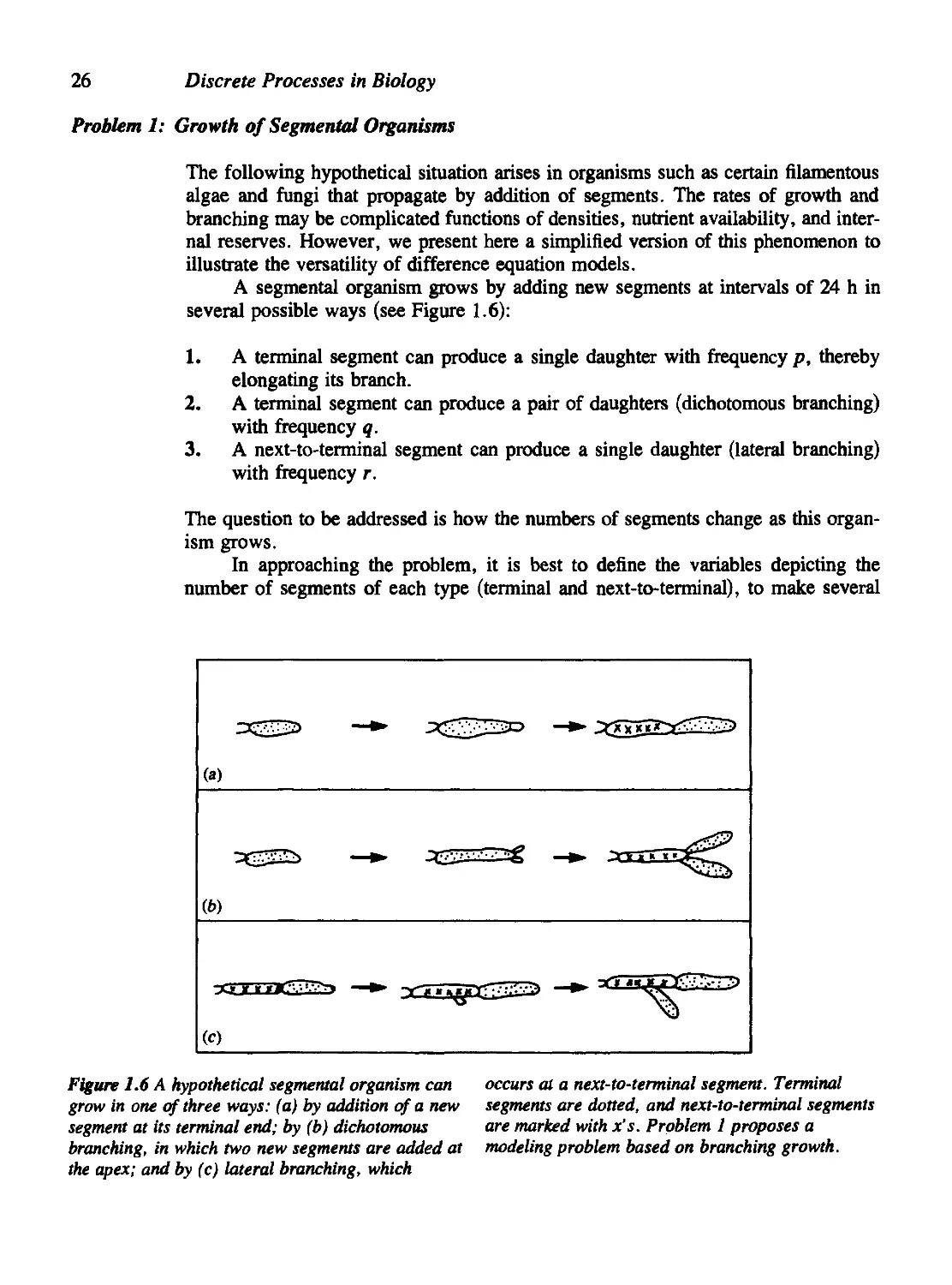
Problem 1: Growth of Segmental Organisms 26
Problem 2: A Schematic Model of Red Blood Cell Production 27
Problem 3: Ventilation Volume and Blood C02 Levels 27
1.10 For Further Study: Linear Difference Equations in Demography 28
Problems 29
References 36
Chapter 2 Nonlinear Difference Equations 39
2.1 Recognizing a Nonlinear Difference Equation 40
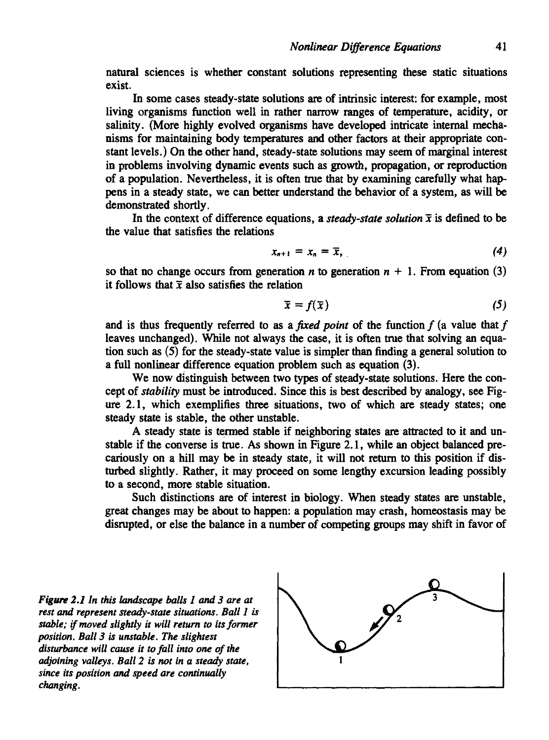
2.2 Steady States, Stability, and Critical Parameters 40
2.3 The Logistic Difference Equation 44
2.4 Beyond r = 3 46
IX

Contents
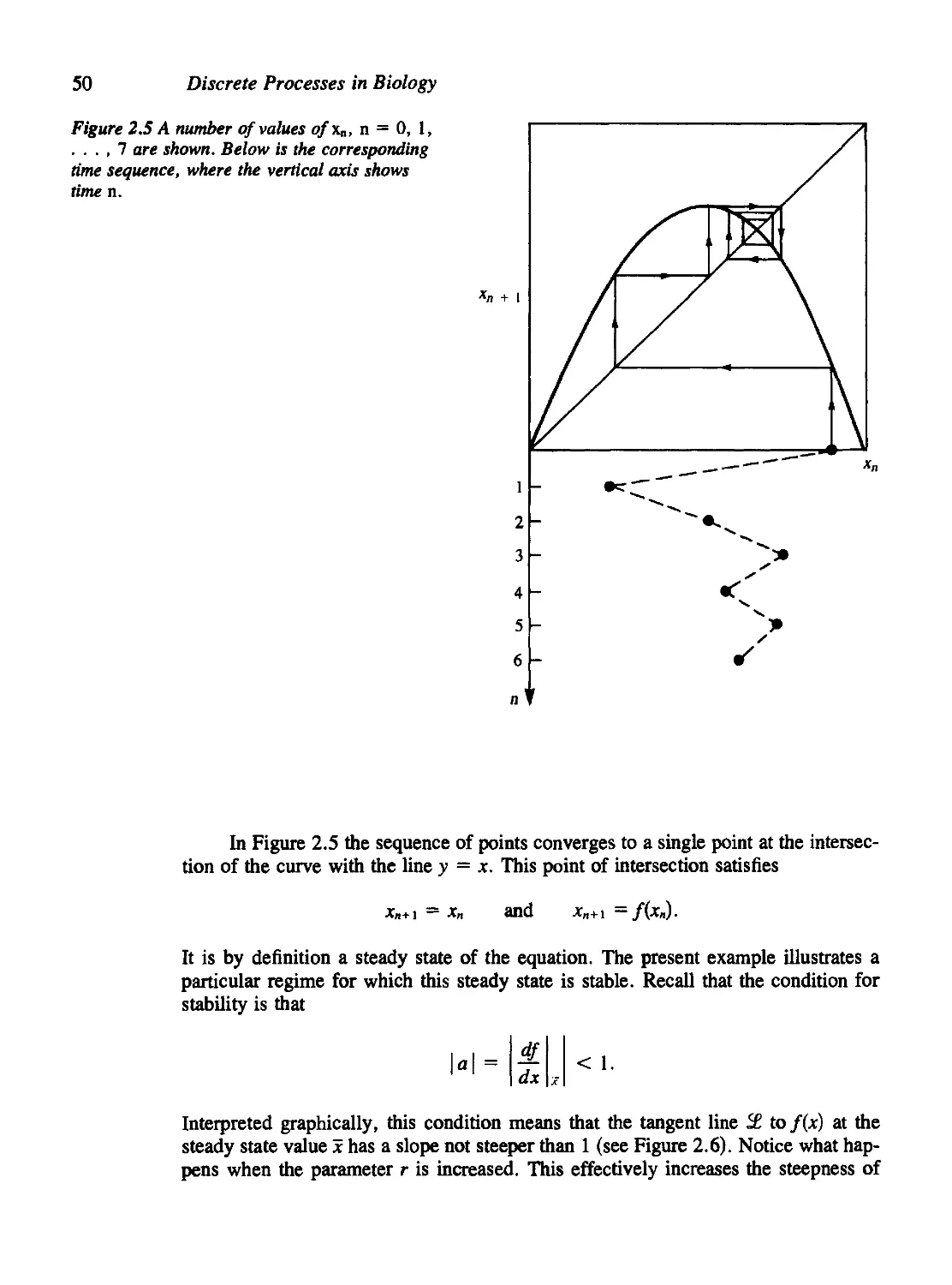
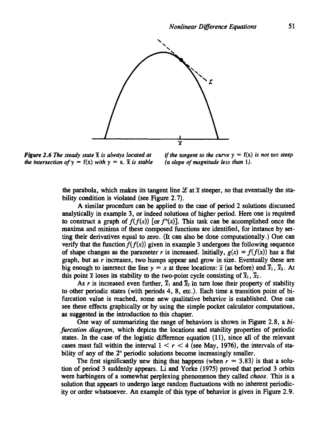
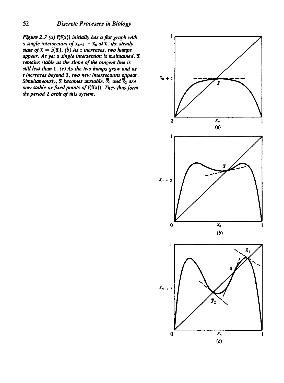
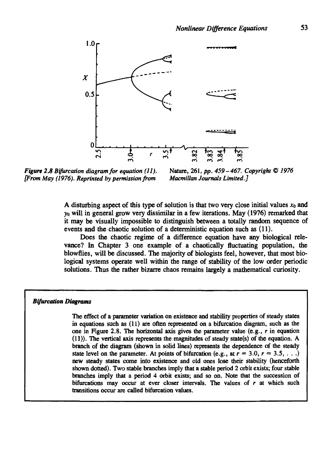
2.5 Graphical Methods for First-Order Equations 49
2.6 A Word about the Computer 55
2.7 Systems of Nonlinear Difference Equations 55
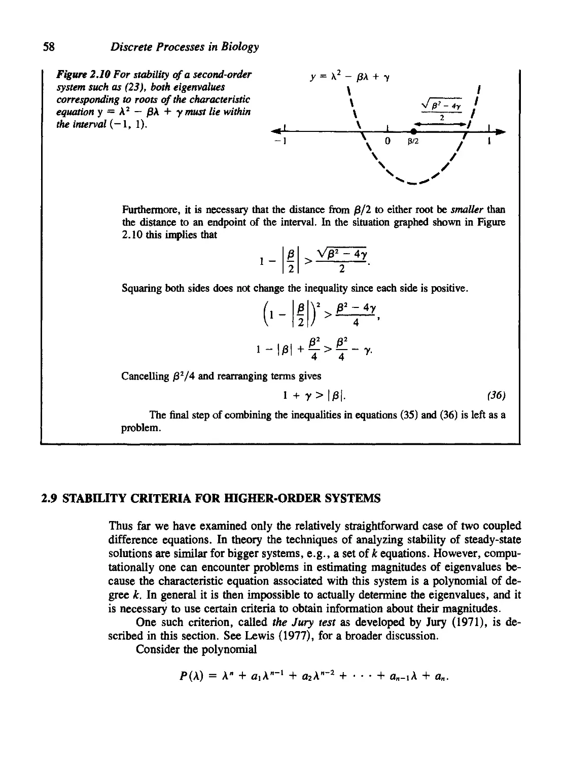
2.8 Stability Criteria for Second-Order Equations 57
2.9 Stability Criteria for Higher-Order Systems 58
2.10 For Further Study: Physiological Applications 60
Problems 61
References 67
Appendix to Chapter 2: Taylor Series 68
Part 1: Functions of One Variable 68
Part 2: Functions of Two Variables 70
Chapter 3 Applications of Nonlinear Difference Equations to Population
Biology 72
3.1 Density Dependence in Single-Species Populations 74
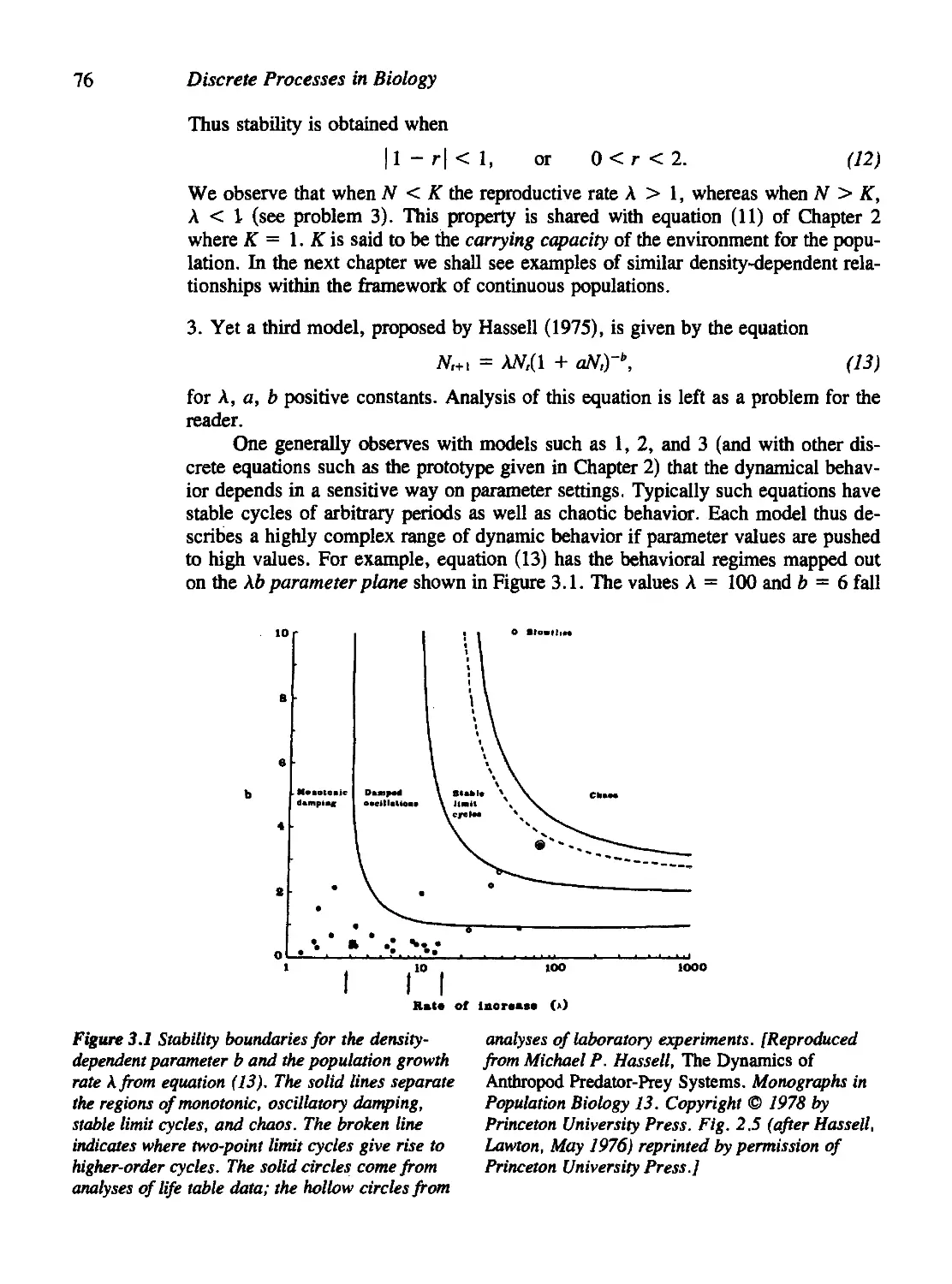
3.2 Two-Species Interactions: Host-Parasitoid Systems 78
3.3 The Nicholson-Bailey Model 79
3.4 Modifications of the Nicholson-Bailey Model 83
Density Dependence in the Host Population 83
Other Stabilizing Factors 86
3.5 A Model for Plant-Herbivore Interactions 89
Outlining the Problem 89
Rescaling the Equations 91
Further Assumptions and Stability Calculations 92
Deciphering the Conditions for Stability 96
Comments and Extensions 98
3.6 For Further Study: Population Genetics 99
Problems 102
Projects 109
References 110
PART H CONTINUOUS PROCESSES AND ORDINARY DIFFERENTIAL
EQUATIONS 113
Chapter 4 An Introduction to Continuous Models 115
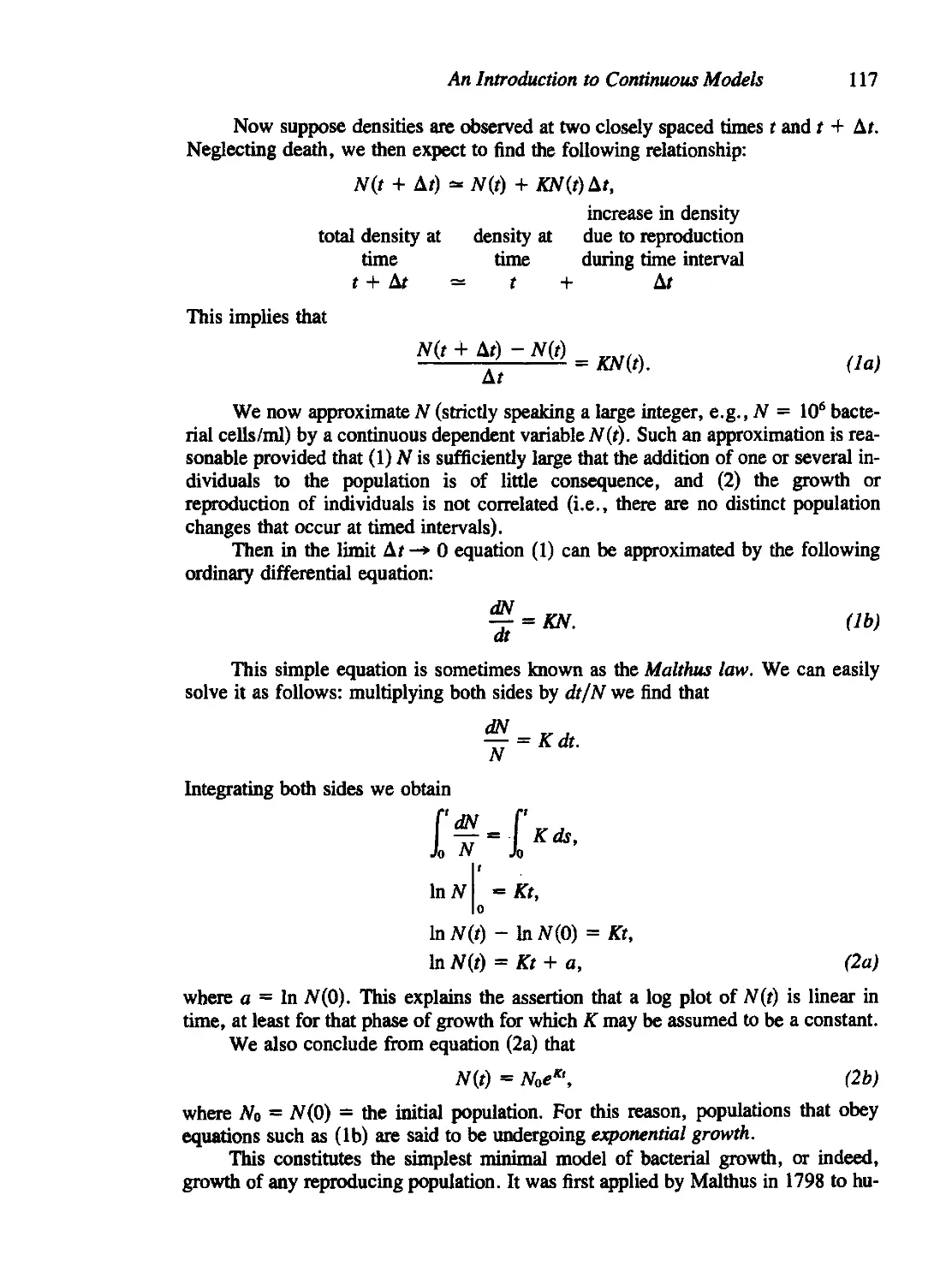
4.1 Warmup Examples: Growth of Microorganisms 116
4.2 Bacterial Growth in a Chemostat 121
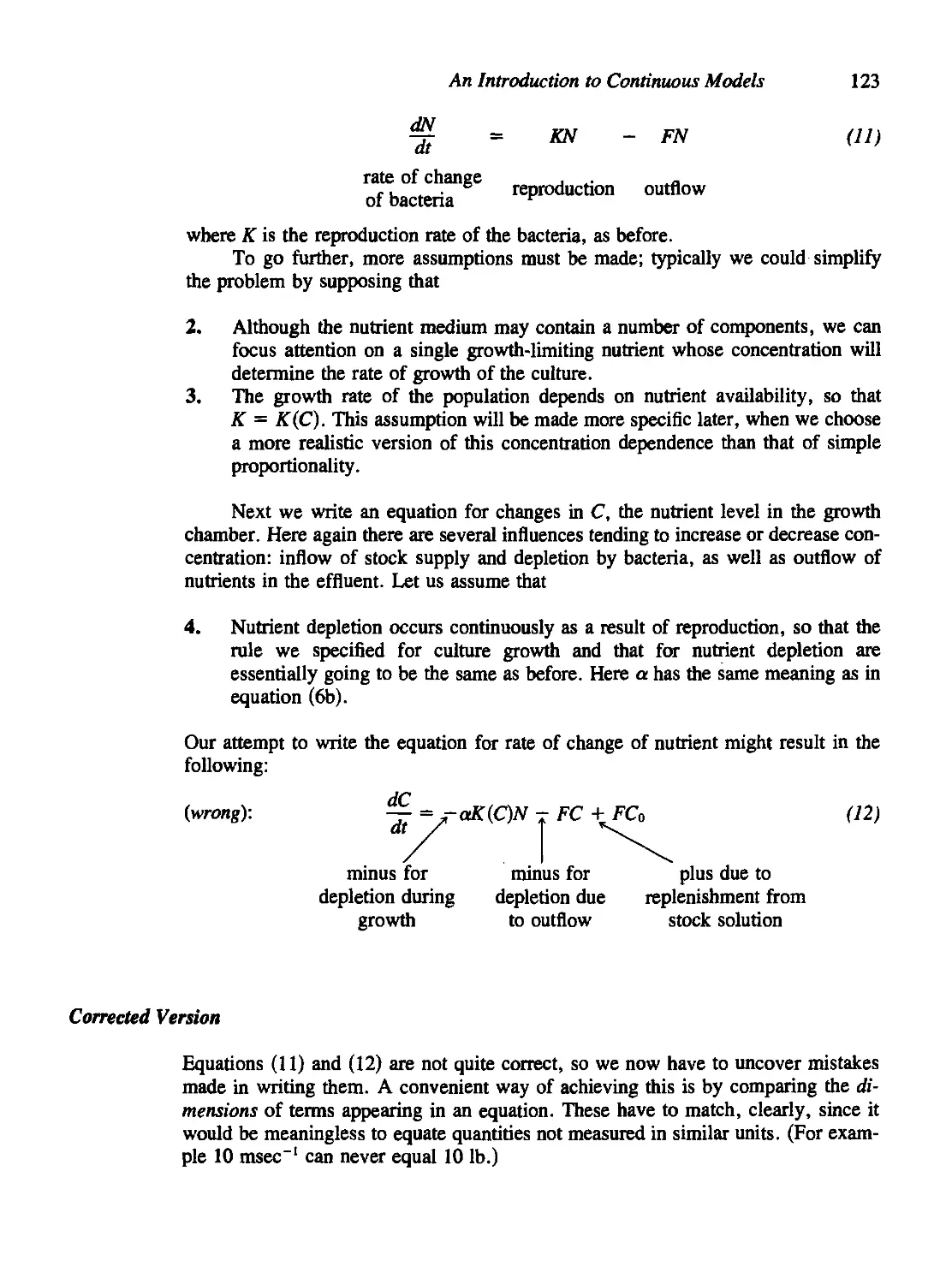
4.3 Formulating a Model
First Attempt 122
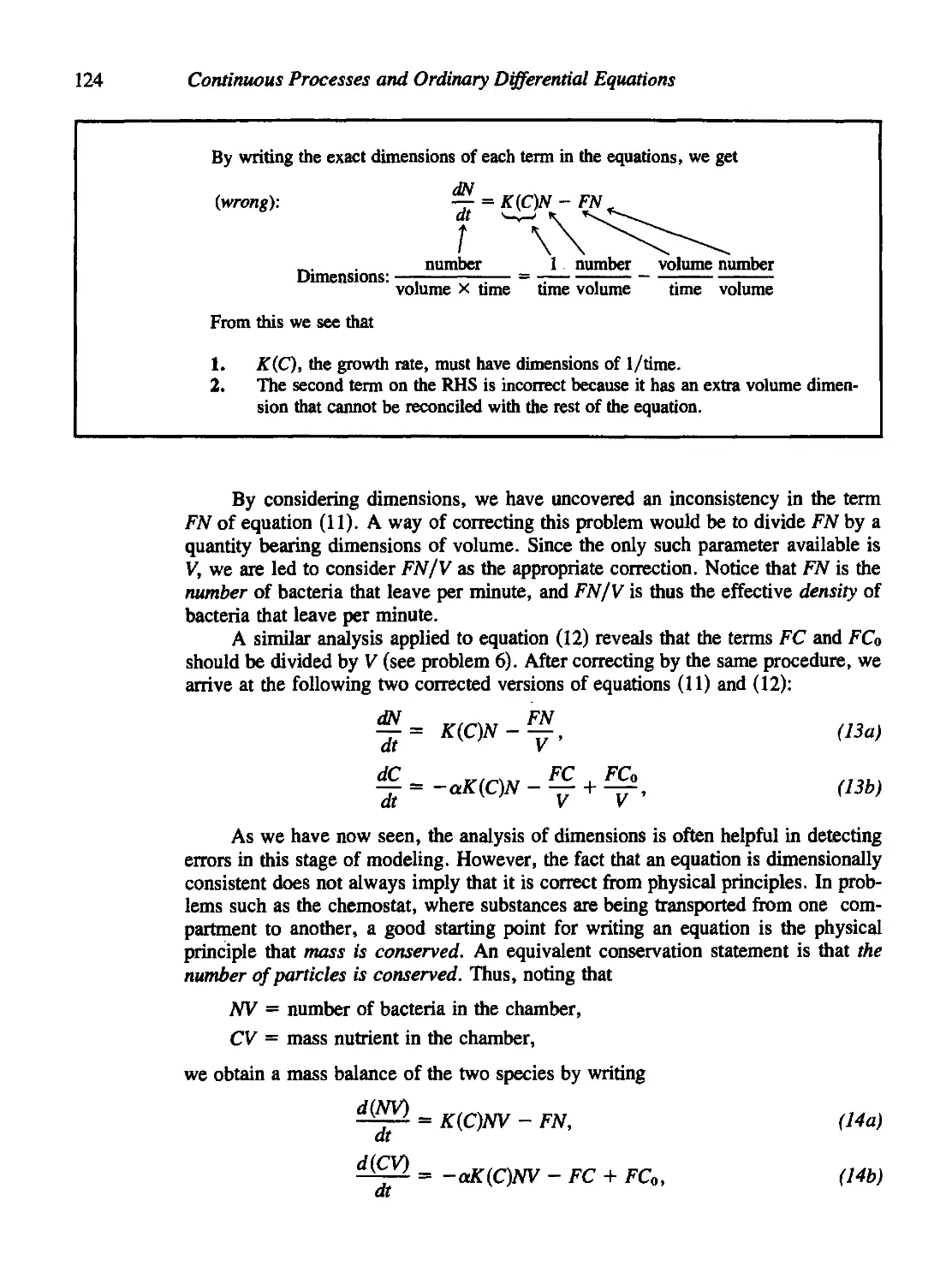
Corrected Version 123
4.4 A Saturating Nutrient Consumption Rate 125
4.5 Dimensional Analysis of the Equations 126
4.6 Steady-State Solutions 128
4.7 Stability and Linearization 129
4.8 Linear Ordinary Differential Equations: A Brief Review 130

Contents
xi
First-Order ODEs 132
Second-Order ODEs 132
A System of Two First-Order Equations (Elimination Method) 133
A System of Two First-Order Equations (Eigenvalue-Eigenvector
Method) 134
4.9 When Is a Steady State Stable? 141
4.10 Stability of Steady States in the Chemostat 143
4.11 Applications to Related Problems 145
Delivery of Drugs by Continuous Infusion 145
Modeling of Glucose-Insulin Kinetics 147
Compartmental Analysis 149
Problems 152
References 162
Chapter 5 Phase-Plane Methods and Qualitative Solutions 164
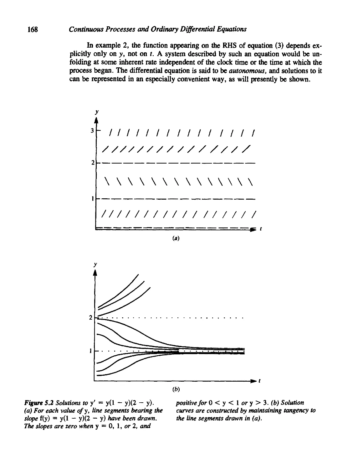
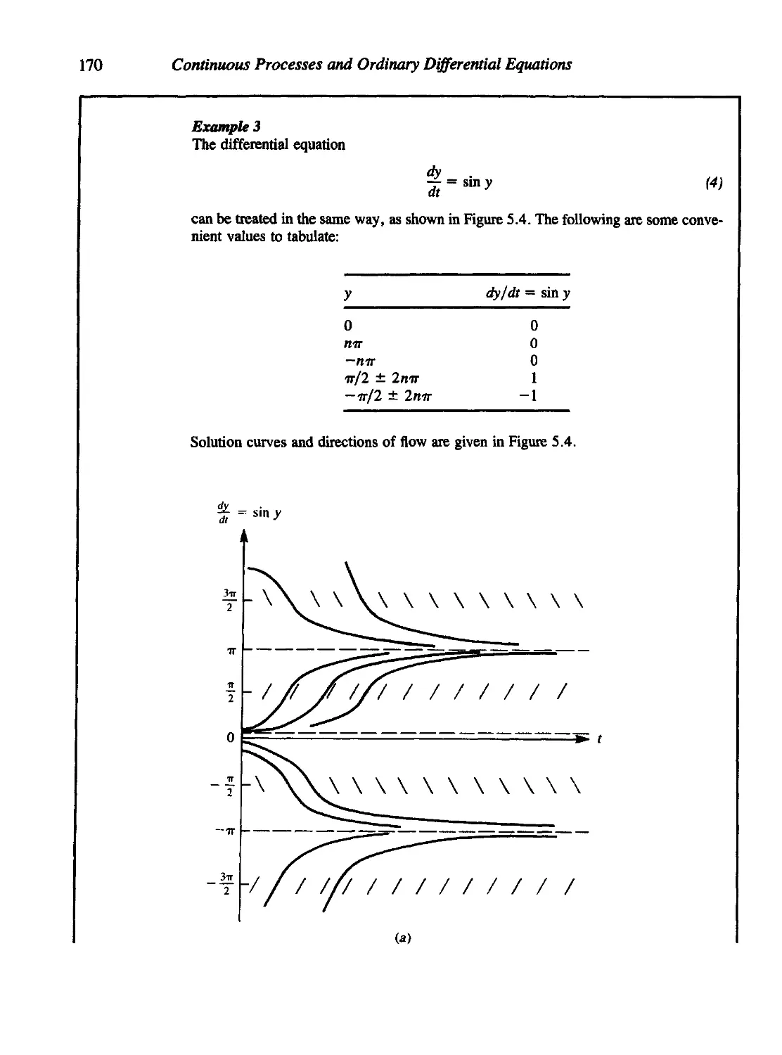
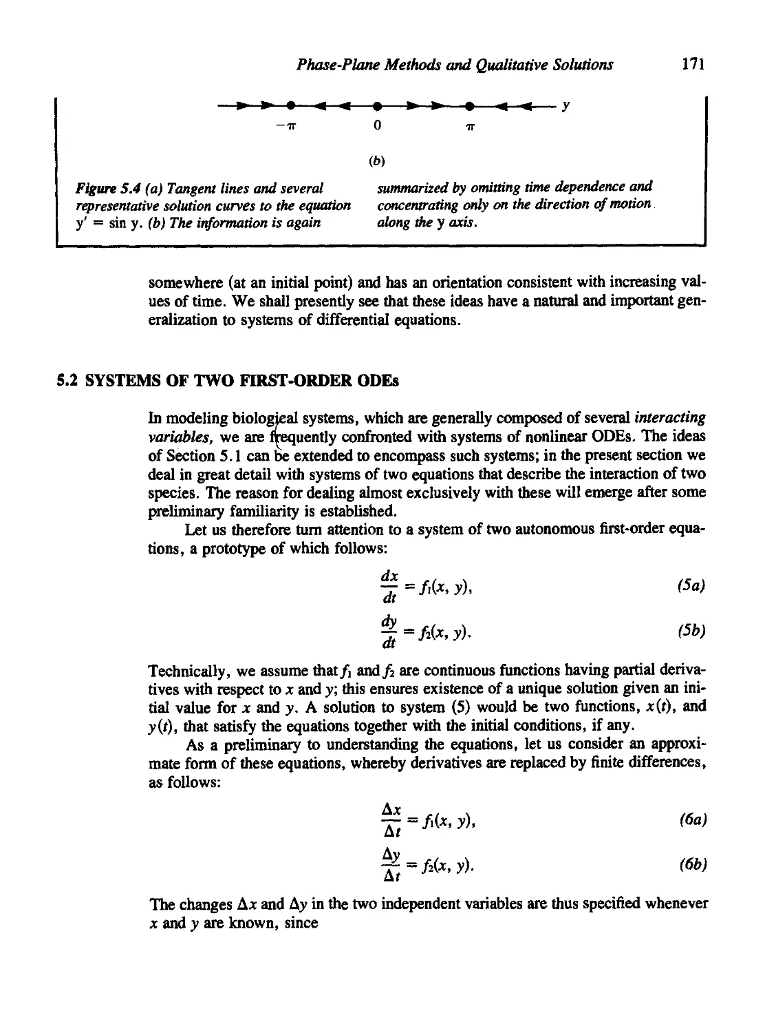
5.1 First-Order ODEs: A Geometric Meaning 165
5.2 Systems of Two First-Order ODEs 171
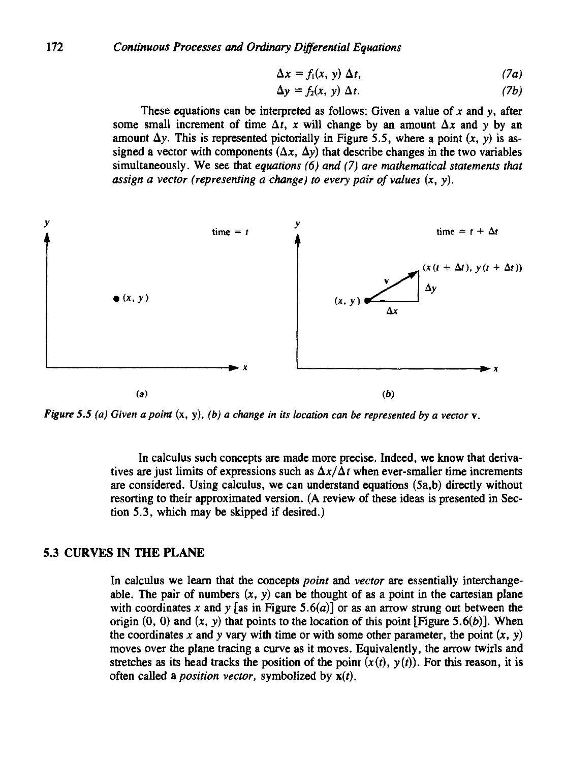
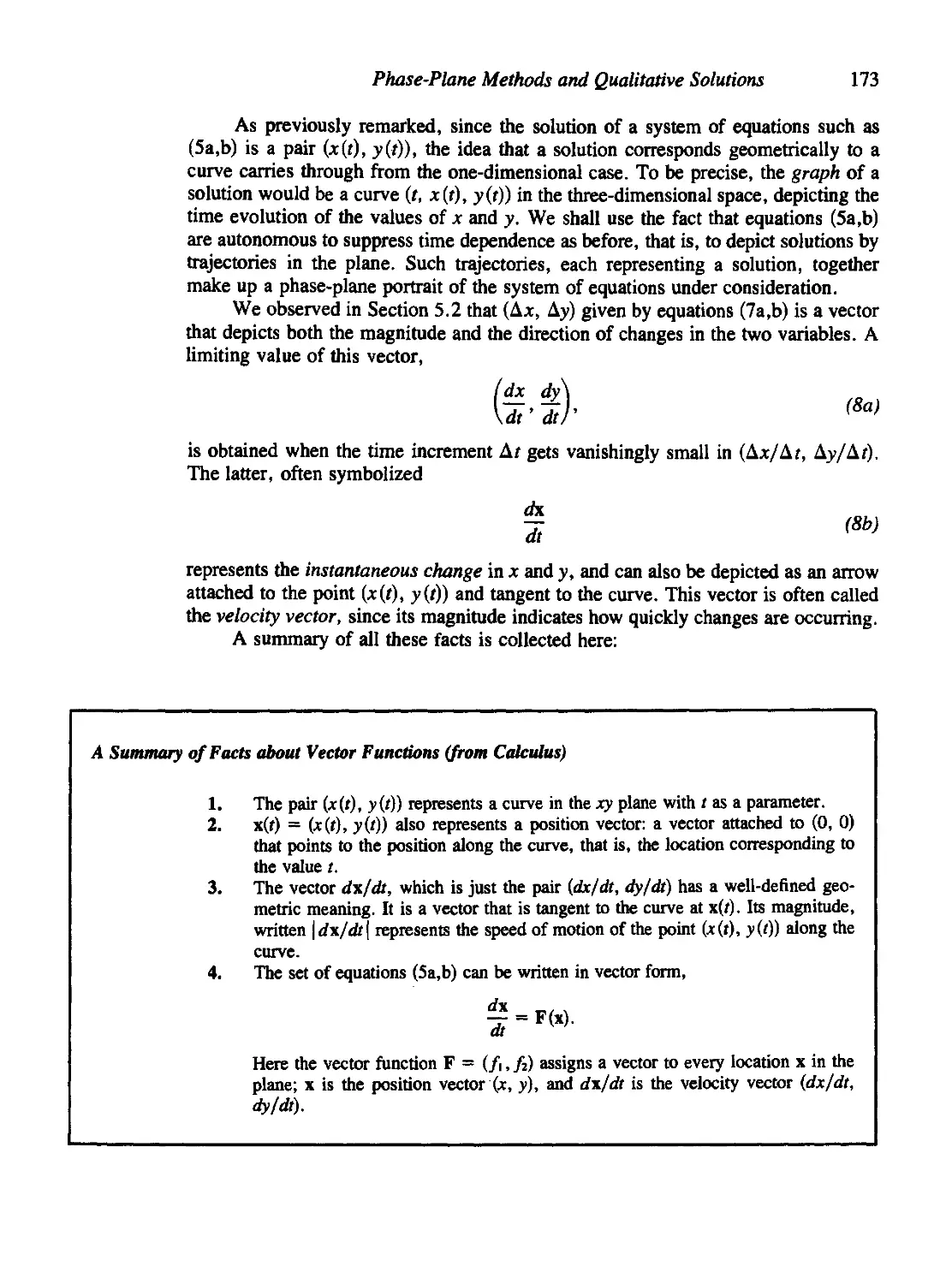
5.3 Curves in the Plane 172
5.4 The Direction Field 175
5.5 Nullclines: A More Systematic Approach 178
5.6 Close to the Steady States 181
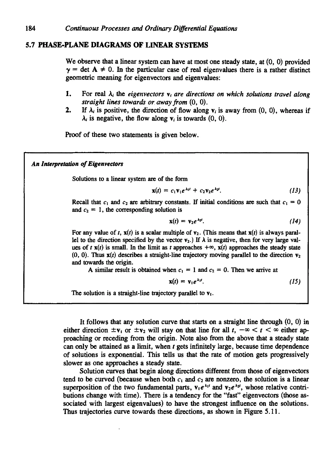
5.7 Phase-Plane Diagrams of Linear Systems 184
Real Eigenvalues 185
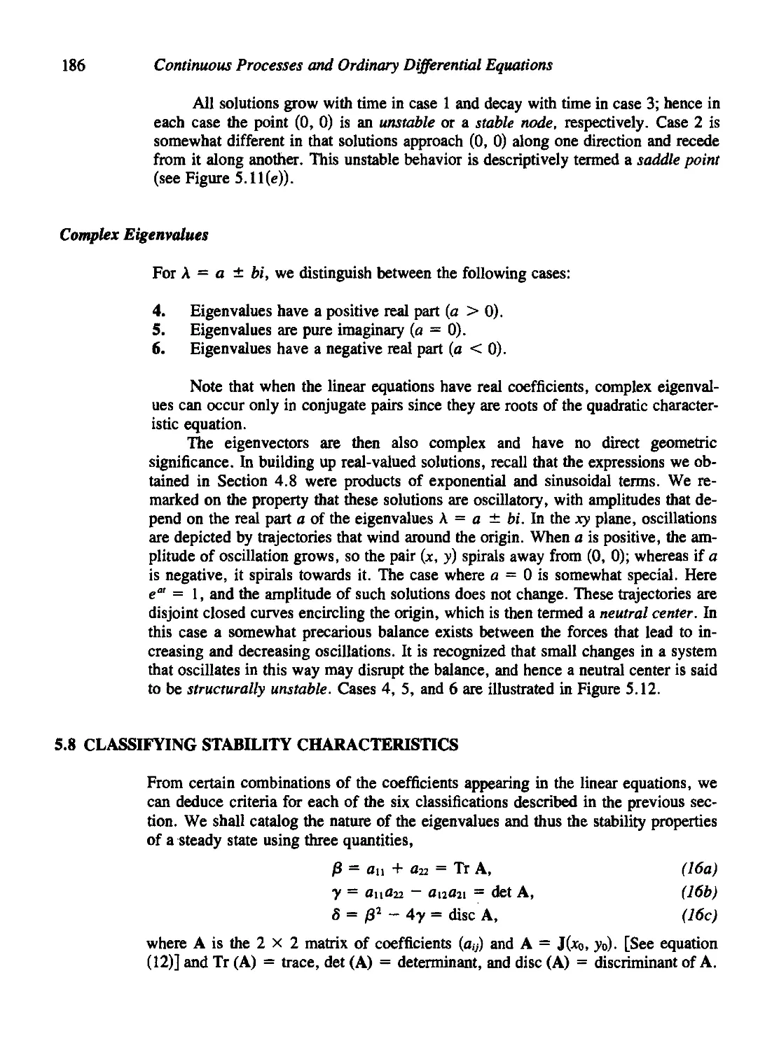
Complex Eigenvalues 186
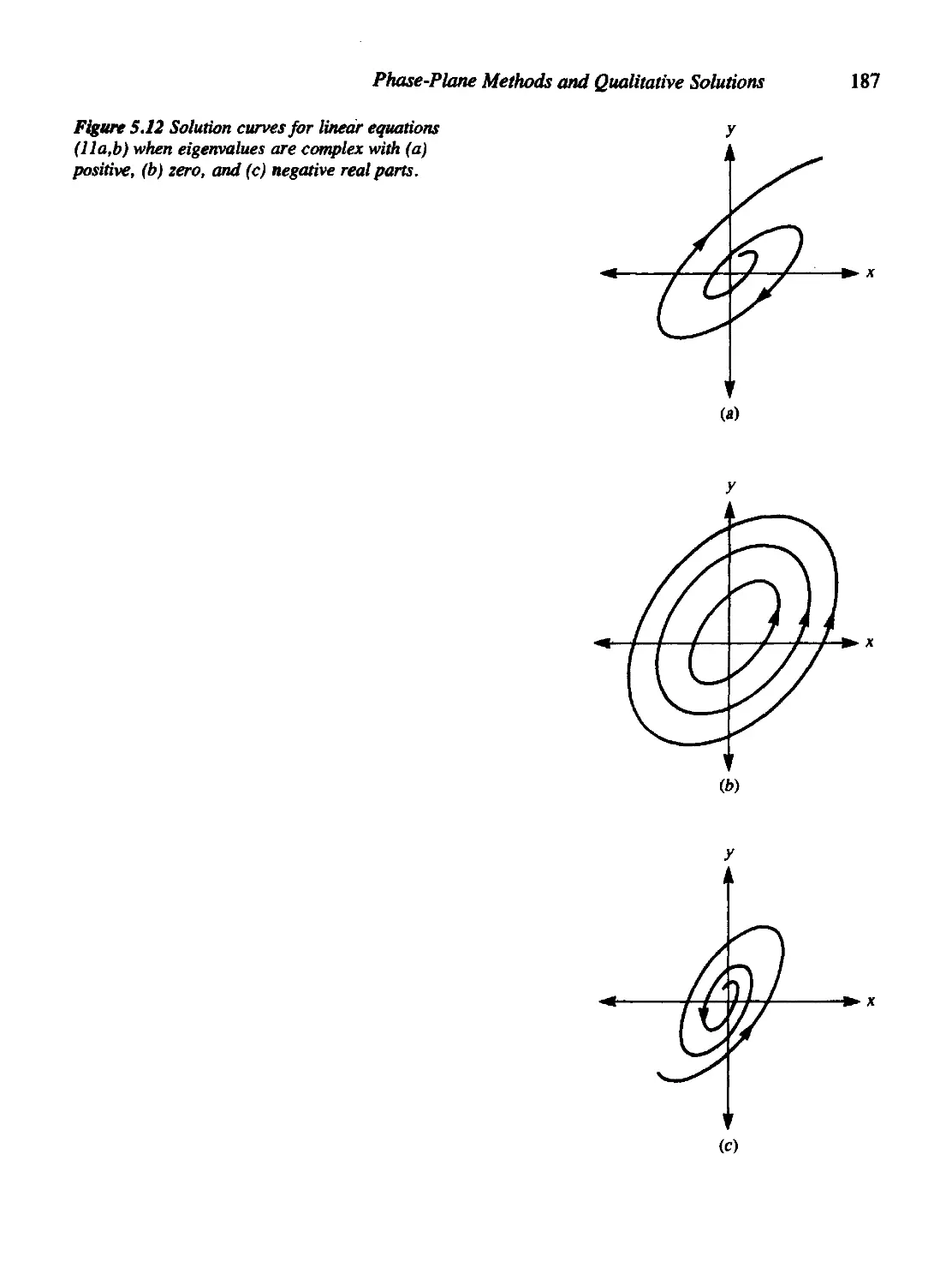
5.8 Classifying Stability Characteristics 186
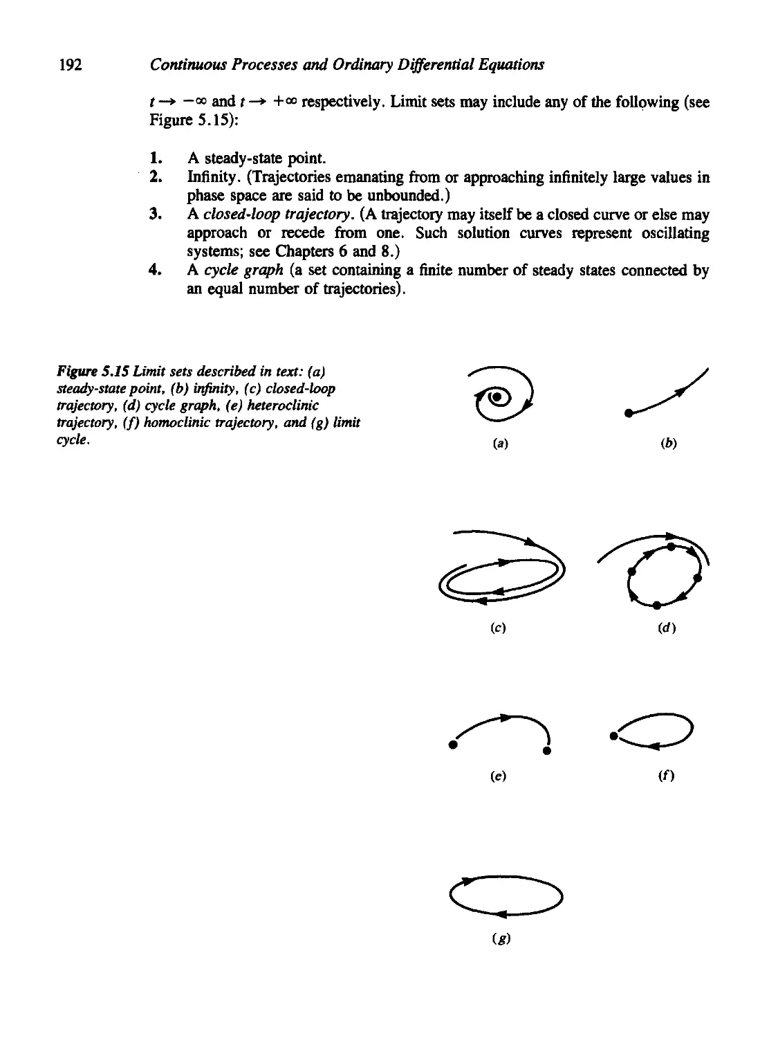
5.9 Global Behavior from Local Information 191
5.10 Constructing a Phase-Plane Diagram for the Chemostat 193
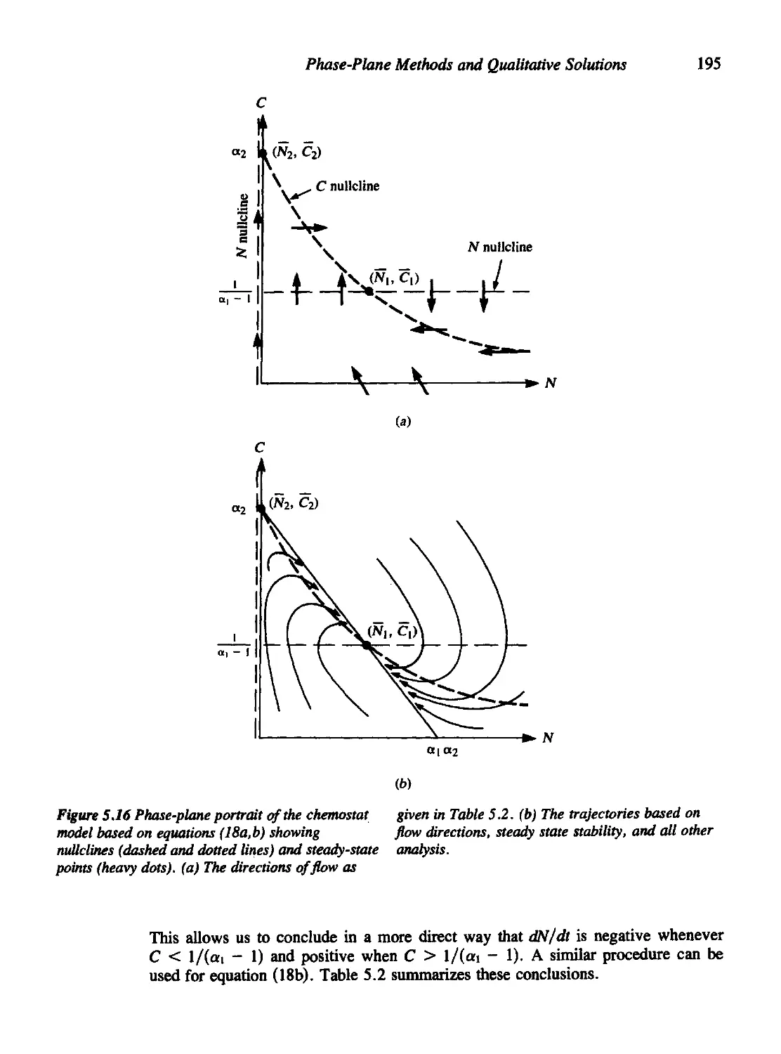
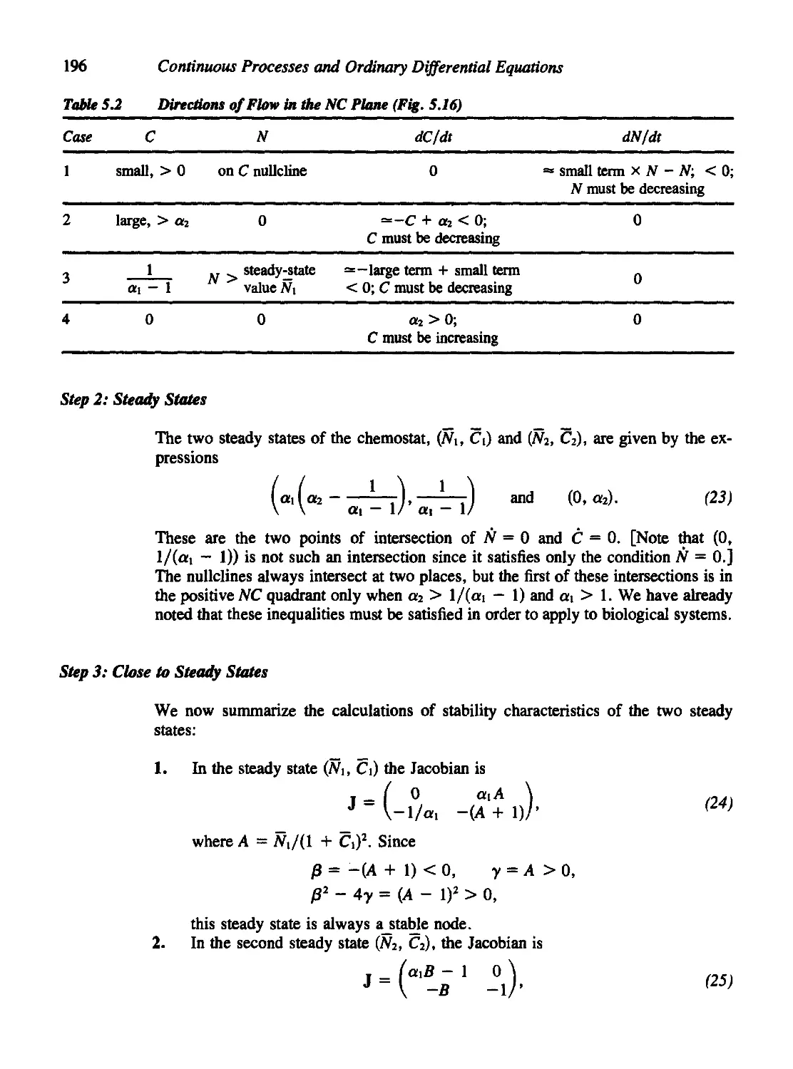
Step 1: The Nullclines 194
Step 2: Steady States 196
Step 3: Close to Steady States 196
Step 4: Interpreting the Solutions 197
5.11 Higher-Order Equations 199
Problems 200
References 209
Chapter 6 Applications of Continuous Models to Population Dynamics 210
6.1 Models for Single-Species Populations 212
Malthus Model 214
Logistic Growth 214
Allee Effect 215
Other Assumptions; Gompertz Growth in Tumors 217
6.2 Predator-Prey Systems and the Lotka-Volterra Equations 218
6.3 Populations in Competition 224
6.4 Multiple-Species Communities and the Routh-Hurwitz Criteria 231
6.5 Qualitative Stability 236
6.6 The Population Biology of Infectious Diseases 242

xii Contents
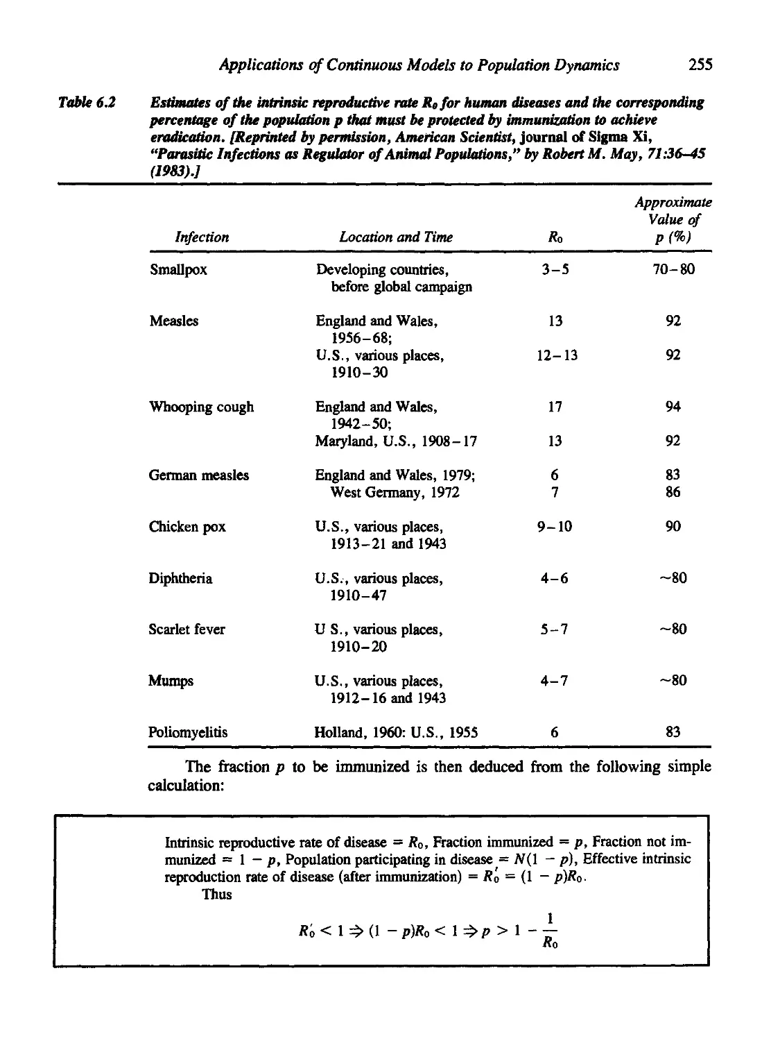
6.7 For Further Study: Vaccination Policies 254
Eradicating a Disease 254
Average Age of Acquiring a Disease 256
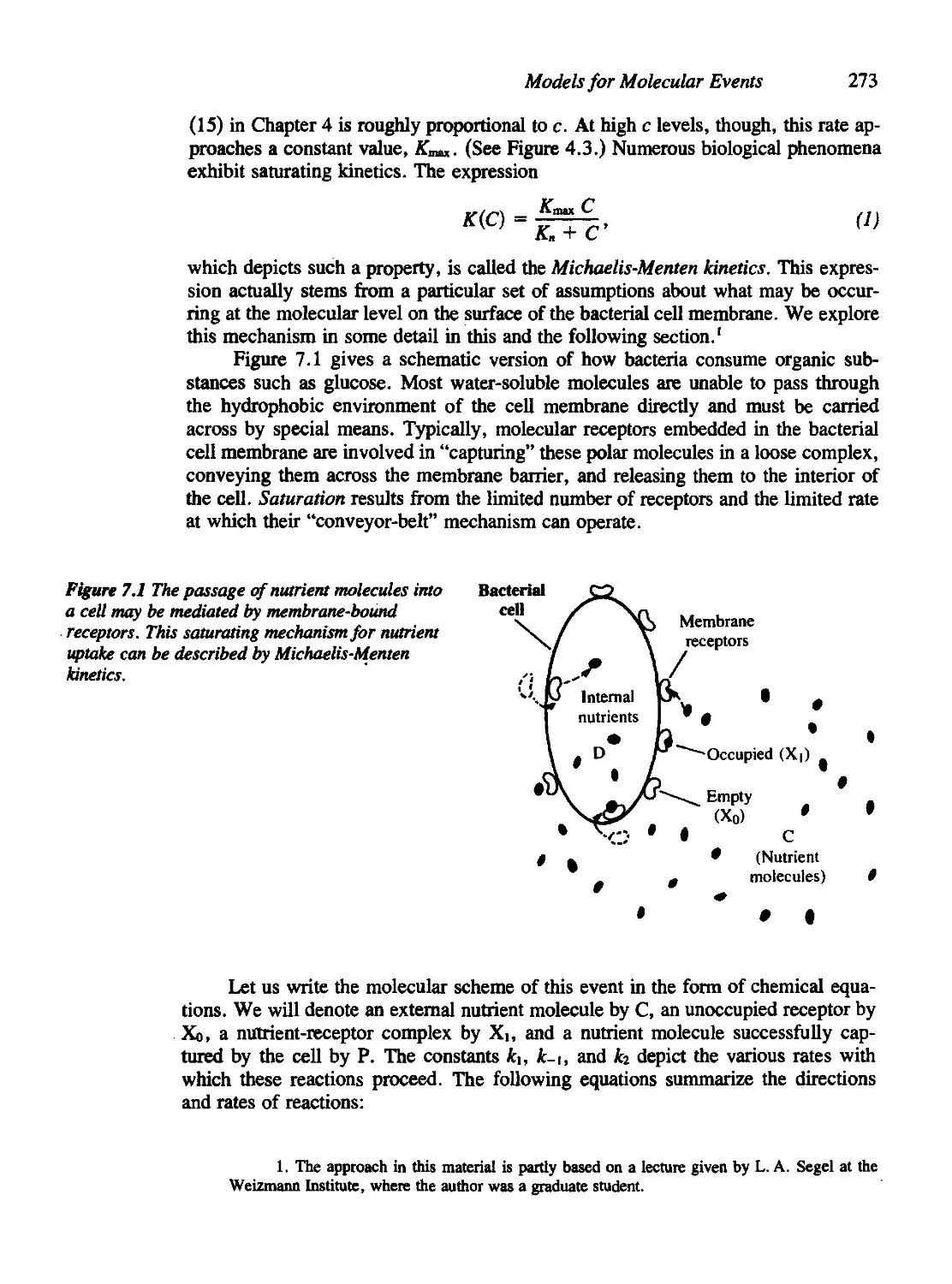
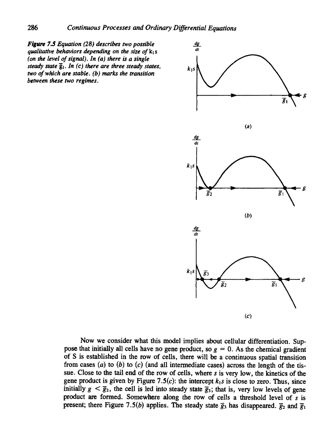
Chapter 7 Models for Molecular Events 271
7.1 Michaelis-Menten Kinetics 272
7.2 The Quasi-Steady-State Assumption 275
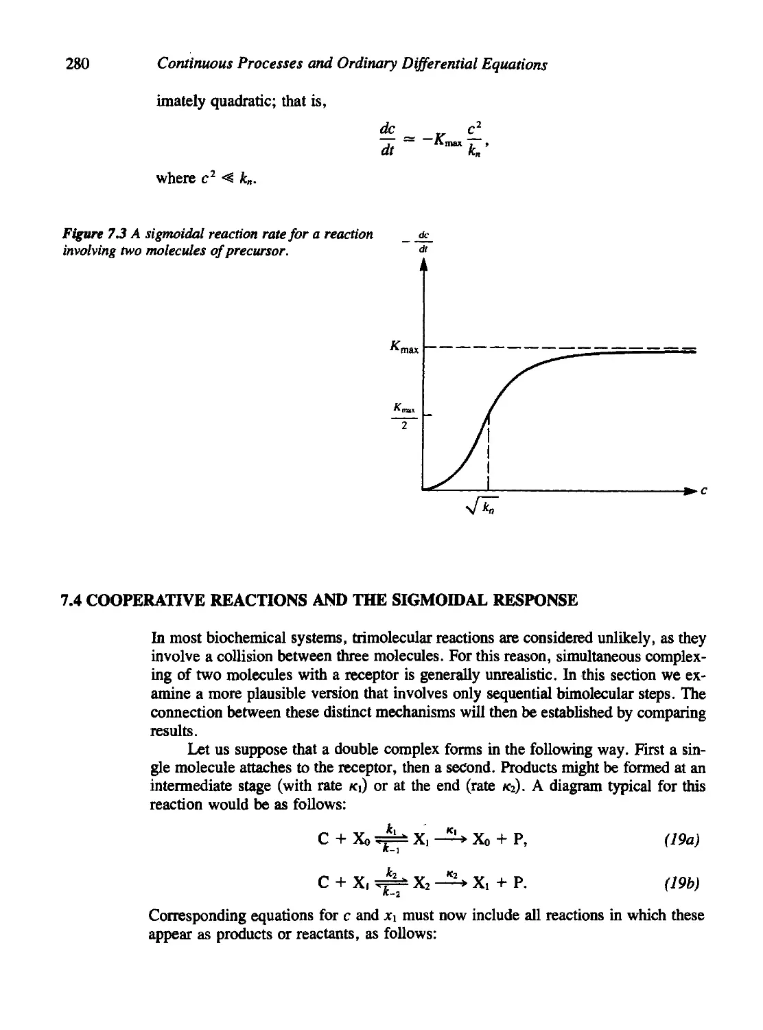
7.3 A Quick, Easy Derivation of Sigmoidal Kinetics 279
7.4 Cooperative Reactions and the Sigmoidal Response 280
7.5 A Molecular Model for Threshold-Governed Cellular Development 283
7.6 Species Competition in a Chemical Setting 287
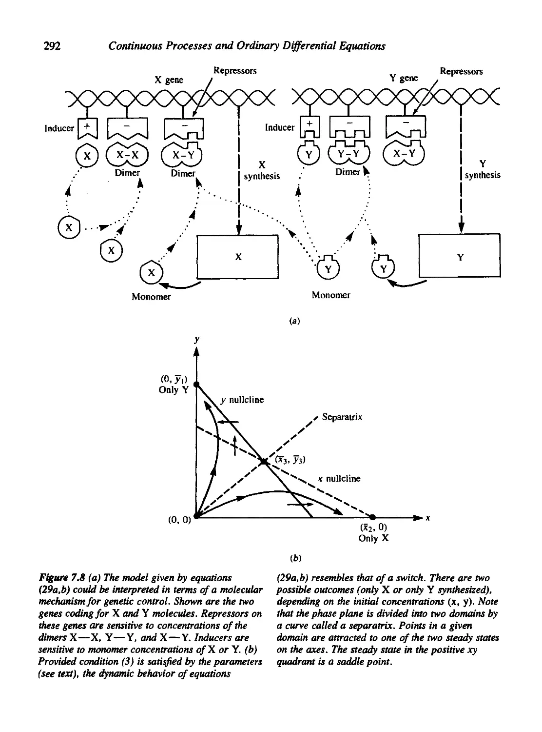
7.7 A Bimolecular Switch 294
7.8 Stability of Activator-Inhibitor and Positive Feedback Systems 295
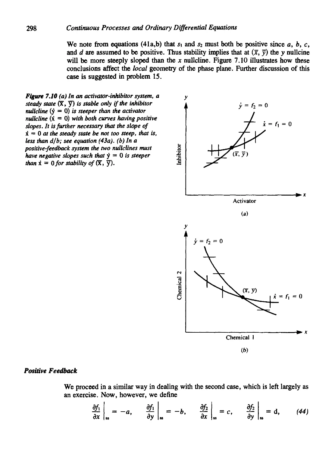
The Activator-Inhibitor System 296
Positive Feedback 298
7.9 Some Extensions and Suggestions for Further Study 299
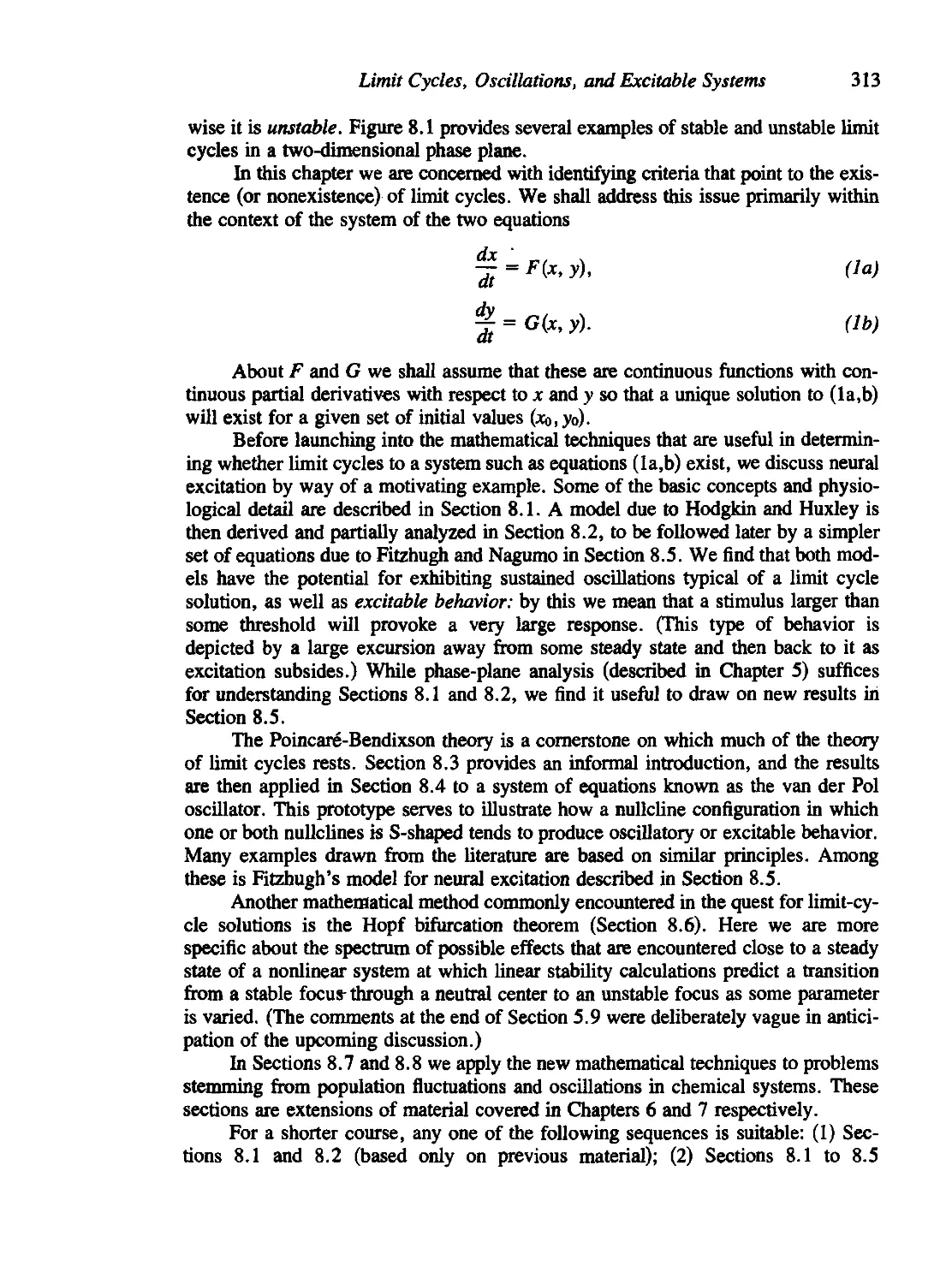
Chapter 8 Limit Cycles, Oscillations, and Excitable Systems 311
8.1 Nerve Conduction, the Action Potential, and the Hodgkin-Huxley
Equations 314
8.2 Fitzhugh's Analysis of the Hodgkin-Huxley Equations 323
8.3 The Poincare'-Bendixson Theory 327
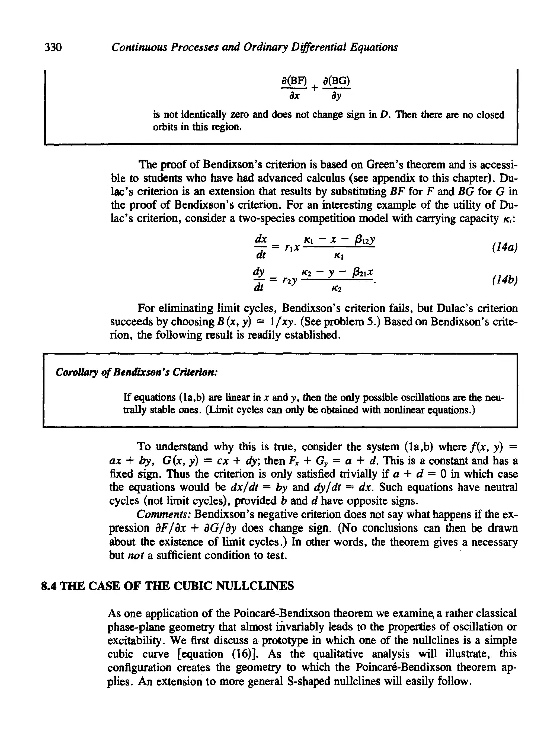
8.4 The Case of the Cubic Nullclines 330
8.5 The Fitzhugh-Nagumo Model for Neural Impulses 337
8.6 The Hopf Bifurcation 341
8.7 Oscillations in Population-Based Models 346
8.8 Oscillations in Chemical Systems 352
Criteria for Oscillations in a Chemical System 354
8.9 For Further Study: Physiological and Orcadian Rhythms 360
Appendix to Chapter 8. Some Basic Topological Notions 375
Appendix to Chapter 8. More about the Poincarg-Bendixson Theory 379
PART m SPATIALLY DISTRIBUTED SYSTEMS AND PARTIAL
DIFFERENTIAL EQUATION MODELS 381
Chapter 9 An Introduction to Partial Differential Equations and Diffusion
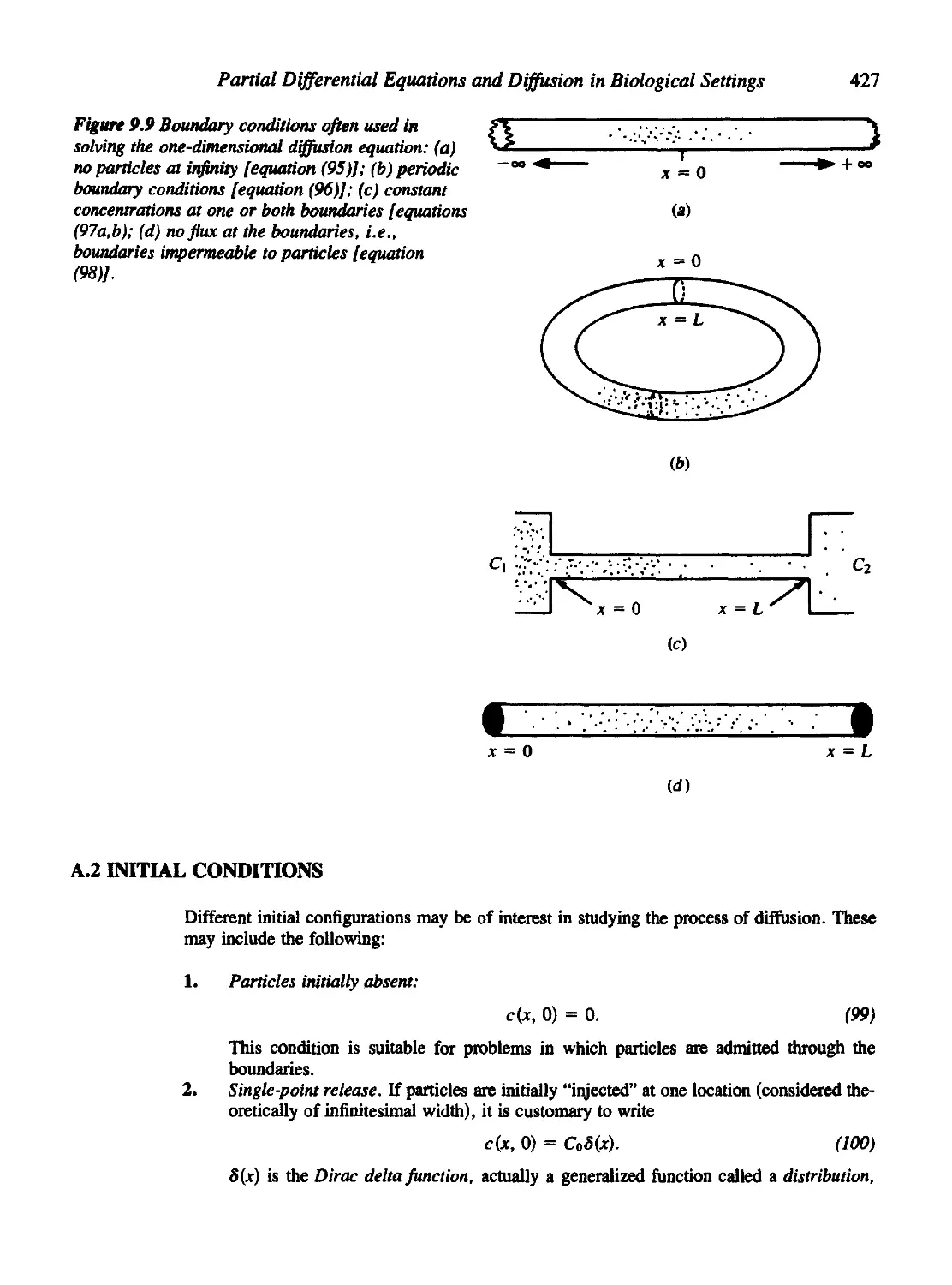
in Biological Settings 383
9.1 Functions of Several Variables: A Review 385
9.2 A Quick Derivation of the Conservation Equation 393
9.3 Other Versions of the Conservation Equation 395
Tubular Flow 395
Flows in Two and Three Dimensions 397
9.4 Convection, Diffusion, and Attraction 403
Convection 403
Attraction or Repulsion 403
Random Motion and the Diffusion Equation 404

Contents
xiii
9.5 The Diffusion Equation and Some of Its Consequences 406
9.6 Transit Times for Diffusion 410
9.7 Can Macrophages Find Bacteria by Random Motion Alone? 412
9.8 Other Observations about the Diffusion Equation 413
9.9 An Application of Diffusion to Mutagen Bioassays 416
Appendix to Chapter 9. Solutions to the One-Dimensional
Diffusion Equation 426
Chapter 10 Partial Differential Equation Models in Biology 436
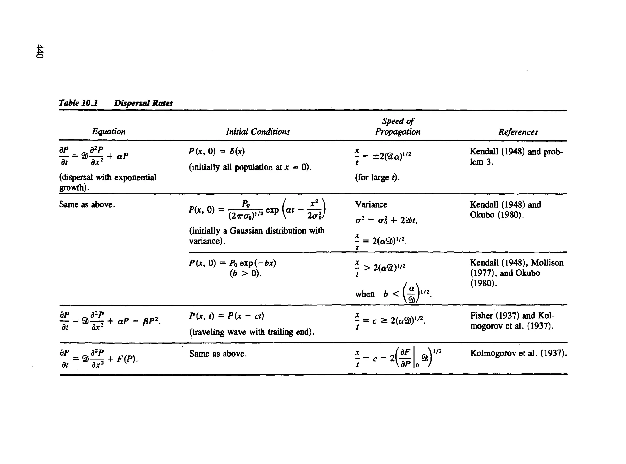
10.1 Population Dispersal Models Based on Diffusion 437
10.2 Random and Chemotactic Motion of Microorganisms 441
10.3 Density-Dependent Dispersal 443
10.4 Apical Growth in Branching Networks 445
10.5 Simple Solutions: Steady States and Traveling Waves 447
Nonuniform Steady States 447
Homogeneous (Spatially Uniform) Steady States 448
Traveling-Wave Solutions 450
10.6 Traveling Waves in Microorganisms and in the Spread of Genes 452
Fisher's Equation: The Spread of Genes in a Population 452
Spreading Colonies of Microorganisms 456
Some Perspectives and Comments 460
10.7 Transport of Biological Substances Inside the Axon 461
10.8 Conservation Laws in Other Settings: Age Distributions and
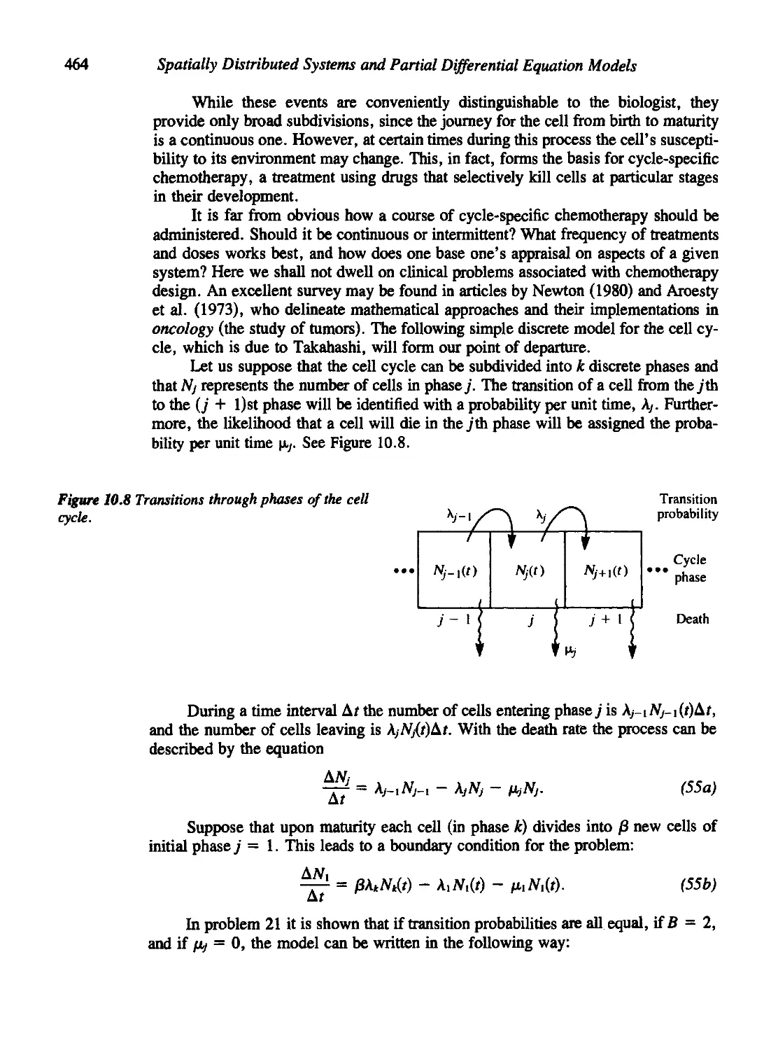
the Cell Cycle 463
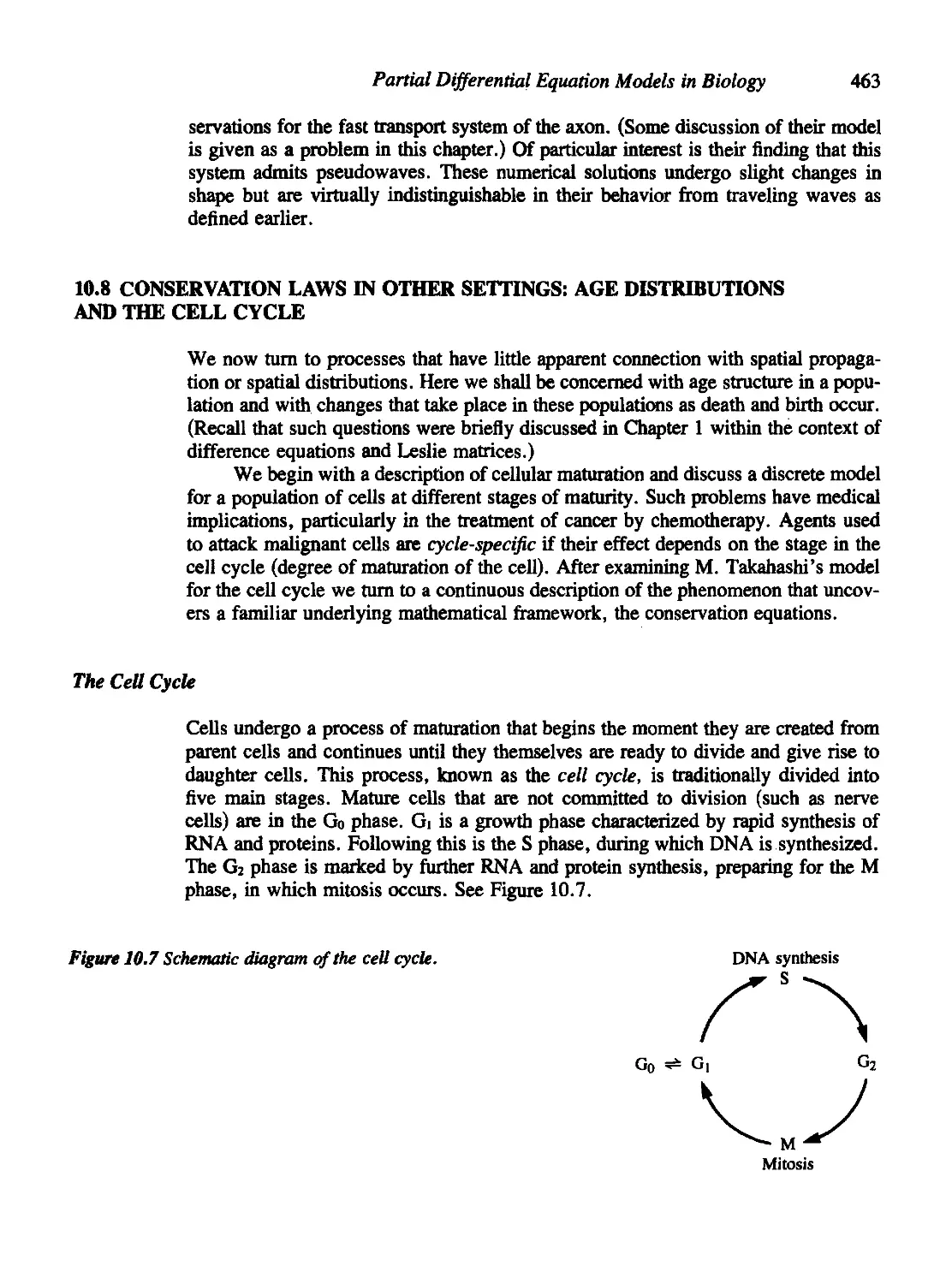
The Cell Cycle 463
Analogies with Particle Motion 466
A Topic for Further Study: Applications to Chemotherapy 469
Summary 469
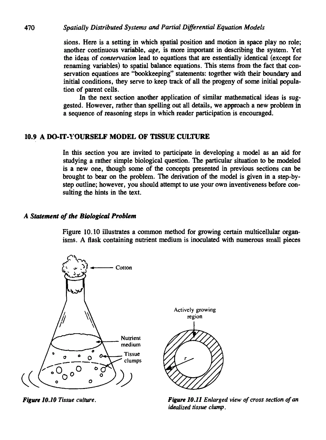
10.9 A Do-It-Yourself Model of Tissue Culture 470
A Statement of the Biological Problem 470
Step 1: A Simple Case 471
Step 2: A Slightly More Realistic Case 472
Step 3: Writing the Equations 473
The Final Step 475
Discussion 476
10.10 For Further Study: Other Examples of Conservation Laws in
Biological Systems 477
Chapter 11 Models for Development and Pattern Formation in Biological
Systems 496
11.1 Cellular Slime Molds 498
11.2 Homogeneous Steady States and Inbomogeneous Perturbations 502
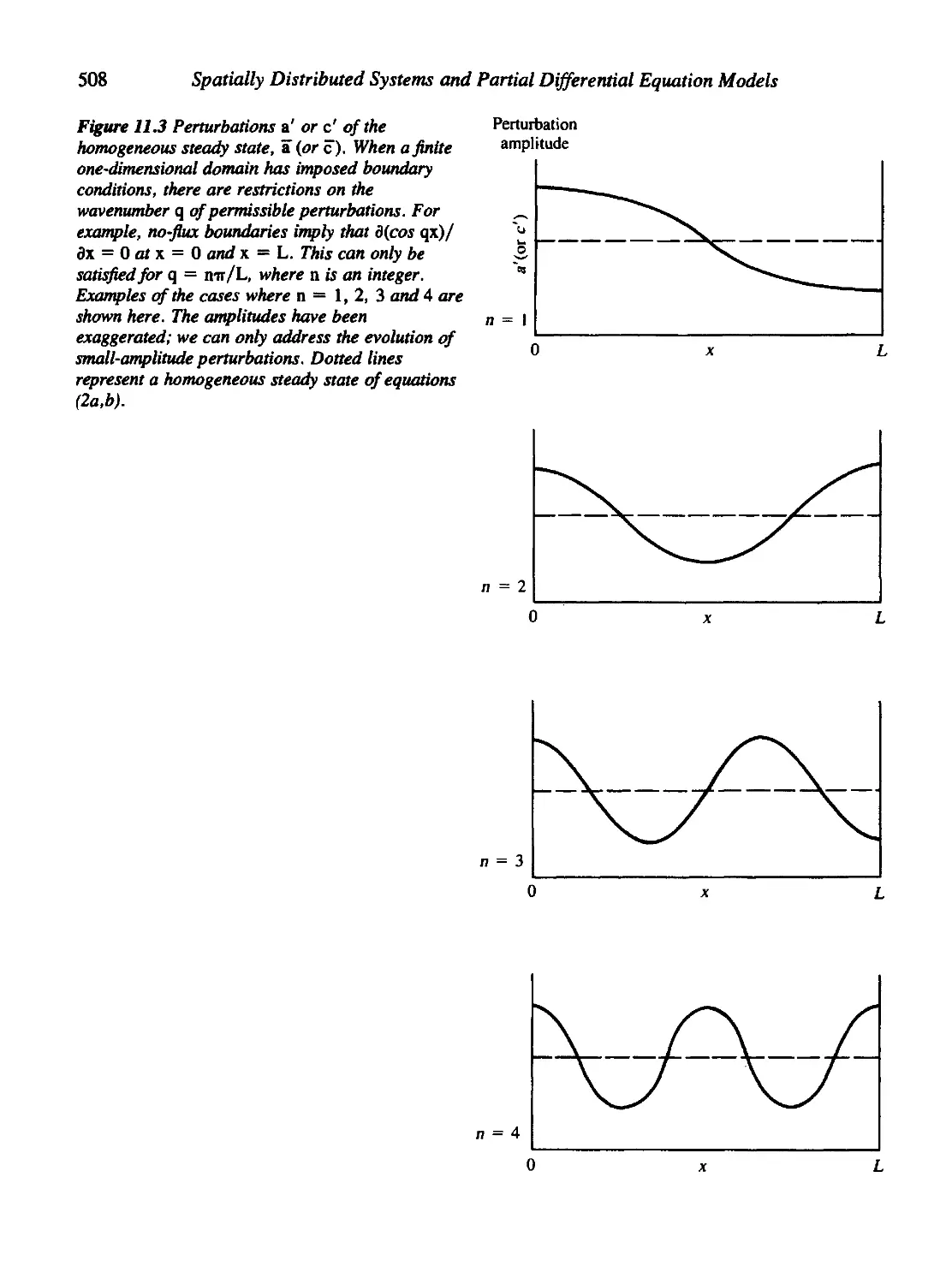
11.3 Interpreting the Aggregation Condition 506
11.4 A Chemical Basis for Morphogenesis 509
11.5 Conditions for Diffusive Instability 512
11.6 A Physical Explanation 516
11.7 Extension to Higher Dimensions and Finite Domains 520

xiv Contents
11.8 Applications to Morphogenesis 528
11.9 For Further Study: 535
Patterns in Ecology 535
Evidence for Chemical Morphogens in Developmental Systems 537
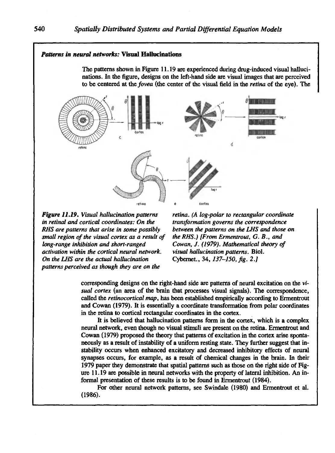
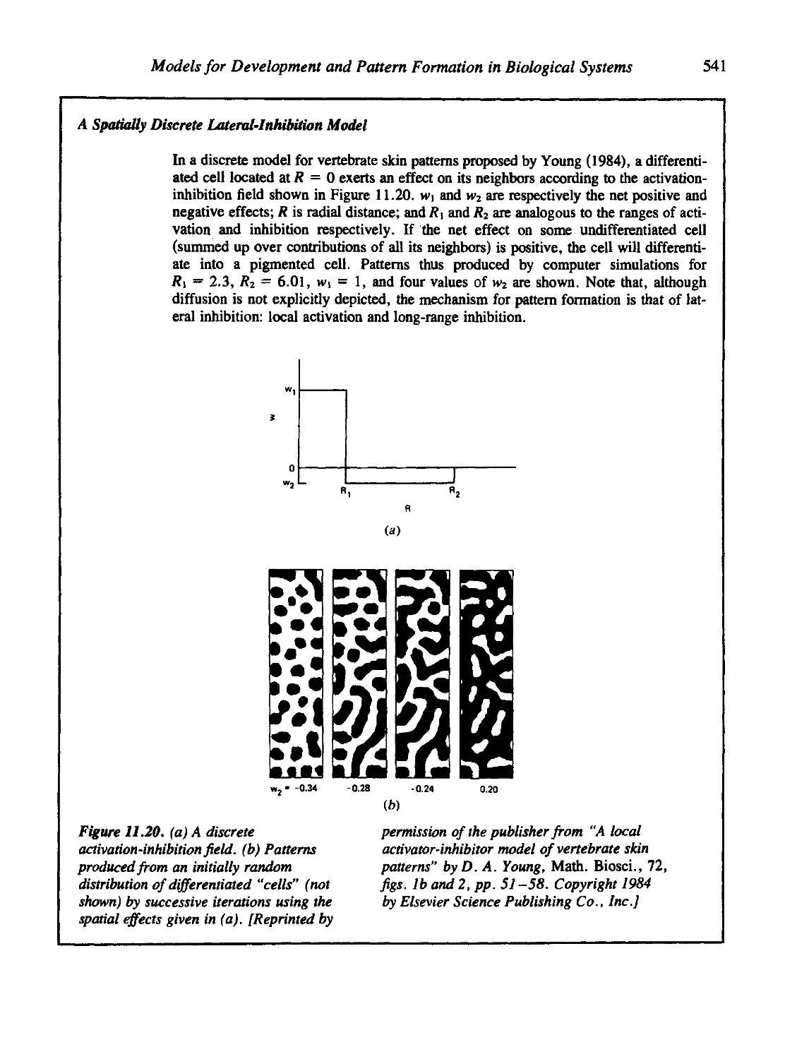
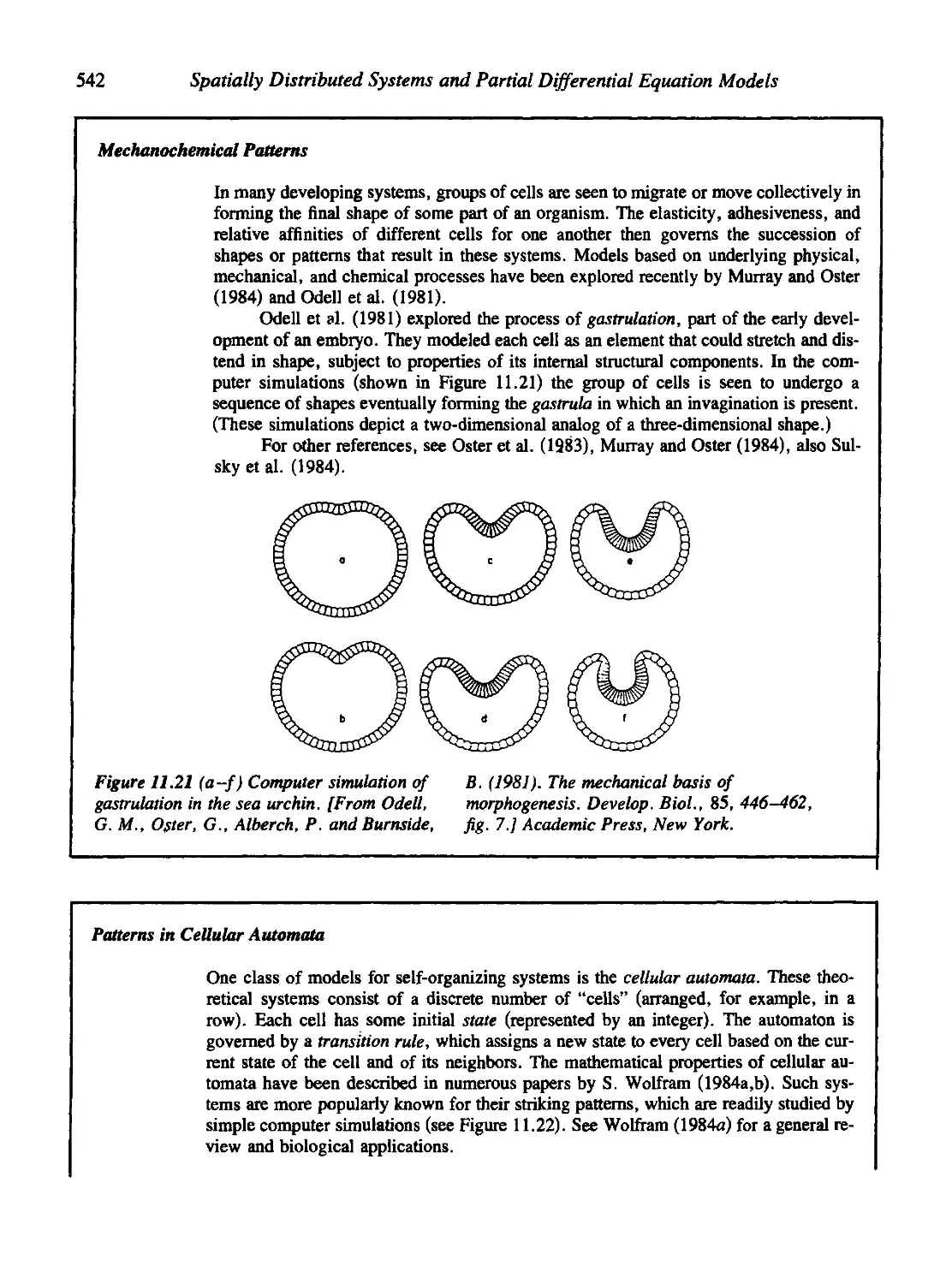
A Broader View of Pattern Formation in Biology 539
Selected Answers 556
Author Index 571
Subject Index 575

Preface to the Classics Edition
This book originated from interests that I developed while still at graduate school,
but its actual writing and evolution spanned the mid 1980s. At that time, I was a
visiting assistant professor, at an early career stage. I had the pleasure of teaching
undergraduate courses in mathematical biology at both Brown and Duke
Universities and this book evolved from those experiences. In a sense, this was a process
of discovery: of the many beautiful areas of application of mathematics, and of
the interconnections between what, at first glance, seem like distinct topics. It is
safe to say that, during this gestation period of Mathematical Models in Biology
(henceforth abbreviated MMIB), the field of mathematical biology was still quite
young. The selection of textbooks and teaching materials at the time was quite
limited. At the time, mathematical biology was viewed by many as a "soft version"
of mathematics, or an "irrelevant" appendix to biology.
Shortly after the birth of MMIB, a revolution was brewing. This was to make
headlines in the 1990s: genomics was about to take center stage. One result of the
genomics era has been the astonishing discovery by biologists that mathematics
is not only useful, but indispensable. This has meant that mathematical biology
has emerged as one of the prominent areas of interdisciplinary research in the new
millennium. As a result, there has been much resurgent interest in, and a huge
expansion of, the field(s) collectively called "Mathematical Biology." This has also
led to numerous books on the subject, at all levels of presentation, and covering
a wealth of new aspects. No single book can give justice to this new wealth of
interesting developments. (A partial list of popular choices is included below.)
When I wrote this book, I was more absorbed in discovering the beauty of the
subject than in writing an authoritative text. The possibility that this collection
of material would find favor in others' eyes was too remote to contemplate. It
came as a pleasant surprise when the book became a useful text for other faculty
and students elsewhere. Some 20 years since its gestation, MMIB is now into its
"gray-haired" days, showing signs of age. It is in many respects out of date, as
the field has evolved and expanded in so many ways. As a senior citizen, the book
has become more costly, and not quite as attractive or fashionable as many of
its younger competitors. But at least, in some respects, a few attributes keep it
from the mortuary: as a summary of simple ordinary differential equation models
(of first and second order), dimensional analysis, phase plane methods, and some
basic behavior of classic models in ecology, epidemiology, and other areas, MMIB is
still intact. An introductory treatment of partial differential equation models, and
especially the linear stability theory applied to Turing reaction-diffusion systems
and to slime mould aggregation, is still seen as useful by some readers.
XV

xvi Mathematical Models in Biology
To many students who have stumbled over errors and typographical
mistakes that were not cleared up over the years in the first edition, I apologize.
In some belated attempt to address these, a list of errata has been assembled
to go with this new printing. It is my intent to update this list on my website,
www.math.ubc.ca/~keshet/, and I welcome and appreciate the help of readers in
spotting other unreported mistakes.
The gaps in coverage of the field have grown and become more prominent with
time: there is no treatment of stochastic methods, game theory and evolution,
and scarce mention of population genetics. The new developments in cellular and
molecular biology (which this author is attempting to follow) are virtually absent,
as are bioinformatics and genomics. While the motivation to rewrite a book for the
new mathematical biology is strong, the presence of many current offerings, and the
continued rush of full academic responsibilities, lengthen the delay. While this long
overdue development is being planned, SIAM has graciously accepted the charge
of keeping this book alive for readers who still find some of the material useful or
instructive. The author hopes that, in this SIAM Classics edition, the availability
of this collection of simple, intuitive modeling will continue to facilitate the entry
of newcomers into the rich and interesting area of mathematical biology.
Bibliography of Recent Books in Related Areas
For the benefit of newcomers to mathematical biology, the list below, with partial
annotations, may be helpful for finding newer books that might complement,
replace, or outdo the current text. I have included here some references that were
suggested by colleagues (on which I could not yet comment from personal
experience).
1. Adler, Frederick R. (1998) Modeling The Dynamics of Life: Calculus and
Probability for Life Scientists, Brooks/Cole. (A first-year undergraduate
text on calculus for astute life-science students.)
2. Allan, Linda J.S. (2003) An Introduction to Stochastic Processes with
Applications to Biology. Pearson Prentice-Hall, Upper Saddle River, NJ.
(Discusses nondeterministic models. Includes MATLAB® code.)
3. Altman, Elizabeth S. and Rhodes, John A. (2004) Mathematical
Models in Biology, An Introduction, Cambridge University Press, Cambridge,
UK. (Introductory text with emphasis on discrete models. Has sections on
Markov models of molecular evolution, phylogenetic tree construction, and
MATLAB examples, curvefitting, and analysis of numerical data.)
4. Beltrami, Edward J. (1993) Mathematical Models in the Social and
Biological Sciences, Jones and Bartlett Publishers, Boston.
5. Bower, James M. and Bolouri, Hamid, eds. (2003) Computational
Modeling of Genetic and Biochemical Networks, MIT Press, Cambridge, MA.

Preface to the Classics Edition xvii
6. Brauer, Fred, and Castillo-Chavez, Carlos (2001) Mathematical Models in
Population Biology and Epidemiology, Springer-Verlag, New York. (This
is a nice recent book that concentrates on models in population biology,
epidemiology, and resource management. It is a collection of material used
over many years to teach summer courses on the subject at Cornell
University.)
7. Britton, Nick F. (2002) Essential Mathematical Biology, Springer, New
York. (A slim and very affordable book with many similar topics.)
8. Brown, James and West, Geoffrey, eds. (2000) Scaling in Biology, Oxford
University Press, Oxford, UK. (An advanced monograph, with a survey of
recent developments in the field.)
9. Burton, Richard F. (2000) Physiology by Numbers: An Encouragement to
Quantitative Thinking, 2nd ed., Cambridge University Press, Cambridge,
UK.
10. Clark, Colin (1990) Mathematical Bioeconomics: The Optimal
Management of Renewable Resources, John Wiley & Sons, Inc., New York. (A
revision of a classic book; an essential reference for resource management
and bio-economic models.)
11. Clark, Colin W. and Mangel, Marc (2000) Dynamic State Variable Models
in Ecology. Oxford University Press, Oxford, UK.
12. Daley, Daryl J. and Gani, Joe (1999; reprinted 2001) Epidemic Modelling,
An Introduction, Cambridge University Press, Cambridge, UK. (Includes
a historical chapter, deterministic and stochastic models in continuous and
discrete time, fitting epidemic data, and discussion of control of disease.)
13. de Vries, Gurda, Hillen, Thomas, Lewis, Mark, Miiller, Johannes, and
Schoenfisch, Birgitt (to appear) Introduction to Mathematical Modeling
of the Biological Systems, SIAM, Philadelphia. (Includes material taught
at yearly summer workshops in mathematical biology at the University of
Alberta.)
14. Denny, Mark and Gaines, Steven (2000) Chance in Biology: Using
Probability to Explore Nature. Princeton University Press, Princeton, NJ.
15. Diekmann, Odo and Heesterbeek, J.A.P. (1999) Mathematical
Epidemiology of Infectious Diseases: Model Building, Analysis and Interpretation,
John Wiley & Sons, Inc., New York. (An introduction to models for
epidemics in structured populations.)

xvm
Mathematical Models in Biology
16. Diekmann, Odo, Durrett, Richard, Hadeler, Karl P., Smith, Hal, and
Capasso, Vincenzo (2000) Mathematics Inspired by Biology, Springer, New
York.
17. Doucet, Paul and Sloep, Peter B. (1992) Mathematical Modeling in the
Life Sciences, Ellis Horwood Ltd., New York.
18. Ermentrout, Bard (2002) Simulating, Analyzing, and Animating
Dynamical Systems: A Guide to XPPAUT for Researchers and Students, SIAM,
Philadelphia. (An excellent resource for simulating ODE and some PDE
models, with many illustrations from biology.)
19. Fall, Christopher, Marland, Eric, Wagner, John, and Tyson, John, eds.
(2002) Computational Cell Biology, Springer-Verlag, New York. (An
introduction to modelling in molecular and cellular biology, with emphasis
on case studies and a computational approach. Joel Kaiser's death in 1999
halted the development of a book he had planned, and this is a compiled,
expanded, edited, and completed version assembled by colleagues and
former students.)
20. Farkas, Miklos (2001) Dynamical Models in Biology, Academic Press, New
York.
21. Goldbeter, Albert (1996) Biochemical Oscillations and Cellular Rhythms:
Molecular Bases of Periodic and Chaotic Behaviour, Cambridge University
Press, Cambridge, UK.
22. Haefner, James (1996) Modeling Biological Systems, Principles and
Applications, Kluwer, Boston.
23. Harmon, Bruce M. and Matthias, Ruth (1997) Modeling Dynamic
Biological Systems, Springer-Verlag, New York. (This book uses software such as
STELLA and MADONNA to explore and simulate model behavior.)
24. Harrison, Lionel G. (1993) Kinetic Theory of Living Pattern, Cambridge
University Press, Cambridge, UK. (This book concentrates predominantly
on pattern formation and is accessible to people with little mathematical
background.)
25. Hastings, Alan (1997) Population Biology: Concepts and Models, Springer-
Verlag, New York.
26. Heinrich, Reinhart and Schuster, Stefan (1996) The Regulation and
Evolution of Cellular Systems, Kluwer, Boston.

Preface to the Classics Edition xix
27. Hilborn, Ray and Mangel, Marc (1997) The Ecological Detective—
Confronting Models with Data. Monographs in Population Biology, no.
28. Princeton University Press, Princeton, NJ.
28. Hoppensteadt, Frank C. and Peskin, Charles S. (2001) Modeling and
Simulation in Medicine and the Life Sciences, Springer, New York. (This book
includes models of physiological processes (circulation, gas exchange in the
lungs, control of cell volume, the renal counter-current multiplier
mechanism, and muscle mechanics, etc.) as well as population biology phenomena
such as demographics, genetics, epidemics, and dispersal.)
29. Jones, D. S. and Sleeman, Brian D. (2003) Differential Equations and
Mathematical Biology, Chapman and Hall/CRC, Boca Raton, FL.
30. Kaplan, Daniel and Glass, Leon (1995) Understanding Nonlinear
Dynamics, Springer-Verlag, New York. (An accessible elementary introduction to
nonlinear dynamics that includes chapters on Boolean networks and
cellular automata, fractals, and time-series analysis.)
31. Kimmel, Marek and Axelrod, David E. (2002) Branching Processes in
Biology, Springer-Verlag, New York.
32. Levin, Simon, ed. (1994) Frontiers in Mathematical Biology. Springer, New
York. (The final, 100th volume in the series Lecture Notes in Biomathe-
matics, with contributions by many leaders in mathematical biology.)
33. Levin, Simon (2000) Fragile Dominion: Complexity and the Commons,
Perseus Books Group, New York. (A book on complexity in ecology for
the general reader.)
34. Keener, James and Sneyd, James (1998) Mathematical Physiology, Springer,
New York. (An excellent graduate-level text on mathematical physiology.)
35. Kot, Mark (2001) Elements of Mathematical Ecology. Cambridge
University Press, Cambridge, UK.
36. Mahaffy, Joseph M. and Chavez-Ross, Alexandra (2004) Calculus: A
Modeling Approach for the Life Sciences, Pearson Custom Publishing, Upper
Saddle River, NJ. (Based on a course for life scientists, with ample
realistic examples. Developed and taught by J.M. Mahaffy at San Diego State
University.)
37. May, Robert M. and Nowak, Martin A. (2000) Virus Dynamics: The
Mathematical Foundations of Immunology and Virology, Oxford
University Press, Oxford, UK. (A book intended for researchers and graduate
students interested in viral diseases, antiviral therapy and drug resistance,
HIV, the immune response, and other advanced research topics.)

XX
Mathematical Models in Biology
38. Mazumdar, J. (1999) An Introduction to Mathematical Physiology and
Biology, Cambridge University Press, Cambridge, UK.
39. Murray, James D. (2002) Mathematical Biology I and II, 3rd ed., Springer-
Verlag, New York. (Originally published one year after MMIB, this was a
more advanced book, suitable for graduate students. It has been a vital
reference for all practitioners in mathematical biology. Now in its third
edition, this book has become a two-volume set.)
40. Neuhauser, Claudia (2003) Calculus for Biology and Medicine, 2nd ed.,
Pearson Custom Publishing, Upper Saddle River, NJ. (A calculus book
aimed at life science students.)
41. Okubo, Akira and Levin, Simon A. (2002) Diffusion and Ecological
Problems, 2nd ed. Springer-Verlag, New York. (An expanded edition of the
original book by Okubo, with edited versions of his earlier work.)
42. Othmer, Hans, Adler, Fred R., Lewis, Mark A., and Dallon, John C. (1996)
Case Studies in Mathematical Modeling: Ecology, Physiology and Cell
Biology, Prentice-Hall, Upper Saddle River, NJ. (This is an edited volume
that comprises 15 chapters grouped loosely into the three categories. The
individual chapters are written by many leading researchers in
mathematical biology. This book is suitable for a more advanced level.)
43. Roughgarden, J. (1998) Primer of Ecological Theory. Prentice-Hall, Upper
Saddle River, NJ.
44. Segel, Lee A. (1992) Biological Kinetics, Cambridge University Press,
Cambridge, UK.
45. Strogatz, Steven H. (2001) Nonlinear Dynamics and Chaos: With
Applications in Physics, Biology, Chemistry, and Engineering (Studies in Non-
linearity), Perseus Books Group, New York. (Anything written by this
wonderful author has a prominent place on my shelf. It is a pleasure to
discover the beautiful explanations and motivations that he has invented.
This book makes teaching the material a pleasure.)
46. Stewart, Ian (1998) Life's Other Secret: The New Mathematics of the
Living World, John Wiley & Sons, Inc., New York. (An introduction for the
general lay reader.)
47. Taubes, Clifford H. (2000) Modeling Differential Equations in Biology,
Prentice-Hall, Upper Saddle River, NJ. (This is a lovely book aimed at
introducing biological readings and concepts to mathematics students. It
has the unique feature of inclusion of a host of interesting and relevant
original papers that can be used for discussion.)

Preface, to the Classics Edition xxi
48. Thieme, Horst R. (2003) Mathematics in Population Biology, Princeton
University Press, Princeton, NJ.
49. Turchin, Peter (2003) Complex Population Dynamics: A Theoretical/
Empirical Synthesis, Princeton University Press, Princeton, NJ. (Combines
a theoretical framework with empirical and data-analysis approaches, with
interesting case studies. This book is a great sequel to any previous
treatise on predator-prey (and other) population cycles. The author's strong
opinions, good writing, and eminent good sense make for a great read.)
50. Vogel, Steven (1996) Life in Moving Fluids: The Physical Biology of Flow,
Princeton University Press, Princeton, NJ. (A recent edition of a classic
with great insights. For readers with little or no mathematical expertise.)
51. Yeargers, Edward K., Shonkwiler, Rau W., and Herod, James V. (1996)
An Introduction to the Mathematics of Biology, Birkhauser, Boston, MA.

This page intentionally left blank

Preface
Mathematical Models in Biology began as a set of lecture notes for a course taught
at Brown University. It has since evolved through several years of classroom testing
at Brown and Duke Universities. The task of setting down words on paper became a
cherished hobby that kept the long process of shaping and reshaping the various
manuscripts from becoming an arduous job.
My aim has been to present instances of interaction between two major disciplines,
biology and mathematics. The goal has been that of addressing a fairly wide audience.
It is my hope that students of biology will find this text useful as a summary of modem
mathematical methods currently used in modelling, and furthermore, that students of
applied mathematics might benefit from examples of applications of mathematics to
real-life problems. As little background as possible (both in mathematics and in
biology) has been assumed throughout the book: prerequisites are basic calculus so that
undergraduate students, as well as beginning graduate students, will find most of the
material accessible.
Other background mathematics such as topics from linear algebra and ordinary
differential equations are given in full detail herein as the need arises. Students familiar
with this material can advance at a more rapid pace through the book.
There is far more material here than can be taught in a single semester. This leaves
some room for personal taste on the part of the instructor as to what to cover. (See table
for several suggestions.) While necessitating selectivity in class, the length of the book
is intended to encourage independent student reading and exploration of material not
formally taught. References to additional sources are included where possible so that
the text may be used as a reference source for the more advanced reader.
Features of this book are outlined below.
Organization: Models discussed fall into three broad categories: discrete,
continuous, and spatially distributed (forming respectively Parts I, II, and III in the text).
The first describes populations that reproduce at fixed intervals; the second pertains to
processes that may be viewed as continuous in time; the last treats systems for which
distribution over space is an important feature.
Approach: (1) Concepts basic in modelling are introduced in the early chapters
and reappear throughout later material. For example steady states, stability, and
parameter variations are first encountered within the context of difference equations
and reemerge in models based on ordinary and partial differential equations.
(2) An emphasis is placed on mathematics as a means of unifying related
xxiii

xxi\ Preface
concepts. For example, we often observe that certain models formulated to describe
a given process, whether biological or not, may apply to a different situation. (An
illustration of this is the fact that molecular diffusion and migration of a population are
describable by the same formal model; see 9.4-9.5, 10.1).
(3) Contrasting modelling approaches or methods are applied to certain biological
topics. (For instance a problem on plant-herbivore dynamics is treated in three
different ways in Chapters 3, S, and 10.)
(4) Mathematics is used as a means of obtaining an appreciation of problems that
would be hard to understand through verbal reasoning alone. Mathematics is used as
a tool rather than as a formalism.
(5) In analyzing models, the emphasis is on qualitative methods and graphical or
geometric arguments, not on lengthy calculations.
Scope: The models treated are deterministic and have deliberately been kept
simple. In most cases, insight can be acquired by mathematical analysis alone, without the
need for extensive numerical simulation. This sometimes restricts realism, but
enhances appreciation of broad features or general trends.
Mathematical topics: Material in this book can be used as an introduction to or as
a review of topics from linear algebra (matrices, eigenvalues, eigenvectors), properties
of ordinary differential equations (classification, qualitative solutions, phase plane
methods), difference equations, and some properties of partial differential equations.
(This is not, however, a self-contained text on these subjects.)
Biological topics: Biological applications discussed range from the subcellular
molecular systems and cellular behavior to physiological problems, population
biology, and developmental biology. Previous biological familiarity is not assumed.
Problems: Problems follow each chapter and have different degrees of difficulty.
Some are geared towards helping the student practice mathematical techniques. Others
guide the student through a modelling topic in which the formulation and analysis of
equations are carried out. Certain problems, based on models which have been
published elsewhere, are meant to promote an appreciation of the literature and encourage
the use of library resources.
Possible usage: The table indicates three possible courses with emphasis on (a)
population biology, (b) molecular, cellular and physiological topics, and (c) a general
modelling survey, which could be taught using this book. Parentheses ( ) indicate
optional material which could be omitted in the interest of saving time. Curly brackets
{ } denote that some selection of the indicated topics is advisable, at the instructor's
discretion. It is possible to omit Chapter 4 and Section 5.10 if Chapter 6 is covered in
detail so that methods of Chapter 5 are amply illustrated. While it is advisable to
combine material from Parts I through m, there is ample material in Part II alone
(Chapters 4-8) for a one-semester course on ordinary differential equation models.
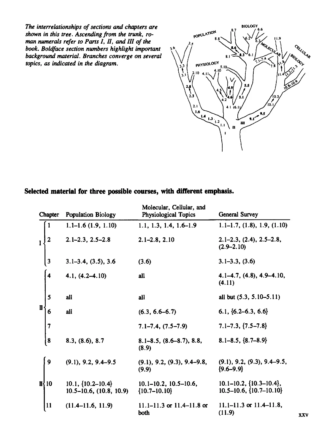
The relationship of various sections in the book is depicted in the following figure.
Beginning at the trunk and ascending upwards along various branches, boldface
section numbers denote material that is basic and essential for the understanding of topics
higher up.

The interrelationships of sections and chapters are
shown in this tree. Ascending from the trunk, ro-
man numerals refer to Parts I, II, and III of the
book. Boldface section numbers highlight important vbv
background material. Branches converge on several
topics, as indicated in the diagram.
hV&*
BIOLOGY
.8.7 / «■«
Selected material for three possible courses, with different emphasis.
Chapter
I
n
n
r
l
2
3
4
5
6
7
8
9
10
11
Population Biology
1.1-1.6(1.9, 1.10)
2.1-2.3,2.5-2.8
3.1-3.4, (3.5), 3.6
4.1,(4.2-4.10)
all
all
8.3, (8.6), 8.7
(9.1),9.2,9.4-9.5
10.1, {10.2-10.4}
10.5-10.6, (10.8, 10.9)
(11.4-11.6, 11.9)
Molecular, Cellular, and
Physiological Topics
1.1, 1.3, 1.4, 1.6-1.9
2.1-2.8,2.10
(3.6)
all
all
(6.3, 6.6-6.7)
7.1-7.4,(7.5-7.9)
8.1-8.5, (8.6-8.7), 8.8,
(8.9)
(9.1), 9.2, (9.3), 9.4-9.8,
(9.9)
10.1-10.2, 10.5-10.6,
{10.7-10.10}
11.1-11.3 or 11.4-11.8 or
both
General Survey
1.1-1.7,(1.8), 1.9,(1.10)
2.1-2.3, (2.4), 2.5-2.8,
(2.9-2.10)
3.1-3.3,(3.6)
4.1-4.7, (4.8), 4.9-4.10,
(4.11)
all but (5.3, 5.10-5.11)
6.1, {6.2-6.3, 6.6}
7.1-7.3, {7.5-7.8}
8.1-8.5, {8.7-8.9}
(9.1), 9.2, (9.3), 9.4-9.5,
{9.6-9.9}
10.1-10.2, {10.3-10.4},
10.5-10.6, {10.7-10.10}
11.1-11.3 or 11.4-11.8,
(11.9)
XXV

This page intentionally left blank

Acknowledgments
I would like to express my gratitude for the helpful comments of the following
reviewers: Carol Newton, University of California, Los Angeles; Robert McKelvey,
University of Montana; Herbert W. Hethcote, University of Iowa; Stephen J. Merrill,
Marquette University; Stavros Busenberg, Harvey Mudd College; Richard E. Plant,
University of California, Davis; and Louis J. Gross, University of Tennessee. I am
especially grateful to Charles M. Biles, Humboldt State University, for many detailed
suggestions, continual encouragement, and for specific contributions of ideas,
improvements, and problems.
The teaching styles, ideas, and specific lectures given by several colleagues and
peers have strongly influenced the selection and treatment of many subjects included
here: Among these are Peter Kareiva, University of Washington, with whom the
original course was designed and taught (Sections 1.10, 3.1-3.4, 3.6, 6.6-6.7, 10.1,
11.8-11.9); Lee A. Segel, Weizmann Institute of Science (4.2-4.5, 4.10, 5.10,
7.1-7.2,9.3, 10.2, 11.1-11.6); H. Tom Banks, Brown University (9.3); and Michael
Reed, Duke University (10.7). I am also greatly indebted to Douglas Lauffenburger
and Elizabeth Fisher, University of Pennsylvania, for providing references and pre-
publication data and results for the material in Section 9.7.
Numerous students have helped at various stages: editing parts of the manuscript—
Marjorie Buff, Saleet Jafri, and Susan Paulsen; with research, written reports and
other specific contributions which were particularly useful—Marjorie Buff (11.8,
Figure 11.16, and the figure for problem 21 of Chapter 11), Laurie Roba (3.1—3.4),
David F. Dabbs (3.4 and Figures 3.5-3.8), Reid Harris, Ross Alford, and Susan
Paulsen (3.6 and problems 18-20 of Chapter 3), Saleet Jafri (1.9 part 2, 4.11b, and
problem 16 of Chapter 1), Richard Fogel (Figure 11.23).
Bertha Livingstone and the Staff of the Biology-Forestry Library (Duke University)
were particularly helpful with procurement of research materials. Initial drafts of the
manuscript were typed by Dottie Libbuti and Susan Schmidt. I would like to express
my sincere appreciation to my greatest helper, Bonnie Farrell, for her speed, elegance,
and accuracy in typing many drafts as well as the final manuscript.
While working on final stages of the book, I have been supported by NSF grant no.
DMS-86-01644. Two grants from the Duke University Research Council were
especially helpful in defraying part of the costs of manuscript preparation.
Finally, I wish to express my appreciation to family members for their help and
support from beginning to end.
Any comments from readers on the material, or on errors and misprints would be
welcomed.
xxvii

xxviii Mathematical Models in Biology
Figure Permissions
Figures 1.1a and 1.1b are reprinted with permission of the University of
Chicago Press.
Figure l.ld was created by and is used with permission of Leah Edelstein-
Keshet.
Figure Lie is reprinted with permission of Benjamin Blom.
Figures l.lf and 9.7 are reprinted with permission of Cambridge University
Press.
Figures 2.8 and 3.4 are reprinted from Nature with permission of the
Nature Publishing Group.
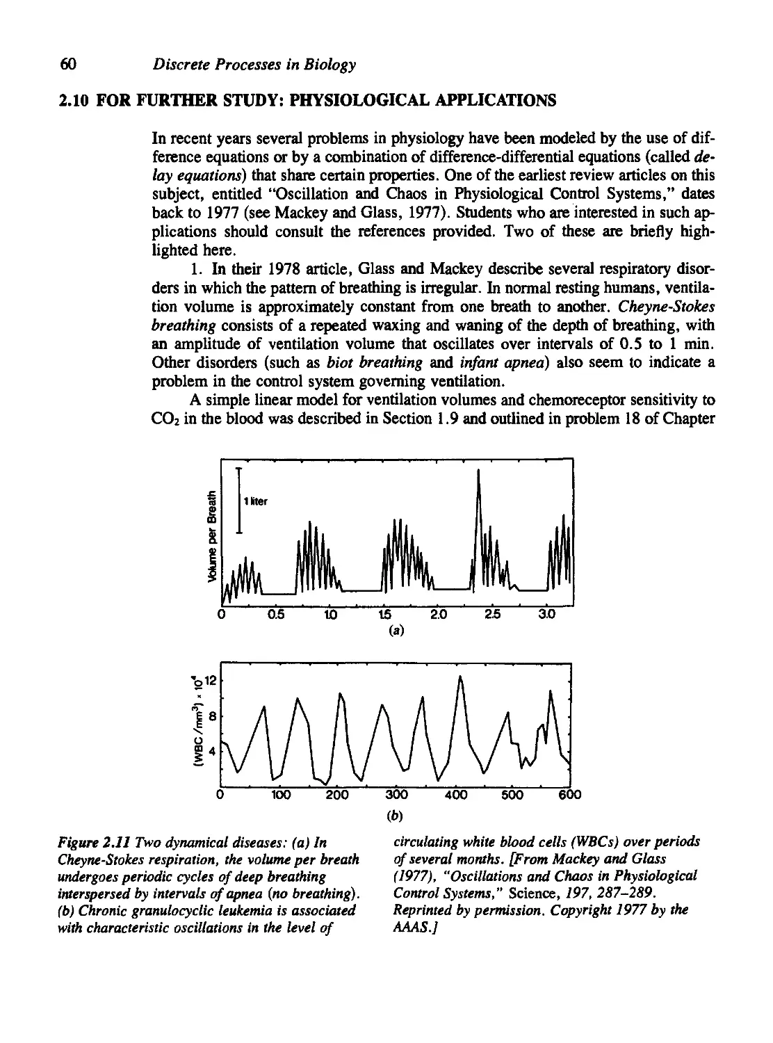
Figure 2.11 is reprinted with permission of the American Association for
the Advancement of Science.
Figures 3.1 and 3.3 are reprinted with permission of Princeton University
Press.
Figures 3.5-3.8 are reprinted with permission of David F. Dabbs.
Figure 4.1 is reprinted with permission of Hafner.
Figure 5.8 is reprinted with permission of Joshua Keshet.
Figure 6.3 is reprinted with permission of Brooks/Cole, a division of
Thomson Learning: www.thomsonrights.com. Fax: 800-730-2215.
Figure 6.9 is reprinted with permission from the Journal of Experimental
Biology and the Company of Biologists Ltd.
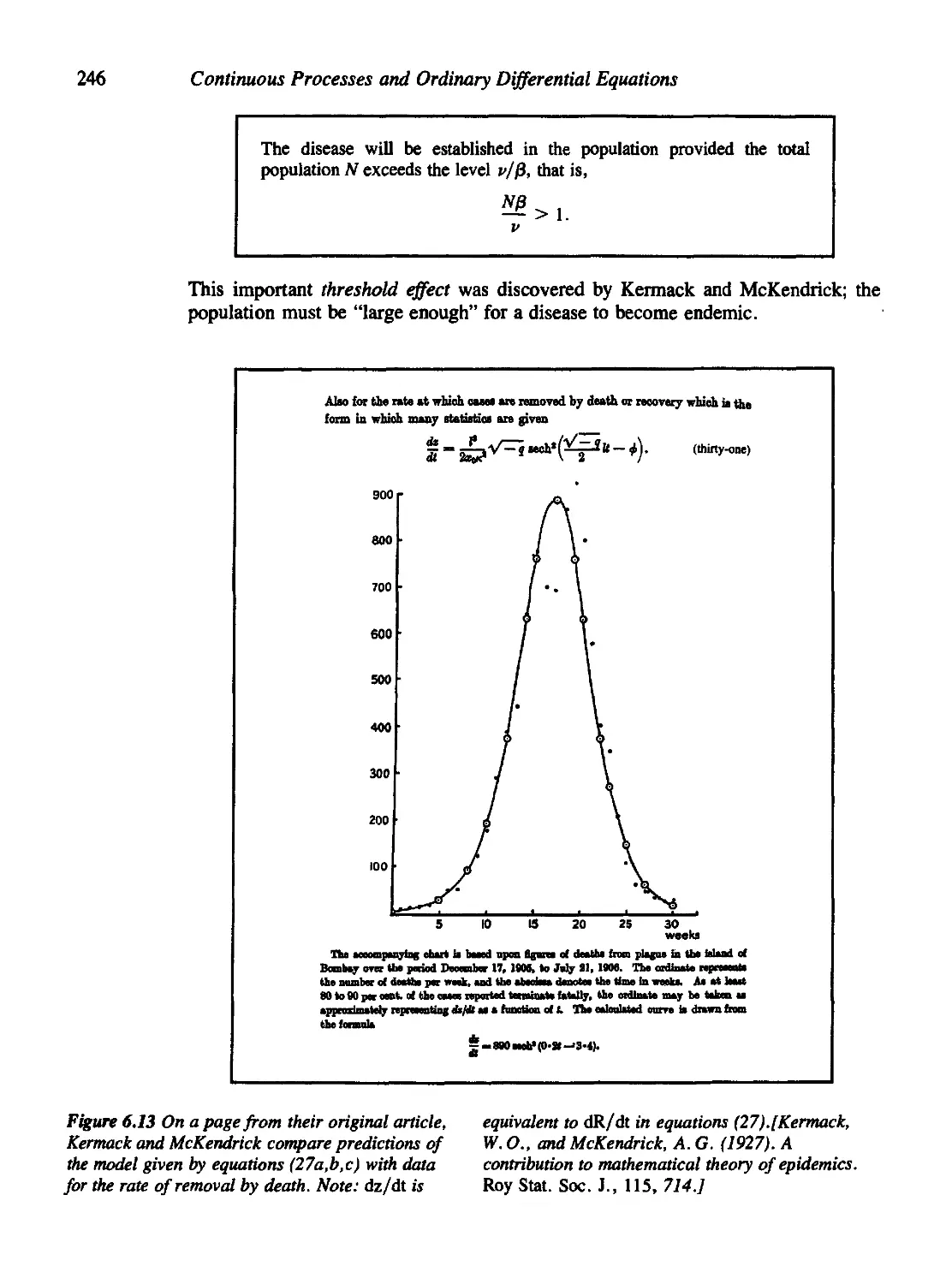
Figure 6.13 is reprinted with permission of the Royal Statistical Society.
Figures 6.15, 7.4, 8.14, 9.8, 11.13, 11.14, 11.15, 11.20, 11.21, 11.22, and
the figure for problem 12 in Chapter 10 are reprinted with permission of
Elsevier.
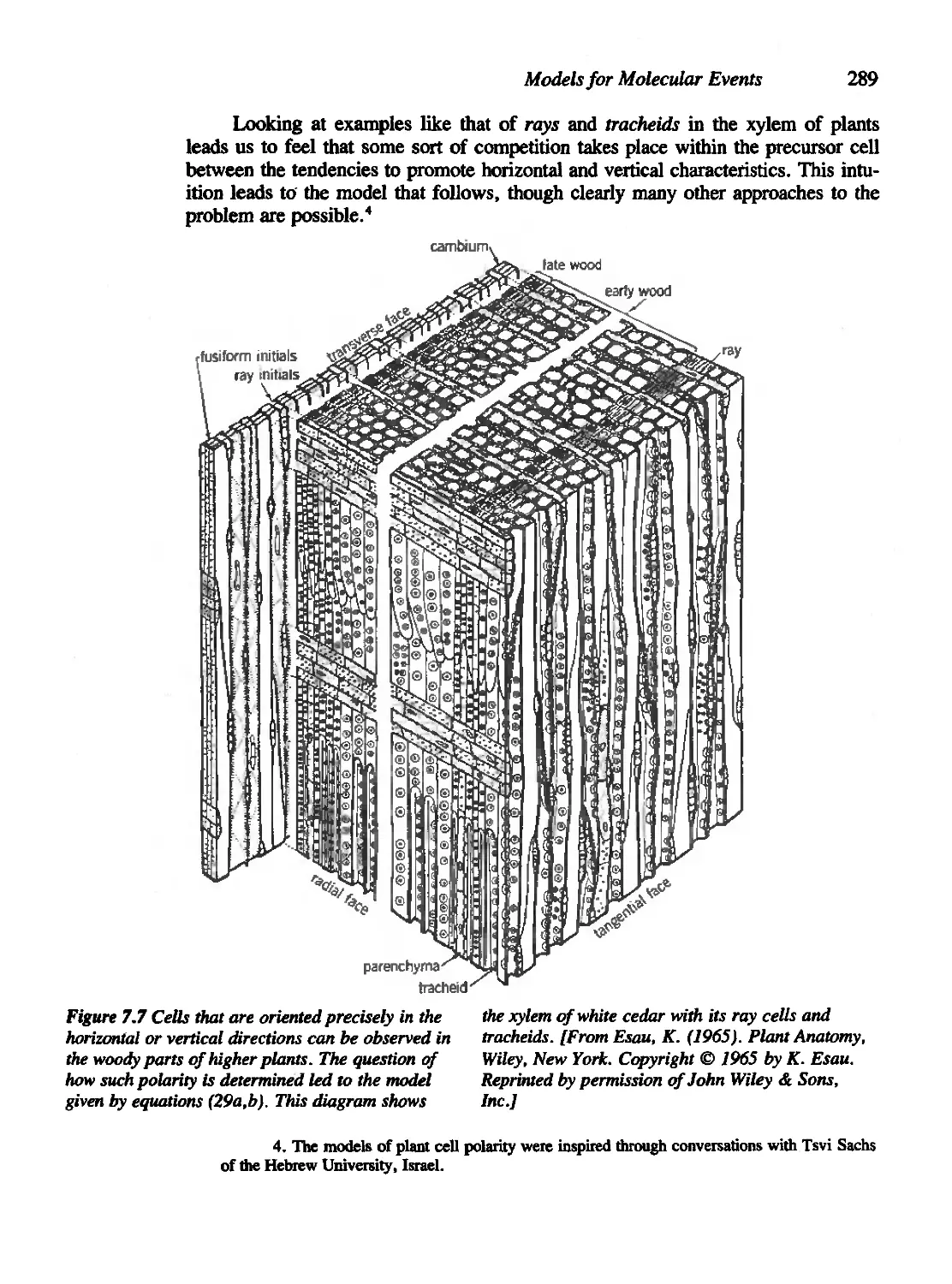
Figure 7.7 is reprinted with permission of John Wiley &; Sons, Inc.
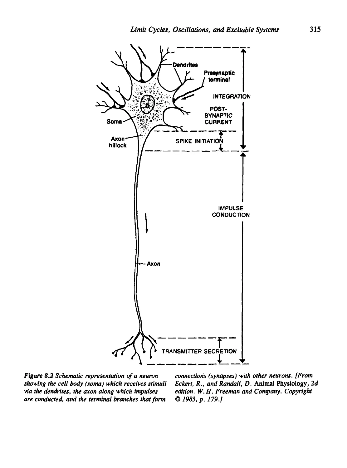
Figure 8.2 is reprinted with permission of W.H. Freeman and Company.
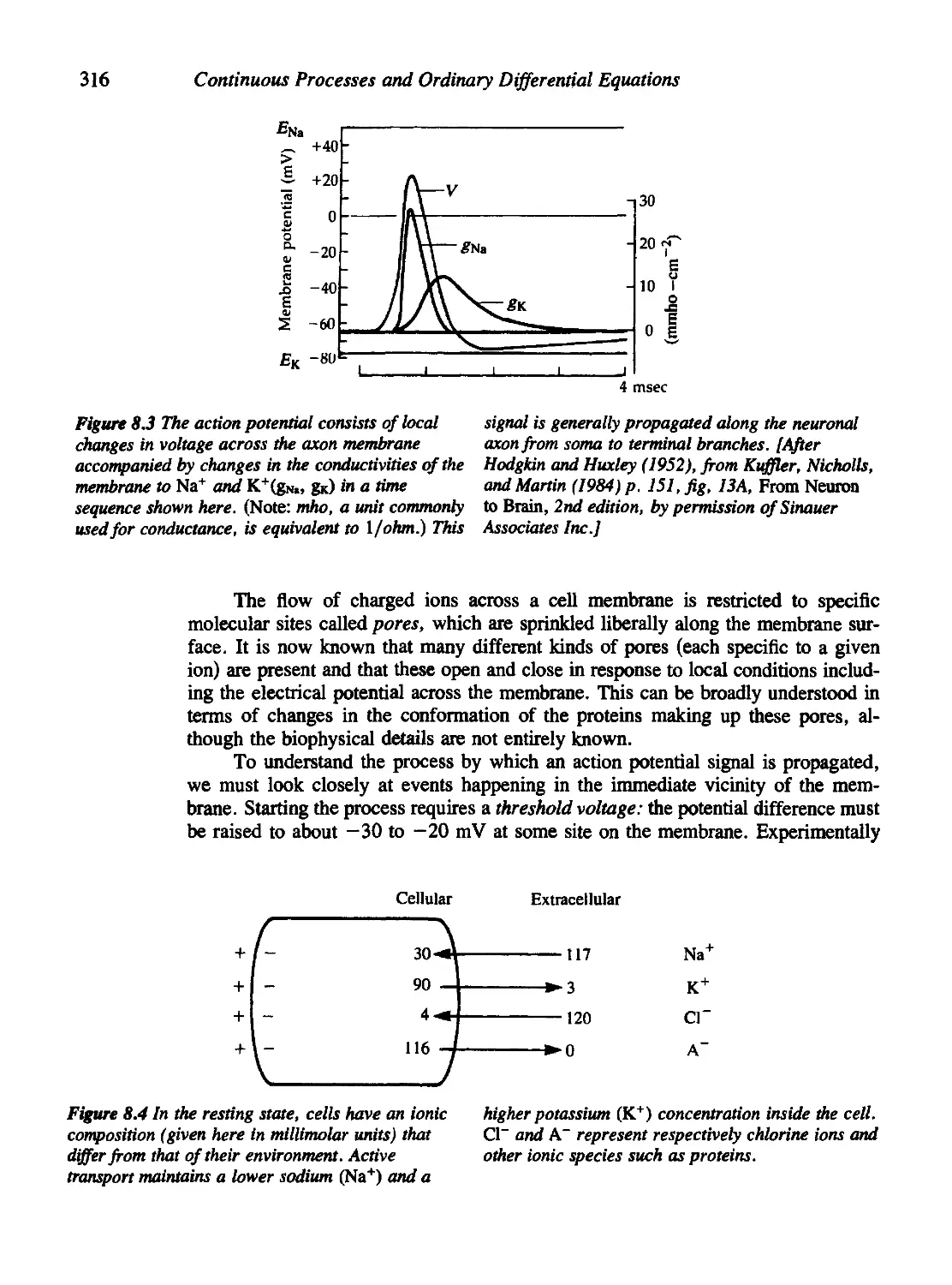
Figures 8.3, 8.6, and 8.7 are reprinted with permission of Sinauer
Associates, Inc.

Acknowledgments xxix
Figures 8.10 and 8.11 are reprinted with permission of The Rockefeller
University Press.
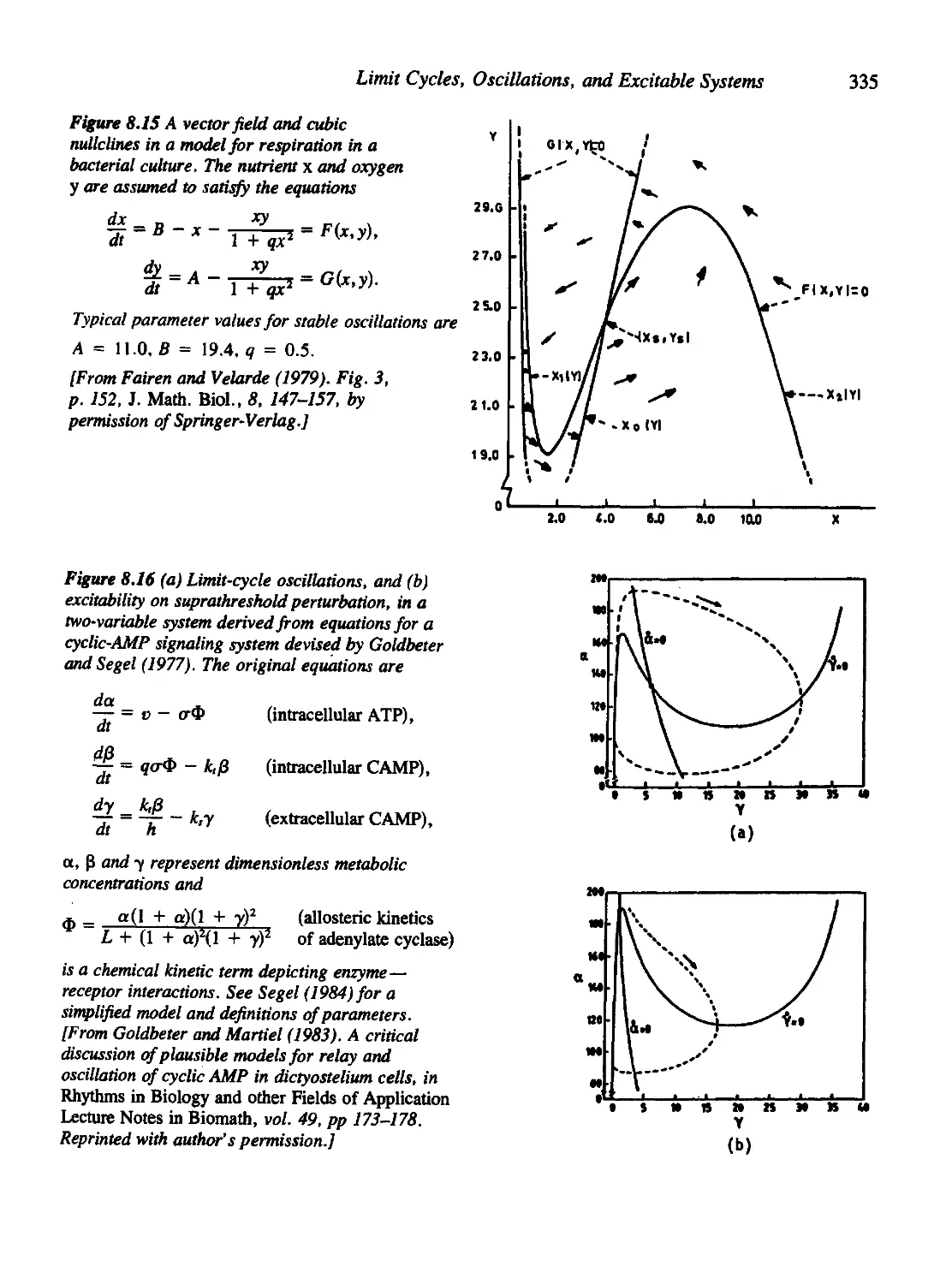
Figures 8.15, 11.11, 11.12, 11.18, and 11.19 are reprinted with permission
of Springer-Verlag.
Figure 8.16 is reprinted with permission of A. Goldbeter and J.L. Martiel.
Figures 8.17 and 8.18 are reprinted from Biophysics Journal with
permission of the Biophysical Society.
Figure 8.23 is reprinted with permission of Creation Tips.
Figures 9.11a, 9.11b, and 10.1 are reprinted with permission of Oxford
University Press.
Figure 9.lie is reprinted with permission of The Minerals, Metals, and
Materials Society (TMS), Warrendale, PA 15086.
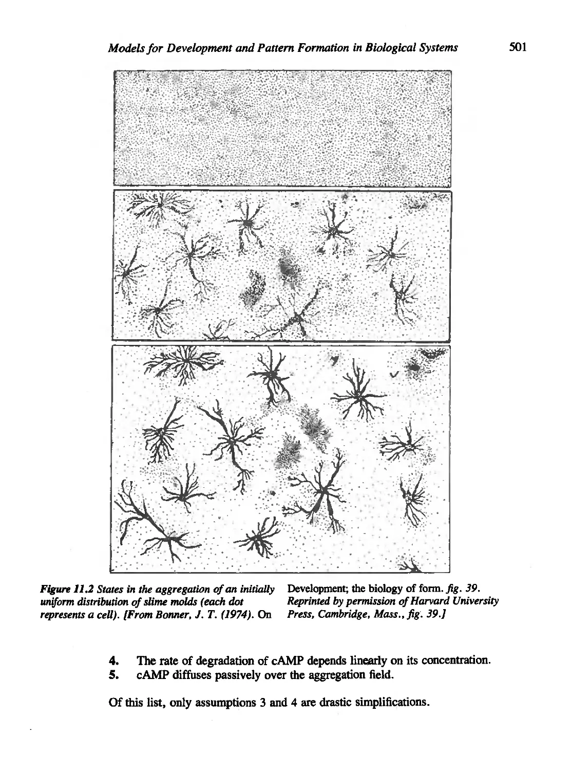
Figures 10.2 and 11.2 are reprinted with permission of the publisher from
On Development: The Biology of Form by John T. Bonner, p. 196,
Cambridge, MA: Harvard University Press. Copyright ©1974 by the President
and Fellows of Harvard College.
Figures 11.7-11.10 are reprinted from American Zoologist with permission
of The Society for Integrative and Comparative Biology.
Figure 11.23 is reprinted with permission of Richard Fogel.
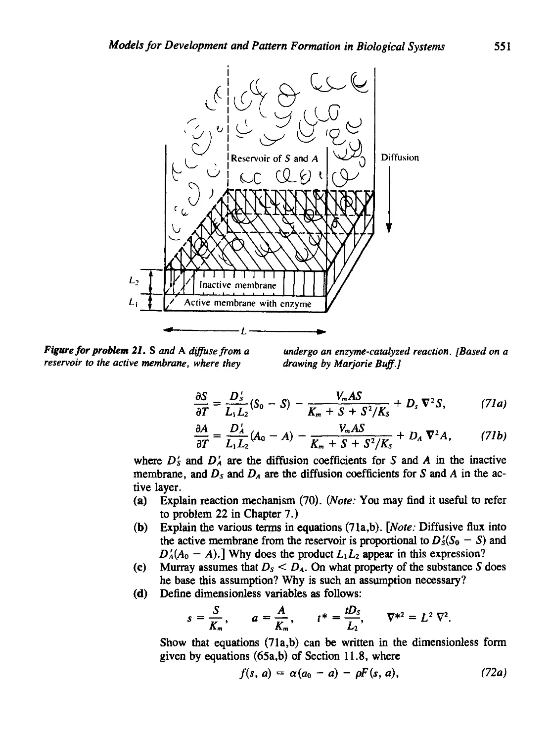
Figure for problem 21 on page 551 is reprinted with permission of Marjorie
Buff.

This page intentionally left blank

Errata
The notation for line numbers refer to lines counting down from the top of the
page (positive values) and lines counting up from the bottom of the page (negative
values). I include footnotes and section headings in the line count.
An updated Errata is maintained at www.math.ubc.ca/~keshet/
Preface.
• Page xv, bottom: Last brace should be labeled III.
Chapter 1.
• Page 12, line -7: Insert C in the last term:
(7An+2 - (an + a22)C\n+l + (ana22 - a12a2l)CXn = 0.
• Page 17, line -16: 7 = 2.0 (not 0.2).
• Page 18: The caption to Table 1.1 should include po = 100, and (a) pi = 80,
(b) jn = 96.
• Page 19: In Section 1.6, delete the subscript n in all occurrences of bn (in
properties 1 and 3).
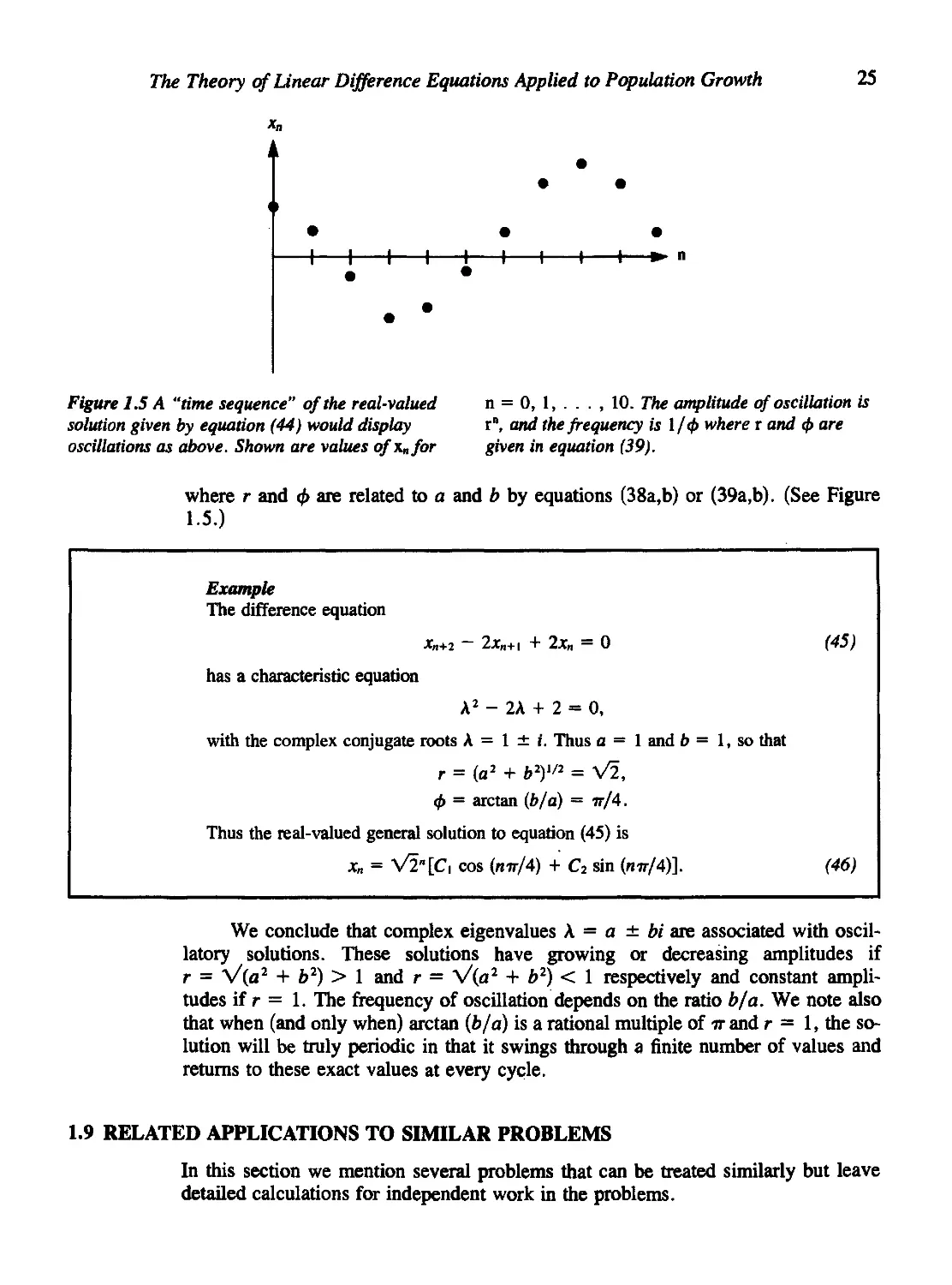
• Page 25, caption to Figure 1.5: Replace the last sentence with "The
amplitude of oscillation is related to rn and the frequency is <j>...".
• Page 27, line -9: "As in problem 1, ..."
• Page 29, Problem 1: Change last sign: xn+2 — 3xn+i + 2x„ = 0. Disregard
3(b).
XXXI

xxxii Mathematical Models in Biology
• Page 30: The Taylor series for sine and cosine in Problem 5 are incorrect
and should be replaced by
~3 ~5 ~7 ~9
X X X X
Sin(x) = x-- + --- + ¥ + .
X2 X4 X6 X8
cos(s) = l-¥ + ¥-¥ + ¥ + ,
Disregard Problem 6(c).
Problem 6(f) should read
Xn+l =
-xf + syn
• Page 31, Problem 9(c): xn+2 + 2xn+i + 2xn = 0.
• Page 33: The historical note is irrelevant to problem 14(b). Disregard.
• Page 34, line 7: a + b > 1.
• Page 34, problem 19(b): The first equation is missing a:
S«+1 = <77(/JSi + aS2)
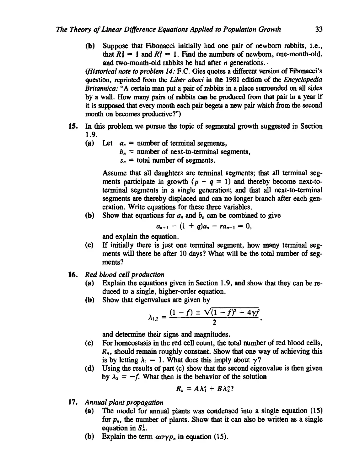
• Page 35: The diagram in the figure for problem 19 is confusing and needs
to be improved. Problem 19(c) (ii) should read
Pn+2 - Cta^Pn+t - /?CT27(1 - Ct)pn = 0.
The matrix in Problem 19(d) should be
/ a^ia. CT7/3 o~j8 CT7C \
a(l-a) 0 0 0
0 a(l + a-0) 0 0
\ 0 0 <r(l + a + 0-6) 0 /

Errata xxxiii
Chapter 2.
• Page 48, line -3: "The two possible roots,... are real if r > -1 and ...".
• Page 59, line -4: Condition 2 should read (-1)4P(-1) =...
• Page 65: In Problem 16(f) the value "B = 12 births per 1000 people" may
be incorrect for the desired effect.
• Page 66, Problem 17: "This problem pursues further the topic... first
described in Section 1.9 and problem 3 (page 27) of Chapter 1."
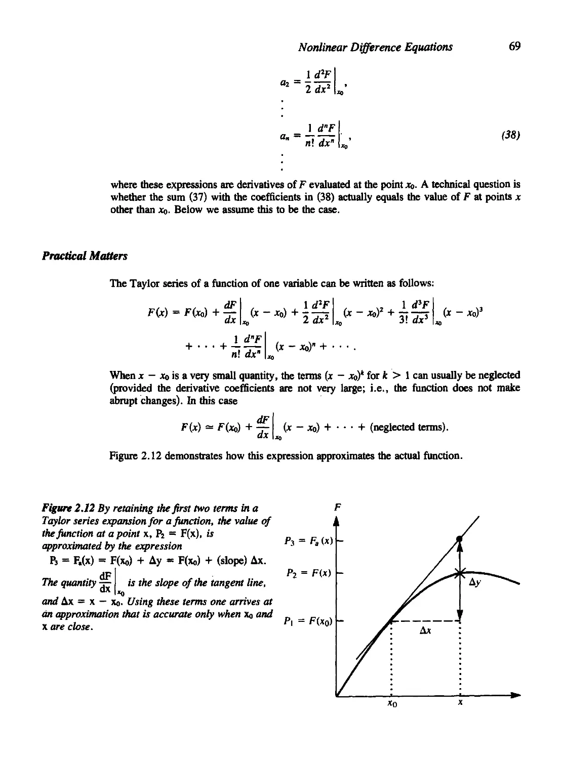
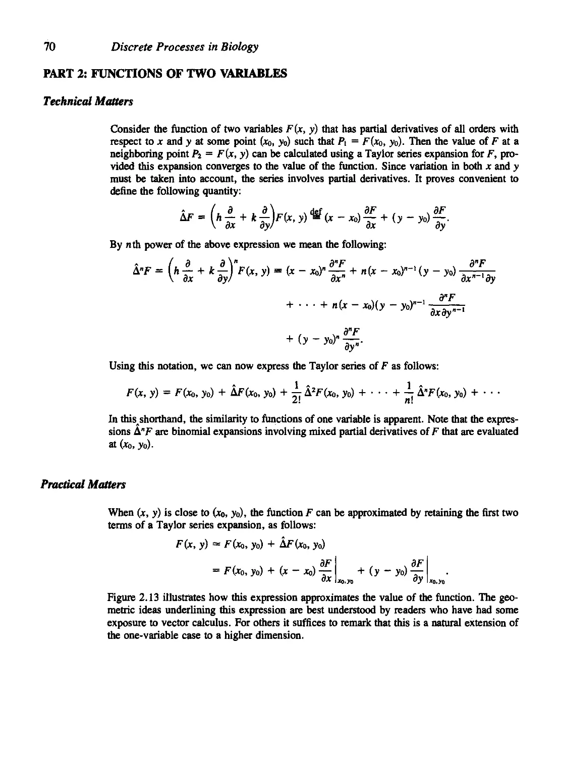
• Page 71, caption to Figure 2.13, second-to-last sentence: "P3 is actually
the height [at (x, y)]..."
Chapter 3.
• Page 80: After equation (16), insert "and r! = r(r- l)(r-2)... 1." Before
equation (19) insert "(Recall that 0! = 1 by definition.)"
• Page 82, line 1: Replace N with P.
Line -3 in box: "consequently S(X) < 0 for A > 1."
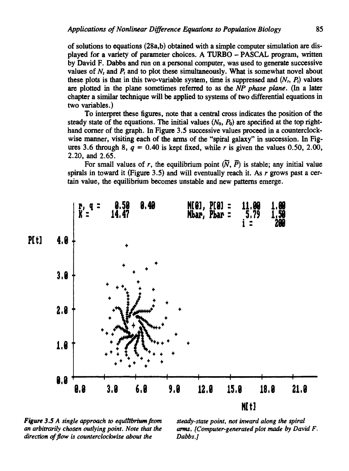
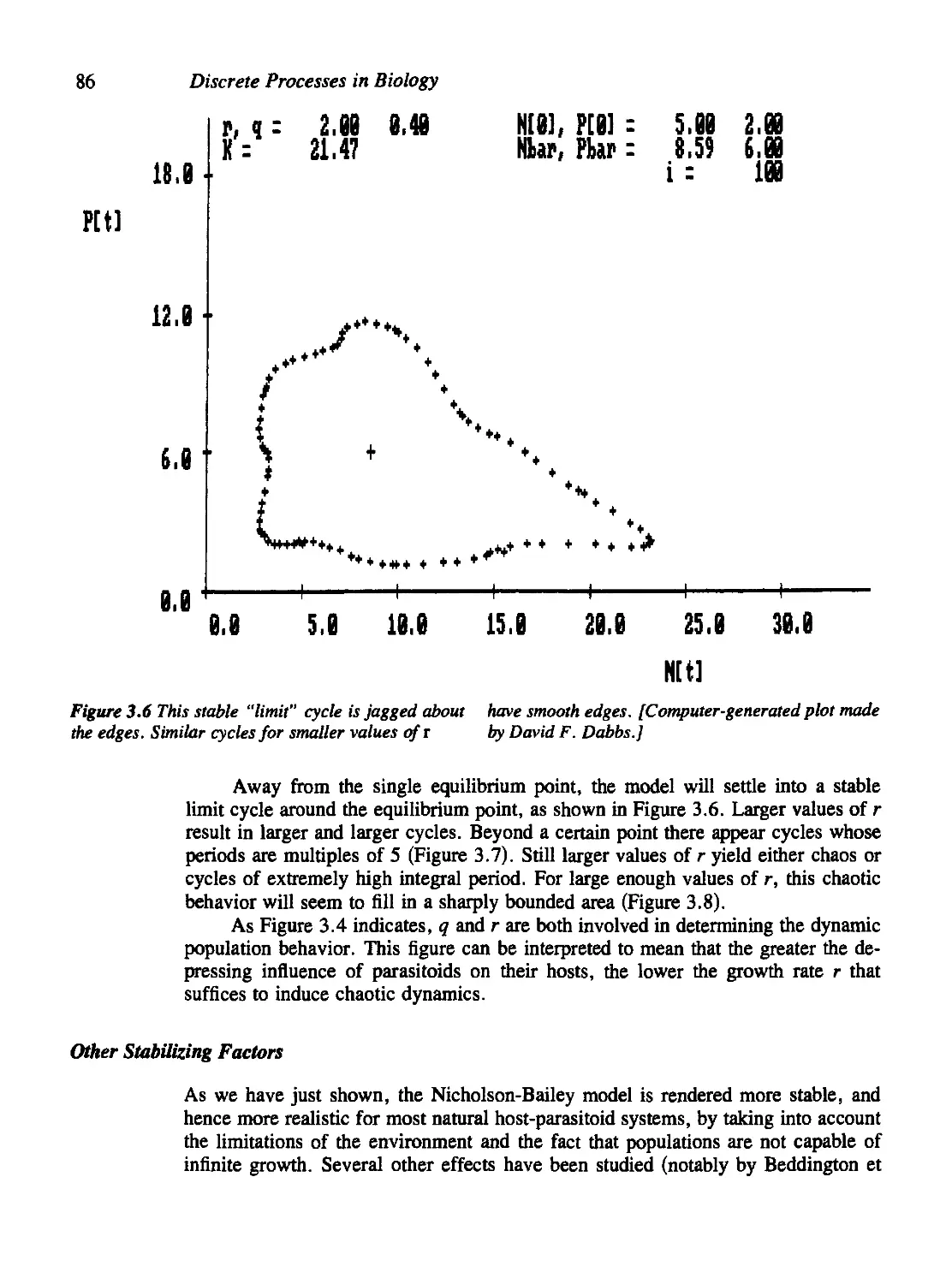
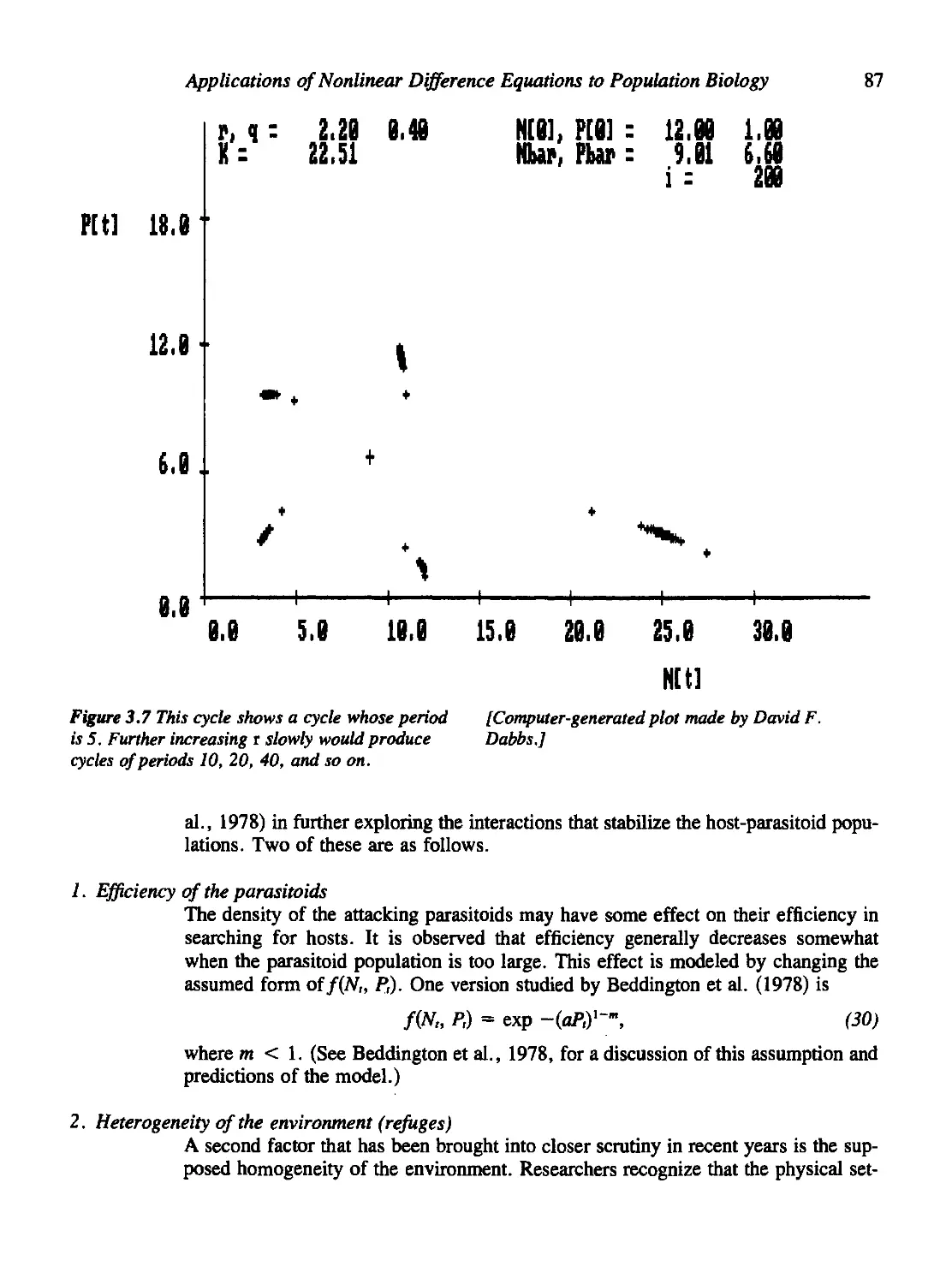
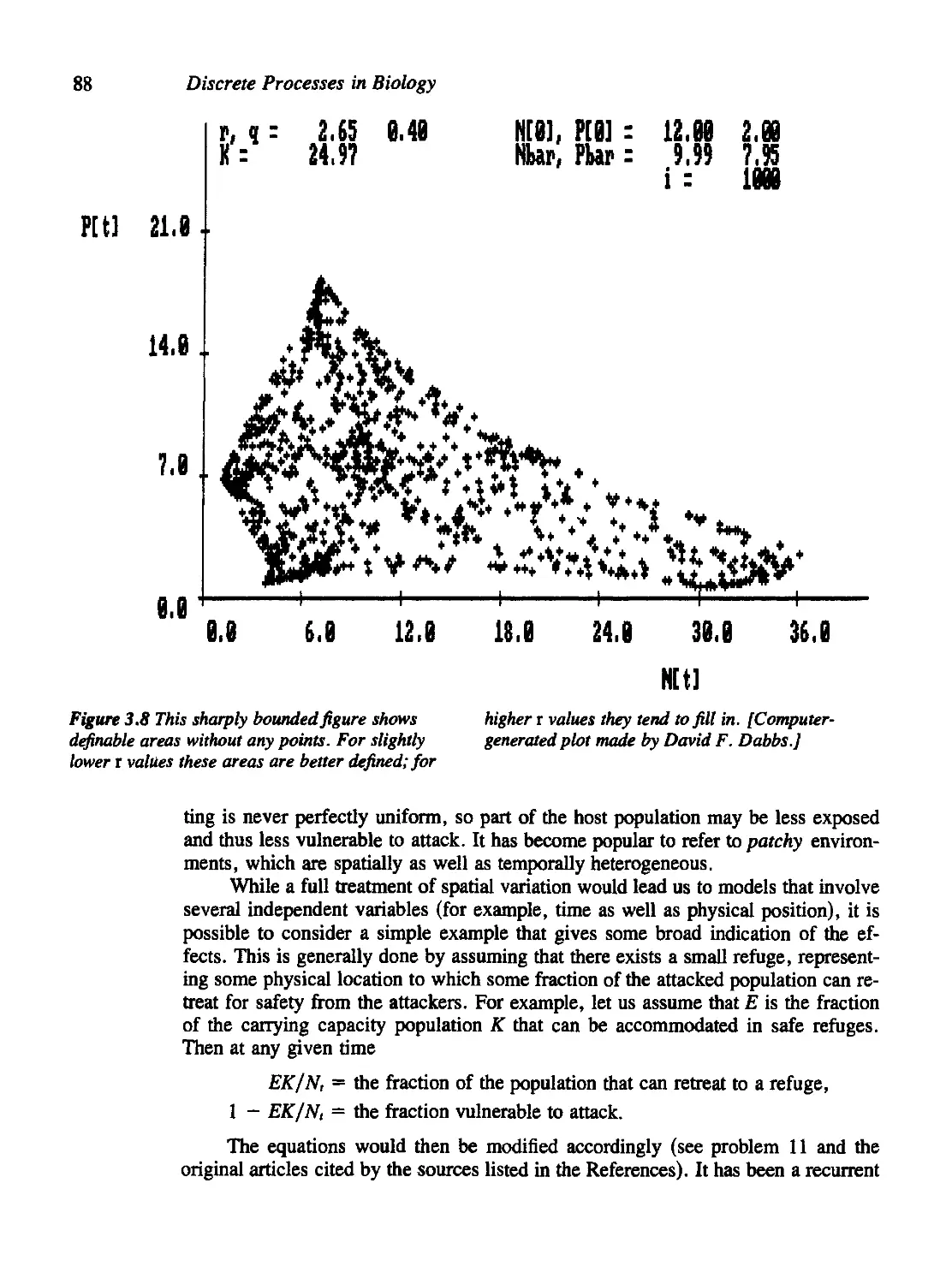
• Page 85, line 12: "In Figures 3.6 through 8 q = 0.40, a = 0.2 are kept
fixed..."
• Pages 89-99: This material on plant-herbivore interactions should be
disregarded.
• Page 94: Equations (43) and (44), and the line immediately following,
should have lowercase vn or un+i (not uppercase).
• Page 103: In Problem 4(b), the equation should read
• Page 105: In Problem 11(e) insert the constant c:
Pt+1=c(Nt- EK)(1 -e~aPt).

xxxiv Mathematical Models in Biology
• Page 106: Problem 15(c) should read V = H = 1.
• Page 109, line -8: "Journal Article Report on Difference Equations"
Chapter 4.
• Page 123: To avoid confusion, equation (11) should be clearly labeled
"Wrong". The corrected version is shown further on in equation (12).
• Page 131, Example 1, first term labeled "nonlinear term": The arrow
dec
should point to the entire group 2x—-.
at
• Page 132: Equation (34) should read
d2x , dx
al? + bTt+cx = 0-
• Page 134: Equation (43a) should have a boldface x:
dx
— = Ax
dt
• Page 134, line -11: Replace sentence with "The notation in equation (43a)
denotes matrix multiplication, and ^ stands for a vector whose entries are
dx dy n
dt' df
• Page 135: After equation (45b), it should read "where I is the identity
matrix (Iv = v)."
In the paragraph after equation (46), it should read "As in the subsection
"Second-Order ODEs" ....
Equation (47) should read
V» = ( Ai-an )
\ ai2 /
• Page 144, line -5: "... the bacteria will not be washed out...".
Equation (81) should read
> Ci, or Co >
Kn "' V/F-l/K„

Errata xxxv
• Page 149, line 20 (middle of page): "(Generally it is not possible to measure
concentrations in compartments other than blood.)"
• Page 151, line -13: "Now suppose that a mass mo-.."
• Page 153: Problem 9(a) refers to equation (14a), and problem 9(b) to
equation (14b).
• Page 157: Problem 25(e): Note that here a does not have the same
meaning as in the chemostat model.
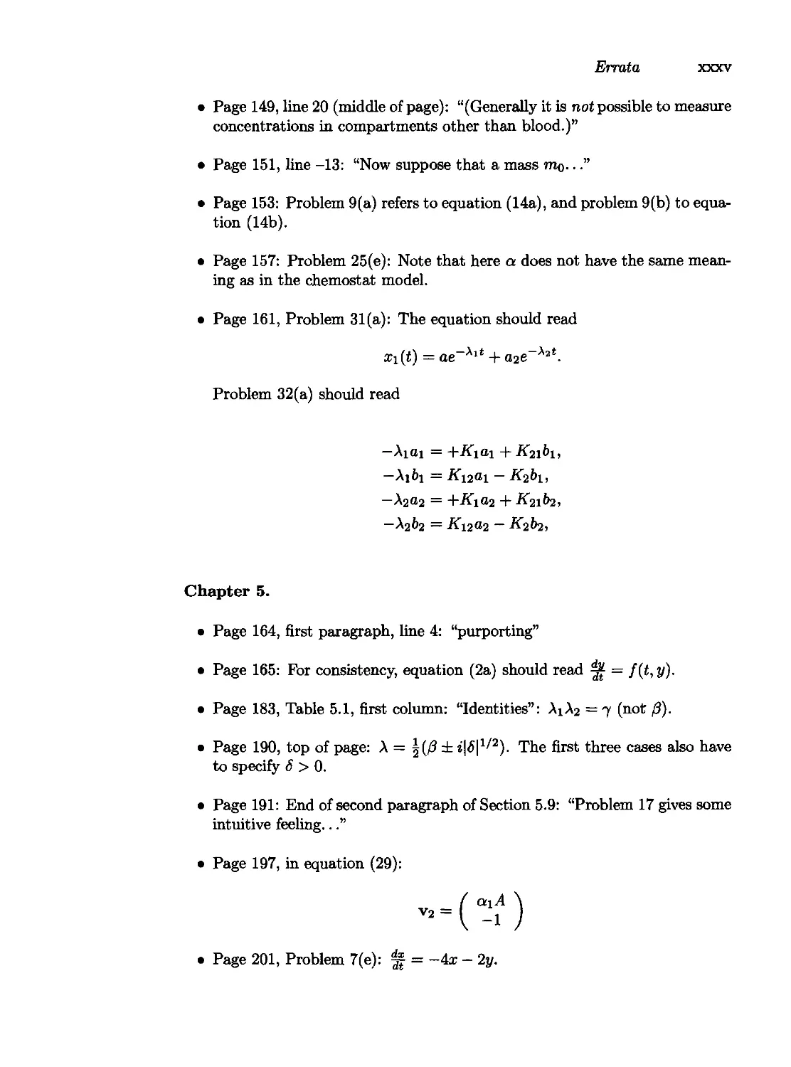
• Page 161, Problem 31(a): The equation should read
xi(t) = ae-Xlt + a2e-X2t.
Problem 32(a) should read
-Aiai = +Kiai + K2ibi,
-A1&1 = Ki2ai - K2h,
—X2a2 = +Kia2 + K2ib2,
—X2b2 — K\2a2 — K2b<2,
Chapter 5.
• Page 164, first paragraph, line 4: "purporting"
• Page 165: For consistency, equation (2a) should read ^ = f(t, y).
• Page 183, Table 5.1, first column: "Identities": AiA2 = 7 (not 0).
• Page 190, top of page: A — \{fi ± i^l1/2). The first three cases also have
to specify S > 0.
• Page 191: End of second paragraph of Section 5.9: "Problem 17 gives some
intuitive feeling..."
• Page 197, in equation (29):
■(-0
v2
• Page 201, Problem 7(e): «jf = -4r - 2y.

xxxvi Mathematical Models in Biology
• Page 206, line 1: "(2) Section 5.9 tells us..."
Problem 19: "Use methods similar to those mentioned in problem 18..."
• Page 208: Problem 23(d) should read
1 ± (1 - 4a2/32)1/2
E =
2a/3
• Page 209: Odell reference is "In L. A. Segel" (note spelling).
Chapter 6.
• Page 234, top of page: The Routh-Hurwitz Criteria for k = 4, second
inequality, should read 0102 > 03. (Thanks to D. Thron)
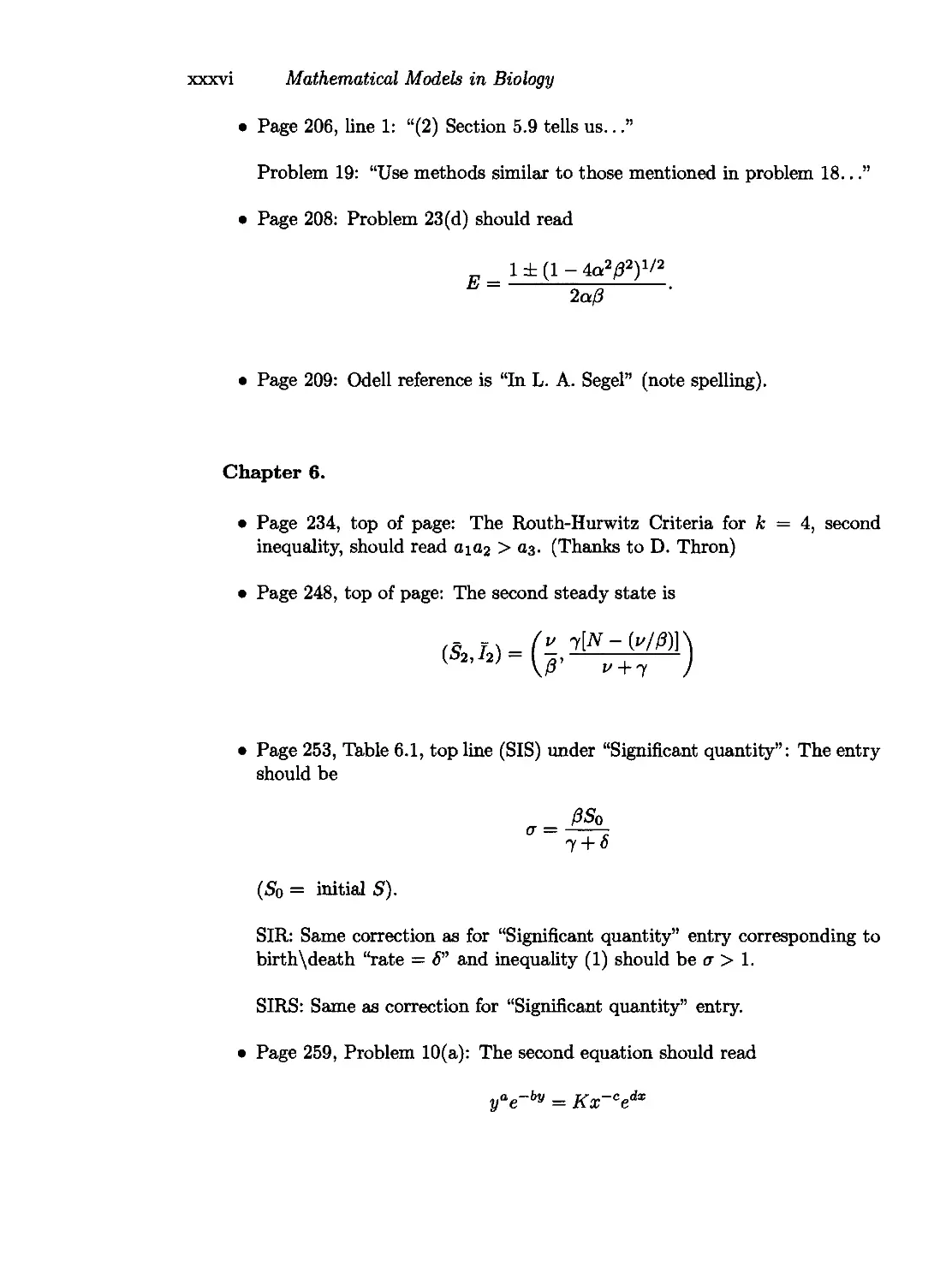
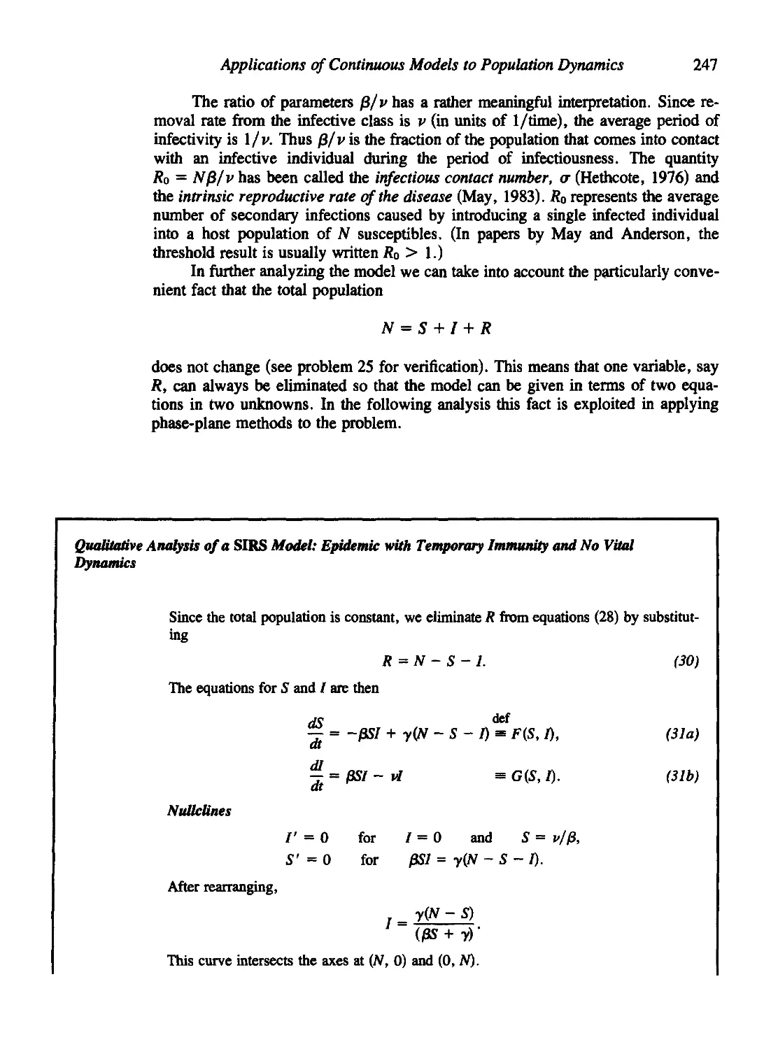
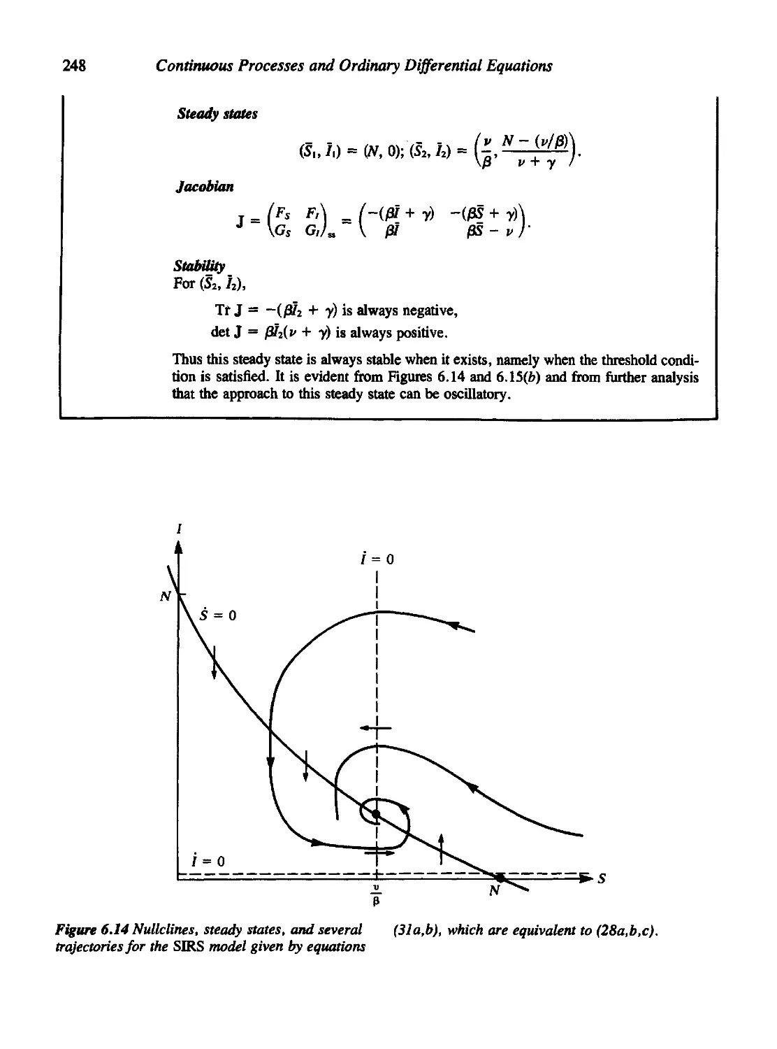
• Page 248, top of page: The second steady state is
• Page 253, Table 6.1, top line (SIS) under "Significant quantity": The entry
should be
<7 =
1 + 8
(So = initial S).
SIR: Same correction as for "Significant quantity" entry corresponding to
birth\death "rate = S" and inequality (1) should be a > 1.
SIRS: Same as correction for "Significant quantity" entry.
• Page 259, Problem 10(a): The second equation should read
yae-by = Kx-cedx

Errata xxxvii
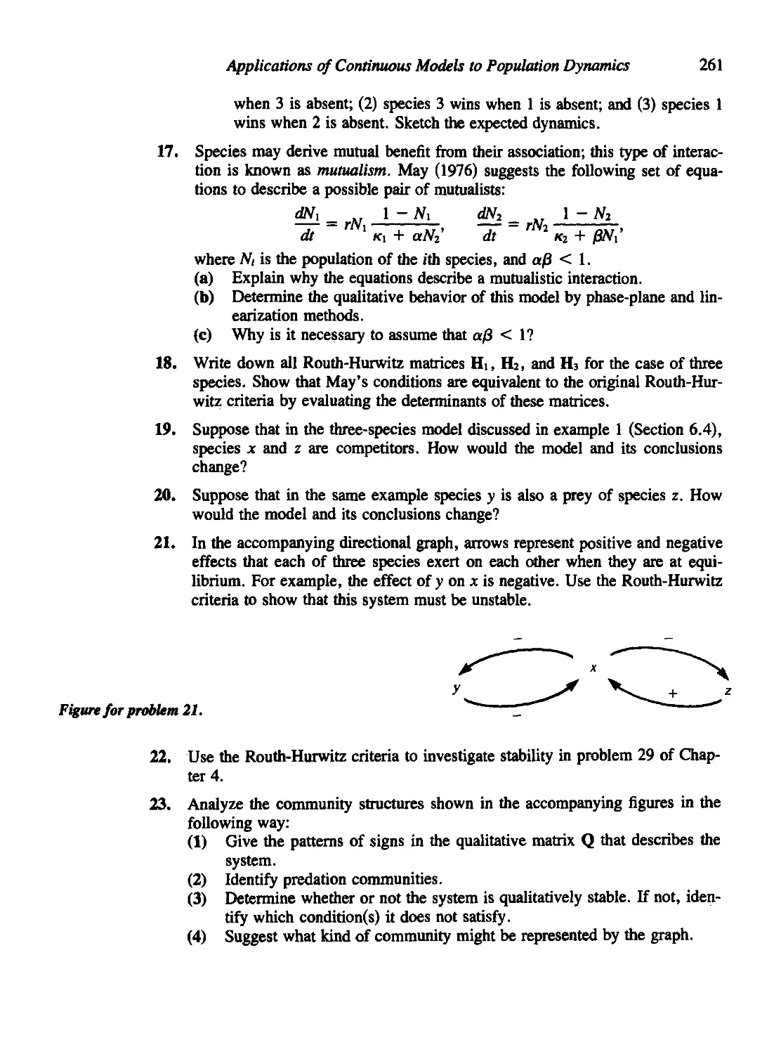
• Page 261, Problem 17: The equations should read
Ni '
-aT = rNl
dN2 ,r
1-
1-
«i + aN2
N2
k2 + 0Ni
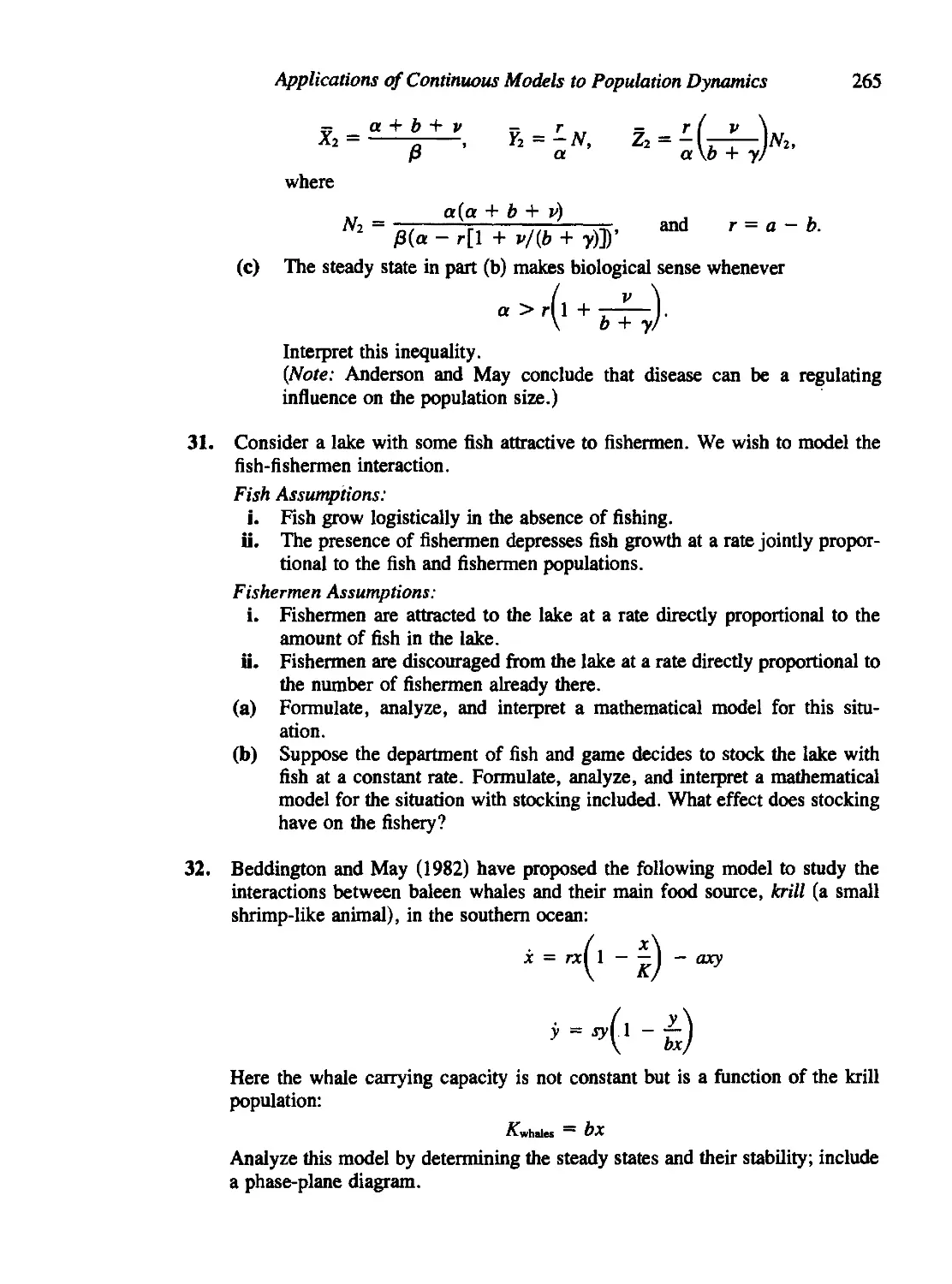
• Page 265, Problem 32: The equations should read
krill: x = rx (l — — J
whales : y = sy (l — —)
• Pages 266-267, Problem 34: The equations should read
KinNi - (diViM).ft:i - nA?
nNiN2
K2r2N2 - (dN2/dt)K2 - r2Nj
r2N^N2
Chapter 7.
• Page 277, Equations 14(a,b): The variable t should be t* on the
denominator of the left-hand sides.
• Page 279, Equations 17a and 18: The right-hand side should be multiplied
by 2.
• Page 295, Section 7.8: The term "substrate depletion" may be more
descriptive than "positive feedback" in all occurrences in this section.
• Page 297, bottom of page: Insert "If detJ < 0 then s2 < si and the steady
state is a saddle point."
• Page 304, Problem 19: Replace the notation GGP -♦ G6P and FGP ->
F6P in all places.
• Page 305, Problem 20(c): The inequality should read B > 1 + A2.
• Page 308, Problem 24(d): ... provided Ot «: Rr

xxxviii Mathematical Models in Biology
Chapter 8.
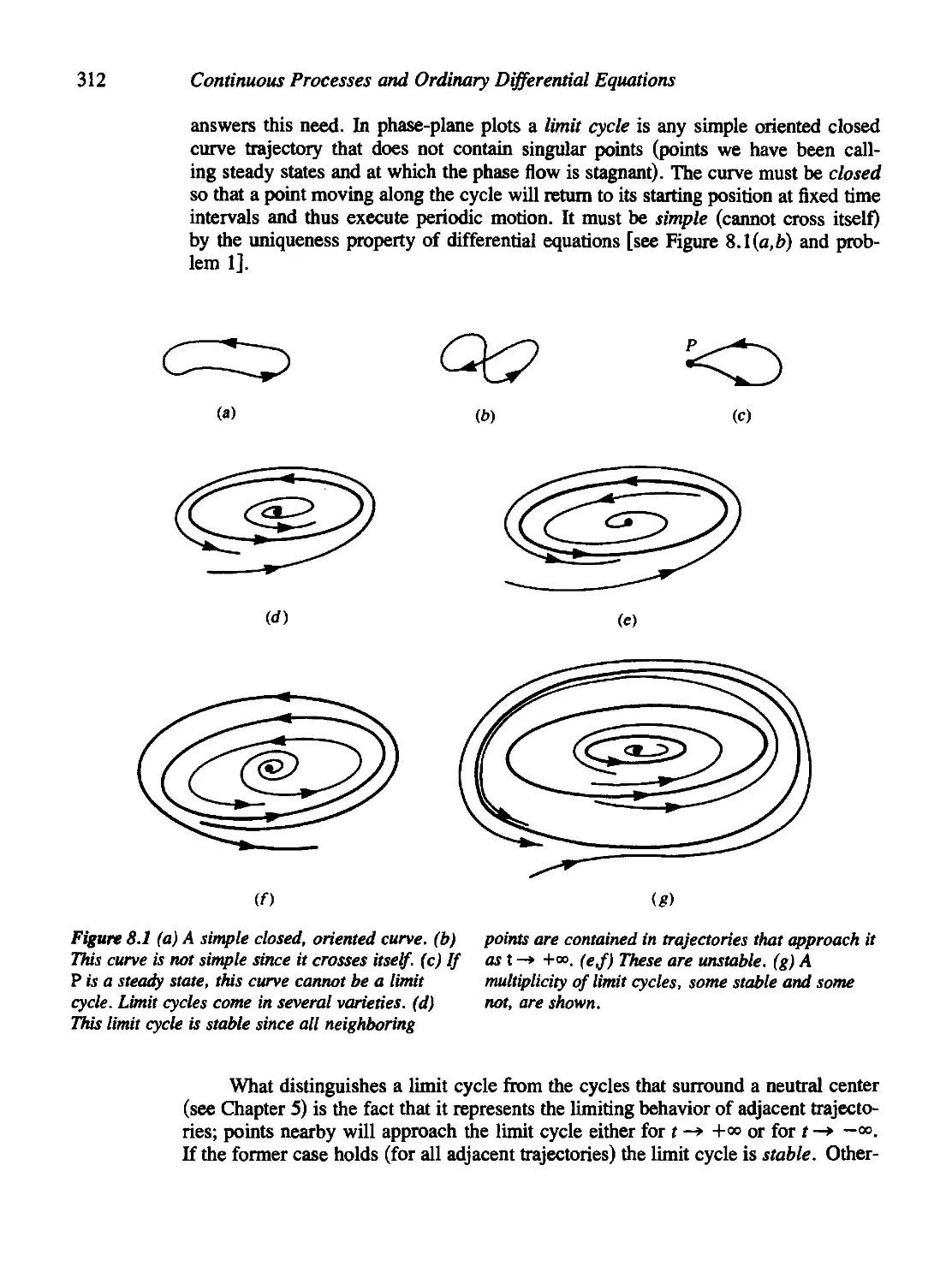
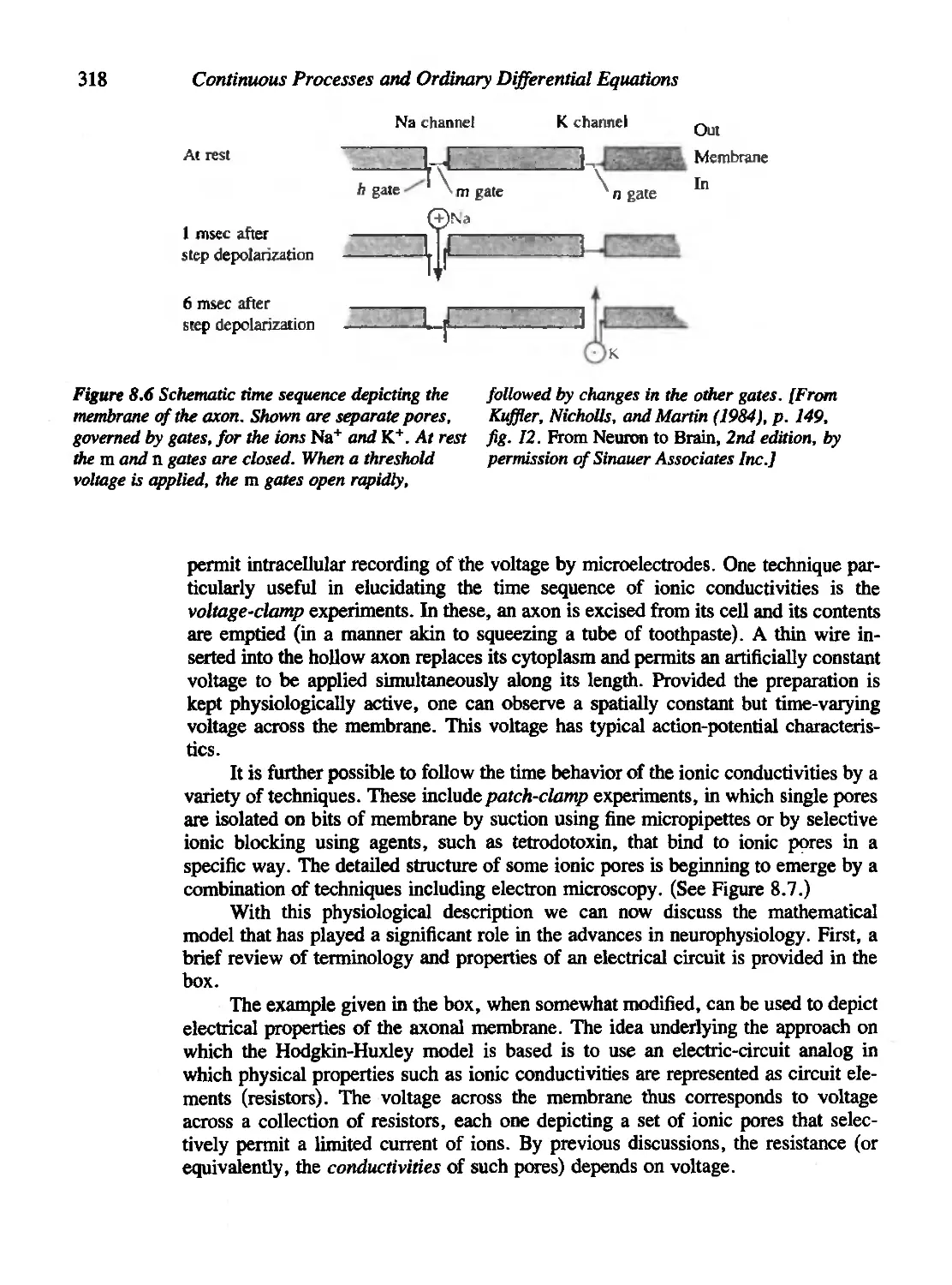
• Page 312, Figure 8.1 caption: (e) and (f) are meta-stable.
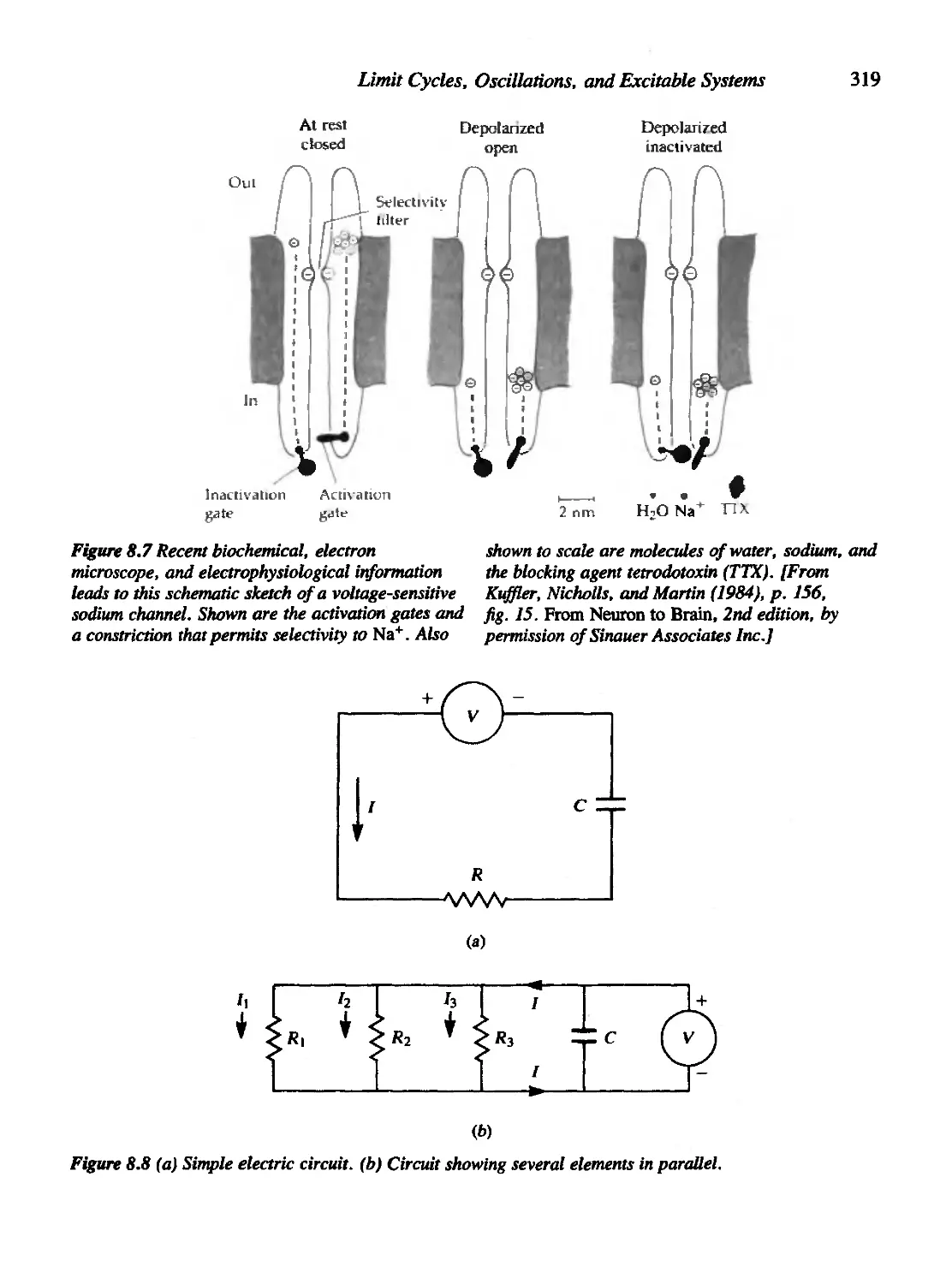
• Page 320: Equation (4b) should read V(t) = q(t)/C.
• Page 321, entry in box (middle of page): "Ii(x,t) = net rate of flow of
positive ions from the interior to the exterior..." After last entry, insert:
"v < 0 when membrane negative on inside."
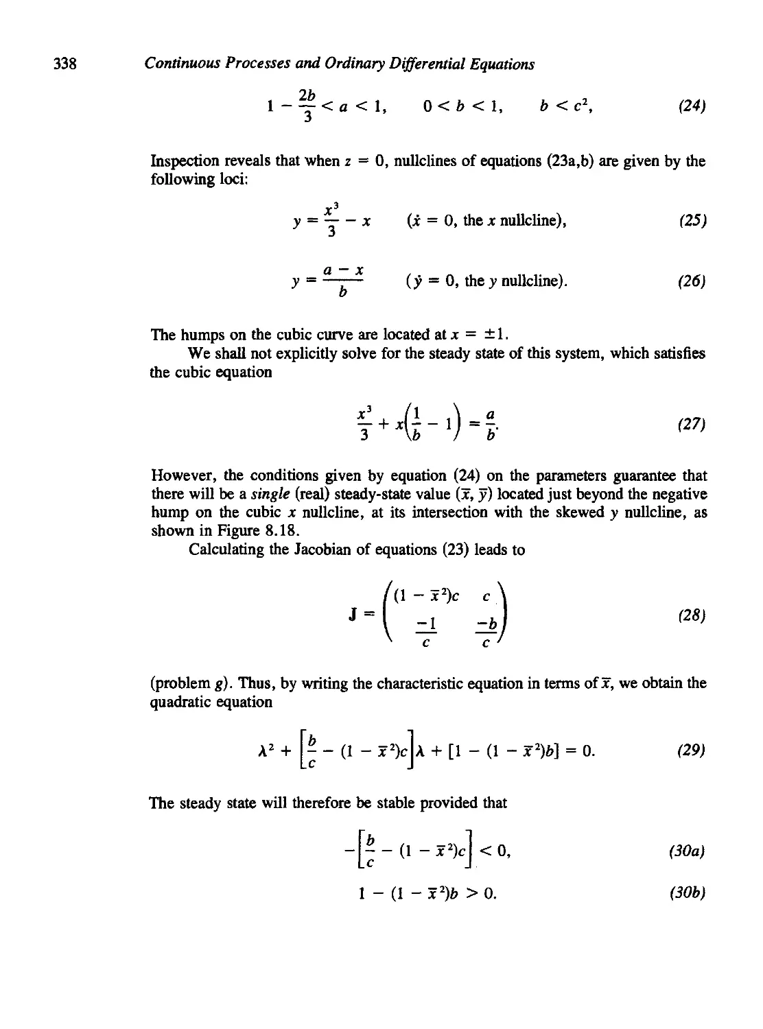
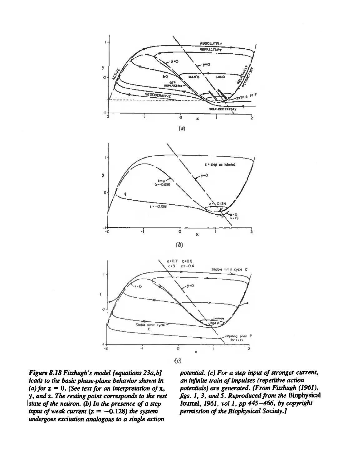
• Page 336, caption to Figure 8.17: "V satisfies an equation like (9)..."
Delete dot over entry dN/dt in first equation. Replace tan h with tanh in
second equation.
• Page 342, box: It should be assumed that da/d'j > 0 so that the steady
state is unstable for 7 > 7* as in Figure 8.19. (Otherwise, if da/dj < 0,
redefine 7 —+ —7.)
• Page 344, line 7: Box on The Hopf Bifurcation Theorem: "with the
appropriate smoothness assumptions on /,..."
In equation (35), the matrix should read
• Page 345, equation (36):
Sw 37T
V" = 4jy (/*«. + etc ) + ^2[-fxy{fxx + fyy) + <*C ].
The conclusions in the box were misleading. A supercritical Hopf
bifurcation denotes a bifurcation to asymptotically stable periodic orbits. The
periodic orbits occur on one side of 7* (but not necessarily for 7 > 7*).
Whether the periodic orbits are to the right or to the left of the critical
value of the bifurcation also depends on a transversality condition (the sign
of da/d'y at 7*). See Marsden and McCracken for other details. The stable
periodic orbit would occur with the unstable equilibrium and the unstable
periodic orbit with the asymptotically stable equilibrium. (N.B. Thanks to
Gail Wolkowicz for pointing out this error.)
In the last sentence of this box: receipe —> recipe.
• Page 354: In equation (60) delete ", 1" from definition of M.
• Page 357: The radical in equation (69) should read
V(l - a2)2 - 4a2

Errata xxxix
• Page 358: The caption to Figure 8.22(b) is inaccurate. Disregard.
• Page 363: In Problem 6, insert "assume k > 0,n > 0".
• Page 364: Figure 7(b) is incorrect (there are incorrect arrows and
misplaced heavy dots). Disregard.
• Page 368, Problem 19: Insert "Assume all parameters are positive."
Chapter 9.
• Page 402: Some units are missing in the box and should be inserted as
follows:
J(x, t) = current in amps (coulombs/sec).
v = voltage (volts).
q(x,t): units of (coulombs/unit length).
C = capacitance in units of (farad/unit area).
Ii is net ionic current per unit area.
• Pages 405-406: We note the following results in dimensions 1, 2, 3, which
follow by straightforward generalization:
Ax2
In 1 dimension V =
In 2 dimensions V =
In 3 dimensions V =
2r
Ax2
4t '
Ax2
6r
• Page 413: Equation (83) should read
I?. L
W a
• Page 414: In equation (88), the right-hand side should read -A2/.
Equations (89a,b,c) should read /i(x) = exp(—iXx), /2(x) = sin(Ax),
/3(x) = cos(Ax).

xl Mathematical Models in Biology
• Page 422, Problem 18(b): See Section 8.1.
(Ax)2
• Page 424, Problem 22: V =
2e
Page 425: Both bibliography items under Hardt should have the name
"Hardt, S. L."
Chapter 10.
• Page 444, line 2: "where K = k/(m + 1)."
• Page 452, line -5: "a population of individuals carrying a slightly
advantageous recessive allele"...
• Page 454: The top figure is incorrect. Disregard.
• Page 464, line before Figure 10.8: "per unit time fj,j."
• Page 477, Problem 2(a): The right-hand side of the equation should read
-V-(/v)-M/-...
• Page 479, Problem 6(b): C0 = 7 x 107.
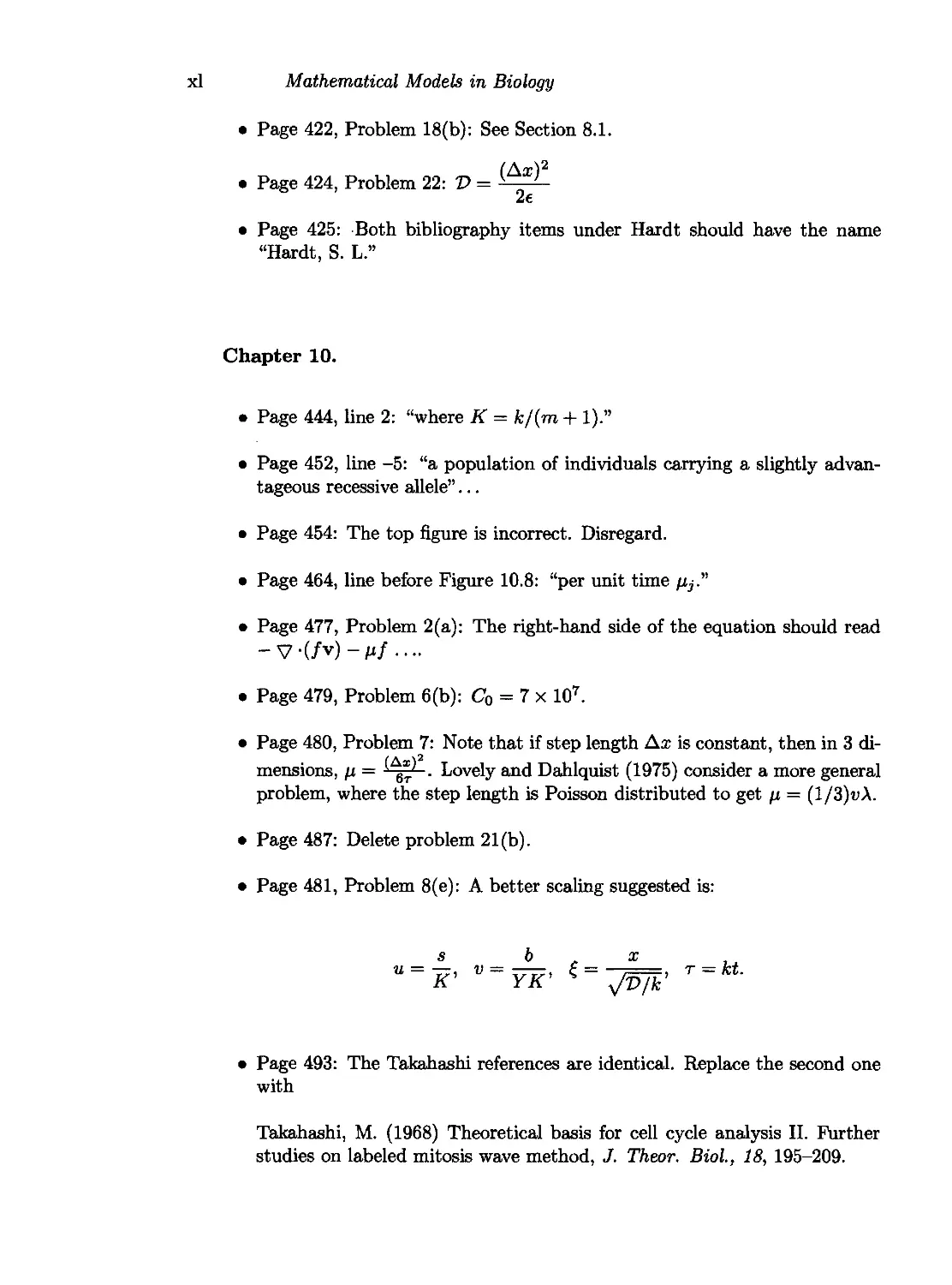
• Page 480, Problem 7: Note that if step length Aa; is constant, then in 3
dimensions, fi = ^ 6y . Lovely and Dahlquist (1975) consider a more general
problem, where the step length is Poisson distributed to get \i = (l/3)uA.
• Page 487: Delete problem 21(b).
• Page 481, Problem 8(e): A better scaling suggested is:
s b x
• Page 493: The Takahashi references are identical. Replace the second one
with
Takahashi, M. (1968) Theoretical basis for cell cycle analysis II. Further
studies on labeled mitosis wave method, J. Theor. Biol, 18, 195-209.

Errata xli
Chapter 11.
• Page 502: Equation (2b) should have the corrected term
MS)
• Page 506, bottom third of page: Second condition should read "2. Values
of L must not be too small."
• Page 507, top part of page: replace first two comments as follows:
1. Aggregation is favored more highly in larger domains than in smaller
ones at fixed a.
2. The perturbations most likely to be unstable are those with low
wavenumbers
The perturbation whose wavenumber is q = n/L...
Comment (due to John Tyson): Let x^f be the bifurcation parameter. For
X&f < pk, the homogeneous solution is stable with respect to
perturbations of all wavenumbers q. As x&f increases above /jfc, the homogeneous
solution becomes unstable with respect to long wavelength perturbations.
The first possible pattern is 11.3(a), and this arises when x^f > M&+M^~-
As x&f increases further, other patterns become possible.
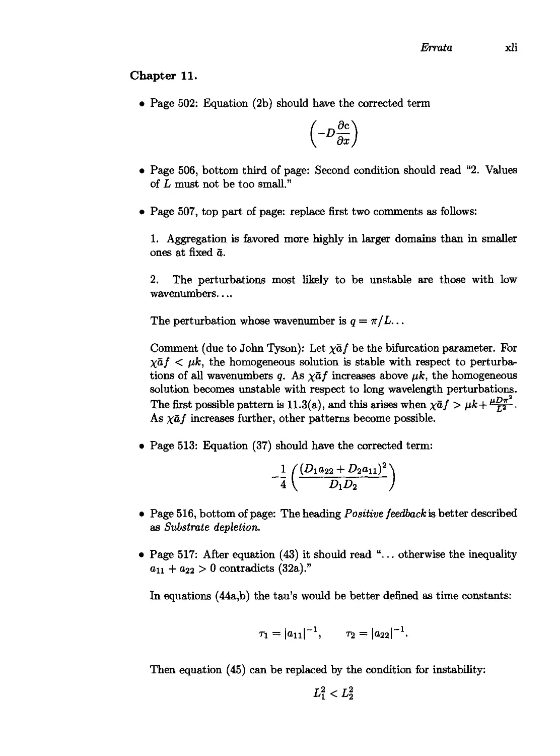
• Page 513: Equation (37) should have the corrected term:
1 f(Dia22 + D2au)2\
4 V A£>2 )
• Page 516, bottom of page: The heading Positive feedback is better described
as Substrate depletion.
• Page 517: After equation (43) it should read "... otherwise the inequality
an + a22 > 0 contradicts (32a)."
In equations (44a,b) the tau's would be better defined as time constants:
n = \au\~1, t2 = |a22l-1-
Then equation (45) can be replaced by the condition for instability:
L\<L\

Mathematical Models in Biology
where L\ = D\T\ is the range of the activator and L% = £>2T2 is the range
of the inhibitor.
• Page 519: Comment about equation (46) by John Tyson:
d = 27t\
\ xk + hj
The term in round braces is then the harmonic mean of the ranges of
activation and inhibition. Further, d « qL\ since L\ « L^-
• Page 521: Comment about gl5 qi by John Tyson: We expect that q\ « 92,
so that Q2 w 2q2. Amplified waves are then those with
-- — — —
9~2Vi?+I|~2L1-
• Page 522, top of page: ^ « area of range of activator, ^ w ratio of
area characterizing domain to range of activation, § = ratio of range of
activation to range of inhibition.
2 area of domain / /area of activation\\
area of activator \ \ area of inhibition / /
• Page 531: The left-hand side of equation 62(a) should read \iDh,-vDa > ...
• Page 545, Problem 3: the inequality is incorrect. Disregard'.
• Page 548, Problem 15(g):
e
n x bci(c2-a)
Ci(l-Cl)-
c2+a
Selected Answers.
• Page 556, Chapter 1, Problem 3: Mislabeling should be corrected as
follows: (i) -+ (ii); (ii) -+ (iii); (iii) -> (iv).
Chapter 1, Problem 9(c): Argument of trig functions should be £p.
/1 \ n
• Page 557, Chapter 2, Problem 1(a): xn = C f _ ] ....

Errata xliii
• Page 558, Chapter 3, 4(c): stable for |1 + b(\-Vb - 1)| < 1.
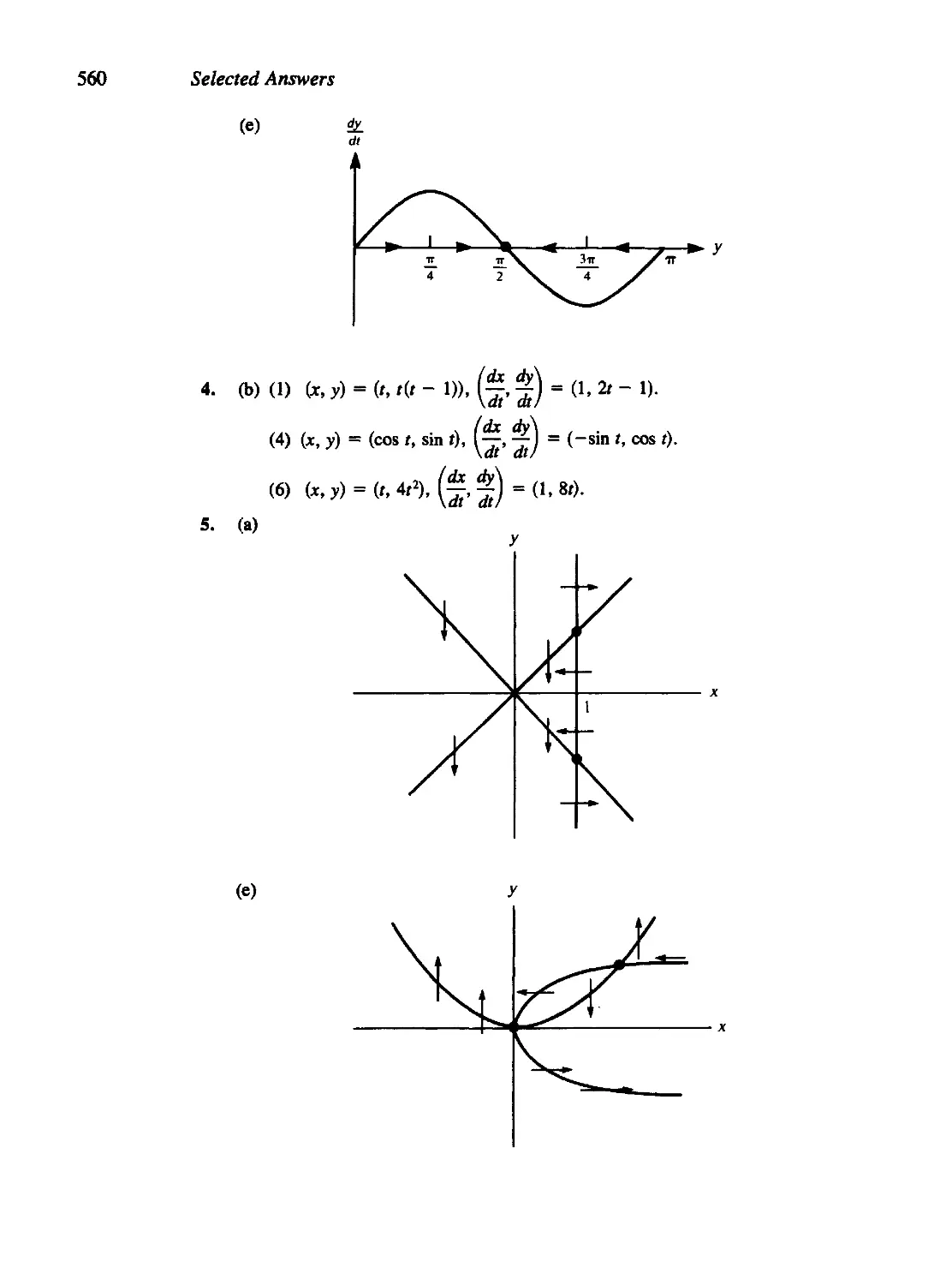
• Page 560, 5(e): Rightmost arrow should point right instead of left.
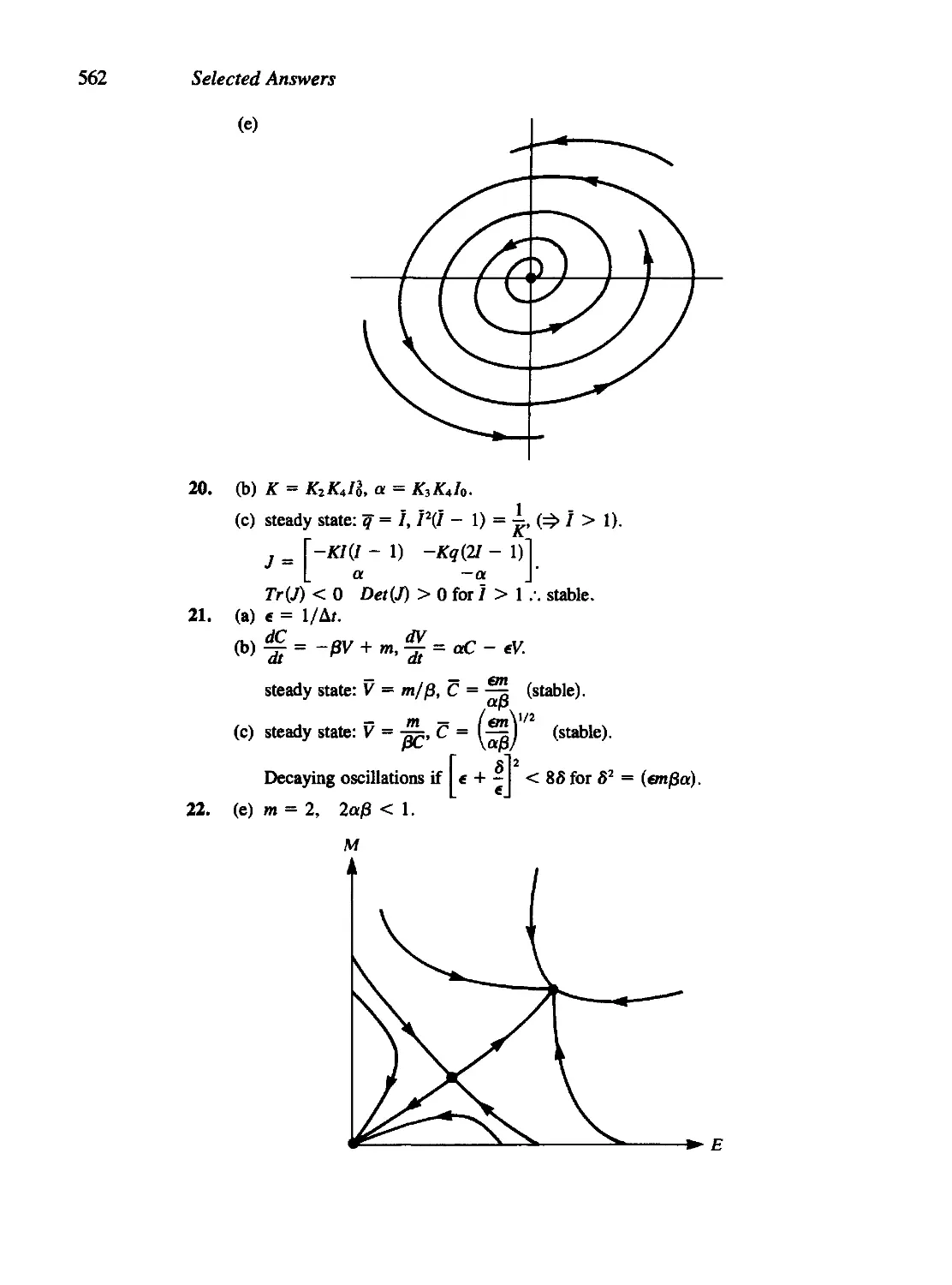
• Page 562: Problems mislabled: 20 -> 21; 21 -► 22
• Page 568: 8(b) is incorrect. Disregard.
• Page 569, 8(e): Replace K with k.
I would like to thank those people who submitted errata. Special thanks to
John Tyson for many helpful comments and for the extended loan of his personal
annotated copy.

This page intentionally left blank

1 Discrete Processes
in Biology

This page intentionally left blank

1 The Theory of Linear
Difference Equations Applied
to Population Growth
For we will always have as 5 is to 8 so is 8 to 13, practically, and as 8 is to
13, so is 13 to 21 almost. I think that the seminal faculty is developed in a
way analogous to this proportion which perpetuates itself, and so in the
flower is displayed a pentagonal standard, so to speak. I let pass all other
considerations which might be adduced by the most delightful study to
establish this truth.
J. Kepler, (1611). Sterna seu de nive sexangule, Opera, ed. Christian
Frisch, tome 7, (Frankefurt a Main, Germany: Heyden & Zimmer,
1858-1871), pp. 722-723.
The early Greeks were fascinated by numbers and believed them to hold special
magical properties. From the Greeks' special blend of philosophy, mathematics,
numerology, and mysticism, there emerged a foundation for the real number system
upon which modern mathematics has been built. A preoccupation with aesthetic
beauty in the Greek civilization meant, among other things, that architects, artisans,
and craftsmen based many of their works of art on geometric principles. So it is that
in the stark ruins of the Parthenon many regularly spaced columns and structures
capture the essence of the golden mean, which derives from the golden rectangle.
Considered to have a most visually pleasing proportion, the golden rectangle
has sides that bear the ratio t = 1:1.618033. . . . The problem of subdividing a line
segment into this so-called extreme and mean ratio was a classical problem in Greek
geometry, appearing in the Elements of Euclid (circa 300 B.C.). It was recognized
then and later that this divine proportion, as Fra Luca Pacioli (1509) called it,
appears in numerous geometric figures, among them the pentagon, and the polyhedral
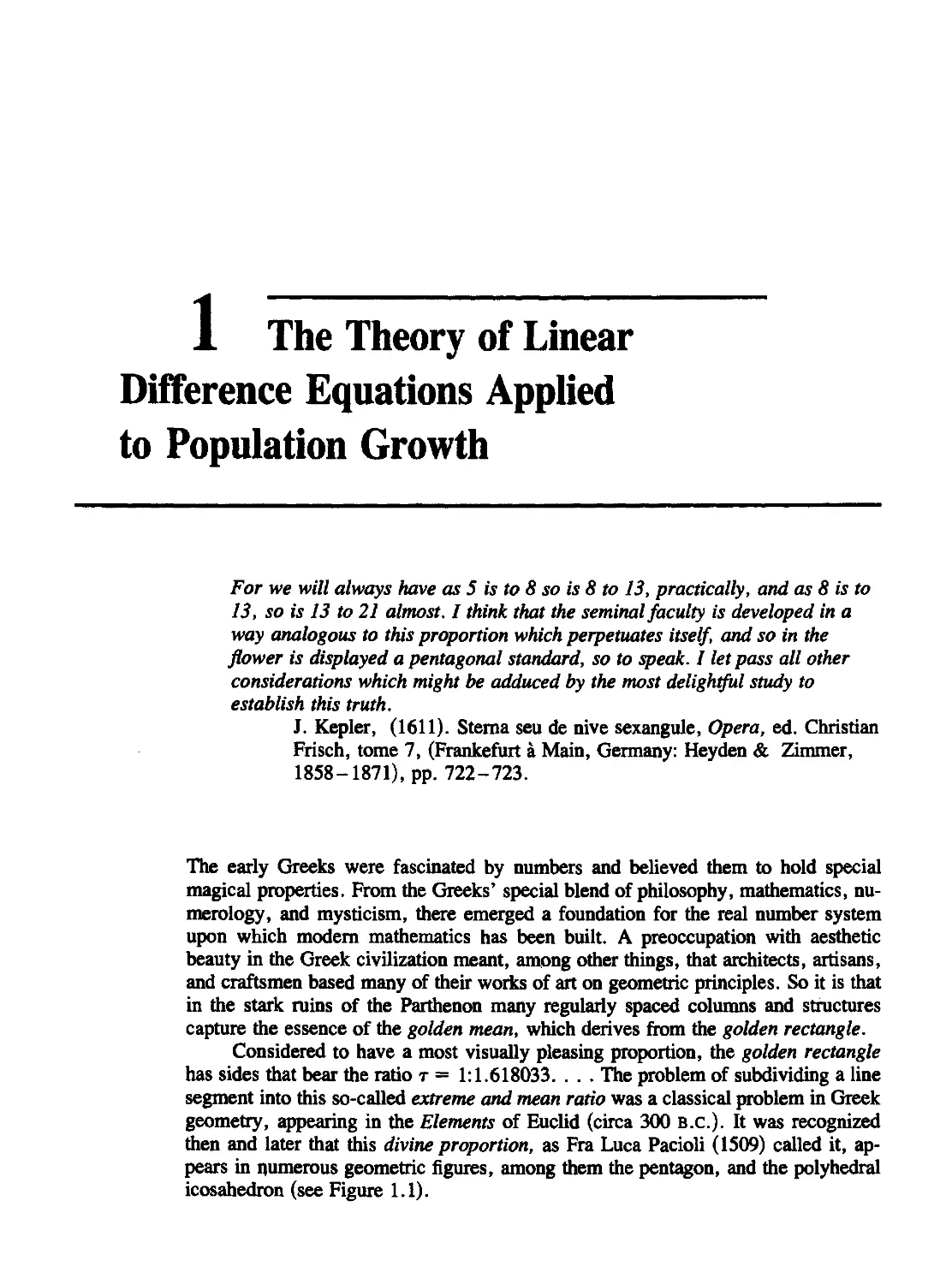
icosahedron (see Figure 1.1).

4 Discrete Processes in Biology
<a>
>\
y{
^
(b)
(cl
(d)
w
(/>

The Theory of Linear Difference Equations Applied to Population Growth 5
About fifteen hundred years after Euclid, Leonardo of Pisa (1175-1250), an
Italian mathematician more affectionately known as Fibonacci ("son of good
nature"), proposed a problem whose solution was a series of numbers that eventually
led to a reincarnation of t. It is believed that Kepler (1571-1630) was the first to
recognize and state the connection between the Fibonacci numbers (0, 1, 1, 2, 3, S,
8, 13, 21, . . .), the golden mean, and certain aspects of plant growth.
Kepler observed that successive elements of the Fibonacci sequence satisfy the
following recursion relation
w*+2 = nk + nk+u (1)
i.e., each member equals the sum of its two immediate predecessors.1 He also noted
that the ratios 2:1, 3:2, 5:3, 8:5, 13:8, . . . approach the value of t.2 Since then,
manifestations of the golden mean and the Fibonacci numbers have appeared in art,
architecture, and biological form. The logarithmic spirals evident in the shells of
certain mollusks (e.g., abalone, of the family Haliotidae) are figures that result from
growth in size without change in proportion and bear a relation to successively
inscribed golden rectangles. The regular arrangement of leaves or plant parts along the
stem, apex, or flower of a plant, known as phyllotaxis, captures the Fibonacci
numbers in a succession of helices (called parastichies); a striking example is the
arrangement of seeds on a ripening sunflower. Biologists have not yet agreed conclu-
1. The values no and n, are defined to be 0 and 1.
2. Certain aspects of the formulation and analysis of the recursion relation (1) governing
Fibonacci numbers are credited to the French mathematician Albert Girard, who developed the
algebraic notation in 1634, and to Robert Simson (1753) of the University of Glasgow, who
recognized ratios of successive members of the sequence as r and as continued fractions (see
problem 12).
Figure 1.1 The golden mean t appears in a variety
of geometric forms that include: (a) Polyhedra such
as the icosahedron, a Platonic solid with 20
equilateral triangle faces (t — ratio of sides of an
inscribed golden rectangle; three golden rectangles
are shown here), (b) The golden rectangle and
every rectangle formed by removing a square from
it. Note that corners of successive squares can be
connected by a logarithmic spiral), (c) A regular
pentagon (t = the ratio of lengths of the diagonal
and a side), (d) The approximate proportions of the
Parthenon (dotted line indicates a golden
rectangle), (e) Geometric designs such as spirals
that result from the arrangement of leaves, scales,
or florets on plants (shown here on the head of a
sunflower). The number of spirals running in
opposite directions quite often bears one of the
numerical ratios 2/3, 3/5, 5/8, 8/13, 13/21,
21/34, 34/5, . . . [see R. V. Jean (1984, 86)];
note that these are the ratios of successive
Fibonacci numbers, (f) Logarithmic spirals (such
as those obtained in (b) are common in shells such
as the abalone Haliotis, where each increment in
size is similar to the preceding one. See D. W.
Thompson (1974) for an excellent summary, ((a and
b)from M. Gardner (1961), The Second Scientific
American Book of Mathematical Puzzles and
Diversions, pp. 92-93. Copyright 1961 by Martin
Gardner. Reprinted by permission of Simon &
Schuster, Inc., N.Y., N.Y. (d)from G. Gromort
(1947), Histoire abregee de rArchitecture en Grece
et a Rome, Fig 43 on p. 75, Vincent Freal & Cie,
Paris, France, (e)from S. Colman (1971), Nature's
Harmonic Unity, plate 64, p. 91; Benjamin Blorn,
N.Y. (reprintedfrom the 1912 edition), (f) D.
Thompson (1961), On Growth and Form (abridged
ed.) figure 84, p. 186. Reprinted by permission of
Cambridge University Press, New York.]

6 Discrete Processes in Biology
sively on what causes these geometric designs and patterns in plants, although the
subject has been pursued for over three centuries.2
Fibonacci stumbled unknowingly onto the esoteric realm of t through a
question related to the growth of rabbits (see problem 14). Equation (1) is arguably the
first mathematical idealization of a biological phenomenon phrased in terms of a
recursion relation, or in more common terminology, a difference equation.
Leaving aside the mystique of golden rectangles, parastichies, and rabbits, we
find that in more mundane realms, numerous biological events can be idealized by
models in which similar discrete equations are involved. Typically, populations for
which difference equations are suitable are those in which adults die and are totally
replaced by their progeny at fixed intervals (i.e., generations do not overlap). In
such cases, a difference equation might summarize the relationship between
population density at a given generation and that of preceding generations. Organisms that
undergo abrupt changes or go through a sequence of stages as they mature (i.e.,
have discrete life-cycle stages) are also commonly described by difference
equations.
The goals of this chapter are to demonstrate how equations such as (1) arise in
modeling biological phenomena and to develop the mathematical techniques to solve
the following problem: given particular starting population levels and a recursion
relation, predict the population level after an arbitrary number of generations have
elapsed. (It will soon be evident that for a linear equation such as (1), the
mathematical sophistication required is minimal.)
To acquire a familiarity with difference equations, we will begin with two
rather elementary examples: cell division and insect growth. A somewhat more
elaborate problem we then investigate is the propagation of annual plants. This topic will
furnish the opportunity to discuss how a slightly more complex model is derived.
Sections 1.3 and 1.4 will outline the method of solving certain linear difference
equations. As a corollary, the solution of equation (1) and its connection to the
golden mean will emerge.
1.1 BIOLOGICAL MODELS USING DIFFERENCE EQUATIONS
Cell Division
Suppose a population of cells divides synchronously, with each member producing a
daughter cells.3 Let us define the number of cells in each generation with a subscript,
that is, Mi, M2, . . . , M„ are respectively the number of cells in the first, second,
. . . , nth generations. A simple equation relating successive generations is
M„+i = aM„. (2)
2. An excellent summary of the phenomena of phyllotaxis and the numerous theories that
have arisen to explain the observed patterns is given by R. V. Jean (1984). His book contains
numerous suggestions for independent research activities and problems related to phyllotaxis. See
also Thompson (1942).
3. Note that for real populations only a > 0 would make sense; a < 0 is unrealistic, and
a = 0 would be uninteresting.

The Theory of Linear Difference Equations Applied to Population Growth 7
Let us suppose that initially there are M0 cells. How big will the population be after
n generations? Applying equation (2) recursively results in the following:
M„+1 = a(aMn-i) = a[a(aMn-2)] = ••■= an+lM0. (3)
Thus, for the nth generation
Mn = a"M0. (4)
We have arrived at a result worth remembering: The solution of a simple linear
difference equation involves an expression of the form (some number)", where n is the
generation number. (This is true in general for linear difference equations.) Note that
the magnitude of a will determine whether the population grows or dwindles with
time. That is,
| a | > 1 M„ increases over successive generations,
| a | < 1 Mn decreases over successive generations,
a = 1 M„ is constant.
An Insect Population
Insects generally have more than one stage in their life cycle from progeny to
maturity. The complete cycle may take weeks, months, or even years. However, it is
customary to use a single generation as the basic unit of time when attempting to write a
model for insect population growth. Several stages in the life cycle can be depicted
by writing several difference equations. Often the system of equations condenses to
a single equation in which combinations of all the basic parameters appear.
As an example consider the reproduction of the poplar gall aphid. Adult female
aphids produce galls on the leaves of poplars. All the progeny of a single aphid are
contained in one gall (Whitham, 1980). Some fraction of these will emerge and
survive to adulthood. Although generally the capacity for producing offspring
(fecundity) and the likelihood of surviving to adulthood (survivorship) depends on
their environmental conditions, on the quality of their food, and on the population
sizes, let us momentarily ignore these effects and study a naive model in which all
parameters are constant.
First we define the following:
an = number of adult female aphids in the nth generation,
p„ = number of progeny in the nth generation,
m = fractional mortality of the young aphids,
/ = number of progeny per female aphid,
r = ratio of female aphids to total adult aphids.
Then we write equations to represent the successive populations of aphids and
use these to obtain an expression for the number of adult females in the nth
generation if initially there were a0 females:

8 Discrete Processes in Biology
Each female produces /progeny; thus
no. of progeny
in (n + l)st
generation
Pn+\ = fan. (5)
\
no. of females in
previous generation
-no. of offspring per female
Of these, the fraction 1 — m survives to adulthood, yielding a final proportion of r
females. Thus
a„+i = r(l - m)p„+i. (6)
While equations (S) and (6) describe the aphid population, note that these can be
combined into the single statement
a«+i =fr{\ ~ m)an. (7)
For the rather theoretical case where/, r, and m are constant, the solution is
an = [/HI - mjfao, (8)
where a0 is the initial number of adult females.
Equation (7) is again a first-order linear difference equation, so that solution (8)
follows from previous remarks. The expression fr{\ - m) is the per capita number of
adult females that each mother aphid produces.
1.2 PROPAGATION OF ANNUAL PLANTS
Annual plants produce seeds at the end of a summer. The flowering plants wilt and
die, leaving their progeny in the dormant form of seeds that must survive a winter to
give rise to a new generation. The following spring a certain fraction of these seeds
germinate. Some seeds might remain dormant for a year or more before reviving.
Others might be lost due to predation, disease, or weather. But in order for the
plants to survive as a species, a sufficiently large population must be renewed from
year to year.
In this section we formulate a model to describe the propagation of annual
plants. Complicating the problem somewhat is the fact that annual plants produce
seeds that may stay dormant for several years before germinating. The problem thus
requires that we systematically keep track of both the plant population and the
reserves of seeds of various ages in the seed bank.
Stage 1: Statement of the Problem
Plants produce seeds at the end of their growth season (say August), after which they
die. A fraction of these seeds survive the winter, and some of these germinate at the
beginning of the season (say May), giving rise to the new generation of plants. The
fraction that germinates depends on the age of the seeds.

The Theory of Linear Difference Equations Applied to Population Growth 9
Stage 2: Definitions and Assumptions
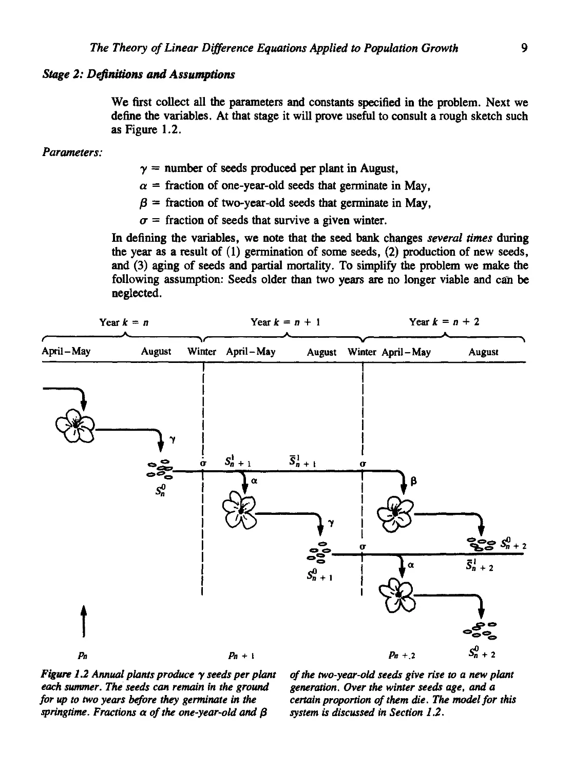
Parameters:
We first collect all the parameters and constants specified in the problem. Next we
define the variables. At that stage it will prove useful to consult a rough sketch such
as Figure 1.2.
y = number of seeds produced per plant in August,
a = fraction of one-year-old seeds that germinate in May,
)3 = fraction of two-year-old seeds that germinate in May,
<7 = fraction of seeds that survive a given winter.
In defining the variables, we note that the seed bank changes several times during
the year as a result of (1) germination of some seeds, (2) production of new seeds,
and (3) aging of seeds and partial mortality. To simplify the problem we make the
following assumption: Seeds older than two years are no longer viable and can be
neglected.
Year k - n
Year k = n + 1
A
April-May
v v
August Winter April-May August Winter April-May
Year k = n + 2
A.
A.
Ai + 1
August
cOt^
\3o
4?
r S„ + i
<4>
Sn + 1
o
og
Sn + 1
a
i *'
a
1 J:
^gti + 2
Sn + 2
1
Figure 1.2 Annual plants produce y seeds per plant
each summer. The seeds can remain in the ground
for up to two years before they germinate in the
springtime. Fractions a of the one-year-old and fi
At+.2 ■Sn + 2
of the two-year-old seeds give rise to a new plant
generation. Over the winter seeds age, and a
certain proportion of them die. The model for this
system is discussed in Section 1.2.

Discrete Processes in Biology
Consulting Figure 1.2, let us keep track of the various quantities by defining
p„ = number of plants in generation n,
Si, = number of one-year-old seeds in April (before germination),
Si = number of two-year-old seeds in April (before germination),
Sj = number of one-year-old seeds left in May (after some have germinated),
SI = number of two-year-old seeds left in May (after some have germinated),
S° = number of new seeds produced in August.
Later we will be able to eliminate some of these variables. In this first attempt at
formulating the equations it helps to keep track of all these quantities. Notice that
superscripts refer to age of seeds and subscripts to the year number.
Stage 3: The Equations
In May, a fraction a of one-year-old and (3 of two-year-old seeds produce the plants.
Thus
_ | plants from \ , /plants from \
P" \one-year-old seeds/ \two-year-old seeds/'
pn = aS\ + PSI (9a)
The seed bank is reduced as a result of this germination. Indeed, for each age class,
we have
seeds left = (fraction not) x Iori8inal number \
Vgerminated / \of seeds in April/"
Thus
Si = (1 - a)Sln, (9b)
Si = (1 - p)Sl. (9c)
In August, new (0-year-old) seeds are produced at the rate of y per plant:
S°n = yPn. (9d)
Over the winter the seed bank changes by mortality and aging. Seeds that were new
in generation n will be one year old in the next generation, n + 1. Thus we have
Sl+l = o$°, (9e)
Sl+i = aSl (9f)
Stage 4: Condensing the Equations
We now use information from equations (9a- f) to recover a set of two equations
linking successive plant and seed generations. To do so we observe that by using
equation (9d) we can simplify (9e) to the following:
Si+1 = (T(ypn). (10)

The Theory of Linear Difference Equations Applied to Population Growth 11
Similarly, from equation (9b) equation (9f) becomes
S2+, = <7(1 - a)Sl (11)
Now let us rewrite equation (9a) for generation n + 1 and make some substitutions:
p.+i = aSj+i+ 052+1. (12)
Using (10), (11), and (12) we arrive at a system of two equations in which plants and
one-year-old seeds are coupled:
p„+i = aayp„ + fio-{\ - a)S\, (13a)
SU\ = oyp„. (13b)
Notice that it is also possible to eliminate the seed variable altogether by first
rewriting equation (13b) as
S\ = aypn-\ (14)
and then substituting it into equation (13a) to get
p„+i = aoypn + j8o-2(l - a)ypn-i. (15)
We observe that the model can be formulated in a number of alternative ways,
as a system of two first-order equations or as one second-order equation (IS).
Equation (15) is linear since no multiples p„pm or terms that are nonlinear in pn occur; it is
second order since two previous generations are implicated in determining the
present generation.
Notice that the system of equations (13a and b) could also have been written as
a single equation for seeds.
Stage 5: Check
To be on the safe side, we shall further explore equation (IS) by interpreting one of
the terms on its right hand side. Rewriting it for the nth generation and reading from
right to left we see that pH is given by
p„ = aaypn-i + /3o-(l - a)ayp„-2
II I \^~^
III | seeds produced
III j two years ago
II I v v '
■ . which then survived First
i i I winter
|| * ¥ '
| | and failed to germinate last year
I* , '
| survived last winter
Y
and were among the fraction of two-year-old
seeds that germinated
The first term is more elementary and is left as an exercise for the reader to translate.

12 Discrete Processes in Biology
1.3 SYSTEMS OF LINEAR DIFFERENCE EQUATIONS
The problem of annual plant reproduction leads to a system of two first-order
difference equations (10,13), or equivalently a single second-order equation (15). To
understand such equations, let us momentarily turn our attention to a general system of
the form
x„+i = anxn + any„, (16a)
y„+i = a2ix„ + a22y„. (16b)
As before, this can be converted to a single higher-order equation. Starting with
(16a) and using (16b) to eliminate yn+u we have
Xn+2 = OuXn + l + du^+l
= anxn+i + an(a2\X„ + a22y„).
From equation (16a),
a\2yn = xn+\ ~ auxn.
Now eliminating y„ we conclude that
xn+2 = aux„+i + al2a2lxn + a^ixn+i - anxn),
or more simply that
xn+2 - (an + a22)xn+i + (a22au - ai2a2i)xn = 0. (17)
In a later chapter, readers may remark on the similarity to situations encountered in
reducing a system of ordinary differential equations (ODEs) to single ODEs (see
Chapter 4). We proceed to discover properties of solutions to equation (17) or
equivalently, to (16a, b).
Looking back at the simple first-order linear difference equation (2), recall that
solutions to it were of the form
xn = CA\ (18)
While the notation has been changed slightly, the form is still the same: constant
depending on initial conditions times some number raised to the power n. Could this
type of solution work for higher-order linear equations such as (17)?
We proceed to test this idea by substituting the expression xn = CA" (in the
form of xn+i = CA"+I and x„+2 = CA"+2) into equation (17), with the result that
CA"+2 - (an + a22)C\n+1 + (a22au - ana2l)\n = 0.
Now we cancel out a common factor of CA". (It may be assumed that CA" ¥= 0 since
x„ = 0 is a trivial solution.) We obtain
A2 - (flu + a22)\ + (auan - ai2a2\) = 0. (19)
Thus a solution of the form (18) would in fact work, provided that A satisfies the
quadratic equation (19), which is generally called the characteristic equation of
(17).

The Theory of Linear Difference Equations Applied to Population Growth 13
To simplify notation we label the coefficients appearing in equation (19) as
follows:
P = aii+ a22, ^
•y — a^an — anai\.
The solutions to the characteristic equation (there are two of them) are then:
These numbers are called eigenvalues, and their properties will uniquely determine
the behavior of solutions to equation (17). {Note: much of the terminology in this
section is common to linear algebra; in the next section we will arrive at identical
results using matrix notation.)
Equation (17) is linear; like all examples in this chapter it contains only scalar
multiples of the variables—no quadratic, exponential, or other nonlinear
expressions. For such equations, Has principle of linear superposition holds: if several
different solutions are known, then any linear combination of these is again a solution.
Since we have just determined that A" and A2 are two solutions to (17), we can
conclude that a general solution is
x„ = A, A? + A2A2, (22)
provided Ai ^ A2. (See problem 3 for a discussion of the case Ai = A2.) This
expression involves two arbitrary scalars, Aj and A2, whose values are not specified by
the difference equation (17) itself. They depend on separate constraints, such as
particular known values attained by x. Note that specifying any two x values uniquely
determines At and A2. Most commonly, xo and jtt, the levels of a population in the
first two successive generations, are given {initial conditions); A, and A2 are
determined by solving the two resulting linear algebraic equations (for an example see
Section 1.7). Had we eliminated x instead of y from the system of equations (16),
we would have obtained a similar result. In the next section we show that general
solutions to the system of first-order linear equations (16) indeed take the form
x„ = A, AT + A2A5,
y„ = S,A? + B2kn2.
The connection between the four constants A\, A2, Bu and B2 will then be
made clear.
1.4 A LINEAR ALGEBRA REVIEW4
Results of the preceding section can be obtained more directly from equations (16a,
b) using linear algebra techniques. Since these are useful in many situations, we will
briefly review the basic ideas. Readers not familiar with matrix notation are encour-
4. To the instructor: Students unfamiliar with linear algebra and/or complex numbers can
omit Sections 1.4 and 1.8 without loss of continuity. An excellent supplement for this chapter is
Sherbert (1980).

14 Discrete Processes in Biology
aged to consult Johnson and Riess (1981), Bradley (197S), or any other elementary
linear algebra text.
Recall that a shorthand way of writing the system of algebraic linear equations,
ax + by = 0,
« + i = o, <*'
using vector notation is:
Mv = 0,
where M is a matrix of coefficients and v is the vector of unknowns. Then for
system (24),
Note that Mv then represents matrix multiplication of M (a 2 x 2 matrix) with v (a
2 X 1 matrix).
Because (24) is a set of linear equations with zero right-hand sides, the vector
is always a solution. It is in fact, a unique solution unless the equations are
"redundant." A test for this is to see whether the determinant of M is zero; i.e.,
det M = ad - be = 0. (26)
When det M = 0, both the equations contain the same information so that in reality,
there is only one constraint governing the unknowns. That means that any
combination of values of x and y will solve the problem provided they satisfy any one of the
equations, e.g.,
x = —by/a.
Thus there are many nonzero solutions when (26) holds.
To apply this notion to systems of difference equations, first note that
equations (16) can be written in vector notation as
VB+1 = MV„ (27a)
where
(°o)
-fc)
(27b)
and
M=(fln fl"). (27c)
It has already been remarked that solutions to this system are of the form
V = (Ak"\
(28a)
Substituting (28a) into (27a) we obtain

The Theory of Linear Difference Equations Applied to Population Growth 15
We expand the RHS to get
AA"+1 = a„AA" + anB\n, (28c)
Bkn+i = aziAA" + a^BA".
We then cancel a factor of A" and rearrange terms to arrive at the following system
of equations:
0 = A(an - A) + Ban, 2g)
0 = A(a2.) + B(a22 - A).
This is equivalent to
0 = (an ~ A fll2 )(A)
These are now linear algebraic equations in the quantities A and B. One solution is
always A = B = 0, but this is clearly a trivial one because it leads to
V = 0,
a continually zero level of both x„ and y„. To have nonzero solutions for A and B we
must set the determinant of the matrix of coefficients equal to zero;
det(an " A an \ = 0. (30)
\an an - A/
This leads to
(tin - A)(a22 - A) - ai2ti2i = 0, (31)
which results, as before, in the quadratic characteristic equation for the eigenvalues
A. Rearranging equation (31) we obtain
where
As before, we find that
A2 - jSA + y = 0
/3 = an + a22,
•y = (anti22 - ai2a2i).
A _ j8 ± Vj82 - 4y
A,,2
are the two eigenvalues. The quantities /3, y, and B2 - 4y have the following names
and symbols:
)3 = an + an = Tr M = the trace of the matrix M
y = a\\a22 - a\2a2\ = det M = the determinant of M
fl2 — 4y = disc(M) = the discriminant of M.
If disc M < 0, we observe that the eigenvalues are complex (see Section 1.8); if
disc M = 0, the eigenvalues are equal.

Discrete Processes in Biology
Corresponding to each eigenvalue is a nonzero vector v, = I '), called an
eigenvector, that satisfies
Mv,- = A,v,
This matrix equation is merely a simplified matrix version of (28c) obtained by
cancelling a factor of A" and then applying the result to a specific eigenvalue A,.
Alternatively the system of equations (29) in matrix form is
(an - A, ai2 \(Ah = n
\a2i an - \J\Bj
It may be shown (see problem 4) that provided a12 # 0,
"~W Li ~au
\ an )
is an eigenvector corresponding to A,. Furthermore, any scalar multiple of an
eigenvector is an eigenvector; i.e., if v is an eigenvector, then so is av for any scalar a.
1.5 WILL PLANTS BE SUCCESSFUL?
With the methods of Sections 1.3 and 1.4 at our disposal let us return to the topic of
annual plant propagation and pursue the investigation of behavior of solutions to
equation (15). The central question that the model should resolve is how many seeds
a given plant should produce in order to ensure survival of the species. We shall
explore this question in the following series of steps.
To simplify notation,
let a
= aay and b = /3er2(l — a)y. Then equation (15) becomes
Pn+i - ap„ - bp„-\ = 0, (32)
with corresponding characteristic equation
Eigenvalues are
where
is a positive quantity
X2 - a\ - b = 0. (33)
I
A,.2 = -(o ± Va2 + 4b) (34)
= £22(1±Vi + 8).
g = 40(1 -«) = 4-0(1 \
ya2 y a\a 1
since a < 1.

The Theory of Linear Difference Equations Applied to Population Growth 17
We have arrived at a rather cumbersome expression for the eigenvalues. The
following rough approximation will give us an estimate of their magnitudes.
Initially we consider a special case. Suppose few two-year-old seeds germinate
in comparison with the one-year-old seeds. Then 8/a is very small, making 8 small
relative to 1. This means that at the very least, the positive eigenvalue At has
magnitude
Al-^E(l + Vr)-2222-a7tt.
Thus, to ensure propagation we need the following conditions:
A, > 1, aya > 1, y > 1/W (35a)
By this reasoning we may conclude that the population will grow if the number of
seeds per plant is greater than 1/W. To give some biological meaning to equation
(35a), we observe that the quantity oya represents the number of seeds produced by
a given plant that actually survive and germinate the following year. The
approximation 8—0 means that the parent plant can only be assured of replacing itself if it
gives rise to at least one such germinated seed. Equation (35a) gives a "strong
condition" for plant success where dormancy is not playing a role. If 8 is not negligibly
small, there will be a finite probability of having progeny in the second year, and
thus the condition for growth of the population will be less stringent. It can be
shown (see problem 17e) that in general Ai > 1 if
y > —r-^27i—t • (35b)
acr + Bo- (1 — a)
When £ = 0 this condition reduces to that of (35a). We postpone the discussion of
this case to problem 12 of Chapter 2.
As a final step in exploring the plant propagation problem, a simple computer
program was written in BASIC and run on an IBM personal computer. The two
sample runs derived from this program (see Table 1.1) follow the population for 20
generations starting with 100 plants and no seeds. In the first case a = 0.5, y = 0.2,
o- = 0.8, 8 = 0.25, and the population dwindles. In the second case a and B have
been changed to a = 0.6, B = 0.3, and the number of plants is seen to increase
from year to year. The general condition (35b) is illustrated by the computer
simulations since, upon calculating values of the expressions \/aa and l/(a<r +
/3<72(1 - a)) we obtain (a) 2.5 and 2.32 in the first simulation and (b) 2.08 and 1.80
in the second. Since y = 2.0 in both cases, we observe that dormancy played an
essential role in plant success in simulation b.
To place this linear model in proper context, we should add various qualifying
remarks. Clearly we have made many simplifying assumptions. Among them, we
have assumed that plants do not interfere with each other's success, that germination
and survival rates are constant over many generations, and that all members of the
plant population are identical. The problem of seed dispersal and dormancy has been
examined by several investigators. For more realistic models in which other factors
such as density dependence, environmental variability, and nonuniform distributions
of plants are considered, the reader may wish to consult Levin, Cohen, and Hastings

18 Discrete Processes in Biology
Table 1.1 Changes in a Plant Population over 20 Generations: (a) a = 0.5, B = 0.25, y = 2.0,
tr - 0.8; (b) a = 0.6, B = 0.3, y = 2.0, a = 0.8
Generation
0
1
2
3
4
5
6
7
8
9
10
11
12
13
14
15
16
17
18
19
20
Generation
0
1
2
3
4
5
6
7
8
9
10
11
12
13
14
15
16
17
18
19
20
Plants
100.0
80.0
80.0
76.8
74.2
71.6
69.2
66.8
64.5
62.3
60.1
58.1
56.1
54.2
52.3
50.5
48.8
47.1
45.5
43.9
42.4
Plants
100.0
96.0
107.5
117.9
129.7
142.6
156.9
172.5
189.7
208.6
229.4
252.3
277.4
305.1
335.5
369.0
405.8
446.2
490.7
539.6
593.4
New seeds
0.0
200.0
160.0
160.0
153.6
148.4
143.3
138.4
133.6
129.1
124.6
120.3
116.2
112.2
108.4
104.7
101.1
97.6
94.2
91.0
87.9
New seeds
0.0
200.0
192.0
215.0
235.9
259.5
285.3
313.8
345.1
379.5
417.3
458.9
504.6
554.9
610.3
671.1
738.0
811.6
892.5
981.4
1079.2
One-year-old seeds
0.0
160.0
128.0
128.0
122.8
118.7
114.6
110.7
106.9
103.2
99.7
96.3
93.0
89.8
86.7
83.7
80.8
78.1
75.4
72.8
70.3
One-year-old seeds
0.0
160.0
153.6
172.0
188.7
207.6
228.3
251.0
276.0
303.6
333.8
367.1
403.7
443.9
488.2
536.9
590.4
649.2
714.0
785.1
863.4
Two-year old seeds
0.0
0.0
64.0
51.2
51.2
49.1
47.5
45.8
44.3
42.7
41.3
39.8
38.5
37.2
35.9
34.6
33.5
32.3
31.2
30.1
29.1
Two-year-old seeds
0.0
0.0
51.2
49.1
55.0
60.3
66.4
73.0
80.3
88.3
97.1
106.8
117.4
129.1
142.0
156.2
171.8
188.9
207.7
228.4
251.2

The Theory of Linear Difference Equations Applied to Population Growth 19
(1984) and references therein. A related problem involving resistance to herbicides
is treated by Segel (1981).
Recent work by Ellner (1986) is relevant to the basic issue of delayed
germination in annual plants. Apparently, there is some debate over the underlying
biological advantage gained by prolonging the opportunities for germination. Germination
is usually controlled exclusively by the seed coat, whose properties derive
genetically from the mother plant. Mechanical or chemical factors in the seed coat may
cause a delay in germination. As a result some of the seeds may not be able-to take
advantage of conditions that favor seedling survival. In this way the mother plant
can maintain some influence on its progeny long after their physical separation. It is
held that spreading germination over a prolonged time period may help the mother
plant to minimize the risk of losing all its seeds to chance mortality due to
environmental conditions. From the point of view of the offspring, however, maternal
control may at times be detrimental to individual survival. This parent-offspring conflict
occurs in a variety of biological settings and is of recent popularity in several
theoretical treatments. See Ellner (1986) for a discussion.
1.6 QUALITATIVE BEHAVIOR OF SOLUTIONS TO LINEAR DIFFERENCE
EQUATIONS
To recapitulate the results of several examples, linear difference equations are
characterized by the following properties:
1. An /nth-order equation typically takes the form
OoXn + a\Xn-\ + • • • + amXn-m = b„,
or equivalently,
aoXn+m + a\Xn+m-l + • • • + OmXn — bn.
2. The order m of the equation is the number of previous generations that directly
influence the value of x in a given generation.
3. When an, ax, . . . , am are constants and bn = 0, the problem is a
constant-coefficient homogeneous linear difference equation; the method
established in this chapter can be used to solve such equations. Solutions are
composed of linear combinations of basic expressions of the form
xn = CA-. (36)
4. Values of A appearing in equation (36) are obtained by finding the roots of the
corresponding characteristic equation
floA"1 + aiAm_1 + • • • + am = 0.
5. The number of (distinct) basic solutions to a difference equation is determined
by its order. For example, a first-order equation has one solution, and a
second-order equation has two. In general, an /nth-order equation, like a
system of m coupled first-order equations, has m basic solutions.

20 Discrete Processes in Biology
6. The general solution is a linear superposition of the m basic solutions of the
equation (provided all values of A are distinct).
7. For real values of A the qualitative behavior of a basic solution (24) depends on
whether A falls into one of four possible ranges:
A > 1, A < -1, 0< A < 1, -1<A<0.
To observe how the nature of a basic solution is characterized by this broad
classification scheme, note that
(a) For A > 1, A" grows as n increases; thus x„ = Ck" grows without
bound.
(b) For 0 < A < 1, A" decreases to zero with increasing n; thus xn decreases
to zero.
(c) For -1<A<0, A" oscillates between positive and negative values
while declining in magnitude to zero.
(d) For A < — 1, A" oscillates as in (c) but with increasing magnitude.
The cases where A= 1, A = 0, or A = — 1, which are marginal points of
demarcation between realms of behavior, correspond respectively to (1) the static
(nongrowing) solution where x = C, (2) x = 0, and (3) an oscillation between
the value x = C and x = —C. Several representative examples are given in
Figure 1.3.
Linear difference equations for which m > 1 have general solutions that
combine these broad characteristics. However, note that linear combinations of
expressions of the form (36) show somewhat more subtle behavior. The dominant
eigenvalue (the value A, of largest magnitude) has the strongest effect on the solution; this
means that after many generations the successive values of x are approximately
related by
Xn+\ — n.iXn.
Clearly, whether the general solution increases or decreases in the long run
depends on whether any one of its eigenvalues satisfies the condition
|A,|>1.
If so, net growth occurs. The growth equation contains an oscillatory component if
one of the eigenvalues is negative or complex (to be discussed). However, any
model used to describe population growth cannot admit negative values of x„. Thus,
while oscillations typically may occur, they are generally superimposed on a larger-
amplitude behavior so that successive x„ levels remain positive.
In difference equations for which m s 2, the values of A from which basic
solutions are composed are obtained by extracting roots of an mth-order polynomial.
For example, a second-order difference equation leads to a quadratic characteristic
equation. Such equations in general may have complex roots as well as repeated
roots. Thus far we have deliberately ignored these cases for the sake of simplicity.
We shall deal with the case of complex (and not real) A in Section 1.8 and touch on
the case of repeated real roots in the problems.

The Theory of Linear Difference Equations Applied to Population Growth 21
Figure 13 Qualitative behavior of\n- CK"
in the four cases (a) A > 1, (b) 0 < A < 1,
(c) -I < A < 0, (d) A < -1.
*■ a
(a)
(c)
Jl

22 Discrete Processes in Biology
1.7 THE GOLDEN MEAN REVISITED
We shall apply techniques of this chapter to equation (1), which stems from
Fibonacci's work. Assuming solutions of the form (18), we arrive at a characteristic
equation corresponding to (1):
A2 = A + 1.
Roots are
A, = (1 - Vs)/2 and A2 = (1 + VS)/2.
Successive members of the Fibonacci sequence are thus given by the formula
xn = AA? + BA2.
Suppose we start the sequence withjfo = 0 and Jti = 1. This will uniquely determine
the values of the two constants A and B, which must satisfy the following algebraic
equations:
0 = AA? + BA§ = A + B,
1 = AA, + BX.2 = \[A(\ -VS) + B{\ + V5)].
It may be shown that A and B are given by
A=-l/V5 and S=+l/V5.
Thus the solution is
1 /l - V5 V 1 /l -f- V5 V
X" = -Vs\—T~) +V5\~T~)-
Observe that A2 > 1 and -1 < Ai < 0. Thus the dominant eigenvalue is
A2 = (1 + VS)/2, and its magnitude guarantees that the Fibonacci numbers form
an increasing sequence. Since the second eigenvalue is negative but of magnitude
smaller than 1, its only effect is to superimpose a slight oscillation that dies out as n
increases. It can be concluded that for large values of n the effect of At is negligible,
so that
Xn - (1/V5)A2".
The ratios of successive Fibonacci numbers converge to
Xn+l _ . _ 1 + V5
__A2_____.
Thus the value of the golden mean is (1 + V5)/2 = 1.618033 ....
1.8 COMPLEX EIGENVALUES IN SOLUTIONS TO DIFFERENCE EQUATIONS
The quadratic characteristic equation (19) can have complex eigenvalues (21) with
nonzero imaginary parts when )32 < 4-y. These occur in conjugate pairs,
Ai = a + bi and A2 = a — bi,

The Theory of Linear Difference Equations Applied to Population Growth 23
where a = fi/2 and b = \\fi2 - 4y|1/2. A similar situation can occur in linear
difference equations of any order greater than 1, since these are associated with
polynomial characteristic equations.
When complex values of A are obtained, it is necessary to make sense of
general solutions that involve powers of complex numbers. For example,
x„ = A,(a + bi)n + A2(a - bi)n. (37)
To do so, we must first review several fundamental properties of complex numbers.
Review of Complex Numbers
A complex number can be represented in two equivalent ways. We may take a + bi to
be a point in the complex plane with coordinates (a, b). Equivalently, by specifying an
angle <b in standard position (clockwise from positive real axis to a + bi) and a
distance, r from (a, b) to the origin, we can represent the complex number by a pair
(r, <$>). These coordinates can be related by
a = r cos <b,
b = r sin tb.
Equivalently
r= (a2 + b2)"2,
<b = arctan (b/a).
The following identities, together known as Eider's theorem,
relations; they can also be considered to define «"*:
a + bi = r(cos 4> + ' sm 41) - ™l*>
a — bi = r(cos <b - i sin <t>) = re~'*.
(38a)
(38b)
(39a)
(39b)
summarize these
(40a)
(40b)
This leads to the conclusion that raising a complex number to some power can be
understood in the following way:
(a + bif = («'*)" = rVn* = c + di.
where
c = r" cos n<b,
d = r" sin n<b.
(41a)
(41b)
Graphically the relationship between the complex numbers a + bi and c + di is as
follows: the latter has been obtained by rotating the vector (a, b) by a multiple n of the
angle <b and then extending its length to a power n of its former length. (See Figure
1.4.) This rotating vector will be lead to an oscillating solution, as will be clarified
shortly.
Proceeding formally, we rewrite (37) using equations (40a,b):
xn = Ai(a + bi)n + A2(a - bi)n
= Air"(cos n<b + i sin n<b) + A2r"(cos n<p — i sin n<b)
= B\r" cos n<b + Uiirn sin n<b,

24 Discrete Processes in Biology
Figure 1.4 (a) Representation of a complex number
as a point in the complex plane in both cartesian
(a,b) and polar (r, <£) coordinates, (b) A succession
of values of the complex numbers (1 + i)". The
radius vector rotates and stretches as higher powers
are taken.
Real axis
(a)
(1 + ')•
(1 + i)7
where B\ = A\ + A2 and B2 = (At - A2). Thus xn has a real part and an imaginary
part. For
we have
un = r" cos n<j>,
v„ = r" sin n<p,
x„ = B\u„ + iB2Vn.
(42a)
(42b)
(43)
Because the equation leading to (43) is linear, it can be proved that the real and
imaginary parts of this complex solution are themselves solutions. It is then
customary to define a real-valued solution by linear superposition of the real quantities u„
and v„:
Xn = ClUn + C2Vn
= r"(C\ cos n<£ + Ci sin n<f>)
(44)

The Theory of Linear Difference Equations Applied to Population Growth
25
n
• •
H 1 1 1 1 1 1 »- n
Figure 1.5 A "time sequence" of the real-valued
solution given by equation (44) would display
oscillations as above. Shown are values ofx.nfor
n = 0, 1, . . . , 10. The amplitude of oscillation is
r", and the frequency is l/4> where r and <f> are
given in equation (39).
where r and <f> are related to a and b by equations (38a,b) or (39a,b). (See Figure
1.5.)
Example
The difference equation
JCn+2 ~ 2JC+| + 2X„ = 0
has a characteristic equation
A2 - 2A + 2 = 0,
with the complex conjugate roots A = 1 ± i. Thus a = 1 and 6=1,
r = (a2 + b2)1/2 = V2,
<f> = arctan (b/a) = v/4.
Thus the real-valued general solution to equation (43) is
x„ = V2"[Ci cos (nir/4) + C2 sin (htt/4)].
so that
(45)
(46)
We conclude that complex eigenvalues A = a ± bi are associated with
oscillatory solutions. These solutions have growing or decreasing amplitudes if
r = V(a2 + b2) > 1 and r = V(a2 + b2) < 1 respectively and constant
amplitudes if r = 1. The frequency of oscillation depends on the ratio b/a. We note also
that when (and only when) arctan (b/a) is a rational multiple of irand r = 1, the
solution will be truly periodic in that it swings through a finite number of values and
returns to these exact values at every cycle.
1.9 RELATED APPLICATIONS TO SIMILAR PROBLEMS
In this section we mention several problems that can be treated similarly but leave
detailed calculations for independent work in the problems.

26 Discrete Processes in Biology
The following hypothetical situation arises in organisms such as certain filamentous
algae and fungi mat propagate by addition of segments. The rates of growth and
branching may be complicated functions of densities, nutrient availability, and
internal reserves. However, we present here a simplified version of this phenomenon to
illustrate the versatility of difference equation models.
A segmental organism grows by adding new segments at intervals of 24 h in
several possible ways (see Figure 1.6):
1. A terminal segment can produce a single daughter with frequency p, thereby
elongating its branch.
2. A terminal segment can produce a pair of daughters (dichotomous branching)
with frequency q.
3. A next-to-terminal segment can produce a single daughter (lateral branching)
with frequency r.
The question to be addressed is how the numbers of segments change as this
organism grows.
In approaching the problem, it is best to define the variables depicting the
number of segments of each type (terminal and next-to-terminal), to make several
Problem 1: Growth of Segmental Organisms
Figure 1.6 A hypothetical segmental organism can
grow in one of three ways: (a) by addition of a new
segment at its terminal end; by (b) dichotomous
branching, in which two new segments are added at
the apex; and by (c) lateral branching, which
occurs at a next-to-terminal segment. Terminal
segments are dotted, and next-to-terminal segments
are marked with x's. Problem 1 proposes a
modeling problem based on branching growth.

The Theory of Linear Difference Equations Applied to Population Growth 27
assumptions, and to account for each variable in a separate equation. The equations
can then be combined into a single higher-order equation by means analogous to
those given in Section 1.2. Problem IS gives a guided approach.
For a more advanced model of branching that deals with transport of vesicles
within the filaments, see Prosser and Trinci (1979).
Problem 2: A Schematic Model of Red Blood Cell Production
The following problem5 deals with the number of red blood cells (RBCs) circulating
in the blood. Here we will present it as a discrete problem to be modeled by
difference equations, though a different approach is clearly possible.
In the circulatory system, the red blood cells (RBCs) are constantly being
destroyed and replaced. Since these cells carry oxygen throughout the body, their
number must be maintained at some fixed level. Assume that the spleen filters out and
destroys a certain fraction of the cells daily and that the bone marrow produces a
number proportional to the number lost on the previous day. What would be the cell
count on the nth day?
To approach this problem, consider defining the following quantities:
/?„ = number of RBCs in circulation on day n,
Mn = number of RBCs produced by marrow on day n,
f = fraction RBCs removed by spleen,
y = production constant (number produced per number lost).
It follows that equations for R„ and M„ are
Rn+i = (1 -f)R. + M„, (4?)
Mn+l = yfR„.
Problem 16 discusses this model. By solving the equations it can be shown that
the only way to maintain a nearly constant cell count is to assume that y = 1.
Moreover, it transpires that the delayed response of the marrow leads to some fluctuations
in the red cell population.
As in problem 2, we apply a discrete approach to a physiological situation in
which a somewhat more accurate description might be that of an underlying
continuous process with a time delay. (Aside from practice at formulating the equations of a
discrete model, this will provide a further example of difference equations analysis.)
Problem 3: Ventilation Volume and Blood C02 Levels
In the blood there is a steady production of C02 that results from the basal metabolic
rate. C02 is lost by way of the lungs at a ventilation rate governed by C02-sensitive
chemoreceptors located in the brainstem. In reality, both the rate of breathing and
S. I would like to acknowledge Saleet Jafri for proposing this problem.

28 Discrete Processes in Biology
the depth of breathing (volume of a breath) are controlled physiologically. We will
simplify the problem by assuming that breathing takes place at constant intervals
t, t + t, t + 2t, . . . and that the volume Vn = V(t + nr) is controlled by the C02
concentration in the blood in the previous time interval, Cn-i = C[t + (n — 1)t].
Keeping track of the two variables C„ and V„ might lead to the following
equations:
(amount of C02\ / . . . ... \
. . I / . . . , / constant production \
previously in J - (amount lost) + ( due to ^tabolism )'
V„+i = volume determined by C02 at time n. (48)
We shall fill in these terms, thereby defining the quantities £ (amount C02 lost), if
(sensitivity to blood C02), and m (constant production rate of C02 in blood), as
follows:
Cn+l = Cn ~ 2-(K, Cn) + tH, ,,q.
V„+l = <f(C„).
Before turning to the approach suggested in problem 18, it is a challenge to think
about possible forms for the unspecified terms and how the resulting equations might
be solved. A question to be addressed is whether the model predicts a steady
ventilation rate (given a constant rate of metabolism) or whether certain parameter regimes
might lead to fluctuations in the basal ventilation rate. This problem is closely
related to one studied by Mackey and Glass (1977) and Glass and Mackey (1978),
who used a differential-delay equation instead of a difference equation. The topic is
thus suitable for a longer project that might include in-class presentation of their
results and a comparison with the simpler model presented here. (See also review by
May (1978) and Section 2.10.)
1.10 FOR FURTHER STUDY: LINEAR DIFFERENCE EQUATIONS
IN DEMOGRAPHY
Demography is the study of age-structured populations. Factors such as death and
birth rates correlate closely with age; such parameters also govern the way a
population evolves over generations. Thus, if one is able to accurately estimate the
age-dependent fecundity and mortality in a population, it is in principle possible to deduce
the age structure of all successive generations. Such estimates have been available
since the mid 1600s, when John Graunt used the London Bills of Mortality, an
account of yearly deaths and their causes compiled in the 1600s, to infer mortality
rates [see reprint of Graunt (1662) in Smith and Keyfitz (1977), and Newman
(1956)]. Later, in 1693, Edmund Halley produced somewhat better estimates for the
population of Breslaw, for which more complete data were available.
The mathematics of demography developed gradually over several centuries
with contributions by Leonard Euler, 1760; Joshua Milne, 1815; Benjamin Gom-
pertz, 1825; Alfred Lotka, 1907; H. Bernardelli, 1941; E. G. Lewis, 1942 and P. H.

The Theory of Linear Difference Equations Applied to Population Growth 29
Leslie (1945). See Smith and Keyfitz (1977) for a historical anthology. Bernardelli
and Lewis were among the first to apply matrix algebra to the problem. They dealt
with age structure in a population with nonoverlapping generations that can thus be
modeled by a set of difference equations, one for each age class. Later Leslie
formalized the theory; it is after him that Leslie matrices, which govern the succession
of generations, are named.
This topic is an excellent extension of methods discussed in this chapter and is
thus suitable for independent study (especially by students who have a good
background in linear algebra and polynomials). See Rorres and Anton (1977) for a good
introduction. Other students less conversant with the mathematics might wish to
focus on the topic from a historical perspective. Smith and Keyfitz (1977) gives an
excellent historical account. Several examples are given as problems at the end of this
chapter and a bibliography is suggested.
PROBLEMS*
1. Consider the difference equation xn+2 ~ 3jc+i + 2xn = 0.
(a) Show that the general solution to this equation is
xn = A, + 2M2.
Now suppose that xo = 10 and x\ = 20. Then A\ and A2 must satisfy the
system of equations
A, + 2% = xo = 10,
A, + 2'A2 = xi = 20.
(b) Solve for A{ and A2 and find the solution to the above initial value
problem.
2. Solve the following difference equations subject to the specified x values and
sketch the solutions:
(a) x„ - 5*,,-, + 6jc-2 = 0; x0 = 2, x\ = 5.
(b) jc+i - 5jc + 4;c„-i = 0; x\ = 9, x2 = 33.
(c) x„ - x„-2 = 0; x\ = 3, Jt2 = 5.
(d) JC+2 - 2xn+l = 0; xo = 10.
(e) jc+2 + Xn+i - 2xn = 0; xo = 6, x\ - 3.
(f) xn+i = 3x„; xi = 12.
3. *(a) In Section 1.3 it was shown that the general solution to equations (16a,b)
is (22) provided Ai + A2. Show that if Ai = A2 = A then the general
solution is
A, A" + A2nA".
(b) Solve and graph the solutions to each of the following equations or
systems
(i) Xn+i - xn = 0,
♦Problems preceded by asterisks (*) are especially challenging.

30 Discrete Processes in Biology
(ii) jc+2 - 2x„+\ + x„ = 0,
(iii) xn+i = -3x„ - 2y„,
yn+i = 2x„ + y„.
(iv) Xn+i = 5xn - 4y„,
y„+i = x„ + y„.
In Section 1.4 we determined that there are two values Ai and A2 and two
vectors Iq1 I and I fi2) called eigenvectors that satisfy equation (29).
(a) Show that this equation can be written in matrix form as
where M is given by equation (27c).
(b) Show that one way of expressing the eigenvectors in terms of ay and A is:
1
ai2
for an + 0.
(c) Show that eigenvectors are defined only up to a multiplicative constant;
i.e., if v is an eigenvector corresponding to the eigenvalue A, then av is
also an eigenvector corresponding to A for all real numbers a.
5. The Taylor series expansions of the functions sin x, cos x, and ex are
x2 x4 x6 , Xs
sin* = *-- + --- + -+-..
X X* JC7
cos*=l-* + --- + --.--
X^ X^ X
eX = l + x + v+h + « + --- ■
Use these identities to prove Euler's theorem (equations 40). (Note: More
details about Taylor series are given in the appendix to Chapter 2.)
6. Convert the following systems of difference equations to single higher-order
equations and find their solutions. Sketch the behavior of each solution,
indicating whether it increases or decreases and whether oscillations occur.
(a)
(b)
(c)
xn+i = 3x„ + 2y„
yB+i = xn + 4yB
Xn j_
x„+i = -t + y„
y"+i 16 4
x„+i = axxn + o-2yn
y„+i = px„
(d)
(e)
(f)
x„+i = x„ + yn
y„+i = 2x„
x„+i = -xn + 3v,
y-+i - 3
Xn+i = -£ + 3y„
y»+i = --£ + yn

The Theory of Linear Difference Equations Applied to Population Growth 31
7. For each system in problem 6 determine the eigenvalues and eigenvectors and
express the solutions in vector form (see problem 4).
8. The following complex numbers are expressed as A = a + bi, where a is the
real part and b the imaginary part. Express the number in polar form A = reiB,
and use your result to compute the indicated power A" of this complex number.
Sketch A , for n = 0, 1, 2, 3, 4, as a function of n.
(a) 1 + i (d) -1 + V3i
(b) 1 - i (e) - \ - |
(c) 10/
9. Complex eigenvalues. Solve and graph the solutions to the following difference
equations
(a) x„+2 + x„ = 0, (c) Xn+2 - 2*„+i + 2xn = 0,
(b) xn+2 - xn+i + Xn = 0, (d) Xn+i + 2j:b+i + 3x„ = 0.
10. (a) Consider the growth of an aphid population described in Section 1.1. If
the fractional mortality of aphids is 80% and the sex ratio (ratio of
females to the total number of aphids) is 50%, what minimum fecundity/
is required to prevent extinction?
(b) Establish a general condition on the fecundity of aphids to guarantee
population growth given a fixed survivorship and a known sex ratio.
11. (a) Solve the first order equation xn+i = axn + b (a, b constants).
(b) Consider the difference equation
aX„+2 + bX„+i + cX„ = d.
If d i=- 0, the equation is called nonhomogeneous. Show that X„ = K,
where K is a particular constant, will solve mis second order
nonhomogeneous equation (provided A = 1 is not an eigenvalue) and find the value
of A". (This is called a particular solution.)
(c) Suppose the solution to the corresponding homogeneous equation
aXn+2 + bX«+i + cX„ = 0 is
Xn = c,A? + c2Xi,
where c\ and c2 are arbitrary constants. (This is called the complementary
or homogeneous solution.) Show that
X„ = K + c,A7 + c2A?
will be a solution to the nonhomogeneous problem (provided At # A2
and Af ^ 1). This solution is called the general solution. Note: As in
linear nonhomogeneous differential equations, one obtains the result that for
nonhomogeneous difference equations:
general solution = complementary solutions + particular solution.
12. (a) Show that equation (1) implies that r, the golden mean, satisfies the
relation
l+i-r.
T

Discrete Processes in Biology
(b) Use this result to demonstrate that t can be expressed as a nonterminating
continued fraction, as follows:
T= 1 +
1
1 +
1 +
1 +
1 + . .
*13. (a)
14.
(b)
(c)
Solve equation (1) subject to the initial values no = go = 2 and
»i = gi — 1 • The sequence of numbers you will obtain was first
considered by E. Lucas (1842-1891). Determine the values of gi, g3,
g* £io-
Show that in general
gn ~ fn-\ + /n+l,
where/n is the nth Fibonacci number and g„ is the nth Lucas number.
Similarly show that
fin = fngn-
The Rabbit problem. In 1202 Fibonacci posed and solved the following
problem. Suppose that every pair of rabbits can reproduce only twice, when they
are one and two months old, and that each time they produce exactly one new
pair of rabbits. Assume that all rabbits survive. Starting with a single pair in the
first generation, how many pairs will there be after n generations? (See figure.)
(a) To solve this problem, define
R° = number of newborn pairs in generation n,
Rl„ = number of one-month-old pairs in generation n,
Rl = number of two-month-old pairs in generation n.
Show that R° satisfies the equation
DO _ pO j. pO
Month 1
for problem 14.
Month 2
Month 3

The Theory of Linear Difference Equations Applied to Population Growth 33
(b) Suppose that Fibonacci initially had one pair of newborn rabbits, i.e.,
that Ro = 1 and /?? = 1. Find the numbers of newborn, one-month-old,
and two-month-old rabbits he had after n generations. ■
(Historical note to problem 14: F.C. Gies quotes a different version of Fibonacci's
question, reprinted from the Liber abaci in the 1981 edition of the Encyclopedia
Britannica: "A certain man put a pair of rabbits in a place surrounded on all sides
by a wall. How many pairs of rabbits can be produced from that pair in a year if
it is supposed that every month each pair begets a new pair which from the second
month on becomes productive?")
15. In this problem we pursue the topic of segmental growth suggested in Section
1.9.
(a) Let a„ = number of terminal segments,
bn = number of next-to-terminal segments,
sn = total number of segments.
Assume that all daughters are terminal segments; that all terminal
segments participate in growth (p + q = 1) and thereby become next-to-
terminal segments in a single generation; and that all next-to-terminal
segments are thereby displaced and can no longer branch after each
generation. Write equations for these three variables.
(b) Show that equations for a„ and b„ can be combined to give
an+i - (1 + q)an - ran~i = 0,
and explain the equation.
(c) If initially there is just one terminal segment, how many terminal
segments will there be after 10 days? What will be the total number of
segments?
16. Red blood cell production
(a) Explain the equations given in Section 1.9, and show that they can be
reduced to a single, higher-order equation.
(b) Show that eigenvalues are given by
_(l-/)±V(l-/)2 + 4y/
and determine their signs and magnitudes.
(c) For homeostasis in the red cell count, the total number of red blood cells,
R„, should remain roughly constant. Show that one way of achieving this
is by letting Ai = 1. What does this imply about y?
(d) Using the results of part (c) show that the second eigenvalue is then given
by A2 = —f. What men is the behavior of the solution
R„ = Akl + BAS?
17. Annual plant propagation
(a) The model for annual plants was condensed into a single equation (15)
forp„, the number of plants. Show that it can also be written as a single
equation in Si.
(b) Explain the term aaypn in equation (15).

Discrete Processes in Biology
(c) Let a = j8 = 0.001 and <r = 1. How big should y be to ensure that the
plant population increases in size?
(d) Explain why the plant population increases or decreases in the two
simulations shown in Table 1.1.
(e) Show that equation (35b) gives a more general condition for plant
success. (Hint: Consider Ai = \(a ± Va2 + 4b) and show that Ai > 1
implies a + b < 1.)
18. Blood CO2 and ventilation. We now consider the problem of blood C02 and
the physiological control of ventilation.
(a) As a first model, assume that the amount of C02 lost, i£(V„, C„), is
simply proportional to the ventilation volume V„ with constant factor )3 (and
does not depend on C„). Further assume that the ventilation at time n + 1
is directly proportional to C„ (with factor a), i.e., that ^(C) = aC„.
(This may be physiologically unrealistic but for the moment it makes the
model linear.) Write down the system of equations (49) and show that it
corresponds to a single equation
C+i - C„ + aj8C„-i = m.
(b) For m + 0 the equation in part (a) is a nonhomogeneous problem. Use
the steps outlined in problem (11) to solve it.
(1) Show that C„ = m/ajS is a particular solution.
(2) Find the general solution.
(c) Now consider the nature of this solution in two stages.
(1) First assume that 4a ff < 1. Interpret this inequality in terms of the
biological process. Give evidence for the assertion that under this
condition, a steady blood CO2 level C equal to m/aj8 will
eventually be established, regardless of the initial conditions. What will
the steady ventilation rate then be? (Hint: Show that | A,| < 1.)
(2) Now suppose 4aj8 > 1. Show that the CO2 level will undergo
oscillations. If a/3 is large enough, show that the oscillations may
increase in magnitude. Find the frequency of the oscillations.
Comment on the biological relevance of this solution. May (1978) refers
to such situations as dynamical diseases.
(d) Suggest how the model might be made more realistic. The equations you
obtain may be nonlinear. Determine whether they admit steady-state
solutions in which C„+i = C„ and V„+] = V„.
19. This problem demonstrates an alternate formulation for the annual plant model
in which we define the beginning of a generation at the time when seeds are
produced. The figure shows the new census method.
(a) Define the variables and write new equations linking them.
(b) Show that the system can be condensed to the following two equations,
S°„+i = y(pSln + oS°),
5i+1 = <r(l - a)S°n,
and that in matrix form the system can be represented by
(S°\ _( ya y(3\(s°)
\SlJn+l V(l-o) 0/\Sl)„-

The Theory of Linear Difference Equations Applied to Population Growth 35
5°
Figure for problem 19.
Y
an + I
fn +
n + !
(O
(d)
(i) Solve the system given in (b).
(ii) Show thatpB+2 - aaypn+i - /3cry(l - a)p„ = 0.
(iii) Show that the adult plant population is preserved (i.e., At ^ 1) if
and only if
1
20.
' a<r + j8cr2(l - a)'
Similarly consider this problem in which now seeds S° can survive and
germinate in generations n, n + 1, n + 2, and n + 3, with germination
fractions a, fi, 8, and e. Show that the corresponding system of
equations in matrix form would be
yS
0
0
0^(1 - a - j8 - 5)
Interpret the terms in this matrix. You may wish to write out explicitly
the system of equations.
(a) Consider a population with m age classes, and let pi, pi, . . . , p? be
the numbers of individuals within each class such that p° is the number of
newborns and p„ is the number of oldest individuals. Define
' ya yj8
<r(l - a) 0
0 tr2(l - a -
k 0 0
-0)
au ■
tfi, .
, OCk,
, <rk,
, am = number of births from individuals of a given
age class,
, <7m-i = fraction of k year olds that survive to be
k + 1 year olds.
Show that the system can be described by the following matrix equation:
PB+1 = APB,

36 Discrete Processes in Biology
where
/p\ /<xi "2 • • • aw \
p-[>:ay a-(2 ° :;; ° I
\_J \0 02 ■•: Oi._10/
A is called a Les/i'e matrix. (See references on demography for a
summary of special properties of such matrices.) Note: For biological
realism, we assume at least one a, > 0 and all o; > 0.)
*(b) The characteristic equation of a Leslie matrix is
pn(k) = det(AI - A) = 0.
Show that this leads to the equation
A" - qtiA"-1 - a2o-i\"~2 - a3o-ia2\n~3 - ■ • • - a„ata2 ■ • • an-\ = 0.
*(c) A Leslie matrix has a unique positive eigenvalue A*. To prove this
assertion, define the function
/(A) = l-^.
Show that/(A) is a monotone decreasing function with/(A) -* +« for
A —» 0, /(A) —» 0 for A —» °°. Conclude that there is a unique value of A,
A* such that/(A*) = 1, and use this observation in proving the assertion.
(Note: This can also be easily proved by Descartes' Rule of Signs.)
*(d) Suppose that v* is the eigenvector corresponding to A*. Further suppose
that | A* | is strictly greater than | A | for any other eigenvalue A of the
Leslie matrix. Reason that successive generations will eventually produce
an age distribution in which die ages are proportional to elements of v*.
This is called a stable age distribution. (Note: Some confusion in the
literature stems from the fact that Leslie matrices are formulated for
systems in which a census of the population is taken after births occur.
Compare with the plant-seed example, which was done in this way in
problem 19 but in another way in Section 1.2. A good reference on this
point is M. R. Cullen (1985), Linear Models in Biology, Halstead Press,
New York.
REFERENCES
Several topics mentioned briefly in this chapter are suggested as excellent subjects
for further independent study.
The Golden Mean and Fibonacci Numbers
Archibald, R.C. (1918). Golden Section, American Mathematical Monthly, 25, 232-238.
Bell, E.T. (1940). The Development of Mathematics. McGraw-Hill, New York.

The Theory of Linear Difference Equations Applied to Population Growth 37
Coxeter, H. S. M. (1961). Introduction to Geometry. Wiley, New York.
Gardner, M. (1961). The Second Scientific American Book of Mathematical Puzzles and
Diversions. Simon & Schuster, New York.
Huntley, H. E. (1970). The Divine Proportion. Dover, New York.
Patterns in Nature and PhyUotaxis
Jean, R. V. (1984). Mathematical Approach to Pattern and Form in Plant Growth. Wiley,
New York.
Jean, R. V. (1986). A basic theorem on and a fundamental approach to pattern formation on
plants. Math. Biosci., 79, 127-154.
Thompson, D'Arcy (1942). On Growth and Form (unabridged ed.). The University Press,
Cambridge, U.K.
Linear Algebra
Bradley, G. L. (1975). A Primer of Linear Algebra. Prentice-Hall, Englewood Cliffs, N. J.
Johnson, L. W., and Riess, R. D. (1981). Introduction to Linear Algebra. Addison-Wesley,
Reading, Mass.
Difference Equations
Brand, L. (1966). Differential and Difference Equations. Wiley, New York.
Grossman, S. I., and Turner, J.E. (1974). Mathematics for the Biological Sciences. Macmil-
lan, New York, chap. 6.
Sherbert, D.R. (1980). Difference Equations with Applications. UMAP Module 322,
COMAP, Lexington, Mass. Published also in UMAP Modules, Tools for Teaching.
Birkhauser, Boston (1982).
Spiegel, M.R. (1971). Calculus of Finite Differences and Difference Equations (Schaum's
Outline Series). McGraw-Hill, New York.
Miscellaneous
Ellner, S. (1986). Germination Dimorphisms and Parent-Offspring Conflict in Seed
Germination, J. Theor. Biol., 123, 173-185.
Glass, L., and Mackey, M.C. (1978). Pathobgical conditions resulting from instabilities in
physiological control systems. Ann. N. Y. Acad. Sri., 316, 214-235 (published 1979).
Hoppensteadt, F. C. (1982). Mathematical Methods of Population Biology. Cambridge
University Press, New York.
Levin, S. A.; Cohen, D.; and Hastings, A. (1984). Dispersal strategies in patchy
environments. Theor. Pop. Biol., 26, 165-191.
Mackey, M.C, and Glass, L. (1977). Oscillation and chaos in physiological control
systems. Science, 197, 287-289.
May, R.M. (1978). Dynamical Diseases. Nature, 272, 673-674.

38 Discrete Processes in Biology
Prosser, J. I., and Trinci, A. P. J. (1979). A model for hyphal growth and branching. J. Gen.
Microbiol, 111, 153-164.
Segel, L. A. (1981). A mathematical model relating to herbicide resistance. In W. E. Boyce,
ed., Case Studies in Mathematical Modeling. Pitman Advanced Publishing, Boston.
Whitham, T. G. (1980). The theory of habitat selection: examined and extended using
Pemphigus aphids. Am. Nat., 115, 449-466.
Demography (For Further Study)6
Historical accounts
Burton, D. M. (1985). The History of Mathematics: An Introduction. Allyn and Bacon, Inc.,
Boston.
Newman, J.R. (1956). The World of Mathematics, vol. 3. Simon & Schuster, New York,
chaps. 1 and 2.
Smith, D., and Keyfitz, N. (1977). Mathematical Demography: selected papers. Springer-
Verlag, New York.
Leslie matrices and related models
Fennel, R. E. (1976). Population growth: An age structured model. Chap. 2 in H. Marcus-
Roberts and M. Thompson, eds., Life Science Models. Springer-Verlag, New York.
Keller, E. (1978). Population Projection. UMAP Module 345, COMAP, Lexington, Mass.
Leslie, P. H. (1945). On the use of matrices in certain population mathematics. Biometrika,
33; 183-212.
Rorres, C, and Anton, H. (1977). Applications of Linear Algebra. Wiley, New York,
chap. 13.
Vandermeer, J. (1981). Elementary Mathematical Ecology. Wiley, New York.
Other references
Charlesworth, B. (1980). Evolution in Age-Structured Populations. Cambridge University
Press, New York.
Impagliazzo, J. (1985). Deterministic Aspects of Mathematical Demography.
Springer-Verlag, New York.
6. Compiled in part by Mike Halverson, Dale Irons, and Bill Shew.

L Nonlinear Difference
Equations
. . . It could be argued that a study of very simple nonlinear difference
equations . . . should be part of high school or elementary college
mathematics courses. They would enrich the intuition of students who are
currently nurtured on a diet of almost exclusively linear problems.
R. M. May and G. F. Oster (1976)
Before reading through this chapter, you are invited to do some exploration using a
calculator and some graph paper. The problem is to understand the behavior of the
rather innocent-looking difference equation shown below:
x„+t = rxn(l - x„). (1)
Set r = 2.5, let Xo = 0.1, and find x\, xi, . . . , jcm using equation (1). Now repeat
the process for r = 3.3, 3.55, and 3.9. As r is increased from 3 to 4, you should
notice some changes in the sort of solutions you get.
In this chapter we will devote some time to understanding this equation while
developing some concepts and techniques of more general applicability.
The first thing to notice about equation (1) is that it is nonlinear, since it
involves a term xl. Attempting to "solve" (1) by setting x„ = A" as for linear problems
leads nowhere. Clearly this problem cannot be understood directly by methods used
in Chapter 1. Indeed, nonlinear difference equations must be handled with special
methods, and many of them, despite their apparent simplicity, to this day puzzle
mathematicians.
Why then should we study nonlinear difference equations? Mainly because
almost all biological processes are truly nonlinear. In Chapter 3 many examples of dif-

40 Discrete Processes in Biology
ference equation models drawn from population biology illustrate the fact that self-
regulation of a population or interactions of competing species lead to nonlinearity.
For example, the per capita growth rate of a population often depends on its size, so
that as density increases, the birth rate or survivorship declines. As a second
example, the proportion of a prey population killed by predators varies depending on the
predator population. Even the problem of annual plants is much more complicated
than implied in Chapter 1 since seed germination and plant survival may be
regulated by the competition for available resources.
On the other hand, transcending the immediate application of difference
equation models are some rather deep philosophical issues. For example, an important
discovery in the last decade is that what may appear to be totally random fluctuations
in a population with discrete (nonoverlapping) generations could in fact arise from a
purely deterministic rule such as equation (1) (May, 1976). At least one example of
this effect is recognized in real populations (see Section 3.1), though broader
application is regarded with some doubt. Before delving more deeply into these exotic
results, some of the methods of tackling equations such as (1) analytically deserve
consideration.
2.1 RECOGNIZING A NONLINEAR DIFFERENCE EQUATION
A nonlinear difference equation is any equation of the form
Xn+l ~ f(Xn, Xn-1, ■ ■ ■ ), (2)
where xn is the value of x in generation n and where the recursion function/depends
on nonlinear combinations of its arguments (/may involve quadratics, exponentials,
reciprocals, or powers of the jc„'s, and so forth). A solution is again a general
formula relating x„ to the generation n and to some initially specified values, e.g., Xo,
xi, and so on. In relatively few cases can an analytic solution be obtained directly
when equation (2) is nonlinear. Thus we must generally be satisfied with
determining something about the nature of solutions or with exploring solutions with the help
of the computer.
While the methods of Chapter 1 cannot be applied directly to solving nonlinear
difference equations, we shall soon see their usefulness in understanding the
characteristics of special classes of solutions. Before proceeding to demonstrate these
linear techniques, certain key concepts must be established to prepare the way. In the
following section we discuss specifically the case of first-order difference equations,
which take the form
Xn+l =f(Xn)- (3)
Properties of solutions of equation (3) will be encountered again in many related
situations.
2.2 STEADY STATES, STABILITY, AND CRITICAL PARAMETERS
The concepts of homeostasis, equilibrium, and steady state relate to the absence of
changes in a system. An important question stemming from many problems in the

Nonlinear Difference Equations 41
natural sciences is whether constant solutions representing these static situations
exist.
In some cases steady-state solutions are of intrinsic interest: for example, most
living organisms function well in rather narrow ranges of temperature, acidity, or
salinity. (More highly evolved organisms have developed intricate internal
mechanisms for maintaining body temperatures and other factors at their appropriate
constant levels.) On the other hand, steady-state solutions may seem of marginal interest
in problems involving dynamic events such as growth, propagation, or reproduction
of a population. Nevertheless, it is often true that by examining carefully what
happens in a steady state, we can better understand the behavior of a system, as will be
demonstrated shortly.
In the context of difference equations, a steady-state solution x is defined to be
the value that satisfies the relations
Xn+l = Xn — X, (4)
so that no change occurs from generation n to generation n + 1. From equation (3)
it follows that x also satisfies the relation
x=f(x) (5)
and is thus frequently referred to as a fixed point of the function / (a value that /
leaves unchanged). While not always the case, it is often true that solving an
equation such as (5) for the steady-state value is simpler than finding a general solution to
a full nonlinear difference equation problem such as equation (3).
We now distinguish between two types of steady-state solutions. Here the
concept of stability must be introduced. Since this is best described by analogy, see
Figure 2.1, which exemplifies three situations, two of which are steady states; one
steady state is stable, the other unstable.
A steady state is termed stable if neighboring states are attracted to it and
unstable if the converse is true. As shown in Figure 2.1, while an object balanced
precariously on a hill may be in steady state, it will not return to this position if
disturbed slightly. Rather, it may proceed on some lengthy excursion leading possibly
to a second, more stable situation.
Such distinctions are of interest in biology. When steady states are unstable,
great changes may be about to happen: a population may crash, homeostasis may be
disrupted, or else the balance in a number of competing groups may shift in favor of
Figure 2.1 In this landscape balls 1 and 3 are at
rest and represent steady-state situations. Ball 1 is
stable; if moved slightly it will return to its former
position. Ball 3 is unstable. The slightest
disturbance will cause it to fall into one of the
adjoining valleys. Ball 2 is not in a steady state,
since its position and speed are continually
changing.

42 Discrete Processes in Biology
the few. Thus, even if an exact mathematical solution is not easy to come by,
qualitative information about whether change is imminent is of potential importance.
With this motivation behind us, we turn to the analysis that permits us to make such
predictions.
Let us assume that, given equation (3), we have already determined x, a
steady-state solution according to equation (S). We now proceed to explore its
stability by asking the following key question: Given some value xn close to 3c, will x„ tend
toward or away from this steady state? To address this question we start with a
solution
Xn = X + Xn , (6)
where x„ is a small quantity termed & perturbation of the steady state x. We then
determine whether x'„ gets smaller or bigger. As we will show presently, these steps
reduce the problem to a linear difference equation, so that we can apply methods
developed in the previous section.
From equations (S) and (6) it follows that the perturbation x'„ satisfies
x'„+\ = Xn+i ~X= f(x„) - X - f{x + X'n) - X. (7)
Equation (7) is still not in a form from which direct information can be gleaned
because the RHS involves the function/evaluated at 3c + jci, a value that often is
not known. Now we resort to a classic step that will be used again in many nonlinear
problems; the value of/will be approximated by exploiting the fact that x'„ is a small
quantity. That is, in writing a Taylor series expansion, we note that for a suitable
function/,
f(x + X'n) = /(*) + (5 W + Oix'n1).
\ax j/ <—,—'
very small terms
The "very small terms" can be neglected, at least close to the steady state. This
approximation results in some cancellation of terms in (7) because/(3c) = x according
to equation (5). Thus the approximation
can be written as
-*«-,+&D":
Xn+l — OX„, (8)
where
— C3E J
The nonlinear problems in equations (3) or (7) have led to a linear equation (8)
that describes what happens close to some steady state. Note that the constant a is a
known quantity, obtained by computing the derivative of /and evaluating it at x.
Thus to understand whether small deviations from steady state increase or decrease,
we can now apply the methods of linear difference equations. From Chapter 1 we
know that the solution of equation (8) will be decreasing whenever \a\ < 1. We
conclude that

Nonlinear Difference Equations 43
Condition for Stability
x is a stable steady state of (3) <=>
df
dx
X
< 1.
(9)
Example 1
Consider the following nonlinear difference equation for population growth:
x„+\ —
kXn
b,k>0.
b + x„'
(1) Does equation (10) have a steady state? (2) If so, is that steady state stable?
Solutions: (1) To compute a steady-state value, let
X = Xn+l — Xn.
Then
kx
(10)
b + r
x(b + x) = kx, x{x + b - k) = 0.
So
x = k-b
or
x = 0.
The steady state makes sense only if k > b, since a negative population x would be
biologically meaningless.
(2) As previously mentioned, any small deviation must satisfy
where now
a =
dx
■*n+l — QXn,
x dx\b + x!
(8)
kb
(b + x)1 k'
Thus, by the stability condition, the steady state is stable if and only if \b/k\ < 1.
Since both b and k are positive, this implies that
k >b.
Thus, the nontrivial steady state is stable whenever it exists. Stability of x = 0 is left as
an exercise.
In example 2, stability of one of the steady states is conditional on & parameter
r. If r is greater or smaller than certain critical values (here 1 or 3), the steady state
x2 is not stable. Such critical parameter values, often called bifurcation values, are
points of demarcation for abrupt changes in qualitative behavior of the equation or of
the system that it models. There may be a multitude of such transitions, so that as
increasing values of the parameter are used, one encounters different behaviors.

44 Discrete Processes in Biology
Example 2
Now consider the following equation:
xn+i = rx„(l - x„), (11)
and determine stability properties of its steady state(s).
Solution:
Again, steady states are computed by setting
x = rJe(l - x),
so that
rx2 - x(r - 1) = 0.
This time two steady states are possible:
X] = 0 and x2 = 1 - l/r.
Perturbations about x2 satisfy
Xit+l — QXn,
where here
dx
= (2 - r).
x2
= r(l - 2x)
'2
Thus x2 will be stable whenever | a | < 1 according to our linear theory. For stability of
this steady state we conclude that the parameter r must satisfy the condition that
1 < r < 3.
Equation (11), which will be the subject of some scrutiny in Section 2.3, provides a
striking example of bifurcations.
One of the particularly important underlying ideas here is that we can think of
a particular difference equation as a rule that governs the behavior of many classes
of systems (e.g., different populations, distinct species, or one species at different
stages of evolution or at different developmental stages). The rules can have shades
of meaning depending on critical parameters that appear in the equation. This point,
which we will amply illustrate and exploit in a variety of settings, will reappear in
discussions of almost all models.
2.3 THE LOGISTIC DIFFERENCE EQUATION
Equation (11) encountered in example 2 has been known for some time to possess
interesting behavior, but it first received public attention as an outcome of a classic
paper by May (1976) which provided an exposition to some of the perhaps
unexpected properties of simple difference equations. Sometimes known as the discrete
logistic equation, (11) is an equivalent version of
y»+i = v»(r - dyn), (12)

Nonlinear Difference Equations 45
where r and d are constants. To see this, we redefine variables as follows. Let
*. - .(;)»■
This just means that quantities are measured in units of d/r. This results in a
reduction of parameters based on consideration of scale, which we will discuss at great
length in later chapters. This type of first step proves an aid in both formulating and
analyzing complicated models.
The resulting equation,
Xn + \ — rXB(l Xn),
(11)
is one of the simplest nonlinear difference equations, containing just one parameter,
r, and a single quadratic nonlinearity. While (11) could be a description of a
population whose reproductive rate is density-regulated, there are practical problems
with this interpretation. (In particular, it is necessary to restrict x and r to the
intervals 0 < * < 1, l<r<4 since otherwise the population becomes extinct; see
May, 1976.)
Comparison with a Continuous Equation
Consider the following ordinary differential equation:
— - rx{\ - x), x a 0.
dt
Sometimes called the Pearl-Verhulst or logistic equation, the above is often used to
describe continuous density-dependent growth rates of populations. Its solutions are
shown in Figure 2.2.
x(0
i
i
l
2
0
i
Figure 2.2 Solutions to the logistic chosen for r. Thus x(t) tends toward a
differential equation are characterized by a limiting value ofx=l for all positive
single nontrivial steady state X = 1, which is starting values,
stable regardless of the parameter value

Discrete Processes in Biology
In example 2 of Section 2.2 we showed that equation (11) has two possible
steady states, only one of which is nontrivial (nonzero): x2 = I - l/r. The steady
state is stable only when the parameter r satisfies 1 < r < 3. (Notice that the
parameter d in equation (12) only influences scaling of the qualitative behavior.)
What happens beyond the value of r = 3 and up to the permitted maximal
value of r? Let us cautiously turn the knob on our metaphorical dial (Figure 2.3) and
find out.
Figure 2.3
2.4 BEYOND r = 3
We shall resort to a clever trick (May, 1976) to prove that as r increases slightly
beyond 3 in equation (11) stable oscillations of period 2 appear. A stable oscillation is
a periodic behavior that is maintained despite small disturbances. Period 2 implies
that successive generations alternate between two fixed values of x, which we will
call xi and %. Thus period 2 oscillations (sometimes called two-point cycles)
simultaneously satisfy two equations:
Xn+i =f(x„), (13a)
Xn+2 = X„. (13b)
Now observe that these can be combined,
/Oc+.)=/(/W),

Nonlinear Difference Equations 47
so that
Xn+2 =/(/(*„)).
Let us call the composite function by the new name g,
and let A: be a new index that skips every other generation:
k = n/2, n even.
Then equation (14) becomes
xk+i = g(xk),
(14)
(15)
and a steady state of equation (15), x (or a fixed point of g), is really a period 2
solution of (13a). Note that there must be two such values, x*i and jc2 since by assumption
x oscillates between two fixed values.
By this trick we have reduced the new problem to one with which we are
familiar. That is, stability of a period 2 oscillation can be determined by using the
methods of Section 2.2 on equation (IS). Briefly, suppose an initial situation is
created whereby xo = xi + eo, where €o is a small quantity. Stability of xi implies that
periodic behavior will be reestablished, i.e., that the deviation eo from this behavior
will grow small. This happens whenever
< 1.
(16)
It is a straightforward calculation (see problem 5) to prove that this condition is
equivalent to stating the following:
From equation (17) we conclude that the stability of period 2 oscillations depends on
the size of df/dx at %. The results will now be applied to further exploration of
equation (11). Steps will include (1) determining jci and %, the steady two-period
oscillation values, and (2) exploring their stability.1
1. To the instructor: This section may be skipped without loss of continuity in the
discussion.

48 Discrete Processes in Biology
Example 3 _
Find x\ and xt for the two-point cycles of equation (11).
Solution
To do so, first determine the composite map g(x) = /(/GO):
g(x) = r[rx(l - jc)](1 - [«(1 - x)])
= r2x(l - x)[l - rx{\ - x)]. (18)
Next, in equation (18) set x equal to g(x) to obtain
1 = r2(l - x)[l - rx(l - x)]. (19)
Here it is necessary to be slightly resourceful, for the expression obtained is a
third-order polynomial. We look back at the information at hand and use an important
fact in solving this problem.
We notice that any steady-state values of the equation xn+\ = /(*„) are
automatically steady states also of x„+] = /(/(*„)) or of any higher composition of/
with itself. (In other words, x is also a periodic solution in the trivial sense.) This
means that x satisfies the equation x = g(x). To see this, note that
X == Xn = Xn+] = Xn+2i
SO
x=f{x)^f(f(x)) = g(x).
Continuing the analysis of example 3, we now exploit the fact that x = 1 - 1/r must
be one solution to equation (19). This enables us to factor the polynomial so that the
problem is reduced to solving a quadratic equation. To do this, we expand equation
(19):
p(x) = x* - 2x2 + (l + ^jjc + (-3 - -J = 0. (20)
Now divide by the factor {x — [1 - (1/r)]}, to get
[x ~ {l ~ lr)][x2 ~ 0+ l)x + (;+ £)]= p(x) = °- (21)
This can be done by standard long division of polynomials.
The second factor is a quadratic expression whose roots are solutions to the
equation
-(^M^H
Hence
-^)W(^r-^].
;,.:,-f+1JV(:-3K^. m
2r
The two possible roots, denoted 3ci and x2, are real if r < -1 or r > 3. Thus for
positive r, steady states of the two-generation map/(/(*„)) exist only when r > 3.
Note that this occurs when 3c = 1 - 1/r ceases to be stable.

Nonlinear Difference Equations 49
With x\ and x2 computed, it is a straightforward (albeit algebraically messy)
task to test their stability. To do so, it is necessary to compute (df/dx) and evaluate
at the values x, and x2. When this is done, we obtain a second range of behavior:
stability of the two-point cycles for 3 < r < r2 with r2 — 3.3. Again we could pose
the question, What happens beyond r = r2?
It should be emphasized that the trick used in exploring period 2 oscillations
could be used for any higher period n: n = 3, 4 Because the analysis
becomes increasingly cumbersome, this method will not be further applied. Instead,
we will explore some underlying geometric ideas that make the process of "tuning" a
parameter more immediately significant.
2.5 GRAPHICAL METHODS FOR FIRST-ORDER EQUATIONS
In this section we examine a simple technique for visualizing the solutions of first-
order difference equations that can be used for gaining insight into the stability of
steady states and the effects of parameter variations. As an example, consider
equation (11). Let us draw a graph of/(je), the next-generation function (Figure 2.4). In
this case/(jc) = rx(l - x), so that / describes a parabola passing through zero at
x = 1 and x = 0 and with a maximum at x = 5.
Choosing an initial value xo, we can read off xi = f(xo) directly from the
parabolic curve. To continue finding xi = f(xt), X3 = f(x2) and so on, we need to
similarly evaluate/at each succeeding value of xn. One way of achieving this is to
use the line v = x to reflect each value of x„+i back to the xn axis (Figure 2.4). This
process, which is equivalent to bouncing between the curves y = x and y = f{x)
(Figure 2.5) is a recursive graphical method for determining the population level. In
Figure 2.S, a time sequence of xn values is also shown. (This method should be
compared to the one outlined in problem 13.)
0 1 1 0 x„ 1 1
2 2
Figure 2.4 The parabola y = f(x) and the line x„, n = 0, 1, 2, . . . . This is known as the
y = x can be used to graph the successive values of cobwebbing method (see Figure 2.5).

50 Discrete Processes in Biology
Figure 2.5 A number of values ofxa, n = 0, 1,
. . . , 7 are shown. Below is the corresponding
time sequence, where the vertical axis shows
time n.
*n + I
In Figure 2.5 the sequence of points converges to a single point at the
intersection of the curve with the line y = x. This point of intersection satisfies
Xn-t
and *„+! =f(xn).
It is by definition a steady state of the equation. The present example illustrates a
particular regime for which this steady state is stable. Recall that the condition for
stability is that
a =
dx
< 1.
Interpreted graphically, this condition means that the tangent line ££ to/(jt) at the
steady state value 3c has a slope not steeper than 1 (see Figure 2.6). Notice what
happens when the parameter r is increased. This effectively increases the steepness of

Nonlinear Difference Equations 51
Figure 2.6 The steady state x is always located at if the tangent to the curve y = f(x) is not too steep
the intersection ofy = f(x) with y = x. x is stable (a slope of magnitude less than I).
the parabola, which makes its tangent line X at x steeper, so that eventually the
stability condition is violated (see Figure 2.7).
A similar procedure can be applied to the case of period 2 solutions discussed
analytically in example 3, or indeed solutions of higher period. Here one is required
to construct a graph of f(f(x)) [or f"(x)]. This task can be accomplished once the
maxima and minima of these composed functions are identified, for instance by
setting their derivatives equal to zero. (It can also be done computationally.) One can
verify that the function f(f(x)) given in example 3 undergoes the following sequence
of shape changes as the parameter r is increased. Initially, g(x) = /(/(*)) has a flat
graph, but as r increases, two humps appear and grow in size. Eventually these are
big enough to intersect the liney = x at three locations: x (as before) and%,%. At
this point x loses its stability to the two-point cycle consisting of ft, %.
As r is increased even further, % and % in turn lose their property of stability
to other periodic states (with periods 4, 8, etc.). Each time a transition point of
bifurcation value is reached, some new qualitative behavior is established. One can
see these effects graphically or by using the simple pocket calculator computations,
as suggested in the introduction to this chapter.
One way of summarizing the range of behaviors is shown in Figure 2.8, a
bifurcation diagram, which depicts the locations and stability properties of periodic
states. In the case of the logistic difference equation (11), since all of the relevant
cases must fall within the interval 1 < r < 4 (see May, 1976), the intervals of
stability of any of the 2" periodic solutions become increasingly smaller.
The first significantly new thing that happens (when r — 3.83) is that a
solution of period 3 suddenly appears. Li and Yorke (1975) proved that period 3 orbits
were harbingers of a somewhat perplexing phenomenon they called chaos. This is a
solution that appears to undergo large random fluctuations with no inherent
periodicity or order whatsoever. An example of this type of behavior is given in Figure 2.9.

52 Discrete Processes in Biology
Figure 2.7 (a) f(f(x)) initially has aflat graph with
a single intersection o/Xn+2 = x„ at x", the steady
state ofTL = f(x). (b) As r increases, two humps
appear. As yet a single intersection is maintained, x
remains stable as the slope of the tangent line is
still less than 1. (c) As the two humps grow and as
r increases beyond 3, two new intersections appear.
Simultaneously, x becomes unstable. Xi and x2 are
now stable as fixed points o/f(f(x)). They thus form
the period 2 orbit of this system.
Xn

Nonlinear Difference Equations 53
1.0
X
0.5
0
(S ^! rn "°. "°. "V. "°.
Ffcwre 2.« Bifurcation diagram for equation (11). Nature, 261, pp. 459-467. Copyright © 1976
[From May (1976). Reprinted by permission from Macmillan Journals Limited.]
A disturbing aspect of this type of solution is that two very close initial values x0 and
yo will in general grow very dissimilar in a few iterations. May (1976) remarked that
it may be visually impossible to distinguish between a totally random sequence of
events and the chaotic solution of a deterministic equation such as (11).
Does the chaotic regime of a difference equation have any biological
relevance? In Chapter 3 one example of a chaotically fluctuating population, the
blowflies, will be discussed. The majority of biologists feel, however, mat most
biological systems operate well within the range of stability of the low order periodic
solutions. Thus the rather bizarre chaos remains largely a mathematical curiosity.
Bifurcation Diagrams
The effect of a parameter variation on existence and stability properties of steady states
in equations such as (11) are often represented on a bifurcation diagram, such as the
one in Figure 2.8. The horizontal axis gives the parameter value (e.g., r in equation
(11)). The vertical axis represents the magnitudes of steady state(s) of the equation. A
branch of the diagram (shown in solid lines) represents the dependence of the steady
state level on the parameter. At points of bifurcation (e.g., at r = 3.0, r = 3.5, . . .)
new steady states come into existence and old ones lose their stability (henceforth
shown dotted). Two stable branches imply that a stable period 2 orbit exists; four stable
branches imply that a period 4 orbit exists; and so on. Note that the succession of
bifurcations may occur at ever closer intervals. The values of r at which such
transitions occur are called bifurcation values.
■ ii ■* r**^M
1 I A.-

54
Discrete Processes in Biology
0 5 10 15 20 (U
10 15 20 (O
A
L.
k
r\.t
"- jO
- J
=?H
*
i/ \
(d>
Figure 2.9 The discrete logistic equation
x„+i = rx„(l - x„) is one of the simplest examples
of a nonlinear difference equation in which complex
behavior results as the single parameter r is varied.
Shown here are four examples of the range of
behaviors. On the left, the parabola y = f(x) =
rx(l — x) and the line y = x provide a graphical
method for following successive iterates Xi, x2,
. . . , x„ by the cobwebbing method. On the right.
successive values of x„ are displayed, r values are
(a) 2.8, (b) 3.3, (c) 3.55, and (d) 3.829. Note that
as r increases, the parabola steepens. There are
transitions from a stable steady state (a), to a
two-point (b), four-point (c) cycle, and eventually to
chaos (d). See text for explanation. These figures
were produced by a FORTRAN program on an
IBM 360 digital computer.

Nonlinear Difference Equations 55
Summary and Applications of the Logistic Difference Equation (11)
Equation (11) has been used as a convenient example for illustrating a number of key
ideas. First, we saw that the number of parameters affecting the qualitative features of a
model may be smaller than the number that initially appear. Further, we observed that
existence and stability of steady states and periodic solutions changed as the critical
parameter was varied (or "tuned"). Finally, we had a brief exposure to the fact that
difference equations can produce somewhat unusual solutions quite unlike their "tame"
continuous counterparts.
Equation (11) is seldom used as an honest-to-goodness biological model.
However, it serves as a useful pedagogical example of calculations and results that also
hold for other, more realistic models, some of which will be described in Chapter 3.
For a more detailed and thorough analysis of this equation, turn to the lucid review by
May (1976).
2.6 A WORD ABOUT THE COMPUTER
Perhaps one of the most pleasing properties of difference equations is that they
readily yield to numerical exploration, whether by calculator or with a digital computer.
This property is not shared with the continuous differential equations. Solutions to
difference equations are obtainable by sequential arithmetic operations, a task for
which the computer is precisely suited. Indeed, the key strategy in tackling the more
problematic differential equations by numerical computations is to find a reliable
approximating difference equation to solve instead. This makes it particularly
important to appreciate the properties and eccentricities of these equations.
2.7 SYSTEMS OF NONLINEAR DIFFERENCE EQUATIONS
To conclude this chapter, we will extend the methods developed for single equations
to systems of n difference equations for arbitrary n. For simplicity of notation we
will discuss here the case where n = 2. Assume therefore that two independent
variables x and y are related by the system of equations
x"+l = f\Xn, V»),
y,i+i = g{xn,ytt),
where /and g are nonlinear functions. Steady-state values x and y satisfy
rf*:yl: (24)
y = g(x, y).
We now explore the stability of these steady states by analyzing the fate of
small deviations. As before, this will result in a linearized system of equations for

56
Discrete Processes in Biology
the small perturbations x' and y' .To achieve this we must now use Taylor series
expansions of the functions of two variables,/and g (see Appendix at end of chapter).
That is, we approximate/(3c + x', y + y') by the expression
f(x + x',y + y')=f(x,y)+¥
dx
dy
(25)
and do the same for g. You should verify that when other steps identical to those
made in the one-variable case are carried out, the result is
x'„+i = aux'„ + any'n,
y»+i = a2ix'„ + a22y'„,
(26)
where now
„ - df
an - —
ox
a2\ =
_*S
dx
*.y
n - V
au~Ty
dy
(27)
?.y
The matrix consisting of these four coefficients, i.e.,
A=fa,t ai2V
\tl21 022/
(28)
is called the Jacobian of the system of equations (23). One often encounters the
matrix notation
x^+1 = Axi, (29)
as a shorthand representation of equations (26), where
*-($■ '*'
The problem has again been reduced to a linear system of equations for states
that are in proximity to the steady state (3c, y). Thus we can determine the stability of
(3c, y) by methods given in Chapter 1. To briefly review, this would entail the
following:
1. Finding the characteristic equation of (26) by setting
det (A - AI) = 0.
The result is always the quadratic equation
A2 - )3A + y = 0,
where
/3 = U|| + tl22,
y = auan — a\2a2\.
2. Determining whether the roots of this equation (the eigenvalues) are of
magnitude smaller than 1.

Nonlinear Difference Equations 57
If the answer to (2) is affirmative, we can conclude that small deviations from
the steady state will decay, i.e., that the equilibrium is stable. In the next section we
show that it is not always necessary to compute the eigenvalues explicitly in order to
determine their magnitudes. Rather, as we will demonstrate, it is sufficient to test
whether the following condition is satisfied:
2 > i + y > l/3|
[both eigenvalues | A,1 < 1
I steady state (x, y) is stable
2.8 STABILITY CRITERIA FOR SECOND-ORDER EQUATIONS
It is possible to formulate stability criteria for systems of difference equations in
terms of the coefficients in the corresponding characteristic equation. May, et al.
(1974) were among the first to derive explicitly a necessary and sufficient condition
for second-order systems:
Given the characteristic equation
(31)
A2 - 0A + y = 0,
both roots will have magnitude less than 1 if
2> 1 + y>|0|.
(32)
Now we examine how this condition is derived.
Derivation of Condition (32)
Recall that roots of equation (31) are
, _ J3 ± V/32 - Ay
Ai., 2
(33)
For stability it is necessary that
|A,| < 1 and |A2| < 1. (34)
Figure 2.10 shows the desired result geometrically when equation (31) has real
roots. Notice that roots of equation (31) are equidistant from the value 0/2. Thus it is
first necessary that this midpoint should be within the interval (-1, 1):
-1<0/2<1, or
0
2
< 1. (35)

58 Discrete Processes in Biology
Figure 2.10 For stability of a second-order y = \2 - p\ + y
system such as (23), both eigenvalues i /
corresponding to roots of the characteristic y \fa*~l— /
equation y = A2 — /3A + ymust lie within \ —- f
the interval {-I, I). _i \ , j« *l \
~X • 7~
\ 0 p/2 J 1
Furthermore, it is necessary that the distance from /3/2 to either root be smaller than
the distance to an endpoint of the interval. In the situation graphed shown in Figure
2.10 this implies that
1 -
;, V/32 ~ 4y
Squaring both sides does not change the inequality since each side is positive.
T
(-If)
'2 > P2 ~ 4y
Cancelling /32/4 and rearranging terms gives
l + y>|j8|. (36)
The final step of combining the inequalities in equations (35) and (36) is left as a
problem.
2.9 STABILITY CRITERIA FOR HIGHER-ORDER SYSTEMS
Thus far we have examined only the relatively straightforward case of two coupled
difference equations. In theory the techniques of analyzing stability of steady-state
solutions are similar for bigger systems, e.g., a set of k equations. However,
computationally one can encounter problems in estimating magnitudes of eigenvalues
because the characteristic equation associated with this system is a polynomial of
degree k. In general it is then impossible to actually determine the eigenvalues, and it
is necessary to use certain criteria to obtain information about their magnitudes.
One such criterion, called the Jury test as developed by Jury (1971), is
described in this section. See Lewis (1977), for a broader discussion.
Consider the polynomial
P(A) = A" + cA""1 + a2A"-2 + • • • + a„_,A + an.

Nonlinear Difference Equations 59
Define the following combinations of parameters:
bn = 1 - a\, c„- b\- b\, dn = &- c\,
b„-\ = fli - ana„-u cn-\ = bnbn-\ - b\bt, dn-\ = c„cn-i - c2c3,
bn-k — Ok — a„an-k, Cn-k — bnb„-k - b\bk+\, d„-k = c„c„-k — Crc^-i,
b\ = an-\ — ana\, ci = bnbi — b\bn-\, di = cnc% — cic„-\.
The list grows shorter at each stage until there are just three quantities that relate to
their predecessors by the rule
On = Pi - pl-1,
On-\ = PnPn-\ — Pn-iPn-2,
qn-2 = PnPn-2 ~ Pn-iPn-X .
Now we formulate the criterion as follows:
Jury Test
Necessary and sufficient conditions for all roots of P(A) to satisfy the condition that
|A| < 1 are the following:
1. P(l) = 1 + fli + • ■ • + a„_, + a„ > 0.
2. (-1)"P(-1) = (-1)"[(-1)" + a.C-ir1 + ■ • • + «.-,(-!) + oj > 0,
3. (a)
4.1 < 1,
b„ | > | b\ |,
Cn | > | C2 |,
dn\ > \d3\.
3. (q) k„|>|«.-*|.
Example
Apply the Jury test to
A4 + A3 + A2 + A + 1 = 0.
Solution
We note that n = 4 and examine conditions 1 and 2:
1. P{\) = 1 + 1 + 1 + 1 + 1>0
2. (~1)4P(1) = 1(1 - 1 + 1 - 1 + 1) > 0
Since these are both satisfied, we go on to the first part of condition 3, namely
that \a„\ < 1. We see that this condition is not satisfied since a* = 1. Thus the
polynomial will have at least one root whose magnitude is not smaller than 1.

60 Discrete Processes in Biology
2.10 FOR FURTHER STUDY: PHYSIOLOGICAL APPLICATIONS
In recent years several problems in physiology have been modeled by the use of
difference equations or by a combination of difference-differential equations (called
delay equations) that share certain properties. One of the earliest review articles on this
subject, entitled "Oscillation and Chaos in Physiological Control Systems," dates
back to 1977 (see Mackey and Glass, 1977). Students who are interested in such
applications should consult the references provided. Two of these are briefly
highlighted here.
1. In their 1978 article, Glass and Mackey describe several respiratory
disorders in which the pattern of breathing is irregular. In normal resting humans,
ventilation volume is approximately constant from one breath to another. Cheyne-Stokes
breathing consists of a repeated waxing and waning of the depth of breaming, with
an amplitude of ventilation volume that oscillates over intervals of 0.5 to 1 min.
Other disorders (such as biot breathing and infant apnea) also seem to indicate a
problem in the control system governing ventilation.
A simple linear model for ventilation volumes and chemoreceptor sensitivity to
CO2 in the blood was described in Section 1.9 and outlined in problem 18 of Chapter
Figure 2.11 Two dynamical diseases: (a) In
Cheyne-Stokes respiration, the volume per breath
undergoes periodic cycles of deep breathing
interspersed by intervals of apnea {no breathing),
(b) Chronic granulocyclic leukemia is associated
with characteristic oscillations in the level of
600
circulating white blood cells (WBCs) over periods
of several months. [From Mackey and Glass
(1977), "Oscillations and Chaos in Physiological
Control Systems," Science, 197, 287-289.
Reprinted by permission. Copyright 1977 by the
AAAS.]

Nonlinear Difference Equations 61
1. We continue to develop the model in problem 17 of this chapter. The articles by
Glass and Mackey are recommended for good summaries of the phenomena -and for
a more sophisticated approach using delay equations. The authors apply similar
models to hematopoiesis (the control and formation of circulating blood
components). This makes for a more detailed model of a process described rather crudely
in Section 1.9.
2. Cardiac and neurological disorders have also been modeled with discrete
equations. These processes too are characterized by events that recur at some regular
time intervals. The beating pattern of the heart is regular in normal resting humans.
Specialized tissues at sites called the sinoatrial (SA) node and the atrioventricular
(AV) node act as pacemakers to set the rhythm of contraction of the atria and
ventricles. When one of these nodes is not functioning properly, arrhythmia (irregular
rhythms) may result. The papers by Keener (1981) and Dceda et al. (1983) outline
models for arrhythmia based on the interaction of the SA node with some secondary
pacemaker in the ventricle.
Collectively, physiological disorders in which a generally adequate control
system becomes unstable have been called dynamical diseases (Figure 2.11). Some
of the very simple abstract models given in this chapter have revealed that such
phenomena can arise spontaneously when one or several parameters of a system have
values slightly beyond certain threshold bifurcation points.
PROBLEMS*
1. Indicate whether each of the following equations is linear or nonlinear. If
linear, determine the solution; if nonlinear, find any steady states of the
equation.
(a) xn = (1 - a)xn-i + j8jc, a and j8 are constants
(b) ^.-r^r
(c) jc+1 = x„ e "", a is a constant
(d) (jc+t - a)2 = a2(x2„ - 2x„ + 1), a is a constant
(e) Xn+i = . , , / , ki, fa and K are constants
K\ T KljXn
2. Determine when the following steady states are stable:
(a) jc+i = rxn(l - xn), x = 0
(b) *.+1 = -x2(l -jc), x = Q + V5)/2
(c) xn+l = 1/(2 + xn), x = V2 - 1
(d) jc+i = Xn In xl, x = el/2
Sketch the functions/(*) given in this problem. Use the cobwebbing method to
sketch the approximate behavior of solutions to the equations from some initial
starting value of xo.
•Problems preceded by an asterisk (*) are especially challenging.

Discrete Processes in Biology
3. In population dynamics a frequently encountered model for fish populations is
based on an empirical equation called the Ricker equation (see Greenwell,
1984):
M,+1 = aNne-^".
In this equation, a represents the maximal growth rate of the organism and /3 is
the inhibition of growth caused by overpopulation.
(a) Show that this equation has a steady state
(b) Show that the steady state in (a) is stable provided that
|1 - lna| < 1.
4. Consider the equation
M+i =JV,exp[r(l - N,/K)].
This equation is sometimes called an analog of the logistic differential equation
(May, 1975). The equation models a single-species population growing in an
environment that has a carrying capacity K. By this we mean that the
environment can only sustain a maximal population level N = K. The expression
A = exp[r(l -N,/K)]
reflects a density dependence in the reproductive rate. To verify this
observation, consider the following steps:
(a) Sketch A as a function of N. Show that the population continues to grow
and reproduce only if N < K.
(b) Show that N = K is a steady state of the equation.
(c) Show that the steady state is stable. (Are there restrictions on parameters
r and Kl)
(d) Using a hand calculator or simple computer program, plot successive
population values N, for some choice of parameters r and K.
*5. Show that a first-order difference equation
Xn+l = f(xn)
has stable two-point cycles if condition (17) is satisfied.
6. Show that by using a Taylor series expansion for the functions/and g in
equations (23) one obtains the linearized equations (26) for perturbations (*', v')
about the steady state (x, y).
7. In Section 2.8 we demonstrated that conditions (35) and (36) are necessary for
both roots of A2 - /8A + y = 0 to be negative.
(a) Derive an additional constraint that y < 1 and hence show that condition
(32) must be satisfied.
(b) Show that the same result is obtained when /3/2 is negative.
(c) Equation (31) admits complex conjugate roots Ai,2 — a ± bi when
/82 < 4y. In this situation it is necessary that the modulus (a2 + b2Y/2
be smaller than 1 for the quantities A" to decay with increasing n (see

Nonlinear Difference Equations 63
Figure 2.2). Show that this will be true whenever condition (32) is
satisfied.
The equation
JVm = AM(1 + aNt)-b,
where \,a,b > 0 is often encountered in the biological literature as an
empirical description of density-limited population growth. For example, see M. P.
Hassell (1975). A is a growth rate, and a and b are parameters related to the
density feedback rate.
(a) Show that by rescaling the equation one can reduce the number of
parameters.
(b) Find the steady states of the equation M+i = AM(1 + aN,)~b and
determine the conditions for stability of each steady state.
(c) Draw the function/(jt) = Ax(l + ax)~b and use it to graph JVi, . . . ,Nto
for some starting value No.
The difference equation
N™ = U + TZ T7^ 5T\N>
L 1 + exp A(N, - B)i
is discussed by C. Pennycuik, R. Compton, and L. Beckingham (1968). A
computer model for simulating the growth of two interacting populations. J.
Theor. Biol. 18, 316-329; and by M.B. Usher (1972). Developments in the
Leslie Matrix Model, in J.N.R. Jeffers, ed., Mathematical Models in
Ecology, Blackwells, Oxford. Determine the behavior of solutions to this equation.
(Assume Ai, A2, A, B > 0.)
Graph the function
Ax
/(*) =
1 + (ax)"'
for A, a, b > 0 and use this to deduce the properties of the equation
N,+1" i + (aN,r
This is one example of a class of equations discussed by Maynard Smith
(1974). What happens when b = 1?
In May (1978), Host-parasitoid systems in patchy environments: a phenomeno-
logical model. J. Anim. Ecol., 47, 833-843, the following system of
equations appear:
H,+l = FH,{\ + aP,/kYk,
Pt+1 — Hi — Ht+\jF.
Determine the steady states and their stability for this system. (The parameters
F, a, k are positive.)
In Chapter 1 a problem for annual plant propagation led to a set of linear
difference equations whose eigenvalues were given by equation (34). Using the

64
Discrete Processes in Biology
criteria in Section 2.8, determine a general condition that ensures growth of the
plant population.
13. In Levine (1975), a single species population is assumed to be governed by the
difference equation
rik+i = F(nk),
where the function F has the shape shown in part (a) of the figure.
(a)
"k (ft)
"* (c)
Figure for problem 13.

Nonlinear Difference Equations 65
(a) Levine shows a variant of the cobwebbing method discussed in this
chapter, in which a graph of F(n) and its reflection F(n) are used to produce
successive iterates n* (see part (b) of the figure). What is the point
marked 5 in this figure? A somewhat different situation is shown in part
(c) of the figure. Interpret the points A, B, C, and discuss what happens
to the population nk.
(b) Levine describes the problem of stability in enriched ecosystems by
suggesting that "enrichment should tend to elevate the curve F(nk) though
not necessarily in a simple fashion." Explain this statement. Illustrate
how a sequence of ecosystems enriched to different degrees might
correspond to functions F(nt), which yield changes in stability of the steady
state, h.
14. Show that the steady state 3c = 0 of equation (10) is unstable whenever the
nontrivial steady state is stable.
15. Advanced exercise or project. Analyze the model
*„+i = axl{\ - x„)
for a > 0. See Marotta (1982).
16. Waves of disease. In a popular article that appeared in the New Scientist,
Anderson and May (1982)2 suggest a simple discrete model for the spread of
disease that demonstrates how regular cycles of infection may arise in a
population. Taking the average period of infection as the unit of time, they write
equations for the number of disease cases C, and the number of susceptible
individuals S, in the tth time interval. They make the following assumptions:
(i) The number of new cases at time t + 1 is some fraction/of the product of
current cases C, and current susceptibles S,; (ii) a case lasts only for a single
time period; (iii) the current number of susceptibles is increased at each time
period by a fixed number, B(B ± 0) and decreased by the number of new cases,
(iv) Individuals who have recovered from the disease are immune.
(a) Explain assumption (i).
(b) Write the equations for C,+i and S,+t based on the above information.
(c) Show that S = l/f, C = B is a steady state of the equations.
(d) Use stability analysis to show mat a small deviation away from steady
state may result in oscillatory behavior.
(e) What happens when/ = 2/fl?
(f) Using a hand calculator or a simple computer program, show how
solutions to the equations depict waves of incidence of the disease. Typical
parameter values given by Anderson and May (1982) are
B = 12 births per 1000 people for the U.K.,
or 36 births per 1000 in a third-world country.
/=0.3 X 10'\
2. Note to the instructor: The article by Anderson and May (1982), which deals with the
control of disease by vaccination, is accessible to students at this stage and may be considered as
a topic for class presentation. More advanced models for epidemics will be discussed in
Chapter 6.

Discrete Processes in Biology
Typical population data are
So = 2000, Co = 20.
17. This problem pursues further the topic of blood C02 and ventilation volume
first described in Section 1.9 and problem 16 of Chapter 1. There we studied a
linear model for the process; we now examine a nonlinear extension.
(a) Whereas in problem 1.16 we assumed that the amount of C02 lost,
%(V„, C„), was simply proportional to V„ and independent of C„, let us
now consider the case in which
2(v„, c„) = w,c..
Explain the biological difference between these distinct hypotheses.
(b) Further assume that the ventilation volume V„+t is simply proportional to
Cn, so that
V„+i = aC„
as before. Write down the system of (nonlinear) equations for C„ and V„.
(c) Show that the steady state of this system is
Cn = Vn/a = (m//8a)1/2
and determine its stability.
(d) Are oscillations in V„ and C„ possible for certain ranges of the
parameters?
(e) Now consider a more realistic model (based on Mackey and Glass, 1977,
1978). Assume that the sensitivity of chemoreceptors to CO2 is not linear
but rather sigmoidal, i.e.,
"(C) = „e , -e
where A u
€ = an integer,
K = some real number.
Further suppose that
vmax
with S£(V„, Cn) as before. Write down the system of equations, and show
that it can be reduced to the following single equation for C„:
C+i = Cn - /SV—CS-i C„/(Ke + Cj-i) + m.
(f) Sketch y(C) as a function of C for € = 0, 1, 2. The integer € can be
described as a cooperativity parameter. (For t > 1 the binding of a single
C02 molecule to its chemoreceptor enhances additional binding; this type
of kinetic assumption is described in Chapter 7.)
(g) Determine what equation is satisfied by the steady states C„ and V„.
(h) For € = 1 find the value of the physiological steady state(s). Give a
condition for their stability,
(i) Investigate the model by writing a computer simulation or by further
analysis. Are oscillations possible for I = 1 or for higher € values?
Comment: After thinking about this problem, you may wish to refer to the
articles by Mackey and Glass. Their model combines differential and difference
equations so that the details of the analysis are different. See references in
Chapter 1.

Nonlinear Difference Equations 67
REFERENCES
Stability, Oscillations, and Chaos in Difference Equations
Frauenthal, J. C. (1979). Introduction to Population Modelling (UMAP Monograph Series).
Birkhauser, Boston, 59-73.
Frauenthal, J. C. (1983). Difference and differential equation population growth models.
Chap. 3 in (M. Braun, C. S. Coleman, and D. A. Drew, eds.), Differential Equation
Models. Springer-Verlag, New York.
Guckenheimer, J.; Oster, G.; and Ipaktchi, A. (1977). The dynamics of density-dependent
population models. J. Math. Biol., 4, 101-147.
Hofstadter, D. (1981). Strange attractors: Mathematical patterns delicately poised between
order and chaos. Sci. Am., November 1981 vol. 245, pp. 22-43.
Kloeden, P.E., and Mees, A.I. (1985). Chaotic phenomena. Bull. Math. Biol, 47,
697-738.
Li, T. Y., and Yorke, J. A. (1975). Period three implies chaos. Amer. Math. Monthly, 82,
985-992.
May, R. M. (1975). Biological populations obeying difference equations: Stable points,
stable cycles, and chaos. J. Theor. Biol., 51, 511-524.
May, R. M. (1976). Simple mathematical models with very complicated dynamics. Nature,
261, 459-467.
May, R. M., and Oster, G. (1976). Bifurcations and dynamic complexity in simple ecological
models. Am. Nat., 110, 573-599.
Perelson, A. (1980). Chaos. In L. A. Segel, ed., Mathematical Models in Molecular and
Cellular Biology. Cambridge University Press, Cambridge.
Rogers, T. D. (1981). Chaos in Systems in Population Biology, in R. Rosen ed., Progress in
Theoretical Biology, 6, 91-146. Academic Press, New York.
Physiological Applications
Glass, L., and Mackey, M. C. (1978). Pathological conditions resulting from instabilities in
physiological control systems. Ann. N. Y. Acad. Sci., 316, 214-235, published 1979.
Bceda, N., Yoshizawa, S., and Sato, T. (1983). Difference equation model of ventricular
parasystole as an interaction between cardiac pacemakers based on the phase response
curve. J. Theor. Biol., 103, 439-465.
Keener, J. P. (1981). Chaotic cardiac dynamics. Pp. 299-325 in F.C. Hoppenstaedt, ed. in
Mathematical Aspects of Physiology. American Mathematical Society, Providence,
R.I.
Mackey, M.C., and Glass, L. (1977). Oscillation and chaos in physiological control
systems. Science, 197, 287-289.
Mackey, M. C, and Milton, J. (1986). Dynamical Diseases, Ann, N.Y. Acad. Sci., in press.
May, R. M. (1978). Dynamical Diseases. Nature, 272, 673-674.
(See also miscellaneous papers in New York Academy of Sciences (1986). Perspectives on
Biological Dynamics and Theoretical Medicine; and in Ann. N.Y. Acad. Sci.,
vol. 316.)

68 Discrete Processes in Biology
Miscellaneous
Anderson, R., and May, R. (1982). The logic of vaccination. New Scientist, November
1982.
Greenwell, R. (1984). The Ricker salmon model. UMAP Unit 653. Reprinted in UMAP
Journal, 5(3), 337-359.
Hassell, M. P. (1975). Density dependence in single-species populations. J. Anim. Ecol., 44,
283-295.
Jury, E. I. (1971). The inners approach to some problems of system theory. IEEE Trans.
Automatic Contr., AC-16, 233-240.
Levine, S. H. (1975). Discrete time modeling of ecosystems with applications in
environmental enrichment. Math. Biosci., 24, 307-317.
Lewis, E. R. (1977). Network Models in Pqpulation Biology (Biomath., vol. 7). Springer-
Verlag, New York.
Marotta, F. R. (1982). The dynamics of a discrete population model with threshold. Math.
Biosci., 58, 123-128.
May, R. M., Conway, G. R., Hassell, M. P., and Southwood, T. R. E. (1974). Time delays,
density dependence and single species oscillations. J. Anim. Ecol., 43, 747-770.
Maynard Smith, J. (1974). Models in Ecology. Cambridge University Press, Cambridge,
Eng.
APPENDIX TO CHAPTER 2: TAYLOR SERIES
PART 1: FUNCTIONS OF ONE VARIABLE
Technical Matters
In order for a function F(x) to have a Taylor series at some point xo, it must have derivatives
of all orders at that point. (The function F(x) = | *| at x = 0 does not qualify because of the
sharp corner it makes at x = 0.)
A Taylor series about x0 is an expression involving powers of (x - x0), where jc0 is a
point at which F and all its derivatives are known. Written in the form
T{x) = £ a„(x - xo)', (37)
this expression is called a power series and may be thought of as a polynomial with infinitely
many terms. Equation (37) makes sense only for values of* for which the infinite sum is
some finite number (i.e., when the series converges). There are precise tests (e.g., the ratio
test) that determine whether a given power series converges.
Suppose T(x) is a power series that converges whenever |x — x0\ < r (r is then called
the radius of convergence). It can be shown that
F(x) = T(x) = £ <>n(x - xo)n
n=0
provided the coefficients a„ are of the following form:
ao = F(xo),
dF

Nonlinear Difference Equations 69
IcPF
Idx
1 d"F
a" n\ dx"
(38)
where these expressions are derivatives of F evaluated at the point xo. A technical question is
whether the sum (37) with the coefficients in (38) actually equals the value of F at points x
other than xq. Below we assume this to be the case.
Practical Matters
The Taylor series of a function of one variable can be written as follows:
F(x) = F(xo) +
dF
dx
t s^1*1*
3(x_JCo) + 2^
. 2 1 rf'F
(x - xo)3
{ 1 d"F
n! dx"
(x - xo)" +
When x - xo is a very small quantity, the terms (x - xo)k for k > 1 can usually be neglected
(provided the derivative coefficients are not very large; i.e., the function does not make
abrupt changes). In this case
F{x) - F(xo) + —
(x - xo) + ■ • • + (neglected terms).
Figure 2.12 demonstrates how this expression approximates the actual function.
Figure 2.12 By retaining the first two terms in a
Taylor series expansion for a function, the value of
the function at a point x, P2 = F(x), is
approximated by the expression
ft = F,(x) = F(xo) + Ay = F(xo) + (slope) Ax.
*o
is the slope of the tangent line,
The quantity -t~
and Ax = x - xo. Using these terms one arrives at
On approximation that is accurate only when Xo and
x are close.
F
i\
P3 = F. (x) -
P2 = F(x)
P\ = F(x0) -
Ay
xo

70 Discrete Processes in Biology
PART 2: FUNCTIONS OF TWO VARIABLES
Technical Matters
Consider the function of two variables F(x, y) that has partial derivatives of all orders with
respect to x and y at some point (*o. yo) such that Pi = F(xo, yo). Then the value of F at a
neighboring point P2 = F(x, y) can be calculated using a Taylor series expansion for F,
provided this expansion converges to the value of the function. Since variation in both x and y
must be taken into account, the series involves partial derivatives. It proves convenient to
define the following quantity:
By nth power of the above expression we mean the following:
A»F=(hj-x+k IJVC*, y) - C* - *>)" ££ + n(x - *>)"-' (y - y0)
+ n(x - xo)(y - yo)""1
d"F
dy/ '"'"■" v" '"" dx" "v" '"" w •"" dx"~ldy
dnF
dxdy"
+ (y-yo)»^.
Using this notation, we can now express the Taylor series of F as follows:
F(x, y) = F(x0, y0) + AF(jt0, yo) + ^r A2F(jt0) yo) + • • • + —. A"F(jc0, yo) + • ■ •
In this shorthand, the similarity to functions of one variable is apparent. Note that the
expressions A"F are binomial expansions involving mixed partial derivatives of F that are evaluated
at (jco, yo)-
Practical Matters
When (x, y) is close to (x0, yo), the function F can be approximated by retaining the first two
terms of a Taylor series expansion, as follows:
F(x, y) = F(xq, y0) + AF(*o, y0)
dF
dF
= F(x0, yo) + (x - xo) —
ox
Figure 2.13 illustrates how this expression approximates the value of the function. The
geometric ideas underlining this expression are best understood by readers who have had some
exposure to vector calculus. For others it suffices to remark that this is a natural extension of
the one-variable case to a higher dimension.

Nonlinear Difference Equations
z = F(x, y)
71
Figure 2.13 Shown is the surface z = F(x, y),
where F is a function of two variables. Assuming
that the value of? at (x0, y0), Pi = F(xo, y0), is
known, we approximate the value ofFat some
neighboring point (x, y), P2 = F(x, y) by a Taylor
series expansion. If only terms up to order 1 are
taken, the expression yields
P3 = F(xo, y0) + § (x - xo)
"o-yo
The value P3 ¥= P2 can be interpreted geometrically.
P3 is actually the height [at (xo, yo)] of a tangent
plane (shaded) that approximates the surface
z = F(x, y). The partial derivatives off are slopes
of the vectors that are shown as bold arrows.
ax
3F
dy
(y - yo).
"O-JO

J Applications
of Nonlinear Difference Equations
to Population Biology
Great fleas have little fleas upon their backs to bite 'em.
And little fleas have lesser fleas, and so ad infinitum.
The great fleas themselves in turn have greater fleas to go on.
While these again have greater still, and greater still, and so on.
Anonymous (1981). The brand x anthology of poetry, Burnt Norton edition,
William Zaranka, ed. Apple-wood Books, Cambridge, Mass.
They hop in tens and in hundreds they fly
Thousands lie still while millions go by
That makes billions of bugs who jump and who crawl
So try as you will, you can't count them all.
Haris Petie (1975). Billions of bugs, Prentice-Hall,
Englewood Cliffs, N.J.
Methods developed in Chapter 2 prove useful in addressing the population dynamics
of organisms that have distinct breeding periods and life-cycle stages, notably
insects and other arthropods (the phylum consisting of segmented-leg organisms).
Since insects often compete with humans for crops or natural resources, efforts at
pest management have been of fundamental economic interest.
Recognizing that chemical sprays and toxins are as unhealthy in the long run
for people as for pests, recent efforts have been directed at biological control of pest

Applications of Nonlinear Difference Equations to Population Biology 73
species using other potential competitors, predators, or parasites. Folk tradition has
held that this would lead to eradication of the undesirable pest. In fact, however, the
outcomes of biological intervention are not always as clear-cut as we might naively
expect. We discover time and again that interactions of a species with the
environment, with other members of its own species, or with another population can be
potentially complex and bizarre.
To understand some of the outcomes of population interactions, an
examination of fairly elementary mathematical models proves quite illuminating. Here again,
we make no claim to describe the full intricacies of a given situation. Rather, the
approach is to examine the consequences of several simplifying assumptions. Often
these assumptions lead us to predictions that are biologically unrealistic (see the
Nicholson-Bailey model, for example, as described in Section 3.3). It is then
instructive to consider how modifying the underlying assumptions tends to change the
predictions.
To introduce discrete models into population dynamics we first consider single-
species populations in Section 3.1. As indicated in Chapter 2, nonlinear difference
equations arise rather naturally in models for populations that have nonoverlapping
generations. Many of these models are based on the observation that the net growth
rate of the population depends in some way on its density. These effects may stem
from competition of individuals for limited resources or from numerous other
environmental considerations including predation, disease, and so forth. Single-species
models are often based on empirical formulae rather than on detailed interactions in
the population. We examine several of these in Section 3.1.
In many ecological settings one finds that two or more species are intimately
related in their influence on each other. A classic example, that of the host-parasitoid
system, is outlined in Sections 3.2 through 3.4. Here one species (the parasitoid) can
reproduce only in the presence and at the expense of the other (its host). We observe
that under the simplest reasonable assumptions, a model for such systems (the
Nicholson-Bailey model) predicts growing population oscillations in the two species.
Section 3.4 summarizes a number of potentially stabilizing influences.
Models described in Sections 3.1 through 3.4 proceed largely from detailed
choices for functions that represent growth rates, fraction of hosts parasitized, or
survivorships. In a model for plant-herbivore interactions (Section 3.5) we depart
somewhat from this traditional approach. We observe that certain logical deductions
about population behavior can be made even when only broad features of the system
are known. For would-be modelers this approach is an instructive one and reappears
in later material. Sections 3.5 and 3.3 as well as 3.1 contain several explicit
examples of how to apply the stability criteria derived in Chapter 2. As such, these
examples may enhance your appreciation of the techniques previously developed.
The concluding section of this chapter contains some introductory material on
population genetics. This topic provides an excellent example of yet another realm
in which discrete difference equations are important.
Note to the instructor: For rapid coverage of this chapter, include only
Sections 3.1 through 3.3 and 3.6, leaving Sections 3.4 and 3.5 for further independent
study by more advanced students.

74 Discrete Processes in Biology
3.1 DENSITY DEPENDENCE IN SINGLE-SPECIES POPULATIONS1
An assumption that growth rate, reproductive rate, or survivorship depends on the
density of the population leads us to consider models of the following form:
NM =f(N,) (I)
where f(N,) is some (nonlinear) function of the population density.
Quite often single-species populations (of insects, for example) are described
by such equations, where /is a function that is fit to data obtained by following
successive generations of the population. Here we consider several models of this type
and demonstrate their properties.
1. A model by Varley, Gradwell, and Hassell (1973) consists of the single equation
M+,=-M'-*. (2)
a
Here A is the reproductive rate, assumed to be greater than 1, and 1/a iVT* is the
fraction of the population that survives from infancy to reproductive adulthood. The
equation is thus best understood in the form
N,+l = (ijVT*)(AJV,). (3)
j no. of progeny at generation t
fraction that survives to generation t + 1
where a, b, A > 0. Since the fraction of survivors can at most equal but not exceed
1, we find that the population must exceed a certain size, N, > Nc for this model to
be biologically reasonable (see problem 1).
Populations satisfying equation (3) can be maintained at steady density levels.
To observe this we look for the steady-state solutions to (3) by setting
N = N,+l = N,.
Substituting into (3) we find that
N = -N1-". (4)
a
Cancelling the common factor N and rearranging terms gives us
»-©
(5)
Next, we let
f(N) = - Nl~"
a
1. This section contains material compiled by Laurie Roba.

Applications of Nonlinear Difference Equations to Population Biology 75
and proceed to test for the stability of N. We find that perturbations 5, from this
steady state must satisfy
N+ 5»+, =f(N+ 8.)
dN
8,+
Since N = f(N), recall that this simplifies to
&+1 =
-£.
dN
8,.
But
dN
_ = -(! - b)N
-b
a
= 1-6.
(6)
Thus stability of N hinges on whether the quantity 1 - b is of magnitude smaller
than 1; that is, N will be stable provided that
or
-1 < 1 - b < 1,
0 < b < 2.
(7)
It is clear that b = 0 is a situation in which survivorship is not density-dependent;
that is, the population grows at the rate A/a. Thus the lower bound for the
stabilizing values of b makes sense. It is at first less clear from an intuitive point of view
why values of b greater than 2 are not consistent with stability; it appears that
density dependence that is too strong is destabilizing due to the potential for boom-and-
bust cycles.
2. A second model cited in the literature (for example, May, 1975) consists of the
equation
Nl+l = N, exp r(l - N,/K), (8)
where r, K are positive constants. The quantity A = exp r(l - N,/K) could be
considered the density-dependent reproductive rate of the population. Again, by
carrying out stability analysis we observe that
N, = JV,+i = K
is the nontrivial steady state. To analyze its stability properties we remark that for
f{N) = N exp r(l - N/K) (9)
we have
f'(N) = [exp r(l - N/K)](l - Nr/K). (10)
Evaluated at N = K, (10) leads to
f'(K) = 1 - K(r/K) = 1 - r. (11)

76 Discrete Processes in Biology
Thus stability is obtained when
|l-r|<l,
or
0 < r < 2.
(12)
We observe that when N < K the reproductive rate A > 1, whereas when N > K,
A < 1 (see problem 3). This property is shared with equation (11) of Chapter 2
where K = 1. K is said to be the carrying capacity of the environment for the
population. In the next chapter we shall see examples of similar density-dependent
relationships within die framework of continuous populations.
3. Yet a third model, proposed by Hassell (1975), is given by the equation
Nl+l = AW,(1 + aN,)-b,
(13)
for A, a, b positive constants. Analysis of this equation is left as a problem for the
reader.
One generally observes with models such as 1,2, and 3 (and with other
discrete equations such as the prototype given in Chapter 2) that the dynamical
behavior depends in a sensitive way on parameter settings. Typically such equations have
stable cycles of arbitrary periods as well as chaotic behavior. Each model thus
describes a highly complex range of dynamic behavior if parameter values are pushed
to high values. For example, equation (13) has the behavioral regimes mapped out
on the Kb parameter plane shown in Figure 3.1. The values A = 100 and b = 6 fall
M«>BOt«Bic
O SIOMlllM
jL*V
100
I I I
Rat* of lnorease (>)
1000
Figure 3.1 Stability boundaries for the density-
dependent parameter b and the population growth
rate kfrom equation (13). The solid lines separate
the regions of monotonic, oscillatory damping,
stable limit cycles, and chaos. The broken line
indicates where two-point limit cycles give rise to
higher-order cycles. The solid circles come from
analyses of life table data; the hollow circles from
analyses of laboratory experiments. [Reproduced
from Michael P. Hassell, The Dynamics of
Anthropod Predator-Prey Systems. Monographs in
Population Biology 13. Copyright © 1978 by
Princeton University Press. Fig. 2.5 (after Hassell,
Lawton, May 1976) reprinted by permission of
Princeton University Press.]

Applications of Nonlinear Difference Equations to Population Biology 77
in the chaotic domain, so that populations fluctuate wildly. The values A = 100 and
b = 0.5, correspond to a stable steady state, so that a perturbed population
undergoes monotonic damping back to its steady-state level.
For a given single-species population, density fluctuations may or may not be
described well by a model such as equation (13). If so, parameters such as b and A
can be estimated by following the observed levels of the population over successive
generations. Such observations are called life table data. Studies of this sort have
been carried out under a variety of conditions, both in the field and in laboratory
settings (see Hassell et al., 1976). Typical species observed in the field have included
insects such as the moth Zeiraphera diniana and the parasitoid fly Cyzenis albicans.
Laboratory data on beetles and on the blowfly Lucilia cuprina (Nicholson, 1954)
have also been collected.
Pooling results of many observations in the literature and in their own
experiments, Hassell et al. (1976) plotted the parameter values b and A of some two dozen
species on the bX parameter plane. In all but two of these cases, the values of b and
A obtained were well within the region of stability; that is, they reflected either
monotonic or oscillatory return to the steady states.
Hassell et al. (1976) found two examples of unstable populations. The only
one occurring in a natural system was that of the Colorado potato beetle (shown as a
circled dot in Figure 3.1), which is known to fluctuate periodically in certain
situations. A single laboratory population, that of the blowfly (Nicholson, 1954), was
found to have (A, b) values corresponding to the chaotic regime in Figure 3.1. Some
controversy surrounds the acceptance of this single example as a true case of chaotic
population dynamics.
From their particular set of examples, Hassel et al. (1976) concluded that
complex behavioral regimes typical of discrete difference equations are not frequently
observed in reality. Of course, to place this deduction in its proper context, we
should remember that only a relatively small sample of species has been sufficiently
well studied to be represented, and that Figure 3.1 describes the fit to one particular
model, chosen somewhat arbitrarily from many equally plausible ones.
One of the contributions of mathematical modeling and analysis to the study of
population behavior has been in bringing forward questions that might otherwise
have been of lesser interest. Comparison between observations and model
predictions indicate that many dynamical behavior patterns, which are theoretically
possible, are not observed in nature. We are thereby led to inquire which effects in
natural systems have stabilizing influences on populations that might otherwise behave
chaotically.
Hassell et al. (1976) comment on some of the key elements of studies based on
data collected in the field versus those collected under controlled laboratory
conditions. In the former, the survival of a population may depend on multiple factors
including predation, parasitism, competition, and environmental conditions (see
Sections 3.2-3.4). Thus a description of the population by a single-species model is, at
best, a crude approximation.
Laboratory experiments on the other hand, can provide conditions in which a
population is truly isolated from other species. In this sense, such data is more
suitable for interpretation by single-species models. However, the influence of a
somewhat artificial setting may result in effects (such as competition in close

78 Discrete Processes in Biology
confinement) that are not significant in the natural setting. Thus, data for laboratory
studies such as those of Nicholson's blowflies, in which erratic chaotic behavior is
observed, may reflect not a realistic trend but rather an artifact observed only in
the laboratory.
3.2 TWO-SPECIES INTERACTIONS: HOST-PARASITOID SYSTEMS
Discrete difference-equation models apply most readily to groups such as insect
populations where there is a rather natural division of time into discrete generations. In
this section we examine a particular two-species model that has received
considerable attention from experimental and theoretical population biologists, that of the
host-parasitoid system.
Found almost entirely in the world of insects, such two-species systems have
several distinguishing features. Typical of insect species, both species have a
number of life-cycle stages that include eggs, larvae, pupae and adults. One of the
species, called the parasitoid, exploits the second in the following way: An adult female
parasitoid searches for a host on which to oviposit (deposit its eggs). In some cases
eggs are attached to the outer surface of the host during its larval or pupal stage. In
other cases the eggs are injected into the host's flesh. The larval parasitoids develop
and grow at the expense of their host, consuming it and eventually killing it before
they pupate. The life cycles of the two species, shown in Figure 3.2, are thus closely
intertwined.
A simple model for this system has the following common set of assumptions:
1. Hosts that have been parasitized will give rise to the next generation of
parasitoids.
2. Hosts that have not been parasitized will give rise to their own progeny.
3. The fraction of hosts that are parasitized depends on the rate of encounter of
the two species; in general, this fraction may depend on the densities of one or
both species.
While other effects causing mortality abound in any natural system, it is
instructive to consider only this minimal set of interactions first and examine their
consequences. We therefore define the following:
N, = density of host species in generation t,
P, = density of parasitoid in generation t,
f = f(N,, P,) = fraction of hosts not parasitized,
A = host reproductive rate,
c = average number of viable eggs laid by a parasitoid on a single host.
Then our three assumptions lead to:
M+i = number of hosts in previous generation x fraction not parasitized
x reproductive rate (A),

Applications of Nonlinear Difference Equations to Population Biology 79
Figure 3.2 Schematic representation of a host. Infected hosts die, giving rise to parasitoid
host-parasitoid system. The adult female parasitoid progeny. Uninfected hosts may develop into adults
deposits eggs on or in either larvae or pupae of the and give rise to the next generation of hosts.
P,+i = number of hosts parasitized in previous generation x fecundity of
parasitoids (c).
Noting that 1 — / is the fraction of hosts that are parasitized, we obtain
AU = AM/(M, P), U4a)
Pl+i =cM[l -f(N„ />,)]. (14b)
These equations outline a general framework for host-parasitoid models. To
proceed further it is necessary to specify the term/(M, Pi) and how it depends on the
two populations. In the next section we examine one particular form suggested by
Nicholson and Bailey (1935).
3.3 THE NICHOLSON-BAILEY MODEL
A. J. Nicholson was one of the first biologists to suggest that host-parasitoid systems
could be understood using a theoretical model, although only with the help of the
physicist V. A. Bailey were his arguments given mathematical rigor. (See Kingsland,
1985 for a historical account.)

80 Discrete Processes in Biology
Nicholson and Bailey made two assumptions about the number of encounters
and the rate of parasitism of a host:
4. Encounters occur randomly. The number of encounters Nt of hosts by
parasitoids is therefore proportional to the product of their densities.
Ne = aN,P„ (15)
where a is a constant, which represents the searching efficiency of the
parasitoid. (This kind of assumption presupposes random encounters and is
known as the law of mass action. It is a common approximation which will
reappear in many mathematical models; see Chapters 4, 6, and 7.)
5. Only the first encounter between a host and a parasitoid is significant. (Once a
host has been parasitized it gives rise to exactly c parasitoid progeny; a second
encounter with an egg-laying parasitoid will not increase or decrease this
number.)
The Poisson Distribution and Escape from Parasitism
The Poisson distribution is a probability distribution that describes the occurrence of
discrete, random events (such as encounters between a predator and its prey). The
probability that a certain number of events will occur in some time interval (such as the
lifetime of the host) is given by successive terms in this distribution. For example, the
probability of r events is
PW=£7/L (16)
where ju. is the average number of events in the given time interval. (For more details
on the Poisson distribution consult any elementary text in statistics, for example, Hogg
and Craig, 1978.) In the case of host-parasitoid encounters, the average number of
encounters per host per unit time is
*=£• <n>
Note that by equation (IS) this is the same as
ix = aP,. (18)
Thus, for example, the probability of exactly two encounters would be given by
p(2)=^W.
The likelihood of escaping parasitism is the same as the probability of zero encounters
during the host lifetime, orp(0). Thus
f(N„ Pt) =p(S» = e-£- (aP,)° = e-». (19)

Applications of Nonlinear Difference Equations to Population Biology 81
Based on the latter assumption it proves necessary to distinguish only between
those hosts that have had no encounters and those that have had n encounters, where
n > 1.
Because the encounters are assumed to be random, one can represent the
probability of r encounters by some distribution based on the average number of
encounters that take place per unit time. It transpires that an appropriate probability
distribution for describing this situation is that of Poisson, highlighted briefly in the box
on page 80.
Combining assumptions 4 and 5 with die comments about the Poisson
distribution leads us to the expression for die fraction that escapes parasitism,
f(N„P,)=p(0) = e-"\ (20)
given by the zero term of the Poisson distribution.
Thus the assumption that parasitoids search independently and randomly and
that their searching efficiently is constant (depicted by the parameter a) leads to die
Nicholson-Bailey equations:
JV,+i = AM e~"; (21a)
Pr+, = cNt(\ - e-"p<). (21b)
We now analyze this model using the methods developed in Chapter 2. The
steps include:
1. Solving for steady states.
2. Finding the coefficients of the Jacobian matrix (for the system linearized about
the steady state).
3. Checking the stability condition derived in Section 2.8.
Nicholson-Bailey Model: Equilibrium and Stability
Let
F(N, P) = We-1",
G(N, P) = cN(l - e~*).
Solving for steady states, we obtain the trivial solution N = 0, or
N = F(N, F) = XN e-*,
P = G(N, P) = dV(l - «-<*).
These imply that
a
e-" = 1/A,
n_ A In A
(A - \)ac'
(22a)
(22b)
(23a)
(23b)
(24a)
(24b)
(24c)

82 Discrete Processes in Biology
From these equations we observe that A > 1 is required, since otherwise N would be a
negative quantity. Computing the coefficients av of the Jacobian, we obtain
an =FN(N,P) = \e^ = I, (25a)
an = Fp(N, P) = -aXNe'^ = -aR, (25b)
a2. = Gn(N, P) = c(l - t~~) = c(l - 1/A), (25c)
a22 = G,(W, P) = caNe--" = caW/A. (25<f)
(Comment: The notation /^(N, F) is shorthand for dF/dN\^j).) To check the stability
of (N, P) the quantities we need to examine are thus
0 = a„ + an = 1 + caW/A = 1 + -2—- (2<5a)
A 1
7 = auto - ai2a2i = caN/\ + caN(l - 1/A) = caN = -. (26b)
A 1
We now show that y > 1. To do so we need to verify that A (In A)/(A - 1) > 1
or S(A) sA-l-AlnA<0. Observe that S(1) = 0, S'(A) = 1 - In A -
A (1/A) = -In A. So S'(A) < 0 for A > 1. Thus S(A) is a decreasing function of A
and consequendy S (A) < 0 for A S: 1.
We have verified that y > 1 and so the stability condition given in Chapter 2,
equation (32), is violated. We conclude that the equilibrium (N, P) can never be stable.
From the analysis we observe that die Nicholson-Bailey model has a single
equilibrium
s=<ra- (27">
n In A /_„,..
P = —> (27b)
and that the equilibrium is never stable; small deviations of either species from the
steady-state level leads to diverging oscillations. Curiously enough, a host-parasitoid
system consisting of a greenhouse whitefly and its parasitoid was found to have such
dynamics when grown under particular, albeit somewhat contrived, laboratory
conditions (see Hassell, 1978, for details). Figure 3.3 demonstrates the fluctuations
observed in this laboratory system and a comparison with the predictions of the
Nicholson-Bailey model.
Most natural host-parasitoid systems are certainly more stable man the
Nicholson-Bailey model seems to indicate. It would therefore seem that the model is not a
satisfactory representation of real host-parasitoid interactions. However, before
dismissing it as an ineffective model we shall exploit this theoretical tool to experiment
with a number of conjectures on the effects (in natural systems) that might act as
stabilizing influences. In the following section we therefore focus on more realistic
assumptions about the searching behavior of the parasitoids and the host survival rate.

Applications of Nonlinear Difference Equations to Population Biology 83
Generations
Figure 3.3 The Nicholson-Bailey model, given by
equations (21a,b), predicts unstable oscillations in
the dynamics of a host-parasitoid system. The
fluctuations of a greenhouse whitefly Trialeurodes
vaporariorum (0) and its chalcid parasitoid
Encarsia formosa (q) give evidence for such
behavior. The solid lines are predictions of
equations (21) where a = 0.068, c = 1, and
A = 2. [From Michael P. Hassell, The Dynamics
of Arthropod Predator-Prey Systems. Monographs
in Population Biology 13. Copyright © 1978 by
Princeton University Press. Fig. 2.3 (after Burnett,
1958) reprinted by permission of Princeton
University Press.]
3.4 MODIFICATIONS OF THE NICHOLSON-BAILEY MODEL2
Density Dependence in the Host Population
Since die Nicholson-Bailey model is unstable for all parameter values, we consider
first a modification of the assumptions underlying the host population dynamics and
investigate whether these are potentially stabilizing factors. Thus, consider the
following assumption:
6. In the absence of parasitoids, the host population grows to some limited
density (determined by the carrying capacity K of its environment).
Thus the equations would be amended as follows:
N,+i = AWCM)*""*.
P,+i = M(l - e-*).
For the growth rate A(M) we might adopt
A(M) = expr(l - N./K),
2. This section is based on a review by David F. Dabbs.

84 Discrete Processes in Biology
as in equation (8). Thus if P = 0, the host population grows up to density Nt = K
and declines ifNt>K. The revised model is
N,+1 = N, exp [r(l - N./K) - ofi],
P,+i = M(l - e-*).
(2Sb)
This model was studied in some detail by Beddington et al. (1975). They found it
convenient to discuss its behavior in terms of the quantity q where
q = N/K = the ratio of steady-state host density with and without parasitoids
present.
The value of q indicates to what extent the steady-state population is depressed by
the presence of parasitoids.
Equations (28a,b) are sufficiently ^complicated that it is impossible to derive
explicit expressions for the states N and P. However, these can be expressed in terms
of q and P as follows:
P = -(1 - N/K) = -(1 - q),
a a
N = Pf{\ - e~n.
(29a)
(29b)
It transpires that the resulting model is stable for a fairly wide range of realistic
parameter values, as desired. Even so, the return to equilibrium in these ranges is
typically rather complex. As parameters are changed, the equilibrium does lose its
stability property, so that cycles and other more complicated dynamics ensue.
Beddington et al. (1975) demonstrate that stability depends on r and the quantity
q = N/K with the system stable within the shaded range in Figure 3.4. We see that
for each value of r, mere exists a range of q values for which the model is stable; the
larger the value of r, the narrower the range.
When the equations of a model are difficult to analyze explicitly, computer
simulations can prove particularly revealing. In Figures 3.5 through 3.8 the behavior
-S 0
Prey reproductive rale (r)
! 2 J_ 4
Figure 3.4 The density-dependent Nicholson-Bailey
model (equations 28) is stable within the hatched
area. Note how the area of stability narrows for
high values oft. [Reprinted by permission from
Nature, 255, 58-60. Copyright © 1975 Macmillan
Journals Limited.]

Applications of Nonlinear Difference Equations to Population Biology 85
of solutions to equations (28a,b) obtained with a simple computer simulation are
displayed for a variety of parameter choices. A TURBO - PASCAL program, written
by David F. Dabbs and run on a personal computer, was used to generate successive
values of N, and Pt and to plot these simultaneously. What is somewhat novel about
these plots is that in this two-variable system, time is suppressed and (N„ P,) values
are plotted in the plane sometimes referred to as the NP phase plane. (In a later
chapter a similar technique will be applied to systems of two differential equations in
two variables.)
To interpret these figures, note that a central cross indicates the position of the
steady state of the equations. The initial values (No, Po) are specified at the top right-
hand corner of the graph. In Figure 3.5 successive values proceed in a
counterclockwise manner, visiting each of the arms of the "spiral galaxy" in succession. In
Figures 3.6 through 8, q = 0.40 is kept fixed, while r is given the values 0.50, 2.00,
2.20, and 2.65.
For small values of r, the equilibrium point (N, P) is stable; any initial value
spirals in toward it (Figure 3.5) and will eventually reach it. As r grows past a
certain value, the equilibrium becomes unstable and new patterns emerge.
Pit] 4.0 -
3.0
2.1"
1,0"
B.e
t, q
K =
8.58 8.'
14.47
NM, PES] :
Nlw, Ptar =
11.88 1.88
5.79 1.58
i: 288
♦ +1 X \^U + +
♦ ♦*♦*♦ *
* + +
+
+
+
8.8 3.8 6.8 9.8 12.8 15.8 18.8 21.8
Nit]
Figure 3.5 A single approach to equtttbrmmfaom steady-state point, not inward along the spiral
an arbitrarily chosen outlying point. Note that the arms. [Computer-generated plot made by David F.
direction of flow is counterclockwise about the Dabbs.]

86
Discrete Processes in Biology
18.6
P[tl
12.6
0,9
h%
2.66
21.47
6.46
NISI, P[81 : 5.66
Nkr, Pbar: 8.59
i =
2.66
6.66
166
J ♦<
6.8" \
L.
++ + ♦#+ + ++ +r
8.6 5.8 16.8 15.8 28.8 25.6 38.8
N[tl
Figure 3.6 This stable "limit" cycle is jagged about have smooth edges. [Computer-generated plot made
the edges. Similar cycles for smaller values oft by David F. Dabbs.]
Away from the single equilibrium point, the model will settle into a stable
limit cycle around the equilibrium point, as shown in Figure 3.6. Larger values of r
result in larger and larger cycles. Beyond a certain point there appear cycles whose
periods are multiples of 5 (Figure 3.7). Still larger values of r yield either chaos or
cycles of extremely high integral period. For large enough values of r, this chaotic
behavior will seem to fill in a sharply bounded area (Figure 3.8).
As Figure 3.4 indicates, q and r are both involved in determining the dynamic
population behavior. This figure can be interpreted to mean that the greater the
depressing influence of parasitoids on their hosts, the lower the growth rate r that
suffices to induce chaotic dynamics.
Other Stabilizing Factors
As we have just shown, the Nicholson-Bailey model is rendered more stable, and
hence more realistic for most natural host-parasitoid systems, by taking into account
the limitations of the environment and the fact that populations are not capable of
infinite growth. Several other effects have been studied (notably by Beddington et

Applications of Nonlinear Difference Equations to Population Biology
8.48
P[tl 18.8 '
12.8 ■
6.8..
8.8
u
2.28
22.51
\
N[0], PI81 : 12.88 1..
Nbap, Pbap = 9.81 6.68
i =
*V
8.8 5.8 18.8 15.8
1,0 25.8 38.8
NM
87
Figure 3.7 This cycle shows a cycle whose period [Computer-generated plot made by David F.
is 5. Further increasing r slowly would produce Dabbs.]
cycles of periods 10, 20, 40, and so on.
al., 1978) in further exploring the interactions that stabilize the host-parasitoid
populations. Two of these are as follows.
/. Efficiency of the parasitoids
The density of the attacking parasitoids may have some effect on their efficiency in
searching for hosts. It is observed that efficiency generally decreases somewhat
when the parasitoid population is too large. This effect is modeled by changing the
assumed form of f(N„ />,). One version studied by Beddington et al. (1978) is
f(N„ P,) = exp -(aP.y
(30)
where m < 1. (See Beddington et al., 1978, for a discussion of this assumption and
predictions of the model.)
2. Heterogeneity of the environment (refuges)
A second factor that has been brought into closer scrutiny in recent years is the
supposed homogeneity of the environment. Researchers recognize that the physical set-

88
Discrete Processes in Biology
h q = 2.65 0.48
K = 24.97
PM 21.8..
14.8 ..
Mil, P[0] : 12.08 2.88
Nbap, Pbap = 9.99 7.95
i : 1888
nasty':
Figure 3.8 This sharply bounded figure shows
definable areas without any points. For slightly
lower r values these areas are better defined; for
Nm
higher r values they tend to fill in. [Computer-
generated plot made by David F. Dabbs.]
ting is never perfectly uniform, so part of the host population may be less exposed
and thus less vulnerable to attack. It has become popular to refer to patchy
environments, which are spatially as well as temporally heterogeneous.
While a full treatment of spatial variation would lead us to models that involve
several independent variables (for example, time as well as physical position), it is
possible to consider a simple example that gives some broad indication of the
effects. This is generally done by assuming that there exists a small refuge,
representing some physical location to which some fraction of the attacked population can
retreat for safety from the attackers. For example, let us assume that E is the fraction
of the carrying capacity population K that can be accommodated in safe refuges.
Then at any given time
EK/N, = the fraction of the population that can retreat to a refuge,
1 - EK/Ni = the fraction vulnerable to attack.
The equations would then be modified accordingly (see problem 11 and the
original articles cited by the sources listed in the References). It has been a recurrent

Applications of Nonlinear Difference Equations to Population Biology 89
theme of articles by Hassell, May, and others that die patchiness of ecosystems leads
to stabilization. Part of the argument is that refuges serve as sites for maintaining
vulnerable species mat might otherwise become extinct. Such sites also indirectly
benefit the exploiting species since a constant spillover of victims into the
unprotected areas guarantees a constant food source. You are encouraged to pursue these
topics by reading the excellent summaries and reviews and through further
independent research.
3.5 A MODEL FOR PLANT-HERBIVORE INTERACTIONS
Outlining the Problem
In Sections 3.1 to 3.4 we saw numerous models that describe particular responses of
a population to its environment, to another species, or to intraspecific competition.
A notable feature of many such models is that they contain functions that are chosen
to fit empirical data and that may or may not reveal any basic insight into underlying
population behavior. What does one do when a plethora of empirical data is
unavailable and one knows only vague, general properties of the processes? Is it always
necessary to restrict attention to well-defined functional relationships when
proceeding with a model?
As the model in this section will demonstrate, often even when data are
available, it may be an advantage to study the problem in a rather general framework
before fitting exact functional forms to the empirical observations. In this section we
introduce a problem stemming from plant-herbivore systems and then use this
general approach to study its properties. The problem to be considered here is
hypothetical but sufficiently general to apply to a variety of cases. We use it to illustrate a
technique and later comment on its applicability.
Consider herbivores that feed on a vegetation and consume part of its
biomass} Unlike predation it need not be true mat the damage or consumption
inflicted by the herbivore, commonly called herbivory, necessarily leads to death of
the victim, which in this case is the host plant. Rather, herbivores might reduce the
biomass of vegetation they consume, possibly also causing other qualitative changes
in the plant. In this first attempt at modeling plant-herbivore interactions we will
focus only on quantitative changes, i.e., changes in the biomass of the populations.
Some comments about plant quality will be made at the end of this section.
To give structure to the problem, we make the following broad assumptions:
1. Herbivores have discrete generations that correspond to the seasonality of the
vegetation.
(Comment: We can thus treat the problem using a set of difference
equations; the generation span will be identical for the two participants. This
assumption is fairly realistic. Many herbivores have coevolved with their host
3. The term biomass is often used as a measure of population size in units of mass rather
than, say, density or numbers of individuals.

90 Discrete Processes in Biology
plant species and have life cycles that are closely linked to seasonality or to
stages of growth of the vegetation.)
2. The availability of vegetation and the current population density of herbivores
are the main factors that determine fecundity and survivorship of the
herbivores.
{Comment: While this statement seems plausible, we are surreptitiously
assuming that other factors do not play major roles. This is an arguable point,
to which we shall return.)
3. The abundance of the vegetation depends on the extent of herbivory to which
the plant was subjected in the previous season as well as on the previous
biomass of die vegetation.
(Comment: This too seems to be a reasonable basic hypothesis. To take
one example, leaf biomass in deciduous trees contributes to production and
storage of substances that will eventually be used to produce the next season's
crop of leaves. Thus the plant biomass contributes in a positive sense to its
future abundance. On the other hand, defoliation or herbivory might reduce the
potential of a plant to grow and so would contribute negatively to the
abundance of the vegetation in the next season.)
The model will be written in terms of the following two variables:
v„ = vegetation biomass in generation n,
h„ = number of herbivores in generation n.
From our three assumptions we infer that die most general framework for a model of
this plant-herbivore system would consist of the two equations
v„+i = F(vn, h„), (31a)
hn+i = G(v„, K). (31b)
The functions F and G, which govern the population levels of the vegetation and
herbivores respectively, will not be assigned particular mathematical expressions.
Rather, we will use certain qualitative features of these functions to reason further.
Our purpose below is to shed light on the following question: Under what
assumptions will it be true that the herbivores and plant populations are mutually
regulating? (The question is deliberately phrased in a vague way and bears more careful
discussion. Before proceeding, you are encouraged to attempt to decipher this
question independently.)
For a "mutually" regulated situation it must be true, first of all, that the model
consisting of equations (31a,b) admits a nonzero steady-state solution (tJ, h). That
is, the populations can coexist at some constant levels at which neither increase nor
decrease occurs. We recall that these values must, by definition, satisfy the relations
« = F(tJ, h), (32)
h = G(v, h).

Applications of Nonlinear Difference Equations to Population Biology 91
In dealing with even the simplest model, it often proves enormously useful to
scale the equations in terms of quantities that are inherent to the process. In this way
we will reduce the number of parameters to consider. For those of you who do not
wish to scrutinize the details of this rescaling procedure (in die following
subsection), the idea is equivalent to assuming that the values v and h are both equal to 1.
Rescaling the Equations
We define new variables that are ratios of the old variables and their steady-state
values as follows:
v* = vn/v, (33a)
h* = hjh. (33b)
The equations^rewritten in terms of the new, scaled variables will have steady-state
values ~v% = hf = 1.
Example
The equations
xn+i = ax„y5,
y-
y"+' y8 + x„>
have the corresponding steady states
y = a-l/",
x = y - 8, y > 8.
Defining
xf = xn/(y - 8),
y* = aWf>y„,
we obtain the reseated form
*?+i = x*y*P,
* _ J"
e + **(1 - e)
(34a)
(34b)
(35)
(36)
(37)
where e = 8/y. It can be verified (see problem 14) that the steady-state solutions to
(37) are
xK = x„+\ — 1,
y* = y?+i = l.
Notice that two parameters rather than the previous four
appear
in equations (37).

92 Discrete Processes in Biology
With the justification given in this example we may at this point assume that
equations (31a,b) have been rescaled and are written in terms of new variables, as
follows:
©*♦, = F*(v*. ft*), (38)
h*+l = G*(v*, ft*),
with steady-state solutions
o?+, = ft\*+I = 1. (39)
For convenience of notation, we shall drop the asterisks, return to the form shown in
(31), and simply assume that both steady-state levels are unity. The reasons for
making this simplification will emerge.
Further Assumptions and Stability Calculations
Assuming that equations (31a,b) have steady states v = 1 and h = 1 will simplify
analysis of the model. To continue defining the problem we use several assumptions
to deduce features of the functions F and G. From the comment on assumption 3 we
may infer that the following two statements are true.
3a. The greater the herbivory, the lower will be the abundance of vegetation in the
next season.
3b. The greater the current vegetation biomass, the greater will be next season's
vegetation biomass.
Since the vegetation level is governed by equation (31a), these statements lead
us to deduce that F is a decreasing function of ft and an increasing function of v.
Mathematically this means that
BF
— < 0 (from 3a),
dF
— > 0 (from 3b).
Bv
In other words, assumptions (3a) and (3b) determine the signs of the partial
derivatives of the function F (see Figure 3.9).
We shall treat the second function in a slightly different way, first noting that it
represents herbivore recruitment. Assuming the herbivore population changes by
reproduction or mortality (and not by migration), we shall rewrite G as a product of
the number of herbivores and the net recruitment per individual; that is, assume G
has the form
G(v„, h„) = hnR(vn, h„). (40)
The function R is the net number of adult herbivores that are progeny of a single
individual herbivore when both fecundity and survivorship are taken into account. It

Applications of Nonlinear Difference Equations to Population Biology
93
Ca)
(ft)
F
dF/dh<0
dF/dv>0
I
x = h/v
(e)
Figure 3.9 The functions F and G, w/udi depict
plant and herbivore responses, may depend on v
and h in some complicated way as shown in (a) and
(b). (c-e) In analyzing the plant-herbivore model
we have only used information about the slopes
(partial derivatives) of_F and R = G/h at the
steady-state point (v, h).

94 Discrete Processes in Biology
follows from equation (40) that
dG udR ,ai i
— = h—, (41a)
dv dv
dG , dR . _, ..,, .
Yh = hTh + *■ {41b)
We now complete the formulation of this model by making assumptions about
the function R.
2a. Recruitment of herbivores depends on the extent of competition for the
vegetation, i.e., on the average number of herbivores that must share a unit of
available vegetation.
2b. The greater the competition in generation n, the lower the recruitment for the
next generation.
(Comment: This will be true of some but not all plant-herbivore systems.
A number of leading biologists maintain that competition for resources plays a
minimal role, if any, in herbivory. See, for example, Strong et al., 1984. The
question is a controversial one.)
By assumption (2a), R is a function of the ratio x = h„/v„ of the two variables;
by assumption (2b), it is a decreasing function of its argument. To summarize:
R = R(x), where x = — (from 2a)
v„
dR
— < 0. (from 2b)
Using the chain rule of elementary calculus we notice that
dR dR dx R' ,„„ v
Th = -dx-Th = ^' (42a>
dR dR dx -R'h ,„Lt
dv dx dv v
where R' = dR/dx.
Collecting all equations and assumptions of the model so far, we have the
following two equations:
V.+, = F(V„, h„), (43)
hn+l = G(Vn, K) = K R(xK), (44)
where x„ = h„/V„, R'(x) < 0, and the partial derivatives of F satisfy Fh < 0,
F„>0.
We now explore the outcome and predictions of the model. We return to a
question posed earlier in this section to determine when the plant-herbivore system is

Applications of Nonlinear Difference Equations to Population Biology 95
self-regulating in the sense that the nonzero steady state is stable. To determine
when this holds, we resort to the stability criteria outlined previously. To formulate
these in a convenient way, we use the following symbols to represent quantities mat
enter into a stability calculation:
Let
(45a)
(45b)
(45c)
dF
>
ss
dF
— € =
dR
dx
x = h/v,
where ss means the steady-state value, v = h = 1. The constants v, (i, and e are
positive, and signs preceding them depict our conclusions about the derivatives of
the functions F and R. Note that partial derivatives are all evaluated at the steady
state v = h = 1. Using the last definition one can show that
BG
dh
dG
dv
= 1 -€,
(46)
= €.
[See_problem 12(b).] Thus the Jacobian of (43) and (44) at the steady state
v = h = 1 is
dv
dF
dh
*-U •?]-(: r-0-
(47)
dv dh
Comment: The fact that equations were scaled in terms of the steady-state values and
that herbivore recruitment depends only on me ratio h/v results in a total of three
independent parameters in equation (47).
The characteristic equation for (47) is
A2 - j8A + y = 0,
where
P=v+{l-e),
y = v(l - e) + ju.e.
(48)
For stability of the steady state, both roots of the characteristic equation must satisfy
| A | < 1. Using the stability criteria (see Chapter 2, equations 32), we conclude mat
for mis to be true
l£l<i + y<2,

96 Discrete Processes in Biology
that is,
| V + (1 - €) | < 1 + V + €(jU, - V) < 2.
(49)
Deciphering the Conditions for Stability
Although the mathematical steps leading to a stability condition are now complete,
there is still work to be done; we must now extract some meaningful information
from the murky inequality in (49). To do so it is necessary to "unravel" the tangle of
parameters to reach a clearer statement and then to interpret the results in their
biological context by using the original definitions. The process of manipulating the
appropriate inequalities is illustrated in the following:
1.
2.
3.
4.
I0l<l + y<2:
10| < 2 means that -2 < v + 1 - c < 2, so
-3 < v - c < 1.
0 < 1 + y means that v+l-e<l + v +
Therefore,
-e < e(ju. - v),
-\<ix- v,
v — ft < 1.
€(fl ~ v).
Subtracting (50b) from (50a) produces /u, - e < 0, or
ix < e.
1 + y < 2 means that
v - ix < 1.
(See problem 13.) Note: This is covered by the results
new information is obtained.
5.
so
| /31 < 1 + y means that
-1 - y <& < 1 + y
by problem 13,
< 2(1 + „)
1 - it, + v
of (50b), so no
(50a)
(50b)
(50c)
(50d)
(50e)
The above procedure yields a set of three relationships (50a- c) linking pairs of
parameters and one inequality of a more complicated form (50e). To interpret these
conditions for stability we now summarize what the parameters represent.

Applications of Nonlinear Difference Equations to Population Biology 97
v — Fv\a — ~r~ at (u, h) = the change in next year's
" vegetation biomass caused
by a change in the current
vegetation biomass.
—p = Fk\x — . ?+1 at (tJ, h) = change in next year's veg-
" etation biomass due to an
increment in current
herbivore level.
Ah
€ = Gv\ss = *n+1 at (u, fi) = change in next year's her-
" bivore population h„+\ due
to increment in current
plant biomass.
1 — € = G*|ss = »T+' at (F, h) = change in h„+i due to in-
" crement in current
herbivore population.
Note: all these quantities are computed when the populations are
close to their steady-state levels.
We see that from equations (50a-e) we can reach the following conclusions:
1. fx < € (50c) means that, close to the steady state,
dF dG /e, .
7 < —. (51a)
dh dv
When paraphrased, equation (51a) implies that
the decline in vegetation
biomass due to an
increment in herbivory
is less than
the increase in the
herbivore population due to an .
increase in vegetation mass
2. v — p, < 1 (50b) means that, close to the steady state,
v + 3i<'- <5"»
dv dh
To interpret, this would mean that the combined changes in plant biomass due
to slight increases in both v and h are not too drastic. It is interesting to note
that if F is independent of h, the condition reduces to the stability condition for
the plant in isolation (i.e., dF/dv\a < 1).

98 Discrete Processes in Biology
3. -3<»>—e<l (50a) means that, close to the steady state,
, 9F dG , ,_, ,
-3<— -— < 1. (51c)
dv av
Thus changes in v and h caused by an increment in the vegetation biomass
should be roughly balanced within the indicated bounds.
Other conclusions are left as an exercise in the problems.
To understand why some of these conditions are a prerequisite for stability,
consider a hypothetical situation in which v„ and h„ are close to (but not at) the
steady state; for example, v„ = 1 + Av, hn = 1.
If condition (51a) is not satisfied, the following chain of events might occur:
the biomass increment causes herbivores to proliferate (h„+i > 1). This causes a
large decline in plant biomass (v„+2 < 1), which leads to a drop in herbivores
(hn+3 < 1). The plant biomass increases again (v„+4 > 1), and the cycle repeats. By
this means a periodic behavior could be established with both populations cycling
about their steady-state values. By considering several other scenarios, the student
should be able to give similar justification for these stability conditions.
Comments and Extensions
Perhaps the most important conclusion to be drawn from the example discussed
above in the previous subsection is that it often makes good sense to treat a problem
in an "impressionistic" way. Rather than adopting particular functional forms for
describing me population growth, fecundity, and interactions, one might consider first
trying rather broad assumptions about their dependence on population levels.
What makes this approach attractive is that it can ease the burden of
manipulating complicated mathematical expressions. After the appropriate inequalities are
derived, it is generally straightforward to determine when particular functions are
likely to satisfy these conditions and so lead to stability in the population. Moreover,
given a whole class of growth functions or fecundity functions, one can identify the
particular feature that contributes to stabilizing the population. [For example,
inequality (51b) tells us that F cannot be a very steeply varying function of its
arguments: small changes in the population levels should not engender large changes in
the predicted vegetation biomass.]
Yet a third positive feature of this general analysis is that it leads to much
greater ease of experimentation with the model, as suggested by several problems at
the end of the chapter. For example, we might like to determine how changing one
assumption alters the conclusions. This is rather easy to do in the abstract and
usually does not require a repetition of all the calculations.
As a conclusion to this model, it may be wise to shed a somewhat broader
perspective on the topic of plant-herbivore interactions. Recent biological research on
this problem has revealed that interactions between herbivores and their vegetation
may be extremely diverse, subtle, and full of surprises. This is especially true of
insect herbivores, whose evolution may be closely linked to those of their plants. In

Applications of Nonlinear Difference Equations to Population Biology 99
many cases it has been discovered that plants have active defense strategies (using
many forms of chemical weapons) or are able to undergo qualitative changes that
may adversely affect their attackers.
Models that treat only the quantitative aspects of herbivory such as reduction in
plant biomass are relatively naive and rarely accurate in portraying the situation. For
this reason, we would want to develop a different type of model that treats more
fully the changes in character of the plant and its host. (For a hint on how this might
be done, see problem 17.)
Several recent books and articles provide excellent summaries of current
thoughts on plant-herbivore interactions. Among these, Crawley (1983) and Rhoades
(1983) are strongly recommended sources for further reading and research.
3.6 FOR FURTHER STUDY: POPULATION GENETICS
The genetics of populations with discrete generations is yet another topic well suited
for difference equation techniques. Many excellent books and articles on this subject
can be recommended for independent research. (A partial list is given in the
References.) This section is an elementary introduction to Hardy-Weinberg genetics,
which is explored further in me problems following the chapter.
The genetic material in eukaryotes* is made up of units called chromosomes.
Organisms (such as humans) that are diploid have two sets of chromosomes, one
obtained from each parent. A locus (a given location on a chromosome) may contain
the blueprint instructions for some physical trait (such as eye color), which is
determined by the combination of genes derived from each of the parents. A given gene
may have one of several forms, called alleles. [It is not always known how many
alleles of a given gene are present in the genetic pool (i.e., total genetic material) of a
population.]
Suppose that there are two alleles, denoted by a and A, and that these are
passed down in the population from one generation to the next. A given individual
could then have one of three combinations: AA, aa, or aA. (The first two
combinations are called homozygous, the last one heterozygous.) It is of interest to follow me
distribution of genes in a population over the course of many generations.
A question we might explore is whether the relative frequencies of genes will
change, and, if so, whether some new stable distribution will emerge. Until 1914 it
was believed that any rare allele would gradually disappear from a population. After
a more rigorous treatment of the problem it was shown that if mating is random and
all genotypes (combinations of alleles, which in this case are aa, A A, and aA) ait
equally fit (have an equal likelihood of surviving to produce offspring), then gene
frequencies do not change. This fact is now known as me Hardy-Weinberg law.
In the problems we investigate how the Hardy-Weinberg law can be
demonstrated, and then explore other areas in which the theory can be extended. For
further independent reading, Li (1976), Roughgarden (1979), Ewens (1979), and Crow
4. Eukaryotes are organisms whose cells have well-defined nuclei in which all the genetic
material is contained.

100 Discrete Processes in Biology
and Kimura (1970) are recommended. A mathematical treatment of the case of
unequal genotype fitness is given by Maynard Smith (1968) and in a more expanded
form by Segel (1984).
To outline the problem, several definitions and assumptions are needed. By
convention we shall define the frequencies of the alleles A and a in the nth
generation as follows:
p = frequency of allele A —
q = frequency of allele a =
total number of A alleles
IN
total number of a alleles
IN
where p + q = 1, and N = the population size.
We now incorporate the following assumptions:
1. Mating is random.
2. There is no variation in the number of progeny from parents of different
genotypes.
3. Progeny have equal fitness (that is, are equally likely to survive).
4. There are no mutations at any step.
We define the genotype frequencies of AA, aA, and aa in a given population to be:
u = frequency of A A genotype,
v = frequency of aA genotype,
w = frequency of aa genotype.
Then u + v + w = 1. Since aA is equivalent to Aa, it is clear that
p = u + fi>, (52a)
q = \v + w. (52b)
The next step is to calculate the probability that parents of particular genotypes
will mate. If mating is random, the mating likelihood depends only on the likelihood
of encounter. This in turn depends on the product of the frequencies of the two
parents. The mating table (Table 3.1) summarizes these probabilities. (Six missing
entries are left as an exercise for the reader.)
Table 3.1 Mating Table
Mothers
Genotype
AA
Aa
aa
Frequency %
u
V
w
Fathers
AA Aa
u v
u2 uv
- V2
aa
w
uw

Applications of Nonlinear Difference Equations to Population Biology 101
u
, I ,
(S) (S) CS) CS)
4 4 4
(a) («
Figure 3.10 Offspring of (a) the cross Aa X Aa relative frequencies with which they occur,
and (b) the cross AA X AA are shown with the
Based on the likelihood of mating, one can determine the probability of a
given match resulting in offspring of a given genotype. To do this, it is necessary to
take into account the four possible combinations of alleles derived from a given pair
of parents. Figure 3.10 demonstrates what happens in the case of two heterozygous
or two homozygous parents. Other cases are left for the reader. The offspring table
(Table 3.2) is a convenient way to summarize the information. (Some entries have
been left blank for you to fill in—see problem 18.)
Table 3.2 Offspring Table
Offspring Genotype Frequencies
Type of Parents Frequency AA aA aa
AA X AA u2
AA X Aa 2uv
AA X aa —
Aa X Aa v2
Aa x aa —
aa X aa —
Total
Note: All genotypes are assumed to have equal likelihood of surviving to reproduce. If fitness depended
on genotype, these entries would be weighted by the probability that a given parent survived to
mate.
Parents
Type:
%
Offspring
%
I ?J-
<S> C*D ® Gt)
'—»—'
— 2— —
4 Z 4 4
uv uv —
0 — —
v2/A v2/2 v2/4
0 — —
0 — —
(u2 + uv + v2/4)

Discrete Processes in Biology
By counting up the total frequency of offspring of each type, we get values for
u, v, and w for the next generation, which we shall call u„+t, v„+i, and wn+i. It can
be shown (see problem 18e) that these are related to the nth-generation frequencies
by the equations
Mn+i = ul + u„v„ + \v2n, (53a)
v„+i = u„vn + 2u„w„ + \vl + v„w„, (53b)
w„+i = Wn + v„w„ + wl. (53c)
As an example, consider equation (53a) and note that the cumulative number
of offspring of genotype A A (in the vertical column of Table 3.2) leads to the given
relationship.
In the problems, you are asked to show that these equations lead to the
conclusion that gene frequencies p and q, as well as genotype frequencies u, v, and w, do
not change under random mating with equal fitness. In addition, Hardy-Weinberg
equilibrium is attained after a single generation. This conclusion depends on an
assumption that the genes are not located on the chromosomes that determine the sex
of an individual.
1. The model for density-dependent growth due to Varley, Gradwell, and Hassell
(1973) given by equation (3), has the undesirable feature that, for low
population levels, the fraction of survivors/ = N,/N, = i(Nt)~b is greater than 1.
(a) Explain why this is faulty.
(b) Find the critical population level, Nc, below which this happens. (Nc
should be expressed in terms of a and b.)
(c) Suggest how the model might be modified to alleviate this problem.
2. Sketch the fraction of survivors as a function of population size for the
following models:
(a) Equation (3).
(b) Equation (13).
3. (a) In the model for single-species populations given by equation (8), show
that N = 0 is one steady state and N = K is another (the only nontrivial
steady state).
(b) Verify equation (10).
(c) Show that the population increases ifN<K and decreases if AT > K by
considering the magnitude of the reproductive rate
A = exp r(l - N,/K).
4. In this problem we investigate the model for density dependence due to Hassell.
(1975) given by equation (13).
♦Problems preceded by an asterisk (*) are especially challenging.

Applications of Nonlinear Difference Equations to Population Biology 103
(a) What are the effects of the three parameters, A, a, and V\ Do increased
values of these parameters strengthen or weaken the growth of the
population?
(b) For certain parameter ranges, this equation has a biologically meaningful
nonzero steady state. Show that this steady state is given by
\\/b
N = ±-,
a
and discuss the appropriate parameter constraints. (Hint: Recall that N
has to be positive.)
(c) Determine conditions for stability of the above steady state.
Hassell et al. (1976) give the following estimates for the parameters A and b of
equation (13) for several insect populations.
Moth: Zeiraphera diniana
Bug: Leptoterna dolobrata
Mosquito: Aedes aegypti
Potato Beetle: Leptinotarsa decemlineata
Parasitoid wasp: Bracon hebetor
0.1
2.1
1.9
3.4
0.9
1.3
2.2
10.6
75.0
54.0
(a) Plot these values on a AA-parameter plane. (Recommendation: use a log
scale for the A axis.)
(b) Use your results from problem 4 to determine which of these species will
have a stable steady-state population level.
6. (a) Give two examples of physical processes that can be described by a Pois-
son distribution. (You may wish to consult a text on probability and
statistics.)
(b) Sketch p (r) as a function of r.
(c) Support the claim that in a host-parasitoid system the average number of
encounters per host per unit time is
ix=wraP'-
(d) Suppose we relax the assumption 5 of Section 3.3 and instead assume
that if a host is encountered once, it gives rise to c parasitoid progeny; if
a host is encountered twice or more, it gives rise to 2c parasitoid
progeny. How would the Nicholson-Bailey model change?
7. (a) From the stability calculations for the Nicholson-Bailey model we
observe that the predictions are independent of the parameters a and c and
depend only on A. Explain the following observation: Consider a
somewhat different formulation of the model. Define
n, = acNi,
p, = aP,

Discrete Processes in Biology
where a, c are the constants defined in Section 3.3. Substitute the new
variables into equations (21a, b) to obtain equations in terms of n, and/?,.
How many (new) parameters do these equations contain?
(b) Interpret n, and p,.
*(c) Determine whether the instability of the Nicholson-Bailey model is
accompanied by oscillations by determining whether /82 — 4y < 0 for j8, y
given by equations (26).
8. Project: One problem that leads to the oscillations in the Nicholson-Bailey
model (equations 21a, b) is the fact mat at low parasitoid densities the host
population behaves approximately as follows:
Nl+i = AM;
that is, it grows at an unchecked rate. Notice that this eventually causes the
parasitoids to increase in number until their hosts are overwhelmed by the
attack. This is what sets up the increasing oscillations in the system.
Consider the effect of introducing other types of density dependence into
the host population. Two examples include
N,+l = XN,(K~KN,) g-», (54)
and,
N,+i = Aty'-V^, (55)
(see Varley and Gradwell (1963) and Hassell (1978)). Use the literature,
computer simulations, and your own analysis to compare the predictions of these
models and to comment on their applicability and/or special features. (Note:
Stability analysis may be algebraically messy in such models.)
9. (a) Show that equations (28a, b) have the steady state given by (29), where q
is defined as q = N/K.
(b) Find the Jacobian matrix that corresponds to the linearized version of
(28).
*(c) Find the stability conditions in terms of the parameter q and other
parameters appearing in equations (28a, b).
*(d) Reason that Figure 3.4 is the expected stability domain in the qr
parameter plane.
10. In this problem we consider the effect of parasitoid searching efficiency in the
Nicholson-Bailey model.
(a) Explain the restriction m < 1 in equation (30).
(b) Write a set of host-parasitoid equations that incorporate equation (30).
(c) Investigate the effect of the new assumption about/(M, Pi)- Determine
whether steady states are elevated or depressed and whether stability is
affected.
(d) Suggest other forms of f(N, Pi) that might be reasonable in view of the
biological assumption that parasitoids interfere with each other less and
are hence more efficient at low densities.

Applications of Nonlinear Difference Equations to Population Biology 105
11. In this problem we consider a host population mat has refuges from parasitoid
attack.
(a) Explain the assertion that EK/N, is the fraction of the population that can
retreat to a refuge.
(b) Explain why the fraction of hosts not parasitized is
*«-«>=f4-fH
(c) Write an equation for M+i.
(d) Explain why at time / + 1 the parasitoid density is given by
P,+i = (M - £K)(1 - e-*).
*(e) Longer Project: Consult the literature and use computer simulations and/
or other analysis to explore the results and predictions of this model.
Questions 12 through 17 are based on the model for plant-herbivore interactions
described in Section 3.5.
12. (a) Show mat the function R takes on the value
R(h/v) = 1
for h = 1 and F = 1, the steady state of equations (31a, b).
(b) Use part (a) and the results of Section 3.5 (subsection "Further
Assumptions and Stability Calculations") to show that for x = h/v and
dR
~€ = Tx
it follows that
dG
dh
dG
dv
= 1 -€,
= e.
13. (a) Demonstrate that the inequalities (50d) and (50e) are correct.
(b) Interpret the biological meaning of (50e).
(c) Discuss why conditions (50d) and (50e) might be necessary to avoid
instability of the plant-herbivore system.
14. Verify that steady-state solutions of equations (37) have the values x = 1 and
7=1.
15. Consider the following model for leaf-eating herbivores whose population size
(number of individuals) is h„ on a tree whose leaf mass is v„:
v„+i =fvn(e~ah*),
hn+i = rh„[ S j, where v„ & 0
and where/, a, r, S are positive constants.

Discrete Processes in Biology
(a) Find the steady state(s) tJ and h of this system. What happens if/ =1?
What restrictions on the parameters should be met for a biologically
reasonable steady state?
*(b) Show that by rescaling the equations, it is possible to reduce the number
of parameters. To do this, define
V„ = v„/v, H„ = h„/h.
Show that the system of equations can then be converted to the following
form:
V.+i = Vn exp 4(1 - HH),
What is the connection between b, k, and the previous four parameters/,
a, r, and 8?
(c) Show that the equations in part (b) now have steady-state solutions
Q = H= 1.
(d) Determine whether the functions in the equations of the model fall into
the general category described in Section 3.5.
(e) Determine when the steady state will be stable.
16. In this question we explore several variants of the model outlined in Section
3.5.
(a) Suppose that for low levels of herbivory the function F, which represents
the vegetation response, does not depend on the herbivore population and
that dF/dh < 0 only beyond some value h = H. How would this affect
the conclusions of the model?
(b) In some plants it is observed that moderate to low herbivory actually
promotes enhanced growth. How would this be incorporated into the model
and what would be the results?
(c) Suggest other ways of incorporating the availability of the vegetation into
the response of the herbivore population and explore the outcomes of
these assumptions.
(d) Suppose that migration into the patch of vegetation takes place at some
rate that is enhanced by greater plant abundance. How would this be
modeled, and how would it change the problem?
17. (Note to the instructor: Problem 17 gives the student good practice at
formulating a model and gradually increasing its complexity. Do not expect the later
stages of this problem to be as amenable to further direct analysis as the more
elementary model. More advanced students may wish to implement their
models in computer simulations.) As indicated near the end of Section 3.5, an
important influence on herbivores is the quality of the host vegetation, not just its
abundance. If the plants have induced chemical defenses or other protective
responses, the population of attackers may suffer from increased mortality,
decreased fecundity, and lower growth rates.

Applications of Nonlinear Difference Equations to Population Biology 107
(a) Define a new variable q„ as the average quality of the vegetation in
generation n. Suggest what general equations might then be used to model
the vH, q„, h„ system.
(b) Instead of treating the vegetation as a uniform collection of identical
plants, consider making a distinction between plants that are nutritious
(or chemically undefended) and tiiose that are not. For example, witii h„
as before, let
un = number of undefended plants,
vn = number of defended plants.
Now suppose mat plants make the transition from u to v after attack by
herbivores and back from v to u at some constant rate that represents the
loss of chemical defenses. Formulate a model for v„, u„, and h„.
(c) As a final step, consider vegetation in which plants can range in quality q
from 0 (very hostile to herbivores) to 1 (very nutritious to herbivores).
Assume mat the change in quality of a given plant takes place in very
small steps every At days at a rate that depends on herbivory in time
interval n and on previous vegetation quality. That is,
<?n+i = qn + F(q„, h„)&T,
where F can be positive or negative. Let v„(q) be me percentage of me
vegetation whose quality is q at the nth step of the process, and assume
that the total biomass
V" = 1 V"^ dq'
does not change over the time scale of the problem. Can you formulate
an equation that describes how the distribution of vegetation quality v„(q)
changes as each plant undergoes the above defense response?
0 q - hq q q + hq 1
Figure for problem 17(c).
Hint: Consider subdividing the interval (0,1) into n quality classes, each
of range Aq. How many plants leave or enter a given quality class during
time At?
Questions 18 through 20 deal with the topic of population genetics suggested in
Section 3.6.
18. (a) From the definitions of u, v, and w it is clear that
u + v + w = 1.
Show that p + q = 1.
(b) Fill in the remaining six entries in Table 3.1.

Discrete Processes in Biology
(c) Draw a diagram similar to that of Figure 3.10 for the mating of parents of
type AA x aa and Aa x AA.
(d) Fill in the remaining entries in Table 3.2.
(e) Verify that the cumulative frequencies of genotypes AA, Aa, and aa in
the offspring are governed by equations (53a, b).
(f) Show that
«n+l + D„+l + W„+i = 1,
i.e., mat u, v, and w will always sum up to 1.
(g) Suppose that («, v, w) is a steady state of equations (53a, b). Use the
information in part (f) to show that
u = t; 2/4vv.
(h) Since w„+i is related to u„+t and vn+i (similarly for w„, u„, and v„) by the
identity in part (f), we can eliminate one variable from equations (53a,
b). Rewrite these equations in terms of u and v.
(i) Using part (h) show that
Kn+l = («„ + iVn)2,
t?„+l = («„ + 3Un)[2 - 2(lin + \V„)].
(j) Now show that
(«„+i + 2t?„+i) = («„ + 5t?„).
*(k) Show that this implies mat the frequencies p and q do not change from
one generation to the next; i.e., that
qn+i — qn, Pn+i = pn-
Hint: you must use the fact thatp2 + 2pq + q2 = 1. When you succeed
at this problem, you have proved the Hardy-Weinberg law.
19. Now consider the following modification of the random mating assumption:
Suppose mat individuals mate only with those of like genotype (e.g., Aa with
Aa, AA with AA, and so forth). This is called positive assortative mating. How
would you set up this problem, and what conclusions do you reach?
20. In negative assortative matings, like individuals do not mate with each other.
Different types of models may be obtained, depending on assumptions made
about the permissible matings. In the questions that follow it is assumed that
homozygous females mate only with homozygous males of opposite type and
that heterozygous females (Aa) mate with AA and aa males depending on their
relative prevalence. The permitted matings are then as follows:
Females Males
AA X aa
aa x AA
Aa x AA
Aa X aa

Applications of Nonlinear Difference Equations to Population Biology 109
Assuming that a single male can fertilize any number of females results in a
mating table that depends largely on the female frequencies, as shown in the
mating table.
Males
Females
Genotype
AA
Aa
aa
Frequency
u
V
w
AA
u
0
vu
u + w
w
Aa
V
0
0
0
aa
w
u
vw
u + w
0
It is assumed that u + v + w = 1.
(a) Explain the entries in the table.
(b) Derive an offspring table by accounting for all possible products of the
matings shown in the above mating table.
(c) Show that die fractions of AA, Aa, and aa offspring denoted by u„+i,
v„+i, and w„+i satisfy die equations
1 Un
Kn+1 = Id
2"" i '
t?„+l = U„ + W„ + ~V„,
1 W„
W„+l =
-Buhl - zu„—T •
2 u„ + w„
(d) Show that u + v + w = 1 in the (n + l)st generation. Use this fact to
eliminate w from the equations.
(e) Show that the equations you obtain have a steady state with U = |. Is
there a unique value of (it, w) for this steady state? Is this steady state
stable?
(f) Show that die ratio u/w does not change from one generation to the next.
PROJECTS
1. Write a short computer program to simulate die Nicholson-Bailey model and
display die oscillatory behavior of its solutions.
2. Journal Article Report Difference Equations
The references contain a list of journal articles, grouped into several general
topics. Select one topic and write a short, concise review of die material
presented in these articles. The objective of mis project is to get you to read and
think about some of die original work in the field. Thus your summary should
deal critically with die ideas, methods, and presentation in these articles, rather
than merely restating die contents. Following are some questions you may
wish to address:

110 Discrete Processes in Biology
1. What is the main focus of the article(s); is a particular question being
addressed?
2. Do the mathematical models help in illuminating the topic; if so, in what
ways?
3. Are there alternative methods or approaches that might have been
suitable for answering the questions the authors addressed?
In certain cases you may need to fill in background details by consulting the
sources cited by the authors of these articles.
Note: The reference list at the end of this chapter is by no means a complete
survey. You may wish to propose your own topic and search through the literature
for relevant papers. Possible sources include the Journal of Theoretical Biology,
American Naturalist, the Journal of Animal Ecology, Ecology, Theoretical
Population Biology, and the Journal of Mathematical Biology.
REFERENCES
Theory of Difference Equations
May, R. M. (197S). Biological populations obeying difference equations: Stable points,
stable cycles, and chaos. J. Theor. Biol., 51, 511-524.
May, R. M. (1975). Deterministic models with chaotic dynamics. Nature, 256, 165-166.
May, R. M. (1976): Simple mathematical models with very complicated dynamics. Nature,
261, 459-467.
May, R. M. and Oster, G. F. (1976). Bifurcations and dynamic complexity in simple
ecological models. Am. Nat., 110, 573-599.
Difference Equations Applied to Single-Species Populations
Hassell, M. P. (1975). Density dependence in single-species populations. J. Anim. Ecol., 44,
283-295.
Hassell, M.P.; Lawton, J.H.; and May, R. M. (1976). Patterns of dynamical behaviour in
single-species populations. J. Anim. Ecol., 45, 471-486.
Varley, G.C., and Gradwell, G. R. (1960). Key rs in population studies. J. Anim.
Ecol., 29, 399-401.
Varley, G.C.; Gradwell, G.R.; and Hassell, M.P. (1973). Insect Population Ecology.
Blackwell Scientific Publications, Oxford.
Predator-Prey Models
Beddington, J.R.; Free, C. A.; and Lawton, J. H. (1975). Dynamic complexity in predator-
prey models framed in difference equations. Nature, 255, 58-60.
Beddington, J. R.; Free, C. A.; and Lawton, J. H. (1978). Characteristics of successful
natural enemies in models of biological control of insect pests. Nature, 273, 513-519.
Host-Parasite Models
Burnett, T. (1958). A model of host-parasite interaction. Proc. 10th Int. Congr. Ent., 2,
679-686.

Applications of Nonlinear Difference Equations to Population Biology 111
Hassell, M. P., and May, R. M. (1973). Stability in insect host-parasite models. J. Anim.
Ecol., 42, 693-726.
Hassell, M. P., and May, R. M. (1974). Aggregation of predators and insect parasites and its
effect on stability. J. Anim. Ecol., 43, 567-594.
Nicholson, A. J., and Bailey, V. A. (1935). The balance of animal populations. Part I. Proc.
Zool. Soc. Lond., 3, 551-598.
Varley, G. C, and Gradwell, G. R. (1963). The interpretation of insect population changes.
Proc. Ceylon Ass. Advmt. Sci., 18, 142-156.
General Sources
Hassell, M.P. (1978). The Dynamics of Arthropod Predator-Prey Systems, Monographs in
Population Biology 13, Princeton University Press, Princeton, N. J.
Hassell, M. P. (1980). Foraging strategies, population models, and biological control: a case
study. J. Anim. Ecol., 49, 603-628.
Hogg, R. V., and Craig, A.T. (1978). Introduction to Mathematical Statistics. 4th ed.
Macmillan, New York.
Nicholson, A. J. (1954). An outline of the dynamics of animal populations. Aust. J. Zool., 2,
9-65.
Plant-Herbivore Systems
Crawley, M. J. (1983). Herbivory: The Dynamics of Animal-Plant Interactions. University of
California Press, Berkeley, 1983.
Rhoades, D. (1983). Herbivore population dynamics and plant chemistry. Pp. 155-220 in
R. F. Denno and M. S. McClure, eds., Variable Plants and Herbivores in Natural and
Managed Systems. Academic Press, New York.
Strong, B. R.; Lawton, J. H.; and Southwood, R. (1984). Insects on plants: Community
Patterns and Mechanisms. Harvard University Press, Cambridge, Mass.
Population Genetics
Crow, J. F., and Kimura, M. (1970). An Introduction to Population Genetics Theory. Harper
& Row, New York.
Ewens, W.J. (1979). Mathematical Population Genetics. Springer-Verlag, New York.
Li, C. C. (1976). A First Course in Population Genetics. Boxwood Press, Pacific Grove,
Calif.
Roughgarden, J. (1979). Theory of Population Genetics and Evolution Ecology: An
Introduction. Macmillan, New York.
Segel, L. A. (1984). Modeling Dynamic Phenomena in Molecular and Cellular Biology.
Cambridge University Press, Cambridge, chap. 3.
Smith, J. M. (1968). Mathematical Ideas in Biology. Cambridge University Press,
Cambridge.
Historical Account
Kingsland, S. (1985). Modeling Nature: Episodes in the History of Population Ecology.
University of Chicago Press, Chicago.

This page intentionally left blank

11 Continuous Processes
and Ordinary Differential Equations

This page intentionally left blank

4 An Introduction
to Continuous Models
The mathematics of uncontrolled growth are frightening. A single cell of the
bacterium E. coli would, under ideal circumstances, divide every twenty
minutes. That is not particularly disturbing until you think about it, but the fact
is that bacteria multiply geometrically: one becomes two, two become four,
four become eight, and so on. In this way, it can be shown that in a single
day, one cell ofE. coli could produce a super-colony equal in size and
weight to the entire planet earth.
M. Crichton (1969), The Andromeda Strain (Dell, New York, p. 247).
This chapter introduces the topic of ordinary differential equation models, their
formulation, analysis, and interpretation. A main emphasis at this stage is on how
appropriate assumptions simplify the problem, how important variables are identified,
and how differential equations are tailored to describing the essential features of a
continuous process.
Because one of the most challenging parts of modeling is writing the
equations, we dwell on this aspect purposely. The equations are written in stages, with
appropriate assumptions introduced as they are needed. We begin with a rather
simple ordinary differential equation as a model for bacterial growth. Gradually, more
realistic aspects of the situation are considered, eventually leading to a system of two
ordinary differential equations that describe the way that the microorganisms
reproduce at the expense of nutrient consumption in a device called the chemostat.
Some of the simplest models are analytically solvable. However, as
complexity increases, even formulating the equations correctly can be tricky. One technique
that proves useful in detecting potential errors in the equations is dimensional
analysis. This method forms an underlying secondary theme in the chapter.

116 Continuous Processes and Ordinary Differential Equations
After defining the problem and formulating a consistent set of equations, we
turn to analysis of solutions. In the chemostat model we find that, due to complexity
of the system, the only solutions that can be found analytically are the steady states.
Their stability properties are of particular importance, and are explored in Section
4.10.
In a brief digression (Sections 4.7-4.9), we review some aspects of the
mathematical background. Those of you familiar with differential equations may skip or
skim over Section 4.8. Others who have had no previous exposure may find it
helpful to supplement this terse review with readings from any standard text on ordinary
differential equations (for example, Boyce and DiPrima, 1977 or Braun, 1979).
Culminating the analysis of the model in Section 4.10 is an interpretation of
the various mathematical results in terms of the biological problem. We shall see
that in this example predictions can be made about how the chemostat is to be
operated for successful harvesting. Treatments of this problem with slightly different
flavors are also to be found in Segel (1984), Rubinow (1975), and Biles (1982).
Methods applied to one situation often prove useful in a host of related or
unrelated problems. Three such examples are described in a concluding section for
further independent study.
4.1 WARMUP EXAMPLES: GROWTH OF MICROORGANISMS
One of the simplest experiments in microbiology consists of growing unicellular
microorganisms such as bacteria and following changes in their population over several
days. Typically a droplet of bacterial suspension is introduced into a flask or test
tube containing nutrient medium (a broth mat supplies all the essentials for bacterial
viability). After this process of inoculation, the culture is maintained at conditions
that are compatible with growth (e.g., at suitable temperatures) and often kept in an
agitated state. The bacteria are then found to reproduce by undergoing successive
cell divisions so that their numbers (and thus density) greatly increase.1
In such situations, one typically observes that the graph of log bacterial density
versus time of observation falls along a straight line at least for certain phases of
growth: after the initial adjustment of the organism and before its nutrient substrate
has been depleted. Here we investigate more closely why this is true and what
limitations to this general observation should be pointed out.
Let
N(t) = bacterial density observed at time t.
Suppose we are able to observe that over a period of one unit time, a single bacterial
cell divides, its daughters divide, and so forth, leading to a total of K new bacterial
cells. We define the reproductive rate of the bacteria by the constant K, (K > 0) that
is,
K = rate of reproduction per unit time.
1. There are several ways of ascertaining bacterial densities m a culture. One is by
successive cell counts in small volumes withdrawn from the flask. Even more convenient is a
determination of the optical density of the culture medium, which correlates with cell density.

An Introduction to Continuous Models 117
Now suppose densities are observed at two closely spaced times t and t + At.
Neglecting death, we then expect to find the following relationship:
N(t + At) - N(t) + KN(t)At,
increase in density
total density at density at due to reproduction
time time during time interval
t + At - t + At
This implies that
N(t + At) - N(t)
At
= KN(t). (la)
We now approximate N (strictly speaking a large integer, e.g. ,N = 106
bacterial cells/ml) by a continuous dependent variable N(t). Such an approximation is
reasonable provided that (I) N is sufficiently large that the addition of one or several
individuals to the population is of little consequence, and (2) the growth or
reproduction of individuals is not correlated (i.e., there are no distinct population
changes that occur at timed intervals).
Then in the limit At -* 0 equation (1) can be approximated by the following
ordinary differential equation:
dN
^T = KN. (lb)
dt
This simple equation is sometimes known as the Malthus law. We can easily
solve it as follows: multiplying bom sides by dt/N we find that
dN
7T-"-
Integrating both sides we obtain
In AM = Kt,
lo
In N(t) - In N(0) = Kt,
In N(t) = Kt + a, (2a)
where a = In N{0). This explains the assertion that a log plot of N(t) is linear in
time, at least for that phase of growth for which K may be assumed to be a constant.
We also conclude from equation (2a) that
N(t) = NoeKl, (2b)
where No = N(0) = the initial population. For this reason, populations that obey
equations such as (lb) are said to be undergoing exponential growth.
This constitutes the simplest rninimal model of bacterial growth, or indeed,
growth of any reproducing population. It was first applied by Malthus in 1798 to hu-

Continuous Processes and Ordinary Differential Equations
man populations in a treatise that caused sensation in the scientific community of his
day. (He claimed that barring natural disasters, the world's population would grow
exponentially and thereby eventually outgrow its resources; he concluded that mass
starvation would befall humanity.) These deductions are discussed at greater length
in problem 1.
Equation (lb), while disarmingly simple, turns up in a number of natural
processes. By reversing the sign of K one obtains a model of a population in which a
fraction K of the individuals is continually removed per unit time, such as by death
or migration. The solution
N(t) = N0e-K', (K > 0) (2c)
thus describes a decaying population. This equation is commonly used to describe
radioactive decay.
One defines a population doubling time r2 (for K), or half-life ti/2 (for —K) in
the following way. For growing populations, we seek a time n such that
N(r2)
= 2.
Wo
Substituting into equation (2b) we obtain
£W - 2 - e"
AT '
No
In 2 = Kt,
- ln2 «»
r~~K- (3)
The doubling time r is thus inversely proportional to the reproductive constant K. In
problem 3 a similar conclusion is obtained for the half-life of a decaying population.
Returning to the biological problem, several comments are necessary:
1. We must avoid the trap of assuming that the model consisting of equation
(lb) is accurate for all time since, realistically, the growth of bacterial populations in
the presence of a limited nutrient supply always decelerates and eventually stops.
This would tend to imply that K is not a constant but changes with time.
2. Suppose we knew the bacterial growth rate K(t) as a function of time. Then
a simple extension of our previous calculations leads to
N(t) =AT(0)exp (I Kds). (4)
(See problem 4.) For example, if K itself decreases at an exponential rate, the
population eventually ceases to grow. (This assumption, known as the Gompertz law,
will be discussed further in Section 6.1.)
3. Generally we have no knowledge of the exact time dependence of the
reproductive rate. However, we may know that it depends directly or indirectly on the
density of the population, as in previous density-dependent models explored in
connection with discrete difference equations. This is particularly true in populations
that are known to regulate their reproduction in response to population pressure.
This phenomenon will be discussed in more detail in Chapter 6.

An Introduction to Continuous Models 119
4. Another possibility is that the growth rate depends directly on the resources
available to the population (e.g., on the level of nutrient remaining in the flask).
Suppose we assume that the reproductive rate K is simply proportional to die nutrient
concentration, C:
K(C) = kC. (5)
Further assume that a units of nutrient are consumed in producing one unit of
population increment (Y = \/a is then called the yield). This then implies that bacterial
growth and nutrient consumption can be described by the following pair of
equations:
Y = K(C)N = kCN, (6a)
dC dN
— = -a— = -ukCN. (6b)
dt dt
This system of ordinary differential equations is solvable as follows:
dC dN
Tt = -a-dl>
so
/ dC = -a / dN,
C(t) = -aN(t) + C0, (7)
where C0 = C(0) + aiV(O) is a constant. If the population is initially very small, Co
is approximately equal to the initial amount of nutrient in the flask. By substituting
(7) into equation (6a) we obtain
^ = k(C0 - aN)N. (8)
dt
[Comment: Observe that the assumptions set forth here are thus mathematically
equivalent to assuming mat reproduction is density-dependent with
K(N) = k(C0 - aN). (9)
This type of growth law, on which we shall comment further, is known as logistic
growth; it appears commonly in population dynamics models in the form
dN/dt = r(l — N/B)N.] The solution to equation (8), obtained in a straightforward
way, is
m = „ , ;?-„,.-*. oo)
N0B
No + (B - No)e-
where Afo = N(0) = initial population,
r = (kCq) = intrinsic growth parameter,
B = (Co/a) = carrying capacity.
(See problem 5 for a discussion of this equation and problem 13 for another
approach to the problem.) A noteworthy feature of equation (10) is mat for large values

120 Continuous Processes and Ordinary Differential Equations
of t the population approaches a level iV(°°) = B = Co/a, whereas at very low
levels the population grows roughly exponentially at a rate r = kCo- It is interesting to
compare this prediction with the experimental data given by Gause (1969) for the
cultivation of the yeast Schizosaccharomyces kephir. (See Figure 4.1.)
lOcn?
A
?
SO
/0Cfll3«
s
s
■u
i
4j3
/
S-8 <*__
f+ g*WSS0-OOtOt9t Jt*0^^
/ °
tb-xto
w
so
to
Hours
too
no
HO
no
Figure 4.1 Vessels for cultivating yeast or other
microorganisms: (a) test tube, (b) Erlenmeyer flask,
(c) Growth of the yeast Schizosaccharomyces kephir
over a period of 160 h. The circles are
experimental observations. The solid line is the curve
N«>- "
[From Gause, G. F. (1969), Figs. 8 and 15. The
Struggle for Existence, Hafner, New York. K2 in
the figure is equivalent to B = Co/a, the carrying
capacity in equations (8)-(10).
1 +e:
,2.47-0.06071

An Introduction to Continuous Models
121
In the following sections we consider a somewhat more advanced model for
bacterial growth in a chemostat.
4.2 BACTERIAL GROWTH IN A CHEMOSTAT2
In experiments on the growth of microorganisms under various laboratory
conditions, it is usually necessary to keep a stock supply of the strain being studied.
Rather man use some dormant form, such as spores or cysts, which would require
time to produce active cultures, a convenient alternative is to maintain a continuous
culture from which actively growing cells can be harvested at any time.
To set up this sort of culture, it is necessary to devise a means of replenishing
the supply of nutrients as they are being consumed and at the same time maintain
some convenient population levels of the bacteria or other organism in the culture.
This is usually done in a device called a chemostat, shown in Figure 4.2.
Stock
nutrient
reservoir
Inflow
F
Figure 4.2 The chemostat is a device for harvesting
bacteria. Stock nutrient of concentration Co enters
the bacterial culture chamber with inflow rate F.
/'
N
C
Volume V
Effluent
There is an equal rate of efflux, so that the volume
V Is constant.
A stock solution of nutrient is pumped at some fixed rate into a growth
chamber where the bacteria are being cultivated. An outflow valve allows the growth
medium to leave at the same rate, so that the volume of the culture remains constant.
Our task is to design the system so that
1. The flow rate will not be so great that it causes the whole culture to be washed
out and eliminated.
2. Portions of this material were adapted from the author's recollection of lectures given
by L. A. Segel to students at the Weizmann Institute. It has also appeared recently in Segel
(1984).

122 Continuous Processes and Ordinary Differential Equations
2. The nutrient replenishment is sufficiently rapid so that the culture continues to
grow normally.
We are able to choose the appropriate stock nutrient concentration, the flow rate,
and the size of the growth chamber.
In this example the purpose of the model will be twofold. First, the
progression of steps culminating in precise mathematical statements will enhance our
understanding of the chemostat. Second, the model itself will guide us in making
appropriate choices for such parameters as flow rates, nutrient stock concentration, and
so on.
4.3 FORMULATING A MODEL
A First Attempt
Table 4.1
Since a number of factors must be considered in keeping track of the bacterial
population and its food supply, we must take great care in assembling the equations. Our
first step is to identify quantities that govern the chemostat operation. Such a list
appears in Table 4.1, along with assigned symbols and dimensions.
Chemostat Parameters
Quantity
Nutrient concentration in growth chamber
Nutrient concentration in reservoir
Bacterial population density
Yield constant
Volume of growth chamber
Intake/output flow rate
Symbol
C
Co
N
Y = \/a
V
F
Dimensions
Mass/volume
Mass/volume
Number/volume
(See problem 6)
Volume
Volume/time
with:
We also keep track of assumptions made in the model; here are a few to begin
1. The culture chamber is kept well stirred, and there are no spatial variations in
concentrations of nutrient or bacteria. (We can describe the events using
ordinary differential equations with time as the only independent variable.)
At this point we write a preliminary equation for the bacterial population density N.
From Fig. 4.2 it can be seen that the way N changes inside the culture chamber
depends on the balance between the number of bacteria formed as me culture
reproduces and the number that flow out of the tank. A first attempt at writing this in an
equation might be,

An Introduction to Continuous Models 123
^ KN - FN (11)
rate of change , ^ ^
of bacteria ^production outflow
where K is the reproduction rate of the bacteria, as before.
To go further, more assumptions must be made; typically we could simplify
the problem by supposing that
2. Although the nutrient medium may contain a number of components, we can
focus attention on a single growth-limiting nutrient whose concentration will
determine the rate of growth of the culture.
3. The growth rate of the population depends on nutrient availability, so that
K = K(C). This assumption will be made more specific later, when we choose
a more realistic version of this concentration dependence than that of simple
proportionality.
Next we write an equation for changes in C, the nutrient level in the growth
chamber. Here again there are several influences tending to increase or decrease
concentration: inflow of stock supply and depletion by bacteria, as well as outflow of
nutrients in the effluent. Let us assume that
4. Nutrient depletion occurs continuously as a result of reproduction, so that the
rule we specified for culture growth and that for nutrient depletion are
essentially going to be the same as before. Here a has the same meaning as in
equation (6b).
Our attempt to write the equation for rate of change of nutrient might result in the
following:
{wrong): — = j-aK{C)N T FC + FCo (12)
at
minus for minus for plus due to
depletion during depletion due replenishment from
growth to outflow stock solution
Corrected Version
Equations (11) and (12) are not quite correct, so we now have to uncover mistakes
made in writing them. A convenient way of achieving this is by comparing the
dimensions of terms appearing in an equation. These have to match, clearly, since it
would be meaningless to equate quantities not measured in similar units. (For
example 10 msec-1 can never equal 10 lb.)

124 Continuous Processes and Ordinary Differential Equations
By writing the exact dimensions of each term in the equations, we get
dN
(wrong): — = K(C)N - FN
at '
t
_. number 1 number volume number
Dimensions: —; :— = :
volume X time time volume time volume
From this we see that
1. K(C), the growth rate, must have dimensions of 1/time.
2. The second term on the RHS is incorrect because it has an extra volume
dimension that cannot be reconciled with the rest of the equation.
By considering dimensions, we have uncovered an inconsistency in the term
FN of equation (11). A way of correcting mis problem would be to divide FN by a
quantity bearing dimensions of volume. Since the only such parameter available is
V, we are led to consider FN/V as the appropriate correction. Notice that FN is the
number of bacteria that leave per minute, and FN/V is thus the effective density of
bacteria that leave per minute.
A similar analysis applied to equation (12) reveals that the terms FC and FCo
should be divided by V (see problem 6). After correcting by the same procedure, we
arrive at the following two corrected versions of equations (11) and (12):
f - «ov-£. <m
f--«KCjv-^ + S (13b)
As we have now seen, the analysis of dimensions is often helpful in detecting
errors in mis stage of modeling. However, the fact that an equation is dimensionally
consistent does not always imply that it is correct from physical principles. In
problems such as the chemostat, where substances are being transported from one
compartment to another, a good starting point for writing an equation is the physical
principle that mass is conserved. An equivalent conservation statement is that the
number of particles is conserved. Thus, noting that
NV = number of bacteria in the chamber,
CV = mass nutrient in the chamber,
we obtain a mass balance of the two species by writing
^P- = K(C)NV - FN, (14a)
dt
^pQ = -aK(C)NV - FC + FCo, (Mb)
dt

An Introduction to Continuous Models 125
(problem 9). Division by the constant V then leads to the correct set of equations
(13a, b).
For further practice at formulating differential-equation models from word
problems an excellent source is Henderson West (1983) and other references in the
same volume.
4.4 A SATURATING NUTRIENT CONSUMPTION RATE
To add a degree of realism to the model we could at this point incorporate the fact
that bacterial growth rates may depend on nutrient availability. For low nutrient
abundance, growth rate typically increases with increasing nutrient concentrations.
Eventually, when an excess of nutrient is available, its uptake rate and the resultant
reproductive rate of the organisms does not continue to increase indefinitely. An
appropriate assumption would thus be one mat incorporates the effect of a saturating
dependence. That is, we will assume that
5. The rate of growth increases with nutrient availability only up to some limiting
value. (The individual bacterium can only consume nutrient and reproduce at
some limited rate.)
One type of mechanism mat incorporates this effect is Michaelis-Menten kinetics,
KnuxC
K(C) =
Kn + C
(15)
shown in Figure 4.3. Chapter 7 will give a detailed discussion of the molecular
events underlying saturating kinetics. For now, it will suffice to note mat Kmu
represents an upper bound for K(C) and that for C = K„, K(C) = j/Cmax.
Figure 43 Michaelis-Menten kinetics: Bacterial
growth rate and nutrient consumption K(C) is
assumed to be a saturating function of nutrient
concentration. See equation (15).
K„
C

126 Continuous Processes and Ordinary Differential Equations
Our model equations can now be summarized as follows:
dN _ ( K^C^, FN
Tt = Kk-Tc)n - T <16a)
dC (K~C\„ FCMFC0
In understanding these statements we draw a distinction between quantities that are
variables, such as N and C and those that are parameters. There is little we can do to
control the former directly, as they undergo changes in response to their inherent
dynamics. However, we may be able to select values of certain parameters (such as F,
Co, and V) that will influence the process. (Other parameters such as K™* and Kn
depend on the types of bacteria and nutrient medium selected in the experiment.)
It is of interest to determine what happens as certain combinations of
parameters are varied over a range of values. Conceivably, an increase in some quantities
could just compensate for a decrease in others so that, qualitatively, the system as a
whole remains the same. Thus, while a total of six parameters appear in equations
(16a,b) the chemostat may indeed have fewer than six degrees of freedom. This idea
can be made more precise through further dimensional analysis of the equations in
order to rewrite the model in terms of dimensionless quantities.
4.5 DIMENSIONAL ANALYSIS OF THE EQUATIONS
As shown in Table 4.1, quantities measured in an experiment such as that of the
chemostat are specified in terms of certain conventional units. These are, to a great
extent, arbitrary. For example a bacterial density of 10s cells per liter can be written
in any one of the following equivalent ways:
N = 105 cells/liter,
= 1 (unit of 105 cells)/liter,
= 100 cells/milliliter,
= N*N.
Here we have distinctly separated the measured quantity into two parts: a number
A7*, which has no dimensions, and a quantity AT, which represents the units of
measurement and carries the physical dimensions. The values 105, 1, 100, and N* all
refer to the same observation but in terms of different scales. As time evolves, N and
N* might change, but N is a constant, reflecting the fact that the scale of
measurement does not change.
All of the original variables can be expressed similarly, as follows:
measured
quantity
N
C
t
=
=
=
scalar
multiple
N*
c*
t*
X
X
X
X
unit
carrying
dimensions,
A
N,
c,
T.

An Introduction to Continuous Models 127
We shall see presently that advantage is gained by expressing the equations in terms
of such dimensionless quantities as N*, C*, and t*. To do so, we first substitute the
expressions N*N, C*C, t*riot N, C, and t respectively in equations (16a,b) and
then exploit the fact that AT, C, and r are time-independent constants. We obtain
d(N*
d(t*
d(C
•t) \k„ + c*a v
*C)- ( K»»*C*C\v-ft FC*C .FC0
TT a\Tr ZTS.)N*N -7— + -77-. (17b)
*t) \K„ + C*CJ V V
d{t
Now multiply both sides by t, divide by N or C, and group constant terms together.
The result is
^-Midr^y-P*' (18a)
d^ = fza^N\( CL_U _ *c* + rJCo
dt* \ C J\K„/C + C*/ V VC
A A
By making judicious choices for the measuring scales N, r, and C, which are
as yet unspecified, we will be able to make the equations look much simpler and
contain fewer parameters. Equations (18a,b) suggest a number of scales mat are
inherent to the chemostat problem. Notice what happens when we choose
V K„
r = ~, C = Kn, N =
The equations now can be written in me following form, in which we have dropped
the stars for notational convenience.
f"-(lTc)w-c + » "9b>
The equations contain two dimensionless parameters, at and a2, in place of the
original six (K„, K^, F, V, Co, and a). These are related by the following equations:
<*1 = (TAmaxJ = —77— ,
tFCo Co
az = —r- = —.
VC Kn
In problem 8 we discuss the physical meaning of the scales r, C, and N and of
the new dimensionless quantities mat appear here.
We have arrived at a dimensionless form of the chemostat model, given by
equations (19a,b). Not only are these equations simpler; they are more revealing. By
the above we see that only two parameters affect the chemostat. No other choice of
t, C, and N yields less than two parameters (see problem 10). Thus the chemostat
has two degrees of freedom.

128 Continuous Processes and Ordinary Differential Equations
Equations (19a,b) are nonlinear because of the term NC/(l + C). Generally
this means that mere is little hope of finding explicit analytic solutions for N(t) and
C(t). However, we can still explore the nature of special classes of solutions, just as
we did in the nonlinear difference-equation models. Since we are interested in
maintaining a continuous culture in which bacteria and nutrients are present at some fixed
densities, we will next determine whether equations (19a,b) admit a steady-state
solution of this type.
4.6 STEADY-STATE SOLUTIONS
A steady state is a situation in which the system does not appear to undergo any
change. To be more precise, the values of state variables, such as bacterial density
and nutrient concentration within the chemostat, would be constant at steady state
even though individual nutrient particles continue to enter, leave, or be consumed.
Setting derivatives equal to zero,
dN
Tt « 0, (20a)
dC
-jt - 0, (20b)
we observe that the quantities on the RHS of equations (19a,b) must be zero at
steady state:
F(N, C) = ^{j^-JN - N = 0, (21a)
G(N, C) = -(j^-JjN -C + a2 = 0. (21b)
This_condition gives two algebraic equations that are readily solved explicitly for N
andC.
From (21a) we see that
either N = 0 (22a)
wTTc = i- <22b)
After some simplification, (22b) becomes C = l/(ai - 1). From equation (21b), if
N = 0 we get C = a2; on the other hand, if N ¥= 0, we get
(i&-
(<*2 - C). (23)
Using (22b), we get
N = ^"=^(«2 - C) = m(a2 - C). (24)

An Introduction to Continuous Models 129
Combining the information in equations (23) and (24) leads to the conclusion
that there are two steady states:
(jvi,c0 = («,(«,-^),^). (25a)
(N2, Cj) - (0, a2). (25b)
The second solution, (Ni, Ci), represents a situation that is not of interest to the
experimentalists: no bacteria are left, and the nutrient is at the same concentration as
the stock solution (remember the meaning of a2 and the concentration scale to which
it refers). The first solution (25a) looks more inspiring, but note that it does not
always exist biologically. This depends on the magnitudes of the terms a\ and a2.
Clearly, if ai < 1, we get negative values. Since population densities and
concentrations must always be positive, negative values would be meaningless in the
biological context. The conclusion is that at and a2 must be such that a, > 1 and
a2 > l/(ai - 1). In problem 8 we reach certain conclusions about how to adjust
the original parameters of the chemostat to satisfy these constraints.
4.7 STABILITY AND LINEARIZATION
Thus far we have arrived at two steady-state solutions that satisfy equations (19a, b).
In realistic situations there are always small random disturbances. Thus it is of
interest to determine whether such deviations from steady state will lead to drastic
changes or will be damped out.
By posing these questions we return once more to stability, a concept that was
intimately explored in the context of difference-equation models. In this section we
retrace the steps that were carried out in Section 2.7 to reach essentially identical
conclusions, namely that, close to the steady state, the problem can be
approximated by a linear one.
Let us look at a more general setting and take our system of ordinary
differential equations to be
^ = F(X, Y), (26a)
Yt = °(x> 10, (26b)
where F and G are nonlinear functions. We assume that X and Y ait steady-state
solutions, i.e., they satisfy
F(X, F) = G(X, F) = 0. (27)
Now consider the close-to-steady-state solutions
X(t) =X + x(t), (28a)
Y(f) = P + y(t). (28b)

130 Continuous Processes and Ordinary Differential Equations
Frequently these are called perturbations of the steady state. Substituting, we arrive
at
jt(X + x)=F(X + x,Y + y), (29a)
jt{Y + y) = G(X + x,Y + y). (29b)
On the left-hand side (LHS) we expand the derivatives and notice that by definition
dX/dt = 0 and dY/dt = 0. On the right-hand side (RHS) we now expand F and G
in a Taylor series about the point (X, Y), remembering that these are functions of two
variables (see Chapter 2 for a more detailed discussion). The result is
dx - - - - - -
— = F(X, Y) + FJX, Y)x + Fy(X, Y)y
+ terms of order x2, y2, xy, and higher, (30a)
^ = G(X, F) + GX(X, Y)x + Gy(X, Y)y
+ terms of order*2, v2, xy, and higher. (30b)
where FX(X, Y) is dF/dx evaluated at (X, P), and similarly for Fy, Gx, Gy and other
terms.
Again by definition, F(X, Y) = 0 = G(X, Y), so we are left with
dx
— = anx + any, (31a)
dy
— = ai\x + any, (31b)
dt
where the matrix of coefficients
a _ (an an\ _ (Fx Fy\ ,,.
U. fl22/ \GX Gy)v,Y)' ' '
is the Jacobian of the system of equations (26a,b). See Section 2.7 for definition.
To ultimately determine the question of stability, we are thus led to the
question of how solutions to equation (31a,b) behave. We shall spend some time on this
topic in the next sections. The methods and conclusions bear a strong relation to
those we use for systems of difference equations.
4.8 LINEAR ORDINARY DIFFERENTIAL EQUATIONS: A BRIEF REVIEW
In this section we rapidly survey the minimal mathematical background required for
analysis of ordinary differential equations (ODEs) such as those encountered in this
chapter. For a broader review this section could be supplemented with material from
any standard text on ODEs. (See references for suggested sources.)

An Introduction to Continuous Models 131
Terminology
Equivalent representations of the first derivative of a function y = f(t) are dy/dt, y',
and y; also, d"y/dt" = yw is the nth derivative. An ordinary differential equation is
any statement linking the values of a function to its derivatives and to a single
independent variable; for example,
F(t,y,y',/',. . . .yWJ-O.
The order of the equation is n, the degree of the highest derivative that appears in the
equation. [See equation (33a) for an example of a first-order equation and (34) for an
example of a second-order equation.]
The solution of an ODE is a function y = f(t) that satisfies the equation for every
value of the independent variable.
Linear equations have the special form
ojyW + a,y("-» + . - . + fl„_2y" + an-xy' + a„y = g(t),
where no multiples or other nonlinearities in y or its derivatives occur. The coefficients
Oq, a\ an may be functions of the independent variable t. The case of constant
coefficients (where oo, . . . , a„ are all constants) is of particular importance to stability
analysis and can in principle be solved completely.
The equation is called homogeneous when the term g(t) = 0.
Examples
1. A second-order, nonhomogeneous, nonlinear ODE:
order = 2
1
d*x „ dx .
—rr + 2x — + xi = sin t.
dt2 * dt
nonlinear nonlinear term independent
term term of x(t)
(nonhomogeneous)
Independent variable = t; unknown function = x(t).
A third-order, linear, homogeneous ODE with nonconstant coefficients:
order = 3
1
d3x , „ dx
-y? + 2t— +
dt3 .dt
nonconstant nonet
coefficient of coefl
dx/dt o
t2x
instant
icient
f*
0
|
1
homogeneous
equation
(terms linear in x and dx/dt)
Independent variable = t; unknown function => *(f).

132 Continuous Processes and Ordinary Differential Equations
3. An nth order, linear, constant-coefficient ODE:
order = n
i
a^ + b^rA+ ■ ■ • +py = g(t)
\ / / \
constant coefficients homogeneous
if a, b p are constant only if g = 0
Independent variable = t; unknown function = y(t).
Now we consider only the case of linear, homogeneous, constant-coefficient
ordinary differential equations. (See box for an explanation of terminology.)
First-Order ODEs
The simplest first-order ODE and its solution are
Yt = &. <33a>
x(t) = x0eKl. (33b)
(See Section 4.1.) The constant Xo is the initial value of x at time t = 0. Below we
see mat the exponential function is useful in solving higher-order equations.
Second-Order ODEs
Consider the ODE
d2x dx
~d7 + b~dl
°^I + b- + c = 0- (34)
(The second derivative implies that the order is 2; a, b, and c are assumed to be
constants.) Following a strategy similar to that of Section 1.3, we proceed with the
assumption that solutions to equation (33) might work for equation (34). Thus,
consider assuming that
x(t) = e" (35)
(where A is a constant) solves equation (34). Then
x'(t) = Xe", x"(t) = X2e"
so by substitution and cancellation of a common factor, we get
aX2e* + bXe" + ceu = 0,
aX2 + bX + c = 0. (36)

An Introduction to Continuous Models 133
The latter characteristic equation has two roots called the eigenvalues:
2a
so the two solutions to equation (34) are
*,(/) = eA", x2(t) = e*. (38)
By the principle of linear superposition (see Chapter 1), if xi and x2 are two solutions
to a linear equation such as (34), then any linear combination is also a solution. The
general solution is thus
xif) = cieXl' + c2eXl', (39)
where c\ and c2 are arbitrary constants determined from other information such as
initial conditions. (See problems 17 and 18.)
Exceptional cases occur when
Ai = A2 = A (repeated eigenvalues),
A = a ± bi (complex conjugate eigenvalues).
The form of the solution is then amended as follows:
1. If Ai = A2 = A, then
x(t) = cxeu + c2teu.
(See problem 19.)
2. If Ai,2 = a ± bi, then
x(t) = ea{ci cos bt + ci sin bt).
(See problem 20.)
(See problems or any standard text on differential equations.)
A System of Two First-Order Equations (Elimination Method)
Consider
— = aux + ai2y, (40a)
~ = a2ix + 022V. (40b)
at
This can be reduced by a procedure of elimination (see problem 21) to a single
second-order equation in x(t):
d2x ndx - /yll.
— -{i-+yx = 0, (41)

134 Continuous Processes and Ordinary Differential Equations
where
/3 = an + 022,
y = aua-a - 012021.
By the procedure given in the subsection "Second-Order ODEs" we then find the
general solution for x(t) to be
x(t) = ciex" + Clekv, (42a)
where
The quantity 5 = /82 - 4? is called me discriminant. (When 8 is negative,
eigenvalues are complex.) y(t) can be found by solving (40a); see problem 21b. (Again, in
me cases of complex or multiple eigenvalues, the form of the general solution must
be amended as before.)
A System of Two First-Order Equations (Eigenvalue-Eigenvector Method)
We write me system of equations in vector notation as
§ = Ax, (43a)
where
A=(a" aA,
W 022/
(43b)
(43c)
for a 2 x 2 system. (More generally, A is a n x n matrix, and x is an n-vector
when we are dealing with a system of n differential equations in n variables.) The
notes matrix multiplication, and -r stands for a vector whose entries are dx/dt,
dy/dt. *
In the spirit of the example given in equations (33a, b) we shall assume
solutions of the form
x(t) = \e". (44)
Now v must be a vector whose entries are independent of time. Using this idea, we
substitute (44) into (43a):
^~ = v 4- e* = Ave* = Ave*.
dt dt
The last equality has to be satisfied if (44) is to be a solution of system (43).
Cancelling the common factor eK' results in

An Introduction to Continuous Models 135
Av = Av. (45a)
Note: v cannot be "cancelled" since Av stands for matrix multiplication; however,
we can rewrite (45a) as
Av - AIv = 0, (45b)
where I is the identity matrix (Iv = vi = v). Now AI is also a matrix, namely
^A
Thus equation (45b) can be written as
(A - AI)v = 0. (45c)
Readers familiar with linear algebra will recognize (45c) as an equation that is
satisfied with eigenvalues A and eigenvectors v of the matrix A. For other than the
trivial solution v = 0, we must have
det (A - AI) = 0. (46)
When A satisfies this equation, vectors which satisfy (45c) can be found. These
vectors will be nonunique; that is, they will depend on an arbitrary constant because the
equations making up the algebraic system (45c) are redundant when (46) is true.
As in the subsection "First-Order ODEs" the eigenvalues of a 2 X 2 system
will always be
. _ P ± Vd
Ai,2 r ,
where
The eigenvectors will be
)3 = trace A = aX\ + 022,
7 = det A = ciucix - ai2a2\,
S = disc A = /J2 - 4y.
1
for au ¥* 0, (See the examples 1 and 2 in the boxes at the end of this section.) Once
the eigenvectors vt and v2 are found, the general solution (provided A] ¥= A2 and
both are real) is given by
x(f) = c,v,«?A" + c2y2e*'. (48)
Recall that this is a shorthand version of the following:
xi(t) = c,u„eA" + c2v2le"1', (49a)
x2(t) = cwneki' + c2v22ek1'. (49b)

136 Continuous Processes and Ordinary Differential Equations
Special cases
1. At = A2 = A (repeated eigenvalues; one eigenvector v):
The form of the general solution must be amended (to allow for two distinct
linearly independent parts). See any text on ODEs for details of the method.
2. Ai,2 = r ± ci (complex eigenvalues): (50a)
This case occurs when disc A = )32 - 4y < 0; then r = fi/2 = real part of
A, c = v5/2 = imaginary part of A, and i = v-1. Note that complex
eigenvalues always come in conjugate pairs.
Complex eigenvalues always have corresponding complex conjugate
eigenvectors
Vi,2 = a ± bi, (50b)
where a and b are two real constant vectors. The general solution can be
expressed in the complex notation
x(t) = c,(a + bi)e{r+ci)' + c2(a - bi)e{r-cl>'. (50c)
A real-valued solution can also be constructed by using the identity
e(r+co, = e«(cos ct + ,- Sin cty (si)
Define
u(f) = e"(a cos ct — b sin ct),
w(f) = e"(a sin ct - b cos ct),
It can be shown that each of these parts is itself a real-valued solution, so that
the general solution in the case of complex eigenvalues takes the form
x(t) = c,u(f) + c2w(t). (53)
As seen in the previous analysis, complex eigenvalues lead to oscillatory
solutions. The imaginary part c governs the frequency of oscillation. The real
part r governs the amplitude.
Summary: Solutions of a second-order linear equation such as (34) or (41), or,
of a system of first-order equations such as (43), are made up of sums of
exponentials or else products of oscillatory functions (sines and cosines) with exponentials.
Figure 4.4 illustrates how the three basic ingredients contribute to the character of
the solution. In the case of real eigenvalues, if one or both eigenvalues are positive,
the solution grows with time. Only if both are negative, as in case 1 does the
solution decrease. Furthermore, if complex eigenvalues are found, i.e., if A = r ± ci,
their real part r determines whether the amplitude of the oscillation increases
(r > 0), decreases (r < 0), or remains constant (r = 0). The complex part c
determines the frequency of oscillation.
Figure 4.4 The three basic ingredients of a solution
to a linear system for r > 0 are (a) a decreasing
exponential function e"rt, (b) an oscillatory function
such as sin t or cos t, and (c) an increasing
exponential function er'. When eigenvalues are real.
the linear combination x(t) = CieA" + c2eA2t is a
decreasing function only when both Xi and X2 are
negative (case 1). When eigenvalues are complex,
the solution is oscillatory with either increasing or
decreasing amplitude, (opposite page)

An Introduction to Continuous Models
137
(a)
sin ct
BSE
(M
(c)
x(t) = c,e\'+ c^V
x(t)
Case 1: two negative
real eigenvalues
*-t
Case 2: one positive and
one negative eigenvalue
X = r ± ci
x (f) = e^C| cos ct + Ci sin ct)
*• t
Case 3: two positive
real eigenvalues
x(0
Case 4: complex conjugate Case 5: zero real part Case 6: negative real part
eigenvalues, positive
real part

138 Continuous Processes and Ordinary Differential Equations
Remarks
1. From equations (33a, b) it is apparent that a solution to a first-order differential
equation involves one arbitrary constant (e.g., zQ) whose value depends on other
information, such as the initial conditions of the problem. Similarly, we see that
a second-order equation, such as equation (34), will have a general solution
containing two arbitrary constants [for example, c, and c2 in equation (39)]. These
would again be determined from initial conditions. (See problem 18.)
2. Given a linear equation of nth order,
d"x m d""ljc j. 4. n
a°'dF ailFT ''' a"x = '
the procedure outlined in equations (35) and (36) would lead to a characteristic
equation
OoA" + fliA""1 + • • • + a„ = 0,
that is, an nth-order polynomial. Generally it is not an easy matter to find the
roots of this polynomial (and thus determine what the eigenvalues are) when
n > 2. We can at best hope to find out something about these eigenvalues. (See
Section 6.4 for details.)
3. Nonlinear equations or equations with nonconstant coefficients are not generally
solved in a straightforward way, unless they are of special form. Indeed, we
cannot always be assured that a solution exists. The mathematical theory that deals
with the question of existence and uniqueness of solutions to ODEs can be found
in most advanced texts on ordinary differential equations.
Example 1
Solve the following system of equations:
dx\ „ dx2 , .
—r- = 3*i - x2, — = 6xi - 4r2. (54)
at at
Solution
Rewrite the equations as
^ = AX'
where x = (*), A - g I*). (55)
To find solutions x(f) = \ek', we must find the eigenvalues A and eigenvectors v of the
matrix A. The former are found by setting det (A - AI) = 0:
0 = det (A - AI)
—[G:J)-(.A9

An Introduction to Continuous Models 139
= (3-A)(-4-A)-(-l)(6)
= A2 + A-12 + 6 = A2 + A-6
= (A - 2)(A + 3)
This quadratic equation has the two solutions
Ai = 2 and A2 = -3.
We now find eigenvectors associated with each eigenvalue
(A — AI)v = 0. Corresponding to Ai, Vi must satisfy
«L-«»-(V ^Jb-O-
Since A, = 2, the system of equations is
U -6/W = W'
that is,
vn - on = 0,
6on — 6012 = 0.
(56)
by solving
(57)
(58)
Notice that the equations are redundant. We use one of these, with an arbitrary value
for one of the variables (for example, vn = 1) to conclude that
-(!)■
or any constant multiple of (59).
To find v2> repeat the procedure with the second eigenvalue, A2 =
system of equations is then
\6 -ljw \0/'
that is,
6021 ~ 022 = 0,
6O21 — «22 = 0.
Arbitrarily selecting 021 = 1, we obtain
-©•
It is worth remarking that the computations in equations 57-60,
reinforce a concept, can be omitted in practice by using equation (47).
that two solutions to the system of equations are
(J)*- Md (!)•*•
The general solution is thus
X(o = *(£)*-*+<*(!)**.
(59)
-3. The
(60)
(61)
here done to
We conclude
(62)
(63)

140 Continuous Processes and Ordinary Differential Equations
Example 2
Solve the following system of equations:
dxi dxj
~dT~Xl~X2' ~dT~Xl + Xl-
Solution
This system is equivalent to
— = Ax where A = 1. . I.
dt VI 1/
The eigenvalues of A satisfy the relation
0 = det(A- AI) = detr ~ A j"^
= (1 - A)2 + 1
= A2 - 2A + 2.
Thus
2 ± V4 - 8
A,.2 " 2 " 1 ± i.
The eigenvector of A corresponding to A, = 1 + i satisfies
(°) = (A - A,Dt,
_ (l - (1 + 0 -1 \(vn\
V i i - (i + o/W
= v i -JU1/"
Thus
-to,, - vn = 0.
Taking arbitrarily vu = 1 one obtains vi2 = -ivu = -i. Thus
-W-$-<!) — *
It follows that v2 is the complex conjugate of vi; that is,
-0)-(o)+<!)—*
Note that this can again be obtained directly from equation (47).
the general solution is
XW = ci(j.)e(,+0r + ci(j)e('-*.
Defining
u(l)-e'[(j)cosf-(j)sinf]
(«)
(65)
(66)
(67)
(68)
(69)
The complex form of
(70)
(71a)

An Introduction to Continuous Models 141
w(f) = e'
Jj sin t + (Jj cos tl (71b)
one obtains the real-valued general solution
x(f) = c,u(0 + c2w(f)
4.9 WHEN IS A STEADY STATE STABLE?
In Section 4.8 we explored solutions to systems of linear equations such as (31) and
concluded that the key quantities were the eigenvalues A, given by
AI>2 2 '
where )3 = an + 022 and 7 = 011022 - 012021 • We then saw that when Ai and A2 are
real numbers and not equal, the basic "building blocks" for solutions to the system
(31) have the time-dependent parts
e^' and e**. (73)
We are now ready to address the main question regarding stability of a steady-
state solution that was posed back in Section 4.7, namely whether the small
deviations away from steady state (28) will grow larger (instability) or decay (stability).
Since these small deviations satisfy a system of linear ordinary differential
equations, the answer to this question depends on whether a linear combination of (73)
will grow or decline with time.
Consider the following two cases:
1. Ai, A2 are real eigenvalues.
2. Ai, A2 are complex conjugates:
A,,2 = r±ci, r = |, c = ±(4y-/32),/2.
In case 2 we require that e" be decreasing [see equations (52) and (53)]; that is, r,
the real part of A, must be negative. In case 1 both e*1' and ex* must be decreasing.
Thus Ai and A2 should both be negative.
To summarize: in a continuous model, a steady state will be stable
provided that eigenvalues of the characteristic equation (associated with
the linearized problem) are both negative (if real) or have negative real
parts (if complex). That is,
Re A, < 0 for all 1.

Continuous Processes and Ordinary Differential Equations
In case 2 we see that this criterion is satisfied whenever j8 < 0. In case 1 we
use the following argument to derive necessary and sufficient conditions. Let
Al _ f
_ p - VjS2 _ 4y
A2- .
We want both Ai and A2 < 0. For Ai < 0 it is essential that
P <0.
Notice that this will always make A2 < 0. However, it is also necessary that
|/3|>V)32-4y.
Otherwise Ai would be positive, since the radical would dominate over /8. Squaring
both sides and rewriting, we see that
P2 > p2 - 4y, or 0 > -y,
so that
y > 0.
We conclude that die steady state will be stable provided that the following
condition is satisfied
(74a)
(74b)
Stability Condition
fi = an + an < 0
y = tfuflte - anau > 0
Now we rephrase this in the context of Section 4.7:
A steady state (X, ?) of a system of equations
Q = F(X,V), ^ = G(X,J0,
will be stable provided
Fx0(,?) + Gy(X,?)<0,
and
F&, T)Gy(X, F) - Fy0(, ?)GX(X, F) > 0.
where the terms are partial derivatives of F and G with respect to X and
Y that are evaluated at the steady state.
(75a)
(75b)

An Introduction to Continuous Models 143
4.10 STABILITY OF STEADY STATES IN THE CHEMOSTAT
Returning to the chemostat problem, we shall now determine whether (Ni,C\) and
{N2, C2) are stable steady-states. Define
F(N, C) = «i(t^)^ - N, (76a)
G(N, C) = -{t^T&N -C+a2. (76b)
Then we compute me partial derivatives of F and G and evaluate them at the
steady states. In doing the evaluation step it is helpful to note the following:
1. At (Ni, Ci) we know that Ci/(1 + Ci) = l/oi.
2. The derivative of x/(l + x) is 1/(1 + x)2. (You should verify this.)
3. We define
A- *'
(1 + C,)2
to avoid carrying this cumbersome expression.
We also define
B= ai
1 + a2
to simplify notation for (Ni, Ci).
We see from Table 4.2 that for the steady state (Ni, Ci) given by
equation (25a)
/3 < 0 and y > 0,
thus the steady state is stable whenever it exists, that is, whenever M and G in (25a)
are positive. We also remark that
p2 - 4y = (A + l)2 - 4A = (A - l)2 > 0,
Table 4.2 Jacobian Coefficients for the Chemostat
Coefficient Evaluated at Evaluated at
in J Relevant Expressions (Ni, Ci) (N2, C2)
an FN = aiC/(l + C) - 1 0 a,B - 1
a,2 Fc = tnJV/U + Cf oti A 0
a2i Ga,= -C/(1+0 -1/a, -B
a22 Gc = —JV/(1 + O2 - 1 -A-I -1
^ = Tr(y) a„ + a22 -(A + 1) a,B - 2
•y = det(J) ai,fl22 - ai2a2) A -(ai/J - 1)

Continuous Processes and Ordinary Differential Equations
which means that the eigenvalues of the linearized equations for (N\, G) are always
real. This means that no oscillatory solutions should be anticipated. Problem 10(d)
demonstrates that the trivial steady state (N2, C2) is only stable when (N\, Ci) is
nonexistent.
As a conclusion to the chemostat model, we will interpret the various results so
that useful information can be extracted from the mathematical analysis. To
summarize our findings, we have determined that a sensibly operating chemostat will
always have a stable steady-state solution (25a) with bacteria populating the growth
chamber. Recall that this equilibrium can be biologically meaningful provided that
a, and a2 satisfy the inequalities
«i > 1, (77a)
a2>—^—:, (77b)
a\ — 1
where these_constraints must be satisfiedjo prevent negative values of the bacteria
population JVi and nutrient concentration C,. In problem 8 it is shown that, in terms
of original parameters appearing in the equations,
a.=^, (78a)
a2 = ^. (78b)
The first condition (77a) is thus equivalent to
Kaax>^. (79)
We notice that both sides of this inequality have dimensions 1/time. It is more
revealing to rewrite this as
1 V
Knaa F
To interpret this, observe that KmiX is the maximal bacterial reproduction rate (in the
presence of unlimited nutrient dN/dt = Km^N)- Thus l/Kma. is proportional to the
doubling-time of the bacterial population. V/F is the time it takes to replace the
whole volume of fluid in the growth chamber with fresh nutrient medium. Equation
(80) reveals that if the bacterial doubling time r2 is smaller than the emptying time of
the chamber (x 1/ln 2), the bacteria will be washed out in the efflux faster than they
can be renewed by reproduction.
_ The second inequality (77b) can be rewritten in terms of the steady-state value
C\ = l/(ai — 1). When this is done the inequality becomes

An Introduction to Continuous Models 145
Since C — K„ is the reference concentration used in rendering equations
(16a,b) dimensionless, we see that
C = CC\ — K„C\,
is the original dimension-carrying steady state (whose units are mass per unit
volume). Thus (81) is equivalent to
Co > C, (82)
which summarizes an intuitively obvious result: that the nutrient concentration
within the chamber cannot exceed the concentration of die stock solution of
nutrients.
4.11 APPLICATIONS TO RELATED PROBLEMS
The ideas mat we used in assembling the mathematical description of a chemostat
can be applied to numerous related situations, some of which have important clinical
implications. In this section we will outline a number of such examples and suggest
similar techniques, mostly as problems for independent exploration.
Delivery of Drugs by Continuous Infusion
In many situations drugs that sustain the health of a patient cannot be administered
orally but must be injected directly into the circulation. This can be done with serial
injections, or in particular instances, using continuous infusion, which delivers some
constant level of medication over a prolonged time interval. Recently there has even
been an implantable infusion system (a thin disk-like device), which is surgically
installed in patients who require long medication treatments. Apparently this reduces
incidence of the infection mat can arise from external infusion devices while
permitting greater mobility for the individual. Two potential applications still in
experimental stages are control of diabetes mellitus by insulin infusion and cancer
chemotherapy. A team that developed this device, Blackshear et al. (1979), also suggests
other applications, such as treatment of thromboembolic disease (a clotting disorder)
by heparin, Parkinson's disease by dopamine, and other neurological disorders by
hormones that could presumably be delivered directly to a particular site in the body.
Even though the internal infusion pump can be refilled nonsurgically, the fact
that it must be implanted to begin with has its drawbacks. However, leaving aside
these medical considerations we will now examine how the problem of adjusting and
operating such an infusion pump can be clarified by mathematical models similar to
one we have just examined.
In the application of cancer chemotherapy, one advantage over conventional
methods is that local delivery of the drug permits high local concentrations at the
tumor site witii fewer systemic side effects. (For example, liver tumors have been
treated by infusing via me hepatic artery.) Ideally one would like to be able to calcu-

Continuous Processes and Ordinary Differential Equations
late in advance the most efficient delivery of drug to be administered (including
concentration, flow rate, and so forth). This question can never be answered
conclusively unless one has detailed information about the tumor growth rate, the extent to
which the drug is effective at killing malignant cells, as well as a host of other
complicating effects such as geometry, effect on healthy cells, and so on.
However, to gain some practice with continuous modeling, a reasonable first
step is to extract the simplest essential features of this complicated system and think
of an idealized caricature, such as that shown in Figure 4.5. For example, as a first
step we could assume that the pump, liver, and hepatic artery together behave like a
system of interconnected chambers or compartments through which the drug can
flow. The tumor cells are restricted to the liver. In this idealization we might assume
that (1) the blood bathing a tumor is perfectly mixed and (2) all tumor cells are
equally exposed to the drug. This, of course, is a major oversimplification.
However, it permits us to define and make statements about two variables:
N = the number of tumor cells per unit blood volume,
C = the number of drug units in circulation per unit blood volume.
Inflow
-»- Dilution
Blood inflow
Liver
N = tumor cells
C = drug units
Removal rate
Figure 4.5 In modeling continuous-injection
chemotherapy, we might idealize the tumor as a
collection of N identical cells that are all equally
exposed to C units of drug.
Several quantities might enter into the formulation of the equations. These
include parameters that can be set or varied by the clinician, as well as those that are
specific to the patient. We may also wish to define the following:
Co = the concentration of drug solution in the chamber (units/volume),
F = the pump flow rate (volume/unit time),
V = volume of the blood in direct contact with tumor area,
u = rate of blood flow away from tumor site,
a = reproductive rate of tumor cells.

An Introduction to Continuous Models 147
Notice that these parameters are somewhat abstract quantities. In general, not
all tumor cells will reproduce at the same rate, due to inherent variability and to
differences in exposure rates to oxygen and nutrients in the blood. It may be difficult to
estimate V and u. On the other hand, the parameters Co and F are theoretically
known, since they are calibrated by the manufacturer of the pump; a typical value of
F is in the range of 1.0-6.0 ml/day).
Keeping in mind the limitations of our assumptions, it is now possible to
describe the course of chemotherapy as a system of equations involving the drug C and
the tumor cells N. The equations might contain terms as follows:
growth rate _ drug-induced (Ria)
of cells death rate '
rate drug _ rate of uptake _ rate of removal by /*?m
infused by cells the circulation
Clearly this example is a somewhat transparent analog of the chemostat, because in
abstracting the real situation, we made a caricature of the pump-tumor-circulatory
system, as shown in Figure 4.5. A few remaining assumptions must still be
incorporated in the model which in principle, can now be written fully. Some analysis of
this example is suggested in problem 25.
It should be pointed out that this simple model for chemotherapy is somewhat
unrealistic, as it treats all tumor cells identically. In most treatments, the drugs
administered actually differentiate between cells in different stages of their cell cycle.
Models that are of direct clinical applicability must take these features into account.
Further reading on this subject in Swan (1984), Newton (1980), and Aroesty et al.
(1973) is recommended. A more advanced approach based on the cell cycle will be
outlined in a later chapter.
Modeling Glucose-Insulin Kinetics
A second area to which similar mathematical models can be applied is the
physiological control of blood glucose by the pancreatic hormone insulin. Models that lead
to a greater understanding of glucose-insulin dynamics are of potential clinical
importance for treating the disorder known as diabetes mellitus.
There are two distinct forms of this disease, juvenile-onset (type I) and adult-
onset (type n) diabetes. In the former, the pancreatic cells that produce insulin
(islets of Langerhans) are destroyed and an insulin deficiency results. In the latter it
appears that the fault lies with mechanisms governing the secretion or response to
insulin when blood glucose levels are increased (for example, after a meal).
The chief role of insulin is to mediate the uptake of glucose into cells. When
the hormone is deficient or defective, an imbalance of glucose results. Because
glucose is a key metabolic substrate in many physiological processes, abnormally low
or high levels result in severe problems. One way of treating juvenile-onset diabetes
is by continually supplying the body with the insulin that it is incapable of making.
There are clearly different ways of achieving this; currently the most widely used is
a repeated schedule of daily injections. Other ways of delivering the drug are
underdo
tumor -j- =
at
drug Tf =

148 Continuous Processes and Ordinary Differential Equations
going development. (Sources dating back several years are given in the references.)
Here we explore a simple model for the way insulin regulates blood glucose
levels following a disturbance in die mean concentration. The model, due to Bolie
(1960), contains four functions (whose exact forms are unspecified). These terms are
meant to depict sources and removal rates of glucose, v, and of insulin, x, in the
blood. The equations he gives are (see the definitions given in Table 4.3)
Table 4.3 Variables in Bolie's (1960) Model for Insulin-Glucose Regulation
Symbol
V
I
G
X(t)
Y(t)
F(X)
ttdo
F3(X. Y)
FJX, Y)
Definition
Extracellular fluid volume
Rate of insulin injection
Rate of glucose injection
Extracellular insulin concentration
Extracellular glucose concentration
Rate of degradation of insulin
Rate of production of insulin
Rate of liver accumulation of glucose
Rate of tissue utilization of glucose
Dimensions
Volume
Units/time
Mass/ time
Units/ volume
Units/volume
(See problem 26)
>r
"
»»
insulin: V^- = t - f,(X) + F2(Y), (84a)
at
glucose: V^ = G - F3{X, Y) - F4(X, Y). (84b)
The model is a minimal one that omits many of die complicating features; see
the original article for a discussion of the validity of the equations. Although the
model's applicability is restricted, it serves well as an example on which to illustrate
the ideas and techniques of this chapter. (See problem 26.)
An aspect of this model worth noting is that Bolie does not attempt to use
experimental data to deduce me forms of the functions Fit i = 1, 2, 3, 4, directly.
Rather, he studies the behavior of die system close to the mean steady-state levels
when no insulin or glucose is being administered [equations (84a, b) where
/ = G = 0 and dX/dt = dY/dt = 0]. He deduces values of die coefficients an,
an, a2i, and a12 in a Jacobian of (84) by looking at empirical data for physiological
responses to small disturbances. The approach is rather like mat of the
plant-herbivore model discussed in Section 3.S. His article is particularly suitable for
independent reading and class presentation as it combines mathematical ideas with
consideration of empirical results.
Equally accessible are contemporary articles by Ackerman et al. (1965, 1969),
Gatewood et al. (1970), and Segre et al. (1973) in which linear models of the release
of hormone and removal rate of both substances are presented and compared to data.
An excellent recent summary of this literature and of me topic in general is given by
Swan (1984, Chap. 3) whose approach to the problem is based on optimal control
meory.

An Introduction to Continuous Models 149
Aside from a multitude of large-scale simulation models that we will not dwell
on here, more recent models have incorporated nonlinear kinetics (Bellomo et al,
1982) and much greater attention to the details of the physiology. Landahl and Grod-
sky (1982) give a model for insulin release in which they describe the spike-like
pattern of insulin secretion in response to a stepped-up glucose concentration stimulus.
Their model consists of four coupled ordinary differential equations. The same
phenomenon has also been treated elsewhere using a partial differential equation model
(for example, Grodsky, 1972; Hagander et al., 1978). These papers would be
accessible to somewhat more advanced readers.
Compartmental Analysis
Physiologists are often interested in following the distribution of biological
substances in the body. For clinical medicine the rate of uptake of drugs by different
tissues or organs is of great importance in determining an optimal regime of
medication. Other substances of natural origin, such as hormones, metabolic substrates,
lipoproteins, and peptides, have complex patterns of distribution. These are also
studied by related techniques that frequently involve radiolabeled tracers: the
substance of interest is radioactively labeled and introduced into the blood (for example,
by an injection at t = 0). Its concentration in the blood can then be ascertained by
withdrawing successive samples at t = u, h, . . . , t„; these samples are analyzed
for amount of radioactivity remaining. (Generally, it is not possible to measure
concentrations in tissues other than blood.)
Questions of interest to a physiologist might be:
1. At what rate is the substance taken up and released by the tissues?
2. At what rate is the substance degraded or eliminated altogether from the
circulation (for example, by the kidney) or from tissue (for example, by
biochemical degradation)?
A common approach for modeling such processes is compartmental analysis:
the body is described as a set of interconnected, well-mixed compartments (see
Figure 4.6b) that exchange the substance and degrade it by simple linear kinetics. One
of the most elementary models is that of a two-compartment system, where pool 1 is
the circulatory system from which measurements are made and pool 2 consists of all
other relevant tissues, not necessarily a single organ or physiological entity. The
goal is then to use the data from pool 1 to make deductions about the magnitude of
the exchange Lij and degradation A from each pool.
To proceed, we define the following parameters:
mi = mass in pool 1,
m2 = mass in pool 2,
Vi = volume of pool 1,
Vz = volume of pool 2,
xi = mass per unit volume in pool 1,

150
Continuous Processes and Ordinary Differential Equations
s
o
<
as
i-
50.
40.
30
20
I I I 1 I 1 I I I l—J L.
100
200
300
TIME (HRS)
(a)
'12
Figure 4.6 (a) Results of a physiological
experiment in which the percentage of tracer
remaining in the blood is followed over 300 h and
is shown by points marked + on this semilog plot.
Using such data one can estimate the quantities \it
&u and bi in (88a,b) and thus make deductions
(b)
about the distribution of the substance in the body.
Dotted-dashed line: aie_Ai'; dashed line: a2e~A2';
and solid line, aie-*'1 + a2e_A2'. Here K% < Ai.
(b) A two-compartment model with exchange rates
Lv, degradation rates Dt and rates of injection ui
and u2. ui = U2 = 0 (see text).

An Introduction to Continuous Models 151
X2 = mass per unit volume in pool 2,
Lij = exchange from pool i to pool j,
Dj = degradation from pool j,
uj = rate of injection of substance into pool j.
Note that Ly and Dj have units of 1/time, while uj has units of mass/time. A linear
model would then lead to the following mass balance equations:
dni\
—7- = —Li2nti + L21OT2 — D\nt\ + ux, (85a)
at
dnt2
—7- = Lunti — Li\tn2 — D2ni2 + K2. (85b)
at
In problem 30 we show that this can be rewritten in the form
^= -KlXi + K2iX2 + wu (86a)
at
where
dxz
~r~ = K12X1
at
Ki =Lu +Di,
U\
Wl=Vr
- K2X2 + W2,
K2 = L21 + D2,
Ku~ v2 '
«2
W2 = V2-
(86b)
Note mat now coefficients are corrected by terms that account for effects of dilution
since compartment sizes are not necessarily the same. This illustrates why equations
should proceed from mass balance rather man from concentration balance.
Now suppose that a mass M0 of substance is introduced into the bloodstream
by a bolus injection (i.e. all at one time, say at t = 0). Assuming that it is rapidly
mixed in the circulation, we may take
m,(0) = mo, m2(0) =0, «, = «2 = 0. (87)
Then equations (86a,b) are readily solved since they are linear and we obtain
x = ciVic"A'' + c2\2e~k2' (88a)
where
*-feS) - «■-(>:)• <*»
Note that the exponents are negative because substance is being removed. In
problems 30 through 32 we discuss how, by fitting such solutions to data for x\(t)
(concentration in the blood), we can gain appreciation for the rates of exchange and
degradation in the body. A thorough treatment of this topic is to be found in Ru-
binow (1975).

Continuous Processes and Ordinary Differential Equations
1. Discuss the deductions made by Malthus (1798) regarding the fate of
humanity. Can the model in equation (lb) give long-range predictions of human
population growth? Malthus assumed that food supplies increase at a linear rate at
most, so that eventually their consumption would exceed their renewal.
Comment on the validity of his model.
2. Determine whether Crichton's statement (The epigram at the beginning of this
chapter. See p. 115) is true. Consider that the average mass of an E. coli
bacterium is 10"12 gm and that the mass of the earth is 5.9763 x 1024 kg.
3. Show that for a decaying population
dN/dt = -KN (K > 0)
the time at which only half of the original population remains (me half-life) is
_ In 2
71/2 -~F-
4. Consider a bacterial population whose growth rate is dN/dt = K(t)N. Show
that
N(t) =N0txp II Kdsj.
5. Below we further analyze the nutrient-depletion model given in Section 4.1.
(a) Show that the equation
dN
— = k(C0 - aN)N
dt
can be written in the form
Tt ~ T ~ b)n>
where r = C0k and B = C0/a. This is called a logistic equation.
Interpret r and B.
(b) Show that the equation can be written
dN
(1 - N/B)N r dt'
and integrate both sides.
(c) Rearrange the equation in (b) to show that the solution thereby
obtained is
M(t\ = N°B
W N0+ (B -N0)e-"-
(d) Show that for t —> °° the population approaches the density B. Also show
that if iV0 is very small, the population initially appears to grow
exponentially at the rate r.
♦Problems preceded by an asterisk are especially challenging.

An Introduction to Continuous Models 153
(e) Interpret the results in terms of the original parameters of the bacterial
model.
(f) Find the values of B, No, and r in the curve that Gause (1934) fit to the
growth of the yeast Schizosaccharomyces kephir (see caption of Figure
4.1c).
In problems 6 through 12 we explore certain details in the chemostat model.
6. (a) Analyze the dimensions of terms in equation 12 and show that an
inconsistency is corrected by changing the terms FC and FCo-
(b) What are the physical dimensions of the constant a?
7. Michaelis-Menten kinetics were selected for the nutrient-dependent bacterial
growth rate in Section 4.4.
(a) Show that if K(C) is given by equation (15) a half-maximal growth rate
is attained when die nutrient concentration is C = K„.
(b) Suppose instead we assume that K(C) -_KmC_, where Km is a constant.
How would this change me steady state (M, Ci)?
(c) Determine whether the steady state found in part (b) would be stable.
8. (a) By using dimensional analysis, we showed that equations (16a,b) can be
rescaled into the dimensionless set of equations (19a,b). What are the
physical meanings of the scales chosen and of the dimensionless
parameters a\ and a2?
(b) Interpret the conditions on a\, on (given at the end of Section 4.6) in
terms of the original chemostat parameters.
9. (a) Show mat each term in equation (14b) has units of (number of bacteria)
(time)-1,
(b) Similarly, show that each of the terms in equation (14a) has dimensions
of (nutrient massXtime)-1.
10. It is usually possible to render dimensionless a set of equations in more than
one way. For example, consider the following choice of time unit and
concentration unit:
1 x rFCo
A
where N is as before.
(a) Determine what would then be the dimensionless set of equations
obtained from (18a, b).
(b) Interpret the meanings of the above quantities r and C and of the new
dimensionless parameters in your equations. How many such
dimensionless parameters do you get, and how are they related to ai and a2 in
equations (19a, b)?
(c) Write the stability conditions for the chemostat in terms of new
parameters. Determine whether or not this leads to the same conditions on K^,
V, F, C*,Kn, and so forth.
(d) Show that (N2, C2) is stable only when (Ni, G) is not.

Continuous Processes and Ordinary Differential Equations
11. In_ industrial applications, one wants not only to ensure that the steady state
(Afi, Ci) given by equations (25a, b) exists, but also to increase the yield of
bacteria, JVi. Given that one can in principle adjust such parameters as V, F,
and Co, how could this be done?
12. In this question we deal with a number of variants of the chemostat.
(a) How would you expect the model to differ if there were two
growth-limiting nutrients?
(b) Suppose that at high densities bacteria start secreting a chemical that
inhibits their own growth. How would you model this situation?
(c) In certain cases two (or more) bacterial species are kept in the same
chemostat and compete for a common nutrient. Suggest a model for such
competition experiments.
13. Consider equation (8) for the growth of a microorganism in a nutrient-limiting
environment.
(a) By making appropriate choices for units of measurement N and r (for
time), bring the equation to dimensionless form.
(b) What are the steady states of the equation?
(c) Determine the stability of these steady states by linearizing the equation
about the steady states obtained in (b).
(d) Verify that your results agree with the exact solution given by equation
(10).
14. In the hypothetical growth chamber shown here, the microorganisms (density
N(t)) and their food supply are kept in a chamber separated by a
semipermeable membrane from a reservoir containing the stock nutrient whose
concentration [Co > C(0] is assumed to be fixed. Nutrient can pass across the
membrane by a process of diffusion at a rate proportional to the concentration
difference. The microorganisms have mortality fi.
/
Semipermeable
membrane
for problem 14.
'.....! (Stock
• , N(t) ■ nutrient
. _ • • reservoir)
(a) Explain the following equations:
dN _ J K^C \
§ = D[Co-C(,)]-«^.
(b) Determine the dimensions of all the quantities in (a).

An Introduction to Continuous Models 155
(c) Bring the equations to a dimensionless form.
(d) Find all steady states.
(e) Carry out a stability analysis and find the constraints that parameters must
satisfy to ensure stability of the nontrivial steady state.
Problems 15 through 24 deal with ODEs and techniques discussed in Section 4.8.
15. Classify the following ordinary differential equations by determining whether
they are linear, what their order is, whether they are homogeneous, and
whether their coefficients are constant.
(a) (sinx);y" + cos* = 0. (f)
(b) y" + y2 = 2y'. (g)
, v d3y , 2dy
(c) -dt + ir = smy- (h)
(d) | (y2 + 2y) = y. (1)
d2y dy
16. Find the steady states of the following systems of equations, and determine the
Jacobian of the system for these steady states:
(a) — = x2 - y2, (c) — = x - x2 - xy,
4 _,„-„. A _,„-„.
dx dx
(b) -^ = y - xy, (d) — = x - xy,
dy _
dt
dy _
dx
d?y_.
dxs
4
dt
1
1 +y-
1
i + x'
= *6 + 5* + 6,
+ ty = 1.
dy dy
-rxy. _.„_
17. Consider the equation
drxy. Jt=x>-y.
d^_2dx_3x = Q
dt2 dt
(a) Show that xi(r) = e3' and x2(f) = e~' are two solutions.
(b) Show that x(t) = c\X\{t) + c2x2(t) is also a solution.
18. The differential equation
has the general solution
d2x dx
—rr + 3— + 2x = 0
dt2 dt
x(t) = cxe~' + C2e~2'.
If we are told that, when t = 0, x(0) = 1 and its derivative x'(0) = 1, we can
determine c\ and c2 by solving the equations

Continuous Processes and Ordinary Differential Equations
x(0) = cie"° + c2e(-2)(0) = ci(l) + c»(l) = 1,
jc'(0) = ci(-l)«-° + c,(-2)e-° = -c, - 2c2 = 1.
(a) Find the values of c\ and c2 by solving the above.
For questions (b) through (e) find the solution of the differential equation subject to
the specified initial condition.
(b) y' = 10j>; y(0) = 0.001.
(c) y" - 3y' - Ay = 0; y(0) = 0, y'(0) = 1.
(d) y"-9y = 0; y(0) = 5,y'(0) = 0.
(e) y"-5/ = 0; y(0) = l,y'(0) = 2.
19. When Ai = A2 = A, one solution of equation (34) is
xi(t) = eu.
To find another solution (that is not just a constant multiple but is linearly
independent of the above solution), consider the assumption
x2(t) = v{t)ek'.
Find first and second derivatives, substitute into equation (34), and show that
v(t) = t. Conclude that the general solution is
x(t) = cieM + c2teM.
20. If Ai,2 = a ± bi are complex conjugate eigenvalues, the complex form of the
solutions is
jci(f) = e(a+w", xi{t) = e*-bC>t.
Use the identity
and consider
eia+b,y = g0»(cos bt + ,■ sin bt}
_ xi(t) + x2(i) . xi(t) - x2(t)
u(t) ~2 , w(t)= .
Reason that these are also solutions by linear superposition and thus show that
a real-valued solution (as in Section 4.8) can be defined.
21. (a) Show that system (40a, b) can be reduced to equation (41) by eliminating
one variable. [Hint: differentiate both sides of (40a) first, and then make
two other substitutions.]
(b) Once x(t) is found [see equation (42a)], y(t) can be found from (40a) by
setting
yW"^(f-°"X) (ai2*0)-
Determine y(t) in terms of the expressions in (42a).
(c) Conclude that in vector form the solution can be written as
w-(4»)

An Introduction to Continuous Models 157
22. In me following exercises find me general solution to the system of equations
dx/dt = Ax, where me matrix A is as follows:
(a) A-("J?). (d) A-(ij*).
(b) a = (] »). c, a-(j :*).
(c) A = {~\ *). (f) A .("J J).
23. For problem 22(a-f) write out the system of equations
dxi , dx2
— = 0\iX\ + ClnX2, — = OllXi + 022X2.
at dt
Then eliminate one variable to arrive at a single second-order equation, using
the method given in problem 21. Find the characteristic equation and solve for
the eigenvalues of the equation. Find solutions for xt(t) and x2(t).
24. Consider the nth-order linear ordinary differential equation
y(n) + aiyb-\) + . . . + an_xy< + any = ().
Show that by assuming solutions of the form
y(t) = Ce»
one obtains a characteristic equation that is an nth-order polynomial.
25. In this problem we write equations to model the continuous chemotherapy
described in Section 4.11.
(a) Assume that the effect of the drug on mortality of tumor cells is given by
Michaelis-Menten kinetics [as in equation (15)] and that the drug is
removed from the site at the rate u. Suggest equations for the tumor cell
population N and the drug concentration C, assuming that tumor cells
grow exponentially.
(b) Carry out dimensional analysis of your equations and indicate which di-
mensionless combinations of parameters are important.
(c) Determine whether the system admits steady-state solutions, and if so,
what their stability properties are.
(d) Interpret your results in me biological context.
(e) A solid tumor usually grows at a declining rate because its interior has no
access to oxygen and other necessary substances mat the circulation
supplies. This has been modeled empirically by the Gompertz growth law,
— = yN where — = -ay.
dt ' dt
y is the effective tumor growth rate, which will decrease exponentially
by this assumption. Show that equivalent ways of writing mis are
dN
— = y0e-°'N = (- a In N)N.

Continuous Processes and Ordinary Differential Equations
[Hint: use the fact that
\dN rf 1
N-*=dt{laN)l-
(f) Use the Gompertz law to make the model equations more realistic.
Assume that the drug causes an increase in a as well as greater tumor
mortality.
26. Insulin-glucose regulation. Equations (84a,b) due to Bolie (1960) are a simple
model for insulin-mediated glucose homeostasis. The following questions are a
guide to investigating this model.
(a) When neither component is injected in normal, healthy individuals, the
blood glucose and insulin levels are regulated to within fairly restricted
concentration ranges. What does this imply about equations (84a, b)?
(b) Explain the appearance of the factor V on the LHS of equations (84a, b).
What are the dimensions of the functions F\, F2, F3, and F4?
(c) Bolie defines X0 and Y0 as the mean equilibrium levels of insulin and
glucose when none is being injected into the body. What equations do X0
and Y0 satisfy?
(d) Consider the following four parameters:
_UdFA a-UdFA
7 V\dX dXl' V\dY dYJ
[Partial derivatives are evaluated at (Xo, Y0).]
Interpret what these represent and comment on the fact that these are
assumed to be positive constants.
(e) Suppose that / = G = 0, but that at time t = 0 a rapid ingestion of
glucose followed by a single insulin injection changes the internal
concentrations to
X = X0 + x', Y=Y0 + y',
where x', y' are small compared to X0, Y0. Discuss what you expect to
happen and how it depends on the parameters a, /3, y, and S.
(f) By extrapolating empirical data for canines to the body mass of a human,
Bolie suggests the values
a = 0.8hr', y = 4.8 g hr-1 unit-1,
/8 = 0.3 unit hrg-1, S = 3.2 hr-1.
Are these values consistent with a stable equilibrium?
27. The following equations were suggested by Bellomo et al. (1982) as a model
for the glucose-insulin {g, i) hormonal system.
^ = -KA + Kg(g - gd) + Ksir,

An Introduction to Continuous Models 159
— = Khg - K0gi - KsKf.
The coefficients Kif Kg, Ks, Kh, K0 are constants whose exact definitions may
be ignored in this problem.
(a) Suggest an interpretation of the terms in these equations.
(b) Explore the steady state(s) and stability properties of this system of
equations.
Note: For a more extended project, the problem can be extended to a full
report or a class presentation based on this model.
28. A model due to Landahl and Grodsky (1982) for insulin secretion is based on
the assumption that there are separate storage and labile compartments, a pro-
visionary factor, and a signal for release. They define the following variables:
G = glucose concentration,
X = moiety formed from glucose in presence of calcium ions Ca++,
P = provisionary quantity required for insulin production,
Q = total amount of insulin available for release = CV, where C is its
concentration and V is the volume,
S = secretion rate of insulin,
/ = concentration of an inhibitory quantity.
(a) The following equation describes the amount of insulin available for
release:
AC*
V— = k+C, - k-C + yVP - S,
at
where k+, k- and y are constant and Cs is the concentration in the storage
compartment (of volume Vs), assumed constant. Explain the terms and
assumptions made in deriving the equation.
(b) Show that another way of expressing part (a) is
42 = H(Go - Q) + y'P ~ S.
How do H, y', and go relate to parameters which appear above?
(c) An equation for the provisional factor P is given as follows:
^ = a[P4G)-Pl
where P~(G) is just some function of G (e.g., P«(G) = G). Explain what
has been assumed about P.
(d) The inhibitory entity / is assumed to be produced at the rate
ft = B(NX-I),
where B is a rate constant and AT is a proportionality constant. Explain
this equation.

Continuous Processes and Ordinary Differential Equations
(e) Secretion of insulin S is assumed to be determined by two processes, and
governed by the equation
S = [MiY(G) + M2(X - f)]Q,
where Mi is constant, Y is a function of the glucose concentration, and
M2 is a step function; mat is,
0
IM2
Explain the equation for S.
29. A semitoxic chemical is ingested by an animal and enters its bloodstream at the
constant rate D. It distributes within the body, passing from blood to tissue to
bones with rate constants indicated in the figure. It is excreted in urine and
sweat at rates u and s respectively. Let xu x2, and x3 represent concentrations
of the chemical in the three pools. The equation for x\ is
M2(X
— {.
if* </,
ifX >/.
dt
UXi — fci2JTl + k2lX2.
D
Blood
*i
1"
T
•♦-
*I2
*2.
-
Tissue
*2
*23
'
i
'
1
*32
Bones
*3
problem 29.
(a) Assuming linear exchange between the three compartments, write
equations for x2 and *3.
(b) Find the steady-state values xu x2, and x3. Simplify notation by using
your own symbols for ratios of rate constants that appear in the
expressions.
(c) How would you investigate whether this steady state is stable?
[For an example of this type of model with realistic parameter values see
Batschelet, E.; Brand, L.; and Steiner, A. (1979), On the kinetics of lead in
the human body, J. Math. Biol., 8, 15 - 23.]
30. Verify and explain equations (85a, b) and (86a, b).

An Introduction to Continuous Models 161
(a) Consider me set of measurements in Figure 4.6(a) indicated by (+).
Assume that in equations 88 A2 < Ai and that bom are positive. Then for
large t it is approximately true that
def
Xi(t) = a,c~A" + aze~k*.
Why? Use Figure 4.6(a) to indicate how A2 and a2 can be approximated
using this information.
(b) Now define
y(t) = xt(t) - a2e~x*.
This curve is shown in Figure 4.6(a) as the dotted-dashed line. Reason
that
y{t) = a,e-A'',
and use Figure 4.6(a) to estimate a\ and Ai. This procedure is known as
exponential peeling. It can be used to give a rough estimate of the
eigenvalues of equations (86a, b). More sophisticated statistical and
computational techniques are used when a more reliable estimate is desired.
(a) Show that the quantities in equations (86) and (88) are related as follows:
Aid = -K\0\ + K21bu
Aifei = Kn<i\ — Kzb\,
\ia2 = —K\Oi + Kzih,
fabi = K\2a2 — K2bt.
(Hint: Use the fact that
are both solutions.)
(b) Another useful relation is
bx + bt = 0.
Why is this true if substance is injected only into pool 1?
(c) Assuming mat the mass injected at t = 0 is m, what is the volume of
pool 1?
*(d) Show that
_ QlAl + Q2A2 „ _ fllA2 + Q2Ai
ivi ; , A2 •
a\ +02 ai + a2
(e) Find the product /C21 Kl2.
(f) Can any of the other parameters be determined (e.g., V2, L\2, La\, D\, or
D2)l
(g) Discuss what sort of conclusions could be drawn from such
determinations.
[A good source for further details on this topic is Rubinow (1975).]

162 Continuous Processes and Ordinary Differential Equations
REFERENCES
Ordinary Differential Equations
Boyce, W. E., and DiPrima, R. C. (1977). Elementary Differential Equations. 3rd ed. Wiley,
New York.
Braun, M. (1979). Differential Equations and Their Applications. 3d ed. Springer-Verlag,
New York.
Braun, M.; Coleman, C. S.; and Drew, D. A., eds. (1983). Differential Equation Models.
Springer-Verlag, New York.
Henderson West, B. (1983). Setting up first order differential equations from word problems.
Chap. 1 in Braun et al. (1983).
Spiegel, M. R. (1981). Applied Differential Equations. 3d ed. Prentice-Hall, Englewood
Cliffs, N.J.
The Chemostat and Growth of Microorganisms
Biles, C. (1982). Industrial Microbiology, UMAP Journal, 5(1), 31-38.
Gause, G.F. (1969). The Struggle for Existence. Hafner Publishing, New York.
Malthus, T. R. (1970). An essay on the principle of population. Penguin, Harmonds worth,
England.
Rubinow, S.I. (1975). Introduction to Mathematical Biology. Wiley, New York.
Segel, L. A. (1984). Modeling Dynamic Phenomena in Molecular and Cellular Biology.
Cambridge University Press, Cambridge.
Chemotherapy and Continuous Infusion
Aroesty, J.; Lincoln, T.; Shapiro, N.; and Boccia, G. (1973). Tumor growth and
chemotherapy: Mathematical methods, computer simulations, and experimental foundations.
MathBiosci., 17, 243-300.
Blackshear, P. J.; Rohde, T. D.; Prosl, F.; and Buchwald, H. (1979). The implantable
infusion pump: A new concept in drug delivery. Med. Progr. Technol., 6, 149-161.
Newton, C. M. (1980). Biomathematics in oncology: Modeling of cellular systems. Ann.
Rev. Biophys. Bioeng., 9, 541-579.
Swan, G. W. (1984). Applications of Optimal Control Theory in Biomedicine. Marcel
Dekker, New York, chap. 6.
Diabetes, Insulin, and Blood Glucose
Ackerman, E.; Gatewood, L. C; Rosevear, J. W.; and Molnar, G. D. (1965). Model studies
of blood-glucose regulation. Bull. Math. Biophys., 27, 21-37.
Ackerman, E. L.; Gatewood, L. C; Rosevear, J. W.; and Molnar, G. (1969). Blood glucose
regulation and diabetes. In F. Heinmets, ed., Concepts and Models of Biomathematics.
Marcel Dekker, New York.

An Introduction to Continous Models 163
Albisser, A.M.; Leibel, B. S.; Ewart, T. G.; Davidovac, Z., Botz, C. K.; Zingg, W.; Schip-
per, H.; and Gander, R. (1974). Clinical control of diabetes by the artificial pancreas.
Diabetes, 23, 397-404.
Bellomo, J.; Brunetti, P.; Calabrese, G.; Mazotti, D.; Sarti, E.; and Vincenzi, A. (1982).
Optimal feedback glycaemia regulation in diabetics. Med. Biol. Eng. Comp., 20,
329-335.
Bolie, V. W. (1960). Coefficients of normal blood glucose regulation. J. Appl. Physiol., 16,
783-788.
Gatewood, L. C; Ackerman, E.; Rosevear, J.W.; and Molnar, G.D. (1970). Modeling
blood glucose dynamics. Behav. Sci., 15, 72-87.
Grodsky, G. M. (1972). A threshold distributian hypothesis for packet storage of insulin and
its mathematical modeling. J. Clin. Invest., 51, 2047-2059.
Hagander, P.; Tranberg, K.G.; Thorell, J.; and Distefano, J. (1978). Models for the insulin
response to intravenous glucose. Math. Biosci., 42, 15-29.
Landahl, H. D., Grodsky, G. M. (1982). "Comparison of Models of Insulin Release," Bull.
Math. Biol., 44, 399-409.
Santiago, J. V.; Clemens, A. H.; Clarke, W. L.; and Kipnis, D. M. (1979). Closed-loop and
open-loop devices for blood glucose control in normal and diabetic subjects. Diabetes,
28, 71-81.
Segre, G.; Turco, G. L.; and Vercellone, G. (1973). Modeling blood glucose and insulin
kinetics in normal, diabetic, and obese subjects. Diabetes, 22, 94-103.
Swan, G. W. (1982). An optimal control model of diabetes mellitus. Bull. Math. Biol., 44,
793-808.
Swan, G. W. (1984). Applications of Optimal Control Theory in Biomedicine. Marcel
Dekker, New York, chap. 3.
General References on Tracer Kinetics
Berman, M. (1979). Kinetic analysis of turnover data. (Intravascular metabolism of
lipoproteins). Prog. Biochem. Pharmacol., 15, 67-108.
Matthews, C. (1957). The theory of tracer experiments with 131I-Labelled Plasma Proteins.
Phys. Med. Biol., 2, 36-53.
Rubinow, S. I. (1975). Introduction to Mathematical Biology. Wiley, New York.

J Phase-Plane Methods and
Qualitative Solutions
Nothing is permanent but change.
Heraclitus (500 B.C.)
Nonlinear phenomena are woven into the fabric of biological systems. Interactions
between individuals, species, or populations lead to relationships that depend on the
variables (such as densities) in ways more complicated than that of simple
proportionality. Among other things, this means that models proporting to describe such
phenomena contain nonlinear equations that are often difficult if not impossible to
solve explicitly in closed analytic form.
To give a rather elementary example, consider the following two superficially
similar differential equations:
Linear: -~ = t2 — y, (la)
dt
dy
Nonlinear: -~ = y2 - t. (lb)
The first is linear (in the dependent variable y) and can be solved by a rather standard
method (see problem 15). The second is nonlinear since it contains the term y2;
equation (lb) is not solvable in terms of elementary functions such as those
encountered in calculus. While the equations both look simple, the nonlinearity in (lb)
means that special methods must be applied in analyzing the nature of its solutions.
Several qualitative approaches to understanding ordinary differential equations
(ODEs) or systems of such equations will make up the subject of this chapter.
Our aim is to circumvent the necessity for calculating explicit solutions to
ODEs; we shall be concerned with determining qualitative features of these
solutions. The flavor of this approach is in large measure graphical and geometric. By

Phase-Plane Methods and Qualitative Solutions 165
blending certain geometric insights with some intuition, we will describe the
behavior of solutions and thus understand the phenomena captured in a model in a pictorial
form. These pictures are generally more informative than mathematical expressions
and lead to a much more direct comprehension of the way that parameters and
constants that appear in the equations affect the behavior of the system.
This introduction to the subject of qualitative solutions and phase-plane
methods is meant to be intuitive rather than formal. While the mathematical theory
underlying these methods is a rich one, the techniques we speak of can be mastered rather
easily by nonmathematicians and applied to a host of problems arising from the
natural sciences. Collectively these methods are an important tool that is equally
accessible to the nonspecialist as to the more experienced modeler.
Reading through Sections 5.4-5.5, 5.7-5.9, and 5.11 and then working
through the detailed example in Section 5.10 leads to a working familiarity with the
topic. A more gradual introduction, with some background in the geometry of
curves in the plane, can be acquired by working through the material in its fuller
form.
Alternative treatments of this topic can be found in numerous sources. Among
these, Odell's (1980) is one of the best, clearest, and most informative. Other
versions are to be found in Chapter 4 of Braun (1979) and Chapter 9 of Boyce and
DiPrima (1977). For the more mathematically inclined, Arnold (1973) gives an
appealing and rigorous exposition in his delightful book.
5.1 FIRST-ORDER ODEs: A GEOMETRIC MEANING
To begin on relatively familiar ground we start with a single first-order ODE and
introduce the concept of qualitative solutions. Here we shall assume only an
acquaintance with the meaning of a derivative and with the graph of a function.
Consider the equation
f=/(y,4 (2a)
and suppose that with this differential equation comes an initial condition that
specifies some starting value of v:
v(0) = vo. (2b)
[To ensure that a unique solution to (2a) exists, we assume from here on that/( v, t)
is continuous and has a continuous partial derivative with respect to v.]
A solution to equation (2a) is some function that we shall call $(*)• Given a
formula for this function, we might graph v = <f>(t) as a function of t to display its
time behavior. This graph would be a curve in the ty plane, as follows. According to
equation (2b) the curve starts at the point t = 0, 0(0) = vo. The equation (2a) tells
us that at time t, the slope of any tangent to the curve must be-/(/, <f>(t)). (Recall that
the derivative of a function is interpreted in calculus as the slope of the tangent to its
graph.)
Let us now drop the assumption that a formula for the solution 0(r) is known

166 Continuous Processes and Ordinary Differential Equations
and resort to some intuitive reasoning. Suppose we make a sketch of the ty plane and
use only the information in equation (2a): at every point (t, y) we could draw a small
line segment of slope/(f, v). This can be done repeatedly for many points, resulting
in a picture aptly termed a direction field [Figure 5.1(a)]. The solution curves shown
in Figure 5.1(b), must be tangent to the directions of the line segments in Figure
5.1(a). Now we reconstruct an approximate graph of the solution by beginning at
(0, y0) and sketching a curve that winds its way through the plane in the general
direction depicted by me field. (The more line segments we have drawn, the better our
approximation will be.) Starting at many different initial points one can generate a
whole family of solution curves that summarize the qualitative behavior specified by
the differential equation. See example 1.
Example 1
Here we explore the nature of solutions to equation (lb). We tabulate several values as
follows:
Location Slope of Tangent Line
y t f(t,y)=y2-t
0 0 0
1 1 0
1 2 -1
2 1 3
In a somewhat more systematic approach, we notice that /(t, y) = K is the locus of
points K = y2 - t. (This is a parabola about the t axis, displaced from the origin by an
amount — K.) Along each of these loci, tangent lines are parallel and of slope = K, as
in Figure 5.1(a). Figure 5.\{b) is an approximate sketch of solution curves for several
initial values. We have made no attempt to depict exact solutions in this picture, but
rather to describe a general behavior pattern.
Example 2
The equation
f = y(i - y)(2 - y) (3)
is autonomous. Its solutions have zero slope whenever y = 0, 1, or 2. The slopes are
positive for 0 < y < 1 and y > 2 and negative for 1 < y < 2. (The exact values of
these slopes could be tabulated but are not important since the sketch is meant to be
only approximate.) From the sketch in Figure 5.2b it is clear that for y initially smaller
than 2, the solution approaches the value y = 1. For y initially larger than 2, the
solution grows without bound. The values y = 0, 1, and 2 are steady states (dy/dt = 0).
y = 1 is stable; the others are unstable.

Phase-Plane Methods and Qualitative Solutions
167
y
rf
:?-.t-\
/0> ~^v\-(-°
,/'>" s
t= -K
\
—. v
/
;/
V,
(a)
Figure 5.1 Solutions to y' = y2 — t. (a) For each
pair of values (t,y), line segments whose slope is
f(*> y) = y2 — t are shown. (Note that slopes are
constant along parabolic curves for which
K = y2 — t, where K is any constant.) (b) Solution
curves are constructed by maintaining tangency to
the directions shown in (a).

168
Continuous Processes and Ordinary Differential Equations
In example 2, the function appearing on the RHS of equation (3) depends
explicitly only on y, not on t. A system described by such an equation would be
unfolding at some inherent rate independent of the clock time or the time at which the
process began. The differential equation is said to be autonomous, and solutions to it
can be represented in an especially convenient way, as will presently be shown.
y
k
■ I I I I I I I I I I I I I I I
////////////// /
\\\\\\\\\\\\\\
/////////////////
(a)
»»f
(«
Figure 5.2 Solutions to y' = y(l - y)(2 - y).
(a) For each value qfy, line segments bearing the
slope f(y) = y(l — y)(2 — y) have been drawn.
The slopes are zero when y = 0, 1, or 2, and
positive for 0 < y < 1 or y > 3. (b) Solution
curves are constructed by maintaining tangency to
the line segments drawn in (a).

Phase-Plane Methods and Qualitative Solutions 169
The fact that a differential equation is autonomous means, pictorially, that the
tangent line segments do not "wobble" along the time axis. This can be used to
represent the same qualitative information in a more condensed form. Let us suppress
the time dependence and instead plot dy/dt as a function of y. See Figure 5.3(a).
Whenever/(y) is positive (that is, for 0 < y < 1 or y > 2), y must be increasing.
Whenever/(y) is negative, y must be decreasing. This can be represented by
drawing arrows pointing to the left or to the right directly along the y axis, as shown in
Figure 5.3(fe). This abbreviated representation is called a one-dimensional phase
portrait, or a phase flow on a line. Figure 5.3(fc) conveys roughly the same
qualitative information as does Figure 5.2, with the omission of the time course, or speed
with which the solution y(t) changes.
f(y) = yd -y)(2-y),y>0
(a)
Figure 5.3 (a) Graph of f(y) versus yfor equation
(3). Since y' = f(y), y is increasing when f is
positive, decreasing when f is negative, and
(b)
stationary when f = 0. (b) The qualitative features
described in (a) can be summarized by drawing the
directions of motion along the y axis.
Example 3 again illustrates the procedure of extracting information from the
equation and depicting the solution as a one-dimensional flow.
As mentioned previously, when a differential equation is autonomous, the
qualitative behavior of its solutions can be characterized even when time dependence
is suppressed. Think of a qualitative solution as a trajectory: a flow that begins

170 Continuous Processes and Ordinary Differential Equations
Example 3
The differential equation
- = SU.y
(4)
can be treated in the same way, as shown in Figure 5.4. The following are some
convenient values to tabulate:
y
0
—ntt
tr/2 ± 2nir
~ir/2 ± 2mr
dy/dt = sin y
0
0
0
l
-l
Solution curves and directions of flow are given in Figure 5.4.
3ir
2
//////////
(a)

Phase-Plane Methods and Qualitative Solutions 171
— IT
Figure 5.4 (a) Tangent lines and several
representative solution curves to the equation
y' = sin y. (b) The information is again
0 ir
(b)
summarized by omitting time dependence and
concentrating only on the direction of motion
along the y axis.
somewhere (at an initial point) and has an orientation consistent with increasing
values of time. We shall presently see that these ideas have a natural and important
generalization to systems of differential equations.
5.2 SYSTEMS OF TWO FIRST-ORDER ODEs
In modeling biologjeal systems, which are generally composed of several interacting
variables, we are frequently confronted with systems of nonlinear ODEs. The ideas
of Section S. I can be extended to encompass such systems; in the present section we
deal in great detail with systems of two equations that describe the interaction of two
species. The reason for dealing almost exclusively with these will emerge after some
preliminary familiarity is established.
Let us therefore turn attention to a system of two autonomous first-order
equations, a prototype of which follows:
§=/,(*, y), (5a)
f =/*(*, y). (5b)
Technically, we assume that/i and/2 are continuous functions having partial
derivatives with respect to x and y; this ensures existence of a unique solution given an
initial value for x and y. A solution to system (5) would be two functions, x{t), and
y(t), that satisfy the equations together with the initial conditions, if any.
As a preliminary to understanding the equations, let us consider an
approximate form of these equations, whereby derivatives are replaced by finite differences,
as follows:
^ =/.(*,?), (6a)
j-t=f2(x,y). (6b)
The changes Ax and Ay in the two independent variables are thus specified whenever
x and y are known, since

172
Continuous Processes and Ordinary Differential Equations
Ax = fi(x, y) At,
Ay =f2(x,y) At.
(7a)
(7b)
These equations can be interpreted as follows: Given a value of x and y, after
some small increment of time At, x will change by an amount Ax and y by an
amount Ay. This is represented pictorially in Figure 5.5, where a point (x, y) is
assigned a vector with components (Ax, Ay) that describe changes in the two variables
simultaneously. We see that equations (6) and (7) are mathematical statements that
assign a vector (representing a change) to every pair of values (x, y).
y
time = t
y
• ix, y)
(x,y)
time = f + At
(x(t + M),y(t + At))
Ay
Ax
-*-x
(a) (6)
Figure 5.5 (a) Given a point (x, y), (b) a change in its location can be represented by a vector v.
In calculus such concepts are made more precise. Indeed, we know that
derivatives are just limits of expressions such as Ax/At when ever-smaller time increments
are considered. Using calculus, we can understand equations (5a,b) directly without
resorting to their approximated version. (A review of these ideas is presented in
Section 5.3, which may be skipped if desired.)
5.3 CURVES IN THE PLANE
In calculus we learn that the concepts point and vector are essentially
interchangeable. The pair of numbers {x, y) can be thought of as a point in the cartesian plane
with coordinates x and y [as in Figure 5.6(a)] or as an arrow strung out between the
origin (0, 0) and (x, y) that points to the location of this point [Figure 5.6(b)]. When
the coordinates x and y vary with time or with some other parameter, the point (x, y)
moves over the plane tracing a curve as it moves. Equivalently, the arrow twirls and
stretches as its head tracks the position of the point (x(t), y(t)). For this reason, it is
often called a position vector, symbolized by x(t).

Phase-Plane Methods and Qualitative Solutions 173
As previously remarked, since the solution of a system of equations such as
(5a,b) is a pair (x(t), y(t)), the idea that a solution corresponds geometrically to a
curve carries through from the one-dimensional case. To be precise, the graph of a
solution would be a curve (t, x(t), y(t)) in the three-dimensional space, depicting the
time evolution of the values of x and y. We shall use the fact that equations (5a,b)
are autonomous to suppress time dependence as before, that is, to depict solutions by
trajectories in the plane. Such trajectories, each representing a solution, together
make up a phase-plane portrait of the system of equations under consideration.
We observed in Section 5.2 that (A*, Ay) given by equations (7a,b) is a vector
that depicts both the magnitude and the direction of changes in the two variables. A
limiting value of this vector,
(dx dy)
\dt' dt/'
(8a)
is obtained when the time increment At gets vanishingly small in (Ax/Ar, Ay/Af).
The latter, often symbolized
~dt <8b)
represents the instantaneous change in x and y, and can also be depicted as an arrow
attached to the point (x(t), y(t)) and tangent to the curve. This vector is often called
the velocity vector, since its magnitude indicates how quickly changes are occurring.
A summary of all these facts is collected here:
A Summary of Facts about Vector Functions (from Calculus)
1. The pair (x(t), y(t)) represents a curve in the xy plane with / as a parameter.
2. x(f) = (x(t), y(t)) also represents a position vector: a vector attached to (0, 0)
that points to the position along the curve, that is, the location corresponding to
the value t.
3. The vector dx/dt, which is just the pair (dx/dt, dy/dt) has a well-defined
geometric meaning. It is a vector that is tangent to the curve at x(t). Its magnitude,
written \d\/dt\ represents the speed of motion of the point (x(t), y(t)) along the
curve.
4. The set of equations (5a,b) can be written in vector form,
dx „/ x
- = F(x).
Here the vector function F = (f,, /2) assigns a vector to every location x in the
plane; x is the position vector (a:, y), and dx/dt is the velocity vector (dx/dt,
dy/dt).

174 Continuous Processes and Ordinary Differential Equations
Figure 5.6 (a) Point and (b) vector representations
of a pair (x, y). (c) A curve (x(t), y(t)) can also be
represented by moving vector x(t), as in (d).
y
a
• (x,y)
*■ x
(a)
y
a
(b)
y
——_..''
■+—I—
I
(x(0),y(0))
(x(t),y(t))
-*> x
(c)

Phase-Plane Methods and Qualitative Solutions 175
5.4 THE DIRECTION FIELD
From concepts that arise in calculus we surmise that solutions to ODEs, whether in
one dimension or higher, correspond to curves, and differential equations are
"recipes" for tangent vectors to these curves. This insight will now be applied to
reconstructing a qualitative picture of solutions to a system of two equations such as
(5). For such autonomous systems each point (x, y) in the plane is assigned a unique
vector (fi(x, y), f2(x, y)) that does not change with time. A solution curve passing
through (x, y) must have these vectors as its tangents. Thus a collection of such
vectors defines a direction field, which can be used as a visual guide in sketching a
family of solution curves, collectively & phase-plane portrait. Example 4 clarifies how
this is done in practice.
Example 4
Let
dx _
dt
dy_
dt
and letfi{x, y) = xy - y,f2(x, y) = xy -
fi are listed for several values of (x, y).
x y
0 0
0 1
1 0
-1 0
0 -1
1 1
1 -1
-2 -1
*y-y,
xy - x,
(9a)
(9b)
• x. In the following table the values of/i and
/.(•*> y)
0
-l
0
0
l
0
2
3
fi(x, y)
0
0
-1
1
0
0
-2
4
After tabulating arbitrarily many values of (x, y) and the corresponding values
of fi(x, y) and fz(x, y), we are ready to construct the direction field. To each point
(x, y) we attach a small line segment in the direction of the vector {fi(x, y),fi(x, y)).

176 Continuous Processes and Ordinary Differential Equations
See Figure 5.7. The slope Ay/Ax of the line segment is to have the ratio
f2(x, y)/fi(x, y). Notice that a vector (fi(x, y), fi{x, y)) has the magnitude
[/!(•*> y)2 +fi(x, y)2]1/2, which we shall not attempt to portray accurately. This
magnitude represents a rate of motion, the speed with which a trajectory is traced. A
cluttered picture emerges should we attempt to draw the vectors (/i, f2) in their true
sizes. Since we are interested in establishing only the direction field, making all
tangent vectors some uniform small size proves most convenient.
y
<>(0, 1)
(-1,0)
I Ay = 4
(-2, -1)« J
Ax = 3
Figure 5.7 Several points (x, y) and the direction
vectors (f i, f2) associated with them have been
(0,0)
•d, 1)
(1,0)
k(l, -1)
f ►
(0, -1)
Ay = -2
L
Ax = 2
sketched above for equations (9a,b).
Two notable locations in example 4 are the points (0, 0) and (1, 1), at both of
which /i = 0 and f2 = 0. Neither x nor y changes given these initial values; the
terms steady state, equilibrium point, or singular point are synonymously used to
denote such locations. Presently we will see that such points play a central role in
determining global phase-plane behavior.
The chore of tabulating and sketching direction fields is in principle
straightforward but tedious. Rather than belabor the process we might consign the job to a
computer, as we have done in Figures 5.8 (a,b). A simple BASIC program run on
an IBM personal computer produced these results.

■
\
\
XXXXXX^.-w-^«.
\\^X^^X^"^_
\ \ \ \ \ \ \ \ X -
Ill
■/////////
'//////,'/x
1 //////// X
'/////XXX--
'//.//yy/xx
'///XXXXXw
'/.//•//xx--
■v X X \ 1 1 / / /
_ -V X \ 1 / / / X
■U -U X \ 1 f / / /
'/ / I I 1 1 H
' / / / 1 1 1 1 1
1 1 1 1 1 1 1 1 1
- V. \ 1 1 1 1 1 1 1
- ^ v \ M 1 1 1 1
- v. \ \ 1 1 / 1 1 1
~ ^ \ \ \ \ t I { t
- "• \ \ \ \ 1 1 1 1 ,
" "- \ \ 1 1 1 I i 1 1
- •- s y i i / / / / /
*~ "• \ \ \ \ i t t { 1
1- "• •+ \ \ \ 1 1 t / J
f
?
if
1
(a)
Figure 5.8 (a) Computer-generated vector field for
example 4. The vectors point away from the points
to which they are attached. For example, along the
positive x axis, they point down, (b) Hand-sketched
solution curves for example 4. The directions are
ascertained by noting whether vectors point into or
out of the region at the boundary of the square.
(Computer plot by Yehoshua Keshet.)

178 Continuous Processes and Ordinary Differential Equations
From the direction field thus generated one gets a good general idea of solution
curves consistent with the flow.Through every point in the plane there is a curve (by
existence of a solution) and only one curve (by uniqueness). Thus curves may not
intersect or touch each other, except at the steady states designated by heavy dots in
Figures 5.7 and 5.8. Rules governing the possible pattern of curves will be outlined
in a subsequent section.
As a word of caution, note that a phase-plane diagram is not a quantitatively
accurate graph. In practice, because only a finite number of tangent vectors can be
drawn in the plane, there will always be some small error in the curve that we
inscribe. Such initially small mistakes could propagate if they result in an improper
choice of tangent vectors along the way. For this reason, solution curves drawn in
this way are approximate. There may be cases where ambiguity arises close to a
steady state and where it is difficult to distinguish between several alternatives. Such
situations call for a more rigorous technique. Before turning to these matters, we
investigate a more systematic way of establishing the direction field in a
computationally efficient way.
5.5 NULLCLINES: A MORE SYSTEMATIC APPROACH
Rather than arbitrarily plotting tabulated values, we prepare the way by noticing
what happens along the locus of points for which one of the two functions, either
f,(x, y) or/iCx, y) is zero. We observe that
1. If fi(x, y) = 0, then dx/dt = 0, so x does not change. This means that the
direction vector must be parallel to the y axis, since its Ax component is zero.
2. Similarly, if fi{x, y) = 0, then dy/dt = 0, so y does not change. Thus the
direction vector is parallel to the x axis, since its Ay component is zero.
The locus of points satisfying one of these two conditions is called a nullcline.
The x nullcline is the set of points satisfying condition 1; similarly, the y nullcline is
the set of points satisfying condition 2. Because the arrows are parallel to the y and x
axis respectively on these loci, it proves helpful to sketch these as a first step.
Example 5 illustrates the procedure.
Example 5
For
1.
2.
equations (9a,b) the nullclines are
x = 0 (the x nullcline);
y = 0. See dotted lines
vertical.
y = 0 (the y nullcline);
that is,
loci for which
xy -y ■■
in Figure 5.9(a).
that is,
xy - x ■
= 0. This
is satisfied when x = 1 or
On these lines, direction vectors are
= 0. This
is satisfied when x = 0 or
y = 1. See the dotted-dashed line in Figure 5.9(a). On these lines direction
vectors are horizontal.

Phase-Plane Methods and Qualitative Solutions
179
1
1
0
'
I
ly = 0
r
1 X
k = 0
y
y = Q
k =0
+444
,-. j> = o
1 tt.fr-
x = 0
(a)
l> = 0
(b)
>x =0
it
HtHHiH
*• x
♦
(c)
Figure 5.9 Nullclines and flow directions for
example 5. (a) Nullclines, which happen to
be straight lines here, are sketched in the
xy-plane and assigned vertical or horizontal
line segments in (b). (c) Directions are
444
Whi
t
determined by tabulating several values and
inscribing arrowheads, (d) Neighboring
arrows are deduced by preserving a
continuous flow.
Points of intersection of nullclines satisfy both x = 0 and y = 0 and thus
represent steady states. To identify these and determine the directions of flow, several
guidelines are useful.

180 Continuous Processes and Ordinary Differential Equations
Rules for determining steady states and direction vectors on nullclines
1. Steady states are located at intersections of an x nullcline with a y nullcline.
2. At steady states there is no change in either x or y values; that is, the vectors
have zero length.
3. Direction vectors must vary continuously from one point to the next on the
nullclines. Thus a change in the orientation (for example, from pointing up to
pointing down) can take place only at steady states.
We note that (0, 0) and (1, 1) are the only two steady states in example 5. It is
important to avoid confusing these with other intersections, for example (1,0) and
(0, 1), for which only one of the two nullcline conditions is satisfied. Generally it is
a good idea to distinguish between the x and y nullclines by using different symbols
or colors for each type.
It should be remarked that in affixing orientations to the arrows along
nullclines we can economize on algebra by being aware of certain geometric properties.
For instance, in example 5 we observe the following patterns of signs:
y
l
-
-
+
l
+, > i
+
0
/>(*, y)
—
+
0
0
+
0
-
0
Mx, y)
0
0
-
-
0
+
0
+
It is evident that on opposite sides of a steady-state point (along a given
nullcline) the orientation of arrows is reversed. This is a property shared by most
systems of equations with the exception of certain singular cases. (We shall be able to
distinguish these exceptions by calculating the Jacobian J and evaluating it at the
steady state in question. If det J ^= 0, the property of arrow reversal holds.) In most
cases where we encounter det J # 0, it suffices to determine the direction vectors at
one or two select places and deduce the rest by preserving continuity and switching
orientation as a steady state is crossed. Thus the arrow-nullcline method can reveal a
fairly complete picture with relatively little calculation (see example 6).
Example 6
Consider the equations
^ = x + y2, (10a)

Phase-Plane Methods and Qualitative Solutions 181
dy
-T = X +
dt
(10b)
The x nullcline is the curve 0 = x + y2; the y nullcline is the line 0 = x + y. Steady
states are thus (0, 0) and (-1, 1). The Jacobian of system (10) is
J(*o, yo) = (i /)
Thus det J(0, 0) = 1 * 0, det J(-l, 1) = -1 * 0, so the property of arrow reversal
holds. It suffices to tabulate two values, for example, as follows:
x = x + y2 y = x + y
y = -x
x = -y2
+
0
After drawing these two arrows, all others follow by the above method. (See Figure
5.10.)
Figure 5 JO Nullclines and arrows far
example 6, equations (10a,b).
5.6 CLOSE TO THE STEADY STATES
The examples we have seen give evidence to the notion that dramatic local changes
in the flow pattern can only take place in the vicinity of steady-state points. We now
invoke a metaphorical magnifying glass to scrutinize the behavior close to these
locations. In the discussions of Chapter 4, we established that close to a steady state

182 Continuous Processes and Ordinary Differential Equations
(xo, yo) [defined by/i(xo, yo) = fiixo, y0) = 0] the nonlinear system (5) behaves very
nearly like a linear one,
dx
— = anx + any, (11a)
dy
— = a2ix + a22y, (lib)
where av, related to partial derivatives of/i and/2, make up the coefficient of the Ja-
cobian matrix J(^», Jo) as follows:
\dX dyjijla.ya)
This result is important, as it reduces the problem to one we understand well. It
remains to interpret the phase-plane equivalents of solutions to systems of linear
ODEs (described in Chapter 4). This will give us the local picture of the flow pattern
about the steady states.
Example 7
Equations (9a,b)
bian is
One obtains
can be linearized about the steady states (0, 0) and (1, 1). The Jaco-
J&>. Jo) =
J(0, 0) = (_J
(/-
-;)■
i'V) ■
1 X 1 (Fo.7o>
«••»-(}?).
Thus close to (0, 0) the system behaves much like the linearized version,
dx
" =
dt
— y
J »
dy _
dt X'
Similarly, close to (1, 1) the linearized equations are
dx
dt
= X,
dy
7t=y-
A summary of properties of linear systems (of two ordinary differential
equations) is given in Table S.l, in which we consider only the real, distinct eigenvalues
case.

Table 5.1 Linear Systems of two ODEs
Full algebraic notation
Equivalent Vector-Matrix Notation
Equations
Significant quantities
Characteristic equation
Eigenvalues
Identities
Eigenvectors
Solutions
dx
dt
= aMx + ai2y
dy
— = a2|X + a^y
dt y'ys = g
)8 = aM + fl22,
y = ana22 ~ ai2a2i,
8 = p2- 4y
A2 - )8A + y = 0
A..2 j
A, + A2 = )8,
/ ai2 \ / ai2 \
U - a,,/' U2 - a,,/
x = Ciai2cA'' + c2ai2CA2',
y = d,cA'' + a^',
where a"i = Ci(Ai - aM), </2 = c2(A2 - a„).
dx
dt
= Ax,
_ (au aJ2\
\02\ a-nl
TrA,
det A,
disc A
det (A - AI) = 0
A,.2 =
Tr A ± Vdisc A
A, + A2 = Tr A, AiA2 = det A
Vi, v2 such that (A - AI)v, = 0
X = CiViCA>' + C2V2CA2'.

184 Continuous Processes and Ordinary Differential Equations
5.7 PHASE-PLANE DIAGRAMS OF LINEAR SYSTEMS
We observe that a linear system can have at most one steady state, at (0, 0) provided
y = det A # 0. In the particular case of real eigenvalues there is a rather distinct
geometric meaning for eigenvectors and eigenvalues:
1. For real A, the eigenvectors v( are directions on which solutions travel along
straight lines towards or away from (0, 0).
2. If A,- is positive, the direction of flow along v, is away from (0, 0), whereas if
A, is negative, the flow along v, is towards (0, 0).
Proof of these two statements is given below.
An Interpretation of Eigenvectors
Solutions to a linear system are of the form
x(f) = ciV!CA" + c2v2ekl'.
Recall that ct and c2 are arbitrary constants. If initial conditions are such that c
and c2 = 1, the corresponding solution is
x(r) = vie*2'.
(13)
= 0
(14)
For any value of t, \{t) is a scalar multiple of v2. (This means that \(t) is always
parallel to the direction specified by the vector v2.) If A is negative, then for very large
values of t x(t) is small. In the limit as t approaches +°°, x(f) approaches the steady state
(0, 0). Thus x(f) describes a straight-line trajectory moving parallel to the direction v2
and towards the origin.
A similar result is obtained when c, = 1 and ci = 0. Then we arrive at
x(f) = v,eA".
The solution is a straight-line trajectory parallel to vi.
(15)
It follows that any solution curve that starts on a straight line through (0, 0) in
either direction ±V| or ±V2 will stay on that line for all t, — °° < t < °° either
approaching or receding from the origin. Note also from the above that a steady state
can only be attained as a limit, when t gets infinitely large, because time dependence
of solutions is exponential. This tells us that the rate of motion gets progressively
slower as one approaches a steady state.
Solution curves that begin along directions different from those of eigenvectors
tend to be curved (because when both ct and c2 are nonzero, the solution is a linear
superposition of the two fundamental parts, VieAl< and v2eA2', whose relative
contributions change with time). There is a tendency for the "fast" eigenvectors (those
associated with largest eigenvalues) to have the strongest influence on the solutions.
Thus trajectories curve towards these directions, as shown in Figure 5.11.

Phase-Plane Methods and Qualitative Solutions
185
»- x
»■ X
(c)
*■ x
Figure 5.11 Sketches of the eigenvectors (a-c) and
solution curves (d-f) of the linear equations
(lla,b)for real eigenvalues. The signs of the two
eigenvalues are as follows: (a, d), both positive;
(b, e), opposite; (c, f), both negative.
Real Eigenvalues
Assuming that eigenvalues are real and distinct (with y # 0, /32 - 4y > 0 where
/3, y are as defined in Table S.l and equation (16), the behavior of solutions can be
classified into one of the three possible categories:
1. Both eigenvalues are positive: Xt > 0, A2 > 0.
2. Eigenvalues are of opposite signs: e.g., Ai > 0, A2 < 0.
3. Both eigenvalues are negative: A( < 0, A2 < 0.
In these three cases the eigenvectors also are real. Both vectors point away
from the origin in case 1 and towards it in case 3. In case 2 they are of opposite
orientations, with the one pointing outwards associated with the positive eigenvalue.
Figure 5.11 (a-c) illustrates this point.

186 Continuous Processes and Ordinary Differential Equations
All solutions grow with time in case 1 and decay with time in case 3; hence in
each case the point (0, 0) is an unstable or a stable node, respectively. Case 2 is
somewhat different in that solutions approach (0, 0) along one direction and recede
from it along another. This unstable behavior is descriptively termed a saddle point
(see Figure 5.11(e)).
Complex Eigenvalues
For A = a ± bi, we distinguish between the following cases:
4. Eigenvalues have a positive real part (a > 0).
5. Eigenvalues are pure imaginary {a = 0).
6. Eigenvalues have a negative real part (a < 0).
Note that when the linear equations have real coefficients, complex
eigenvalues can occur only in conjugate pairs since they are roots of the quadratic
characteristic equation.
The eigenvectors are then also complex and have no direct geometric
significance. In building up real-valued solutions, recall that the expressions we
obtained in Section 4.8 were products of exponential and sinusoidal terms. We
remarked on the property that these solutions are oscillatory, with amplitudes that
depend on the real part a of the eigenvalues A = a ± bi. In the xy plane, oscillations
are depicted by trajectories that wind around the origin. When a is positive, the
amplitude of oscillation grows, so the pair (x, y) spirals away from (0, 0); whereas if a
is negative, it spirals towards it. The case where a = 0 is somewhat special. Here
e" = 1, and the amplitude of such solutions does not change. These trajectories are
disjoint closed curves encircling the origin, which is then termed a neutral center. In
this case a somewhat precarious balance exists between the forces that lead to
increasing and decreasing oscillations. It is recognized that small changes in a system
that oscillates in this way may disrupt the balance, and hence a neutral center is said
to be structurally unstable. Cases 4, 5, and 6 are illustrated in Figure 5.12.
5.8 CLASSIFYING STABILITY CHARACTERISTICS
From certain combinations of the coefficients appearing in the linear equations, we
can deduce criteria for each of the six classifications described in the previous
section. We shall catalog the nature of the eigenvalues and thus the stability properties
of a steady state using three quantities,
/3 = flu + fl22 = Tr A, (16a)
y = flnfl22 - fli2fl2i = det A, (16b)
S = p2 - 4y = disc A, (16c)
where A is the 2 x 2 matrix of coefficients (fly) and A = J(jco, y0). [See equation
(12)] and Tr (A) = trace, det (A) = determinant, and disc (A) = discriminant of A.

Phase-Plane Methods and Qualitative Solutions 187
Figure 5.12 Solution curves for linear equations
(11a,b) when eigenvalues are complex with (a)
positive, (b) zero, and (c) negative real parts.
»• x

188 Continuous Processes and Ordinary Differential Equations
Criteria stem from the fact that eigenvalues are related to these by
B ±V8
^ = E—^ • 07)
Consult Figure 5.13 for a graphical interpretation of the arguments that follow.
For real eigenvalues, 8 must be a positive number. Now if y is positive,
5 = B2 - 4y will be smaller than B2 so that V5 < B. In that case, B+ VSand
B — V&* will have the same sign [see Figures 5.13(a) and 5.13(c)]. In other words,
the eigenvalues will then be positive if B > 0 [case 1, Figure 5.13(a)] and negative
if B < 0 [case 3, Figure 5.13(c)]. On the other hand, if y is negative, we arrive at
the conclusion that VS is bigger than B. Thus B + V5 and B - Vs will have
opposite signs whether B is positive or negative [case 2, Figure 5.13(2;)].
Example 8
In Section 5.6 we saw that the Jacobian of equations (9a,b) for the two steady states
(0,0) and (1,1) are
.«-(_;-J)- ».»=(;?).
J(0
Thus for (0,0), jS = 0 and y = -1; so (0,0) is a saddle point. For (1,1), /3 = 2 and
y = 1; so (1,1) is an unstable node.
Example 9
Consider the system of equations
dx dy
Then
p = (2 + 2) = 4, y = (2)(2) + (1)(3) - 7,
5= j32-4y= 16- 28 = -12.
Since j32 < 4y, the eigenvalues will be complex. Since )8 = 4 > 0, the behavior is
that of an unstable spiral.
Example 10
Consider the system
-=-4x + y, --x-2,.
Then
fi = (_4 - 2) = -6, y = (-4)(-2) - (1)(1) = 7,
5 = )82 - 4y = 36 - 28 = 12.
Since 0 < 0 and y > 0, the system is a stable node.

Phase-Plane Methods and Qualitative Solutions 189
Figure 5.13 Eigenvalues are those values X at
which the parabola y = X2 - 0X + y crosses the X
axis. Signs of these values depend on |3 and on the
ratio ofVE to 0 where 8 = 02 - 4"y. When
•y > 0, both eigenvalues have the same sign as p.
ff 8 < 0, the parabola does not intersect the X axis,
so both eigenvalues are complex.
^>0, 7>0
7<0
(3<0, -y>0
+~K
IV
P/2
5<0
(d)

190
Continuous Processes and Ordinary Differential Equations
For eigenvalues to be complex (and not real) it is necessary and sufficient that
S = B2 - Ay be negative. Then
. _ B ± tV^fi
A~ 2 •
Cases 4, 5, and 6 then follow for positive, zero, or negative B respectively.
To summarize, the steady state can be classified into six cases as follows:
1.
2.
3.
4.
5.
6.
Unstable node: B > 0 and y > 0.
Saddle point: y < 0.
Stable node: B < 0 and y > 0.
Unstable spiral: B2 < Ay and B > 0.
Neutral center: B2 < Ay and B = 0.
Stable spiral: B2 < Ay and B < 0.
The By parameter plane, shown in Figure 5.14, consists of six regions in
which one of the above qualitative behaviors obtains. This figure captures in a com-
(2) Saddle point
(2) Saddle point
Figure 5.14 To get a general idea of what happens
in a linear system such as
x = aux + any, y = a2\X + a^y,
we need only compute the quantities
B = a,i + «22,
tf||fl22 ~ 312021.
The above parameter plane can then be consulted
to determine whether the steady state (0, 0) is a
node, a spiral point, a center, or a saddle point.

Phase-Plane Methods and Qualitative Solutions 191
prehensive way the fundamental characteristics of a linear system. Notice that the
region associated with a neutral center occupies a small part of parameter space,
namely the positive y axis.
The stability and behavior of a linear system, or the properties of a steady state
of a nonlinear system can in practice be ascertained by determining /3 and y and
noting the region of the parameter plane in which these values occur. See examples 8,
9, and 10.
5.9 GLOBAL BEHAVIOR FROM LOCAL INFORMATION
Systems of nonlinear ODEs may have multiple steady states (see examples 5 and 6).
Close to the steady states, behavior is approximated by the linearized equations, a
fact that does not depend on the degree of the system; that is, it holds true in general
for » x » systems.
An attribute of 2 x 2 systems that is not shared by those of higher dimensions
is that local behavior at steady states can be used to reconstruct global behavior. By
this we mean that stability properties of steady states and various gross features of
the direction field determine a flow in the plane in an unambiguous way. The reason
bigger systems of equations cannot be treated in the same way is that curves in
higher dimensions are far less constrained by imposing a continuity requirement. A
result that holds in the plane but not in higher dimensions is that a simple closed
curve (for example, an ellipse or a circle) separates the plane into two disjoint
regions, the "inside" and the "outside." It can be shown in a mathematically rigorous
way that this limits the ways in which curves can form a smooth flow pattern in a
planar region. Problem 16 gives some intuitive feeling for why this fact plays such a
central role in establishing the qualitative behavior of 2 x 2 systems.
The terminology commonly used in the theory of ODEs reflects an underlying
analogy between abstract mathematical equations and physical flows. We tend to
associate the behavior of solutions to a 2 x 2 system with the motion of a
two-dimensional fluid that emanates or vanishes at steady-state points. This at least imparts the
idea of what a smooth phase-plane picture should look like. (We note a slight
exception since saddle points have no readily apparent fluid analogy.) By smooth, or
continuous flow we understand that a small displacement from a position (xi,yt) to one
close to it (x2,y2) should not cause a drastic change in the direction of the flow.
There are a limited number of ways that trajectories can be combined to create
a flow pattern that accommodates the local (steady-state) properties with the global
property of continuity. A partial list follows:
1. Solution curves can only intersect at steady-state points.
2. If a solution curve is a closed loop, it must encircle at least one steady state
that cannot be a saddle point (see Chapter 8).
Trajectories can have any one of several asymptotic behaviors (limiting
behavior for t —* +°° or t —* — °°). It is customary to refer to the a-limit set and u>-limit
set, which are simply the sets of points that are approached along a trajectory for

192 Continuous Processes and Ordinary Differential Equations
t -* -oo and t ■
Figure 5.15):
l-oo respectively. Limit sets may include any of the following (see
1. A steady-state point.
2. Infinity. (Trajectories emanating from or approaching infinitely large values in
phase space are said to be unbounded.)
3. A closed-loop trajectory. (A trajectory may itself be a closed curve or else may
approach or recede from one. Such solution curves represent oscillating
systems; see Chapters 6 and 8.)
4. A cycle graph (a set containing a finite number of steady states connected by
an equal number of trajectories).
Figure 5.15 Limit sets described in text: (a)
steady-state point, (b) infinity, (c) closed-loop
trajectory, (d) cycle graph, (e) heteroclinic
trajectory, (f) homoclinic trajectory, and (g) limit
cycle.
(a)
<*)
(c)
(rf)
(e)
(O
is)

Phase-Plane Methods and Qualitative Solutions 193
Certain types of trajectories are further distinguished by name since they
represent interesting or important properties. Three of these are listed here:
5. A heteroclinic trajectory connects two (different) steady states. (The term
connects is often used loosely to convey that an orbit tends to each of the
steady states for t —» ±».)
6. A homoclinic trajectory returns to the same steady state from whence it
originates.
7. A limit cycle is a closed orbit that is the a or w limit set of neighboring orbits
(see Figure S.1S and Chapter 8).
It has been shown that by linearizing a set of (nonlinear) equations about a
given steady state, we can understand local behavior rather thoroughly. Indeed, this
behavior falls into a small number of possible cases, six of which were described in
Figure 5.14. (We did not go into details of several other singular cases, for example,
if det A = 0 or disc A = 0. These are discussed in several sources in the
references.)
Suppose we arrive at a prediction that some steady state is a spiral, a node, or
a saddle point according to linear theory. The nonlinearity of the equations might
distort that local behavior somewhat, but its basic features would not change. An
exception to this occurs when linearization predicts a neutral center. In that case,
somewhat more advanced analysis is necessary to establish whether this prediction
holds true. A hint for why this prediction is not trustworthy has been given
previously and involves the concept of structural stability. Briefly, even though the effect
of nonlinearities is small near a steady state, it may suffice to disrupt the delicate
balance of a neutral center. What happens when the delicate rings of a neutral center
are broken? We postpone discussion of this to a later chapter.
5.10 CONSTRUCTING A PHASE-PLANE DIAGRAM FOR THE CHEMOSTAT
To demonstrate how to apply the theory given in Chapters 4 and 5 to a given
situation, we return to the example of the chemostat. In Section 4.5 we discovered the
following set of dimensionless equations depicting bacterial density N and nutrient
concentration C:
As we saw, these nonlinear equations have two steady states, one of which
represents a stable level of nutrient and cells. We now apply the method of phase-plane
analysis to this example. Because only positive values of N and C are biologically
meaningful, we shall restrict attention to the positive quadrant of the NC plane.
(18a)
(18b)

194 Continuous Processes and Ordinary Differential Equations
Step 1: Nullclines
The N nullcline
N = 0 represents all the points such that
cti
{tTc)n-n = 0>
which are N = 0, or a,C/(l + C) = 1. After rearranging, the latter leads to
C 1—r. (19)
a, - 1
This horizontal line crosses the C axis at I/(at - 1). On this line and on the
line N = 0, the value of N cannot change, so arrows are parallel to the C axis.
The C nullcline
C = 0 represents all the points satisfying
-(ih>
C + a2 = 0.
For a better way of expressing this implicit equation of a nullcline, we solve for N to
get
N=(a2-C)^-. (20)
This is a single curve with the following properties:
1. It passes through (ai, 0).
2. It is asymptotic to C = 0 and tends to +<» there.
3. Arrows along this nullcline are parallel to the N axis.
The curves corresponding to the N nullclines and C nullcline are shown on
Figure 5.16. Notice that we have drawn the two curves intersecting in the first quadrant;
in other words, we assume that
^-f<«, (2„
When this fails to be true, the picture will be quite different, as shown in problem
11. Direction of arrows will be determined by tabulating several judiciously chosen
values. Having calculated the Jacobian of equations (18a,b) previously, we observe
that det J # 0 at either steady state. This means that arrows along nullclines have
opposite orientations on opposite sides of a steady state.
In determining the signs of dC/dt and dN/dt, it is sometimes helpful to prepare
the ground by rewriting the equations in a more transparent form. For example, after
rearranging equation (18a) we get
dN _(ai- \)C - 1
Tt (i + c) "■ (22)

Phase-Plane Methods and Qualitative Solutions
195
{
«2 WQh, C2)
U
a,- I
1
\ ^ C nullcline
\
\
\
N nullcline
^4^*_Eij__^
-v-v
N
(a)
+~ N
0|02
(b)
Figure 5.16 Phase-plane portrait of the chemostat
model based on equations (18a,b) showing
nullclines (dashed and dotted lines) and steady-state
points (heavy dots), (a) The directions of flow as
given in Table 5.2. (b) The trajectories based on
flow directions, steady state stability, and all other
analysis.
This allows us to conclude in a more direct way that dN/dt is negative whenever
C < l/(ai - 1) and positive when C > l/(ai - 1). A similar procedure can be
used for equation (18b). Table 5.2 summarizes these conclusions.

196 Continuous Processes and Ordinary Differential Equations
Table 5.2 Directions of Flow in the NC Plane (Fig. 5.16)
Case
1
2
3
4
C
small, > 0
large, > a2
1
a,- 1
0
N
on C nulkline
0
„ > steady-state
value Ni
0
dC/dt
0
=-C + a2 < 0;
C must be decreasing
=-large term + small term
< 0; C must be decreasing
a2>0;
C must be increasing
dN/dt
« small term x N - N; < 0;
N must be decreasing
0
0
0
Step 2: Steady States
The two steady states of the chemostat, (Nu Ci) and (Afe, C2), are given by the
expressions
(ai(a2-^r)'^-r) ind (0'a2)-
(23)
These are the two points of intersection of N = 0 and C = 0. [Note that (0,
l/(a( — 1)) is not such an intersection since it satisfies only the condition N = 0.]
The nullclines always intersect at two places, but the first of these intersections is in
the positive NC quadrant only when a2 > l/(ai — 1) and a\ > 1. We have already
noted that these inequalities must be satisfied in order to apply to biological systems.
Step 3: Close to Steady States
We now summarize the calculations of stability characteristics of the two steady
states:
1. In the steady state (AS, G) the Jacobian is
where A = W,/(l + d)2. Since
/3 = -(A + 1) < 0, y = A > 0,
)82 - 4y = (A - l)2 > 0,
this steady state is always a_stable node.
2. In the second steady state (A^, C2), the Jacobian is

Phase-Plane Methods and Qualitative Solutions 197
where B = a2/(l + a2). Thus
B= ctiB - 2 and y = 1 - atB.
This steady state will be a saddle point whenever 1 - axB < 0, that is, when
In problem 11(a) it is shown that this is satisfied precisely when
«2>^T- (27>
This condition ensures that the nonzero steady stateJ/Vi^G) exists. Thus, when
(JVi, G) is a biologically meaningful steady state, (iV2, C2) = (0, a2) is a saddle
point.
The Shape of Trajectories Close to (ftu Ct)
Problem 12 demonstrates that eigenvalues and corresponding eigenvectors of the
Jacobian in equation (24) are as follows:
Ai = -A, A2 = -1; (28)
.-(«,). *-fr). m
In_ problem 12(d) we show that v, defines a straight line through the steady state
(AT,, Ct) and two other points (aia2, 0) and (0, a2). In problem 13 it is also shown that
all trajectories approach this line as t approaches infinity.
It is worth remarking that several steps carried out in the chemostat example
simplify the analysis. The first was that of reducing equations to dimensionless form;
this eliminated many parameters that would complicate the expressions appearing in
the Jacobian. The second step was recognizing certain recurring expressions, such as
M/(l + C\)2, and representing these by suitably defined constants. Such steps are
recommended as an aid to organization when analyzing the behavior of a model.
We can complete a. phase-plane portrait of the chemostat by combining the
nullcline-and-arrow method with knowledge of the steady-state behavior ascertained
above. [See also box on the shape of trajectories near the steady state (Nu Ci).]
Figure 5.16(b) shows a smooth flow pattern consistent with both local and global clues.
Other details of the flow are worked out in problems 10 through 13. We see that no
matter what die initial values of C and N, solution curves eventually approach the
steady state (M,Ci).
Step 4: Interpreting the Solutions
Three hypothetical ways of starting a chemostat culture are described below. Figure
S. 16 is used to deduce what happens in each situation.

198 Continuous Processes and Ordinary Differential Equations
First, suppose that the growth chamber in the chemostat initially has no
bacteria or nutrient. As the stock solution of nutrient flows into the chamber, it causes the
nutrient level there to increase. From Figure 5.16 we see that after starting at (0,0)
we gradually approach the steady state (0, a2). Thus C is building up to a level
equivalent to that of the stock solution (recall the definition of ai). N never
increases, because bacteria are not present and thus cannot reproduce.
Now consider inoculating the chamber with a small bacterial population,
N = e, and again starting with C = 0. Note that the solution curves through the N
axis (for N small) sweep into the positive quadrant. N initially decreases, because
until a nutrient level is established, bacteria cannot reproduce fast enough to replace
those that are lost in the effluent. Once excess nutrient is available, bacterial
densities rise dramatically, so that the solution curve has a nearly vertical "kink." At this
point, rapid consumption causes decline in the nutrient and N and C approach their
steady-state values. (In theory, the steady state is only attained at t = ±°o. In
practice it may take only a finite time such as a few hours to be close enough to steady
state as to be indistinguishable from it.) _ _
As a third example, starting with N > Ni, C > Ci we find that N initially
increases, thereby causing nutrient depletion. (C drops below its steady-state value.)
The bacterial population declines so that nutrient consumption is less rapid. Again,
after these transients, the steady state is once more established.
In problem 14 we return once again to the original parameters of the
chemostat. There it is shown that the following relevant conclusions are reached:
Summary of the Chemostat Model
1. If either
— ^ A mM, Or
- > K™, and Co ^ — 7Z77R.
V Amax - (F/V)
(N2,C2) - (0, Co) is the only steady-state point and it is stable. This situation is
called a washout since the microbe will be washed out of the chemostat.
2. If both
y > **max and
_JFMK1_
K^ - (F/V) ^ Co'
then (JVi, Ci) is a stable steady-state point. Provided N(Q) is initially nonzero and
Co > 0, the bacterial density and nutrient concentration will converge to N, and
Ci respectively.

Phase-Plane Methods and Qualitative Solutions 199
5.11 HIGHER-ORDER EQUATIONS
So far we have dealt only with systems of first-order equations. However, the
geometric theory used here can also be applied to problems consisting of higher-order
equations, such as
«*"'--'-' - ■ (30)
d"y r(d"-ly <T~2y , \
df \df-1' dt"-2,--,y ,yr
The problem will be reduced to one that is familiar by converting this nth-order
equation to a set of » first-order equations. To do so, define y0 = y and » — 1 new
variables, each of which represents the derivative of the preceding variable:
yo = y,
_ dyo _ dy
-dhzi- - d"~ly
y"-1 dt '" df-1'
Now rewrite this as a "system" of equations in the variables yo, . . . , y»-i, using
equation (30) in the final equation:
dy0
~d7 = yi>
dyx
; (31)
dyn~2 _
dt
dyn~
y«-i
,- = F{y„-U y„-2, . . . , y,, yo).
The system (31) can be summarized by a vector equation,
f = f(y) = </o,/i /-i), (32)
where/o = yufi = yi, . . . ,/„-i = F, and so on.
A solution to (32), y(t) is a curve in n-dimensional space, parameterized by t.
While f(y) again represents a direction field, it is now much more difficult to
visualize. Nullclines are hyperplanes or hypersurfaces of dimension n - 1; in the
examples given here, the subspaces are yt = 0, yi = 0, . . . , and F(y„-i, y„-2, . . . ,
yi, yo) — 0. It is clear that while the geometric interpretation underlying the
equations can be thus generalized, we must abandon the idea of visualizing qualitative
behavior in all but the simplest cases.

200 Continuous Processes and Ordinary Differential Equations
In theory, steady states can be determined analytically (when equations such as
jo = 0, ... , y„-\ = 0 can be solved). The stability of these steady states is
ascertained by linearizing the equations, but technical difficulties ensue (see Section 6.4).
Even given complete local information about steady states, the global qualitative
behavior is generally unknown, with few exceptions. So while in theory the scope of
the analysis of the 2 x 2 case can be extended, in practice we obtain valuable
insights in the general case only rarely.
PROBLEMS*
For the following first-order ordinary differential equations, sketch solution
curves y{t) by first plotting the tangent vectors specified by the differential
equations:
(a)
(b)
(c)
dt y "
dy _ . y
dt 1 + y'
f = ^-2).
(d) | = ye<>-»
dy
(e) — = sin y cos y
2. For problem l(a-e) above, graph dy/dt as a function of y. Use this graph to
summarize the behavior of solutions to the equations on the y axis by drawing
arrows to indicate when y increases or decreases.
3. Prove that solution curves of equation (3) have inflection points at
y=i±—.
{Hint: Consider/'(y) and see Figure 5.3(a).)
4. Curves in the plane. The locus of points for which x = y3 can be written in the
form {x{t), y{t)) by choosing some parameter t. For example,
x(t) = t, y(f) = t3.
Other choices are possible, for example,
x = sl/3, y = s.
These would depict the same curve but a different rate of motion along the
curve. Then, using this parameterized form we can depict any position on the
curve by the vector
»W = (r, t3)
and any tangent vector to the curve by the vector
'»-!- (^)-c*
* Problems preceded by an asterisk are especially challenging.

Phase-Plane Methods and Qualitative Solutions 201
For example, at t = 1, x = (1,1) and v = (1,3).
(a) Using the parameterized form given here, sketch the curve, and compute
the tangent vectors at points (0,0), (2,8), and (-1, -1).
(b) Find a way of parameterizing the following curves, and determine the
form of the tangent vector to the curve:
(1) y = x(x - 1). (4) x2 + y2 = 1.
(2) y2 = sin x. (5) y = ax + b.
(3) x = \/y. (6) y = 4x2.
Sketch the nuUclines in the xy phase plane, identify steady states, and draw
directions of arrows on the nuUclines for the following systems of first-order
equations:
(a) *±^y*-x\ (e)
(b) -± = x(y2-y), (f)
dx _
dt "
dy _
dt
dx _
dt
dy _
dt
dx _
dt
dy _
dt
dx _
dt ~
dy _
dt
y2 - x2,
x- l.
x(y2 - y),
x-y.
x2 + y,
-y.
-xy,
(1 + *)d "
■y).
(c) ~r = x2 + y, (g)
(d)
dx _
dt
dy _
dt
dx _
dt
dy _
dt
dx _
dt
x2 - y,
y2 - x.
-xy
1 + x
xy
1 + x
*y(l-
+ x,
-y-
x) + C,
!-(-4
For problem S(a-g) find the Jacobian of each system of equations and
determine stability properties of each steady state.
Sketch the phase-plane behavior of the following systems of linear equations
and classify the stability characteristic of the steady state at (0,0):
(a) f =-2y, (d) f «& + 8,.
^ = x & = -3x - 5y
dt dt y
dx dx
(b) — = 3* + 2y, (e) — = -4 - 2y,
f = 4* + y. Jt = 3*-y-

Continuous Processes and Ordinary Differential Equations
/ v dx « , ,« dx
(c) li = 2x + y, (f) ^ = x-4y,
dy , ~ dy
Jt=x + 2y. ft=X + y.
8. Write a system of linear first-order ODEs whose solutions have the following
qualitative behaviors:
(a) (0,0) is a stable node with eigenvalues A( = -1 and A2 = —2.
(b) (0,0) is a saddle point with eigenvalues A( = -1 and A2 = 3.
(c) (0,0) is a center with eigenvalues A = ±2i.
(d) (0,0) is an unstable node with eigenvalues A( = 2 and A2 = 3.
Hint: Use the fact that Ai and A2 are eigenvalues of a matrix A, then
Ai + A2 = Tr A = au + 022,
Ai A2 = det A = an 022 ~ fli2fl2i •
Note that there will be many possible choices for each of the above.
9. Consider the system of equations
x = y - x2, y = y - 2x2.
(a) Show that the only steady state is (0,0).
(b) Draw nullclines and determine the directions of arrows on the nullcline.
Note that (0,0) is a point of tangency of the two nullclines, which
intersect but do not cross.
(c) Find the Jacobian at (0,0), show that its determinant is equal to zero, and
conclude that two eigenvalues are Ai = 0 and A2 = 1.
(d) Sketch solution curves in the xy plane.
10. By examining Figure 5.16 describe in words what would happen if we set up
the chemostat to contain the following:
(a) A small number of bacteria with excess nutrient in the growth chamber.
(b) A large number of bacteria with very little nutrient in the growth
chamber.
11. In drawing the phase-plane diagram of the chemostat, we assumed that
a2 > l/(a, - 1);
(a) Show that (N2, C2) is a saddle point whenever this inequality is satisfied.
(b) Now suppose this inequality is not satisfied. Sketch the resulting phase-
plane diagram and interpret the biological meaning.
12. (a) In the chemostat model find the quantity
A =
_ (1 + c,)2
in terms of ai and 012 [where (Ni, Ci) is given by (23)].
(b) Show that the two eigenvalues of the Jacobian given by (24) are
Ai = —A, and A2 = —1.

Phase-Plane Methods and Qualitative Solutions 203
(c) Show that the corresponding eigenvectors are
"(d) Show that the eigenvector v( and the steady state (M> G) define a straight
line whose equation is
N — a\ai = -a\C.
[Hint: Use the fact that the slope is given by the ratio ax/{— 1) = — a\ of
the components of V|.]
(e) Show that this line passes through the points (aia2,0) and (0, a2).
In this problem we establish that, for the chemostat all trajectories approach
the line
N — a\ai = aiC.
(a) Multiply equation (18b) by <x\ and add to equation (18a). Show that this
leads to
4-(N + axC) = axa2 - (N + axQ.
at
(b) Let x = N + a\C and integrate the equation in part (a). Show that
x(t) = Ke~' + aia2
is a solution (K = a constant of integration).
(c) Show that in the limit for t —*■ °° one obtains x(t) -*■ ai a2; that is,
N + aiC = a\<xi.
Conclude that as t approaches infinity, all points (N(t), C(t)) approach
this line.'
(a) Verify that conclusions outlined in the summary of the chemostat model
at the end of Section 5.10 are correct.
(b) Sketch the phase-plane behavior of the original dimension-carrying
variables of the problem. (Your sketch should be similar to Figure S. 16 but
with relabeled axes.)
Equation (la) is linear but nonhomogeneous. To solve this problem consider
first the corresponding homogeneous problem
Find the solution y = <l»(f) of this equation and look for solutions of the
equation (la) of the form
y = *WC(f)
where C(t) is an unknown function. Solve for C(t). This procedure is known
as the method of variation of parameters.
1. This problem was kindly suggested by C. M. Biles.

204 Continuous Processes and Ordinary Differential Equations
16. In the accompanying figure, locations and stability properties of steady states
have been indicated by arrows. Fill in the global flow pattern using the fact that
continuity of the flow must be preserved (that is, no sharp transitions at
neighboring points except in the vicinity of steady states). In some cases more than
one qualitative flow pattern is possible. Can you determine which of the
following gives ambiguous clues?
¥
*
X
(a)
y
e) "
(c)
Y
(d)
\
\
\
76
X
^ x
a—»-
^
(e)
Figure for problem 16.
(f)

Phase-Plane Methods and Qualitative Solutions 205
17. In this problem we explore one of the major distinctions between 2X2
systems of equations, which are represented by flows in the plane, and those of
higher dimensionality.
y
n
B
(a)
Figure for problem 17.
(b)
(a) In diagram (a) of a 2 x 2 system, a closed orbit (©) has been drawn in
the xy plane. The arrows A and B represent the local directions of motion
at two points on the inside and outside of the closed curve.
(1) By preserving a continuous flow, sketch several different
qualitative flow patterns consistent with the diagram.

Continuous Processes and Ordinary Differential Equations
(2) Section 5.11 tells us there must be a steady state somewhere in the
diagram. In which region must it be, and why?
(b) A similar diagram in three dimensions (for a system xyz of three
equations) leads to some ambiguity. Is it possible to define inside and outside
regions for the orbit? Give some sketches or verbal descriptions of flow
patterns consistent with this orbit. Show that it is not necessary to assume
that a steady state is associated with the closed orbit.
18. Use phase-plane methods to find qualitative solutions to the model for the
glucose-insulin system due to Bellomo et al. (1982). (See problem 27 in Chapter
4.) Draw nullc lines, identify steady states, and sketch trajectories in the ig
plane. Interpret your graph and discuss how parameters might influence the
nature of the solutions.
19. Use methods similar to those mentioned in problem 17 to explore the model
for continuous chemotherapy that was suggested in problem 25 of Chapter 4.
20. Extended problem or project. Using plausible assumptions or sources in the
literature, suggest appropriate forms for the functions F,(X), F2(Y), F3(X, Y), and
Fa{X, Y) in the model for insulin and glucose proposed by Bolie (1960) (see
equations (84a) and (84b) in Chapter 4). Use these functions to treat the
problem by phase-plane methods and interpret your solutions.
21. In this problem we examine a continuous plant-herbivore model. We shall
define q as the chemical state of the plant. Low values of q mean that the plant
is toxic; higher values mean that the herbivores derive some nutritious value
from it. Consider a situation in which plant quality is enhanced when the
vegetation is subjected to a low to moderate level of herbivory, and declines when
herbivory is extensive. Assume that herbivores whose density is / are small
insects (such as scale bugs) that attach themselves to one plant for long periods
of time. Further assume that their growth rate depends on the quality of the
vegetation they consume. Typical equations that have been suggested for such
a system are
f = *> " KiqI(I - /o),
(a) Explain the equations, and suggest possible meanings for Kt, K2, /0, K3,
and £4.
(b) Show that the equations can be written in the following dimensionless
form:
f = 1 " Kql(l - 1),
2--H-
Determine K and a in terms of original parameters.

Phase-Plane Methods and Qualitative Solutions 207
(c) Find qualitative solutions using phase-plane methods. Is there a steady
state? What are its stability properties?
(d) Interpret your solutions in part (c).
A continuous ventilation-volume model. In Chapters 1 and 2 we considered a
simple model for irregular patterns of breathing. It was assumed that the
sensitivity of the CO2 chemoreceptor controls the depth (volume) of breathing. Over
the time scale of 10 to 100 breaths the discontinuous nature of breathing and
the delay in CO2 sensitivity play significant roles. However, suppose we now
view the process over a much longer time length (t = several hours). Define
C{t) = blood C02 concentration at time t
V(t) = magnitude of ventilation volume at time t.
(a) By making the approximations
c+, - c„ dc vn+l -v„ __dv
At dt' At dt
reason that the continuous equations for the CO2 ventilation volume
systems based on equations (49) of Chapter 1 take the form
^=-2(V.O + «,
where it = CO2 loss rate per unit time and if = C02-induced ventilation
change per unit time. What is e in terms of Atl
(b) Now investigate the problem using the following steps: First assume that
£E and if are linear functions (as in problem 18 in Chapter 1); that is,
#(V,C) = /3V, if(C) = aC.
(1) Write out the system of equations, find their steady state, and
determine the eigenvalues of the equations. Show that decaying
oscillations may occur if e2 < 4a/3.
(2) Sketch the phase-plane diagram of the system. Interpret your results
biologically.
(c) Now consider the situation where
£(V,C) = /3VT, y(C) = aC.
(1) Explain the biological significance of this system. When is this a
more valid assumption?
(2) Repeat the analysis requested in part (b).
(d) Finally, suppose that
<£(V,C) = /3V, <f.(Q = £f£.
How does this model and its predictions differ from that of part (b)?
The following equations were given by J. S. Griffith (1971, pp. 118-122), as
a model for the interactions of messenger RNA M and protein E:

Continuous Processes and Ordinary Differential Equations
aKEm
M = TTkP ~bM' E = cM~ dE-
(See problem 25 in Chapter 7 for an interpretation.)
(a) Show that by changing units one can rewrite these in terms of dimension-
less variables, as follows
M = , E"_m - aM, E = M - QE.
1 + E
Find a and 3 in terms of the original parameters.
(b) Show that one steady state is E = M = 0 and that others satisfy
£<"-' = ajg(i + £•■*•). For m = 1 show that this steady state exists only
if aB < 1.
(c) Case 1. Show that for m = 1 and a/3 > 1, the only steady state
E = M = 0 is stable. Draw a phase-plane diagram of the system.
(d) Case 2. Show that for m = 2, at steady state
I ± (1 + 4a2/32)'/2
2aj8
Conclude that there are two solutions if 2a/3 < 1, one if 2aB = 1, and
none if 2a/3 > 1.
(e) Case 2 continued. For m = 2 and 2a/3 < 1, show that there are two
stable steady states (one of which is at E = M = 0) and one saddle point.
Draw a phase-plane diagram of this system.
24. In modeling the effect of spruce budworm on forest, Ludwig et al. (1978)
defined the following set of variables for the condition of the forest:
S{t) = total surface area of trees
E{t) = energy reserve of trees.
They considered the following set of equations for these variables in the
presence of a constant budworm population B:
The factors r, K, and P are to be considered constant.
*(a) Interpret possible meanings of these equations.
(b) Sketch nullclines and determine how many steady states exist.
(c) Draw a phase-plane portrait of the system. Show that the outcomes differ
qualitatively depending on whether B is small or large.
*(d) Interpret what this might imply biologically.
[Note: You may wish to consult Ludwig et al. (1978) or to return to parts (a)
and (d) after reading Chapter 6.]

Phase-Plane Methods and Qualitative Solutions 209
REFERENCES
Arnold, V. I. (1973). Ordinary Differential Equations. MIT Press, Cambridge, Mass.
Bellomo, J.; Brunetti, P.; Calabrese, G.; Mazotti, D.; Sarti, E.; and Vincenzi, A. (1982).
Optimal feedback glaecemia regulation in diabetics. Med. & Biol. Eng. & Comp., 20,
329-335.
Bolie, V. W. (1960). Coefficients of normal blood glucose regulation. J. Appl. Physiol., 16,
783-788.
Boyce, W. E., and Diprima, R. C. (1977). Elementary Differential Equations. 3rd ed. Wiley,
New York.
Braun, M. (1979). Differential equations and their applications: An introduction to applied
mathematics. 3rd ed. Springer-Verlag, New York.
Griffith, J. S. (1971). Mathematical Neurobiology. Academic Press, New York.
Hale, J.K. (1980). Ordinary Differential Equations. Krieger Publishing Company, Hunting
ton, N.Y.
Ludwig, D.; Jones, D. D.; and HoUing, C. S. (1978). Qualitative analysis of insect outbreak
systems: the spruce budworm and forest. J. Anim. Ecol., 47, 315-332.
Odell, G. M. (1980). Qualitative theory of systems of ordinary differential equations,
including phase plane analysis and the use of the Hopf bifurcation theorem. In L. A. Siegel,
ed., Mathematical Models in Molecular and Cellular Biology. Cambridge University
Press, Cambridge.
Ross, S.L. (1984). Differential Equations. 3ded. Wiley, New York, chap. 13.

0 Applications of Continuous
Models to Population Dynamics
Each organic being is striving to increase in a geometrical ratio . . . each at
some period of its life, during some season of the year, during each
generation or at intervals has to struggle for life and to suffer great destruction.
. . . The vigorous, the healthy, and the happy survive and multiply.
Charles R. Darwin. (1860). On the Origin of Species by Means of Natural
Selection, D. Appleton and Company, New York, chap. 3.
The growth and decline of populations in nature and the struggle of species to
predominate over one another has been a subject of interest dating back through the
ages. Applications of simple mathematical concepts to such phenomena were noted
centuries ago. Among the founders of mathematical population models were
Malthus (1798), Verhulst (1838), Pearl and Reed (1908), and then Lotka and
Volterra, whose works were published primarily in the 1920s and 1930s.
The work of Lotka and Volterra, who arrived independently at several models
including those for predator-prey interactions and two-species competition, had a
profound effect on the field now known as population biology. They were among the
first to study the phenomena of interacting species by making a number of
simplifying assumptions that led to nontnvial but tractable mathematical problems. Since
their pioneering work, many other notable contributions were made. Among these is
the work of Kermack and McKendrick (1927), who addressed the problem of
outbreaks of epidemics in a population.
Today, students of ecology and population biology are commonly taught such
classical models as part of their regular biology curriculum. Critics of these
historical models often argue that certain biological features, such as environmental
effects, chance random events, and spatial heterogeneity to mention a few, were ig-

Applications of Continuous Models to Population Dynamics 211
nored. However, the importance of these models stems not from realism or the
accuracy of their predictions but rather from the simple and fundamental principles
that they set forth; the propensity of predator-prey systems to oscillate, the tendency
of competing species to exclude one another, the threshold dependence of epidemics
on population size are examples.
While appreciation of the Lotka-Volterra models in the biological community
is mixed, it is nevertheless interesting to note that in subtle yet important ways they
have helped to shape certain research directions in current biology. As demonstrated
by the Nicholson-Bailey model of Chapter 3, a model does not have to be accurate
to serve as a helpful diagnostic tool. We shall later discuss more specific ways in
which the unrealistic predictions of simple models have led to new empirical as well
as theoretical progress.
The classic population biology models serve several purposes in this text.
Aside from being interesting in their own right, models of two interacting species or
of epidemics in a fixed population are ideal illustrations of the techniques and
concepts outlined in Chapters 4 and 5. The models also demonstrate how the predictions
of a model change when slight alterations are made in the equations or in values of
the critical quantities that appear in them. Finally, the fact that these models are
fairly simple allows us to assess critically the various assumptions and their
consequences.
As in previous discussions, we set the stage by a brief discussion of models for
single-species populations. (Section 4.1 introduced this topic; here we somewhat
broaden the context.) In Sections 6.2 and 6.3 the Lotka-Volterra predator-prey and
species competition models are described and then analyzed. The story of Volterra's
initiation to this biological area is well known. This Italian mathematician became
interested in the area of population biology through conversations with a colleague,
U. d'Ancona, who had observed a puzzling biological trend. During World War I,
commercial fishing in the Adriatic Sea fell to rather low levels. It was anticipated
that this would cause a rise in the availability of fish for harvest. Instead, the
population of commercially valuable fish declined on average while the number of sharks,
which are their predators, increased. The two populations were also perceived to
fluctuate.
Volterra suggested a somewhat naive model to describe the predator-prey
interactions in the fish populations and was thereby able to explain the trends d'Ancona
had observed. As we shall see, the model's basic prediction is that predators tend to
overrespond to increases in the population of their prey. This can give rise to
oscillations in the populations of both species.
Because natural communities are composed of numerous interacting species no
two of which can be entirely isolated from the rest, theoretical tools for dealing with
larger systems are often required. The Routh-Hurwitz criteria and the methods of
qualitative stability are thus briefly outlined in Sections 6.4 and 6.6. For rapid
coverage of this chapter, these sections may be omitted without loss of continuity. In
Sections 6.6 and 6.7 we study models for the spread of an epidemic in a population and
then explore certain consequences of the policy of vaccinating against
disease-causing agents.
Since the scope of this material is vast, a thorough documentation of sources is

212 Continuous Processes and Ordinary Differential Equations
impossible. There are numerous recent reviews (for example, May, 1973). An
excellent companion to this chapter is Van der Vaart (1983), which contains historical,
biological, and mathematical details on certain topics and which uses an instructive
and guided approach. [See also Braun (1979, 1983).] All of these sources have been
used repeatedly in putting together the material for this chapter.
6.1 MODELS FOR SINGLE-SPECIES POPULATIONS
Two examples of ODEs modeling continuous single-species populations have
already been encountered and analyzed in Section 4.1. To summarize, these are
Exponential growth (Malthus, 1798):
-d7 = rN'
Solution: N(t) = N0e".
Logistic growth (Verhulst, 1838):
*■ - r - ir
Solution: N(t) = „ , J?**, _„■
(la)
(lb)
(2a)
(2b)
No = #(0) = the initial population. (See Figure 6.1.)
To place both of the above into a somewhat broader context we proceed from a
more general assumption, namely that for an isolated population (no migration) the
rate of growth depends on population density. Therefore
f =/(">• (3)
This approach is based on an instructive summary by Lamberson and Biles (1981),
which should be consulted for further details.
Observe that for equations (la) and (2a) the function/is the polynomial
f(N) = ao + axN + a2N2
where ao = 0; for equation (la) a\ = r and a2 = 0; for equation (2a) a\ - r and
ai = —r/K. More generally, it is possible to write an infinite power (Taylor) series
for /if it is sufficiently smooth:
co-
f(N) = 2 a„Nn = ao + OiN+ a2N2 + a3N3 + • • •.
n=0
Thus any growth function may be written as a (possibly infinite) polynomial (see
Lamberson and Biles, 1981).

Applications of Continuous Models to Population Dynamics
213
JV(r) = JVoe", (r>0)
n
(a)
iV(r) = JVoe", (r<0)
N(r) =
Wo*
(r>0)
»-r
(O
Figure 6.1 Changes in population size N(t)
predicted by two models for single-species growth:
Exponential growth with (a) r > 0, (b) r < 0, and
(c) logistic growth. See equations (la) and (2a).

214 Continuous Processes and Ordinary Differential Equations
About (3) we require that /(0) = 0 to dismiss the possibility of spontaneous
generation, the production of living organisms from inanimate matter. (See also
Hutchinson, 1978 for this Axiom of Parenthood: every organism must have parents.)
In any growth law this is equivalent to
dN
dt
= /(0) = 0,
N=0
so that we may assume that
oo = 0,
dN
— = aiN + a2N2 + a,N3 +
dt
= N(a, + a2N + a3N2 +
= Ng(N).
•),
(4)
The polynomial g(N) is called the intrinsic growth rate of the population.
Now we examine more closely several specific growth models, including those
given in equations (la) and (2a).
Malthus Model
This can be viewed as the simplest form of equation (4) in which the coefficients of
g(N) are a\ = r and a2 = a3 = • • • = 0. As noted before, this model predicts
exponential growth if r > 0 and exponential decline if r < 0.
Logistic Growth
To correct the prediction that a population can grow indefinitely at an exponential
rate, consider a nonconstant intrinsic growth rate g(N). The logistic growth model is
perhaps the simplest extension of equation (la). It can be explained by any of the
following comments.
Formal mathematical justification
Equation (2a) makes use of more terms in the (possibly infinite) series for f(N) and
is thus more faithful to the true population growth rate.
Density-dependent growth rate
Equation (2a) takes the form of equation (4), where
«<"> = '('"I)-
It is essentially the simplest rule in which the intrinsic growth rate g depends on the

Applications of Continuous Models to Population Dynamics 215
population density (in a linear decreasing relationship). It thus accounts for a
decreasing per capita growth rate as population size increases.
Carrying capacity
From equation (2a) we observe that
?-. <*-*.
Thus N = K is a steady state of the logistic equation. It is easy to establish that this
steady state is stable; note in particular that
dN
— > 0 (N<K),
dN
— < 0 (N > K).
The constant K can represent the carrying capacity of the environment for the
species. See also Section 4.1 for a derivation of (2a) based on nutrient consumption.
Intraspecific competition
The fact that individuals compete for food, habitat, and other limited resources
means that such an increase in the net population mortality may be observed under
crowded conditions. Such effects are most pronounced when there are frequent
encounters between individuals. Equation (2a) can be written in the form
dN r ,
_ = rN - - N*.
dt K
The second term thus depicts a mortality proportional to the rate of .paired
encounters.
The solution of equation (2a) given by (2b) can be obtained in a relatively
straightforward calculation (see problem 5 of Chapter 4). Aside from Gause's work
on yeast cultures (Section 4.1), such models have been applied to a variety of
populations including humans (Pearl and Reed, 1920), microorganisms (Slobodkin,
1954), and other species. See Lamberson and Biles (1981) for examples and
references.
Allee Effect
A further direct extension of equations (1) and (2) is an assumption of the form
g(N) = fll + aiN + a3N2.
Provided a2 > 0, and a3 < 0, one obtains the Allee effect, which represents a
population that has a maximal intrinsic growth rate at intermediate density. This effect
may stem from the difficulty of finding mates at very low densities.
Figure 6.2 is an example of a density-dependent form of g(N) that depicts the

216
Continuous Processes and Ordinary Differential Equations
Allee effect. Its general character can be summarized by the inequalities
g'(N) > 0 (N < V),
g'(N) < 0 (N > tj),
where -n is the density for optimal reproduction.
^N
(a)
g(N)
i
Id
ai
'
L
'
1
■n
n\
N
Figure 6.2 A comparison between three types of
density-dependent intrinsic growth rates g(N). (a)
Logistic growth decreases linearly with density (or
population size), (b) In the Allee effect the rate of
reproduction is maximal at intermediate densities,
(c) The Gompertz law shows a negative logarithmic
dependence of growth rate on population size. See
text for details.
»-iV
(c)

Applications of Continuous Models to Population Dynamics 217
The simplest example of an Allee effect would be
g(N) = r„ - a(N - tj)2, (tj < V^/a).
Notice that this inverted parabola, shown in Figure 6.2(b), intersects the
axis at r0 — otj2, has a maximum of r0 when N = tj, and drops below 0
when
N > N0 = tj + VW«.
Thus for densities above N0, the population begins to decline. From the
curve in Figure 6.2(a) we can deduce that N = N0 is a stable equilibrium
for the population. (N0 is an equilibrium point because g(N0) = 0; it is
stable because g'(No) < 0.)
In equation (5) we assumed that a\ = r0 ~ a-q2, ai = lay, and a3 = -a.
(5)
Other Assumptions; Gompertz Growth in Tumors
Yet a fourth growth law that frequently appears in models of single-species growth is
the Gompertz law (introduced in Chapter 4), which is used mainly for depicting the
growth of solid tumors. The problems of dealing with a complicated geometry and
with the fact that cells in the interior of a tumor may not have ready access to
nutrients and oxygen are simplified by assuming that the growth rate declines as the cell
mass grows. Three equivalent versions of this growth rate are as follows:
= Ae-W,
dt
dN xr dy
-d7=yN' H =
-ay,
dN
dt
- -kNItiN.
(6a)
(6b)
(6c)
See Figure 6.2(c). In (6c) we can identify the intrinsic growth rate as
g(N) = -Kin W.
Since In N is undefined at N = 0, this relation is not valid for very small populations
and cannot be considered a direct extension of any of the previous growth laws. It is,
however, a popular model in clinical oncology. (See Braun, 1979, sec. 1.8;
Newton, 1980; Aroesty et al., 1973.) Biological interpretations for these equations are
discussed in problem 7. Considering their relatively simple form, the predictions of
any of the Gompertz equations agree remarkably well with the data for tumor
growth. (See Aroesty et al., 1973, or Newton, 1980, for examples.)
A valid remark about most of the models for population growth is that they are
at best gross simplifications of true events and often are used simply as an expedient
fit to the data. To be more realistic one needs a greater mathematical sophistication.
For example, in Chapter 13 we will see that partial differential equations provide a

218 Continuous Processes and Ordinary Differential Equations
more powerful way to deal with age-dependent growth, fecundity, or mortality rates.
Equations such as (3) or (6) are frequently used by modelers as a convenient first
approach to complicated situations and thus are quite useful provided their limitations
are not ignored.
6.2 PREDATOR.PREY SYSTEMS AND THE LOTKA-VOLTERRA EQUATIONS
The fact that predator-prey systems have a tendency to oscillate has been observed
for well over a century. The Hudson Bay Company, which traded in animal furs in
Canada, kept records dating back to 1840. In these records, oscillations in the
populations of lynx and its prey the snowshoe hare are remarkably regular (see
Figure 6.3).
1855
1935
Figure 6.3 Records dating back to the 1840s kept
by the Hudson Bay Company. Their trade in pelts
of the snowshoe hare and its predator the lynx
reveals that the relative abundance of the two
species undergoes dramatic cycles. The period of
these cycles is roughly 10 years.
[From E. P. Odum (1953), fig- 39.]
In this section we explore a model for predator-prey interactions that Volterra
proposed to explain oscillations in fish populations in the Mediterranean. To
reconstruct his line of reasoning and arrive at the equations independently, let us list some
of the simplifying assumptions he made:
1. Prey grow in an unlimited way when predators do not keep them under
control.
2. Predators depend on the presence of their prey to survive.
3. The rate of predation depends on the likelihood that a victim is encountered by
a predator.
4. The growth rate of the predator population is proportional to food intake (rate
of predation).

Applications of Continuous Models to Population Dynamics 219
Taking the simplest set of equations consistent with these assumptions, Volterra
wrote down the following model:
dx
— = ax - bxy, (7a)
Q = -cy + dxy, (7b)
where x and y represent prey and predator populations respectively; the variables can
represent, for example, biomass or population densities of the species. To acquaint
ourselves with this model we proceed by answering several questions. First let us
consider the meaning of parameters a, b, c, and d and of each of the four terms on
the RHS of the equations.
The net growth rate a of the prey population when predators are absent is a
positive quantity (with dimensions of 1/time) in accordance with assumption 1. The
net death rate c of the predators in the absence of prey follows from assumption 2.
The term xy approximates the likelihood that an encounter will take place between
predators and prey given that both species move about randomly and are uniformly
distributed over their habitat.
The form of this encounter rate is derived from the law of mass action that, in
its original context, states that the rate of molecular collisions of two chemical
species in a dilute gas or solution is proportional to the product of the two
concentrations (see Chapter 7). We should bear in mind that this simple relationship may be
inaccurate in describing the subtle interactions and motion of organisms. An
encounter is assumed to decrease the prey population and increase the predator population
by contributing to their growth. The ratio b/d is analogous to the efficiency of preda-
tion, that is, the efficiency of converting a unit of prey into a unit of predator mass.
Further practice in linear stability techniques given in Chapter 5 can be
revealing:
It is clear that two possible steady states of equation (7) exist:
(*i, yd = (0, 0) and (x2, y2) = (^, fy.
Their stability properties are determined by the methods given in
Chapter 5.
The Jacobian of this system is
G.y)
for steady state 2
~bc\

Continuous Processes and Ordinary Differential Equations
eigenvalues are
Ai = a, A2 = — c. A|,2 = ±vcai.
Thus (xi, yi) is a saddle. Thus (x2, y2) is a center1.
From the analysis of this model we arrive at a number of somewhat
counterintuitive results. First, notice that the steady-state level of prey is independent of its
own growth rate or mortality; rather, it depends on parameters associated with the
predator (x2 = c/d). A similar result holds for steady-state levels of the predator
(y2 = a/b). It is the particular coupling of the variables that leads to this effect. To
paraphrase, the presence of predator (y # 0) means that the available prey has to
just suffice to make growth rate due to predation, dx, equal predator mortality c for a
steady predator population to persist. Similarly, when prey are present (x ¥= 0),
predators can only keep them under control when prey growth rate a and mortality
due to predation, by, are equal. This helps us to understand the steady-state
equations.
A second result (see problem 10) is that the steady state (x2, y2) is neutrally
stable (a center). The eigenvalues of J(x2, y2) are pure imaginary and the steady state is
not a spiral point. See problem 10. Note that the off-diagonal terms, -bc/d and
da/b, are of opposite sign (since the influence of each species on the other is
opposite) and that the diagonal terms evaluated at (x2, yi) are zero. Stability analysis
predicts oscillations about the steady state (x2, y2). The factor V(ca) governs the
frequency of these oscillations, so that larger prey reproduction or predator mortality
(which means a greater turnover rate) result in more rapid cycles. A complete phase-
plane diagram of the predator-prey system (7) can be arrived at with minimal further
work. See Figure 6.4(a).
To gain deeper understanding of the neutral stability of system (7) we will
examine a slight variant in which prey populations have the property of self-regulation.
Assuming logistic prey growth, equations (7a, b) become
dx _ ax (K - x)
It ~ K ** m
& = -cy + dxy. (8b)
This leads to steady-state values
/_ _ v _ (c a ca\
fe,y2)-^-,--^j,
1. To be more accurate we must include the possibility that this steady state could be a
spiral point since the system is nonlinear. (See Section 5.10 for comments.) In problem 10 we will
demonstrate that this option can be dismissed for the predator-prey equations.

Applications of Continuous Models to Population Dynamics
221
1
♦
t
L^:
W---I
y = 0
1
1
i
1
1-
i
L
-H
—«.
-4—-.
V
(a)
(b)
Figure 6.4 (a) The Lotka-Volterra equations (7a,b) equation (8a)], the steady state becomes a stable
predict neutral stability at the steady state (eld, spiral with somewhat depressed predator population
bla). (b) When the prey grow logistically [as in levels.

222 Continuous Processes and Ordinary Differential Equations
and the Jacobian is then
(The condition 1 > c/dK must be satisfied so that the steady-state predator level y is
positive.) Now Tr J = —ac/dK is always negative, and det J = bcyi is positive, so
that the steady state is always stable. In other words, its neutral stability has been
lost. In problem 14 you are asked to investigate whether oscillations accompany the
return to steady state after a perturbation.
The lesson to be learned from this example is that a relatively minor change in
equations (7a, b) has a major influence on the predictions. In particular, this means
that neutral stability, and thus also the oscillations that accompany a neutrally stable
steady state, tend to be somewhat ephemeral. This is a serious criticism of the
realism of the Lotka-Volterra model.
Taking a somewhat more philosophical approach, we could argue that the
Lotka-Volterra model serves a useful purpose precisely because it is so delicately
balanced between stability and instability. We could use this model together with
minor variants to test out a set of assumptions and so identify stabilizing and
destabilizing influences. Following are some of the frequently suggested alterations. It is a
relatively easy task to understand what effects such changes have on the stability of
the equilibrium. More theoretical results on stable cycles due to Kolmogorov (1936)
and others (briefly mentioned below) are recommended for further independent
exploration and will be discussed in detail in Chapter 8.
For Further Study
Stable cycles in predator-prey systems
The main objection to the Lotka-Volterra model is that its cycles are only neutrally
stable. What additional features are necessary to yield stable oscillations? As we shall see
in Chapter 8, stable oscillations (usually called limit cycles) are closed trajectories that
attract nearby flow in the phase plane. Kolmogorov (1936) investigated conditions on
the general predator-prey system
Jt = yg(x,y),
that would lead to such solutions. The functions/and g are assumed to satisfy several
relations consistent with the nature of predator-prey systems:
df/dx < 0 (for large x), dg/dx > 0,
df/dy < 0, dg/dy < 0.

Applications of Continuous Models to Population Dynamics 223
An interpretation of these is left as an exercise. Additional conditions (for example,
Coleman, 1978; May 1973) are equivalent to the nullcline geometry shown in Figure
6.5 (Rosenzweig, 1969). It can be proved that when the steady state S is unstable, any
trajectory winding out of its vicinity approaches a stable limit cycle that is trapped
somewhere inside the rectangular region. See Chapter 8 for further details.
Figure 6.S With a set of conditions given by
Kolmogorov (1936), the phase plane for a
predator-prey system has a nullcline geometry
that gives rise to stable (limit cycle)
oscillations. See Chapter 8.
1
Prey
Other modifications of Volterra's equations
Other assumptions which have been made over the years to modify Volterra's
equations are listed below. Details about their effect can be found in May (1973) and in the
references as follows.
1.
Density dependence: More realistic prey growth-rate assumptions in which a is
replaced by a density-dependent function/:
fix)
■•{•"J
Pielou (1969, pp. 19-21),
/W = ,(f-i)
(1 2 g > 0)
Schoener (1973).
Rosenzweig (1971),
2.
Attack rate: More realistic rates of predation where the term bxy is replaced by a
term in which the attack capacity of predators is a limited one. Terms replacing
bxy in equation (7a) are:
ky(\ - e~a)
kxy
x + D
kyx" (1 > g > 0)
kyx2
x2 + D2
Ivlev (1961),
Holling (1965),
Rosenzweig (1971),
Takahashi (1964).

224 Continuous Processes and Ordinary Differential Equations
6.3 POPULATIONS IN COMPETITION
When two or more species live in proximity and share the same basic requirements,
they usually compete for resources, habitat, or territory. Sometimes only the
strongest prevails, driving the weaker competitor to extinction. (This is the principle
of competitive exclusion, a longstanding concept in population biology.) One species
wins because its members are more efficient at finding or exploiting resources,
which leads to an increase in population. Indirectly this means that a population of
competitors finds less of the same resources and cannot grow at its maximal
capacity.
In the following model, proposed by Lotka and Volterra and later studied
empirically by Gause (1934), the competition between two species is depicted without
direct reference to the resources they share. Rather, it is assumed that the presence
of each population leads to a depression of its competitor's growth rate. We first
give the equations and then examine their meanings and predictions systematically.
See also Braun (1979, sec. 4.10) and Pielou (1969, sec. 5.2) for further discussion
of this model.
The Lotka-Volterra model for species competition is given by the equations
dN, ._ ki - Ni - ftiAfr
___ = ritfl
dt Ki
dN2 .. K2~ N2- PuNy
—— = r2N2
dt K2
where N\ and N2 are the population densities of species 1 and 2. Again we proceed
to understand the equations by addressing several questions:
1. Suppose only species 1 is present. What has been assumed about its growth?
What are the meanings of the parameters ru Ki, r2, and k2?
2. What kind of assumption has been made about the effect of competition on the
growth rate of each species? What are the parameters jSu and j&i?
To answer these questions observe the following:
1. In the absence of a competitor (N2 = 0) the first equation reduces to the
logistic equation (2a). This means that the population of species 1 will stabilize
at the value Nt = k( (its carrying capacity), as we have already seen in
Section 6.1.
2. The term #21M in equation (9a) can be thought of as the contribution made by
species 2 to a decline in the growth rate of species 1. jSu is the per capita
decline (caused by individuals of species 2 on the population of species 1).
The next step will be to study the behavior of the system of equations. The task
will again be divided into a number of steps, including (1) identifying steady states,
(2) drawing nullclines, and (3) determining stability properties as necessary in
putting together a complete phase-plane representation of equation (9) using the
(9a)
(9b)

Applications of Continuous Models to Population Dynamics 225
Nullclines are just all point sets that satisfy one of the following equations:
1.
2.
dNi .
—r- = 0 OT
dt
From equation (9a) we arrive at the N\
#i = 0 and «i
^ = 0.
dt
nullclines:
-Ni- P12N2 - 0,
Whereas equation (9b) leads to the N2 nullclines:
Afc = 0 and Ki
- N2 - ftiM = 0.
To simplify the notation slightly, we shall refer to these lines as L„, Lih, Lu
respectively. Notice mat L„ and Lu are just the N2 and N, axes respectively,
Lib and La, intersect the axes as follows:
U
L*
goes through (0, Ki//3,2) and (ki, 0).
goes through (0, k2) and ta/Zfei, 0).
and La
whereas
methods given in Chapter 5. (For practice, it is advisable to attempt this
independently before continuing to the procedure in the box.)
It follows that the points (0, 0), (ki, 0), and (0, k2) are always steady states.
These correspond to three distinct situations:
(0, 0) = both species absent,
(ki, 0) = species 2 absent and species 1 at its carrying capacity ku
(0, k2) = species 1 absent and species 2 at its carrying capacity.
There is a fourth possible steady-state value that corresponds to coexistence of the
two species. (We leave the computation of this steady state as an exercise.)
Proceeding to the second stage, we sketch the nullcline curves on a phase
plane. If you have already attempted this independently, you may have hesitated
slightly because numerous situations are possible. Figure 6.6 illustrates four distinct
possibilities, all of them correct. In order to choose any one of the four cases we
must make some assumptions about the relative magnitudes of k2 and ki //3n, and of
Ki and K2/P11. The cases shown in Figure 6.6 correspond to the following situations:
case 1: -£- > kx and k2 > -^-,
P21 P12
case 2: kx > -£■ and -^- > k2,
P21 pn
case 3: Kt > -£■ and k2 > -^-,
P21 P12
case 4: ■==■ > *ci and -5- > k2.
fhi P12

226 Continuous Processes and Ordinary Differential Equations
*•*■
•►JV.
(a)
(b)
»- AT,
**• AT
(O
(d)
Figure 6.6 Four possible cases corresponding to (b) k, > K2/P21 and K1/P12 > k2; (c) Ki > K2/P21
four choices in the relative positions of nullclines of and k2 > Ki/($i2; (d) K1/P12 > k2 and K2/P21 > *i-
equations (9): (a) K2/P21 > *i and k2 > K1/P12;
In problem IS the reader is asked to interpret these inequalities within the biological
context of the problem.
Our next step will be to identify the steady states of equations (9a,b) in Figure
6.6(a-d). By drawing arrows on the nullclines we will also indicate the directions
of flow in the JV( A/2 plane for each of the four cases shown. To do this, one can
combine geometric reasoning with results of analysis. We recall that steady states are
located at the intersections of two nullclines (which must be of opposite types). It
helps to remember that Lib (the line AA = 0) is an AA nullcline; it is simply the N2
axis. Thus the point at which any N2 nullcline meets the M> axis will be a steady
state. It is evident that this happens at (0, 0) as well as at (0, k2). By similar
reasoning we find that (k(, 0) is at the intersection of two (opposite type) nullclines. A
fourth steady state occurs only when L(b and L2b intersect, as is true in (c) and id) of
Figure 6.6.
To sketch arrows on the N\ and N2 nullclines, recall that the directions of flow

Applications of Continuous Models to Population Dynamics 227
on these are parallel to the N2 and M axes respectively. Arrows have been put in for
cases 1 and 4 in Figure 6.7, with case 2 and 3 left as an exercise. Notice that once
the flow along the M and N2 axes is drawn the rest of the picture can be completed
by preserving the continuity of flow. (See remarks in Section 5.5.) For a more
pedestrian approach, we can use equations (9a,b) to tabulate the directions
associated with several points in the plane.
At this stage the problem is practically solved; with the directions of flow
determined on the nullclines, we can draw sensible phase-plane pictures in only one
distinct way for each case. For example, it should be evident in case 1 that for any
starting value of (Nt, N2) provided N2 ¥* 0, the populations eventually converge to
the steady state on the N2 axis. (To see this, notice that there is no other exit from
the region bounded by the two slanted lines Lib and L2b in case 1; moreover, all flows
pass through this region.) In case 4, any point within the two triangular regions must
eventually converge to the steady state at the intersection of Lib and L^. (What can
be said about other regions of the plane in case 4?)
No
"2
\
\
\
s
\
\
s
\
\
JV,
*l
(a)
(b)
N2
N?
N,
(c)
Figure 6.7 Steady states of equation (9) shown as
heavy dots at the intersections of the Ni nullclines
(dashed lines) and the N2 nullclines (solid lines).
(a-d) correspond to cases 1-4 shown in Figure
6.6 and described in text.

228 Continuous Processes and Ordinary Differential Equations
As a somewhat optional final step, we can confirm the conjectured flow by
determining what happens close to steady-state values, using the linearization
procedures outlined in Chapter 5 [see problem 15(c)]. By carrying out this analysis it can
be shown that the outcome of competition is as follows:
case 1: only (0, k2) is stable,
case 2: only (k,, 0) is stable,
case 3: both (0, Kt) and (0, k2) are stable,
case 4: only the steady state given by the expression in problem 15(b) is stable.
With the combined information above, the qualitative pictures in Figure 6.8
can be confirmed, and the mathematical steps in understanding the model are
complete. It is now necessary to make a biological interpretation of the result. Part of
this is left as a problem for the reader. A rather clear prediction is that in three out of
the four cases, competition will lead to extinction of one species. Only in case 4
does the interaction result in coexistence, and then at population levels below the
normal carrying capacities.
N2
K"W
(a)
(f>)
(c)
Figure 6.8 The final phase-plane behavior of
solutions to equations (9a,b). (a-d) correspond to
cases 1 -4 in Figure 6.6. See text for details.

Applications of Continuous Models to Population Dynamics 229
A small change in the format of the inequalities for cases 1 through 4 will
reveal how the intensity of competition, which is represented by the 0 parameters,
influences the outcome. To make things more transparent, suppose the carrying
capacities are equal (ki = ki). Conditions 1 to 4 can be written as follows:
1. j&i < 1 and/312> 1.
2. 02i > 1 and/3i2 < 1.
3. 02i > 1 and 0n > 1.
4. 02i < 1 and 0i2 < 1.
From this, observe that in cases 1, 2, and 3, one or both species are aggressive in
competing with their adversary (that is, at least one 0 is large). In case 4, for which
coexistence is obtained, 02i and 0i2 are both small, indicating that competition is
less intense.
An accepted biological fact is that species very similar in habits, size, and/or
feeding preferences tend to compete more strongly for resources when confined to
the same habitat (Roughgarden, 1979). For example, species of fish that have
similar mouth parts and thus seek the same type of food would overlap in their resource
utilization and, thus be more aggressive competitors than those that feed differently.
With this observation, a prediction of the model is that similar species in the same
habitat will not coexist. (This is a popular version of the principle of competitive
exclusion.)
Recent research directions in population biology have focused on questions
raised by this principle. Because ecosystems frequently consist of many competitors
that appear to vie for common resources, the predictions of this simple model have
reshaped some preconceptions about coexistence and species interactions. It has
become more challenging to discover the numerous ways competitive exclusion can be
foiled.
The model ignores spatial distributions of species and variations in both space
and time of the significant quantities as well as many other subtle influences (such as
the effects of predation on one of the species). This points to numerous possible
effects that could come into play in permitting species to live and share a common
habitat. In fact, it is now recognized that species are distributed in a patchy way,
rather than uniformly partitioning their habitat so that competition tends to diminish
somewhat. A time-sharing arrangement with succession of species or seasonal
variability can effect a similar result. Other factors include gradual evolution of differing
traits (character displacement) to minimize competition, and more complex multi-
species interactions in which predation mediates competition. Observations of such
special cases are abundant in the current biological literature. Sources for additional
readings are Whitaker and Levin (1975) and a forthcoming monograph on theoretical
ecology by Simon Levin (Cornell University). Chapter 21 of Roughgarden (1979)
also makes for good reading on the competition model and its implications.
There are recent extensions of the competition model to handle » species. Lu-
enberger (1979, sec. 9.5) gives an excellent presentation. A good discussion of the
principle of competitive exclusion is given in Armstrong and McGehee (1980). A
number of other contributors have included T. G. Hallam, T. C. Gard, R. M. May,
H. I. Freedman, P. Waltman, and J. Hofbauer.

230
Continuous Processes and Ordinary Differential Equations
K,-qo
CO o 0Oo
Saccharomyces separately
o
Saccharomyces in mixed population.
so
60.
(a)
Schizosaccha romyces separately
Kj'S.80
° Schizosaccharomyces in mixed population
o
no
NO
/to
Figure 6.9 Growth of (a) Saccharomyces
cervisiae and (b) Schizosaccharomyces kephir
in original experiments by Gause (1932). The
organisms were grown separately (open
circles) as well as in a mixed culture
(b)
containing both (open rectangles). From
Gause, G.F. (1932), Experimental studies on
the struggle for existence. I. Mixed
population of two species of yeast. J. Exp.
Biol., 9, Figures 2 and 3.
Gause: Empirical Tests of the Species-Competition Model
In his book, The Struggle for Existence, Gause (1934) describes a series of laboratory
experiments in which two yeast species, Saccharomyces cerevisiae and
Schizosaccharomyces kephir were grown separately and then paired in a mixed population (Figure

Applications of Continuous Models to Population Dynamics 231
6.9). Using results shown in Figure 6.9 (a and b), he was able to estimate the following
values for parameters in equation (9):
r, = 0.21827, tf, = 13.0, j8,2 = 3.15,
r2 = 0.06069, K2 = 5.8, 02, = 0.439.
See problems 33 and 34 for some details and analysis, and Gause for a very readable
summary of these and other experiments.
6.4 MULTIPLE-SPECIES COMMUNITIES AND THE ROUTH-HURWITZ CRITERIA
Now that we have spent some time mastering the techniques of linear stability
theory, it seems discouraging to realize that the elegance and simplicity of phase-plane
methods apply only to two-species systems. In this section we briefly touch on
methods for gaining insight into models for k species interacting in a community, where
k >2.
The models we have seen thus far take the form
^■=f(Nl,N2), (10a)
~ = j(V,,^. (10b)
at
More generally a system comprised of k species with populations Ni, N2, . . . , Nk
would be governed by k equations:
dN\
-^-/itrVi.Afc Nk),
^=HNuN2,...,Nk), (]1}
^d~=MNuN2 M).
Since it is cumbersome to carry this longhand version, one often sees the shorthand
notation
dN-
^ =f(Nu Nt,..., Nk) (i = 1, 2, *), (12)
or, better still, the vector notation
^ = F(N), (13)
for N = (Ni, N2 Nt), F = (fi, f2 /*), where each of the functions/,,
f2, . . . ,fk may depend on all or some of the species populations Ni, N2, . . . , Nk.

Continuous Processes and Ordinary Differential Equations
We shall now suppose that it is possible to solve the equation (or set of
equations)
F(N) = 0, (14)
so as to identify one (or possibly several) steady-state points, N = (M, Afe, . . . ,
Nk), satisfying F(N) = 0. The next step, as a diligent reader might have guessed,
would be to determine stability properties of this steady solution. While the idea is
essentially identical to previous linear stability analysis, a slightly greater
sophistication may be necessary to extract an answer. Let us see why this is true.
In linearizing equation (13) we find, as before, the Jacobian of F(N). This is
often symbolized
Recall that this really means
J =
8Nt
V*
= dN
dN2
dN2
(N).
# /
dNk/s
(15)
J = (16)
so that J is now a k x k matrix. Population biologists frequently refer to J as the
community matrix (see Levins, 1968). Eigenvalues A of this matrix now satisfy
det (J - AI) = 0. (17)
Thinking of what this means, you should arrive at the conclusion that A must satisfy
a characteristic equation of the form
A* + ax A*"1 + a2A*-2 + • ■ • + at = 0. (18)
If you find this baffling, you may wish to verify this with a 3 x 3 matrix, that is, by
evaluating
(The result is a cubic polynomial.) In general, the characteristic equation is a
polynomial whose degree k is equal to the number of species interacting. Although for
k = 2 the quadratic characteristic equation is easily solved, for k > 2 this is no
longer true.
While we are unable in principle to find all eigenvalues, we can still obtain
information about their magnitudes. Suppose A,, A2, . . . , A* are all (known)
eigenvalues of the linearized system
dN
-r-J-N. (,9,

Applications of Continuous Models to Population Dynamics 233
What must be true about these eigenvalues so that the steady state N would be
stable? Recall that they must all have negative real parts since close to the steady states
each of the species populations can be represented by a sum of exponentials in A,f as
follows:
N, = N, + a,eA" + me* + • • • + ate*". (20)
(This is a direct generalization of Section S.6.) If one or more eigenvalues have
positive real parts, M — Ni will be_an increasing function of t, meaning that Nt will not
return to its equilibrium value Nt. Thus the question of stability of a steady state can
be settled if it can be determined whether or not all eigenvalues A(, . . . , A* have
negative real parts. (Contrast this with stability conditions for difference equations.)
This can be done without actually solving for these eigenvalues by checking certain
criteria. Recall that in the two-species case we derived conditions on quantities B
and y (which were, respectively, the trace and the determinant of the Jacobian) that
ensured eigenvalues with negative real parts. For k > 2 these conditions are known
as the Routh-Hurwitz criteria and are summarized in the box.
The Routh-Hurwitz Criteria
Given the characteristic equation (18), define k matrices as follows:
Hl = (fll)) H2 = (*; J, h, =
H,=
0
where the (/, m) term in the matrix H, is
ay-m for 0 < 11 - m < k,
1 for 21 = m,
0 for 21 < m or 2/ > it + m.
Then all eigenvalues have negative real parts; that is, the steady-state N is stable if and
only if the determinants of all Hurwitz matrices are positive:
detH, > 0 0= 1, 2, . . . ,*).
See Pielou (1969, chap. 6) for a treatment of the above and further references.
May (1973) summarizes these stability conditions in the cases k = 2, . . . , 5.
Some of these are given in the small box.
Example 1 illustrates how the Routh-Hurwitz criteria might be applied in a
situation in which three species interact.

234 Continuous Processes and Ordinary Differential Equations
Routh-Hurwitz Criteria for k = 2, 3, 4
it = 2: «i > 0,
it = 3: ai > 0,
k = 4: a, > 0,
a2 >0.
fl3>0;
fl3 >0;
flifl2 > (h-
04 >0;
aifl203 > a? + a?04.
Example 1
Suppose X is a predator and y and z are both its prey, z grows logistically in the absence
of its predator, x dies out in the absence of prey, and y grows at an exponential rate in
the absence of predator. We shall use the Routh-Hurwitz techniques to discover
whether these species can coexist in a stable equilibrium.
Step 1
Writing equations for this system we get
^ = a(xz) + jBfey) - yx, (21a)
growth from from eating y mortality
eating z
% = Sy - e(xy), (21b)
dt / \
growth when no predation
predator present mortality
dz
— = fiz(v - z) - X(xz)- (21c)
at t |
logistic predation
growth mortality
Step 2
Solving for steady state values we get
axz + fixy - yx = 0 ^ az + j3y = J, or x = 0, (22a)
by - e(xy) = 0 ^> 3c = -, or y = 0, (22b)
p.z(v - z) - xxz = 0 ^> p,v - pi - xx = 0. (22c)
From the above we arrive at the nontrivial steady state
- S _ *_
x = -, y = y — az, z = v x.
e p
This equilibrium makes sense biologically whenever y > az and v > xlp *•
S'fcpJ
Calculating the Jacobian of the system, we get

Applications of Continuous Models to Population Dynamics 235
(az + j3y - y fix ax
-cy 8-ex 0 |. (23)
-Xl 0 fiv - lul - xxJ
Using the conclusions of step 2, we notice that terms on the diagonal of J evaluated at
steady state lead to particularly simple forms, so that J is
0 px ax\
-ey 0 0 I (24)
-Xz 0 -i±zj
Step 4
To find eigenvalues we must set
det (J - AI) = 0.
Thus we must evaluate
(0-A JK ax \
~ey 0-A 0 I, (25)
-Xl 0 -ul - A/
and set the result equal to zero to get the characteristic equation. Expanding, we get
= (-A)(-A)(-^I - A) - (-€5QGB)(-*m - A) + (-^7)(-a3c)(-A)
= -A3 - \2fjJz + A(-eyj8Jc - x^ax) + (~fizeyf3x) = 0.
Cancelling a factor of -1 we obtain
A3 + fl,A2 + OsA + a3 = 0, (26a)
where
a\ = fiz, (26b)
a2 = effxy + xoixz, (26c)
«3 = fiefixyl. (26d)
Step 5
Now we check the three conditions using the Routh-Hurwitz criteria for the case k = 3
(three species): The three conditions are
1. ai > 0,
2. a3 > 0,
3. 0102 > 03.
Condition 1 is true since a, = /xz is a positive quantity. Condition 2 is true for the
same reason. Looking at condition 3, we note that
0102 = nz(tfSxy + x<*x~z)-
This is clearly bigger than «3 = fiefixyl since the quantity ^a/ixz2 is positive. Thus
condition 3 is also satisfied.
We conclude that the steady state is a stable one.

236 Continuous Processes and Ordinary Differential Equations
Remark 1
Because calculations of 3 x 3 (and higher-order) determinants can be particularly
cumbersome, it is advisable to express the Jacobian in the simplest possible
notation. We do this by leaving entries in terms of x, y, and z except where further
simplification can be made (such as along the diagonal of J). In step 5 we then use the
fact that the quantities x, y, and I are positive.
Remark 2
In some situations the magnitudes of the steady-state values also enter into the
stability conditions. We will see in a later section why this is not the case here in
example 1.
6.5 QUALITATIVE STABILITY
The Routh-Hurwitz criteria outlined in Section 6.4 are an exact but cumbersome
method for determining stability of a large system. For communities of five or more
species, the technique proves so computationally involved that it is of diminishing
practical value. Shortcuts, when available, can be quite useful.
In this section we explore a shortcut method for investigating large systems
that needs little if any computation. Because this method is not universally
applicable, its importance is viewed as secondary. Furthermore, to understand exactly why
the method works requires knowledge of matrices beyond elementary linear algebra.
Nevertheless, what makes the technique of qualitative stability appealing is that it is
easy to explain, easy to test, and thus a refreshing change from intensive
computations.
The technique of qualitative stability analysis applies ideally to large
complicated systems in which there is no quantitative information about the
interrelationship of species or subsystems. Motivation for this method actually came from
economics. A paper by the economists Quirk and Ruppert (196S) was followed later by
further work and application to ecology by May (1973), Levins (1974), and Jeffries
(1974).
In a complex community composed of many species, numerous interactions
take place. The magnitudes of the mutual effects of species on each other are seldom
accurately known, but one can establish with greater certainty whether predation,
competition, or other influences are present. This means that technically the
functions appearing in equations that describe the system [such as equation (11)] are not
known. What is known instead is the pattern of signs of partial derivatives of these
functions [contained, for example, in the Jacobian of equation (16)]. We
encountered a similar problem in the context of a plant-herbivore system (Chapter 3) and of
a glucose-insulin model (Chapter 4). Here the problem consists of larger systems in
a continuous setting, and even the magnitudes of partial derivatives may not be
known.
There are two equivalent ways of representing qualitative information. A more
obvious one is to assign the symbols +, 0, and - to the (i, j)th entry of a matrix if
the species j has respectively a positive influence, no influence, or a negative

Applications of Continuous Models to Population Dynamics 237
influence on species i. An alternate, visual representation captures the same ideas in
a directed graph (also called digraph) in which nodes represent species and arrows
between them represent the mutual interactions, as shown in Figures 6.10 and 6.11.
The question is then whether it can be concluded, from this graph or sign pattern
only, that the system is stable. If so, the system is called qualitatively stable.
(a)
(c)
Figure 6.10 Signed directed graphs (digraphs) can equivalent to the matrix representation of sign
be used to represent species interactions in a patterns given in the text (a) example 2, (b)
complex ecosystem. The graphs shown here are example 3, and (c) example 4.

238 Continuous Processes
and
Ordinary Differential Equations
^,^0^
(ft)
(c)
Figure 6.11 Properties of signed directed graphs
can be used to deduce whether the system is
qualitatively stable (stable regardless of the
magnitudes of mutual effects). The Jeffries color
test and the Quirk-Ruppert conditions are applied to
these graphs to conclude that (a), which
corresponds to example 2, and (c) are stable
communities, whereas (b), which corresponds to
example 4, is not.
Systems that are qualitatively stable are also stable in the ordinary sense. (The
converse is not true.) Systems that are not qualitatively stable can still be stable
under certain conditions (for example, if the magnitudes of interactions are
appropriately balanced.)
Following Quirk and Ruppert (1965), May (1973) outlined five conditions for

Applications of Continuous Models to Population Dynamics 239
Example 2
Here we study the sign pattern of the community described in equations (21a, b, c) of
Section 6.4. From Jacobian (24) of the system we obtain the qualitative matrix
Q = sign J =
0 + +
-00
- 0 -
This means that close to equilibrium, the community can also be represented by the
graph in Figure 6.10. Reading entries in Q from left to right, top to bottom:
Species 1 gets positive feedback from species 2 and 3.
Species 2 gets negative feedback from species 1.
Species 3 gets negative feedback from species 1 and from itself.
Example 3 (Levins, 1977)
In a closed community, three predators or parasitoides, labeled Pt, Pi, and P3, attack
three different stages in the life cycle of a host, H,,H2, and H3. The presence of hosts
is a positive influence for their predators but predators have a negative influence on
their prey. Figure 6.10(b) and the following matrix summarize the interactions:
Pl Pi P3 ff, H2 H3
Px
Pl
p3
Hi
H2
H3
0
0
0
-
0
0
0
0
0
0
-
0
0
0
0
0
0
-
+
0
0
-
+
0
0
+
0
0
-
+
0
0
+
+
0
-
Note that Hu H2, and H3 each exert negative feedback on themselves.
Example 4 (Jeffries, 1974)
In a five-species ecosystem, species 2 preys on species 1, species 3 on species 2, and
so on in a food chain up to species 5. Species 3 is also self-regulating. A qualitative
matrix for this community is
Q =
0
+
0
0
0
-
0
+
0
0
0
-
-
+
0
0
0
-
0
+
0
0
0
-
0
See Figure 6.10(c).

240 Continuous Processes and Ordinary Differential Equations
qualitative stability. Suppose a,; is the yth element of the matrix of signs Q. Then it
is necessary for all of the following conditions to hold:
1. au < 0 for all i.
2. an < 0 for at least one i.
3. aijOji ^ 0 for all i # j.
4. aijOjic • • • avart = 0 for any sequences of three or more distinct indices i, j, k,
. . . ,q,r.
5. det Q # 0.
These conditions can be interpreted in the following way:
1. No species exerts positive feedback on itself.
2. At least one species is self-regulating.
3. The members of any given pair of interacting species must have opposite
effects on each other.
4. There are no closed chains of interactions among three or more species.
5. There is no species that is unaffected by interactions with itself or with other
species.
For mathematical proof of these five necessary conditions, consult Quirk and Rup-
pert (1965). May (1973) and Pielou (1969) comment on the biological significance,
particularly of conditions 3 and 4. The conditions can be tested by looking at graphs
representing the communities. One must check that these graphs have all the
following properties:
1. No + loops on any single species (that is, no positive feedback).
2. At least one - loop on some species in the graph.
3. No pair of like arrows connecting a pair of species.
4. No cycles connecting three or more species.
5. No node devoid of input arrows.
These five conditions are equivalent to the original algebraic statement.
Example 5
For examples 2 to 4 we check off the five conditions given
Condition
Number
1
2
3
4
5
Example 2
J
J
J
J
y
Example 3
J
J
J
No
J
earlier:
Example 4
J
J
J
y
y

Applications of Continuous Models to Population Dynamics 241
It was shown by Jeffries (1974) that these five conditions alone cannot
distinguish between neutral stability (as in the Lotka-Volterra cycles) and asymptotic
stability, wherein the steady state is a stable node or spiral. (In other words, the
conditions are necessary but not sufficient to guarantee that the species will coexist in a
constant steady state). In example 4 Jeffries notes that pure imaginary eigenvalues
can occur, so that even though the five conditions are met, the system will oscillate.
To weed out such marginal cases, Jeffries devised an auxiliary set of conditions,
which he called the "color test," that replaces condition 2. Before describing the
color test, it is necessary to define the following:
A predation link is a pair of species connected by one + line and one - line.
A predation community is a subgraph consisting of all interconnected predation
links.
If one defines a species not connected to any other by a predation link as a trivial
predation community, then it is possible to decompose any graph into a set of
distinct predation communities. The systems shown in Figure 6.10 have predation
communities as follows: (a) {2, 1, 3}; (b) {#,, Pi}, {H2, ft}, {H3, P3}; and (c) {1, 2, 3,
4, 5}. In Figure 6.11(c) there are diree predation communities: {1, 2, 3}, {4, 5}, and
{6, 7, 8}.
The following color scheme constitutes the test to be made. A predation
community is said to fail the color test if it is not possible to color each node in the
subgraph black or white in such a way that
1. Each self-regulating node is black.
2. There is at least one white point.
3. Each white point is connected by a predation link to at least one other white
point.
4. Each black point connected by a predation link to one white node is also
connected by a predation link to one other white node.
Jeffries (1974) proved that for asymptotic stability, a community must satisfy the
original Quirk-Ruppert conditions 1, 3, 4, and 5, and in addition must have only
predation communities that fail the color test.
Example 5 (continued)
Examples 2 and 4 satisfy the original conditions. In Figure 6.11 the color test is applied
to their communities. We see that example 2 consists of a single predation community
Dm fails part 4 of the color test. Example 4 satisfies the test. A final example shown in
Figure 6.11(c) has three predation communities, and each one fails the test. We
conclude that Figure 6.11(a) and (c) represent systems that have the property of asymptotic
stability; that is, these ecosystems consist of species that coexist at a stable fixed steady
state without sustained oscillations.
A proof and discussion of the revised conditions is to be found in Jeffries
(1974). For other applications and properties of graphs, you are encouraged to
peruse Roberts (1976).

242 Continuous Processes and Ordinary Differential Equations
6.6 THE POPULATION BIOLOGY OF INFECTIOUS DISEASES
Infectious diseases can be classified into two broad categories: those caused by
viruses and bacteria are microparasitic diseases, and those due to worms (more
commonly found in third-world countries) are macroparasitic. Other than the relative
sizes of the infecting agents, the main distinction is that microparasites reproduce
within their host and are transmitted directly from one host to another. Most
macroparasites, on the other hand, have somewhat more complicated life cycles,
often with a secondary host or carrier implicated. (Examples of these include malaria
and schistosomiasis; see Anderson, 1982 for a review.)
This section briefly summarizes some of the classical models for microparasitic
infections. The mathematical techniques required for analyzing the models parallel
the techniques applied in Sections 6.2 and 6.3. However, as a general remark, it
should be said that the flavor of the models differs somewhat from the
species-interactions models introduced in this chapter.
With no a priori knowledge, suppose we are asked to model the process of
infection of a viral disease such as measles or smallpox. In keeping with the style of
population models for predation or competition, it would be tempting to start by
defining variables for population densities of the host x and infecting agent y. Here is
how such a model might proceed:
Primitive Model for a Viral Infection
This model is for illustrative purposes only. Let
x = population of human hosts,
y = viral population.
The assumptions are that
1. There is a constant human birth rate a.
2. Viral infection causes an increased mortality due to disease, so g(y) > 0.
3. Reproduction of viral particles depends on human presence.
4. In the absence of human hosts, virus particles "die" or become nonviable at
rate y.
The equations then read:
-jt = [« - g(y)]x,
— = j8*y - yy.

Applications of Continuous Models to Population Dynamics 243
The approach leads us to a modified Lotka-Volterra predation model. This
view, to put it simply, is that viruses y are predatory organisms searching for human
prey x to consume. The conclusions given in Section 6.2 follow with minor
modification.
The philosophical view of disease as a process of predation is an unfortunate
and somewhat misleading analogy on several counts. First, no one can reasonably
suppose it possible to measure or even estimate total viral population, which may
range over several orders of magnitude in individual hosts. Second, a knowledge of
this number is at best uninteresting and trivial since it is the distribution of viruses
over hosts that determines what percentage of people will actually suffer from the
disease. To put it another way, some hosts will harbor the infecting agent while
others will not. Finally, in the "primitive" model an underlying hidden assumption is
that viruses roam freely in the environment, randomly encountering new hosts.This
is rarely true of microparasitic diseases. Rather, diseases are spread by contact or
close proximity between infected and healthy individuals. How the disease is spread
in the population is an interesting question. This crucial point is omitted and is thus a
serious criticism of the model.
A new approach is necessary. At the very least it seems sensible to make a
distinction between sick individuals who harbor the disease and those who are as yet
healthy. This forms the basis of all microparasitic epidemiological models, which,
as we see presently, virtually omit the population of parasites from direct
consideration.
Instead, the host population is subdivided into distinct classes according to the
health of its members. A typical subdivision consists of susceptibles 5, infectives /,
and a third, removed class R of individuals who can no longer contract the disease
because they have recovered with immunity, have been placed in isolation, or have
died. If the disease confers a temporary immunity on its victims, individuals can also
move from the third class to the first.
Time scales of epidemics can vary greatly from weeks to years. Vital dynamics
of a population (the normal rates of birth and mortalities in the absence of disease)
can have a large influence on the course of an outbreak. Whether or not immunity is
conferred on individuals can also have an important impact. Many models using the
general approach with variations on the assumptions have been studied. An excellent
summary of several is given by Hethcote (1976) and Anderson and May (1979),
although different terminology is unfortunately used in each source.
Some of the earliest classic work on the theory of epidemics is due to Kermack
and McKendrick (1927). One of the special cases they studied is shown in Figure
6.12(a). The diagram summarizes transition rates between the three classes with the
parameter )3, the rate of transmission of the disease, and the rate of removal v. It is
assumed that each compartment consists of identically healthy or sick individuals
and that no births or deaths occur in the population. (In more current terminology,
the situation shown in Figure 6.12(a) would be called an SIR model without vital
dynamics because the transitions are from class 5 to / and then to R; see for example,
Hethcote, 1976.)

244 Continuous Processes and Ordinary Differential Equations
Figure 6.12 A number of epidemic models
that have been studied. The total population
N is subdivided into susceptible (S), infective
(I) and removed (R) classes. Transitions
between compartments depict the course of
transmission, recovery, and loss of immunity
with rate constants (J, v, and y. A population
with vital dynamics is assumed to be
producing new susceptibles at rate 8 which is
identical to the mortality rate, (a) SIR model;
(b, c) SIRS models; and (d) SIS model.
s
p
I
V
R
(a)
1'
p
/
V
(W
w-
"
s
1
s
p
♦
/
\
s
(c)
y
P
V
R
I
5
(d)
Figure 6.12(a) and those following it are somewhat reminiscent of models we
have already studied for the physical flows between well-mixed compartments (for
example, the chemostat). A subtle distinction must be made though, since the
passage of individuals from the susceptible to the infective class generally occurs as a
result of close proximity or contact between healthy and infective individuals. Thus
the rate of exchange between 5 and / has a special character summarized by the
following assumption:
Assumption
The rate of transmission of a microparasitic disease is proportional to the
rate of encounter of susceptible and infective individuals modelled by the
product (psf).

Applications of Continuous Models to Population Dynamics 245
The equations due to Kermack and MacKendrick for the disease shown in
Figure 6.12(a) are thus
(27a)
(27b)
dS _
dt
dl
dt
dR _
dt ~
-pis,
pis-
vl.
vl,
(27c)
It is easily verified that the total population N = S + I + R does not change.
Though these equations are nonlinear, Kermack and MacKendrick derived an
approximate expression for the rate of removal dR/dt (in their paper called dz/dt) as a
function of time. The result is a rather messy expression involving hyperbolic
secants; when plotted with the appropriate values given to the parameters it compares
rather well with data for death by plague in Bombay during an epidemic in 1906 (see
Figure 6.13).
A more instructive approach is to treat the problem by qualitative methods.
Now we shall carry out this procedure on a slightly more general case, allowing for
a loss of immunity that causes recovered individuals to become susceptible again
[Figured 6.12(6)]. It will be assumed that this takes place at a rate proportional to
the population in class R, with proportionality constant y. Thus the equations
become
jt = -PSI + yR, (28a)
? = PS1- vl, (28b)
dt
^ = vl - yR. (28c)
This model is called an SIRS model since removed individuals can return to class
S(y = 0 is the special case studied by Kermack and McKendrick). It is readily
shown that these equations have two steady states:
5, =N, /, = 0, Ri = 0; (29a)
52 = -, h = y—-—, Ri = —. (29b)
fi v + y y
In (29a) the whole population is healthy (but susceptible) and disease is eradicated.
In (29b)_the community consists of some constant proportions of each type provided
(&>, h, Ri) are all positive quantities. For h to be positive, N must be larger than 52.
Since & = v/fi, mis leads to the following conclusion:

246
Continuous Processes and Ordinary Differential Equations
The disease will be established in the population provided the total
population N exceeds the level v/fi, that is,
Nfi
> 1.
This important threshold effect was discovered by Kermack and McKendrick; the
population must be "large enough" for a disease to become endemic.
Abo for the imte at which oaaea are removed by death or recovery which ia the
form in which many atatistiea are given
3? " 4^~"'1 "^'(^T^" ~ *)' (thirty-one)
900
800
700
600
500
400
300
200
100
/\ '
1 \*
1 •. 1
/ 1*
/ \
f * 1
y »b^
5 10 IS 20 25 30
weeks
The aeoompanyiag; chart ii baled upon Agarce of death* from plague ia the falaad of
Bombay over the period Deoomber IT, IMS, to Joly SI, IMS. The ordinate repweniM
the number of deaths pat week, and the abeeaaa denotee the time ia week*. Ae at fcaet
M to M pet cent, of the eaeei reported terminate fatally, the ordinate may be taken ae
approximately iimieiiiiliiia, iijil aa a function of t The ealrnilrted mare k diawn from
tbeforarala
2 - MO eech* (0-S -<3-*).
Figure 6.13 On a page from their original article,
Kermack and McKendrick compare predictions of
the model given by equations (27a,b,c) with data
for the rate of removal by death. Note: dz/dt is
equivalent to dR/dt in equations (27).[Kermack,
W. O., and McKendrick, A. G. (1927). A
contribution to mathematical theory of epidemics.
Roy Stat. Soc. J., 115, 714.]

Applications of Continuous Models to Population Dynamics 247
The ratio of parameters B/v has a rather meaningful interpretation. Since
removal rate from the infective class is v (in units of 1/time), the average period of
infectivity is 1/ v. Thus B/v is the fraction of the population that comes into contact
with an infective individual during the period of infectiousness. The quantity
Ro = NB/v has been called the infectious contact number, a (Hethcote, 1976) and
the intrinsic reproductive rate of the disease (May, 1983). R0 represents the average
number of secondary infections caused by introducing a single infected individual
into a host population of N susceptibles. (In papers by May and Anderson, the
threshold result is usually written R0> 1.)
In further analyzing the model we can take into account the particularly
convenient fact that the total population
N=5+/+R
does not change (see problem 25 for verification). This means that one variable, say
R, can always be eliminated so that the model can be given in terms of two
equations in two unknowns. In the following analysis this fact is exploited in applying
phase-plane methods to the problem.
Qualitative Analysis of a SIRS Model: Epidemic with Temporary Immunity and No Vital
Dynamics
Since the total population is constant, we eliminate R from equations (28) by
substituting
R=*N- S-l. (30)
The equations for S and / are then
dS **
— =-pSI+y(N-S-I)= F(S, /), (31a)
jt=pSI-vI m G(S, I). (31b)
Nullclines
/' = 0 for / = 0 and S = v/&,
S' = 0 for &S1 = y(N - S - /).
After rearranging,
y(N - S)
(ps+y)'
This curve intersects the axes at (N, 0) and (0, N).

248 Continuous Processes and Ordinary Differential Equations
Steady states
(y1,70.Cvf(%^^.(f,^fi).
\j8 v + y I
Jacobian
t = lF' F'\ = (~(fi + r) -OS + y)\
J \Gs G,L \ # /3S- k/-
Stability
For (S2, /2),
Tf J = -(j3/2 + y) is always negative,
det J = /^(p + y) is always positive.
Thus this steady state is always stable when it exists, namely when the threshold
condition is satisfied. It is evident from Figures 6.14 and 6.15(6) and from further analysis
mat the approach to this steady state can be oscillatory.
Figure 6.14 Nullclines, steady states, and several (31a,b), which are equivalent to (28a,b,c).
trajectories for the SIRS model given by equations

Applications of Continuous Models to Population Dynamics
10
249
2 4 .6 B
Susceptible Fraction
ia)
10
■■5= 6
Figure 6.15 Epidemic models are characterized by
the magnitude of an infectious contact number cr.
(a) When cr < 1, the infective class will disappear.
(b) When a > 1, there is some stable steady state
in which both susceptibles and infectives are
present. Shown here is an SIRS model with vital
A .6 .6 1.0
Susceptible Fraction
(b)
dynamics.) [Reprinted by permission of the
publisher from Hethcote, H. W. (1976). Qualitative
analyses of communicable disease models. Math.
Biosci., 28, 344 and 345. Copyright 1976 by
Elsevier Science Publishing Co., Inc.]

250 Continuous Processes and Ordinary Differential Equations
'gg LO 3^7)0 J^'S QrendfdViptmm: %.
LUl Or, A Col-i c c r i o h of All die Ulj
^_, Bills of Mortality . J
If
Foi ihit Prefcni Yeir:
Beginning the 17th of 'December \66$. and
1 TAP I ending the ip*. of Vmmitr following:
1,1 Ai life, Tfc 9 £ HE %* L •' »Wr j«n 2 / *.£
j According to the Report made to the
King's Moll Excellent Mijcftv-,
$} tit Ci*>fi'] if ftn/i Cttttf if London. &t
II
r"
it
I
n
to*?*
I , Printer i
old bv £. C«m lin'i
Hnntrr w the laid Comjuny I * * j.
Pimred imJ ire to be fold by E.Cttn liking in JtJafattP'"'.
0
>-0
<®
. •
Mortality from a variety of afflictions, only some of
which were caused by disease, were systematically
recorded as early as the 1600s in the Bills of
Mortality published in London. Reproduced here is
the title page of the London Bills of Mortality for
1665, the year of the great plague. The people of
the city followed with anxiety the rise and fall in
the number of deaths from the plague, hoping
always to see the sharp decline which they knew
from past experience indicated that the epidemic
was nearing its end. When the decline came the
refugees, mostly from the nobility and wealthy
merchants, returned to the city, and then for a time
the mortality rose again as the disease attacked
these new arrivals. The plague of 1665 started in
June; its peak came in September and its decline in
October. The secondary rise occurred in November
and cases of the disease were reported as late as
March of the following year. [From H. W. Haggard
(1957), Devils, Drugs, Doctors, Harper & Row,
New York.]
The World of Mathematics, Vol. 3. Copyright
©1956 by James R. Newman; renewed ©1984 by
Ruth G. Newman. Reprinted by permission of
Simon & Schuster, Inc.

Applications of Continuous Models to Population Dynamics 251
The Diseases, and Casualties this year heing 1632.
ABortive, and Stilbora .. 445
Affrighted 1
Aged 628
Ague 43
Apoplez, and Meagrom 17
Bit with a mad dog 1
Bleeding 3
Bloody flux, scowring, and
flux 348
Brused, Issues, sores, and
ulcers, 28
Burnt, and Scalded 6
Burst,- and Rupture 9
Cancer, and Wolf 10
Canker 1
Childbed 171
Chrisomes, and Infants 2288
Cold, and Cough 66
Colick, Stone, and Strangury 66
Consumption 1707
Convulsion 241
Cut of the Stone 6
Dead in the street, and
starved 6
Dropsie, and Swelling 267
Drowned 34
Executed, and preat to death 18
Falling Sickness 7
Fever 1108
Fistula 13
Flocks, and small Pox 631
French Pox 12
Gangrene 6
Gout 4
{Males....4994] f Males....4932] Whereof,
Females..4590 > Buried -j Females..4603 Vol the
In all... .9684 J [in all... .9536 J Plague.8
Increased in the Burials in the 122 Parishes, and at the Pest-
house this year 993
Decreased of the Plague in the 122 Parishes, and at the Pest-
house this year 266 [io]
Grief 11
Jaundies 43
Jawfaln 8
Impostume 74
Sil'd by several accidents.. 46
King's Evil 38
Lethargic 2
Livergrown 87
Lunatique 6
Made away themselves 16
Measles 80
Murthered 7
Over-laid, and starved at
nurse 7
Palsia 25
Piles 1
Plague 8
Planet 13
Pleurisie, and Spleen 36
Purples, and spotted Feaver 38
Quinsie 7
Rising of the Lights 96
Sciatica 1
Scurvey, and Itch 9
Suddenly 62
Surfet 86
Swine Pox 6
Teeth 470
Thrush, and Sore mouth... 40
Tympany 13
Tissick 34
Vomiting 1
Worms 27

Continuous Processes and Ordinary Differential Equations
Numerous other cases have been analyzed in detail. Perhaps the best summary
is given by Hethcote (1976), in which theoretical results are followed by biocorol-
laries that spell out the biological predictions. His paper was used in drawing up
Table 6.1, a composite that describes a number of cases.
One point worth mentioning is the essential difference between models in
which the susceptible class is renewed (by recovery or loss of immunity) and those
in which it is not. [The SIRS and SIS examples shown in Figure f>.l2(b-d) belong
to the former category.] These distinct types behave differently when the normal
turnover of births and deaths is superimposed on the dynamics of the disease. In the
SIR type without births, the continual decrease of the susceptible class results in a
decline in the effective reproductive rate of the disease. The epidemic stops for want
of infectives, not, as it might seem, for want of susceptibles (Hethcote, 1976). On
the other hand, if the susceptible class is replenished by births or recoveries, the sub-
population that participates in the disease is maintained, and the disease can persist.
From Table 6.1 we see that SIR models are subdivided into those with and
without births and deaths. In other models the chief effect of normal birth and
mortality at rates 8 is to decrease the infectious contact number cr. This means that a
smaller population can sustain an endemic disease. Note that the total population N
is taken to be constant in all of these models since the number of deaths from all
classes is assumed to exactly balance the births of new susceptibles. Among other
things, this permits all such models to be analyzed by methods similar to the method
used here since one variable can always be eliminated.
A somewhat different philosophical approach was taken by Anderson and May
(1979), who were less interested in the dynamics of the disease itself. By analyzing
a model in which a disease-free population grows exponentially, rather than being
maintained at a constant level, they demonstrated that epidemics increasing host
mortality have the potential to regulate population levels (see problem 30). This adds
yet another interesting possiblity to the list of causes of decelerating growth rates in
natural populations. Aside from inter- and intraspecies competition and predation,
disease-causing agents (much like parasites) can control the population dynamics of
their hosts.
The theory of epidemics has numerous ramifications, some of which are
mathematical and some practical. In recent years more advanced mathematical models
have been studied to determine the effects of delay factors (such as a waiting time in
the infectious class), age structure, migration, and spatial distributions. Many of
these models require sophisticated mathematical methods of analysis (see, for
example, Busenberg and Cooke, 1978). An excellent survey with detailed references is
given by Hethcote et al. (1981).
One theoretical question such papers often address is whether models with
particular structures lead to stable (limit-cycle) oscillations. This question is of interest
since some diseases are associated with periodic outbreaks with very low endemic
periods followed by peak epidemic cycles. In some cases the forces driving such
cyclic behavior are related to seasonality and to changes in contact rates. (A good
example is childhood diseases, which invariably peak during the school year when
contact between their potential hosts is greatest.) However, even in the absence of
externally imposed periodicity, models similar to SIRS can have an inherent ten-

Table 6.1 A Summary of Several Epidemic Models
Type
Immunity Birth/Death Significant quantity
Results
Figures
SIS
None
Rate = 5
a =
IS
y + 8
(1) er > 1: constant endemic infection
(2) er < 1: infection disappears
6.9(d)
Additional
disease
fatality
rate 17
a as above, and
y + 8
Disease always eventually disappears leaving some
susceptibles.
(1) a > 1: infection peaks and then disappears , Q. .
(2) a < 1: infection disappears ' ( '
(1) o- < 1: susceptibles and infectives approach 6.9(c) with
constant levels y = 0
(2) a < 1: infectives disappear; only S remains
SIR
Yes,
recovery
gives
immunity.
None
Yes,
rate = 5
Sop
a =
y
(So = initial S)
a~ v+ 8
(SIR with
carriers)
Yes
Yes
Disease always remains endemic.
SIRS
Temporary,
lost at
rate y
Rate = 5
'-7+1
(1) a > 1: same as SIR(l) but higher levels of
infectives
(2) a < 1: sameasS7/f(2)
6.9(c)

254 Continuous Processes and Ordinary Differential Equations
dency to give rise to oscillations. This is particularly true of models with long
periods of immunity or some other delaying factor. Hethcote notes that a sequence of at
least three removed classes will also achieve the result (for example, SIR1R2R3S).
The implications of many aspects of applying mathematical theory to natural
populations are eloquently described in numerous papers by May and Anderson.
Some questions are of a basic scientific nature. For example, the extent to which
diseases and hosts have coevolved is a fascinating topic; a second controversial
question is whether or not diseases are in fact a predominant factor in controlling natural
populations. Other questions have more immediate medical ramifications. Anderson
and May suggest that theory has an important place in illuminating the impact of
disease on human populations and the ability to eradicate or control disease. Two
applications of the theory to vaccination programs are briefly highlighted in the following
section.
6.7 FOR FURTHER STUDY: VACCINATION POLICIES
Models for infectious diseases lead to a better understanding of how vaccination
programs affect the control or eradication of the disease. Several popular articles by
Anderson and May (1982) and a more detailed mathematical version (1983) are
thought-provoking and informative. The full theory that takes into account age
structure of the population uses a partial differential equation model (which would be
understood more fully after covering Chapter 11). However, a number of rather
interesting consequences of the theory can be understood with no further preparation.
Eradicating a Disease
Immunization can reduce or eliminate the incidence of infection, even when only
part of the population receives the treatment. Those individuals who have been
vaccinated will be protected from acquiring infection (this is the obvious direct effect).
A secondary effect is that since vaccinated individuals are essentially removed from
participating in transmission of the disease, there will be fewer infectious individuals
and thus a decreased likelihood that an unvaccinated susceptible will come in contact
with the disease. This indirect effect is known as herd immunity.
Administering vaccinations to an entire population can be costly. Some
vaccines (for example, some measles and whooping cough vaccines) also carry the risk,
though rare, of causing various reactions or neurological damage. Thus, if disease
eradication can be achieved by partially vaccinating some fraction p of the
population, an advantage is gained.
The fraction to be immunized must be such that the remaining population,
(1 — p)N, will no longer exceed the threshold level necessary to perpetuate the
disease. In the terminology of Anderson and May, the reproductive factor R0 of the
infection is to be reduced below 1. Since Ro = NB/v, for a given disease this factor
can be estimated from epidemiological and population records. Table 6.2 lists
several common diseases with their corresponding Ro factors.

Applications of Continuous Models to Population Dynamics 255
Table 6.2 Estimates of the intrinsic reproductive rate R0 for human diseases and the corresponding
percentage of the population p that must be protected by immunization to achieve
eradication. [Reprinted by permission, American Scientist, journal of Sigma Xi,
"Parasitic Infections as Regulator of Animal Populations," by Robert M. May, 71:36-45
(1983).]
Infection
Smallpox
Measles
Whooping cough
German measles
Chicken pox
Diphtheria
Scarlet fever
Mumps
Poliomyelitis
Location and Time
Developing countries,
before global campaign
England and Wales,
1956-68;
U.S., various places,
1910-30
England and Wales,
1942-50;
Maryland, U.S., 1908-17
England and Wales, 1979;
West Germany, 1972
U.S., various places,
1913-21 and 1943
U.S., various places,
1910-47
US., various places,
1910-20
U.S., various places,
1912-16 and 1943
Holland, 1960: U.S., 1955
Ro
3-5
13
12-13
17
13
6
7
9-10
4-6
5-7
4-7
6
Approximate
Value of
p(%)
70-80
92
92
94
92
83
86
90
-80
-80
-80
83
The fraction p
calculation:
to be immunized is then deduced from the following simple
Intrinsic reproductive rate of disease = R0, Fraction immunized = p, Fraction not
immunized = 1 - p, Population participating in disease = N(l - p), Effective intrinsic
reproduction rate of disease (after immunization) = /?o = (1 — p)Ro-
Thus
R0 < 1 ^> (1 - P)R0 < 1 ^> p > 1 -
1

256 Continuous Processes and Ordinary Differential Equations
The percentage of the population to be vaccinated thus depends strongly on the
infectiousness of the disease. It is noteworthy that smallpox, a disease essentially
eradicated by vaccination, has one of the lowest Ro values and a correspondingly low
required vaccination fraction. By contrast, measles and whooping cough require a
much higher percentage of immunization and would be harder to eradicate.
Average Age of Acquiring a Disease
Is it always wise to vaccinate at least some people, even if the disease will not be
eradicated? When a disease has different impacts on individuals of different ages,
vaccination at a young age can have a somewhat surprising deleterious effect. A
case in point is German measles (Rubella). Normally a mild short-lasting infection,
Rubella can be particularly devastating when contracted by a pregnant woman, as it
results in birth defects to the fetus during the first trimester of pregnancy.
Vaccinating against Rubella raises the average age at which the disease is first acquired (see
box). Thus, rather than incurring the disease on average at age 12, it may be more
prevalent at ages 20 to 30, precisely the most dangerous period for women of child-
bearing ages.
How Vaccinations Raise the Age of First Acquiring a Disease
Define A = j3/. Called the per capitaforce of infection, A has units of 1/time and is the
rate of acquiring the disease given a population containing / infectives and a
transmission constant j8.
Let A = 1/A. A is the average age of first infection, or average waiting time in
the susceptible compartment before acquiring the disease. A has units of time.
Now note that a vaccination program tends to reduce the number of infectives /,
thus reducing A and raising A.
For other aspects of the topic of vaccinations, epidemiology, and population
dynamics, the many excellent sources quoted in the references are highly
recommended.

Applications of Continuous Models to Population Dynamics 257
PROBLEMS4"
1. (a) Assuming that N(0) = No, integrate equation (2a) and show that its
solution is given by equation (2b). (See problem 5 of Chapter 4 or Braun,
1979; sec. 1.5.)
(b) Show that the solution given by (2b) has the following properties:
(1) N -+ K as t -* «.
(2) The graph is concave up for N0 < N < K/2.
(3) The graph is concave down for K/2 <N < K.
(4) If No > K, the graph is concave up.
2. Consider the model
dN
~ = rN(K - N)(N - M) where r>0and0<A/</i:
(a) Express the intrinsic growth rate g(N) as a polynomial in N and find the
coefficients a\, ai, 03.
(b) Show that N = 0, N = K, and N = M are steady states and determine
their stability.
(c) Solve the equation and graph the solution.
3. Models that are commonly used in fisheries are
where g(N) is given by
Ricker model: g(N) = re""".
r
Beverton-Holt: g(N) =
a + N
Analyze the behavior of the solutions to these questions. (Assume a, fi,
r > 0).
4. For single-species populations, which of the following density-dependent
growth rates would lead to a decelerating rate of growth as the population
increases? Which would result in a stable population size?
(a) 8(N) = j^,fi>0. (c) g(N) = N - e°», a > 0.
(b) g(N) = p-N,p>0. (d) g(N) = log N.
5. List the assumptions that underlie the logistic equation (2a). You may wish to
think about such factors as environmental or individual variability,
reproductive ages, and the effects of the spatial distribution of the population. Which
assumptions are not generally valid?
'"Problems preceded by an asterisk are especially challenging.
1. Several problems were kindly suggested by C. Biles.

Continuous Processes and Ordinary Differential Equations
6. The factor g(N) = r(l - N/K) in equation (2a) is a per capita growth rate.
Smith (1963) observed that in cultures of the unicellular alga Daphnia magna g
decreases at a nonlinear rate as N increases. To account for this fact, Smith
suggested that the growth rate depends on the rate at which food is utilized:
T — F
g{N)^r1-^-
where F is the rate of utilization when the population size is N, and T is the
maximal rate, when the population has reached a saturated level. He further
assumed that
dN
F = CiN + C2—, (d,C2>0)
at
as long as dN/dt > 0.
(a) Explain this assumption for F.
(b) Show that the modified logistic equation is then
a= J" k~n 1
dt U + (yAOJ*
where y = rci/cx and K = T/ci.
(c) Sketch the expression in square brackets as a function of N.
(d) What would be the qualitative behavior of this population growth? (For a
deeper analysis of this problem see Pielou, 1977.)
7. (a) Show that equations (6a,b,c) for the Gompertz growth law are
equivalent. Find k in terms of a.
(b) In a tumor the cells without access to nutrients and oxygen stop
reproducing and generally die, leaving a necrotic center. The Gompertz growth
law can be interpreted as a description of this necrosis. Discuss this point
and give alternative interpretations of equations (6a,b).
8. Suppose that prey have a refuge from predators into which they can retreat.
Assume the refuge can hold a fixed number of prey. How would you model
this situation, and what predictions can you make?
9. (a) Suppose a one-time fishing expedition reduced the prey population by
10% of its current level. What does the Lotka-Volterra model predict
about the subsequent behavior of the system? (Note: this prediction is one
of the most objectionable features of the model and will be dealt with in a
later chapter.)
(b) Now consider the situation in which there is a constant level of fishing in
which both prey and predatory fish are caught and removed at rates
proportional to their densities, <f>x and <f>y. Compare this to the situation in
the absence of fishing, and show what Volterra concluded about
d'Ancona's observation. (For one treatment of this problem see Braun,
1979; a more advanced mathematical treatment can be found in Brauer
and Soudack, 1979.)
*10. In Section 6.2 we showed that the steady state (x2, ^2) = {c/d, a/b) is associ-

Applications of Continuous Models to Population Dynamics 259
ated with pure imaginary eigenvalues. Since the equations are nonlinear, it is
necessary to consider the possibility that the steady state is a spiral point.
(a) Write the system of equations in the form
dy _ —cy + dxy
dx ax — bxy '
Separate variables and integrate both sides to obtain
y"e-*» = Kx'e'*
(where AT is an arbitrary constant).
(b) On the nullcline x = c/d observe that
y"e~by = constant.
Graph the function/(y) = y<,e~*y and use your graph to demonstrate that
f(y) = constant can have at most two solutions for any given constant.
(c) Conclude that the trajectory cannot be a spiral. (Hint: Consider how
many times it intersects the line x = c/d.)
11. Interpret the assumptions 1 to 4 made in the Kolmogorov equations for a
predator-prey system.
12. (a) At the end of Section 6.2 a number of modifications of the Lotka-
Volterra equations are described. Explain these modifications, paying
particular attention to their predictions for low and high values of the
prey population x.
(b) For each modification you discuss in (a), assume it is the only change
made in equations (7a,b) and determine the effect on steady states and
their stability properties.
13. Show it is possible, by introducing dimensionless variables, to rewrite the
Lotka-Volterra equations as
- = v{l - e), - = ae(v - 1),
where v = victims and e = exploiters.
14. Determine whether the nontrivial steady state of equations (8a,b) is a stable
node or a stable spiral.
15. In this problem we attend to several details that arise in the species competition
model [equations (9a,b)J.
(a) The four cases shown in Figure 6.6 correspond to four possible sets of
inequalities satisfied by the parameters Ki, k2 , (in, and fin. Give a
biological interpretation of these relations.
(b) Show that a fourth steady state to equations (9a,b) is
K,y) Vft.0.2-l'ft.j3.»-l/'
and demonstrate that this steady state has biological relevance only in
cases 3 and 4.

Continuous Processes and Ordinary Differential Equations
(c) The Jacobian of (9a,b) has off-diagonal elements as follows:
Ki
9
'W.Ni)-
(d)
(e)
Verify this fact, find the remaining entries, and then compute J for each
of the steady states of (9a,b). (Note: one of these involves rather
cumbersome expressions.)
Verify the stability properties of steady states to the species competition
model [equations (9a,b)] in the four cases discussed in Section 6.3.
Give a biological interpretation of cases 1 through 4 in Figure 6.8.
(1) What is the outcome of competition in case 1? How does this differ
from case 3?
In cases 1, 2, and 4 the final outcome does not depend on the initial
levels of the competing populations. This is not true in case 3. Give
a rough rule of thumb for determining which species wins in
case 3.
(2)
*16. In this problem you are asked to generalize the competition model of equations
(9a,b) to the case of k species, with particular emphasis on k = 3.
(a) Write a set of equations for the populations of species 1, 2 k that
compete pairwise as in equations (9a,b).
(b) For it = 3 how many steady states are possible? (Hint: in the absence of
a third species, each pair behaves according to the original two-species
competition model.)
(c) The accompanying figure sketches the case roughly corresponding to
case 4. Now suppose that the populations are such that (1) species 2 wins
Species 3
Species
problem 16(c).
Species 2

Applications of Continuous Models to Population Dynamics 261
when 3 is absent; (2) species 3 wins when 1 is absent; and (3) species 1
wins when 2 is absent. Sketch the expected dynamics.
Species may derive mutual benefit from their association; this type of
interaction is known as mutualism. May (1976) suggests the following set of
equations to describe a possible pair of mutualists:
dNi 1 -Ni dN2 .. 1 - N2
= rNi —;—rr> ~r = rNi
dt ki + aNi dt Ki + j8W,'
where M is the population of the /th species, and a/3 < 1.
(a) Explain why the equations describe a mutualistic interaction.
(b) Determine the qualitative behavior of this model by phase-plane and
linearization methods.
(c) Why is it necessary to assume that a/3 < 1?
Write down all Routh-Hurwitz matrices Hi, H2, and H3 for the case of three
species. Show that May's conditions are equivalent to the original
Routh-Hurwitz criteria by evaluating the determinants of these matrices.
Suppose that in the three-species model discussed in example 1 (Section 6.4),
species x and z are competitors. How would the model and its conclusions
change?
Suppose that in the same example species y is also a prey of species z. How
would the model and its conclusions change?
In the accompanying directional graph, arrows represent positive and negative
effects that each of three species exert on each other when they are at
equilibrium. For example, the effect of y on x is negative. Use the Routh-Hurwitz
criteria to show that this system must be unstable.
21.
Use the Routh-Hurwitz criteria to investigate stability in problem 29 of
Chapter 4.
Analyze the community structures shown in the accompanying figures in the
following way:
(1) Give the patterns of signs in the qualitative matrix Q that describes the
system.
(2) Identify predation communities.
(3) Determine whether or not the system is qualitatively stable. If not,
identify which condition(s) it does not satisfy.
(4) Suggest what kind of community might be represented by the graph.

Continuous Processes and Ordinary Differential Equations
V
o
**b** Q4
(a)
(b)
3 + .. 4
^<tb^:
(c)
(d)
(<?)
s (a-e) for problem 23.
24. Draw directed graphs, identify predation communities, and determine whether
the systems depicted in the following qualitative matrices are stable or not.
(a)
(b)
"0
—
0
.0
0
—
+
"™
+
+
0
+
0
0
—
"™
0
0
0
—
0
+
—
0
0"
-
+
0.
+'
+
0
(Levins, 1977: one of two competitors for a
common resource is itself preyed on: the
other is resistant.)
(Levins, 1974: nutrients and organisms in a
lake. Two species are algae; the others
represent nutrients, one of which is produced
by an alga.)

Applications of Continuous Models to Population Dynamics 263
(c)
--00
(d)
(e)
+
0
0
—
0
+
+
0
—
+
+
0
0
—
+
0
0
—
-
0
+
0
-
0
+
0
—
-
+
0
0
0
-
—
0
0
-
0
+
0
-
-
+
0
0
+
0
0
0
0
0
—
0
0
-
0
0
0
0
—
0
Unlikely food chain.
A larval prey and predator whose roles
reverse in adulthood.
A species that can exist in two types that
compete in adulthood.
In this problem you are asked to verify several results quoted in Section 6.6.
(a) Show that N = S + I + R is constant for the SIRS model given by
equations (28a,b,c).
(b) Verify that the two steady states of (28) are given by (29a,b).
(c) Suppose that all members of a population give birth to susceptibles (at
rate S) and die (at rate S). How would the equations change?
(d) Find steady states for part (c), and determine what the infectious contact
number is in terms of the parameters.
(e) Compare the model with and without the above vital dynamics.
Analyze an SIR model with and without vital dynamics. Verify the results
summarized in Table 6.1.
Show that in an SIR model with disease fatality at rate tj the disease will
always eventually disappear.
Show that in an SIR model with carriers who show no symptoms of the
disease, the disease always remains endemic.
Capasso and Serio (1978) considered the following model with emigration of
susceptibles:
f( = -g(I)S - AS,
ft = s(r)s-yi,
dR
dt
= as + y.
The function g(I), shown in the accompanying graph, takes into account
"psychological" effects. Explain the equations and show that the epidemic will
always tend to extinction with respect to both infectives and susceptibles.

264
Continuous Processes and Ordinary Differential Equations
Figure for problem 29.
»►/
30. Anderson and May (1979) describe a model in which the natural birth and
death rates, a and b, are not necessarily equal so that the disease-free
population may grow exponentially:
dN ,
-d7 = {a
b)N.
The disease increases mortality of infected individuals (additional rate of death
by infection = a), as shown in the accompanying figure. In their terminology
the population consists of the following:
X = susceptible class (= 5),
Y = infectious class (= /),
Z = temporarily immune class (=/?).
Figure for problem 30.
(a) Write equations describing the disease.
(b) Show that the steady-state solution representing the presence of disease is
given by

Applications of Continuous Models to Population Dynamics 265
x2
where
=
N,
a
_
+ b +
i
V
i
a(a
Y2 =
+ b +
a
v)
a \b + y/
fi(a - r[l + v/{b + yW "* *■-"-»■
(c) The steady state in part (b) makes biological sense whenever
«>r(1 + ^)-
Interpret this inequality.
(Note: Anderson and May conclude that disease can be a regulating
influence on the population size.)
Consider a lake with some fish attractive to fishermen. We wish to model the
fish-fishermen interaction.
Fish Assumptions:
i. Fish grow logistically in the absence of fishing.
ii. The presence of fishermen depresses fish growth at a rate jointly
proportional to the fish and fishermen populations.
Fishermen Assumptions:
i. Fishermen are attracted to the lake at a rate directly proportional to the
amount of fish in the lake.
ii. Fishermen are discouraged from the lake at a rate directly proportional to
the number of fishermen already there.
(a) Formulate, analyze, and interpret a mathematical model for this
situation.
(b) Suppose the department of fish and game decides to stock the lake with
fish at a constant rate. Formulate, analyze, and interpret a mathematical
model for the situation with stocking included. What effect does stocking
have on the fishery?
Beddington and May (1982) have proposed the following model to study the
interactions between baleen whales and their main food source, krill (a small
shrimp-like animal), in the southern ocean:
= «(l - |) - oxv
J.^l-i)
Here the whale carrying capacity is not constant but is a function of the krill
population:
^whales = OX
Analyze this model by determining the steady states and their stability; include
a phase-plane diagram.

Continuous Processes and Ordinary Differential Equations
33. Estimating parameters in the logistic equation: We would like to address the
curve-fitting problem of how to find the logistic equation of best fit when given
appropriate data. First, rearrange equation (2b) and show that
is
NU) = l+[(K- N0)/No]e-"-
Then conclude that
K
N(t) =
1 + exp {-rt + In [(K - M,)/M>]}'
Now rearrange the above to demonstrate that
K-N ( K-No\
Thus
, K- N , K- No
i„_=-rt + i„_^.
Now the quantity In [(K - N)/N] is a linear function of time with slope r. The
following data is given in Gause (1969) for the growth in volume of each of
the yeasts Saccharomyces and Schizosaccharomyces growing separately. (See
Figure 6.9, top curves in each graph.)
Age (h) (1) Saccharomyces (2) Schizosaccharomyces
6 0.37 —
16 8.87 1.00
24 10.66 —
29 12.50 1.70
40 13.27 —
48 12.87 2.73
53 12.70 —
72 — 4.87
93 — 5.67
141 — 5.83
(a) Use the maximal population levels to estimate Ki and K2, the carrying
capacities for each of the two species.
(b) Plot (Kt - Nt)/Ni on a log scale and use this to determine n and n. Do
your values agree with those given by Gause in Figure 6.9?
34. Estimating the species-competition parameters,
(a) Use equations (9a,b) to show that
_ _K,- [dNx/dt)^ - Nx
"l2 _ \T~\T '

Applications of Continuous Models to Population Dynamics 267
Q _K2~ (dN2/dt)K2 - N2
*■ ^ •
(b) Suggest how such parameters might be estimated given empirical
observations of Ni and N2 growing in a mixed population. (See Gause for
experimental data.)
(c) The values of all parameters determined by Gause are given in Section
6.3, Figure 6.9. Determine whether the two species can coexist in a
stable mixed population or if one wins over the other.
35. Populations of lemmings, voles, and other small rodents are known to fluctuate from
year to year. Early Scandinavians believed the lemmings to fall down from heaven
during stormy weather. Later in history, the legend developed that they migrate
periodically into the sea for suicide in order to reduce their numbers. . . . None of these
theories, however, was supported by any accurate observations. (H. Dekker, 1975)
An alternate hypothesis was suggested by Dekker to account for rodent
population cycles. His theory is based on the idea that the rodents fall into two geno-
typic classes (Myers and Krebs, 1971) that interact. Type 1 reproduces rapidly,
but migrates in response to overcrowding; type 2 is less sensitive to high
densities but has a lower reproductive capacity.
The following simple mathematical model was given by Dekker to
demonstrate that oscillations could be produced when types 1 and 2 rodents
were both present in the population:
-r1 = n,[a\ - (bt - ci)n2 - Ci(n, + n2)],
at
—^ = n2[-a2 + b2ni],
where
«i = density per acre of type 1,
«2 = density per acre of type 2.
The term bi - o was chosen for convenience in the mathematical calculations
rather than for particular biological reasons.
(a) On the basis of the information, give an interpretation of the individual
terms in the equations.
(b) Using phase-plane methods, determine the qualitative behavior of
solutions to Dekker's equations. If there is more than one case, pay particular
attention to the case in which oscillations are present. Give conditions on
the parameters a,, bh and c} for which oscillatory behavior will be seen.
(c) Give a short critique of Dekker's model, indicating whether you would
change his assumptions and/or equations. Dekker's article has received a
somewhat critical peer review by Nichols et. al. (1979). You may wish
to comment on their specific points of contention.

268 Continuous Processes and Ordinary Differential Equations
REFERENCES
Single Species Growth
Lamberson, R., and Biles, C. (1981). Polynomial models of biological growth, UMAP
Journal, 2(2), 9-25.
Malthus, T. R. (1798). An essay on the principle of population, and A summary view of the
principle of population. Penguin, Harmondsworth, England.
Pearl, R., and Reed, L.J. (1920). On the rate of growth of the population of the United
States since 1790 and its mathematical representation. Proc. Natl. Acad. Sci. USA, 6,
275-288.
Slobodkin, L. B. (1954). Population dynamics in Daphnia obtusa Kurz. Ecol. Monogr., 24,
69-88.
Smith, F. E. (1963). Population dynamics in Daphnia magna. Ecology, 44, 651-663.
Verhulst, P. F. (1838). Notice sur la loi que la population suit dans son accroissement. Corre-
spondance Mathematique et Physique, 10, 113-121.
Predator-Prey Interactions and Species Competition
Armstrong, R. A., and McGehee, R. (1980). Competitive exclusion. Am. Nat., 775(2),
151-170.
Brauer, F., and Soudack, A. C. (1979). Stability regions and transition phenomena for
harvested predator-prey systems. J. Math. Biol., 7, 319-337.
Braun, M. (1979). Differential Equations and Their Applications. 3d ed., Springer-Verlag,
New York.
Braun, M. (1983). Chaps. 4, 5, 15, 17 in M. Braun, C. S. Coleman, and D. A. Drew, eds.
Differential Equation Models. Springer-Verlag, New York.
Coleman, C. S. (1978). Biological cycles and the fivefold way. In M. Braun, C. S. Coleman,
and D. A. Drew, eds., Differential Equation Models, Springer-Verlag, New York.
Gause, G. F. (1932). Experimental studies on the struggle for existence. I. Mixed population
of two species of yeast. J. Exp. Biol., 9, 389-402.
Gause, G. F. (1934). The Struggle for Existence. Hafner Publishing, New York. (Reprinted
1964, 1969).
Holling, C. S. (1965). The functional response of predators to prey density and its role in
mimicry and population regulation. Mem. Entomol. Soc. Can., 45, 1-60.
Ivlev, V. S. (1961). Experimental Ecology of the Feeding of Fishes. Yale University Press,
New Haven, Conn.
Kolmogorov, A. (1936). Sulla Teoria di Volterra della Lotta per I'Esistenza. G. 1st. Hal. At-
tuari, 7, 74-80.
Lotka, A.J. (1925). Elements of Physical Biology. Williams & Wilkins, Baltimore.
May, R. (1973). Stability and Complexity in Model Ecosystems. Princeton University Press,
Princeton, N. J.
May, R. (1976). Theoretical Ecology, Principles and Applications. Saunders, Philadelphia.
Odum, E. P. (1953). Fundamentals in Ecology. Saunders, Philadelphia.
Pielou, E. C. (1969). An Introduction to Mathematical Ecology. Wiley-Interscience, New
York. (Reprinted 1977).
Rosenzweig, M. L. (1969). Why the prey curve has a hump. Am. Nat. 103, 81 -87.
Rosenzweig, M. L. (1971). Paradox of enrichment: Destabilization of exploitation
ecosystems in ecological time. Science, 171, 385-387.

Applications of Continuous Models to Population Dynamics 269
Roughgarden, J. (1979). Theory of Population Genetics and Evolutionary Ecology: An
Introduction. Macmillan, New York.
Schoener, T. W. (1973). Population growth regulated by intraspecific competition for energy
or time. Theor. Pop. Biol., 4, 56-84.
Takahashi, F. (1964). Reproduction curve with two equilibrium points: A consideration on
the fluctuation of insect population. Res. Pop. Ecol., 6, 28-36.
Van der Vaart, H. R. (1983). Some examples of mathematical models for the dynamics of
several-species ecosystems. Chap. 4 in H. Marcus-Roberts and M. Thompson, eds.
Life Science Models. Springer-Verlag, New York.
Volterra, V. (1926). Variazioni e fluttuazioni del numero d'individui in specie animal con-
viventi. Mem. Acad. Lincei., 2, 31-113. Translated as an appendix to Chapman,
R. N. (1931). Animal Ecology. McGraw-Hill, New York.
Volterra, V. (1931). Lecons sur la theorie mathematique de la luttepour la vie. Gauthier-Vil-
lars, Paris.
Volterra, V. (1937). Principe de biologie mathematique. Acta Biotheor., 3, 1-36.
Whitaker, R. H., and Levin, S. A., eds. (1975). Niche: Theory and Application. Dowden,
Hutchinson & Ross, New York.
Qualitative Stability
Jeffries, C. (1974). Qualitative stability and digraphs in model ecosystems. Ecology, 55,
1415-1419.
Levins, R. (1974). The qualitative analysis of partially specified systems. Ann. N. Y. Acad.
Sci.,231, 123-138.
Levins, R. (1977). Qualitative analysis of complex systems, in D. E. Matthews, ed.,
Mathematics and the Life Sciences. Lecture Notes in Biomathematics, vol. 18, 153-199.
Springer-Verlag, New York.
Roberts, F. S. (1976). Discrete Mathematical Models, with Applications to Social, Biological
and Environmental Problems. Prentice-Hall, Englewood Cliffs, N. J.
Quirk, J., and Ruppert, R. (1965). Qualitative economics and the stability of equilibrium.
Rev. Econ. Stud., 32, 311-326.
Mathematical Theory of Epidemics
Anderson, R. M., ed. (1982). Population Dynamics of Infectious Diseases, Theory and
Applications. Chapman & Hall, New York.
Anderson, R. M., and May, R. M. (1979). Population biology of infectious diseases, part I.
Nature, 280, 361-367; part II, Nature, 280, 455-461.
Busenberg, S. N., and Cooke, K. L. (1978). Periodic solutions of delay differential equations
arising in some models of epidemics. In Proceedings of the Applied Nonlinear Analysis
Conference, University of Texas. Academic Press, New York.
Capasso, V., and Serio, G. (1978). A generalization of the Kermack-McKendrick
deterministic epidemic model. Math. BioscL, 42, 43-61.
Hethcote, H. W.; Stech, H. W.; and van den Driessche, P. (1981). Periodicity and stability in
epidemic models: A Survey. In Differential Equations and Applications in Ecology,
Epidemics, and Population Models. Academic Press, New York, pp. 65-82.
Hethcote, H. W. (1976). Qualitative analyses of communicable disease models. Math.
BioscL, 28, 335-356.

270 Continuous Processes and Ordinary Differential Equations
Kermack, W.O., and McKendrick, A.G. (1927). Contributions to the mathematical theory
of epidemics. Roy. Stat. Soc. J., 115, 700-721.
May, R. M., (1983). Parasitic infections as regulators of animal populations. Am. Sci., 71,
36-45.
Vaccination Programs
Anderson, R. M., and May, R. M. (1982). The logic of vaccination. New Scientist,
(November 18, 1982 issue) pp. 410-415.
Anderson, R. M., and May, R. M. (1983). Vaccination against rubella and measles:
Quantitative investigations of different policies. J. Hyg. Camb., 90, 259-325.
May, R. M. (1982). Vaccination programmes and herd immunity. Nature, 300, 481-483.
Miscellaneous
Aroesty, J., Lincoln, T., Shapiro, N., and Boccia, G. (1973). Tumor growth and
chemotherapy: mathematical methods, computer simulations, and experimental foundations.
Math. Biosci., 17, 243-300.
Beddington, J. R., and May, R. M. (1982). The harvesting of interacting species in a natural
ecosystem. Sci. Am., November 1982, pp. 62-69.
Dekker, H. (1975). A simple mathematical model of rodent population cycles. J. Math.
Biol., 2, 57-67.
Freedman, H.I. (1980). Deterministic Mathematical Models in Population Ecology. Marcel
Dekker, New York.
Greenwell, R. (1982). Whales and Krill: A Mathematical Model. UMAP module unit 610.
COMAP, Lexington, Mass.
Hofbauer, J. (in press). Permanence and persistence of Lotka-Volterra systems.
Hutchinson, G. E. (1978). Introduction to Population Ecology. Yale University Press, New
Haven, Conn.
Kingsland, S. E. (1985). Modelling Nature. University of Chicago Press, Chicago.
Levins, R. (1968). Evolution in Changing Environments. Princeton University Press,
Princeton.
Luenberger, D. G. (1979). Introduction to Dynamic Systems. Wiley, New York, pp.
328-331.
May, R.M., Beddington, J. R., Clark, C.W., Holt, S. J., and Laws, R.M. (1979).
Management of multispecies fisheries. Science, 205, 267-277.
Myers, J.H., and Krebs, C.J. (1971). Genetic, behavioral, and reproductive attributes of
dispersing field voles Microtus pennsylvanicus and Microtus Ochrogaster. Ecol.
Monogr.,41, 53-78.
Newton, CM. (1980). Biomathematics in oncology: modelling of cellular systems. Ann.
Rev. Biophys. Bioeng., 9, 541-579.
Nichols, J. D.; Hestbeck, J. B.; and Conley, W. (1979). Mathematical models and population
cycles: A critical evaluation of a recent modelling effort. J. Math. Biol., 8, 259-263.
Nisbet, R. M., and Gurney, W.S.C. (1982). Modelling Fluctuating Populations. Wiley,
New York.

7 Models
for Molecular Events
All the effects of nature are only the mathematical consequences of a small
number of immutable laws.
-P. S. Laplace (1749-1827) quoted in E. T. Bell (1937) Men of Mathematics
p. 172 Simon & Schuster, N.Y.
The realm of molecular biology lies at the outermost limits of resolution of our best
microscopes. Just beyond is a world that is both fascinating and mysterious. This is
the world of macromolecules: versatile entities that give cells their structure, store or
transmit information, recognize and respond to other macromolecules, build or
synthesize each other, and regulate all the other chemical events in the living cell.
It is sometimes easy to forget that our familiarity with the subcellular realm is
very recent. Until 1838, when Schleiden and Schwann proposed their cell theory,
scientists scarcely appreciated that living things were made up of smaller units called
cells. Only by the mid 1900s had the electron microscope extended our visual
frontier into the finer structures of the cell. Numerous contemporary techniques
eventually led to the important discovery by J. Watson and F. Crick in 1953 of the
structure of DNA (deoxyribonucleic acid), the fundamental genetic material. Since that
time, and especially within the last two decades, the field of molecular biology has
undergone rapid, explosive growth. It is now universally recognized as a field of
nearly unlimited promise in medicine, industry, agriculture, and many other areas of
application.
Despite this recent surge ot knowledge and tervent ongoing exploration oi me
molecular world, much is still unknown about the microcosm inside the living cell.
How do all of these complicated entities work so well as a unit? How are a multitude
of simultaneous processes controlled, each with split-second accuracy? What makes

272 Continuous Processes and Ordinary Differential Equations
it all a cohesive living unit that can respond to its environment while maintaining an
identity despite potentially destructive influences? Answers to these questions are not
within our immediate grasp and must await further discoveries on the experimental
frontier. They are, broadly speaking, related to similar questions one could pose
about any complex system that consists of myriad interrelated units working in
concert.
While molecular biology owes much, in its advances, to the technological
breakthroughs that stem from the "hard" sciences, it may be considered
presumptuous to overplay the role of mathematics. Nevertheless, mathematics does indeed
have a contribution to make, at least in helping us understand the very basic building
blocks of behavior exhibited by the cell, the gene, and the enzyme. A traditionally
mathematical approach underlies enzymology, the study of dynamic interactions
between enzymes (large protein molecules that catalyze reactions in the living cell) and
their substrates. It is not always clear whether mathematical modeling can help
illuminate fundamental questions about "how things work." Yet, it is our gradual
perception that such approaches have borne fruit in disciplines of parallel complexity
such as ecology and physiology; it is to be hoped that similar combinations of theory
and experiment will lead to progress in molecular biology as well.
This chapter could be viewed as an analog of Chapter 6 dealing with the
"population dynamics" of molecules rather than whole organisms. Perhaps the key
ideas presented here are that some parallels exist between such disparate realms and
that certain dynamic properties are shared by unrelated entities. To begin this
excursion, we delve into a familiar macroscopic observation and study its molecular
foundation. Looking more closely at events on a bacterial cell's membrane, we show that
Michaelis-Menten kinetics (used in Section 4.4) correspond to saturating nutrient-
conveying carrier molecules. Mathematical methods applied to this problem are used
again for studying two related situations (Sections 7.3 and 7.4) in which sigmoidally
saturating kinetics are implicated.
As a departure from the somewhat technical enzyme kinetics, we explore how
two simple molecular events lead to an aspect of behavior that mimics certain
properties of the cell. Here a somewhat abstract mathematical approach leads to insights
that, although oversimplified, are nevertheless useful.
An extension of the geometric and graphical analysis of Chapter 5 is applied to
two chemical situations (Sections 7.7 and 7.8) simply for further practice in abstract
reasoning. Finally, we conclude with a brief expose of mathematical theories that
could be applied to certain biochemical and molecular systems too complicated to be
analyzed by standard modeling techniques.
For a condensed coverage of this chapter, the following material could be
covered: Section 7.1 and part of Section 7.2, Sections 7.3, 7.5, and 7.6; the material in
Sections 7.7 and 7.8 can be assigned to more advanced students or omitted.
7.1 MICHAELIS-MENTEN KINETICS
In describing bacterial growth within a chemostat (Chapter 4) we assumed an
expression for the nutrient-dependent growth rate that had the property of saturation;
for low levels of the nutrient concentration c, bacterial growth rate given by equation

Models for Molecular Events 273
(15) in Chapter 4 is roughly proportional to c. At high c levels, though, this rate
approaches a constant value, Kan. (See Figure 4.3.) Numerous biological phenomena
exhibit saturating kinetics. The expression
K{C) =
KK + C
(1)
which depicts such a property, is called the Michaelis-Menten kinetics. This
expression actually stems from a particular set of assumptions about what may be
occurring at the molecular level on the surface of the bacterial cell membrane. We explore
this mechanism in some detail in this and the following section.'
Figure 7.1 gives a schematic version of how bacteria consume organic
substances such as glucose. Most water-soluble molecules are unable to pass through
the hydrophobic environment of the cell membrane directly and must be carried
across by special means. Typically, molecular receptors embedded in the bacterial
cell membrane are involved in "capturing" these polar molecules in a loose complex,
conveying them across the membrane barrier, and releasing them to the interior of
the cell. Saturation results from the limited number of receptors and the limited rate
at which their "conveyor-belt" mechanism can operate.
Figure 7.1 The passage of nutrient molecules into
a cell may be mediated by membrane-bound
receptors. This saturating mechanism for nutrient
uptake can be described by Michaelis-Menten
kinetics.
Bacterial
cell
Membrane
receptors
Occupied (X|)
Empty
(X0) '
C
• (Nutrient
molecules)
Let us write the molecular scheme of this event in the form of chemical
equations. We will denote an external nutrient molecule by C, an unoccupied receptor by
Xo, a nutrient-receptor complex by Xi, and a nutrient molecule successfully
captured by the cell by P. The constants k\, k-t, and fc> depict the various rates with
which these reactions proceed. The following equations summarize the directions
and rates of reactions:
1. The approach in this material is partly based on a lecture given by L. A. Segel at the
Weizmann Institute, where the author was a graduate student.

Continuous Processes and Ordinary Differential Equations
C + Xo^X,, (2a)
X, -&* P + Xo. (2b)
That is, C and Xo can combine to form the complex Xi, which either breaks down
into the former constituents, or else produces P and Xo- The fact that reaction (2a) is
reversible means that the carrier receptor sometimes fails to transport its nutrient
load into the cell interior, dumping it instead outside the cell.
A reaction diagram such as the one given by equations (2a,b) can be translated
into a set of differential equations that describe rates of change of concentrations of
the participating reactants. The diagram encodes both the sequence of steps and the
rates with which these steps occur. To write corresponding equations, we must use
the law of mass action (encountered previously), which states mat when two or more
reactants are involved in a reaction step, the rate of reaction is proportional to the
product of their concentrations. By convention, the rate constants k> in the reaction
diagram are the proportionality constants. We define the volumetric receptor
concentration by averaging over a population of bacteria, as follows:
number of receptors _ average number of number of cells
per unit volume receptors per cell per unit volume'
The lower-case letters c, x0, X\, and/? will be used to denote concentrations of
C, Xo, Xi, and P. Keeping track of each chemical participant allows us to derive the
set of equations (3). (It is a good idea to attempt to write these equations
independently before proceeding.)
— = — kicxo + k-tXt, (3a)
dt
dxp
dt
= — kicxo + k-iXi + kjX\, (3b)
— = ktcxo — k-iXi — k2Xt, (3c)
dt
tr = *2X,. (3d)
dt
Adding equations (3b,c) reveals a feature common to many enzymatic
reactions:
f + f = o,
which simply means that x0 + X\, the total of occupied and unoccupied receptors, is
a constant. This is not at all surprising, since receptors are neither formed nor
destroyed in the process of conveying their cargo into the cell. Suppose we started out
with an initial concentration of receptors r. Then the total concentration would
remain r:
X\ + xo = r. (5)
It is generally true that the enzymes are conserved in the reactions in which they
participate.

Models for Molecular Events 275
Equation (5) permits us to simplify the system of equations (3a,b,c) by
eliminating either xx or xq. We arbitrarily choose to eliminate *>. Furthermore, because
equations (3a,b,c) are not dependent on concentration p, we shall set aside (3d),
which can always be solved independently once solutions for the other variables are
known. In problem 1 you are asked to verify that these steps lead to the following:
dc
— = -k\rc + (k-i + fcic)*,, (6a)
dt
— = kirc - (k-i + ki + ktc)xi. (6b)
dt
7.2 THE QUASI-STEADY-STATE ASSUMPTION
At this point we could proceed with a full analysis of equations (6a,b) using the
phase-plane methods described in Chapter 6 (see problem 7). However, in this
section we concentrate on an assumption that leads directly to the Michaelis-Menten
rate law and then examine the restrictions to which this approximation is subject.
Typically, small molecules such as glucose or other nutrients are found in
concentrations much higher than those of the receptors (in the sense of our previous
definition of receptor concentration). We could argue, therefore, that receptors are
always working at maximal capacity, so that their occupancy rate is virtually
constant. This assumption, which leads us to write
f-o, W
or equivalent^,
kxrc - (Jfc-i + k2 + ktc)xi - 0 (7b)
is called the quasi-steady-state hypothesis and permits further simplification by
allowing xi to be eliminated from the system of equations (6a,b).
In problem 2 you are asked to detail the algebraic steps showing that this
assumption results in
UC KwmC _
where
dt kn + c'
= k2r, k„ = : .
There is one serious problem with this reasoning. Setting dxt/dt = 0 in
equation (6b) changes the character of the mathematical problem from a system of two
ODEs to a simple ODE coupled with the algebraic equation (7b). This change in the
problem can have drastic consequences and should not be taken lightly. In order to
more fully understand when this approximation can be used, it seems prudent to
make a more careful comparison of magnitudes of terms in these equations.
Because these magnitudes really depend on the system of units adopted to
measure concentrations and time, a prerequisite step in making such comparisons is

Continuous Processes and Ordinary Differential Equations
to reduce the equations to a dimensionless form. (Detailed steps are left as an
exercise in problem 3.) First we choose the following scales:
t = 1/fcir, for units of time, (9a)
Jci = r = initial receptor concentration, for units of x, (9b)
c = Co = initial nutrient concentration, for units of c. (9c)
The equations can then be written in the dimensionless form,
dc* (k-t \
dt* r r\ ktCo I
Next, drop the asterisks and define
- L v - k~l + *2 i - *2
e — , K — , a. — .
Co KiCo KiCo
Notice that e is the ratio of concentrations of receptors and nutrient molecules. The
equations become
^ = -c + (K - k + c)Xl, (11a)
dt
e^-= c - (K + c)Xl. (lib)
We now realize that neglecting the LHS of equation (6b) is equivalent to
assuming that £ dxi/dt is small. This would be fine provided e is small, that is, the
receptor concentration is lower than nutrient concentration. Notice that dimensional
analysis has given a much more precise meaning to the quasi-steady-state
assumption.
To summarize results, it has been concluded that for time scales on the order
of t = l/(k\r) the process of receptor-mediated nutrient uptake is, to first-order
approximation, given by the equations
jt = -c + (K - A + c)xu
(12a)
(12b)
More
simply
stated,
this
0 =
means
c - (K
that
dc _
dt
+ c)xi.
-Ac
K+ c
c
K + c'
We recognize this as another version of the Michaelis-Menten rate law. From
equation (12a) observe that whenever c > 0, dc/dt < 0 so that c is a decreasing
function of time. [This equation can be integrated to obtain an implicit solution for c(t):

Models for Molecular Events 277
See problem 4a.] From (12b) we also observe that x{ decreases as c decreases. [See
problem 4b.] Thus on the time scale r, the concentrations of both the nutrient and
the nutrient-receptor complex will be decreasing with time. This is one
approximation of the nutrient-receptor kinetics.2
We now repeat a step in our analysis by examining the same process again but
with a different choice of time scale. Let us now choose
kiCo
and retain the previous choices xt = r and c = c0. In problem 5 it is shown that
resulting dimensionless equations are
JL = -ec* + e(K- k + c*)xu (14a)
at
=T- = c*-(K + c*)xf, (14b)
at
where e, K, and A have their previous meaning.
How do the two time scales t and f compare? According to our assumption, e
is small; that is, Co > r. Thus
T > f.
With our second choice of time scales we are studying the behavior for short times,
close to t = 0. For example, in a situation in which substrate at concentration c0 is
abruptly added to the solution at t = 0, this second time scale would be appropriate
for understanding the way initially free receptor sites fill up with their ligands.
Again exploiting the fact that e is small now leads to the conclusion that the
RHS of equation (14a) can be neglected to first-order approximation, so that for time
scales on the order of f we can say that
i jfc
^_«0 (c* = l,c = c0), (15a)
%£ ~ 1 - (K + l)*f. (15b)
The equation for x* can then be integrated (this is left as an exercise), and we then
observe that the receptors that at t = 0 are unoccupied [xi(0) = 0] quickly fill up,
approaching a fixed fractional occupancy rate. By our previous analysis, xt
eventually decreases as c is depleted from the environment of the cells.
2. To achieve greater accuracy, we can refine this approximation by assuming that the
functions x, and c are made up of sums of terms that are proportional to e", el, e2, . . . , e".
These are called asymptotic expansions, and the procedure for then getting successive
approximations for jci and c is called a singular perturbation method. This important method has rather
broad application to problems in applied mathematics. However, the numerous technical details
involved are beyond the scope of this book.
A thorough exposition of the method of asymptotic expansions and its application to
enzyme kinetics is given by Murray (1977) and Lin and Segel (1974).

278 Continuous Processes and Ordinary Differential Equations
Summary of Steps Leading to the Michaelis-Menten Rate Equation
1.
2.
3.
4.
5.
Draw the following reaction diagram:
C + Xo^Xi-*L>X0 + P-
Write equations for changes in concentrations c, x0, xt, and p using the law of
mass action.
Use the fact that the total number of receptor molecules xo + x, = r is fixed and
eliminate one variable.
Assume receptors are at quasi steady state so that dx,/dt = 0 to get a
relationship between xx and c.
Eliminate x, from the equation for dc/dt, and obtain3
dc _ c
dt k„ + c
where
ir - i. - i. _ *-' + *J
Amax A2T, K„
k,
We have seen previously that on two different time scales one can ascertain the
behavior by solving different approximate versions of the equations. The final step,
that of matching these short and long time solutions, is accomplished by the
technique of matched asymptotic analysis and will not be discussed here. However, the
results enable us to establish a complete time sequence of events, as illustrated in
Figure 7.2.
■■0C7)
Figure 7.2 A reversible reaction such as equation
(2a) has distinctly different kinetics at different time
scales: On a short time scale (t — 0(t)) receptors
fill up quickly, and c = Co. On longer time scales
t «s 0(t)
(t — 0(t)) the receptor occupancy \, decreases as c
is progressively depleted. (Most of the nutrient has
been transported into the cell interior.)
3. dc/dt is negative since the concentration of substance outside of the cell is decreasing.

Models for Molecular Events 279
In problem 7 it is shown that these results are consistent with a phase-plane
analysis of equations (6a,b) in which no quasi-steady-state approximation is made.
7.3 A QUICK, EASY DERIVATION OF SIGMOIDAL KINETICS
One of the features of Michaelis-Menten kinetics not shared by more complex
molecular pathways is that for low precursor concentrations it yields an
approximately linear rate of reaction. (The graph of —dc/dt versus c is almost a straight line
close to c = 0.) Stated another way, for moderately low precursor levels (those that
do not oversaturate the receptors), increasing the precursor concentration by 50%
tends to increase the reaction rate by 50% simply because the chances of encounter
between receptors and precursors increase proportionately.
We shall see that this simple proportionality changes when more than one
precursor molecule is implicated in forming a complex. Instead we typically observe a
sigmoidally saturating graph of the rate kinetics. A simple but naive way of
demonstrating this is to consider the following double-substrate complexing reaction:
2C + Xo *p* X2 -^*X<> + 2P. (16)
Here two molecules of the substance C are required for forming the complex X2,
which then yields products Xo and P. With the preparation given in Sections 7.1 and
7.2, it is a straightforward matter to draw the necessary conclusions. Indeed, we
need only insert a single change in the previous steps to see the result. According to
the law of mass action the reaction that feeds on two molecules of C and one of Xo
proceeds at a rate kiC2Xo. Thus the first two equations describing the reaction are
— = — kic2x0 + k~ix2) (17a)
at
— = ~kic2x0 + k-ix2 + kiXi, (17b)
at
Others in the series are equally easy to write down. We recognize (17) as a thinly
disguised version of the previous rate laws but with the following changes:
c is replaced by c2,
Xi is replaced by x2.
For practice, you may want to reconstruct the steps (identical to those of the
previous sections) that lead to the rate equation for c given a quasi-steady-state
assumption for xi. Because the only substantive change is replacing c with c2, it should
come as no surprise that the result is
dc _ KamC
7t-~k^Tc~2' (18)
where Kaua. = k2r and k„ = (Jfc-i + fa)Ai as before. The graph of this function,
shown in Figure 7.3, is sigmoidal, where vlc„ the concentration required for half-
maximal response, c = V*„ gives dc/dt = JTm«/2. For small c the graph is approx-

280 Continuous Processes and Ordinary Differential Equations
imately quadratic; that is,
dc c^
dt kn
where c2 < k„.
Figure 7.3 A sigmoidal reaction rate for a reaction _ dc
involving two molecules of precursor.
^max
V*n"
7.4 COOPERATIVE REACTIONS AND THE SIGMOIDAL RESPONSE
In most biochemical systems, trimolecular reactions are considered unlikely, as they
involve a collision between three molecules. For this reason, simultaneous complex-
ing of two molecules with a receptor is generally unrealistic. In this section we
examine a more plausible version that involves only sequential bimolecular steps. The
connection between these distinct mechanisms will then be established by comparing
results.
Let us suppose that a double complex forms in the following way. First a
single molecule attaches to the receptor, then a second. Products might be formed at an
intermediate stage (with rate k{) or at the end (rate k2). A diagram typical for this
reaction would be as follows:
C + Xo ^ X, -2+ Xo + P, (19a)
C + X, ^=f X2 -%• X, + P. (19b)
Corresponding equations for c and X\ must now include all reactions in which these
appear as products or reactants, as follows:

Models for Molecular Events 281
dc
-r = -kicxo + Xi(k-\ - k2c) + k-2x2, (20a)
— = -ktcxo + x,(ki + k-i), (20b)
At
—T1 = kicxo + x2(k2 + k-2) - Xi(ki + k-i + k2c), (20c)
dx2
— = k2cxi — x2(k-2 + k2), (20d)
dt
dp
-j- = Ktxi + k2x2. (20e)
dt
The conservation of receptors in the reaction now implies that
xo + xi + x2 = r (20f)
where r is a fixed constant. This equation can be used to eliminate any x from
equations (20a-e) for example, xo.
We now make a quasi-steady-state assumption for each receptor occupancy
state and set dxx/dt = dx2/dt = 0 after eliminating jco). The resulting relations
involve certain ratios of rate constants that we shall define, following Rubinow (1975),
as follows:
_ Ki + k-i
Km ; , (21a)
k\
K'M=^-^. (21b)
k2
In problem 9 you are asked to demonstrate that the quasi-steady-state assumptions
lead to the relations
Kmx\ = cxo, (22a)
KmK'mx2 = c2xo. (22b)
Consequently, using equation (20f), it is possible to express x0 in terms of c; when
this is done, the following relation is obtained:
xo = -!-—(KnK'm + K'mc + c2). (23)
As a last step, we rewrite the equation for dc/dt using equations (21) to (23). The
result is
dc -rc(KiK'„ + k2c)
dt KmKL + KLc + c2'
(24)
This equation bears an apparent connection with the simpler sigmoidal kinetics in
equation (18), but it contains several terms that were absent before. It is somewhat
revealing to examine when these terms can be ignored so as to establish a connection
between the two mechanisms shown in equations (16) and (19).

282 Continuous Processes and Ordinary Differential Equations
We notice in the numerator that the term linear in c vanishes if Ki = 0, that is,
if products are not formed in the intermediate steps of the reaction. When is the term
KlnC in the denominator of equation (24) small enough to neglect? This term is small
relative to c2 and to KmK'm provided
K„K'M > K'mc and c2 > K'mc.
Combining inequalities leads to
K„ > c > K'm, (25)
which indicates that the constant K„ must be larger than K'm. Furthermore, the term
K'mC can only be neglected at intermediate levels of concentrations c; that is, at lower
or higher levels the presence of this term tends to distort somewhat the graph of the
function shown in Figure 7.3 (see problem 11).
Rewriting the above inequalities in terms of original parameters leads to the
following:
±>±,
Km Km
^"fr^^rr;- (26)
This indicates that the tendency of the first reaction step in (19b) to proceed in the
forward direction is greater than that of the first step in (19a). Stated another way,
once a single molecule of C has complexed with a receptor, a second molecule
complexes more readily. Thus the intermediate complex Xi is short-lived and can almost
be neglected, as it has been in the simplified scheme of the trimolecular mechanism,
equation (16).
Many biologically important reactions have the characteristic that once a first
step is complete, others follow rapidly. A notable example is that of hemoglobin (a
macromolecule in red blood cells which conveys oxygen). Hemoglobin has four
polypeptide (protein) components, each of which contains a heme group that can
bind with an oxygen molecule. After a single oxygen molecule is attached, the
binding of others is enhanced. This reaction and others like it are termed positively
cooperative. Mechanisms for cooperativity may include conformational changes
(changes in shape) of the macromolecule that enhance exposure of active sites.
Further details about these fascinating topics can be obtained from any current text on
biochemistry or molecular biology.
Based on the investigation in this section we conclude that for highly
cooperative bimolecular reactions involving a complex between one macromolecule and two
substrate molecules, equation (18) is a reasonable approximation for the reaction rate
(subject to all the appropriate conditions outlined earlier). A generalization of this
rate law to n-substrate complexes is
aC Amax£ (01 \
~dt~ {K + CY

Models for Molecular Events 283
7.5 A MOLECULAR MODEL FOR THRESHOLD-GOVERNED
CELLULAR DEVELOPMENT
Over the years our understanding of molecular processes within the cell has
increased. This knowledge has led to much greater insight into the way cells acquire a
commitment to specific developmental pathways. The quest to probe these complex
processes further is at the forefront of science, technology, and perhaps even our
philosophical view of living things.
All cells in our body have one ancestral cell: the fertilized egg created at
conception. Since the advent of molecular biology of the gene we know that all these
progeny cells, no matter how diverse their functions, have identical "blueprints"
encoded in genetic material in the nucleus. Somehow during the life history of the cell
these blueprints are selectively transcribed and used in building the unique character
of the cell, be it neuron, epithelial cell, hepatic cell, or one of thousands of other cell
types in our bodies. How this developmental process occurs is still largely a
mystery.
Mathematics has played an admittedly modest role in solving the mysteries of
molecular biology. Nevertheless, mathematical reasoning can illuminate specific
questions that may then be clues to a tremendously complex puzzle. We shall see
two examples in this and the following sections.
We first discuss a model by Lewis et al. (1977) that illustrates the idea that
chemical reactions can act as logical elements, helping to make decisions about the
developmental processes that occur in a cell. To discover how this works, a rather
simple idealized example serves as the focal point of our discussion.
Consider a row of cells connected to each other in a one-dimensional filament.
Originally the cells are identical; after a process of differentiation the row consists of
two distinct cell types (say, pigmented and unpigmented cells). A well-defined
border between these types appears in a predictable and controlled position. How is this
achieved?
One theory, by no means the only one, is that cells have positional
information, cues by which they assess their locations relative to particular points of
demarcation. (The ends of a filament and the boundary of a two-dimensional tissue are
examples of such demarcation points.) These cues, which may be carried by chemical
messages, then have to be interpreted by the cell to arrive at a set of instructions that
determine the course of differentiation.
We can imagine how positional information might be created and maintained.
For example, in our example of filament of cells, a chemical source at one end (say
the "head") and a sink at the other (the "tail" end) could result in a permanent and
continuous gradient of a chemical signal S across the tissue. Cells closest to the head
would be exposed to high levels of S; those closest to the tail would sense low S
concentrations; and those at intermediate positions would detect moderate levels [see
Figure 1.4(b)]. Each cell could then "feel its position" by assessing the
concentrations of S about it. S could be called a morphogenetic substance since it controls the
differentiation and development of form in the tissue.
It still remains to determine how a continuous spatially varying signal is inter-

284 Continuous Processes and Ordinary Differential Equations
Signal S
XXXXXXXXX*™
Product
(Degradation)
(a)
sr
-3-
-4
10
0-5
Morphogenetic ^s0^
gradient ^s^
/^
Alfosteric / 1
~ response / '
j J Clll position
1 1
DC
v
/_»
Ternlory1
Intermedial*
Territory 2
(b)
Figure 7.4 (a) In this model, S is the signal for
gene activation and G is the product synthesized by
the gene that contributes to further activation, (b) A
continuous morphogenetic gradient cfS thus results
in a response that undergoes a rapid transition
from 0 to 1. [y represents the magnitude of the
sigmoidal term in equation (28).] This means that
sharp transitions in developmental processes can
occur in a row of cells that experience a continuous
signal gradient. (Reprinted with permission of the
authors and publisher from Lewis, J., Slack,
JM.W., and Wolpert, L. (1977). Thresholds in
development. J. Theor. Biol., 65, 579-590.)

Models for Molecular Events 285
preted in a discontinuous developmental response. Clearly what is needed is a
cellular on-off switch, a mechanism that governs whether pigment is synthesized or not,
depending on the concentration of S. It happens that simple biochemical processes
can provide such decision elements.
While many possible hypothetical molecular systems could work in principle,
we examine now a simple example due to Lewis et al. (1977). What is attractive
about this example is that it is relatively elementary, uses chemical kinetics
discussed in a previous section, and has rather interesting dynamical behavior that we
will ascertain by methods given in Section 5.1.
It is an acceptable assumption that production of a pigment (or, for that matter,
any other protein product of the cell) requires activation of a gene that may normally
be quiescent. Suppose gene G produces its product (whose concentration is g) at a
rate that depends linearly on the level s of signal S. Furthermore, suppose G exerts a
sigmoidal positive feedback effect on its formation and is degraded at a rate
proportional to its concentration [see Figure 7.4(a)]. The level of the product of G within
the cell could then be governed by the equation
f - fc» - ^ + &■ m
To understand the implications of (28), we study a graph of dg/dt versus g. A
simple way of arriving at such a graph is to superimpose graphs of the two functions
k\S — k2g and Kg2/{k„ + g2) and add these. The first is a straight line of slope -k2
that intercepts the g axis at kis. The second is a sigmoidal function like the one in
Figure 7.3. The sum of the two leads to one of the graphs shown in Figure 7.5
depending on the size of kts.
This model consists of a single nonlinear differential equation (28), whose
form is dg/dt = f(g). (s is assumed to be a known parameter, so g is the only
variable.) We have encountered such equations in Section 5.1. Figure 7.5 identifies the
steady states of (28) as points of intersection of y = f(g) with the g axis. It can be
seen that the number of such intersections can vary from one to three, depending on
the height of the dip in the curve. Moreover, the stability properties of these states
can also change in the transition from Figure 7.5(a) to (c). Recall that stability of the
steady states can be inferred from the direction in which changes take place close to
these points. This in turn depends only on the sign of dg/dt, which can be read
directly from the graphs.
For example, in Figures 1.5(a,b), dg/dt is positive for all g values to the left
of gi. In Figure 7.5(c) the fact that the valley in the graph dips below the g axis
means that dg/dt is negative for g~3 < g < 3>2. As shown in the graphs, these
observations lead us to deduce a "flow" along the g axis. In cases (a) and (b) this flow is
towards £1 (which is then a globally stable steady state). In case (c) both £3 and £1
are stable; if g is initially smaller than £2 it will approach £3 with time, whereas if g
is initially higher than ~gi, it will be attracted to £1. Using the methods given in
Chapter 5 we have determined qualitative properties of the chemical kinetics
depicted by equation (28) without explicitly calculating anything.

286 Continuous Processes and Ordinary Differential Equations
Figure 7 J Equation (28) describes two possible
qualitative behaviors depending on the size of kis
(on the level of signal). In (a) there is a single
steady state gi. In (c) there are three steady states,
two of which are stable, (b) marks the transition
between these two regimes.
(a)
_* ■« g
(b)
(c)
Now we consider what this model implies about cellular differentiation.
Suppose that initially all cells have no gene product, so g = 0. As the chemical gradient
of S is established in the row of cells, there will be a continuous spatial transition
from cases (a) to {b) to (c) (and all intermediate cases) across the length of the
tissue. Close to the tail end of the row of cells, where s is very low, the kinetics of the
gene product is given by Figure 7.5(c): the intercept kis is close to zero. Thus, since
initially g < g2, the cell is led into steady state g3; that is, very low levels of gene
product are formed. Somewhere along the row of cells a threshold level of s is
present; there Figure 1.5(b) applies. The steady state g3 has disappeared. g2 and gi

Models for Molecular Events 287
are the only remaining steady states; the former is an ephemeral one, vanishing
when s increases by the slightest amount. Thenceforth, in all cells beyond the
transition point, gene product is synthesized up to a concentration g = gi, which is the
unique steady state.
We see that the mechanism indeed captures the essence of a threshold switch.
Another interesting feature noted by Lewis et al. (1977) is the memory built into the
scheme: Once s is raised above threshold, the state of the cell changes permanently
to ~g\. Even if s subsequently decreases, so that Figure 7.5(c) is obtained, the cell is
"trapped" in gi and will not return to its former state. The authors point out that a
transient signal can thus be used to control discontinuous transitions in this
developmental model as well as in other cellular processes.
7.6 SPECIES COMPETITION IN A CHEMICAL SETTING
A second example of biochemical control is discussed in this section. The model is
presented here more to provoke your imagination and amuse you than to make a
serious claim about cellular development. Perhaps as important as the message is the
approach that differs from previous modeling in that a mechanism is inferred from
an abstract set of equations.
Consider the following hypothetical situation. A cell can produce two types of
chemical products X and Y. Under some circumstances it is advantageous to produce
only one of the two products, while under other circumstances it is requisite to form
both in a predetermined ratio. How is this to be achieved?
Suppose X and Y are components of some structural macromolecules. Figure
7.6 illustrates an artist's conception of how the axis of polarity of a two-dimensional
cell could be determined by combining monomers of two types into longer
structures. The scheme only works if the cell is "glued" into position with a permanently
affixed immobile cornerstone on which macromolecular structures are built like
scaffolds. The idea is then to combine appropriate ratios of X-type and Y-type bricks,
thereby obtaining a structure whose orientation is given approximately by the vector
(percent X type, percent Y type). Thus a way of controlling the polarity of the cell
(whether it elongates horizontally, vertically, or in some other direction) is by
controlling the relative percentages of X- and Y-type monomers that are synthesized
inside the cell.
How cellular polarity is actually controlled is still an unsolved problem.
Beautiful and exciting examples of the effects of polarity differentiation are often
demonstrated in plant cells (which, incidentally are largely immobile, unlike the fluid-like
cells of animals). A particularly striking pattern of horizontal-versus-vertical cellular
orientation is exhibited in tree trunks and other woody parts of plants in the tissue
called the xylem (which consists of cells that have died after differentiating). There
one sees "islands" of horizontal radially directed cells (called ray cells) embedded in
a sea of vertical cells {tracheids). (See Figure 7.7.) The remarkable point is that both
cell types arise from rather similar precursors in the actively growing tissue called
the cambium. There are virtually no cells that do not fall into this dichotomy,
indicating that the control mechanism governing polarity commitment is rather strict.

288 Continuous Processes and Ordinary Differential Equations
rlh
Y X
Y
/
Y
/
A
Y
/ x / x /
(a)
(b)
(c)
A
Y
A
Y
A
Y
>/x / x /
(e)
(d)
(f)
Figure 7.6 7%c polarity of structures within the cell
and hence the orientation of the cell could perhaps
be governed by the relative proportions of
monomers X and Y that are made. The cell must
have (a) a fixed "cornerstone" and (b) synthesize X
and Y, which conform complexes such as (c)
*
Y
I
Y
/
X / X ,
^ \
^ I
> Y
f /
> X
X / X
7
Y
/
/
Y
V
dimers or larger polymers, (d) If only Y is made or
(e) only X, the cell will have a horizontal or
vertical polarity, (f) Intermediate orientations occur
if both products are made in some relative
proportion.

Models for Molecular Events 289
Looking at examples like that of rays and tracheids in the xylem of plants
leads us to feel that some sort of competition takes place within the precursor cell
between the tendencies to promote horizontal and vertical characteristics. This
intuition leads to the model mat follows, though clearly many other approaches to the
problem are possible.4
cambium^
Jate wood
early wood
parenchyma
tracheid
Figure 7.7 Cells that are oriented precisely in the
horizontal or vertical directions can be observed in
the woody parts of higher plants. The question of
how such polarity is determined led to the model
given by equations {29a,b). This diagram shows
the xylem of white cedar with its ray cells and
tracheids. [From Esau, K. (1965). Plant Anatomy,
Wiley, New York. Copyright © 1965 by K. Esau.
Reprinted by permission of John Wiley & Sons,
Inc.]
4. The models of plant cell polarity were inspired through conversations with Tsvi Sachs
of the Hebrew University, Israel.

Continuous Processes and Ordinary Differential Equations
At this point we pause for a pitch on the advantages of modeling. We are about
to witness the fact that a mathematical abstraction permits us to make a connection
between two seemingly unrelated phenomena that share similar dynamical
properties. In this case the suspicion that competition between two forces or two chemical
species might be involved leads us to recollect that a competition model in another
context is already known to us. From Section 6.3 we borrow equations (9a,b):
—r- = riNi - , (9a, Chap. 6)
dt k\
dN2 k2-N2- fiuNj /n. „. <x
—r- = r2N2 - . (9b, Chap. 6)
at k2
These equations describe the populations of two animal species. One wonders to
what extent they could pertain to chemical species, where reproduction,
survivorship, or mortality have vague meanings if any. If we are to proceed with a reinter-
pretation, we must use a more general restatement of the equations. Accordingly, we
replace variable names by x and v (concentrations of the two molecular species X
and Y), use new parameters (i, a, y and multiply the RHS expressions to get the
following rejuvenated model:
dx , ,„ ,
— = fiix - aix2 - ynxy, (29a)
dt
dy ,
~r = pay ~ a*y ~ ynxy- (29b)
Note that the new parameters are related to the old as follows: k, = /Ay/a, and
Ki/A/ = fr/ytj. The behavior of solutions to these equations falls into one of the
four categories shown in Figure 6.6:
1. species Y always predominates.
2. species X always predominates.
3. X or Y predominates depending on initial conditions.
4. Stable coexistence of both species at some ratio.
Which case is obtained depends on the relative magnitudes of certain combinations
of the parameters:
1.
2.
3.
4.
(ii/fii > ji\la.\ and
Ve/v-i < W<*i and
Vb/pi < Tii/ai and
fi2/fi\ > yi\/a\ and
fx2/lii > a2/yi2.
fii/fi\ < 02/712.
iial\i\ > 0:2/712.
lia/fii < 0:2/712.
On the face of it, the equations can potentially describe the very phenomenon that
we are attempting to understand in this section, namely a mechanism of controlling
synthesis of species at some relative proportions. However, in order to reap some
benefit from this conclusion we might wish for some kind of molecular interpretation

Models for Molecular Events 291
for terms in equations (29a,b). Since the control of synthesis of large molecules
ultimately resides within the genome, a suitable interpretation would be to view these
terms as effects on the genetic material that codes for species X and Y.
A positive feature of equations (29a,b) that was not readily apparent in their
previous form is that the quadratic terms they contain are rather familiar mass-action
terms for interactions of pairs of molecules (X with X, Y with Y, or X with Y). This
suggests the following intriguing hypothesis.
Suppose the X and Y molecules can form dimers such as X—X, X—Y, and
Y—Y in some rapidly equilibrating reversible reaction. In this case, the cellular
concentration of such dimers would be approximately proportional to the products of
concentrations of the participating monomers (see problem 12). Precisely such terms
appear in equations (29a,b) accompanied by minus signs. This suggests that these
dimers tend to inhibit the production of the substances X and/or Y (or possibly
activate enzymes that degrade these chemicals).
We can go further in putting together the puzzle by interpreting a complete
molecular mechanism as follows:
1. Each monomer activates its own gene. (Witness the positive contributions of
terms fi\X and fj^y in the equations.)
2. Dimers made up of identical monomers (X—X and Y—Y) repress only the
gene that codes for that particular molecule.
3. Mixed dimers (X—Y) repress both the X gene and the Y gene.
See Figure 7.8(a) for a schematic view of these events.
We have seen earner that with the appropriate relations between the various
rate constants this regulatory mechanism would select for the synthesis of a single
product or some proportion of both products. What do such rate constants represent?
Previous analysis in this chapter demonstrates that rate constants are often ratios or
more complicated combinations of parameters that depict forward or reverse reaction
rates. Loosely speaking, the constants appearing in equations (29a,b) may depict
affinities of molecules for each other (as for dimers) or for regions of the genome
that control synthesis of the products X and Y.
Since it is known that slight changes in molecular conformations can alter such
affinities, it is reasonable to think of cells as having a whole range of permissible
values of (fit, ou, y#). Some values would lead to all-or-none behavior, while others
would govern the relative frequency of X and Y synthesis. What makes this fact
intriguing is that we can envision a developmental pathway, in which a cell changes its
character throughout various stages of its cycle to meet various needs. This could be
accomplished by a gradual variation of one or several rate constants. (See problem
13.)
For example, if fii/fii < yii/ai and fa/fii > 0:2/712 (case 3) the cell would
have the dynamical behavior shown in Figure 7.8(b): given any initial concentrations
(xo, yo) the final outcome would be synthesis of only X or only Y depending on
which gene gets more strongly repressed. This in turn depends on whether (xo, yo)
falls above or below a separatrix in the xy plane, a curve that subdivides the positive

292 Continuous Processes and Ordinary Differential Equations
X gene
Repressors
Y gene
Repressors
Inducer +
0(22) (33
Dimer Dimer
x
synthesis
0<SD <SD
Dimer V
Y
synthesis
Monomer
Monomer
(a)
(0, 7,)
Only Y
• Separatrix
(0,0)
Figure 7.8 (a) The model given by equations
(29a,b) could be interpreted in terms of a molecular
mechanism for genetic control. Shown are the two
genes coding for X and Y molecules. Repressors on
these genes are sensitive to concentrations of the
dimers X—X, Y—Y, and X—Y. Inducers are
sensitive to monomer concentrations of X or Y. (b)
Provided condition (3) is satisfied by the parameters
(see text), the dynamic behavior of equations
(x2. 0)
Only X
»-x
(W
(29a,b) resembles that of a switch. There are two
possible outcomes (only X or only Y synthesized),
depending on the initial concentrations (x, y). Note
that the phase plane is divided into two domains by
a curve called a separatrix. Points in a given
domain are attracted to one of the two steady states
on the axes. The steady state in the positive xy
quadrant is a saddle point.

Models for Molecular Events 293
xy quadrant into two separate basins of attraction [see Figure 7.8(6)]. Should the
parameters change so that one or both of the above inequalities is reversed, the
outcome would be independent of the initial concentrations.
Within the context of cellular polarity, we see that depending on molecular
affinities and initial conditions, the (percent X type, percent Y type) structural
molecules in the cell could so evolve that the cell is eventually polarized entirely in the x
or in the y direction. (Alternately, in case 4 the cell could attain some intermediate
orientation governed by the coordinates (3t3, y3) of the steady state in the positive
quadrant.)
The problem of control of relative proportions of biosynthesis is clearly of
much wider applicability. To give but one other related example, consider the events
underlying synthesis of an enzyme, lactate dehydrogenase (LDH). It is known that a
single enzyme molecule is comprised of four subunits. Subunits come in two
varieties, A and B, and any of the following five combinations can occur:
LDH-1: BBBB, LDH-4: AAAB,
LDH-2: ABBB, LDH-5: AAAA.
LDH-3: AABB,
It is interesting to learn that in certain cells in the body (for example, mouse
kidney cells) there is a progressive shift from production of LDH-5 to LDH-1 from
birth to adulthood. This may imply that biosynthesis gradually changes from
production of all B subunits to certain proportions of B to A and finally to all A subunits.
There is no indication that the genetic mechanism is related to the simple scheme
discussed in this section. However, we nevertheless observe that such developmental
transitions could stem from gradual parameter changes in some underlying system of
molecular interactions.
What do we gain from this modeling exercise? First and foremost is an
appreciation of the fact that mathematical equations are abstract statements that may have
applications to more than one area. But can we really believe that the simple
mechanism proposed on the basis of the species-competition equations could be at work
inside a cell? Here we must take some care, for even appealing analogies such as the
one used here may be false or inaccurate. Ultimately the test lies in empirical
evidence for or against a given hypothesis. You may wish to consult Edelstein (1982)
for indications of possible empirical tests of the model just discussed.
The two models examined in these sections were obtained in a way different
from previous examples; here a dynamical behavior was known a priori. The
behavior was reminiscent of solutions to previous equations that derived from quite
different contexts. These equations were then rewritten and reinterpreted, leading to new
suggestions for underlying mechanisms. This approach cannot be expected to work
in every case, but it is of surprising value when it does. One is led to feel that some
control mechanisms are universal, reappearing in the contexts of ecology,
engineering, molecular biology, and other systems. This observation underscores the power
and generality of mathematical modeling that directly illuminates the connection
between such diverse problems.

294 Continuous Processes and Ordinary Differential Equations
In the next section we regard one of the four cases discussed here somewhat
more abstractly and identify the particular attributes that generate switch-like
behavior. For further examples of this abstract modeling approach, a good source is Rosen
(1970, 1972). For more about the versatility of biochemical control, consult Sav-
ageau (1976).
7.7 A BIMOLECULAR SWITCH
In this section we examine case 3 of equations (29a,b) and explore what general
assumptions suffice to produce similar dynamic behavior in other systems. Recall in
case 3 that whether x or y predominates depends only on initial concentrations of X
and Y. In the .*y-plane shown in Figure 7.8(2>), the first quadrant is divided into two
regimes of influence; in one, all starting points head towards (0, yi), whereas in the
other the attractor is (x2, 0). (3c2 and $i stand for the steady state values on the two
axes). A system that behaves in this way can be described as a switch, a means for
sorting an initial situation into one of two possible outcomes.
Since such mechanisms can have potential aplications to other physical
phenomena, we shall extract the features of equations (29a,b) that lead to this behavior.
From Figure 7.8(fc) it is evident that a rather general property of the switch is
that the positions of steady states meet the following conditions:
1. There are four steady states: one at (0, 0), two on the axes, and one in the first
quadrant at (*3, y3).
2. (0, 0) is an unstable node.
3. (3c3, y3) is a saddle point.
Below we restrict attention to equations of the form
x = xf(x, y) (30a)
y=yg(x,y). (30b)
These will satisfy condition 1 provided there are values 3t3, and y3 such that
M, y3) = g%, y3) = 0 (**, y* > 0). (31)
The proof of this assertion is left as a problem. We note that the fact that (3t3, y3) is
in the first quadrant is equivalent to assuming that the nullclines/ = 0 and g = 0
intersect in this quadrant.
To satisfy condition 2 we need to assume that/(0, 0) and g(0, 0) are both
positive. (See problem 14.)
To satisfy condition 3 it is necessary that (/*//>)!« < {gx/gy)\» where/,, /„ gx,
and gy are partial derivatives of/and g evaluated at (3c3, y3). This condition is rather
interesting. It can be obtained by either one of two reasoning processes. A
straightforward calculation of the Jacobian of (30) at (x3, y3) reveals that
fet 5 = xy(fx8y - fy8x). (32)
(See problem 14.) Requiring that det J < 0 leads to the above inequality.

Models for Molecular Events 295
A more novel approach is to use geometric reasoning. To obtain case 3 the
nullclines have to be so situated that the y nullcline g(x, y) = 0 is more steeply
inclined than the x nullcline f{x, y) = 0 at their intersection (3c3, y3) such that both
have negative slopes.
Using implicit differentiation below, we arrive at die following results:
x nullcline: f(x, y) = 0, (33a)
/x+/,£ = 0, (33b)
dy fx
slope of x nullcline: -f = - 7 < 0, (33c)
dx fy
y nullcline: g(x, y) = 0, (34a)
S* + &£ = 0, (34b)
slope of y nullcline: =f=-—<0. (34c)
dx gy
The slopes must satisfy the relation fx/fy < gx/gy, establishing the result. In the
alternate form (fxgy < fygx), we can interpret this result as follows. The product of the
effect of each species on its own growth rate should be smaller than the product of
the cross effects of species i on species j.
We see now that more general kinetic expressions can also be used to construct
a switching mechanism. [See problem 14(d).] Another rather nice example of a
switching mechanism is given by Thomley (1976) for the biochemistry of flower
initiation.
The abstract way in which we studied properties of the nullclines of equations
(30) can be used for other general questions. In the next section a similar approach
will be used to derive geometric conditions for stability of interacting chemical
species.
7.8 STABHJTY IN ACTIVATOR-INHD3ITOR AND POSITIVE FEEDBACK SYSTEMS
Systems in which only qualitative properties of the interactions are known were
discussed in Section 6.5. We now investigate a pair of chemical systems that have
particular qualitative sign patterns (and associated graphs shown in Figure 7.9). The
analysis is of interest for two reasons. First, it illustrates a method for understanding
stability in a geometric way. Second, the results will be of relevance to material
discussed in Chapter 11, where activator-inhibitor and positive-feedback systems are of
special importance.
The systems considered here each consist of two chemicals, with mutual
effects depicted by the following sign patterns:
1. Activator-inhibitor system: Qj = [+ Z], (35a)
2. Positive feedback system: Q2 = [+ +]. (35b)

296 Continuous Processes and Ordinary Differential Equations
Figure 7.9 Signed directed graphs for (a) the
activator-inhibitor and (b) positive feedback systems
discussed in Section 7.8.
(a)
(*>>
To be more explicit, Qi and Q2 are sign patterns of elements in the Jacobian of each
system, evaluated at some steady state. In equation (35a) the distribution of signs
implies that chemical 1 has a positive effect on its own synthesis and on the
synthesis of chemical 2, whereas chemical 2 inhibits the formation of both substances. For
this reason, chemical 1 is termed the activator and chemical 2 the inhibitor. (Notice
that this is a molecular analog of an ecological predator-prey pair.) In equation (35b)
either participant promotes increase in the second chemical and decrease in the first.
The term positive feedback system has a historical source and should not be taken too
literally since, in fact, both (35a) and (35b) have positive as well as negative
feedback loops.
Indeed from Figure 7.9 it is evident that neither system is qualitatively stable
in the sense discussed in Section 6.5 because of the positive feedback loops on one
of the participating species. Stability thus depends on other constraints, to be
reviewed presently. Rather than merely restating these in terms of the coefficients in
the Jacobian, we will derive analogous conditions on the intersection properties of
the nullclines. Thus, let us momentarily suppose that we have functional expressions
for the kinetic terms and work backwards. We deal first with (35a) and men with
(35b).
The Activator-Inhibitor System
Suppose the kinetics of chemical interactions are governed by the rate laws
dt
hix, y),
(36a)
(36b)

Models for Molecular Events 297
and that (x, v) is a nontrivial steady state of this system. In the xy phase plane, null-
clines for x and v would then be those curves for which
/,(*, v) = 0 (x nullcline), (37a)
f2(x, y) = 0 (y nullcline), (37b)
and (jc, y) would be a point of intersection of these curves. We now resort to implicit
differentiation to draw conclusions about the slope of the nullclines at (x, y).
First note that, after differentiating both sides of the equations with respect to
x, we arrive at
& + &(*) =0>
dx dy \dx/i
Mte)-0.
dy \dx/2
dx dy
(38a)
(38b)
Here (dy/dx)i means "slope of the nullcline f = 0 at some point P." Similarly
(dy/dx)2 is the slope of f2 = 0 at some point P.
We must now use information specified in the problem, namely that the sign
pattern in equation (35a) determines the signs of elements of the Jacobian. Since
these elements are precisely partial derivatives evaluated at (x, y), we use this fact in
deducing that
Mi
dx
= «» —
Mi
dy
= ~b,
dfi.
dx
= c.
dfr
dy
= -d
(39)
where a, b, c, and d are some positive constants.
Define the quantities
-(f),
Q,y)
(x.y)
(40a)
(40b)
Then, as mentioned above, si and s2 are slopes of the two nullclines at their
intersection, (x, y). Equations (38a,b) can now be written in terms of the new quantities as
follows:
a ~ bs\ = 0
c - ds2 = 0
(41a)
(41b)
This implies that a = bs{ and c = ds2. Thus the Jacobian of equations (36a,b) can
be written in two ways:
I = (a ~b) = (bsi ~b)
J \c -d) \ds2 -d)'
Now we may determine when (x, y) is stable. The conditions are that
0 = Tr J = bsi - d < 0 ^> si < d/b,
and y = det J = — dbsi + dbs2 > 0 ^> s2 > si.
(42)
(43a)
(43b)

298 Continuous Processes and Ordinary Differential Equations
We note from equations (41a,b) that s\ and s2 must both be positive since a, b, c,
and d are assumed to be positive. Thus stability implies that at (3c, y) the y nullcine
will be more steeply sloped than the x nullcline. Figure 7.10 illustrates how these
conclusions affect the local geometry of the phase plane. Further discussion of this
case is suggested in problem IS.
Figure 7.10 (a) In an activator-inhibitor system, a
steady state (x, y) is stable only if the inhibitor
nullcline (y = 0) is steeper than the activator
nullcline (x = 0) with both curves having positive
slopes. It is further necessary that the slope of
x = 0 at the steady state be not too steep, that is,
less than d/b; see equation (43a). (b) In a
positive-feedback system the two nullclines must
have negative slopes such that y = 0 is steeper
than x = Ofor stability o/(x, f).
y
1
Activator
(a)
-+-x
y
k
I
A = 0
x = f, = 0
Chemical 1
m
Positive Feedback
We proceed in a similar way in dealing with the second case, which is left largely as
an exercise. Now, however, we define
Mi
dx
= ~a> T
dy
= ~b,
#2
dx
= C,
dy
= d,
(44)

Models for Molecular Events 299
where a, b, c and d are again positive constants. In problem 16 you are asked to
verify that this method, with *i, and s2 defined as before, leads to the conclusion that
both s-i and si are negative, such that
-d
S2<si< —. (45)
b
That is, si is "more negative" than s\, so that the y nullcline is again steeper than the
x nullcline, but now both have negative slopes. Figure 1.10(b) shows what this
implies about the local geometry of the nullclines in the positive feedback case.
Based on these properties, it was proved by Kadas (1982) that a two-species
reaction mechanism with a monotonic nullcline cannot have steady states of both
types (35a) and (35b). This allows one to classify the mechanisms as
activator-inhibitor or positive-feedback in a broader sense, even though their properties are only
known locally (close to their steady-state levels).
7.9 SOME EXTENSIONS AND SUGGESTIONS FOR FURTHER STUDY
In this section we outline several alternate approaches to molecular systems, some of
which are longstanding and others more recent. References for independent
exploration are suggested.
1. Summaries of enzyme action and of the pertinent mathematical methods
appear in the encyclopedic book by Dixon and Webb (1979). Reiner (1969),
and Boyer (1970) are much shorter. Numerous special cases, such as
multivalent enzymes, product inhibition, allosteric effects, and endogenous
activators are discussed and accompanied by standard kinetic analysis. The
chief visual device used in studying such systems is graphs of the reaction rate
v plotted against concentration c of one of the chemical participants. (The
reaction rate is a measure of the disappearance of substrate or appearance of
product; for example, v = dc/dt; see Figure 7.3 for example.) Alternative
graphical constructions include the Lineweaver-Burk plot, which is simply a
graph of l/v versus 1/c. Such graphs have conventionally been used to
identify rate constants in chemical kinetic studies and as a convenient way of
summarizing and comparing enzyme systems.
2. Understanding large chemical systems from network structure. Most
biochemical pathways contain a large number of intermediates that react and
affect each other in complex chemical networks. Mathematical analysis of
such chemical systems by standard methods is impractical, yet one is often
interested in addressing fairly general and important questions, such as:
(a) Does the system admit steady-state solutions? (Are there multiple steady
states?)
(b) Are such steady states stable?
(c) Can such systems admit temporal oscillations of chemical
concentrations?
In a series of papers, Feinberg (1977, 1980, in press) has addressed such
questions by methods that utilize the structure of the chemical network rather

Continuous Processes and Ordinary Differential Equations
than the differential equations that correspond to the chemical kinetics. The
approach consists of defining three integers, n, I, and s, which represent
respectively the number of entities appearing in the network, the extent of
linkage of the network, and the span of a vectorspace defined by assigning a
vector to each of the reactions. The integer 8 = n — € — s, called the
deficiency of the network, is then indicative of the expected dynamics. For
example, in a network in which all reactions are reversible, if 8 = 0, then
there is always a single (strictly positive) steady state that is stable and no
oscillatory solutions exist. (See references for details of the definitions and
stronger statements of these results.) The Feinberg network method is
unfortunately not yet general enough to lead to strong conclusions in every
case. However, where applicable it is a valuable and computationally
inexpensive technique.
Papers given in the references are expository and would be accessible to
students who have a minimal background in linear algebra. (It is, for example,
necessary to be able to find the rank of a matrix in computing the integer s.)
3. A brief but thorough summary of enzyme kinetics that gives most of the
technical highlights is to be found in Rubinow (1975). This source
demonstrates a somewhat different application of graph theory (based on
Volkenshtein, 1969); here the goal is to derive expressions for the reaction
velocity of a chemical system. Using the quasi-steady-state assumption, this
problem is essentially one of solving a system of linear algebraic equations.
When the network is large, the corresponding system of algebraic equations
can be rather cumbersome. However, by invoking certain rules, it is possible
to simplify the network (for example, by adding parallel branches and merging
nodes in a particular way) and so deduce a relation between the reaction
velocity v and the concentrations and kinetic rate constants in the pathway
without solving a complicated system of algebraic equations. You should
recognize that this method does not address questions regarding the dynamic
behavior of a chemical reaction scheme under general conditions since the
quasi-steady-state assumption underlies the method. Rubinow (1975) gives
details and several worked-out examples.
4. A contemporary approach to the analysis of biochemical systems has been
described by Rosen (1970, 1972) and Savageau (1976) and comes under the
general heading "biochemical systems analysis." An important point their
work addresses is that enzymes are not only catalysts of reactions but also the
control elements that can be modulated by a variety of influences. It is
commonplace in biochemical pathways to encounter examples of feedback
control. End products of the reaction may directly affect the catalysis of a key
enzyme by attaching to it and changing its physical conformation. This leads to
changes in the biological function of the enzyme and may result in total
inhibition of further product synthesis.
Savageau (1976) compares the design of a number of biochemical and
genetic control pathways, summarized by reaction diagrams that convey the
sequence of products and their feedback control. (This systems approach
appears in Rosen, 1970, 1972.) An interesting feature Savageau then explores

Models for Molecular Events 301
is comparison of alternative control patterns, in which control is exerted at a
variety of nodes and by a variety of intermediates. In the cases where the
number of intermediates is small (for example, « = 3), explicit stability
analysis is carried out. Certain networks lead to more stable interactions than
others. (For example, a simple end-product inhibition in which the last product
inhibits the first reaction step has a steady state that can more readily be
destabilized by parameter variations than can a system of the same size with
another pattern of feedback interactions.) Using such analysis, Savageau
addresses the question of optimality of design in assessing whether real
biochemical networks have advantages over other possible networks less
commonly encountered. Detailed discussions of stability, Routh-Hurwitz tests,
and many interesting examples make Savageau's book a good source for
further study.
Rapp (1979) gives a control-theory approach to metabolic regulation. His
paper, suitable for advanced students, contains numerous interesting examples,
a clear discussion of techniques, and a thorough bibliography.
PROBLEMS*
The following questions pertain to Michaelis-Menten kinetics.
1. Verify that equations (6a,b) are obtained by eliminating Xo from equations
(3a,c).
2. Show that when the quasi-steady-state assumption is made for x\ in equations
(6a,b) one can algebraically simplify the model with the following procedure;
(a) First write x\ in terms of an expression involving only c.
(b) Substitute this expression into equation (6a) and simplify to obtain
equation (8).
3. Show that equations (6a,b) can be reduced to the dimensionless equations
(10a,b) by the choice of reference scales given by equations (9a-c). Interpret
the meanings of t, e, k, and A. Verify that the equations can be written in the
form (lla,b).
4. (a) Integrate equation (12a) to obtain an implicit solution (an expression
linking the variables c and t.) Use the fact that at t = 0, c = Co to
eliminate the constant of integration,
(b) Use equation (12b) and the fact that [by (12a)] c(t) -*■ 0 to reason that
x(t) -* 0. (Hint: Consider lim c/[k + c].)
5. Show that equations (6a,b) can be reduced to the second dimensionless
equations (14a,b) by choosing the reference time scale of equation (13).
'Problems preceded by an asterisk are especially challenging.

Continuous Processes and Ordinary Differential Equations
6. Integrate equation (15b). Is xt (t) an increasing or a decreasing function of time
on this time scale? (Note: You should use the initial conditions described in the
text to get a meaningful solution.)
*7. Equations (6a,b) can be studied by phase-plane methods,
(a) Show that c and X\ nullclines have the form
• n Kc
c — 0 when Xi = ,
a + c
Jti = 0 when x\ — .
b + c
Identify K, a, and b in terms of the original parameters, r0, k\, k-i, and Jt2.
Which is larger, a or bl
(b) Sketch the nullclines in an xtc phase plane. One point of intersection is
x\ = c = 0. Is there another? Determine directions of flow along these
curves and along the c and xt axes.
(c) Draw a trajectory beginning at the state in which all receptors are
unoccupied and the initial nutrient concentration is Co. What is the eventual
outcome? Explain your result in terms of the original cellular process.
(d) Which portions of your trajectory correspond to the initial fast transition
and which to the gradual slow decline shown in Figure 7.2?
In problems 8-11 we discuss details of the derivation and implications of sigmoidal
kinetics.
8. Write down a complete set of equations for the reaction diagram (16). [The
first two equations are given in (17a,b).] Show that equation (18) is obtained
by making a quasi-steady-state assumption.
9. (a) Verify that the relations (22a,b) are obtained when we assume that
dx2/dt — 0 and dxo/dt — 0.
(b) Demonstrate that equation (23) is obtained by eliminating all variables
except c and x0 in equation (20f).
(c) Show that this leads to equation (24) for c.
10. Find examples of other positively cooperative biochemical reactions and
describe their kinetics.
11. Determine how a graph of the kinetics given by equation (24) compares with
that for equation (18).
12. Suppose A and B are monomers that undergo dimerization in a rapidly
equilibrating reaction:
A + B ^=^ [A—B]
Show that the concentration of dimers is proportional to the product of the
monomer concentrations.
13. Discuss what gradual changes in the rate constants appearing in equations
(29a,b) would lead to the following developmental process:

Models for Molecular Events 303
(a) A cell that initially produces only product x will eventually produce only
y-
(b) A cell that initially produces some fixed ratio of product x to product y
eventually produces either x or y but not both.
14. (a) Suggest why it is reasonable to assume equations of the form (30) in
Section 7,7.
(b) Show that to satisfy condition 2 we must assume that/(0, 0) and g(0, 0)
are both positive.
(c) Show that the determinant of the Jacobian of equations (30a,b) at the
steady state (x, y) is given by equation (32).
(d) Suggest other reaction mechanisms that would give dynamic behavior
like that of the biochemical switch discussed in Section 7.6. Interpret
your model(s) biochemically.
*15. Stability in an activator-inhibitor system. From the information given in
Section 7.8 can one deduce the directions of arrows on the nullclines shown in
Figure (10a,b)? Is the result unique, or are there several possibilities?
16. Stability in a positive-feedback system
(a) With the definitions given in equation (44), use implicit differentiation
along the nullclines to show that
a = — bs\ and c = — ds^.
(b) What is the Jacobian matrix in terms of b, d, s\, and sil
(c) Use stability conditions to verify equation (45).
17. The following chemical reaction mechanism was studied by Lotka in 1920 and
later in 1956:
Assume that A and B are kept at a constant concentration.
(a) Write a set of equations for the concentrations of X and Y using the law
of mass action. Suggest a dimensionless form of the equations.
(b) Show that there are two steady states, and use the methods of Chapter 5
to demonstrate that Lotka's system has oscillatory solutions. Compare
with the Lotka-Volterra predator-prey system.
18. A system of three chemical species has a steady state x, y, I. The Jacobian of
the system at steady state is
(an an an\
flu 0 0 1.
03i 0 a33/
Magnitudes of ay are not known. It is known that an, 033, a2i, and ai3 are
negative, while Ai2, and a*\ are positive. Is the steady state stable or unstable?

Continuous Processes and Ordinary Differential Equations
19. The glycolytic oscillator. A biochemical reaction that is ubiquitous in
metabolic systems contains the following sequence of steps:
PFK
glucose -» GGP -» FGP -» —-—> FDP -» products,
ATP ADP
where
GGP = glucose-6-phosphate,
FGP = fructose-6-phosphate,
FDP = fructose-1,6-diphosphate,
ATP = adenosine triphosphate,
ADP =■ adenosine diphosphate,
PFK = phosphofructokinase.
An assumption generally made is that the enzyme phosphofructokinase has two
states, one of which has a higher activity. ADP stimulates this allosteric
regulatory enzyme and produces the more active form. Thus a product of the
reaction step mediated by PFK enhances the rate of reaction. A schematic version
of the kinetics is
+
/
N
substrates -* FGP -* ADP —*■ products
Equations for this system, where x stands for FGP and y for ADP, are as
follows:
— = 8 — kx — xy2,
dt J
— = kx + xy1- - y.
dt 'J
These equations, derived in many sources (see references), are known to have
stable oscillations as well as other interesting properties,
(a) Show that the steady state of these equations is
^y) = \-(kTVys)-
(b) Find the Jacobian of the glycolytic oscillator equations at the above
steady state.
(c) Find conditions on the parameters so that the system is a
positive-feedback system as described in Section 7.8.
20. The Brusselator. This hypothetical system was first proposed by a group
working in Brussels [see Prigogine and Lefever (1968)] in connection with spatially
nonuniform chemical patterns. Because certain steps involve trimolecular
reactions, it is not a model of any real chemical system but rather a prototype that
has been studied extensively. The reaction steps are

Models for Molecular Events 305
A-»X,
B + X -» Y + D,
2X + Y -» 3X,
X-»E.
It is assumed that concentrations of A, B, D, and E are kept artificially
constant so that only X and Y vary with time.
(a) Show that if all rate constants are chosen appropriately, the equations
describing a Brusselator are:
^ = A - (B + l)x + x2y,
% = Bx-x2y.
dt '
(b) Find the steady state.
(c) Calculate the Jacobian and show that if B > 1, the Brusselator is a
positive-feedback system as described in Section 7.8.
An activator-inhibitor system (Gierer-Meinhardt). A system also studied in
connection with spatial patterns (see Chapter 10) consists of two substances.
The activator enhances its own synthesis as well as that of the inhibitor. The
inhibitor causes the formation of both substances to decline. Several versions
have been studied, among them is the following system:
dx _
dt
dy _
dt
P +
2
x* -
*L-
y
- yy-
x,
(a) Find the steady state for this system.
(b) Show that if the input of activator is sufficiently small compared to the-
decay rate of inhibitor, the system is an activator-inhibitor system as
described in Section 7.8.
(c) In a modified version of these equations the term x2/y is replaced by
x2/y{\ + kx2). Suggest what sort of chemical interactions may be
occurring in this and in the original system.
(d) Why is it not possible to solve for the steady state of the modified Gierer-
Meinhardt equations?
(e) Find the Jacobian of the modified system. When does the Jacobian have
the sign pattern of an activator-inhibitor system?
Consider the following hypothetical chemical system:
M0(a catalyst) + X ■*=*■ Mi (active complex),
fa
Mi + X ■*?=*■ M2 (inactive complex),
M, + Y -k* P + Q + Mo (products plus catalyst).

Continuous Processes and Ordinary Differential Equations
This system is called a substrate-inhibited reaction since the chemical X can
deactivate the complex Mi which is required in forming the products.
(a) Write equations for the chemical components.
(b) Assume Mo + Mi + M2 = C (where wio, mi, and m2 are concentrations
of Mo, Mi, and M2, and C is a constant). Make a quasi-steady-state
assumption for Mo, Mi, and M2 and show that
k-i + hy mi
mo — m{ —; , m2 — K2x-—.
K\X K-2
(c) Use these results to show that
Chx
m\ =
k-i + k3y + *|jr[l + (k2/k-2)x]
(d) Now show that x will satisfy an equation whose dimensionless form is
dx Bxy
— -y-x
dt ' 1 + x + v + (a/8)x2
Identify the various combinations of parameters. When can the term y in
the denominator be neglected?
23. The following model was proposed by Othmer and Aldridge (1978): A cell can
produce two chemical species x and v from a substrate according to the
reaction
substrate —> x —> y —> products.
Species x can diffuse across the cell membrane at a rate that depends linearly
on its concentration gradient. The ratio of the volume of cells to the volume of
external medium is given by a parameter e; x and v are intracellular
concentrations of X and Y and x° is the extracellular concentration of X. The equations
they studied were
dx
— = S- F(x,y) + P{x° - x)m,
dt
f( = a[F(x, y) - G(y)],
dx°
^- = eP(x - x°).
(a) Explain the equations. Determine the values of 3c, F(x, y) and G(y) at
the steady state (3c, y, x°).
(b) The matrix of linearization of these equations about this steady state is
(kn - P ka P
J = hi k22 0
\ eP 0 -ePJ
What are the constants fc,y?
(c) For the characteristic equation
A3 + a, A2 + a2k + a3 = 0,

Models for Molecular Events 307
find ai, ai, and 03 in terms of ky and in terms of partial derivatives of F
andG.
24. A model for control of synthesis of a gene product that activates mitosis was
suggested by Tyson and Sachsenmaier (1979), based on repression and
derepression (the reversal of repression) of a genetic operon (a sequence of
genes that are controlled as a unit by a single gene called the operator.) They
assumed that the gene consists of two portions, one replicating earlier than the
second, with the following control system.
Protein R (coded by 1) binds to the operator region O of gene 2,
repressing transcription of genes GP and GA. Protein P (product of GP) inactivates the
repressor and thus has a positive influence on its own synthesis, as well as on
synthesis of A (see figure).
Early-replicating DNA (gene 1) Late-replicating DNA (gene 2)
1 1 :
i i
I I
P A
Assume that R, P, and A have removal rates €1, €2, and €3. Let Gr, Gf,
and GA be the number of genes coding for R, P, and A, at rates K\, K2, and K3
(when actively transcribing). Let/be the fraction of operons of the
late-replicating DNA that are active at a given time.
(a) Give equations governing the concentrations of R, P, and A in terms of
Rts, G,s, and/.
(b) Following are the operator and repressor binding reactions:
R + O^O*
where X is an inducer-repressor complex and Or is a repressed operator.
Write down equations for P, R, and O based on these kinetics,
(c) Now assume that these reactions are always in equilibrium and that the
total number of operator molecules is 0T, a constant. Let
Figure for problem 24. [After Tyson and
Sachsenmaier (1979).]

Continuous Processes and Ordinary Differential Equations
j, h ki
fa =■ -,— and K\ = ■;—.
k-i k-i
Find an expression relating the fraction / of repressed operators
(/ = 0/0T) (1) to these rate constants and to the concentration of R.
(d) For the specific situation in which- more than one repressor molecule can
bind the operator,
tiR + O ^± OR„,
(again where K2 = fe/fc-2 is the equilibrium constant), Tyson and Sach-
senmaier showed that
/ = (e + *)"[1 + (€ + x)T, for x = j|£
e = (K2Rr)-1.
provided (Or ** X).
Sketch / as a function of x for « = 2.
25. Positive feedback to one gene. The following model and analysis appears in
Griffith (1971, pp 118 - 122). Parts d-f of this problem depend on the solution
to problem 22 in Chapter 5. Consider a gene that is directly induced by m
copies of the protein E for which it codes. Suppose
G + mE-*X
where G is the gene and X is a complex composed of m molecules of E and
one molecule of G. Let M be the concentration of messenger RNA (mRNA)
that conveys the code for synthesis of the protein to the ribosomes (where the
protein is assembled from amino acids).
(a) Griffith assumes that the fraction of time p for which the gene G is active
given by
KE"
P 1 + KEm'
where E is the concentration of E and m the number of E molecules that
participate in forming a complex X. Explain this assumption.
(b) Explain the following equations:
aKEm
M — -—;—,._,_ — bM
1 + KEm
E = cM - dE.
(c) What are the meanings of the constants K, b, c, and dl
(d) In problem 22 of Chapter 5 it was shown that the behavior of this system
depends on m and on a dimensionless multiple where
K~m
a = br, {} = dr, r = .
Interpret the meanings of each of these quantities.
(e) Use the results of phase-plane analysis in each of the cases given in
problem 22 of Chapter 5 to draw biological conclusions about this system.

Models for Molecular Events 309
(f) Suggest situations in which the dynamic behavior may be of biological
relevance.
REFERENCES
Enzyme and Biochemical Kinetics (General)
Boyer, P. D. (1970). Kinetics and Mechanisms. (The Enzymes, vol. 2.) Academic Press,
New York.
Dixon, M., and Webb, E.C. (1979). Enzymes. 3d ed. Academic Press, New York.
Reiner, J. M. (1969). Behavior of Enzyme Systems. 2d ed. Van Nostrand, New York.
Rubinow, S. I. (1975). Introduction to Mathematical Biology. Wiley, New York.
Savageau, M. A. (1976). Biochemical Systems Analysis: A Study of Function and Design in
Molecular Biology. Addison-Wesley, London.
Volkenshtein, M. V. (1969). Enzyme Physics. Plenum Press, New York.
Molecular Biology and Biochemistry (Nonmathematical References)
Lehninger, A. L. (1982). Principles of Biochemistry. Worth Publishing, New York.
Price, F. N. (1979). Basic Molecular Biology. Wiley, New York.
Yudkin, M., and Offord, R. (1980). A Guidebook to Biochemistry. 4th ed. Cambridge
University Press, Cambridge.
Genetic Control
Edelstein, L. (1982). A molecular switching mechanism in differentiation: Induction of
polarity in cambial cells. Differentiation, 23, 1-9.
Griffith, J. S. (1971). Mathematical Neurobiology. Academic Press, New York.
Lewis, J.; Slack, J.M.W.; and Wolpert, L. (1977). Thresholds in development. J. Theor.
Biol., 65, 579-590.
Rosen, R. (1970). Dynamical System Theory in Biology. Wiley-Interscience, New York.
Rosen, R. (1972). Mechanics of Epigenetic Control. In R. Rosen, ed. Foundations of
Mathematical Biology, II. Academic Press, New York, pp. 79-140.
Thomley, J. H. M. (1976). Mathematical Models in Plant Physiology. Academic Press, New
York.
Network Analysis
Feinberg, M. (1977). Mathematical aspects of mass action kinetics. In L. Lapidus and
N. Amundson, eds., Chemical Reactor Theory: A Review. Prentice-Hall, Englewood
Cliffs, N.J., pp. 59-130.
Feinberg, M. (1980). Chemical oscillations, multiple equilibria, and reaction network
structure. In W. E. Stewart, W. H. Ray, and C. C. Conley, eds., Dynamics and Modelling
of Reactive Systems. Academic Press, New York.

310 Continuous Processes and Ordinary Differential Equations
Feinberg, M. (in press). Chemical reaction network structure and the stability of complex
isothermal reactors. I. The deficiency zero and deficiency one theorems; II. Multiple
steady states for networks of deficiency one. Chemical Engineering Science.
Other References:
Banks, H. T., and Mahaffy, J. M. (1979). Mathematical Models for Protein Biosynthesis.
LCDS Report. Brown University, Providence, Rhode Island.
Banks, H. T.; Miech, R. P.; and Zinberg, D. S. (1975). Nonlinear systems in models for
enzyme cascades. In A. Ruberti and R. Mohler, eds. Variable Structure Systems with
Applications to Economy and Biology. (Lecture Notes in Economy and Mathematical
Systems, vol. 3.) Springer-Verlag, New York.
Kadas, Z. M. (1982). A piecewise linear activator-inhibitor model, (preprint of unpublished
paper).
Lin, C. C., and Segel, L. A. (1974). Mathematics Applied to Deterministic Problems in the
Natural Sciences. Macmillan, New York.
Murray, J. D. (1977). Lectures on Nonlinear Differential Equation Models in Biology.
Clarendon Press, Oxford.
Othmer, H., and Aldridge, J. (1978). The effects of cell density and metabolite flux on
cellular dynamics. J. Math. Biol., 5, 169-200.
Prigogine, I. and Lefever, R. (1968). Symmetry-breaking instabilities in dissipative systems.
n J. Chem. Phys., 48, 1695-1700.
Prigogine, I., and Nicolis, G. (1967). On symmetry-breaking instabilities in dissipative
systems. J. Chem. Phys., 46, 3542-3550.
Rapp, P. E. (1979): Bifurcation theory, control theory, and metabolic regulation, in D. A.
Linkens, ed. Biological Systems, Modelling and Control. Peregrinus, New York.
Segel, L. A., ed. (1980). Mathematical Models in Molecular and Cellular Biology.
Cambridge University Press, Cambridge.
Tyson, J., and Sachsenmaier, W. (1979). Derepression as a model for control of the DNA-
division cycle in eukaryotes. J. Theor. Biol., 79, 275-280.

O Limit Cycles,
Oscillations,
and Excitable Systems
One ring to rule them all, one ring to find them,
One ring to bring them all, and in the darkness bind them
J.R.R. Tolkien (1954) The Lord of the Rings, Part 1 Ballantine Books,
NY (1965)
Periodicity is an inherent phenomenon in living things. From the cell cycle, which
governs the rate and timing of mitosis (cell division), to the diurnal (circadian) cycle
that results in sleep-wake patterns, to the ebb and flow of populations in their natural
environment—life proceeds in a rhythmic and periodic style. The stability of these
periodic phenomena, the fact that they are not easily disrupted or changed by a noisy
and random environment, leads us to believe that the pattern is a ubiquitous part of
the process of growth, of biochemical and metabolic control systems, and of
population fluctuations.
Oscillations are easily found in such physical examples as spring-mass systems
and electrical circuits, which ideally are linear in behavior. Nonlinear equations such
as the Lotka-Volterra predation model yield oscillations too. However, as previously
suggested, the Lotka-Volterra equations are not sufficiently descriptive of the
oscillations encountered in natural population cycles. For one thing, the Lotka-Volterra
cycles are neutrally stable. This means that the amplitude of oscillations depends on
the initial population level. (We shall see in Section 8.8 that all conservative systems
share this property.) Another unrealistic feature is that the Lotka-Volterra model is
structurally unstable: very slight modifications of the equations will disrupt the
cycling behavior (see comments in Chapter 6).
For this combination of reasons, we are led to consider more suitable
descriptions of the stable biological cycles. It transpires that the notion of a limit cycle

312 Continuous Processes and Ordinary Differential Equations
answers this need. In phase-plane plots a limit cycle is any simple oriented closed
curve trajectory that does not contain singular points (points we have been
calling steady states and at which the phase flow is stagnant). The curve must be closed
so that a point moving along the cycle will return to its starting position at fixed time
intervals and thus execute periodic motion. It must be simple (cannot cross itself)
by the uniqueness property of differential equations [see Figure 8.1(a,fc) and
problem 1].
oo
(a)
(b)
(c)
(d)
(e)
(f)
Figure 8.1 (a) A simple closed, oriented curve, (b)
This curve is not simple since it crosses itself, (c) If
P is a steady state, this curve cannot be a limit
cycle. Limit cycles come in several varieties, (d)
This limit cycle is stable since all neighboring
(g)
points are contained in trajectories that approach it
as t -* +oo. (ef) These are unstable, (g) A
multiplicity of limit cycles, some stable and some
not, are shown.
What distinguishes a limit cycle from the cycles that surround a neutral center
(see Chapter 5) is the fact that it represents the limiting behavior of adjacent
trajectories; points nearby will approach the limit cycle either for t —*■ +<» or for t -* —°°.
If the former case holds (for all adjacent trajectories) the limit cycle is stable. Other-

Limit Cycles, Oscillations, and Excitable Systems 313
wise it is unstable. Figure 8.1 provides several examples of stable and unstable limit
cycles in a two-dimensional phase plane.
In this chapter we are concerned with identifying criteria that point to the
existence (or nonexistence) of limit cycles. We shall address this issue primarily within
the context of the system of the two equations
§ = F(x, y), (la)
§ = G(x, y). (lb)
About F and G we shall assume that these are continuous functions with
continuous partial derivatives with respect to x and y so that a unique solution to (la,b)
will exist for a given set of initial values (xo, yo).
Before launching into the mathematical techniques that are useful in
determining whether limit cycles to a system such as equations (la,b) exist, we discuss neural
excitation by way of a motivating example. Some of the basic concepts and
physiological detail are described in Section 8.1. A model due to Hodgkin and Huxley is
then derived and partially analyzed in Section 8.2, to be followed later by a simpler
set of equations due to Fitzhugh and Nagumo in Section 8.5. We find that both
models have the potential for exhibiting sustained oscillations typical of a limit cycle
solution, as well as excitable behavior: by this we mean that a stimulus larger than
some threshold will provoke a very large response. (This type of behavior is
depicted by a large excursion away from some steady state and then back to it as
excitation subsides.) While phase-plane analysis (described in Chapter 5) suffices
for understanding Sections 8.1 and 8.2, we find it useful to draw on new results in
Section 8.5.
The Poincare-Bendixson theory is a cornerstone on which much of the theory
of limit cycles rests. Section 8.3 provides an informal introduction, and the results
are then applied in Section 8.4 to a system of equations known as the van der Pol
oscillator. This prototype serves to illustrate how a nullcline configuration in which
one or both nullclines is S-shaped tends to produce oscillatory or excitable behavior.
Many examples drawn from the literature are based on similar principles. Among
these is Fitzhugh's model for neural excitation described in Section 8.5.
Another mathematical method commonly encountered in the quest for
limit-cycle solutions is the Hopf bifurcation theorem (Section 8.6). Here we are more
specific about the spectrum of possible effects that are encountered close to a steady
state of a nonlinear system at which linear stability calculations predict a transition
from a stable focus- through a neutral center to an unstable focus as some parameter
is varied. (The comments at the end of Section 5.9 were deliberately vague in
anticipation of the upcoming discussion.)
In Sections 8.7 and 8.8 we apply the new mathematical techniques to problems
stemming from population fluctuations and oscillations in chemical systems. These
sections are extensions of material covered in Chapters 6 and 7 respectively.
For a shorter course, any one of the following sequences is suitable: (1)
Sections 8.1 and 8.2 (based only on previous material); (2) Sections 8.1 to 8.5

314 Continuous Processes and Ordinary Differential Equations
(physiological emphasis); (3) Sections 8.3 and 8.7 (population biology); (4) Sections
8.3, 8.4, 8.6, and 8.8 (mathematical techniques with examples drawn from
molecular models).
8.1 NERVE CONDUCTION, THE ACTION POTENTIAL,
AND THE HODGKIN-HUXLEY EQUATIONS
One of the leading frontiers of biophysics is the study of neurophysiology, which
only several decades ago spawned an understanding of the basic processes
underlying the unique electrochemical communication system that constitutes our nervous
system. Our brains and every other subsystem in the nervous system are composed
of cells called neurons. While these vary greatly in size, shape, and properties, such
cells commonly share certain typical features (see Figure 8.2). Anatomically, the
cell body (soma) is the site at which the nucleus and major subcellular structures are
located and is the central point from which synthesis and metabolism are
coordinated.
A more prominent feature is a long tube-like structure called the axon whose
length can exceed 1 meter (that is, ~105 times the dimension of the cell body). It is
known that the propagation of a nerve signal is electrical in nature; after being
initiated at a site called the axon hillock (see Figure 8.2) propagates down the length of
the axon to terminal branches, which form loose connections (synapses) with
neighboring neurons. A propagated signal is called an action potential (see Figure 8.3).
A neuron has a collection of dendrites (branched, "root-like" appendages),
which receive incoming signals by way of the synapses and convey them to the
soma.
How the detailed electrochemical mechanism operates is a fascinating story
that, broadly speaking, is now well understood. It is known that neuronal signals
travel along the cell membrane of the axon in the form of a local voltage difference
across the membrane. A word of explanation is necessary. In the resting state the
cytoplasm (cellular fluid) inside the axon contains an ionic composition that makes
the cell interior slightly negative in potential (-50 mV difference) with respect to
the outside (see Figure 8.4). Such a potential difference is maintained at a metabolic
expense to the cell by active pumps located on the membrane. These continually
transport sodium ions (Na+) to the outside of the cell and convey potassium ions
(K+) inwards so that concentration gradients in both species are maintained. The
differences in these and other ionic concentrations across the membrane result in the
net electric potential that is maintained across the membrane of the living cell. In
this section we take the convention that the voltage v is the potential difference
(inside minus outside) for the membrane.
Thinking of the axon as a long electrical cable is a vivid but somewhat
erroneous conception of its electrical properties. First, while a current is implicated, it is
predominantly made up of ionic flow (not electrons), and its direction is not
longitudinal but transverse (into the cell) as shown in Figure 8.5. Second, while a passive
cable has fixed resistance per unit length, an axon has an excitable membrane whose
resistance to the penetration of ions changes as the potential difference v is raised.

Limit Cycles, Oscillations, and Excitable Systems
315
IMPULSE
CONDUCTION
f_
TRANSMITTER SECRETION
1 I
Figure 8.2 Schematic representation of a neuron
showing the cell body (soma) which receives stimuli
via the dendrites, the axon along which impulses
are conducted, and the terminal branches that form
connections (synapses) with other neurons. [From
Eckert, R., and Randall, D. Animal Physiology, 2d
edition. W. H. Freeman and Company. Copyright
© 1983, p. 179.]

316 Continuous Processes and Ordinary Differential Equations
Figure 8.3 The action potential consists of heal
changes in voltage across the axon membrane
accompanied by changes in the conductivities of the
membrane to Na+ and K+(gn., gic) in a time
sequence shown here. (Note: mho, a unit commonly
used for conductance, is equivalent to l/ohm.) This
4 msec
signal is generally propagated along the neuronal
axon from soma to terminal branches. [After
Hodgkin and Huxley (1952), from Kuffler, Nicholls,
and Martin (1984) p. 151, fig, 13A, From Neuron
to Brain, 2nd edition, by permission ofSinauer
Associates Inc.]
The flow of charged ions across a cell membrane is restricted to specific
molecular sites called pores, which are sprinkled liberally along the membrane
surface. It is now known that many different kinds of pores (each specific to a given
ion) are present and that these open and close in response to local conditions
including the electrical potential across the membrane. This can be broadly understood in
terms of changes in the conformation of the proteins making up these pores,
although the biophysical details are not entirely known.
To understand the process by which an action potential signal is propagated,
we must look closely at events happening in the immediate vicinity of the
membrane. Starting the process requires a threshold voltage: the potential difference must
be raised to about -30 to -20 mV at some site on the membrane. Experimentally
Cellular
Extracellular
30
90
4
116
\
t
Figure 8.4 In the resting state, cells have an ionic
composition (given here in millimolar units) that
differ from that of their environment. Active
transport maintains a lower sodium (Na+) and a
■117
•3
■120
■0
Na+
K+
cr
A"
higher potassium (K+) concentration inside the cell.
Cl~ and A" represent respectively chlorine ions and
other ionic species such as proteins.

Limit Cycles, Oscillations, and Excitable Systems 317
Extracellular
+ +
#=
0
Propagating
action potential
Na+ £~^\ ^\
+ 4- + + + +
\ V
Intracellular __.
Axonal
membrane .
,»^ K+
?-i -^+J + +~
+ + + + +
Na+S>-—^,.
Figure 8.5 When the axon of a neuron receives a
sufficiently large stimulus at some point along its
length, the conductivities of the membrane forNa+
and K+ changes. This permits ions to cross the
membrane, creating local currents. Since adjacent
portions of the membrane are thereby stimulated,
die wave of activity known as the action potential
can be propagated.
this can be done by a stimulating electrode that pierces a single neuron. Biologically
this happens at the axon hillock in response to an integrated appraisal of excitatory
inputs impinging on the soma. As a result of reaching this threshold voltage, the
following sequence of events occurs (see Figure 8.6):
1. Sodium channels open, letting a flood of Na+ ions enter the cell interior. This
causes the membrane potential to depolarize further; that is, the inside
becomes positive with respect to the outside, the reverse of resting-state
polarization.
2. After a slight delay, the potassium channels open, letting K+ leave the cell.
This restores the original polarization of the membrane, and further causes an
overshoot of the negative rest potential.
3. The sodium channels then close in response to a decrease in the potential
difference.
4. Adjacent to a site that has experienced these events the potential difference
exceeds the threshold level necessary to set in motion step 1. The process
repeats, leading to spatial conduction of the spike-like signal. The action
potential can thus be transported down the length of the axon without attenuation or
change in shape. Mathematically, this makes it a traveling wave.
The finer details of this somewhat impressionistic description were uncovered
in 1952 in a series of brilliant but painstaking experiments due to Hodgkin, Huxley,
and Katz on the giant squid axon, a cell whose axonal diameter is large enough to

318 Continuous Processes and Ordinary Differential Equations
Na channel
K channel
At rest
1 msec after
step depolarization
6 msec after
step depolarization
n gate
Out
Membrane
In
Figure 8.6 Schematic time sequence depicting the
membrane of the axon. Shown are separate pores,
governed by gates, for the ions Na+ and K+. At rest
the m and n gates are closed. When a threshold
voltage is applied, the m gates open rapidly,
followed by changes in the other gates. [From
Kuffler, Nicholls, and Martin (1984), p. 149.
fig. 12. From Neuron to Brain, 2nd edition, by
permission ofSinauer Associates Inc.]
permit intracellular recording of the voltage by microelectrodes. One technique
particularly useful in elucidating the time sequence of ionic conductivities is the
voltage-clamp experiments. In these, an axon is excised from its cell and its contents
are emptied (in a manner akin to squeezing a tube of toothpaste). A thin wire
inserted into the hollow axon replaces its cytoplasm and permits an artificially constant
voltage to be applied simultaneously along its length. Provided the preparation is
kept physiologically active, one can observe a spatially constant but time-varying
voltage across the membrane. This voltage has typical action-potential
characteristics.
It is further possible to follow the time behavior of the ionic conductivities by a
variety of techniques. These include patch-clamp experiments, in which single pores
are isolated on bits of membrane by suction using fine micropipettes or by selective
ionic blocking using agents, such as tetrodotoxin, that bind to ionic pores in a
specific way. The detailed structure of some ionic pores is beginning to emerge by a
combination of techniques including electron microscopy. (See Figure 8.7.)
With this physiological description we can now discuss the mathematical
model that has played a significant role in the advances in neurophysiology. First, a
brief review of terminology and properties of an electrical circuit is provided in the
box.
The example given in the box, when somewhat modified, can be used to depict
electrical properties of the axonal membrane. The idea underlying the approach on
which the Hodgkin-Huxley model is based is to use an electric-circuit analog in
which physical properties such as ionic conductivities are represented as circuit
elements (resistors). The voltage across the membrane thus corresponds to voltage
across a collection of resistors, each one depicting a set of ionic pores that
selectively permit a limited current of ions. By previous discussions, the resistance (or
equivalent^, the conductivities of such pores) depends on voltage.

Limit Cycles, Oscillations, and Excitable Systems
319
At rest
closed
Depot an zed
open
Oui
Selectivity
\ niter
In
Inactive lion
gate
e
i1/
Activation
gjte
Depolarised
inactivated
O
* i
2nm H2ONa+ TL\
Figure 8.7 Recent biochemical, electron
microscope, and electrophysiological information
leads to this schematic sketch of a voltage-sensitive
sodium channel. Shown are the activation gates and
a constriction that permits selectivity to Na+. Also
shown to scale are molecules of water, sodium, and
the blocking agent tetrodotoxin (TTX). [From
Kuffler, NichoUs, and Martin (1984), p. 156,
fig. 15. From Neuron to Brain, 2nd edition, by
permission of Sinauer Associates Inc.]
\
R
-A/VW
(a)
*
h
♦
Ri
h
R3 ZC
0>)
Figure 8.8 (a) Simple electric circuit, (b) Circuit showing several elements in parallel.

320 Continuous Processes and Ordinary Differential Equations
A Simple Electric Circuit
The following terms are applied in describing a circuit, such as the one shown in Figure
8.8(a).
q(t) — the charge (net positive or negative charge carried by particles in the
circuit at time f),
/(f) - the current (rate of flow of charge in the circuit) = dq/dt,
V(f) = the voltage (electromotive force that causes motion of charge; also a
measure of the difference in the electrical potential across a given
element or set of elements),
R = resistance (property of a material that tends to impede the flow of
charged particles),
g — conductance = \/R,
C = capacitance (a property of any element that tends to separate physically
one group of charged particles from another; this causes a difference in
electric potential across the element, called a capacitor).
The following physical relationships hold in a circuit:
1. Ohm's law: the voltage drop across a resistor is proportional to the current
through the resistor; R or \/g is the factor of proportionality:
y,(r) = i(t)R = ^. (2)
8
2. Faraday's law: the voltage drop across a capacitor is proportional to the electric
charge; 1/C is the factor of proportionality:
Vctt = & (3)
3. Kirchhoffs law: the voltage supplied is equal to the total voltage drops in the
circuit. For example:
V(r) - V„(t) + VcW.
4. For several elements in parallel, the total current is equal to the sum of currents
in each branch; the voltage across each branch is then the same. In the example
shown in Figure 8.8(b) the current is
/(») = /,« + hit) + /,(*) = J + J + J
K1 /C2 J*3
= V(j, + gi + g3). (4a)
Also,
V(t) - q{t)C. (4b)
Differentiating (4b) leads to
dV _ 1 dq _ I(t)
dt C dt C
(4c)

Limit Cycles, Oscillations, and Excitable Systems 321
Thus
<*V V(r),
-j- - -^ (*. + ft + g3). (<M)
In the circuit analog of an axon shown in Figure 8.9, resistance to ionic flow
across the membrane is depicted by the conductivities gn, gN», and gL. Resistance to
ionic motion inside the axon in an axial direction is represented by longitudinal
elements whose resistance per unit length is fixed and much higher than that of the
medium surrounding the outer membrane. (The axon has a small radius, which
implies greater resistance to flow.) The finite thickness of the membrane is associated
with its property of capacitance, that is, a separation of charge. We must remember,
in looking at this schematic representation, that the axon is cylindrical. Therefore the
following modified definitions prove convenient:
q(x, t) = charge density inside the axon at locationx and time t (units of
charge per unit length),
C = capacitance of the membrane per unit area,
a = radius of the axon,
Ii(x, t) = net rate of exit of positive ions from the exterior to the interior
of the axon per unit membrane area at (x, t),
v(x, i) = departure from the resting voltage of the membrane at (x, t).
Then by previous remarks the following relationship is satisfied:
q(x, t) = 2naCv(x, t). (5)
We shall now assume that a voltage clamp is applied to the axon so that
q = £(0, Ii = h(t), and v = v(t) and thus all points on the inside of the axon are at
the same voltage at any instant. This means that charge will not move longitudinally
(there is no force leading to its motion). It can only change by currents that convey
ions across the cell membrane. In this case the rate of change of internal charge can
be written
^ = -2tto/(. (6)
The current h can be further expressed as a sum of the three currents /N«, /k , and h
(sodium, potassium, and all other ions) and related to the potential difference that
causes these, as follows:
^ = -2TTfl(/N. + h + h), (7)

322 Continuous Processes and Ordinary Differential Equations
^W
Vv/v—I—VW
gNa CZZ
^/Vv
Axon (interior)
-VA—I—Wv—
Vn/V
■A^V--1-
Figure 8.9 A schematic version of the electric
wiring diagram roughly equivalent to the axonal
membrane. gK, gNa, and go are the voltage-
dependent conductivites to K+, Na+, and CI"; R|
and Ro represent the resistance of inside and
outside environments; C depicts the membrane
capacitance. (Note: ga is assumed to be constant.)
Is, = £Na(t> - t>Na),
/k = Sk(u - t>K),
k = gh(v - uL).
(8a)
(8b)
(8c)
Here uNa, uk, and «l represent that part of the resting membrane potential that is due
to the contributions of the ions Na+, K+, and L (all other mobile species).
Furthermore, equation (7) in its entirety may be written in terms of voltage by using
equation (5), with the result that
-jt = -(jtgmivKv ~ **«) + 8k(v)(v - vk) + gdv - Vl)]- (9)
It is generally assumed that g\_ is independent of v (is constant). At this point
Hodgkin, Huxley, and Katz departed somewhat from a straightforward electrical
analysis and went on to speculate on a possible mechanism governing the ionic
conductivities gN« and gK- After numerous trial-and-error models, laboriously solved on
mechanical calculators, they found it necessary to introduce three variables n, m,
and h in the dynamics of the ionic pores. These hypothetical quantities could perhaps
be interpreted as concentrations of proteins that must act in concert to open or close
a pore. (See Figure 8.6.) However, the equations were chosen to fit the data, not
from a more fundamental knowledge of molecular mechanisms.

Limit Cycles, Oscillations, and Excitable Systems 323
They defined
gs» = g~N*m3h, (10)
gK = gkn\ (7/)
where g"'s are constant conductivity parameters. They suggested that n, m, and h are
voltage-sensitive gate proteins (see Figures 8.6 and 8.7), that obey differential
equations in which voltage dependence is described:
«) - #,(u)n, (12a)
m) - fr,(i;)m, (12b)
h) - 0*(u)/i. (12c)
/8m, and /ft, are assumed to be voltage-de-
£■(») = 4 e»/18, (13a,b)
Pk(v) = (e(»+30Vl° + I)"1, (13c,d)
fin{v) = 0.125e^» (13e J)
The values of other constants appearing in the equations are g"Na = 120, gk = 36,
and gL = 0.3 mmho cm-2; uNa = -115, vK = 12, and ul = -10.5989 mV.
With a physiological system as intricate as the neural axon, it is reasonable to
expect rather complicated interactions between variables. In assessing the Hodgkin-
Huxley model, we should keep in mind that all but one of its equations were tailored
to fit experimental observations. Part of the surprisingly great success of the model
lies in its ability to predict fairly accurately the results of many other observations
not used in formulating the equations. A valid criticism of the model is that the
internal variables m, n, and h do not clearly relate to underlying molecular mechanisms;
these were, of course, unknown at the time).
The Hodgkin-Huxley equations consist of four coupled ODEs with highly
nonlinear terms. For this reason they are quite difficult to understand in an analytic
mathematical way. In the next section we explore this model in the elegant way
suggested by Fitzhugh. After drawing certain conclusions about the behavior of these
equations, we will go on to a much simpler model that captures essential features of
the dynamics.
8.2 FITZHUGH'S ANALYSIS OF THE HODGKIN-HUXLEY EQUATIONS
In an elegant paper written in 1960 Fitzhugh set out "to expose to view part of the
inner working mechanism of the Hodgkin-Huxley equations." In the year this paper
appeared, the three most advanced techniques applied to analysis of nerve
conduction models were (1) calculations on a desk calculator (Hodgkin and Huxley's
method), (2) Runge-Kutta integration on the digital computers of the late 1950s, (3)
^ „.<„,<■-
— = aM(u)(l -
§-<,<•»«-
In addition, the quantities ttn, OLmy ttA, pn,
pendent as follows:
a„(e) = 0.1(t5 + 25)(e("+M,/I° - l)"1,
ah(v) = 0.07 e»/2°,
a.(e) = 0.01(u + 10)(e<o+10,/10 - l)"1,

Continuous Processes and Ordinary Differential Equations
use of the analog computer. Fitzhugh (1960) notes that on the digital computer the
solution was very slow, "involving a week or more for a solution, including time for
relaying instructions to the operating personnel. . . ." The analog computer used by
Fitzhugh was an electronic device consisting of 40 operational amplifiers, six diode
function generators, and five servo multipliers. Being much faster than the digital
machines then in use, it permitted greater flexibility in experimenting with the
equations, but special precautions were necessary to overcome inaccuracies that would
have drastically changed the results for reasons that will become clear presently.
Fitzhugh was the first investigator to apply qualitative phase-plane methods to
understanding the Hodgkin-Huxley equations. Since this is a system of four coupled
equations (in the variables V, m, n, and h), the phase space resides in R4. To make
headway in gaining analytic insight, Fitzhugh first considered the variables that
change most rapidly, viewing all others as slowly varying parameters of the system.
In this way he derived a reduced two-dimensional system that could be viewed as a
phase plane. We follow his method here.
The voltage convention adopted by Fitzhugh V = Uow - Uin is unfortunately
opposite to what subsequently became entrenched in the scientific literature. Thus
the first and second quadrants of his phase plane appear reversed relative to the
Hodgkin-Huxley model. To avoid possible confusion in conventions we use capital
V when referring to Fitzhugh's analysis.
From the Hodgkin-Huxley equations Fitzhugh noticed that the variables V and
m change more rapidly than h and n, at least during certain time intervals. By
arbitrarily setting h and n to be constant we can isolate a set of two equations which
describe a two-dimensional (V, m) phase plane. Plotting the functional relationships
representing the nullcline equations (m = 0 and V = 0) we obtain Figure 8.10. On
this figure the three intersections A, B, and C are steady states; A and C are stable
nodes, and B is a saddle point.
The directions of flow in this plane prescribe the following: A small
displacement from the "rest state" at A causes a return to this stable node, but a slightly
larger deviation (for example, m = 0 and V = — 20 mV) will lead to a large
excursion whose final destination is the attracting point C. Note, however, that the null-
clines intersect at very small angles at the points A and B. [See enlarged view,
Figure 8.11(a).] Consequently there is great sensitivity to any parameter variations that
tend to produce small displacements in these curves. This essentially is the effect of
incorporating the modulating influence of the other variables. As some critical
parameter changes, a displacement is produced, resulting in the following sequence
of dynamic behavior:
1. The points A and B approach each other and coalesce.
2. These both vanish as the nullclines separate, leaving a single stable steady state
at C. When this transition has occurred, any initial state in the Vm plane is
drawn towards C.
Adding a third variable, we might next consider the (V, m, h) equations. A
heuristic interpretation given by Fitzhugh is to imagine that as a point traces out a
trajectory of Figure 8.10(a) the orbits themselves are "wiggling," so that the phase
plane is changing with time. By considering the equation for h, Fitzhugh remarks

-l60 35 Vtaw)-*- O
(b)
Figure 8.10 (a) The reduced phase plane, (b) A figs. 2 and 9. Reproduced from the J. Gen. Physiol.
projection of the complete Hodgkin-Huxley model 1960, vol. 43, pp. 867-896 by copyright permission
on the Vm phase plane. [From Fitzhugh (1960), of the Biophysical Society.]

326
Continuous Processes and Ordinary Differential Equations
yn«0
Figure 8.11 Expanded view of the region of the Vm
phase plane near the steady states B and A. {a) In
the absence of stimulating current, A is a stable
node and B a saddle point, (b) For super-
threshold stimulation, A and B coalesce and
disappear; only C will be a steady state, (c) An
inhibitory stimulus can cause a greater separation
of A and B, making it less likely that threshold will
be exceeded. [From Fitzhugh (1960), figs. 3, 5,
and 6. Reproduced from the J. Gen. Physiol. 1960,
vol. 43, pp. 867-896 by copyright permission of the
Biophysical Society.]
that as V becomes negative, h decreases, causing an upwards movement in the V
nullcline. For small displacements from rest state A this means that B moves to the
left, escaping from the moving phase point, which would then return to A. Larger
displacements may initially lie to the left of B, in a region that is initially attracted
towards C. However, as the geometry shifts, these points may be overtaken by the
moving nullclines and forced back to the rest state of A. Fitzhugh gives more details,
described in greater subtlety, in a good expository way.
The entire Vmhn phase space was reconstructed and represented by a schematic
diagram, a projection into the Vm plane. In the complete system there is no saddle
point. However, for the variables h and « close to their resting values the system is

Limit Cycles, Oscillations, and Excitable Systems 327
essentially equivalent to the reduced (V, m) system in which the point B is a saddle
point. As seen in Figure 8.10(fc) small deviations from the stable resting point do not
lead to excitation, but rather to a gradual return to rest. Larger, above-threshold
deviations result in a large excursion through phase space, in which V first increases
and finally returns with overshoot to the resting state. Such superthreshold
trajectories are the phase-space representations of an action potential. The regions marked
on these curves with circled numbers correspond to parts of the physiological
response which have been called the (1) regenerative, (2) active, (3) absolutely
refractory, and (4) relatively refractory phases.
A familiarity with the Hodgkin-Huxley equations underscores the following:
1. Excitability: Above-threshold initial voltage leads to rapid response with large
changes in the state of the system.
2. Stable oscillations: While not described earlier, the presence of an applied
input current represented by an additional term, 7(f), on the RHS of equation
(9) (e.g. a step function with I = -10 ^uA cm-2) can lead to the formation of a
stable limit cycle in the full model (see Fitzhugh, 1961).
Working with these basic characteristics of the Hodgkin-Huxley model led
Fitzhugh to propose a simpler model that gives a descriptive portrait of the neural
excitation without direct reference to known or conjectured physiological variables.
In preparation for an analysis of his much simpler model we take a mathematical
detour to become acquainted with several valuable techniques that will prove useful in
a number of upcoming results.
8.3. THE POINCARE-BENDIXSON THEORY
As previously mentioned, two-dimensional vector fields and thus also
two-dimensional phase planes have attributes quite unlike those of their n-dimensional
counterparts. One important feature, on which much of the following theory depends, is the
fact that a simple closed curve (for example, a circle) subdivides a plane into two
disjoint open regions (the "inside" and the "outside"). This result, known as the
Jordan curve theorem implies (through a chain of reasoning we shall briefly highlight in
Appendix 2 for this chapter) that there are restrictions on the trajectories of a smooth
two-dimensional phase flow. As discussed in Chapter 5, a trajectory can approach as
its limiting value only one of the following: (1) a critical point, (2) a periodic orbit,
(3) a cycle graph (see Figure 8.12), and (4) infinite xy values. A trajectory contained
in a bounded region of the plane can only fall into cases 1 to 3.
The following result is particularly useful for establishing the existence of
periodic orbits.
Theorem 1: The Poincare-Bendixson Theorem
If for t s to a trajectory is bounded and does not approach any singular
point, then it is either a closed periodic orbit or approaches a closed
periodic orbit for r —> oo.

328 Continuous Processes and Ordinary Differential Equations
Comment: The theorem still holds if we replace t ^ t0 with t ^ U> and t —> » with
r-» -».
The boxed material outlines properties of a phase plane that are essentially
equivalent to the Poincare-Bendixson theorem and that serve equally well for
discovering periodic orbits.
Theorem 2
Suppose the direction field of the system of equations (la,b) has the following
properties:
1. There is a bounded region D in the plane that contains a single repelling steady
state and into which flow enters but from which it does not exit. Then the system
(la,b) possesses a periodic solution (represented by a closed orbit lying entirely
inside A or D.
2. There is a bounded annular region A in the plane into which flow enters but from
which flow does not exit, and A contains no steady states of equations (la,b).
It is shown in the appendix that the steady state in part 1 can only be an unstable
node or focus.
Two other statements outline the stability properties of periodic solutions.
Theorems
1. If either of the regions described in theorem 2 contains only a single periodic
solution, that solution is a stable limit cycle.
2. If r, and T2 are two periodic orbits such that T2 is in the interior of the region
bounded by T\ and no periodic orbits or critical points lie between r, and r2,
then one of the orbits must be unstable on the side facing the other orbit.
Much of the theoretical work on proving the existence of oscillatory solutions
to nonlinear equations such as (la,b) rests on identifying regions in the phase plane
that have the properties described in theorem 2. We now summarize the Poincare-
Bendixson limit-cycle recipe.
Existence of Periodic Solutions
If you can find a region in the xy phase plane containing a single repelling steady state
(i.e. unstable node or spiral) and show that the arrows along the boundary of the region
never point outwards, you may conclude that there must be at least one closed periodic
trajectory inside the region.

Limit Cycles, Oscillations, and Excitable Systems 329
x,.
. ^
"*&#*
(a)
<«
«0
(e)
F&ure 8.12 The Poincare-Bendixson theory
prescribes the existence of a limit cycle in two
equivalent cases: (a) Flow cannot leave some
region D that contains an unstable node or focus,
(b) Flow is trapped inside an annular region A in
the xy plane. There are three possible fates of a
bounded semiorbit: (c) approach to a steady state,
(d) approach to a periodic orbit, and (e) approach
to a cycle graph.
An analogous statement corresponding to Figure 8.12(b) can be made. We
shall see several examples of the usefulness of the Poincare-Bendixson theory in this
chapter.
The two following criteria are sometimes useful in ruling out the presence of a
limit cycle, and for this reason have been called the negative criteria:
Bendixson's criterion. Suppose D is a simply connected region of the plane (that
is, D is a region without holes). If the expression dF/dx + dG/dy is not
identically zero (i.e. is not zero for all (jc, y) in D) and does not change sign in D, then
there are no closed orbits in this region.
Dulac's criterion: Suppose D is a simply connected region in the plane, and
suppose there exists a function B(x, y), continuously differentiable on D, such that
the expression

330 Continuous Processes and Ordinary Differential Equations
3(BF) ; 3(BG)
dx dy
is not identically zero and does not change sign in D. Then there are no closed
orbits in this region.
The proof of Bendixson's criterion is based on Green's theorem and is
accessible to students who have had advanced calculus (see appendix to this chapter).
Dulse's criterion is an extension that results by substituting BF for F and BG for G in
the proof of Bendixson's criterion. For an interesting example of the utility of Du-
lac's criterion, consider a two-species competition model with carrying capacity k(:
For eliminating limit cycles, Bendixson's criterion fails, but Dulac's criterion
succeeds by choosing B (x, y) = l/xy. (See problem 5.) Based on Bendixson's
criterion, the following result is readily established.
Corollary of Bendixson's Criterion:
If equations (la,b) are linear in x and y, then the only possible oscillations are the
neutrally stable ones. (Limit cycles can only be obtained with nonlinear equations.)
To understand why this is true, consider the system (la,b) where f{x, y) =
ax + by, G(x, y) = ex + dy; then Fx + Gy = a + d. This is a constant and has a
fixed sign. Thus the criterion is only satisfied trivially if a + d = 0 in which case
the equations would be dx/dt = by and dy/dt = dx. Such equations have neutral
cycles (not limit cycles), provided b and d have opposite signs.
Comments: Bendixson's negative criterion does not say what happens if the
expression dF/dx + dG/dy does change sign. (No conclusions can then be drawn
about the existence of limit cycles.) In other words, the theorem gives a necessary
but not a sufficient condition to test.
8.4 THE CASE OF THE CUBIC NULLCLINES
As one application of the Poincare-Bendixson theorem we examine, a rather classical
phase-plane geometry that almost invariably leads to the properties of oscillation or
excitability. We first discuss a prototype in which one of the nullclines is a simple
cubic curve [equation (16)]. As the qualitative analysis will illustrate, this
configuration creates the geometry to which the Poincare-Bendixson theorem
applies. An extension to more general S-shaped nullclines will easily follow.

Limit Cycles, Oscillations, and Excitable Systems 331
Consider the system of equations
it = v - G(u),
v = -u,
where for our prototype we take G(u) to be
G(«) = j - u. (16)
We shall postpone a discussion of the motivation underlying these equations and
concentrate first on understanding their behavior. One important feature of the
function to be exploited presently is that
G(«) = -G(-u),
that is, G is an odd function. Nullclines of this system are the loci of points
v = G{u) (the u nullcline), (17)
u = 0 (the v nullcline). (18)
The term cubic nullcline now becomes somewhat more transparent. The shape
of the loci given by equation (17) is that of a cubic curve, symmetric about the
origin. The two humps to the left and right of the origin also play an important role
in the properties of the system. (For this reason the function G(u) = u3 would not
be satisfactory; see problem 10 and Figure 8.13.)
Now consider the pattern of flow along these nullclines. The following points
can be deduced from the equations:
1. , The direction must be "vertical" on the u nullcline and "horizontal" on the v
nullcline (since u = 0 or v — 0, respectively).
2. Whenever u is positive, v decreases.
3. On the v nullcline, u is zero so that G(u) is also zero. Thus by equation (15a)
u = v, and u will increase when v is positive and decrease when v is negative.
These conclusions are depicted in Figure 8.13(a).
Now consider a trajectory emanating from some arbitrary point Po(*o> yo) in the
stippled annulus in Figure 8.13(6). The flow in proximity to the u nullcline will
carry it across and towards decreasing u values. After arriving at Pi, the flow drifts
horizontally across the v axis and over to the left branch of the cubic curve (P2).
Here a current in the positive v direction conveys the point to P3 and then back
across the top of the hump and into the positive quadrant. From the construction in
the diagram it is further evident that the direction of flow is everywhere into or
parallel to the boundary of the annular region, indicating that once a trajectory has
entered the region, it is forever trapped. There are no steady-state points in A, and A is
bounded. By the PoincarS-Bendixson theorem we can conclude that there is a limit-
cycle trajectory inside this region.
Furthermore, it is possible to shrink the thickness of A to an arbitrarily fine
region and draw similar conclusions. In particular, this means that we can dismiss the
(15a)
(I5b)

332 Continuous Processes and Ordinary Differential Equations
v = G(u)
u ^r
(a)
(b)
v = C2(u)
(c)
Figure 8.13 Flow along cubic nullclines described
by equations (15) and (16); (b) an annular region
A that traps flow in the uv plane; (c) a limit cycle
(d)
oscillation contained in the region A; (d) more
general shapes of the function G that lead to similar
results.
possibility that there is more than one limit cycle in the dynamical system. (See
Problem 10.)
We have chosen a particular example in which the form of the equations leads
to certain specific features: (steady state at (0, 0), flow symmetric with respect to the
origin, and one nullcline along the y axis). These features can be changed somewhat
without losing the main dynamic features of the system. More generally, a broader
class known as the Lienard equations exhibit similar behavior. Sometimes written as
the following single equation,

Limit Cycles, Oscillations, and Excitable Systems 333
d2u , , . du
-a¥ + 8{u)Jt
I* + *(") T. + « = °' (W
it can be shown to be equivalent to the system of (15a,b), where
w"f
Giu) = j g(g) ds. (20)
Then the following properties of G(u) lead to a generalized cubic that results in
essentially identical conditions:
1. G(u) = -G(-u) (thus G(u) is an odd function).
2. G (u) -* oo for u -> <» (the right and left branches of G extend to +« and —»)
and for some positive j8, G(«) > 0 and dG/du > 0 whenever u > j8; (G is
eventually positive and monotonically increasing).
3. For some positive a, G(a) = 0 and G(«) < 0 whenever u < a. (G is
negative for small positive u values).
Condition 1 means that all trajectories will be symmetric about the origin.
Condition 2 is necessary to cause the flow to be trapped or confined to the given an-
nulus. Condition 3 means that the steady state at (0, 0) is unstable. (Details are
investigated in problem 11.) An example of a "bumpy" function satisfying these
conditions is shown in Figure 8.13(d). It can be rigorously established (with reasoning
similar to that used earlier) that such conditions guarantee that the system of
equations (15) (or the single equation 19) admits a nontrivial periodic solution, that is, a
limit cycle. In the particular case where a = 0, as in the example we have analyzed,
there is indeed a single periodic orbit that is asymptotically stable. Rigorous proof
and further details may be found in Hale (1980), (p. 57-63).
The example used as a prototype in this section is called the Van der Pol
oscillator, sometimes written in the form
U - k{\ - «2)jI + « = 0 (k > 0). (21)
(See problem 12.) Van der Pol first used it in 1927 to represent an electric circuit
containing a nonlinear element (a triode valve whose resistance depends on the
applied current). Even then, van der Pol realized the parallel between this circuit and
certain biological oscillations such as the heart beat. For large values of the constant
k, the corresponding system of equations
eu = v - G(«), (22a)
i - -ue, (22b)
contains a small parameter e = l/k. (Recall that this can be exploited in calculating
approximate solutions using techniques of asymptotic expansions. See problem 12
for a taste of the idea.) The solutions to this small-parameter system are called
relaxation oscillations for the following reasons: as long as v is close to G(») (that is, in
vicinity of the cubic curve), u and v both change rather slowly. When the trajectory

334
Continuous Processes and Ordinary Differential Equations
departs from this curve, it = [v - G(u)]/e is quite large. The horizontal
progression across from Pi to Pi is thus rapid. A plot of u(t) reveals a succession of time
intervals in which u changes slowly followed by ones in which it changes more
rapidly.
Models related to van der Pol's oscillator have been important in many
physical settings and, as we shall see, have also been valuable in describing oscillating
biological systems. (A example of an application to the heart-beat cycle is discussed in
Jones and Sleeman, 1983.) More generally, the idea underlying s-shaped nuUclines
has been exploited in a variety of models for excitable and oscillatory phenomena.
Figures 8.14 to 8.17 are a sampling drawn from the literature, and Section 8.5 deals
in greater detail with one particular application in the study of neural signals.
Figure 8.14 Several regimes of behavior in a model
for substrate inhibition with S-shaped nuUclines. s
and a represent substrate and cosubstrate. Their
chemical kinetics are represented by the equations
ds , •.
■jt = g(s, a),
da ri \
(b)/r»/r2>/r,
where
K is the inhibition parameter, a, p, ao and So are
constants (see details in the original reference.) M
and N represent the maximum and minimum points
along the nullcline g = 0, and P is the steady state.
The transition a) —* b) —» c) is for decreasing K-
values. [From Murray (1981), fig. 2, p. 168.
J. Theor. Biol., 88, 161-199. Reprinted by
permission of Academic Press Inc. (London)]

Limit Cycles, Oscillations, and Excitable Systems 335
Figure 8.15 A vector field and cubic
nullclines in a model for respiration in a
bacterial culture. The nutrient x and oxygen
y are assumed to satisfy the equations
dx - n
x —
*y
TTlj? = F^>
xy
l = G(x,y).
& = A-
dt 1 + qx
Typical parameter values for stable oscillations are
A = 11.0, B = 19.4, q = 0.5.
[From Fairen and Velarde (1979). Fig. 3,
p. 152, J. Math. Biol., 8, 147-157, by
permission of Springer-Verlag.]
29.0
27.0
2S.0
23.0 ■
21.0
19.0
-L.
JL
F|X,Yl=0
— XalYI
2.0
(.0
6.0
».0 100
Figure 8.16 (a) Limit-cycle oscillations, and (b)
excitability on suprathreshold perturbation, in a
two-variable system derived from equations for a
cyclic-AMP signaling system devised by Goldbeter
andSegel (1977). The original equations are
da .
—• = v - o-<P
dt
-J = gtr* - k,p
dt h
ksj
(intracellular ATP),
(intracellular CAMP),
(extracellular CAMP),
a, p and -y represent dimensionless metabolic
concentrations and
^_ a(l +<*)(! + #
L + (1 + a)2(l + r)2
(allosteric kinetics
of adenylate cyclase)
is a chemical kinetic term depicting enzyme—
receptor interactions. See Segel (1984) for a
simplified model and definitions of parameters.
[From Goldbeter and Martiel (1983). A critical
discussion of plausible models for relay and
oscillation of cyclic AMP in dictyostelium cells, in
Rhythms in Biology and other Fields of Application
Lecture Notes in Biomath, vol. 49, pp 173-178.
Reprinted with author's permission.]
IN
IN
K<
a
Hi
11*
IN
N
•
/
f
1
1
P"\
Vv J\
-! » * A 1 J-
/?••
Y

336 Continuous Processes and Ordinary Differential Equations
is d 25
v <nvi
(a)
DAflPED OSCILLATION rMX
t
A'
"»* * 100
/ 1
i
X /
X
1
t
W
-x-
LIBIT CVCLE
inflG
0
Figure 8.17 (a) S-shaped nullclines in a model for
voltage oscillations in the barnacle giant muscle
fiber. Shown is a limit cycle in a reduced V, N
system (V = voltage and N = fraction of open K+
channels); V satisfies an equation like (9), and N is
given by
where
(b)
(b) The eigenvalues of the linearized system change
as the current is increased and cross the imaginary
axis twice. [From Morris and Lecar (1981), figs. 7
and 8. Reproduced from the Biophysical Journal
(1981) vol 35, 193-213, by copyright permission of
the Biophysical Society.]
^ = MV)(/Vo.(V) ~ AO,
*..!(, ^-ZJa).
Conclusions
A system of equations (la,b) in which one of the nullclines F(x, y) = 0 or G(x, y) = 0
is an S-shaped curve can give rise to oscillations provided the steady state on this curve
is unstable.
When the steady state is stable, the system may exhibit a somewhat different
behavior called excitability. We discuss this property further in Section 8.5.

Limit Cycles, Oscillations, and Excitable Systems 337
8.5 THE FITZHUGH-NAGUMO MODEL FOR NEURAL IMPULSES
In Section 8.2 we followed an analysis of the Hodgkin-Huxley model published by
Fitzhugh in the biophysical literature in 1960. The elegance of applying phase-plane
methods and reduced systems of equations to this rather complicated problem should
not be underestimated. (Similar ideas are used in more recent examples; see Morris
andLecar, 1981.)
Using such analysis, Fitzhugh was able to explain the occurrence of thresholds
in the Hodgkin-Huxley model of neural excitation. The analysis was, however, less
instructive in demonstrating causes of repetitive impulses (a sequence of action
potentials in the neuron) because here the interactions of all four variables—V, m, h,
and «—were important [see equations (9) to (12).] A greater reliance on numerical,
rather than analytic techniques was thus necessary.
In a succeeding paper published in 1961, Fitzhugh proposed to demonstrate
that the Hodgkin-Huxley model belongs to a more general class of systems that
exhibit the properties of excitability and oscillations. As a fundamental prototype, the
van der Pol oscillator was an example of this class, and Fitzhugh therefore used it
(after suitable modification). A similar approach was developed independently by
Nagumo et al. (1962) so the following model has subsequently been called the
Fitzhugh-Nagumo equations.
To avoid misunderstanding, it should be emphasized that the main purpose of
the model is not to portray accurately quantitative properties of impulses in the axon.
Indeed, the variables in the equations have somewhat imprecise meanings, and their
interrelationship does not correspond to exact physiological facts or conjectures.
Rather, the system is meant as a simpler paradigm in which one can exhibit the sorts
of interactions between variables that lead to properties such as excitability and
oscillations (repetitive impulses).
Fitzhugh proposed the following equations:
f = c[y + x - ^ + z(t)], (23a)
dz=_x_^jL±by (23b)
at c
In these equations the variable x represents the excitability of the system and could
be identified with voltage (membrane potential in the axon); y is a recovery variable,
representing combined forces that tend to return the state of the axonal membrane to
rest. Finally, z(t) is the applied stimulus that leads to excitation (such as input
current). In typical physiological situations, such stimuli might be impulses, step
functions, or rectangular pulses. It is thus of interest to explore how equations (23a,b)
behave when various functions z{t) are used as inputs. Before addressing this
question we first take z = 0 and analyze the behavior of the system in the xy phase
plane.
In order to obtain suitable behavior, Fitzhugh made the following assumptions
about the constants a, b, and c:

Continuous Processes and Ordinary Differential Equations
1 -~<a < 1, 0<b<l, b<c2, (24)
Inspection reveals that when z = 0, nullclines of equations (23a,b) are given by the
following loci:
x3
y = — - x (x = 0, the x nullcline), (25)
y = —-— (y = 0, the y nullcline). (26)
b
The humps on the cubic curve are located at x = ± 1.
We shall not explicitly solve for the steady state of this system, which satisfies
the cubic equation
j+*il -')■!■ <27>
However, the conditions given by equation (24) on the parameters guarantee that
there will be a single (real) steady-state value (3c, y) located just beyond the negative
hump on the cubic x nullcline, at its intersection with the skewed y nullcline, as
shown in Figure 8.18.
Calculating the Jacobian of equations (23) leads to
(1 - x2)c c
J = l _1 _ftl (28)
c c
(problem g). Thus, by writing the characteristic equation in terms of x, we obtain the
quadratic equation
A2 + I - - (1 - 3c2)c]a + [1 - (1 - x2)b] = 0.
(29)
The steady state will therefore be stable provided that
- --(1 -3c2)c <0, (30a)
1 - (1 - x2)b > 0. (30b)

2
\ ABSOLUTELY .
--< \ ——s?
^^~-<^ —-V-— ~^iM
no ^St man's \ umo ?/*
<">X \ 3&
"^i^i^—^i 11
HLf-KxaTjiTDftr
-i 6 „ i j
(a)
(c)
Figure 8.18 Fitzhugh's model [equations 23a,b]
leads to the basic phase-plane behavior shown in
(a) for z = 0. (See text for an interpretation ofx,
y, and z. The resting point corresponds to the rest
I state of the neuron, (b) In the presence of a step
input of weak current (z = —0.128) the system
undergoes excitation analogous to a single action
potential, (c) For a step input of stronger current,
an infinite train of impulses (repetitive action
potentials) are generated. [From Fitzhugh (1961).
figs. 1, 3, and 5. Reproduced from the Biophysical
Journal, 1961. vol 1. pp 445-466, by copyright
permission of the Biophysical Society.J

Continuous Processes and Ordinary Differential Equations
Note that these conclusions are not affected if z in equation (23a) is nonzero. Since
b < 1 and b < c2, it may be shown (problem g) that the steady state is stable for all
values of x that are not in the range
-y<x<y, (31)
where y = (1 — b/c2)in is a positive number whose magnitude is smaller than 1.
The geometry shown in Figure 8.18 tells us that if the v nullcline were to intersect
the cubic x nullcline somewhere on the middle branch between the two humps, the
steady state would be unstable.
We next consider the behavior of the stimulated neuron, described by
equations (23a,b) with a nonzero stimulating current z(t). A particularly simple set of
stimuli might consist of the following:
1. A step function z = 0 for t < 0; z = i0 for t s 0).
2. A pulse (z = i'o for 0 s t ^ t0; z = 0 otherwise.
3. A constant current z = io.
For as long as z = i0, the configuration of the x nullcline is given by the equation
y = ~ - x + i0. (32)
This cubic curve has been shifted in the positive y direction if io is positive and in the
opposite direction if i0 is negative. Let S* represent the intersection of (32) with the
y nullcline, S° the intersection of (25) with the y nullcline, and S the instantaneous
state of the system. Thus 5* and S° are the steady states of the stimulated and
unstimulated system, respectively and S = (x(t), y(t)).
At the instant a stimulus is applied, S = S° is no longer a rest state, since the
steady state has shifted to S*. This means that S will change, tracing out some
trajectory in the xy plane. The following possibilities arise:
1. If io is very small, S* will be close to S°, on the region of the cubic curve for
which steady states are stable and S = (x(t), y(t)) will be attracted to S*
without undergoing a large displacement.
2. If io is somewhat larger, S* may still be in the stable regime, but a more abrupt
dynamics could ensue: in particular, if S falls beyond the separatrix shown in
Figure 8.18(a), the state of the system will undergo a large excursion in the xy
plane before settling into the attracting steady state S*.
Such cases represent a single action-potential response that occurs for superthreshold
stimuli. (See Figure 8.3.) This type of behavior, in which a steady state is attained
only after a long detour in phase space, is typical of excitable systems. As we have
seen, it is also a property intimately associated with systems in which one or both of
the nullclines have the S shape (also referred to sometimes as N shape or z shape)
similar to that of the cubic curve.
3. For yet larger i0, S* will fall into the middle branch of the cubic curve so that
it is no longer stable. In this case the situation discussed in Section 8.5 occurs
and a stable, closed, periodic trajectory is created. All points, and in particular

Limit Cycles, Oscillations, and Excitable Systems 341
5, will undergo cyclic dynamics, approaching ever closer to the stable limit
cycle. This behavior corresponds to repetitive firing of the axon, which results
when a step stimulus of sufficiently high intensity is applied.
In all of these cases, when the applied stimulus is removed (at z = 0), 5°
becomes an attracting rest state once more; the repetitive firing ceases, and the excited
state eventually returns to rest.
With a few masterful strokes, Fitzhugh has painted a caricature of the
behavior of neural excitation. His model is not meant to accurately portray the
physiological mechanisms operating inside the axonal membrane. Rather, it is a behavioral
paradigm, phrased in terms of equations that are mathematically tractable. As such it
has played an important role in leading to an understanding of the nature of excitable
systems and in studying more complicated models of the action potential that include
the effect of spatial propagation in the native (nonclamped) axon.
8.6 THE HOPF BIFURCATION
A further diagnostic tool that can help in establishing the existence of a limit-cycle
trajectory is the Hopf bifurcation theorem. It is quoted widely, applied in numerous
contexts, and for this reason merits discussion.
Subject to certain restrictions, this theorem predicts the appearance of a limit
cycle about any steady state that undergoes a transition from a stable to an unstable
focus as some parameter is varied. The result is local in the following sense: (1) The
theorem only holds for parameter values close to the bifurcation value (the value at
which the just-mentioned transition occurs). (2) The predicted limit cycle is close to
the steady state (has a small diameter). (The Hopf bifurcation does not specify what
happens as the bifurcation parameter is further varied beyond the immediate vicinity
of its critical bifurcation value.)
In the following box the theorem is stated for the case « = 2. A key
requirement corresponding to our informal description is that the given steady state be
associated with complex eigenvalues whose real part changes sign (from — to +). In
popular phrasing, such eigenvalues are said to "cross the real axis." To recall the
connection between complex eigenvalues and oscillatory trajectories, consider the
discussion in Section 5.7 (and in particular, Figure 5.12 of Chapter 5).
Advanced mathematical statements of this theorem and its applications can be
found in Marsden and McCracken (1976). Odell (1980) and Rapp (1979) give good
informal descriptions of this result that are suitable for nonmathematical readers.
One of the attractive features of the Hopf bifurcation theorem is that it applies
to larger systems of equations, again subject to certain restrictions. This makes it
somewhat more applicable than the Poincare-Bendixson theorem, which holds only
for the case « = 2.

342 Continuous Processes and Ordinary Differential Equations
The Hopf Bifurcation Theorem for the Case n - 2
Consider a system of two equations that contains a parameter y.
jt=f(x,y,y), (33a)
jt - g(x, y; y). (33b)
The usual differentiability and continuity assumptions are made about/ and g as
functions ofx,y, and y (see Chapter 5). Suppose that for each value of y die equations
admit a steady state whose value may depend on y, mat is, (x{y), y(y)). Consider me Ja-
cobian matrix evaluated at the parameter-dependent steady state:
Suppose eigenvalues of mis matrix are A(y) = a(y) ± b(y)i. Also suppose mat there
is a value y*, called the bifurcation value, such that a(y*) = 0, b(y*) =£ 0, and as y
is varied through y*, the real parts of die eigenvalues change signs (da/dy ^ 0 at
y - y*)-
Given these hypotheses, the following possibilities arise:
1. At the value y = y* a center is created at the steady state, and thus infinitely
many neturally stable concentric closed orbits surround the point (x, y).
2. There is a range of y values such mat y* < y < c for which a single closed
orbit (a limit cycle) surrounds (x, y). As y is varied, the diameter of the limit cycle
changes in proportion to | y — y*\l/2. There are no other closed orbits near
(3c, y). Since die limit cycle exists for y values above y*, mis phenomenon is
known as a supercritical bifurcation.
3. There is a range of values such that d < y < y* for which a conclusion similar
to case 2 holds. (The limit cycle exists for values below y*, and this is termed a
subcritical bifurcation.)
Figure 8.19 illustrates what can happen close to a bifurcation value y* (in the
case « = 2). Here the xy phase plane has been drawn for several values of the
parameter y. In Figure 8.19(a) observe that as y increases from small values through
y* and up to y = c the steady state changes from a stable focus to an unstable
focus. A stable limit cycle appears at y*, and its diameter grows as indicated by the
parabolic envelope. This succession, called a supercritical bifurcation, is often
represented schematically by the bifurcation diagram of Figure 8.19(c).
In Figure 8.19(2>) an unstable limit cycle accompanies the stable focus until y
increases beyond y* and disappears. This type of transition, called a subcritical
bifurcation, is represented by Figure 8.19(a). (Recall that in bifurcation diagrams solid

Limit Cycles, Oscillations, and Excitable Systems
y y y
343
(W
Supercritcal
(c)
Figure 8.19 Limit cycles can appear close to a
bifurcation value y* of some parameter y when a
transition from stable to unstable focus occurs at a
steady state (a) A supercritical bifurcation occurs
for y > y*. (b) A subcritical bifurcation occurs for
y < y*. The Hopf bifurcation theorem gives
Subcritical
id)
conditions that guarantee the existence and stability
properties of such limit-cycle solutions. It has been
assumed that the steady state is stable when y < y*
and unstable when y > y*. (c, d) The bifurcation
diagrams summarize this parameter dependence.

344 Continuous Processes and Ordinary Differential Equations
The Hopf Bifurcation Theorem for the Case n > 2
Consider a system of n equations in n variables,
4 - F(X' *
where
X = (Xi, X2, . . . , X„),
F = (/i(x;r),/2(x;r) /„(x; y)),
with the appropriate smoothness assumptions on/, which are functions of the variables
and a parameter y. If x is a steady state of this system and linearization about this point
yields n eigenvalues
Ai, A2, . . . , A„-2, a + bi, a - bi,
where eigenvalues A, through A„-2 have negative real parts and A„-i, A„ (precisely
these two) are complex conjugates that cross the imaginary axis when y varies through
some critical value, men the theorem still predicts closed (limit-cycle) trajectories. The
extension of this theorem to arbitrary dimensions depends in large part on another
important theorem (called the center manifold theorem), which ensures mat close to the
steady state the interesting events take place on a plane-like subset of R"
(mathematically called a two-dimensional manifold).
curves represent stable steady states or periodic solutions, whereas dotted curves
represent unstable states.)
While in Figure 8.19(a,6) the limit cycle is shown originating at y*, the
theorem actually does not specify at what exact value the closed orbit appears.
Furthermore, to determine whether or not the limit cycle is stable a rather complicated
calculation must be done. A simple case is given as an example in the following box.
Other examples can be found in Marsden and McCracken (1976, sections 4a,b),
Odell (1980), Guckenheimer and Holmes (1983) and Rand et al. (1981).
Calculations of Stability of the Limit Cycle in Hopf Bifurcation for the Case n = 2
For the system of equations (33a,b) it will be assumed mat for y = y* the Jacobian
matrix is of the form
J = (x,y)\y-y = (_°b J). (35)
In this case the eigenvalues (at the critical parameter value) are
Ai = bi, A2 = —bi.
Marsden and McCracken (1976) derive a rather elaborate stability criterion.

Limit Cycles, Oscillations, and Excitable Systems
345
The following expression must be calculated and evaluated at the steady state
when y = y*:
+ -fit[fxyifja + fyy) + gxyigvc + gyy) + fag„ ~ fyygyyl (36)
Then the conclusions are as follows:
1. If V" < 0, then the limit cycle occurs for y > y* (supercritical) and is stable.
2. If V" > 0, the limit cycle occurs for y < y* (subcritical) and is repelling
(unstable).
3. If V"' = 0, the test is inconclusive.
Note: If the Jacobian matrix obtained by linearization of equations (33a,b) has diagonal
terms but the eigenvalues are still complex and on the imaginary axis when y = y*,
then it is necessary to transform variables so that the Jacobian appears as in (35) before
the stability receipe can be applied. (See Marsden and McCracken, 1976, for several
examples.)
Example 1
Consider the system of equations
dx
— = y = f{x, y; y),
— = -y3 + yy - x = gix
y,y)-
(37a)
(37b)
(This system comes from Marsden and McCracken, 1976, pp. 136, and references
therein.) We consider these equations, where y plays the role of a bifurcation
parameter.
The only steady state occurs when x — y — 0; at that point the Jacobian is
'*«■»-(££)-(_; ^
Eigenvalues of this system are given by
x y ± Vy2 - 4
A 2
In the range | y| < 2, the eigenvalues are complex A =
V
a = Re A = — and b = Im A =
2
Note that as y increases from negative values through
'(0.0)
■(-? J)
= {a ± bi}, where
(V4
-r2)
z
0 to positive values, the
(38)
(39)
eigen-

346 Continuous Processes and Ordinary Differential Equations
values cross the imaginary axis. In particular, at the bifurcation value y = 0 we have
A= ±i
(pure imaginary eigenvalues) and da/dy # 0.
The Hopf bifurcation theorem therefore applies, predicting the existence of
periodic orbits for equations (37a, b). We next calculate the expression V"' and determine
stability. For equations (37a,b) we have
(40)
This means that
/«r=0,
Jxyy — 0,
gxxy = 0,
Em ~ ~°>
-> + o + o-
= ^(-6)<0.
U = o,
g*y = 0,
/« = o,
fy, = 0.
3ir ,**
-6)+^i(0)
(41)
This falls into case 1 (see previous box), and so the limit cycle is stable.
8.7 OSCILLATIONS IN POPULATION-BASED MODELS
A number of natural populations are known to exhibit long-term oscillations.
Although conjectures about the underlying mechanisms vary, it is commonly
recognized that the relationship between prey and predators can lead to such fluctuations
in species abundance.
One model that predicts the tendency of predator-prey systems to oscillate is
the Lotka-Volterra model, which we discussed in some detail in Chapter 6, Section
6.2. As previously remarked, however, this model is not sufficiently faithful to the
real dynamical behavior of populations. Part of the problem stems from the fact that
the Lotka-Volterra model is structurally unstable, that is, subject to drastic changes
when relatively minor changes are made in the equations. A second problem is that
the cycles in species abundance are sensitive to initial population levels. For
example, if we start with large populations, the fluctuations too will be very large (see
Figure 6.4a). (In the next section we shall discover that this property stems from the
fact that the Lotka-Volterra system is conservative.)
Since oscillations in natural populations are more regular and stable than those
of the simple Lotka-Volterra model, we explore the possibility that the underlying
dynamical behavior suitable for depicting these is the limit cycle. Our main goal in
this section is to start with a more general set of equations, retain some of the
properties of the predator-prey model, and make minimal further assumptions in order to
ensure that stable limit-cycle oscillations exist. (This approach is to some extent
similar to problems discussed in Sections 3.5, 4.11, and 7.7.) With the theory of Poin-
care, Bendixson, and Hopf, we are in a position to reason geometrically and
analytically about stable oscillations.

Limit Cycles, Oscillations, and Excitable Systems 347
As a starting set of equations we shall consider
jt = xf(x, y), (42a)
jt = yg(x, y), (42b)
where x is the prey density, y is the predator density, and the functions /and g
represent the species-dependent per capita growth and death rates. Furthermore, we
consider, as before, spatially uniform populations comprised of identical individuals.
Based on this form we may conclude that system (42) has nullclines that
satisfy
x = 0: x = 0 or f(x, y) = 0, (43a)
y = 0: y = 0 or g(x,y) = 0. (43b)
Thus the x and y axes are nullclines, as are the other loci described by equations
(43a,b). We shall assume that the loci corresponding to/(x, y) = 0 and g(x, y) = 0
are single curves and that these intersect once in the positive xy quadrant at (3c, y);
that is, that there is a single, strictly positive steady state.
In connection with these assumptions, recall that in the Lotka-Volterra model,
f(x, y) = 0, g(x, y) = 0 are straight lines, parallel to the x or y axes respectively,
and that the steady state at their intersection is a neutral center for all parameter
values. This presents two features to be corrected if we are to discover stable limit-
cycle solutions. First, as evident from Figure 6.4, there is the possibility of flow
escaping to infinitely large x values, whereas, to use the Poincare-Bendixson theorem
we are required to exhibit a bounded region that traps flow. Second, if we were to
exploit the Hopf bifurcation theorem, the steady state should not be forever poised at
the brink of neutral stability; rather, it should undergo some transition (from stable to
unstable focus) as parameters are changed.
We now list four assumptions that will be made in view of the minimal
information consistent with the biological system.
1. df/dy < 0 (Predators adversely affect the prey; that is, net growth rate of
the prey population is smaller when they are being exploited by
more predators.)
2. dg/dx > 0 (The availability of more prey enhances the predator's growth
rate.)
3. There is a threshold level of predators, yi, that reduces the per capita prey
growth rate to zero (even when the prey population is very small); that is, y\ is
defined by
/(0, y.) = 0.
4. There is a level of prey Xi that is minimally required to sustain the predator
population; Xi is defined by the relationship
g(xu 0) = 6.
Assumptions 3 and 4 simply mean that we retain the property that prey (x) and

348
Continuous Processes and Ordinary Differential Equations
predator (y) nullclines intersect the predator and prey axes as in Figure 8.20(a).
Further, assumptions 1 and 2 imply that along the y and x axes the flow is respectively
toward and away from (0, 0) (see problem 17). Moreover, this also determines the
directions of flow along the nullclines/(x, y) = 0 and g(x, y) = 0 since continuity
must be preserved.
We now consider what other minimal assumptions could produce a geometrical
situation to which the Poincar6-Bendixson theorem might apply, that is, a region in
the xy plane that confines flow. According to our previous remark, it is necessary to
prevent the escape of trajectories along the x axis to infinite x values. This could be
9
* = o •
/
close to /
(x,7)
y\—T ~Tr/'=0
far
away
y
w"
/■= o
'r~~S
\ -
V-
\
n 9
g = 0
y$,y) V
X
-^4
x
^^
*2
(a)
(b)
f= 0
\l X
£ = 0
\
\
\
X2
Figure 8.20 The Lotka-Volterra model of Section
6.2 must be changed to ensure that a trajectory-
trapping region surrounds (x, y). (a) Far away
flow must be towards decreasing x and y values,
(b) Flow along the x direction can be reversed by
allowing for a steady state at (x2, 0), in absence of
(d)
predators, (c) Flow along the y axis can be
controlled by bending the y nullcline (g = 0). To
ensure that (x, y) is unstable, the curve f = 0 must
have positive slope at its intersection with g = 0
(hence f = 0 has a "hump"). These conditions lead
to a stable limit cycle, shown in (d).

Limit Cycles, Oscillations, and Excitable Systems 349
done by assuming that there is a second steady state somewhere along the positive x
axis, at (x2, 0). At such a point the flow will be halted and reversed. The appropriate
assumption is that
5. There is a value of x, say x2, such that (x2, 0) is also a steady state.
In other words, in the absence of predators, the prey population will eventually
attain a constant level given by its natural carrying capacity, here denoted as x2. The
prey population does not continue to grow ad infinitum.
An easy way of achieving this predation-free steady state geometrically is to
bend the curve f(x, v) = 0 so that it intersects the x axis at x2, in other words, so that
/(jc2, 0) = 0 is exactly as shown in Figure 8.20(6). This then implies that
6. The *-nuUcline corresponding to fix, y) = 0 has a negative slope for prey
levels that are sufficiently large (so that it eventually comes down and
intersects the x axis).
The condition can be made precise by implicit differentiation: Everywhere on
the curve
fix, y) = 0 (44)
it is true that
df dx 3f dy
dx dx dx dx
that is,
£+ ?'-<>. (46)
dx dy
where s = dy/dx is the slope of the curve. Requiring a negative slope means that
By assumption 1 this can only be true if
-^<0 (for large*). (47)
ox
This means that at large population levels the prey's growth rate diminishes as
density increases. The qualifier "large x" simply means that we wish the intersection x2
to occur at prey values bigger that Xi (see problem 17).
The above six conditions lead to the sketch shown in Figure 8.20(6). This
restricts flow along the x axis but is not sufficient to rule out narrow but infinitely long
flow regimes down the y axis, around the steady state, and back up to y —*■ <». The
problem is alleviated by suitably positioning the "tail end" of the y nuUcline
g(x, y) = 0. Figure 8.20(c) illustrates the way to proceed. We see that the slope of

Continuous Processes and Ordinary Differential Equations
this curve is positive for all values of x. By implicit differentiation it can be
established (as previously) that this leads to a condition on g, namely
7. bgfby < 0. (48)
We see that the predator population also experiences density-dependent growth
regulation and cannot grow explosively, even in an abundance of prey.
Conditions 1 to 7 result in the phase-plane behavior shown in Figure 8.20(c).
To summarize, we have now obtained a subset of the xy plane, shown as a dotted
rectangle in Figure 8.20(c) from which flow cannot depart. In order to obtain a limit
cycle it is now necessary to ensure that the steady state (3c, y) is unstable (repellent)
so that the conditions of the Poincare-Bendixson theorem will be met. To determine
the constraints that this requirement imposes, we define the Jacobian of equations
(42):
-eu)-
(49)
by J (x,y)
Then, since/(3c, y) = g(x, y) = 0, we have
a = xfx\*s, (50a)
b = xfy\ss, (50b)
c = ygx\», (50c)
d = ygyU- (50d)
[where ss denotes that the quantities are to be evaluated at (3c, y)]. Furthermore,
requiring (3c, y) to be an unstable node or focus is equivalent to the conditions for two
positive eigenvalues of (49):
a + d > 0, (51a)
ad- be > 0. (51b)
Details leading to this result and further comments are given in problem 18. It
transpires that the appropriate instability at (3c, y) can only be obtained if one assumes
that at (3c, y) the slope of the nullcline/(x, y) = 0 is positive but smaller than that of
the nullcline g(x, y) = 0; that is,
0 < s,(x, y) < sg(x, y). (52)
where
/ x dy
sf(x, y) = -
(*.y)
is the slope of the nullcline/(x, y) = 0, and similarly sg is the slope of g(x, y) = 0
at (3c, y). Therefore, the curve/(x, y) = 0 must have curvature as shown in Figure
8.20(c), with (3c, y) to the left of the hump.
With this informal reasoning we have essentially arrived at a rather famous
theorem due to Kolmogorov, summarized here:

Limit Cycles, Oscillations, and Excitable Systems 351
Kolmogorov's Theorem
For
a predator-prey system given by equations (42a,b) let the functions/and g satisfy
the following conditions:
1.
2.
3.
4.
5.
6.
7.
8.
9.
df/dy < 0;
dg/dx > 0;
For some y, > 0, /(0, yi) = 0.
For some xx > 0, g(x,, 0) = 0.
There exists y2 > 0 such that/fe, 0) = 0.
df/dx < 0 for large x (equivalently, .72 > *i), but df/dx > 0 for small x.
dg/dy < 0.
There is a positive steady state (x, y) that is unstable; that is
(*f* + ygyU > 0 and (fxgy - fygx)x > 0.
Moreover, (X, y) is located on the section of the curve/(x, y) = 0 whose slope is
positive.
Then there is a (strictly positive) limit cycle, and the populations will undergo sustained
periodic oscillations.
Figure 8.20(</) depicts the nature of these oscillations in the xy plane.
A Summary of the Biological Conditions Leading to Predator-Prey Oscillations
1. An increase in the predator population causes a net decrease in the per capita
growth rate of the prey population.
2. An increase in the prey density results in an increase in the per capita growth rate
of the predator population.
3. There is a predator density y, that will prevent a small prey population from
growing.
4. There is a prey density x{ that is minimally required to maintain growth in the
predator population.
5, 6. Growth rate of the prey is density-dependent, so that there is a density x2 at
which the trend reverses from net growth to net decline. At small densities an
increase in the population leads to increased net rate of growth (for example, by
enhancing reproduction or survivorship). The opposite is true for densities
greater than ~x2. (This is the so-called Allee effect, discussed in Section 6.1.)
7. The predator population undergoes density-dependent growth. As density
increases, competition for food or similar effects causes a net decline in the growth
rate (for example, by decreasing the rate of reproduction).
8. The species coexistence at some constant levels (?, y) is unstable, so that small
fluctuations lead to bigger fluctuations. This is what creates the limit-cycle
oscillations.

352 Continuous Processes and Ordinary Differential Equations
These eight conditions are sufficient to guarantee stable population cycles in
any system in which one of the species exploits the other (sometimes called an
exploiter-victim system; see Odell, 1980, for example). Of course it should be
remarked that other population interactions may also lead to stable oscillations and that
we have by no means exhausted the list of reasonable interactions leading to the
appropriate dynamics.
For an example of oscillations in a plant-herbivore system, see problem 21.
You may wish to consult Freedman (1980) for more details and an extensive
bibliography, or Coleman (1983) for a good summary of this material.
8.8 OSCILLATIONS IN CHEMICAL SYSTEMS
The discovery of oscillations in chemical reactions dates back to 1828, when A.T.H.
Fechner first reported such behavior in an electrochemical cell. About seventy years
later, in the late 1890s, J. Liesegang also discovered periodic precipitation patterns
in space and time. The first theoretical analysis, dating back to 1910 was due to
Lotka (whose models are also used in an ecological contex; see Chapter 6).
However, misconceptions and old ideas were not easily changed. The scientific
community held the unshakable notion that chemical reactions always proceed to an
equilibrium state. The arguments used to support such intuition were based on
thermodynamics of closed systems (those that do not exchange material or energy
with their environment). It was only later recognized that many biological and
chemical systems are open and thus not subject to the same thermodynamic principles.
Over the years other oscillating reactions have been found (see, for example,
Bray, 1921). One of the most spectacular of these was discovered in 1959 by a
Russian chemist, B. P. Belousov. He noticed that a chemical mixture containing citric
acid, acid bromate, and a cerium ion catalyst (in the presence of a dye indicator)
would undergo striking periodic changes in color, right in the reaction beaker. His
results were greeted with some skepticism and disdain, although his reaction (later
studied also by A. M. Zhabotinsky) has since received widespread acclaim and
detailed theoretical treatment. It is now a common classroom demonstration of the
effects of nonlinear interactions in chemistry. (See Winfree, 1980 for the recipe and
Tyson, 1979, for a review.)
The bona fide acceptance of chemical oscillations is quite recent, in part owing
to the discovery of oscillations in biochemical systems (for example, Ghosh and
Chance, 1964; Pye and Chance, 1966). After much renewed interest since the early
1970s, the field has blossomed with the appearance of hundreds of empirical and
theoretical publications. Good summaries and references can be found in Degn
(1972), Nicolis and Portnow (1973), Berridge and Rapp (1979), and Rapp (1979).
The first theoretical work on the subject by Lotka (discussed presently) led to a
reaction mechanism which, like the Lotka-Volterra model, suffered from the defect
of structural instability. That is, his equations predict neutral cycles that are easily
disrupted when minor changes are made in the dynamics. An important observation
is that this property is shared by all conservative systems of which the Lotka system
is an example. A simple mechanical example of a conservative system is the ideal
linear pendulum: the amplitude of oscillation depends only on its initial configura-

Limit Cycles, Oscillations, and Excitable Systems 353
tion since some quantity (namely the total energy in this mechanical system) is
conserved. Such systems cannot lead to the structurally stable limit-cycle oscillations. It
can be shown (see box) that in the Lotka system there is a quantity that remains
constant along solution curves. Each value of this constant corresponds to a distinct
periodic solution. (Thus there are uncountably many closed orbits, each within an
infinitesimal distance of one another.) This leads to structural instability.
Lotka's Reaction
The following mechanism was studied by Lotka (1920):
JCi
A + x, * 2x\,
Xi + X2 * 2 X2,
X2 * B.
Corresponding equations are
dx\
— = —kAxi + 2kiAxi - kiXix2 - kiAxt
at
—r- = — fe*l-*2 + 2k2XtX2 — fe*2 = fe*l*2
at
- k2X,X2
- k&2
(53)
(54a)
(54b)
When the substance A is maintained at a constant concentration, the above equations
(after renaming constants) are identical with the predator-prey model analyzed in
some detail in Chapter 6. The presence of a steady state with neutral cycles is thus
clear.
It can also be shown mat the following expression is constant along trajectories:
v = Xi + x2 — — In Xi - -7— In x2. (55)
k2 k2
To see this it is necessary to rewrite the system of equations (54) as follows:
dxx _ kiAxi - k2Xix2
dx2 k2XiX2 — kjX2
or equivalently as
Now we shall discuss the properties of this so called exact equation.
Let us inquire whether the LHS of equation (57) can be written as a total differential of
some scalar function v(x,, x2). If so then
do = 0, (58)
(which means that v is a constant). This implies that

354 Continuous Processes and Ordinary Differential Equations
— dxi +— dx2 = Q
dxi dx2
Let us define the following, taken from expressions in
M= 1 -t^-, 1 N= 1
These should satisfy the relations
Mdxx + Ndx2 = 0
where
M = —, N = —
3x, dx2
.
equation (57):
_ kiA
*2*2'
(59)
(60)
(61)
As will be emphasized in Chapter 10 in connection with partial differentiation,
this can only be true when the following relation between M and N holds (provided v
has continuous second partial derivatives):
dM do do
dx2 dxzdx, dx,dx2
Checking equations (60) for this condition leads to
dx2 dx2\ kiX\l djciV
dN
dx\'
kiA\ _ dN
krxj dxi'
(62)
(63)
Equations that satisfy (61), (62) are called exact equations. Once identified as
such, they can be solved in a standard way (see problem 23). Geometrically the
solution curves of such equations can be viewed as the level curves of a potential
function (v in this case) or, in a more informal description, as the constant-altitude
contours on a topographical map of a mountain range. (See Figure 8.21.) Each curve
corresponds to a fixed "total energy", a fixed potential v, or a fixed height on the
mountain, depending on the way one interprets the conserved quantity. Since there
is an infinity of possible closed curves, they are neutrally but not asymptotically
stable.
Just as it was possible to modify the Lotka-Volterra model in population
dynamics, so too we can write modified Lotka reactions in which limit-cycle
trajectories exist. (See problem 22.) This has been the basis of much recent work in the
topic of oscillating reactions.
More generally, a number of guidelines and requirements for chemical
oscillations has been established. A partial list follows.
Criteria for Oscillations in a Chemical System
1. The theory of Poincare and Bendixson (in two dimensions) and Hopf
bifurcations (in n dimensions) applies as before to a given system.
2. Some sort of feedback is required to obtain oscillations; following are

Limit Cycles, Oscillations, and Excitable Systems 355
' -J
V(*i, Xt) = C
*l
Figure 8.21 A conservative system is characterized constant along solution curves. Such systems can
by the property that some quantity (for example, have neutrally stable cycles but not limit-cycle
potential, total energy, or height on a hill) is trajectories.
examples of activation and inhibition, which are particular types of feedback:
activation
i : » —1 +
a\ ■*=*■ ai -. • • an-\ v=^ an
activation
c
+ £-
a\ ► 02 •
a2
— *
a3 *■ •
inhibition
■ <
inhibition
n
a„

Continuous Processes and Ordinary Differential Equations
In these examples one of the chemicals affects the rate of a reaction step in the
network. (Activation implies enhancing a reaction rate, whereas inhibition implies
the opposite effect.) Since most biological reactions are mediated by enzymes, a
common mechanism through which such effects could occur is allosteric
modification; for example, the substrate attaches to the enzyme, thereby causing a
conformational change that reduces the activity of the enzyme. It is common to refer
to a feedback influence if the chemical has an effect on its precursors (substances
required for its own formation). Similarly, feedforward refers to a chemical's
influence on its products (those chemicals for which it is a precursor).
Nicolis and Portnow (1973) comment particularly on chemical systems that can
be described by a pair of differential equations such as
—£ = «i(xi, x2), (64a)
— = v2(xi, x2), (64b)
The Lotka chemical system and equations (54a,b) would be an example of this type.
Equations (64a,b) indicate that to obtain limit-cycle oscillations, one of the
following two situations should hold:
2a. At least one intermediate, Xi or x2 is autocatalytic, (catalyses its own
production or activates a substance that produces it).
2b. One substance participates in cross catalysis (x\ activates x2 or vice versa).
These two conditions are based on the mathematical prerequisites of the Poin-
car6-Bendixson theory (see Nicolis and Portnow, 1973). For more than two
variables it has been shown the inhibition without additional catalysis can lead to
oscillations.)
3. Thermodynamic considerations dictate that closed chemical systems (which
receive no input and cannot exchange material or heat with their environment)
cannot undergo sustained oscillations because as reactants are used up the
system settles into a steady state.
4. Oscillations cannot occur close to a thermodynamic equilibrium (see Nicolis
and Portnow, 1973, for definition and discussion).
Schnakenberg (1979), who also considers in generality the case of chemical
reactions involving two chemicals, concludes that when each reaction has a rate that
depends monotonically on the concentrations (meaning that increasing xi will always
increase the rate of reactions in which it participates) trajectories in the xix2 phase
space are bounded. Thus, when the steady state of the network is an unstable focus,
conditions for limit-cycle oscillations are produced.
The following additional observations were made by Schnakenberg:
1. Chemical systems with two variables and less than three reactions cannot have
limit cycles.

Limit Cycles, Oscillations, and Excitable Systems 357
2. Limit cycles can only occur if one of the three reactions is autocatalytic.
3. Furthermore, in such systems limit cycles will only occur if the autocatalytic
step involves the reaction of at least three molecules. When exactly three
molecules are involved, the reaction is said to be trimolecular; for example,
the reaction (65a).
Details and further references may be found in Schnakenberg (1979).
To demonstrate oscillations in a simple chemical network, we consider a
system described by Schnakenberg (1979):
2X+ Y*=±3X, (65a)
A * Y, (65b)
X >B. (65c)
The network bears similarity to the Brusselator (see problem 20 of Chapter 7). It is
also related to a model for the glycolytic oscillator due to Sel'kov (1968). The
reaction is said to be trimolecular since there is a reaction step in which an encounter
between three molecules is required. Presently we shall use this example for the
purposes of illustrating techniques rather than as a prototype of real chemical
oscillators, which tend to be far more complicated.
Before beginning the calculations, it is worth remarking that the network has
an autocatalytic step (X makes more X), consists of three reaction steps, and has a
trimolecular step. It is thus a prime candidate for oscillations.
Equations for the Schnakenberg system (65a,b,c) are as follows:
— = x*y - x, (66a)
f^a-xty, (66b)
where x, v, and a are the concentrations of X, Y, and A. These have a steady state at
(jp, 5>) = (a, 1/a) and a Jacobian
(2xy-l x2) _ ( 1 a\
3-\-2xy -W» V-2 -a2/'
(67)
since
p = Tr J = 1 - a2, (68a)
y = det J = a2(-l + 2) = a2, (68b)
we observe that eigenvalues are
i - (1 ~ a2) ± Vd ~ a2)2 ~ 4a .„.
Ai.2 = t . (69)
If a2 = 1, these are pure imaginary (A = ±ai), and for a2 < 1 eigenvalues
have a positive real part, so that the steady state is an unstable focus. The Hopf
bifurcation indicates the presence of a small-amplitude limit cycle as a is decreased
from a > 1 to a < 1. However, the stability of the limit cycle is uncertain. Notice

358 Continuous Processes and Ordinary Differential Equations
that for a = 1 the Jacobian is not in the "normal" form necessary for direct
determination of the stability expression V' discussed in Section 8.6. While it is possible to
transform variables to get this normal form, the calculations are formidably messy
(and preferably avoided).
Looking at a phase-plane diagram of equations (66a,b) in Figure 8.22(a)
reveals a problem: There is the possibility that close to the y axis trajectories may
sweep off to y = » so that it is impossible to define a Poincare-Bendixson region
that traps flow.
x = 0
j = 0
(a)
Figure 822 (a) A simple chemical network taken
from equations (66a,b) (suggested by
Schnakenberg, 1979) has this qualitative phase
plane, (b) (By modifying the system slightly to
equations (70a,b), we can use the Poincare-
Bendixson theorem to conclude that a limit cycle
exists somewhere in the dotted box.
To circumvent this problem, Schnakenberg changed the last reaction step to a
reversible one,
*^=^B. (65c')
This changes the equations into the system
— = x2y - x + b,
at
- = -x*y + a.
(70a)
(70b)
The new steady state is (a + b, a/(a + b)2), and the new Jacobian is

Limit Cycles, Oscillations, and Excitable Systems 359
[ir* -* + *
Letting
0 = TrJ=^|-(a + *>)2, (72a)
a + b
y = det J = -(a - b)(a + b) + 2a(a + b) = (a + bf, (72b)
we see that y is always a positive quantity and that a bifurcation occurs when 0 = 0,
that is, when
a - b
a + b
= (a + bf. (73)
The eigenvalues are then
-t-V-4v
A,.2 = ~ \ = Ma + b)i. (74)
Suppose b is much smaller than a. An approximate result is that
£XT-£=1. (a + *)2 = a2, (75)
a + b a
so that from equation (73) we have
fl2-l.
Thus the bifurcation occurs close to a = 1. (For larger a values, the steady state is
stable; for smaller values it is an unstable focus.) Again, the Hopf bifurcation
theorem can be applied to conclude that closed periodic trajectories will be found.
Summary of Biological Factors Necessary for limit-Cycle Dynamics
1. Structural stability: infinitesimal changes in parameters or terms appearing in the
model description of the system should not totally disrupt the dynamic behavior
(as in the Lotka-Volterra model).
2. Open systems: systems should be open in the thermodynamic sense. Systems that
are not open have finite, nonrenewable components that are consumed. Such
closed systems will eventually be dissipated and thus cannot undergo undamped
oscillations.
3. Feedback: some form of autocatalysis or feedback is generally required to
maintain oscillations. For example, a species may indirectly influence its growth rate
by affecting a secondary species upon which it depends.
4. Steady state: the system must have at least one steady state. In the case of
populations or chemical concentrations, this steady state must be strictly positive. For
oscillations to occur, the steady state must be unstable.

360 Continuous Processes and Ordinary Differential Equations
5. Limited growth: there should be limitations on the growth rates of all
intermediates in the system to ensure mat bounded oscillations can occur.
(See Murray, 1977 for detailed discussion.)
Summary of Mathematical Criteria for the Existence of limit Cycles
1. There must exist at least one steady state that loses stability to become an
unstable node or focus. (See Appendix 1 to this chapter on topological index
theory.)
2. At such a steady state, there must be complex eigenvalues K = a ± hi whose
real part a changes sign as some parameter in the equations is tuned (Hopf
bifurcation).
3. A bounded annular region in xy phase space admits flow inwards but not
outwards (Poincare-Bendixson theory).
4. A region in the xy phase space must have the quantity dF/dx + dG/dy change
sign (Bendixson's negative criterion). This is a necessary but not a sufficient
condition.
5. A region in the xy phase space must have the quantity d(BF)/dx + d(BG)/dy
change sign where B is any continuously differentiable function (Dulac's
criterion). This is a necessary but not a sufficient condition.
6. One or more S-shaped nullclines, suitably positioned, often lead to oscillations
or excitability. Examples are the Lienard equation or van der Pol oscillator.
(For more advanced methods see also Cronin, 1977.)
Now examining the phase-plane behavior of the modified system, we remark
that the nullclines, given by curves
prevent flow from leaving a finite region in the first quadrant. Thus, by the Poincare-
Bendixson theory, it can be conclusively established that stable periodic behavior
results whenever the steady state is unstable.
8.9 FOR FURTHER STUDY: PHYSIOLOGICAL AND CIRCADIAN RHYTHMS
One of the earliest recorded observations of biological rhythms was made by an
officer in the army of Alexander the Great who noted (in 350 bc) that the leaves of
certain plants were open during daytime and closed at night. Until the 1700s such
rhythms were viewed as passive responses to a periodic environment, that is, to the
succession of light and dark cycles due to the natural day length (see Figure 8.23).

Limit Cycles, Oscillations, and Excitable Systems 361
Figure 8.23 In 1751 Linnaeus designed a "flower were open. [Drawing by Ursula Schleicher-Benz
clock" based on the times at which petals for from Lindauer Bilderbogen no. 5, edited by
various plant species opened and closed. Thus, a Friedrich Boer. Copyright by Jan Thorbecke
botanist should be able to estimate the time of day Verlag, eds., Sigmaringen, West Germany.]
without a watch merely by noticing which flowers
In 1729 the astronomer Jean Jacques d'Ortous De Mairan conducted experiments
with a plant and reported that its periodic behavior persisted in a total absence of
light cues. Although his results were disputed at first, further demonstrations and
experiments by others (such as Wilhelm Pfeffer, in 1875, 1915) gave clear evidence in

362 Continuous Processes and Ordinary Differential Equations
support of the observations that many physiological rhythms are endogeneous
(independent of any external environment influences).
We now know that most organisms have innate "clocks" that govern peaks of
activity, times devoted to sleep, and a variety of physiological states that fluctuate
over the course of time. Rhythms close in period to the day length have been called
circadian. Recent experimental work on a variety of organisms, including numerous
plants, the fruitfly Drosophila, a variety of fungi, bees, birds, and mammals have
been carried out (C. S. Pittendrigh, E. Bunning, J. Aschoff, R.A. Wever, A. T.
Winfree). The results are often intriguing. For example, the circadian clocks of
migratory birds allow them to navigate by compensating for the constantly shifting
position of the sun.
As yet, our knowledge of the basic mechanisms underlying circadian rhythm,
as well as other longer or shorter physiological cycles, remains uncertain. It appears
that there are often numerous distinct physiological or cellular oscillators that are
coupled (influence one another) but that maintain certain mutually independent
characteristics. A brief summary of theoretical questions related to such problems is
given by Winfree (1979). For fascinating historical summaries see Reinberg and
Smolensky (1984) and Moore-Ede et al. (1982). Other references are provided as a
starting point for further independent research on this topic. An excellent up-to-date
synopsis of the human sleep-wake cycle is given by Strogatz (1986).
PROBLEMS*
1. Discuss what is meant by the statement that a limit cycle must be a simple
closed curve. Why is Figure 8.1(b) not permissible? Why is Figure 8.1(c) not a
limit cycle?
2. Consider the following system of equations (Lefschetz, 1977):
J- = x(a2 -x2) + by = g(x, y) (a * 0, b ± 0).
at
(a) Show that the critical points are (0, 0), (a, 0), and (—a, 0).
(b) Evaluate the expression df/dx + dg/dy at these steady states.
(c) Use Bendixson's negative criterion to rule out the presence of limit-cycle
solutions about each one of these steady states.
(d) Sketch the phase-plane behavior.
*3. Use Bendixson's negative criterion to show that if P is an isolated saddle point
there cannot be a limit cycle in the neighborhood of P that contains only P.
4. Use Bendixson's negative criterion to indicate whether or not limit cycles can
be ruled out in the following systems of equations in the indicated regions of
the plane:
* Problems preceded by an asterisk (*) are especially challenging.

Limit Cycles, Oscillations, and Excitable Systems 363
(a) -£ = 2x- 3y, (c) -^ = aix + bxy + Cix2,
ft = 10* + y, & = d2x + b2y + ay2,
(in R2). (x>0,y> 0).
(b) ^ = x + 2y(Sin2y) + y1'2, (d) ^ = ax - bxy,
4l x ,*2 . dy . ,
ft=xe> + 1 + y, ^m-ey + dxyt
(in R2). (x>0,y> 0).
5. Show that Dulac's criterion but not Bendixson's criterion can be used to
establish the fact that no limit cycles exist in the two-species competition model
given in Section 6.3. (Hint: Let B(x, y) = l/xy.)
6. Consider the following system of equations (Odell, 1980), which are said to
describe a predator-prey system:
— = x[x(l - x) - y],
*-<-*)>
(a) Interpret the terms in these equations.
(b) Sketch the nullclines in the xy plane and determine whether the Poincare-
Bendixson theory can be applied.
(c) Show that the steady states are located at
(0, 0), (1, 0),
\fl [LI
(d) Show that at the last of these steady states the linearized system is
characterized by the matrix
(e) Can the Bendixson negative criterion be used to rule out limit-cycle
oscillations?
(f) If your results so far are not definitive, consider applying the Hopf
bifurcation theorem. What is the stability of the strictly positive steady state?
What is the bifurcation parameter, and at what value does the bifurcation
occur?
*(g) Show that at bifurcation the matrix in part (d) is not in the "normal" form
required for Hopf stability calculations. Also show that if you transform
the variables by defining

364 Continuous Processes and Ordinary Differential Equations
x,
2
you obtain a new system that is in normal form.
*(h) Find the transformed system, calculate V" and show that it is negative.
(i) What conclusions can be drawn about the system?
7. If all steady states (indicated by large dots) in Figures (a) through (d) are
unstable, can the Poincare-Bendixson theorem be applied to prove existence of
limit cycles?
I
I
Y.
/
/
n
i
-K
X
\
y^^.
■V
^
^
\.
(a)
(b)
--H:
(c)
Figures for problem 7.
i
V"
\
A-
\
/
/
\._
/
T
(d)
8. The Hodgkin-Huxley model
(a) What might be an interpretation of equations (10) and (11)? Of (12a-c)?
(b) Sketch the functions given in equations (13a-c). You may do this by
hand or by computer.
(c) Discuss Fitzhugh's assumption that V and m change more rapidly than h
and n.
(d) Demonstrate that the nullclines of Fitzhugh's reduced system are as
shown in Figure 8.10(a).
9. The Fitzhugh model
(a) Verify the Jacobian given by (28) and the stability conditions of
equations (30a,b).

Limit Cycles, Oscillations, and Excitable Systems 365
(b) Show that the steady state of Fitzhugh's model is stable if it falls in the
range
provided b < \, b < c2 and y = (1 - b/c2)l/2.
(c) Show that this constraint places x on the portion of the cubic nullcline
between the two humps.
(a) Graph the functions Gi(«) = u3 and G2(«) = «3/3 + 1. In what way do
these differ from the function v = G(u) shown in Figure 8.13(a)?
(b) Draw nullclines and sketch the phase-plane flow behavior for the system
of equations (15) where G — Gi(m) and G = Giiu) given in part (a).
(a) Show that the Lienard equation (19) is equivalent to the system of
equations (15a,b) where G(u) is given by equation (20).
(b) Give justification for the claim that condition 1 of Section 8.4 guarantees
that all trajectories will be symmetric about the origin.
(c) Show that condition 3 implies that (0, 0) is an unstable steady state of
(15) where G(u) is given by equation (20).
(d) IfG(u) satisfies conditions 1 to 3 and a = f}, give a reason for the
assertion that there can be only one limit cycle in the Lienard system.
(a) The van der Pol oscillator. Show that equations (15a,b) and (16) are
equivalent to equation (21).
(b) Suppose £ in equations (22a,b) is a small quantity and that the solutions
to (22) can be expressed as
u(t) =/o(r) + e/,(r) + e2f2(t) + • ■ • + e%(t) + • • •
v(t) = go(t) + egi(t) + e2f2(t) + -•• + e"gn(t) + • • • .
What equations do the functions f0, go,fi, g\,fi, and g2 satisfy?
(a) Suggest a possible molecular mechanism that might lead to the equations
derived by Murray (1981) and thus the nullcline formation shown in
Figure 8.14. {Hint: refer to problem 22 of Chapter 7.)
(b) Of the various configurations in Figure 8.14, which would you expect to
lead to a limit-cycle oscillation?
(c) Is it possible to determine the steady state and its stability directly from
Murray's equations?
(a) Suggest a possible mechanism that would lead to the equations given by
Fairen and Velarde (1979) for bacterial respiration (see Figure 8.15).
(b) How does this model compare with that of Murray?
(a) Demonstrate that the Segel-Goldbeter model for oscillations in the cyclic
AMP signaling system leads to the phase-plane configuration shown in
Figure 8.16. What has been assumed to obtain the reduced ya system?
(b) Investigate the mechanism underlying the assumption for 4> that
supposedly depicts allosteric kinetics of adenylate cyclase. (You may wish to
consult original papers by Segel and Goldbeter or Segel, 1984.)

Continuous Processes and Ordinary Differential Equations
16. Morris and Lecar (1981) describe a semiqualitative model for voltage
oscillations in the giant muscle fiber of the barnacle. In this system the important ions
are potassium and calcium (not sodium). The equations they suggest are the
following:
dv
I = C— + gu(v - Vl) + gc*M(v - UCa) + gKN(v - VK),
^ = Xm(vXM.(v) - M],
dt
™ = -Mi>)[JV„(i>) - n],
where
v = voltage,
M = fraction of open Ca2+ channels,
N = fraction of open K+ channels.
(a) Interpret these three equations. For reasons detailed in their papers
Morris and Lecar define the functions M*,, \M, N„, and Ay as follows:
M.(v) = |(l + tanh HJl£ljs N^v) = I^ + tanh ^-^j,
\m(v) = Am cosh ——-, Aat(u) = KN cosh — .
2v2 2vt
(b) Sketch or describe the voltage dependence of these functions.
e* + e~x ex - e~x
Note: cosh x = , sinh x = ,
sinhx
tanh x = —:—.
cosh x
(c) Morris and Lecar consider the reduced vN system to be an approximation
to the whole model. What assumption underlies this approximation?
(d) Show that in the reduced vN system the variables are constrained to
satisfy the following inequalities:
0<JV < 1,
gLVL + gKVK + I . . gLt>L + gCatfca + I
gL + gK gL + gC.
(You may need to use the fact that 0 < M < 1.)
(e) Give support for the configuration of nullclines shown in Figure 8.17(a).
Notice that there is an intersection within the region described by the
inequalities in part (d) of this problem.
(f) Suppose you are told that at the steady state the linearized system has a
pair of complex eigenvalues A = a + bi such that a + bi behaves as in
Figure 8.11(b) as the current / changes. Use your results from parts (a) to
(e) to make a statement about the existence and stability of a limit-cycle
solution.

Limit Cycles, Oscillations, and Excitable Systems 367
(g) Interpret this in the biological context of electrical signal propagation in
the barnacle giant muscle fiber,
(h) Compare the assumptions and results obtained from this model to the
Hodgkin-Huxley and Fitzhugh models.
(This problem could be extended to an independent project with in-class
discussion. See Morris and Lecar, 1981, for other details.)
Limit cycles in predator-prey systems. In this problem we investigate details
that arise in Section 8.7.
(a) Justify the particular form of equations (42a,b) used in discussing a
predator-prey system.
*(b) Suppose the orientations of the nullclines is as shown in Figure 8.20(a).
Use conditions 1 and 2 in Section 8.7, along with the fact that on these
curves f(x, y) = 0 and g(x, y) = 0 respectively, to reason that the
direction of flow along nullclines must conform to that shown in Figure
8.20(a). (Hint: Use the inequalities to determine in which regions/, or g,
must be positive and in which negative.)
(c) A condition for a limit cycle is that Jci > Xi. Interpret this biologically
and describe why this inequality is necessary.
(d) Verify condition 7 [equation (48)] by implicit differentiation of
g(x,y) = 0.
(e) A steady state (x, y) is unstable if any one of the eigenvalues of the
equations [linearized about (3c, y)] has a positive real part- Why then is it
necessary to have two positive eigenvalues to ensure that a limit cycle exists?
In this problem we compute the stability properties of the nonzero steady state
of the predator-prey equations (42a,b).
(a) Find the Jacobian of equations (42a,b).
(b) Show that conditions for an unstable node or spiral at (3c, y) are as given
in equations (51a-b).
(c) Verify the following relationship between the slope sg of the nullcline
g = 0 and the partial derivatives of g:
slope of g nullcline: sg = —-.
gy
(d) Use the inequality a + d > 0 and the inequalities fy < 0, gx > 0, and
gy < 0 to establish the following result: for (3c, y) to be an unstable node
or spiral, it is necessary and sufficient that
xfxix, y) > y\ gy(x, y) |.
Why does this imply that
Mx, y) > 0?
Why does it follow that
sAx, y) > 0,
in other words, that the slope of the curve f(x, y) = 0 must be positive at
the steady state?

Continuous Processes and Ordinary Differential Equations
(e) Use the inequality ad — be > 0 to show that at the steady state
**,*(*-l)>0.
Note: all quantities are evaluated at the steady state, as in part (i). Reason
that this inequality implies that
*/(*, y) < sg(x, y).
19. The following predator-prey system is discussed by May (1974):
dH /, H\ kPH /u ,
*■= rHV -k)-WTd (host)'
f = SP{1 ~ £) parasite).
(a) Interpret the terms appearing in these equations and suggest what the
various parameters might represent.
(b) Sketch the H and P nullclines on an HP phase plane.
(c) Apply Bendixson's criterion and Dulac's criterion (for B = l/HP).
20. A number of modifications of the Lotka-Volterra predator-prey model that
have been suggested over the years are given in the last box in Section 6.2. By
considering several combinations of prey density-dependent growth and
predator density-dependent attack rate, determine whether such modifications might
lead to limit-cycle oscillations. You may wish to do the following:
(a) Check to see whether the Kolmogorov conditions are satisfied.
(b) Plot nullclines by hand (or by writing a simple computer program and
check to see whether the Poincare-Bendixson conditions are satisfied.
(c) Determine the stability properties of steady states.
21. This problem arises in a model of a plant-herbivore system: (Edelstein-Keshet,
1986). Assume that a population of herbivores of density y causes changes in
the vegetation on which it preys. An internal variable x reflects some physical
or chemical property of the plants which undergo changes in response to her-
bivory. We refer to this attribute as the plant quality of the vegetation and
assume that it may in turn affect the fitness or survivorship of the herbivores. If
this happens in a graded, continuous interaction, plant quality may be modeled
by a pair of ODEs such as
— = f(x, y) (rate of change of vegetation quality),
at
~r = yg(x> y) (herbivore density).
at
(a) In one case the function f(x, y) is assumed to be
/(*, y) = x(l - x)[a(l ~y)+x] (0 < x < 1).
Sketch this as a function of x and reason that the plant quality x always
remains within the interval (0, 1) if x(0) is in this range. Show that plant
quality may either decrease or increase depending on (1) initial value of x

Limit Cycles, Oscillations, and Excitable Systems 369
and (2) population of herbivores. For a given herbivore population
density y, what is the "breakeven" point (the level of x for which
dx/dt = 0)?
(b) It is assumed that the herbivore population undergoes logistic growth (see
Section 6.1) with a carrying capacity that is directly proportional to
current plant quality and reproductive rate /3. What is the function g?
(c) With a suitable definition of constants in this problem your equations
should have the following nullclines:
x nullclines: x = 0,
x=U
x = a(y - 1),
y nullclines: y = 0,
y = Kx.
Draw these curves in the xy plane. (There is more than one possible
configuration, depending on the parameter values.)
(d) Now find the direction of motion along all nullclines in part (c). Show
that under a particular configuration there is a set in the xy plane that
"traps" trajectories.
(e) Define y = a/(aK — 1). Interpret the meaning of this parameter. Show
that (y, Ky) is a steady state of your equations and locate it on your phase
plot. Find the other steady state.
(f) Using stability analysis, show that for y > 1, (y, Ky) is a saddle point
whereas for y < 1 it is a focus.
(g) Now show that as /3 decreases from large to small values, the steady state
(y < 1) undergoes the transition from a stable to an unstable focus.
(h) Use your results in the preceding parts to comment on the existence of
periodic solutions. What would be the biological interpretation of your
answer?
Lotka's chemical model given in Section 8.8 is dynamically equivalent to the
Lotka-Volterra predator-prey model. Thus modifications in the chemical
kinetics should result in system(s) that exhibit limit-cycle oscillations. Explore
whether the Kolmogorov conditions (see box in Section 8.8) apply to a
chemical system; if so, interpret the inequalities (points 1 through 8 in the box) in the
context of chemical (rather than animal) species.
Exact equations and Lotka's model. Let M and AT be the functions defined by
equations (60), and let V be some function satisfying
— = M, — = N.
OXi 0X2
Define
V, = I Mdxi + h(x2),
dx2 + g(x{).
-Jn.

Continuous Processes and Ordinary Differential Equations
The integrals are to be performed with respect to one of the variables only, the
other one being held fixed. Show that
k
Vi = Xi - — In xt + h(x2),
*2
V2 = x2 - -J— In x2 + g(xi).
K2
If VI = V2 = V, show that V must be given by equation (55).
24. The following equations were developed by Goodwin (1963) as a model of
protein-mRNA interactions:
dM 1 dE w „
~di = m-^ -di = M-fi-
Show that this system is conservative and has oscillatory solutions.
In the remaining problems we consider systems in which it is possible to explicitly
solve for limit cycles and deduce their stability by transforming variables to polar
form.
25. Consider a system of equations such as (la,b). Transform variables by defining
x = r cos 0, y = r sin 8.
(a) Show that
(b) Show that
(c) Verify that
26. Consider the equations
y
r2 = x2 + y2, 6 = arctan -.
X
1 d{r2) dx dy
2 dt X dt y dt'
,dd dy dx
dt dt dt
dx dy
dt ~y' dt~ X'
(b) By transforming variables, obtain
dr2 n dd
dt dt
(b) Conclude that there are circular solutions. What is the direction of
rotation? Are these cycles stable?
27. Show that the system
dx „ dy

Limit Cycles, Oscillations, and Excitable Systems 371
has closed elliptical orbits. (Hint: Consider first transforming x to x — 5 and y
to y/2 and then using a polar transformation.)
28. Consider the nonlinear system of equations
^=-y + x(x2 + y2-l)=f(x,y),
Q = x + y(x2 + y2-l) = g(x, y).
Show that r = 1 is an unstable limit cycle of the equations.
29. Lefschetz (1977) discusses the following system of equations
ft=x + yf(x> + y2).
Show that this system is equivalent to the polar equation
30. Find the polar form of the following equations and determine whether periodic
trajectories exist. If so, find their stability.
dx 2try dy_ 2vx
dt " 1 + (x2 + y2)1'2' dt " 1 + (x2 + y2)"2*
(a)
(b) i=y+^fwdx-{x2+y2)l
Problems 31 and 32 follow Appendix 1 for Chapter 8.
REFERENCES
General Mathematical Sources
Arnold, V.I. (1981). Ordinary Differential Equations. MIT Press, Cambridge, Mass.
Cronin, J. (1977). Some Mathematics of Biological Oscillations, SIAM Rev., 19, 100-138.
Golubitsky, M., and Schaeffer, D. G. (1984). Singularity and Groups in Bifurcation Theory.
(Applied Mathematical Sciences, vol. 51.) Springer-Verlag, New York.
Guckenheimer, J. and Holmes, P. (1983). Nonlinear Oscillations, Dynamical Systems, and
Bifurcations of Vector Fields. Springer-Verlag, New York.
Hale, J. K. (1980). Ordinary Differential Equations. Krieger, Huntington, New York.
Lefschetz, S. (1977). Differential Equations: Geometric Theory. 2d ed. Dover, New York.
Minorsky, N. (1962). Nonlinear Oscillations. Van Nostrand, New York.

372 Continuous Processes and Ordinary Differential Equations
Odell, G. M. (1980). Appendix A3 in L. A. Segel, ed., Mathematical Models in Molecular
and Cellular Biology. Cambridge University Press, Cambridge.
Ross, S. (1984). Differential Equations. 3d ed. Wiley, New York, chap. 13 and pp.
693-695.
Oscillations (Summaries and Reviews)
Berridge, M. J., and Rapp, P. E. (1979). A comparative survey of the function, mechanism
and control of cellular oscillators. J. Exp. Biol., 81, 217-279.
Chance, B.; Pye, E. K.; Ghosh, A. K.; and Hess, B. (1973). Biological and Biochemical
Oscillators. Academic Press, New York.
Goodwin, B.C. (1963). Temporal Organization in Cells. Academic Press, London.
Hoppensteadt, F.C., ed. (1979). Nonlinear Oscillations in Biology. {AMS Lectures in
Applied Mathematics, vol. 17). American Mathematical Society, Providence, R.I.
Murray, J.D. (1977). Lectures on Nonlinear Differential Equation Models in Biology.
Clarendon Press, Oxford, chap. 4.
Pavlidis, T. (1973). Biological Oscillators: Their mathematical analysis. Academic Press,
New York.
Rapp, P. E. (1979). Bifurcation theory, control theory and metabolic regulation. In D. A.
Linkens, ed., Biological Systems, Modelling and Control. Peregrinus, New York.
Winfree, A. T. (1980). The Geometry of Biological Time. Springer-Verlag, New York.
Nerves and Neuronal Excitation
Eckert, R., and Randall, D. (1978). Animal Physiology. W. H. Freeman, San Francisco.
Fitzhugh, R. (1960). Thresholds and plateaus in the Hodgkin-Huxley nerve equations. J.
Gen. Physiol., 43, 867-896.
Fitzhugh, R. (1961). Impulses and physiological states in theoretical models of nerve
membrane. Biophys. J., 1, 445-466.
Hodgkin, A. L. (1964). The Conduction of the Nervous Impulse. Liverpool University Press,
Liverpool.
Hodgkin, A. L., and Huxley, A. F. (1952). A quantitative description of membrane current
and its application to conduction and excitation in nerve. J. Physiol., 117, 500-544.
Kuffler, S. W.; Nicholls, J.G.; and Martin, A.R. (1984). From Neuron to Brain. Sinauer
Associates, Sunderland, Mass.
Morris, C. and Lecar, H. (1981). Voltage oscillations in the barnacle giant muscle fiber.
Biophys. J., 35, 193-213.
Nagumo, J., Arimoto, S., and Yoshizawa, S. (1962). An active pulse transmission line
simulating nerve axon. Proc. IRE. 50, 2061-2070.
Models with S-shaped ("Cubic") NullcUnes
Fairen, V., and Velarde, M. G: (1979). Time-periodic oscillations in a model for the
respiratory process of a bacterial culture. J. Math. Biol., 8, 147-157.
Goldbeter, A., and Martiel, J. L. (1983). A critical discussion of plausible models for relay
and oscillation of cyclic AMP in dictyostelium cells. In M. Cosnard, J. Demongeot,

Limit Cycles, Oscillations, and Excitable Systems 373
and A. L. Breton, eds., Rhythms in Biology and Other Fields of Application. Springer-
Verlag, New York, pp. 173-188.
Goldbeter, A., and Segel, L. A. (1977). Unified mechanism for relay and oscillations of
cyclic AMP in Dictyostelium discoideum. Proc. Natl. Acad. Sci. USA, 74, 1543-
1547.
Murray, J. D. (1981). A Pre-pattern formation mechanism for animal coat markings. J.
Theor. Biol., 88, 161-199.
Segel, L. A. (1984). Modeling dynamic phenomena in molecular and cellular biology.
Cambridge University Press, Cambridge, chap. 6.
The Hopf Bifurcation and Its Applications
See previous references and also the following:
Marsden, J.E., and McCracken, M. (1976). The Hopf Bifurcation and Its Applications.
(Applied Mathematical Sciences, vol. 19.) Springer-Verlag, New York.
Pham Dinh, T.; Demongeot, J.; Baconnier, P.; and Benchetrit, G. (1983). Simulation of a
biological oscillator: The respiratory system. J. Theor. Biol., 103, 113-132.
Rand, R. H.; Upadhyaya, S. K.; Cooke, J. R.; and Storti, D. W. (1981). Hopf bifurcation in a
stomatal oscillator. J. Math. Biol., 12, 1-11.
The van der Pol Oscillator
See Hale (1980), Minorsky (1962), Ross (1984) and also the following:
Jones, D. S., and Sleeman, B.D. (1983). Differential Equations and Mathematical Biology.
Allen & Unwin, London.
van der Pol, B. (1927). Forced oscillations in a circuit with nonlinear resistance (receptance
with reactive triode). Phil. Mag. (London, Edinburgh, and Dublin), 3, 65-80.
van der Pol, B., and van der Mark, J. (1928). The heart beat considered as a relaxation
oscillation, and an electrical model of the heart. Phil. Mag. (7th ser.), 6, 763-775.
Limit Cycles in Population Dynamics
Coleman, C. S. (1983). Biological cycles and the five-fold way. Chap. 18 in M. Braun, C. S.
Coleman, and D. Drew, eds., Differential Equation Models. Springer-Verlag, New
York.
Edelstein-Keshet, L. (1986). Mathematical theory for plant-herbivore systems. J. Math.
Biol., 24, 25-58.
Freedman, H. I. (1980). Deterministic Mathematical Models in Population Ecology. Dekker,
New York.
Kolmogorov, A. (1936). Sulla Teoria di Volterra della Lotta per l'Esistenza, G. 1st. Ital. At-
tuari, 7, 74-80.
May, R. M. (1974). Stability and Complexity in Model Ecosystems. 2d ed. Princeton
University Press, Princeton, N.J.
Rescigno, A., and Richardson, I. W. (1967). The struggle for life I: Two species, Bull.
Math. Biophys., 29, 377-388.

374 Continuous Processes and Ordinary Differential Equations
Oscillations in Chemical Systems
Belousov, B. P. (1959). An oscillating reaction and its mechanism. Sb. Ref. Radiats. Med.,
Medgiz, Moscow, p. 145. (In Russian.)
Bray, W. C. (1921). A periodic reaction in homogeneous solution and its relation to catalysis.
J. Amer. Chem. Soc, 43, 1262-1267.
Degn, H. (1972). Oscillating chemical reactions in homogeneous phase. J. Chem. Ed., 49,
302-307.
Escher, C. (1979). Models of chemical reaction systems with exactly evaluable limit cycle
oscillations. Z. PhysikB, 35, 351-361.
Ghosh, A., and Chance, B. (1964). Oscillations of glycolytic intermediates in yeast cells.
Biochem. Biophys. Res. Commun., 16, 174-181.
Hyver, C. (1984). Local and global limit cycles in biochemical systems. J. Theor. Biol.,
107, 203-209.
Lotka, A.J. (1920). Undamped oscillations derived from the law of mass action. J. Amer.
Chem. Soc, 42, 1595-1599.
Nicolis, G., and Portnow, J. (1973). Chemical oscillations. Chem. Rev., 73, 365-384.
Pye, K., and Chance, B. (1966). Sustained sinusoidal oscillations of reduced pyridine
nucleotide in a cell-free extract of Saccharomyces carlsbergensis. Proc. Natl. Acad. Sci.,
55, 888-894.
Schnakenberg, J. (1979). Simple chemical reaction systems with limit cycle behavior, J.
Theor. Biol., 81, 389-400.
SeFkov, E. E. (1968). Self-oscillations in glycolysis. A simple kinetic model. Eur. J.
Biochem., 4, 79-86.
Tyson, J.J. (1979). Oscillations, bistability, and echo waves in models of the Belousov-
Zhabotinskii reaction. In O. Gurel and O. E. Rossler, eds., Bifurcation Theory and
Applications in Scientific Disciplines. Ann. N.Y. Acad. Sci., 316, pp. 279-295.
Zhabotinskii, A.M. (1964). Periodic process of the oxidation of malonic acid in solution.
Biofizika, 9, 306-311. (In Russian.)
Circadian and Physiological Oscillations
See Winfree (1980) as well as the following:
Brown, F. A.; Hastings, J. W.; and Palmer, J. D. (1970). The Biological Clock: Two Views.
Academic Press, New York.
Bunning, E. (1967). The Physiological Clock. 2d ed. Springer-Verlag, New York.
Edmunds, L.N., ed. (1984). Cell Cycle Clocks. Marcel Dekker, New York.
Kronauer, R. E.; Czeisler, C. A.; Pilato, S. F.; and Moore-Ede, M. C. and Weitzman, E. D.
(1982). Mathematical model of the human circadian system with two interacting
oscillators. Am. J. Physiol., 242, R3-R17.
Moore-Ede, M. C; Czeisler, C. A., eds. (1984). Mathematical Models of the Circadian
Sleep-Wake Cycle. Raven Press, New York.
Moore-Ede, M. C; Sulzman, F. M.; and Fuller, C. A. (1982). The Clocks that Time Us.
Harvard University Press, Cambridge, Mass.
Reinberg, A., and Smolensky, M. H. (1984). Biological Rhythms and Medicine. Springer-
Verlag, New York.
Strogatz, S. (1986). The Mathematical Structure of the Human Sleep-Wake Cycle, Lecture
Notes in Biomathematics, 69, Springer-Verlag, New York.
Ward, R.R. (1971). The Living Clocks. Knopf, New York.

Limit Cycles, Oscillations, and Excitable Systems 375
APPENDIX 1 TO CHAPTER 8: SOME BASIC TOPOLOGICAL NOTIONS
Many of the theorems that apply to systems of two ordinary differential equations such as
(la,b) are based on what are called topological properties of curves in the plane. While the
topological theory itself is abstract and exceptionally beautiful, we shall avoid formal details,
giving instead a descriptive outline of some key concepts. (See Arnold, 1981, for an
introductory summary.)
Imagine a vector field in the xy plane. The vector field may have been generated by the
set of equations (la,b). Figure 8.24 serves as an example. In this vector field we place a
simple oriented closed curve; (we may think of this curve as a deformed circle along which some
point moves in a particular direction). We first consider arbitrary curves as "test" objects that
are used to understand the vector field. (Only later will we turn to closed curves generated by
the vector field itself.) Tracing the path of a single point around the test curve we may follow
the rotation of a field vector attached to the point. If the curve does not go through any
singular point [point at which F = G = 0 in equations (1)], the rotation will be continuous as the
curve is traversed, and the field vector will have returned to its original orientation when the
point has returned to its initial position. The number of revolutions and the direction of
rotation executed by the field vector depend on details of the flow patterns. (Several possibilities
are shown in Figure 8.24.) The index of a curve is the number of revolutions, and the sign of
the index reflects whether the rotation is in the same sense or in an opposite sense to that of
the curve.
A number of properties make the concept of the index important:
1. The index does not change if the curve is distorted, twisted, or enlarged, provided that
in the process of change the curve does not go through any singular points.
2. Similarly, if the vector field is warped, distorted, or rearranged, the index of the curve
will not change if no singular points cross the curve or are on the curve during the
process.
Using such properties it can be shown (see Problem 31a) that the following fact holds
true:
3. The index of a simple closed curve is zero unless there is at least one singular point in
the region bounded by the curve.
We now define the index of a singular point P as the index of any circle of small radius
centered at P. (See Figure 8.24.) According to property 1 the radius of this circle is
immaterial as long as the curve encloses only one singular point and does not itself go
through any singular points.
4. The indices of common isolated singular points are as follows [see Figure 8.24{f-h)]:
(i) The index of a node is +1.
(ii) The index of a focus is +1.
(ili) The index of a center is +1.
(iv) The index of a saddle point is -1.
(These are independent of stability in cases 1 and 2 and independent of direction of rotation in
cases 3 and 4. See problem 31b.)

376
Continuous Processes and Ordinary Differential Equations
\
\
\
(a)
(d)
(e)
(i)
0)
Figure 8.24 (a) A vector field, (b) A test curve T;
the vector field does not complete a revolution as
curve is traversed (index = 0^. (c) The field vector
rotates by one revolution in the direction opposite
to the curve (index = — I), (d) The field vector
rotates by one revolution in the same direction
(index = +1). (e) Limit cycle or any closed
periodic trajectory (index = +1). (f) Saddle point
(index = -I), (g) Node (index = +1). (h)
Focus/center (index = +1). (The index of a
singular point = index of a small circle encircling
the point.) (i) The index of a test curve encircling
several points equals (j) the sum of indices of the
individual points. [After Arnold (1981).]

Limit Cycles, Oscillations, and Excitable Systems 377
Now consider a curve T that surrounds a region containing several singular points.
Then the following can be proved:
5. The index of a curve is equal to the sum of the indices of singular points in the region D
which it surrounds.
This result can be established by considering a picture similar to Figure 8.24(», ;'). Here two
artificial extensions of the original curve have been so added that their net contribution to the
total rotation "cancels." The index of T must therefore be the same as that of Y\ plus r2.
However, according to property 1, these can be distorted to small circles about their
respective singular points without change of index. This verifies the claim. (The argument is made
more formal by giving a rigorous definition of index in terms of a line integral and
demonstrating that the sum of line integrals around T\ and T2 equals the line integral of I\ Students
who have had advanced calculus may recognize Figure 8.24(i, /) as a familiar trick used in
Green's theorem.)
These notions are useful in establishing the relation between a periodic solution of
equations (la,b) and singular points (or in our popular phrasing, steady states) of the flow
(F(x, y), G(x, y)). According to previous remarks, a periodic solution corresponds to a
solution curve that is itself simple and closed; the flow causes the point (x(t), y(t)) to rotate
around this curve. In particular, the field vectors are tangent to the curve itself. By referring
to Figure 8.24(e) we can clearly see that the field vector must therefore execute one complete
rotation in the positive sense as the curve is traversed. We have thus observed the following:
6. The index of a closed (periodic-orbit) solution curve is +1.
Collecting all of our remarks and observations, we conclude the following:
7. (a) A limit cycle (or any closed periodic orbit) must contain at least one singular
point.
(b) If it contains exactly one, that singular point must be a node, a focus, or a center.
(c) If it contains more than one, the number of saddle points must be one less than
the total number of foci, nodes, and centers. (Note that only these four types of
singular points are permitted).
More discussion of these observations is given in the problems. We now consider their
applicability. First, an important comment is that the properties we have described derive from the
basic topology of the plane. It is possible to generalize ideas to other "locally flat" objects
called manifolds (such as the surface of a sphere, a torus, and so forth.) We shall leave the
abstract development at this point and remark merely that conclusions of this section are
specific to two-dimensional systems. In three dimensions, for example, more complicated
flow patterns may accompany closed periodic trajectories, so that the number and locations of
singular points may have no bearing on the presence of a limit cycle.
While the index properties do not predict whether limit cycles occur, they do shed light
on restrictions that apply. Using these we can rule out, for example, any closed periodic
trajectories about regions that contain exactly two nodes or exactly one node and one saddle
point.

378 Continuous Processes and Ordinary Differential Equations
PROBLEMS FOR APPENDIX 1*
31. Index of a curve
(a) Give reasons to support the assertion that the index of a simple closed curve is
zero unless there is at least one singular point in the region bounded by the
curve.
(b) Show that the index of a singular point is independent of its stability.
(c) A rigorous definition of the index of a curve is as follows:
for the vector field V = {F(x, y), G(x, y)) the quantity
G(x,y)
F{x, y)
is the slope of a field vector in the xy plane. Define
Show that
d<f> = dlarctan —).
_,, GdF - FdG
The rest of this problem requires familiarity with line integrals.
*(d) Now define the index of a closed curve ind y by the following line integral
~2^l'
ind y = — d<j>.
ITT Jy
Show that this definition corresponds to the concept of index previously
described.
*(e) Use this definition together with Green's theorem to verify the claim that the
index of a curve is equal to the sum of the indices of all singular points inside the
region bounded by the curve. [Hint: Consult figure (a) for problem 32.]
32. (a) Show or give reason for the assertion that the index of a node, a focus, or a
center is + 1 and that of a saddle point is — 1.
(b) Which of the cases shown in the accompanying figures is possible?
-/-<§>
<2> ®
(a)
* Problems preceded by asterisks (*) are especially challenging.

Limit Cycles, Oscillations, and Excitable Systems 379
Figure for problem 32. (c)
APPENDIX 2 TO CHAPTER 8: MORE ABOUT THE
POINCARE-BENDIXSON THEORY
In this appendix we collect some mathematical terminology commonly encountered in the
Poincare-Bendixson theory. Using these definitions we then give a more precise statement of
the Poincare-Bendixson theorem. Also included is a proof of Bendixson's negative criterion.
Definitions
1. An orbit T through the point P is the curve
{j*p(0 | -oo < t < oo with Xp(0) = P}.
2. A positive semiorbit r+ through P is the curve
{Xr(t) |0 < t < oo with Xp(0) = P}-
Similarly the negative semiorbit T~ is defined for -oo <isO,
3. The a limit set of T is the set of points in R2 that are approached along T with
increasing time. Similarly, the a limit set of T is defined as the set of points approached with
decreasing time.
4. A limit cycle is a periodic orbit T0 that is the co limit set or the a limit set for all other
orbits in some neighborhood of IV
To paraphrase, we draw a distinction between solutions of equations (la,b) for all time
(which are represented by orbits T in the plane) and those for t s <b or t ^ «b (represented by
semiorbits T* and T~). We have also introduced above the important notion of limiting sets;
these come in two varieties (o> and a) depending on whether the limit is taken for t ~* oo or
t -* -oo respectively. They are thus the point sets that are approached along a trajectory in
the forward (co) or reverse (a) time direction.

380 Continuous Processes and Ordinary Differential Equations
A limit cycle is a special periodic solution of the autonomous dynamic system (la,b)
that is also simultaneously a limiting set for nearby trajectories. Physically this means that for
t -* oo (or t -» -oo, depending on stability) a solution that starts out close to the periodic
solution will eventually be indistinguishable from it. (Of course, from the mathematical
standpoint the two will never be exactly equal during finite time.)
We now state the Poincar6-Bendixson theorem, whose proof is to be found in
numerous advanced books on ODEs (for example, see Hale, 1980):
Theorem 1: The Poincari-Bendixson Theorem:
A bounded semiorbit that does not approach any singular point is either
a closed periodic orbit or approaches a closed periodic orbit.
Finally, we prove Bendixson's criterion (stated in Section 8.3) using Green's theorem.
A Proof of Bendixson's Criterion
Suppose C is a closed-curve trajectory in the simply connected region D. Then by
Green's theorem
J^fc,)*-GU,,)*-JJ(£ + |)**. (77)
s
where 5 is the region contained within the curve C.
For the system of equations (la,b) we have the following relations:
dx _ dx/dt _ Fix, y)
ay ~ dy/dt ~ G(x, y)'
(78)
so that G(x, y) dx = F(x, y) dy.
The integral of the LHS above must therefore be zero, forcing the conclusion that
//(S+D
dx dy = 0. (79)
The quantity dF/dx + dG/dy will not have a vanishing integral over 5 unless it
is (1) always zero or (2) alternately positive and negative in 5. This proves the
theorem.

Ill Spatially Distributed
Systems and Partial Differential
Equation Models

This page intentionally left blank

7 An Introduction
to Partial Differential Equations
and Diffusion in Biological Settings
/ do not know what I may appear to the world; but to myself I seem to have
been only like a boy playing on the seashore, and diverting myself in now
and then finding a smoother pebble or prettier shell than ordinary, whilst the
great ocean of truth lay all undiscovered before me.
Isacc Newton (1642-1727) p 90 E. T. Bell (1937) Men of Mathematics
Simon & Schuster, N.Y.
Part of our admiration for nature stems from the fact that it continually surprises us
with its infinite variation, regardless of the scale of observation. This holds true of
microscopic worlds; the surface of a cell for example, consists of myriad buoyant
macromolecules distributed haphazardly in a viscous lipid sea. On the broad scale,
that of continents or ecosystems, the fabric of habitats is like a patchwork quilt with
a wide variety of local conditions, some favoring one species, some favoring
another.
For this reason, real natural systems behave in a way that reflects an
underlying spatial variation. Despite our idealizations, no species actually consists of
identical individuals, since not all individuals are equally exposed to a constant
environment. Similarly, on the molecular level, rarely do reactions take place in a
homogeneous soup of chemicals. Somehow the effect of spatial organization does
influence the way individual particles or molecules interact.
In the three chapters to follow, our purpose is to expose how spatial variation
influences the motion, distribution, and persistence of species. We shall see that in
the fine balance that exists between interdependent species, the spatial diversity of
the system can have subtle but important effects. Conversely, the interactions of
unlike species can result in spatial heterogeneity and lead to the appearance of patterns

Spatially Distributed Systems and Partial Differential Equation Models
out of a uniform state. Our initial goal is to introduce the concepts underlying
spatially dependent processes and the partial differential equations (PDEs) that describe
these. The discussion is somewhat general, with examples drawn from molecular,
cellular, and population levels. Later we will apply the ideas to more specific cases
with the aim of gaining an understanding of phenomena.
In this chapter we discover primarily how partial differential equations arise
and by what procedures they can be assembled into statements that are reasonable
mathematically as well as physically. We see that under appropriate assumptions the
motion of groups of particles (whether molecules, cells, or organisms) can be
represented by statements of mass or particle conservation that involve partial derivatives.
Such statements, often called conservation or balance equations, are universal in
mathematical descriptions of the natural sciences. Indeed practically every PDE that
depicts a physical process is ultimately based on principles of conservation—of
matter, momentum, or energy.
Before undertaking the derivation of balance equations, we devote Section 9.1
to a review of the material that forms much of the structural underpinning of the
mathematical framework. Students well versed in advanced calculus may skim
through this section. One of the key observations we make is that the spatial
variation in a distribution can lead to directional information. This proves conceptually
useful in later discussions.
With this preparation we then proceed with the derivation of statements of
conservation. This is accomplished in two stages. First, a simple argument for
one-dimensional settings is given in Section 9.2. This is followed by more rigorous
derivations and a generalization to other geometries and higher dimensions. We then
consider several specific phenomena—including convection, diffusion, and
attraction—that result in the motion of particles. Each phenomenon leads to special cases
of the conservation equation. Such equations are derived in Section 9.4 and explored
more fully later.
One example of applying such ideas to a universal process—that of
diffusion— is illustrated in Sections 9.5 to 9.9. Derivation of the equation governing
diffusion is rather straightforward if one accepts an assumption known as Fick's law. A
more fundamental approach based on random-walk models is rather more
sophisticated. Okubo (1980) and references therein should be consulted for finer details.
Less straightforward is the process of actually solving the diffusion equation (or any
other) PDE. Exploring the host of powerful techniques commonly applied by
mathematicians in analyzing PDEs is beyond our scope. However, even before attempting
to find a full solution, the form of the equation leads to an appreciation for the role
of diffusion as a biological transport mechanism. A ubiquitous and metabolically
free process on the subcellular level, diffusion proves inefficient or totally useless on
somewhat larger distance scales. Some of these observations and their implications
are presented in Sections 9.5 to 9.7.
Section 9.8 and the Appendix give some guidance on ways of solving the
diffusion equation. We limit ourselves to separation of variables, a technique that is
readily applied given a familiarity with ordinary differential equations (ODEs).
Several basic solutions are derived, and others are given without formal justification in
order to circumvent a lengthy mathematical excursion into the relevant techniques.

Partial Differential Equations and Diffusion in Biological Settings 385
Section 9.9 describes an application of the diffusion equation to bioassay for
mutation-inducing substances.
For a rapid coverage of the key ideas in this chapter, the following sequence is
recommended: Section 9.1 should be included or covered briefly in the interests of
review. Sections 9.2 and 9.4 are essential for later material. Sections 9.3 and 9.S
can be assigned as independent reading or further research. Some highlights of the
material in Section 9.8 or in the Appendix should be given, with particular emphasis
on the role of boundary conditions in solutions of the diffusion equation. Familiarity
with the examples may prove helpful but is not essential for mastering the material
in Chapter 11.
9.1 FUNCTIONS OF SEVERAL VARIABLES: A REVIEW
We begin this chapter by briefly reviewing the theory of functions of several
variables with emphasis on the geometric concepts behind the mathematical ideas.
Those of you who have had advanced calculus can skim quickly through this section
or go directly to the next one.
First consider a real-valued function of two variables x and y. In this chapter x
and y will symbolize spatial coordinates of a point (x, y), and
2=f{x,y), (1)
die value assigned to (x, y) by the function/, will generally represent some spatially
distributed quantity. Examples include
1. The density of a population at (x, y).
2. The concentration of a substance at (x, y).
3. The temperature at (x, y).
A graph of the function / is the set of points (x, y, f(x, y)) in R3. The value
z = f(x, y) can be visualized as the height [assigned by the function/to each point
in the plane, (x, y)]. Equation (1) thus describes a surface, as shown in Figure
9.1(a).
Similarly, a function of three variables
z = g(x, y, w) (2)
has a graph consisting of all points (x, y, w, g(x, y, w)). This is not as easy to draw,
but the idea is analogous. (Every point in space is assigned a value by the function.)
Sometimes it is more convenient to depict functions in other ways, some of which
are shown in Figure 9.1 for functions of two and three variables. It is common to
represent the behavior of a function of two variables by a set of contours for which
f(x, y) — constant. (3)
In R2 these are called level curves and are simply loci for which a constant
concentration or a constant density (or height) is maintained. As we shall see, they play an
important role in me geometry of gradients and gradient fields.

386
Spatially Distributed Systems and Partial Differential Equation Models
R2: z = /(*, y)
(a)
^ ■'<■';■
ii?
R3: z = /(x, y, w)
(«
(c)
«0
(e)
Figure 9.1 Functions of two or three variables can distributions in R3 or R2; or (d, c) by loci
be represented graphically in several ways: (a) as a representing constant f. The latter are called
surface (two variables only); (b, c) by density (d) level surfaces or (e) level curves.

Partial Differential Equations and Diffusion in Biological Settings 387
In R3 the function of three variables given by (2) can similarly be represented
by sets of points for which
f(x, y, w) = constant. (4)
Such loci are a generalized version of level curves, but for obvious reasons these are
called level surfaces [see Figure 9.1(d)]. To clarify with an example, consider a
temperature field in three dimensions. The equitherms are then surfaces at which
some given constant temperature is maintained. If heat sources are located at two
points, the resulting equithermal surfaces might look something like those shown in
Figure 9.1(d).
In the context of this chapter, level curves or surfaces might represent the loci
on which (1) population density is constant or (2) chemical concentration is
constant.
We shall be concerned primarily with statements about how spatial
distributions change with time; frequently it will be clear that the movement of one
substance or population is closely linked to the distribution of another.
Consider the following simple example. An organism crawling on a flat
surface may adapt its motion to the search for food particles. Imagine then that the dots
in Figure 9.1(c) represent nutrient particle concentration. The observed path should
ideally lead to the site of greatest concentration. To sense an increase in the ambient
concentration level, an organism must continually cross level curves of the particle
distribution. Per unit distance traveled, this crossing can be done most efficiently by
maintaining a path orthogonal to the level curves; in other words, a tangent vector to
the path should be perpendicular to a tangent to a level curve through a given point.
This assertion can be verified using rather elementary calculus of several variables.
It can also be shown that the destination will be a critical point of the function (in
this case a local maximum) but not necessarily the global maximum.
In calculus a commonplace analogy is often drawn in explaining these ideas.
Hikers often use topographical maps which are two-dimensional representations of
the height of the terrain. The curves on such maps are level curves for the function
f(x, y) = height above sea level at latitude x and longitude y. Mountain peaks,
valleys, and mountain passes are critical points off(x, y) that correspond to local
maxima, minima, and saddle points respectively. Using local information only (for
example, walking uphill with no information other than the local slope), one can attain
a local maximum, but this may or may not be the highest possible peak.
These two-dimensional examples can be extended to higher dimensions. A
motile organism that swims in a droplet of water might also use local cues in
orienting itself and moving towards sites mat have higher nutrient levels. This type of
motion, called chemotaxis, will be discussed at greater length in Section 10.2. In /?3 the
path of a highly efficient chemotactic organism would be orthogonal to the level
surfaces of the nutrient distribution c(x, y, z).
The descriptive statements in this section can be made more rigorous by
introducing partial derivatives and gradients which are reviewed in the boxed material.
Several examples follow the general discussion and definitions.

388 Spatially Distributed Systems and Partial Differential Equation Models
Partial Derivatives (A Review)
For a function of two variables /(*, y) we define
g. to* +*«•;>-*•*>, (5)
dx Ax-o Ajc
A similar definition holds for df/dy. Shorthand notation for partial derivatives is
fx and/,.
To understand the geometrical meaning of these derivatives, imagine standing at
a point (x0, yo) on a plane. Suppose /(*o, yo) is the height of a surface above this
location. The expression following "lim" in equation (5) (and similarly for df/dy)
represents the changes in the height of the surface per unit distance as we take a step in the x
(or the y) direction. A partial derivative is the limit of this quantity as the length of the
step shrinks to an infinitesimal size. It is therefore analogous to an ordinary derivative
and also represents a slope.
To clarify, suppose we slice away part of the surface z = f(x, y) along a
direction parallel to the x (or y) axis. (See Figure 9.2.) In such cutaway drawings the partial
derivative is the slope of a tangent to the curve forming the surface edge. The idea of a
partial derivative is a special case of the somewhat more general concept of directional
derivative. We shall not deal in more depth with this but rather refer the reader to any
standard calculus text for a definition and explanation.
The following properties of partial derivatives follow from their basic definition:
ir-cTx' m
dx dx dx
for functions /and g and constant c. Similar equations ensue for partial differentiation
with respect to y.
For functions that are continuously differentiable sufficiently many times, it is
also true that mixed partial differentiation in any order produces the same result. For
example
f -±(MS -J?L-JL-±(tf\-f ,M
Jyx dxKdyl dxdy dydx dyKdxJ J'y' (°C>
Note: Equation (6c) also defines the equivalent notation used for multiple partial
differentiation.

Partial Differential Equations and Diffusion in Biological Settings
389
Figure 9.2 An interpretation of partial
derivatives and gradient vectors. The surface
z = f(x, y) intersects planes for which y =
constant or\ = constant along curves €1 and
€2. The slope of a tangent to d is df/dx, and
the slope of a tangent to t% is df/dy.
Gradient vectors, Vf [for f = f(x, y)] live in
the xy plane and have (df/dx, df/3y) as
components. These vectors are always
orthogonal to level curves ofz = f(x, y),
shown here by dashed lines (see inset).
Gradients
For a function/of several variables the gradient, symbolized Vf, is a vector consisting
of the partial derivatives off. For example, if/ = f(x, y), then
Uf = f(x,y,z), then
(7)
(8)
and so on for functions of n variables. The symbol V is called the del operator, and is
discussed in greater detail in Section 9.3.
The gradient vector has the following properties:
1. The magnitude of Vf, \Vf |, represents the steepness of the local variations in the
function/. For example,
lYM = (/,2+//),/2.
(9)

390 Spatially Distributed Systems and Partial Differential Equation Models
2. (a) The direction of V/,
is a unit vector in the direction of steepest (increasing) slope, in the sense
that a step in this direction leads to the greatest increase in/per unit distance,
(b) The gradient vector at a point (xq, Vq) is perpendicular to a level curve
fix, y) = c that goes through fa, yo) as long as (x0, yo) is not a local
maximum, minimum, or saddle point.
For every point in R2 (analogously, R3 or R") at which the function /is defined,
is continuous, and has partial derivatives, there will be a gradient vector. The vector
will have all zero components at the critical points of/.
It is common to visualize a whole collection of these vectors, one at each point in
space, as a vector field. A vector field that arises thus is called a gradient field and has
certain special properties. (Note that a gradient field is a vector field, but the converse
is not necessarily true.)
Gradient fields can always be paired (up to an arbitrary constant) with differen-
tiable multivariate functions and vice versa (see examples in the following boxes). We
see that the variations in a spatial distribution lead to orientation cues that are
represented by the geometry of the gradient field.
The proof of the statements in this box are based on the chain rule of functions of
several variables and on the properties of curves and vector dot products. These can be
found in any text dealing with the calculus of several variables.
Example 1
Consider the function
fix, y) = x2
- 2x + y2 + Ay + 5.
Level curves of this function have the equation
c = x2-
-(*-
2x + y2 + Ay + 5
D2 + (y + 2f.
These are circles of radius c'/2 centered at the point (1, -2).
fix, y) are the following:
dx
d2f = o,
dx dy
dx2 lt
2, | = 2y + 4,
dy
*f = o,
dy dx
3y2 2'
Partial derivatives of

Partial Differential Equations and Diffusion in Biological Settings
391
The gradient vector at a point (x, y) is
*-(&#-*->.* + *
This vector is perpendicular to a level curve going through the point (x, y). A
critical point of/occurs at (1, -2), where Vf = (0, 0). At this point,/(l, -2) = 0. At
any other point/is greater. For example,/(l, 1) = 1-2+1+4 + 5 = 9.
Therefore (1, -2) is a local minimum. (A more rigorous second-derivative test to distinguish
between local minima, maxima, and saddle points is given in most calculus books).
Example 2
Consider the vector field
F = (M(x,
= (2x +
y), N{x, y))
2y + y cos xy,2x -\- x cos xy).
We would like to determine whether F is a gradient field, that is
function fix, y) such mat
F
If so, then
F
where M(x, y) = df/dx and N =
By a previous observation
dy fxy
Checking this, we note that
= V/.
-<"•»-(!•#•
df/dy.
we must have
hx dx'
dM „ dN
— = 2 + cos xy - xy sin xy = —,
dy J J dx
(10)
i, whether there is a
Ola)
(Ub)
(12)
so that no contradiction results by assuming that (11a) holds. The condition given by
(12) in fact guarantees that F is a gradient field (a fact whose proof will be omitted
here).
To find /we need a function whose partial derivatives satisfy the following:
3/
dx
a/
dy
= 2x + 2y + y cos xy,
= 2x + x cos xy.
(13a)
(13b)

392 Spatially Distributed Systems and Partial Differential Equation Models
Integrating each expression with respect to a single variable while holding the other
variable constant leads to these results:
f(x, y) = (2x + 2y + y cos xy)dx (14)
•/(y-conw)
= x2 + 2xy + sin xy + H,
and
fix, y) = (2x + x cos xy)dy (15)
J (r—const)
= 2xy + sinxy + G.
In ordinary one-variable calculus, a single integration introduces a single arbitrary
constant. However, in the partial integration of (14) and (15) one must account for the
distinct possibility that the integration "constants" H and G may depend on the values
given to the fixed variables (to y = const and to x = const). For this reason it is
necessary to presuppose that
H = h(y) and G = g(x) (16)
are functions. Indeed, the only possibility for matching the two different expressions,
(14) and (IS), both of which equal the same function/(x, y), would be to take
G(x) = x1 + c, H(y) = c,
for constant c.
The conclusion then is that
f(x, y) = x2 + 2xy + sin xy + c. (17)
To check this result, observe that
Vf = (2x + 2y - y cos xy, 2x - x cos xy) = F,
which confirms the calculation. Note that adding any constant to f(x, y) results in the
same gradient. Thus/(x, y) is defined only up to some arbitrary additive constant.
Example 3
The concentration of nutrient particles suspended in a pond is given by the expression
c(x, y, z) = Co exp -a(x2 + y2 + z2). (18)
An organism located at (x, y, z) = (1, -1, 1) moves in the direction of increasing
concentration. In which direction should it move? Where is the maximum concentration?
Answer
To find the direction of greatest increase per unit distance, compute the gradient vector.
Since c is a function of three variables, Vc is a vector in R3:
(dc dc dc\
Vc = \Tx'Ty>i;) <19a>
= (-2axC0e-'"2, -2ayC0e-'"1, -2azC0e-'"1), (19b)

Partial Differential Equations and Diffusion in Biological Settings
393
where
r2 = x2 + y2 + z2 (19c)
at(l, -1, 1)
r2 = 3 and Vc = (-y, y, -y),
where
y = 2aC0e-3a.
Furthermore, Vc = 0 only when (x, y, z) = (0, 0, 0), so that the origin is a
critical point. It is readily observed that this is a local maximum, since c(x, y, z) is a
function that decreases exponentially with distance from the origin. Thus, the maximal
concentration of nutrient particles is c(0, 0,0) = C0. We further observe that equicon-
centration loci are surfaces that satisfy
Co exp -a(x2 + y2 + z2) = constant. (20a)
After algebraic simplification this becomes
x2 + y2 + z2 = K (K = constant), (20b)
which represents spheres with centers at (0, 0, 0) and radii VAT.
Thus the organism will move in the direction of the gradient, and its path will
eventually end at (0, 0, 0).
In the next section our purpose is to understand the basic process through which a
partial differential description of motion through space is obtained. We shall be
concerned mainly with the dynamic processes that lead to changes in a spatial
distribution over time. Some of the many examples cited pertain to the motion and
continuous redistribution of animals, cells, and molecules through space. For this reason we
shall deal with functions that depend on both space and time.
9.2 A QUICK DERIVATION OF THE CONSERVATION EQUATION
The conservation equation in its various forms is the most fundamental statement
through which changes in spatial distributions are described. Most of the PDEs we
will encounter are ultimately based on such statements of balance. To gain an easy
familiarity with the basic concepts we will consider a rather special case and give an
informal derivation first, later to be made more rigorous and more general.
Our initial assumptions are that
1. Motion takes place in a single space dimension (as, for example, in the thin
tube of Figure 9.3a).
2. The cross-sectional area of the vessel or container is constant along its entire
length.
We shall let x represent the distance along the tube from some arbitrary
location. Fixing attention on the interval between x and x + &x, let us describe changes

394 Spatially Distributed Systems and Partial Differential Equation Models
(£MZ
JU, t)
3)
Ax
•J(x + Ax,r)
A(x, t)
A(x + Ax, t)
x + Ax
(«
Figure 9.3 Equations of balance are derived for
flow of particles [concentration c(x, t)] along a
tube, (a) If the tube has uniform cross-sectional
area A, equation (24) results from a balance of
flows into and out of a small section (b) of length
Id)
Ax. (c) If the tube has spatially or temporally
varying area A(x, t), one obtains equation (29) by
formulating the balance statement for the small
region shown in (d).
in the concentration by accounting for two possible effects: (1) flow of particles into
and out of the interval (x, x + Ax), and (2) processes that introduce new particles or
degrade particles locally (such as through a chemical reaction). The balance equation
can be written either in terms of mass or number of particles. We arbitrarily choose
the latter description, and so our statement will be
(rate of changeN
of particle
population in
(x, x + Ax)
per unit time
rate of entry
| = | into(x, x + Ax)]
per unit time
(rate of
departure
from
(x, x + Ax)
per unit time t
(rate of
local
degradation or
creation per
unit time
(21)
To go further, define the following quantities:
c(x, t) = concentration of particles (number per unit volume) at (x, t),
J(x, t) = flux of particles at (x, t) = number of particles crossing a unit area
at x in the positive direction per unit time,
o~{x, t) = sink/source density = number of particles created or eliminated per
unit volume at (x, t).
We note that the only_/7ux that changes the total population is that entering or leaving
through the cross sections at x and x + Ax, namely, J(x, t) and J(x + Ax, r).

Partial Differential Equations and Diffusion in Biological Settings 395
To now translate (21) into a dimensionally correct equation, it is necessary to
take into account the following quantities:
A = cross-sectional area of tube,
AV = volume of length element Ax = A Ax.
Every term in the equation must have the same units as the terms on the LHS of
(21): number per unit volume per unit time.
This leads to the following equation:
?-[c{x, t)A A*] = i(x, t)A - J(x + Ax, t)A ± <r(x, t)A A*. (22)
at
Note that since c depends on two variables, its derivative with respect to time is a
partial derivative. Choosing to write equation (22) in terms of x, the coordinate of
the left boundary of the interval, is entirely arbitrary since we are about to take the
limit Ax -* 0.
We observe that a flux in the positive x direction tends to contribute to the net
population positively at x but negatively at x + Ax; hence the signs of the terms in
(22). See Figure 9.3(b).
Now dividing through by A Ax, which by assumption is constant, we obtain
Be (x, t) _ J(x, t) - J(x + Ax, t)
—t £ ± <r(x, t). (23)
Taking a limit of this equation as Ax —* 0, that is, as the slice width gets vanish-
ingly small, we arrive at a local statement, the one-dimensional balance equation,
*fe4_-«fcj&±. „(,,,). (24)
net motion source/sink.
The minus sign on di/dx stems from the fact that the finite difference in (23) has a
sign opposite to that in the definition of a derivative.
This is the basic form of the balance law that we shall soon apply to numerous
specific problems. Before doing so, we will make a number of extensions and
general statements. It is possible to skip this material and go on to Section 9.4 without
loss of continuity.
9.3 OTHER VERSIONS OF THE CONSERVATION EQUATION
Tubular Flow
We shall drop assumption (2) and consider the possibility that the cross-sectional
area of the tube may vary over space and time. To be somewhat more formal, we
take the following definitions: By the concentration c(x, t) we mean a quantity such
that
c(x, t)A(x, t) dx = total number of particles located within (25a)
'" the tube in the interval (xi, x2) at time t.
f

1
Spatially Distributed Systems and Partial Differential Equation Models
Similarly, the source density a(x, t) is defined by
<r(x, t)A (x, t) dx — net rate of particle creation or (25b)
degradation within the interval (xi, x2) at time t.
The equation of balance can then be written in integral form (sometimes called the
weak form), as follows:
— c(x, t)A(x, t)dx = J(xo, t)A(xo, t) - J(xo + Ax, t)A(xo + Ax, t)
Ot Jxo
f"jno+Ax
<r(x, t)A(x, t) dx. (26)
J XO
(This is similar to a derivation in Segel (1980, 1984) for constant area.)
An integral mean value theorem allows one to conclude that at some locations
(xi, X2) (where xo ^ x< ^ xo + Ax for i = 1, 2) the following is true:
— [c(xi, t)A(xi, t)] Ax = J(xo, t)A(xo, t) - J(xo + Ax, i)A(xo + Ax, t)
ot
±[<r(x2, f)A(x2, r)]Ax. (27)
Now dividing through by Ax and letting Ax —> 0, we get Xi —* xo and x2 —*■ xo, so
that in the limit equation (27) becomes
-[c(xo, t)A(xo, t)] = -^[J(*>. t)A(x<>, t)] ± [a(xo, t)A(xa, r)] (28)
1. If A(xo, t) = A is constant, dividing by A reduces equation (28) to equation
(24).
2. If A(x, t) = A(x) t£ 0 (that is, if the area does not change with time), then the
equation can be written in the form
^7^ = -TT^W*' '^W] ± <r(x, t) (29)
dt A (x) ox
When the partial derivative is expanded, one obtains
BcOcJ) = _ BJOcj) _ J£j) BAtf
3r dx A(x) dx v ' ' ' y
The equation is thus similar to (24) but contains an extra term which accounts
for an effect similar to dilution; that is, a change in concentration that stems
from local changes in the fluid volume "felt" by particles as they move along
the length of the tube.
3. If A(x, t) = A(t) # 0 (if the area of the tube is uniform along its length but
possibly time varying), then equation (28) leads to the following:
T,.dc(x,t) , , , dA(t) r..dJ(x, 0^ , >;,, ,,,,
dt at ox

Partial Differential Equations and Diffusion in Biological Settings 397
After some rearranging, this becomes
dc (x, t) c(x,t)dA(t) dj(x,t)
± <r(x, t). (32)
dt A(t) dt dx
Again the equation resembles (24), with an additional term that roughly
speaking also describes a dilution effect as the tube expands or contracts.
4. In a situation where the cross-sectional area varies both spatially and
temporally [A = A (x, t)] it follows that equation (28) can be written
dc(x, t) _ dj(x,t) , 1 L, .i dA(x, t)
Flows in Two and Three Dimensions
To write a balance equation analogous to (24) in higher dimensions we consider a
small rectangular element of volume AV = AxAyAz situated in R3 and account for
motion of particles into and out of the region. First it proves necessary to extend
somewhat our definition of flux, for now both direction and magnitude of flow have
to be considered.
Let us focus attention on a point (xo, yo, z0) in R3. We shall define flux by
counting the number of particles per unit time that traverse an imaginary unit area A
suspended at (xo, yo, z0) with some particular orientation. As the orientation of the
"test area" is varied, the rate of crossings changes. Indeed, the highest rate of
crossing is achieved when the predominant flow direction is orthogonal to the area that it
must cross. This leads us to define flux as a vector in the direction n whose
magnitude is given by:
net number of particles crossing
I J(*, y> z, t) I = a unit area at (x, y, z) per (34)
unit time at time t
where n is the unit normal vector to that element of area that admits the greatest net
crossings. [See Figure 9.4(a).]
We shall symbolize the components of J (in R3) as follows:
J(x, y,z) = (Jx,Jy, Jt). (35)
Each of the components Jx, Jy, and Jz may in general depend on both space and
time.
In three dimensions the magnitude of flux is given by the quantity
I j | = {Ji + p, + W2 = (j • j),/2 (36)
(where - represents a vector dot product). Given some test area A, this definition of
flux allows one to calculate the number of particle crossings N that take place in a
given time f. If m is a unit vector perpendicular to the test area, one obtains
N= (J-m)A Ar.
(37)

398
Spatially Distributed Systems and Partial Differential Equation Models
(a)
(x0 + Ax, y0 + Ay, z0 + Az)
(b)
Figure 9.4 (a) In R3 flux J is a vector. Its
magnitude represents the net number of particles
crossing an imaginary unit area per unit time. Its
direction is given by the normal vector n to the
given area A. (b) The equation of conservation
(39) is derived by considering net flow into a small
rectangular volume of dimensions Ax X Ay X Az.
To illustrate this idea, consider a wall of unit area at the point (-1,0, 3) orthogonal
to the direction m = (1, 0, 0), and a flux J = (z - y, x — z, y — x). At the point in
question,
J = (3, -4, 1),

Partial Differential Equations and Diffusion in Biological Settings 399
so that the number of crossings is
N = (J m) lAr = [(3, -4, 1) • (1, 0, 0)] At = 3At.
Thus three particles traverse the wall per unit time.
Given a small rectangular volume as shown in Figure 9.4(b), the statement of
balance must accommodate, as before, local creation and entry or departure through
each of the six planar surfaces. Since these planes are parallel to the coordinate
planes, we can readily determine their normal vectors and calculate the net number
of particles crossing (inwards) through each wall. (See Table 9.1.)
The net rate of change of concentration inside the volume that accrues from
combining all these factors is the following:
dc _ Jx(xq, y0> zo) - Jx(xp + Ax, yo, z0)
dt Ax
. /y(*o> yo. zo) - 4»(*o> yo + Ay. z0)
Ay
+ Uxo,yo,zo)-Uxo,y0,z0 + Az) ± ^ ^ ^ ^
Taking the limit as Ax —*■ 0, Ay -*■ 0, and Az —* 0, one obtains
dc
dt
(dJx dJy dJ,\ -
= -\Tx+-o-y- + Tz)±a{x>y>z)- <39)
|=-V-J±cr (40)
where V • J, called the divergence of J, is the parenthetical term in equation (39).
This scalar quantity can be described roughly as the net tendency of particles to
leave an infinitesimal volume at the point (x, y,z). More details about the del
operator V are given in the box.
We have completed the derivation of the three-dimensional conservation
equation. Note the similarity of equations (40) and (24). The two-dimensional case is left
as an easy exercise for the reader. We must next turn to the question of what induces
the motion of particles, molecules, or organisms so we can relate the idea of flux to
the functions mat describe spatial distributions.
Table 9.1 Particles Entering the Box (See Figure 9.4b.)
Wall
number
1
2
3
4
5
6
Location
on the plane
x = xo
x = Xo + Ax
y = yo
y = yo + Ay
z = Zo
z = zo + Az
Inwards
normal vector n
(1, 0, 0)
(-1,0,0)
(0, 1, 0)
(0.-1.0)
(0, 0, 1)
(0,0,-1)
Net inwards
crossing J ■ n
Jx(xo, yo, zo)
-JxUo + Ax, yo, zo)
•M*o> yo, zo)
-Jy(x0, yo + Ay, zo)
•J*(*o. yo, zo)
~Jz(xo, yo, zo + Az)

400 Spatially Distributed Systems and Partial Differential Equation Models
The Del Operator V
Loosely speaking, the quantity V behaves like a vector whose components in R3 are
» (d d d\
V = {TX'Vy'Yj- (41>
We can think of the components as partial derivatives "hungry for a function to
differentiate." The del operator can be combined with vector or scalar functions in several
ways that parallel standard vector operations, as shown in Table 9.2.
Table 9.2 Analogies between Vector and Del Operations
Ordinary vector operations
Analogous del operations
Scalar multiplication
Dot products
Cross products
For v = (t?i, u2, v-i) and a scalar a,
av = (at?i, at?2, av-*).
The result is a vector.
For v = (t?i, v2, u3) and
u = (m,, m2, m3),
V-U = V\U\ + V2U2 + U3M3.
The result is a scalar.
For two vectors v and u as defined
above,
(i J k
V X O = I Vi V2 U3
\Ml «2 U3/
= (U2«3 - M2U3, «3«1 _ U|«3,
«l«2 — t?2«l).
The result is a vector.
For V as defined in (41) and a
function f{x, y, z),
w=(± i- i-V
' \a*' dy' dz//
= fif if K)
\dx' dy' dz/'
This is the gradient of/ and is a
vector.
For V as defined in (41) and
V = (t?|, U2, t?3),
V-v
= (A A i^
\&c' dy' dz)'
(vt, V2, V))
_ dvi dv2 , df3
d* dy dz '
This is the divergence of the vector
field v and is a scalar quantity.
For V and v as defined above,
V x v =
dt)2 dv\ _ §V3
dz ' dz dx'
dv2
dx
dy)'
This is the curl of the vector field v
and is a vector.

Partial Differential Equations and Diffusion in Biological Settings 401
In descriptive terms, the vector Vf measures local variations in a function and
points to the direction of greatest steepness. The scalar quantity V - v measures the
tendency of a vector field to represent the divergence (departure) of a fluid; the vector
V x v (called the curl of v) depicts a magnitude and axis of rotation (for example, of
fluid in a vortex). Figure 9.5 demonstrates several vector fields that have net curl or
divergence. We shall not concern ourselves too greatly with curl since in biological
situations rotation is rarely encountered. (It does play a role in other physical sciences such
as meteorology, where rotating atmospheric flows can be viewed as generating
turbulent storms.) As equation (40) indicates, however, divergence is more relevant since
we attempt to keep track of changes in densities of biological substances or
populations. More details and basics about the properties of vector fields and the operations on
them can be obtained in most standard calculus texts.
v,\
(a) (b)
X \
/ /
id)
(c)
Figure 9.5 Several examples of vector fields
depicting such properties as divergence and
///
rotation of particles, (a) V • v # 0 and * / , /
V x v = 0. (b)V- v = QandV x v ± 0. / '
(c) V ■ v * 0 and V x v # 0. (d) V ■ v * 0 *
and V x v = 0 (atpoint V). (e) V • v = 0
and V x v = 0. <e>

402 Spatially Distributed Systems and Partial Differential Equation Models
Example 4. Propagation of the Action Potential Along an Axon
In Section 8.1 equation (9) was derived for the action potential in the membrane of a
voltage-clamped nerve axon. (Recall that voltage clamping means keeping the voltage
the same all along the axon.) In real axons the action potential is a signal that
propagates from the soma (cell body) along the axon to the terminal synapses. A space-
dependent model must take this into account. Here we derive a balance equation for
charge that incorporates the effect of transport in the axial direction. Define
x = distance along axon,
q(x, t) = charge density per unit length inside axon at location x and time t,
J(x, t) = flux of charged particles (= current) at location x and time t.
cr(x, t) = rate at which charge enters or leaves axon through its
membrane at (x, t).
By referring to Figure 9.3 and to equation (24) one concludes that q is governed by the
equation
da BJ
i = ~Tx + (T- <42>
(See problem 18.) In Section 8.1 we established that
qix, t) = 2iraCv(x, t), (43)
where
C = the capacitance of the axonal membrane,
a = the radius of the axon,
v = the voltage across the membrane.
It has further been shown that the rate at which charge enters the axon is
cr(x, t) = -lirah, (44)
where /, is the net ionic current into the axon. Note that a is analogous to a local source
of charge. (It is the only term that leads to changes in q in the voltage-clamped
equation (6) of Section 8.1.)
To find an expression for J we now use Ohm's law, which states that the current
(in the axial direction) is proportional to a voltage gradient and inversely proportional
to the resistance of the intracellular fluid. This implies that the net axial current in the
axon would be
— —('7ra2\ ^v
\R~)~dx
(45)
where dv/dx is a local voltage gradient and R is the intracellular resistivity (ohm-cm).
Making the appropriate substitutions leads to the following equation for voltage:
dt 2RC dx2 C" ' '
(See problem 18.) This equation with the appropriate assumptions about /, is used to
study propagated action potentials.

Partial Differential Equations and Diffusion in Biological Settings 403
9.4 CONVECTION, DIFFUSION, AND ATTRACTION
Equations (24) and (40) are general statements that apply to numerous possible
situations. To be more specific, it is necessary to select terms for J and <r capturing the
particular forces and effects that lead to the motion, and to the creation or
elimination of particles. The choices may be made on the basis of known underlying
mechanisms, suitable approximations, or analogy with classical cases. We deal here with
three classical forms of the flux term J.
Convection
Particles in a moving fluid take on the fluid's velocity and participate in a net
collective motion. If v(x, y, z, t) is the velocity of the fluid, one can easily demonstrate
that the flux of particles is given by
J = cv, (47)
where all quantities may vary with space and time. (See problem 10 for the key idea
in proving this.)
Substituting (47) into equation- (24) leads to the following one-dimensional
transport equation:
dc(x, t) d r - . . , ., . .„.
dt = ~ Tx[c(*'r)v(*' ^' ( *
or, in arbitrary space dimensions,
ft = -v-(cy). (49)
Attraction or Repulsion
Suppose iff is a function that represents some source of attraction for particles. (For
example, the particles could be charged, and 4> could be an electrostatic field.) An
attractive force would pull particles towards the site of greatest attraction. The
direction and the magnitude of motion would thus be determined by the gradient of \j/ (for
example, it might be aVtp for some scalar a); the net flux in that direction would be
J - caVtl/. (50)
(In one dimension this is simply J = ca(d\]//dx).) Substituting into equation (24)
results in the following one-dimensional equation for attraction to ifi:
dc(x, t) d [ , dtff] ....

404 Spatially Distributed Systems and Partial Differential Equation Models
or, in arbitrary space dimensions,
Jt = -V' (caVtf. (52)
We will later encounter two realistic versions of this general form, one of which
depicts the motion of organisms towards sites of high nutrient concentration, and
another the avoidance of overcrowding.
Random Motion and the Diffusion Equation
One of the most important sources of collective motion on the molecular level is
diffusion, which results from the perpetual random motion of individual molecules.
Diffusion is an important "metabolically cheap" transport mechanism in biological
systems, but as we shall see, its effectiveness decreases rapidly with distance. A
familiar assumption made in the context of diffusion through cell membranes is that
the rate of flow depends linearly on concentration differences. This is an
approximation to a more complicated situation. An extension of this concept to more general
situations is known as Fick's law, which states that the flux due to random motion is
approximately proportional to the local gradient in the particle concentration:
J = -3Vc. (53)
The constant of proportionality 2) is the diffusion coefficient. The net migration
due to diffusion is "down the concentration gradient," in a direction away from the
most concentrated locations. This makes sense since in most situations where there
is a relatively large local concentration, more molecules leave on average than return
(due to the random character of their motions).
In one dimension, diffusive flux is simply given by J = -2)(dc/dx), so that
upon substitution into equation (24) one gets
dc (x, t) d_
dt dx
ix^'t]
9 - c(x, t) (54)
(If 2> is a constant and does not depend on c or x, it can be drawn outside the outer
derivative, giving the most familiar version of the one-dimensional diffusion
equation:
dc _ d2c
— = 2) —
dt dx
1--9T3. (55a)
In arbitrary dimensions this result would be written
or, if 2> is constant, then
jt = V ■ (2>Vc), (55b)
^ = 2) Ac = 2)V2c. (55c)
dt ' '

Partial Differential Equations and Diffusion in Biological Settings 405
Random Walk and the Diffusion Equation
A collection of particles shown in Figure 9.6 moves randomly with an average step
length Ax every time unit r. Assume that the probability of moving to the left, A,, and
to the right, Ar, are both equal; that is, A, = Ar = \. The x axis is subdivided into
segments of length Ax. We write a discrete equation that describes the change in the
number of particles located at x.
J_
x — Ax x x + Ax
Figure 9.6 Particles arrive at or depart from moving left or right.
x randomly, with probabilities k> and Ar of
Let C(x, t) Ax be the number of particles within the segment [x, x + Ax] at time
t. Then
C(x, t + t) = C(x, t) + ArC(x - Ax, t) - ArC(x, t)
+ A,C(x + Ax, t) - A,C(x, t). (56)
Now we write Taylor-series expansions of these terms, as follows:
d£ 1_PC
dt T 2 dt2
C(x, t + t) = C(x, t) + — r + - —j t2 +
C(x ± Ax, t) = C(x, t)±^-Ax +~2C
(57)
Substituting into (56) and using the fact that A, = A; = \, we obtain
3c 1 d2c , 1 d2c . , 1 d*c A ,
_t + __t2+...=__^+__A^+.... (58)
Dividing through by t, we look at a limiting form of this equation for t -» 0, Ax -* 0
such that
(Ax)2
It
Then the result is
= constant = 2). (59)
dt 2t dx2 dx2 ' '
Note that (60) is equivalent to equation (55a).
Extensions of the random walk model for A( ^ Ar and for numerous other special
cases are described by Okubo (1980).
The symbol A is the Laplacian of c; it stands for the combination V • V (read "div
dot grad"), also written V2. Equations (54) and (55a) are also known as heat equa-

406 Spatially Distributed Systems and Partial Differential Equation Models
tions since they describe equally well the diffusion of heat following Newton's law
of cooling.
Fick's law is just one version of flux of diffusion and warrants several remarks.
Clearly the term — 2>Vc gives a directionality to J. The diffusion coefficient 2)
represents the degree of random motion (how "motile" the particles are); 2) depends
strongly on the size of the particles, the type of solvent, and the temperature.
While the assumption is common that diffusive flux takes the form of equation
(S3), this is not the only possibility. From a consideration of the Taylor series,
diffusive flux can be appreciated as a reasonable first approximation. Since diffusion
derives from concentration differences, consider the Taylor-series expansion
c(x + A*, t) — c(x, t)
. dc (tfx\ d2c
If flux depends linearly on differences in concentrations, for quite small Ax, it is
approximately proportional to dc/dx, which is the one-dimensional version of (53).
In more complicated situations (chiefly for high concentrations when
interactions between molecules become important), Fick's law is no longer accurate and
other versions of diffusion are more applicable. It is a challenging physical problem
to deal with such situations. A full treatment of the diffusion equation and of random
walks is given in Okubo (1980) along with references and outlines of its extension to
more complicated situations.
9.5 THE DIFFUSION EQUATION AND SOME OF ITS CONSEQUENCES
The one-dimensional diffusion equation derived in Section 9.4 is
dt dx
T1 = ®TT2- P5a)
In radially and spherically symmetric cases in two and three dimensions the
equation is slightly different: In two dimensions one obtains
3c _ 2) d ( dc\
Tt-77ArTr)' (61>
whereas in three dimensions the result is
dt-R*dR\R Skh (62)
where r and R are the distances away from the origin. (See problem 12 for an easy
derivation.)
The methods one would apply to solving each of these equations would be
somewhat different. However, even without solving them explicitly, certain
interesting conclusions can be made. Based on dimensional considerations alone it follows
from any one of equations (55a), (61), or (62) that 2> has the following units:
_ (distance^
time '

Partial Differential Equations and Diffusion in Biological Settings 407
Table 93
Diffusion Coefficients of Biological Molecules
Temperature (°C)
0
20
18
25
20
Substance
Oxygen in air
Oxygen in air
Oxygen in water
Oxygen in water
Sucrose in water
%(cm2 sec~')
1.78 x 10"'
2.01 x 10-'
1.98 x lO-5
2.41 x 10"5
4.58 x 10"6
Ref
1
1
1
1
2
Sources:
1. L. Leyton (1975), Fluid Behavior in Biological Systems, Clarendon Press, New York.
2. K. E. Van Holde (1971), Physical Biochemistry, Prentice-Hall, Englewood Cliffs, N. J.
From this simple observation follow a number of results whose consequences are
important in numerous biological systems. First, as we shortly see, equation (63)
implies that
1. The average distance through which diffusion works in a given time is
proportional to (2>f)1/2-
2. The average time taken to diffuse a distance d is proportional to d2/(3>.
The diffusion coefficients of several key biological substances are given in
Table 9.3. As a typical magnitude for the diffusion coefficient of small molecules
such as oxygen in a medium such as water, we shall take
2>oxygen =* 10"5 CHI2 SeC-1 .
The dimensions of a single cell are roughly 1 to 10 microns (1 fi = 10"4 cm =
10~6 m). As shown in Table 9.4, the amount of time it takes to diffuse through a
given distance increases rapidly with the length scale.
On the scale of intracellular structures, diffusion is an extremely rapid process
and can thus act as a metabolically free transport mechanism, in the sense that no
energy need be expended by the cell to maintain it. On somewhat larger scales, (such
as 1 mm), diffusion is already inadequate for such critical functions as oxygen
transport. The longest cells of the human body are neurons; some of these have axons
that are at least 1 m in length. Transport of small molecules from one end to the
other would take roughly 30 years if diffusion were the only available mechanism.
Table 9.4 Time Taken to Diffuse Through a Given Distance
Distance Diffusion time
1 um = 10-6 m 10"3 sec
10 um 0.1 sec
1 mm 103 sec = 15 min
1 cm 103 sec = 25 h = 1 day
1 m 108 sec — 27 years

Spatially Distributed Systems and Partial Differential Equation Models
The following simple arguments due to, for example, Haldane (1928) and LaBarbera
and Vogel (1982) lead to a number of deductions about the limitations of
diffusion.
Consider a spherical cell of radius r. The volume and surface area of such a
cell are
V = |7rr3, S = 4tjt2. (64)
Suppose that the cell metabolizes a given substance completely, so that its
concentration at r = 0 is c(r, t) = 0, while its concentration at the surface is c0. The
gradient thus established is co/r (concentration difference per unit distance). Thus a
diffusive flux of magnitude 2>co/r would admit molecules through the cell surface. The
total number of molecules entering the cell per unit time would be
JS = 2)- 47JT2 = 47r2>c„r. (65)
The rate of degradation of substance, however, is generally proportional to the
volume of the cell:
4 7JT3 y,,%
rate used = , (66)
where t is the time constant for the degradation process. Thus
^^^32>co^. (67)
rate used rz
Since for a viable cell this ratio should not fall below 1, it is necessary that
1-32)co 4. (68)
r'
or
To match supply and demand the minimum external substance concentration must be
proportional to the square of the cell radius. It is therefore unrealistic to expect
spherical cells whose radii are large to rely solely on diffusion as a means of
conveying crucial substances inside the cell.
LaBarbera and Vogel (1982) point out some of the most common ways
adopted by organisms to reduce the limitations due to diffusion. These are
highlighted below.
shape
Geometry influences diffusion rates. Flat shapes (such as algal leaves) or long
branched filaments (such as fungi, filamentous algae, roots, and capillaries) are
ideally suited for organisms that rely heavily on direct absorption of substances from
their environment; these shapes can increase in volume (for example, by getting
longer) without changing the distance through which diffusion must act (that is, the

Partial Differential Equations and Diffusion in Biological Settings 409
radius of the cylinder). La Barbera and Vogel suggest a dimensionless flatness
index
S3
7 =
(70)
as an appropriate description of shape; they point out that with increasing size, an
organism relying on diffusion must increase its flatness.
Dimensionality
It can be shown that the diffusion time taken to reach some internal sink depends
differently on length scales in one, two, and three dimensions; one obtains somewhat
different results from the equations (55a), (61), or (62). With the geometries given
in Figure 9.7 one can establish the results that the diffusion time is as follows:
in one dimension: ti =
in two dimensions: T2
in three dimensions: T3 =
22),'
D , L
Mlna-
L2 2L
22)33a'
(71a)
(71b)
(71c)
Transit times
l-D
Diffusion from
release site to sink
Corresponding
steady state
concentration profiles
Number of particles
N_
C„
Flux
£
C„
Transit time
x F
2-D
3-D
D
L
2D
(a)
2nD
In (L/a)
(b)
4nDa
2D
Ik
3 a
(c)
Figure 9.7 The average time it takes a particle to
diffuse from a source to a sink, called the transit
time t, depends on the dimensionality, (a) In one
dimension, t is proportional to V where L is the
distance, (b) In two dimensions, t is greater by a
factor of In (L/a) where a is the radius of the sink,
(c) In three dimensions the multiplicative factor is
L/a. [From Hardt, S. (1980). Transit times.
Fig. 6.2.1, p. 455. Copyright © 1980 by
Cambridge University Press and reprinted with
their permission.] In L. A. Segel, Mathematical
Models in Molecular and Cellular Biology.
Cambridge University Press, England.

410 Spatially Distributed Systems and Partial Differential Equation Models
Here L is the cell radius and a is the radius of an internal sink (for example, an
enzyme molecule that degrades substance). (See details in Figure 9.7 and Section 9.6.)
Murray (1977, chap. 3) gives an in-depth analysis and application of the
effects of dimensionality to the antenna receptors of moths. In a set of papers,
S. Hardt describes a convenient way of calculating transit times without explicitly
solving the time-dependent diffusion equation.
We thus see that diffusion acts much more quickly in one- or two-dimensional
settings than in three dimensions. This provides an advantage for intracellular
organization of chemical reactions on membranes (which are two-dimensional) rather
than on "loose" enzymes in the cytoplasm. Hardt (1978) compares the two- and
three-dimensional cases where a represents the dimensions of an enzyme (—10 A)
and 2>2 — 1002b. She concluded that for the cells of diameter larger than 1 fi, the
organism benefits by arranging enzymes on internal membranes.
Circulatory systems
Where geometric solutions to diffusion limitations have failed, organisms have
evolved ingenious mechanisms to convey substances to their desired destinations.
From the intracellular cytoplasmic streaming and assorted mechanochemical
methods to the circulatory system of macroscopic organisms, the ultimate purpose is to
overcome the deficiency of long-distance diffusion and to transport substances
efficiently. A fascinating account of the minimal design principle necessary to make
a circulatory system work is given by LaBarbera and Vogel.
9.6 TRANSIT TIMES FOR DIFFUSION
Despite limitations on large distance scales, diffusion is of great importance in many
processes on the cellular level. To give one example, communication between
neighboring neurons is based on a chemical information system. Substances such as
acetylcholine (called a neurotransmitter) are released by vesicles at the terminal
branches of a given neuron, diffuse across the synapses, and relay messages to the
neighboring neuron. An important consideration, particularly so in this example, is
the average length of time taken to diffuse a given distance and how this time
depends on particular features of the geometry.
Until a recent innovation suggested by Hardt, the problem of diffusion transit
times was addressed by solving the time-dependent diffusion equation in the
geometry of interest and using the resulting solution to derive a relationship. This process
tends to be rather cumbersome for all but the simplest cases because solving
diffusion equations in complicated geometries is a nontrivial task. Thus the approach was
less than ideal.
A simpler method, proposed by Hardt (1978), is based on the observation that
the mean transit time t of a particle is independent of the presence or absence of
other particles (given that no interactions occur) and can thus be computed in a
steady-state situation. Hardt remarked that t is then given by a simple ratio of two
quantities that can be calculated in a straightforward way once the steady-state
diffusion equation is solved. Solving the latter is always easier than solving the time-de-

Partial Differential Equations and Diffusion in Biological Settings 411
pendent problem, since it is an ordinary differential equation. To establish Hardt's
result we define the following quantities:
N = total number of particles in the region,
F = total number entering the region per unit time,
A = average removal rate of particles,
t = 1/A = average time of residency in the region.
Regardless of spatial variations, one can make an approximate general
statement about the total number of particles in a given region. For instance, if particles
enter at some constant rate F and are removed at a sink with rate A, then
dN _ entering _ removal _ „ _ . N ._-.
dt rate rate
In steady state (dN/dt = 0) we obtain the result that
F = \N = - =>r = £. (73)
t F
Example 5
Consider the one-dimensional geometry shown in Figure 9.7(a), with particles entering
at x = L and diffusing to x = 0. Then assuming particles cannot leave the region (the
interval [0, L]), the mean residency time for a particle is the same as the mean time it
takes to diffuse from the source (wall at x = L) to the sink (at x = 0). (It is assumed
that particles are removed only at the sink.)
The time-dependent particle concentration is given by equation (55a). However,
according to Hardt's observation, to compute the mean time for diffusion it suffices to
find the steady-state quantities. To do so we consider the steady-state equation
;(•£)-*
|^-j-0, 04)
and assume that c(L) = Co, c(0) = 0. (These are boundary conditions, to be discussed
in more detail in Section 9.8 and the Appendix. In the equation to be solved c depends
only on x, so we have an ODE whose solution is easily found to be
c(x) = ax + p. (75)
By using the boundary conditions we find a = Co/L and )8 = 0, so that
cW = Co|. (76)
(See problem 21.) The total number of particles is
Particles enter through x = L due to diffusive flux,
dx

412 Spatially Distributed Systems and Partial Differential Equation Models
Assuming a wall of unit area at x = L, we obtain the result that
F = fluxxarea=/xl= 9-2. (78)
i-i
Note that in higher dimensions it will be necessary to take into account the area
through which particles can enter, which depends in a less trivial way on the geometry
of the region (see problems 19 and 20).
Thus the mean transit time from source to sink is
= N=CoL _L_ = £_
7 F 2 9C„ 29" ' '
Derivations of similar results for two and three dimensions are outlined in the
problems.
9.7 CAN MACROPHAGES FIND BACTERIA BY RANDOM MOTION ALONE?
Macrophages are cells that are implicated in a number of defense responses to
infection in the body. One of their important roles is to clear the lung surface of the
bacteria we inhale with every breath. Macrophages are motile, crawling about on the
walls of alveoli (the small air sacs in the lung at which gas exchange with the blood
takes place) until they locate and eliminate an invader. Although the whole process
is a complicated one involving several types of cells and chemical intermediates, the
basic goal can be summarized simply: the macrophage response must be sufficiently
rapid and accurate to prevent the proliferation of invading microorganisms. A good
summary of the macrophage response to the bacterial challenge is given by Lauffen-
burger (1986) and Fisher and Lauffenburger (1986).
These authors propose an interesting question regarding the motion of the
defending macrophages: Is random motion by the macrophages adequate to find their
bacterial targets before rapid population increase has occurred? To answer this
question, Lauffenburger observes that a macrophage moves at a characteristic speed s.
The direction of motion is typically fairly constant for a time duration r, and then
some reorientation may occur. If the motion is truly random, it is possible to define
an "effective diffusion coefficient" for macrophages.
2) = $ts2. (80)
(This can be based on rigorous random-walk calculations; see problem 22.)
We now consider a simple two-dimensional geometry such as the one shown in
Figure 9.1(b). The sink (or "target") will represent a bacterium, assumed to have an
approximate radius of detection a, and the disk (with radius R) will depict the
surface of an alveolus. We shall assume that a macrophage enters the region through its
circular boundary and searches until it arrives at its target. The transit time based on
a purely random motion is given by equation (71b). According to Lauffenburger and
Fisher (1986), the values of constants that enter into consideration are as follows:
a = radius of bacterial cell = 20 /x,

Partial Differential Equations and Diffusion in Biological Settings 413
s = speed of motion of macrophage = 3 fi min-1
e = time spent moving in given direction = 5 min,
A = area of alveolus = 2.5 x 10s /x.2,
N = number of bacteria = 1,
v = reproductive rate of bacteria = 0.2 hr_l.
Then the radius of the disk is
HeM^vT-"* «>*
The effective diffusion coefficient is
3=^=(3jLi)2x^-m^ = 22.5jLi2min-1. (82)
Thus the average time to reach the bacterial cell is
L2 , L (2.8 x 102)2, 2.8 X 102 .„.
T"»taA" (2)(22.5) ln~l0—' (83)
= 1.74 x 103 (2.64) » 4.6 x 103 min = 76 h.
However, the bacterial doubling time t* is given by
Thus if random motion was the only means of locomotion, the macrophage would
on average be unable to find its target before proliferation of bacteria takes place.
By contrast, if macrophages are perfectly sensitive to the relative location of
their targets, the time taken to reach the bacteria would be
T = - = 2.8 x ^- = 93 min - 1.5 h. (85)
s 3
In practice, neither one of these two extremes is totally accurate; the
orientation of the macrophage is indeed governed by gradients in chemical factors produced
as byproducts of infection, although some random motion is also present. We shall
discuss chemotaxis more fully in the following chapters.
9.8 OTHER OBSERVATIONS ABOUT THE DIFFUSION EQUATION
In this section we make some general observations about the mathematical properties
of the diffusion equation, leaving certain technical details to the Appendix at the end
of this chapter.
Consider the one-dimensional diffusion equation
dt dx
^ = 2> ~2 c. (86)

Spatially Distributed Systems and Partial Differential Equation Models
By a solution to equation (86) we mean a real-valued function of (x, t) whose partial
derivatives satisfy (86). We first remark that (86) is linear. Thus if c = <f>t(x, t) and
c = <f>2(x, t) are two solutions of (86), then so is c = A<f>t(x, t) + B<t>2(x, t). This
follows from the superposition principle, as in linear difference or differential
equations.
We can reinforce the connection between partial and ordinary differential
equations by writing (86) in "operator notation":
Jt = 2c, (87a)
where
2 = ®£i- (87b)
X is a linear operator, also called the diffusion operator; it is an entity that takes a
function c and produces another function (2) x the second x partial derivative of c).
It will soon be clear why such notation is helpful.
Equation (86) has two spatial derivatives and one time derivative. Thus, in
order to select out a single (unique) solution from an infinite class of possibilities, it is
necessary to specify, in addition to (86), two other spatial constraints (boundary
conditions) and one time constraint (an initial condition). However, were this done in an
arbitrary or haphazard way, the problem might be such that no sensible solutions to
it would exist. ("Sensible" solutions are those that conform to real physical
processes.) The problem is then said to be ill posed. What constitutes a well-posed
problem depends on the character of the PDE and the combination of added
conditions. (Mathematicians are particularly concerned with proving well-posedness,
since this is essentially equivalent to guaranteeing that a unique and meaningful
solution exists.) We shall avoid this issue entirely since it is beyond our scope.
Several examples of initial and boundary conditions typically applied to
equation (86) are given in the Appendix. Physically such conditions specify the initial
configuration [the concentration at time zero at every point in the region, c(x, 0)]
and what happens at the boundary of the domain. It makes intuitive sense that both
factors will influence the evolution of the concentration c(x, t) with time. For
example, a region for which particles are admitted through the boundaries will support
different behavior than one that has impermeable boundaries.
In forming solutions to the diffusion equation, one finds especially useful
functions f(x) that satisfy the relation
3T-V, (88)
where 3? is given by (87b). Such functions are called eigenfunctions, and here again,
in terminology previously encountered, A is an eigenvalue. Eigenfunctions of the
diffusion operator have the property that their second derivative is a multiple of the
original function. Three familiar functions that fall into this category are the
following:
/,(*) = exp (±VLc), (89a)
f2(x) = sin (±VXx), (89b)
f3(x) = cos (+VA*). (89c)

Partial Differential Equations and Diffusion in Biological Settings 415
By straightforward partial differentiation, the reader may verify that
c{x, t) = eKtMx) (i = 1, 2, 3) (90)
are solutions to (86) if the constant K is chosen appropriately [see problem 15(a,b)].
We arrive at the same result in the Appendix using the technique of separation of
variables.
To illustrate an important point, let us momentarily consider a finite
one-dimensional domain of length L and assume that at the boundary of the region there is
a sink that eliminates all particles. By this we mean that the concentration c(x, t) is
zero (and held fixed) at the ends of the interval so that for x E [0, L] the appropriate
boundary conditions are
t(0, t) = 0, (91a)
c(L, t) = 0. (91b)
From the form of the solution in (90) it is readily verified that to satisfy (91a) one
should select f\(x) = sin (±VAx), since neither of the other two eigenfunctions are
zero at x = 0. Further restrictions are necessary to ensure that (91b) too is satisfied.
This can be done by choosing
VX = nj- (n = 1, 2, . . .), (92)
since then sin (VXL) = 0.
Now consider a second situation. Suppose that this finite one-dimensional
domain has impermeable boundaries, so that particles neither enter nor leave at the
ends of the interval. This means that diffusive flux is zero at x = 0 and x = L.
According to our definitions in Section 9.4,
J(0) = J(L) = 2>^
ox
= 0.
boundary
Thus no-flux boundary conditions are equivalent to the conditions
— = 0 at x = 0,
dx
— = 0 at x = L.
dx
To satisfy the first boundary condition we must choose in the solution (90) the eigen-
function fc(x) = cos (± VX x). (This has a "flat" graph at x = 0.) Similarly, to
satisfy the second condition we need
VX = n? (n = 0, 1, 2, . . .). (92)
Since then cos (VX L) = cos (rnr) = ±1. (In other words, the cosine has a "flat"
graph also at x = L.)
This discussion illustrates the idea that imposing boundary conditions tends to
weed out certain classes of solutions (for example, (89a,c) in the first example). Fur-

416 Spatially Distributed Systems and Partial Differential Equation Models
thermore, in a given class of eigenfunctions only certain members are compatible.
(For example, in the first case discussed, only those sine functions that go through
zero at both ends of the interval are compatible.) This has important implications
that will be touched on in later discussions.
The diffusion equation has many other types of solutions. Some of these will
be described in the Appendix. In higher dimensions the geometry of the region may
be much more complicated and difficult to treat analytically. At times certain
features such as radial symmetry are exploited in solving the two- or three-dimensional
diffusion equation. Crank (1979) and Carslaw and Jaeger (1959) describe methods
of solution in such cases. An application to chemical bioassay is described in the
next section.
9.9 AN APPLICATION OF DIFFUSION TO MUTAGEN BIOASSAYS
Chemical substances that are suspected of being carcinogens are frequently tested for
mutagenic properties using a bioassay. Typically one seeks to determine whether a
critical concentration of the substance causes genetic mutations (aberrations in the
genetic material), for example in bacteria. The bacteria are grown on the surface of a
solid agar nutrient medium to which a small amount of mutagen is applied.
Generally, the chemical is applied on a presoaked filter paper at the center of apetri dish
and spreads outwards gradually by diffusion. If the substance has an effect, one
eventually observes concentric variations in the density and appearance of the
bacterial culture that correlate with different levels of exposure to the substance.
While such qualitative tests have been commonly used for antibiotic,
mutagenic, and other chemical tests, more recently quantitative aspects of the test were
developed by Awerbuch et al (1979). These investigators noted that the radius of the
observed zones of toxicity and mutagenesis (see Figure 9.8) could be used directly
in obtaining good estimates of the threshold concentrations that produce these
effects.
Working in radially symmetric situations, Awerbuch et al. (1979) used the
radial form of the diffusion equation,
£_»(£ + !£) _£ m
dt \dr2 r drj r
where
r = radial distance from the center of the dish,
c(r, t) = the concentration at a radial distance r and time t,
2) = diffusion coefficient of the mutagen,
1/t = the rate of spontaneous decay of the mutagen. (See problem 17.)
Because the probability of a mutation taking place depends both on the
exposure concentration and the exposure duration, a time-integrated concentration was
defined as follows:
C(r) = (T 1 T, J c(r,t)dt, (94)
(r2 - Ti)s M

Partial Differential Equations and Diffusion in Biological Settings 417
Figure 9.8 (a) In a test for mutagenicity, Awerbuch
et al. (1979) place a mutagen-soaked filter paper
(radius = a) at the center qfapetri plate
(radius = R). The substance diffuses outwards.
Beyond some threshold level the substance fails to
be toxic but does cause changes in the appearance
of the bacteria growing on the plate (due to
increased mutation), (b) The time-integrated
concentration of mutagen [equation (94)] can be
computed as a function of radial distance by solving
the diffusion equation; a plot of log c(r) versus r
can then be used to determine the threshold
concentrations for toxicity c(ru>x) and for
mutagenesis C(rmut). [From Awerbuch et al. (1979).
A quantitative model of diffusion bioassays. J.
Theor. Biol., 79, figs. 1 and 2; reproduced by
permission of Academic Press Inc. (London)]
(a)
where s is the width of the agar and 7i and T2 represent times before and after the
diffusion wave arrives at the point r.
The initial situation, shown in Rgure 9.8(a), corresponds to a constant
mutagen level within the filter paper disk (radius a) at the center of the dish. Thus at
t = 0 the concentration can be described by the equation
c{r,
■■<»-{?
for r < a
foir^a
This statement is an initial condition (see Appendix).

Spatially Distributed Systems and Partial Differential Equation Models
Furthermore, because the walls of the dish (at radius r = R) are impermeable
to chemical diffusion, there is no radially directed flux of particles at r = R. Thus an
additional condition is that
*£ = o for r = R.
dr
This is the radial equivalent of the one-dimensional no-flux condition discussed in
the previous section. It is also trivially true that dc/dr = 0 at r — 0 in this example.
More discussion of boundary and initial conditions is given in the Appendix.
We will not go into the details of how the radially symmetric diffusion
equation (93) is solved (see Awerbuch et al., 1979, and Caslaw and Jaeger, 1959). The
methods are well known but not of particular importance to our discussion. Once a
solution is obtained, the quantity (94) can be computed and tabulated. Figure 9.8(6)
demonstrates a typical relationship between the value of C(r)/c0s and radial distance
that can then be used directly in making a quantitative estimate of the time-averaged
mutagen threshold. Observe that if bacteria were exposed to a uniform fixed
chemical concentration C0, the value of C{r) would be the same for all r and would equal
Co. In this way a correspondence can be made between results of the diffusion
bioassay and similar homogeneous bioassay concentrations.
To illustrate the method, Awerbuch et al. (1979) quote the following example
for the bacteria Salmonella typhimurium and the mutagen Af-methyl-N-nitro-Af'-ni-
trosoguanidine. Conditions of the bioassay were as follows:
a = radius of chemically treated filter paper = 0.318 cm,
R — radius of petri plate = 2.5 cm,
s = thickness of agar = 0.356 cm,
t = decay time of mutagen = 2.25 h,
2) = diffusion coefficient of chemical in agar = 7.2 x 10~6 cm2 sec-1,
co/5 = initial concentration of chemical (applied on filter paper)
corrected for agar thickness = 221.04 /Ag cm-3.
[Note: Co, c{r, t), and c(r) have dimensions of grams per centimeter squared since
only two-dimensional diffusion is being considered here. For this reason it is
necessary to divide by agar thickness so as to obtain a concentration in grams per
centimeter cubed.]
Under these conditions, a ring of mutated bacteria occurs at a radial distance of
2.17 cm. We thus have
R 2.5
From Figure 9.8(6) we observe that corresponding to this radius is a dimensionless
time-averaged concentration,
T^r = 1.95 x lO"5.
(Co/S)

Partial Differential Equations and Diffusion in Biological Settings 419
Thus the critical concentration for mutagenicity is
C™ = 1.95 x 10"5 x 221.04 fig ml-',
= 4.31 x 10"3 /igmT1.
The diffusion-based assay is of wide applicability. Considering the older
methods of serial dilutions and tests of bacteria cultured at numerous mutagen
concentrations, one appreciates the elegance of this simple and time-saving procedure..
PROBLEMS*
Problems 1 through 6 are suitable for reviewing the properties of functions of several
variables.
1. For the following functions, sketch the surface corresponding to z = fix, y)
and the level curves in the xy plane:
(a) fix, y) = x2 + y\ (d) fix, y) = 2x + y.
(b) fix, y) = -2x2 - 2y2. (e) /(*, y) = xy.
, -> ,, ■> ~(*2 + y2) (f) fix, y) = sin x cos v.
(c) fix, y) = exp - . J » '
2. For each function in problem 1 find the following:
(2) IxTy'lyTx'™*
(3) Vf
3. For each function in problem 1, determine whether there are any critical
points. Which if any are local maxima?
4. Sketch the level curves described by the following equations. Give an equation
for a surface that has these level curves. Sketch the vector field corresponding
to V/by using its property of orthogonality to level curves:
(a) c=£ + g. (d) *-£-£.
(b) c = x2 + y. (e) c = ix2 + y2).
(c) c = x — y.
5. For the following vector fields, find V X F, V • F:
(a) ix,y,z). A 1 1\
(b) (y - z, z - x, x - y). \x'y'z/'
(c) ix2 + 2y + z,y2- x, z2 - y2). (f) ix + y,y + z, z + x).
(d) (sin xyz, cos xyz, e^).
♦Problems preceded by an asterisk (*) are especially challenging.

Spatially Distributed Systems and Partial Differential Equation Models
*6. Determine whether the following vector fields are gradient fields. If so, find <f>
such that F = V<f>:
(a) (x,y). (d) (x + y,x-y).
(b) (y2,x2). (e) {ye*\xe*>).
(c) (sinry, cosjry). (f) (x2y,y2x).
7. (a) Verify that terms in equation (22) carry the correct dimensions.
(b) Explain why the integral in equation (25a) represents the number of
particles in the interval (jti, x2).
(c) Similarly, explain the integral in equation (25b).
(d) Give justification for equation (26).
(e) Verify that equation (27) leads to (28) when the appropriate limit is
taken.
8. The cross-sectional area of the small intestine varies periodically in space and
time due to peristaltic motion of the gut muscles. Suppose that at position x
(where x = length along the small intestine) the area can be described by
A(jc, 0 = |[2 + cos(jc - or)],
where vis a constant.
(a) Write an equation of balance for c(x, t), the concentration of digested
material at location x.
(b) Suppose there is a constant flux of material throughout the intestine from
the stomach [that is, J(x, t) = 1] and that material is absorbed from the
gut into the bloodstream at a rate proportional to its concentration for
every unit area of intestinal wall. Give the appropriate balance equation.
(c) Show that even if J(x, t) — 0 and cr(x, t) = 0, the concentration c(x, t)
appears to change.
9. For a planar flow, consider a small rectangular region of dimensions Ax x Ay.
Carry out steps analogous to those of Section 9.3 (subsection "Flows in Two
and Three Dimensions") to derive the two-dimensional form of the equation of
conservation.
10. Consider the fluid shown in the accompanying diagram. Assume that every
particle has the same velocity v.
(a) What is the flux of particles through the unit area dA7 (Hint: Consider all
particles contained in an imaginary prism of length vAt, where v is the
magnitude of v. During a time At they will have all crossed the wall dA.
Now use the definition of flux to show that (47) holds.
(b) Extend your reasoning in part (a) to the case where v varies over space
and time.
11. Suppose the diffusion coefficient of a substance is a function of its
concentration; that is,
2>=/(c).

Partial Differential Equations and Diffusion in Biological Settings 421
Figure for problem 10.
dA
Show that c satisfies the equation
dc
dt * dx2 8
m-
where g =f'(c).
12. (a) Consider a radially symmetric region 2) in the plane, and let c(r, t) be
the concentration of substance at distance r from the origin and J(r, t) the
radical flux. Use the derivation of the conservation laws in Section 9.3
(subsection "Tubular Flow") to show that c(r, t) satisfies the following
relation:
— = — — (Jr) ± o-(r,t)
dt r dr
Hint: consider a pie-shaped "tube," that is, a small sliver removed from a
circular disk—see Figure (a), and determine how its cross-sectional area
changes with radial distance.
Figure (a) for problem 12.
Figure (b) for problem 12.
(b) Extend the idea in part (a) to a spherically symmetric region S in R3, and
show that c(R, t), the concentration at distance R from the origin,
satisfies the following:
dc 1 d(JR2)
dt R2 BR
± a(R, t).

Spatially Distributed Systems and Partial Differential Equation Models
Hint: For the "tube," consider an element of volume of a sphere and
determine how its cross-sectional area depends on radial distance. See
Figure (b).
(c) Use parts (a) and (b) to obtain the radially and spherically symmetric
diffusion equations given in Section 9.S.
13. The time to diffuse from source to sink depends on dimensionality as
demonstrated in equations (71a-c). Give conditions on the ratio L/a for which
Ti > T2 > Ti.
14. (a) Show that the conclusions regarding diffusion transport into a cell hold
equally well if the cell is nonspherical (such as a cell that has length /,
width w, and girth g), provided that as it grows all three dimensions are
expanded.
(b) Find the flatness ratio y for the following shapes:
(1) An ellipsoid of dimensions a x b x c.
(2) A sphere of radius R.
(3) A long cylinder of radius r and height h (neglect the top and bottom
caps).
(4) A cone whose radius is r when its height is h (neglect the top).
(c) Extended project. Make a summary of the various ways in which
organisms overcome diffusional limitations, and illustrate these with examples
drawn from the biological literature.
15. (a) Verify that equation (90) is a solution to equation (86).
(b) Determine what the restrictions are on K.
(c) Show that equations (91a,b) can only be satisfied by choosing
/(*) = sin (±V\x), where VX = ~.
16. (a) Suppose that in a diffusion bioassay for the mutagen yV-methyl-N-nitro-
JV'-nitrosoguanidine, one finds that mutations occur at a radial distance
r = OAR, where R is the radius of the petri dish. Using constants quoted
in Section 9.9 determine Cmm, the threshold concentration for mutation,
(b) Repeat part (a) for r = 0.6/?.
17. (a) Explain equation (93) by expanding equation (61).
(b) Suppose the bioassay devised by Awerbuch et al. (1979) is performed in
a thin tube rather than a radially symmetric plate. What would the
appropriate equations and conditions of the problem be?
(c) Referring to your answers to part (a), what solutions for c(x, t) would
then typically be encountered?
18. Propagated action potentials.
(a) Explain equation (42) based on the definitions given for charge density,
current, and charge "creation" a.
(b) Explain equations (43) and (44). What would /, depend on? (See Section
8.6.)

Partial Differential Equations and Diffusion in Biological Settings 423
(c) Ohm's law states that V = IR, where V = potential difference across a
resistance R, and / = current. How is equation (45) related to this law?
(d) Show that equations (42-45) together imply equation (46).
Problems 19 and 20 suggest generalized versions of mean diffusion transit times.
Solution requires familiarity with double and triple integration.
19. In two dimensions consider the radially symmetric region shown in Figure
9.7(b) with a sink of radius a and a source of radius L. Assume that
c(a) = 0, c(L) = Co.
(a) Solve the steady-state two-dimensional equation of diffusion
(b) Define
N = I I c dA - I J c(r)r dr d%.
disk
Compute this integral and interpret its meaning.
(c) Define
F = flux x circumference of circle
-(•£)
{IttL)
Calculate F.
(d) Find t = N/F, and compare this with the value given in Figure 9.7.
20. In three dimensions consider the spherically symmetric region of Figure 9.7(c),
again taking the sink radius to be a and the source radius to be L, where
c(a) = 0 and c{L) = Co. Let p = radial distance from the origin,
(a) Solve the steady-state equation
n a a ( , dc\
N = J J J cdV = J I J c(p)p2 sin 4> dpd(f> d%.
(b) Define
rlrr fir fL
sphere
Compute this integral and interpret its meaning,
(c) Define
F — flux x surface area of sphere
-(•3
(4ttL2)
Find F.
(d) Find t = JV/F.

424 Spatially Distributed Systems and Partial Differential Equation Models
21. Transit times for diffusion. Consider the steady-state equation
0
dx\ dxl
with boundary conditions c{L) = Co and c(0) = 0.
(a) Show that the solution is
c(*) = Co£.
Jo
(b) Explain why
C(x) dx
Jo
is the number of particles in [0, L\.
(c) If A is the average removal rate at the sink, explain why 1/A is the
average diffusion transit time in example 2 in Section 9.6.
22. Random versus chemotactic motion of macrophages.
(a) Define
Ax = average distance traveled by a macrophage in a fixed
direction,
e = time taken to move this distance,
s = Ax/e = speed of motion.
Justify the relationship 2) = jes2 based on the results of the random-
walk calculation in Section 9.4.
(b) How would the conclusions of Section 9.7 change under each of the
following circumstances:
(1) The macrophage moves twice as fast.
(2) The target is twice as big.
(3) The area of the alveolus is half as big.
(4) The reproductive rate of the bacteria is twice as large.
(c) Define
t = time to reach bacterium based on random motion,
T = time to reach bacterium based on direct motion towards the
target,
Ro = t/T.
Find an expression for R0 based on parameters of the problem. Is R0 ever
equal to 1?
REFERENCES
The Mathematics of Diffusion
Boyce, W. E., and DiPrima, R. C. (1969). Elementary Differential Equations and Boundary
Value Problems. 2d ed. Wiley, New York.

Partial Differential Equations and Diffusion in Biological Settings 425
Cannon, J.R. (1984). The One-Dimensional Heat Equation. Addison-Wesley, Menlo Park,
Calif.
Carslaw, H. S., and Jaeger, J.C. (1959). Conduction of Heat in Solids. 2d ed. Clarendon
Press, Oxford.
Crank, J. (1979). The Mathematics of Diffusion. 2d ed. Oxford University Press, London.
Kendall, M. G. (1948). A form of wave propagation associated with the equation of heat
conduction. Proc. Comb. Phil. Soc., 44, 591-593.
Shewmon, P. G. (1963). Diffusion in Solids. McGraw-Hill, New York.
Widder, D. V. (1975). The Heat Equation. Academic Press, New York.
Diffusion: Limitations and Geometric Considerations
Adam, G., and Delbruck, M. (1968). Reduction of dimensionality in biological diffusion
processes. In A. Rich and N. Davidson, eds., Structural Chemistry and Molecular
Biology, Freeman, San Francisco, Calif., pp. 198-215.
Berg, H. C. (1983). Random Walks in Biology. Princeton University Press, Princeton, N.J.
Haldane, J. B. S. (1928). On being the right size. In Possible Worlds, Harper & Brothers,
New York. Reproduced in J.R. Newman (1967). The World of Mathematics, vol. 2.
Simon & Schuster, New York.
Hardt, S. L. (1978). Aspects of diffusional transport in microorganisms. In S. R. Caplan and
M. Ginzburg, eds. Energetics and Structure ofHalophilic Microorganisms, Elsevier,
Amsterdam.
Hardt, S. L. (1980). Transit times. In L. A. Segel, ed., Mathematical Models in Molecular
and Cellular Biology, Cambridge University Press, Cambridge, England, pp. 451-457.
Hardt, S. L. (1981). The diffusion transit time: A simple derivation. Bull. Math. Biol., 43, 89-
99.
Jones, D. S., and Sleeman, B. D. (1983). Differential Equations and Mathematical Biology.
Allen & Unwin, Boston.
LaBarbera, M., and Vogel, S. (1982). The design of fluid transport systems in organisms.
Am. Sci., 70, 54-60.
Murray, J. D. (1977). Lectures on Nonlinear Differential Equation Models in Biology.
Clarendon Press, Oxford.
Okubo, A. (1980). Diffusion and Ecological Problems: Mathematical Models. Springer-Ver-
lag, New York.
Segel, L. A., ed. (1980). Mathematical Models in Molecular and Cellular Biology.
Cambridge University Press, Cambridge, U.K.
Diffusion Bioassays
Awerbuch, T. E., and Sinskey, A. J. (1980). Quantitative determination of half-lifetimes and
mutagenic concentrations of chemical carcinogens using a diffusion bioassay. Mut.
Res., 74, 125-143.
Awerbuch, T. E., Samson, R.; and Sinskey, A.J. (1979). A quantitative model of diffusion
bioassays. J. Theor. Biol., 79, 333-340.
Macrophages and Bacteria on the Lung Surface
Fisher, E. S., and Lauffenburger, D. A. (1987). Mathematical analysis of cell-target
encounter rates in two dimensions: the effect of chemotaxis. Biophys. J., 51, 705-716.

426 Spatially Distributed Systems and Partial Differential Equation Models
Lauffenburger, D. A. (1986). Mathematical analysis of the macrophage response to bacterial
challenge in the lung. In R. van Furth, Z. Cohn, and S. Gordon, eds. Mononuclear
Phagocytes: Characteristics, Physiology, and Function. Martinas Nijhoff, Holland.
APPENDIX TO CHAPTER 9
SOLUTIONS TO THE ONE-DIMENSIONAL DIFFUSION EQUATION
A.1 REMARKS ABOUT BOUNDARY CONDITIONS
Here we consider a number of boundary conditions that could be suitable for the diffusion
equation (86).
1. Infinite domains. In some problems one is interested in observing the changes in a finite
distribution of particles that are far away from walls or boundaries. See Figure 9.9(a).
It is then customary to assume that the concentration is "zero at infinity":
c{x, t) >0 as x > ±oo. (95)
The approximation is valid provided that in the time scale of interest there is little or no
reflection at the boundaries.
2. Periodic boundary conditions. If diffusion takes place in an annular tube of length L,
the concentration at x has to equal that at x + L [see Figure 9.9(b)]. Thus periodic
boundary conditions lead to
c(x, t) = c(x + L, t),
or in particular,
c(0, t) = c(L, t). (96)
3. Constant concentrations at the boundary. The hollow tube in Figure 9.9(c) is
suspended between two large reservoirs whose concentrations are assumed to be fixed.
This leads to the following boundary conditions:
c(0, t) = Cu (97a)
c(L, t) = C2. (97b)
If C = Ci = 0, the boundary conditions are said to be homogeneous.
4. No flux through the boundaries. When the ends of the tube are sealed, no particles can
cross the barriers at x = 0 and x = L. This means that the flux, defined by (53) must
be zero; that is,
dc \x = 0,
T= ° at i
dx (x = L.
(98)
In general, it is true that the solution of the diffusion equation, or for that matter any
PDE, depends greatly on the boundary conditions that are imposed. Carslaw and Jaeger
(19S9) show the derivations of solutions appropriate for many sets of boundary and initial
conditions.

Partial Differential Equations and Diffusion in Biological Settings 427
Figure 9.9 Boundary conditions often used in
solving the one-dimensional diffusion equation: (a)
no particles at infinity [equation (95)]; (b) periodic
boundary conditions [equation (96)]; (c) constant
concentrations at one or both boundaries [equations
(97a,b); (d) no flux at the boundaries, i.e.,
boundaries impermeable to particles [equation
(98)].
<E
—i—
x =0
(a)
x =0
3
+ oo
X = 0
A.2 INITIAL CONDITIONS
(6)
F
ci ■:;..■■' .•••.■:.•.:•••*,•••. • • ■ ■. ■ ■ c2
x =0
(0
x = L
id)
Different initial configurations may be of interest in studying the process of diffusion. These
may include the following:
1. Particles initially absent:
c(x, 0) = 0.
(99)
This condition is suitable for problems in which particles are admitted through the
boundaries.
Single-point release. If particles are initially "injected" at one location (considered
theoretically of infinitesimal width), it is customary to write
c(x, 0) = C0S(x). (100)
8(x) is the Dirac delta function, actually a generalized function called a distribution,

428 Spatially Distributed Systems and Partial Differential Equation Models
which has the property that
and
foo if x = 0,
s(x) - to if. # o,
£
S(x)dx = 1.
(101)
(102)
See Figure 9.10(a).
3. Extended initial distribution. The initial configuration shown in Figure 9.10(6) would
be described by
c(x
•°>-{o"
x <0,
jc > 0.
(103)
Release in a finite region. If the concentration is initially constant within a small subre-
gion of the domain [see Figure 9.10(c)], the appropriate initial condition is
c(x
■■«-{?
-a < x < a,
otherwise.
(104)
Figure 9.10 Typical initial conditions for which the
diffusion equation might be solved: (a) particles
initially at x = 0 [equation (100)]; (b) extended
initial distribution [equation (103)]; (c) release in a
finite region [equation (104)]; (d) arbitrary initial
distribution [equation (105)].
0
(a)
0
(b)
^i„
0
(c)

Partial Differential Equations and Diffusion in Biological Settings 429
5. More general initial conditions. It can more broadly be assumed that
c(*,0) =/(*). (105)
See Figure 9.10(d). Such initial conditions must generally be handled by
Fourier-transform or Fourier-series methods unless/(x) is of an especially elementary form. (Jones
and Sleeman, 1983, discuss the details of this case.)
A.3 SOLVING THE EQUATION BY SEPARATION OF VARIABLES
In this section we briefly highlight a way of solving the one-dimensional diffusion equation
given a set of boundary and initial conditions. Since this is not meant to be a self-contained
guide but rather a quick introduction, the only method we discuss is separation of variables.
Serious applied mathematics students should plan on taking a course on partial differential
equations in which the more advanced and useful methods of Fourier transforms are taught.
We consider the equation
c, = 3c„. (106)
We will discuss problems in which the general solution takes the form
c(x, t) = cT(x, t) + c(x) (707)
where cT(x, t) is a transient space- and time-dependent function that decays to zero and c(x) is
the steady-state solution. We use separation of variables to find ct.
Separation of Variables
Assume that cT(x, t) can be expressed as a product of two functions:
cT(x, t) = S(x)T(i), (108)
where S depends only on the spatial variable and T only on time. Substitute (108) into (106)
to obtain
S(x)T'(t) = <3)S"(x)T(t). (109)
Rearranging (109) gives the following:
T(t) S(x)
This is called separation of variables. In equation (110) we have equated both sides to a
constant K. This is the only possibility; otherwise by independently varying x and t, it would be
possible to change one or the other side of the equation separately and a contradiction would
be reached. Three distinct cases arise: K — 0, K < 0, and K > 0. In any of these the
solutions to T(t) and S(x) can be obtained by solving
T'(t) - KT(t), (Ilia)
S"(x) - §S(*). (111b)
These are bom linear ODEs since each function depends on a single variable. The case K = 0
will not concern us since it leads to the somewhat uninteresting situation T(t) = constant. If

430 Spatially Distributed Systems and Partial Differential Equation Models
K > 0, then by problem 24(c),
T{t) = exp Kt, ,_ (112a)
(112b)
Observe that transient solutions to equation (106) are thus of the form
expttexp(± V§;x). <113>
T(t) = exp Kt,
S(x) = exp(± y|*J.
;i06) are thus
k Vf *)■
If K < 0 then a more convenient way of expressing these is to set
Vk
where A is a constant (previously called the eigenvalue in section 9.8). Then complex
exponentials lead to sinusoidal terms; one finds that by forming real-valued linear combinations, a
(real-valued) transient solution can be written in the form
cT(x, t) = exp (-A3/) (A cos Vkx + B sin VXx). (114)
Note that cT(pc, i) -* 0 for t —> °°. The values of A, A, and B depend on the boundary and
initial conditions of the problem.
Examples
Consider equation (106) with the following boundary (BC) and initial (IC) conditions:
BC: c(0, t) = c(L, t) = 0, (115a)
IC: c(x,0)=f(x) (to be specified below). (115b)
It is easily verified that c(x) = 0 is the steady-state solution (since the steady-
state solution must satisfy the boundary condition). The boundary condition further
implies that
T(t)S(0) = T(t)S(L) = 0. (116)
Otherwise, if T(t) = 0, one would get cT = 0 for all t. Then observe that equation
(11 lb) together with the first of these conditions leads to the conclusion that
S(x) = B sin VLc, (117)
since sin (0) = 0. Thus the separation constant K is necessarily negative in this case.
The second condition can only be satisfied by choosing VA to be an integral multiple
of w/L:
-(t)'
(n = 0, 1, 2, . . .). (118)
There is thus an infinite set of eigenfunctions that satisfy equation (106) and the
homogeneous boundary condition. From the previous discussion we must conclude that
the solution is cf the form
cr(,,.)=Bexp[-(^]sin(^)
(n-0,1,2,...). (U9)

Partial Differential Equations and Diffusion in Biological Settings 431
In treating this problem, we have thus far neglected the initial condition from
consideration. Notice that at t = 0 equation (119) reduces to the function
cT{x, 0) = B sin
(nirx\
which is supposed to match the a priori specified initial condition (115b). Thus it would
appear that the problem is consistent only with sinusoidal initial distributions. However, what
makes its applicability much broader is the fact that all well-behaved functions f(x) can be
represented as a superposition of possibly infinitely many trigonometric functions such as
sines, cosines or both. Such infinite superpositions are called Fourier series. We state this in
the following important theorem.
The Fourier Theorem
If /and its derivative are continuous (or piecewise so) on some interval 0 s x < L,
then on this interval /can be represented by an infinite series of sines:
/(*) =
X (a* sin fax).
Equation (120) is called a Fourier sine series, and it converges to f(x) at all
where/is continuous. The constants a„ are then related to/by the formula
a" = I
1 f(x) sin fax dx.
See Boyce and DiPrima (1969) for more details and for similar theorems about
expansions.
(120)
points
(121)
cosine
Now recall that since equation (106) is linear, any linear superposition of solutions
such as equation (119) will be a solution. With this in mind, we return to example 5.
Example 5 (continued)
From the observations in the previous box, we are led to consider solutions of the form
ct(x, f) = 2<"» exp 1-(t") 2"J sin (~7~)-
At t = 0 this must satisfy the initial condition. Then
as as
^i n , nirx ^i nvx , .
Z, an e" sin ——■ = z an sin —— = fix).
»-i L B-i L
According to Fourier's theorem this will hold provided that
2 f ,. , . ntrx ,
On = 7 fix) sin —r- dx.
L Jo L
To find the full solution it then remains only to solve for the
tion, c(x), which satisfies the equation
0 = ^-
(122)
(123)
steady-state solu-
(124)

432 Spatially Distributed Systems and Partial Differential Equation Models
Two integration steps lead to
c(x) - ax + )8, (125)
where a and j3 are integration constants. To satisfy the boundary conditions it is
necessary to select c(0) and c(L) such that
c(0) = )8 = 0, (126a)
c(L) = aL = 0. (726&)
Thus a = /3 = 0, and the steady state of this problem is the trivial solution
m = o.
The full solution is thus
c(x, t) = cT(x, t), (127)
where cT(x, t) is given by (122). For a particular/(*) it is necessary to integrate the
expression in equation (123) in order to obtain the values of the constants a„. For
examples and further details see Boyce and DiPrima (1969).
General Summary of Methods
1. Assume the transient solution cT(x, t) = S(x)T(t), and substitute this into the equation.
2. Separate variables to obtain ODEs for each part S and T separately.
3. Determine whether the separation constant K should be positive or negative by noting
which eigenfunctions will satisfy the boundary conditions. (K < 0 => sines or
cosines; K > 0 => exponentials.)
4. Further determine which eigenvalues A will be consistent with the boundary conditions.
5. Write cT(x, t) as a (possibly infinite) superposition of solutions of the form Sa(*)7a(0 as
inequation (122).
6. Find the constants a„ by using the initial condition of the problem along with equation
(123).
7. Find the steady-state solution c (x) of equation (106).
8. The general solution is then
c(x, t) = cT(x, t) + c(x).
Note: Other boundary conditions may call for other eigenfunctions. (For example,
boundary conditions of type 4 are only consistent with cosine eigenfunctions.) The general
solution will then consist of Fourier cosine series or possibly of a full Fourier series. Such
cases are described in greater detail in any text that treats boundary-value problems and the
heat equation.
A.4 OTHER SOLUTIONS
New solutions to equation (106) can always be generated from preexisting ones by forming
(1) linear combinations, (2) translations, or by (3) differentiation or integration with respect
to a parameter. Also important are the following special classes of solutions that we describe
without formal justification.

Partial Differential Equations and Diffusion in Biological Settings 433
Point release into an "infinite region." With initial conditions (101) and boundary
conditions (95), it can be shown that the solution to (106) is
M -x2
c{x't)=W^teXP^-t' (128)
where M is the total number of particles:
c dx.
-i
See Figure 9.11 for die time behavior of this function, which is known as the
fundamental solution of (106).
Extended initial distributions. An initial condition (103) with "far away" boundaries as
in class 1 can be treated by considering the contributions of a whole array of point
sources and summing these (integrating) over the appropriate region. This leads one to
define a quantity known as the error function:
erf z = -3- I exp (-jc2) dx. (129)
with the properties that
erf (-z) = -erf z, (130a)
erf 0 = 0, (130b)
erf oo = 1.
The solution of (106) can then be written in the form
c(*,,)=ico(l-erf^). (131)
While the integral in equation (129) cannot be reduced to more elementary functions, it
is a tabulated function of its argument. See most mathematics handbooks for such
Finite initial distributions. If the initial distnbution is concentrated in a finite interval
-h < x < h, the integration of equation (129) over this domain leads to die solution
^H4rf^+erfiv¥J- (132>
The problem is more complicated if the effects of boundaries are to be considered. See
Carslaw and Jaeger (19S9) for the detailed treatment of such cases.

i.25r
M (-x2\
(b)
/
f
x
1]
i !
(c)
Figure 9.11 Solutions of the diffusion equation for
some discontinuous initial distributions: (a) point
release [c(x, 0) = b(x)]; (b) finite extended
distribution [c(x, 0)) = 1 for -1 < x < 1]; (c)
infinite extended distribution [c(x, 0) = 1 for
2 f
erf z = -r= exp (-7j2) dr)
Virh
x > 0]. [Parts (a) and (b)frorn Crank, J. (1979).
The Mathematics of Diffusion. 2 ed. Oxford
University Press, London, Figs. 2.1 and 2.4. Part
(c)from Skewmon, P. G. (1963). Diffusion in
Solids, McGraw-Hill, New York, Fig. 1.5.]

Partial Differential Equations and Diffusion in Biological Settings 435
PROBLEMS FOR THE APPENDIX
Problems 23 to 27 are based on the Appendix to Chapter 9.
23. Determine the boundary and initial conditions appropriate for the diffusion of
salt in each of the following situations.
(a) A hollow tube initially containing pure water connects two reservoirs
whose salt concentrations are C\ and 0 respectively.
(b) The tube is sealed at one end. Its other end is placed in a salt solution of
fixed concentration C\.
(c) The tube is sealed at both ends and initially has its greatest salt
concentrations halfway along its length. Assume the initial distribution is a
trigonometric function.
24. In this problem we investigate certain details that arise in solving the diffusion
equation by separation of variables.
(a) Show that equation (108) implies (109).
(b) Determine the consequences of assuming K = 0 in equation (110).
(c) Show that for K > 0 solutions to (110) are given by equations (112a,b).
(d) Justify the assertion that for K < 0 solutions are of the form (114).
25. (a) What kind of boundary and initial conditions are used in (1 IS)?
(b) Show that the steady-state solution of equation (106) is then trivially
c(x) = 0.
(c) Show that equations (110) and (115) lead to (l 17).
(d) Justify the assumption (118).
26. Solve the one-dimensional diffusion equation subject to the following
conditions:
(a) c(0, t) = c(l, t) = 0,
c(x, 0) = sin ttx.
(b) c(0, t) = c(L, t) = 0,
, n. . (2tt \ , . /3tt \
c{x, 0) = sin \~j~xl + sin \~yxj.
27. (a) Verify that (128) is a solution to the diffusion equation by performing
partial differentiation with respect to t and x.
(b) Similarly, verify that (131) is also a solution.
(c) Use your result in part (b) to argue that (132) is also a solution without
calculating partial derivatives. (Hint: Use the properties of solutions
described in the Appendix, Section A.4.)

10 Partial Differential
Equation Models in Biology
Give me space and motion and I will give you a world
R. Descartes (1596-1650) quoted in E. T. Bell (1937) Men of Mathematics,
Simon & Schuster
Because populations of molecules, cells, or organisms are rarely distributed evenly
over a featureless environment, their motions, migrations, and redistributions are of
some interest. At the level of the individual, movement might result from special
mechanochemical processes, from macroscopic contractions of muscles, or from
amoeboid streaming. On the population level, these different mechanisms may have
less bearing on net migration than other aspects such as (1) variations in the
environment, (2) population densities and degree of overcrowding, and (3) motion of the
fluid or air in which the organisms live.
On the collective level it is often appropriate to make a continuum assumption,
that is, to depict discrete cells or organisms by continuous density distributions. This
leads to partial differential equation models mat are quite often analogous to
classical models for molecular diffusion, convection, or attraction.
Historically, biological models involving partial differential equations (PDEs)
date back to the work of K. Pearson and J. Blakeman in the early 1900s. In the
1930s others, including R. A. Fisher, applied PDEs to the spatial spread of genes
and of diseases. The 1950s witnessed several important developments including the
work of A.M. Turing on pattern formation (see Chapter 11) and the analysis of
Skellam (1951), who was among the first to formally apply the diffusion equation in
modeling the random dispersal of a population in nature. Some of these models and
several others drawn from molecular, cellular, and population biology are outlined
in this chapter.

Partial Differential Equation Models in Biology 437
In Section 10.1 we begin with an account of Skellam's work and his analysis
of spreading populations of animals and plants. Models for the collective motion of
microorganisms are then developed in Section 10.2. There is an underlying parallel
between the equations for moving populations and the conservation equations
encountered in physical phenomena such as particle diffusion. However, there are
some noteworthy differences; among these are models for density-dependent
dispersal, which are mentioned in Section 10.3. Two applications of convection equations
to growth in a branching network are described in 10.4.
Many models discussed in this chapter cannot be solved analytically in closed
form. This is particularly true of the nonlinear equations. We must often work with
relatively elementary solutions that do not address the full complexity inherent in the
time-dependent evolution of the system. A standard first approach is to reduce the
problem to one that can be solved, generally by converting the PDEs to ordinary
differential equations (ODEs) that describe some simpler situation. Two types of
solutions can be thus ascertained: steady-state distributions and traveling waves.
Methods for finding such solutions are described in Section 10.S. In Section 10.6 we
apply such techniques to Fisher's equation, which depicts the spread of an
advantageous gene in a population. A second example of biological waves emerges from the
study of microorganisms such as yeast growing on glucose. Remarkably, phase-
plane analysis reemerges as a handy tool in this unlikely setting. The phenomenon of
long-range transport of biological substances inside the neural axon is described in
Section 10.7.
In Sections 10.8 and 10.9 our emphasis shifts slightly. Here again we aim to
uncover the generality and power of abstract thinking by demonstrating that familiar
equations can be applied in novel and surprising ways to seemingly unrelated
settings. We begin with a calculation due to Takahashi that uncovers a connection
between the aging of a cell and the processes of spatial redistribution previously
studied. The analogy between age distributions and spatial distributions is then more
fully explored. Section 10.9 is a do-it-yourself modeling venture that exploits such
analogies, and Section 10.10 provides references and suggestions for further study.
10.1 POPULATION DISPERSAL MODELS BASED ON DIFFUSION
Among the first to draw an analogy between the random motion of molecules and
that of organisms was Skellam (1951). He suggested that for a population
reproducing continuously with rate a and spreading over space in a random way, a suitable
continuous description would be
an
— = 2>V2P + aP. (1)
dt
2), called the dispersion rate, is analogous to a diffusion coefficient (also called the
mean square dispersion per unit time). P(x, t) is the population density at a given
time and location.
Skellam was particularly interested in the rate with which the area initially
colonized by a population expands with time, and quoted two interesting examples

Spatially Distributed Systems and Partial Differential Equation Models
based on biological data. Here we examine equation (1) in more detail but in a one-
dimensional, rather than a full two-dimensional setting.
The growth term aP not only increases the density locally but also causes a
faster spatial spread in the population than that anticipated by diffusion alone.
Indeed, as Skellam pointed out, the outward propagation of the equipopulation
contours (the level curves of the population density) eventually takes place at a constant
radial rate.
To see why this is true, we consider a point release of the species at time t — 0
and location x = 0. Then it can be shown that a solution of equation (1) is
P(x't) = 2{^exp\at-W)- (2>
See problem 3.
To study the lateral population expansion one could observe the translation of
those points xi for which
P(xi, t) = Pt — constant.
(These points are analogous to the equipopulation contours in higher dimensions.)
After initial spreading, the population will have achieved a detectable level at
some distance x from its origin. The outer boundary of the population will continue
to spread so that x will translate outwards. It is of interest to derive some estimate of
this rate of propagation. (Note: We are investigating a one-dimensional setting for
the sake of simplicity. In two dimensions we would be asking a similar question
about the rate of propagation of level curves; see Figure 10.1 for an example.)
In problem 3 it is shown that by setting P(x, t) = P (a constant) in equation
(2) and looking at the large-time behavior, one obtains in the limit,
x - 2(a2>)"2f, (3)
so that the location at which the population density is P travels asymptotically at a
constant speed, 2(a2))1/2. One reason this equation admits a more rapid advance rate
than does a diffusion equation without the growth term stems from the fact that the
birth rate reinforces gradients. Where the population is large, the population gets
larger quickly so that the diffusion process is driven by internal growth.
A similar asymptotic expansion rate holds for radially outwards diffusion in a
two-dimensional distribution; that is, one can verify that for large t, equipopulation
contours expand at the rate
(area)1/2 = 2(a2))1/2f. (4)
Skellam used this result to demonstrate that the spread of certain populations can be
explained on the basis of a diffusion approximation (in other words, an underlying
random walk of individuals). Particularly noteworthy is his example of recorded
spread of a muskrat population over central Europe after a Bohemian landowner
mistakenly allowed several to escape in 190S. Because of uneven spatial terrain
(presence of towns, for example) the population contours are not particularly
regular. However, Skellam showed that the square root of the area increases linearly
with time, as anticipated from equation (4).

Partial Differential Equation Models in Biology 439
• Breslau
(a)
Figure 10 J Spread ofmuskrats over central
Europe during a period of 27 years described by
Skellam (1951) as a random dispersal, (a)
Equipopulation contours (level curves ofp(x, t)for
the lowest detectable muskrat population. A graph
of (area)1'2 of the regions enclosed by these curves
*
XJ-
1910
■4 f-
1920
1930
(6)
reveals linear dependence on time t, as predicted by
the growth-dispersal model of equation (1). [From
Skellam J. G. (1951). Random dispersal in
theoretical populations. Biometrika, 38, figs. 1 and
2, p. 200. Reprinted with permission of the
Biometrika Trustees.]
Skellam applied similar conclusions to the spread of oak forests over Britain
and by simple calculations argued that small animals must have played an important
role in the dispersal of acorns (see problem 5).
In the recent literature, diffusion-like models for population dispersal have
become quite common. The homing and migration of birds, fish, and other animals
have been described by diffusion with a "sticky" target site (see Okubo, 1980, for
survey and references). Smaller organisms such as insects have also been modeled
by diffusion equations. Ludwig et al. (1979) describe the spread of the spruce bud-
worm by the equation
dt
<"('-£)-
P
H1 + P2
(5)
where (3 is the rate of mortality due to predation, and K is a constant. See problem
2(d) for an exercise in interpreting the equation. Kareiva (1983) applied diffusion
models to data for herbivorous insects under a number of conditions and derived
rigorous tests for the validity of such approximations.
Aside from the motion of organisms, it has also been recently popular to
describe by diffusion the spread of genes, disease, and other similar properties. A good
general survey of many references is given by Okubo (1980), Fife (1979), and
Murray (1977).

Table 10.1 Dispersal Rates
Equation
Initial Conditions
Speed of
Propagation
References
dP . d2P
— = 9>—r + aP
dt dx2
(dispersal with exponential
growth).
/>(*, 0) = 8(x)
(initially all population at x = 0).
- = ±2(2)a),/2
(for large t).
Kendall (1948) and
problem 3.
Same as above.
P(x, 0) =
ft
(2iro-0)
1/2
exp
(ar - £i)
(initially a Gaussian distribution with
variance).
Variance
or2 = arl + 22)*,
- = 2(a9)'/2.
P(x, 0) = ftexpt-to)
(b > 0).
- > 2(a2)),/2
when b <
(!)'"•
Kendall (1948) and
Okubo (1980).
Kendall (1948), Mollison
(1977), and Okubo
(1980).
E = &#* + aP _ pp*.
dt dx2 H
P{x, t) = P{x - ci)
(traveling wave with trailing end).
- = c > 2(a2l),/2.
Fisher (1937) and Kol-
mogorov et al. (1937).
^- = 9^ + F(P).
3P
Same as above.
x JdF\ A"*
-= c = 2l— S)
Kolmogorov et al. (1937).

Partial Differential Equation Models in Biology 441
A preoccupation with propagation rates is still quite current. Many recent
papers address these questions, with emphasis on the role of initial conditions and of
growth rates other man simple exponential growth. Another interesting question is
whether equations such as (1) or its various modifications admit traveling-wave
solutions (solutions that move in space without changing their "profiles"). Table 10.1
lists some of the results regarding propagation speeds. In a later section we deal at
greater length with traveling-wave solutions.
10.2 RANDOM AND CHEMOTACTIC MOTION OF MICROORGANISMS
Many unicellular organisms have elaborate patterns of locomotion that may include
ciliary beating (synchronous motion of hair-like appendages on the cell surface,)
helical swimming, crawling on surfaces, tumbling in three dimensions, and pseudopo-
dial extension (protrusion of part of the cell and streaming of the cellular contents.)
In the absence of overriding external cues, such motion may appear saltatory (jerky)
or random, although of course, it is strictly determined by events on subcellular
levels. At the population level, the pseudo-random motion could be approximately
described as a process analogous to molecular diffusion. A one-dimensional equation
that would represent changes in the spatial distribution of a large population of such
microorganisms would then be
db d2b
*-"■*? + *■ m
where
b(x, t) = population density at location x and time t,
fj, = coefficient that depicts the motility or dispersal rate of the
organisms,
r — growth rate (if positive) or death rate (if negative).
Note that rb is a local source/sink term, previously denoted by a, since it accounts
for local addition or elimination of individuals; note also that equation (6) is a
diffusion equation.
Segel et al. (1977) applied equation (6), where r = 0, to the dispersal of
bacteria. Based on experimental observations, they calculated a value of /x of 0.2 cm2 h~'
for Pseudomonas fluorescens. (See Segel, 1984, and problem 6 for a summary.)
Similar equations (with negative r) have been applied to plankton (microscopic
marine organisms) by Kierstead and Slobodkin (1953). Bergman (1983) discusses a
model for contact-inhibited cell division that reduces to a diffusion equation in the
limit of unrestricted cell division.
When the microorganisms depend on some growth-limiting nutrient for their
survival, the relative rate of nutrient diffusion to organism motility may be of some
importance. An example of substrate-dependent growth is given by Gray and Kir-
wan (1974) for yeast growing on solid medium. A recent model for the effects of
random motility on bacteria that consume a diffusible substrate is described by Lauf-
fenburger et al. (1981), who suggest the following equations:

442 Spatially Distributed Systems and Partial Differential Equation Models
db=^b
dt ~ M dx
ds = ^d2s 1
dt dx2 Y
t: = ra + Lfo) " W> (7a)
" = 2>73 " £/W*. ^
where
b(x, t) = bacterial density,
s(x, t) = substrate concentration,
Y = the yield (mass of bacteria per unit mass of nutrient),
f(s) = the substrate-dependent growth rate,
kt = the bacterial death rate when s is depleted.
Some details of their model are explored in problem 8.
Keller and Segel (1970, 1971) were among the first to describe a continuum
equation for the phenomenon of chemotaxis in microorganisms, discussed earlier in
Chapter 9. Taxis refers to the purposeful motion of organisms in response to
environmental cues. Some animals are known to be attracted to brighter light, wanner
temperatures, and higher levels of certain chemical substances (for example,
pheromones or nutrients) while being repelled from potentially damaging influences
(such as toxins, extremes of temperature or extremes of pH).
Keller and Segel applied the idea of attraction and repulsion in deriving their
equation for bacterial chemotaxis:
attraction random motion
where
B (x, t) = bacterial density at location x and time r,
X = chemotactic constant.
X depicts the relationship between a gradient in the substance c and the velocity of
migration of the population. In other words, the chemotactic flux is assumed to be
proportional to a gradient dc/dx:
J chemotactic =
XB —. (9)
dx
The second term of equation (8) contains, as before, the flux due to random motion
i _ dB
Jrandom — ~ fl — . (10)
OX
Underlying molecular mechanisms that might produce a chemotactic response in
microorganisms have been studied by Segel (1977). The equations have also been ap-

Partial Differential Equation Models in Biology 443
plied in a model for aggregation of microorganisms that will be described more fully
in Section 11.1.
Certain cells implicated in the immune response of higher organisms are also
able to undergo chemotactic motion in response to substances associated with
infection or inflammation. White blood cells known as polymorphonuclear leukocytes
(PMNs) are responsible for engulfing small foreign bodies in a process called
phagocytosis. To locate such bodies, PMNs first orient their motion chemotactically in
response to chemical substances released by damaged tissue (Zigmohd, 1977). Lauf-
fenburger (1982) who developed several models for the chemotaxis of PMNs
demonstrated that the accuracy of the response can only be explained by assuming
that cells average local concentrations over a time scale of several minutes. A slight
modification of the Keller-Segel equations has also been applied (Lauffenburger and
Kennedy, 1983) to describe spatial properties of the immune response to bacterial
infection (see problem 11).
Chemotactic equations can be rigorously derived from first principles once
certain assumptions are made about the "choice" of step size and direction of motion of
individuals in a population. Okubo (1980) discusses derivation of such equations
from one-dimensional "biased" random-walk models. Alt (1980) and others have
similarly made the connection in higher dimensions.
10.3 DENSITY-DEPENDENT DISPERSAL
In recent work, Gurtin and MacCamy (1977) have extended the more classical
models to density-dependent population dispersal. They suggest that more realistic
assumptions about dispersal might include a nonconstant rate of dispersal that
increases when overcrowded conditions prevail. Typically this would lead to a
modified diffusion flux
J = -2>(p)Vp, (11)
or, in one dimension,
J=-S(p)^. (12)
A form the authors use for 2>(p) is
Wp) = kpm, (13)
where k is positive, and m > 1. An increase in the population thus causes the
dispersal rate to increase. In one dimension an equation describing the population
movement would then be
where F is the local growth rate. It is readily shown that an equivalent form is

Spatially Distributed Systems and Partial Differential Equation Models
Tt ~ K^x^ + F{P)' (15)
where K = k/(m + 1). Several interesting and somewhat desirable properties of this
equation include the following: (1) If the population initially occupies a finite region,
it will always occupy a finite region. (2) The size of this region will increase if birth
dominates over mortality; (3) however, if mortality is the stronger influence, the
population will not expand spatially beyond certain bounds.
Similar equations have since been applied to epidemic models in which the
disease spreads with a migrating population (see, for example, Busenberg and Travis,
1983).
A particularly striking extension of the idea of density-dependent dispersal
appears in a recent publication by Bertsch et al. (198S). These authors consider a pair
of interacting populations with densities u(x, t) and v(x, t), in which dispersal is a
response to the total population at a location that is, to [u(x, t) + v(x, r)]. It is
assumed that the velocities of motion are proportional to gradients in the total
population:
q = -kMu + v), (16a)
w = -k2V(u + v), (16b)
where q and w are velocities, and &i and fe are constants. This means that
individuals are moving away from sites of high total population at velocities proportional to
the gradient of u + v. For the case of no net death or growth, the conservation
statements are
^=-V-(«q), (17a)
^=-V-(«w), (17b)
so that in one-dimension the full equations are
The following interesting result is proved by Bertsch et al (1985). If the initial
populations colonize distinct regions without overlap (that is, if they are
segregated), they will remain segregated for all future times by virtue of these
interactions. This prediction is independent of k\ and fc and of the details of the initial
distributions, provided only that they are segregated.
Models such as this point to the rather nonintuitive and surprising features of
fairly simple sets of PDEs. In the next chapter we briefly examine two models in
which pairs of PDEs lead to rather interesting predictions.

Partial Differential Equation Models in Biology 445
10.4 APICAL GROWTH IN BRANCHING NETWORKS
We next consider a pair of related models in which growth of a branching organism
or network is described as a translation of apices, (endpoints of branches, at which
growth takes place). Collectively this kind of growth can sometimes be
approximated as a convection, provided the appropriate definitions of variables are made.
If one is concerned with the spatial distribution of density in filamentous
organisms, it often makes sense to define two densities, which are then used
simultaneously in describing growth, branching, and other possible interactions (to be
mentioned later): One model focuses on fungi, which often grow in densely branched
colonies (see Figure 10.2). The model consists of the following variables:
p(x, t) = length of filaments per unit area,
n(x, t) = number of growing apices per unit area.
It is assumed that apical growth leads to a constant rate of elongation that makes
apices move at a fixed velocity. Define
v = growth rate in length per unit time.
Using these assumptions, it can be shown that an appropriate system of equations in
a one-dimensional setting is
dp
— = nv - yp, (19a)
| - -!& ♦ ,
where y = the rate of filament mortality and a = the rate of creation of new apices
(which occurs whenever branching takes place). More details about this model can
be found in Edelstein (1982), and a detailed derivation of these equations is given as
a modeling exercise in problem 12.
Perhaps underscoring the generality of mathematics is a recent application of
similar equations to the seemingly unrelated phenomenon of tumor-induced blood
vessel growth. Balding and McElwain (1985) have modified (19) to describe the
formation and growth of capillary sprouts into a tumor. It is known that a chemical
intermediate secreted by tumors (called tumor angiogenesis factor, or TAF) promotes
rapid growth of the endothelial cells that line the blood vessels. This leads to the
sprouting of new capillaries, which apparently grow chemotactically toward high
concentrations of TAF. In the model suggested by Balding and McElwain the
diffusion of TAF [whose concentration is represented by c(x, t)] and its effect on
capillary tip growth and sprouting are represented as follows:
7,' »!?• <TA* »w
-£- = nv — yp, (capillary density) (20b)
at

446 Spatially Distributed Systems and Partial Differential Equation Models
(a)
(M
Figure 10.2 Branching organisms such as fungi
grow by extension and ramification of long slender
filaments. Growth can take place in one, two, or
three dimensions. A one-dimensional model also
applicable to other networks such as blood vessels
is given by equations (20a-c). (a) Two stages in the
growth of Coprinus. (b) Stages in the development
o/Pterula gracilis, [(a) FromA.R.M. Buller
(1931), Researches in Fungi, vol. 4, Longmans,
Green, London, figs. 87 and 88; (b)from J. T.
Bonner (1974), On Development; the biology of
form, fig. 17, reprinted by permission of Harvard
University Press.]

Partial Differential Equation Models in Biology 447
dn d(nv) ,.■,,*
— = — + o; (capillary tips) (20c)
at ox
where
r-Af|, (20e)
a = acp - finp. (20f)
In these equations, c may be determined independently and leads to a concentration
field that acts as a chemotactic gradient. Equations (20b,c) include capillary-tip
chemotaxis with rate #, sprouting from vessels at a rate proportional to the
concentration c, and loss of capillary tips due to anastomosis (reconnections that form
closed networks). The equation for vessels (20b) includes growth by extension of
tips and a rate y of degradation of old vessels. This model illustrates the connection
between the general concept of convective flux (as defined in Section 9.4) and the
particular case of chemotaxis.
10.5 SIMPLE SOLUTIONS: STEADY STATES AND TRAVELING WAVES
Many models described in this chapter cannot be solved in full generality by analytic
techniques, since they consist of coupled PDEs, some of which may be nonlinear. It
is frequently challenging to make even broad generalizations about their
time-dependent solutions, and abstract mathematical theory is called for in such endeavors.
We shall skirt these issues entirely and deal only with easier questions that can
be settled by applying methods developed for ODEs to understand certain special
cases. Two types of solutions can be obtained by such means: the first are steady
states (time-independent distributions); a familiarity with the concept of steady states
can thus be extended into the realm of spatially distributed systems. The second and
distinctly new class of solutions are the traveling waves, distributions that move over
space while maintaining a characteristic "shape" or profile. A special trick will be
used to address the question of existence and properties of such solutions.
Nonuniform Steady States
By a steady state c{x) of a PDE model we mean a solution to the equations of the
model that additionally satisfies the equation

448 Spatially Distributed Systems and Partial Differential Equation Models
If the problem is written for a single space dimension, setting the time
derivative to zero turns the equations into a set of ODEs. Often, but not always, these can
be solved to obtain an analytical formula for the steady-state spatial distribution c\x).
Homogeneous (Spatially Uniform) Steady States
A homogeneous steady state is a solution for which both time and space derivatives
vanish. For example, in one space dimension
& „ 9c „
— = 0, — = 0.
dt dx
These solutions satisfy algebraic relationships that are often relatively easy to solve
explicitly. They describe spatially uniform unvarying levels of the population. Often
such solutions are less interesting on their own merits but are rather significant for
their special stability properties. The effects of spatially nonuniform perturbations of
such homogeneous steady states forms a separate topic to be discussed in
Chapter 11.
Example 1
Find a (nonuniform) steady-state solution of equation (8) for bacterial chemotaxis
Solution
Setting BB/dt = 0 leads to
dX\ dx
Integrating once then results in
J = c
+"fH
constant
where J is bacterial flux, the expression in parentheses in equation (21).
Suppose (21) is confined to a domain [0, L] and that no bacteria enter or
the boundaries. Then by equation (22), J = 0 at x = 0 implies that J = 0 for all
Thus
Be BB
Integrating once more leads to
Xc{x) = fi
where k is an integration constant. Thus
B(x) = k
where k = exp (—k).
3c _ /Jt. BB
X dx~ B dx
\nB(x) + k,
Xc(x)
exp ,
for B * 0.
i.
(21)
(22)
leave
X.
(23)
(24)

Partial Differential Equation Models in Biology 449
Observe from (24) that a steady-state distribution of bacteria B (x) can be related
to a given chemical concentration c(x). In general, another equation might describe the
distribution of this substance. For a simple example, consider plain diffusion, for
which
dc _ d2c
* = 3a^ <25>
c(0) = Co, and c{L) = 0. This is an artificial example chosen purely for illustrative
purposes: the chemical concentration is contrived to be fixed at the ends of the tube
while bacteria are not permitted to enter or leave; furthermore, bacteria orient chemo-
tactically according to the c gradient but do not consume the substance.
By results of Section 9.5, a steady-state solution of equation (25) is
c(r)-C0|. (26)
The corresponding bacterial profile would be
From this solution it follows that at every location x the bacterial flux due to chemotac-
tic motion is exactly equal and opposite to the flux due to random bacterial dispersion.
For this reason a nonuniform distribution can be maintained.
Example 2
Find steady states of the density-dependent dispersal equations (18a,b).
Solution
Set du/dt = 0 and dv/dt = 0 in equations (18a,b) to obtain
i[.*£4]-a
After integrating once, observe that
mB^+AmC (29a)
dx
*&±4 - C, (29o)
dx

450 Spatially Distributed Systems and Partial Differential Equation Models
Note that C, and C2 are constants and represent population flux terms for species u and
v respectively. If Ci = Ci = 0, then two possibilities emerge:
1. « = 0, v = K2 or v = 0,u = Ki, (30)
where K, and K2 are non-negative real numbers; or
d(u + v)
2. u # 0, t; # 0; -^- i = 0; u = K - v, (31)
ox
where K is a positive constant.
If Ci # 0 and C2 # 0, then neither « or u can ever be zero, so that a third result
is obtained:
3. *" + «>,£■,£. r52)
d* u v
This means that u = (C\/C2)v, so that
/ °3u = \rrkic2
dx,
v = {2xt£tc2 + KT' <33)
where AT is a constant.
These solutions are written for the case of infinite one-dimensional domains. If a
finite domain is to be considered, the steady states just given may or may not exist
depending on boundary conditions (see problem IS).
It is possible to patch together a mosaic of solutions (of type 1, for example) that
would satisfy the given system of equations at all points save for a few singular
locations where a transition between one species and the next occurs. (The spatial
derivatives are undefined at such places.) Such mosaics depict a partitioning of the domain
into separate habitats where either u or v (but not both) prevail. In this situation the
populations are said to be segregated.
We next turn to traveling-wave solutions and indicate how a similar reduction
to ODEs can be made.
Traveting'Wave Solutions
Let/(x, t) be a function that represents a wave moving to the right at constant rate v
while retaining a fixed shape; / is thus a traveling wave. An observer moving at the
same speed in the direction of motion of the wave sees an unchanging picture, which
he or she might describe alternately as F(z). The connection between the stationary
and moving observers is

Partial Differential Equation Models in Biology 451
F(z) ~ /(*> *) provided
z = x - vt.
(34)
See Figure 10.3. We note that F(z) is now a function of a single variable: distance
along the wave from some point arbitrarily chosen to be z = 0. Using equation (34)
and the chain rule of differentiation, we may conclude that
(35a)
(35b)
dx
dt
dFdz_
dz dx
dFdz _
dz dt
dF
dz
—v
>
dF
dz
f(x. 0)
Stationary
observer
*o
F(z)
Moving
observer
00
f(x, t)
Stationary
observer
*o
Moving
observer
F(z)
Figure 103 Traveling waves in stationary and
moving descriptions. A function f(x, t) is a traveling
wave if there is a coordinate system moving with
constant speed v such that f(x, t) = F(z) where
(6)
z = x — vt (or z p x + vt/or motion in the
opposite direction). One exploits this fact in
converting a PDE in f into an ODE or possibly a
set ofODEs in F. (a) time = 0, (b) time = t.

452 Spatially Distributed Systems and Partial Differential Equation Models
Example 3
Consider the equation
dp_
dt
The motivation for this equation is
for
we obtain
dP
~VTz
9§+ap(l-
/>)•
discussed in the next section
P(z) = p{x, t)
z = x — vt,
d2P
dz
-p).
Letting
(36)
(37a)
(37b)
(38)
This is a second-order ODE. We shall convert it to a system of first-order ODEs by
making the substitution
The system we obtain is
dP _
dz
dS _
dz
--S-
-s
+ I'd - P) -
Is-
(39)
(40a)
(40b)
If we can find a way of understanding this system of ODEs, then we can make
a statement about the existence and properties of the traveling-wave solutions. This
is our main topic in the next section.
10.6 TRAVELING WAVES IN MICROORGANISMS AND IN THE SPREAD
OF GENES
In this section we describe two problems that can be approached by applying
familiar techniques in a rather novel way. We first deal with a classic model due to Fisher
that illustrates ideas in a simple, clear setting. A second modeling problem is then
handled using similar methods.
Fisher's Equation: The Spread of Genes in a Population
Fisher (1937) considered a population of individuals carrying an advantageous allele
(call it a) of some gene and migrating randomly into a region in which only the
allele A is initially present. If p is the frequency of a in the population and q = 1 — p
the frequency of A, it can be shown that under Hardy-Weinberg genetics, the rate of
change of the frequency p at a given location is governed by the equation

Partial Differential Equation Models in Biology 453
3e = 2>i!p
dt dx
-t = ®^2+*p{\-p), (36)
where a is a constant coefficient that depicts the intensity of selection (see
Hoppensteadt, 1975). Note that 0 < p < 1. Historically this model elicited considerable
interest and was investigated and generalized by a host of mathematicians. Good
reviews of the historical perspective and of the mathematical methods can be found in
Fife (1979), Murray (1977), and Hoppensteadt (1975). We remark that the equation
can also describe a population p (x, t) that reproduces logistically and disperses
randomly.
Equation (36) has a variety of solutions depending on other constraints (such as
boundary conditions). Here we shall deal exclusively with propagating waves on an
infinite domain. The goal before us is to ascertain whether a process described by
equation (36) can give rise to biologically realistic waves of gene spread in a
population.
In Section 10.5 we observed that the strategy behind studying traveling-wave
solutions is that the mathematical problem is thereby reduced to one of solving a set
of ODEs. From example 3 it transpires that if equation (36) has traveling-wave
solutions, these must satisfy equation (38), or equivalently the system of equations
f = S, (40a)
This system of ODEs is nonlinear and therefore not necessarily analytically
solvable. However, the system can be understood qualitatively by phase-plane
methods, as follows:
Consider a PS phase plane corresponding to system (40). By our previous methods of
attack we first deduce that nullclines are those curves for which
5 = 0, (P nuUcline) (41a)
S = -P(l - P), (S nullcline) (41b)
v
and that intersections ("steady states") occur at
(/>,,£,) = (0,0), (42a)
{P2,S2) = (1,0). (42b)
The Jacobian of (40a,b) is
0 -1
J; = I a ,. v v
,— (1-2P) -■
V9S 28;
so that
(43a)
fi.sd
'0 -1
J, - I a v), (43b)

454 Spatially Distributed Systems and Partial Differential Equation Models
J2 =
(43c)
This makes (Pi,Si) a stable node and (P2,S2) a saddle point provided
c > 2(a9))1/2 (see problem 16). The PS phase plane is shown in Figure 10.4(a). On
this figure arrows correspond to increasing z values, since z is the independent variable
in equations (40a,b). A single trajectory emanates from the saddle point and
approaches the node as z increases from — °° to +°°. A trajectory that connects two steady
states is said to be heteroclinic. Such trajectories have special significance to our
analysis, as will presently be shown.
S
(a)
(Pi, S2)
(b)
Figure 10.4 (a) Traveling-wave solutions to
Fisher's equation (36) satisfy a set ofODEs
(40) whose phase-plane diagram is shown
here. The heteroclinic trajectory shown
connecting the two steady states (Pi, St) =
(0, 0) and (P2, S2) = (1, 0) is the only
bounded positive trajectory, (b) The
qualitative shape of the wave. P(z) -* 1 (for
z -» -oo) and P(z) -» 0 (for z -» +oo). The
direction and speed of motion is indicated.

Partial Differential Equation Models in Biology 455
To interpret Figure 10.4(a) in light of propagating waves we must first recall
the interpretation given to the functions P(z) and S(z). Forfeiting a role previously
played by time t, the variable z stands for distance along the length of a wave. Any
one curve in the PS plane thus depicts the gene frequency (P) and its spatial
variation (5) from one end of the wave (z = — oo) to the other (z = +»). We are
primarily interested in the former, P(z). However, not all the phase-plane trajectories give
reasonable depictions of a biological wave. We consider first the distinguished hete-
roclinic orbit mentioned earlier and observe the following properties of this curve:
P(z)-»P2=1 (z->-°°), (44a)
P(z) -► Pi = 0 (z-» +oo), (44b)
Pi < P(z) < Pi (-» < Z <+oo). (44c)
A sketch of P as a function of z derived exclusively from these observations is given
in Figure (10.4(6). This wave has the shape of a moving front. At large positive z
values P{z) is very small (approaching zero for z —* +«), whereas at large negative
z values P(z) is very close to 1 (approaching 1 for z —> —»). This means that allele
a has become dominant in the population at the left part of the domain, whereas
allele A is still the only gene present towards the right.
Recall that z - x - vt depicts a wave traveling from left to right. The arrow in
Figure 10.4(6) indicates the direction that the given wave would move with respect
to a stationary observer. We observe that the advantageous allele a becomes
dominant in the population as the wave sweeps through the domain; that is, allele a
spreads in the population towards fixation at any particular location.
Now examining other phase-plane trajectories shown in Figure 10.4(a) we
encounter unrealistic features that lead us to reject these as possible candidates for
biological traveling waves. Some of these trajectories tend to infinitely large P values
for z —* -£». This would lead to unbounded levels of P that are inconsistent with the
assumption that P is confined to the interval O^Psl. These waves are
biologically meaningless. Other trajectories that lead to negative P values are equally
unacceptable. It can be thus established that only the heteroclinic trajectory depicts a
bounded positive wave consistent with a biological interpretation. We conclude the
following:
Biologically meaningful propagating solutions are only obtained if the
phase plane corresponding to traveling waves admits a bounded trajectory
that is contained entirely in the positive population quadrant.
In the Fisher equation (36) the only (nontrivial) bounded trajectory is the
heteroclinic one. It remains in the positive P half-plane provided v > 2(a2>),/2 (see
problem 16). This means that waves of the shape shown in Figure 10.4(6) must
move at speeds that exceed the minimum velocity
Umin = 2(a2>)1/2. (45)
It is generally true that propagating-wave solutions of PDEs, if they exist at
all, must satisfy constraints on the speed of propagation. Less clear from this result

456 Spatially Distributed Systems and Partial Differential Equation Models
is which of the infinitely many possible speeds is most stable; this turns out to be a
rather formidable theoretical question. Fisher's equation is simple enough that an
answer to this problem could be given. It was shown by Kolmogorov et al. (1937) that
if suitable initial conditions are assumed, the solution of equation (36) would evolve
into a traveling wave such as that of Figure 10.4(6) and would move at the minimal
wavespeed Cm,. Readers interested in learning further details should consult Murray
(1977, sec. 5.3).
Spreading Colonies of Microorganisms
A remarkable attribute of many living things is an ability to grow in size while
maintaining a particular shape or geometry. This property is common in advanced
multicellular organisms where strong intercellular communication links are present. It
also occurs in much more primitive settings such as populations of microorganisms,
although the underlying mechanisms might be rather different. Here we consider the
nutrient-dependent growth of yeast cells and determine whether a colony can exhibit
a coordinated spread over space.
Let us focus on the growth of yeast under normal laboratory conditions. A
typical experiment begins with a petri dish containing a small volume of sterile nutrient-
rich medium. Usually the medium is a solidified gel-like substance called agar,
which permits free diffusion of small molecules and provides a convenient
two-dimensional surface on which to grow microorganisms. A small number of yeast cells
are placed on the agar surface. By absorbing nutrient from below, they grow and
multiply to such an extent that the population gradually expands and spreads over the
surface of the substrate. In many cases, the shape of the colony remains essentially
unchanged as it grows in size.
Gray and Kirwan (1974) introduced a model for the spread of yeast colonies
which, with some modifications, will serve as our example. A colony of yeast
usually takes the form of a glossy disk, visible to the naked eye, that continually
enlarges in diameter. We will find it more convenient to deal with a one-dimensional
model of the colony, as depicted in Figure 10.5. Accordingly we define the
following:
n (x, t) = density of cells at location x at time t,
g{x, t) = concentration of glucose in medium at location x at time t.
Assuming that yeast cells undergo slight random motion and that they produce
progeny only when glucose is sufficiently abundant, a simple set of equations to
describe the situation would be as follows:
*i), (46a)
Si). (46b)
In these equations gi is a constant, representing the minimal amount of glucose
necessary for cell proliferation. The yeast reproduction rate is k(g — gi); that is, cells
dn
dt
dt

Partial Differential Equation Models in Biology 457
Yeast
colony
Nutrient
agar
+ °°
Figure 10.5 Side view ofpetri dish with yeast colony.
are assumed to increase proportionately with the amount of glucose in excess of gi.
Glucose undergoes diffusion with rate 2) and is depleted at a rate proportionate to the
production rate of yeast cells (c units of glucose used per new cell made). Recall
that, although both equations contain diffusion-like terms, these represent on the one
hand the approximate nature of random yeast-cell motion, 2>o(d2/j/dx2), and on the
other hand true diffusion of glucose in a medium in which it is dissolved. (Agar is
90% or more water and permits essentially free diffusion.)
As a first step, let us define g for convenience as
g(x, t) = g(x, t) - gi.
Assuming that the motility of cells is very slow compared with diffusion of glucose
and with the rate of budding of cells, we take the simplified version of the model
proposed by Gray and Kirwan:
dn A
Tt = kn8'
d2g
dg
dt
(47a)
(47b)
This step, though recognized by the advanced reader as fraught with pitfalls, will
considerably aid the analysis. In fact, Gray and Kirwan began with equations
(47a,b) and to avoid these pitfalls assumed that yeast cells were nonmotile.
Let us now consider as possible traveling-wave solutions to equations (47a,b)
functions N and G, where
N(z) = n(x, t), G(z) = g(x, t),
z = x — vt,
which satisfy the equations of the model.
Using the identities (35a,b), N and G would then have to satisfy
-« — = kNG,
dz
dG _ d2G ,.,_
-v —- = 2) —r ~ ckNG.
dz dz2
(48a)
(48b)
Multiplying (48a) by the constant c and adding to (48b) yields

458 Spatially Distributed Systems and Partial Differential Equation Models
dN_ dG _ d2G
dz dz dz2
Equation (49) can be integrated once, resulting in
constant — vcN
vG = 2>—.
dz
(49)
(50)
By considering values of N and G far behind the edge of the colony, it may be
verified that the arbitrary constant introduced by integration has the value cvN0,
where N0 is the maximal density of cells in the colony interior. This calculation is
given in the boxed insert.
The system of equations to be considered is therefore
dG v_ Ncv _ vcNp
dz~ 2) 2> 2> '
dz
kNG
(51a)
(51b)
Conditions at z — —»
Far behind the leading edge of the colony where the colony has existed for a long time
(large t, i.e., z —» —°°) we might expect that cells have attained some limiting density
N0. (No is in general limited by the amount of available glucose that could be used up).
At z = —oo we would also expect G = 0, since glucose has been depleted to its lag
concentration gt. Furthermore, it is reasonable to assume that
dz
= 0,
that is, the glucose concentration profile is relatively flat.
Integrating equation (49) from — °° to z we obtain
(-vcN
Now using the conditions at z = —oo, we obtain
*;*-jl9
dz
>g(-oo) = a^
dz
-d?dZ>
z
—00
-a —
dz
(52a)
(52b)
■ (52c)
— 00
vcN0 - vcN(z) - cG(z) = 3
dz
(53)
Thus equation (SIa) is confirmed.
Thus, for the special solutions in which we are interested, it suffices to explore the
behavior of these two ODEs. Although these are nonlinear by virtue of the NG term,

Partial Differential Equation Models in Biology 459
again by recourse to phase-plane methods one may obtain qualitative solutions. It is
left as an exercise for the reader to show that the result is the GN phase-plane
diagram given in Figure 10.6(a).
It now remains to interpret what the information in Figure 10.6(a) reveals
about N(z) and G(z). Again a single bounded trajectory extends between two points,
(0, No) and (cNo, 0) in the GN plane. This trajectory describes a transition from a
situation in which glucose is absent and cell density is given by No to one in which
glucose is at its maximal level cNo and no cells are present. This transition is also
depicted qualitatively in Figure 10.6(6). As the yeast colony propagates to the right, it
depletes the nutrient that was initially available to it. Gray and Kirwan (1974) draw a
parallel between this biological process of contagion and the propagation of a flame
N in combustion of a fuel G. Further details of the analysis are suggested in
problem 17.
(a)
cN0
(Glucose)
_oo-«
>• +oo
Figure 10.6 (a) Phase-plane diagram of equations
(51a,b) showing a heteroclinic trajectory joining
(0, No) with (cN0, 0). (b) Qualitative shape of
traveling-wave solutions corresponding to (a) for
(b)
ike yeast cell-glucose model. The glucose is
depleted in places over which the yeast colony has
advanced.

460 Spatially Distributed Systems and Partial Differential Equation Models
Some Perspectives and Comments
1. The two examples discussed in this section (Fisher's equation and spreading
microbial colonies) are readily approached by phase-plane analysis. The versatility
of such mathematical methods are thus gratifying, but can they always be expected
to work? Inspection of both examples reveals that our analysis depended crucially on
the fact that traveling waves satisfied a pair of ODEs. In the second example
(spreading colonies of microorganisms) this was only true by virtue of a fortuitous
integration step that reduced the order of equation (49). In many instances this good
fortune does not occur. Higher-order equations or bigger systems of PDEs may have
traveling-wave solutions that satisfy a larger system of ODEs. While the concepts
are the same, the analysis is much harder. For bounded traveling waves, one would
still seek bounded trajectories (but in a higher-dimensional phase space). As we
already know, phase-plane analysis is a well-developed technique only in the plane,
so the problem may be much harder when the ODE system is larger.
2. Both our examples also shared a phase-plane feature, the heteroclinic
trajectory that depicts bounded waves. Two other types of waves can be encountered
that correspond to other bounded trajectories, (a) A homoclinic orbit (one that
emerges from and eventually returns to a single steady state) would result in a wave
that asymptotically approaches the same value for z —* ±f». (For example, the
propagating action potential in the nerve axon is a peaked disturbance that tapers off
to the resting voltage both far ahead and far behind its peak.) (b) A limit cycle would
depict an infinite train of peaks or oscillations that propagate over space. (We have
indicated that a train of action potentials can occur in nerve cells, given prolonged
superthreshold stimulation.)
3. Traveling-wave solutions are sometimes abstractions of reality that give a
good general description of the phenomenon of propagation but have unrealistic
features as well. Both examples we have discussed share the inaccurate prediction that
density of the propagating material (for example, genes or yeast cells) is never
actually zero, even far ahead of the "front." (This stems from the fact that the solutions
only approach zero for z —* +°°.) In reality, of course, there are sharp transitions at
the edge of an expanding population.
4. The question of wave speed was touched on but not carefully deliberated. In
principle one would like to ascertain which of the possible family of waves (for
different velocities) is the most stable. In practice the techniques for establishing this
are rather advanced, and often such problems are too formidable to yield to analysis.
(There are some instances when linear analysis predicts a unique wave speed. This
occurs whenever phase-plane analysis reveals a heteroclinic trajectory connecting
two saddle points. Such trajectories are easily disrupted by slight parameter
changes.)
5. Even if analysis does not lead us to find bounded traveling-wave solutions in
the exact sense described in this section, there may still be biologically interesting
propagating solutions, such as those that undergo very slight changes in shape or
velocity with time. In the next section we briefly discuss another biological setting in
which long-range transport is important. A recent model for axonal transport due to
Blum and Reed (1985) has been shown to lead to such pseudowaves (wavelike mov-

Partial Differential Equation Models in Biology 461
ing fronts of material that propagate down the length of the axon). The analysis of
such examples is generally based heavily on computer simulations.
10.7 TRANSPORT OF BIOLOGICAL SUBSTANCES INSIDE THE AXON
The anatomy of a neural axon was described in Section 8.1, where our primary
concern was the electrical property of its membrane. Other quite unrelated transport
processes take place within the axonal interior. All substances essential for metabolism
and for normal turnover of the components of the membrane are synthesized in the
soma (cell body). Since these are to be used throughout the axon, which may be
many centimeters or even meters in length, a transport process other than diffusion
is called for. Indeed, with the aid of the light microscope one can distinguish motion
of large particles called vesicles (macromolecular complexes in which smaller
molecules such as acetylcholine are packaged). The motion is saltatory
(discontinuous rather than smooth), with frequent stops along the way. There seem to be
several operational processes, including the following:
1. Fast transport mechanism(s), which can convey substances at speeds on the
order of 1 m day-1.
2. Slow transport, with typical speeds of 1 mm day-1.
3. Retrograde transport (movement in the reverse direction, from the terminal
end to the soma), at speeds on the order of 1 m day-1.
There have been numerous hypotheses for underlying mechanisms, mostly
based in some way on the interaction of particles with microtubules. Microtubules
are long cable-like macromolecules that are important structural components of a
cell, and apparently have functional or organizational properties as well. It was held
that microtubule sliding, paddling, or change of conformation might lead to fluid
motion that would carry particles in microstreams within the axon (see Odell, 1977).
Many of the original theories were thus based on bulk fluid flow inside the axon.
There were problems with an understanding of the simultaneous forward and
retrograde transport that led to rather elaborate explanations, none of which completely
agreed with experimental observations.
A somewhat different concept has been suggested by Rubinow and Blum
(1980) who propose that transport is not fluid-mediated but stems from reversible
binding of particles such as vesicles to an intracellular "track" that moves at a
constant velocity. They model this hypothetical mechanism by considering interactions
of three intermediates, P, Q, and S, whose concentrations, p, q, and s, are defined
as follows:
p(x, t) = density of free particles at location x and time t,
q(x, t) = density of particles bound to track at location x and time t,
s(x, t) = density of unoccupied tracks at location x and time t.
It was assumed that particles bind reversibly to tracks as follows:

Spatially Distributed Systems and Partial Differential Equation Models
nP + sJ^Q.
The factor n is incorporated as a possible form of cooperativity in binding. Their
assumptions lead to two equations:
^ = -klP"s + k2q, (54a)
In these equations bound particles move with the tracks, whereas free particles are
stationary. The authors include diffusion terms that are omitted from (54a,b) and
that were in fact shown to be unimportant in later work. The Rubinow-Blum model
is suggestive, but several conceptual errors made by the authors in analysis of the
model have engendered some confusion in the literature. (For reasons outlined in
their paper, they deduce that cooperativity is essential, so that n ^ 2, but the
solutions they describe are not biologically accurate.)
In more recent work, Blum and Reed (198S) have corrected some of these
errors and produced a more realistic description. The authors propose that particles can
only move along the track if they are bound to intermediates that couple them to the
microtubules. In a curious coincidence, the development of this model and new
experimental observations simultaneously point to similar conclusions. Indeed, new
technology such as enhanced videomicroscopy reveals that all moving particles have
leglike appendages to which they are reversibly bound and which seem to propel
them along the track. These intermediates have been called kinesins.
In their model, Blum and Reed define
e(x, t) = concentration of kinesins ("legs" or "engines"),
andpCc, t), q(x, t), and s(x, t) as previously defined. The assumed chemical
interactions are as follows:
1. Binding of kinesins to free particles:
P + nE ?=± C,
where C is the P—nE complex.
2. Binding of C complexes to track(s):
C + mS ^==i Q.
3. Binding of kinesins directly to tracks:
E + S t==± ES.
4. Binding of free particles to the complex of kinesins and tracks, (E5):
P + m(ES)^==^Q.
By a combination of numerical simulation and analysis Blum and Reed
demonstrated that the above mechanism adequately describes all accurate experimental ob-

Partial Differential Equation Models in Biology 463
servations for the fast transport system of the axon. (Some discussion of their model
is given as a problem in this chapter.) Of particular interest is their finding that this
system admits pseudowaves. These numerical solutions undergo slight changes in
shape but are virtually indistinguishable in their behavior from traveling waves as
defined earlier.
10.8 CONSERVATION LAWS IN OTHER SETTINGS: AGE DISTRIBUTIONS
AND THE CELL CYCLE
We now turn to processes that have little apparent connection with spatial
propagation or spatial distributions. Here we shall be concerned with age structure in a
population and with changes that take place in these populations as death and birth occur.
(Recall that such questions were briefly discussed in Chapter 1 within the context of
difference equations and Leslie matrices.)
We begin with a description of cellular maturation and discuss a discrete model
for a population of cells at different stages of maturity. Such problems have medical
implications, particularly in the treatment of cancer by chemotherapy. Agents used
to attack malignant cells are cycle-specific if their effect depends on the stage in the
cell cycle (degree of maturation of the cell). After examining M. Takahashi's model
for the cell cycle we turn to a continuous description of the phenomenon that
uncovers a familiar underlying mathematical framework, the conservation equations.
The Cell Cycle
Cells undergo a process of maturation that begins the moment they are created from
parent cells and continues until they themselves are ready to divide and give rise to
daughter cells. This process, known as the cell cycle, is traditionally divided into
five main stages. Mature cells that are not committed to division (such as nerve
cells) are in the Go phase. Gi is a growth phase characterized by rapid synthesis of
RNA and proteins. Following this is the S phase, during which DNA is synthesized.
The G2 phase is marked by further RNA and protein synthesis, preparing for the M
phase, in which mitosis occurs. See Figure 10.7.
Figure 10.7 Schematic diagram of the cell cycle. DNA synthesis
G0 ^ G, G2
Mitosis

464 Spatially Distributed Systems and Partial Differential Equation Models
While these events are conveniently distinguishable to the biologist, they
provide only broad subdivisions, since the journey for the cell from birth to maturity
is a continuous one. However, at certain times during this process the cell's
susceptibility to its environment may change. This, in fact, forms the basis for cycle-specific
chemotherapy, a treatment using drugs that selectively kill cells at particular stages
in their development.
It is far from obvious how a course of cycle-specific chemotherapy should be
administered. Should it be continuous or intermittent? What frequency of treatments
and doses works best, and how does one base one's appraisal on aspects of a given
system? Here we shall not dwell on clinical problems associated with chemotherapy
design. An excellent survey may be found in articles by Newton (1980) and Aroesty
et al. (1973), who delineate mathematical approaches and their implementations in
oncology (the study of tumors). The following simple discrete model for the cell
cycle, which is due to Takahashi, will form our point of departure.
Let us suppose that the cell cycle can be subdivided into k discrete phases and
that Nj represents the number of cells in phase j. The transition of a cell from they'th
to the (j + l)st phase will be identified with a probability per unit time, A,.
Furthermore, the likelihood that a cell will die in they'th phase will be assigned the
probability per unit time u,;. See Figure 10.8.
Figure 10.8 Transitions through phases of the cell
cycle.
'i 'L'i
Transition
probability
Cycle
phase
Death
During a time interval A* the number of cells entering phase j is Xj-i Nj-i(t)kt,
and the number of cells leaving is A,N/f)Af. With the death rate the process can be
described by the equation
M = A._,^_, _ A/Ar. _ ^Njm
(55a)
Suppose that upon maturity each cell (in phase k) divides into )3 new cells of
initial phase j = 1. This leads to a boundary condition for the problem:
AAT,
At
= p\kNk(t) - A,Ar,(f) - jLi,M(r).
(55b)
In problem 21 it is shown that if transition probabilities are all equal, if B = 2,
and if jUy = 0, the model can be written in the following way:

Partial Differential Equation Models in Biology 465
dNj
dt
dNi
dt
*■ = A(A&_, - A0,
= \{2Nk - Nd.
(56a)
(56b)
The steady-state solution of (56) reveals that the fraction of cells in each stage
follows a r distribution.
The discrete model leads to a set of k equations, one for each of the cell-cycle
stages. Only the first of these contains a term for birth since we have assumed mat,
on cell division, daughter cells are in the initial stage of their cycle.
At this point two options are available: First, one could study these equations
in their present form, as difference equations. A computer simulation program could
then directly use this discrete recipe for generating the phase distributions. Cycle-
specific death rates could optionally be included. However, a second approach
proves rather illuminating in that it leads to insight based on familiarity with other
physical processes. The approach is based on deriving a statement that represents the
process of maturation as a continuous and gradual transition. Instead of subdividing
the cycle strictly into discrete stages, suppose we represent the degree of maturity of
a cell by a continuous variable a, which might typically range between 0 and 1.
Instead of accounting for the number of cells in a given stage (that is, in one of the k
compartments of Figure 10.8), let us consider a continuous description of cell
density along the scale of maturity a.
We will define a cell-age distribution frequency in the following way:
Nj(t) = n(aj, t) Aa (a, = j Aa).
In other words, think of n(a, t) as a cell density per unit age. Then, provided that
the compartment width Aa is small, a formal translation can be made from discrete
to continuous language using Taylor-series expansions. We write
n(aj-i, t) = n(aj - Aa, t)
= n(a,, t) -
da
Aa +
d2n
da2
(Aa)2
2!
d3n
da3
(Aa)3
3!
(57)
Neglecting cell death, omitting terms of order (Aa)3 or higher, and substituting into
equation (56a) leads to
d2n (Aa)2
da2
1 dn, . dn
Aa +
(58)
Note that for k equal subdivisions Aa = \/k, so that
A d2n
Now let
dn , . , dn
k
da2
1A +
2/fc2
(59)
, 1 w»
* = 2l-

466 Spatially Distributed Systems and Partial Differential Equation Models
A somewhat familiar equation results from these substitutions:
dn dn , d2n
dt da da2
(60)
This equation contains one term that resembles diffusion and a second that resembles
convective transport. This suggests some kind of analogy between the process of
cellular maturation and physical particle motion. We explore this more fully in the
following subsection and discuss several details in the problems.
Analogies with Particle Motion
To approach the same problem in a more informal way, we abandon temporarily the
detailed discrete derivation and view the process of cellular maturation as a
continuous transition from birth to maturity of the cell. It is rather natural to picture cell
maturation as "motion" of the cell along a scale a. We now make the analogy more
precise.
Consider the physical motion of particles in a one-dimensional setting. For
x = the distance and c (x, t) = the density of particles (per unit length) we derived a
conservation equation (24 in Chapter 9) to describe collective particle motion. If
particles move at some velocity v, then the displacement of each individual particle
might be described by
§ = v(x, t). (61)
Collectively, their flux would then be
Jc(x, t) = c(x, t)v(x, t). (62)
Now replace (1) physical distance in space by "distance" along a scale of
maturation (x —> a) and (2) density of particles in space by density of cells along the
maturation cycle [c(x, t) —* n(a, t)]. Then the velocity of a particle would
correspond to the rate of change of cellular maturity:
Yt = *(«• ')• (63)
In other words, we make the connection that v(x, t) —> v(a, t). This means that the
number of cells that mature through a stage a0 per unit time (the cell flux) would be
Jn = n(a, t)v(a, t), (64)
that is, Jc —* Jn- Finally, a local loss of particles ac{x, t) would be analogous to a
local cellular loss rate <r„(a, t). This could stem from a mortality /ii, where fi might be
a function of the cellular maturity:

Partial Differential Equation Models in Biology 467
a„(a, t) = -fi(a)n(a),
and <rc(x, t) -* o*„(a, t).
Based on these analogies the following connection emerges:
(65)
dc dJc
dt dx
particle
conservation equation
dn djn ,
dt da
cell conservation
equation
Thus, without further derivation we have arrived at a continuous description of the
maturity distribution of the cell population, given by the equation
dn
dt
dnv
la
fin.
(66)
See Figure 10.9. This equation merits several comments in light of the somewhat
different result derived from Takahashi's model:
1. The maturation rate v is not assumed to be a constant.
2. The age-dependent death rate fj, is explicitly assumed.
3. Most notably, the diffusion term is missing.
Figure 10.9 Analogy between (a) particle motion
through a distance x (at speed w) and (b) cellular
maturation through maturity a (at speed v) forms
the basis for the derivation of equation (66).
Particle distribution
Speed
v
• 0 , •
0 0 •
Distance x
(a)
Cell age
distribution
Maturation _
rate W
a = 0
Maturity a
(«
Cell
division
a = I
In many of the more recent models, diffusion terms such as that in the RHS of
equation (60) are often omitted. Note that this term arises formally when maturation
is depicted as a chain of random transitions rather than a deterministic
"unidirectional flow." It is important to note that the constants vo and do in equation
(60) are not independent! Letting vo —*■ 0 means that do —*■ 0 simultaneously. Other-

Spatially Distributed Systems and Partial Differential Equation Models
wise a curious contradiction is obtained: if vo = 0 and da > 0, the cells appear to
undergo pure diffusion, with some continually getting younger while others increase
in age. Some modified versions of the diffusion term have recently been suggested
to alleviate this conceptual problem, particularly when a terminal age is attained (see
Thompson, 1982).
4. A term for birth of new individuals or increase in the population due to
cell division again merits a separate equation. It cannot be incorporated directly into
equation (66) because cells are only "born into" the lowest maturity class, a = 0.
Thus birth is specified as a boundary condition of the problem. For cells that divide
only at maturity, when a = 1, such birth terms could be given by
n(0, t) = /ML t), (67)
where /3 is the number of divisions at mitosis. However, note that (66) could apply
to more general age-structured populations, where n(a, t) is the "density" of
individuals at different ages a (commonly called the age distribution of a population). In
such cases females of different ages may give birth to newborns. Thus the number of
newborns is a sum of all such contributions, given by
n(0, t) = n(a, t)P(a) da, (68)
Jo
where )3 is the age-specific fecundity (average number of births from a female
between the ages a and a + da), and n is the number of females. If the initial age
distribution <f>(a) is known, equation (66) is supplemented with the initial condition
n(0, a) = 0(a). (69)
Further discussion of equation (66) and its associated conditions is given in problems
23 and 24.
To give some historical perspective to the model for age distributions, a long
list of contributors deserve mention.
Apparently, the first formulation of a PDE for the age distribution of a
population is due to McKendrick (1926). Much later, Von Foerster (1959) independently
derived a similar equation and applied it to the dynamics of blood cell populations.
(Equations such as (66) are often given his name despite the historical inaccuracy.)
Analytic solutions of such equations were given by Trucco (1965) and Rubinow
(1968), who somewhat generalized the original models.
In the last two decades, PDE models have been applied to problems stemming
from demography. Hoppensteadt (1975) gives a good review of this area.
Theoretical results have proliferated rapidly, many of them involving a considerable depth of
mathematical analysis. Gurtin and MacCamy (1974) dealt with density-dependent
birth and mortality. Reviews of this abstract topic may be found in Webb (1985),
Heijmans (1985), and Metz and Diekmann (1986).
A further direction has been the generalization of the concept underlying the
derivation of the age-distribution equation to rather different problems where
variables other than age are of interest. We shall encounter a second example of this
type in the do-it-yourself modeling problem outlined in Section 10.9.

Partial Differential Equation Models in Biology 469
A Topic for Further Study: Applications to Chemotherapy
Equations such as (55), (56) and (66) are now commonly applied to modeling the
effect of chemotherapeutic agents on malignant cells. Several references provided in
the "For Further Study" section of the References could be used as the basis for
independent study or further discussion. One example, briefly indicated in the box, is
explored in more detail in problem 25.
Example 4
Bischoff et al. (1971) suggested a simplified model for a particular course of
chemotherapy of the leukemia strain L12I0 using arabinose-cytosine. They assumed
that the maturation rate of malignant cells is a constant v and that the drug results in
cell death with rate constant fi that varies with drug concentration and cell age.
The equations of their model are:
-=-,-- »n, (70)
where
A _ K,(a, t)c(t)
^')-«i(M + c»- (71>
An equation that describes mitosis in their model is
n(0, t) - 2n(l, t). (72)
The authors explored the limiting case when cycle specificity of the drug was low
and found an asymptotic solution:
n(a, t) = N0(2 In l)!^"-^ exp I -fi(t') dt'. (73)
In problem 25 this observation is used in showing that eventually the number of
cells at lowest maturity level a = 0 is a constant fraction of the total population. It is
further shown that equation (70) implies that
dN
— = aN - fiN (74)
where
f1
t) da and a = v In 2.
N - I n(a,
Other references, notably those of Newton (1980) and Aroesty et al. (1973),
discuss the role of mathematics in oncology in a much broader setting.
Summary
In this section we observed, by considering the aging of a cell, that conservation
laws apply to a much broader class of problems than described in previous discus-

470 Spatially Distributed Systems and Partial Differential Equation Models
sions. Here is a setting in which spatial position and motion in space play no role;
another continuous variable, age, is more important in describing the system. Yet
the ideas of conservation lead to equations that are essentially identical (except for
renaming variables) to spatial balance equations. This stems from the fact that
conservation equations are "bookkeeping" statements: together with their boundary and
initial conditions, they serve to keep track of all the progeny of some initial
population of parent cells.
In the next section another application of similar mathematical ideas is
suggested. However, rather than spelling out all details, we approach a new problem in
a sequence of reasoning steps in which reader participation is encouraged.
10.9 A DO-IT-YOURSELF MODEL OF TISSUE CULTURE
In this section you are invited to participate in developing a model as an aid for
studying a rather simple biological question. The particular situation to be modeled
is a new one, though some of the concepts presented in previous sections can be
brought to bear on the problem. The derivation of the model is given in a step-by-
step outline; however, you should attempt to use your own inventiveness before
consulting the hints in the text.
A Statement of the Biological Problem
Figure 10.10 illustrates a common method for growing certain multicellular
organisms. A flask containing nutrient medium is inoculated with numerous small pieces
Figure 10.10 Tissue culture. Figure 10.11 Enlarged view of cross section of an
idealized tissue clump.

Partial Differential Equation Models in Biology 471
or clumps of tissue, which may each consist of many cells. Provided conditions are
right (such as plentiful nutrient), each of the pieces will grow. Eventually they may
be harvested and used in performing biological experiments.
Question
Suppose the initial biomass is known. What will be the total biomass at some later
timer?
Step 1: A Simple Case
We start by making some drastically simplifying assumptions about the geometry of
the tissue clumps:
Assumption la. All the clumps are spherical.
Assumption lb. All pieces have the same radius r (see Figure 10.11).
At this point some information about how the tissue pieces grow is required.
(This would generally come from empirical observations.) Often one finds that
because the core of a tissue particle is not exposed to the nutrient medium, active
growth can take place largely at its surface, so that the volume of a single spherical
clump, V(t), changes at a rate that is proportional to its surface area, S(t).
Problem 1 (easy)
Relate this information to the radial growth of the particle.
Answer
Using the formulae for the volume and the surface area of a sphere,
and the relation
we get
Differentiating r3 and
V = ~ irr\ S = Airr2,
dV
-dl~kS'
4 ^ A fel
3 dt
cancelling a factor of Air r2 front both sides, we get
7-*-
dt

472 Spatially Distributed Systems and Partial Differential Equation Models
We will take this last equation as our basic initial assumption about radial
growth of the particles:
Assumption lc. The radial growth rate of each tissue clump is given by
dt *•
Problem 2
Use the previous information to deduce the total volume of tissue after time t if initially
its volume at t = 0 was V0.
Answer
If there are N
particles, their initial radial size is
ro =
The solution of equation (75) is simply
r(t)
implying that the volume at time t is
V{t) = N~rHt) =
/ 3 v0y3
= kt + r0,
»*[*♦
-K^r-H"
f 3 VoV/3l3
V4ir n) J '
(76)
Conclusion
The total volume increases in a way that is cubic with time. This stems from the
assumption that radial expansion is constant.
Step 2: A Slightly More Realistic Case
Rarely is it true that all tissue pieces will have an initially identical size. For
example, in growing filamentous fungi for the purposes of experimental microbiology, the
initial suspension of particles is prepared by grinding or blending the mycelium (the
vegetative part of the fungus consisting of numerous interconnected branched
filaments and resembling a furry disk). In that case many initial particle sizes are
present in the suspension. As time passes, each small particle indeed grows to
resemble a spherical clump (or pellet).
We now treat this more general situation of growth when a size distribution is
present. Again, some simplifying assumptions are necessary:
Assumption 2a. All the clumps are spherical (same as assumption la).
Assumption 2b. Initially there is some distribution a{r) of pellet sizes.

Partial Differential Equation Models in Biology
473
Assumption 2c. Each pellet grows at a constant radial rate as given by
equation (75).
Assumption 2d. There are no pieces smaller in size than some small radius e.
Problem 3
Before continuing, you are encouraged to attempt to define some meaningful variables
and write an equation or equations to describe the situation.
Step 3: Writing the Equations
Hint I.
Hint 2.
Think about the "number density" of particles with radius r at time t. In other
words, define the distribution p (r, t) such that
fr+Ar
p(r, t) dr = number of pellets whose radii range between r and r + Ar.
f
What kind of equation would p satisfy?
See Figure 10.12.
c(x. t)
(a)
p(r. t)
s
o
GO 'C
Speed
dx
dl
Position
(b) Size
Figure 10.12 (a) The spatial distribution of
particles c(x, t), changes as each particle moves
with rate v along the x axis, (b) The size
ill
A-v
+ o-
o o
oi§
Radial growth rate
dr i
dt ~ k
-* (7^
\y
distribution of pellets, p(r, t), changes as each
pellet grows to a bigger size with rate k.

474 Spatially Distributed Systems and Partial Differential Equation Models
Answer
Using a little imagination, we see that the rate of change of the size of a pellet is
somewhat analogous to the speed or rate of change of location of a particle. Thus a direct
translation from the spatial variables of particles to size variables for pellets would be
as follows:
Spatial
Variables
Analogous
Size Variables
Position,
Particle
spatial
distribution,
Rate of
change of
position
(speed),
Source/
sink term
X
c{x, t)
dx
~dl = t
a
With the above correspondence
Size,
Pellet
size
distribution
Rate of
change of
size
(growth rate),
Source/
sink term
r
P(r, t)
dt
er
we deduce that an equation forp(r, t) is:
dp
dt
dpk
dr
a would be present in the equation only if pellets
(a < 0) during growth. We will at present assume
matical problem as follows:
main equation
initial condition
boundary condition
dp
dt
P(
dpk
dr'
r, 0) = a{r)
p(0, t) = 0,
(77)
are added (a > 0) or eliminated
that a = 0 and define the mathe-
(77a)
(from assumption 2b) (77b)
(from assumption 2d). (77c)
Problem 4
Find a solution to the above set of equations (77a-c).
Hint 1
If you are not familiar with equations such as (77), you might try looking for special
solutions such as p(z) for z = r — ct. This would be equivalent to a pellet size
distribution that shifts to higher sizes without altering its basic shape; recall that in the
context of motion in space such solutions were called traveling-wave solutions.

Partial Differential Equation Models in Biology 475
P(r, t)
Answer
Answer
It may be verified by carrying out the appropriate differentiation that the equation
p(r, t) = a(r - kt)
(78)
solves problem 4 provided the initial distribution a(r) satisfies a(0) = 0 [that is, the
boundary condition (77c) and the initial condition (77b) do not conflict]. This makes
good sense when you remember that pellets are all growing in size at the same rate k.
Figure 10.13 illustrates several successive size distribution profiles at times t\, ft, and
so forth, based on the initial distribution at t = 0.
t = 0
t = t\
t = t7
Size
Figure 10.13 A traveling-wave solution to that at later times (ti = t and t = t2) the
equations (77a-c); Pellets in an initial size distribution shifts towards larger size, r,
distribution (labeled t = 0) grow uniformly so without undergoing a change in shape.
The Final Step
Now close to our goal, it remains for us to perform several computations to obtain
the mass accumulation. In preparation for this, consider the following definitions of
quantities that are average properties of the tissue culture; in technical terminology
these are moments of the distribution p(r, t):
Total number of pellets:
2. Average radius of a pellet:
N(t)
! p(r,t)dr.
0
kit)=mi rp{r't)dr-
3. Average surface area of a pellet:
4ir
f
Jo
4. Average volume of a pellet:
*t)=m[r3pir't)dr-
(79a)
(79b)
(79c)
(79d)

476 Spatially Distributed Systems and Partial Differential Equation Models
Problems
Use the fact that equation (78) is a solution to derive the dependence of the total
volume V(t) of the tissue on the moments N0, Ro, So, V0 of the initial distribution.
Answer
The computation to be carried out is integration of the following expression:
V(t)
= yj["r3a(r-fo)dr.
This can be done by making the substitution u = r — kt [which implies that du = dr
and r3 = (« + to)3] and expanding the cubic expression:
vw = tI (m + fa)3 a(u) du-
/>oo
= T1 ^ + 3"2(fa) + 3"(fa)2 + (fa)3^a(M) dM-
After multiplying throughout by a(u), we find that
V(t) = ^y J «3a(«) ^« + 47r(to) Jf u2a(«) du
+ 4n(kt)2 I «a(«) du + ^{ktf I a(u) d«.
The integrals in this equation are moments of the initial size distribution as given in
the definitions (79a-d). Thus the answer to our problem may be stated as follows:
V(f) = I Vo + (Ufa, + 4ir(kt)2R0 + y(*f)3
N0, (80)
for Vo, So, ^o (the average volume, surface area, and radius respectively of the initial
pellets in the culture), and N0 (the initial number of pellets). If the pellets are all of a
single size, you should be able to demonstrate that equation (80) reduces to equation
(76).
Discussion
The assorted computations which were stepping stones to the final answer contained
in equation (80) should not cloud our vision. The single key step in the model is
realizing that an equation such as (77a) can be applied to pellet growth as it previously
was applied to cellular aging. This permits generalization of the simple situation of
identical pellets to the more realistic case of many pieces in many sizes.

Partial Differential Equation Models in Biology All
10.10 FOR FURTHER STUDY: OTHER EXAMPLES OF CONSERVATION LAWS
IN BIOLOGICAL SYSTEMS
The ideas discussed in Sections 10.8 and 10.9 have appeared in a variety of models
in the recent scientific literature. A small selection of references is given in the "For
Further Study" section of the References. Some of these papers are rather
sophisticated mathematically but many would be accessible to readers who have grasped the
basic concepts of our discussion. These references have been subdivided into three
topics, each suitable for further independent study and presentation to the class.
PROBLEMS*
1. Suggest a (set of) partial differential equations to describe the following
processes:
(a) A predator-prey system in which both species move randomly in a one-
dimensional setting.
(b) A predator-prey system in which the predator moves towards higher prey
densities and the prey moves towards lower predator densities.
(c) A pair of reacting and diffusing chemicals such that species 1 activates
the formation of both substances and species 2 inhibits the formation of
both substances. Design your model so that it has a homogeneous steady
state that is stable.
(d) A population of cells that secretes a chemical substance. Assume that the
cells orient and move chemotactically in gradients of this chemical and
also more randomly. Further assume that the chemical diffuses and is
gradually broken down at some rate.
2. What kinds of processes might be described by the following equations
(a) ^-^ = V-(/v)-jLt/ (/= fish density).
(b) & = 9,V> + rp,(l - Pi - pljPj) (i,j =1,2).
(c) % = j[S(e)^ - co] + rc(l - c).
dt dx dx
(d) Equation (5) for the spruce budworm population.
t
3. Consider a population described by the equation
BP _, d2P
dt dx
— = 2>— + aP, (1)
Problems preceded by an asterisk (*) are especially challenging.

Spatially Distributed Systems and Partial Differential Equation Models
which at t = 0 is concentrated entirely at x = 0. Then the solution of this
equation is
P("'r) = 2(JrpeXP(ar-4¥-J- <2>
(a) Explain what is being assumed in equation (1).
(b) Verify that (2) is a solution by differentiating and showing that the PDE
is satisfied.
(c) Now consider equipopulation contours: points (x, t) such that
P(x,t)=P = constant.
Show that on such a contour the ratio x/t is given by
7-4—T--T"(^s)r
(d) Show that as t —> » one can approximate the above by
- = ±2(a2>),/2.
4. Many of Skellam's arguments are based directly on random-walk calculations,
not derived from the continuous PDEs such as equation (1). In his original
article he defines the following:
a2 = mean square dispersion per generation,
R = radial distance from point at which population was released,
A = growth rate of the population,
n = number of elapsed generations,
p = proportion of the population lying outside a circle of radius R after
n generations.
He proves that
-R2
p = exp —j-.
na
(a) If the population growth is described by
/V„+i = AM,,
and initially there is just a single individual, show that the population in
the nth generation is Nm = A".
(b) Now consider a region that contains all but a single individual. Show that
the radius of this region at the nth generation is given by
R„ = (na2 In Nny2.
[Hint: Why is it true that l/N„ = exp (-R2/na2) holds for this radius?]
(c) Use parts (a) and (b) to show that
R„ = na (In A)l/2.

Partial Differential Equation Models in Biology 479
(d) Show that, save for a proportionality factor, this result agrees with the
rate of spread of a population given by equation (4).
5. This problem is based on the formula for R„ derived in problem 4. Skellam
(1951) quotes the following sentence from Clement Reid (1899), The Origin of
the British Flora, Dulow, London:
. . . Few plants that merely scatter their seed could advance more than a yard in
a year, for though the seed might be thrown further, it would be several seasons
before an oak, for instance, would be sufficiently grown to form a fresh starting
point.
He then illustrates, by a simple calculation, that the dispersal of oaks in Great
Britain was assisted by small animals. The following estimates are used:
i. The generation time of an oak tree is roughly 60 years. This is the
approximate age at which it produces acorns.
ii. The time available for dispersal (from the end of the ice age in 18,000
B.C. until records were first kept in Roman Britain) is roughly 18,000
years, or n generations.
Hi. The approximate number of daughter oaks produced by a single parent
during one generation is estimated as 9 million.
(a) Use these estimates to show that after n generations
— « 1,200,
a
where Rn = the radius that encloses all but a single oak tree, and a2 =
the mean-square displacement defined in problem 4.
(b) From Reid's data, Skellam estimated that the actual radius of the oak
forests in Roman Britain was 600 miles. What is the value of a (the root-
mean-square distance of daughter oaks about their parents)?
(c) How did Skellam conclude that animals assisted in dispersing the acorns?
6. Segel et al. (1977) calculated the motility coefficients based on equation (6)
(where r = 0) as follows. A capillary tube (cross-sectional area = A) is filled
with fluid. At time t = 0 the open end is placed in a bacterial suspension of
concentration Co and removed at time t = T. The number of bacteria in the
tube is counted. Motility fi is then computed as follows:
irN2
M 4CU2T'
*(a) Give justification for or derive their formula.
(b) Suppose that (1) the radius of the capillary is approximately 0.01 cm, (2)
the bacterial suspension contains a density C0 = (1/7 x 10~7) bacteria
per milliliter, and (3) the following observations (from Segel et al., 1977)
are made:

480 Spatially Distributed Systems and Partial Differential Equation Models
T (min) N (bacteria)
2
5
10
12.5
15
1800
3700
4800
5500
6700
What do you conclude about p?
Segel et al. (1977) consider the following more detailed description of bacterial
motion. They point out that bacteria undergo a series of straight swimming
(with average speed v) interrupted by random tumbles in which the orientation
is changed. (See figure.) The mean free path, A (average length of a straight
swim) and the bacterial motility, p. satisfy the following relationship.
p. = \vk
[Lovely and Dahlquist (1975)].
Figure for problem 7.
(a) Why is this a reasonable assumption based on dimensional
considerations?
(b) Suppose that the speed d of a cell is proportional to the force F that
drives it through a fluid of viscosity ij. Show that
FA 1
3k 17
where £ is a constant depicting frictional effects.
(c) If t is the mean time between turns, show that p can be written in terms
of t as follows:
P =
tF2 1
2k2 7i2'
8. In this problem we investigate several details of a model for bacterial motility
and growth proposed by Lauffenburger et al. (1981) [see equations (7a,b)].
(a) A one-dimensional geometry is considered, with bacteria confined to a
tube of length L. In the experiment the substrate level at x = L is kept
artificially constant at concentration so- At x = 0 the tube is sealed. What
are the appropriate boundary conditions on b(x, t) and s(x, t)l
(b) For the reproductive rate of the bacteria, G*, the authors assume that
Gb = -p^-b - Kb,
K T S

Partial Differential Equation Models in Biology 481
and for the rate of consumption of substrate, G, is taken to be
* YK + s
Explain these assumptions and give the meanings of Y, K, k, and K.
Sketch Gb/b and G,/b as functions of s.
(c) To simplify the model it is then assumed that a somewhat simpler
relationship holds, namely that
_ Uk - k*)b s > sc
1-*
Gb ' -Kb s ^sc'
Explain these approximations and sketch G'b/b and G'Jb as functions
of s.
(d) Use part (c) to explain equations (7a,b) and determine the functional
form for the function/(s) which appears in equations (7a,b).
(e) To reduce the number of parameters, the following dimensionless
quantities are defined:
s
u = —,
So
A 2>'
F(u) = j
(J
b
v = —,
Vo
a_k.L2
H > He,
H < He.
L' T~L2'
„_kL2 L _ Yso®
3 ' ^ ~ kL2 '
Write the equations and other conditions in terms of these quantities.
Consider the Keller-Segel equation for bacterial chemotaxis given by (8).
Explain how the equation would be modified to incorporate the following further
assumptions:
(a) The chemotactic sensitivity increases linearly with the chemical
concentration.
(b) The random motion decreases as the cell density increases.
(c) The cell population increases logistically with carrying capacity
proportional to the concentration of the chemical.
Density-dependent dispersal
(a) Interpret equation (13).
(b) Show that equation (14) is equivalent to equation (IS).
(c) Show that if m = 1 and F(p) = 0, equations (18a,b) are analogous to
equation (14) given that the total population density causes the dispersal
of individuals.
(d) Find biological examples of density-dependent dispersal.
Polymorphonuclear (PMN) phagocytes (white blood cells) are generally the
first defense mechanism employed in the body in response to bacterial inva-

Spatially Distributed Systems and Partial Differential Equation Models
sion. PMN phagocytes are rapidly mobilized cells that emigrate across walls of
venules (small veins that connect capillaries and systemic veins) to ingest and
eliminate microbes and other foreign bodies in the tissue. Lauffenburger and
Kennedy (1983) suggest a model to describe this process. They consider the
density of bacteria (b) and of phagocytes (c) and assume the following:
i. Bacteria, microbes or other foreign bodies disperse randomly (motility
coefficient /u* = area/time).
ii. Phagocytes undergo both random motion (with motility coefficient fic)
and chemotaxis towards relatively high bacterial densities (\ = chemo-
taxis coefficient).
iii. Bacteria grow at rate/(£) and are eliminated at the rate d(b, c), where
b = bacterial density and c = phagocyte density.
iv. Phagocytes emigrate from venules at the rate s&(c, b) and die with rate
constant g.
(a) Write a set of equations to describe the motions and interactions of
microbes b and phagocytes c.
(b) Additional assumptions made were that
m = TTWr d(b'c) = KTTb'
d{c,b) = ho^Cb{l+^b),
where kg = bacterial growth rate constant,
kd = phagocytic killing rate constant,
ho = rate of emigration from venules when inflammation is
absent,
hi = inflammation-enhanced emigration rate,
A/V = ratio of venule wall-surface area to tissue volume,
Cb = phagocyte density in the venules.
(1) Explain the meaning of these assumptions.
(2) Define AT, and Kb and give dimensions of all parameters above.
(c) By dimensional analysis, it is possible to reduce the equations to the
following form:
dv _ d2v yv uv
dr ~ P d? 1 + v k + v'
du d2u J/ dv\
where v, u, £, and t are dimensionless varibles.
(1) Find the definitions of the parameters appearing in these equations
in terms of the original parameters.
*(2) Explain the meanings of these parameters.

Partial Differential Equation Models in Biology 483
(d) Show that the equations in part (c) have two types of uniform steady-state
solutions'.
(1) v = 0, u= 1.
(2) v > 0, « = 1 + av.
Identify the biological meaning of these steady states.
12. In this problem we investigate the model for branching discussed in Section
10.4. (See figure on page 484.)
(a) A given apex is assumed to move a distance vAt during Af time units.
This gives rise to elongation of a branch and thus contributes to an
increment of the branch density p by an amount vkt. (Note that a filament is
thus deposited in the trail of the moving apex.) Elaborate on this
reasoning to explain the term nv in equation (19a).
(b) Explain the term -yp in equation (19a).
(c) Now consider equation (19b). Explain the term —d(nv)/dx by defining
flux J„ of the moving particles.
(d) The term a is actually a difference of two terms:
0~ — <7br — <7mon,
where && is a branching rate and <rmon is a loss rate. Explain why such
terms appear in this equation.
(e) Branching can occur in several possible ways, including the following:
(1) Dichotomous branching: One apex produces a pair of daughter
apices.
(2) Lateral branching: A filament produces a new branch apex
somewhere along its length.
See Figure (c). Suggest appropriate forms for ov in each of these two
cases.
(f) Apices disappear by anastomosis when the end of a filament forms a
connection with a neighboring filament. This can happen in one of two
possible ways:
(1) if two ends (apices) come into contact,
(2) if one apex forms a contact directly with a filament.
Suggest appropriate forms for crmon in each of these cases, and others
shown in Figure (c).
13. Explain the Balding-McElwain equations for capillary growth. (See problem
12.)
14. Odell (1980) describes the following model for chemical wave fronts in a
separation column (see figure on page 48S). He defines:
Ui(x, t) = concentration of free protein at distance x along the column,
u2(x, t) = concentration of protein bound (reversibly) to stationary
beads at location x,
B = total number of binding sites on beads per unit distance {B is
constant),
Po = protein concentration in the stock solution (at x = 0.)

484 Spatially Distributed Systems and Partial Differential Equation Models
Figure for problem 12. Equation (19a,b) can be
derived by considering changes in length of
branches and in the numbers of apices at a given
location, as shown in (a) and (b). The branching
term a would contain terms that account for the
biological events shown in (c). [From Edelstein,
(1982). The propagation of fungal colonies. A
model for tissue growth. J. Theor. Biol., 98, fig. 1
and Table 1. Reprinted by permission of Academic
Press.]
"i r
i
I
¥**
i_x£
._i L I
f + Af
(a)
-2L *___! £'__^ ■
J £.
(b)
t + Af
Branching
Biological Type
f
f
%
Dichotomous branching
Lateral branching
Tip-branch anastomosis
Tip-tip anastomosis
Tip death
Tip death due to
overcrowding
(c)

Partial Differential Equation Models in Biology 485
I
e
x =0
Figure for problem 14.
V
He derives the following equations for «,(*, t):
li = Tx\D^- "") ~ [kl(B ~ U2)u> ~ *2"2]'
(a)
(b)
(c)
(d)
-^ = kt(B - u2)u, - hui.
Interpret the terms in these equations and define kit k2, D, and v. What
boundary conditions apply at x = 0? (The problem is idealized as a half-
infinite, one-dimensional domain.)
Determine whether the system has nonuniform steady-state solutions.
Determine whether the system has homogeneous steady-state solutions.
Determine whether the system has bounded traveling-wave solutions.
[Note: Readers consulting the original reference should be forewarned of
a mistake in Odell's equation (49), which unfortunately significantly
changes his conclusions J
15. Discuss the effect of boundary conditions on the existence and nature of steady
states that one might obtain for the density-dependent dispersal model given by
equations (28a,b). Consider a finite domain x € [0, L] and let
(a) 7,(0) - ML) = 7,, 72(0) = ML) = h,
where A and J2 are constants representing fluxes of species 1 and 2.
(b) 7,(0) = 7,o, UL) = Ju. 7,o * Jxl
72(0) = 7m, ML) =Jn. Jz>±Jl.

Spatially Distributed Systems and Partial Differential Equation Models
(c) «(0) = 0, u(L) = u, v(0) = 0, v(L) = v,
where it and 6 are constants representing species densities.
(d) MO) = h(L) = /,, v(0) = t)(L) = 6.
(e) «(0) = «(I) = «, t)(0) = c(L) = v.
(Note: Your conclusion for some of these might be that no steady state exists.)
16. Fisher's equation
(a) Show that traveling-wave solutions to Fisher's equation (36) must satisfy
equations (40a,b).
(b) Verify the locations of steady states given in (42a,b) and show that the
Jacobian matrices at these steady states are then given by (43a,b).
(c) Show that (Pu Si) is a stable node and (Pi, S2) is a saddle point provided
that
(-1)' -*% > °
(d) What happens if the condition in part (c) is not met? (Sketch the resulting
phase-plane diagram and discuss why one cannot obtain biologically
realistic traveling waves.)
(e) Conclude that the minimum wave speed is
ou. = 2(a2))l/2.
17. (a) Show that traveling-wave solutions to equations (47a,b) for yeast cells on
glucose medium would have to satisfy (48).
(b) Verify that these equations lead to the system of ODEs (51a,b).
(c) Find steady states of equations (51a,b), sketch nullclines, and compute
the stability properties of the steady states.
(d) Determine whether there is any constraint on the speed v of the wave.
(Hint: You must determine whether the heteroclinic trajectory always
exists and remains in the positive GN quadrant.)
18. Equations for space-dependent voltage in the membrane of the neural axon
were derived in Section (9.3). Determine what equations would be satisfied by
traveling-wave solutions to these equations. (Note: The ionic current/, is given
in the Hodgkin-Huxley model in Section 8.1). Such solutions correspond to
propagating action potential.
*19. Rubinow and Blum (1980) studied propagating (traveling-wave) solutions P(z)
and Q(z) to equations (54a,b), for z — x - ct.
(a) Find the equations satisfied by P(z) and Q(z).
(b) Sketch the phase-plane diagrams for the case n = 1.
(c) Sketch the phase-plane diagram for the case n = 2 (cooperativity).
(d) Why did they conclude that traveling waves exist only if binding is
cooperative?
(e) Sketch the shape of waves they predicted based on part (c).
(f) Rubinow and Blum claim that the waves described in part (e) could
represent the following observation. Substances normally present (and
transported) by the axon can also be added artifically. (These could be ra-
dioactively labeled and injected into the axon.) One then observes a
propagating front of radioactivity transported down the length of the

Partial Differential Equation Models' in Biology 487
axon. Blum and Reed later found the mistake in this claim. Why are
these traveling-wave solutions not consistent with the biological
phenomenon?
(a) Write a system of equations for the Blum-Reed model for fast axonal
transport. Assume that only the complex Q can move along the track and
that velocity of motion v is constant.
(b) Show that the total number of units of E in various forms, E0, remains
fixed.
(c) Similarly show that the total number of tracks in various complexes, So,
remains fixed.
(Note: The Blum-Reed model, like the Rubinow-Blum model admits pseu-
dowaves—propagating solutions—without additional assumptions about co-
operativity.)
Takahashi's cell-cycle model. Consider equations (55a,b). Assume that
transition probabilities A, = A are the same for all phases, that cell death is
negligible, and that the cell divides into two daughter cells.
(a) Show that the model can be written in the following way:
f = AW-, - *,), ^ = AOAfc - *,).
(b) Verify that the following T distribution is a solution:
Nj(t) =
.0
Note that this is a consequence of the way that cell cycle stages were dis-
cretized in the model, not in the biology.
(a) Interpret equation (60) derived on the basis of Takahashi's model. What
are the constants v0 and do in relation to the process of maturation?
(b) Verify that
i \ 1 (a~ °oA
is a solution of equation (60).
(c) Give a boundary condition for equation (60) which would be analogous
to equation (56b).
Equation (66) may be applied to age distributions in populations of cells,
plants, humans, or other organisms. The assumptions about birth, death, and
maturation rates would depend on the particular situation. How would you
formulate boundary conditions (and/or change the maturation equation) for each
of the following examples?
23 (b).
o

Spatially Distributed Systems and Partial Differential Equation Models
(a) Bacterial cells divide into a pair of identical daughter cells when they
mature.
(b) In yeast a mature cell undergoes "budding," eventually producing a small
daughter cell and a larger parent cell. The parent cell is permanently
marked by a bud scar for each daughter cell that it has produced. After a
certain number of buds have been made, the parent cell dies.
24. The variable a in equation (66) may be identified with any one of a number of
measurable cellular parameters. How would equation (66) be written if
(a) a — the chronologic age of a cell.
(b) a = the volume of a cell (assuming that the radius grows at a constant
rate per unit time, dr/dt = K),
(c) a is the level of activity of an enzyme required in mitosis. (Assume rate
of activity increases at a rate proportional to the current level of activity.)
{Hint: Consider v{a, t) in each case.)
25. Model for chemotherapy of leukemia. Consider the model due to Bischoff et
al. (1971) given by equations (70) to (72).
(a) What has been assumed about the rate of maturation c?
(b) Assume that cycle specificity of the drug is low, in other words, that fi is
nearly independent of maturity. Take
Ut)c(t)
Further assume a solution of equation (70) of the form
n(a,t) = N0e^h(a)e-M'\
Show that
-f
A(t)= p(t')dt'
Jo
and that boundary condition (72) implies that n(a, t) is given by equation
(73).
(c) Show that eventually the number of cells of maturity a = 0 is a constant
fraction of the total population:
n(0,t) = 21n2#(f).
{Hint: Note that
n{a,
Jo
N{t) = n{a, t) da.)
Jo
(d) Show that if N is the total population, then
dN
— = oN - fj.N
where a = v In 2 and fx is defined as in part (b).
(e) Bischoff et al. (1971) estimate that the mean generation time of L1210
leukemia cells is t = 14.4 h. (What does this imply about v, the
maturation speed?) The authors further take the parameters for mortality due to
the chemotherapeutic drug arabinose-cytosine to be
K, = 0.25 h-\ K2 = 0.3 fig ml"1.

Partial Differential Equation Models in Biology 489
How long would it take for the cells to fall off to 10~3 of their initial
population if a constant drug concentration of c{t) = 15 mg kg-1 body
weight is maintained in the patient?
Other modeling problems related to tissue cultures
(a) Suppose a tissue culture is grown in a chemostat, with constant outflow
at some rate F. Give a set of equations to describe the problem.
(b) If particles of size r„„ always break apart into n identical particles of size
r„ how would the problem be formulated?
*(c) Suppose now that pellets can diminish in size due to shaving off of
minute pieces (such as single cells) as a result of friction or turbulence.
Assume this takes place at a rate proportional to the pellet radius. How
would you model this effect in the following two situations?
(1) All minute pieces can then grow into bigger pieces (participate in
the overall growth).
(2) All fragments die.
Plant-herbivore systems and the quality of the vegetation. In problem 17 of
Chapter 3 and problem 20 of Chapter S we discussed models of plant-herbivore
interactions that considered the quality of the vegetation. We now further
develop a mathematical framework for dealing with the problem. We shall
assume that the vegetation is spatially uniform but that there is a variety in the
quality of the plants. By this we mean that some chemical or physical plant
trait q governs the success of herbivores feeding on the vegetation. For
example, q might reflect the succulence, nutritional content, or digestibility of the
vegetation, or it may signify the degree of induced chemical substances, which
some plants produce in response to herbivory. We shall be primarily interested
in the mutual responses of the vegetation and the herbivores to one another.
(a) Define
q(t) = quality of the plant at time t,
h{t) = average number of herbivores per plant at time t.
Reason that equations describing herbivores interacting with a (single)
plant might take the form
f «/(*.*). jt=g{q,h)=hr{q,h).
What assumptions underly these equations?
(b) We wish to define a variable to describe the distribution of plant quality
in the vegetation. Consider
p{q,t) = biomass of the vegetation whose quality is q at time t.
Give a more accurate definition by interpreting the following integral:
p(q,t)dq = l
f
J*
(c) Show that the total amount of vegetation and total quality of the plants at
time t is given by

490 Spatially Distributed Systems and Partial Differential Equation Models
PROJECTS
P(t)= p(q,t)dq,
Jo
Q(t)= qp{q,t)dq.
Jo
What would be the average quality Q (t) of the vegetation at time f ?
*(d) Suppose that there is no removal (death) or addition of plant material.
Write down an equation of conservation for p (q, t) that describes how the
distribution of quality changes as herbivory occurs (Hint: Use an analogy
similar to that of Sections 10.8 and 10.9.)
(e) Suppose that the herbivores are only affected by the average plant
quality. Q (*)• What would this mean biologically? What would it imply about
the equation for dh/dtl
(f) Further suppose that the function f(q, h) is linear in q. (Note: This is
probably an unrealistic assumption, but it will be used to illustrate a
point.) Assume that
f(q, h) = /,(/») + qf2(h).
Interpret the meanings of/i and/2.
•■(g) Show that the model thus far can be used to conclude that an equation for
the average quality of the vegetation is
^=Mh)+f2(h)Q.
[Use the assumptions in parts (d) and (f), the equation you derived in (d),
and integration by parts.]
(h) Explore what this model would imply about average quality and average
number of herbivores per plant if/and r are given by
f(q,h)=Kl -K2qh(h-ho),
r(q, h) = U\ - K*h/Q).
[Hint: See problem 20 of Chapter 5 where /(f) -* h(t).] Interpret your
results.
(Note: This problem is based on Edelstein-Keshet, 1986. It can be extended
into a longer project for more advanced students.)
1. Extended project. Analyze the model given in problem 8, referring to methods
outlined in the paper by Lauffenburger et al. (1981).
2. This project is suitable only for mathematically advanced students. Discuss the
qualitative behavior of the traveling-wave solutions described in problem 18.
For references, see Jones and Sleeman (1983), sec. 6.2, and other references
in Rinzel (1981).
3. Write a short simulation program incorporating the discrete Takahashi model
for the cell cycle, given the following assumptions:

Partial Differential Equation Models in Biology 491
(a) For A/ = A = constant,
(b)
(c)
For A, =
For any
= Aa,(l
P-
**~ K2 + c'
other set of assumptions
kxc
h + c'
Kx{a) = 1 - e~".
that are of biological relevance,
REFERENCES
Dispersal in Biology
Chemotaxis
Bertsch, M.; Gurtin, M.E.; Hilhorst, D.; and Peletier, L. A. (198S). On interacting
populations that disperse to avoid crowding: Preservation of segregation. J. Math. Biol., 23,
1-13.
Busenberg, S. N., and Travis, C. C. (1983). Epidemic models with spatial spread due to
population migration. J. Math. Biol., 16, 181-198.
Fisher, R. A. (1937). The wave of advance of advantageous genes. Ann. Eugen. (London), 7,
355-369.
Gurtin, M.E., and MacCamy, R. C. (1977). On the diffusion of biological populations.
Math. Biosci., 33, 35-49.
Kareiva, P. M. (1983). Local movement in herbivorous insects: Applying a passive diffusion
model to mark-recapture field experiments. Oecologia, 57, 322-327.
Kierstead, H., and Slobodkin, L. B. (1953). The size of water masses containing plankton
blooms. J. Mar. Res., 12, 141 -147.
Kolmogorov, A.; Petrovsky, I.; and Piscounov, N. (1937). Etude de ('equation de la
diffusion avec croissance de la quantite de matiere et son application a un probleme bi-
ologique. Moscow Univ. Bull. Ser. Internal. Sec. A, 1, 1 — 25.
Levin, S. (1981). Models of population dispersal. In S. Busenberg and K. Cooke, eds.,
Differential Equations and Applications in Ecology, Epidemics, and Population Problems.
Academic Press, New York.
Ludwig, D.; Aronson, D. G.; and Weinberger, H. F. (1979). Spatial patterning of the spruce
budworm. J. Math. Biol., 8, 217-258.
Mollison, D. (1977). Spatial contact model for ecological and epidemic spread. J. Roy.
Statist. Soc. B, 39, 283-326.
Okubo, A. (1980). Diffusion and Ecological Problems: Mathematical Models. Springer-Ver-
lag, New York.
Skellam, J. G. (1951). Random dispersal in theoretical populations. Biometrika, 38,
196-218.
Alt, W. (1980). Biased random walk models for chemotaxis and related diffusion
approximations. J. Math. Biol. 9, 147-177.
Bonner, J. T. (1974). On Development: The Biology of Form. Harvard University Press,
Cambridge, Mass.

492 Spatially Distributed Systems and Partial Differential Equation Models
Keller, E. F., and Segel, L. A. (1970). Initiation of slime mold aggregation viewed as an
instability. J. Theor. Biol., 26, 399-415.
Keller, E. F., and Segel, L. A. (1971). Model for chemotaxis. J. Theor. Biol, 30, 225-234.
Lauffenburger, D. A., (1982). Influence of external concentration fluctuations on leukocyte
chemotactic orientation. CellBiophys., 4, Ml-209.
Lauffenburger, D. A., and Kennedy, C.R. (1983). Localized bacterial infection in a
distributed model for tissue inflammation. J. Math. Biol., 16, 141-163.
Lovely, P. S., and Dahlquist, F. W. (1975). Statistical measures of bacterial motility and
chemotaxis. J. Theor. Biol., 50, 4,11-496.
Okubo, A. (1986). Dynamical aspects of animal grouping: Swarms, schools, flocks, and
herds. Adv. in Biophys., 22, 1-94.
Segel, L. A. (1977). A theoretical study of receptor mechanisms in bacterial chemotaxis.
S1AMJ. Appl. Math., 32, 653-665.
Segel, L. A.; Chet, I.; and Henis, Y. (1977). A simple quantitative assay for bacterial
motility. J. Gen. Microbiol., 98, 329-337.
Segel, L. A., and Jackson, J. L. (1973). Theoretical analysis of chemotactic movement in
bacteria. J. Mechanochem. Cell. Motil., 2, 25-34.
Zigmond, S. H. (1977). Ability of polymorphonuclear leukocytes to orient in gradients of
chemotactic factors. J. Cell Biol., 75, 606-616.
Traveling Waves and Fisher's Equation
See Fisher (1937), Kolmogorov et al. (1937), and the following:
Fife, P. C. (1979). Mathematical Aspects of Reacting and Diffusing Systems. Springer- Ver-
lag, New York.
Hoppensteadt, F. C. (1975). Mathematical Theories of Populations: Demographics,
Genetics, and Epidemics. (Regional Conference Series in Applied Mathematics, no. 20).
SIAM, Philadelphia.
Murray, J. D. (1977). Lectures on Nonlinear Differential Equation Models in Biology.
Clarendon Press, Oxford, sec. 5.3.
Odell, G. M. (1980). Biological waves. In L. A. Segel, ed., Mathematical Models in
Molecular and Cellular Biology. Cambridge University Press, Cambridge.
The Cell Cycle and Models for Cancer Chemotherapy
Aroesty, J.; Lincoln, T., Shapiro, N.; and Boccia, G. (1973). Tumor growth and
chemotherapy: Mathematical methods, computer simulations, and experimental foundations.
Math. Biosci., 17, 243-300.
Bischoff, K. B.; Himmelstein, K. J.; Dedrick, R. L.; andZaharko, D. S. (1973).
Pharmacokinetics and cell population growth models in cancer chemotherapy. Chem. Eng. Med.
Biol., (Advances in Chemistry Series.), 118, 47-64.
McKendrick, A. G. (1926). Application of mathematics to medical problems. Proc. Edin.
Math. Soc.,44, 98-130.
Merkle, T.C.; Stuart, R.N.; and Gofman, J.W. (1965). The Calculation of Treatment
Schedules for Cancer Chemotherapy. UCRL-14505. University of California
Lawrence Livermore Radiation Laboratory, Livermore, Calif.

Partial Differential Equation Models in Biology 493
Newton, C. M. (1980). Biomathematics in oncology: Modeling of cellular systems. Ann.
Rev. Biophys. Bioeng., 9, 541-579.
Rubinow, S.I. (1968). A maturity-time representation for cell populations. Biophys. J.,8,
1055-1073.
Stuart, R. M. and Merkle, T. C. (1965). The Calculation of Treatment Schedules for Cancer
Chemotherapy, II, UCRL-14505, University of California Lawrence Livermore
Radiation Laboratory, Livermore, Calif.
Takahashi, M. (1966). Theoretical basis for cell cycle analysis, I. labelled mitosis wave
method. J. Theor. Biol., 13, 201-211.
Takahashi, M. (1968). Theoretical basis for cell cycle analysis, II. Further studies on labelled
mitosis wave method. J. Theor. Biol., 18, 195-209.
Trucco, E. (1965). Mathematical models for cellular systems. The von Foerster equation, I
and III. Bull. Math. Biophy., 27, 285-304, and 449-471.
Von Foerster, J. (1959). Some remarks on changing populations. In F. Stohlman, ed. The
Kinetics of Cell Proliferation. Grune & Stratton, New York, pp. 382-407.
Axonal Transport
Blum, J. J., and Reed, M.C. (1985). A model for fast axonal transport. Cell Motil., 5,
507-527.
Odell, G. M. (1977). Theories ofAxoplasmic Transport. (Lectures on Mathematics in the Life
Sciences, Vol. 9.) American Mathematical Society, Providence, R.I., pp. 141-186.
Rubinow, S.I., and Blum, J.J. (1980). A theoretical approach to the analysis of axonal
transport. Biophys. J., 30, 137-148.
Branching
Balding, D., and McElwain, D. L. S. (1985). A mathematical model of tumour-induced
capillary growth. J. Theor. Biol., 114, 53-73.
Edelstein, L. (1982). The propagation of fungal colonies: A model for tissue growth. J.
Theor. Biol., 98, 679-701.
Edelstein, L., and Segel, L. A. (1983). Growth and metabolism in mycelial fungi. J. Theor.
Biol., 104, 187-210.
Miscellaneous
See Fife (1979) and references below:
Bergman, M. (1983). Mathematical model for contact inhibited cell division. J. Theor. Biol.,
102, 375-386.
Bird, R.B.; Stewart, W.E.; and Lightfoot, E.N. (1960). Transport Phenomena. Wiley,
New York.
Gray, B. F., and Kirwan, N. A. (1974). Growth rates of yeast colonies on solid media.
Biophys. Ckem., 1, 204-213.
Jones, D. S., and Sleeman, B. D. (1983). Differential Equations and Mathematical Biology.
Allen & Unwin, London.
Kendall, M. G. (1948). A form of wave propagation associated with the equation of heat
conduction. Proc. Cambridge Phil. Soc. 44, 591-593.

494 Spatially Distributed Systems and Partial Differential Equation Models
Lauffenburger, D; Aris, R.; and Keller, K. H. (1981). Effects of random motility on growth
of bacterial populations. Microb. Ecol., 7, 207-227.
Rinzel, J. (1981). Models in neurobiology. In F. C. Hoppensteadt, ed., Mathematical
Aspects of Physiology. American Mathematical Society, Providence, R.I., pp 281-297.
Rubinow, S. I. (1975). Introduction to Mathematical Biology. Wiley, New York, chap. 5.
Segel, L. A. (1984). Modelling Dynamic Phenomena in Molecular and Cellular Biology.
Cambridge University Press, Cambridge, chap. 7.
For Further Study
Age distributions
Gurtin, M. E., and MacCamy, R. C. (1974). Nonlinear age-dependent population dynamics.
Arch. Rat. Mech. Anal, 5, 281-300.
Gyllenberg, M. (1982). Nonlinear age-dependent population dynamics in continuously
propagated bacterial cultures. Math. Biosci., 62, 45-74.
Lee, K. Y.; Barr, R. O.; Gage, S. H.; and Kharkar, A. N. (1976). Formulation of a
mathematical model for insect pest ecosystems: The cereal leaf beetle problem. J. Theor.
Biol., 59, 33-76.
Oster, G., and Takahashi, Y. (1974). Models for age-specific interactions in a periodic
environment. Ecol. Mono., 44, 483-501.
Saleem, M. (1983). Predator-prey relationships: Egg-eating predators. Math. Biosci., 65,
187-197.
Sinko, J. W., and Streifer, W. (1969). Applying models incorporating age-size structure of a
population to Daphnia. Ecology, 50, 608-615.
Sinko, J. W., and Streifer, W. (1971). A model for populations reproducing by fission.
Ecology, 52, 330-335.
Thompson, R. W., and Cauley, D. A. (1979). A population balance model for fish population
dynamics. J. Theor. Biol., 81, 289-307.
Wang, Y.; Gutierrez, A. P.; Oster, G.; and Daxl, R. (1977). A population model for plant
growth and development: Coupling cotton-herbivore interaction. Can. Entomol., 109,
1359-1374.
Webb, G. F. (1985). Theory of Nonlinear Age-Dependent Population Dynamics, Marcel
Dekker, New York.
Size distributions
Edelstein, L., and Hadar, Y. (1983). A model for pellet size distributions in submerged
Mycelial cultures. J. Theor. Biol., 105, 427-452.
Hara, T. (1984). A stochastic model and the moment dynamics of the growth and size
distribution in plant populations. J. Theor. Biol., 109, 173-190.
Thompson, R. W. (1982). Comments on size dispersion in living systems. J. Theor. Biol.,
96, 87-94.
Van Sickle, J. (1977). Mortality rates from size distributions. Oecologia, 27, 311-318.

Partial Differential Equation Models in Biology 495
Other Structured-Population Models
Edelstein-Keshet, L. (1986). Mathematical theory for plant-herfoivore systems. J. Math.
Biol., 24, 25-58.
Heijmans, H. J. A. M. (1985). Dynamics of structured populations. PhD thesis, University of
Amsterdam.
Metz, J. A. J., and Diekmann, O., eds. (1986). The dynamics of physiologically structured
populations. Lecture notes in Biomathematics 68, Springer-Verlag, Berlin.

11 Models for Development
and Pattern Formation
in Biological Systems
It is suggested that a system of chemical substances, called morphogens,
reacting together and diffusing through a tissue, is adequate to account for the
main phenomena of morphogenesis.
A. M. Turing, (1952).
The chemical basis for morphogenesis.
Phil. Trans. Roy. Soc. Lond., 237, 37-72.
. . . Simple interactions can have consequences that are not predictable by
intuition based on biological experience alone.
L. A. Segel, (1980). ed.
Mathematical Models in Molecular and Cellular Biology,
Cambridge University Press, Cambridge, England.
This indicates a genuine developmental constraint, namely that it is not
possible to have a striped animal with a spotted tail . . .
J. D. Murray (1981a).
The beauty of natural forms and the intricate shapes, structures, and patterns in
living things have been a source of wonder for natural philosophers long before our
time. Like the spiral arrangement of leaves or florets on a plant, the shapes of shells,
horns, and tusks were thought to signify some underlying geometric concepts in Na-

Models for Development and Pattern Formation in Biological Systems A91
ture's designs. The teeming world of minute organisms was found to hold patterns
no less amazing than those on the grander scales. Forms of living things were used
from ancient times as a means of classifying relationships among organisms. The
study of phenomena underlying such forms, although more recent, also dates back to
previous centuries.
Initially, a primary fascination with static designs was characterized by
attempts to fathom the secrets of natural forms with geometric concepts or simple
physical analogies. Phyllotaxis (the study of the geometric arrangement of plant
parts; e.g. leaves on a stem, scales on a cone, etc.) was then restricted to
classification of spiral patterns on the basis of mathematical sequences (such as the
Fibonacci numbers). The shapes of minute aquatic organisms and the structures
created by successive cell divisions were compared to those formed by soap bubbles
suspended on thin wire frames. (Forces holding these shapes together were described
formally by F. Plateau and P. S. Laplace in the 1800s.) Spiral growth was explained
in the early 1900s by D. W. Thompson as a continuous addition of self-similar
increments.
In recent times the emphasis has shifted somewhat in our study of
development, differentiation, and morphogenesis (morpho = shape or form; genesis =
formation) of living things. We have come to recognize that the forms of organisms, as
well as the patterns on their leaves, coats, or scales, arise by complex dynamic
processes that span many levels of organization, from the subcellular through to the
whole individual. While detailed understanding is incomplete, some broad concepts
are now recognized as underlying principles.
First, at some level, forms of organisms are genetically determined. Second,
the final shape, design, or structure is usually a result of multiple stages of
development, each one involving a variety of influences, intermediates, and chemical or
physical factors. Third, dramatic events during development are sometimes due to
rather gradual changes that culminate in sudden transitions. (This can be likened to a
stroll that takes one unexpectedly over a precipice.) Finally, environmental
influences and interactions with other organisms, cells, or chemicals can play non-
trivial roles in a course of development.
There are numerous unrelated theories and models for differentiation and
morphogenesis, just as there are many aspects to the phenomena. Here it would be
impossible to give all these theories their due consideration, although some brief
indications of references for further study are suggested in a concluding section. Instead
of dealing in generalities, the discussion will be based on two rather interesting
models for development and morphogenesis that are of recent invention.
In the first model we focus on the phenomenon of aggregation, a specific
aspect of one unusually curious developmental system, the cellular slime molds. A
partial differential equation (PDE) model due to Keller and Segel is described and
analyzed. An explanation of several observations then follows from the
mathematical results.
A second topic is then presented, that of chemical morphogens, (the putative
molecular prepatterns that form signals for subsequent cellular differentiation). The
theory (due to A. M. Turing) is less than 40 years old but stands as one of the single
most important contributions mathematics has made to the realm of developmental
biology.

498 Spatially Distributed Systems and Partial Differential Equation Models
While these topics are somewhat more advanced than those in the earlier
chapters of this book, a number of factors combine to motivate their inclusion. From the
pedagogic point of view, these are good illustrations of some analysis of PDE
models. (While the analysis falls short of actually solving the equations in full generality,
it nevertheless reveals interesting results.) Furthermore, techniques of linear stability
methods, and the important concepts of gradual parameter variations (which are
familiar to the reader) are reapplied here. (Although certain subtleties may require
some guidance, the underlying philosophy and basic steps are the same.) This then is
a final "variation on a theme" that threads it way through the approach to the three
distinctly different types of models (discrete, continuous, and spatially distributed).
Even more to the point, the models presented here are examples of genuine
insight that mathematics can contribute to biology. These case studies point to
fundamental issues that would be difficult, if not impossible, to resolve based on verbal
arguments and biological intuition alone. These examples reinforce the belief that
theory may have an important role to play in the biological sciences.
The chapter is organized as follows: Sections 11.1 to 11.3 are devoted to the
problem of aggregation. In particular, Section 11.2 introduces the methods of
analyzing (spatially nonuniform) deviations from a (uniform) steady state. Readers who
have not covered Chapters 9 and 10 in full detail can nevertheless follow this
analysis provided that the equations of the model are motivated and that the form of the
perturbations given by equations (9a,b) is taken at face value.
Sections 11.4 and 11.5 then introduce reaction-diffusion systems and chemical
morphogens. The general model requires a very cursory familiarity with the
diffusion equation (or faith that the special choice of perturbations given by equation (27)
are appropriate; see motivation in Section 11.2). Further analysis is essentially
straightforward given familiarity with Taylor series, eigenvalues, and characteristic
equations. (A somewhat novel feature encountered is that the growth rate a of
perturbations depends on their spatial "waviness" q.) It is possible to omit the details of
the derivation leading up to the conditions for diffusive instability, (32a,b) and (38),
in the interest of saving time or making the material more accessible. Section 11.6 is
an important one in which we use simple logical deductions to make physically
interesting statements based on the conditions derived in the preceding analysis. The
concepts in Section 11.7 are more subtle but lead to an appreciation of the role of the
domain size on the chemical patterns. Implications for morphogenesis and for other
systems are then given in Sections 11.8 and 11.9.
11.1 CELLULAR SLIME MOLDS
Despite their mildly repelling name, slime molds are particularly fascinating
creatures offering an extreme example of "split personality." In its native state a slime
mold population might consist of hundreds or thousands of unicellular amoeboid
cells. Each one moves independently and feeds on bacteria by phagocytosis (i.e. by
engulfing its prey). There are many species of slime molds commonly encountered
in the soil; one of the most frequently studied is Dictyostelium discoideum.

Models for Development and Pattern Formation in Biological Systems 499
When food becomes scarce, the amoebae enter a phase of starvation and an
interesting sequence of events ensues. First, an initially uniform cell distribution
develops what appear to be centers of organization called aggregation sites. Cells are
attracted to these loci and move towards them, often in a pulsating, wavelike
manner. Contacts begin to form between neighbors, and streams of cells converge on a
single site, eventually forming a shapeless multicellular mass. The aggregate
undergoes curious contortions in which its shape changes several times. For a while it
takes on the appearance of a miniature slug that moves about in a characteristic way.
The cells making up the forward portion become somewhat different biochemically
from their colleagues in the rear. Already a process of differentiation has occurred; if
left undisturbed the two cell types (called prespore and prestalk) will have quite
distinct fates: Anterior cells turn into stalk cells while posterior cells become spores.
At this stage the differentiation of the multicellular mass is as yet reversible. A
fascinating series of experiments (see box in Section 11.3) has been carried out to
demonstrate that the ratio of the two cell types is self-regulating; if a portion of the
slug is excised, some of the cells change their apparent type so as to preserve the
proper ratio.
The sluglike collection of cells executes a crawling motion; understanding of
the underlying mechanism is just beginning to emerge (see Odell and Bonner,
1986). It then undertakes a sequence of shapes including that of a dome. As a
culmination of this amazing sequence of events, cellular streaming resembling a "reverse
fountain" brings all prestalk cells around the outside and down through the center of
the mass. The result is a slender, beautifully sculptured stalk bearing a spore-filled
capsule at its top. In order to provide a rigid structural basis, the stalk cells harden
and eventually die. The spore cells are thereby provided with an opportunity to
survive the harsh conditions, to be dispersed by air currents, and to thus propagate the
species into more favorable environments. Since individual slime mold cells do not
reproduce after the onset of aggregation, there is always some fraction of the
population that is destined to die as part of the structural material. (There is a natural
tendency to view this anthropomorphically as an example of self-sacrifice for the group
interest.)
Slime molds have fascinated biologists for many decades, not simply for their
amazing repertoire, but also because of their easily accessible and malleable
developmental system. There are many intriguing questions to be addressed in
understanding the complicated social behavior of this population of relatively primitive
organisms. To outline just a few theoretical questions, consider:
1. What causes cells to aggregate, and how do cells "know" where an aggregation
center should form?
2. What mechanisms underly motion in the slug?
3. What determines the prespore-prestalk commitment, and how is the ratio
controlled? (This is a problem of size regulation in a pattern.)
4. How are cells sorted so that prestalk and prespore cells fall into appropriate
places in the structure?
5. What forces lead to the formation of a variety of shapes including that of the
final sporangiophore (the spore-bearing structure)?

500 Spatially Distributed Systems and Partial Differential Equation Models
Sporangiophore
Figure 11.1 Life cycle of the slime mold of events leading to formation of the spore-bearing
Dictyostelium discoideum showing the sequence stalk, the sporangiophore.
While the theoretical literature deals with such questions, we shall address only
the first of these. (Other topics are excellent material for advanced independent
study.) Perhaps best understood to date, the aggregation process has been rather
successfully analyzed by Keller and Segel (1970) in a mathematical model that leads to
a more fundamental appreciation of this key step in the longer chain of events.
For many years it has been known that starved slime mold amoebae secrete a
chemical that attracts other cells. Initially named acrasin, it was subsequently
identified as cyclic AMP (cAMP), a ubiquitous molecule whose role is that of an
intracellular messenger. The cells also secrete phosphodiesterase, an enzyme that
degrades cAMP. cAMP secretion is autocatalytic in the sense that free extracellular
cAMP promotes further cAMP secretion by a chain of enzymatic reactions (in which
a membrane-bound enzyme, adenylate cyclase, is implicated). The molecular
system has been studied in some depth (see references).
To give a minimal model for the aggregation phase, Keller and Segel (1970)
made a number of simplifying assumptions:
1. Individual cells undergo a combination of random motion and chemotaxis
towards cAMP.
2. Cells neither die nor divide during aggregation.
3. The attractant cAMP'is produced at a constant rate by each cell.

Models for Development and Pattern Formation in Biological Systems
Figure 11.2 States in the aggregation of an initially Development; the biology of form. fig. 39.
uniform distribution of slime molds (each dot Reprinted by permission of Harvard University
represents a cell). [From Bonner. J. T. (1974). On Press. Cambridge, Mass., fig. 39.]
4. The rate of degradation of cAMP depends linearly on its concentration.
5. cAMP diffuses passively over the aggregation field.
Of this list, only assumptions 3 and 4 are drastic simplifications.

502 Spatially Distributed Systems and Partial Differential Equation Models
These assumptions lead to the following set of equations, given here for a one-
dimensional domain:
~T~ ~ ~~ T" \Jrandom + </chenwtactic) > (la)
at ox
— = - — (Jam*™) + sources, (lb)
at ox
where
a(x, t) = density of cellular slime mold amoebae per unit area at (x, t),
c(x, t) = concentration of cAMP (per unit area) at (x, t),
J = flux.
By the results of Chapter 9, the appropriate assumptions for chemotactic and for
random motion lead to flux terms that can be incorporated into these equations; we then
obtain the following:
da d ( da dc\
-o-t = -o-xV*Tx + XaTxh (2a>
* = -±( -&) + fa - fa, (2b)
dt dx\ d) J
where
fi = amoeboid motility,
X = chemotactic coefficient,
D = diffusion rate of cAMP,
/ = rate of cAMP secretion per unit density of amoebae,
k = rate of degradation of cAMP in environment.
The quantities fi, \,f, and k may in principle depend on cellular densities and
chemical concentrations, but for a first step they are assumed to be constant parameters of
the system.
We shall study this model in two stages. First we find the simplest solution of
the equations, that is, a solution constant in both space and time. This is called the
homogeneous steady state. We will next examine its stability properties and thereby
address the question of aggregation.
11.2 HOMOGENEOUS STEADY STATES AND INHOMOGENEOUS
PERTURBATIONS
A homogeneous steady state of a PDE model is a solution that is constant in space
and in time. For equations (2) such solutions must then satisfy the following:
c(x, t) = c, a(x, t) = a, (3a)

Models for Development and Pattern Formation in Biological Systems 503
where
dc da
— = _ = o, (3b)
dt dt '
dc _ da _
dx dx
Now substitute these into equations (2a,b). Observe that, since all derivatives are
zero, one obtains
0 = 0,
0 = 0+fa- kc,
In the homogeneous steady state it must follow that
fa = kc. (4)
This means that in every location the amount of cAMP degraded per unit time
matches the amount secreted by cells per unit time.
It is of interest to determine whether or not such steady states are stable. As
before, we analyze stability properties by considering the effect of small perturbations.
However, a somewhat novel.feature of the problem to be exploited is its space
dependence. In determining whether aggregation of slime molds is likely to begin, we
must look at spatially nonuniform (also called inhomogeneous) perturbations, and
explore whether these are amplified or attenuated.
If an amplification occurs, then a situation close to the spatially uniform steady
state will destabilize, leading to some new state in which spatial variations
predominate. Keller and Segel (1970) identified the onset of aggregation with a process of
destabilization.
Starting close to a and c we take our distributions to be
a(x, t) = a + a'(x, t), (5a)
c{x, t) = c + c'(x, t), (5b)
where a' and c' are small. In preparation, we rewrite (2) in the expanded form
da d2a (da dc d2c\
Jt = fX-^-x\TxTx + a^)' (6a)
dt dx
T.-D—i+fo-te. (6b)
In this form equations (6a,b) contain two nonlinear terms within parentheses.
(All other terms contain no multiples or nonlinear functions of the dependent
variables.) However, the fact that a' and c' are small permits us to neglect the nonlinear
terms. To see this, substitute (5a,b) into (6a,b) and expand. Then using the fact that
a and c are constant and uniform we arrive at the following equations:
da' d2a' (da'dc' _dic' , d2c'\
-d7 = fX-dl?-x{lx-dx- + a-dV + a a?J« (7a)

504 Spatially Distributed Systems and Partial Differential Equation Models
^ = D^+fa'-kC'- <7b>
The terms (da'/dx)(dc'/dx) and a'd2c'/dxz are quadratic in the perturbations or
their derivatives and consequently are of smaller magnitude than other terms,
provided a' and c' and their derivatives are small (see problem 1).
We now rewrite the approximate equations:
da' _ aV _d2c'
-to-*!*-*0-^' (8a)
Be' d2c'
■jf'D-^+V-kc'. (8b)
Note that they are now linear in the quantities a' and c'. Based on a similarity with
the diffusion equation discussed in the previous chapter, we shall build solutions to
equations (8a,b) from the basic functions e" cos qx and e"' sin qx. Without
attempting to deal in full generality we restrict our attention to the following possibilities:
a '(x, t) = Ae" cos qx, (9a)
c'(x, t) = Ce"'cos qx, (9b)
While this rather special assumption may seem at first sight surprising, it
makes sense for several reasons.
1. The functions appearing as factors in equations (9a,b) are related to their own
first and second partial derivatives (with respect to time and space
respectively). These functions are thus good candidates for solutions to equations
such as (8) in which d2/dx2 and d/dt appear. (Indeed, such functions were
shown to appear rather naturally in Chapter 9, where we encountered their
spatial parts as eigenfunctions of the diffusion operator.)
2. The spatial dependence of cos qx is that of a function with maxima and
minima—precisely descriptive of an aggregation field where there is depletion
of cells in some places and accumulation in others.
3. Later we explicitly consider the effect of domain size and boundary conditions
on the aggregation process. We saw in Section 9.8 that for impermeable
boundaries, the eigenfunction cos qx (where the wavenumber q is suitably
defined) is appropriate. This will soon be discussed more fully.
4. The time dependence of (9a,b), e" would be suitable for either increasing or
decreasing perturbations. It is up to the analysis to determine whether a > 0
(that is, instability of the uniform state) is compatible with the model.
5. In a given realistic example, a'(x, t) and c'(x, t) might have more complicated
spatial forms. There is then a theorem (called the Fourier theorem) analogous
to that in the Appendix to Chapter 9, which guarantees that the spatial
functional form of the perturbations can be expressed as an infinite sum of
cosines. (Such an expansion is called a Fourier cosine series.) For simplicity,
we are merely isolating one component in (9). Since the approximate equations
(8a,b) are linear, it is always possible to construct general solutions from linear
superpositions of simpler ones.

Models for Development and Pattern Formation in Biological Systems 505
Pursuing the consequences of assumptions (9) for the perturbations, we
substitute (9) into (8) and differentiate. This leads to
Ave"" cos qx = -fiq^e" cos qx + xaCq1e'" cos qx, (10a)
Cae"" cos qx = -Dq^e" cos qx + fAem cos qx - kCem cos qx. (10b)
A factor of e"' cos qx can be cancelled to obtain a pair of equations in A and C:
A(a + w2)-C(xaq2) = 0, (Ua)
A(-f) + C(<r + Dq2 + k) = 0. (lib)
Thus equations (9a,b) indeed constitute a solution to (8a,b) provided that algebraic
equations (1 la,b) are satisfied. One trivial way of solving these is to set A = C = 0.
(This is in fact the unique solution unless the equations are redundant.) But this is
not what we want since it means that the perturbations a' and c' are identically zero
for all t. To study nonzero perturbations it is essential to have A # 0 and C # 0; the
only way this can be achieved is by setting the determinant of equations (lla.b)
equal to zero:
The resulting equation for a is then
(o- + nq2)((T + Dq2 + k) - xaq^ = 0, (13)
or, after rearranging terms, the quadratic equation in a:
a2 + Btr + y = 0, (14a)
where
B = q V + D) + k, (14b)
y = q\ii(Dq2 + k) - tffl. (14c)
We can now address the question of whether the growth rate a of the perturbations
can ever have a positive real part (Re a > 0). First note that the two possible roots
of (14a) are
_-j3±VJ8^4i
<Ti,2 r . (15)
From (14b) we observe that B is always positive, so there is always one root whose
real part is negative. In order for the second root to have a positive real part it is
therefore necessary that the value of y given by (14c) be negative [see problem (le)]:
Condition for Aggregation of Cellular Slime Molds
p(Dq2 + k)< Xaf
(16)
(Note: This also implies that both ci and cr2 are real numbers.) Under this condition

506 Spatially Distributed Systems and Partial Differential Equation Models
we may conclude that the homogeneous cell distribution is unstable to perturbations
of the form (9) and that the uniform population will begin to aggregate.
11.3. INTERPRETING THE AGGREGATION CONDITION
We shall now pay closer attention to what is actually implied by inequality (16). To
do so, first consider the effect of boundary conditions on the quantity q. Suppose the
amoebae are confined to a region with length dimension L; that is, 0 < x < L. This
means that equations (2a,b) and therefore also equations (8a,b) are equipped with
the boundary conditions
— = 0 at x = 0, x = L, (17a)
dx
4r = 0 at x = 0, x = L. (17b)
ox
As we have seen in Section 9.8 such conditions can only be satisfied provided
functions (9a,b) are chosen appropriately. In particular, it is essential that
— (cos qx) = 0 at x = L,
ox
that is, sin qL = 0. This is satisfied only for
flTT
q = — (n = 0,1,2,...), (18)
where the nonnegative integer n is called the mode. Thus inequality (16) implies that
/u[j^(n7r)2 + *] <Xaf. (19)
To satisfy this it is necessary to have one or several of the following conditions met:
1. Values of fi, D, k, and/or n must be small.
2. Values of L must be large.
3. Values of x, % and/or/must be large.
This means that the factors promoting the onset of aggregation (leading to
instability) are as follows:
1. Low random motility of the cells and a low rate of degradation of cAMP.
2. Large chemotactic sensitivity, high secretion rate of cAMP, and a high density
of amoebae, a.
Indeed, it has been observed experimentally that the onset of Dictyostelium
aggregation is accompanied by an increase in chemotactic sensitivity and cAMP
production, so it appears that these changes indeed bring about the condition for
instability, given by inequality (19), that leads to aggregation.

Models for Development and Pattern Formation in Biological Systems 507
Several other factors apparently promote aggregation; of particular note is the
prediction that large L and small n are favorable for instability. This gives the
following somewhat surprising results:
1. Aggregation is favored more highly in larger domains than in smaller ones.
2. The perturbations most likely to be unstable are those with low wavelength.
For example, n = 1 leads to the smallest possible LHS of inequality (19), all
else being equal.
The perturbation whose wavelength is q = tr/L (that is, where n = 1) looks
like the function shown in Figure 11.3(a). If this is the most unstable mode, we
expect that the aggregation domain should first be roughly bisected, with amoebae
moving away from one side of the dish and toward the other. Of course, if the
parameter values gradually shift so that inequality (19) is also satisfied for n = 2,
one can expect further subdivision of the domain into smaller aggregation domains.
Biologists were at one time puzzled about the fact that the size of aggregation
domains is not proportional to the density of amoebae a. This result, too, is explained
by inequality (19). (See problem 4.)
From this analysis one gains evidence for Segel's (1980) statement that even
relatively simple interactions can have consequences that are not predictable based
only on intuition or biological experience. With the hindsight that mathematical
analysis gives, Keller and Segel (1970) were able to explain the counterintuitive
aspects of the results as follows:
1. The forces of diffusion act most efficiently to smooth large gradients on small
length scales. For this reason, in a large dish the long-range variation in cAMP
concentrations and in cell densities has a greater chance of being
self-reinforced before being obliterated by diffusion.
2. Similarly, the lower wavelengths present locally shallower gradients and are
less prone to being effaced by diffusion and random motility.
Suggestions for Further Study or Independent Projects on Cellular Slime Molds
1. The prespore-prestalk ratio. See Bonner (1967, 1974) for surveys of older
papers and a summary of the observed phenomena. For a more recent review of
modeling efforts consult MacWillians and Bonner (1979) and Williams et al.
(1981).
2. cAMP activity and secretion in D. discoideum. The substance cAMP can be
secreted in an excitable or an oscillatory response as well as constant steady
levels. In a series of models, Segel and Goldbetter outline the possible underlying
molecular events. See Figure 8.16 and Segel (1984), Goldbetter and Segel
(1980), and Devreotes and Steck (1979).
3. Later developmental stages (shape of the aggregate). See Rubinow et al. (1981).
4. Locomotion in the slug. See Odell and Bonner (1981).

508 Spatially Distributed Systems and Partial Differential Equation Models
Figure 11.3 Perturbations a' or c' of the Perturbation
homogeneous steady state, a" (or c). When a finite amplitude
one-dimensional domain has imposed boundary
conditions, there are restrictions on the
wavenumber q of permissible perturbations. For _
example, no-flux boundaries imply that d(cos qx)/ ~°
dx = 0 at x = 0 and x = L. This can only be 3
satisfied for q = nir/L, where n is an integer. *
Examples of the cases where n = 1, 2, 3 and 4 are
shown here. The amplitudes have been n = \
exaggerated; we can only address the evolution of
small-amplitude perturbations. Dotted lines
represent a homogeneous steady state of equations
(2a,b).
n = 2
n = 3
n = 4

Models for Development and Pattern Formation in Biological Systems 509
While it may be said that developmental biologists have to some extent resisted
the intrusion of mathematics, the Keller-Segel model has become a classic in this
field and is now frequently quoted in biological references. Many other aspects of
the differentiation of cellular slime molds are equally, if not more, amazing than the
aggregation phase. The topic continues to attract the most refined experimental and
theoretical efforts.
11.4. A CHEMICAL BASIS FOR MORPHOGENESIS
Morphogenesis describes the development of shape, pattern, or form in an organism.
The processes that underly morphogenesis are rather complex, spanning subcellular
to multicellular levels within the individual. They have been studied empirically and
theoretically for over a century. Among the first to devote considerable attention to
the topic was D'Arcy Thompson, whose eclectic and imaginative book On Growth
and Form could be considered as one of the first works on theoretical biology.
Thompson emphasized the parallels between physical, inorganic, and geometric
concepts and the shapes of a variety of plant and animal structures.
Some 35 years ago the theoretical study of morphogenesis received new
impetus from a discovery made by a young British mathematician, Alan Turing. In a
startling paper dated 1952, Turing exposed a previously little-known physical result
that foretold the potential of diffusion to lead to "chemical morphogenesis."
From our daily experience most of us intuitively associate diffusion with a
smoothing and homogenizing influence that eliminates chemical gradients and leads
to uniform spatial distributions. It comes as some surprise, then, to be told that
diffusion can have an opposite effect, engendering chemical gradients and fostering
nonuniform chemical "patterns." Indeed, this is what the theory predicts. The
following sections demonstrate the mathematical basis for this claim and outline
applications of the idea to morphogenesis.
The key elements necessary for chemical pattern formation are:
1. Two or more chemical species.
2. Different rates of diffusion for the participants.
3. Chemical interactions (to be more fully specified shortly).
An appropriate combination of these factors can result in chemical patterns that arise
as a destabilization of a uniform chemical distribution.
Turing recognized the implications of his result to biological morphogenesis.
He suggested that during stages in the development of an organism, chemical
constituents generate a prepattern that is later interpreted as a signal for cellular
differentiation. Since his paper, chemical substances that play a role in cellular
differentiation have been given the general label morphogen.
The steps given in this section are aimed at exposing the basic idea on which
the Turing (1952) theory is built. To deal in specific terms we consider a set of two
chemicals that diffuse and interact. For simplicity, a one-dimensional domain is con-

Spatially Distributed Systems and Partial Differential Equation Models
sidered, although it is later shown that the conclusions hold in higher dimensions as
well. See Segel and Jackson (1972) for the source of this method.
Let
C, = Ci(x, t), C2 = C2{x, t),
be the concentrations of chemicals 1 and 2, and let
Ri{Ci, C2) = rate of production of Cu
R2{C\, C2) = rate of production of C2,
D, = diffusion coefficient of chemical 1,
D2 = diffusion coefficient of chemical 2.
The quantities R\ and R2 (kinetic terms) generally depend on concentrations of the
participating molecules. By previous remarks we know that a set of equations for G
and C2 consists of the following:
^ = /?,(C„C2) + Dl^) (20a)
dt dx2
dC2
dt -—■'— -' dx
= R2(CUC2)+D2^J. (20b)
To underscore the role of diffusion in pattern formation we assume that in
absence of its effects (when solutions are well_mixed) the chemical system has some
positive spatially uniform steady state, (C,, C2). By definition this means that
f= = 0, (21a)
2<* (i = 1, 2).
j = 0. (21b)
PC,
dx
We therefore conclude that
rti(C C2) = 0, (22a)
Ri(£u C2) = 0. (22b)
As in Section 11.2 we now examine the effects of small inhomogeneous
perturbations of this steady state. We are specifically interested in those perturbations that are
amplified by the combined forces of reaction and diffusion in equations (1) and (2).
When such perturbations are introduced, the uniform distributions C, and C2 are
upset.
Let
C\(x, t) = d(jt, i) -Cu (23a)
C2(x, t) = C2(x, t) - C2, (23b)
be small nonhomogeneous perturbations of the uniform steady state. Provided these
are sufficiently small, it is again possible to linearize equations (20a,b) about the
homogeneous steady state. Recall thatjhis can be achieved by writing Taylor-series
expansions for R i (Ci, C2) and R2 (G, C2) about the values G, and C2 and retaining the

Models for Development and Pattern Formation in Biological Systems
511
linear contributions (see problem 9). We then obtain the linearized version of
equations (20a,b):
-77 = allC[ + and + D, ^rl,
at by
dC2
Bt
= a2iCl + a22C2 + D2
62C2
IF
where
an
an
dRi
dCt
dRi
BCX
c,,c2
Ci,C2
an
a22
dRi
dC2
dR2
dC2
Ci,C2
C|,C2
(24a)
(24b)
(25)
and C[ and C2 are perturbations from Ci and C2. For convenience, these equations
can be written in the shorthand matrix form:
where
c; = mc + bcl,
,, = (c[(x,t)\ = /c,U,r)-C,\
\C2(x, t)J \C2(x, t) - Cj
\l=(a" an),
\a2i a^l
(26a)
(26b)
(26c)
(26d)
The resulting system of equations is linear. It can be solved by various
methods, including separation of variables. One set of possible solutions is
C
-g)-t)
cos qx e"
(27)
(See problem 9.) While this is a special form, considerations identical to those of
Section 11.2 are again viewed as sufficient justification for restricting analysis to this
set of solutions.
By substituting perturbations (27) into equations (24) or (26) we obtain
aiO- = audi + a\2a2 — Diq2ai,
a2a = a2\cii + 0220:2 — D2q2a2.
While the quantities at, a2, q, and a are a priori unknown to us, we are interested
specifically in the situation in which small perturbations grow with time. Rewriting
these as linear equations in at and a2, we obtain
«i(o- - atl + Diq2) + a2(-an) = 0,
<*i(-a2i) + (a - aji + D2q2)a2 = 0,
(28a)
(28b)
As in Section 11.2, we arrive at a set of algebraic equations in the perturbation
amplitudes «i and a2. Since the RHS is (0,0), one solution is always at = a2 = 0.

Spatially Distributed Systems and Partial Differential Equation Models
This is dismissed as a trivial case; that is, perturbations are absent altogether for all
t. But a nontrivial solution can only exist if the determinant of the coefficients
appearing in equations (28a,b) is zero. It is thus essential that
(o~ - an + D\q2 -an \ _
V —an a — an + D2q2/
detl -a21 --- ^-J=0. (29)
This leads to the following equation:
(a - aM + £>i02)(o- - 022 + D2q2) - al2a2l = 0,
or
a2 + o-(-a22 + D2q2 - a,, + Diq2)
+ [(a,, - Diq2)(a22 - D2q2) - al2a2l] = 0. (30)
Equation (30) is called the eigenvalue or the characteristic equation.
Our next goal is to determine whether for some q, the eigenvalue a can have a
positive real part, in other words, whether perturbations of particular "waviness" can
cause instability to occur.
11.5. CONDITIONS FOR DIFFUSIVE INSTABILITY
As in previous analysis (of both ordinary and partial differential equations) the
characteristic equation (30) will now be used to determine whether growing perturbations
are possible. From equation (27) it is clear that the eigenvalue a (the growth rate of
the perturbations) should have a positive real part: Re a > 0.
To concentrate solely on diffusion as a destabilizing influence we now
incorporate the assumption that in the absence of diffusion the reaction mixture is stable.
This implies that by setting D\ = D2 = 0 in equations (24) or in equation (30) one
obtains only negative values of Re a (consistent with stability). Eliminating Dx and
D2 from equation (30) leads to
a2 — o-(an + 022) + (auto — 012^21) = 0. (31)
This quadratic equation is identical (save for the renaming of quantities) to the
characteristic equation of the system of 2 ODEs obtained by omitting the diffusion
terms in equations (20a,b). The conditions under which Re a is negative are thus
identical to stability conditions derived in Section 4.9:
Conditions for Stability of the Chemicals in the Absence of Diffusion
1. an + an < 0,
2. fliia^ - al2a2l > 0,
(32a)
(32b)
Strictly speaking, the second of these is required in the case where a is real.
To appreciate how diffusion can act as a destabilizing influence, we consider
analogous conditions obtained from equation (30) where DX,D2^ 0. By violating

Models for Development and Pattern Formation in Biological Systems 513
any one of these, a regime of instability would be created. The inequalities are as
follows:
1. (a„ + 022 - Dtq2 - Dtq2) < 0,
2. [(a,i - Diq2)(axt - D2q2) - ana2i] > 0.
Violation of either (1) or (2) leads to diffusive instability.
(33a)
(33b)
Because Dt and D2 and q2 are positive quantities, it is clear that condition
33(a) always holds whenever 32(a) is true. The only other possibility then is that
33(b) may be reversed for certain parameter values. To study this more closely, we
represent the LHS of 33(b) by H. We require that
H < 0. (34)
By expanding the expression, H is found to be
H = DiD2(q2)2 ~ (Z),a22 + D2an)(q2) + (auan - a,2a2l). (35)
This expression seems complicated at first glance, but it can be understood in a
straightforward way. Let us consider H as a function of q2 and note that equation
(35) is then simply a quadratic expression (with coefficients that depend on the a#
and Di).
Since the coefficient of (q2)2, D\D2, is positive, the graph of H(q2) is a
parabola opening upwards (see Figure 11.4). The function thus has a minimum for
some value of q2. By simple calculus the value of this minimum can be determined.
It is found to be
_ _1 (a22 On |
2\D2 Dj
(See problem 10.) Clearly, in order to satisfy (34) a minimal condition is that
H{ql»r) should be negative:
H(qU < 0, (36b)
In problem 10 the reader is asked to evaluate tf(aL>) and thus demonstrate that (36)
implies that
. . 1 {Dxaii +Diau\ , n „-.
(fluazz - ai2a2i) - -I -jtj: 1 < 0. (37)
A more common way of writing this expression, after some rearranging and
incorporating (32b), is as follows:
(auD2 + aziDi) > 2Vb\D2(ana12 - al2a2i)l/1 > 0. (38)
(See problem 10.) When (38) is satisfied, H(qim) will be negative, so that for
wavenumbers close to ql^ the growth rate of perturbations a can be positive. This in
turn implies that diffusive instability to small perturbations of the form (27) will take
place. Following is a summary of the key steps leading to this result.

514 Spatially Distributed Systems and Partial Differential Equation Models
Summary of Procedure for Deriving Conditions for Diffusive Instability
1.
2.
3.
4.
5.
6.
7.
8.
9.
10.
Equations:
(Cf), = Di(Ct)a + «,(C„ C2) (i = 1, 2).
Assume a spatially uniform steady state (G, C2).
Assume perturbations C/(x, t) = ate"' cos gx, where
a = growth rate in time,
a, = amplitude at t = 0,
q = wavenumber (~ 2 7r/distance between peaks).
Find set of algebraic equations (28a,b) for a„ a, and q that must have zero
determinant for nontrivial perturbations.
Obtain a characteristic equation (30) for a from step 4. Then next steps are
conditions that guarantee Re(cr) > 0.
Assume conditions (32a,b) to insure stability of chemical mixture when D, = 0.
Violate (33b) for instability of the system when Di # 0. [It is impossible to
violate (33a)].
Find a quadratic expression H(q2) that must be negative to violate (33b).
Constrain the minimal value of this expression, H(?iL) to be negative, thus
obtaining (37).
Use (32b) to rewrite the condition as (38).
The three conditions for diffusive instability are then as follows:
Necessary and Sufficient Conditions for Diffusive Instabilty
1. an + an < 0, (32a)
2. aua22 ~ ana2i > 0, (32b)
3. auD2 + aziDi > 2VDiD2(anfl22 - al2a2iy/2 > 0. (38)
It can be shown by simple rearrangement that the last of these may also be
written in the following dimensionless form:
3. j81/2 + a/3",/2 > 2(a - e)l/2 > 0, where (39)
~ D2
Di an an
(See problem 10.) We thus see that the condition for diffusive instability depends on
dimensionless ratios of diffusion constants (and of kinetic terms) and not on any
absolute magnitude.
In the next section we follow a physical interpretation of conditions (38)
proposed by Segel and Jackson (1972).

Models for Development and Pattern Formation in Biological Systems 515
Figure 11.4 This sequence illustrates how the
graph o/H(q2) given by equation (35) might change
as a parameter variation causes the onset of
diffusive instability, (a) H is positive for all q2.
(b) H = 0 at qfni,,, which would then be the
wavenumber of destabilizing perturbations, (c) A
whole range ofq2 values makes H negative. Any
one of these wavenumbers would lead to diffusive
instability.
H(q2)

516 Spatially Distributed Systems and Partial Differential Equation Models
11.6 A PHYSICAL EXPLANATION
Turing's (1952) paper was followed a decade later by generalizations and extensions
of the theory. The Brussels school, including G. Nicolis, I. Prigogine, and
coworkers, based most of their ideas on mathematical and thermodynamic arguments, many
of which would be inaccessible to most readers [see, for example, Nicolis and
Prigogine, (1977)]. Segel and Jackson (1972) were apparently the first team to derive
necessary and sufficient conditions for diffusive instability [equations (32a,b) and
(38)] and then explain the meaning in an elegantly simple way. The logical
progression of steps leading to their conclusions is reproduced here.
1. By condition (32a) at least one of the two coefficients, an or 022, is negative.
Suppose a-a is negative.
Interpretation: dR2/dc2 < 0; chemical 2 inhibits its own rate of formation. We shall
call this substance an inhibitor.
2. From condition (38), auD2 + a22Di > 0, so clearly an and 022 cannot both be
zero. Therefore an must be positive.
Interpretation: dRi/dc\ > 0; chemical 1 promotes or activates its own formation.
This chemical species is called an activator.
3. Steps 1 and 2 together imply that
auan< 0. (40)
4. From step 3 it follows that the inequality (32b) (an 022 - 012021 > 0) can only
be met if
anau < 0. (41)
This means that one of the two quantities, a12 or a2i, but not both, is negative. There
are then two possibilities, each giving a distinct sign pattern to the Jacobian matrix
M [equation (26c)]:
1. Activator-inhibitor:
an < 0, an > 0 M =
2. Positive feedback (also called substrate depletion).
ai2 > 0, a2l < 0 M =
These are precisely the two cases that were explored in connection with pairs
of chemically interacting substances in Section 7.8. Recall that these were called,
: :
: -

Models for Development and Pattern Formation in Biological Systems 517
partly for historic reasons, an activator-inhibitor and a positive-feedback system
respectively.
By Segel and Jackson's reasoning, two chemical species that have the attribute
of diffusive instability can only fall under one of these two classes. Moreover, in
order for the chemical system to be stable when diffusion is absent (for example, in a
well-stirred solution), a steady state of the (spatially) homogeneous system
^ = Rid, C2), (42)
must be stable.
Necessary and sufficient geometric conditions for stability of such steady states
were derived in Section 7.8. There we discovered that the nullclines of the present
system must satisfy certain intersection properties (see Figure 7.10). If a given set of
reactants has such qualitative geometry in the G C2 phase plane, it makes a strong
candidate for diffusive instability provided that the condition given by (38) is also
satisfied. (Please note that axes in Figure 7.10(b) should be renamed in case 2 since
the roles of the two chemicals have been permuted in the positive-feedback case.)
We continue to draw further conclusions about the two chemicals:
5. Dividing (38) through by D2 leads to the following:
an + aj^ > °- <43)
This condition is met only if Dt # D2 because otherwise the inequality
an + fltol < 0 contradicts (32a).
Interpretation: The diffusion coefficients of chemicals 1 and 2 must be dissimilar for
diffusive instability to occur.
6. In both cases 1 and 2, signs of au and an are opposite.
Now define
t, = l/|ai,|, (44a)
t2 = l/|a22|, (44b)
where Tt and t2 are time constants associated with activation and inhibition. One can
deduce from inequality (38) that
0it, < D2r2 (45)
(see problem 11). Based on dimensional considerations and the discussion in
Chapter 9, the ratios in (45) have units of area or, more precisely, mean square
displacement during the doubling time of the activator or the half-life of the inhibitor (see
problem 11). The quantities VDyTy and Vd2t2 are referred to as the ranges of activation

518 Spatially Distributed Systems and Partial Differential Equation Models
or inhibition. They represent a unit of length over which a peak concentration of chemical
tends to exert its effect. Thus inequality (45) can be restated in word as follows:
The range of inhibition VD2t2 is larger than the range of activation VDiT|.
Based on these conclusions, it can also be shown that D2> D\ (problem 11).
Together these observations give us the following picture of how diffusive instability
is caused. Consider in particular the activator-inhibitor case. As a result of random
perturbations, a small peak concentration of the activator is created at some location.
This causes an enhanced local production of the inhibitor that, were it not for
diffusion, would halt and reverse the process. However, the inhibitor diffuses away more
rapidly than the activator (D2 > Z)i), so it cannot control the local activator
production; thus the peak will grow). Now the region surrounding the initial peak will
contain sufficient levels of inhibition to prevent further peaks of activation. This leads to
the typical peak areas characterized by the expression D2/t2 in inequality (45). (Case
2 is left as an exercise for the reader.)
The idea described in the previous paragraph is actually a special case of a
much more general and ubiquitous pattern-forming mechanism called lateral
inhibition. Briefly, positive reinforcement on a local scale together with a longer range of
inhibition is universally applied in a variety of pattern-generating mechanisms, many
of which are not driven by diffusion per se. Several examples for further study are
given in the concluding sections of the chapter.
Can any other statements be made regarding the actual chemical patterns that
are produced by these reaction-diffusion schemes? Here some care must be taken;
our analysis will work only as long as the perturbations are sufficiently small to
render the linear approximation of equations (24a,b) a valid representation of the truly
nonlinear system of equations (20a,b). When the perturbations have been amplified
beyond a small size, the analysis is no longer adequate. As in previous examples,
linear stability theory applies only to states close to a steady state.
To extract even more information from our analysis we now consider how
parameter variations bring about the onset of diffusive instability and what might be
anticipated as a natural progression of events. It is well known that, as in the
example of cellular slime molds, the process of development is often accompanied by
gradual variations in characteristics of cells or tissues that could be depicted by key
parameters. Such changes may stem from enhanced enzyme activity, increased
affinity of reactions, or changes in cell-cell contacts (gap junctions) that permit
intercellular communication.
It is often the case that dependence on cellular parameters enter into
expressions such as (38) in nontrivial ways since the coefficients afJ may depend in a
complicated way on any given coefficient in the original nonlinear equations.
Nevertheless, to take a simplified view, consider the following plausible (but not necessarily
exclusive) progression brought about as a single parameter T varies through a
critical bifurcation value T*:

Models for Development and Pattern Formation in Biological Systems 519
1. For T < T*, diffusive instability is not possible. The parabola H(qz) is
positive for all wavelengths q. No perturbations of any wavelength can lead to
pattern formation.
2. For T = T*, H(qlm) = 0. This is the threshold situation. Just beyond it lies
the realm of diffusive instability; that is, for slightly larger values of I\ H is
negative but only for values of q2 very close to qlw- Only perturbations whose
wavenumber is ^ will be amplified and expressed in the final patterns.
3. For r > T*, Hiq2) < 0 for a whole range of q values:
Any perturbation whose wavenumber falls within this range will be amplified.
Situation 2 is often called the onset of diffusive instability. At this critical point
one would expect patterns with a typical spacing between chemical concentration
peaks d, where
2tt
</ = —. (46)
qtxun
Summary of Two-Species Chemical Interactions Leading to Pattern Formation
Necessary conditions
1. The system must have a nontrivial spatially uniform steady state S.
2. The pair must interact as an activator-inhibitor or a positive feedback system (in
the sense that the sign pattern of the Jacobian of the system at S is the same as
one of the cases given in this section).
3. (a) The steady state S should be stable in the well-mixed system. This is
equivalent to the following:
(b) The configuration of nullclines R,(CU C2) - 0 and /J2(Ci, C2) = 0 at their
nontrivial intersection should be of the type shown in Figures 7.10(a or b).
4. The rate of diffusion of the inhibitor (in case 1) or of the substance receiving
negative feedback (in case 2) must be larger than that of the other activating
substance.
Necessary and sufficient conditions
5. (a) Conditions (32a,b) and (38) should be satisfied, or
(b) All necessary conditions 1 through 4 hold and, in addition,
22 + 5!i > o.
D2 Di
This is equivalent to the statement that the range of activation is smaller than the
range of inhibition.

Spatially Distributed Systems and Partial Differential Equation Models
Beyond the onset of diffusive instability the situation becomes somewhat more
complicated. A whole range of possible wavenumbers can have a destabilizing
effect. In general, perturbations might consist of many modes superimposed on one
another, for example,
(?) = 2 He*" cos qkx. (47)
\C2/ k-i Wat/
Once nonlinear effects become important, different modes may compete for
dominance. Those that initially grow fastest may gain an advantage over others. It is
possible to solve equation (30) for the growth rate a* associated with a given
wavenumber qk and thus determine the maximum possible growth rate. See Segel
(1984) and problem 12. Beyond this, little more can be said analytically about the
final patterns that diffusive instability creates. Further understanding requires
considerably more elaborate nonlinear analysis and is beyond our scope.
An alternative to further analytical techniques is numerical simulation. In
Section 11.8 we describe several references that present results based solely on
computer-aided numerical solutions.
EXTENSION TO HIGHER DIMENSIONS AND FINITE DOMAINS
The analysis of reaction-diffusion systems has thus far been restricted to infinite one-
dimensional domains. We now extend it to higher dimensions and indicate what new
features arise when the system is confined to a bounded domain, for example, a
rectangle in the plane.
Consider the following general reaction-diffusion system:
Ri(Cu C2) + D, V2C,, (48a)
/?2(C,, C2) + Di V2C2, (48b)
with homogeneous steady state (G, C2).
It is a straightforward matter to carry out the linearization of (48). Results are
similar to (24) where V2C, replaces (dzCi/dx2). The form of perturbations to be used
in testing stability is slightly different since variation in both spatial dimensions may
occur. In problem 14 the reader is asked to verify the following set of possible
solutions to a two -dimensional linear system:
C!(x, y; t) = ate"' cos q\X cos qiy (49)
where q\ and qi are the wavenumbers for variations in the x and y directions
respectively.
Now consider a finite rectangular domain of size Lx x Ly. By way of example,
suppose that the boundaries are impermeable (that is, no flux boundary conditions
apply). Then
ad
dt
dt

Models for Development and Pattern Formation in Biological Systems 521
^■ = 0 at x = 0,Lx, (50a)
^- = 0 at y = 0,Ly,. (50b)
ay
To satisfy these additional constraints, qt can only take on one of a discrete set of
values:
fi = HT (» = 0, 1, • • ■). (51a)
qi = % («= °. l ■ • •)■ <5lb)
(See problem 19.)
Define
Q2 = q\ + ql (52)
Then it may be shown that one obtains a set of algebraic equations for the
perturbation amplitudes a, identical to (28) where Q2 replaces q2. This leads to an identical
condition for diffusive instability after a procedure analogous to that of Section 11.5
(The dimensionality and geometry of the region have no influence on the stability
condition.) However, one finds that the most destabilizing perturbations are those for
which
_ _1 fan , an j
2U>2 Dxl'
Qlm^'l\t + t)- (53>
Thus, at the onset of diffusive instability the waves that are amplified are those
that satisfy
Q -*\j* + w = 2\d; + w- (54)
As we shall soon see, this implies that the wavenumbers qx and q2 are
interdependent. For a given value of the RHS of equation (53), increasing q\ must mean
decreasing q2. To examine the effects of geometry and chemistry on the most excitable
waves, it proves convenient to use the following dimensionless quantities:
Ly Di an ,cc>
Lz D\ an
Then equation (54) can be rewritten in the following dimensionless form:
+$-M+$-«
m^-^^^il+jJ^E2, (56)
where we have written L = Lx, a = an, and D = D\ for a more convenient
notation. Ratios appearing in (56) bear important physical interpretations:

522 Spatially Distributed Systems and Partial Differential Equation Models
2 _
area characteristic of the domain (= area of domain if y = 1),
— «* area of range of inhibitor,
a
-—- — ratio of area characterizing domain to range of inhibition,
a _ anjaw _ Di/an
0 ~ D2/D, ~ D2/c22
= ratio of range of inhibition to range of activation.
Thus the quantity E2, defined by the RHS of equation (56), stands for
2 _ area of domain / range of inhibition\
range of inhibition V range of activation/'
Note that, by (54), E2 = Q2L2x/tt2.
In the following example of parameter variations it will be assumed that a and
/8 [and e appearing in (39)] are held fixed so that condition (39) is just satisfied. Thus
we consider a system at the onset of diffusive instability when only the modes
satisfying (54) or alternatively (56) lead to the formation of patterns. From equation (56)
it can be seen that the value of E2 can be changed even though a and /3 might be
held constant. For example, this can be done by
1. Increasing the diffusion rates D\ and £>2 of both chemicals but keeping
j8 = D2/Di fixed.
2. Altering all the chemical reaction rates atf while keeping a = a22/'an and
e = ai2a2i/a?i fixed.
3. Increasing or decreasing the domain size L.
The effect of any such parameter variation is that the relative ratios of the
domain size and the chemical range size will change. As such changes occur, the value
of E2 changes. One then expects abrupt transitions in the values of m and n that
satisfy (56).
In the following example we take y = 2 for illustrative purposes. We compute
the expression
,2
E2 = m2 + —r
y
m = 0, 1, 2, .
In = 0, 1,2, . .
and then rank the pairs of integers (m, n) in order of increasing values of E2 (see
Figure 11.5). The succession of modes thus generated might arise from any one of
the above parameter variations (as long as E2 is thereby made to vary gradually and
monotonically). A different value of y would lead to a somewhat different sequence
of modes. Some of the chemical patterns corresponding to such modes are then
displayed schematically in Figure 11.6.

Models for Development and Pattern Formation in Biological Systems
Domain shape
523
Figure 11.5 In a two-dimensional region the most
excitable modes (m, n) of a given reaction-diffusion
system would depend on the interplay between
geometric and chemical aspects. For a given ratio
of sides (7 = Ly/L„) in a rectangular domain, the
h
= 2
number of wave peaks in the x and y directions
(m, n) changes as the ratio of domain size to range
of inhibitor changes, that is, as E2 is altered. Here
we have taken y — 2 by way of example.

524 Spatially Distributed Systems and Partial Differential Equation Models
(0,0)
(a)
A
. i • •
• •/ •
•»'.•'
•#•
•/ • . . •
/ •. . . •
/.
• • ." . .
"
. .
• •
i
/
/
/
/
i
/
J
1
i
V
A
i
i
i
i
»
/
/
r
/
/
V
-
• 1 • •
•1. ■ ■
!
■ 1.
1 .
/• . " •
/•
V .
■ \
\ . ■
. .1 • -.
. 1 ■
/c~~~~~
. • _ •
'
'
/
/
1
1
1
\
A
i
j
/
i
y
/
t
. . . %
"~"
(0,
\
\
\
i
7
2)
(ft)
(0, 1)
(c)
^"""~N»
r --■-*
^
(1,0)
(£/)
• '.'
(1,
(1.2)
(0. 3)
(1,3)
(e)
(/")
Figure 11.6 The first several modes (m, n) in the
sequence predicted in Figure 11.5. (b = d) The
functional shapes of the excitable perturbations are
shown by dotted outlines. Stippled areas are those
in which chemical concentrations are higher than
(g)
(h)
their steady-state values. A transition from (a) to
(h) (and beyond) would occur if the size of the
domain was increased or the size of the chemical
range was decreased.
2.
From such results several observations can be made:
The transitions from one mode to the next do not necessarily occur at equal
increments of the parameter E2; some transitions are closer than others.
There are certain values of the parameter E1 that correspond to more than one
possible mode. Which mode is actually expressed would then depend on initial

Models for Development and Pattern Formation in Biological Systems 525
conditions and nonlinear interactions that might tend to stabilize one pattern at
the expense of a second.
3. When the domain is wider in one direction (such as in the example in Figure
11.5 Ly = 2LX), there is a tendency for successive subdivisions to occur in the
longer direction before they occur in the shorter one.
Such results bear several interesting implications in developmental systems.
The first of these is that the interactions of diffusing morphogens in a growing
domain will lead to a discrete succession of patterns. Kauffman et. al. (1978) have
proposed an intriguing application of such ideas to the sequence of compartmental
subdivision in the imaginal disks of Drosophila (see box "Chemical Patterns and
Compartments in Drosophila"). Murray (1981) has similarly applied these concepts
to the spatial succession of patterns that occur on animal coats as the geometry of the
domain changes (for example, from an extremity to a broader region such as the
body). His model is discussed in greater detail in section 11.8.
Similar ideas with constant domain size and other spatially varying parameters
have been used in a number of different contexts. Berding et al. (1983) have shown,
for example, that spiral patterns typical of those found on sunflower heads can be
generated by a reaction-diffusion system in a circular domain with diffusivities that
vary as r2, where r is the radial distance. Other implications for pattern formation
systems are suggested in the problems as topics for independent exploration.
To keep the limitations of this theory in perspective, one must remember that
we have been operating under the admittedly artificial assumption that the patterns
develop at or close to the critical bifurcation (that is, at the onset of diffusive
instability). When a whole range of Q2 values are excitable, one must again address the
possible nonlinear effects that lead to considerably more complicated problems.
Although linear analysis of two- or three-dimensional cases is an immediate
generalization of the one-dimensional case, there are genuinely novel effects that
arise beyond the predictive power of these theories. For large-amplitude
perturbations, nonlinear interactions of the waves in the x and y directions play an
increasingly important role. The final patterns may be different from those anticipated
solely on the basis of the linear approximations.
We summarize some of our findings in the following statements:
1. Pattern formation can only occur if the range of inhibition is greater than the
range of activation:
D,
—^
an
>
D?
a-a
2. The type of patterns that then occur depends on two factors:
Ly
a. y = — = the geometry of the domain,
Lx
L%
b. -rr = the ratio of the size of the domain to the range of the inhibitor.
D/a
3. Parameter variations can lead to changes in the factors described in 2 without
affecting the inequality given in 1 or vice versa.

526 Spatially Distributed Systems and Partial Differential Equation Models
Chemical Patterns and Compartments in Drosophila
Drosophila melanogaster, the common fruitfly, has a number of distinct life stages
including egg, larva, pupa, and adult. In the transition from egg to larva, certain groups
of cells are reserved in the structures known as imaginal discs. Specific parts of these
objects will eventually undergo growth and differentiation to produce adult structures.
In the larval tissues there are pairs of imaginal discs for eyes, legs, wings, and other
body parts. Moreover, each of these may be subdivided into groups of cells destined
for specific parts of the final structure. For example, the wing disc has compartments
corresponding to subdivisions of a wing including (1) anterior-posterior wing parts,
(2) dorsal-ventral wing parts, (3) wing-thorax wing parts, and others.
Based on experimental evidence, it is held that commitment to a given fate is
attained as a result of a sequence of stages, each of which increases the restrictions on a
given group of cells. It is possible to map cells (according to their positions on the wing
disc) with their eventual destinations. (See compartments in Figure 11.7.) Moreover,
the sequence of subdivision of the wing discs can also be ascertained (successive
boundaries labeled 1 to 5 in the figure). Such compartmentalization appears
spontaneously as the imaginal disc grows.
Figure 11.7. Actual shape and Figure 11.8. Wave patterns on a disk-shaped
compartmental boundaries of imaginal disc in domain. The peaks may correspond to places
Drosophilia. [From Figure 5 in Kauffman where certain chemical concentrations are
(1977), American Zoologist 17:631 -648.] high. [From Figure 2 in Kauffman (1977),
American Zoologist 17:631-648.]

Models for Development and Pattern Formation in Biological Systems 527
On the basis of such information, Kauffman et. al. (197S) has proposed the
following model of successive compartmentalization. Identify the imaginal disc of a wing
with an approximate shape of an elliptical region. Consider a hypothetical
reaction-diffusion system on this elliptical domain. As the domain grows in size, a discrete
sequence of chemical wave patterns is created. Figure 11.8 demonstrates typical wave
patterns on circular or elliptical domains. Note a basic similarity to Figure 11.6. The
nodal lines of successive patterns that fit on an ellipse as it enlarges are shown in the
sequence in Figure 11.9. Projecting all five such predicted boundaries onto a single
ellipse results in the compartmentalization shown in Figure 11.10.
This type of sequential process of compartmentalization could, then, arise
spontaneously by virtue of the fact that an increasing domain size [analogous to increasing
L2 in the expression on the RHS of (56)] causes a succession of modes (m, n) to appear
in the chemical patterns that are expressed.
In this example the geometry of the domain is elliptical; however, the basic idea
of a succession of patterns (or rather compartmental subdivisions) resulting from a
gradual shift in a key parameter (in this case the size) is very much the same as that in
a rectangular domain. The actual nodal lines are computed by solving the diffusion
equation on a circular disk.
While there is as yet no direct evidence mat a reaction-diffusion system underlies
the differentiation of Drosophila imaginal discs, the time sequence and geometry of
compartmentalization proves quite suggestive of some underlying wave phenomenon.
Figure 11.9. Successive nodal lines on a
growing ellipse. [From Figure 3 in Kauffman
(1977), American Zoologist 17:631-648.]
Figure 11.10. Successive boundaries formed
in the idealized elliptical domain. Compare
with the actual compartmental boundaries
shown in Figure 11.7. [From Figure 6 in
Kauffman (1977), American Zoologist
17:631-648.]
©

528 Spatially Distributed Systems and Partial Differential Equation Models
11.8. APPLICATIONS TO MORPHOGENESIS1
Since Turing's (19S2) paper, two parallel directions have arisen in the research on
reaction-diffusion systems. A highly abstract mathematical development
characterizes one branch (see, for example, Smoller, 1983 and Rothe, 1984); a more
biologically oriented approach characterizes the other. The abstract theories have addressed
numerous questions, including the existence of nonstationary (travelling-wave)
patterns, spirals, solitary peaks, and fronts. See Fife (1979) for a summary. The more
biological directions have formed the connection between specific models and
developmental patterns found in biological systems.
The interest of biologists was largely aroused due to contributions by
Meinhardt and Gierer in the 1970s. Their work consists predominantly of numerical
simulations of reaction-diffusion systems in various geometries. The results often bear a
realistic likeness to patterns commonly found in nature. (See the survey in
Meinhardt, 1982, and Figures 11.11 to 11.13.)
Figure 11.11. Phyllotaxis, the regular arrangement Comparable leaf arrangements. [From Meinhardt,
of leaves on the stem of a plant, was modeled by
Meinhardt using an activator-inhibitor mechanism
with reaction-diffusion occurring on the surface of
the cylindrical stem, (a—f) Locations of activator
peaks (obtained by computer simulation); (g—i)
H. (1978). Models for the ontogenetic development
of higher organisms. Rev. Physiol. Biochem.
Pharmacol., 80, 47-104, fig. 5. Reprinted by
permission of Springer Verlag.J
Biology students will find the Meinhardt-Gierer papers readily accessible since
very little mathematical analysis is given. Indeed, in the initial stages of their
research these authors were unaware of the Turing theory and based their ideas
entirely on a familiarity with lateral inhibition in other contexts. They have since de-
1. Part of the material in this section is based on a review by Marjorie Buff.

Models for Development and Pattern Formation in Biological Systems 529
veloped considerable insight into the combinations of geometry, chemical kinetics,
and other effects that lead to interesting patterns. (Not always is their insight
imparted to readers.) We now discuss two examples of models proposed by Gierer and
Meinhardt.
Consider their first set of equations:
dA _ pA2
dt (1 + kA2)H
- pA + DAV2A + pop,
(57a)
8H
— = p'A2-vH + D„V2tf + p,
at
(57b)
In these equations A and H are the concentrations of activator and inhibitor
respectively. The parameters p0, p, p., p\ p\, v, k, Da, and DH reflect source terms, decay
rates, reaction rates, and diffusional properties.
One interpretation of terms in equations (57a,b) is as follows. In (57a) the
activator A decays spontaneously with rate p, diffuses at the rate D/tf2A, and is created
in two ways: by a small source term p0p, which could vary over space, and by an
l-^P^
iii#
Figure 11.12. (a,b) Bristlelike patterns and (c)
irregularly spaced structures such as stomata (pores
on leaf surfaces) were also obtained by Meinhardt
using activator-inhibitor mechanisms. Results of his
simulations are shown in (d) and (e). [From
Meinhardt, H. (1978). Models for the ontogenic
development of higher organisms. Rev. Physiol.
Biochem. Pharmacol., 80, 47-104, fig. 6.
Reprinted by permission of Springer Verlag.J

530 Spatially Distributed Systems and Partial Differential Equation Models
(•) <c> («) <S>
Figure 11.13. (a-h) stripes and other patterns that naturally occurring stripes (i) in zebras and (j) in
can be produced by reaction-diffusion mechanisms the visual cortex. [From Meinhardt, H. (1982).
in a planar domain (under a variety of initial Models of Biological Pattern Formation. Academic
conditions and chemical interactions). Examples of Press, New York, fig. 12.2.]
autocatalytic reaction represented by the first term of (57a). The sigmoidal kinetic
term A2/(l + kA2) depicts a cooperativity effect (an enhanced reaction rate when
two molecules of A are present). (See Chapter 7 for the derivation of such terms.)
The presence of H in the denominator indicates that the inhibitor would tend to
decrease the rate of production of the activator. The effect of these two terms is to limit
the maximal activator production rate so that an activator peak will not grow
indefinitely.
In equation (57b) the inhibitor H is produced as a result of the cross-catalytic
influence of the activator A2. Hence A indirectly results in its own inhibition. H also
decays spontaneously at the rate v, diffuses (D«V2//), and has a small
activator-independent source term (p'A2) that prevents pattern formation at low concentrations of
the activator. To produce patterns with particular polarity, Gierer and Meinhardt

Models for Development and Pattern Formation in Biological Systems 531
have often biased the source distribution by assuming a convenient spatial
dependence. There has been some controversy regarding the validity of this approach.
A second simpler set of equations they have used is given in the box and
analyzed as an example illustrating the techniques developed in this chapter. (An
interpretation is left as a problem for the reader.)
Example
Gierer and Meinhardt applied the following set of equations to a pattern-forming
process.2 Define
a(x, y; t) = concentration of activator at location (x, y) and time t,
h{x, y, t) = concentration of inhibitor at location (x, y) and time t.
Then
¥■ = ^ ~ m + DaV2a, (58a)
at n
^ = C2fl2 - vh + D^h. (58b)
at
A homogeneous steady state (a, Ji) satisfies
cia2 _
—g ap = 0
c2a
- vK = o
a = ^-, (59a)
* I = f* {59b)
C2fl
The Jacobian for this system is
J=l I =1. * I. m
so
det J = /w(-l + 2) = fiv. (61)
The condition for diffusive instability is
pD* - vDh > 2((ivy/2(DaD„)"2, (62a)
2. In the original paper c% = c2 ■» cy, this leads to inconsistency in the dimensions and so
has been modified here.

Spatially Distributed Systems and Partial Differential Equation Models
or
e8-78>2>
where
-©"■ "(
2jlY2
dJ '
(62b)
(62c)
Problem 17 shows that (62b) implies that eS, which must be a positive quantity,
satisfies
e8 > 1 + V2.
At the onset of instability, the most excitable modes are characterized by
o-«+•*-?(£
DJ
(63)
(64)
Note that the instability condition depends only on dimensionless ratios such as e and
5, whereas Q2 carries dimensions of (1 /distance)2 and thus depends on absolute
magnitudes of the diffusion coefficients.
Figures 11.11 through 11.13 are a sample of some of the elegant patterns
produced over the years by Meinhardt and Gierer. Unfortunately, rarely do they specify
the exact conditions and parameter values used in their simulations. It has been
shown (see Murray, 1982) that the sets of parameter values leading to pattern
formation in these models are unrealistically restrictive.
Bridging the gap between the totally abstract and the predominantly biological
literature are several partly theoretical papers whose main concern is explaining
properties of patterns on the basis of chemical interactions and geometric
considerations. Among these are several classic contributions by Murray, including his
model for animal coat patterns briefly highlighted here.
Murray (198la,b) describes a hypothetical mechanism for melanogenesis
(synthesis and deposition of melanin granules, which are responsible for the dark
pigmentation of mammalian skin and fur). It is assumed that reactions and diffusion
occur on the plane of an active membrane and that the kinetics stem from a
substrate-inhibited enzymatic reaction between two substances, S and A whose
concentrations we represent by s and a (see problem 21).
In dimensionless form the model equations are as follows:
jt = yg(s, a) + V2s, (65a)
% = yf(s, a) + j8V2a, (65b)
at

Models for Development and Pattern Formation in Biological Systems 533
where
/8 = DJDS = ratio of diffusion coefficients,
y = dimensionless parameter proportional to the area of the domain,
g,f— the functions given in Figure 8.14.
These phase-plane drawings reveal a cubic nullcline configuration, with an
intersection that depends on the size of a parameter K, which represents the degree of
substrate inhibition. Decreasing K results in the transition of (a) to (b) to (c) in Figure
8.14. While these equations do not permit easy analysis since their steady state
cannot be explicitly obtained, it transpires mat only in one configuration, namely the
one shown in Figure 8.14(fc), is diffusive instability possible. (See problem 21.)
This leads to a suggestive but entirely hypothetical mechanism for the development
of the patterns.
Suppose that there is a substance that inhibits melanogenesis whose
concentration early in embryonic development is high. Suppose that, at later stages, a
decrease in the level of this inhibitor is brought about. At that point, diffusive
instability leading to spatial patterns will occur, resulting in the prepattern for coat
markings. If, however, there is further decrease in inhibition, diffusive instability
will no longer be possible, and no further development of pattern can take place.
A second prediction concerns the interchange between size or geometry and
the nature of the patterns. Variations in the area of the domain can be conveniently
depicted by variation in the parameter y (see Figure 11.14). Murray demonstrates
that as y increases, there is a succesion of excitable modes, as we discovered in
Section 11.7. If one of the dimensions (for example, Lx, length in x direction) is
sufficiently small compared to the other (Ly), there is a tendency for a succession of
patterns with modes characterized by m = 0 and n = 1, 2, . . . , k before the first
pattern with m > 1 is obtained. This means that stripes predominate on this narrow
domain and spots are more characteristic of wider regions. (See Figure 11.6(g) for
"stripes" and Figure 11.6(f) for "spots".) A common feature in many spotted
animals is that their slender extremities retain a striped pattern, as predicted by this
theory.
As an endpoint of his model Murray terminates with a whimsical but ingenious
prediction about pigmentation patterns on tails. Tails are often broader at their base
than at their end, so that their shape is roughly conical. If the fur is removed and the
cone opened by a longitudinal bisection, one obtains a triangular domain with a
narrow end and a broader base of radius r0. This geometry can be represented by letting
the size parameter y vary gradually across the length of die domain (see Figure
11.IS). According to our previous discussion, such variation is consistent with a
transition from stripes at the thin one-dimensional end to spots at the broader base.
The opposite transition would be inconsistent and thus contradictory of the theory.
To date, animals with the proper tail patterns have been found in great abundance.
As yet no single possessor of an inconsistent tail has reportedly been sighted. (See
Figure 11.16.)

534
Spatially Distributed Systems and Partial Differential Equation Models
<d)y=l250
(e)y=3000
<ny=50oo
Figure 11.14. Effects of size of an animal on the
patterns formed on its coat by a reaction-diffusion
prepattern mechanism proposed by Murray (1981).
As the size parameter y changes from (a) to (f), a
succession of patterns (typical of different animals)
occurs. For very large domains the nonlinear
effects make a substantial contribution, so that
patterns are no longer predictable based on linear
theory. [From Murray, J. D. (1981). A prepattern
formation mechanism for animal coat markings. J.
Theor. Biol. 88, 161-199, fig. 8. Reprinted by
permission of Academic Press.]
z*0
(0)
(b)
Figure 11.15. Effects of geometry on patterns.
Reaction diffusion on a conical surface (such as a
tail) may result in a progression from stripes to
spots in only one way. The spots tend to appear if
(a) to, the radius of the base, is large enough to
admit several chemical "peaks" around its
(c)
circumference, as in (c) [From Murray, J. D.
(1981a). A prepattern formation mechanism for
animal coat markings. J. Theor. Biol., 88,
161-199, fig. 5. Reprinted by permission of
Academic Press.]

Models for Development and Pattern Formation in Biological Systems 535
(a) (ft)
Figure 11.16. (a) Tail pattern predicted by linear (Drawn by Marjorie Buff. J
theory; (b) tail pattern impossible by linear theory.
11.9. FOR FURTHER STUDY
Patterns in Ecology
A recurring theme in this book is that mathematical models lead us to draw parallels
between situations that may seem totally unrelated on first inspection. Analogies
between the microscopic molecular realm and the macroscopic population level have
appeared repeatedly in previous discussions. For this reason it is to be anticipated
that spatial patterns emerging from unstable uniform distributions may occur in
ecological settings as well, particularly in species that interact and disperse at different
rates.
The first prediction that this may indeed occur appears in Segel and Jackson
(1972). The authors realized that a similarity between activator-inhibitor chemicals
and prey-predator species exists. However, merely "tinkering" with the Lotka-
Volterra models, augmented by dispersal terms, was unsuccessful in producing
diffusive instability. One of the attractive features of the Segel-Jackson paper is the
detailed discussion of the motivation that led to their specific model. (Rarely are
authors as candid about the development of a theory.) A good topic for advanced
w

Spatially Distributed Systems and Partial Differential Equation Models
students would be to independently address the following question posed by the
authors:
[What are] the characteristics of a situation where uneven geographic distribution of
predator and prey would be mutually advantageous? (1972, p. SS3.)
As a second stage, students might attempt to write their own model and test the
Turing criteria (32a,b) and (38) before turning to the papers provided in the
references by way of a comparison. For reasons outlined in their paper, Segel and
Jackson (1972) considered the following set of equations:
SV
Prey: ZL = VR(V) - AVE + ^,V2V, (66a)
at
8E
Predators: — = BVE -ME- CE2 + imV2E, (66b)
where V(x, t) = the prey ("victims"), E(x, t) = the predators ("exploiters"), and
R(V) = K0 + K,V. (67)
Interpretation of the model and its parameters is left as an exercise.
Patchy distributions of populations have been observed in nature under
numerous conditions. One well-documented example is plankton, the microscopic aquatic
organisms often found in uneven distributions at or close to the surface of the water.
(See Okubo, 1980, for review and references.) Plankton actually consists of a
multitude of uni- and multicellular organisms, which are frequently characterized simply
as zooplankton or phytoplankton. The latter are capable of photosynthesis; like
higher plants they are in a sense self-sufficient, relying mainly on sunlight for their
energy. The former are predatory, feeding on phytoplankton and on each other.
Patchy distributions of plankton may arise from different mechanisms, and a
conclusive explanation has not been given. However, the idea that the natural
dispersal rate of these microscopic organisms might lead to instability of the type
described in this chapter is rather intriguing.
Mimura and Murray (1978) discuss a slightly different theoretical model given
by the equations
f = [/(/>)- Q¥ + 2)p0, (68a)
f=-[*(0-/>]0 + ^
-f: = -b(fi) - p]Q + ae^f, (68b)
where P is phytoplankton and Q is zooplankton. A particular assumption made is
that the graph of f(P) has a "hump" and that g(Q) has a positive slope (see Figure
11.17). A typical set of functions proposed in the paper is the following:
/(/>) = TO + KiP - P2), (69a)
g(Q) =K2 + K3Q. (69b)
Noting that/(P) represents the prey growth rate, one might attribute its hump

Models for Development and Pattern Formation in Biological Systems 537
Figure 11.17. The predator-prey phase plane for Q
equations (68a, b) with f(P) and g(Q) given by
equations (69a, b) in a model by Mimura and
Murray (1978). Note the hump effect in f(P).
i
p*
Prey
to an Allee effect (see Section 6.1). The authors prove that the hump in/leads to a
property crucial for realistic solutions; namely, that spatial patterns resulting from
diffusive instability will in certain limiting cases tend to have alternately low and
high plateaus of population density. Models in which the hump effect is absent tend
to have sharply peaked spikelike patterns of prey density. These are considered to be
less realistic. (Proof rests on singular perturbation analysis and may be too advanced
for some readers.)
Evidence for Chemical Morphogens in Developmental Systems
How has the chemical theory for morphogenesis fared in light of empirical research?
The true test of such theories would be to isolate and characterize chemical
substances that have demonstrable morphogenetic effects. This is a challenging task
given that such substances, if they are present, may be found in minute quantities.
Work in this direction is being carried out. It is said that in an attempt to
isolate such substances in one accessible system, the hydra, it was necessary to process
and analyze material from several tons of sea anemone, which are relatives of this
organism. (H. C. Schaller 1973, 1976).
The hydra is a small freshwater organism (3 to 4 mm long) with the ability to
regenerate body parts [see Figure 11.18(a)]. Any small piece excised from its body
column (a roughly cylindrical shape) can form a whole new hydra by making a ten-
tacled "head" and a "foot" in the appropriate ends. Chemical studies by Schaller and
others have revealed several molecular morphogenetic substances, among them the
head activator and the head inhibitor. Characterization of the nature and interactions
of such substances is proceeding, but many details are still missing.
Based on this partial characterization, Kemmner (1984) has formulated a
model for a possible reaction-diffusion system in the hydra [see Figure 11.18(6) and
Table 11.1]. The evidence indicates a somewhat more subtle underlying mechanism,

538 Spatially Distributed Systems and Partial Differential Equation Models
Head
Release control:
Gastric
region
Of HI t ° » HA
Production of sources:
HA © . . 0 HI
-— [HJJ-^
Interaction of head inhibitor
and head activator
(a)
Figure 11.18. (a) Simple diagram of the hydra, a
freshwater polyp, (b) Chemicals identified as
morphogenetic substances in hydra. The head
inhibitor (HI) inhibits both its own release and the
release of head activator (HA) from sources. The
formation of sources depends on the presence of
(b)
HA. In this sense HA is autocatalytic. [(b) From
Kemmner, W. (1984). Head regeneration in Hydra:
Biological studies and a model. In W. Jager and J.
D. Murray, eds., Modelling of Patterns in Space
and Time. Springer-Verlag, New York, fig. 3.J
Table 11.1 Properties of morphogenetic substances from hydra controlling head and foot formation.
Morphogen
Head activator
Head inhibitor
Foot activator
Foot inhibitor
Molecular
Weight
Nature
Purification
(x-fold)
Active
Concentration
1142
<500
-1000
<500
Peptide
Nonpeptide
Peptide
Nonpeptide
109
105
105
104
10"13 M
<10"9M
<1<T9M
<10~3 M
Gradient
V
Source: Kemmner, W. (1984). Head regeneration in Hydra: Biological studies and a model. In W. Jager
and J. D. Murray, eds., Modelling of Patterns in Space and Time. Springer-Verlag, New York,
table 1.

Models for Development and Pattern Formation in Biological Systems 539
namely that one of the two substances inhibits the release of both from preexisting
sources. Moreover, self-enhancement arises not by direct autocatalysis but rather by
virtue of the fact that sources of the substances are restored (if removed) by the
presence of the activator. The paper by Kemmner and other references provided therein
are recommended as good sources for further independent investigation.
Few other systems have so readily revealed their secrets to us. It would at
present appear that many developmental systems are not governed (even partially)
by simple pairs of chemical species. The Turing theory as yet remains a vivid
paradigm rather than an accurate description of any one real morphogenetic event.
A Broader View of Pattern Formation in Biology
A recent review paper by Levin and Segel (1985) provides a general survey and
further recent references on pattern-generating processes. While the Turing theory still
ranks among the top contenders for pattern-forming mechanisms, a variety of
different theories have been formulated for special systems. It has been shown in recent
papers that neural networks (with excitatory and inhibitory elements) can generate
patterns of various sorts. A number of self-organizing systems such as cellular
automata and clonal organisms (both described in boxes to come), which are governed
by simple recursive rules, have been studied. Mechanochemical theories have
addressed the morphogenesis of tissues formed by migration and movement or
deformation of cells. Some of these theories are entirely unrelated to those described in
this chapter. Others do share certain common conceptual features; for instance,
many are based on the property of lateral inhibition. One example, to be described
here, is drawn from neural interactions.
As previously mentioned, nerves communicate with one another over great
distances. One can define the range of activation and the range of inhibition in a neural
network as the average distance over which one neuron transmits stimulatory or
inhibitory signals to its neighbors via synapses. The effect modulated by a synapse can
be either positive (excitatory) or negative (inhibitory) to the neuron on which it
impinges. Thus, interactions over a distance in a neural network are analogous to
interactions over the diffusional range of activator-inhibitor chemicals in the Turing
system we described. The details of the mechanism and its mathematical description,
though, are different.
The boxes in this section give a brief survey of recent work in other theories of
pattern formation. For details and further sources, consult the appropriate
References.

540 Spatially Distributed Systems and Partial Differential Equation Models
Patterns in neural networks: Visual Hallucinations
The patterns shown in Figure 11.19 are experienced during drug-induced visual
hallucinations. In the figure, designs on the left-hand side are visual images that are perceived
to be centered at the. fovea (the center of the visual field in the retina of the eye). The
I 1.1m
10,1
Figure 11.19. Visual hallucination patterns
in retinal and cortical coordinates: On the
RHS are patterns that arise in some possibly
small region of the visual cortex as a result of
long-range inhibition and short-ranged
activation within the cortical neural network.
On the LHS are the actual hallucination
patterns perceived as though they are on the
retina. (A log-polar to rectangular coordinate
transformation governs the correspondence
between the patterns on the IMS and those on
the RHS.) [From Ermentrout, G. B., and
Cowan, J. (1979). Mathematical theory of
visual hallucination patterns. Biol.
Cybernet., 34,137-150, fig. 2.]
corresponding designs on the right-hand side are patterns of neural excitation on the
visual cortex (an area of the brain that processes visual signals). The correspondence,
called the retinocortical map, has been established empirically according to Ermentrout
and Cowan (1979). It is essentially a coordinate transformation from polar coordinates
in the retina to cortical rectangular coordinates in the cortex.
It is believed that hallucination patterns form in the cortex, which is a complex
neural network, even though no visual stimuli are present on the retina. Ermentrout and
Cowan (1979) proposed the theory that patterns of excitation in the cortex arise
spontaneously as a result of instability of a uniform resting state. They further suggest that
instability occurs when enhanced excitatory and decreased inhibitory effects of neural
synapses occurs, for example, as a result of chemical changes in the brain. In their
1979 paper they demonstrate that spatial patterns such as those on the right side of
Figure 11.19 are possible in neural networks with the property of lateral inhibition. An
informal presentation of these results is to be found in Ermentrout (1984).
For other neural network patterns, see Swindale (1980) and Ermentrout et al.
(1986).

Models for Development and Pattern Formation in Biological Systems
541
A Spatially Discrete Lateral-Inhibition Model
In a discrete model for vertebrate skin patterns proposed by Young (1984), a
differentiated cell located at R = 0 exerts an effect on its neighbors according to the activation-
inhibition field shown in Figure 11.20. w\ and w2 are respectively the net positive and
negative effects; R is radial distance; and /?, and R2 are analogous to the ranges of
activation and inhibition respectively. If the net effect on some undifferentiated cell
(summed up over contributions of all its neighbors) is positive, the cell will
differentiate into a pigmented cell. Patterns thus produced by computer simulations for
Ri = 2.3, R2 = 6.01, wi = 1, and four values of w2 are shown. Note that, although
diffusion is not explicitly depicted, the mechanism for pattern formation is that of
lateral inhibition: local activation and long-range inhibition.
(a)
v«j - -0.34
Figure 11.20. (a) A discrete
activation-inhibition field, (b) Patterns
produced from an initially random
distribution of differentiated "cells" (not
shown) by successive iterations using the
spatial effects given in (a). [Reprinted by
-0.28
(ft)
permission of the publisher from "A local
activator-inhibitor model of vertebrate skin
patterns" byD.A. Young, Math. Biosci., 72,
figs. lb and 2, pp. 51 -58. Copyright 1984
by Elsevier Science Publishing Co., Inc.]

542 Spatially Distributed Systems and Partial Differential Equation Models
MechanochemiccU Patterns
In many developing systems, groups of cells are seen to migrate or move collectively in
forming the final shape of some part of an organism. The elasticity, adhesiveness, and
relative affinities of different cells for one another then governs the succession of
shapes or patterns that result in these systems. Models based on underlying physical,
mechanical, and chemical processes have been explored recently by Murray and Oster
(1984) and Odell et al. (1981).
Odell et al. (1981) explored the process of gastrulation, part of the early
development of an embryo. They modeled each cell as an element that could stretch and
distend in shape, subject to properties of its internal structural components. In the
computer simulations (shown in Figure 11.21) the group of cells is seen to undergo a
sequence of shapes eventually forming the gastrula in which an invagination is present.
(These simulations depict a two-dimensional analog of a three-dimensional shape.)
For other references, see Oster et al. (1983), Murray and Oster (1984), also Sul-
sky et al. (1984).
Figure 11.21 (a-f) Computer simulation of
gastrulation in the sea urchin. [From Odell,
G. M., Oster, G., Alberch, P. and Burnside,
B. (1981). The mechanical basis of
morphogenesis. Develop. Biol., 85, 446-462,
fig. 7.] Academic Press, New York.
Patterns in Cellular Automata
One class of models for self-organizing systems is the cellular automata. These
theoretical systems consist of a discrete number of "cells" (arranged, for example, in a
row). Each cell has some initial state (represented by an integer). The automaton is
governed by a transition rule, which assigns a new state to every cell based on the
current state of the cell and of its neighbors. The mathematical properties of cellular
automata have been described in numerous papers by S. Wolfram (1984a,b). Such
systems are more popularly known for their striking patterns, which are readily studied by
simple computer simulations (see Figure 11.22). See Wolfram (1984a) for a general
review and biological applications.

Models for Development and Pattern Formation in Biological Systems 543
Figure 11.22. In these one-dimensional [From Figures selected from Wolfram, S.
cellular automata, the initial state of a row of (1984). Universality and complexity in
cells (at the top of each frame) changes cellular automata, Physica, 10D. Reprinted
successively as the transition rule is applied. by permission of North-Holland Physics
The resulting space-time patterns are created. Publishing.]
Patterns in clonal organisms
Many simple organisms grow by adding new segments to preexisting structures (see
Sections 1.9 and 10.4). Branching of filaments is one instance of clonal growth. The
patterns shown in Figure 11.23 are produced by a simple set of recursive rules applied
successively in a numerical simulation of the growth of such networks. Here the final
patterns result from local interactions of parts of the structure and the continual random
formation of new segments by branching. For other references on a similar subject see
Cohen (1967) and Jackson et al. (1986).
(a) (ft)

544 Spatially Distributed Systems and Partial Differential Equation Models
(c)
Figure 11.23. Patterns formed by computer
simulations of simple branching rules. (a,b)
Branching occurs only along a preexisting
branch. (c,d) Branching is apical.
Anastomoses (reconnections) occur between
(d)
apices and branches in (a,d) and between
apices only in (b,c). [Simulation program
written and figures produced by Richard
Fogel.]
PROBLEMS*
1. Cellular aggregation
(a) Justify each of the terms appearing in equations (2a,b).
Verify that equations (6a,b) and (7a,b) are obtained by expanding (2a,b)
and then linearizing about the steady state (a, c).
In order for linearization to be a valid approximation it is necessary to
assume that the perturbations a' and c' are small. What else must be
assumed about the perturbations so that nonlinear terms in (7a,b) can be
neglected? How does this assumption influence the validity of the special
forms (9a,b)?
Verify that equations (14a-c) are obtained from (13).
Explain the reasoning used to deduce condition (16) from equations
(14a-c).
Show that if equations (2a,b) for a(x, t) and c(x, t) have the no-flux
boundary conditions of equations (17a,b) imposed on them, then the
perturbations a'(x, t) and c'(x, t) must also satisfy the same no-flux
boundary conditions.
(b)
*(c)
(d)
(e)
(f)
♦Problems preceded by an asterisk (*) are especially challenging.

Models for Development and Pattern Formation in Biological Systems 545
(g) The functions sin x and cos x have periods of 2w. Why then are
permissible values of the wavenumber q given by equation (18) rather than by
q = n(2v)/L(n = 0, 1,2, ...)?
2. Which of the following procedures would tend to promote the onset of
aggregation?
(a) Placing barriers so that the domain is subdivided into several subregions.
(b) Increasing the ambient cAMP concentration in the initial homogeneous
state.
(c) Causing the amoeba to reproduce vigorously before entering the starved
state.
(d) Raising the temperature.
(e) Adding phosphodiesterase to the medium.
3. For n = 1, inequality (19) can also be written in the form
1 (I/tt)2 1 (L/tt)2
f Xa k+ {ir/LfD fi '
(See Segel, 1980.)
(a) Verify this fact.
(b) Interpret the meaning of each of the four terms in the equation.
(c) Give a verbal interpretation of the above aggregation condition.
4. What quantity in the model discussed in Section 11.3 depicts the size of the
aggregation domain? (Observe that the amoeba density does not enter into this
quantity.)
5. Possible modification of the cellular aggregation model
(a) Suggest how such quantities as x> H> /> and k (assumed constant in the
simplest model) might depend on the variables a and c.
(b) How would equations (2a,b) and (6a,b) change under the assumption that
the parameters in (a) are nonconstant? [You may wish to take general
forms such as x ~ x(c)> k = k(a),f = f(c), and so forth.
(c) How would equations (8a,b) change?
*(d) By assuming small perturbations of the form shown in (9a,b) and
proceeding with a similar analysis, derive a stability condition analogous to
(16).
*(e) Use your result to argue what properties of the functions #, fi, f, and k
might promote aggregation.
6. Generalize the Keller-Segel model to rectangular two-dimensional aggregation
domain of dimensions Lx x Ly.
7. Lauffenburger and Kennedy (1983) suggest a model for the chemotaxis of
phagocytes (white blood cells) towards high bacterial densities (part of the
tissue inflammatory response to bacterial infection). A set of dimensionless
equations that they studied are:

546
Spatially Distributed Systems and Partial Differential Equation Models
dv _ c^t) yv uv
Tt ~ Plx2 1 + v k + v
du d2u „ d( dv\ .,
Tt = l?-8lAuTj+ail + av-u)
where
v = dimensionless bacterial density,
u = dimensionless phagocyte density.
y = ratio of maximum bacterial growth rate to maximum phagocyte
killing rate;
a = ratio of enhanced phagocyte emigration rate to normal
"background" emigration rate;
k — ratio of inhibition effect of increasing bacteria density on bacterial
growth to inhibition effect of killing;
a( = ratio of phagocyte death rate to maximum phagocytic killing rate.
(See problem 11 of Chapter 10.)
(a) Show that the stability of a uniform steady state to uniform (i.e.
space-independent) perturbations is governed by the Jacobian matrix
J, =
(b) What would be the corresponding matrix J governing stability of
nonuniform perturbations?
(c) For the steady state (w, "u) = (1,0) show that the eigenvalues of the
matrix in part (b) are
Ai = -pq2 + y , A2
y ku
(1 + v)2 (k + v)2
aa
V
K + V
— a
-q1
a.
(d) Which mode (i.e. which value of q) is the most likely to cause
instability? What is the implication?
(e) For the second steady state of the equations, V > 0, u = 1 + crv, show
that the stability matrix is
T-pq2 + F(v) -H(v) "I
L Suq1 + acr —q1 — a-l
where
and
F(v) =
8uq2 + eta —q*
v(l + av){l - k)
(1 + v)(k + v)2
H(v) =
K + V

Models for Development and Pattern Formation in Biological Systems 547
and that eigenvalues have negative real parts provided the following
inequalities are satisfied:
tr J, - (1 + p)q2 < 0,
det J, + (pq2 + pa+ SuH(5) - F(u))q2 > 0.
*(f) Further discuss how diffusive instability might arise in this model. You
may wish to refer to the analysis in Lauffenburger and Kennedy (1983).
8. Cells in the sluglike phase of Dictyostelium discoideum are either prespore or
prestalk, and the two cell classes maintain a definite ratio despite experimental
manipulations such as excision of part of the mass. Use a simple model
outlined in Chapter 7 to suggest one type of mechanism that might lead to this
ratio regulation. Comment on ways of testing such a model.
9. Reaction-diffusion systems
(a) Use Taylor-series expansions for /?i and R2 to show that equations
(20a,b) lead to equations (24a,b) for small perturbations.
(b) Show that equations (24a,b) are equivalent to system (26a-d).
(c) Show that by assuming perturbations of the form (27) one arrives at
equations (28a,b).
(d) Verify that equation (30) results.
(e) Use the inequality (33b) directly to reason that diffusion has the capacity
to act as a destabilizing influence [Hint: note the effect of D,q2 on the
self-influencing terms a,,.]
10. (a) Show that the expression on the LHS of inequality (33b) corresponds to
the quantity defined in equation (35).
(b) Demonstrate that H{q2) has a minimum, and prove that ql^ is given by
(36a) (Hint: Set dH/dq2 = 0 and solve for q2^.)
(c) Evaluate H(qliD).
(d) Show that (34) implies (37).
(e) Derive inequality (38) from (37) and (32b).
(f) Verify that (38) can be written in the dimensionless form given in (39).
11. (a) Justify inequalities (40) and (41).
(b) Verify inequality (45). What are the dimensions of t\ and Ti? of Z)2/t2
andDi/Ti?
(c) Explain what is meant physically by the statement that the range of
inhibition should be larger than the range of activation.
(d) Show that for (45) to hold it must also be true that D2 > D,.
(e) Explain the deduction that spacing between patterns will be
approximately given by (46) at the onset of diffusive instability.
(f) Suggest what sort of biological influences might bring about the
parameter variation that leads to diffusive instability.
•12. The growth rate of a given wavenumber qt is oj, and is given by (30). Describe
how one could use this equation to solve for ov, and find the wavenumber of
the fastest -growing perturbation.

Spatially Distributed Systems and Partial Differential Equation Models
14.
13. Generalize the physical arguments given in Section 11.6 for the case of
activator-inhibitor systems to the case of positive-feedback systems.
Reaction-diffusion in two dimensions
(a) Write out the linearized system corresponding to equations (48a,b).
By explicitly differentiating equation (49) show that these are solutions to
the linearized equations. Obtain a set of algebraic equations in ax and a2
(involving a, qt, and other parameters.)
An alternate assumption about perturbations is that they take the
following form:
Ci(x, t) = one1" cos (?i* + q2y).
Use a trigonometric identity and boundary conditions (50a,b) to show
that this is equivalent to equation (49).
Verify that equation (S3) is obtained for the quantity Q2 characterizing
the most destabilizing perturbations.
15.
16.
(b)
(c)
(d)
In the following problems you are given a set of reaction terms Ri(ct, c2) and
Ri(cu c2). Determine whether or not a homogeneous steady state can be
obtained and whether the system is capable of giving rise to diffusive instability.
If so, give explicit conditions for instability to arise, and determine which
modes would be most destabilizing.
(a)
(b)
Lotka-Volterra:
Ri = ac\ — bc\c2,
R2 = — ec2 + dcxc2.
Species competition:
Rx = fjiiCi - a,ci2 -
R.i = p2c2
J2l
— a2c2 -
p-i yi2.
•V12C1C2,
y2\CiC2,
a2
(c)
(d)
Glycolytic oscillator:
Ri = 5 — kci — C1C22,
R2 = kci + cxc2 — c2.
Schnakenberg chemical
system:
R\ = ci2c2 ~ ci + b,
R2 = —c2c2 + a.
(e)
(f)
(g)
Van der Pol oscillator:
Rx = c2 —— + c\,
R2 = -cu
Phytoplankton-herbivore
system (Levin and Segel, 1976):
Ri = ac\ + ec2 — b\C\c2,
R2 = — dc2 + b2cic2.
Tyson-Fife model for Be-
lousov-Zhabotinsky reaction:
Ri =
1 C|(l - ci) - bci(c2 — a)
€
R2
c2 + a
c\ - c2.
(h)
Meinhardt (1983) model:
Ri = ec2c2 - fjiCu
R2 = eo — ec2c2.
In this problem you are asked to explore the mechanism Meinhardt and Gierer
suggested [equations (57a,b)] by using linear stability theory. Set p0 = pi = 0
and assume that p' and p are constant,
(a) Suppose diffusion is absent. Draw a phase-plane portrait of the reaction
scheme in equations (57a,b) and show the location of the nullclines and
steady state (A, H).

Models for Development and Pattern Formation in Biological Systems 549
(b) Using the conditions derived in thisj:hapter, show that diffusive
instability of a homogeneous steady state (A, H) is possible, and give the
necessary conditions on the parameters.
Interpret equations (58a,b) of the Gierer-Meinhardt model in terms of a
hypothetical set of interacting chemicals a and h. Show that C\ = c2 = c
leads to dimensional inconsistency.
Explain conditions (62a,b) in physical terms.
Verify that (62b) implies (63). (Hint: Consider the equation
x — l/x = 2 and solve for x.)
18. Interpret the Segel-Jackson equations (66a,b) for a spatially distributed
predator-prey system. Why would die term -CE2 be described as a "combat" term?
(a) The authors claim that for C = 0 the model will not yield a diffusive
instability. Justify and interpret this result.
(b) The assumption M = 0 does not prevent instability from occurring.
Why?
(c) Assume that M = 0, in other words, that predator mortality from
"combat" predominates over that due to other causes. Show mat the
equations can be written in the following dimensionless form:
dv
—- = (1 + kv)v - aev + S2 V2v,
— = ev - e2 + V2e,
dt
where e = EC/K0, v = VB/K0, distances are scaled in units of
(fi2/K0)~wl and time is scaled in units of K0.
(d) Show that the dimensionless parameters appearing in part (c) are
k = Ki/B, a = A/C, and S2 = fii/fii. Interpret the meanings of these
quantities.
(e) Show that the nontrivial steady state of this system is
1
e — v = -.
a — k
(f) Show that the instability condition is
it - 52 > 2(c - k)l/2,
and that the wavenumber of the excitable modes is given by
S(a - k)U2'
19. Effects of geometry on patterns formed. Consider a rectangle of sides Lx and Ly
where
Lx = L, Ly = yL.
(a) Suppose that the boundaries are impermeable (that is, no flux boundary
conditions apply). Show that the wavenumbers q\ and q2 of a perturbation
in the x and v directions satisfy (51a,b).
17. (a)
(b)
(c)

Spatially Distributed Systems and Partial Differential Equation Models
(b) Suppose that the quantities L, D,h and ai} are kept fixed but that the size
proportion y is gradually decreased. Interpret what effect this would have
on the shape of the domain.
(c) Now assume that the only excitable modes are those satisfying (56). If
initially m = n = 4 and y = 1, determine the succession of modes
(mjt nj) corresponding to a sequence of increasing values of y.
(d) Draw several of these patterns.
20. Effects of boundary conditions on patterns formed. Now suppose that in
problem 19 the boundaries are not impermeable but rather are artificially kept at the
steady-state concentrations G and C2:
C,(x, y,t) = Ci {x = 0,x = L,y = 0,y= yL),
Ci{x, y,t)=Ci (x = 0,x = L,y = 0,y= yL).
(a) How would this change the assumed form of the perturbations given by
equation (49)?
(b) How would this affect the form of the wavenumbers given by (51a,b)?
(c) What effect would this have on expressions in (54) and (56)?
(d) Now consider mixed boundary conditions: constant concentrations along
the x boundaries and no flux along the y boundaries. Repeat steps (a)
through (c).
(e) In each of the above two cases, assume that y = 2 and that the size of
the region, L2, is gradually increased (all else being held constant).
Describe the succession of modes you might expect to encounter by drawing
up a table analogous to the one in Figure 11.5.
21. A model for animal coat patterns (Murray, 1981a) In melanogenesis the
precursor tyrosine is oxidized to dihydrophenylalanine (DOPA) in the presence of
the enzyme tyrosinase. DOPA oxidizes further before the final polymerization
to melanin. Murray (1981a) proposes that prepattern formation occurs before
the arrival of melanoblasts (precursors of the melanin-producing melanocytes)
at the epidermal surface. He considers two species, a high-molecular-weight
substrate S and a cosubstrate A. For example, the substrate could be associated
with tyrosine or the enzyme tyrosinase, and the cosubstrate might be an
inhibitor governing melanogenesis initiation. The kinetics are taken to be that of
substrate inhibition of an immobile enzyme. It is assumed that the two reactive
species S and A are maintained at constant concentrations S0 and A0 in a
reservoir. From this reservoir they diffuse through an inactive membrane of
thickness Li onto an active membrane of thickness L2. (See accompanying
diagram.) The active membrane contains the immobile enzyme tyrosinase, which
allows 5 and A to react at the following rate:
R = Km + S + S>/Ks' (?0)
where Vm, Km, and Ks are assumed to be constant. Murray then suggests the
following reaction-diffusion equations:

Models for Development and Pattern Formation in Biological Systems 551
C
(■
4»
Diffusion
Figure for problem 21. S ami A diffuse from a
reservoir to the active membrane, where they
undergo an enzyme-catalyzed reaction. [Based on a
drawing by Marjorie Buff.]
dS D's
dT'LiLz{S°
dA DA ,.
ar~L,L2(Ao
-S)-
-A)
VmAS
Km + S + S2/Ks
VmAS
Km + S + S2/Ks
+ D, V2S,
+ DA V2A,
(77a)
(71b)
where D's and DA are the diffusion coefficients for S and A in the inactive
membrane, and Ds and DA are the diffusion coefficients for S and A in the
active layer.
(a) Explain reaction mechanism (70). (Note: You may find it useful to refer
to problem 22 in Chapter 7.)
(b) Explain the various terms in equations (71a,b). [Note: Diffusive flux into
the active membrane from the reservoir is proportional to Ds(So - S) and
DA(A0 - A).] Why does the product UU appear in this expression?
(c) Murray assumes that Ds < DA. On what property of the substance S does
he base this assumption? Why is such an assumption necessary?
(d) Define dimensionless variables as follows:
s = —, a=—, t*=—, V*2 = L2V2.
Km Km Ll
Show that equations (71a,b) can be written in the dimensionless form
given by equations (65a,b) of Section 11.8, where
f(s, a) = a(ao - a) - pF(s, a), (72a)

552 Spatially Distributed Systems and Partial Differential Equation Models
g(s, a) = s0- s - pF{s, a), (72b)
ns,a)=l+Ssa+Ks2. (72c)
(e) What are the dimensionless parameters a, /3, y, K, and p that appear in
equations (65) and (72)? (For example, find that K = Km/Ks, and so
forth.)
(f) Interpret the biological significance of these parameters.
(g) Why is it not possible to obtain a simple analytical solution for the
homogeneous steady state (?, ~a) of this model?
(h) Find the Jacobian matrix
' - (* *)
for/and g given in part (d).
(i) Show that df/da < 0 and dg/da < 0. What must be true about df/ds
and dg/ds at the steady state (J, ~a) if this chemical reaction is to exhibit
diffusive instability? Which of the two types of chemical interactions
given in Section 11.6 is consistent with the signs of the partial derivatives
in J?
(j) Show that the requirements found in part (i) are consistent with
J > 1 VAT. Can you interpret this result biologically?
(k) It is not an easy task to graph the curves corresponding to the nullclines
of this system. However, given that for three different K values the
graphs have the qualitative features shown in Figures 8.6(a), it is a
straightforward process to deduce which of these corresponds to a
situation mat implies diffusive instability. Use results of Section 7.8 to make
this deduction.
22. Diffusive predator-prey model (Mimura and Murray, 1978). Consider the
general jtiodel suggested by Mimura and Murray [equations (68a,b)]. Suppose
(P, Q) stands for the homogeneous steady state of these equations.
(a) What are the equations of the jiullclines in the spatially homogeneous
equations? (What equations do P and Q satisfy?)
(b) Give conditions for stability of this steady state in the absence of
diffusion. Determine the possible sign patterns of elements in the Jacobian.
(c) The two nullclines shown in Figure 11.17 intersect to the left of the
hump in the P-nullcline. Is this configuration consistent with diffusive
instability?
(d) Give the full condition for diffusive instability in this system.
REFERENCES
Reaction Diffusion and Models for Developmental Biology
Bard, J. B. L. (1977). A unity underlying the different zebra striping patterns. J. Zool.
(London), 183, 527-539.

Models for Development and Pattern Formation in Biological Systems 553
Berding, C; Harbich, T.; and Haken, H. (1983). A prepattern formation mechanism for the
spiral-type patterns of the sunflower head. J. Theor. Biol., 104, 53-70.
Gierer, A., and Meinhardt, H. (1972). A theory of biological partem formation. Kybernetik,
12, 30-39.
Kauffman, S. A. (1977). Chemical patterns, compartments, and a binary epigenetic code in
Drosophila. Am. Zool., 17, 631-648.
Kauffman, S. A., Shymko, R. M., Trabert, K. (1978). Control of sequential compartment
formation in Drosphila. Science, 199, 259.
Lacalli, T. C. (1981). Dissipative structures and morphogenetic pattern in unicellular algae.
Phil. Trans. Roy. Soc. Lond. B (Biol. Sci.), 294, 547-588.
Lacalli, T. C, and Harrison, L. G. (1979). Turing's conditions and the analysis of
morphogenetic models. J. Theor. Biol., 76, 419-436.
Meinhardt, H. (1978). Models for the ontogenetic development of higher organisms. Rev.
Physiol. Biochem. Pharmacol., 80, 47-104.
Meinhardt, H. (1982). Models of Biological Pattern Formation. Academic Press, New York.
Meinhardt, H., and Gierer, A. (1974). Applications of a theory of biological pattern
formation based on lateral inhibition. J. Cell. Sci., 15, 321-346.
Meinhardt, H., and Gierer, A. (1980). Generation and regeneration of sequence of structures
during morphogenesis. J. Theor. Biol., 85, 429-450.
Murray, J.D. (1981a). A prepattern formation mechanism for animal coat markings. J.
Theor. Biol., 88. 161-199.
Murray, J. D. (1981b). On partem formation mechanisms for Lepidopteran wing patterns and
mammalian coat markings. Phil. Trans. R. Soc. Lond. B, 295, 473-496.
Segel, L. A., ed. (1980). Mathematical Models in Molecular and Cellular Biology.
Cambridge University Press, Cambridge.
Segel, L. A. (1984). Modeling Dynamic Phenomena in Molecular and Cellular Biology.
Cambridge University Press, Cambridge, chap. 8.
Reaction Diffusion and Ecological Patterns
Conway, E. D. (1983). Diffusion and the predator-prey interaction: Pattern in closed systems.
Tulane University Report in Computing and Applied Mathematics, New Orleans.
Mimura, M., and Murray, J. D. (1978). On a diffusive prey-predator model which exhibits
patchiness. J. Theor. Biol., 75, 249-262.
Okubo, A. (1980). Diffusion and Ecological Problems: Mathematical Models. Springer-Ver-
lag, New York.
Segel, L. A., and Jackson, J. L. (1972). Dissipative structure: An explanation and an
ecological example. J. Theor. Biol., 37, 545-59.
Cellular Slime Molds and Mathematical Models
Bonner, J. T. (1944). A descriptive study of the development of the slime mold Dictyostelium
discoideum, Amer. J. Bot., 31, 175-182.
Bonner, J. T. (1959). The Cellular Slime Molds. Princeton University Press, Princeton, N.J.
Bonner, J. T. (1974). On Development; the biology of form. Harvard University Press,
Cambridge, Mass.
Devreotes, P.N., and Steck, T. L. (1979). Cyclic 3'5' AMP relay in Dictyostelium
discoideum. J. Cell Biol., 80, 300-309.

554 Spatially Distributed Systems and Partial Differential Equation Models
Goldbeter, A., and Segel, L. A. (1980). Control of developmental transitions in the cyclic
AMP signalling system of Dictyostelium discoideum. Differentiation, 17, 127-135.
Keller, E. F., and Segel, L. A. (1970). The initiation of slime mold aggregation viewed as an
instability. J. Theor. Biol., 26, 399-415.
Odell, G. M., and Bonner, J. T. (1986). How the Dictyostelium discoideum grex crawls.
Phil. Trans. Roy. Soc. Lond. B, 312, 487-525.
Pate, E. F., and Odell, G. M. (1981). A computer simulation of chemical signaling during the
aggregation phase of Dictyostelium discoideum. J. Theor. Biol., 88, 201-239.
Pate, E. F., and Othmer, H.G. (1986). Differentiation, cell sorting, and proportion
regulation in the slug stage of Dictyostelium discoideum. J. Theor. Biol., 118, 301-319.
Rubinow, S. I., Segel, L. A.; Ebel, W. (1981). A mathematical framework for the study of
morphogenetic development in the slime mold. J. Theor. Biol., 91, 99-113.
Segel, L. A. ed. (1980). Mathematical Models in Molecular and Cellular Biology,
Cambridge University Press, Cambridge.
Segel, L. A. (1981). Analysis of population chemotaxis. Sect. 6.5 in Segel, L. A. ed.
Mathematical Models in Molecular and Cellular Biology, Cambridge University Press,
Cambridge, pp. 486-501.
Segel, L. A. (1984). Modeling dynamic phenomena in molecular and cellular Biology,
(Chapter 6), Cambridge University Press, Cambridge.
Segel, L. A., and Stoeckly, B. (1972). Instability of a layer of chemotactic cells, attractant,
and degrading enzyme. J. Theor. Biol., 37, 561-585.
Mathematical and General Sources
Fife, P. C. (1979). Mathematical Aspects of Reacting and Diffusing Systems. Springer-Ver-
lag, New York.
Murray, J. D. (1982). Parameter space for Turing instability in reaction diffusion
mechanisms: A comparison of models. J. Theor. Biol., 98, 143-163.
Rothe, F. (1984). Global Solutions of Reaction-Diffusion Systems. Springer-Verlag, Berlin.
Smoller, J. (1983). Shock Waves and Reaction-Diffusion Equations. Springer-Verlag, New
York.
Tyson, J. J., and Fife, P. C. (1980). Target patterns in a realistic model of the Belousov-
Zhabotinski reaction. J. Chem. Phys., 73, 2224-2237.
Reviews
Bard, J., and Lauder, I. (1974). How well does Turing's theory of morphogenesis work? J.
Theor. Biol., 45, 501-531.
Levin, S., ed. (1983). Modelling of Patterns in Space and Time. Springer-Verlag, New
York.
Levin, S. A., and Segel, L. A. (1985). Pattern generation in space and aspect. S1AM Rev.,
27, 45-67.
Chemical Morphogens in Hydra
Kemmner, W. (1984). Head regeneration in Hydra: Biological studies and a model. In W.
Jager and J. D. Murray, eds., Modelling of Patterns in Space and Time.
Springer-Verlag, New York. (See also references therein.)

Models for Development and Pattern Formation in Biological Systems 555
Other Pattern Formation Models
Ermentrout, G. B.; Campbell, J.; and Oster, G. (1986). A model for shell patterns based on
neural activity. Veliger, 28, 369-388.
Ermentrout, G. B., and Cowan, J. D. (1979). A mathematical theory of visual hallucination
patterns. Biol. Cybernet., 34, 137-150.
Ermentrout, G. B. (1984). Mathematical models for the patterns of premigrainous auras, in
A. V. Holden and W. Winlow, eds., The Neurobiology of Pain, Manchester University
Press, Manchester, England.
Cohen, D. (1967). Computer simulation of biological pattern generation processes. Nature,
216, 246-248.
Jackson, J. B. C; Buss, L. W.; and Cook, R. E., ed. (198S). Population Biology and
Evolution of Clonal Organisms. Yale University Press, New Haven, Conn.
Murray, J. D., and Oster, G. F. (1984). Cell traction models for generating pattern and form
in morphogenesis. J. Math. Biol., 19, 265-279.
Nijhout, H. F. (1981). The color patterns of butterflies and moths. Sci. Am., November 1981,
pp. 140-151.
Odell, G. M.; Oster, G.; Alberch, P.; and Burnside, B. (1981). The mechanical basis of
morphogenesis. Develop. Biol., 85, 446-462.
Oster, G. F.; Murray, J. D.; and Harris, A. K. (1983). Mechanical aspects of mesenchymal
morphogenesis. J. Embryol. Exp. Morph., 78, 83-125.
Sulsky, D.; Childress, S.; and Percus, J. K. (1984). A model of cell sorting. J. Theor. Biol.,
106. 275-301.
Swindale, N. V. (1980). A model for the formation of ocular dominance stripes. Proc. R.
Soc. Land. B, 208, 243-264.
Thompson, D'Arcy, W. (1942). On Growth and Form. Cambridge University Press,
Cambridge.
Young, D.A. (1984). A local activator-inhibitor model of vertebrate skin patterns. Math.
Biosci., 72, 51-58.
Wolfram, S. (1984a). Cellular automata as models of complexity. Nature, 311, 419-424.
Wolfram, S. (1984b). Universality and complexity in cellular automata. Physica, WD,
1-35.
Miscellaneous
Lauffenburger, D. A., and Kennedy, C.R. (1983). Localized bacterial infection in a
distributed model for tissue inflammation. J. Math. Biol., 16, 141 -163.
Schaller, H. C. (1973). Isolation and characterization of a low molecular weight substance
activating head and bud formation in hydra. J. Embryol. Exp. Morphol., 29, 27-38.
Schaller, H. C. (1976). Action of the head activator on the determination of interstitial cells
in hydra. Cell. Differ. 5, 13-20.
Nicolis, G., and Prigogine, I. (1977). Self-Organization in Nonequilibrium Systems. Wiley,
New York.

Selected Answers
CHAPTER 1
1. (b) xn = 10-2".
2. (b) x„ = 1 + 2-(4)"; (c) xn = (-1)" + 4; (e) *„ = 5 + (-2)"
3. (b) (i) A, + nA2; (ii) (-1)"[A, + «A2]; (iii) 3"[A, + «Aj.
6. (a) A(5)" + B(2)«; (b) A(±)" + B(-|)"; (e) A(i)" + fl(-l)".
(b) c,
(d) c,
(f) c,
4](-ir + c2[;](2)»;
8. (a) {V2)"eh'n/4; (c) (10)"e""'/2; (e) (-UV5m,/4.
9. (a) c, cos^yj + c2 sin( y); (c) "^"l Cl C0S("T7 + C2 sin\T7
10. (b) / > l/r(l - m).
11. (b) A" = d/{fl + b + c).
13. (a) 2,1,3,4,7, 1;18,29,47,76,123.
" i + V5V+' _ A - VsV+'l
(a) CB+1 = C„ - j8V„ + m,
V„+i = aC„.
(c) 4a/3 < 1 ^ amount of C02 lost per breath is less than \ (amount of C02 that
induces a unit volume of breathing).
4a& > 1: A = Hi ± Y<}. 7 = (4«/3 - 1),/2. | A| a= 1 when
y & V3 ^> a/3 > 1. Frequency (f> = —.
14
18
(b) «S = ^

Selected Answers
557
20. (c)
CHAPTER 2
1.
2.
4.
(a) Linear, x„ —
(c) Nonlinear, J
(e) Nonlinear, J
(a) Stable for \r\
(a)
f1"
Vi-
= 0.
= (K
< 1.
"V 8*1
B/' P*L
- *2)/fc, ifc, * 0
(b) Unstable.
(c) Stable. (d) Unstable.
8.
11.
14.
16.
17.
(b) AT, = 0 or N2 = (Xi/b - l)/a.
Ni stable iff A < 1; N2 stable iff 0 < b(\ - A""*) < 2.
Steady states: (0, 0) and Y^l'" " l\ - (Fi/k - 1)).
\ a{f — l) a I
f'(x) = tt/(* + xf, /'(0) « fc/b > 1.
(b) Cm » /C,S,; S,+1 = 5, - /C,S, + B.
(b) C.+, = C„ - /3C„K, + m, V„+l = aC„.
(c) Need (ma/3) < 1 for stability.
(d) yes, for \x - 3| < 2V2 wherex = (ma/3)1/2.
(h) C = Hj ± Vy2 + 4ifcy} where 7 = m//3a,
V = aC/(K + C).

558
Selected Answers
CHAPTER 3
9.
10.
15.
19.
(c) N stable for 11 - 6(A_,/» - 1)| < 1.
(b) 1-stable, 2-stable, 3-stable, 4-unstable, S-stable.
(a) n,+ i = \n,e~p<, pl+i = n,(l - e~">) for W = —,r, P --.
(ac) a
(b) an - (1 - rN/K), al2 = -Na, a2l » P/N, a^ = a(N - P).
(b) N,+ l = AMexp[r(a/>,V-"'], fl+i = MU - expE-^,)'-']).
(c) P = (In A/a)1, JV = A/>/(A - 1).
(a) Steady states h = (ln/)/a, ^=h/(d-jj.
(b) k = In/, 6 = r[s - ij.
(d) For F(Q, H) = Qe«'-«, G(G, H) = M/(l + £ - |).
fe(G. fi) = 1, F„(g, ff) = -fc, &(g, ff) = -b
(where/? = G/H,x = H/Q).
u„+,
CHAPTER 4
6.
8.
10.
11.
15.
16.
18.
22.
(a) r = intrinsic growth rate. B = carrying capacity.
(d) For / -» «>, e'" -»0 so N(t) -> N0B/N0 = B.
for No small, tf(r) * N0B/Be~" = M,e".
(b) (mass nutrient)/(number of bacteria).
«i = -pKmn = ratio of [emptying time of chamber] to [(1/ln 2) times bacterial
doubling time].
«2 — c0/Kn = ratio of [stock nutrient concentration] to [concentration which produces
a half-maximal bacterial growth rate].
for a = #„ VK^/FCo, b = F/#m„ V.
Increase Co, V, decrease F. (No local maximum).
(a) y" = — cot(x): linear, order 2, not homogeneous, constant coefficients.
(d) (2y + 2)y' - y = 0; nonlinear, order 1, homogeneous, nonconstant coefficients.
(i) -± + y = - (t ^ 0); linear, order 1, nonhomogeneous, constant coefficients.
(d) Steady states (0, 0), (1, 1); 7(0, 0) = [* _j], 7(1, 1) = [j "Jj.
(b) y(r) - .OOle* (d) ?« = §(** +<?"3'),
yWJ 'L2 - V7JC + C2L2 + V7je
(a)
(c)
(f)
(e) y(t) = J (3 + 2c5').

Selected Answers 559
where A = (« + *i2)/*2i, fi = D/fei, C = ki2/(k2i + s + *»).
£ = W(fc' . + J + fe), F = JtJ2//t23.
(b)
/////////
V. L L L L L L L+.
(e)
3ir
k
/,
Vv
/>
S? / / / /
^\_\ \ \ \
/?////
/ /
\ \
w r
(b)

560 Selected Answers
(e)
»- y
4. (b) (1) (x, y) = (t, t{t - 1)), (^, ^) = (1, 2r - 1).
/dx </y\
(4) (x, y) = (cos t, sin t), ^, ^J = (-sin ', cos t).
(6) (x,y) = (r(4r2),(^)^)=(l,8r).
(a)
(e) /

Selected Answers
561
(g)
6. (a) 7(1, 1) = J Jl, saddle; 7(1, -1) = I J J stable spiral.
(d) 7(0, 1) = ~J _°J stable node; /(-l, 0) = I J JI saddle point.
7. (a) neutral center, (b) saddle, (c) unstable node,
(d) saddle, (e) stable spiral, (f) unstable spiral.
12. (a)A=J(a,-l)2-*eiJLi2.
a* an
(b) 0 = -{A + 1), 7 = A, A12 = ±{-(,4 + 1) ± V((A + l)2 - 44)} = -4, -1.
Af — ai(«2 — Ci) v ., „
_ ^ ~ = -a,^>N - aia2 = -a^C.
15. (c)

562
Selected Answers
(e)
20. (b) K = #2*4/0, a = #,#4/0.
(c) steady state: ? = /, PQ - 1) = p, (z> / > 1).
= ["-#/(/ - 1)
-KqQl - 1)
7V(./) < 0 Det(J) > 0 for 7 > 1 .-. stable.
21. (a) e = 1/A/.
(b) ^£ = -0V + m, ^ = aC - eV.
steady state: V = m//3, C = —3 (stable).
(c) steady state: V = jg, C = f^)"2 (stable).
Decaying oscillations if
22. (e) m = 2, 2a0 < 1.
HJ
<85for52 = (em0a).

Selected Answers 563
(a) a, - -rKM, a2 = r(K + M), a3 = -r.
1 \N-M\C
(c) jyw» |g-jv|" = Pe"'P = constant
(b) Beverton-Holt solution: We" = P e",P = constant,
(steady state N = 0 is unstable).
(a) not stabilizing. (d) not stabilizing.
(d) N = K is a stable steady state.
J = -(c + 0)y + dry;
(b) § = (a - #r - fcry,
steady states: (0, 0) and (c * ?, a ~ ^J.
Oscillations when ac < (2dK)2( 1 - -g=).
(a) (A'i + aN2) is the carrying capacity of species 1. Thus the presence of species 2
contributes positively to the carrying capacity of species 1.
(b) steady states: (0, 0) (unstable node), (K,, 0), (0, K2) (saddle points).
(Kj + aK2 K2 + $K,\ , ... ..
rn^r T^fe-j <stable node>-
(c) (Last steady state exists only if_a/3 < 1). ^
"a, 1 o"
a3 a2 a\
0 0 a3_
det Hi = ai, det H2 = a\a2 - a3, detH3 = a3(delH2).
«-^).ft-fc J.*-
(1) (a)
0
+
0
0
-
0
+
0
0
0
0
-
0
0
-
-
(e)
0
-
0
0
0
+
0
+
0
0
0
0
0
+
0
0
0
0
0
-
0
0
0
+
0
(2) (a) {1, 2}. (e) {1, 2}, {4, 5}.
(3) (a) not qualitatively stable; (e) not qualitatively stable,
(b)
predation community:
{1, 4, 2, 3}.
Not qualitatively stable.

Selected Answers
29. For A > 0, the only equilibrium of S, I equations is (S, I) = (0, 0).
But 7(0, 0) = [J _° h» (0, 0) stable.
32. Steady states: (K, 0) (saddle point), (x2, bx2) where x2 = r \ab + —J (stable).
2.
4.
6.
7.
fore
(a) *' (fa + fa) + fac"
AT In c + c = -Af+ constant.
*,(») = (l - e-<*+'*)/(A: + l), x,(r) t {K + 1}
(a) AT = r, a = (jfc_,/fa), ft = (*-, + fa)/*,,
(b)
1
for f -» oo.
12. ^ = -AT.ab + tf-ix, ^ = -AT, aft + AT-,*.
dx „ , „ , Ai .... - da db dx
■jt = -AT-,* + ftafr. At equilibrium - = - = ^
"• <»'- [-S ~s]-
0=>*-^(«&).
(c) Tr7 = for, + d < 0, det J = Mfci - ft) > 0
-(A + S2) i0
19
20
(b)J =
(* + S2)
ifc + S2
S2-fc
S2 + ifc.
; sign pattern
[;;]•
* < 52.
(a) Let fa = fa = fa = fa = 1.
(b) x=A,y = B/A.
rB - 1 A2I
-B -A2]
21. (a) Steady state: (p + % (p + y)2/^).
23. (b) fai = -Fx, fa! = aF,, fa2 = -Fy, fa2 = a(Fy - Gy).
(c) J
:]■

Selected Answers
565
CHAPTER 8
(b)
[dx dy]
b >0.
4. (a-c) No limit cycle possible.
(d) Cannot rule out limit cycle
6. (b)
Flow can escape to (or emanate from) arbitrarily large y values. Poincare-Bendixson
theory inconclusive.
7. (b) No limit cycle,
(c) limit cycle exists.
10. (a) Functions have no maxima or minima, only an inflection point.
13. (b) Figure b. (c) Cannot solve cubic equation.
17. (c) Condition guarantees/ = 0 nullcline intersects a:-axis to the right of the
intersection of g = 0 with x-axis.
18. (a) J
21. (a)
■[■
yg* ygy + g\
But/ = g = 0 at the nontrivial steady state.
(a) a(y - 1) > 1.
(b), (c) 0 < a{y - 1) < 1.

566 Selected Answers
(b) g(x,y) = p(Kx-y)
(c,d)
1'
V
' /
v -y*
/(7, Ky) ,,
IL
1
(h) periodic solution about an unstable steady state (y, Ky) will exist.
26. (a) Let r2 = xz + y2. %■ = 2x^- + 2y$ = 2xy - 2xy = 0
' dt dt J dt J J
so r2 — Constant is a solution (neutrally stable).
CHAPTER 9
1. (a) Level curves are circles. Surface is a paraboloid
*-y

Selected Answers 567
(b) Level curves are circles. Surface is a Gaussian, with maximum at (0, 0).
»■ y
dx
dxdy
Vf
3. critical points
(a) 2x
(c) -xe-«2'2
(e) y
0
yxe
-R'-n
(2x, 2y)
(-x, -y)e-*2'*
(y.x)
minimum at (0, 0).
maximum at (0, 0), R2 =
(0, 0) is a saddle point.
x2 + y2
4. (c)

568 Selected Answers
(d)
5. (b) V xf = (-2,-2,-2), V-F = 0.
(c) V x F = (-2y, 1, -3), VF = 2x + 2y + 2z.
6. (a) 0 = K*2 + ?2) + C.
(d) Not a gradient field.
(e) <f» = e*> + C.
8- Q>) j( = -ac- ^ ([2 - sin(x - or)] + c[2 + u sin(x - «)]).
12. (a) Hint: LelA = rA0AA (where A0, M are constant).
(b) Let 4 =R\ABA4>).
14. (b) sphere: 7 = 36ir,
cylinder: y = %ir—.
16. (a) C(OAR) « 3 x 10"3 x (CQ/s) = .663/ig/ml (see Figure 9.7b).
dc _ d2c c . „. (co x < a
of djr t L 0 x ^ a
17. (b)
dc
— = 0 for x = L where L is length of tube.
dx
c(0, r) = c0.
19. (a) c(r)lnQ =c0lnQ.
22. (b) (i) so - 2j 4> to = |t.
o,^*.-,ln(A)/ta(i).^-^)
CHAPTER 10
GO
(a) For « = prey (victim), e = predator (exploiter)
with F, G any predator-prey kinetic terms.

Selected Answers
(b) Two species competition with random motion of each of the species,
(b) fi ~ 0.2 cm2*-1.
(b) Use F = kvrf.
(c) The mean time between turns is t = A/o.
(a) — = 0, s = so at x = I,
— = 0, —= 0 at x = 0.
dx dx
(e) yt = A|p + B^M ~ fl°«
[with boundary conditions — = 0, k = 1 at f = 1, and — = 0, — — 0
at£=0]. * d* d*
M* A*r kdCo K,ca
(b) — yp = rate of branch mortality,
(e) dichotomous: a* — oat;
lateral: a* = <*p.
(a) k, = rate of molecular binding to free sites,
k2 — rate of unbinding.
D = effective diffusivity of free molecules.
v = speed of buffer through column.
(c) H2 - *i£H/(jfc|H, + k2), Hi > 0.
(d) Traveling Waves:
« • „ „ „ dU, „r
Require Ui,U2-> 0, — * 0for z-» »
waves satisfy-r^ = [(« - c)/D]I/i - (c/D)V2,
az
^ - -(*,/c)CB - U2)(U,) + (k2/c)U2.
, , Bn Bn
, . dw . (ftna)
(c) — = -B — Am, k a constant.
dr da
(e) v = 1/t = .0694 hr1, a = « In 2 = .048,
/i « 0.25 hr"1, flBV/df * -.2tf,
rio-3 ■■ 34.5 hr.
(b) Biomass of vegetation whose quality is within the range (q, q+bq) at time t.
(c) Q = Q/P.
K ' dt dq
(e) ^ = h r<&, h).
Integrate rt#S by parts.

570 Selected Answers
CHAPTER 11
2. (a) No. (b) Yes. (c) Yes. (d) inconclusive. (e) No.
3. (b) -1 = time to build up a significant local cAMP concentration,
■; tt,—ttt; = time to efface a c AMP perturbation by chemical decay and
U + DWLrt Effusion.
7. (bw(i.o)-rw2+if"(i/jD ° l
|_ aa -q2 - a\
IS. (a) No diffusive instability possible.
(b) No diffusive instability possible.
(f) Diffusive instability if b\b2 > de, b2> e
£>2/D. > [(V4,/2 - {bi/d - e/biY'*]-*.
19. (b) Increasing y tends to stretch domain in the v direction.
(c) E2 = 32, assumed fixed.
m
4
5
4
4
5
4
3
5
6
4
1
1.28
1.56
2.25
2.28
20. (a) CI - atiem sin(^ix) sinfoy).
(b) Same form of wavenumbers.
(c) C'i = aie" cosfaix) sia(q2y),
q, = mir/L, q2 - nir/yL.
21. (e) o - D'AlD's, B = DA/DS, y = L2D's/U L2Ds,
p = LiUVnKjD's.
22. (a) NuUclines: Q =/(/>), P = g(Q).
(b) J = [P/^P) _e^(G)] = [X -J for P t0 &e left of humP-
(d)Pf -Qg' <0,fg' <l, and
(P/'Oj - Qg'0.) > 2Vd7dI (PQ(l -fg'))lfl > 0.

Author Index
Ackerman, E. L., 148, 162, 163
Adam, G., 425
Albereh, P., 542, 555
Albisser, A. M., 163
Aldridge, J. 306, 310
Alexander the Great, 360
Alt, W., 443, 491
Anderson, R. M., 65, 67, 242, 243,
247, 252, 254, 264, 269, 270
Anton, H., 29, 38
Archibald, R. C, 36
Arimoto, S. 372
Arts, R., 493
Armstrong, R. A., 229, 268
Arnold, V. I., 165, 209, 371, 375,
376
Aroesty, J., 147, 162, 217, 270, 464,
469, 492
Aronson, D. G., 491
Aschoff, J., 362
Awerbuch, T. E., 416, 417, 418, 422,
425
Baconnier, P., 373
Bailey, V. A., 79, 80, 81, 111
Balding, D., 445, 493
Banks, H. T., 310
Bard, J. B. L., 552, 554
Barr, R. O., 494
Batschelet, E., 160
Beckingham, L., 63
Beddington, J. R., 84, 86, 110, 265,
270
Bell, E. T., 36, 271, 383, 436
Bellomo, J., 149, 158, 163, 206, 209
Belousov, B. P., 352, 374
Benchetrit, G., 373
Berding, C, 525, 553
Berg, H. C, 425
Bergman, M., 441, 493
Berman, M., 163
Bernardelli, H., 28
Berridge, M. J., 352, 372
Bertsch, M., 444, 491
Biles, C, 116, 162, 212, 215, 257,
268
Bird, R. B., 493
Bischoff, K. B., 469, 488, 492
Blackshear, P. J., 145, 162
Blakeman, J., 436
Blum, J. J., 460, 461, 462, 486, 493
Boccia, G., 162, 270, 492
Bolie, V. W., 148, 158, 163, 206,
207, 209
Bonner, J. T., 447, 491, 499, 501,
507, 553, 554
Botz, C. K., 163
Boyce, W. E., 116, 162, 165, 209,
424,431,432
Boyer, P. D., 299, 309
Bradley, G. L., 14, 37
Brand, L., 37, 160
Brauer, F., 258, 268
Braun, M„ 116, 162, 165, 209, 212,
217, 224, 257, 258, 268
Bray, W. C, 352, 374
Brown, F. A., 374
Brunetti, P., 163, 209
Buchwald, H., 162
Buff, Marjorie, 535
Buller, A. R. M., 447
Bunning, E., 362, 374
Burnett, T., 110
Burnside, B., 542, 555
Burton, D. M., 38
Busenberg, S. N., 252, 269, 444, 491
Buss, L. W., 555
Calabrese, G., 163, 209
Campbell, J., 555
Cannon, J. R., 425
Capasso, V., 263, 269
Carslaw, H. S., 416, 418, 425, 426,
433
Cauley, D. A., 495
Chance, B., 352, 372, 374
Charlesworth, B., 38
Chet, I., 492
Childress, S., 555
Clarke, C. W., 270
Clarke, W. L., 163
Clemens, A. H., 163
Cohen, D., 17, 37, 543, 555
Coleman, C. S., 162, 223, 268, 352,
373
Compton, R., 63
Conley, W., 270
Conway, E. D., 553
Conway, G. R., 68
Cook, R. E., 555
Cooke, J. R., 373
Cooke, K. L., 252, 269
Cowan, J. D., 540, 555
Coxeter, H. S. M., 37
Craig, A. T., 80, 111
Crank, J., 416, 425, 435
Crawley, M. J., 99, 111
Crichton, M. 115, 152

572 Author Index
Crick, F. 271
Cronin, J., 360, 371
Crow, J. F, 99, 111
Cullen, M. R., 36
Czeisler, C. A., 374
Dahlquist, F. W., 480, 492
D'Ancona, U., 211, 258
Darwin, Charles R., 210
Davidovac, Z., 163
Daxl, R., 494
Dedrick, R. L., 492
Degn, H., 352, 374
Dekker, H., 267, 270
Delbruck, M., 425
De Mairan, Jean Jacques d'Ortous,
361
Demongeot, J., 373
Descartes, R., 436
Devreotes, P. N., 507, 553
Diekmann, O., 468, 495
DiPrima, R. C, 116, 162, 165, 209,
424, 431, 432
Distefano, J., 163
Dixon, M., 299, 309
Drew, D. A., 162
Ebel, W., 554
Eckert, R., 315, 372
Edelstein, L., 293, 309, 445, 484, 494
Edelstein-Keshet, L., 368, 373, 490,
495
Edmunds, L. N., 374
Ellner, S., 19, 37
Ermentrout, G. B., 540, 555
Esau, K., 289
Escher, C, 374
Euclid, 1
Euler, Leonard, 28
Ewart, T. G., 163
Ewens, W. J., 99, HI
Fairen, V., 335, 365, 372
Fechner, A. T. H., 352
Feinberg, M., 299, 309, 310
Fennel, R. E., 38
Fibonacci, 5, 32
Fife, P. C, 439, 453, 492, 528, 554
Fisher, E. S., 4l2, 425
Fisher, R. A., 436, 440, 452, 491
Fitzhugh, R., 313, 323, 325, 326,
337, 339, 372
Frauenthal, J. C, 67
Free, C. A., 110
Freedman, H. I., 229, 270, 352, 373
Fuller, C. A., 374
Gage, S. H., 494
Gander, R., 163
Gard, T. C, 229
Gardner, M., 37
Gatewood, L. C, 148, 162, 163
Gause, G. F., 120, 153, 162, 215,
224, 230, 266, 268
Ghosh, A., 352, 374
Gierer, A., 305, 528, 531, 548, 553
Gies, F. C, 33
Glass, L., 28, 37, 60, 66, 67
Gofman, J. W., 492
Goldbeter, A., 335, 365, 372, 373,
507, 554
Golubitsky, M., 371
Gompertz, Benjamin, 28
Goodwin, B. C, 370, 372
Gradwell, G. R., 74, 102, 104, 110,
111
Graunt, John, 28
Gray, B. F., 441, 456, 457, 459, 493
Greenwell, R., 62, 68, 270
Griffith, J. S., 207, 209, 308, 309
Grodsky, G. M, 149, 159, 163
Grossman, S. I., 37
Guckenheimer, J., 67, 344, 371
Gurney, W. S. C, 270
Gurtin, M. E., 443, 468, 491, 494
Gutierrez, A. P., 494
Gyllenberg, M., 494
Hadar, Y., 494
Hagander, P., 149, 163
Haggard, H. W., 250
Haken, H., 553
Haldane, J. B. S., 408, 425
Hale, J. K., 209, 333, 371, 380
Hallam, T. G., 229
Halley, Edmund, 28
Hara, T., 494
Harbich, T., 553
Hardt, S., 409, 410, 425
Harris, A. K., 555
Harrison, L. G., 553
Hassell, M. P., 63, 68, 74, 76, 77,
82, 83, 102, 103, 104, 110, 111
Hastings, A., 17, 37
Hastings, J. W., 374
Heijmans, H. J. A. M., 468, 495
Henderson West, B., 125, 162
Henis, Y., 491
Hestbeck, J. B., 270
Hethcote, H. W., 243, 247, 252, 254,
269
Hilhorst, D-, 491
Himmelstein, K. J., 492
Hodgkin, A. L., 313, 316, 317, 322,
372
Hofbauer, J., 229, 270
Hofstadter, D., 67
Hogg, R. V., 89, 111
Holling, C. S., 209, 223, 268
Holmes, P., 344, 371
Holt, S. J., 270
Hoppensteadt, F. C, 37, 453, 468,
492
Huntley, H. E., 37
Hutchinson, G. E., 214, 270
Huxley, A. F„ 313, 316, 317, 322,
372
Hyver, C, 374
Ikeda, N., 61, 67
Impagliazzo, J., 38
Ivlev, V. S., 223, 268
Jackson, J. B. C, 543, 555
Jackson, J. L., 492, 510, 514, 516,
535, 536, 553
Jaeger, J. C, 416, 418, 425, 426, 433
Jager, W., 538, 554
Jean, R. V., 37
Jeffries, C, 236, 239, 241, 269
Johnson, L. W., 14, 37
Jones, D. D., 209
Jones, D. S., 334, 373, 425, 429,
490, 493
Jury, E. I., 58, 68
Kadas, Z. M., 299, 310
Kareiva, P. M., 439, 491
Katz, 317, 322
Kauffman, S. A., 525, 526, 527, 553
Keener, J. P., 61, 67
Keller, E. F., 442, 492, 497, 500,
503, 507, 554
Keller, K. H., 493
Kemmner, W., 537, 538, 554
Kendall, M. G., 425, 440, 493
Kennedy, C. R., 443, 482, 492, 545,
547, 555
Kepler, J., 1, 5
Kermack, W. O., 210, 243, 245, 246,
270
Keyfitz, N., 28, 38
Kharkar, A. N., 494
Kierstead, H., 441, 491
Kimura, M., 100, 111
Kingsland, S. E., 79, HI, 270
Kipnis, D. M., 163

Author Index 573
Kirwin, N. A., 441, 456, 457, 459,
493
Kloeden, P. E., 67
Kolmogorov, A., 222, 223, 268, 350,
351,373,440, 456,491
Krebs, C. J., 267, 270
Kronauer, R. E., 374
Knffler, S. W., 316, 318, 319, 372
LaBarbera, M., 408, 425
Lacalli, T. C, 553
Lamberson, R., 212, 215, 268
Landahl, H. D., 149, 159, 163
Laplace, P. S., 271, 497
Lauder, I., 554
Lauffenburger, D. A., 412, 425, 426,
441, 443, 480, 482, 490, 492, 493,
545, 547, 555
Laws, R. M., 270
Lawton, J. H., 110, 111
Lecar, R, 336, 337, 366, 372
Lee, K. Y., 494
Lefever, R., 304, 310
Lefschetz, S., 362, 371
Lehninger, A. L., 309
Leibel, B. S., 163
Leonardo of Pisa, 5
Leslie, P. H., 29, 38
Levin, S. A., 17, 37, 269, 491, 539,
548, 554
Levin, Simon, 229
Levine, S. H., 64, 68
Levins, R., 232, 236, 239, 262, 269,
270
Lewis, E. G., 28
Lewis, E. R., 58, 68
Lewis, J., 283, 284, 285, 287, 309
Leyton, L., 407
Li, C. C, 99, 111
Li, T. Y., 51, 67
Liesegang, J., 352
Lightfoot, E. N., 493
Lin, C. C, 310
Lincoln, T., 162, 270, 492
Linnaeus, 361
Lotka, A. J., 28, 210, 224, 268, 303,
352, 374
Lovely, P. S., 480, 492
Lucas, E., 32
Ludwig, D., 208, 209, 439, 491
Luenberger, D. G., 229, 270
MacCamy, R. C, 443, 468, 491, 494
MacWilliams, 507
McCracken, M., 341, 344, 345, 373
McElwain, D. L. S., 445, 493
McGehee, R., 229, 268
McKendrick, A. G., 210, 243, 245,
246, 270, 468, 492
Mackey, M. C, 28, 37, 60, 66, 67
Mahaffy, J. M., 310
Malthus, T. R., 117, 152, 162, 210,
212, 268
Marotta, F. R., 65, 68
Marsden, J. E., 341, 344, 345, 373
Martiel, J. L., 335, 372
Martin, A. R., 316, 318, 319, 372
Matthews, C, 163
May, R. M., 28, 34, 37, 39, 40, 44,
46, 51, 53, 57, 62, 63, 65, 67, 68,
75, 110, 111, 212, 223, 229, 233,
236, 238, 240, 243, 247, 252, 254,
255, 261, 264, 265, 268, 269, 270,
368, 373
Maynard Smith, J., 63, 68, 100, 111
Mazotti, D., 163, 209
Mees, A. I., 67
Meinhardt, H., 305, 528, 529, 530,
531, 548, 553
Merkle, T. C, 493
Metz, J. A. J., 468, 495
Miech, R. P., 310
Milne, Joshua, 28
Milton, J., 67
Mimura, M., 536, 537, 552, 553
Minorsky, N„ 371
Mollison, D., 440, 491
Molnar, G. D., 162, 163
Moore-Ede, M. C, 362, 374
Morris, C, 336, 337, 366, 372
Murray, J. D., 310, 334, 360, 365,
372, 373, 410, 425, 439, 453, 456,
492, 496, 525, 532, 534, 536, 537,
538, 542, 550, 552, 553, 554, 555
Myers, J. H., 267, 270
Nagumo, J., 313, 337, 372
Newman, I. R., 28, 38, 250
Newton, C. M., 147, 162, 217, 270,
464, 469, 492
Newton, Isaac, 383
Nicholls, J. G., 316, 318, 319, 372
Nichols, I. D., 267, 270
Nicholson, A. J., 77, 79, 80, 81, 111
Nicolis, G., 352, 356, 374, 516, 555
Nijhout, H. F., 555
Nisbet, R. M., 270
Odell, G. M., 165, 209, 341, 344,
352, 363, 372, 461, 485, 492, 493,
499, 507, 542, 554, 555
Odum, E. P., 218, 268
Offord, R., 309
Okubo, A., 384, 405, 425, 439, 440,
443, 491, 492, 536, 553
Oster, G. F., 39, 110, 494, 542, 555
Othmer, H. G., 306, 310, 554
Pacioli, Fra Luca, 1
Palmer, I. D., 374
Pate, E. F., 554
Pearl, R., 210, 215, 268
Pearson, K., 436
Peletier, L. A., 491
Pennycuik, C, 63
Percus, J. K., 555
Perelson, A., 67
Petie, Haris, 72
Petrovsky, I., 491
Pfeffer, Wilhelm, 361
Pham Dinh, T., 373
Pielou, E. C, 223, 224, 233, 240,
258, 268
Pilato, S. F., 374
Piseounov, N., 491
Pittendrigh, C. S., 362
Plateau, F., 497
Portnow, J., 352, 356, 374
Price, F. N., 309
Prigogine, I., 304, 310, 516, 555
Prosl, F., 162
Prosser, I. 1., 27, 38
Pye, K., 352, 372, 374
Quirk, I., 236, 238, 240, 269
Rand, R. H., 344, 373
Randall, D., 315, 372
Rapp, P. E., 301, 310, 341, 352, 372
Reed, L. J., 210, 215, 268
Reed, M. C, 460, 462, 493
Reid, Clement, 479
Reinberg, A., 362, 374
Reiner, J. M., 299, 309
Rescigno, A., 373
Rhoades, D., 99, HI
Richardson, I. W., 373
Riess, R. D., 14, 37
Rinzel, J., 490, 494
Roberts, F. S., 241, 269
Rogers, T. D., 67
Rohde, T. D., 162
Rorres, C, 29, 38
Rosen, R., 294, 300, 309
Rosenzweig, M. L., 223, 268
Rosevear, J. W., 162, 163
Ross, S. L., 209, 372
Rothe, F., 528, 534, 554

574 Author Index
Roughgarden, J., 99, 111, 229, 269
Rubinow, S. I., 116, 151, 161, 162,
163, 281, 300, 309, 461, 468, 486,
493, 494, 501, 507, 554
Ruppert, R., 236, 238, 240, 269
Sachsenmaier, W., 307, 310
Saleem, M., 494
Samson, R., 425
Santiago, J. V., 163
Saiti, E., 163, 209
Sato, T., 67
Savageau, M. A., 294, 300, 309
Schaeffer, D. G„ 371
Schaller, H. C, 537, 555
Schippcr, H., 163
Schleiden, 271
Schnakenberg, J., 356, 357, 358, 374
Schoener, T. W., 223, 269
Schwann, 271
Segel, L. A., 19, 38, 100, 111, 116,
121, 162, 310, 335, 365, 373, 396,
409, 425, 441, 442, 479, 491, 492,
494, 496, 497, 500, 503, 507, 510,
514, 516, 520, 535, 536, 539, 545,
548, 553, 554
Segre, G., 148, 163
Sel'kov, E. E., 357, 374
Serio, G., 263, 269
Shapiro, N., 162, 270, 492
Sherbert, D. R., 37
Shewmon, P. G., 425, 435
Shymko, R. M., 553
Sinko, J. W., 494
Sinskey, A. J., 425
Skellam, J. G., 436, 437, 439, 478,
479, 491
Slack, J. M. W., 284, 309
Sleeman, B. D., 334, 373, 425, 428,
429, 490, 493
Slobodlcin, L. B., 215, 268, 441, 491
Smith, D., 28, 38
Smith, F. E., 258, 268
Smith, J. M., Ill
Smolensky, M. H., 362, 374
Smoller, J., 528, 534, 554
Soudack, A. C, 258, 268
Southwood, R., Ill
Southwood, T. R. E., 68
Spiegel, M. R., 37, 162
Stech, H. W., 269
Steck, T. L., 507, 553
Steiner, A., 160
Stewart, W. E., 493
Stoeckly, B., 554
Storti, D. W., 373
Streifer, W., 494
Strogatz, S., 362, 374
Strong, B. R., Ill
Stuart, R. N., 492, 493
Sulsky, D., 542, 555
Sulzman, F. M., 374
Swan, G. W., 147, 148, 162, 163
Swindale, N. V., 540, 555
Takahashi, F., 223, 269
Takahashi, M., 437, 463, 493
Takahashi, Y., 494
Thompson, D'Arcy, 37, 509, 555
Thompson, D. W., 497
Thompson, R. W., 468, 494
Thorell, J., 163
Thornley, J. H. M.. 295, 309
Tolkien, I. R. R., 311
Trabert, K., 553
Tranberg, K. G., 163
Travis. C. C, 444, 491
Trinci, A. P. J., 27, 38
Trucco, E., 468, 493
Turco, G. L., 163
Tnrner, I. E., 37
Turing, A. M. (Alan), 436, 496, 497,
509, 516, 528
Tyson, J., 307, 310, 352, 374, 554
Upadhyaya, S. K., 373
Usher, M. B., 63
Van der Driessche, P., 269
Van der Mark, J., 373
Vandermeer, J., 38
Van der Pol, B., 333, 373
Vander Vaart, H. R., 212, 269
Van Holde, K. E., 407
Van Sickle, J., 494
Varley, G. C, 74, 102, 104, 110, 111
Velarde, M. G., 335, 365, 372
Vercellone, G., 163
Verhulst, P. F., 210, 212, 268
Vincenzi, A., 163, 209
Vogel, S., 408, 425
Volkenshtein, M. V., 300, 309
Volterra, V., 210, 224, 258, 269
Von Foerster, J., 468, 493
Waltman, P., 229
Wang, Y., 494
Ward, R. R., 374
Watson, J., 271
Webb, E. C, 299, 309
Webb, G. F., 468, 494
Weinberger, H. F., 491
Weitzman, E. D., 374
Wever, R. A., 362
Whitaker, R. H., 229, 269
Whitham, T. G., 38
Widder, D. V., 425
Winfree, A. T., 352, 362, 372, 374
Wolfram, S-, 542, 543, 555
Wolpert, L., 284, 309
Yorke, J. A., 51, 67
Yoshizawa, S., 67, 372
Young, D. A., 541, 555
Yudkin, M., 309
Zaranka, William, 72
Zaharko, D. S., 492
Zhabotinsky, A. M., 352, 374
Zigmond, S. R, 443, 492
Zinberg, D. S., 310
Zingg, W., 163

Subject Index
Acoms, dispersal of, 479
Acrasin, 500
Action potential, 314, 316-317, 339
Activation
chemical, 355-356
range of, 517-518, 522
Activator-inhibitor
mechanism (Meinhardt), 305, 528
system, 295-299, 303, 516-518
Active pumps, 314
transport, 316
Adenosine diphosphate (ADP), 304
Adenosine triphosphate (ATP), 304,
335
Adenylate cyclase, 335, 365, 500
Adhesiveness, 542
ADP (adenosine diphosphate), 304
Adult-onset diabetes, 147
Advantageous allele, spread of, 452
Aedes aegypli (mosquito), 103
Affinities, of cells, 540
Agar, 456, 457
Age
classes, discrete, 28, 35 ■
distribution of cells, 463-468
distribution of a population, 437,
468
specific fecundity, 468
structure, discrete, 28
Aggregate
slime mold, 500
shape of, 507
Aggregation, 498-507, 544
of cellular slime molds, condition
for, 505, 506-507
domains, 507
as instability, 506ff
onset of, 503, 506, 542
Algae
filamentous, 26
and nutrients, 262
All-or-none behavior, 291
Allee effect, 215-217, 535
Allele, 99ff
advantageous, 452
frequencies, 99
Allosteric
effects, 299
modification, 356
regulation, 304
Alpha- (a-) limit set, 191, 379
Alveolus (alveoli), 412
Amoeba (cellular slime molds), 499-
502
Amoeboid motility, 502
Analog computer, 324
Anastomosis, 447, 484-485, 544
tip-branch, 484
tip-tip, 484
Angle in standard position, 23
Animal coat patterns, 532-534, 550
Annual plants, 8-11, 16-19, 33
Antenna receptors of moths, 410
Apical growth, branching networks,
445-447, 484-485, 544
Apnea, infant, 60
Arrhythmia, 61
Arthropods, 72
Asymptotic
behavior, 191
stability, 241
ATP (adenosine triphosphate, 304, 335
Attack rate, 223, 368
Attraction, (motion due to), 384, 403,
442
basins of, 293
Attractive force, 403
Autocatalytic reaction, 356
Autonomous, 166
Average age of first infection, 256
Axiom of Parenthood, 214
Axis of polarity, 287
Axon, nerve, 314-317, 402, 461
current in, 402
hillock, 314, 315
repetitive firing of, 341
Axonal
membrane, 317-319
membrane, electric circuit analog,
318, 320
transport, 437, 461-463
Bacteria, 242
dispersal of, 441-442, 480-*82
growth of, 116, 152
Bacterial
chemotaxis, 442, 482
culture, 116, 121
density, 116
density, log, 116
growth (chemostat), 121-123
motility, 480
motion, 480-482
Balance equations, 384, 393-397
for charge, 402
in ID, 395
in 3D, 399

576 Subject Index
Baldwin-McElwain equations, 445,
485
Barnacle giant muscle fiber, 336
Basins of attraction, 293
Belousov-Zhabotinsky
reaction, 352, 546
Bendixson's negative criterion, 329-
330, 360, 362, 363, 368
proof of, 380
Beta-gamma (B-7) parameter plane,
190
Beverton-Holt model, 257
Bifurcation
critical, 518, 525
diagrams, 51, 53, 342, 343
Hopf theorem, 313, 341-346, 359,
363
parameter, 341, 363
subcritical, 342-344
supercritical, 342-344
value, 43, 53, 341
Bills of Mortality, 28, 250
Bimolecular
reactions, 280
switch, 294-295
Bioassay
diffusion, 416-418, 422
homogeneous, 418
mutation-inducing substances, 385
Biochemical
control, 287
switch, 294-295, 303
system analysis, 300
Biological
control (of pests), 72
rhythms, 360-362
Biomass, 89
Biot breathing, 60
Birth defects, Rubella, 256
Blood
C02, 27-28, 34, 66, 207
vessel growth, 445-447
Blowfly (Lucilia cuprina), 76, 77
Blum-Reed model, 462, 487
Bolus injection, 151
Bombay plague, 245, 247
Boundary
conditions, 411, 414, 415, 426-427
conditions, homogeneous, 430
value problems, 432
Bracon hebetor (parasitoid wasp), 103
Branching, 26-27, 437, 445-447,
483-485, 543-544
dichotomous, 26, 484
lateral, 26, 484
Breathing
biot, 60
volume, 27
Bristlelike patterns, 529
Brusselator, 304, 357
Bud scar, 488
Ca2+ channels, 366
Cambium, 287
cAMP, 335, 500-502, 545, 548 {See
also cyclic AMP)
secretion, 507
Cancer chemotherapy, 145-147, 463,
469
Capacitance, 320
Capillary
density, 445
growth, 445-447, 485
-tip chemotaxis, 447
Carbon dioxide (See C02)
Carcinogen, 416
Carriers, of disease, 253, 263
Carrying capacity, 62, 76, 119, 215
Cell
age distribution frequency, 465
conservation equation, 467
cycle, 463-465
division, 6
membrane receptors, 273
theory, 271
Cells, 271
motility of, 457
yeast, 456-459
Cellular
aggregation, 541
automata, 540
development, 283
maturation, 466
oscillators, 362
parameters, 488
polarity, 287
slime molds, 497, 498-502, 507
Center manifold theorem, 344
Chaos, 51, 54, 60, 67, 76-77
Chaotic
behavior, 76-77
population dynamics, 77, 86
Character displacement, 229
Characteristic equation, 12, 15, 133,
157, 512
polynomial, 232
Chemical
oscillations, 313, 352-359
patterns, 509
signal, 283
wave fronts, 485
Chemoreceptors, 27
C02, 62, 66, 207
Chemostat, 115, 121-125, 128-129,
143-145, 153, 193-197, 202,
489
dimensions, 122
model, dimensionless, 127ff
parameters, 122
phase plane, 193-197, 202
variants of, 154
washout, 198
Chemotactic
coefficient, 442, 502
motion of macrophages, 424
motion of microorganisms, 441-443
Chemotaxis, 387, 413, 477, 482, 502
bacterial, 442-443
capillary tip, 447
cellular slime molds, 502ff
of phagocytes, 545
PMNs, 443
Chemotherapy
of cancer, 145-147
continuous, 157
cycle specific, 463, 464
of leukemia, 469, 488
Cheyne-Stokes breathing, 60
Chicken pox, 255
Childhood diseases (See also specific
diseases), 252
Chromosomes, 99
Ciliary beating, 441
Orcadian rhythm, 311, 360-362
Circuit, electric, 319-321
Circular domain, patterns on, 525
Circulatory systems, 410
Clocks, biological, 362
Clonal
growth, 543
organisms, 534, 543
Closed
chains, 240
curve trajectory, 312
-loop trajectory, 192
periodic orbit, 327
periodic trajectories, 359
systems, 352
C02
chemoreceptor, 62, 66, 207
levels in blood, 27-28, 34, 66, 287
Cobwebbing method, 49, 54, 61, 64
Coevolution, 89, 254
Coexistence, 228
Collective motion, 437ff

Subject Index 577
Colonies, microorganisms, 445, 456-
459
Colorado potato beetle, 77
Combat term, 549
Community, 211
complex, 236-240
matrix, 232
structures, 261
Compartmental
analysis, 149-15]
subdivision, 527
Competition, 224-231, 259-260, 290
for common resources, 262
intensity of, 229
k species, 260
molecular, 290-293
Complementary
solution, 31
Complex
community, 236-240
eigenvalues, Hopf bifurcation, 341
eigenvalues, linear difference
equations, 15, 22-25
eigenvalues, linear differential
equations, 133, 136, 140-141, 156
numbers, powers of, 23
plane, 22
Computer simulation
of annual plants, 18
direction fields, 177
of host parasitoid systems, 84, 104
of patterns, 528-529, 541-544
Concentration of particles, 394
Condition
for aggregation of cellular slime
molds, 505
for diffusive instability, 514
for stability, difference equations,
43, 57
for stability, differential equations,
142
Conductance, 320
Conductivity, axonal membrane, 316-
319
Conformational changes, 282, 356
Conjugate pairs, (See also complex
numbers), 22
Conservation, 470
equations, 384, 393-397, 467
equations in ID, 395
laws, 463-^67
of mass, 124
of number, 124
principles of, 384
of receptors, 281
Conservative systems, 311, 346, 352,
355
Constant concentration at boundary,
426
Continued fraction, 32
Continuity of flow, 204
Continuous
chemotherapy, 157
infusion, 145
ventilation-volume model, 207
Continuum assumption, 436
Control of synthesis, 291
Convection, 384, 403, 445
Conventional units, 126
Convergence, radius of, 68
Convergent series, 68
Cooling, Newton's law of, 406
Cooperative reaction, 280-282
Cooperativity parameter, 66
Coprinus, (fungus), 447
Criteria for oscillations
biological systems, 359
chemical systems, 354
Critical
bifurcation, 518, 525
parameters, 40
points, 387, 393
Cross catalysis, 356
Cross products, 500
Cubic nullclines, 330-336
Culture, bacterial, 121
Curl (vector), 400, 401
Current, 320
in axon, 321-322, 402
Curve fitting problem, 266
Curve in the plane, 172-175
Cycle
graphs, 192, 327
specific chemotherapy, 463, 464
specificity of drug, 488
Cycles
of infection, 65
predator-prey, 218-221, 346-351
Cyclic AMP (See also cAMP), 335,
500-502, 545, 548
signaling system, 365
Cytoplasmic streaming, 410
Cyzems albicans (parasitoid fly), 77
Daphnia magna, 258
Decaying population, 118
Deceleration rate of growth, 257
Deficiency of networks, 300
Defoliation (herbivory), 90
Degree of maturity, 465
Degrees of freedom, 126
Del
operator, 389, 399, 400
Delay equation, 60
Delayed germination, 19
Demography, 28, 38, 468
Dendrites, 314, 315
Density
log bacterial, 116
sink/source, 394
Density dependence, 74-78, 83, 104,
223
Density-dependent
attack rate, 368
dispersal, 443-444, 449, 481, 485
growth, 351, 368
intrinsic growth, 216
Depolarization, axonal membrane, 317
Derepression, 307
Derivative, 165
Destabilizing influence, 222
Determinant, of 2x2 matrix, 15
Development, 496ff
Developmental
pathway, 291
process, 283, 302
transitions, 293
Diabetes mellitus, 145, 147
adult-onset, 147
juvenile-onset, 147
Diagram, phase plane—chemostat, 202
Dichotomous branching, 26, 484
Dictyostelium discoideum, 498-502,
547
Difference equations, 6ff
constant coefficients, 19
first order, 40
first order linear, 8
graphical methods, 49-52
linear, 7
nonlinear, 39ff
in physiology, 60
Differentiation, 283
(See also Morphogenesis)
Diffusion, 384, 403, 404ff
bioassay, 416-419, 422
coefficient, 404, 406, 407
as destabilizing influence, 512
equations (See Diffusion equations)
molecular, 441
nutrient, 441
operator, 414
population, 437
rate, geometry, 308
and reaction, 510

578 Subject Index
Diffusion, (continued)
and reaction, finite domains, 520
reaction in two dimensions, 548
reaction systems, 547
time, 407, 409
transit time, 410-412, 423, 424,
425
Diffusion equation, 384, 404, 405,
434, 441
consequences, 406-410
mathematical properties, 413-416
one dimensional, 404, 405ff
Diffusive instability, 498, 514, 516-
519
conditions for, 514
onset of, 515, 519
Digraph (directed graph), 237
Dihydrophenylalanine (DOPA), 550
Dilution effect, 151, 397
Dimensional analysis, 115, 126-127,
153, 276
Dimensionless
parameters, 153
quantities, 127
Dimensions, terms, 122
Dimers, 291-292
Deoxyribonucleic acid (See DNA)
Diphtheria, 255
Diploid, 99
Dirac, delta function, 427
Directed graph (digraph), 237
Direction field, 166, 175-177
Directional
derivative, 388
information, 384
Discontinuous initial distribution,
434
life-cycle stage, 6
Discriminant, 15, 134
Disease (See also specific diseases)
childhood, 252
dynamical, 34, 61
endemic, 252, 263
eradication, 254
fatality, 263
infectious, 242-254
intrinsic reproductive rate Ro, 247,
254-255
macroparasitic, 242
microparasitic, 242-254
thromboembolic, 145
waves of, 65
Disk-shaped domains, 527
Dispersal
of bacteria, 441
density-dependent, 443, 457, 481,
485
due to overcrowding, 444
of oaks, 479
of population, 436, 437
random, 439
rate, 440, 441
seed, 17
Dispersion, mean square, 437, 478
Displacement, mean square, 517
Distribution, 383, 427
of pellet size, 473
of plant quality, 489
source, 53
spatial, 387, 473
steady state, 437
Disturbance, random, 129
Diurnal cycle, 311
Div dot grad, 405
Divergence, 399, 400, 401
Divine proportion, 1
DNA, 271
synthesis, 463
Domain
disk-shaped, 527
geometry of, 525
size, 522, 525
Dominant eigenvalue, 20
DOPA (dihydrophenylalanine), 550
Dormancy of seeds, 17, 19
Dot
product, 400
Double-substrate reaction, 279
Doubling time, 118, 144
Drosophita melanogaster, (fruitfly),
362, 525, 526
Dulac's criterion, 329-330, 360, 363,
368
Dynamical disease, 34, 61
E. coli, 115
Ecology, patterns in, 535
Ecosystems
enriched, 65
patchiness, of, 89
Efficiency
of parasitoids, 87
of predation, 219
Eggs, 78
Eigenfunctions
of diffusion operator, 414, 430, 504
Eigenvalues, 13, 132-136, 141, 183-
189, 414
complex, 15, 22-25, 133, 136, 156,
341
difference equations, 13-16, 22-25
of diffusion operator, 414
dominant, 20
in Hopf bifurcation, 341-345
ordinary differential equations, 132—
136, 183-189
pure imaginary, 220
repeated, 20, 29, 133, 136
Eigenvectors, 16, 134-135, 139-141,
183-184
"fast," 184
Electric
circuit, 319-321
potential, 314
Electrostatic field, 403
Emptying time, 144
Encarsia formosa, (parasitoid), 83
Encounters, 81, 215, 219
Endemic disease, 252, 263
Endogenous
activators, 299
rhythms, 362
End-product inhibition, 301
Enriched ecosystem, 65
Enzymatic reaction, 274
Enzyme kinetics, 300
Enzymes, 272, 274, 356
Epidemic
cycles, 252
models, 244-253, 444
Epidemics, 20, 252
effects of
age structure, 252
delay factor, 252
migration, 252
spatial distribution, 252, 444
vaccination, 254-256
Equations
balance, 384, 393-397, 402
Baldwin-McElwain, 445, 485
characteristic, 12, 15, 133, 157,
232, 512
conservation, 384, 393-399, 467
delay, 60
difference, 6ff, 39, 44, 55, 60
diffusion, 384, 404, 405, 406, 413,
434,441
exact, 353-354, 369
Fisher's, 452-456, 460, 486
Fitzhugh-Nagumo, 337-341
Gierer-Meinhardt, 305, 528-532
heat, 405, 432
higher order difference, 58-60
higher-order, differential, 199
Hodgkin-Huxley, 314, 322-327

Subject Index 579
Keller-Segel, 442, 443, 481, 500-
503
Lienard, 332-333, 360, 365
logistic, 39, 44, 45, 55, 119, 152,
214, 257, 259, 266
Lotka-Volterra, 218-222, 224-229,
259
Pearl-Verhulst, 45
Ricker, 62, 257
Segel-Jackson, 549
Equiconcentration loci, 393
Equilibrium, 40
point, 176
Equipopulation contours, 438, 439,
478
Equitherras, 387
Error function, 433, 434
Estimating parameters, 266
Eukaryotes, 99
Euler's theorem, 23, 30
Evidence for chemical morphogens,
537
Exact equation, 353-354, 369
Excitability, 327
Excitable
behavior, 313
membrane, 314
modes, 523-524
systems, 311, 340-341
Excitation, neural, 339-341
Excitatory input, 317
Exploiters/victims, 259, 352, 536, 549
(See also predator/prey, host/
parasitoid)
Exponential
function, 132
growth, 117, 212
peeling, 161
Extended initial distribution, 428, 433
Extinction, 228
Extreme and mean ratio, 1
Family of solution curves, 166
Faraday's law, 320
"Fast eigenvector," 184
Fastest-growing perturbation, 547
FDP (fructose-1,6-diphosphate), 304
Fecundity, 7
Feedback, 354, 356, 358
interactions, 301
positive, 240, 295-299, 303-305,
516
Feedforward, 356
Feinberg network method, 300
FGP (fructose-6-phosphate), 304
Fibonacci numbers, 5, 22, 36, 497
Fick's law, 384, 404-406
Finite initial distribution, 433
Filamentous algae, 26
Filaments, 447
First-order
difference equations, 40
linear difference equations, 6-8
ordinary differential equations
(ODE), 165-171, 200
ODE, nonhomogeneous, 203
ODE, variation of parameters, 203
Fisheries, 257
Fisher's equation, 437, 452-456, 460,
486
Fishing, 258, 265
in Adriatic Sea, 211
Fitzhugh-Nagumo equations, 337-341
Fitzhugh's
model, 337-341, 364
reduced Hodgkin-Huxley system,
324-326, 364
voltage convention, 324
Fitness, 100, 101
Fixed
concentration boundaries, 415
point, 41, 47
Flatness
index, 409, 422
Flow
of particles along a tube, 394
in the plane, 191
-trapping region, 329, 331, 350
Flows in two and three dimensions,
397
Flower
clock, 361
initiation, 295
Fluctuations in species abundance,
211, 218, 346
Flux, 394-395, 397-399, 403-
404
attraction, 403
convection, 403, 420
diffusion, 404
magnitude of, 397
of particles, 394
Food chain, 239, 263
Formation of patterns, 496, 509ff,
525
Forms of organisms, 497
Formulating a model, 122-125
Fourier
cosine series, 504
series, 431
sine series, 431
theorem, 431, 504
Fraction of survivors, 74
Fractional mortality, 7
Fruitfly (Drosopkila), 362, 525
Functions
of one variable, 68
of several variables, 385-387
of two variables, 70
Fungi, 26, 445-447
Gap functions, 518
Gastrulation, 542
Gene
activation signal, 283-287
frequencies, 99-102
General solution, 20
Generalized function, 427
Genes, spread of, 439, 452-456
Genetic
control, 292
mutations, 416
pool, 99
Genetics, 99-102, 107-109
Hardy-Weinberg, 99, 452
Genotype, 99
frequencies, lOOff
Geometric reasoning, 295
Geometry of domain, 525
German measles (Rubella), 255, 256
Germination, 9-10
delayed, 19
GGP (glucose-6-phosphate), 304
Gierer-Meinhardt
equations, 305, 528-532
model, 549
Global behavior, 191-193
Glucose
yeast cell model, 456-459, 486
Glucose-insulin
models, 147-149, 158-160, 206
Glycolytic oscillator, 304, 357, 548
Golden
mean, 3-5, 22
rectangle, 3-5
Gompertz growth, 118, 157, 216-217,
258
Gradient, 387-393, 400, 420
field, 390, 391, 420
Graphs, directed, 237, 238
Graphical methods
difference equations, 49-52
differential equations, 165-171,
175ff
Great plague, 250

580 Subject Index
Greenhouse whitefly, 82, 83
Green's theorem, 377, 378, 380
Gierer-Meinhardt model, 528-532,
549
Growth-dispersal model, 437-439
Growth
function, 212
of microorganisms, 116-120
rate of perturbations, 512
of yeast cells, 456-459
Habitat, common, 229
Half-life, 118, 152
Half-maximal response, (K„), 125,
279
Haliotidae, 4-5
Hallucination patterns, 540
Hardy-Weinberg
equilibrium, 102
genetics, 99, 452
Head
activator, 537
in hydra, 538
inhibitor, 537
regeneration (hydra), 538
Heart beat, 60, 333
Heat equation, 405, 432
Helices
in mollusks, 5
in plants, 5
Hematopoiesis, 61
Hemoglobin, 282
Herbicides, resistance to, 19
Herbivore
phytoplankton system, 548
plant interactions, 73, 89-99, 105—
107, 206, 368-369, 489-491
recruitment, 92
Herbivory, 89
Herd immunity, 254
Heteroclinic trajectory, 192-193, 454,
459, 460
Heterogeneity, spatial, 383
Heterozygous, 99
Higher order difference equations, 58-
60
Higher-order differential equations, 199
Hillock, axon, 314, 315
Hodgkin-Huxley equations, 314, 322-
327
reduced phase plane, 325
Hodgkin-Huxley model, 337, 364
Homeostasis, 40
Homoclinic
trajectory, 192-193, 460
Homogeneous
bioassay, 418
steady state, 502ff, 508
Homozygous, 99
Hopf bifurcation (theorem), 313, 341-
346, 354, 357, 359, 360, 363
Host, 78, 83, 239
-parasitoid system, 73, 78-79, 103
-parasitoid system, computer
simulation, 84-87
Hydra, 537, 538
head regeneration, 538
morphogenetic substances in, 538
Imaginal disks, 525, 526
Immunity, 253
herd, 254
loss of, 244, 246
temporary, 243, 247, 249, 264
Immunization, 254-256
Impermeable boundaries, 415
Implicit differentiation, 295, 297
Index, 375-379
of curve, 376, 377
of singular point, 375, 378
Induced defenses, in plants, 106, 489
Inducer, 292
-repressor complex, 307
Infant apnea, 60
Infection, 242ff
average age of first, 256
cycles of, 65
discrete model, 65
per capita force of, 256
Infectious
class, 264
contact number, 249, 263
diseases, 242ff
Infective, 243
class, 244, 249
fraction, 249
Infinite train of peaks, 460
Inflammation, 482
Infusion pump, 145-147
Inhibition, 355, 356, 516, 517
end product, 39
range of, 518, 522, 525
substrate, 306, 334, 532, 550
Inhibitor, 296, 298
Inhomogeneous perturbations, 502-
504, 510-511
Initial conditions, 13, 133, 155-156,
165, 427^*29
Injection, bolus, 151
Inoculation, 116
Insects, life cycle, 7
Instability
diffusive, 498, 512-515, 516
Insulin
and glucose, 147-149, 158-160,
206
release, 149
Integral mean value theorem, 396
Integration, partial, 392
Intensity
of competition, 229
of selection, 453
Intracellular resistivity, 402
Intraspecific
competition, 215
Intrinsic
growth parameter, 119
growth rate, 214
Intrinsic reproductive rate Ro for
disease, 247, 254-255
Invagination, 542
Ionic
flow, 314
pores, 318-319, 322
Jacobian, 56, 130, 155, 182
Jeffries color test, 238, 241
Jordan curve theorem, 327
Junctions, gap, 518
Jury test, 58-60
Juvenile-onset, diabetes, 147
K+ (See Potassium)
A-species, competition, 260
Keller-Segel
equations, 442, 443, 481, 500-503
model, 509, 545
Kinesins, 462
Kinetic terms, 510
Kinetics
enzyme, 300
glucose-insulin, 147-149
nutrient-receptor, 273-277
sigmoidal, 279-282
Kirchhoffs law, 320
Kolmogorov
conditions, 351, 368, 369
Kolmogorov's theorem, 351
Krill and whales, 265
Lactate dehydrogenase (LDH), 293
Laplacian, 405
Large chemical systems, 299
Larvae, 78
Lateral branching, 26, 484, 485

Subject Index 581
Lateral inhibition, 518, S39
discrete, 541
local activation, S41
Law of mass action, 80, 219, 274
LDH (lactate dehydrogenase), 293
Leaf arrangements, 528
Lemmings, 267
Leptinotarsa decemlineata (potato
beetle), 103
Leptoterna dolobrata (bug), 103
Leslie matrices, 29, 36, 38
Leukemia
chemotherapy of, 469, 488
chronic granulocyclic, 60
Leukocytes, polymorphonuclear, 443
Level curves, 385-386, 388-390
of potential function, 354
Level surfaces, 386-387
Liber abaci, 33
Lienard equation, 332-333, 360, 365
Life-cycle stages, discrete, 6
Life cycle, insects, 7
Life table data, 76, 77
Ligands, 277
Limit cycles, 192-193, 222-223,
31 Iff, 332-333, 339, 343ff, 362,
377, 379
dynamics, biological factors
necessary for, 359
in chemical systems, 352-359
in epidemic models, 252
in a host-parasitoid system, 86
mathematical criteria for, 360
osculations, 223, 350, 351
Poincaig-Bendixson, 328
in polar coordinates, 370-371
predator-prey models, 223, 346-351,
367-368
stability of, (Hopf), 341-346
Limitations of diffusion, 408
Limited resources, 215
Line integral, 377, 378
Linear
algebra (review), 13-16
operator, 414
stability, 219, 498
superposition, 13, 133, 156
system, difference equations, 12-13
system, (ODEs), 133-135, 183,
184-190
Linear difference equations, 3ff
constant coefficient, homogeneous,
19
constant coefficient,
nonhomogeneous, 31
first-order, 8
general solution, 20
oscillations in, 25
repeated roots, 20
second-order, 12
systems, 12-13
Linear ordinary differential equations
(See also ODEs), 130-137, 184-
190
Linear stability theory, 518
Linearization, 129
Linearized systems
difference equations, 55-56
differential equations, 129-130, 182
Linearly independent, 156
Lineweaver-Burk plot, 299
Linkage of networks, 300
Local
degradation, 394
maxima, 387, 393
minima, 387
saddle points, 387
Locomotion, slime mold slug, 507
Locus (gene), 99
Log bacterial density, 116
Logarithmic spirals, 5
Logistic
growth, 119, 212-214, 216
prey, 220
Logistic equations
difference, 39, 54-55, 152
differential, 45, 119, 212-214, 257-
258, 266
Long-range inhibition, 541
Loss of immunity, 244
Lotka's
chemical reaction, 353-354, 369
Lotka-Volterra
cycles, 311
equations, 218-222, 224-229, 259,
548
model, structurally unstable, 346
Lucas numbers, 32
Lucilia cuprina (blowfly), 77
Lynx-snowshoe hare, 218
Macromolecules, 271
Macroparasitic disease, 242
Macrophages, 412
motion of, 413, 424
Magnitude of flux, 397
Malaria, 242
Malthus'
law, 117, 214
prediction, 117
Manifolds, 377
Mass
balance, 124, 151
Mass action
law of, 80, 219, 274
Matched asymptotic analysis, 278
Mating table, 100
Matrix
community, 232
determinant of 2x2, 15
discriminant of 2x2, 15
Leslie, 29, 36, 38
multiplication, 14, 134
qualitative, 239, 261
trace of 2x2, 15
Matrices (Also see Matrix), rank of,
300
Maturation, 463
speeds, 488
Maximal concentration, 393
Mean
and extreme ratio, 3
free path, 480
Mean square
dispersion, 437, 478
displacement, 517
Measles, 255
Mechanical basis of morphogenesis,
542
Mechanochemical
patterns, 542
theories, 539
Melanin, 532
Melanoblasts, 550
Melanocytes, 550
Melanogenesis, 532-533, 552
Membrane
axonal, 317-319, 322
bound receptor, 273
cell, 273
excitable, 314
potential, 314, 337
receptors, 273
Messenger RNA, 207, 308
mho, 316
Michaelis-Menten
dimensionless equations, 301
kinetics, 125, 153, 272-278, 301
phase plane analysis, 301
Microorganisms
chemotactic motion of, 441-443
growth, 116-120
spreading colonies, 445, 456-459
Microparasitic diseases, 242
Microstreams, 461

582 Subject Index
Microtubules, 461
Migration, 436
Mitosis, 307, 311, 463, 468, 469
Mixed culture, 230
Model of tissue culture, 470-477
Models
Beverton-Holt, 257
Blum-Reed, 487
chemostat, 121-127, 128-129, 143-
145, 153, 193-198
continuous ventilation-volume, 207
density-dependent, 74-78, 118, 214-
215
epidemic, 242ff
Fitzhugh-Nagumo, 337-341
Gierer-Meinhardt, 528-532, 549
Hodgkin-Huxley, 322-327, 337, 364
infection, 65
KeUer-Segel, 500-503, 509, 545
Lotka's chemical, 353-354, 369
Lotka-Volterra, 218-222, 224-229,
259, 346, 548
Malthus, 117, 214
molecular competition, 290-293
Nicholson-Bailey, 73, 79-83, 103
PDE, 436ff, 498ff
predator-prey, 218-223, 259, 346-
351, 368, 536, 552
random walk, 384, 405
Ricker, 62, 257
Rubinow-Blum, 461-462, 487
Segel-Goldbeter, 335, 365
SIR, 243, 244, 253, 263
SIRS, 244, 245, 247, 248, 253
SIS, 244, 253
species competition, 224-231
Takahashi's, 464-467, 487
three-compartment, 160
tissue culture, 470-477
two compartment, 149-151
Modulation
by synapse, 539
Molecular
biology, 271ff
competition model, 290-293
events, 27lff
receptors, 273
species competition, 287ff
Moments, of distribution, 475
Monomer, 291, 292
Morphogenesis, 496-498, 509ff, 528-
534
mechanical basis of, 542
Morphogenetic substances in hydra,
538
Morphogens, 496, 497, 509ff
Mortality, 215
fractional, 7
Mortality, Bills of, 28, 250
Mosquito (Aedes aegypti), 102
Moths, antenna receptors, 410
Motion, 383, 436
of macrophage, 412-413
of particles, 384, 393ff
random, 404-406, 412-413, 442
saltatory, 461
source/sink, 395
Motility, 441
of yeast cells, 457
coefficient, 479
Moving coordinate systems, 451
Moving front, 455
mRNA, protein interactions, 370
Multiple
steady states, 286
time scales, 277
Multiple-species communities, 231-
235, 236ff
Multivalent enzymes, 299
Mumps, 255
Muskrat population, spread of, 438-
439
Mutagen, 416
bioassay, 416-418
Mutagenicity, test for, 417
Mutation, 100
genetic, 416
threshold concentration for, 422
Mutualism, 261
Mycelium, 472
n substrate complexes, 282
n-vector, 134
Na+ (See Sodium)
Necrotic center, 258
Negative assortative mating, 108
Negative criteria
Bendixson's, 329-330
Dulac's, 329-330
Negative semiorbit, 379
Nerve
axon, 314-317, 402
conduction, 314
signal, 314
Network, 447
branching, 437, 445-447, 483-485,
543-544
chemical, 299
linkage of, 300
neural, 539, 540
Neural
excitation, 313, 339-341
network, 539, 540
networks, visual hallucinations, 540
Neurological disorders, 145
Neuron, (See axom), nerve, neural
Neurophysiology, 314ff
excitability in, 327
oscillations in, 327
Neutral
center, 186-187, 220-221, 312
stability, 220-221, 241
Neutrally stable cycles, 311, 353-355
Newton's law of cooling, 406
Nicholson-Bailey model, 73, 79-83,
103
Nodal lines on ellipse, 527
Node, (critical point), 186
No-flux boundary conditions, 415, 426
Nonhomogeneous difference equations,
31
Nonlinear difference equations, 39ff
first order, 40ff
higher-order systems, 58-60
systems, 55-57
Nonlinear effects, (in pattern
formation), 520
Nonuniform steady state, 447-448
Normal vector, 398
Nullclines, 178-181, 194-198, 202,
223, 225-227, 245, 249-250,
313, 330-338, 348
cubic, (S-shaped), 330-338, 360
Nutrient, 119. 121
consumption, 119, 125
depletion, 152
diffusion, 441
medium, 116, 457, 470
-receptor complex, 273
-receptor kinetics, 272-278
transport, 273
Nutrients
algae and, 262
distribution of, 392
Oaks, dispersal of, 439, 479
ODEs, 12, 45, 130-141, 165ff, 200ff
constant coefficients, 13 Iff
first-order, 131, 165-171, 200
homogeneous, 13 Iff
linear, 131-137, 166, 183, 184-186
model, 115
nonlinear, 164ff
second order, 131
systems, 133-135, 171-172, 183

Subject Index 583
Offspring, parent conflict in seeds, 19
Offspring table, 101
Ohm's law, 320, 402, 423
Omega (to) limit set, 191, 379
Oncology {See Cancer chemotherapy.
Leukemia)
One-dimensional
balance equation, 395
diffusion equation, 404, 405ff
phase portrait, 169, 286
transport equation, 403
Onset
of aggregation, 503, 506, 545
of diffusive instability, 515, 519
Open systems, 352, 359
Operator, 307
Operon, 307
Optical density, 116
Optimally of design, 301
Orbit, {See also trajectory), 379
periodic, {See also limit cycle),
327ff, 346
Order
difference equation, 8, 9, 19
differential equation, 131
Ordinary differential equations {See
ODEs)
Orientation, 287-288, 387, 390
Oscillations, 136-137, 186,187, 220,
221, 267, 311
chemical, 299, 304, 313, 352-359
in linear difference equations, 25
in neurophysiology, 327
in plant-herbivore system, 352, 368-
369
population, 21 Iff, 346-350
population-based models, 346
predator-prey, 218-223, 346-351
relaxation, 333
voltage, giant muscle fiber of
barnacle, 336, 366
Oscillators, cellular, 362
Oviposit, 78
Parameter plane, 76, 84, 190
Parameters, 7, 40ff, 91, 120
dimensionless, 91, 127
reduction of, 45, 91, 127
Parasitism, 78ff, 80
Parasitoid, 239
computer simulations, 84-87
efficiency of, 87, 104
Parasitoid fly (Cyzenis albicans), 77
Parasitoid, host system, 73, 78ff, 103
Parastichies, 4-5
Parent-offspring conflict, in seeds, 19
Parenthood, Axiom of, 214
Parkinson's disease, 145
Partial derivatives, 70-71, 387-389
Partial differential equations (PDEs),
383ff, 436ff
Partial integration, 392
Particle
creation, 394, 396
degradation, 394, 396
flow of, 394ff
flux of, 394ff, 403ff
motion of, 384, 394, 467, 474
Particles in box, 399
Particular solution, 31
Patch-clamp experiment, 318
Patchy
distribution, 536
ecosystems, 89
environment, 229
Patterns, 384ff, 498ff
animal coat, 532, 534-535, 550
bristlelike, 529
chemical, 509
in ecology, 535
effects of boundary conditions on,
550
effects of geometry on, 534, 549
formation, 496, 509ff, 525
hallucination, 540
mechanochemical, 542
on tails, 533, 535
on vertebrate skin, 541
PDE models, 436ff, 498ff
PDEs, 383ff, 436ff, 498ff
Peaks, infinite train of, 460
Pearl-Verhulst equation, 45
Pellet, 472
size distribution, 473-477
Per capita force of infection, 256
Periodic
boundary conditions, 426-427
orbit {See also limit cycle) 327ff,
346
Periodicity, externally imposed, 252
Perturbations, 42, 130, 503-504, 507,
510ff
excitable, 524
Pests, 72
Petri dish, 416
PFK (phosphofructokinase), 304
Phagocytes, 482
chemotaxis of, 545
Phagocytosis, 443, 498
Phase, cell cycle (G0, G,, G2, S), 463
Phase-plane
difference equations, 85-87
linear systems, 184-190
methods, (ODE's), 164ff
Phosphodiesterase, 500, 545
Phyllotaxis, 5, 37, 497, 528
Physical dimensions, 126
Physiological cycles, 362
Phytoplankton, 536
•-herbivore system, 548
Plague
Bombay, 245, 246
great, 250
Planar flow, 420
Plankton, 441, 536
Plant
cell, 287-289
defenses, 99, 106, 489
-herbivore interaction, 73, 89-99,
105-107, 206, 368-369, 489-490
quality, 107, 368-369, 489-490
Plant-herbivore models, self-regulation,
95
Plant-herbivore system, oscillations in,
352
Plants
annual, 8-11, 16-19, 33
Poincart-Bendixson theory, 313, 327-
330, 354, 360, 379-380
Point release, 438
into infinite region, 433
Poisson distribution, 80-81
Polar coordinates, limit cycle in, 370-
371
Polarity (model for), 287-293
Poliomyelitis, 255
Polymorphonuclear (PMN)
leukocytes, 443
phagocytes, 481
Polypeptide, 282
Poplar gall aphid, 7
Population
biology, 210ff
decaying, 118
dispersal, diffusion, 437-441
dynamics, 21 Off
dynamics, chaotic, 77
dynamics of molecules, 272
fluctuation, 313
oscillations in, 211, 346ff
Position vector, 172
Positional information, 283
Positive assortative mating, 108
Positive feedback, 240, 295-299, 303-
305, 516

584 Subject Index
Positive semiorbit, 379
Positively cooperative reactions, 282,
302
Potassium (K+), 314, 316ff
channels, 317-318, 366
Potato beetle Lept'motarsa de-
cemlineata, 103
Potential
electric, 314
membrane, 314ff, 337
Power
of complex numbers, 23
series, 68
Precursors, 356
Predation, 218ff
community, 241, 261
efficiency of, 219
link, 241
Predator-prey, 210, 218-223, 346-351,
536
limit cycles in systems, 346-351,
367-368
oscillation, 351
spatially distributed systems, 477,
549, 552
stable oscillations, 222, 346-351
Predators, 239
Prepattem, chemical, 509ff
Prespore-prestalk, 547
commitment, 499
ratio, 507
Presynaptic terminal, 315
Prey, logistic, 220
Principle(s)
competitive exclusion, 224, 229
conservation, 124, 384, 393ff
linear superposition, 13, 133, 156,
414
Product inhibition, 299
Proof of Bendixson's criterion, 380
Propagated action potentials, 402,
422-423, 487
Propagating
waves, 451, 453ff
Propagation
speed of, 439-441, 455, 460
Protein-mRNA interactions, 370
Pseudomonas fluorescens, 441
Pseudopodial extension, 441
Pseudowaves, 460, 463
Pterula gracilis, 446-447
Pump(s)
active, 314
infusion, 145-147
Pupae, 78
Qualitative
matrix, 239, 261
solutions, 165ff
stable system, 237, 238, 261
stability, 211, 236-241
Quality
of plants, 107, 368-369, 489-491
Quasi-steady-state assumption, 275-
279, 281, 300, 301-302
Quirk-Ruppert conditions, 238
Rabbit problem, 32
Radially symmetric
diffusion equation, 406, 416, 418
region in plane, 421
Radiolabeled tracers, 149-151
Radius of convergence, 68
Random
dispersal, 439
disturbance, 129
mating, 99, 100
motion, 404-406, 412-413, 442
walk and the diffusion equation,
405, 478
-walk models, 384
Range of inhibition, 517-518, 522,
525
Range of activation, 517-518, 522
Rank of matrices, 300
Rate
of encounter, 78, 245
of propagation, 438
of transmission of disease, 243
Ratio test, 68
Ray cells, 287-289
RBCs (See Red blood cells)
Reacting and diffusing chemicals, 496-
498, 509ff
Reaction
Belousov-Zhabotinsky, 352, 548
diagram, 274
velocity, 300
Reaction diffusion, 496-498, 509ff,
547-548
finite domains, 520-527
in two dimensions, 548
Real-valued solution, 24, 136, 156
Receptor
membrane, 273
nntrient complex, 273
nutrient kinetics, 272-277
occupancy, 278, 281
Recovery, 244
variable, 337
Recursion relation, 5
Red blood cells, 27, 33
Reduction of parameters, 45, 91, 127
Refuge, 87-89, 105, 258
Relaxation oscillations, 333
Release in finite region, 428
Removed class, 244ff
Repeated eigenvalues, 20, 29, 133,
136
Repetitive firing of axon, 341
Repetitive impulses, 337
Repressor, 292
Reproductive factor Ro of infection,
247, 254-255
Repulsion, 403
Reseating (equations), 91, 127
Resistance, (electrical), 320
to herbicides, 19
Resistivity, intracellular, 402
Respiration in bacterial culture, 335
Resting state, 316, 324-325, 340
Retina, 540
Retinocortical map, 540
Reversible reaction, 274ff
Rhythms
circadian, 360
endogenous, 362
Ribosomes, 308
Ricker equation, 62, 257
Rodent population cycles, 267
Rotation, 401
Routh-Hurwitz criteria, 211, 231-235
Rubella (German measles), 255, 256
Rubinow-Blum model, 461-462, 487
Saccharomyces cervisiae, 230, 266
Saddle point, 180, 185-186, 190
local, 387
Salmonella typhimurium, 418
Saltatory motion, 461
Saturation, in nutrient consumption,
125, 273ff
in chemical kinetics, 273
Scalar multiplication, 400
Scale of measurement, 126
Scarlet fever, 255
Schistosomiasis, 242
Schizosaccharomyces kephir, 120, 153,
266, 230
Schnakenberg
chemical system, 357-359, 548
Searching efficiency (parasitoids),
104
Seasonality, 252
Second-order, linear difference
equations, 12

Subject Index 585
Secondary host, 242
Seed, 8
bank, 10
coat, 19
dispersal, 17
dormancy of, 17
parent-offspring conflict in, 19
Segel-Goldbeter model, 335, 365
Segel-Jackson equations, 549
Segmental growth, 33
Segmental organisms, 26
Segregated populations, 444, 450
Self-organizing system, 539
Self-regulation, 220, 240
in plant-herbivore models, 95
Separation
column, 485-486
of variables, 384, 415, 429-430
Separatrix, 291-292, 339
Sigmoidal kinetics, 66, 279-282, 285,
302, 530
Sign patterns, 237-239, 262, 296
Signal
for development, 283-287
nerve, 314ff
Simple, closed, oriented curve, 312,
375
Single-point release, 427, 438
Single-species population, 74-78, 116-
120, 211, 212-218
Singular point, 176
Sink/source density, 394
SIR model, 243, 244, 253, 263
SIRS, 252
model, 244, 245, 247, 248, 253
SIS, 252
model, 244, 253
Size
distribution, 473
of domain, 525
Sleep-wake cycles, 362
Slime molds
cellular, 497, 498-502, 505, 507
slug, 499, 507
Slope (derivatives), 165, 388
Slug, cellular slime mold
locomotion, 507
Smallpox, 255
Snowshoe hare, lynx, 218
Sodium, 316
channels, 317-318, 319
ions, 314
Solid tumor, 157, 216-217, 258
Solution curves, 165ff, 175, 177, 187,
200
Soma, 314, 315
Source distribution, 531
Spatial distribution, 387ff, 437ff
Spatial variation, 88, 385
Species competition, 159, 210, 224-
231, 259-260, 548
parameters, 266
Species interactions, 210ff, 237-241
Spherically symmetric diffusion
equation, 406, 421-422
Spiral growth, 5, 497
Spontaneous generation, 214
Sporangiophore, 499, 500
Spores, amoeba, 500
Spots, 533
Spread of muskrat population, 438-439
Spreading colonies of microorganisms,
456-459
Sprouting, 445
Spruce budworm, 208, 439, 477
S-shaped nullclines, 330-338, 360
Stability, 40, 129
in systems of ODEs, 141
Stability condition,
differential equations, 142
first-order difference equations, 43
second-order difference equations,
57
two-point cycles, 47
Stabilizing factors, 77, 86, 222
Stable
age distribution, 36
coexistence, 290
cycles, predator-prey system, 222-
223, 346-351, 367-368
limit cycle, 76, 342ff
node, 185-186, 190
oscillations, logistic difference
equation, 46
spiral, 190, 221
steady state, 43, 55ff, 141-142
State variable, 128
Steady state, 40, 128, 176, 447
distribution, 437
homogeneous, 502, 508
multiple, 299
nonnniform, 444
solution, 41
spatially uniform, 448
stable, 43, 55ff, 141-142
Steepness of local variations, 389
Stimulated neuron, 340
Stimulating electrode, 317
Stomata, 529
Stripes, 530, 533
Structural
instability, 186, 311, 353
molecules, 287
stability, 359
Subcritical bifurcation, 342, 344
Substrate-inhibited reaction, 306, 334,
532, 550
Substrates, 272
Succession
of excitable modes, 522-524, 533
Supercritical bifurcation, 342-344
Superposition principle, 13, 133, 156,
414
Surface, 385
Survivorship, 7
Susceptible, 243ff
Switch, 282
bimolecular, 294-295
cellular, 285ff
Synapses, 314-315, 402
Synthesis, 292, 307
control, 291
Systems analysis, biochemical, 300
Systems of equations
linear difference, 12-13
linear differential 133-137, 184ff
nonlinear difference, 55-57
nonlinear differential, 142, 17Iff,
182
Tail pattern, 533-535
Takahashi's model, 464-467
Tangent vectors, 175
Taxis, 442
Taylor series, 30, 42, 56, 68-71, 130
functions of one variable, 68-69
functions of two variables, 70-71
Temporary immunity, 243, 247, 264
Test for mutagenicity, 417
Tetrodotoxin, 318, 319
Theorems
center manifold, 344
Fourier, 431, 504
Green's, 377, 378, 380
Hopf bifurcation, 313, 341-346,
354, 357, 359, 360, 363
Jordan curve, 327
Kolmogorov's, 351
Theories
cell, 271
Poincarl-Bendixson, 313, 327-330,
354, 360, 379-380
topological index, 360, 375ff
Thermodynamic equilibrium, 356
Three-compartment model, 160

586 Subject Index
Three-dimensional conservation
equation, 399
Threshold, 286, 313
concentration for mutation, 422
population for disease, 211, 247
voltage, 316
Thromboembolic disease, 145
Time scales, 277-278
Tip-branch anastomosis, 484
Tip-tip anastomosis, 484
Tissue
culture, 470-477, 489
Topological index theory, 360, 375ff
Topological properties of curves, 375ff
Total differential of scalar function,
353
Trace, of 2x2 matrix, 15
Tracheids, 287, 289
Trajectory, 169, 173
closed periodic, 192, 312, 327
heteroclinic, 192-193, 454, 459,
460
homoclinic, 192, 193, 460
Transient solutions, (diffusion
equation), 430
Transit time
diffusion, 409, 410-412, 423-424
and dimensionality, 409
Transition
probability, 464, 487
rule, 542, 543
Transmission, (disease), 244ff
Transport
active, 316
axonal, 437, 461-463
by diffusion, 407
nutrient, 273ff
Traveling waves, 317, 437, 447, 450-
460
spread of genes, 452-455
Trialeurodes vaporarionim (greenhouse
whitefly), 82, 83
Trimolecular reactions, 280, 304, 357
Tubular flow, 395
Tumbles, 480
Tumor, 146
angiogenesis factor (TAF), 445
growth, 216-217
solid, 157, 216-217, 258
Tuning a parameter, 55
Two-compartment model, 149—151
Two-dimensional manifold, 344
Two-point cycles, 46-48, 62
Tyrosinase, 550
Uncontrolled growth, 115
Uniform steady state, 448
Unit normal vector, 397
Units
conventional, 126
of measurement, 126
Unstable node, 185-186, 190
Unstable spiral, 187, 190
Vaccination, 211, 254-256
Van der Pol oscillator, 313, 333ff,
337, 360, 365, 548
Variants of the chemostat, 154
Vectors, 172, 400
curl, 400, 401
dot products, 390, 397, 400
field, 177, 375, 376, 391, 401
gradient, 389ff
operations, 400
position, 172
tangent, 175
unit normal, 397-398
velocity, 173
Vegetation, 90
quality of, (See plant quality)
Velocity, reaction, 300
Velocity vector, 173
Ventilation volume, 27-28, 34, 66,
207
Venules, 482
Vertebrate skin patterns, 541
Vesicles, 461
Victims/exploiters, 259, 352, 536, 549
Viruses, 242
Visual cortex, 530, 540
Visual hallucination patterns, 540
Vital dynamics, 243, 247, 249, 263
Voles, 267
Voltage, 320
clamp experiment, 318, 321
Fitzhugh's convention, 324
oscillation, 336
oscillation, giant muscle fiber of
barnacle, 366
threshold, 316
Volumetric receptor concentration, 274
Wake, sleep cycles, 362
Wave fronts, chemical, 485
Wave speed, 439-441, 455, 460
Wavenumber, 504ff
permissible perturbations, 508
Waves
traveling, 317, 437, 447, 449ff
Waves of disease, 65
WBCs (See White blood cells)
Well-posed problem, 414
Whales, krill, 265
White blood cells, 60
Whooping cough, 255
Wing disc, 526
Worms, 242
Xylem, 287, 289
Yeast
cell-glucose model, 456-459
Yield, 119, 122, 442
Zebras, 530
Zeiraphera diniana (moth), 77, 103
Zones of toxicity, 416
Zooplankton, 536